Discrete math for CS students
344
Discrete Math for Computer Science Students Ken Bogart Dept. of Mathematics Dartmouth College Scot Drysdale Dept. of Computer Science Dartmouth College Cliff Stein Dept. of Industrial Engineering and Operations Research Columbia University
-
Upload
hoctracnghiem -
Category
Documents
-
view
2 -
download
0
Transcript of Discrete math for CS students

Discrete Math for Computer Science Students
Ken BogartDept. of MathematicsDartmouth College
Scot DrysdaleDept. of Computer ScienceDartmouth College
Cliff SteinDept. of Industrial Engineeringand Operations ResearchColumbia University

ii
c©Kenneth P. Bogart, Scot Drysdale, and Cliff Stein, 2004

Contents
1 Counting 1
1.1 Basic Counting . . . . . . . . . . . . . . . . . . . . . . . . . . . . . . . . . . . . . 1
The Sum Principle . . . . . . . . . . . . . . . . . . . . . . . . . . . . . . . . . . . 1
Abstraction . . . . . . . . . . . . . . . . . . . . . . . . . . . . . . . . . . . . . . . 2
Summing Consecutive Integers . . . . . . . . . . . . . . . . . . . . . . . . . . . . 3
The Product Principle . . . . . . . . . . . . . . . . . . . . . . . . . . . . . . . . . 3
Two element subsets . . . . . . . . . . . . . . . . . . . . . . . . . . . . . . . . . . 5
Important Concepts, Formulas, and Theorems . . . . . . . . . . . . . . . . . . . . 6
Problems . . . . . . . . . . . . . . . . . . . . . . . . . . . . . . . . . . . . . . . . 7
1.2 Counting Lists, Permutations, and Subsets. . . . . . . . . . . . . . . . . . . . . . 9
Using the Sum and Product Principles . . . . . . . . . . . . . . . . . . . . . . . . 9
Lists and functions . . . . . . . . . . . . . . . . . . . . . . . . . . . . . . . . . . . 10
The Bijection Principle . . . . . . . . . . . . . . . . . . . . . . . . . . . . . . . . . 12
k-element permutations of a set . . . . . . . . . . . . . . . . . . . . . . . . . . . . 13
Counting subsets of a set . . . . . . . . . . . . . . . . . . . . . . . . . . . . . . . 13
Important Concepts, Formulas, and Theorems . . . . . . . . . . . . . . . . . . . . 15
Problems . . . . . . . . . . . . . . . . . . . . . . . . . . . . . . . . . . . . . . . . 16
1.3 Binomial Coefficients . . . . . . . . . . . . . . . . . . . . . . . . . . . . . . . . . . 19
Pascal’s Triangle . . . . . . . . . . . . . . . . . . . . . . . . . . . . . . . . . . . . 19
A proof using the Sum Principle . . . . . . . . . . . . . . . . . . . . . . . . . . . 20
The Binomial Theorem . . . . . . . . . . . . . . . . . . . . . . . . . . . . . . . . 22
Labeling and trinomial coefficients . . . . . . . . . . . . . . . . . . . . . . . . . . 23
Important Concepts, Formulas, and Theorems . . . . . . . . . . . . . . . . . . . . 24
Problems . . . . . . . . . . . . . . . . . . . . . . . . . . . . . . . . . . . . . . . . 25
1.4 Equivalence Relations and Counting (Optional) . . . . . . . . . . . . . . . . . . . 27
The Symmetry Principle . . . . . . . . . . . . . . . . . . . . . . . . . . . . . . . . 27
iii

iv CONTENTS
Equivalence Relations . . . . . . . . . . . . . . . . . . . . . . . . . . . . . . . . . 28
The Quotient Principle . . . . . . . . . . . . . . . . . . . . . . . . . . . . . . . . . 29
Equivalence class counting . . . . . . . . . . . . . . . . . . . . . . . . . . . . . . . 30
Multisets . . . . . . . . . . . . . . . . . . . . . . . . . . . . . . . . . . . . . . . . 31
The bookcase arrangement problem. . . . . . . . . . . . . . . . . . . . . . . . . . 32
The number of k-element multisets of an n-element set. . . . . . . . . . . . . . . 33
Using the quotient principle to explain a quotient . . . . . . . . . . . . . . . . . . 34
Important Concepts, Formulas, and Theorems . . . . . . . . . . . . . . . . . . . . 34
Problems . . . . . . . . . . . . . . . . . . . . . . . . . . . . . . . . . . . . . . . . 35
2 Cryptography and Number Theory 39
2.1 Cryptography and Modular Arithmetic . . . . . . . . . . . . . . . . . . . . . . . . 39
Introduction to Cryptography . . . . . . . . . . . . . . . . . . . . . . . . . . . . . 39
Private Key Cryptography . . . . . . . . . . . . . . . . . . . . . . . . . . . . . . . 40
Public-key Cryptosystems . . . . . . . . . . . . . . . . . . . . . . . . . . . . . . . 42
Arithmetic modulo n . . . . . . . . . . . . . . . . . . . . . . . . . . . . . . . . . . 43
Cryptography using multiplication mod n . . . . . . . . . . . . . . . . . . . . . . 47
Important Concepts, Formulas, and Theorems . . . . . . . . . . . . . . . . . . . . 48
Problems . . . . . . . . . . . . . . . . . . . . . . . . . . . . . . . . . . . . . . . . 49
2.2 Inverses and GCDs . . . . . . . . . . . . . . . . . . . . . . . . . . . . . . . . . . . 52
Solutions to Equations and Inverses mod n . . . . . . . . . . . . . . . . . . . . . 52
Inverses mod n . . . . . . . . . . . . . . . . . . . . . . . . . . . . . . . . . . . . . 53
Converting Modular Equations to Normal Equations . . . . . . . . . . . . . . . . 55
Greatest Common Divisors (GCD) . . . . . . . . . . . . . . . . . . . . . . . . . . 55
Euclid’s Division Theorem . . . . . . . . . . . . . . . . . . . . . . . . . . . . . . . 56
The GCD Algorithm . . . . . . . . . . . . . . . . . . . . . . . . . . . . . . . . . . 58
Extended GCD algorithm . . . . . . . . . . . . . . . . . . . . . . . . . . . . . . . 59
Computing Inverses . . . . . . . . . . . . . . . . . . . . . . . . . . . . . . . . . . 61
Important Concepts, Formulas, and Theorems . . . . . . . . . . . . . . . . . . . . 62
Problems . . . . . . . . . . . . . . . . . . . . . . . . . . . . . . . . . . . . . . . . 63
2.3 The RSA Cryptosystem . . . . . . . . . . . . . . . . . . . . . . . . . . . . . . . . 66
Exponentiation mod n . . . . . . . . . . . . . . . . . . . . . . . . . . . . . . . . . 66
The Rules of Exponents . . . . . . . . . . . . . . . . . . . . . . . . . . . . . . . . 66
Fermat’s Little Theorem . . . . . . . . . . . . . . . . . . . . . . . . . . . . . . . . 68

CONTENTS v
The RSA Cryptosystem . . . . . . . . . . . . . . . . . . . . . . . . . . . . . . . . 69
The Chinese Remainder Theorem . . . . . . . . . . . . . . . . . . . . . . . . . . . 72
Important Concepts, Formulas, and Theorems . . . . . . . . . . . . . . . . . . . . 73
Problems . . . . . . . . . . . . . . . . . . . . . . . . . . . . . . . . . . . . . . . . 74
2.4 Details of the RSA Cryptosystem . . . . . . . . . . . . . . . . . . . . . . . . . . . 76
Practical Aspects of Exponentiation mod n . . . . . . . . . . . . . . . . . . . . . 76
How long does it take to use the RSA Algorithm? . . . . . . . . . . . . . . . . . . 77
How hard is factoring? . . . . . . . . . . . . . . . . . . . . . . . . . . . . . . . . . 78
Finding large primes . . . . . . . . . . . . . . . . . . . . . . . . . . . . . . . . . . 78
Important Concepts, Formulas, and Theorems . . . . . . . . . . . . . . . . . . . . 81
Problems . . . . . . . . . . . . . . . . . . . . . . . . . . . . . . . . . . . . . . . . 81
3 Reflections on Logic and Proof 83
3.1 Equivalence and Implication . . . . . . . . . . . . . . . . . . . . . . . . . . . . . . 83
Equivalence of statements . . . . . . . . . . . . . . . . . . . . . . . . . . . . . . . 83
Truth tables . . . . . . . . . . . . . . . . . . . . . . . . . . . . . . . . . . . . . . . 85
DeMorgan’s Laws . . . . . . . . . . . . . . . . . . . . . . . . . . . . . . . . . . . . 88
Implication . . . . . . . . . . . . . . . . . . . . . . . . . . . . . . . . . . . . . . . 89
Important Concepts, Formulas, and Theorems . . . . . . . . . . . . . . . . . . . . 92
Problems . . . . . . . . . . . . . . . . . . . . . . . . . . . . . . . . . . . . . . . . 94
3.2 Variables and Quantifiers . . . . . . . . . . . . . . . . . . . . . . . . . . . . . . . 96
Variables and universes . . . . . . . . . . . . . . . . . . . . . . . . . . . . . . . . 96
Quantifiers . . . . . . . . . . . . . . . . . . . . . . . . . . . . . . . . . . . . . . . 97
Standard notation for quantification . . . . . . . . . . . . . . . . . . . . . . . . . 98
Statements about variables . . . . . . . . . . . . . . . . . . . . . . . . . . . . . . 99
Rewriting statements to encompass larger universes . . . . . . . . . . . . . . . . . 100
Proving quantified statements true or false . . . . . . . . . . . . . . . . . . . . . . 101
Negation of quantified statements . . . . . . . . . . . . . . . . . . . . . . . . . . . 101
Implicit quantification . . . . . . . . . . . . . . . . . . . . . . . . . . . . . . . . . 103
Proof of quantified statements . . . . . . . . . . . . . . . . . . . . . . . . . . . . . 104
Important Concepts, Formulas, and Theorems . . . . . . . . . . . . . . . . . . . . 105
Problems . . . . . . . . . . . . . . . . . . . . . . . . . . . . . . . . . . . . . . . . 106
3.3 Inference . . . . . . . . . . . . . . . . . . . . . . . . . . . . . . . . . . . . . . . . . 108
Direct Inference (Modus Ponens) and Proofs . . . . . . . . . . . . . . . . . . . . 108

vi CONTENTS
Rules of inference for direct proofs . . . . . . . . . . . . . . . . . . . . . . . . . . 109
Contrapositive rule of inference. . . . . . . . . . . . . . . . . . . . . . . . . . . . . 110
Proof by contradiction . . . . . . . . . . . . . . . . . . . . . . . . . . . . . . . . . 112
Important Concepts, Formulas, and Theorems . . . . . . . . . . . . . . . . . . . . 114
Problems . . . . . . . . . . . . . . . . . . . . . . . . . . . . . . . . . . . . . . . . 115
4 Induction, Recursion, and Recurrences 117
4.1 Mathematical Induction . . . . . . . . . . . . . . . . . . . . . . . . . . . . . . . . 117
Smallest Counter-Examples . . . . . . . . . . . . . . . . . . . . . . . . . . . . . . 117
The Principle of Mathematical Induction . . . . . . . . . . . . . . . . . . . . . . 120
Strong Induction . . . . . . . . . . . . . . . . . . . . . . . . . . . . . . . . . . . . 123
Induction in general . . . . . . . . . . . . . . . . . . . . . . . . . . . . . . . . . . 124
Important Concepts, Formulas, and Theorems . . . . . . . . . . . . . . . . . . . . 125
Problems . . . . . . . . . . . . . . . . . . . . . . . . . . . . . . . . . . . . . . . . 126
4.2 Recursion, Recurrences and Induction . . . . . . . . . . . . . . . . . . . . . . . . 128
Recursion . . . . . . . . . . . . . . . . . . . . . . . . . . . . . . . . . . . . . . . . 128
First order linear recurrences . . . . . . . . . . . . . . . . . . . . . . . . . . . . . 129
Iterating a recurrence . . . . . . . . . . . . . . . . . . . . . . . . . . . . . . . . . 130
Geometric series . . . . . . . . . . . . . . . . . . . . . . . . . . . . . . . . . . . . 131
First order linear recurrences . . . . . . . . . . . . . . . . . . . . . . . . . . . . . 133
Important Concepts, Formulas, and Theorems . . . . . . . . . . . . . . . . . . . . 136
Problems . . . . . . . . . . . . . . . . . . . . . . . . . . . . . . . . . . . . . . . . 137
4.3 Growth Rates of Solutions to Recurrences . . . . . . . . . . . . . . . . . . . . . . 139
Divide and Conquer Algorithms . . . . . . . . . . . . . . . . . . . . . . . . . . . . 139
Recursion Trees . . . . . . . . . . . . . . . . . . . . . . . . . . . . . . . . . . . . . 140
Three Different Behaviors . . . . . . . . . . . . . . . . . . . . . . . . . . . . . . . 146
Important Concepts, Formulas, and Theorems . . . . . . . . . . . . . . . . . . . . 148
Problems . . . . . . . . . . . . . . . . . . . . . . . . . . . . . . . . . . . . . . . . 148
4.4 The Master Theorem . . . . . . . . . . . . . . . . . . . . . . . . . . . . . . . . . . 150
Master Theorem . . . . . . . . . . . . . . . . . . . . . . . . . . . . . . . . . . . . 150
Solving More General Kinds of Recurrences . . . . . . . . . . . . . . . . . . . . . 152
More realistic recurrences (Optional) . . . . . . . . . . . . . . . . . . . . . . . . . 154
Recurrences for general n (Optional) . . . . . . . . . . . . . . . . . . . . . . . . . 155
Appendix: Proofs of Theorems (Optional) . . . . . . . . . . . . . . . . . . . . . . 157

CONTENTS vii
Important Concepts, Formulas, and Theorems . . . . . . . . . . . . . . . . . . . . 159
Problems . . . . . . . . . . . . . . . . . . . . . . . . . . . . . . . . . . . . . . . . 161
4.5 More general kinds of recurrences . . . . . . . . . . . . . . . . . . . . . . . . . . . 163
Recurrence Inequalities . . . . . . . . . . . . . . . . . . . . . . . . . . . . . . . . . 163
A Wrinkle with Induction . . . . . . . . . . . . . . . . . . . . . . . . . . . . . . . 164
Further Wrinkles in Induction Proofs . . . . . . . . . . . . . . . . . . . . . . . . . 165
Dealing with Functions Other Than nc . . . . . . . . . . . . . . . . . . . . . . . . 167
Important Concepts, Formulas, and Theorems . . . . . . . . . . . . . . . . . . . . 171
Problems . . . . . . . . . . . . . . . . . . . . . . . . . . . . . . . . . . . . . . . . 172
4.6 Recurrences and Selection . . . . . . . . . . . . . . . . . . . . . . . . . . . . . . . 174
The idea of selection . . . . . . . . . . . . . . . . . . . . . . . . . . . . . . . . . . 174
A recursive selection algorithm . . . . . . . . . . . . . . . . . . . . . . . . . . . . 174
Selection without knowing the median in advance . . . . . . . . . . . . . . . . . . 175
An algorithm to find an element in the middle half . . . . . . . . . . . . . . . . . 177
An analysis of the revised selection algorithm . . . . . . . . . . . . . . . . . . . . 179
Uneven Divisions . . . . . . . . . . . . . . . . . . . . . . . . . . . . . . . . . . . . 180
Important Concepts, Formulas, and Theorems . . . . . . . . . . . . . . . . . . . . 182
Problems . . . . . . . . . . . . . . . . . . . . . . . . . . . . . . . . . . . . . . . . 182
5 Probability 185
5.1 Introduction to Probability . . . . . . . . . . . . . . . . . . . . . . . . . . . . . . 185
Why do we study probability? . . . . . . . . . . . . . . . . . . . . . . . . . . . . . 185
Some examples of probability computations . . . . . . . . . . . . . . . . . . . . . 186
Complementary probabilities . . . . . . . . . . . . . . . . . . . . . . . . . . . . . 187
Probability and hashing . . . . . . . . . . . . . . . . . . . . . . . . . . . . . . . . 188
The Uniform Probability Distribution . . . . . . . . . . . . . . . . . . . . . . . . 188
Important Concepts, Formulas, and Theorems . . . . . . . . . . . . . . . . . . . . 191
Problems . . . . . . . . . . . . . . . . . . . . . . . . . . . . . . . . . . . . . . . . 192
5.2 Unions and Intersections . . . . . . . . . . . . . . . . . . . . . . . . . . . . . . . . 194
The probability of a union of events . . . . . . . . . . . . . . . . . . . . . . . . . 194
Principle of inclusion and exclusion for probability . . . . . . . . . . . . . . . . . 196
The principle of inclusion and exclusion for counting . . . . . . . . . . . . . . . . 200
Important Concepts, Formulas, and Theorems . . . . . . . . . . . . . . . . . . . . 201
Problems . . . . . . . . . . . . . . . . . . . . . . . . . . . . . . . . . . . . . . . . 202

viii CONTENTS
5.3 Conditional Probability and Independence . . . . . . . . . . . . . . . . . . . . . . 204
Conditional Probability . . . . . . . . . . . . . . . . . . . . . . . . . . . . . . . . 204
Independence . . . . . . . . . . . . . . . . . . . . . . . . . . . . . . . . . . . . . . 206
Independent Trials Processes . . . . . . . . . . . . . . . . . . . . . . . . . . . . . 208
Tree diagrams . . . . . . . . . . . . . . . . . . . . . . . . . . . . . . . . . . . . . . 209
Important Concepts, Formulas, and Theorems . . . . . . . . . . . . . . . . . . . . 212
Problems . . . . . . . . . . . . . . . . . . . . . . . . . . . . . . . . . . . . . . . . 213
5.4 Random Variables . . . . . . . . . . . . . . . . . . . . . . . . . . . . . . . . . . . 215
What are Random Variables? . . . . . . . . . . . . . . . . . . . . . . . . . . . . . 215
Binomial Probabilities . . . . . . . . . . . . . . . . . . . . . . . . . . . . . . . . . 215
Expected Value . . . . . . . . . . . . . . . . . . . . . . . . . . . . . . . . . . . . . 218
Expected Values of Sums and Numerical Multiples . . . . . . . . . . . . . . . . . 220
The Number of Trials until the First Success . . . . . . . . . . . . . . . . . . . . 222
Important Concepts, Formulas, and Theorems . . . . . . . . . . . . . . . . . . . . 224
Problems . . . . . . . . . . . . . . . . . . . . . . . . . . . . . . . . . . . . . . . . 225
5.5 Probability Calculations in Hashing . . . . . . . . . . . . . . . . . . . . . . . . . 227
Expected Number of Items per Location . . . . . . . . . . . . . . . . . . . . . . . 227
Expected Number of Empty Locations . . . . . . . . . . . . . . . . . . . . . . . . 228
Expected Number of Collisions . . . . . . . . . . . . . . . . . . . . . . . . . . . . 228
Expected maximum number of elements in a slot of a hash table (Optional) . . . 230
Important Concepts, Formulas, and Theorems . . . . . . . . . . . . . . . . . . . . 234
Problems . . . . . . . . . . . . . . . . . . . . . . . . . . . . . . . . . . . . . . . . 235
5.6 Conditional Expectations, Recurrences and Algorithms . . . . . . . . . . . . . . . 237
When Running Times Depend on more than Size of Inputs . . . . . . . . . . . . 237
Conditional Expected Values . . . . . . . . . . . . . . . . . . . . . . . . . . . . . 238
Randomized algorithms . . . . . . . . . . . . . . . . . . . . . . . . . . . . . . . . 240
A more exact analysis of RandomSelect . . . . . . . . . . . . . . . . . . . . . . . 245
Important Concepts, Formulas, and Theorems . . . . . . . . . . . . . . . . . . . . 247
Problems . . . . . . . . . . . . . . . . . . . . . . . . . . . . . . . . . . . . . . . . 248
5.7 Probability Distributions and Variance . . . . . . . . . . . . . . . . . . . . . . . . 251
Distributions of random variables . . . . . . . . . . . . . . . . . . . . . . . . . . . 251
Variance . . . . . . . . . . . . . . . . . . . . . . . . . . . . . . . . . . . . . . . . . 253
Important Concepts, Formulas, and Theorems . . . . . . . . . . . . . . . . . . . . 258
Problems . . . . . . . . . . . . . . . . . . . . . . . . . . . . . . . . . . . . . . . . 259
CONTENTS ix
6 Graphs 263
6.1 Graphs . . . . . . . . . . . . . . . . . . . . . . . . . . . . . . . . . . . . . . . . . . 263
The degree of a vertex . . . . . . . . . . . . . . . . . . . . . . . . . . . . . . . . . 265
Connectivity . . . . . . . . . . . . . . . . . . . . . . . . . . . . . . . . . . . . . . 267
Cycles . . . . . . . . . . . . . . . . . . . . . . . . . . . . . . . . . . . . . . . . . . 269
Trees . . . . . . . . . . . . . . . . . . . . . . . . . . . . . . . . . . . . . . . . . . . 269
Other Properties of Trees . . . . . . . . . . . . . . . . . . . . . . . . . . . . . . . 270
Important Concepts, Formulas, and Theorems . . . . . . . . . . . . . . . . . . . . 272
Problems . . . . . . . . . . . . . . . . . . . . . . . . . . . . . . . . . . . . . . . . 274
6.2 Spanning Trees and Rooted Trees . . . . . . . . . . . . . . . . . . . . . . . . . . . 276
Spanning Trees . . . . . . . . . . . . . . . . . . . . . . . . . . . . . . . . . . . . . 276
Breadth First Search . . . . . . . . . . . . . . . . . . . . . . . . . . . . . . . . . . 278
Rooted Trees . . . . . . . . . . . . . . . . . . . . . . . . . . . . . . . . . . . . . . 281
Important Concepts, Formulas, and Theorems . . . . . . . . . . . . . . . . . . . . 283
Problems . . . . . . . . . . . . . . . . . . . . . . . . . . . . . . . . . . . . . . . . 285
6.3 Eulerian and Hamiltonian Paths and Tours . . . . . . . . . . . . . . . . . . . . . 288
Eulerian Tours and Trails . . . . . . . . . . . . . . . . . . . . . . . . . . . . . . . 288
Hamiltonian Paths and Cycles . . . . . . . . . . . . . . . . . . . . . . . . . . . . 291
NP-Complete Problems . . . . . . . . . . . . . . . . . . . . . . . . . . . . . . . . 295
Important Concepts, Formulas, and Theorems . . . . . . . . . . . . . . . . . . . . 297
Problems . . . . . . . . . . . . . . . . . . . . . . . . . . . . . . . . . . . . . . . . 298
6.4 Matching Theory . . . . . . . . . . . . . . . . . . . . . . . . . . . . . . . . . . . . 300
The idea of a matching . . . . . . . . . . . . . . . . . . . . . . . . . . . . . . . . . 300
Making matchings bigger . . . . . . . . . . . . . . . . . . . . . . . . . . . . . . . 303
Matching in Bipartite Graphs . . . . . . . . . . . . . . . . . . . . . . . . . . . . . 305
Searching for Augmenting Paths in Bipartite Graphs . . . . . . . . . . . . . . . . 306
The Augmentation-Cover algorithm . . . . . . . . . . . . . . . . . . . . . . . . . 307
Good Algorithms . . . . . . . . . . . . . . . . . . . . . . . . . . . . . . . . . . . . 309
Important Concepts, Formulas, and Theorems . . . . . . . . . . . . . . . . . . . . 310
Problems . . . . . . . . . . . . . . . . . . . . . . . . . . . . . . . . . . . . . . . . 311
6.5 Coloring and planarity . . . . . . . . . . . . . . . . . . . . . . . . . . . . . . . . . 313
The idea of coloring . . . . . . . . . . . . . . . . . . . . . . . . . . . . . . . . . . 313
Interval Graphs . . . . . . . . . . . . . . . . . . . . . . . . . . . . . . . . . . . . . 315
Planarity . . . . . . . . . . . . . . . . . . . . . . . . . . . . . . . . . . . . . . . . 317

x CONTENTS
The Faces of a Planar Drawing . . . . . . . . . . . . . . . . . . . . . . . . . . . . 318
The Five Color Theorem . . . . . . . . . . . . . . . . . . . . . . . . . . . . . . . . 321
Important Concepts, Formulas, and Theorems . . . . . . . . . . . . . . . . . . . . 323
Problems . . . . . . . . . . . . . . . . . . . . . . . . . . . . . . . . . . . . . . . . 324

Chapter 1
Counting
1.1 Basic Counting
The Sum Principle
We begin with an example that illustrates a fundamental principle.
Exercise 1.1-1 The loop below is part of an implementation of selection sort, which sortsa list of items chosen from an ordered set (numbers, alphabet characters, words, etc.)into non-decreasing order.
(1) for i = 1 to n − 1(2) for j = i + 1 to n(3) if (A[i] > A[j])(4) exchange A[i] and A[j]
How many times is the comparison A[i] > A[j] made in Line 3?
In Exercise 1.1-1, the segment of code from lines 2 through 4 is executed n − 1 times, oncefor each value of i between 1 and n − 1 inclusive. The first time, it makes n − 1 comparisons.The second time, it makes n − 2 comparisons. The ith time, it makes n − i comparisons. Thusthe total number of comparisons is
(n − 1) + (n − 2) + · · · + 1 . (1.1)
This formula is not as important as the reasoning that lead us to it. In order to put thereasoning into a broadly applicable format, we will describe what we were doing in the languageof sets. Think about the set S containing all comparisons the algorithm in Exercise 1.1-1 makes.We divided set S into n−1 pieces (i.e. smaller sets), the set S1 of comparisons made when i = 1,the set S2 of comparisons made when i = 2, and so on through the set Sn−1 of comparisons madewhen i = n− 1. We were able to figure out the number of comparisons in each of these pieces byobservation, and added together the sizes of all the pieces in order to get the size of the set of allcomparisons.
1

2 CHAPTER 1. COUNTING
in order to describe a general version of the process we used, we introduce some set-theoreticterminology. Two sets are called disjoint when they have no elements in common. Each of thesets Si we described above is disjoint from each of the others, because the comparisons we makefor one value of i are different from those we make with another value of i. We say the set ofsets S1, . . . , Sm (above, m was n − 1) is a family of mutually disjoint sets, meaning that it isa family (set) of sets, any two of which are disjoint. With this language, we can state a generalprinciple that explains what we were doing without making any specific reference to the problemwe were solving.
Principle 1.1 (Sum Principle) The size of a union of a family of mutually disjoint finite setsis the sum of the sizes of the sets.
Thus we were, in effect, using the sum principle to solve Exercise 1.1-1. We can describe thesum principle using an algebraic notation. Let |S| denote the size of the set S. For example,|a, b, c| = 3 and |a, b, a| = 2.1 Using this notation, we can state the sum principle as: if S1,S2, . . .Sm are disjoint sets, then
|S1 ∪ S2 ∪ · · · ∪ Sm| = |S1| + |S2| + · · · + |Sm| . (1.2)
To write this without the “dots” that indicate left-out material, we write
|m⋃
i=1
Si| =m∑
i=1
|Si|.
When we can write a set S as a union of disjoint sets S1, S2, . . . , Sk we say that we havepartitioned S into the sets S1, S2, . . . , Sk, and we say that the sets S1, S2, . . . , Sk form a partitionof S. Thus 1, 3, 5, 2, 4 is a partition of the set 1, 2, 3, 4, 5 and the set 1, 2, 3, 4, 5 canbe partitioned into the sets 1, 3, 5, 2, 4. It is clumsy to say we are partitioning a set intosets, so instead we call the sets Si into which we partition a set S the blocks of the partition.Thus the sets 1, 3, 5, 2, 4 are the blocks of a partition of 1, 2, 3, 4, 5. In this language,we can restate the sum principle as follows.
Principle 1.2 (Sum Principle) If a finite set S has been partitioned into blocks, then the sizeof S is the sum of the sizes of the blocks.
Abstraction
The process of figuring out a general principle that explains why a certain computation makessense is an example of the mathematical process of abstraction. We won’t try to give a precisedefinition of abstraction but rather point out examples of the process as we proceed. In a coursein set theory, we would further abstract our work and derive the sum principle from the axioms of
1It may look strange to have |a, b, a| = 2, but an element either is or is not in a set. It cannot be in a setmultiple times. (This situation leads to the idea of multisets that will be introduced later on in this section.) Wegave this example to emphasize that the notation a, b, a means the same thing as a, b. Why would someoneeven contemplate the notation a, b, a. Suppose we wrote S = x|x is the first letter of Ann, Bob, or Alice.Explicitly following this description of S would lead us to first write down a, b, a and the realize it equals a, b.

1.1. BASIC COUNTING 3
set theory. In a course in discrete mathematics, this level of abstraction is unnecessary, so we willsimply use the sum principle as the basis of computations when it is convenient to do so. If ourgoal were only to solve this one exercise, then our abstraction would have been almost a mindlessexercise that complicated what was an “obvious” solution to Exercise 1.1-1. However the sumprinciple will prove to be useful in a wide variety of problems. Thus we observe the value ofabstraction—when you can recognize the abstract elements of a problem, then abstraction oftenhelps you solve subsequent problems as well.
Summing Consecutive Integers
Returning to the problem in Exercise 1.1-1, it would be nice to find a simpler form for the sumgiven in Equation 1.1. We may also write this sum as
n−1∑
i=1
n − i.
Now, if we don’t like to deal with summing the values of (n − i), we can observe that thevalues we are summing are n − 1, n − 2, . . . , 1, so we may write that
n−1∑
i=1
n − i =n−1∑
i=1
i.
A clever trick, usually attributed to Gauss, gives us a shorter formula for this sum.
We write1 + 2 + · · · + n − 2 + n − 1
+ n − 1 + n − 2 + · · · + 2 + 1n + n + · · · + n + n
The sum below the horizontal line has n− 1 terms each equal to n, and thus it is n(n− 1). Itis the sum of the two sums above the line, and since these sums are equal (being identical exceptfor being in reverse order), the sum below the line must be twice either sum above, so either ofthe sums above must be n(n − 1)/2. In other words, we may write
n−1∑
i=1
n − i =n−1∑
i=1
i =n(n − 1)
2.
This lovely trick gives us little or no real mathematical skill; learning how to think aboutthings to discover answers ourselves is much more useful. After we analyze Exercise 1.1-2 andabstract the process we are using there, we will be able to come back to this problem at the endof this section and see a way that we could have discovered this formula for ourselves withoutany tricks.
The Product Principle
Exercise 1.1-2 The loop below is part of a program which computes the product of twomatrices. (You don’t need to know what the product of two matrices is to answerthis question.)

4 CHAPTER 1. COUNTING
(1) for i = 1 to r(2) for j = 1 to m(3) S = 0(4) for k = 1 to n(5) S = S + A[i, k] ∗ B[k, j](6) C[i, j] = S
How many multiplications (expressed in terms of r, m, and n) does this code carryout in line 5?
Exercise 1.1-3 Consider the following longer piece of pseudocode that sorts a list of num-bers and then counts “big gaps” in the list (for this problem, a big gap in the list isa place where a number in the list is more than twice the previous number:
(1) for i = 1 to n − 1(2) minval = A[i](3) minindex = i(4) for j = i to n(5) if (A[j] < minval)(6) minval = A[j](7) minindex = j(8) exchange A[i] and A[minindex](9)(10) for i = 2 to n(11) if (A[i] > 2 ∗ A[i − 1])(12) bigjump = bigjump +1
How many comparisons does the above code make in lines 5 and 11 ?
In Exercise 1.1-2, the program segment in lines 4 through 5, which we call the “inner loop,”takes exactly n steps, and thus makes n multiplications, regardless of what the variables i and jare. The program segment in lines 2 through 5 repeats the inner loop exactly m times, regardlessof what i is. Thus this program segment makes n multiplications m times, so it makes nmmultiplications.
Why did we add in Exercise 1.1-1, but multiply here? We can answer this question usingthe abstract point of view we adopted in discussing Exercise 1.1-1. Our algorithm performs acertain set of multiplications. For any given i, the set of multiplications performed in lines 2through 5 can be divided into the set S1 of multiplications performed when j = 1, the set S2 ofmultiplications performed when j = 2, and, in general, the set Sj of multiplications performedfor any given j value. Each set Sj consists of those multiplications the inner loop carries outfor a particular value of j, and there are exactly n multiplications in this set. Let Ti be the setof multiplications that our program segment carries out for a certain i value. The set Ti is theunion of the sets Sj ; restating this as an equation, we get
Ti =m⋃
j=1
Sj .

1.1. BASIC COUNTING 5
Then, by the sum principle, the size of the set Ti is the sum of the sizes of the sets Sj , and a sumof m numbers, each equal to n, is mn. Stated as an equation,
|Ti| = |m⋃
j=1
Sj | =m∑
j=1
|Sj | =m∑
j=1
n = mn. (1.3)
Thus we are multiplying because multiplication is repeated addition!
From our solution we can extract a second principle that simply shortcuts the use of the sumprinciple.
Principle 1.3 (Product Principle) The size of a union of m disjoint sets, each of size n, ismn.
We now complete our discussion of Exercise 1.1-2. Lines 2 through 5 are executed once foreach value of i from 1 to r. Each time those lines are executed, they are executed with a differenti value, so the set of multiplications in one execution is disjoint from the set of multiplicationsin any other execution. Thus the set of all multiplications our program carries out is a unionof r disjoint sets Ti of mn multiplications each. Then by the product principle, the set of allmultiplications has size rmn, so our program carries out rmn multiplications.
Exercise 1.1-3 demonstrates that thinking about whether the sum or product principle isappropriate for a problem can help to decompose the problem into easily-solvable pieces. If youcan decompose the problem into smaller pieces and solve the smaller pieces, then you eitheradd or multiply solutions to solve the larger problem. In this exercise, it is clear that thenumber of comparisons in the program fragment is the sum of the number of comparisons in thefirst loop in lines 1 through 8 with the number of comparisons in the second loop in lines 10through 12 (what two disjoint sets are we talking about here?). Further, the first loop makesn(n + 1)/2 − 1 comparisons2, and that the second loop has n − 1 comparisons, so the fragmentmakes n(n + 1)/2 − 1 + n − 1 = n(n + 1)/2 + n − 2 comparisons.
Two element subsets
Often, there are several ways to solve a problem. We originally solved Exercise 1.1-1 by using thesum principal, but it is also possible to solve it using the product principal. Solving a problemtwo ways not only increases our confidence that we have found the correct solution, but it alsoallows us to make new connections and can yield valuable insight.
Consider the set of comparisons made by the entire execution of the code in this exercise.When i = 1, j takes on every value from 2 to n. When i = 2, j takes on every value from 3 ton. Thus, for each two numbers i and j, we compare A[i] and A[j] exactly once in our loop. (Theorder in which we compare them depends on whether i or j is smaller.) Thus the number ofcomparisons we make is the same as the number of two element subsets of the set 1, 2, . . . , n3.In how many ways can we choose two elements from this set? If we choose a first and secondelement, there are n ways to choose a first element, and for each choice of the first element, thereare n− 1 ways to choose a second element. Thus the set of all such choices is the union of n sets
2To see why this is true, ask yourself first where the n(n + 1)/2 comes from, and then why we subtracted one.3The relationship between the set of comparisons and the set of two-element subsets of 1, 2, . . . , n is an
example of a bijection, an idea which will be examined more in Section 1.2.
6 CHAPTER 1. COUNTING
of size n− 1, one set for each first element. Thus it might appear that, by the product principle,there are n(n − 1) ways to choose two elements from our set. However, what we have chosen isan ordered pair, namely a pair of elements in which one comes first and the other comes second.For example, we could choose 2 first and 5 second to get the ordered pair (2, 5), or we couldchoose 5 first and 2 second to get the ordered pair (5, 2). Since each pair of distinct elementsof 1, 2, . . . , n can be ordered in two ways, we get twice as many ordered pairs as two elementsets. Thus, since the number of ordered pairs is n(n − 1), the number of two element subsets of1, 2, . . . , n is n(n − 1)/2. Therefore the answer to Exercise 1.1-1 is n(n − 1)/2. This numbercomes up so often that it has its own name and notation. We call this number “n choose 2”and denote it by
(n2
). To summarize,
(n2
)stands for the number of two element subsets of an n
element set and equals n(n − 1)/2. Since one answer to Exercise 1.1-1 is 1 + 2 + · · · + n − 1 anda second answer to Exercise 1.1-1 is
(n2
), this shows that
1 + 2 + · · · + n − 1 =
(n
2
)=
n(n − 1)2
.
Important Concepts, Formulas, and Theorems
1. Set. A set is a collection of objects. In a set order is not important. Thus the set A, B, Cis the same as the set A, C, B. An element either is or is not in a set; it cannot be in aset more than once, even if we have a description of a set which names that element morethan once.
2. Disjoint. Two sets are called disjoint when they have no elements in common.
3. Mutually disjoint sets. A set of sets S1, . . . , Sn is a family of mutually disjoint sets, ifeach two of the sets Si are disjoint.
4. Size of a set. Given a set S, the size of S, denoted |S|, is the number of distinct elementsin S.
5. Sum Principle. The size of a union of a family of mutually disjoint sets is the sum of thesizes of the sets. In other words, if S1, S2, . . .Sn are disjoint sets, then
|S1 ∪ S2 ∪ · · · ∪ Sn| = |S1| + |S2| + · · · + |Sn|.To write this without the “dots” that indicate left-out material, we write
|n⋃
i=1
Si| =n∑
i=1
|Si|.
6. Partition of a set. A partition of a set S is a set of mutually disjoint subsets (sometimescalled blocks) of S whose union is S.
7. Sum of first n − 1 numbers.n∑
i=1
n − i =n−1∑
i=1
i =n(n − 1)
2.
8. Product Principle. The size of a union of m disjoint sets, each of size n, is mn.
9. Two element subsets.(n2
)stands for the number of two element subsets of an n element set
and equals n(n − 1)/2.(n2
)is read as “n choose 2.”

1.1. BASIC COUNTING 7
Problems
1. The segment of code below is part of a program that uses insertion sort to sort a list A
for i = 2 to nj=iwhile j ≥ 2 and A[j] < A[j − 1]
exchange A[j] and A[j − 1]j −−
What is the maximum number of times (considering all lists of n items you could be askedto sort) the program makes the comparison A[j] < A[j − 1]? Describe as succinctly as youcan those lists that require this number of comparisons.
2. Five schools are going to send their baseball teams to a tournament, in which each teammust play each other team exactly once. How many games are required?
3. Use notation similar to that in Equations 1.2 and 1.3 to rewrite the solution to Exercise1.1-3 more algebraically.
4. In how many ways can you draw a first card and then a second card from a deck of 52cards?
5. In how many ways can you draw two cards from a deck of 52 cards.
6. In how many ways may you draw a first, second, and third card from a deck of 52 cards?
7. In how many ways may a ten person club select a president and a secretary-treasurer fromamong its members?
8. In how many ways may a ten person club select a two person executive committee fromamong its members?
9. In how many ways may a ten person club select a president and a two person executiveadvisory board from among its members (assuming that the president is not on the advisoryboard)?
10. By using the formula for(n2
)is is straightforward to show that
n
(n − 1
2
)=
(n
2
)(n − 2).
However this proof just uses blind substitution and simplification. Find a more conceptualexplanation of why this formula is true.
11. If M is an m element set and N is an n-element set, how many ordered pairs are therewhose first member is in M and whose second member is in N?
12. In the local ice cream shop, there are 10 different flavors. How many different two-scoopcones are there? (Following your mother’s rule that it all goes to the same stomach, a conewith a vanilla scoop on top of a chocolate scoop is considered the same as a cone with a achocolate scoop on top of a vanilla scoop.)

8 CHAPTER 1. COUNTING
13. Now suppose that you decide to disagree with your mother in Exercise 12 and say that theorder of the scoops does matter. How many different possible two-scoop cones are there?
14. Suppose that on day 1 you receive 1 penny, and, for i > 1, on day i you receive twice asmany pennies as you did on day i − 1. How many pennies will you have on day 20? Howmany will you have on day n? Did you use the sum or product principal?
15. The “Pile High Deli” offers a “simple sandwich” consisting of your choice of one of fivedifferent kinds of bread with your choice of butter or mayonnaise or no spread, one of threedifferent kinds of meat, and one of three different kinds of cheese, with the meat and cheese“piled high” on the bread. In how many ways may you choose a simple sandwich?
16. Do you see any unnecessary steps in the pseudocode of Exercise 1.1-3?

1.2. COUNTING LISTS, PERMUTATIONS, AND SUBSETS. 9
1.2 Counting Lists, Permutations, and Subsets.
Using the Sum and Product Principles
Exercise 1.2-1 A password for a certain computer system is supposed to be between4 and 8 characters long and composed of lower and/or upper case letters. Howmany passwords are possible? What counting principles did you use? Estimate thepercentage of the possible passwords that have exactly four characters.
A good way to attack a counting problem is to ask if we could use either the sum principleor the product principle to simplify or completely solve it. Here that question might lead us tothink about the fact that a password can have 4, 5, 6, 7 or 8 characters. The set of all passwordsis the union of those with 4, 5, 6, 7, and 8 letters so the sum principle might help us. To writethe problem algebraically, let Pi be the set of i-letter passwords and P be the set of all possiblepasswords. Clearly,
P = P4 ∪ P5 ∪ P6 ∪ P7 ∪ P8 .
The Pi are mutually disjoint, and thus we can apply the sum principal to obtain
|P | =8∑
i=4
|Pi| .
We still need to compute |Pi|. For an i-letter password, there are 52 choices for the first letter, 52choices for the second and so on. Thus by the product principle, |Pi|, the number of passwordswith i letters is 52i. Therefore the total number of passwords is
524 + 525 + 526 + 527 + 528.
Of these, 524 have four letters, so the percentage with 54 letters is
100 · 524
524 + 525 + 526 + 527 + 528.
Although this is a nasty formula to evaluate by hand, we can get a quite good estimate as follows.Notice that 528 is 52 times as big as 527, and even more dramatically larger than any other termin the sum in the denominator. Thus the ratio thus just a bit less than
100 · 524
528,
which is 100/524, or approximately .000014. Thus to five decimal places, only .00001% of thepasswords have four letters. It is therefore much easier guess a password that we know has fourletters than it is to guess one that has between 4 and 8 letters—roughly 7 million times easier!
In our solution to Exercise 1.2-1, we casually referred to the use of the product principle incomputing the number of passwords with i letters. We didn’t write any set as a union of sets ofequal size. We could have, but it would have been clumsy and repetitive. For this reason we willstate a second version of the product principle that we can derive from the version for unions ofsets by using the idea of mathematical induction that we study in Chapter 4.
Version 2 of the product principle states:
10 CHAPTER 1. COUNTING
Principle 1.4 (Product Principle, Version 2) If a set S of lists of length m has the proper-ties that
1. There are i1 different first elements of lists in S, and
2. For each j > 1 and each choice of the first j − 1 elements of a list in S there are ij choicesof elements in position j of those lists,
then there are i1i2 · · · im =∏m
k=1 ik lists in S.
Let’s apply this version of the product principle to compute the number of m-letter passwords.Since an m-letter password is just a list of m letters, and since there are 52 different first elementsof the password and 52 choices for each other position of the password, we have that i1 = 52, i2 =52, . . . , im = 52. Thus, this version of the product principle tells us immediately that the numberof passwords of length m is i1i2 · · · im = 52m.
In our statement of version 2 of the Product Principle, we have introduced a new notation,the use of Π to stand for product. This notation is called the product notation, and it is usedjust like summation notation. In particular,
∏mk=1 ik is read as “The product from k = 1 to m of
ik.” Thus∏m
k=1 ik means the same thing as i1 · i2 · · · im.
Lists and functions
We have left a term undefined in our discussion of version 2 of the product principle, namelythe word “list.” A list of 3 things chosen from a set T consists of a first member t1 of T , asecond member t2 of T , and a third member t3 of T . If we rewrite the list in a different order,we get a different list. A list of k things chosen from T consists of a first member of T througha kth member of T . We can use the word “function,” which you probably recall from algebra orcalculus, to be more precise.
Recall that a function from a set S (called the domain of the function) to a set T (calledthe range of the function) is a relationship between the elements of S and the elements of Tthat relates exactly one element of T to each element of S. We use a letter like f to stand for afunction and use f(x) to stand for the one and only one element of T that the function relatesto the element x of S. You are probably used to thinking of functions in terms of formulas likef(x) = x2. We need to use formulas like this in algebra and calculus because the functions thatyou study in algebra and calculus have infinite sets of numbers as their domains and ranges. Indiscrete mathematics, functions often have finite sets as their domains and ranges, and so it ispossible to describe a function by saying exactly what it is. For example
f(1) = Sam, f(2) = Mary, f(3) = Sarah
is a function that describes a list of three people. This suggests a precise definition of a list of kelements from a set T : A list of k elements from a set T is a function from 1, 2, . . . , k to T .
Exercise 1.2-2 Write down all the functions from the two-element set 1, 2 to the two-element set a, b.
Exercise 1.2-3 How many functions are there from a two-element set to a three elementset?

1.2. COUNTING LISTS, PERMUTATIONS, AND SUBSETS. 11
Exercise 1.2-4 How many functions are there from a three-element set to a two-elementset?
In Exercise 1.2-2 one thing that is difficult is to choose a notation for writing the functionsdown. We will use f1, f2, etc., to stand for the various functions we find. To describe a functionfi from 1, 2 to a, b we have to specify fi(1) and fi(2). We can write
f1(1) = a f1(2) = b
f2(1) = b f2(2) = a
f3(1) = a f3(2) = a
f4(1) = b f4(2) = b
We have simply written down the functions as they occurred to us. How do we know we have allof them? The set of all functions from 1, 2 to a, b is the union of the functions fi that havefi(1) = a and those that have fi(1) = b. The set of functions with fi(1) = a has two elements,one for each choice of fi(2). Therefore by the product principle the set of all functions from 1, 2to a, b has size 2 · 2 = 4.
To compute the number of functions from a two element set (say 1, 2) to a three elementset, we can again think of using fi to stand for a typical function. Then the set of all functionsis the union of three sets, one for each choice of fi(1). Each of these sets has three elements, onefor each choice of fi(2). Thus by the product principle we have 3 · 3 = 9 functions from a twoelement set to a three element set.
To compute the number of functions from a three element set (say 1, 2, 3) to a two elementset, we observe that the set of functions is a union of four sets, one for each choice of fi(1) andfi(2) (as we saw in our solution to Exercise 1.2-2). But each of these sets has two functions init, one for each choice of fi(3). Then by the product principle, we have 4 · 2 = 8 functions froma three element set to a two element set.
A function f is called one-to-one or an injection if whenever x = y, f(x) = f(y). Notice thatthe two functions f1 and f2 we gave in our solution of Exercise 1.2-2 are one-to-one, but f3 andf4 are not.
A function f is called onto or a surjection if every element y in the range is f(x) for somex in the domain. Notice that the functions f1 and f2 in our solution of Exercise 1.2-2 are ontofunctions but f3 and f4 are not.
Exercise 1.2-5 Using two-element sets or three-element sets as domains and ranges, findan example of a one-to-one function that is not onto.
Exercise 1.2-6 Using two-element sets or three-element sets as domains and ranges, findan example of an onto function that is not one-to-one.
Notice that the function given by f(1) = c, f(2) = a is an example of a function from 1, 2to a, b, c that is one-to one but not onto.
Also, notice that the function given by f(1) = a, f(2) = b, f(3) = a is an example of afunction from 1, 2, 3 to a, b that is onto but not one to one.

12 CHAPTER 1. COUNTING
The Bijection Principle
Exercise 1.2-7 The loop below is part of a program to determine the number of trianglesformed by n points in the plane.
(1) trianglecount = 0(2) for i = 1 to n(3) for j = i + 1 to n(4) for k = j + 1 to n(5) if points i, j, and k are not collinear(6) trianglecount = trianglecount +1
How many times does the above code check three points to see if they are collinearin line 5?
In Exercise 1.2-7, we have a loop embedded in a loop that is embedded in another loop.Because the second loop, starting in line 3, begins with j = i + 1 and j increase up to n, andbecause the third loop, starting in line 4, begins with k = j + 1 and increases up to n, our codeexamines each triple of values i, j, k with i < j < k exactly once. For example, if n is 4, thenthe triples (i, j, k) used by the algorithm, in order, are (1, 2, 3), (1, 2, 4), (1, 3, 4), and (2, 3, 4).Thus one way in which we might have solved Exercise 1.2-7 would be to compute the numberof such triples, which we will call increasing triples. As with the case of two-element subsetsearlier, the number of such triples is the number of three-element subsets of an n-element set.This is the second time that we have proposed counting the elements of one set (in this case theset of increasing triples chosen from an n-element set) by saying that it is equal to the numberof elements of some other set (in this case the set of three element subsets of an n-element set).When are we justified in making such an assertion that two sets have the same size? There isanother fundamental principle that abstracts our concept of what it means for two sets to havethe same size. Intuitively two sets have the same size if we can match up their elements in sucha way that each element of one set corresponds to exactly one element of the other set. Thisdescription carries with it some of the same words that appeared in the definitions of functions,one-to-one, and onto. Thus it should be no surprise that one-to-one and onto functions are partof our abstract principle.
Principle 1.5 (Bijection Principle) Two sets have the same size if and only if there is aone-to-one function from one set onto the other.
Our principle is called the bijection principle because a one-to-one and onto function is calleda bijection. Another name for a bijection is a one-to-one correspondence. A bijection from a setto itself is called a permutation of that set.
What is the bijection that is behind our assertion that the number of increasing triples equalsthe number of three-element subsets? We define the function f to be the one that takes theincreasing triple (i, j, k) to the subset i, j, k. Since the three elements of an increasing tripleare different, the subset is a three element set, so we have a function from increasing triples tothree element sets. Two different triples can’t be the same set in two different orders, so differenttriples have to be associated with different sets. Thus f is one-to-one. Each set of three integerscan be listed in increasing order, so it is the image under f of an increasing triple. Therefore fis onto. Thus we have a one-to-one correspondence, or bijection, between the set of increasingtriples and the set of three element sets.

1.2. COUNTING LISTS, PERMUTATIONS, AND SUBSETS. 13
k-element permutations of a set
Since counting increasing triples is equivalent to counting three-element subsets, we can countincreasing triples by counting three-element subsets instead. We use a method similar to theone we used to compute the number of two-element subsets of a set. Recall that the first stepwas to compute the number of ordered pairs of distinct elements we could chose from the set1, 2, . . . , n. So we now ask in how many ways may we choose an ordered triple of distinctelements from 1, 2, . . . , n, or more generally, in how many ways may we choose a list of kdistinct elements from 1, 2, . . . , n. A list of k-distinct elements chosen from a set N is called ak-element permutation of N .4
How many 3-element permutations of 1, 2, . . . , n can we make? Recall that a k-elementpermutation is a list of k distinct elements. There are n choices for the first number in the list.For each way of choosing the first element, there are n−1 choices for the second. For each choiceof the first two elements, there are n− 2 ways to choose a third (distinct) number, so by version2 of the product principle, there are n(n − 1)(n − 2) ways to choose the list of numbers. Forexample, if n is 4, the three-element permutations of 1, 2, 3, 4 are
L = 123, 124, 132, 134, 142, 143, 213, 214, 231, 234, 241, 243,
312, 314, 321, 324, 341, 342, 412, 413, 421, 423, 431, 432. (1.4)
There are indeed 4 · 3 · 2 = 24 lists in this set. Notice that we have listed the lists in the orderthat they would appear in a dictionary (assuming we treated numbers as we treat letters). Thisordering of lists is called the lexicographic ordering.
A general pattern is emerging. To compute the number of k-element permutations of the set1, 2, . . . , n, we recall that they are lists and note that we have n choices for the first element ofthe list, and regardless of which choice we make, we have n− 1 choices for the second element ofthe list, and more generally, given the first i− 1 elements of a list we have n− (i− 1) = n− i + 1choices for the ith element of the list. Thus by version 2 of the product principle, we haven(n− 1) · · · (n− k + 1) (which is the first k terms of n!) ways to choose a k-element permutationof 1, 2, . . . , n. There is a very handy notation for this product first suggested by Don Knuth.We use nk to stand for n(n − 1) · · · (n − k + 1) =
∏k−1i=0 n − i, and call it the kth falling factorial
power of n. We can summarize our observations in a theorem.
Theorem 1.1 The number k-element permutations of an n-element set is
nk =k−1∏
i=0
n − i = n(n − 1) · · · (n − k + 1) = n!/(n − k)! .
Counting subsets of a set
We now return to the question of counting the number of three element subsets of a 1, 2, . . . , n.We use
(n3
), which we read as “n choose 3” to stand for the number of three element subsets of
4In particular a k-element permutation of 1, 2, . . . k is a list of k distinct elements of 1, 2, . . . , k, which,by our definition of a list is a function from 1, 2, . . . , k to 1, 2, . . . , k. This function must be one-to-one sincethe elements of the list are distinct. Since there are k distinct elements of the list, every element of 1, 2, . . . , kappears in the list, so the function is onto. Therefore it is a bijection. Thus our definition of a permutation of aset is consistent with our definition of a k-element permutation in the case where the set is 1, 2, . . . , k.

14 CHAPTER 1. COUNTING
1, 2, . . . , n, or more generally of any n-element set. We have just carried out the first step ofcomputing
(n3
)by counting the number of three-element permutations of 1, 2, . . . , n.
Exercise 1.2-8 Let L be the set of all three-element permutations of 1, 2, 3, 4, as inEquation 1.4. How many of the lists (permutations) in L are lists of the 3 elementset 1, 3, 4? What are these lists?
We see that this set appears in L as 6 different lists: 134, 143, 314, 341, 413, and 431. Ingeneral given three different numbers with which to create a list, there are three ways to choosethe first number in the list, given the first there are two ways to choose the second, and giventhe first two there is only one way to choose the third element of the list. Thus by version 2 ofthe product principle once again, there are 3 · 2 · 1 = 6 ways to make the list.
Since there are n(n − 1)(n − 2) permutations of an n-element set, and each three-elementsubset appears in exactly 6 of these lists, the number of three-element permutations is six timesthe number of three element subsets. That is, n(n − 1)(n − 2) =
(n3
)· 6. Whenever we see that
one number that counts something is the product of two other numbers that count something,we should expect that there is an argument using the product principle that explains why. Thuswe should be able to see how to break the set of all 3-element permutations of 1, 2, . . . , ninto either 6 disjoint sets of size
(n3
)or into
(n3
)subsets of size six. Since we argued that each
three element subset corresponds to six lists, we have described how to get a set of six listsfrom one three-element set. Two different subsets could never give us the same lists, so our setsof three-element lists are disjoint. In other words, we have divided the set of all three-elementpermutations into
(n3
)mutually sets of size six. In this way the product principle does explain
why n(n − 1)(n − 2) =(n3
)· 6. By division we get that we have
(n
3
)= n(n − 1)(n − 2)/6
three-element subsets of 1, 2, . . . , n. For n = 4, the number is 4(3)(2)/6 = 4. These sets are1, 2, 3, 1, 2, 4, 1, 3, 4, and 2, 3, 4. It is straightforward to verify that each of these setsappears 6 times in L, as 6 different lists.
Essentially the same argument gives us the number of k-element subsets of 1, 2, . . . , n. Wedenote this number by
(nk
), and read it as “n choose k.” Here is the argument: the set of all
k-element permutations of 1, 2, . . . , n can be partitioned into(nk
)disjoint blocks5, each block
consisting of all k-element permutations of a k-element subset of 1, 2, . . . , n. But the numberof k-element permutations of a k-element set is k!, either by version 2 of the product principle orby Theorem 1.1. Thus by version 1 of the product principle we get the equation
nk =
(n
k
)k!.
Division by k! gives us our next theorem.
Theorem 1.2 For integers n and k with 0 ≤ k ≤ n, the number of k element subsets of an nelement set is
nk
k!=
n!k!(n − k)!
5Here we are using the language introduced for partitions of sets in Section 1.1

1.2. COUNTING LISTS, PERMUTATIONS, AND SUBSETS. 15
Proof: The proof is given above, except in the case that k is 0; however the only subset of ourn-element set of size zero is the empty set, so we have exactly one such subset. This is exactlywhat the formula gives us as well. (Note that the cases k = 0 and k = n both use the fact that0! = 1.6) The equality in the theorem comes from the definition of nk.
Another notation for the numbers(nk
)is C(n, k). Thus we have that
C(n, k) =
(n
k
)=
n!k!(n − k)!
. (1.5)
These numbers are called binomial coefficients for reasons that will become clear later.
Important Concepts, Formulas, and Theorems
1. List. A list of k items chosen from a set X is a function from 1, 2, . . . k to X.
2. Lists versus sets. In a list, the order in which elements appear in the list matters, andan element may appear more than once. In a set, the order in which we write down theelements of the set does not matter, and an element can appear at most once.
3. Product Principle, Version 2. If a set S of lists of length m has the properties that
(a) There are i1 different first elements of lists in S, and
(b) For each j > 1 and each choice of the first j − 1 elements of a list in S there are ijchoices of elements in position j of those lists,
then there are i1i2 · · · im lists in S.
4. Product Notaton. We use the Greek letter Π to stand for product just as we use the Greekletter Σ to stand for sum. This notation is called the product notation, and it is used justlike summation notation. In particular,
∏mk=1 ik is read as “The product from k = 1 to m
of ik.” Thus∏m
k=1 ik means the same thing as i1 · i2 · · · im.
5. Function. A function f from a set S to a set T is a relationship between S and T thatrelates exactly one element of T to each element of S. We write f(x) for the one and onlyone element of T that the function f relates to the element x of S. The same element of Tmay be related to different members of S.
6. Onto, Surjection A function f from a set S to a set T is onto if for each element y ∈ T ,there is at least one x ∈ S such that f(x) = y. An onto function is also called a surjection.
7. One-to-one, Injection. A function f from a set S to a set T is one-to-one if, for each x ∈ Sand y ∈ S with x = y, f(x) = f(y). A one-to-one function is also called an injection.
8. Bijection, One-to-one correspondence. A function from a set S to a set T is a bijection if itis both one-to-one and onto. A bijection is sometimes called a one-to-one correspondence.
9. Permutation. A one-to-one function from a set S to S is called a permutation of S.
6There are many reasons why 0! is defined to be one; making the formula for(
nk
)work out is one of them.

16 CHAPTER 1. COUNTING
10. k-element permutation. A k-element permutation of a set S is a list of k distinct elementsof S.
11. k-element subsets. n choose k. Binomial Coefficients. For integers n and k with 0 ≤ k ≤ n,the number of k element subsets of an n element set is n!/k!(n − k)!. The number of k-element subsets of an n-element set is usually denoted by
(nk
)or C(n, k), both of which are
read as “n choose k.” These numbers are called binomial coefficients.
12. The number of k-element permutations of an n-element set is
nk = n(n − 1) · · · (n − k + 1) = n!/(n − k)!.
13. When we have a formula to count something and the formula expresses the result as aproduct, it is useful to try to understand whether and how we could use the productprinciple to prove the formula.
Problems
1. The “Pile High Deli” offers a “simple sandwich” consisting of your choice of one of fivedifferent kinds of bread with your choice of butter or mayonnaise or no spread, one of threedifferent kinds of meat, and one of three different kinds of cheese, with the meat and cheese“piled high” on the bread. In how many ways may you choose a simple sandwich?
2. In how many ways can we pass out k distinct pieces of fruit to n children (with no restrictionon how many pieces of fruit a child may get)?
3. Write down all the functions from the three-element set 1, 2, 3 to the set a, b. Indicatewhich functions, if any, are one-to-one. Indicate which functions, if any, are onto.
4. Write down all the functions form the two element set 1, 2 to the three element set a, b, cIndicate which functions, if any, are one-to-one. Indicate which functions, if any, are onto.
5. There are more functions from the real numbers to the real numbers than most of us canimagine. However in discrete mathematics we often work with functions from a finite setS with s elements to a finite set T with t elements. Then there are only a finite number offunctions from S to T . How many functions are there from S to T in this case?
6. Assuming k ≤ n, in how many ways can we pass out k distinct pieces of fruit to n children ifeach child may get at most one? What is the number if k > n? Assume for both questionsthat we pass out all the fruit.
7. Assume k ≤ n, in how many ways can we pass out k identical pieces of fruit to n children ifeach child may get at most one? What is the number if k > n? Assume for both questionsthat we pass out all the fruit.
8. What is the number of five digit (base ten) numbers? What is the number of five digitnumbers that have no two consecutive digits equal? What is the number that have at leastone pair of consecutive digits equal?

1.2. COUNTING LISTS, PERMUTATIONS, AND SUBSETS. 17
9. We are making a list of participants in a panel discussion on allowing alcohol on campus.They will be sitting behind a table in the order in which we list them. There will be fouradministrators and four students. In how many ways may we list them if the administratorsmust sit together in a group and the students must sit together in a group? In how manyways may we list them if we must alternate students and administrators?
10. (This problem is for students who are working on the relationship between k-element per-mutations and k-element subsets.) Write down all three element permutations of the fiveelement set 1, 2, 3, 4, 5 in lexicographic order. Underline those that correspond to the set1, 3, 5. Draw a rectangle around those that correspond to the set 2, 4, 5. How manythree-element permutations of 1, 2, 3, 4, 5 correspond to a given 3-element set? How manythree-element subsets does the set 1, 2, 3, 4, 5 have?
11. In how many ways may a class of twenty students choose a group of three students fromamong themselves to go to the professor and explain that the three-hour labs are actuallytaking ten hours?
12. We are choosing participants for a panel discussion allowing on allowing alcohol on campus.We have to choose four administrators from a group of ten administrators and four studentsfrom a group of twenty students. In how many ways may we do this?
13. We are making a list of participants in a panel discussion on allowing alcohol on campus.They will be sitting behind a table in the order in which we list them. There will befour administrators chosen from a group of ten administrators and four students chosenfrom a group of twenty students. In how many ways may we choose and list them ifthe administrators must sit together in a group and the students must sit together in agroup? In how many ways may we choose and list them if we must alternate students andadministrators?
14. In the local ice cream shop, you may get a sundae with two scoops of ice cream from 10flavors (in accordance with your mother’s rules from Problem 12 in Section 1.1, the way thescoops sit in the dish does not matter), any one of three flavors of topping, and any (or allor none) of whipped cream, nuts and a cherry. How many different sundaes are possible?
15. In the local ice cream shop, you may get a three-way sundae with three of the ten flavorsof ice cream, any one of three flavors of topping, and any (or all or none) of whippedcream, nuts and a cherry. How many different sundaes are possible(in accordance withyour mother’s rules from Problem 12 in Section 1.1, the way the scoops sit in the dish doesnot matter) ?
16. A tennis club has 2n members. We want to pair up the members by twos for singlesmatches. In how many ways may we pair up all the members of the club? Suppose that inaddition to specifying who plays whom, for each pairing we say who serves first. Now inhow many ways may we specify our pairs?
17. A basketball team has 12 players. However, only five players play at any given time duringa game. In how may ways may the coach choose the five players? To be more realistic, thefive players playing a game normally consist of two guards, two forwards, and one center.If there are five guards, four forwards, and three centers on the team, in how many wayscan the coach choose two guards, two forwards, and one center? What if one of the centersis equally skilled at playing forward?

18 CHAPTER 1. COUNTING
18. Explain why a function from an n-element set to an n-element set is one-to-one if and onlyif it is onto.
19. The function g is called an inverse to the function f if the domain of g is the range of f , ifg(f(x)) = x for every x in the domain of f and if f(g(y)) = y for each y in the range of f .
(a) Explain why a function is a bijection if and only if it has an inverse function.
(b) Explain why a function that has an inverse function has only one inverse function.

1.3. BINOMIAL COEFFICIENTS 19
1.3 Binomial Coefficients
In this section, we will explore various properties of binomial coefficients. Remember that wedefined the quantitu
(mk
)to be the number of k-element subsets of an n-element set.
Pascal’s Triangle
Table 1 contains the values of the binomial coefficients(nk
)for n = 0 to 6 and all relevant k
values. The table begins with a 1 for n = 0 and k = 0, because the empty set, the set withno elements, has exactly one 0-element subset, namely itself. We have not put any value intothe table for a value of k larger than n, because we haven’t directly said what we mean by thebinomial coefficient
(nk
)in that case. However, since there are no subsets of an n-element set that
have size larger than n, it is natural to say that(nk
)is zero when k > n. Therefore we define
(nk
)
to be zero7 when k > n. Thus we could could fill in the empty places in the table with zeros.The table is easier to read if we don’t fill in the empty spaces, so we just remember that they arezero.
Table 1.1: A table of binomial coefficients
n\k 0 1 2 3 4 5 60 11 1 12 1 2 13 1 3 3 14 1 4 6 4 15 1 5 10 10 5 16 1 6 15 20 15 6 1
Exercise 1.3-1 What general properties of binomial coefficients do you see in Table 1.1
Exercise 1.3-2 What is the next row of the table of binomial coefficients?
Several properties of binomial coefficients are apparent in Table 1.1. Each row begins with a 1,because
(n0
)is always 1. This is the case because there is just one subset of an n-element set with
0 elements, namely the empty set. Similarly, each row ends with a 1, because an n-element set Shas just one n-element subset, namely S itself. Each row increases at first, and then decreases.Further the second half of each row is the reverse of the first half. The array of numbers calledPascal’s Triangle emphasizes that symmetry by rearranging the rows of the table so that theyline up at their centers. We show this array in Table 2. When we write down Pascal’s triangle,we leave out the values of n and k.
You may know a method for creating Pascal’s triangle that does not involve computingbinomial coefficients, but rather creates each row from the row above. Each entry in Table 1.2,except for the ones, is the sum of the entry directly above it to the left and the entry directly
7If you are thinking “But we did define(
nk
)to be zero when k > n by saying that it is the number of k element
subsets of an n-element set, so of course it is zero,” then good for you.

20 CHAPTER 1. COUNTING
Table 1.2: Pascal’s Triangle
11 1
1 2 11 3 3 1
1 4 6 4 11 5 10 10 5 1
1 6 15 20 15 6 1
above it to the right. We call this the Pascal Relationship, and it gives another way to computebinomial coefficients without doing the multiplying and dividing in Equation 1.5. If we wish tocompute many binomial coefficients, the Pascal relationship often yields a more efficient way todo so. Once the coefficients in a row have been computed, the coefficients in the next row can becomputed using only one addition per entry.
We now verify that the two methods for computing Pascal’s triangle always yield the sameresult. In order to do so, we need an algebraic statement of the Pascal Relationship. In Table1.1, each entry is the sum of the one above it and the one above it and to the left. In algebraicterms, then, the Pascal Relationship says
(n
k
)=
(n − 1k − 1
)+
(n − 1
k
), (1.6)
whenever n > 0 and 0 < k < n. It is possible to give a purely algebraic (and rather dreary)proof of this formula by plugging in our earlier formula for binomial coefficients into all threeterms and verifying that we get an equality. A guiding principle of discrete mathematics is thatwhen we have a formula that relates the numbers of elements of several sets, we should find anexplanation that involves a relationship among the sets.
A proof using the Sum Principle
From Theorem 1.2 and Equation 1.5, we know that the expression(nk
)is the number of k-element
subsets of an n element set. Each of the three terms in Equation 1.6 therefore represents thenumber of subsets of a particular size chosen from an appropriately sized set. In particular, thethree terms are the number of k-element subsets of an n-element set, the number of (k−1)-elementsubsets of an (n − 1)-element set, and the number of k-element subsets of an (n − 1)-elementset. We should, therefore, be able to explain the relationship among these three quantities usingthe sum principle. This explanation will provide a proof, just as valid a proof as an algebraicderivation. Often, a proof using the sum principle will be less tedious, and will yield more insightinto the problem at hand.
Before giving such a proof in Theorem 1.3 below, we work out a special case. Suppose n = 5,k = 2. Equation 1.6 says that (
52
)=
(41
)+
(42
). (1.7)

1.3. BINOMIAL COEFFICIENTS 21
Because the numbers are small, it is simple to verify this by using the formula for binomialcoefficients, but let us instead consider subsets of a 5-element set. Equation 1.7 says that thenumber of 2 element subsets of a 5 element set is equal to the number of 1 element subsets ofa 4 element set plus the number of 2 element subsets of a 4 element set. But to apply the sumprinciple, we would need to say something stronger. To apply the sum principle, we should beable to partition the set of 2 element subsets of a 5 element set into 2 disjoint sets, one of whichhas the same size as the number of 1 element subsets of a 4 element set and one of which hasthe same size as the number of 2 element subsets of a 4 element set. Such a partition provides aproof of Equation 1.7. Consider now the set S = A, B, C, D, E. The set of two element subsetsis
S1 = A, B, AC, A, D, A, E, B, C, B, D, B, E, C, D, C, E, D, E.
We now partition S1 into 2 blocks, S2 and S3. S2 contains all sets in S1 that do contain theelement E, while S3 contains all sets in S1 that do not contain the element E. Thus,
S2 = AE, BE, CE, DE
andS3 = AB, AC, AD, BC, BD, CD.
Each set in S2 must contain E and thus contains one other element from S. Since there are 4other elements in S that we can choose along with E, we have |S2| =
(41
). Each set in S3 contains
2 elements from the set A, B, C, D. There are(42
)ways to choose such a two-element subset of
A < B < C < D. But S1 = S2 ∪ S3 and S2 and S3 are disjoint, and so, by the sum principle,Equation 1.7 must hold.
We now give a proof for general n and k.
Theorem 1.3 If n and k are integers with n > 0 and 0 < k < n, then(
n
k
)=
(n − 1k − 1
)+
(n − 1
k
).
Proof: The formula says that the number of k-element subsets of an n-element set is thesum of two numbers. As in our example, we will apply the sum principle. To apply it, we needto represent the set of k-element subsets of an n-element set as a union of two other disjointsets. Suppose our n-element set is S = x1, x2, . . . xn. Then we wish to take S1, say, to be the(nk
)-element set of all k-element subsets of S and partition it into two disjoint sets of k-element
subsets, S2 and S3, where the sizes of S2 and S3 are(n−1k−1
)and
(n−1k
)respectively. We can do this
as follows. Note that(n−1
k
)stands for the number of k element subsets of the first n− 1 elements
x1, x2, . . . , xn−1 of S. Thus we can let S3 be the set of k-element subsets of S that don’t containxn. Then the only possibility for S2 is the set of k-element subsets of S that do contain xn. Howcan we see that the number of elements of this set S2 is
(n−1k−1
)? By observing that removing xn
from each of the elements of S2 gives a (k − 1)-element subset of S′ = x1, x2, . . . xn−1. Furthereach (k − 1)-element subset of S′ arises in this way from one and only one k-element subset ofS containing xn. Thus the number of elements of S2 is the number of (k − 1)-element subsets

22 CHAPTER 1. COUNTING
of S′, which is(n−1k−1
). Since S2 and S3 are two disjoint sets whose union is S, the sum principle
shows that the number of elements of S is(n−1k−1
)+
(n−1k
).
Notice that in our proof, we used a bijection that we did not explicitly describe. Namely,there is a bijection f between S3 (the k-element sets of S that contain xn) and the (k−1)-elementsubsets of S′. For any subset K in S3, We let f(K) be the set we obtain by removing xn fromK. It is immediate that this is a bijection, and so the bijection principle tells us that the size ofS3 is the size of the set of all subsets of S′.
The Binomial Theorem
Exercise 1.3-3 What is (x + y)3? What is (x + 1)4? What is (2 + y)4? What is (x + y)4?
The number of k-element subsets of an n-element set is called a binomial coefficient becauseof the role that these numbers play in the algebraic expansion of a binomial x+y. The BinomialTheorem states that
Theorem 1.4 (Binomial Theorem) For any integer n ≥ 0
(x + y)n =
(n
0
)xn +
(n
1
)xn−1y +
(n
2
)xn−2y2 + · · · +
(n
n − 1
)xyn−1 +
(n
n
)yn, (1.8)
or in summation notation,
(x + y)n =n∑
i=0
(n
i
)xn−iyi .
Unfortunately when most people first see this theorem, they do not have the tools to see easilywhy it is true. Armed with our new methodology of using subsets to prove algebraic identities,we can give a proof of this theorem.
Let us begin by considering the example (x + y)3 which by the binomial theorem is
(x + y)3 =
(30
)x3 +
(31
)x2y +
(32
)xy2 +
(33
)y3 (1.9)
= x3 + 3x2y + 3xy2 + x3 . (1.10)
Suppose that we did not know the binomial theorem but still wanted to compute (x + y)3.Then we would write out (x + y)(x + y)(x + y) and perform the multiplication. Probably wewould multiply the first two terms, obtaining x2 + 2xy + y2, and then multiply this expressionby x + y. Notice that by applying distributive laws you get
(x + y)(x + y) = (x + y)x + (x + y)y = xx + xy + yx + y. (1.11)
We could use the commutative law to put this into the usual form, but let us hold off for amoment so we can see a pattern evolve. To compute (x + y)3, we can multiply the expression onthe right hand side of Equation 1.11 by x + y using the distributive laws to get
(xx + xy + yx + yy)(x + y) = (xx + xy + yx + yy)x + (xx + xy + yx + yy)y (1.12)= xxx + xyx + yxx + yxx + xxy + xyy + yxy + yyy (1.13)

1.3. BINOMIAL COEFFICIENTS 23
Each of these 8 terms that we got from the distributive law may be thought of as a productof terms, one from the first binomial, one from the second binomial, and one from the thirdbinomial. Multiplication is commutative, so many of these products are the same. In fact, wehave one xxx or x3 product, three products with two x’s and one y, or x2y, three products withone x and two y’s, or xy2 and one product which becomes y3. Now look at Equation 1.9, whichsummarizes this process. There are
(30
)= 1 way to choose a product with 3 x’s and 0 y’s,
(31
)= 3
way to choose a product with 2 x’s and 1 y, etc. Thus we can understand the binomial theoremas counting the subsets of our binomial factors from which we choose a y-term to get a productwith k y’s in multiplying a string of n binomials.
Essentially the same explanation gives us a proof of the binomial theorem. Note that when wemultiplied out three factors of (x + y) using the distributive law but not collecting like terms, wehad a sum of eight products. Each factor of (x+y) doubles the number of summands. Thus whenwe apply the distributive law as many times as possible (without applying the commutative lawand collecting like terms) to a product of n binomials all equal to (x+y), we get 2n summands.Each summand is a product of a length n list of x’s and y’s. In each list, the ith entry comesfrom the ith binomial factor. A list that becomes xn−kyk when we use the commutative law willhave a y in k of its places and an x in the remaining places. The number of lists that have a yin k places is thus the number of ways to select k binomial factors to contribute a y to our list.But the number of ways to select k binomial factors from n binomial factors is simply
(nk
), and
so that is the coefficient of xn−kyk. This proves the binomial theorem.
Applying the Binomial Theorem to the remaining questions in Exercise 1.3-3 gives us
(x + 1)4 = x4 + 4x3 + 6x2 + 4x + 1(2 + y)4 = 16 + 32y + 24y2 + 8y3 + y4 and(x + y)4 = x4 + 4x3y + 6x2y2 + 4xy3 + y4.
Labeling and trinomial coefficients
Exercise 1.3-4 Suppose that I have k labels of one kind and n − k labels of another. Inhow many different ways may I apply these labels to n objects?
Exercise 1.3-5 Show that if we have k1 labels of one kind, k2 labels of a second kind, andk3 = n − k1 − k2 labels of a third kind, then there are n!
k1!k2!k3! ways to apply theselabels to n objects.
Exercise 1.3-6 What is the coefficient of xk1yk2zk3 in (x + y + z)n?
Exercise 1.3-4 and Exercise 1.3-5 can be thought of as immediate applications of binomialcoefficients. For Exercise 1.3-4, there are
(nk
)ways to choose the k objects that get the first label,
and the other objects get the second label, so the answer is(nk
). For Exercise 1.3-5, there are
( nk1
)
ways to choose the k1 objects that get the first kind of label, and then there are(n−k1
k2
)ways to
choose the objects that get the second kind of label. After that, the remaining k3 = n − k1 − k2
objects get the third kind of label. The total number of labellings is thus, by the product principle,the product of the two binomial coefficients, which simplifies as follows.
(n
k1
)(n − k1
k2
)=
n!k1!(n − k1)!
(n − k1)!k2!(n − k1 − k2)!

24 CHAPTER 1. COUNTING
=n!
k1!k2!(n − k1 − k2)!
=n!
k1!k2!k3!.
A more elegant approach to Exercise 1.3-4, Exercise 1.3-5, and other related problems appearsin the next section.
Exercise 1.3-6 shows how Exercise 1.3-5 applies to computing powers of trinomials. In ex-panding (x + y + z)n, we think of writing down n copies of the trinomial x + y + z side by side,and applying the distributive laws until we have a sum of terms each of which is a product of x’s,y’s and z’s. How many such terms do we have with k1 x’s, k2 y’s and k3 z’s? Imagine choosingx from some number k1 of the copies of the trinomial, choosing y from some number k2, and zfrom the remaining k3 copies, multiplying all the chosen terms together, and adding up over allways of picking the kis and making our choices. Choosing x from a copy of the trinomial “labels”that copy with x, and the same for y and z, so the number of choices that yield xk1yk2zk3 isthe number of ways to label n objects with k1 labels of one kind, k2 labels of a second kind,and k3 labels of a third. Notice that this requires that k3 = n − k1 − k2. By analogy with ournotation for a binomial coefficient, we define the trinomial coefficient
( nk1,k2,k3
)to be n!
k1!k2!k3! ifk1 + k2 + k3 = n and 0 otherwise. Then
( nk1,k2,k3
)is the coefficient of xk1yk2zk3 in (x + y + z)n.
This is sometimes called the trinomial theorem.
Important Concepts, Formulas, and Theorems
1. Pascal Relationship. The Pascal Relationship says that(
n
k
)=
(n − 1k − 1
)+
(n − 1
k
),
whenever n > 0 and 0 < k < n.
2. Pascal’s Triangle. Pascal’s Triangle is the triangular array of numbers we get by puttingones in row n and column 0 and in row n and column n of a table for every positive integern and then filling the remainder of the table by letting the number in row n and column jbe the sum of the numbers in row n − 1 and columns j − 1 and j whenever 0 < j < n.
3. Binomial Theorem. The Binomial Theorem states that for any integer n ≥ 0
(x + y)n = xn +
(n
1
)xn−1y +
(n
2
)xn−2y2 + · · · +
(n
n − 1
)xyn−1 +
(n
n
)yn ,
or in summation notation,
(x + y)n =n∑
i=0
(n
i
)xn−iyi .
4. Labeling. The number of ways to apply k labels of one kind and n − k labels of anotherkind to n objects is
(nk
).
5. Trinomial coefficient. We define the trinomial coefficient( nk1,k2,k3
)to be n!
k1!k2!k3! if k1 +k2 +k3 = n and 0 otherwise.
6. Trinomial Theorem. The coefficient of xiyjzk in (x + y + z)n is( ni,j,k
).

1.3. BINOMIAL COEFFICIENTS 25
Problems
1. Find(12
3
)and
(129
). What can you say in general about
(nk
)and
( nn−k
)?
2. Find the row of the Pascal triangle that corresponds to n = 8.
3. Find the following
a. (x + 1)5
b. (x + y)5
c. (x + 2)5
d. (x − 1)5
4. Carefully explain the proof of the binomial theorem for (x + y)4. That is, explain whateach of the binomial coefficients in the theorem stands for and what powers of x and y areassociated with them in this case.
5. If I have ten distinct chairs to paint, in how many ways may I paint three of them green,three of them blue, and four of them red? What does this have to do with labellings?
6. When n1, n2, . . .nk are nonnegative integers that add to n, the number n!n1!,n2!,...,nk! is
called a multinomial coefficient and is denoted by( nn1,n2,...,nk
). A polynomial of the form
x1 + x2 + · · · + xk is called a multinomial. Explain the relationship between powers ofa multinomial and multinomial coefficients. This relationship is called the MultinomialTheorem.
7. Give a bijection that proves your statement about(nk
)and
( nn−k
)in Problem 1 of this
section.
8. In a Cartesian coordinate system, how many paths are there from the origin to the pointwith integer coordinates (m, n) if the paths are built up of exactly m + n horizontal andvertical line segments each of length one?
9. What is the formula we get for the binomial theorem if, instead of analyzing the numberof ways to choose k distinct y’s, we analyze the number of ways to choose k distinct x’s?
10. Explain the difference between choosing four disjoint three element sets from a twelveelement set and labelling a twelve element set with three labels of type 1, three labels oftype two, three labels of type 3, and three labels of type 4. What is the number of ways ofchoosing three disjoint four element subsets from a twelve element set? What is the numberof ways of choosing four disjoint three element subsets from a twelve element set?
11. A 20 member club must have a President, Vice President, Secretary and Treasurer as wellas a three person nominations committee. If the officers must be different people, and ifno officer may be on the nominating committee, in how many ways could the officers andnominating committee be chosen? Answer the same question if officers may be on thenominating committee.
12. Prove Equation 1.6 by plugging in the formula for(nk
).

26 CHAPTER 1. COUNTING
13. Give two proofs that (n
k
)=
(n
n − k
).
14. Give at least two proofs that(
n
k
)(k
j
)=
(n
j
)(n − j
k − j
).
15. Give at least two proofs that(
n
k
)(n − k
j
)=
(n
j
)(n − j
k
).
16. You need not compute all of rows 7, 8, and 9 of Pascal’s triangle to use it to compute(96
).
Figure out which entries of Pascal’s triangle not given in Table 2 you actually need, andcompute them to get
(96
).
17. Explain whyn∑
i=0
(−1)i
(n
i
)= 0
18. Apply calculus and the binomial theorem to (1 + x)n to show that(
n
1
)+ 2
(n
2
)+ 3
(n
3
)+ · · · = n2n−1.
19. True or False:(nk
)=
(n−2k−2
)+
(n−2k−1
)+
(n−2k
). If true, give a proof. If false, give a value of n
and k that show the statement is false, find an analogous true statement, and prove it.

1.4. EQUIVALENCE RELATIONS AND COUNTING (OPTIONAL) 27
1.4 Equivalence Relations and Counting (Optional)
The Symmetry Principle
Consider again the example from Section 1.2 in which we wanted to count the number of 3element subsets of a four element set. To do so, we first formed all possible lists of k = 3 distinctelements chosen from an n = 4 element set. (See Equation 1.4.) The number of lists of k distinctelements is nk = n!/(n − k)!. We then observed that two lists are equivalent as sets, if one canbe obtained by rearranging (or “permuting”) the other. This process divides the lists up intoclasses, called equivalence classes, each of size k!. Returning to our example in Section 1.2, wenoted that one such equivalence class was
134, 143, 314, 341, 413, 431.
The other three are234, 243, 324, 342, 423, 432,132, 123, 312, 321, 213, 231,
and124, 142, 214, 241, 412, 421.
The product principle told us that if q is the number of such equivalence class, if each equiva-lence class has k! elements, and the entire set of lists has n!/(n− k)! element, then we must havethat
qk! = n!/(n − k)! .
Dividing, we solve for q and get an expression for the number of k element subsets of an n elementset. In fact, this is how we proved Theorem 1.2.
A principle that helps in learning and understanding mathematics is that if we have a math-ematical result that shows a certain symmetry, it often helps our understanding to find a proofthat reflects this symmetry. We call this the Symmetry Principle.
Principle 1.6 If a formula has a symmetry (e.g. interchanging two variables doesn’t change theresult), then a proof that explains this symmetry is likely to give us additional insight into theformula.
The proof above does not account for the symmetry of the k! term and the (n − k)! term in theexpression n!
k!(n−k)! . This symmetry arises because choosing a k element subset is equivalent tochoosing the (n − k)-element subset of elements we don’t want. In Exercise 1.4-4, we saw thatthe binomial coefficient
(nk
)also counts the number of ways to label n objects, say with the labels
“in” and “out,” so that we have k “ins” and therefore n − k “outs.” For each labelling, the kobjects that get the label “in” are in our subset. This explains the symmetry in our formula, butit doesn’t prove the formula. Here is a new proof that the number of labellings is n!/k!(n − k)!that explains the symmetry.
Suppose we have m ways to assign k blue and n − k red labels to n elements. From eachlabeling, we can create a number of lists, using the convention of listing the k blue elements firstand the remaining n− k red elements last. For example, suppose we are considering the numberof ways to label 3 elements blue (and 2 red) from a five element set A, B, C, D, E. Consider

28 CHAPTER 1. COUNTING
the particular labelling in which A, B, and D are labelled blue and C and E are labelled red.Which lists correspond to this labelling? They are
ABDCE ABDEC ADBCE ADBEC BADCE BADECBDACE BDAEC DABCE DABEC DBACE DBAEC
that is, all lists in which A, B, and D precede C and E. Since there are 3! ways to arrange A,B, and D, and 2! ways to arrange C and E, by the product principal, there are 3!2! = 12 lists inwhich A, B, and D precede C and E. For each of the q ways to construct a labelling, we couldfind a similar set of 12 lists that are associated with that labelling. Since every possible list of 5elements will appear exactly once via this process, and since there are 5! = 120 five-element listsoverall, we must have by the product principle that
q · 12 = 120, (1.14)
or that q = 10. This agrees with our previous calculations of(53
)= 10 for the number of ways to
label 5 items so that 3 are blue and 2 are red.
Generalizing, we let q be the number of ways to label n objects with k blue labels and n − kred labels. To create the lists associated with a labelling, we list the blue elements first andthen the red elements. We can mix the k blue elements among themselves, and we can mix then − k red elements among themselves, giving us k!(n − k)! lists consisting of first the elementswith a blue label followed by the elements with a red label. Since we can choose to label anyk elements blue, each of our lists of n distinct elements arises from some labelling in this way.Each such list arises from only one labelling, because two different labellings will have a differentfirst k elements in any list that corresponds to the labelling. Each such list arises only once froma given labelling, because two different lists that correspond to the same labelling differ by apermutation of the first k places or the last n − k places or both. Therefore, by the productprinciple, qk!(n − k)! is the number of lists we can form with n distinct objects, and this mustequal n!. This gives us
qk!(n − k)! = n!,
and division gives us our original formula for q. Recall that our proof of the formula we had inExercise 1.4-5 did not explain why the product of three factorials appeared in the denominator,it simply proved the formula was correct. With this idea in hand, we could now explain why theproduct in the denominator of the formula in Exercise 1.4-5 for the number of labellings withthree labels is what it is, and could generalize this formula to four or more labels.
Equivalence Relations
The process above divided the set of all n! lists of n distinct elements into classes (another wordfor sets) of lists. In each class, all the lists are mutually equivalent, with respect to labeling withtwo labels. More precisely, two lists of the n objects are equivalent for defining labellings if weget one from the other by mixing the first k elements among themselves and mixing the lastn−k elements among themselves. Relating objects we want to count to sets of lists (so that eachobject corresponds to an set of equivalent lists) is a technique we can use to solve a wide varietyof counting problems. (This is another example of abstraction.)

1.4. EQUIVALENCE RELATIONS AND COUNTING (OPTIONAL) 29
A relationship that divides a set up into mutually exclusive classes is called an equivalencerelation.8 Thus, if
S = S1 ∪ S2 ∪ . . . ∪ Sm
and Si ∩Sj = ∅ for all i and j with i = j, then the relationship that says any two elements x ∈ Sand y ∈ S are equivalent if and only if they lie in the same set Si is an equivalence relation. Thesets Si are called equivalence classes, and, as we noted in Section 1.1 the family S1, S2, . . . , Sm iscalled a partition of S. One partition of the set S = a, b, c, d, e, f, g is a, c, d, g, b, e, f.This partition corresponds to the following (boring) equivalence relation: a and c are equivalent,d and g are equivalent, and b, e, and f are equivalent. A slightly less boring equivalence relationis that two letters are equivalent if typographically, their top and bottom are at the same height.This give the partition a, c, e, b, d, f, g.
Exercise 1.4-1 On the set of integers between 0 and 12 inclusive, define two integers to berelated if they have the same remainder on division by 3. Which numbers are relatedto 0? to 1? to 2? to 3? to 4?. Is this relationship an equivalence relation?
In Exercise 1.4-1, the set of numbers related to 0 is the set 0, 3, 6, 9, 12, the set to 1 is1, 4, 7, 10, the set related to 2 is 2, 5, 8, 11, the set related to 3 is 0, 3, 6, 9, 12, the setrelated to 4 is 1, 4, 7, 10. A little more precisely, a number is related to one of 0, 3, 6, 9, or 12,if and only if it is in the set 0, 3, 6, 9, 12, a number is related to 1, 4, 7, or 10 if and only if itis in the set 1, 4, 7, 10 and a number is related to 2, 5, 8, or 11 if and only if it is in the set2, 5, 8, 11. Therefore the relationship is an equivalence relation.
The Quotient Principle
In Exercise 1.4-1 the equivalence classes had two different sizes. In the examples of countinglabellings and subsets that we have seen so far, all the equivalence classes had the same size.This was very important. The principle we have been using to count subsets and labellings isgiven in the following theorem. We will call this principle the Quotient Principle.
Theorem 1.5 (Quotient Principle) If an equivalence relation on a p-element set S has qclasses each of size r, then q = p/r.
Proof: By the product principle, p = qr, and so q = p/r.
Another statement of the quotient principle that uses the idea of a partition is
Principle 1.7 (Quotient Principle.) If we can partition a set of size p into q blocks of size r,then q = p/r.
Returning to our example of 3 blue and 2 red labels, s = 5! = 120, t = 12 and so by Theorem1.5,
m =s
t=
12012
= 10 .
8The usual mathematical approach to equivalence relations, which we shall discuss in the exercises, is differentfrom the one given here. Typically, one sees an equivalence relation defined as a reflexive (everything is related toitself), symmetric (if x is related to y, then y is related to x), and transitive (if x is related to y and y is relatedto z, then x is related to z) relationship on a set X. Examples of such relationships are equality (on any set),similarity (on a set of triangles), and having the same birthday as (on a set of people). The two approaches areequivalent, and we haven’t found a need for the details of the other approach in what we are doing in this course.

30 CHAPTER 1. COUNTING
Equivalence class counting
We now give several examples of the use of Theorem 1.5.
Exercise 1.4-2 When four people sit down at a round table to play cards, two lists oftheir four names are equivalent as seating charts if each person has the same personto the right in both lists9. (The person to the right of the person in position 4 ofthe list is the person in position 1). We will use Theorem 1.5 to count the number ofpossible ways to seat the players. We will take our set S to be the set of all 4-elementpermutations of the four people, i.e., the set of all lists of the four people.
(a) How many lists are equivalent to a given one?
(b) What are the lists equivalent to ABCD?
(c) Is the relationship of equivalence an equivalence relation?
(d) Use the Quotient Principle to compute the number of equivalence classes, andhence, the number of possible ways to seat the players.
Exercise 1.4-3 We wish to count the number of ways to attach n distinct beads to thecorners of a regular n-gon (or string them on a necklace). We say that two lists ofthe n beads are equivalent if each bead is adjacent to exactly the same beads in bothlists. (The first bead in the list is considered to be adjacent to the last.)
• How does this exercise differ from the previous exercise?
• How many lists are in an equivalence class?
• How many equivalence classes are there?
In Exercise 1.4-2, suppose we have named the places at the table north, east, south, and west.Given a list we get an equivalent one in two steps. First we observe that we have four choices ofpeople to sit in the north position. Then there is one person who can sit to this person’s right, onewho can be next on the right, and one who can be the following on on the right, all determinedby the original list. Thus there are exactly four lists equivalent to a given one, including thatgiven one. The lists equivalent to ABCD are ABCD, BCDA, CDAB, and DABC. This showsthat two lists are equivalent if and only if we can get one from the other by moving everyone thesame number of places to the right around the table (or we can get one from the other movingeveryone the same number of places to the left around the table). From this we can see we havean equivalence relation, because each list is in one of these sets of four equivalent lists, and iftwo lists are equivalent, they are right or left shifts of each other, and we’ve just observed thatall right and left shifts of a given list are in the same class. This means our relationship dividesthe set of all lists of the four names into equivalence classes each of size four. There are a totalof 4! = 24 lists of four distinct names, and so by Theorem 1.5 we have 4!/4 = 3! = 6 seatingarrangements.
Exercise 1.4-3 is similar in many ways to Exercise 1.4-2, but there is one significant difference.We can visualize the problem as one of dividing lists of n distinct beads up into equivalence classes,
9Think of the four places at the table as being called north, east, south, and west, or numbered 1-4. Thenwe get a list by starting with the person in the north position (position 1), then the person in the east position(position 2) and so on clockwise

1.4. EQUIVALENCE RELATIONS AND COUNTING (OPTIONAL) 31
but now two lists are equivalent if each bead is adjacent to exactly the same beads in both ofthem. Suppose we number the vertices of our polygon as 1 through n clockwise. Given a list, wecan count the equivalent lists as follows. We have n choices for which bead to put in position 1.Then either of the two beads adjacent to it10 in the given list can go in position 2. But now, onlyone bead can go in position 3, because the other bead adjacent to position 2 is already in position1. We can continue in this way to fill in the rest of the list. For example, with n = 4, the listsABCD, ADCB, BCDA, BADC, CDAB, CBAD, DABC, and DCBA are all equivalent. Noticethe first, third , fifth and seventh lists are obtained by shifting the beads around the polygon, asare the second, fourth, sixth and eighth (though in the opposite direction). Also note that theeighth list is the reversal of the first, the third is the reversal of the second, and so on. Rotating anecklace in space corresponds to shifting the letters in the list. Flipping a necklace over in spacecorresponds to reversing the order of a list. There will always be 2n lists we can get by shiftingand reversing shifts of a list. The lists equivalent to a given one consist of everything we can getfrom the given list by rotations and reversals. Thus the relationship of every bead being adjacentto the same beads divides the set of lists of beads into disjoint sets. These sets, which have size2n, are the equivalence classes of our equivalence relation. Since there are n! lists, Theorem 1.5says there are
n!2n
=(n − 1)!
2bead arrangements.
Multisets
Sometimes when we think about choosing elements from a set, we want to be able to choose anelement more than once. For example the set of letters of the word “roof” is f, o, r. Howeverit is often more useful to think of the of the multiset of letters, which in this case is f, o, o, r.We use the double brackets to distinguish a multiset from a set. We can specify a multiset chosenfrom a set S by saying how many times each of its elements occurs. If S is the set of Englishletters, the “multiplicity” function for roof is given by m(f) = 1, m(o) = 2, m(r) = 1, andm(letter) = 0 for every other letter. In a multiset, order is not important, that is the multisetr, o, f, o is equivalent to the multiset f, o, o, r. We know that this is the case, becausethey each have the same multiplicity function. We would like to say that the size of f, o, o, ris 4, so we define the size of a multiset to be the sum of the multiplicities of its elements.
Exercise 1.4-4 Explain how placing k identical books onto the n shelves of a bookcasecan be thought of as giving us a k-element multiset of the shelves of the bookcase.Explain how distributing k identical apples to n children can be thought of as givingus a k-element multiset of the children.
In Exercise 1.4-4 we can think of the multiplicity of a bookshelf as the number of books itgets and the multiplicity of a child as the number of apples the child gets. In fact, this idea ofdistribution of identical objects to distinct recipients gives a great mental model for a multisetchosen from a set S. Namely, to determine a k-element multiset chosen from S form S, we“distribute” k identical objects to the elements of S and the number of objects an element x getsis the multiplicity of x.
10Remember, the first and last bead are considered adjacent, so they have two beads adjacent to them.

32 CHAPTER 1. COUNTING
Notice that it makes no sense to ask for the number of multisets we may choose from a setwith n elements, because A, A, A, A, A, A, and so on are infinitely many multisetschosen from the set A. However it does make sense to ask for the number of k-element multisetswe can choose from an n-element set. What strategy could we employ to figure out this number?To count k-element subsets, we first counted k-element permutations, and then divided by thenumber of different permutations of the same set. Here we need an analog of permutations thatallows repeats. A natural idea is to consider lists with repeats. After all, one way to describea multiset is to list it, and there could be many different orders for listing a multiset. Howeverthe two element multiset A, A can be listed in just one way, while the two element multisetA, B can be listed in two ways. When we counted k-element subsets of an n-element setby using the quotient principle, it was essential that each k-element subset corresponded to thesame number (namely k!) of permutations (lists), because we were using the reasoning behindthe quotient principle to do our counting here. So if we hope to use similar reasoning, we can’tapply it to lists with repeats because different k-element multisets can correspond to differentnumbers of lists.
Suppose, however, we could count the number of ways to arrange k distinct books on then shelves of a bookcase. We can still think of the multiplicity of a shelf as being the numberof books on it. However, many different arrangements of distinct books will give us the samemultiplicity function. In fact, any way of mixing the books up among themselves that does notchange the number of books on each shelf will give us the same multiplicities. But the number ofways to mix the books up among themselves is the number of permutations of the books, namelyk!. Thus it looks like we have an equivalence relation on the arrangements of distinct books ona bookshelf such that
1. Each equivalence class has k! elements, and
2. There is a bijection between the equivalence classes and k-element multisets of the n shelves.
Thus if we can compute the number of ways to arrange k distinct books on the n shelves of abookcase, we should be able to apply the quotient principle to compute the number of k-elementmultisets of an n-element set.
The bookcase arrangement problem.
Exercise 1.4-5 We have k books to arrange on the n shelves of a bookcase. The order inwhich the books appear on a shelf matters, and each shelf can hold all the books. Wewill assume that as the books are placed on the shelves they are moved as far to theleft as they will go so that all that matters is the order in which the books appearand not the actual places where the books sit. When book i is placed on a shelf, itcan go between two books already there or to the left or right of all the books on thatshelf.
(a) Since the books are distinct, we may think of a first, second, third, etc. book.In how many ways may we place the first book on the shelves?
(b) Once the first book has been placed, in how many ways may the second bookbe placed?
(c) Once the first two books have been placed, in how many ways may the thirdbook be placed?

1.4. EQUIVALENCE RELATIONS AND COUNTING (OPTIONAL) 33
(d) Once i − 1 books have been placed, book i can be placed on any of the shelvesto the left of any of the books already there, but there are some additional waysin which it may be placed. In how many ways in total may book i be placed?
(e) In how many ways may k distinct books be place on n shelves in accordancewith the constraints above?
Exercise 1.4-6 How many k-element multisets can we choose from an n-element set?
In Exercise 1.4-5 there are n places where the first book can go, namely on the left side ofany shelf. Then the next book can go in any of the n places on the far left side of any shelf,or it can go to the right of book one. Thus there are n + 1 places where book 2 can go. Atfirst, placing book three appears to be more complicated, because we could create two differentpatterns by placing the first two books. However book 3 could go to the far left of any shelf or tothe immediate right of any of the books already there. (Notice that if book 2 and book 1 are onshelf 7 in that order, putting book 3 to the immediate right of book 2 means putting it betweenbook 2 and book 1.) Thus in any case, there are n+2 ways to place book 3. Similarly, once i− 1books have been placed, there are n + i − 1 places where we can place book i. It can go at thefar left of any of the n shelves or to the immediate right of any of the i − 1 books that we havealready placed. Thus the number of ways to place k distinct books is
n(n + 1)(n + 2) · · · (n + k − 1) =k∏
i=1
(n + i − 1) =k−1∏
j=0
(n + j) =(n + k − 1)!
(n − 1)!. (1.15)
The specific product that arose in Equation 1.15 is called a rising factorial power. It hasa notation (also introduced by Don Knuth) analogous to that for the falling factorial notation.Namely, we write
nk = n(n + 1) · · · (n + k − 1) =k∏
i=1
(n + i − 1).
This is the product of k successive numbers beginning with n.
The number of k-element multisets of an n-element set.
We can apply the formula of Exercise 1.4-5 to solve Exercise 1.4-6. We define two bookcasearrangements of k books on n shelves to be equivalent if we get one from the other by permutingthe books among themselves. Thus if two arrangements put the same number of books on eachshelf they are put into the same class by this relationship. On the other hand, if two arrangementsput a different number of books on at least one shelf, they are not equivalent, and therefore theyare put into different classes by this relationship. Thus the classes into which this relationshipdivides the the arrangements are disjoint and partition the set of all arrangements. Each classhas k! arrangements in it. The set of all arrangements has nk arrangements in it. This leads tothe following theorem.
Theorem 1.6 The number of k-element multisets chosen from an n-element set is
nk
k!=
(n + k − 1
k
).
34 CHAPTER 1. COUNTING
Proof: The relationship on bookcase arrangements that two arrangements are equivalent ifand only if we get one from the other by permuting the books is an equivalence relation. The setof all arrangements has nk elements, and the number of elements in an equivalence class is k!.By the quotient principle, the number of equivalence classes is nk
k! . There is a bijection betweenequivalence classes of bookcase arrangements with k books and multisets with k elements. Thesecond equality follows from the definition of binomial coefficients.
The number of k-element multisets chosen from an n-elements is sometimes called the numberof combinations with repetitions of n elements taken k at a time.
The right-hand side of the formula is a binomial coefficient, so it is natural to ask whether thereis a way to interpret choosing a k-element multiset from an n-element set as choosing a k-elementsubset of some different n + k − 1-element set. This illustrates an important principle. When wehave a quantity that turns our to be equal to a binomial coefficient, it helps our understandingto interpret it as counting the number of ways to choose a subset of an appropriate size from aset of an appropriate size. We explore this idea for multisets in Problem 8 in this section.
Using the quotient principle to explain a quotient
Since the last expression in Equation 1.15 is quotient of two factorials it is natural to ask whetherit is counting equivalence classes of an equivalence relation. If so, the set on which the relationis defined has size (n + k − 1)!. Thus it might be all lists or permutations of n + k − 1 distinctobjects. The size of an equivalence class is (n− 1)! and so what makes two lists equivalent mightbe permuting n − 1 of the objects among themselves. Said differently, the quotient principlesuggests that we look for an explanation of the formula involving lists of n + k − 1 objects, ofwhich n − 1 are identical, so that the remaining k elements are distinct. Can we find such aninterpretation?
Exercise 1.4-7 In how many ways may we arrange k distinct books and n − 1 identicalblocks of wood in a straight line?
Exercise 1.4-8 How does Exercise 1.4-7 relate to arranging books on the shelves of abookcase?
In Exercise 1.4-7, if we tape numbers to the wood so that so that the pieces of wood aredistinguishable, there are (n + k− 1)! arrangements of the books and wood. But since the piecesof wood are actually indistinguishable, (n − 1)! of these arrangements are equivalent. Thus bythe quotient principle there are (n + k − 1)!/(n− 1)! arrangements. Such an arrangement allowsus to put the books on the shelves as follows: put all the books before the first piece of woodon shelf 1, all the books between the first and second on shelf 2, and so on until you put all thebooks after the last piece of wood on shelf n.
Important Concepts, Formulas, and Theorems
1. Symmetry Principle. If we have a mathematical result that shows a certain symmetry, itoften helps our understanding to find a proof that reflects this symmetry.
2. Partition. Given a set S of items, a partition of S consists of m sets S1, S2, . . . , Sm, some-times called blocks so that S1∪S2∪· · ·∪Sm = S and for each i and j with i = j, Si∩Sj = ∅.

1.4. EQUIVALENCE RELATIONS AND COUNTING (OPTIONAL) 35
3. Equivalence relation. Equivalence class. A relationship that partitions a set up into mutu-ally exclusive classes is called an equivalence relation. Thus if S = S1∪S2∪ . . .∪Sm is apartition of S, the relationship that says any two elements x ∈ S and y ∈ S are equivalentif and only if they lie in the same set Si is an equivalence relation. The sets Si are calledequivalence classes
4. Quotient principle. The quotient principle says that if we can partition a set of p objectsup into q classes of size r, then q = p/r. Equivalently, if an equivalence relation on a set ofsize p has q equivalence classes of size r, then q = p/r. The quotient principle is frequentlyused for counting the number of equivalence classes of an equivalence relation. When wehave a quantity that is a quotient of two others, it is often helpful to our understanding tofind a way to use the quotient principle to explain why we have this quotient.
5. Multiset. A multiset is similar to a set except that each item can appear multiple times. Wecan specify a multiset chosen from a set S by saying how many times each of its elementsoccurs.
6. Choosing k-element multisets. The number of k-element multisets that can be chosen froman n-element set is
(n + k − 1)!k!(n − 1)!
=
(n + k − 1
k
).
This is sometimes called the formula for “combinations with repetitions.”
7. Interpreting binomial coefficients. When we have a quantity that turns out to be a binomialcoefficient (or some other formula we recognize) it is often helpful to our understanding totry to interpret the quantity as the result of choosing a subset of a set (or doing whateverthe formula that we recognize counts.)
Problems
1. In how many ways may n people be seated around a round table? (Remember, two seatingarrangements around a round table are equivalent if everyone is in the same position relativeto everyone else in both arrangements.)
2. In how many ways may we embroider n circles of different colors in a row (lengthwise,equally spaced, and centered halfway between the top and bottom edges) on a scarf (asfollows)?
3. Use binomial coefficients to determine in how many ways three identical red apples andtwo identical golden apples may be lined up in a line. Use equivalence class counting (inparticular, the quotient principle) to determine the same number.

36 CHAPTER 1. COUNTING
4. Use multisets to determine the number of ways to pass out k identical apples to n children.
5. In how many ways may n men and n women be seated around a table alternating gender?(Use equivalence class counting!!)
6. In how many ways may we pass out k identical apples to n children if each child must getat least one apple?
7. In how many ways may we place k distinct books on n shelves of a bookcase (all bookspushed to the left as far as possible) if there must be at least one book on each shelf?
8. The formula for the number of multisets is (n + k − 1)! divided by a product of two otherfactorials. We seek an explanation using the quotient principle of why this counts multisets.The formula for the number of multisets is also a binomial coefficient, so it should have aninterpretation involving choosing k items from n + k − 1 items. The parts of the problemthat follow lead us to these explanations.
(a) In how many ways may we place k red checkers and n − 1 black checkers in a row?
(b) How can we relate the number of ways of placing k red checkers and n − 1 blackcheckers in a row to the number of k-element multisets of an n-element set, say theset 1, 2, . . . , n to be specific?
(c) How can we relate the choice of k items out of n+ k− 1 items to the placement of redand black checkers as in the previous parts of this problem?
9. How many solutions to the equation x1 + x2 + · · ·xn = k are there with each xi ≥ 0?
10. How many solutions to the equation x1 + x2 + · · ·xn = k are there with each xi > 0?
11. In how many ways may n red checkers and n + 1 black checkers be arranged in a circle?(This number is a famous number called a Catalan number.)
12. A standard notation for the number of partitions of an n element set into k classes isS(n, k). S(0, 0) is 1, because technically the empty family of subsets of the empty set is apartition of the empty set, and S(n, 0) is 0 for n > 0, because there are no partitions of anonempty set into no parts. S(1, 1) is 1.
(a) Explain why S(n, n) is 1 for all n > 0. Explain why S(n, 1) is 1 for all n > 0.
(b) Explain why, for 1 < k < n, S(n, k) = S(n − 1, k − 1) + kS(n − 1, k).
(c) Make a table like our first table of binomial coefficients that shows the values of S(n, k)for values of n and k ranging from 1 to 6.
13. You are given a square, which can be rotated 90 degrees at a time (i.e. the square hasfour orientations). You are also given two red checkers and two black checkers, and youwill place each checker on one corner of the square. How many lists of four letters, two ofwhich are R and two of which are B, are there? Once you choose a starting place on thesquare, each list represents placing checkers on the square in clockwise order. Consider twolists to be equivalent if they represent the same arrangement of checkers at the corners ofthe square, that is, if one arrangement can be rotated to create the other one. Write downthe equivalence classes of this equivalence relation. Why can’t we apply Theorem 1.5 tocompute the number of equivalence classes?

1.4. EQUIVALENCE RELATIONS AND COUNTING (OPTIONAL) 37
14. The terms “reflexive”, “symmetric” and “transitive” were defined in Footnote 2. Which ofthese properties is satisfied by the relationship of “greater than?” Which of these propertiesis satisfied by the relationship of “is a brother of?” Which of these properties is satisfiedby “is a sibling of?” (You are not considered to be your own brother or your own sibling).How about the relationship “is either a sibling of or is?”
a Explain why an equivalence relation (as we have defined it) is a reflexive, symmetric,and transitive relationship.
b Suppose we have a reflexive, symmetric, and transitive relationship defined on a setS. For each x is S, let Sx = y|y is related to x. Show that two such sets Sx andSy are either disjoint or identical. Explain why this means that our relationship isan equivalence relation (as defined in this section of the notes, not as defined in thefootnote).
c Parts b and c of this problem prove that a relationship is an equivalence relation ifand only if it is symmetric, reflexive, and transitive. Explain why. (A short answer ismost appropriate here.)
15. Consider the following C++ function to compute(nk
).
int pascal(int n, int k)if (n < k)
cout << "error: n<k" << endl;exit(1);
if ( (k==0) || (n==k))return 1;
return pascal(n-1,k-1) + pascal(n-1,k);
Enter this code and compile and run it (you will need to create a simple main program thatcalls it). Run it on larger and larger values of n and k, and observe the running time of theprogram. It should be surprisingly slow. (Try computing, for example,
(3015
).) Why is it so
slow? Can you write a different function to compute(nk
)that is significantly faster? Why
is your new version faster? (Note: an exact analysis of this might be difficult at this pointin the course; it will be easier later. However, you should be able to figure out roughly whythis version is so much slower.)
16. Answer each of the following questions with either nk, nk,(nk
), or
(n+k−1k
).
(a) In how many ways can k different candy bars be distributed to n people (with anyperson allowed to receive more than one bar)?
(b) In how many ways can k different candy bars be distributed to n people (with nobodyreceiving more than one bar)?

38 CHAPTER 1. COUNTING
(c) In how many ways can k identical candy bars distributed to n people (with any personallowed to receive more than one bar)?
(d) In how many ways can k identical candy bars distributed to n people (with nobodyreceiving more than one bar)?
(e) How many one-to-one functions f are there from 1, 2, . . . , k to 1, 2, . . . , n ?
(f) How many functions f are there from 1, 2, . . . , k to 1, 2, . . . , n ?
(g) In how many ways can one choose a k-element subset from an n-element set?
(h) How many k-element multisets can be formed from an n-element set?
(i) In how many ways can the top k ranking officials in the US government be chosenfrom a group of n people?
(j) In how many ways can k pieces of candy (not necessarily of different types) be chosenfrom among n different types?
(k) In how many ways can k children each choose one piece of candy (all of different types)from among n different types of candy?

Chapter 2
Cryptography and Number Theory
2.1 Cryptography and Modular Arithmetic
Introduction to Cryptography
For thousands of years people have searched for ways to send messages secretly. There is a storythat, in ancient times, a king needed to send a secret message to his general in battle. The kingtook a servant, shaved his head, and wrote the message on his head. He waited for the servant’shair to grow back and then sent the servant to the general. The general then shaved the servant’shead and read the message. If the enemy had captured the servant, they presumably would nothave known to shave his head, and the message would have been safe.
Cryptography is the study of methods to send and receive secret messages. In general, wehave a sender who is trying to send a message to a receiver. There is also an adversary, whowants to steal the message. We are successful if the sender is able to communicate a message tothe receiver without the adversary learning what that message was.
Cryptography has remained important over the centuries, used mainly for military and diplo-matic communications. Recently, with the advent of the internet and electronic commerce,cryptography has become vital for the functioning of the global economy, and is something thatis used by millions of people on a daily basis. Sensitive information such as bank records, creditcard reports, passwords, or private communication, is (and should be) encrypted—modified insuch a way that, hopefully, it is only understandable to people who should be allowed to haveaccess to it, and undecipherable to others.
Undecipherability by an adversary is, of course, a difficult goal. No code is completely undeci-pherable. If there is a printed “codebook,” then the adversary can always steal the codebook, andno amount of mathematical sophistication can prevent this possibility. More likely, an adversarymay have extremely large amounts of computing power and human resources to devote to tryingto crack a code. Thus our notion of security is tied to computing power—a code is only as safeas the amount of computing power needed to break it. If we design codes that seem to needexceptionally large amounts of computing power to break, then we can be relatively confident intheir security.
39

40 CHAPTER 2. CRYPTOGRAPHY AND NUMBER THEORY
Private Key Cryptography
Traditional cryptography is known as private key cryptography. The sender and receiver agreein advance on a secret code, and then send messages using that code. For example, one of theoldest codes is known as a Caesar cipher. In this code, the letters of the alphabet are shifted bysome fixed amount. Typically, we call the original message the plaintext and the encoded textthe ciphertext. An example of a Caesar cipher would be the following code:
plaintext A B C D E F G H I J K L M N O P Q R S T U V W X Y Zciphertext E F G H I J K L M N O P Q R S T U V W X Y Z A B C D .
Thus if we wanted to send the plaintext message
ONE IF BY LAND AND TWO IF BY SEA ,
we would send the ciphertext
SRI MJ FC PERH ERH XAS MJ FC WIE .
A Caeser cipher is especially easy to implement on a computer using a scheme known asarithmetic mod 26. The symbolism
m mod n
means the remainder we get when we divide m by n. A bit more precisely we can give thefollowing definition.
Definition 2.1 For integers m and n, m mod n is the smallest nonnegative integer r such that
m = nq + r (2.1)
for some integer q.
We will refer to the fact that m mod n is always well defined as Euclid’s division theorem. Theproof appears in the next section.1
Theorem 2.1 (Euclid’s division theorem) For every integer m and positive integer n, thereexist unique integers q and r such that m = nq + r and 0 ≤ r < n.
Exercise 2.1-1 Use The definition of m mod n to compute 10 mod 7 and −10 mod 7.What are q and r in each case? Does (−m) mod n = −(m mod n)?
1In an unfortunate historical evolution of terminology, the fact that for every nonnegative integer m and positiveinteger n, there exist unique nonnegative integers q and r such that m = nq + r and r < n is called “Euclid’salgorithm.” In modern language we would call this “Euclid’s Theorem” instead. While it seems obvious that there issuch a smallest nonnegative integer r and that there is exactly one such pair q, r with r < n, a technically completestudy would derive these facts from the basic axioms of number theory, just as “obvious” facts of geometry arederived from the basic axioms of geometry. The reasons why mathematicians take the time to derive such obviousfacts from basic axioms is so that everyone can understand exactly what we are assuming as the foundations ofour subject; as the “rules of the game” in effect.
2.1. CRYPTOGRAPHY AND MODULAR ARITHMETIC 41
Exercise 2.1-2 Using 0 for A, 1 for B, and so on, let the numbers from 0 to 25 stand forthe letters of the alphabet. In this way, convert a message to a sequence of strings ofnumbers. For example SEA becomes 18 4 0. What does (the numerical representationof) this word become if we shift every letter two places to the right? What if we shiftevery letter 13 places to the right? How can you use the idea of m mod n to implementa Caeser cipher?
Exercise 2.1-3 Have someone use a Caeser cipher to encode a message of a few words inyour favorite natural language, without telling you how far they are shifting the lettersof the alphabet. How can you figure out what the message is? Is this something acomputer could do quickly?
In Exercise 2.1-1, 10 = 7(1)+3 and so 10 mod 7 is 3, while −10 = 7(−2)+4 and so −10 mod 7is 4. These two calculations show that (−m) mod n = −(m mod n) is not necessarily true. Notethat −3 mod 7 is 4 also. Furthermore, −10 + 3 mod 7 = 0, suggesting that −10 is essentially thesame as −3 when we are considering integers mod 7.
In Exercise 2.1-2, to shift each letter two places to the right, we replace each number n in ourmessage by (n+2) mod 26, so that SEA becomes 20 8 2. To shift 13 places to the right, we replaceeach number n in our message with (n + 13) mod 26 so that SEA becomes 5 17 13. Similarly toimplement a shift of s places, we replace each number n in our message by (n+ s) mod 26. Sincemost computer languages give us simple ways to keep track of strings of numbers and a “modfunction,” it is easy to implement a Caeser cipher on a computer.
Exercise 2.1-3 considers the complexity of encoding, decoding and cracking a Ceasar cipher.Even by hand, it is easy for the sender to encode the message, and for the receiver to decode themessage. The disadvantage of this scheme is that it is also easy for the adversary to just try the26 different possible Caesar ciphers and decode the message. (It is very likely that only one willdecode into plain English.) Of course, there is no reason to use such a simple code; we can useany arbitrary permutation of the alphabet as the ciphertext, e.g.
plaintext A B C D E F G H I J K L M N O P Q R S T U V W X Y Zciphertext H D I E T J K L M X N Y O P F Q R U V W G Z A S B C
If we encode a short message with a code like this, it would be hard for the adversary to decode it.However, with a message of any reasonable length (greater than about 50 letters), an adversarywith a knowledge of the statistics of the English language can easily crack the code. (These codesappear in many newspapers and puzzle books under the name cryptograms. Many people areable to solve these puzzles, which is compelling evidence of the lack of security in such a code.)
We do not have to use simple mappings of letters to letters. For example, our coding algorithmcan be to
• take three consecutive letters,
• reverse their order,
• interpret each as a base 26 integer (with A=0; B=1, etc.),
• multiply that number by 37,

42 CHAPTER 2. CRYPTOGRAPHY AND NUMBER THEORY
• add 95 and then
• convert that number to base 8.
We continue this processing with each block of three consecutive letters. We append the blocks,using either an 8 or a 9 to separate the blocks. When we are done, we reverse the number, andreplace each digit 5 by two 5’s. Here is an example of this method:
plaintext: ONEIFBYLANDTWOIFBYSEA
block and reverse: ENO BFI ALY TDN IOW YBF AESbase 26 integer: 3056 814 310 12935 5794 16255 122*37 +95 base 8: 335017 73005 26455 1646742 642711 2226672 11001appended : 33501787300592645591646742964271182226672811001reverse, 5rep : 10011827662228117246924764619555546295500378710533
As Problem 20 shows, a receiver who knows the code can decode this message. Furthermore,a casual reader of the message, without knowledge of the encryption algorithm, would have nohope of decoding the message. So it seems that with a complicated enough code, we can havesecure cryptography. Unfortunately, there are at least two flaws with this method. The first isthat if the adversary learns, somehow, what the code is, then she can easily decode it. Second, ifthis coding scheme is repeated often enough, and if the adversary has enough time, money andcomputing power, this code could be broken. In the field of cryptography, some entities have allthese resources (such as a government, or a large corporation). The infamous German Enigmacode is an example of a much more complicated coding scheme, yet it was broken and this helpedthe Allies win World War II. (The reader might be interested in looking up more details on this;it helped a lot in breaking the code to have a stolen Enigma machine, though even with thestolen machine, it was not easy to break the code.) In general, any scheme that uses a codebook,a secretly agreed upon (possibly complicated) code, suffers from these drawbacks.
Public-key Cryptosystems
A public-key cryptosystem overcomes the problems associated with using a codebook. In a public-key cryptosystem, the sender and receiver (often called Alice and Bob respectively) don’t haveto agree in advance on a secret code. In fact, they each publish part of their code in a publicdirectory. Further, an adversary with access to the encoded message and the public directorystill cannot decode the message.
More precisely, Alice and Bob will each have two keys, a public key and a secret key. We willdenote Alice’s public and secret keys as KPA and KSA and Bob’s as KPB and KSB. They eachkeep their secret keys to themselves, but can publish their public keys and make them availableto anyone, including the adversary. While the key published is likely to be a symbol string ofsome sort, the key is used in some standardized way (we shall see examples soon) to create afunction from the set D of possible messages onto itself. (In complicated cases, the key might bethe actual function). We denote the functions associated with KSA, KPA, KSB and KPB by

2.1. CRYPTOGRAPHY AND MODULAR ARITHMETIC 43
SA, PA, SB, and PB, respectively. We require that the public and secret keys are chosen so thatthe corresponding functions are inverses of each other, i.e for any message M ∈ D we have that
M = SA(PA(M)) = PA(SA(M)), and (2.2)M = SB(PB(M)) = PB(SB(M)). (2.3)
We also assume that, for Alice, SA and PA are easily computable. However, it is essential thatfor everyone except Alice, SA is hard to compute, even if you know PA. At first glance, this mayseem to be an impossible task, Alice creates a function PA, that is public and easy to computefor everyone, yet this function has an inverse, SA, that is hard to compute for everyone exceptAlice. It is not at all clear how to design such a function. In fact, when the idea for publickey cryptography was proposed (by Diffie and Hellman2), no one knew of any such functions.The first complete public-key cryptosystem is the now-famous RSA cryptosystem, widely usedin many contexts. To understand how such a cryptosystem is possible requires some knowledgeof number theory and computational complexity. We will develop the necessary number theoryin the next few sections.
Before doing so, let us just assume that we have such a function and see how we can makeuse of it. If Alice wants to send Bob a message M , she takes the following two steps:
1. Alice obtains Bob’s public key PB.
2. Alice applies Bob’s public key to M to create ciphertext C = PB(M).
Alice then sends C to Bob. Bob can decode the message by using his secret key to computeSB(C) which is identical to SB(PB(M)), which by (2.3) is identical to M , the original message.The beauty of the scheme is that even if the adversary has C and knows PB, she cannot decodethe message without SB, since SB is a secret that only Bob has. Even though the adversaryknows that SB is the inverse of PB, the adversary cannot easily compute this inverse.
Since it is difficult, at this point, to describe an example of a public key cryptosystem that ishard to decode, we will give an example of one that is easy to decode. Imagine that our messagesare numbers in the range 1 to 999. Then we can imagine that Bob’s public key yields the functionPB given by PB(M) = rev(1000 − M), where rev() is a function that reverses the digits of anumber. So to encrypt the message 167, Alice would compute 1000−167 = 833 and then reversethe digits and send Bob C = 338. In this case SB(C) = 1000 − rev(C), and Bob can easilydecode. This code is not secure, since if you know PB, you can figure out SB. The challenge is todesign a function PB so that even if you know PB and C = PB(M), it is exceptionally difficultto figure out what M is.
Arithmetic modulo n
The RSA encryption scheme is built upon the idea of arithmetic mod n, so we introduce thisarithmetic now. Our goal is to understand how the basic arithmetic operations, addition, sub-traction, multiplication, division, and exponentiation behave when all arithmetic is done modn. As we shall see, some of the operations, such as addition, subtraction and multiplication,are straightforward to understand. Others, such as division and exponentiation, behave verydifferently than they do for normal arithmetic.
2Whitfield Diffie and Martin Hellman. “New directions in cryptography” IEEE Transactions on InformationTheory , IT-22(6) pp 644-654, 1976.

44 CHAPTER 2. CRYPTOGRAPHY AND NUMBER THEORY
Exercise 2.1-4 Compute 21 mod 9, 38 mod 9, (21 · 38) mod 9, (21 mod 9) · (38 mod 9),(21 + 38) mod 9, (21 mod 9) + (38 mod 9).
Exercise 2.1-5 True or false: i mod n = (i + 2n) mod n; i mod n = (i − 3n) mod n
In Exercise 2.1-4, the point to notice is that
(21 · 38) mod 9 = (21 mod 9)(38 mod 9)
and(21 + 38) mod 9 = (21 mod 9) + (38 mod 9).
These equations are very suggestive, though the general equations that they first suggest aren’ttrue! As we shall soon see, some closely related equations are true.
Exercise 2.1-5 is true in both cases, as adding multiples of n to i does not change the valueof i mod n. In general, we have
Lemma 2.2 i mod n = (i + kn) mod n for any integer k.
Proof: By Theorem 2.1, for unique integers q and r, with 0 ≤ r < n, we have
i = nq + r. (2.4)
Adding kn to both sides of Equation 2.4, we obtain
i + kn = n(q + k) + r. (2.5)
Applying the definition of i mod n to Equation 2.4, we have that r = i mod n and applying thesame definition to Equation 2.5 we have that r = (i + kn) mod n. The lemma follows.
Now we can go back to the equations of Exercise 2.1-4; the correct versions are stated below.Informally, we are showing if we have a computation involving addition and multiplication, andwe plan to take the end result mod n, then we are free to take any of the intermediate resultsmod n also.
Lemma 2.3
(i + j) mod n = [i + (j mod n)] mod n
= [(i mod n) + j] mod n
= [(i mod n) + (j mod n)] mod n
(i · j) mod n = [i · (j mod n)] mod n
= [(i mod n) · j] mod n
= [(i mod n) · (j mod n)] mod n

2.1. CRYPTOGRAPHY AND MODULAR ARITHMETIC 45
Proof: We prove the first and last terms in the sequence of equations for plus are equal; theother equalities for plus follow by similar computations. The proofs of the equalities for productsare similar.
By Theorem 2.1, we have that for unique integers q1 and q2,
i = (i mod n) + q1n and j = (j mod n) + q2n.
Then adding these two equations together mod n, and using Lemma 2.2, we obtain
(i + j) mod n = [(i mod n) + q1n + (j mod n) + q2n)] mod n
= [(i mod n) + (j mod n) + n(q1 + q2)] mod n
= [(i mod n) + (j mod n)] mod n.
We now introduce a convenient notation for performing modular arithmetic. We will use thenotation Zn to represent the integers 0, 1, . . . , n−1 together with a redefinition of addition, whichwe denote by +n, and a redefinition of multiplication, which we denote ·n. The redefinitions are:
i +n j = (i + j) mod n (2.6)i ·n j = (i · j) mod n (2.7)
We will use the expression “x ∈ Zn” to mean that x is a variable that can take on any ofthe integral values between 0 and n − 1. In addition, x ∈ Zn is a signal that if we do algebraicoperations with x, we are will use +n and ·n rather than the usual addition and multiplication.In ordinary algebra it is traditional to use letters near the beginning of the alphabet to standfor constants; that is, numbers that are fixed throughout our problem and would be known inadvance in any one instance of that problem. This allows us to describe the solution to manydifferent variations of a problem all at once. Thus we might say “For all integers a and b, thereis one and only one integer x that is a solution to the equation a + x = b, namely x = b − a.”We adopt the same system for Zn. When we say “Let a be a member of Zn,” we mean the samething as “Let a be an integer between 0 and n − 1,” but we are also signaling that in equationsinvolving a, we will use +n and ·n.
We call these new operations addition mod n and multiplication mod n. We must nowverify that all the “usual” rules of arithmetic that normally apply to addition and multiplicationstill apply with +n and ·n. In particular, we wish to verify the commutative, associative anddistributive laws.
Theorem 2.4 Addition and multiplication mod n satisfy the commutative and associative laws,and multiplication distributes over addition.
Proof: Commutativity follows immediately from the definition and the commutativity ofordinary addition and multiplication. We prove the associative law for addition in the followingequations; the other laws follow similarly.
a +n (b +n c) = (a + (b +n c)) mod n (Equation 2.6)= (a + ((b + c) mod n)) mod n (Equation 2.6)

46 CHAPTER 2. CRYPTOGRAPHY AND NUMBER THEORY
= (a + (b + c)) mod n (Lemma 2.3)= ((a + b) + c) mod n (Associative law for ordinary sums)= ((a + b) mod n + c) mod n (Lemma 2.3)= ((a +n b) + c) mod n (Equation 2.6)= (a +n b) +n c (Equation 2.6).
Notice that 0 +n i = i, 1 ·n i = i, (these equations are called the additive identity propertiesand the multiplicative identity properties) and 0 ·n i = 0, so we can use 0 and 1 in algebraicexpressions in Zn (which we may also refer to as agebraic expressions mod n) as we use them inordinary algebraic expressions. We use a −n b to stand for a +n (−b).
We conclude this section by observing that repeated applications of Lemma 2.3 and Theorem2.4 are useful when computing sums or products mod n in which the numbers are large. Forexample, suppose you had m integers x1, . . . , xm and you wanted to compute (
∑mj=1 xi) mod n.
One natural way to do so would be to compute the sum, and take the result modulo n. However,it is possible that, on the computer that you are using, even though (
∑mj=1 xi) mod n is a number
that can be stored in an integer, and each xi can be stored in an integer,∑m
j=1 xi might be toolarge to be stored in an integer. (Recall that integers are typically stored as 4 or 8 bytes, andthus have a maximum value of roughly 2 × 10⁹ or 9 × 10¹⁸.) Lemma 2.3 tells us that if we arecomputing a result mod n, we may do all our calculations in Zn using +n and ·n, and thus nevercomputing an integer that has significantly more digits than any of the numbers we are workingwith.
Cryptography using addition mod n
One natural way to use addition of a number a mod n in encryption is first to convert themessage to a sequence of digits—say concatenating all the ASCII codes for all the symbolsin the message—and then simply add a to the message mod n. Thus P (M) = M +n a andS(C) = C +n (−a) = C−n a. If n happens to be larger than the message in numerical value, thenit is simple for someone who knows a to decode the encrypted message. However an adversarywho sees the encrypted message has no special knowledge and so unless a was ill chosen (forexample having all or most of the digits be zero would be a silly choice) the adversary who knowswhat system you are using, even including the value of n, but does not know a, is essentiallyreduced to trying all possible a values. (In effect adding a appears to the adversary much likechanging digits at random.) Because you use a only once, there is virtually no way for theadversary to collect any data that will aid in guessing a. Thus, if only you and your intendedrecipient know a, this kind of encryption is quite secure: guessing a is just as hard as guessingthe message.
It is possible that once n has been chosen, you will find you have a message which translatesto a larger number than n. Normally you would then break the message into segments, each withno more digits than n, and send the segments individually. It might seem that as long as youwere not sending a large number of segments, it would still be quite difficult for your adversaryto guess a by observing the encrypted information. However if your adversary knew n but nota and knew you were adding a mod n, he or she could take two messages and subtract themin Zn, thus getting the difference of two unencrypted messages. (In Problem 13 we ask you toexplain why, even if your adversary didn’t know n, but just believed you were adding some secret

2.1. CRYPTOGRAPHY AND MODULAR ARITHMETIC 47
number a mod some other secret number n, she or he could use three encoded messages to findthree differences in the integers, instead of Zn, one of which was the difference of two messages.)This difference could contain valuable information for your adversary.3 And if your adversarycould trick you into sending just one message z that he or she knows, intercepting the messageand subtracting z would give your adversary a. Thus adding a mod n is not an encoding methodyou would want to use more than once.
Cryptography using multiplication mod n
We will now explore whether multiplication is a good method for encryption. In particular, wecould encrypt by multiplying a message (mod n) by a prechosen value a. We would then expectto decrypt by “dividing” by a. What exactly does division mod a mean? Informally, we think ofdivision as the “inverse” of multiplication, that is, if we take a number x, multiply by a and thendivide by a, we should get back x. Clearly, with normal arithmetic, this is the case. However,with modular arithmetic, division is trickier.
Exercise 2.1-6 One possibility for encryption is to take a message x and compute a ·n x,for some value a, that the sender and receiver both know. You could then decrypt bydoing division by a in Zn if you knew how to divide in Zn. How well does this work?In particular, consider the following three cases. First, consider n = 12 and a = 4and x = 3. Second, consider n = 12 and a = 3 and x = 6. Third, consider n = 12and a = 5 and x = 7. In each case, ask if your recipient, knowing a, could figure outwhat the message x is.
When we encoded a message by adding a in Zn, we could decode the message simply bysubtracting a in Zn. However, this method had significant disadvantages, even if our adversarydid not know n. Suppose that instead of encoding by adding a mod n, we encoded by multiplyingby a mod n. (This doesn’t give us a great secret key cryptosystem, but it illustrates some keypoints.) By analogy, if we encode by multiplying by a in Zn, we would expect to decode bydividing by a in Zn. However, Exercise 2.1-6 shows that division in Zn doesn’t always make verymuch sense. Suppose your value of n was 12 and the value of a was 4. You send the message 3as 4 ·12 3 = 0. Thus you send the encoded message 0. Now your recipient sees 0, and says themessage might have been 0; after all, 4 ·12 0 = 0. On the other hand, 4 ·12 3 = 0, 4 ·12 6 = 0, and4 ·12 9 = 0 as well. Thus your recipient has four different choices for the original message, whichis almost as bad as having to guess the original message itself!
It might appear that special problems arose because the encoded message was 0, so the nextquestion in Exercise 2.1-6 gives us an encoded message that is not 0. Suppose that a = 3 andn = 12. Now we encode the message 6 by computing 3 ·12 6 = 6. Straightforward calculationshows that 3 ·12 2 = 6, 3 ·12 6 = 6, and 3 ·12 10 = 6. Thus, the message 6 can be decoded in threepossible ways, as 2, 6, or 10.
The final question in Exercise 2.1-6 provides some hope. Let a = 5 and n = 12. The messageis 7 is encoded as 5 ·12 7 = 11. Simple checking of 5 ·12 1, 5 ·12 2, 5 ·12 3, and so on shows that 7 is
3If each segement of a message were equally likely to be any number between 0 and n, and if any second (orthird, etc.) segment were equally likely to follow any first segement, then knowing the difference between twosegments would yield no information about the two segments. However, because language is structured and mostinformation is structured, these two conditions are highly unlikely to hold, in which case your adversary couldapply structural knowledge to deduce information about your two messages from their difference.

48 CHAPTER 2. CRYPTOGRAPHY AND NUMBER THEORY
the unique solution in Z12 to the equation 5 ·12 x = 11. Thus in this case we can correctly decodethe message.
One key point that this example shows is that our system of encrypting messages must beone-to-one. That is, each unencrypted message must correspond to a different encrypted message.
As we shall see in the next section, the kinds of problems we had in Exercise 2.1-6 happenonly when a and n have a common divisor that is greater than 1. Thus, when a and n have nocommon factors greater than one, all our receiver needs to know is how to divide by a in Zn, andshe can decrypt our message. If you don’t now know how to divide by a in Zn, then you canbegin to understand the idea of public key cryptography. The message is there for anyone whoknows how to divide by a to find, but if nobody but our receiver can divide by a, we can telleveryone what a and n are and our messages will still be secret. That is the second point oursystem illustrates. If we have some knowledge that nobody else has, such as how to divide by amod n, then we have a possible public key cryptosystem. As we shall soon see, dividing by a isnot particularly difficult, so a better trick is needed for public key cryptography to work.
Important Concepts, Formulas, and Theorems
1. Cryptography is the study of methods to send and receive secret messages.
(a) The sender wants to send a message to a receiver.
(b) The adversary wants to steal the message.
(c) In private key cryptography, the sender and receiver agree in advance on a secret code,and then send messages using that code.
(d) In public key cryptography, the encoding method can be published. Each person hasa public key used to encrypt messages and a secret key used to encrypt an encryptedmessage.
(e) The original message is called the plaintext.
(f) The encoded text is called the ciphertext.
(g) A Caesar cipher is one in which each letter of the alphabet is shifted by a fixed amount.
2. Euclid’s Division Theorem. For every integer m and positive integer n, there exist uniqueintegers q and r such that m = nq + r and 0 ≤ r < n. By definition, r is equal to m mod n.
3. Adding multiples of n does not change values mod n. That is, i mod n = (i + kn) mod nfor any integer k.
4. Mods (by n) can be taken anywhere in calculation, so long as we take the final result modn.
(i + j) mod n = [i + (j mod n)] mod n
= [(i mod n) + j] mod n
= [(i mod n) + (j mod n)] mod n
(i · j) mod n = [i · (j mod n)] mod n
= [(i mod n) · j] mod n
= [(i mod n) · (j mod n)] mod n

2.1. CRYPTOGRAPHY AND MODULAR ARITHMETIC 49
5. Commutative, associative and distributive laws. Addition and multiplication mod n satisfythe commutative and associative laws, and multiplication distributes over addition.
6. Zn. We use the notation Zn to represent the integers 0, 1, . . . , n − 1 together with a redef-inition of addition, which we denote by +n, and a redefinition of multiplication, which wedenote ·n. The redefinitions are:
i +n j = (i + j) mod n
i ·n j = (i · j) mod n
We use the expression “x ∈ Zn” to mean that x is a variable that can take on any of theintegral values between 0 and n − 1, and that in algebraic expressions involving x we willuse +n and ·n. We use the expression a ∈ Zn to mean that a is a constant between 0 andn − 1, and in algebraic expressions involving a we will use +n and ·n.
Problems
1. What is 14 mod 9? What is −1 mod 9? What is −11 mod 9?
2. Encrypt the message HERE IS A MESSAGE using a Caeser cipher in which each letter isshifted three places to the right.
3. Encrypt the message HERE IS A MESSAGE using a Caeser cipher in which each letter isshifted three places to the left.
4. How many places has each letter been shifted in the Caesar cipher used to encode themessage XNQQD RJXXFLJ?
5. What is 16 +23 18? What is 16 ·23 18?
6. A short message has been encoded by converting it to an integer by replacing each “a” by1, each “b” by 2, and so on, and concatenating the integers. The result had six or fewerdigits. An unknown number a was added to the message mod 913,647, giving 618,232.Without the knowledge of a, what can you say about the message? With the knowledge ofa, what could you say about the message?
7. What would it mean to say there is an integer x equal to 14 mod 9? If it is meaningful to
say there is such an integer, what is it? Is there an integer equal to 13 mod 9? If so, what
is it?
8. By multiplying a number x times 487 in Z30031 we obtain 13008. If you know how to findthe number x, do so. If not, explain why the problem seems difficult to do by hand.
9. Write down the addition table for +7 addition. Why is the table symmetric? Why doesevery number appear in every row?
10. It is straightforward to solve, for x, any equation of the form
x +n a = b

50 CHAPTER 2. CRYPTOGRAPHY AND NUMBER THEORY
in Zn, and to see that the result will be a unique value of x. On the other hand, we sawthat 0, 3, 6, and 9 are all solutions to the equation
4 ·12 x = 0.
a) Are there any integral values of a and b, with 1 ≤ a, b < 12, for which the equationa ·12 x = b does not have any solutions in Z12? If there are, give one set of values fora and b. If there are not, explain how you know this.
b) Are there any integers a, with 1 < a < 12 such that for every integral value of b,1 ≤ b < 12, the equation a ·12 x = b has a solution? If so, give one and explain why itworks. If not, explain how you know this.
11. Does every equation of the form a ·n x = b, with a, b ∈ Zn have a solution in Z5? in Z7? inZ9? in Z11?
12. Recall that if a prime number divides a product of two integers, then it divides one of thefactors.
a) Use this to show that as b runs though the integers from 0 to p− 1, with p prime, theproducts a ·p b are all different (for each fixed choice of a between 1 and p − 1).
b) Explain why every integer greater than 0 and less than p has a unique multiplicativeinverse in Zp, if p is prime.
13. Explain why, if you were encoding messages x1, x2, and x3 to obtain y1, y2 and y3 by addinga mod n, your adversary would know that at least one of the differences y1 − y2, y1 − y3 ory2−y3 taken in the integers, not in Zn, would be the difference of two unencoded messages.(Note: we are not saying that your adversary would know which of the three was such adifference.)
14. Modular arithmetic is used in generating pseudo-random numbers. One basic algorithm(still widely used) is linear congruential random number generation. The following piece ofcode generates a sequence of numbers that may appear random to the unaware user.
(1) set seed to a random value(2) x = seed(3) Repeat(4) x = (ax + b) mod n(5) print x(6) Until x = seed
Execute the loop by hand for a = 3, b = 7, n = 11 and seed = 0. How “random” are theserandom numbers?
15. Write down the ·7 multiplication table for Z7.
16. Prove the equalities for multiplication in Lemma 2.3.
17. State and prove the associative law for ·n multiplication.

2.1. CRYPTOGRAPHY AND MODULAR ARITHMETIC 51
18. State and prove the distributive law for ·n multiplication over +n addition.
19. Write pseudocode to take m integers x1, x2, . . . , xm, and an integer n, and return Πmi xi mod
n. Be careful about overflow; in this context, being careful about overflow means that atno point should you ever compute a value that is greater than n2.
20. Write pseudocode to decode a message that has been encoded using the algorithm
• take three consecutive letters,
• reverse their order,
• interpret each as a base 26 integer (with A=0; B=1, etc.),
• multiply that number by 37,
• add 95 and then
• convert that number to base 8.
Continue this processing with each block of three consecutive letters. Append the blocks,using either an 8 or a 9 to separate the blocks. Finally, reverse the number, and replaceeach digit 5 by two 5’s.
52 CHAPTER 2. CRYPTOGRAPHY AND NUMBER THEORY
2.2 Inverses and GCDs
Solutions to Equations and Inverses mod n
In the last section we explored multiplication in Zn. We saw in the special case with n = 12 anda = 4 that if we used multiplication by a in Zn to encrypt a message, then our receiver wouldneed to be able to solve, for x, the equation 4 ·n x = b in order to decode a received message b.We saw that if the encrypted message was 0, then there were four possible values for x. Moregenerally, Exercise 2.1-6 and some of the problems in the last section show that for certain valuesof n, a, and b, equations of the form a ·n x = b have a unique solution, while for other values ofn, a, and b, the equation could have no solutions, or more than one solution.
To decide whether an equation of the form a ·n x = b has a unique solution in Zn, it helpsknow whether a has a multiplicative inverse in Zn, that is, whether there is another number a′
such that a′ ·n a = 1. For example, in Z9, the inverse of 2 is 5 because 2 ·9 5 = 1. On the otherhand, 3 does not have an inverse in Z9, because the equation 3 ·9 x = 1 does not have a solution.(This can be verified by checking the 9 possible values for x.) If a does have an inverse a′, thenwe can find a solution to the equation
a ·n x = b .
To do so, we multiply both sides of the equation by a′, obtaining
a′ ·n (a ·n x) = a′ ·n b.
By the associative law, this gives us
(a′ ·n a) ·n x = a′ ·n b.
But a′ ·n a = 1 by definition so we have that
x = a′ ·n b .
Since this computation is valid for any x that satisfies the equation, we conclude that the only xthat satisfies the equation is a′ ·n b. We summarize this discussion in the following lemma.
Lemma 2.5 Suppose a has a multiplicative inverse a′ in Zn. Then for any b ∈ Zn, the equation
a ·n x = b
has the unique solutionx = a′ ·n b .
Note that this lemma holds for any value of b ∈ Zn.
This lemma tells us that whether or not a number has an inverse mod n is important for thesolution of modular equations. We therefore wish to understand exactly when a member of Zn
has an inverse.

2.2. INVERSES AND GCDS 53
Inverses mod n
We will consider some of the examples related to Problem 11 of the last section.
Exercise 2.2-1 Determine whether every element a of Zn has an inverse for n= 5, 6, 7, 8,and 9.
Exercise 2.2-2 If an element of Zn has a multiplicative inverse, can it have two differentmultiplicative inverses?
For Z5, we can determine by multiplying each pair of nonzero members of Z5 that the followingtable gives multiplicative inverses for each element a of Z5. For example, the products 2 ·5 1 = 2,2 ·5 2 = 4, 2 ·5 3 = 1, and 2 ·5 4 = 3 tell us that 3 is the unique multiplicative inverse for 2 in Z5.This is the reason we put 3 below 2 in the table. One can make the same kinds of computationswith 3 or 4 instead of 2 on the left side of the products to get the rest of the table.
a 1 2 3 4a′ 1 3 2 4
For Z7, we have similarly the table
a 1 2 3 4 5 6a′ 1 4 5 2 3 6
.
For Z9, we have already said that 3 ·9 x = 1 does not have a solution, so by Lemma 2.5, 3does not have an inverse. (Notice how we are using the Lemma. The Lemma says that if 3 hadan inverse, then the equation 3 ·9 x = 1 would have a solution, and this would contradict the factthat 3 ·9 x = 1 does not have a solution. Thus assuming that 3 had an inverse would lead us toa contradiction. Therefore 3 has no multiplicative inverse.)
This computation is a special case of the following corollary4 to Lemma 2.5.
Corollary 2.6 Suppose there is a b in Zn such that the equation
a ·n x = b
does not have a solution. Then a does not have a multiplicative inverse in Zn.
Proof: Suppose that a ·n x = b has no solution. Suppose further that a does have a multi-plicative inverse a′ in Zn. Then by Lemma 2.5, x = a′b is a solution to the equation a ·n x = b.This contradicts the hypothesis given in the corollary that the equation does not have a solution.Thus some supposition we made above must be incorrect. One of the assumptions, namely thata ·n x = b has no solution was the hypothesis given to us in the statement of the corollary. Theonly other supposition we made was that a has an inverse a′ in Zn. Thus this supposition mustbe incorrect as it led to the contradiction. Therefore, it must be case that a does not have amultiplicative inverse in Zn.
Our proof of the corollary is a classical example of the use of contradiction in a proof. Theprinciple of proof by contradiction is the following.
4In the next section we shall see that this corollary is actually equivalent to Lemma to Lemma 2.5.

54 CHAPTER 2. CRYPTOGRAPHY AND NUMBER THEORY
Principle 2.1 (Proof by contradiction) If by assuming a statement we want to prove is false,we are lead to a contradiction, then the statement we are trying to prove must be true.
We can actually give more information than Exercise 1 asks for. You can check that the tablebelow shows an X for the elements of Z9 that do not have inverses and gives an inverse for eachelement that has one
a 1 2 3 4 5 6 7 8a′ 1 5 X 7 2 X 4 8
.
In Z6, 1 has an inverse, namely 1, but the equations
2 ·6 1 = 2, 2 ·6 2 = 4, 2 ·6 3 = 0, 2 ·6 4 = 2, 2 ·6 5 = 4
tell us that 2 does not have an inverse. Less directly, but with less work, we see that the equation2 ·6 x = 3 has no solution because 2x will always be even, so 2x mod 6 will always be even. ThenCorollary 2.6 tells us that 2 has no inverse. Once again, we give a table that shows exactly whichelements of Z6 have inverses.
a 1 2 3 4 5a′ 1 X X X 5
A similar set of equations shows that 2 does not have an inverse in Z8. The following tableshows which elements of Z8 have inverses.
a 1 2 3 4 5 6 7a′ 1 X 3 X 5 X 7
.
We see that every nonzero element in Z5 and Z7 does have a multiplicative inverse, but in Z6,Z8, and Z9, some elements do not have a multiplicative inverse. Notice that 5 and 7 are prime,while 6, 8, and 9 are not. Further notice that the elements in Zn that do not have a multiplicativeinverse are exactly those that share a common factor with n.
We showed that 2 has exactly one inverse in Z5 by checking each multiple of 2 in Z5 andshowing that exactly one multiple of 2 equals 1. In fact, for any element that has an inversein Z5, Z6, Z7, Z8, and Z9, you can check in the same way that it has exactly one inverse. Weexplain why in a theorem.
Theorem 2.7 If an element of Zn has a multiplicative inverse, then it has exactly one inverse.
Proof: Suppose that an element a of Zn has an inverse a′. Suppose that a∗ is also an inverseof a. Then a′ is a solution to a ·n x = 1 and a∗ is a solution to a ·n x = 1. But by Lemma 2.5, theequation a ·n x = 1 has a unique solution. Therefore a′ = a∗.
Just as we use a−1 to denote the inverse of a in the real numbers, we use a−1 to denote theunique inverse of a in Zn when a has an inverse. Now we can say precisely what we mean bydivision in Zn. We will define what we mean by dividing a member of Zn by a only in the casethat a has an inverse a−1 mod n. In this case dividing b by a mod n is defined to be same asmultiplying b by a−1 mod n. We were led to our discussion of inverses because of their role insolving equations. We observed that in our examples, an element of Zn that has an inverse modn has no factors greater than 1 in common with n. This is a statement about a and n as integerswith ordinary multiplication rather than multiplication mod n. Thus to prove that a has aninverse mod n if and only if a and n have no common factors other than 1 and -1, we have toconvert the equation a ·n x = 1 into an equation involving ordinary multiplication.
2.2. INVERSES AND GCDS 55
Converting Modular Equations to Normal Equations
We can re-express the equationa ·n x = 1
asax mod n = 1.
But the definition of ax mod n is that it is the remainder r we get when we write ax = qn+r,with 0 ≤ r < n. This means that ax mod n = 1 if and only if there is an integer q withax = qn + 1, or
ax − qn = 1. (2.8)
Thus we have shown
Lemma 2.8 The equationa ·n x = 1
has a solution in Zn if and only if there exist integers x and y such that
ax + ny = 1.
Proof: We simply take y = −q.
We make the change from −q to y for two reasons. First, if you read a number theory book,you are more likely to see the equation with y in this context. Second, to solve this equation,we must find both x and y, and so using a letter near the end of the alphabet in place of −qemphasizes that this is a variable for which we need to solve.
It appears that we have made our work harder, not easier, as we have converted the problemof solving (in Zn) the equation a ·n x = 1, an equation with just one variable x (that could onlyhave n−1 different values), to a problem of solving Equation 2.8, which has two variables, x andy. Further, in this second equation, x and y can take on any integer values, even negative values.
However, this equation will prove to be exactly what we need to prove that a has an inversemod n if and only if a and n have no common factors larger than one.
Greatest Common Divisors (GCD)
Exercise 2.2-3 Suppose that a and n are integers such that ax+ny = 1, for some integersx and y. What does that tell us about being able to find a (multiplicative) inversefor a (mod n)? In this situation, if a has an inverse in Zn, what is it?
Exercise 2.2-4 If ax+ny = 1 for integers x and y, can a and n have any common divisorsother than 1 and -1?
In Exercise 2.2-3, since by Lemma 2.8, the equation a ·n x = 1 has a solution in Zn if andonly if there exist integers x and y such that ax + ny = 1, we can can conclude that
Theorem 2.9 A number a has a multiplicative inverse in Zn if and only if there are integers xand y such that ax + ny = 1.

56 CHAPTER 2. CRYPTOGRAPHY AND NUMBER THEORY
We answer the rest of Exercise 2.2-3 with a corollary.
Corollary 2.10 If a ∈ Zn and x and y are integers such that ax+ny = 1, then the multiplicativeinverse of a in Zn is x mod n.
Proof: Since n ·n y = 0 in Zn, we have a ·n x = 1 in Zn and therefore x is the inverse of a inZn.
Now let’s consider Exercise 2.2-4. If a and n have a common divisor k, then there must existintegers s and q such that
a = sk
andn = qk .
Substituting these into ax + ny = 1, we obtain
1 = ax + ny
= skx + qky
= k(sx + qy).
But then k is a divisor of 1. Since the only integer divisors of 1 are ±1, we must have k = ±1.Therefore a and n can have no common divisors other than 1 and -1.
In general, the greatest common divisor of two numbers j and k is the largest number dthat is a factor of both j and k.5 We denote the greatest common divisor of j and k by gcd(j, k).
We can now restate Exercise 2.2-4 as follows:
Lemma 2.11 Given a and n, if there exist integers x and y such that ax + ny = 1 thengcd(a, n) = 1.
If we combine Theorem 2.9 and Lemma 2.11, we see that that if a has a multiplicative inversemod n, then gcd(a, n) = 1. It is natural to ask whether the statement that “if gcd a, n = 1, thena has a multiplicative inverse” is true as well.6 If so, this would give us a way to test whether ahas a multiplicative inverse mod n by computing the greatest common divisor of a and n. Forthis purpose we would need an algorithm to find gcd(a, n). It turns out that there is such analgorithm, and a byproduct of the algorithm is a proof of our conjectured converse statement!When two integers j and k have gcd(j, k) = 1, we say that j and k are relatively prime.
Euclid’s Division Theorem
One of the important tools in understanding greatest common divisors is Euclid’s Division The-orem, a result which has already been important to us in defining what we mean by m mod n.While it appears obvious, as do some other theorems in number theory, it follows from simplerprinciples of number theory, and the proof helps us understand how the greatest common divisor
5There is one common factor of j and k for sure, namely 1. No common factor can be larger than the smallerof j and k in absolute value, and so there must be a largest common factor.
6Notice that this statement is not equivalent to the statement in the lemma. This statement is what is calledthe “converse” of the lemma; we will explain the idea of converse statements more in Chapter 3.

2.2. INVERSES AND GCDS 57
algorithm works. Thus we restate it and present a proof here. Our proof uses the method ofproof by contradiction, which you first saw in Corollary 2.6. Notice that we are assuming mis nonnegative which we didn’t assume in our earlier statement of Euclid’s Division Theorem,Theorem 2.1. In Problem 16 we will explore how we can remove this additional assumption.
Theorem 2.12 (Euclid’s Division Theorem, restricted version) For every nonnegative in-teger m and positive integer n, there exist unique integers q and r such that m = nq + r and0 ≤ r < n. By definition, r is equal to m mod n.
Proof: To prove this theorem, assume instead, for purposes of contradiction, that it is false.Among all pairs (m, n) that make it false, choose the smallest m that makes it false. We cannothave m < n because then the statement would be true with q = 0 and r = m, and we cannothave m = n because then the statement is true with q = 1 and r = 0. This means m − n isa positive number smaller than m. We assumed that m was the smallest value that made thetheorem false, and so the theorem must be true for the pair (m − n, n). Therefore, there mustexist a q′ and r′ such that
m − n = q′n + r′, with 0 ≤ r′ < n.
Thus m = (q′+1)n+r′. Now, by setting q = q′+1 and r = r′, we can satisfy the theorem for thepair (m, n), contradicting the assumption that the statement is false. Thus the only possibilityis that the statement is true.
The proof technique used here is a special case of proof by contradiction. We call the techniqueproof by smallest counterexample. In this method, we assume, as in all proofs by contradiction,that the theorem is false. This implies that there must be a counterexample which does notsatisfy the conditions of the theorem. In this case that counterexample would consist of numbersm and n such that no integers q and r exist which satisfy m = qn + r. Further, if there arecounterexamples, then there must be one having the smallest m. We assume we have chosena counter example with such a smallest m. the we reason that if such an m exists, then everyexample wit a smaller m satisfies the conclusion of the theorem. If we can then use a smallertrue example to show that our supposedly false example is true as well, we have created acontradiction. The only thing this can contradict is our assumption that the theorem was false.Therefore this assumption has to be invalid, and the theorem has to be true. As we will see inChapter 4.1, this method is closely related to a proof method called proof by induction and torecursive algorithms. In essence, the proof of Theorem 2.1 describes a recursive program to findq and r in the theorem above so that 0 ≤ r < n.
Exercise 2.2-5 Suppose that k = jq + r as in Euclid’s Division Theorem. Is there arelationship between gcd(j, k) and gcd(r, j)?
In this exercise, if r = 0, then gcd(r, j) is j, because any number is a divisor of zero. But thisis the GCD of k and j as well since in this case k = jq. The answer to the remainder of Exercise2.2-5 appears in the following lemma.
Lemma 2.13 If j, k, q, and r are positive integers such that k = jq + r then
gcd(j, k) = gcd(r, j). (2.9)

58 CHAPTER 2. CRYPTOGRAPHY AND NUMBER THEORY
Proof: In order to prove that both sides of Equation 2.9 are equal, we will show that they haveexactly the same set of factors. That is, we will first show that if d is a factor of the left-handside, then it is a factor of the right-hand side. Second, we will show that if d is a factor of theright-hand side, then it is a factor of the left-hand side.
If d is a factor of gcd(j, k) then it is a factor of both j and k. There must be integers i1 andi2 so that k = i1d and j = i2d. Thus d is also a factor of
r = k − jq
= i1d − i2dq
= (i1 − i2q)d .
Since d is a factor of j (by supposition) and r (by the equation above), it must be a factor ofgcd(r, j).
Similarly, if d is a factor of gcd(r, j), it is a factor of j and r, and we can write j = i3d andr = i4d. Therefore,
k = jq + r
= i3dq + i4d
= (i3q + i4)d ,
and d is a factor of k and therefore of gcd(j, k).
Since gcd(j, k) has the same factors as gcd(r, j) they must be equal.
While we did not need to assume r < j in order to prove the lemma, Theorem 2.1 tells uswe may assume r < j. The assumption in the lemma that j, q and r are positive implies thatj < k. Thus this lemma reduces our problem of finding gcd(j, k) to the simpler (in a recursivesense) problem of finding gcd(r, j).
The GCD Algorithm
Exercise 2.2-6 Using Lemma 2.13, write a recursive algorithm to find gcd(j, k), given thatj ≤ k. Use it (by hand) to find the GCD of 24 and 14 and the GCD of 252 and 189.
Our algorithm for Exercise 2.2-6 is based on Lemma 2.13 and the observation that if k = jq,for any q, then j = gcd(j, k). We first write k = jq + r in the usual way. If r = 0, then wereturn j as the greatest common divisor. Otherwise, we apply our algorithm to find the greatestcommon divisor of j and r. Finally, we return the result as the greatest common divisor of jand k.
To findgcd(14, 24)
we write24 = 14(1) + 10.
In this case k = 24, j = 14, q = 1 and r = 10. Thus we can apply Lemma 2.13 and conclude that
gcd(14, 24) = gcd(10, 14).

2.2. INVERSES AND GCDS 59
We therefore continue our computation of gcd(10, 14), by writing 14 = 10 · 1 + 4, and have that
gcd(10, 14) = gcd(4, 10).
Now,10 = 4 · 2 + 2,
and sogcd(4, 10) = gcd(2, 4).
Now4 = 2 · 2 + 0,
so that now k = 4, j = 2, q = 2, and r = 0. In this case our algorithm tells us that our currentvalue of j is the GCD of the original j and k. This step is the base case of our recursive algorithm.Thus we have that
gcd(14, 24) = gcd(2, 4) = 2.
While the numbers are larger, it turns out to be even easier to find the GCD of 252 and 189.We write
252 = 189 · 1 + 63,
so that gcd(189, 252) = gcd(63, 189), and
189 = 63 · 3 + 0.
This tells us that gcd(189, 252) = gcd(189, 63) = 63.
Extended GCD algorithm
By analyzing our process in a bit more detail, we will be able to return not only the greatestcommon divisor, but also numbers x and y such that gcd(j, k) = jx + ky. This will solve theproblem we have been working on, because it will prove that if gcd(a, n) = 1, then there areintegers x and y such that ax + ny = 1. Further it will tell us how to find x, and therefore themultiplicative inverse of a.
In the case that k = jq and we want to return j as our greatest common divisor, we also wantto return 1 for the value of x and 0 for the value of y. Suppose we are now in the case that thatk = jq + r with 0 < r < j (that is, the case that k = jq). Then we recursively compute gcd(r, j)and in the process get an x′ and a y′ such that gcd(r, j) = rx′ + jy′. Since r = k − jq, we get bysubstitution that
gcd(r, j) = (k − jq)x′ + jy′ = kx′ + j(y′ − qx′).
Thus when we return gcd(r, j) as gcd(j, k), we want to return the value of x′ as y and and thevalue of y′ − qx′ as x.
We will refer to the process we just described as “Euclid’s extended GCD algorithm.”
Exercise 2.2-7 Apply Euclid’s extended GCD algorithm to find numbers x and y suchthat the GCD of 14 and 24 is 14x + 24y.

60 CHAPTER 2. CRYPTOGRAPHY AND NUMBER THEORY
For our discussion of Exercise 2.2-7 we give pseudocode for the extended GCD algorithm.While we expressed the algorithm more concisely earlier by using recursion, we will give aniterative version that is longer but can make the computational process clearer. Instead of usingthe variables q, j, k, r, x and y, we will use six arrays, where q[i] is the value of q computed on theith iteration, and so forth. We will use the index zero for the input values, that is j[0] and k[0]will be the numbers whose gcd we wish to compute. Eventually x[0] and y[0] will become the xand y we want.
(In Line 0 we are using the notation x to stand for the floor of x, the largest integer lessthan or equal to x.)
gcd(j, k)// assume that j < k(1) i = 0; k[i] = k; j[i] = j(2) Repeat(3) q[i] = k[i]/j[i](4) r[i] = k[i] − q[i]j[i](5) k[i + 1] = j[i]; j[i + 1] = r[i](6) i = i + 1(7) Until (r[i − 1] = 0)// we have found the value of the gcd, now we compute the x and y(8) i = i − 1(9) gcd = j[i](10) y[i] = 0;x[i] = 1(11) i = i − 1(12) While (i ≥ 0)(13) y[i] = x[i + 1](14) x[i] = y[i + 1] − q[i]x[i + 1](15) i = i − 1(16) Return gcd(17) Return x(18) Return y
We show the details of how this algorithm applies to gcd(24, 14) in Table 2.1. In a row, theq[i] and r[i] values are computed from the j[i] and k[i] values. Then the j[i] and r[i] are passeddown to the next row as k[i + 1] and j[i + 1] respectively. This process continues until we finallyreach a case where k[i] = q[i]j[i] and we can answer j[i] for the gcd. We can then begin computingx[i] and y[i]. In the row with i = 3, we have that x[i] = 0 and y[i] = 1. Then, as i decreases, wecompute x[i] and y[i] for a row by setting y[i] to x[i + 1] and x[i] to y[i + 1] − q[i]x[i + 1]. Wenote that in every row, we have the property that j[i]x[i] + k[i]y[i] = gcd(j, k).
We summarize Euclid’s extended GCD algorithm in the following theorem:
Theorem 2.14 Given two integers j and k, Euclid’s extended GCD algorithm computes gcd(j, k)and two integers x and y such that gcd(j, k) = jx + ky .
We now use Eculid’s extended GCD algorithm to extend Lemma 2.11.

2.2. INVERSES AND GCDS 61
i j[i] k[i] q[i] r[i] x[i] y[i]0 14 24 1 101 10 14 1 42 4 10 2 23 2 4 2 0 1 02 4 10 2 2 −2 11 10 14 1 4 3 −20 14 24 1 10 −5 3gcd = 2x = −5y = 3
Table 2.1: The computation of gcd(14, 24) by algorithm gcd(j, k).
Theorem 2.15 Two positive integers j and k have greatest common divisor 1 (and thus arerelatively prime) if and only if there are integers x and y such that jx + ky=1.
Proof: The statement that if there are integers x and y such that jx+ky = 1, then gcd(j, k) =1 is proved in Lemma 2.11. In other words, gcd(j, k) = 1 if there are integers x and y such thatjx + ky = 1.
On the other hand, we just showed, by Euclid’s extended GCD algorithm, that given positiveintegers j and k, there are integers x and y such that gcd(j, k) = jx+ky. Therefore, gcd(j, k) = 1only if there are integers x and y such that jx + ky = 1.
Combining Lemma 2.8 and Theorem 2.15, we obtain:
Corollary 2.16 For any positive integer n, an element a of Zn has a multiplicative inverse ifand only if gcd(a, n) = 1.
Using the fact that if n is prime, gcd(a, n) = 1 for all non-zero a ∈ Zn, we obtain
Corollary 2.17 For any prime p, every non-zero element a of Zp has an inverse.
Computing Inverses
Not only does Euclid’s extended GCD algorithm tell us if an inverse exists, but, just as we sawin Exercise 2.2-3 it computes it for us. Combining Exercise 2.2-3 with Theorem 2.15, we get
Corollary 2.18 If an element a of Zn has an inverse, we can compute it by running Euclid’sextended GCD algorithm to determine integers x and y so that ax + ny = 1. Then the inverse ofa in Zn is x mod n.
For completeness, we now give pseudocode which determines whether an element a in Zn has aninverse and computes the inverse if it exists:

62 CHAPTER 2. CRYPTOGRAPHY AND NUMBER THEORY
inverse(a, n)(1) Run procedure gcd(a, n) to obtain gcd(a, n), x and y(2) if gcd(a, n) = 1(3) return x(4) else(5) print ‘‘no inverse exists’’
The correctness of the algorithm follows immediately from the fact that gcd(a, n) = ax + ny,so if gcd(a, n) = 1, ax mod n must be equal to 1.
Important Concepts, Formulas, and Theorems
1. Multiplicative inverse. a′ is a multiplicative inverse of a in Zn if a ·n a′ = 1. If a has amultiplicative inverse, then it has a unique multiplicative inverse which we denote by a−1.
2. An important way to solve modular equations. Suppose a has a multiplicative inverse modn, and this inverse is a−1. Then for any b ∈ Zn, the unique solution to the equation
a ·n x = b
isx = a−1 ·n b .
3. Converting modular to regular equations. The equation
a ·n x = 1
has a solution in Zn if and only if there exist integers x and y such that
ax + ny = 1 .
4. When do inverses exist in Zn? A number a has a multiplicative inverse in Zn if and onlyif there are integers x and y such that ax + ny = 1.
5. Greatest common divisor (GCD). The greatest common divisor of two numbers j and k isthe largest number d that is a factor of both j and k.
6. Relatively prime. When two numbers, j and k have gcd(j, k) = 1, we say that j and k arerelatively prime.
7. Connecting inverses to GCD. Given a and n, if there exist integers x and y such thatax + ny = 1 then gcd(a, n) = 1.
8. GCD recursion lemma. If j, k, q, and r are positive integers such that k = jq + r thengcd(j, k) = gcd(r, j).
9. Euclid’s GCD algorithm. Given two numbers j and k, this algorithm returns gcd(j, k).
10. Euclid’s extended GCD algorithm. Given two numbers j and k, this algorithm returnsgcd(j, k), and two integers x and y such that gcd(j, k) = jx + ky.
2.2. INVERSES AND GCDS 63
11. Relating GCD of 1 to Euclid’s extended GCD algorithm. Two positive integers j and k havegreatest common divisor 1 if and only if there are integers x and y such that jx + ky=1.One of the integers x and y could be negative.
12. Restatement for Zn. gcd(a, n) = 1 if and only if there are integers x and y such thatax + ny = 1.
13. Condition for multiplicative inverse in Zn For any positive integer n, an element a of Zn
has an inverse if and only if gcd(a, n) = 1.
14. Multiplicative inverses in Zp, p prime For any prime p, every non-zero element a of Zp hasa multiplicative inverse.
15. A way to solve some modular equations a ·n x = b. Use Euclid’s extended GCD algorithmto compute a−1 (if it exists), and multiply both sides of the equation by a−1. (If a has noinverse, the equation might or might not have a solution.)
Problems
1. If a · 133−m · 277 = 1, does this guarantee that a has an inverse mod m? If so, what is it?If not, why not?
2. If a · 133 − 2m · 277 = 1, does this guarantee that a has an inverse mod m? If so, what isit? If not, why not?
3. Determine whether every nonzero element of Zn has a multiplicative inverse for n = 10 andn = 11.
4. How many elements a are there such that a ·31 22 = 1? How many elements a are theresuch that a ·10 2 = 1?
5. Given an element b in Zn, what can you say in general about the possible number ofelements a such that a ·n b = 1 in Zn?
6. If a · 133−m · 277 = 1, what can you say about all possible common divisors of a and m?
7. Compute the GCD of 210 and 126 by using Euclid’s GCD algorithm.
8. If k = jq + r as in Euclid’s Division Theorem, is there a relationship between gcd(q, k) andgcd(r, q). If so, what is it?
9. Bob and Alice want to choose a key they can use for cryptography, but all they have tocommunicate is a bugged phone line. Bob proposes that they each choose a secret number,a for Alice and b for Bob. They also choose, over the phone, a prime number p with moredigits than any key they want to use, and one more number q. Bob will send Alice bq modp, and Alice will send Bob aq mod p. Their key (which they will keep secret) will then beabq mod p. (Here we don’t worry about the details of how they use their key, only withhow they choose it.) As Bob explains, their wire tapper will know p, q, aq mod p, and bqmod p, but will not know a or b, so their key should be safe.
Is this scheme safe, that is can the wiretapper compute abq mod p? If so, how does she doit?

64 CHAPTER 2. CRYPTOGRAPHY AND NUMBER THEORY
Alice says “You know, the scheme sounds good, but wouldn’t it be more complicated forthe wire tapper if I send you qa mod p, you send me qb (mod p) and we use qab mod p asour key?” In this case can you think of a way for the wire tapper to compute qab mod p?If so, how can you do it? If not, what is the stumbling block? (It is fine for the stumblingblock to be that you don’t know how to compute something; you don’t need to prove thatyou can’t compute it.)
10. Write pseudocode for a recursive version of the extended GCD algorithm.
11. Run Euclid’s extended GCD algorithm to compute gcd(576, 486). Show all the steps.
12. Use Euclid’s extended GCD algorithm to compute the multiplicative inverse of 16 modulo103.
13. Solve the equation 16 ·103 x = 21 in Z103.
14. Which elements of Z35 do not have multiplicative inverses in Z35?
15. If k = jq + r as in Euclid’s Division Theorem, is there a relationship between gcd(j, k) andgcd(r, k). If so, what is it?
16. Notice that if m is negative, then −m is positive, so that by Theorem 2.12 −m = qn + r,where 0 ≤ r < n. This gives us m = −qn− r. If r = 0, then we have written m = q′n + r′,where 0 ≤ r′ ≤ n and q′ = −q. However if r > 0, we cannot take r′ = −r and have0 ≤ r′ < n. Notice, though, that since since we have already finished the case r = 0 we mayassume that 0 ≤ n − r < n. This suggests that if we were to take r′ to be n − r, we mightbe able to find a q′ so that m = q′n + r′ with 0 ≤ r′ ≤ n, which would let us conclude thatEuclid’s Division Theorem is valid for negative values m as well as nonnegative values m.Find a q′ that works and explain how you have extended Euclid’s Division Theorem fromthe version in Theorem 2.12 to the version in Theorem 2.1.
17. The Fibonacci numbers Fi are defined as follows:
Fi =
1 if i is 1 or 2Fi−1 + Fi−2 otherwise.
What happens when you run Euclid’s extended GCD algorithm on Fi and Fi−1? (We areasking about the execution of the algorithm, not just the answer.)
18. Write (and run on several different inputs) a program to implement Euclid’s extended GCDalgorithm. Be sure to return x and y in addition to the GCD. About how many times doesyour program have to make a recursive call to itself? What does that say about how long weshould expect it to run as we increase the size of the j and k whose GCD we are computing?
19. The least common multiple of two positive integers x and y is the smallest positive integerz such that z is an integer multiple of both x and y. Give a formula for the least commonmultiple that involves the GCD.
20. Write pseudocode that given integers a, b and n in Zn, either computes an x such thata ·n x = b or concludes that no such x exists.
21. Give an example of an equation of the form a ·n x = b that has a solution even though aand n are not relatively prime, or show that no such equation exists.

2.2. INVERSES AND GCDS 65
22. Either find an equation of the form a ·n x = b in Zn that has a unique solution even thougha and n are not relatively prime, or prove that no such equation exists. In other words,you are either to prove the statement that if a ·n x = b has a unique solution in Zn, then aand n are relatively prime or to find a counter example.

66 CHAPTER 2. CRYPTOGRAPHY AND NUMBER THEORY
2.3 The RSA Cryptosystem
Exponentiation mod n
In the previous sections, we have considered encryption using modular addition and multiplica-tion, and have seen the shortcomings of both. In this section, we will consider using exponentia-tion for encryption, and will show that it provides a much greater level of security.
The idea behind RSA encryption is exponentiation in Zn. By Lemma 2.3, if a ∈ Zn,
aj mod n = a ·n a ·n · · · ·n a︸ ︷︷ ︸j factors
. (2.10)
In other words aj mod n is the product in Zn of j factors, each equal to a.
The Rules of Exponents
Lemma 2.3 and the rules of exponents for the integers tell us that
Lemma 2.19 For any a ∈ Zn, and any nonnegative integers i and j,
(ai mod n) ·n (aj mod n) = ai+j mod n (2.11)
and(ai mod n)j mod n = aij mod n. (2.12)
Exercise 2.3-1 Compute the powers of 2 mod 7. What do you observe? Now computethe powers of 3 mod 7. What do you observe?
Exercise 2.3-2 Compute the sixth powers of the nonzero elements of Z7. What do youobserve?
Exercise 2.3-3 Compute the numbers 1 ·7 2, 2 ·7 2, 3 ·7 2, 4 ·7 2, 5 ·7 2, and 6 ·7 2. Whatdo you observe? Now compute the numbers 1 ·7 3, 2 ·7 3, 3 ·7 3, 4 ·7 3, 5 ·7 3, and6 ·7 3. What do you observe?
Exercise 2.3-4 Suppose we choose an arbitrary nonzero number a between 1 and 6. Arethe numbers 1 ·7 a, 2 ·7 a, 3 ·7 a, 4 ·7 a, 5 ·7 a, and 6 ·7 a all different? Why or whynot?
In Exercise 2.3-1, we have that
20 mod 7 = 121 mod 7 = 222 mod 7 = 423 mod 7 = 124 mod 7 = 225 mod 7 = 426 mod 7 = 127 mod 7 = 228 mod 7 = 4.

2.3. THE RSA CRYPTOSYSTEM 67
Continuing, we see that the powers of 2 will cycle through the list of three values 1, 2, 4 againand again. Performing the same computation for 3, we have
30 mod 7 = 131 mod 7 = 332 mod 7 = 233 mod 7 = 634 mod 7 = 435 mod 7 = 536 mod 7 = 137 mod 7 = 338 mod 7 = 2.
In this case, we will cycle through the list of six values 1, 3, 2, 6, 4, 5 again and again.
Now observe that in Z7, 26 = 1 and 36 = 1. This suggests an answer to Exercise 2.3-2. Is itthe case that a6 mod 7 = 1 for all a ∈ Z7? We can compute that 16 mod 7 = 1, and
46 mod 7 = (2 ·7 2)6 mod 7= (26 ·7 26) mod 7= (1 ·7 1) mod 7= 1.
What about 56? Notice that 35 = 5 in Z7 by the computations we made above. Using Equation2.12 twice, this gives us
56 mod 7 = (35)6 mod 7= 35·6 mod 7= 36·5 mod 7= (36)5 = 15 = 1
in Z7. Finally, since −1 mod 7 = 6, Lemma 2.3 tells us that 66 mod 7 = (−1)6 mod 7 = 1. Thusthe sixth power of each element of Z7 is 1.
In Exercise 2.3-3 we see that
1 ·7 2 = 1 · 2 mod 7 = 22 ·7 2 = 2 · 2 mod 7 = 43 ·7 2 = 3 · 2 mod 7 = 64 ·7 2 = 4 · 2 mod 7 = 15 ·7 2 = 5 · 2 mod 7 = 36 ·7 2 = 6 · 2 mod 7 = 5.
Thus these numbers are a permutation of the set 1, 2, 3, 4, 5, 6. Similarly,
1 ·7 3 = 1 · 3 mod 7 = 32 ·7 3 = 2 · 3 mod 7 = 6

68 CHAPTER 2. CRYPTOGRAPHY AND NUMBER THEORY
3 ·7 3 = 3 · 3 mod 7 = 24 ·7 3 = 4 · 3 mod 7 = 55 ·7 3 = 5 · 3 mod 7 = 16 ·7 3 = 6 · 3 mod 7 = 4.
Again we get a permutation of 1, 2, 3, 4, 5, 6.In Exercise 2.3-4 we are asked whether this is always the case. Notice that since 7 is a prime,
by Corollary 2.17, each nonzero number between 1 and 6 has a mod 7 multiplicative inverse a−1.Thus if i and j were integers in Z7 with i ·7 a = j ·7 a, we multiply mod 7 on the right by a−1 toget
(i ·7 a) ·7 a−1 = (j ·7 a) ·7 a−1.
After using the associative law we get
i ·7 (a ·7 a−1) = j ·7 (a ·7 a−1). (2.13)
Since a ·7 a−1 = 1, Equation 2.13 simply becomes i = j. Thus, we have shown that the only wayfor i ·7 a to equal j ·7 a is for i to equal j. Therefore, all the values i ·7 a for i = 1, 2, 3, 4, 5, 6 mustbe different. Since we have six different values, all between 1 and 6, we have that the values iafor i = 1, 2, 3, 4, 5, 6 are a permutation of 1, 2, 3, 4, 5, 6.
As you can see, the only fact we used in our analysis of Exercise 2.3-4 is that if p is a prime,then any number between 1 and p−1 has a multiplicative inverse in Zp. In other words, we havereally proved the following lemma.
Lemma 2.20 Let p be a prime number. For any fixed nonzero number a in Zp, the numbers(1 · a) mod p, (2 · a) mod p, . . . , ((p− 1) · a) mod p, are a permutation of the set 1, 2, · · · , p− 1.
With this lemma in hand, we can prove a famous theorem that explains the phenomenon wesaw in Exercise 2.3-2.
Fermat’s Little Theorem
Theorem 2.21 (Fermat’s Little Theorem). Let p be a prime number. Then ap−1 mod p = 1 inZp for each nonzero a in Zp.
Proof: Since p is a prime, Lemma 2.20 tells us that the numbers 1 ·p a, 2 ·p a, . . . , (p− 1) ·p a,are a permutation of the set 1, 2, · · · , p − 1. But then
1 ·p 2 ·p · · · ·p (p − 1) = (1 ·p a) ·p (2 ·p a) ·p · · · ·p ((p − 1) ·p a).
Using the commutative and associative laws for multiplication in Zp and Equation 2.10, we get
1 ·p 2 ·p · · · ·p (p − 1) = 1 ·p 2 ·p · · · ·p (p − 1) ·p (ap−1 mod p).
Now we multiply both sides of the equation by the multiplicative inverses in Zp of 2, 3, . . . , p− 1and the left hand side of our equation becomes 1 and the right hand side becomes ap−1 mod p.But this is exactly the conclusion of our theorem.

2.3. THE RSA CRYPTOSYSTEM 69
Corollary 2.22 (Fermat’s Little Theorem, version 2) For every positive integer a, and prime p,if a is not a multiple of p,
ap−1 mod p = 1.
Proof: This is a direct application of Lemma 2.3, because if we replace a by a mod p, thenTheorem 2.21 applies.
The RSA Cryptosystem
Fermat’s Little Theorem is at the heart of the RSA cryptosystem, a system that allows Bob totell the world a way that they can encode a message to send to him so that he and only he canread it. In other words, even though he tells everyone how to encode the message, nobody exceptBob has a significant chance of figuring out what the message is from looking at the encodedmessage. What Bob is giving out is called a “one-way function.” This is a function f that hasan inverse f−1, but even though y = f(x) is reasonably easy to compute, nobody but Bob (whohas some extra information that he keeps secret) can compute f−1(y). Thus when Alice wants tosend a message x to Bob, she computes f(x) and sends it to Bob, who uses his secret informationto compute f−1(f(x)) = x.
In the RSA cryptosystem Bob chooses two prime numbers p and q (which in practice eachhave at least a hundred digits) and computes the number n = pq. He also chooses a number e = 1which need not have a large number of digits but is relatively prime to (p − 1)(q − 1), so that ithas an inverse d in Z(p−1)(q−1), and he computes d = e−1 mod (p − 1)(q − 1). Bob publishes eand n. The number e is called his public key. The number d is called his private key.
To summarize what we just said, here is a pseudocode outline of what Bob does:
Bob’s RSA key choice algorithm(1) Choose 2 large prime numbers p and q(2) n = pq(3) Choose e = 1 so that e is relatively prime to (p − 1)(q − 1)(4) Compute d = e−1 mod (p − 1)(q − 1).(5) Publish e and n.(6) Keep d secret.
People who want to send a message x to Bob compute y = xe mod n and send that to himinstead. (We assume x has fewer digits than n so that it is in Zn. If not, the sender has tobreak the message into blocks of size less than the number of digits of n and send each blockindividually.)
To decode the message, Bob will compute z = yd mod n.
We summarize this process in pseudocode below:
Alice-send-message-to-Bob(x)Alice does:(1) Read the public directory for Bob’s keys e and n.(2) Compute y = xe mod n

70 CHAPTER 2. CRYPTOGRAPHY AND NUMBER THEORY
(3) Send y to BobBob does:(4) Receive y from Alice(5) Compute z = yd mod n, using secret key d(6) Read z
Each step in these algorithms can be computed using methods from this chapter. In Section2.4, we will deal with computational issues in more detail.
In order to show that the RSA cryptosystem works, that is, that it allows us to encodeand then correctly decode messages, we must show that z = x. In other words, we must showthat, when Bob decodes, he gets back the original message. In order to show that the RSAcryptosystem is secure, we must argue that an eavesdropper, who knows n, e, and y, but doesnot know p, q or d, can not easily compute x.
Exercise 2.3-5 To show that the RSA cryptosystem works, we will first show a simplerfact. Why is
yd mod p = x mod p?
Does this tell us what x is?
Plugging in the value of y, we have
yd mod p = xed mod p. (2.14)
But, in Line 4 we chose e and d so that e ·m d = 1, where m = (p − 1)(q − 1). In other words,
ed mod (p − 1)(q − 1) = 1.
Therefore, for some integer k,ed = k(p − 1)(q − 1) + 1.
Plugging this into Equation (2.14), we obtain
xed mod p = xk(p−1)(q−1)+1 mod p
= x(k(q−1))(p−1)x mod p. (2.15)
But for any number a which is not a multiple of p, ap−1 mod p = 1 by Fermat’s Little Theorem(Theorem 2.22). We could simplify equation 2.15 by applying Fermat’s Little Theorem to xk(q−1),as you will see below. However we can only do this when xk(q−1) is not a multiple of p. Thisgives us two cases, the case in which xk(q−1) is not a multiple of p (we’ll call this case 1) and thecase in which xk(q−1) is a multiple of p (we’ll call this case 2). In case 1, we apply Equation 2.12and Fermat’s Little Theorem with a equal to xk(q−1), and we have that
x(k(q−1))(p−1) mod p =(xk(q−1)
)(p−1)mod p (2.16)
= 1.
Combining equations 2.14, 2.15 and 2.17, we have that
yd mod p = xk(q−1)(p−1)x mod p = 1 · x mod p = x mod p,

2.3. THE RSA CRYPTOSYSTEM 71
and hence yd mod p = x mod p.
We still have to deal with case 2, the case in which xk(q−1) is a multiple of p. In this casex is a multiple of p as well since x is an integer and p is prime. Thus x mod p = 0. CombiningEquations 2.14 and 2.15 with Lemma 2.3, we get
yd mod p = (xk(q−1)(p−1) mod p)(x mod p) = 0 = x mod p.
Hence in this case as well, we have yd mod p = x mod p.
While this will turn out to be useful information, it does not tell us what x is, however,because x may or may not equal x mod p.
The same reasoning shows us that yd mod q = x mod q. What remains is to show what thesetwo facts tell us about yd mod pq = y mod n, which is what Bob computes.
Notice that by Lemma 2.3 we have proved that
(yd − x) mod p = 0 (2.17)
and(yd − x) mod q = 0. (2.18)
Exercise 2.3-6 Write down an equation using only integers and addition, subtraction andmultiplication in the integers, but perhaps more letters, that is equivalent to Equation2.17, which says that (yd − x) mod p = 0. (Do not use mods.)
Exercise 2.3-7 Write down an equation using only integers and addition, subtraction andmultiplication in the integers, but perhaps more letters, that is equivalent to Equation2.18, which says that (yd − x) mod q = 0. (Do not use mods.)
Exercise 2.3-8 If a number is a multiple of a prime p and a different prime q, then whatelse is it a multiple of? What does this tell us about yd and x?
The statement that yd−x mod p = 0 is equivalent to the statement that yd−x = ip for someinteger i. The statement that yd−x mod q = 0 is equivalent to the statement that yd−x = jq forsome integer j. If something is a multiple of the prime p and the prime q, then it is a multiple of pq.Thus (yd−x) mod pq = 0. Lemma 2.3 tells us that (yd−x) mod pq = (yd mod pq−x) mod pq = 0.But x and yd mod pq are both integers between 0 and pq − 1, so their difference is between−(pq − 1) and pq − 1. The only integer between these two values that is 0 mod pq is zero itself.Thus (yd mod pq) − x = 0. In other words,
x = yd mod pq
= yd mod n ,
which means that Bob will in fact get the correct answer.
Theorem 2.23 (Rivest, Shamir, and Adleman) The RSA procedure for encoding and decodingmessages works correctly.
Proof: Proved above.
One might ask, given that Bob published e and n, and messages are encrypted by computingxe mod n, why can’t any adversary who learns xe mod n just compute eth roots mod n andbreak the code? At present, nobody knows a quick scheme for computing eth roots mod n, foran arbitrary n. Someone who does not know p and q cannot duplicate Bob’s work and discoverx. Thus, as far as we know, modular exponentiation is an example of a one-way function.

72 CHAPTER 2. CRYPTOGRAPHY AND NUMBER THEORY
The Chinese Remainder Theorem
The method we used to do the last step of the proof of Theorem 2.23 also proves a theoremknown as the “Chinese Remainder Theorem.”
Exercise 2.3-9 For each number in x ∈ Z15, write down x mod 3 and x mod 5. Is xuniquely determined by these values? Can you explain why?
x x mod 3 x mod 50 0 01 1 12 2 23 0 34 1 45 2 06 0 17 1 28 2 39 0 410 1 011 2 112 0 213 1 314 2 4
Table 2.2: The values of x mod 3 and x mod 5 for each x between zero and 14.
As we see from Table 2.2, each of the 3 · 5 = 15 pairs (i, j) of integers i, j with 0 ≤ i ≤ 2 and0 ≤ j ≤ 4 occurs exactly once as x ranges through the fifteen integers from 0 to 14. Thus thefunction f given by f(x) = (x mod 3, x mod 5) is a one-to-one function from a fifteen elementset to a fifteen element set, so each x is uniquely determined by its pair of remainders.
The Chinese Remainder Theorem tells us that this observation always holds.
Theorem 2.24 (Chinese Remainder Theorem) If m and n are relatively prime integers anda ∈ Zm and b ∈ Zn, then the equations
x mod m = a (2.19)x mod n = b (2.20)
have one and only one solution for an integer x between 0 and mn − 1.
Proof: If we show that as x ranges over the integers from 0 to mn − 1, then the orderedpairs (x mod m, x mod n) are all different, then we will have shown that the function given byf(x) = (x mod m, x mod n) is a one to one function from an mn element set to an mn element

2.3. THE RSA CRYPTOSYSTEM 73
set, so it is onto as well.7 In other words, we will have shown that each pair of equations 2.19and 2.20 has one and only one solution.
In order to show that f is one-to-one, we must show that if x and y are different numbersbetween 0 and mn − 1, then f(x) and f(y) are different. To do so, assume instead that we havean x and y with f(x) = f(y). Then x mod m = y mod m and x mod n = y mod n, so that(x−y) mod m = 0 and (x−y) mod n = 0. That is, x−y is a multiple of both m and n. Then aswe show in Problem 11 in the problems at the end of this section, x− y is a multiple of mn; thatis, x− y = dmn for some integer d. Since we assumed x and y were different, this means x and ycannot both be between 0 and mn − 1 because their difference is mn or more. This contradictsour hypothesis that x and y were different numbers between 0 and mn − 1, so our assumptionmust be incorrect; that is f must be one-to-one. This completes the proof of the theorem.
Important Concepts, Formulas, and Theorems
1. Exponentiation in Zn. For a ∈ Zn, and a positive integer j:
aj mod n = a ·n a ·n · · · ·n a︸ ︷︷ ︸j factors
.
2. Rules of exponents. For any a ∈ Zn, and any nonnegative integers i and j,
(ai mod n) ·n (aj mod n) = ai+j mod n
and(ai mod n)j mod n = aij mod n.
3. Multiplication by a fixed nonzero a in Zp is a permutation. Let p be a prime number. For anyfixed nonzero number a in Zp, the numbers (1·a) mod p, (2·a) mod p, . . . , ((p−1)·a) mod p,are a permutation of the set 1, 2, · · · , p − 1.
4. Fermat’s Little Theorem. Let p be a prime number. Then ap−1 mod p = 1 for each nonzeroa in Zp.
5. Fermat’s Little Theorem, version 2. For every positive integer a and prime p, if a is not amultiple of p, then
ap−1 mod p = 1.
6. RSA cryptosystem. (The first implementation of a public-key cryptosystem) In the RSAcryptosystem Bob chooses two prime numbers p and q (which in practice each have at leasta hundred digits) and computes the number n = pq. He also chooses a number e = 1 whichneed not have a large number of digits but is relatively prime to (p − 1)(q − 1), so that ithas an inverse d, and he computes d = e−1 mod (p − 1)(q − 1). Bob publishes e and n. Tosend a message x to Bob, Alice sends y = xe mod n. Bob decodes by computing yd mod n.
7If the function weren’t onto, then because the number of pairs is the same as the number of possible x-values,two x values would have to map to the same pair, so the function wouldn’t be one-to-one after all.

74 CHAPTER 2. CRYPTOGRAPHY AND NUMBER THEORY
7. Chinese Remainder Theorem. If m and n are relatively prime integers and a ∈ Zm andb ∈ Zn, then the equations
x mod m = a
x mod n = b
have one and only one solution for an integer x between 0 and mn − 1.
Problems
1. Compute the powers of 4 in Z7. Compute the powers of 4 in Z10. What is the most strikingsimilarity? What is the most striking difference?
2. Compute the numbers 1 ·11 5, 2 ·11 5, 3 ·11 5, . . . , 10 ·11 5. Do you get a permutation of the set1, 2, 3, 4, 5, 6, 7, 8, 9, 10? Would you get a permutation of the set 1, 2, 3, 4, 5, 6, 7, 8, 9, 10if you used another nonzero member of of Z11 in place of 5?
3. Compute the fourth power mod 5 of each element of Z5. What do you observe? Whatgeneral principle explains this observation?
4. The numbers 29 and 43 are primes. What is (29− 1)(43− 1)? What is 199 · 1111 in Z1176?What is (231111)199 in Z29? In Z43? In Z1247?
5. The numbers 29 and 43 are primes. What is (29− 1)(43− 1)? What is 199 · 1111 in Z1176?What is (1051111)199 in Z29? In Z43? In Z1247? How does this answer the second questionin Exercise 2.3-5?
6. How many solutions with x between 0 and 34 are there to the system of equations
x mod 5 = 4x mod 7 = 5?
What are these solutions?
7. Compute each of the following. Show or explain your work, and do not use a calculator orcomputer.
(a) 1596 in Z97
(b) 6772 in Z73
(c) 6773 in Z73
8. Show that in Zp, with p prime, if ai mod p = 1, then an mod p = an mod i mod p.
9. Show that there are p2 − p elements with multiplicative inverses in Zp2 when p is prime. Ifx has a multiplicative inverse in Z2
p , what is xp2−p mod p2? Is the same statement true foran element without an inverse? (Working out an example might help here.) Can you findsomething (interesting) that is true about xp2−p when x does not have an inverse?
10. How many elements have multiplicative inverses in Zpq when p and q are primes?

2.3. THE RSA CRYPTOSYSTEM 75
11. In the paragraph preceding the proof of Theorem 2.23 we said that if a number is a multipleof the prime p and the prime q, then it is a multiple of pq. We will see how that is provedhere.
(a) What equation in the integers does Euclid’s extended GCD algorithm solve for uswhen m and n are relatively prime?
(b) Suppose that m and n are relatively prime and that k is a multiple of each one ofthem; that is, k = bm and k = cn for integers b and c. If you multiply both sidesof the equation in part (a) by k, you get an equation expressing k as a sum of twoproducts. By making appropriate substitutions in these terms, you can show that kis a multiple of mn. Do so. Does this justify the assertion we made in the paragraphpreceding the proof of Theorem 2.23?
12. The relation of “congruence modulo n” is the relation ≡ defined by x ≡ y mod n if andonly if x mod n = y mod n.
(a) Show that congruence modulo n is an equivalence relation by showing that it definesa partition of the integers into equivalence classes.
(b) Show that congruence modulo n is an equivalence relation by showing that it is reflex-ive, symmetric, and transitive.
(c) Express the Chinese Remainder theorem in the notation of congruence modulo n.
13. Write and implement code to do RSA encryption and decryption. Use it to send a messageto someone else in the class. (You may use smaller numbers than are usually used inimplementing the RSA algorithm for the sake of efficiency. In other words, you may chooseyour numbers so that your computer can multiply them without overflow.)
14. For some non-zero a ∈ Zp, where p is prime, consider the set
S = a0 mod p, a1 mod p, a2 mod p, . . . , ap−2 mod p, ap−1 mod p,
and let s = |S|. Show that s is always a factor of p − 1.
15. Show that if xn−1 mod n = 1 for all integers x that are not multiples of n, then n is prime.(The slightly weaker statement that xn−1 mod n = 1 for all x relatively prime to n, doesnot imply that n is prime. There is a famous family of numbers called Carmichael numbersthat are counterexamples.8)
8See, for example, Cormen, Leiserson, Rivest, and Stein, cited earlier.

76 CHAPTER 2. CRYPTOGRAPHY AND NUMBER THEORY
2.4 Details of the RSA Cryptosystem
In this section, we deal with some issues related to implementing the RSA cryptosystem: expo-nentiating large numbers, finding primes, and factoring.
Practical Aspects of Exponentiation mod n
Suppose you are going to raise a 100 digit number a to the 10120th power modulo a 200 digitinteger n. Note that the exponent is a 121 digit number.
Exercise 2.4-1 Propose an algorithm to compute a10120mod n, where a is a 100 digit
number and n is a 200 digit number.
Exercise 2.4-2 What can we say about how long this algorithm would take on a computerthat can do one infinite precision arithmetic operation in constant time?
Exercise 2.4-3 What can we say about how long this would take on a computer that canmultiply integers in time proportional to the product of the number of digits in thetwo numbers, i.e. multiplying an x-digit number by a y-digit number takes roughlyxy time?
Notice that if we form the sequence a, a2, a3, a4, a5, a6, a7, a8, a9, a10, a11 we are modelingthe process of forming a11 by successively multiplying by a. If, on the other hand, we formthe sequence a, a2, a4, a8, a16, a32, a64, a128, a256, a512, a1024, we are modeling the process ofsuccessive squaring, and in the same number of multiplications we are able to get a raised to afour digit number. Each time we square we double the exponent, so every ten steps or so we willadd three to the number of digits of the exponent. Thus in a bit under 400 multiplications, wewill get a10120
. This suggests that our algorithm should be to square a some number of timesuntil the result is almost a10120
, and then multiply by some smaller powers of a until we getexactly what we want. More precisely, we square a and continue squaring the result until we getthe largest a2k1 such that 2k1 is less than 10120, then multiply a2k1 by the largest a2k2 such that2k1 + 2k2 is less than 10120 and so on until we have
10120 = 2k1 + 2k2 + · · · + 2kr
for some integer r. (Can you connect this with the binary representation of 10120?) Then we get
a10120= a2k1
a2k2 · · · a2kr.
Notice that all these powers of a have been computed in the process of discovering k1. Thus itmakes sense to save them as you compute them.
To be more concrete, let’s see how to compute a43. We may write 43 = 32 + 8 + 2 + 1, andthus
a43 = a25a23
a21a20
. (2.21)
So, we first compute a20, a21
, a22, a23
, a24, a25
, using 5 multiplications. Then we can com-pute a43, via equation 2.21, using 3 additional multiplications. This saves a large number ofmultiplications.

2.4. DETAILS OF THE RSA CRYPTOSYSTEM 77
On a machine that could do infinite precision arithmetic in constant time, we would needabout log2(10120) steps to compute all the powers a2i
, and perhaps equally many steps to do themultiplications of the appropriate powers. At the end we could take the result mod n. Thusthe length of time it would take to do these computations would be more or less 2 log2(10120) =240 log2 10 times the time needed to do one operation. (Since log2 10 is about 3.33, it will takeat most 800 times the amount of time for one operation to compute a10120
. )
You may not be used to thinking about how large the numbers get when you are doingcomputation. Computers hold fairly large numbers (4-byte integers in the range roughly −231
to 231 are typical), and this suffices for most purposes. Because of the way computer hardwareworks, as long as numbers fit into one 4-byte integer, the time to do simple arithmetic operationsdoesn’t depend on the value of the numbers involved. (A standard way to say this is to saythat the time to do a simple arithmetic operation is constant.) However, when we talk aboutnumbers that are much larger than 231, we have to take special care to implement our arithmeticoperations correctly, and also we have to be aware that operations are slower.
Since 210 = 1024, we have that 231 is twice as big as 230 = (210)3 = (1024)3 and so issomewhat more than two billion, or 2 · 109. In particular, it is less than 1010. Since 10120 is aone followed by 120 zeros, raising a positive integer other than one to the 10120th power takesus completely out of the realm of the numbers that we are used to making exact computationswith. For example, 10(10120) has 119 more zeros following the 1 in the exponent than does 1010.
It is accurate to assume that when multiplying large numbers, the time it takes is roughlyproportional to the product of the number of digits in each. If we computed our 100 digit numberto the 10120th power, we would be computing a number with more than 10120 digits. We clearlydo not want to be doing computation on such numbers, as our computer cannot even store sucha number!
Fortunately, since the number we are computing will ultimately be taken modulo some 200digit number, we can make all our computations modulo that number. (See Lemma 2.3.) Bydoing so, we ensure that the two numbers we are multiplying together have at most 200 digits,and so the time needed for the problem proposed in Exercise 2.4-1 would be a proportionalityconstant times 40,000 times log2(10120) times the time needed for a basic operation plus the timeneeded to figure out which powers of a are multiplied together, which would be quite small incomparison.
This algorithm, on 200 digit numbers, could be on the order of a million times slower thanon simple integers.9 This is a noticeable effect and if you use or write an encryption program,you can see this effect when you run it. However, we can still typically do this calculation in lessthan a second, a small price to pay for secure communication.
How long does it take to use the RSA Algorithm?
Encoding and decoding messages according to the RSA algorithm requires many calculations.How long will all this arithmetic take? Let’s assume for now that Bob has already chosen p,q, e, and d, and so he knows n as well. When Alice wants to send Bob the message x, she
9If we assume that we can multiply four digit integers exactly but not five digit numbers exactly, then effi-ciently multiplying two 200 digit numbers is like multiplying 50 integers times 50 integers, or 2500 products, andlog2(10
120) ≈ log2((210)40 = log2(2
400) = 400, so we would have something like million steps, each equivalent tomultiplying two integers, in executing our algorithm.

78 CHAPTER 2. CRYPTOGRAPHY AND NUMBER THEORY
sends xe mod n. By our analyses in Exercise 2.4-2 and Exercise 2.4-3 we see that this amountof time is more or less proportional to log2 e, which is itself proportional to the number of digitsof e, though the first constant of proportionality depends on the method our computer uses tomultiply numbers. Since e has no more than 200 digits, this should not be too time consumingfor Alice if she has a reasonable computer. (On the other hand, if she wants to send a messageconsisting of many segments of 200 digits each, she might want to use the RSA system to send akey for another simpler (secret key) system, and then use that simpler system for the message.)
It takes Bob a similar amount of time to decode, as he has to take the message to the dthpower, mod n.
We commented already that nobody knows a fast way to find x from xe mod n. In fact,nobody knows that there isn’t a fast way either, which means that it is possible that the RSAcryptosystem could be broken some time in the future. We also don’t know whether extractingeth roots mod n is in the class of #P-complete problems, an important family of problems withthe property that a reasonably fast solution of any one of them will lead to a reasonably fastsolution of any of them. We do know that extracting eth roots is no harder than these problems,but it may be easier.
However, here someone is not restricted to extracting roots to discover x. Someone whoknows n and knows that Bob is using the RSA system, could presumably factor n, discover pand q, use the extended GCD algorithm to compute d and then decode all of Bob’s messages.However, nobody knows how to factor integers quickly either. Again, we don’t know if factoringis #P-complete, but we do know that it is no harder than the #P-complete problems. Thushere is a second possible way around the RSA system. However, enough people have worked onthe factoring problem that most compputer scientists are confident that it is in fact difficult, inwhich case the RSA system is safe, as long as we use keys that are long enough.
How hard is factoring?
Exercise 2.4-4 Factor 225,413. (The idea is to try to do this without resorting to com-puters, but if you give up by hand and calculator, using a computer is fine.)
With current technology, keys with roughly 100 digits are not that hard to crack. In otherwords, people can factor numbers that are roughly 100 digits long, using methods that are a littlemore sophisticated than the obvious approach of trying all possible divisors. However, when thenumbers get long, say over 120 digits, they become very hard to factor. The record, as of the year2000, for factoring is a roughly 155-digit number. To factor this number, thousands of computersaround the world were used, and it took several months. So given the current technology, RSAwith a 200 digit key seems to be very secure.
Finding large primes
There is one more issue to consider in implementing the RSA system for Bob. We said that Bobchooses two primes of about a hundred digits each. But how does he choose them? It followsfrom some celebrated work on the density of prime numbers that if we were to choose a numberm at random, and check about loge(m) numbers around m for primality, we would expect thatone of these numbers was prime. Thus if we have a reasonably quick way to check whether a

2.4. DETAILS OF THE RSA CRYPTOSYSTEM 79
number is prime, we shouldn’t have to guess too many numbers, even with a hundred or so digits,before we find one we can show is prime.
However, we have just mentioned that nobody knows a quick way to find any or all factorsof a number. The standard way of proving a number is prime is by showing that it and 1 areits only factors. For the same reasons that factoring is hard, the simple approach to primalitytesting, test all possible divisors, is much too slow. If we did not have a faster way to checkwhether a number is prime, the RSA system would be useless.
In August of 2002, Agrawal, Kayal and Saxena announced an algorithm for testing whetheran integer n is prime which they can show takes no more than the twelveth power of the numberof digits of n to determine whether n is prime, and in practice seems to take significantly lesstime. While the algorithm requires more than the background we are able to provide in thisbook, its description and the proof that it works in the specified time uses only results that onemight find in an undergraduate abstract algebra course and an undergraduate number theorycourse! The central theme of the algorithm is the use of a variation of Fermat’s Little Theorem.
In 1976 Miller10 was able to use Fermat’s Little Theorem to show that if a conjecture calledthe “Extended Reiman Hypothesis” was true, then an algorithm he developed would determinewhether a number n was prime in a time bounded above by a polynomial in the number of digitsof n. In 1980 Rabin11 modified Miller’s method to get one that would determine in polynomialtime whether a number was prime without the extra hypothesis, but with a probability of errorthat could be made as small a positive number as one might desire, but not zero. We describe thegeneral idea behind all of these advances in the context of what people now call the Miller-Rabinprimality test. As of the writing of this book, variations on this kind of algorithm are used toprovide primes for cryptography.
We know, by Fermat’s Little Theorem, that in Zp with p prime, xp−1 mod p = 1 for every xbetween 1 and p − 1. What about xm−1, in Zm, when m is not prime?
Exercise 2.4-5 Suppose x is a member of Zm that has no multiplicative inverse. Is itpossible that xn−1 mod n = 1?
We answer the question of the exercise in our next lemma.
Lemma 2.25 Let m be a non-prime, and let x be a number in Zm which has no multiplicativeinverse. Then xm−1 mod m = 1.
Proof: Assume, for the purpose of contradiction, that
xm−1 mod m = 1.
Thenx · xm−2 mod m = 1.
But then xm−2 mod m is the inverse of x in Zm, which contradicts the fact that x has nomultiplicative inverse. Thus it must be the case that xm−1 mod m = 1.
10G.L. Miller. “Riemann’s Hypothesis and tests for primality,” J. Computer and Systems Science 13, 1976, pp300-317.
11M. O. Rabin. “Probabilistic algorithm for testing primality.” Journal of Number Theory, 12, 1980. pp 128-138.

80 CHAPTER 2. CRYPTOGRAPHY AND NUMBER THEORY
This distinction between primes and non-primes gives the idea for an algorithm. Suppose wehave some number m, and are not sure whether it is prime or not. We can run the followingalgorithm:
(1) PrimeTest(m)(2) choose a random number x, 2 ≤ x ≤ m − 1.(3) compute y = xm−1 mod m(4) if (y = 1)(5) output ‘‘ m might be prime’’(6) else(7) output ‘‘m is definitely not prime’’
Note the asymmetry here. If y = 1, then m is definitely not prime, and we are done. Onthe other hand, if y = 1, then the m might be prime, and we probably want to do some othercalculations. In fact, we can repeat the algorithm Primetest(m) for t times, with a differentrandom number x each time. If on any of the t runs, the algorithm outputs “m is definitely notprime”, then the number m is definitely not prime, as we have an x for which xm−1 = 1. Onthe other hand, if on all t runs, the algorithm Primetest(m) outputs “m might be prime”, then,with reasonable certainty, we can say that the number m is prime. This is actually an exampleof a randomized algorithm; we will be studying these in greater detail later in the course. Fornow, let’s informally see how likely it is that we make a mistake.
We can see that the chance of making a mistake depends on, for a particular non-prime m,exactly how many numbers a have the property that am−1 = 1. If the answer is that very fewdo, then our algorithm is very likely to give the correct answer. On the other hand, if the answeris most of them, then we are more likely to give an incorrect answer.
In Exercise 12 at the end of the section, you will show that the number of elements in Zm
without inverses is at least√
m. In fact, even many numbers that do have inverses will also failthe test xm−1 = 1. For example, in Z12 only 1 passes the test while in Z15 only 1 and 14 pass thetest. (Z12 really is not typical; can you explain why? See Problem 13 at the end of this sectionfor a hint.)
In fact, the Miller-Rabin algorithm modifies the test slightly (in a way that we won’t describehere12) so that for any non-prime m, at least half of the possible values we could choose for xwill fail the modified test and hence will show that m is composite. As we will see when welearn about probability, this implies that if we repeat the test t times, and assert that an x whichpasses these t tests is prime, the probability of being wrong is actually 2−t. So, if we repeatthe test 10 times, we have only about a 1 in a thousand chance of making a mistake, and if werepeat it 100 times, we have only about a 1 in 2100 (a little less than one in a nonillion) chanceof making a mistake!
Numbers we have chosen by this algorithm are sometimes called pseudoprimes. They arecalled this because they are very likely to be prime. In practice, pseudoprimes are used insteadof primes in implementations of the RSA cryptosystem. The worst that can happen when apseudoprime is not prime is that a message may be garbled; in this case we know that ourpseudoprime is not really prime, and choose new pseudoprimes and ask our sender to send the
12See, for example, Cormen, Leiserson, Rivest and Stein, Introduction to Algorithms, McGraw Hill/MIT Press,2002

2.4. DETAILS OF THE RSA CRYPTOSYSTEM 81
message again. (Note that we do not change p and q with each use of the system; unless we wereto receive a garbled message, we would have no reason to change them.)
A number theory theorem called the Prime Number Theorem tells us that if we check aboutloge n numbers near n we can expect one of them to be prime. A d digit number is at least 10d−1
and less than 10d, so its natural logarithm is between (d− 1) loge 10 and d loge 10. If we want tofind a d digit prime, we can take any d digit number and test about d loge 10 numbers near it forprimality, and it is reasonable for us to expect that one of them will turn out to be prime. Thenumber loge 10 is 2.3 to two decimal places. Thus it does not take a really large amount of timeto find two prime numbers with a hundred (or so) digits each.
Important Concepts, Formulas, and Theorems
1. Exponentiation. To perform exponentiation mod n efficiently, we use repeated squaring,and take mods after each arithmetic operation.
2. Security of RSA. The security of RSA rests on the fact that no one has developed anefficient algorithm for factoring, or for finding x, given xe mod n.
3. Fermat’s Little Theorem does not hold for composites. Let m b e a non-prime, and let x bea number in Zn which has no multiplicative inverse. Then xm−1 mod m = 1.
4. Testing numbers for primality. The randomized Miller-Rabin algorithm will tell you almostsurely if a given number is prime.
5. Finding prime numbers. By applying the randomized Miller-Rabin to d ln 10 (which isabout 2.3d) numbers with d digits, you can expect to find at least one that is prime.
Problems
1. What is 31024 in Z7? (This is a straightforward problem to do by hand.)
2. Suppose we have computed a2, a4, a8, a16 and a32. What is the most efficient way for usto compute a53?
3. A gigabyte is one billion bytes; a terabyte is one trillion bytes. A byte is eight bits, eacha zero or a 1. Since 210 = 1024, which is about 1000, we can store about three digits(any number between 0 and 999) in ten bits. About how many decimal digits could westore in a five gigabytes of memory? About how many decimal digits could we store in fiveterabytes of memory? How does this compare to the number 10120? To do this problem itis reasonable to continue to assume that 1024 is about 1000.
4. Find all numbers a different from 1 and −1 (which is the same as 8) such that a8 mod 9 = 1.
5. Use a spreadsheet, programmable calculator or computer to find all numbers a different from1 and −1 mod 33 = 32 with a32 mod 33 = 1. (This problem is relatively straightforward todo with a spreadsheet that can compute mods and will let you “fill in” rows and columnswith formulas. However you do have to know how to use the spreadsheet in this way tomake it strightforward!)

82 CHAPTER 2. CRYPTOGRAPHY AND NUMBER THEORY
6. How many digits does the 10120th power of 10100 have?
7. If a is a 100 digit number, is the number of digits of a10120closer to 10120 or 10240? Is it a
lot closer? Does the answer depend on what a actually is rather than the number of digitsit has?
8. Explain what our outline of the solution to Exercise 2.4-1 has to do with the binary repre-sentation of 10120.
9. Give careful pseudocode to compute ax mod n. Make your algorithm as efficient as possible.You may use right shift n in your algorithm.
10. Suppose we want to compute ae1e2···em mod n. Discuss whether it makes sense to reducethe exponents mod n as we compute their product. In particular, what rule of exponentswould allow us to do this, and do you think this rule of exponents makes sense?
11. Number theorists use ϕ(n) to stand for the number of elements of Zn that have inverses.Suppose we want to compute ae1e2···em mod n. Would it make sense for us to reduce ourexponents mod ϕ(n) as we compute their product? Why?
12. Show that if m is not prime, then at least√
m elements of Zm do not have multiplicativeinverses.
13. Show that in Zp+1, where p is prime, only one element passes the primality test xm−1 = 1(mod m). (In this case, m = p + 1.)
14. Suppose for RSA, p = 11, q = 19, and e = 7. What is the value of d? Show how to encryptthe message 100, and then show how to decrypt the resulting message.
15. Suppose for applying RSA, p = 11, q = 23, and e = 13. What is the value of d? Show howto encrypt the message 100 and then how to decrypt the resulting message.
16. A digital signature is a way to securely sign a document. That is, it is a way to put your“signature” on a document so that anyone reading it knows that it is you who have signedit, but no one else can “forge” your signature. The document itself may be public; it isyour signature that we are trying to protect. Digital signatures are, in a way, the oppositeof encryption, as if Bob wants to sign a message, he first applies his signature to it (thinkof this as encryption) and then the rest of the world can easily read it (think of this asdecryption). Explain, in detail, how to achieve digital signatures, using ideas similar tothose used for RSA. In particular, anyone who has the document and has your signatureof the document (and knows your public key) should be able to determine that you signedit.

Chapter 3
Reflections on Logic and Proof
In this chapter, we cover some basic principles of logic and describe some methods for constructingproofs. This chapter is not meant to be a complete enumeration of all possible proof techniques.The philosophy of this book is that most people learn more about proofs by reading, watching,and attempting proofs than by an extended study of the logical rules behind proofs. On theother hand, now that we have some examples of proofs, it will help you read and do proofs if wereflect on their structure and discuss what constitutes a proof. To do so so we first develop alanguage that will allow us to talk about proofs, and then we use this language to describe thelogical structure of a proof.
3.1 Equivalence and Implication
Equivalence of statements
Exercise 3.1-1 A group of students are working on a project that involves writing a mergesort program. Joe and Mary have each written an algorithm for a function that takestwo lists, List1 and List2, of lengths p and q and merges them into a third list,List3. Part of Mary’s algorithm is the following:
(1) if ((i + j ≤ p + q) && (i ≤ p) && ((j ≥ q)||(List1[i] ≤ List2[j])))(2) List3[k] = List1[i](3) i = i + 1(4) else(5) List3[k] = List2[j](6) j = j + 1
(7) k = k + 1(8) Return List3
The corresponding part of Joe’s algorithm is
(1) if (((i + j ≤ p + q) && (i ≤ p) && (j ≥ q))|| ((i + j ≤ p + q) && (i ≤ p) && (List1[i] ≤ List2[j])))
83

84 CHAPTER 3. REFLECTIONS ON LOGIC AND PROOF
(2) List3[k] = List1[i](3) i = i + 1(4) else(5) List3[k] = List2[j](6) j = j + 1
(7) k = k + 1(8) Return List3
Do Joe and Mary’s algorithms do the same thing?
Notice that Joe and Mary’s algorithms are exactly the same except for the if statement inline 1. (How convenient; they even used the same local variables!) In Mary’s algorithm we putentry i of List1 into position k of List3 if
i + j ≤ p + q and i ≤ p and (j ≥ q or List1[i] ≤ List2[j]),
while in Joe’s algorithm we put entry i of List1 into position k of List3 if
(i+j ≤ p+q and i ≤ p and j ≥ q) or (i+j ≤ p+q and i ≤ p and List1[i] ≤ List2[j]).
Joe and Mary’s statements are both built up from the same constituent parts (namely com-parison statements), so we can name these constituent parts and rewrite the statements. Weuse
• s to stand for i + j ≤ p + q,
• t to stand for i ≤ p,
• u to stand for j ≥ q, and
• v to stand for List1[i] ≤ List2[j]
The condition in Mary’s if statement on Line 1 of her code becomes
s and t and (u or v)
while Joe’s if statement on Line 1 of his code becomes
(s and t and u) or (s and t and v).
By recasting the statements in this symbolic form, we see that s and t always appear togetheras “s and t.” We can thus simplify their expressions by substituting w for “s and t.” Mary’scondition now has the form
w and (u or v)
and Joe’s has the form

3.1. EQUIVALENCE AND IMPLICATION 85
(w and u) or (w and v).
Although we can argue, based on our knowledge of the structure of the English language,that Joe’s statement and Mary’s statement are saying the same thing, it will help us understandlogic if we formalize the idea of “saying the same thing.” If you look closely at Joe’s and Mary’sstatements, you can see that we are saying that, the word “and” distributes over the word “or,”just as set intersection distributes over set union, and multiplication distributes over addition.In order to analyze when statements mean the same thing, and explain more precisely what wemean when we say something like “and” distributes over “or,” logicians have adopted a standardnotation for writing symbolic versions of compound statements. We shall use the symbol ∧ tostand for “and” and ∨ to stand for “or.” In this notation, Mary’s condition becomes
w ∧ (u ∨ v)
and Joe’s becomes
(w ∧ u) ∨ (w ∧ v).
We now have a nice notation (which makes our compound statements look a lot like the twosides of the distributive law for intersection of sets over union), but we have not yet explained whytwo statements with this symbolic form mean the same thing. We must therefore give a precisedefinition of “meaning the same thing,” and develop a tool for analyzing when two statementssatisfy this definition. We are going to consider symbolic compound statements that may bebuilt up from the following notation:
• symbols (s, t, etc.) standing for statements (these will be called variables),
• the symbol ∧, standing for “and,”
• the symbol ∨, standing for “or,”
• the symbol ⊕ standing for “exclusive or,” and
• the symbol ¬, standing for “not.”
Truth tables
We will develop a theory for deciding when a compound statement is true based on the truth orfalsity of its component statements. Using this theory, we will determine, for a particular settingof variables, say s, t and u, whether a particular compound statement, say (s ⊕ t) ∧ (¬u ∨ (s ∧t))∧¬(s⊕(t∨u)), is true or false. Our technique uses truth tables, which you have probably seenbefore. We will see how truth tables are the proper tool to determine whether two statementsare equivalent.
As with arithmetic, the order of operations in a logical statement is important. In our samplecompound statement (s ⊕ t) ∧ (¬u ∨ (s ∧ t)) ∧ ¬(s ⊕ (t ∨ u)) we used parentheses to make itclear which operation to do first, with one exception, namely our use of the ¬ symbol. Thesymbol ¬ always has the highest priority, which means that when we wrote ¬u∨(s∧ t), we meant(¬u) ∨ (s ∧ t), rather than ¬(u ∨ (s ∧ t)). The principle we use here is simple; the symbol ¬

86 CHAPTER 3. REFLECTIONS ON LOGIC AND PROOF
applies to the smallest number of possible following symbols needed for it to make sense. Thisis the same principle we use with minus signs in algebraic expressions. With this one exception,we will always use parentheses to make the order in which we are to perform operations clear;you should do the same.
The operators ∧, ∨, ⊕ and ¬ are called logical connectives. The truth table for a logicalconnective states, in terms of the possible truth or falsity of the component parts, when thecompound statement made by connecting those parts is true and when it is false. The the truthtables for the connectives we have mentioned so far are in Figure 3.1
Figure 3.1: The truth tables for the basic logical connectives.
ANDs t s ∧ t
T T TT F FF T FF F F
ORs t s ∨ t
T T TT F TF T TF F F
XORs t s ⊕ t
T T FT F TF T TF F F
NOTs s ⊕ t
T FF T
These truth tables define the words “and,” “or,” “exclusive or” (“xor” for short), and “not”in the context of symbolic compound statements. For example, the truth table for ∨—or—tellsus that when s and t are both true, then so is “s or t.” It tells us that when s is true and t isfalse, or s is false and t is true, then “s or t” is true. Finally it tells us that when s and t are bothfalse, then so is “s or t.” Is this how we use the word “or” in English? The answer is sometimes!The word “or” is used ambiguously in English. When a teacher says “Each question on the testwill be short answer or multiple choice,” the teacher is presumably not intending that a questioncould be both. Thus the word “or” is being used here in the sense of “exclusive or”—the “⊕” inthe truth tables above. When someone says “Let’s see, this afternoon I could take a walk or Icould shop for some new gloves,” she probably does not mean to preclude the possibility of doingboth—perhaps even taking a walk downtown and then shopping for new gloves before walkingback. Thus in English, we determine the way in which someone uses the word “or” from context.In mathematics and computer science we don’t always have context and so we agree that we willsay “exclusive or” or “xor” for short when that is what we mean, and otherwise we will meanthe “or” whose truth table is given by ∨. In the case of “and” and “not” the truth tables areexactly what we would expect.
We have been thinking of s and t as variables that stand for statements. The purpose ofa truth table is to define when a compound statement is true or false in terms of when itscomponent statements are true and false. Since we focus on just the truth and falsity of ourstatements when we are giving truth tables, we can also think of s and t as variables that cantake on the values “true” (T) and “false” (F). We refer to these values as the truth values of sand t. Then a truth table gives us the truth values of a compound statement in terms of thetruth values of the component parts of the compound statement. The statements s ∧ t, s ∨ tand s ⊕ t each have two component parts, s and t. Because there are two values we can assignto s, and for each value we assign to s there are two values we can assign to t, by the productprinciple, there are 2 · 2 = 4 ways to assign truth values to s and t. Thus we have four rows inour truth table, one for each way of assigning truth values to s and t.
For a more complex compound statement, such as the one in Line 1 in Joe and Mary’sprograms, we still want to describe situations in which the statement is true and situations in

3.1. EQUIVALENCE AND IMPLICATION 87
Table 3.1: The truth table for Joe’s statement
w u v u ∨ v w ∧ (u ∨ v)T T T T TT T F T TT F T T TT F F F FF T T T FF T F T FF F T T FF F F F F
which the statement is false. We will do this by working out a truth table for the compoundstatement from the truth tables of its symbolic statements and its connectives. We use a variableto represent the truth value each symbolic statement. The truth table has one column for each ofthe original variables, and for each of the pieces we use to build up the compound statement. Thetruth table has one row for each possible way of assigning truth values to the original variables.Thus if we have two variables, we have, as above, four rows. If we have just one variable, thenwe have, as above, just two rows. If we have three variables then we will have 23 = 8 rows, andso on.
In Table 3.1 we give the truth table for the symbolic statement that we derived from Line 1of Joe’s algorithm. The columns to the left of the double line contain the possible truth values ofthe variables; the columns to the right correspond to various sub-expressions whose truth valueswe need to compute. We give the truth table as many columns as we need in order to correctlycompute the final result; as a general rule, each column should be easily computed from one ortwo previous columns.
In Table 3.2 we give the truth table for the statement that we derived from Line 1 of Mary’salgorithm.
Table 3.2: The truth table for Mary’s statement
w u v w ∧ u w ∧ v (w ∧ u) ∨ (w ∧ v)T T T T T TT T F T F TT F T F T TT F F F F FF T T F F FF T F F F FF F T F F FF F F F F F
You will notice that the pattern of T’s and F’s that we used to the left of the double linein both Joe’s and Mary’s truth tables are the same—namely, reverse alphabetical order.1 Thus
1Alphabetical order is sometimes called lexicographic order. Lexicography is the study of the principles and

88 CHAPTER 3. REFLECTIONS ON LOGIC AND PROOF
row i of Table 3.1 represents exactly the same assignment of truth values to u , v, and w asrow i of Table 3.2. The final columns of the two truth tables are identical, which means thatJoe’s symbolic statement and Mary’s symbolic statement are true in exactly the same cases.Therefore, the two statements must say the same thing, and Mary and Joe’s program segmentsreturn exactly the same values. We say that two symbolic compound statements are equivalentif they are true in exactly the same cases. Alternatively, two statements are equivalent if theirtruth tables have the same final column (assuming both tables assign truth values to the originalsymbolic statements in the same pattern).
Tables 3.1 and 3.2 actually prove a distributive law:
Lemma 3.1 The statementsw ∧ (u ∨ v)
and(w ∧ u) ∨ (w ∧ v)
are equivalent.
DeMorgan’s Laws
Exercise 3.1-2 DeMorgan’s Laws say that ¬(p ∨ q) is equivalent to ¬p ∧ ¬q, and that¬(p ∧ q) is equivalent to ¬p ∨ ¬q,. Use truth tables to demonstrate that DeMorgan’slaws are correct.
Exercise 3.1-3 Show that p⊕q, the exclusive or of p and q, is equivalent to (p∨q)∧¬(p∧q).Apply one of DeMorgan’s laws to ¬(¬(p ∨ q)) ∧ ¬(p ∧ q) to find another symbolicstatement equivalent to the exclusive or.
To verify the first DeMorgan’s Law, we create a pair of truth tables that we have condensed intoone “double truth table” in Table 3.3. The second double vertical line separates the computationof the truth values of ¬(p∨q) and ¬p∧¬q We see that the fourth and the last columns are identical,
Table 3.3: Proving the first DeMorgan Law.
p q p ∨ q ¬(p ∨ q) ¬p ¬q ¬p ∧ ¬q
T T T F F F FT F T F F T FF T T F T F FF F F T T T T
and therefore the first DeMorgan’s Law is correct. We can verify the second of DeMorgan’s Lawsby a similar process.
To show that p ⊕ q is equivalent to (p ∨ q) ∧ ¬(p ∧ q), we use the “double truth table” inTable 3.4.
practices used in making dictionaries. Thus you will also see the order we used for the T’s and F’s called reverselexicographic order, or reverse lex order for short.
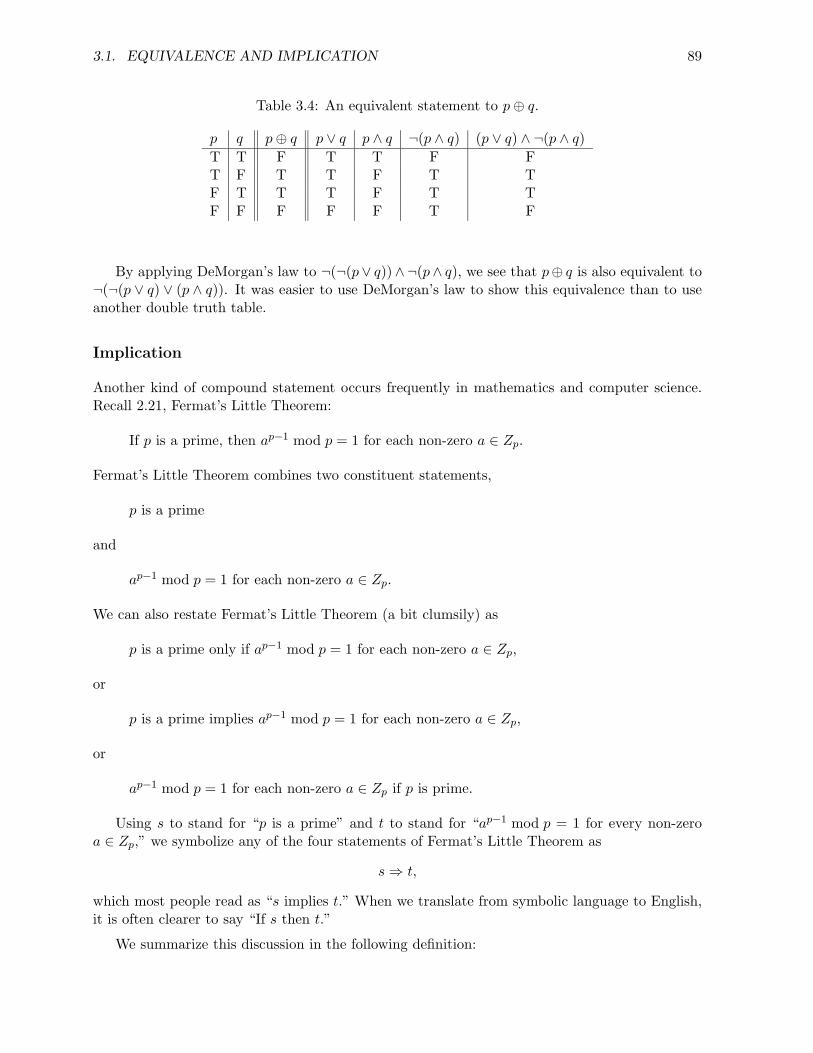
3.1. EQUIVALENCE AND IMPLICATION 89
Table 3.4: An equivalent statement to p ⊕ q.
p q p ⊕ q p ∨ q p ∧ q ¬(p ∧ q) (p ∨ q) ∧ ¬(p ∧ q)T T F T T F FT F T T F T TF T T T F T TF F F F F T F
By applying DeMorgan’s law to ¬(¬(p∨ q))∧¬(p∧ q), we see that p⊕ q is also equivalent to¬(¬(p ∨ q) ∨ (p ∧ q)). It was easier to use DeMorgan’s law to show this equivalence than to useanother double truth table.
Implication
Another kind of compound statement occurs frequently in mathematics and computer science.Recall 2.21, Fermat’s Little Theorem:
If p is a prime, then ap−1 mod p = 1 for each non-zero a ∈ Zp.
Fermat’s Little Theorem combines two constituent statements,
p is a prime
and
ap−1 mod p = 1 for each non-zero a ∈ Zp.
We can also restate Fermat’s Little Theorem (a bit clumsily) as
p is a prime only if ap−1 mod p = 1 for each non-zero a ∈ Zp,
or
p is a prime implies ap−1 mod p = 1 for each non-zero a ∈ Zp,
or
ap−1 mod p = 1 for each non-zero a ∈ Zp if p is prime.
Using s to stand for “p is a prime” and t to stand for “ap−1 mod p = 1 for every non-zeroa ∈ Zp,” we symbolize any of the four statements of Fermat’s Little Theorem as
s ⇒ t,
which most people read as “s implies t.” When we translate from symbolic language to English,it is often clearer to say “If s then t.”
We summarize this discussion in the following definition:

90 CHAPTER 3. REFLECTIONS ON LOGIC AND PROOF
Definition 3.1 The following four English phrases are intended to mean the same thing. Inother words, they are defined by the same truth table:
• s implies t,
• if s then t,
• t if s, and
• s only if t.
Observe that the use of “only if” may seem a little different than the normal usage in English.Also observe that there are still other ways of making an “if . . . then” statement in English. In anumber of our lemmas, theorems, and corollaries (for example, Corollary 2.6 and Lemma 2.5) wehave had two sentences. In the first we say “Suppose . . . .” In the second we say “Then . . . .” Thetwo sentences “Suppose s.” and “Then t.” are equivalent to the single sentence s ⇒ t. When wehave a statement equivalent to s ⇒ t, we call the statement s the hypothesis of the implicationand we call the statement t the conclusion of the implication.
If and only if
The word “if” and the phrase “only if” frequently appear together in mathematical statements.For example, in Theorem 2.9 we proved
A number a has a multiplicative inverse in Zn if and only if there are integers x andy such that ax + ny = 1.
Using s to stand for the statement “a number a has a multiplicative inverse in Zn” and t to standfor the statement “there are integers x and y such that ax+ny = 1,” we can write this statementsymbolically as
s if and only if t.
Referring to Definition 3.1, we parse this as
s if t, and s only if t,
which again by the definition above is the same as
s ⇒ t and t ⇒ s.
We denote the statement “s if and only if t” by s ⇔ t. Statements of the form s ⇒ t and s ⇔ t arecalled conditional statements, and the connectives ⇒ and ⇔ are called conditional connectives.
Exercise 3.1-4 Use truth tables to explain the difference between s ⇒ t and s ⇔ t.

3.1. EQUIVALENCE AND IMPLICATION 91
In order to be able to analyze the truth and falsity of statements involving “implies” and “ifand only if,” we need to understand exactly how they are different. By constructing truth tablesfor these statements, we see that there is only one case in which they could have different truthvalues. In particular if s is true and t is true, then we would say that both s ⇒ t and s ⇔ t aretrue. If s is true and t is false, we would say that both s ⇒ t and s ⇔ t are false. In the casethat both s and t are false we would say that s ⇔ t is true. What about s ⇒ t? Let us try anexample. Suppose that s is the statement “it is supposed to rain” and t is the statement “I carryan umbrella.” Then if, on a given day, it is not supposed to rain and I do not carry an umbrella,we would say that the statement “if it is supposed to rain then I carry an umbrella” is true onthat day. This suggests that we also want to say s ⇒ t is true if s is false and t is false.2 Thusthe truth tables are identical in rows one, two, and four. For “implies” and “if and only if” tomean different things, the truth tables must therefore be different in row three. Row three is thecase where s is false and t is true. Clearly in this case we would want s if and only if t to befalse, so our only choice is to say that s ⇒ t is true in this case. This gives us the truth tables inFigure 3.2.
Figure 3.2: The truth tables for “implies” and for “if and only if.”
IMPLIESs t s ⇒ t
T T TT F FF T TF F T
IF AND ONLY IFs t s ⇔ t
T T TT F FF T FF F T
Here is another place where (as with the usage for “or”) English usage is sometimes inconsis-tent. Suppose a parent says “I will take the family to McDougalls for dinner if you get an A onthis test,” and even though the student gets a C, the parent still takes the family to McDougallsfor dinner. While this is something we didn’t expect, was the parent’s statement still true? Somepeople would say “yes”; others would say “no”. Those who would say “no” mean, in effect,that in this context the parent’s statement meant the same as “I will take the family to dinnerat McDougalls if and only if you get an A on this test.” In other words, to some people, incertain contexts, “If” and “If and only if” mean the same thing! Fortunately questions of childrearing aren’t part of mathematics or computer science (at least not this kind of question!). Inmathematics and computer science, we adopt the two truth tables just given as the meaning ofthe compound statement s ⇒ t (or “if s then t” or “t if s”) and the compound statement s ⇔ t(or “s if and only if t.”) In particular, the truth table marked IMPLIES is the truth table referredto in Definition 3.1. This truth table thus defines the mathematical meaning of s implies t, orany of the other three statements referred to in that definition.
Some people have difficulty using the truth table for s ⇒ t because of this ambiguity inEnglish. The following example can be helpful in resolving this ambiguity. Suppose that I hold
2Note that we are making this conclusion on the basis of one example. Why can we do so? We are not tryingto prove something, but trying to figure out what the appropriate definition is for the ⇒ connective. Since wehave said that the truth or falsity of s ⇒ t depends only on the truth or falsity of s and t, one example serves tolead us to an appropriate definition. If a different example led us to a different definition, then we would want todefine two different kinds of implications, just as we have two different kinds of “ors,” ∨ and ⊕. Fortunately, theonly kinds of conditional statements we need for doing mathematics and computer science are “implies” and “ifand only if.”

92 CHAPTER 3. REFLECTIONS ON LOGIC AND PROOF
an ordinary playing card (with its back to you) and say “If this card is a heart, then it is aqueen.” In which of the following four circumstances would you say I lied:
1. the card is a heart and a queen
2. the card is a heart and a king
3. the card is a diamond and a queen
4. the card is a diamond and a king?
You would certainly say I lied in the case the card is the king of hearts, and you would certainlysay I didn’t lie if the card is the queen of hearts. Hopefully in this example, the inconsistencyof English language seems out of place to you and you would not say I am a liar in either of theother cases. Now we apply the principle called the principle of the excluded middle
Principle 3.1 A statement is true exactly when it is not false.
This principle tells us that that my statement is true in the three cases where you wouldn’t sayI lied. We used this principle implicitly before when we introduced the principle of proof bycontradiction, Principle 2.1. We were explaining the proof of Corollary 2.6, which states
Suppose there is a b in Zn such that the equation
a ·n x = b
does not have a solution. Then a does not have a multiplicative inverse in Zn.
We had assumed that the hypothesis of the corollary was true so that a ·n x = b does not havea solution. Then we assumed the conclusion that a does not have a multiplicative inverse wasfalse. We saw that these two assumptions led to a contradiction, so that it was impossible forboth of them to be true. Thus we concluded whenever the first assumption was true, the secondhad to be false. Why could we conclude this? Because the principle of the excluded middle saysthat the second assumption has to be either true or false. We didn’t introduce the principle ofthe excluded middle at this point for two reasons. First, we expected that the reader would agreewith our proof even if we didn’t mention the principle, and second, we didn’t want to confusethe reader’s understanding of proof by contradiction by talking about two principles at once!
Important Concepts, Formulas, and Theorems
1. Logical statements. Logical statements may be built up from the following notation:
• symbols (s, t, etc.) standing for statements (these will be called variables),
• the symbol ∧, standing for “and,”
• the symbol ∨, standing for “or,”
• the symbol ⊕ standing for “exclusive or,”
• the symbol ¬, standing for “not,”

3.1. EQUIVALENCE AND IMPLICATION 93
• the symbol ⇒, standing for “implies,” and
• the symbol ⇔ , standing for “if and only if.”
The operators ∧, ∨, ⊕, ⇒, ⇔, and ¬ are called logical connectives. The operators ⇒ and⇔ are called conditional connectives.
2. Truth Tables. The following are truth tables for the basic logical connectives:
ANDs t s ∧ t
T T TT F FF T FF F F
ORs t s ∨ t
T T TT F TF T TF F F
XORs t s ⊕ t
T T FT F TF T TF F F
NOTs s ⊕ t
T FF T
3. Equivalence of logical statements. We say that two symbolic compound statements areequivalent if they are true in exactly the same cases.
4. Distributive Law. The statements
w ∧ (u ∨ v)
and
(w ∧ u) ∨ (w ∧ v)
are equivalent.
5. DeMorgan’s Laws. DeMorgan’s Laws say that ¬(p ∨ q) is equivalent to ¬p ∧ ¬q, and that¬(p ∧ q) is equivalent to ¬p ∨ ¬q.
6. Implication. The following four English phrases are equivalent:
• s implies t,
• if s then t,
• t if s, and
• s only if t.
7. Truth tables for implies and if and only if.
IMPLIESs t s ⇒ t
T T TT F FF T TF F T
IF AND ONLY IFs t s ⇔ t
T T TT F FF T FF F T
8. Principle of the Excluded Middle. A statement is true exactly when it is not false.

94 CHAPTER 3. REFLECTIONS ON LOGIC AND PROOF
Problems
1. Give truth tables for the following expressions:
a. (s ∨ t) ∧ (¬s ∨ t) ∧ (s ∨ ¬t)
b. (s ⇒ t) ∧ (t ⇒ u)
c. (s ∨ t ∨ u) ∧ (s ∨ ¬t ∨ u)
2. Find at least two more examples of the use of some word or phrase equivalent to “implies”in lemmas, theorems, or corollaries in Chapters One or Two.
3. Find at least two more examples of the use of the phrase “if and only if” in lemmas,theorems, and corollaries in Chapters One or Two.
4. Show that the statements s ⇒ t and ¬s ∨ t are equivalent.
5. Prove the DeMorgan law which states ¬(p ∧ q) = ¬p ∨ ¬q.
6. Show that p ⊕ q is equivalent to (p ∧ ¬q) ∨ (¬p ∧ q).
7. Give a simplified form of each of the following expressions (using T to stand for a statementthat is always true and F to stand for a statement that is always false)3:
• s ∨ s,
• s ∧ s,
• s ∨ ¬s,
• s ∧ ¬s.
8. Use a truth table to show that (s∨t)∧(u∨v) is equivalent to (s∧u)∨(s∧v)∨(t∧u)∨(t∧v).What algebraic rule is this similar to?
9. Use DeMorgan’s Law, the distributive law, and Problems 7 and 8 to show that ¬((s ∨ t) ∧(s ∨ ¬t)) is equivalent to ¬s.
10. Give an example in English where “or” seems to you to mean exclusive or (or where youthink it would for many people) and an example in English where “or” seems to you tomean inclusive or (or where you think it would for many people).
11. Give an example in English where “if . . . then” seems to you to mean “if and only if” (orwhere you think it would to many people) and an example in English where it seems toyou not to mean “if and only if” (or where you think it would not to many people).
12. Find a statement involving only ∧, ∨ and ¬ (and s and t) equivalent to s ⇔ t. Does yourstatement have as few symbols as possible? If you think it doesn’t, try to find one withfewer symbols.
13. Suppose that for each line of a 2-variable truth table, you are told whether the final columnin that line should evaluate to true or to false. (For example, you might be told that thefinal column should contain T, F, T, and F in that order.) Explain how to create a logicalstatement using the symbols s, t, ∧, ∨, and ¬ that has that pattern as its final column.Can you extend this procedure to an arbitrary number of variables?
3A statement that is always true is called a tautology; a statement that is always false is called a contradiction

3.1. EQUIVALENCE AND IMPLICATION 95
14. In Problem 13, your solution may have used ∧, ∨ and ¬. Is it possible to give a solutionusing only one of those symbols? Is it possible to give a solution using only two of thesesymbols?
15. We proved that ∧ distributes over ∨ in the sense of giving two equivalent statements thatrepresent the two “sides” of the distributive law. For each question below, explain whyyour answer is true.
a. Does ∨ distribute over ∧?
b. Does ∨ distribute over ⊕?
c. Does ∧ distribute over ⊕?

96 CHAPTER 3. REFLECTIONS ON LOGIC AND PROOF
3.2 Variables and Quantifiers
Variables and universes
Statements we use in computer languages to control loops or conditionals are statements aboutvariables. When we declare these variables, we give the computer information about their possiblevalues. For example, in some programming languages we may declare a variable to be a “boolean”or an “integer” or a “real.”4 In English and in mathematics, we also make statements aboutvariables, but it is not always clear which words are being used as variables and what valuesthese variables may take on. We use the phrase varies over to describe the set of values avariable may take on. For example, in English, we might say “If someone’s umbrella is up, thenit must be raining.” In this case, the word “someone” is a variable, and presumably it variesover the people who happen to be in a given place at a given time. In mathematics, we mightsay “For every pair of positive integers m and n, there are nonnegative integers q and r with0 ≤ r < n such that m = nq + r.” In this case m, n, q, and r are clearly our variables; ourstatement itself suggests that two of our variables range over the positive integers and two rangeover the nonnegative integers. We call the set of possible values for a variable the universe ofthat variable.
In the statement “m is an even integer,” it is clear that m is a variable, but the universe isnot given. It might be the integers, just the even integers, or the rational numbers, or one ofmany other sets. The choice of the universe is crucial for determining the truth or falsity of astatement. If we choose the set of integers as the universe for m, then the statement is true forsome integers and false for others. On the other hand, if we choose integer multiples of 10 as ouruniverse, then the statement is always true. In the same way, when we control a while loop witha statement such as “i < j” there are some values of i and j for which the statement is true andsome for which it is false. In statements like “m is an even integer” and “i < j” our variablesare not constrained and so are called free variables. For each possible value of a free variable,we have a new statement, which might be either true or false, determined by substituting thepossible value for the variable. The truth value of the statement is determined only after such asubstitution.
Exercise 3.2-1 For what values of m is the statement m2 > m a true statement and forwhat values is it a false statement? Since we have not specified a universe, youranswer will depend on what universe you choose to use.
If you used the universe of positive integers, the statement is true for every value of m but1; if you used the real numbers, the statement is true for every value of m except for those inthe closed interval [0, 1]. There are really two points to make here. First, a statement about avariable can often be interpreted as a statement about more than one universe, and so to makeit unambiguous, the universe must be clearly stated. Second, a statement about a variable canbe true for some values of a variable and false for others.
4Note that to declare a variable x as an integer in, say, a C program does not mean that same thing as sayingthat x is an integer. In a C program, an integer may really be a 32-bit integer, and so it is limited to valuesbetween 231 − 1 and −231. Similarly a real has some fixed precision, and hence a real variable y may not be ableto take on a value of, say, 10−985.

3.2. VARIABLES AND QUANTIFIERS 97
Quantifiers
In contrast, the statementFor every integer m, m2 > m. (3.1)
is false; we do not need to qualify our answer by saying that it is true some of the time and falseat other times. To determine whether Statement 3.1 is true or false, we could substitute variousvalues for m into the simpler statement m2 > m, and decide, for each of these values, whetherthe statement m2 > m is true or false. Doing so, we see that the statement m2 > m is true forvalues such as m = −3 or m = 9, but false for m = 0 or m = 1. Thus it is not the case thatfor every integer m, m2 > m, so Statement 3.1 is false. It is false as a statement because it isan assertion that the simpler statement m2 > m holds for each integer value of m we substitutein. A phrase like “for every integer m” that converts a symbolic statement about potentiallyany member of our universe into a statement about the universe instead is called a quantifier. Aquantifier that asserts a statement about a variable is true for every value of the variable in itsuniverse is called a universal quantifier.
The previous example illustrates a very important point.
If a statement asserts something for every value of a variable, then to show thestatement is false, we need only give one value of the variable for which the assertionis untrue.
Another example of a quantifier is the phrase “There is an integer m” in the sentence
There is an integer m such that m2 > m.
This statement is also about the universe of integers, and as such it is true—there are plentyof integers m we can substitute into the symbolic statement m2 > m to make it true. This is anexample of an “existential quantifier.” An existential quantifier asserts that a certain element ofour universe exists. A second important point similar to the one we made above is:
To show that a statement with an existential quantifier is true, we need only exhibitone value of the variable being quantified that makes the statement true.
As the more complex statement
For every pair of positive integers m and n, there are nonnegative integers q and rwith 0 ≤ r < n such that m = qn + r,
shows, statements of mathematical interest abound with quantifiers. Recall the following defini-tion of the “big-O” notation you have probably used in earlier computer science courses:
Definition 3.2 We say that f(x) = O(g(x)) if there are positive numbers c and n0 such thatf(x) ≤ cg(x) for every x > n0.
Exercise 3.2-2 Quantification is present in our everyday language as well. The sentences“Every child wants a pony” and “No child wants a toothache” are two differentexamples of quantified sentences. Give ten examples of everyday sentences that usequantifiers, but use different words to indicate the quantification.
98 CHAPTER 3. REFLECTIONS ON LOGIC AND PROOF
Exercise 3.2-3 Convert the sentence “No child wants a toothache” into a sentence of theform “It is not the case that...” Find an existential quantifier in your sentence.
Exercise 3.2-4 What would you have to do to show that a statement about one variablewith an existential quantifier is false? Correspondingly, what would you have to doto show that a statement about one variable with a universal quantifier is true?
As Exercise 3.2-2 points out, English has many different ways to express quantifiers. Forexample, the sentences, “All hammers are tools”, “Each sandwich is delicious”, “No one in theirright mind would do that”, “Somebody loves me”, and “Yes Virginia, there is a Santa Claus” allcontain quantifiers. For Exercise 3.2-3, we can say “It is not the case that there is a child whowants a toothache.” Our quantifier is the phrase “there is.”
To show that a statement about one variable with an existential quantifier is false, we haveto show that every element of the universe makes the statement (such as m2 > m) false. Thusto show that the statement “There is an x in [0, 1] with x2 > x” is false, we have to show thatevery x in the interval makes the statement x2 > x false. Similarly, to show that a statementwith a universal quantifier is true, we have to show that the statement being quantified is true forevery member of our universe. We will give more details about how to show a statement abouta variable is true or false for every member of our universe later in this section.
Mathematical statements of theorems, lemmas, and corollaries often have quantifiers. Forexample in Lemma 2.5 the phrase “for any” is a quantifier, and in Corollary 2.6 the phrase“there is” is a quantifier.
Standard notation for quantification
Each of the many variants of language that describe quantification describe one of two situations:
A quantified statement about a variable x asserts either
• that the statement is true for all x in the universe, or
• that there exists an x in the universe that makes the statement true.
All quantified statements have one of these two forms. We use the standard shorthand of ∀ forthe phrase “for all” and the standard shorthand of ∃ for the phrase “there exists.” We also adoptthe convention that we parenthesize the expression that is subject to the quantification. Forexample, using Z to stand for the universe of all integers, we write
∀n ∈ Z (n2 ≥ n)
as a shorthand for the statement “For all integers n, n2 ≥ n.” It is perhaps more natural to readthe notation as “For all n in Z, n2 ≥ n,” which is how we recommend reading the symbolism.We similarly use
∃n ∈ Z(n2 > n)
to stand for “There exists an n in Z such that n2 > n.” Notice that in order to cast our symbolicform of an existence statement into grammatical English we have included the supplementaryword “an” and the supplementary phrase “such that.” People often leave out the “an” as they

3.2. VARIABLES AND QUANTIFIERS 99
read an existence statement, but rarely leave out the “such that.” Such supplementary languageis not needed with ∀.
As another example, we rewrite the definition of the “Big Oh” notation with these symbols.We use the letter R to stand for the universe of real numbers, and the symbol R+ to stand forthe universe of positive real numbers.
f = O(g) means that ∃c ∈ R+(∃n0 ∈ R+(∀x ∈ R(x > n0 ⇒ f(x) ≤ cg(x))))
We would read this literally as
f is big Oh of g means that there exists a c in R+ such that there exists an n0 in R+
such that for all x in R, if x > n0, then f(x) ≤ cg(x).
Clearly this has the same meaning (when we translate it into more idiomatic English) as
f is big Oh of g means that there exist a c in R+ and an n0 in R+ such that for allreal numbers x > n0, f(x) ≤ cg(x).
This statement is identical to the definition of “big Oh” that we gave earlier in Definition 3.2,except for more precision as to what c and n0 actually are.
Exercise 3.2-5 How would you rewrite Euclid’s division theorem, Theorem 2.12 using theshorthand notation we have introduced for quantifiers? Use Z+ to to stand for thepositive integers and N to stand for the nonnegative integers.
We can rewrite Euclid’s division theorem as
∀m ∈ N(∀n ∈ Z+(∃q ∈ N(∃r ∈ N((r < n) ∧ (m = qn + r))))).
Statements about variables
To talk about statements about variables, we need a notation to use for such statements. Forexample, we can use p(n) to stand for the statement n2 > n. Now, we can say that p(4) andp(−3) are true, while p(1) and p(.5) are false. In effect we are introducing variables that standfor statements about (other) variables! We typically use symbols like p(n), q(x), etc. to standfor statements about a variable n or x. Then the statement “For all x in U p(x)” can be writtenas ∀x ∈ U(p(x)) and the statement “There exists an n in U such that q(n)” can be writtenas ∃n ∈ U(q(n)). Sometimes we have statements about more than one variable; for example,our definition of “big Oh” notation had the form ∃c(∃n0(∀x(p(c, n0, x)))), where p(c, n0, x) is(x > n0 ⇒ f(x) ≤ cg(x)). (We have left out mention of the universes for our variables here toemphasize the form of the statement.)
Exercise 3.2-6 Rewrite Euclid’s division theorem, using the notation above for statementsabout variables. Leave out the references to universes so that you can see clearly theorder in which the quantifiers occur.
The form of Euclid’s division theorem is ∀m(∀n(∃q(∃r(p(m, n, q, r))))).

100 CHAPTER 3. REFLECTIONS ON LOGIC AND PROOF
Rewriting statements to encompass larger universes
It is sometimes useful to rewrite a quantified statement so that the universe is larger, and thestatement itself serves to limit the scope of the universe.
Exercise 3.2-7 Let R to stand for the real numbers and R+ to stand for the positive realnumbers. Consider the following two statements:
a) ∀x ∈ R+(x > 1)
b) ∃x ∈ R+(x > 1)
Rewrite these statements so that the universe is all the real numbers, but the state-ments say the same thing in everyday English that they did before.
For Exercise 3.2-7, there are potentially many ways to rewrite the statements. Two partic-ularly simple ways are ∀x ∈ R(x > 0 ⇒ x > 1) and ∃x ∈ R(x > 0 ∧ x > 1). Notice that wetranslated one of these statements with “implies” and one with “and.” We can state this rule asa general theorem:
Theorem 3.2 Let U1 be a universe, and let U2 be another universe with U1 ⊆ U2. Suppose thatq(x) is a statement such that
U1 = x| q(x) is true. (3.2)
Then if p(x) is a statement about U2, it may also be interpreted as a statement about U1, and
(a) ∀x ∈ U1(p(x)) is equivalent to ∀x ∈ U2(q(x) ⇒ p(x)).
(b) ∃x ∈ U1(p(x)) is equivalent to ∃x ∈ U2(q(x) ∧ p(x)).
Proof: By Equation 3.2 the statement q(x) must be true for all x ∈ U1 and false for all x in U2
but not U1. To prove part (a) we must show that ∀x ∈ U1(p(x)) is true in exactly the same casesas the statement ∀x ∈ U2(q(x) ⇒ p(x)). For this purpose, suppose first that ∀x ∈ U1(p(x)) istrue. Then p(x) is true for all x in U1. Therefore, by the truth table for “implies” and our remarkabout Equation 3.2, the statement ∀x ∈ U2(q(x) ⇒ p(x)) is true. Now suppose ∀x ∈ U1(p(x)) isfalse. Then there exists an x in U1 such that p(x) is false. Then by the truth table for “implies,”the statement ∀x ∈ U2(q(x) ⇒ p(x)) is false. Thus the statement ∀x ∈ U1(p(x)) is true if andonly if the statement ∀x ∈ U2(q(x) ⇒ p(x)) is true. Therefore the two statements are true inexactly the same cases. Part (a) of the theorem follows.
Similarly, for Part (b), we observe that if ∃x ∈ U1(p(x)) is true, then for some x′ ∈ U1, p(x′)is true. For that x′, q(x′) is also true, and hence p(x′)∧ q(x′) is true, so that ∃x ∈ U2(q(x)∧p(x))is true as well. On the other hand, if ∃x ∈ U1(p(x)) is false, then no x ∈ U1 has p(x) true.Therefore by the truth table for “and” q(x)∧p(x) won’t be true either. Thus the two statementsin Part (b) are true in exactly the same cases and so are equivalent.

3.2. VARIABLES AND QUANTIFIERS 101
Proving quantified statements true or false
Exercise 3.2-8 Let R stand for the real numbers and R+ stand for the positive realnumbers. For each of the following statements, say whether it is true or false andwhy.
a) ∀x ∈ R+(x > 1)
b) ∃x ∈ R+(x > 1)
c) ∀x ∈ R(∃y ∈ R(y > x))
d) ∀x ∈ R(∀y ∈ R(y > x))
e) ∃x ∈ R(x ≥ 0 ∧ ∀y ∈ R+(y > x))
In Exercise 3.2-8, since .5 is not greater than 1, statement (a) is false. However since 2 > 1,statement (b) is true. Statement (c) says that for each real number x there is a real number ybigger than x, which we know is true. Statement (d) says that every y in R is larger than everyx in R, and so it is false. Statement (e) says that there is a nonnegative number x such thatevery positive y is larger than x, which is true because x = 0 fills the bill.
We can summarize what we know about the meaning of quantified statements as follows.
Principle 3.2 (The meaning of quantified statements)
• The statement ∃x ∈ U(p(x)) is true if there is at least one value of x in U for which thestatement p(x) is true.
• The statement ∃x ∈ U(p(x)) is false if there is no x ∈ U for which p(x) is true.
• The statement ∀x ∈ U(p(x)) is true if p(x) is true for each value of x in U .
• The statement ∀x ∈ U(p(x)) is false if p(x) is false for at least one value of x in U .
Negation of quantified statements
An interesting connection between ∀ and ∃ arises from the negation of statements.
Exercise 3.2-9 What does the statement “It is not the case that for all integers n, n2 > 0”mean?
From our knowledge of English we see that since the statement ¬∀n ∈ Z(n2 > 0) asserts that itis not the case that, for all integers n, we have n2 > 0, there must be some integer n such thatn2 > 0. In other words, it says there is some integer n such that n2 ≤ 0. Thus the negationof our “for all” statement is a “there exists” statement. We can make this idea more precise byrecalling the notion of equivalence of statements. We have said that two symbolic statements areequivalent if they are true in exactly the same cases. By considering the case when p(x) is truefor all x ∈ U , (we call this case “always true”) and the case when p(x) is false for at least onex ∈ U (we call this case “not always true”) we can analyze the equivalence. The theorem thatfollows, which formalizes the example above in which p(x) was the statement x2 > 0, is provedby dividing these cases into two possibilities.

102 CHAPTER 3. REFLECTIONS ON LOGIC AND PROOF
Theorem 3.3 The statements ¬∀x ∈U(p(x)) and ∃x ∈ U(¬p(x)) are equivalent.
Proof: Consider the following table which we have set up much like a truth table, exceptthat the relevant cases are not determined by whether p(x) is true or false, but by whether p(x)is true for all x in the universe U or not.
p(x) ¬p(x) ∀x ∈ U(p(x)) ¬∀x ∈ U(p(x)) ∃x ∈ U(¬p(x))always true always false true false false
not always true not always false false true true
Since the last two columns are identical, the theorem holds.
Corollary 3.4 The statements ¬∃x ∈ U(q(x)) and ∀x ∈ U(¬q(x)) are equivalent.
Proof: Since the two statements in Theorem 3.3 are equivalent, their negations are alsoequivalent. We then substitute ¬q(x) for p(x) to prove the corollary.
Put another way, to negate a quantified statement, you switch the quantifier and “push” thenegation inside.
To deal with the negation of more complicated statements, we simply take them one quantifierat a time. Recall Definition 3.2, the definition of big Oh notation,
f(x) = O(g(x)) if ∃c ∈ R+(∃n0 ∈ R+(∀x ∈ R(x > n0 ⇒ f(x) ≤ cg(x)))).
What does it mean to say that f(x) is not O(g(x))? First we can write
f(x) = O(g(x)) if ¬∃c ∈ R+(∃n0 ∈ R+(∀x ∈ R(x > n0 ⇒ f(x) ≤ cg(x)))).
After one application of Corollary 3.4 we get
f(x) = O(g(x)) if ∀c ∈ R+(¬∃n0 ∈ R+(∀x ∈ R(x > n0 ⇒ f(x) ≤ cg(x)))).
After another application of Corollary 3.4 we obtain
f(x) = O(g(x)) if ∀c ∈ R+(∀n0 ∈ R+(¬∀x ∈ R(x > n0 ⇒ f(x) ≤ cg(x)))).
Now we apply Theorem 3.3 and obtain
f(x) = O(g(x)) if ∀c ∈ R+(∀n0 ∈ R+(∃x ∈ R(¬(x > n0 ⇒ f(x) ≤ cg(x))))).
Now ¬(p ⇒ q) is equivalent to p ∧ ¬q, so we can write
f(x) = O(g(x)) if ∀c ∈ R+(∀n0 ∈ R+(∃x ∈ R((x > n0) ∧ (f(x) ≤ cg(x)))))).
Thus f(x) is not O(g(x)) if for every c in R+ and every n0 in R+, there is an x such thatx > n0 and f(x) ≤ cg(x).
In our next exercise, we use the “Big Theta” notation defined as follows:

3.2. VARIABLES AND QUANTIFIERS 103
Definition 3.3 f(x) = Θ(g(x)) means that f(x) = O(g(x)) and g(x) = O(f(x)).
Exercise 3.2-10 Express ¬(f(x) = Θ(g(x))) in terms similar to those we used to describef(x) = O(g(x)).
Exercise 3.2-11 Suppose the universe for a statement p(x) is the integers from 1 to 10.Express the statement ∀x(p(x)) without any quantifiers. Express the negation interms of ¬p without any quantifiers. Discuss how negation of “for all” and “thereexists” statements corresponds to DeMorgan’s Law.
By DeMorgan’s law, ¬(f = Θ(g)) means ¬(f = O(g)) ∨ ¬(g = O(f)). Thus ¬(f = Θ(g)) meansthat either for every c and n0 in R+ there is an x in R with x > n0 and f(x) < cg(x) or for everyc and n0 in R+ there is an x in R with x > n0 and g(x) < cf(x) (or both).
For Exercise 3.2-11 we see that ∀x(p(x)) is simply
p(1) ∧ p(2) ∧ p(3) ∧ p(4) ∧ p(5) ∧ p(6) ∧ p(7) ∧ p(8) ∧ p(9) ∧ p(10).
By DeMorgan’s law the negation of this statement is
¬p(1) ∨ ¬p(2) ∨ ¬p(3) ∨ ¬p(4) ∨ ¬p(5) ∨ ¬p(6) ∨ ¬p(7) ∨ ¬p(8) ∨ ¬p(9) ∨ ¬p(10).
Thus the relationship that negation gives between “for all” and “there exists” statements is theextension of DeMorgan’s law from a finite number of statements to potentially infinitely manystatements about a potentially infinite universe.
Implicit quantification
Exercise 3.2-12 Are there any quantifiers in the statement “The sum of even integers iseven?”
It is an elementary fact about numbers that the sum of even integers is even. Another wayto say this is that if m and n are even, then m + n is even. If p(n) stands for the statement “nis even,” then this last sentence translates to p(m) ∧ p(n) ⇒ p(m + n). From the logical form ofthe statement, we see that our variables are free, so we could substitute various integers in form and n to see whether the statement is true. But in Exercise 3.2-12, we said we were stating amore general fact about the integers. What we meant to say is that for every pair of integers mand n, if m and n are even, then m + n is even. In symbols, using p(k) for “k is even,” we have
∀m ∈ Z(∀n ∈ Z(p(m) ∧ p(n) ⇒ p(m + n))).
This way of representing the statement captures the meaning we originally intended. This is oneof the reasons that mathematical statements and their proofs sometimes seem confusing—just asin English, sentences in mathematics have to be interpreted in context. Since mathematics hasto be written in some natural language, and since context is used to remove ambiguity in naturallanguage, so must context be used to remove ambiguity from mathematical statements made innatural language. In fact, we frequently rely on context in writing mathematical statements withimplicit quantifiers because, in context, it makes the statements easier to read. For example, inLemma 2.8 we said

104 CHAPTER 3. REFLECTIONS ON LOGIC AND PROOF
The equationa ·n x = 1
has a solution in Zn if and only if there exist integers x and y such that
ax + ny = 1.
In context it was clear that the a we were talking about was an arbitrary member of Zn. It wouldsimply have made the statement read more clumsily if we had said
For every a ∈ Zn, the equationa ·n x = 1
has a solution in Zn if and only if there exist integers x and y such that
ax + ny = 1.
On the other hand, we were making a transition from talking about Zn to talking about theintegers, so it was important for us to include the quantified statement “there exist integers xand y such that ax+ny = 1.” More recently in Theorem 3.3, we also did not feel it was necessaryto say “For all universes U and for all statements p about U ,” at the beginning of the theorem.We felt the theorem would be easier to read if we kept those quantifiers implicit and let the reader(not necessarily consciously) infer them from context.
Proof of quantified statements
We said that “the sum of even integers is even” is an elementary fact about numbers. How dowe know it is a fact? One answer is that we know it because our teachers told us so. (Andpresumably they knew it because their teachers told them so.) But someone had to figure it outin the first place, and so we ask how we would prove this statement? A mathematician asked togive a proof that the sum of even numbers is even might write
If m and n are even, then m = 2i and n = 2j so that
m + n = 2i + 2j = 2(i + j)
and thus m + n is even.
Because mathematicians think and write in natural language, they will often rely on contextto remove ambiguities. For example, there are no quantifiers in the proof above. However thesentence, while technically incomplete as a proof, captures the essence of why the sum of twoeven numbers is even. A typical complete (but more formal and wordy than usual) proof mightgo like this.
Let m and n be integers. Suppose m and n are even. If m and n are even, then bydefinition there are integers i and j such that m = 2i and n = 2j. Thus there areintegers i and j such that m = 2i and n = 2j. Then
m + n = 2i + 2j = 2(i + j),
so by definition m + n is an even integer. We have shown that if m and n are even,then m + n is even. Therefore for every m and n, if m and n are even integers, thenso is m + n.

3.2. VARIABLES AND QUANTIFIERS 105
We began our proof by assuming that m and n are integers. This gives us symbolic notation fortalking about two integers. We then appealed to the definition of an even integer, namely thatan integer h is even if there is another integer k so that h = 2k. (Note the use of a quantifierin the definition.) Then we used algebra to show that m + n is also two times another number.Since this is the definition of m + n being even, we concluded that m + n is even. This allowedus to say that if m and n are even, the m + n is even. Then we asserted that for every pair ofintegers m and n, if m and n are even, then m + n is even.
There are a number of principles of proof illustrated here. The next section will be devoted toa discussion of principles we use in constructing proofs. For now, let us conclude with a remarkabout the limitations of logic. How did we know that we wanted to write the symbolic equation
m + n = 2i + 2j = 2(i + j)?
It was not logic that told us to do this, but intuition and experience.
Important Concepts, Formulas, and Theorems
1. Varies over. We use the phrase varies over to describe the set of values a variable may takeon.
2. Universe. We call the set of possible values for a variable the universe of that variable.
3. Free variables. Variables that are not constrained in any way whatever are called freevariables.
4. Quantifier. A phrase that converts a symbolic statement about potentially any member ofour universe into a statement about the universe instead is called a quantifier. There aretwo types of quantifiers:
• Universal quantifier. A quantifier that asserts a statement about a variable is true forevery value of the variable in its universe is called a universal quantifier.
• Existential quantifier. A quantifier that asserts a statement about a variable is truefor at least one value of the variable in its universe is called an existential quantifier.
5. Larger universes. Let U1 be a universe, and let U2 be another universe with U1 ⊆ U2.Suppose that q(x) is a statement such that
U1 = x| q(x) is true.
Then if p(x) is a statement about U2, it may also be interpreted as a statement about U1,and
(a) ∀x ∈ U1(p(x)) is equivalent to ∀x ∈ U2(q(x) ⇒ p(x)).
(b) ∃x ∈ U1(p(x)) is equivalent to ∃x ∈ U2(q(x) ∧ p(x)).
6. Proving quantified statements true or false.
• The statement ∃x ∈ U(p(x)) is true if there is at least one value of x in U for whichthe statement p(x) is true.

106 CHAPTER 3. REFLECTIONS ON LOGIC AND PROOF
• The statement ∃x ∈ U(p(x)) is false if there is no x ∈ U for which p(x) is true.
• The statement ∀x ∈ U(p(x)) is true if p(x) is true for each value of x in U .
• The statement ∀x ∈ U(p(x)) is false if p(x) is false for at least one value of x in U .
7. Negation of quantified statements. To negate a quantified statement, you switch the quan-tifier and push the negation inside.
• The statements ¬∀x ∈U(p(x)) and ∃x ∈ U(¬p(x)) are equivalent.
• The statements ¬∃x ∈U(p(x)) and ∀x ∈ U(¬p(x)) are equivalent.
8. Big-Oh We say that f(x) = O(g(x)) if there are positive numbers c and n0 such thatf(x) ≤ cg(x) for every x > n0.
9. Big-Theta. f(x) = Θ(g(x)) means that f = O(g(x)) and g = O(f(x)).
10. Some notation for sets of numbers. We use R to stand for the real numbers, R+ to standfor the positive real numbers, Z to stand for the integers (positive, negative, and zero), Z+
to stand for the positive integers, and N to stand for the nonnegative integers.
Problems
1. For what positive integers x is the statement (x − 2)2 + 1 ≤ 2 true? For what integersis it true? For what real numbers is it true? If we expand the universe for which weare considering a statement about a variable, does this always increase the size of thestatement’s truth set?
2. Is the statement “There is an integer greater than 2 such that (x − 2)2 + 1 ≤ 2” true orfalse? How do you know?
3. Write the statement that the square of every real number is greater than or equal to zeroas a quantified statement about the universe of real numbers. You may use R to stand forthe universe of real numbers.
4. The definition of a prime number is that it is an integer greater than 1 whose only positiveinteger factors are itself and 1. Find two ways to write this definition so that all quantifiersare explicit. (It may be convenient to introduce a variable to stand for the number andperhaps a variable or some variables for its factors.)
5. Write down the definition of a greatest common divisor of m and n in such a way thatall quantifiers are explicit and expressed explicitly as “for all” or “there exists.” Writedown Euclid’s extended greatest common divisor theorem that relates the greatest commondivisor of m and n algebraically to m and n. Again make sure all quantifiers are explicitand expressed explicitly as “for all” or “there exists.”
6. What is the form of the definition of a greatest common divisor, using s(x, y, z) to be thestatement x = yz and t(x, y) to be the statement x < y? (You need not include referencesto the universes for the variables.)
7. Which of the following statements (in which Z+ stands for the positive integers and Zstands for all integers) is true and which is false, and why?

3.2. VARIABLES AND QUANTIFIERS 107
(a) ∀z ∈ Z+(z2 + 6z + 10 > 20).
(b) ∀z ∈ Z(z2 − z ≥ 0).
(c) ∃z ∈ Z+(z − z2 > 0).
(d) ∃z ∈ Z(z2 − z = 6).
8. Are there any (implicit) quantifiers in the statement “The product of odd integers is odd?”If so, what are they?
9. Rewrite the statement “The product of odd integers is odd,” with all quantifiers (includingany in the definition of odd integers) explicitly stated as “for all” or “there exist.”
10. Rewrite the following statement without any negations. It is not the case that there existsan integer n such that n > 0 and for all integers m > n, for every polynomial equationp(x) = 0 of degree m there are no real numbers for solutions.
11. Consider the following slight modification of Theorem 3.2. For each part below, eitherprove that it is true or give a counterexample.
Let U1 be a universe, and let U2 be another universe with U1 ⊆ U2. Suppose that q(x) is astatement such that U1 = x| q(x) is true.
(a) ∀x ∈ U1(p(x)) is equivalent to ∀x ∈ U2(q(x) ∧ p(x)).
(b) ∃x ∈ U1(p(x)) is equivalent to ∃x ∈ U2(q(x) ⇒ p(x)).
12. Let p(x) stand for “x is a prime,” q(x) for “x is even,” and r(x, y) stand for “x = y.” Writedown the statement “There is one and only one even prime,” using these three symbolicstatements and appropriate logical notation. (Use the set of integers for your universe.)
13. Each expression below represents a statement about the integers. Using p(x) for “x isprime,” q(x, y) for “x = y2,” r(x, y) for “x ≤ y,” s(x, y, z) for “z = xy,” and t(x, y) for“x = y,” determine which expressions represent true statements and which represent falsestatements.
(a) ∀x ∈ Z(∃y ∈ Z(q(x, y) ∨ p(x)))
(b) ∀x ∈ Z(∀y ∈ Z(s(x, x, y) ⇔ q(x, y)))
(c) ∀y ∈ Z(∃x ∈ Z(q(y, x)))
(d) ∃z ∈ Z(∃x ∈ Z(∃y ∈ Z(p(x) ∧ p(y) ∧ ¬t(x, y)))
14. Find a reason why (∃x ∈ U(p(x)))∧(∃y ∈ U(q(y))) is not equivalent to ∃z ∈ U(p(z)∨q(z)).Are the statements (∃x ∈ U(p(x))) ∨ (∃y ∈ U(q(y))) and ∃z ∈ U(p(z) ∨ q(z)) equivalent?
15. Give an example (in English) of a statement that has the form ∀x ∈ U(∃y ∈ V (p(x, y))).(The statement can be a mathematical statement or a statement about “everyday life,” orwhatever you prefer.) Now write in English the statement using the same p(x, y) but of theform ∃y ∈ V (∀x ∈ U(p(x, y))). Comment on whether “for all” and “there exist” commute.

108 CHAPTER 3. REFLECTIONS ON LOGIC AND PROOF
3.3 Inference
Direct Inference (Modus Ponens) and Proofs
We concluded our last section with a proof that the sum of two even numbers is even. Thatproof contained several crucial ingredients. First, we introduced symbols for members of theuniverse of integers. In other words, rather than saying “suppose we have two integers,” weintroduced symbols for the two members of our universe we assumed we had. How did we knowto use algebraic symbols? There are many possible answers to this question, but in this case ourintuition was probably based on thinking about what an even number is, and realizing that thedefinition itself is essentially symbolic. (You may argue that an even number is just twice anothernumber, and you would be right. Apparently no symbols are in that definition. But they reallyare there; they are the phrases “even number” and “another number.” Since we all know algebrais easier with symbolic variables rather than words, we should recognize that it makes sense touse algebraic notation.) Thus this decision was based on experience, not logic.
Next we assumed the two integers were even. We then used the definition of even numbers,and, as our previous parenthetic comment suggests, it was natural to use the definition symbol-ically. The definition tells us that if m is an even number, then there exists another integer isuch that m = 2i. We combined this with the assumption that m is even to conclude that infact there does exist an integer i such that m = 2i. This is an example of using the principle ofdirect inference (called modus ponens in Latin).
Principle 3.3 (Direct inference) From p and p ⇒ q we may conclude q.
This common-sense principle is a cornerstone of logical arguments. But why is it true? In Table3.5 we take another look at the truth table for implication.
Table 3.5: Another look at implication
p q p ⇒ q
T T TT F FF T TF F T
The only line which has a T in both the p column and the p ⇒ q column is the first line. Inthis line q is true also, and we therefore conclude that if p and p ⇒ q hold then q must hold also.While this may seem like a somewhat “inside out” application of the truth table, it is simply adifferent way of using a truth table.
There are quite a few rules (called rules of inference) like the principle of direct inference thatpeople commonly use in proofs without explicitly stating them. Before beginning a formal studyof rules of inference, we complete our analysis of which rules we used in the proof that the sumof two even integers is even. After concluding that m = 2i and n = 2j, we next used algebra toshow that because m = 2i and n = 2j, there exists a k such that m + n = 2k (our k was i + j).Next we used the definition of even number again to say that m + n was even. We then used arule of inference which says

3.3. INFERENCE 109
Principle 3.4 (Conditional Proof) If, by assuming p, we may prove q, then the statementp ⇒ q is true.
Using this principle, we reached the conclusion that if m and n are even integers, then m + nis an even integer. In order to conclude that this statement is true for all integers m and n, weused another rule of inference, one of the more difficult to describe. We originally introducedthe variables m and n. We used only well-known consequences of the fact that they were in theuniverse of integers in our proof. Thus we felt justified in asserting that what we concluded aboutm and n is true for any pair of integers. We might say that we were treating m and n as genericmembers of our universe. Thus our rule of inference says
Principle 3.5 (Universal Generalization) If we can prove a statement about x by assumingx is a member of our universe, then we can conclude the statement is true for every member ofour universe.
Perhaps the reason this rule is hard to put into words is that it is not simply a description of atruth table, but is a principle that we use in order to prove universally quantified statements.
Rules of inference for direct proofs
We have seen the ingredients of a typical proof. What do we mean by a proof in general? A proofof a statement is a convincing argument that the statement is true. To be more precise aboutit, we can agree that a direct proof consists of a sequence of statements, each of which is either ahypothesis5, a generally accepted fact, or the result of one of the following rules of inference forcompound statements.
Rules of Inference for Direct Proofs
1) From an example x that does not satisfy p(x), we may conclude ¬p(x).
2) From p(x) and q(x), we may conclude p(x) ∧ q(x).
3) From either p(x) or q(x), we may conclude p(x) ∨ q(x).
4) From either q(x) or ¬p(x) we may conclude p(x) ⇒ q(x).
5) From p(x) ⇒ q(x) and q(x) ⇒ p(x) we may conclude p(x) ⇔ q(x).
6) From p(x) and p(x) ⇒ q(x) we may conclude q(x).
7) From p(x) ⇒ q(x) and q(x) ⇒ r(x) we may conclude p(x) ⇒ r(x).
8) If we can derive q(x) from the hypothesis that x satisfies p(x), then we may concludep(x) ⇒ q(x).
9) If we can derive p(x) from the hypothesis that x is a (generic) member of our universe U ,we may conclude ∀x ∈ U(p(x)).
5If we are proving an implication s ⇒ t, we call s a hypothesis. If we make assumptions by saying “Let. . . ,” “Suppose . . . ,” or something similar before we give the statement to be proved, then these assumptions arehypotheses as well.
110 CHAPTER 3. REFLECTIONS ON LOGIC AND PROOF
10) From an example of an x ∈ U satisfying p(x) we may conclude ∃x ∈ U(p(x)).
The first rule is a statement of the principle of the excluded middle as it applies to statementsabout variables. The next four four rules are in effect a description of the truth tables for “and,”“or,” “implies” and “if and only if.” Rule 5 says what we must do in order to write a proof ofan “if and only if” statement. Rule 6, exemplified in our earlier discussion, is the principle ofdirect inference, and describes one row of the truth table for p ⇒ q. Rule 7 is the transitive law,one we could derive by truth table analysis. Rule 8, the principle of conditional proof, which isalso exemplified earlier, may be regarded as yet another description of one row of the truth tableof p ⇒ q. Rule 9 is the principle of universal generalization, discussed and exemplified earlier.Rule 10 specifies what we mean by the truth of an existentially quantified statement, accordingto Principle 3.2.
Although some of our rules of inference are redundant, they are useful. For example, we couldhave written a portion of our proof that the sum of even numbers is even as follows without usingRule 8.
“Let m and n be integers. If m is even, then there is a k with m = 2k. If n is even,then there is a j with n = 2j. Thus if m is even and n is even, there are a k and jsuch that m + n = 2k + 2j = 2(k + j). Thus if m is even and n is even, there is aninteger h = k + j such that m + n = 2h. Thus if m is even and n is even, m + n iseven.”
This kind of argument could always be used to circumvent the use of Rule 8, so Rule 8 is notrequired as a rule of inference, but because it permits us to avoid such unnecessarily complicated“silliness” in our proofs, we choose to include it. Rule 7, the transitive law, has a similar role.
Exercise 3.3-1 Prove that if m is even, then m2 is even. Explain which steps of the proofuse one of the rules of inference above.
For Exercise 3.3-1, we can mimic the proof that the sum of even integers is even.
Let m be integer. Suppose that m is even. If m is even, then there is a k with m = 2k.Thus, there is a k such that m2 = 4k2. Therefore, there is an integer h = 2k2 suchthat m2 = 2h. Thus if m is even, m2 is even. Therefore, for all integers m, if m iseven, then m2 is even.
In our first sentence we are setting things up to use Rule 9. In the second sentence we are simplystating an implicit hypothesis. In the next two sentences we use Rule 6, the principle of directinference. When we said “Therefore, there is an integer h = 2k2 such that m2 = 2h,” we weresimply stating an algebraic fact. In our next sentence we used Rule 8. Finally, we used Rule 9.You might have written the proof in a different way and used different rules of inference.
Contrapositive rule of inference.
Exercise 3.3-2 Show that “p implies q” is equivalent to “¬q implies ¬p.”

3.3. INFERENCE 111
Exercise 3.3-3 Is “p implies q” equivalent to “q implies p?”
To do Exercise 3.3-2, we construct the double truth table in Table 3.6. Since the columnsunder p ⇒ q and under ¬q ⇒ ¬p are exactly the same, we know the two statements are equivalent.This exercise tells us that if we know that ¬q ⇒ ¬p, then we can conclude that p ⇒ q. This is
Table 3.6: A double truth table for p ⇒ q and ¬q ⇒ ¬p.
p q p ⇒ q ¬p ¬q ¬q ⇒ ¬p
T T T F F TT F F F T FF T T T F TF F T T T T
called the principle of proof by contraposition.
Principle 3.6 (Proof by Contraposition) The statement p ⇒ q and the statement ¬q ⇒ ¬pare equivalent, and so a proof of one is a proof of the other.
The statement ¬q ⇒ ¬p is called the contrapositive of the statement p ⇒ q. The followingexample demonstrates the utility of the principle of proof by contraposition.
Lemma 3.5 If n is a positive integer with n2 > 100, then n > 10.
Proof: Suppose n is not greater than 10. (Now we use the rule of algebra for inequalities whichsays that if x ≤ y and c ≥ 0, then cx ≤ cy.) Then since 1 ≤ n ≤ 10,
n · n ≤ n · 10 ≤ 10 · 10 = 100.
Thus n2 is not greater than 100. Therefore, if n is not greater than 10, n2 is not greater than100. Then, by the principle of proof by contraposition, if n2 > 100, n must be greater than 10.
We adopt Principle 3.6 as a rule of inference, called the contrapositive rule of inference.
11) From ¬q(x) ⇒ ¬p(x) we may conclude p(x) ⇒ q(x).
In our proof of the Chinese Remainder Theorem, Theorem 2.24, we wanted to prove that for acertain function f that if x and y were different integers between 0 and mn−1, then f(x) = f(y).To prove this we assumed that in fact f(x) = f(y) and proved that x and y were not differentintegers between 0 and mn − 1. Had we known the principle of contrapositive inference, wecould have concluded then and there that f was one-to-one. Instead, we used the more commonprinciple of proof by contradiction, the major topic of the remainder of this section, to completeour proof. If you look back at the proof, you will see that we might have been able to shorten itby a sentence by using contrapositive inference.
For Exercise 3.3-3, a quick look at the double truth table for p ⇒ q and q ⇒ p in Table 3.7demonstrates that these two statements are not equivalent. The statement q ⇒ p is called theconverse of p ⇒ q. Notice that p ⇔ q is true exactly when p ⇒ q and its converse are true. Itis surprising how often people, even professional mathematicians, absent-mindedly try to provethe converse of a statement when they mean to prove the statement itself. Try not to join thiscrowd!

112 CHAPTER 3. REFLECTIONS ON LOGIC AND PROOF
Table 3.7: A double truth table for p ⇒ q and q ⇒ p.
p q p ⇒ q q ⇒ p
T T T TT F F TF T T FF F T T
Proof by contradiction
Proof by contrapositive inference is an example of what we call indirect proof. We have actuallyseen another example indirect proof, the principle of proof by contradiction. In our proof ofCorollary 2.6 we introduced the principle of proof by contradiction, Principle 2.1. We weretrying to prove the statement
Suppose there is a b in Zn such that the equation
a ·n x = b
does not have a solution. Then a does not have a multiplicative inverse in Zn.
We assumed that the hypothesis that a ·n x = b does not have a solution was true. We alsoassumed that the conclusion that a does not have a multiplicative inverse was false. We showedthat these two assumptions together led to a contradiction. Then, using the principle of theexcluded middle, Principle 3.1 (without saying so), we concluded that if the hypothesis is in facttrue, then the only possibility was that the conclusion is true as well.
We used the principle again later in our proof of Euclid’s Division Theorem. Recall that inthat proof we began by assuming that the theorem was false. We then chose among the pairsof integers (m, n) such that m = qn + r with 0 ≤ r < n a pair with the smallest possible m.We then made some computations by which we proved that in this case there are a q and r with0 ≤ r < n such that m = qn + r. Thus we started out by assuming the theorem was false, andfrom that assumption we drew drew a contradiction to the assumption. Since all our reasoning,except for the assumption that the theorem was false, used accepted rules of inference, the onlysource of that contradiction was our assumption. Thus, by the principle of the excluded middle,our assumption had to be incorrect. We adopt the principle of proof by contradiction (also calledthe principle of reduction to absurdity) as our last rule of inference.
12) If from assuming p(x) and ¬q(x), we can derive both r(x) and ¬r(x) for some statementr(x), then we may conclude p(x) ⇒ q(x).
There can be many variations of proof by contradiction. For example, we may assume p istrue and q is false, and from this derive the contradiction that p is false, as in the followingexample.
Prove that if x2 + x − 2 = 0, then x = 0.
Proof: Suppose that x2 + x − 2 = 0. Assume that x = 0. Then x2 + x − 2 =0 + 0 − 2 = −2. This contradicts x2 + x − 2 = 0. Thus (by the principle of proof bycontradiction), if x2 + x − 2 = 0, then x = 0.

3.3. INFERENCE 113
Here the statement r was identical to p, namely x2 + x − 2 = 0.
On the other hand, we may instead assume p is true and q is false, and derive a contradictionof a known fact, as in the following example.
Prove that if x2 + x − 2 = 0, then x = 0.
Proof: Suppose that x2 + x − 2 = 0. Assume that x = 0. Then x2 + x − 2 =0 + 0 − 2 = −2. Thus 0 = −2, a contradiction. Thus (by the principle of proof bycontradiction), if x2 + x − 2 = 0, then x = 0.
Here the statement r is the known fact that 0 = −2.
Sometimes the statement r that appears in the principle of proof by contradiction is simplya statement that arises naturally as we are trying to construct our proof, as in the followingexample.
Prove that if x2 + x − 2 = 0, then x = 0.
Proof: Suppose that x2 + x − 2 = 0. Then x2 + x = 2. Assume that x = 0. Thenx2 + x = 0 + 0 = 0. But this is a contradiction (to our observation that x2 + x = 2).Thus (by the principle of proof by contradiction), if x2 + x − 2 = 0, then x = 0.
Here the statement r is “x2 + x = 2.”
Finally, if proof by contradiction seems to you not to be much different from proof by con-traposition, you are right, as the example that follows shows.
Prove that if x2 + x − 2 = 0, then x = 0.
Proof: Assume that x = 0. Then x2+x−2 = 0+0−2 = −2, so that x2+x−2 = 0.Thus (by the principle of proof by contraposition), if x2 + x − 2 = 0, then x = 0.
Any proof that uses one of the indirect methods of inference is called an indirect proof. The lastfour examples illustrate the rich possibilities that indirect proof provides us. Of course they alsoillustrate why indirect proof can be confusing. There is no set formula that we use in writing aproof by contradiction, so there is no rule we can memorize in order to formulate indirect proofs.Instead, we have to ask ourselves whether assuming the opposite of what we are trying to provegives us insight into why the assumption makes no sense. If it does, we have the basis of anindirect proof, and the way in which we choose to write it is a matter of personal choice.
Exercise 3.3-4 Without extracting square roots, prove that if n is a positive integer suchthat n2 < 9, then n < 3. You may use rules of algebra for dealing with inequalities.
Exercise 3.3-5 Prove that√
5 is not rational.
To prove the statement in Exercise 3.3-4, we assume, for purposes of contradiction, that n ≥ 3.Squaring both sides of this equation, we obtain
n2 ≥ 9 ,

114 CHAPTER 3. REFLECTIONS ON LOGIC AND PROOF
which contradicts our hypothesis that n2 < 9. Therefore, by the principle of proof by contradic-tion, n < 3.
To prove the statement in Exercise 3.3-5, we assume, for the purpose of contradiction, that√
5is rational. This means that it can be expressed as the fraction m
n , where m and n are integers.Squaring both sides of the equation m
n =√
5, we obtain
m2
n2= 5,
orm2 = 5n2.
Now m2 must have an even number of prime factors (counting each prime factor as many timesas it occurs) as must n2. But 5n2 has an odd number of prime factors. Thus a product of aneven number of prime factors is equal to a product of an odd number of prime factors, which isa contradiction since each positive integer may be expressed uniquely as a product of (positive)prime numbers. Thus by the principle of proof by contradiction,
√5 is not rational.
Important Concepts, Formulas, and Theorems
1. Principle of direct inference or modus ponens. From p and p ⇒ q we may conclude q.
2. Principle of conditional proof. If, by assuming p, we may prove q, then the statement p ⇒ qis true.
3. Principle of universal generalization. If we can prove a statement about x by assuming x isa member of our universe, then we can conclude it is true for every member of our universe.
4. Rules of Inference. 12 rules of inference appear in this chapter. They are
1) From an example x that does not satisfy p(x), we may conclude ¬p(x).
2) From p(x) and q(x), we may conclude p(x) ∧ q(x).
3) From either p(x) or q(x), we may conclude p(x) ∨ q(x).
4) From either q(x) or ¬p(x) we may conclude p(x) ⇒ q(x).
5) From p(x) ⇒ q(x) and q(x) ⇒ p(x) we may conclude p(x) ⇔ q(x).
6) From p(x) and p(x) ⇒ q(x) we may conclude q(x).
7) From p(x) ⇒ q(x) and q(x) ⇒ r(x) we may conclude p(x) ⇒ r(x).
8) If we can derive q(x) from the hypothesis that x satisfies p(x), then we may concludep(x) ⇒ q(x).
9) If we can derive p(x) from the hypothesis that x is a (generic) member of our universeU , we may conclude ∀x ∈ U(p(x)).
10) From an example of an x ∈ U satisfying p(x) we may conclude ∃x ∈ U(p(x)).
11) From ¬q(x) ⇒ ¬p(x) we may conclude p(x) ⇒ q(x).
12) If from assuming p(x) and ¬q(x), we can derive both r(x) and ¬r(x) for some statementr, then we may conclude p(x) ⇒ q(x).

3.3. INFERENCE 115
5. Contrapositive of p ⇒ q. The contrapositive of the statement p ⇒ q is the statement¬q ⇒ ¬p.
6. Converse of p ⇒ q. The converse of the statement p ⇒ q is the statement q ⇒ p.
7. Contrapositive rule of inference. From ¬q ⇒ ¬p we may conclude p ⇒ q.
8. Principle of proof by contradiction. If from assuming p and ¬q, we can derive both r and¬r for some statement r, then we may conclude p ⇒ q.
Problems
1. Write down the converse and contrapositive of each of these statements.
(a) If the hose is 60 feet long, then the hose will reach the tomatoes.
(b) George goes for a walk only if Mary goes for a walk.
(c) Pamela recites a poem if Andre asks for a poem.
2. Construct a proof that if m is odd, then m2 is odd.
3. Construct a proof that for all integers m and n, if m is even and n is odd, then m + n isodd.
4. What do we really mean when we say “prove that if m is odd and n is odd then m + n iseven?” Prove this more precise statement.
5. Prove that for all integers m and n if m is odd and n is odd, then m · n is odd.
6. Is the statement p ⇒ q equivalent to the statement ¬p ⇒ ¬q?
7. Construct a contrapositive proof that for all real numbers x if x2 − 2x = −1, then x = 1.
8. Construct a proof by contradiction that for all real numbers x if x2−2x = −1, then x = 1.
9. Prove that if x3 > 8, then x > 2.
10. Prove that√
3 is irrational.
11. Construct a proof that if m is an integer such that m2 is even, then m is even.
12. Prove or disprove the following statement. “For every positive integer n, if n is prime, then12 and n3 − n2 + n have a common factor.”
13. Prove or disprove the following statement. “For all integers b, c, and d, if x is a rationalnumber such that x2 + bx + c = d, then x is an integer.” (Hints: Are all the quantifiersgiven explicitly? It is ok to use the quadratic formula.)
14. Prove that there is no largest prime number.
15. Prove that if f(x), g(x) and h(x) are functions from R+ to R+ such that f(x) = O(g(x))and g(x) = O(h(x)), then f(x) = O(h(x)).

116 CHAPTER 3. REFLECTIONS ON LOGIC AND PROOF

Chapter 4
Induction, Recursion, andRecurrences
4.1 Mathematical Induction
Smallest Counter-Examples
In Section 3.3, we saw one way of proving statements about infinite universes: we considered a“generic” member of the universe and derived the desired statement about that generic member.When our universe is the universe of integers, or is in a one-to-one correspondence with theintegers, there is a second technique we can use.
Recall our our proof of Euclid’s Division Theorem (Theorem 2.12), which says that for eachpair (m, n) of positive integers, there are nonnegative integers q and r such that m = nq + r and0 ≤ r < n. For the purpose of a proof by contradiciton, we assumed that the statement wasfales. Then we said the following. “Among all pairs (m, n) that make it false, choose the smallestm that makes it false. We cannot have m < n because then the statement would be true withq = 0 and r = m, and we cannot have m = n because then the statement is true with q = 1and r = 0. This means m − n is a positive number smaller than m. We assumed that m wasthe smallest value that made the theorem false, and so the theorem must be true for the pair(m − n, n). Therefore, there must exist a q′ and r′ such that
m − n = q′n + r′, with 0 ≤ r′ < n.
Thus m = (q′+1)n+r′. Now, by setting q = q′+1 and r = r′, we can satisfy the theorem for thepair (m, n), contradicting the assumption that the statement is false. Thus the only possibilityis that the statement is true.”
Focus on the sentences “This means m−n is a positive number smaller than m. We assumedthat m was the smallest value that made the theorem false, and so the theorem must be true forthe pair (m − n, n). Therefore, there must exist a q′ and r′ such that
m − n = q′n + r′, with 0 ≤ r′ < n.
Thus m = (q′ + 1)n + r′.” To analyze these sentences, let p(m, n) denote the statement “thereare nonnegative integers q and r with 0 ≤ r < n such that m = nq + r” The quoted sentences
117

118 CHAPTER 4. INDUCTION, RECURSION, AND RECURRENCES
we focused on provide a proof that p(m − n, n) ⇒ p(m, n). This implication is the crux of theproof. Let us give an analysis of the proof that shows the pivotal role of this impliction.
• We assumed a counter-example with a smallest m existed.
• Then using the fact that p(m′, n) had to be true for every m′ smaller than m, we chosem′ = m − n, and observed that p(m′, n) had to be true.
• Then we used the implication p(m − n, n) ⇒ p(m, n) to conclude the truth of p(m, n).
• But we had assumed that p(m, n) was false, so this is the assumption we contradicted inthe proof by contradiction.
Exercise 4.1-1 In Chapter 1 we learned Gauss’s trick for showing that for all positiveintegers n,
1 + 2 + 3 + 4 + ... + n =n(n + 1)
2. (4.1)
Use the technique of asserting that if there is a counter-example, there is a smallestcounter-example and deriving a contradiction to prove that the sum is n(n + 1)/2.What implication did you have to prove in the process?
Exercise 4.1-2 For what values of n ≥ 0 do you think 2n+1 ≥ n2 + 2? Use the techniqueof asserting there is a smallest counter-example and deriving a contradiction to proveyou are right. What implication did you have to prove in the process?
Exercise 4.1-3 For what values of n ≥ 0 do you think 2n+1 ≥ n2 + 3? Is it possibleto use the technique of asserting there is a smallest counter-example and deriving acontradiction to prove you are right? If so, do so and describe the implication youhad to prove in the process. If not, why not?
Exercise 4.1-4 Would it make sense to say that if there is a counter example there is alargest counter-example and try to base a proof on this? Why or why not?
In Exercise 4.1-1, suppose the formula for the sum is false. Then there must be a smallestn such that the formula does not hold for the sum of the first n positive integers. Thus for anypositive integer i smaller than n,
1 + 2 + · · · + i =i(i + 1)
2. (4.2)
Because 1 = 1 · 2/2, Equation 4.1 holds when n = 1, and therefore the smallest counterexampleis not when n = 1. So n > 1, and n − 1 is one of the positive integers i for which the formulaholds. Substituting n − 1 for i in Equation 4.2 gives us
1 + 2 + · · · + n − 1 =(n − 1)n
2.
Adding n to both sides gives
1 + 2 + · · · + n − 1 + n =(n − 1)n
2+ n
=n2 − n + 2n
2
=n(n + 1)
2.

4.1. MATHEMATICAL INDUCTION 119
Thus n is not a counter-example after all, and therefore there is no counter-example to theformula. Thus the formula holds for all positive integers n. Note that the crucial step wasproving that p(n − 1) ⇒ p(n), where p(n) is the formula
1 + 2 + · · · + n =n(n + 1)
2.
In Exercise 4.1-2, let p(n) be the statement that 2n+1 ≥ n2 + 2. Some experimenting withsmall values of n leads us to believe this statement is true for all nonnegative integers. Thus wewant to prove p(n) is true for all nonnegative integers n. To do so, we assume that the statementthat “p(n) is true for all nonnegative integers n” is false. When a “for all” statement is false,there must be some n for which it is false. Therefore, there is some smallest nonnegative integern so that 2n+1 ≥ n2 + 2. Assume now that n has this value. This means that for all nonnegativeintegers i with i < n, 2i+1 ≥ i2 + 2. Since we know from our experimentation that n = 0, weknow n − 1 is a nonnegative integer less than n, so using n − 1 in place of i, we get
2(n−1)+1 ≥ (n − 1)2 + 2,
or
2n ≥ n2 − 2n + 1 + 2= n2 − 2n + 3. (4.3)
From this we want to draw a contradiction, presumably a contradiction to 2n+1 ≥ n2 + 2.
To get the contradiction, we want to convert the left-hand side of Equation 4.3 to 2n+1. Forthis purpose, we multiply both sides by 2, giving
2n+1 = 2 · 2n
≥ 2n2 − 4n + 6 .
You may have gotten this far and wondered “What next?” Since we want to obtain a contra-diction, we want to convert the right hand side into something like n2 + 2. More precisely, wewill convert the right-hand side into n2 + 2 plus an additional term. If we can show that theadditional term is nonnegative, the proof will be complete. Thus we write
2n+1 ≥ 2n2 − 4n + 6= (n2 + 2) + (n2 − 4n + 4)= n2 + 2 + (n − 2)2
≥ n2 + 2 , (4.4)
since (n − 2)2 ≥ 0. This is a contradiction, so there must not have been a smallest counter-example, and thus there must be no counter-example. Therefore 2n ≥ n2 + 2 for all nonnegativeintegers n.
What implication did we prove above? Let p(n) stand for 2n+1 ≥ n2 + 2. Then in Equations4.3 and 4.4 we proved that p(n − 1) ⇒ p(n). Notice that at one point in our proof we had tonote that we had considered the case with n = 0 already. Although we have given a proof bysmallest counterexample, it is natural to ask whether it would make more sense to try to provethe statement directly. Would it make more sense to forget about the contradiction now that we

120 CHAPTER 4. INDUCTION, RECURSION, AND RECURRENCES
have p(n − 1) ⇒ p(n) in hand and just observe that p(0) and p(n − 1) ⇒ p(n) implies p(1),thatp(1) and p(n − 1) ⇒ p(n) implies p(2), and so on so that we have p(k) for every k? We willaddress this question shortly.
Now let’s consider Exercise 4.1-3. Notice that 2n+1 > n2+3 for n = 0 and 1, but 2n+1 > n2+3for any larger n we look at at. Let us try to prove that 2n+1 > n2 + 3 for n ≥ 2. We now letp′(n) be the statement 2n+1 > n2 +3. We can easily prove p′(2): since 8 = 23 ≥ 22 +3 = 7. Nowsuppose that among the integers larger than 2 there is a counter-example m to p′(n). That is,suppose that there is an m such that m > 2 and p′(m) is false. Then there is a smallest such m, sothat for k between 2 and m−1, p′(k) is true. If you look back at your proof that p(n−1) ⇒ p(n),you will see that, when n ≥ 2, essentially the same proof applies to p′ as well. That is, withvery similar computations we can show that p′(n − 1) ⇒ p′(n), so long as n ≥ 2. Thus sincep′(m − 1) is true, our implication tells us that p′(m) is also true. This is a contradiction to ourassumption that p′(m) is false. therefore, p′(m) is true. Again, we could conclude from p′(2) andp′(2) ⇒ p′(3) that p′(3) is true, and similarly for p′(4), and so on. The implication we had toprove was p′(n − 1) ⇒ p′(n).
For Exercise 4.1-4 if we have a counter-example to a statement p(n) about an integer n,this means that there is an m such that p(m) is false. To find a smallest counter example wewould need to examine p(0), p(1), . . . , perhaps all the way up to p(m) in order to find a smallestcounter-example, that is a smallest number k such that p(k) is false. Since this involves only afinite number of cases, it makes sense to assert that there is a smallest counter-example. But, inanswer to Exercise 4.1-4, it does not make sense to assert that there is a largest counter example,because there are infinitely many cases n that we would have to check in hopes if finding a largestone, and thus we might never find one. Even if we found one, we wouldn’t be able to figure outthat we had a largest counter-example just by checking larger and larger values of n, because wewould never run out of values of n to check. Sometimes there is a largest counter-example, as inExercise 4.1-3. To prove this, though, we didn’t check all cases. Instead, based on our intuition,we guessed that the largest counter example was n = 1. Then we proved that we were right byshowing that among numbers greater than or equal to two, there is no smallest counter-example.Sometimes there is no largest counter example n to a statement p(n); for example n2 < n is falsefor all all integers n, and therefore there is no largest counter-example.
The Principle of Mathematical Induction
It may seem clear that repeatedly using the implication p(n−1) ⇒ p(n) will prove p(n) for all n (orall n ≥ 2). That observation is the central idea of the Principle of Mathematical Induction, whichwe are about to introduce. In a theoretical discussion of how one constructs the integers from firstprinciples, the principle of mathematical induction (or the equivalent principle that every set ofnonnegative integers has a smallest element, thus letting us use the “smallest counter-example”technique) is one of the first principles we assume. The principle of mathematical induction isusually described in two forms. The one we have talked about so far is called the “weak form.”It applies to statements about integers n.
The Weak Principle of Mathematical Induction. If the statement p(b) is true, and thestatement p(n − 1) ⇒ p(n) is true for all n > b, then p(n) is true for all integers n ≥ b.
Suppose, for example, we wish to give a direct inductive proof that 2n+1 > n2 + 3 for n ≥ 2.We would proceed as follows. (The material in square brackets is not part of the proof; it is a

4.1. MATHEMATICAL INDUCTION 121
running commentary on what is going on in the proof.)
We shall prove by induction that 2n+1 > n2 +3 for n ≥ 2. First, 22+1 = 23 = 8, while22 + 3 = 7. [We just proved p(2). We will now proceed to prove p(n − 1) ⇒ p(n).]Suppose now that n > 2 and that 2n > (n − 1)2 + 3. [We just made the hypothesisof p(n − 1) in order to use Rule 8 of our rules of inference.]
Now multiply both sides of this inequality by 2, giving us
2n+1 > 2(n2 − 2n + 1) + 6= n2 + 3 + n2 − 4n + 4 + 1= n2 + 3 + (n − 2)2 + 1 .
Since (n − 2)2 + 1 is positive for n > 2, this proves 2n+1 > n2 + 3. [We just showedthat from the hypothesis of p(n − 1) we can derive p(n). Now we can apply Rule 8to assert that p(n − 1) ⇒ p(n).] Therefore
2n > (n − 1)2 + 3 ⇒ 2n+1 > n2 + 3.
Therefore by the principle of mathematical induction, 2n+1 > n2 + 3 for n ≥ 2.
In the proof we just gave, the sentence “First, 22+1 = 23 = 8, while 22 + 3 = 7” is calledthe base case. It consisted of proving that p(b) is true, where in this case b is 2 and p(n) is2n+1 > n2 + 3. The sentence “Suppose now that n > 2 and that 2n > (n − 1)2 + 3.” is calledthe inductive hypothesis. This is the assumption that p(n − 1) is true. In inductive proofs, wealways make such a hypothesis1 in order to prove the implication p(n− 1) ⇒ p(n). The proof ofthe implication is called the inductive step of the proof. The final sentence of the proof is calledthe inductive conclusion.
Exercise 4.1-5 Use mathematical induction to show that
1 + 3 + 5 + · · · + (2k − 1) = k2
for each positive integer k.
Exercise 4.1-6 For what values of n is 2n > n2? Use mathematical induction to showthat your answer is correct.
For Exercise 4.1-5, we note that the formula holds when k = 1. Assume inductively that theformula holds when k = n − 1, so that 1 + 3 + · · · + (2n − 3) = (n − 1)2. Adding 2n − 1 to bothsides of this equation gives
1 + 3 + · · · + (2n − 3) + (2n − 1) = n2 − 2n + 1 + 2n − 1= n2. (4.5)
Thus the formula holds when k = n, and so by the principle of mathematical induction, theformula holds for all positive integers k.
1At times, it might be more convenient to assume that p(n) is true and use this assumption to prove thatp(n + 1) is true. This proves the implication p(n) ⇒ p(n + 1), which lets us reason in the same way.

122 CHAPTER 4. INDUCTION, RECURSION, AND RECURRENCES
Notice that in our discussion of Exercise 4.1-5 we nowhere mentioned a statement p(n). Infact, p(n) is the statement we get by substituting n for k in the formula, and in Equation 4.5 wewere proving p(n − 1) ⇒ p(n). Next notice that we did not explicitly say we were going to givea proof by induction; instead we told the reader when we were making the inductive hypothesisby saying “Assume inductively that . . . .” This convention makes the prose flow nicely but stilltells the reader that he or she is reading a proof by induction. Notice also how the notation inthe statement of the exercise helped us write the proof. If we state what we are trying to provein terms of a variable other than n, say k, then we can assume that our desired statement holdswhen this variable (k) is n − 1 and then prove that the statement holds when k = n. Withoutthis notational device, we have to either mention our statement p(n) explicitly, or avoid anydiscussion of substituting values into the formula we are trying to prove. Our proof above that2n+1 > n2 + 3 demonstrates this last approach to writing an inductive proof in plain English.This is usually the “slickest” way of writing an inductive proof, but it is often the hardest tomaster. We will use this approach first for the next exercise.
For Exercise 4.1-6 we note that 2 = 21 > 12 = 1, but then the inequality fails for n = 2, 3, 4.However, 32 > 25. Now we assume inductively that for n > 5 we have 2n−1 > (n − 1)2.Multiplying by 2 gives us
2n > 2(n2 − 2n + 1) = n2 + n2 − 4n + 2> n2 + n2 − n · n= n2 ,
since n > 5 implies that −4n > −n·n. (We also used the fact that n2+n2−4n+2 > n2+n2−4n.)Thus by the principle of mathematical induction, 2n > n2 for all n ≥ 5.
Alternatively, we could write the following. Let p(n) denote the inequality 2n > n2. Then p(5)is true because 32 > 25. Assume that n > 5 and p(n − 1) is true. This gives us 2n−1 > (n − 1)2.Multiplying by 2 gives
2n > 2(n2 − 2n + 1)= n2 + n2 − 4n + 2> n2 + n2 − n · n= n2 ,
since n > 5 implies that −4n > −n · n. Therefore p(n − 1) ⇒ p(n). Thus by the principle ofmathematical induction, 2n > n2 for all n ≥ 5.
Notice how the “slick” method simply assumes that the reader knows we are doing a proofby induction from our ”Assume inductively. . . ,” and mentally supplies the appropriate p(n) andobserves that we have proved p(n − 1) ⇒ p(n) at the right moment.
Here is a slight variation of the technique of changing variables. To prove that 2n > n2 whenn ≥ 5, we observe that the inequality holds when n = 5 since 32 > 25. Assume inductively thatthe inequality holds when n = k, so that 2k > k2. Now when k ≥ 5, multiplying both sides ofthis inequality by 2 yields
2k+1 > 2k2 = k2 + k2
≥ k2 + 5k
> k2 + 2k + 1= (k + 1)2 ,

4.1. MATHEMATICAL INDUCTION 123
since k ≥ 5 implies that k2 ≥ 5k and 5k = 2k+3k > 2k+1. Thus by the principle of mathematicalinduction, 2n > n2 for all n ≥ 5.
This last variation of the proof illustrates two ideas. First, there is no need to save the namen for the variable we use in applying mathematical induction. We used k as our “inductivevariable” in this case. Second, as suggested in a footnote earlier, there is no need to restrictourselves to proving the implication p(n − 1) ⇒ p(n). In this case, we proved the implicationp(k) ⇒ p(k +1). Clearly these two implications are equivalent as n ranges over all integers largerthan b and as k ranges over all integers larger than or equal to b.
Strong Induction
In our proof of Euclid’s division theorem we had a statement of the form p(m, n) and, assumingthat it was false, we chose a smallest m such that p(m, n) is false for some n. This meant wecould assume that p(m′, n) is true for all m′ < m, and we needed this assumption, because weended up showing that p(m − n, n) ⇒ p(m, n) in order to get our contradiction. This situationdiffers from the examples we used to introduce mathematical induction, for in those we used animplication of the form p(n− 1) ⇒ p(n). The essence of our method in proving Euclid’s divisiontheorem is that we have a statement q(k) we want to prove. We suppose it is false, so that theremust be a smallest k for which q(k) is false. This means we may assume q(k′) is true for all k′
in the universe of q with k′ < k. We then use this assumption to derive a proof of q(k), thusgenerating our contradiction.
Again, we can avoid the step of generating a contradiction in the following way. Suppose firstwe have a proof of q(0). Suppose also that we have a proof that
q(0) ∧ q(1) ∧ q(2) ∧ . . . ∧ q(k − 1) ⇒ q(k)
for all k larger than 0. Then from q(0) we can prove q(1), from q(0) ∧ q(1) we can prove q(2),from q(0)∧ q(1)∧ q(2) we can prove q(3) and so on, giving us a proof of q(n) for any n we desire.This is another form of the mathematical induction principle. We use it when, as in Euclid’sdivision theorem, we can get an implication of the form q(k′) ⇒ q(k) for some k′ < k or whenwe can get an implication of the form q(0) ∧ q(1) ∧ q(2) ∧ . . . ∧ q(k − 1) ⇒ q(k). (As is the casein Euclid’s division theorem, we often don’t really know what the k′ is, so in these cases the firstkind of situation is really just a special case of the second. Thus, we do not treat the first ofthe two implications separately.) We have described the method of proof known as the StrongPrinciple of Mathematical Induction.
The Strong Principle of Mathematical Induction. If the statement p(b) is true, and thestatement p(b) ∧ p(b + 1) ∧ . . . ∧ p(n − 1) ⇒ p(n) is true for all n > b, then p(n) is true forall integers n ≥ b.
Exercise 4.1-7 Prove that every positive integer is either a power of a prime number orthe product of powers of prime numbers.
In Exercise 4.1-7 we can observe that 1 is a power of a prime number; for example 1 = 20.Suppose now we know that every number less than n is a power of a prime number or a productof powers of prime numbers. Then if n is not a prime number, it is a product of two smaller

124 CHAPTER 4. INDUCTION, RECURSION, AND RECURRENCES
numbers, each of which is, by our supposition, a power of a prime number or a product of powersof prime numbers. Therefore n is a power of a prime number or a product of powers of primenumbers. Thus, by the strong principle of mathematical induction, every positive integer is apower of a prime number or a product of powers of prime numbers.
Note that there was no explicit mention of an implication of the form
p(b) ∧ p(b + 1) ∧ . . . ∧ p(n − 1) ⇒ p(n) .
This is common with inductive proofs. Note also that we did not explicitly identify the base caseor the inductive hypothesis in our proof. This is common too. Readers of inductive proofs areexpected to recognize when the base case is being given and when an implication of the formp(n − 1) ⇒ p(n) or p(b) ∧ p(b + 1) ∧ · · · ∧ p(n − 1) ⇒ p(n) is being proved.
Mathematical induction is used frequently in discrete math and computer science. Manyquantities that we are interested in measuring, such as running time, space, or output of aprogram, typically are restricted to positive integers, and thus mathematical induction is a naturalway to prove facts about these quantities. We will use it frequently throughout this book. Wetypically will not distinguish between strong and weak induction, we just think of them both asinduction. (In Problems 14 and 15 at the end of the section you will be asked to derive eachversion of the principle from the other.)
Induction in general
To summarize what we have said so far, a typical proof by mathematical induction showing thata statement p(n) is true for all integers n ≥ b consists of three steps.
1. First we show that p(b) is true. This is called “establishing a base case.”
2. Then we show either that for all n > b, p(n − 1) ⇒ p(n), or that for all n > b,
p(b) ∧ p(b + 1) ∧ . . . ∧ p(n − 1) ⇒ p(n).
For this purpose, we make either the inductive hypothesis of p(n − 1) or the inductivehypothesis p(b)∧ p(b + 1)∧ . . .∧ p(n− 1). Then we derive p(n) to complete the proof of theimplication we desire, either p(n − 1) ⇒ p(n) or p(b) ∧ p(b + 1) ∧ . . . ∧ p(n − 1) ⇒ p(n).
Instead we could
2.′ show either that for all n ≥ b, p(n) ⇒ p(n + 1) or
p(b) ∧ p(b + 1) ∧ · · · ∧ p(n) ⇒ p(n + 1).
For this purpose, we make either the inductive hypothesis of p(n) or the inductive hypothesisp(b)∧p(b+1)∧ . . .∧p(n). Then we derive p(n = 1) to complete the proof of the implicationwe desire, either p(n) ⇒ p(n = 1) or p(b) ∧ p(b + 1) ∧ . . . ∧ p(n) ⇒ p(n = 1).
3. Finally, we conclude on the basis of the principle of mathematical induction that p(n) istrue for all integers n greater than or equal to b.

4.1. MATHEMATICAL INDUCTION 125
The second step is the core of an inductive proof. This is usually where we need the most insightinto what we are trying to prove. In light of our discussion of Exercise 4.1-6, it should be clearthat step 2′ is simply a variation on the theme of writing an inductive proof.
It is important to realize that induction arises in some circumstances that do not fit the “pat”typical description we gave above. These circumstances seem to arise often in computer science.However, inductive proofs always involve three things. First we always need a base case or cases.Second, we need to show an implication that demonstrates that p(n) is true given that p(n′) istrue for some set of n′ < n, or possibly we may need to show a set of such implications. Finally,we reach a conclusion on the basis of the first two steps.
For example, consider the problem of proving the following statement:
n∑
i=0
⌊i
2
⌋=
n2
4 if n is evenn2−1
4 if n is odd(4.6)
In order to prove this, one must show that p(0) is true, p(1) is true, p(n − 2) ⇒ p(n) if n isodd, and that p(n− 2) ⇒ p(n), if n is even. Putting all these together, we see that our formulashold for all n ≥ 0. We can view this as either two proofs by induction, one for even and onefor odd numbers, or one proof in which we have two base cases and two methods of derivingresults from previous ones. This second view is more profitable, because it expands our view ofwhat induction means, and makes it easier to find inductive proofs. In particular we could findsituations where we have just one implication to prove but several base cases to check to coverall cases, or just one base case, but several different implications to prove to cover all cases.
Logically speaking, we could rework the example above so that it fits the pattern of stronginduction. For example, when we prove a second base case, then we have just proved that thefirst base case implies it, because a true statement implies a true statement. Writing a descriptionof mathematical induction that covers all kinds of base cases and implications one might want toconsider in practice would simply give students one more unnecessary thing to memorize, so weshall not do so. However, in the mathematics literature and especially in the computer scienceliterature, inductive proofs are written with multiple base cases and multiple implications withno effort to reduce them to one of the standard forms of mathematical induction. So long as it ispossible to ”cover” all the cases under consideration with such a proof, it can be rewritten as astandard inductive proof. Since readers of such proofs are expected to know this is possible, andsince it adds unnecessary verbiage to a proof to do so, this is almost always left out.
Important Concepts, Formulas, and Theorems
1. Weak Principle of Mathematical Induction. The weak principle of mathematical inductionstates that
If the statement p(b) is true, and the statement p(n − 1) ⇒ p(n) is true for alln > b, then p(n) is true for all integers n ≥ b.
2. Strong Principle of Mathematical Induction. The strong principle of mathematical induc-tion states that
If the statement p(b) is true, and the statement p(b)∧p(b+1)∧. . .∧p(n−1) ⇒ p(n)is true for all n > b, then p(n) is true for all integers n ≥ b.

126 CHAPTER 4. INDUCTION, RECURSION, AND RECURRENCES
3. Base Case. Every proof by mathematical induction, strong or weak, begins with a base casewhich establishes the result being proved for at least one value of the variable on which weare inducting. This base case should prove the result for the smallest value of the variablefor which we are asserting the result. In a proof with multiple base cases, the base casesshould cover all values of the variable which are not covered by the inductive step of theproof.
4. Inductive Hypothesis. Every proof by induction includes an inductive hypothesis in whichwe assume the result p(n) we are trying to prove is true when n = k − 1 or when n < k (orin which we assume an equivalent statement).
5. Inductive Step. Every proof by induction includes an inductive step in which we prove theimplication that p(k−1) ⇒ p(k) or the implication that p(b)∧p(b+1)∧· · ·∧p(k−1) ⇒ p(k),or some equivalent implication.
6. Inductive Conclusion. A proof by mathematical induction should include, at least implicitly,a concluding statement of the form “Thus by the principle of mathematical induction . . . ,”which asserts that by the principle of mathematical induction the result p(n) which we aretrying to prove is true for all values of n including and beyond the base case(s).
Problems
1. This exercise explores ways to prove that 23 + 2
9 + · · · + 23n = 1 −
(13
)nfor all positive
integers n.
(a) First, try proving the formula by contradiction. Thus you assume that there is someinteger n that makes the formula false. Then there must be some smallest n that makesthe formula false. Can this smallest n be 1? What do we know about 2
3 + 29 + · · ·+ 2
3i
when i is a positive integer smaller than this smallest n? Is n − 1 a positive integerfor this smallest n? What do we know about 2
3 + 29 + · · · + 2
3n−1 for this smallest n?Write this as an equation and add 2
3n to both sides and simplify the right side. Whatdoes this say about our assumption that the formula is false? What can you conclude
about the truth of the formula? If p(k) is the statement 23 + 2
9 + · · · + 23k = 1 −
(13
)k,
what implication did we prove in the process of deriving our contradiction?
(b) What is the base step in a proof by mathematical induction that 23 + 2
9 + · · ·+ 23n = 1−(
13
)nfor all positive integers n? What would you assume as an inductive hypothesis?
What would you prove in the inductive step of a proof of this formula by induction?Prove it. What does the principle of mathematical induction allow you to conclude?
If p(k) is the statement 23 + 2
9 + · · ·+ 23k = 1−
(13
)k, what implication did we prove in
the process of doing our proof by induction?
2. Use contradiction to prove that 1 · 2 + 2 · 3 + · · · + n(n + 1) = n(n+1)(n+2)3 .
3. Use induction to prove that 1 · 2 + 2 · 3 + · · · + n(n + 1) = n(n+1)(n+2)3 .
4. Prove that 13 + 23 + 33 + · · · + n3 = n2(n+1)2
4 .
5. Write a careful proof of Euclid’s division theorem using strong induction.

4.1. MATHEMATICAL INDUCTION 127
6. Prove that∑n
i=j
(ij
)=
(n+1j+1
). As well as the inductive proof that we are expecting, there is
a nice “story” proof of this formula. It is well worth trying to figure it out.
7. Prove that every number greater than 7 is a sum of a nonnegative integer multiple of 3 anda nonnegative integer multiple of 5.
8. The usual definition of exponents in an advanced mathematics course (or an intermediatecomputer science course) is that a0 = 1 and an+1 = an · a. Explain why this defines an forall nonnegative integers n. Prove the rule of exponents am+n = aman from this definition.
9. Our arguments in favor of the sum principle were quite intuitive. In fact the sum principlefor n sets follows from the sum principle for two sets. Use induction to prove the sumprinciple for a union of n sets from the sum principle for a union of two sets.
10. We have proved that every positive integer is a power of a prime number or a product ofpowers of prime numbers. Show that this factorization is unique in the following sense: Ifyou have two factorizations of a positive integer, both factorizations use exactly the sameprimes, and each prime occurs to the same power in both factorizations. For this purpose,it is helpful to know that if a prime divides a product of integers, then it divides one of theintegers in the product. (Another way to say this is that if a prime is a factor of a productof integers, then it is a factor of one of the integers in the product.)
11. Prove that 14 + 24 + · · · + n4 = O(n5 − n4).
12. Find the error in the following “proof” that all positive integers n are equal. Let p(n) bethe statement that all numbers in an n-element set of positive integers are equal. Thenp(1) is true. Now assume p(n − 1) is true, and let N be the set of the first n integers. LetN ′ be the set of the first n − 1 integers, and let N ′′ be the set of the last n − 1 integers.Then by p(n − 1) all members of N ′ are equal and all members of N ′′ are equal. Thus thefirst n − 1 elements of N are equal and the last n − 1 elements of N are equal, and so allelements of N are equal. Thus all positive integers are equal.
13. Prove by induction that the number of subsets of an n-element set is 2n.
14. Prove that the Strong Principle of Mathematical Induction implies the Weak Principle ofMathematical Induction.
15. Prove that the Weak Principal of Mathematical Induction implies the Strong Principal ofMathematical Induction.
16. Prove (4.6).

128 CHAPTER 4. INDUCTION, RECURSION, AND RECURRENCES
4.2 Recursion, Recurrences and Induction
Recursion
Exercise 4.2-1 Describe the uses you have made of recursion in writing programs. Includeas many as you can.
Exercise 4.2-2 Recall that in the Towers of Hanoi problem we have three pegs numbered1, 2 and 3, and on one peg we have a stack of n disks, each smaller in diameter thanthe one below it as in Figure 4.1. An allowable move consists of removing a disk
Figure 4.1: The Towers of Hanoi
1 2 3 1 2 3
from one peg and sliding it onto another peg so that it is not above another disk ofsmaller size. We are to determine how many allowable moves are needed to move thedisks from one peg to another. Describe the strategy you have used or would use ina recursive program to solve this problem.
For the Tower of Hanoi problem, to solve the problem with no disks you do nothing. To solvethe problem of moving all disks to peg 2, we do the following
1. (Recursively) solve the problem of moving n − 1 disks from peg 1 to peg 3,
2. move disk n to peg 2,
3. (Recursively) solve the problem of moving n − 1 disks on peg 3 to peg 2.
Thus if M(n) is the number of moves needed to move n disks from peg i to peg j, we have
M(n) = 2M(n − 1) + 1.
This is an example of a recurrence equation or recurrence. A recurrence equation for afunction defined on the set of integers greater than or equal to some number b is one that tellsus how to compute the nth value of a function from the (n− 1)st value or some or all the valuespreceding n. To completely specify a function on the basis of a recurrence, we have to give enoughinformation about the function to get started. This information is called the initial condition (orthe initial conditions) (which we also call the base case) for the recurrence. In this case we havesaid that M(0) = 0. Using this, we get from the recurrence that M(1) = 1, M(2) = 3, M(3) = 7,M(4) = 15, M(5) = 31, and are led to guess that M(n) = 2n − 1.
Formally, we write our recurrence and initial condition together as
M(n) =
0 if n = 02M(n − 1) + 1 otherwise
(4.7)

4.2. RECURSION, RECURRENCES AND INDUCTION 129
Now we give an inductive proof that our guess is correct. The base case is trivial, as wehave defined M(0) = 0, and 0 = 20 − 1. For the inductive step, we assume that n > 0 andM(n − 1) = 2n−1 − 1. From the recurrence, M(n) = 2M(n − 1) + 1. But, by the inductivehypothesis, M(n − 1) = 2n−1 − 1, so we get that:
M(n) = 2M(n − 1) + 1 (4.8)= 2(2n−1 − 1) + 1 (4.9)= 2n − 1. (4.10)
thus by the principle of mathematical induction, M(n) = 2n − 1 for all nonnegative integers n.
The ease with which we solved this recurrence and proved our solution correct is no accident.Recursion, recurrences and induction are all intimately related. The relationship between recur-sion and recurrences is reasonably transparent, as recurrences give a natural way of analyzingrecursive algorithms. Recursion and recurrences are abstractions that allow you to specify thesolution to an instance of a problem of size n as some function of solutions to smaller instances.Induction also falls naturally into this paradigm. Here, you are deriving a statement p(n) fromstatements p(n′) for n′ < n. Thus we really have three variations on the same theme.
We also observe, more concretely, that the mathematical correctness of solutions to recur-rences is naturally proved via induction. In fact, the correctness of recurrences in describing thenumber of steps needed to solve a recursive problem is also naturally proved by induction. Therecurrence or recursive structure of the problem makes it straightforward to set up the inductionproof.
First order linear recurrences
Exercise 4.2-3 The empty set (∅) is a set with no elements. How many subsets does ithave? How many subsets does the one-element set 1 have? How many subsets doesthe two-element 1, 2 set have? How many of these contain 2? How many subsetsdoes 1, 2, 3 have? How many contain 3? Give a recurrence for the number S(n) ofsubsets of an n-element set, and prove by induction that your recurrence is correct.
Exercise 4.2-4 When someone is paying off a loan with initial amount A and monthlypayment M at an interest rate of p percent, the total amount T (n) of the loan after nmonths is computed by adding p/12 percent to the amount due after n−1 months andthen subtracting the monthly payment M . Convert this description into a recurrencefor the amount owed after n months.
Exercise 4.2-5 Given the recurrence
T (n) = rT (n − 1) + a,
where r and a are constants, find a recurrence that expresses T (n) in terms of T (n−2)instead of T (n − 1). Now find a recurrence that expresses T (n) in terms of T (n − 3)instead of T (n − 2) or T (n − 1). Now find a recurrence that expresses T (n) in termsof T (n − 4) rather than T (n − 1), T (n − 2), or T (n − 3). Based on your work so far,find a general formula for the solution to the recurrence
T (n) = rT (n − 1) + a,
with T (0) = b, and where r and a are constants.

130 CHAPTER 4. INDUCTION, RECURSION, AND RECURRENCES
If we construct small examples for Exercise 4.2-3, we see that ∅ has only 1 subset, 1 has 2subsets, 1, 2 has 4 subsets, and 1, 2, 3 has 8 subsets. This gives us a good guess as to whatthe general formula is, but in order to prove it we will need to think recursively. Consider thesubsets of 1, 2, 3:
∅ 1 2 1, 23 1, 3 2, 3 1, 2, 3
The first four subsets do not contain three, and the second four do. Further, the first foursubsets are exactly the subsets of 1, 2, while the second four are the four subsets of 1, 2 with 3added into each one. This suggests that the recurrence for the number of subsets of an n-elementset (which we may assume is 1, 2, . . . , n) is
S(n) =
2S(n − 1) if n ≥ 11 if n = 0
. (4.11)
To prove this recurrence is correct, we note that the subsets of an n-element set can be partitionedby whether they contain element n or not. The subsets of 1, 2, . . . , n containing element n canbe constructed by adjoining the element n to the subsets not containing element n. So thenumber of subsets containing element n is the same as the number of subsets not containingelement n. The number of subsets not containing element n is just the number of subsets of ann − 1-element set. Therefore each block of our partition has size equal to the number of subsetsof an n − 1-element set. Thus, by the sum principle, the number of subsets of 1, 2, . . . , n istwice the number of subsets of 1, 2, . . . , n− 1. This proves that S(n) = 2S(n− 1) if n > 0. Wealready observed that ∅ has no subsets, so we have proved the correctness of Recurrence 4.11.
For Exercise 4.2-4 we can algebraically describe what the problem said in words by
T (n) = (1 + .01p/12) · T (n − 1) − M,
with T (0) = A. Note that we add .01p/12 times the principal to the amount due each month,because p/12 percent of a number is .01p/12 times the number.
Iterating a recurrence
Turning to Exercise 4.2-5, we can substitute the right hand side of the equation T (n − 1) =rT (n − 2) + a for T (n − 1) in our recurrence, and then substitute the similar equations forT (n − 2) and T (n − 3) to write
T (n) = r(rT (n − 2) + a) + a
= r2T (n − 2) + ra + a
= r2(rT (n − 3) + a) + ra + a
= r3T (n − 3) + r2a + ra + a
= r3(rT (n − 4) + a) + r2a + ra + a
= r4T (n − 4) + r3a + r2a + ra + a

4.2. RECURSION, RECURRENCES AND INDUCTION 131
From this, we can guess that
T (n) = rnT (0) + an−1∑
i=0
ri
= rnb + an−1∑
i=0
ri. (4.12)
The method we used to guess the solution is called iterating the recurrence because we re-peatedly use the recurrence with smaller and smaller values in place of n. We could instead havewritten
T (0) = b
T (1) = rT (0) + a
= rb + a
T (2) = rT (1) + a
= r(rb + a) + a
= r2b + ra + a
T (3) = rT (2) + a
= r3b + r2a + ra + a
This leads us to the same guess, so why have we introduced two methods? Having differentapproaches to solving a problem often yields insights we would not get with just one approach.For example, when we study recursion trees, we will see how to visualize the process of iteratingcertain kinds of recurrences in order to simplify the algebra involved in solving them.
Geometric series
You may recognize that sum∑n−1
i=0 ri in Equation 4.12. It is called a finite geometric series withcommon ratio r. The sum
∑n−1i=0 ari is called a finite geometric series with common ratio r and
initial value a. Recall from algebra the factorizations
(1 − x)(1 + x) = 1 − x2
(1 − x)(1 + x + x2) = 1 − x3
(1 − x)(1 + x + x2 + x3) = 1 − x4
These factorizations are easy to verify, and they suggest that (1−r)(1+r+r2+· · ·+rn−1) = 1−rn,or
n−1∑
i=0
ri =1 − rn
1 − r. (4.13)
In fact this formula is true, and lets us rewrite the formula we got for T (n) in a very nice form.
Theorem 4.1 If T (n) = rT (n − 1) + a, T (0) = b, and r = 1 then
T (n) = rnb + a1 − rn
1 − r(4.14)
for all nonnegative integers n.

132 CHAPTER 4. INDUCTION, RECURSION, AND RECURRENCES
Proof: We will prove our formula by induction. Notice that the formula gives T (0) =r0b + a1−r0
1−r which is b, so the formula is true when n = 0. Now assume that n > 0 and
T (n − 1) = rn−1b + a1 − rn−1
1 − r.
Then we have
T (n) = rT (n − 1) + a
= r
(rn−1b + a
1 − rn−1
1 − r
)+ a
= rnb +ar − arn
1 − r+ a
= rnb +ar − arn + a − ar
1 − r
= rnb + a1 − rn
1 − r.
Therefore by the principle of mathematical induction, our formula holds for all integers n greaterthan 0.
We did not prove Equation 4.13. However it is easy to use Theorem 4.1 to prove it.
Corollary 4.2 The formula for the sum of a geometric series with r = 1 isn−1∑
i=0
ri =1 − rn
1 − r. (4.15)
Proof: Define T (n) =∑n−1
i=0 ri. Then T (n) = rT (n − 1) + 1, and since T (0) is a sum with noterms, T (0) = 0. Applying Theorem 4.1 with b = 0 and a = 1 gives us T (n) = 1−rn
1−r .
Often, when we see a geometric series, we will only be concerned with expressing the sumin big-O notation. In this case, we can show that the sum of a geometric series is at most thelargest term times a constant factor, where the constant factor depends on r, but not on n.
Lemma 4.3 Let r be a quantity whose value is independent of n and not equal to 1. Let t(n) bethe largest term of the geometric series
n−1∑
i=0
ri.
Then the value of the geometric series is O(t(n)).
Proof: It is straightforward to see that we may limit ourselves to proving the lemma for r > 0.We consider two cases, depending on whether r > 1 or r < 1. If r > 1, then
n−1∑
i=0
ri =rn − 1r − 1
≤ rn
r − 1
= rn−1 r
r − 1= O(rn−1).

4.2. RECURSION, RECURRENCES AND INDUCTION 133
On the other hand, if r < 1, then the largest term is r0 = 1, and the sum has value
1 − rn
1 − r<
11 − r
.
Thus the sum is O(1), and since t(n) = 1, the sum is O(t(n)).
In fact, when r is nonnegative, an even stronger statement is true. Recall that we said that,for two functions f and g from the real numbers to the real numbers that f = Θ(g) if f = O(g)and g = O(f).
Theorem 4.4 Let r be a nonnegative quantity whose value is independent of n and not equal to1. Let t(n) be the largest term of the geometric series
n−1∑
i=0
ri.
Then the value of the geometric series is Θ(t(n)).
Proof: By Lemma 4.3, we need only show that t(n) = O( rn−1r−1 ). Since all ri are nonnegative,
the sum∑n−1
i=0 ri is at least as large as any of its summands. But t(n) is one of these summands,so t(n) = O( rn−1
r−1 ).
Note from the proof that t(n) and the constant in the big-O upper bound depend on r. Wewill use this Theorem in subsequent sections.
First order linear recurrences
A recurrence of the form T (n) = f(n)T (n − 1) + g(n) is called a first order linear recurrence.When f(n) is a constant, say r, the general solution is almost as easy to write down as in thecase we already figured out. Iterating the recurrence gives us
T (n) = rT (n − 1) + g(n)
= r(rT (n − 2) + g(n − 1)
)+ g(n)
= r2T (n − 2) + rg(n − 1) + g(n)
= r2(rT (n − 3) + g(n − 2)
)+ rg(n − 1) + g(n)
= r3T (n − 3) + r2g(n − 2) + rg(n − 1) + g(n)
= r3(rT (n − 4) + g(n − 3)
)+ r2g(n − 2) + rg(n − 1) + g(n)
= r4T (n − 4) + r3g(n − 3) + r2g(n − 2) + rg(n − 1) + g(n)...
= rnT (0) +n−1∑
i=0
rig(n − i)
This suggests our next theorem.

134 CHAPTER 4. INDUCTION, RECURSION, AND RECURRENCES
Theorem 4.5 For any positive constants a and r, and any function g defined on the nonnegativeintegers, the solution to the first order linear recurrence
T (n) =
rT (n − 1) + g(n) if n > 0a if n = 0
is
T (n) = rna +n∑
i=1
rn−ig(i). (4.16)
Proof: Let’s prove this by induction.
Since the sum∑n
i=1 rn−ig(i) in Equation 4.16 has no terms when n = 0, the formula givesT (0) = 0 and so is valid when n = 0. We now assume that n is positive and T (n − 1) =rn−1a +
∑n−1i=1 r(n−1)−ig(i). Using the definition of the recurrence and the inductive hypothesis
we get that
T (n) = rT (n − 1) + g(n)
= r
(rn−1a +
n−1∑
i=1
r(n−1)−ig(i)
)+ g(n)
= rna +n−1∑
i=1
r(n−1)+1−ig(i) + g(n)
= rna +n−1∑
i=1
rn−ig(i) + g(n)
= rna +n∑
i=1
rn−ig(i).
Therefore by the principle of mathematical induction, the solution to
T (n) =
rT (n − 1) + g(n) if n > 0a if n = 0
is given by Equation 4.16 for all nonnegative integers n.
The formula in Theorem 4.5 is a little less easy to use than that in Theorem 4.1 because itgives us a sum to compute. Fortunately, for a number of commonly occurring functions g thesum
∑ni=1 rn−ig(i) is reasonable to compute.
Exercise 4.2-6 Solve the recurrence T (n) = 4T (n − 1) + 2n with T (0) = 6.
Exercise 4.2-7 Solve the recurrence T (n) = 3T (n − 1) + n with T (0) = 10.
For Exercise 4.2-6, using Equation 4.16, we can write
T (n) = 6 · 4n +n∑
i=1
4n−i · 2i
= 6 · 4n + 4nn∑
i=1
4−i · 2i
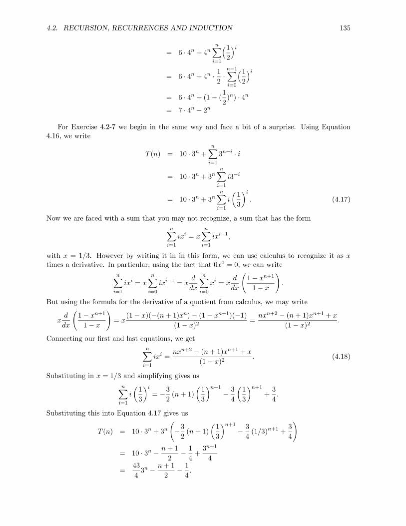
4.2. RECURSION, RECURRENCES AND INDUCTION 135
= 6 · 4n + 4nn∑
i=1
(12
)i
= 6 · 4n + 4n · 12·
n−1∑
i=0
(12
)i
= 6 · 4n + (1 − (12)n) · 4n
= 7 · 4n − 2n
For Exercise 4.2-7 we begin in the same way and face a bit of a surprise. Using Equation4.16, we write
T (n) = 10 · 3n +n∑
i=1
3n−i · i
= 10 · 3n + 3nn∑
i=1
i3−i
= 10 · 3n + 3nn∑
i=1
i
(13
)i
. (4.17)
Now we are faced with a sum that you may not recognize, a sum that has the formn∑
i=1
ixi = xn∑
i=1
ixi−1,
with x = 1/3. However by writing it in in this form, we can use calculus to recognize it as xtimes a derivative. In particular, using the fact that 0x0 = 0, we can write
n∑
i=1
ixi = xn∑
i=0
ixi−1 = xd
dx
n∑
i=0
xi = xd
dx
(1 − xn+1
1 − x
).
But using the formula for the derivative of a quotient from calculus, we may write
xd
dx
(1 − xn+1
1 − x
)= x
(1 − x)(−(n + 1)xn) − (1 − xn+1)(−1)(1 − x)2
=nxn+2 − (n + 1)xn+1 + x
(1 − x)2.
Connecting our first and last equations, we getn∑
i=1
ixi =nxn+2 − (n + 1)xn+1 + x
(1 − x)2. (4.18)
Substituting in x = 1/3 and simplifying gives usn∑
i=1
i
(13
)i
= −32
(n + 1)(
13
)n+1
− 34
(13
)n+1
+34.
Substituting this into Equation 4.17 gives us
T (n) = 10 · 3n + 3n
(−3
2(n + 1)
(13
)n+1
− 34
(1/3)n+1 +34
)
= 10 · 3n − n + 12
− 14
+3n+1
4
=434
3n − n + 12
− 14.

136 CHAPTER 4. INDUCTION, RECURSION, AND RECURRENCES
The sum that arises in this exercise occurs so often that we give its formula as a theorem.
Theorem 4.6 For any real number x = 1,
n∑
i=1
ixi =nxn+2 − (n + 1)xn+1 + x
(1 − x)2. (4.19)
Proof: Given before the statement of the theorem.
Important Concepts, Formulas, and Theorems
1. Recurrence Equation or Recurrence. A recurrence equation is one that tells us how tocompute the nth term of a sequence from the (n − 1)st term or some or all the precedingterms.
2. Initial Condition. To completely specify a function on the basis of a recurrence, we have togive enough information about the function to get started. This information is called theinitial condition (or the initial conditions) for the recurrence.
3. First Order Linear Recurrence. A recurrence T (n) = f(n)T (n − 1) + g(n) is called a firstorder linear recurrence.
4. Constant Coefficient Recurrence. A recurrence in which T (n) is expressed in terms of asum of constant multiples of T (k) for certain values k < n (and perhaps another functionof n) is called a constant coefficient recurrence.
5. Solution to a First Order Constant Coefficient Linear Recurrence. If T (n) = rT (n−1)+a,T (0) = b, and r = 1 then
T (n) = rnb + a1 − rn
1 − r
for all nonnegative integers n.
6. Finite Geometric Series. A finite geometric series with common ratio r is a sum of theform
∑n−1i=0 ri. The formula for the sum of a geometric series with r = 1 is
n−1∑
i=0
ri =1 − rn
1 − r.
7. Big-Theta Bounds on the Sum of a Geometric Series. Let r be a nonnegative quantitywhose value is independent of n and not equal to 1. Let t(n) be the largest term of thegeometric series
n−1∑
i=0
ri.
Then the value of the geometric series is Θ(t(n)).
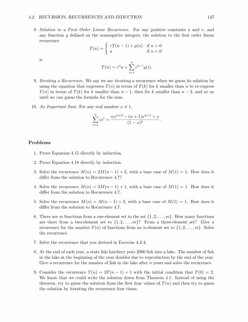
4.2. RECURSION, RECURRENCES AND INDUCTION 137
8. Solution to a First Order Linear Recurrence. For any positive constants a and r, andany function g defined on the nonnegative integers, the solution to the first order linearrecurrence
T (n) =
rT (n − 1) + g(n) if n > 0a if n = 0
is
T (n) = rna +n∑
i=1
rn−ig(i).
9. Iterating a Recurrence. We say we are iterating a recurrence when we guess its solution byusing the equation that expresses T (n) in terms of T (k) for k smaller than n to re-expressT (n) in terms of T (k) for k smaller than n − 1, then for k smaller than n − 2, and so onuntil we can guess the formula for the sum.
10. An Important Sum. For any real number x = 1,
n∑
i=1
ixi =nxn+2 − (n + 1)xn+1 + x
(1 − x)2.
Problems
1. Prove Equation 4.15 directly by induction.
2. Prove Equation 4.18 directly by induction.
3. Solve the recurrence M(n) = 2M(n − 1) + 2, with a base case of M(1) = 1. How does itdiffer from the solution to Recurrence 4.7?
4. Solve the recurrence M(n) = 3M(n − 1) + 1, with a base case of M(1) = 1. How does itdiffer from the solution to Recurrence 4.7.
5. Solve the recurrence M(n) = M(n − 1) + 2, with a base case of M(1) = 1. How does itdiffer from the solution to Recurrence 4.7.
6. There are m functions from a one-element set to the set 1, 2, . . . , m. How many functionsare there from a two-element set to 1, 2, . . . , m? From a three-element set? Give arecurrence for the number T (n) of functions from an n-element set to 1, 2, . . . , m. Solvethe recurrence.
7. Solve the recurrence that you derived in Exercise 4.2-4.
8. At the end of each year, a state fish hatchery puts 2000 fish into a lake. The number of fishin the lake at the beginning of the year doubles due to reproduction by the end of the year.Give a recurrence for the number of fish in the lake after n years and solve the recurrence.
9. Consider the recurrence T (n) = 3T (n − 1) + 1 with the initial condition that T (0) = 2.We know that we could write the solution down from Theorem 4.1. Instead of using thetheorem, try to guess the solution from the first four values of T (n) and then try to guessthe solution by iterating the recurrence four times.

138 CHAPTER 4. INDUCTION, RECURSION, AND RECURRENCES
10. What sort of big-Θ bound can we give on the value of a geometric series 1+r+r2 + · · ·+rn
with common ratio r = 1?
11. Solve the recurrence T (n) = 2T (n − 1) + n2n with the initial condition that T (0) = 1.
12. Solve the recurrence T (n) = 2T (n − 1) + n32n with the initial condition that T (0) = 2.
13. Solve the recurrence T (n) = 2T (n − 1) + 3n with T (0) = 1.
14. Solve the recurrence T (n) = rT (n − 1) + rn with T (0) = 1.
15. Solve the recurrence T (n) = rT (n − 1) + r2n with T (0) = 1
16. Solve the recurrence T (n) = rT (n − 1) + sn with T (0) = 1.
17. Solve the recurrence T (n) = rT (n − 1) + n with T (0) = 1.
18. The Fibonacci numbers are defined by the recurrence
T (n) =
T (n − 1) + T (n − 2) if n > 01 if n = 0 or n = 1
(a) Write down the first ten Fibonacci numbers.
(b) Show that (1+√
52 )n and (1−
√5
2 )n are solutions to the equation F (n) = F (n − 1) +F (n − 2).
(c) Why is
c1(1 +
√5
2)n + c2(
1 −√
52
)n
a solution to the equation F (n) = F (n − 1) + F (n − 2) for any real numbers c1 andc2?
(d) Find constants c1 and c2 such that the Fibonacci numbers are given by
F (n) = c1(1 +
√5
2)n + c2(
1 −√
52
)n

4.3. GROWTH RATES OF SOLUTIONS TO RECURRENCES 139
4.3 Growth Rates of Solutions to Recurrences
Divide and Conquer Algorithms
One of the most basic and powerful algorithmic techniques is divide and conquer. Consider, forexample, the binary search algorithm, which we will describe in the context of guessing a numberbetween 1 and 100. Suppose someone picks a number between 1 and 100, and allows you to askquestions of the form “Is the number greater than k?” where k is an integer you choose. Yourgoal is to ask as few questions as possible to figure out the number. Your first question shouldbe “Is the number greater than 50?” Why is this? Well, after asking if the number is biggerthan 50, you have learned either that the number is between one and 50, or that the number isbetween 51 and 100. In either case have reduced your problem to one in which the range is onlyhalf as big. Thus you have divided the problem up into a problem that is only half as big, andyou can now (recursively) conquer this remaining problem. (If you ask any other question, thesize of one of the possible ranges of values you could end up with would be more than half thesize of the original problem.) If you continue in this fashion, always cutting the problem size inhalf, you will reduce the problem size down to one fairly quickly, and then you will know whatthe number is. Of course it would be easier to cut the problem size exactly in half each time ifwe started with a number in the range from one to 128, but the question doesn’t sound quite soplausible then. Thus to analyze the problem we will assume someone asks you to figure out anumber between 0 and n, where n is a power of 2.
Exercise 4.3-1 Let T (n) be number of questions in binary search on the range of numbersbetween 1 and n. Assuming that n is a power of 2, give a recurrence for T (n).
For Exercise 4.3-1 we get:
T (n) =
T (n/2) + 1 if n ≥ 21 if n = 1
(4.20)
That is, the number of guesses to carry out binary search on n items is equal to 1 step (the guess)plus the time to solve binary search on the remaining n/2 items.
What we are really interested in is how much time it takes to use binary search in a computerprogram that looks for an item in an ordered list. While the number of questions gives us afeel for the amount of time, processing each question may take several steps in our computerprogram. The exact amount of time these steps take might depend on some factors we have littlecontrol over, such as where portions of the list are stored. Also, we may have to deal with listswhose length is not a power of two. Thus a more realistic description of the time needed wouldbe
T (n) ≤
T (n/2) + C1 if n ≥ 2C2 if n = 1,
(4.21)
where C1 and C2 are constants.
Note that x stands for the smallest integer larger than or equal to x, while x stands forthe largest integer less than or equal to x. It turns out that the solution to (4.20) and (4.21)are roughly the same, in a sense that will hopefully become clear later. (This is almost always

140 CHAPTER 4. INDUCTION, RECURSION, AND RECURRENCES
the case.) For now, let us not worry about floors and ceilings and the distinction between thingsthat take 1 unit of time and things that take no more than some constant amount of time.
Let’s turn to another example of a divide and conquer algorithm, mergesort. In this algorithm,you wish to sort a list of n items. Let us assume that the data is stored in an array A in positions1 through n. Mergesort can be described as follows:
MergeSort(A,low,high)if (low == high)
returnelse
mid = (low + high)/2MergeSort(A,low,mid)MergeSort(A,mid+1,high)Merge the sorted lists from the previous two steps
More details on mergesort can be found in almost any algorithms textbook. Suffice to saythat the base case (low = high) takes one step, while the other case executes 1 step, makes tworecursive calls on problems of size n/2, and then executes the Merge instruction, which can bedone in n steps.
Thus we obtain the following recurrence for the running time of mergesort:
T (n) =
2T (n/2) + n if n > 11 if n = 1
(4.22)
Recurrences such as this one can be understood via the idea of a recursion tree, which weintroduce below. This concept allows us to analyze recurrences that arise in divide-and-conqueralgorithms, and those that arise in other recursive situations, such as the Towers of Hanoi, aswell. A recursion tree for a recurrence is a visual and conceptual representation of the process ofiterating the recurrence.
Recursion Trees
We will introduce the idea of a recursion tree via several examples. It is helpful to have an“algorithmic” interpretation of a recurrence. For example, (ignoring for a moment the base case)we can interpret the recurrence
T (n) = 2T (n/2) + n (4.23)
as “in order to solve a problem of size n we must solve 2 problems of size n/2 and do n units ofadditional work.” Similarly we can interpret
T (n) = T (n/4) + n2
as “in order to solve a problem of size n we must solve one problem of size n/4 and do n2 unitsof additional work.”
We can also interpret the recurrence
T (n) = 3T (n − 1) + n

4.3. GROWTH RATES OF SOLUTIONS TO RECURRENCES 141
Figure 4.2: The initial stage of drawing a recursion tree diagram.
Problem Size
n
Work
n
n/2
as “in order to solve a problem of size n, we must solve 3 subproblems of size n − 1 and do nadditional units of work.
In Figure 4.2 we draw the beginning of the recursion tree diagram for (4.23). For now, assumen is a power of 2. A recursion tree diagram has three parts, a left, a middle, and a right. Onthe left, we keep track of the problem size, in the middle we draw the tree, and on right we keeptrack of the work done. We draw the diagram in levels, each level of the diagram representinga level of recursion. Equivalently, each level of the diagram represents a level of iteration of therecurrence. So to begin the recursion tree for (4.23), we show, in level 0 on the left, that wehave problem of size n. Then by drawing a root vertex with two edges leaving it, we show in themiddle that we are splitting our problem into 2 problems. We note on the right that we do nunits of work in addition to whatever is done on the two new problems we created. In the nextlevel, we draw two vertices in the middle representing the two problems into which we split ourmain problem and show on the left that each of these problems has size n/2.
You can see how the recurrence is reflected in levels 0 and 1 of the recursion tree. Thetop vertex of the tree represents T (n), and on the next level we have two problems of size n/2,representing the recursive term 2T (n/2) of our recurrence. Then after we solve these two problemswe return to level 0 of the tree and do n additional units of work for the nonrecursive term ofthe recurrence.
Now we continue to draw the tree in the same manner. Filling in the rest of level one andadding a few more levels, we get Figure 4.3.
Let us summarize what the diagram tells us so far. At level zero (the top level), n units ofwork are done. We see that at each succeeding level, we halve the problem size and double thenumber of subproblems. We also see that at level 1, each of the two subproblems requires n/2units of additional work, and so a total of n units of additional work are done. Similarly level2 has 4 subproblems of size n/4 and so 4(n/4) = n units of additional work are done. Noticethat to compute the total work done on a level we multiply the number of subproblems by theamount of additional work per subproblem.
To see how iteration of the recurrence is reflected in the diagram, we iterate the recurrenceonce, getting
T (n) = 2T (n/2) + n
T (n) = 2(2T (n/4) + n/2) + n
T (n) = 4T (n/4) + n + n = 4T (n/4) + 2n

142 CHAPTER 4. INDUCTION, RECURSION, AND RECURRENCES
Figure 4.3: Four levels of a recursion tree diagram.
8(n/8) = n
Problem Size
n
n/2
n
Work
n/4
n/8
n/2 + n/2 = n
n/4 + n/4 + n/4 + n/4 = n
If we examine levels 0, 1, and 2 of the diagram, we see that at level 2 we have four vertices whichrepresent four problems, each of size n/4 This corresponds to the recursive term that we obtainedafter iterating the recurrence. However after we solve these problems we return to level 1 wherewe twice do n/2 additional units of work and to level 0 where we do another n additional unitsof work. In this way each time we add a level to the tree we are showing the result of one moreiteration of the recurrence.
We now have enough information to be able to describe the recursion tree diagram in general.To do this, we need to determine, for each level, three things:
• the number of subproblems,
• the size of each subproblem,
• the total work done at that level.
We also need to figure out how many levels there are in the recursion tree.
We see that for this problem, at level i, we have 2i subproblems of size n/2i. Further, sincea problem of size 2i requires 2i units of additional work, there are (2i)[n/(2i)] = n units of workdone per level. To figure out how many levels there are in the tree, we just notice that at eachlevel the problem size is cut in half, and the tree stops when the problem size is 1. Thereforethere are log2 n + 1 levels of the tree, since we start with the top level and cut the problem sizein half log2 n times.2 We can thus visualize the whole tree in Figure 4.4.
The computation of the work done at the bottom level is different from the other levels. Inthe other levels, the work is described by the recursive equation of the recurrence; in this casethe amount of work is the n in T (n) = 2T (n/2) + n. At the bottom level, the work comes fromthe base case. Thus we must compute the number of problems of size 1 (assuming that one isthe base case), and then multiply this value by T (1) = 1. In our recursion tree in Figure 4.4,the number of nodes at the bottom level is 2log2 n = n. Since T (1) = 1, we do n units of work at
2To simplify notation, for the remainder of the book, if we omit the base of a logarithm, it should be assumedto be base 2.

4.3. GROWTH RATES OF SOLUTIONS TO RECURRENCES 143
Figure 4.4: A finished recursion tree diagram.
levels
Problem Size
n
n/2
n
Work
n/4
n/8
n/2 + n/2 = n
n/4 + n/4 + n/4 + n/4 = n
8(n/8) = n
1 n(1) = n
log n +1
the bottom level of the tree. Had we chosen to say that T (1) was some constant other than 1,this would not have been the case. We emphasize that the correct value always comes from thebase case; it is just a coincidence that it sometimes also comes from the recursive equation of therecurrence.
The bottom level of the tree represents the final stage of iterating the recurrence. We haveseen that at this level we have n problems each requiring work T (1) = 1, giving us total work nat that level. After we solve the problems represented by the bottom level, we have to do all theadditional work from all the earlier levels. For this reason, we sum the work done at all the levelsof the tree to get the total work done. Iteration of the recurrence shows us that the solution tothe recurrence is the sum of all the work done at all the levels of the recursion tree.
The important thing is that we now know how much work is done at each level. Once weknow this, we can sum the total amount of work done over all the levels, giving us the solutionto our recurrence. In this case, there are log2 n + 1 levels, and at each level the amount of workwe do is n units. Thus we conclude that the total amount of work done to solve the problemdescribed by recurrence (4.23) is n(log2 n + 1). The total work done throughout the tree is thesolution to our recurrence, because the tree simply models the process of iterating the recurrence.Thus the solution to recurrence (4.22) is T (n) = n(log n + 1).
Since one unit of time will vary from computer to computer, and since some kinds of workmight take longer than other kinds, we are usually interested in the big-θ behavior of T (n). Forexample, we can consider a recurrence that it identical to (4.22), except that T (1) = a, for someconstant a. In this case, T (n) = an + n log n, because an units of work are done at level 1 andn additional units of work are done at each of the remaining log n levels. It is still true thatT (n) = Θ(n log n), because the different base case did not change the solution to the recurrenceby more than a constant factor3. Although recursion trees can give us the exact solutions (suchas T (n) = an + n log n above) to recurrences, our interest in the big-Θ behavior of solutions willusually lead us to use a recursion tree to determine the big-Θ or even, in complicated cases, justthe big-O behavior of the actual solution to the recurrence. In Problem 10 we explore whether
3More precisely, n log n < an + n log n < (a + 1)n log n for any a > 0.

144 CHAPTER 4. INDUCTION, RECURSION, AND RECURRENCES
the value of T (1) actually influences the big-Θ behavior of the solution to a recurrence.
Let’s look at one more recurrence.
T (n) =
T (n/2) + n if n > 11 if n = 1
(4.24)
Again, assume n is a power of two. We can interpret this as follows: to solve a problem ofsize n, we must solve one problem of size n/2 and do n units of additional work. We draw thetree for this problem in Figure 4.5 and see that the problem sizes are the same as in the previoustree. The remainder, however, is different. The number of subproblems does not double, rather
Figure 4.5: A recursion tree diagram for Recurrence 4.24.
Problem Size
n
n/2
1
n
Work
n/4
n/8
1
log n + 1levels
n/2
n/4
n/8
it remains at one on each level. Consequently the amount of work halves at each level. Note thatthere are still log n + 1 levels, as the number of levels is determined by how the problem size ischanging, not by how many subproblems there are. So on level i, we have 1 problem of size n/2i,for total work of n/2i units.
We now wish to compute how much work is done in solving a problem that gives this recur-rence. Note that the additional work done is different on each level, so we have that the totalamount of work is
n + n/2 + n/4 + · · · + 2 + 1 = n
(1 +
12
+14
+ · · · +(
12
)log2 n)
,
which is n times a geometric series. By Theorem 4.4, the value of a geometric series in which thelargest term is one is Θ(1). This implies that the work done is described by T (n) = Θ(n).
We emphasize that there is exactly one solution to recurrence (4.24); it is the one we get byusing the recurrence to compute T (2) from T (1), then to compute T (4) from T (2), and so on.What we have done here is show that T (n) = Θ(n). In fact, for the kinds of recurrences we havebeen examining, once we know T (1) we can compute T (n) for any relevant n by repeatedly usingthe recurrence, so there is no question that solutions do exist and can, in principle, be computedfor any value of n. In most applications, we are not interested in the exact form of the solution,but a big-O upper bound, or Big-Θ bound on the solution.

4.3. GROWTH RATES OF SOLUTIONS TO RECURRENCES 145
Exercise 4.3-2 Find a big-Θ bound for the solution to the recurrence
T (n) =
3T (n/3) + n if n ≥ 31 if n < 3
using a recursion tree. Assume that n is a power of 3.
Exercise 4.3-3 Solve the recurrence
T (n) =
4T (n/2) + n if n ≥ 21 if n = 1
using a recursion tree. Assume that n is a power of 2. Convert your solution to abig-Θ statement about the behavior of the solution.
Exercise 4.3-4 Can you give a general big-Θ bound for solutions to recurrences of theform T (n) = aT (n/2) + n when n is a power of 2? You may have different answersfor different values of a.
The recurrence in Exercise 4.3-2 is similar to the mergesort recurrence. One difference isthat at each step we divide into 3 problems of size n/3. Thus we get the picture in Figure 4.6.Another difference is that the number of levels, instead of being log2 n + 1 is now log3 n + 1, so
Figure 4.6: The recursion tree diagram for the recurrence in Exercise 4.3-2.
Problem Size
n n
Work
n/3 + n/3 + n/3 = n
1 n(1) = n
log n + 1levels
n/3
n/9 9(n/9) = n
the total work is still Θ(n log n) units. (Note that logb n = Θ(log2 n) for any b > 1.)
Now let’s look at the recursion tree for Exercise 4.3-3. Here we have 4 children of size n/2,and we get Figure 4.7. Let’s look carefully at this tree. Just as in the mergesort tree there arelog2 n + 1 levels. However, in this tree, each node has 4 children. Thus level 0 has 1 node, level1 has 4 nodes, level 2 has 16 nodes, and in general level i has 4i nodes. On level i each nodecorresponds to a problem of size n/2i and hence requires n/2i units of additional work. Thusthe total work on level i is 4i(n/2i) = 2in units. This formula applies on level log2 n (the bottom

146 CHAPTER 4. INDUCTION, RECURSION, AND RECURRENCES
Figure 4.7: The Recursion tree for Exercise 4.3-3.
Problem Size
n n
Work
n/2 + n/2 + n/2 + n/2 = 2n
1 n^2(1) = n^2
log n + 1levels
n/2
n/4 16(n/4) = 4n
level) as well since there are n2 = 2log2 nn nodes, each requiring T (1) = 1 work. Summing overthe levels, we get
log2 n∑
i=0
2in = n
log2 n∑
i=0
2i.
There are many ways to simplify that expression, for example from our formula for the sumof a geometric series we get
T (n) = n
log2 n∑
i=0
2i
= n1 − 2(log2 n)+1
1 − 2
= n1 − 2n
−1= 2n2 − n
= Θ(n2).
More simply, by Theorem 4.4 we have that T (n) = nΘ(2log n) = Θ(n2).
Three Different Behaviors
Now let’s compare the recursion tree diagrams for the recurrences T (n) = 2T (n/2) + n, T (n) =T (n/2) + n and T (n) = 4T (n/2) + n. Note that all three trees have depth 1 + log2 n, as this isdetermined by the size of the subproblems relative to the parent problem, and in each case, thesize of each subproblem is 1/2 the size of of the parent problem. The trees differ, however, in theamount of work done per level. In the first case, the amount of work on each level is the same.In the second case, the amount of work done on a level decreases as you go down the tree, withthe most work being at the top level. In fact, it decreases geometrically, so by Theorem 4.4 the

4.3. GROWTH RATES OF SOLUTIONS TO RECURRENCES 147
total work done is bounded above and below by a constant times the work done at the root node.In the third case, the number of nodes per level is growing at a faster rate than the problemsize is decreasing, and the level with the largest amount of work is the bottom one. Again wehave a geometric series, and so by Theorem 4.4 the total work is bounded above and below by aconstant times the amount of work done at the last level.
If you understand these three cases and the differences among them, you now understand thegreat majority of the recursion trees that arise in algorithms.
So to answer Exercise 4.3-4, which asks for a general Big-Θ bound for the solutions to recur-rences of the form T (n) = aT (n/2) + n, we can conclude the following:
Lemma 4.7 Suppose that we have a recurrence of the form
T (n) = aT (n/2) + n,
where a is a positive integer and T (1) is nonnegative. Thus we have the following big-Thetabounds on the solution.
1. If a < 2 then T (n) = Θ(n).
2. If a = 2 then T (n) = Θ(n log n)
3. If a > 2 then T (n) = Θ(nlog2 a)
Proof: Cases 1 and 2 follow immediately from our observations above. We can verify case 3as follows. At each level i we have ai nodes, each corresponding to a problem of size n/2i. Thusat level i the total amount of work is ai(n/2i) = n(a/2)i units. Summing over the log2 n levels,we get
alog2 nT (1) + n
(log2 n)−1∑
i=0
(a/2)i.
The sum given by the summation sign is a geometric series, so, since a/2 = 1, the sum will bebig-Θ of the largest term (see Theorem 4.4). Since a > 2, the largest term in this case is clearlythe last one, namely n(a/2)(log2 n)−1, and applying rules of exponents and logarithms, we get thatn times the largest term is
n
(a
2
)(log2 n)−1
=2a· n · alog2 n
2log2 n=
2a· n · alog2 n
n=
2a· alog2 n
=2aalog2(alog2a
=2a· 2log2 a log2 n =
2a· nlog2 a. (4.25)
Thus T (1)alog2 n = T (1)nlog2 a. Since 2a and T (1) are both nonnegative, the total work done is
Θ(nlog2 a).
In fact Lemma 4.7 holds for all positive real numbers a; we can iterate the recurrence to seethis. Since a recursion tree diagram is a way to visualize iterating the recurrence when a is aninteger, iteration is the natural thing to try when a is not an integer.
Notice that in the last two equalities of computation we made in Equation 4.25, we showedthat alog n = nlog a. This is a useful and, perhaps, surprising fact, so we state it (in slightly moregenerality) as a corollary to the proof.
Corollary 4.8 For any base b, we have alogb n = nlogb a.

148 CHAPTER 4. INDUCTION, RECURSION, AND RECURRENCES
Important Concepts, Formulas, and Theorems
1. Divide and Conquer Algorithm. A divide and conquer algorithm is one that solves a problemby dividing it into problems that are smaller but otherwise of the same type as the originalone, recursively solves these problems, and then assembles the solution of these so-calledsubproblems into a solution of the original one. Not all problems can be solved by such astrategy, but a great many problems of interest in computer science can.
2. Mergesort. In mergesort we sort a list of items that have some underlying order by dividingthe list in half, sorting the first half (by recursively using mergesort), sorting the secondhalf (by recursively using mergesort), and then merging the two sorted list. For a list oflength one mergesort returns the same list.
3. Recursion Tree. A recursion tree diagram for a recurrence of the form T (n) = aT (n/b)+g(n)has three parts, a left, a middle, and a right. On the left, we keep track of the problemsize, in the middle we draw the tree, and on right we keep track of the work done. Wedraw the diagram in levels, each level of the diagram representing a level of recursion. Thetree has a vertex representing the initial problem and one representing each subproblemwe have to solve. Each non-leaf vertex has a children. The vertices are divided into levelscorresponding to (sub-)problems of the same size; to the left of a level of vertices we writethe size of the problems the vertices correspond to; to the right of the vertices on a givenlevel we write the total amount of work done at that level by an algorithm whose work isdescribed by the recurrence, not including the work done by any recursive calls from thatlevel.
4. The Base Level of a Recursion Tree. The amount of work done on the lowest level in arecursion tree is the number of nodes times the value given by the initial condition; it is notdetermined by attempting to make a computation of “additional work” done at the lowestlevel.
5. Bases for Logarithms. We use log n as an alternate notation for log2 n. A fundamental factabout logarithms is that logb n = Θ(log2 n) for any real number b > 1.
6. An Important Fact About Logarithms. For any b > 0, alogb n = nlogb a.
7. Three behaviors of solutions. The solution to a recurrence of the form T (n) = aT (n/2) + nbehaves in one of the following ways:
(a) if a < 2 then T (n) = Θ(n).
(b) if a = 2 then T (n) = Θ(n log n)
(c) if a > 2 then T (n) = Θ(nlog2 a).
Problems
1. Draw recursion trees and find big-Θ bounds on the solutions to the following recurrences.For all of these, assume that T (1) = 1 and n is a power of the appropriate integer.
(a) T (n) = 8T (n/2) + n
(b) T (n) = 8T (n/2) + n3

4.3. GROWTH RATES OF SOLUTIONS TO RECURRENCES 149
(c) T (n) = 3T (n/2) + n
(d) T (n) = T (n/4) + 1
(e) T (n) = 3T (n/3) + n2
2. Draw recursion trees and find exact solutions to the following recurrences. For all of these,assume that T (1) = 1 and n is a power of the appropriate integer.
(a) T (n) = 8T (n/2) + n
(b) T (n) = 8T (n/2) + n3
(c) T (n) = 3T (n/2) + n
(d) T (n) = T (n/4) + 1
(e) T (n) = 3T (n/3) + n2
3. Find the exact solution to Recurrence 4.24.
4. Show that logb n = Θ(log2 n), for any constant b > 1.
5. Prove Corollary 4.8 by showing that alogb n = nlogb a for any b > 0.
6. Recursion trees will still work, even if the problems do not break up geometrically, or evenif the work per level is not nc units. Draw recursion trees and and find the best big-Obounds you can for solutions to the following recurrences. For all of these, assume thatT (1) = 1.
(a) T (n) = T (n − 1) + n
(b) T (n) = 2T (n − 1) + n
(c) T (n) = T (√n) + 1 (You may assume n has the form n = 22i.)
(d) T (n) = 2T (n/2) + n log n (You may assume n is a power of 2.)
7. In each case in the previous problem, is the big-O bound you found a big-Θ bound?
8. If S(n) = aS(n − 1) + g(n) and g(n) < cn with 0 ≤ c < a, how fast does S(n) grow (inbig-Θ terms)?
9. If S(n) = aS(n−1)+g(n) and g(n) = cn with 0 < a ≤ c, how fast does S(n) grow in big-Θterms?
10. Given a recurrence of the form T (n) = aT (n/b) + g(n) with T (1) = c > 0 and g(n) > 0for all n and a recurrence of the form S(n) = aS(n/b) + g(n) with S(1) = 0 (and the samea, b, and g(n)), is there any difference in the big-Θ behavior of the solutions to the tworecurrences? What does this say about the influence of the initial condition on the big-Θbehavior of such recurrences?

150 CHAPTER 4. INDUCTION, RECURSION, AND RECURRENCES
4.4 The Master Theorem
Master Theorem
In the last section, we saw three different kinds of behavior for recurrences of the form
T (n) =
aT (n/2) + n if n > 1d if n = 1.
These behaviors depended upon whether a < 2, a = 2, or a > 2. Remember that a was thenumber of subproblems into which our problem was divided. Dividing by 2 cut our problem sizein half each time, and the n term said that after we completed our recursive work, we had nadditional units of work to do for a problem of size n. There is no reason that the amount ofadditional work required by each subproblem needs to be the size of the subproblem. In manyapplications it will be something else, and so in Theorem 4.9 we consider a more general case.Similarly, the sizes of the subproblems don’t have to be 1/2 the size of the parent problem. Wethen get the following theorem, our first version of a theorem called the Master Theorem. (Lateron we will develop some stronger forms of this theorem.)
Theorem 4.9 Let a be an integer greater than or equal to 1 and b be a real number greater than1. Let c be a positive real number and d a nonnegative real number. Given a recurrence of theform
T (n) =
aT (n/b) + nc if n > 1d if n = 1
in which n is restricted to be a power of b,
1. if logb a < c, T (n) = Θ(nc),
2. if logb a = c, T (n) = Θ(nc log n),
3. if logb a > c, T (n) = Θ(nlogb a).
Proof: In this proof, we will set d = 1, so that the work done at the bottom level of the treeis the same as if we divided the problem one more time and used the recurrence to compute theadditional work. As in Footnote 3 in the previous section, it is straightforward to show that weget the same big-Θ bound if d is positive. It is only a little more work to show that we get thesame big-Θ bound if d is zero.
Let’s think about the recursion tree for this recurrence. There will be 1 + logb n levels. Ateach level, the number of subproblems will be multiplied by a, and so the number of subproblemsat level i will be ai. Each subproblem at level i is a problem of size (n/bi). A subproblem of sizen/bi requires (n/bi)c additional work and since there are ai problems on level i, the total numberof units of work on level i is
ai(n/bi)c = nc
(ai
bci
)= nc
(a
bc
)i
. (4.26)
Recall from Lemma 4.7 that the different cases for c = 1 were when the work per level wasdecreasing, constant, or increasing. The same analysis applies here. From our formula for work

4.4. THE MASTER THEOREM 151
on level i, we see that the work per level is decreasing, constant, or increasing exactly when ( abc )i
is decreasing, constant, or increasing, respectively. These three cases depend on whether ( abc ) is
less than one, equal to one, or greater than one, respectively. Now observe that
( abc ) = 1
⇔ a = bc
⇔ logb a = c logb b
⇔ logb a = c.
This shows us where the three cases in the statement of the theorem come from. Now weneed to show the bound on T (n) in the different cases. In the following paragraphs, we will usethe facts (whose proof is a straightforward application of the definition of logarithms and rulesof exponents) that for any x, y and z, each greater than 1, xlogy z = zlogy x (see Corollary 4.8,Problem 5 at the end of the previous section, and Problem 3 at the end of this section) and thatlogx y = Θ(log2 y) (see Problem 4 at the end of the previous section).
In general, the total work done is computed by summing the expression for the work per levelgiven in Equation 4.26 over all the levels, giving
logb n∑
i=0
nc(
a
bc
)i
= nclogb n∑
i=0
(a
bc
)i
In case 1, (part 1 in the statement of the theorem) this is nc times a geometric series with a ratioof less than 1. Theorem 4.4 tells us that
nclogb n∑
i=0
(a
bc
)i
= Θ(nc).
Exercise 4.4-1 Prove Case 2 (part 2 of the statement) of the Master Theorem.
Exercise 4.4-2 Prove Case 3 (part 3 of the statement) of the Master Theorem.
In Case 2 we have that abc = 1 and so
nclogb n∑
i=0
(a
bc
)i
= nclogb n∑
i=0
1i
= nc(1 + logb n)= Θ(nc log n).
In Case 3, we have that abc > 1. So in the series
logb n∑
i=0
nc(
a
bc
)i
= nclogb n∑
i=0
(a
bc
)i
,
the largest term is the last one, so by Theorem 4.4,the sum is Θ(nc
(abc
)logb n). But

152 CHAPTER 4. INDUCTION, RECURSION, AND RECURRENCES
nc(
a
bc
)logb n
= nc · alogb n
(bc)logb n
= nc · nlogb a
nlogb bc
= nc · nlogb a
nc
= nlogb a.
Thus the solution is Θ(nlogb a).
We note that we may assume that a is a real number with a > 1 and give a somewhat similarproof (replacing the recursion tree with an iteration of the recurrence), but we do not give thedetails here.
Solving More General Kinds of Recurrences
Exercise 4.4-3 What can you say about the big-θ behavior of the solution to
T (n) =
2T (n/3) + 4n3/2 if n > 1d if n = 1,
where n can be any nonnegative power of three?
Exercise 4.4-4 If f(n) = n√
n + 1, what can you say about the Big-Θ behavior of solu-tions to
S(n) =
2S(n/3) + f(n) if n > 1d if n = 1,
where n can be any nonnegative power of three?
For Exercise 4.4-3, the work done at each level of the tree except for the bottom level will befour times the work done by the recurrence
T ′(n) =
2T ′(n/3) + n3/2 if n > 1d if n = 1,
Thus the work done by T will be no more than four times the work done by T ′, but will belarger than the work done by T ′. Therefore T (n) = Θ(T ′(n)). Thus by the master theorem, sincelog3 2 < 1 < 3/2, we have that T (n) = Θ(n3/2).
For Exercise 4.4-4, Since n√
n + 1 > n√
n = n3/2 we have that S(n) is at least as big as thesolution to the recurrence
T ′(n) =
2T ′(n/3) + n3/2 if n > 1d if n = 1,
where n can be any nonnegative power of three. But the solution to the recurrence for S will beno more than the solution to the recurrence in Exercise 4.4-3 for T , because n
√n + 1 ≤ 4n3/2
for n ≥ 0. Since T (n) = Θ(T ′(n)), then S(n) = Θ(T ′(n)) as well.

4.4. THE MASTER THEOREM 153
Extending the Master Theorem
As Exercise 4.4-3 and Exercise 4.4-4 suggest, there is a whole range of interesting recurrences thatdo not fit the master theorem but are closely related to recurrences that do. These recurrenceshave the same kind of behavior predicted by our original version of the Master Theorem, but theoriginal version of the Master Theorem does not apply to them, just as it does not apply to therecurrences of Exercise 4.4-3 and Exercise 4.4-4.
We now state a second version of the Master Theorem that covers these cases. A still strongerversion of the theorem may be found in Introduction to Algorithms by Cormen, et. al., but theversion here captures much of the interesting behavior of recurrences that arise from the analysisof algorithms.
Theorem 4.10 Let a and b be positive real numbers with a ≥ 1 and b > 1. Let T (n) be definedfor powers n of b by
T (n) =
aT (n/b) + f(n) if n > 1d if n = 1.
Then
1. if f(n) = Θ(nc) where logb a < c, then T (n) = Θ(nc) = Θ(f(n)).
2. if f(n) = Θ(nc), where logb a = c, then T (n) = Θ(nlogb a logb n)
3. if f(n) = Θ(nc), where logb a > c, then T (n) = Θ(nlogb a).
Proof: We construct a recursion tree or iterate the recurrence. Since we have assumed thatf(n) = Θ(nc), there are constants c1 and c2, independent of the level, so that the work at eachlevel is between c1n
c(
abc
)i and c2nc(
abc
)i so from this point on the proof is largely a translationof the original proof.
Exercise 4.4-5 What does the Master Theorem tell us about the solutions to the recur-rence
T (n) =
3T (n/2) + n
√n + 1 if n > 1
1 if n = 1?
As we saw in our solution to Exercise 4.4-4 x√
x + 1 = Θ(x3/2). Since 23/2 =√
23 =√
8 < 3,we have that log2 3 > 3/2. Then by conclusion 3 of version 2 of the Master Theorem, T (n) =Θ(nlog2 3).
The remainder of this section is devoted to carefully analyzing divide and conquer recurrencesin which n is not a power of b and T (n/b) is replaced by T (n/b). While the details aresomewhat technical, the end result is that the big-Θ behavior of such recurrences is the same asthe corresponding recurrences for functions defined on powers of b. In particular, the followingtheorem is a consequence of what we prove.

154 CHAPTER 4. INDUCTION, RECURSION, AND RECURRENCES
Theorem 4.11 Let a and b be positive real numbers with a ≥ 1 and b ≥ 2. Let T (n) satisfy therecurrence
T (n) =
aT (n/b) + f(n) if n > 1d if n = 1.
Then
1. if f(n) = Θ(nc) where logb a < c, then T (n) = Θ(nc) = Θ(f(n)).
2. if f(n) = Θ(nc), where logb a = c, then T (n) = Θ(nlogb a logb n)
3. if f(n) = Θ(nc), where logb a > c, then T (n) = Θ(nlogb a).
(The condition that b ≥ 2 can be changed to B > 1 with an appropriate change in the base caseof the recurrence, but the base case will then depend on b.) The reader should be able to skipover the remainder of this section without loss of continuity.
More realistic recurrences (Optional)
So far, we have considered divide and conquer recurrences for functions T (n) defined on integersn which are powers of b. In order to consider a more realistic recurrence in the master theorem,namely
T (n) =
aT (n/b) + nc if n > 1d if n = 1,
or
T (n) =
aT (n/b) + nc if n > 1d if n = 1,
or even
T (n) =
a′T (n/b) + (a − a′)T (n/b) + nc if n > 1d if n = 1,
it turns out to be easiest to first extend the domain for our recurrences to a much bigger set thanthe nonnegative integers, either the real or rational numbers, and then to work backwards.
For example, we can write a recurrence of the form
t(x) =
f(x)t(x/b) + g(x) if x ≥ bk(x) if 1 ≤ x < b
for two (known) functions f and g defined on the real [or rational] numbers greater than 1 andone (known) function k defined on the real [or rational] numbers x with 1 ≤ x < b. Then so longas b > 1 it is possible to prove that there is a unique function t defined on the real [or rational]numbers greater than or equal to 1 that satisfies the recurrence. We use the lower case t in thissituation as a signal that we are considering a recurrence whose domain is the real or rationalnumbers greater than or equal to 1.
Exercise 4.4-6 How would we compute t(x) in the recurrence
t(x) =
3t(x/2) + x2 if x ≥ 25x if 1 ≤ x < 2
if x were 7? How would we show that there is one and only one function t that satisfiesthe recurrence?

4.4. THE MASTER THEOREM 155
Exercise 4.4-7 Is it the case that there is one and only one solution to the recurrence
T (n) =
f(n)T (n/b) + g(n) if n > 1k if n = 1
when f and g are (known) functions defined on the positive integers, and k and b are(known) constants with b an integer larger than or equal to 2?
To compute t(7) in Exercise 4.4-6 we need to know t(7/2). To compute t(7/2), we need toknow t(7/4). Since 1 < 7/4 < 2, we know that t(7/4) = 35/4. Then we may write
t(7/2) = 3 · 354
+494
=1544
=772
.
Next we may write
t(7) = 3t(7/2) + 72
= 3 · 772
+ 49
=3292
.
Clearly we can compute t(x) in this way for any x, though we are unlikely to enjoy the arithmetic.On the other hand suppose all we need to do is to show that there is a unique value of t(x)determined by the recurrence, for all real numbers x ≥ 1. If 1 ≤ x < 2, then t(x) = 5x, whichuniquely determines t(x). Given a number x ≥ 2, there is a smallest integer i such that x/2i < 2,and for this i, we have 1 ≤ x/2i. We can now prove by induction on i that t(x) is uniquelydetermined by the recurrence relation.
In Exercise 4.4-7 there is one and only one solution. Why? Clearly T (1) is determined bythe recurrence. Now assume inductively that n > 1 and that T (m) is uniquely determined forpositive integers m < n. We know that n ≥ 2, so that n/2 ≤ n − 1. Since b ≥ 2, we knowthat n/2 ≥ n/b, so that n/b ≤ n − 1. Therefore n/b < n, so that we know by the inductivehypothesis that T (n/b) is uniquely determined by the recurrence. Then by the recurrence,
T (n) = f(n)T(⌈
n
b
⌉)+ g(n),
which uniquely determines T (n). Thus by the principle of mathematical induction, T (n) isdetermined for all positive integers n.
For every kind of recurrence we have dealt with, there is similarly one and only one solution.Because we know solutions exist, we don’t find formulas for solutions to demonstrate that solu-tions exist, but rather to help us understand properties of the solutions. In this section and thelast section, for example, we were interested in how fast the solutions grew as n grew large. Thisis why we were finding Big-O and Big-Θ bounds for our solutions.
Recurrences for general n (Optional)
We will now show how recurrences for arbitrary real numbers relate to recurrences involvingfloors and ceilings. We begin by showing that the conclusions of the Master Theorem apply torecurrences for arbitrary real numbers when we replace the real numbers by “nearby” powersof b.

156 CHAPTER 4. INDUCTION, RECURSION, AND RECURRENCES
Theorem 4.12 Let a and b be positive real numbers with b > 1 and c and d be real numbers.Let t(x) be the solution to the recurrence
t(x) =
at(x/b) + xc if x ≥ bd if 1 ≤ x < b.
Let T (n) be the solution to the recurrence
T (n) =
aT (n/b) + nc if n ≥ 0d if n = 1,
defined for n a nonnegative integer power of b. Let m(x) be the largest integer power of b lessthan or equal to x. Then t(x) = Θ(T (m(x)))
Proof: If we iterate (or, in the case that a is an integer, draw recursion trees for) the tworecurrences, we can see that the results of the iterations are nearly identical. This means thesolutions to the recurrences have the same big-Θ behavior. See the Appendix to this Section fordetails.
Removing Floors and Ceilings (Optional)
We have also pointed out that a more realistic Master Theorem would apply to recurrences ofthe form T (n) = aT (n/b) + nc, or T (n) = aT (n/b) + nc, or even T (n) = a′T (n/b) + (a −a′)T (n/b)+nc. For example, if we are applying mergesort to an array of size 101, we really breakit into pieces, of size 50 and 51. Thus the recurrence we want is not really T (n) = 2T (n/2) + n,but rather T (n) = T (n/2) + T (n/2) + n.
We can show, however, that one can essentially “ignore” the floors and ceilings in typicaldivide-and-conquer recurrences. If we remove the floors and ceilings from a recurrence relation,we convert it from a recurrence relation defined on the integers to one defined on the rationalnumbers. However we have already seen that such recurrences are not difficult to handle.
The theorem below says that in recurrences covered by the master theorem, if we removeceilings, our recurrences still have the same big-Θ bounds on their solutions. A similar proofshows that we may remove floors and still get the same big-Θ bounds. Without too much morework we can see that we can remove floors and ceilings simultaneously without changing thebig-Θ bounds on our solutions. Since we may remove either floors or ceilings, that means that wemay deal with recurrences of the form T (n) = a′T (n/b)+ (a−a′)T (n/b)+nc. The conditionthat b > 2 can be replaced by b > 1, but the base case for the recurrence will depend on b.
Theorem 4.13 Let a and b be positive real numbers with b ≥ 2 and let c and d be real numbers.Let T (n) be the function defined on the integers by the recurrence
T (n) =
aT (n/b) + nc if n > 1d n = 1,
and let t(x) be the function on the real numbers defined by the recurrence
t(x) =
at(x/b) + xc if x ≥ bd if 1 ≤ x < b
Then T (n) = Θ(t(n)). The same statement applies with ceilings replaced by floors.

4.4. THE MASTER THEOREM 157
Proof: As in the previous theorem, we can consider iterating the two recurrences. It isstraightforward (though dealing with the notation is difficult) to show that for a given value ofn, the iteration for computing T (n) has at most two more levels than the iteration for computingt(n). The work per level also has the same Big-Θ bounds at each level, and the work for the twoadditional levels of the iteration for T (n) has the same Big-Θ bounds as the work at the bottomlevel of the recursion tree for t(n). We give the details in the appendix at the end of this section.
Theorem 4.12 and Theorem 4.13 tell us that the Big-Θ behavior of solutions to our morerealistic recurrences
T (n) =
aT (n/b) + nc if n > 1d n=1
is determined by their Big-Θ behavior on powers of the base b.
Floors and ceilings in the stronger version of the Master Theorem (Optional)
In our first version of the master theorem, we showed that we could ignore ceilings and assumeour variables were powers of b. In fact we can ignore them in circumstances where the functiontelling us the “work” done at each level of our recursion tree is Θ(xc) for some positive realnumber c. This lets us apply the second version of the master theorem to recurrences of the formT (n) = aT (n/b) + f(n).
Theorem 4.14 Theorems 4.12 and 4.13 apply to recurrences in which the xc or nc term isreplaced by f(x) or f(n) for a function f with f(x) = Θ(xc).
Proof: We iterate the recurrences or construct recursion trees in the same way as in the proofsof the original theorems, and find that the condition f(x) = Θ(xc) gives us enough informationto again bound the solution above and below with multiples of the solution of the recurrencewith xc. The details are similar to those in the original proofs.
Appendix: Proofs of Theorems (Optional)
For convenience, we repeat the statements of the earlier theorems whose proofs we merely out-lined.
Theorem 4.12 Let a and b be positive real numbers with b > 1 and c and d be real numbers.Let t(x) be the solution to the recurrence
t(x) =
at(x/b) + xc if x ≥ bd if 1 ≤ x < b.
Let T (n) be the solution to the recurrence
T (n) =
aT (n/b) + nc if n ≥ 0d if n = 1,
defined for n is a nonnegative integer power of b. Let m(x) be the largest integer power of b lessthan or equal to x. Then t(x) = Θ(T (m(x)))

158 CHAPTER 4. INDUCTION, RECURSION, AND RECURRENCES
Proof: By iterating each recursion 4 times (or using a four level recursion tree in the casethat a is an integer), we see that
t(x) = a4t( x
b4
)+
( a
bc
)3xc +
( a
bc
)2xc +
a
bcxc
andT (n) = a4T
( n
b4
)+
( a
bc
)3nc +
( a
bc
)2nc +
a
bcnc.
Thus, continuing until we have a solution, in both cases we get a solution that starts with a raisedto an exponent that we will denote as either e(x) or e(n) when we want to distinguish betweenthem and e when it is unnecessary to distinguish. The solution for t will be ae times t(x/be)
plus xc times a geometric series∑e−1
i=0
(abc
)i. The solution for T will be ae times d plus nc times
a geometric series∑e−1
i=0
(abc
)i. In both cases t(x/be) (or T (n/be)) will be d. In both cases the
geometric series will be Θ(1), Θ(e) or Θ(
abc
)e, depending on whether a
bc is less than 1, equal to 1,or greater than one. Clearly e(n) = logb n. Since we must divide x by b an integer number greaterthan logb x− 1 times in order to get a value in the range from 1 to b, e(x) = logb x. Thus, if mis the largest integer power of b less than or equal to x, then 0 ≤ e(x) − e(m) < 1. Let us use rto stand for the real number a
bc . Then we have r0 ≤ re(x)−e(m) < r, or re(m) ≤ re(x) ≤ r · re(m).Thus we have re(x) = Θ(re(m)) Finally, mc ≤ xc ≤ bcmc, and so xc = Θ(mc). Therefore, everyterm of t(x) is Θ of the corresponding term of T (m). Further, there are only a fixed number ofdifferent constants involved in our Big-Θ bounds. Therefore since t(x) is composed of sums andproducts of these terms, t(x) = Θ(T (m)).
Theorem 4.13 Let a and b be positive real numbers with b ≥ 2 and let c and d be real numbers.Let T (n) be the function defined on the integers by the recurrence
T (n) =
aT (n/b) + nc if n ≥ bd n = 1,
and let t(x) be the function on the real numbers defined by the recurrence
t(x) =
at(x/b) + xc if x ≥ bd if 1 ≤ x < b.
Then T (n) = Θ(t(n)).
Proof: As in the previous proof, we can iterate both recurrences. Let us compare what theresults will be of iterating the recurrence for t(n) and the recurrence for T (n) the same numberof times. Note that
n/b < n/b + 1n/b/b < n/b2 + 1/b < n/b2 + 1/b + 1
n/b/b/b < n/b3 + 1/b2 + 1/b < n/b3 + 1/b2 + 1/b + 1
This suggests that if we define n0 = n, and ni = ni−1/b, then, using the fact that b ≥ 2, itis straightforward to prove by induction, or with the formula for the sum of a geometric series,

4.4. THE MASTER THEOREM 159
that ni < n/bi + 2. The number ni is the argument of T in the ith iteration of the recurrencefor T . We have just seen that it differs from the argument of t in the ith iteration of t by atmost 2. In particular, we might have to iterate the recurrence for T twice more than we iteratethe recurrence for t to reach the base case. When we iterate the recurrence for t, we get thesame solution we got in the previous theorem, with n substituted for x. When we iterate therecurrence for T , we get for some integer j that
T (n) = ajd +j−1∑
i=0
ainci ,
with nbi ≤ ni ≤ n
bi + 2. But, so long as n/bi ≥ 2, we have n/bi + 2 ≤ n/bi−1. Since the number ofiterations of T is at most two more than the number of iterations of t, and since the number ofiterations of t is logb n, we have that j is at most logb n + 2. Therefore all but perhaps thelast three values of ni are less than or equal to n/bi−1, and these last three values are at most b2,b, and 1. Putting all these bounds together and using n0 = n gives us
j−1∑
i=0
ai( n
bi
)c≤
j−1∑
i=0
ainci
≤ nc +j−4∑
i=1
ai( n
bi−1
)c+ aj−2(b2)c + aj−1bc + aj1c,
orj−1∑
i=0
ai( n
bi
)c≤
j−1∑
i=0
ainci
≤ nc + bj−4∑
i=1
ai( n
bi
)c+ aj−2
(bj
bj−2
)c
+ aj−1
(bj
bj−1
)c
+ aj
(bj
bj
)c
.
As we shall see momentarily these last three “extra” terms and the b in front of the summationsign do not change the Big-Θ behavior of the right-hand side.
As in the proof of the master theorem, the Big-Θ behavior of the left hand side depends onwhether a/bc is less than 1, in which case it is Θ(nc), equal to 1, in which case it is Θ(nc logb n),or greater than one in which case it is Θ(nlogb a). But this is exactly the Big-Θ behavior of theright-hand side, because n < bj < nb2, so bj = Θ(n), which means that
(bj
bi
)c= Θ
((nbi
)c),
and the b in front of the summation sign does not change its Big-Θ behavior. Adding ajd tothe middle term of the inequality to get T (n) does not change this behavior. But this modifiedmiddle term is exactly T (n). Since the left and right hand sides have the same big-Θ behavioras t(n), we have T(n) = Θ(t(n)).
Important Concepts, Formulas, and Theorems
1. Master Theorem, simplified version. The simplified version of the Master Theorem states:Let a be an integer greater than or equal to 1 and b be a real number greater than 1. Let cbe a positive real number and d a nonnegative real number. Given a recurrence of the form
T (n) =
aT (n/b) + nc if n > 1d if n = 1
then for n a power of b,
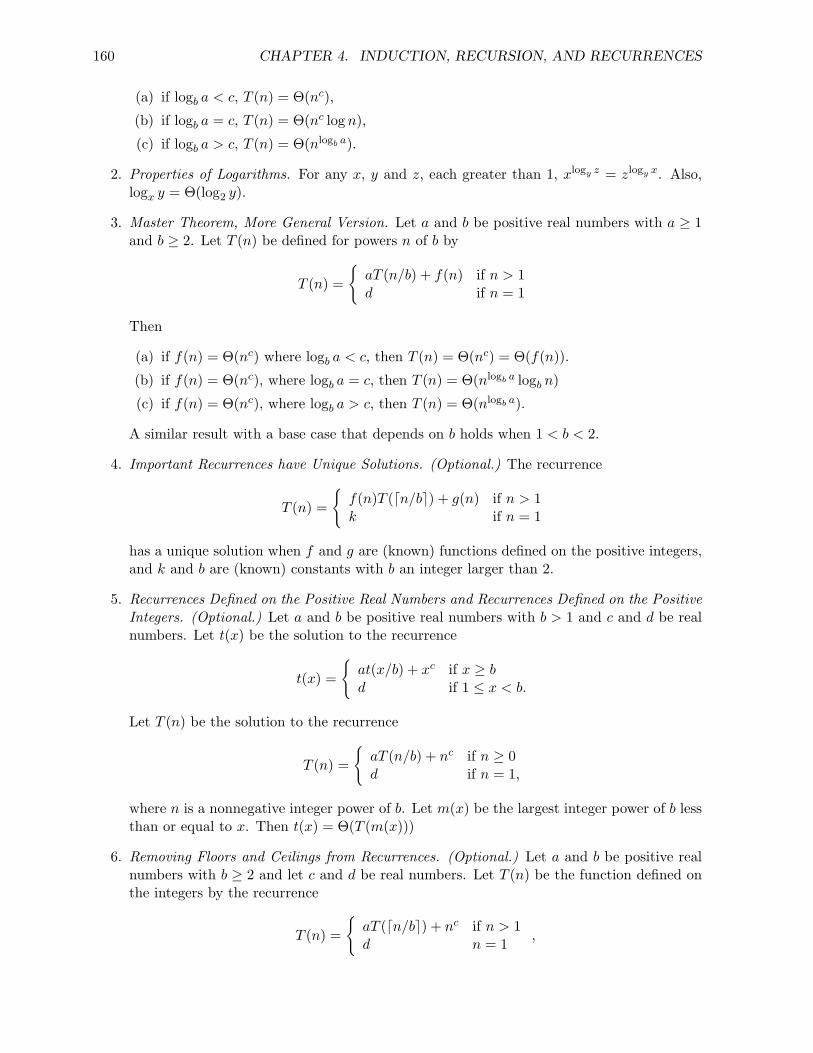
160 CHAPTER 4. INDUCTION, RECURSION, AND RECURRENCES
(a) if logb a < c, T (n) = Θ(nc),
(b) if logb a = c, T (n) = Θ(nc log n),
(c) if logb a > c, T (n) = Θ(nlogb a).
2. Properties of Logarithms. For any x, y and z, each greater than 1, xlogy z = zlogy x. Also,logx y = Θ(log2 y).
3. Master Theorem, More General Version. Let a and b be positive real numbers with a ≥ 1and b ≥ 2. Let T (n) be defined for powers n of b by
T (n) =
aT (n/b) + f(n) if n > 1d if n = 1
Then
(a) if f(n) = Θ(nc) where logb a < c, then T (n) = Θ(nc) = Θ(f(n)).
(b) if f(n) = Θ(nc), where logb a = c, then T (n) = Θ(nlogb a logb n)
(c) if f(n) = Θ(nc), where logb a > c, then T (n) = Θ(nlogb a).
A similar result with a base case that depends on b holds when 1 < b < 2.
4. Important Recurrences have Unique Solutions. (Optional.) The recurrence
T (n) =
f(n)T (n/b) + g(n) if n > 1k if n = 1
has a unique solution when f and g are (known) functions defined on the positive integers,and k and b are (known) constants with b an integer larger than 2.
5. Recurrences Defined on the Positive Real Numbers and Recurrences Defined on the PositiveIntegers. (Optional.) Let a and b be positive real numbers with b > 1 and c and d be realnumbers. Let t(x) be the solution to the recurrence
t(x) =
at(x/b) + xc if x ≥ bd if 1 ≤ x < b.
Let T (n) be the solution to the recurrence
T (n) =
aT (n/b) + nc if n ≥ 0d if n = 1,
where n is a nonnegative integer power of b. Let m(x) be the largest integer power of b lessthan or equal to x. Then t(x) = Θ(T (m(x)))
6. Removing Floors and Ceilings from Recurrences. (Optional.) Let a and b be positive realnumbers with b ≥ 2 and let c and d be real numbers. Let T (n) be the function defined onthe integers by the recurrence
T (n) =
aT (n/b) + nc if n > 1d n = 1
,

4.4. THE MASTER THEOREM 161
and let t(x) be the function on the real numbers defined by the recurrence
t(x) =
at(x/b) + xc if x ≥ bd if 1 ≤ x < b
.
Then T (n) = Θ(t(n)). The same statement applies with ceilings replaced by floors.
7. Extending 5 and 6 (Optional.) In the theorems summarized in 5 and 6 the nc or xc termmay be replaced by a function f with f(x) = Θ(xc).
8. Solutions to Realistic Recurrences. The theorems summarized in 5, 6, and 7 tell us thatthe Big-Θ behavior of solutions to our more realistic recurrences
T (n) =
aT (n/b) + f(n) if n > 1d n=1,
where f(n) = Θ(nc), is determined by their Big-Θ behavior on powers of the base b andwith f(n) = nc.
Problems
1. Use the master theorem to give Big-Θ bounds on the solutions to the following recurrences.For all of these, assume that T (1) = 1 and n is a power of the appropriate integer.
(a) T (n) = 8T (n/2) + n
(b) T (n) = 8T (n/2) + n3
(c) T (n) = 3T (n/2) + n
(d) T (n) = T (n/4) + 1
(e) T (n) = 3T (n/3) + n2
2. Extend the proof of the Master Theorem, Theorem 4.9 to the case T (1) = d.
3. Show that for any x, y and z, each greater than 1, xlogy z = zlogy x.
4. (Optional) Show that for each real number x ≥ 0 there is one and only one value of t(x)given by the recurrence
t(x) =
7xt(x − 1) + 1 if x ≥ 11 if 0 ≤ x < 1.
5. (Optional) Show that for each real number x ≥ 1 there is one and only one value of t(x)given by the recurrence
t(x) =
3xT (x/2) + x2 if x ≥ 21 if 1 ≤ x < 2
.

162 CHAPTER 4. INDUCTION, RECURSION, AND RECURRENCES
6. (Optional) How many solutions are there to the recurrence
T (n) =
f(n)T (n/b) + g(n) if n > 1k if n = 1
if b < 2? If b = 10/9, by what would we have to replace the condition that T (n) = k ifn = 1 in order to get a unique solution?
7. Give a big-Θ bound on the solution to the recurrence
T (n) =
3T (n/2) +
√n + 3 if n > 1
d if n = 1.
8. Give a big-Θ bound on the solution to the recurrence
T (n) =
3T (n/2) +
√n3 + 3 if n > 1
d if n = 1.
9. Give a big-Θ bound on the solution to the recurrence
T (n) =
3T (n/2) +
√n4 + 3 if n > 1
d if n = 1.
10. Give a big-Θ bound on the solution to the recurrence
T (n) =
2T (n/2) +
√n2 + 3 if n > 1
d if n = 1.
11. (Optional) Explain why theorem 4.11 is a consequence of Theorem 4.12 and Theorem 4.13

4.5. MORE GENERAL KINDS OF RECURRENCES 163
4.5 More general kinds of recurrences
Recurrence Inequalities
The recurrences we have been working with are really idealized versions of what we know aboutthe problems we are working on. For example, in merge-sort on a list of n items, we say wedivide the list into two parts of equal size, sort each part, and then merge the two sorted parts.The time it takes to do this is the time it takes to divide the list into two parts plus the timeit takes to sort each part, plus the time it takes to merge the two sorted lists. We don’t specifyhow we are dividing the list, or how we are doing the merging. (We assume the sorting is doneby applying the same method to the smaller lists, unless they have size 1, in which case we donothing.) What we do know is that any sensible way of dividing the list into two parts takes nomore than some constant multiple of n time units (and might take no more than constant time ifwe do it by leaving the list in place and manipulating pointers) and that any sensible algorithmfor merging two lists will take no more than some (other) constant multiple of n time units. Thuswe know that if T (n) is the amount of time it takes to apply merge sort to n data items, thenthere is a constant c (the sum of the two constant multiples we mentioned) such that
T (n) ≤ 2T (n/2) + cn. (4.27)
Thus real world problems often lead us to recurrence inequalities rather than recurrenceequations. These are inequalities that state that T (n) is less than or equal to some expressioninvolving values of T (m) for m < n. (We could also include inequalities with a greater thanor equal to sign, but they do not arise in the applications we are studying.) A solution to arecurrence inequality is a function T that satisfies the inequality. For simplicity we will expandwhat we mean by the word recurrence to include either recurrence inequalities or recurrenceequations.
In Recurrence 4.27 we are implicitly assuming that T is defined only on positive integer valuesand, since we said we divided the list into two equal parts each time, our analysis only makessense if we assume that n is a power of 2.
Note that there are actually infinitely many solutions to Recurrence 4.27. (For example forany c′ < c, the unique solution to
T (n) =
2T (n/2) + c′n if n ≥ 2k if n = 1
(4.28)
satisfies Inequality 4.27 for any constant k.) The idea that Recurrence 4.27 has infinitely manysolutions, while Recurrence 4.28 has exactly one solution is analogous to the idea that x− 3 ≤ 0has infinitely many solutions while x − 3 = 0 has one solution. Later in this section we shall seehow to show that all the solutions to Recurrence 4.27 satisfy T (n) = O(n log2 n). In other words,no matter how we sensibly implement merge sort, we have a O(n log2 n) time bound on how longthe merge sort process takes.
Exercise 4.5-1 Carefully prove by induction that for any function T defined on the non-negative powers of 2, if
T (n) ≤ 2T (n/2) + cn
for some constant c, then T (n) = O(n log n).

164 CHAPTER 4. INDUCTION, RECURSION, AND RECURRENCES
A Wrinkle with Induction
We can analyze recurrence inequalities via a recursion tree. The process is virtually identical toour previous use of recursion trees. We must, however, keep in mind that on each level, we arereally computing an upper bound on the work done on that level. We can also use a variant of themethod we used a few sections ago, guessing an upper bound and verifying by induction. We usethis method for the recurrence in Exercise 4.5-1. Here we wish to show that T (n) = O(n log n).From the definition of Big-O, we can see that we wish to show that T (n) ≤ kn log n for somepositive constant k (so long as n is larger than some value n0).
We are going to do something you may find rather curious. We will consider the possibilitythat we have a value of k for which the inequality holds. Then in analyzing the consequencesof this possibility, we will discover that there are assumptions that we need to make about k inorder for such a k to exist. What we will really be doing is experimenting to see how we willneed to choose k to make an inductive proof work.
We are given that T (n) ≤ 2T (n/2) + cn for all positive integers n that are powers of 2. Wewant to prove there is another positive real number k > 0 and an n0 > 0 such that for n > n0,T (n) ≤ kn log n. We cannot expect to have the inequality T (n) ≤ kn log n hold for n = 1,because log 1 = 0. To have T (2) ≤ k · 2 log 2 = k · 2, we must choose k ≥ T (2)
2 . This is the firstassumption we must make about k. Our inductive hypothesis will be that if n is a power of 2 andm is a power of 2 with 2 ≤ m < n then T (m) ≤ km log m. Now n/2 < n, and since n is a powerof 2 greater than 2, we have that n/2 ≥ 2, so (n/2) log n/2 ≥ 2. By the inductive hypothesis,T (n/2) ≤ k(n/2) log n/2. But then
T (n) ≤ 2T (n/2) + cn ≤ 2kn
2log
n
2+ cn (4.29)
= kn logn
2+ cn (4.30)
= kn log n − kn log 2 + cn (4.31)= kn log n − kn + cn. (4.32)
Recall that we are trying to show that T (n) ≤ kn log n. But that is not quite what Line 4.32tells us. This shows that we need to make another assumption about k, namely that −kn+cn ≤ 0,or k ≥ c. Then if both our assumptions about k are satisfied, we will have T (n) < kn log n, andwe can conclude by the principle of mathematical induction that for all n > 1 (so our n0 is 2),T (n) ≤ kn log n, so that T (n) = O(n log n).
A full inductive proof that T (n) = O(n log n) is actually embedded in the discussion above,but since it might not appear to everyone to be a proof, below we will summarize our observationsin a more traditional looking proof. However you should be aware that some authors and teachersprefer to write their proofs in a style that shows why we make the choices about k that we do,and so you should learn how to to read discussions like the one above as proofs.
We want to show that if T (n) ≤ T (n/2) + cn, then T (n) = O(n log n). We are given a realnumber c > 0 such that T (n) ≤ 2T (n/2) + cn for all n > 1. Choose k to be larger than or equalto T (2)
2 and larger than or equal to c. Then
T (2) ≤ k · 2 log 2

4.5. MORE GENERAL KINDS OF RECURRENCES 165
because k ≥ T (n0)/2 and log 2 = 1. Now assume that n > 2 and assume that for m with2 ≤ m < n, we have T (m) ≤ km log m. Since n is a power of 2, we have n ≥ 4, so that n/2 is anm with 2 ≤ m < n. Thus, by the inductive hypothesis,
T
(n
2
)≤ k
n
2log
n
2.
Then by the recurrence,
T (n) ≤ 2kn
2log
n
2+ cn
= kn(log n − 1) + cn
= kn log n + cn − kn
≤ kn log n,
since k ≥ c. Thus by the principle of mathematical induction, T (n) ≤ kn log n for all n > 2, andtherefore T (n) = O(n log n).
There are three things to note about this proof. First without the preceding discussion, thechoice of k seems arbitrary. Second, without the preceding discussion, the implicit choice of 2 forthe n0 in the big-O statement also seems arbitrary. Third, the constant k is chosen in terms ofthe previous constant c. Since c was given to us by the recurrence, it may be used in choosing theconstant we use to prove a Big-O statement about solutions to the recurrence. If you comparethe formal proof we just gave with the informal discussion that preceded it, you will find eachstep of the formal proof actually corresponds to something we said in the informal discussion.Since the informal discussion explained why we were making the choices we did, it is natural thatsome people prefer the informal explanation to the formal proof.
Further Wrinkles in Induction Proofs
Exercise 4.5-2 Suppose that c is a real number greater than zero. Show by inductionthat any solution T (n) to the recurrence
T (n) ≤ T (n/3) + cn
with n restricted to integer powers of 3 has T (n) = O(n).
Exercise 4.5-3 Suppose that c is a real number greater than zero. Show by inductionthat any solution T (n) to the recurrence
T (n) ≤ 4T (n/2) + cn
with n restricted to integer powers of 2 has T (n) = O(n2).
In Exercise 4.5-2 we are given a constant c such that T (n) ≤ T (n/3) + cn if n > 1. Sincewe want to show that T (n) = O(n), we want to find two more constants n0 and k such thatT (n) ≤ kn whenever n > n0.
We will choose n0 = 1 here. (This was not an arbitrary choice; it is based on observing thatT (1) ≤ kn is not an impossible condition to satisfy when n = 1.) In order to have T (n) ≤ kn for

166 CHAPTER 4. INDUCTION, RECURSION, AND RECURRENCES
n = 1, we must assume k ≥ T (1). Now assuming inductively that T (m) ≤ km when 1 ≤ m < nwe can write
T (n) ≤ T (n/3) + cn
≤ k(n/3) + cn
= kn +(
c − 2k
3
)n
Thus, as long as c − 2k3 ≤ 0, i.e. k ≥ 3
2c, we may conclude by mathematical induction thatT (n) ≤ kn for all n ≥ 1. Again, the elements of an inductive proof are in the precedingdiscussion. Again you should try to learn how to read the argument we just finished as a validinductive proof. However, we will now present something that looks more like an inductive proof.
We choose k to be the maximum of T (1) and 3c/2 and we choose n0 = 1. To prove byinduction that T (x) ≤ kx we begin by observing that T (1) ≤ k · 1. Next we assume that n > 1and assume inductively that for m with 1 ≤ m < n we have T (m) ≤ km. Now we may write
T (n) ≤ T (n/3) + cn ≤ kn/3 + cn = kn + (c − 2k/3)n ≤ kn,
because we chose k to be at least as large as 3c/2, making c − 2k/3 negative or zero. Thus bythe principle of mathematical induction we have T (n) ≤ kn for all n ≥ 1 and so T (n) = O(n).
Now let’s analyze Exercise 4.5-3. We won’t dot all the i’s and cross all the t’s here becausethere is only one major difference between this exercise and the previous one. We wish to provethat there are an n0 and a k such that T (n) ≤ kn2 for n > n0. Assuming that we have chosen n0
and k so that the base case holds, we can bound T (n) inductively by assuming that T (m) ≤ km2
for m < n and reasoning as follows:
T (n) ≤ 4T
(n
2
)+ cn
≤ 4
(k
(n
2
)2)
+ cn
= 4
(kn2
4
)+ cn
= kn2 + cn.
To proceed as before, we would like to choose a value of k so that cn ≤ 0. But we see thatwe have a problem because both c and n are always positive! What went wrong? We have astatement that we know is true, and we have a proof method (induction) that worked nicely forsimilar problems.
The usual way to describe the problem we are facing is that, while the statement is true, itis too weak to be proved by induction. To have a chance of making the inductive proof work,we will have to make an inductive hypothesis that puts some sort of negative quantity, say aterm like −kn, into the last line of our display above. Let’s see if we can prove something that isactually stronger than we were originally trying to prove, namely that for some positive constantsk1 and k2, T (n) ≤ k1n
2 − k2n. Now proceeding as before, we get
T (n) ≤ 4T (n/2) + cn

4.5. MORE GENERAL KINDS OF RECURRENCES 167
≤ 4
(k1
(n
2
)2
− k2
(n
2
))+ cn
= 4
(k1n
2
4− k2
(n
2
))+ cn
= k1n2 − 2k2n + cn
= k1n2 − k2n + (c − k2)n.
Now we have to make (c − k2)n ≤ 0 for the last line to be at most k1n2 − k2n, and so we just
choose k2 ≥ c (and greater than whatever we need in order to make a base case work). SinceT (n) ≤ k1n
2 − k2n for some constants k1 and k2, then T (n) = O(n2).
At first glance, this approach seems paradoxical: why is it easier to prove a stronger statementthan it is to prove a weaker one? This phenomenon happens often in induction: a strongerstatement is often easier to prove than a weaker one. Think carefully about an inductive proofwhere you have assumed that a bound holds for values smaller than n and you are trying toprove a statement for n. You use the bound you have assumed for smaller values to help provethe bound for n. Thus if the bound you used for smaller values is actually weak, then that ishindering you in proving the bound for n. In other words when you want to prove somethingabout p(n) you are using p(1)∧ . . .∧ p(n− 1). Thus if these are stronger, they will be of greaterhelp in proving p(n). In the case above, the problem was that the statements, p(1), . . . , p(n− 1)were too weak, and thus we were not able to prove p(n). By using a stronger p(1), . . . , p(n − 1),however, we were able to prove a stronger p(n), one that implied the original p(n) we wanted.When we give an induction proof in this way, we say that we are using a stronger inductivehypothesis.
Dealing with Functions Other Than nc
Our statement of the Master Theorem involved a recursive term plus an added term that wasΘ(nc). Sometimes algorithmic problems lead us to consider other kinds of functions. The mostcommon such is example is when that added function involves logarithms. For example, considerthe recurrence:
T (n) =
2T (n/2) + n log n if n > 11 if n = 1,
where n is a power of 2. Just as before, we can draw a recursion tree; the whole methodologyworks, but our sums may be a little more complicated. The tree for this recurrence is shown inFigure 4.8.
This is similar to the tree for T (n) = 2T (n/2)+n, except that the work on level i is n log(
n2i
)
for i ≥ 2, and, for the bottom level, it is n, the number of subproblems, times 1. Thus if we sumthe work per level we get
log n−1∑
i=0
n log(
n
2i
)+ n = n
log n−1∑
i=0
log(
n
2i
)+ 1
= n
log n−1∑
i=0
(log n − log 2i) + 1

168 CHAPTER 4. INDUCTION, RECURSION, AND RECURRENCES
Figure 4.8: The recursion tree for T (n) = 2T (n/2) + n log n if n > 1 and T (1) = 1.
n log n
n/2 log(n/2) + n/2 log(n/2) = n log(n/2)
4(n/4 log(n/4)) = n log(n/4)
8(n/8 log(n/8)) = n log(n/8)
n/2( n/(n/2) log(n/(n/2))) = n
WorkProblem Size
n
n/2
n/4
n/8
2
log n +1levels
1 n(1) = n
= n
log n−1∑
i=0
log n −log n−1∑
i=0
i
+ n
= n
((log n)(log n) − (log n)(log n − 1)
2
)+ n
= O(n log2 n) .
A bit of mental arithmetic in the second last line of our equations shows that the log2 n will notcancel out, so our solution is in fact Θ(n log2 n).
Exercise 4.5-4 Find the best big-O bound you can on the solution to the recurrence
T (n) =
T (n/2) + n log n if n > 11 if n = 1,
assuming n is a power of 2. Is this bound a big-Θ bound?
The tree for this recurrence is in Figure 4.9
Notice that the work done at the bottom nodes of the tree is determined by the statementT (1) = 1 in our recurrence; it is not 1 log 1. Summing the work, we get
1 +log n−1∑
i=0
n
2ilog
(n
2i
)= 1 + n
log n−1∑
i=0
12i
(log n − log 2i)
= 1 + n
log n−1∑
i=0
(12
)i
(log(n) − i)
≤ 1 + n
log nlog n−1∑
i=0
(12
)i

4.5. MORE GENERAL KINDS OF RECURRENCES 169
Figure 4.9: The recursion tree for the recurrence T (n) = T (n/2) + n log n if n > 1 and T (1) = 1.
Problem Size
n
n/2
n
Work
n/4
n/8
2
log nlevels
n/2 log(n/2)
n/4 log(n/4)
n/8 log(n/8)
2 log 2
≤ 1 + n(log n)(2)= O(n log n).
Note that the largest term in the sum in our second line of equations is log(n), and none of theterms in the sum are negative. This means that n times the sum is at least n log n. Therefore,we have T (n) = Θ(n log n).
Removing Ceilings and Using Powers of b. (Optional)
We showed that in our versions of the master theorem, we could ignore ceilings and assume ourvariables were powers of b. It might appear that the two theorems we used do not apply to themore general functions we have studied in this section any more than the master theorem does.However, they actually only depend on properties of the powers nc and not the three differentkinds of cases, so it turns out we can extend them.
Notice that (xb)c = bcxc, and this proportionality holds for all values of x with constantof proportionality bc. Putting this just a bit less precisely, we can write (xb)c = O(xc). Thissuggests that we might be able to obtain Big-Θ bounds on T (n) when T satisfies a recurrence ofthe form
T (n) = aT (n/b) + f(n)
with f(nb) = Θ(f(n)), and we might be able to obtain Big-O bounds on T when T satisfies arecurrence of the form
T (n) ≤ aT (n/b) + f(n)
with f(nb) = O(f(n)). But are these conditions satisfied by any functions of practical interest?Yes. For example if f(x) = log(x), then
f(bx) = log(b) + log(x) = Θ(log(x)).
Exercise 4.5-5 Show that if f(x) = x2 log x, then f(bx) = Θ(f(x)).

170 CHAPTER 4. INDUCTION, RECURSION, AND RECURRENCES
Exercise 4.5-6 If f(x) = 3x and b = 2, is f(bx) = Θ(f(x))? Is f(b(x)) = O(f(x))?
For Exercise 4.5-5 if f(x) = x2 log x, then
f(bx) = (bx)2 log bx = b2x2(log b + log x) = Θ(x2 log x).
However, if f(x) = 3x, thenf(2x) = 32x = (3x)2 = 3x · 3x,
and there is no way that this can be less than or equal to a constant multiple of 3x, so it isneither Θ(3x) nor O(3x). Our exercises suggest the kinds of functions that satisfy the conditionf(bx) = O(f(x)) might include at least some of the kinds of functions of x which arise in thestudy of algorithms. They certainly include the power functions and thus polynomial functionsand root functions, or functions bounded by such functions.
There was one other property of power functions nc that we used implicitly in our discussionsof removing floors and ceilings and assuming our variables were powers of b. Namely, if x > y (andc ≥ 0) then xc ≥ yc. A function f from the real numbers to the real numbers is called (weakly)increasing if whenever x > y, then f(x) ≥ f(y). Functions like f(x) = log x and f(x) = x log xare increasing functions. On the other hand, the function defined by
f(x) =
x if x is a power of bx2 otherwise
is not increasing even though it does satisfy the condition f(bx) = Θ(f(x)).
Theorem 4.15 Theorems 4.12 and 4.13 apply to recurrences in which the xc term is replacedby an increasing function f for which f(bx) = Θ(f(x)).
Proof: We iterate the recurrences in the same way as in the proofs of the original theorems,and find that the condition f(bx) = Θ(f(x)) applied to an increasing function gives us enoughinformation to again bound the solution to one kind of recurrence above and below with a multipleof the solution of the other kind. The details are similar to those in the original proofs so weomit them.
In fact there are versions of Theorems 4.12 and 4.13 for recurrence inequalities also. Theproofs involve a similar analysis of iterated recurrences or recursion trees, and so we omit them.
Theorem 4.16 Let a and b be positive real numbers with b > 2 and let f : R+ → R+ be anincreasing function such that f(bx) = O(f(x)). Then every solution t(x) to the recurrence
t(x) ≤
at(x/b) + f(x) if x ≥ bc if 1 ≤ x < b,
where a, b, and c are constants, satisfies t(x) = O(h(x)) if and only if every solution T (n) to therecurrence
T (n) ≤
aT (n/b) + f(n) if n > 1d if n = 1,
where n is restricted to powers of b, satisfies T (n) = O(h(n)).

4.5. MORE GENERAL KINDS OF RECURRENCES 171
Theorem 4.17 Let a and b be positive real numbers with b ≥ 2 and let f : R+ → R+ be anincreasing function such that f(bx) = O(f(x)). Then every solution T (n) to the recurrence
T (n) ≤
at(n/b) + f(n) if n > 1d if n = 1,
satisfies T (n) = O(h(n)) if and only if every solution t(x) to the recurrence
t(x) ≤
aT (x/b) + f(x) if x ≥ bd if 1 ≤ x < b,
satisfies t(x) = O(h(x)).
Important Concepts, Formulas, and Theorems
1. Recurrence Inequality. Recurrence inequalities are inequalities that state that T (n) is lessthan or equal to some expression involving values of T (m) for m < n. A solution to arecurrence inequality is a function T that satisfies the inequality.
2. Recursion Trees for Recurrence Inequalities. We can analyze recurrence inequalities via arecursion tree. The process is virtually identical to our previous use of recursion trees. Wemust, however, keep in mind that on each level, we are really computing an upper boundon the work done on that level.
3. Discovering Necessary Assumptions for an Inductive Proof. If we are trying to prove astatement that there is a value k such that an inequality of the form f(n) ≤ kg(n) orsome other statement that involves the parameter k is true, we may start an inductiveproof without knowing a value for k and determine conditions on k by assumptions thatwe need to make in order for the inductive proof to work. When written properly, such anexplanation is actually a valid proof.
4. Making a Stronger Inductive Hypothesis. If we are trying to prove by induction a statementof the form p(n) ⇒ q(n) and we have a statement s(n) such that s(n) ⇒ q(n), it is sometimesuseful to try to prove the statement p(n) ⇒ s(n). This process is known as proving astronger statement or making a stronger inductive hypothesis. It sometimes works becauseit gives us an inductive hypothesis which suffices to prove the stronger statement eventhough our original statement q(n) did not give an inductive hypothesis sufficient to provethe original statement. However we must be careful in our choice of s(n), because we haveto be able to succeed in proving p(n) ⇒ s(n).
5. When the Master Theorem does not Apply. To deal with recurrences of the form
T (n) =
aT (n/b) + f(n) if n > 1d if n = 1
where f(n) is not Θ(nc), recursion trees and iterating the recurrence are appropriate toolseven though the Master Theorem does not apply. The same holds for recurrence inequalities.
6. Increasing function. (Optional.) A function f : R → R is said to be (weakly) increasing ifwhenever x > y, f(x) ≥ f(y)

172 CHAPTER 4. INDUCTION, RECURSION, AND RECURRENCES
7. Removing Floors and Ceilings when the Master Theorem does not Apply. (Optional.) Todeal with big-Θ bounds with recurrences of the form
T (n) =
aT (n/b) + f(n) if n > 1d if n = 1
where f(n) is not Θ(nc), we may remove floors and ceilings and replace n by powers of bif f is increasing and satisfies the condition f(nb) = Θ(f(n)). To deal with big-O boundsfor a similar recurrence inequality we may remove floors and ceilings if f is increasing andsatisfies the condition that f(nb) = O(f(n)).
Problems
1. (a) Find the best big-O upper bound you can to any solution to the recurrence
T (n) =
4T (n/2) + n log n if n > 11 if n = 1.
(b) Assuming that you were able to guess the result you got in part (a), prove by inductionthat your answer is correct.
2. Is the big-O upper bound in the previous problem actually a big-Θ bound?
3. Show by induction that
T (n) =
8T (n/2) + n log n if n > 1d if n = 1
has T (n) = O(n3) for any solution T (n).
4. Is the big-O upper bound in the previous problem actually a big-Θ bound?
5. Show by induction that any solution to a recurrence of the form
T (n) ≤ 2T (n/3) + c log3 n
is O(n log3 n). What happens if you replace 2 by 3 (explain why)? Would it make adifference if we used a different base for the logarithm (only an intuitive explanation isneeded here)?
6. What happens if you replace the 2 in Problem 5 by 4? (Hint: one way to attack this iswith recursion trees.)
7. Is the big-O upper bound in Problem 5 actually a big Θ bound?
8. (Optional) Give an example (different from any in the text) of a function for which f(bx) =O(f(x)). Give an example (different from any in the text) of a function for which f(bx) isnot O(f(x)).
9. Give the best big O upper bound you can for the solution to the recurrence T (n) = 2T (n/3−3) + n, and then prove by induction that your upper bound is correct.

4.5. MORE GENERAL KINDS OF RECURRENCES 173
10. Find the best big-O upper bound you can to any solution to the recurrence defined onnonnegative integers by
T (n) ≤ 2T (n/2 + 1) + cn.
Prove by induction that your answer is correct.

174 CHAPTER 4. INDUCTION, RECURSION, AND RECURRENCES
4.6 Recurrences and Selection
The idea of selection
One common problem that arises in algorithms is that of selection. In this problem you are givenn distinct data items from some set which has an underlying order. That is, given any two itemsa and b, you can determine whether a < b. (Integers satisfy this property, but colors do not.)Given these n items, and some value i, 1 ≤ i ≤ n, you wish to find the ith smallest item in theset. For example in the set
3, 1, 8, 6, 4, 11, 7, (4.33)
the first smallest (i = 1) is 1, the third smallest (i = 3) is 4 and the seventh smallest (i = n = 7)is 11. An important special case is that of finding the median, which is the case of i = n/2.Another important special case is finding percentiles; for example the 90th percentile is the casei = .9n. As this suggests, i is frequently given as some fraction of n.
Exercise 4.6-1 How do you find the minimum (i = 1) or maximum (i = n) in a set?What is the running time? How do you find the second smallest element? Does thisapproach extend to finding the ith smallest? What is the running time?
Exercise 4.6-2 Give the fastest algorithm you can to find the median (i = n/2).
In Exercise 4.6-1, the simple O(n) algorithm of going through the list and keeping track ofthe minimum value seen so far will suffice to find the minimum. Similarly, if we want to find thesecond smallest, we can go through the list once, find the smallest, remove it and then find thesmallest in the new list. This also takes O(n + n − 1) = O(n) time. If we extend this to findingthe ith smallest, the algorithm will take O(in) time. Thus for finding the median, this methodtakes O(n2) time.
A better idea for finding the median is to first sort the items, and then take the item inposition n/2. Since we can sort in O(n log n) time, this algorithm will take O(n log n) time. Thusif i = O(log n) we might want to run the algorithm of the previous paragraph, and otherwise runthis algorithm.4
All these approaches, when applied to the median, take at least some multiple of (n log n)units of time.5 The best sorting algorithms take O(n log n) time also, and one can prove everycomparison-based sorting algorithm takes Ω(n log n) time. This raises the natural question ofwhether it is possible to do selection any faster than sorting. In other words, is the problem offinding the median element, or of finding the ith smallest element of a set, significantly easierthan the problem of ordering (sorting) the whole set?
A recursive selection algorithm
Suppose for a minute that we magically knew how to find the median in O(n) time. That is, wehave a routine MagicMedian, that given as input a set A, returns the median. We could thenuse this in a divide and conquer algorithm for Select as follows:
4We also note that the running time can be improved to O(n + i log n) by first creating a heap, which takesO(n) time, and then performing a Delete-Min operation i times.
5An alternate notation for f(x) = O(g(x)) is g(x) = Ω(f(x)). Notice the change in roles of f and g. In thisnotation, we say that all of these algorithms take Ω(n log n) time.

4.6. RECURRENCES AND SELECTION 175
Select(A, i, n)(selects the ith smallest element in set A, where n = |A|)(1) if (n = 1)(2) return the one item in A(3) else(4) p = MagicMedian(A)(5) Let H be the set of elements greater than p(6) Let L be the set of elements less than or equal to p(7) if (i ≤ |L|)(8) Return Select(L, i, |L|)(9) else(10) Return Select(H, i − |L|, |H|).
By H we do not mean the elements that come after p in the list, but the elements of thelist which are larger than p in the underlying ordering of our set. This algorithm is based onthe following simple observation. If we could divide the set A up into a “lower half” (L) and an“upper” half (H), then we know in which of these two sets the ith smallest element in A will be.Namely, if i ≤ n/2, it will be in L, and otherwise it will be in H. Thus, we can recursively lookin one or the other set. We can easily partition the data into two sets by making two passes,in the first we copy the numbers smaller than p into L, and in the second we copy the numberslarger than p into H.6
The only additional detail is that if we look in H, then instead of looking for the ith smallest,we look for the i − n/2th smallest, as H is formed by removing the n/2 smallest elementsfrom A.
For example, if the input is the set given in 4.33, and p is 6, the set L would be 3, 1, 6, 4,and H would be 8, 11, 7. If i were 2, we would recurse on the set L, with i = 2. On the otherhand, if i were 6, we would recurse on the set H, with i = 6 − 4 = 2. Observe that the secondsmallest element in H is 8, as is the sixth smallest element in the original set.
We can express the running time of Select by the following recurrence:
T (n) ≤ T (n/2) + cn . (4.34)
From the master theorem, we know any function which satisfies this recurrence has T (n) = O(n).
So we can conclude that if we already know how to find the median in linear time, wecan design a divide and conquer algorithm that will solve the selection problem in linear time.However, this is nothing to write home about (yet)!
Selection without knowing the median in advance
Sometimes a knowledge of solving recurrences can help us design algorithms. What kinds ofrecurrences do we know about that have solutions T (n) with T (n) = O(n)? In particular,consider recurrences of the form T (n) ≤ T (n/b) + cn, and ask when they have solutions withT (n) = O(n). Using the master theorem, we see that as long as logb 1 < 1 (and since logb 1 = 0
6We can do this more efficiently, and “in place”, using the partition algorithm of quicksort.

176 CHAPTER 4. INDUCTION, RECURSION, AND RECURRENCES
for any b, then any b allowed by the master theorem works; that is, any b > 1 will work), allsolutions to this recurrence will have T (n) = O(n). (Note that b does not have to be an integer.)If we let b′ = 1/b, we can say equivalently that as long as we can solve a problem of size n bysolving (recursively) a problem of size b′n, for some b′ < 1, and also doing O(n) additional work,our algorithm will run in O(n) time. Interpreting this in the selection problem, it says that aslong as we can, in O(n) time, choose p to ensure that both L and H have size at most b′n, wewill have a linear time algorithm. (You might ask “What about actually dividing our set into Land H, doesn’t that take some time too?” The answer is yes it does, but we already know wecan do the division into H and L in time O(n), so if we can find p in time O(n) also, then wecan do both these things in time O(n).)
In particular, suppose that, in O(n) time, we can choose p to ensure that both L and H havesize at most (3/4)n. Then the running time is described by the recurrence T (n) = T (3n/4)+O(n)and we will be able to solve the selection problem in linear time.
To see why (3/4)n is relevant, suppose instead of the “black box” MagicMedian, we have amuch weaker magic black box, one which only guarantees that it will return some number inthe middle half of our set in time O(n). That is, it will return a number that is guaranteed tobe somewhere between the n/4th smallest number and the 3n/4th smallest number. If we usethe number given by this magic box to divide our set into H and L, then neither will have sizemore than 3n/4. We will call this black box a MagicMiddle box, and can use it in the followingalgorithm:
Select1(A,i,n)(selects the ith smallest element in set A, where n = |A| )(1) if (n = 1)(2) return the one item in A(3) else(4) p = MagicMiddle(A)(5) Let H be the set of elements greater than p(6) Let L be the set of elements less than or equal to p(7) if (i ≤ |L|)(8) Return Select1(L, i, |L|)(9) else(10) Return Select1(H, i − |L|, |H|).
The algorithm Select1 is similar to Select. The only difference is that p is now only guaranteedto be in the middle half. Now, when we recurse, we decide whether to recruse on L or H basedon whether i is less than or equal to |L|. The element p is called a partition element, because itis used to partition our set A into the two sets L and H.
This is progress, as we now don’t need to assume that we can find the median in order tohave a linear time algorithm, we only need to assume that we can find one number in the middlehalf of the set. This problem seems simpler than the original problem, and in fact it is. Thus ourknowledge of which recurrences have solutions which are O(n) led us toward a more plausiblealgorithm.
It takes a clever algorithm to find an item in the middle half of our set. We now describesuch an algorithm in which we first choose a subset of the numbers and then recursively find themedian of that subset.

4.6. RECURRENCES AND SELECTION 177
An algorithm to find an element in the middle half
More precisely, consider the following algorithm in which we assume that |A| is a multiple of 5.(The condition that n < 60 in line 2 is a technical condition that will be justified later.)
MagicMiddle(A)(1) Let n = |A|(2) if (n < 60)(3) use sorting to return the median of A(4) else(5) Break A into k = n/5 groups of size 5, G1, . . . , Gk
(6) for i = 1 to k(7) find mi, the median of Gi (by sorting)(8) Let M = m1, . . . , mk(9) return Select1 (M, k/2, k).
In this algorithm, we break A into n/5 sets of size 5, and then find the median of each set.We then (using Select1 recursively) find the median of medians and return this as our p.
Lemma 4.18 The value returned by MagicMiddle(A) is in the middle half of A.
Proof: Consider arranging the elements as follows. List each set of 5 vertically in sortedorder, with the smallest element on top. Then line up all n/5 of these lists, ordered by theirmedians, smallest on the left. We get the picture in Figure 4.10. In this picture, the medians
Figure 4.10: Dividing a set into n/5 parts of size 5, finding the median of each part and themedian of the medians.
are in white, the median of medians is cross-hatched, and we have put in all the inequalities thatwe know from the ordering information that we have. Now, consider how many items are lessthan or equal to the median of medians. Every smaller median is clearly less than the median

178 CHAPTER 4. INDUCTION, RECURSION, AND RECURRENCES
of medians and, in its 5 element set, the elements smaller than the median are also smaller thanthe median of medians. Now in Figure 4.11 we circle a set of elements that is guaranteed to besmaller than the median of medians. In one fewer (or in the case of an odd number of columns
Figure 4.11: The circled elements are less than the median of the medians.
as in Figure 4.11, one half fewer) than half the columns, we have circled 3 elements and in onecolumn we have circled 2 elements. Therefore, we have circled at least7
(12
(n
5
)− 1
)3 + 2 =
3n
10− 1
elements.
So far we have assumed n is an exact multiple of 5, but we will be using this idea in cir-cumstances when it is not. If it is not an exact multiple of 5, we will have n/5 columns (inparticular more than n/5 columns), but in one of them we might have only one element. It ispossible that this column is one of the ones we counted on for 3 elements, so our estimate couldbe two elements too large.8 Thus we have circled at least
3n
10− 1 − 2 =
3n
10− 3
elements. It is a straightforward argument with inequalities that as long as n ≥ 60, this quantityis at least n/4. So if at least n/4 items are guaranteed to be less than the median, then at most3n/4 items can be greater than the median, and hence |H| ≤ 3n/4.
A set of elements that is guaranteed to be larger than the median of medians is circled in theFigure 4.12. We can make the same argument about the number of larger elements circled whenthe number of columns is odd; when the number of columns is even, a similar argument showsthat we circle even more elements. By the same argument as we used with |H|, this shows thatthe size of L is at most 3n/4.
7We say “at least” because our argument applies exactly when n is even, but underestimates the number ofcircled elements when n is odd.
8A bit less than 2 because we have more than n/5 columns.

4.6. RECURRENCES AND SELECTION 179
Figure 4.12: The circled elements are greater than the median of the medians.
Note that we don’t actually identify all the nodes that are guaranteed to be, say, less thanthe median of medians, we are just guaranteed that the proper number exists.
Since we only have the guarantee that MagicMiddle gives us an element in the middle half ofthe set if the set has at least sixty elements, we modify Select1 to start out by checking to see ifn < 60, and sorting the set to find the element in position i if n < 60. Since 60 is a constant,sorting and finding the desired element takes at most a constant amount of time.
An analysis of the revised selection algorithm
Exercise 4.6-3 Let T (n) be the running time of the modified Select1 on n items. Howcan you express the running time of Magic Middle in terms of T (n)?
Exercise 4.6-4 What is a recurrence for the running time of Select1? Hint: how couldExercise 4.6-3 help you?
Exercise 4.6-5 Can you prove by induction that each solution to the recurrence for Select1is O(n)?
For Exercise 4.6-3, we have the following steps.
• The first step of MagicMiddle is to divide the items into sets of five; this takes O(n) time.
• We then have to find the median of each five-element set. (We can find this median by anystraightforward method we choose and still only take at most a constant amount of time;we don’t use recursion here.) There are n/5 sets and we spend no more than some constanttime per set, so the total time is O(n).
• Next we recursively call Select1 to find the median of medians; this takes T (n/5) time.
• Finally, we partition A into those elements less than or equal to the “magic middle” andthose that are not, which takes O(n) time.

180 CHAPTER 4. INDUCTION, RECURSION, AND RECURRENCES
Thus the total running time is T (n/5)+O(n), which implies that for some n0 there is a constantc0 > 0 such that, for all n > n0, the running time is no more than c0n. Even if n0 > 60, thereare only finitely many cases between 60 and n0 so there is a constant c such that for n ≥ 60, therunning time of Magic Middle is no more than T (n/5) + cn.
We now get a recurrence for the running time of Select1. Note that for n ≥ 60 Select1 has tocall Magic Middle and then recurse on either L or H, each of which has size at most 3n/4. Forn < 60, note that it takes time no more than some constant amount d of time to find the medianby sorting. Therefore we get the following recurrence for the running time of Select1:
T (n) ≤
T (3n/4) + T (n/5) + c′n if n ≥ 60d if n < 60.
(4.35)
This answers Exercise 4.6-4.
As Exercise 4.6-5 requests, we can now verify by induction that T (n) = O(n). What we wantto prove is that there is a constant k such that T (n) ≤ kn. What the recurrence tells us is thatthere are constants c and d such that T (n) ≤ T (3n/4) + T (n/5) + cn if n ≥ 60, and otherwiseT (n) ≤ d. For the base case we have T (n) ≤ d ≤ dn for n < 60, so we choose k to be at least dand then T (n) ≤ kn for n < 60. We now assume that n ≥ 60 and T (m) ≤ km for values m < n,and get
T (n) ≤ T (3n/4) + T (n/5) + cn
≤ 3kn/4 + kn/5 + cn
= 19/20kn + cn
= kn + (c − k/20)n .
As long as k ≥ 20c, this is at most kn; so we simply choose k this big and by the principle ofmathematical induction, we have T (n) < kn for all positive integers n.
Uneven Divisions
The kind of recurrence we found for the running time of Select1 is actually an instance of a moregeneral class which we will now explore.
Exercise 4.6-6 We already know that when g(n) = O(n), then every solution of T (n) =T (n/2) + g(n) satisfies T (n) = O(n). Use the master theorem to find a Big-O boundto the solution of T (n) = T (cn) + g(n) for any constant c < 1, assuming that g(n) =O(n).
Exercise 4.6-7 Use the master theorem to find Big-O bounds to all solutions of T (n) =2T (cn) + g(n) for any constant c < 1/2, assuming that g(n) = O(n).
Exercise 4.6-8 Suppose g(n) = O(n) and you have a recurrence of the form T (n) =T (an) + T (bn) + g(n) for some constants a and b. What conditions on a and bguarantee that all solutions to this recurrence have T (n) = O(n)?
Using the master theorem for Exercise 4.6-6, we get T (n) = O(n), since log1/c 1 < 1. We alsoget T (n) = O(n) for Exercise 4.6-7, since log1/c 2 < 1 for c < 1/2. You might now guess that as

4.6. RECURRENCES AND SELECTION 181
long as a + b < 1, any solution to the recurrence T (n) ≤ T (an) + T (bn) + cn has T (n) = O(n).We will now see why this is the case.
First, let’s return to the recurrence we had, T (n) = T (3/4n)+T (n/5)+g(n), were g(n) = O(n)and let’s try to draw a recursion tree. This recurrence doesn’t quite fit our model for recursiontrees, as the two subproblems have unequal size (thus we can’t even write down the problem sizeon the left), but we will try to draw a recursion tree anyway and see what happens. As we draw
Figure 4.13: Attempting a recursion tree for T (n) = T (3/4n) + T (n/5) + g(n).
n
3/4 n 1/5 n
(3/4)(1/5)n (1/5)(3/4)n (1/5)(1/5)n(3/4)(3/4)n
Work
n
(3/4+1/5)n
((3/4)(3/4)+ (3/4)(1/5)+(1/5)(3/4)+(1/5)(1/5)) n
levels one and two, we see that at level one, we have (3/4 + 1/5)n work. At level two we have((3/4)2 +2(3/4)(1/5)+(1/5)2)n work. Were we to work out the third level we would see that wehave ((3/4)3 + 3(3/4)2(1/5) + 3(3/4)(1/5)2 + (1/5)3)n. Thus we can see a pattern emerging. Atlevel one we have (3/4+1/5)n work. At level 2 we have, by the binomial theorem, (3/4+1/5)2nwork. At level 3 we have, by the binomial theorem, (3/4 + 1/5)3n work. And, similarly, at level
i of the tree, we have(
34 + 1
5
)in =
(1920
)in work. Thus summing over all the levels, the total
amount of work isO(log n)∑
i=0
(1920
)i
n ≤(
11 − 19/20
)n = 20n.
We have actually ignored one detail here. In contrast to a recursion tree in which all subproblemsat a level have equal size, the “bottom” of the tree is more complicated. Different branches ofthe tree will reach problems of size 1 and terminate at different levels. For example, the branchthat follows all 3/4’s will bottom out after log4/3 n levels, while the one that follows all 1/5’s willbottom out after log5 n levels. However, the analysis above overestimates the work. That is, itassumes that nothing bottoms out until everything bottoms out, i.e. at log20/19 n levels. In fact,the upper bound we gave on the sum “assumes” that the recurrence never bottoms out.
We see here something general happening. It seems as if to understand a recurrence of theform T (n) = T (an) + T (bn) + g(n), with g(n) = O(n), we can study the simpler recurrenceT (n) = T ((a + b)n) + g(n) instead. This simplifies things (in particular, it lets us use theMaster Theorem) and allows us to analyze a larger class of recurrences. Turning to the medianalgorithm, it tells us that the important thing that happened there was that the sizes of the tworecursive calls, namely 3/4n and n/5, summed to less than 1. As long as that is the case for an

182 CHAPTER 4. INDUCTION, RECURSION, AND RECURRENCES
algorithm with two recursive calls and an O(n) additional work term, whose recurrence has theform T (n) = T (an) + T (bn) + g(n), with g(n) = O(n), the algorithm will work in O(n) time.
Important Concepts, Formulas, and Theorems
1. Median. The median of a set (with an underlying order) of n elements is the element thatwould be in position n/2 if the set were sorted into a list in order.
2. Percentile. The pth percentile of a set (with an underlying order) is the element that wouldbe in position p
100n if the set were sorted into a list in order.
3. Selection. Given an n-element set with some underlying order, the problem of selection ofthe ith smallest element is that of finding the element that would be in the ith position ifthe set were sorted into a list in order. Note that often i is expressed as a fraction of n.
4. Partition Element. A partition element in an algorithm is an element of a set (with anunderlying order) which is used to divide the set into two parts, those that come beforeor are equal to the element (in the underlying order), and the remaining elements. Noticethat the set as given to the algorithm is not necessarily (in fact not usually) given in theunderlying order.
5. Linear Time Algorithms. If the running time of an algorithm satisfies a recurrence of theform T (n) ≤ T (an) + cn with 0 ≤ a < 1, or a recurrence of the form T (n) ≤ T (an) +T (bn) + cn with a and b nonnegative and a + b < 1, then T (n) = O(n).
6. Finding a Good Partition Element. If a set (with an underlying order) has sixty or moreelements, then the procedure of breaking the set into pieces of size 5 (plus one leftover pieceif necessary), finding the median of each piece and then finding the median of the mediansgives an element guaranteed to be in the middle half of the set.
7. Selection algorithm. The Selection algorithm that runs in linear time sorts a set of size lessthan sixty to find the element in the ith position; otherwise
• it recursively uses the median of medians of five to find a partition element,
• it uses that partition element to divide the set into two pieces and
• then it looks for the appropriate element in the appropriate piece recursively.
Problems
1. In the MagicMiddle algorithm, suppose we broke our data up into n/3 sets of size 3. Whatwould the running time of Select1 be?
2. In the MagicMiddle algorithm, suppose we broke our data up into n/7 sets of size 7. Whatwould the running time of Select1 be?
3. Let
T (n) =
T (n/3) + T (n/2) + n if n ≥ 61 otherwise,
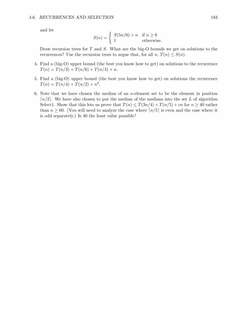
4.6. RECURRENCES AND SELECTION 183
and let
S(n) =
S(5n/6) + n if n ≥ 61 otherwise.
Draw recursion trees for T and S. What are the big-O bounds we get on solutions to therecurrences? Use the recursion trees to argue that, for all n, T (n) ≤ S(n).
4. Find a (big-O) upper bound (the best you know how to get) on solutions to the recurrenceT (n) = T (n/3) + T (n/6) + T (n/4) + n.
5. Find a (big-O) upper bound (the best you know how to get) on solutions the recurrenceT (n) = T (n/4) + T (n/2) + n2.
6. Note that we have chosen the median of an n-element set to be the element in positionn/2. We have also chosen to put the median of the medians into the set L of algorithmSelect1. Show that this lets us prove that T (n) ≤ T (3n/4) + T (n/5) + cn for n ≥ 40 ratherthan n ≥ 60. (You will need to analyze the case where n/5 is even and the case where itis odd separately.) Is 40 the least value possible?

184 CHAPTER 4. INDUCTION, RECURSION, AND RECURRENCES
Chapter 5
Probability
5.1 Introduction to Probability
Why do we study probability?
You have likely studied hashing as a way to store data (or keys to find data) in a way that makesit possible to access that data quickly. Recall that we have a table in which we want to storekeys, and we compute a function h of our key to tell us which location (also known as a “slot”or a “bucket”) in the table to use for the key. Such a function is chosen with the hope that itwill tell us to put different keys in different places, but with the realization that it might not. Ifthe function tells us to put two keys in the same place, we might put them into a linked list thatstarts at the appropriate place in the table, or we might have some strategy for putting them intosome other place in the table itself. If we have a table with a hundred places and fifty keys toput in those places, there is no reason in advance why all fifty of those keys couldn’t be assigned(hashed) to the same place in the table. However someone who is experienced with using hashfunctions and looking at the results will tell you you’d never see this in a million years. Onthe other hand that same person would also tell you that you’d never see all the keys hash intodifferent locations in a million years either. In fact, it is far less likely that all fifty keys wouldhash into one place than that all fifty keys would hash into different places, but both events arequite unlikely. Being able to understand just how likely or unlikely such events are is our reasonfor taking up the study of probability.
In order to assign probabilities to events, we need to have a clear picture of what these eventsare. Thus we present a model of the kinds of situations in which it is reasonable to assignprobabilities, and then recast our questions about probabilities into questions about this model.We use the phrase sample space to refer to the set of possible outcomes of a process. For now,we will deal with processes that have finite sample spaces. The process might be a game ofcards, a sequence of hashes into a hash table, a sequence of tests on a number to see if it failsto be a prime, a roll of a die, a series of coin flips, a laboratory experiment, a survey, or any ofmany other possibilities. A set of elements in a sample space is called an event. For example,if a professor starts each class with a 3 question true-false quiz the sample space of all possiblepatterns of correct answers is
TTT, TTF, TFT, FTT, TFF, FTF, FFT, FFF.
185

186 CHAPTER 5. PROBABILITY
The event of the first two answers being true is TTT, TTF. In order to compute probabilities weassign a probability weight p(x) to each element of the sample space so that the weight representswhat we believe to be the relative likelihood of that outcome. There are two rules we must followin assigning weights. First the weights must be nonnegative numbers, and second the sum of theweights of all the elements in a sample space must be one. We define the probability P (E) of theevent E to be the sum of the weights of the elements of E. Algebraically we can write
P (E) =∑
x:x∈E
p(x). (5.1)
We read this as p(E) equals the sum, over all x such that x is in E, of p(x).
Notice that a probability function P on a sample space S satisfies the rules1
1. P (A) ≥ 0 for any A ⊆ S.
2. P (S) = 1.
3. P (A ∪ B) = P (A) + P (B) for any two disjoint events A and B.
The first two rules reflect our rules for assigning weights above. We say that two events aredisjoint if A ∩ B = ∅. The third rule follows directly from the definition of disjoint and ourdefinition of the probability of an event. A function P satisfying these rules is called a probabilitydistribution or a probability measure.
In the case of the professor’s three question quiz, it is natural to expect each sequence of truesand falses to be equally likely. (A professor who showed any pattern of preferences would endup rewarding a student who observed this pattern and used it in educated guessing.) Thus it isnatural to assign equal weight 1/8 to each of the eight elements of our quiz sample space. Thenthe probability of an event E, which we denote by P (E), is the sum of the weights of its elements.Thus the probability of the event “the first answer is T” is 1
8 + 18 + 1
8 + 18 = 1
2 . The event “Thereis at exactly one True” is TFF, FTF, FFT, so P (there is exactly one True) is 3/8.
Some examples of probability computations
Exercise 5.1-1 Try flipping a coin five times. Did you get at least one head? Repeat fivecoin flips a few more times! What is the probability of getting at least one head infive flips of a coin? What is the probability of no heads?
Exercise 5.1-2 Find a good sample space for rolling two dice. What weights are appro-priate for the members of your sample space? What is the probability of getting a6 or 7 total on the two dice? Assume the dice are of different colors. What is theprobability of getting less than 3 on the red one and more than 3 on the green one?
Exercise 5.1-3 Suppose you hash a list of n keys into a hash table with 20 locations.What is an appropriate sample space, and what is an appropriate weight function?(Assume the keys and the hash function are not in any special relationship to the
1These rules are often called “the axioms of probability.” For a finite sample space, we could show that if westarted with these axioms, our definition of probability in terms of the weights of individual elements of S is theonly definition possible. That is, for any other definition, the probabilities we would compute would still be thesame if we take w(x) = P (x).

5.1. INTRODUCTION TO PROBABILITY 187
number 20.) If n is three, what is the probability that all three keys hash to differentlocations? If you hash ten keys into the table, what is the probability that at leasttwo keys have hashed to the same location? We say two keys collide if they hash tothe same location. How big does n have to be to insure that the probability is at leastone half that has been at least one collision?
In Exercise 5.1-1 a good sample space is the set of all 5-tuples of Hs and T s. There are 32elements in the sample space, and no element has any reason to be more likely than any other, soa natural weight to use is 1
32 for each element of the sample space. Then the event of at least onehead is the set of all elements but TTTTT . Since there are 31 elements in this set, its probabilityis 31
32 . This suggests that you should have observed at least one head pretty often!
Complementary probabilities
The probability of no heads is the weight of the set TTTTT, which is 132 . Notice that the
probabilities of the event of “no heads” and the opposite event of “at least one head” add toone. This observation suggests a theorem. The complement of an event E in a sample space S,denoted by S−E, is the set of all outcomes in S but not E. The theorem tells us how to computethe probability of the complement of an event from the probability of the event.
Theorem 5.1 If two events E and F are complementary, that is they have nothing in common(E ∩ F = ∅) and their union is the whole sample space (E ∪ F = S), then
P (E) = 1 − P (F ).
Proof: The sum of all the probabilities of all the elements of the sample space is one, andsince we can break this sum into the sum of the probabilities of the elements of E plus the sumof the probabilities of the elements of F , we have
P (E) + P (F ) = 1,
which gives us P (E) = 1 − P (F ).
For Exercise 5.1-2 a good sample space would be pairs of numbers (a, b) where (1 ≤ a, b ≤ 6).By the product principle2, the size of this sample space is 6 · 6 = 36. Thus a natural weight foreach ordered pair is 1
36 . How do we compute the probability of getting a sum of six or seven?There are 5 ways to roll a six and 6 ways to roll a seven, so our event has eleven elements each ofweight 1/36. Thus the probability of our event is is 11/36. For the question about the red andgreen dice, there are two ways for the red one to turn up less than 3, and three ways for the greenone to turn up more than 3. Thus, the event of getting less than 3 on the red one and greaterthan 3 on the green one is a set of size 2 · 3 = 6 by the product principle. Since each element ofthe event has weight 1/36, the event has probability 6/36 or 1/6.
2From Section 1.1.

188 CHAPTER 5. PROBABILITY
Probability and hashing
In Exercise 5.1-3 an appropriate sample space is the set of n-tuples of numbers between 1 and20. The first entry in an n-tuple is the position our first key hashes to, the second entry isthe position our second key hashes to, and so on. Thus each n tuple represents a possible hashfunction, and each hash function, applied to our keys, would give us one n-tuple. The size ofthe sample space is 20n (why?), so an appropriate weight for an n-tuple is 1/20n. To computethe probability of a collision, we will first compute the probability that all keys hash to differentlocations and then apply Theorem 5.1 which tells us to subtract this probability from 1 to getthe probability of collision.
To compute the probability that all keys hash to different locations we consider the event thatall keys hash to different locations. This is the set of n tuples in which all the entries are different.(In the terminology of functions, these n-tuples correspond to one-to-one hash functions). Thereare 20 choices for the first entry of an n-tuple in our event. Since the second entry has to bedifferent, there are 19 choices for the second entry of this n-tuple. Similarly there are 18 choicesfor the third entry (it has to be different from the first two), 17 for the fourth, and in general20 − i + 1 possibilities for the ith entry of the n-tuple. Thus we have
20 · 19 · 18 · · · · · (20 − n + 1) = 20n
elements of our event.3 Since each element of this event has weight 1/20n, the probability thatall the keys hash to different locations is
20 · 19 · 18 · · · · · (20 − n + 1)20n
=20n
20n.
In particular if n is 3 the probability is (20 · 19 · 18)/203 = .855.
We show the values of this function for n between 0 and 20 in Table 5.1. Note how quicklythe probability of getting a collision grows. As you can see with n = 10, the probability thatthere have been no collisions is about .065, so the probability of at least one collision is .935.
If n = 5 this number is about .58, and if n = 6 this number is about .43. By Theorem 5.1 theprobability of a collision is one minus the probability that all the keys hash to different locations.Thus if we hash six items into our table, the probability of a collision is more than 1/2. Ourfirst intuition might well have been that we would need to hash ten items into our table to haveprobability 1/2 of a collision. This example shows the importance of supplementing intuitionwith careful computation!
The technique of computing the probability of an event of interest by first computing theprobability of its complementary event and then subtracting from 1 is very useful. You will seemany opportunities to use it, perhaps because about half the time it is easier to compute directlythe probability that an event doesn’t occur than the probability that it does. We stated Theorem5.1 as a theorem to emphasize the importance of this technique.
The Uniform Probability Distribution
In all three of our exercises it was appropriate to assign the same weight to all members of oursample space. We say P is the uniform probability measure or uniform probability distribution
3Using the notation for falling factorial powers that we introduced in Section 1.2.

5.1. INTRODUCTION TO PROBABILITY 189
n Prob of empty slot Prob of no collisions1 1 12 0.95 0.953 0.9 0.8554 0.85 0.726755 0.8 0.58146 0.75 0.436057 0.7 0.3052358 0.65 0.198402759 0.6 0.1190416510 0.55 0.06547290811 0.5 0.03273645412 0.45 0.01473140413 0.4 0.00589256214 0.35 0.00206239715 0.3 0.00061871916 0.25 0.0001546817 0.2 3.09359E-0518 0.15 4.64039E-0619 0.1 4.64039E-0720 0.05 2.3202E-08
Table 5.1: The probabilities that all elements of a set hash to different entries of a hash table ofsize 20.
when we assign the same probability to all members of our sample space. The computations inthe exercises suggest another useful theorem.
Theorem 5.2 Suppose P is the uniform probability measure defined on a sample space S. Thenfor any event E,
P (E) = |E|/|S|,the size of E divided by the size of S.
Proof: Let S = x1, x2, . . . , x|S|. Since P is the uniform probability measure, there must besome value p such that for each xi ∈ S, P (xi) = p. Combining this fact with the second and thirdprobability rules, we obtain
1 = P (S)= P (x1 ∪ x2 ∪ · · · ∪ x|S|)= P (x1) + P (x2) + . . . + P (x|S|)= p|S| .
Equivalently
p =1|S| . (5.2)
E is a subset of S with |E| elements and therefore
P (E) =∑
xi∈E
p(xi) = |E|p . (5.3)

190 CHAPTER 5. PROBABILITY
Combining equations 5.2 and 5.3 gives that P (E) = |E|p = |E|(1/|S|) = |E|/|S| .
Exercise 5.1-4 What is the probability of an odd number of heads in three tosses of acoin? Use Theorem 5.2.
Using a sample space similar to that of first example (with “T” and “F” replaced by “H”and “T”), we see there are three sequences with one H and there is one sequence with three H’s.Thus we have four sequences in the event of “an odd number of heads come up.” There are eightsequences in the sample space, so the probability is 4
8 = 12 .
It is comforting that we got one half because of a symmetry inherent in this problem. Inflipping coins, heads and tails are equally likely. Further if we are flipping 3 coins, an oddnumber of heads implies an even number of tails. Therefore, the probability of an odd numberof heads, even number of heads, odd number of tails and even number of tails must all be thesame. Applying Theorem 5.1 we see that the probability must be 1/2.
A word of caution is appropriate here. Theorem 5.2 applies only to probabilities that comefrom the equiprobable weighting function. The next example shows that it does not apply ingeneral.
Exercise 5.1-5 A sample space consists of the numbers 0, 1, 2 and 3. We assign weight18 to 0, 3
8 to 1, 38 to 2, and 1
8 to 3. What is the probability that an element of thesample space is positive? Show that this is not the result we would obtain by usingthe formula of Theorem 5.2.
The event “x is positive” is the set E = 1, 2, 3. The probability of E is
P (E) = P (1) + P (2) + P (3) =38
+38
+18
=78
.
However, |E||S| = 3
4 .
The previous exercise may seem to be “cooked up” in an unusual way just to prove a point.In fact that sample space and that probability measure could easily arise in studying somethingas simple as coin flipping.
Exercise 5.1-6 Use the set 0, 1, 2, 3 as a sample space for the process of flipping a cointhree times and counting the number of heads. Determine the appropriate probabilityweights P (0), P (1), P (2), and P (3).
There is one way to get the outcome 0, namely tails on each flip. There are, however, threeways to get 1 head and three ways to get two heads. Thus P (1) and P (2) should each be threetimes P (0). There is one way to get the outcome 3—heads on each flip. Thus P (3) should equalP (0). In equations this gives P (1) = 3P (0), P (2) = 3P (0), and P (3) = P (0). We also have theequation saying all the weights add to one, P (0) + P (1) + P (2) + P (3) = 1. There is one andonly one solution to these equations, namely P (0) = 1
8 , P (1) = 38 , P (2) = 3
8 , and P (3) = 18 . Do
you notice a relationship between P (x) and the binomial coefficient(3x
)here? Can you predict
the probabilities of 0, 1, 2, 3, and 4 heads in four flips of a coin?
Together, the last two exercises demonstrate that we must be careful not to apply Theorem5.2 unless we are using the uniform probability measure.

5.1. INTRODUCTION TO PROBABILITY 191
Important Concepts, Formulas, and Theorems
1. Sample Space. We use the phrase sample space to refer to the set of possible outcomes ofa process.
2. Event. A set of elements in a sample space is called an event.
3. Probability. In order to compute probabilities we assign a weight to each element of thesample space so that the weight represents what we believe to be the relative likelihood ofthat outcome. There are two rules we must follow in assigning weights. First the weightsmust be nonnegative numbers, and second the sum of the weights of all the elements in asample space must be one. We define the probability P (E) of the event E to be the sum ofthe weights of the elements of E.
4. The axioms of Probability. Three rules that a probability measure on a finite sample spacemust satisfy could actually be used to define what we mean by probability.
(a) P (A) ≥ 0 for any A ⊆ S.
(b) P (S) = 1.
(c) P (A ∪ B) = P (A) + P (B) for any two disjoint events A and B.
5. Probability Distribution. A function which assigns a probability to each member of a samplespace is called a (discrete) probability distribution.
6. Complement. The complement of an event E in a sample space S, denoted by S−E, is theset of all outcomes in S but not E.
7. The Probabilities of Complementary Events. If two events E and F are complementary,that is they have nothing in common (E ∩ F = ∅), and their union is the whole samplespace (E ∪ F = S), then
P (E) = 1 − P (F ).
8. Collision, Collide (in Hashing). We say two keys collide if they hash to the same location.
9. Uniform Probability Distribution. We say P is the uniform probability measure or uniformprobability distribution when we assign the same probability to all members of our samplespace.
10. Computing Probabilities with the Uniform Distribution. Suppose P is the uniform proba-bility measure defined on a sample space S. Then for any event E,
P (E) = |E|/|S|,
the size of E divided by the size of S. This does not apply to general probability distribu-tions.

192 CHAPTER 5. PROBABILITY
Problems
1. What is the probability of exactly three heads when you flip a coin five times? What is theprobability of three or more heads when you flip a coin five times?
2. When we roll two dice, what is the probability of getting a sum of 4 or less on the tops?
3. If we hash 3 keys into a hash table with ten slots, what is the probability that all threekeys hash to different slots? How big does n have to be so that if we hash n keys to a hashtable with 10 slots, the probability is at least a half that some slot has at least two keyshash to it? How many keys do we need to have probability at least two thirds that someslot has at least two keys hash to it?
4. What is the probability of an odd sum when we roll three dice?
5. Suppose we use the numbers 2 through 12 as our sample space for rolling two dice andadding the numbers on top. What would we get for the probability of a sum of 2, 3, or 4,if we used the equiprobable measure on this sample space. Would this make sense?
6. Two pennies, a nickel and a dime are placed in a cup and a first coin and a second coin aredrawn.
(a) Assuming we are sampling without replacement (that is, we don’t replace the first coinbefore taking the second) write down the sample space of all ordered pairs of lettersP , N , and D that represent the outcomes. What would you say are the appropriateweights for the elements of the sample space?
(b) What is the probability of getting eleven cents?
7. Why is the probability of five heads in ten flips of a coin equal to 63256?
8. Using 5-element sets as a sample space, determine the probability that a “hand” of 5 cardschosen from an ordinary deck of 52 cards will consist of cards of the same suit.
9. Using 5 element permutations as a sample space, determine the probability that a “hand”of 5 cards chosen from an ordinary deck of 52 cards will have all the cards from the samesuit
10. How many five-card hands chosen from a standard deck of playing cards consist of five cardsin a row (such as the nine of diamonds, the ten of clubs, jack of clubs, queen of hearts, andking of spades)? Such a hand is called a straight. What is the probability that a five-cardhand is a straight? Explore whether you get the same answer by using five element sets asyour model of hands or five element permutations as your model of hands.
11. A student taking a ten-question, true-false diagnostic test knows none of the answers andmust guess at each one. Compute the probability that the student gets a score of 80 orhigher. What is the probability that the grade is 70 or lower?
12. A die is made of a cube with a square painted on one side, a circle on two sides, and atriangle on three sides. If the die is rolled twice, what is the probability that the two shapeswe see on top are the same?

5.1. INTRODUCTION TO PROBABILITY 193
13. Are the following two events equally likely? Event 1 consists of drawing an ace and a kingwhen you draw two cards from among the thirteen spades in a deck of cards and event 2consists of drawing an ace and a king when you draw two cards from the whole deck.
14. There is a retired professor who used to love to go into a probability class of thirty ormore students and announce “I will give even money odds that there are two people inthis classroom with the same birthday.” With thirty students in the room, what is theprobability that all have different birthdays? What is the minimum number of studentsthat must be in the room so that the professor has at least probability one half of winningthe bet? What is the probability that he wins his bet if there are 50 students in the room.Does this probability make sense to you? (There is no wrong answer to that question!)Explain why or why not.

194 CHAPTER 5. PROBABILITY
5.2 Unions and Intersections
The probability of a union of events
Exercise 5.2-1 If you roll two dice, what is the probability of an even sum or a sum of 8or more?
Exercise 5.2-2 In Exercise 5.2-1, let E be the event “even sum” and let F be the event“8 or more.” We found the probability of the union of the events E and F. Why isn’tit the case that P (E ∪ F ) = P (E) + P (F )? What weights appear twice in the sumP (E) + P (F )? Find a formula for P (E ∪ F ) in terms of the probabilities of E, F ,and E ∩F . Apply this formula to Exercise 5.2-1. What is the value of expressing oneprobability in terms of three?
Exercise 5.2-3 What is P (E ∪F ∪G) in terms of probabilities of the events E, F , and Gand their intersections?
In the sum P (E) + P (F ) the weights of elements of E ∩ F each appear twice, while theweights of all other elements of E ∪F each appear once. We can see this by looking at a diagramcalled a Venn Diagram, as in Figure 5.1. In a Venn diagram, the rectangle represents the samplespace, and the circles represent the events. If we were to shade both E and F , we would wind
Figure 5.1: A Venn diagram for two events.
E E ∩ F F
up shading the region E ∩ F twice. In Figure 5.2, we represent that by putting numbers in theregions, representing how many times they are shaded. This illustrates why the sum P (E)+P (F )includes the probability weight of each element of E ∩ F twice. Thus to get a sum that includesthe probability weight of each element of E ∪ F exactly once, we have to subtract the weight ofE ∩ F from the sum P (E) + P (F ). This is why
P (E ∪ F ) = P (E) + P (F ) − P (E ∩ F ) (5.4)
.
We can now apply this to Exercise 5.2-1 by noting that the probability of an even sum is 1/2,while the probability of a sum of 8 or more is
136
+236
+336
+436
+536
=1536
.

5.2. UNIONS AND INTERSECTIONS 195
Figure 5.2: If we shade each of E and F once, then we shade E ∩ F twice
E E ∩ F F
1 2 1
From a similar sum, the probability of an even sum of 8 or more is 9/36, so the probability of asum that is even or is 8 or more is
12
+1536
− 936
=23.
(In this case our computation merely illustrates the formula; with less work one could add theprobability of an even sum to the probability of a sum of 9 or 11.) In many cases, however,probabilities of individual events and their intersections are more straightforward to computethan probabilities of unions (we will see such examples later in this section), and in such casesour formula is quite useful.
Now let’s consider the case for three events and draw a Venn diagram and fill in the numbersfor shading all E, F , and G. So as not to crowd the figure we use EF to label the regioncorresponding to E ∩ F , and similarly label other regions. Doing so we get Figure 5.3. Thus we
Figure 5.3: The number of ways the intersections are shaded when we shade E, F , and G.
EEF
F
EFG
EG FG
G
3
112
1
2 2
have to figure out a way to subtract from P (E) + P (F ) + P (G) the weights of elements in theregions labeled EF , FG and EG once, and the the weight of elements in the region labeled EFGtwice. If we subtract out the weights of elements of each of E ∩ F , F ∩ G, and E ∩ G, this doesmore than we wanted to do, as we subtract the weights of elements in EF , FG and EG once

196 CHAPTER 5. PROBABILITY
but the weights of elements in of EFG three times, leaving us with Figure 5.4. We then see that
Figure 5.4: The result of removing the weights of each intersection of two sets.
EEF
F
EFG
EG FG
G
0
111
1
1 1
all that is left to do is to add weights of elements in the E ∩ F ∩ G back into our sum. Thus wehave that
P (E ∪ F ∪ G) = P (E) + P (F ) + P (G) − P (E ∩ F ) − P (E ∩ G) − P (F ∩ G) + P (E ∩ F ∩ G).
Principle of inclusion and exclusion for probability
From the last two exercises, it is natural to guess the formula
P (n⋃
i=1
Ei) =n∑
i=1
P (Ei) −n−1∑
i=1
n∑
j=i+1
P (Ei ∩ Ej) +n−2∑
i=1
n−1∑
j=i+1
n∑
k=j+1
P (Ei ∩ Ej ∩ Ek) − . . . . (5.5)
All the sum signs in this notation suggest that we need some new notation to describe sums.We are now going to make a (hopefully small) leap of abstraction in our notation and introducenotation capable of compactly describing the sum described in the previous paragraph. Thisnotation is an extension of the one we introduced in Equation 5.1. We use
∑
i1,i2,...,ik:
1≤i1<i2<···<ik≤n
P (Ei1 ∩ Ei2 ∩ · · ·Eik) (5.6)
to stand for the sum, over all sequences i1, i2, . . . ik of integers between 1 and n of the probabil-ities of the sets Ei1 ∩ Ei2 . . . ∩ Eik . More generally,
∑
i1,i2,...,ik:
1≤i1<i2<···<ik≤n
f(i1, i2, . . . , ik) is the sum of
f(i1, i2, . . . , ik) over all increasing sequences of k numbers between 1 and n.
Exercise 5.2-4 To practice with notation, what is∑
i1,i2,i3:1≤i1<i2<i3≤4
i1 + i2 + i3?

5.2. UNIONS AND INTERSECTIONS 197
The sum in Exercise 5.2-4 is 1+2+3+1+2+4+1+3+4+2+3+4 = 3(1+2+3+4) = 30.
With this understanding of the notation in hand, we can now write down a formula thatcaptures the idea in Equation 5.5 more concisely. Notice that in Equation 5.5 we include prob-abilities of single sets with a plus sign, probabilities of intersections of two sets with a minussign, and in general, probabilities of intersections of any even number of sets with a minus signand probabilities of intersections of any odd number of sets (including the odd number one) witha plus sign. Thus if we are intersecting k sets, the proper coefficient for the probability of theintersection of these sets is (−1)k+1 (it would be equally good to use (−1)k−1, and correct butsilly to use (−1)k+3). This lets us translate the formula of Equation 5.5 to Equation 5.7 in thetheorem, called the Principle of Inclusion and Exclusion for Probability, that follows. We willgive two completely different proofs of the theorem, one of which is a nice counting argument butis a bit on the abstract side, and one of which is straightforward induction, but is complicatedby the fact that it takes a lot of notation to say what is going on.
Theorem 5.3 (Principle of Inclusion and Exclusion for Probability) The probability ofthe union E1 ∪ E2 ∪ · · · ∪ En of events in a sample space S is given by
P
(n⋃
i=1
Ei
)=
n∑
k=1
(−1)k+1∑
i1,i2,...,ik:
1≤i1<i2<···<ik≤n
P (Ei1 ∩ Ei2 ∩ · · · ∩ Eik) . (5.7)
First Proof: Consider an element x of⋃n
i=1 Ei. Let Ei1 , Ei2 , . . . Eik be the set of all eventsEi of which x is a member. Let K = i1, i2, . . . , ik. Then x is in the event Ej1 ∩Ej2 ∩ · · · ∩Ejm
if and only if j1, j2 . . . jm ⊆ K. Why is this? If there is a jr that is not in K, then x ∈ Ej andthus x ∈ Ej1 ∩ Ej2 ∩ · · · ∩ Ejm . Notice that every x in
⋃ni=1 Ei is in at least one Ei, so it is in at
least one of the sets Ei1 ∩ Ei2 ∩ · · · ∩ Eik .
Recall that we define P (Ej1 ∩ Ej2 ∩ · · · ∩ Ejm) to be the sum of the probability weightsp(x) for x ∈ Ej1 ∩ Ej2 ∩ · · · ∩ Ejm . Suppose we substitute this sum of probability weightsfor P (Ej1 ∩ Ej2 ∩ · · · ∩ Ejm) on the right hand side of Equation 5.7. Then the right hand sidebecomes a sum of terms, each of which is plus or minus a probability weight. The sum of all theterms involving p(x) on the right hand side of Equation 5.7 includes a term involving p(x) foreach nonempty subset j1, j2, . . . , jm of K, and no other terms involving p(x). The coefficientof the probability weight p(x) in the term for the subset j1, j2, . . . , jm is (−1)m+1. Since thereare
( km
)subsets of K of size m, the sum of the terms involving p(x) will therefore be
k∑
m=1
(−1)m+1
(k
m
)p(x) =
(−
k∑
m=0
(−1)m
(k
m
)p(x)
)+ p(x) = 0 · p(x) + p(x) = p(x),
because k ≥ 1 and thus by the binomial theorem,∑k
j=0
(kj
)(−1)j = (1 − 1)k = 0. This proves
that for each x, the sum of all the terms involving p(x) after we substitute the sum of probabilityweights into Equation 5.7 is exactly p(x). We noted above that for every x in ∪n
i=1Ei appears inat least one of the sets Ei1 ∩Ei2 ∩ · · · ∩Eik . Thus the right hand side of Equation 5.7 is the sumof every p(x) such that x is in ∪n
i=1Ei. By definition, this is the left-hand side of Equation 5.7.
Second Proof: The proof is simply an application of mathematical induction using Equation5.4. When n = 1 the formula is true because it says P (E1) = P (E1). Now suppose inductively

198 CHAPTER 5. PROBABILITY
that for any family of n − 1 sets F1, F2, . . . , Fn−1
P
(n−1⋃
i=1
Fi
)=
n−1∑
k=1
(−1)k+1∑
i1,i2,i...,ik:
1≤i1<i2<···<ik≤n−1
P (Fi1 ∩ Fi2 ∩ . . . ∩ Fik) (5.8)
If in Equation 5.4 we let E = E1 ∪ . . . ∪ En−1 and F = Em, we may apply Equation 5.4 to tocompute P (∪n
i=1Ei) as follows:
P
(n⋃
i=1
Ei
)= P
(n−1⋃
i=1
Ei
)+ P (En) − P
((n−1⋃
i=1
Ei
)∩ En
). (5.9)
By the distributive law, (n−1⋃
i=1
Ei
)∩ En =
n−1⋃
i=1
(Ei ∩ En) ,
and substituting this into Equation 5.9 gives
P
(n⋃
i=1
Ei
)= P
(n−1⋃
i=1
Ei
)+ P (En) − P
(n−1⋃
i=1
(Ei ∩ En)
).
Now we use the inductive hypothesis (Equation 5.8) in two places to get
P
(n⋃
i=1
Ei
)=
n−1∑
k=1
(−1)k+1∑
i1,i2,i...,ik:
1≤i1<i2<···<ik≤n−1
P (Ei1 ∩ Ei2 ∩ · · · ∩ Eik)
+ P (En)
−n−1∑
k=1
(−1)k+1∑
i1,i2,i...,ik:
1≤i1<i2<···<ik≤n−1
P (Ei1 ∩ Ei2 ∩ · · · ∩ Eik ∩ En).
The first summation on the right hand side sums (−1)k+1P (Ei1 ∩ Ei2 ∩ · · · ∩ Eik) over all listsi1, i2, . . . , ik that do not contain n, while the P (En) and the second summation work together tosum (−1)k+1P (Ei1 ∩ Ei2 ∩ · · · ∩ Eik) over all lists i1, i2, . . . , ik that do contain n. Therefore,
P
(n⋃
i=1
Ei
)=
n∑
k=1
(−1)k+1∑
i1,i2,i...,ik:
1≤i1<i2<···<ik≤n
P (Ei1 ∩ Ei2 ∩ · · · ∩ Eik).
Thus by the principle of mathematical induction, this formula holds for all integers n > 0.
Exercise 5.2-5 At a fancy restaurant n students check their backpacks. They are the onlyones to check backpacks. A child visits the checkroom and plays with the check ticketsfor the backpacks so they are all mixed up. If there are 5 students named Judy, Sam,Pat, Jill, and Jo, in how many ways may the backpacks be returned so that Judy getsher own backpack (and maybe some other students do, too)? What is the probabilitythat this happens? What is the probability that Sam gets his backpack (and maybesome other students do, too)? What is the probability that Judy and Sam both gettheir own backpacks (and maybe some other students do, too)? For any particular

5.2. UNIONS AND INTERSECTIONS 199
two element set of students, what is the probability that these two students get theirown backpacks (and maybe some other students do, too)? What is the probabilitythat at least one student gets his or her own backpack? What is the probability thatno students get their own backpacks? What do you expect the answer will be forthe last two questions for n students? This classic problem is often stated using hatsrather than backpacks (quaint, isn’t it?), so it is called the hatcheck problem. It isalso known as the derangement problem; a derangement of a set being a one-to-onefunction from a set onto itself (i.e., a bijection) that sends each element to somethingnot equal to it.
For Exercise 5.2-5, let Ei be the event that person i on our list gets the right backpack. ThusE1 is the event that Judy gets the correct backpack and E2 is the event that Sam gets the correctbackpack. The event E1∩E2 is the event that Judy and Sam get the correct backpacks (and maybesome other people do). In Exercise 5.2-5, there are 4! ways to pass back the backpacks so thatJudy gets her own, as there are for Sam or any other single student. Thus P (E1) = P (Ei) = 4!
5! .For any particular two element subset, such as Judy and Sam, there are 3! ways that these twopeople may get their backpacks back. Thus, for each i and j, P (Ei ∩ Ej) = 3!
5! . For a particulargroup of k students the probability that each one of these k students gets his or her own backpackback is (5 − k)!/5!. If Ei is the event that student i gets his or her own backpack back, then theprobability of an intersection of k of these events is (5− k)!/5!. The probability that at least oneperson gets his or her own backpack back is the probability of E1 ∪E2 ∪E3 ∪E4 ∪E5. Then bythe principle of inclusion and exclusion, the probability that at least one person gets his or herown backpack back is
P (E1 ∪ E2 ∪ E3 ∪ E4 ∪ E5) =5∑
k=1
(−1)k+1∑
i1,i2,...,ik:
1≤i1<i2<···<ik≤5
P (Ei1 ∩ Ei2 ∩ · · · ∩ Eik). (5.10)
As we argued above, for a set of k people, the probability that all k people get their backpacksback is (5 − k)!/5!. In symbols, P (Ei1 ∩ Ei2 ∩ · · · ∩ Eik) = (5−k)!
5! . Recall that there are(5k
)
sets of k people chosen from our five students. That is, there are(5k
)lists i1, i2, . . . ik with
1 < i1 < i2 < · · · < ik ≤ 5. Thus, we can rewrite the right hand side of the Equation 5.10 as
5∑
k=1
(−1)k+1
(5k
)(5 − k)!
5!.
This gives us
P (E1 ∪ E2 ∪ E3 ∪ E4 ∪ E5) =5∑
k=1
(−1)k−1
(5k
)(5 − k)!
5!
=5∑
k=1
(−1)k−1 5!k!(5 − k)!
(5 − k)!5!
=5∑
k=1
(−1)k−1 1k!
= 1 − 12
+13!
− 14!
+15!
.

200 CHAPTER 5. PROBABILITY
The probability that nobody gets his or her own backpack is 1 minus the probability thatsomeone does, or
12− 1
3!+
14!
− 15!
.
To do the general case of n students, we simply substitute n for 5 and get that the probabilitythat at least one person gets his or her own backpack is
n∑
i=1
(−1)i−1 1i!
= 1 − 12
+13!
− · · · + (−1)n−1
n!
and the probability that nobody gets his or her own backpack is 1 minus the probability above,or
n∑
i=2
(−1)i 1i!
=12− 1
3!+ · · · + (−1)n
n!. (5.11)
Those who have had power series in calculus may recall the power series representation of ex,namely
ex = 1 + x +x2
2!+
x3
3!+ · · · =
∞∑
i=0
xi
i!.
Thus the expression in Equation 5.11 is the approximation to e−1 we get by substituting −1 for xin the power series and stopping the series at i = n. Note that the result depends very “lightly”on n; so long as we have at least four or five people, then, no matter how many people we have,the probability that no one gets their hat back remains at roughly e−1. Our intuition mighthave suggested that as the number of students increases, the probability that someone gets hisor her own backpack back approaches 1 rather than 1 − e−1. Here is another example of why itis important to use computations with the rules of probability instead of intuition!
The principle of inclusion and exclusion for counting
Exercise 5.2-6 How many functions are there from an n-element set N to a k-element setK = y1, y2, . . . yk that map nothing to y1? Another way to say this is if I have ndistinct candy bars and k children Sam, Mary, Pat, etc., in how ways may I pass outthe candy bars so that Sam doesn’t get any candy (and maybe some other childrendon’t either)?
Exercise 5.2-7 How many functions map nothing to a j-element subset J of K? Anotherway to say this is if I have n distinct candy bars and k children Sam, Mary, Pat, etc.,in how ways may I pass out the candy bars so that some particular j-element subsetof the children don’t get any (and maybe some other children don’t either)?
Exercise 5.2-8 What is the number of functions from an n-element set N to a k elementset K that map nothing to at least one element of K? Another way to say this is ifI have n distinct candy bars and k children Sam, Mary, Pat, etc., in how ways may Ipass out the candy bars so that some child doesn’t get any (and maybe some otherchildren don’t either)?
Exercise 5.2-9 On the basis of the previous exercises, how many functions are there froman n-element set onto a k element set?

5.2. UNIONS AND INTERSECTIONS 201
The number of functions from an n-element set to a k-element set K = y1, y2, . . . yk thatmap nothing to y1 is simply (k−1)n because we have k−1 choices of where to map each of our nelements. Similarly the number of functions that map nothing to a particular set J of j elementswill be (k − j)n. This warms us up for Exercise 5.2-8.
In Exercise 5.2-8 we need an analog of the principle of inclusion and exclusion for the size ofa union of k sets (set i being the set of functions that map nothing to element i of the set K).Because we can make the same argument about the size of the union of two or three sets thatwe made about probabilities of unions of two or three sets, we have a very natural analog. Thatanalog is the Principle of Inclusion and Exclusion for Counting
∣∣∣∣∣
n⋃
i=1
Ei
∣∣∣∣∣ =n∑
k=1
(−1)k+1∑
i1,i2,...,ik:
1≤i1<i2<···<ik≤n
|Ei1 ∩ Ei2 ∩ · · · ∩ Eik | . (5.12)
In fact, this formula is proved by induction or a counting argument in virtually the same way.Applying this formula to the number of functions from N that map nothing to at least oneelement of K gives us
|k⋃
i=1
Ei| =n∑
k=1
(−1)k+1∑
i1,i2,...,ik:
1≤i1<i2<···<ik≤n
|Ei1 ∩ Ei2 ∩ · · · ∩ Eik | =k∑
j=1
(−1)j−1
(k
j
)(k − j)n.
This is the number of functions from N that map nothing to at least one element of K. Thetotal number of functions from N to K is kn. Thus the number of onto functions is
kn −k∑
j=1
(−1)j−1
(k
j
)(k − j)n =
k∑
j=0
(−1)j
(k
j
)(k − j)n,
where the second equality results because(k0
)is 1 and (k − 0)n is kn.
Important Concepts, Formulas, and Theorems
1. Venn Diagram. To draw a Venn diagram, for two or three sets, we draw a rectangle thatrepresents the sample space, and two or three mutually overlapping circles to represent theevents.
2. Probability of a Union of Two Events. P (E ∪ F ) = P (E) + P (F ) − P (E ∩ F )
3. Probability of a Union of Three Events. P (E ∪ F ∪ G) = P (E) + P (F ) + P (G) − P (E ∩F ) − P (E ∩ G) − P (F ∩ G) + P (E ∩ F ∩ G).
4. A Summation Notation.∑
i1,i2,...,ik:
1≤i1<i2<···<ik≤n
f(i1, i2, . . . , ik) is the sum of f(i1, i2, . . . , ik) over all
increasing sequences of k numbers between 1 and n.
5. Principle of Inclusion and Exclusion for Probability. The probability of the union E1∪E2∪· · · ∪ En of events in a sample space S is given by
P
(n⋃
i=1
Ei
)=
n∑
k=1
(−1)k+1∑
i1,i2,...,ik:
1≤i1<i2<···<ik≤n
P (Ei1 ∩ Ei2 ∩ · · · ∩ Eik) .

202 CHAPTER 5. PROBABILITY
6. Hatcheck Problem. The hatcheck problem or derangement problem asks for the probabilitythat a bijection of an n element set maps no element to itself. The answer is
n∑
i=2
(−1)i 1i!
=12− 1
3!+ · · · + (−1)n
n!,
the result of truncating the power series expansion of e−1 at the (−1)n
n! . Thus the result isvery close to 1
e , even for relatively small values of n.
7. Principle of Inclusion and Exclusion for Counting. The Principle of inclusion and exclusionfor counting says that
∣∣∣∣∣
n⋃
i=1
Ei
∣∣∣∣∣ =n∑
k=1
(−1)k+1∑
i1,i2,...,ik:
1≤i1<i2<···<ik≤n
|Ei1 ∩ Ei2 ∩ · · · ∩ Eik | .
Problems
1. Compute the probability that in three flips of a coin the coin comes heads on the first flipor on the last flip.
2. The eight kings and queens are removed from a deck of cards and then two of these cardsare selected. What is the probability that the king or queen of spades is among the cardsselected?
3. Two dice are rolled. What is the probability that we see a die with six dots on top?
4. A bowl contains two red, two white and two blue balls. We remove two balls. What is theprobability that at least one is red or white? Compute the probability that at least one isred.
5. From an ordinary deck of cards, we remove one card. What is the probability that it is anAce, is a diamond, or is black?
6. Give a formula for the probability of P (E∪F ∪G∪H) in terms of the probabilities of E,F ,G, and H, and their intersections.
7. What is ∑
i1,i2,i3:1≤i1<i2<i3≤4
i1i2i3 ?
8. What is ∑
i1,i2,i3:1≤i1<i2<i3≤5
i1 + i2 + i3 ?
9. The boss asks the secretary to stuff n letters into envelopes forgetting to mention that hehas been adding notes to the letters and in the process has rearranged the letters but notthe envelopes. In how many ways can the letters be stuffed into the envelopes so thatnobody gets the letter intended for him or her? What is the probability that nobody getsthe letter intended for him or her?

5.2. UNIONS AND INTERSECTIONS 203
10. If we are hashing n keys into a hash table with k locations, what is the probability thatevery location gets at least one key?
11. From the formula for the number of onto functions, find a formula for S(n, k) which isdefined in Problem 12 of Section 1.4. These numbers are called Stirling numbers (of thesecond kind).
12. If we roll 8 dice, what is the probability that each of the numbers 1 through 6 appear ontop at least once? What about with 9 dice?
13. Explain why the number of ways of distributing k identical apples to n children is(n+k−1
k
).
In how many ways may you distribute the apples to the children so that Sam gets morethan m? In how many ways may you distribute the apples to the children so that no childgets more than m?
14. A group of n married couples sits a round a circular table for a group discussion of maritalproblems. The counselor assigns each person to a seat at random. What is the probabilitythat no husband and wife are side by side?
15. Suppose we have a collection of m objects and a set P of p “properties,” an undefined term,that the objects may or may not have. For each subset S of the set P of all properties,define Na(S) (a is for “at least”) to be the number of objects in the collection that have atleast the properties in S. Thus, for example, Na(∅) = m. In a typical application, formulasfor Na(S) for other sets S ⊆ P are not difficult to figure out. Define Ne(S) to be thenumber of objects in our collection that have exactly the properties in S. Show that
Ne(∅) =∑
K:K⊆P
(−1)|K|Na(K).
Explain how this formula could be used for computing the number of onto functions ina more direct way than we did it using unions of sets. How would this formula apply toProblem 9 in this section?
16. In Problem 14 of this section we allow two people of the same sex to sit side by side. If werequire in addition to the condition that no husband and wife are side by side the conditionthat no two people of the same sex are side by side, we obtain a famous problem known asthe menage problem. Solve this problem.
17. In how many ways may we place n distinct books on j shelves so that shelf one gets atleast m books? (See Problem 7 in Section 1.4.) In how many ways may we place n distinctbooks on j shelves so that no shelf gets more than m books?
18. In Problem 15 in this section, what is the probability that an object has none of theproperties, assuming all objects to be equally likely? How would this apply Problem 10 inthis section?

204 CHAPTER 5. PROBABILITY
5.3 Conditional Probability and Independence
Conditional Probability
Two cubical dice each have a triangle painted on one side, a circle painted on two sides anda square painted on three sides. Applying the principal of inclusion and exclusion, we cancompute that the probability that we see a circle on at least one top when we roll them is1/3 + 1/3 − 1/9 = 5/9. We are experimenting to see if reality agrees with our computation. Wethrow the dice onto the floor and they bounce a few times before landing in the next room.
Exercise 5.3-1 Our friend in the next room tells us both top sides are the same. Nowwhat is the probability that our friend sees a circle on at least one top?
Intuitively, it may seem as if the chance of getting circles ought to be four times the chanceof getting triangles, and the chance of getting squares ought to be nine times as much as thechance of getting triangles. We could turn this into the algebraic statements that P (circles)= 4P (triangles) and P (squares) = 9P (triangles). These two equations and the fact that theprobabilities sum to 1 would give us enough equations to conclude that the probability that ourfriend saw two circles is now 2/7. But does this analysis make sense? To convince ourselves,let us start with a sample space for the original experiment and see what natural assumptionsabout probability we can make to determine the new probabilities. In the process, we will beable to replace intuitive calculations with a formula we can use in similar situations. This is agood thing, because we have already seen situations where our intuitive idea of probability mightnot always agree with what the rules of probability give us.
Let us take as our sample space for this experiment the ordered pairs shown in Table 5.2along with their probabilities.
Table 5.2: Rolling two unusual dice
TT TC TS CT CC CS ST SC SS136
118
112
118
19
16
112
16
14
We know that the event TT, CC, SS happened. Thus we would say while it used to haveprobability
136
+19
+14
=1436
=718
(5.13)
this event now has probability 1. Given that, what probability would we now assign to the eventof seeing a circle? Notice that the event of seeing a circle now has become the event CC. Shouldwe expect CC to become more or less likely in comparison than TT or SS just because we knownow that one of these three outcomes has occurred? Nothing has happened to make us expectthat, so whatever new probabilities we assign to these two events, they should have the sameratios as the old probabilities.
Multiplying all three old probabilities by 187 to get our new probabilities will preserve the
ratios and make the three new probabilities add to 1. (Is there any other way to get the threenew probabilities to add to one and make the new ratios the same as the old ones?) This gives

5.3. CONDITIONAL PROBABILITY AND INDEPENDENCE 205
us that the probability of two circles is 19 · 18
7 = 27 . Notice that nothing we have learned about
probability so far told us what to do; we just made a decision based on common sense. Whenfaced with similar situations in the future, it would make sense to use our common sense in thesame way. However, do we really need to go through the process of constructing a new samplespace and reasoning about its probabilities again? Fortunately, our entire reasoning process canbe captured in a formula. We wanted the probability of an event E given that the event Fhappened. We figured out what the event E ∩ F was, and then multiplied its probability by1/P (F ). We summarize this process in a definition.
We define the conditional probability of E given F , denoted by P (E|F ) and read as “theprobability of E given F” by
P (E|F ) =P (E ∩ F )
P (F ). (5.14)
Then whenever we want the probability of E knowing that F has happened, we compute P (E|F ).(If P (F ) = 0, then we cannot divide by P (F ), but F gives us no new information about oursituation. For example if the student in the next room says “A pentagon is on top,” we have noinformation except that the student isn’t looking at the dice we rolled! Thus we have no reason tochange our sample space or the probability weights of its elements, so we define P (E|F ) = P (E)when P (F ) = 0.)
Notice that we did not prove that the probability of E given F is what we said it is; wesimply defined it in this way. That is because in the process of making the derivation we madean additional assumption that the relative probabilities of the outcomes in the event F don’tchange when F happens. This assumption led us to Equation 5.14. Then we chose that equationas our definition of the new concept of the conditional probability of E given F .4
In the example above, we can let E be the event that there is more than one circle and F bethe event that both dice are the same. Then E ∩ F is the event that both dice are circles, andP (E ∩ F ) is, from the table above, 1
9 . P (F ) is, from Equation 5.13, 718 . Dividing, we get the
probability of P (E|F ), which is 19/ 7
18 = 27 .
Exercise 5.3-2 When we roll two ordinary dice, what is the probability that the sum ofthe tops comes out even, given that the sum is greater than or equal to 10? Use thedefinition of conditional probability in solving the problem.
Exercise 5.3-3 We say E is independent of F if P (E|F ) = P (E). Show that when we rolltwo dice, one red and one green, the event “The total number of dots on top is odd”is independent of the event “The red die has an odd number of dots on top.”
Exercise 5.3-4 Sometimes information about conditional probabilities is given to us in-directly in the statement of a problem, and we have to derive information aboutother probabilities or conditional probabilities. Here is such an example. If a studentknows 80% of the material in a course, what do you expect her grade to be on a (well-balanced) 100 question short-answer test about the course? What is the probabilitythat she answers a question correctly on a 100 question true-false test if she guessesat each question she does not know the answer to? (We assume that she knows what
4For those who like to think in terms of axioms of probability, we could give an axiomatic definition of conditionalprobability, and one of our axioms might be that for events E1 and E2 that are subsets of F , the ratio of theconditional probabilities P (E1|F ) and P (E2|F ) is the same as the ratio of P (E1) and P (E2).
206 CHAPTER 5. PROBABILITY
she knows, that is, if she thinks that she knows the answer, then she really does.)What do you expect her grade to be on a 100 question True-False test to be?
For Exercise 5.3-2 let’s let E be the event that the sum is even and F be the event thatthe sum is greater than or equal to 10. Thus referring to our sample space in Exercise 5.3-2,P (F ) = 1/6 and P (E ∩ F ) = 1/9, since it is the probability that the roll is either 10 or 12.Dividing these two we get 2/3.
In Exercise 5.3-3, the event that the total number of dots is odd has probability 1/2. Similarly,given that the red die has an odd number of dots, the probability of an odd sum is 1/2 sincethis event corresponds exactly to getting an even roll on the green die. Thus, by the definitionof independence, the event of an odd number of dots on the red die and the event that the totalnumber of dots is odd are independent.
In Exercise 5.3-4, if a student knows 80% of the material in a course, we would hope thather grade on a well-designed test of the course would be around 80%. But what if the test isa True-False test? Let R be the event that she gets the right answer, K be the event that sheknows that right answer and K be the event that she guesses. Then R = P (R∩K) + P (R∩K).Since R is a union of two disjoint events, its probability would be the sum of the probabilitiesof these two events. How do we get the probabilities of these two events? The statement ofthe problem gives us implicitly the conditional probability that she gets the right answer giventhat she knows the answer, namely one, and the probability that she gets the right answer if shedoesn’t know the answer, namely 1/2. Using Equation 5.14, we see that we use the equation
P (E ∩ F ) = P (E|F )P (F ) (5.15)
to compute P (R ∩ K) and P (R ∩ K), since the problem tells us directly that P (K) = .8 andP (K) = .2. In symbols,
P (R) = P (R ∩ K) + P (R ∩ K)= P (R|K)P (K) + P (R|K)P (K)= 1 · .8 + .5 · .2 = .9.
We have shown that the probability that she gets the right answer is .9. Thus we would expecther to get a grade of 90%.
Independence
We said in Exercise 5.3-3 that E is independent of F if P (E|F ) = P (E). The product principlefor independent probabilities (Theorem 5.4) gives another test for independence.
Theorem 5.4 Suppose E and F are events in a sample space. Then E is independent of F ifand only if P (E ∩ F ) = P (E)P (F ).
Proof: First consider the case when F is non-empty. Then, from our definition in Exercise5.3-3
E is independent of F ⇔ P (E|F ) = P (E).

5.3. CONDITIONAL PROBABILITY AND INDEPENDENCE 207
(Even though the definition only has an “if”, recall the convention of using “if” in definitions,even though “if and only if” is meant.) Using the definition of P (E|F ) in Equation 5.14, in theright side of the above equation we get
P (E|F ) = P (E)
⇔ P (E ∩ F )P (F )
= P (E)
⇔ P (E ∩ F ) = P (E)P (F ).
Since every step in this proof was an if and only if statement we have completed the proof forthe case when F is non-empty.
If F is empty, then E is independent of F and both P (E)P (F ) and P (E ∩F ) are zero. Thusin this case as well, E is independent of F if and only if P (E ∩ F ) = P (E)P (F ).
Corollary 5.5 E is independent of F if and only if F is independent of E.
When we flip a coin twice, we think of the second outcome as being independent of thefirst. It would be a sorry state of affairs if our definition of independence did not capture thisintuitive idea! Let’s compute the relevant probabilities to see if it does. For flipping a cointwice our sample space is HH, HT, TH, TT and we weight each of these outcomes 1/4. Tosay the second outcome is independent of the first, we must mean that getting an H second isindependent of whether we get an H or a T first, and same for getting a T second. This gives usthat P (H first) = 1/4+1/4 = 1/2 and P (H second) = 1/2, while P (H first and H second) = 1/4.Note that
P (H first)P (H second) =12· 12
=14
= P (H first and H second).
By Theorem 5.4, this means that the event “H second” is independent of the event“H first.” Wecan make a similar computation for each possible combination of outcomes for the first and secondflip, and so we see that our definition of independence captures our intuitive idea of independencein this case. Clearly the same sort of computation applies to rolling dice as well.
Exercise 5.3-5 What sample space and probabilities have we been using when discussinghashing? Using these, show that the event “key i hashes to position p” and the event“key j hashes to position q” are independent when i = j. Are they independent ifi = j?
In Exercise 5.3-5 if we have a list of n keys to hash into a table of size k, our sample spaceconsists of all n-tuples of numbers between 1 and k. The event that key i hashes to some number
p consists of all n-tuples with p in the ith position, so its probability is(
1k
)n−1/
(1k
)n= 1
k . The
probability that key j hashes to some number q is also 1k . If i = j, then the event that key i
hashes to p and key j hashes to q has probability(
1k
)n−2/
(1k
)n=
(1k
)2, which is the product of
the probabilities that key i hashes to p and key j hashes to q, so these two events are independent.However if i = j the probability of key i hashing to p and key j hashing to q is zero unless p = q,in which case it is 1. Thus if i = j, these events are not independent.

208 CHAPTER 5. PROBABILITY
Independent Trials Processes
Coin flipping and hashing are examples of what are called “independent trials processes.” Supposewe have a process that occurs in stages. (For example, we might flip a coin n times.) Let us usexi to denote the outcome at stage i. (For flipping a coin n times, xi = H means that the outcomeof the ith flip is a head.) We let Si stand for the set of possible outcomes of stage i. (Thus ifwe flip a coin n times, Si = H, T.) A process that occurs in stages is called an independenttrials process if for each sequence a1, a2, . . . , an with ai ∈ Si,
P (xi = ai|x1 = a1, . . . , xi−1 = ai−1) = P (xi = ai).
In other words, if we let Ei be the event that xi = ai, then
P (Ei|E1 ∩ E2 ∩ · · · ∩ Ei−1) = P (Ei).
By our product principle for independent probabilities, this implies that
P (E1 ∩ E2 ∩ · · ·Ei−1 ∩ Ei) = P (E1 ∩ E2 ∩ · · ·Ei−1)P (Ei). (5.16)
Theorem 5.6 In an independent trials process the probability of a sequence a1, a2, . . . , an ofoutcomes is P (a1)P (a2) · · ·P (an).
Proof: We apply mathematical induction and Equation 5.16.
How do independent trials relate to coin flipping? Here our sample space consists of sequencesof n Hs and T s, and the event that we have an H (or T ) on the ith flip is independent of theevent that we have an H (or T ) on each of the first i−1 flips. In particular, the probability of anH on the ith flip is 2n−1/2n = .5, and the probability of an H on the ith flip, given a particularsequence on the first i − 1 flips is 2n−i−1/2n−i = .5.
How do independent trials relate to hashing a list of keys? As in Exercise 5.3-5 if we have alist of n keys to hash into a table of size k, our sample space consists of all n-tuples of numbersbetween 1 and k. The probability that key i hashes to p and keys 1 through i − 1 hash to q1,
q2,. . . qi−1 is(
1k
)n−i/
(1k
)nand the probability that keys 1 through i − 1 hash to q1, q2,. . . qi−1
is(
1k
)n−i+1/
(1k
)n. Therefore
P (key i hashes to p|keys 1 through i − 1 hash to q1, q2,. . . qi−1) =
(1k
)n−i/
(1k
)n
(1k
)n−i+1/
(1k
)n =1k.
Therefore, the event that key i hashes to some number p is independent of the event that the firsti − 1 keys hash to some numbers q1, q2,. . . qi−1. Thus our model of hashing is an independenttrials process.
Exercise 5.3-6 Suppose we draw a card from a standard deck of 52 cards, replace it,draw another card, and continue for a total of ten draws. Is this an independenttrials process?
Exercise 5.3-7 Suppose we draw a card from a standard deck of 52 cards, discard it (i.e.we do not replace it), draw another card and continue for a total of ten draws. Is thisan independent trials process?

5.3. CONDITIONAL PROBABILITY AND INDEPENDENCE 209
In Exercise 5.3-6 we have an independent trials process, because the probability that wedraw a given card at one stage does not depend on what cards we have drawn in earlier stages.However, in Exercise 5.3-7, we don’t have an independent trials process. In the first draw, wehave 52 cards to draw from, while in the second draw we have 51. In particular, we do not havethe same cards to draw from on the second draw as the first, so the probabilities for each possibleoutcome on the second draw depend on whether that outcome was the result of the first draw.
Tree diagrams
When we have a sample space that consists of sequences of outcomes, it is often helpful to visualizethe outcomes by a tree diagram. We will explain what we mean by giving a tree diagram of thefollowing experiment. We have one nickel, two dimes, and two quarters in a cup. We draw a firstand second coin. In Figure 5.3 you see our diagram for this process. Notice that in probabilitytheory it is standard to have trees open to the right, rather than opening up or down.
Figure 5.5: A tree diagram illustrating a two-stage process.
N
D
Q
D
Q
N
D
Q
N
D
Q
.2
.4
.4
.5
.5
.5
.25
.25
.25
.25
.5
.1
.1
.1
.1
.2
.1
.2
.1
Each level of the tree corresponds to one stage of the process of generating a sequence in oursample space. Each vertex is labeled by one of the possible outcomes at the stage it represents.Each edge is labeled with a conditional probability, the probability of getting the outcome atits right end given the sequence of outcomes that have occurred so far. Since no outcomeshave occurred at stage 0, we label the edges from the root to the first stage vertices with theprobabilities of the outcomes at the first stage. Each path from the root to the far right of thetree represents a possible sequence of outcomes of our process. We label each leaf node with theprobability of the sequence that corresponds to the path from the root to that node. By thedefinition of conditional probabilities, the probability of a path is the product of the probabilitiesalong its edges. We draw a probability tree for any (finite) sequence of successive trials in thisway.
Sometimes a probability tree provides a very effective way of answering questions about a

210 CHAPTER 5. PROBABILITY
process. For example, what is the probability of having a nickel in our coin experiment? We seethere are four paths containing an N , and the sum of their weights is .4, so the probability thatone of our two coins is a nickel is .4.
Exercise 5.3-8 How can we recognize from a probability tree whether it is the probabilitytree of an independent trials process?
Exercise 5.3-9 In Exercise 5.3-4 we asked (among other things), if a student knows 80% ofthe material in a course, what is the probability that she answers a question correctlyon a 100 question True-False test (assuming that she guesses on any question she doesnot know the answer to)? (We assume that she knows what she knows, that is, ifshe thinks that she knows the answer, then she really does.) Show how we can use aprobability tree to answer this question.
Exercise 5.3-10 A test for a disease that affects 0.1% of the population is 99% effective onpeople with the disease (that is, it says they have it with probability 0.99). The testgives a false reading (saying that a person who does not have the disease is affectedwith it) for 2% of the population without the disease. We can think of choosingsomeone and testing them for the disease as a two stage process. In stage 1, we eitherchoose someone with the disease or we don’t. In stage two, the test is either positiveor it isn’t. Give a probability tree for this process. What is the probability thatsomeone selected at random and given a test for the disease will have a positive test?What is the probability that someone who has positive test results in fact has thedisease?
A tree for an independent trials process has the property that at each level, for each nodeat that level, the (labeled) tree consisting of that node and all its children is identical to eachlabeled tree consisting of another node at that level and all its children. If we have such a tree,then it automatically satisfies the definition of an independent trials process.
In Exercise 5.3-9, if a student knows 80% of the material in a course, we expect that she hasprobability .8 of knowing the answer to any given question of a well-designed true-false test. Weregard her work on a question as a two stage process; in stage 1 she determines whether sheknows the answer, and in stage 2, she either answers correctly with probability 1, or she guesses,in which case she answers correctly with probability 1/2 and incorrectly with probability 1/2.Then as we see in Figure 5.3 there are two root-leaf paths corresponding to her getting a correctanswer. One of these paths has probability .8 and the other has probability .1. Thus she actuallyhas probability .9 of getting a right answer if she guesses at each question she does not know theanswer to.
In Figure 5.3 we show the tree diagram for thinking of Exercise 5.3-10 as a two stage process.In the first stage, a person either has or doesn’t have the disease. In the second stage weadminister the test, and its result is either positive or not. We use D to stand for having thedisease and ND to stand for not having the disease. We use “pos” to stand for a positive testand “neg” to stand for a negative test, and assume a test is either positive or negative. Thequestion asks us for the conditional probability that someone has the disease, given that theytest positive. This is
P (D|pos) =P (D ∩ pos)
P (pos).

5.3. CONDITIONAL PROBABILITY AND INDEPENDENCE 211
Figure 5.6: The probability of getting a right answer is .9.
Knows
Doesn’tKnow
Guesses Wrong
GuessesRight
.2
.8.8
.5
.5
.1
.1
Figure 5.7: A tree diagram illustrating Exercise 5.3-10.
.999
.001
.02
.98
.01
.99
D
ND
pos
neg
pos
neg
.0198
.97902
.00099
.00001
From the tree, we read that P (D∩pos) = .00099 because this event consists of just one root-leafpath. The event “pos” consists of two root-leaf paths whose probabilities total .0198 + .00099 =.02097. Thus P (D|pos) = P (D ∩ pos)/P (pos) = .00099/.02097 = .0472. Thus, given a diseasethis rare and a test with this error rate, a positive result only gives you roughly a 5% chance ofhaving the disease! Here is another instance where a probability analysis shows something wemight not have expected initially. This explains why doctors often don’t want to administer atest to someone unless that person is already showing some symptoms of the disease being testedfor.
We can also do Exercise 5.3-10 purely algebraically. We are given that
P (disease) = .001, (5.17)P (positive test result|disease) = .99, (5.18)
P (positive test result|no disease) = .02. (5.19)
We wish to compute
P (disease|positive test result).

212 CHAPTER 5. PROBABILITY
We use Equation 5.14 to write that
P (disease|positive test result) =P (disease ∩ positive test result)
P (positive test result). (5.20)
How do we compute the numerator? Using the fact that P (disease ∩ positive test result) =P (positive test result ∩ disease) and Equation 5.14 again, we can write
P (positive test result|disease) =P (positive test result ∩ disease)
P (disease).
Plugging Equations 5.18 and 5.17 into this equation, we get
.99 =P (positive test result ∩ disease)
.001
or P (positive test result ∩ disease) = (.001)(.99) = .00099.
To compute the denominator of Equation 5.20, we observe that since each person either hasthe disease or doesn’t, we can write
P (positive test) = P (positive test ∩ disease) + P (positive test ∩ no disease). (5.21)
We have already computed P (positive test result∩disease), and we can compute the probabilityP (positive test result ∩ no disease) in a similar manner. Writing
P (positive test result|no disease) =P (positive test result ∩ no disease)
P (no disease),
observing that P (no disease) = 1 − P (disease) and plugging in the values from Equations 5.17and 5.19, we get that P (positive test result∩no disease) = (.02)(1− .001) = .01998 We now havethe two components of the right hand side of Equation 5.21 and thus P (positive test result) =.00099 + .01998 = .02097. Finally, we have all the pieces in Equation 5.20, and conclude that
P (disease|positive test result) =P (disease ∩ positive test result)
P (positive test result)=
.00099
.02097= .0472.
Clearly, using the tree diagram mirrors these computations, but it both simplifies the thoughtprocess and reduces the amount we have to write.
Important Concepts, Formulas, and Theorems
1. Conditional Probability. We define the conditional probability of E given F , denoted byP (E|F ) and read as “the probability of E given F” to be
P (E|F ) =P (E ∩ F )
P (F ).
2. Independent. We say E is independent of F if P (E|F ) = P (E).
3. Product Principle for Independent Probabilities. The product principle for independentprobabilities (Theorem 5.4) gives another test for independence. Suppose E and F areevents in a sample space. Then E is independent of F if and only if P (E∩F ) = P (E)P (F ).
5.3. CONDITIONAL PROBABILITY AND INDEPENDENCE 213
4. Symmetry of Independence. The event E is independent of the event F if and only if F isindependent of E.
5. Independent Trials Process. A process that occurs in stages is called an independent trialsprocess if for each sequence a1, a2, . . . , an with ai ∈ Si,
P (xi = ai|x1 = a1, . . . , xi−1 = ai−1) = P (xi = ai).
6. Probabilities of Outcomes in Independent Trials. In an independent trials process the prob-ability of a sequence a1, a2, . . . , an of outcomes is P (a1)P (a2) · · ·P (an).
7. Coin Flipping. Repeatedly flipping a coin is an independent trials process.
8. Hashing. Hashing a list of n keys into k slots is an independent trials process with n stages.
9. Probability Tree. In a probability tree for a multistage process, each level of the treecorresponds to one stage of the process. Each vertex is labeled by one of the possibleoutcomes at the stage it represents. Each edge is labeled with a conditional probability,the probability of getting the outcome at its right end given the sequence of outcomes thathave occurred so far. Each path from the root to a leaf represents a sequence of outcomesand is labelled with the product of the probabilities along that path. This is the probabilityof that sequence of outcomes.
Problems
1. In three flips of a coin, what is the probability that two flips in a row are heads, given thatthere is an even number of heads?
2. In three flips of a coin, is the event that two flips in a row are heads independent of theevent that there is an even number of heads?
3. In three flips of a coin, is the event that we have at most one tail independent of the eventthat not all flips are identical?
4. What is the sample space that we use for rolling two dice, a first one and then a second one?Using this sample space, explain why it is that if we roll two dice, the event “i dots are ontop of the first die” and the event “j dots are on top of the second die” are independent.
5. If we flip a coin twice, is the event of having an odd number of heads independent of theevent that the first flip comes up heads? Is it independent of the event that the second flipcomes up heads? Would you say that the three events are mutually independent? (Thishasn’t been defined, so the question is one of opinion. However you should back up youropinion with a reason that makes sense!)
6. Assume that on a true-false test, students will answer correctly any question on a subjectthey know. Assume students guess at answers they do not know. For students who know60% of the material in a course, what is the probability that they will answer a questioncorrectly? What is the probability that they will know the answer to a question they answercorrectly?
214 CHAPTER 5. PROBABILITY
7. A nickel, two dimes, and two quarters are in a cup. We draw three coins, one at a time,without replacement. Draw the probability tree which represents the process. Use the treeto determine the probability of getting a nickel on the last draw. Use the tree to determinethe probability that the first coin is a quarter, given that the last coin is a quarter.
8. Write down a formula for the probability that a bridge hand (which is 13 cards, chosenfrom an ordinary deck) has four aces, given that it has one ace. Write down a formula forthe probability that a bridge hand has four aces, given that it has the ace of spades. Whichof these probabilities is larger?
9. A nickel, two dimes, and three quarters are in a cup. We draw three coins, one at a timewithout replacement. What is the probability that the first coin is a nickel? What is theprobability that the second coin is a nickel? What is the probability that the third coin isa nickel?
10. If a student knows 75% of the material in a course, and a 100 question multiple choice testwith five choices per question covers the material in a balanced way, what is the student’sprobability of getting a right answer to a given question, given that the student guesses atthe answer to each question whose answer he or she does not know?
11. Suppose E and F are events with E ∩F = ∅. Describe when E and F are independent andexplain why.
12. What is the probability that in a family consisting of a mother, father and two children ofdifferent ages, that the family has two girls, given that one of the children is a girl? Whatis the probability that the children are both boys, given that the older child is a boy?

5.4. RANDOM VARIABLES 215
5.4 Random Variables
What are Random Variables?
A random variable for an experiment with a sample space S is a function that assigns a numberto each element of S. Typically instead of using f to stand for such a function we use X (at first,a random variable was conceived of as a variable related to an experiment, explaining the use ofX, but it is very helpful in understanding the mathematics to realize it actually is a function onthe sample space).
For example, if we consider the process of flipping a coin n times, we have the set of allsequences of n Hs and T s as our sample space. The “number of heads” random variable takes asequence and tells us how many heads are in that sequence. Somebody might say “Let X be thenumber of heads in 5 flips of a coin.” In that case X(HTHHT ) = 3 while X(THTHT ) = 2. Itmay be rather jarring to see X used to stand for a function, but it is the notation most peopleuse.
For a sequence of hashes of n keys into a table with k locations, we might have a randomvariable Xi which is the number of keys that are hashed to location i of the table, or a randomvariable X that counts the number of collisions (hashes to a location that already has at leastone key). For an n question test on which each answer is either right or wrong (a short answer,True-False or multiple choice test for example) we could have a random variable that gives thenumber of right answers in a particular sequence of answers to the test. For a meal at a restaurantwe might have a random variable that gives the price of any particular sequence of choices ofmenu items.
Exercise 5.4-1 Give several random variables that might be of interest to a doctor whosesample space is her patients.
Exercise 5.4-2 If you flip a coin six times, how many heads do you expect?
A doctor might be interested in patients’ ages, weights, temperatures, blood pressures, choles-terol levels, etc.
For Exercise 5.4-2, in six flips of a coin, it is natural to expect three heads. We might arguethat if we average the number of heads over all possible outcomes, the average should be halfthe number of flips. Since the probability of any given sequence equals that of any other, it isreasonable to say that this average is what we expect. Thus we would say we expect the numberof heads to be half the number of flips. We will explore this more formally later.
Binomial Probabilities
When we study an independent trials process with two outcomes at each stage, it is traditionalto refer to those outcomes as successes and failures. When we are flipping a coin, we are ofteninterested in the number of heads. When we are analyzing student performance on a test, we areinterested in the number of correct answers. When we are analyzing the outcomes in drug trials,we are interested in the number of trials where the drug was successful in treating the disease.This suggests a natural random variable associated with an independent trials process with twooutcomes at each stage, namely the number of successes in n trials. We will analyze in general

216 CHAPTER 5. PROBABILITY
the probability of exactly k successes in n independent trials with probability p of success (andthus probability 1 − p of failure) on each trial. It is standard to call such an independent trialsprocess a Bernoulli trials process.
Exercise 5.4-3 Suppose we have 5 Bernoulli trials with probability p of success on eachtrial. What is the probability of success on the first three trials and failure on the lasttwo? Failure on the first two trials and success on the last three? Success on trials1, 3, and 5, and failure on the other two? Success on any particular three trials, andfailure on the other two?
Since the probability of a sequence of outcomes is the product of the probabilities of theindividual outcomes, the probability of any sequence of 3 successes and 2 failures is p3(1 − p)2.More generally, in n Bernoulli trials, the probability of a given sequence of k successes and n− kfailures is pk(1− p)n−k. However this is not the probability of having k successes, because manydifferent sequences could have k successes.
How many sequences of n successes and failures have exactly k successes? The number ofways to choose the k places out of n where the successes occur is
(nk
), so the number of sequences
with k successes is(nk
). This paragraph and the last together give us Theorem 5.7.
Theorem 5.7 The probability of having exactly k successes in a sequence of n independent trialswith two outcomes and probability p of success on each trial is
P (exactly k successes) =
(n
k
)pk(1 − p)n−k
.
Proof: The proof follows from the two paragraphs preceding the theorem.
Because of the connection between these probabilities and the binomial coefficients, the prob-abilities of Theorem 5.7 are called binomial probabilities, or the binomial probability dis-tribution.
Exercise 5.4-4 A student takes a ten question objective test. Suppose that a studentwho knows 80% of the course material has probability .8 of success an any question,independently of how the student did on any other problem. What is the probabilitythat this student earns a grade of 80 or better (out of 100)? What grade would youexpect the student to get?
Exercise 5.4-5 Recall the primality testing algorithm from Section 2.4. Here we said thatwe could, by choosing a random number less than or equal to n, perform a test onn that, if n was not prime, would certify this fact with probability 1/2. Supposewe perform 20 of these tests. It is reasonable to assume that each of these tests isindependent of the rest of them. What is the probability that a non-prime number iscertified to be non-prime?
5.4. RANDOM VARIABLES 217
Since a grade of 80 or better on a ten question test corresponds to 8, 9, or 10 successes in tentrials, in Exercise 5.4-4 we have
P (80 or better) =
(108
)(.8)8(.2)2 +
(109
)(.8)9(.2)1 + (.8)10.
Some work with a calculator gives us that this sum is approximately .678. The grade we wouldexpect the student to get is 80.
In Exercise 5.4-5, we will first compute the probability that a non-prime number is not certifiedto be non-prime. If we think of success as when the number is certified non-prime and failurewhen it isn’t, then we see that the only way to fail to certify a number is to have 20 failures. Usingour formula we see that the probability that a non-prime number is not certified non-prime isjust
(2020
)(.5)20 = 1/1048576. Thus the chance of this happening is less than one in a million, and
the chance of certifying the non-prime as non-prime is 1 minus this. Therefore the probabilitythat a non-prime number will be certified non-prime is 1048575/1048576, which is more than.999999, so a non-prime number is almost sure to be certified non-prime.
A Taste of Generating Functions We note a nice connection between the probability ofhaving exactly k successes and the binomial theorem. Consider, as an example, the polynomial(H + T )3. Using the binomial theorem, we get that this is
(H + T )3 =
(30
)H3 +
(31
)H2T +
(32
)HT 2 +
(33
)T 3.
We can interpret this as telling us that if we flip a coin three times, with outcomes heads or tailseach time, then there are
(30
)= 1 way of getting 3 heads,
(32
)= 3 ways of getting two heads and
one tail,(31
)= 3 ways of getting one head and two tails and
(33
)= 1 way of getting 3 tails.
Similarly, if we replace H and T by px and (1 − p)y we would get the following:
(px + (1 − p)y)3 =
(30
)p3x3 +
(31
)p2(1 − p)x2y +
(32
)p(1 − p)2xy2 +
(33
)(1 − p)3y3.
Generalizing this to n repeated trials where in each trial the probability of success is p, wesee that by taking (px + (1 − p)y)n we get
(px + (1 − p)y)n =k∑
k=0
(n
k
)pk(1 − p)n−kxkyn−k.
Taking the coefficient of xkyn−k from this sum, we get exactly the result of Theorem 5.7.This connection is a simple case of a very powerful tool known as generating functions. We saythat the polynomial (px + (1− p)y)n generates the binomial probabilities. In fact, we don’t evenneed the y, because
(px + 1 − p)n =n∑
i=0
(n
i
)pi(1 − p)n−ixi.
In general, the generating function for the sequence a0, a1, a2, . . . , an is∑n
i=1 aixi, and the gen-
erating function for an infinite sequence a0, a1, a2, . . . , an, . . . is the infinite series∑∞
i=1 aixi.

218 CHAPTER 5. PROBABILITY
Expected Value
In Exercise 5.4-4 and Exercise 5.4-2 we asked about the value you would expect a randomvariable(in these cases, a test score and the number of heads in six flips of a coin) to have.We haven’t yet defined what we mean by the value we expect, and yet it seems to make sense inthe places we asked about it. If we say we expect 1 head if we flip a coin twice, we can explainour reasoning by taking an average. There are four outcomes, one with no heads, two with onehead, and one with two heads, giving us an average of
0 + 1 + 1 + 24
= 1.
Notice that using averages compels us to have some expected values that are impossible to achieve.For example in three flips of a coin the eight possibilities for the number of heads are 0, 1, 1, 1,2, 2, 2, 3, giving us for our average
0 + 1 + 1 + 1 + 2 + 2 + 2 + 38
= 1.5.
Exercise 5.4-6 An interpretation in games and gambling makes it clear that it makessense to expect a random variable to have a value that is not one of the possibleoutcomes. Suppose that I proposed the following game. You pay me some money,and then you flip three coins. I will pay you one dollar for every head that comes up.Would you play this game if you had to pay me $2.00? How about if you had to payme $1? How much do you think it should cost, in order for this game to be fair?
Since you expect to get 1.5 heads, you expect to make $1.50. Therefore, it is reasonable toplay this game as long as the cost is at most $1.50.
Certainly averaging our variable over all elements of our sample space by adding up oneresult for each element of the sample space as we have done above is impractical even when weare talking about something as simple as ten flips of a coin. However we can ask how many timeseach possible number of heads arises, and then multiply the number of heads by the number oftimes it arises to get an average number of heads of
0(10
0
)+ 1
(101
)+ 2
(102
)+ · · · + 9
(109
)+ 10
(1010
)
1024=
∑10i=0 i
(10i
)
1024. (5.22)
Thus we wonder whether we have seen a formula for∑n
i=0 i(n
i
). Perhaps we have, but in any case
the binomial theorem and a bit of calculus or a proof by induction show that
n∑
i=0
i
(n
i
)= 2n−1n,
giving us 512 · 10/1024 = 5 for the fraction in Equation 5.22. If you are asking “Does it have tobe that hard?” then good for you. Once we know a bit about the theory of expected values ofrandom variables, computations like this will be replaced by far simpler ones.
Besides the nasty computations that a simple question lead us to, the average value of arandom variable on a sample space need not have anything to do with the result we expect. Forinstance if we replace heads and tails with right and wrong, we get the sample space of possible
5.4. RANDOM VARIABLES 219
results that a student will get when taking a ten question test with probability .9 of getting theright answer on any one question. Thus if we compute the average number of right answers in allthe possible patterns of test results we get an average of 5 right answers. This is not the numberof right answers we expect because averaging has nothing to do with the underlying process thatgave us our probability! If we analyze the ten coin flips a bit more carefully, we can resolve thisdisconnection. We can rewrite Equation 5.22 as
0(10
0
)
1024+ 1
(101
)
1024+ 2
(102
)
1024+ · · · + 9
(109
)
1024+ 10
(1010
)
1024=
10∑
i=0
i
(10i
)
1024. (5.23)
In Equation 5.23 we see we can compute the average number of heads by multiplying eachvalue of our “number of heads” random variable by the probability that we have that value for ourrandom variable, and then adding the results. This gives us a “weighted average” of the valuesof our random variable, each value weighted by its probability. Because the idea of weighting arandom variable by its probability comes up so much in Probability Theory, there is a specialnotation that has developed to use this weight in equations. We use P (X = xi) to stand for theprobability that the random variable X equals the value xi. We call the function that assignsP (xi) to the event P (X = xi) the distribution function of the random variable X. Thus, forexample, the binomial probability distribution is the distribution function for the “number ofsuccesses” random variable in Bernoulli trials.
We define the expected value or expectation of a random variable X whose values are theset x1, x2, . . . xk to be
E(X) =k∑
i=1
xiP (X = xi).
Then for someone taking a ten-question test with probability .9 of getting the correct answeron each question, the expected number of right answers is
10∑
i=0
i
(10i
)(.9)i(.1)10−i.
In the end of section exercises we will show a technique (that could be considered an application ofgenerating functions) that allows us to compute this sum directly by using the binomial theoremand calculus. We now proceed to develop a less direct but easier way to compute this and manyother expected values.
Exercise 5.4-7 Show that if a random variable X is defined on a sample space S (youmay assume X has values x1, x2, . . .xk as above) then the expected value of X isgiven by
E(X) =∑
s:s∈S
X(s)P (s).
(In words, we take each member of the sample space, compute its probability, multiplythe probability by the value of the random variable and add the results.)
In Exercise 5.4-7 we asked for a proof of a fundamental lemma
220 CHAPTER 5. PROBABILITY
Lemma 5.8 If a random variable X is defined on a (finite) sample space S, then its expectedvalue is given by
E(X) =∑
s:s∈S
X(s)P (s).
Proof: Assume that the values of the random variable are x1, x2, . . .xk. Let Fi stand for theevent that the value of X is xi, so that P (Fi) = P (X = xi). Then, in the sum on the right-handside of the equation in the statement of the lemma, we can take the items in the sample space,group them together into the events Fi and and rework the sum into the definition of expectation,as follows:
∑
s:s∈S
X(s)P (s) =k∑
i=1
∑
s:s∈Fi
X(s)P (s)
=k∑
i=1
∑
s:s∈Fi
xiP (s)
=k∑
i=1
xi
∑
s:s∈Fi
P (s)
=k∑
i=1
xiP (Fi)
=k∑
i=1
xiP (X = xi) = E(X).
The proof of the lemma need not be so formal and symbolic as what we wrote; in English, itsimply says that when we compute the sum in the Lemma, we can group together all elementsof the sample space that have X-value xi and add up their probabilities; this gives us xiP (xi),which leads us to the definition of the expected value of X.
Expected Values of Sums and Numerical Multiples
Another important point about expected value follows naturally from what we think about whenwe use the word “expect” in English. If a paper grader expects to earn ten dollars gradingpapers today and expects to earn twenty dollars grading papers tomorrow, then she expects toearn thirty dollars grading papers in these two days. We could use X1 to stand for the amountof money she makes grading papers today and X2 to stand for the amount of money she makesgrading papers tomorrow, so we are saying
E(X1 + X2) = E(X1) + E(X2).
This formula holds for any sum of a pair of random variables, and more generally for any sum ofrandom variables on the same sample space.
Theorem 5.9 Suppose X and Y are random variables on the (finite) sample space S. Then
E(X + Y ) = E(X) + E(Y ).

5.4. RANDOM VARIABLES 221
Proof: From Lemma 5.8 we may write
E(X + Y ) =∑
s:s∈S
(X(s) + Y (s))P (s) =∑
s:s∈S
X(s)P (s) +∑
s:s∈S
Y (s)P (s) = E(X) + E(Y ).
If we double the credit we give for each question on a test, we would expect students’ scoresto double. Thus our next theorem should be no surprise. In it we use the notation cX for therandom variable we get from X by multiplying all its values by the number c.
Theorem 5.10 Suppose X is a random variable on a sample space S. Then for any number c,E(cX) = cE(X).
Proof: Left as a problem.
Theorems 5.9 and 5.10 are very useful in proving facts about random variables. Taken to-gether, they are typically called linearity of expectation. (The idea that the expectation of asum is the same as the sum of expectations is called the additivity of expectation.) The idea oflinearity will often allow us to work with expectations much more easily than if we had to workwith the underlying probabilities.
For example, on one flip of a coin, our expected number of heads is .5. Suppose we flip acoin n times and let Xi be the number of heads we see on flip i, so that Xi is either 0 or 1. (Forexample in five flips of a coin, X2(HTHHT ) = 0 while X3(HTHHT ) = 1.) Then X, the totalnumber of heads in n flips is given by
X = X1 + X2 + · · ·Xn, (5.24)
the sum of the number of heads on the first flip, the number on the second, and so on throughthe number of heads on the last flip. But the expected value of each Xi is .5. We can take theexpectation of both sides of Equation 5.24 and apply Lemma 5.9 repeatedly (or use induction)to get that
E(X) = E(X1 + X2 + · · · + Xn)= E(X1) + E(X2) + · · · + E(Xn)= .5 + .5 + · · · + .5= .5n
Thus in n flips of a coin, the expected number of heads is .5n. Compare the ease of this methodwith the effort needed earlier to deal with the expected number of heads in ten flips! Dealingwith probability .9 or, in general with probability p poses no problem.
Exercise 5.4-8 Use the additivity of expectation to determine the expected number ofcorrect answers a student will get on an n question “fill in the blanks” test if he orshe knows 90% of the material in the course and the questions on the test are anaccurate and uniform sampling of the material in the course.
In Exercise 5.4-8, since the questions sample the material in the course accurately, the mostnatural probability for us to assign to the event that the student gets a correct answer on a given

222 CHAPTER 5. PROBABILITY
question is .9. We can let Xi be the number of correct answers on question i (that is, either 1 or0 depending on whether or not the student gets the correct answer). Then the expected numberof right answers is the expected value of the sum of the variables Xi. From Theorem 5.9 seethat in n trials with probability .9 of success, we expect to have .9n successes. This gives thatthe expected number of right answers on a ten question test with probability .9 of getting eachquestion right is 9, as we expected. This is a special case of our next theorem, which is provedby the same kind of computation.
Theorem 5.11 In a Bernoulli trials process, in which each experiment has two outcomes andprobability p of success, the expected number of successes is np.
Proof: Let Xi be the number of successes in the ith of n independent trials. The expectednumber of successes on the ith trial (i.e. the expected value of Xi) is, by definition,
p · 1 + (1 − p) · 0 = p.
The number of successes X in all n trials is the sum of the random variables Xi. Then byTheorem 5.9 the expected number of successes in n independent trials is the sum of the expectedvalues of the n random variables Xi and this sum is np.
The Number of Trials until the First Success
Exercise 5.4-9 How many times do you expect to have to flip a coin until you first see ahead? Why? How many times to you expect to have to roll two dice until you see asum of seven? Why?
Our intuition suggests that we should have to flip a coin twice to see a head. However wecould conceivably flip a coin forever without seeing a head, so should we really expect to see ahead in two flips? The probability of getting a seven on two dice is 1/6. Does that mean weshould expect to have to roll the dice six times before we see a seven?
In order to analyze this kind of question we have to realize that we are stepping out ofthe realm of independent trials processes on finite sample spaces. We will consider the processof repeating independent trials with probability p of success until we have a success and thenstopping. Now the possible outcomes of our multistage process are the infinite set
S, FS, FFS, . . . , F iS, . . .,in which we have used the notation F iS to stand for the sequence of i failures followed by asuccess. Since we have an infinite sequence of outcomes, it makes sense to think about whetherwe can assign an infinite sequence of probability weights to its members so that the resultingsequence of probabilities adds to one. If so, then all our definitions make sense, and in factthe proofs of all our theorems remain valid.5 There is only one way to assign weights that isconsistent with our knowledge of (finite) independent trials processes, namely
P (S) = p, P (FS) = (1 − p)p, . . . , P (F iS) = (1 − p)ip, . . . .
5for those who are familiar with the concept of convergence for infinite sums (i.e. infinite series), it is worthnoting that it is the fact that probability weights cannot be negative and must add to one that makes all the sumswe need to deal with for all the theorems we have proved so far converge. That doesn’t mean all sums we mightwant to deal with will converge; some random variables defined on the sample space we have described will haveinfinite expected value. However those we need to deal with for the expected number of trials until success doconverge.
5.4. RANDOM VARIABLES 223
Thus we have to hope these weights add to one; in fact their sum is
∞∑
i=0
(1 − p)ip = p∞∑
i=0
(1 − p)i = p1
1 − (1 − p)=
p
p= 1.
Therefore we have a legitimate assignment of probabilities and the set of sequences
F, FS, FFS, FFFS, . . . , F iS, . . .
is a sample space with these probability weights. This probability distribution, P (F iS) = (1 −p)ip, is called a geometric distribution because of the geometric series we used in proving theprobabilities sum to 1.
Theorem 5.12 Suppose we have a sequence of trials in which each trial has two outcomes,success and failure, and where at each step the probability of success is p. Then the expectednumber of trials until the first success is 1/p.
Proof:
We consider the random variable X which is i if the first success is on trial i. (In other words,X(F i−1S) is i.) The probability that the first success is on trial i is (1 − p)i−1p, since in orderfor this to happen there must be i − 1 failures followed by 1 success. The expected number oftrials is the expected value of X, which is, by the definition of expected value and the previoustwo sentences,
E[number of trials] =∞∑
i=0
p(1 − p)i−1i
= p∞∑
i=0
(1 − p)i−1i
=p
1 − p
∞∑
i=0
(1 − p)ii
=p
1 − p
1 − p
p2
=1p
To go from the third to the fourth line we used the fact that
∞∑
j=0
jxj =x
(1 − x)2, (5.25)
true for x with absolute value less than one. We proved a finite version of this equation asTheorem 4.6; the infinite version is even easier to prove.
Applying this theorem, we see that the expected number of times you need to flip a coin untilyou get heads is 2, and the expected number of times you need to roll two dice until you get aseven is 6.

224 CHAPTER 5. PROBABILITY
Important Concepts, Formulas, and Theorems
1. Random Variable. A random variable for an experiment with a sample space S is a functionthat assigns a number to each element of S.
2. Bernoulli Trials Process. An independent trials process with two outcomes, success andfailure, at each stage and probability p of success and 1− p of failure at each stage is calleda Bernoulli trials process.
3. Probability of a Sequence of Bernoulli Trials. In n Bernoulli trials with probability p ofsuccess, the probability of a given sequence of k successes and n−k failures is pk(1−p)n−k.
4. The Probability of k Successes in n Bernoulli Trials The probability of having exactly ksuccesses in a sequence of n independent trials with two outcomes and probability p ofsuccess on each trial is
P (exactly k successes) =
(n
k
)pk(1 − p)n−k
.
5. Binomial Probability Distribution. The probabilities of of k successes in n Bernoulli trials,(nk
)pk(1 − p)n−k, are called binomial probabilities, or the binomial probability distribution.
6. Generating Function. The generating function for the sequence a0, a1, a2, . . . , an is∑n
i=1 aixi,
and the generating function for an infinite sequence a0, a1, a2, . . . , an, . . . is the infinite se-ries
∑∞i=1 aix
i. The polynomial (px + 1 − p)n is the generating function for the binomialprobabilities for n Bernoulli trials with probability p of success.
7. Distribution Function. We call the function that assigns P (xi) to the event P (X = xi) thedistribution function of the random variable X.
8. Expected Value. We define the expected value or expectation of a random variable X whosevalues are the set x1, x2, . . . xk to be
E(X) =k∑
i=1
xiP (X = xi).
9. Another Formula for Expected Values. If a random variable X is defined on a (finite) samplespace S, then its expected value is given by
E(X) =∑
s:s∈S
X(s)P (s).
10. Expected Value of a Sum. Suppose X and Y are random variables on the (finite) samplespace S. Then
E(X + Y ) = E(X) + E(Y ).
This is called the additivity of expectation.
11. Expected Value of a Numerical Multiple. Suppose X is a random variable on a sample spaceS. Then for any number c, E(cX) = cE(X). This result and the additivity of expectationtogether are called the linearity of expectation.

5.4. RANDOM VARIABLES 225
12. Expected Number of Successes in Bernoulli Trials. In a Bernoulli trials process, in whicheach experiment has two outcomes and probability p of success, the expected number ofsuccesses is np.
13. Expected Number of Trials Until Success. Suppose we have a sequence of trials in whicheach trial has two outcomes, success and failure, and where at each step the probability ofsuccess is p. Then the expected number of trials until the first success is 1/p.
Problems
1. Give several random variables that might be of interest to someone rolling five dice (as onedoes, for example, in the game Yatzee).
2. Suppose I offer to play the following game with you if you will pay me some money. Youroll a die, and I give you a dollar for each dot that is on top. What is the maximum amountof money a rational person might be willing to pay me in order to play this game?
3. How many sixes do we expect to see on top if we roll 24 dice?
4. What is the expected sum of the tops of n dice when we roll them?
5. In an independent trials process consisting of six trials with probability p of success, whatis the probability that the first three trials are successes and the last three are failures?The probability that the last three trials are successes and the first three are failures? Theprobability that trials 1, 3, and 5 are successes and trials 2, 4, and 6 are failures? What isthe probability of three successes and three failures?
6. What is the probability of exactly eight heads in ten flips of a coin? Of eight or moreheads?
7. How many times do you expect to have to role a die until you see a six on the top face?
8. Assuming that the process of answering the questions on a five-question quiz is an inde-pendent trials process and that a student has a probability of .8 of answering any givenquestion correctly, what is the probability of a sequence of four correct answers and oneincorrect answer? What is the probability that a student answers exactly four questionscorrectly?
9. What is the expected value of the constant random variable X that has X(s) = c for everymember s of the sample space? We frequently just use c to stand for this random variable,and thus this question is asking for E(c).
10. Someone is taking a true-false test and guessing when they don’t know the answer. We aregoing to compute a score by subtracting a percentage of the number of incorrect answersfrom the number of correct answers. When we convert this “corrected score” to a percentagescore we want its expected value to be the percentage of the material being tested that thetest-taker knows. How can we do this?
11. Do Problem 10 of this section for the case that someone is taking a multiple choice testwith five choices for each answer and guesses randomly when they don’t know the answer.

226 CHAPTER 5. PROBABILITY
12. Suppose we have ten independent trials with three outcomes called good, bad, and indiffer-ent, with probabilities p, q, and r, respectively. What is the probability of three goods, twobads, and five indifferents? In n independent trials with three outcomes A, B, and C, withprobabilities p, q, and r, what is the probability of i As, j Bs, and k Cs? (In this problemwe assume p + q + r = 1 and i + j + k = n.)
13. In as many ways as you can, prove that
n∑
i=0
i
(n
i
)= 2n−1n.
14. Prove Theorem 5.10.
15. Two nickels, two dimes, and two quarters are in a cup. We draw three coins, one after theother, without replacement. What is the expected amount of money we draw on the firstdraw? On the second draw? What is the expected value of the total amount of money wedraw? Does this expected value change if we draw the three coins all together?
16. In this exercise we will evaluate the sum
10∑
i=0
i
(10i
)(.9)i(.1)10−i
that arose in computing the expected number of right answers a person would have on aten question test with probability .9 of answering each question correctly. First, use thebinomial theorem and calculus to show that
10(.1 + x)9 =10∑
i=0
i
(10i
)(.1)10−ixi−1
Substituting in x = .9 gives us almost the sum we want on the right hand side of theequation, except that in every term of the sum the power on .9 is one too small. Use somesimple algebra to fix this and then explain why the expected number of right answers is 9.
17. Give an example of two random variables X and Y such that E(XY ) = E(X)E(Y ). HereXY is the random variable with (XY )(s) = X(s)Y (s).
18. Prove that if X and Y are independent in the sense that the event that X = x andthe event that Y = y are independent for each pair of values x of X and y of Y , thenE(XY ) = E(X)E(Y ). See Exercise 5-17 for a definition of XY .
19. Use calculus and the sum of a geometric series to show that
∞∑
j=0
jxj =x
(1 − x)2
as in Equation 5.25.
20. Give an example of a random variable on the sample space S, FS, FFS, . . . , F iS, . . . withan infinite expected value.
5.5. PROBABILITY CALCULATIONS IN HASHING 227
5.5 Probability Calculations in Hashing
We can use our knowledge of probability and expected values to analyze a number of interestingaspects of hashing including:
1. expected number of items per location,
2. expected time for a search,
3. expected number of collisions,
4. expected number of empty locations,
5. expected time until all locations have at least one item,
6. expected maximum number of items per location.
Expected Number of Items per Location
Exercise 5.5-1 We are going to compute the expected number of items that hash to anyparticular location in a hash table. Our model of hashing n items into a table ofsize k allows us to think of the process as n independent trials, each with k possibleoutcomes (the k locations in the table). On each trial we hash another key into thetable. If we hash n items into a table with k locations, what is the probability thatany one item hashes into location 1? Let Xi be the random variable that counts thenumber of items that hash to location 1 in trial i (so that Xi is either 0 or 1). Whatis the expected value of Xi? Let X be the random variable X1 + X2 + · · · + Xn.What is the expected value of X? What is the expected number of items that hashto location 1? Was the fact that we were talking about location 1 special in any way?That is, does the same expected value apply to every location?
Exercise 5.5-2 Again we are hashing n items into k locations. Our model of hashing isthat of Exercise 5.5-1. What is the probability that a location is empty? What isthe expected number of empty locations? Suppose we now hash n items into thesame number n of locations. What limit does the expected fraction of empty placesapproach as n gets large?
In Exercise 5.5-1, the probability that any one item hashes into location 1 is 1/k, because allk locations are equally likely. The expected value of Xi is then 1/k. The expected value of X isthen n/k, the sum of n terms each equal to 1/k. Of course the same expected value applies toany location. Thus we have proved the following theorem.
Theorem 5.13 In hashing n items into a hash table of size k, the expected number of items thathash to any one location is n/k.

228 CHAPTER 5. PROBABILITY
Expected Number of Empty Locations
In Exercise 5.5-2 the probability that position i will be empty after we hash 1 item into the tablewill be 1− 1
k . (Why?) In fact, we can think of our process as an independent trials process withtwo outcomes: the key hashes to slot i or it doesn’t. From this point of view, it is clear that theprobability of nothing hashing to slot i in n trials is (1 − 1
k )n. Now consider the original samplespace again and let Xi be 1 if slot i is empty for a given sequence of hashes or 0 if it is not. Thenthe number of empty slots for a given sequence of hashes is X1 +X2 + · · ·+Xk evaluated at thatsequence. Therefore, the expected number of empty slots is, by Theorem 5.9, k(1 − 1
k )n. Thuswe have proved another nice theorem about hashing.
Theorem 5.14 In hashing n items into a hash table with k locations, the expected number ofempty locations is k(1 − 1
k )n.
Proof: Given above.
If we have the same number of slots as places, the expected number of empty slots is n(1− 1n)n,
so the expected fraction of empty slots is (1− 1n)n. What does this fraction approach as n grows?
You may recall that limn→∞(1 + 1n)n is e, the base for the natural logarithm. In the problems at
the end of the section, we show you how to derive from this that limn→∞(1− 1n)n is e−1. Thus for
a reasonably large hash table, if we hash in as many items as we have slots, we expect a fraction1/e of those slots to remain empty. In other words, we expect n/e empty slots. On the otherhand, we expect n
n items per location, which suggests that we should expect each slot to have anitem and therefore expect to have no empty locations. Is something wrong? No, but we simplyhave to accept that our expectations about expectation just don’t always hold true. What wentwrong in that apparent contradiction is that our definition of expected value doesn’t imply thatif we have an expectation of one key per location then every location must have a key, but onlythat empty locations have to be balanced out by locations with more than one key. When wewant to make a statement about expected values, we must use either our definitions or theoremsto back it up. This is another example of why we have to back up intuition about probabilitywith careful analysis.
Expected Number of Collisions
We say that we have a collision when we hash an item to a location that already contains anitem. How can we compute the expected number of collisions? The number of collisions willbe the number n of keys hashed minus the number of occupied locations because each occupiedlocation will contain one key that will not have collided in the process of being hashed. Thus, byTheorems 5.9 and 5.10,
E(collisions) = n − E(occupied locations) = n − k + E(empty locations) (5.26)
where the last equality follows because the expected number of occupied locations is k minus theexpected number of unoccupied locations. This gives us yet another theorem.
Theorem 5.15 In hashing n items into a hash table with k locations, the expected number ofcollisions is n − k + k(1 − 1
k )n.

5.5. PROBABILITY CALCULATIONS IN HASHING 229
Proof: We have already shown in Theorem 5.14 that the expected number of empty locationsis k(1 − 1
k )n. Substituting this into Equation 5.26 gives our formula.
Exercise 5.5-3 In real applications, it is often the case that the hash table size is not fixedin advance, since you don’t know, in advance, how many items you will insert. Themost common heuristic for dealing with this is to start k, the hash table size, at somereasonably small value, and then when n, the number of items, gets to be greaterthan 2k, you double the hash table size. In this exercise we propose a different idea.Suppose you waited until every single slot in the hash table had at least one item init, and then you increased the table size. What is the expected number of items thatwill be in the table when you increase the size? In other words, how many items doyou expect to insert into a hash table in order to ensure that every slot has at leastone item? (Hint: Let Xi be the number of items added between the time that thereare i − 1 occupied slots for the first time and the first time that there are i occupiedslots.)
For Exercise 5.5-3, the key is to let Xi be the number of items added between the time thatthere are i− 1 full slots for the first time and i full slots for the first time. Let’s think about thisrandom variable. E(X1) = 1, since after one insertion there is one full slot. In fact X1 itself isequal to 1.
To compute the expected value of X2, we note that X2 can take on any value greater than1. In fact if we think about it, what we have here (until we actually hash an item to a new slot)is an independent trials process with two outcomes, with success meaning our item hashes to anunused slot. X2 counts the number of trials until the first success. The probability of success is(k − 1)/k. In asking for the expected value of X2, we are asking for expected number of stepsuntil the first success. Thus we can apply Lemma 5.12 to get that it is k/(k − 1).
Continuing, X3 similarly counts the number of steps in an independent trials process (withtwo outcomes) that stops at the first success and has probability of success (k − 2)/k. Thus theexpected number of steps until the first success is k/(k − 2).
In general, we have that Xi counts the number of trials until success in an independent trialsprocess with probability of success (k− i + 1)/k and thus the expected number of steps until thefirst success is k/(k − i + 1), which is the expected value of Xi.
The total time until all slots are full is just X = X1 + · · · + Xk. Taking expectations andusing Lemma 5.12 we get
E(X) =k∑
j=1
E(Xj)
=k∑
j=1
k
k − j + 1
= kk∑
j=1
1k − j + 1
= kk∑
k−j+1=1
1k − j + 1

230 CHAPTER 5. PROBABILITY
= kk∑
i=1
1i,
where the last line follows just by switching the variable of the summation, that is, lettingk − j + 1 = i and summing over i.6 Now the quantity
∑ki=1
1i is known as a harmonic number,
and is sometimes denoted by Hk. It is well known (and you can see why in the problems at theend of the section) that
∑ki=1
1i = Θ(log k), and more precisely
14
+ ln k ≤ Hk ≤ 1 + ln k, (5.27)
and in fact,12
+ ln k ≤ Hk ≤ 1 + ln k, (5.28)
when k is large enough. As n gets large, Hn − lnn approaches a limit called Euler’s constant;Euler’s constant is about .58. Equation 5.27 gives us that E(X) = O(k log k).
Theorem 5.16 The expected number of items needed to fill all slots of a hash table of size k isbetween k ln k + 1
2k and k ln k + k.
Proof: Given above.
So in order to fill every slot in a hash table of size k, we need to hash roughly k ln k items.This problem is sometimes called the coupon collectors problem.
The remainder of this section is devoted to proving that if we hash n items into a hash tablewith n slots, then the expected number of items per slot is O(log n/ log log n). It should be nosurpise that a result of this form requires a somewhat complex proof. The remainder of thissection can be skipped without losss of continuity.
Expected maximum number of elements in a slot of a hash table (Optional)
In a hash table, the time to find an item is related to the number of items in the slot where youare looking. Thus an interesting quantity is the expected maximum length of the list of items ina slot in a hash table. This quantity is more complicated than many of the others we have beencomputing, and hence we will only try to upper bound it, rather than compute it exactly. In doingso, we will introduce a few upper bounds and techniques that appear frequently and are usefulin many areas of mathematics and computer science. We will be able to prove that if we hashn items into a hash table of size n, the expected length of the longest list is O(log n/ log log n).One can also prove, although we won’t do it here, that with high probability, there will be somelist with Ω(log n/ log log n) items in it, so our bound is, up to constant factors, the best possible.
Before we start, we give some useful upper bounds. The first allows us to bound terms thatlook like (1 + 1
x)x, for any positive x, by e.
Lemma 5.17 For all x > 0, (1 + 1x)x ≤ e.
6Note that k − j + 1 runs from k to 1 as j runs from 1 to k, so we are describing exactly the same sum.

5.5. PROBABILITY CALCULATIONS IN HASHING 231
Proof: limx→∞(1 + 1x)x = e, and (1 + 1
x)x has positive first derivative.
Second, we will use an approximation called Stirling’s formula,
x! =(
x
e
)x √2πx(1 + Θ(1/n)),
which tells us, roughly, that (x/e)x is a good approximation for x!. Moreover the constant in theΘ(1/n) term is extremely small, so for our purposes we will just say that
x! =(
x
e
)x √2πx.
(We use this equality only in our proof of Lemma 5.18. You will see in that Lemma that we makethe statement that
√2π > 1. In fact,
√2π > 2, and this is more than enough to make up for any
lack of accuracy in our approximation.) Using Stirling’s formula, we can get a bound on(n
t
),
Lemma 5.18 For n > t > 0, (n
t
)≤ nn
tt(n − t)n−t.
Proof:(
n
t
)=
n!t!(n − t)!
(5.29)
=(n/e)n
√2πn
(t/e)t√
2πt((n − t)/e)n−t√
2π(n − t)(5.30)
=nn√n
tt(n − t)n−t√
2π√
t(n − t)(5.31)
Now if 1 < t < n − 1, we have t(n − t) ≥ n, so that√
t(n − t) ≥ √n. Further
√2π > 1. We can
use these facts to upper bound the quantity marked 5.31 by
nn
tt(n − t)n−t.
When t = 1 or t = n − 1, the inequality in the statement of the lemma is n ≤ nn/(n − 1)n−1
which is true since n − 1 < n.
We are now ready to attack the problem at hand, the expected value of the maximum listsize. Let’s start with a related quantity that we already know how to compute. Let Hit be theevent that t keys hash to slot i. P (Hit) is just the probability of t successes in an independenttrials process with success probability 1/n, so
P (Hit) =
(n
t
) (1n
)t (1 − 1
n
)n−t
. (5.32)
Now we relate this known quantity to the probability of the event Mt that the maximum listsize is t.

232 CHAPTER 5. PROBABILITY
Lemma 5.19 Let Mt be the event that t is the maximum list size in hashing n items into a hashtable of size n. Let H1t be the event that t keys hash to position 1. Then
P (Mt) ≤ nP (H1t)
Proof: We begin by letting Mit be the event that the maximum list size is t and this listappears in slot i. Observe that that since Mit is a subset of Hit,
P (Mit) ≤ P (Hit). (5.33)
We know that, by definition,Mt = M1t ∪ · · · ∪ Mnt,
and soP (Mt) = P (M1t ∪ · · · ∪ Mnt).
Therefore, since the sum of the probabilities of the individual events must be at least as large asthe probability of the union,
P (Mt) ≤ P (M1t) + P (M2t) + · · · + P (Mnt). (5.34)
(Recall that we introduced the Principle of Inclusion and Exclusion because the right hand sideoverestimated the probability of the union. Note that the inequality in Equation 5.34 holds forany union, not just this one: it is sometimes called Boole’s inequality.)
In this case, for any i and j, P (Mit) = P (Mjt), since there is no reason for slot i to be morelikely than slot j to be the maximum. We can therefore write that
P (Mt) = nP (M1t) ≤ nP (H1t).
Now we can use Equation 5.32 for P (H1t) and then apply Lemma 5.18 to get that
P (H1t) =
(n
t
) (1n
)t (1 − 1
n
)n−t
≤ nn
tt(n − t)n−t
(1n
)t (1 − 1
n
)n−t
.
We continue, using algebra, the fact that (1 − 1n)n−t ≤ 1 and Lemma 5.17 to get
≤ nn
tt(n − t)n−tnt
=nn−t
tt(n − t)n−t
=(
n
n − t
)n−t 1tt
=(
1 +t
n − t
)n−t 1tt
=
((1 +
t
n − t
)n−tt
)t1tt
≤ et
tt.

5.5. PROBABILITY CALCULATIONS IN HASHING 233
We have shown the following:
Lemma 5.20 P (Mt), the probability that the maximum list length is t, is at most net/tt.
Proof: Our sequence of equations and inequalities above showed that P (H1t) ≤ et
tt . Multiply-ing by n and applying Lemma 5.19 gives our result.
Now that we have a bound on P (Mt), we can compute a bound on the expected length ofthe longest list, namely
n∑
t=0
P (Mt)t.
However, if we think carefully about the bound in Lemma 5.20, we see that we have a problem.For example when t = 1, the lemma tells us that P (M1) ≤ ne. This is vacuous, as we know thatany probability is at most 1. We could make a stronger statement that P (Mt) ≤ maxnet/tt, 1,but even this wouldn’t be sufficient, since it would tell us things like P (M1) + P (M2) ≤ 2, whichis also vacuous. All is not lost however. Our lemma causes this problem only when t is small.We will split the sum defining the expected value into two parts and bound the expectation foreach part separately. The intuition is that when we restrict t to be small, then
∑P (Mt)t is small
because t is small (and over all t,∑
P (Mt) ≤ 1). When t gets larger, Lemma 5.20 tells us thatP (Mt) is very small and so the sum doesn’t get big in that case either. We will choose a wayto split the sum so that this second part of the sum is bounded by a constant. In particular wesplit the sum up by
n∑
t=0
P (Mt)t ≤5 log n/ log log n∑
t=0
P (Mt)t +n∑
t=5 log n/ log log nP (Mt)t (5.35)
For the sum over the smaller values of t, we just observe that in each term t ≤ 5 log n/ log log nso that
5 log n/ log log n∑
t=0
P (Mt)t ≤5 log n/ log log n∑
t=0
P (Mt)5 log n/ log log n (5.36)
= 5 log n/ log log n
5 log n/ log log n∑
t=0
P (Mt) (5.37)
≤ 5 log n/ log log n (5.38)
(Note that we are not using Lemma 5.20 here; only the fact that the probabilities of disjointevents cannot add to more than 1.) For the rightmost sum in Equation 5.35, we want to firstcompute an upper bound on P (Mt) for t = (5 log n/ log log n). Using Lemma 5.20, and doing abit of calculation we get that in this case P (Mt) ≤ 1/n2. Since the bound on P (Mt) from Lemma5.20 decreases as t grows, and t ≤ n, we can bound the right sum by
n∑
t=5 log n/ log log n
P (Mt)t ≤n∑
t=5 log n/ log log n
1n2
n ≤n∑
t=5 log n/ log log n
1n≤ 1. (5.39)
Combining Equations 5.38 and 5.39 with 5.35 we get the desired result.
Theorem 5.21 If we hash n items into a hash table of size n, the expected maximum list lengthis O(log n/ log log n).

234 CHAPTER 5. PROBABILITY
The choice to break the sum into two pieces here—and especially the breakpoint we chose—may have seemed like magic. What is so special about log n/ log log n? Consider the bound onP (Mt). If you asked what is the value of t for which the bound equals a certain value, say 1/n2,you get the equation net/tt = n−2. If we try to solve the equation net/tt = n−2 for t, we quicklysee that we get a form that we do not know how to solve. (Try typing this into Mathematica orMaple, to see that it can’t solve this equation either.) The equation we need to solve is somewhatsimilar to the simpler equation tt = n. While this equation does not have a closed form solution,one can show that the t that satisfies this equation is roughly c log n/ log log n, for some constantc. This is why some multiple of log n/ log log n made sense to try as the the magic value. Forvalues much less than log n/ log log n the bound provided on P (Mt) is fairly large. Once we getpast log n/ log log n, however, the bound on P (Mt) starts to get significantly smaller. The factorof 5 was chosen by experimentation to make the second sum come out to be less than 1. Wecould have chosen any number between 4 and 5 to get the same result; or we could have chosen4 and the second sum would have grown no faster than the first.
Important Concepts, Formulas, and Theorems
1. Expected Number of Keys per Slot in Hash Table. In hashing n items into a hash table ofsize k, the expected number of items that hash to any one location is n/k.
2. Expected Number of Empty Slots in Hash Table. In hashing n items into a hash table withk locations, the expected number of empty locations is k(1 − 1
k )n.
3. Collision in Hashing. We say that we have a collision when we hash an item to a locationthat already contains an item.
4. The Expected Number of Collisions in Hashing. In hashing n items into a hash table withk locations, the expected number of collisions is n − k + k(1 − 1
k )n.
5. Harmonic Number. The quantity∑k
i=11i is known as a harmonic number, and is sometimes
denoted by Hk. It is a fact that that∑k
i=11i = Θ(log k), and more precisely
12
+ ln k ≤ Hk ≤ 1 + ln k.
6. Euler’s Constant. As n gets large, Hn − lnn approaches a limit called Euler’s constant;Euler’s constant is about .58.
7. Expected Number of Hashes until all Slots of a Hash Table are Occupied. The expectednumber of items needed to fill all slots of a hash table of size k is between k ln k + 1
2k andk ln k + k.
8. Expected Maximum Number of Keys per Slot. If we hash n items into a hash table of sizen, the expected maximum list length is O(log n/ log log n).
9. Stirling’s Formula for n!. (Optional.) n! is approximately(
ne
)n √2πn.

5.5. PROBABILITY CALCULATIONS IN HASHING 235
Problems
1. A candy machine in a school has d different kinds of candy. Assume (for simplicity) that allthese kinds of candy are equally popular and there is a large supply of each. Suppose that cchildren come to the machine and each purchases one package of candy. One of the kinds ofcandy is a Snackers bar. What is the probability that any given child purchases a Snackersbar? Let Yi be the number of Snackers bars that child i purchases, so that Yi is either 0or 1. What is the expected value of Yi? Let Y be the random variable Y1 + Y2 + · · · + Yc.What is the expected value of Y ? What is the expected number of Snackers bars that ispurchased? Does the same result apply to any of the varieties of candy?
2. Again as in the previous exercise, we have c children choosing from among ample suppliesof d different kinds of candy, one package for each child, and all choices equally likely. Whatis the probability that a given variety of candy is chosen by no child? What is the expectednumber of kinds of candy chosen by no child? Suppose now that c = d. What happens tothe expected number of kinds of candy chosen by no child?
3. How many children do we expect to have to observe buying candy until someone has boughta Snackers bar?
4. How many children to we expect to have to observe buying candy until each type of candyhas been selected at least once?
5. If we have 20 kinds of candy, how many children have to buy candy in order for theprobability to be at least one half that (at least) two children buy the same kind of candy?
6. What is the expected number of duplications among all the candy the children have se-lected?
7. Compute the values on the left-hand and right-hand side of the inequality in Lemma 5.18for n = 2, t = 0, 1, 2 and for n = 3, t = 0, 1, 2, 3.
8. When we hash n items into k locations, what is the probability that all n items hash todifferent locations? What is the probability that the ith item is the first collision? Whatis the expected number of items we must hash until the first collision? Use a computerprogram or spreadsheet to compute the expected number of items hashed into a hash tableuntil the first collision with k = 20 and with k = 100.
9. We have seen a number of occasions when our intuition about expected values or probabilityin general fails us. When we wrote down Equation 5.26 we said that the expected numberof occupied locations is k minus the expected number of unoccupied locations. While thisseems obvious, there is a short proof. Give the proof.
10. Write a computer program that prints out a table of values of the expected number ofcollisions with n keys hashed into a table with k locations for interesting values of n andk. Does this value vary much as n and k change?
11. Suppose you hash n items into a hash table of size k. It is natural to ask about the timeit takes to find an item in the hash table. We can divide this into two cases, one when theitem is not in the hash table (an unsuccessful search), and one when the item is in the hashtable (a successful search). Consider first the unsuccessful search. Assume the keys hashing
236 CHAPTER 5. PROBABILITY
to the same location are stored in a list with the most recent arrival at the beginning of thelist. Use our expected list length to bound the expected time for an unsuccessful search.Next consider the successful search. Recall that when we insert items into a hash table, wetypically insert them at the beginning of a list, and so the time for a successful search foritem i should depend on how many entries were inserted after item i. Carefully computethe expected running time for a successful search. Assume that the item you are searchingfor is randomly chosen from among the items already in the table. (Hint: The unsuccessfulsearch should take roughly twice as long as the successful one. Be sure to explain why thisis the case.)
12. Suppose I hash n log n items into n buckets. What is the expected maximum number ofitems in a bucket?
13. The fact that limn→∞(1 + 1n)n = e (where n varies over integers) is a consequence of the
fact that limh→0(1 + h)1h = e (where h varies over real numbers). Thus if h varies over
negative real numbers, but approaches 0, the limit still exists and equals e. What does thistell you about limn→−∞(1+ 1
n)n? Using this and rewriting (1− 1n)n as (1+ 1
−n)n show that
14. What is the expected number of empty slots when we hash 2k items into a hash table withk slots? What is the expected fraction of empty slots close to when k is reasonably large?
15. Using whatever methods you like (hand calculations or computer), give upper and/or lowerbounds on the value of the x satisfying xx = n.
16. Professor Max Weinberger decides that the method proposed for computing the maximumlist size is much too complicated. He proposes the following solution. Let Xi be the size oflist i. Then what we want to compute is E(maxi(Xi)). Well
E(maxi
(Xi)) = maxi
(E(Xi)) = maxi
(1) = 1.
What is the flaw in his solution?
17. Prove as tight upper and lower bounds as you can on∑k
i=11i . For this purpose it is useful
to remember the definition of the natural logarithm as an integral involving 1/x and todraw rectangles and other geometric figures above and below the curve.
18. Notice that lnn! =∑n
i=1 ln i. Sketch a careful graph of y = lnx, and by drawing ingeometric figures above and below the graph, show that
n∑
i=1
ln i − 12
lnn ≤∫ n
1lnx dx ≤
n∑
i=1
ln i.
Based on your drawing, which inequality do you think is tighter? Use integration by partsto evaluate the integral. What bounds on n! can you get from these inequalities? Whichone do you think is tighter? How does it compare to Stirling’s approximation? What bigOh bound can you get on n!?
5.6. CONDITIONAL EXPECTATIONS, RECURRENCES AND ALGORITHMS 237
5.6 Conditional Expectations, Recurrences and Algorithms
Probability is a very important tool in algorithm design. We have already seen two importantexamples in which it is used—primality testing and hashing. In this section we will study severalmore examples of probabilistic analysis in algorithms. We will focus on computing the runningtime of various algorithms. When the running time of an algorithm is different for different inputsof the same size, we can think of the running time of the algorithm as a random variable on thesample space of inputs and analyze the expected running time of the algorithm. This gives us adifferent understanding from studying just the worst case running time for an input of a givensize. We will then consider randomized algorithms, algorithms that depend on choosing somethingrandomly, and see how we can use recurrences to give bounds on their expected running timesas well.
For randomized algorithms, it will be useful to have access to a function which generatesrandom numbers. We will assume that we have a function randint(i,j), which generates arandom integer uniformly between i and j (inclusive) [this means it is equally likely to be anynumber between i and j] and rand01(), which generates a random real number, uniformlybetween 0 and 1 [this means that given any two pairs of real numbers (r1, r2) and (s1, s2) withr2 − r1 = s2 − s1 and r1, r2, s1 and s2 all between 0 and 1, our random number is just as likely tobe between r1 and r2 as it is to be between s1 and s2]. Functions such as randint and rand01are called random number generators. A great deal of number theory goes into the constructionof good random number generators.
When Running Times Depend on more than Size of Inputs
Exercise 5.6-1 Let A be an array of length n − 1 (whose elements are chosen from someordered set), sorted into increasing order. Let b be another element of that orderedset that we want to insert into A to get a sorted array of length n. Assuming that theelements of A and b are chosen randomly, what is the expected number of elementsof A that have to be shifted one place to the right to let us insert b?
Exercise 5.6-2 Let A(1 : n) denote the elements in positions 1 to n of the array A. Arecursive description of insertion sort is that to sort A(1 : n), first we sort A(1 : n−1),and then we insert A(n), by shifting the elements greater than A(n) each one place tothe right and then inserting the original value of A(n) into the place we have openedup. If n = 1 we do nothing. Let Sj(A(1 : j)) be the time needed to sort the portionof A from place 1 to place j, and let Ij(A(1 : j), b) be the time needed to insert theelement b into a sorted list originally in the first j positions of A to give a sorted listin the first j + 1 positions of A. Note that Sj and Ij depend on the actual arrayA, and not just on the value of j. Use Sj and Ij to describe the time needed to useinsertion sort to sort A(1 : n) in terms of the time needed to sort A(1 : n− 1). Don’tforget that it is necessary to copy the element in position i of A into a variable bbefore moving elements of A(1 : i−1) to the right to make a place for it, because thismoving process will write over A(i). Let T (n) be the expected value of Sn; that is,the expected running time of insertion sort on a list of n items. Write a recurrence forT (n) in terms of T (n−1) by taking expected values in the equation that correspondsto your previous description of the time needed to use insertion sort on a particulararray. Solve your recurrence relation in big-Θ terms.

238 CHAPTER 5. PROBABILITY
If X is the random variable with X(A, b) equal to the number of items we need to move oneplace to the right in order to insert b into the resulting empty slot in A, then X takes on thevalues 0, 1, . . . , n − 1 with equal probability 1/n. Thus we have
E(x) =n−1∑
i=0
i1n
=1n
n−1∑
i=0
i =1n
(n − 1)n2
=n − 1
2.
Using Sj(A(1 : j)) to stand for the time to sort the portion of the array A from places 1 toj by insertion sort, and Ij(A(1 : j), b) to stand for the time needed to insert b into a sorted listin the first j positions of the array A, moving all items larger than j to the right one place andputting b into the empty slot, we can write that for insertion sort
Sn(A(1 : n)) = Sn−1(A(1 : n − 1)) + In−1(A(1 : n − 1), A(n)) + c1.
We have included the constant term c1 for the time it takes to copy the value of A(n) intosome variable b, because we will overwrite A(n) in the process of moving items one place to theright. Using the additivity of expected values, we get
E(Sn) = E(Sn−1) + E(In−1) + E(c1).
Using T (n) for the expected time to sort A(1 : n) by insertion sort, and the result of the previousexercise, we get
T (n) = T (n − 1) + c2n − 1
2+ c1.
where we include the constant c2 because the time needed to do the insertion is going to beproportional to the number of items we have to move plus the time needed to copy the value ofA(n) into the appropriate slot (which we will assume we have included in c1). We can say thatT (1) = 1 (or some third constant) because with a list of size 1 we have to realize it has size 1,and then do nothing. It might be more realistic to write
T (n) ≤ T (n − 1) + cn
andT (n) ≥ T (n − 1) + c′n,
because the time needed to do the insertion may not be exactly proportional to the number ofitems we need to move, but might depend on implementation details. By iterating the recurrenceor drawing a recursion tree, we see that T (n) = Θ(n2). (We could also give an inductive proof.)Since the best-case time of insertion sort is Θ(n) and the worst case time is Θ(n2), it is interestingto know that the expected case is much closer to the worst-case than the best case.
Conditional Expected Values
Our next example is cooked up to introduce an idea that we often use in analyzing the expectedrunning times of algorithms, especially randomized algorithms.

5.6. CONDITIONAL EXPECTATIONS, RECURRENCES AND ALGORITHMS 239
Exercise 5.6-3 I have two nickels and two quarters in my left pocket and 4 dimes in myright pocket. Suppose I flip a penny and take two coins from my left pocket if it isheads, and two coins from my right pocket if it is tails. Assuming I am equally likelyto choose any coin in my pocket at any time, what is the expected amount of moneythat I draw from my pocket?
You could do this problem by drawing a tree diagram or by observing that the outcomes canbe modeled by three tuples in which the first entry is heads or tails, and the second and thirdentries are coins. Thus our sample space is HNQ, HQN, HQQ, HNN, TDD The probabilitiesof these outcomes are 1
6 , 16 , 1
12 , 112 , and 1
2 respectively. Thus our expected value is
3016
+ 3016
+ 50112
+ 10112
+ 2012
= 25.
Here is a method that seems even simpler. If the coin comes up heads, I have an expectedvalue of 15 cents on each draw, so with probability 1/2, our expected value is 30 cents. If the coincomes up tails, I have an expected value of ten cents on each draw, so with probability 1/2 ourexpected value is 20 cents. Thus it is natural to expect that our expected value is 1
230+ 1220 = 25
cents. In fact, if we group together the 4 outcomes with an H first, we see that their contributionto the expected value is 15 cents, which is 1/2 times 30, and if we look at the single elementwhich has a T first, then its contribution to the sum is 10 cents, which is half of 20 cents.
In this second view of the problem, we took the probability of heads times the expected value ofour draws, given that the penny came up heads, plus the probability of tails times the expectedvalue of our draws, given that the penny came came up tails. In particular, we were using anew (and as yet undefined) idea of conditional expected value. To get the conditional expectedvalue if our penny comes up heads, we could create a new sample space with four outcomes,NQ, QN, NN, QQ, with probabilities 1
3 , 13 , 1
6 , and 16 . In this sample space the expected amount
of money we draw in two draws is 30 cents (15 cents for the first draw plus 15 cents for thesecond), so we would say the conditional expected value of our draws, given that the penny cameup heads, was 30 cents. With a one-element sample space DD, we see that we would say thatthe conditional expected value of our draws, given that the penny came up tails, is 20 cents.
How do we define conditional expected value? Rather than create a new sample space as wedid above, we use the idea of a new sample space (as we did in discovering a good definitionfor conditional probability) to lead us to a good definition for conditional expected value. Inparticular, to get the conditional expected value of X given that an event F has happened weuse our conditional probability weights for the elements of F , namely P (s)/P (F ) is the weightfor the element s of F , and pretend F is our sample space. Thus we define the conditionalexpected value of X given F by
E(X|F ) =∑
x:s∈F
X(x)P (x)P (F )
. (5.40)
Remember that we defined the expected value of a random variable X with values x1, x2, . . . xk
by
E(X) =k∑
i=1
xiP (X = xi),

240 CHAPTER 5. PROBABILITY
where X = xi stands for the event that X has the value xi. Using our standard notation forconditional probabilities, P (X = xi|F ) stands for the conditional probability of the event X = xi
given the event F . This lets us rewrite Equation 5.40 as
E(X|F ) =k∑
i=1
xiP (X = xi|F ).
Theorem 5.22 Let X be a random variable defined on a sample space S and let F1, F2, . . .Fn
be disjoint events whose union is S (i.e. a partition of S). Then
E(X) =n∑
i=1
E(X|Fi)P (Fi).
Proof: The proof is simply an exercise in applying definitions.
Randomized algorithms
Exercise 5.6-4 Consider an algorithm that, given a list of n numbers, prints them all out.Then it picks a random integer between 1 and 3. If the number is 1 or 2, it stops.If the number is 3 it starts again from the beginning. What is the expected runningtime of this algorithm?
Exercise 5.6-5 Consider the following variant on the previous algorithm:
funnyprint(n)if (n == 1)
returnfor i = 1 to n
print ix = randint(1,n)if (x > n/2)
funnyprint(n/2)else
return
What is the expected running time of this algorithm?
For Exercise 5.6-4, with probability 2/3 we will print out the numbers and quit, and withprobability 1/3 we will run the algorithm again. Using Theorem 5.22, we see that if T (n) is theexpected running time on a list of length n, then there is a constant c such that
T (n) =23cn +
13(cn + T (n)),
which gives us 23T (n) = cn. This simplifies to T (n) = 3
2cn.

5.6. CONDITIONAL EXPECTATIONS, RECURRENCES AND ALGORITHMS 241
Another view is that we have an independent trials process, with success probability 2/3where we stop at the first success, and for each round of the independent trials process we spendΘ(n) time. Letting T be the running time (note that T is a random variable on the sample space1, 2, 3 with probabilities 1
3 for each member) and R be the number of rounds, we have that
T = R · Θ(n)
and soE(T ) = E(R)Θ(n).
Note that we are applying Theorem 5.10 since in this context Θ(n) behaves as if it were aconstant7, since n does not depend on R. By Lemma 5.12, we have that E(R) = 3/2 and soE(T ) = Θ(n).
In Exercise 5.6-5, we have a recursive algorithm, and so it is appropriate to write down arecurrence. We can let T (n) stand for the expected running time of the algorithm on an input ofsize n. Notice how we are changing back and forth between letting T stand for the running timeof an algorithm and the expected running time of an algorithm. Usually we use T to stand forthe quantity of most interest to us, either running time if that makes sense, or expected runningtime (or maybe worst-case running time) if the actual running time might vary over differentinputs of size n. The nice thing will be that once we write down a recurrence for the expectedrunning time of an algorithm, the methods for solving it will be those for we have already learnedfor solving recurrences. For the problem at hand, we immediately get that with probability 1/2we will be spending n units of time (we should really say Θ(n) time), and then terminating, andwith probability 1/2 we will spend n units of time and then recurse on a problem of size n/2.Thus using Theorem 5.22, we get that
T (n) = n +12T (n/2)
Including a base case of T (1) = 1, we get that
T (n) =
12T (n/2) + n if n > 11 if n = 1
.
A simple proof by induction shows that T (n) = Θ(n). Note that the Master Theorem (as weoriginally stated it) doesn’t apply here, since a < 1. However, one could also observe that thesolution to this recurrence is no more than the solution to the recurrence T (n) = T (n/2) + n,and then apply the Master Theorem.
Selection revisited
We now return to the selection algorithm from Section 4.6. The purpose of the algorithm is toselect the ith smallest element in a set with some underlying order. Recall that in this algorithm,we first picked an an element p in the middle half of the set, that is, one whose value wassimultaneously larger than at least 1/4 of the items and smaller than at least 1/4 of the items.We used p to partition the items into two sets and then recursed on one of the two sets. If yourecall, we worked very hard to find an item in the middle half, so that our partitioning would
7What we mean here is that T ≥ Rc1n for some constant c1 and T ≤ Rc2n for some other constant c2. Thenwe apply Theorem 5.10 to both these inequalities, using the fact that if X > Y , then E(X) > E(Y ) as well.

242 CHAPTER 5. PROBABILITY
work well. It is natural to try instead to just pick a partition element at random, because, withprobability 1/2, this element will be in the middle half. We can extend this idea to the followingalgorithm:
RandomSelect(A,i,n)(selects the ith smallest element in set A, where n = |A| )if (n = 1)
return the one item in Aelse
p = randomElement(A)Let H be the set of elements greater than pLet L be the set of elements less than or equal to pIf (H is empty)
put p in Hif (i ≤ |L|)
Return RandomSelect(L, i, |L|)else
Return RandomSelect(H, i − |L|, |H|).
Here randomElement(A) returns one element from A uniformly at random. We use thiselement as our partition element; that is, we use it to divide A into sets L and H with everyelement less than the partition element in L and every element greater than it in H. We add thespecial case when H is empty, to ensure that both recursive problems have size strictly less thann. This simplifies a detailed analysis, but is not strictly necessary. At the end of this section wewill show how to get a recurrence that describes fairly precisely the time needed to carry out thisalgorithm. However, by being a bit less precise, we can still get the same big-O upper boundwith less work.
When we choose our partition element, half the time it will be between 14n and 3
4n. Thenwhen we partition our set into H and L, each of these sets will have no more than 3
4n elements.The other half of the time each of H and L will have no more than n elements. In any case, thetime to partition our set into H and L is O(n). Thus we may write
T (n) ≤
12T (3
4n) + 12T (n) + bn if n > 1
d if n = 1.
We may rewrite the recursive part of the recurrence as
12T (n) ≤ 1
2T
(34n
)+ bn,
orT (n) ≤ T
(34n
)+ 2bn = T
(34n
)+ b′n.
Notice that it is possible (but unlikely) that each time our algorithm chooses a pivot element,it chooses the worst one possible, in which case the selection process could take n rounds, andthus take time Θ(n2). Why, then, is it of interest? It involves far less computation than findingthe median of medians, and its expected running time is still Θ(n). Thus it is reasonable tosuspect that on the average, it would be significantly faster than the deterministic process. Infact, with good implementations of both algorithms, this will be the case.

5.6. CONDITIONAL EXPECTATIONS, RECURRENCES AND ALGORITHMS 243
Exercise 5.6-6 Why does every solution to the recurrence
T (n) ≤ T
(34n
)+ b′n
have T (n) = O(n)?
By the master theorem we know that any solution to this recurrence is O(n), giving a proofof our next Theorem.
Theorem 5.23 Algorithm RandomSelect has expected running time O(n).
Quicksort
There are many algorithms that will efficiently sort a list of n numbers. The two most commonsorting algorithms that are guaranteed to run in O(n log n) time are MergeSort and HeapSort.However, there is another algorithm, Quicksort, which, while having a worst-case running time ofO(n2), has an expected running time of O(n log n). Moreover, when implemented well, it tends tohave a faster running time than MergeSort or HeapSort. Since many computer operating systemsand programs come with Quicksort built in, it has become the sorting algorithm of choice in manyapplications. In this section, we will see why it has expected running time O(n log n). We will notconcern ourselves with the low-level implementation issues that make this algorithm the fastestone, but just with a high-level description.
Quicksort actually works similarly to the RecursiveSelect algorithm of the previous subsection.We pick a random element, and then use it to partition the set of items into two sets L and H.In this case, we don’t recurse on one or the other, but recurse on both, sorting each one. Afterboth L and H have been sorted, we just concatenate them to get a sorted list. (In fact, Quicksortis usually done “in place” by pointer manipulation and so the concatenation just happens.) Hereis a pseudocode description of Quicksort:
Quicksort(A,n)if (n = 1)
return the one item in Aelse
p = randomElement(A)Let H be the set of elements greater than p; Let h = |H|Let L be the set of elements less than or equal to p; Let = |L|If (H is empty)
put p in HA1 = QuickSort(H,h)A2 = QuickSort(L,)return the concatenation of A1 and A2.
There is an analysis of Quicksort similar to the detailed analysis of RecursiveSelect at theend of the section, and this analysis is a problem at the end of the section. Instead, based on thepreceding analysis of RandomSelect we will think about modifying the algorithm a bit in order
244 CHAPTER 5. PROBABILITY
to make the analysis easier. First, consider what would happen if the random element was themedian each time. Then we would be solving two subproblems of size n/2, and would have therecurrence
T (n) =
2T (n/2) + O(n) if n > 1O(1) if n = 1
and we know by the master theorem that all solutions to this recurrence have T (n) = O(n log n).In fact, we don’t need such an even division to guarantee such performance.
Exercise 5.6-7 Suppose you had a recurrence of the form
T (n) ≤
T (ann) + T ((1 − an)n) + cn if n > 1d if n = 1,
where an is between 1/4 and 3/4. Show that all solutions of a recurrence of this formhave T (n) = O(n log n). What do we really need to assume about an in order toprove this upper bound?
We can prove that T (n) = O(n log n) by induction, or via a recursion tree, noting that thereare O(log n) levels, and each level has at most O(n) work. (The details of the recursion tree arecomplicated somewhat by the fact that an varies with n, while the details of an inductive proofsimply use the fact that an and 1 − an are both no more than 3/4.) So long as we know thereis some positive number a < 1 such that an < a for every n, then we know we have at mostlog(1/a) n levels in a recursion tree, with at most cn units of work per level for some constant c,and thus we have the same upper bound in big-O terms.
What does this tell us? As long as our problem splits into two pieces, each having size at least1/4 of the items, Quicksort will run in O(n log n) time. Given this, we will modify our algorithmto enforce this condition. That is, if we choose a pivot element p that is not in the middle half,we will just pick another one. This leads to the following algorithm:
Slower Quicksort(A,n)if (n = 1)
return the one item in Aelse
Repeatp = randomElement(A)Let H be the set of elements greater than p; Let h = |H|Let L be the set of elements less than or equal to p; Let = |L|
Until (|H| ≥ n/4) and (|L| ≥ n/4)A1 = QuickSort(H,h)A2 = QuickSort(L,)return the concatenation of A1 and A2
Now let’s analyze this algorithm. Let r be the number of times we execute the loop to pickp, and let ann be the position of the pivot element. Then if T (n) is the expected running timefor a list of length n, then for some constant b
T (n) ≤ E(r)bn + T (ann) + T ((1 − an)n),

5.6. CONDITIONAL EXPECTATIONS, RECURRENCES AND ALGORITHMS 245
since each iteration of the loop takes O(n) time. Note that we take the expectation of r, becauseT (n) stands for the expected running time on a problem of size n. Fortunately, E(r) is simple tocompute, it is just the expected time until the first success in an independent trials process withsuccess probability 1/2. This is 2. So we get that the running time of Slower Quicksort satisfiesthe recurrence
T (n) ≤
T (ann) + T ((1 − an))n + b′n if n > 1d if n = 1
,
where an is between 1/4 and 3/4. Thus by Exercise 5.6-7 the running time of this algorithm isO(n log n).
As another variant on the same theme, observe that looping until we have(|H| ≥ n/4 and|L| ≥ n/4, is effectively the same as choosing p, finding H and L and then calling SlowerQuicksort(A,n) once again if either H or L has size less than n/4. Then since with probability1/2 the element p is between n/4 and 3n/4, we can write
T (n) ≤ 12T (n) +
12(T (ann) + T ((1 − an)n) + bn),
which simplifies toT (n) ≤ T (ann) + T ((1 − an)n) + 2bn,
orT (n) ≤ T (ann) + T ((1 − an)n) + b′n.
Again by Exercise 5.6-7 the running time of this algorithm is O(n log n).
Further, it is straightforward to see that the expected running time of Slower Quicksort is noless than half that of Quicksort (and, incidentally, no more than twice that of Quicksort) and sowe have shown:
Theorem 5.24 Quicksort has expected running time O(n log n).
A more exact analysis of RandomSelect
Recall that our analysis of the RandomSelect was based on using T (n) as an upper bound forT (|H|) or T (|L|) if either the set H or the set L had more than 3n/4 elements. Here we showhow one can avoid this assumption. The kinds of computations we do here are the kind we wouldneed to do if we wanted to try to actually get bounds on the constants implicit in our big-Obounds.
Exercise 5.6-8 Explain why, if we pick the kth element as the random element in Ran-domSelect (k = n), our recursive problem is of size no more than maxk, n − k.
If we pick the kth element, then we recurse either on the set L, which has size k, or on theset H, which has size n − k. Both of these sizes are at most maxk, n − k. (If we pick the nthelement, then k = n and thus L actually has size k − 1 and H has size n − k + 1.)
Now let X be the random variable equal to the rank of the chosen random element (e.g. if therandom element is the third smallest, X = 3.) Using Theorem 5.22 and the solution to Exercise5.6-8, we can write that
T (n) ≤ ∑n−1
k=1 P (X = k)(T (maxk, n − k) + bn) + P (X = n)(T (max1, n − 1 + bn) if n > 1d if n = 1.

246 CHAPTER 5. PROBABILITY
Since X is chosen uniformly between 1 and n, P (X = k) = 1/n for all k. Ignoring the base casefor a minute, we get that
T (n) ≤n−1∑
k=1
1n
(T (maxk, n − k) + bn) +1n
(T (n − 1) + bn)
=1n
(n−1∑
k=1
T (maxk, n − k))
+ bn +1n
(T (n − 1) + bn).
Now if n is odd and we write out∑n−1
k=1 T (maxk, n − k), we get
T (n − 1) + T (n − 2) + · · · + T (n/2) + T (n/2) + · · · + T (n − 2) + T (n − 1),
which is just 2∑n−1
k=n/2 T (k). If n is even and we write out∑n−1
k=1 T (maxk, n − k), we get
T (n − 1) + T (n − 2) + · · · + T (n/2) + T (1 + n/2) + · · · + T (n − 2) + T (n − 1),
which is less than 2∑n−1
k=n/2 T (k). Thus we can replace our recurrence by
T (n) ≤
2n
(∑n−1k=n/2 T (k)
)+ 1
nT (n − 1) + bn if n > 1d if n = 1.
(5.41)
If n is odd, the lower limit of the sum is a half-integer, so the possible integer values of the dummyvariable k run from n/2 to n − 1. Since this is the natural way to interpret a fractional lowerlimit, and since it corresponds to what we wrote in both the n even and n odd case above, weadopt this convention.
Exercise 5.6-9 Show that every solution to the recurrence in Equation 5.41 has T (n) =O(n).
We can prove this by induction. We try to prove that T (n) ≤ cn for some constant c. By thenatural inductive hypothesis, we get that
T (n) ≤ 2n
n−1∑
k=n/2
ck
+1n
c(n − 1) + bn
=2n
n−1∑
k=1
ck −n/2−1∑
k=1
ck
+1n
c(n − 1) + bn
≤ 2c
n
((n − 1)n
2− (n
2 − 1)n2
2
)+ c + bn
=2c
n
3n2
4 − n2
2+ c + bn
=34cn +
c
2+ bn
= cn − (14cn − bn − c
2)
Notice that so far, we have only assumed that there is some constant c such that T (k) < ck fork < n. We can choose a larger c than the one given to us by this assumption without changing

5.6. CONDITIONAL EXPECTATIONS, RECURRENCES AND ALGORITHMS 247
the inequality T (k) < ck. By choosing c so that 14cn− bn− c
2 is nonnegative (for example c ≥ 8bmakes this term at least bn − 2b which is nonnegative for n ≥ 2), we conclude the proof, andhave another proof of Theorem 5.23.
This kind of careful analysis arises when we are trying to get an estimate of the constant ina big-O bound (which we decided not to do in this case).
Important Concepts, Formulas, and Theorems
1. Expected Running Time. When the running time of an algorithm is different for differentinputs of the same size, we can think of the running time of the algorithm as a randomvariable on the sample space of inputs and analyze the expected running time of the algo-rithm. This gives us a different understanding from studying just the worst case runningtime.
2. Randomized Algorithm. Arandomized algorithm is an algorithm that depends on choosingsomething randomly.
3. Random Number Generator. A random number generator is a procedure that generates anumber that appears to be chosen at random. Usually the designer of a random numbergenerator tries to generate numbers that appear to be uniformly distributed.
4. Insertion Sort. A recursive description of insertion sort is that to sort A(1 : n), first wesort A(1 : n− 1), and then we insert A(n), by shifting the elements greater than A(n) eachone place to the right and then inserting the original value of A(n) into the place we haveopened up. If n = 1 we do nothing.
5. Expected Running Time of Insertion Sort. If T (n) is the expected time to use insertion sorton a list of length n, then there are constants c and c′ such that T (n) ≤ T (n− 1) + cn andT (n) ≥ T (n − 1) + c′n. This means that T (n) = Θ(n2). However the best case runningtime of insertion sort is Θ(n).
6. Conditional Expected Value. We define the conditional expected value of X given F byE(X|F ) =
∑x:x∈F X(x) P (x)
P (F ) . This is equivalent to E(X|F ) =∑k
i=1 xiP (X = xi|F ).
7. Randomized Selection Algorithm. In the randomized selection algorithm to select the ithsmallest element of a set A, we randomly choose a pivot element p in A, divide the restof A into those elements that come before p (in the underlying order of A) and those thatcome after, put the pivot into the smaller set, and then recursively apply the randomizedselection algorithm to find the appropriate element of the appropriate set.
8. Running Time of Randomized Select. Algorithm RandomSelect has expected running timeO(n). Because it does less computation than the deterministic selection algorithm, onthe average a good implementation will run faster than a good implementation of thedeterministic algorithm, but the worst case behavior is Θ(n2).
9. Quicksort. Quicksort is a sorting algorithm in which we randomly choose a pivot elementp in A, divide the rest of A into those elements that come before p (in the underlying orderof A) and those that come after, put the pivot into the smaller set, and then recursivelyapply the Quicksort algorithm to sort each of the smaller sets, and concatenate the twosorted lists. We do nothing if a set has size one.

248 CHAPTER 5. PROBABILITY
10. Running Time of Quicksort. Quicksort has expected running time O(n log n). It has worstcase running time Θ(n2). Good implementations of Quicksort have proved to be faster onthe average than good implementations of other sorting algorithms.
Problems
1. Given an array A of length n (chosen from some set that has an underlying ordering),we can select the largest element of the array by starting out setting L = A(1), and thencomparing L to the remaining elements of the array one at a time, replacing L by A(i) ifA(i) is larger than L. Assume that the elements of A are randomly chosen. For i > 1, letXi be 1 if element i of A is larger than any element of A(1 : i − 1). Let X1 = 1. Thenwhat does X1 + X2 + · · · + Xn have to do with the number of times we assign a value toL? What is the expected number of times we assign a value to L?
2. Let A(i : j) denote the array of items in positions i through j of the Array A. In selectionsort, we use the method of Exercise 5.6-1 to find the largest element of the array A and itsposition k in the array, then we exchange the elements in position k and n of Array A, andwe apply the same procedure recursively to the array A(1 : n − 1). (Actually we do this ifn > 1; if n = 1 we do nothing.) What is the expected total number of times we assign avalue to L in the algorithm selection sort?
3. Show that if Hn stands for the nth harmonic number, then
Hn + Hn−1 + · · · + H2 = Θ(n log n).
4. In a card game, we remove the Jacks, Queens, Kings, and Aces from a deck of ordinarycards and shuffle them. You draw a card. If it is an Ace, you are paid a dollar and the gameis repeated. If it is a Jack, you are paid two dollars and the game ends; if it is a Queen,you are paid three dollars and the game ends; and if it is a King, you are paid four dollarsand the game ends. What is the maximum amount of money a rational person would payto play this game?
5. Why does every solution to T (n) ≤ T (23n) + bn have T (n) = O(n)?
6. Show that if in Algorithm Random Select we remove the instruction
If H is emptyput p in H,
then if T (n) is the expected running time of the algorithm, there is a constant b such thatT (n) satisfies the recurrence
T (n) ≤ 2n − 1
n−1∑
k=n/2
T (k) + bn.
Show that if T (n) satisfies this recurrence, then T (n) = O(n).

5.6. CONDITIONAL EXPECTATIONS, RECURRENCES AND ALGORITHMS 249
7. Suppose you have a recurrence of the form
T (n) ≤ T (ann) + T ((1 − an)n) + bn if n > 1,
where an is between 15 and 4
5 . Show that all solutions to this recurrence are of the formT (n) = O(n log n).
8. Prove Theorem 5.22.
9. A tighter (up to constant factors) analysis of Quicksort is possible by using ideas verysimilar to those that we used for the randomized selection algorithm. More precisely, weuse Theorem 5.6.1, similarly to the way we used it for select. Write down the recurrenceyou get when you do this. Show that this recurrence has solution O(n log n). In order todo this, you will probably want to prove that T (n) ≤ c1n log n− c2n for some constants c1
and c2.
10. It is also possible to write a version of the randomized Selection algorithm analogous toSlower Quicksort. That is, when we pick out the random pivot element, we check if it is inthe middle half and discard it if it is not. Write this modified selection algorithm, give arecurrence for its running time, and show that this recurrence has solution O(n).
11. One idea that is often used in selection is that instead of choosing a random pivot element,we choose three random pivot elements and then use the median of these three as our pivot.What is the probability that a randomly chosen pivot element is in the middle half? Whatis the probability that the median of three randomly chosen pivot elements is in the middlehalf? Does this justify the choice of using the median of three as pivot?
12. Is the expected running time of Quicksort Ω(n log n)?
13. A random binary search tree on n keys is formed by first randomly ordering the keys, andthen inserting them in that order. Explain why in at least half the random binary searchtrees, both subtrees of the root have between 1
4n and 34n keys. If T (n) is the expected
height of a random binary search tree on n keys, explain why T (n) ≤ 12T (n) + 1
2T (34n) + 1.
(Think about the definition of a binary tree. It has a root, and the root has two subtrees!What did we say about the possible sizes of those subtrees?) What is the expected heightof a one node binary search tree? Show that the expected height of a random binary searchtree is O(log n).
14. The expected time for an unsuccessful search in a random binary search tree on n keys (seeProblem 13 for a definition) is the expected depth of a leaf node. Arguing as in Problem13 and the second proof of Theorem 5.6.2, find a recurrence that gives an upper bound onthe expected depth of a leaf node in a binary search tree and use it to find a big Oh upperbound on the expected depth of a leaf node.
15. The expected time for a successful search in a random binary search tree on n nodes (seeproblem 13 for a definition) is the expected depth of a node of the tree. With probability1n the node is the root, which has depth 0; otherwise the expected depth is one plus theexpected depth of one of its subtrees. Argue as in Problem 13 and the first proof ofTheorem 5.23 to show that if T (n) is the expected depth of a node in a binary search tree,then T (n) ≤ n−1
n (12T (n) + 1
2T (34n)) + 1. What big Oh upper bound does this give you on
the expected depth of a node in a random binary search tree on n nodes?
250 CHAPTER 5. PROBABILITY
16. Consider the following code for searching an array A for the maximum item:
max = −∞for i = 1 to n
if (A[i] > max)max = A[i]
If A initially consists of n nodes in a random order, what is the expected number of timesthat the line max = A[i] is executed? (Hint: Let Xi be the number of times that max = A[i]is executed in the ith iteration of the loop.)
17. You are a contestant in the game show “Let’s make a Deal.” In this game show, there arethree curtains. Behind one of the curtains is a new car, and behind the other two are cansof spam. You get to pick one of the curtains. After you pick that curtain, the emcee, MonteHall, who we assume knows where the car is, reveals what is behind one of the curtainsthat you did not pick, showing you some cans of spam. He then asks you if you would liketo switch your choice of curtain. Should you switch? Why or why not? Please answer thisquestion carefully. You have all the tools needed to answer it, but several math Ph.D.’s areon record (in Parade Magazine) giving the wrong answer.

5.7. PROBABILITY DISTRIBUTIONS AND VARIANCE 251
5.7 Probability Distributions and Variance
Distributions of random variables
We have given meaning to the phrase expected value. For example, if we flip a coin 100 times,the expected number of heads is 50. But to what extent do we expect to see 50 heads. Wouldit be surprising to see 55, 60 or 65 heads instead? To answer this kind of question, we have toanalyze how much we expect a random variable to deviate from its expected value. We will firstsee how to analyze graphically how the values of a random variable are distributed around itsexpected value. The distribution function D of a random variable X is the function on the valuesof X defined by
D(x) = P (X = x).
You probably recognize the distribution function from the role it played in the definition ofexpected value. The distribution function of the random variable X assigns to each value x ofX the probability that X achieves that value. (Thus D is a function whose domain is the set offvalues of X.) When the values of X are integers, it is convenient to visualize the distributionfunction with a diagram called a histogram. In Figure 5.8 we show histograms for the distributionof the “number of heads” random variable for ten flips of a coin and the “number of right answers”random variable for someone taking a ten question test with probability .8 of getting a correctanswer. What is a histogram? Those we have drawn are graphs which show for for each integervalue x of X a rectangle of width 1, centered at x, whose height (and thus area) is proportionalto the probability P (X = x). Histograms can be drawn with non-unit width rectangles. Whenpeople draw a rectangle with a base ranging from x = a to x = b, the area of the rectangle is theprobability that X is between a and b.
The function D(a, b) = P (a ≤ X ≤ b) is often called a cumulative distribution function.When sample spaces can be infinite, it doesn’t always make sense to assign probability weights toindividual members of our sample space, but cumulative distribution functions still make sense.Thus for infinite sample spaces, the treatment of probability is often based on random variablesand their cumulative distribution functions. Histograms are a natural way to display informationabout the cumulative distribution function.
Figure 5.8: Two histograms.
number of heads0 1 2 3 4 5 6 7 8 9 10
prob
abili
ty
0 1 2 3 4 5 6 7 8 9 10
number of right answers
prob
abili
ty
0
.05
.10
.15
.20
.25
.30
0
.05
.10
.15
.20
.25
.30
.35
From the histograms in Figure 5.8 you can see the difference between the two distributions.

252 CHAPTER 5. PROBABILITY
You can also see that we can expect the number of heads to be somewhat near the expectednumber, though as few heads as 2 or as many as 8 are not out of the question. We see that thenumber of right answers tends to be clustered between 6 and ten, so in this case we can expect tobe reasonably close to the expected value. With more coin flips or more questions, however, willthe results spread out? Relatively speaking, should we expect to be closer to or farther from theexpected value? In Figure 5.9 we show the results of 25 coin flips or 25 questions. The expectednumber of heads is 12.5. The histogram makes it clear that we can expect the vast majorityof our results to have between 9 and 16 heads. Essentially all the results lie between 5 and 20Thus the results are not spread as broadly (relatively speaking) as they were with just ten flips.Once again the test score histogram seems even more tightly packed around its expected value.Essentially all the scores lie between 14 and 25. While we can still tell the difference between theshapes of the histograms, they have become somewhat similar in appearance.
Figure 5.9: Histograms of 25 trials
In Figure 5.10 we have shown the thirty most relevant values for 100 flips of a coin and a 100question test. Now the two histograms have almost the same shape, though the test histogram isstill more tightly packed around its expected value. The number of heads has virtually no chanceof deviating by more than 15 from its expected value, and the test score has almost no chanceof deviating by more than 11 from the expected value. Thus the spread has only doubled, eventhough the number of trials has quadrupled. In both cases the curve formed by the tops of therectangles seems quite similar to the bell shaped curve called the normal curve that arises in somany areas of science. In the test-taking curve, though, you can see a bit of difference betweenthe lower left-hand side and the lower right hand side.
Since we needed about 30 values to see the most relevant probabilities for these curves, whilewe needed 15 values to see most of the relevant probabilities for independent trials with 25 items,we might predict that we would need only about 60 values to see essentially all the results infour hundred trials. As Figure 5.11 shows, this is indeed the case. The test taking distributionis still more tightly packed than the coin flipping distribution, but we have to examine it closelyto find any asymmetry. These experiments are convincing, and they suggest that the spread ofa distribution (for independent trials) grows as the square root of the number of trials, becauseeach time we quadruple the number of elements, we double the spread. They also suggest thereis some common kind of bell-shaped limiting distribution function for at least the distribution ofsuccesses in independent trials with two outcomes. However without a theoretical foundation we

5.7. PROBABILITY DISTRIBUTIONS AND VARIANCE 253
Figure 5.10: One hundred independent trials
36 40 44 48 52 58 62 66 66 70 74 78 82 86 90 940
.02
.04
.06
.08
.10
.12
0
.02
.04
.06
.08
Figure 5.11: Four hundred independent trials
170 180 190 200 210 220 2300
.005
.010
.015
.020
.025
.030
.035
.040
.045
290 300 310 320 330 340 3500
.01
.02
.03
.04
.05
.06
don’t know how far the truth of our observations extends. Thus we seek an algebraic expressionof our observations. This algebraic measure should somehow measure the difference between arandom variable and its expected value.
Variance
Exercise 5.7-1 Suppose the X is the number of heads in four flips of a coin. Let Ybe the random variable X − 2, the difference between X and its expected value.Compute E(Y ). Does it effectively measure how much we expect to see X deviatefrom its expected value? Compute E(Y 2). Try repeating the process with X beingthe number of heads in ten flips of a coin and Y being X − 5.
Before answering these questions, we state a trivial, but useful, lemma (which appeared asProblem 9 in Section 5.4 of this chapter) and corollary showing that the expected value of anexpectation is that expectation.
Lemma 5.25 If X is a random variable that always takes on the value c, then E(X) = c.

254 CHAPTER 5. PROBABILITY
Proof: E(X) = P (X = c) · c = 1 · c = c.
We can think of a constant c as a random variable that always takes on the value c. Whenwe do, we will just write E(c) for the expected value of this random variable, in which case ourlemma says that E(c) = c. This lemma has an important corollary.
Corollary 5.26 E(E(X)) = E(X).
Proof: When we think of E(X) as a random variable, it has a constant value, µ. By Lemma5.25 E(E(x)) = E(µ) = µ = E(x).
Returning to Exercise 5.7-1, we can use linearity of expectation and Corollary 5.26 to showthat
E(X − E(X)) = E(X) − E(E(X)) = E(X) − E(X) = 0. (5.42)
Thus this is not a particularly useful measure of how close a random variable is to its expectation.If a random variable is sometimes above its expectation and sometimes below, you would likethese two differences to somehow add together, rather than cancel each other out. This suggestswe try to convert the values of X − E(X) to positive numbers in some way and then take theexpectation of these positive numbers as our measure of spread. There are two natural waysto make numbers positive, taking their absolute value and squaring them. It turns our that toprove things about the spread of expected values, squaring is more useful. Could we have guessedthat? Perhaps, since we see that the spread seems to grow with the square root, and the squareroot isn’t related to the absolute value in the way it is related to the squaring function. On theother hand, as you saw in the example, computing expected values of these squares from whatwe know now is time consuming. A bit of theory will make it easier.
We define the variance V (X) of a random variable X as the expected value of E((X − E(X))2
).
We can also express this as a sum over the individual elements of the sample space S and getthat
V (X) = E(X − E(X))2 =∑
s:s∈S
P (s)(X(s) − E(X))2. (5.43)
Now let’s apply this definition and compute the variance in the number X of heads in fourflips of a coin. We have
V (X) = (0 − 2)2 · 116
+ (1 − 2)2 · 14
+ (2 − 2)2 · 38
+ (3 − 2)2 · 14
+ (4 − 2)2 · 116
= 1.
Computing the variance for ten flips of a coin involves some very inconvenient arithmetic. Itwould be nice to have a computational technique that would save us from having to figure outlarge sums if we want to compute the variance for ten or even 100 or 400 flips of a coin to checkour intuition about how the spread of a distribution grows. We saw before that the expectedvalue of a sum of random variables is the sum of the expected values of the random variables.This was very useful in making computations.
Exercise 5.7-2 What is the variance for the number of heads in one flip of a coin? Whatis the sum of the variances for four independent trials of one flip of a coin?
5.7. PROBABILITY DISTRIBUTIONS AND VARIANCE 255
Exercise 5.7-3 We have a nickel and quarter in a cup. We withdraw one coin. What isthe expected amount of money we withdraw? What is the variance? We withdrawtwo coins, one after the other without replacement. What is the expected amount ofmoney we withdraw? What is the variance? What is the expected amount of moneyand variance for the first draw? For the second draw?
Exercise 5.7-4 Compute the variance for the number of right answers when we answerone question with probability .8 of getting the right answer (note that the numberof right answers is either 0 or 1, but the expected value need not be). Compute thevariance for the number of right answers when we answer 5 questions with probability.8 of getting the right answer. Do you see a relationship?
In Exercise 5.7-2 we can compute the variance
V (X) = (0 − 12)2 · 1
2+ (1 − 1
2)2 · 1
2=
14.
Thus we see that the variance for one flip is 1/4 and sum of the variances for four flips is 1. InExercise 5.7-4 we see that for one question the variance is
V (X) = .2(0 − .8)2 + .8(1 − .8)2 = .16
For five questions the variance is
42 · (.2)5 + 32 · 5 · (.2)4 · (.8) + 22 · 10 · (.2)3 · (.8)2 + 12 · 10 · (.2)2 · (.8)3 +02 · 5 · (.2)1 · (.8)4 + 12 · (.8)5 = .8.
The result is five times the variance for one question.
For Exercise 5.7-3 the expected amount of money for one draw is $.15. The variance is
(.05 − .15)2 · .5 + (.25 − .15)2 · .5 = .01.
For removing both coins, one after the other, the expected amount of money is $.30 and thevariance is 0. Finally the expected value and variance on the first draw are $.15 and .01 and theexpected value and variance on the second draw are $.15 and .01.
It would be nice if we had a simple method for computing variance by using a rule like “theexpected value of a sum is the sum of the expected values.” However Exercise 5.7-3 shows thatthe variance of a sum is not always the sum of the variances. On the other hand, Exercise 5.7-2and Exercise 5.7-4 suggest such a result might be true for a sum of variances in independent trialsprocesses. In fact slightly more is true. We say random variables X and Y are independent whenthe event that X has value x is independent of the event that Y has value y, regardless of thechoice of x and y. For example, in n flips of a coin, the number of heads on flip i (which is 0 or 1) isindependent of the number of heads on flip j. To show that the variance of a sum of independentrandom variables is the sum of their variances, we first need to show that the expected value ofthe product of two independent random variables is the product of their expected values.
Lemma 5.27 If X and Y are independent random variables on a sample space S with valuesx1, x2, . . . , xk and y1, y2, . . . , ym respectively, then
E(XY ) = E(X)E(Y ).
256 CHAPTER 5. PROBABILITY
Proof: We prove the lemma by the following series of equalities. In going from (5.44) to(5.45), we use the fact that X and Y are independent; the rest of the equations follow fromdefinitions and algebra.
E(X)E(Y ) =k∑
i=1
xiP (X = xi)m∑
j=1
yjP (Y = yj)
=k∑
i=1
m∑
j=1
xiyjP (X = xi)P (y = yj)
=∑
z: zis a value of XY
z∑
(i,j):xiyj=z
P (X = xi)P (Y = yj) (5.44)
=∑
z: zis a value of XY
z∑
(i,j):xiyj=z
P ((X = xi) ∧ (Y = yj)) (5.45)
=∑
z: zis a value of XY
zP (XY = z)
= E(XY ).
Theorem 5.28 If X and Y are independent random variables then
V (X + Y ) = V (X) + V (Y ).
Proof: Using the definitions, algebra and linearity of expectation we have
V (X + Y ) = E((X + Y − E(X + Y ))2
)
= E((X − E(X) + Y − E(Y ))2
)
= E(((X − E(X))2 + 2(X − E(X))(Y − E(Y )) + (Y − E(Y ))2)
)
= E((X − E(X))2
)+ 2E((X − E(X))(Y − E(Y ))) + E
((Y − E(Y ))2
).
Now the first and last terms are just the definitions of V (X) and V (Y ) respectively. Note alsothat if X and Y are independent and b and c are constants, then X−b and Y −c are independent(See Problem 8 at the end of this section.) Thus we can apply Lemma 5.27 to the middle termto obtain
= V (X) + 2E(X − E(X))E(Y − E(Y )) + V (Y ).
Now we apply Equation 5.42 to the middle term to show that it is 0. This proves the theorem.
With this theorem, computing the variance for ten flips of a coin is easy; as usual we havethe random variable Xi that is 1 or 0 depending on whether or not the coin comes up heads. Wesaw that the variance of Xi is 1/4, so the variance for X1 + X2 + · · · + X10 is 10/4 = 2.5.
Exercise 5.7-5 Find the variance for 100 flips of a coin and 400 flips of a coin.
Exercise 5.7-6 The variance in the previous problem grew by a factor of four when thenumber of trials grew by a factor of 4, while the spread we observed in our histogramsgrew by a factor of 2. Can you suggest a natural measure of spread that fixes thisproblem?

5.7. PROBABILITY DISTRIBUTIONS AND VARIANCE 257
For Exercise 5.7-5 recall that the variance for one flip was 1/4. Therefore the variance for 100flips is 25 and the variance for 400 flips is 100. Since this measure grows linearly with the size,we can take its square root to give a measure of spread that grows with the square root of thequiz size, as our observed “spread” did in the histograms. Taking the square root actually makesintuitive sense, because it “corrects” for the fact that we were measuring expected squared spreadrather than expected spread.
The square root of the variance of a random variable is called the standard deviation of therandom variable and is denoted by σ, or σ(X) when there is a chance for confusion as to whatrandom variable we are discussing. Thus the standard deviation for 100 flips is 5 and for 400 flipsis 10. Notice that in both the 100 flip case and the 400 flip case, the “spread” we observed in thehistogram was ±3 standard deviations from the expected value. What about for 25 flips? For25 flips the standard deviation will be 5/2, so ±3 standard deviations from the expected valueis a range of 15 points, again what we observed. For the test scores the variance is .16 for onequestion, so the standard deviation for 25 questions will be 2, giving us a range of 12 points. For100 questions the standard deviation will be 4, and for 400 questions the standard deviation willbe 8. Notice again how three standard deviations relate to the spread we see in the histograms.
Our observed relationship between the spread and the standard deviation is no accident. Aconsequence of a theorem of probability known as the central limit theorem is that the percentageof results within one standard deviation of the mean in a relatively large number of independenttrials with two outcomes is about 68%; the percentage within two standard deviations of themean is about 95.5%, and the percentage within three standard deviations of the mean is about99.7%.
The central limit theorem tells us about the probability that the sum of independent ran-dom variables with the same distribution function is between two numbers. When the numberof random variables we are adding is sufficiently large, the theorem tells us the approximateprobability that the sum is between a and b standard deviations from its expected value. (Forexample if a = −1.5 and b = 2, the theorem tells us an approximate probability that the sumis between 1.5 standard deviations less than its expected value and 2 standard deviations morethan its expected value.) This approximate value is 1√
2π
∫ ba e−x2/2 dx.8 The distribution given
by that multiple of the integral is called the normal distribution. Since many of the things weobserve in nature can be thought of as the outcome of multistage processes, and the quantitieswe measure are often the result of adding some quantity at each stage, the central limit theorem“explains” why we should expect to see normal distributions for so many of the things we domeasure. While weights can be thought of as the sum of the weight change due to eating andexercise each week, say, this is not a natural interpretation for blood pressures. Thus while weshouldn’t be particularly surprised that weights are normally distributed, we don’t have the samebasis for predicting that blood pressures would be normally distributed9, even though they are!
Exercise 5.7-7 If we want to be 95% sure that the number of heads in n flips of a coin iswithin ±1% of the expected value, how big does n have to be?
Exercise 5.7-8 What is the variance and standard deviation for the number of right an-swers for someone taking a 100 question short answer test where each answer is graded
8Still more precisely, if we let µ be the expected value of the random variable Xi and σ be its standard deviation(all Xi have the same expected value and standard distribution since they have the same distribution) and scale the
sum of our random variables by Z = X1+X2+....Xn−nµσ√
n, then the probability that a ≤ Z ≤ b is 1√
2π
∫ b
ae−x2/2 dx.
9Actually, this is a matter of opinion. One might argue that blood pressures respond to a lot of little additivefactors.

258 CHAPTER 5. PROBABILITY
either correct or incorrect if the person knows 80% of the subject material for the testthe test and answers correctly each question she knows? Should we be surprised ifsuch a student scores 90 or above on the test?
Recall that for one flip of a coin the variance is 1/4, so that for n flips it is n/4. Thus for nflips the standard deviation is
√n/2. We expect that 95% of our outcomes will be within 2
standard deviations of the mean (people always round 95.5 to 95) so we are asking when twostandard deviations are 1% of n/2. Thus we want an n such that 2
√n/2 = .01(.5n), or such that√
n = 5 · 10−3n, or n = 25 · 10−6n2. This gives us n = 106/25 = 40, 000.
For Exercise 5.7-8, the expected number of correct answers on any given question is .8. Thevariance for each answer is .8(1− .8)2 + .2(0− .8)2 = .8 · .04 + .2 · .64 = .032 + .128 = .16. Noticethis is .8 · (1 − .8). The total score is the sum of the random variables giving the number ofpoints on each question, and assuming the questions are independent of each other, the varianceof their sum is the sum of their variances, or 16. Thus the standard deviation is 4. Since 90% is2.5 standard deviations above the expected value, the probability of getting that a score that farfrom the expected value is somewhere between .05 and .003 by the Central Limit Theorem. (Infact it is just a bit more than .01). Assuming that someone is just as likely to be 2.5 standarddeviations below the expected score as above, which is not exactly right but close, we see thatit is quite unlikely that someone who knows 80% of the material would score 90% or above onthe test. Thus we should be surprised by such a score, and take the score as evidence that thestudent likely knows more than 80% of the material.
Coin flipping and test taking are two special cases of Bernoulli trials. With the same kind ofcomputations we used for the test score random variable, we can prove the following.
Theorem 5.29 In Bernoulli trials with probability p of success, the variance for one trial isp(1 − p) and for n trials is np(1 − p), so the standard deviation for n trials is
√np(1 − p).
Proof: You are asked to give the proof in Problem 7.
Important Concepts, Formulas, and Theorems
1. Histogram. Histograms are graphs which show for for each integer value x of a randomvariable X a rectangle of width 1, centered at x, whose height (and thus area) is proportionalto the probability P (X = x). Histograms can be drawn with non-unit width rectangles.When people draw a rectangle with a base ranging from x = a to x = b, the area of therectangle is the probability that X is between a and b.
2. Expected Value of a Constant. If X is a random variable that always takes on the value c,then E(X) = c. In particular, E(E(X)) = E(X).
3. Variance. We define the variance V (X) of a random variable X as the expected value of(X −E(X))2. We can also express this as a sum over the individual elements of the samplespace S and get that V (X) = E
((X − E(X))2
)=
∑s:s∈S P (s)(X(s) − E(X))2.
4. Independent Random Variables. We say random variables X and Y are independent whenthe event that X has value x is independent of the event that Y has value y, regardless ofthe choice of x and y.

5.7. PROBABILITY DISTRIBUTIONS AND VARIANCE 259
5. Expected Product of Independent Random Variables. If X and Y are independent randomvariables on a sample space S, then E(XY ) = E(X)E(Y ).
6. Variance of Sum of Independent Random Variables. If X and Y are independent randomvariables then V (X + Y ) = V (X) + V (Y ).
7. Standard deviation. The square root of the variance of a random variable is called thestandard deviation of the random variable and is denoted by σ, or σ(X) when there is achance for confusion as to what random variable we are discussing.
8. Variance and Standard Deviation for Bernoulli Trials. In Bernoulli trials with probabilityp of success, the variance for one trial is p(1−p) and for n trials is np(1−p), so the standarddeviation for n trials is
√np(1 − p).
9. Central Limit Theorem. The central limit theorem says that the sum of independent ran-dom variables with the same distribution function is approximated well as follows. Theprobability that the random variable is between a and b is an appropriately chosen multipleof
∫ ba e−cx2
dx, for some constant c, when the number of random variables we are adding issufficiently large. This implies that the probability that a sum of independent random vari-ables is within one, two, or three standard deviations of its expected value is approximately.68, .955, and .997.
Problems
1. Suppose someone who knows 60% of the material covered in a chapter of a textbook istaking a five question objective (each answer is either right or wrong, not multiple choiceor true-false) quiz. Let X be the random variable that for each possible quiz, gives thenumber of questions the student answers correctly. What is the expected value of therandom variable X − 3? What is the expected value of (X − 3)2? What is the varianceof X?
2. In Problem 1 let Xi be the number of correct answers the student gets on question i, sothat Xi is either zero or one. What is the expected value of Xi? What is the varianceof Xi? How does the sum of the variances of X1 through X5 relate to the variance of Xfor Problem 1?
3. We have a dime and a fifty cent piece in a cup. We withdraw one coin. What is theexpected amount of money we withdraw? What is the variance? Now we draw a secondcoin, without replacing the first. What is the expected amount of money we withdraw?What is the variance? Suppose instead we consider withdrawing two coins from the cuptogether. What is the expected amount of money we withdraw, and what is the variance?What does this example show about whether the variance of a sum of random variables isthe sum of their variances.
4. If the quiz in Problem 1 has 100 questions, what is the expected number of right answers,the variance of the expected number of right answers, and the standard deviation of thenumber of right answers?
5. Estimate the probability that a person who knows 60% of the material gets a grade strictlybetween 50 and 70 in the test of Exercise 5.7-4

260 CHAPTER 5. PROBABILITY
6. What is the variance in the number of right answers for someone who knows 80% of thematerial on which a 25 question quiz is based? What if the quiz has 100 questions? 400questions? How can we ”correct” these variances for the fact that the “spread” in thehistogram for the number of right answers random variable only doubled when we multipliedthe number of questions in a test by 4?
7. Prove Theorem 5.29.
8. Show that if X and Y are independent and b and c are constant, then X − b and Y − c areindependent.
9. We have a nickel, dime and quarter in a cup. We withdraw two coins, first one and thenthe second, without replacement. What is the expected amount of money and variance forthe first draw? For the second draw? For the sum of both draws?
10. Show that the variance for n independent trials with two outcomes and probability p ofsuccess is given by np(1−p). What is the standard deviation? What are the correspondingvalues for the number of failures random variable?
11. What are the variance and standard deviation for the sum of the tops of n dice that weroll?
12. How many questions need to be on a short answer test for us to be 95% sure that someonewho knows 80% of the course material gets a grade between 75% and 85%?
13. Is a score of 70% on a 100 question true-false test consistent with the hypothesis that thetest taker was just guessing? What about a 10 question true-false test? (This is not a plugand chug problem; you have to come up with your own definition of “consistent with.”)
14. Given a random variable X, how does the variance of cX relate to that of X?
15. Draw a graph of the equation y = x(1 − x) for x between 0 and 1. What is the maximumvalue of y? Why does this show that the variance (see Problem 10 in this section) of the“number of successes” random variable for n independent trials is less than or equal ton/4?
16. This problem develops an important law of probability known as Chebyshev’s law. Supposewe are given a real number r > 0 and we want to estimate the probability that the difference|X(x) − E(X)| of a random variable from its expected value is more than r.
(a) Let S = x1, x2, . . . , xn be the sample space, and let E = x1, x2, . . . , xk be the setof all x such that |X(x) − E(X)| > r. By using the formula that defines V (X), showthat
V (X) >k∑
i=1
P (xi)r2 = P (E)r2
(b) Show that the probability that |X(x) − E(X)| ≥ r is no more than V (X)/r2. This iscalled Chebyshev’s law.
17. Use Problem 15 of this section to show that in n independent trials with probability p ofsuccess,
P
(∣∣∣∣# of successes − np
n
∣∣∣∣ ≥ r
)≤ 1
4nr2

5.7. PROBABILITY DISTRIBUTIONS AND VARIANCE 261
18. This problem derives an intuitive law of probability known as the law of large numbers fromChebyshev’s law. Informally, the law of large numbers says if you repeat an experimentmany times, the fraction of the time that an event occurs is very likely to be close to theprobability of the event. In particular, we shall prove that for any positive number s, nomatter how small, by making the number n independent trials in a sequence of independenttrials large enough, we can make the probability that the number X of successes is betweennp− ns and np + ns as close to 1 as we choose. For example, we can make the probabilitythat the number of successes is within 1% (or 0.1 per cent) of the expected number as closeto 1 as we wish.
(a) Show that the probability that |X(x) − np| ≥ sn is no more than p(1 − p)/s2n.
(b) Explain why this means that we can make the probability that X(x) is between np−snand np + sn as close to 1 as we want by making n large.
19. On a true-false test, the score is often computed by subtracting the number of wronganswers from the number of right ones and converting that number to a percentage of thenumber of questions. What is the expected score on a true-false test graded this way ofsomeone who knows 80% of the material in a course? How does this scheme change thestandard deviation in comparison with an objective test? What must you do to the numberof questions to be able to be a certain percent sure that someone who knows 80% gets agrade within 5 points of the expected percentage score?
20. Another way to bound the deviance from the expectation is known as Markov’s inequality.This inequality says that if X is a random variable taking only non-negative values, then,for any k ≥ 1,
P (X > kE(X)) ≤ 1k.
Prove this inequality.

262 CHAPTER 5. PROBABILITY

Chapter 6
Graphs
6.1 Graphs
In this chapter we introduce a fundamental structural idea of discrete mathematics, that of agraph. Many situations in the applications of discrete mathematics may be modeled by the useof a graph, and many algorithms have their most natural description in terms of graphs. It is forthis reason that graphs are important to the computer scientist. Graph theory is an ideal subjectfor developing a deeper understanding of proof by induction because induction, especially stronginduction, seems to enter into the majority of proofs in graph theory.
Exercise 6.1-1 In Figure 6.1, you see a stylized map of some cities in the eastern UnitedStates (Boston, New York, Pittsburgh, Cincinnati, Chicago, Memphis, New Orleans,Atlanta, Washington DC, and Miami). A company has major offices with data pro-cessing centers in each of these cities, and as its operations have grown, it has leaseddedicated communication lines between certain pairs of these cities to allow for effi-cient communication among the computer systems in the various cities. Each greydot in the figure stands for a data center, and each line in the figure stands for adedicated communication link. What is the minimum number of links that could beused in sending a message from B (Boston) to NO (New Orleans)? Give a route withthis number of links.
Exercise 6.1-2 Which city or cities has or have the most communication links emanatingfrom them?
Exercise 6.1-3 What is the total number of communication links in the figure?
The picture in Figure 6.1 is a drawing of what we call a “graph”. A graph consists of a setof vertices and a set of edges with the property that each edge has two (not necessarily different)vertices associated with it and called its endpoints. We say the edge joins the endpoints, andwe say two endpoints are adjacent if they are joined by an edge. When a vertex is an endpointof an edge, we say the edge and the vertex are incident. Several more examples of graphs aregiven in Figure 6.2. To draw a graph, we draw a point (in our case a grey circle) in the planefor each vertex, and then for each edge we draw a (possibly curved) line between the points thatcorrespond to the endpoints of the edge. The only vertices that may be touched by the line
263

264 CHAPTER 6. GRAPHS
Figure 6.1: A stylized map of some eastern US cities.
B
NY
W
A
MI
NO
ME
CI
P
CH
representing an edge are the endpoints of the edge. Notice that in graph (d) of Figure 6.2 wehave three edges joining the vertices marked 1 and 2 and two edges joining the vertices marked 2and 3. We also have one edge that joins the vertex marked 6 to itself. This edge has two identicalendpoints. The graph in Figure 6.1 and the first three graphs in Figure 6.2 are called simplegraphs. A simple graph is one that has at most one edge joining each pair of distinct vertices, andno edges joining a vertex to itself.1 You’ll note in Figure 6.2 that we sometimes label the verticesof the graph and we sometimes don’t. We label the vertices when we want to give them meaning,
1The terminology of graph theory has not yet been standardized, because it is a relatively young subject. Theterminology we are using here is the most popular terminology in computer science, but some graph theoristswould reserve the word graph for what we have just called a simple graph and would use the word multigraph forwhat we called a graph.
Figure 6.2: Some examples of graphs
(a) (b) (c) (d)1
2
3 4
5
6

6.1. GRAPHS 265
as in Figure 6.1 or when we know we will want to refer to them as in graph (d) of Figure 6.2.We say that graph (d) in Figure 6.2 has a “loop” at vertex 6 and multiple edges joining vertices1 and 2 and vertices 2 and 3. More precisely, an edge that joins a vertex to itself is called a loopand we say we have multiple edges between vertices x and y if there is more than one edge joiningx and y. If there is an edge from vertex x to vertex y in a simple graph, we denote it by x, y.Thus P, W denotes the edge between Pittsburgh and Washington in Figure 6.1 Sometimes itwill be helpful to have a symbol to stand for a graph. We use the phrase “Let G = (V, E)” as ashorthand for “Let G stand for a graph with vertex set V and edge set E.”
The drawings in parts (b) and (c) of Figure 6.2 are different drawings of the same graph. Thegraph consists of five vertices and one edge between each pair of distinct vertices. It is calledthe complete graph on five vertices and is denoted by K5. In general, a complete graph on nvertices is a graph with n vertices that has an edge between each two of the vertices. We useKn to stand for a complete graph on n vertices. These two drawings are intended to illustratethat there are many different ways we can draw a given graph. The two drawings illustrate twodifferent ideas. Drawing (b) illustrates the fact that each vertex is adjacent to each other vertexand suggests that there is a high degree of symmetry. Drawing (c) illustrates the fact that it ispossible to draw the graph so that only one pair of edges crosses; other than that the only placeswhere edges come together are at their endpoints. In fact, it is impossible to draw K5 so that noedges cross, a fact that we shall explain later in this chapter.
In Exercise 6.1-1 the links referred to are edges of the graph and the cities are the vertices ofthe graph. It is possible to get from the vertex for Boston to the vertex for New Orleans by usingthree communication links, namely the edge from Boston to Chicago, the edge from Chicago toMemphis, and the edge from Memphis to New Orleans. A path in a graph is an alternatingsequence of vertices and edges such that
• it starts and ends with a vertex, and
• each edge joins the vertex before it in the sequence to the vertex after it in the sequence.2
If a is the first vertex in the path and b is the last vertex in the path, then we say the path is a pathfrom a to b. Thus the path we found from Boston to New Orleans is BB, CHCHCH, ME, MEME, NONO.Because the graph is simple, we can also use the shorter notation B, CH, ME, NO to describethe same path, because there is exactly one edge between successive vertices in this list. Thelength of a path is the number of edges it has, so our path from Boston to New Orleans has length3. The length of a shortest path between two vertices in a graph is called the distance betweenthem. Thus the distance from Boston to New Orleans in the graph of Figure 6.1 is three. Byinspecting the map we see that there is no shorter path from Boston to New Orleans. Noticethat no vertex or edge is repeated on our path from Boston to New Orleans. A path is called asimple path if it has no repeated vertices or edges.3
The degree of a vertex
In Exercise 6.1-2, the city with the most communication links is Atlanta (A). We say the vertexA has “degree” 6 because 6 edges emanate from it. More generally the degree of a vertex in a
2Again, the terminology we are using here is the most popular terminology in computer science, but what wejust defined as a path would be called a walk by most graph theorists.
3Most graph theorists reserve the word path for what we are calling a simple path, but again we are using thelanguage most popular in computer science.

266 CHAPTER 6. GRAPHS
graph is the number of times it is incident with edges of the graph; that is, the degree of a vertexx is the number of edges from x to other vertices plus twice the number of loops at vertex x. Ingraph (d) of Figure 6.2 vertex 2 has degree 5, and vertex 6 has degree 4. In a graph like the onein Figure 6.1, it is somewhat difficult to count the edges just because you can forget which onesyou’ve counted and which ones you haven’t.
Exercise 6.1-4 Is there a relationship between the number of edges in a graph and thedegrees of the vertices? If so, find it. Hint: computing degrees of vertices andnumber of edges in some relatively small examples of graphs should help you discovera formula. To find one proof, imagine a wild west movie in which the villain is hidingunder the front porch of a cabin. A posse rides up and is talking to the owner of thecabin, and the bad guy can just barely look out from underneath the porch and countthe horses hoofs. If he counts the hooves accurately, what can he do to figure out thenumber of horses, and thus presumably the size of the posse?
In Exercise 6.1-4, examples such as those in Figure 6.2 convince us that the sum of the degreesof the vertices is twice the number of edges. How can we prove this? One way is to count thetotal number of incidences between vertices and edges (similar to counting the horses hooves inthe hint). Each edge has exactly two incidences, so the total number of incidences is twice thenumber of edges. But the degree of a vertex is the number of incidences it has, so the sum of thedegrees of the vertices is also the total number of of incidences. Therefore the sum of the degreesof the vertices of a graph is twice the number of edges. Thus to compute the number of edges ofa graph, we can sum the degrees of the vertices and divide by two. (In the case of the hint, thehorses correspond to edges and the hooves to endpoints.) There is another proof of this resultthat uses induction.
Theorem 6.1 Suppose a graph has a finite number of edges. Then the sum of the degrees of thevertices is twice the number of edges.
Proof: We induct on the number of edges of the graph. If a graph has no edges, then eachvertex has degree zero and the sum of the degrees is zero, which is twice the number of edges.Now suppose e > 0 and the theorem is true whenever a graph has fewer than e edges. Let G bea graph with e edges and let ε be an edge of G.4 Let G′ be the graph (on the same vertex setas G) we get by deleting ε from the edge set E of G. Then G has e − 1 edges, and so by ourinductive hypothesis, the sum of the degrees of the vertices of G′ is twice e − 1. Now there aretwo possible cases. Either e was a loop, in which case one vertex of G′ has degree two less inG′ than it has in G. Otherwise e has two distinct endpoints, in which case exactly two verticesof G′ have degree one less than their degree in G. Thus in both cases the sum of the degrees ofthe vertices in G′ is two less than the sum of the degrees of the vertices in G, so the sum of thedegrees of the vertices in G is (2e − 2) + 2 = 2e. Thus the truth of the theorem for graphs withe− 1 edges implies the truth of the theorem for graphs with e edges. Therefore, by the principleof mathematical induction, the theorem is true for a graph with any finite number of edges.
There are a couple instructive points in the proof of the theorem. First, since it wasn’t clearfrom the outset whether we would need to use strong or weak induction, we made the inductive
4Since it is very handy to have e stand for the number of edges of a graph, we will use Greek letters such asepsilon (ε) to stand for edges of a graph. It is also handy to use v to stand for the number of vertices of a graph,so we use other letters near the end of the alphabet, such as w, x, y,and z to stand for vertices.

6.1. GRAPHS 267
hypothesis we would normally make for strong induction. However in the course of the proof, wesaw that we only needed to use weak induction, so that is how we wrote our conclusion. This isnot a mistake, because we used our inductive hypothesis correctly. We just didn’t need to use itfor every possible value it covered.
Second, instead of saying that we would take a graph with e − 1 edges and add an edge toget a graph with e edges, we said that we would take a graph with e edges and remove an edgeto get a graph with e− 1 edges. This is because we need to prove that the result holds for everygraph with e edges. By using the second approach we avoided the need to say that “every graphwith e edges may be built up from a graph with e − 1 edges by adding an edge,” because in thesecond approach we started with an arbitrary graph on e edges. In the first approach, we wouldhave proved that the theorem was true for all graphs that could be built from an e−1 edge graphby adding an edge, and we would have had to explicitly say that every graph with e edges couldbe built in this way.
In Exercise 3 the sum of the degrees of the vertices is (working from left to right)
2 + 4 + 5 + 6 + 5 + 2 + 5 + 4 + 2 = 40,
and so the graph has 20 edges.
Connectivity
All of the examples we have seen so far have a property that is not common to all graphs, namelythat there is a path from every vertex to every other vertex.
Exercise 6.1-5 The company with the computer network in Figure 6.1 needs to reduceits expenses. It is currently leasing each of the communication lines shown in theFigure. Since it can send information from one city to another through one or moreintermediate cities, it decides to only lease the minimum number of communicationlines it needs to be able to send a message from any city to any other city by usingany number of intermediate cities. What is the minimum number of lines it needs tolease? Give two examples of subsets of the edge set with this number of edges thatwill allow communication between any two cities and two examples of a subset of theedge set with this number of edges that will not allow communication between anytwo cities.
Some experimentation with the graph convinces us that if we keep eight or fewer edges, thereis no way we can communicate among the cities (we will explain this more precisely later on),but that there are quite a few sets of nine edges that suffice for communication among all thecities. In Figure 6.3 we show two sets of nine edges each that allow us to communicate among allthe cities and two sets of nine edges that do not allow us to communicate among all the cities.
Notice that in graphs (a) and (b) it is possible to get from any vertex to any other vertexby a path. A graph is called connected there is a path between each two vertices of the graph.Notice that in graph (c) it is not possible to find a path from Atlanta to Boston, for example,and in graph (d) it is not possible to find a path from Miami to any of the other vertices. Thusthese graphs are not connected; we call them disconnected. In graph (d) we say that Miami isan isolated vertex.

268 CHAPTER 6. GRAPHS
Figure 6.3: Selecting nine edges from the stylized map of some eastern US cities.B
NY
W
A
MI
NO
ME
CI
P
CHB
NY
W
A
MI
NO
ME
CI
P
CH
B
NY
W
A
MI
NO
ME
CI
P
CH B
NY
W
A
MI
NO
ME
CI
P
CH
(a) (b)
(c) (d)
We say two vertices are connected if there is a path between them, so a graph is connectedif each two of its vertices are connected. Thus in Graph (c) the vertices for Boston and NewOrleans are connected. The relationship of being connected is an equivalence relation (in thesense of Section 1.4). To show this we would have to show that this relationship divides the setof vertices up into mutually exclusive classes; that is, that it partitions the vertices of the graph.The class containing Boston, for example is all vertices connected to Boston. If two vertices arein that set, they both have paths to Boston, so there is a path between them using Boston as anintermediate vertex. If a vertex x is in the set containing Boston and another vertex y is not, thenthey cannot be connected or else the path from y to x and then on to Boston would connect y toBoston, which would mean y was in the class containing Boston after all. Thus the relation ofbeing connected partitions the vertex set of the graph into disjoint classes, so it is an equivalencerelation. Though we made this argument with respect to the vertex Boston in the specific caseof graph (c) of Figure 6.3, it is a perfectly general argument that applies to arbitrary verticesin arbitrary graphs. We call the equivalence relation of “being connected to” the connectivityrelation. There can be no edge of a graph between two vertices in different equivalence classes ofthe connectivity relation because then everything in one class would be connected to everythingin the other class, so the two classes would have to be the same. Thus we also end up with apartition of the edges into disjoint sets. If a graph has edge set E, and C is an equivalence class ofthe connectivity relation, then we use E(C) to denote the set of edges whose endpoints are bothin C. Since no edge connects vertices in different equivalence classes, each edge must be in someset E(C). The graph consisting of an equivalence class C of the connectivity relation togetherwith the edges E(C) is called a connected component of our original graph. From now on ouremphasis will be on connected components rather than on equivalence classes of the connectivityrelation. Notice that graphs (c) and (d) of Figure 6.3 each have two connected components. In

6.1. GRAPHS 269
graph (c) the vertex sets of the connected components are NO, ME, CH, CI, P, NY, B andA, W, MI. In graph (d) the connected components are NO, ME, CH, B, NY, P, CI, W, Aand MI. Two other examples of graphs with multiple connected components are shown inFigure 6.4.
Figure 6.4: A simple graph G with three connected components and a graph H with four con-nected components.
G H
Cycles
In graphs (c) and (d) of Figure 6.3 we see a feature that we don’t see in graphs (a) and (b),namely a path that leads from a vertex back to itself. A path that starts and ends at the samevertex is called a closed path. A closed path with at least one edge is called a cycle if, except forthe last vertex, all of its vertices are different. The closed paths we see in graphs (c) and (d) ofFigure 6.3 are cycles. Not only do we say that NO, ME, CH, B, NY, P, CI, W, A, NO is a cyclein in graph (d) of Figure 6.3, but we also say it is a cycle in the graph of Figure 6.1. The way wedistinguish between these situations is to say the cycle NO, ME, CH, B, NY, P, CI, W, A, NOis an induced cycle in Figure 6.3 but not in Figure 6.1. More generally, a graph H is called asubgraph of the graph G if all the vertices and edges of H are vertices and edges of G. We call Han induced subgraph of G if every vertex of H is a vertex of G, and every edge of G connectingvertices of H is an edge of H. Thus the first graph of Figure 6.4 has an induced K4 and aninduced cycle on three vertices.
We don’t normally distinguish which point on a cycle really is the starting point; for examplewe consider the cycle A, W, MI, A to be the same as the cycle W, MI, A, W. Notice thatthere are cycles with one edge and cycles with two edges in the second graph of Figure 6.4. Wecall a graph G a cycle on n vertices or an n-cycle and denote it by Cn if it has a cycle thatcontains all the vertices and edges of G and a path on n vertices and denote it by Pn if it has apath that contains all the vertices and edges of G. Thus drawing (a) of Figure 6.2 is a drawingof C4. The second graph of Figure 6.4 has an induced P3 and an induced C2 as subgraphs.
Trees
The graphs in parts (a) and (b) of Figure 6.3 are called trees. We have redrawn them slightly inFigure 6.5 so that you can see why they are called trees. We’ve said these two graphs are calledtrees, but we haven’t given a definition of trees. In the examples in Figure 6.3, the graphs wehave called trees are connected and have no cycles.
Definition 6.1 A connected graph with no cycles is called a tree.

270 CHAPTER 6. GRAPHS
Figure 6.5: A visual explanation of the name tree.
B
NY
W
A
MI
NO
ME
CI
P
CH
B NY
W
A
MI
NO MECI
P
CH
(a) (b)
Other Properties of Trees
In coming to our definition of a tree, we left out a lot of other properties of trees we could havediscovered by a further analysis of Figure 6.3
Exercise 6.1-6 Given two vertices in a tree, how many distinct simple paths can we findbetween the two vertices?
Exercise 6.1-7 Is it possible to delete an edge from a tree and have it remain connected?
Exercise 6.1-8 If G = (V, E) is a graph and we add an edge that joins vertices of V , whatcan happen to the number of connected components?
Exercise 6.1-9 How many edges does a tree with v vertices have?
Exercise 6.1-10 Does every tree have a vertex of degree 1? If the answer is yes, explainwhy. If the answer is no, try to find additional conditions that will guarantee that atree satisfying these conditions has a vertex of degree 1.
For Exercise 6.1-6, suppose we had two distinct paths from a vertex x to a vertex y. Theybegin with the same vertex x and might have some more edges in common as in Figure 6.6. Letw be the last vertex after (or including) x the paths share before they become different. Thepaths must come together again at y, but they might come together earlier. Let z be the firstvertex the paths have in common after w. Then there are two paths from w to z that have onlyw and z in common. Taking one of these paths from w to z and the other from z to w gives us acycle, and so the graph is not a tree. We have shown that if a graph has two distinct paths fromx to y, then it is not a tree. By contrapositive inference, then, if a graph is a tree, it does nothave two distinct paths between two vertices x and y. We state this result as a theorem.
Theorem 6.2 There is exactly one path between each two vertices in a tree.

6.1. GRAPHS 271
Figure 6.6: A graph with multiple paths from x to y.
x yw z
Proof: By the definition of a tree, there is at least one path between each two vertices. Byour argument above, there is at most one path between each two vertices. Thus there is exactlyone path.
For Exercise 6.1-7, note that if ε is an edge from x to y, then x, ε, y is the unique path fromx to y in the tree. Suppose we delete ε from the edge set of the tree. If there were still a pathfrom x to y in the resulting graph, it would also be a path from x to y in the tree, which wouldcontradict Theorem 6.2. Thus the only possibility is that there is no path between x and y inthe resulting graph, so it is not connected and is therefore not a tree.
For Exercise 6.1-8, if the endpoints are in the same connected component, then the numberof connected components won’t change. If the endpoints of the edge are in different connectedcomponents, then the number of connected components can go down by one. Since an edge hastwo endpoints, it is impossible for the number of connected components to go down by more thanone when we add an edge. This paragraph and the previous one lead us to the following usefullemma.
Lemma 6.3 Removing one edge from the edge set of a tree gives a graph with two connectedcomponents, each of which is a tree.
Proof: Suppose as before the lemma that ε is an edge from x to y. We have seen that thegraph G we get by deleting ε from the edge set of the tree is not connected, so it has at least twoconnected components. But adding the edge back in can only reduce the number of connectedcompponents by one. Therefore G has exactly two connected components. Since neither has anycycles, both are trees.
In Exercise 6.1-9, our trees with ten vertices had nine edges. If we draw a tree on two verticesit will have one edge; if we draw a tree on three vertices it will have two edges. There are twodifferent looking trees on four vertices as shown in Figure 6.7, and each has three edges. On the
Figure 6.7: Two trees on four vertices.
(a) (b)
basis of these examples we conjecture that a tree on n vertices has n − 1 edges. One approachto proving this is to try to use induction. To do so, we have to see how to build up every treefrom smaller trees or how to take a tree and break it into smaller ones. Then in either case we

272 CHAPTER 6. GRAPHS
have to figure out how use the truth of our conjecture for the smaller trees to imply its truth forthe larger trees. A mistake that people often make at this stage is to assume that every tree canbe built from smaller ones by adding a vertex of degree 1. While that is true for finite trees withmore than one vertex (which is the point of Exercise 6.1-10), we haven’t proved it yet, so we can’tyet use it in proofs of other theorems. Another approach to using induction is to ask whetherthere is a natural way to break a tree into two smaller trees. There is: we just showed in Lemma6.3 that if you remove an edge ε from the edge set of a tree, you get two connected componentsthat are trees. We may assume inductively that the number of edges of each of these trees is oneless than its number of vertices. Thus if the graph with these two connected components has vvertices, then it has v − 2 edges. Adding ε back in gives us a graph with v − 1 edges, so exceptfor the fact that we have not done a base case, we have proved the following theorem.
Theorem 6.4 For all integers v ≥ 1, a tree with v vertices has v − 1 edges.
Proof: If a tree has one vertex, it can have no edges, for any edge would have to connect thatvertex to itself and would thus give a cycle. A tree with two or more vertices must have an edgein order to be connected. We have shown before the statement of the theorem how to use thedeletion of an edge to complete an inductive proof that a tree with v vertices has v − 1 edges,and so for all v ≥ 1, a tree with v vertices has v − 1 edges.
Finally, for Exercise 6.1-10 we can now give a contrapositive argument to show that a finitetree with more than one vertex has a vertex of degree one. Suppose instead that G is a graphthat is connected and all vertices of G have degree two or more. Then the sum of the degrees ofthe vertices is at least 2v, and so by Theorem 6.1 the number of edges is at least v. Thereforeby Theorem 6.4 G is not a tree. Then by contrapositive inference, if T is a tree, then T musthave at least one vertex of degree one. This corollary to Theorem 6.4 is so useful that we stateit formally.
Corollary 6.5 A finite tree with more than one vertex has at least one vertex of degree one.
Important Concepts, Formulas, and Theorems
1. Graph. A graph consists of a set of vertices and a set of edges with the property that eachedge has two (not necessarily different) vertices associated with it and called its endpoints.
2. Edge; Adjacent. We say an edge in a graph joins its endpoints, and we say two endpointsare adjacent if they are joined by an edge.
3. Incident. When a vertex is an endpoint of an edge, we say the edge and the vertex areincident.
4. Drawing of a Graph. To draw a graph, we draw a point in the plane for each vertex, andthen for each edge we draw a (possibly curved) line between the points that correspond tothe endpoints of the edge. Lines that correspond to edges may only touch the vertices thatare their endpoints.
5. Simple Graph. A simple graph is one that has at most one edge joining each pair of distinctvertices, and no edges joining a vertex to itself.

6.1. GRAPHS 273
6. Length, Distance. The length of a path is the number of edges. The distance between twovertices in a graph is the length of a shortest path between them.
7. Loop; Multiple Edges. An edge that joins a vertex to itself is called a loop and we say wehave multiple edges between vertices x and y if there is more than one edge joining x and y.
8. Notation for a Graph. We use the phrase “Let G = (V, E)” as a shorthand for “Let Gstand for a graph with vertex set V and edge set E.”
9. Notation for Edges. In a simple graph we use the notation x, y for an edge from x to y.In any graph, when we want to use a letter to denote an edge we use a Greek letter like εso that we can save e to stand for the number of edges of the graph.
10. Complete Graph on n vertices. A complete graph on n vertices is a graph with n verticesthat has an edge between each two of the vertices. We use Kn to stand for a completegraph on n vertices.
11. Path. We call an alternating sequence of vertices and edges in a graph a path if it starts andends with a vertex, and each edge joins the vertex before it in the sequence to the vertexafter it in the sequence.
12. Simple Path. A path is called a simple path if it has no repeated vertices or edges.
13. Degree of a Vertex. The degree of a vertex in a graph is the number of times it is incidentwith edges of the graph; that is, the degree of a vertex x is the number of edges from x toother vertices plus twice the number of loops at vertex x.
14. Sum of Degrees of Vertices. The sum of the degrees of the vertices in a graph with a finitenumber of edges is twice the number of edges.
15. Connected. A graph is called connected if there is a path between each two vertices of thegraph. We say two vertices are connected if there is a path between them, so a graph isconnected if each two of its vertices are connected. The relationship of being connected isan equivalence relation on the vertices of a graph.
16. Connected Component. If C is a subset of the vertex set of a graph, we use E(C) tostand for the set of all edges both of whose endpoints are in C. The graph consisting of anequivalence class C of the connectivity relation together with the edges E(C) is called aconnected component of our original graph.
17. Closed Path. A path that starts and ends at the same vertex is called a closed path.
18. Cycle. A closed path with at least one edge is called a cycle if, except for the last vertex,all of its vertices are different.
19. Tree. A connected graph with no cycles is called a tree.
20. Important Properties of Trees.
(a) There is a unique path between each two vertices in a tree.
(b) A tree on v vertices has v − 1 edges.
(c) Every finite tree with at least two vertices has a vertex of degree one.

274 CHAPTER 6. GRAPHS
Problems
1. Find the shortest path you can from vertex 1 to vertex 5 in Figure 6.8.
Figure 6.8: A graph.
1 2 3
4
5
6
7
8
10911
12
2. Find the longest simple path you can from vertex 1 to vertex 5 in Figure 6.8.
3. Find the vertex of largest degree in Figure 6.8. What is it’s degree?
Figure 6.9: A graph with a number of connected components.
4. How many connected components does the graph in Figure 6.9 have?
5. Find all induced cycles in the graph of Figure 6.9.
6. What is the size of the largest induced Kn in Figure 6.9?
7. Find the largest induced Kn (in words, the largest complete subgraph) you can in Fig-ure 6.8.
8. Find the size of the largest induced Pn in the graph in Figure 6.9.
9. A graph with no cycles is called a forest. Show that if a forest has v vertices, e edges, andc connected components, then v = e + c.
10. What can you say about a five vertex simple graph in which every vertex has degree four?
11. Find a drawing of K6 in which only three pairs of edges cross.
12. Either prove true or find a counter-example. A graph is a tree if there is one and only onesimple path between each pair of vertices.
13. Is there some number m such that if a graph with v vertices is connected and has m edges,then it is a tree? If so, what is m in terms of v?

6.1. GRAPHS 275
14. Is there some number m such that a graph on n vertices is a tree if and only if it has medges and has no cycles.
15. Suppose that a graph G is connected, but for each edge, deleting that edge leaves a discon-nected graph. What can you say about G? Prove it.
16. Show that each tree with four vertices can be drawn with one of the two drawings inFigure 6.7.
17. Draw the minimum number of drawings of trees you can so that each tree with five verticeshas one of those drawings. Explain why you have drawn all possible trees.
18. Draw the minimum number of drawings of trees you can so that each tree with six verticesis represented by exactly one of those drawings. Explaining why you have drawn all possibledrawings is optional.
19. Find the longest induced cycle you can in Figure 6.8.

276 CHAPTER 6. GRAPHS
6.2 Spanning Trees and Rooted Trees
Spanning Trees
We introduced trees with the example of choosing a minimum-sized set of edges that wouldconnect all the vertices in the graph of Figure 6.1. That led us to discuss trees. In fact the kindsof trees that solve our original problem have a special name. A tree whose edge set is a subset ofthe edge set of the graph G is called a spanning tree of G if the tree has exactly the same vertexset as G. Thus the graphs (a) and (b) of Figure 6.3 are spanning trees of the graph of Figure6.1.
Exercise 6.2-1 Does every connected graph have a spanning tree? Either give a proof ora counter-example.
Exercise 6.2-2 Give an algorithm that determines whether a graph has a spanning tree,finds such a tree if it exists, and takes time bounded above by a polynomial in v ande, where v is the number of vertices, and e is the number of edges.
For Exercise 6.2-1, if the graph has no cycles but is connected, it is a tree, and thus is its ownspanning tree. This makes a good base step for a proof by induction on the number of cycles ofthe graph that every connected graph has a spanning tree. Let c > 0 and suppose inductively thatwhen a connected graph has fewer than c cycles, then the graph has a spanning tree. Suppose thatG is a graph with c cycles. Choose a cycle of G and choose an edge of that cycle. Deleting thatedge (but not its endpoints) reduces the number of cycles by at least one, and so our inductivehypothesis implies that the resulting graph has a spanning tree. But then that spanning treeis also a spanning tree of G. Therefore by the principle of mathematical induction, every finiteconnected graph has a spanning tree. We have proved the following theorem.
Theorem 6.6 Each finite connected graph has a spanning tree.
Proof: The proof is given before the statement of the theorem.
In Exercise 6.2-2, we want an algorithm for determining whether a graph has a spanning tree.One natural approach would be to convert the inductive proof of Theorem 6.6 into a recursivealgorithm. Doing it in the obvious way, however, would mean that we would have to search forcycles in our graph. A natural way to look for a cycle is to look at each subset of the vertex setand see if that subset is a cycle of the graph. Since there are 2v subsets of the vertex set, wecould not guarantee that an algorithm that works in this way would find a spanning tree in timewhich is big Oh of a polynomial in v and e. In an algorithms course you will learn a much faster(and much more sophisticated) way to implement this approach. We will use another approach,describing a quite general algorithm which we can then specialize in several different ways fordifferent purposes.
The idea of the algorithm is to build up, one vertex at a time, a tree that is a subgraph (notnecessarily an induced subgraph) of the graph G = (V, E). (A subgraph of G that is a tree iscalled a subtree of G.) We start with some vertex, say x0. If there are no edges leaving the vertexand the graph has more than one vertex, we know the graph is not connected and we thereforedon’t have a spanning tree. Otherwise, we can choose an edge ε1 that connects x0 to another

6.2. SPANNING TREES AND ROOTED TREES 277
vertex x1. Thus x0, x1 is the vertex set of a subtree of G. Now if there are no edges thatconnect some vertex in the set x0, x1 to a vertex not in that set, then x0, x1 is a connectedcomponent of G. In this case, either G is not connected and has no spanning tree, or it just hastwo vertices and we have a spanning tree. However if there is an edge that connects some vertexin the set x0, x1 to a vertex not in that set, we can use this edge to continue building a tree.This suggests an inductive approach to building up the vertex set S of a subtree of our graphone vertex at a time. For the base case of the algorithm, we let S = x0. For the inductive step,given S, we choose an edge ε that leads from a vertex in S to a vertex in V − S (provided suchan edge exists) and add it to the edge set E′ of the subtree. If no such edge exists, we stop. IfV = S when we stop then E′ is the edge set of a spanning tree. (We can prove inductively thatE′ is the edge set of a tree on S, because adding a vertex of degree one to a tree gives a tree.) IfV = S when we stop, G is not connected and does not have a spanning tree.
To describe the algorithm a bit more precisely, we give pseudocode.
Spantree(V ,E)// Assume that V is an array that lists the vertex set of the graph.// Assume that E is an array with |V | entries, and entry i of E is the set of// edges incident with the vertex in position i of V .(1) i = 0;(2) Choose a vertex x0 in V .(3) S = x0(4) While there is an edge from a vertex in S to a vertex not in S(5) i=i+1(6) Choose an edge εi from a vertex y in S to a vertex xi not in S(7) S = S ∪ xi(8) E′ = E′ ∪ εi
(9) If i = |V | − 1(10) return E′
(11) Else(12) Print "The graph is not connected."
The way in which the vertex xi and the edge εi are chosen was deliberately left vague becausethere are several different ways to specify xi and εi that accomplish several different purposes.However, with some natural assumptions, we can still give a big Oh bound on how long thealgorithm takes. Presumably we will need to consider at most all v vertices of the graph in orderto choose xi, and so assuming we decide whether or not to use a vertex in constant time, thisstep of the algorithm will take O(v) time. Presumably we will need to consider at most all eedges of our graph in order to choose εi, and so assuming we decide whether or not to use anedge in constant time, this step of the algorithm takes at most O(e) time. Given the generalityof the condition of the while loop that begins in line 4, determining whether that condition istrue might also take O(e) time. Since we repeat the While loop at most v times, all executionsof the While loop should take at most O(ve) time. Since line 9 requires us to compute |V |, ittakes O(v) steps, and all the other lines take constant time. Thus, with the assumptions we havemade, the algorithm takes O(ve + v + e) = O(ve) time.

278 CHAPTER 6. GRAPHS
Breadth First Search
Notice that algorithm Spantree will continue as long as a vertex in S is connected to a vertexnot in S. Thus when it stops, S will be the vertex set of a connected component of the graphand E′ will be the edge set of a spanning tree of this connected component. This suggests thatone use that we might make of algorithm Spantree is to find connected components of graphs.If we want the connected component containing a specific vertex x, then we make this choice ofx0 in Line 2. Suppose this is our goal for the algorithm, and suppose that we also want to makethe algorithm run as quickly as possible. We could guarantee a faster running time if we couldarrange our choice of εi so that we examined each edge no more than some constant number oftimes between the start and the end of the algorithm. One way to achieve this is to first use alledges incident with x0 as εis, then consider all edges incident with x1, using them as εi if we can,and so on.
We can describe this process inductively. We begin by choosing a vertex x0 and puttingvertex x0 in S and (except for loops or multiple edges) all edges incident with x0 in E′. As weput edges into E′, we number them, starting with ε1. This creates a list ε1, ε2, . . . of edges. Whenwe add edge εi to the tree, one of its two vertices is not yet numbered. We number it as xi. Thengiven vertices 0 through i, all of whose incident edges we have examined and either acceptedor (permanently) rejected as a member of E′ (or more symbolically, as an εj), we examine theedges leaving vertex i + 1. For each of these edges that is incident with a vertex not already inS, we add the edge and that vertex to the tree, numbering the edges and vertices as describedabove. Otherwise we reject that edge. Eventually we reach a point where we have examined allthe edges leaving all the vertices in S, and we stop.
To give a pseudocode description of the algorithm, we assume that we are given an array Vthat contains the names of the vertices. There are a number of ways to keep track of the edgeset of a graph in a computer. One way is to give a list, called an adjacency list, for each vertexlisting all vertices adjacent to it. In the case of multiple edges, we list each adjacency as manytimes as there are edges that give the adjacency. In our pseudocode we implement the idea ofan adjacency list with the array E that gives in position i a list of all locations in the array V ofvertices adjacent in G to vertex V [i].
In our pseudocode we also use an array “Edge” to list the edges of the set we called E′ inalgorithm Spantree, an array “Vertex” to list the positions in V of the vertices in the set S in thealgorithm Spantree, an array “Vertexname” to keep track of the names of the vertices we add tothe set S, and an array “Intree” to keep track of whether the vertex in position i of V is in S.Because we want our pseudocode to be easily translatable into a computer language, we avoidsubscripts, and use x to stand for the place in the array V that holds the name of the vertexwhere we are to start the search, i.e. the vertex x0.
BFSpantree(x,V ,E)// Assume that V is an array with v entries, the names of the vertices,// and that x is the location in V of the name of the vertex with which we want// to start the tree.// Assume that E is an array with v entries, each a list of the positions// in V of the names of vertices adjacent to the corresponding entry of V .(1) i = 0 ; k = 0 ; Intree[x] = 1; Vertex[0] = x; Vertexname[0] = V [x](2) While i <= k(3) i = i + 1

6.2. SPANNING TREES AND ROOTED TREES 279
(4) For each j in the list E[Vertex[i]](5) If Intree[j] = 1(6) k = k + 1(7) Edge[k] = V [Vertex[i]], V [j](8) Intree[j] = 1(9) Vertex[k] = j(10) Vertexname[k] = V [j].(11) Print "Connected component"(12) return Vertexname[0 : k](13) print "Spanning tree edges of connected component"(14) return Edge[1 : k]
Notice that the pseudocode allows us to deal with loops and multiple edges through the testwhether vertex j is in the tree in Line 5. However the primary purpose of this line is to makesure that we do not examine edges that point from vertex i back to a vertex that is already inthe tree.
This algorithm requires that we execute the “For” loop that starts in Line 4 once for eachedge incident with vertex i. The “While” loop that starts in Line 2 is executed at most oncefor each vertex. Thus we execute the “For” loop at most twice for each edge, and carry out theother steps of the “While” loop at most once for each vertex, so that the time to carry out thisalgorithm is O(V + E).
The algorithm carries out what is known as a “breadth first search”5 of the graph centered atV [x]. The reason for the phrase “breadth first” is because each time we start to work on a newvertex, we examine all its edges (thus exploring the graph broadly at this point) before going onto another vertex. As a result, we first add all vertices at distance 1 from V [x] to S, then allvertices at distance 2 and so on. When we choose a vertex V [Vertex[k]] to put into the set Sin Line 9, we are effectively labelling it as vertex k. We call k the breadth first number of thevertex V [j] and denote it as BFN(V [j])6. The breadth first number of a vertex arises twice inthe breadth first search algorithm. The breadth first search number of a vertex is assigned tothat vertex when it is added to the tree, and (see Problem 7) is the number of vertices that havebeen previously added. But it then determines when a vertex of the tree is used to add othervertices to the tree: the vertices are taken in order of their breadth first number for the purposeof examining all incident edges to see which ones allow us to add new vertices, and thus newedges, to the tree.
This leads us to one more description of breadth first search. We create a breadth first searchtree centered at x0 in the following way. We put the vertex x0 in the tree and give it breadth firstnumber zero. Then we process the vertices in the tree in the order of their breadth first numberas follows: We consider each edge leaving the vertex. If it is incident with a vertex z not in thetree, we put the edge into the edge set of the tree, we put z into the vertex set of the tree, andwe assign z a breadth first number one more than that of the vertex most recently added to thetree. We continue in this way until all vertices in the tree have been processed.
We can use the idea of breadth first number to make our remark about the distances ofvertices from x0 more precise.
5This terminology is due to Robert Tarjan who introduced the idea in his PhD thesis.6In words, we say that the breadth first number of a vertex is k if it is the kth vertex added to a breadth-first
search tree, counting the initial vertex x as the zeroth vertex added to the tree

280 CHAPTER 6. GRAPHS
Lemma 6.7 After a breadth first search of a graph G centered at V [x], if d(V [x], V [z]) >d(V [x], V [y]), then BFN(V [z]) >BFN(V [y]).
Proof: We will prove this in a way that mirrors our algorithm. We shall show by inductionthat for each nonnegative k, all vertices of distance k from x0 are added to the spanning tree(that is, assigned a breadth first number and put into the set S) after all vertices of distancek − 1 and before any vertices of distance k + 1. When k = 1 this follows because S starts as theset V [x] and all vertices adjacent to V [x] are next added to the tree before any other vertices.Now assume that n > 1 and all vertices of distance n from V [x] are added to the tree after allvertices of distance n − 1 from V [x] and before any vertices of distance n + 1. Suppose somevertex of distance n added to the tree has breadth first number m. Then when i reaches m inLine 3 of our pseudocode we examine edges leaving vertex V [Vertex[m]] in the “For loop.” Since,by the inductive hypothesis, all vertices of distance n− 1 or less from V [x] are added to the treebefore vertex V [Vertex[m]], when we examine vertices V [j] adjacent to vertex V [Vertex[m]], wewill have Intree[j] = 1 for these vertices. Since each vertex of distance n from V [x] is adjacent tosome vertex V [z] of distance n− 1 from V [x], and BFN[V [z]] < m (by the inductive hypothesis),any vertex of distance n from V [x] and adjacent to vertex V [Vertex[m]] will have Intree[j] = 1.Since any vertex adjacent to vertex V [Vertex[m]] is of distance at most n + 1 from V [x], everyvertex we add to the tree from vertex V [Vertex[m]] will have distance n + 1 from the tree. Thusevery vertex added to the tree from a vertex of distance n from V [x] will have distance n + 1from V [x]. Further, all vertices of distance n + 1 are adjacent to some vertex of distance n fromV [x], so each vertex of distance n + 1 is added to the tree from a vertex of distance n. Note thatno vertices of distance n + 2 from vertex V [x] are added to the tree from vertices of distance nfrom vertex V [x]. Note also that all vertices of distance n+1 are added to the tree from verticesof distance n from vertex V [x]. Therefore all vertices with distance n+1 from V [x] are added tothe tree after all edges of distance n from V [x] and before any edges of distance n + 2 from V [x].Therefore by the principle of mathematical induction, for every positive integer k, all verticesof distance k from V [x] are added to the tree before any vertices of distance k + 1 from vertexV [x] and after all vertices of distance k − 1 from vertex V [x]. Therefore since the breadth firstnumber of a vertex is the number of the stage of the algorithm in which it was added to the tree,if d(V [x], V [z]) > d(V [x], V [y]), then BFN(V [z]) >BFN(V [y]).
Although we introduced breadth first search for the purpose of having an algorithm thatquickly determines a spanning tree of a graph or a spanning tree of the connected component ofa graph containing a given vertex, the algorithm does more for us.
Exercise 6.2-3 How does the distance from V [x] to V [y] in a breadth first search centeredat V [x] in a graph G relate to the distance from V [x] to V [y] in G?
In fact the unique path from V [x] to V [y] in a breadth first search spanning tree of a graph Gis a shortest path in G, so the distance from V [x] to another vertex in G is the same as theirdistance in a breadth first search spanning tree centered at V [x]. This makes it easy to computethe distance between a vertex V [x] and all other vertices in a graph.
Theorem 6.8 The unique path from V [x] in a breadth first search spanning tree centered at thevertex V [x] of a graph G to a vertex V [y] is a shortest path from V [x] to V [y] in G.
Proof: We prove the theorem by induction on the distance from V [x] to V [y]. Fix a breadthfirst search tree of G centered at V [x]. If the distance is 0, then the single vertex V [x] is a shortest

6.2. SPANNING TREES AND ROOTED TREES 281
path from V [x] to V [x] in G and the unique path in the tree. Assume that k > 0 and that whendistance from V [x] to V [y] is less than k, the path from V [x] to V [y] in the tree is a shortestpath from V [x] to V [y] in G. Now suppose that the distance from V [x] to V [y] is k. Supposethat a shortest path from V [x] to V [y] has V [z] and V [y] as its last two vertices. Suppose thatthe unique path from V [x] to V [y] in the tree has V [z′] and V [y] as its last two vertices. ThenBFN(V [z′]) < BFN(V [z]), because otherwise we would have added V [y] to the tree from vertexV [z]. Then by the contrapositive of Lemma 6.7, the distance from V [x] to V [z′] is less than orequal to that from V [x] to V [z]. But then by the inductive hypothesis, the distance from V [x]to V [z′] is the length of the unique path in the tree, and by our previous comment is less than orequal to the distance from V [x] to V [z]. However then the length of the unique path from V [x]to V [y] in the tree is no more than the distance from V [x] to V [y], so the two are equal. By theprinciple of mathematical induction, the distance from V [x] to V [y] is the length of the uniquepath in the tree for every vertex y of the graph.
Rooted Trees
A breadth first search spanning tree of a graph is not simply a tree, but a tree with a selectedvertex, namely V [x]. It is one example of what we call a rooted tree. A rooted tree consists ofa tree with a selected vertex, called a root, in the tree. Another kind of rooted tree you havelikely seen is a binary search tree. It is fascinating how much additional structure is provided toa tree when we select a vertex and call it a root. In Figure 6.10 we show a tree with a chosenvertex and the result of redrawing the tree in a more standard way. The standard way computerscientists draw rooted trees is with the root at the top and all the edges sloping down, as youmight expect to see with a family tree.
Figure 6.10: Two different views of the same rooted tree.
r
r
a
a
b
b
d
d
c
c
e
e
g
g
h
hii
f
f
j
We adopt the language of family trees—ancestor, descendant, parent, and child—to describerooted trees in general. In Figure 6.10, we say that vertex j is a child of vertex i, and a descendant

282 CHAPTER 6. GRAPHS
of vertex r as well as a descendant of vertices f and i. We say vertex f is an ancestor of vertexi. Vertex r is the parent of vertices a, b, c, and f . Each of those four vertices is a child of vertexr. Vertex r is an ancestor of all the other vertices in the tree. In general, in a rooted tree withroot r, a vertex x is an ancestor of a vertex y, and vertex y is a descendant of vertex x if x and yare different and x is on the unique path from the root to y. Vertex x is a parent of vertex y andy is a child of vertex x in a rooted tree if x is the unique vertex adjacent to y on the unique pathfrom r to y. A vertex can have only one parent, but many ancestors. A vertex with no childrenis called a leaf vertex or an external vertex; other vertices are called internal vertices.
Exercise 6.2-4 Prove that a vertex in a rooted tree can have at most one parent. Doesevery vertex in a rooted tree have a parent?
In Exercise 6.2-4, suppose x is not the root. Then, because there is a unique path between avertex x and the root of a rooted tree and there is a unique vertex on that path adjacent to x,each vertex other than the root has a unique parent. The root, however, has no parent.
Exercise 6.2-5 A binary tree is a special kind of rooted tree that has some additionalstructure that makes it tremendously useful as a data structure. In order to describethe idea of a binary tree it is useful to think of a tree with no vertices, which we callthe null tree or empty tree. Then we can recursively describe a binary tree as
• an empty tree (a tree with no vertices), or
• a structure T consisting of a root vertex, a binary tree called the left subtree ofthe root and a binary tree called the right subtree of the root. If the left or rightsubtree is nonempty, its root node is joined by an edge to the root of T .
Then a single vertex is a binary tree with an empty right subtree and an empty leftsubtree. A rooted tree with two vertices can occur in two ways as a binary tree, eitherwith a root and a left subtree consisting of one vertex or as a root and a right subtreeconsisting of one vertex. Draw all binary trees on four vertices in which the root nodehas an empty right child. Draw all binary trees on four vertices in which the root hasa nonempty left child and a nonempty right child.
Exercise 6.2-6 A binary tree is a full binary tree if each vertex has either two nonemptychildren or two empty children (a vertex with two empty children is called a leaf.)Are there any full binary trees on an even number of vertices? Prove that what yousay is correct.
For Exercise 6.2-5 we have five binary trees shown in Figure 6.11 for the first question. Then
Figure 6.11: The four-vertex binary trees whose root has an empty right child.

6.2. SPANNING TREES AND ROOTED TREES 283
Figure 6.12: The four-vertex binary trees whose root has both a left and a right child.
in Figure 6.12 we have four more trees as the answer to the second question.
For Exercise 6.2-6, it is possible to have a full binary tree with zero vertices, so there is onesuch binary tree. But, if a full binary tree is not empty, it must have an odd number of vertices.We can prove this inductively. A full binary tree with 1 vertex has an odd number of vertices.Now suppose inductively that n > 1 and any full binary tree with fewer than n vertices hasan odd number of vertices. For a full binary tree with n > 1 vertices, the root must have twononempty children. Thus removing the root gives us two binary trees, rooted at the children ofthe original root, each with fewer than n vertices. By the definition of full, each of the subtreesrooted in the two children must be full binary tree. The number of vertices of the original treeis one more than the total number of vertices of these two trees. This is a sum of three oddnumbers, so it must be odd. Thus, by the principle of mathematical induction, if a full binarytree is not empty, it must have odd number of vertices.
The definition we gave of a binary tree was an inductive one, because the inductive definitionmakes it easy for us to prove things about binary trees. We remove the root, apply the inductivehypothesis to the binary tree or trees that result, and then use that information to prove ourresult for the original tree. We could have defined a binary tree as a special kind of rooted tree,such that
• each vertex has at most two children,
• each child is specified to be a left or right child, and
• a vertex has at most one of each kind of child.
While it works, this definition is less convenient than the inductive definition.
There is a similar inductive definition of a rooted tree. Since we have already defined rootedtrees, we will call the object we are defining an r-tree. The recursive definition states that anr-tree is either a single vertex, called a root, or a graph consisting of a vertex called a root anda set of disjoint r-trees, each of which has its root attached by an edge to the original root. Wecan then prove as a theorem that a graph is an r-tree if and only if it is a rooted tree. Sometimesinductive proofs for rooted trees are easier if we use the method of removing the root and applyingthe inductive hypothesis to the rooted trees that result, as we did for binary trees in our solutionof Exercise 6.2-6.
Important Concepts, Formulas, and Theorems
1. Spanning Tree. A tree whose edge set is a subset of the edge set of the graph G is called aspanning tree of G if the tree has exactly the same vertex set as G.

284 CHAPTER 6. GRAPHS
2. Breadth First Search. We create a breadth first search tree centered at x0 in the followingway. We put the vertex x0 in the tree and give it breadth first number zero. Then weprocess the vertices in the tree in the order of their breadth first number as follows: Weconsider each edge leaving the vertex. If it is incident with a vertex z not in the tree, weput the edge into the edge set of the tree, we put z into the vertex set of the tree, and weassign z a breadth first number one more than that of the vertex most recently added tothe tree. We continue in this way until all vertices in the tree have been processed.
3. Breadth first number. The breadth first number of a vertex in a breadth first search treeis the number of vertices that were already in the tree when the vertex was added to thevertex set of the tree.
4. Breadth first search and distances. The distance from a vertex y to a vertex x may becomputed by doing a breadth first search centered at x and then computing the distancefrom y to x in the breadth first search tree. In particular, the path from x to y in a breadthfirst search tree of G centered at x is a shortest path from x to y in G.
5. Rooted tree. A rooted tree consists of a tree with a selected vertex, called a root, in the tree.
6. Ancestor, Descendant. In a rooted tree with root r, a vertex x is an ancestor of a vertexy, and vertex y is a descendant of vertex x if x and y are different and x is on the uniquepath from the root to y.
7. Parent, Child. In a rooted tree with root r, vertex x is a parent of vertex y and y is a childof vertex x in if x is the unique vertex adjacent to y on the unique path from r to y.
8. Leaf (External) Vertex. A vertex with no children in a rooted tree is called a leaf vertex oran external vertex.
9. Internal Vertex. A vertex of a rooted tree that is not a leaf vertex is called an internalvertex.
10. Binary Tree. We recursively describe a binary tree as
• an empty tree (a tree with no vertices), or
• a structure T consisting of a root vertex, a binary tree called the left subtree of theroot and a binary tree called the right subtree of the root. If the left or right subtreeis nonempty, its root node is joined by an edge to the root of T .
11. Full Binary Tree. A binary tree is a full binary tree if each vertex has either two nonemptychildren or two empty children.
12. Recursive Definition of a Rooted Tree. The recursive definition of a rooted tree states thatit is either a single vertex, called a root, or a graph consisting of a vertex called a root anda set of disjoint rooted trees, each of which has its root attached by an edge to the originalroot.

6.2. SPANNING TREES AND ROOTED TREES 285
Figure 6.13: A graph.
ee
e
e
e1
34
5
2
Problems
1. Find all spanning trees (list their edge sets) of the graph in Figure 6.13.
2. Show that a finite graph is connected if and only if it has a spanning tree.
3. Draw all rooted trees on 5 vertices. The order and the place in which you write the verticesdown on the page is unimportant. If you would like to label the vertices (as we did in thegraph in Figure 6.10), that is fine, but don’t give two different ways of labelling or drawingthe same tree.
4. Draw all rooted trees on 6 vertices with four leaf vertices. If you would like to label thevertices (as we did in the graph in Figure 6.10), that is fine, but don’t give two differentways of labelling or drawing the same tree.
5. Find a tree with more than one vertex that has the property that all the rooted trees youget by picking different vertices as roots are different as rooted trees. (Two rooted trees arethe same (isomorphic), if they each have one vertex or if you can label them so that theyhave the same (labelled) root and the same (labelled) subtrees.)
6. Create a breadth first search tree centered at vertex 12 for the graph in Figure 6.8 and useit to compute the distance of each vertex from vertex 12. Give the breadth first numberfor each vertex.
7. It may seem clear to some people that the breadth first number of a vertex is the numberof vertices previously added to the tree. However the breadth first number was not actuallydefined in this way. Give a proof that the breadth first number of a vertex is the numberof vertices previously added to the tree.
8. A(left, right) child of a vertex in a binary tree is the root of a (left, right) subtree of thatvertex. A binary tree is a full binary tree if each vertex has either two nonempty childrenor two empty children (a vertex with two empty children is called a leaf.) Draw all fullbinary trees on seven vertices.
9. The depth of a node in a rooted tree is defined to be the number of edges on the (unique)path to the root. A binary tree is complete if it is full (see Problem 8) and all its leaveshave the same depth. How many vertices does a complete binary tree of depth 1 have?Depth 2? Depth d? (Proof required for depth d.)
10. The height of a rooted or binary tree with one vertex is 0; otherwise it is 1 plus the maximumof the heights of its subtrees. Based on Exercise 6.2-9, what is the minimum height of anybinary tree on n vertices? (Please prove this.)

286 CHAPTER 6. GRAPHS
11. A binary tree is complete if it is full and all its leaves have the same depth (see Exercise6.2-8 and Exercise 6.2-9). A vertex that is not a leaf vertex is called an internal vertex.What is the relationship between the number I of internal vertices and the number L ofleaf vertices in a complete binary tree. A full binary tree? (Proof please.)
12. The internal path length of a binary tree is the sum, taken over all internal (see Exercise6.2-11) vertices of the tree, of the depth of the vertex. The external path length of a binarytree is the sum, taken over all leaf vertices of the tree, of the depth of the vertex. Showthat in a full binary tree with n internal vertices, internal path length i and external pathlength e, we have e = i + 2n.
13. Prove that a graph is an r-tree, as defined at the end of the section if and only if it is arooted tree.
14. Use the inductive definition of a rooted tree (r-tree) given at the end of the section to proveonce again that a rooted tree with n vertices has n − 1 edges if n ≥ 1.
15. In Figure 6.14 we have added numbers to the edges of the graph of Figure 6.1 to givewhat is usually called a weighted graph—the name for a graph with numbers, often calledweights associated with its edges. We use w(ε) to stand for the weight of the edge ε. Thesenumbers represent the lease fees in thousands of dollars for the communication lines theedges represent. Since the company is choosing a spanning tree from the graph to savemoney, it is natural that it would want to choose the spanning tree with minimum totalcost. To be precise, a minimum spanning tree in a weighted graph is a spanning tree of thegraph such that the sum of the weights on the edges of the spanning tree is a minimumamong all spanning trees of the graph.
Figure 6.14: A stylized map of some eastern US cities.
B
NY
W
A
MI
NO
ME
CI
P
CH
86
6
4
7
6
65
4
64
5
7
911
3
55
6 7
Give an algorithm to select a spanning tree of minimum total weight from a weighted graph

6.2. SPANNING TREES AND ROOTED TREES 287
and apply it to find a minimum spanning tree of the weighted graph in Figure 6.14. Showthat your algorithm works and analyze how much time it takes.

288 CHAPTER 6. GRAPHS
6.3 Eulerian and Hamiltonian Paths and Tours
Eulerian Tours and Trails
Exercise 6.3-1 In an article generally acknowledged to be one of the origins of the graphtheory 7 Leonhard Euler (pronounced Oiler) described a geographic problem thathe offered as an elementary example of what he called “the geometry of position.”The problem, known as the “Konigsberg Bridge Problem,” concerns the town ofKonigsberg in Prussia (now Kaliningrad in Russia), which is shown in a schematicmap (circa 1700) in Figure 6.15. Euler tells us that the citizens amused themselves
Figure 6.15: A schematic map of Konigsberg
RiverIsland
River
River
Point
by trying to find a walk through town that crossed each of the seven bridges once andonly once (and, hopefully, ended where it started). Is such a walk possible?
In Exercise 6.3-1, such a walk will enter a land mass on a bridge and leave it on a different bridge,so except for the starting and ending point, the walk requires two new bridges each time it entersand leaves a land mass. Thus each of these land masses must be at the end of an even numberof bridges. However, as we see from Figure 6.15 each land mass is at the end of an odd numberof bridges. Therefore no such walk is possible.
We can represent the map in Exercise 6.3-1 more compactly with the graph in Figure 6.16.In graph theoretic terminology Euler’s question asks whether there is a path, starting and ending
Figure 6.16: A graph to replace the schematic map of Konigsberg
IslandPoint
Right Bank
Left Bank
7Reprinted in Graph Theory 1736-1936 by Biggs, Lloyd and Wilson (Clarendon, 1976)

6.3. EULERIAN AND HAMILTONIAN PATHS AND TOURS 289
at the same vertex, that uses each edge exactly once.
Exercise 6.3-2 Determine whether the graph in Figure 6.1 has a closed path that includeseach edge of the graph exactly once, and find one if it does.
Exercise 6.3-3 Find the strongest condition you can that has to be satisfied by a graphthat has a path, starting and ending at the same place, that includes each vertex atleast once and each edge once and only once. Such a path is known as an EulerianTour or Eulerian Circuit.
Exercise 6.3-4 Find the strongest condition you can that has to be satisfied by a graphthat has a path, starting and ending at different places, that includes each vertex atleast once and each edge once and only once. Such a path is known as an EulerianTrail
Exercise 6.3-5 Determine whether the graph in Figure 6.1 has an Eulerain Trail and findone if it does.
The graph in Figure 6.1 cannot have a closed path that includes each edge exactly oncebecause if the initial vertex of the path were P , then the number of edges incident with P wouldhave to be one at the beginning of the path, plus two for each time P appears before the endof the path, plus one more for the time P would appear at the end of the path, so the degreeof P would have to be even. But if P were not the initial vertex of a closed path including allthe edges, each time we entered P on one edge, we would have to leave it on a second edge, sothe number of edges incident with P would have to be even. Thus in Exercise 6.3-2 there is noclosed path that includes each edge exactly once.
Notice that, just as we argued for a walk through Konigsberg, in any graph with an EulerianCircuit, each vertex except for the starting-finishing one will be paired with two new edges (thosepreceding and following it on the path) each time it appears on the path. Therefore each of thesevertices is incident with an even number of edges. Further, the starting vertex is incident withone edge at the beginning of the path and is incident with a different edge at the end of the path.Each other time it occurs, it will be paired with two edges. Thus this vertex is incident with aneven number of edges as well. Therefore a natural condition a graph must satisfy if it has anEulerian Tour is that each vertex has even degree. But Exercise 6.3-3 asked us for the strongestcondition we could find that a graph with an Eulerian Tour would satisfy. How do we knowwhether this is as strong a condition as we could devise? In fact it isn’t, the graph in Figure 6.17clearly has no Eulerian Tour because it is disconnected, but every vertex has even degree.
Figure 6.17: This graph has no Eulerian Tour, even though each vertex has even degree.
The point that Figure 6.17 makes is that in order to have an Eulerian Tour, a graph must beconnected as well as having only vertices of even degree. Thus perhaps the strongest condition

290 CHAPTER 6. GRAPHS
we can find for having an Eulerian Tour is that the graph is connected and every vertex has evendegree. Again, the question comes up “How do we show this condition is as strong as possible,if indeed it is?” We showed a condition was not as strong as possible by giving an example ofa graph that satisfied the condition but did not have an Eulerian Tour. What if we could showthat no such example is possible, i.e. we could prove that a graph which is connected and inwhich every vertex has even degree does have an Eulerian Tour? Then we would have shown ourcondition is as strong as possible.
Theorem 6.9 A graph has an Eulerian Tour if and only if it is connected and each vertex haseven degree.
Proof: A graph must be connected to have an Eulerian tour, because there must be a paththat includes each vertex, so each two vertices are joined by a path. Similarly, as explained earlier,each vertex must have even degree in order for a graph to have an Eulerian Tour. Therefore weneed only show that if a graph is connected and each vertex has even degree, then it has anEulerain Tour. We do so with a recursive construction. If G has one vertex and no edges, wehave an Eulerian tour consisting of one vertex and no edges. So suppose G is connected, has atleast one edge, and each vertex of G has even degree. Now, given distinct vertices x0, x1, . . . ,xi and edges ε1, ε2, . . . , εi such that x0ε1x1 . . . εixi is a path, choose an edge εi+1 from xi toa vertex xj+1. If xj+1 is x0, stop. Eventually this process must stop because G is finite, and(since each vertex in G has even degree) when we enter a vertex other than x0, there will be anedge on which we can leave it. This gives us a closed path C. Delete the edges of this closedpath from the edge set of G. This gives us a graph G′ in which each vertex has even degree,because we have removed two edges incident with each vertex of the closed path (or else we haveremoved a loop). However, G′ need not be connected. Each connected component of G′ is aconnected graph in which each vertex has even degree. Further, each connected component ofG′ contains at least one element xi. (Suppose a connected component C contained no xi. SinceG is connected, for each i, there is a path in G from each vertex in C to each vertex xi. Choosethe shortest such path, and suppose it connects a vertex y in C to xj . Then no edge in the pathcan be in the closed path, or else we would have a shorter path from y to a different vertex xi.Therefore removing the edges of the closed path leaves y connected to xj in C, so that C containsan xi after all, a contradiction.) We may assume inductively that each connected component hasfewer edges than G, so each connected component has an Eulerian Tour. Now we may begin torecursively construct an Eulerian Tour of G by starting at xj , and taking an Eulerian Tour ofthe connected component containing xj . Then given a sequence xj , x1, . . . , xk such that theEulerian tour we have constructed so far includes the vertices xj through xk, the vertices andedges of the connected components of G′ containing the vertices xk through xk, the edges εj+1
through εk, we add the edge ek+1 and the vertex xk+1 to our tour, and if the vertices and edges ofthe connected component of G′ containing xk+1 are not already in our tour, we add an EulerianTour of the connected component of G′ containing xk+1 to our tour. When we add the last edgeand vertex of our closed path to the path we have been constructing, every vertex and edge of thegraph will have to be in the path we have constructed, because every vertex is in some connectedcomponent of G′, and every edge is either an edge of the first closed path or an edge of someconnected component of G′. Therefore if G is connected and each vertex of G has even degree,then G has an Eulerian Tour.
A graph with an Eulerian Tour is called an Eulerian Graph.

6.3. EULERIAN AND HAMILTONIAN PATHS AND TOURS 291
In Exercise 6.3-4, each vertex other than the initial and final vertices of the walk must haveeven degree by the same reasoning we used for Eulerian tours. But the initial vertex must haveodd degree, because the first time we encounter it in our Eulerian Trail it is incident with oneedge in the path, but each succeeding time it is incident with two edges in the path. Similarlythe final vertex must have odd degree. This makes it natural to guess the following theorem.
Theorem 6.10 A graph G has an Eulerian Trail if and only if G is connected and all but twoof the vertices of G have even degree.
Proof: We have already shown that if G has an Eulerian Trail, then all but two vertices of Ghave even degree and these two vertices have odd degree.
Now suppose that G is a connected graph in which all but two vertices have even degree.Suppose the two vertices of odd degree are x and y. Add an edge ε joining x and y to the edgeset of G to get G′. Then G′ has an Eulerian Tour by Theorem 6.9. One of the edges of the touris the added edge. We may traverse the tour starting with any vertex and any edge followingthat vertex in the tour, so we may begin the tour with either xεy or yεx. By removing the firstvertex and ε from the tour, we get an Eulerian Trail.
By Theorem 6.10, there is no Eulerian Trail in Exercise 6.3-5.
Notice that our proof of Theorem 6.9 gives us a recursive algorithm for constructing a Tour.Namely, we find a closed walk W starting and ending at a vertex we choose, identify the connectedcomponents of the graph G−W that results from removing the closed walk, and then follow ourclosed walk, pausing each time we enter a new connected component of G − W to recursivelyconstruct an Eulerian Tour of the component and traverse it before returning to following ourclosed walk. It is possible that the closed walk we remove has only one edge (or in the case of asimple graph, some very small number of edges), and the number of steps needed for a breadthfirst search is Θ(e′), where e′ the number of edges in the graph we are searching. Thus ourconstruction could take Θ(e) steps, each of which involves examining Θ(e) edges, and thereforeour algorithm takes O(e2) time. (We get a big Oh bound and not a big Theta bound because itis also possible that the closed walk we find the first time is an Eulerian tour.)
It is an interesting observation on the progress of mathematical reasoning that Euler made abig deal in his paper of explaining why it is necessary for each land mass to have an even numberof bridges, but seemed to consider the process of constructing the path rather self-evident, as if itwas hardly worth comment. For us, on the other hand, proving that the construction is possibleif each land mass has an even number of bridges (that is, showing that the condition that eachland mass has an even number of bridges is a sufficient condition for the existence of an Euleriantour) was a much more significant effort than proving that having an Eulerian tour requires thateach land mass has an even number of bridges. The standards of what is required in order toback up a mathematical claim have changed over the years.
Hamiltonian Paths and Cycles
A natural question to ask in light of our work on Eulerian tours is whether we can state necessaryand sufficient conditions for a graph to have a closed path that includes each vertex exactly once(except for the beginning and end). An answer to this question would have the potential to bequite useful. For example, a salesperson might have to plan a trip through a number of cities

292 CHAPTER 6. GRAPHS
which are connected by a network of airline routes. Planning the trip so the salesperson wouldtravel through a city only when stopping there for a sales call would minimize the number of flightsthe needed. This question came up in a game, called “around the world,” designed by WilliamRowan Hamilton. In this game the vertices of the graph were the vertices of a dodecahedron (atwelve sided solid in which each side is a pentagon), and the edges were the edges of the solid.The object was to design a trip that started at one vertex and visited each vertex once and thenreturned to the starting vertex along an edge. Hamilton suggested that players could take turns,one choosing the first five cities on a tour, and the other trying to complete the tour. It is becauseof this game that a cycle that includes each vertex of the graph exactly once (thinking of thefirst and last vertex of the cycle as the same) is called a Hamiltonian Cycle. A graph is calledHamiltonian if it has a Hamiltonian cycle.. A Hamiltonian Path is a simple path that includeseach vertex of the graph exactly once. It turns out that nobody yet knows (and as we shall explainbriefly at the end of the section, it may be reasonable to expect that nobody will find) uesfulnecessary and sufficient conditions for a graph to have a Hamiltonian Cycle or a HamiltonianPath that are significantly easier to verify than trying all permutations of the vertices to see iftaking the vertices in the order of that permutation to see if that order defines a HamiltonianCycle or Path. For this reason this branch of graph theory has evolved into theorems that givesufficient conditions for a graph to have a Hamiltonian Cycle or Path; that is theorems that sayall graphs of a certain type have Hamiltonian Cycles or Paths, but do not characterize all graphsthat have Hamiltonian Cycles of Paths.
Exercise 6.3-6 Describe all values of n such that a complete graph on n vertices has aHamiltonian Path. Describe all values of n such that a complete graph on n verticeshas a Hamiltonian Cycle.
Exercise 6.3-7 Determine whether the graph of Figure 6.1 has a Hamiltonian Cycle orPath, and determine one if it does.
Exercise 6.3-8 Try to find an interesting condition involving the degrees of the verticesof a simple graph that guarantees that the graph will have a Hamiltonian cycle.Does your condition apply to graphs that are not simple? (There is more than onereasonable answer to this exercise.)
In Exercise 6.3-6, the path consisting of one vertex and no edges is a Hamiltonian path butnot a Hamiltonian cycle in the complete graph on one vertex. (Recall that a path consisting ofone vertex and no edges is not a cycle.) Similarly, the path with one edge in the complete graphK2 is a Hamiltonian path but not a Hamiltonian cycle, and since K2 has only one edge, thereis no Hamiltonian cycle in the K2. In the complete graph Kn, any permutation of the verticesis a list of the vertices of a Hamiltonian path, and if n > 3, such a Hamiltonian Path from x1
to xn, followed by the edge from xn to x1 and the vertex x1 is a Hamiltonian Cycle. Thus eachcomplete graph has a Hamiltonian Path, and each complete graph with more than three verticeshas a Hamiltonian Cycle.
In Exercise 6.3-7, the path with vertices NO, A, MI, W , P , NY , B, CH, CL, and ME is aHamiltonian Path, and adding the edge from ME to NO gives a Hamiltonian Cycle.
Based on our observation that the complete graph on n vertices has a Hamiltonian Cycle ifn > 2, we might let our condition be that the degree of each vertex is one less than the numberof vertices, but this would be uninteresting since it would simply restate what we already know
6.3. EULERIAN AND HAMILTONIAN PATHS AND TOURS 293
for complete graphs. The reason why we could say that Kn has a Hamiltonian Cycle when n > 3was that when we entered a vertex, there was always an edge left on which we could leave thevertex. However the condition that each vertex has degree n − 1 is stronger than we needed,because until we were at the second-last vertex of the cycle, we had more choices than we neededfor edges on which to leave the vertex. On the other hand, it might seem that even if n wererather large, the condition that each vertex should have degree n − 2 would not be sufficient toguarantee a Hamiltonian cycle, because when we got to the second last vertex on the cycle, allof the n − 2 vertices it is adjacent to might already be on the cycle and different from the firstvertex, so we would not have an edge on which we could leave that vertex. However there is thepossibility that when we had some choices earlier, we might have made a different choice andthus included this vertex earlier on the cycle, giving us a different set of choices at the secondlast vertex. In fact, if n > 3 and each vertex has degree at least n − 2, then we could choosevertices for a path more or less as we did for the complete graph until we arrived at vertex n− 1on the path. Then we could complete a Hamiltonian path unless xn−1 was adjacent only to thefirst n − 2 vertices on the path. In this last case, the first n − 1 vertices would form a cycle,because xn−1 would be adjacent to x1. Suppose y was the vertex not yet on the path. Since yhas degree n − 2 and y is not adjacent to xn−1, y would have to be adjacent to the first n − 2vertices on the path. Then since n > 3, we could take the path x1yx2 . . . xn−1x1 and we wouldhave a Hamiltonian cycle. Of course unless n were four, we could also insert y between x2 andx3 (or any xi−1 and xi such that i < n − 1, so we would still have a great deal of flexibility.To push this kind of reasoning further, we will introduce a new technique that often appears ingraph theory. We will point out our use of the technique after the proof.
Theorem 6.11 (Dirac) If every vertex of a v-vertex simple graph G with at least three verticeshas degree at least v/2, then G has a Hamiltonian cycle.
Proof: Suppose, for the sake of contradiction that there is a graph G1 with no HamiltonianCycle in which each vertex has degree at least v/2. If we add edges joining existing vertices toG1, each vertex will still have degree at least v/2. If add all possible edges to G1 we will get acomplete graph, and it will have a Hamiltonian cycle. Thus if we continue adding edges to G1,we will at some point reach a graph that does have a Hamiltonian cycle. Instead, we add edges toG1 until we reach a graph G2 that has no Hamiltonian cycle but has the property that if we addany edge to G2, we get a Hamiltonian cycle. We say G2 is maximal with respect to not havinga Hamiltonian cycle. Suppose x and y are not adjacent in G2. Then adding an edge betweenx and y to G2 gives a graph with a Hamiltonian cycle, and x and y must be connected by theadded edge in this Hamiltonian cycle. (Otherwise G2 would have a Hamiltonian cycle.) Thus G2
has a Hamiltonian path x1x2 . . . xv that starts at x = x1 and ends at y = xv. Further x and yare not adjacent.
Before we stated our theorem we considered a case where we had a cycle on f − 1 verticesand were going to put an extra vertex into it between two adjacent vertices. Now we have a pathon f vertices from x = x1 to y = xf , and we want to convert it to a cycle. If we had that yis adjacent to some vertex xi on the path while x is adjacent to xi+1, then we could constructthe Hamiltonian cycle x1xi+1xi+2 . . . xfxixi−1 . . . x2x1. But we are assuming our graph does nothave a Hamiltonian cycle. Thus for each xi that x is adjacent to on the path x1x2 . . . xv, y is notadjacent to xi−1. Since all vertices are on the path, x is adjacent to at least v/2 vertices amongx2 through xv. Thus y is not adjacent to at least v/2 vertices among x1 through xv−1. But thereare only v − 1 vertices, namely x1 through xv−1, vertices y could be adjacent to, since it is not

294 CHAPTER 6. GRAPHS
adjacent to itself. Thus y is adjacent at most v − 1 − v/2 = v/2 − 1 vertices, a contradiction.Therefore if each vertex of a simple graph has degree at least v/2, the graph has a HamiltonianCycle. The new tachnique was that of assuming we had a maximal graph (G2) that did nothave our desired property and then using this maximal graph in a proof by contradiction.
Exercise 6.3-9 Suppose v = 2k and consider a graph G consisting of two complete graphs,one with k vertices, x1, . . . xk and one with k + 1 vertices, xk, . . . x2k. Notice that weget a graph with exactly 2k vertices, because the two complete graphs have one vertexin common. How do the degrees of the vertices relate to v? Does the graph you gethave a Hamiltonian cycle? What does this say about whether we can reduce the lowerbound on the degree in Theorem 6.11?
Exercise 6.3-10 In the previous exercise, is there a similar example in the case v = 2k+1?
In Exercise 6.3-9, the vertices that lie in the complete graph with k vertices, with the exceptionof xk, have degree k − 1. Since v/2 = k, this graph does not satisfy the hypothesis of Dirac’stheorem which assumes that every vertex of the graph has degree at least v/2. We show the casein which k = 3 in Figure 6.18.
Figure 6.18: The vertices of K4 are white or grey; those of K3 are black or grey.
You can see that the graph in Figure 6.18 has no Hamiltonian cycle as follows. If an attemptat a Hamiltonian cycle begins at a white vertex, after crossing the grey vertex to include theblack ones, it can never return to a white vertex without using the grey one a second time. Thesituation is similar if we tried to begin a Hamiltonian cycle at a black vertex. If we try to begina Hamiltonian cycle at the grey vertex, we would next have to include all white vertices or allblack vertices in our cycle and would then be stymied because we would have to take our paththrough the grey vertex a second time to change colors between white and black. As long ask ≥ 2, the same argument shows that our graph has no Hamiltonian cycle. Thus the lower boundof v/2 in Dirac’s theorem is tight; that is, we have a way to construct a graph with minimumdegree v/2 − 1 (when v is even) for which there is no Hamiltonian cycle. If v = 2k + 1 we mightconsider two complete graphs of size k + 1, joined at a single vertex. Each vertex other thanthe one at which they are joined would have degree k, and we would have k < k + 1/2 = v/2,so again the minimum degree would be less than v/2. The same kind of argument that we usedwith the graph in Figure 6.18 would show that as long as k ≥ 1, we have no Hamiltonian cycle.
If you analyze our proof of Dirac’s theorem, you will see that we really used only a consequenceof the condition that all vertices have degree at least v/2, namely that for any two vertices, thesum of their degrees is at least n.
Theorem 6.12 (Ore) If G is a v-vertex simple graph with n ≥ 3 such that for each two nonad-jacent vertices x and y the sum of the degrees of x and y is at least v, then G has a Hamiltoniancycle.

6.3. EULERIAN AND HAMILTONIAN PATHS AND TOURS 295
Proof: See Problem 13.
NP-Complete Problems
As we began the study of Hamiltonian Cycles, we mentioned that the problem of determiningwhether a graph has a Hamiltonian Cycle seems significantly more difficult than the problemof determining whether a graph has a Eulerian Tour. On the surface these two problems havesignificant similarities.
• Both problems whether a graph has a particular property. (Does this graph have a Hamil-tonian/Eulerian closed path?) The answer is simply yes or no.
• For both problems, there is additional information we can provide that makes it relativelyeasy to check a yes answer if there is one. (The additional information is a closed path. Wesimply check whether the closed path includes each edge or each vertex exactly once.)
But there is a striking difference between the two problems as well. It is reasonably easy tofind an Eulerian path in a graph that has one (we saw that the time to use the algorithm implicitin the proof of Theorem 6.9 is O(e2) where e is the number of edges of the graph. However,nobody knows how to actually find a permutation of the vertices that is a Hamiltonian pathwithout checking essentially all permutations of the vertices.8 This puts us in an interestingposition. Although if someone gets lucky and guesses a permutation that is a Hamiltonian path,we can quickly verify the person’s claim to have a Hamiltonian path, but in a graph of reasonablylarge size we have no practical method for finding a Hamiltonian path.
This difference is the essential difference between the class P of problems said to be solvable inpolynomial time and the class NP of problems said to be solvable in nondeterministic polynomialtime. We are not going to describe these problem classes in their full generality. A course in formallanguages or perhaps algorithms is a more appropriate place for such a discussion. However inorder to give a sense of the difference between these kinds of problems, we will talk about themin the context of graph theory. A question about whether a graph has a certain property is calleda graph decision problem. Two examples are the question of whether a graph has an Euleriantour and the question of whether a graph has a Hamiltonian cycle.
A graph decision problem has a yes/no answer. A P-algorithm or polynomial time algorithmfor a property takes a graph as input and in time O(nk), where k is a positive integer independentof the input graph and n is a measure of the amount of information needed to specify the inputgraph, it outputs the answer “yes” if and only if the graph does have the property. We say thealgorithm accepts the graph if it answers yes. (Notice we don’t specify what the algorithm doesif the graph does not have the property, except that it doesn’t output yes.) We say a propertyof graphs is in the class P if there is a P-algorithm that accepts exactly the graphs with theproperty.
An NP-algorithm (non-deterministic polynomial time) for a property takes a graph and O(nj)additional information, and in time O(nk), where k and j are positive integers independent of
8We say essentially because one can eliminate some permutations immediately; for example if there is no edgebetween the first two elements of the permutation, then not only can we ignore the rest of this permutation, but wemay ignore any other permutation that starts in this way. However nobody has managed to find a sub-exponentialtime algorithm for solving the Hamiltonian cycle problem.

296 CHAPTER 6. GRAPHS
the the input graph and n is a measure of the amount of information needed to specify the inputgraph, outputs the answer yes if and only if it can use the additional information to determine thatthe graph has the property. For example for the property of being Hamiltonian, the algorithmmight input a graph and a permutation of the vertex set of the graph. The algorithm would thencheck the permutation to see if it lists the vertices in the order of a Hamiltonian cycle and output“yes” if it does. We say the algorithm accepts a graph if there is additional information it can usewith the graph as an input to output “yes.” We call such an algorithm nondeterministic, becausewhether or not it accepts a graph is determined not merely by the graph but by the additionalinformation as well. In particular, the algorithm might or might not accept every graph with thegiven property. We say a property is in the class NP if there is an NP-algorithm that acceptsexactly the graphs with the property. Since graph decision problems ask us to decide whetheror not a graph has a given problem, we adopt the notation P and NP to describe problems aswell. We say a decision problem is in P or NP if the graph property it asks us to decide is in Por NP respectively.
When we say that a nondeterministic algorithm uses the additional information, we are think-ing of “use” in a very loose way. In particular, for a graph decision problem in P, the algorithmcould simply ignore the additional information and use the polynomial time algorithm to de-termine whether the answer should be yes. Thus every graph property in P is also in NP aswell. The question as to whether P and NP are the same class of problems has vexed computerscientists since it was introduced in 1968.
Some problems in NP, like the Hamiltonian path problem have an exciting feature: anyinstance9 of any problem in NP can be translated in O(nk) steps, where n and k are as before,into O(nj) instances of the Hamilton path problem, where j is independent of n and k. Inparticular, the answer to the original problem is yes if and only if the answer to one of theHamiltonian path problems is yes. The translation preserves whether or not the graph in theoriginal instance of the problem is accepted. We say that the Hamiltonian Path problem is NP-complete. More generally, a problem in NP is called NP-complete if, for each other problemin NP, we can devise an algorithm for the second problem that has O(nk) steps (where n is ameasure of the size of the input graph, and k is independent of n), including counting as one stepsolving an instance of the first problem, and accepts exactly the instances of the second problemthat have a yes answer. The question of whether a graph has a clique (a subgraph that is acomplete graph) of size j is another problem in NP that is NP-complete. In particular, if oneNP complete problem has a polynomial time algorithm, every problem in NP is in P. Thus wecan determine in polynomial time whether an arbitrary graph has a Hamiltonian path if and onlyif we can determine in polynomial time whether an arbitrary graph has a clique of (an arbitrary)size j. Literally hundreds of interesting problems are NP-complete. Thus a polynomial timesolution to any one of them would provide a polynomial time solution to all of them. For thisreason, many computer scientists consider a demonstration that a problem is NP-complete to bea demonstration that it is unlikely to be solved by a polynomial time algorithm.
This brief discussion of NP-completeness is intended to give the reader a sense of the natureand importance of the subject. We restricted ourselves to graph problems for two reasons. First,we expect the reader to have a sense of what a graph problem is. Second, no treatment of graphtheory is complete without at least some explanation of how some problems seem to be much moreintractable than others. However, there are NP-complete problems throughout mathematics and
9An instance of a problem is a case of the problem in which all parameters are specified; for example a particularinstance of the Hamiltonian Cycle problem is a case of the problem for a particular graph.

6.3. EULERIAN AND HAMILTONIAN PATHS AND TOURS 297
computer science. Providing a real understanding of the subject would require much more timethan is available in an introductory course in discrete mathematics.
Important Concepts, Formulas, and Theorems
1. A graph that has a path, starting and ending at the same place, that includes each vertexat least once and each edge once and only once is called an Eulerian Graph. Such a pathis known as an Eulerian Tour or Eulerian Circuit.
2. A graph has an Eulerian Tour if and only if it is connected and each vertex has even degree.
3. A path that includes each vertex of the graph at least once and each edge of the graphexactly once, but has different first and last endpoints, is known as an Eulerian Trail
4. A graph G has an Eulerian Trail if and only if G is connected and all but two of the verticesof G have even degree.
5. A cycle that includes each vertex of a graph exactly once (thinking of the first and lastvertex of the cycle as the same) is called a Hamiltonian Cycle. A graph is called Hamiltonianif it has a Hamiltonian cycle.
6. A Hamiltonian Path is a simple path that includes each vertex of the graph exactly once.
7. (Dirac’s Theorem) If every vertex of a v-vertex simple graph G with at least three verticeshas degree at least v/2, then G has a Hamiltonian cycle.
8. (Ore’s Theorem) If G is a v-vertex simple graph with v ≥ 3 such that for each two non-adjacent vertices x and y the sum of the degrees of x and y is at least v, then G has aHamiltonian cycle.
9. A question about whether a graph has a certain property is called a graph decision problem.
10. A P-algorithm or polynomial time algorithm for a property takes a graph as input and intime O(nk), where k is a positive integer independent of the input graph and n is a measureof the amount of information needed to specify the input graph, it outputs the answer “yes”if and only if the graph does have the property. We say the algorithm accepts the graph ifit answers yes.
11. We say a property of graphs is in the class P if there is a P-algorithm that accepts exactlythe graphs with the property.
12. An NP-algorithm (non-deterministic polynomial time) for a property takes a graph andO(nj) additional information, and in time O(nk), where k and j are positive integersindependent of the the input graph and n is a measure of the amount of informationneeded to specify the input graph, outputs the answer yes if and only if it can use theadditional information to determine that the graph has the property.
13. A graph decision problem in NP if called NP-complete if, for each other problem in NP,we can devise an algorithm for the second problem that has O(nk) steps (where n is ameasure of the size of the input graph, and k is independent of n), including counting asone step solving an instance of the first problem, and accepts exactly the instances of thesecond problem that have a yes answer.
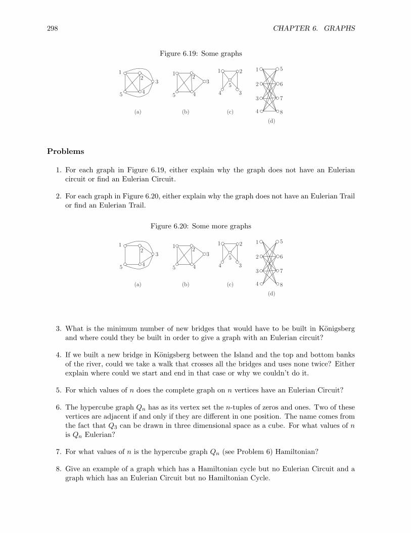
298 CHAPTER 6. GRAPHS
Figure 6.19: Some graphs
(a) (b) (c)
(d)
1 1 1 1
3 3
33
4 4 4
4
5 5
5
5
2 22
2 6
7
8
Problems
1. For each graph in Figure 6.19, either explain why the graph does not have an Euleriancircuit or find an Eulerian Circuit.
2. For each graph in Figure 6.20, either explain why the graph does not have an Eulerian Trailor find an Eulerian Trail.
Figure 6.20: Some more graphs
(a) (b) (c)
(d)
1 1 1 1
3 3
33
4 4 4
4
5 5
5
5
2 22
2 6
7
8
3. What is the minimum number of new bridges that would have to be built in Konigsbergand where could they be built in order to give a graph with an Eulerian circuit?
4. If we built a new bridge in Konigsberg between the Island and the top and bottom banksof the river, could we take a walk that crosses all the bridges and uses none twice? Eitherexplain where could we start and end in that case or why we couldn’t do it.
5. For which values of n does the complete graph on n vertices have an Eulerian Circuit?
6. The hypercube graph Qn has as its vertex set the n-tuples of zeros and ones. Two of thesevertices are adjacent if and only if they are different in one position. The name comes fromthe fact that Q3 can be drawn in three dimensional space as a cube. For what values of nis Qn Eulerian?
7. For what values of n is the hypercube graph Qn (see Problem 6) Hamiltonian?
8. Give an example of a graph which has a Hamiltonian cycle but no Eulerian Circuit and agraph which has an Eulerian Circuit but no Hamiltonian Cycle.

6.3. EULERIAN AND HAMILTONIAN PATHS AND TOURS 299
9. The complete bipartite graph Km,n is a graph with m + n vertices. These vertices aredivided into a set of size m and a set of size n. We call these sets the parts of the graph.Within each of these sets there are no edges. But between each pair of vertices in differentsets, there is an edge. The graph K4,4 is pictured in part (d) of Figure 6.19.
(a) For what values of m and n is Km,n Eulerian?
(b) For which values of m and n is Km,n Hamiltonian?
10. Show that the edge set of a graph in which each vertex has even degree may be partitionedinto edge sets of cycles of the graph.
11. A cut-vertex of a graph is a vertex whose removal (along with all edges incident with it)increases the number of connected components of the graph. Describe any circumstancesunder which a graph with a cut vertex can be Hamiltonian.
12. Which of the graphs in Figure 6.21 satisfy the hypotheses of Dirac’s Theorem? of Ore’sTheorem? Which have Hamiltonian cycles?
Figure 6.21: Which of these graphs have Hamiltonian Cycles?
(a) (b) (c) (d)
13. Prove Theorem 6.12.
14. The Hamiltonian Path problem is the problem of determining whether a graph has a Hamil-tonian Path. Explain why this problem is in NP. Explain why the problem of determiningwhether a graph has a Hamiltonian Path is NP-complete.
15. The k-Path problem is the problem of determining whether a graph on n vertices has apath of length k, where k is allowed to depend on n. Show that the k-Path problem isNP-complete.
16. We form the Hamiltonian closure of a graph by constructing a sequence of graphs Gi withG0 = G, and Gi formed from Gi−1 by adding an edge between two nonadjacent verticeswhose degree sum is at least nv. When we reach a Gi to which we cannot add such anedge, we call it a Hamiltonian Closure of G. Prove that a Hamiltonian Closure of a simplegraph G is Hamiltonian if and only if G is.
17. Show that a simple connected graph has one and only one Hamiltonian closure.

300 CHAPTER 6. GRAPHS
6.4 Matching Theory
The idea of a matching
Suppose a school board is deciding among applicants for faculty positions. The school board haspositions for teachers in a number of different grades, a position for an assistant librarian, twocoaching positions, and for high school math and English teachers. They have many applicants,each of whom can fill more than one of the positions. They would like to know whether they canfill all the positions with people who have applied for jobs and have been judged as qualified.
Exercise 6.4-1 Table 6.1 shows a sample of the kinds of applications a school district mightget for its positions. An x below an applicant’s number means that that applicant
Table 6.1: Some sample job application data
job\applicant 1 2 3 4 5 6 7 8 9assistant librarian x x xsecond grade x x x xthird grade x x xhigh school math x x xhigh school English x x xasst baseball coach x x x xasst football coach x x x
qualifies for the position to the left of the x. Thus candidate 1 is qualified to teachsecond grade, third grade, and be an assistant librarian. The coaches teach physicaleducation when they are not coaching, so a coach can’t also hold one of the listedteaching positions. Draw a graph in which the vertices are labelled 1 through 9 forthe applicants, and s, t, l, m, e, b, and f for the positions. Draw an edge from anapplicant to a position if that applicant can fill that position. Use the graph to helpyou decide if it is possible to fill all the positions from among the applicants deemedsuitable. If you can do so, give an assignment of people to jobs. If you cannot, try toexplain why not.
Exercise 6.4-2 Table 6.2 shows a second sample of the kinds of applications a schooldistrict might get for its positions. Draw a graph as before and use it to helpyou decide if it is possible to fill all the positions from among the applicants deemedsuitable. If you can do so, give an assignment of people to jobs. If you cannot, try toexplain why not.
The graph of the data in Table 6.1 is shown in Figure 6.22.
From the figure it is clear that l:1, s:2, t:4, m:5, e:6, b:7, f :8 is one assignment of jobs to peoplethat works. This assignment picks out a set of edges that share no endpoints. For example, theedge from l to 1 has no endpoint among s, t, m, e, b, f , 2, 3, 4, 5, 6, 7, or 8. A set of edgesin a graph that share no endpoints is called a matching of the graph. Thus we have a matchingbetween jobs and people that can fill the jobs. Since we don’t want to assign two jobs to one
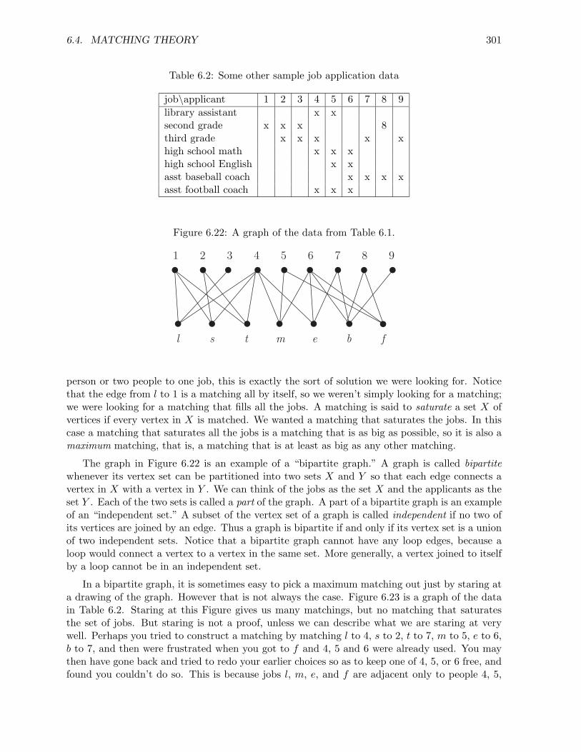
6.4. MATCHING THEORY 301
Table 6.2: Some other sample job application data
job\applicant 1 2 3 4 5 6 7 8 9library assistant x xsecond grade x x x 8third grade x x x x xhigh school math x x xhigh school English x xasst baseball coach x x x xasst football coach x x x
Figure 6.22: A graph of the data from Table 6.1.
l s t m e b f
1 2 3 4 5 6 7 8 9
person or two people to one job, this is exactly the sort of solution we were looking for. Noticethat the edge from l to 1 is a matching all by itself, so we weren’t simply looking for a matching;we were looking for a matching that fills all the jobs. A matching is said to saturate a set X ofvertices if every vertex in X is matched. We wanted a matching that saturates the jobs. In thiscase a matching that saturates all the jobs is a matching that is as big as possible, so it is also amaximum matching, that is, a matching that is at least as big as any other matching.
The graph in Figure 6.22 is an example of a “bipartite graph.” A graph is called bipartitewhenever its vertex set can be partitioned into two sets X and Y so that each edge connects avertex in X with a vertex in Y . We can think of the jobs as the set X and the applicants as theset Y . Each of the two sets is called a part of the graph. A part of a bipartite graph is an exampleof an “independent set.” A subset of the vertex set of a graph is called independent if no two ofits vertices are joined by an edge. Thus a graph is bipartite if and only if its vertex set is a unionof two independent sets. Notice that a bipartite graph cannot have any loop edges, because aloop would connect a vertex to a vertex in the same set. More generally, a vertex joined to itselfby a loop cannot be in an independent set.
In a bipartite graph, it is sometimes easy to pick a maximum matching out just by staring ata drawing of the graph. However that is not always the case. Figure 6.23 is a graph of the datain Table 6.2. Staring at this Figure gives us many matchings, but no matching that saturatesthe set of jobs. But staring is not a proof, unless we can describe what we are staring at verywell. Perhaps you tried to construct a matching by matching l to 4, s to 2, t to 7, m to 5, e to 6,b to 7, and then were frustrated when you got to f and 4, 5 and 6 were already used. You maythen have gone back and tried to redo your earlier choices so as to keep one of 4, 5, or 6 free, andfound you couldn’t do so. This is because jobs l, m, e, and f are adjacent only to people 4, 5,

302 CHAPTER 6. GRAPHS
Figure 6.23: A graph of the data of Table 6.2.
l s t m e b f
1 2 3 4 5 6 7 8 9
and 6. Thus there are only three people qualified for these four jobs, and so there is no way wecan fill them all.
We call the set N(S) of all vertices adjacent to at least one vertex of S the neighborhood of Sor the neighbors of S. In these terms, there is no matching that saturates a part X of a bipartitegraph if there is some subset S of X such that the set N(S) of neighbors of S is smaller than S.We call the set N(S) of all vertices adjacent to at least one vertex of S the neighborhood of S orthe neighbors of S. In symbols, we can summarize as follows.
Lemma 6.13 If we can find a subset S of a part X of a bipartite graph G such that |N(S)| < |S|,then there is no matching of G that saturates X.
Proof: A matching that saturates X must saturate S. But if there is such a matching,each element of S must be matched to a different vertex, and this vertex cannot be in S sinceS ⊆ X. Therefore there are edges from vertices in S to at least |S| different vertices not in S, so|N(S)| > |S|, a contradiction. Thus there is no such matching.
This gives a proof that there is no matching that saturates all the jobs, so the matching thatmatches l to 4, s to 2, t to 7, m to 5, e to 6, b to 7 is a maximum matching for the graph inFigure 6.23.
Another method you may have used to prove that there is no larger matching than the onewe found is the following. When we matched l to 4, we may have noted that 4 is an endpoint ofquite a few edges. Then when we matched s to 2, we may have noted that s is an endpoint ofquite a few edges, and so is t. In fact, 4, s, and t touch 12 edges of the graph, and there are only23 edges in the graph. If we could find three more vertices that touch the remaining edges of thegraph, we would have six vertices that among them are incident with every edge. A set of verticessuch that at least one of them is incident with each edge of a graph G is called a vertex coverof the edges of G, or a vertex cover of G for short. What does this have to do with a matching?Each matching edge would have to touch one, or perhaps two of the vertices in a vertex cover ofthe edges. Thus the number of edges in a matching is always less than the number of vertices ina vertex cover of the edges of a graph. Thus if we can find a vertex cover of size six in our graphin Figure 6.23, we will know that there is no matching that saturates the set of jobs since thereare seven jobs. For future reference, we state our result about the size of a matching and the sizeof a vertex cover as a lemma.
Lemma 6.14 The size of a matching in a graph G is no more than the size of a vertex cover ofG.

6.4. MATCHING THEORY 303
Proof: Given in the preceding discussion.
We have seen that 4, s, and t are good candidates for being members of a relatively smallvertex cover of the graph in Figure 6.23, since they cover more than half the edges of the graph.Continuing through the edges we first examined, we see that m, 6, and b are good candidatesfor a small vertex cover as well. In fact, 4, s, t, m, 6, b do form a vertex cover. Since we havea vertex cover of size six, we know a maximum matching has size no more than six. Since wehave already found a six-edge matching, that is a maximum matching. Therefore with the datain Table 6.2, it is not possible to fill all the jobs.
Making matchings bigger
Practical problems involving matchings will usually lead us to search for the largest possiblematching in a graph. To see how to use a matching to create a larger one, we will assume wehave two matchings of the same graph and see how they differ, especially how a larger one differsfrom a smaller one.
Exercise 6.4-3 In the graph G of Figure 6.22, let M1 be the matching l, 1, s, 2, t, 4,m, 5, e, 6, b, 9, f, 8, and let M2 be the matching l, 4, s, 2 t, 1, m, 6,e, 7 b, 8. Recall that for sets S1 and S2 the symmetric difference of S1 and S2,denoted by S1∆S2 is (S1 ∪ S2) − (S1 ∩ S2). Compute the set M1∆M2 and draw thegraph with the same vertex set as G and edge set M1∆M2. Use different colors ortextures for the edges from M1 and M2 so you can see their interaction. Describe thekinds of graphs you see as connected components as succinctly as possible.
Exercise 6.4-4 In Exercise 6.4-3, one of the connected components suggests a way tomodify M2 by removing one or more edges and substituting one or more edges fromM1 that will give you a larger matching M ′
2 related to M2. In particular, this largermatching should saturate everything M2 saturates and more. What is M ′
2 and whatelse does it saturate?
Exercise 6.4-5 Consider the matching M = s, 1, t, 4, m, 6, b, 8 in the graph ofFigure 6.23. How does it relate to the simple path whose vertices are 3, s, 1, t, 4, m, 6, f?Say as much as you can about the set M ′ that you obtain from M by deleting theedges of M that are in the path and adding to the result the edges of the path thatare not in M .
In Exercise 6.4-3
M1∆M2 = l, 1, l, 4, t, 4, t, 1, m, 5, m, 6, e, 6, e, 7, b, 8, f, 8, b, 9.
We have drawn the graph in Figure 6.24. We show the edges of M2 as dashed. As you see,it consists of a cycle with four edges, alternating between edges of M1 and M2, a path with fouredges, alternating between edges of M1 and M2, and a path with three edges, alternating betweenedges of M1 and M2. We call a simple path or cycle an alternating path or alternating cycle fora matching M of a graph G if its edges alternate between edges in M and edges not in M . Thusour connected components were alternating paths and cycles for both M1 and M2. The examplewe just discussed shows all the ways in which two matchings can differ in the following sense.

304 CHAPTER 6. GRAPHS
Figure 6.24: The graph for Exercise 6.4-3.
l s t m e b f
1 2 3 4 5 6 7 8 9
Lemma 6.15 (Berge) If M1 and M2 are matchings of a graph G = (V, E) then the connectedcomponents of M1∆M2 are cycles with an even number of vertices and simple paths. Further,the cycles and paths are alternating cycles and paths for both M1 and M2.
Proof: Each vertex of the graph (V, M1∆M2) has degree 0, 1, or two. If a component hasno cycles it is a tree, and the only kind of tree that has vertices of degree 1 and two is a simplepath. If a component has a cycle, then it cannot have any edges other than the edges of the cycleincident with its vertices because the graph would then have a vertex of degree 3 or more. Thusthe component must be a cycle. If two edges of a path or cycle in (V, M1∆M2) share a vertex,they cannot come from the same matching, since two edges in the same matching do not sharea vertex. Thus alternating edges of a path or cycle of (V, M1∆M2) must come from differentmatchings.
Corollary 6.16 If M1 and M2 are matchings of a graph G = (V, E) and |M2| < |M1|, then thereis an alternating path for M1 and M2 that starts and ends with vertices saturated by M2 but notby M1.
Proof: Since an even alternating cycle and an even alternating path in (V, M1∆M2) haveequal numbers of edges from M1 and M2, at least one component must be an alternating pathwith more edges from M1 than M2, because otherwise |M2| ≤ |M1|. Since this is a component of(V, M1∆M2), its endpoints lie only in edges of M2, so they are saturated by M2 but not M1.
The path with three edges in Exercise 6.4-3 has two edges of M1 and one edge of M2. We seethat if we remove b, 8 from M2 and add b, 9 and f, 8, we get the matching
M ′2 = l, 4, s, 2, t, 1, m, 6, e, 7, b, 9, f, 8.
This answers the question of Exercise 6.4-4. Notice that this matching saturates everything M2
does, and also saturates vertices f and 9.
In Figure 6.25 we have shown the matching edges of the path in Exercise 6.4-5 in bold andthe non-matching edges of the path as dashed. The edge of the matching not in the path isshown in zig-zag. Notice that the dashed edges and the zig-zag edge form a matching which islarger than M and saturates all the vertices that M does in addition to 3 and f . The path beginsand ends with unmatched vertices, namely 3 and f , and and alternates between matching edgesand non-matching edges. All but the first and last vertices of such a path lie on matching edgesof the path and the endpoints of the path do not lie on matching edges. Thus no edges of thematching that are not path-edges will be incident with vertices on the path. Thus if we delete allthe matching edges of the path from M and add all the other edges of the path to M , we will get

6.4. MATCHING THEORY 305
Figure 6.25: The path and matching of Exercise 6.4-5.
l s t m e b f
1 2 3 4 5 6 7 8 9
a new matching, because by taking every second edge of a simple path, we get edges that do nothave endpoints in common. An alternating path is called an augmenting path for a matching Mif it begins and ends with M -unsaturated vertices. That is, it is an alternating path that beginsand ends with unmatched vertices. Our preceding discussion suggests the proof of the followingtheorem.
Theorem 6.17 (Berge) A matching M in a graph is of maximum size if and only if M has noaugmenting path. Further, if a matching M has an augmenting path P with edge set E(P ), thenwe can create a larger matching by deleting the edges in M ∩ E(P ) from M and adding in theedges of E(P ) − M .
Proof: First if there is a matching M1 larger than M , then by Corollary 6.16 there is anaugmenting path for M . Thus if a matching has maximum size, it has no augmenting path.Further, as in our discussion of Exercise 6.4-5, if there is an augmenting path for M , then thereis a larger matching for M . Finally, this discussion showed that if P is an augmenting path, wecan get such a larger matching by deleting the edges in M ∩ E(P ) and adding in the edges ofE(P ) − M .
Corollary 6.18 While the larger matching of Theorem 6.17 may not contain M as a subset, itdoes saturate all the vertices that M saturates and two additional vertices.
Proof: Every vertex incident with an edge in M is incident with some edge of the largermatching, and each of the two endpoints of the augmenting path is also incident with a matchingedge. Because we may have removed edges of M to get the larger matching, it may not containM .
Matching in Bipartite Graphs
While our examples have all been bipartite, all our lemmas, corollaries and theorems aboutmatchings have been about general graphs. In fact, it some of the results can be strengthened inbipartite graphs. For example, Lemma 6.14 tells us that the size of a matching is no more thanthe size of a vertex cover. We shall soon see that in a bipartite graph, the size of a maximummatching actually equals the size of a minimum vertex cover.

306 CHAPTER 6. GRAPHS
Searching for Augmenting Paths in Bipartite Graphs
We have seen that if we can find an augmenting path for a matching M in a graph G, thenwe can create a bigger matching. Since our goal from the outset has been to create the largestmatching possible, this helps us achieve that goal. However, you may ask, how do we find anaugmenting path? Recall that a breadth-first search tree centered at a vertex x in a graphcontains a path, in fact a shortest path, from x to every vertex y to which it is connected. Thusit seems that we ought to be able to alternate between matching edges and non-matching edgeswhen doing a breadth-first search and find alternating paths. In particular, if we add vertex i toour tree by using a matching edge, then any edge we use to add a vertex from vertex i shouldbe a non-matching edge. And if we add vertex i to our tree by using a non-matching edge, thenany edge we use to add a vertex from vertex i should be a matching edge. (Thus there is justone such edge.) Because not all edges are available to us to use in adding vertices to the tree, thetree we get will not necessarily be a spanning tree of our original graph. However we can hopethat if there is an augmenting path starting at vertex x and ending at vertex y, then we will findit by using breadth first search starting from x in this alternating manner.
Exercise 6.4-6 Given the matching s, 2, t, 4, b, 7f, 8 of the graph in Figure 6.22use breadth-first search starting at vertex 1 in an alternating way to search for anaugmenting path starting at vertex 1. Use the augmenting path you get to create alarger matching.
Exercise 6.4-7 Continue using the method of Exercise 6.4-6 until you find a matching ofmaximum size.
Exercise 6.4-8 Apply breadth-first search from vertex 0 in an alternating way to graph (a)in Figure 6.26. Does this method find an augmenting path? Is there an augmentingpath?
Figure 6.26: Matching edges are shown in bold in these graphs.
1
2
43
1
2
43
5
567
(a)(b)
8 9 10
0
0
For Exercise 6.4-6, if we begin at vertex 1, we add vertices l,s and t to our tree, giving thembreadth-first numbers 1,2, and 3. Since l is not incident with a matching edge, we cannot continuethe search from there. Since vertex s is incident with matching edge s, 2, we can use this edgeto add vertex 2 to the tree and give it breadth-first number 4. This is the only vertex we canadd from l since we can only use matching edges to add vertices from l. Similarly, from t wecan add vertex 4 by using the matching edge t, 4 and giving it breadth-first number 5. All
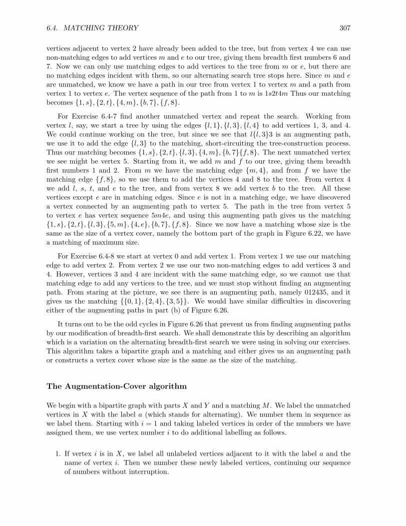
6.4. MATCHING THEORY 307
vertices adjacent to vertex 2 have already been added to the tree, but from vertex 4 we can usenon-matching edges to add vertices m and e to our tree, giving them breadth first numbers 6 and7. Now we can only use matching edges to add vertices to the tree from m or e, but there areno matching edges incident with them, so our alternating search tree stops here. Since m and eare unmatched, we know we have a path in our tree from vertex 1 to vertex m and a path fromvertex 1 to vertex e. The vertex sequence of the path from 1 to m is 1s2t4m Thus our matchingbecomes 1, s, 2, t, 4, m, b, 7, f, 8.
For Exercise 6.4-7 find another unmatched vertex and repeat the search. Working fromvertex l, say, we start a tree by using the edges l, 1, l, 3, l, 4 to add vertices 1, 3, and 4.We could continue working on the tree, but since we see that ll, 33 is an augmenting path,we use it to add the edge l, 3 to the matching, short-circuiting the tree-construction process.Thus our matching becomes 1, s, 2, t, l, 3, 4, m, b, 7f, 8. The next unmatched vertexwe see might be vertex 5. Starting from it, we add m and f to our tree, giving them breadthfirst numbers 1 and 2. From m we have the matching edge m, 4, and from f we have thematching edge f, 8, so we use them to add the vertices 4 and 8 to the tree. From vertex 4we add l, s, t, and e to the tree, and from vertex 8 we add vertex b to the tree. All thesevertices except e are in matching edges. Since e is not in a matching edge, we have discovereda vertex connected by an augmenting path to vertex 5. The path in the tree from vertex 5to vertex e has vertex sequence 5m4e, and using this augmenting path gives us the matching1, s, 2, t, l, 3, 5, m, 4, e, b, 7, f, 8. Since we now have a matching whose size is thesame as the size of a vertex cover, namely the bottom part of the graph in Figure 6.22, we havea matching of maximum size.
For Exercise 6.4-8 we start at vertex 0 and add vertex 1. From vertex 1 we use our matchingedge to add vertex 2. From vertex 2 we use our two non-matching edges to add vertices 3 and4. However, vertices 3 and 4 are incident with the same matching edge, so we cannot use thatmatching edge to add any vertices to the tree, and we must stop without finding an augmentingpath. From staring at the picture, we see there is an augmenting path, namely 012435, and itgives us the matching 0, 1, 2, 4, 3, 5. We would have similar difficulties in discoveringeither of the augmenting paths in part (b) of Figure 6.26.
It turns out to be the odd cycles in Figure 6.26 that prevent us from finding augmenting pathsby our modification of breadth-first search. We shall demonstrate this by describing an algorithmwhich is a variation on the alternating breadth-first search we were using in solving our exercises.This algorithm takes a bipartite graph and a matching and either gives us an augmenting pathor constructs a vertex cover whose size is the same as the size of the matching.
The Augmentation-Cover algorithm
We begin with a bipartite graph with parts X and Y and a matching M . We label the unmatchedvertices in X with the label a (which stands for alternating). We number them in sequence aswe label them. Starting with i = 1 and taking labeled vertices in order of the numbers we haveassigned them, we use vertex number i to do additional labelling as follows.
1. If vertex i is in X, we label all unlabeled vertices adjacent to it with the label a and thename of vertex i. Then we number these newly labeled vertices, continuing our sequenceof numbers without interruption.

308 CHAPTER 6. GRAPHS
2. If vertex i is in Y , and it is incident with an edge of M , its neighbor in the matching edgecannot yet be labeled. We label this neighbor with the label a and the name of vertex i.
3. If vertex i is in Y , and it is not incident with an edge of M , then we have discovered anaugmenting path: the path from vertex i to the vertex we used to add it (and recordedat vertex i) and so on back to one of the unlabeled vertices in X. It is alternating by ourlabeling method, and it starts and ends with unsaturated vertices, so it is augmenting.
If we can continue the labelling process until no more labeling is possible and we do not find anaugmenting path, then we let A be the set of labeled vertices. The set C = (X − A) ∪ (Y ∩ A)then turns out to be a vertex cover whose size is the size of M . We call this algorithm theaugmentation-cover algorithm.
Theorem 6.19 (Konig and Egervary) In a bipartite graph with parts X and Y , the size ofa maximum sized matching equals the size of a minimum-sized vertex cover.
Proof: In light of Berge’s Theorem, if the augmentation-cover algorithm gives us an augment-ing path, then the matching is not maximum sized, and in light of Lemma 6.14, if we can provethat the set C the algorithm gives us when there is no augmenting path is a vertex cover whosesize is the size of the matching, we will have proved the theorem. To see that C is a vertex cover,note that every edge incident with a vertex in X ∩ A is covered, because its endpoint in Y hasbeen marked with an a and so is in Y ∩ A. But every other edge must be covered by X − Abecause in a bipartite graph, each edge must be incident with a vertex in each part. ThereforeC is a vertex cover. If an element of Y ∩ A, were not matched, it would be an endpoint of anaugmenting path, and so all elements of Y ∩ A are incident with matching edges. But everyvertex of X − A is matched because A includes all unmatched vertices of X. By step 2 of theaugmentation-cover algorithm, if ε is a matching edge with an endpoint in Y ∩A, then the otherendpoint must be in A. Therefore each matching edge contains only one member of C. Thereforethe size of a maximum matching is the size of C.
Corollary 6.20 The augmentation-cover algorithm applied to a bipartite graph and a matchingof that graph produces either an augmenting path for the matching or a minimum vertex coverwhose size equals the size of the matching.
Before we proved the Konig-Egervary Theorem, we knew that if we could find a matching anda vertex cover of the same size, then we had a maximum sized matching and a minimum sizedvertex cover. However it is possible that in some graphs we can’t test for whether a matchingis as large as possible by comparing its size to that of a vertex cover because a maximum sizedmatching might be smaller than a minimum sized vertex cover. The Konig-Egarvary Theoremtells us that in bipartite graphs this problem never arises, so the test always works.
We had a second technique we used to show that a matching could not saturate the set Xof all jobs in Exercise 6.4-2. In Lemma 6.13 we showed that if we can find a subset S of a partX of a bipartite graph G such that |N(S)| < |S|, then there is no matching of G that saturatesX. In other words, to have a matching that saturates X in a bipartite graph on parts X and Y ,it is necessary that |N(S)| ≥ |S| for every subset S of X. (When S = ∅, then so does N(S).)This necessary condition is called Hall’s condition, and Hall’s theorem says that this necessarycondition is sufficient.
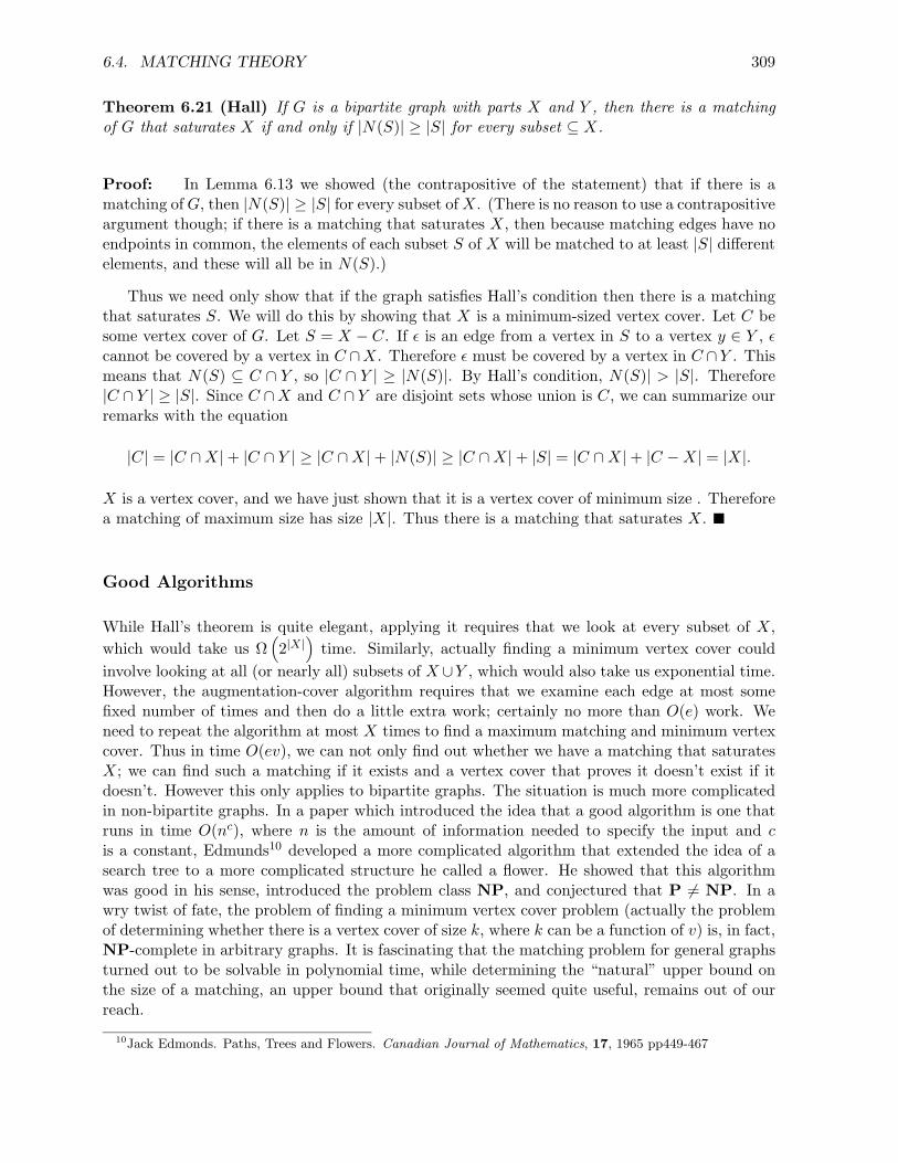
6.4. MATCHING THEORY 309
Theorem 6.21 (Hall) If G is a bipartite graph with parts X and Y , then there is a matchingof G that saturates X if and only if |N(S)| ≥ |S| for every subset ⊆ X.
Proof: In Lemma 6.13 we showed (the contrapositive of the statement) that if there is amatching of G, then |N(S)| ≥ |S| for every subset of X. (There is no reason to use a contrapositiveargument though; if there is a matching that saturates X, then because matching edges have noendpoints in common, the elements of each subset S of X will be matched to at least |S| differentelements, and these will all be in N(S).)
Thus we need only show that if the graph satisfies Hall’s condition then there is a matchingthat saturates S. We will do this by showing that X is a minimum-sized vertex cover. Let C besome vertex cover of G. Let S = X − C. If ε is an edge from a vertex in S to a vertex y ∈ Y , εcannot be covered by a vertex in C ∩X. Therefore ε must be covered by a vertex in C ∩Y . Thismeans that N(S) ⊆ C ∩ Y , so |C ∩ Y | ≥ |N(S)|. By Hall’s condition, N(S)| > |S|. Therefore|C ∩ Y | ≥ |S|. Since C ∩X and C ∩ Y are disjoint sets whose union is C, we can summarize ourremarks with the equation
|C| = |C ∩ X| + |C ∩ Y | ≥ |C ∩ X| + |N(S)| ≥ |C ∩ X| + |S| = |C ∩ X| + |C − X| = |X|.
X is a vertex cover, and we have just shown that it is a vertex cover of minimum size . Thereforea matching of maximum size has size |X|. Thus there is a matching that saturates X.
Good Algorithms
While Hall’s theorem is quite elegant, applying it requires that we look at every subset of X,which would take us Ω
(2|X|
)time. Similarly, actually finding a minimum vertex cover could
involve looking at all (or nearly all) subsets of X ∪Y , which would also take us exponential time.However, the augmentation-cover algorithm requires that we examine each edge at most somefixed number of times and then do a little extra work; certainly no more than O(e) work. Weneed to repeat the algorithm at most X times to find a maximum matching and minimum vertexcover. Thus in time O(ev), we can not only find out whether we have a matching that saturatesX; we can find such a matching if it exists and a vertex cover that proves it doesn’t exist if itdoesn’t. However this only applies to bipartite graphs. The situation is much more complicatedin non-bipartite graphs. In a paper which introduced the idea that a good algorithm is one thatruns in time O(nc), where n is the amount of information needed to specify the input and cis a constant, Edmunds10 developed a more complicated algorithm that extended the idea of asearch tree to a more complicated structure he called a flower. He showed that this algorithmwas good in his sense, introduced the problem class NP, and conjectured that P = NP. In awry twist of fate, the problem of finding a minimum vertex cover problem (actually the problemof determining whether there is a vertex cover of size k, where k can be a function of v) is, in fact,NP-complete in arbitrary graphs. It is fascinating that the matching problem for general graphsturned out to be solvable in polynomial time, while determining the “natural” upper bound onthe size of a matching, an upper bound that originally seemed quite useful, remains out of ourreach.
10Jack Edmonds. Paths, Trees and Flowers. Canadian Journal of Mathematics, 17, 1965 pp449-467

310 CHAPTER 6. GRAPHS
Important Concepts, Formulas, and Theorems
1. Matching. A set of edges in a graph that share no endpoints is called a matching of thegraph.
2. Saturate. A matching is said to saturate a set X of vertices if every vertex in X is matched.
3. Maximum Matching. A matching in a graph is a maximum matching if it is at least as bigas any other matching.
4. Bipartite Graph. A graph is called bipartite whenever its vertex set can be partitioned intotwo sets X and Y so that each edge connects a vertex in X with a vertex in Y . Each ofthe two sets is called a part of the graph.
5. Independent Set. A subset of the vertex set of a graph is called independent if no two of itsvertices are connected by an edge. (In particular, a vertex connected to itself by a loop isin no independent set.) A part of a bipartite graph is an example of an ‘independent set.
6. Neighborhood. We call the set N(S) of all vertices adjacent to at least one vertex of S theneighborhood of S or the neighbors of S.
7. Hall’s theorem for a Matching in a Bipartite Graph. If we can find a subset S of a partX of a bipartite graph G such that |N(S)| < |S|, then there is no matching of G thatsaturates X. If there is no subset S ⊆ X such that |N(S)| < |S|, then there is a matchingthat saturates X.
8. Vertex Cover. A set of vertices such that at least one of them is incident with each edgeof a graph G is called a vertex cover of the edges of G, or a vertex cover of G for short. Inany graph, the size a matching is less than or equal to the size of any vertex cover.
9. Alternating Path, Augmenting Path. A simple path is called an alternating path for amatching M if, as we move along the path, the edges alternate between edges in M andedges not in M . An augmenting path is an alternating path that begins and ends atunmatched vertices.
10. Berge’s Lemma. If M1 and M2 are matchings of a graph G then the connected componentsof M1∆M2 are cycles with an even number of vertices and simple paths. Further, the cyclesand paths are alternating cycles and paths for both M1 and M2.
11. Berge’s Corollary. If M1 and M2 are matchings of a graph G = (V, E) and |M1| > |M2|,then there is an alternating path for M1 and M2 that starts and ends with vertices saturatedby M1 but not by M2.
12. Berge’s Theorem. A matching M in a graph is of maximum size if and only if M has noaugmenting path. Further, if a matching M has an augmenting path P with edge set E(P ),then we can create a larger matching by deleting the edges in M∩E(P ) from M and addingin the edges of E(P ) − M .
13. Augmentation-Cover Algorithm. The Augmentation-Cover algorithm is an algorithm thatbegins with a bipartite graph and a matching of that graph and produces either an aug-menting path or a vertex cover whose size equals that of the matching, thus proving thatthe matching is a maximum matching.

6.4. MATCHING THEORY 311
14. Konig-Egervary Theorem. In a bipartite graph with parts X and Y , the size of a maximumsized matching equals the size of a minimum-sized vertex cover.
Problems
1. Either find a maximum matching or a subset S of the set X = a, b, c, d, e such that|S| > |N(S)| in the graph of Figure 6.27
Figure 6.27: A bipartite graph
a b c d e
1 2 3 4 5 6 7
2. Find a maximum matching and a minimum vertex cover in the graph of Figure 6.27
3. Either find a matching which saturates the set X = a, b, c, d, e, f in Figure 6.28 or find aset S such that |N(S)| < |X|.
Figure 6.28: A bipartite graph
a b c d fe
1 2 3 4 5 6
4. Find a maximum matching and a minimum vertex cover in the graph of Figure 6.28.
5. In the previous exercises, when you were able to find a set S with |S| > |N(S)|, how didN(S) relate to the vertex cover? Why did this work out as it did?
6. A star is a another name for a tree with one vertex connected to each of n other vertices.(So a star has n + 1 vertices.) What are the size of a maximum matching and a minimumvertex cover in a star with n + 1 vertices?
7. In Theorem 6.17 is it true that if there is an augmenting path P with edge set E(P ) for amatching M , then M∆E(P ) is a larger matching than M?
8. Find a maximum matching and a minimum vertex cover in graph (b) of Figure 6.26.
9. In a bipartite graph, is one of the parts always a maximum-sized independent set? Whatif the graph is connected?
312 CHAPTER 6. GRAPHS
10. Find infinitely many examples of graphs in which a maximum-sized matching is smallerthan a minimum-sized vertex cover.
11. Find an example of a graph in which the maximum size of a matching is less than onequarter of the size of a minimum vertex cover.
12. Prove or give a counter-example: Every tree is a bipartite graph. (Note, a single vertexwith no edges is a bipartite graph; one of the two parts is empty.)
13. Prove or give a counter-example. A bipartite graph has no odd cycles.
14. Let G be a connected graph with no odd cycles. Let x be a vertex of G. Let X be allvertices at an even distance from x, and let Y be all vertices at an odd distance from x.Prove that G is bipartite with parts X and Y .
15. What is the sum of the maximum size of an independent set and the minimum size of avertex cover in a graph G? Hint: it is useful to think both about the independent set andits complement (relative to the vertex set).

6.5. COLORING AND PLANARITY 313
6.5 Coloring and planarity
The idea of coloring
Graph coloring was one of the origins of graph theory. It arose from a question from FrancisGuthrie, who noticed that that four colors were enough colors to color the map of the counties ofEngland so that if two counties shared a common boundary line, then they got different colors. Hewondered whether this was the case for any map. Through his brother he passed it on to AgustusDeMorgan, and in this way it seeped into the consciousness of the mathematical community. Ifwe think of the counties as vertices and draw an edge between two vertices if their counties sharesome boundary line, we get a representation of the problem that is independent of such things asthe shape of the counties, the amount of boundary line they share, etc. so that it captures thepart of the problem we need to focus on. We now color the vertices of the graph, and for thisproblem we want to do so in such a way that adjacent vertices get different colors. We will returnto this problem later in the section; we begin our study with another application of coloring.
Exercise 6.5-1 The executive committee of the board of trustees of a small college hasseven members, Kim, Smith, Jones, Gupta, Ramirez, Wang, and Chernov. It has sixsubcommittees with the following membership
• Investments: W, R, G
• Operations: G, J, S, K
• Academic affairs: S, W, C
• Fund Raising: W, C, K
• Budget: G, R, C
• Enrollment: R, S, J, K
Each time the executive committee has a meeting, first each of the subcommitteesmeets with appropriate college officers, and then the executive committee gets to-gether as a whole to go over subcommittee recommendations and make decisions.Two committees cannot meet at the same time if they have a member in common,but committees that don’t have a member in common can meet at the same time. Inthis exercise you will figure out the minimum number of time slots needed to scheduleall the subcommittee meetings. Draw a graph in which the vertices are named by theinitials of the committee names and two vertices are adjacent if they have a memberin common. Then assign numbers to the vertices in such a way that two adjacentvertices get different numbers. The numbers represent time slots, so they need not bedistinct unless they are on adjacent vertices. What is the minimum possible numberof numbers you need?
Because the problem of map coloring motivated much of graph theory, it is traditional to referto the process of assigning labels to the vertices of a graph as coloring the graph. An assignmentof labels, that is a function from the vertices to some set, is called a coloring. The set of possiblelabels (the range of the coloring function) is often referred to as a set of colors. Thus in Exercise6.5-1 we are asking for a coloring of the graph. However, as with the map problem, we want acoloring in which adjacent vertices have different colors. A coloring of a graph is called a propercoloring if it assigns different colors to adjacent vertices.

314 CHAPTER 6. GRAPHS
We have drawn the graph of Exercise 6.5-1 in Figure 6.29. We call this kind of graph anintersection graph, which means its vertices correspond to sets and it has an edge between twovertices if and only if the corresponding sets intersect.
Figure 6.29: The “intersection” graph of the committees.
I O A
D
BE
The problem asked us to color the graph with as few colors possible, regarding the colors as1,2,3, etc. We will represent 1 as a white vertex, 2 as a light grey vertex, 3 as a dark grey vertexand 4 as a black vertex. The triangle on the bottom requires three colors simply because all threevertices are adjacent. Since it doesn’t matter which three colors we use, we choose arbitrarily tomake them white, light grey, and dark grey. Now we know we need at least three colors to colorthe graph, so it makes sense to see if we can finish off a coloring using just three colors. VertexI must be colored differently from E and D, so if we use the same three colors, it must have thesame color as B. Similarly, vertex A would have to be the same color as E if we use the samethree colors. But now none of the colors can be used on vertex O, because it is adjacent to threevertices of different colors. Thus we need at least four colors rather than 3, and we show a properfour-coloring in Figure 6.30.
Figure 6.30: A proper coloring of the committee intersection graph.
I O A
D
BE
Exercise 6.5-2 How many colors are needed to give a proper coloring of the completegraph Kn?
Exercise 6.5-3 How many colors are needed for a proper coloring of a cycle Cn on n =3, 4, 5, and 6 vertices?
In Exercise 6.5-2 we need n colors to properly color Kn, because each pair of vertices isadjacent and thus must have two different colors. In Exercise 6.5-3, if n is even, we can justalternate two colors as we go around the cycle. However if n is odd, using two colors wouldrequire that they alternate as we go around the cycle, and when we colored our last vertex, itwould be the same color as the first. Thus we need at least three colors, and by alternating two

6.5. COLORING AND PLANARITY 315
of them as we go around the cycle until we get to the last vertex and color it the third color weget a proper coloring with three colors.
The chromatic number of a graph G, traditionally denoted χ(G), is the minimum numberof colors needed to properly color G. Thus we have shown that the chromatic number of thecomplete graph Kn is n, the chromatic number of a cycle on an even number of vertices is two,and the chromatic number of a cycle on an odd number of vertices is three. We showed that thechromatic number of our committee graph is 4.
From Exercise 6.5-2, we see that if a graph G has a subgraph which is a complete graph onn vertices, then we need at least n colors to color those vertices, so we need at least n colors tocolor G. this is useful enough that we will state it as a lemma.
Lemma 6.22 If a graph G contains a subgraph that is a complete graph on n vertices, then thechromatic number of G is at least n.
Proof: Given above.
Interval Graphs
An interesting application of coloring arises in the design of optimizing compilers for computerlanguages. In addition to the usual RAM, a computer typically has some memory locations calledregisters which can be accessed at very high speeds. Thus values of variables which are going tobe used again in the program are kept in registers if possible, so they will be quickly availablewhen we need them. An optimizing compiler will attempt to decide the time interval in which agiven variable may be used during a run of a program and arrange for that variable to be storedin a register for that entire interval of time. The time interval is not determined in absoluteterms of seconds, but the relative endpoints of the intervals can be determined by when variablesfirst appear and last appear as one steps through the computer code. This information is what isneeded to set aside registers to use for the variables. We can think of coloring the variables by theregisters as follows. We draw a graph in which the vertices are labeled with the variable names,and associated to each variable is the interval during which it is used. Two variables can use thesame register if they are needed during non-overlapping time intervals. This is helpful, becauseregisters are significantly more expensive than ordinary RAM, so they are limited in number.We can think of our graph on the variables as the intersection graph of the intervals. We wantto color the graph properly with a minimum number of registers; hopefully this will be no morethan the number of registers our computer has available. The problem of assigning variables toregisters is called the register assignment problem.
An intersection graph of a set of intervals of real numbers is called an interval graph. Theassignment of intervals to the vertices is called an interval representation. You will notice thatso far in our discussion of coloring, we have not given an algorithm for properly coloring a graphefficiently. This is because the problem of whether a graph has a proper coloring with k colors,for any fixed k greater than 2 is another example of an NP-complete problem. However, forinterval graphs, there is a very simple algorithm for properly coloring the graph in a minimumnumber of colors.
Exercise 6.5-4 Consider the closed intervals [1, 4], [2, 5], [3, 8], [5, 12], [6, 12], [7, 14], [13, 14].Draw the interval graph determined by these intervals and find its chromatic number.

316 CHAPTER 6. GRAPHS
We have drawn the graph of Exercise 6.5-4 in Figure 6.31. (We have not included the squarebraces to avoid cluttering the figure.) Because of the way we have drawn it, it is easy to see a
Figure 6.31: The graph of Exercise 6.5-4
1,4
2,5
3,8
5,12
6,12
9,1413,14
subgraph that is a complete graph on four vertices, so we know by our lemma that the graph haschromatic number at least four. In fact, Figure 6.32 shows that the chromatic number is exactlyfour. This is no accident.
Figure 6.32: A proper coloring of the graph of Exercise 6.5-4 with four colors.
1,4
2,5
3,8
5,12
6,12
9,1413,14
Theorem 6.23 In an interval graph G, the chromatic number is the size of the largest completesubgraph.
Proof: List the intervals of an interval representation of the graph in order of their leftendpoints. Then color them with the integers 1 through some number n by starting with 1 onthe first interval in the list and for each succeeding interval, use the smallest color not used onany neighbor of the interval earlier in the list. This will clearly give a proper coloring. To see thatthe number of colors needed is the size of the largest complete subgraph, let n denote the largestcolor used, and choose an interval I colored with color n. Then, by our coloring algorithm, Imust intersect with earlier intervals in the list colored 1 through n − 1; otherwise we could haveused a smaller color on I. All these intervals must contain the left endpoint of I, because theyintersect I and come earlier in the list. Therefore they all have a point in common, so they forma complete graph on n vertices. Therefore the minimum number of colors needed is the size of acomplete subgraph of G. But by Lemma 6.22, G can have no larger complete subgraph. Thusthe chromatic number of G is the size of the largest complete subgraph of G.
Corollary 6.24 An interval graph G may be properly colored using χ(G) consecutive integers ascolors by listing the intervals of a representation in order of their left endpoints and going through

6.5. COLORING AND PLANARITY 317
the list, assigning the smallest color not used on an earlier adjacent interval to each interval inthe list.
Proof: This is the coloring algorithm we used in the proof of Theorem 6.23.
Notice that using the correspondence between numbers and grey-shades we used before, thecoloring in Figure 6.32 is the one given by this algorithm. An algorithm that colors an (arbitrary)graph G with consecutive integers by listing its vertices in some order, coloring the first vertexin the list 1, and then coloring each vertex with the least number not used on any adjacentvertices earlier in the list is called a greedy coloring algorithm. We have just seen that the greedycoloring algorithm allows us to find the chromatic number of an interval graph. This algorithmtakes time O(n2), because as we go through the list, we might consider every earlier entry whenwe are considering a given element of the list. It is good luck that we have a polynomial timealgorithm, because even though we stated in Theorem 6.23 that the chromatic number is the sizeof the largest complete subgraph, determining whether the size of a largest complete subgraph ina general graph (as opposed to an interval graph) is k (where k may be a function of the numberof vertices) is an NP-complete problem.
Of course we assumed that we were given an interval representation of our graph. Supposewe are given a graph that happens to be an interval graph, but we don’t know an intervalrepresentation. Can we still color it quickly? It turns out that there is a polynomial timealgorithm to determine whether a graph is an interval graph and find an interval representation.This theory is quite beautiful,11 but it would take us too far afield to pursue it now.
Planarity
We began our discussion of coloring with the map coloring problem. This problem has a specialaspect that we did not mention. A map is drawn on a piece of paper, or on a globe. Thus amap is drawn either on the plane or on the surface of a sphere. By thinking of the sphere as acompletely elastic balloon, we can imagine puncturing it with a pin somewhere where nothingis drawn, and then stretching the pinhole until we have the surface of the balloon laid out flaton a table. This means we can think of all maps as drawn in the plane. What does this meanabout the graphs we associated with the maps? Say, to be specific, that we are talking aboutthe counties of England. Then in each county we take an important town, and build a road tothe boundary of each county with which it shares more than a single boundary point. We canbuild these roads so that they don’t cross each other, and the roads to a boundary line betweentwo different counties join together at that boundary line. Then the towns we chose are thevertices of a graph representing the map, and the roads are the edges. Thus given a map drawnin the plane, we can draw a graph to represent it in such a way that the edges of the graph donot meet at any point except their endpoints.12 A graph is called planar if it has a drawing inthe plane such that edges do not meet except at their endpoints. Such a drawing is called aplanar drawing of the graph. The famous four color problem asked whether all planar graphshave proper four colorings. In 1976, Apel and Haken, building on some of the early attemptsat proving the theorem, used a computer to demonstrate that four colors are sufficient to color
11See, for example, the book Algorithmic Graph Theory and the Perfect Graph Conjecture, by Martin Golumbic,Academic Press, New York, 1980.
12We are temporarily ignoring a small geographic feature of counties that we will mention when we have theterminology to describe it

318 CHAPTER 6. GRAPHS
any planar graph. While we do not have time to indicate how their proof went, there is now abook on the subject that gives a careful history of the problem and an explanation of what thecomputer was asked to do and why, assuming that the computer was correctly programmed, thatled to a proof.13
What we will do here is derive enough information about planar graphs to show that five colorssuffice, giving the student some background on planarity relevant to the design of computer chips.
We start out with two problems that aren’t quite realistic, but are suggestive of how planarityenters chip design.
Exercise 6.5-5 A circuit is to be laid out on a computer chip in a single layer. The designincludes five terminals (think of them as points to which multiple electrical circuitsmay be connected) that need to be connected so that it is possible for a current to gofrom any one of them to any other without sending current to a third. The connectionsare made with a narrow layer of metal deposited on the surface of the chip, whichwe will think of as a wire on the surface of the chip. Thus if one connection crossesanother one, current in one wire will flow through the other as well. Thus the chipmust be designed so that no two wires cross. Do you think this is possible?
Exercise 6.5-6 As in the previous exercise, we are laying out a computer circuit. Howeverwe now have six terminals, labeled a, b, c, 1, 2, and 3, such that each of a, b, and cmust be connected to each of 1, 2, and 3, but there must be no other connections. Asbefore, the wires cannot touch each other, so we need to design this chip so that notwo wires cross. Do you think this is possible?
The answer to both these exercises is that it is not possible to design such a chip. One canmake compelling geometric arguments why it is not possible, but they require that we visualizesimultaneously a large variety of configurations with one picture. We will instead develop afew equations and inequalities relating to planar graphs that will allow us to give convincingarguments that both these designs are impossible.
The Faces of a Planar Drawing
If we assume our graphs are finite, then it is easy to believe that we can draw any edge of agraph as a broken line segment (i.e. a bunch of line segments connected at their ends) ratherthan a smooth curve. In this way a cycle in our graph determines a polygon in our drawing. Thispolygon may have some of the graph drawn inside it and some of the graph drawn outside it.We say a subset of the plane is geometrically connected if between any two points of the regionwe can draw a curve.14 (In our context, you may assume this curve is a broken line segment,but a careful study of geometric connectivity in general situations is less straightforward.) If weremove all the vertices and edges of the graph from the plane, we are likely to break it up into anumber of connected sets.
Such a connected set is called a face of the drawing if it not a proper subset of any otherconnected set of the plane with the drawing removed. For example, in Figure 6.33 the faces are
13Robin Wilson, Four Colors Suffice. Princeton University Press, Princeton NJ 2003.14The usual thing to say is that it is connected, but we want to distinguish this kind of connectivity form
graphical connectivity. The fine point about counties that we didn’t point out earlier is that they are geometricallyconnected. If they were not, the graph with a vertex for each county and an edge between two counties that sharesome boundary line would not necessarily be planar.

6.5. COLORING AND PLANARITY 319
Figure 6.33: A typical graph and its faces.
1
2
3 4
5
6
ab
c
d
hg
marked 1, a triangular face, 2, a quadrilateral face that has a line segment and point removedfor the edge a, b and the vertex z, 3, another quadrilateral that now has not only a line but atriangle removed from it as well, 4, a triangular face, 5, a quadrilateral face, and 6 a face whoseboundary is a heptagon connected by a line segment to a quadrilateral. Face 6 is called the“outside face” of the drawing and is the only face with infinite area. Each planar drawing ofa graph will have an outside face, that is a face of infinite area in which we can draw a circlethat encloses the entire graph. (Remember, we are thinking of our graphs as finite at this point.)Each edge either lies between two faces or has the same face on both its sides.The edges a, b,c, d and g, h are the edges of the second type. Thus if an edge lies on a cycle, it must dividetwo faces; otherwise removing that edge would increase the number of connected components ofthe graph. Such an edge is called a cut edge and cannot lie between two distinct faces. It isstraightforward to show that any edge that is not a cut edge lies on a cycle. But if an edge lieson only one face, it is a cut edge, because we can draw a broken line segment from one side of theedge to the other, and this broken line segment plus part of the edge forms a closed curve thatencloses part of the graph. Thus removing the edge disconnects the enclosed part of the graphfrom the rest of the graph.
Exercise 6.5-7 Draw some planar graphs with at least three faces and experiment to see ifyou can find a numerical relationship among v, the number of vertices, e, the numberof edges, and f the number of faces. Check your relationship on the graph in Figure6.33.
Exercise 6.5-8 In a simple graph, every face has at least three edges. This means thatthe number of pairs of a face and an edge bordering that face is at least 3f . Usethe fact that an edge borders either one or two faces to get an inequality relating thenumber of edges and the number of faces in a simple planar graph.
Some playing with planar drawings usually convinces people fairly quickly of the followingtheorem known as Euler’s Formula.
Theorem 6.25 (Euler) In a planar drawing of a graph G with v vertices, e edges, and f faces,
v − e + f = 2.

320 CHAPTER 6. GRAPHS
Proof: We induct on the number of cycles of G. If G has no cycles, it is a tree, and a tree hasone face because all its edges are cut-edges. Then v − e + f = v − (v − 1) + 1 = 2. Now supposeG has n > 0 cycles. Choose an edge which is between two faces, so it is part of a cycle. Deletingthat edge joins the two faces it was on together, so the new graph has f ′ = f − 1 faces. The newgraph has the same number of vertices and one less edge. It also has fewer cycles than G, so wehave v − (e − 1) − (f − 1) = 2 by the inductive hypothesis, and this gives us v − e + f = 2.
ForExercise 6.5-8 let’s define an edge-face pair to be an edge and a face such that the edgeborders the face. Then we said that the number of such pairs is at least 3f in a simple graph.Since each edge is in either one or two faces, the number of edge-face pairs is also no more than2e. This gives us
3f ≤ # of edge-face pairs ≤ 2e,
or 3f ≤ 2e, so that f ≤ 23e in a planar drawing of a graph. We can combine this with Theorem
6.25 to get
2 = v − e + f ≤ v − e +23e = v − e/3
which we can rewrite ase ≤ 3v − 6
in a planar graph.
Corollary 6.26 In a simple planar graph, e ≤ 3v − 6.
Proof: Given above.
In our discussion of Exercise 6.5-5 we said that we would see a simple proof that the circuitlayout problem was impossible. Notice that the question in that exercise was really the questionof whether the complete graph on 5 vertices, K5, is planar. If it were, the inequality e ≤ 3v − 6would give us 10 ≤ 3 · 5 − 6 = 9, which is impossible, so K5 can’t be planar. The inequality ofCorollary 6.26 is not strong enough to solve Exercise 6.5-6. This exercise is really asking whetherthe so-called “complete bipartite graph on two parts of size 3,” denoted by K3,3, is planar. Inorder to show that it isn’t, we need to refine the inequality of Corollary 6.26 to take into accountthe fact that in a simple bipartite graph there are no cycles of size 3, so there are no faces thatare bordered by just 3 edges. You are asked to do that in Problem 13.
Exercise 6.5-9 Prove or give a counter-example: Every planar graph has at least onevertex of degree 5 or less.
Exercise 6.5-10 Prove that every planar graph has a proper coloring with six colors.
In Exercise 6.5-9 suppose that G is a planar graph in which each vertex has degree six ormore. Then the sum of the degrees of the vertices is at least 6v, and also is twice the number ofedges. Thus 2e ≥ 6v, or e ≥ 3v, contrary to e ≤ 3v − 6. This gives us yet another corollary toEuler’s formula.
Corollary 6.27 Every planar graph has a vertex of degree 5 or less.
Proof: Given above.

6.5. COLORING AND PLANARITY 321
The Five Color Theorem
We are now in a position to give a proof of the five color theorem, essentially Heawood’s proof,which was based on his analysis of an incorrect proof given by Kempe to the four color theoremabout ten years earlier in 1879. First we observe that in Exercise 6.5-10 we can use straightforwardinduction to show that any planar graph on n vertices can be properly colored in six colors. As abase step, the theorem is clearly true if the graph has six or fewer vertices. So now assume n > 6and suppose that a graph with fewer than n vertices can be properly colored with six colors. Letx be a vertex of degree 5 or less. Deleting x gives us a planar graph on n − 1 vertices, so bythe inductive hypothesis it can be properly colored with six colors. However only five or fewer ofthose colors can appear on vertices which were originally neighbors of x, because x had degree 5or less. Thus we can replace x in the colored graph and there is at least one color not used onits neighbors. We use such a color on x and we have a proper coloring of G. Therefore, by theprinciple of mathematical induction, every planar graph on n ≥ 1 vertices has a proper coloringwith six colors.
To prove the five color theorem, we make a similar start. However, it is possible that afterdeleting x and using an inductive hypothesis to say that the resulting graph has a proper coloringwith 5 colors, when we want to restore x into the graph, five distinct colors are already used onits neighbors. This is where the proof will become interesting.
Theorem 6.28 A planar graph G has a proper coloring with at most 5 colors.
Proof: We may assume that every face except perhaps the outside face of our drawing is atriangle for two reasons. First, if we have a planar drawing with a face that is not a triangle,we can draw in additional edges going through that face until it has been divided into triangles,and the graph will remain planar. Second, if we can prove the theorem for graphs whose facesare all triangles, then we can obtain graphs with non-triangular faces by removing edges fromgraphs with triangular faces, and a proper coloring remains proper if we remove an edge from ourgraph. Although this appears to muddy the argument at this point, at a crucial point it makesit possible to give an argument that is clearer than it would otherwise be.
Our proof is by induction on the number of vertices of the graph. If G has five or fewervertices then it is clearly properly colorable with five or fewer colors. Suppose G has n verticesand suppose inductively that every planar graph with fewer than n vertices is properly colorablewith five colors. G has a vertex x of degree 5 or less. Let G′ be the graph obtained by deletingx form G. By the inductive hypothesis, G′ has a coloring with five or fewer colors. Fix such acoloring. Now if x has degree four or less, or if x has degree 5 but is adjacent to vertices coloredwith just four colors in G′, then we may replace x in G′ to get G and we have a color availableto use on x to get a proper coloring of G.
Thus we may assume that x has degree 5, and that in G′ five different colors appear on thevertices that are neighbors of x in G. Color all the vertices of G other than x as in G′. Let the fivevertices adjacent to x be a, b, c, d, e in clockwise order, and assume they are colored with colors1, 2, 3, 4, and 5. Further, by our assumption that all faces are triangles, we have that a, b,b, c4,c,d,d, e, and e, a are all edges, so that we have a pentagonal cycle surroundingx. Consider the graph G1,3 of G which has the same vertex set as G but has only edges withendpoints colored 1 and 3. (Some possibilities are shown in Figure 6.34. We show only edgesconnecting vertices colored 1 and 3, as well as dashed lines for the edges from x to its neighbors

322 CHAPTER 6. GRAPHS
and the edges between successive neighbors. There may be many more vertices and edges in G.)
Figure 6.34: Some possibilities for the graph G1,3.
x
a
b
cd
e
1
3
1
3
31
31
31
1
3
3
1x
a
b
cd
e
1
3
1
3
31
31
31
1
3
3
1
1
31
3
The graph G1,3 will have a number of connected components. If a and c are not in the samecomponent, then we may exchange the colors on the vertices of the component containing awithout affecting the color on c. In this way we obtain a coloring of G with only four colors,3,2,3,4,5 on the vertices a, b, c, d, e. We may then use the fifth color (in this case 1) on vertex xand we have properly colored G with five colors.
Otherwise, as in the second part of Figure 6.34, since a and c are in the same component ofG1,3, there is a path from a to c consisting entirely of vertices colored 1 and 3. Now temporarilycolor x with a new color, say color 6. Then in G we have a cycle C of vertices colored 1, 3, and6. This cycle has an inside and an outside. Part of the graph can be on the inside of C, and partcan be on the outside. In Figure 6.35 we show two cases for how the cycle could occur, one in
Figure 6.35: Possible cycles in the graph G1,3.
x
a
b
cd
e
1
3
1
3
31
31
31
1
3
3
1
1
31
3
x
a
b
cd
e
1
3
11
3
31
31
311
1
3
3
3
3
1
3
which vertex b is inside the cycle C and one in which it is outside C. (Notice also that in bothcases, we have more than one choice for the cycle because there are two ways in which we coulduse the quadrilateral at the bottom of the figure.)
In G we also have the cycle with vertex sequence a, b, c, d, e which is colored with five differentcolors. This cycle and the cycle C can intersect only in the vertices a and c. Thus these two cyclesdivide the plane into four regions: the one inside both cycles, the one outside both cycles, and thetwo regions inside one cycle but not the other. If b is inside C, then the area inside both cyclesis bounded by the cycle aa, bbb, ccc, xxx, aa. Therefore e and d are not inside the cycle

6.5. COLORING AND PLANARITY 323
C. If one of d and e is inside C, then both are (because the edge between them cannot cross thecycle) and the boundary of the region inside both cycles is aa, eee, ddd, ccc, xxx, aa.In this case b cannot be inside C. Therefore one of b and d is inside the cycle c and one is outsideit. Therefore if we look at the graph G2,4 with the same vertex set as G and just the edgesconnecting vertices colored 2 and 4, the connected component containing b and the connectedcomponent containing d must be different, because otherwise a path of vertices colored 2 and 4would have to cross the cycle C colored with colors 1, 3, and 6. Therefore in G′ we may exchangethe colors 2 and 4 in the component containing d, and we now have only colors 1, 2, 3, and 5used on vertices a, b, c, d, and e. Therefore we may use this coloring of G′ as the coloring forthe vertices of G different from x and we may change the color on x from 6 to 4, and we havea proper five coloring of G. Therefore by the principle of mathematical induction, every finiteplanar graph has a proper coloring with 5 colors.
Kempe’s argument that seemed to prove the four color theorem was similar to this, thoughwhere we had five distinct colors on the neighbors of x and sought to remove one of them, hehad four distinct colors on the five neighbors of x and sought to remove one of them. He had amore complicated argument involving two cycles in place of our cycle C, and he missed one ofthe ways in which these two cycles can interact.
Important Concepts, Formulas, and Theorems
1. Graph Coloring. An assignment of labels to the vertices of a graph, that is a function fromthe vertices to some set, is called a coloring of the graph. The set of possible labels (therange of the coloring function) is often referred to as a set of colors.
2. Proper Coloring. A coloring of a graph is called a proper coloring if it assigns differentcolors to adjacent vertices.
3. Intersection Graph. We call a graph an intersection graph if its vertices correspond to setsand it has an edge between two vertices if and only if the corresponding sets intersect.
4. Chromatic Number. The chromatic number of a graph G, traditionally denoted χ(G), isthe minimum number of colors needed to properly color G.
5. Complete Subgraphs and Chromatic Numbers. If a graph G contains a subgraph that is acomplete graph on n vertices, then the chromatic number of G is at least n.
6. Interval Graph. An intersection graph of a set of intervals of real numbers is called an in-terval graph. The assignment of intervals to the vertices is called an interval representation.
7. Chromatic Number of an Interval Graph. In an interval graph G, the chromatic number isthe size of the largest complete subgraph.
8. Algorithm to Compute the Chromatic number and a proper coloring of an Interval Graph.An interval graph G may be properly colored using χ(G) consecutive integers as colors bylisting the intervals of a representation in order of their left endpoints and going throughthe list, assigning the smallest color not used on an earlier adjacent interval to each intervalin the list.
9. Planar Graph and Planar Drawing. A graph is called planar if it has a drawing in the planesuch that edges do not meet except at their endpoints. Such a drawing is called a planardrawing of the graph.

324 CHAPTER 6. GRAPHS
10. Face of a Planar Drawing. A geometrically connected connected subset of the plane withthe vertices and edges of a planar graph taken away is called a face of the drawing if it nota proper subset of any other connected set of the plane with the drawing removed.
11. Cut Edge. An edge whose removal from a graph increases the number of connected compo-nents is called a cut edge of the graph. A cut edge of a planar graph lies on only one faceof a planar drawing.
12. Euler’s Formula. Euler’s formula states that in a planar drawing of a graph with v vertices,e edges and f faces, v − e + f = 2. As a consequence, in a planar graph, e ≤ 3v − 6.
Problems
1. What is the minimum number of colors needed to properly color a path on n vertices ifn > 1?
2. What is the minimum number of colors needed to properly color a bipartite graph withparts X and Y .
3. If a graph has chromatic number two, is it bipartite? Why or why not?
4. Prove that the chromatic number of a graph G is the maximum of the chromatic numbersof its components.
5. A wheel on n vertices consists of a cycle on n − 1 vertices together with one more vertex,normally drawn inside the cycle, which is connected to every vertex of the cycle. What isthe chromatic number of a wheel on 5 vertices? What is the chromatic number of a wheelon an odd number of vertices?
6. A wheel on n vertices consists of a cycle on n − 1 vertices together with one more vertex,normally drawn inside the cycle, which is connected to every vertex of the cycle. What isthe chromatic number of a wheel on 6 vertices? What is the chromatic number of a wheelon an even number of vertices?
7. The usual symbol for the maximum degree of any vertex in a graph is ∆. Show that thechromatic number of a graph is no more than ∆ + 1. (In fact Brooks proved that if G isnot complete or an odd cycle, then χ(G) ≤ ∆. Though there are now many proofs of thisfact, none are easy!)
8. Can an interval graph contain a cycle with four vertices and no other edges between verticesof the cycle?
9. The Petersen graph is in Figure 6.36. What is its chromatic number?
10. Let G consist of a five cycle and a complete graph on four vertices, with all vertices of thefive-cycle joined to all vertices of the complete graph. What is the chromatic number ofG?
11. In how many ways can we properly color a tree on n vertices with t colors?
12. In how many ways may we properly color a complete graph on n vertices with t colors?

6.5. COLORING AND PLANARITY 325
Figure 6.36: The Petersen Graph.
13. Show that in a simple planar graph with no triangles, e ≤ 2v − 4.
14. Show that in a simple bipartite planar graph, e ≤ 2v − 4, and use that fact to prove thatK3,3 is not planar.
15. Show that in a planar graph with no triangles there is a vertex of degree three or less.
16. Show that if a planar graph has fewer than twelve vertices, then it has at least one vertexof degree 4.
17. The Petersen Graph is in Figure 6.36. What is the size of the smallest cycle in the PetersenGraph? Is the Petersen Graph planar?
18. Prove the following Theorem of Welsh and Powell. If a graph G has degree sequenced1 ≥ d2 ≥ · · · ≥ dn, then χ(G) ≤ 1 + maxi[min(di, i − 1)]. (That is the maximum over alli of the minimum of di and i − 1.)
19. What upper bounds do Problem 18 and Problem 7 and the Brooks bound in Problem 7give you for the chromatic number in Problem 10. Which comes closest to the right value?How close?

326 CHAPTER 6. GRAPHS

Index
k-element permutation of a set, 13n choose k, 6Zn, 48
abstraction, 2absurdity
reduction to, 112addition mod n, 48additive identity, 45adjacency list, 278adjacent in a graph, 263, 272Adleman, 70adversary, 39, 42, 48algorithm
non-deterministic, 294, 296divide and conquer, 139, 148polynomial time, 294randomized, 79, 237, 247
alternating cycle for a matching, 302alternating path, 309alternating path for a matching, 302ancestor, 282, 284and (in logic), 85, 86, 92associative law, 48augmentation-cover algorithm, 307augmenting path, 309augmenting path for a matching, 304axioms of probability, 186
base case for a recurrence, 128base case in proof by induction, 121, 124, 125Berge’s Theorem (for matchings), 304Berge’s Theorem for matchings, 309Bernoulli trials
expected number of successes, 222, 224variance and standard deviation, 258, 259
Bernoulli trials process, 216, 224bijection, 12Bijection Principle, 12binary tree, 282–284
full, 282, 284binomial coefficient, 14–15, 18–25binomial probabilities, 216, 224Binomial Theorem, 21, 23bipartite graph, 298, 300, 309block of a partition, 2, 33bookcase problem, 32Boole’s inequality, 232breadth first number, 279breadth first search, 279, 283
Caesar cipher, 48Caeser cipher, 40ceilings
removing from recurrences, 156, 170, 172removing from recurrences, 160
child, 282, 284Chinese Remainder Theorem, 71, 73cipher
Caeser, 40, 48ciphertext, 40, 48Circuit
Eulerian, 288, 296closed path in a graph, 269, 273codebook, 42coefficient
binomial, 15, 18, 21multinomial, 24trinomial, 23
collision in hashing, 187, 191collisions in hashing, 228, 234
expected number of, 228, 234coloring
proper, 312, 322coloring of a graph, 312, 322combinations
with repetitions, 34with repititions, 33
commutative law, 48complement, 187, 191
327

328 INDEX
complementary events, 187, 191complementary probability, 189complete bipartite graph, 298complete graph, 265, 273component
connected, 268, 273conclusion (of an implication), 90conditional connective, 90, 93conditional expected value, 239, 247conditional probability, 205, 212conditional proof
principle of, 114conditional statements, 90connected
geometrically, 317connected component of a graph, 268, 273connected graph, 267, 273connective
conditional, 90, 93logical, 86, 93
connectivity relation, 268constant coefficient recurrence, 136contradiction, 94
proof by, 52, 112, 115contraposition
proof by, 111contrapositive, 111contrapositive (of an implication), 115converse (of an implication), 111, 115correspondence
one-to-one, 12counterexample
smallest, 56counting, 1–37coupon collector’s problem, 230cryptography, 39, 47
private key, 40, 48public key, 42, 48
RSA, 68, 70, 72cut edge, 318, 323cut-vertex, 298cycle, 269
Hamiltonian, 291, 296cycle in a graph, 269, 273
decision problem, 294, 296degree, 265, 273DeMorgan’s Laws, 88, 93
derangement, 199derangement problem, 199descendant, 282, 284diagram
Venn, 194, 195, 201digital signature, 81direct inference, 108, 114direct proof, 109disjoint, 2, 6
mutually, 6distribution
probability, 186, 189, 191distribution function, 219, 224, 251distributive law, 48distributive law (and over or), 88divide and conquer algorithm, 139, 148divide and conquer recurrence, 150division in Zn, 53domain of a function, 10drawing
planarof a graph, 316, 322
edge in a graphmultiple, 265
edge of a graph, 263, 272empty slots in hashing, 228, 234encrypted, 39encryption
RSA, 70equations in Zn
solution of, 61, 62solutions to, 51
equivalence classes, 28, 34equivalence relation, 27, 34equivalent (in logic), 93equivalent statements, 88, 101Euclid’s Division Theorem, 48, 56Euclid’s extended greatest common divisor
algorithm, 58, 59, 61Euclid’s greatest common divisor algorithm,
57, 61Euler”s Formula, 318Euler’s constant, 230, 234Euler, Leonhard, 287Eulerian Circuit, 288, 296Eulerian Graph, 289, 296Eulerian Tour, 288, 296

INDEX 329
Eulerian Trail, 288, 296event, 185, 191events
complementary, 187, 191independent, 205, 212
excluded middleprinciple of, 92, 93
exclusive or, 86exclusive or (in logic), 85, 86, 92existential quantifier, 97, 105expectation, 219, 224
additivity of, 221, 224conditional, 239, 247linearity of, 221, 224
expected number of trials until first success,223, 225
expected running time, 237, 247expected value, 219, 224
conditional, 239, 247number of successes in Bernoulli trials,
222, 224exponentiation in Zn, 65, 72exponentiation mod n, 65
practical aspects, 75extended greatest common divisor algorithm,
58, 59, 61external vertex, 282, 284
face of a planar drawing, 317, 323factorial
falling, 13factoring numbers
difficulty of, 77falling factorial, 13family of sets, 2Fermat’s Little Theorem, 67, 72Fermat’s Little Theorem for integers, 68, 72first order linear constant coefficient recur-
rencesolution to, 136
first order linear recurrence, 133, 136solution to, 137
floorsremoving from recurrences, 156, 160, 170,
172forest, 274fractions in Zn, 49free variable, 96, 105
full binary tree, 282, 284function, 10
one-to-one, 11hash, 187increasing, 170inverse, 17one-way, 68, 70onto, 11
gcd, 55generating function, 217, 224geometric series
bounds on the sum, 136finite, 131, 136
geometrically connected, 317graph, 263, 272
bipartite, 298, 300, 309coloring, 312, 322complete, 265, 273complete bipartite, 298connected, 267, 273
GraphEulerian, 289, 296
graphHamiltonian, 291, 296hypercube, 297interval, 314, 322interval representation, 314, 322neighborhood, 301, 309planar, 316, 322planar drawing, 316, 322
face of, 317, 323weighted, 286
graph decision problem, 294, 296greatest common divisor, 55, 60–62greatest common divisor algorithm, 57, 61
extended, 58, 59, 61
Hall’s condition (for a matching), 307Hall’s Theorem for matchings, 308Hall’s Theorem for matchings., 309Hamilton, William Rowan, 291Hamiltonian Cycle, 291, 296Hamiltonian graph, 291, 296Hamiltonian Path, 291, 296hanoi, towers of, 128harmonic number, 230, 234hash

330 INDEX
function, 187hash table, 186hashing
collision, 187, 191collisions, 228, 234empty slots, 228, 234expected maximum number of keys per
slot, 233, 234expected number of collisions, 228, 234expected number of hashes until all slots
occupied, 230, 234expected number of items per slot, 227,
234hatcheck problem, 199histogram, 251hypercube graph, 297hypothesis (of an implication), 90
identityadditive, 45multiplicative, 45
if (in logic), 93if and only if (in logic), 93if . . . then (in logic), 93implies, 93implies (in logic), 93incident in a graph, 263, 272increasing function, 170independent events, 205, 212independent random variables, 255, 258
product of, 255, 258variance of sum, 256, 259
independent set (in a graph), 300, 309indirect proof, 112, 113induced subgraph, 269induction, 117–125, 164–167
base case, 121, 125inductive conclusion, 121, 126inductive hypothesis, 121, 126inductive step, 121, 126strong, 123, 125stronger inductive hypothesis, 167weak, 120, 125
inductive conclusion in proof by induction,121, 126
inductive hypothesis in proof by induction,121, 126
inductive step in proof by induction, 121, 126
inferencedirect, 108, 114rule of, 115rules of, 109, 111, 112, 114
initial condition for a recurrence, 128initial condition for recurrence, 136injection, 11insertion sort, 237, 238, 247integers mod n, 48internal vertex, 282, 284interval graph, 314, 322intervalrepresentation of a graph, 314, 322inverse
multiplicativein Zn, 51, 53, 55, 60–62in Zn, computing, 61in Zp, p prime, 60, 62
inverse function, 17iteration of a recurrence, 131, 137, 141
keyprivate, 48
for RSA, 68public, 42, 48
for RSA, 68secret, 42
Konig-Egervary Theorem, 310Konigsberg Bridge Problem, 287
labeling with two labels, 23law
associative, 48commutative, 48distributive, 48
leaf, 282, 284length of a path in a graph, 265lexicographic order, 13, 87linear congruential random number genera-
tor, 50list, 10logarithms
important properties of, 147, 149, 151,159, 161
logic, 83–115logical connective, 86, 93loop in a graph, 265
Master Theorem, 150, 153, 159, 160matching, 299, 309

INDEX 331
alternating cycle, 302alternating path, 302augmenting path, 304Hall’s condition for, 307increasing size, 304maximum, 300, 309
mathematical induction, 117–125, 164–167base case, 121, 125inductive conclusion, 121, 126inductive hypothesis, 121, 126inductive step, 121, 126strong, 123, 125stronger inductive hypothesis, 167weak, 120, 125
maximum matching, 300, 309measure
probability, 186, 189, 191median, 174, 181mergesort, 140, 148Miller-Rabin primality testing algorithm, 79minimum spanning tree, 286mod n
using in a calculation, 48modus ponens, 108, 114multinomial, 24multinomial coefficient, 24Multinomial Theorem, 24multiple edges, 265multiple edges in a graph, 265multiplication mod n, 48multiplicative identity, 45multiplicative inverse in Zn, 51, 53, 55, 60–62
computing, 61multiplicative inverse in Zp, p prime, 60, 62multiset, 30, 34
size of, 30mutually disjoint sets, 2, 6
negation, 85, 92neighbor in a graph, 301, 309neighborhood, 301, 309non-deterministic algorithm, 296non-deterministic graph algorithm, 294not (in logic), 85, 86, 92NP, problem class, 295NP-complete, 295, 296NP-complete Problems, 294number theory, 40–81
one-to-one function, 11one-way function, 68, 70only if (in logic), 93onto function, 11or
exclusive (in logic), 85or (in logic), 85, 86, 92
exclusive, 86order
lexicographic, 13ordered pair, 6overflow, 50
P, problem class, 294, 296pair
ordered, 6parent, 282, 284part of a bipartite graph, 300, 309partition, 28
blocks of, 2partition element, 176, 182, 242partition of a set, 2, 6, 33Pascal Relationship, 18, 23Pascal’s Triangle, 18, 23path, 269
alternating, 309augmenting, 309Hamiltonian, 291, 296
path in a graph, 265, 273closed, 269, 273length of, 265simple, 265, 273
percentile, 174, 181permutation, 12
k-element, 13permutation of Zp, 67, 72Pi notation, 32, 34plaintext, 40, 48planar drawing, 316, 322planar drawing face of, 317, 323planar graph, 316, 322polynomial time graph algorithm, 294power
falling factorial, 13rising factorial, 32
primality testing, 216deterministic polynomial time, 78difficulty of, 78

332 INDEX
randomized algorithm, 79Principle
Symmetry, 33Bijection, 12Product, 5, 6
Version 2, 10Quotient, 28
principlequotient, 34
PrincipleSum, 2, 6Symmetry, 26
Principle of conditional proof, 114Principle of Inclusion and exclusion
for counting, 201, 202principle of inclusion and exclusion
for probability, 197Principle of proof by contradiction, 52, 115principle of the excluded middle, 92, 93Principle of universal generalization, 114private key, 48
for RSA, 68private key cryptography, 40, 48probability, 186, 191
axioms of, 186Bernoulli trials, 216, 224
ProbabilityBernoulli trials
variance and standard deviation, 258,259
probabilitybinomial, 216, 224complementary, 189complementary events, 187, 191conditional, 205, 212distribution, 186, 189, 191
binomial, 216, 224event, 185, 191independence, 205, 212independent random variables
variance of sum, 256, 259measure, 186, 189, 191random variable, 215, 223
distribution function, 219, 224, 251expectation, 219, 224expected value, 219, 224independent, 255, 258numerical multiple of, 221, 224
standard deviation, 257, 259variance, 254, 258
random variablesproduct of, 255, 258sum of, 220, 224
sample space, 185, 190uniform, 189, 191union of events, 194, 196, 197, 201weight, 186, 191
product notation, 32, 34Product Principle, 5, 6
Version 2, 10proof
direct, 109indirect, 112, 113
proof by contradiction, 52, 112, 115proof by contraposition, 111proof by smallest counterexample, 56proper coloring, 312, 322pseudoprime, 79public key, 42, 48
for RSA, 68public key cryptography, 42, 48
quantified statementstruth or falsity, 101, 105
quantifier, 97, 105existential, 97, 105universal, 97, 105
quicksort, 243quotient principle, 28, 34
random number, 50random number generator, 237random variable, 215, 223
distribution function, 219, 224, 251expectation, 219, 224expected value, 219, 224independence, 255, 258numerical multiple of, 221, 224standard deviation, 257, 259variance, 254, 258
random variablesindependent
variance of sum, 256, 259product of, 255, 258sum of, 220, 224
randomized algorithm, 79, 237, 247

INDEX 333
randomized selection algorithm, 242, 247range of a function, 10recurence
iterating, 131, 137recurrence, 128, 136
base case for, 128constant coefficient, 136divide and conquer, 150first order linear, 133, 136
solution to, 137first order linear constant coefficient
solution to, 136initial condition, 128, 136iteration of, 141
recurrence equation, 128, 136recurrence inequality, 163
solution to, 163recurrences on the positive real numbers, 154,
160recursion tree, 141, 148, 150, 167reduction to absurdity, 112register assignment problem, 314relation
equivalence, 27relatively prime, 55, 60, 61removing floors and ceilings from recurrences,
160, 172removing floors and ceilings in recurrences,
156, 170rising factorial, 32Rivest, 70root, 281, 284rooted tree, 281, 284RSA Cryptosystem, 68RSA cryptosystem, 70, 72
security of, 77time needed to use it, 76
RSA encryption, 70rule of inference, 115rules of exponents in Zn, 65, 72rules of inference, 109, 111, 112, 114
sample space, 185, 190saturate(by matching edges), 300, 309secret key, 42selection algorithm, 174, 182
randomized, 242, 247recursive, 182
running time, 180set, 6
k-element permutation of, 13partition of, 2, 6, 33permutation of, 12size of, 2, 6
setsdisjoint, 2mutually disjoint, 2, 6
Shamir, 70signature
digital, 81simple path, 265, 273size of a multiset, 30size of a set, 2, 6solution of equations in Zn, 61solution to a recurrence inequality, 163solutions of equations in Zn, 62solutions to equations in Zn, 51spanning tree, 276, 283
minimum, 286standard deviation, 257, 259statement
conditional, 90contrapositive, 111converse, 111
statementsequivalent, 88
Stirling Numbers of the second kind, 203Stirling’s formula, 230stronger induction hypothesis, 167subgraph, 269
induced, 269subtree of a graph, 276success
expected number of trials until, 223, 225Sum Principle, 2, 6surjection, 11Symmetry Principle, 26, 33
tablehash, 186
tautology, 94Theorem
Binomial, 21, 23Multinomial, 24Trinomial, 23
Tour

334 INDEX
Eulerian, 288, 296towers of Hanoi problem, 128Trail
Eulerian, 288, 296tree, 269, 273
binary, 282, 284recursion, 148, 150, 167rooted, 281, 284spanning, 276, 283
minimum, 286tree recursion, 141trinomial coefficient, 23Trinomial Theorem, 23truth values, 86
uniform probability, 189, 191union
probability of, 194, 196, 197, 201universal generalization
Principle of, 114universal quantifier, 97, 105universe for a statement, 96, 105
variablefree, 96, 105
variance, 254, 258Venn diagram, 194, 195, 201vertex
external, 282, 284internal, 282, 284
vertex cover, 301, 309vertex of a graph, 263, 272
weightprobability, 186, 191
weighted graph, 286weights for a graph, 286wheel, 323
xor (in logic), 86, 92