DISCRETE CHARACTERIZATION OF COHESION IN GAS-SOLID FLOWS

by

Kunal Jain

B.E. in Ch. E., Panjab University, India, 2000

Submitted to the Graduate Faculty of

the School of Engineering in partial fulfillment

of the requirement for the degree of

Master of Science in Chemical Engineering

University of Pittsburgh

2002

ii

UNIVERSITY OF PITTSBURGH

School of Engineering

This thesis was presented

by

Kunal Jain

It was defended on

August 26, 2002

and approved by

Thesis Advisor: Joseph. J. McCarthy, Assistant Professor, Chemical and Petroleum Engineering Department

ABSTRACT

DISCRETE CHARACTERIZATION OF COHESION IN GAS-SOLID

FLOWS

Kunal Jain , M.S.

University of Pittsburgh

Fluidization and the transport of solid particles either by gravity or by pneumatic means

are used in a variety of industrial operations, including fluid catalytic cracking, fluid hy-

droforming and solid fuel processes such as coal gasification and liquefaction [1]∗. Despite

the fact that a sizeable portion of gas-solid flows are cohesive in nature, the mechanics of

cohesive flowing gas-particle systems is still poorly understood, and manipulation/control

of the flow variables is still largely done on a trial-and-error basis.

Cohesive forces between grains can arise from a variety of sources – such as liquid bridge

(capillary) forces, van der Waals forces, or electrostatic forces – and may play a significant

role in the processing of fine and/or moist powders. While recent advances have been made

in our understanding of liquid-induced cohesion in quasi-static systems at the macroscopic

level [2,3], in general, it is still not possible to directly connect this macroscopic under-

standing of cohesion with a microscopic picture of the particle properties and interaction

∗Bracketed references placed superior to the line of text refer to the bibliography.

iii

level [2,3], in general, it is still not possible to directly connect this macroscopic under-

standing of cohesion with a microscopic picture of the particle properties and interaction

forces. Moreover, conventional theories on gas-solid flows, make no attempt to distinguish

between these modes of cohesion, despite clear qualitative differences (lubrication forces in

wet systems or electrostatic repulsion are two good examples).

In this work, we extend the previous work on discrete characterization tools of wet gran-

ular flows [4], using computations of gas-solid flows, in order to examine the transition from

non-cohesive (dry) to cohesive (wet) behavior in gas-solid systems. Gas velocity and bridg-

ing liquid surface tension are varied to explore a range of the possible fluidization parameter

space and a characterization criterion based on the the physical picture of liquid-induced

particle-level cohesion is developed for gas-solid flows. Cohesion between wet particles has

been modeled using the concept of liquid bridges. The characterization tool developed,

namely the Granular Capillary Number, is tested by measuring both the minimum fluidiza-

tion velocity as well as the mixing rate in fluidized systems. The systems explored here are

traditionally thought to be cohesive but a marked difference is observed as the Granular

Capillary Number changes.

DESCRIPTORS

Gas-solid Flows Fluidization

Particle Dynamics CFD

Cohesion Liquid Bridges

iv

ACKNOWLEDGMENTS

I would like to thank my advisor, Prof. J. J. McCarthy, for his support, patience and

invaluable guidance throughout my graduate studies. I’m also thankful to my committee

members Prof. Robert Enick and Prof. Robert Parker for their feedback and suggestions.

Special thanks are due to John Harrold and Watson Vargas for always helping me whenever

I ran into problems. I would also like to acknowledge all the past and current inhabitants

of my lab for their help and friendship: Adetola Abatan, Aditya Bedekar, Lei Hong, Philip

Lenart, Hongming Li and Abhishek Soni.

Finally, I would like to thank my family for their support and understanding and to all

the people that have supported and helped me over the years.

v

TABLE OF CONTENTS

Page

ABSTRACT . . . . . . . . . . . . . . . . . . . . . . . . . . . . . . . . . . . . . . . . iii

ACKNOWLEDGMENTS . . . . . . . . . . . . . . . . . . . . . . . . . . . . . . . . v

LIST OF TABLES . . . . . . . . . . . . . . . . . . . . . . . . . . . . . . . . . . . . viii

LIST OF FIGURES . . . . . . . . . . . . . . . . . . . . . . . . . . . . . . . . . . . ix

1.0 INTRODUCTION . . . . . . . . . . . . . . . . . . . . . . . . . . . . . . . . . 1

2.0 MODELING . . . . . . . . . . . . . . . . . . . . . . . . . . . . . . . . . . . . 4

2.1 Background . . . . . . . . . . . . . . . . . . . . . . . . . . . . . . . . . . . . 4

2.2 Particle Dynamics . . . . . . . . . . . . . . . . . . . . . . . . . . . . . . . . 5

2.2.1 Capillary Forces . . . . . . . . . . . . . . . . . . . . . . . . . . . . . 10

2.2.2 Viscous Forces . . . . . . . . . . . . . . . . . . . . . . . . . . . . . . 12

2.2.3 Drag Force . . . . . . . . . . . . . . . . . . . . . . . . . . . . . . . . 14

2.3 Fluid Dynamics . . . . . . . . . . . . . . . . . . . . . . . . . . . . . . . . . . 15

3.0 CODE DEVELOPMENT . . . . . . . . . . . . . . . . . . . . . . . . . . . . 18

3.1 CFD . . . . . . . . . . . . . . . . . . . . . . . . . . . . . . . . . . . . . . . . 18

3.1.1 Discretization . . . . . . . . . . . . . . . . . . . . . . . . . . . . . . . 19

3.1.2 SIMPLE . . . . . . . . . . . . . . . . . . . . . . . . . . . . . . . . . . 23

3.2 Particle Dynamics . . . . . . . . . . . . . . . . . . . . . . . . . . . . . . . . 26

vi

4.0 CHARACTERIZATION TOOLS . . . . . . . . . . . . . . . . . . . . . . . 31

4.1 Granular Capillary Number . . . . . . . . . . . . . . . . . . . . . . . . . . . 31

4.2 Applications . . . . . . . . . . . . . . . . . . . . . . . . . . . . . . . . . . . . 35

4.2.1 Mixing . . . . . . . . . . . . . . . . . . . . . . . . . . . . . . . . . . . 37

4.2.2 Fluidization . . . . . . . . . . . . . . . . . . . . . . . . . . . . . . . . 41

5.0 OUTLOOK . . . . . . . . . . . . . . . . . . . . . . . . . . . . . . . . . . . . . 46

BIBLIOGRAPHY . . . . . . . . . . . . . . . . . . . . . . . . . . . . . . . . . . . . 48

vii

LIST OF TABLES

Table No. Page

4.1 Parameters used in the simulation . . . . . . . . . . . . . . . . . . . . . . . 35

viii

LIST OF FIGURES

Figure No. Page

1.1 Geldart’s classification . . . . . . . . . . . . . . . . . . . . . . . . . . . . . . 3

2.1 Contact point between two particles. . . . . . . . . . . . . . . . . . . . . . . 6

2.2 Models of contact force . . . . . . . . . . . . . . . . . . . . . . . . . . . . . 7

2.3 Types of liquid bridges . . . . . . . . . . . . . . . . . . . . . . . . . . . . . . 11

2.4 Schematic of a symmetric liquid bridge . . . . . . . . . . . . . . . . . . . . . 13

2.5 Boundary Conditions . . . . . . . . . . . . . . . . . . . . . . . . . . . . . . . 17

3.1 Staggered Grid . . . . . . . . . . . . . . . . . . . . . . . . . . . . . . . . . . 20

3.2 No Binary Search Grid. . . . . . . . . . . . . . . . . . . . . . . . . . . . . . 27

3.3 Comparison of contact-detection algorithms. . . . . . . . . . . . . . . . . . . 30

4.1 Characterization via the Granular Bond Number . . . . . . . . . . . . . . . 32

4.2 Characterization via the Collision Number . . . . . . . . . . . . . . . . . . . 34

4.3 Mixing progress for Cohesive/Non-Cohesive materials . . . . . . . . . . . . 36

4.4 Mixing Rates at different gas velocities . . . . . . . . . . . . . . . . . . . . . 38

4.5 Mixing Rates at different surface tensions . . . . . . . . . . . . . . . . . . . 39

4.6 Mixing Rate versus Granular Capillary Number . . . . . . . . . . . . . . . . 40

4.7 Pressure Drop versus Time for different gas velocities . . . . . . . . . . . . . 42

4.8 Standard Deviation of the Pressure Drop versus Gas-Velocity . . . . . . . . 43

4.9 %change in minimum fluidization velocity versus Granular Capillary Number 44

ix

1.0 INTRODUCTION

It has been estimated that approximately $61 billion in the U.S. chemical industry is

linked to particle technology [5]. In particular, gas-solid transport is crucial in a variety of

industrially important applications, ranging from fluidized-bed reactors and dryers to pneu-

matic conveyors and classifiers to spray dryers and coaters. In many instances the cohesive

nature of a powder sample is a prime factor contributing to difficulties in proper plant op-

eration where powder flow-ability may cause, for example, channeling and defluidization in

combustion/feeder systems. The Rand Corporation conducted a six-year study of 40 solids

processing plants in the U.S. and Canada [6]. Their study revealed that almost 80% of

these plants experienced solids handling problems. Hence, the problems arising due to the

cohesive nature of powders concern a diverse range of industries. Despite recent advances

[2,3], an understanding of the flow and characterization of cohesive gas-solid flows remains

poor.

The most widely used classification system for particles in gas-solid flows was introduced

by Geldart [7] based on the density difference between the particles and the gas (ρp − ρg)

and the average particle diameter dp (Figure 1.1). Powders which when fluidized by air at

ambient conditions give a region of non-bubbling fluidization beginning at the minimum

fluidization velocity followed by bubbling fluidization as fluidizing velocity increases are

classified as Group A. Powders which under these conditions give only bubbling fluidization

are classified as Group B. Geldart identified two further groups; Group C powders - very

fine, cohesive powders which are incapable of fluidization in the strict sense, and Group

D powders - large particles distinguished by their ability to produce deep spouting beds.

This semi-theoretical classification is ostensibly based on van der Waals cohesion; however

a first principles basis for the group boundaries and/or how they change as a function of

particle interaction forces is elusive. In particular, the group A/C demarcation is by no

1

means absolute and in addition to the particle size and density, also shows a dependence on

a multiplicity of other factors such as the width of the particle size distribution, the particle

shape and the surface texture and composition [8]. Recently, computational studies of gas-

fluidized beds [2,3,9,10] based on the combined approach of discrete element modeling and

computational fluid dynamics have been used to investigate the impact of liquid-induced

cohesion in these systems. But, the tools available to characterize the flow are not generic.

An improved understanding of the role of inter-particle forces in gas-solid flows is essential

for improvements in the industrial processes with regards to quality control, equipment

design, improved material handling efficiency, etc.

In this work, we discuss several discrete characterization tools for wet (cohesive) gran-

ular material with simple, physically relevant interpretations and also examine the utility

of these tools by exploring a range of cohesive strengths (from cohesionless to cohesive) in

several prototypical applications of solid and gas-solid flows. The document is organized

as follows. Chapter 2 gives a brief discussion of background relevant to modeling of gas-

solid flows. We also describe the Particle Dynamics method and the various inter-particle

forces necessary to model liquid-induced cohesion. We finish the section with a description

of Fluid Dynamics modeling. Chapter 3 describes briefly the numerical schemes used in

the code development. In Chapter 4, characterization criterion based on the the physical

picture of liquid-induced particle-level cohesion is reviewed for static and sheared beds and

is developed for gas-solid flows. We test the characterization tools by measuring both the

minimum fluidization velocity as well as the mixing rate in fluidized systems. Finally, in

Chapter 5, limitations and potential extensions of the current work are examined.

2

10-5 10-4 10-3 10-2

dp , m

102

103

104

ρ p -

ρg

, kg

/m3

CCohesive

AAeratable

BSandlike D

Spoutable

Figure 1.1 Geldart’s classification of fluidized particles

3

2.0 MODELING

2.1 Background

Two-fluid models and discrete particle simulation are the commonly used methods of

simulating gas-solid flows. Two-fluid models [11,12,13] use the Eulerian/continuum ap-

proach for the gas as well as the solid phase. The equations developed for the fluid phase

(Navier-Stokes equation) are applied to the solid phase with little modification. But the

constitutive equations for solid-phase stress description rely strongly on empirical relations

and lack generality [14]. In addition to the difficulty of constitutive equations, this approach

is unable to model the discrete flow characteristics of individual particles making it impos-

sible to study bed dynamics at the particle level. Concepts from the kinetic theory of gases

[15,16,17] have also been extended to describe the stresses. However the same equations

run into problems for multiple-particle collisions and the fact that contacts may last a finite

interval of time.

Discrete particle simulation is a combined approach where the solid phase is given a

Lagrangian treatment and the fluid phase an Eulerian treatment. The solid phase can

be modeled using either the soft sphere model or a hard sphere model. The hard sphere

model works well in the grain-inertial regime which is dominated by binary collision. This

computation is performed by creating an initial condition including the initial positions and

velocities for each particle. The time of the first collision for each particle is calculated and

the collisions are placed in a sequential order. The simulation then simply steps through

the collision list updating it whenever necessary. The soft sphere approach works well in

the quasi-static regime where lasting particle contacts are evident. Cundall and Strack’s

[18] Discrete Element Method (DEM) – also known as Particle Dynamics (PD) – is the

commonly used soft sphere model and has been used by several researchers [9,10,14,19] to

4

model the solid phase in gas-solid flows. The model is discussed in detail in the following

section.

2.2 Particle Dynamics

Particle Dynamics, a discrete method of simulation, has emerged as one of the most

important tools in probing granular flows [10]. The method is extremely general in that

Newton’s second law of motion is used to determine the trajectories of individual particles

and the time evolution of these trajectories then determines the global flow of the granular

material. The equations that describe the particle motion, therefore are:

Linear Motion:

mpdvp

dt= −mpg + Fn + Ft (2-1)

Angular Motion:

Ipdωp

dt= Ft × R (2-2)

where Fn and Ft are the normal and tangential forces acting on the particle and are func-

tions of contact, drag and capillary forces. The particle-to-particle interaction is established

by allowing the particles to overlap at the contact point (Figure 2.1). This overlap serves

as a parameter in contact mechanics models used to determine the resultant contact force.

Cundall and Strack [18] first formulated their force model accounting for the contact me-

chanics through the use of a spring, a dash-pot and a slider configuration, as shown in

Figure 2.2.

The key feature of PD is that many simultaneous two-body interactions may be used

to model a many-body system; however care must be taken while choosing the time step.

Generally the time-step chosen is smaller than Rλ , where R is the particle radius and λ

represents the relevant disturbance wave speed (dilational, distortional or Rayleigh waves

5

R1

α

R1

R2R2

Figure 2.1 Contact point between two particles, showing definition of the overlap(α)

6

Compressive force

1

2

Fn

Shearing force

1

2

SliderFt

Figure 2.2 Models of contact force. Schematic illustration of the forces – e.g., compressiveand shearing – acting on particle 1 from contacting particle 2.

7

[20]). Under these conditions, the method becomes explicit, and therefore at any time in-

crement the resultant forces on any particle are determined exclusively by its interaction

with the closest neighbors in contact. With the accelerations known, the velocities and

displacements may be obtained by numerical integration using a finite differences scheme.

The inter-particle forces for cohesionless interactions are typically determined from

contact mechanics considerations. In their simplest form, these relations include normal

Hertzian repulsion and some approximation of tangential friction. For a thorough descrip-

tion of the possible contact mechanics implementations the reader is referred to Schafer et

al. [21]. In the present work, normal interactions are modeled as elastic with a viscous

dissipation [18]. The normal force, Fn, is given by:

Fn = knα3/2 − ηnvn12α, (2-3)

where α is the deformation of the particles (computationally an “overlap” given by α =

(R1 + R2) − D12 where Ri is the particle radius and D is the distance between particle

centers), kn is the normal force constant from the Hertz theory [22], ηn is the damping

coefficient in the normal direction and vn12 is the relative normal velocity of approach of

the two particles. The constant kn is related to the particle radii, Ri, and elastic properties

(Young’s modulus, Ei, and Poisson ratio, νi) by:

kn =4

3E∗

√R∗, (2-4)

where R∗ and E∗ are:

1

E∗=

1 − ν21

E1+

1 − ν22

E2(2-5)

1

R∗=

1

R1+

1

R2. (2-6)

8

respectively.

The damping coefficient ηn , as proposed by Cundall and Strack [18] is given as:

ηn = 2√

mkn (2-7)

where m is the mass of the particle. The equation has been derived from the condition of

the critical damping of the single degree-of-freedom system consisting of a mass, spring and

dash-pot.

The tangential or frictional force is derived from Mindlin [23]. At any time-step, the new

tangential force acting at a particle-particle contact, Ft, is given by the sum of the old

tangential force, Fto , and the incremental change in the tangential force – due to motion

during the present time-step. This yields:

Ft = Fto − kt∆s, (2-8)

where ∆s is the displacement during the present time-step and is easily calculated from the

component of velocity tangent to the contact surface, vt (i.e., ∆s = vtdt where dt is the

time-step). The frictional stiffness, kt, is given by:

kt =2√

2R∗G∗

2 − ν

√α, (2-9)

where G∗ is a function of Shear modulus (Gi) and Poisson Ratio (νi) given by:

1

G∗=

1 − ν21

G1+

1 − ν22

G2(2-10)

Gi =Ei

2(1 + νi). (2-11)

The overall tangential force is limited by Amonton’s Law limit (Ft ≤ µfFn where µf is the

coefficient of sliding friction). For Ft ≥ µfFn the tangential force is given by:

Ft = µfFn. (2-12)

9

2.2.1 Capillary Forces

Moisture is a common cause of cohesion in gas-solid flows and the forces arising due to the

same have been modeled using the concept of liquid bridges. The amount of moisture/liquid

determines the degree of saturation which may be characterized as pendular, funicular,

capillary and droplet (see Figure 2.3). The pendular regime assumes the saturation is low

enough that discrete binary bridges are present between solid surfaces. Several models based

on the solution of the Young-Laplace equation are available in the literature [9,10,24]. The

capillary force, Fc, due to both the surface tension of the bridge fluid as well as the pressure

difference arising from neck curvature may be expressed as:

Fc = 2πr2γsin β sin(β + θ) + πR2∆P sin2 β (2-13)

where r2 is the bridge neck radius, β is the half filling angle, θ is the contact angle, γ is the

fluid’s surface tension and ∆P is the pressure difference across the air-liquid interface (see

Figure 2.4). This pressure reduction across the capillary is given by the Laplace equation:

∆P = γ

[

1

r1− 1

r2

]

(2-14)

where r1 is the bridge meridional radius of curvature. Mikami et al. [10] provide an empirical

fit to the numerical solution of the Laplace-Young equations expressed as:

F = exp(Ah + B) + C (2-15)

A = −1.1V −0.53

B = (−0.34lnV − 0.96)θ2 − 0.019lnV + 0.48 (2-16)

C = 0.0042lnV + 0.0078

10

(a) (b)

(c) (d)

Figure 2.3 Degrees of liquid saturation: (a) pendular; (b) funicular; (c) capillary; (d)droplet.

11

where F is the normalized capillary force (Fc/2πRγ), V is the bridge volume made dimen-

sionless by the particle radius (R), and A, B and C are constants. In a simulation, the

moisture content is assumed to be sufficiently low that bridges only form upon contact of

the solid surfaces. These bridges remain in place, however, after solid contact has ceased,

until the particles reach a critical separation (rupture) distance (hc), where hc = hc

R is given

by:

hc = (0.62θ + 0.99)V 0.34. (2-17)

In order to avoid, as much as possible, system-size effects, no bridges are formed between

the particles and confining walls.

2.2.2 Viscous Forces

Dynamic formation/breakage of liquid bridges results in a viscous force resisting mo-

tion, which may be derived from lubrication theory. It is essential that any liquid-induced

cohesion model include these effects as they may become large relative to the capillary force

as the particle velocity increases [25]. In the limit of rigid spheres, Adams and Perchard

[26] derive the viscous force in the normal direction (Fvn) to be:

Fvn = 6πµRvn12

R

2h(2-18)

where µ is the bridge fluid’s viscosity, vn12 is the relative normal velocity of the approach of

two spheres 1 and 2, and h is the separation between particles. In the tangential direction

(Fvt), Lian et al. [9] suggest the use of the the solution due to Goldman et al.’s [27] for the

viscous force between a sphere and a planar surface:

Fvt = (8

15ln

R

2h+ 0.9588)6πµRvt12 (2-19)

where vt12 is the relative tangential velocity of the spheres. One consideration in code

development for wet systems is the surface roughness of the particles. Strictly speaking,

12

β

θ

2h

R

2h

1r

r2

Figure 2.4 Schematic of a symmetric liquid bridge

13

perfectly smooth spheres would encounter a decreasing attractive force for increasing liquid

contact (while in the pendular regime), and viscous forces could become arbitrarily large

for infinitely small separation distances. In practice, surface asperities limit the minimum

separation distance to some constant value, So. In this work, So ∼ 10−6m, a reasonable

value for commercial grade particles.

2.2.3 Drag Force

Drag between the fluidizing medium (gas) and the particle(s) couples the discrete simu-

lation to the (continuum) fluid flow and represents the primary mode of inter-phase momen-

tum transfer. The drag force not only depends on the local fluid flow field but also on the

presence of the neighboring particles. Theoretical determination of this force is extremely

difficult but semi-empirical correlations have been in place for some time [28]. In this work,

we use the drag force (Fd) suggested by Hoomans et al. [29] as being analogous to the

two-fluid implementation of Kuiper et al. [30] i.e.,

Fd =βVp

1 − ε(u − vp) (2-20)

where u is the local gas velocity, vp is the particle velocity and β represents an inter-phase

momentum exchange coefficient.

For low void fractions (ε < 0.8), β is obtained from the well-known Ergun equation:

β = 150(1 − ε)2

ε

µg

2R2+ 1.75(1 − ε)

ρg

2R(u − vp) (2-21)

where µg and ρg are the gas viscosity and density, respectively.

For higher void fractions (ε ≥ 0.80), correlations presented by Wen and Yu [31], who ex-

tended the work of Richardson and Zaki [32] are used:

β =3

4Cd

ε(1 − ε)

2Rρg(u − vp)ε

−2.65 (2-22)

14

where the drag coefficient Cd is a function of the particle Reynolds Number (Re =2Rρgε(u−vp)

µg)

Cd =

{

24Re(1 + 0.15Re0.687) Re < 1000

0.44 Re ≥ 1000.(2-23)

2.3 Fluid Dynamics

Anderson and Jackson [12] formulated continuum equations representing mass and mo-

mentum balances from the point Navier-Stokes and continuity equations using the concept

of local mean variables. The point variables are averaged over regions that are large com-

pared to the particle diameter but small with respect to the characteristic dimension of

the complete system. A weighting function, g(|x − y|), is used in the formulation of local

averages of the point variables, where |x− y| denotes the separation of two arbitrary points

in space. The integral of g over the total space is normalized to unity:

4π

∫

∞

0dr =

∫

∞

0g(r)r2dr. (2-24)

The gas-phase volume-fraction at a point can be written as:

ε(x)g =

∫

Vg

g(|x − y|)dVg (2-25)

where Vg is the fluid-phase volume. The local mean averages of the fluid-phase point

properties, < f >g, is defined by:

ε(x)g < f >g (x) =

∫

Vg

f(y)g(|x − y|)dVg. (2-26)

The resulting mass and momentum balances for the fluid-phase, dropping the averaging

brackets (<>) on the variables are as follows:

Continuity Equation:

∂(ερg)

∂t+ (∇ · ερgu) = 0 (2-27)

15

Momentum Equation:

∂(ερgu)

∂t+ (∇ · ερguu) = − ε∇p − β(u − vp) −∇ · ετg (2-28)

+ ερgg

where the inter-phase momentum transfer parameter, β, is obtained as in Equation 2-21 or

Equation 2-22 depending upon the local particle Reynolds Number.

No-slip velocity boundary conditions are employed on the left and right walls of the

fluidized bed and a Dirichlet boundary condition at the bottom with a known uniform gas

inlet velocity. At the top Neumann boundary conditions are applied assuming the flow is

fully developed. The outlet must be placed at a distance such that even if the bed expands,

the disturbance does not reaches the top and flow remains fully developed. The pressure is

fixed to a reference value at the inlet.

16

1

1

1

1

1

1 2 2 2

1

1

1

1

1

1

333

1

1

1

1

1

2 2 1

1

1

1

1

1

1

1

1 33

Figure 2.5 Boundary conditions used in the CFD code: [1: No-slip, 2: Specified Gas-velocity and pressure, 3: Neumann/No-flux condition]

17

3.0 CODE DEVELOPMENT

3.1 CFD

CFD codes are structured around the numerical algorithms which can solve not only for

the flow and pressure field but also for the transfer of mass, heat and stress [33]. Any CFD

code consists of three main parts:-

1. Pre-processor

Pre-processing mainly consists of the input of a flow problem. The input includes the

definition of the geometry of the region of interest, the specification of fluid properties

as well as the boundary conditions. Grid-generation is also done as part of the pre-

processing.

2. Solver

The numerical methods that form the basis of the solver can be outlined as

(a) Approximation of the dependent variables using any of the differencing schemes.

(b) Discretization of the partial differential equations by using the approximation

in the previous step. The commonly used numerical techniques are the finite

difference, finite volume and the finite element methods.

(c) Solving for the algebraic equations.

3. Post-processor

Most CFD codes are equipped with data visualization tools which include the domain

geometry and grid display, velocity vectors and pressure/temperature contours.

In this document the pre-processor and solver are discussed together in the later part of

this chapter.

18

3.1.1 Discretization

In our model, we use the finite volume technique for obtaining the discretized equations.

The advantage of finite volume over finite differences and finite element is that conservation

is enforced in the constuction of the discretized equations. The finite volume scheme begins

with an integration of the governing equation over a control volume. The conservation law

for the transport of a property φ can be written as:

∂

∂t(ρφ) + div(ρuφ) = div(τgradφ) + Sφ (3-1)

where u represents the velocity vector and τ represents the diffusion coefficient. The first

term of the equation represents the rate of change term. The second term gives the net

convective flux. The right hand side of the equation represents the net diffusive flux and

the generation of property φ within the control volume. A formal integration over a control

volume ∆V gives:

∫

∆V

(∫ t+∆t

t

∂

∂t(ρφ)dt

)

dV +

∫ t+∆t

t

(∫

An · (ρuφ)dA

)

dt = (3-2)

∫ t+∆t

t

(∫

An · (τgradφ)dA

)

dt +

∫ t+∆t

t

∫

∆V

SφdV dt.

The whole domain is subdivided into small control volumes and a staggered grid is em-

ployed to store the variables. In a staggered grid arrangement (Figure 3.1), scalar variables

are stored at the nodes marked (·) and denoted by upper case alphabets. The velocities

are defined at the cell faces in between the nodes denoted by lower case alphabets. In our

notation W, E, N and S denote the nodes lying west, east, north and south of node P and

w, e, n and s denote the faces lying west, east, north and south of node P respectively.

Horizontal (→) arrows indicate the locations for x-velocities(ux) and vertical(↑) ones de-

note those for v-velocities(uy). Unrealistic oscillating pressures which might be produced

by using a co-located grid are easily avoided by using a staggered grid [33,34]. In order

19

N

P E

n

eW

S

w

s

Figure 3.1 Staggered Grid arrangement where scalar variables are stored at the nodesmarked (·) and the velocities are defined at the cell faces in between the nodes.

20

to derive useful forms of the discretized equation, an approximation of the diffusive and

convective terms is needed. Here the central differencing scheme is used to approximate

the diffusive terms (τA∂φ∂x ). For a uniform grid, an expression for the value of a property at

a face can be written as:

(τA∂φ

∂x)e = τeAe

(

φE − φP

δxPE

)

(3-3)

(τA∂φ

∂x)w = τwAw

(

φP − φW

δxWP

)

(3-4)

where δxPE and δxWP represent the distances between points P and E and W and P

respectively, Ae and Aw represent the face areas, τe and τw represent the diffusivity at the

faces. The central differencing is a direct outcome of the Taylor-Series formulation.

For the convective terms (ρuφ), using the central differencing scheme results in the

possibility of negative discretized coefficients which can lead to physically unrealistic results.

One method of avoiding this difficulty is to use the upwind scheme. According to the upwind

scheme, the value of φ at an interface is equal to the value of φ at the grid point on the

upwind side. In other words,

φe = φP if Fe ≥ 0 (3-5)

φe = φW if Fe ≤ 0

where Fe = (ρux)e.

The conditional statements can be re-written as:

Feφe = φP ||Fe, 0|| − φE || − Fe, 0|| (3-6)

where ||A, B|| represents the maximum of A and B.

A fully implicit scheme is adopted for discretizing the temporal terms, where the variable

assumes the new value at the beginning of the time step. With the implicit time scheme,

21

all flux coefficients are positive making it stable and robust for any size of time step. Any

discretized equation for a property φ at a point p then has the following form:

apφp = Σanbφnb + b (3-7)

where the subscript nb denotes a neighbor point, a represents the discretised flux at the

point p and b represents the source term.

Any given discretized equation should have the following properties:

1. Conservativeness: To ensure conservation of φ for the whole solution domain the flux

of φ leaving a control volume across a certain face must be equal to the flux of φ

entering the adjacent control volume through the same face. To achieve this the flux

through a common face must be represented by the same expression.

2. Boundedness: The ‘boundedness’ criterion states that in the absence of sources, the

internal nodal values of property φ, should be bounded by its boundary values. To

ensure this the following should be kept in mind:

• All coefficients of the discretized equation should have the same sign.

• The Scarborough criterion must be satisfied.

Σanb

aP

{

≤ 1 at all nodes< 1 at one node at least

(3-8)

The final two-dimensional discretized equation for a property φ can be written as:

apφp = aEφE + aW φW + aNφN + aSφS + b, (3-9)

where,

aE = τeAe + || − Fe, 0|| (3-10)

aW = τwAw + ||Fw, 0|| (3-11)

22

aN = τnAn + || − Fn, 0|| (3-12)

aS = τsAs + ||Fs, 0|| (3-13)

aoP =

ρoP δxδy

δt(3-14)

b = SC + aoP φo

P (3-15)

aP = aE + aW + aN + aS + aoP − SP δxδy (3-16)

where δx and δy represent the dimensions of the control volume. φoP and ρo

P refer to the

values at the previous time step.

3.1.2 SIMPLE

A discretized equation for pressure is needed for solving the pressure-velocity field. If

the flow is compressible, the continuity euqation is used as a transport equation for density.

However for incompressible flows the density is constant and not linked to the pressure. The

continuity equation is used to derive an equation for pressure but it introduces a constraint

on the solution of the flow field: if the correct pressure field is applied in the momentum

equations the resulting velocity field should satisfy continuity. The SIMPLE (Semi-Implicit

Pressure Linked Equations) algorithm [34] tackles these problems by adopting an iterative

solution strategy. The pressure and velocities are resolved into two components, guessed

and corrected:

p = p∗ + p′

(3-17)

ux = u∗

x + u′

x (3-18)

23

uy = u∗

y + u′

y (3-19)

where superscript ∗ denotes the guessed part and ′ denotes the corrected portion. The

momentum equation for x-velocity can be written by replacing φ with the ux in the Equa-

tion 3-9:

aeuxe = Σanbuxnb+ (pP − pE)Ae + b (3-20)

where subscript nb represents the neighbor coefficients.

The momentum equation for y-velocity can be written as:

anuyn = Σanbuynb+ (pP − pN )An + b. (3-21)

Using Equation 3-17 and Equation 3-18, the x-momentum equation can be rewritten as:

aeu∗

xe= Σanbu

∗

xnb+ (p∗P − p∗E)Ae + b (3-22)

aeu′

xe= Σanbu

′

xnb+ (p

′

P − p′

E)Ae. (3-23)

Similarly the y-momentum equation can be rewritten as:

anu∗

yn= Σanbu

∗

ynb+ (p∗P − p∗N )An + b (3-24)

anu′

yn= Σanbu

′

ynb+ (p

′

P − p′

N )An. (3-25)

If the term Σanbu′

nb is dropped from the Equation 3-23, the equation can be rewritten as:

u′

xe= de(p

′

P − p′

E)Ae (3-26)

where de = Ae

ae.

Hence, the total velocity can be written as:

uxe = u∗

xe+ de(p

′

P − p′

E). (3-27)

24

A similar procedure can be applied to the y-velocities to obtain:

uyn = u∗

yn+ dn(p

′

P − p′

N ). (3-28)

These x and y velocities can be plugged into the continuity equation and a pressure correc-

tion equation can be obtained. The continuity equation for an incompressible flow can be

written as:

∂ux

∂x+

∂uy

∂y= 0. (3-29)

The corresponding discretized equation becomes:

aP P′

P = aEP′

E + aW P′

W + aNP′

N + aSP′

S + b′

(3-30)

where,

aE = ρedeAe (3-31)

aW = ρwdwAw (3-32)

aN = ρndnAn (3-33)

aS = ρsdsAs (3-34)

aP = aE + aW + aN + aS ; (3-35)

b′

= [(ρwu∗

xwAw) − (ρeu

∗

xeAe)] + [(ρsu

∗

ysAs) − (ρsu

∗

ynAn)]. (3-36)

The sequence of the operations in the SIMPLE algorithm is as follows:

1. Guess the pressure field p∗

25

2. Solve the momentum Equation 3-22

3. Solve the p′

Equation 3-30

4. Calculate the total p by adding p to p∗

5. Calculate ux, uy from their starred values using the velocity-correction formulas:

Equation 3-27 and Equation 3-28

6. Treat the corrected pressure p as a new guessed pressure and repeat the above steps

until a converged solution is obtained.

The solver used in the code was the Gauss-Seidel step-by-step method. The values of the

variable are calculated by visiting each grid point sequentially. Only one set of variables

are maintained in the memory. For the first iteration these represent initial guesses. For

neighbors that have already been visited during the current iteration, the new values are

used. When all grid points have been visited, one iteration of Gauss-Seidel is over.

3.2 Particle Dynamics

Like any Lagrangian simulation, PD is computationally intensive. A considerable amount

of time is spent in the contact detection. To overcome this issue we implemented the No

Binary Search algorithm as put forward by Munjiza et al. [35]. The NBS contact detection

is based on space decomposition. The space is divided into identical square cells of size 2R

where R is the radius of the largest particle. Mapping of a particle is defined in such a way

that each particle is assigned to one and only one cell. A particle with center coordinates

(x, y, z) is assigned to the cell (ix, iy, iz), where ix and iy are integerized co-ordinates of

the particle. For example, in Figure 3.2, particle 5 would have integerized coordinates of

(1, 3, 0).

26

4 5321

1

2

3

4

0

1

2

3

4

5

Figure 3.2 NBS Space decomposition. The cell size is equal to the largest particle diam-eter.

27

The sequence of operations in a NBS is as follows:

l oop ove r a l l p a r t i c l e s / d i s c r e t e e l ement s

{c a l c u l a t e i n t e g e r i z e d c o o r d i n a t e s o f the p a r t i c l e c e n t e r ix, iy and iz

p l a c e the c u r r e n t p a r t i c l e onto Ziz l i s t

mark the l i s t Ziz as new}l oop ove r a l l e l ement s

{i f the e l ement be l ong s to a new l i s t Ziz

{mark the l i s t Ziz as oldl oop ove r a l l e l ement s from the l i s t Ziz

{p l a c e c u r r e n t e l ement onto (Yiy, Ziz) l i s t

mark the (Yiy, Ziz) as new}l oop ove r a l l e l ement s from the l i s t Ziz−1

{p l a c e c u r r e n t e l ement onto (Yiy, Ziz−1) l i s t

}l oop ove r a l l e l ement s from the l i s t Ziz l i s t

{i f the e l ement be l ong s to a new l i s t (Yiy, Ziz){

mark the l i s t (Yiy, Ziz) as oldl oop ove r a l l e l ement s from the l i s t (Yiy, Ziz){

p l a c e c u r r e n t e l ement onto (X[0][0][ix]) l i s t

mark the (X[0][0][ix]) as new}l oop ove r a l l e l ement s from the l i s t (Yiy−1, Ziz){

p l a c e c u r r e n t e l ement onto (X[0][1][ix]) l i s t

mark the (X[0][1][ix]) as new}l oop ove r a l l e l ement s from the l i s t (Yiy, Ziz−1){

p l a c e c u r r e n t e l ement onto (X[1][0][ix]) l i s t

mark the (X[1][0][ix]) as new}l oop ove r a l l e l ement s from the l i s t (Yiy−1, Ziz−1){

p l a c e c u r r e n t e l ement onto (X[1][1][ix]) l i s t

mark the (X[1][1][ix]) as new}l oop ove r a l l e l ement s from the l i s t (Yiy+1, Ziz−1){

p l a c e c u r r e n t e l ement onto (X[1][2][ix]) l i s t

mark the (X[1][2][ix]) as new}l oop ove r a l l e l ement s from the l i s t (Yiy, Ziz){

28

i f the e l ement be l ong s to a new l i s t (X[0][0][ix]){

mark the (X[0][0][ix]) as oldl oop ove r a l l e l ement s from the l i s t (X[0][0][ix]){

check f o r c on t a c t s between e l ement s from l i s t (X[0][0][ix]) ,(X[0][0][ix−1]) , (X[0][1][ix]) , (X[0][1][ix−1]) , (X[0][1][ix+1]) , (X[1][0][ix]) ,(X[1][0][ix−1]) , (X[1][0][ix+1]) , (X[1][1][ix]) , (X[1][1][ix−1]) , (X[1][1][ix+1]) ,(X[1][2][ix]) , (X[1][2][ix−1]) and (X[1][2][ix+1]) .

}}

}l oop ove r a l l e l ement s from the l i s t (Yiy, Ziz){

remove X[0][0][ix] , X[0][1][ix] , X[1][0][ix] , X[1][1][ix] and X[1][2][ix] l i s t s .}

}}l oop ove r a l l e l ement s from the l i s t (Yiy, Ziz){

remove a l l (Yiy, Ziz) l i s t s

}l oop ove r a l l e l ement s from the l i s t Yiy, Ziz−1

{remove a l l (Yiy, Ziz) l i s t s

}}

}

The NBS algorithm works equally well for both dense and loose packing since contact

detection is performed for only those cells which have particles linked to them. Also, a

separate sorting step is not required in this method. These characteristics often yield

improved performance for NBS. The algorithm is compared with conventional brute force

and binary search algorithms in Figure 3.3 and is seen to be much more efficient. However, a

limitation of NBS is that this improvement is seen only when the particles are of comparable

sizes.

Since the grid sizes of the particle phase and fluid phase are different, properties of fluid

phase (velocity, void-fraction) are calculated on a local basis. The particles are first mapped

on to the Eulerian grid and the local properties are then calculated by taking a weighted

contribution.

29

0 900 1800 2700 3600Number of Particles

0

100

200

300

400

Tim

e [s

ec.]

/100

00 it

erat

ions No Binary Search

Brute ForceBinary Search

Figure 3.3 Comparison of contact-detection algorithms.

30

4.0 CHARACTERIZATION TOOLS

4.1 Granular Capillary Number

The relevant variables that need to be considered in studying gas-solid flows include

(R, ρs, ρg, g, γ, V , g, δ, µg), where δ is a height of the bed and V is the relative velocity of

the particle with respect to the fluid velocity (V = u − vp). It should be noted that, in

this study, the viscosity of the liquid bridge fluid, µ, is maintained constant as the effects of

dynamic viscous forces in wet media have been aptly explored by Ennis et al. [36,25]. By

a Buckingham Pi analysis, five dimensionless groups are determined:

φ1 =δ

R, φ2 =

ρs

ρg, φ3 =

γ

ρsgR2, φ4 =

V 2

gR, φ5 =

γ

µgV. (4-1)

The trivial dimensionless groups arising from the density and length-scale ratios do not

directly factor into studying cohesion and are ignored. The remaining three may be thought

of as combinations of forces acting in the system: the cohesive force, the force due to parti-

cle collisions, the weight of a particle and the drag force. Previous work by Nase et al. [4]

detail the significance of the third and fourth group of variables for characterization of wet

granular systems, so they are only briefly reviewed below.

The third group, the Granular Bond Number [4] (Bog), represents the ratio of the maxi-

mum capillary force to the weight of a particle. This group is dominant in characterizing the

effects of cohesion in static or near-static systems. Figure 4.1 shows that, while essentially

no cohesive effects are present at Bog < 1, a dramatic transition in the slope of a static pile

is evidenced as the Bog is increased above unity. The fourth group along with the Bog and

the first group represents the ratio of maximum cohesive force to the collisional force due to

Bagnold [37] and is called the Collision Number [4] (Co). This number becomes dominant

in highly sheared granular materials where Bog > 1.

31

10–2 10–1 1 101 102 103

Bog

0

10

20

30

40

50

60

70

80

90

Stat

ic A

ngle

glass (experimental)acetate (experimental)acrylic (computational)soft (computational)

Figure 4.1 Characterization via the Granular Bond Number (Nase et al. [4]).

32

Figure 4.2 shows how the difference between the dynamic angle of repose of wet versus

dry material changes with increasing Co. A marked decrease in cohesive effects is observed

as shearing forces are increased, even in cases where Bog > 1. The fifth group, newly

introduced in this work, can be thought of as the ratio of the cohesive force to the drag

force. For Re < 10, an easily interpreted dimensionless number can be obtained directly

from this fifth group. The drag force on particles can be derived from the Carman-Kozeny

equation as:

Fd = 60µg(u − vp)R(1 − ε2)

ε3(4-2)

which may be combined with an expression for the maximum capillary force:

Fc = 2πRγ (4-3)

to yield the Granular Capillary Number as:

Cag =Fc

Fd=

ε3γ

30(1 − ε)2µg(u − vp)(4-4)

For Re > 2000, the fluid drag on the particle is no longer linearly proportional to the

velocity difference, instead φ2φ3

φ4can be used to represent the ratio of the cohesive to the

drag force. The drag force on the particle can be derived from the Burke-Plummer equation

as:

Fd =7

6ρg(u − vp)

2R2 (1 − ε)

ε3(4-5)

which yields:

Cag =12ε3γ

7(1 − ε)ρg(u − vp)2R. (4-6)

A general equation for the drag force (Cag) can be written using the Ergun’s equation:

Fd = 50µg(u − vp)R(1 − ε2)

ε3+

7

6ρg(u − vp)

2R2 (1 − ε)

ε3(4-7)

33

10–4 10–3 10–2 10–1 1 101 102 103

Co

-2

0

2

4

6

8

10

12

14

16

Ang

le D

iffe

renc

e

0.5 mm glass0.8 mm glass1.5 mm glass2 mm glass10 mm glass1.5 mm glass(low γ)4 mm glass

Figure 4.2 Characterization via the Collision Number (Nase et al. [4]).

34

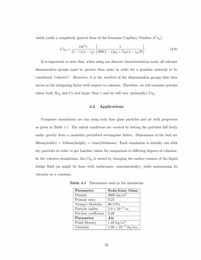
which yields a completely general form of the Granular Capillary Number (Cag)

Cag =12ε3γ

(1 − ε)(u − vp)

[

1

300(1 − ε)µg + 7ρg(u − vp)R

]

. (4-8)

It is important to note that, when using our discrete characterization tools, all relevant

dimensionless groups must be greater than unity in order for a granular material to be

considered “cohesive”. Moreover, it is the smallest of the dimensionless groups that then

serves as the mitigating factor with respect to cohesion. Therefore, we will examine systems

where both Bog and Co and larger than 1 and we will vary (primarily) Cag.

4.2 Applications

Computer simulations are run using soda lime glass particles and air with properties

as given in Table 4.1. The initial conditions are created by letting the particles fall freely

under gravity from a randomly perturbed rectangular lattice. Dimensions of the bed are

30mm(width) × 510mm(height) × 1mm(thickness). Each simulation is initially run with

dry particles in order to get baseline values for comparison to differing degrees of cohesion.

In the cohesive simulations, the Cag is varied by changing the surface tension of the liquid

bridge fluid (as might be done with surfactants, experimentally), while maintaining its

viscosity as a constant.

Table 4.1 Parameters used in the simulation

Parameter Soda-Lime Glass

Density 2600 kg/m3

Poisson ratio 0.25

Young’s Modulus 66 GPa

Particle radius 5.0 × 10−4 m

Friction coefficient 0.29

Parameter Air

Fluid Density 1.23 kg/m3

Viscosity 1.80 × 10−5 kg/ms

35

DRY

t=0.00s t=0.25s t=0.50s t=1.00s t=1.25s

WET

Figure 4.3 Mixing progress for Cohesive/Non-Cohesive materials.

36

4.2.1 Mixing

The mixing in gas-solid systems is often extremely rapid compared to mixing in surface-

dominated flows [38]. Powder mixing in a gas-solid flow predominantly occurs by convective

mixing. Convective mixing occurs by deliberate movement of packets of particles around the

mixture. These packets break down into smaller clumps and continue to displace relative to

each other. This proceeds while the clumps become smaller and smaller [39]. The reduction

in size of clumps with time depends on the extent of cohesion amongst the solids. In this

Section we examine changes of the mixing rate of mechanically identical particles with

changes in gas velocity as well as liquid bridge surface tension. In all cases, the system is

assumed to be completely segregated initially with the right-half of the bed consisting of

one type (color) of particle and the left-half another. Typical snapshots of a dry and wet

simulation can be seen in Figure 4.3. We measure the intensity of segregation, essentially

the standard deviation of the local concentration, where we define the local concentration

to consist of each particle’s 20 nearest neighbors. If the intensity of segregation is plotted

as a function of time, the value – initially at 0.5 for completely segregated – will decrease

as the system proceeds toward a completely mixed state. Figure 4.4 shows the evolution of

the intensity of segregation at several different gas velocities, while Figure 4.5 shows similar

results for a fixed gas velocity and varying liquid bridge surface tension. By fitting these

data to an exponential function, a mixing rate constant can be extracted.

Examining both Figure 4.4 and Figure 4.5, it is clear that higher velocities and/or lower

surface tensions result in larger (faster) mixing rates. Our definition of the Granular Capil-

lary Number (Cag), then suggests that the importance of cohesion to mixing is determined

by an interplay between the capillary force and the fluid drag. Plotting the resultant mixing

rate constants as a function of Cag, in Figure 4.6, shows that this assertion is valid. Mixing

rates are high for Cag < 1 and drop dramatically when Cag > 1.

37

0 1 2 3 4Time(s)

10-1

1

Inte

nstit

y of

Seg

rega

tion

u(m/s) Cag1.3 1.641.4 1.441.5 1.29

Figure 4.4 Mixing Rates at different gas velocities.

38

0 1 2 3 4Time(s)

10-1

1

Inte

nstit

y of

Seg

rega

tion

γ CagDry 0.001.0e-3 0.187.0e-3 1.291.0e-2 1.83

Figure 4.5 Mixing Rates at different surface tensions.

39

10-2 10-1 1 101

Cag

0

0.04

0.08

0.12

0.16

0.2

Mix

ing

Rat

e

Dry at umf

Figure 4.6 Mixing Rate versus Granular Capillary Number

40

4.2.2 Fluidization

Perhaps a more practical test of the utility of the Granular Capillary Number is for

quantifying the onset of fluidization in gas-solid systems. The minimum fluidization velocity

(umf ) is typically defined as the velocity at which the bed pressure drop goes through a

maximum value. A critical component of this definition is that, while the pressure drop

is ultimately determined solely by the weight of the fluidized particles, the value of the

pressure drop can exceed this limit prior/after to fluidization. In the small fluidization

systems examined here a simpler, but equivalent, definition of the minimum fluidization

velocity is used. The approach used for determining the minimum fluidization velocity is

similar in spirit to that followed by Kafui et al. [40] which is based on monitoring the state

of the particle connectivity network. Figure 4.7 shows a plot of pressure drop versus time

for different gas-velocities with a traditional time-averaged pressure drop (∆P ) versus umf .

For u < umf , the pressure drop essentially remains constant, and for u ≥ umf , the pressure

drop varies with time. The amplitude and standard deviation of the pressure disturbance

also increase with an increase in the fluidization velocity. Hence, the minimum fluidization

velocity can be defined as the velocity at which the magnitude of fluctuations (standard

deviation) of the pressure drop goes through a step change (see Figure 4.8). This technique

provides for more reproducible results and avoids difficulties in averaging for small systems.

We find that, with an increase in the Cag (surface tension), the velocity necessary to

achieve a fluidized system increases from that of the completely dry (non-cohesive) case.

Figure 4.9 shows a plot of the percentage increase in the minimum fluidization velocity as

a function of the Cag. For values of surface tension where the Cag < 1, changes in the

fluidization velocity from that of a completely dry granular material are essentially unmea-

surable; however, for larger surface tensions, where the values of Cag > 1, the minimum

41

0 1 2 3 4Time(s)

600

1200

1800

2400

3000

∆P(P

a)

u < umfu = umfu > umf

1 1.5u (m/s)

1450

1500∆P

(Pa)

Figure 4.7 Pressure Drop versus Time for different gas velocities. Inset graph shows thevariation of pressure drop with velocity.

42

0 1 2u (m/s)

0

1000

2000

σ

Dry

Wet

Figure 4.8 Standard Deviation of the Pressure Drop versus Gas-Velocity for dry and wetsystems.

43

10-2 10-1 1 101 102

Cag

0

5

10

15

20

25

30

%ch

ange

in u

mf

Figure 4.9 %change in minimum fluidization velocity versus Granular Capillary Number

44

fluidization velocity increase markedly requiring as much as a 30% increase in umf at the

highest Cag examined.

45

5.0 OUTLOOK

Cohesive gas-solid flows are one of the least understood and at the same time, one of the

most important areas in particle technology. Characterization tools are extremely useful for

studying the practical applications of these flows as approximate behavior can be predicted

based on the simple knowledge of equipment, gas and particle parameters with no need for

costly eqxperimentation.

In this work we examined the transition from non-cohesive to cohesive behavior in gas-

solid systems. We show that, while Bog > 1 is a necessary condition for cohesive behavior,

it is not a sufficient condition. In fact, a newly suggested dimensionless group, the Granular

Capillary Number (Cag), must also be larger than unity. By looking at systems traditionally

thought to be cohesive (Bog > 1), we see a marked change in behavior as the Cag changes

from non-cohesive (Cag < 1) to cohesive (Cag > 1) both in mixing rates and in fluidization

behavior. This simple characterization tool may serve as a useful a priori test of the

fluidization character to be expected in a wet gas-solid system; however, at present no

allowance is made for particles with different properties, changes in liquid bridge volume,

or wall effects.

As presented in this work, cohesion is induced in these beds through liquid bridges. The

next step of this research should involve examining other inter particle forces, van der Waals

and electrostatic forces. An extensive computational analysis of practical applications,

in particular pneumatic conveying needs to be done; although proper choice of periodic

boundary conditions in these simulations is unclear. Further, polydispersity in size, shape

and properties should be explored as well. Finally, incorporation of TPD (Thermal Particle

Dynamics) with a Discrete Particle simulation may allow the analysis of more industrially

relevant problems where evaporation of moisture may take place.

46

BIBLIOGRAPHY

BIBLIOGRAPHY

[1] C.Y. Wen and L.H. Chen. Flow modeling concepts of fluidized beds. In N.P. Cheremisi-noff and R. Gupta, editors, The Handbook of Fluids in Motion, pages 665–714. 1983.

[2] M.J. Rhodes, X.S. Wang, M. Nguyen, P. Stewart, and K. Liffman. Onset of cohesivebehavior in gas fluidized beds: a numerical study using dem simulation. Chem. Eng.

Sci., 56:4433–4438, 2001.

[3] L.J. McLaughlin and M.J. Rhodes. Prediction of fluidized bed behavior in the presenceof liquid bridges. Powder Technology, 114:213–223, 2001.

[4] S.T. Nase, W.L. Vargas, A.A. Abatan, and J.J. McCarthy. Discrete characterizationtools for cohesive granular material. Powder Technology, 116:214–223, 2001.

[5] B. J. Ennis, J. Green, and R. Davies. The legacy of neglect. Chem. Eng. Prog.,April:32–43, 1994.

[6] T. M. Knowlton, J.W. Carson, G.E. Klinzing, and W.C. Yang. The importance ofstorage, transfer, and collection. Chem. Eng. Prog., April:44–54, 1994.

[7] D. Geldart. Types of gas fluidization. Powder Technology, 7:285–292, 1973.

[8] J.L.R. Orband and D. Geldart. Direct measurement of powder cohesion using a tor-sional device. Powder Technology, 92:25–33, 1997.

[9] G. Lian, C. Thornton, and M.J. Adams. Discrete particle simulation of agglomerateimpact coalescence. Chem. Eng. Sci., 53:3381–3391, 1998.

[10] T. Mikami, H. Kamiya, and M. Horio. Numerical simulation of cohesive powder in afluidized bed. Chem. Eng. Sci., 53:1927–1940, 1998.

[11] J.F. Davidson. Symposium on fluidization–discussion. Trans. Inst. Chem. Engng.,39:1961, 223–240.

[12] T.B. Anderson and R. Jackson. A fluid mechanical description of fluidized beds. Ind.

Eng. Chem. Fundam., 6:527–539, 1967.

[13] J.W. Pritchett, T.R. Blake, and S.K. Garg. A numerical model of gas fluidized beds.AIChE Symp. Ser. No. 176, 74:134–148, 1978.

[14] Y. Tsuji, T. Kawaguchi, and T. Tanaka. Discrete particle simulation of two-dimensionalfluidized bed. Powder Technology, 77:79–87, 1993.

[15] J. Ding and D. Gidaspow. A bubbling fluidization model using kinetic theory of gran-ular flow. AIChEJ, 36:523–528, 1990.

[16] M. Syamlal, W. Rogers, and T.J. O’Brien. MFIX documentation, Theory Guide, U.S.Dept. of Energy, Office of Fossil Energy, Tech. Note. 1993.

48

[17] C.K.K. Lun, S.B. Savage, D.J. Jefferey, and N. Chepurniy. Kinetic theories for granularflow: inelastic particles in couette flow and slightly inelastic particles in a generalflowfield. J. Fluid Mech., 140:223, 1984.

[18] P.A. Cundall and O.D.L. Strack. A discrete numerical model for granular assemblies.Geotechnique, 29:47–65, 1979.

[19] B.H. Xu and A.B. Yu. Numerical simulation of the gas-solid flow in a fluidized bed bycombining discrete particle method with computational fluid dynamics. Chem. Eng.

Sci., 52:2785–2809, 1997.

[20] C. Thornton and C. W. Randall. Applications of theoretical contact mechanics to solidparticle system simulation. In M. Satake and J. T. Jenkins, editors, Micromechanics

of Granular Material, pages 133–142. Elsevier Science Publishers, Amsterdam, 1988.

[21] J. Schafer, S. Dippel, and E. Wolf. Force schemes in simulations of granular materials.J. Phys. I, 67:1751–1776, 1991.

[22] H. Hertz. Ueber die berhrungfester elastischer korper. J. renie ange. Math., 92:1–15,1881.

[23] R.D. Mindlin. Compliance of elastic bodies in contact. J. Appl. Mech., 16:256–270,1949.

[24] R.A. Fisher. On the capillary forces in an ideal soil. J. Agric. Sci., 16:491–505, 1926.

[25] B.J. Ennis, J. Li, G.I. Tardos, and R. Pfeffer. The influence of viscosity on the strengthof an axially strained pendular liquid bridge. Chem. Eng. Sci., 45:3071–3088, 1990.

[26] M.J. Adams and V. Perchard. The cohesive forces between particles with interstitialfluid. Inst. Chem. Eng. Symp., 91:147–160, 1985.

[27] A.J. Goldman, R.G. Cox, and H. Brenner. Slow viscous motion of a sphere parallel toa plan wall i. motion through a quiescent fluid. Chem. Eng. Sci., 22:637–651, 1967.

[28] L. S. Fan and C. Zhu. Principles of Gas-Solid Flows. Cambridge University Press,New York, 1998.

[29] B.P.B. Hoomans, J.A.M. Kuipers, and W.P.M. van Swaaij. Granular dynamics sim-ulation of segregation phenomena in bubbling gas-fluidized beds. Powder Technology,109:41–48, 2000.

[30] J.A.M. Kuipers, K.J. van Duin, F.P.H. van Beckum, and W.P.M. van Swaaij. Anumerical model for gas-fluidized beds. Chem. Eng. Sci., 47:1913, 1992.

[31] C.Y. Wen and H.Y. Yu. Mechanics of fluidization. Chem. Engng. Prog. Symp. Ser.,62:100, 1966.

[32] J.F. Richardson and W.N. Zaki. Sedimentation and fluidization: part 1. Trans. Inst.

Chem. Engng., 32:35, 1954.

49

[33] H.K. Versteeg and W. Malalasekera. An introduction to Computational Fluid Dynam-

ics: The Finite Volume Method. John Wiley & Sons Inc., New York, 1995.

[34] S.V. Patankar. Numerical Heat and Transfer and Fluid Flow. Hemisphere, New York,1980.

[35] A. Munjiza and K.R.F. Andrews. NBS contact detection algorithm for bodies of similarsize. Int. J. Numer. Meth. Engng., 43:131–149, 1998.

[36] B. J. Ennis, G. I. Tardos, and R. Pfeffer. A microlevel-based characterization of gran-ulation phenomena. Powder Technol., 65:257–272, 1991.

[37] R.A. Bagnold. Experiments on a gravity-free dispersion of large solid spheres in anewtonian fluid under shear. Proc. R. Soc., 225:4–63, 1954.

[38] J. J. McCarthy, D. V. Khakhar, and J. M. Ottino. Computational studies of granularmixing. Pow. Technol., 109:72–82, 2000.

[39] M. Poux, P. Fayolle, J. Betrand, D. Bridoux, and J. Bousquet. Powder mixing: Somepractical rules applied to agitated systems. Powder Technol., 68:213–234, 1991.

[40] K.D. Kafui, C. Thornton, and M.J. Adams. Discrete particle-continuum fluid modelingof gas-solid fluidized beds. Chem. Eng. Sci., 57:2395–2410, 2002.

50