Magnetization Control of Magnetic Liquids for Sink-Float ...
Upload
khangminh22Category
view
4download
0
Dirty float or clean intervention? The Bank of England in the
foreign exchange market
Alain Naef1
Abstract
The effectiveness of central bank intervention is debated and despite literature showing mixed results, central banks regularly intervene in the foreign exchange market, both in developing and developed economies. Does foreign exchange intervention work? Using over 60,000 new daily observations on intervention and exchange rates, this paper is the first study of the Bank of England’s foreign exchange intervention between 1952 and 1972. The main finding is that the Bank of England was unsuccessful in managing a credible exchange rate over that period. Running an event study, I demonstrate that betting systematically against the Bank of England would have been a profitable trading strategy. Pressures increased in the 1960s and the Bank eventually manipulated the publication of its reserve figures to avoid a run on sterling.
Keywords: intervention, foreign exchange, central bank, Bank of England, Bretton Woods JEL classification: F31, E5, N14, N24
1 This research was supported by the Economic and Social Research Council (grant number ESRC KFW/10324121/0) and the Swiss National Science Foundation (grant number P2SKP1_181320). For discussions and comments, I am grateful to William Allen, Mike Bordo, Chris Briggs, Jason Cen, David Chambers, Devika Dutt, Max Harris, Susan Howson, Ryuichiro Izumi, Walter Jansson, Chris Meissner, Éric Monnet, Duncan Needham, the participants at the Economic History Seminar in Oxford, the University of Neuchatel, the INET YSI plenary in Budapest, Eastern Economic Association Annual conference in New York, Rutgers University, the Economic History Society annual conference in Keele, NYU Shanghai, Lund University, UC Berkeley, and the Financial History workshop in Cambridge.

Dirty float or clean intervention?
2
1. Introduction
Understanding central bank foreign exchange intervention is essential today when over 80
percent of countries are in a fixed exchange rate system and many intervene to defend their
currency (Taylor 2010, 370). Intervention is defined as monetary authorities buying or selling
foreign currencies to influence the exchange rate. Our understanding of central bank intervention
is limited by the lack of data, as central banks keep their intervention records secret. Here, I
unveil hand-collected intervention data on over 6,000 trading days to understand central bank
foreign exchange intervention.
I test the effectiveness of British intervention on the foreign exchange market during the
Bretton Woods period. There is debate in the literature on the effectiveness of sterilized
intervention, or intervention followed by open market operations to offset the effect on monetary
conditions (see for example Bordo, Humpage, and Schwartz 2015; Fratzscher et al. 2018). A
previous consensus, challenged by recent findings, was that sterilized intervention does not work.
Despite that, central banks are using sterilized intervention on the currency market, especially
in developing economies. I ask whether sterilized intervention actually works and what lessons
we can draw from the Bank of England’s intervention during the Bretton Woods period.
I find that while the Bank of England (the Bank) managed to keep the exchange rate
within the Bretton Woods official bands, sterilized intervention cannot be described as successful.
Before 1958, offshore and forward foreign exchange data indicate that the official exchange rate
was not credible. In the 1960s, sterling entered a period of crisis, leading the Bank to
progressively manipulate its official reserve data. Over the whole period, by measuring daily
intervention successes, I demonstrate that betting systematically against the Bank of England

Dirty float or clean intervention?
3
would have been a profitable trading strategy. This shows that the Bank did not have any
significant informational advantage on other market participants.
At the end of the 20th century, central bank intervention waned as most central banks
in developed economies decided to pursue inflation targeting and let their exchange rate float
freely. This changed in recent years as intervention became more frequent in many developing
countries as well as developed economies such as Switzerland or Japan. Central bank intervention
can either be sterilized (the monetary base is unaffected) or unsterilized (affecting the monetary
base). Unsterilized intervention mainly affects the exchange rate through changes in interest
rates, making the currency more or less attractive to investors. The effectiveness of sterilized
intervention, on the other hand, has long been questioned and the debate is still ongoing.
The consensus in the 1990s was that sterilized central bank intervention was ineffective
(Dominguez and Frankel 1993). Recent research is more nuanced. In a cross-country study
analyzing 35 countries, Blanchard, Adler, and Filho (2015) demonstrate that sterilized
intervention can hinder unwanted currency appreciation due to capital inflows. Fratzscher et al.
(2019) are more positive about the policy and argue that intervention is effective in over 80% of
cases according to one of their criteria. Empirical evidence on the effectiveness of sterilized
intervention is inconsistent. According to Bordo, Humpage, and Schwartz (2015, 13) the findings
of empirical studies are “not robust across currencies, time periods, and empirical techniques.
Intervention often seems more like a hit-or-miss proposition than a sure thing”.
Economic historians have investigated the effect of foreign exchange intervention. Jobst
(2009) has shown how foreign exchange intervention was a feature of the gold standard which
helped smooth the system beyond the rules of the game. In a similar vein, Blancheton and
Dirty float or clean intervention?
4
Maveyraud (2009) analyze how the 1920s in France were not a period of free float but implied
foreign exchange operations of the Banque de France. Naef (2019) offers an overview of British
central bank intervention and shows how intraday news about the currency can influence testing
of exchange rate success.
Surveying central bankers, Mohanty and Berger (2013) find that only 18% of the central
banks studied frequently communicated on their intervention practice. That means that most
central bank intervene in secret, against findings in the literature arguing that communicating
intervention is more effective (Burkhard and Fischer 2009). The sample presented here
exclusively uses secret central bank intervention, as it seems to be the preferred mode of
intervention today. The data can shed light on how sterilized central bank intervention works.
The issue with most current studies on central bank intervention is that they use data
from central banks that publicly share their intervention data (for example Turkey or Colombia
who frequently publish their intervention record). What is missing is a study on intervention
data that central bankers refuse to share. Although contemporary data is unavailable, historical
data is accessible. This paper offers a unique source of central bank intervention data by looking
at intervention from a major central bank, the Bank of England. My findings have implication
for our understanding of secret central bank intervention which is the way most central banks
still intervene today (Mihaljek 2005).
Sarno and Taylor (2001, 851–52) emphasize that many studies use reconstructed data
from newspapers that lack information on secret operations, especially smaller ones. Harry
Siepmann, former head of the Exchange Equalisation Account (EEA), the British intervention
account, already understood this issue in 1938 when he reported on the accuracy of the financial

Dirty float or clean intervention?
5
press: “It is sometimes surprising to find how wide off the mark are the Press reports of the
E.E.A. activity, as when on the 6th April we bought nearly Fcs. 200 million but were reported
by the ‘Financial News’ the next morning as having ‘retired from the Market soon after the
opening’.”2 Fratzscher et al. (2019, 133) stress the importance of data and emphasize that “the
bottleneck of research on foreign exchange intervention is data availability”.
2. Historical background – the Bretton Woods system and Bank of England operations
The Bretton Woods system of pegged exchange rates was in place from 1944 to 1971. All
currencies within the system were pegged to the dollar with a band of 2%.3 The dollar was fixed
to gold at $35 an ounce. Currencies experienced large fluctuations within the official exchange
rate bands and the IMF charged national governments with the management of their currencies.
In the UK, the Government managed exchange with the help of the Treasury who delegated
operations to the Bank of England. Sterling was fixed at $2.80 between 1949 and 1967, and at
$2.40 between 1967 and the collapse of the system in 1971. The Bretton Woods period was also
marked by cooperation amongst central banks (Toniolo and Clement 2007) and the Bank of
England outsourced some of its intervention operations to the New York Federal Reserve and
other central banks.
The main interest in analyzing the case of the UK lies in the fact that the period
corresponds to the decline of sterling as an international reserve currency. Sterling was the
2 London, Archive of the Bank of England, Papers of Sir Henry Clay: Harry Arthur Siepmann – Memoranda, ADM22/21, 26 October 1938. 3 Currencies also had a gold parity.

Dirty float or clean intervention?
6
dominant currency until the dollar overtook it as the leading reserve currency in the mid-1920s.
The two currencies then kept fighting for leadership during the interwar period (Eichengreen
and Flandreau 2009). During most of the Bretton Woods period, sterling played a secondary
role as a reserve currency (Eichengreen, Mehl, and Chitu 2017). Despite its secondary role,
sterling impacted the stability of the international monetary system and sterling crises (especially
the 1967 devaluation) contributed to the fall of the Gold Pool, an international syndicate put in
place to support the official dollar price of gold (Bordo, Monnet, and Naef 2019). This gold crisis
led to the introduction of a two-tier gold market, prefiguring the end of the Bretton Woods
system and opening the era of floating exchange rates.
The Bretton Woods period was characterized by capital controls which were
progressively removed over the period analyzed in this paper. In the UK, wartime exchange
control remained in place well into the 1950s. Schenk argues that during the 1950s, the pound
was “gradually and without great fanfare made convertible on the current account for those
resident outside the United Kingdom or other sterling area countries” (Schenk 2010, 102). On
Saturday, 27 December 1958 the UK Treasury announced convertibility:
‘From 9 a. m. on Monday, December 29th, sterling held or acquired by non-residents of
the sterling area will be freely transferable throughout the world. As a consequence, all
non-resident sterling will be convertible into dollars at the official rate of exchange.’4
Non-residents of the sterling area were now allowed to convert sterling into dollars in
London. Sterling area residents were still not allowed to convert their sterling abroad without a
valid reason (for example, for import/export or for travel). Convertibility meant that businesses
4 As explained in Chapter I, section 2, sterling was divided into different types and resident sterling was the currency held by residents of the sterling area. See ‘Exchange Control Retained’, Manchester Guardian, 29 December 1958, 5.

Dirty float or clean intervention?
7
and individuals were no longer limited to the amount of foreign exchange they could access to
buy imports. Convertibility made the mission of the Bank of England on the foreign exchange
market more difficult. This is visible on Figure 1 further down where the amplitude of
interventions increases drastically after 1959.
Capital controls during the Bretton Woods period meant that there were sterling markets
with different prices in different places. These ‘unofficial’ markets in sterling were located in New
York, Kuwait, Hong Kong and Switzerland among other places (see for example Schenk 1994a
for data on the Hong Kong market).
Transferable sterling was a special kind of sterling allowed to be transferred among
different countries but not in and out of the sterling area.5 For example, transferable sterling
could be wired from the Netherlands to Sweden but not to the UK.6 The Bank of England also
intervened in the transferable sterling market. Interventions in transferable sterling mainly
started in 1955 with the goal of making the market more integrated. Most of the interventions
in transferable sterling occurred in 1957-58 and in the whole sample there were 172 days out of
the 6099 days analyzed (2.8% of the days). The Bank of England purchased 139 million dollars
on the transferable sterling market or 0.49% of the total intervention aggregate amount of -
28,208 million dollars. 7
5 The sterling area was a group of countries pegging their currencies to the pound including Australia, Sudan, Malaysia, Ireland and 70 other countries. For more about transferable sterling and the sterling area, see Allen (2014, 64–89) and Schenk (2010). 6 For more detail on the list of the 20 transferable countries, see (Schenk 1994b, 9). Another type of sterling which is not discussed here is security sterling. This type of sterling was from the proceed of overseas security sales and it could mainly be reinvested in other securities (Schenk 2010, 101). 7 See Klug and Smith (1999) for more detail on transferable sterling operations. And see Strange (1971)for more on the functioning of transferable sterling.

Dirty float or clean intervention?
8
3.1 Sterilization of interventions
Unsterilized intervention is known to work by affecting monetary policy. The question of this
paper is to understand whether sterilized intervention has an impact on the exchange rate. The
Bank of England operation were automatically sterilized as they were all done through the EEA
(Exchange Equalisation Account), which was independent from the Bank of England and
belonged to the Treasury. Howson (1980b; 1980a; 1993) has studied Bank of England operations
in detail and gives a great overview of the sterilization process and how it was a built-in feature
of the EEA. The EEA was endowed with Treasury bills as starting capital. All operations had
a counterparty in Treasury bills. If the EEA was selling dollars against pounds, this would reduce
the amount of pounds in circulation. But once the EEA had these pounds on its account, it
would re-invest them into Treasuries and doing so the number of pounds in circulation remained
unchanged. Reversely, when the Bank wanted to buy US dollars, it first had to sell Treasuries
to obtain sterling to purchase dollars. This meant that any operation was automatically sterilized
as a feature of the EEA.
Allen (2019) argues that operations were even “super-sterilized”, as from time to time
the Bank would want to reduce the amount of Treasury bills in circulation and would offer the
Treasury to exchange them against longer term gilts. This means that the sterilization not only
changed the supply of short term Treasuries (which are closer to money because easy to sell and
buy) but also longer term bonds.
3.2 The strategy of the Bank of England
What was the strategy of the Bank of England on the market? There is no clear handbook of
operations and anecdotical evidence and oral testimony point that it was not a set process. In
Dirty float or clean intervention?
9
November 1965, after sterling came under stress, the Bank governor appointed Lord Kahn, a
Cambridge economist, to assess the underlying reasons for the pressure on sterling (Capie 2010,
219). The Kahn report that resulted from the investigation reads:
“If sterling is just coming under pressure the wise course is to allow the rate to fall
smartly and fully and then bring it up somewhat a little later. This punishes the bears
and discourages them later, refutes bearish predictions in the financial press and induces
others to take a bullish position on another occasion.”8
The goal was either to prevent the exchange rate from depreciating too quickly or to
encourage or amplify an appreciation. The Bank of England sold dollars when sterling was under
downward pressure, and when the market was stabilized, the Bank took advantage of that
stability to replenish the reserves by buying back the dollars gradually. While operations to
weaken sterling occurred on occasion, they were not the norm. Most dollar purchases during the
Bretton Woods period were done to replenish reserves, not to avoid an appreciation of the pound.
M. Gouzerh from the Banque de France visited the room of Bank of England foreign
exchange dealers and in a letter to his hierarchy reported what he saw. This testimony is
interesting as it offers an external perspective. He noted that orders were placed over the phone
and that they were done either to avoid the exchange rate from depreciating or to encourage an
appreciation.9 There is no mention of any movements meant to avoid an appreciation of the
exchange rate, only mentions of operations meant to avoid depreciation.
8 Archives of the Bank of England, reference EID1-6, Kahn Report, Chapter V, p. 124. 9 The French reads: “Les ordres sont passés par téléphone sur décision de M. Preston soit pour empêcher les cours de baisser trop vite, soit pour essayer d’encourager ou d’amplifier un mouvement de reprise” Archives of the Bank of France, reference 1495200501/564, ‘Extract of a letter from M. Gouzerh staying at the Bank of England to M. Floch’, 19 May 1951.
Dirty float or clean intervention?
10
Another document shows how the Bank viewed its role in the market. Before the October
1959 general election, the Bank prepared a foreign exchange intervention plan. At the time the
exchange rate was fixed between 2.78 and 2.82 sterling per dollar. It reads:
‘So long as the outcome of the election remains unclear, confusion in the exchange
market must be expected, some operations one way, some another. In that event we
will endeavour to maintain relative stability in the sterling/dollar rate until the results
become more apparent, aiming provisionally at something like 2.79¾–2.80¾, i.e., a wider
fluctuation than one normally sees during the day.’10
After the election, the Bank had two scenarios in mind. In the event of downward
pressure, the Bank would
“not offer much resistance but let the rate fall quite quickly to say, 2.78 1/16, testing
the market periodically on the way down. There would be no point in spending much
on the way down, which would be expensive and encourage speculation against the
pound. Later, when election influences had subsided, we would examine the possibility
of bringing about an improvement in the rate.” 11
In the event of upward pressure, the Bank would “let the rate go over 2.81 fairly easily;
then we would begin to take in dollars on a rising market. If the demand proved to be large we
would let the rate go to the upper limit.”12
The wording in this internal memo also shows how the event of an upward pressure was
less a problem for the Bank and would only lead to “taking in dollars”, not restraining
10 Contingency plan, the exchanges – Friday, 9th October, 8 October 1959, London, Archive of the Bank of England, C43/32. 11 Contingency plan, the exchanges – Friday, 9th October, 8 October 1959, London, Archive of the Bank of England, C43/32.. 12 Ibid.
Dirty float or clean intervention?
11
intervention per se. Even if there might have been occasional restraining interventions, this paper
focuses only on defending interventions meant to avoid the exchange rate from falling.
3. New confidential data
I present a wealth of hand-collected data here for the first time. Unlike other studies on central
bank intervention, which are bound to data confidentiality, I collected data that are available
for replication or further study. This article uses three types of data: intervention data from the
Bank of England’s dealers’ reports, new offshore and official exchange rate data, and British
reserve data.
Intervention data come from the Bank of England dealers’ reports which offer daily records on
all activities on the gold and foreign exchange market.13 The reports start in 1952 and describe
the Bank’s foreign exchange operations, separated into market operations and customer
operations. Customer operations were made on behalf of other central banks or the UK
government. In these cases, the Bank of England acted as agent. This article considers market
operations only, since they were designed to influence the exchange rate and can therefore be
considered as intervention.14 The data are plotted in Figure 1. Bordo, MacDonald, and Oliver
(2009; 2012) use similar data on the Bank of England from 1964 to 1967, however they do not
present actual intervention data but changes in reserves.
13 Bank of England Archives, Cashier's Department: Foreign Exchange and Gold Markets – Dealers’ Reports, C8. 14 This is in line with current literature, for example Fratzscher et al. (2019).

Dirty float or clean intervention?
12
-400
-300
-200
-100
0
100
200
300
400
1952 1954 1956 1958 1960 1962 1964 1966 1968 1970
Bank of England intervention (in million dollars)
Figure 1 – Bank of England intervention data in US dollar. Source: Bank of England Archives, Dealers’ reports, reference C8. Note: the scale is truncated at +/- 400 million dollars to better present the data.
In the reports, the data is split into different kinds of intervention: spot, forward and
overnight. Overnight operations were managed by the New York Fed on behalf of the Bank of
England once the London market closed. For the purpose of this article, all these data are
aggregated into one intervention variable.
This research relies on new exchange rate data. As exchange rates were fixed under the
Bretton Woods system, the London spot market offers little information on the credibility of the
peg as the exchange rate fluctuates between relatively narrow bands. I use four exchange rate
data series, two from existing datasets and two new hand-collected exchange rate data series.
The existing data is composed of spot exchange rates from Global Financial Data (GFD) as well
as forward exchange rates from the Financial Times collected by Accominotti et al. (2019). The
two new hand-collected series are offshore exchange rates for banknotes in Switzerland and
+ = dollar purchases
- = dollar sales

Dirty float or clean intervention?
13
transferable sterling exchange rates from 1952 to 1958, when transferable sterling was abolished.15
Swiss banknote exchange rates are important, as estimates by the Bank of England in 1954
establish that the biggest offshore market for sterling was in Zurich, which traded even larger
volumes than New York.16 The banknote exchange rates available at the Swiss National Bank
do not offer direct sterling/dollar exchange rate and therefore I use crossrates.17 The banknote
rates were the rates at which tourists and retail customers could exchange currency at a bank
counter.18 The Swiss National Bank has recorded those daily in manuscript form. The institution
collected them from commercial banks such as Credit Suisse. The second source of new exchange
rates are the data for transferable sterling, collected by the Bank of England and recorded in the
dealers’ reports.19 Transferable sterling was a special kind of sterling allowed to be transferred
among different countries but not in and out of the sterling area as described in the previous
section.
Finally, this paper presents exclusive daily reserve data. The EEA, the reserve account
of the UK, was established in 1932 to check ‘undue fluctuations in the exchange value of
sterling’.20 The operations of the account were kept secret, allowing the Bank of England to
defend sterling without informing the market of the true state of gold and dollar reserves. As
15 Note that transferable sterling rates had already been presented at monthly frequency in Schenk (2010, 101), here the data is presented at a daily frequency allowing a more granular analysis. 16 Bank of England archive, Exchange control transferable sterling, reference C43/132. Large US firms often ran foreign exchange operations through European banks which were the correspondents of US banks. This explains in part the large size of the market in Switzerland. Other offshore markets include Kuwait and Hong Kong. 17 Obtained by dividing the CHF/USD rate by the CHF/GBP rate. 18 This market was certainly also used by speculators and people illegally exporting currency from the sterling area, therefore it can be identified as a black market, as it allows sterling area resident to illegally purchase dollars with sterling for example. These transactions were not illegal per se, but exporting large amounts of sterling was. 19 Bank of England Archives, Cashier's Department: Foreign Exchange and Gold Markets – Dealers’ Reports, C8. 20 Finance Act, 1932.

Dirty float or clean intervention?
14
the Bank was executing orders on behalf of the Treasury, it kept ledgers on all EEA activity.21
The daily data span from October 1939 to March 1971.
4. How did the Bank of England manage exchange rates?
I use four empirical methods to assess the operations of the Bank of England in the
foreign exchange market. First, I analyze alternative exchange rates to assess the credibility of
the monetary authorities. Second, I run a reaction function to better understand the intervention
goal of the Bank of England. Then, running an event study, I assess the success of interventions.
Finally, I present narrative evidence exposing how the Bank of England manipulated its
accounts.
4.1 How credible was the pound?
I start with a rudimentary test of currency credibility by presenting alternative exchange
rates. Just as investors today look at the offshore renminbi to understand the credibility of the
Chinese currency, investors during the Bretton Woods period were looking at offshore and
alternative exchange rates to analyze the strength of sterling. This measure is imperfect as it
does not account for other factors such as lower liquidity in alternative markets due to smaller
size as well as higher transaction cost. Svensson (1991) showed that exchange rate credibility
can be tested by whether expected future exchange rates fall within the exchange rate band. His
model assumes uncovered interest parity which is a strong assumption to make. Despite these
21 Bank of England archives, Ledgers of the Exchange Equalisation Account, 2A141/1-17.

Dirty float or clean intervention?
15
limitations, looking if forward rates lie within exchange bands provides some information on the
credibility of the currency.
Similar tests of credibility have been used in the literature. Klug and Smith (1999) study
the Suez crisis in 1956 and test whether forward rates stayed within the Bretton Woods bands
to ascertain the level of pressure on the Bank of England. Bordo, MacDonald, and Oliver (2009)
use similar measures to assess sterling credibility between 1964 and 1967. Here I use a wide range
of different exchange rates to assess the credibility of the official exchange rate.
As an illustration, Figure 2 plots the one- and three-month forward exchange rates from
the Financial Times. The period starts after the market opening in December 1951. While the
Bank of England was active on the spot market, forward interventions were timid. Additionally,
a report by the Bank for International Settlements noted that at the reopening of the London
foreign exchange market in 1951, forward rates were given “full freedom of movement” and were
not constrained to upper and lower bands.22 As the forward was free to move, it makes it a good
indicator of the credibility of the British currency. The chart shows that in December 1951 with
the opening of the foreign exchange market, credibility was questioned, as the forward rates
breaching the Bretton Woods official bands show.
It is important to note that forward rates are not a perfect indicator of a currency’s
credibility. Forward rates also encompass a foreign exchange risk premia compensation, which
tends to be sizeable across exchange rates and over time. This risk premia exists for currencies
that do not have overvalued official exchange rates as well. What is striking here is that forward
rates systematically show a discount and break the lower bands around the times of known crises
22 Bank for International Settlements, Annual Report 1952, 136.

Dirty float or clean intervention?
16
(for example in late 1964 with the British election, when Labour won, which lead to pressure on
the exchange rate). This helps establish the value of this exchange rate as a measure of
credibility.
Figure 2 – Financial Times spot and forward exchange rate data. Source: Accominotti et al. (2019). Note that the bands were not exactly 1% on each side but set at 2.82 and 2.78.
I also present new data on offshore markets and transferable sterling. As explained above,
transferable sterling was a special kind of sterling allowed to be transferred among different
countries but not in and out of the sterling area. Because of capital controls, these alternative
exchange rates had different supply and demand to London, offering additional information on
the stability of the currency.23 Table 1 highlights all breaches of official exchange rate bands by
the different rates used to assess the credibility of the Bank of England. Again, it is important
23 Note that a range of Transferable sterling markets and rates across the world were unified in 1954 and from 1955 the Bank of England intervened to keep this unified transferable sterling rate close the official rate. Therefore, transferrable sterling was not completely independent from the main sterling rate from 1955 to 1958. But as interventions were not constant during the period, the rate still offers some information on sterling credibility.
2.742.752.762.772.782.792.8
2.812.822.83
1951 1952 1953 1954 1955 1956 1957 1958 1959 1960 1961 1962 1963 1964 1965 1966 1967
Daily 1 and 3 months forward exchange rate, 1951-1967
London 1 month forward London 3 month forward
Lower band Upper band
Dirty float or clean intervention?
17
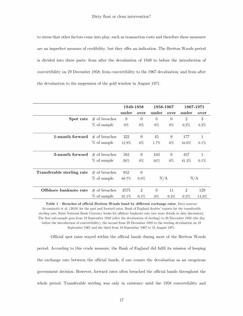
to stress that other factors come into play, such as transaction costs and therefore these measures
are an imperfect measure of credibility, but they offer an indication. The Bretton Woods period
is divided into three parts: from after the devaluation of 1949 to before the introduction of
convertibility on 29 December 1958; from convertibility to the 1967 devaluation; and from after
the devaluation to the suspension of the gold window in August 1971.
1949-1958 1958-1967 1967-1971 under over under over under over
Spot rate # of breaches 0 0 0 0 2 3 % of sample 0% 0% 0% 0% 0.2% 0.3%
1-month forward # of breaches 322 0 45 0 177 1 % of sample 12.9% 0% 1.7% 0% 16.0% 0.1%
3-month forward # of breaches 582 0 443 0 457 1 % of sample 28% 0% 16% 0% 41.3% 0.1%
Transferable sterling rate # of breaches 852 0 N/A N/A % of sample 68.7% 0.0%
Offshore banknote rate # of breaches 2575 2 0 11 2 129
% of sample 91.1% 0.1% 0% 0.4% 0.2% 14.3%
Table 1 – Breaches of official Bretton Woods band by different exchange rates. Data sources: Accominotti et al. (2019) for the spot and forward rates, Bank of England dealers’ reports for the transferable
sterling rate, Swiss National Bank Currency books for offshore banknote rate (see more details in data discussion). The first sub-sample goes from 19 September 1949 (after the devaluation of sterling) to 28 December 1958 (the day
before the introduction of convertibility), the second from 29 December 1959 to the sterling devaluation on 18 September 1967 and the third from 19 September 1967 to 15 August 1971.
Official spot rates stayed within the official bands during most of the Bretton Woods
period. According to this crude measure, the Bank of England did fulfil its mission of keeping
the exchange rate between the official bands, if one counts the devaluation as an exogenous
government decision. However, forward rates often breached the official bands throughout the
whole period. Transferable sterling was only in existence until the 1958 convertibility and

Dirty float or clean intervention?
18
breached the lower band of the official exchange rate for 68.7% of the trading days. Finally, the
last row of Table 1 presents the Swiss banknote rate. This rate was outside of the control of the
Bank of England. The fact that the rate was systematically below the Bretton Wood bands until
1958 highlights that this free market perceived the pound as overvalued. Convertibility
integrated this offshore market with the official spot market and therefore shows no breach of
the official bands after 1958.
By looking at alternative exchange rates, I find that the exchange rate policy was showing
strong premiums until 1958 as demonstrated with the forward, transferable and offshore rates
breaching the Bretton Woods bands. From 1958 onward, with the introduction of convertibility
, the offshore markets integrated with the London market and removing the premium from
offshore rates.
4.2 Why was the Bank of England intervening?
In order to understand how central banks respond to exchange rate fluctuations, the
literature has estimated reaction functions.24 Klug and Smith (1999) determine a reaction
function of the monetary authorities and find that the Bank of England intervened in reaction
to variations in the transferable sterling exchange rate during the Suez crisis. This reveals that
the Bank was not only worried about exchange rates in London but also abroad. Bordo,
MacDonald, and Oliver (2009) use a reaction function to study foreign exchange market
intervention for the UK during the sterling crises from 1964 to 1967. They demonstrate that the
Bank not only reacted to the lower band of the exchange rate but also within the bands of
24 For a review of the literature on reaction functions, see Edison (1993, 18:37–42); Neely (2005, 2–3); Ito and Yabu (2007).

Dirty float or clean intervention?
19
Bretton Woods. Here I use the reaction function to determine which specific exchange rate was
influencing the monetary authorities’ policies before the introduction of convertibility in 1958.
As highlighted in the previous section, there were several exchange rates and it is unclear which
one the Bank was using to guide its intervention account.
The reaction function relates several exchange rates to Bank of England intervention.
Four different rates have been collected at daily frequency as presented in the section above:
London spot exchange rate, 3-month London forward rate, Transferable sterling rate (a specific
rate only used between 20 specific countries as described) and the Swiss banknote crossrate (a
rate available for banknotes in Zurich).
The goal of this reaction function is to determine which exchange rate among these four
influences the intervention decision most. But, as these exchange rates are correlated, I take the
difference of the rate with the previous day, which helps mitigate multicollinearity. After taking
the difference, I run a unit root test and the four variables and I can reject a unit root at the
1% level of confidence. However, caution is still necessary. Even when taking the rates as
difference with the previous days’ spot rate S (in the form St – St-1), the rates are still highly
correlated as shown in Table 2. To reduce issue with multicollinearity, the forward rate is taken
as the difference with the spot rate (as the forward premium).

Dirty float or clean intervention?
20
3-month London forward
rate
London spot
exchange rate
Swiss banknotes crossrate
Transferable sterling
3-month London
forward rate 1.00 0.68 0.10 0.28
London spot exchange rate
0.68 1.00 0.04 0.30
Swiss banknotes crossrate
0.10 0.04 1.00 0.06
Transferable sterling
0.28 0.30 0.06 1.00
Table 2 – Correlation matrix. Correlation matrix for the differences (St – St-1) of the four available exchange rates. This shows how correlated the difference is, especially between the London spot and the forward rate.
The model aims to understand how the London spot exchange rate, the forward
premium, the Swiss banknotes crossrate and the transferable sterling exchange rate influenced
the intervention decision by the Bank of England. It is formulated as follows:
𝐼 = 𝛽 + 𝛽 𝐼 − + 𝛽 (𝑆 − 𝑆−
) + 𝛽 (𝑆 − 𝑆 ) + 𝛽 (𝑆 − 𝑆 − ) + 𝛽 (𝑆 − 𝑆 − ) + 𝜖
where It is intervention in dollars taking positive value for purchase of dollars and
negative value for sales of dollars, 𝐼 is lagged intervention to allow for autocorrelation, 𝑆 −
𝑆 is the difference between the London spot rate on the day of the intervention and the close
the day before 𝑆 − 𝑆 is the forward premium on the day of the intervention, 𝑆 −
𝑆 is the difference between the Swiss banknote crossrate rate on the day of the intervention
Dirty float or clean intervention?
21
and the close the day before and 𝑆 − 𝑆 is the difference between the transferable
sterling rate on the day of the intervention and the close the day before.25
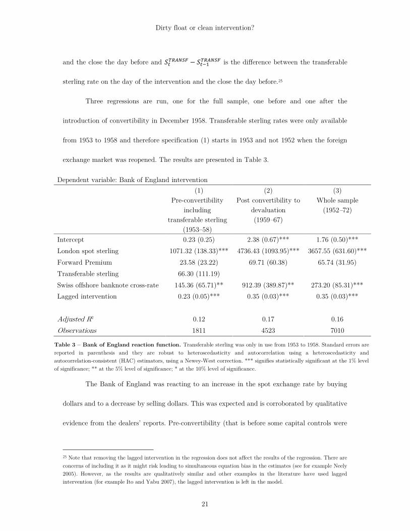
Three regressions are run, one for the full sample, one before and one after the
introduction of convertibility in December 1958. Transferable sterling rates were only available
from 1953 to 1958 and therefore specification (1) starts in 1953 and not 1952 when the foreign
exchange market was reopened. The results are presented in Table 3.
Dependent variable: Bank of England intervention
(1) Pre-convertibility
including transferable sterling
(1953–58)
(2) Post convertibility to
devaluation (1959–67)
(3) Whole sample
(1952–72)
Intercept 0.23 (0.25) 2.38 (0.67)*** 1.76 (0.50)*** London spot sterling 1071.32 (138.33)*** 4736.43 (1093.95)*** 3657.55 (631.60)*** Forward Premium 23.58 (23.22) 69.71 (60.38) 65.74 (31.95) Transferable sterling 66.30 (111.19) Swiss offshore banknote cross-rate 145.36 (65.71)** 912.39 (389.87)** 273.20 (85.31)*** Lagged intervention 0.23 (0.05)*** 0.35 (0.03)*** 0.35 (0.03)*** Adjusted R2 0.12 0.17 0.16 Observations 1811 4523 7010
Table 3 – Bank of England reaction function. Transferable sterling was only in use from 1953 to 1958. Standard errors are reported in parenthesis and they are robust to heteroscedasticity and autocorrelation using a heteroscedasticity and autocorrelation-consistent (HAC) estimators, using a Newey-West correction. *** signifies statistically significant at the 1% level of significance; ** at the 5% level of significance; * at the 10% level of significance.
The Bank of England was reacting to an increase in the spot exchange rate by buying
dollars and to a decrease by selling dollars. This was expected and is corroborated by qualitative
evidence from the dealers’ reports. Pre-convertibility (that is before some capital controls were
25 Note that removing the lagged intervention in the regression does not affect the results of the regression. There are concerns of including it as it might risk leading to simultaneous equation bias in the estimates (see for example Neely 2005). However, as the results are qualitatively similar and other examples in the literature have used lagged intervention (for example Ito and Yabu 2007), the lagged intervention is left in the model.

Dirty float or clean intervention?
22
lifted in 1959 and convertibility introduced), a decrease in the spot rate of $0.01 per sterling (for
example $2.80 to $2.79 per sterling) would have led to the Bank spending $10.71 million on any
given day, other things remaining constant (and an additional $1.45 million linked to the
banknote rate). Post-convertibility once some capital controls were lifted, the Bank would spend
$47.36 million for a similar decrease in the spot rate, almost five times as much (and an addition
$9.12 million linked to the banknote rate). This shows that with the introduction of
convertibility, the Bank was more vulnerable to global investors and had to deal with a larger
foreign exchange market leading to more intervention. Keeping the pound afloat had a higher
marginal cost.
Note that in that the forward premium does not have any significant effect on Bank of
England intervention. This absence of reaction to the forward market is partly a legacy from
Montagu Norman’s reign, the governor of the Bank from 1920 to 1944, who saw the forward
market as ‘dominated by speculators’ and was an ‘anathema’ for the Bank (Sayers 1976, 420).
The Bank of England refrained from trying to influence this market until the mid-1960s, which
also explains the lack of significance of the coefficient for the forward market.
All coefficients of interest in in Table 3 show the expected sign, an increase in exchange
rate is associated with the Bank buying dollars on the market. Or, more relevant for our
purposes, any fall in exchange rate is associated with the Bank intervening and selling dollars
from its reserves to defend the pound.
Not all coefficients are significant. Transferable sterling and the forward premium do not
seem to have prompted a reaction by the Bank of England, in this model. But note that these

Dirty float or clean intervention?
23
two markets were on occasion supported by the Bank of England which might somewhat bias
the result (in 1955 and 1957-58 for transferrable sterling and mainly 1965-68 for forward sterling).
What stands out from these regressions is that the spot rate was the focus of the Bank
of England when it came to its intervention strategy. In specification (3), when comparing the
coefficients of the Swiss offshore banknote crossrate with the spot rate, it appears that the spot
rate drained 13 times more intervention resources. To get a better idea of how well these different
rates explain Bank of England intervention, I compare them in a “horse race”.
The idea is to compare in univariate regressions how well each of these rates explain
intervention. The results are presented in Table 4. I report both the coefficients which show the
relationship between the exchange rates and the actions of the Bank of England, as well as the
adjusted R2. Each model is run as follows:
𝐼 = 𝛽 + 𝛽 (𝐹𝑥 − 𝐹𝑥 − ) + 𝜖
where Fx is any of the four exchange rates under analysis, taking the difference between the day
of intervention and the previous day. Comparing the models shows that for all specification the
spot rate offers the smallest standard errors. The coefficient for the spot rate is close to twice as
big as the coefficient for the forward rate. In terms of model fit, the explanatory power of the
spot rate is bigger than all other except for the specification from 1953-58.

Dirty float or clean intervention?
24
Dependent variable: Bank of England intervention
Pre-convertibility including
transferable sterling (1953–58)
Post convertibility to devaluation (1959–67)
Whole sample (1952–72)
Coefficient Model
adjusted R2
Coefficient Model
adjusted R2
Coefficient Model
adjusted R2
Model 1: London spot sterling
697.7 (96.7)***
0.023 4436.4
(1044.5)*** 0.029
3420.6 (610.3)***
0.023
Model 2: London forward sterling
742.6 (143.6)***
0.057 2156.4
(508.6)*** 0.017
1814 (363.6)***
0.015
Model 3: Swiss offshore banknote cross-rate
138.8 (56)**
0.026 1597.9
(672.2)** 0.011
486.5 (106.9)***
0.004
Model 4: Transferable sterling
282.2 (119.7)**
0.006
Table 4 – Univariate regression comparing different exchange rates. Transferable sterling was only in use from 1953 to 1958. Standard errors are reported in parenthesis and they are robust to heteroscedasticity and autocorrelation using a heteroscedasticity and autocorrelation-consistent (HAC) estimators, using a Newey-West correction. *** signifies statistically significant at the 1% level of significance; ** at the 5% level of significance; * at the 10% level of significance.
Both the result from the multivariate model as well as the “horse race” seem to point
that the London spot rate was the main focus of the Bank of England. The next section tries to
understand how well the Bank performed in managing the spot rate.

Dirty float or clean intervention?
25
4.3 Is betting against the Bank of England profitable?
The case of the Bank of England offers a unique dataset to get better insights on the
effectiveness of sterilized intervention. To understand whether intervention was successful, the
policy goal of the Bank of England needs to be understood. As shown in the previous section,
the focus of the Bank was mainly on the London spot market. But what was the Bank trying to
achieve with intervention? The Bretton Woods agreement required sterling to remain between
official bands. Section 3.2 above presents archival record to give more details on the goal of the
Bank of England. The goal of the Bank was more frequently to avoid the spot rate getting close
to or below the lower bands defined in the Bretton Woods system (2.78 until 1967 and 2.38
afterwards) than it was to avoid appreciation of the pound. This is why I focus mainly on
defending operations, meant to avoid a depreciation. Another motivation for this choice is that
it is unclear which dollar purchases operation were meant to increase reserves and which ones
were meant to depreciate the pound. The assumption behind this is that the Bank only sold
sterling for dollars, to replenish reserves. When replenishing reserves, the Bank always tried to
avoid depreciating sterling. This is apparent when reading through the dealers’ daily reports;
their goal is clearly to both defend sterling and build up reserves in case of an attack on the
currency. In the context of a constantly declining pound, the central bank needed as much
reserves as possible to be able to defend the pound. And in a fixed exchange rate system, reserves
mattered as higher reserves signal the strength of the currency to market participants (Krugman
1979).
The underlying theoretical question when assessing the success of intervention is to
understand whether intervention is a reaction of the central bank to adverse conditions
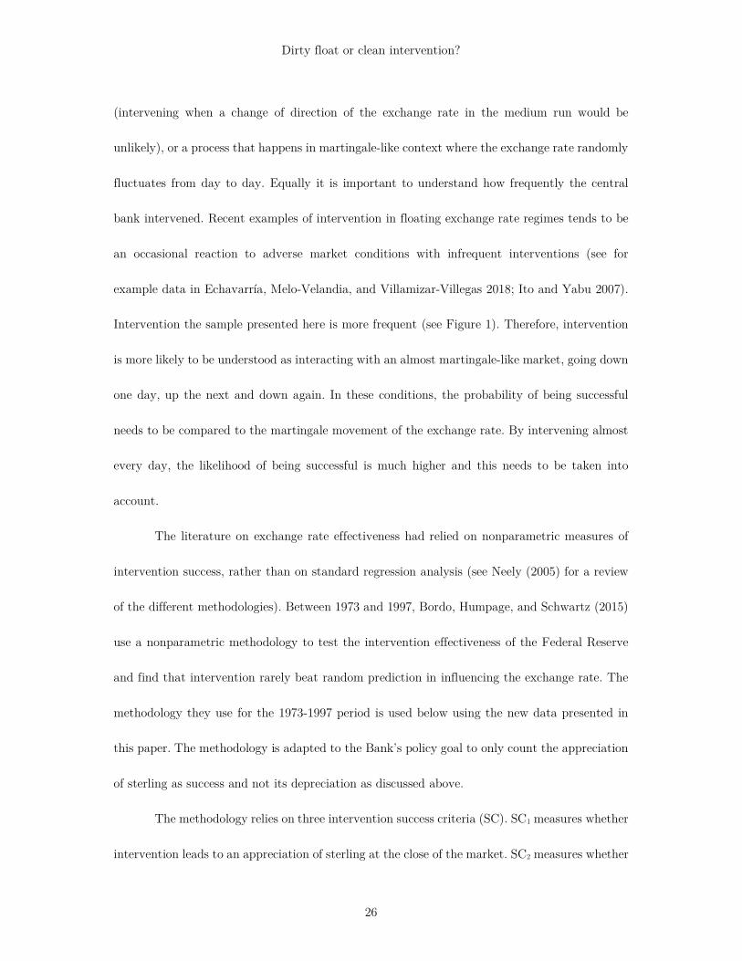
Dirty float or clean intervention?
26
(intervening when a change of direction of the exchange rate in the medium run would be
unlikely), or a process that happens in martingale-like context where the exchange rate randomly
fluctuates from day to day. Equally it is important to understand how frequently the central
bank intervened. Recent examples of intervention in floating exchange rate regimes tends to be
an occasional reaction to adverse market conditions with infrequent interventions (see for
example data in Echavarría, Melo-Velandia, and Villamizar-Villegas 2018; Ito and Yabu 2007).
Intervention the sample presented here is more frequent (see Figure 1). Therefore, intervention
is more likely to be understood as interacting with an almost martingale-like market, going down
one day, up the next and down again. In these conditions, the probability of being successful
needs to be compared to the martingale movement of the exchange rate. By intervening almost
every day, the likelihood of being successful is much higher and this needs to be taken into
account.
The literature on exchange rate effectiveness had relied on nonparametric measures of
intervention success, rather than on standard regression analysis (see Neely (2005) for a review
of the different methodologies). Between 1973 and 1997, Bordo, Humpage, and Schwartz (2015)
use a nonparametric methodology to test the intervention effectiveness of the Federal Reserve
and find that intervention rarely beat random prediction in influencing the exchange rate. The
methodology they use for the 1973-1997 period is used below using the new data presented in
this paper. The methodology is adapted to the Bank’s policy goal to only count the appreciation
of sterling as success and not its depreciation as discussed above.
The methodology relies on three intervention success criteria (SC). SC1 measures whether
intervention leads to an appreciation of sterling at the close of the market. SC2 measures whether
Dirty float or clean intervention?
27
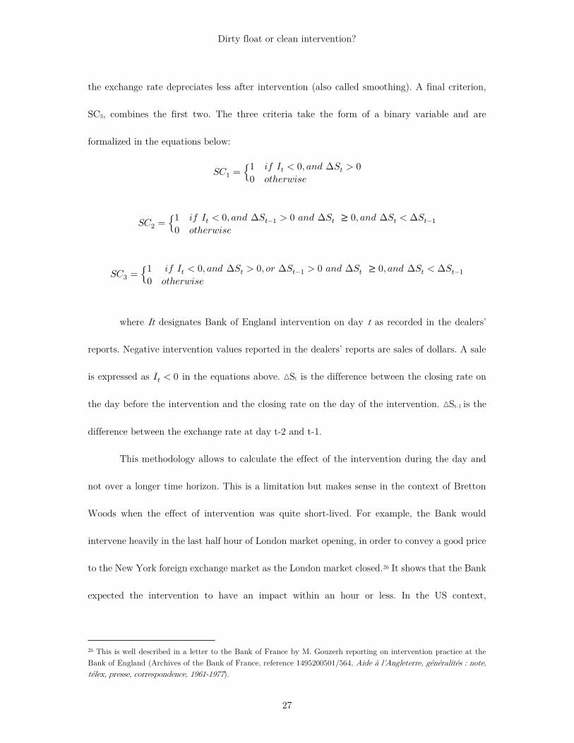
the exchange rate depreciates less after intervention (also called smoothing). A final criterion,
SC3, combines the first two. The three criteria take the form of a binary variable and are
formalized in the equations below:
𝑆𝐶 =1 𝑖𝑓 𝐼 < 0, 𝑎𝑛𝑑 ∆𝑆 > 0
0 𝑜𝑡ℎ𝑒𝑟𝑤𝑖𝑠𝑒
𝑆𝐶 =1 𝑖𝑓 𝐼 < 0, 𝑎𝑛𝑑 ∆𝑆 − > 0 𝑎𝑛𝑑 ∆𝑆 ≥ 0, 𝑎𝑛𝑑 ∆𝑆 < ∆𝑆 −
0 𝑜𝑡ℎ𝑒𝑟𝑤𝑖𝑠𝑒
𝑆𝐶 =1 𝑖𝑓 𝐼 < 0, 𝑎𝑛𝑑 ∆𝑆 > 0, 𝑜𝑟 ∆𝑆 − > 0 𝑎𝑛𝑑 ∆𝑆 ≥ 0, 𝑎𝑛𝑑 ∆𝑆 < ∆𝑆 −
0 𝑜𝑡ℎ𝑒𝑟𝑤𝑖𝑠𝑒
where It designates Bank of England intervention on day t as recorded in the dealers’
reports. Negative intervention values reported in the dealers’ reports are sales of dollars. A sale
is expressed as 𝐼 < 0 in the equations above. ∆St is the difference between the closing rate on
the day before the intervention and the closing rate on the day of the intervention. ∆St-1 is the
difference between the exchange rate at day t-2 and t-1.
This methodology allows to calculate the effect of the intervention during the day and
not over a longer time horizon. This is a limitation but makes sense in the context of Bretton
Woods when the effect of intervention was quite short-lived. For example, the Bank would
intervene heavily in the last half hour of London market opening, in order to convey a good price
to the New York foreign exchange market as the London market closed.26 It shows that the Bank
expected the intervention to have an impact within an hour or less. In the US context,
26 This is well described in a letter to the Bank of France by M. Gouzerh reporting on intervention practice at the Bank of England (Archives of the Bank of France, reference 1495200501/564, Aide à l’Angleterre, généralités : note, télex, presse, correspondence, 1961-1977).
Dirty float or clean intervention?
28
Dominguez (2003) also suggests that traders in the 1990s usually knew that the Fed was
intervening at least one hour before any news outlets would report it. The methodology therefore
captures the short-term effect of intervention but not any longer-term effect.
The results of the success counts are then compared with virtual successes, which are the
successes of the different criteria, ignoring the effect of intervention. In other words, it measures
how successful the Bank of England would be if it intervened every day. This captures, for
criterion SC1 for example, on how many of the trading days the exchange rate appreciated
against the previous day. This is problematic as it ignores the effect of intervention, but it is in
line with the martingale nature of the market that is assumed to fluctuate daily regardless of
intervention. These values are then compared to the value obtained with the success criteria
described below using a hypergeometric distribution (described in more detail in the appendix).
If the intervention success criterion is two standard deviations below the expected success, the
intervention is said to have no exchange rate forecasting value. If the intervention success
criterion is two standard deviations above the expected success, the intervention is said to have
a positive forecasting value. Finally, in any other case, the intervention is said to have a random
forecasting value.
Table 5 presents the result of the analysis for the whole sample from 1952 to 1972. The
data are sorted by the three success criteria presented above. The first column displays the total
number of days offering exchange rate data (6099) followed by the days on which the Bank of
England intervened by selling foreign currency (1454).

Dirty float or clean intervention?
29
total number
intervention success
virtual success
expected success
variance standard deviation
random range
outcome
# % # % #
Observations 6099
SC1 (appreciation)
1454 211 15% 1500 25% 358 205 14 between 329
and 386
Negative forecasting
value
SC2 (smoothing)
1454 398 27% 1326 22% 316 188 14 between 289
and 344
Positive forecasting
value
SC3 (combined)
1454 587 40% 3276 54% 781 275 17 between 748
and 814
Negative forecasting
value
Table 5 - Success counts according to success criteria 1 to 3 from 1952 to 1972.
Columns labelled “intervention successes” count intervention successes according to the
three criteria, both in number of successful days and in percentage. For example, the first entry
establishes that out of 1454 intervention days selling foreign currency, the Bank managed to get
the exchange rate to appreciate on 211 occasions, or 15% of the time. This measure is descriptive
and does not infer causality.
The “virtual success” column reveals, ignoring the effect of intervention, the number of
days when the exchange rate appreciated. For SC1 this means that on 1500 instances, the
exchange appreciated relative to the previous day’s close. The percentage of virtual successes
(25%) is then used to establish the expected success. The Bank sold dollars on 1454 days, and
therefore would be expected to be successful at least 25% of the time or 358 times out of pure
luck. The actual number of successes (211) should lie two standard deviations above the expected
success to demonstrate that the Bank had a positive forecasting value. For SC1, 211 lies below
Dirty float or clean intervention?
30
the random range of ± two standard deviations (329-386) and consequently the Bank had a
negative forecasting value.
In other words, a trader systematically betting against the Bank after noticing an
intervention would have made money. If information about intervention had been leaked on
every given morning, betting against the Bank during the day would have been profitable in the
long run.
All but the smoothing criterion display negative forecasting value. The smoothing
criterion establishes that the Bank of England was successful in taming depreciation, which was
one of its policy goals. When compared with the findings by Bordo, Humpage, and Schwartz
(2015) for the Fed between 1973 and 1995, these results highlight that the Bank intervened more
frequently, which was expected during a period of fixed exchange rates. The Bank of England
was on the market almost every day or 85.2 % of the days if we include purchase and sales
operations (as opposed to 15% and 3% respectively for Deutschmark and Yen intervention in
the Bordo, Humpage, and Schwartz (2015) study). This is high compared to modern rates, as
Fratzscher et al. (2019) find that between 1995 and 2011, developed countries’ central bank
intervened on 8.7% of trading days and developing countries on 34% of trading days. By
intervening every day, success is expected to be lower as the intervention bears less signaling
value, not giving the market any new information. Yet, the Bank at the time was a much bigger
actor relative to the market size and should have been expected to be more successful than
central banks are today.

Dirty float or clean intervention?
31
4.4 When all else fails, cheat?
How did the Bank deal with the decline of the pound, once intervention was insufficient to
reassure markets? In a fixed exchange rate system, reserve levels are important in how market
participants value a currency (Krugman 1979). The Bank was conscious of this issue and took
the publication of reserves figures seriously. To support sterling, the Bank started manipulating
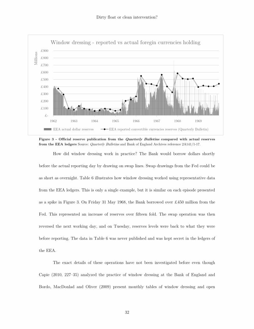
or “window dressing” its reserve account. Figure 3 compares classified data from the EEA ledgers
with public data from the Bank’s published Quarterly Bulletins.
Until 1966, public and classified figures seem to be matching relatively closely, exposing only
minor differences.27 After 1966, the actual reserves of the EEA ledger drop far below the
published reserves. This is because of short-term swaps and loans from the Fed. Every spike in
Figure 3 shows the Bank borrowing short term to hide its true reserve position. This accounting
manipulation was made possible by publishing only the asset side of the EEA’s balance sheet in
the Quarterly Bulletins, not the liabilities. The Bank was only showing how much reserves it
had, not the short time liabilities to the Fed in the form of swap contracts. These contracts were
in place from 1962 onward for the Fed to grant liquidity to other central banks (for more on
swaps, see McCauley and Schenk 2020 and Bordo, Humpage, and Schwartz 2015).
27 Note that EEA figures only report dollars whereas the Quarterly Bulletin figures report convertible currencies. By surveying the EEA accounts for other convertible currency holding, however, it quickly becomes clear that the largest part of reserves is made of dollars. This reflects the fact that the Bank wanted to avoid running any risk by keeping reserves other than dollars.
Dirty float or clean intervention?
32
Figure 3 - Official reserve publication from the Quarterly Bulletins compared with actual reserves from the EEA ledgers Source: Quarterly Bulletins and Bank of England Archives reference 2A141/1-17.
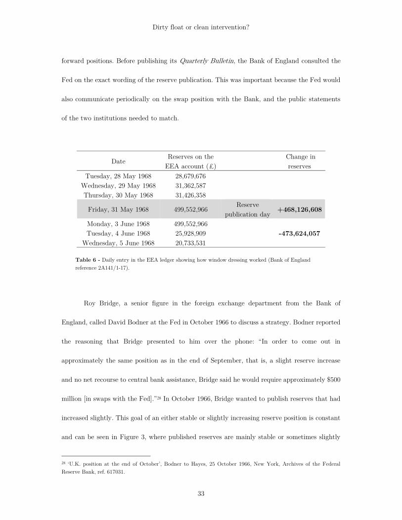
How did window dressing work in practice? The Bank would borrow dollars shortly
before the actual reporting day by drawing on swap lines. Swap drawings from the Fed could be
as short as overnight. Table 6 illustrates how window dressing worked using representative data
from the EEA ledgers. This is only a single example, but it is similar on each episode presented
as a spike in Figure 3. On Friday 31 May 1968, the Bank borrowed over £450 million from the
Fed. This represented an increase of reserves over fifteen fold. The swap operation was then
reversed the next working day, and on Tuesday, reserves levels were back to what they were
before reporting. The data in Table 6 was never published and was kept secret in the ledgers of
the EEA.
The exact details of these operations have not been investigated before even though
Capie (2010, 227–35) analyzed the practice of window dressing at the Bank of England and
Bordo, MacDonlad and Oliver (2009) present monthly tables of window dressing and open
£-
£100
£200
£300
£400
£500
£600
£700
£800
£900
1962 1963 1964 1965 1966 1967 1968 1969
Mill
ions
Window dressing - reported vs actual foregin currencies holding
EEA actual dollar reserves EEA reported convertible currencies reserves (Quarterly Bulletin)
Dirty float or clean intervention?
33
forward positions. Before publishing its Quarterly Bulletin, the Bank of England consulted the
Fed on the exact wording of the reserve publication. This was important because the Fed would
also communicate periodically on the swap position with the Bank, and the public statements
of the two institutions needed to match.
Date Reserves on the
EEA account (£) Change in
reserves Tuesday, 28 May 1968 28,679,676
Wednesday, 29 May 1968 31,362,587
Thursday, 30 May 1968 31,426,358
Friday, 31 May 1968 499,552,966 Reserve
publication day +468,126,608
Monday, 3 June 1968 499,552,966
Tuesday, 4 June 1968 25,928,909 -473,624,057 Wednesday, 5 June 1968 20,733,531
Table 6 - Daily entry in the EEA ledger showing how window dressing worked (Bank of England reference 2A141/1-17).
Roy Bridge, a senior figure in the foreign exchange department from the Bank of
England, called David Bodner at the Fed in October 1966 to discuss a strategy. Bodner reported
the reasoning that Bridge presented to him over the phone: “In order to come out in
approximately the same position as in the end of September, that is, a slight reserve increase
and no net recourse to central bank assistance, Bridge said he would require approximately $500
million [in swaps with the Fed].”28 In October 1966, Bridge wanted to publish reserves that had
increased slightly. This goal of an either stable or slightly increasing reserve position is constant
and can be seen in Figure 3, where published reserves are mainly stable or sometimes slightly
28 ‘U.K. position at the end of October’, Bodner to Hayes, 25 October 1966, New York, Archives of the Federal Reserve Bank, ref. 617031.

Dirty float or clean intervention?
34
on the rise, despite declining real reserves. The quote also illustrates how the Bank and the Fed
were working together closely to decide on a figure for the publication of the British reserve
position.
The Fed supported the Bank in its window dressing to the extent that it helped the
Bank to cover its tracks. Before publishing the minutes of the Federal Open Market Committee
(FOMC), the Fed sent the excerpts of the minutes to the Bank of England so they could edit
out anything mentioning window dressing. A letter from Charles Coombs at the Fed reads:
“we invited you to look over selected excerpts from the 1966 FOMC minutes involving certain
delicate points that we thought you might wish to have deleted from the published version.
We have subsequently deleted all of the passages which you found troublesome. Recently, we
have made a final review of the minutes and have turned up one other passage that I am not
certain you had an opportunity to go over. I am enclosing a copy of the excerpt, with possible
deletions bracketed in red ink.”29
Coombs suggested deleting passages of the minutes where some FOMC members
criticized window dressing; Mitchell from the FOMC suggested that the Bank of England would
get better results “if they reported their reserve position accurately than if they attempted to
conceal their true reserve position”.30 Despite disagreement by some FOMC members, reserve
figure manipulation was an important question for the stability of sterling and led to close
cooperation between the Bank and the Fed.
29 ‘Letter from Coombs to Hallet’, 1 December 1971, New York, Archive of the Federal Reserve, Box 107320. 30 Ibid., p. 10.

Dirty float or clean intervention?
35
5. Conclusion
This paper has presented new intervention data during the Bretton Woods period in order to
assess how Britain managed its exchange rate with sterilized intervention. With regards to the
crude goal of keeping the exchange rate within the approved bands, the Bank managed to fulfil
its mission throughout the period, when counting the devaluations as exogenous government
actions. Considering intervention in more detail, sterilized intervention during the Bretton
Woods period cannot be described as having a significant effect on exchange rates. Before 1958,
offshore and forward foreign exchange rates show that the exchange rate was lower in markets
without Bank of England interventions. After the introduction of convertibility in 1958, offshore
markets stopped showing a discount on sterling. Sterling entered a period of crisis, pushing the
Bank of England to progressively manipulate its official reserve data and undertake substantial
international borrowing. The daily intervention data presented also demonstrates how
intervention cannot be portrayed as a successful short-term tool; any investor having access to
classified information and systematically betting against the Bank of England would profit from
the strategy in the long run.

Dirty float or clean intervention?
36
6. Appendix
Hypergeometric distribution criteria
The testing methodology uses a hypergeometric distribution. The variance and standard
deviation of the hypergeometric distribution are as follows:
Variance = 𝑛 ( − ) −−
N is the population size (total number of days with exchange rate data) K is the number of expected successes (intervention virtual successes according to the three criteria SC1-3) n is the number of draws (total number of interventions with a buy or sell mark) k is the number of observed successes (the actual number of successes according to the three criteria SC1-3). The null hypothesis is that intervention has a random forecasting value. The null
hypothesis is rejected if the number of actual successes (k) is smaller than the number of expected
successes (K) by two standard deviations. This means that the forecasting value is negative. The
null hypothesis is also rejected if the number of actual successes (k) is larger than that of expected
successes (K) by two standard deviations. If the null hypothesis cannot be rejected either way,
the forecasting value of the central bank is said to be random.

Dirty float or clean intervention?
37
7. References
Accominotti, Olivier, Jason Cen, David Chambers, and Ian W. Marsh. 2019. ‘Currency Regimes and the Carry Trade’. Journal of Financial and Quantitative Analysis 54 (5): 2233–60. https://doi.org/10.1017/S002210901900019X.
Allen, William. 2014. Monetary Policy and Financial Repression in Britain, 1951-59. New York: Palgrave Macmillan.
Blanchard, Olivier, Gustavo Adler, and Irineu de Carvalho Filho. 2015. ‘Can Foreign Exchange Intervention Stem Exchange Rate Pressures from Global Capital Flow Shocks?’ Working Paper 21427. National Bureau of Economic Research. http://www.nber.org/papers/w21427.
Blancheton, Bertrand, and Samuel Maveyraud. 2009. ‘French Exchange Rate Management in the 1920s’. Financial History Review 16 (02): 183–201.
Bordo, Michael D., Owen F. Humpage, and Anna J. Schwartz. 2015. Strained Relations: US Foreign-Exchange Operations and Monetary Policy in the Twentieth Century. Chicago: University of Chicago Press.
Bordo, Michael D., Ronald MacDonald, and Michael J. Oliver. 2009. ‘Sterling in Crisis, 1964–1967’. European Review of Economic History 13 (3): 437–59. https://doi.org/10.1017/S1361491609990128.
———. 2012. ‘Sterling in Crisis 1964–1967’. In Credibility and the International Monetary Regime: A Historical Perspective, edited by Michael D. Bordo and Ronald MacDonald, 151–74. Cambridge ; New York: Cambridge University Press.
Bordo, Michael, Eric Monnet, and Alain Naef. 2019. ‘The Gold Pool (1961–1968) and the Fall of the Bretton Woods System: Lessons for Central Bank Cooperation’. The Journal of Economic History, 1–33. https://doi.org/10.1017/S0022050719000548.
Burkhard, Lukas, and Andreas M. Fischer. 2009. ‘Communicating Policy Options at the Zero Bound’. Journal of International Money and Finance 28 (5): 742–54. https://doi.org/10.1016/j.jimonfin.2008.06.006.
Capie, Forrest. 2010. The Bank of England: 1950s to 1979. Cambridge: Cambridge University Press. Dominguez, Kathryn, and Jeffrey A. Frankel. 1993. ‘Does Foreign-Exchange Intervention Matter? The
Portfolio Effect’. The American Economic Review 83 (5): 1356–69. Dominguez, Kathryn M. 2003. ‘The Market Microstructure of Central Bank Intervention’. Journal of
International Economics 59 (1): 25–45. https://doi.org/10.1016/S0022-1996(02)00091-0. Echavarría, Juan J., Luis F. Melo-Velandia, and Mauricio Villamizar-Villegas. 2018. ‘The Impact of Pre-
Announced Day-to-Day Interventions on the Colombian Exchange Rate’. Empirical Economics 55 (3): 1319–36. https://doi.org/10.1007/s00181-017-1299-1.
Edison, Hali J. 1993. The Effectiveness of Central-Bank Intervention: A Survey of the Literature after 1982. Vol. 18. Princeton.
Eichengreen, Barry, and Marc Flandreau. 2009. ‘The Rise and Fall of the Dollar (or When Did the Dollar Replace Sterling as the Leading Reserve Currency?)’. European Review of Economic History 13 (3): 377–411. https://doi.org/10.1017/S1361491609990153.
Eichengreen, Barry, Arnaud Mehl, and Livia Chitu. 2017. How Global Currencies Work: Past, Present, and Future. Princeton, NJ: Princeton University Press.
Fratzscher, Marcel, Oliver Gloede, Lukas Menkhoff, Lucio Sarno, and Tobias Stöhr. 2019. ‘When Is Foreign Exchange Intervention Effective? Evidence from 33 Countries’. American Economic Journal: Macroeconomics. https://doi.org/10.1257/mac.20150317.
Howson, Susan. 1980a. Sterling’s Managed Float: The Operations of the Exchange Equalisation Account, 1932-39. International Finance Section, Department of Economics, Princeton University. https://www.princeton.edu/~ies/IES_Studies/S46.pdf.
———. 1980b. ‘The Management of Sterling, 1932–1939’. The Journal of Economic History 40 (01): 53–60.
———. 1993. British Monetary Policy, 1945-51. Oxford: New York: Clarendon Press.

Dirty float or clean intervention?
38
Ito, Takatoshi, and Tomoyoshi Yabu. 2007. ‘What Prompts Japan to Intervene in the Forex Market? A New Approach to a Reaction Function’. Journal of International Money and Finance 26 (2): 193–212. https://doi.org/10.1016/j.jimonfin.2006.12.001.
Jobst, Clemens. 2009. ‘Market Leader: The Austro-Hungarian Bank and the Making of Foreign Exchange Intervention, 1896–1913’. European Review of Economic History 13 (3): 287–318. https://doi.org/10.1017/S1361491609990104.
Klug, Adam, and Gregor W. Smith. 1999. ‘Suez and Sterling, 1956’. Explorations in Economic History 36 (3): 181–203. https://doi.org/10.1006/exeh.1999.0720.
Krugman, Paul. 1979. ‘A Model of Balance-of-Payments Crises’. Journal of Money, Credit and Banking 11 (3): 311–25. https://doi.org/10.2307/1991793.
McCauley, Robert N., and Catherine R. Schenk. 2020. ‘Central Bank Swaps Then and Now: Swaps and Dollar Liquidity in the 1960s’, April. https://www.bis.org/publ/work851.htm.
Mihaljek, Dubravko. 2005. ‘Survey of Central Banks’ Views on Effects of Intervention’. In BIS Papers Chapters, 24:82–96. Bank for International Settlements. https://ideas.repec.org/h/bis/bisbpc/24-06.html.
Mohanty, Madhusudan S., and Bat-el Berger. 2013. ‘Central Bank Views on Foreign Exchange Intervention’. BIS working paper No 73.
Naef, Alain. 2019. ‘Blowing Against the Wind? A Narrative Approach to Central Bank Foreign Exchange Intervention’. UC Berkeley Mimeo, November. http://dx.doi.org/10.2139/ssrn.3483895.
Neely, Christopher. 2005. ‘An Analysis of Recent Studies of the Effect of Foreign Exchange Intervention’. Federal Reserve Bank of St. Louis Working Paper No. 2005-030B.
Sarno, Lucio, and Mark P. Taylor. 2001. ‘Official Intervention in the Foreign Exchange Market: Is It Effective and, If so, How Does It Work?’ Journal of Economic Literature 39 (3): 839–68. https://doi.org/10.1257/jel.39.3.839.
Sayers, Richard Sidney. 1976. The Bank of England, 1891-1944. Cambridge: Cambridge University Press,. Schenk, Catherine. 1994a. ‘Closing the Hong Kong Gap: The Hong Kong Free Dollar Market in the 1950s’.
The Economic History Review 47 (2): 335–53. https://doi.org/10.1111/j.1468-0289.1994.tb01379.x.
———. 1994b. Britain and the Sterling Area: From Devaluation to Convertibility in the 1950s. London; New York: Routledge.
———. 2010. The Decline of Sterling: Managing the Retreat of an International Currency, 1945–1992. Cambridge University Press.
Strange, Susan. 1971. Sterling and British Policy: A Political Study of an International Currency in Decline. Oxford University Press.
Svensson, Lars E. O. 1991. ‘The Simplest Test of Target Zone Credibility’. Staff Papers 38 (3): 655–65. https://doi.org/10.2307/3867162.
Taylor, Alan M. 2010. ‘Global Finance after the Crisis’. Bank of England Quarterly Bulletin 50 (4): 366–77. Toniolo, Gianni, and Piet Clement. 2007. Central Bank Cooperation at the Bank for International
Settlements, 1930-1973. Cambridge University Press.
Copyright © 2022 FDOKUMEN