
dinámica de los pinares de montaña bajo gestión forestal ...
226
UNIVERSIDAD POLITÉCNICA DE MADRID ESCUELA TÉCNICA SUPERIOR DE INGENIERÍA DE MONTES, FORESTAL Y DEL MEDIO NATURAL DINÁMICA DE LOS PINARES DE MONTAÑA BAJO GESTIÓN FORESTAL SOSTENIBLE EN UN CONTEXTO DE CAMBIO GLOBAL Tesis doctoral DANIEL MORENO FERNÁNDEZ 2018
-
Upload
khangminh22 -
Category
Documents
-
view
1 -
download
0
Transcript of dinámica de los pinares de montaña bajo gestión forestal ...

UNIVERSIDAD POLITÉCNICA DE MADRID
ESCUELA TÉCNICA SUPERIOR
DE INGENIERÍA DE MONTES, FORESTAL Y DEL MEDIO NATURAL
DINÁMICA DE LOS PINARES DE MONTAÑA BAJO
GESTIÓN FORESTAL SOSTENIBLE EN UN CONTEXTO
DE CAMBIO GLOBAL
Tesis doctoral
DANIEL MORENO FERNÁNDEZ
2018


UNIVERSIDAD POLITÉCNICA DE MADRID
ESCUELA TÉCNICA SUPERIOR DE INGENIERÍA DE MONTES, FORESTAL Y
DEL MEDIO NATURAL
DINÁMICA DE LOS PINARES DE MONTAÑA BAJO GESTIÓN
FORESTAL SOSTENIBLE EN UN CONTEXTO DE CAMBIO GLOBAL
TESIS DOCTORAL
DANIEL MORENO FERNÁNDEZ
Ingeniero Técnico Forestal
Máster en Investigación en Ingeniería para la Conservación y Uso Sostenible de los
Sistemas Forestales
2018

PROGRAMA DE DOCTORADO EN INVESTIGACIÓN FORESTAL AVANZADA
ESCUELA TÉCNICA SUPERIOR DE INGENIERÍA DE MONTES, FORESTAL Y
DEL MEDIO NATURAL
DINÁMICA DE LOS PINARES DE MONTAÑA BAJO GESTIÓN
FORESTAL SOSTENIBLE EN UN CONTEXTO DE CAMBIO GLOBAL
DANIEL MORENO FERNÁNDEZ
Ingeniero Técnico Forestal
Máster en Investigación en Ingeniería para la Conservación y Uso Sostenible
de los Sistemas Forestales
DIRECTORAS
ISABEL CAÑELLAS MARÍA DE LA O SÁNCHEZ
Doctora en Ingeniería de Montes Doctora en Ingeniería de Montes
2018


Tribunal nombrado por el Excmo. Sr. Rector de la Universidad Politécnica de
Madrid, el día ....... de .............................. de 2018
Presidente D. ..................................................................................................
Vocal D. .........................................................................................................
Vocal D. .........................................................................................................
Vocal D. .........................................................................................................
Secretario D. ..................................................................................................
Realizado el acto de defensa y lectura de la Tesis el día ….
de …………………… de 2018 en Madrid
Calificación…………………………………..
EL/LA PRESIDENTE/A LOS/LAS VOCALES
EL/LA SECRETARIO/A


“Allá muevan feroz guerra,
ciegos reyes,
por un palmo más de tierra,
que yo tengo aquí por mío
cuanto abarca el mar bravío,
a quien nadie impuso leyes.”
La Canción del Pirata. José de Espronceda


Agradecimientos
It´s a long way to the top (if you wanna Rock ´n´ Roll) es el título de una canción de AC/DC
con Bon Scott a la voz y a la gaita escocesa. La tesis doctoral no es otra cosa que un camino
largo en el que te caes mil y una veces y en el que la constancia, el trabajo y el empeño hacen
que te vuelvas a levantar. Sin embargo, durante ese largo camino siempre se necesita una
mano, o incluso un brazo, al que agarrarte.
En primer lugar, tengo que dar mi más sincero agradecimiento a mis dos directoras,
Isabel Cañellas y Mariola Sánchez. Allá por el 2012, comencé a trabajar con ellas en el
Trabajo Fin de Máster. Desde un principio, las dos confiaron en mí y me enseñaron cómo
funciona esto de la investigación, las publicaciones, el análisis de datos, etc. Desde el primer
momento han favorecido tanto las colaboraciones con investigadores de otros centros y han
impulsado mi crecimiento como investigador. También, estoy enormemente agradecido al
resto de colaboradores en los distintos trabajos, en especial a Fernando Montes - quien ha
sido prácticamente un director más - y a Nicole H. Augustin quién supervisó mi trabajo en
la estancia en la Universidad de Bath. A Alfonso San Miguel le agradezco su ofrecimiento
para ser el tutor académico de esta tesis.
Durante años en el INIA he conocido a grandes personas que sin duda han hecho que
levantarse, coger la bici e ir a trabajar todas las mañanas fuera menos duro. La lista es
interminable. Me gustaría destacar a Marta y a Nerea porque han sido las dos mejores
compañeras-compiyoguis (somos del 10%). Ha sido genial teneros en el Despacho 2016 del
CIFOR. Nunca olvidaré las conversaciones en las que llovían puñales. Tampoco olvidaré el
apoyo mutuo con el R o con cualquier otro asunto. Alicia Ledo ha siempre estado cerca
aunque fuera por email (Sempre Suaves!). Cualquier persona debería agradecer a Javier su
desinteresada preocupación por los demás, nunca fallas compañero. A Laura punki le quiero
agradecer el tremendo buen rollo que transmite, siempre sonriendo y de buen humor (menos
algunos lunes). Con Carol he tenido grandes conversaciones políticas y de otros temas, ya
sea en el INIA, a través de internet o por Lavapiés. A Antonio le quiero decir que nos
tenemos que dejar de copiar los lugares de estudio y trabajo, la EUIT Forestal, Erasmus en
Finlandia, Máster en Palencia y, finalmente, hemos acabamos en el INIA haciendo la tesis.
A Laura Fernández le agradezco muchas cosas, principalmente, su paciencia por aguantar
mis comentarios sobre sus abetos de chocolate. Mario, José Pablo, Ana, Álvaro, Guille, Mar,
Isabel, Miren, Hortensia, Mayte, Silvia, María, Rafa, Edu y Raquel son de la gente más maja

que te puedes encontrar en el INIA. También estoy muy contento de haber coincidido con la
gente que ha estado haciendo la tesis en el Departamento de Genética: Rose, Ruth, Andrés,
Maje, Sanna, Natalia, Marta, Quique, etc. Ha sido un gustazo trabajar con Laura Hernández
e Icíar. Siempre están dispuestas a ayudar con el Inventario Forestal Nacional, con el ArcGis
o con cualquier otro tema. Por otro lado, hay tres personas cuyos nombres son habituales en
los agradecimientos de los artículos, Ángel Bachiller, Estrella Viscasillas y Enrique Garriga.
Son los tres capataces con los que he salido a tomar datos al monte, tanto para esta tesis
como para otros trabajos. Ha sido un placer haber echado tantas horas en el monte con gente
tan simpática. También gracias a Nicholas Devaney, mi tío, y a Adam Collins por haber
revisado la gramática inglesa de esta tesis. Un abrazo enorme al personal administrativo del
CIFOR y del INIA así como al personal de la cafetería, de jardinería y de la limpieza.
También quiero dar las gracias a mi compañero de la carrera, Rubén González Andrés quien
ha dejado su huella de artista del Photoshop retocando las fotos de la portada principal de la
tesis así como la de los capítulos 1 y 2.
Además de investigar, también he participado en tareas de docencia, primero en la
Universidad de Valladolid y luego en la Universidad Politécnica de Madrid. Sinceramente,
ha sido una experiencia genial, muy bonita. Agradezco a José Reque y a Sonia Roig haber
supervisado mis prácticas. Llegado a este punto tengo que nombrar a dos docentes que me
dieron clase durante la carrera: Rafael Serrada y Valentín Gómez. Ambos me descubrieron
la Selvicultura, el cómo y porqué hay que gestionar los montes. Ambos son, sin la menor
duda, en parte responsables de que yo decidiera seguir aprendiendo y trabajando en
Selvicultura.
Al margen de lo estrictamente científico y profesional, hay una serie de personas que
también han sido importantes de una manera directa o más indirecta, empezando por los
compañeros y compañeras de la Ingeniería Técnica Forestal en la Universidad Politécnica
de Madrid y del Máster de Investigación en Ingeniería para la Conservación y Uso Sostenible
de los Sistemas Forestales de la Universidad de Valladolid. Un abrazo a la gente de Usera,
a la de otros barrios de Madrid y a la de los múltiple lugares que he llegado a conocer durante
este tiempo. Muchas de estas personas no tenían muy claro qué es lo que iba a hacer cada
mañana pero aun así me preguntaban qué tal iba el curro. Casi superado el ecuador de la
tesis apareció María Ángeles, me ha apoyado enormemente con la tesis, con la ciencia y en
otros miles de asuntos. Entre otras muchas cosas, he aprendido un montón de bacterias

gracias a ti ¡Gracias por estar ahí!. Por último y no menos importante, estoy orgulloso de mi
familia, en especial de mis padres por la educación recibida, por el apoyo que me han dado
y por enseñarme a no conformarme con lo mínimo y a que nada cae del cielo y se necesita
hacer un esfuerzo.


Financiación
Para la realización de la presente tesis doctoral yo, Daniel Moreno Fernández, he sido
beneficiario de un contrato de Formación del Personal Investigador de la Universidad de
Valladolid desde abril del 2014 a septiembre del 2014 y de un contrato de Formación del
Profesorado Universitario del Ministerio de Educación, Cultura y Deporte (FPU13/02113)
desde septiembre del 2014 hasta abril del 2018. He trabajado bajo la supervisión de la Dra.
Isabel Cañellas y Dra. Mariola Sánchez González. Al igual que ellas, he estado adscrito al
Centro de Investigación Forestal del Instituto Nacional de Investigación y Tecnología
Agraria y Alimentaria. Además, realicé una estancia de 3 meses en la Universidad de Bath
(Inglaterra) bajo la supervisión de la Dra. Nicole H. Augustin. Dicha estancia fue financiada
por el Programa de Estancias Breves FPU del Ministerio de Educación, Cultura y Deporte
(EST15/00242).
En el plano académico, comencé la tesis doctoral matriculado en el programa de
doctorado en Conservación y Uso Sostenible de los Sistemas Forestales de la Universidad
de Valladolid hasta 2016, año en el que me matriculé en el programa de Investigación
Forestal Avanzada de la Universidad Politécnica de Madrid.


Table of contents
i
Table of contents
Resumen ........................................................................................................................ 1 Summary ...................................................................................................................... 3
Chapter 1 General introduction 1.1. Global change in Mediterranean mountain forest systems ........................................ 7 1.2. Sustainable Forest Management: Adaptation and mitigation .................................... 9 1.3. Dynamics of Pinus sylvestris in Mediterranean mountains .................................... 11 1.4. Study areas ............................................................................................................... 13
1.4.1. Site characteristics ............................................................................................ 13 1.4.2. Brief description of the data ............................................................................. 15
1.5. Methodology ............................................................................................................ 16 1.5.1. Statistical overview........................................................................................... 16 1.5.2. Multiscale framework ....................................................................................... 18
1.6. Objectives ................................................................................................................ 19 1.7. Thesis structure ........................................................................................................ 20
Chapter 2 Alternative approaches to assessing the natural regeneration of Scots pine in a Mediterranean forest Abstract ........................................................................................................................... 25 2.1. Introduction ............................................................................................................. 26 2.2. Materials and methods ............................................................................................. 29
2.2.1. Study site .......................................................................................................... 29 2.2.2. Parametric regression: GLMM using a negative binomial ............................... 33 2.2.3. Including uncorrelated variables in the GLMM. PCA as ordination method .. 35 2.2.4. Ordination using NMDS ................................................................................... 36 2.2.5. Decision tree automatic classification method: CHAID algorithm .................. 37 2.2.6. The Random Forests algorithm and conditional inference tree ........................ 38
2.3. Results ..................................................................................................................... 39 2.3.1. Parametric regression: GLMM using a negative binomial ............................... 39 2.3.2. Including uncorrelated variables in the GLMM. PCA as ordination method .. 40 2.3.3. Ordination with NMDS .................................................................................... 43 2.3.4. Decision tree automatic classification method: CHAID algorithm .................. 44 2.3.5. Random Forests algorithm and conditional inference tree ............................... 45
2.4. Discussion ................................................................................................................ 47 2.4.1. Factors underlying Scots pine regeneration in Central Spain........................... 47 2.4.2. Methods comparison ........................................................................................ 48
Acknowledgements ........................................................................................................ 50

Table of contents
ii
Chapter 3 Modeling sapling distribution over time using a functional predictor in a generalized additive model Abstract ........................................................................................................................... 55 3.1. Introduction ............................................................................................................. 56 3.2. Materials and methods ............................................................................................. 59
3.2.1. Study site and data ............................................................................................ 59 3.2.2. Edge effect correction ....................................................................................... 62 3.2.3. Statistical analysis ............................................................................................ 63
3.3. Results ..................................................................................................................... 66 3.3.1. Intermediate stages of the regeneration period ................................................. 66 3.3.2. End of the regeneration period ......................................................................... 68
3.4. Discussion ................................................................................................................ 73 3.5. Conclusions ............................................................................................................. 76 Acknowledgements ........................................................................................................ 76
Chapter 4
Temporal carbon dynamics over the rotation period of two alternative management systems in Mediterranean mountain Scots pine forests Abstract ........................................................................................................................... 79 4.1. Introduction ............................................................................................................. 80 4.2. Materials and methods ............................................................................................. 82
4.2.1. Study areas ........................................................................................................ 82 4.2.2. Sampling design and estimation of C fractions ................................................ 83
4.2.2.1. Plot description and estimation of LTC and dead wood carbon ............... 83 4.2.2.2. Sampling of soil pool C stock (Carbon stock in O-horizon and mineral soil) ................................................................................................................................ 85 4.2.2.3. Laboratory analyses ................................................................................... 86
4.2.3. Statistical analyses ............................................................................................ 88 4.2.3.1. Living Tree Carbon ................................................................................... 88 4.2.3.2. Soil organic carbon pool ............................................................................ 89
4.3. Results ..................................................................................................................... 90 4.3.1. LTC, extracted C and dead wood C ................................................................. 90 4.3.2. Litterfall C rates ................................................................................................ 94 4.3.3. Soil organic carbon stocks ................................................................................ 95 4.3.4. Relationships between C pools ......................................................................... 96
4.4. Discussion ................................................................................................................ 98 4.4.1. Living tree carbon ............................................................................................. 98 4.4.2. Mineral soil organic carbon and forest floor .................................................... 99 4.4.3. Conclusions .................................................................................................... 101
Acknowledgements ...................................................................................................... 102

Table of contents
iii
Chapter 5 Space-time modeling of changes in the abundance and distribution of tree species Abstract ......................................................................................................................... 105 5.1. Introduction ........................................................................................................... 106 5.2. Material and methods ............................................................................................ 108
5.2.1. Study area ....................................................................................................... 108 5.2.2. Forest inventory data and climate data ........................................................... 109 5.2.3. Statistical analysis: space-time models........................................................... 111
5.2.3.1. Distribution (absence/presence) models: Space-time Universal Kriging 111 5.2.3.2. Abundance models: Space-time Universal Cokriging............................. 112 5.2.3.3. Assessment of the statistical significance of the mean function coefficients ............................................................................................................................. .114 5.2.3.4. Relative structural correlation assessment ............................................... 114 5.2.3.5. Model selection: Cross-validation ........................................................... 115
5.3. Results ................................................................................................................... 116 5.3.1. Rainfall and temperature measurements......................................................... 116 5.3.2. Shifts in the absence/presence of Scots pine and Pyrenean oak ..................... 117 5.3.3. Shifts in the abundance of Scots pine and Pyrenean oak ............................... 120
5.4. Discussion .............................................................................................................. 124 Acknowledgements ...................................................................................................... 126 Supplementary Material ............................................................................................... 127
Chapter 6 Discussion 6.1. Regeneration dynamics of Pinus sylvestris L. in Mediterranean areas ................. 133 6.2. Pinus sylvestris L. forests as a climate change mitigation tool ............................. 134 6.3. Retrospective view of Pinus sylvestris L. in Central Spain: influence of global change ...................................................................................................................................... 135 6.4. Methodological remarks ........................................................................................ 137
6.4.1. Multiscale framework ..................................................................................... 137 6.4.2. Statistical approaches ..................................................................................... 137 6.4.3. Spatio-temporal modeling .............................................................................. 139 6.4.4. Alternative data sources.................................................................................. 140
6.5. One step further: new challenges for the forestry sector ....................................... 141
Chapter 7 Conclusions 7.1. Conclusiones generales.......................................................................................... 147 7.2. General conclusions ............................................................................................... 149
Chapter 8 References List of references .......................................................................................................... 153

Table of contents
iv
Chapter 9 Curriculum Vitae 9.1. Personal data .......................................................................................................... 189 9.2. Education ............................................................................................................... 189
9.2.1. University degrees .......................................................................................... 189 9.2.2. Awards ............................................................................................................ 189 9.2.3. Other courses related to research .................................................................... 190
9.3. Fellowships and contracts ...................................................................................... 190 9.4. Publications ........................................................................................................... 191
9.4.1. Scientific papers ............................................................................................. 191 9.4.2. Science popularization articles ....................................................................... 192 9.4.3. Chapters in books ........................................................................................... 192 9.4.4. Conferences .................................................................................................... 193
9.4.5. Reviewer ......................................................................................................... 194 9.5. Participation in research projects ........................................................................... 195 9.6. Teaching ................................................................................................................ 195 9.7. Short term missions ............................................................................................... 196 9.8. Languages .............................................................................................................. 196
Appendix Front page of articles published in SCI journals .......................................................... 199

Index of figures
v
Index of figures
Chapter 1 Introduction Figure 1.1 Distribution map estimating the relative probability presence of P. sylvestris in
Europe (Houston Durrant et al. 2016).. ............................................................ 10 Figure 1.2 Regeneration establishment under the fellings of the uniform shelterwood in
Navafría forest .................................................................................................. 15 Figure 1.3 Summary of contents, study scale and topics addressed in Chapters 2, 3, 4 and 5.
REG=regeneration, FG= forest growth, CCA=climate change adaptation, CCM=climate change mitigation ...................................................................... 21
Chapter 2
Alternative approaches to assessing the natural regeneration of Scots pine in a Mediterranean forest Figure 2.1 NMDS Ordination of the variables showing the centroids of the quartiles of the
number of seedlings. Variables within Q4 hull not shown to facilitate the visualization. Red ellipse and red hull: Q4 (fourth quartile of the number of seedlings). Blue ellipse and blue hull: Q123 (first, second and third quartiles of the number of seedlings). Yellow smooth surfaces = IPOT gradient. Green surfaces = Mg gradients .................................................................................... 44
Figure 2.2 Regression tree as result of the CHAID algorithm for seedlings density. Mean indicates the mean number of seedlings per subplot and n the number of subplots per node ............................................................................................................ 45
Figure 2.3 Conditional variable importance measured following the “permutation principle of the mean” decrease in accuracy importance in the Random Forests algorithm. Larger values of conditional variable importance indicate more importance in the Random Forests model ............................................................................... 46
Figure 2.4 Implementation of conditional inference trees for seedlings density into the defined theory of conditional inference procedures. Mean indicates the mean number of seedlings per subplot and n the number of subplots per node ........ 46

Index of figures
vi
Chapter 3
Modeling sapling distribution using a functional predictor in a generalized additive model Figure 3.1 Position of adult trees (dbh≥20 cm; red circles), small trees (10≤dbh≤20 cm; green
dots) and number of saplings per quadrat (darker tones indicate larger number of saplings) of the six plots of the chronosequence in 2001. Size of adult trees is proportional to dbh .......................................................................................... 60
Figure 3.2 Position of adult trees (dbh≥20 cm; red circles), small trees (10≤dbh≤20 cm; green dots) and number of saplings per quadrat (black and gray squares) at intermediate stages of the regeneration period in 2001 (upper left), 2006 (upper right), 2010 (bottom left) and 2014 (bottom right). Size of adult trees is proportional to dbh .......................................................................................... 61
Figure 3.3 Position of adult trees (dbh≥20 cm; red circles), small trees (10≤dbh≤20 cm; green dots) and number of saplings per quadrat (black and gray squares) at the end of the regeneration period in 2001 (upper left), 2006 (upper right), 2010 (bottom left) and 2014 (bottom right). Size of adult trees is proportional to dbh .......... 62
Figure 3.4 Estimated f2(Xi, Yi) spatial smooth function (continuous black contour lines) and standard errors (dashed red and green contour lines) on the scale of the linear predictor at intermediate stages of the regeneration period. Large values of f2(Xi, Yi) indicate large number of saplings ................................................................ 67
Figure 3.5 Semivariograms (circles) and envelopes (dashed lines) of the Pearson residuals from the sapling distribution model at intermediate stages of the regeneration in 2001 (upper left), 2006 (upper right), 2010 (lower left) and 2014 (lower right) .......................................................................................................................... 70
Figure 3.6 Estimated f1(Distin) smooth coefficient function of the diameter at breast height of adult trees over the distance between adult trees and saplings (continuous lines) and 95% confidence intervals (dashed lines) at intermediate stages (upper) and the end (lower) of the regeneration period. Positive values of f1(Distin) indicate positive effects of the diameter at breast height of adult trees on the number of saplings ........................................................................................... 71
Figure 3.7 Estimated f2(Xi, Yi) spatial smooth function (continuous black contour lines) and standard errors (dashed red and green contour lines) on the scale of the linear predictor at the end of the regeneration period. Large values of f2(Xi, Yi) indicate large number of saplings ................................................................................... 72
Figure 3.8 Semivariograms (circles) and envelopes (dashed lines) of the Pearson residuals from the sapling distribution model at the end of the regeneration period in 2001 (upper left), 2006 (upper right), 2010 (lower left) and 2014 (lower right) ....... 72

Index of figures
vii
Chapter 4
Temporal carbon dynamics over the rotation period of two alternative management systems in Mediterranean mountain Scots pine forests Figure 4.1 C transfer links among forest pools ................................................................... 81 Figure 4.2 Estimated smooth trends of the living tree carbon (LTC) in Navafría (solid blue
line) and in Valsaín (dashed red line), the 95 % confidence limits (bands) and the observed values (blue circles in Navafría and red crosses in Valsaín) ....... 91
Figure 4.3 Extracted C (Mg ha-1 of C) in the periods between inventories in Navafría and Valsaín plot ....................................................................................................... 92
Figure 4.4 Living tree carbon (LTC) growth rates (Mg ha-1 year-1 of C) in Navafría and Valsaín plots ..................................................................................................... 93
Figure 4.5 Coarse woody debris in Navafría and Valsaín plots. d=diameter (cm). ............ 94 Figure 4.6 Mean (± standard error) soil organic carbon stocks over the rotation period in
Navafría (N) and Valsaín (V). FF=forest floor ................................................. 95 Figure 4.7 Model p-value, R2 and p-values of the factors for the different soil layers. ..... 97
Chapter 5
Space-time modeling of changes in the abundance and distribution of tree species Figure 5.1 Number of trees (trees ha-1) of Scots pine (upper) and Pyrenean oak (lower) per
diameter class in each inventory. .................................................................... 110 Figure 5.2 Annual average values, variance and linear trendline of the temperature (upper)
and rainfall (lower) over the study period after the performance of the block kriging. ............................................................................................................ 116
Figure 5.3 Distribution (absence/presence) of Scots pine pure stands (green), Pyrenean oak pure stands (blue) and mixed stands (red) in 1965 (upper left), 1990 (upper right), 2000 (lower left) and 2012 (lower right) ........................................................ 119
Figure 5.4 Basal area of Scots pine in 1965 (upper left), 1990 (upper right), 2000 (lower left) and 2012 (lower right). Yellow: (0-10 m2 ha-1], green: (10-20 m2 ha-1], red: (20-30 m2 ha-1], violet: (30-40 m2 ha-1] and purple: (40-50 m2 ha-1]. ................... 121
Figure 5.5 Basal area of Pyrenean oak in 1965 (upper left), 1990 (upper right), 2000 (lower left) and 2012 (lower right). Yellow: (0-4 m2 ha-1], blue: (4-8 m2 ha-1], green (8-12 m2 ha-1] and red (12-16 m2 ha-1] ................................................................ 122
Figure A.1 Variogram of the distribution of the Scots pine model ................................... 127 Figure A.2 Trend function of the temperature for the distribution of the Scots pine model
........................................................................................................................ 127 Figure A.3 Residual variogram of the distribution of the Scots pine model ..................... 128 Figure A.4 Variogram of the distribution of the Pyrenean oak model .............................. 128 Figure A.5 Trend function of the square of the temperature for the distribution of the
Pyrenean oak model ........................................................................................ 129 Figure A.6 Residual variogram of the distribution of the Pyrenean oak model ............... 129 Figure A.7 Distribution (absence/presence) of Scots pine (left) and Pyrenean oak (right) in
the area of study in 1965 (red), 1990 (blue), 2000 (yellow) and 2012 (green) ........................................................................................................................ 130


Index of tables
ix
Index of tables
Chapter 1 Introduction Table 1.1 European Forests Types where P. sylvestris is present. Modified from (Pividori et
al. 2016) ................................................................................................................ 9
Chapter 2 Alternative approaches to assessing the natural regeneration of Scots pine in a Mediterranean forest Table 2.1 Methods used to study natural pine regeneration in Mediterranean mountains .. 27 Table 2.2 Summary of the main characteristics of the study area ....................................... 32 Table 2.3 Summary of the selection process of the environmental variables and the fitting
statistics of the forward stepwise regression. The chosen model in bold ........... 41 Table 2.4 Eigenvectors of the environmental variables obtained from the PCAs. In bold, the
eigenvectors of the main variables related to each component ........................... 42 Table 2.5 Summary of the selection process of the principal components and the fitting
statistics of the forward stepwise regression. The chosen model in bold ........... 43 Table 2.6 Significant variables involved in the regeneration process according to the
alternative approaches employed. The effect of the variables is in brackets ...... 47
Chapter 3 Modeling sapling distribution over time using a functional predictor in a generalized additive model Table 3.1 Summary of the mean forest features in each plot during the four inventories. Trees
(dbh>= 10cm), adult trees (dbh≥20 cm), small trees (10≤dbh<20 cm), saplings (dbh<10cm and height ≥1.30m). Standard deviation is within brackets . .......... 65
Table 3.2 Percentage of deviance explained, AIC (Akaike´s Information Criterion), θ parameter in the variance of the negative binomial distribution, basis dimension (k) and effective degrees of freedom (e.df) of the functional linear predictor and the spatial smooth according to model 3.1 and model 3.2 in both plots. Inventory 2001, Inventory 2006, Inventory 2010 and Inventory 2014 indicate the effective degrees of freedom of the spatial smooth during the four inventories in model 3.2. ............................................................................................................................. 68
Table 3.3 Summary of the backward stepwise variables selection process according to the Akaike´s Information Criterion (AIC). In bold, the selected model. .................. 69

Index of tables
x
Chapter 4 Temporal carbon dynamics over the rotation period of two alternative management systems in Mediterranean mountain Scots pine forests Table 4.1 Management characteristic in Navafría and Valsaín forests ............................... 83 Table 4.2 Mean characteristics of the plots at the time of establishment (2001) ................ 84 Table 4.3 Biomass models and fitting statistics for Scots pine (Ruiz-Peinado et al. 2011)
used in our study ................................................................................................. 84 Table 4.4 SOC concentration, bulk density and stone content in each plot ........................ 87 Table 4.5 Estimates of the parameters of the fixed effects and covariance parameters of
random effects for the living tree carbon model (see Equation 1) ...................... 91
Table 4.6 Average (± standard error) aboveground litterfall C rates for Navafría and Valsaín estimated for the period April 2009-April 2010 ................................................. 94
Table 4.7 Model p-value, R2 and p-values of the factors for the different soil layers. ....... 96
Chapter 5 Space-time modeling of changes in the abundance and distribution of tree species Table 5.1 Year and type of the National Forest Inventory of the plots and number of plots in
the study area ................................................................................................... 109 Table 5.2 Space-time UK models, estimations of the spherical variogram parameters and β
coefficients of the auxiliary variables for the Scots pine and Pyrenean oak distributions (absence/presence). The p-values of the auxiliary variables are in brackets ............................................................................................................. 117
Table 5.3 Number of prediction points and proportion, between brackets, of pure stands of Scots pine, pure stands of Pyrenean oak and mixed stands. Mixed stands are where both species coexist. Scots pine and Pyrenean oak are pure stands of these species ........................................................................................................................... 118
Table 5.4 Average altitude (m asl) of the prediction points where Scots pine and Pyrenean oak occurred. In brackets, the 5th and the 95th percentiles. Mixed stands are where both species coexist. .......................................................................................... 120
Table 5.5 β coefficients of the auxiliary variables of the space-time UCK model for the basal area of Scots pine and Pyrenean oak and the statistics of the cross-validation. The p-values of the auxiliary variables are in brackets ............................................ 120
Table 5.6 Ranges of the elemental variograms, coefficients of the coregionalization model of space-time UCK and relative structural correlations of the elemental variograms ......................................................................................................... 122
Table 5.7 Number of prediction points placed in each basal area range for the two species studied. The percentage of points in each basal area range is given in bracket. 123

Resumen
1
Resumen
El principal objetivo de esta tesis doctoral es evaluar a distintas escalas, la influencia de la
gestión forestal sostenible en la dinámica de los pinares de Pinus sylvestris L. (pino silvestre)
en el Sistema Central el efecto del cambio global en los montes mediterráneos. En primer
lugar se estudia a microescala la influencia de distintos factores ecológicos y de la intensidad
de las cortas de regeneración en las primeras etapas de regeneración de P. sylvestris.
Además, se comparan distintas técnicas estadísticas y se analizan las debilidades y las
fortalezas de cada una de ellas. Las distintas técnicas estadísticas muestran que el número de
plántulas del P. sylvestris está positivamente relacionado con la intensidad de las cortas y
negativamente con el contenido de sodio en el suelo (Capítulo 2). A continuación, se plantea
un modelo espacio-temporal para determinar la distribución espacial del número de pies
menores en función del tamaño y de la distancia entre los pies adultos. Se encuentra una
influencia negativa en la distancia de los pies adultos a los pies menores de hasta 7 m
(Capítulo 3). En el Capítulo 4 se trabaja a escala monte comparando el efecto de dos
sistemas de gestión forestal en el carbono almacenado en los distintos compartimentos
durante el periodo de rotación. El sistema de gestión menos intenso y con periodo de rotación
más largo almacena, como media anual, más carbono que el sistema más intenso. Sin
embargo, el carbono almacenado en los horizontes superficiales no se ve afectado ni por el
sistema de gestión ni por la edad de la masa. Finalmente, se estudian los cambios de
distribución y abundancia del P. sylvestris y del Quercus pyrenaica Willd. (rebollo) en los
últimos 40 años en la Sierra de Guadarrama de la Comunidad de Madrid como consecuencia
del cambio global (Capítulo 5). Además, se valida una metodología para determinar la
significación de las variables auxiliares y la varianza asociada a la función principal, así
como a la autocorrelación espacio-temporal en modelos de krigeado y cokrigeado universal.
Los resultados indican que tanto la distribución y la abundancia del P. sylvestris se han
mantenido constante mientras que la distribución y la abundancia del Q. pyrenaica han
aumentado significativamente. Como consecuencia, la superficie donde ambas especies
coexisten se ha triplicado.
Palabras clave: multiescala; mitigación; gestión forestal adaptativa; cambio climático; área
Mediterránea; selvicultura; modelización forestal; ecología forestal; estructura de masa


Abstract
3
Abstract
The main objective of this thesis is to assess the influence of sustainable forest management
at different scales on the dynamics of Pinus sylvestris L. (Scots pine) stands in Central Spain
as well as the effects of global change on Mediterranean forests. Firstly, the influence of
ecological factors and of the intensity of regeneration fellings on the first stages of the
regeneration of P. sylvestris at microscale are assessed. Additionally, several statistical
approaches are used to model forest regeneration and the weaknesses and strengths of each
are discussed. The alternative approaches show that the number of P. sylvestris seedlings is
positively related to heavy fellings and negatively related to sodium content (Chapter 2).
On a larger scale (plot level), a spatio-temporal recruitment model is proposed. This model
determines the spatial distribution of the saplings as a function of the size of adult trees and
the distance between adult trees and saplings. The model detects a negative association
between the diameter of adult trees and number of saplings up to a distance of 7 m (Chapter
3). Chapter 4 analyses the way in which two management systems affect the carbon stored
in forest pools over the rotation period. The results reveal that less severe management
systems with longer rotation periods increase carbon fixation. On the other hand, neither the
forest management nor the stand age have a significant effect on the carbon stored in the
soil. Finally, the shifts in distribution and changes in abundance of P. sylvestris and Quercus
pyrenaica Willd. (Pyrenean oak) as a result of global change over the last 40 years are
assessed in the Sierra of Guadarrama (Comunidad de Madrid) are assessed (Chapter 5).
Furthermore, it is addressed the performance of a novel method to calculate the significance
of climatic variables as auxiliary variables and to estimate which part of the variance is
linked to the mean function and which part is linked to the space-time autocorrelation in
space-time universal kriging and co-kriging distribution models. The results indicate that
both the distribution and the abundance of P. sylvestris remained relatively constant, whereas
the distribution and abundance of Q. pyrenaica increased significantly. As a consequence,
the area where the two species coexist has increased three fold.
Key words: multiscale; mitigation; adaptive forest management; climate change;
Mediterranean area; silviculture; forest modeling; forest ecology; stand structure


General introduction
CHAPTER 1


General introduction
7
1.1. Global change in Mediterranean mountain forest systems
Human-induced climate change along with land use/land cover change are two of the drivers
underlying global change (Hansen et al. 2001; Boysen et al. 2014). Related changes in
climatic variables such as precipitation, temperature, water vapor, heat waves, and
cloudiness are expected to occur extensively (Solomon et al. 2009). Moreover, many studies
have already reported a decrease in precipitation and a rise in temperatures in some large
regions such as the Mediterranean basin (Brunet et al. 2007; Gao and Giorgi 2008; Giorgi
and Lionello 2008). Mountain forests are particularly vulnerable to climate change (Guisan
et al. 1995; Theurillat and Guisan 2001) since they are isolated at high elevations (Beniston
2003). If they are unable to adapt to the new conditions, upward migration to more favorable
sites may be the only possibility for their continued persistence (Hughes 2000; Jump et al.
2009; Lenoir et al. 2009). Migration of Pinus sylvestris L., Fagus sylvatica L. and Quercus
species towards higher elevations has, in fact, already been detected in certain mountain
systems in Spain (Peñuelas and Boada 2003; Hernández et al. 2014; Urli et al. 2014;
Hernández et al. 2017).
Furthermore, land use and land cover changes commonly reflect the conversion of
native grasslands, forests, and wetlands to croplands, tree plantations and urban areas (Weng
2002; Wright and Wimberly 2013; Lawler et al. 2014). Indeed, the modification of forest
areas by humans is a major contributor to global change (Wimberly and Ohmann 2004)
involving a reduction in global forest area (Foley et al. 2005). Nevertheless, due to the
abandonment of agricultural land use (Peñuelas and Boada 2003; Améztegui et al. 2010;
Kouba et al. 2012) the forested area in the European region has increased over the last 25
years, although the rate of expansion is currently decreasing. European forest expansion was
greatest in South-West Europe with an annual increase of 242,000 ha (0.9% over the last 25
years, followed by South-East Europe at 166,000 (0.6%) and Central-Western Europe at
142,000 ha (0.4%) per year (Domínguez et al. 2015).
Finally, the severity, frequency and magnitude of biotic and abiotic disturbances in
forests may increase (Brotons et al. 2013). For instance, increasing attacks of Thaumetopoea
pityocampa (Denis and Schiff.) in populations of P. sylvestris in Andalusia have been
identified as consequence of climate change (Hódar et al. 2003; Hódar and Zamora 2004).
Furthermore, according to Vilà-Cabrera et al. (2012), as a result of climate change P.
sylvestris may be more vulnerable to forest fires in the future.

Chapter 1
8
In this context, direct services provided by montane forests such as wood production
and indirect services such as watershed protection, are threatened (van Mantgem et al. 2009;
Arnaez et al. 2011; Lü et al. 2012; Pretzsch et al. 2014). However, although wood growth
rates in the Mediterranean basin are generally expected to decline, wood production may
increase in some areas, as reported by Martin-Benito et al. (2011) for Spanish montane
stands of Pinus nigra Arn. The role of montane ecosystems in biodiversity conservation
should also be highlighted. In this regard, certain mountain stands, such as those in the
Central Range forests, gain biological importance not only because of the rich diversity of
endemic plant species they contain but also as part of a migratory route and speciation center
(Médail and Quézel 1999; López-Sáez et al. 2014). Therefore, changes in the structure and
composition of mountain forest can cause changes in habitat suitability and therefore in the
distribution of associated species (Braunisch et al. 2014).
Several native pine species can be found in the mountains of the Iberian Peninsula,
growing both in monospecific or in mixed forests: Pinus halepensis Mill., Pinus pinaster
Ait., P. nigra, P. sylvestris and Pinus uncinata Ram. One of the most important species is P.
sylvestris, which covers 1.28 million ha (Cañellas et al. 2000; Montero et al. 2001) and is
highly appreciated in industry due to the quality of the wood and its relatively fast growth
(Montero et al. 2001; Hermoso et al. 2002; Moreno-Fernández et al. 2014). P. sylvestris is
the fourth most felled (860000 m3 year-1) species in Spain (MAGRAMA 2013) although
forests of this species in the Iberian Peninsula tend to be relict, fragmented and mainly
located in mountain regions (Cañellas et al. 2000; Robledo-Arnuncio et al. 2004).
The importance of P. sylvestris, or Scots pine, stretches beyond the Iberian Peninsula.
In fact, it is the most widely distributed pine species in the world and the second most
widespread conifer after Juniperus communis L. It grows naturally in Euroasia, from the
Iberian Peninsula almost to the Pacific Ocean in Russia, and from above the Arctic Circle in
Scandinavia to the Mediterranean Sea, occupying 28 million ha in Europe and Northwest
Asia (Mason and Alía 2000; Houston Durrant et al. 2016). P. sylvestris is present in 7 forest
categories and 13 European Forests Types (Table 1.1 and Fig. 1.1; Barbati et al. 2007;
Barbati et al. 2014). The genuine Forest Type in the Mediterranean Basin is the 10.4
(Mediterranean and Anatolian Scots pine forest).
Because of the huge distribution area of P. sylvestris, it has high genetic variability
and the number of separate subspecies which should be recognized continues to be debated

General introduction
9
(Sinclair et al. 1999; Eckenwalder 2009). In this regard, the Iberian stands of P. sylvestris
contain an important amount of the total genetic variability in this species, which is also well
differentiated (Sinclair et al. 1999; Soranzo et al. 2000). Thus, from the perspective of
genetic conservation, an appropriate conservation strategy for native populations of P.
sylvestris in the Iberian Peninsula is imperative (Robledo-Arnuncio et al. 2004).
Table 1.1 European Forest Types in which P. sylvestris is present. Modified from (Pividori
et al. 2016).
Category Forest Type Presence
1. Boreal forest 1.2. Pine and pine-birch boreal forest
2. Hemiboreal forest and
nemoral coniferous and mixed
broadleaved-coniferous
forest
2.1. Hemiboreal forest
2.2. Nemoral Scots pine forest
2.5. Mixed Scots pine-birch forest
2.6. Mixed Scots pine-pedunculate oak forest
3. Alpine coniferous forest 3.2. Subalpine and mountainous spruce and mountainous
mixed spruce-silver fir forest
3.3. Alpine Scots pine and Black pine forest
7. Montaniuous beech forest 7.6. Moesian mountainous beech forest
8. Thermophilous deciduous
forest
8.1.1. Downy oak forest – western
8.1.2. Downy oak forest - Italian
10. Coniferous forests of the
Mediterranean, Anatolian and
Macaronesian regions
10.1.1. Mediterranean pine forest – Pinus pinaster
10.4. Mediterranean and Anatolian Scots pine forest
11. Mire and swamp forest 11.2. Pine mire forest
P. sylvestris is abundant and dominant
P. sylvestris is either secondary or predominant
Presence of P. sylvestris is both dominant and secondary in some cases
1.2. Sustainable Forest Management: Adaptation and mitigation
Under the current scenario of global change, forests play a central role in climate change
mitigation and adaptation (Canadell and Raupach 2008; FAO 2010) since they sequester one
third of the total carbon emissions from fossil fuel every year (Denman and Brasseur 2007).
It should be emphasized that under sustainable forest management, climate change
mitigation and adaptation practices must be balanced with other objectives such as

Chapter 1
10
production of goods and services like wood, soil protection, conversation of biodiversity and
socio-cultural services (FAO 2010).
Figure 1.1 Distribution map estimating the relative probability of presence of P. sylvestris
in Europe (Houston Durrant et al. 2016).
Mitigation of climate change by forests is tackled, on the one hand, by conserving
the current forest carbon stocks. This is achieved through reducing deforestation and forest
degradation by favoring health and vitality, biodiversity and fire prevention. On the other
hand, carbon storage is enhanced through appropriate management practices and
afforestation, reforestation and forest restoration (FAO 2010). In recent decades, research
efforts have focused on quantifying the carbon stored in the different forest pools and on
studying the effects of management on carbon stocks in mountain forests (Bravo et al. 2008a;
Chiti et al. 2012; Ruiz-Peinado et al. 2013).
From a silvicultural perspective, in order to enhance the adaptive capacity of trees
and forests it is necessary to reconsider forest strategies such as rotation periods, thinning
intensity and regeneration methods (Sabaté et al. 2002; FAO 2010). For instance, reducing

General introduction
11
competition through thinning has proved to be an effective forest management tool for
reducing tree vulnerability to extreme droughts in both mixed forests (Aldea et al. 2017) and
P. sylvestris monospecific stands (Ameztegui et al. 2017). Natural regeneration is a key stage
in the spatial and temporal continuity of a forest after regeneration fellings (Lucas-Borja et
al. 2017). Nevertheless, the establishment of new individuals in Mediterranean areas is
threatened by summer drought, long intervals between large seed crops, presence of
livestock and shrub, herb and litter layers (Calama and Montero 2007; Bravo Fernández et
al. 2008). Hence, it would appear reasonable to re-evaluate the current methods used to
achieve natural regeneration. In the case of P. sylvestris, for example, regeneration periods
may be lengthened to favor more progressive establishment of regeneration (Barbeito et al.
2011). In this regard, more flexible management systems, such as the floating blocks
approach, which allows the regeneration period to be extended, may substitute more rigid
methods such as periodic blocks. Furthermore, the density of the remaining trees must
optimized according to the species, site conditions and regeneration stage, although
depending on the precise objectives pursued, the most appropriate density and spatial pattern
of the remaining trees over the regeneration period are often unknown (Barbeito et al. 2011).
1.3. Dynamics of Pinus sylvestris in Mediterranean mountains
The shade tolerance of P. sylvestris varies greatly across its distribution. This variation is
associated with the latitudinal gradient. Whereas this species is classified as a light
demanding species in Central and northern Europe (Mátyás et al. 2003), it is commonly
considered to have a half-shade tolerant behavior in southern locations such as the Iberian
Peninsula (Montes and Cañellas 2007). As a consequence of the variations in light tolerance
across its distribution range, different regeneration methods are employed. While the
shelterwood approaches are commonly used in the Mediterranean basin, clearcutting or seed
tree methods are the main approaches used in northern and Central Europe (Mátyás et al.
2003).
Regeneration of P. sylvestris is often less successful than that of other Mediterranean
species (Pardos et al. 2007; Barbeito et al. 2011). Hence, given the economic and ecological
value of this species and the problems observed as regards the establishment of new
individuals, several regeneration studies have been carried out at both small scales
(González-Martínez and Bravo 2001; Pardos et al. 2007; Barbeito et al. 2009) and larger

Chapter 1
12
scales (Montes and Cañellas 2007; Barbeito et al. 2011). Barbeito et al. (2011) and González-
Martínez and Bravo (2001) highlighted the need for soil preparation to break up the grass
and organic layer, thereby reducing competition with shrubs to facilitate seedling
establishment. However, seedling establishment is affected by year-to-year conditions, such
as meteorological conditions and variations in seed production (Pardos et al. 2007).
Extending regeneration periods can therefore favor the establishment of new individuals.
Additionally, fencing off regeneration areas could help to minimize herbivore grazing
damage on seedlings (González-Martínez and Bravo 2001; Barbeito et al. 2011). As regards
the spatial pattern of young individuals, both seedlings and saplings occur as clumped
structures in favorable microsites (Barbeito et al. 2011). Another consideration is that while
P. sylvestris seedlings in southern locations have been found to require moderate shade
conditions (Pardos et al. 2007; Barbeito et al. 2009), the overstory canopy must be reduced
in order to favor sapling development (Montes and Cañellas 2007). However, other
questions such as the effect of canopy openness (level of canopy cover) on seedlings or the
spatio-temporal relationships between the size of the adult trees and the number of saplings
of P. sylvestris have not been investigated.
Regeneration failure due to inadequate forest management practices or climate
change can lead to shifts in species distribution (Zhu et al. 2012; Vilà-Cabrera et al. 2012).
Identifying and monitoring these effects poses a major challenge to forest managers and
researchers (Hernández et al. 2014). Several authors (Benito Garzón et al. 2008; Ruiz-
Labourdette et al. 2012) have predicted reductions in the Iberian populations of P. sylvestris
and shifts towards higher elevations over the coming decades. However, retrospective
analyses based on historical series are limited to local scales. Hernández et al. (2014) and
Hernández et al. (2017), for example, reported that this pine species has moved towards
higher elevations, increasing its distribution in the Western Pyrenees between 1971 and
2010. However, shifts in the distribution and abundance of P. sylvestris in southern locations,
which are more susceptible to the effects of climate change, have scarcely been studied.
In the past, research concerning forest management and silviculture in Spanish P.
sylvestris stands has mainly focused on maximizing wood production in the rotation period
(Rojo et al. 2005; del Río and Sterba 2009). Hence, the effects of alternative thinning regimes
on timber yield and growth have been extensively studied in the mountains of Central Spain
(Montero et al. 2001; Río et al. 2008; Moreno-Fernández et al. 2014) as well as in other
regions (Crecente-Campo et al. 2010), while increasing importance is being attached to other

General introduction
13
management-related aspects, such as the determination of site quality. In this regard, site
quality models have been developed for central Spain (Rojo and Montero 1996),
northwestern Spain (Diéguez-Aranda et al. 2005), northern Spain (Bravo and Montero 2001;
Bueis et al. 2016) and for the country as a whole (Moreno-Fernández et al. Under review)
with the aim of optimizing forest management.
However, as previously mentioned, the mitigation of climate change through carbon
sequestration in forest systems is a priority for foresters and researchers. Thus, recent lines
of research have focused on quantifying forest carbon and the way in which carbon stocks
are affected by management (Bravo et al. 2008a). Various studies addressing these issues
have been undertaken in P. sylvestris stands located in Mediterranean mountains. Ruiz-
Peinado et al. (2011) fit additive biomass equations to estimate the carbon stored in the stem,
branches, needles and roots of P. sylvestris. Ruiz-Peinado et al. (2014) evaluated the effects
of thinning on carbon stored in P. sylvestris tree biomass as well as in the mineral soil,
concluding that unthinned stands store a greater amount of carbon in tree biomass while the
carbon stored in the soil is not significantly affected by thinning intensity. Despite the current
need for tools to mitigate the effects of climate change, scarce research has focused on the
influence of forest management on carbon stocks in living tree biomass, coarse woody
debris, forest floor and mineral soil or on carbon transference links over the complete
rotation period.
1.4. Study area
1.4.1. Site characteristics
The research for this thesis was conducted in stands of P. sylvestris located in the Central
Range (Central Spain). In this area, the annual rainfall is 1,100 mm and the annual mean
temperature is about 7.5 ºC with four months (June, July, August and September) of water
deficit and two of a severe drought (July and August), which can cause complete seedling
mortality (Pardos et al. 2007; Serrada and Bravo-Fernández 2011). The north-facing slopes
of the Central Range are located in the region of Castilla y León, while the south-facing
slopes are in the Comunidad de Madrid, each having different ecological characteristics. The
south-facing slopes are drier and warmer than the north-facing slopes. Consequently, P.
sylvestris occurs at lower altitudes on the north-facing slopes than on the south-facing ones.

Chapter 1
14
The region has been exploited for timber for centuries (Rojo and Montero 1996;
Franco Múgica et al. 1998). In addition to timber resources, this mountain system also has
great biological importance as a migratory route and center of speciation (Peinado-Lorca and
Rivas-Martínez 1987; López-Sáez et al. 2014). The Central Range also receives a large
number of visitors, especially at weekends due to its proximity to Madrid, the most populated
Spanish city. Hence, pressure from tourism is intense. Furthermore, the protected status of
some of the mountain summits increased when the Guadarrama National Park was created
in 2013 (BOE 2013). These conditioning factors mean that forest management planning must
consider biological, economic, productive and social issues to guarantee the
multifunctionality and sustainability of these stands.
Although P. sylvestris is native in the study area (Franco Múgica et al. 1998), the
forestry administration reforested large areas at the beginning of the 20th century to stop
deforestation, control soil erosion and increase wood production; P. sylvestris being
favoured for this purpose over other species (Cañellas et al. 2000; Sánchez-Palomares et al.
2008). The first forest management plans for the region were also drawn up at the end of
19th century/beginning of the 20th century (Rojo et al. 2011). In Central Range, the
regeneration of P. sylvestris stands is commonly achieved using the group shelterwood
system (as in Valsaín) or the uniform shelterwood system (as in Navafría forest); whereas
the selection system is only used in the protective working circles located close to the
summits (Bravo-Fernández and Serrada Hierro 2011; Barbeito et al. 2011).
As mentioned above, forest management and silviculture differ in Valsaín and
Navafría. Valsaín is managed using floating blocks with a rotation period of 120 years. The
regeneration system employed is the group shelterwood method over a 40 year period.
Management is more intensive in Navafría than in Valsaín and the rotation period is shorter
(100 years). Additionally, thinnings are heavier in Navafría and the management system,
periodic blocks, is stricter than in Valsaín. Uniform shelterwood fellings (Fig. 1.2) are used
to regenerate this forest over a period of 20 years (Barbeito et al. 2011). Although the forestry
is less intensive in Comunidad de Madrid, P. sylvestris is the most widely used species by
the forestry industry in this region (CAM 2012).

General introduction
15
Figure 1.2 Regeneration establishment under the uniform shelterwood felling system in
Navafría forest.
1.4.2. Brief description of the data
Three types of plots were used, covering different spatio-temporal scales. Finer scale data
were taken from temporal plots established in five regeneration blocks at Navafría forest
after the first regeneration fellings. Nine square plots (64 m2) were installed in each
regeneration block, 45 plots in total. In each plot, all the seedlings were measured and topsoil
and light variables were taken. In addition, all the remaining trees within a 15-m radius from
the center of each plot were mapped and their dbh and height was measured. These plots are
of particular use for assessing the biotic and abiotic variables driving ecological processes
at microsite scale (Pardos et al. 2007; Barbeito et al. 2009).
The second type of data consisted of two chronosequences. In forestry and forest
ecology, chronosequences are used to study processes that take place over long periods (such
as a complete forest cycle) in shorter periods through different plots that share similar
ecological features but are of different ages. Therefore, the use of chronosequences is
common in ecological succession studies (Foster and Tilman 2000) or when analyzing
dynamics over the rotation period, such as carbon changes (Yanai et al. 2000). Two

Chapter 1
16
chronosequences spanning the entire regeneration period in Valsaín (six 0.5 ha plots) and
Navafría (five 0.5 ha plots) were installed in 2001. In each plot, all the trees (dbh ≥10 cm)
were mapped and the saplings (height ≥ 1.30 m and dbh ≤10 cm) were grouped into grids.
Additionally, both trees and saplings were labelled and their dbh and height were measured.
These measurements were repeated in 2006, 2010 and 2014.
Finally, the four Spanish National Forest Inventory cycles (NFI; from 1965 to 2012)
in Comunidad de Madrid provide coarser scale data. NFIs record data on seedlings, saplings
and trees in each plot and distinguish between species. The plots are also mapped. Thus,
NFIs provide data for monitoring aspects such as tree mortality (Ruiz-Benito et al. 2013) or
species distribution (Hernández et al. 2014). However, the design of the NFIs, plot locations,
number of plots and plot design varied from one NFI cycle to another (Hernández et al.
2014), which complicates comparison between inventories.
1.5. Methodology
1.5.1. Statistical overview
Scientific analysis of data requires the use of an appropriate statistical approach according
to the nature of the data and researcher´s purposes. Advances in statistical science in
conjunction with the progress in computer technology allow sophisticated models and large
data sets to be fitted. Hence, the researcher has at his disposal a great variety of methods
ranging from the simpler linear models to more complicated approaches, such as machine
learning algorithms. Some studies have compared the strengths and weaknesses of different
statistical methodologies in forestry or ecological fields. For instance, Segurado and Araújo
(2004) and Dormann et al. (2007) evaluated alternative methods for modeling species
distribution. Moreno-Fernández et al. (2014) compared linear mixed models with smooth
penalized splines for assessing forest growth. Montes and Ledo (2010) explored the
performance of different techniques to estimate the parameters of the variogram in universal
kriging. However, the strengths and weaknesses of alternative statistical methodologies in
other ecological processes such as regeneration phases have not been addressed.
According to Pretzsch (2009), the study of forest dynamics is concerned with the
changes in forest structure and composition over time, including its behavior in response to
anthropogenic and natural disturbances. Sustainable forest management must, as far as

General introduction
17
possible, mimic natural forest dynamics. Therefore, understanding system dynamics is a key
requirement of forest management (Kulakowski et al. 2016). Different variables can be used
to account for the temporal component in forest models: age of the trees, stand or plots
(Moreno-Fernández et al. 2013), year of the survey (Augustin et al. 2009) and tree or stand
variables as proxy for the age (Manso et al. 2014).
The spatial component is crucial to understanding the relationships among
individuals and the role of site conditions (Ledo et al. 2014). Alternative approaches can be
used to consider the spatial component. In this regard, Ripley´s K and related functions have
been used to study the spatial pattern of individuals and the spatial relationships between
two categories of individuals; for instance, the association and repulsion between two
cohorts of pines (Montes and Cañellas 2007). Other techniques, such as geographical
regression, incorporate spatial autocorrelation in the regression model. Geostatistical
methods, such as kriging and cokriging, are spatial regression procedures that use the
variogram in order to describe the degree of spatial dependence of a given variable
(Hernández et al. 2014; Moreno-Fernández et al. Under review). These methods account for
the spatial correlation among measurements introducing a spatial smooth term in site quality
models. For a more in-depth understanding of methods considering spatial correlation, see
the exhaustive review by Dormann et al. (2007).
The effect of adult trees on new individuals has been tackled by including local stand
structure indices in models. Examples of local stand structure indices are the influence
potential (Wu et al. 1985; Kuuluvainen and Pukkala 1989) and the index of influence
(Woods and Acer 1984). These indices relate tree size features - height, dbh or crown
diameter - and distances from trees to a given point and have been widely applied in different
fields of forestry or ecology. For instance, Pardos et al. (2007) and Manso et al. (2014) used
local stand structure to assess the influence of adult trees on seedlings. If the position of the
adult trees over several inventories is known, then the spatio-temporal influence of adult
trees on seedlings can be estimated easily.
In recent years, a need has arisen to develop tools (spatio-temporal models) to
understand the occurrence of spatial processes over time (Gratzer et al. 2004). Thus,
alternative approaches have been used to fit spatio-temporal models in different fields of
forestry and forest ecology. Augustin et al. (2009), for example, developed a spatio-temporal
model in a generalized additive framework to assess forest health. Jost et al. (2005) proposed

Chapter 1
18
a spatio-temporal kriging approach to study the distribution of soil water storage in forest
ecosystems over time. Similarly, Hernández et al. (2014) compared the four cycles of the
NFI to assess shifts in the distribution of F. sylvatica and P. sylvestris in northern Spain
using block kriging variances, fitting a universal kriging model per NFI cycle rather than a
spatio-temporal model, considering all the NFI cycles. One weakness of universal
kriging/cokriging techniques is the lack of statistical tests to check the significance of the
auxiliary variables. Furthermore, the percentage of variance attributable to auxiliary
variables and spatial autocorrelation has not been evaluated.
A new school of researchers have addressed the evolution of marked point pattern
through time via growth interaction models (Renshaw and Särkkä 2001). These techniques
simulate data, forest growth, interactions, mortality and arrival of new individuals through
algorithms based on literature values rather than field data. Redenbach and Särkkä (2012)
and Comas (2008) modified the original models to compare the regeneration patterns under
two regeneration methods. Several software packages such as SILVA-ND or SORTIE-ND
have been specifically designed to simulate tree spatial processes evolving through time.
Both of these software packages have been employed in forest simulation studies, including
regeneration and recruitment phases (Hanewinkel and Pretzsch 2000; Ameztegui et al.
2015).
Although there are a large number of techniques available, none of the statistical
models address in sufficient depth the way in which the size of a given cohort is associated
in space and time with the number of individuals of another cohort.
1.5.2. Multiscale framework
Different research goals, such as determining the ecological causes and consequences of
global climate change, require the analysis of phenomena that occur at different spatial scales
(Levin 1992). Moreover, a given ecological process might show alternative patterns when
observed at different spatial scales (Barbeito et al. 2009; Barbeito et al. 2011). Furthermore,
if the scale at which a system is studied is not appropriate, we may be unable to detect its
actual dynamics (Wiens 1989).
In recent times, several authors have emphasized the necessity to analyze forest
dynamics, integrating a multi-scale approach to anthropogenic and abiotic disturbances at

General introduction
19
different scales (Ulanova 2000; Barbeito 2009). Abundant literature exists in relation to
forestry or forest ecology studies based on small or medium scale data (Slodicak et al. 2005;
Moreno-Fernández et al. 2013; Ledo et al. 2014; Ruano et al. 2015). However, although the
impacts of human activity on ecosystem services, such as wood production, carbon
sequestration and biodiversity are more clearly reflected at larger scales (Lü et al. 2012),
published studies at this level are more scarce (e.g. Eid and Hobbelstad 2000) and broadly
focus on climate change (Bala et al. 2007) and species distribution (Lenoir et al. 2008;
Hernández et al. 2014). Therefore, since regional and global scales have become more
important to researchers and managers, methods have been developed to use the existing
fine-scale knowledge to predict larger-scale ecosystem services or products (Rastetter et al.
1992). For instance, García et al. (2009) integrated multi-scale data in a seed dispersal study
using casual modeling and path analysis.
1.6. Objectives
The main objective of this thesis is to assess the influence of ecological factors and forest
management at different scales on the multiple functions of P. sylvestris forests in
Mediterranean mountains in order to ensure their sustainability and persistence over time
under the current scenario of global change. This main objective can be split into the
following specific objectives:
1. To identify the biotic and abiotic variables related to the development of P. sylvestris
seedlings.
2. To assess the strengths and weaknesses of different statistical methods used to model
forest regeneration.
3. To fit a spatio-temporal model to determine the effect of adult tree size on the number
of P. sylvestris saplings as a function of the distance between saplings and adult trees.
4. To assess the way in which two management systems; one more intensive and the
other more moderate, affect the carbon stored in the different forest pools over the
rotation period.
5. To analyze shifts in the distribution and changes in the basal area of P. sylvestris and
Quercus pyrenaica Willd. over the last 40 years and to assess the role of global
change in these shifts.

Chapter 1
20
6. To address the performance of a novel method to calculate the significance of
climatic variables as auxiliary variables and to estimate which part of the variance is
linked to the mean function and which part is linked to the space-time autocorrelation
in space-time universal kriging and co-kriging distribution models.
1.7. Thesis structure
This doctoral dissertation is organized as follows: Chapter 1 (this chapter) is the general
introduction to the thesis. Chapters 2, 3, 4 and 5 are original research studies tackling the
objectives described in the previous section. These four chapters are entirely based on full,
published articles in journals indexed in the Journal Citation Reports in the Web of Science
and in Scopus databases (Fig. 1.3 and Appendix). Chapter 6 presents a general discussion of
the thesis while Chapter 7 contains the main conclusions of this doctoral dissertation, both
in English and in Spanish. Finally, the complete list of references can be found in Chapter
8.
A brief summary of the contents, objectives, spatial scale and remarks on the statistics
presented in Chapters 2, 3, 4 and 5 follows (see also Fig. 1.3). The aim of Chapter 2 is to
study the biotic and abiotic variables associated with the regeneration process of P. sylvestris
at microsite scale, using data from temporal plots installed at Navafría (Objective 1).
Additionally, alternative statistical methods are compared and their weaknesses and
strengths are discussed (Objective 2).
Chapter 3 analyzes the spatial relationship between the size of the adult trees and the
number of P. sylvestris saplings using a spatio-temporal model (Objective 3). In this study,
we use two plots for the Valsaín chronosequence, i.e. this is conceived at plot scale. The
statistical analysis is carried out fitting a spatio-temporal model with a functional predictor
in a generalized additive model framework. Thus, our approach allows different growth
patterns to be identified.
The main aim of Chapter 4 is to assess the influence of two forest management
alternatives on carbon stocks in the living tree biomass, coarse woody debris, forest floor
and mineral soil over the rotation period (Objective 4). To this end, the complete
chronosequences installed in Valsaín and Navafría are used. Thus, the working spatial scale
used in Chapter 4 is stand scale. The data analysis is performed using smooth penalized

General introduction
21
splines in a linear mixed-effects modeling framework and general linear models. In addition
to the direct application of this research in mitigating and adapting to the effects of climate
change, this chapter also shows the forest growth trends associated with two management
systems.
Finally, Chapter 5 analyzes the shifts in presence and changes in abundance of two
representative tree species (P. sylvestris and Q. pyrenaica) in Comunidad de Madrid
(Objective 5) using NFI data, i.e. landscape scale. This is achieved using space-time
universal kriging and co-kriging distribution models, which allow us to determine the
significance of the climatic variables as auxiliary variables and also to estimate the variance
linked to the mean function and the part linked to the space-time autocorrelation (Objective
6).
Figure 1.3 Summary of contents, study scale and topics addressed in Chapters 2, 3, 4 and 5.
REG=regeneration, FG= forest growth, CCA=climate change adaptation, CCM=climate
change mitigation.

Chapter 1
22
Finally, as the reader will observe, the temporal component is included in all of the
chapters except for the case of Chapter 2. However, it should be noted that whereas Chapter
2 studies seedling development after regeneration fellings, Chapter 3 deals with saplings, i.e.
both chapters follow a temporal line in the development of the new individuals.

Alternative approaches to assessing the natural
regeneration of Scots pine in a Mediterranean forest
Moreno-Fernández D, Cañellas I, Barbeito I, Sánchez-González M, Ledo A (2015)
Alternative approaches to assessing the natural regeneration of Scots pine in a Mediterranean
forest. Ann For Sci 72:569–583. doi: 10.1007/s13595-015-0479-4
CHAPTER 2

Alternative approaches in regeneration modeling
25
Abstract
The establishment of seedlings after regeneration fellings is key to guaranteeing the
development and persistence of the forest. Depending on the objective pursued, data
available, or type of forest, a number of different methods have been employed to assess the
relationship between seedling establishment and both environmental and stand factors. Most
authors have conducted their analyses using parametric regression or point pattern analysis.
We analysed the way in which light, stand conditions, edaphic and topographic variables
affect the regeneration of Pinus sylvestris L. in Central Spain. We used different methods to
analyse the same data set. The strengths and weaknesses of each method were discussed. We
used two parametric approaches: generalized linear mixed model regression using a negative
binomial followed by the variant explanatory variables reduction prior to regression as well
as three nonparametric approaches not commonly employed in forest regeneration:
nonmetric multidimensional scaling, regression trees and Random Forests algorithm. The
parametric regression identified a larger number of variables associated with the
regeneration process and the inclusion of a random effect in the model allowed considering
the spatial variability among plots. However, decision trees captured the complex interaction
among variables, which typical parametric methods were unable to detect. Different
statistical methods gave similar insights into the ecological process underlying. However,
different statistical premises with inference implications can be noticed. This may give
misinterpretation of the model depending on the nature of the data. The choice of a given
method should be made according to the nature of the data and the achievement of desirable
results.
Keywords: CHAID, Random Forests, PCA, NMDS, negative binomial, generalized linear
mixed models
Abbreviations: CART, Classification and Regression Trees; CHAID, Chi-squared
Automatic Interaction Detection; GLMM, Generalized Linear Mixed Model; GSF, Global
Site Factor; INF, Index of Influence; IPOT, Influence Potential; NMDS, Nonmetric
Multidimensional Scaling; OBB, out-of-bag; OOB-MSE, Mean Square Error from the OBB
data; PCA, principal component analysis; SST, sum of squares.

Chapter 2
26
2.1. Introduction
Natural forest regeneration is a key process in ensuring forest sustainability (Lucas-Borja
2014). However, in the Mediterranean basin, natural regeneration is hampered by the
summer drought, high summer temperatures, long intervals between good seed crops, the
presence of livestock and the existence of a too dense herb and litter layer (Barbeito et al.
2011; Calama and Montero 2007; Manso et al. 2013; Pardos et al. 2007). Therefore,
understanding the dynamics, patterns, factors involved in the success or failure of
regeneration and interactions at the seedling level, can provide foresters with the
fundamental knowledge required for decision-making in forest management (Lucas-Borja
2014).
Regeneration in forest stands has been studied using different statistical methods
depending on the aim, data available, or type of forest (Table 2.1). Analyses have been
refined as statistical techniques have improved (Zuur et al. 2007). Regeneration studies often
involve counts of the number of seedlings per sampling unit. However, a wider range of
techniques can be applied to assess seedling abundance. An initial, simple approach is the
linear model (del Cerro et al. 2009; Osem et al. 2013). However, regeneration data rarely
satisfy the basic assumptions for linear models: normality of errors, linearity of parameters,
homogeneity of variance and independence of the covariates (Zuur et al. 2010).
Explanatory spatial covariates that influence recruitment patterns have also been
incorporated into different types of recruitment models, as explanatory variables. The
covariates most used are: soil nutrients and/or soil moisture (Barbeito et al. 2009), light
availablility (Adili et al. 2013; Fyllas et al. 2008;), environmental conditions (Rathbun and
Fei 2006) and stand structure (Manso et al. 2013a). Vertical and horizontal forest structure
determines light availability and, therefore, regeneration dynamics (Catovsky and Bazzaz
2002 Montgomery 2004) and the development of the stand (Boyden et al. 2005; Montes and
Cañellas 2007). Some authors have assessed the influence of the retained trees on
regeneration through the inclusion of structure influence indices in the model (Barbeito et
al. 2011; Kuuluvainen and Pukkala 1989; Paluch 2005).

Alternative approaches in regeneration modeling
27
Table 2.1 Methods used to study natural pine regeneration in Mediterranean mountains.
Study Pine species
studied
Methods
Barbeito et al. 2009 P. sylvestris Point pattern
Barbeito et al. 2011 P. sylvestris Generalized linear model after
ordination method
Christopoulou et al. 2014 P. nigra Mixed effect model and boosted
regression trees
del Cerro et al. 2009 P. nigra General linear model
Fyllas et al. 2008 P. brutia and
P. nigra
Generalized linear model
Gómez-Aparicio et al. 2006 P. nigra General linear model
González-Martínez and
Bravo 2001
P. sylvestris General linear model after ordination
method
Lucas-Borja et al. 2012 P. nigra General linear model
Montes and Cañellas 2007 P. sylvestris Point pattern analysis
Osem et al. 2013 P. halepensis General linear model
Pardos et al. 2007 P. sylvestris Point pattern analysis and general
linear model
Pausas et al. 2004 P. halepensis General linear model
Prévosto et al. 2012 P. halepensis Generalized and general linear model
Spanos et al. 2000 P. brutia Linear and exponential regression
Regeneration studies often involve the consideration of a lot of explanatory variables
that may be highly correlated. Collinearity among covariates increases the risk of inferring
that these covariates have no explanatory power (increasing the risk of type I errors) and in
addition, it can be especially problematic when ecological signals are weak (Zuur et al.
2010). Collinearity is often assessed through variance inflation factors, pairwise scatterplots
comparing covariates or correlation coefficients (Zuur et al. 2010). In order to avoid
correlation and to reduce the number of independent variables, scaling techniques can be
used to create a dimensionally reduced dataset with uncorrelated variables (Borcard and
Legendre 2002; Legendre and Legendre 1998; Strobl et al. 2009). The most widely used
tools in this regard are principal component analysis (PCA) and factor analysis or nonmetric

Chapter 2
28
multidimensional scaling procedure (NMDS). The obtained uncorrelated new covariates
obtained can be then used in standard regression methods. The requirement of normality of
the data in the PCA analysis is under discussion (Jolliffe 2002; Borcard and Legendre 2002;
Zuur et al. 2010). In this respect, NMDS is not sensitive to normality, to outliers and
homoscedasticity assumptions of classical metric scaling (Casini et al. 2004; Legendre and
Legendre 1998). In addition, NMDS allows the identification of non-linear gradients of the
environmental covariates. However, the disadvantage of using ordination methods is that the
original input variables are projected into a reduced set of components or axes, so that their
individual effect is no longer identifiable (Strobl et al. 2009).
This interpretability problem can be avoided using decision or regression trees, such
as classification and regression trees (CART; Breiman et al. 1984), conditional inference
trees (Hothorn et al. 2006) or Chi-squared automatic interaction detection (CHAID; Kass
1980). Besides allowing the use of multiple variables in the data set, these nonparametric
procedures are capable of identifying interactions between the variables which are too
complex to be captured by parametric regression models (Strobl et al. 2009). This can be
especially useful in the field of ecology. Forest data have been analysed using regression
trees (CHAID, Álvarez-Álvarez et al. 2011; conditional inference trees, Barbeito et al. 2012)
but their use in regeneration studies is scarce (Fei 2010). However, simple tree models are
vulnerable to small changes in the learning data (Strobl et al. 2008). Machine learning
methods, such as the Random Forests algorithm (Breiman 2001) or boosted regression trees
(Elith et al. 2008), solve the problem of instability by averaging an ensemble of trees into a
more robust composite model (Cutler et al. 2007; Strobl et al. 2009).
Natural, rather than artificial, regeneration is the preferred option in Mediterranean
areas. The shelterwood system is commonly employed to ensure the establishment of new
Scots pine seedlings (Pinus sylvestris L.) in Central Spain (Cañellas et al. 2000). However,
regeneration is sometimes hampered by excessively short regeneration periods or by a
number of abiotic and biotic factors, such as competition from grass or the large fluctuation
in cone production over the years (Barbeito et al. 2011; Cañellas et al. 2000; González-
Martínez and Bravo 2001) which is especially notable in masting species such as Pinus pinea
L. (Calama et al. 2011; Manso et al. 2013a). With regards the abiotic factors, the survival of
P. sylvestris seedlings is closely linked to climate. In particular, summer drought can cause
complete seedling mortality during the first summer after the regeneration fellings (Pardos
et al. 2007). In addition, light availability has been shown to be relevant for regeneration on

Alternative approaches in regeneration modeling
29
a small scale, with moderate light conditions being optimum to maximize the regeneration
density of Scots pine in the Central Mountain Range in Central Spain (Barbeito et al. 2009;
Pardos et al. 2007). Topsoil variables, such as soil moisture and nutrients, as well as soil
preparation have also been identified as important factors in forest regeneration (Barbeito et
al. 2011).
The aim of this study is to employ and compare five different statistical techniques
in order to evaluate the influence of environmental factors on natural regeneration, using as
a case study a Scots pine forest in Central Spain. The techniques considered are (i) a
generalized linear mixed model (GLMM) (ii) data reduction using the PCA ordination
method prior to GLMM, (iii) ordination using the NMDS, (iv) CHAID algorithm and (v)
Random Forests algorithm and the conditional inference trees. Additionally, we aimed to
answer the following question: what is the most suitable method to evaluate tree recruitment
and factors implicated? We compared the results obtained using the different methods, then
assessed and discussed the strengths and weakness of each methodology. We calculated the
goodness of fit for each methodology to assess how well the different models fit the
observations. Measures of goodness of fit summarize the discrepancy between the observed
values and the values expected under a statistical model (Maydeu-Olivares and García-
Forero 2010). The importance of the methodology used in regeneration studies will be
evident if not all the approaches identify the same biotic and abiotic variables that are
associated with the regeneration abundance. Additionally, owing to the presence of complex
interactive effects among the underlying variables and to correlations among the potential
covariates used to represent those variables, it is expected that the parametric modeling
strategies considered in this study would fail to identify the importance of covariates detected
as important by decision trees.
2.2. Materials and methods
2.2.1. Study site
This study was conducted at the mountain forest of Navafría (41º 00´N, 3º 48´W), located
on a north-facing slope in the Central Mountain Range in Spain. The altitude of this Scots
pine forest ranges from approximately 1,200 to 2,200 m, and the altitudinal position of the
timberline is around 1,800 m. Annual rainfall exceeds 730 mm and mean annual temperature
is around 9.9 ºC. These mountains are composed of granite and gneiss, with fairly

Chapter 2
30
homogeneous soils throughout the pinewoods, predominantly humic cambisol type soils or
leptosols at the higher sites (Forteza et al. 1988) according to the FAO taxonomic soil
classification of 1989. The site index of these stands ranges between 21.4 and 29.9 m
(Montes et al. 2007). Scots pine forms pure stands in the middle and high altitudes of the
forest whereas in the lower parts of the forest this species grows alongside Quercus
pyrenaica Willd. Some shrubs, such as Genista florida L., Cytisus scoparius (L.) Link and
Cistus laurifolius L., appear in patches of forest which are at the reinitiation stage of the
stand development.
The Navafría forest is managed using a permanent block plan with a 100 year rotation
period. The management plans date from the end of the 19th century. The forest is divided
into three working groups and these in turn into three wood production circles. Each wood
production circle is made up of five blocks (García López 1994). Natural regeneration is
achieved through the uniform shelterwood system over a 20 year regeneration period.
Artificial regeneration is only employed in exceptional circumstances as a supplementary
measure or aid. The silvicultural management applied consists of an intensive thinning from
below regime from years 30 to 80 (removing subcanopy trees) or mixed (removing
dominated and co-dominant trees). The canopy is then opened, leaving a density of 200-250
trees ha-1 at the beginning of the regeneration period. Additional trees are subsequently
removed in a uniform manner throughout the regeneration block in two or three harvests
over the regeneration period, leaving a low residual tree density. Thus, the seedlings become
established under the protection of the older trees (Loftis 1990). The remaining trees (30-40
trees ha-1) are finally harvested at 100 years of age. In order to facilitate the establishment of
the regeneration, soil preparation operations, subsoil and blade scarification are carried out
before the final harvest. Through this management approach, natural regeneration of Scots
pine throughout the forest is achieved successfully.
We installed a linear transect along a contour line in each of the five regeneration
blocks. The five transects were installed after the first regeneration fellings and prior to the
final felling, in the middle of the regeneration period. Square plots of 64 m2 in size were
established for regeneration inventory purposes at 50 m intervals along these transects,
making a total of 45 plots across the five blocks (Table 2.2). Each plot was subdivided into
4 square subplots where seedlings (individuals shorter than 130 cm) were counted.
Additionally, all the trees and the stumps within a 15 m radius from the centre of each
regeneration plot were mapped. Measurements included: diameter at breast height (dbh) of

Alternative approaches in regeneration modeling
31
the trees, total tree height and diameter of the stumps at ground level. The topsoil
characteristics of each plot were also recorded, consisting of a mixture of samples taken from
a depth of 20 cm and collected at the centre of each subplot to obtain the following topsoil
variables: soil pH (in distilled water), percentage of sand, lime and silt according to the
International Society of Soil Science, the percentage of oxidizable organic matter (Walkey
and Black method), available P (Olsen method), colloidal K, Ca, Mg, Na (all atomic
absorption), the electrical conductivity (in distilled water) and the stoniness (percentage of
stones in the uppermost 20 cm of the soil) (Table 2.2). We took a hemispherical photograph
at the centre of each plot at a height of 1.30 m above the ground to measure light availability
(Table 2.2). The Global Site Factor (GSF) was then calculated using HemiView Canopy
Analysis software (Delta-T Devices Ltd.). The GSF is the proportion of total radiation under
a plant relative to that in the open, ranging from 0 (completely closed canopy) to 1
(completely open canopy). We also measured plot slope, expressed as a percentage and the
altitude (Table 2.2). We considered the same altitude for all the plots in each transect.
In order to assess the influence of local stand structure, two indices for the measured
trees were calculated: the influence potential (IPOT) and the index of influence (INF; Woods
and Acer 1984) of the retained trees at a given point. IPOT is based on the concept of
ecological field theory (Wu et al. 1985), empirically modified by Kuuluvainen and Pukkala
(1989):
1j jIPOT GPOT (2.1)
where
1
1
and dbh / max(dbh) exp( )
jn
j ij
i
ij ij ij ij
GPOT
b s
ij is the potential influence of tree i at plot centre j, sij is the distance from tree i to the plot
centre, dbhij is the diameter of tree i at the plot centre j. max(dbh) is the maximum diameter
at breast height in the dataset, 95 cm in our dataset. The parameter bij was replaced by 1/(a
hij), where hij is the height (m) of tree i at plot centre j and a is a parameter to be estimated.
Alternative values of a from 0 to 1 by 0.1 based on the correlation between regeneration
density and IPOT were tested. The highest correlation between a and regeneration density

Chapter 2
32
was found for the value a=0.4. IPOT ranges from 0 (no competition) to 1 (maximum
competition).
Table 2.2 Summary of the main characteristics of the study area.
Variables Mean Minimum Maximum Stand.
Deviation
Number seedlings per subplot (4 x 4 m) 17 1 125 24
Edaphic variables
pH 6.04 4.37 8.57 1.50
Electric conductivity (mS/cm) 0.11 0.03 0.48 0.09
Sand (%) 65.85 55.68 81.96 5.44
Silt (%) 13.91 5.64 23.64 3.74
Clay (%) 20.26 9.68 29.40 4.20
Organic matter (%) 10.86 4.75 21.97 3.58
Available P (mg/kg) 7.7 4.3 20.5 4.2
Available K (mg/kg) 181 87 379 61
Available Ca (meq/100g) 4.5 1.9 9.1 1.8
Available Mg (meq/100g) 0.85 0.25 2.50 0.45
Available Na (meq/100g) 0.06 0.01 0.16 0.03
Stoniness (%) 19.60 2.50 100 15.10
Light variable
Global Site Factor (0-1) 0.62 0.22 0.94 0.16
Topographic variables
Slope (%) 25 5 65 10
Elevation (m) 1540 1381 1730 138
Competition variables
IPOT (0-1) 0.68 0.11 0.97 0.23
INF 39.24 0.01 152.80 33.41
Number of retained trees 6 0 15 4
Number of stumps 4 0 17 4
Stoniness: percentage of stones in the uppermost 20 cm of the soil. Global Site Factor: the proportion of total
radiation under a plant. IPOT: influence potential (Wu et al. 1985; Kuuluvainen and Pukkala 1989) IFN: index
of influence (Woods and Acer 1984).

Alternative approaches in regeneration modeling
33
Moreover, the INF competition index was defined as:
2 1
1
dbh exp( 2 dbh )n
j ij ij ij
i
INF s
(2.2)
where INFj represents the index of influence in a plot centre j, and sij, dbhij are defined
above. INF acquires low values in gaps and high values in dense overstory patches (Paluch
2005).
The target variable in our case study was the number of seedlings per plot, i.e. count
data. This is an important attribute that should be considered in the method selection. All the
measured variables (edaphic, light, topographic and stand condition variables; Table 2.2)
were included as explanatory variables in the following fitted models.
2.2.2. Parametric regression: GLMM using a negative binomial
Generalized linear mixed models (GLMMs) extend linear regression mixed models to
accommodate non-constant variance through a variance function, non-linear relationships
and certain types of non-normally distributed errors (Bolker 2008; Hardin and Hilbe 2012;
Venables and Ripley 2002). There are three steps in GLMMs: (1) choose a distribution
function for the response variable, which is a function from the exponential family; (2) define
a linear predictor function specifying the covariates; and (3) link the predictor function and
the mean of the distribution (Zuur et al 2007). The connection of the mean of the distribution
function to the linear predictor is done using link functions, e.g. logit, log or probit (Venables
and Ripley 2002). Count data may be assumed to follow a Poisson distribution or a negative
binomial distribution. However, in the Poisson distribution a single parameter quantifies
both the mean and the variance, so the use of Poisson distribution is reduced to data that
matches the requirement of having a value of variance similar to the mean value (Crotteau
et al. 2014; Lawless 1987).When the variance values are higher than the mean, the negative
binomial distribution is more appropriate than the Poisson distribution (Bliss and Fisher
1953; Venables and Ripley 2002). Although the negative binomial distribution cannot
strictly be included in the exponential family, negative binomial models can be fitted using
a small extension of the GLMs (Bolker 2008). The negative binomial distribution is
characterized by a dispersion parameter, θ, which relates the mean (μ) of a response variable
y and its variance: 2V y (Bolker 2008; Crotteau et al. 2014). This

Chapter 2
34
parameterization of the variance, termed NB2 by Hardin and Hilbe (2012) or restricted
negative binomial by Crotteau et al. (2014), assumes that the value of θ is constant across
factors.
Observations recorded in forestry and ecology frequently present spatial or temporal
correlation: several measurements are taken from the same subject or the sampling is carried
out hierarchically. If these correlations are ignored, the assumption of independence of the
observations and the error terms is violated and the standard error and p-values of the
covariates might be affected (Zuur et al. 2007). The correlation among measurements can
be taken into account by including random effects in the model (Fisher 1918; Henderson et
al. 1959; Zuur et al. 2009). Pure spatial and temporal correlation can be addressed through
semivariograms or correlograms, respectively (Zuur et al. 2009). Nevertheless, in our study,
subplots are nested within the plots and the plots in turn nested within transect. Hence, a plot
random intercept and a plot nested within transects random intercept effects were included
in the model. Thus, the full negative binomial mixed model can be written as follows:
negative binomial ,y (2.3)
log X u (2.4)
where X is the matrix of the covariates and β is the vector of the unknown (although
estimable) parameters of fixed effects, Z is the random-effects design matrix; u is the vector
of random effects with mean zero and variance to be estimated. After fitting the model, we
used the McFadden’s pseudo- 2R to assess the goodness of fit (Domenich and McFadden
1975):
2 2logMc Fadden´s 1
2logFull
Null
LR
L
(2.5)
where LFull and LNull are the likelihood of the full model and the likelihood of the null model.
McFadden’s pseudo- 2R values can range between 0 and 1. Nevertheless, the resulting values
are not equivalent to the classical 2R values. Indeed, values of McFadden’s pseudo- 2
R
between 0.2 and 0.4 should be taken to represent a very good model fit (Louviere et al. 2000).
To avoid over parameterization, the inclusion of the random effects, the covariates
(Table 2.2), the interaction of the variables in the model was carried out via a forward
stepwise procedure according to the Likelihood Ratio test using a [Pr>(Chi)]=0.05 as a
Alternative approaches in regeneration modeling
35
confidence level. This analysis was conducted by using the “glmmadmb” function of the
“glmmADMB” package (Fournier et al. 2012) in R 3.0.2. (R Core Team 2013).
2.2.3. Including uncorrelated variables in the GLMM. PCA as ordination method
In the former section (2.2.), the explanatory variables were included sequentially to avoid
collineality. A second option to deal with this problem is presented in this section. The
measured covariates represent a multivariate data set, a collection of sites positioned in a
space where each variable defines one dimension (Borcard et al. 2011). In this case, an
ordination method can be used to reduce the number of variables to a new set of uncorrelated
variables, which can be therefore included as explanatory variables in the GLMM fitting.
The PCA is a classic multivariate technique (Legendre and Legendre 1998). It reduces the
dimensionality of a group of variables into a new set of uncorrelated variables, called the
principal components. The principal components retain all of the variable information, but
weight linear combinations of the original variables (Abdi and Williams 2010; Jolliffe 2002;
Legendre and Legendre 1998). The first principal-component axis a data set is the line that
goes through the most explanatory dimension describing a multinomial distribution. The
following axes are orthogonal to one another and explain successively less (Abdi and
Williams 2010; Borcard and Legendre 2002). The PCA is an eigenvector-based method and
requires the construction of a disperse matrix S, which assesses the distance among
observations. The mathematical details are beyond the scope of this study, but this
information can be found in Jolliffe (2002) and Legendre and Legendre (1998). The
requirement of normality of the original variables in the PCA analysis has been widely
discussed and some authors state that normality is not required (Jolliffe 2002; Zuur et al.
2010) whereas others argue that data must be normally distributed (Borcard and Legendre
2002).
We carried out two PCAs, one using edaphic variables and the other using the
competition and light variables. The eigenvectors and the scores of the principal components
were calculated after applying an orthogonal varimax rotation (Legendre and Legendre
1998). The PCA was conducted using the “principal” function of the “psych” package
(Revelle 2013) in R. Seedling abundance was then modeled using eq (1). In this case, the
predictors were the scores of the first and second principal components of each PCA and the
topographic variables (slope and altitude). Two or three components are commonly used

Chapter 2
36
following ordination methods (Barbeito et al. 2011; González-Martínez and Bravo 2001)
because those components typically explain a large amount of the total variance. The criteria
described in the previous section (2.2) were also used for the inclusion of covariates. As a
measure of goodness of fit we used the statistics described in the previous section.
2.2.4. Ordination using NMDS
NMDS (Shepard 1962) is another ordination method. As with PCA, it is also an ordination
technique, because it reduces a multivariable set into orthogonal univariate axes. However,
unlike PCA and other ordination methods, NMDS is not based on an eigenvalue solution
(Legendre and Legendre 1998). This method requires the construction of a community
dissimilarity distance matrix (Legendre and Legendre 1998). For this purpose, any measure
of association can be used, not only correlation, which sometimes is not the most appropriate
measure (Zuur et al 2007). Several distance measures can be employed to build the
dissimilarity distance matrix, e.g. Bray-Curtis, Manhattan or Jaccard. Measure selection
depends on the availability and nature of the data. To calculate those dissimilarities,
numerical optimization methods have to be used. NMDS is an iterative method. The iterative
procedure attempts to position the objects in the three dimensions so as to minimize a stress
function (scaled from 0 to 1), which measures how far the distances in the reduced-space
configuration are from the original distances (Borcard et al. 2011; Legendre and Legendre
1998). The mathematical details can be found in Legendre and Legendre (1998).
We selected the Bray-Curtis empirical dissimilarity distance matrix (Bray and Curtis
1957) to reduce the observed 19 variables (Table 2.2) in three dimensions or axes. We
selected this distance because it is one of the most appropriate metric distance for community
ecology data (Legendre & Fortin 1989), and it has been used in recruitment patterns
assessment before (Ledo et al. Accepted) We then plotted the Shepard diagram (Borcard et
al. 2011; Legendre and Legendre 1998) to compare the original (empirical) distances with
the ordination distances in the three dimensional space. The goodness of fit of the ordination
is measured as the 2R of both a linear and a monotone (nonparametric) regression of the
NMDS distances on the original ones (Borcard et al. 2011).
We grouped the number of seedlings for each subplot into a categorical variable with
two levels: one corresponding to the fourth quartile (Q4) and the other to the first, second
and third quartiles (Q123) of the distribution of the number of seedlings. We chose this

Alternative approaches in regeneration modeling
37
division because the number of seedlings was relatively homogeneous in the first, second
and third quartiles of the distribution, but increased greatly in the fourth quartile. We plotted
the centroids of the quartiles to interpret the environmental variables with respect to the
quartiles. We drew an ordination hull to enclose and cluster the environmental variables into
the two levels (Q123 and Q4). Ellipses for the 95 % confidence areas of the class centroids
were also calculated (Oksanen 2013). Furthermore, smooth surfaces of covariates to
ordinations can be fitted using generalized additive models (Cayuela et al. 2006; Oksanen et
al. 2013). NMDS was conducted using the function “metaMDS” implemented by the R
package “vegan” (Oksanen et al. 2013).
2.2.5. Decision tree automatic classification method: CHAID algorithm
CHAID is a nonparametric procedure that splits a data set (root node) into groups, classes or
segments that differ with respect to the response variable (Kass 1980; Kleppin et al. 2008).
CHAID does not necessarily produce dichotomous categories and therefore a node can be
split into more than two categories (Álvarez-Álvarez et al. 2011; van Diepen and Franses
2006). No distributional assumptions of the data are required in the CHAID, which implies
a great advantage over other methods such as the GLMM parametric approach that we
followed in section 2.2. The CHAID mode operates as follows: in a first step, continuous
variables are divided into a number of categories with approximately equal numbers of
observations, since the CHAID procedure operates on nominal variables (Álvarez-Álvarez
et al. 2011; van Diepen and Franses 2006). CHAID then splits the data for the specific
predictors which exhibit the strongest degree of association with the response variable
(Álvarez-Álvarez et al. 2011; Kleppin et al. 2008; van Diepen and Franses 2006). Since
CHAID is a forward stepwise approach, it is possible that a better segmentation solution can
be found by using another variable at an earlier stage (Vriens 2001). Mathematical details of
the method are in van Diepen and Franses (2006) and Kass (1980).
The root node in the present study is the seedling density. We used a significance
level of 5% of the Chi-squared test of independence to decide which categories of each
predictor to merge and which predictor to split. As the Chi-squared test is only approximately
Chi-squared distributed, a large sample size is required (van Diepen and Franses 2006).
CHAID was carried out using SPSS (IBM Corp 2012).

Chapter 2
38
We evaluated the goodness of fit using the classic 2R :
2
2 1
2
1
ˆ1
n
i i
i
n
i
i
y y
R
y y
(2.6)
where iy is the observed density, ˆiy is the estimated seedling density, y is the mean of the
density and n is the number of observations.
2.2.6. The Random Forests algorithm and conditional inference tree
The Random Forests algorithm (Breiman 2001) is a nonparametric technique that combines
the prediction of many independent decision-tree models into a robust composite model
(Cutler et al. 2007), thereby improving the accuracy of the prediction (James et al. 2013). To
achieve this, the Random Forests procedure generated 500 bootstrapped data sets from the
original data set. The procedure then constructs, by default, 500 bagged regression trees on
the bootstrapped training samples and aggregates the bagged trees for prediction (James et
al. 2013; Strobl et al. 2009). The remaining observations not used to fit a given bagged tree,
referred to as out-of-bag (OOB) observations, are used to compute the prediction accuracy
of the given tree (Strobl et al. 2009). In addition, the algorithm permutes a random sample
of the predictors for determining each split in each tree, producing diverse uncorrelated trees
(James et al. 2013; Strobl et al. 2009). Thus, the preference for certain predictors due to their
scale of measurement or importance is avoided (Barbeito et al. 2012). The preference for a
given predictor could result in the bagged trees being quite similar to each other and hence,
highly correlated predictions (James et al. 2013). The predictor importance is the difference
in prediction accuracy before and after permuting, averaged over all trees (Breiman 2001;
Strobl et al. 2009). A conditional permutation scheme for the computation of the variable
importance measure was used in order to account for the correlation among the variables
(Strobl et al. 2008). The variable importance measure is based upon the mean decrease in
accuracy of predictions on the out-of-bag samples when a given variable is excluded from
the model (James et al. 2013). According to Grömping (2009), the prediction of the Random
Forests algorithm can be estimated via Mean Square Error from the OOB data (OOB-MSE)
as:

Alternative approaches in regeneration modeling
39
2
1
1 ˆOOB-MSEn
i iOBB
i
y yn
(2.7)
where ˆiOBBy denotes the average prediction for the i-th observation from all trees for which
this observation has been OOB. As with linear regression, with the average of sum of squares
2
1
1SST
n
i
i
y yn
, OOB-R2 can be obtained as 1−OOB-MSE/SST.
Finally, we built an unbiased tree based on non-parametrical conditional inference
procedures for testing independence between response and each predictor. The split selection
criterion is based on conditional inference tests or permutation test (Hothorn et al. 2006).
We used a significance level of 5% as a splitting node criterion in tree construction. The
goodness of fit of the conditional inference tree was evaluated thorough the R2 described in
the CHAID section. We employed the functions cforest and ctree of the R package “party”
(Hothorn et al. 2006; Strobl et al. 2008) to perform the Random Forests analysis and the
conditional inference tree.
2.3. Results
2.3.1. Parametric regression: GLMM using a negative binomial
We assessed the influence of environmental variables on the number of seedlings per subplot
through a negative binomial regression with a log link. Seedling distribution was explained
through various models in which the different covariates were sequentially included (Table
2.3). The most accurate model (in terms of lower log-Likelihood) describing seedling
abundance included the content of Na, P and the number of stumps within a 15 m radius
(Table 2.3). The Na (estimation coefficient ± standard errors=-12.90 ± 3.20, p<0.0001) and
P (estimation coefficient ± standard errors=-0.07 ± 0.029, p=0.012) content showed a
negative association, while stump density had a positive association (estimation coefficient
± standard errors=0.09 ± 0.028, p=0.0001) on regeneration density (Table 2.3). Altitude,
GSF, the logarithm of electric conductivity and stoniness improved the model only very
slightly (0.05<[Pr>(Chi)]<0.1) in terms of log-likelihood, so these were not included in the
model. GSF (estimation coefficient ± standard errors=1.18 ± 0.71, p=0.0941) and altitude
(estimation coefficient ± standard errors=0.016 ± 0.0008, p=0.0579) were positively
correlated with seedling density whereas the logarithm of electric conductivity (estimation

Chapter 2
40
coefficient ± standard errors=-0.35 ± 0.20, p=0.0832) and stoniness (estimation coefficient
± standard errors=-0.01 ± 0.01, p=0.0657) were negatively correlated. As regards the
interactions among variables, we did not find a significant effect of any of the three
interactions tested (Table 2.3). The model including the plot random effect performed better,
in terms of likelihood, than the model without random effects. This fact pointed out the
importance of considering the spatial correlation within the plots in the model (Table 2.3).
McFadden’s pseudo- 2R was 0.022, indicating poor model fit (Louviere et al. 2000).
2.3.2. Including uncorrelated variables in the GLMM. PCA as ordination method
The edaphic variables were reduced to two principal components, the first component was
mainly related to the available Ca and Mg whereas the second component was related to the
pH and the electric conductivity (Table 2.4). Together, the two components explained 32%
of the total variance. Concerning the light and competition variables, the PCA reduced the
number of variables to two principal components. The number of trees was related to the
first component and the number of stumps to the second (Table 2.4). In this PCA, the two
components explained 48 % of the total variance.
We found that the second component of the PCA of the light and competition
variables (related to the number of stumps) was positively associated (estimation coefficient
± standard errors=0.342 ± 0.119, p=0.004) in terms of Likelihood Ratio test
(([Pr>(Chi)]<0.05); Table 2.5) to the seedling density. We did not find a significant effect
([Pr>(Chi)]>0.05) of the two other components or the two topographic variables (slope and
altitude) on the number of seedlings. In this regression, the variance of the plot random
intercept was 0.45. Regardless of the goodness of fit, McFadden’s pseudo- 2R was 0.01
indicating quite poor model fit (Louviere et al. 2000).

Alternative approaches in regeneration modeling
41
Table 2.3 Summary of the selection process of the environmental variables and the fitting
statistics of the forward stepwise regression. The chosen model in bold.
Model Fixed effects Random
Effect
Log-
Likelihood
Compared
to model
Pr>(Chi)
(0) Intercept - -543.56 - -
(1) Intercept Plot -512.74 (0) <0.001
(2) Intercept Plot/Transect -512.40 (1) 0.4124
(3) Na Plot -508.77 (1) 0.0048
(4) Na, P Plot -506.45 (3) 0.0312
(5) Na, P, altitude Plot -504.71 (4) 0.0663
(6) Na, P, GSF Plot -505.10 (4) 0.0999
(7) Na, P, slope Plot -505.33 (4) 0.1340
(8) Na, P, pH Plot -506.44 (4) 0.8993
(9) Na, P, IPOT Plot -505.24 (4) 0.1201
(10) Na, P, IFN Plot -505.31 (4) 0.1305
(11) Na, P, organic matter Plot -506.29 (4) 0.5668
(12) Na, P, Mg Plot -505.67 (4) 0.2114
(13) Na, P, Ca Plot -505.29 (4) 0.1272
(14) Na, P, K Plot -506.34 (4) 0.6375
(15) Na, P, stumps Plot -501.28 (5) 0.0013
(16) Na, P, stumps, trees Plot -501.21 (15) 0.7043
(17) Na, P, stumps,
Ln(electric conductivity)
Plot -499.83 (15) 0.0889
(18) Na, P, stumps, clay Plot -501.27 (15) 0.8580
(19) Na, P, stumps, sand Plot -501.26 (15) 0.8415
(20) Na, P, stumps, silt Plot -501.28 (15) 0.9383
(21) Na, P, stumps, stoniness Plot -449.62 (15) 0.0681
(22) Na, P, stumps,
Na*stumps
Plot -501.28 (15) 0.9643
(23) Na, P, stumps, Na*P Plot -501.23 (15) 0.7567
(24) Na, P, stumps, stumps*P Plot -501.24 (15) 0.7773

Chapter 2
42
Table 2.4 Eigenvectors of the environmental variables obtained from the PCAs. In bold, the
eigenvectors of the main variables related to each component.
Group of variables Variables Component 1 Component 2
Edaphic variables pH -0.10 0.95
Electric conductivity -0.04 0.94
Sand (%) 0.11 0.03
Silt (%) 0.18 -0.04
Clay (%) 0.01 0.00
Organic matter 0.02 -0.01
K 0.10 0.02
P -0.14 -0.11
Mg 0.85 -0.17
Ca 0.96 -0.03
Na 0.34 0.17
Stoniness (%) -0.02 -0.14
Light and competition
variables
GSF -0.40 0.36
IPOT 0.40 -0.36
IFN 0.24 -0.10
Number of trees 0.89 -0.11
Number of stumps -0.11 0.95

Alternative approaches in regeneration modeling
43
Table 2.5 Summary of the selection process of the principal components and the fitting
statistics of the forward stepwise regression. The chosen model in bold.
Model Fixed effects Random
Effect
Log-
Likelihood
Compared
to model
Pr>(Chi)
(0) Intercept - -543.56 - -
(1) Intercept Plot -512.74 (0) <0.001
(2) Intercept Plot/Transect -512.40 (1) 0.412
(3) PC1 com Plot -512.55 (1) 0.540
(4) PC2 com Plot -508.86 (1) 0.005
(5) PC2 com + PC1 ed Plot -508.20 (4) 0.252
(6) PC2 com + PC2 ed Plot -507.81 (4) 0.147
(7) PC2 com + altitude Plot -508.86 (4) 0.950
(8) PC2 com + slope Plot -508.07 (4) 0.209
PC1 ed: component related to the Ca and Mg. PC2 ed: component related to the pH and the electric
conductivity. PC1 com: component related to the number of trees. PC2 com: component related to the number
of stumps.
2.3.3. Ordination with NMDS
The NMDS (method section 2.2.4.) reduced the dimensionality of the 19 variables to three
dimensions; one related to the light variables and to the indices of the influence of retained
trees on regeneration; the second related to the soil variables; and the last related to the
number of stumps. The 2R of the linear ordination and the monotone of regression of the
NMDS distances on the original ones were 0.88 and 0.98, respectively. The stress value was
minimized to 0.14. The NMDS diagram shows that the entire hull of Q4 was enclosed by
the hull of Q123 (Fig. 2.1). The ellipses for the 95 % confidence areas of both classes were
almost overlapped, indicating only very slight differences between classes. IPOT and Mg
centroids were enclosed by Q123 but not by Q4. The gradient (via contours) of the projected
smooth surfaces of IPOT and Mg influenced regeneration density (Fig. 2.1). The projected
smooth surfaces of the IFN and the number of trees followed the same pattern as the IPOT,
parallel with the IPOT projected smooth surfaces; whereas the surfaces of the number of
stumps was also parallel respect to the IPOT projected smooth surfaces but showed a positive
association with the regeneration density. Moreover, both the contours of the projected
smooth surfaces of the Ca and the Na followed the same pattern than the projected smooth

Chapter 2
44
surfaces of the Mg, parallel to the latter and displaying a negative relationship with the
regeneration density. The rest of the other variables overlapped each other and were very
close to the centroids of Q4 and Q123. Therefore, we assumed that there was no association
with the regeneration density; hence they are not shown in Fig. 2.1.
Figure 2.1 NMDS Ordination of the variables showing the centroids of the quartiles of the
number of seedlings. Variables within Q4 hull not shown to facilitate the visualization. Red
ellipse and red hull: Q4 (fourth quartile of the number of seedlings). Blue ellipse and blue
hull: Q123 (first, second and third quartiles of the number of seedlings). Yellow smooth
surfaces = IPOT gradient. Green surfaces = Mg gradient.
2.3.4. Decision tree automatic classification method: CHAID algorithm
The CHAID procedure split the data into two main branches according to the Na
concentration. Thus, this variable played the most statistically important role (p<0.0001) in
the subplot seedling density (Fig. 2.2). The lowest concentrations of Na (≤0.030 meq/100g)
were related to the highest number of seedlings. In the case of higher concentrations of Na
(>0.030 meq/100g) the algorithm split the data into six branches according to the number of
retained trees (P<0.0001). The distribution of the data in these six branches did not follow a
linear pattern. The 2R of the CHAID was 0.23, pointing to a poor model fit.

Alternative approaches in regeneration modeling
45
Figure 2.2 Regression tree as result of the CHAID algorithm for seedlings density. Mean
indicates the mean number of seedlings per subplot and n the number of subplots per node.
2.3.5. Random Forests algorithm and conditional inference tree
Across all the trees considered in the Random Forests algorithm (method section 2.2.6.), the
content of sodium and the number of stumps were the two most important variables since
they reached the greatest values of conditional variable importance (Fig. 2.3). The OOB-
MSE and the OOB-R2 of the Random Forests algorithm were 434.77 and 0.17 respectively.
The first node of the conditional inference tree split the data according to the content
of Na (p<0.001) (Fig. 2.4). The largest number of seedlings was related to the lowest
concentrations of Na (≤0.040 meq/100g). For the highest concentrations of Na (>0.040
meq/100g), the branch was divided according to the number of stumps (p=0.002), which
were positively related to the number of seedlings per subplot (Table 2.6). The 2R of the
conditional inference tree was 0.17, indicating a poor model fit.

Chapter 2
46
Figure 2.3 Conditional variable importance measured following the “permutation principle
of the mean” decrease in accuracy importance in the Random Forests algorithm. Larger
values of conditional variable importance indicate more importance in the Random Forests
model.
Figure 2.4 Implementation of conditional inference trees for seedlings density into the
defined theory of conditional inference procedures. Mean indicates the mean number of
seedlings per subplot and n the number of subplots per node.

Alternative approaches in regeneration modeling
47
Table 2.6 Significant variables involved in the regeneration process according to the
alternative approaches employed. The effect of the variables is in brackets.
Method Edaphic and
topographic variables
Competition and stand
variables
GLMM Na (-); P (-) Number of stumps (+)
GLMM after PCA n.s. Component related to the
number of stumps (+)
NMDS n.s. n.s.
CHAID Na (-) Number of remaining trees
(non-linear)
Random forest and conditional
inference tree
Na (-) Number of stumps (+)
n.s.: no statistically significant variables identified.
2.4. Discussion
2.4.1. Factors underlying Scots pine regeneration in Central Spain
A minimum of 2,000 ha-1 (4 seedlings per subplot) denotes a sufficient regeneration density
for Scots pine (e.g. Hyppönen et al. 2013). In our study we found that at least 4 seedlings
per subplot (2,500 seedlings ha-1) were present in 99% of the subplots suggesting
regeneration success and good management practices. Therefore, we can state that the ranges
of the measured variables are suitable for achieving natural regeneration. The current values
of these variables are within a range that does not limit the regeneration process in the studied
forest. Thus, some of the relationships found between the environmental variables and the
regeneration density may be arbitrary rather than causal.
The different methods pointed to similar, although not identical factors underlying
the regeneration process (Table 2.6). The models obtained using the different methods had
low goodness of fit values. This indicates that the low association between the environmental
variables and the seedling density may be due to the lack of limiting factors in the
regeneration process.
The parametric regression, the CHAID, the Random Forests algorithm and the
conditional inference tree found a negative association between available Na and the
seedling density. This negative relationship can be explained by the salt sensitivity of Scots
Chapter 2
48
pine (Bravo-Oviedo and Montero 2008). However, the sodium concentrations in the study
area are lower than those found in other Scots pine forests (Bravo and Montero 2001).
Furthermore, there was a positive relationship between the number of stumps and the
seedling density according to the GLMM, the GLMM after PCAs reduction, the Random
Forests algorithm and the conditional inference tree. The number of stumps is related to
recently cut trees, so seedling density is directly related to canopy openness indicating that
higher intensities in the regeneration fellings favoured the establishment of seedlings. In
addition, the extraction of the wood resulted in a soil preparation effect, which facilitated the
establishment of the Scots pine seedlings (Barbeito et al. 2011). The CHAID found an
interaction between the highest levels of Na and the remaining trees. It indicates that the Na
is the most important factor driving the regeneration and when its concentration increases
over the optimum, other factor, the remaining trees also appeared as a driver. The NMDS
placed the two classes (the fourth quartile and the first, second and third quartiles of the
distribution of the number of seedlings) quite close to each other reporting a weak negative
relationship between the number of remaining trees and the competition indices with the
regeneration density. The remaining trees play an important role in the regeneration, as Scots
pine seedlings prefer moderate light conditions in Mediterranean areas (Barbeito et al. 2009;
Pardos et al. 2007) rather than intensive light conditions as in Northern countries (Valkonen
2000). Furthermore, in Mediterranean areas the success of Scots pine regeneration depends
on summer droughts, so silviculture operations in our study area is also aiming at reducing
the competition for resources thorough the soil preparation and thinnings (Barbeito et al.
2011).
2.4.2. Methods comparison
The variables used to predict the seedling recruitment were highly correlated. Including this
in a regression model is a problem because it increases the risk of type I errors (Zuur et al.
2007). The PCA solved this problem reducing the data into uncorrelated components.
Nevertheless, the full-dimensional GLMM had higher values of the goodness of fit statistics
(McFadden’s pseudo- 2R ) than the GLMM including the components of the PCAs. In
addition, the reduced components present another flaw, which is that the effect of the
individual covariates is not fully identifiable (Strobl et al. 2009).

Alternative approaches in regeneration modeling
49
NMDS could also have been used to reduce the dimensionality of the data for the
parametric regression. However, since the NMDS is based directly on the dissimilarities, it
does not provide correlations between derived axis scores and the variables, whereas
techniques based on the eigenvalues and eigenvectors allow the researcher to relate, at least
in part, the original variables to the components (Quinn and Keough 2001). Therefore, if the
objective of the ordination technique is to reduce the data to use the scores of the axes in a
regression model, the eigenvalue techniques may be more useful, since the correspondence
to the component-variables is maintained. However, eigenvalue techniques are based only
on correlation or covariate coefficients and limited to Euclidean distances, and this may not
be the most appropriate measure of association (Legendre and Legendre 1998; Zuur et al
2007). In addition, the method can also proceed with missing distance estimates as long as
there are enough measures left to position each object with respect to a few of the others
(Legendre and Legendre 1998). Furthermore, the NMDS allowed to fit non-linear
relationships between the covariates to ordinations using generalized additive models
whereas other methods, such as PCA, implies linear relationships and it cannot always be
appropriate (Oksanen 2013).
As regards the regression trees, the 2R of the CHAID was larger than that of the
conditional inference tree. Additionally, the CHAID has the main advantage that split each
node can be split into more than two branches, i.e., it is not a binary partitioning method
(Kass 1980; Kleppin et al. 2008; van Diepen and Franses 2006) as the conditional inference
tree (Hothorn et al. 2006). However, since the CHAID is a forward stepwise method, i.e. not
all the variables are considered simultaneously but sequentially, there is the possibility that
a better segmentation solution can be found using another variable at an earlier stage (Vriens
2001). Thus, CHAID cannot guarantee a single optimal solution (Perreault and Barksdale
1980). In relation to this, the bias in the variable selection is solved by the conditional
inference trees using the permutation test principle (Hothorn et al. 2006). Both decision trees,
the CHAID and the conditional inference tree, found second order interactions. In addition,
decision trees may outperform the classical approaches if there is a non-linear and complex
interaction between the variables and the results of the decision trees are easier to interpret
than those of other regression models (James et al. 2013; Strobl et al. 2009). Nevertheless,
the main weakness of simple tree models is their instability to small changes in the learning
data (Strobl et al. 2008). The Random Forests algorithm solves the problem of instability by
averaging an ensemble of trees into a more robust composite model (Cutler et al. 2007; Strobl

Chapter 2
50
et al. 2009). However, the 2R of the CHAID was larger than that of the Random Forests
algorithm.
Forest regeneration studies in Mediterranean areas have often been conducted using
parametric regression or point pattern analysis (Table 2.1). Despite all the assessed models
performed in a similar way and gave similar ecological results, the election of the statistical
technique must be done according to the characteristics and structure of the data. Ecological
data often presents both spatial and temporal dependence among the observations. The
hierarchical structure of our design indicates spatial dependence among measurements. The
GLMM was the only method which allow the spatial correlation between subplots to be
considered entering random effects (Fisher 1918; Henderson et al. 1959; Zuur et al. 2007).
In studies with multiple hierarchies, like ours, random effects are specially important (Ten
Have et al. 1999). We found a significant effect of the plot random effect indicating high
correlation among subplots within the same plot. The model with the plot random effect
captured more variability than the model without the random part. The other methods
employed did not consider this correlation which can provide biased results and hide the
effect of some explanatory covariates. Model misspecification is a frequent mistake
disregarded in ecological modeling. Additionally, this method also identified the largest
number of variables associated with seedling density. Thus, in studies with nested data, the
parametric regression model is the most useful statistical approach. In studies with a large
set of predictors, decision trees and the Random Forests algorithm through the conditional
variable importance and ordination methods can be used to select and reduce the number of
variables to be included in the model. If complex interactions are expected and the data set
is large, then, decision trees are advisable (Strobl et al. 2009). Whether the researcher had to
analyse data sets from a hierarchal design with complex interactions among variables, the
parametric regression models could account both issues.
Acknowledgements
We wish to thank Adam Collins and Dr. Nicholas Devaney (National University of Ireland,
Galway) for revising the English grammar and everybody who participated in the field work,
especially Ángel Bachiller. We also thank two anonymous reviewers who provided good
comments to improve the paper. Funding was provided by the Spanish Ministry of Economy
and Competitiveness (project AGL2010-21153-C02-01), Madrid Regional Government

Alternative approaches in regeneration modeling
51
(project BOSSANOVA). The Ministerio de Educación, Cultura y Deporte (Ministry of
Education, Culture and Sport) funded the corresponding DMF´s PhD studies thorough the
FPU program.


Modeling saplings distribution over time using a functional
predictor in a generalized additive model
Moreno-Fernández D, Augustin NH, Montes F, Cañellas I, Sánchez-González M (2018)
Modeling saplings distribution over time using a functional predictor in a generalized
additive model. Ann For Sci. doi: 10.1007/s13595-017-0685-3
CHAPTER 3


Modeling sapling distribution
55
Abstract
Spatial pattern of adult trees determines the number of new individuals after regeneration
fellings, which modify the light and air temperature under tree canopy. We proposed a novel
spatio-temporal model with a functional predictor in a generalized additive model
framework to describe non linear relationships between the size of the adult trees and the
number of saplings of Pinus sylvestris and to determine if the spatial pattern of the number
of saplings remained constant or changed in time. In 2001, two plots (0.5 ha) were set up in
two phases of regeneration fellings under the group shelterwood method. We mapped the
trees and saplings and measured their diameter and height. The inventories were repeated in
2006, 2010 and 2014. We found a negative association between the diameter of adult trees
and number of saplings up to 7 – 8 m. Beyond these distances, the diameter of adult trees
was not associated with the number of saplings. Our results indicate that the spatial pattern
of the number of saplings remained quite constant in time. The generalized additive models
are a flexible tool to determine the distance range of inhibition of saplings by adult trees.
Keywords: edge effect; intra-specific competition; mountain forest; shade tolerance;
Mediterranean areas
Abbreviations: AIC, Akaike´s Information Criteria; GAM, Generalized additive model;

Chapter 3
56
3.1. Introduction
Two main types of models can be used to explain or predict the renewal of a forest after
regeneration fellings, seed dispersion and germination: regeneration and recruitment models.
The former is related to the youngest individuals, seedlings, whereas the latter is related to
larger stems, saplings, which reach or exceed a nominal size limit determined by the
researcher (Vanclay 1992; Eerikäinen et al. 2007; Miina and Heinonen 2008). Since it is
both difficult and expensive to obtain suitable data for modeling the regeneration,
recruitment is more often modeled than regeneration. Both processes are influenced by the
capacity of the soil to supply water and the amount of light that reaches the young seedlings.
These are the most important factors for success in the establishment of new individuals
(Kozlowski 2002). Hence, the summer drought in dry environments cause high mortality
rates of seedlings over Mediterranean areas (Castro et al. 2004; Pardos et al. 2007;
McDowell et al. 2008), where the water is a limited resource in the vegetative period.
Regeneration fellings can modify the effect of summer drought on seedlings and
saplings by setting different target densities or spacing between remaining trees and, thus,
modify the shade and the air temperature (Caccia and Ballaré 1998; Pardos et al. 2007).
However, not all species can tolerate the same amount of shade and the shade tolerance
behavior may vary with site conditions (Kobe and Coates 1997; Gómez-Aparicio et al.
2006). Additionally, the light requirement of plants varies with age. Indeed, the light
requirement increases faster with plant age in light-demanding species than in shade tolerant
species (Valladares and Niinemets 2008). This determines the density and spacing between
remaining trees after regeneration fellings. Therefore, it is necessary to have a clear
understanding of the effects of the density of residual trees on new individuals over the
regeneration period in order to ensure the spatial continuity of the forest stand after the
regeneration fellings.
In addition to the density and spacing between remaining trees after regeneration
fellings, several features should be taken into account to model the number of saplings. The
age of the stand should also be considered, particularly where shifts in the spatial relationship
between trees and offspring over the stages of the forest renewal may occur (Wada and
Ribbens 1997). Changes in spatial patterns of trees over time are determined by regeneration
mechanisms, substrate characteristics, moisture and light availability as well as intra and
inter specific competition (LeMay et al. 2009). Hence, the time perspective allows us to

Modeling sapling distribution
57
distinguish between competition and the initial spatial pattern of individuals (Wolf 2005;
Getzin et al. 2006), i.e., the initial distribution of seedlings as a consequence of the dispersion
and germination of the seeds can vary with the development of the seedlings and competition
for resources.
The spatial relationships between adult trees and new cohorts have previously been
evaluated using different approaches. The bivariate Ripley’s K and related functions have
been used to determine if stems of two mapped cohorts of trees show spatial positive,
negative or random association (see Montes and Cañellas 2007; Wild et al. 2014) by testing
the spatial independence between the two cohorts. Ledo et al. (2014) used inhomogeneous
Poisson process spatial models. These models allow the spatial distribution of new
individuals to be defined in function of attributes of adult trees. Other authors used distance-
dependent influence indices (Contreras et al. 2011) and available light under the forest
canopy or the global site factor as explanatory variables in different models (Pardos et al.
2007; Moreno-Fernández et al. 2015a). Distance-dependent influence indices determine, at
a given point, the influence of the tree size (such as diameter, height, or crown variables)
and the distance between trees and the studied point whereas the global site factor measures
the amount of light at a given point by analyzing hemispherical photographs. Influence
indices and site factors can easily be entered in a time-dynamic model as additional variables
(Eerikäinen et al. 2007; Manso et al. 2013b). However, the temporal modeling of Ripley’s
K and related functions over time is complex. LeMay et al. (2009) investigated the evolution
of these functions in the regeneration of Pseudotsuga menziesii var glauca (Mirb.) Franco
over time using a random coefficient mixed model. Furthermore, specific distance dependent
models implemented using packages such as SILVA or SORTIE-ND have been used in
forest development simulation studies which include the regeneration establishment phase
(Hanewinkel and Pretzsch 2000; Ameztegui et al. 2015). These software packages are
compounded of several submodels for the biological processes operating at individual tree
level. Comas (2008) and Redenbach and Särkkä (2012) adapted the growth-interaction
model proposed by Renshaw and Särkkä (2001) to develop a spatio-temporal regeneration
model under two regeneration methods using values taken from the literature to estimate the
parameters. This approach generates marked point configurations changing over time.
Generalized additive models (GAMs) may describe a complex relationship between
the response and the predictors. This is especially useful in research fields such as ecology,
biology or forestry in which simple models cannot capture the structure of the data and more

Chapter 3
58
complex models may be required (Faraway 2006). Whereas GAMs have been used in
different areas of forest science such as wood quality (Jordan et al. 2008), annual radial
growth (Moreno-Fernández et al. 2014), mortality (Barbeito et al. 2012) or species
distribution (Franklin 1998), their use in regeneration or recruitment studies is relatively
scarce (Rabasa et al. 2013). Augustin et al. (2009) fit spatio-temporal models within a GAM
framework to monitor forest health data. However, these techniques have never been used
to assess the dynamics of forest regeneration.
Pinus sylvestris L. is the most widely distributed pine species in the world (Mason
and Alía 2000). It can be found throughout Eurasia, stretching from Spain in the South-West
to the far east of Russia (Houston Durrant et al. 2016). This pine species is commonly
considered to be a light-demanding species in Central and northern Europe (Mátyás et al.
2003). However, it has a half-shade tolerant behavior in southern locations like Spain
(Montes and Cañellas 2007), partially due to the high temperatures and drought conditions
present during the summer months. Whereas during the early stages P. sylvestris seedlings
prefer moderate light conditions (Pardos et al. 2007; Barbeito et al. 2009), the later
development of saplings is inhibited by competition from the adult trees (Montes and
Cañellas 2007). The variation on shade tolerance and climate conditions across its
distribution condition the regeneration method; while seed tree and clear cutting are the main
methods used in Central and Northern Europe, different alternatives of the shelterwood
method are commonly used in Southern Europe (Mason and Alía 2000). In general, 2,000
seedlings per hectare are considered to be a sufficient natural regeneration density
(Rodríguez-García et al. 2010; Hyppönen et al. 2013).
In this work, we propose a methodology to describe non-linear relationships between
the size of the adult trees and number of saplings of P. sylvestris in Mediterranean mountains
as a smooth function. We carried it out analyzing data from repeated measurements of two
large plots at two stages of the regeneration period where all the stems were mapped. We
modeled the spatio-temporal distribution of the number of saplings using a functional
predictor (see for example Wood 2011) in a GAM framework (Hastie and Tibshirani 1989;
Wood 2006). The functional predictor allowed us to weight the effect of every adult tree on
the number of saplings per quadrat based on the distance between adult trees and saplings.
In addition, the approach can deal with spatial correlation and a spatio-temporal trend, i.e.
changes in the spatial pattern of number of saplings during the development of the stand. In

Modeling sapling distribution
59
this regard, we fitted two models with different spatio-temporal structures to determine if
the spatial pattern of the number of saplings remained constant or changed in time.
3.2. Material and methods
3.2.1. Study area and data
The study was carried out in a Scots pine forest (Pinar de Valsaín) located on the north facing
slopes of the Central Range of Spain (40º 49´N, 4º 01´W). The elevation ranges from 1,200
to 1,600 m, the annual rainfall is about 1,000 mm and the mean temperature is around 9.8
ºC. Regeneration is achieved using the group shelterwood method over a 40-year
regeneration period. The regeneration fellings create small gaps (0.1-0.2 ha) for the
establishment of the regeneration. As regeneration appears, subsequent harvests are carried
out over the regeneration period to widen the gaps. The final fellings under the group
shelterwood method take place at 120-140 years but some legacy trees are left for
biodiversity conservation reasons at the end of the regeneration period.
In 2001, we set up a chronosequence of six plots (0.5 ha) covering all the rotation
period (see Moreno-Fernández et al. 2015b for details) to study the dynamics and structure
in Mediterranean forests of P. sylvestris. This chronosequence represents the management
of P. sylvestris in the study area from the beginning to the end of the rotation period (Fig.
3.1) and it contains six plots. The plots were as homogeneous as possible in terms of altitude,
exposure and site quality. Since we aim to address the influence of the adult trees on the
saplings, we selected two plots at different stages of the regeneration period: at an
intermediate stage of the regeneration period (100 x 50 m, Fig. 3.2, ca. 19-years-old) and at
the end of the regeneration period (58.82 x 85 m, Fig. 3.3, ca. 32-years-old). Young
individuals with different size were spread over the youngest studied plot. In this plot,
regeneration fellings were done from 2010 to 2014 removing mainly trees located in the
corners of the plot (Fig. 3.2). At the end of the regeneration period, the arrival of new
individuals has almost been completed and the crown cover is getting closer. Additionally,
some legacy trees (larger trees) appear in this plot (Fig. 3.3). Another plot, at the first stages
of the regeneration period, was available. However, the arrival of new individuals has started
as consequence of the natural dynamics but the number of saplings was still quite low (Fig.
3.1). Therefore, we did not include this plot in the analysis.

Chapter 3
60
Figure 3.1 Position of adult trees (dbh≥20 cm; red circles), small trees (10≤dbh≤20 cm;
green dots) and number of saplings per quadrat (darker tones indicate larger number of
saplings) of the six plots of the chronosequence in 2001. Size of adult trees is proportional
to dbh.
At the time the plots were set up, we carried out the first inventory in which all the
stems higher than 1.30 m were labelled individually and their diameter at breast height (dbh)
and height were measured. We numbered and classified the stems into the following: trees
(dbh≥10 cm) and saplings (height≥1.30 m and dbh<10 cm). We distinguished two cohorts
of trees: adult trees (dbh≥20 cm) and small trees (10≤dbh<20 cm). We mapped the position
of every tree (adult and small trees) in each plot and additionally, we grouped the saplings
into a 2 x 2 m quadrat grid. The coordinates of the center of each quadrat were used to
determine the position of each quadrat. These measurements were repeated in 2006, 2010
and 2014.

Modeling sapling distribution
61
Figure 3.2 Position of adult trees (dbh≥20 cm; red circles), small trees (10≤dbh≤20 cm;
green dots) and number of saplings per quadrat (black and gray squares) at intermediate
stages of the regeneration period in 2001 (upper left), 2006 (upper right), 2010 (bottom left)
and 2014 (bottom right). Size of adult trees is proportional to dbh.
In order to model the sapling distribution, we used the number of saplings per quadrat
(Ns) in each plot as response variable. We expected Ns to be highly related to the density of
surrounding trees and distance to the surrounding trees, as well as to the time since the
beginning of the regeneration fellings. However, the spatial dependence between the
saplings and the two cohorts, adult and small trees, varies over stand development (Montes
and Cañellas 2007). Thus, we considered as predictors the dbh of the adult trees (dbh≥20
cm), the distance in meters from adult tree to each sapling quadrat (considering all the adult
trees within a maximum radious of 30 m from each sapling quadrat; Montes and Cañellas
2007) and the number of small trees (Nsmall; 10≤dbh<20 cm) surrounding every sampling
quadrat within a radius of 10 m and the inventory year. The distribution of Ns, number of
small and adult trees over inventories is shown in Figs. 3.1, 3.2 and 3.3. We assume that at
a given distance, larger dbh of the adult trees entails greater competition between adult trees
and saplings. Furthermore, we consider that this competition effect between adult trees and
Ns decreases with distance. Therefore, a model in which the coefficient of the dbh depends
on the distance between adult trees and the sapling quadrat would be very suitable. These
requirements can be taken into account using a linear functional predictor in a GAM. Thus,

Chapter 3
62
this approach allowed us to weight the effect of every adult tree on the number of saplings
per quadrat based on the distance between adult trees and saplings.
Figure 3.3 Position of adult trees (dbh≥20 cm; red circles), small trees (10≤dbh≤20 cm;
green dots) and number of saplings per quadrat (black and gray squares) at the end of the
regeneration period in 2001 (upper left), 2006 (upper right), 2010 (bottom left) and 2014
(bottom right). Size of adult trees is proportional to dbh.
3.2.2. Edge effect correction
The quadrats close to the boundaries of the plots are affected by the edge effect and this must
be corrected (Ledo et al. 2014). Thus, the number of adult and small trees which surround a
quadrat within 30 m and 10 m, respectively, can be underestimated because some of them
may be located outside the plot (Goreaud and Pélissier 1999). Several authors (Lancaster
and Downes 1998; Perry et al. 2006; Pommerening and Stoyan 2006) have investigated the
edge effect and have analyzed the suitability of different edge-corrections for the calculation
of the indices of spatial forest structure, Ripley´s K and related second order functions.

Modeling sapling distribution
63
In order to take account of the edge effect on the number of small and adult trees we
used values per unit area, i.e., density. For each quadrat, we estimated the area of the 10 m
radius circle within the plot (AreaIn10 in m2). Therefore, AreaIn10 changes with the distance
between the quadrat and plot border, i.e, AreaIn10 is smaller in the quadrats closer to the
plot border. Then, we obtained the density of small trees as Nsmall/AreaIn10. We corrected
the edge effect on adult trees by using the dbh density as dbh/AreaIn30. AreaIn30 is the area
(in m2) of the 30 m radius circle within the plot. Thus, we assume that the surrounding shelter
trees outside the plot would be of similar density than within the area. AreaIn30 is the area
(in m2) of the 30 m radius circle within the plot.
3.2.3. Statistical analysis
For each of the two plots we modeled the expected number of saplings E(Nsij) = µ ij in quadrat
i and j-th inventory (j=1,…,4) using the following GAM:
1 21
log( ) ( ) ,3
Nij jn
ij in i i j
ni i
Nsmall dbhf Dist f X Y Time
AreaIn10 AreaIn 0
(3.1)
with Nsij following a negative binomial distribution. This distribution is suitable for
overdispersed counts such as those we are dealing with here. The variance function is
2
ijij ijV , involving the extra parameter θ to be estimated. The greater θ is, the
more similar the negative binomial distribution is to the Poisson distribution. Small values
for θ indicate aggregation. The parameter α is the intercept of the model, β is the unknown
but estimable parameter of the number of small trees. Distin is a matrix which contains the
distances (in m) from the adult tree (n=1, ..., N) to the i-th quadrat, whereas dbhjn is the
matrix of the dbh of the adult tree (n=1,..., N). When the distance of the n-th adult tree to the
i-th quadrat was greater than 30 m, the dbh was set to 0. 11
( )N
in jn in
f Dist dbh AreaIn30
is
functional predictor where f1(Distin) is the smooth coefficient of dbhjn. The function f2(Xi, Yi)
is a spatial smooth term to account the spatial trend and spatial correlation of the number of
saplings. Any spatial trend will caused by other unmeasured environmental variables and
hence the spatial smooth term is a proxy for other unmeasured environmental effects. Xi and
Yi are the coordinates of the i-th quadrat and Timej is the temporal factor referred to the j-th
inventory.

Chapter 3
64
Model 3.1 above separates the effects of space and time, i.e. the two effects are
additive. The model can be made more flexible by allowing the spatial smooth to change in
time, i.e., this model contains a spatial smooth per j-th inventory:
1 21
log( ) ( ) ,3
Nij jn j
ij in i i
ni i
Nsmall dbhf Dist f X Y
AreaIn10 AreaIn 0
(3.2)
We used Akaike´s Information Criterion (AIC) to select the variables by using
backward stepwise procedure and choosing the best spatio-temporal structure.
Functions f1 and f2 were represented using thin plate regression splines (Wood 2003).
Thin plate regression splines keep the basis and the penalty of the full thin plate splines
(Duchon 1977) but the basis is truncated to obtain low rank smoothers. This avoids the
problems of the knot placement of the regression splines and reduces the computational
requirements of the smoothing splines (Wood 2003). Penalized regression smoothers such
as thin plate regression splines are computationally efficient because their basis have a
relatively modest size, k. In practice, k determines the upper limit on the degrees of freedom
associated with the smooth function, hence k must be chosen when fitting models. However,
the actual effective degrees of freedom of the smooth function are controlled by the degree
of penalization selected during fitting. The degree of penalization determines how smooth
the function is. So, k should be chosen to be large enough to represent the underlying process
reasonably well, but small enough to ensure reasonable computational efficiency. The exact
choice of k is not critical (Wood 2006).
The spatial smooth f2(Xi, Yi) is confounded with the functional predictor term,
11
( )N
in jn in
f Dist dbh AreaIn30
, since both terms describe, in some way, the spatial pattern
in the response. To avoid further confounding, we decided to include the effect of small trees
in a linear form rather than a functional predictor. We used k=10 for f1 since it was enough
to represent the variation of the coefficient of dbh as the actual effective degrees of freedom
for f1 was between 3 and 4 - well below 10. As we are ultimately interested in estimating
the f1 of the functional predictor and f2 is entered to eliminate the spatial correlation, we
selected the smallest basis dimension (k) in f2 that eliminated the spatial correlation. For the
different values of k in f2, we checked whether the spatial correlation had been eliminated in
the model by plotting semivariograms of the model residuals per inventory with envelopes

Modeling sapling distribution
65
from 99 permutations under the assumption of no spatial correlation (see Augustin et al.
2009 for a description).
Table 3.1 Summary of the mean forest features in each plot during the four inventories.
Trees (dbh>= 10cm), adult trees (dbh≥20 cm), small trees (10≤dbh<20 cm), saplings
(dbh<10cm and height ≥1.30m). Standard deviation is within brackets.
Feature 2001 2006 2010 2014
Intermediate stage of the regeneration period
Number of saplings 1,861 1,625 1,498 1,347
Mean diameter of
saplings (cm)
3.68 (2.31) 4.42 (2.29) 4.61 (2.38) 4.77 (2.36)
Mean height of saplings
(m)
4.20 (1.78) 4.86 (2.03) 5.38 (2.21) 5.76 (2.36)
Number of adult trees 80 62 75 102
Number of small trees 152 250 351 399
Number of trees 232 312 426 501
Mean diameter of trees
(cm)
23.07 (14.75) 17.89 (11.30) 16.68 (8.89) 16.96 (8.72)
Mean height of trees (m) 15.00 (6.90) 12.46 (5.32) 12.31 (4.23) 13.26 (4.16)
End of the regeneration period
Number of saplings 558 364 208 117
Mean diameter of
saplings (cm)
5.54 (2.66) 6.43 (2.32) 6.55 (2.24) 6.97 (2.19)
Mean height of saplings 7.03 (3.27) 7.82 (3.32) 8.61 (3.44) 8.70 (3.55)
Number of adult trees 174 233 283 317
Number of small trees 568 492 434 366
Number of trees 742 725 717 683
Mean diameter of trees
(cm)
16.88 (6.04) 17.77 (5.99) 19.15 (6.45) 20.30 (6.78)
Mean height of trees (m) 14.72 (3.06) 16.21 (3.44) 17.16 (3.13) 18.85 (3.33)

Chapter 3
66
The statistical analyses were carried out in R 3.3.3. (R Core Team 2017) using the
“gam” function of the package “mgcv” (Wood 2011) for fitting the models where we used
the restricted maximum likelihood option. This means that the smoothness parameters are
estimated using restricted maximum likelihood estimation and a penalized iterative re-
weighted least squares algorithm is used to find all other parameters, i.e. the coefficients of
basis functions and coefficients of linear terms. See Wood (2011) for the theory and
Augustin et al. (2015) for a functional predictor example. For model checking we used the
functions “variog” and “variog.mc.env” of the package “geoR” (Ribeiro and Diggle 2016)
for estimating the semivariograms and the envelopes.
3.3. Results
3.3.1. Intermediate stages of the regeneration period
The total number of saplings was inversely related to the time whereas the mean size (dbh
and height) of the saplings increased with time (Table 3.1). Saplings were spread around the
plot except in the center and the bottom left corner (Fig. 3.2). Unlike the saplings, we found
that the number of trees, both small and adult trees, increased with time, the mean dbh and
size of this stratum decreasing with time due to ingrowth of individuals from the previous
class (Table 3.1). During the study period, we found a great increase in small trees, especially
in the lower right part of the plot (Fig. 3.2).
Both model 3.1 and model 3.2 explained a similar amount of deviance, almost 41%.
However, the AIC of model 3.1 was lower than that of model 3.2 (Table 3.2). Therefore, we
selected model 1, the more parsimonious model, with additive effects of space and time.
This entails that the spatial distribution of the saplings remained constant over the time. The
spatial smooth function (f2) and the temporal factor (Time) improved the model in terms of
AIC (Table 3.3). Fig. 3.4 shows the estimated spatial smooth function f2 on the scale of the
linear predictor. The estimate of the aggregation parameter θ of the negative binomial
distribution is 1.5 and 1.4 in model 3.1 and 3.2, respectively. Our results show that we have
chosen k large enough for both functions f1 and f2, as we see that the effective degrees of
freedom given in Table 3.2 are below k-1; the same applies to results for the other plot. The
coefficients of dbh were robust to changes in k. This also applies to results of the other plot.
Fig. 3.5 shows that the spatial correlation was eliminated.
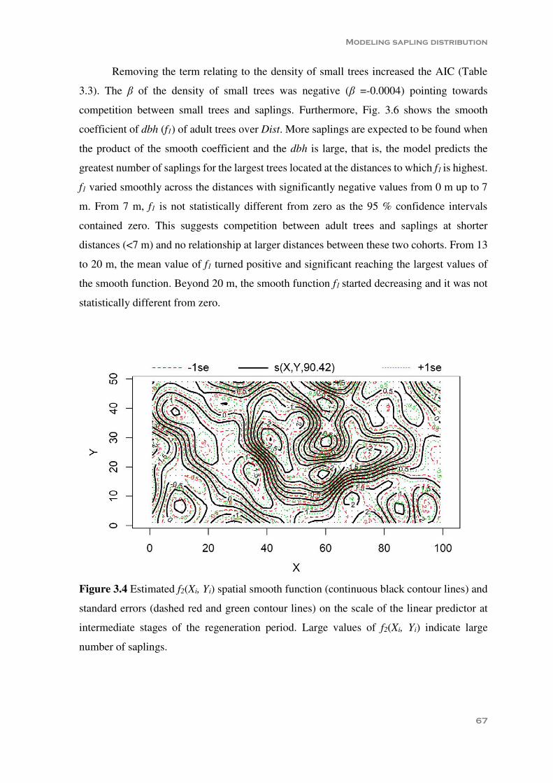
Modeling sapling distribution
67
Removing the term relating to the density of small trees increased the AIC (Table
3.3). The β of the density of small trees was negative (β =-0.0004) pointing towards
competition between small trees and saplings. Furthermore, Fig. 3.6 shows the smooth
coefficient of dbh (f1) of adult trees over Dist. More saplings are expected to be found when
the product of the smooth coefficient and the dbh is large, that is, the model predicts the
greatest number of saplings for the largest trees located at the distances to which f1 is highest.
f1 varied smoothly across the distances with significantly negative values from 0 m up to 7
m. From 7 m, f1 is not statistically different from zero as the 95 % confidence intervals
contained zero. This suggests competition between adult trees and saplings at shorter
distances (<7 m) and no relationship at larger distances between these two cohorts. From 13
to 20 m, the mean value of f1 turned positive and significant reaching the largest values of
the smooth function. Beyond 20 m, the smooth function f1 started decreasing and it was not
statistically different from zero.
Figure 3.4 Estimated f2(Xi, Yi) spatial smooth function (continuous black contour lines) and
standard errors (dashed red and green contour lines) on the scale of the linear predictor at
intermediate stages of the regeneration period. Large values of f2(Xi, Yi) indicate large
number of saplings.

Chapter 3
68
Table 3.2 Percentage of deviance explained, AIC (Akaike´s Information Criterion), θ
parameter in the variance of the negative binomial distribution, basis dimension (k) and
effective degrees of freedom (e.df) of the functional linear predictor and the spatial smooth
according to model 3.1 and model 3.2 in both plots. Inventory 2001, Inventory 2006,
Inventory 2010 and Inventory 2014 indicate the effective degrees of freedom of the spatial
smooth during the four inventories in model 3.2.
Feature Intermediate stage of the
regeneration period
End of the regeneration
period
Model 3.1 Model 3.2 Model 3.1 Model 3.2
Deviance explained (%) 40.7 41.0 34.8 41
AIC 1,3120.98 1,3432.74 5,083.48 5,184.80
θ of variance 1.53 1.42 0.83 0.76
k of f1 10 10 10 10
e.df of f1 3.47 3.599 4.33 4.40
k of f2 100 100 30 30
e.df of f2 in model 3.1 90.42 - 24.50 -
Inventory 2001 - 69.60 - 19.47
Inventory 2006 - 65.64 - 17.30
Inventory 2010 - 63.42 - 16.28
Inventory 2014 - 63.11 - 13.15
f1: linear predictor. f2: spatial smoother
3.3.2. End of the regeneration period
The dynamics of the saplings and the trees followed the same trends as at intermediate stages
of the regeneration period: the number of saplings decreased and their mean size increased
with time. The number of trees decreased but the mean dbh and height increased over the
four inventories because of fellings. However, in this plot there were less saplings and their
mean size was larger than in the youngest studied plot. Additionally, there were more trees
overall at the end of the regeneration period than in the previous stages. Nevertheless, Table
3.1 shows that the number of small trees reduced with time whereas the number of adult
trees increased.

Modeling sapling distribution
69
Table 3.3 Summary of the backward stepwise variables selection process according to the
Akaike´s Information Criterion (AIC). In bold, the selected model.
Variables included in the alternative models during backward stepwise
selection process
AIC
Intermediate stage of the regeneration period
(1) 1 2
1
( ) ,3
Nij jn
in i i j
ni i
Nsmall dbhf Dist f X Y Time
AreaIn10 AreaIn 0
1,3120.98
(2) 1 2
1
( ) ,3
Njn
in i i j
n i
dbhf Dist f X Y Time
AreaIn 0
1,3126.06
(3) 2 ,ij
i i j
i
Nsmallf X Y Time
AreaIn10
1,3125.11
(4)
11
( )3
Nij jn
in
ni i
Nsmall dbhf Dist
AreaIn10 AreaIn 0
1,500.13
(5) 1 2
1
( ) ,3
Nij jn j
in i i
ni i
Nsmall dbhf Dist f X Y
AreaIn10 AreaIn 0
1,3432.74
End of the regeneration period
(1) 1 2
1
( ) ,3
Nij jn
in i i j
ni i
Nsmall dbhf Dist f X Y Time
AreaIn10 AreaIn 0
5,083.94
(2) 1 2
1
( ) ,3
Njn
in i i j
n i
dbhf Dist f X Y Time
AreaIn 0
5,083.48
(3) 2 ,i i jf X Y Time 5,120.71
(4)
11
( )3
Njn
in
n i
dbhf Dist
AreaIn 0
5,387.18
(5) 1 2
1
( ) ,3
Nij jn j
in i i
ni i
Nsmall dbhf Dist f X Y
AreaIn10 AreaIn 0
5,184.80
As in the youngest studied plot, the model with the additive spatio-temporal structure
(model 3.1), which assumes a constant spatial distribution of the saplings over the studied
period, showed a lower AIC than model 3.2 (Table 3.2). We also found a significant effect
of the spatio-temporal terms (f2 and Time) in terms of AIC (Table 3.3). The map of the
contour lines (Fig. 3.7) represents well the spatial distribution of the saplings during the last
stages of the regeneration period (Fig. 3.3). The semivariograms showed that the spatial

Chapter 3
70
structure eliminated the spatial correlation (Fig. 3.8). The estimate of the aggregation
parameter θ of the negative binomial distribution is smaller than in the other plot, it is around
0.8 (Table 3.2). This indicates that saplings were more aggregated at the end of the
regeneration period than in the previous stage, which is also confirmed by the visual
inspection of the spatial distribution of saplings (Figs. 3.2 and 3.3) showing a more
homogenous spread of saplings in earlier stages of the regeneration process.
Figure 3.5 Semivariograms (circles) and envelopes (dashed lines) of the Pearson residuals
from the sapling distribution model at intermediate stages of the regeneration in 2001 (upper
left), 2006 (upper right), 2010 (lower left) and 2014 (lower right).
In this plot, the β of density of small trees did not reduce the AIC whereas the rest of
the terms reduced the AIC significantly (Table 3.3). Table 3.2 shows the effective degrees
of freedom of the basis functions. The coefficient of the dbh of adult trees (f1) took significant
negative values from 0 to 8 m (Fig. 3.6). From 8 m, the 95 % confidence intervals contained
the zero, and therefore we can state that the coefficient is not statistically different from 0.

Modeling sapling distribution
71
This suggests competition between saplings and adult trees at very small distances and no
effect beyond 8 m.
Figure 3.6 Estimated f1(Distin) smooth coefficient function of the diameter at breast height
of adult trees over the distance between adult trees and saplings (continuous lines) and 95%
confidence intervals (dashed lines) at intermediate stages (upper) and the end (lower) of the
regeneration period. Positive values of f1(Distin) indicate positive effects of the diameter at
breast height of adult trees on the number of saplings.

Chapter 3
72
Figure 3.7 Estimated f2(Xi, Yi) spatial
smooth function (continuous black contour
lines) and standard errors (dashed red and
green contour lines) on the scale of the linear
predictor at the end of the regeneration
period. Large values of f2(Xi, Yi) indicate
large number of saplings.
Figure 3.8 Semivariograms (circles) and envelopes (dashed lines) of the Pearson residuals
from the sapling distribution model at the end of the regeneration period in 2001 (upper left),
2006 (upper right), 2010 (lower left) and 2014 (lower right).

Modeling sapling distribution
73
3.4. Discussion
We fitted a GAM with a functional predictor in the model to describe the influence of size
of trees on the number of saplings by distance in two stages of the regeneration period. We
have confirmed that the functional predictor is useful to achieve this aim. In GAMs
explanatory variables may enter the model in many different forms: as variables with linear
effects, smooth terms, tensor products of several variables, with varying coefficients or as
functional predictors. Additionally, alternative response distribution families and link
functions can be selected (see for example Wood 2006). Therefore, all this makes the
approach employed suitable to be used in other fields of forestry or ecology in which the
response variable depends on the size and distance of the neighbors. For instance, this
approach could be useful to fit growth or mortality models instead of using competition
indices in parametric models (Contreras et al. 2011).
In this work, we have studied the last stages of the renewal of a forest after
regeneration fellings. Other authors have modeled the whole renewal of the forest using
multistage models. For instance, Manso et al. (2014) proposed a multistage model based on
partial studies or submodels in order to predict the regeneration occurrence of Pinus pinea
L. in space and time. They considered different stages such as seed dispersal, seed
germination, post-dispersal predation and seedling survival. Multistage models provide
deeper ecological understanding than ours but the implementation is harder and requires
stronger ecological hypotheses. However, our approach shows great flexibility and might be
used to determine the effects of a limited number of factors on sapling distribution without
making any assumptions about other factors involved on dispersion and survival processes.
As mentioned above, this methodology allows different types of variables to be
included in the model. In this work, we included the density of small trees as a linear term
and the spatio-temporal structure. It might be useful to use variables driving the regeneration
as predictors in the model, like shrub cover, soil characteristics, cover and depth of litter or
grass in each quadrat. However, gathering this data on large plots requires a great effort and
the influence of these variables on the seedlings of P. sylvestris has already been studied at
smaller scales (González-Martínez and Bravo 2001; Pardos et al. 2007; Barbeito et al. 2011;
Moreno-Fernández et al. 2015a). On the other hand, new individuals of P. sylvestris are
expected to be more affected by soil moisture than by other microsite characteristics
(Barbeito et al. 2009; Moreno-Fernández et al. 2015a). However, because youngest

Chapter 3
74
individuals – seedlings – are less resistant to drought than older – saplings (Maseda and
Fernández 2006; Rodríguez-García et al. 2011; Manso et al. 2014), it seems it is more
necessary to include environmental variables in models dealing with seedlings rather than in
those dealing with older individuals – saplings. Moreover, it is likely the distance to adult
trees is confounded with other local factors. Any residual spatial trend in a model without a
spatial smooth term is caused by missing (unmeasured) environmental variables.
Furthermore, the residual spatial trend could be due to the seedling spatial structure that
would result from past dispersal events from adjacent mother trees. We have included the
spatial smooth term as a proxy for effects of unmeasured environmental variables and for
the spatial pattern of the new individuals during previous stages of the forest renewal. We
have investigated goodness-of-fit thoroughly, and found that we did not have any spatial
trend in residuals or residual spatial correlation. This means that the models fit well and there
was no model mis-specification. Although we have only results from two plots, it is striking
that the estimated functions f1 (of the effect of dbh) shown in Fig. 3.6 are very similar.
Our approach allows to test whether the spatial pattern remained constant over time
by comparing model 3.1 which assumes a constant spatial pattern with model 3.2 which
allows for a spatial pattern changing in time in the model selection. In our case, model 3.1
was selected suggesting that the spatial pattern of the saplings remained constant over time.
If model 3.2 had been selected, the spatial pattern of saplings would have changed over the
time. Due to the gradual low intensity fellings regime, which avoids damaging the
established saplings clumps, these clumps persist and the spatial structure of the saplings
remains fairly constant in each plot during the 15-year measurement period. On the other
hand, if we were dealing with faster-growth species the saplings could move to the next
cohort faster and then change the spatial pattern. Our results are consistent with LeMay et
al. (2009) who reported that the spatial pattern of the new individuals of P. menziesii did not
change very much over time.
Although we only analyzed data from two large plots (0.5 ha) we re-measured the
plots four times, leading to four observations per plot. Large-sized plots with few sampling
over time are common in regeneration studies describing spatial processes. These kind of
plots have been used in tropical (Ledo et al. 2015), temperate (McDonald et al. 2003) and
Mediterranean forests (Montes and Cañellas 2007; Ledo et al. 2014). Additionally, we
modeled the number of saplings per 4 m2 quadrat, i.e., we used 5 000 quadrats covering
different competition conditions to fit every model. Moreover, the models presented in this

Modeling sapling distribution
75
work were fitted for explanatory purposes rather than predictive purposes. If we had aimed
to fit a predictive model, we would have needed more temporal measurements to cover all
the regeneration period.
The underlying process studied here is the competition between trees and saplings.
Our findings are in concordance with other studies: the saplings of P. sylvestris require high
light conditions for successful development (Montes and Cañellas 2007). In Mediterranean
areas, P. sylvestris seedlings require microsites with moderate light conditions (Pardos et al.
2007). These microsites ensure higher soil moisture than in open canopies but conserve
enough level of sun radiation. In this regard, Castro et al. (2005) analyzed the growth of P.
sylvestris seedlings in southern Spain under different light and water conditions concluding
that the effects of water addition on seedlings growth are more evident in lightly microsites.
Moreover, once the seedlings have stepped into saplings, the maintenance costs increase
with size (Falster and Westoby 2003) and higher minimum light levels are required for
survival (Williams et al. 1999). Additionally, their roots can reach deeper soil layers with
more water availability (Ritchie 1981). Considering this, it seems it is necessary to reduce
the canopy to favor the development of the saplings after seedling establishment under
moderate light conditions in Mediterranean areas. However, the shade tolerance of P.
sylvestris differ among regions. In northern locations where the summer drought is not a
limiting factor for seedling development, natural regeneration takes place in open canopies
by using the seed tree method (Hyppönen et al. 2013). In these latitudes, the negative spatial
association between P. sylvestris adult trees and saplings may be even more pronounced than
in our study.
The establishment of the new stand has been achieved successfully at the end of the
regeneration period, the number of saplings decreased and the arrival of new individuals is
no longer expected. Hence, the mean dbh of the saplings is getting close to 10 cm, the lower
limit for small trees. In this plot, the number of small trees decreased over time due to the
mortality as well as the growth and consequent reclassification of trees as adult trees. Most
of the trees in this plot were not mother trees of the saplings but rather new cohorts of trees
established at the first and intermediate stages of the regeneration period, such as those in
our youngest studied plot. Therefore, the spacing between saplings and adult trees is a
consequence of the competition between trees of different sizes.

Chapter 3
76
3.5. Conclusions
We show that functional predictor in GAMs is a useful tool for modeling these kind of data
as they allow to model nonlinear and linear relationships. In addition they allow to take
account of the spatio-temporal structure of the data by inclusion of spatial and spatio-
temporal smooth predictors. The methodology proposed has not been employed in forestry
or ecology and can be broadly used in regeneration studies or in other fields of forestry or
ecology dealing with spatio-temporal data. Therefore this methodology is potentially
applicable in future ecological studies because of its flexibility. Additionally, this model can
be used as a first step for a predictive model when more temporal data is available. We found
that once the seedlings have become established, the density of the adult trees must be
reduced heavily to allow the saplings to grow under high light conditions. In Mediterranean
stands of P. sylvestris, the radius of the gaps created during the regeneration fellings under
the group shelterwood should be always larger than 7-8 m in order to minimize the
competition between adult trees and saplings; whereas if the radius is between 13 – 20 m the
number of saplings will be maximized.
Acknowledgements
We wish to thank everybody who participated in the field work, especially Ángel Bachiller,
Estrella Viscasillas and Enrique Garriga. We appreciate the comments made by the referees
and the editors of Annals of Forest Science during the revision process. We also thank Adam
Collins for revising the English writing. DMF has been funded by Spanish Ministry of
Education, Culture and Sport thorough the FPU program (FPU13/02113) and by the short-
term visiting program (EST15/00242). This work has been funded by AGL2013-46028-R
and BOSSANOVA-CM (S2013/MAE-2760).

Temporal carbon dynamics over the rotation period of
two alternative management systems in Mediterranean
mountain Scots pine forests
Moreno-Fernández D, Díaz-Pinés E, Barbeito I, Sánchez-González M, Montes F, Rubio A,
Cañellas I (2015) Temporal carbon dynamics over the rotation period of two alternative
management systems in Mediterranean mountain Scots pine forests. For Ecol Manage 348,
186-195. doi: 10.1016/j.foreco.2015.03.043
CHAPTER 4


Temporal carbon dynamics
79
Abstract
Forests play an important role in the mitigation of global warming, acting as carbon sinks.
However, the effects of forest management on the carbon pools over the rotation period in
Mediterranean areas are scarcely understood. The objective of this chapter is to assess the
way in which two alternative management systems; one more intensive and the other more
moderate (with less severe harvesting and more spread over time) affect the carbon stocks
in the living tree biomass, coarse woody debris, forest floor and mineral soil in
Mediterranean forests. For this purpose, two chronosequences were established covering the
whole rotation period in two Pinus sylvestris L. forests. We conducted four forest inventories
over a period of 15 years, measuring the diameter and the height of all the trees higher than
1.3 m in order to calculate the carbon stored in the living parts of the tree. Soil pits were
excavated and we collected soil samples to estimate the soil organic carbon. We found that
the temporal trends for living tree biomass were similar in both forests. However, the total
living tree carbon stored at the end of the rotation period was greater in the forest with the
longer rotation period and lighter thinning regime (345.5 Mg ha-1 of carbon) than in the
intensively-managed forest (223.8 Mg ha-1 of carbon). On average, more carbon was found
to be stored in the forest floor under the more intensive management system, whereas more
carbon was present in the first 20 cm of mineral soil under the moderate management system.
Moreover, in each forest, the carbon stocks of the forest floor and in the uppermost cm of
the soil remained constant over the rotation period. Therefore, management systems with
longer rotation periods and moderate harvesting intensities are recommended to increase
carbon fixation in Mediterranean forests.
Keywords: carbon stocks, climate change, adaptive forest management, silviculture
Abbreviations: AIC, Akaike´s Information Criteria; C, Carbon; CWD, Coarse Woody
Debris; SOC, Soil Organic Carbon; LTC: Living Tree Carbon

Chapter 4
80
4.1. Introduction
Rising atmospheric concentrations of carbon dioxide contribute to global warming (IPCC
2013). Forests are considered to play an important role in mitigating this global warming
through carbon (C) sequestration (Dixon et al. 1994; Lal 2004; Bravo et al. 2008b). Forests
store between 40 % - 60 % of all terrestrial C (Bonan 2008; Pan et al. 2011) and sequester
33% of C emission from fossil fuels every year (Denman and Brasseur 2007). However,
forests can become a net source of carbon dioxide, depending on the climatic conditions and
the forest management employed, since both affect C gains and losses within the forest
system (Kim Phat et al. 2004; Vayreda et al. 2012).
The quantification of forest C and the influence of management on C sequestration
have become a focus of interest for both researchers and forest managers (Smith and Heath
2001; Jandl et al. 2007; Alvarez et al. 2014). In recent years, many studies have assessed the
way in which C stocks are affected by various aspects of management such as thinning
(Finkral and Evans 2008; Boerner et al. 2008; Ruiz-Peinado et al. 2013), length of the
rotation period (Liski et al. 2001; Pohjola and Valsta 2007), different management systems
(Balboa-Murias et al. 2006; Seidl et al. 2007), stand tree species composition (Kirby and
Potvin 2007; Díaz-Pinés et al. 2011; Alvarez et al. 2014), harvesting technique (Johnson and
Curtis 2001), the reproductive origin of the tree (Bruckman et al. 2011) and site preparation
(Yildiz et al. 2010; Fonseca et al. 2014) among others.
Penman et al. (2003) defined five pools of C within forest ecosystems: living tree
biomass –aboveground and belowground (roots), deadwood, forest floor and soil organic
carbon (SOC). The living tree biomass and the SOC are the pools which store the most C in
forest ecosystems (Peichl and Arain 2006; Nunes et al. 2010; Ruiz-Peinado et al. 2013). The
C stored in the living parts of the trees, i.e. living tree carbon (LTC), is highly conditioned
by the age of the stand, site index and management (De Simon et al. 2012; Ruiz-Peinado et
al. 2013). However, SOC is more resistant to changes in forest management and disturbances
than the LTC (Vesterdal et al. 2002; Peichl and Arain 2006; Bradford et al. 2008). Indeed,
most studies have reported that management has no significant effect on SOC (Johnson and
Curtis 2001; Ruiz-Peinado et al. 2014) or that harvesting only causes a small, temporal
reduction in SOC after harvesting (Yanai et al. 2000; Peltoniemi et al. 2004; Nave et al.
2010). The effect of forest management on the forest floor is still somewhat debataed. Nave
et al. (2010) reported losses in forest floor C storage after harvesting operations whereas in

Temporal carbon dynamics
81
Mediterranean areas, Ruiz-Peinado et al. (2014, 2013) found that thinning had no significant
impact on forest floor C stocks.
A better understanding of the dynamics of the different C pools throughout stand
development is required in order to make a reliable assessment of the long-term effects of
forest management on C (Kolari et al. 2004; Peltoniemi et al. 2004). Only a small number
of studies have adopted a comprehensive approach embracing tree and SOC pools in the
evaluation of C dynamics (Peichl and Arain 2006). Furthermore, most of the studies have
been conducted in boreal and temperate forests, while information with regard to C dynamics
in Mediterranean areas is scarce (Montes and Cañellas 2006; De Simon et al. 2012). In
addition to determining how C stocks are distributed among the different pools and the way
in which forest management affects these stocks, the mechanisms underlying C transfer
among pools (Fig. 4.1) must also be identified in order to elucidate the impact of forest
management on the C transference processes (e.g. Bradford et al. 2008).
Figure 4.1 C transfer links among forest pools.
Scots pine is the most widely distributed pine species in the world, ranging from the
Iberian Peninsula to Siberia (Mason and Alía 2000). The importance of this species in Spain
is due not only to its extensive distribution area and high quality wood, but also to its
ecological value and protective function against soil erosion (Montero et al. 2001). The
rotation period in Mediterranean pine forests is around 100-140 years, depending on the

Chapter 4
82
intensity of the silvicultural operations. The establishment of new seedlings is often achieved
under the shelterwood system and is sometimes aided by soil preparation (Cañellas et al.
2000; Barbeito et al. 2011). It is assumed that the group shelterwood system leads to an
increase in structural biodiversity (Barbeito et al. 2009) and that it encourages more
continuous establishment of regeneration to remain more constant over time. Under the
shelterwood system the seedlings are also less affected by summer drought (Barbeito et al.
2011). However, the way in which the management alternative affects C sequestration in
Mediterranean pine forests is still scarcely understood.
In this study, we used a chronosequence approach to quantify the LTC and soil
carbon pool (SOC and forest floor C storage) over the rotation period in Scots pine
Mediterranean forests under two management alternatives. The objective of this study is to
assess the influence of the management regime on forest C dynamics over the rotation
period. Three hypotheses were evaluated: i) long rotation length and a moderate thinning
regime increase the LTC sequestration rate, ii) the SOC and the forest floor C pool are
affected by the forest management regime and iii) SOC remains constant throughout the
rotation period whereas forest floor C is affected by the silvicultural operations.
4.2. Materials and methods
4.2.1. Study areas
The study was conducted in two managed Scots pine forests, Navafría (41º 0´N, 3º 48´W)
and Valsaín (40º 49´N, 4º 01´W), located in the Central Range of Spain. Both forests are
located on north-facing slopes of the mountain range and they share similar ecological
characteristics, with elevations ranging from 1,200 to 2,200 m above sea level, annual
rainfall of about 730 mm, and mean annual temperature of around 9.8 ºC. Despite these
similarities, the average site quality is slightly higher in Valsaín than in Navafría (Rojo and
Montero 1996). The management plans and harvest history of both forests date back 100
years and reveal several differences between the forests (Table 4.1). At Navafría, the
thinning regime is more intense and begins at an earlier age. The uniform shelterwood
system is used in this forest, consisting of two or three regeneration fellings over a 20 year
regeneration period. In addition, in order to facilitate the establishment of the seedlings,
mechanical soil tilling is carried out. At Valsaín, regeneration is achieved using the group
shelterwood system, opening small gaps (0.1-0.2 ha) in the regeneration area over a 40 year

Temporal carbon dynamics
83
regeneration period. Thus, natural regeneration becomes established progressively under the
protection of the remaining trees (Barbeito et al. 2009).
Table 4.1 Management characteristic in Navafría and Valsaín forests.
Management characteristic Navafría forest Valsaín forest
Management system Permanent blocks Floating periodic blocks
Rotation period 100 years 120 years
Thinning intensity >30% G removed 20-30% G removed
Regeneration method Uniform shelterwood Group shelterwood
Regeneration period 20 years 40 years
Area of regeneration
cuttings
20 ha 2-3 ha
Soil preparation Ripper and blade scarification No
G: basal area.
4.2.2. Sampling design and estimation of C fractions
4.2.2.1. Plot description and estimation of LTC and dead wood carbon
Two chronosequences spanning the whole rotation period in the two Scots pine forests were
established in 2001: six 0.5 ha plots were set up in Valsaín and five in Navafría (Table 4.2).
The plots were as homogeneous as possible in terms of altitude, exposure and site quality,
the aim being to consider confounding factors other than stand age (Foster and Tilman 2000).
At the time of establishment (2001), all the trees higher than 1.30 m were labeled
individually and their diameters at breast height (dbh) and heights were measured. The
measurements were carried out again in 2006, 2011 and 2014. The main characteristics of
the plots at the time of establishment are shown in Table 4.2. We applied the additive
biomass models for Scots pine developed by Ruiz-Peinado et al. (2011) using data from our
study area to estimate the biomass of stem, thick branches, medium branches, thin branches
plus needles and roots of living Scots pine trees (Table 4.3). We then added up all the various
components to obtain the living tree biomass. The LTC stock was calculated using a C
weight / biomass weight ratio of 0.509 (Ibañez et al. 2002).

Chapter 4
84
Table 4.2 Mean characteristics of the plots at the time of establishment (2001).
Plot Age N≥10cm N<10cm Dm≥10cm Dm<10cm G Hm≥10cm Hm<10cm
Navafría N1 10 810 4906 11.9 6.6 27.0 7.6 6.0
N2 28 2184 298 14.8 9.2 41.9 12.1 11.2
N3 65 680 - 32.9 - 60.6 22.0 -
N4 94 364 - 40.6 - 48.2 20.4 -
N5 110 304 - 42.5 - 44.2 22.1 -
Valsaín V1 19 458 8876 23.2 5.5 37.0 15.1 3.2
V2 32 1484 1118 16.9 9.2 40.8 14.7 7.0
V3 49 1296 26 20.8 9.2 48.3 16.4 11.9
V4 75 686 - 30.5 - 53.3 23.5 -
V5 96 552 - 34.7 - 54.2 22.1 -
V6 115 332 516 38.9 1.5 54.2 24.0 2.0
Age in years; G= basal area (m2 ha-1); N= number of trees per hectare; Dm= mean diameter (cm); Hm= mean
height (m); ≥10cm and <10cm indicate attributes for trees with dbh equal or larger than 10 cm and trees with dbh
of less than 10 cm.
Table 4.3 Biomass models and fitting statistics for Scots pine (Ruiz-Peinado et al. 2011)
used in our study.
Component Model RMSE ME
Stem Ws = 0.0154 d2 h 34.01 0.99
Thick branches If d ≤ 37.5 cm then Z = 0; If d > 37.5 cm then Z = 1; Wb7 = [0.540 (d-37.5)2 – 0.0119 (d-37.5)2 h] Z
12.63 0.86
Medium branches Wb2-7 = 0.0295 d2.742 h–0.899 10.83 0.87
Thin branches +
needles
Wb2+n = 0.530 d2.199 h–1.153 11.41 0.87
Roots Wr = 0.130 d2 110.17 0.98
Ws: Biomass of the stem fraction (kg). Wb7: Biomass of thick branch fraction (diameter larger than 7 cm) (kg).
Wb2-7: Biomass of medium branch fraction (diameter between 2 and 7 cm) (kg). Wb2+n Biomass of thin branch
fraction (diameter smaller than 2 cm) with needles (kg). Wr: Biomass of the roots (kg); d: dbh (cm). h: tree
height (m). RMSE: Root Mean Square Error. ME: Model Efficiency.

Temporal carbon dynamics
85
Since each individual tree was numbered it was possible to monitor which trees had
died or were harvested. Mortality rates were quite low, affecting mainly saplings. The sum
of harvested and dead trees was referred to as “extracted trees” and was estimated in each
plot between consecutive inventories. We calculated the total tree C at the end of the rotation
period by summing the LTC in the oldest plot in each forest in 2014 plus the cumulative
extracted C in each forest (sum of the C removed from the forest during the rotation period).
In addition, we estimated the LTC growth rates (Mg ha-1 year-1 of C) for each plot and period
between inventories.
Dead wood C was assessed using the coarse woody debris (CWD) data from a study
by Montes and Cañellas (2006), recorded in our study plots in 2002. They classified the
CWD into five decay classes and four elements: logs and branches (diameter at midpoint
larger than 10 cm or between 5 and 10 cm) and stumps (cut surface diameter greater than 30
cm or between 5 and 30 cm). Detailed information on the sampling design is given in Montes
and Cañellas (2006). The weight of the stumps was estimated using the biomass model for
roots proposed by Ruiz-Peinado et al. (2011) (Table 4.3), assuming that the shape of the
stem between dbh and the soil surface is cylindrical (i.e. dbh equals the stump diameter). We
calculated the volume of logs and branches from their length and diameter, and then we
converted the volume into biomass weight using empirical density data (unpublished data)
according to decay class. Finally, the biomass of the stumps, branches and logs was
transformed into C using a C weight / biomass weight ratio of 0.509 (Ibañez et al. 2002).
4.2.2.2. Sampling of soil pool C stock (Carbon stock in O-horizon and mineral soil)
Estimation of the forest floor C pool was performed in April 2009, using 4 replicates per
plot. In each replicate, the whole forest floor down to the mineral soil was collected in a 1 x
1 m square. No differentiation was made between organic layers (Ol, Oh, Of) when collecting
the samples. The depth of the forest floor layer was measured on each side of the square and
then averaged. The exact location of the square was marked appropriately by inserting
wooden sticks into the soil.
Freshly incorporated material to the forest floor layer was collected between April
2009 and April 2010, following the same procedure in the same squares. It was decided to
start and end the measurements in April since the late winter and spring periods present the
lowest seasonal litterfall C rates in this area (Díaz-Pinés et al 2011b), hence potential bias

Chapter 4
86
caused by seasonal variability was minimized. We took three measurements: in August and
November 2009 and in April 2010. This allowed the annual aboveground litterfall C rates to
be calculated.
To estimate SOC pools, five soil pits (70 cm x 70 cm x 50 cm, treated as replicates)
were excavated at each of the plots. In each of the pits, genetic horizons were identified
down to 50 cm. Soil samples were collected separately for each genetic horizon, beginning
with the deepest one to avoid up-down soil contamination. In addition, intact soil cores (5
cm height, 5 cm diameter) were taken by triplicate at each of the soil horizons for soil bulk
density determination. Stone content was estimated in the field for each horizon. A sampling
approach based on genetic horizons was chosen to avoid potential bias associated with fixed
depth approaches when the horizon development is markedly different among sites
(Davidson and Ackerman 1993).
4.2.2.3. Laboratory analyses
The forest floor material was dried at 65 °C to constant weight and sieved (2 mm-mesh).
Both fine and coarse fractions were weighed separately. Particles that passed through the
sieve were milled and the total organic C in this fraction was determined using a Total
Organic Carbon Analyzer (TOC 5000A, Shimadzu Corporation, Kyoto, Japan) equipped
with a soil sample module (SSM-500, Shimadzu Corporation). Particles larger than 2 mm
were assumed to have a content of 50.9 % organic C (Ibañez et al. 2002). The TOC 5000-A
equipped with the SSM-500 was also used to determine the SOC content of the ground
mineral soil samples.
Organic C stocks of the forest floor were calculated based on the weight of the layer
per unit of area and the organic C content. Aboveground litterfall C rates were calculated by
summing the amounts of litterfall collected during a time span of 12 months and expressed
in Mg ha-1 year-1 of C. In the case of the mineral soil, organic C stocks were calculated
according to the recommendations of the IPCC (Aalde et al. 2006), taking into account
organic C content, soil bulk density, fine earth content and depth of each layer (Table 4.4).
Since the mineral soils were collected according to genetic horizons, the depths were not
consistent among different plots and replicates. Therefore, we calculated the SOC stocks per
cm depth within the soil profile; for comparison purposes among plots, we virtually divided
the soil profile into 10 cm deep layers.

Temporal carbon dynamics
87
Table 4.4 SOC concentration, bulk density and stone content in each plot.
SOC concentration (g kg-1 fine soil)
Plot 0-10 10-20 20-30 30-40 40-50 10N 72.9 ± 6.3 72.9 ± 6.3 66.0 ± 2.7 57.6 ± 5.5 50.7 ± 10.6 30N 46.1 ± 4.5 39.9 ± 3.7 27.4 ± 4.1 17.8 ± 5.2 7.8 ± 1.9 50N 49.3 ± 4.0 40.2 ± 5.8 24.6 ± 7.2 20.6 ± 8.8 16.7 ± 9.7 70N 59.1 ± 5.1 59.1 ± 5.1 47.3 ± 5.7 41.7 ± 4.0 33.6 ± 2.0 90N 67.9 ± 4.7 62.8 ± 5.3 52.6 ± 4.8 48.8 ± 5.7 39.3 ± 7.0 10V 76.5 ±7.2 65.5 ±4.9 34.4 ±11.3 12.6 ±4.0 8.8 ±0.5 30V 89.6 ±11.7 68.2 ±6.2 51.1 ±4.3 35.7 ±5.4 12.9 ±3.1 50V 58.8 ±7.8 59.1 ±7.5 33.4 ±2.7 30.0 ±2.5 8.7 ±1.8 70V 77.1 ±4.8 60.5 ±6.2 37.8 ±3.7 15.2 ±5.0 9.1 ±2.7 90V 77.4 ±10.4 61.5 ±9.6 34.4 ±6.3 18.2 ±3.2 10.0 ±2.0 110V 97.5 ±12.0 81.5 ±9.6 62.5 ±11.7 27.0 ±9.1 11.1 ±1.8
Bulk density (g cm-3)
Plot 0-10 10-20 20-30 30-40 40-50 10N 0.80 ± 0.03 0.80 ± 0.03 0.92 ± 0.07 0.98 ± 0.08 1.03 ± 0.12 30N 0.88 ± 0.03 0.87 ± 0.02 0.96 ± 0.03 1.04 ± 0.07 1.19 ± 0.09 50N 0.89 ± 0.03 0.92 ± 0.03 0.96 ± 0.06 1.02 ± 0.06 1.08 ± 0.07 70N 0.83 ± 0.04 0..83 ± 0.04 0.90 ± 0.04 0.95 ± 0.04 1.00 ± 0.01 90N 0.74 ± 0.08 0.87 ± 0.06 0.89 ± 0.05 0.89 ± 0.05 0.92 ± 0.06 10V 0.83 ± 0.03 0.85 ± 0.03 0.89 ± 0.03 0.93 ± 0.02 0.95 ± 0.02 30V 0.72 ± 0.03 0.82 ± 0.06 0.88 ± 0.07 0.97 ± 0.04 1.07 ± 0.05 50V 0.82 ± 0.04 0.81 ± 0.04 0.84 ± 0.02 0.87 ± 0.03 1.08 ± 0.02 70V 0.80 ± 0.04 0.92 ± 0.08 0.97 ± 0.06 1.13 ± 0.04 1.18 ± 0.03 90V 0.88 ± 0.01 0.92 ± 0.03 0.96 ± 0.04 1.01 ± 0.01 1.02 ± 0.01 110V 0.86 ± 0.04 0.91 ± 0.03 0.94 ± 0.03 0.99 ± 0.01 1.03 ± 0.03
Stone content (%)
Plot 0-10 10-20 20-30 30-40 40-50 10N 58 ±5 58 ±5 54 ±4 52 ± 6 53 ± 6 30N 38 ±4 40 ±3 38 ±3 40 ± 6 41 ± 6 50N 37 ±2 41 ±2 49 ±4 53 ± 3 55 ± 3 70N 40 ±3 40 ±3 41 ±4 42 ± 3 44 ± 4 90N 49 ±3 48 ±3 45 ±4 43 ± 3 46 ± 3 10V 31 ± 2 33 ± 3 39 ± 5 48 ± 6 49 ±5 30V 32 ± 2 37 ± 4 42 ± 6 48 ± 7 59 ±8 50V 39 ± 4 42 ± 3 46 ± 3 46 ± 3 46 ±15 70V 37 ± 4 35 ± 3 36 ± 4 37 ± 4 36 ± 4 90V 38 ± 5 40 ± 5 48 ± 11 56 ± 9 54 ± 10 110V 45 ± 6 54 ± 2 59 ± 2 72 ± 2 78 ± 1

Chapter 4
88
4.2.3. Statistical analyses
4.2.3.1. Living Tree Carbon
In order to describe the LTC trends over the rotation period we fitted the data using an
approach that ensured sufficient flexibility of the LTC trends. In this study we attempted to
model the LTC trends over time using penalized smoothing splines or P-splines (Eilers and
Marx 1996) in a mixed model-effects framework (Durbán et al. 2005). The P-splines are
curves formed by joining together several low-order polynomials at specified locations
known as knots (Eilers and Marx 1996; Durbán et al. 2005; Jordan et al. 2008). The penalty
approach relaxes the importance of the number and location of the knots (Eilers and Marx
1996; Currie et al. 2004). We fitted a separate mean curve for each forest using a factor-by-
curve interaction to assess the differences in the LTC trends between forests (Currie et al.
2004; Durbán et al. 2005; Jordan et al. 2008). The penalized spline formulation of the model
is written as:
ilj i i lj iljy A f B Z u (4.1)
where yilj is the LTC (in Mg ha-1 of C), i is the forest stand number, l is the plot number and
j is the age (years)., Ai is a dummy variable for the forest, α is the forest fixed-effects
parameter vector, and fi(.) is a smooth function which reflects the trend of the LTC over each
year Blj. Detailed explanation of the smooth function f(.) is given further. Z is the random-
effects matrix and u is the vector of random effects with mean zero and variance to be
estimated. Given that the data available consisted of repeated measurements taken in the
same plot and that such measurements are likely to be more correlated than measurements
taken in different plots (Littell et al. 2000) we entered plot random intercept and slope
effects. Due to the differences in the site quality of the plots according to the Rojo and
Montero (1996) site index models, we included site quality random intercept and slope
effects. εilj is a random error term defining the within-subject pattern of variability. In the
first instance we fitted the model without including random effects and compared it to
models with more complicated random effects structures. The comparisons were performed
according to Akaike´s Information Criteria (AIC).
The smooth functions f(.) were represented by cubic B-splines and second order
difference penalties (Eilers and Marx 1996; Currie et al. 2004). Eilers and Marx (1996)
proposed a simple idea based on two main aspects: a regression basis and modifying the

Temporal carbon dynamics
89
likelihood function by adding a penalty term over adjacent regression coefficient to control
the smoothness of the fit. There are several alternatives for choice of the regression basis,
we used the B-spline basis due to their flexibility and ease of computation. The mixed model
representation of the smooth function f(.) is Currie et al. (2004):
i lj lj lj i lj ljf B x w z x h (4.2)
where zi = 1 for Valsaín and zi = 0 for Navafría, and wlj and hlj are the random effects of the
nonlinear functions. The first two terms in Eq. (4.2) specify the fitted curve for the Navafría
forest and the last term represents the deviation of the fitted curve for Valsaín as compared
with Navafría. Both wlj and hlj are assumed to follow a normal distribution with mean zero
and variances 2w
and 2h
. The smoothing parameter is given by the ratio of the variance
components. We have assumed a common variance parameter for both curves but the
random effects are independent from function to function, i.e., the curves are different but
have the same amount of smoothing (Durbán et al. 2005).
Finally, we plotted the estimated smooth predictor trend with 95 % variability bands
(Greven et al. 2006). All statistical analyses were conducted using SAS 9.2 (SAS Institute
Inc 2009). Once the smooth trends were fitted we calculated the average C in each forest as
the ratio of the areas under the curves and the rotation age.
4.2.3.2. Soil organic carbon pool
Soil organic C stocks at different depths were compared between the two forests under
investigation as well as among different forest ages. Since the number of plots (6 plots for
Valsaín, 5 for Navafría) and the ages of the plots differ between forests, we performed a
nested analysis of variance, with the factor “plot age” nested in the factor “forests”. The
following model was proposed:
( )ijk i j i ijks F C (4.3)
where sijk is the soil C stock in the different soil layers (forest floor, 0-10 cm, 10-20 cm, 20-
30 cm, 30-40 cm, 40-50 cm, 0-50 cm and 0-50 cm plus forest floor) of the k-th observation
in the forest i-th in the plot age j-th, μ is the intercept of the model or overall mean; Fi is the
effect of the i-th forest and Cj(i) is the plot age effect of the j-th plot age nested in the i-th

Chapter 4
90
forest; εijk is the experimental error term of the k-th observation from the j-th plot age within
the i-th forest. We assumed that εijk~N (0, σ2). All analyses were carried out using the GLM
procedure in SAS 9.2 (SAS Institute Inc 2009).
We applied linear regressions to look for relationships between different C pools, and
used the coefficient of determination (R2) as a metric for the goodness-of-fit. In order to
compare the time evolution of different SOC stocks in different soil layers, we used
standardized scores. Thus, for a specific soil layer, we standardized the SOC stocks with the
mean SOC stocks over the whole rotation period
4.3. Results
4.3.1. LTC, extracted C and dead wood C
We fitted the LTC trends using B-splines of degree 3. We selected 6 knots in each smooth
trend to ensure the flexibility of the curve. We found a significant effect of the forest on the
LTC (p-value<0.0001). The Valsaín forest had a higher estimation coefficient than Navafría
(Table 4.5) indicating that, on average, Valsaín stored more LTC than Navafría. In addition,
the differences between the forests were statistically constant over the rotation period since
the interaction forest x age emerged as non-significant (p-value=0.8997). The
autocorrelation among the plots was accounted for by entering the random plot slope as a
significant effect in terms of AIC. Both forests followed similar LTC smooth trends over
time (Fig. 4.2) from the beginning of the rotation period (76.2 Mg ha-1 of C in Navafría at
an age of 10 years and 112.1 Mg ha-1 of C in Valsaín at 19 years). The LTC trends increased
up to an age of 80 years in Navafría (191.5 Mg ha-1 of C) and up to 106 years in Valsaín
(189.5 Mg ha-1 of C). The LTC then fell after the last thinning and regeneration fellings.
Prior to the regeneration fellings, the LTC in Navafría was 156.0 Mg ha-1 of C (stand
age=110 years) and in Valsaín 210.89 Mg ha-1 of C (stand age=100 years). At the end of the
rotation period, the estimated LTC was 99.3 and 160.0 Mg ha-1 of C in Navafría and Valsaín,
respectively. The ratio of the area under the curve and the rotation age was also smaller in
Navafría than in Valsaín (148.9 and 162.9 Mg ha-1 of C, respectively), indicating larger
average LTC stocks in Valsaín than in Navafría over the rotation period.

Temporal carbon dynamics
91
Figure 4.2 Estimated smooth trends of the living tree carbon (LTC) in Navafría (solid blue
line) and in Valsaín (dashed red line), the 95 % confidence limits (bands) and the observed
values (blue circles in Navafría and red crosses in Valsaín).
Table 4.5 Estimates of the parameters of the fixed effects and covariance parameters of
random effects for the living tree carbon model (see Equation 4.1).
Source Effect Estimate Standard error p-value
Forest Navafría 108.39 20.13 <0.0001
Forest Valsaín 136.97 21.58 <0.0001
Forest x Age Navafría -0.31 4.21 0.9428
Forest x Age Valsaín 1.96 4.29 0.6589
Random slope plot effect 17.41 12.88 0.0882
In Navafría, N5 was the plot from which the most C was extracted. In this plot,
regeneration fellings were carried out from 2001-2006 (stand age: 110 years), removing
95.93 Mg ha-1 of C (Fig. 4.3). The remaining trees in N5 were removed at the end of 2014,
before conducting our last forest inventory. The last thinning and regeneration felling

Chapter 4
92
operations started at an age of 106 years (V5 and V6). Thinnings began in N1 in Navafría
when the plot was 20 years old and were also carried out in N2 at 28 and 38 years. In Valsaín,
first thinning was performed in V2 (32 years of age) and the second thinning was carried out
10 years later. Thinnings were carried out in V3 in the same forest from 2001-2006 and
between 2012-2014, when the plot was 49 and 59 years old respectively. The silvicultural
operations were quite light or null in N3, N4 and V4. In the youngest plot of the Valsaín
forest (V1), a large amount of C was extracted between 2001 and 2011 (stand age: 19 years),
mainly associated with the remaining trees from the regeneration fellings under the group
shelterwood method. At the end of the rotation period, the amount of extracted C in Navafría
was less than in Valsaín (161.79 and 218.40 Mg ha-1 of C, respectively). The total tree carbon
(cumulative extracted C plus LTC of the oldest plot in 2014) was greater in Valsaín than in
Navafría (345.48 and 223.83 Mg ha-1 of C, respectively). Prior to the regeneration fellings,
the total tree carbon was 218.40 Mg ha-1 of C in Valsaín at an age of 100 years and 217.65
Mg ha-1 of C in Navafría at an age of 110.
Figure 4.3 Extracted C (Mg ha-1 of C) in the periods between inventories in Navafría and
Valsaín plots.
The LTC growth rates evolved differently over time in the two forests (Fig. 4.4). In
Navafría, LTC growth rates were negatively related to plot age: the largest LTC growth rates
were found in the youngest plot (average LTC growth rate in N1=3.98 Mg ha-1 year-1 of C)
and the growth rates decreased as the stand got older (average LTC growth rate in N5=0.59

Temporal carbon dynamics
93
Mg ha-1 year-1 of C). In Valsaín, the LTC growth rate increased from V1 (average 1.90 Mg
ha-1 year-1 C) to V2 (average 4.50 Mg ha-1 year-1 of C), followed by a progressive decrease
to the end of the rotation age (average LTC growth rate in V6=1.31 Mg ha-1 year-1 of C).
Differences in LTC growth rates among observation periods for the same plot were usually
moderate (Fig. 4.4).
Figure 4.4 Living tree carbon (LTC) growth rates (Mg ha-1 year-1 of C) in Navafría and
Valsaín plots.
The CWD elements which stored the most C were the stumps of large trees (d ≥30
cm) and the stumps of the rest of the trees (5≤d<30 cm) whereas logs and branches
represented a small part of the C stored in the CWD (Fig. 4.5). The smallest stumps (5≤d<30
cm) were the main source of CWD in N2 and V3 (percentage of small stumps with 5≤d<30
cm in N2 and V3: 97.5% and 62.3%, respectively). Plot N5 presented the highest values for
branches and logs (sum of all the branches and logs=1.6 Mg ha-1 of C). Both in V6 and N5
(C in total CWD=16.6 and 26.2 Mg ha-1 of C, respectively) presented an important increment
in CWD C with respect to the next youngest plots (V5 and N4, both over 7 Mg ha-1 of C)
due to stumps of trees felled in the regeneration cuttings. The C stored in such stumps also
made up an important part of the total CWD C of N1, V2 and V1 (13.6, 20.4 and 15.5 Mg
ha-1 of C, respectively). It is important to note that dead trees are extracted during the
thinning operations and part of the felling residue is used as firewood.
0
1
2
3
4
5
6
N1 N2 N3 N4 N5 V1 V2 V3 V4 V5 V6
LTC
gro
wth
rat
e (M
g ha
-1ye
ar-1
of C
)
2001-2006 2007-2011 2012-2014

Chapter 4
94
Figure 4.5 Coarse woody debris in Navafría and Valsaín plots. d=diameter (cm).
4.3.2. Litterfall C rates
Aboveground litterfall rates showed a similar pattern for both the studied forests: from values
of approximately 4 Mg ha-1 year-1 of C, litterfall rates increased up to about 6 Mg ha-1
year-1 of C at intermediate ages. As the regeneration period began, values dropped again to
3-4 Mg ha-1 of C (Table 4.6).
Table 4.6 Average (± standard error) aboveground litterfall C rates for Navafría and
Valsaín estimated for the period April 2009-April 2010.
Plot Aboveground litterfall rate (Mg ha-1 year-1 of C) Navafría N1 4.05 ± 0.61 N2 5.06 ± 0.69 N3 6.67 ± 0.78 N4 5.35 ± 0.64 N5 2.90 ± 0.50 Valsaín V1 4.54 ±0.65 V2 5.53 ± 0.75 V3 6.05 ± 0.18 V4 6.41 ± 0.99 V5 3.55 ± 0.51 V6 4.22 ± 0.39
0
5
10
15
20
25
30
N1 N2 N3 N4 N5 V1 V2 V3 V4 V5 V6
Coa
rse
woo
dy
deb
ris
C(M
g h
a-1
of C
)
Stumps 5≤d<30 Stumps d≥30Logs and branches 5≤d<10 Logs and branches d≥10

Temporal carbon dynamics
95
4.3.3. Soil organic carbon stocks
Soil organic C stocks (forest floor + 50 cm) ranged from around 95 to 140 Mg ha-1 of C for
the two forests (Fig. 4.6), with no statistically significant differences between them (Table
4.7). However, differences were found when individual soil layers were compared. Navafría
had larger C stocks in the forest floor and in the 30-40 and 40-50 cm soil layers, while
Valsaín showed higher SOC storage values in the uppermost 20cm of the mineral soil,
indicating a different vertical SOC distribution in each forest.
Figure 4.6 Mean (± standard error) soil organic carbon stocks over the rotation period in
Navafría (N) and Valsaín (V). FF=forest floor.
Age had a statistically significant effect on the SOC pool of both the whole soil
profile (mineral soil + forest floor) and the mineral soil (Table 4.7). Layer-wise analyses
indicated that the influence of age on the SOC stocks was due to differences in layers beyond
20 cm depth only.
We found no significant effect of plot age nested within the factor forest on forest
floor C although the dynamics of forest floor C stocks exhibited slight differences between
Navafría and Valsaín. In Navafría, the forest floor steadily increased its C storage from 12.2
± 2.2 Mg ha-1 of C in the youngest stand to 16.4 ± 1.5 Mg ha-1 of C at the age of 65 years
(N3). As tree density and LTC decreased (Fig. 4.2), forest floor C levels dropped slightly,
resulting in 14.2 ± 0.6 Mg ha-1 of C at the end of the rotation period (N5). Valsaín presented
statistically significant lower overall forest floor C storage values (Table 4.7). The C stored

Chapter 4
96
in the forest floor evolved from 6.3 ± 1.3 Mg ha-1 of C at the beginning of the rotation period
(V1), to a maximum of 11.6 ± 1.7 Mg ha-1 of C at the age of 48 years (V3). A similar value
was obtained at 75 years (V4), after which, and coinciding with the decrease in LTC, forest
floor C pools declined to a value at the end of the rotation period of 7.1 ± 2.0 Mg ha-1 of C
(V6).
Table 4.7 Model p-value, R2 and p-values of the factors for the different soil layers (in cm).
Soil layer p-value
model
R2 p-value
forest
p-value plot age
(forest)
Forest floor 0.0046 0.5004 0.0001 0.1594
Mineral soil 0-10 0.0002 0.5041 <0.0001 0.1967
10-20 0.1566 0.2569 0.0017 0.8832
20-30 0.0185 0.3610 0.7259 0.0122
30-40 <0.0001 0.5812 <0.0001 0.0002
40-50 <0.0001 0.5919 <0.0001 0.0008
0-50 0.0415 0.3268 0.3846 0.0334
Soil profile 0-50 + Forest floor 0.0279 0.4224 0.7250 0.0191
Deeper soil layers generally exhibited greater variability between forests as well as
among stand ages. For example, in Navafria, the lowest SOC stocks in N2 and N3 were
found in deeper soil layers (20-30, 30-40 and 40-50 cm), with SOC concentrations two to
four-fold lower than in the rest of the plots in Navafría, even though the bulk density and
stone content values were similar (Table 4.4). In contrast, high stone content in Valsaín (up
to 78 %) was responsible for lower SOC stocks in deeper layers. High within-plot SOC
variability did not differ significantly when forest floor C stocks at different stand ages were
compared.
4.3.4. Relationships between C pools
We found a positive relationship between the aboveground biomass C and the litterfall rates
in Navafría (R2=0.90), whereas no linear relationship could be established in Valsaín due to
the low values for litterfall in V5 and V6.
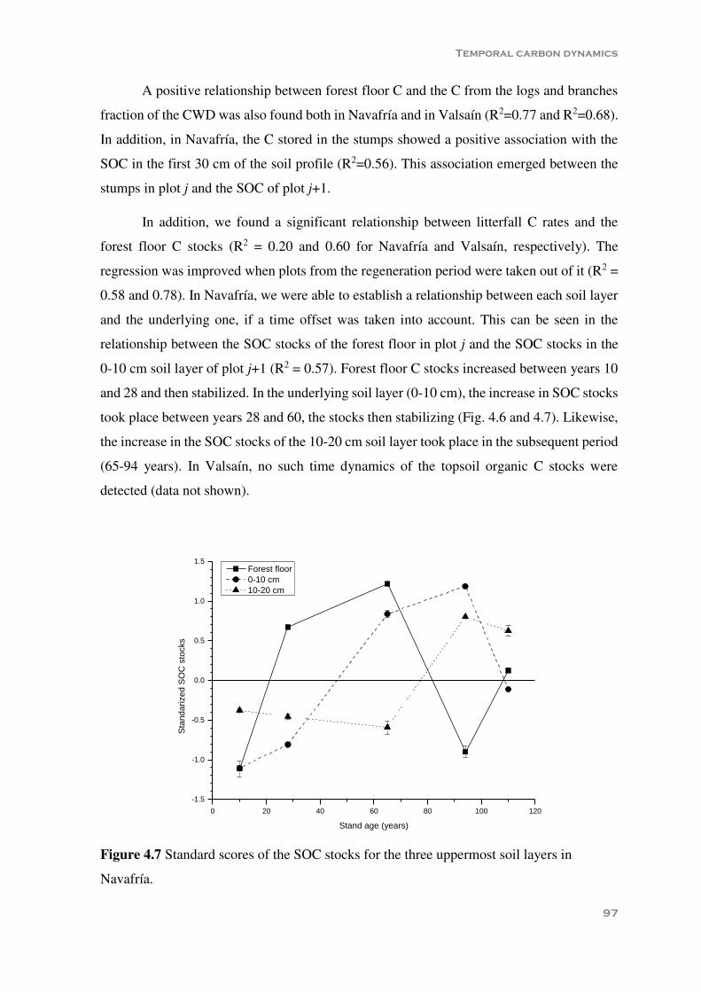
Temporal carbon dynamics
97
A positive relationship between forest floor C and the C from the logs and branches
fraction of the CWD was also found both in Navafría and in Valsaín (R2=0.77 and R2=0.68).
In addition, in Navafría, the C stored in the stumps showed a positive association with the
SOC in the first 30 cm of the soil profile (R2=0.56). This association emerged between the
stumps in plot j and the SOC of plot j+1.
In addition, we found a significant relationship between litterfall C rates and the
forest floor C stocks (R2 = 0.20 and 0.60 for Navafría and Valsaín, respectively). The
regression was improved when plots from the regeneration period were taken out of it (R2 =
0.58 and 0.78). In Navafría, we were able to establish a relationship between each soil layer
and the underlying one, if a time offset was taken into account. This can be seen in the
relationship between the SOC stocks of the forest floor in plot j and the SOC stocks in the
0-10 cm soil layer of plot j+1 (R2 = 0.57). Forest floor C stocks increased between years 10
and 28 and then stabilized. In the underlying soil layer (0-10 cm), the increase in SOC stocks
took place between years 28 and 60, the stocks then stabilizing (Fig. 4.6 and 4.7). Likewise,
the increase in the SOC stocks of the 10-20 cm soil layer took place in the subsequent period
(65-94 years). In Valsaín, no such time dynamics of the topsoil organic C stocks were
detected (data not shown).
0 20 40 60 80 100 120
-1.5
-1.0
-0.5
0.0
0.5
1.0
1.5
Sta
nd
ari
ze
d S
OC
sto
cks
Stand age (years)
Forest floor
0-10 cm
10-20 cm
Figure 4.7 Standard scores of the SOC stocks for the three uppermost soil layers in
Navafría.

Chapter 4
98
4.4. Discussion
4.4.1. Living tree carbon
It is necessary to identify the way in which forest management affects C stocks in order to
define management guidelines aimed at increasing these stocks (Schulze et al. 2000; Millar
et al. 2007; Ruiz-Peinado et al. 2013). In this study, we evaluated two different management
systems employed in Mediterranean Scots pine forests: one more intensive with a higher
felling intensity and shorter rotation period, the other with a more moderate felling intensity
and longer rotation period.
We identified an inflection point in LTC trends during the first part of the rotation
period in both forests although this inflection point occurs at an earlier point in time in
Navafría, probably because thinning operations take place at earlier development stages in
this forest (Montero et al. 2001). This inflection point coincides with the maximum current
annual increment. Maximum LTC levels were reached in both forests when stand density
was more than 500 trees ha-1 and the dbh was greater than 30 cm. The density was then
reduced in order to promote the development of crop trees and further facilitate the
regeneration (Lavender et al. 1990). Due to the higher intensity of regeneration fellings
under the uniform shelterwood system (used in Navafría), the decline in LTC was more
evident at the beginning of the regeneration period in Navafría than in Valsaín. Hence, the
three last inventories for the oldest plot at Navafría (N5) were conducted when the
regeneration fellings had almost finished and only the residual trees were still to be removed.
Furthermore, the lower density of residual trees and the soil preparation carried out in
Navafría allowed the regeneration to become established more quickly and favored the
development of the seedlings (Barbeito et al. 2011).
Forest C stocks reported in different studies vary greatly due to differences in forest
types, management systems, the monitoring methodology or because only certain parts of
the C dynamics are taken into consideration. In long-term Mediterranean thinning
experiments, Ruiz-Peinado et al. (2014, 2013) reported mean values for LTC ranging from
113.8 to 168.5 Mg ha-1 of C in Pinus pinaster Ait. stands (from years 33 to 59) and 128.5 to
193.3 Mg ha-1 of C in P. sylvestris (from years 22 to 52) stands depending on the thinning
treatment. LTC values in Valsaín and Navafría fall well within these intervals. However, the
LTC values found in the present study were greater than those reported in others papers.
Nunes et al. (2010) found average LTC values of between 47.9 and 62.6 Mg ha-1 of C in

Temporal carbon dynamics
99
young stands of P pinaster. Xiao et al. (2003) estimated 176.4 Mg ha-1 as the total tree
biomass (89.8 Mg ha-1 of C considering 0.509 as the factor to convert the biomass into C) in
a 73 year-old Scots pine stand on a poor site in Belgium. Bascietto et al. (2012) reported
40.1 Mg ha-1 of C stored in the aboveground biomass fraction of a Scots pine stand (80 years-
old) in The Netherlands. The large difference with respect to our data is explained by the
fact that the basal area of this Scots pine stand (24.4 m2 ha-1) was much lower than ours
(basal area in Navafría and Valsaín=64.5 and 56.3 m2 ha-1, respectively) at an age of 80
years.
The total tree carbon (extracted and standing C) at the end of the rotation period and
the ratio of the area below the smooth trends and the rotation age were larger in Valsaín,
which is subjected to a more moderate management system (with less severe harvesting and
more spread over time). Other studies have also found that longer rotation periods result in
greater C accumulation, such as in Spanish stands of Pinus radiata D. Don and P. pinaster
(Balboa-Murias et al. 2006), Finnish forests of Picea abies (L.) H.Karst (Pohjola and Valsta
2007), North American stands of Pseudotsuga menziesii (Mirb.) Franco and in Tsuga
heterophylla (Raf.) Sarg. (Harmon and Marks 2002) and in US forests of Pinus taeda L.
(Nepal et al. 2012). However, Pohjola and Valsta (2007) reported that thinnings account for
a greater proportion (70-80 %) than the rotation period (20-30 %) in C sequestration in
Finnish Scots pine forests. The fact that growth rates in Valsaín were more stable than in
Navafría can be explained, on the one hand, by differences in the regeneration systems and
on the other, by the lighter thinning regime in Valsaín.
The positive relationship found between aboveground C and literfall rates in
Navafría was expected and has already been reported in Mediterranean areas (Roig et al.
2005).
4.4.2. Mineral soil organic carbon and forest floor
Forest management comprises a number of different interventions affecting both the
vegetation and the soil, with a specific time sequence over the rotation period. Each of these
interventions (e.g. soil preparation, thinning, regeneration fellings) can influence the SOC
stocks in different ways by altering the rate of soil C input as well as output (Jandl et al.
2007). Therefore, making an overall assessment of the effect of forest management on SOC
stocks is highly complex. This complexity is further compounded by the generally high

Chapter 4
100
spatial variability of Mediterranean forest soil characteristics (Rodeghiero et al. 2011). In
the present study, the comparison involved differences in several aspects of forest
management, hence differences were expected between forests.
Interventions in aboveground vegetation usually have a more evident effect on
topsoil C stocks, these effects diminishing with increasing soil depth. However, since a
significant amount of C is stored beyond 30 cm (Chiti et al. 2012) we considered it
worthwhile investigating deeper layers in our study. Additionally, by computing SOC stocks
down to 50 cm a more meaningful comparison can be made with other studies. At local to
regional level, Díaz-Pinés et al. (2011a) found values of between 80 and 130 Mg ha-1 of C
for Scots pine forests in the same mountain range; Schindlbacher et al (2010) found slightly
higher values for plots located in Navafría (up to 150 Mg ha-1 of C for the first 36 cm of the
soil profile + 20 in the forest floor); and Alvarez et al. (2014) found values of 100-120 Mg
ha-1 of C in a modeling study conducted for the Valsaín forest. Our results, therefore, fall
well within the range of other observations in the same study area. In P. pinaster forests in
southwestern France, C values ranged from 58 to 203 Mg ha-1 of C for the entire soil pool
(Augusto et al. 2010). Organic C stocks in forest floor ranged from 14.7 to 19.3 Mg ha-1 of
C in Scots pine and from 17.04 to 24.50 Mg ha-1 of C in P. pinaster, whereas the 30
uppermost cm of mineral soil accounted for 85.9-88.9 Mg ha-1 of C in Scots pine and 90.52-
96.62 Mg ha-1 of C in P. pinaster (Ruiz-Peinado et al. 2013; Ruiz-Peinado et al. 2014).
Hence, our results are also similar to those reported for other study areas and/or species.
Navafría underwent soil preparation, causing a disturbance along the soil profile
which is usually associated with the loss of a steady-state, therefore enhanced SOC losses
were expected (Johnson and Curtis 2001; Jandl et al. 2007). No substantial SOC releases
were observed. Our results showed indications of a buffering mechanism of C re-allocation
from the forest floor to the underlying soil layers, curbing the loss of C from the system.
Some of the C entering the forest floor via litterfall is incorporated into the mineral soil a
few years after soil preparation. As a result, the equilibrium between SOC inputs and outputs
is probably already achieved at the start of the rotation period, with the exception of small C
flows between soil layers.
The topsoil in Valsaín may be less prone to exchanges in SOC stocks within the soil
profile since a steady-state may already have been reached. Furthermore, since forest
operations in Valsaín take place more gradually than in Navafría, mineralization conditions

Temporal carbon dynamics
101
have not changed dramatically over time (Jandl et al. 2007). Moreover, as could be the case
of plot V3, spatial variability may play a greater role than forest management. With the
exception of this plot, C pools in the mineral soil remained within a narrow threshold over
the whole rotation period. In summary, the evolution over time of the SOC in the forest floor
and the top mineral soil in both forests seems to be minimally affected over the rotation
period, supporting the findings of previous investigations which suggest that forest
management has either no effect at all or only a small, temporal effect on the SOC during
the rotation period (Johnson and Curtis 2001; Peichl and Arain 2006; Bradford et al. 2008;
Nave et al. 2010).
Deeper soil layers were found to be significant SOC pools, especially in Valsaín.
However, it would be highly speculative to associate differences found in SOC over the
rotation period with management operations given that, on the one hand, the influence of the
vegetation on the soil usually decreases with increasing soil depth (Díaz-Pinés et al 2011b),
and on the other, abiotic factors (mainly stone content) contributed as much as 80 % to the
calculation of SOC stock, overshadowing the potential effects of forest management.
4.4.3. Conclusions
A complete analysis of C sequestration in forests requires all the different C pools to be taken
into account. However, obtaining data for all the pools can be complicated and entails
exhaustive sampling. On average, no significant differences were found in terms of the C
stored in the whole soil profile of each system. However, the situation may be different in
other areas under other climatic conditions. The main difference as regards carbon storage
in the two management systems studied concerns the LTC pool. The system with longer
rotation periods and more moderate harvesting intensity had higher LTC stocks. In addition,
this management system also favors structural biodiversity, greater continuity of
regeneration over time and lower susceptibility to drought. Therefore, if one of the
management objectives pursued is C sequestration, we recommend management systems
with longer rotation periods along with harvesting which is both less severe and more spread
over time.

Chapter 4
102
Acknowledgements
We wish to thank Adam Collins for revising the English grammar and everybody who
participated in the field work, especially Ángel Bachiller. We also thank two anonymous
reviewers who provided good comments to improve the manuscript. This work has been
funded by the following projects: AGL2010-21153-C02, AGL2010-16862, AGL2013-
46028R of the Spanish Government. The Ministerio de Educación, Cultura y Deporte
(Ministry of Education, Culture and Sport) funded DMF´s PhD studies thorough the FPU
program
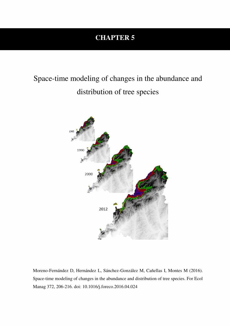
Space-time modeling of changes in the abundance and
distribution of tree species
Moreno-Fernández D, Hernández L, Sánchez-González M, Cañellas I, Montes M (2016).
Space-time modeling of changes in the abundance and distribution of tree species. For Ecol
Manag 372, 206-216. doi: 10.1016/j.foreco.2016.04.024
CHAPTER 5


Changes in the abundance and distribution of tree species
105
Abstract
Land use change and global warming are important drivers in the distribution of tree species.
The Mediterranean mountain forest ecosystems can be severely affected by climate change
since an increment in temperature has been observed. The main aim of this chapter was to
analyze shifts in the distribution and changes in the abundance of Pyrenean oak (Quercus
pyrenaica Willd.) and Scots pine (Pinus sylvestris L.) in Mediterranean mountains over a
period of 47 years (1965-2012) by using data from the National Forest Inventories, extending
the Universal Kriging/Cokriging models to the space-time case for long-term forest
inventory data analysis including climatic variables. Our results indicated that both the
distribution and the abundance of Scots pine remained quite constant during the study period.
Pyrenean oak increased its presence by 42 % whereas its abundance doubled between 1965
and 2012. This movement took place towards both higher and lower altitudes. With regard
to climatic factors, the kriging models showed a negative association between the presence
of Scots pine and the temperature. However, we found a quadratic relationship between the
Pyrenean oak and temperature, pointing to the occurrence of at intermediate altitudes.
Additionally, we found significant relationships between the rainfall and the abundance of
both species. Rainfall was positively related to the abundance of Scots pine and negatively
to that of Pyrenean oak. Our results indicate that there has been a threefold increase in the
area covered by mixed stands. However, successive land use changes as well as forest
policies related to conservation have played an important role in the distribution of both
species and therefore are taken into account in the discussion of these results.
Key words: global change, land use, data autocorrelation, mixed stands, species distribution
models.
Abbreviations: IRWGLS, Iteratively Reweighted Generalized Least Squares; VLS,
Variance Least Square; ML, Maximum Likelihood; NFI, National Forest Inventory; SEE,
Sum of estimations errors; UCK, Universal Cokriging; UK, Universal Kriging; VSEE,
Variance of the Standardised Estimation Errors.

Chapter 5
106
5.1. Introduction
Climate change and land use change are the main drivers of global change in ecological
ecosystems (Hansen et al. 2001). The effects of both in forest ecosystems are associated with
changes in species productivity (Boisvenue and Running 2006), species distribution (Hampe
and Petit 2005; Aitken et al. 2008; Lenoir et al. 2008; Améztegui et al. 2010), forest
dynamics (Kellomäki and Väisänen 1997; Palombo et al. 2013) and forest disturbances such
as pest outbreaks (Kurz et al. 2008) or forest fires (Flannigan et al. 2009; Brotons et al. 2013),
especially in the Mediterranean area (Hódar and Zamora 2004; Pausas 2004).
Mountain ecosystems exhibit high biodiversity because many species, often
endemic, remain isolated at high elevations (Beniston 2003). This makes that high mountain
systems are particularly vulnerable to climate change (Guisan et al. 1995; Theurillat and
Guisan 2001). Three possibilities exist as regards the fate of mountain forest species in a
rapidly changing environment: migration; persistence through adaptation to new conditions
in current locations; and extirpation (Guisan et al. 1995; Aitken et al. 2008). During previous
periods of climate change, species have tended to respond by migrating rather than adapting
to new conditions (Huntley 1991). Hence, in mountain areas, forest species might migrate
upward towards more favorable ecological niches in response to climate warming (Hughes
2000; Lenoir et al. 2008; Jump et al. 2009).
In particular, the montane species of the Iberian Peninsula can be especially
vulnerable to climate change scenarios (Thuiller et al. 2005). In fact, changes in the
distribution of the species have already been detected. Peñuelas and Boada (2003) found that
the European beech (Fagus sylvatica L.) is occupying the summits of the mountains at the
highest altitudes and it is being replaced at mid-altitudes in Northern Spain by the holm oak
(Quercus ilex L.), which is a more xeritic species. Hernández et al. (2014) demonstrated that
both Scots pine (Pinus sylvestris L.) and the European beech are shifting towards higher
elevations in the Pyrenees. Similarly, Sanz-Elorza et al. (2003) reported movements in shrub
species towards higher altitudes over recent decades, mainly associated with changes in
climatic conditions. Furthermore, Améztegui et al. (2010) found an expansion in the
distribution of mountain pine (Pinus uncinata Ram.) in the Pyrenees associated with the land
use change (abandonment of rural communities and losses in the primary sector) rather than
climate change. The effects of global change on the distribution of species must be
understood by forest managers and policy-makers and taken into account in forest

Changes in the abundance and distribution of tree species
107
management and decision making (Hernández et al. 2014). However, scarce information
exists with regard to shifts in species distribution in other mountain areas of the Iberian
Peninsula, such as Central Spain.
The broad scale response of species to environmental change has been often assessed
by analyzing the distribution of the species (Lenoir et al. 2008; Ruiz-Labourdette et al. 2012;
Hernández et al. 2014) since this is easy to measure providing that information is available
regarding where a species is present and where it may interact with other species (Ehrlén
and Morris 2015). Nevertheless, the absence/presence data may not provide a complete
picture of the shifts in distribution of the species or detect changes in the size of the
populations (Joseph et al. 2006). Hence, abundance will be much more useful as an indicator
of the carry-on effects that one species will have upon interacting species in the community
than presence alone (Ehrlén and Morris 2015). However, few studies to date have taken into
account the abundance of tree species in population trends (Ficko et al. 2011; Caouette et al.
2015).
Alternative data sources have been used to model changes in species distributions,
such as forest maps (Benito Garzón et al. 2008), National Forest Inventories (NFIs)
(Hernández et al. 2014) or remote sensing techniques such as aerial photographs and satellite
images (Wittmann et al. 2002; Blázquez-Casado et al. 2015). NFIs provide estimates of
forest resources, growth, mortality, forest health and other valuable information (McRoberts
and Tomppo 2007). Additionally, a large number of species are identified in the NFIs,
allowing direct comparisons of species distribution among inventories. Different statistical
methods have previously been used to model the distribution and identify the environmental
factors that drive this process (reviews in Segurado and Araújo 2004; Miller et al. 2007;
Osborne et al. 2007). Among these approaches, kriging techniques have been found suitable
for determining species distribution by spatial interpolation from survey data (Carroll and
Pearson 1998; Hernández et al. 2014). In this study, we take a step further in species
distribution modeling by adding the temporal dimension to the Universal Kriging models
(Matheron 1973). These models allow the space-time structure of the variance as well as the
effects of climatic and geographical factors to be included in the model. Additionally, these
techniques incorporate both spatial and temporal autocorrelation in the kriging prediction,
so they are suitable for analyzing survey data when the locations of the samples vary
temporally.

Chapter 5
108
The main objective was to analyze shifts in the distribution and changes in the
abundance of Scots pine and Pyrenean oak (Quercus pyrenaica Willd.) in Mediterranean
mountain over the last 47 years. To achieve this objective we develop species dynamics
space-time models integrating NFIs and climate data. These models can be an useful tool in
order to understand the past distribution trends of tree species in order to develop forest
policies in a global change context. The species studied spread from the lower montane
broadleaved forests to the oromediterraneous coniferous forest across the altitudinal gradient
of the Mediterranean mountains of Central Spain. We hypothesized an upward altitudinal
shift of the ecotone between Scots pine and Pyrenean oak that entails an increase in mixed
stands. Additionally, we expected an increase in the presence and abundance of the Pyrenean
oak and Scots pine.
5.2. Material and methods
5.2.1. Study area
This study was conducted in the Central Mountain Range, in Madrid province (Spain). The
study area was delimited by 4,557N – 4,415S and 366E – 469W (UTM, ED50, zone 30N)
covering 554,411 ha. The altitude ranged from 430 m asl in the lowest flattest areas to 2408
m asl in the mountains of the Central Range. The study area in the mountains mainly faces
south and south-east. The climate of the region is continental Mediterranean with montane
variations and is characterized by a severe summer drought and high seasonal temperature
fluctuations. The total rainfall and annual mean temperature are respectively 535 mm and
15º C in the lowest areas and 1,340 mm and 7º C in the highest areas.
The lower altitudes (<1,000 m asl) are mainly dominated by Mediterranean forests
of holm oak, and less frequent, stone pine (Pinus pinea L.) forest in the South-West. Between
1,000 m asl and 1,500 m asl sub-Mediterranean forests of Pyrenean oak and pinewoods of
Maritime pine (Pinus pinaster Ait.) predominate. Scots pine dominates the mountain forests
between 1,500 m asl and the timberline (2,000 m asl). In the transitional areas between the
sub-Mediterranean and the mountain conifer belts, Scots pine is mixed with the Pyrenean
oak, Maritime pine and black pine (Pinus nigra Arnold) (<1,700 m asl). Above the
timberline, the common juniper (Juniperus communis L.), mixtures of broom leguminous
bushes and open montane grasslands are the dominant plant communities (Franco Múgica
et al. 1998; Cañellas et al. 2000; Benito Garzón et al. 2008; López-Sáez et al. 2014).

Changes in the abundance and distribution of tree species
109
The stands of Scots pine have been subjected to long-term forest management and
their range have been extended as a result of the forest policy (Gil and Aranzazu Prada 1993;
Franco Múgica et al. 1998). Hence, this species is the widest used in the forestry industry in
the study area (CAM 2012). The main traditional treatment in Pyrenean oak stands, the
coppice management, was abandoned during the 1980s due to the decrease in use of
firewood and charcoal as an energy source and to rural emigration to the cities (Gonzalez
Molina 1995; Cañellas et al. 2004; Adame et al. 2008; Gea-Izquierdo et al. 2015). To a lesser
extent, the Pyrenean oak makes up open woodlands (López Estébanez and Sáez Pombo
2002).
5.2.2. Forest inventory data and climate data
We used data from the four existing Spanish NFIs (Table 5.1; Alberdi Asensio et al., 2010)
to evaluate the changes in the spatial distribution of Scots pine and Pyrenean oak. The
number of trees per hectare of each species in the plots of the four NFI cycle can be found
in Fig. 5.1. The NFI plots were only installed in woodland areas (i.e. none in non-forested
areas). The highest altitude of NFI plots in the study area coincided with the uppermost limit
of Scots pine.
Table 5.1 Year and type of the National Forest Inventory of the plots and number of plots
in the study area.
NFI Year Type of forest inventory Number of plots in the study area
First 1965 Relascopic 693
Second 1990 Circular plots 1919
Third 2000 Circular plots 1783
Fourth 2012 Circular plots 1182
NFI: National Forest Inventory
We used two climatic variables to explain the space-time dynamics of Scots pine and
Pyrenean oak: the annual average temperature (temperature, hereafter) and the yearly rainfall
(rainfall, hereafter). The annual average temperature and the yearly rainfall are the variables
most common used in species distribution models (Porfirio et al. 2014). We obtained the
climatic data from the meteorological stations belonging to the Spanish Meteorological

Chapter 5
110
Agency (www.aemet.es). We established 1950 as the beginning of the time series and 2014
as last year. The length of the climatic time series differed from one station to another. We
used Universal Kriging (UK) with altitude as auxiliary variable to interpolate the
temperature and rainfall in the NFI plots in the years of the four NFIs (305 meteorological
stations for temperature data and 241 for rainfall data). Additionally, we calculated the
annual average temperature and rainfall in the study area using block kriging (Isaaks and
Srivastava 1989) to show the temporal trends of both variables.
Figure 5.1 Number of trees (trees ha-1) of Scots pine (upper) and Pyrenean oak (lower) per
diameter class in each inventory.

Changes in the abundance and distribution of tree species
111
5.2.3. Statistical analysis: space-time models
5.2.3.1. Distribution (absence/presence) models: Space-time Universal Kriging
Environmental variables such as rainfall, temperature and elevation, as well as ecological
processes such as dispersion or mortality, exhibit spatial dependence, some of which are
responsible for spatial structure in the distribution of vegetation. Thus, the distribution of
vegetation is not random and each observation is not independent (Segurado and Araújo
2004; Miller et al. 2007). The spatial autocorrelation must be accounted for in the model
because otherwise the risk of Type I errors is increased (Legendre and Legendre 1998). The
Kriging techniques used in this work incorporated spatial and temporal autocorrelation, and
deals non-geostationarity through the mean function which depends on the auxiliary
variables.
The distribution of the species was evaluated using an indicator variable that took a
value 1 if the species was present in the plot and 0 if the species was absent in the plot. We
defined a species as present in a given plot when trees, saplings or seedlings were registered
in the plot. We used the space-time UK (De Iaco et al. 2002; Montes et al. 2011) to model
and map the distribution of Scots pine and the Pyrenean oak in the study area.
Z(s,t) being as the realization of a space-time random process, the UK model can be
expressed as:
0
( , ) ( , ) ( , )p
k k
k
Z s t f s t s t
(5.1)
or, in matrix form:
Z X (5.2)
where s R2 and t T, fk(s,t) are p + 1 functions of the auxiliary variables which estimate
the space-time mean and ( , )t s is an intrinsically stationary zero-mean residual random
process.
The estimation of the optimal weights i involves modeling the variogram. The
generalized product-sum model (De Iaco et al. 2002) was used to fit the variogram ( )st h
( , ) ( ,0) (0, ) ( ,0) (0, )s t s t s th h h h k h h (5.3)
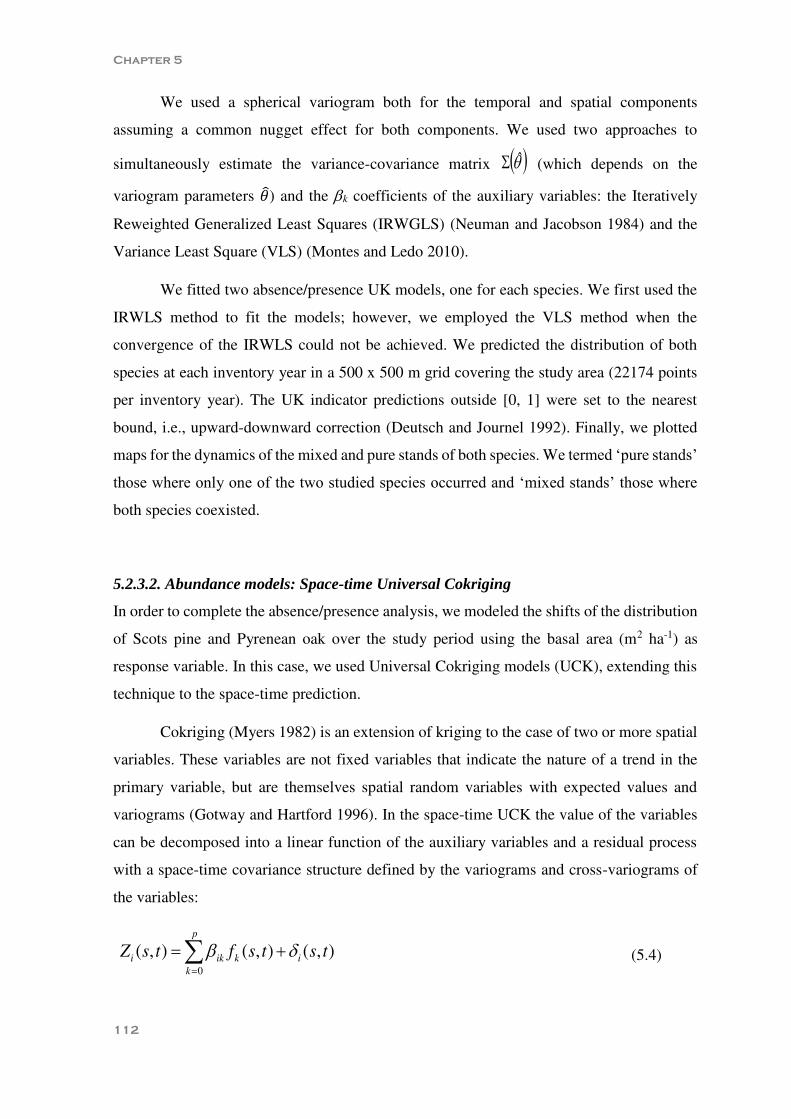
Chapter 5
112
We used a spherical variogram both for the temporal and spatial components
assuming a common nugget effect for both components. We used two approaches to
simultaneously estimate the variance-covariance matrix ̂ (which depends on the
variogram parameters �̂) and the k coefficients of the auxiliary variables: the Iteratively
Reweighted Generalized Least Squares (IRWGLS) (Neuman and Jacobson 1984) and the
Variance Least Square (VLS) (Montes and Ledo 2010).
We fitted two absence/presence UK models, one for each species. We first used the
IRWLS method to fit the models; however, we employed the VLS method when the
convergence of the IRWLS could not be achieved. We predicted the distribution of both
species at each inventory year in a 500 x 500 m grid covering the study area (22174 points
per inventory year). The UK indicator predictions outside [0, 1] were set to the nearest
bound, i.e., upward-downward correction (Deutsch and Journel 1992). Finally, we plotted
maps for the dynamics of the mixed and pure stands of both species. We termed ‘pure stands’
those where only one of the two studied species occurred and ‘mixed stands’ those where
both species coexisted.
5.2.3.2. Abundance models: Space-time Universal Cokriging
In order to complete the absence/presence analysis, we modeled the shifts of the distribution
of Scots pine and Pyrenean oak over the study period using the basal area (m2 ha-1) as
response variable. In this case, we used Universal Cokriging models (UCK), extending this
technique to the space-time prediction.
Cokriging (Myers 1982) is an extension of kriging to the case of two or more spatial
variables. These variables are not fixed variables that indicate the nature of a trend in the
primary variable, but are themselves spatial random variables with expected values and
variograms (Gotway and Hartford 1996). In the space-time UCK the value of the variables
can be decomposed into a linear function of the auxiliary variables and a residual process
with a space-time covariance structure defined by the variograms and cross-variograms of
the variables:
0
( , ) ( , ) ( , )p
i ik k i
k
Z s t f s t s t
(5.4)

Changes in the abundance and distribution of tree species
113
In our study we have two dependent variables (i = 1, 2), the basal area of the Scots
pine and the basal area of the Pyrenean oak. The UCK prediction p(Z1,s0,t0) of the variable
Z1(s0,t0) is a linear combination of the values of this variable in the n sampling points placed
in s11…sn1 and the value of the other variable Z2(sj2) in the m points s12…sm2:
1 0 0 11 1 12 21 1
, ,n m
i i j j
i j
p Z s t Z s Z s
(5.5)
and analogously:
2 0 0 21 1 22 21 1
, ,n m
i i j j
i j
p Z s t Z s Z s
(5.6)
Each variable shows a space-time auto-semivariance function, which is modeled
through the variograms 11 and 22 . The cross-variogram characterizes the space-time
covariance between each pair of distinct variables (Clark et al. 1989; Cressie 1993):
2
12 1 21
1, ,
2
N h
a a a s a t
a
h Z u t Z u h t hN h
(5.7)
The variables Z1 and Z2 were standardized to ensure the unbiasedness of the
estimators (Deutsch and Journel 1992). In order to obtain a valid variance-covariance matrix,
the variogram and cross-variograms should form a corregionalization model, i.e, each
variogram (or cross-variogram) is the linear combination of g spatial or temporal unitary
variograms that stand for the different spatial structures i (i = 1…g), multiplied by the
corregionalization coefficients b11i y b22i, which stand for the contribution of the spatial
structure i to the variogram of the variable 1 and 2 respectively, and b12i, which stands for
the contribution of the spatial structure i to the cross-variogram.
We included two variograms in the model of corregionalization (g = 2): a temporal
spherical model and a spatial spherical model, plus a pure nugget effect variogram that stands
for the variance which is neither associated to the auxiliary variables nor to associated to the
temporal and spatial structures. The direct and cross variograms are linear combinations of
variograms for each structure, that is, the variogram of a given variable is a linear
combination of the nugget effect and the temporal and spatial variogram models. The
corregionalization model parameters (range and b coefficient of each elemental structure)

Chapter 5
114
and mean function coefficients were estimated through IRWGLS, analogously to the UK
model.
We assumed that the abundance of one species is not independent of the abundance
of the other. Thus, this technique would appear to be useful for modeling the basal area of
both species. The basal area of each species was kriged at those prediction points where the
presence/absence indicator UK was above 0.5.
5.2.3.3. Assessment of the statistical significance of the mean function coefficients
The covariance matrix V̂ of the generalized least squares estimates ̂ is obtained as
follows:
1ˆ ˆ´ΣXV X
(5.8)
We calculated the standard error estimates ˆk kks v for each beta parameter
estimate, ˆk , k=0,1,…,p to construct p-values for significance test of these coefficients based
on the t-ratios:
ˆ /k k kt s , k=0,1,…,p (5.9)
the degrees of freedom for the t-tests being the difference between the number of
observations and the number of auxiliary variables.
5.2.3.4. Relative structural correlation assessment
We can calculate the relative structural correlation to assess the correlation between the
variables associated with each spatial or temporal structure i (Goovaerts and Webster 1994;
Pelletier et al. 2009):
ii
ii
bb
b
2211
1212
(5.10)

Changes in the abundance and distribution of tree species
115
In order to quantify the part of the total correlation between variables associated with
each structure, we propose the following definition of the relative structural correlation:
g
j
j
g
j
j
ir
i
bb
b
122
111
1212 (5.11)
Positive values of the relative structural correlation indicate positive association
between the variables and negative values indicate negative association between the
variables.
5.2.3.5. Model selection: Cross-validation
Cross-validation was used to assess the performance of the UK and UCK model in term of
bias and predicted variance. We selected randomly 500 points from data set to carry out the
cross-validation of the UK and UCK. The sum of the estimation errors (SEE) was used to
check for bias:
n
sZsZpn
i
ii
1
)(),*SEE
(5.12)
where n is the number of observations and p*(Z, si) is the prediction of Z(si) leaving out the
value observed at si. The variance of the standardised estimation errors (VSEE; which should
be approximately 1 if the model performed well) was used to check the validity of the
prediction error given by the kriging variance:
n
s
sZsZpn
i iUK
ii
12
2
)(
)(,*
VSEE
(5.13)
where 02
sUK is the UK error variance (Cressie 1993).
The selected space-time UK and space-time UCK models presented SEE values
closest to 0 and VSEE values closest to 1. All the statistical analyses were done using a
MATLAB R2009a (MATLAB 2009) package developed by the authors. Maps were created
using ArcGis 10.2.2. (ESRI 2014).

Chapter 5
116
5.3. Results
5.3.1. Rainfall and temperature measurements
We employed the VLS method to fit the UK models for the rainfall and temperature. We
found significant relationships between both variables and the altitude. As expected, the
relationship temperature-altitude was negative and the relationship rainfall-altitude was
positive. The spatial correlation was larger for the rainfall (104.16 km) than for temperature
(8.67 km), i.e., the rainfall measurements were more constant over the study area than the
temperature. Moreover, we found similar temporal ranges of both climatic variables, close
to 1 year. Concerning the temporal trends of temperature and rainfall, the block kriging
revealed great interannual variations in both variables. In addition, we found a rise in average
temperatures and a slight decrease in average rainfall over the study period (Fig. 5.2).
Figure 5.2 Annual average values, variance and linear trendline of the temperature (upper)
and rainfall (lower) over the study period after the performance of the block kriging.
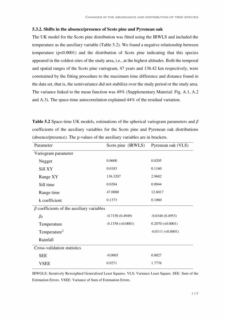
Changes in the abundance and distribution of tree species
117
5.3.2. Shifts in the absence/presence of Scots pine and Pyrenean oak
The UK model for the Scots pine distribution was fitted using the IRWLS and included the
temperature as the auxiliary variable (Table 5.2). We found a negative relationship between
temperature (p<0.0001) and the distribution of Scots pine indicating that this species
appeared in the coldest sites of the study area, i.e., at the highest altitudes. Both the temporal
and spatial ranges of the Scots pine variogram, 47 years and 136.42 km respectively, were
constrained by the fitting procedure to the maximum time difference and distance found in
the data set, that is, the semivariance did not stabilize over the study period or the study area.
The variance linked to the mean function was 49% (Supplementary Material: Fig. A.1, A.2
and A.3). The space-time autocorrelation explained 44% of the residual variation.
Table 5.2 Space-time UK models, estimations of the spherical variogram parameters and β
coefficients of the auxiliary variables for the Scots pine and Pyrenean oak distributions
(absence/presence). The p-values of the auxiliary variables are in brackets.
Parameter Scots pine (IRWLS) Pyrenean oak (VLS)
Variogram parameter
Nugget 0.0600 0.0205
Sill XY 0.0183 0.1160
Range XY 136.3207 2.9682
Sill time 0.0284 0.0044
Range time 47.0000 12.6017
k coefficient 0.1373 0.1060
β coefficients of the auxiliary variables
β0 -0.7150 (0.4949) -0.6348 (0.4953)
Temperature -0.1358 (<0.0001) 0.2070 (<0.0001)
Temperature2 -0.0111 (<0.0001)
Rainfall
Cross-validation statistics
SEE -0.0065 0.0027
VSEE 0.9271 1.7776
IRWGLS: Iteratively Reweighted Generalized Least Squares. VLS: Variance Least Square. SEE: Sum of the
Estimation Errors. VSEE: Variance of Sum of Estimation Errors.

Chapter 5
118
We used the VLS method to fit the UK model for the absence/presence of Pyrenean
oak (Table 5.2). The selected model included the temperature and the square of the
temperature with positive and negative β coefficients, respectively, (p-value of both
variables<0.0001) indicating a quadratic relationship between the temperature and the
presence of the Pyrenean oak. The negative β coefficient of the square of the temperature
indicated that the curve opened downward; the presence of this species reaching a maximum
at 9.3 ºC. We found a spatial correlation among measurements of 3.0 km and a temporal
correlation of 12.6 years. The mean function absorbed 14% of the variance (Supplementary
Material: Fig. A.4, A.5 and A.6) and the space-time autocorrelation explained 63% of the
residual variance. Additionally, in this case, the spatial sill was 26 times larger than the
temporal sill, indicating larger variability in space than in time.
Table 5.3 Number of prediction points and proportion, between brackets, of pure stands of
Scots pine, pure stands of Pyrenean oak and mixed stands. Mixed stands are where both
species coexist. Scots pine and Pyrenean oak are pure stands of these species.
Type of stand 1965 1990 2000 2012
Mixed stand 191 (0.9) 384 (1.7) 471 (2.1) 626 (2.8)
Pyrenean oak stand 1,550 (7.0) 1,969 (8.9) 2,101 (9.5) 2,361 (10.6)
Scots pine pure stand 1,698 (7.7) 1,579 (7.1) 1,638 (7.4) 1,472 (6.6)
No presence 18,735 (84.5) 18,242 (82.3) 17,964 (81.0) 17,715 (79.9)
Total prediction points 22,174 (100) 22,174 (100) 22,174 (100) 22,174 (100)
According to the UK prediction maps (Fig. 5.3; Supplementary Material: Fig. A.7),
the distribution of Scots pine has hardly changed over the study period. We found that the
presence of Scots pine has increased by 11% during the period from 1965 to 2012 (Table
5.3). The altitudinal range of this species has remained constant over the study period (Table
5.4).

Changes in the abundance and distribution of tree species
119
Figure 5.3 Distribution (absence/presence) of Scots pine pure stands (green), Pyrenean oak
pure stands (blue) and mixed stands (red) in 1965 (upper left), 1990 (upper right), 2000
(lower left) and 2012 (lower right).
Furthermore, the UK revealed an expansion of Pyrenean oak in the study area (Table
5.3). This species increased its distribution by 42% from 1965 to 2012 (Fig. 5.3;
Supplementary Material: Fig. A.7). In contrast to the distribution of Scots pine, the Pyrenean
oak expanded its distribution both towards higher elevations and lower elevations, while the
average altitude remained constant (Table 5.4). From 1965 to 2012, Pyrenean oak occupied
new areas, creating pure stands (92%) rather than mixed stands (8%). In this respect, we
found that there has been a threefold increase in mixed stands over the study period whereas
the area occupied by pure stands of Scots pine has reduced by 14% and the area occupied by
pure stands of Pyrenean oak has increased by 52%. In this regard, we found an increase in
the altitude of the upper limit of the mixed pine-oak stands in 2012 compared to 1965
whereas the increment in altitude was less pronounced at the lower limit (Table 5.4).

Chapter 5
120
Table 5.4 Average altitude (m asl) of the prediction points where Scots pine and Pyrenean
oak occurred. In brackets, the 5th and the 95th percentiles. Mixed stands are where both
species coexist.
Year Scots pine Pyrenean oak Mixed stands
1965 1,646 (1,343-2,040) 1,195 (929-1,503) 1,474 (1,264-1,722)
1990 1,638 (1,338-2,034) 1,211 (929-1,582) 1,506 (1,262-1,780)
2000 1,619 (1,317-2,026) 1,203 (923-1,578) 1,490 (1,245-1,765)
2012 1,620 (1,322-2,024) 1,214 (911-1,617) 1,505 (1,272-1,783)
5.3.3. Shifts in the abundance of Scots pine and Pyrenean oak
The selected model included rainfall as explanatory variable, presenting a significant
association with the basal area of both species (Table 5.5). The relationship between rainfall
and the basal area of Scots pine was positive whereas it was negative in the case of the
Pyrenean oak.
Table 5.5 β coefficients of the auxiliary variables of the space-time UCK model for the basal
area of Scots pine and Pyrenean oak and the statistics of the cross-validation. The p-values
of the auxiliary variables are in brackets.
Basal area of Scots pine
β0 -0.1264 (0.4200)
β of the rainfall 0.6111 (<0.0001)
β of the temperature
β of the temperature2
Sum of the Estimation Errors -0.0250
Variance of Sum of Estimation Errors 0.9733
Basal area of Pyrenean oak
β0 0.3798 (0.2906)
β of the rainfall -0.4069 (<0.0001)
β of the temperature
β of the temperature2
Sum of the Estimation Errors -0.0272
Variance of Sum of Estimation Errors 0.9448

Changes in the abundance and distribution of tree species
121
Figure 5.4 Basal area of Scots pine in 1965 (upper left), 1990 (upper right), 2000 (lower
left) and 2012 (lower right). Yellow: (0-10 m2 ha-1], green: (10-20 m2 ha-1], red: (20-30 m2
ha-1], violet: (30-40 m2 ha-1] and purple: (40-50 m2 ha-1].
The ranges of the spatial and temporal spherical elemental variograms were the
maximum distance among plots and the whole study period, respectively (Table 5.6). We
found a positive value of relative structural correlation between the basal area of species in
case of the spatial structure, whereas the relative structural correlation was negative for the
temporal structure (Table 5.6, calculated in Eq. 5.11). This indicates a positive relationship
between the basal area of both species in space and negative in time. Additionally, the
absolute value of the relative structural correlation was larger in the time spherical structure
than in the spatial one, highlighting that the species abundance for each of the two species
has changed oppositely over the successive surveys, although the denser stands of both
species tended to coincide geographically.

Chapter 5
122
Figure 5.5 Basal area of Pyrenean oak in 1965 (upper left), 1990 (upper right), 2000 (lower
left) and 2012 (lower right). Yellow: (0-4 m2 ha-1], blue: (4-8 m2 ha-1], green (8-12 m2 ha-1]
and red (12-16 m2 ha-1].
Table 5.6 Ranges of the elemental variograms, coefficients of the coregionalization model
of space-time UCK and relative structural correlations of the elemental variograms.
Elemental
variogram
Range Sills Relative
structural
correlation
Scots pine
variogram
Pyrenean oak
variogram
Cross-variogram
Nugget 0.00 0.4652 0.6070 0.6680 0.4588
Spherical XY 136.32 0.2534 0.9417 0.1889 0.1300
Spherical time 47.00 0.5302 0.1485 -0.2806 -0.1927

Changes in the abundance and distribution of tree species
123
We found great differences in the basal area of both species. Scots pine always
displayed larger basal areas than the Pyrenean oak. The basal area of the Scots pine (Fig.
5.4) remained quite constant over the study period (18.39 m2 ha-1 in 1965, 16.14 m2 ha-1 in
1990, 17.81 in 2000 m2 ha-1 and 21.32 in m2 ha-1). However, we found a reduction in the
number of plots with the lowest basal area whereas the number of plots in the intermediate
and uppermost ranges increased from the first NFI to the last (Table 5.7). The average basal
area of the Pyrenean oak increased with time (Fig. 5.5). Hence, the average basal area of this
species in 2012 (4.00 m2 ha-1) doubled compared to that in 1965 (1.79 m2 ha-1).
Table 5.7 Number of prediction points placed in each basal area range for the two species
studied. The percentage of points in each basal area range is given in brackets.
Basal area range (m2 ha-1) 1965 1990 2000 2012
Scots pine
(0-10] 414 (21.9) 383 (19.5) 291 (13.8) 156 (7.4)
(10-20] 679 (36.0) 985 (50.2) 1055 (50.0) 876 (41.8)
(20-30] 575 (30.5) 552 (28.1) 627 (29.7) 702 (33.5)
(30-40] 213 (11.3) 43 (2.2) 135 (6.4) 349 (16.6)
(40-50] 7 (0.4) 0 (0.0) 1 (0.0) 15 (0.7)
Total (0-50] 1,888 (100.0) 1,963 (100.0) 2,109 (100.0) 2,098 (100.0)
Pyrenean oak
(0-4] 1,515 (97.7) 1,590 (72.4) 1,552 (61.4) 1,584 (53.5)
(4-8] 16 (1.0) 571 (26.0) 887 (35.1) 1,208 (40.8)
(8-12] 19 (1.2) 30 (1.4) 72 (2.8) 144 (4.9)
(12-16] 0 (0.0) 5 (0.2) 18 (0.7) 27 (0.9)
Total (0-16] 1,550 (100.0) 2,196 (100.0) 2,529 (100.0) 2,963 (100.0)

Chapter 5
124
5.4. Discussion
The methods used in these work, space-time UK and UCK, have been shown to be
appropriate for monitoring changes in the distributions of forest species using long-term
data. The space-time correlation allowed us to use the information from different inventories
for data interpolation, thus improving the predictions where the location of the plots varied
among inventories. We incorporate the climatic variables in the mean function, which can
be interpreted as the climatic potential in basis to the species distribution (derived from the
NFI samples over the forest area along the studied period). The spatial and temporal
correlation determines the oscillations from this climatic potential in different areas along
the period. Three novel approaches used in this work enhanced the model performance and
provided a complete framework to understand the relationships between variables: i) the p-
values estimation to calculate the significance of the coefficients of the auxiliary variables
in the mean function, ii) the relative structural correlation based on the structural correlations
proposed by Goovaerts and Webster (1994) and iii) the method proposed to determine the
part of the variance linked to the mean function and the part linked to the space-time
autocorrelation, based on Montes and Ledo (2010).
Our findings indicate a relatively steady distribution of Scots pine during the period
analyzed in the study area. This is in contrast to the elevation shift of Scots pine towards
high mountain grasslands and the reduction in the stands of Scots pine in the Iberian
Peninsula predicted by species distribution models as a consequence of climate warming
(Benito Garzón et al. 2008; Ruiz-Labourdette et al. 2012). Hernández et al. (2014) found
that Scots pine shifted approximately 200 m towards higher elevations but increased its
distribution in the Western Pyrenees between 1971 and 2010, stressing the importance of
land use changes in species dynamics. However, in the study area the shallow and stony
terrain impedes the establishment of trees above the tree line. Since the late 20th century,
wood production has been reduced towards protective function in those Scots pine stands
located at higher altitudes. This may explain the increasing trend in the basal area in the last
inventory.
In contrast, the population of Pyrenean oak increased both in presence and
abundance. From 1990 (Fig. 5.1, lower), a large number of trees of this species was
incorporated to the upper diameter classes (diameter>55cm) entailing the increase in basal
area. Ruiz-Labourdette et al. (2012) predicted that the Pyrenean oak would move slightly
Changes in the abundance and distribution of tree species
125
towards higher elevations. However, our findings indicate that Pyrenean oak range has not
shifted to higher elevations (in terms of average altitude) over the last 47 years but rather
widen both upwards and downwards. The upwards expansion maybe related to climate
factors, but also to changes in forestry policy that favored Scots pine stands over the oak
woodlands at the uppermost limit of the Pyrenean oak altitudinal range at beginning of the
20th century (Cañellas et al. 2000; Sánchez-Palomares et al. 2008). The reduction of firewood
exploitation, the conversion of the coppice into high forests, the decrease in human local
population, the scarcity of recent large fires in the study area (differently to other Iberian
mountains), the protection of Pyrenean oak by the forest policy led to expansion to lower
elevation of this species, the increase of the basal area and, the shift of the diameter
distribution towards larger sizes (Gómez et al. 2003; Cañellas et al. 2004; Pausas 2004;
PORN 2010; Gea-Izquierdo et al. 2015).
The area where both species coexist has increased considerably. The Scots pine could
facilitate the establishment and development of the Pyrenean oak as occurs with other pine
and oak species in southern Spain (Urbieta et al. 2011). The positive spatial correlation
between the basal area of both species found in the UCK model indicated that the areas
where the basal area of both species is higher coincide. In fact, del Río and Sterba (2009)
reported that the competition in mixed stands of Scots pine and Pyrenean oak is lower than
in pure stands and the increase in stocking per occupied area is greater in mixed stands. The
areas where both species coexist were mainly areas proximal to the ecotone between the
pinewood and the oak woodland: the lowest areas Scots pine range and the uppermost range
for Pyrenean oak. Current forestry policy promote mixed stands with complex structures to
increase stability and biodiversity (e.g. Spiecker 2003). Some authors (Gimmi et al. 2010;
Ruiz-Labourdette et al. 2012) predict that the Pyrenean oak and other broadleaf species will
replace the stands of Scots pine since the increase in the intensity of the summer drought can
cause a decrease in the regeneration and recruitment of Scots pine, therefore limiting its
distribution (Martı́nez-Vilalta and Piñol 2002; Castro et al. 2004; Pardos et al. 2007;
Fernández-de-Uña et al. 2015). In addition, a temperature rise may lead to a higher incidence
of some outbreaks on pine forests (Hódar and Zamora 2004). Accordingly, the forecasted
increase in temperatures, if not accompanied by an increase in rainfall, will threaten existing
populations of Pyrenean oak at lower altitudes (Benito Garzón et al. 2008; de Dios et al.
2009; Ruiz-Labourdette et al. 2012; Gea-Izquierdo et al. 2013). However, despite the

Chapter 5
126
climatic trends over the last 47 years (Fig. 5.2), the Pyrenean oak has expand to lower
altitudes as we discussed above.
Concerning the climatic variables, we found that temperature was negatively
associated with the presence of Scots pine and rainfall was positively related to its
abundance. The quadratic form of the mean function of the Pyrenean oak distribution model
indicated that this species occurred at intermediate altitudes in our study area. At lower
altitudes (warmer and drier areas), other species such as holm oak are the dominant species
whereas Scots pine is established at higher altitudes with colder, more humid conditions
(López-Sáez et al. 2014).
It is important not only to monitor the progress of these species but also to study their
past and future dynamics in the context of global change in order to develop scientific tools
for forest management. In our study area, the long life of these species combined with the
changes in use seem to have contributed to the maintenance of Scots pine populations while
the distribution range and density of Pyrenean oak as well as the coexistence areas have
increased. This is not an equilibrium stage and future changes in the climate may lead to the
retraction to the Scots pine with ongoing colonization of the Pyrenean oak (Gea-Izquierdo
et al. 2015).
Acknowledgements
We wish to thank José Alfredo Bravo Fernández (UPM) for his advice, Adam Collins for
revising the English grammar and everybody who digitized the data of the First National
Forest Inventory. We also thank the reviewers who provided good comments to improve the
manuscript. This work has been funded by the following projects: AGL2013-46028-R,
949S/2013 (funded by National Parks Autonomous Agency) and S2013/MAE-2760.
Ministry of Education, Culture and Sport funded DMF’s PhD studies thorough the FPU
program. Spanish Meteorological Agency (www.aemet.es) provided the climatic data.

Changes in the abundance and distribution of tree species
127
Supplementary Material
Figure A.1 Variogram of the distribution of the Scots pine model.
Figure A.2 Trend function of the temperature for the distribution of the Scots pine model.

Chapter 5
128
Figure A.3 Residual variogram of the distribution of the Scots pine model.
Figure A.4 Variogram of the distribution of the Pyrenean oak model.

Changes in the abundance and distribution of tree species
129
Figure A.5 Trend function of the square of the temperature for the distribution of the
Pyrenean oak model.
Figure A.6 Residual variogram of the distribution of the Pyrenean oak model.

Chapter 5
130
Figure A.7 Distribution (absence/presence) of Scots pine (left) and Pyrenean oak (right) in
the area of study in 1965 (red), 1990 (blue), 2000 (yellow) and 2012 (green).

Discussion
CHAPTER 6


Discussion
133
6.1. Regeneration dynamics of Pinus sylvestris L. in
Mediterranean areas
Regeneration, classified into seedlings and saplings, and its association with adult trees was
studied at microscale (Chapter 2) and plot scale (Chapter 3), respectively. Hence, although
the approach to regeneration differs between the uniform shelterwood and group
shelterwood systems, these two studies together cover the whole process of the establishment
of new individuals following seedling germination. We found that P. sylvestris seedlings
require moderate light conditions for successful development in Mediterranean areas, which
is in concordance with previous findings for this species (Pardos et al. 2007; Barbeito et al.
2009). The results of this study also show a positive relationship between the number of
stumps and the number of seedlings. The number of stumps is a proxy of the intensity of the
regeneration fellings and therefore, of the canopy openness. This suggests that higher
intensities of regeneration fellings (cutting around 70 trees ha-1, about 45 % of standing trees)
promote the establishment of new individuals of P. sylvestris. In fact, the mean density of
mother trees reported in this study (85 trees ha-1) is within the tree density range after the
seedling cuttings (70-100 trees ha-1) proposed by García López (1995). In addition, the stem
extraction operations may have a soil-preparation effect by removing the herb layer and
facilitating the establishment of the P. sylvestris seedlings (Fig.1.1; Barbeito et al. 2011).
Furthermore, the conditions at sites where P. sylvestris is found can vary greatly over its
distribution range (Mason and Alía 2000; Mátyás et al. 2003). At sites with severe summer
drought, such as those in this study, moderate canopy cover may ensure higher levels of soil
moisture than open canopies, while also permitting a sufficient level of solar radiation. In
contrast, at sites in northern latitudes the limiting factor is the amount of light, thus the
regeneration appears in open gaps (Mátyás et al. 2003). Consequently, natural regeneration
in northern countries is usually achieved using the seed-tree method, whereas in southern
locations the different alternatives offered by the shelterwood approach tend to be employed
(Mason and Alía 2000; Barbeito et al. 2008; Hyppönen et al. 2013). Our results confirm that
natural regeneration in this forest is successfully achieved under the current management
practices (uniform shelterwood), suggesting that, from a scientific perspective, the temporal
and spatial continuity of the forest is ensured. In this regard, Montes et al. (2005) studied the
historical records of the inventories (the first inventory took place in 1889) in Valsaín forest
and concluded that despite changes in forest management, the continuity and sustainability
of this forest is assured.

Chapter 6
134
Once the factors underlying the establishment of seedlings has been analyzed, the
dynamic of individuals at a later stage of development (saplings) was investigated on a larger
scale. The exploration of the linear predictor function reveals a negative relationship between
the diameter of adult trees and the number of saplings up to 7-8 m. This means that saplings
prefer not to grow in close proximity to larger trees. Once the seedlings become saplings,
the maintenance costs increase (Falster and Westoby 2003) and plants require higher
minimum levels of solar radiation for survival (Williams et al. 1999). Additionally, their
roots can penetrate into deeper and more humid soil layers (Ritchie 1981). The spatio-
temporal structure selected means that the spatial distribution of the saplings remains
constant over time. This may be due to the fact that our study only covers less than half of
the regeneration period. As a consequence, given the growth rate of P. sylvestris, the length
of the study period is insufficient for the saplings to move into the next cohort, changing
their spatial distribution. Furthermore, the regeneration fellings are carried out in Valsaín
forest using the group shelterwood system over a 40 year period, whereas the regeneration
fellings in Navafría forest are more intense and take place over 20 years. Hence, the latter
silvicultural approach entails more rapid establishment of the regeneration (Fig. 4.2) and
therefore, it may have been easier to identify changes in the spatial pattern of the saplings.
Finally, we can also confirm from a scientific perspective that the group shelterwood system
is a suitable method for regenerating P. sylvestris in southern latitudes.
Our results with regard to regeneration suggest that it is necessary to reduce the
density of the remaining trees after the establishment of seedlings in order to promote the
growth of saplings in stands of P. sylvestris in Mediterranean mountains.
6.2. Pinus sylvestris L. forests as a climate change mitigation tool
Chapter 4 is related to the role of forests in global change mitigation. This chapter assesses
the way in which two alternative management systems, one more intensive and the other
more moderate (with less severe harvesting and more spread over time), affect the carbon
stored in the five compartments in Mediterranean forests.
The biomass of living trees emerged as the compartment which stores the most
carbon, followed by the mineral soil (SOC). Our results indicate that at the end of the rotation
period, the amount of carbon stored in the living biomass of the forest subjected to a more

Discussion
135
moderate management system (Valsaín forest) is greater than the amount stored in the forest
subjected to a more intensive forest management system (Navafría forest). This agrees with
previous findings of studies undertaken at different latitudes (Balboa-Murias et al. 2006;
Pohjola and Valsta 2007; Nepal et al. 2012).
As regards the carbon stored in the mineral soil, our results show that the SOC stored
in the uppermost layers (0-20 cm) – those more prone to be affected by interventions in
aboveground vegetation – is more abundant in Valsaín than in the Navafría forest. In both
of these forests, the SOC hardly changes over the rotation period. This is in accordance with
the findings of previous studies which report that forest management has either null or only
a small, temporal effect on the SOC during the rotation period (Johnson and Curtis 2001;
Peichl and Arain 2006; Bradford et al. 2008; Nave et al. 2010).
It seems that management systems with longer rotation periods and harvests which
are both less severe and spread over a longer period of time provide a valuable tool for global
change mitigation. Additionally, the more moderate management system favors structural
biodiversity, greater continuity of regeneration over time and lower susceptibility to drought.
All of these concerns should be considered in forest planning. However, the regeneration
fellings under the group shelterwood system and the floating periodic block method used in
Valsaín create multi-layer forest structures, especially at the beginning of the regeneration
period (see Figs. 3.1 and 4.2), increasing vertical fuel continuity and therefore, the intensity
of forest fires (Vélez 2002). Although the number of large fires in the study area (such as the
one which occurred at San Lorenzo de El Escorial in 1999) is relatively low, predictions
point to an increase in fire risk in the Mediterranean basin (Moriondo et al. 2006).
6.3. Retrospective view of Pinus sylvestris L. in Central Spain:
influence of global change
In order to gain a better understanding of the current state of forests and forest practices
(Chapters 2, 3 and 4) it is necessary to analyze the previous state of forests and past forest
management. Chapter 5 studies the shifts in distribution of two Mediterranean species, P.
sylvestris and Quercus pyrenaica Willd., and the climatic variables driving these shifts.
However, the absence/presence of a given species may not provide a complete picture of the
shifts in its distribution or detect changes in population sizes (Joseph et al. 2006). In this

Chapter 6
136
regard, Ehrlén and Morris (2015) suggest that abundance, rather than presence alone, is
much more useful as an indicator of the effects that one species has upon interacting species
in the community. Hence, changes in species abundance are also considered in our study.
Additionally, the way in which the changes in land use and changes in forest policies can
modify the dynamics of P. sylvestris and Q. pyrenaica at landscape scale are discussed.
The study has been developed in the Sierra de Guadarrama in Comunidad de Madrid
over the last 37 years (from 1965 to 2012), using data from the National Forest Inventory
(NFI). This area was selected as the four NFI cycles had been completed whereas the
Northern slopes of the Sierra de Guadarrama (Segovia province) were not considered
because the fourth cycle of NFI had not yet been completed when we were carrying out this
research.
Our findings indicate that presence of P. sylvestris has increased by 11% in the study
area between 1965 and 2012 but its altitudinal range has remained relatively constant over
this period, in contrast to other regions in northern Spain where this species is moving
towards higher elevations (Hernández et al. 2014). This underlines the suitability of the
current forest management practices in terms of ensuring the spatial and temporal continuity
of P. sylvestris forests, despite the more intensive management approach used on north-
facing slopes (Segovia province, previous Chapters) in comparison to south-facing ones
(Comunidad de Madrid). Hence, the reduction in wood production in this area may explain
the rise in basal area reflected in the inventory for the period between 2000 and 2012. In the
case of Q. pyrenaica, both its presence and basal area increased during the study period.
Changes in forest policy may explain, at least in part, the shifts in presence and changes in
basal area of Q. pyrenaica. At the beginning of the 20th century, P. sylvestris stands were
favored at the uppermost limit of the Q. pyrenaica altitudinal range. However, forest policy
supported the protection of broadleaf species, such as Q. pyrenaica, during the last part of
the 20th century (Cañellas et al. 2000; Sánchez-Palomares et al. 2008). The expansion of Q.
pyrenaica to higher altitudes led to an increase in the area where P. sylvestris and Q.
pyrenaica coexist, especially in the areas adjoining the ecotone between the two species. The
mortality of P. sylvestris seedlings associated with summer drought (Pardos et al. 2007) and
the increase in the intensity of summer drought under the current climate change scenario
could eventually result in the replacement of P. sylvestris by Q. pyrenaica (Gimmi et al.
2010; Ruiz-Labourdette et al. 2012). Therefore, taking into consideration the

Discussion
137
abovementioned challenges, adaptive management is necessary to ensure the persistence of
P. sylvestris forests in Mediterranean areas over time.
6.4. Methodological remarks
6.4.1. Multiscale framework
The assessment of several processes at four spatial scales has proved to be very useful to
gain further insight into forest dynamics. Some of the processes studied at smaller scales,
such as regeneration and recruitment, are strongly related to the temporal evolution of the
carbon stored in forests or the past and future distribution of forests. Furthermore, the models
developed at medium and intermediate spatial scales could provide the basis for a sub-model
included in a more complex multistage model or simulation model which would function at
larger scales, especially in the case of the sapling distribution model.
6.4.2. Statistical approaches
The data analyses were carried out using various statistical approaches taken from different
branches of statistics: parametric, semiparametric and nonparametric methods implemented
in R, SAS and SPSS (Table 6.1). Additionally, we propose novel approaches rarely used in
forestry or ecology, but which help to further our methodological knowledge in these fields.
All of these factors have contributed to improving the performance of the statistical analyses.
In fact, three of the objectives (Objectives 2, 3 and 6) set out in this thesis are closely related
to the advances in statistical methodologies.
In Chapter 2, the performance, weaknesses and strengths of alternative methods used
to model forest regeneration are assessed (Objective 2). The generalized linear mixed model
(GLMM) identified the largest number of variables associated with the response, seedling
density. In addition, this approach allows nested designs be accounted for via random effect
(Zuur et al. 2007), whereas the nonparametric approaches employed are not able to consider
this type of correlation, which can lead to biased results and hide the effect of certain
explanatory covariates. In any case, GLMM has two main weaknesses; it fits linear
relationships between the response variable and the explanatory variables and it is necessary
to address correlated variables. Nonparametric methods such as chi-squared automatic
interaction detection (CHAID), nonmetric multidimensional scaling procedure (NMDS) and

Chapter 6
138
Random Forest, can identify non-linear and complex relationships between the variables
and, hence, have been used to make spatial predictions (Hengl et al. 2017). However,
additive models or generalized additive models (GAM), depending on the distribution of
errors, may also describe non-linear relationships between variables as smooth functions. In
this thesis, additive models using penalized smoothing splines or P-splines (Eilers and Marx
1996) were employed to describe the living tree carbon trends over time whereas the sapling
distribution was modeled by fitting GAMs, using thin plate regression splines (Wood 2003).
Both P-splines and thin plate regression splines avoid the problems associated with knot
placement of the regression splines and reduce the computational requirements of the
smoothing splines (Wood 2003; Durbán et al. 2005). These semiparametric methods
identified complex relationship between variables, which are too complicated to model
parametrically. Additionally, additive models and GAM may consider correlation in
hierarchical designs by including random effects as in the case of GLMM. Therefore, it
would seem reasonable to conclude that GAM and additive models are highly applicable in
ecological and forestry studies where the influence of one or a set of variables on the
response may not be nonlinear (Faraway 2006; Wood 2006). However, GAMs present the
same limitation as GLMs in terms of the correlation among explanatory variables. Including
correlated variables simultaneously in a model increases the risk of type I errors (Zuur et al.
2007). Principal component analysis (PCA) and NMDS may reduce the dimensionality of
the data, eliminating the correlation of the variables but the effect of the individual covariates
is not fully identifiable (Strobl et al. 2009).
Objective 3 is to fit a model to determine the effect of adult tree size on the number
of P. sylvestris saplings as a function of the distance between saplings and adults over time.
This was successfully achieved using a functional predictor in a GAM (Wood 2006;
Augustin et al. 2015). The model fitted allows the diameter of adult trees to vary smoothly
over the distance between adult trees and saplings. The application of this technique has
never been used in forestry or ecology and it is expected to become widely accepted.
One of the main drawbacks of universal kriging and universal cokriging is the lack
of significance of the auxiliary variables. In this thesis, we test a methodology which
eliminates this shortcoming by estimating the p-values associated with each auxiliary
variable (Objective 6). However, the improvements in kriging performance are more far
reaching. The estimation of the relative structural correlation based on the structural
correlations (Goovaerts and Webster 1994) in universal cokriging allows the relationship

Discussion
139
between the basal area of P. sylvestris and Q. pyrenaica to be described in space and time.
Additionally, the method to determine which part of the variance is linked to the mean
function and which the part is linked to the space-time autocorrelation is closer to the
variance portioning variance-partitioning analysis (Legendre and Legendre 1998), thus
making this approach even more applicable.
Table 6.1 Alternative methods used in the different Chapters according to the branch of
statistics.
Chapter Parametric methods Semiparametric methods Nonparametric methods
Chapter 2 Generalized linear
mixed model
CHAID
PCA
NMDS
Random Forests
Chapter 3 Generalized additive model
Chapter 4 Nested ANOVA
Linear regression
Additive model
Chapter 5 Universal kriging
Universal cokriging
ANOVA: analysis of variance; CHAID: chi-squared automatic interaction detection; PCA: principal
component analysis; NMDS: nonmetric multidimensional scaling procedure.
6.4.3. Spatio-temporal modeling
Certain data used in this work (both the location of the quadrats where saplings are grouped
and the plots of the National Forest Inventory) are spatially correlated. Different techniques
can take into account the spatial correlation such as autoregressive methods or geographical
weighted regression (Segurado and Araújo 2004; Miller et al. 2007; Osborne et al. 2007).
The remaining spatial correlation is eliminated (Fig. 3.5 and 3.8) by adding a spatial smooth
function in the sapling distribution model (GAM), whereas the spatial correlation is
addressed through the variograms of the universal kriging and universal cokriging (Fig. A3,
A6). Another aim of this thesis is to develop models which help us to understand the
occurrence of spatial processes over time. The GAMs fitted in Chapter 3 allow the temporal
component to be included in the model in two ways; either by separating the time and the
space, i.e., as additive effects, or by allowing the spatial component to change in time. The

Chapter 6
140
selection process of the spatio-temporal structure determines whether the spatial pattern of
the response variable (in this case the number of saplings) remains constant or whether it
changes over time. In contrast, the temporal component is included in the kriging model as
another coordinate. The spatio-temporal variograms appear to be quite flexible (Fig. A.3,
A.6).
Therefore, Chapter 3 and Chapter 5 reveal that GAM and universal kriging/ universal
cokriging are appropriate techniques for dealing with spatio-temporal data. However,
explanatory variables can be included in many different forms in GAMs: as variables with
linear effects, smooth terms, tensor products of several variables, with varying coefficients
or as functional predictors, i.e., both linear and non-linear relationships between variables
are allowed in this kind of model. On the other hand, the relationships between the auxiliary
variables and the response variable are strictly linear in kriging techniques. This can be a
drawback of kriging techniques as opposed to GAMs, especially when dealing with
ecological data.
6.4.4. Alternative data sources
The data employed in this PhD thesis came from three kinds of plot: 1) temporal plots used
to analyze processes at finer scales, 2) permanent plots grouped in a chronosquence and 3)
NFI plots. Gadow et al. (2008) reviewed the main strengths and weaknesses of the temporal,
interval and permanent plots in a production-modeling framework. According to these
authors, temporal plots present certain important advantages in comparison to permanent
plots in that the former allow data from different states of stand development to be gathered
over short periods. Additionally, they state that information on previous silviculture in
permanent plots is known whereas such data may not be available when using temporal plots.
Hence, the data from permanent plots (where the size and the position of the trees removed
during fellings is known) are used to model the sapling distribution and to model carbon
trends, whereas the intensity of regeneration fellings was estimated through the number of
stumps when using the temporal plots.
The NFI constitutes a powerful tool for monitoring forest state and forest dynamics.
The position of the trees within the plots and their size is known and therefore growth,
density or mortality are variables which can be easily quantified. Even though the location
and design of the plots as well as the sampling method has varied from one NFI to another

Discussion
141
(Hernández et al. 2014), with new plots being added in each inventory cycle (Alberdi
Asensio et al. 2010), many of the plots have been re-measured several times.
Finally, it should be mentioned that other information, such as shrub or regeneration
data, are also recorded in the NFIs. In this regard, a future line of research might include
further development of P. sylvestris regeneration models for larger scales (landscape scale)
using NFI data.
6.5. One step further: new challenges for the forestry sector
This thesis addresses different aspects of the wood-industry chain, in particular, the first
steps; regeneration and stand growth. Under a classic and static scenario in the absence of
global change, the next steps could be to assess the quality of the wood, its profitability and
the by-products trade (Koga et al. 2002; Jaakkola et al. 2005; Mäkinen et al. 2015). However,
under the current scenario of global change, causing a lack of regeneration as well as shifts
in species distribution, the situation is far more complicated. In addition to the
aforementioned effects of climate change, the increase in temperatures and reduction in
rainfall are linked to a rise in the mortality rates of adult trees (Gea-Izquierdo et al. 2014;
Prieto-Recio et al. 2015). Unfortunately, the forestry sector also has to face other kinds of
threats.
The capacity to transport goods rapidly, wood among others, also entails the
movement of organisms which are harmful to plants, such as insects or fungi. The damage
caused by these organisms is often minimized in their natural distribution areas but they can
cause dramatic losses in other areas due to the lack of adaptation of native plant species. This
is the case of the nematode Bursaphelenchus xylophilus (Steiner & Buhrer 1934, Nickle
1970), known as the pine wood nematode, in the Iberian Peninsula and Asia (Mota et al.
1999). This agent causes mortality in pine trees (P. sylvestris being one of the species prone
to attack) as a result of cavitation. Tackling this situation is an important challenge to
managers and researchers (Abelleira et al. 2011). The damage caused by the seed bug
Leptoglossus occidentalis (Heid.) in Pinus pinea L. cones (Lis et al. 2008) or infection by
Xylella fastidiosa Wells. in agricultural trees (Olmo et al. 2017) are other examples of the
impact of alien pathogens in plants species. Pathogen management, control and removal

Chapter 6
142
requires an understanding of the biology and ecology of the pathogen, the interaction
between agent and plant, as well as the ecology of the invaded forest (Rizzo et al. 2005).
All of this could lead to loss, or reduced quality, of services and wood along with
non-wood products. Therefore, tools for adaptation to this scenario are required, such as
optimizing regeneration fellings and thinnings (Aldea et al. 2017) along with mitigation, for
instance through carbon sequestration. In addition to economic profit from wood and non-
wood products or the adaptation to and mitigation of climate change, society demands other
functions and services from forests. In this regard, conservationist groups and other
stakeholders have highlighted the role of forests as biodiversity hotspots since the beginning
of the 90s. These social demands were recorded in the management plans, considering the
conservation and enhancement of biodiversity as other functions of forests (Kangas and
Kuusipalo 1993). As a consequence, new lines of research concerned with assessing the
impacts of forest management on biodiversity were initiated (Torras and Saura 2008).
From another perspective, the new paradigm of the bioeconomy and circular
economy offers new opportunities to the forestry sector. The circular economy states that
society is benefitted by minimizing the use of the environment as a sink for residuals and
reducing the use of raw materials for economic activity. The benefits are based on the
assumption that the loss of material residuals is minimized (e.g., Andersen 2007). Within
the forestry sector, the bioeconomy and circular economy may play an important role, for
example, in the production of renewable energy using forest biomass; in constructions
employing wood as a building material, in industry by replacing synthetic fibers in textiles
or the development of new products in the biorefinery field.
Forest biomass provides an option for producing renewable, sustainable, clean
energy for communities, using wood and residues from cuttings operations in forests
(Heikkilä et al. 2009; Hevia et al. 2017) and plantations (Oliveira et al. 2017). In contrast to
other sources of energy, such as petrol, the carbon balance is almost neutral, since natural
processes like plant decay would have released the carbon to the atmosphere in any case.
Additionally, the carbon emitted when burning biomass is absorbed by other plants during
their growth cycle. The use of forest biomass may also contribute to energy self-sufficiency
in rural areas, helping rural populations to continue living in the countryside. Thanks to
subsidies such as Kemera, some northern countries such as Finland have promoted the use
of forest biomass as a source of energy.

Discussion
143
Furthermore, through the integration of ‘green chemistry’ in biorefineries and the use
of low environmental impact technology, biofuels and biochemicals provide alternatives
which could replace, at least in part, the use of fossil fuels (Cherubini 2010; Ibarra et al.
2017)
The use of wood as building material presents certain advantages over other
materials, such as the relatively low energy required to manufacture wood products
compared with alternative materials; the reduction in carbon emissions associated with
industrial processes such as cement manufacture; or the carbon stored in wood buildings
(Eriksson et al. 2012). Hence, important innovations in timber construction have been
developed in recent years, such as the use of Cross Laminated Timber for high rise
construction (Guaita Fernández 2017).
Another use of forest biomass is as a raw material in the textile industry to replace,
at least partially, synthesis and cotton production. The main advantage of cellulose over
synthetics is the high availability of the former. In the case of cotton, production cannot be
increased further as it competes with arable crops for cultivable land. However, the main
weakness of cellulose as a raw material in textile production is that it is extremely difficult
to process (Nykänen 2017).
The forestry sector, therefore, faces new challenges in a rapidly changing world,
although a wide range of opportunities are emerging. It is essential for scientists, managers
and social stakeholders to work together in order achieve their common goal.


Conclusions
CHAPTER 7


Conclusions
147
7.1. Conclusiones generales
1. Las plántulas de Pinus sylvestris tienden a aparecer en condiciones moderadas de luz
en los sistemas montañosos de la cuenca mediterránea. Reducciones de densidad
fuertes durante las cortas diseminatorias, apeando más de 70 pies por hectárea (45%
del número de pies por hectárea de la masa remanente), maximizan la aparición de
nuevos individuos de esta especie. Una vez instaladas las nuevas plántulas de P.
sylvestris bajo condiciones moderadas de luz, es necesario abrir la masa para facilitar
el desarrollo de las plántulas en estadíos superiores.
2. Las distintas aproximaciones estadísticas detectaron diferentes variables ambientales
relacionadas con el proceso de regeneración en masas de P. sylvestris. El modelo
lineal generalizado mixto fue la técnica que identificó un mayor número de
relaciones significativas entre el número de plántulas y las variables ambientales
considerando, además, la correlación espacial. Sin embargo, las técnicas
semiparamétricas, como el escalamiento multidimensional no lineal o los árboles de
decisión, permiten establecer relaciones no lineales entre la variable dependiente y
las independientes. La elección de la técnica empleada para llevar a cabo los análisis
estadísticos en estudios de dinámica forestal tiene que ir determinada por la
naturaleza de los datos, la posible correlación espacial y temporal así como por la
complejidad de las relaciones entre la variables dependiente e independientes.
3. Se ha identificado un efecto negativo del diámetro de los pies adultos en los pies
menores de P. sylvestris en distancias inferiores a los 7-8 m. En distancias superiores
no se detecta ningún efecto significativo. Esto indica que los pies menores necesitan
condiciones de insolación elevadas para un correcto desarrollo. Además, el patrón
espacial de distribución de los pies menores se mantiene bastante constante a lo largo
del periodo de regeneración cuando las cortas se realizan mediante el método de
aclareo sucesivo por bosquetes.
4. Los modelos semiparamétricos (modelos generalizados aditivos) han demostrado
una gran flexibilidad al detectar relaciones no lineales complejas entre variables
ambientales. Además, permiten considerar tanto correlación espacial como temporal
incluyendo componentes aleatorias y distintas estructuras de correlación. Por lo
tanto, su uso es altamente recomendable en estudios forestales y de ecología siempre
y cuando se tenga en cuenta la correlación entre variables independientes.

Chapter 7
148
5. Los sistemas de gestión forestal con turnos largos (120 años) y regímenes de claras
moderadas almacenan, como media a lo largo del turno, más carbono en el arbolado
vivo que sistemas de gestión con turnos algo más cortos (100 años) y claras más
fuertes (162.9 y 148.9 Mg ha-1 de C, respectivamente). Los efectos de la gestión
forestal realizada en estas masas de pinares sobre el carbono almacenado en los
horizontes superficiales del suelo son escasos, tanto si se analiza el turno completo
dentro de un mismo sistema como si se comparan las dos alternativas de gestión
forestal estudiadas. Por lo tanto, si el principal objetivo de la gestión del monte es el
almacenamiento de carbono se recomienda usar esquemas selvícolas con turnos
largos y regímenes de claras moderadas.
6. Tanto la presencia como la abundancia, cuantificada a través del área basimétrica,
del P. sylvestris en la Comunidad de Madrid se ha mantenido relativamente constante
desde 1965 hasta 2012, mientras que la presencia del Quercus pyrenaica ha
aumentado 42 % y su área basimétrica se ha duplicado. Los aumentos significativos
en la distribución del Q. pyrenaica están asociados al abandono de tierras de cultivo,
a la reducción de demandas de leñas y a la política proteccionista para con esta
especie. Cambios futuros en el clima pueden llevar asociados una reducción en la
superficie ocupada por el P. sylvestris, así como un aumento de la distribución,
especialmente hacia cotas más altas, del Q. pyrenaica en la Comunidad de Madrid.
7. El hecho de que la distribución del P. sylvestris apenas haya cambiado desde 1965
hasta 2012 y de que la distribución del Q. pyrenaica haya aumentado
significativamente en ese periodo, unido a un posible efecto de facilitación entre
ambas especies, se traduce en un incremento de la superficie donde las dos especies
coexisten y se prevea una extensión de las masas mixtas de estas dos especies en el
territorio de estudio.
8. Los avances en las técnicas de krigeado mostrados en esta tesis – la determinación
de la significación de los coeficientes de las variables auxiliares en la función
principal, la estimación de la varianza asociada a la función principal así como a la
autocorrelación y la formulación de la correlación estructural relativa– han
confirmado la utilidad de estas técnicas en los estudios de dinámica forestal.

Conclusions
149
7.2. General conclusions
1. P. sylvestris seedlings grow under moderate light conditions in Mediterranean
mountains. It seems that more intensive regeneration cuttings, removing more than
70 trees ha-1 (45 % of the remaining trees), maximizes the establishment of new
individuals of this species. After the establishment of P. sylvestris seedlings under
moderate light conditions, it is necessary to reduce the stand density to favor the
development of P. sylvestris saplings.
2. Alternative statistical approaches have detected different environmental variables
underlying the regeneration process in P. sylvestris stands. The approach that found
the largest number of variables associated with the regeneration process was the
generalized linear mixed model. Additionally, this method accounts for the spatial
correlation. Nevertheless, semiparametric techniques, such as non-metric
multidimensional scaling or decision trees, were able to detect non-linear
relationships between the response and the predictors. The choice of a given method
to perform statistical analyses in forest dynamics studies should be made according
to the nature of the data, the spatial and temporal correlation and the complexity of
the relationships among variables.
3. A negative association between the diameter of adult trees and the number of saplings
up to 7 – 8 m was identified. Beyond this distance, the diameter of the adult trees
shows no association with the number of saplings. This means that saplings require
higher light conditions for successful development. The spatial pattern of the sapling
distribution remains constant over time when the regeneration fellings are carried out
using the group shelterwood method.
4. Semiparametric models (generalized additive models) present great flexibility,
allowing complex non-linear relationships between environmental variables to be
detected. Additionally, they can deal with spatially and temporally correlated data
including random effects and several types of structures. Therefore, the use of this
type of model is highly recommendable in forestry and ecological studies where the
correlation between independent variables is considered.
5. The average of the total living tree carbon stored at the end of the rotation period is
greater in the forest with the longer rotation period (120 years) and lighter thinning
regime than in the intensively-managed forest (rotation period of 100 years and
heavier thinning intensity), 162.9 and 148.9 Mg ha-1 of C, respectively. The carbon

Chapter 7
150
stored in the uppermost layers of the soil remains constant over the rotation period
and is not affected by the management system. Therefore, if the main function of the
forest is to maximize the carbon storage, the use of management systems with longer
rotation periods and moderate harvesting intensities is recommended.
6. P. sylvestris populations in Comunidad de Madrid have remained constant between
1965 and 2012, both in presence and abundance (quantified through basal area),
whereas the presence of Q. pyrenaica has increased by 42% and its basal area has
doubled. The significant increment in Q. pyrenaica distribution is linked to the
abandonment of crop lands and the protection of Q. pyrenaica through forest policy
aimed at reducing the use of firewood. Future climate change may lead to a reduction
in P. sylvestris distribution as well as an increase in Q. pyrenaica distribution,
especially at higher altitudes.
7. The area in which both species coexist has increased three fold as a result of increased
distribution of Q. pyrenaica, stable distribution of P. sylvestris and the possible
facilitation phenomenon between the two species. The area in which both species
coexist in Comunidad de Madrid is expected to continue increasing.
8. The methodological advances in kriging techniques shown in this thesis (estimation
of the significance of the coefficients of the auxiliary variables in the mean function,
the determination of the part of the variance linked to the mean function and the part
linked to the space-time autocorrelation and the relative structural correlation)
confirm the suitability of these techniques in studies assessing forest dynamics.

References
CHAPTER 8

References
153
List of references
Aalde H, Gonzalez P, Gytarsky M, et al (2006) Generic methodologies applicable to multiple
land-use categories. In: Eggleston S, Buendia L, Miwa K, et al (eds) IPCC Guidelines
for National Greenhouse Gas Inventories, Prepared by the National Greenhouse Gas
Inventories Programme. Institute for Global Environmental Strategies. Hayama, Japan,
Abdi H, Williams L (2010) Principal Component Analysis. Wiley Interdiscip Rev Comput
Stat 2:433–459.
Abelleira A, Picoaga A, Mansilla JP, Aguin O (2011) Detection of Bursaphelenchus
Xylophilus, causal agent of pine wilt disease on Pinus pinaster in northwestern Spain.
Plant Dis 95:776–776. doi: 10.1094/PDIS-12-10-0902
Adame P, Hynynen J, Cañellas I, del Río M (2008) Individual-tree diameter growth model
for rebollo oak (Quercus pyrenaica Willd.) coppices. For Ecol Manage 255:1011–
1022. doi: 10.1016/j.foreco.2007.10.019
Adili B, El Aouni MH, Balandier P (2013) Unravelling the influence of light, litter and
understorey vegetation on Pinus pinea natural regeneration. Forestry 86:297–304. doi:
10.1093/forestry/cpt005
Aitken SN, Yeaman S, Holliday J a., et al (2008) Adaptation, migration or extirpation:
climate change outcomes for tree populations. Evol Appl 1:95–111. doi:
10.1111/j.1752-4571.2007.00013.x
Alberdi Asensio I, Condés Ruiz S, Millán J, et al (2010) National Forest Inventories Report,
Spain. In: Tomppo E, Gschwantner T, Lawrence M, McRoberts R (eds) National Forest
Inventories: pathways for Common Reporting. Springer, pp 529–540
Aldea J, Bravo F, Bravo-Oviedo A, et al (2017) Thinning enhances the species-specific
radial increment response to drought in Mediterranean pine-oak stands. Agric For
Meteorol 237:371–383. doi: 10.1016/j.agrformet.2017.02.009
Álvarez-Álvarez P, Khouri EA, Cámara-Obregón A, et al (2011) Effects of foliar nutrients
and environmental factors on site productivity in Pinus pinaster Ait. stands in Asturias
(NW Spain). Ann For Sci 68:497–509. doi: 10.1007/s13595-011-0047-5
Alvarez S, Ortiz C, Díaz-Pinés E, Rubio A (2014) Influence of tree species composition,

Chapter 8
154
thinning intensity and climate change on carbon sequestration in Mediterranean
mountain forests: a case study using the CO2Fix model. Mitig Adapt Strateg Glob
Chang. doi: 10.1007/s11027-014-9565-4
Améztegui A, Brotons L, Coll L (2010) Land-use changes as major drivers of mountain pine
(Pinus uncinata Ram.) expansion in the Pyrenees. Glob Ecol Biogeogr 19:632–641.
doi: 10.1111/j.1466-8238.2010.00550.x
Ameztegui A, Cabon A, De Cáceres M, Coll L (2017) Managing stand density to enhance
the adaptability of Scots pine stands to climate change: A modelling approach. Ecol
Modell 356:141–150. doi: 10.1016/j.ecolmodel.2017.04.006
Ameztegui A, Coll L, Messier C (2015) Modelling the effect of climate-induced changes in
recruitment and juvenile growth on mixed-forest dynamics: The case of montane–
subalpine Pyrenean ecotones. Ecol Modell 313:84–93. doi:
10.1016/j.ecolmodel.2015.06.029
Andersen MS (2007) An introductory note on the environmental economics of the circular
economy. Sustain Sci 2:133–140. doi: 10.1007/s11625-006-0013-6
Arnaez J, Lasanta T, Errea MP, Ortigosa L (2011) Land abandonment, landscape evolution,
and soil erosion in a Spanish Mediterranean mountain region: The case of Camero
Viejo. L Degrad Dev 22:537–550. doi: 10.1002/ldr.1032
Augustin NH, Mattocks C, Faraway JJ, et al (2015) Modelling a response as a function of
high-frequency count data: The association between physical activity and fat mass. Stat
Methods Med Res 1–20. doi: 10.1177/0962280215595832
Augustin NH, Musio M, von Wilpert K, et al (2009) Modeling spatiotemporal forest health
monitoring data. J Am Stat Assoc 104:899–911. doi: 10.1198/jasa.2009.ap07058
Augusto L, Bakker MR, Morel C, et al (2010) Is “grey literature” a reliable source of data
to characterize soils at the scale of a region? A case study in a maritime pine forest in
southwestern France. Eur J Soil Sci 61:807–822. doi: 10.1111/j.1365-
2389.2010.01286.x
Bala G, Caldeira K, Wickett M, et al (2007) Combined climate and carbon-cycle effects of
large-scale deforestation. Proc Natl Acad Sci U S A 104:6550–5. doi:
10.1073/pnas.0608998104

References
155
Balboa-Murias MÁ, Rodríguez-Soalleiro R, Merino A, Álvarez-González JG (2006)
Temporal variations and distribution of carbon stocks in aboveground biomass of
radiata pine and maritime pine pure stands under different silvicultural alternatives. For
Ecol Manage 237:29–38. doi: 10.1016/j.foreco.2006.09.024
Barbati A, Corona P, Marchetti M (2007) A forest typology for monitoring sustainable forest
management: The case of European Forest Types. Plant Biosyst - An Int J Deal with all
Asp Plant Biol 141:93–103. doi: 10.1080/11263500601153842
Barbati A, Marchetti M, Chirici G, Corona P (2014) European Forest Types and Forest
Europe SFM indicators: Tools for monitoring progress on forest biodiversity
conservation. For Ecol Manage 321:145–157. doi: 10.1016/j.foreco.2013.07.004
Barbeito I (2009) Structure and natural regeneration in Iberian pine forests: Implications for
management. Universidad Politénica de Madrid
Barbeito I, Dawes MA, Rixen C, et al (2012) Factors driving mortality and growth at treeline:
a 30-year experiment of 92 000 conifers. Ecology 93:389–401.
Barbeito I, Fortin M-J, Montes F, Cañellas I (2009) Response of pine natural regeneration
to small-scale spatial variation in a managed Mediterranean mountain forest. Appl Veg
Sci 12:488–503. doi: 10.1111/j.1654-109X.2009.01043.x
Barbeito I, LeMay V, Calama R, Cañellas I (2011) Regeneration of Mediterranean Pinus
sylvestris under two alternative shelterwood systems within a multiscale framework.
Can J For Res 41:341–351. doi: 10.1139/X10-214
Barbeito I, Pardos M, Calama R, Cañellas I (2008) Effect of stand structure on Stone pine
(Pinus pinea L.) regeneration dynamics. Forestry 81:617–629. doi:
10.1093/forestry/cpn037
Beniston M (2003) Climatic change in mountain regions: a review of possible impacts.
Climate Variability and Change in High Elevation Regions: Past, Present & Future.
Springer Netherlands, pp 5–31
Benito Garzón M, Sánchez de Dios R, Sainz Ollero H (2008) Effects of climate change on
the distribution of Iberian tree species. Appl Veg Sci 11:169–178. doi: 10.3170/2008-
7-18348

Chapter 8
156
Blázquez-Casado Á, González-Olabarria JR, Martin-Alcón S, et al (2015) Assessing post-
storm forest dynamics in the pyrenees using high-resolution LIDAR data and aerial
photographs. J Mt Sci 12:841–853. doi: 10.1007/s11629-014-3327-3
Bliss CI, Fisher RA (1953) Fitting the Negative Binomial Distribution to Biological Data.
Biometrics 9:176–200.
BOE (2013) Boletín Oficial del Estado, 26th June.
Boerner REJ, Huang J, Hart SC (2008) Fire, thinning, and the carbon economy: Effects of
fire and fire surrogate treatments on estimated carbon storage and sequestration rate.
For Ecol Manage 255:3081–3097. doi: 10.1016/j.foreco.2007.11.021
Boisvenue C, Running SW (2006) Impacts of climate change on natural forest productivity
- Evidence since the middle of the 20th century. Glob Chang Biol 12:862–882. doi:
10.1111/j.1365-2486.2006.01134.x
Bolker BM (2008) Ecological Models and Data in R. Pricenton University Press, New Jersey
Bonan GB (2008) Forests and climate change: forcings, feedbacks, and the climate benefits
of forests. Science 320:1444–9. doi: 10.1126/science.1155121
Borcard D, Guillet F, Legendre P (2011) Numerical Ecology with R. New York
Borcard D, Legendre P (2002) All-scale spatial analysis of ecological data by means of
principal coordinates of neighbour matrices. Ecol Modell 153:51–68. doi:
10.1016/S0304-3800(01)00501-4
Boysen LR, Brovkin V, Arora VK, et al (2014) Global and regional effects of land-use
change on climate in 21st century simulations with interactive carbon cycle. Earth Syst
Dynam 5:309–319. doi: 10.5194/esd-5-309-2014
Bradford JB, Birdsey R a., Joyce L a., Ryan MG (2008) Tree age, disturbance history, and
carbon stocks and fluxes in subalpine Rocky Mountain forests. Glob Chang Biol
14:2882–2897. doi: 10.1111/j.1365-2486.2008.01686.x
Braunisch V, Coppes J, Arlettaz R, et al (2014) Temperate mountain forest fiodiversity under
climate change: compensating negative effects by increasing structural complexity.
PLoS One 9:e97718. doi: 10.1371/journal.pone.0097718
Bravo-Fernández A, Serrada Hierro R (2011) “Cabeza de Hierro”: Un monte privado,

References
157
ordenador y ejemplo de multifuncionalidad. Foresta 52:184–192.
Bravo-Oviedo A, Montero G (2008) Desprición de los caracteres culturales de las principales
especies forestales de España. In: Serrada R, Montero G, Reque JA (eds) Compendio
de Selvicultura Aplicada en España. INIA & Ministerio de Educación y Ciencia,
Madrid, p 1178
Bravo F, Bravo-Oviedo a., Diaz-Balteiro L (2008a) Carbon sequestration in Spanish
Mediterranean forests under two management alternatives: a modeling approach. Eur J
For Res 127:225–234. doi: 10.1007/s10342-007-0198-y
Bravo F, Bravo-Oviedo A, Ruiz-Peinado R, Montero G (2008b) Selvicultura y cambio
climático. In: Serrada R, Montero G, Reque JA (eds) Compendio de Selvicultura
Aplicada en España. pp 981–1003
Bravo F, Montero G (2001) Site index estimation in Scots pine (Pinus sylvestris L.) stands
in the High Ebro Basin (northern Spain) using soil attributes. Forestry 74:395–406.
Bravo Fernández A, Roig Gómez S, Aroca Fernández MJ, et al (2008) Pastoreo y
regeneración: condicionantes a la gestión forestal. Caso del monte Cabeza de Hierro
(Rascafría, Madrid). Actas la XLVII Reun Científica la Soc Española para el Estud los
Pastos 551–557.
Bray J, Curtis J (1957) An ordination of upland forest communities of southern Wisconsin.
Ecol Monogr 27:325–349.
Breiman L (2001) Random Forests. Mach Learn 45:5–32.
Breiman L, Friedman J, Olshen R, Stone C (1984) Classification and Regression Trees.
Chapman and Hall, New York
Brotons L, Aquilué N, de Cáceres M, et al (2013) How fire history, fire suppression practices
and Climate Change affect wildfire regimes in Mediterranean landscapes. PLoS One
8:e62392. doi: 10.1371/journal.pone.0062392
Bruckman VJ, Yan S, Hochbichler E, Glatzel G (2011) Carbon pools and temporal dynamics
along a rotation period in Quercus dominated high forest and coppice with standards
stands. For Ecol Manage 262:1853–1862. doi: 10.1016/j.foreco.2011.08.006
Brunet M, Jones PD, Sigró J, et al (2007) Temporal and spatial temperature variability and

Chapter 8
158
change over Spain during 1850–2005. J Geophys Res 112:D12117. doi:
10.1029/2006JD008249
Bueis T, Bravo F, Pando V, Turrión MB (2016) Relationship between environmental
parameters and Pinus sylvestris L. site index in forest plantations in northern Spain
acidic plateau. IForest 9:394–401. doi: 10.3832/ifor1600-008
Caccia FD, Ballaré CL (1998) Effects of tree cover, understory vegetation, and litter on
regeneration of Douglas-fir (Pseudotsuga menziesii) in southwestern Argentina. Can J
For Res 28:683–692. doi: 10.1139/cjfr-28-5-683
Calama R, Montero G (2007) Cone and seed production from stone pine (Pinus pinea L.)
stands in Central Range (Spain). Eur J For Res 126:23–35. doi: 10.1007/s10342-005-
0100-8
Calama R, Mutke S, Tomé J, et al (2011) Modelling spatial and temporal variability in a
zero-inflated variable: The case of stone pine (Pinus pinea L.) cone production. Ecol
Modell 222:606–618. doi: 10.1016/j.ecolmodel.2010.09.020
CAM (2012) El medio ambiente en la Comunidad de Madrid 2010-2011. BOCM, Madrid
Canadell JG, Raupach MR (2008) Managing Forests for Climate Change Mitigation. Science
(80- ) 1456:1456–1457. doi: 10.1126/science.1155458
Cañellas I, Del Rio M, Roig S, Montero G (2004) Growth response to thinning in Quercus
pyrenaica Willd. coppice stands in Spanish central mountain. Ann For Sci 61:243–250.
doi: 10.1051/forest
Cañellas I, García FM, Montero G (2000) Silviculture and dynamics of Pinus sylvestris
stands in Spain. Investig Agrar Sist y Recur For Fuera de s:233–253.
Caouette JP, Steel AA, Hennon PE, et al (2015) Influence of elevation and site productivity
on conifer distributions across Alaskan temperate rainforests. Can J For Res cjfr-2015-
0283. doi: 10.1139/cjfr-2015-0283
Carroll S, Pearson D (1998) Spatial modeling of butterfly species richness using tiger beetles
(Cicindelidae) as a bioindicator taxon. Ecol Appl 8:531–543. doi: 10.2307/2641091
Casini M, Cardinale M, Arrhenius F (2004) Feeding preferences of herring (Clupea
harengus) and sprat (Sprattus sprattus) in the southern Baltic Sea. ICES J Mar Sci

References
159
61:1267–1277. doi: 10.1016/j.icesjms.2003.12.011
Castro J, Zamora R, Hodar JA, Gomez JM (2004) Seedling establishment of a boreal tree
species (Pinus sylvestris) at its southernmost distribution limit: consequences of being
in a marginal Mediterranean habitat. J Ecol 92:266–277. doi: 10.1111/j.0022-
0477.2004.00870.x
Castro J, Zamora R, Hódar JA, Gómez JM (2005) Alleviation of summer drought boosts
establishment success of Pinus sylvestris in a Mediterranean mountain: An
experimental approach. Plant Ecol 181:191–202. doi: 10.1007/s11258-005-6626-5
Cayuela L, Golicher DJ, Benayas JMR, et al (2006) Fragmentation, disturbance and tree
diversity conservation in tropical montane forests. J Appl Ecol 43:1172–1181. doi:
10.1111/j.1365-2664.2006.01217.x
Cherubini F (2010) The biorefinery concept: Using biomass instead of oil for producing
energy and chemicals. Energy Convers Manag 51:1412–1421. doi:
10.1016/J.ENCONMAN.2010.01.015
Chiti T, Díaz-Pinés E, Rubio A (2012) Soil organic carbon stocks of conifers, broadleaf and
evergreen broadleaf forests of Spain. Biol Fertil Soils 48:817–826. doi:
10.1007/s00374-012-0676-3
Christopoulou A, Fyllas NM, Andriopoulos P, et al (2014) Post-fire regeneration patterns of
Pinus nigra in a recently burned area in Mount Taygetos, Southern Greece: The role of
unburned forest patches. For Ecol Manage 327:148–156. doi:
10.1016/j.foreco.2014.05.006
Clark I, Basinger K, Harper W (1989) Anovel approach to co-kriging. Conference on
geostatistical, Sensitivity and Uncertainty Methods for Ground Water Flow and
Redionuclide Transport Modelling. Batelle Press, pp 473–493
Comas C (2008) Modelling forest regeneration strategies through the development of a
spatio-temporal growth interaction model. Stoch Environ Res Risk Assess 23:1089–
1102. doi: 10.1007/s00477-008-0282-y
Contreras MA, Affleck D, Chung W (2011) Evaluating tree competition indices as predictors
of basal area increment in western Montana forests. For Ecol Manage 262:1939–1949.
doi: 10.1016/j.foreco.2011.08.031
Chapter 8
160
Crecente-Campo F, Soares P, Tomé M, Diéguez-Aranda U (2010) Modelling annual
individual-tree growth and mortality of Scots pine with data obtained at irregular
measurement intervals and containing missing observations. For Ecol Manage
260:1965–1974. doi: 10.1016/j.foreco.2010.08.044
Cressie N (1993) Statistics for Spatial Data. Wiley, New York
Crotteau JS, Ritchie MW, Varner JM (2014) A Mixed-Effects Heterogeneous Negative
Binomial. For Sci 60:275–287.
Currie ID, Durban M, Eilers PH (2004) Smoothing and forecasting mortality rates. Stat
Modelling 4:279–298. doi: 10.1191/1471082X04st080oa
Cutler DR, Edwards TC, Beard KH, et al (2007) Random forests for classification in
ecology. Ecology 88:2783–2792. doi: 10.1890/07-0539.1
Davidson E a, Ackerman IL (1993) Changes in soil carbon inventories following cultivation
of previously untilled soils. Biogeochemistry 20:161–193. doi: 10.1007/BF00000786
de Dios RS, Benito-Garzón M, Sainz-Ollero H (2009) Present and future extension of the
Iberian submediterranean territories as determined from the distribution of marcescent
oaks. Plant Ecol 204:189–205. doi: 10.1007/s11258-009-9584-5
De Iaco S, Myers DE, Posa D (2002) Nonseparable Space-Time Covariance Models : Some
Parametric Families 1. Math Geol 34:23–42. doi: 10.1023/A:1014075310344
De Simon G, Alberti G, Delle Vedove G, et al (2012) Carbon stocks and net ecosystem
production changes with time in two Italian forest chronosequences. Eur J For Res
131:1297–1311. doi: 10.1007/s10342-012-0599-4
del Cerro A, Lucas ME, Martínez E, et al (2009) Influence of stand density and soil treatment
on the Spanish Black Pine (Pinus nigra Arn. ssp. salzmannii) regeneration in Spain.
Investig Agrar Sist y Recur For 18:167–180.
del Río M, Sterba H (2009) Comparing volume growth in pure and mixed stands of Pinus
sylvestris and Quercus pyrenaica. Ann For Sci 66:502p1-502p11. doi:
10.1051/forest/2009035
Denman K, Brasseur G (2007) Couplings Between Changes in the Climate System and
Biogeochemistry. In: Solomon S, Qin D, Manning M, et al (eds)Cambridge University

References
161
Press, Cambridge, United Kingdom and New York, NY, USA, New York,
Deutsch C, Journel A (1992) GSLIB geostatistical software library and user’s guide. Oxford
University Press, London
Díaz-Pinés E, Rubio A, Van Miegroet H, et al (2011) Does tree species composition control
soil organic carbon pools in Mediterranean mountain forests? For Ecol Manage
262:1895–1904. doi: 10.1016/j.foreco.2011.02.004
Diéguez-Aranda U, Álvarez-González JG, Barrio-Anta M, Rojo Alboreca A (2005) Site
quality equations for Pinus sylvestris L. plantations in Galicia (northwestern Spain).
Ann For Sci 62:143–152. doi: 10.1051/forest:2005006
Dixon RK, Solomon AM, Brown S, et al (1994) Carbon pools and flux of global forest
ecosystems. Science (80- ) 263:185–90. doi: 10.1126/science.263.5144.185
Domenich T, McFadden D (1975) Urban travel demand: a behavioural approach. North-
Holland Publishing Co, Amsterdam
Domínguez G, Köhl M, San Miguel J (2015) European Forests: Status, trends and policy
responses. State of Europe´s Forests 2015. Madrid,
Dormann CF, McPherson JM, Araújo MB, et al (2007) Methods to account for spatial
autocorrelation in the analysis of species distributional data: A review. Ecography
(Cop) 30:609–628. doi: 10.1111/j.2007.0906-7590.05171.x
Duchon J (1977) Splines minimizing rotation-invariant semi-norms in Sobolev spaces. In:
Schempp W, Zeller K (eds) Constructive Theory of Functions of Several Variables:
Proceedings of a Conference Held at Oberwolfach April 25 -- May 1, 1976. Springer
Berlin Heidelberg, Berlin, Heidelberg, pp 85–100
Durbán M, Harezlak J, Wand MP, Carroll RJ (2005) Simple fitting of subject-specific curves
for longitudinal data. Stat Med 24:1153–67. doi: 10.1002/sim.1991
Eckenwalder J (2009) Conifers of the World. Timber press
Eerikäinen K, Miina J, Valkonen S (2007) Models for the regeneration establishment and
the development of established seedlings in uneven-aged, Norway spruce dominated
forest stands of southern Finland. For Ecol Manage 242:444–461. doi:
10.1016/j.foreco.2007.01.078
Chapter 8
162
Ehrlén J, Morris WF (2015) Predicting changes in the distribution and abundance of species
under environmental change. Ecol Lett 18:303–314. doi: 10.1111/ele.12410
Eid T, Hobbelstad K (2000) AVVIRK-2000: A large-scale forestry scenario model for long-
term investment, income and harvest analyses. Scand J For Res 15:472–482. doi:
10.1080/028275800750172736
Eilers PHC, Marx BD (1996) Flexible smoothing with B-splines and penalties. Stat Sci
11:89–121.
Elith J, Leathwick JR, Hastie T (2008) A working guide to boosted regression trees. J Anim
Ecol 77:802–13. doi: 10.1111/j.1365-2656.2008.01390.x
Eriksson LO, Gustavsson L, Hänninen R, et al (2012) Climate change mitigation through
increased wood use in the European construction sector—towards an integrated
modelling framework. Eur J For Res 131:131–144. doi: 10.1007/s10342-010-0463-3
ESRI (2014) ArcGIS Desktop: Release 10.2.2. Redlands, CA: Environmental Systems
Research Institute.
Falster DS, Westoby M (2003) Plant height and evolutionary games. TRENDS Ecol Evol
18:337–342. doi: 10.1016/S0169-5347(03)00061-2
FAO (2010) Managing forests for climate change.
Faraway JJ (2006) Extending the linear model with R: generalized linear, mixed effects and
nonparametric regression models.
Fei S (2010) Applying Hotspot Detection Methods in Forestry: A Case Study of Chestnut
Oak Regeneration. Int J For Res 2010:1–8. doi: 10.1155/2010/815292
Fernández-de-Uña L, Cañellas I, Gea-Izquierdo G (2015) Stand competition determines how
different tree species will wope with a warming climate. PLoS One 10:e0122255. doi:
10.1371/journal.pone.0122255
Ficko A, Poljanec A, Boncina A (2011) Do changes in spatial distribution, structure and
abundance of silver fir (Abies alba Mill.) indicate its decline? For Ecol Manage
261:844–854. doi: 10.1016/j.foreco.2010.12.014
Finkral AJ, Evans AM (2008) The effects of a thinning treatment on carbon stocks in a
northern Arizona ponderosa pine forest. For Ecol Manage 255:2743–2750. doi:

References
163
10.1016/j.foreco.2008.01.041
Fisher R (1918) The correlation between relatives on the supposition of Mendelian
Inheritance. Philos Trans R Soc Edinburgh 52:399–433. doi:
doi:10.1017/S0080456800012163
Flannigan M, Krawchuk M, de Groot W, et al (2009) Implications of changing climate for
global wildland fire. Int J Wildl Fire 18:483–507.
Foley JA, DeFries R, Asner GP, et al (2005) Global consequences of land use. Science (80-
) 309:570–574. doi: 10.1126/science.1111772
Fonseca F, de Figueiredo T, Martins A (2014) Carbon storage as affected by different site
preparation two years after mixed forest stand installation. For Syst 23:84–92. doi:
http://dx.doi.org/10.5424/fs/2014231-04233
Forteza J, Lorenzo L, Najac N, et al (1988) Mapa de suelos de Castilla y León, escala 1:500
000. Consejería de Fomento, Junta de Castilla y León, Valladolid
Foster BL, Tilman D (2000) Dynamic and static views of succession : Testing the descriptive
power of the chronosequence approach. Plant Ecol 146:1–10.
Fournier DA, Skaug HJ, Ancheta J, et al (2012) AD Model Builder: using automatic
differentiation for statistical inference of highly parameterized complex nonlinear
models. Optim Methods Softw 27:233–249. doi: 10.1080/10556788.2011.597854
Franco Múgica F, Antón García M, Sainz Ollero H (1998) Vegetation dynamics and human
impact in the Sierra de Guadarrama, Central System, Spain. The Holocene 8:69–82.
doi: 10.1191/095968398675691171
Franklin J (1998) Predicting the distribution of shrub species in southern California from
climate and terrain-derived variables. J Veg Sci 9:733–748. doi: 10.2307/3237291
Fyllas NM, Dimitrakopoulos PG, Troumbis AY (2008) Regeneration dynamics of a mixed
Mediterranean pine forest in the absence of fire. For Ecol Manage 256:1552–1559. doi:
10.1016/j.foreco.2008.06.046
Gadow K v., Alboreca AR, Gonzalez JGA, Soalleiro RR (1999) Ensayos de crecimiento.
Parcelas permanentes, temporales y de intervalo. Investig Agrar Sist y Recur For Fuera
de s:299–310.

Chapter 8
164
Gao X, Giorgi F (2008) Increased aridity in the Mediterranean region under greenhouse gas
forcing estimated from high resolution simulations with a regional climate model. Glob
Planet Change 62:195–209. doi: 10.1016/j.gloplacha.2008.02.002
García D, Rodríguez-Cabal MA, Amico GC (2009) Seed dispersal by a frugivorous
marsupial shapes the spatial scale of a mistletoe population. J Ecol 97:217–229. doi:
10.1111/j.1365-2745.2008.01470.x
García López J (1994) Short description of the Navafría pine forest and its management
history. In: Montero G, Elena Roselló R (eds) Mountain Silviculture, Investigac.
García López JM (1995) Breve reseña del monte Pinar de Navafría y de la evolución. Cuad
la Soc Española Ciencias For 1:389–398.
Gea-Izquierdo G, Fernández-de-Uña L, Cañellas I (2013) Growth projections reveal local
vulnerability of Mediterranean oaks with rising temperatures. For Ecol Manage
305:282–293. doi: 10.1016/j.foreco.2013.05.058
Gea-Izquierdo G, Montes F, Gavilán RG, et al (2015) Is this the end? Dynamics of a relict
stand from pervasively deforested ancient Iberian pine forests. Eur J For Res 134:525–
536. doi: 10.1007/s10342-015-0869-z
Gea-Izquierdo G, Viguera B, Cabrera M, Cañellas I (2014) Drought induced decline could
portend widespread pine mortality at the xeric ecotone in managed mediterranean pine-
oak woodlands. For Ecol Manage 320:70–82. doi: 10.1016/j.foreco.2014.02.025
Getzin S, Dean C, He F, et al (2006) Spatial patterns and competition of tree species in a
Douglas fir chronosequence on Vancouver Island. Ecography (Cop) 29:671–682. doi:
10.1111/j.2006.0906-7590.04675.x
Gil L, Aranzazu Prada M (1993) Los pinos como especies básicas de la restauración forestal
en el medio mediterráneo. Ecología 7:113–125.
Gimmi U, Wohlgemuth T, Rigling A, et al (2010) Land-use and climate change effects in
forest compositional trajectories in a dry Central-Alpine valley. Ann For Sci 67:701–
701. doi: 10.1051/forest/2010026
Giorgi F, Lionello P (2008) Climate change projections for the Mediterranean region. Glob
Planet Change 63:90–104. doi: 10.1016/j.gloplacha.2007.09.005

References
165
Gómez-Aparicio L, Valladares F, Zamora R (2006) Differential light responses of
Mediterranean tree saplings: linking ecophysiology with regeneration niche in four co-
occurring species. Tree Physiol 26:947–958. doi: 10.1093/treephys/26.7.947
Gómez JM, García D, Zamora R (2003) Impact of vertebrate acorn- and seedling-predators
on a Mediterranean Quercus pyrenaica forest. For Ecol Manage 180:125–134. doi:
10.1016/S0378-1127(02)00608-4
González-Martínez SC, Bravo F (2001) Density and population structure of the natural
regeneration of Scots pine (Pinus sylvestris L.) in the High Ebro Basin (Northern
Spain). Ann For Sci 58:277–288. doi: 10.1051/forest:2001126
Gonzalez Molina JM (1995) Tipificación selvícola de las masas mixtas de pino y rebollo en
el Sistema Ibérico (España): Estudio sobre su calidad forestal. Investig. Agrar. Sist. y
Recur. For. 4:221–249.
Goovaerts P, Webster R (1994) Scale-dependent correlation between topsoil copper and
cobalt concentrations in Scotland. Eur J Soil Sci 45:79–95. doi: 10.1111/j.1365-
2389.1994.tb00489.x
Goreaud F, Pélissier R (1999) On explicit formulas of edge effect correction for Ripley’s K
-function. J Veg Sci 10:433–438. doi: 10.2307/3237072
Gotway C, Hartford AH (1996) Geostatistical methods for incorporating auxiliary
information in the prediction of spatial variables. J Agric Biol Environ Stat 1:17–39.
Gratzer G, Canham C, Dieckmann U, et al (2004) Spatio-temporal development of forests -
current trends in field methods and models. Oikos 107:3–15. doi: 10.1111/j.0030-
1299.2004.13063.x
Greven S, Küchenhoff H, Peters A (2006) Additive mixed models with P-Splines. In: Hinde
J, Einbeck J, Newell J (eds) Proceedings of the 21st International workshop on
Statistical Modelling. Amsterdam: Statistical Modelling Society, Galway, Ireland, pp
201–207
Grömping U (2009) Variable Importance Assessment in Regression: Linear Regression
versus Random Forest. Am Stat 63:308–319. doi: 10.1198/tast.2009.08199
Guaita Fernández M (2017) Reflexiones sobre la construcción urbana con madera masiva.

Chapter 8
166
VII Congreso Forestal Español. SECF, Plasencia, Spain,
Guisan A, Holten JI, Spichiger R, Tessier L (1995) Potential ecological impacts of Climate
Change in the Alps and Fennoscandian Mountains. Conservatoire et Jardin botaniques,
Genève
Hampe A, Petit RJ (2005) Conserving biodiversity under climate change: The rear edge
matters. Ecol Lett 8:461–467. doi: 10.1111/j.1461-0248.2005.00739.x
Hanewinkel M, Pretzsch H (2000) Modelling the conversion from even-aged to uneven-aged
stands of Norway spruce (Picea abies L. Karst.) with a distance-dependent growth
simulator. For Ecol Manage 134:55–70. doi: 10.1016/S0378-1127(99)00245-5
Hansen AJ, Neilson RP, Dale VH, et al (2001) Global change in forests: responses of species,
communities and biomes. Bioscience 51:765. doi: 10.1641/0006-
3568(2001)051[0765:GCIFRO]2.0.CO;2
Hardin J, Hilbe J (2012) Generalized Linear Models and Extensions, Third Edit. Strata Press,
Lake Drive, College Station, Texas
Harmon ME, Marks B (2002) Effects of silvicultural practices on carbon stores in Douglas-
fir – western hemlock forests in the Pacific Northwest, U.S.A.: results from a simulation
model. Can J For Res 32:863–877. doi: 10.1139/x01-216
Hastie T, Tibshirani R (1989) Generalized additive models. Stat Sci 10:297–318. doi:
10.1214/ss/1177013604
Heikkilä J, Sirén M, Ahtikoski A, et al (2009) Energy wood thinning as a part of the stand
management of Scots pine and Norway spruce.
Henderson C, Kempthorne O, Searle S, von Krosigk C (1959) The estimation of
environmental and genetic trends from records subject to culling. Biometrics 15:192–
218. doi: 10.2307/2527669
Hengl T, Mendes de Jesus J, Heuvelink GBM, et al (2017) SoilGrids250m: Global gridded
soil information based on machine learning. PLoS One 12:e0169748. doi:
10.1371/journal.pone.0169748
Hermoso E, Fernández-Golfín J, Díez R (2002) Madera estructural de pino silvestre:
caracterización mecánica. Investig Agrar Sist y Recur For 11:425–440.

References
167
Hernández L, Cañellas I, Alberdi I, et al (2014) Assessing changes in species distribution
from sequential large-scale forest inventories. Ann For Sci 71:161–171. doi:
10.1007/s13595-013-0308-6
Hernández L, Sánchez de Dios R, Montes F, et al (2017) Exploring range shifts of
contrasting tree species across a bioclimatic transition zone. Eur J For Res 1–12. doi:
10.1007/s10342-017-1047-2
Hevia A, Crabiffosse A, Álvarez-González JG, et al (2017) Novel approach to assessing
residual biomass from pruning: A case study in Atlantic Pinus pinaster Ait. timber
forests. Renew Energy 107:620–628. doi: 10.1016/j.renene.2017.02.029
Hódar JA, Castro J, Zamora R (2003) Pine processionary caterpillar Thaumetopoea
pityocampa as a new threat for relict Mediterranean Scots pine forests under climatic
warming. Biol Conserv 110:123–129. doi: 10.1016/S0006-3207(02)00183-0
Hódar JA, Zamora R (2004) Herbivory and climatic warming: A Mediterranean outbreaking
caterpillar attacks a relict, boreal pine species. Biodivers Conserv 13:493–500. doi:
10.1023/B:BIOC.0000009495.95589.a7
Hothorn T, Hornik K, Zeileis A (2006) Unbiased recursive partitioning: A conditional
inference framework. J Comput Graph Stat 15:651–674. doi: 10.1002/bimj.200810425
Houston Durrant T, de Rigo D, Caudullo G (2016) Pinus sylvestris in Europe: distribution,
habitat, usage and threats. In: San-Miguel-Ayanz J, de Rigo D, Caudullo G, et al (eds)
European Atlas of Forest Tree Species. Publication Office of the European Union,
Luxembourg,
Hughes L (2000) Biological consequences of global warming: is the signal already apparent?
Trends Ecol Evol 15:56–61. doi: 10.1016/S0169-5347(99)01764-4
Huntley B (1991) How plants respond to climate change: migration rates, individualism and
the consequences for plant communities. Ann Bot 67:15–22.
Hyppönen M, Hallikainen V, Niemelä J, Rautio P (2013) The contradictory role of
understory vegetation on the success of Scots pine regeneration. Silva Fenn 47:1–19.
Ibañez J, Vayreda J, Gracia C (2002) Metodología complementaria al Inventario Forestal
Nacional en Catalunya. el Inventario Forestal Nacional: Elemento clave para la gestión

Chapter 8
168
forestal sostenible. Fundación General de la Universidad de Valladolid
Ibarra D, Eugenio ME, Cañellas I, et al (2017) Potential of different poplar clones for sugar
production. Wood Sci Technol 51:669–684. doi: 10.1007/s00226-017-0899-4
IBM Corp (2012) IBM SPSS Statistics for Windows.
IPCC (2013) Climate Change 2013: The Physical Science Basis. Contribution of Working
Group I to the Fifth Assessment Report of the Intergovernmental Panel on Climate
Change. Cambridge University Press, Cambridge, United Kingdom and New York,
NY, USA
Isaaks E, Srivastava R (1989) Applied geostatistics. Oxford University Press, New York
Jaakkola T, Mäkinen H, Saranpää P (2005) Wood density in Norway spruce: changes with
thinning intensity and tree age. Can J For Res 35:1767–1778. doi: 10.1139/x05-118
James G, Witten D, Hastie T, Tibshirani R (2013) An Introduction to Statistical Learning:
with Applications in R. Springer Texts in Statistics
Jandl R, Lindner M, Vesterdal L, et al (2007) How strongly can forest management influence
soil carbon sequestration? Geoderma 137:253–268. doi:
10.1016/j.geoderma.2006.09.003
Johnson DW, Curtis PS (2001) Effects of forest management on soil C and N storage: meta
analysis. For Ecol Manage 140:227–238. doi: 10.1016/S0378-1127(00)00282-6
Jolliffe I (2002) Principal Component Analysis. Springer, New York
Jordan L, Clark A, Schimleck LR, et al (2008) Regional variation in wood specific gravity
of planted loblolly pine in the United States. Can J For Res 38:698–710. doi:
10.1139/X07-158
Joseph LN, Field S a., Wilcox C, Possingham HP (2006) Presence-absence versus
abundance data for monitoring threatened species. Conserv Biol 20:1679–1687. doi:
10.1111/j.1523-1739.2006.00529.x
Jost G, Heuvelink GBM, Papritz a. (2005) Analysing the space-time distribution of soil
water storage of a forest ecosystem using spatio-temporal kriging. Geoderma 128:258–
273. doi: 10.1016/j.geoderma.2005.04.008

References
169
Jump AS, Mátyás C, Peñuelas J (2009) The altitude-for-latitude disparity in the range
retractions of woody species. Trends Ecol Evol 24:694–701. doi:
10.1016/j.tree.2009.06.007
Kangas J, Kuusipalo J (1993) Integrating biodiversity into forest management planning and
decision-making. For Ecol Manage 61:1–15. doi: 10.1016/0378-1127(93)90186-Q
Kass G (1980) An Exploratory Technique for Investigating Large Quantities of Categorical
Data. J R Stat Soc 29:119–127.
Kellomäki S, Väisänen H (1997) Modelling the dynamics of the forest ecosystem for climate
change studies in the boreal conditions. Ecol Modell 97:121–140. doi: 10.1016/S0304-
3800(96)00081-6
Kim Phat N, Knorr W, Kim S (2004) Appropriate measures for conservation of terrestrial
carbon stocks—Analysis of trends of forest management in Southeast Asia. For Ecol
Manage 191:283–299. doi: 10.1016/j.foreco.2003.12.019
Kirby KR, Potvin C (2007) Variation in carbon storage among tree species: Implications for
the management of a small-scale carbon sink project. For Ecol Manage 246:208–221.
doi: 10.1016/j.foreco.2007.03.072
Kleppin L, Pesch R, Schröder W (2008) CHAID Models on boundary conditions of metal
accumulation in mosses collected in Germany in 1990, 1995 and 2000. Atmos Environ
42:5220–5231. doi: 10.1016/j.atmosenv.2008.02.058
Kobe RK, Coates KD (1997) Models of sapling mortality as a function of growth to
characterize interspecific variation in shade tolerance of eight tree species of
northwestern British Columbia. Can J For Res 27:227–236. doi: 10.1139/x96-182
Koga S, Zhang S, Bégin J (2002) Effects of precommercial thinning on annual radial growth
and wood density in balsam fir (Abies balsamea). Wood Fiber Sci 34:625–642.
Kolari P, Pumpanen J, Rannik Ü, et al (2004) Carbon balance of different aged Scots pine
forests in Southern Finland. Glob Chang Biol 10:1106–1119. doi: 10.1111/j.1529-
8817.2003.00797.x
Kouba Y, Camarero JJ, Alados CL (2012) Roles of land-use and climate change on the
establishment and regeneration dynamics of Mediterranean semi-deciduous oak forests.

Chapter 8
170
For Ecol Manage 274:143–150. doi: 10.1016/j.foreco.2012.02.033
Kozlowski TT (2002) Physiological ecology of natural regeneration of harvested and
disturbed forest stands: implications for forest management. For Ecol Manage
158:195–221. doi: 10.1016/S0378-1127(00)00712-X
Kulakowski D, Seidl R, Holeksa J, et al (2016) A walk on the wild side: Disturbance
dynamics and the conservation and management of European mountain forest
ecosystems. For Ecol Manage 2–7. doi: 10.1016/j.foreco.2016.07.037
Kurz W a, Dymond CC, Stinson G, et al (2008) Mountain pine beetle and forest carbon
feedback to climate change. Nature 452:987–990. doi: 10.1038/nature06777
Kuuluvainen T, Pukkala T (1989) Simulation of within-tree and between-tree shading of
direct-radiation in a forest canopy: effect of crown shape and sun elevation. Ecol
Modell 49:89–100.
Lal R (2004) Soil carbon sequestration to mitigate climate change. Geoderma 123:1–22. doi:
10.1016/j.geoderma.2004.01.032
Lancaster J, Downes BJ (1998) Spatial point pattern analysis of available and exploited
resources. Ecography (Cop) 27:94–102.
Lavender D, Parish R, Johnson C, et al (1990) Regenerating British Columbia’s forests.
University of British Columbia Press, Vancouver
Lawler JJ, Lewis DJ, Nelson E, et al (2014) Projected land-use change impacts on ecosystem
services in the United States. Proc Natl Acad Sci U S A 111:7492–7. doi:
10.1073/pnas.1405557111
Lawless JF (1987) Negative binomial and mixed Poisson regression. Can J Stat 15:209–225.
Ledo A, Cañellas I, Barbeito I, et al (2014) Species coexistence in a mixed Mediterranean
pine forest: Spatio-temporal variability in trade-offs between facilitation and
competition. For Ecol Manage 322:89–97. doi: 10.1016/j.foreco.2014.02.038
Ledo A, Cayuela L, Manso R, Condés S (2015) Recruitment patterns and potential
mechanisms of community assembly in an Andean Cloud Forest. J Veg Sci 26:876–
888. doi: 10.1111/jvs.12287
Legendre P, Legendre L (1998) Numerical Ecology, Second Edi. Elsevier, Amsterdam

References
171
LeMay V, Pommerening A, Marshall P (2009) Spatio-temporal structure of multi-storied,
multi-aged interior Douglas fir (Pseudotsuga menziesii var. glauca) stands. J Ecol
97:1062–1074. doi: 10.1111/j.1365-2745.2009.01542.x
Lenoir J, Gégout JC, Marquet P a, et al (2008) A significant upward shift in plant species
optimum elevation during the 20th century. Science (80- ) 320:1768–1771. doi:
10.1126/science.1156831
Lenoir J, Gégout JC, Pierrat JC, et al (2009) Differences between tree species seedling and
adult altitudinal distribution in mountain forests during the recent warm period (1986-
2006). Ecography (Cop) 32:765–777. doi: 10.1111/j.1600-0587.2009.05791.x
Levin SA (1992) The problem of pattern and scale in Ecology: The Robert H. MacArthut
award Lecture. Ecology 73:1943–1967.
Lis JA, Lis B, Gubernator J (2008) Will the invasive western conifer seed bug Leptoglossus
occidentalis Heidemann (Hemiptera: Heteroptera: Coreidae) seize all of Europe?
Zootaxa 1740:66–68.
Liski J, Pussinen A, Pingoud K, et al (2001) Which rotation length is favourable to carbon
sequestration? Can J For Res 31:2004–2013.
Littell R, Pendergast J, Natarajan R (2000) Tutorial in biostatistics: Modelling covariance
structure in the analysis of repeated measures data. Stat Med 19:1793–1819.
Loftis DL (1990) A shelterwood method for regenerating Red Oak in the southern
Appalachians. For Sci 36:917–929.
López-Sáez JA, Abel-Schaad D, Pérez-Díaz S, et al (2014) Vegetation history, climate and
human impact in the Spanish Central System over the last 9000 years. Quat Int 353:98–
122. doi: 10.1016/j.quaint.2013.06.034
López Estébanez N, Sáez Pombo E (2002) Gestión, aprovechamiento y paisaje de las
dehesas de Guadarrama y Somosierra (Madrid). Ería 58:231–245.
Louviere J, Hensher A, Swait D (2000) Stated choice methods. Cambridge University Press,
New York
Lü Y, Fu B, Feng X, et al (2012) A policy-driven large scale ecological restoration:
Quantifying ecosystem services changes in the Loess Plateau of China. PLoS One

Chapter 8
172
7:e31782. doi: 10.1371/journal.pone.0031782
Lucas-Borja ME (2014) Climate change and forest natural regeneration in Mediterranean
mountain areas. For Res 3:2–3. doi: 10.4172/2168-9776.1000e108
Lucas-Borja ME, Candel-Pérez D, Onkelinx T, et al (2017) Early Mediterranean pine
recruitment in burned and unburned Pinus nigra Arn. ssp. salzmannii stands of central
Spain: Influence of species identity, provenances and post-dispersal predation. For Ecol
Manage 390:203–211. doi: 10.1016/j.foreco.2017.01.026
Lucas-Borja ME, Fidalgo Fonseca T, Lousada JL, et al (2012) Natural regeneration of
Spanish black pine [Pinus nigra Arn. ssp. salzmannii (Dunal) Franco] at contrasting
altitudes in a Mediterranean mountain area. Ecol Res 27:913–921. doi:
10.1007/s11284-012-0969-x
MAGRAMA (2013) Estadísticas anuales de cortas. In: Estadísticas For.
http://www.mapama.gob.es/es/biodiversidad/estadisticas/.
Mäkinen H, Hynynen J, Penttilä T (2015) Effect of thinning on wood density and tracheid
properties of Scots pine on drained peatland stands. Forestry 359–367. doi:
10.1093/forestry/cpv006
Manso R, Calama R, Madrigal G, Pardos M (2013a) A silviculture-oriented spatio-temporal
model for germination in Pinus pinea L. in the Spanish Northern Plateau based on a
direct seeding experiment. Eur J For Res 132:969–982. doi: 10.1007/s10342-013-0724-
z
Manso R, Fortin M, Calama R, Pardos M (2013b) Modelling seed germination in forest tree
species through survival analysis: The Pinus pinea L. case study. For Ecol Manage
289:515–524. doi: 10.1016/j.foreco.2012.10.028
Manso R, Pukkala T, Pardos M, et al (2014) Modelling Pinus pinea forest management to
attain natural regeneration under present and future climatic scenarios. Can J For Res
44:250–262. doi: 10.1139/cjfr-2013-0179
Martin-Benito D, Kint V, del Río M, et al (2011) Growth responses of West-Mediterranean
Pinus nigra to climate change are modulated by competition and productivity: Past
trends and future perspectives. For Ecol Manage 262:1030–1040. doi:
10.1016/j.foreco.2011.05.038

References
173
Martı́nez-Vilalta J, Piñol J (2002) Drought-induced mortality and hydraulic architecture in
pine populations of the NE Iberian Peninsula. For Ecol Manage 161:247–256. doi:
10.1016/S0378-1127(01)00495-9
Maseda PH, Fernández RJ (2006) Stay wet or else: three ways in which plants can adjust
hydraulically to their environment. J Exp Bot 57:3963–77. doi: 10.1093/jxb/erl127
Mason W, Alía R (2000) Current and future status of Scots pine (Pinus sylvestris L.) forests
in Europe. Investig Agrar Sist y Recur For Fuera de s:317–335.
Matheron G (1973) The intrinsic random functions and their applications. Adv Appl Probab
5:439–468. doi: 10.2307/1425829
MATLAB (2009) MATLAB and Statistics Toolbox Release. The MathWorks, Inc., Natick,
Massachusetts, United States.
Mátyás C, Ackzell L, Samuel C (2003) EUFORGEN Technical guidelines for genetic
conservation and use for Scots pine (Pinus sylvestris).
Maydeu-Olivares A, García-Forero C (2010) Goodness-of-Fit Testing. Int Encycl Educ
7:190–196.
McDonald RI, Peet RK, Urban DL (2003) Spatial pattern of Quercus regeneration limitation
and Acer rubrum invasion in a Piedmont forest. J Veg Sci 14:441–450. doi:
10.1658/1100-9233(2003)014[0441:SPOQRL]2.0.CO;2
McDowell N, Pockman WT, Allen CD, et al (2008) Mechanisms of plant survival and
mortality during drought: Why do some plants survive while others succumb to
drought ? New Phytol 178:719–739. doi: 10.1111/j.1469-8137.2008.02436.x
McRoberts RE, Tomppo EO (2007) Remote sensing support for national forest inventories.
Remote Sens Environ 110:412–419. doi: http://dx.doi.org/10.1016/j.rse.2006.09.034
Médail F, Quézel P (1999) Biodiversity hotspots in the Mediterranean Basin: Setting global
conservation priorities. Conserv Biol 13:1510–1513. doi: 10.1046/j.1523-
1739.1999.98467.x
Miina J, Heinonen J (2008) Stochastic simulation of forest regeneration establishment using
a multilevel multivariate model. For Sci 54:206–219. doi:
http://dx.doi.org/10.1016/j.csda.2012.08.006

Chapter 8
174
Millar CI, Stephenson NL, Stephens SL (2007) Climate change and forests of the future:
managing in the face of uncertainty. Ecol Appl 17:2145–2151.
Miller J, Franklin J, Aspinall R (2007) Incorporating spatial dependence in predictive
vegetation models. Ecol Modell 202:225–242. doi: 10.1016/j.ecolmodel.2006.12.012
Montero G, Cañellas I, Ortega C, Rio M Del (2001) Results from a thinning experiment in
a Scots pine (Pinus sylvestris L.) natural regeneration stand in the Sistema Ibérico
Mountain Range (Spain). For Ecol Manage 145:151–161.
Montes F, Cañellas I (2007) The spatial relationship between post-crop remaining trees and
the establishment of saplings in Pinus sylvestris stands in Spain. Appl Veg Sci 10:151.
doi: 10.1658/1402-2001(2007)10[151:TSRBPR]2.0.CO;2
Montes F, Cañellas I (2006) Modelling coarse woody debris dynamics in even-aged Scots
pine forests. For Ecol Manage 221:220–232. doi: 10.1016/j.foreco.2005.10.019
Montes F, Hernández M, Ledo A, Pita P (2011) Space-time universal Kriging model for leaf
area growth in Eucalyptus globulus plantations: a weighted least squares fitting
approach. Spatial Statistics 2011: Mapping Global Change. Enschede (Holland),
Montes F, Ledo A (2010) Incorporating environmental and geographical information in
forest data analysis: a new fitting approach for universal kriging. Can J For Res
40:1852–1861. doi: 10.1139/X10-131
Montes F, Pita P, Rubio A, Cañellas I (2007) Leaf area index estimation in mountain even-
aged Pinus sylvestris L. stands from hemispherical photographs. Agric For Meteorol
145:215–228. doi: 10.1016/j.agrformet.2007.04.017
Montes F, Sánchez M, Del Río M, Cañellas I (2005) Using historic management records to
characterize the effects of management on the structural diversity of forests. For Ecol
Manage 207:279–293. doi: 10.1016/j.foreco.2004.10.031
Moreno-Fernández D, Álvarez-González JG, Rodríguez- Sollaeiro R, et al (Under Review)
National-scale assessment of forest site productivity using the National Forest
Inventory. For Ecol Manage. FORECO_2018_37
Moreno-Fernández D, Cañellas I, Barbeito I, et al (2015a) Alternative approaches to
assessing the natural regeneration of Scots pine in a Mediterranean forest. Ann For Sci

References
175
72:569–583. doi: 10.1007/s13595-015-0479-4
Moreno-Fernández D, Cañellas I, Calama R, et al (2013) Thinning increases cone production
of stone pine (Pinus pinea L.) stands in the Northern Plateau (Spain). Ann For Sci
70:761–768. doi: 10.1007/s13595-013-0319-3
Moreno-Fernández D, Díaz-Pinés E, Barbeito I, et al (2015b) Temporal carbon dynamics
over the rotation period of two alternative management systems in Mediterranean
mountain Scots pine forests. For Ecol Manage 348:186–195. doi:
10.1016/j.foreco.2015.03.043
Moreno-Fernández D, Sánchez-González M, Álvarez-González JG, et al (2014) Response
to the interaction of thinning and pruning of pine species in Mediterranean mountains.
Eur J For Res 133:833–843. doi: 10.1007/s10342-014-0800-z
Moriondo M, Good P, Durao R, et al (2006) Potential impact of climate change on fire risk
in the Mediterranean area. Clim. Res. 31:85–95.
Mota M, Braasch H, Bravo MA, et al (1999) First report of Bursaphelenchus xylophilus in
Portugal and in Europe. Nematology 1:727–734. doi: 10.1163/156854199508757
Myers DE (1982) Matrix formulation of co-kriging. J Int Assoc Math Geol 14:249–257. doi:
10.1007/BF01032887
Nave LE, Vance ED, Swanston CW, Curtis PS (2010) Harvest impacts on soil carbon storage
in temperate forests. For Ecol Manage 259:857–866. doi: 10.1016/j.foreco.2009.12.009
Nepal P, Grala RK, Grebner DL (2012) Financial feasibility of increasing carbon
sequestration in harvested wood products in Mississippi. For Policy Econ 14:99–106.
doi: 10.1016/j.forpol.2011.08.005
Neuman S, Jacobson E (1984) Analysis of nonintrinsic spatial variability by residual kriging
with application to regional groundwater levels. J Int Assoc Math Geol 16:499–521.
doi: 10.1007/BF01886329
Nunes L, Patricio M, Tomé J, Tomé M (2010) Carbon and nutrients stocks in even-aged
maritime pine stands from Portugal. For Syst 19:434–448.
Nykänen T (2017) Fantastic fibres. In: MetsäFibre.
http://www.metsafibre.com/en/echo/Pages/Fantastic-fibres.aspx. Accessed 26 Oct

Chapter 8
176
2017
Oksanen J (2013) Multivariate Analysis of Ecological Communities in R: vegan tutorial.
Oksanen J, Blanchet FG, Kindt R, et al (2013) vegan: Community Ecology Package. vegan
Community Ecol. Packag.
Oliveira N, Rodríguez-Soalleiro R, Hernández MJ, et al (2017) Improving biomass
estimation in a Populus short rotation coppice plantation. For Ecol Manage 391:194–
206. doi: 10.1016/j.foreco.2017.02.020
Olmo D, Nieto A, Adrover F, et al (2017) First Detection of Xylella fastidiosa Infecting
Cherry ( Prunus avium ) and Polygala myrtifolia Plants, in Mallorca Island, Spain. Plant
Dis PDIS-04-17-0590. doi: 10.1094/PDIS-04-17-0590-PDN
Osborne PE, Foody GM, Suárez-Seoane S (2007) Non-stationarity and local approaches to
modelling the distributions of wildlife. Divers Distrib 13:313–323. doi: 10.1111/j.1472-
4642.2007.00344.x
Osem Y, Yavlovich H, Zecharia N, et al (2013) Fire-free natural regeneration in water
limited Pinus halepensis forests: a silvicultural approach. Eur J For Res 132:679–690.
doi: 10.1007/s10342-013-0704-3
Palombo C, Chirici G, Marchetti M, Tognetti R (2013) Is land abandonment affecting forest
dynamics at high elevation in Mediterranean mountains more than climate change?
Plant Biosyst - An Int J Deal with all Asp Plant Biol 147:1–11. doi:
10.1080/11263504.2013.772081
Paluch JG (2005) The influence of the spatial pattern of trees on forest floor vegetation and
silver fir (Abies alba Mill.) regeneration in uneven-aged forests. For Ecol Manage
205:283–298. doi: 10.1016/j.foreco.2004.10.010
Pan Y, Birdsey RA, Fang J, et al (2011) A large and persistent carbon sink in the world’s
forests. Science 333:988–93. doi: 10.1126/science.1201609
Pardos M, Montes F, Aranda I, Cañellas I (2007) Influence of environmental conditions on
germinant survival and diversity of Scots pine (Pinus sylvestris L.) in central Spain. Eur
J For Res 126:37–47. doi: 10.1007/s10342-005-0090-6
Pausas JG (2004) Changes in Fire and Climate in the Eastern Iberian Peninsula

References
177
(Mediterranean Basin). Clim Change 63:337–350. doi:
10.1023/B:CLIM.0000018508.94901.9c
Pausas JG, Ribeiro E, Vallejo R (2004) Post-fire regeneration variability of Pinus halepensis
in the eastern Iberian Peninsula. For Ecol Manage 203:251–259. doi:
10.1016/j.foreco.2004.07.061
Peichl M, Arain MA (2006) Above- and belowground ecosystem biomass and carbon pools
in an age-sequence of temperate pine plantation forests. Agric For Meteorol 140:51–
63. doi: 10.1016/j.agrformet.2006.08.004
Peinado-Lorca M, Rivas-Martínez S (1987) La vegetation de España. Universidad de Alcalá
de Henares, Madrid
Pelletier B, Dutilleul P, Larocque G, Fyles J (2009) Coregionalization analysis with a drift
for multi-scale assessment of spatial relationships between ecological variables 2.
Estimation of correlations and coefficients of determination. Environ Ecol Stat 16:467–
494. doi: 10.1007/s10651-008-0096-6
Peltoniemi M, Makipaa R, Liski J, Tamminen P (2004) Changes in soil carbon with stand
age - an evaluation of a modelling method with empirical data. Glob Chang Biol
10:2078–2091. doi: 10.1111/j.1365-2486.2004.00881.x
Peñuelas J, Boada M (2003) A global change-induced biome shift in the Montseny
mountains (NE Spain). Glob Chang Biol 9:131–140. doi: 10.1046/j.1365-
2486.2003.00566.x
Perreault W, Barksdale H (1980) A model-free approach for analysis of complex
contingency data in survey research. J Mark Res 17:503–515.
Perry GLW, Miller BP, Enright NJ (2006) A comparison of methods for the statistical
analysis of spatial point patterns in plant ecology. Plant Ecol 187:59–82. doi:
10.1007/s11258-006-9133-4
Pividori M, Giannetti F, Barbati A, Chirici G (2016) European Forest Types: tree species
matrix. In: San-Miguel-Ayanz J, de Rigo D, Caudullo G, et al (eds) European Atlas of
Forest Tree Species. Publication Office of the European Union, Luxembourg,
Pohjola J, Valsta L (2007) Carbon credits and management of Scots pine and Norway spruce

Chapter 8
178
stands in Finland. For Policy Econ 9:789–798. doi: 10.1016/j.forpol.2006.03.012
Pommerening A, Stoyan D (2006) Edge-correction needs in estimating indices of spatial
forest structure. Can J For Res 36:1723–1739. doi: 10.1139/X06-060
Porfirio LL, Harris RMB, Lefroy EC, et al (2014) Improving the use of species distribution
models in conservation planning and management under climate change. PLoS One
9:1–21. doi: 10.1371/journal.pone.0113749
PORN (2010) Plan de Ordenación de los Recursos Naturales de La Comunidad de Madrid.
Boletín Oficial de La Comunidad de Madrid
Pretzsch H (2009) Forest dynamics, growth and yeld: from measurements to model. Springer
Berlin Heidelberg
Pretzsch H, Biber P, Schütze G, et al (2014) Forest stand growth dynamics in Central Europe
have accelerated since 1870. Nat Commun 5:4967. doi: 10.1038/ncomms5967
Prévosto B, Amandier L, Quesney T, et al (2012) Regenerating mature Aleppo pine stands
in fire-free conditions: Site preparation treatments matter. For Ecol Manage 282:70–
77. doi: 10.1016/j.foreco.2012.06.043
Prieto-Recio C, Martín-García J, Bravo F, Diez JJ (2015) Unravelling the associations
between climate, soil properties and forest management in Pinus pinaster decline in the
Iberian Peninsula. For Ecol Manage 356:74–83. doi: 10.1016/j.foreco.2015.07.033
Quinn G, Keough M (2001) Experimental design and data analysis for biologists. Cambridge
University Press
Rabasa SG, Granda E, Benavides R, et al (2013) Disparity in elevational shifts of European
trees in response to recent climate warming. Glob Chang Biol 19:2490–2499. doi:
10.1111/gcb.12220
R Core Team (2017) R: A language and environment for statistical computing.
Rastetter EB, King AW, Cosby BJ, et al (1992) Aggregating fine-scale ecological knowledge
to model coarser-scale attributes of ecosystems. Ecol Appl 2:55–70. doi:
10.2307/1941889
Rathbun SL, Fei S (2006) A spatial zero-inflated poisson regression model for oak
regeneration. Environ Ecol Stat 13:409–426. doi: 10.1007/s10651-006-0020-x

References
179
Redenbach C, Särkkä A (2012) Parameter estimation for growth interaction processes using
spatio-temporal information. Comput Stat Data Anal 57:672–683.
Renshaw E, Särkkä A (2001) Gibbs point processes for studying the development of spatial-
temporal stochastic processes. Comput Stat Data Anal 36:85–105. doi: 10.1016/S0167-
9473(00)00028-1
Revelle W (2013) psych: Procedures for Personality and Psychological Research.
Ribeiro PJ, Diggle PJ (2016) geoR: Analysis of Geostatistical Data. www.leg.ufpr.br/geoR.
Río M, Calama R, Cañellas I, et al (2008) Thinning intensity and growth response in SW-
European Scots pine stands.
Ritchie J (1981) Soil water availability. Plant Soil 58:357–338.
Rizzo DM, Garbelotto M, Hansen EM (2005) Phytophthora ramorum: Integrative research
and management of an emerging pathogen in California and Oregon forests. Annu Rev
Phytopathol 43:1–13. doi: 10.1146/annurev.phyto.42.040803.140418
Robledo-Arnuncio JJ, Smouse PE, Gil L, Alía R (2004) Pollen movement under alternative
silvicultural practices in native populations of Scots pine (Pinus sylvestris L.) in central
Spain. For Ecol Manage 197:245–255. doi: 10.1016/j.foreco.2004.05.016
Rodeghiero M, Rubio A, Díaz-Pinés E, et al (2011) Mediterranean ecosystems. In: Jandl R,
Olssons M, Rodeghiero M (eds) Soil Carbon in Sensitive European Ecosystems, John
Wiley. West Sussex, UK,
Rodríguez-García E, Bravo F, Spies TA (2011) Effects of overstorey canopy, plant-plant
interactions and soil properties on Mediterranean maritime pine seedling dynamics. For
Ecol Manage 262:244–251. doi: 10.1016/j.foreco.2011.03.029
Rodríguez-García E, Juez L, Bravo F (2010) Environmental influences on post-harvest
natural regeneration of Pinus pinaster Ait. in Mediterranean forest stands submitted to
the seed-tree selection method. Eur J For Res 129:1119–1128. doi: 10.1007/s10342-
010-0399-7
Roig S, Del Río M, Cañellas I, Montero G (2005) Litter fall in Mediterranean Pinus pinaster
Ait. stands under different thinnings regimes. For Ecol Manage 206:179–190. doi:
10.1016/j.foreco.2004.10.068

Chapter 8
180
Rojo a, Dieguez-Aranda U, Rodriguez-Soalleiro R, Von Gadow K (2005) Modelling
silvicultural and economic alternatives for Scots pine (Pinus sylvestris L.) plantations
in north-western Spain. Forestry 78:385–401. doi: 10.1093/forestry/cpi030
Rojo A, Montero G (1996) El pino silvestre en la Sierra de Guadarrama. MAPA, Madrid
Rojo A, Pasalodos M, Ruiz-Peinado R, et al (2011) Historia de los aprovechamientos de los
montes de Pinus sylvestris L. de Cercedilla y Navacerrada (1873-1990). Foresta
52:130–141.
Ruano I, Manso R, Fortin M, Bravo F (2015) Extreme climate conditions limit seed
availability to successfully attain natural regeneration of Pinus pinaster in sandy areas
of central Spain. Can J For Res 1802:1795–1802. doi: 10.1139/cjfr-2015-0257
Ruiz-Benito P, Lines ER, Gómez-Aparicio L, et al (2013) Patterns and Drivers of Tree
Mortality in Iberian Forests: Climatic Effects Are Modified by Competition. PLoS One
8:e56843. doi: 10.1371/journal.pone.0056843
Ruiz-Labourdette D, Nogués-Bravo D, Ollero HS, et al (2012) Forest composition in
Mediterranean mountains is projected to shift along the entire elevational gradient
under climate change. J Biogeogr 39:162–176. doi: 10.1111/j.1365-2699.2011.02592.x
Ruiz-Peinado R, Bravo-Oviedo A, López-Senespleda E, et al (2013) Do thinnings influence
biomass and soil carbon stocks in Mediterranean maritime pinewoods? Eur J For Res
132:253–262. doi: 10.1007/s10342-012-0672-z
Ruiz-Peinado R, Bravo-Oviedo A, Montero G, del Río M (2014) Carbon stocks in a Scots
pine afforestation under different thinning intensities management. Mitig Adapt Strateg
Glob Chang. doi: 10.1007/s11027-014-9585-0
Ruiz-Peinado R, Rio M, Montero G (2011) New models for estimating the carbon sink
capacity of Spanish softwood species. For Syst 20:176–188.
Sabaté S, Gracia CA, Sánchez A (2002) Likely effects of climate change on growth of
Quercus ilex, Pinus halepensis, Pinus pinaster, Pinus sylvestris and Fagus sylvatica
forests in the Mediterranean region. For Ecol Manage 23–37. doi: 10.1016/S0378-
1127(02)00048-8
Sánchez-Palomares O, Roig S, del Río M, et al (2008) Las estaciones ecológicas actuales y

References
181
potenciales de los rebollares españoles. Monografías INIA: Serie forestal no 17, Madrid
Sanz-Elorza M, Dana ED, González A, Sobrino E (2003) Changes in the high-mountain
vegetation of the central Iberian Peninsula as a probable sign of global warming. Ann
Bot 92:273–280. doi: 10.1093/aob/mcg130
SAS Institute Inc (2009) SAS/STAT® 9.2 User´s Guide. Second Edition.
Schulze E-D, Wirth C, Heimann M (2000) Managing forests after Kyoto. Science (80- )
289:2058–2059.
Segurado P, Araújo MB (2004) An evaluation of methods for modelling species
distributions. J Biogeogr 31:1555–1568. doi: 10.1111/j.1365-2699.2004.01076.x
Seidl R, Rammer W, Jäger D, et al (2007) Assessing trade-offs between carbon sequestration
and timber production within a framework of multi-purpose forestry in Austria. For
Ecol Manage 248:64–79. doi: 10.1016/j.foreco.2007.02.035
Serrada R, Bravo-Fernández A (2011) “Cabeza de Hierro”: Un monte privado, ordenado y
ejemplo de multifuncionalidad. Foresta 52:184–192.
Shepard R (1962) The analysis of proximities: multidimensional scaling with an unknown
distance function. Psychometrika 27:125–140.
Sinclair WT, Morman JD, Ennos RA (1999) The postglacial history of Scots pine (Pinus
sylvestris L.) in western Europe: evidence from mitochondrial DNA variation. Mol Ecol
8:83–88. doi: 10.1046/j.1365-294X.1999.00527.x
Slodicak M, Novak J, Skovsgaard JP (2005) Wood production, litter fall and humus
accumulation in a Czech thinning experiment in Norway spruce (Picea abies (L.)
Karst.). For Ecol Manage 209:157–166. doi: 10.1016/j.foreco.2005.01.011
Smith JE, Heath LS (2001) Identifying influences on model uncertainty: an application using
a forest carbon budget model. Environ Manage 27:253–67. doi:
10.1007/s002670010147
Solomon S, Plattner G-K, Knutti R, Friedlingstein P (2009) Irreversible climate change due
to carbon dioxide emissions. Proc Natl Acad Sci U S A 106:1704–9. doi:
10.1073/pnas.0812721106
Soranzo N, Alia R, Provan J, Powell W (2000) Patterns of variation at a mitochondrial

Chapter 8
182
sequence-tagged-site locus provides new insights into the postglacial history of
European Pinus sylvestris populations. Mol Ecol 9:1205–11.
Spanos IA, Daskalakou EN, Thanos CA (2000) Postfire, natural regeneration of Pinus brutia
forests in Thasos island, Greece. Acta Oecologica 21:13–20. doi: 10.1016/S1146-
609X(00)00107-7
Spiecker H (2003) Silvicultural management in maintaining biodiversity and resistance of
forests in Europe—temperate zone. J Environ Manage 67:55–65. doi: 10.1016/S0301-
4797(02)00188-3
Strobl C, Boulesteix A-L, Kneib T, et al (2008) Conditional variable importance for random
forests. BMC Bioinformatics 9:307. doi: 10.1186/1471-2105-9-307
Strobl C, Malley J, Tutz G (2009) An introduction to Recursive Partitioning: rationale,
application and characteristics of Classification and Regression Trees, Bagging and
Random Forests. Psychol Methods 14:323–348. doi: 10.1037/a0016973.An
Ten Have TR, Kunselman AR, Tran L (1999) A comparison of mixed effects logistic
regression models for binary response data with two nested levels of clustering. Stat
Med 18:947–60.
Theurillat J, Guisan A (2001) Potential impact of Climate Change on vegetation in the
European Alps : A review. Clim Change 50:77–109. doi: 10.1023/A:1010632015572
Thuiller W, Lavorel S, Araújo MB, et al (2005) Climate change threats to plant diversity in
Europe. Proc Natl Acad Sci U S A 102:8245–8250. doi: 10.1073/pnas.0409902102
Torras O, Saura S (2008) Effects of silvicultural treatments on forest biodiversity indicators
in the Mediterranean. For Ecol Manage 255:3322–3330. doi:
10.1016/j.foreco.2008.02.013
Ulanova NG (2000) The effects of windthrow on forests at different spatial scales : a review.
For Ecol Manage 135:155–167. doi: 10.1016/S0378-1127(00)00307-8
Urbieta IR, García L V., Zavala MA, Marañón T (2011) Mediterranean pine and oak
distribution in southern Spain: Is there a mismatch between regeneration and adult
distribution? J Veg Sci 22:18–31. doi: 10.1111/j.1654-1103.2010.01222.x
Urli M, Delzon S, Eyermann A, et al (2014) Inferring shifts in tree species distribution using

References
183
asymmetric distribution curves: a case study in the Iberian mountains. J Veg Sci
25:147–159. doi: 10.1111/jvs.12079
Valkonen S (2000) Effect of retained Scots pine trees on regeneration, growth, form and
yield of forest stands. Investig Agrar Sist y Recur For Fuera de s:121–145.
Valladares F, Niinemets Ü (2008) Shade tolerance, a key plant feature of complex nature
and consequences. Annu Rev Ecol Evol Syst 39:237–257. doi:
10.1146/annurev.ecolsys.39.110707.173506
van Diepen M, Franses PH (2006) Evaluating chi-squared automatic interaction detection.
Inf Syst 31:814–831. doi: 10.1016/j.is.2005.03.002
van Mantgem PJ, Stephenson NL, Byrne JC, et al (2009) Widespread Increase of Tree
Mortality Rates in the Western United States.
Vanclay JK (1992) Modelling regeneration and recruitment in a tropical rain forest. Can J
For Res 22:1235–1248. doi: 10.1139/x92-165
Vayreda J, Martinez-Vilalta J, Gracia M, Retana J (2012) Recent climate changes interact
with stand structure and management to determine changes in tree carbon stocks in
Spanish forests. Glob Chang Biol 18:1028–1041. doi: 10.1111/j.1365-
2486.2011.02606.x
Vélez R (2002) Causes of forest fires in the Mediterranean Basin. In: Arbez M, Birton Y,
Carnus J (eds) Risk management and sustainable forestry. Bordeaux, France,
Venables W, Ripley R (2002) Modern applied statistics with S, Fourth Edi. Springer, New
York
Vesterdal L, Ritter E, Gundersen P (2002) Change in soil organic carbon following
afforestation of former arable land. For Ecol Manage 169:137–147. doi:
10.1016/S0378-1127(02)00304-3
Vilà-Cabrera A, Rodrigo A, Martínez-Vilalta J, Retana J (2012) Lack of regeneration and
climatic vulnerability to fire of Scots pine may induce vegetation shifts at the southern
edge of its distribution. J Biogeogr 39:488–496. doi: 10.1111/j.1365-
2699.2011.02615.x
Vriens M (2001) Market segmentation: analytical developments and application guidelines.

Chapter 8
184
Millward Brown Intelli-Quest, Technical Overview Series
Wada N, Ribbens E (1997) Japanese maple (Acer palmatum var. matsumurae, Aceraceae)
recuitment patterns: seeds,seedlings and salings in relation to conspecific adult
neighbors. Oikos 84:1294–1300.
Weng Q (2002) Land use change analysis in the Zhujiang Delta of China using satellite
remote sensing, GIS and stochastic modelling. J Environ Manage 64:273–284. doi:
10.1006
Wiens J (1989) Spatial scaling in ecology. Funct Ecol 3:385–397.
Wild J, Kopecký M, Svoboda M, et al (2014) Spatial patterns with memory: tree regeneration
after stand-replacing disturbance in Picea abies mountain forests. J Veg Sci 25:1327–
1340. doi: 10.1111/jvs.12189
Williams H, Messier C, Kneeshaw DD (1999) Effects of light availability and sapling size
on the growth and crown morphology of understory Douglas-fir and lodgepole pine.
Can J For Res 29:222–231. doi: 10.1139/x98-189
Wimberly MC, Ohmann JL (2004) A multi-scale assessment of human and environmental
constraints on forest land cover change on the Oregon (USA) coast range. Landsc Ecol
19:631–646.
Wittmann F, Anhuf D, Funk WJ (2002) Tree species distribution and community structure
of central Amazonian várzea forests by remote-sensing techniques. J Trop Ecol 18:805–
820. doi: 10.1017/S0266467402002523
Wolf A (2005) Fifty year record of change in tree spatial patterns within a mixed deciduous
forest. For Ecol Manage 215:212–223. doi: 10.1016/j.foreco.2005.05.021
Wood SN (2003) Thin-plate regression splines. J R Stat Soc 65:95–114. doi: 10.1111/1467-
9868.00374
Wood SN (2011) Fast stable restricted maximum likelihood and marginal likelihood
estimation of semiparametric generalized linear models. J R Stat Soc Ser B Stat
Methodol 73:3–36. doi: 10.1111/j.1467-9868.2010.00749.x
Wood SN (2006) Generalized Additive Models: an Introduction with R. CRC Press, United
States of America

References
185
Woods KD, Acer K (1984) Patterns of tree replacement : canopy effects on understory
pattern in hemlock - northern hardwood forests. Vegetatio 56:87–107.
Wright CK, Wimberly MC (2013) Recent land use change in the Western Corn Belt
threatens grasslands and wetlands. Proc Natl Acad Sci U S A 110:4134–9. doi:
10.1073/pnas.1215404110
Wu H-I, Sharpe PJH, Walker J, Penridge LK (1985) Ecological field theory: A spatial
analysis of resource interference among plants. Ecol Modell 29:215–243. doi:
10.1016/0304-3800(85)90054-7
Yanai RD, Arthur MA, Siccama TG, Federer CA (2000) Challenges of measuring forest
floor organic matter dynamics: Repeated measures from a chronosequence. For Ecol
Manage 138:273–283. doi: 10.1016/S0378-1127(00)00402-3
Yildiz O, Esen D, Karaoz OM, et al (2010) Effects of different site preparation methods on
soil carbon and nutrient removal from Eastern beech regeneration sites in Turkey’s
Black Sea region. Appl Soil Ecol 45:49–55. doi: 10.1016/j.apsoil.2010.01.007
Zhu K, Woodall C, Clark J (2012) Failure to migrate: lack of tree range expansion in
response to climate change. Glob Chang Biol 18:1042–1052. doi: 10.1111/j.1365-
2486.2011.02571.x
Zuur A, Ieno E, Smith G (2007) Analyzing Ecological Data. Springer, New York
Zuur A, Ieno EN, Walker N, et al (2009) Mixed effects models and extensions in ecology
with R. Springer, New York
Zuur AF, Ieno EN, Elphick CS (2010) A protocol for data exploration to avoid common
statistical problems. Methods Ecol Evol 1:3–14. doi: 10.1111/j.2041-
210X.2009.00001.x


Curriculum Vitae
CHAPTER 9


Curriculum vitae
189
9.1. Personal data
Surname and name
Date of birth
Place of birth
Address
Telephone number
ResearcherID
ORCID
Driving license
Moreno Fernández, Daniel
23/09/1987
Madrid (Madrid)
Avenida de Córdoba 2, 8º 13. 28026. Madrid
(+34) 686 35 46 50
E-7958-2016
0000-0002-9597-6609
B and A
9.2. Education
9.2.1. University degrees
Title
University
Date
Grade (0-10)
Masters in Research in Engineering for the Conservation and
Sustainable Use of the Forests Systems
University of Valladolid. School of Agrarian Sciences
July 22th, 2013
8.89
Title
University
Date
Grade (0-10)
Forest Engineer
School of Forestry. Polytechnic University of Madrid
July 20th, 2011
7.12
9.2.2. Awards
Award for the best academic performance of first-year students of the University School of
Forestry Technical Engineering in the 2006-2007 academic year granted by the Polytechnic
University of Madrid.

Chapter 9
190
9.2.3. Other courses related to research
Title
University
Duration
Date
Title
University
Date
Biostatistical analysis with regression models in R
Universidad Autónoma de Madrid
47 hours
2014
Training School on “Modelling nonwood forest products”
Cost Action FP1203. “European NWFPs Network”
September 29th – October 3th, 2014
9.3. Fellowships and contracts
Institution
Date
INIA-CIFOR. FPU Pre-doctoral contract supported by Ministry
of Education, Culture and Sport and INIA-CIFOR
September, 2014 – (April, 2018)
Institution
Date
University of Valladolid. FPI Pre-doctoral contract supported by
UVA and Banco Santander
April, 2014 – September, 2014
Institution
Date
Freelance
April, 2013 – Februrary, 2014
Institution
Date
School of Forestry. Polytechnic University of Madrid. Fellow
Collaboration in the Project of Educational Innovation Project of
the School of Forestry coordinated by Dr. Yolanda Ambrosio
Torrijos
July, 2010 – November, 2010
Institution
Date
School of Forestry. Polytechnic University of Madrid Fellow
Collaboration in the informatics room of the School of Forestry
October, 2009 – June, 2010

Curriculum vitae
191
9.4. Publications
9.4.1. Scientific papers
1. Moreno-Fernández D, Álvarez-González JG, Rodríguez-Soalleiro R, Pasalodos-
Tato M, Cañellas I, Montes F, Díaz-Varela E, Sánchez- González M, Crecente-
Campo F, Álvarez-Álvarez P, Barrio-Anta M, Pérez-Cruzado C. Under review.
National-scale assessment of forest site productivity using the National Forest
Inventory. Forest Ecology and Management. FORECO_2018_37
2. Moreno-Fernández D, Hevia A, Majada J, Cañellas I. Under review. Do common
silvicultural treatments affect wood density of Mediterranean montane pines?
Forests. Forests-267775
3. Moreno-Fernández D, Augustin N, Montes F, Cañellas I, Sánchez-González M.
2018. Modeling sapling distribution over time using a functional predictor in a
generalized additive model. Annals of Forest Science. DOI 10.1007/s13595-017-
0685-3
4. Moreno-Fernández D, Montes F, Sánchez-González M, Gordo J, Cañellas I. In
press. Regeneration dynamics of mixed stands of Pinus pinaster Ait. and Pinus pinea
L. in Central Spain. European Journal of Forest Research. DOI 10.1007/s10342-017-
1086-8
5. Hernández L, Jandl R, Blujdea V, Lehtonen A, Kriiska K, Alberdi I, Adermann V,
Cañellas I, Marin G, Moreno-Fernández D, Ostonen I, Varik M, Didion M. 2017.
Towards complete and harmonized assessment of soil carbon stocks and balance in
forests: The Ability of the Yasso07 model across a wide gradient of climatic and
forest conditions in Europe. Science of the Total Environment 599-600, 1171-1180.
DOI 10.1016/j.scitotenv.2017.03.298
6. Moreno-Fernández D, Hernández L, Sánchez-González M, Cañellas I, Montes F.
2016. Space-time modeling of changes in the abundance and distribution of tree
species. Forest Ecology and Management 372, 206-216. DOI
10.1016/j.foreco.2016.04.024
7. Moreno-Fernández D, Díaz-Pinés E, Barbeito I, Sánchez-González M, Montes F,
Rubio A, Cañellas I. 2015. Temporal carbon dynamics over the rotation period of
two alternative management systems in Mediterranean mountain Scots pine forests.
Forest Ecology and Management 348, 186-195. DOI 10.1016/j.foreco.2015.03.043

Chapter 9
192
8. Moreno-Fernández D, Cañellas I, Barbeito I, Sánchez-González M, Ledo A. 2015.
Alternative approaches to assessing the natural regeneration of Scots pine in a
Mediterranean forest. Annals of Forest Science 72, 569-583. DOI 10.1007/s13595-
015-0479-4
9. Moreno-Fernández D, Sánchez-González M, Álvarez-González JG, Hevia A,
Majada JP, Cañellas I, Gea-Izquierdo G. 2014. Response to the interaction of
thinning and pruning of pine species in Mediterranean mountains. European Journal
of Forest Research 133, 833-843. DOI 10.1007/s10342-014-0800-z
10. Moreno-Fernández D, Cañellas I, Calama R, Gordo J, Sánchez-González M. 2013.
Thinning increases cone production of stone pine (Pinus pinea L.) stands in the
Northern Plateau (Spain). Annals of Forest Science 70, 761-768. DOI
10.1007/s13595-013-0319-3
9.4.2. Science popularization articles
1. Moreno Fernández D, Montes F, Sánchez-González M, Alberdi I, Sánchez de Dios
R, Cañellas I, Hernández L. 2016. Cambios en la distribución y abundancia de
especies forestales a partir del Inventario Forestal Nacional. Foresta 66, 64-68.
9.4.3. Chapters in books
1. Cañellas I, Sánchez-González M, Bogino SM, Adame P, Moreno-Fernández D, et
al. 2017. Carbon sequestration in Mediterranean oak forests. In Managing Forest
Ecosystems: The Challenge of Climate Change (Eds: Bravo F, LeMay V, Jandl R,
von Gadow K). Chapter 20. pp 403-427. Springer. ISBN 978-1-4020-8343-3
2. Del Río M, Barbeito I, Bravo-Oviedo A, Calama R, Cañellas I, Herrero C, Montero
G, Moreno-Fernández D, et al. 2017. Mediterranean pine forests: management
effects on carbon stocks. In Managing Forest Ecosystems: The Challenge of Climate
Change (Eds: Bravo F, LeMay V, Jandl R, von Gadow K). Chapter 15. pp 301-327
Springer. ISBN 978-1-4020-8343-3

Curriculum vitae
193
9.4.4. Conferences
1. Moreno-Fernández D, Cañellas I, Gordo J, Montero G, Nunes L, Piqué M, Calama
R. 2017. Cone production of stone pine in Spain. Proceedings of the VIII Portuguese
Forest Congress (Viana do Castelo, Portugal, October 11 – October 14, 2017). Poster
2. Rego F, Nunes L, Moreno-Fernández D, Alberdi I, Cañellas I. 2017. A procura de
equações para estimar a produção de cortiça e de pinha na Península Ibérica a partir
de variáveis de povoamento: um ensaio para Portugal. VIII Portuguese Forest
Congress (Viana do Castelo, Portugal, October 11 – October 14, 2017). Poster
3. Moreno-Fernández D, Augustin NH, Montes F, Cañellas I, Bachiller A, Viscasillas
E, Sánchez-González. 2017. Modelo espacio-temporal de regeneración del pino
silvestre en la Sierra de Guadarrama. VIII Spanish Forest Congress (Plasencia, Spain,
June 26 – June 30, 2017). Oral presentation
4. Moreno-Fernández D, Montes F, Sánchez-González M, Cañellas I. 2017.
Regeneration in mixed-pinewoods in Mediterranean áreas. IV Jornadas de Jóvenes
Investigadores de la ETSI Montes, Forestal y del Medio Natural. (Madrid, Spain,
March 24, 2017). Oral presentation
5. Moreno-Fernández D, Hernández L, Sánchez-González M, Cañellas I, Montes F.
2016. Assesing shifts in the distribution and abundance of Mediterranean montane
tree species in mountains using novel spatio-temporal kriging models. X Meeting of
Young Researchers in Conservation and Sustainable Use of Forest Systems (Valsaín,
Spain, January 25 – January 26, 2016). Oral presentation
6. Moreno-Fernández D, Díaz-Pinés E, Barbeito I, Sánchez-González M, Montes F,
Rubio A, Cañellas I. 2015. Carbon temporal dynamics along the rotation period of
two management systems in Mediterranean mountain forests. Mountain Forest
Management in a Changing World conference (Smokovec, Slovakia, July 7 - July 9,
2015). Oral presentation
7. Moreno-Fernández D, Díaz-Pinés E, Barbeito I, Sánchez-González M, Montes F,
Rubio A, Cañellas I. 2015. Trends of biomass carbon and soil organic carbon under
two management systems in Mediterranean mountain forests. IX Meeting of Young
Researchers in Conservation and Sustainable Use of Forest Systems (Valsaín, Spain,
Januray 28 - Januray 29, 2015). Oral presentation

Chapter 9
194
8. Moreno-Fernández D, Sánchez-González M, Cañellas I, Gea-Izquierdo G. 2014.
Response to thinning and pruning of black pine. Medpine meeting 2014. (Solsona,
Spain, September 22 –September 26, 2014). Poster
9. Moreno-Fernández D, Cañellas I, Sánchez-González M. 2014. Response to
thinning and pruning of black pine. VIII Meeting of Young Researchers in
Conservation and Sustainable Use of Forest Systems (Valsaín, Spain February 3 –
February 5, 2014). Poster
10. Moreno D, Bachiller A, Calama R, Cañellas I, Gordo J, Sánchez-González M. 2013.
Efecto de las claras tempranas en el crecimiento y la producción de piña en masas
repobladas de Pinus pinea L. VI Spanish Forest Congress (Vitoria-Gasteiz, Spain,
June 10 – June 14, 2013). ISBN: 978-84-937964-9-5 Poster
11. Moreno D, Calama R, Gordo J, Cañellas I, Sánchez-González M. 2013. Effect of the
first thinning on cone production of stone pine (Pinus pinea L.) in the Northern
Plateau (Spain). VII Meeting of Young Researchers in Conservation and Sustainable
Use of Forest Systems (Valsaín, Spain, Januray 30 – February 1, 2013). ISBN: 978-
84-695-8204-6 Oral presentation
12. Moreno D. 2012. Scots pine (Pinus sylvestris L.) management in Finland. VI
Jornada de Jóvenes Investigadores en Conservación y Uso Sostenible de Sistemas
forestales (Valsaín, Spain, March 27 – March 28, 2012). ISBN: 978-84-695-5280-3
Poster
9.4.5. Reviewer
I have reviewed manuscripts in the following journals (for confidential policies, the articles
and authors are not shown):
1. Small-scale Forestry (1 paper)
2. Journal of Ecosystem & Ecography (1 paper)
3. Forests (1 paper)

Curriculum vitae
195
9.5. Participation in research projects
AGL2016-76769-C2-1-R. Influencia del régimen de perturbaciones y la gestión en el
balance de carbono, estructura y dinámica de las masas forestales. Project
coordinator: Fernando Montes (INIA)
633464-DIABOLO H2020. DIABOLO. Distributed, integred and harmonised forest
information for bioeconomy outlooks. Project coordinator: Tuula Packalen (Natural
Resource Institute of Finland)
S2013/MAE-2760 BOSSANOVA-CM. Bosques Sanos y Variados: gestión sostenible
en sistemas forestales de la CM en el contexto del cambio global. Project coordinator:
Luis Gil (UPM)
388432-IGN EFDAC E-forest platform. Coordinator at INIA: Isabel Cañellas
AGL2013-46028-R La gestión forestal frente a los cambios en la dinámica de los
ecosistemas forestales: un enfoque multiescala. Project coordinator: Fernando
Montes (INIA)
9.6. Teaching
University
Academic year
Number of hours
Subjects
School of Forest Engineering and Natural Resources. Polytechnic
University of Madrid
2017-2018
30 hours
Silviculture. Reforestations and nurseries.
University
Academic year
Number of hours
Subjects
School of Forest Engineering and Natural Resources. Polytechnic
University of Madrid
2016-2017
30 hours
Silviculture. Reforestations and nurseries. Dasometry
University
Academic year
Number of hours
Subjects
School of Agrarian Sciences. University of Valladolid.
2015-2016
30 hours
Silviculture. Reforestations, nurseries and gardening

Chapter 9
196
9.7. Short term missions
University
Date
Funding
Supervisor
Department of Mathematical Sciences. University of Bath (England)
April 16th –July 14th, 2016
FPU Short term program
Nicole H Augustin
9.8. Languages
Language
Reading
Writing
Speaking
English
Good
Good
Good

Front page of articles published in SCI journals
Appendix