Diffusion and Mass Transfer, lecture 13 3/2/2020 1 - Michigan ...
21
Diffusion and Mass Transfer, lecture 13 3/2/2020 1 © Faith A. Morrison, Michigan Tech U. 1 Homework 3B: Finish Week 8 It’s week 8. Next week is Break. Exam 3: Tuesday March 17 Utkarsh will be doing a HW/Exam prep 3/15, the Sunday before classes start back up. Exam 3 topics: • Lectures 9-12 and 1-11 and all prereqs • HW3a 3b, also HW1, HW2 and prereqs 2 © Faith A. Morrison, Michigan Tech U.
-
Upload
khangminh22 -
Category
Documents
-
view
1 -
download
0
Transcript of Diffusion and Mass Transfer, lecture 13 3/2/2020 1 - Michigan ...

Diffusion and Mass Transfer, lecture 13 3/2/2020
1
© Faith A. Morrison, Michigan Tech U.1
Homework 3B:Finish Week 8
It’s week 8. Next week is Break.Exam 3: Tuesday March 17Utkarsh will be doing a HW/Exam prep 3/15, the Sunday before classes start back up.
Exam 3 topics:• Lectures 9-12 and 1-11 and
all prereqs• HW3a 3b, also HW1, HW2
and prereqs
2© Faith A. Morrison, Michigan Tech U.

Diffusion and Mass Transfer, lecture 13 3/2/2020
2
CM3120 Transport/Unit Operations 2
© Faith A. Morrison, Michigan Tech U.3
Professor Faith A. Morrison
Department of Chemical EngineeringMichigan Technological University
www.chem.mtu.edu/~fmorriso/cm3120/cm3120.html
Diffusion and Mass Transfer
We began a few weeks ago…
© Faith A. Morrison, Michigan Tech U.4
We first introduced the topic of diffusion and mass transfer a few weeks ago…
Summary:
• Occurs in mixtures; this complicates things
• Is slow and often the rate-limiting process
• Mass is conserved, but often moles are more convenient to keep track of what’s going on
• Is the third transport field (momentum, energy, species A mass)
• Up to mass transfer, have been readily modeling using the continuum; this approach needs to be adapted to mixtures
Species A transport law: Fick’s law of diffusion
𝑗 , 𝜌𝐷𝜕𝜔𝜕𝑧
A diffuses in B• We had decided to “skip ahead” (QUICK
START) to avoid getting bogged down…

Diffusion and Mass Transfer, lecture 13 3/2/2020
3
Species Fluxes
The community has found use for four (actually more) different fluxes. The differences in the various fluxes are related to several questions:
Flux of what? And due to what mechanism?𝑁 combined molar flux (includes both convection and diffusion)𝑛 combined mass flux (includes both convection and diffusion)�̲� mass flux (diffusion only)�̲�∗ molar flux (diffusion only)
Written relative to what velocity?𝑁 relative to stationary coordinates𝑛 relative to stationary coordinates�̲� relative to the mass average velocity 𝑣�̲�∗ relative to the molar average velocity 𝑣∗
Microscopic species A mass balance
rate of change
convection
diffusion (all directions)
source
(mass of species 𝐴 generated by homogeneous reaction per time)
These different definitions lead to different forms for the microscopic species mass
balance and for the transport law.
© Faith A. Morrison, Michigan Tech U.5
These different fluxes are a significant
complication.
It will take some time and practice to get used to all
this
QUICK START
Recap:
© Faith A. Morrison, Michigan Tech U.6
Microscopic species A mass balance—Five forms
𝜌𝜕𝜔𝐴𝜕𝑡
𝑣 ⋅ ∇𝜔𝐴 ∇ ⋅ 𝑗�̲� 𝑟𝐴
𝜌𝐷 𝛻 𝜔 𝑟
𝑐𝜕𝑥𝐴𝜕𝑡
𝑣∗ ⋅ ∇𝑥𝐴 ∇ ⋅ �̲�𝐴∗ 𝑥𝐵𝑅𝐴 𝑥𝐴𝑅𝐵
𝑐𝐷𝐴𝐵∇2𝑥𝐴 𝑥𝐵𝑅𝐴 𝑥𝐴𝑅𝐵
𝜕𝑐𝐴𝜕𝑡
∇ ⋅ 𝑁𝐴 𝑅𝐴
In terms of mass flux and mass
concentrations
In terms of molar flux and molar
concentrations
In terms of combined molar flux and molar
concentrations
These different definitions lead to different forms
for the microscopic species mass balance
and for the species transport law, Fick’s law.
It will take some time and practice to get used to all
this
QUICK START
Recap:

Diffusion and Mass Transfer, lecture 13 3/2/2020
4
© Faith A. Morrison, Michigan Tech U.7
Various quantities in diffusion and mass transfer
𝑗�̲� ≡ mass flux of species 𝐴 relative to a mixture’s mass average velocity, 𝑣𝜌𝐴 𝑣𝐴 𝑣
𝑗�̲� 𝑗�̲� 0 , i.e. these fluxes are measured relative to the mixture’s center of mass
𝑛𝐴 ≡ 𝜌𝐴𝑣𝐴 𝑗�̲� 𝜌𝐴𝑣 combined mass flux relative to stationary coordinates𝑛𝐴 𝑛𝐵 𝜌𝑣
𝐽̲𝐴∗ ≡ molar flux relative to a mixture’s molar average velocity, 𝑣∗
𝑐𝐴 𝑣𝐴 𝑣 ∗
𝐽�̲�∗ 𝐽�̲�
∗ 0
𝑁𝐴 ≡ 𝑐𝐴𝑣𝐴 𝐽�̲�∗ 𝑐𝐴𝑣 ∗ combined molar flux relative to stationary coordinates
𝑁𝐴 𝑁𝐵 𝑐𝑣∗
𝑣𝐴 ≡ velocity of species 𝐴 in a mixture, i.e. average velocity of all molecules of species 𝐴within a small volume
𝑣 𝜔𝐴𝑣𝐴 𝜔𝐵𝑣𝐵 ≡ mass average velocity; same velocity as in the microscopic momentum and energy balances
𝑣∗ 𝑥𝐴𝑣𝐴 𝑥𝐵𝑣𝐵 ≡ molar average velocity
How much is present:
Part of the problem is that we have grown
comfortable with the continuum, but now we
are peering into the details of the continuum
It will take some time and practice to get used to all
this
QUICK START
Recap:
© Faith A. Morrison, Michigan Tech U.8
We will be introduced to handy worksheets and to the common assumptions and boundary conditions (just like in momentum and energy balances)
It will take some time and practice to get used to all
this
QUICK START
Recap:

Diffusion and Mass Transfer, lecture 13 3/2/2020
5
© Faith A. Morrison, Michigan Tech U.9
We skipped to one version of the Species A mass balance (and Fick’s law) and got some practice.
Microscopic species A mass balance—Five forms
𝜌𝜕𝜔𝐴𝜕𝑡
𝑣 ⋅ ∇𝜔𝐴 ∇ ⋅ 𝑗�̲� 𝑟𝐴
𝜌𝐷 𝛻 𝜔 𝑟
𝑐𝜕𝑥𝐴𝜕𝑡
𝑣∗ ⋅ ∇𝑥𝐴 ∇ ⋅ �̲�𝐴∗ 𝑥𝐵𝑅𝐴 𝑥𝐴𝑅𝐵
𝑐𝐷𝐴𝐵∇2𝑥𝐴 𝑥𝐵𝑅𝐴 𝑥𝐴𝑅𝐵
𝜕𝑐𝐴𝜕𝑡
∇ ⋅ 𝑁𝐴 𝑅𝐴
In terms of mass flux and mass
concentrations
In terms of molar flux and molar
concentrations
In terms of combined molar flux and molar
concentrations
We’ll do a “Quick Start” and get into some examples and return to the “why” of it all a
bit later.
It turns out that there are many interesting and applicable problems we can address readily with thisform of the species mass balance.
Let’s jump in!
Microscopic species mass balance in terms of
combined molar flux 𝑵𝑨
Example: Heterogeneous catalysis
gases
catalyst particle
gas A gases A, B
“film”
solid catalyst surface
𝑧 𝛿 gases A, B𝑥 𝑧
gases A, B 𝑥 𝑥
An irreversible, instantaneous chemical reaction (2𝐴 → 𝐵 takes place at a catalyst surface, as shown. The reaction is “diffusion-limited,” however, because the rate of completion of the reaction is determined by the rate of diffusion through the “film” near the catalyst surface. Calculate the steady state composition distribution in the film (𝑥 𝑧 ).
QUICK START
Example: A water mist forms in an industrial printing operation. Spherical water droplets slowly and steadily evaporate into the air (mostly nitrogen). The evaporation creates a film around the droplets through which the evaporating water diffuses. We can model the diffusion process as shown in the figure. What is the water mole fraction in the film as a function of radial position? You may assume ideal gas properties for air.
𝑟
𝑁
𝐻 𝑂2ℛ 2ℛ
𝑁 and 𝐻 0
QUICK START
𝛻 ⋅ 𝑁 𝑅
𝑁 𝑥 𝑁 𝑁 𝑐𝐷 𝛻𝑥
Example: Water (40 𝐶, 1.0 𝑎𝑡𝑚) slowly and steadily evaporates into nitrogen (40 𝐶, 1.0 𝑎𝑡𝑚) from the bottom of a cylindrical tank as shown in the figure below. A stream of dry nitrogen flows slowly past the open tank. The mole fraction of water in the gas at the top opening of the tank is 0.02. The geometry is as shown in the figure. What is water mole fraction as a function of vertical position? You may assume ideal gas properties. What is the rate of water evaporation?
𝑧
𝑧 𝑧 0.3𝑚
𝑧 𝑧 1.0𝑚
2𝑅
𝑁
𝐻 𝑂
0.25𝑚
𝑧 0
QUICK STARTQUICK START
10
Introduction to Diffusion and Mass Transfer in Mixtures
Recurring Modeling Assumptions in Diffusion
• Near a liquid-gas interface, the region in the gas near the liquid is a film where diffusion takes place
• The vapor near the liquid-gas interface is often saturated (Raoult’slaw, 𝑥 𝑝∗/𝑝)
• If component 𝐴 has no sink, 𝑁 0.
• If 𝐴 diffuses through stagnant 𝐵, 𝑁 0.
• If, for example, two moles of 𝐴 diffuse to a surface at which a rapid, irreversible reaction coverts it to one mole of 𝐵, then at steady state 0.5𝑁 𝑁 .
• Because diffusion is slow, we can make a quasi-steady-state assumption
• Homogeneous reactions appear in the mass balance; heterogeneous reactions appear in the boundary conditions
• If a binary mixture of 𝐴 and 𝐵 are undergoing steady equimolarcounter diffusion, 𝑁 𝑁 . (coming)
•
• © Faith A. Morrison, Michigan Tech U.
QUICK START
Recap:

Diffusion and Mass Transfer, lecture 13 3/2/2020
6
© Faith A. Morrison, Michigan Tech U.11
We skipped to one version of the Species A mass balance (and Fick’s law) and got some practice.
Microscopic species A mass balance—Five forms
𝜌𝜕𝜔𝐴𝜕𝑡
𝑣 ⋅ ∇𝜔𝐴 ∇ ⋅ �̲�𝐴 𝑟𝐴
𝜌𝐷 𝛻 𝜔 𝑟
𝑐 𝜕𝑥𝐴𝜕𝑡
𝑣∗ ⋅ ∇𝑥𝐴 ∇ ⋅ �̲�𝐴∗ 𝑥𝐵𝑅𝐴 𝑥𝐴𝑅𝐵
𝑐𝐷𝐴𝐵∇2𝑥𝐴 𝑥𝐵𝑅𝐴 𝑥𝐴𝑅𝐵
𝜕𝑐𝐴𝜕𝑡
∇ ⋅ 𝑁𝐴 𝑅𝐴
In terms of mass flux and mass
concentrations
In terms of molar flux and molar
concentrations
In terms of combined molar flux and molar
concentrations
We’ll do a “Quick Start” and get into some examples and return to the “why” of it all a
bit later.
It turns out that there are many interesting and applicable problems we can address readily with thisform of the species mass balance.
Let’s jump in!
Microscopic species mass balance in terms of
combined molar flux 𝑵𝑨
Example: Heterogeneous catalysis
gases
catalyst particle
gas A gases A, B
“film”
solid catalyst surface
𝑧 𝛿 gases A, B𝑥 𝑧
gases A, B 𝑥 𝑥
An irreversible, instantaneous chemical reaction (2𝐴 → 𝐵 takes place at a catalyst surface, as shown. The reaction is “diffusion-limited,” however, because the rate of completion of the reaction is determined by the rate of diffusion through the “film” near the catalyst surface. Calculate the steady state composition distribution in the film (𝑥 𝑧 ).
QUICK START
Example: A water mist forms in an industrial printing operation. Spherical water droplets slowly and steadily evaporate into the air (mostly nitrogen). The evaporation creates a film around the droplets through which the evaporating water diffuses. We can model the diffusion process as shown in the figure. What is the water mole fraction in the film as a function of radial position? You may assume ideal gas properties for air.
𝑟
𝑁
𝐻 𝑂2ℛ 2ℛ
𝑁 and 𝐻 0
QUICK START
𝛻 ⋅ 𝑁 𝑅
𝑁 𝑥 𝑁 𝑁 𝑐𝐷 𝛻𝑥
Example: Water (40 𝐶, 1.0 𝑎𝑡𝑚) slowly and steadily evaporates into nitrogen (40 𝐶 , 1.0 𝑎𝑡𝑚) from the bottom of a cylindrical tank as shown in the figure below. A stream of dry nitrogen flows slowly past the open tank. The mole fraction of water in the gas at the top opening of the tank is 0.02. The geometry is as shown in the figure. What is water mole fraction as a function of vertical position? You may assume ideal gas properties. What is the rate of water evaporation?
𝑧
𝑧 𝑧 0.3𝑚
𝑧 𝑧 1.0𝑚
2𝑅
𝑁
𝐻 𝑂
0.25𝑚
𝑧 0
QUICK STARTQUICK START
The QUICK START has perhaps led to the impression that the combined molar flux version is all we need to address problems in mass transfer…
This is unfortunately not true. We have thus far been selective in choosing problems addressable by that approach.
To succeed more broadly, we need to address additional complexities of mixtures and mass transfer.
12
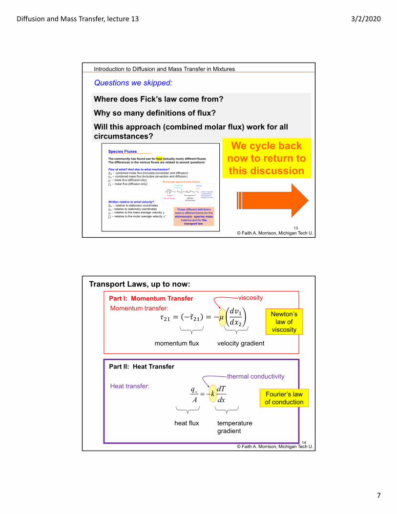
Questions we skipped:
© Faith A. Morrison, Michigan Tech U.
Where does Fick’s law come from?
Why so many definitions of flux?
Will this approach (combined molar flux) work for all circumstances?
Introduction to Diffusion and Mass Transfer in Mixtures
Species Fluxes
The community has found use for four (actually more) different fluxes. The differences in the various fluxes are related to several questions:
Flux of what? And due to what mechanism?𝑁 combined molar flux (includes convection and diffusion)𝑛 combined mass flux (includes convection and diffusion)�̲� mass flux (diffusion only)�̲�∗ molar flux (diffusion only)
Written relative to what velocity?𝑁 relative to stationary coordinates𝑛 relative to stationary coordinates�̲� relative to the mass average velocity 𝑣�̲�∗ relative to the molar average velocity 𝑣∗
Microscopic species A mass balance
rate of change
convection
diffusion (all directions)
source
(mass of species 𝐴 generated by homogeneous reaction per time)
These different definitions lead to different forms for the microscopic species mass
balance and for the transport law.
Diffusion and Mass Transfer, lecture 13 3/2/2020
7
13
Questions we skipped:
© Faith A. Morrison, Michigan Tech U.
Where does Fick’s law come from?
Why so many definitions of flux?
Will this approach (combined molar flux) work for all circumstances?
Introduction to Diffusion and Mass Transfer in Mixtures
Species Fluxes
The community has found use for four (actually more) different fluxes. The differences in the various fluxes are related to several questions:
Flux of what? And due to what mechanism?𝑁 combined molar flux (includes convection and diffusion)𝑛 combined mass flux (includes convection and diffusion)�̲� mass flux (diffusion only)�̲�∗ molar flux (diffusion only)
Written relative to what velocity?𝑁 relative to stationary coordinates𝑛 relative to stationary coordinates�̲� relative to the mass average velocity 𝑣�̲�∗ relative to the molar average velocity 𝑣∗
Microscopic species A mass balance
rate of change
convection
diffusion (all directions)
source
(mass of species 𝐴 generated by homogeneous reaction per time)
These different definitions lead to different forms for the microscopic species mass
balance and for the transport law.
We cycle back now to return to this discussion
14
Part II: Heat Transfer
Momentum transfer:
velocity gradientmomentum flux
dx
dTk
A
qx Heat transfer:
temperature gradient
heat flux
thermal conductivity
Part I: Momentum Transfer
𝜏 �̃� 𝜇𝑑𝑣𝑑𝑥
viscosity
Newton’s law of
viscosity
Fourier’s law of conduction
Transport Laws, up to now:
© Faith A. Morrison, Michigan Tech U.

Diffusion and Mass Transfer, lecture 13 3/2/2020
8
15
Part III: Mass Transfer
Mass transfer:
species mass fraction gradient
Mass flux of species 𝐴
diffusivity
Fick’s law of diffusion𝑗 , 𝜌𝐷
𝜕𝜔𝜕𝑥
Momentum transfer:
velocity gradientmomentum flux
Part I: Momentum Transfer viscosity
Newton’s law of
viscosity
Part II: Heat Transfer
dx
dTk
A
qx Heat transfer:
temperature gradientheat flux
thermal conductivity
Fourier’s law of conduction
Now:
© Faith A. Morrison, Michigan Tech U.
𝑗 , 𝜌𝐷𝜕𝜔𝜕𝑥
16
Part III: Mass Transfer
Mass transfer:
species mass fraction gradient
Mass flux of species 𝐴
diffusivity
Fick’s law of diffusion
Momentum transfer:
velocity gradientmomentum flux
Part I: Momentum Transfer viscosity
Newton’s law of
viscosity
Part II: Heat Transfer
dx
dTk
A
qx Heat transfer:
temperature gradientheat flux
thermal conductivity
Fourier’s law of conduction
Now:
© Faith A. Morrison, Michigan Tech U.
Where do these
equations come from?

Diffusion and Mass Transfer, lecture 13 3/2/2020
9
17
Momentum transfer:
velocity gradientmomentum flux
Part I: Momentum Transfer viscosity
Newton’s law of
viscosity
Part II: Heat Transfer
dx
dTk
A
qx Heat transfer:
temperature gradientheat flux
thermal conductivity
Fourier’s law of conduction
© Faith A. Morrison, Michigan Tech U.
Where does this
equation come from?
The Physics of the Transport Laws
Part III: Mass Transfer
Mass transfer:
species mass fraction gradient
Mass flux of species 𝐴
diffusivity
Fick’s law of diffusion
𝑗 ,
momentum flux
yz
0zv)(yvz
𝑥𝑥 𝑣 𝑥
18
Simple One-dimensional Species Mass Diffusion
© Faith A. Morrison, Michigan Tech U.
Initially:
solid species 𝐵: fused silica
air
air
Suddenly 𝑡 0 :
air
gas species 𝐴: helium
(slow flow)
𝜔 0 𝜔 𝑦, 𝑡 ?
BSL2, p514
helium
𝑦
(gas)
(gas)
(solid)
What is the physics behind the mass diffusion transport law?
Assumptions: • wide, deep⇒ 1D diffusion• no reaction• species B not moving

Diffusion and Mass Transfer, lecture 13 3/2/2020
10
19© Faith A. Morrison, Michigan Tech U.
solid species 𝐵: fused silica
𝑡 0 :
air
gas species 𝐴: helium
(slow flow)
𝜔 𝑦, 𝑡 =?
BSL2, p514
helium diffuses
𝑦
𝜔 ,
What does 𝝎𝑨 𝒚, 𝒕
look like?
.. ... . .
.. ..
.... . .. . .. . . .. .
..
.
. . . ...
Simple One-dimensional Species Mass Diffusion
ω mass fraction of A
20© Faith A. Morrison, Michigan Tech U.
solid species 𝐵: fused silica
air
Gas species 𝐴: helium
(slow flow)
𝜔 𝑦, 𝑡 =?
helium
𝑦
𝜔 ,
What does 𝝎𝑨 𝒚, 𝒕
look like?
𝑡 0 :
Simple One-dimensional Species Mass Diffusion
BSL2, p514

Diffusion and Mass Transfer, lecture 13 3/2/2020
11
21© Faith A. Morrison, Michigan Tech U.
solid species 𝐵: fused silica
• 𝜔 𝑦, 𝑡 =?
• What is the domain we’re asking about?
BSL2, p514
Simple One-dimensional Species Mass Diffusion
air
Gas species 𝐴: helium
(slow flow)
helium
𝑦
𝜔 ,
𝑡 0 :
22© Faith A. Morrison, Michigan Tech U.
solid species 𝐵: fused silica
Suddenly 𝑡 0 :
air
Gas species 𝐴: helium
(slow flow)
helium
𝑦
𝜔 ,
What does 𝝎𝑨 𝒚, 𝒕
look like?
At steady state, 𝜔 𝑦, 𝑡 , 𝑦 𝜔 ,
Simple One-dimensional Species Mass Diffusion
sink
source
BSL2, p514

Diffusion and Mass Transfer, lecture 13 3/2/2020
12
23© Faith A. Morrison, Michigan Tech U.B
SL2
, p51
4
At steady state, 𝜔 𝑦, 𝑡 , 𝑦 𝜔 ,
mass flux 𝜌𝐷0 𝜔 ,
𝑦 𝑦
𝑗 , 𝜌𝐷
𝐷 Diffusion coefficient of 𝐴 through 𝐵
Fick’s law of diffusion
Suddenly 𝑡 0 :
air
Gas species 𝐴: helium
(slow flow)
helium
𝑦
𝜔 ,
D
Suddenly 𝑡 0 :
Simple One-dimensional Species Mass Diffusion
j , mass flux of 𝐴 through 𝐵
(in terms of mass flux)
24© Faith A. Morrison, Michigan Tech U.
At steady state, 𝜔 𝑦, 𝑡 , 𝑦 𝜔 ,
Suddenly 𝑡 0 :
air
Gas species 𝐴: helium
(slow flow)
helium
𝑦
𝜔 ,
D
Suddenly 𝑡 0 :
Simple One-dimensional Species Mass Diffusion
BS
L2, p
514
mass flux 𝜌𝐷0 𝜔 ,
𝑦 𝑦
𝑗 , 𝜌𝐷
𝐷 Diffusion coefficient of 𝐴 through 𝐵
Fick’s law of diffusion
j , mass flux of 𝐴 through 𝐵
(in terms of mass flux)
This is the fundamental version of Fick’s Law
(1D)

Diffusion and Mass Transfer, lecture 13 3/2/2020
13
25© Faith A. Morrison, Michigan Tech U.
•Mass diffuses flows down a concentration gradient
•Flux is proportional to magnitude of concentration gradient
Gibbs notation: �̲� 𝜌D 𝛻𝜔
�̲�
𝜌D𝜕𝜔𝜕𝑥
𝜌D𝜕𝜔𝜕𝑦
𝜌D𝜕𝜔𝜕𝑧
Fick’s law
Law of Species Diffusion
This is the fundamental version of Fick’s Law
(3D)
26© Faith A. Morrison, Michigan Tech U.
Law of Species Diffusion
This is the fundamental version of Fick’s Law
(3D)
But not the one we have been using!
Diffusion and Mass Transfer, lecture 13 3/2/2020
14
27© Faith A. Morrison, Michigan Tech U.
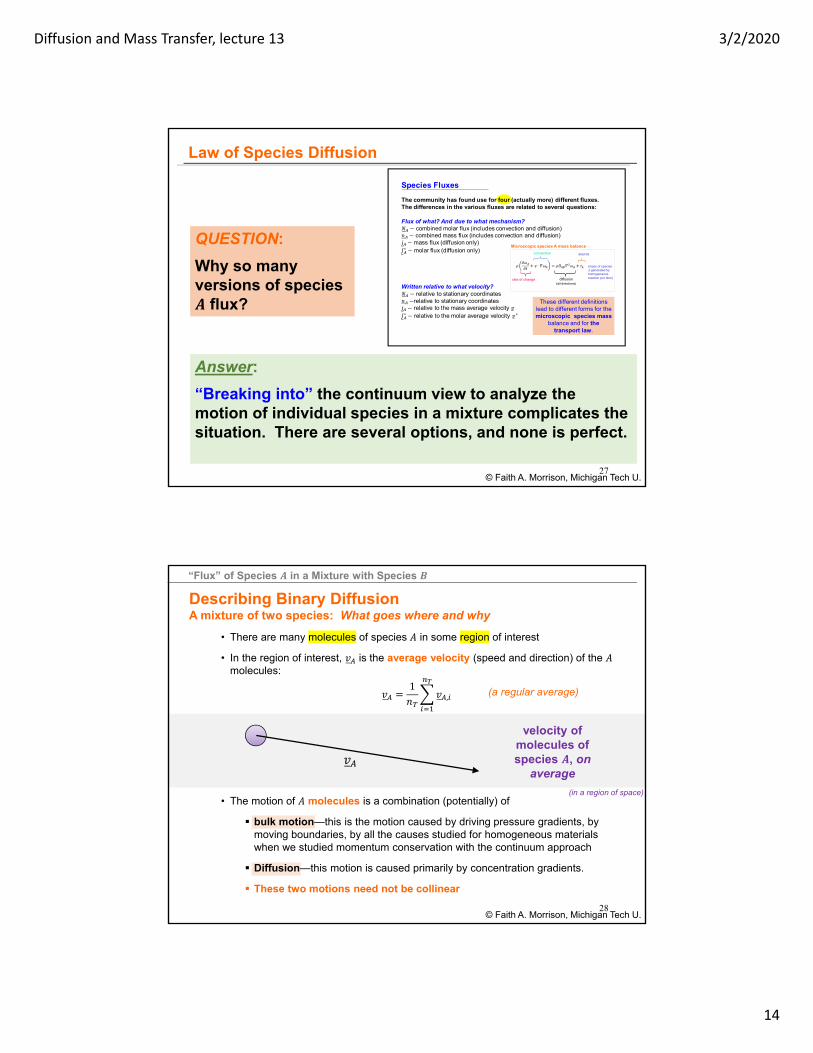
Law of Species Diffusion
QUESTION:
Why so many versions of species 𝑨 flux?
Species Fluxes
The community has found use for four (actually more) different fluxes. The differences in the various fluxes are related to several questions:
Flux of what? And due to what mechanism?𝑁 combined molar flux (includes convection and diffusion)𝑛 combined mass flux (includes convection and diffusion)�̲� mass flux (diffusion only)�̲�∗ molar flux (diffusion only)
Written relative to what velocity?𝑁 relative to stationary coordinates𝑛 relative to stationary coordinates�̲� relative to the mass average velocity 𝑣�̲�∗ relative to the molar average velocity 𝑣∗
Microscopic species A mass balance
rate of change
convection
diffusion (all directions)
source
(mass of species 𝐴 generated by homogeneous reaction per time)
These different definitions lead to different forms for the microscopic species mass
balance and for the transport law.
Answer:
“Breaking into” the continuum view to analyze the motion of individual species in a mixture complicates the situation. There are several options, and none is perfect.
28© Faith A. Morrison, Michigan Tech U.
𝑣
• There are many molecules of species 𝐴 in some region of interest
• In the region of interest, 𝑣 is the average velocity (speed and direction) of the 𝐴molecules:
𝑣1𝑛
𝑣 ,
• The motion of 𝐴 molecules is a combination (potentially) of
bulk motion—this is the motion caused by driving pressure gradients, by moving boundaries, by all the causes studied for homogeneous materials when we studied momentum conservation with the continuum approach
Diffusion—this motion is caused primarily by concentration gradients.
These two motions need not be collinear
velocity of molecules of species 𝑨, on
average
Describing Binary Diffusion A mixture of two species: What goes where and why
“Flux” of Species 𝑨 in a Mixture with Species 𝑩
(a regular average)
(in a region of space)

Diffusion and Mass Transfer, lecture 13 3/2/2020
15
29© Faith A. Morrison, Michigan Tech U.
𝑣
• The motion of 𝐴 molecules is a combination (potentially) of
bulk motion of the mixture—this is the motion caused by driving pressure gradients, by moving boundaries, by all the causes studied for homogeneous materials when we studied momentum conservation
diffusion—this motion is caused by concentration gradients.
These two motions need not be collinear
“Flux” of Species 𝑨 in a Mixture with Species 𝑩
velocity of molecules of species 𝑨, on average
(in a region of space)
𝑣
• The motion of 𝐴 molecules is a combination (potentially) of
bulk motion of the mixture—this is the motion caused by driving pressure gradients, by moving boundaries, by all the causes studied for homogeneous materials when we studied momentum conservation
diffusion—this motion is caused by concentration gradients.
These two motions need not be collinear
30© Faith A. Morrison, Michigan Tech U.
How do we write expressions for these?
“Flux” of Species 𝑨 in a Mixture with Species 𝑩
velocity of molecules of species 𝑨, on average
(in a region of space)
Diffusion and Mass Transfer, lecture 13 3/2/2020
16
31© Faith A. Morrison, Michigan Tech U.
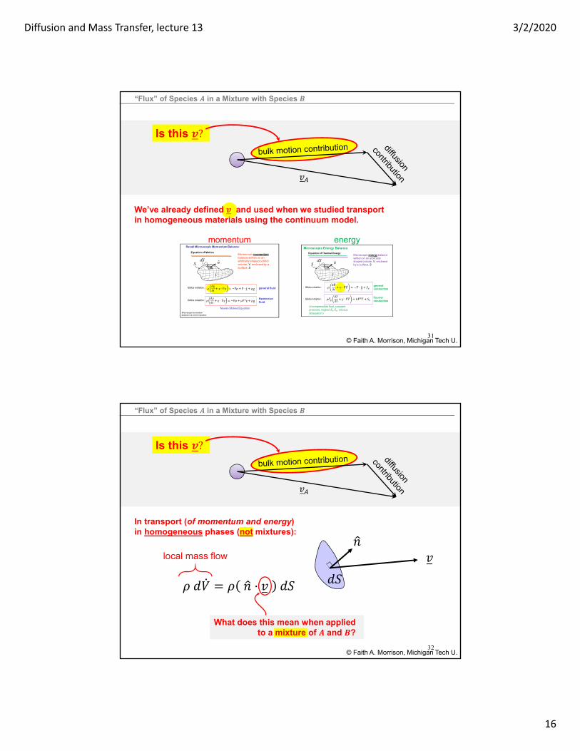
𝑣
Is this 𝒗?
We’ve already defined 𝒗 and used when we studied transport in homogeneous materials using the continuum model.
Equation of Motion
V
n̂dSS
Microscopic momentumbalance written on an arbitrarily shaped control volume, V, enclosed by a surface, S
Gibbs notation: general fluid
Gibbs notation: Newtonian fluid
Navier-Stokes Equation
Microscopic momentum balance is a vector equation.
Recall Microscopic Momentum Balance:
Equation of Thermal Energy
V
n̂dSS
Microscopic energy balance written on an arbitrarily shaped volume, V, enclosed by a surface, S
Gibbs notation:general conduction
Gibbs notation: Fourier conduction
Microscopic Energy Balance:
(incompressible fluid, constant pressure, neglect 𝐸 ,𝐸 , viscous dissipation )
momentum energy
“Flux” of Species 𝑨 in a Mixture with Species 𝑩
32© Faith A. Morrison, Michigan Tech U.
𝑣
Is this 𝒗?
𝜌 𝑑𝑉 𝜌 𝑛 ⋅ 𝑣 𝑑𝑆
𝑣𝑛
𝑑𝑆
local mass flow
What does this mean when applied to a mixture of 𝑨 and 𝑩?
In transport (of momentum and energy) in homogeneous phases (not mixtures):
“Flux” of Species 𝑨 in a Mixture with Species 𝑩

Diffusion and Mass Transfer, lecture 13 3/2/2020
17
33© Faith A. Morrison, Michigan Tech U.
𝜌 𝑑𝑉 𝜌 𝑛 ⋅ 𝑣 𝑑𝑆
local mass flow mass average velocity of individual molecules
𝑐 𝑑𝑉 𝑐 𝑛 ⋅ 𝑣∗ 𝑑𝑆
local molar flow
molar average velocity of individual molecules
If, however, the molar average velocity 𝒗∗ of the molecules in a mixture is calculated, a local molar flow is readily obtained and is not the same:
𝑣𝑛
𝑑𝑆 𝑣∗
“Flux” of Species 𝑨 in a Mixture with Species 𝑩
When we apply the other transport laws to mixtures of 𝐴 and 𝐵, they work, if 𝒗 is the mass average velocity of the molecular velocities 𝑣 and 𝑣
(continuum is divided into mass “particles”)
(continuum is divided into molar “particles”)
Sorry about the re-used nomenclature: 𝑣∗ = the molar average velocity
34© Faith A. Morrison, Michigan Tech U.
𝜌 𝑑𝑉 𝜌 𝑛 ⋅ 𝑣 𝑑𝑆
local mass flow mass average velocity of individual molecules
“Flux” of Species 𝑨 in a Mixture with Species 𝑩
When we apply the other transport laws to mixtures of 𝐴 and 𝐵, they work, if 𝒗 is the mass average velocity of the molecular velocities 𝑣 and 𝑣
This is what I mean when I say we are
“breaking into” the continuum picture.
𝑣 𝜔 𝑣 𝜔 𝑣
𝑣∗ 𝑥 𝑣 𝑥 𝑣
If, however, the molar average velocity 𝒗∗ of the molecules in a mixture is calculated, a local molar flow is readily obtained and is not the same:
Sorry about the re-used nomenclature: 𝑣∗ = the molar average velocity
𝑐 𝑑𝑉 𝑐 𝑛 ⋅ 𝑣∗ 𝑑𝑆
local molar flow
molar average velocity of individual molecules

Diffusion and Mass Transfer, lecture 13 3/2/2020
18
𝜌 𝑑𝑉 𝜌 𝑛 ⋅ 𝑣 𝑑𝑆
local mass flow mass average velocity of individual molecules
𝑐 𝑑𝑉 𝑐 𝑛 ⋅ 𝑣∗ 𝑑𝑆
local molar flow
molar average velocity of individual molecules
If, however, the molar average velocity 𝒗∗ of the molecules in a mixture is calculated, a local molar flow is readily obtained:
𝑣𝑛
𝑑𝑆 𝑣∗
“Flux” of Species 𝑨 in a Mixture with Species 𝑩
When we apply the other transport laws to mixtures of 𝐴 and 𝐵, they work, if 𝒗 is the mass average velocity of the molecular velocities 𝑣 and 𝑣
𝑣 𝜔 𝑣 𝜔 𝑣
𝑣∗ 𝑥 𝑣 𝑥 𝑣
Law of Species Diffusion
QUESTION:
Why so many versions of species 𝑨 flux?
Species Fluxes
The community has found use for four (actually more) different fluxes. The differences in the various fluxes are related to several questions:
Flux of what? And due to what mechanism?𝑁 combined molar flux (includes convection and diffusion)𝑛 combined mass flux (includes convection and diffusion)�̲� mass flux (diffusion only)�̲�∗ molar flux (diffusion only)
Written relative to what velocity?𝑁 relative to stationary coordinates𝑛 relative to stationary coordinates�̲� relative to the mass average velocity 𝑣�̲�∗ relative to the molar average velocity 𝑣∗
Microscopic species A mass balance
rate of change
convection
diffusion (all directions)
source
(mass of species 𝐴 generated by homogeneous reaction per time)
These different definitions lead to different forms for the microscopic species mass
balance and for the transport law.
Answer:
“Breaking into” the continuum view to analyze the motion of individual species in a mixture complicates the situation. There are several options, and none is perfect.
35© Faith A. Morrison, Michigan Tech U.
We are concerning ourselves with sub-characteristics of
the continuum.
This is what I mean when I say we are
“breaking into” the continuum picture.
36© Faith A. Morrison, Michigan Tech U.
𝑣
• The motion of 𝐴 molecules is a combination (potentially) of
bulk motion of the mixture—this is the motion caused by driving pressure gradients, by moving boundaries, by all the causes studied for homogeneous materials when we studied momentum conservation
diffusion—this motion is caused by concentration gradients.
These two motions need not be collinear How do we write expressions for these?
velocity of molecules of species 𝑨, on
average
“Flux” of Species 𝑨 in a Mixture with Species 𝑩
So, what’s the answer?
How do we write expressions for the two contributions to the average motion of molecules when diffusion is present?
Two contributions:
• Bulk motion• Diffusion

Diffusion and Mass Transfer, lecture 13 3/2/2020
19
37© Faith A. Morrison, Michigan Tech U.
𝑣
Is this 𝒗?
It can be. We have a choice as to how to write the bulk motion contribution.
If the diffusion contribution is calculated as the mass flux relative to 𝒗𝑨 𝒗 , then the model works.
“Flux” of Species 𝑨 in a Mixture with Species 𝑩
Answer:
How do we write expressions for the two contributions to the average motion of molecules when diffusion is present?
First Approach
𝑣 𝜔 𝑣 𝜔 𝑣
38© Faith A. Morrison, Michigan Tech U.
𝑣
𝑣
Now, what is this?
“Flux” of Species 𝑨 in a Mixture with Species 𝑩
Choose: Bulk contribution expressed as 𝒗First Approach

Diffusion and Mass Transfer, lecture 13 3/2/2020
20
39© Faith A. Morrison, Michigan Tech U.
𝑣
𝑣
volumetric flow rate per area in the direction of diffusion
𝑣𝑜𝑙𝑢𝑚𝑒𝑎𝑟𝑒𝑎 ⋅ 𝑡𝑖𝑚𝑒
𝑚𝑎𝑠𝑠 𝐴𝑣𝑜𝑙𝑢𝑚𝑒
Start with mass flux:
Recall in a pipe: ⟨𝑣⟩
“Flux” of Species 𝑨 in a Mixture with Species 𝑩
Fick’s law in mass terms
Mass flux of 𝐴 ≡
⋅
𝑣 𝑣 𝜌 𝜔 ≡ �̲� 𝜌𝐷 𝛻𝜔
Choose: Bulk contribution expressed as 𝒗
𝑣 𝑣
diffusion contribution
First Approach
40© Faith A. Morrison, Michigan Tech U.
“Flux” of Species 𝑨 in a Mixture with Species 𝑩
What if I want to use a molar flux?
How do we write expressions for the two contributions to the average motion of molecules when diffusion is present?
Second Approach
𝑣

Diffusion and Mass Transfer, lecture 13 3/2/2020
21
41© Faith A. Morrison, Michigan Tech U.
“Flux” of Species 𝑨 in a Mixture with Species 𝑩
What if I want to use a molar flux?
𝑣
This is possible too.
To express diffusion in moles, the bulk motion contribution, however, cannot be given by the mass average velocity; instead we must use the molar average velocity 𝒗∗.
How do we write expressions for the two contributions to the average motion of molecules when diffusion is present?
bulk molar contribution 𝒗
Answer:
Second Approach
𝑣∗ 𝑥 𝑣 𝑥 𝑣
42© Faith A. Morrison, Michigan Tech U.
“Flux” of Species 𝑨 in a Mixture with Species 𝑩
What if I want to use a molar flux?
𝑣
This is possible too.
To express diffusion in moles, the bulk motion contribution, however, cannot be given by the mass average velocity; instead we must use the molar average velocity 𝒗∗.
How do we write expressions for the two contributions to the average motion of molecules when diffusion is present?
bulk molar contribution 𝒗
Answer:
Second Approach
To be continued