http://sgo.sagepub.com/SAGE Open

/content/4/4/2158244014551713The online version of this article can be found at:

 DOI: 10.1177/2158244014551713

2014 4: SAGE OpenFarjana Mostafiz Shatu, Md. Kamruzzaman and Kaveh Deilami

Did Brisbane Grow Smartly? Drivers of City Growth 1991-2001 and Lessons for Current Policies  

Published by:

http://www.sagepublications.com 

 

can be found at:SAGE OpenAdditional services and information for    

  /cgi/alertsEmail Alerts:

 

/subscriptionsSubscriptions:  

http://www.sagepub.com/journalsReprints.navReprints:  

SAGE Open are in each case credited as the source of the article.permission from the Author or SAGE, you may further copy, distribute, transmit, and adapt the article, with the condition that the Author and © 2014 the Author(s). This article has been published under the terms of the Creative Commons Attribution License. Without requesting

by guest on October 25, 2014Downloaded from by guest on October 25, 2014Downloaded from

SAGE OpenOctober-December 2014: 1 –19© The Author(s) 2014DOI: 10.1177/2158244014551713sgo.sagepub.com

Creative Commons CC BY: This article is distributed under the terms of the Creative Commons Attribution 3.0 License (http://www.creativecommons.org/licenses/by/3.0/) which permits any use, reproduction and distribution of the work without further

permission provided the original work is attributed as specified on the SAGE and Open Access page (http://www.uk.sagepub.com/aboutus/openaccess.htm).

Article

Introduction

Land cover and land uses have distinct meanings. However, they are often used interchangeably in the literature (Jansen, Carrai, & Petri, 2007; Koomen & Stillwell, 2007). Land cover can be observed (e.g., grass, building) whereas land uses refer to the actual use to which the land is put (e.g., grassland for grazing, building for residences; Lambin et al., 2001). This research focuses on land-cover changes, which are arguably a major factor of climate change (Ahmed, Kamruzzaman, Zhu, Rahman, & Keechoo, 2013; Dale, 1997; Feddema et al., 2005; Pena et al., 2007; Shaw, 1992; Watson et al., 2000). However, this relationship is not unidirectional; rather, it is more complex and interdependent (Koomen & Stillwell, 2007; Lambin, Geist, & Lepers, 2003). For exam-ple, a change in land-cover pattern (e.g., deforestation) is likely to affect the climate whereas any climatic changes (e.g., excessive temperature) are also likely to alter the land-cover patterns (e.g., deforestation) of an area. As a result, it is critical to examine whether our land covers are changing sus-tainably, and in particular, in urban areas, given that urban land covers are more susceptible to unsustainable changes due to rapid urbanization (Chang & Franczyk, 2008). Such

an analysis not only enables to monitor changes but also allows steering urban growth in a more sustainable way (Meyer & Turner, 1994; Walker, Steffen, Canadell, & Ingram, 1997).

Sustainable development has been defined as develop-ment that “meets the needs of the present without compro-mising the ability of future generations to meet their own needs” (World Commission on Environment and Development, 1987, p. 8). This general definition has been expanded with various scopes for sustainable urban develop-ment such as the concept of smart growth (Li & Yeh, 2000). Smart growth principles highlight the need to foster compact development through promoting infill development, and thereby to preserve open spaces, and to limit the outward expansion of cities (Berke, Godschalk, Kaiser, & Rodriguez,

551713 SGOXXX10.1177/2158244014551713SAGE OpenShatu et al.research-article2014

1Queensland University of Technology, Brisbane, Australia

Corresponding Author:Md. Kamruzzaman, School of Civil Engineering and the Built Environment, Queensland University of Technology, 2 George Street, Brisbane, Queensland 4000, Australia. Email: md.kamruzzaman@qut.edu.au

Did Brisbane Grow Smartly? Drivers of City Growth 1991-2001 and Lessons for Current Policies

Farjana Mostafiz Shatu1, Md. Kamruzzaman1, and Kaveh Deilami1

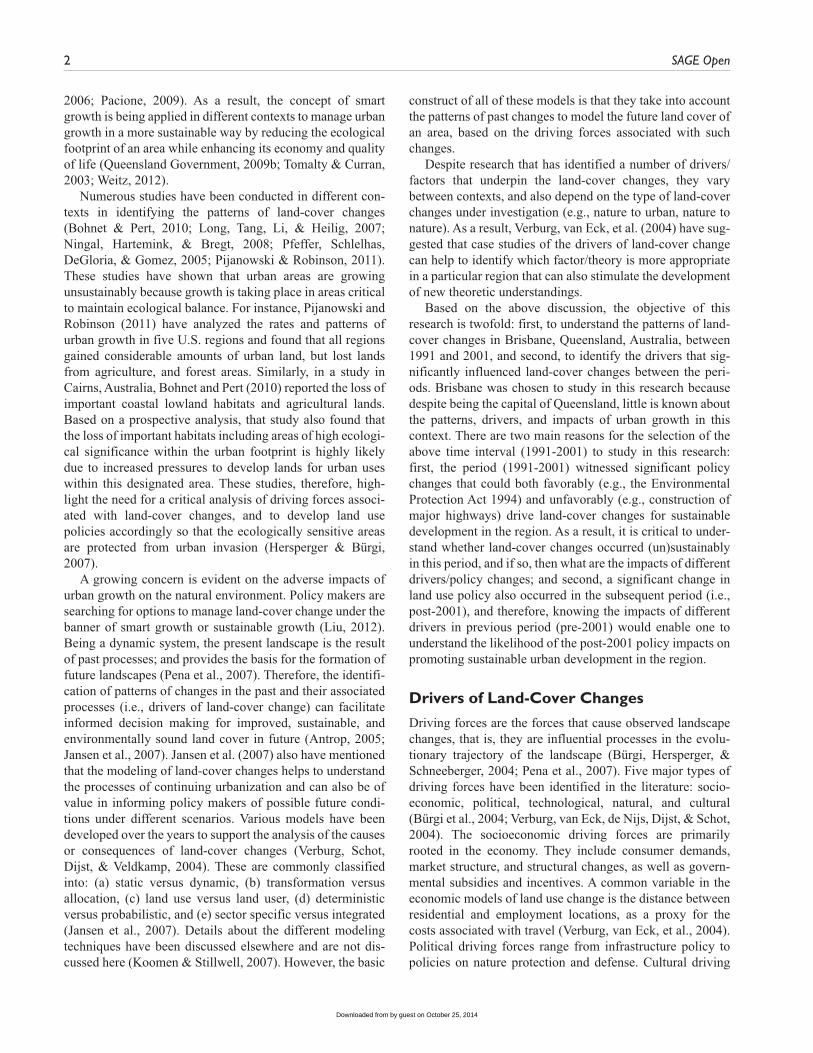
AbstractUrban areas are growing unsustainably around the world; however, the growth patterns and their associated drivers vary between contexts. As a result, research has highlighted the need to adopt case study based approaches to stimulate the development of new theoretic understandings. Using land-cover data sets derived from Landsat images (30 m × 30 m), this research identifies both patterns and drivers of urban growth in a period (1991-2001) when a number of policy acts were enacted aimed at fostering smart growth in Brisbane, Australia. A linear multiple regression model was estimated using the proportion of lands that were converted from non-built-up (1991) to built-up usage (2001) within a suburb as a dependent variable to identify significant drivers of land-cover changes. In addition, the hot spot analysis was conducted to identify spatial biases of land-cover changes, if any. Results show that the built-up areas increased by 1.34% every year. About 19.56% of the non-built-up lands in 1991 were converted into built-up lands in 2001. This conversion pattern was significantly biased in the northernmost and southernmost suburbs in the city. This is due to the fact that, as evident from the regression analysis, these suburbs experienced a higher rate of population growth, and had the availability of habitable green field sites in relatively flat lands. The above findings suggest that the policy interventions undertaken between the periods were not as effective in promoting sustainable changes in the environment as they were aimed for.

Keywordssustainable urban growth, exurbanization, drivers of change, spatial biases, land use policy

by guest on October 25, 2014Downloaded from

2 SAGE Open

2006; Pacione, 2009). As a result, the concept of smart growth is being applied in different contexts to manage urban growth in a more sustainable way by reducing the ecological footprint of an area while enhancing its economy and quality of life (Queensland Government, 2009b; Tomalty & Curran, 2003; Weitz, 2012).

Numerous studies have been conducted in different con-texts in identifying the patterns of land-cover changes (Bohnet & Pert, 2010; Long, Tang, Li, & Heilig, 2007; Ningal, Hartemink, & Bregt, 2008; Pfeffer, Schlelhas, DeGloria, & Gomez, 2005; Pijanowski & Robinson, 2011). These studies have shown that urban areas are growing unsustainably because growth is taking place in areas critical to maintain ecological balance. For instance, Pijanowski and Robinson (2011) have analyzed the rates and patterns of urban growth in five U.S. regions and found that all regions gained considerable amounts of urban land, but lost lands from agriculture, and forest areas. Similarly, in a study in Cairns, Australia, Bohnet and Pert (2010) reported the loss of important coastal lowland habitats and agricultural lands. Based on a prospective analysis, that study also found that the loss of important habitats including areas of high ecologi-cal significance within the urban footprint is highly likely due to increased pressures to develop lands for urban uses within this designated area. These studies, therefore, high-light the need for a critical analysis of driving forces associ-ated with land-cover changes, and to develop land use policies accordingly so that the ecologically sensitive areas are protected from urban invasion (Hersperger & Bürgi, 2007).

A growing concern is evident on the adverse impacts of urban growth on the natural environment. Policy makers are searching for options to manage land-cover change under the banner of smart growth or sustainable growth (Liu, 2012). Being a dynamic system, the present landscape is the result of past processes; and provides the basis for the formation of future landscapes (Pena et al., 2007). Therefore, the identifi-cation of patterns of changes in the past and their associated processes (i.e., drivers of land-cover change) can facilitate informed decision making for improved, sustainable, and environmentally sound land cover in future (Antrop, 2005; Jansen et al., 2007). Jansen et al. (2007) also have mentioned that the modeling of land-cover changes helps to understand the processes of continuing urbanization and can also be of value in informing policy makers of possible future condi-tions under different scenarios. Various models have been developed over the years to support the analysis of the causes or consequences of land-cover changes (Verburg, Schot, Dijst, & Veldkamp, 2004). These are commonly classified into: (a) static versus dynamic, (b) transformation versus allocation, (c) land use versus land user, (d) deterministic versus probabilistic, and (e) sector specific versus integrated (Jansen et al., 2007). Details about the different modeling techniques have been discussed elsewhere and are not dis-cussed here (Koomen & Stillwell, 2007). However, the basic

construct of all of these models is that they take into account the patterns of past changes to model the future land cover of an area, based on the driving forces associated with such changes.

Despite research that has identified a number of drivers/factors that underpin the land-cover changes, they vary between contexts, and also depend on the type of land-cover changes under investigation (e.g., nature to urban, nature to nature). As a result, Verburg, van Eck, et al. (2004) have sug-gested that case studies of the drivers of land-cover change can help to identify which factor/theory is more appropriate in a particular region that can also stimulate the development of new theoretic understandings.

Based on the above discussion, the objective of this research is twofold: first, to understand the patterns of land-cover changes in Brisbane, Queensland, Australia, between 1991 and 2001, and second, to identify the drivers that sig-nificantly influenced land-cover changes between the peri-ods. Brisbane was chosen to study in this research because despite being the capital of Queensland, little is known about the patterns, drivers, and impacts of urban growth in this context. There are two main reasons for the selection of the above time interval (1991-2001) to study in this research: first, the period (1991-2001) witnessed significant policy changes that could both favorably (e.g., the Environmental Protection Act 1994) and unfavorably (e.g., construction of major highways) drive land-cover changes for sustainable development in the region. As a result, it is critical to under-stand whether land-cover changes occurred (un)sustainably in this period, and if so, then what are the impacts of different drivers/policy changes; and second, a significant change in land use policy also occurred in the subsequent period (i.e., post-2001), and therefore, knowing the impacts of different drivers in previous period (pre-2001) would enable one to understand the likelihood of the post-2001 policy impacts on promoting sustainable urban development in the region.

Drivers of Land-Cover Changes

Driving forces are the forces that cause observed landscape changes, that is, they are influential processes in the evolu-tionary trajectory of the landscape (Bürgi, Hersperger, & Schneeberger, 2004; Pena et al., 2007). Five major types of driving forces have been identified in the literature: socio-economic, political, technological, natural, and cultural (Bürgi et al., 2004; Verburg, van Eck, de Nijs, Dijst, & Schot, 2004). The socioeconomic driving forces are primarily rooted in the economy. They include consumer demands, market structure, and structural changes, as well as govern-mental subsidies and incentives. A common variable in the economic models of land use change is the distance between residential and employment locations, as a proxy for the costs associated with travel (Verburg, van Eck, et al., 2004). Political driving forces range from infrastructure policy to policies on nature protection and defense. Cultural driving

by guest on October 25, 2014Downloaded from

Shatu et al. 3

forces include way of life, demography, and the past devel-opment of a society. Technology has shaped the landscape enormously. Striking examples are the distinct impacts of railroads and highways on settlement patterns (Bürgi et al., 2004). Road expansion and improvement not only lead to more development but may also lead to a different pattern through a reorganization of the market structure, which then feeds back to further infrastructure development (Verburg, Schot, et al., 2004). The natural/spatial configuration driving forces can be classified into the following: site factors such as spatial configuration (e.g., existing land uses and transpor-tation networks), topography and soil conditions, and natural disturbances such as global change and mudslides (Bürgi et al., 2004; Hersperger & Bürgi, 2007).

A number of studies have found that accessibility, and especially the road network, acts as a major driving force for the development of cities (Antrop, 2005; Verburg, van Eck, et al., 2004). Mediterranean landscapes have undergone major changes, mainly because of population growth (Sonis, Shoshany, & Goldshlager, 2007). Shi, Wang, Fan, Li, and Yang (2010) have examined the correlation between popula-tion growth and land-cover changes in Original-stream Zone of Tarim River between 1994 and 2005. This work found that cropland area increased in the region with the increases of population density at the expense of grassland. Similarly, in a study in Papua New Guinea, Ningal et al. (2008) found that agricultural land use increased by 58% and population grew by 99% between 1975 and 2000. However, this study also reported that most new agricultural lands were taken from primary forest; and consequently, the forest area decreased from 9.8 hectare per person in 1975 to 4.4 hectare per person in 2000. Population growth has also been identified as a sig-nificant factor by Pfeffer et al. (2005) in Honduras. This study reported that in areas of high population density, fal-lows give way to more intensive land uses between 1993 and 1999 (Pfeffer et al., 2005). Long et al. (2007) found that paddy fields, dry land, and forested land decreased by 8.2%, 29%, and 2.6% from 1987 to 1994, and by 4.1%, 7.6%, and 8% from 1994 to 2000, respectively, in Kunshan, China. In contrast, urban settlements increased by 87.6% between 1987 and 1994. This study concluded that industrialization, urbanization, population growth, and China’s economic reform policies are the four major driving forces that contrib-uted to land-cover changes in the region. However, after reviewing different cases, Lambin et al. (2001) found that neither population nor poverty alone constitute the sole and major underlying causes of land-cover change worldwide. Rather, peoples’ responses to economic opportunities, as mediated by institutional factors, drive land-cover changes. Similar findings have also been reported by Skonhoft and Solem (2001) in their analyses of macroeconomic factors in explaining the reduction of wilderness land in Norway between 1988 and 1994. Based on regression analyses, this study found that the relative amount of wilderness land (i.e., wilderness land as a fraction of the total area within each county) is negatively related to the level of economic

activity, as measured by gross domestic product (GDP) per capita. This research also reported that the wilderness land decreased with the increase of GDP over the period.

Data and Method

This research identifies land-cover patterns and the drivers of land-cover changes in Brisbane, Australia. Both macro (city level) and micro level (suburbs) changes were investigated in this research. The former analysis focuses on the patterns of changes at the city level (i.e., entire Brisbane) whereas the latter identifies the drivers of such changes at the suburb level. Micro level analysis is important to understand detailed land-cover change patterns whereas the macro/aggregated level of analysis (e.g., community, city) may show patterns that remain invisible at the detailed scale, which are impor-tant in the land use policy and planning process (Jansen et al., 2007; Veldkamp, Kok, De Koning, Verburg, & Bergsma, 2001). The research also focuses on the temporal dynamics and measured land-cover changes between 1991 and 2001. The factors/drivers of land-cover changes were also selected from different sub-systems (e.g., transport/infrastructure, population growth, housing market/rent) operating within a system (e.g., urban) and thereby incorporated in the “level of integration” concept as identified by Verburg, Schot, et al. (2004). The following sub-sections describe the methodol-ogy used to take into account the above issues in this research.

Study Area and Policy Context

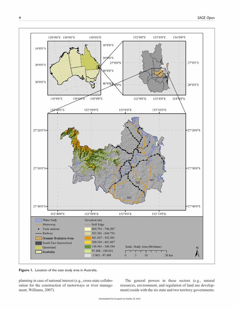
This study was conducted in the context of Brisbane, located in the middle of South East Queensland, Australia (Figure 1). Brisbane, the capital of Queensland, is one of the fastest growing cities in Australia, and currently, it is the third larg-est city in terms of population in Australia. However, Brisbane is the largest urban local government body (in terms of size) in Australia with an area of about 1,163 km2 (by excluding areas located at different islands). A major por-tion of the city is undulating and the elevation ranges between −3.96 m and 706.21 m above the sea level. The city is cen-tered along the Brisbane River. The spatial extent of the study area is shown in Figure 1.

Australia has a three-tiered system of urban governance: federal (national), state and territory, and local government. The role of each tier in the planning and management of land uses can be found elsewhere (Williams, 2007), and as a result, they are not discussed here in detail. Briefly, the fed-eral government plays little to no role in the formulation of planning policies in Australia. Examples of federal powers include trade and commerce with other countries; taxation; postal, telegraphic, and similar services; quarantine; foreign affairs; immigration; foreign corporations; and defense. Significantly for urban planning, these powers do not include a general power over management of natural resources, plan-ning, environment, and regulation of land use development. However, the federal government has certain role to play for

by guest on October 25, 2014Downloaded from

4 SAGE Open

planning in case of national interest (e.g., cross-state collabo-ration for the construction of motorways or river manage-ment; Williams, 2007).

The general powers in these sectors (e.g., natural resources, environment, and regulation of land use develop-ment) reside with the six state and two territory governments.

Figure 1. Location of the case study area in Australia.

by guest on October 25, 2014Downloaded from

Shatu et al. 5

This has meant that each state and territory has established its own planning system complete with statutory, policy, and procedural frameworks. The administration of these systems is the responsibility of each state and territory government, although in practice, they do delegate a number of day-to-day decision-making functions to local government. Local government is a creation of the states. Most day-to-day plan-ning decisions are made at local government level. Bulk of applications for development or planning permission are being lodged at local government level and these are assessed and determined by local councils based on strategic guidance rather than state governments. However, strategic planning is usually subject to state government direction. As a result, Brisbane is subjected to both state level policies in Queensland and in particular to the South East Queensland (SEQ) regional policies, and other policies associated with Brisbane City Council (Queensland Government, 2008, 2009b).

Brisbane has experienced 4.4% population growth between 1981 and 1991 (from 736,660 to 769,087 persons; Queensland Government, 2009a). To accommodate such population growth in a more sustainable way while main-taining the economic prosperity of the region, the Queensland Government enacted a range of policies/acts in the subse-quent period (1991-2001) including the Environmental Protection Act 1994, the Integrated Planning Act 1997, and the Water Act 2000. The pre-1991 anticipation of the govern-ment that population growth will continue in the post-1991 period was proven. Statistics showed that population increased by 17% between 1991 and 2001 (from 754,042 to 884,054 persons1; Queensland Government, 2009a). However, to accommodate this further growth while ensur-ing a balanced economic growth in the region, several major infrastructure projects were undertaken in this period such as the construction/upgrade of the Pacific Motorway (M1), Logan Motorway (M2), Inner City Bypass, and M3 (Figure 1; Queensland Motorways, 2012). Therefore, the period (1991-2001) experienced both favorable policy changes for sustainable development (e.g., the Acts) and drivers of land-cover changes that can lead to unsustainable growth (e.g., population, infrastructure).

A further population growth has also been anticipated for the post-2001 period and the government intended to man-age such growth in a sustainable way by maintaining the region’s ecological footprint while enhancing its economy and residents’ quality of life. One of the long-term strategic visions for the Queensland Government (2008) is to build Queensland as a strong, green, smart, and healthy state by reducing congestion and by cutting one third of its current carbon emissions. The SEQ Regional Plan 2009-2031, oper-ational since 2005, provides specific policy guidelines to meet these stated goals (Queensland Government, 2009b). One of the policy guidelines is to identify an Urban Footprint, as a means to control unplanned urban expansion. The Urban Footprint establishes a boundary for urban development,

containing urban growth and promoting a higher density urban form. By consolidating urban growth into an identified area, travel times and distances can be greatly reduced and accessibility to essential services improved. The Urban Footprint identifies land that can meet the region’s urban development needs to 2031 in a more compact form.

As a result, it is critical to investigate the following: (a) the impacts of the policies undertaken in the 1991-2001 period on land-cover changes, and (b) the differential impacts of various drivers that influenced land-cover changes between 1991 and 2001 so that the likelihood of the post-2001 policy impacts on promoting sustainable urban devel-opment in the region can be understood.

Data

This research analyzed land-cover changes in Brisbane between 1991 and 2001. Two Landsat satellite images (5 TM [thematic mapper] and 7 ETM [enhanced thematic map-per]), one for each period containing scene of WRS-2 Path 89 and Row 79, were acquired from the United States Geological Surveys (USGS) database. Cloud-free images were selected based on the highest temporal consistency (i.e., collected in the same month/season) to reduce the effects of both seasonal and phonological differences on land covers (Ottinger, Kuenzer, Liu, Wang, & Dech, 2013). The Landsat TM and ETM images were captured on September 6, 1991, and September 9, 2001, respectively. Both images were geo-referenced and corrected to obtain a systematic radiometric and geometric accuracy according to the USGS Level 1 terrain (L1T) correction system based on ground control points and a digital elevation model (DEM) for topographic accuracy. Note that the study area covers only a portion of the whole scene, and as a result, the images were extracted to the extent of the study area as shown in Figure 1. The Transverse Mercator projection (within Zone 56) and the Australian Geographic Datum (GDA) 1994 were applied to the images to match with other spatial data sets used in this research. The other spatial data sets (e.g., road network, statistical local area vis-à-vis suburb, digital eleva-tion model) were downloaded from the Queensland Government Information website (http://dds.information.qld.gov.au/dd-s/). In addition, a land use map prepared in 1994 and an aerial photograph acquired by Nearmap in 2004 were collected from the library of Queensland University of Technology. These were used as reference maps. The former and the latter were used to assess the accuracy of the 1991 and 2001 land-cover maps generated from the satellite images.

Derivation of Land-Cover Classes

This research followed the USGS land-cover classification scheme, which was found to be consistent in this context according to the data reported by the Australian Bureau of

by guest on October 25, 2014Downloaded from

6 SAGE Open

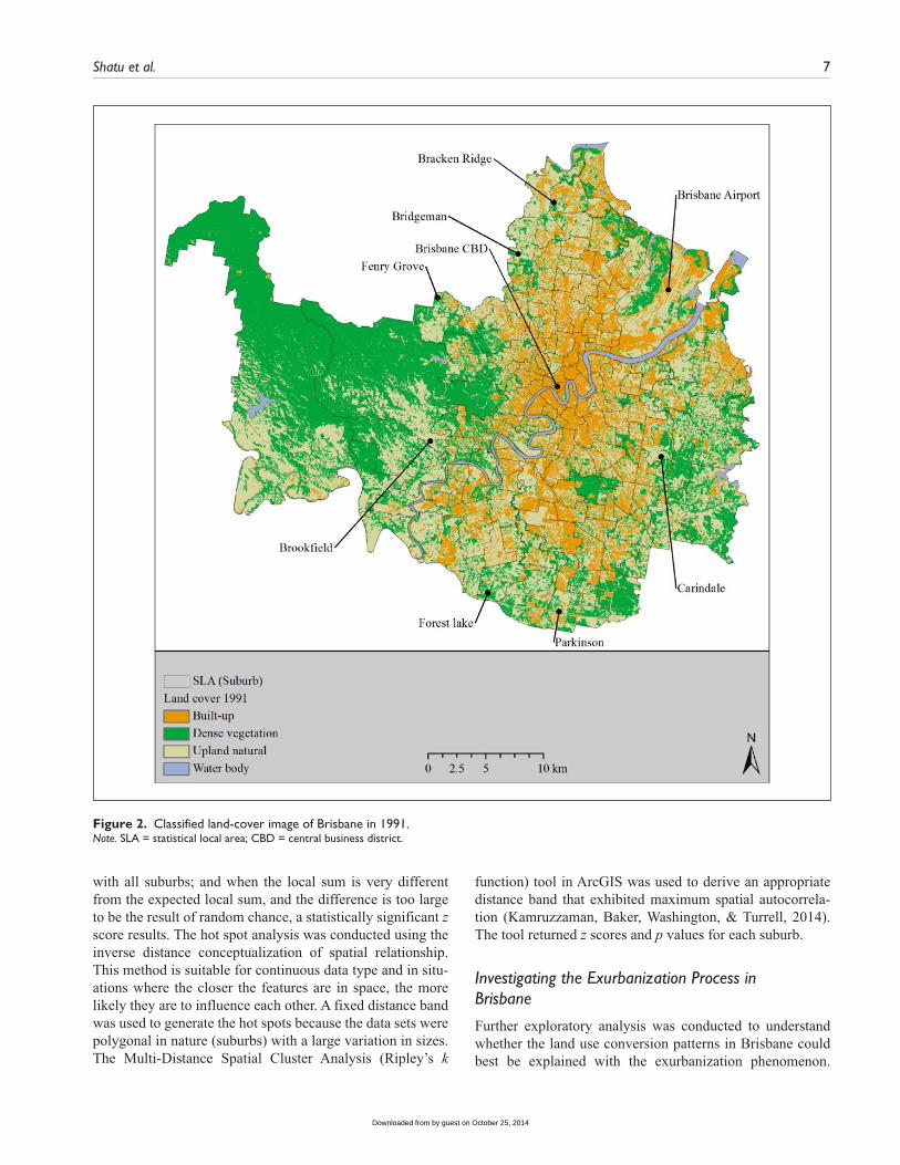
Statistics (ABS, 2008; Table 1). The supervised classifica-tion method was used to classify the acquired satellite images into four broad land-cover types using ENVI 5.0 software (Table 1). This method was chosen because the researchers had a priori knowledge of the study area. As a part of the classification process, a number of training sites were identi-fied and digitized for each land-cover type based on the ref-erenced aerial photographs. The number of training sites for each class varies between 20 (for water body) and 50 (for built-up areas). In total, 150 training sites were selected for each period, which was found to be representative of previ-ous studies on this topic (Cai, Zhang, Pan, Chen, & Wang, 2012; Tan, Lim, Matjafri, & Abdullah, 2010). The training sites of both images were then analyzed in terms of their spectral and spatial profiles. Based on the training sites, the statistical characterizations (i.e., signatures) of each land-cover class were developed. The maximum likelihood clas-sification method was then applied with equal priori probability for all classes—one of the most commonly used methods in the literature (White, Shao, Kennedy, & Campbell, 2013). The maximum likelihood classifier calcu-lated the probability of each pixel belonging to each class based on their attributes. A filtering technique was also applied to generalize the classified land-cover images. This post-processing operation replaced the isolated pixels to the most common neighboring class. Finally, the generalized images were reclassified to produce the final version of land-cover maps for different years. Figures 2 and 3 show classi-fied land-cover maps of Brisbane for 1991 and 2001 respectively.

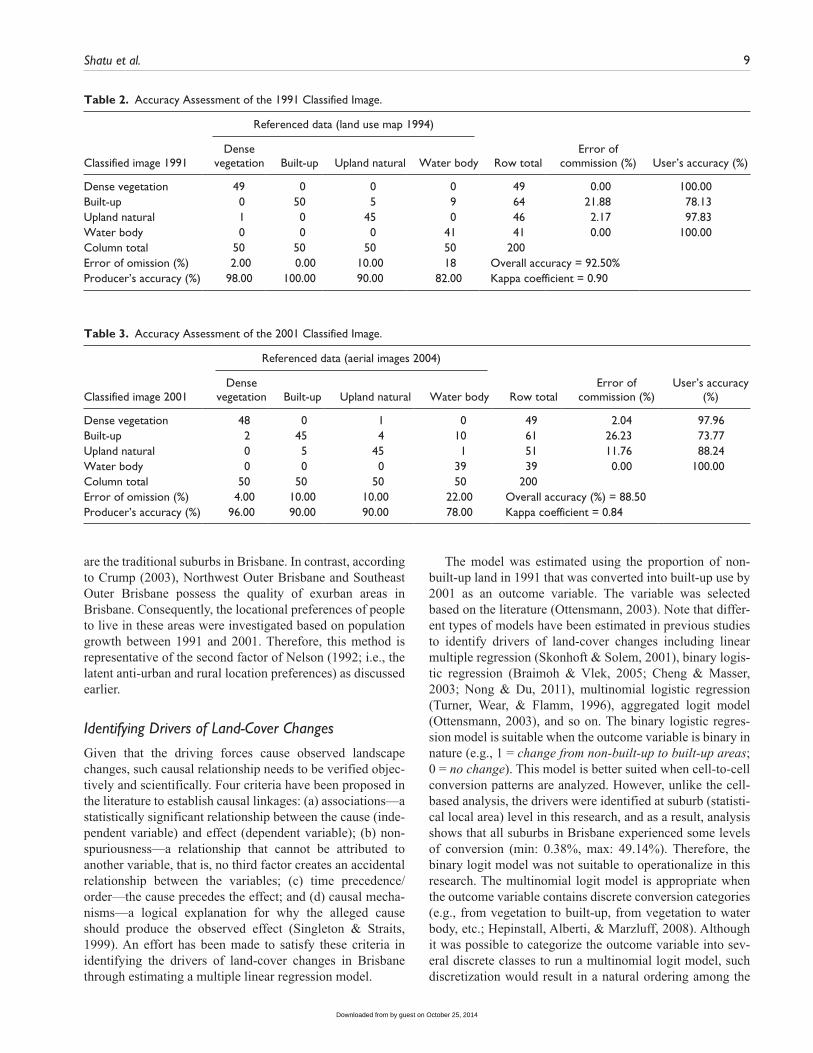
An accuracy assessment exercise was then carried out to identify the quality of the classified images. Using the litera-ture, a total of 200 pixels were selected from the classified images of each period based on a stratified random sampling technique (Ahmed et al., 2013; Bakr, Weindorf, Bahnassy, Marei, & El-Badawi, 2010; Tan et al., 2010). The selected pixels from the 1991 satellite image were then matched against the 1994 land use maps whereas the pixels from the 2001 image were checked against the aerial photograph. The evaluation results in Tables 2 and 3 show that the overall accuracies of the classified images (1991, 2001) were 92.5% and 88.5% in respective year. The high overall accuracies for both images signify that the selected classes produce very distinguishable reflectance and are clearly identifiable on earth surface.

Deriving Land-Cover Changes

The classified data sets of the two periods were used to ana-lyze their patterns for each period. In addition to analyzing land-cover patterns, a conversion matrix of land covers (cell to cell) between the periods was derived using the “Conditional Or” tool in ArcGIS.

Table 1 shows that only the built-up category bears the characteristics of urban land use whereas the remaining three categories are more related to ecologically sensitive land uses. As a result, the classified images were further reclassi-fied into built-up and non-built-up categories, and a similar conversion matrix was derived. These conversion matrices were then used to examine the patterns of land-cover changes in Brisbane between the periods.

Measuring Spatial Biases in Land-Cover Changes

In addition to identifying the statistical patterns, this research further investigates the spatial patterns of land-cover changes. The aim was to examine whether the conversion patterns followed any spatial biases or whether they are ran-domly distributed across Brisbane. As a result, the hot spot analysis was conducted in ArcGIS based on the percentage of suburb’s lands that were converted from non-built-up to built-up areas in each suburb (157) in Brisbane. The suburbs were chosen as a unit of analysis because of their relevance to planning and policy in Brisbane, Australia. Although all properties in Brisbane are subject to at least two plans (e.g., SEQ Regional Plan, Council’s City Plan), many suburbs/communities in Brisbane also have their own local or neigh-borhood plan as a part of the City Plan. Consequently, these neighborhood plans are used to focus where growth and change occur, and to protect the character of housing and ecologically sensitive areas (e.g., parks and wildlife corri-dors; Brisbane City Council, 2013).

The hot spot analysis tool calculated the Getis-Ord Gi* statistics for each suburb based on the proportion of con-verted land in each suburb and also taking into account the proportion of conversion in surrounding suburbs. This means that a suburb with a high percentage may not be a statistically significant hot spot unless it is surrounded by suburbs with high percentages of conversion. The tool calculated local sum of conversion for a suburb and its neighbors and com-pares proportionately with the sum of conversions associated

Table 1. Details of the Land-Cover Types.

Land-cover type Description

Built-up area All infrastructure—residential, commercial, mixed use and industrial areas, villages, settlements, road network, pavements, and man-made structures.

Water body River, permanent open water, lakes, ponds, canals, permanent/seasonal wetlands, low-lying areas, marshy land, and swamps.

Dense vegetation Dense trees, mixed forest, tropical forestsUpland natural Fallow land, urban recreations, grasses, pastures, sparse vegetation, wetland areas

by guest on October 25, 2014Downloaded from

Shatu et al. 7

with all suburbs; and when the local sum is very different from the expected local sum, and the difference is too large to be the result of random chance, a statistically significant z score results. The hot spot analysis was conducted using the inverse distance conceptualization of spatial relationship. This method is suitable for continuous data type and in situ-ations where the closer the features are in space, the more likely they are to influence each other. A fixed distance band was used to generate the hot spots because the data sets were polygonal in nature (suburbs) with a large variation in sizes. The Multi-Distance Spatial Cluster Analysis (Ripley’s k

function) tool in ArcGIS was used to derive an appropriate distance band that exhibited maximum spatial autocorrela-tion (Kamruzzaman, Baker, Washington, & Turrell, 2014). The tool returned z scores and p values for each suburb.

Investigating the Exurbanization Process in Brisbane

Further exploratory analysis was conducted to understand whether the land use conversion patterns in Brisbane could best be explained with the exurbanization phenomenon.

Figure 2. Classified land-cover image of Brisbane in 1991.Note. SLA = statistical local area; CBD = central business district.

by guest on October 25, 2014Downloaded from

8 SAGE Open

Crump (2003) has mentioned that exurban development occurs beyond the suburbs and is outside easy commuting range to the central city. As a result, the exurban locations are viewed as the middle ground between densely populated (urban and suburban) regions and sparsely settled rural (towns and countryside) areas (Pacione, 2009). Therefore, it is neither urban nor rural; it may, in fact, represent a new settlement form that is giving rise to a unique landscape. Nelson (1992) has identified four principal factors explain-ing the exurbanization phenomenon: (a) continued decon-centration of employment and the rise of exurban

industrialization; (b) the latent anti-urban and rural location preferences; (c) improved technology that makes exurban living possible (e.g., car); and (d) an apparent policy bias favoring exurban development over compact development.

To assess the exurbanization process, the converted built-up areas were spatially classified according to five major sub-divisions in Brisbane: (a) Inner Brisbane, (b) Northwest Inner Brisbane, (c) Southeast Inner Brisbane, (d) Northwest Outer Brisbane, and (e) Southeast Outer Brisbane. Therefore, the Inner Brisbane area represents the core of the city whereas both Northwest Inner Brisbane and Southeast Inner Brisbane

Figure 3. Classified land-cover image of Brisbane in 2001.Note. SLA = statistical local area.

by guest on October 25, 2014Downloaded from

Shatu et al. 9

are the traditional suburbs in Brisbane. In contrast, according to Crump (2003), Northwest Outer Brisbane and Southeast Outer Brisbane possess the quality of exurban areas in Brisbane. Consequently, the locational preferences of people to live in these areas were investigated based on population growth between 1991 and 2001. Therefore, this method is representative of the second factor of Nelson (1992; i.e., the latent anti-urban and rural location preferences) as discussed earlier.

Identifying Drivers of Land-Cover Changes

Given that the driving forces cause observed landscape changes, such causal relationship needs to be verified objec-tively and scientifically. Four criteria have been proposed in the literature to establish causal linkages: (a) associations—a statistically significant relationship between the cause (inde-pendent variable) and effect (dependent variable); (b) non-spuriousness—a relationship that cannot be attributed to another variable, that is, no third factor creates an accidental relationship between the variables; (c) time precedence/order—the cause precedes the effect; and (d) causal mecha-nisms—a logical explanation for why the alleged cause should produce the observed effect (Singleton & Straits, 1999). An effort has been made to satisfy these criteria in identifying the drivers of land-cover changes in Brisbane through estimating a multiple linear regression model.

The model was estimated using the proportion of non-built-up land in 1991 that was converted into built-up use by 2001 as an outcome variable. The variable was selected based on the literature (Ottensmann, 2003). Note that differ-ent types of models have been estimated in previous studies to identify drivers of land-cover changes including linear multiple regression (Skonhoft & Solem, 2001), binary logis-tic regression (Braimoh & Vlek, 2005; Cheng & Masser, 2003; Nong & Du, 2011), multinomial logistic regression (Turner, Wear, & Flamm, 1996), aggregated logit model (Ottensmann, 2003), and so on. The binary logistic regres-sion model is suitable when the outcome variable is binary in nature (e.g., 1 = change from non-built-up to built-up areas; 0 = no change). This model is better suited when cell-to-cell conversion patterns are analyzed. However, unlike the cell-based analysis, the drivers were identified at suburb (statisti-cal local area) level in this research, and as a result, analysis shows that all suburbs in Brisbane experienced some levels of conversion (min: 0.38%, max: 49.14%). Therefore, the binary logit model was not suitable to operationalize in this research. The multinomial logit model is appropriate when the outcome variable contains discrete conversion categories (e.g., from vegetation to built-up, from vegetation to water body, etc.; Hepinstall, Alberti, & Marzluff, 2008). Although it was possible to categorize the outcome variable into sev-eral discrete classes to run a multinomial logit model, such discretization would result in a natural ordering among the

Table 3. Accuracy Assessment of the 2001 Classified Image.

Classified image 2001

Referenced data (aerial images 2004)

Row totalError of

commission (%)User’s accuracy

(%)Dense

vegetation Built-up Upland natural Water body

Dense vegetation 48 0 1 0 49 2.04 97.96Built-up 2 45 4 10 61 26.23 73.77Upland natural 0 5 45 1 51 11.76 88.24Water body 0 0 0 39 39 0.00 100.00Column total 50 50 50 50 200 Error of omission (%) 4.00 10.00 10.00 22.00 Overall accuracy (%) = 88.50Producer’s accuracy (%) 96.00 90.00 90.00 78.00 Kappa coefficient = 0.84

Table 2. Accuracy Assessment of the 1991 Classified Image.

Classified image 1991

Referenced data (land use map 1994)

Row totalError of

commission (%) User’s accuracy (%)Dense

vegetation Built-up Upland natural Water body

Dense vegetation 49 0 0 0 49 0.00 100.00Built-up 0 50 5 9 64 21.88 78.13Upland natural 1 0 45 0 46 2.17 97.83Water body 0 0 0 41 41 0.00 100.00Column total 50 50 50 50 200 Error of omission (%) 2.00 0.00 10.00 18 Overall accuracy = 92.50%Producer’s accuracy (%) 98.00 100.00 90.00 82.00 Kappa coefficient = 0.90

by guest on October 25, 2014Downloaded from

10 SAGE Open

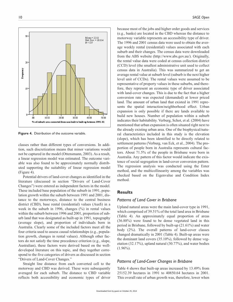
classes rather than different types of conversions. In addi-tion, such discretization means that minor variations would not be captured in the model (Ottensmann, 2003). As a result, a linear regression model was estimated. The outcome vari-able was also found to be approximately normally distrib-uted supporting the suitability of linear regression model (Figure 4).

Potential drivers of land-cover changes as identified in the literature (discussed in section “Drivers of Land-Cover Changes”) were entered as independent factors in the model. These included base population of the suburb in 1991, popu-lation growth within the suburb between 1991 and 2001, dis-tance to the motorways, distance to the central business district (CBD), base rental (residential) values (Aus$) in a week in the suburb in 1996, changes (%) in rental values within the suburb between 1996 and 2001, proportion of sub-urb land that was designated as built-up in 1991, topography (average slope), and proportion of individuals born in Australia. Clearly some of the included factors meet all the four criteria used to assess causal relationships (e.g., popula-tion growth, changes in rental values). Although other fac-tors do not satisfy the time precedence criterion (e.g., slope, Australian), these factors were derived based on the well-developed literature on this topic, and they together corre-spond to the five categories of drivers as discussed in section “Drivers of Land-Cover Changes.”

Straight line distance from each converted cell to the motorway and CBD was derived. These were subsequently averaged for each suburb. The distance to CBD variable reflects both accessibility and economic types of driver

because most of the jobs and higher order goods and services (e.g., banks) are located in the CBD whereas the distance to motorway variable represents an accessibility type of driver. The 1996 and 2001 census data were used to obtain the aver-age weekly rental (residential) values associated with each suburb and their changes. The census data were downloaded from the ABS website (http://www.abs.gov.au/). Originally, the rental value data were coded at census collection district (CCD) level (the smallest administrative unit used to collect census data in Australia). This was summarized to get an average rental value at suburb level (suburb is the next higher level unit of CCDs). The rental values were assumed to be representative of property values in these suburbs, and there-fore, they represent an economic type of driver associated with land-cover changes. This is due to the fact that a higher conversion rate was expected (demanded) at lower priced land. The amount of urban land that existed in 1991 repre-sents the spatial interaction/neighborhood effect. Urban expansion is only possible if there are lands available to build new houses. Number of population within a suburb indicates their habitability. Verburg, Schot, et al. (2004) have mentioned that urban expansion is often situated right next to the already existing urban area. One of the biophysical/natu-ral characteristics included in this study is the elevation (slope), which has been identified to be directly related to settlement patterns (Verburg, van Eck, et al., 2004). The pro-portion of people born in Australia represents cultural fac-tors. About 71.5% of the people in Brisbane were born in Australia. Any pattern of this factor would indicate the exis-tence of social segregation in land-cover conversion pattern. The regression analysis was conducted using the Enter method, and the multicollinearity among the variables was checked based on the Eigenvalue and Condition Index method.

Results

Patterns of Land Cover in Brisbane

Upland natural areas were the main land-cover type in 1991, which comprised of 39.51% of the total land area in Brisbane (Table 4). An approximately equal proportion of areas (36.88%) were found to be dense vegetated land in this period in Brisbane, followed by built-up (21.61%) and water body (2%). The overall patterns of land-cover classes changed dramatically in 2001 (Table 4). Built-up areas were the dominant land covers (35.10%), followed by dense veg-etation (32.17%), upland natural (30.77%), and water bodies (1.96%).

Patterns of Land-Cover Changes in Brisbane

Table 4 shows that built-up areas increased by 13.49% from 25152.39 hectares in 1991 to 40850.64 hectares in 2001. This overall rate of urban growth was, therefore, lower when

Figure 4. Distribution of the outcome variable.

by guest on October 25, 2014Downloaded from

Shatu et al. 11

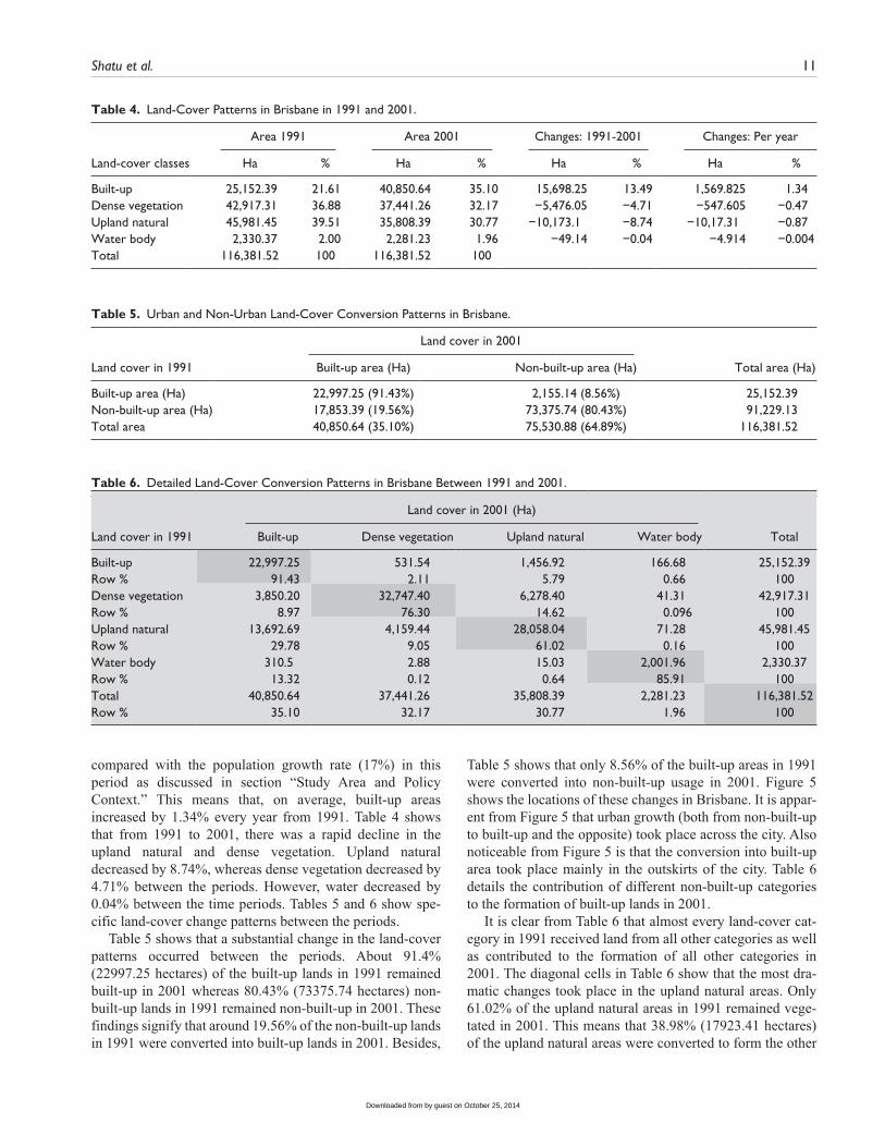
compared with the population growth rate (17%) in this period as discussed in section “Study Area and Policy Context.” This means that, on average, built-up areas increased by 1.34% every year from 1991. Table 4 shows that from 1991 to 2001, there was a rapid decline in the upland natural and dense vegetation. Upland natural decreased by 8.74%, whereas dense vegetation decreased by 4.71% between the periods. However, water decreased by 0.04% between the time periods. Tables 5 and 6 show spe-cific land-cover change patterns between the periods.

Table 5 shows that a substantial change in the land-cover patterns occurred between the periods. About 91.4% (22997.25 hectares) of the built-up lands in 1991 remained built-up in 2001 whereas 80.43% (73375.74 hectares) non-built-up lands in 1991 remained non-built-up in 2001. These findings signify that around 19.56% of the non-built-up lands in 1991 were converted into built-up lands in 2001. Besides,

Table 5 shows that only 8.56% of the built-up areas in 1991 were converted into non-built-up usage in 2001. Figure 5 shows the locations of these changes in Brisbane. It is appar-ent from Figure 5 that urban growth (both from non-built-up to built-up and the opposite) took place across the city. Also noticeable from Figure 5 is that the conversion into built-up area took place mainly in the outskirts of the city. Table 6 details the contribution of different non-built-up categories to the formation of built-up lands in 2001.

It is clear from Table 6 that almost every land-cover cat-egory in 1991 received land from all other categories as well as contributed to the formation of all other categories in 2001. The diagonal cells in Table 6 show that the most dra-matic changes took place in the upland natural areas. Only 61.02% of the upland natural areas in 1991 remained vege-tated in 2001. This means that 38.98% (17923.41 hectares) of the upland natural areas were converted to form the other

Table 4. Land-Cover Patterns in Brisbane in 1991 and 2001.

Land-cover classes

Area 1991 Area 2001 Changes: 1991-2001 Changes: Per year

Ha % Ha % Ha % Ha %

Built-up 25,152.39 21.61 40,850.64 35.10 15,698.25 13.49 1,569.825 1.34Dense vegetation 42,917.31 36.88 37,441.26 32.17 −5,476.05 −4.71 −547.605 −0.47Upland natural 45,981.45 39.51 35,808.39 30.77 −10,173.1 −8.74 −10,17.31 −0.87Water body 2,330.37 2.00 2,281.23 1.96 −49.14 −0.04 −4.914 −0.004Total 116,381.52 100 116,381.52 100

Table 5. Urban and Non-Urban Land-Cover Conversion Patterns in Brisbane.

Land cover in 1991

Land cover in 2001

Total area (Ha)Built-up area (Ha) Non-built-up area (Ha)

Built-up area (Ha) 22,997.25 (91.43%) 2,155.14 (8.56%) 25,152.39Non-built-up area (Ha) 17,853.39 (19.56%) 73,375.74 (80.43%) 91,229.13Total area 40,850.64 (35.10%) 75,530.88 (64.89%) 116,381.52

Table 6. Detailed Land-Cover Conversion Patterns in Brisbane Between 1991 and 2001.

Land cover in 1991

Land cover in 2001 (Ha)

TotalBuilt-up Dense vegetation Upland natural Water body

Built-up 22,997.25 531.54 1,456.92 166.68 25,152.39Row % 91.43 2.11 5.79 0.66 100Dense vegetation 3,850.20 32,747.40 6,278.40 41.31 42,917.31Row % 8.97 76.30 14.62 0.096 100Upland natural 13,692.69 4,159.44 28,058.04 71.28 45,981.45Row % 29.78 9.05 61.02 0.16 100Water body 310.5 2.88 15.03 2,001.96 2,330.37Row % 13.32 0.12 0.64 85.91 100Total 40,850.64 37,441.26 35,808.39 2,281.23 116,381.52Row % 35.10 32.17 30.77 1.96 100

by guest on October 25, 2014Downloaded from

12 SAGE Open

land classes. Among them, the upland natural areas contrib-uted most to the formation of built-up areas (29.78%), dense vegetation (9.5%), and water bodies (0.16%).

The next dramatic changes took place in the dense vegeta-tion category. About 23.70% (10169.91 hectares) of the dense vegetation lands in 1991 were converted into different land-cover types. Table 6 shows that these conversions were mainly to form the upland natural (14.62%) and built-up (8.97%) areas. According to Table 6, a very small portion of the built-up areas in 1991 were converted into upland natural (5.79%), followed by dense vegetation lands (2.11%). Moreover, the conversions from dense vegetation and upland

natural lands into water body areas were estimated 0.66% and 0.09% respectively. About 328 hectares of water body were converted into different types of land classes between 1991 and 2001. Among these, 310.5 hectares were converted into built-up, followed by upland natural (15.03 hectares), and dense vegetation land (2.88 hectares).

Figure 6 shows the locations of the conversion patterns for different land classes within the study area. Clearly, Figure 6d shows that the coastal areas located in the east of Brisbane were subjected to conversion from water body to built-up areas. However, the conversions to the built-up areas were mainly in the southern and northern part of the city.

Figure 5. Spatial patterns of land-cover conversion in Brisbane between 1991 and 2001.Note. SLA = statistical local area; CBD = central business district.

by guest on October 25, 2014Downloaded from

Shatu et al. 13

Figure 6. Specific land-cover conversion patterns in Brisbane.Note. SLA = statistical local area.

by guest on October 25, 2014Downloaded from

14 SAGE Open

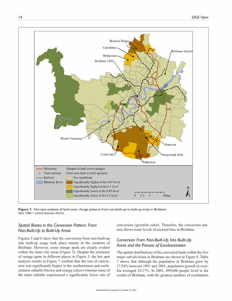
Spatial Biases in the Conversion Pattern: From Non-Built-Up to Built-Up Areas

Figures 5 and 6 show that the conversion from non-built-up into built-up usage took place mainly in the outskirts of Brisbane. However, some orange spots are clearly evident within the inner city areas (Figure 5). Despite the existence of orange spots in different places in Figure 5, the hot spot analysis results in Figure 7 confirm that the rate of conver-sion was significantly higher in the southernmost and north-ernmost suburbs (brown and orange colors) whereas some of the inner suburbs experienced a significantly lower rate of

conversion (greenish color). Therefore, the conversion pat-tern shows some levels of sectoral bias in Brisbane.

Conversion From Non-Built-Up Into Built-Up Areas and the Process of Exurbanization

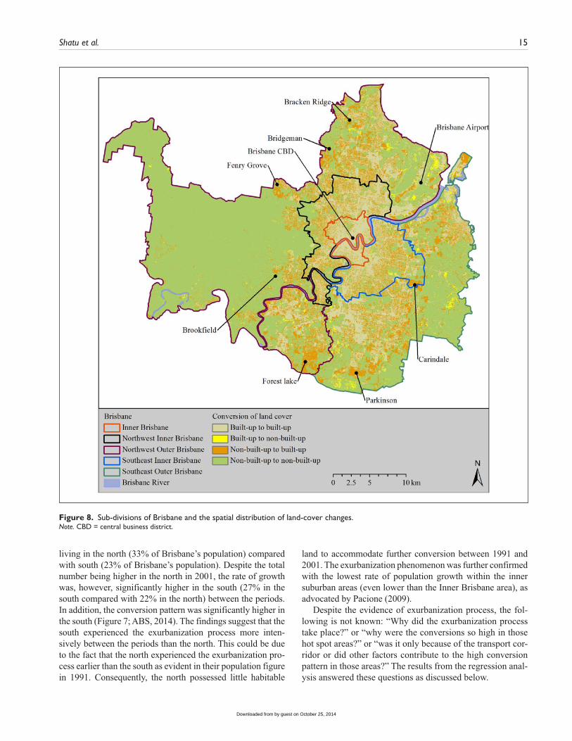
The spatial distributions of the converted lands within the five major sub-divisions in Brisbane are shown in Figure 8. Table 7 shows that although the population in Brisbane grew by 17.24% between 1991 and 2001, population growth in exur-bia averaged 24.17%. In 2001, 499,606 people lived in the exurbs of Brisbane, with the greatest numbers of exurbanites

Figure 7. Hot spot analyses of land-cover change patterns from non-built-up to built-up areas in Brisbane.Note. CBD = central business district.

by guest on October 25, 2014Downloaded from

Shatu et al. 15

living in the north (33% of Brisbane’s population) compared with south (23% of Brisbane’s population). Despite the total number being higher in the north in 2001, the rate of growth was, however, significantly higher in the south (27% in the south compared with 22% in the north) between the periods. In addition, the conversion pattern was significantly higher in the south (Figure 7; ABS, 2014). The findings suggest that the south experienced the exurbanization process more inten-sively between the periods than the north. This could be due to the fact that the north experienced the exurbanization pro-cess earlier than the south as evident in their population figure in 1991. Consequently, the north possessed little habitable

land to accommodate further conversion between 1991 and 2001. The exurbanization phenomenon was further confirmed with the lowest rate of population growth within the inner suburban areas (even lower than the Inner Brisbane area), as advocated by Pacione (2009).

Despite the evidence of exurbanization process, the fol-lowing is not known: “Why did the exurbanization process take place?” or “why were the conversions so high in those hot spot areas?” or “was it only because of the transport cor-ridor or did other factors contribute to the high conversion pattern in those areas?” The results from the regression anal-ysis answered these questions as discussed below.

Figure 8. Sub-divisions of Brisbane and the spatial distribution of land-cover changes.Note. CBD = central business district.

by guest on October 25, 2014Downloaded from

16 SAGE Open

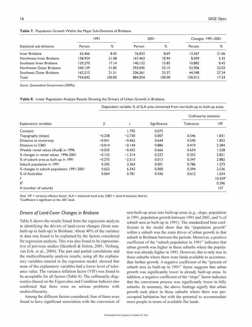
Drivers of Land-Cover Changes in Brisbane

Table 8 shows the results found from the regression analysis in identifying the drivers of land-cover changes (from non-built-up to built-up) in Brisbane. About 40% of the variance in data was found to be explained by the factors considered for regression analysis. This was also found to be representa-tive of previous studies (Skonhoft & Solem, 2001; Verburg, van Eck, et al., 2004). The part and partial correlations and the multicollinearity analysis results, using all the explana-tory variables entered in the regression model, showed that none of the explanatory variables had a lower level of toler-ance value. The variance inflation factor (VIF) was found to be acceptable for all factors (Table 8). The collinearity diag-nostics (based on the Eigenvalue and Condition Indices) also confirmed that there were no serious problems with multicollinearity.

Among the different factors considered, four of them were found to have significant association with the conversion of

non-built-up areas into built-up areas (e.g., slope, population in 1991, population growth between 1991 and 2001, and % of suburb area as built-up in 1991). The standardized beta coef-ficients in the model show that the “population growth” within a suburb was the main driver of urban growth in that suburb in Brisbane between the periods. Moreover, a positive coefficient of the “suburb population in 1991” indicates that urban growth was higher in those suburbs where the popula-tion was already higher in 1991. However, this is only true in those suburbs where there were lands available to accommo-date further growth. A negative coefficient of the “percent of suburb area as built-up in 1991” factor suggests that urban growth was significantly lower in already built-up areas. In addition, a negative coefficient of the “slope” factor indicates that the conversion process was significantly lower in hilly suburbs. In summary, the above findings signify that urban growth took place in those suburbs where there was pre- occupied habitation but with the potential to accommodate more people in terms of available flat lands.

Table 7. Population Growth Within the Major Sub-Divisions of Brisbane.

Statistical sub-divisions

1991 2001 Changes: 1991-2001

Person % Person % Person %

Inner Brisbane 63,466 8.42 76,833 8.69 13,367 21.06Northwest Inner Brisbane 158,954 21.08 167,463 18.94 8,509 5.35Southeast Inner Brisbane 129,270 17.14 140,152 15.85 10,882 8.42Northwest Outer Brisbane 240,139 31.85 293,045 33.15 52,906 22.03Southeast Outer Brisbane 162,213 21.51 206,561 23.37 44,348 27.34Total 754,042 100.00 884,054 100.00 130,012 17.24

Source. Queensland Government (2009a).

Table 8. Linear Regression Analysis Results Showing the Drivers of Urban Growth in Brisbane.

Explanatory variables

Dependent variable: % of SLA area converted from non-built-up to built-up areas

β t Significance

Collinearity statistics

Tolerance VIF

Constant 1.795 0.075 Topography (slope) −0.238 −2.730 0.007 0.546 1.831Distance to motorway −0.041 −0.462 0.644 0.540 1.852Distance to CBD −0.014 −0.144 0.886 0.419 2.384Weekly rental values (Aus$) in 1996 −0.035 −0.432 0.666 0.654 1.528% changes in rental values: 1996-2001 −0.132 −1.214 0.227 0.355 2.821% of suburb area as built-up in 1991 −0.275 −2.513 0.013 0.347 2.882Suburb population in 1991 0.245 3.364 0.001 0.786 1.273% changes in suburb population: 1991-2001 0.652 6.343 0.000 0.394 2.536% of Australian 0.064 0.781 0.436 0.612 1.634F 10.559a

R2 0.396N (number of suburb) 157

Note. VIF = variance inflation factor; SLA = statistical local area; CBD = central business district.aCoefficient is significant at the .001 level.

by guest on October 25, 2014Downloaded from

Shatu et al. 17

Discussion and Conclusion

This research is the first of its kind in the context of Brisbane that empirically investigates the patterns of land-cover changes between 1991 and 2001, and also identifies their associated driving forces. The findings from this research bear important policy implications for Brisbane vis-à-vis Queensland in Australia, given that the drivers of land-cover changes vary depending on the context (Verburg, van Eck, et al., 2004). However, the lessons learnt from this research can effectively be used to make an informed land use policy deci-sion around the globe (Antrop, 2005; Jansen et al., 2007). The Queensland Government aimed at promoting sustain-able urban growth by enacting various policies and Acts (e.g., the Environmental Protection Act 1994, the Integrated Planning Act 1997). The analyses presented in this research enabled us to evaluate the effectiveness of such policy mea-sures based on an understanding of the patterns of land-cover changes and by identifying their associated processes.

The findings presented in this study clearly show that the policy interventions undertaken in the study period (1991-2001) were not as effective in promoting sustainable changes in the environment as they were aimed for. Most new devel-opments took place in green fields, thereby increasing the ecological footprint in the city (Tewolde & Cabral, 2011). The influence of nature protection policies (e.g., the Environmental Protection Act 1994) was found to have little role because about 3,850 hectares of vegetated lands and 13,692 hectares of upland natural lands in 1991 were con-verted into built-up areas in 2001.

The results from both the exploratory (e.g., hot spot, descriptive statistics showing population growth with differ-ent sub-divisions of Brisbane) and confirmatory (e.g., regres-sion) analyses showed the evidence of exurbanization process in Brisbane. The hot spot analysis showed that the conversions were significantly clustered in the outer (Northern and Southern) parts of the city. Population growth in these areas was significantly higher, whereas the popula-tion growth in Inner Suburb areas was significantly lower. Consistent with prior studies (Pfeffer et at., 2005; Sonis et al., 2007), results presented in this study showed that popula-tion growth is the main driving force of land-cover change in Brisbane. From this perspective, the findings clearly justify that the current land use policies (e.g., South Queensland Regional Plan 2009-2031) are more promising in Brisbane in promoting sustainable urban growth. This is due to the fact that the current policies aim to accommodate population growth through facilitating development in a more compact way—that is, smart growth—either through infill develop-ment or through increasing density in some selected nodes or activity centers (Queensland Government, 2009b). The cur-rent policy would also be effective because it identified urban footprint areas, and all developments must be located within the footprint to protect, manage, and enhance the region’s biodiversity values and associated ecosystem ser-vices and maximize the resilience of ecosystems to the

impacts of climate change. However, care must be taken to protect the natural lands located within the urban footprint areas.

In addition to verifying the demographic hypothesis (pop-ulation growth) of land-cover changes, this research also verifies the natural configuration hypothesis that topography (e.g., steep slope) can act as a natural constraint on urban growth (Müller, Steinmeier, & Küchler, 2010). However, the insignificant influence of the ethnicity (e.g., percent Australian) factor falsified the cultural hypothesis of land-cover changes in this context (Bürgi et al., 2004; Hersperger & Bürgi, 2007; Zeug & Eckert, 2010). This is also true in case of technological (access to motorways) and economic (access to CBD, rental values) drivers.

Despite the evidence of exurbanization process presented in this research, the findings are not complete because a number of other relevant factors were not analyzed in this research. Pacione (2009) has indicated that exurbia tends to be dominated by middle-class residents, many of whom commute long distances to work in the city or in the newer suburbs. Other groups are also present in the exurban loca-tions including retirees and young households seeking social status, more land, and new housing at a lower cost than is available in the suburbs. In addition, this study investigates the exurbanization process only within the local government boundary of Brisbane. It is possible that the exurbanization process was more pronounced outside the study area bound-ary. Future research should seek to explore this issue in a wider geographic context by utilizing the above omitted indicators and improve on the model presented in this research. Despite the rental values being considered in this research as a proxy of land value, the results were somewhat surprising showing their insignificant impacts on urban growth in this context. Future studies should utilize the land value data to verify the findings reported in this study. In addition, although evidence in this research shows a surpris-ing and significant land conversion pattern—from built-up into non-built-up areas—these were not investigated inten-sively. Future research should examine this phenomenon to further the knowledge on this topic.

Declaration of Conflicting Interests

The author(s) declared no potential conflicts of interest with respect to the research, authorship, and/or publication of this article.

Funding

The author(s) received no financial support for the research and/or authorship of this article.

Note

1. Excluding island population.

References

Ahmed, B., Kamruzzaman, M., Zhu, X., Rahman, M. S., & Keechoo, C. (2013). Simulating land cover changes and their

by guest on October 25, 2014Downloaded from

18 SAGE Open

impacts on land surface temperature in Dhaka, Bangladesh. Remote Sensing, 5, 5969-5998.

Antrop, M. (2005). Why landscapes of the past are important for the future. Landscape and Urban Planning, 70, 21-34.

Australia Bureau of Statistics. (2008). National regional profile: Brisbane (C) (Local government area). Available from http://www.abs.gov.au/

Australia Bureau of Statistics. (2014). Regional population growth, Australia. Available from http://www.abs.gov.au/

Bakr, N., Weindorf, D. C., Bahnassy, M. H., Marei, S. M., & El-Badawi, M. M. (2010). Monitoring land cover changes in a newly reclaimed area of Egypt using multi-temporal Landsat data. Applied Geography, 30, 592-605.

Berke, P. R., Godschalk, D. R., Kaiser, E. J., & Rodriguez, D. A. (2006). Urban land use planning (5th ed.). Urbana: University of Illinois Press.

Bohnet, I. C., & Pert, P. L. (2010). Patterns, drivers, and impacts of urban growth—A study from Cairns, Queensland, Australia from 1952 to 2031. Landscape and Urban Planning, 97, 239-248.

Braimoh, A., & Vlek, P. G. (2005). Land-cover change trajectories in Northern Ghana. Environmental Management, 36, 356-373.

Brisbane City Council. (2013). Planning for the future: The draft new city plan. Brisbane, Australia: Author.

Bürgi, M., Hersperger, A., & Schneeberger, N. (2004). Driving forces of landscape change—Current and new directions. Landscape Ecology, 19, 857-868.

Cai, Y., Zhang, H., Pan, W., Chen, Y., & Wang, X. (2012). Urban expansion and its influencing factors in natural wetland dis-tribution area in Fuzhou city, China. Chinese Geographical Science, 22, 568-577.

Chang, H., & Franczyk, J. (2008). Climate change, land-use change, and floods: Toward an integrated assessment. Geography Compass, 2, 1549-1579.

Cheng, J., & Masser, I. (2003). Urban growth pattern modeling: A case study of Wuhan city, PR China. Landscape and Urban Planning, 62, 199-217.

Crump, J. R. (2003). Finding a place in the country: Exurban and suburban development in Sonoma County, California. Environment & Behavior, 35, 187-202.

Dale, V. H. (1997). The relationship between land use change and climate change. Ecological Applications, 7, 753-769.

Feddema, J. J., Oleson, K. W., Bonan, G. B., Mearns, L. O., Buja, L. E., Meehl, G. A., & Washington, W. M. (2005). The impor-tance of land-cover change in simulating future climates. Science, 310(5754), 1674-1678.

Hepinstall, J. A., Alberti, M., & Marzluff, J. M. (2008). Predicting land cover change and avian community responses in rapidly urbanizing environments. Landscape Ecology, 23, 1257-1276.

Hersperger, A. M., & Bürgi, M. (2007). Driving forces of land-scape change in the urbanizing Limmat Valley, Switzerland. In E. Koomen, J. Stillwell, A. Bakema, & H. J. Sholten (Eds.), Modelling land-use change: Progress and applications (pp. 45-60). Dordrecht, The Netherlands: Springer.

Jansen, L. J. M., Carrai, G., & Petri, M. (2007). Land-use change at cadastral parcel level in Albania: An object-oriented geo- database approach to analyse spatial developments in a period of transition (1991-2003). In E. Koomen, J. Stillwell, A. Bakema, & H. J. Sholten (Eds.), Modelling land-use change: Progress and applications (pp. 25-44). Dordrecht, The Netherlands: Springer.

Kamruzzaman, M., Baker, D., Washington, S., & Turrell, G. (2014). Advance transit oriented development typology: Case study in Brisbane, Australia. Journal of Transport Geography, 34, 54-70.

Koomen, E., & Stillwell, J. (2007). Modelling land-use change. In E. Koomen, J. Stillwell, A. Bakema, & H. J. Sholten (Eds.), Modelling land-use change: Progress and applications (pp. 1-21). Dordrecht, The Netherlands: Springer.

Lambin, E. F., Geist, H. J., & Lepers, E. (2003). Dynamics of land-use and land-cover change in tropical regions. Annual Review of Environment and Resources, 28, 205-241.

Lambin, E. F., Turner, B. L., Geist, H. J., Agbola, S. B., Angelsen, A., Bruce, J. W., . . .Xu, J. (2001). The causes of land-use and land-cover change: Moving beyond the myths. Global Environmental Change, 11, 261-269.

Li, X., & Yeh, A. G. O. (2000). Modelling sustainable urban devel-opment by the integration of constrained cellular automata and GIS. International Journal of Geographical Information Science, 14, 131-152.

Liu, Y. (2012). Modelling sustainable urban growth in a rapidly urbanising region using a fuzzy-constrained cellular automata approach. International Journal of Geographical Information Science, 26, 151-167.

Long, H., Tang, G., Li, X., & Heilig, G. K. (2007). Socio-economic driving forces of land-use change in Kunshan, the Yangtze River Delta economic area of China. Journal of Environmental Management, 83, 351-364.

Meyer, W. B., & Turner, B. L. (1994). Changes in land use and land cover. Cambridge, UK: Cambridge University Press.

Müller, K., Steinmeier, C., & Küchler, M. (2010). Urban growth along motorways in Switzerland. Landscape and Urban Planning, 98, 3-12.

Nelson, A. (1992). Characterizing exurbia. Journal of Planning Literature, 5, 350-368.

Ningal, T., Hartemink, A. E., & Bregt, A. K. (2008). Land use change and population growth in the Morobe Province of Papua New Guinea between 1975 and 2000. Journal of Environmental Management, 87, 117-124.

Nong, Y., & Du, Q. (2011). Urban growth pattern modeling using logistic regression. Geo-Spatial Information Science, 14, 62-67.

Ottensmann, J. R. (2003). LUCI land use in Central Indiana model and the relationships of public infrastructure to urban develop-ment. Public Works Management & Policy, 8, 62-76.

Ottinger, M., Kuenzer, C., Liu, G., Wang, S., & Dech, S. (2013). Monitoring land cover dynamics in the Yellow River Delta from 1995 to 2010 based on Landsat 5 TM. Applied Geography, 44, 53-68.

Pacione, M. (2009). Urban geography: A global perspective. London, England: Routledge.

Pena, J., Bonet, A., Bellot, J., Sanchez, J. R., Eisenhuth, D., Hallett, S., & Aledo, A. (2007). Driving forces of land-use change in a cultural landscape of Spain. In E. Koomen, J. Stillwell, A. Bakema, & H. J. Sholten (Eds.), Modelling land-use change: Progress and applications (pp. 1-21). Dordrecht, The Netherlands: Springer.

Pfeffer, M. J., Schlelhas, J. W., DeGloria, S. D., & Gomez, J. (2005). Population, conservation, and land use change in Honduras. Agriculture, Ecosystems & Environment, 110(1–2), 14-28.

Pijanowski, B. C., & Robinson, K. D. (2011). Rates and patterns of land use change in the Upper Great Lakes states, USA: A

by guest on October 25, 2014Downloaded from

Shatu et al. 19

framework for spatial temporal analysis. Landscape and Urban Planning, 102, 102-116.

Queensland Government. (2008). Toward Q2: Tomorrow’s Queensland. Brisbane, Australia: Author. Retrieved from http://rti.cabinet.qld.gov.au/documents/2008/sep/toward%20q2/a t t a c h m e n t s / T o w a r d s % 2 0 Q 2 _ % 2 0 T o m o r r o w s % 20Queensland.pdf

Queensland Government. (2009a). Historical tables, population, 1823 to 2008. Brisbane, Australia: Office of Economic and Statistical Research, Queensland Treasury.

Queensland Government. (2009b). South East Queensland regional plan 2009–2031. Brisbane, Australia: Queensland Department of Infrastructure and Planning. Retrieved from http://www.dsdip.qld.gov.au/resources/plan/seq/regional-plan-2009/seq-regional-plan-2009.pdf

Queensland Motorways. (2012). Our Roads Retrieved from http://www.qldmotorways.com.au/ontheroad.aspx

Shaw, R. P. (1992). The impact of population growth on environ-ment: The debate heats up. Environmental Impact Assessment Review, 12, 11-36.

Shi, Y., Wang, R., Fan, L., Li, J., & Yang, D. (2010). Analysis on land-use change and its demographic factors in the original-stream watershed of Tarim river based on GIS and statistic. Procedia Environmental Sciences, 2, 175-184.

Singleton, R. A., & Straits, B. C. (1999). Approaches to social research. New York, NY: Oxford University Press.

Skonhoft, A., & Solem, H. (2001). Economic growth and land-use changes: The declining amount of wilderness land in Norway. Ecological Economics, 37, 289-301.

Sonis, M., Shoshany, M., & Goldshlager, N. (2007). Landscape changes in the Israeli Carmel area: An application of matrix land-use analysis. In E. Koomen, J. Stillwell, A. Bakema, & H. J. Sholten (Eds.), Modelling land-use change: Progress and applications (pp. 61-82). Dordrecht, The Netherlands: Springer.

Tan, K. C., Lim, H. S., Matjafri, M. Z., & Abdullah, K. (2010). Landsat data to evaluate urban expansion and determine land use/land cover changes in Penang Island, Malaysia. Environmental Earth Sciences, 60, 1509-1521.

Tewolde, M. G., & Cabral, P. (2011). Urban sprawl analysis and modeling in Asmara, Eritrea. Remote Sensing, 3, 2148-2165.

Tomalty, R., & Curran, D. (2003). Living it up: The wide range of support for smart growth in Canada promises more livable towns and cities. Alternatives Journal, 29(3), 10-18. Retrieved from ProQuest Central.

Turner, M. G., Wear, D. N., & Flamm, R. O. (1996). Land owner-ship and land-cover change in the Southern Appalachian high-lands and the Olympic Peninsula. Ecological Applications, 6, 1150-1172.

Veldkamp, A., Kok, K., De Koning, G. H. J., Verburg, P. H., & Bergsma, A. R. (2001). The need for multi-scale approaches

in spatial specific land-use change modeling. Environmental Modeling & Assessment, 6, 111-121.

Verburg, P. H., Schot, P. P., Dijst, M. J., & Veldkamp, A. (2004). Land use change modelling: Current practice and research pri-orities. GeoJournal, 61, 309-324.

Verburg, P. H., van Eck, J. R. R., de Nijs, T. C. M., Dijst, M. J., & Schot, P. (2004). Determinants of land-use change patterns in the Netherlands. Environment and Planning B: Planning and Design, 31, 125-150.

Walker, B., Steffen, W., Canadell, J., & Ingram, J. (Eds.). (1997). The terrestrial biosphere and global change: Implications for natural and managed ecosystems (Vol. Synthesis volume). Cambridge, UK: Cambridge University Press.

Watson, R. T., Noble, I. R., Bolin, B., Ravindranath, N. H., Verardo, D. J., & Dokken, D. J. (Eds.). (2000). Land use, land-use change, and forestry (A Special Report of the Intergovernmental Panel on Climatic Change) (p. 375). Cambridge: Cambridge University Press. Retrieved from http://www.ipcc.ch/ipccrep-orts/sres/land_use/index.php?idp=0

Weitz, J. (2012). Growth management in the United States, 2000–2010: A decennial review and synthesis. Journal of Planning Literature, 27, 394-433.

White, J., Shao, Y., Kennedy, L. M., & Campbell, J. B. (2013). Landscape dynamics on the island of La Gonave, Haiti, 1990–2010. Land, 2, 493-507.

Williams, P. (2007). Government, people, and politics. In S. Thompson (Ed.), Planning Australia: An overview of urban and regional planning (pp. 29-48). Cambridge, UK: Cambridge University Press.

World Commission on Environment and Development. (1987). Our common future. Oxford, UK: Oxford University Press.

Zeug, G., & Eckert, S. (2010). Population growth and its expres-sion in spatial built-up patterns: The Sana’a, Yemen case study. Remote Sensing, 2, 1014-1034.

Author Biographies

Farjana Mostafiz Shatu is a research assistant at Queensland University of Technology. She has a bachelor’s degree in architec-ture. She is skillful in geographical information systems (GIS) and remote sensing (RS).

Md. Kamruzzaman in an early career academic at Queensland University of Technology. He has a PhD in transport planning and an MSc in geoinformation science and earth observation. His research interests include transport geography, integrated transport and land use planning, and GIS and RS applications in planning.

Kaveh Deilami is a PhD researcher at Queensland University of Technology. His research focuses on the climatic impacts of land cover changes.

by guest on October 25, 2014Downloaded from