Development of mathematical models to predict the atmospheric corrosion rate of carbon steel in...

Int. J. Electrochem. Sci., 9 (2014) 6514 - 6528

International Journal of

ELECTROCHEMICAL SCIENCE

www.electrochemsci.org

Development of Mathematical Models to predict the

Atmospheric Corrosion Rate of Carbon Steel in Fragmented

Subtropical Environments

H.C. Vasconcelos1, B.M. Fernández-Pérez

2, J. Morales

2, R.M. Souto

2,*, S. González

2, V. Cano

3,

J.J. Santana4,*

1Department of Technological Sciences and Development, Azores University, 9501-801 Ponta

Delgada, Portugal 2Department of Chemistry, University of La Laguna, 38071 La Laguna, Tenerife, Spain;

3Department of Economy, Statistics and Econometry, University of La Laguna, 38071 La Laguna,

Tenerife, Spain 4Department of Process Engineering, University of Las Palmas de Gran Canaria, 35017 Las Palmas de

Gran Canaria, Gran Canaria, Spain *E-mail: [email protected]; [email protected]

Received: 27 May 2014 / Accepted: 11 June 2014 / Published: 25 August 2014

Mathematical modelling of atmospheric corrosion based on the aggressiveness categories defined by

standard ISO 9223 greatly fail to predict the actual corrosion rates of metals in subtropical

environments. Therefore, new concepts for modelling are required as to adequately predict corrosion

rates from environmental factors such as the deposition rate of chemical agents (namely chloride and

sulphur dioxide), climate effects (such as moisture and time of wetness), and the duration of metal

exposure. The novel methodology is based on the definition of a set of qualitative variables to

distribute locations exhibiting distinctive initial characteristics towards metal corrosion. The validity of

the method was checked by using data obtained during three years of exposure of carbon steel in 74

stations distributed along the seven main islands of the Canary Islands (Spain). A definite evaluation of

the impact of environmental factors on the extent of corrosion was achieved, and good results were

defined in terms of fitting quality.

Keywords: Atmospheric corrosion, carbon steel, subtropical region, mathematical model.

1. INTRODUCTION

Atmospheric corrosion is a problem of great interest, mainly due to high costs arising from

failure and leakage, disruption in service and operation, maintenance and renovation, environmental

http://www.electrochemsci.org/

mailto:[email protected]

mailto:[email protected]

Int. J. Electrochem. Sci., Vol. 9, 2014

6515

pollution from leakage of hazardous materials and corrosion products, and replacement of

infrastructure, utilities, industrial operation, transportation, materials storage, transmission lines, etc. In

a study about the cost of corrosion, undertaken by CC Technologies Laboratories, Inc. with support

from the FHWA and NACE between 1999 and 2001, it was determined that the annual cost due to

direct corrosion would be in the order of ca. 3.1% of GNP [1]. Generically, it is estimated that the total

cost due to corrosion amounts between 4-5% of the gross domestic product of a country, being the

atmospheric corrosion the main factor that influences that cost [2-4]. The characterization of the

aggressiveness of a particular atmosphere, is therefore a topic of major interest since its knowledge and

application of adequate prevention measures presume a considerable cost saving.

For this reason numerous research programs were conducted in several countries, aimed to

characterize atmospheric corrosion in various geographical areas. A major objective of those studies

was to obtain mathematical models for the prediction of the degradation rate of the exposed metal in a

wide geographical area. As a result, several models were developed that predict the corrosion rate.

Among them, the ISO CORRAG model supported by NACE [5,6], and the models obtained by The

International Cooperative Program on Effects and The Iberoamerican Atmospheric Corrosion Map

Project MICAT (Mapa Iberoamericano de Corrosión Atmosférica) [7] are applied extensively. The

same effort was performed in Spain with the objective to derive a map of corrosivity for the whole

country. As a result, corrosivity maps are available in regions such as Galicia, Catalonia, the Basque

Country, Andalusia and Extremadura [8]. Despite the diversity of working parties, they all performed

the classification of environments in terms of corrosion rates pursuant to ISO 9223 [9]. A similar

approach was also attempted in smaller geographical areas of subtropical character [10,11], but it was

found that the ISO 9223 norm presented major limitations as to account for the experimental corrosion

rates [12].

Therefore, a project has been funded to elaborate the Corrosivity Map of the Canary Islands, a

fragmented subtropical region directly affected by oceanic conditions. The Canarian Archipelago is a

group of seven islands in the Atlantic Ocean, near the African coast (see Figure 1). The islands are

distributed between latitudes 27º and 29º North, covering an area of approximately of 7,447 km2

surrounded by 1,583 km shoreline. The Canary Islands conforms a rather unique geographic location,

because six distinct microclimates have been characterized in this small stretch of land. More

interestingly, though the microclimates are differently distributed among the islands, all of them can be

found simultaneously in the case of Tenerife Island, whereas five of them are found in Gran Canaria

Island. The variety of microclimates is a major cause for the observation of atmospheric corrosion rates

that can be ascribed to any of the proposed corrosive categories ranging from those specific to tropical

areas, to marine, industrial and even rural environments. The first stage of the project was directed to

determine the distribution of atmospheres existing in the archipelago, and to quantify their

aggressiveness by exposing several metals of extensive industrial use such as carbon steel, galvanized

steel, zinc, copper and aluminium. In order to cover the widest possible variety of environments, 74

test stations were distributed along the seven islands (Tenerife, La Palma, La Gomera, El Hierro, Gran

Canaria, Fuerteventura and Lanzarote). The location and characteristics of the 74 sites have been given

in previous work, together with the corrosivity categories relative to carbon steel, zinc and copper

degradation that were assigned to each place [10,12,13]. At present, the corrosion rates for the


6516

investigated materials have been determined at each location with high reproducibility, whereas it was

observed that the mathematical models available in the scientific literature do not satisfactorily

describe and predict those experimental corrosion rates. Therefore, new mathematical models must be

derived to predict the corrosion rate of metallic materials in fragmented subtropical environments such

as those occurring in the Canary Islands.

Figure 1. Geographical location of the Canary Islands (Spain). The islands are distributed in two

provinces for political administration: Santa Cruz de Tenerife is composed by the four islands

at the West (Tenerife, Gomera, La Palma and El Hierro), and Las Palmas de Gran Canaria by

the remaining three islands (Gran Canaria, Fuerteventura and Lanzarote).

In this work we report the process undertaken to develop models for the atmospheric corrosion

of carbon steel. Firstly, we proceeded to derive empirical corrosion equations for either single sites or

groups of stations with the same category of corrosion in a given island. In this way, models with good

regression ratios were obtained but their applicability was restricted to very small geographical areas

within the same island. In that process, the first model tested was the power law [14], widely used in

studies of atmospheric corrosion. Unfortunately, this equation leads to major discrepancies with

experimental data in the subtropical environments of the Canary Islands. Next, modified models [11]

based on a new expansion of the power law exponent n containing the distributed time of wetness

(TOW) and the concentrations of pollutants were tested. Alternately, equations containing qualitative

variables were introduced with the intention to alleviate the problem originating from test sites

exhibiting a wide variety of corrosion categories [10]. Rather good results were attained using those

models, thus subsequent work was directed to the extension of those methods to describe the entire

archipelago, i.e., in order to derive more general models that can be applied in all the islands by taking

carbon steel as the model metallic system.

Canary

Islands

CANARY ISLANDS

Gran Canaria

Fuerteventura

Lanzarote

Atlantic Ocean

Tenerife

La Gomera

La Palma

El

Hierro

AFRICA


6517

2. EXPERIMENTAL

The 74 test sites consisted of a metallic frame on which the metal samples were attached using

a nylon screw to avoid the formation of galvanic couples. The pollutant sensors were located at the

frame rear. For the determination of sulphur dioxide SO2 pollution, either the candel lead dioxide

method under ASTM D 2010-85 [15], or the Husy method according to ISO/TC 156 N 250 norm [16],

were employed. Chloride measurements were performed using the wet candle method following the

instruct ions of ISO 9225:1992 (E) [17]. Pollutants were collected on a monthly basis.

The composition of carbon steel samples is shown in Table 1. Plates of approximate

dimensions: 100 x 40 x 20 mm3 were employed. Before being placed in the corresponding stations, the

samples were marked for identification, cleaned according to the ASTMG G1-90 norm [18],

subsequently measured and weighed. Samples were collected from the test sites at various durations of

exposure, namely 3, 6, 9, 12, 18, 24, and 36 months. Corrosion products were removed by chemical

operation as described by the ISO/DIS 8403.3 [19]. The evaluation of the corrosion rate was made by

weight loss of the samples. After the samples were cleaned and dried, they were weighed again.

Corrosion rates were evaluated from weight loss measurements.

Table 1. Composition of carbon steel test sheets used in this study.

Metal Composition (wt.%)

Si Fe C Mn P S

Carbon steel 0.080 99.467 0.060 0.370 0.009 0.014

The time of wetness (TOW) was determined from the data collected using relative humidity

hygrometers placed in a small cabinet at the rear of the station frames, and they were complemented

with data supplied by the National Meteorological Institute of Spain (AEMET, Madrid, Spain). The

latter were cumulative values taken over 8 hour-periods in a systematic way, whereas the autonomous

hygrometers produced a continuous recording with autonomy for about one month. Data on the speed

and direction of wind were kindly supplied by AEMET.

3. RESULTS

3.1. Concentrations of pollutants and atmospheric conditions

The distribution of concentrations of chloride ions and sulphur dioxide determined with annual

periodicity up to 3 years for the 74 test sites are given in Figures 2 and 3, organized as 39 sites in the

three eastern islands constituting the province of Las Palmas de Gran Canaria (namely Gran Canaria,

Fuerteventura and Lanzarote), and 35 sites in the remaining four islands conforming the western

province of Santa Cruz de Tenerife (i.e., Tenerife, La Palma, Gomera and El Hierro), respectively.

Though the amounts of pollutants show some variations among the annual accumulated values


6518

for a given test site, these changes are very small compared to the big variability found between

different stations, even among those placed in the same island. Despite the abrupt orography present in

the islands, with the highest point reaching up to 3,718 m height in Tenerife Island, measurable

chloride concentrations were found at all the sites. The big variations between them should be related

to climate conditions imposed by the dominating wind regimes and the amount of humidity occurring

at each place.

Station

0 5 10 15 20 25 30 35 40

Cl- (

g/(

m2 y

ea

r)

0

50

200

250

300

350

400

1st year

2nd

year

3rd

year

A

Station

0 5 10 15 20 25 30 35 40

SO

2 (

g/(

m2 y

ea

r)

0

2

4

61

st year

2nd

year

3rd

year

B

Figure 2. Temporal variations of pollutant concentrations collected in the test sites planted in the

eastern province (i.e., Las Palmas de Gran Canaria, GC). Number of sites: N = 39. Pollutants:

(A) chloride, and (B) sulphur dioxide.


6519

Station

0 5 10 15 20 25 30 35

Cl- (

g/(

m2 y

ea

r)

0

10

20

60

80

100

120

140

160

1st

year

2nd

year

3rd

year

A

Station

0 5 10 15 20 25 30 35

SO2 (g/(m2 year)

0.0

0.5

1.0

1.5

2.0

2.5

3.0

3.5

1st

year

2nd

year

3rd

year

B

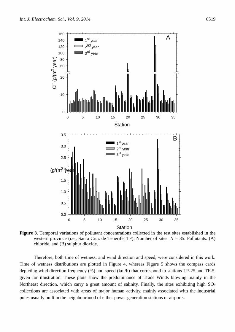
Figure 3. Temporal variations of pollutant concentrations collected in the test sites established in the

western province (i.e., Santa Cruz de Tenerife, TF). Number of sites: N = 35. Pollutants: (A)

chloride, and (B) sulphur dioxide.

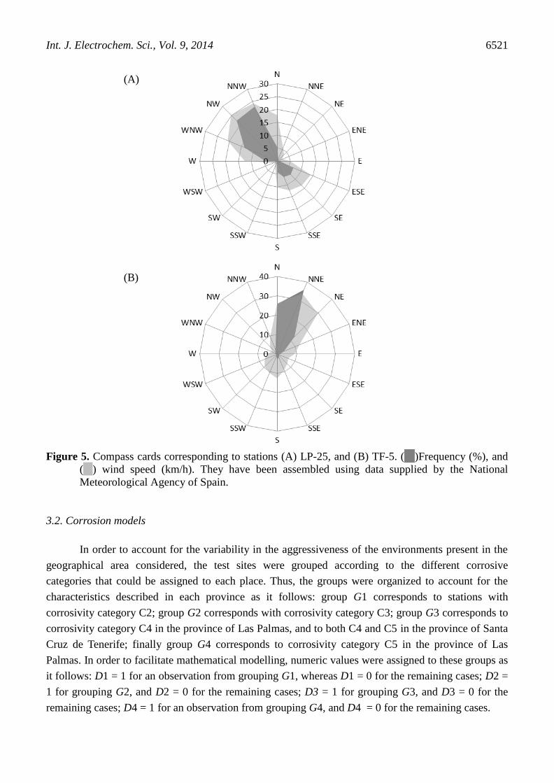
Therefore, both time of wetness, and wind direction and speed, were considered in this work.

Time of wetness distributions are plotted in Figure 4, whereas Figure 5 shows the compass cards

depicting wind direction frequency (%) and speed (km/h) that correspond to stations LP-25 and TF-5,

given for illustration. These plots show the predominance of Trade Winds blowing mainly in the

Northeast direction, which carry a great amount of salinity. Finally, the sites exhibiting high SO2

collections are associated with areas of major human activity, mainly associated with the industrial

poles usually built in the neighbourhood of either power generation stations or airports.


6520

Station

0 5 10 15 20 25 30 35 40

TO

W (

ye

ars

)

0

1

2

3

4

5

6

1st

year

2nd

year

3rd

year

A

Station

0 5 10 15 20 25 30 35

TO

W (

ye

ars

)

0

1

2

3

4

5

1st

year

2nd

year

3rd

year

B

Figure 4. Temporal variation of time of wetness (TOW) collected in the test sites established in (A)

the eastern province (Las Palmas de Gran Canaria, GC), and (B) the western province (Santa

Cruz de Tenerife, TF).


6521

Figure 5. Compass cards corresponding to stations (A) LP-25, and (B) TF-5. ( )Frequency (%), and

(as) wind speed (km/h). They have been assembled using data supplied by the National

Meteorological Agency of Spain.

3.2. Corrosion models

In order to account for the variability in the aggressiveness of the environments present in the

geographical area considered, the test sites were grouped according to the different corrosive

categories that could be assigned to each place. Thus, the groups were organized to account for the

characteristics described in each province as it follows: group G1 corresponds to stations with

corrosivity category C2; group G2 corresponds with corrosivity category C3; group G3 corresponds to

corrosivity category C4 in the province of Las Palmas, and to both C4 and C5 in the province of Santa

Cruz de Tenerife; finally group G4 corresponds to corrosivity category C5 in the province of Las

Palmas. In order to facilitate mathematical modelling, numeric values were assigned to these groups as

it follows: D1 = 1 for an observation from grouping G1, whereas D1 = 0 for the remaining cases; D2 =

1 for grouping G2, and D2 = 0 for the remaining cases; D3 = 1 for grouping G3, and D3 = 0 for the

remaining cases; D4 = 1 for an observation from grouping G4, and D4 = 0 for the remaining cases.

(A)

(B)


6522

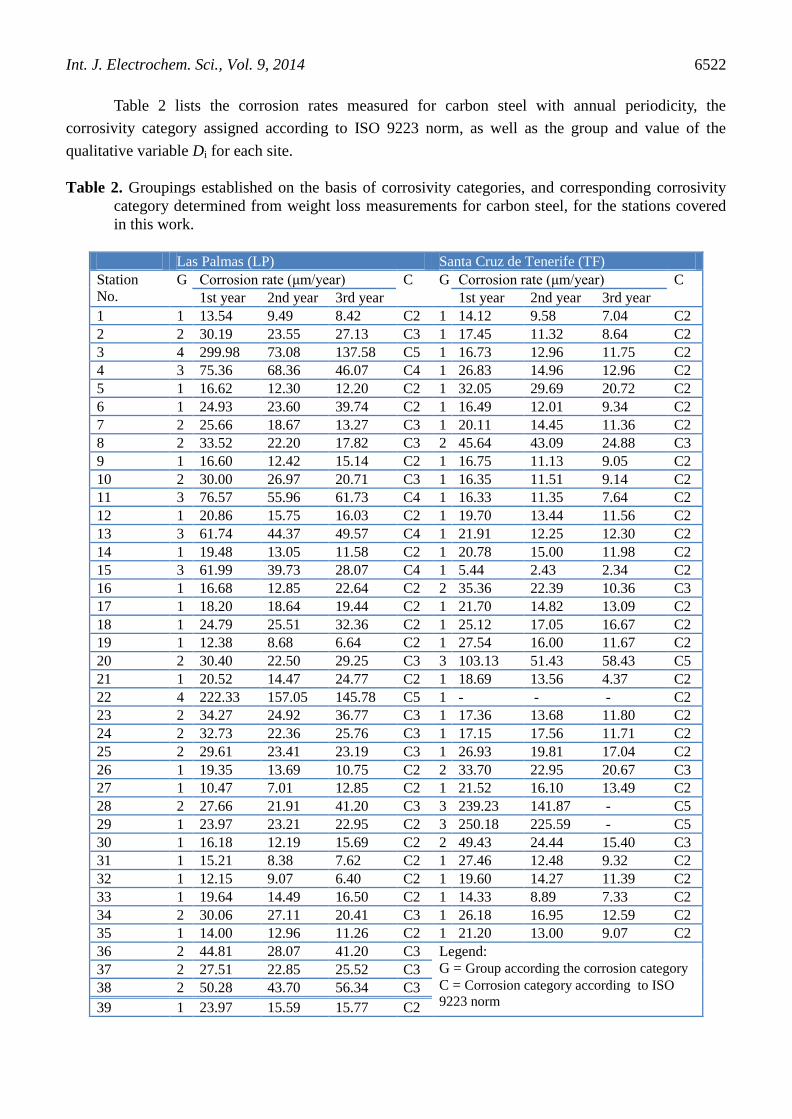
Table 2 lists the corrosion rates measured for carbon steel with annual periodicity, the

corrosivity category assigned according to ISO 9223 norm, as well as the group and value of the

qualitative variable Di for each site.

Table 2. Groupings established on the basis of corrosivity categories, and corresponding corrosivity

category determined from weight loss measurements for carbon steel, for the stations covered

in this work.

Las Palmas (LP) Santa Cruz de Tenerife (TF)

Station

No.

G Corrosion rate (μm/year) C G Corrosion rate (μm/year) C

1st year 2nd year 3rd year 1st year 2nd year 3rd year

1 1 13.54 9.49 8.42 C2 1 14.12 9.58 7.04 C2

2 2 30.19 23.55 27.13 C3 1 17.45 11.32 8.64 C2

3 4 299.98 73.08 137.58 C5 1 16.73 12.96 11.75 C2

4 3 75.36 68.36 46.07 C4 1 26.83 14.96 12.96 C2

5 1 16.62 12.30 12.20 C2 1 32.05 29.69 20.72 C2

6 1 24.93 23.60 39.74 C2 1 16.49 12.01 9.34 C2

7 2 25.66 18.67 13.27 C3 1 20.11 14.45 11.36 C2

8 2 33.52 22.20 17.82 C3 2 45.64 43.09 24.88 C3

9 1 16.60 12.42 15.14 C2 1 16.75 11.13 9.05 C2

10 2 30.00 26.97 20.71 C3 1 16.35 11.51 9.14 C2

11 3 76.57 55.96 61.73 C4 1 16.33 11.35 7.64 C2

12 1 20.86 15.75 16.03 C2 1 19.70 13.44 11.56 C2

13 3 61.74 44.37 49.57 C4 1 21.91 12.25 12.30 C2

14 1 19.48 13.05 11.58 C2 1 20.78 15.00 11.98 C2

15 3 61.99 39.73 28.07 C4 1 5.44 2.43 2.34 C2

16 1 16.68 12.85 22.64 C2 2 35.36 22.39 10.36 C3

17 1 18.20 18.64 19.44 C2 1 21.70 14.82 13.09 C2

18 1 24.79 25.51 32.36 C2 1 25.12 17.05 16.67 C2

19 1 12.38 8.68 6.64 C2 1 27.54 16.00 11.67 C2

20 2 30.40 22.50 29.25 C3 3 103.13 51.43 58.43 C5

21 1 20.52 14.47 24.77 C2 1 18.69 13.56 4.37 C2

22 4 222.33 157.05 145.78 C5 1 - - - C2

23 2 34.27 24.92 36.77 C3 1 17.36 13.68 11.80 C2

24 2 32.73 22.36 25.76 C3 1 17.15 17.56 11.71 C2

25 2 29.61 23.41 23.19 C3 1 26.93 19.81 17.04 C2

26 1 19.35 13.69 10.75 C2 2 33.70 22.95 20.67 C3

27 1 10.47 7.01 12.85 C2 1 21.52 16.10 13.49 C2

28 2 27.66 21.91 41.20 C3 3 239.23 141.87 - C5

29 1 23.97 23.21 22.95 C2 3 250.18 225.59 - C5

30 1 16.18 12.19 15.69 C2 2 49.43 24.44 15.40 C3

31 1 15.21 8.38 7.62 C2 1 27.46 12.48 9.32 C2

32 1 12.15 9.07 6.40 C2 1 19.60 14.27 11.39 C2

33 1 19.64 14.49 16.50 C2 1 14.33 8.89 7.33 C2

34 2 30.06 27.11 20.41 C3 1 26.18 16.95 12.59 C2

35 1 14.00 12.96 11.26 C2 1 21.20 13.00 9.07 C2

36 2 44.81 28.07 41.20 C3 Legend:

G = Group according the corrosion category

C = Corrosion category according to ISO

9223 norm

37 2 27.51 22.85 25.52 C3

38 2 50.28 43.70 56.34 C3

39 1 23.97 15.59 15.77 C2


6523

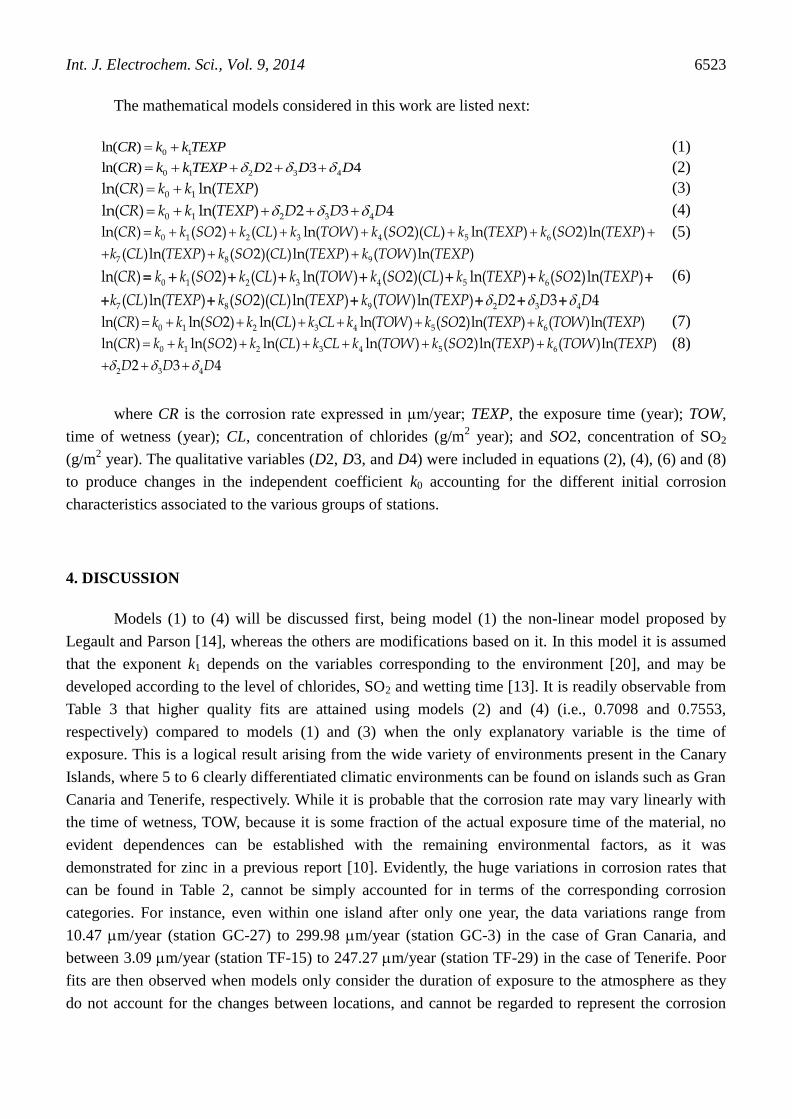
The mathematical models considered in this work are listed next:

0 1ln( ) CR k k TEXP (1)

0 1 2 3 4ln( ) 2 3 4 CR k k TEXP D D D (2)

0 1ln( ) ln( )CR k k TEXP (3)

0 1 2 3 4ln( ) ln( ) 2 3 4CR k k TEXP D D D (4)

0 1 2 3 4 5 6

7 8 9

ln( ) ( 2) ( ) ln( ) ( 2)( ) ln( ) ( 2)ln( )

( )ln( ) ( 2)( )ln( ) ( )ln( )

CR k k SO k CL k TOW k SO CL k TEXP k SO TEXP

k CL TEXP k SO CL TEXP k TOW TEXP

(5)

0 1 2 3 4 5 6

7 8 9 2 3 4

ln( ) ( 2) ( ) ln( ) ( 2)( ) ln( ) ( 2)ln( )

( )ln( ) ( 2)( )ln( ) ( )ln( ) 2 3 4

CR k k SO k CL k TOW k SO CL k TEXP k SO TEXP

k CL TEXP k SO CL TEXP k TOW TEXP D D D

(6)

0 1 2 3 4 5 6ln( ) ln( 2) ln( ) ln( ) ( 2)ln( ) ( )ln( )CR k k SO k CL k CL k TOW k SO TEXP k TOW TEXP (7)

0 1 2 3 4 5 6

2 3 4

ln( ) ln( 2) ln( ) ln( ) ( 2)ln( ) ( )ln( )

2 3 4

CR k k SO k CL k CL k TOW k SO TEXP k TOW TEXP

D D D

(8)

where CR is the corrosion rate expressed in µm/year; TEXP, the exposure time (year); TOW,

time of wetness (year); CL, concentration of chlorides (g/m2 year); and SO2, concentration of SO2

(g/m2 year). The qualitative variables (D2, D3, and D4) were included in equations (2), (4), (6) and (8)

to produce changes in the independent coefficient k0 accounting for the different initial corrosion

characteristics associated to the various groups of stations.

4. DISCUSSION

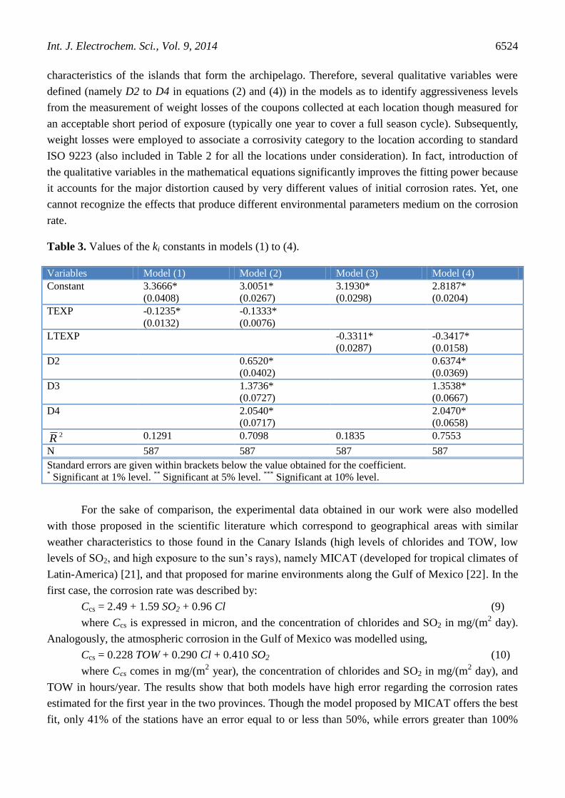
Models (1) to (4) will be discussed first, being model (1) the non-linear model proposed by

Legault and Parson [14], whereas the others are modifications based on it. In this model it is assumed

that the exponent k1 depends on the variables corresponding to the environment [20], and may be

developed according to the level of chlorides, SO2 and wetting time [13]. It is readily observable from

Table 3 that higher quality fits are attained using models (2) and (4) (i.e., 0.7098 and 0.7553,

respectively) compared to models (1) and (3) when the only explanatory variable is the time of

exposure. This is a logical result arising from the wide variety of environments present in the Canary

Islands, where 5 to 6 clearly differentiated climatic environments can be found on islands such as Gran

Canaria and Tenerife, respectively. While it is probable that the corrosion rate may vary linearly with

the time of wetness, TOW, because it is some fraction of the actual exposure time of the material, no

evident dependences can be established with the remaining environmental factors, as it was

demonstrated for zinc in a previous report [10]. Evidently, the huge variations in corrosion rates that

can be found in Table 2, cannot be simply accounted for in terms of the corresponding corrosion

categories. For instance, even within one island after only one year, the data variations range from

10.47 m/year (station GC-27) to 299.98 m/year (station GC-3) in the case of Gran Canaria, and

between 3.09 m/year (station TF-15) to 247.27 m/year (station TF-29) in the case of Tenerife. Poor

fits are then observed when models only consider the duration of exposure to the atmosphere as they

do not account for the changes between locations, and cannot be regarded to represent the corrosion


6524

characteristics of the islands that form the archipelago. Therefore, several qualitative variables were

defined (namely D2 to D4 in equations (2) and (4)) in the models as to identify aggressiveness levels

from the measurement of weight losses of the coupons collected at each location though measured for

an acceptable short period of exposure (typically one year to cover a full season cycle). Subsequently,

weight losses were employed to associate a corrosivity category to the location according to standard

ISO 9223 (also included in Table 2 for all the locations under consideration). In fact, introduction of

the qualitative variables in the mathematical equations significantly improves the fitting power because

it accounts for the major distortion caused by very different values of initial corrosion rates. Yet, one

cannot recognize the effects that produce different environmental parameters medium on the corrosion

rate.

Table 3. Values of the ki constants in models (1) to (4).

Variables Model (1) Model (2) Model (3) Model (4)

Constant 3.3666*

(0.0408)

3.0051*

(0.0267)

3.1930*

(0.0298)

2.8187*

(0.0204)

TEXP -0.1235*

(0.0132)

-0.1333*

(0.0076)

LTEXP -0.3311*

(0.0287)

-0.3417*

(0.0158)

D2 0.6520*

(0.0402)

0.6374*

(0.0369)

D3 1.3736*

(0.0727)

1.3538*

(0.0667)

D4 2.0540*

(0.0717)

2.0470*

(0.0658) 2R 0.1291 0.7098 0.1835 0.7553

N 587 587 587 587

Standard errors are given within brackets below the value obtained for the coefficient. * Significant at 1% level.

** Significant at 5% level.

*** Significant at 10% level.

For the sake of comparison, the experimental data obtained in our work were also modelled

with those proposed in the scientific literature which correspond to geographical areas with similar

weather characteristics to those found in the Canary Islands (high levels of chlorides and TOW, low

levels of SO2, and high exposure to the sun’s rays), namely MICAT (developed for tropical climates of

Latin-America) [21], and that proposed for marine environments along the Gulf of Mexico [22]. In the

first case, the corrosion rate was described by:

Ccs = 2.49 + 1.59 SO2 + 0.96 Cl (9)

where Ccs is expressed in micron, and the concentration of chlorides and SO2 in mg/(m2 day).

Analogously, the atmospheric corrosion in the Gulf of Mexico was modelled using,

Ccs = 0.228 TOW + 0.290 Cl + 0.410 SO2 (10)

where Ccs comes in mg/(m2 year), the concentration of chlorides and SO2 in mg/(m

2 day), and

TOW in hours/year. The results show that both models have high error regarding the corrosion rates

estimated for the first year in the two provinces. Though the model proposed by MICAT offers the best

fit, only 41% of the stations have an error equal to or less than 50%, while errors greater than 100%


6525

were found for all the test sites using the equation proposed for the Gulf of Mexico. Evidently, neither

of the two models describes the atmospheric corrosion behaviour of carbon steel in the Canarian

Islands.

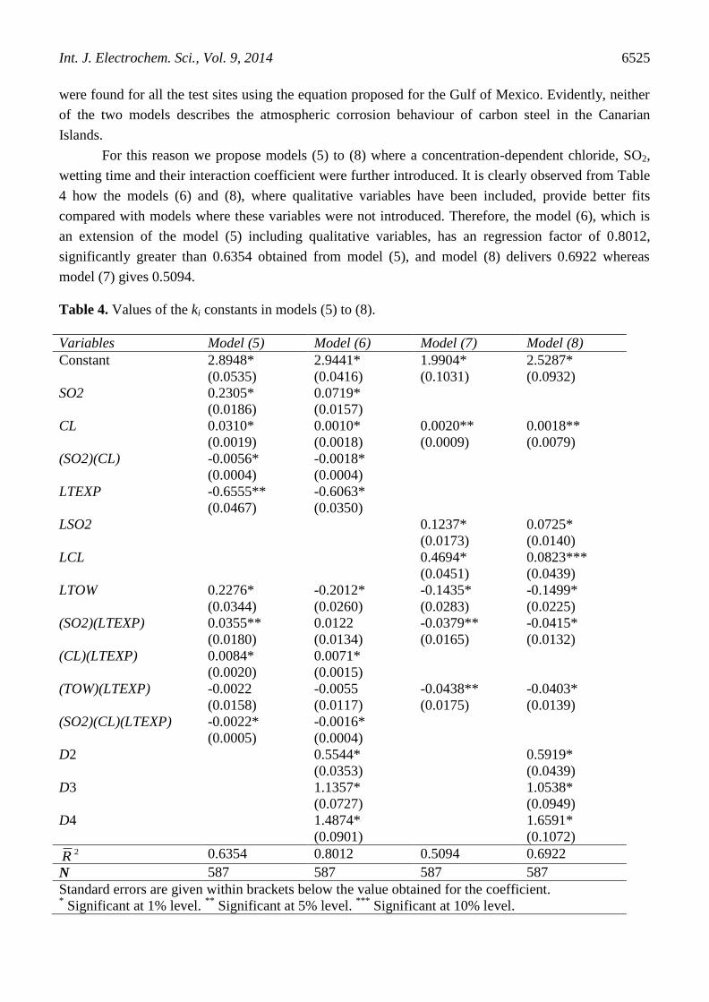
For this reason we propose models (5) to (8) where a concentration-dependent chloride, SO2,

wetting time and their interaction coefficient were further introduced. It is clearly observed from Table

4 how the models (6) and (8), where qualitative variables have been included, provide better fits

compared with models where these variables were not introduced. Therefore, the model (6), which is

an extension of the model (5) including qualitative variables, has an regression factor of 0.8012,

significantly greater than 0.6354 obtained from model (5), and model (8) delivers 0.6922 whereas

model (7) gives 0.5094.

Table 4. Values of the ki constants in models (5) to (8).

Variables Model (5) Model (6) Model (7) Model (8)

Constant 2.8948*

(0.0535)

2.9441*

(0.0416)

1.9904*

(0.1031)

2.5287*

(0.0932)

SO2 0.2305*

(0.0186)

0.0719*

(0.0157)

CL 0.0310*

(0.0019)

0.0010*

(0.0018)

0.0020**

(0.0009)

0.0018**

(0.0079)

(SO2)(CL) -0.0056*

(0.0004)

-0.0018*

(0.0004)

LTEXP -0.6555**

(0.0467)

-0.6063*

(0.0350)

LSO2 0.1237*

(0.0173)

0.0725*

(0.0140)

LCL 0.4694*

(0.0451)

0.0823***

(0.0439)

LTOW 0.2276*

(0.0344)

-0.2012*

(0.0260)

-0.1435*

(0.0283)

-0.1499*

(0.0225)

(SO2)(LTEXP) 0.0355**

(0.0180)

0.0122

(0.0134)

-0.0379**

(0.0165)

-0.0415*

(0.0132)

(CL)(LTEXP) 0.0084*

(0.0020)

0.0071*

(0.0015)

(TOW)(LTEXP) -0.0022

(0.0158)

-0.0055

(0.0117)

-0.0438**

(0.0175)

-0.0403*

(0.0139)

(SO2)(CL)(LTEXP) -0.0022*

(0.0005)

-0.0016*

(0.0004)

D2 0.5544*

(0.0353)

0.5919*

(0.0439)

D3 1.1357*

(0.0727)

1.0538*

(0.0949)

D4 1.4874*

(0.0901)

1.6591*

(0.1072) 2R 0.6354 0.8012 0.5094 0.6922

N 587 587 587 587

Standard errors are given within brackets below the value obtained for the coefficient. * Significant at 1% level.

** Significant at 5% level.

*** Significant at 10% level.


6526

A further improvement was produced by removing from equation (6) those variables that we

consider non significant for the atmospheric corrosion of carbon steel in these environments. In this

way, a new model (11) was developed, which is given by:

ln( ) 2.9378 0.0738( 2) 0.0097( ) 0.1987 ln( ) 0.0018( 2)( )

0.5985ln( ) 0.0067( )ln( ) 0.0014( 2)( )ln( ) 0.5544· 2

1.1423 3 1.4916 4

CR SO CL TOW SO CL

TEXP CL TEXP SO CL TEXP D

D D

(11)

The best fits were obtained using equation (11). We regard this model to satisfactorily describe

corrosion rates of carbon steel over the complete archipelago. When defining the errors committed by

the estimates made with this model along three years of exposure, 34% of the stations have an error

smaller than 10%, 26.03% present an error comprised between 10 and 20%, 17.81% an error between

20 and 30%, 12.32% an error between 30 and 40%, and 4.11% an error between 40 and 50%. Less

satisfactory results were only obtained in 6.85% of the locations (with an error between 50 and 100%),

whereas errors in excess of 100% only occurred at 2 stations.

5. CONCLUSIONS

Modelling the atmospheric corrosion of carbon steel in a fragmented subtropical environment,

presenting a wide variety of microclimates such as those found in the archipelago of the Canary

Islands, faces major difficulties. Neither the double-logarithmic law, widely accepted in the modeling

of atmospheric corrosion, or other models proposed for larger geographic areas with environmental

conditions apparently close to those exiting in the Canary Islands, can provide satisfactory predictions

for the corrosion rates of carbon steel.

To improve the modeling of atmospheric corrosion, qualitative variables accounting for the

major differences in corrosion aggressiveness between close locations were introduced in the

mathematical equations. They were defined from a classification of the locations according to their

corresponding index of corrosivity according to norm ISO 9223, though this norm does not adequately

describe the atmospheric corrosion of a fragmented subtropical environment by itself. In this way, a

major improvement of fit quality for corrosion rate prediction is achieved, though error ranges are still

unacceptably big.

Further improvement was achieved by allowing variable levels of the pollutants SO2 and

chlorides and for the time of wetness in the mathematical model using observations during one year

exposure. In this way, fitting errors in the prediction of corrosion rates for periods longer than one year

were greatly diminished, as ca. 74% of the stations delivered absolute errors in the predicted corrosion

rates below 30%.

ACKNOWLEDGMENTS

The authors wish to acknowledge the assistance of National Meteorological Agency of Spain

(AEMET, Madrid, Spain) by supplying data on time of wetness and the speeds and the directions of


6527

the winds at various locations in the Canary Islands. This work was partially funded by the Ministerio

de Economía y Competitividad (Madrid, Spain) and the European Regional Development Fund

(Brussels, Belgium) under Project No. CTQ2012-36787, and by the University of La Laguna (Ayudas

al Fomento de Nuevos Proyectos de Investigación - Modalidad de Reincorporación a la Actividad

Investigadora, 2013).

References

1. Corrosion Costs and Preventive Strategies in the United States, Publication No. FHWA-RD-01-

156; NACE International, Houston, 2001.

2. B.Y.R. Surnam, Anti-Corros. Method. M., 60 (2013) 73.

3. M. Natesan, G. Venkatachari and N. Palaniswamy, Corros. Prev. Control, June (2005) 43.

4. R.W. Revie, Uhlig’s Corrosion Handbook, 2nd edn., Wiley, New York, 2000, p. 305.

5. S.W. Dean and D.B. Reiser, in: Corrosion 1998; NACE International, Houston, 1998, Paper #340.

6. S.W. Dean and D.B. Reiser, in: Corrosion 2000; NACE International, Houston, 2000, Paper #455.

7. P.R. Roberge, R.D. Klassen and P.W. Haberecht, Mater. Design, 23 (2002) 321.

8. M. Morcillo and S. Feliu, Mapas de España de Corrosividad Atmosférica; CYTED, Madrid, 1993.

9. ISO 9223:1992(E), Corrosion of Metals and Alloys – Corrosivity of Atmospheres –Classification,

International Standars Organizations, Geneve, 1992.

10. J. Morales, F. Díaz, J. Hernández-Borges, S. González and V. Cano, Corros. Sci., 49 (2007) 526.

11. J.J. Santana Rodríguez, F.J. Santana Hernández and J.E. González González, Corros. Sci., 45

(2003) 799.

12. J. Morales, S. Martín-Krijer, F. Díaz, J. Hernández-Borges and S. González, Corros. Sci., 47 (2005)

2005.

13. J.J. Santana Rodríguez, F.J. Santana Hernández and J.E. González González, Corros. Sci., 44

(2002) 2425.

14. R.A. Legault and V.P. Pearson, in: Atmospheric factors affecting the corrosion of engineering

metals; S.K. Coburn (Ed.), ASTM Stock Number 646; American Society for Testing Materials,

Philadelphia, 1978, p. 83.

15. ASTM D 2010-85: Standard Method for Evaluation of total Sulfation Activity in the Atmosphere

by the Lead Dioxide Candle; American Society for Testing Materials, Philadelphia, 1985.

16. ISO/TC 156 N 250: Corrosion of Metals and Alloys. Aggressivity of Atmospheres. Methods of

Measurement of Pollution Data; International Standard Organizations, Geneve, 1986.

17. ISO 9225: 1992(E): Corrosion of Metals and Alloys-Corrosivity of Atmospheres-Measurement of

Pollution, First edition; International Standards Organization, Geneve, 1992.

18. ASTM G1-90: Standard Practice for Preparing, Cleaning, and Evaluating Corrosion Test

Specimens; American Society for Testing Materials, Philadelphia, 1990.

19. ISO/DIS 8403.3: Metals and Alloys. Procedures for Removal of Corrosion Products from

Corrosion Test Specimens; International Standards Organization, Geneve, 1985.

20. A. Porro, T.F. Otero and A.S. Elola, Brit. Corros. J., 27 (1992) 231.

21. L. Mariaca-Rodriguez, E. Almeida, A. Debosquez, A. Cabezas, J. Fernando-Alvarez, G. Joseph, M.

Marrocos, M. Morcillo, J. Peña, M.R. Prato, S. Rivero, B. Rosales, G. Salas, J. Urruchurtu-

Chavarín and A. Valencia, in: Marine Corrosion in Tropical Environments; S.W. Dean, G.

Hernandez-Duque Delgadillo and J.B. Bushman (Eds.), ASTM Stock Number STP1399; American

Society for Testing Materials, Philadelphia, PA, 2000, p. 3.

22. D. C. Cook, A. C. Van Orden, J. Reyes, S. J. Oh, R. Balasubramanian, J. J. Carpio and H. E.

Townsend, Atmospheric corrosion in marine environments along the Gulf of Mexico. In: Marine

Corrosion in Tropical Environments; S.W. Dean, G. Hernandez-Duque Delgadillo and J.B.


6528

Bushman (Eds.). ASTM Stock Number STP1399, American Society for Testing Materials,

Philadelphia, 2000, p. 75.

© 2014 The Authors. Published by ESG (www.electrochemsci.org). This article is an open access

article distributed under the terms and conditions of the Creative Commons Attribution license

(http://creativecommons.org/licenses/by/4.0/).

http://www.electrochemsci.org/

Development of mathematical models to predict the atmospheric corrosion rate of carbon steel in...

Documents

Transcript of Development of mathematical models to predict the atmospheric corrosion rate of carbon steel in...