DEVELOPMENT OF IRRIGATION GUIDELINES FOR CITRUS UNDER DRIP IRRIGATION IN ZIMBABWE

By

Farai Solomon Zirebwa

A thesis submitted in partial fulfilment of the requirements of the Master of Science Degree in Agricultural Meteorology

Department of Physics

Faculty of Science

University of Zimbabwe

Harare

May 2010

i

Abstract This study was carried out to develop drip irrigation guidelines for citrus in Zimbabwe. In order to achieve this, the average ETo values for the study site were derived from climatic data. The study, which was carried out at Mazowe Citrus Estate, also involved the determination of the class A evaporation pan coefficient, Kpan to enable local estimations of ETo from the class A evaporation pan. The whole season crop coefficient, Kc, curve for citrus was developed for the estimation of crop water requirements. The ETo trend for the study site was established from the FAO Penman Monteith equation using observed and historical climatic data. Kpan was determined using two methods. The first method was empirical and Kpan was estimated from the mean relative humidity, mean wind speed at 2 m height and the fetch conditions. In the second method, Kpan was determined as the slope of the plot of the FAO Penman Monteith ETo against the pan evaporation, Epan. The Kc curve was developed after the empirical determination of Kc during the initial growth stage, the mid season stage and at the end of fruit development. The Kc value of the initial growth stage that was developed for the sub humid climates was adjusted to reflect the wetting frequency of the soil. The mid season Kc value developed for the sub humid climate was adjusted to the local climatic conditions using wind speed at 2 m height, the minimum relative humidity and the average tree height. During the crop development and the late season stages, Kc was estimated by considering that Kc varies linearly between the value at the end of the previous stage and that at the beginning of the next stage. Transpiration rate was monitored using a Stem Heat Balance sap flow gauge that was installed on a branch of the tree. The leaf area was used as the scaling up factor for the sap flow from the branch to the whole hectare. This was done to compare the crop water requirement to the irrigation depth prescribed by the developed irrigation guidelines. BUDGET (version 6.2), a soil water balance model was used to develop irrigation calendars using a fixed irrigation interval of one day. The model was also used to simulate the soil water status after using the irrigation guidelines. Four treatments were established to assess the effect of different irrigation strategies on fruit growth and abscission. These were the control (use of ETo data for irrigation scheduling), well watered (where both sides of the tree were irrigated but each side receiving half the amount of water as the control), the grower’s scheduling practice and the last one was a PRD 50 where one side of the tree was irrigated whilst the other one was drying out. The switching of the drip lines was done on a 10 day interval. The effects of the different irrigation strategies were evaluated in terms of fruit growth rate and fruit abscission during the fruit drop period. ETo was approximately 4 mm day-1 from January to April, lowest in winter (almost 3 mm day-1) and was highest in October (slightly above 5 mm day-1). The green fetch Kpan was high from January to April (almost 0.8). The value fell from May and the lowest Kpan value of 0.72 was established in October. Using the second method, a Kpan value of 0.78 was determined for October to March. The initial Kc value was 0.47 but it rose sharply during the crop development stage. Kc values for the mid season and at the end of the season were 0.84 and 0.76 respectively. There is a possibility that the grower was over irrigating based on simulated soil moisture conditions usually above the field capacity. High drainage losses of up to 1964 mm for the whole season were simulated compared to 381 mm for the irrigation scheduling guidelines. No significant differences (p < 0.05) were observed on fruit growth rates although the control treatment had larger fruit diameters than the other treatments. Fruit abscission was generally low for all treatments. A single Kpan value

ii

can not be used throughout the season and the variations along the season should be taken into account for better estimations of ETo using the evaporation pan. Kc fluctuations during the crop development stage should be noted to reduce errors in the estimation of citrus crop water requirements. Taking into account the atmosphere’s evaporative demand is an effective way of irrigation scheduling. Irrigating both sides of the tree at the same time is not effective if the irrigation depth is low. PRD 50 showed great potential in balancing fruit growth and water conservation. Zimbabwean citrus farmers are encouraged to adopt the developed irrigation guidelines as well as the Kpan and Kc values. PRD, if well timed, proves to be a better irrigation strategy.

iii

Acknowledgements

To the Almighty God, be the glory and honour. I extend my profound gratitude to the entire Agrometeorological team of the Department of Physics, University of Zimbabwe for taking me this far. I would like acknowledge my appreciation to the help rendered to me by my supervisor Mr. E. Mashonjowa. Without your expert guidance, this work would have been different. My gratitude is also extended to Dr. S. Dzikiti, Dr. T. Mhizha and Prof. J.R. Milford for helping in the shaping up of this of this project. Mr. B. Chipindu, the coordinator of the program, I salute you for visionary guidance and making this program a success. The help and healthy cooperation by the management at Mazowe Citrus Estate is greatly appreciated. I would like to thank you for providing the study site and accommodating me. Mr. Tsamba and Whisky of MCE, thank you for taking the evaporation pan readings and being available when needed. Thank you Mr. Gwara, Mr. Muroyiwa and Mr. Mutungura for sacrificing your time and driving me to the study site. I would like to give thanks to the whole MAGM group of 2008 – 2010 (Joseph, Farai, Niclah, Sebastain, Hellen, Nkulumo and Juwawa), for their support throughout the work. Finally, to my family members, you are not ordinary. Thank you for your support in various ways directly or indirectly that gave me hope and strength to achieve this work. May the dear Lord bless you.

iv

Table of Contents

Abstract ...........................................................................................................................i Acknowledgements...................................................................................................... iii Table of Contents..........................................................................................................iv List of Figures ..............................................................................................................vii List of Tables ................................................................................................................xi List of Appendices ..................................................................................................... xiii List of Acronyms and symbols ...................................................................................xiv CHAPTER 1 INTRODUCTION..........................................................................1

1.1 Background ....................................................................................................1 1.2 Justification ....................................................................................................3 1.3 Objectives ......................................................................................................4 1.4 Expected Benefits ..........................................................................................5 1.5 Thesis Outline ................................................................................................6

CHAPTER 2 LITERATURE REVIEW .............................................................7

2.0 Introduction....................................................................................................7 2.1 Crop water requirements, CWR.....................................................................7 2.2 Citrus production in Zimbabwe .....................................................................8

2.2.1 Stage lengths for citrus at MCE.................................................................8 2.3 Irrigation strategies of citrus trees................................................................10

2.3.1 Partial Root – zone Drying (PRD)...........................................................10 2.3.2 Regulated Deficit Irrigation (RDI)...........................................................11

2.3.2.1 Merits and demerits of RDI..................................................................11 2.3.3 Pulsed Irrigation (PI)................................................................................12

2.4 Irrigation scheduling ....................................................................................12 2.4.1 Empirical methods ...............................................................................13

2.4.1.1 Merits and demerits of empirical methods.......................................16 2.4.2 Soil moisture based methods ...................................................................16

2.4.2.1 Basic procedure for water balance scheduling ...............................18 2.4.2.2 Advantages and disadvantages of the soil water balance scheduling ..........................................................................................................19

2.4.3 Estimates of water use from weather data ...............................................20 2.4.3.1 The FAO Penman – Monteith method .............................................20 2.4.3.2 Class A evaporation pan..................................................................22

2.4.3.2.1 Merits and demerits of the evaporation pan ...............................25 2.4.4 Tracking crop condition...............................................................................26

2.4.4.1 Stem diameter micro variation.........................................................26 2.4.4.2 Sap flow measurements....................................................................27

2.4.4.2.1 Stem Heat Balance (SHB) method.............................................27 2.4.4.2.2 Thermal Dissipation Probe (TDP) method.................................30 2.4.4.2.3 Determination of the cross sectional area of the sap conducting wood 32

2.4.5 Merits and demerits of tracking the crop condition .................................34 2.5 The crop coefficient, Kc ...............................................................................34

2.5.1 Kc for citrus ..............................................................................................36

v

CHAPTER 3 MATERIALS AND METHODS ................................................38 3.0 Introduction..................................................................................................38 3.1 Study site......................................................................................................38 3.2 Treatments and experimental design ...........................................................38 3.3 Microclimatic data collection ......................................................................41 3.4 Measurement of ETo using the class A evaporation pan..............................42 3.5 Determination of the pan coefficient, Kpan...................................................43 3.6 Establishment of the crop coefficient, Kc curve for citrus ...........................43

3.6.1 Kc ini for trees ............................................................................................44 3.6.1.1 Time interval between wetting events ..............................................44 3.6.1.2 Adjustment for partial wetting by irrigation....................................47

3.6.2 Kc mid .........................................................................................................47 3.6.3 Kc end – end of the late season stage .........................................................48

3.7 Sap flow measurements ...............................................................................49 3.7.1 Measurement of branch sap flow by the SHB method ............................49 3.7.2 Installation of the SGB 35-ws gauge .......................................................50 3.7.3 Determination of SHB sap flow...............................................................51 3.7.4 Up scaling of sap flow measurements .....................................................52

3.8 The development of irrigation calendars .....................................................53 3.8.1 Model description ....................................................................................53

3.8.1.1 Input .................................................................................................54 3.8.1.2 Output ..............................................................................................55

3.8.2 ETo generation for the trial site ................................................................56 3.8.3 Rainfall data .............................................................................................56 3.8.4 Crop parameters .......................................................................................57 3.8.5 Soil parameters.........................................................................................58 3.8.6 Irrigation data...........................................................................................60

3.9 Fruit growth measurements..........................................................................61 3.9.1 Fruit diameter...........................................................................................61 3.9.2 Fruit abscission ........................................................................................62

CHAPTER 4 RESULTS AND DISCUSSION ..................................................63

4.0 Introduction..................................................................................................63 4.1 Study site climate.........................................................................................63 4.2 Sap flow .......................................................................................................68

4.2.1 Sap flux density........................................................................................70 4.3 The pan coefficient, Kpan ..............................................................................71 4.4 KC curve for citrus .......................................................................................74

4.4.1 The Kc curve.............................................................................................74 4.5 Irrigation guidelines .....................................................................................76

4.5.1 Soil moisture status for the irrigation guidelines .....................................78 4.5.2 Normal conditions....................................................................................79 4.5.3 Hot and dry condition ..............................................................................82 4.5.4 Cool and humid condition........................................................................84 4.5.5 Dry condition ...........................................................................................87 4.5.6 Irrigation calendars ..................................................................................90 4.5.7 Grower’s practice soil water status ..........................................................93

4.6 Comparison of the irrigation guidelines with the grower’s practice...............97 4.7 The effect of irrigation strategies.................................................................98

4.7.1 Effects of irrigation treatments on yield variable ....................................98

vi

4.7.2 Fruit drop ...............................................................................................100 4.8 Summary ....................................................................................................101

CHAPTER 5 CONCLUSIONS AND RECOMMENDATIONS.....................103

5.0 CONCLUSIONS........................................................................................103 5.1 RECOMMENDATIONS FOR FURTHER STUDIES .............................105

REFERENCES ..........................................................................................................106 APPENDICES ...........................................................................................................111

vii

List of Figures

Figure 2.1: An illustration of the soil water balance showing the root zone as a

reservoir (Adapted from Raes, 2001)………………………………… 17

Figure 2.2: Features of the class A evaporation pan (Adapted from Allen et al.,

1998)…................................................................................................. 23

Figure 2.3: Outline of the Stem Heat Balance method for sap flow measurement

………..................................................................................................... 29

Figure 2.4: Thermal Dissipation Probe (TDP) sap velocity probe (Dynamax, 1997) ....

..................................................................................................................31

Figure 2.5: The linear relationship between the conducting sapwood area and the

stem cross sectional area in young potted navel orange trees showing that

approximately 83 % of the stem area comprised the conducting sapwood

(Dzikiti, 2007)............................................................................................33

Figure 3.1: Schematic layout of the study site showing the row and inter row spacing

as well as the position of the Automatic Weather Station

(AWS)……………………………………………………………………40

Figure 3.2: Drip irrigation of citrus trees showing a) a single line for the control and

grower’s practice and b) double drip lines for the PRD 50 and well

watered treatments. ....................................................................................41

Figure 3.3: Automatic weather station to monitor orchard microclimate at the trial

site at Mazowe Citrus Estate, Zimbabwe. The orchard can be seen in the

background.................................................................................................42

Figure 3.4: Average Kc ini as related to the level of ETo and the interval between

irrigations and or significant rain during the initial growth stage for all soil

types when wetting events are light to medium (3 – 10 mm per event).

Adapted from Allen et al., 1998)….…………………………………… 46

Figure 3.5: Average Kc ini as related to the level of ETo and the interval between

irrigations greater than or equal to 40 mm per wetting event, during the

initial growth stage for medium and fine textured soils (Allen et al., 1998).

....................................................................................................................47

viii

Figure 3.6: An illustration of the installation of the SGB 35-ws gauge on the branch

of a tree a) before and b) after wrapping with an aluminised shield..........50

Figure 3.7: Calculation scheme of the budget model (Raes, 2005)............................54

Figure 3.8: An illustration of the BUDGET main menu showing the model input

requirements needed to run the model. ......................................................55

Figure 3.9: Creation of a crop file in BUDGET (Raes,

2005)………………………….................................................... 58

Figure 3.10: Creation of a soil file in BUDGET (Raes,

2005)…………………………................................................. 59

Figure 3.11: A BUDGET file outlining the irrigation options used for the generation

of irrigation schedules........................................................................... 60

Figure 3.12: A tag with the fruit number tied to the last twig leading to the fruit for

easy identification................................................................................61

Figure 3.13: An illustration of the measurement of fruit diameter where a) the

measurement was taken along the equator of the fruit and b) the

measurement was taken perpendicular to the first one. ..........................62

Figure 4.1: The average monthly mean temperature, maximum temperature and

minimum temperature for MCE from 2006 to 2009...............................64

Figure 4.2: The mean monthly morning Relative Humidity (0200 hrs – 0600 hrs,

local time: GMT + 2 hrs), afternoon Relative Humidity (1200 hrs – 1600

hrs) and the mean Relative Humidity for MCE from 2006 to 2009. .........65

Figure 4.3: The average daily total solar radiation for MCE from 2006 to 2009.......66

Figure 4.4: Average (2005 – 2009) Relative Humidity and Wind speed at 2 m height

for Mazowe Citrus Estate…….......………………………………………67

Figure 4.5: The average (2005 – 2009) annual variation of ETo calculated using the

FAO Penman – Monteith equation ............................................................68

Figure 4.6: The typical course of sap flow measured on DOY 82 – 83. ....................69

Figure 4.7: The typical course of solar radiation measured on DOY 82-83 ..............69

Figure 4.8: Whole year K pan values for a class A evaporation pan with a dry fetch

and a green fetch at Mazowe Citrus Estate................................................72

Figure 4.9: Estimation of the pan coefficient (K pan) for the class –A evaporation pan

measurements at Mazowe Citrus Estate. The data used was collected

ix

during the period October 2009 to March 2010, but spurious pan

evaporation readings were filtered..........................................................73

Figure 4.10: Whole season crop coefficient curve for citrus at MCE ........................76

Figure 4.11: Mean daily ETo of MCE for the cool, normal and hot scenarios ...........77

Figure 4.12: Mean monthly rainfall totals of MCE for the dry, normal and humid

scenarios ................................................................................................78

Figure 4.13: BUDGET simulated initial and final soil moisture depletion under

normal conditions……….............................................................. 79

Figure 4.14: Water movement in and out of the root zone under normal conditions. 80

Figure 4.15: BUDGET simulated soil water balance terms under normal conditions

…............................................................................................... 81

Figure 4.16: BUDGET simulated initial and final soil moisture depletion under hot

and dry conditions........................................................................................................82

Figure 4.17: BUDGET simulated water movement in and out of the root zone under

hot and dry conditions. ..........................................................................83

Figure 4.18: BUDGET simulated soil water balance terms under hot and dry

conditions.....................................................................................................................84

Figure 4.19: BUDGET simulated initial and final soil moisture depletion under cool

and humid conditions ............................................................................85

Figure 4.20: BUDGET simulated water movement in and out of the root zone under

cool and humid conditions. ...................................................................86

Figure 4.21: BUDGET simulated soil water balance terms under cool and humid

conditions.....................................................................................................................87

Figure 4.22: BUDGET simulated initial and final soil moisture depletion under dry

conditions.....................................................................................................................88

Figure 4.23: BUDGET simulated soil moisture movement into and out of the root

zone under dry conditions. ....................................................................88

Figure 4.24: BUDGET simulated soil water balance terms under dry conditions .....89

Figure 4.25: Irrigation calendar for the first trimester of citrus production ...............91

Figure 4.26: Irrigation calendar for the second trimester of citrus production...........92

Figure 4.27: Irrigation calendar for the last trimester of citrus production ................93

x

Figure 4.28: Initial and final soil moisture depletion under normal conditions

considering the grower’s irrigation scheduling practices. ......................94

Figure 4.29: Soil moisture movement in and out of the root zone under normal

conditions considering the grower’s irrigation scheduling practices......95

Figure 4.30: Soil water balance terms under normal conditions considering the

grower’s irrigation scheduling practices. ................................................96

Figure 4.31: Fruit growth rates of the control, well – watered, grower’s practice and

PRD applying half of the control from 16 December 2009 to 03 February

2010.......................................................................................................100

Figure 4.32: Treatment effects on fruit abscission monitored from the first decade of

December to the first decade of January at MCE. ................................101

xi

List of Tables

Table 2.1: Typical growth cycle of citrus fruit at Mazowe Citrus Estate in Northern

Zimbabwe (Dzikiti, 2007).................................................................... 9 Table 2.2: Examples of empirical methods used to estimate ETo (Lee et al., (2004)

..................................................................................................................15

Table 2.3: K pan values for class A pan for different pan siting and environment and different levels of mean relative humidity and wind speed (Allen et al., 1998)………............................................................................................ 25

Table 2.4: Crop growth stages and their influences on the crop coefficient, Kc

(Adapted from Allen et al., 1998)..............................................................36 Table 2.5: Kc values for the sub tropics for large, mature trees providing

approximately 70 % tree ground cover (FAO, 2002). ...............................37 Table 2.6: Kc for citrus under different canopy and ground cover conditions (Allen et

al., 1998). ...................................................................................................37 Table 3.1: Experimental design using computer generated random numbers

(Genstat)….......................................................................................... 39 Table 3.2: Single (time-averaged) crop coefficients, Kc, and mean maximum plant

heights for non-stressed, well-managed crops in sub humid climates (RH min ≈ 45%, U2 ≈ 2 m s-1) for use with the FAO Penman-Monteith ETo (Allen et al., 1998). ....................................................................................44

Table 3.3: Characteristics of rainfall depths (Allen et al., 1998) ................................45

Table 3.4: Citrus crop parameters that were used to run the model............................57

Table 3.5: Characteristics of the soil at Mazowe Citrus Estate (after Hussein,

1982)….....................................................................................................59

Table 4.1: Branch leaf area determination using the branch diameter........................70

Table 4.2: Determination of the transpiration rate (mm/day) on DOY 82 – 83 and 84 using the sap flux density and leaf area per hectare...................................70

Table 4.3: Whole season Kc values per decade for the study site derived from the

daily values. ...............................................................................................75 Table 4.4: Irrigation requirements, drainage losses and water deficiency under normal

conditions for irrigation scheduling guidelines and grower’s practice. .....97

xii

Table 4.5: Total irrigation water received per treatment per hectare from October 2009 to December 2009. ............................................................................98

Table 4.6: The effect of irrigation treatments on fruit growth rate. ............................99

xiii

List of Appendices Appendix 1: Day of year (Julian days) calendar..................................................... 111

Appendix 2: Determination of K pan using RH mean, U2 and FET........................... 112

Appendix 3: Determination of irrigation duration from October to December........113

Appendix 4: Determination of the Kc curve.............................................................. 116

Appendix 5: Calculation of the amount of irrigation water used per treatment....... 117

Appendix 6: Determination of the average leaf area per tree................................... 119

Appendix 7: Analysis of variance for fruit growth rates......................................... 120

Appendix 8: Data logger program for the SHB sap flow gauge............................. 121

xiv

List of Acronyms and symbols AWC Available Water Capacity

AWS Automatic Weather Station

BUDGET A soil water and salt balance model

CWR Crop Water Requirements

DOY Day of year (in Julian days)

Epan Pan Evaporation

ETc Crop Evapotranspiration

ETo Reference evapotranspiration

FAO Food and Agriculture Organisation

FC Field Capacity

FET Fetch i.e. the distance of the identified surface

type upwind of the evaporation pan

fw The fraction of the surface wetted by irrigation

or rain

Kpan Pan Coefficient

Kc Crop Coefficient

Kc end Crop Coefficient value that corresponds to the

end of the season

Kc ini Crop Coefficient value for the initial crop

growth stage

Kc mid Crop Coefficient value for the mid season stage

of crop development

Kc next Crop Coefficient value for the next crop growth

stage

Kc prev Crop Coefficient value for the previous crop

growth stage

Ksh Thermal conductance constant for a particular

gauge installation

Kst Thermal conductivity of the stem

MCE Mazowe Citrus Estate

MDS Maximum Daily Trunk Shrinkage

PI Pulsed Irrigation

xv

PRD Partial Root zone Drying

PRD 50 Partial Root zone Drying applying half the

amount as the control

RAM Readily Available Moisture

RDI Regulated Deficit Irrigation

RH Relative Humidity

RHmin Minimum Relative Humidity

RZ Root Zone

SHB Stem Heat Balance

TAM Total Available Moisture

TDP Thermal Dissipation Probe

U2 Wind speed at 2 m height

WMO World Meteorological Organisation

1

CHAPTER 1 INTRODUCTION

1.1 Background The recent uncertainties in the rainfall patterns of Southern Africa and the prevalence of

drought in the region are the major driving factors that call for the efficient utilization of

water resources. Climatic variability and change that result in increased evaporation rates

coupled with reduced capacities of reservoirs in Zimbabwe due to siltation has recently led to

increased pressure on the limited and diminishing water resources. Agriculture is the largest

consumer of water in all regions of the world except Europe and North America and up to 70

% of water abstracted from rivers and ground water goes to irrigation (FAO, 2002a;

Lenntech, 2003).

Water can be utilized efficiently in agriculture through properly designed irrigation

schedules. Irrigation scheduling is an important aspect of management that determines when

to irrigate and how much water to apply. Water applied at the proper time and quantity can

influence fruit yield and quality. Crops require water in the root zone and any water applied

should be equal to the water lost through evapotranspiration. The type of irrigation rather

than scheduling mainly governs irrigation efficiency. Drip irrigation is more efficient than

sprinkler irrigation and flood irrigation is the least efficient. All these irrigation types are in

use in Zimbabwe but resources permitting, farmers should move to drip irrigation because of

its high efficiency.

Recent studies have shown that the drip irrigation system can be modified to increase

application efficiency. Some of the strategies to be used in drip irrigation are the Partial Root

zone Drying (PRD), Regulated Deficit Irrigation (RDI) and the Pulsed Irrigation (PI)

techniques. PRD is a water application technique that involves alternately wetting each half

2

of the root zone during successive irrigation events. RDI is an irrigation strategy in which

water is either withheld or reduced during specific periods of crop (fruit) growth (Dzikiti,

2007). A certain level of drought stress is maintained in the root zone and the objective in tree

crops is to control the canopy size and to limit the applied water. A fraction of crop

evapotranspiration is replaced during each irrigation event rather than applying full irrigation

(100 % ETc). The applied amount of water, however, must not affect production (yield and

quality of the crop).

PI is the application of small amounts of water at intervals across the day rather than

applying the required amount of water at once. This is beneficial in that all water applied will

be used by the plant reducing deep percolation losses. PRD and RDI have been found to have

high water use efficiencies in citrus production and improve yield with no negative effects on

fruit quality (Chalmers et al., 1981; Cohen et al., 1985; Dry et al., 1996; Dzikiti et al., 2008).

The citrus species are perennial in growth habit. The most common species are Citrus

sinensis (sweet orange), Citrus aurantium (sour orange), Citrus aurantifolia (lime), Citrus

limon (lemon) and Citrus paradis (grape fruit). In 2001, the world production of citrus was

around 98.7 million tonnes of fresh fruit, 62 % of which were oranges (FAO, 2002a). The

production levels of citrus reflect that citrus production is one of the major agricultural

activities contributing to the irrigation water demand.

In citrus production, there should be a well-defined irrigation calendar that is derived from

the evaporative demand of the atmosphere, soil type as well as water application strategies

that are effective. The vegetative and fruit development phases in citrus trees consist of bud

break, flowering, fruit set, fruit growth, summer flush and autumn flush. Water application

3

throughout the season should take into account the water requirements of these phases so as

to enhance yield and fruit quality. The use of the drip irrigation strategy in Zimbabwe is

expected to enhance the water use efficiency, yield and fruit quality of citrus trees, and has

been applied by some growers in Zimbabwe. However, productivity under this strategy has in

some cases failed to surpass, let alone match that under less precise water application

methods such as flood irrigation. One of the main constraints identified is the lack of

operational guidelines for system and site-specific irrigation scheduling.

1.2 Justification About 6000 hectares are under citrus cultivation in Zimbabwe (Ministry of Foreign Affairs,

2009). More resources must be directed towards citrus production as it has potential to

increase the country’s revenue, since it is one of the major horticultural exports. The quality

and quantity of produce can be drastically reduced when the trees are not receiving the right

amount of water. Citrus production in Zimbabwe depends largely upon the availability of

water for irrigation since rainfall occurs mainly during summer.

The mean monthly precipitation for Mazowe Citrus Estate (MCE) is less than the mean

monthly potential evapotranspiration for eight months i.e. from April to November with an

average of ninety-three rain days per year (Grieser, 2006). The climatic net primary

production is precipitation limited. MCE is in natural region II of Zimbabwe and is hence

even better in terms of precipitation compared to natural regions III, IV and V (Vincent and

Thomas, 1960). For viable citrus production, the precipitation deficit has to be covered by

irrigation since citrus are annual crops. There is need for irrigation for more than two thirds

of the year. It is apparent that there is heavy reliance on irrigation and hence proper irrigation

4

strategies have to be implemented for higher production as well as effective water

management.

The development of site-specific operational guidelines for citrus irrigation is a requirement

for the local citrus growers. Irrigation must take into account the evaporative demand of the

atmosphere at any given day. The use of the irrigation guidelines will aid growers to apply

the required amount of water. This ensures the optimal utilisation of water resources (avoids

over irrigation and under irrigation). The current blanket recommendations for citrus

irrigation do not take into account the variations in the evaporative demand of the atmosphere

from day to day and even from season to season.

The study promotes the effective use of simple weather stations for the estimation of potential

evapotranspiration, ETo by the growers. Since most growers do not afford and or do not have

the expertise for advanced instrumentation for estimating ETo, they can use evaporation pans

and obtain reliable results. The reliable ETo from the evaporation pans is aided by the

application of a site-specific pan coefficient, Kpan. The Kpan value was obtained by the

calibration of pan evaporation, Epan against ETo computed with the Penman Monteith method.

The determination of the site-specific crop coefficient, Kc curve from the study allows for

better estimation of crop water requirements by the growers. The growers will therefore know

the optimum amount of water to apply as demanded by the trees.

1.3 Objectives

The main aim of this study was to establish irrigation guidelines for citrus trees under PRD

and non-PRD drip irrigation in Zimbabwe. The specific objectives of the study were to:

1. Determine the evapotranspiration of citrus trees using the FAO Penman Monteith

method.

5

2. Determine a site-specific crop coefficient curve, Kc for citrus.

3. Develop appropriate irrigation guidelines for citrus under PRD and non-PRD drip

irrigation.

4. Evaluate the performance of these guidelines by comparison against an existing

operational system (the current grower practice) at Mazowe Citrus Estate.

1.4 Expected Benefits

The benefits derived from this study are of great value to citrus farmers in Zimbabwe. This

study provides comprehensive yet user friendly irrigation guidelines for all weather

conditions and these guidelines can be transferred to other areas after proper adjustments.

Citrus plant water use throughout the season is outlined to enable farmers to know the

amount of water expected to be used through irrigation for planning purposes.

The study provides a means for farmers to estimate crop water requirements by using the

mean daily ETo values derived from the reliable FAO Penman – Monteith equation as well as

a site specific empirically determined crop coefficient curve. One of the major benefits of this

study is that it transformed the complex and expensive way of estimating citrus water

requirements. Farmers will be able to use the easy and cheap evaporation pan method

because of the establishment of site specific pan coefficients throughout the growing season.

The study also gives an illustration of the soil moisture dynamics throughout the season for

all scenarios of rainfall and ETo. This is essential for irrigation planning and decision making.

This gives a better understanding of when to irrigate and the depth of application. The

understanding of soil water dynamics provides a way for timing of water harvesting in

orchards during periods of excess rainfall. This reduces the amount of water that will be lost

6

through drainage beyond the root zone. If captured and well stored, the water can be used for

other purposes.

1.5 Thesis Outline

The thesis consists of 5 chapters. In chapter 1, the thesis is introduced by giving a brief

background, the justification of the study and an outline of the objectives of the research.

Chapter 2 outlines the literature that is linked to the study. The study site description,

treatments, materials and methods applied for the collection of the required information are

described in chapter 3. The results and their subsequent discussion from different

experiments of the study are displayed in chapter 4. The findings from the research work are

concluded in chapter 5. The recommendations for further studies and possible ways for the

improvement of citrus water management are also outlined in chapter 5. The appendices at

the end of the thesis give more details on sections that could not be included in the main

body.

7

CHAPTER 2 LITERATURE REVIEW

2.0 Introduction Water management is an important aspect for successful citrus production. Irrigation

scheduling strategies are an integral part of water management. Huygen et al., (1995) outlined

the following as objectives of irrigation management:

• Maximum net return

• Reduction of irrigation costs

• Rational use of the limited water supply

• Reduction of ground water pollution

Irrigation water management is principally achieved by irrigation scheduling in the form of

an irrigation calendar or guidelines. There are many methods that are used for irrigation

scheduling and the choice depends mainly on the availability of weather data, level of

instrumentation and expertise. The three major forms of irrigation scheduling are: empirical,

weather based and the tracking of crop condition. Irrigation guidelines are produced from the

evaporative demand of the atmosphere, crop type and growth stage.

2.1 Crop water requirements, CWR Water is essential for plant survival and growth and approximately 1 % of water taken up by

plants is used for metabolic activities and the rest is transpired (Raes, 2007). Water is a

solvent in most physiological processes, is vital for chemical reactions and is involved in

photosynthesis. Evaluation of crop water requirements in irrigation scheduling is based on the

estimation of crop evapotranspiration, ETc. The CWR is expressed as depth of water in unit

8

time (usually a day) and is affected by weather variables, crop factors, management and

environmental conditions.

The vapour pressure gradient i.e. the difference between vapour pressure at the transpiring

surface and that of the surrounding air is the major force in removing water vapour from the

transpiring surface (the leaf). There is need for accurate methods for measuring CWR on real

time basis. This is very crucial since the reduction of irrigation needs by 10 % would free up

enough water to double domestic water use world wide (Lascano et al., 1996). The

determination of CWR breaks the obstacle of the evaluation of water inventories and future

demands since ETc is a basic component of the hydrological cycle (Lascano et al., 1996).

2.2 Citrus production in Zimbabwe

Citrus is an evergreen, cold sensitive plant with a geographical distribution mainly influenced

by low temperatures (Gat et. al., 1997). Major citrus growing areas i.e. citrus belt, extend

from 40 0 North to 40 0 South latitude (Gat et. al., 1997; FAO, 2002b) and an altitude of up to

1800 m in the subtropics (FAO, 2002b) thus making Zimbabwe a citrus growing region.

Citrus production in Zimbabwe depends largely upon the availability of water for irrigation

since rainfall occurs mainly during summer. In Zimbabwe, an estimated 6000 hectares are

under citrus cultivation (Ministry of Foreign Affairs, 2009). Citrus fruits grown include

grapefruits, lemons, naartijies, nectarines and oranges. Fruit bearing for citrus is usually three

years after planting but economic yields are realised from the fifth year.

2.2.1 Development of citrus at MCE

The phenological stage lengths for citrus at MCE are outlined in Table 2.1. The citrus growth

cycle is divided into four growth stages. The initial stage is during spring where there is

9

maximum shoot initiation. These shoots form the sites on which flowers develop. The initial

stage is approximately 70 days and begins from August to almost the first decade of October.

Part of the initial stage involves the first flower opening and flowering.

Table 2.1: Typical growth cycle of citrus fruit at Mazowe Citrus Estate in Northern Zimbabwe (Dzikiti, 2007).

The second stage (crop development) initiates from the second decade of October and

stretches to end of December. The crop development stage is approximately 81 days. During

this stage, there will be flowering up to end of October; fruit set up to end of December and

the fruit growth consists of cell division. The mid season stage is characterised by cell

expansion i.e. fruit growth. Cell expansion starts from end of December to the end of March.

The mid season stage is approximately 120 days. The late season stage for citrus in

Zimbabwe is about 94 days long. The fruit development and maturation stages are however

not clearly distinguishable and they overlap considerably.

10

2.3 Irrigation strategies of citrus trees

Irrigation is one of the critical factors for the production of high value citrus fruits (Ramsey,

2007). Real time irrigation scheduling systems are usually used for high value crops e.g.

citrus. Full season irrigation schedules for citrus can also be developed from historical

meteorological data based on long term average data (De Jager and Kennedy, 1996). Water

application for citrus should be aimed in the effective root zone i.e. 30 to 40 cm, depending

on soil type (Ramsey, 2007). The prime objective is to reduce water losses and leaching

through deep percolation. There are a number of drip irrigation strategies for citrus that are in

use in Zimbabwe. The most common are the Partial Root zone Drying (PRD), Regulated

Deficit Irrigation (RDI) and Pulsed Irrigation (PI). All these strategies have been developed

with the main objectives of enhancing the water use efficiency of citrus and maintaining or

even increasing fruit quality and yield.

2.3.1 Partial Root – zone Drying (PRD)

PRD is a water application technique that involves alternately wetting each half of the root

zone during successive irrigation events. PRD also involves the gradual drying out of part of

the root system while keeping the other part wet by scheduled irrigation (Chalmers et al.,

2004). This is done for a pre-determined period before the irrigation is swapped to the dry

side, allowing the wet side to start drying out. The PRD strategy seeks to reduce, artificially,

stomatal conductance while maintaining the plant water status (Dzikiti et al., 2006). This

irrigation strategy is designed to increase water use efficiency in citrus thereby decreasing

production costs (Lovatt and Faber, undated).

The increased water use efficiency is linked to stomatal control of transpiration and

favourable plant water status. This is enhanced by a chemical signal, Absissic Acid (ABA)

11

i.e. a plant growth regulator produced in drying roots that is transported to leaves after night

time rehydration of the roots in the dry soil (During et al., 1996; O’Connell et al., 2004). This

results in a non-hydraulic effect by causing partial closing of leaf stomata (During et al.,

1996). PRD was reported to increase water use efficiency, reduce vegetative growth and

maintain fruit yield and quality in grape vines (Dry and Loveys, 1999). PRD is tipped to

increase yields in orchards where reduced internal shading result in increased flower

initiation, fruit set, fruit size and fruit colour (O’ Connell and Goodwin, 2004).

2.3.2 Regulated Deficit Irrigation (RDI)

RDI is an irrigation strategy in which water is either withheld or reduced during specific

periods of crop (fruit) growth (Dzikiti, 2007). A certain level of drought stress is maintained

in the root zone and the objective in tree crops is to control the canopy size and to limit the

applied water. A fraction of crop evapotranspiration is replaced during each irrigation event

rather than the application of full irrigation (100 % ETc). RDI is a valuable and sustainable

production strategy in dry regions (Geerts and Raes, 2009). Water application is limited for

periods that correspond to drought tolerant growth stages especially the vegetative and early

ripening. RDI aims at stabilising yields and obtaining maximum water productivity rather

than maximising yields (Geerts and Raes, 2009).

2.3.2.1 Merits and demerits of RDI

RDI maximises water productivity and stabilises yields i.e. does not cause severe yield

reductions. In areas where water is the limiting factor, maximising water productivity may be

economically more profitable to the farmer than maximising yields (Geerts and Raes, 2009).

Although a certain reduction in yield is observed, yield quality (sugar content, grain size)

12

tends to be equal or even superior (Geerts and Raes, 2009). RDI creates a less humid

environment around the crop decreasing the risk of fungal diseases as well as reducing

nutrient loss through leaching.

The major shortfall of RDI is that it requires precise knowledge of crop response to drought

stress. All water restrictions are supposed to be linked to crop phenological stages that are

less affected by water stress. There should also be unrestricted access to irrigation water

during sensitive growth stages. RDI can induce salinisation and hence measures are to be

taken to avoid salinisation.

2.3.3 Pulsed Irrigation (PI)

PI is the application of small amounts of water at intervals across the day rather than applying

the required amount of water at once. This is beneficial in that water and nutrients are

supplied at a rate that is close to plant uptake, thus enhancing growth and production

(Assouline et al., 2006). PI is mainly recommended for situations where the daily water

requirement exceeds the amount of water that can be held in the root zone (Ramsey, 2007).

The observed shortcomings of PI include the build up of salts in the root zone (Assouline et

al., 2006). Under PI, it was noted that there is improved P mobilisation and uptake as well as

higher Mn concentrations in leaves and fruits (Assouline et al., 2006). PI is essential in

reducing clogging problems in drip irrigation systems.

2.4 Irrigation scheduling

Irrigation scheduling is an important aspect of management that determines when to irrigate

and how much water to apply (Ramsey, 2007; Taylor and Rieger, undated). Jensen (1981)

defined irrigation scheduling as “a planning and decision making activity that an operator of

13

an irrigated farm is involved in before and during most of the growing season for each crop

that is grown.” It is important to determine the exact crop water requirements for more

precise irrigation scheduling (Garcia – Orellana et al., 2007).

Itier et al., (1996) grouped irrigation scheduling criteria into two i.e. depth and time. They

defined the depth criteria as back to Field Capacity, FC or a fixed depth. Three timing criteria

were outlined as follows:

• Allowable daily stress or relative evapotranspiration, ET = a (with 0.5 < a < 1). This is

obtained through the soil water balance or from plant water stress indicators.

• Readily Available Water Capacity (AWC) consumed or some fixed percentage of

AWC consumed (obtained by a means of soil water balance).

• Critical pressure head or moisture content at sensor depth (obtained by means of a soil

moisture measuring device).

Irrigation scheduling options are linked to the level of technology, expertise or data

availability. Various methods for irrigation scheduling have been developed so far. These

include empirical (no measurement), soil moisture based, estimates of water use from

weather data and tracking crop condition i.e. crop – water stress (van Bavel et al., 1996).

2.4.1 Empirical methods

Empirical data is information that is derived from the trials and errors of experience.

Empirical scheduling involves the use of known effects, through established equations. A

simple correlation is developed between ETo and a meteorological parameter(s) using long-

term data. The method is more applicable to areas where meteorological data is not readily

14

available. The shortcoming of this method is that it is not very accurate compared to other

methods of irrigation scheduling.

Most empirical methods are temperature based because of the assumption that temperature is

an indicator of the evaporative power of the atmosphere. Temperature is one of the major

factors influencing ETo and it is not possible to estimate ETo without temperature data (Raes,

2007). The estimates produced are generally less reliable than those that take other climatic

variables into consideration. The Blaney Criddle method, and to a lesser extend the Senami –

Hargreaves and the Hargreaves methods are most sensitive to temperature change (Lee et al.,

2004). The sensitivity however, varies with location and the time of the year. Table 2.2 shows

some of the empirical methods that are used to estimate ETo. Lee et al., (2004) outlined an

example of the use of direct measurement of net radiation to estimate ETo. The correlation

(with a considerable accuracy i.e. r2 = 0.97) was established using 30-year daily data

(equation 2.1).

3183.0187.0 += so RET r2 = 0.9733 (2.1)

(Lee et al., 2004)

Where ETo is potential evapotranspiration computed using the Penman – Monteith method

(mm hr-1) and Rs is the net global radiation (MJ m-2 day-1).

15

Table 2.2: Examples of empirical methods used to estimate ETo (Lee et al., (2004)

Method Formula Applied Hargreaves 5.0)(0038.0 TTRET ao ∂= ,

)408.0()()8.17( minmax RTTTkET meano −+= )846.0( += meano TpET

Senami – Hargreaves ffor TTSET ∂= 00094.0 Blaney – Criddle fbaET BCBCo ++=

)13.846.0( += Tpf

41.1)()(0043.0 min −−= N

nRHaBC

))((0006.0))((006.0

)(066.0)(07.1)(0041.082.0

minmin

min

d

dBC

URHNnRH

UNnRHb

−

−++−=

Where ETo is the reference evapotranspiration (mm day-1), Ra is the extraterrestrial radiation

expressed in equivalent evaporation (mm day-1), T is the mean air temperature (oC), ∂T is the

difference between mean monthly maximum and mean monthly minimum temperatures (oC),

k is a coefficient and has a default value of 0.0023, Tmean is the mean daily air temperature

(oC), Tmax is the mean daily maximum air temperature (oC), Tmin is the mean daily minimum

air temperature (oC), R is the extraterrestrial radiation (MJ m-2 day-1), So is the water

equivalent of extraterrestrial radiation (mm day-1), ∂Tf is the difference between mean

monthly maximum and mean monthly minimum temperatures (oF), Tf is the mean

temperature (oF), aBC, bBC and f are functions, (n/N) is the ratio of actual to possible sunshine

hours, RHmin is the minimum daily relative humidity, p is the ratio of actual daily daytime

hours to annual mean daily daytime hours and Ud is the daytime wind speed at 2 m height

(m s-1).

16

2.4.1.1 Merits and demerits of empirical methods

The method usually employs simpler models with less input variables and hence can be

broadly applied and not limited to data availability. Most of the empirical methods are

appropriate for humid conditions where the aerodynamic term is relatively small.

Most of the methods do not consider humidity or wind factors hence they are less likely

accurate in arid and semi arid conditions. Hargreaves ETo equations were designed primarily

for irrigation planning and designing rather than scheduling and the daily estimates are

subject to errors caused by the fluctuation of the temperature range caused by the movement

of weather fronts and by the large variations in wind speed and cloud cover (Raes, 2007). The

Hargreaves methods are recommended for use with five day or larger time steps and less

reliable with smaller time steps. The Thornthwaite method i.e. a temperature based method

results in underestimation especially for arid conditions (Raes, 2007). Local calibration is

required for satisfactory results.

2.4.2 Soil moisture based methods

The basis for irrigation scheduling is through the soil water balance in which the soil root

zone, RZ is taken as a reservoir (a bank) where there is input, storage and output of water

from the system. Crop evapotranspiration (ETc) is the daily withdrawal from the bank and

replenishment is through irrigation and or rainfall (Ministry of Agriculture, Food and

Fisheries, 2004). The objective of the soil water balance is to predict soil water content in the

RZ through a water conservation equation (equation 2.2). Soil water affects plant growth

through its effect on plant water status. The availability of soil water is assessed through soil

water content and soil water potential. The components of the soil water balance are

illustrated in Figure 2.1.

17

∆ (AWC * RZ) = Balance of entering + Outgoing water fluxes (2.2)

(Itier et al., 1996)

Figure 2.1: An illustration of the soil water balance showing the root zone as a reservoir (Adapted from Raes, 2001).

The soil water balance scheduling requires accurate measurement of the volume of water

applied or the depth of application. It is the day to day accounting of the amounts of water

coming into and going out of the effective root zone of the crop. The total water in the root

zone can be represented using equation 2.3.

netTTTcTTTT FLUXRunoffDEEPETRainIrrTWTWT

+−−−++= −1 (2.3)

(Harris, 2006)

18

Where TWT is total water in the root zone on day T, TWT-1 is the total water in the root zone

on previous day (T-1), Irr is the irrigation water applied, Rain is the rainfall amount, ETc is

the evapotranspiration (soil evaporation and plant use), DEEP is the drainage or percolation

below the root zone and FLUX net is any change in total water in the root zone from

underground water movement e.g. high water table or moving laterally into the ground on

day T.

2.4.2.1 Basic procedure for water balance scheduling

The procedure for the basic water balance scheduling was outlined by Harris (2006) and its

main objective is to illustrate how each of the water balance terms is established. The

procedure consists of seven steps that are:

a) Determination of the effective root zone depth

b) Determination of the Total Available Moisture (TAM). This is the amount of soil

water in the effective root zone that is available to plants and is soil specific.

c) Determination of the Readily Available Moisture (RAM). This is the fraction of TAM

that the crop can extract from the root zone without suffering water stress. It is found

as the product of TAM and the depletion factor i.e. the fraction of plant available

water that can be depleted from the effective root zone before irrigation is necessary.

d) Determination of the refill point. This is the total soil water balance in the effective

root zone at which irrigation is required. It is found by subtracting RAM from total

soil moisture at field capacity.

e) Determination of the starting point for total soil water in the effective root zone. This

can be established from direct measurements e.g. gravimetric, neutron probes.

19

f) Quantifying water movement into and from the effective root zone. This involves

measurement of rainfall and irrigation depth. If rainfall / irrigation is greater than the

depth of soil water depleted from the root zone, the difference is considered to be

deep drainage and or runoff. FLUXnet is usually considered to be negligible although it

can be significant where a perched water table exists. ETc is estimated from weather

and crop information.

g) Irrigation decision

2.4.2.2 Advantages and disadvantages of the soil water balance scheduling

The timing and depths of future irrigations can be planned through the calculation of the soil

water balance of the RZ on a daily basis. Soil water measurements of the water balance

method are necessary for feedback information on irrigation scheduling based on

evapotranspiration. Since most models are unreliable in the prediction of the water balance

terms, the soil water balance method is vital because periodical measurements of soil water

may be used to ‘adjust’ model output for irrigation application. The soil water balance

method is effective at assessing drainage losses and hence a good reference for estimation of

optimum irrigation depths for a particular soil.

A lot of measurements are required in the field and the measurements are to be done over a

long period. The method is not as accurate as direct measurement and needs local estimation

of precipitation, runoff and evapotranspiration. The measurement of evapotranspiration offers

the major problem for the water balance method since it requires good estimates of the crop

coefficient and the associated climatic parameters for the computation of ETo.

20

2.4.3 Estimates of water use from weather data

Irrigation scheduling is done more appropriately if meteorological data is used to estimate

daily evapotranspiration, ETc (Nakamura et al., 1996). The factors affecting daytime ETc are

radiation, air temperature, relative humidity, wind velocity, soil heat flux and vegetation

coverage. Most of the automated irrigation control systems are based on the measurement of

meteorological factors as inputs for feedback control (Ton and Kopyt, 2003).

Various methods have been developed for estimating ETc, which is a basis for the

development of irrigation calendars. Some of these methods are the FAO Penman Monteith,

FAO radiation, FAO Blaney Criddle and the FAO pan evaporation.

2.4.3.1 The FAO Penman – Monteith method

A panel of experts and researchers organised by FAO in May 1990 in consultation with the

World Meteorological Organisation (WMO) recommended the adoption of the Penman

Monteith method as the standard for computing evapotranspiration (Allen et al., 1998).

Penman and Monteith developed the method of estimating ETo based on the correlation

between energy conservation and the aerodynamics in the crop area (Aguila and Garcia,

1996; Allen et al., 1998). The energy component suggests the amount of water available for

evaporation whilst the aerodynamic term relates the effect of advection on the crop surface in

the removal of water vapour from the soil. Smith et al., (1996) rated the performance of the

method as being superior. The expression of computing ETo using the FAO Penman –

Monteith method is shown in equation 2.4.

21

)34.01(

)(273

900)(408.0

2

2

U

eeUT

GRET

dan

o ++∆

−+

+−∆=

γ

γ (2.4)

(Smith et al., 1996)

Where:

ETo is the reference crop evapotranspiration (mm day-1), Rn is net radiation at the crop surface

(MJ m-2 day-1), G is the soil heat flux (MJ m-2 day-1), T is the average air temperature (oC), U2

is wind speed measured at 2 m height (m s-1), (ea – ed) is the vapour pressure deficit (Kpa), ∆

is the Slope of the vapour pressure curve (Kpa oC-1), γ is the psychrometric constant

(Kpa oC-1) and 900 is a conversion factor.

The FAO Penman-Monteith equation is a close, simple representation of the physical and

physiological factors governing the evapotranspiration process. By using the FAO Penman

Monteith definition for ETo, one may calculate crop coefficients at research sites by relating

the measured crop evapotranspiration (ETc) with the calculated ETo, i.e., Kc = ETc/ETo (Allen

et al., 1998). For computing ETo, site data is required for the adjustment of some weather

parameters. This data include the altitude above sea level and latitude (degrees North or

South). Site elevation above the mean sea level is used for the adjustment of the local average

value of atmospheric pressure and to compute extraterrestrial radiation, Ra and daylight

hours, N (Allen et al., 1998). In situations where some weather variables are missing, it is not

advisable to use other methods of estimating ETo requiring few data. It is recommended that

the missing weather data should be resolved first and then the FAO Penman Monteith

equation used (Allen et al., 1998).

22

Irrigation control systems use environmental factors as inputs (Ton and Kopyt, 2003).

Weather variables required for the computation of the FAO Penman Monteith equation are

recorded using agrometeorological Automatic Weather Stations (AWS). The stations are

supposed to be sited in the cropped area to expose instruments to conditions similar to that of

the cropped area.

2.4.3.2 Class A evaporation pan

The evaporation pan is an instrument used to measure evaporation. This method is

extensively used in agrometeorological stations. The measured evaporation of water has been

used as an ETo parameter applied in many irrigation studies. Evaporation is determined from

the variations in water level from day to day. The evaporation pan (Figure 2.2) is made up of

glass reinforced plastic, black on the inside and white on the outside. The inside diameter is

120.7 cm and the depth is 25.4 cm. Water level measurements are taken from a stilling well

where a segment of the pan is protected by a barrier. The evaporation pan is to be installed

where there is free air circulation around the pan. The pan should be level and the pan rim

must be 36 cm above the ground. The instrument is read daily and readings entered in a daily

register.

23

Figure 2.2: Features of the class A evaporation pan (Adapted from Allen et al., 1998)

The measurement from evaporation pans is the integrated effect of radiation, wind,

temperature and relative humidity on the evaporation from an open water surface. Pan

readings do not give ETo directly but have to be multiplied by a ‘pan coefficient’, Kpan

(equation 2.5).

panpano KEET ×= (2.5)

Kpan varies between 0.35 and 0.85 with an average of 0.7 (Natural resource and environment

department, undated). The average value can be used for approximation if the exact value is

not known. Table 2.3 outlines the estimated Kpan values for class A evaporation pan.

24

The Kpan value is empirically driven and is pan specific. Kpan is a function of pan type, ground

cover in the station and its surroundings, wind, relative humidity and the upwind buffer zone

i.e. fetch (Allen et al., 1998). Regression equations 2.6 and 2.7 (from Allen et al., 1998) are

used to compute class A Kpan values for a site with a green fetch and a dry fetch respectively.

)ln()][ln(000631.0

)ln(1434.0)ln(0422.00286.0108.02

2

mean

meanpan

RHFET

RHFETUK −++−= (2.6)

Kpan = 0.61 + 0.00341 RHmean – 0.000162U2 RHmean – 0.00000959IU2FET + 0.00327U2

ln(FET) – 0.00289U2 ln(86.4U2) – 0.0106 ln(86.4U2) ln(FET) + 0.00063 [ln(FET)]2 ln

(86.4U2) (2.7)

Where U2 is the mean daily wind speed at 2 m height (m s-1), RHmean is the average daily

relative humidity (%) = ( )2/)minmax RHRH + , FET is the fetch, or distance of the identified

surface type (grass or short green agricultural crop for equation 2.6, dry crop or bare soil

upwind of the evaporation pan for equation 2.7).

25

Table 2.3: K pan values for class A pan for different pan siting and environment and different levels of mean relative humidity and wind speed (Allen et al., 1998).

Class A pan

Case A: Pan placed in a short green cropped area

Case B: Pan placed in a dry fallow area

RH mean (%)

Low <40

Medium 40-70

High >70

Low <40

Medium 40-70

High >70

Wind speed (m s-1)

Windward side distance of green crop (m)

Windward side distance of dry fallow (m)

1 0.55 0.65 0.75 1 0.7 0.8 0.85 10 0.65 0.75 0.85 10 0.6 0.7 0.8 100 0.7 0.8 0.85 100 0.55 0.65 0.75

Light <2

1000 0.75 0.85 0.85 1000 0.5 0.6 0.7 1 0.5 0.6 0.65 1 0.65 0.75 0.8 10 0.6 0.7 0.75 10 0.55 0.65 0.7 100 0.65 0.75 0.8 100 0.5 0.6 0.65

Moderate 2-5

1000 0.7 0.8 0.8 1000 0.45 0.55 0.6 1 0.45 0.5 0.6 1 0.6 0.65 0.7 10 0.55 0.6 0.65 10 0.5 0.55 0.65 100 0.6 0.65 0.7 100 0.45 0.5 0.6

Strong 5-8

1000 0.65 0.7 0.75 1000 0.4 0.45 0.55 1 0.4 0.45 0.5 1 0.5 0.6 0.65 10 0.45 0.55 0.6 10 0.45 0.5 0.55 100 0.5 0.6 0.65 100 0.4 0.45 0.5

Very strong >8

1000 0.55 0.6 0.65 1000 0.35 0.4 0.45

2.4.3.2.1 Merits and demerits of the evaporation pan

The evaporation pan method is an easy, successful estimate when applying empirical

coefficients. Although the evaporation pan is an archaic tool, it is a very practical device

which most growers have confidence in only that they need appropriate pan coefficients and

crop factors.

There are significant differences between water loss from an open water surface and the crop

surface resulting in some errors in the estimation of ETo. The method doesn’t account for the

adhesive and cohesive properties of water. Heat storage within the pan can be appreciable

26

and may induce significant evaporation during the night which is not the case with transpiring

crops (Allen et al., 1998). Errors may arise due to differences in turbulence, temperature and

relative humidity of the air immediately above a pan and that of a crop surface. The energy

balance of the pan is affected by heat transfers through the sides.

2.4.4 Tracking crop condition

Under this method, irrigation is scheduled by assessing the crop condition i.e. ‘the speaking

plant concept’ where messages are derived from the plant itself indicating that the time has

come to irrigate. The idea employs plants themselves to schedule irrigation depending on the

water levels in plant leaves or stems (Ton and Kopyt, 2003). Plant variables e.g. leaf – air

temperature difference, sap flow rate (Sakuratani, 1981; Steinberg et al., 1989), and stem

diameter micro variation (Huguet, 1985; Li et al., 1989; Itier et al., 1996; Garcia – Orellana et

al., 2007) have been used for irrigation scheduling.

Measures of the plant water status provide a promising technique for irrigation management

because of its dynamic nature that is linked with climatic and soil conditions (Garcia –

Orellana et al., 2007). The strength of direct plant monitoring is in its ability to detect sub

optimal growth conditions at an early stage. Growers can intervene when symptoms of

physiological disorder e.g. wilting (Nortes et al., 2005), fruit cracking and blossom – end –

rot are not visible (Vermeulen et al., 2007).

2.4.4.1 Stem diameter micro variation

One of the irrigation schedules is based on the maximum daily trunk shrinkage (MDS)

measurements. This involves the measurements of stem water potentials and the micrometric

trunk diameter fluctuations. MDS is calculated as the difference between maximum and

27

minimum daily trunk diameter (Garcia – Orellana et al., 2007). MDS values depend not only

on the plant water status but also on the evaporative demand of the atmosphere. MDS has

been found to be a very reliable tool for precise irrigation (Goldhamer and Fereres, 2001).

MDS signal intensity threshold values of 1.25 and 1.35 were adopted for irrigation

scheduling of lemon trees (Garcia – Orellana et al., 2007). Stem diameter micro variation is

however, not suitable for irrigation scheduling during periods of low evaporative demand.

Trunk diameter fluctuations derived indices can be applied for automatic irrigation

scheduling (Nortes et al., 2005).

2.4.4.2 Sap flow measurements

Sap flow is measured to determine transpiration rate of plants using a continuous supply of

heat as a tracer (Sakuratani, 1981; Baker and Van Bavel, 1987; Steinberg et al., 1989). The

flow of sap in the xylem vessel is equated to transpiration losses. Sap flow gauges fall into

three categories i.e. heat balance method, heat probe (thermal dissipation probe) and heat

pulse timing. In this section, the heat balance method and the heat probe methods are

described.

2.4.4.2.1 Stem Heat Balance (SHB) method

A constant and known amount of heat is applied to a small segment of the stem from a thin

flexible heater that encircles the stem. The heat input must be balanced by heat fluxes out of

the segment (Figure 2.3) i.e. conduction up the stem, conduction down the stem, conduction

outward through the foam sheath and convection in the moving transpiration stream (Baker

and Nieber, 1989). The conductive fluxes are estimated using Fourier’s law and the

28

temperature gradients are estimated from the output of strategically placed thermocouples.

The energy balance equations (2.8 – 2.14) used to determine sap flow were outlined by van

Bavel (1999).

fvrin QQQP ++= (2.8)

Where Pin is the power input to the stem from the heater, Qr is the radial heat conducted

through the gauge to the ambient, Qv is the vertical or axial heat conduction through the stem

and Qf is the heat convection carried by the sap.

RVPin

2= From Ohms law (2.9)

Pin is computed using Ohms law (equation 2.9), where V is the input voltage and R is the

impedance of the gauge.

The vertical conduction through the stem is computed using equation 2.10.

( ) 040.0/ ×−= dXAHBHAKQ stv (2.10)

Kst is the thermal conductivity of the stem (W/m*K), A is the stem cross sectional area (m2),

the temperature gradients are dTu/dX (K/m) and dTd/dX, is the spacing between thermocouple

junctions (m).

After solving equation 2.8 for Qf, the flow rate per unit time is calculated from the equation

for sap flow that takes the residual of the energy balance in Watts and converts it to a flow

29

rate by dividing by the temperature increase of the sap and the heat capacity of water

(equation 2.11).

( )dTC

QQPFp

rvin×

−−= (2.11)

The radial heat loss is computed by equation 2.12:

CHKQ shr ×= (2.12)

Ksh is the thermal conductance constant for a particular gauge installation and is computed

using equation 2.14, Cp is the specific heat capacity of water (4.186 J/g*oC) and dT is the

temperature increase of the sap.

Figure 2.3: Outline of the Stem Heat Balance method for sap flow measurement

30

dT is measured in mV by averaging the AH and BH signals, and then converted to oC by

dividing by the thermocouple temperature conversion constant (equation 2.13).

( )040.0

2/BHAHdT += (2.13)

( )CH

QPK vin

sh−

= (2.14)

This method of sap flow measurement was reported to have an accuracy of ± 10 % (Baker

and Van Bavel, 1987) and supported by Steinberg et al., (1989) who used young peach trees

in a field and green house study. The use of the sap flow gauges does not alter any of the

environmental and physiological factors affecting the transpiration process (Baker and

Nieber, 1989). The SHB method is direct, requires no calibration and does not need the

knowledge of the cross sectional area of the xylem vessel.

2.4.4.2.2 Thermal Dissipation Probe (TDP) method

The transpiration rate of a plant is approximated by sap flow rate in the main stem (Dynamax,

1997). The TDP heated needle is an improved heat dissipation sensor which measures the

temperature of a line heat source implanted in the sapwood of a tree, referenced to a sapwood

temperature at a location well below the heated needle (Dynamax, 1997). The probe

measures sapwood heat dissipation, which increases with sap flow and the resultant cooling

of the heat source. The temperature difference, dT is maximal when sap velocity is zero or

minimal.

31

Figure 2.4: Thermal Dissipation Probe (TDP) sap velocity probe (Dynamax, 1997)

The mass flow rate of water through the stem xylem is estimated from steady state energy

balances of undisturbed sapwood. The TDP consists of two cylindrical probes that are

inserted into the sapwood area of a tree, one above the other (Figure 2.4). Each probe

contains a copper – constantan thermocouple and the difference in temperature between the

two probes is influenced by sap velocity close to the heated probe (upper probe). The upper

probe contains a heating element that is heated with a constant power source and the lower

probe serves as a reference. Whole tree sap flow for the TDP is calculated as the product of

the measured sap velocity and the sapwood area and this is achieved by using equations 2.15,

2.16 and 2.17.

32

dTdTdTMK )( −= (2.15)

Where: K is a dimensionless parameter, dT is the measured difference in temperature between

that of the heated needle, referenced to the lower non-heated needle, placed at a fixed

distance below the heated one and dTM is the value of dT when there is no sap flow (zero set

value).

Granier (1987) found empirically that the average sap flow velocity; V (cm/s) could be

related to K by an exponential expression:

231.10119.0 KV ×= (2.16)

To convert the velocity to sap flow rate, one uses:

3600××= VAF ss (s h-1) (2.17)

Where: Fs (cm3 h-1) is the sap flow and As is the cross sectional area of the sap conducting

wood (cm2).

2.4.4.2.3 Determination of the cross sectional area of the sap conducting wood The conducting sapwood area is used for relating sap velocity to sap flux density as well as

for scaling up transpiration from a single tree to plantation level. The conducting sapwood

area of the trees could have been quantified using the coloured dye approach. This approach

is limited when applied to trees of commercial value e.g. citrus because of high risk of

contamination of the fruit by the dye (Dzikiti, 2007). Given the practical difficulties in the

quantification of the sapwood area, allometric relationships between different plant organs

33

e.g. stem diameter can be developed (Medhurst and Beadle, 2002 in Dzikiti, 2007). The

sapwood area can be estimated based on detailed knowledge of the statistical distribution of

stem diameters at certain reference locations on the trees.

The conducting sapwood area of navel orange trees was estimated by Dzikiti (2007) by

injecting a dye (methyl blue) in the stem just above the bud union and on the rootstock. The

stem was cut under the methyl blue dye using a sharp chisel. Fresh stem discs, collected at 8

cm below the first branch point were cut after a day and estimates of the proportion of the

conducting sapwood area were made using a travelling microscope. A typical relationship

between the stem cross sectional area and the conducting sapwood area is shown in Figure

2.5. It was deduced that the sapwood area is approximately 83 % of the stem diameter in

navel orange trees.

Figure 2.5: The linear relationship between the conducting sapwood area and the stem cross sectional area in young potted navel orange trees showing that approximately 83 % of the stem area comprised the conducting sapwood (Dzikiti, 2007).

34

2.4.5 Merits and demerits of tracking the crop condition

The method measures the plant stress response directly and it integrates environmental effects

as well. Plant based methods are potentially very sensitive and stress can be detected early

before there are any visible symptoms. This is essential since mitigation measures can be

taken avoiding the resultant loss in yield or quality of the crop.

In general, the plant based methods do not indicate ‘how much’ water to apply, calibration is

required to determine control thresholds. Most of these methods are still largely at the

research stage and little used yet for routine scheduling. The major set back of the method

that restricts its wider application is linked to the complex instrumentation and technical

expertise. A major challenge is also associated with the scaling up of water use from one tree

or plant organ to the whole tree or orchard.

2.5 The crop coefficient, Kc

ETc is calculated from reference evapotranspiration, ETo that is derived from climatic data. Kc

is a multiplicative crop coefficient introduced in the computation of ETc to include the effect

of different crops and their changing morphology (size and shape) through the season. ETo is

calculated from a reference crop. The reference crop is a hypothetical crop with an assumed

height of 0.12 m having a surface resistance of 70 s m-1, an albedo of 0.23, closely

resembling the evaporation of an extensive surface of green grass of uniform height, actively

growing and adequately watered (Smith et al., 1996). Kc values range from 0.3 to 1.5 (Allen

et al., 1998). Equation 2.18 gives the expression for the computation of ETc from ETo and Kc.

35

occ ETKET *= (2.18)

Kc integrates the effect of characteristics that distinguishes a typical field crop from the grass

reference, which has a constant appearance and a complete ground cover. The Kc takes into

account crop growth stages and plant physiology. Several Kc can be used for the same crop

throughout an irrigation season depending on the stage of development. Kc values are a

function of crop type, climate, soil evaporation and crop growth stages.

Crop type: Crop characteristics that determine Kc are height, albedo, aerodynamic

properties, leaf and stomata properties. Kc increases as plants are closely spaced, have taller

canopy heights and roughness. The Kc values are smaller for species with stomata on only the

lower side of the leaf and or large leaf resistances e.g. citrus and most deciduous fruit trees

(Allen et al., 1998).

Climate: Variations in wind speed that ultimately determine the aerodynamic resistances of

crops affect Kc. The ratio, ETc / ETo increases as wind speed increases and as relative

humidity decreases. More arid climates and conditions of greater wind speed will have higher

Kc values than the more humid climates and conditions of lower wind speed.

Soil evaporation: Kc integrates the difference in soil evaporation and crop transpiration. The

contribution of soil evaporation is high when canopy is small or scarcely shades the ground

and is reduced as canopy cover increases.

Crop growth stages: The growing period of crops is divided into four distinct growth stages

as outlined in Table 2.4. The growth stages are the initial stage, crop development stage, mid

season stage and the late season stage.

36

Table 2.4: Crop growth stages and their influences on the crop coefficient, Kc (Adapted from Allen et al., 1998)

Growth stage Description Influence on Kc Initial From planting date to approximately

10 % ground surface covered by green vegetation. For perennial crops e.g. citrus, planting date is replaced by the ‘green up’ date i.e. the time when the initiation of new leaves occurs.

Leaf area is small and evapotranspiration is mostly due to soil evaporation.

Crop development

From 10 % ground cover to effective full cover (occurs at the initiation of flowering for many crops). For crops above 0.5 m in height, full cover is achieved when the average fraction of the ground surface covered by vegetation is about 0.7 – 0.8.

Soil evaporation is reduced and crop transpiration is increased.

Mid season From effective full cover to start of maturity – indicated by beginning of ageing, yellowing or senescence of leaves, leaf drop or the browning of fruit. For perennials, this is the longest stage.

Crop evapotranspiration is reduced relative to ETo. Kc reaches its maximum value.

Late season From start of maturity to harvest or full senescence.

Senescence is linked to reduced stomatal conductance due to ageing effects hence causing a reduction in Kc.

2.5.1 Kc for citrus

Citrus trees are evergreens (transpire throughout the year). The water requirement for citrus,

which govern the Kc value, is a function of climate, ground cover, weed control, species and

rootstock. Tables 2.5 and 2.6 present Kc values for the subtropics for large, mature trees

providing approximately 70 % tree ground cover and Kc values for citrus under different

canopy and ground cover conditions respectively.

37

Table 2.5: Kc values for the sub tropics for large, mature trees providing approximately 70 % tree ground cover (FAO, 2002).

Jan Feb Mar Apr May June July Aug Sept Oct Nov Dec Clean, cultivated

0.75 0.75 0.70 0.70 0.70 0.65 0.65 0.65 0.65 0.70 0.70 0.70

No weed control

0.90 0.90 0.85 0.85 0.85 0.85 0.85 0.85 0.85 0.85 0.85 0.85

Table 2.6: Kc for citrus under different canopy and ground cover conditions (Allen et al., 1998).

Ground cover Canopy (%) Kc ini Kc mid Kc end 70 0.70 0.65 0.70 50 0.65 0.60 0.65

No ground cover

20 0.50 0.45 0.55 70 0.75 0.7 0.75 50 0.80 0.80 0.80

Active ground cover or weeds

20 0.85 0.85 0.85

38

CHAPTER 3 MATERIALS AND METHODS

3.0 Introduction

The objectives outlined in chapter 1 were achieved through a number of experiments carried

out in the field at Mazowe citrus estate and the use of historical data.

3.1 Study site

The study was carried out at Mazowe Citrus Estate (MCE), a commercial citrus producing

estate in Zimbabwe (17.46 °S, 31.00 °E, 1189 m above sea level). Trees used for the study

belong to the Palmer navel variety budded to a Troyer rootstock. The 5239 trees were planted

in 2001 at an area of 8.6 hectares in Urrys section. The study site was situated on a gentle

sloping terrain with dark red clayey loam soils in excess of 1 m depth (Hussein, 1982).

3.2 Treatments and experimental design

To achieve the objectives of this study, the following treatments were established:

1) Control – One drip line, one side of the tree irrigated according to ETo data from

the Automatic Weather Station (AWS).

2) Well watered – Both sides of the tree irrigated, each line delivering half the

quantity of water as the control;

3) Current grower’s practice – Single drip line, scheduled according to the grower

and

4) Partial Root zone Drying (PRD 50) – Two drip lines applying half of the control.

Switching under PRD was done at 10 day intervals.

39

Each treatment (replicated twice) comprised of ten single trees in a row. The experimental

design (Table 3.1) was established using computer generated random numbers (Genstat). The

experimental design was generated from 8 treatments (4 of which were outside the scope of

this study. Historical ETo data for the corresponding periods was used to determine the

irrigation depth for the control treatment. The procedure used for the determination of

irrigation duration is outlined in Appendix 3.

Table 3.1: Experimental design using computer generated random numbers (Genstat)

Tree row Replicate Treatment

3 1 8*

4 1 6*

5 1 1

6 1 7*

7 1 3

8 1 2

9 1 5*

10 1 4

11 2 6*

12 2 1

13 2 7*

14 2 4

15 2 5*

16 2 2

17 2 8*

18 2 3

*Treatments falling outside the scope of this study

The orchard tree spacing was approximately 2.75 m in each row with an inter row spacing of

approximately 6 m (Figure 3.1).

40

6 m

6 m

AWS

2.75 m

2.75 m

Tree rows

Tree position

Figure 3.1: Schematic layout of the study site showing the row and inter row spacing as well as the position of the Automatic Weather Station (AWS).

The drip line positions for the control treatment and the grower’s practice i.e. a single line

and the well watered and PRD 50 treatments i.e. double lines is shown in Figure 3.2.

41

Figure 3.2: Drip irrigation of citrus trees showing a) a single line for the control and grower’s practice and b) double drip lines for the PRD 50 and well watered treatments.

3.3 Microclimatic data collection

An automatic weather station was used to monitor the microclimate of the orchard. The

Automatic Weather Station and the orchard background are displayed in Figure 3.3. The

climatic parameters that were observed include wind speed and direction, incoming solar

radiation, Photosynthetically Active Radiation (PAR), net radiation, ground heat flux, air

temperature and relative humidity and precipitation. A NR light net radiometer (Kipp and

Zonen, Delft, The Netherlands) was used to measure net radiation and this was positioned

horizontal to the ground at about 1.5 m. Wind speed and direction were determined using a

wind monitor consisting of a wind vane and a propeller (RM Young and Co., Traverse city,

USA) fixed at 2 m height above the ground level. Air temperature and humidity were

obtained using a temperature and relative humidity probe equipped with a capacitive relative

humidity chip and a platinum resistance thermometer (model HMP 45 C, Campbell Scientific

Limited, UK) inserted in a 12-plate Gill radiation shield at screen height of approximately 1.5

m above the surface.

A B

42

Figure 3.3: Automatic weather station to monitor orchard microclimate at the trial site at Mazowe Citrus Estate, Zimbabwe. The orchard can be seen in the background.

The ground heat flux was measured using the ground heat flux plates inserted 10 cm and 25

cm below the surface. Precipitation was evaluated using an RG1 tipping bucket rain gauge

(Delta-T Devices, Cambridge, UK). All sensors were connected to a CR23X data logger

(Campbell Scientific Limited, UK) programmed with a scan interval of 5 seconds and all

signals averaged every 15 minutes.

3.4 Measurement of ETo using the class A evaporation pan

A class A evaporation pan (Fig 2.2) was used to determine the reference evapotranspiration

of the orchard. The pan was made up of glass – reinforced plastic, black on the inside and

white on the outside. The inside diameter and depth of the pan were 120.7 cm and 25.4 cm

Data logger

Rain gauge

Temperature & RH probe

Pyranometer Wind monitor

Net Radiometer

PAR Sensor

43

respectively. The instrument was installed on a stand at a weather station adjacent to the

orchard in a position that allowed free air circulation. The pan was level and its rim was 36

cm above the surrounding ground. Pan readings were taken daily (at 0800 hours) and entered

in the daily register. Epan was determined from day to day from the variations in water level

taking into account precipitation recorded on that day (if any).

3.5 Determination of the pan coefficient, Kpan

Two methods (empirical and a plot of Penman Monteith ETo against Epan) were used to

determine Kpan. The Kpan value, which is pan specific, was empirically determined from the

pan type, ground cover in the station and its surroundings, wind speed, relative humidity and

the upwind buffer zone i.e. fetch (Allen et al., 1998). Equation 2.6 was used to compute the

average monthly pan coefficients. Since the buffer zone was constant, Kpan varied with wind

speed and relative humidity.

The second method was used after the measurement of Epan and the corresponding Penman

Monteith ETo from October 2009 to March 2010. Kpan was given by the slope of the graph of

ETo against Epan.

3.6 Establishment of the crop coefficient, Kc curve for citrus

The following procedure was used for the determination of the Kc curve:

a) Selection of crop growth stage lengths (stage lengths outlined in section 2.2.1

were adopted);

b) Selection of values for Kc ini, Kc mid and Kc end from typical values (Table 3.2)

(Doorenbos and Pruitt, 1977; Doorenbos and Kassam, 1979; Wright, 1981; Pruitt,

1986; Snyder et al., 1989);

44

c) Adjustment of Kc ini to reflect the wetting frequency of soil surface;

d) Adjustment of Kc mid and Kc end to local climatic conditions

e) Construction of the Kc curve

Table 3.2: Single (time-averaged) crop coefficients, Kc, and mean maximum plant heights for non-stressed, well-managed crops in sub humid climates (RH min ≈ 45 %, U2 ≈ 2 m s-1) for use with the FAO Penman-Monteith ETo (Allen et al., 1998).

Crop Kc ini Kc mid Kc end Maximum crop

height, h (m) Citrus, no ground cover

- 70 % canopy - 50 % canopy - 20 % canopy

0.70 0.65 0.50

0.65 0.60 0.45

0.70 0.65 0.55

4 3 2

Citrus, with active ground cover or weeds

- 70 % canopy - 50 % canopy - 20 % canopy

0.75 0.80 0.85

0.70 0.80 0.85

0.75 0.80 0.85

4 3 2

3.6.1 Kc ini for trees

The Kc value should reflect the ground condition during the low active period for evergreen

trees i.e. just before spring and bud break. Kc depends upon the amount of grass or weeds

cover, frequency of soil wetting, tree density and mulch density. Kc ini for an evergreen

orchard (having no concerted leaf drop) with a dormant period has less variation from Kc mid

as exemplified for citrus.

3.6.1.1 Time interval between wetting events

The mean time interval between wetting events was estimated by counting all rainfall and

irrigation events that occurred during the initial period that are greater than 0.2ETo. The

wetting events that occurred on adjacent days were computed as one event. The mean wetting

interval was estimated by dividing the length of the initial period by the number of events.

45

The number of events within the month was also estimated by dividing the monthly rainfall

depth by the depth of a typical rain event defined in Table 3.3. A typical rainfall depth was

estimated for the region and time of the year.

Table 3.3: Characteristics of rainfall depths (Allen et al., 1998)

Rain event Depth (mm) Very light (drizzle) ≤ 3 Light (light showers) 5 Medium (showers) ≥ 10 Heavy (rainstorms) ≥ 40 Kc ini was derived from Figures 3.4 and 3.5, which provided estimates for Kc ini as a function

of the average interval between wetting events, the evaporation power, ETo and the

importance of the wetting event. For average infiltration depths between 10 and 40 mm, the

Kc ini value was estimated using both Figure 3.4 and 3.5 and using equation 3.1.

][)1040(

)10()4.3.()5.3.()4.3.( FigciniFigciniFigcinicini KKIKK −

−−

+= (3.1)

Where:

Kc ini (Fig. 3.4) is the value for Kc ini from Figure 3.4; Kc ini (Fig. 3.5) is the value for Kc ini from

Figure 3.5 and I is the average infiltration depth (mm).

46

Figure 3.4: Average Kc ini as related to the level of ETo and the interval between irrigations and or significant rain during the initial growth stage for all soil types when wetting events are light to medium (3 – 10 mm per event). Adapted from Allen et al., 1998).

)(Figciniwcini KfK ∗= (3.2)

Where; fw is the fraction of the surface wetted by irrigation or rain and Kc ini(Fig) is the value of Kc ini

from Figure 3.4 or 3.5.

The average infiltrated depth (mm) over the entire field surface was divided by fw to represent

the true infiltrated depth of water for the part of the surface that was wetted. Since irrigation

of part of the soil surface and precipitation over the entire soil surface both occurred during

the initial period, fw represented the average of fw for each type of wetting, weighted

according to the total infiltration depth received by each type.

47

Figure 3.5: Average Kc ini as related to the level of ETo and the interval between irrigations greater than or equal to 40 mm per wetting event, during the initial growth stage for medium and fine textured soils (Allen et al., 1998).

3.6.1.2 Adjustment for partial wetting by irrigation

Only a fraction of the soil was wetted and hence Kc ini obtained from Figures 3.4 and 3.5 was

multiplied by the fraction of the surface wetted to adjust for the partial wetting using equation

3.2.

3.6.2 Kc mid

The relative impact of climate on Kc is apparent at this stage. The Kc values were adjusted

taking into account the differences in climate, mean daily wind speeds and crop heights

between the study site and the non stressed, well managed citrus in sub humid climates.

Equation 3.3 is used for the adjustment of the Kc mid values.

48

3.0min2)( )3)](45(004.0)2(04.0[ hRHUKK Tabcmidcmid −−−+= (3.3)

Where:

Kc mid(Tab) is the value for Kc mid taken from Table 3.2, U2 is the mean value for daily wind

speed at 2 m height over grass during the mid season growth stage (m s-1) for 1 ms-1 ≤ U2 ≤

6 ms-1, RH min is the mean value for daily minimum RH during the mid season growth stage

(%), for 20 % ≤ RH min ≤ 80 % and h is the mean plant height during the mid season stage

(m) for 0.1 m < h < 10 m.

3.6.3 Kc end – end of the late season stage

The values given for Kc end reflect crop and water management practices particular to the crop.

Since citrus is irrigated frequently until harvested fresh, the topsoil remains wet and the Kc end

value will be relatively high. Adjustment to values given in Table 3.2 was done using

equation 3.3.

The adjustment equation is only used when the tabulated values for Kc end exceed 0.45. The

equation reduces the Kc end with increasing RH min. This reduction in Kc end is characteristic

of crops that are harvested ‘green’ or before becoming completely dead and dry (i.e. Kc end >

0.45). No adjustment is made when Kc end (Table) < 0.45.

Kc values for any period of the growing period were derived by considering that during the

initial and mid season stages Kc is constant and equal to Kc value of the growth stage under

consideration. During the crop development and the late season stages, Kc varies linearly

between the Kc at the end of the previous stage, Kc prev and Kc at the beginning of the next

stage, Kc next, which is Kc end in the case of the late season stage.

49

Kc during the crop development and late season stages was estimated using equation 3.4. The

curve was constructed by connecting straight-line segments through each of the 4 growth

stages. Horizontal lines were drawn through Kc ini in the initial stage and through Kc mid in the

mid season stage. Diagonal lines were drawn from Kc ini to Kc mid within the course of the crop

development stage and from Kc mid to Kc end within the course of the late season stage (Allen et

al., 1998)

( ) ( )cprevcnextstage

prevcprevci KK

LLi

KK −

−+= ∑ (3.4)

Where i is the day number within the growing season, K ci is the crop coefficient on day i, L

stage is the length of the stage under consideration (days) and ∑ (L prev) is the sum of lengths of

all previous stages (days).

3.7 Sap flow measurements

3.7.1 Measurement of branch sap flow by the SHB method

Branch sap flow was measured on one model tree using an SGB 35-ws trunk gauge. A branch

free of petioles, leaves and scars was selected for the measurement of sap flow. To ensure

that the branch diameter was within the range of the gauge, branch diameter was measured at

four sections using a vernier calliper. The girth at the mid point for the gauge position was

measured and recorded in order to figure out the cross sectional area for entering into the set

up constant settings. A medium sand paper was used to remove roughness caused by the

accumulation of naturally occurring dead bark. The sanding was done 10 cm above and

below the gauge position to smoothen the stem around the gauge thereby enabling better

measurement of heat flow in the xylem (Van Bavel, 1999).

50

Figure 3.6: An illustration of the installation of the SGB 35-ws gauge on the branch of a tree a) before and b) after wrapping with an aluminised shield.

3.7.2 Installation of the SGB 35-ws gauge

The selected branch was cleaned with a rag soaked in plenty of water to remove dust and grit.

The top O – ring was placed in position above where the sensor was to be applied. Teflon

liquid was sprayed in two coats around the circumference of the branch where the sensors

went, avoiding the top O – ring area. The Teflon wax release compound prevents the sensor

from sticking to the tree and aids insulation as well. The Teflon liquid was allowed to dry

between coats.

Before the installation of the gauge on the plant, G4 Silicone insulating compound was

applied onto the sensor heater and inner insulation. Approximately 2 g of the compound was

used i.e. about 2 cm long from the tube. The compound was thoroughly rubbed on until it had

a very thin layer on the inside of the sensor. This was done to seal out moisture from

penetrating inside of the sensor, to prevent sensor thermocouples corrosion and aid the

A B

51

expansion and contraction of the branch. During installation, it was made sure that the correct

end of the gauge was up i.e. towards the plant apex.

The gauge was opened widely enough to slip the jacket around the branch. This was done

carefully to prevent damage to the gauge components. The heater strip was tucked inside the

gauge adjacent to the stem and the Velcro straps in the middle of the gauge were closed

tightly. The remaining straps were tightened very snugly so that the thermocouple junctions

A, B, Ha and Hb were in direct contact with the stem. The gauge was firmly in place and

could not slide or twist with application of gentle force. The upper O – ring and shield mating

surfaces were sealed with a film of G 4 compound. An aluminised shield was wrapped

around the upper and the lower O – rings securely forming a cylindrical form. The shield

keeps water out and prevents radiation from affecting readings. The installed branch gauge is

outlined in Figure 3.6.

3.7.3 Determination of SHB sap flow

Equations 2.8 to 2.14 were used for the computation of sap flow rates. A voltage regulator

was used to set the input voltage at 6 V and the heater impedance was noted from the gauge.

This enabled the computation of input power. The thermocouple gap, dX for the SGB35-ws

gauge was 10 mm and a Kst value of 0.42 was used. The branch cross sectional area (where

the gauge was installed) was determined from the average diameter measured from four

points along the branch. The Ksh value was determined using equation 2.14 from

measurements taken predawn (0300 – 0600 hrs), when Qf is zero.

52

3.7.4 Up scaling of sap flow measurements

Up scaling of branch sap flow was done after assuming that transpiration rate by a unit area

of the leaf surface was the same for all the trees. The measured branch sap flow was scaled

up to the whole tree and eventually to the whole orchard using the leaf area. The branch leaf

area was used to determine the sap flux density (m3 m-2 day-1). Equation 3.5 was used to

relate the branch diameter to the total leaf area (Dzikiti, 2007) for navel orange trees.

3988.213420 dAl ×= (3.5)

Al is the total leaf area (m2) and d is the stem / branch diameter (m).

The sap flux density was obtained by dividing the sap flow with the total branch leaf area.

The whole orchard transpiration rate (mm day-1) was determined using the sap flux density

and the total mean leaf area per hectare. The total leaf area per tree was determined using

equation 3.5 considering the stem diameters. Stem diameters were measured on three trees

per row (for sixteen rows) and three measurements were taken per tree. Tree stem diameters

were measured using hand held callipers and were taken 8 cm below the first branch point.

The average total leaf area for a single tree per row was obtained (Appendix 5) and

subsequently the representative total leaf area of a single tree for the whole orchard was

determined.

Considering an orchard tree spacing of 2.75 m and 6 m, 1 hectare of the orchard was assumed

to have 606 trees. The average total leaf area per hectare was determined by multiplying the

average total leaf area of a single tree by the number of trees per hectare. The total leaf area

per hectare was used to calculate transpiration (m3 Ha-1 day-1) and this was converted to mm

day-1 using the following conversion:

53

1 m3 Ha-1 day-1 = 0.1 mm day-1 (Allen et al., 1998)

3.8 The development of irrigation calendars

The irrigation scheduling guidelines were generated using BUDGET, (Version 6.2), a model

developed by Raes (2005). BUDGET is comprised of a set of validated sub routines (Figure

3.7) describing the various processes involved in water extraction by plant roots and soil –

water movement in the absence of a water table. Infiltration and internal drainage are

described by an exponential drainage function (Raes et al., 1988 in Raes, 2005) that takes into

account the initial wetness and the drainage characteristics of the various soil layers.

Irrigation schedules were generated by time and depth criteria as described by Smith (1985)

in Raes (2005) and used in the irrigation scheduling software packages Irrigation Scheduling

Information Systems, IRSIS (Raes et al., 1988) and CROPWAT (Smith, 1990 in Raes, 2005).

With the help of the dual crop coefficient procedure (Allen et al., 1998) the soil evaporation

rate and crop transpiration rate of a well-watered soil were calculated.

3.8.1 Model description

Budget is composed of a set of validated subroutines describing the various processes

involved in water extraction by plant roots and water movement in the soil profile. By

calculating the water content in the soil profile as affected by input and withdrawal of water

during the simulation period, the program can design irrigation schedules and evaluate

irrigation strategies.

54

Figure 3.7: Calculation scheme of the budget model (Raes, 2005)

3.8.1.1 Input

The input into the model consists of the following parameters:

1. Daily or 10 day or monthly climatic data (ETo and rainfall)

2. Crop parameters i.e. the parameters describing crop development and root – water

uptake. This is done by the specification of the appropriate:

• Class of crop type

• Class of rooting depth

• Class of sensitivity to water stress

• Class of degree of ground cover at maximum crop canopy

• And specifying the total length of the growing period

3. Soil parameters i.e. the identification of soil layers at the trial site and the

corresponding specific characteristics.

55

4. Irrigation data i.e. irrigation intervals and water application depths or criteria to

generate the irrigation schedules.

5. Initial soil water conditions in the soil profile.

An illustration of the BUDGET main menu showing all the input requirements of the model

is shown on Figure 3.8.

Figure 3.8: An illustration of the BUDGET main menu showing the model input requirements needed to run the model.

3.8.1.2 Output

With the described input and for given initial conditions, BUDGET simulates the water

uptake in the specified climate / crop / soil environment and for the specified irrigation

56

option. During the simulation process, the variation of the soil – water content is visualised

by displaying at the end of each day of the simulation period:

• The soil water content at different depths in the soil profile

• The water level in the soil – water reservoir

• The root zone depletion

At the end of the simulation process, BUDGET displays:

• The final soil moisture profile

• The total value for each of the parameters of the soil water balance

• The expected relative crop yield

• And the irrigation water requirement.

3.8.2 ETo generation for the trial site

Average values for ETo were obtained using historical and observed climatic data (2004 –

2009) of the trial site. An AWS was used for the collection of climatic data as described in

3.3. The FAO Penman Monteith equation (equation 2.3) was used for the computation of ETo.

The average ETo values obtained using historical data were regarded as the representative

(normal) values for the study site. Increasing the normal ETo values by 30 % generated the

hot environment for input into the model and the subsequent lowering of the normal ETo

values by 30 % generated the cool environment.

3.8.3 Rainfall data

The mean monthly rainfall data for the study site was generated using the FAO LocClim

model. The generated mean monthly rainfall totals were assumed to be the normal values for

57

the study site. Raising the normal mean monthly rainfall totals by 30 % generated the humid

condition and a dry condition was established by lowering the normal values by 30 %.

3.8.4 Crop parameters

The citrus crop type is a perennial evergreen, which completely covers the ground at

maximum crop canopy. After studying the growth cycle and water requirements of citrus, the

following parameters (Table 3.4) were specified. The file used for the creation of a crop file

in BUDGET is outlined in Figure 3.9.

Table 3.4: Citrus crop parameters that were used to run the model

Parameter Description Water stress Sensitive to water stress with a soil water

depletion fraction, p for non stress of 0.3 Growth stages and Kc coefficients Four growth stages were specified i.e. initial, crop

development, mid season and late season. The stage lengths are 70 days, 81 days, 120 days and 94 days respectively

Aeration stress Crop stress as a result of deficient aeration conditions i.e. when soil water is greater than saturation (50 %).

Mulch No mulching was considered. Water extraction pattern Throughout the root zone of 40 % in the first

quarter, 30 % in the second quarter, 2O % in the third quarter and 10 % in the last quarter.

Partitioning of ET crop Potential soil evaporation was considered to be 10 % and potential crop transpiration 90 % of the total evapotranspiration.

Yield response A yield response factor of 1.2 was used for all the growth stages.

Rooting depth Rooting depth was considered to be up to 1 m for all the growth stages.

58

Figure 3.9: Creation of a crop file in BUDGET (Raes, 2005)

3.8.5 Soil parameters

Table 3.5 describes the soil properties at MCE that formed the basis for the creation of a soil

file (Figure 3.10) in BUDGET

59

Table 3.5: Characteristics of the soil at Mazowe Citrus Estate (after Hussein, 1982)

Soil Property Top soil Sub soil Sample depth (mm) 0 - 150 600 - 750 % Clay 63 81 pH (CaCl2) 6.6 5.7 Bases exchangeable (me %) 27.5 15.9 Cation exchange (me %) 33.2 18.1 E / C value (%) 53 22 S / C value 44 20 Bulk density (Kg.m-3) 1330 1350 Available Water Capacity (mm / 100 mm) 14.9 14.3 The topsoil layer i.e. a clay loam was considered to have a saturated hydraulic conductivity of

70 mm day-1, a field capacity of 39.0 %, a wilting point of 23.0 % and a saturation point of 50

%. The bottom layer, a sandy clay was considered to have a saturated hydraulic conductivity

of 75 mm day-1, a field capacity of 39 %, a wilting point of 27 % and a saturation point of 50

%. No soil bunds were considered for the soils.

Figure 3.10: Creation of a soil file in BUDGET (Raes, 2005)

60

3.8.6 Irrigation data

Irrigation events were generated by specifying the two key irrigation parameters required for

the generation of irrigation schedules i.e. time and depth criteria. A fixed irrigation interval of

1 day and irrigation amounts of back to field capacity were used for the generation of the

irrigation schedules. An illustration of the BUDGET file used to specify irrigation parameters

is displayed in Figure 3.11. The fraction of soil wetted using drip irrigation was assumed to

be between 30 % and 40 %.

Figure 3.11: A BUDGET file outlining the irrigation options used for the generation of irrigation schedules.

61

3.9 Fruit growth measurements

3.9.1 Fruit diameter

Four trees per treatment i.e. two trees per row were selected for the evaluation of fruit

growth. Ten fruit were selected from each tree during the first decade of December. Fruit

were tagged following a procedure outlined by Sithole (2005). Four fruit were tagged on the

eastern side (exposed to sunlight in the morning); the other four on the western side (exposed

to sunlight in the afternoon) and the remaining two fruit were tagged deep inside the canopy

(shaded all day). For each fruit, a number was assigned, from 1 to 10 and a tag with the fruit

number was tied to the last twig leading to the fruit for easy identification (Figure 3.12). Fruit

numbering was made systematically for easy fruit location during the measuring process.

Figure 3.12: A tag with the fruit number tied to the last twig leading to the fruit for easy identification.

62

Fruit diameter was measured at 10 day intervals using a 0.05 mm accurate pair of vernier

callipers. Two measurements were taken on each fruit and averaged to reduce errors. Figure

3.13 Illustrates how fruit diameters were measured. The first measurement was taken along

the equator of the fruit and the second measurement was taken perpendicular to the first one.

Fruit that dropped were quickly replaced by the nearest one whose diameter represented the

one for the fruit that dropped.

Figure 3.13: An illustration of the

measurement of fruit diameter where a) the measurement was taken along the equator of the fruit and b) the measurement was taken perpendicular to the first one.

3.9.2 Fruit abscission

Fruit abscission monitoring was initiated during the same period as fruit growth measurement

and was stopped during the first decade of January. The timing was chosen from the basis

that fruit drop is prevalent after fruit set and usually decreases drastically at the end of

December. The same tagged fruit used for measuring fruit growth rate were also used for the

assessment of fruit abscission. The number of tagged fruit (per treatment) that dropped during

the assessment period was noted.

A B

63

CHAPTER 4 RESULTS AND DISCUSSION

4.0 Introduction

This chapter outlines the findings of the experiments outlined in Chapter 3. The study site

climate is described first in terms of temperatures, relative humidity, solar radiation, wind

speed and ultimately the monthly average ETo values for the study site. Sap flow

measurements are given for the estimation of transpiration rates. In this chapter, the whole

season Kpan and Kc curve values are outlined. The chapter also presents the modelled soil

moisture status under various actual weather conditions for the developed irrigation

guidelines. The whole season irrigation calendars are displayed in terms of the irrigation

depth taking into account the actual weather condition. The irrigation guidelines are

compared to the grower’s scheduling practices in terms of the total amount of water used,

fruit growth rates and fruit abscission.

4.1 Study site climate

The irrigation guidelines were developed after evaluation of the crop water requirements of

the citrus trees at the study site. This was done through the determination of the monthly

average ETo values from climatic parameters of the study site and the development of the

crop coefficient curve. The climatic parameters under consideration were the wind speed,

solar radiation, net radiation, relative humidity, air temperature, vapour pressure deficit and

the soil heat flux.

64

Figure 4.1: The average monthly mean temperature, maximum temperature and minimum temperature for MCE from 2006 to 2009.

Air temperatures are usually influenced by solar radiation and this is the reason why the mean

air temperatures have the same trend (Figure 4.1) as solar radiation (Figure 4.3). Air

temperatures were low in winter (April to early August) with values as low as 3 oC, 12 oC and

22 oC for the minimum temperature, mean temperature and maximum temperatures

respectively. The maximum mean monthly air temperatures were experienced in summer

with values of up to 17 oC, 22 oC and 31 oC for the minimum temperatures, mean

temperatures and maximum temperatures respectively.

65

Figure 4.2: The mean monthly morning Relative Humidity (0200 hrs – 0600 hrs, local time: GMT + 2 hrs), afternoon Relative Humidity (1200 hrs – 1600 hrs) and the mean Relative Humidity for MCE from 2006 to 2009.

The Relative Humidity (RH) trends for the trial site are outlined in Figure 4.2. The mean RH

decreased from January (approximately 90 %) to October (about 50 %). From October, RH

increased to almost 85 % in December. Relative humidity was generally high during the

rainfall season (November to March). Generally, the morning RH was greater than the

afternoon RH. In October, there was a small variation in the morning and afternoon RH as

well as being the period with the lowest mean RH. Plants transpired more during this period

for cooling especially because of the high temperatures experienced during this period.

66

Figure 4.3: The average daily total solar radiation for MCE from 2006 to 2009.

The daily total solar radiation values decreased from January to June (Figure 4.3) as winter

approached. This was caused by the increasing cloud cover conditions in winter. From

August, solar radiation increased as summer was approaching. Peak solar radiation values

were experienced during October and November.

The mean wind speed generally decreased (Figure 4.4) from January (1.1 m s-1) to May (<

0.9 m s-1). The mean wind speed was observed to increase from June to October with a peak

of 1.6 m s-1 in October. The peak mean wind speed corresponds to the peak ETo value. The

mean monthly rainfall totals for the study site are outlined in Figure 4.12. The rainfall season

stretched from October to March with effective rains expected in November (about 100 mm

for an average season). This amount approximately doubled in December with the highest

67

rainfall amount received in January. The dry season occurred from winter to spring (April to

September).

0.5

0.7

0.9

1.1

1.3

1.5

1.7

30

35

40

45

50

55

60

65

70

75

80

85

90

95

Janu

ary

Febr

uary

Mar

ch

April

May

June

July

Augu

st

Sept

embe

r

Oct

ober

Nov

embe

r

Dec

embe

r

Win

d sp

eed

(m/s

)

Rel

ativ

e H

umid

ity (%

)

Month

Mean Relative Humidity

Mean wind speed

Figure 4.4: Average (2005 – 2009) Relative Humidity and Wind speed at 2 m height for Mazowe Citrus Estate.

ETo values were slightly above 4 mm a day from January to April. During winter (May to

early August), ETo was low i.e. around 3 mm a day. Peak values were observed in summer

especially in October with values greater than 5 mm a day. The trend shown in Figure 4.5

reflects that there was little variation (about 2 mm a day) in ETo values throughout the year.

68

0

1

2

3

4

5

6

Janu

ary

Febr

uary

Mar

ch

Apr

il

May

June

July

Aug

ust

Sept

embe

r

Oct

ober

Nov

embe

r

Dec

embe

r

ETo

(mm

)

Month

Figure 4.5: The average (2005 – 2009) annual variation of ETo calculated using the FAO Penman – Monteith equation

4.2 Sap flow Sap flow was measured on 1 model tree using the SHB method. The sap flow sensor

however, could not be aligned to any of the irrigation treatments because the period of

installation coincided with rains where no irrigation was applied. Prolonged use of sap flow

sensor was not feasible because of high frequency power failures which could last for more

than a day in some cases. Sap flow sensors require more energy and could not be sustained by

back up sources. It was hence not possible to get a continuous data set.

A 24 hour recording of sap flow measurements was achieved from DOY 82 – 83. A

continuous record of sap flow would have been more favourable but Figure 4.6 serves as an

example. The corresponding solar radiation trend during the same period is outlined in Figure

4.7.

69

Figure 4.6: The typical course of sap flow measured on DOY 82 – 83.

Figure 4.7: The typical course of solar radiation measured on DOY 82 - 83.

70

The sap flow rates for the SHB on DOY 82 – 83 (see Appendix 1 for the day of year

calendar) are outlined in Figure 4.6. It was evident that solar radiation is the major drive for

transpiration since there was no sap flow when solar radiation was zero.

4.2.1 Sap flux density Up scaling of the sap flow measurements was done using the branch diameter. Table 4.1

outlines the parameters used for the determination of the sap flux density.

Table 4.1: Branch leaf area determination using the branch diameter.

DOY Mean branch diameter

(*10-2 m) Whole tree / branch leaf area (m2)

82 – 83 4.2588 6.9

The leaf area was used to determine the sap flux density. Transpiration rate (mm / day) was

determined from the product of sap flux density and the average leaf area per hectare (Table

4.2).

Table 4.2: Determination of the transpiration rate (mm/day) on DOY 82 – 83 using the sap flux density and leaf area per hectare.

DOY Sap flux density (m3 m-2 day-1)

Number of trees

per hectare

Mean leaf area per tree

(m2)

Mean leaf area

per hectare

(m2)

Sap flux density

(m3 Ha-1 day)

Transpiration (mm day-1)

82 – 83 7.28x10-4 606 47 28 482 20.74 2.1 The data for the determination of mean leaf area is outlined on Appendix 6.

71

DOY 82 and 83 fall into the third decade of March. The observed ETo was 3.9 mm day-1 and

4.1 mm day-1 for DOY 82 and 83 respectively and these values fall into the normal ETo range

i.e. average values for the study site. The transpiration rates obtained using the sap flow are

analogous to the prescribed 2 mm to be applied during the third decade of March (Irrigation

calendar, Figure 4.14). The SHB method can hence be effectively used for irrigation

scheduling but its application is however limited since the gauges can not be used for a long

period.

4.3 The pan coefficient, Kpan

The pan coefficient was determined using two procedures:

(i) Empirically determined (Fig. 4.8) from the pan type, ground cover in the station

and its surroundings, wind speed, relative humidity and the upwind buffer zone

i.e. fetch (Allen et al., 1998).

(ii) A plot of the FAO Penman – Monteith ETo against daily pan readings for the

corresponding days (Fig. 4.9)

For the empirical determination of the pan coefficient, it was necessary to establish the mean

monthly relative humidity and wind speed, as these are the main determinants of the pan

coefficients. The mean relative humidity and wind speed seasonal distributions are expressed

in Fig. 4.4. Generally, the pan coefficient was directly proportional and inversely proportional

to relative humidity and wind speed respectively. The second method of pan coefficient

determination resulted in a single representative coefficient from October 2009 to March

2010 but the first method took into account the variation of pan coefficients throughout the

season.

72

Depending on the condition of the windward side prior to the weather station (dry fetch or

green fetch), the pan coefficients for the study site followed a trend shown in Figure 4.8. Kpan

values for a green fetch are higher than those for a dry fetch. Generally, Kpan was highest in

January and decreases up to October and the values rise again in November and December. It

implies then, that Kpan is high during the rain season and low during the dry season.

Figure 4.8: Whole year K pan values for a class A evaporation pan with a dry fetch and a green fetch at Mazowe Citrus Estate

For a green fetch (the study site’s windward side condition), Kpan was approximately 0.8 from

January to April (Figure 4.8). Kpan fell from May and the lowest value (0.72) was in October.

Throughout the season, Kpan varied between 0.72 and 0.82. The green fetch K pan values from

May to November are in the 0.7 to 0.77 range (Doorenbos and Pruitt, 1977) for days of light

to moderate wind (< 425 Km day-1) and median relative humidity (40-70 %). The K pan values

73

for both green fetch and dry fetch conditions in summer is synonymous to the 0.8 value given

by Penman (1948) for summer months.

The dry fetch Kpan was lower than the green fetch one but followed the same trend (Figure

4.8). The highest Kpan value of 0.78 was recorded in January and the lowest value (0.65) in

October giving a range of 0.13. In situations where the windward side fetch condition is ill

defined, an average value of 0.75 (dry and green fetch) can be assumed to be the

representative Kpan throughout the year. This value is close to 0.7 which was recommended as

the average Kpan value (Natural Resources and Environment, undated).

Figure 4.9: Estimation of the pan coefficient (Kpan) for the class –A evaporation pan measurements at Mazowe Citrus Estate. The data used was collected during the period October 2009 to March 2010, but spurious pan evaporation readings were filtered.

74

An average pan coefficient value of 0.78 was determined from October 2009 to March 2010

(Figure 4.9). This value was obtained from a plot of the FAO Penman Monteith ETo against

the corresponding daily pan readings. Considering the first method, the average Kpan from

October to March is 0.79. There is a similarity in the Kpan value using both methods implying

that they are both suitable for estimating Kpan. The choice however depends on the

availability of data required to compute the estimations.

For the second method to be more effective there is need for the determination of Kpan at least

on a monthly basis to cater for the variations throughout the season. Considering the study

site’s climate and fetch condition (light winds i.e. < 2 m s-1, a windward side distance of

green fetch between 10 m and 100 m and medium to high relative humidity i.e. > 40 %), K pan

must be between 0.8 and 0.85 (Allen et al., 1998). The average Kpan (green fetch) of 0.78 that

was estimated from this study is close to the values given in literature. It is suggested that the

Kpan values from this study be adopted by the local farmers.

4.4 Kc curve for citrus

The determination of Kc values for the initial, mid season and late season stages is outlined in

Appendix 4. The first step involved the selection of the growth stages and their corresponding

durations.

4.4.1 The Kc curve Figure 4.10 outlines the whole season Kc curve that was generated for Mazowe Citrus Estate.

Kc was low during the initial stage probably because of the low wetted fraction when using

drip irrigation. Kc rose sharply during the crop development stage, with the value changing

remarkably every decade until the mid season stage (Table 4.3). The reason for this sharp rise

75

can be linked to the critical fruit development processes associated with this stage. The

processes include flowering, fruit let drop (fruit set) and cell division.

Table 4.3: Whole season Kc values per decade for the study site derived from the daily values.

Month August September October November Decade 1 2 3 1 2 3 1 2 3 1 2 3 Kc 0.47 0.47 0.47 0.47 0.47 0.47 0.47 0.50 0.54 0.59 0.63 0.68

Month December January February March Decade 1 2 3 1 2 3 1 2 3 1 2 3 Kc 0.72 0.77 0.81 0.84 0.84 0.84 0.84 0.84 0.84 0.84 0.84 0.84

Month April May June July Decade 1 2 3 1 2 3 1 2 3 1 2 3 Kc 0.84 0.84 0.84 0.84 0.83 0.82 0.81 0.80 0.79 0.78 0.77 0.76

Kc was highest (0.84) and constant during the mid season stage for almost 13 decades. The

high value may be linked to the increased wetted fraction of the soil because of rainfall

during this period. During the late season stage, Kc gradually fell ending the season (last

decade) with an average value of 0.76. There is a small shift from the Kc values from mid

season to late season because the fruit is harvested ‘green’ i.e. the fruit requires water until

harvested. The flowering stage Kc and the maximum Kc values (September to October and

January to April respectively) relationship shows a closer resemblance to that of Table grape

cultivars i.e. Kc at flowering = Kc max * 0.5 (Gurovich, 1996).

76

Figure 4.10: Whole season crop coefficient curve for citrus at MCE. Day 1 refers to the start of the initial phenological stage during the first decade of August.

4.5 Irrigation guidelines

Irrigation calendars were developed considering the probable climatic scenarios for the study

site. The climatic parameters used are the ETo and rainfall. ETo integrates solar radiation, net

radiation, relative humidity, wind speed, vapour pressure deficit and soil heat flux. The

climatic scenarios are displayed in Figures 4.11 and 4.12. The normal condition was regarded

as the mean monthly values for the study site and these are expected for ‘normal’ seasons.

A hot season (high estimate) was assumed to have ETo values that are 30 % higher than the

average values where as a cool season (low estimate) was assumed to have ETo values that

are 30 % lower than the average. A humid scenario (high estimate) was considered to have

77

rainfall values that are 30 % greater than the average rainfall and consequently a dry season

(low estimate) was assumed to have rainfall values that are 30 % lower than the average

rainfall values. There is however no difference in rainfall amount for the three rainfall

scenarios from May to September because this is a dry period.

Figure 4.11: Mean daily ETo of MCE for the cool, normal and hot scenarios

78

Figure 4.12: Mean monthly rainfall amounts of MCE for the dry, normal and humid scenarios.

4.5.1 Soil moisture status for the irrigation guidelines

A projection of the daily soil moisture status in the root zone and beyond for the irrigation

scheduling guidelines under all climatic conditions was done. The projection was also done

considering the grower’s irrigation scheduling practices. There was an assessment of the soil

moisture depletion, soil moisture content and the soil water balance. Soil moisture depletion

is presented in terms of the daily initial and final depletion amounts.

The initial depletion amount is the amount of water to be applied to the soil to reach FC. The

FC is represented by the 0 mm line. The final depletion amount refers to the soil moisture

level after irrigation and or rainfall. The soil moisture content projection indicates the soil

79

moisture level after input through irrigation and rainfall (Input) and the amount of soil water

leaving the root zone (Output). The soil water balance is outlined with the four main

parameters i.e. irrigation, rainfall, infiltration and drainage. The water balance levels were

obtained after taking into account the daily evapotranspiration losses i.e. the difference

between infiltration and drainage. The infiltration amount is the sum of the irrigation and

rainfall amounts.

4.5.2 Normal conditions

Under normal climatic conditions, the soil moisture depletion, soil water content and some

terms of the soil water balance are displayed in figures 4.13, 4.14 and 4.15 respectively. The

maximum final depletion amount is approximately 6 mm and the maximum initial depletion

amount is about 14 mm. From day 1 to nearly day 120, the final depletion amount is zero

indicating that the soil will be at field capacity.

Figure 4.13: BUDGET simulated initial and final soil moisture depletion under normal conditions.

80

From day 120 (a period almost 90 days) the final moisture depletion is greater than zero

hence the soil moisture will be above field capacity. This scenario is brought about by the

effective rain season where there will be uncontrolled application of water into the soil.

During the same period, the initial soil moisture depletion is also increased.

The movement of water out of the root zone is almost zero from day 1 to about day 90. For a

period lasting approximately 140 days, water moved out of the root zone. The maximum rate

of water movement out of the root zone is approximately 4 mm per day and the

corresponding moisture input is about 7.5 mm per day. From day 250 to maturity, water flow

out of the root system is zero. This period resembles the end of the rain season and the

resumption of a proper irrigation schedule.

Figure 4.14: BUDGET simulated water movement in and out of the root zone under normal conditions.

81

Figure 4.15: BUDGET simulated soil water balance terms under normal conditions

Rainfall input into the soil under normal conditions begins around day 50, reaching its peak

of about 7.5 mm a day around day 150. Rainfall input end around day 300. The initial

irrigation amount is 3 mm reaching a peak of 4 mm around day 75. Irrigation is terminated

from day 120 to day 220 and after day 220, irrigation is resumed. Infiltration increases

gradually from day 1 to reach a maximum of 7.5 mm around day 150 and then drops to 2.5

mm at the end of the season. Drainage losses are experienced from day 90 to day 250. The

maximum drainage loss is 4 mm.

82

4.5.3 Hot and dry condition

Figure 4.16: BUDGET simulated initial and final soil moisture depletion under hot and dry conditions

The final moisture depletion throughout the whole season is zero indicating a soil

environment of almost field capacity. This condition is achievable because irrigation is the

only input into the soil system. The initial depletion amount reaches a peak of approximately

5.5 mm (Figure 4.16) from day 60 to about day 90 and is reduced to 3.7 mm around day 150.

The minimum initial depletion amount of 2.8 mm is experienced at the end of the season.

83

Figure 4.17: BUDGET simulated water movement in and out of the root zone under hot and dry conditions.

All the water applied (through irrigation) is held and used within the root system hence there

is no water movement out of the root zone throughout the season (Figure 4.17). Water input

follows the same pattern as the initial depletion for the reasons already given. Since

irrrigation is the only input into the root zone, the infiltrated water is the same as the

irrigation amount (Figure 4.18). Drainage from the root zone is zero.

84

Figure 4.18: BUDGET simulated soil water balance terms under hot and dry conditions

4.5.4 Cool and humid condition

The soil moisture status in a cool and humid climate is outlined in Figures 4.19, 4.20 and 4.21

representing the soil moisture depletion, water movement in and out of the root zone and

terms of the soil water balance respectively. There is a low initial depletion amount of 2 mm

at day 1, increasing gradually to nearly 5 mm on day 100. From day 100, the initial depletion

amount rises steeply to 25 mm day-1 around day 150 for almost 60 days. This rise is

associated with the large rainfall amounts experienced during this period. After day 250, the

initial depletion amount falls back to about 2 mm a day indicating the end of the rain season.

From day 1 to day 100, the final depletion amount is zero. From approximately day 100 to

day 240, there is a peak final depletion of almost 15 mm. During this period, the soil water

85

content will be above the FC. The soil moisture level will return to FC from day 250 to

maturity.

Figure 4.19: BUDGET simulated initial and final soil moisture depletion under cool and humid conditions

Water input reaches a peak of 10 mm per day from day 150 to 200. Before and after this

period, the moisture input is nearly 2 mm reflecting that low irrigation levels are associated

with the cool and humid condition. Water flow out of the root zone is maximum (almost 7

mm day-1) for about 70 days from day 150. After day 250 and before day 80, there will be no

water movement out of the root zone.

The rainfall input reaches a maximum of approximately 10 mm day-1 for almost 5 decades.

The rains start at around the 10th decade and ends around the 25th decade. Because of the high

input and long duration of rainfall, irrigation levels are relatively low (a maximum of 2.5 mm

86

day-1). For almost 15 decades from the 10th decade, there is no need for irrigation. Drainage

losses are high (7 mm day-1) during the same period as the peak of rainfall.

Figure 4.20: BUDGET simulated water movement in and out of the root zone under cool and humid conditions.

There are no drainage losses during the first 8 decades and the last 6 decades. For most of the

growing season, water is being lost because the crop requirements will be relatively

depressed by the low evaporative demand. Generally high infiltration amounts are expected

since there will be high input of water (through rainfall) into the soil system.

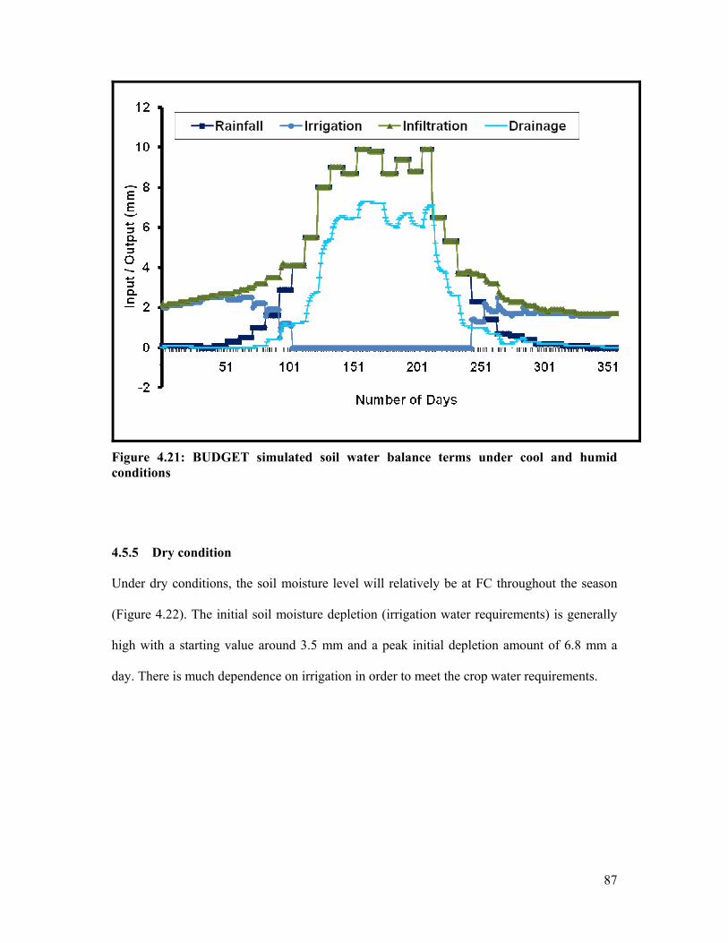
87

Figure 4.21: BUDGET simulated soil water balance terms under cool and humid conditions

4.5.5 Dry condition Under dry conditions, the soil moisture level will relatively be at FC throughout the season

(Figure 4.22). The initial soil moisture depletion (irrigation water requirements) is generally

high with a starting value around 3.5 mm and a peak initial depletion amount of 6.8 mm a

day. There is much dependence on irrigation in order to meet the crop water requirements.

88

Figure 4.22: BUDGET simulated initial and final soil moisture depletion under dry conditions

Figure 4.23: BUDGET simulated soil moisture movement into and out of the root zone under dry conditions.

89

There are generally very low values of water movement out of the root zone (< 2 mm) at peak

and as a result, drainage losses are very low during dry conditions (Figure 4.23). For the

major part of the season (the first 10 decades and the last 11 decades), there is no water flow

out of the root zone. Soil moisture input to the root zone is relatively high with values above

5 mm a day for most of the season.

Figure 4.24: BUDGET simulated soil water balance terms under dry conditions

The soil water balance of the irrigation guidelines under dry conditions is outlined in Figure

4.24. The rainfall input into the water balance is low throughout the season with a maximum

value of approximately 5 mm a day. Although the rainfall season seems to be long, the

resultant rainfall amounts are low. High irrigation levels are anticipated throughout the

season. Irrigation will still be required even during the rain season. Infiltration levels are

90

moderate and even close to that under normal conditions. Drainage losses are also very low

(< 2 mm a day) during peak values.

4.5.6 Irrigation calendars

Irrigation calendars were produced for a citrus growing season beginning during the first

decade of August. A fixed irrigation interval of one day was used. This was done for

operational purposes. An irrigation interval of more than one day results in longer irrigation

duration and this is usually not practical. Depending on the drip line specifications, the

irrigation duration may be very long and usually disrupted by power cuts. With shorter

irrigation duration, irrigation can be timed to periods where there will be uninterrupted power

supplies.

Irrigation amounts shown in the calendars were based on a depth criterion of back to FC. The

initial soil water content was assumed to be at FC. The irrigation calendar for the whole

season was divided into three segments (Figures 4.25, 4.26 and 4.27) for the first trimester,

second trimester and third trimester respectively. The calendars show irrigation depth instead

of duration because of the differences in the design of drip lines. Irrigation duration is

affected by the drip line emitter discharge and emitter spacing. The determination of

irrigation duration for specific emitter discharge and spacing is shown in Appendix 3.

91

Month

August

September

October

November

Decade (10 days) 1 2 3 1 2 3 1 2 3 1 2 3

Hot and dry

3.8 mm

4.4 mm

4.9 mm

5.2 mm

4.6 mm

Dry Dry

3.7 mm

4.2 mm

5.0 mm

4.4 mm

3.6 mm

3.0 mm

2.3 mm

Normal

3.0 mm

3.5 mm

3.8 mm

3.2 mm

2.4 mm

1.9 mm

1.2 mm

Humid

2.2 mm

2.6 mm

2.2 mm

1.2 mm

Growing stage

1 Bud break, Shoot elongation, Flowering, Fruit set begins

2 Flowering, Fruit set, Fruit growth (cell division)

Sensitivity to water stress

Very sensitive

Very sensitive

Irrigation interval is 1 day

Figure 4.25: Irrigation calendar for the first trimester of citrus production. 1 and 2 are the initial and crop development stages respectively

A

ctua

l wea

ther

con

ditio

n

92

Month

December

January

February

March

Decade (10 days) 1 2 3 1 2 3 1 2 3 1 2 3

Hot and dry

4.2 mm

3.6 mm

4.6 mm

Dry Dry

1.8 mm

1.0 mm

1.8 mm

1.2 mm

3.0 mm

Normal

1.5 mm

2.0 mm

Humid

Growing stage

2 Fruit let drop (Fruit set), cell expansion

3 Cell expansion

Sensitivity to water stress

Very sensitive

Moderate sensitivity

Irrigation interval is 1 day

Figure 4.26: Irrigation calendar for the second trimester of citrus production. 2 and 3 refers to the crop development and mid season stages respectively.

A

ctua

l wea

ther

con

ditio

n

93

Month

April

May

June

July

Decade (10 days) 1 2 3 1 2 3 1 2 3 1 2 3

Hot and dry

4.0 mm

3.5 mm

3.0 mm

Dry Dry

3.5 mm

3.0 mm

Normal

3.0 mm

2.5 mm

Humid

1.4 mm

2.0 mm

Growing stage

3

Maturation

4

Maturation

Sensitivity to water stress

Moderate sensitivity

Moderate sensitivity

Irrigation interval is 1 day

Figure 4.27: Irrigation calendar for the last trimester of citrus production. 3 and 4 refers to the mid season and the late season stages respectively.

4.5.7 Grower’s practice soil water status The grower’s irrigation depths throughout the season were input into the model (BUDGET)

and the projected soil moisture status is given in Figures 4.28, 4.29 and 4.30

A

ctua

l wea

ther

con

ditio

n

94

Figure 4.28: BUDGET simulated initial and final soil moisture depletion under normal conditions considering the grower’s irrigation scheduling practices.

The grower’s scheduling practices is a reflection of soil moisture conditions that are usually

above the FC (Figure 4.28) since the final depletion is usually greater than zero. Final

depletion amounts of high as 55 mm day-1 show that a lot of water is being added into the

soil. The level of irrigation is high and is compatible with a 2 day or 3 day irrigation interval.

The margin between the initial and the final depletion is very low indicating that more water

is being applied than the water requirements of the trees. It is assumed that the grower’s

guidelines were developed under very extreme weather conditions and non limiting irrigation

water conditions.

95

Figure 4.29: BUDGET simulated soil moisture movement in and out of the root zone under normal conditions considering the grower’s irrigation scheduling practices.

This irrigation scheduling practice is not economic and adds no value in terms of fruit yield

and quality. Excess application of water can have negative impacts on the quality and yield of

the fruit. There are operational constraints mainly due to the need for high water use

efficiency especially during these periods of increased pressure on water resources. Weather

varies from season to season and even from day to day and hence there is need to have

irrigation guidelines that take into account the water requirements under specific weather

conditions. A water deficit condition is predicted for almost 3 decades from day 220 (Figure

4.28).

96

Figure 4.30: BUDGET simulated soil water balance terms under normal conditions considering the grower’s irrigation scheduling practices.

There are generally very high soil water flows out of the root zone with a peak of about 10

mm a day (Figure 4.29). The high drainage losses of as high as 14 mm a day are as a result of

the excessive application of irrigation water (Figure 4.30). These losses can be very high

under cool and humid conditions. This type of scheduling is short coming because there are

even drainage losses when it is not raining. From day 240 to day 270, the irrigation level is

appropriate since there are no drainage losses.

97

4.6 Comparison of the irrigation guidelines with the grower’s practice

The comparison of the soil water status was done under normal weather conditions only and

this serves as a guideline for all weather conditions. After receiving the same total rainfall

amount of 926.6 mm, the projected drainage losses, water deficiency and irrigation

requirements are outlined in Table 4.4. The grower’s practice total irrigation amount is too

much and approximately only a third (of 2322 mm) is required for the whole season. The

application of excess water is the major cause of the high drainage losses beyond the root

zone under the grower’s practice. The drainage losses could be reduced if the irrigation

guidelines are implemented.

Table 4.4: Irrigation requirements, drainage losses and water deficiency under normal conditions for irrigation scheduling guidelines and grower’s practice.

Total Rainfall

Total Irrigation

Total Drainage Losses

Drainage loss duration

Total water deficiency

Water Deficiency duration

Scheduling Method

(mm) (mm) (mm) (days) (mm) (days) Guideline 926.6 709.5 381 150 - - Grower’s practice

926.6 2322 1963.9 290 275.1 49*

* From first decade of March to second decade of April.

These high drainage losses cause the leaching of plant nutrients and consequently affect fruit

yield and quality. There are however, drainage losses of 381 mm under the irrigation

scheduling guidelines. These losses are experienced during the rain season where there is

uncontrolled input of water into the soil system. With proper scheduling, about 1582.9 mm

would have been saved. The drainage losses can be even higher under cool and humid

conditions. For nearly 290 days, there will be drainage losses considering the grower’s

scheduling practices compared to almost 150 days considering the irrigation scheduling

guidelines. Water deficiency of about 275 mm is experienced from the first decade of March

98

to the second decade of April. This deficiency coincides with the cell expansion to maturation

stages that are moderately sensitive to water stress and hence does not affect yield and

growth. It is actually a form of regulated deficit irrigation. Under hot and dry and dry

conditions, this deficiency can lead to reduction in fruit quality and yield.

4.7 The effect of irrigation strategies The irrigation strategies under consideration were the well waterd, control, grower’s practice

and PRD 50 %. The assessment period was from October 2009 to December 2009. Irrigation

strategies were compared in terms of fruit diameter growth rate and fruit abscission against

the irrigation water used.

Table 4.5: Total irrigation water received per treatment per hectare from October 2009 to December 2009.

Treatment Total water received (ML/Ha) Control 2.6 Well – watered (Both sides of the tree irrigated, each line delivering half the quantity of water as the control).

2.6

Grower’s practice 3.06 PRD: 2 drip lines applying half of control 1.3

4.7.1 Effects of irrigation treatments on yield variable

There were no significant differences (p < 0.05) between the fruit growth rates among all the

treatments (Table 4.6). The control treatment however, exhibited the highest fruit diameter

compared to other treatments (Figure 4.31). This may be linked to the fact that the trees

required adequate water especially during the critical phases of flowering and fruit set. The

trees were irrigated according to the evaporative demand of the atmosphere. The fruit

diameter growth rates are shown in Fig. 4.31. The well watered treatment; the grower’s

practice and PRD 50 % do not show much difference in fruit diameters. The well-watered

99

treatment did not perform well may be because of restricted irrigation depth. Although both

sides of the tree row were irrigated, the halved irrigation duration resulted in some water

deficiency that restricted fruit growth. The PRD treatment supplying half the amount of water

as the control also had reduced fruit growth rate. This may be due to water deficiency

especially during the critical stages of fruit development.

The PRD method however, has potential in balancing fruit yield and water conservation if the

PRD is correctly timed. An improved growth rate may have been realised if PRD was

initiated after the flowering and the fruit set stages. At exactly half the amount of water

applied as the control and well watered treatment and almost 42 % of the grower’s practice

(Table 4.5), the PRD performed even slightly better than the well watered and the grower’s

practice. Although the grower’s practice used about 15 % more water (Table 4.5) as the

control, this did not have any advantage towards fruit growth during this period. This may

have been due to limited aeration (soil moisture condition usually above FC) thereby

affecting root respiration and subsequent growth and development.

Table 4.6: The effect of irrigation treatments on fruit growth rate.

Treatment Mean Fruit diameter (cm) Control 5.571a

Well watered 5.146a

Grower’s practice 5.140a

PRD 50 % 5.228a

The fruit growth rates were not significantly different from the control at p (≤0.05)

100

3

3.5

4

4.5

5

5.5

6

6.5

12/1

7/20

09

12/2

7/20

09

1/6/

2010

1/16

/201

0

1/26

/201

0

2/5/

2010

Frui

t dia

met

er (c

m)

Date

control well-watered grower's practice PRD (half of control)

Figure 4.31: Fruit growth rates of the control, well – watered, grower’s practice and PRD applying half of the control from 16 December 2009 to 03 February 2010.

4.7.2 Fruit drop

The fruit drop was generally low for all the treatments with a highest value of 10 % (Figure

4.32) although the grower’s practice and well watered had higher fruit drops. The well

watered treatment, with half the amount of water as the control applied on both sides of the

tree (although the total amount was the same), might have induced a form of stress that

resulted in the doubling of fruit drop. Despite the fact that the grower’s irrigation scheduling

practise was over irrigating, the fruit drop is higher than the control. The PRD 50 treatment

101

had the same fruit drop as the control. It is assumed that the PRD 50 treatment had adjusted

to the water deficit condition through the root to shoot chemical signals and has proved to be

a better method of deficit irrigation than the application of reduced amount of water on both

sides of the tree.

Figure 4.32: Treatment effects on fruit abscission monitored from the first decade of December to the first decade of January at MCE.

4.8 Summary The outcomes of the experiments described in chapter 3 are presented in this chapter. The

k pan was found to range between 0.72 and 0.82 and that it changes throughout the season.

The Kc curve for the entire season of citrus production was produced as well as the Kc values

per decade. Whole day transpiration rates were given for two days and were found to match

102

to the irrigation depth recommended (irrigation calendar) for that period. The soil water status

of the developed irrigation calendars was projected for the actual weather condition of the

day. The soil water status was presented in terms of the soil moisture depletion, movement of

water in and out of the root zone and the soil water balance. Irrigation calendars of the whole

season for a fixed irrigation interval of 1 day were presented in terms of the actual irrigation

depth the corresponding weather condition of the day. A comparison of the total irrigation

water required under the grower’s scheduling practice and that required using irrigation

guidelines was done. The effect of the different irrigation strategies on fruit growth rate and

abscission concludes the contents of chapter 4.

103

CHAPTER 5 CONCLUSIONS AND RECOMMENDATIONS

5.0 CONCLUSIONS

The FAO Penman Monteith ETo for the study site was between 4 and 4.5 mm day-1 from

January to April. From May to early August, ETo was approximately 3 mm day-1. Peak ETo

values (up to 5.5 mm day-1) were experienced around October. ETo for the study site ranged

between 3 mm day-1 and 5.5 mm day-1.

Zimbabwean citrus farmers without sophisticated equipment and the required expertise are

able to do daily ETo estimations using the class A evaporation pan. More accurate estimations

of ETo using the evaporation pan are possible if site specific pan coefficients are used. It was

observed that a single Kpan value cannot be used throughout the season since it changes

throughout the season. The Kpan for the study site was found to be highest in January and

lowest in October i.e. 0.82 and 0.72 respectively.

The main factors controlling the Kpan values are the fetch condition, the mean wind speed at

2 m height and the mean relative humidity. Kpan values follow almost the same trend as the

mean RH. Kpan can also be successfully estimated from a plot of the FAO Penman Monteith

ETo against pan evaporation. This method can be applied for sites without or with unreliable

RH and wind speed data.

The local Kc ini for citrus is low (0.47) during the initial stage (spring) where there is shoot

initiation. During the crop development stage, Kc rises rapidly and changes every decade

because of the higher demand for water for flowering and fruit set. Kc changes during this

stage should be noted to avoid inaccurate estimations of ETc. Peak Kc values (0.84) occur

during the mid season stage. Kc values after the mid season stage decrease gradually as

reflected by a Kc end value of 0.76.

104

The irrigation depth varies significantly during each day after considering the actual weather

condition. It is essential to take into account the actual weather condition for a particular day

for efficient irrigation scheduling. A variation in irrigation depth of up to 3 mm day-1 is

possible if the actual weather condition is not taken into consideration. This results in both

unregulated water deficit and over irrigation. Both scenarios are not desirable for citrus

production. The seasonal or monthly irrigation scheduling guidelines (blanket

recommendations) should therefore be replaced by the developed irrigation calendars. During

the rain season, irrigation can only be terminated under normal and humid conditions alone.

During the dry condition, irrigation depth can only be reduced during the rain season. If the

weather is hot and dry, irrigation is required throughout the season even during the rainfall

season.

The grower’s irrigation scheduling practices usually resulted in soil moisture conditions

above the FC. The irrigation depths are not compatible with a 1 day irrigation interval.

Almost a third of the current irrigation depth is required under normal weather conditions.

The excessive application of water results in high drainage losses. Irrigation depth was

reduced after considering the developed irrigation calendars.

There were no significant differences (p < 0.05) in the fruit growth rates of the well watered,

control, PRD 50 and the grower’s practice. The only difference was in the fruit sizes where

the control produced the largest fruit diameters. The conventional irrigation scheduling was

the better method compared to the other methods under consideration. The PRD 50 method

showed great potential at balancing water use and fruit size. PRD was done during the

flowering and fruit set stage and if it was well timed (linked to the less critical growth stages),

it could have been better than the control. PRD could have done better may be at PRD 75 /

80. Applying water to both sides of the tree (well watered) was not beneficial especially when

105

the irrigation depths are low. Halving the irrigation duration resulted in low irrigation depths

and the fact that both sides were irrigated did not offer any advantage at all. Increasing the

irrigation duration on both sides may lead to the use of more irrigation water and this is not

sustainable. The grower’s irrigation scheduling practice of applying excess water was not

beneficial to the fruit as the fruit diameters were even less than those of the control.

5.1 RECOMMENDATIONS FOR FURTHER STUDIES

Although the modelled soil moisture status using the developed irrigation calendars gave a

forecast of the soil water movement and balance, future research may look into the soil water

dynamics of the citrus trees using the irrigation calendars. Substantial amount of water was

projected to be lost through drainage especially during the rain season and the loss is even

more under humid conditions. Devising ways by which the excess water received through

rainfall can be harvested in the orchards may be beneficial.

Future research may also be aimed at assessing the feasibility of the installation of sub

surface drainage systems to enable the harnessing of the drained water for reuse during

periods of need. More research should be linked to the use of PRD as a drip irrigation

strategy. The research should look at the best timing of the PRD as well as the right deficit

level for the growth stages of the citrus crop. Since the daily water requirements of citrus is

linked to the actual weather condition of a particular day, future research can assess the

possibility of automating irrigation of citrus using sap flow.

106

REFERENCES Aguila, A. and Garcia, N.H., 1996. NEC – HID Irrigation scheduling: Evapotranspiration and irrigation scheduling, Proceedings of the International conference, November 3 – 6, San Antonio, Texas. Allen, R.G., Pereira, L.S., Raes, D. and Smith, M., 1998. Crop evapotranspiration: Guidelines for computing crop water requirements, FAO Irrigation and Drainage paper No. 56, FAO, Rome, Italy Assouline, S., Moller, M., Cohen, S., Ben-Hur, M., Grava, A., Narkis, K. and Silber, A., 2006. Soil – Plant system response to pulsed drip irrigation and salinity: Bell pepper case study, Soil science society of America journal 70:1556-1568. Baker, J.M. and van Bavel, C.H.M., 1987. Measurement of mass flow of water in stems of herbaceous plants. Plant, cell and environment 10, 777 – 782. Baker, J.M. and Nieber, J.L., 1989. An analysis of the steady state heat balance method of measuring sap flow in plants. Agriculture and Forestry Meteorology 48, 93 – 109. Chalmers, D.J., Mitchell, P.D. and Vanhek, L., 1981. Control of peach tree growth and productivity by regulated water supply, tree density and summer pruning. Journal of American Society for Horticultural science 106, 307 – 312. Chalmers, Y.M., Kelly, G. and Krstic, M.P., 2004. Partial Root zone Drying of Vitis vinifera cv. ‘Shiraz’ wine grapes in a semi arid climate, IVth International Symposium on Irrigation of Hort. Crops, Acta Hort, 664: 133 – 138. Cohen, Y., Moreshet, S. and Fuchs, M., 1985. Change in transpiration rate of mature citrus trees in response to reduction of wetted soil volume. Acta Horticulturae 171, 45 – 49. De Jager, J.M. and Kennedy, J.A., 1996. Weather – based irrigation scheduling for various farms (commercial and small scale) In: Irrigation scheduling: From theory to practice, Proceedings ICID/FAO Workshop, Sept 1995, Rome. Water report No. 8, FAO, Rome Doorenbos, J. and Pruitt, W. O., 1977. Crop water requirements. Irrigation and Drainage Paper No. 24, (rev.) FAO, Rome, Italy. 144 p. Doorenbos, J. and Kassam, A.H., 1979. Yield response to water. FAO Irrig. and Drain. Paper No. 33, FAO, Rome, Italy. 193 pp. Dry, P., Loveys, B., Botting, D. and During, H., 1996. Effects of partial root zone drying on grapevine vigour, yield, composition of fruit and use of water. Proceedings of the Australian wine Industry Technical Conference 9, 129 – 131. Dry, P.R., and Loveys, B.R., 1999. Grape vine shoot growth and stomatal conductance are reduced when part of the root system is dried. Vitis 38: 151 – 156. During, H., Dry, P.R. and Loveys, B.R., 1996. Root signals affect water use efficiency and shoot growth. Acta Hort. 427: pp 1 – 13.

107

Dynamax, Inc., 1997. A Thermal Dissipation Sap Velocity Probe for measurement of sap flow in plants, Houston, USA Dzikiti, S., Steppe, K., Lemeur, R. and Milford, J.R., 2006. Water use by young navel orange trees (Citrus sinensis(L.) Osbeck) in Zimbabwe. Acta Horticulturae 707, 135 – 141. Dzikiti, S., 2007. Stomatal oscillations and the response of citrus trees to different irrigation strategies in northern Zimbabwe. PhD thesis, Ghent University, Ghent, pp 111 - 195. Dzikiti, S., Steppe, K. and Lemeur, R., 2008. Partial root zone drying of drip irrigated ‘Navel’ orange trees [Citrus sinensis (L.) Osbeck] under semi arid tropical conditions. Acta Horticulturae 792, 249 – 256. FAO., 2002a. Agriculture, food and water – a contribution to the world water development report, Rome, Italy FAO., 2002b. Crop water management – Citrus, FAO Land and water development division, Rome Italy, http://www.fao.org/landandwater/aglw/cropwater/citrus.stm Garcı´a-Orellana, Y., Ruiz-Sa´ nchez, M.C., Alarco´n, J.J., Conejero, W., Ortun˜ o M.F., Nicola´ s, E. and Torrecillas, A., 2007. Preliminary assessment of the feasibility of using maximum daily trunk shrinkage for irrigation scheduling in lemon trees, Agricultural water management 89: 167 – 171 Gat, Z., Erner, Y. and Goldschmidt, E.E., 1997. The effect of temperature on the citrus crop, World Meteorological Organisation, Technical note number 198, Geneva, Switzerland. Geerts, S. and Raes, D., 2009. Deficit irrigation as an on farm strategy to maximise crop water productivity in dry areas, Agriculture Water Management, Vol 96, Issue 9, pp 1275-1284 Goldhamer, D.A., Fereres, E., 2001. Irrigation scheduling protocols using continuously recorded trunk diameter measurements. Irrig. Sci. 20, 115–125. Granier, A., 1987. Evaluation of transpiration in a Douglas fir stand by means of sap flow measurements. Tree Physiology, 3:309-320 Grieser, J., 2006. New LocClim 1.10, Local climate estimator, FAO, Rome, Italy. Gurovich, L.A., 1996. Irrigation scheduling of table grape vine cultivars in Chile. Proceedings of the International conference on evapotranspiration and irrigation scheduling, November 3 – 6 1996, San Antonio, Texas. Harris, G., 2006. Irrigation – Water balance scheduling, Department of primary Industries and fisheries, Queensland government. Huguet J.G., 1985. Appreciation of the hydrous state of a plant through consultation

108

of the micrometric variations of the size of fruit or stems during the day. Agronomie, 5: 733-741. Hussein, J., 1982. An investigation into methods of flood irrigation of orange trees. Zimbabwe Agricultural Journal 79, 73 – 79. Huygen, J., Van den Broek, B.J. and Kabat, P., 1995. Hydra Model Trigger, A soil water balance and crop growth simulation system for irrigation water management purposes. Paper submitted to ICID/FAO Workshop, September 1995, Rome. Irrigation scheduling: From theory to practice, FAO, Rome, Italy Itier, B., Maraux, F., Ruelle, P. and Deumier, J.M., 1996. Applicability and limitations of irrigation scheduling methods and techniques, Irrigation scheduling: From theory to practice, FAO Corporate document repository, FAO, Rome, Italy Jensen, M.J., 1981. Summary and challenges. In Fereres. (1996). Irrigation Scheduling and its impact on the 21st century. Proceedings of the International conference on evapotranspiration and irrigation scheduling, November 3 – 6 1996, San Antonio, Texas Lascano, R.J., Baumherdt, R.L., Hicks, S.K., Evett, S.R. and Heilman, J.L., 1996. Daily measurement and calculation of crop water use. Proceedings of the International conference on evapotranspiration and irrigation scheduling, November 3 – 6 1996, San Antonio, Texas Lee, T.S., Najim, M.M.M. and Aminul, M.H., 2004. Estimating evapotranspiration of irrigated rice at the West coast of the Peninsular of Malaysia, Jour. Of Applied Irrigation Science, Vol. 39, No. 1/2004, pp. 103-117. Lenntech., 2003. Use of water in food and agriculture, http://www.lenntech.com/water-food-agriculture.htm Li S.H., Huguet J.G. and Bussi C., 1989. Irrigation Scheduling in a mature peach orchard using tensiometers and dendrometers. Irrigation and Drainage Systems. 3: 1-12. Lovatt, C.J. and Faber, B.A., undated. Reducing water use in navel orange production with partial root zone drying, Center for water resources, University of California Medhurst, J.L. and Beadle, C.L., 2002. Sapwood hydraulic conductivity and leaf area sapwood area relationships following thinning of a Eucalyptus nitens plantations. Plant Cell and Environment 25, 1011-1019. Ministry of Agriculture, Food and Fisheries., 2004. Water conservation fact sheet: Trickle irrigation scheduling using evapotranspiration data, Agdex 561, British Columbia. Ministry of Foreign Affairs., 2009. Zimbabwe in brief, Agriculture, http://www.idc.co.zw Nakamura, K., Aoki, M., Machimura, T., Hideshima, Y. and Wada, M., 1996. Forecast of evapotranspiration by meteorologic information: Evapotranspiration and irrigation scheduling, Proceedings of the International conference, November 3 – 6, San Antonio, Texas

109

Natural Resources Management and Environment Department., undated. Water harvesting, FAO Corporate document repository, http://www.fao.org/docrep/u3160c/u3160e04.htm Nortes, P.A., Perez-Pastor, A., Egea, G., Conejero, W. and Domingo, R., 2005. Comparison of changes in stem diameter and water potential values for detecting water stress in young almond trees, Agriculture Water Management 77: 296-307. O’ Connell, M.G. and Goodwin, I., 2004. Pear water relations under Partial Root zone Drying, IVth International Symposium on irrigation of Hort. Crops, Acta Hort. 664 pp 453 – 459. Penman, H.L., 1948. Natural evaporation from open water, bare soil and grass. Proc. R. Soc. Land. Ser. A. 193; 120-145.

Pruitt, W.O., 1986. "Traditional methods 'Evapotranspiration research priorities for the next decade'." ASAE Paper No. 86-2629. 23 p. Raes, D., Lemmens, H., Van Aelst, P., Vanden Bulcke, M. and Smith, M., 1988. IRSIS – Irrigation scheduling information system. Volume 1. Manual. K.U.Leuven, Dep. Land Management, Reference Manual 3. 199 p. Raes, D., 2001. Water balance of a cropped soil, K.U. Leuven, Department of land management, Leuven, Belgium. Raes, D., 2005. Budget: Reference manual, Department of Land Mnagement, K.U. Leuven University, Leuven, Belgium. Raes, D., 2007. Reference evapotranspiration calculator, Reference manual, Version 2.3, K.U. Leuven, Belgium. Ramsey, H., 2007. Citrus irrigation, Farm note 275, Department of food and agriculture, Government of Western Australia Sakuratani T., 1981. A heat balance method for measuring flux in stem of intact plants. J. Agric. Met. (Japan), 37:9-17. Sithole, P., 2005. An evaluation of the effect of canopy microclimate and architecture on the growth and quality of navel orange fruits (Citrus sinensis (L) Osbeck) in Zimbabwe, M Sc thesis, University of Zimbabwe, Zimbabwe. Smith, M., 1985. Irrigation scheduling and water distribution. Proceedings of ‘Les besoins en Eau des Cultures’. Conférence Internationale INRA – ICID. Paris, France: 497-510. Smith, M., 1990. CROPWAT- a computer program for irrigation planning and management. FAO Irrigation and Drainage Paper N° 46. FAO, Rome, Italy. 126 p.

110

Smith, M., Allen, R. and Pereira, L., 1996. Revised FAO methodology for crop water requirements, Proceedings of the International conference, November 3 – 6, San Antonio, Texas. Snyder, R.L., Lanini, B.J., Shaw, D.A., and Pruitt, W.O., 1989. Using reference evapotranspiration (ETo) and crop coefficients to estimate crop evapotranspiration (ETc) for trees and vines. Cooperative Extension, Univ. California, Berkeley, CA, Leaflet No. 21428, 8 p. Steinberg S.L., van Bavel C.H.M. and McFarland M.J., 1989. A gauge to measure mass flow in stems and trunks of woody plants. J. Am. Soc. Hort. Sci. 114: 466- 472. Taylor, K.C. and Rieger, M., Undated. Irrigation for peaches – Irrigation scheduling, University of Georgia, Antens. Ton, Y. and Kopyt, M., 2003. Phytomonitoring in Irrigation Scheduling of Horticulture Crops: Proceedings of the 4-th International Symposium on Irrigation of Horticultural Crops. September 1-6, 2003. Davis, California, USA. Van Bavel, C.H.M., Van Bavel, M.G. and Lascano, R.J., 1996. Automatic irrigation based on monitoring plant transpiration, Proceedings of the International conference, November 3 – 6, San Antonio, Texas. Van Bavel, M.G., 1999. DynagageTM installation and operation manual, Dynamax Inc Vermeulen, K., Steppe, K., Linh, N.S. and Lemeur, R., 2007. Simultaneous response of stem diameter, sap flow rate and leaf temperature of tomato plants to drought stress, Proceedings of the International Society on Greenhouse systems, Acta, Hort. 801: 1259-1266. Vincent, V. and Thomas, R.G., 1960. An agricultural survey of Southern Rhodesia, Part 1: Agro-ecological survey. Government Printers, Salisbury. Wright J.L., 1981. Crop coefficients for estimates of daily crop evapotranspiration. Irrig. Scheduling for Water and Energy Conservation in the 80s, ASAE, Dec. 1981.

111

APPENDICES APPENDIX 1: Day of the year (Julian days) calendar Month Day

Jan

Feb

Mar

Apr

May

Jun

Jul

Aug

Sep

Oct

Nov

Dec

1 1 32 60 91 121 152 182 213 244 274 305 335 2 2 33 61 92 122 153 183 214 245 275 306 336 3 3 34 62 93 123 154 184 215 246 276 307 337 4 4 35 63 94 124 155 185 216 247 277 308 338 5 5 36 64 95 125 156 186 217 248 278 309 339 6 6 37 65 96 126 157 187 218 249 279 310 340 7 7 38 66 97 127 158 188 219 250 280 311 341 8 8 39 67 98 128 159 189 220 251 281 312 342 9 9 40 68 99 129 160 190 221 252 282 313 343 10 10 41 69 100 130 161 191 222 253 283 314 344 11 11 42 70 101 131 162 192 223 254 284 315 345 12 12 43 71 102 132 163 193 224 255 285 316 346 13 13 44 72 103 133 164 194 225 256 286 317 347 14 14 45 73 104 134 165 195 226 257 287 318 348 15 15 46 74 105 135 166 196 227 258 288 319 349 16 16 47 75 106 136 167 197 228 259 289 320 350 17 17 48 76 107 137 168 198 229 260 290 321 351 18 18 49 77 108 138 169 199 230 261 291 322 352 19 19 50 78 109 139 170 200 231 262 292 323 353 20 20 51 79 110 140 171 201 232 263 293 324 354 21 21 52 80 111 141 172 202 233 264 294 325 355 22 22 53 81 112 142 173 203 234 265 295 326 356 23 23 54 82 113 143 174 204 235 266 296 327 357 24 24 55 83 114 144 175 205 236 267 297 328 358 25 25 56 84 115 145 176 206 237 268 298 329 359 26 26 57 85 116 146 177 207 238 269 299 330 360 27 27 58 86 117 147 178 208 239 270 300 331 361 28 28 59 87 118 148 179 209 240 271 301 332 362 29 29 88 119 149 180 210 241 272 302 333 363 30 30 89 120 150 181 211 242 273 303 334 364 31 31 90 151 212 243 304 365 Add 1 to unshaded values during leap years

112

APPENDIX 2: Determination of K pan using RH mean, U2 and FET Month

RHmean U2 mean

ln (RH mean)

FET

ln (FET)

ln (86.4U2) Kpan Kpan

(%)

m/s m

dry fetch

green fetch

January 89.02 1.0809 4.48882366 15 2.708 4.536782 0.7839 0.8142

February 81.5 1.07243 4.40056216 15 2.708 4.528918 0.7599 0.8022March 84.07 1.0076 4.43164979 15 2.708 4.466559 0.7711 0.8084April 76.7 0.8875 4.33990171 15 2.708 4.339641 0.7526 0.7991May 75.2 0.8746 4.32008474 15 2.708 4.324999 0.7482 0.7967June 70.5 1.15173 4.25565994 15 2.708 4.600255 0.7211 0.7799July 65.56 1.1603 4.18296575 15 2.708 4.607666 0.7049 0.7695August 62.66 1.22567 4.13767014 15 2.708 4.662473 0.6930 0.7614September 53.05 1.47637 3.97129763 15 2.708 4.848572 0.6536 0.7311October 52.67 1.61927 3.9640935 15 2.708 4.940961 0.6477 0.7260November 68.11 1.4632 4.22112405 15 2.708 4.839613 0.7018 0.7662December 83.12 1.0853 4.42028535 15 2.708 4.540844 0.7646 0.8046 RH mean is the mean monthly relative humidity (%), FET is the fetch (m) and U2 is the mean monthly wind speed at 2 m height.

113

APPENDIX 3: Determination of the irrigation duration from October to December 2009

The duration of irrigation events at the experimental site was calculated using orchard

characteristics, drip line specifications and the evaporative demand of the atmosphere. Tree

spacing in the orchard is approximately 2.75 m in each row, with an inter-row spacing of

approximately 6 m. The trees were surface drip irrigated using standard 15 mm

polypropylene dripper lines with pressure compensated button emitters delivering water at a

rate of 1.7 L/h. The emitter spacing along the line is 0.3 m. The irrigation depth for October

was calculated using potential evapotranspiration, ETo data of the same site from past studies.

A daily average ETo value of 5.5 mm for October was used for the determination of irrigation

duration. Since there is a smaller variation in the extend of vegetation cover throughout the

year in citrus because its evergreen (Allen et al., 2004), a constant value for the crop

coefficient, Kc was used. For citrus, an assumed Kc value of 0.7 was used (Allen et al., 2004;

Dzikiti, 2007). The mean daily crop evapotranspiration, ETc (irrigation depth), for the month

of October was determined using equation 1.

coc KETET ×= (1)

= 5.5 mm day-1 * 0.7

= 3.85 mm day-1

The irrigation duration for the control was calculated by considering a hypothetical one-

hectare area of the orchard with simplified dimensions of 100m * 100 m. given the fact that

the rate of emission of water by the drippers is 1.7 L/h and if we consider an irrigation event

lasting X hours, then the total volume of water, Vw applied per hectare in litres is

114

nXVw ××= 7.1 (2)

Where n is the total number of emitters per hectare and is given by:

6

1003.0

100×=n (3)

= 5 555.55 emitters

The fraction of the orchard that is irrigated can be estimated by considering the region

between four emitters in neighbouring tree rows. The wetted region around each emitter is

almost elliptical extending approximately 1.0 m along the major axis of the ellipse at right

angles to the drip line and 0.375m along the minor axis parallel to the drip line (Dzikiti,

2007).

The wetted fraction of the soil = 65.03.06

0.1375.0≈

×××π (4)

Irrigation depth 65.010000 ×

= wV (5)

Since the irrigation depth is 3.85 mm day-1, Vw = 25 025 litres. From equation 2, the irrigation

duration, X is

115

n

VX w

×=

7.1 (6)

= 55.55557.1

25025×

3≈ Hours

116

APPENDIX 4: The determination of the Kc curve

Determination of Kc ini for partial wetting of the soil surface During the initial stage, the trees are irrigated using drip system daily with 4.0 mm each application expressed as an equivalent depth over the field area. The average fraction of surface wet is 0.4 and little to no precipitation is expected during the initial period. The average depth of infiltration per event in the wetted fraction of the surface:

===4.0

4mmfIIw

w 10 mm

Therefore, the chart using light wetting events is used for the determination of Kc ini For: and: Kc ini Fig for light events

ETo = 4 mm/day a 1 day wetting interval: Kc ini = 1.1

4 - 1.1

mm/day - -

Contribution of rainfall during the initial period Mean monthly rainfall: fw rain

August September First decade of October Initial period

3 4 5 12

mm mm mm mm

fw rain + fw irrigation Wetted fraction (irrigation) Wetted fraction (rainfall) Mean wetted fraction, fw

Initial period

=

+

=

2924.0*280

2921*12

292 0.4 1 0.42

mm - - -

Because the fraction of soil surface wetted by irrigation and rainfall is 0.42, the actual Kc ini for the initial period was calculated as: From equation 3.2: === 1.1*42.0* figKfK ciniwcini

The value 0.47 represents the Kc

ini as applied over the entire field area.

0.47 -

Determination of Kc mid under the local wind speed, relative humidity and crop height conditions During the mid season period, the mean wind speed is 1.06 m s-1, the mean minimum relative humidity is 41.62 % and an average tree height of 3 m was observed. From equation 3.3: ( ) ( )[ ] =

−−−+=

3.0

334562.41004.0206.104.070.0cmidK

0.84

-

Kc end = 0.75 (The fruit is harvested as ‘green’) hence no adjustment was made to the table

value. Equation 3.4 was used for the estimation of the daily Kc values during the crop

development and the late season stages.

117

APPENDIX 5: Calculation of the amount of irrigation water used per treatment

The amount of irrigation water used per treatment was computed from October to December.

During the last decade of December, irrigation was stopped because of considerable rainfall.

The total amount of water used for each treatment was calculated using the emitter discharge

rate of the drip lines, irrigation duration and the number of emitters per hectare. For all

treatments, the emitter discharge rate was 1.7 l hr-1 and there were 5555.55 emitters per

hectare. The only variation was on irrigation duration.

Control treatment and well watered treatment

Emitter discharge per day = 1.7 l hr-1 * 3 hr day-1

= 5.1 l day-1

Water received per hectare per day = emitter discharge per day * number of

emitters per hectare

= 5.1 l day-1 * 5555.55

= 28 333.3 l

Total irrigation water received (October to December) = 2 606 663.6 l

= 2.6 Ml / Ha

For the PRD treatment applying half of the control, total water received per hectare is

1.3 Ml / Ha

118

Grower’s practice

Emitter discharge = 2.3 l hr-1

Emitter spacing = 0.75 m

Number of emitters per hectare = 2 222.22

Irrigation duration = 6.5 hrs

Water received per hectare per day = 2.3 l hr-1 *6. 5 hrs * 2 222.22

= 33 222.19 l / Ha

Total irrigation water received (October to December) = 3.06 Ml / Ha

119

APPENDIX 6: Determination of the average leaf area per tree

ROW D1 D2 D3 Mean mean diameter

leaf Area row leaf area

cm cm cm cm (m) (m2) (m2) 3 11 11.4 8.4 10.26667 0.102666667 57.06496 58.61812946 10.6 11 8.8 10.13333 0.101333333 55.30332 11.4 11.6 9.2 10.73333 0.107333333 63.48611 4 11.2 10.4 10.2 10.6 0.106 61.61071 43.98249336 6.5 6.7 6.4 6.533333 0.065333333 19.29736 9.6 9.8 10 9.8 0.098 51.03941 5 11.7 7.9 8.3 9.3 0.093 45.01419 53.49550627 10.8 10 10.3 10.36667 0.103666667 58.40737 10 11.3 9.5 10.26667 0.102666667 57.06496 6 10.7 10.4 10.2 10.43333 0.104333333 59.31244 55.28531811 9.3 9.6 9.45 0.0945 46.77549 10 10.1 11.3 10.46667 0.104666667 59.76802 7 10 10.2 10 10.06667 0.100666667 54.43456 49.94515743 9.1 8.9 9.4 9.133333 0.091333333 43.10326 10.4 9.5 9.8 9.9 0.099 52.29766 8 10.3 10 10.5 10.26667 0.102666667 57.06496 49.05439566 9.4 9 8.9 9.1 0.091 42.72686 10 9.6 8.9 9.5 0.095 47.37137 9 10.9 10.7 10.9 10.83333 0.108333333 64.91422 56.78112014 11.8 10.2 10.8 10.93333 0.109333333 66.36089 9 8.5 8.8 8.766667 0.087666667 39.06824 10 8.4 8.6 9 8.666667 0.086666667 38.00775 46.80962537 8.6 8.1 8.3 8.333333 0.083333333 34.59494 11 10.9 11.2 11.03333 0.110333333 67.82619 11 10.1 9.3 8.9 9.433333 0.094333333 46.57784 50.67596747 9.6 10 10 9.866667 0.098666667 51.87625 10.1 9.7 10.2 10 0.1 53.57381 12 9 8.8 9.1 8.966667 0.089666667 41.24049 33.88140376 8.5 8.1 7.9 8.166667 0.081666667 32.95836 7.4 7.7 7.6 7.566667 0.075666667 27.44536 13 9.2 9.4 9.1 9.233333 0.092333333 44.24401 44.98776342 8.5 8.7 9.5 8.9 0.089 40.50879 10 9.5 9.7 9.733333 0.097333333 50.21049 14 7.3 7.9 7.2 7.466667 0.074666667 26.58331 31.89570686 8.4 7.6 7.8 7.933333 0.079333333 30.74446 8.5 8.6 9 8.7 0.087 38.35936 15 10.4 9.8 10.2 10.13333 0.101333333 55.30332 59.00617001 10.9 11.3 10.7 10.96667 0.109666667 66.84725 10.4 10 9.9 10.1 0.101 54.86794 16 9.4 9.8 10.1 9.766667 0.097666667 50.62396 43.30068833 8.6 8.4 7.9 8.3 0.083 34.26392 9.4 9.6 8.9 9.3 0.093 45.01419 17 9.62 8.91 9.35 9.293333 0.092933333 44.93682 43.01728596 9.6 9.5 8.9 9.333333 0.093333333 45.40218 9.3 8.4 8.5 8.733333 0.087333333 38.71285 18 10.03 9.91 9.82 9.92 0.0992 52.55145 34.91777173 7.14 7.15 7.03 7.106667 0.071066667 23.61178 7.75 8.01 7.33 7.696667 0.076966667 28.59008 Average Leaf Area/ tree = 47 m2

120

APPENDIX 7: Analysis of Variance for fruit growth rates

Treatments

Replications

Treatment Total, xi

Mean −

x 1 4.66 4.55 5.03 4.95 5.58 5.42 6.19 5.91 6.79 6.64 55.71 5.571 2 4.37 4.16 4.64 4.64 5.07 4.96 5.75 5.45 6.31 6.11 51.46 5.146 3 4.35 4.39 4.65 4.57 5.30 4.94 5.55 5.42 6.16 6.07 51.4 5.140 4 4.52 3.89 5.01 4.35 5.48 4.78 6.09 5.29 6.85 6.03 52.28 5.228 x..

=206.85 −

x .. =5.2713

Required F Source of Variation

Degrees of Freedom

Sum of Squares (SS)

Mean Sum of Squares (MS)

Observed F 5 % 1%

Total 39 65.1681 Treatments 3 43.02 14.34 23.309 2.87 4.38 Error 36 22.1481 0.6152 LSD 0.712

121

APPENDIX 8: Data logger program for the SHB sap flow gauge ;{ CR23X} ; *Table 1 Program 01: 10 Execution Interval (seconds) 1: Panel Temperature (P17) 1: 1 Loc [ IntTemp ] 2: Batt Voltage (P10) 1: 2 Loc [ BattVot ] 3: Volt (SE) (P1) 1: 1 Reps 2: 35 5000 mV, 50 Hz Reject, Fast Range 3: 1 SE Channel 4: 3 Loc [ Vin ] 5: 0.004 Mult 6: 0.0 Offset 4: Volt (SE) (P1) 1: 3 Reps 2: 35 5000 mV, 50 Hz Reject, Fast Range 3: 2 SE Channel 4: 4 Loc [ AH ] 5: 1 Mult 6: 0.0 Offset 5: Volt (Diff) (P2) 1: 2 Reps 2: 21 10 mV, 60 Hz Reject, Slow Range 3: 3 DIFF Channel 4: 7 Loc [ dV_1 ] 5: 1.0 Mult 6: 0.0 Offset 6: Beginning of Loop (P87) 1: 0 Delay 2: 2 Loop Count 7: Step Loop Index (P90) 1: 1 Step 8: Z=X*F (P37) 1: 7 X Loc [ dV_1 ] 2: 25 F 3: 9 Z Loc [ dT ] 9: End (P95)

122

10: Volt (Diff) (P2) 1: 1 Reps 2: 35 5000 mV, 50 Hz Reject, Fast Range 3: 4 DIFF Channel 4: 10 Loc [ SWC_25 ] 5: 0.050 Mult 6: -5.0 Offset 11: Volt (Diff) (P2) 1: 1 Reps 2: 35 5000 mV, 50 Hz Reject, Fast Range 3: 5 DIFF Channel 4: 11 Loc [ SWC_75 ] 5: 0.050 Mult 6: -5.0 Offset 12: If time is (P92) 1: 0 Minutes (Seconds --) into a 2: 30 Interval (same units as above) 3: 10 Set Output Flag High (Flag 0) 13: Real Time (P77) 1: 110 Day,Hour/Minute (midnight = 0000) 14: Average (P71) 1: 11 Reps 2: 1 Loc [ IntTemp ] 15: Sample (P70) 1: 11 Reps 2: 1 Loc [ IntTemp ] 16: Maximum (P73) 1: 3 Reps 2: 10 Value with Hr-Min 3: 7 Loc [ dV_1 ] *Table 2 Program 02: 0.0000 Execution Interval (seconds) *Table 3 Subroutines End Program -Input Locations- 1 IntTemp 1 2 1 2 BattVot 1 2 1 3 Vin 1 2 1 4 AH 5 2 1

123

5 BH 9 2 1 6 CH 17 2 1 7 dV_1 5 4 1 8 dV_2 17 3 1 9 dT 1 3 1 10 SWC_25 1 2 1 11 SWC_75 1 2 1 12 _________ 0 0 0 13 _________ 0 0 0 14 _________ 0 0 0 15 _________ 0 0 0 16 _________ 0 0 0 17 _________ 0 0 0 18 _________ 0 0 0 19 _________ 0 0 0 20 _________ 0 0 0 21 _________ 0 0 0 22 _________ 0 0 0 23 _________ 0 0 0 24 _________ 0 0 0 25 _________ 0 0 0 26 _________ 0 0 0 27 _________ 0 0 0 28 _________ 0 0 0 -Program Security- 0000 0000 0000 -Mode 4- -Final Storage Area 2- 0 -CR10X ID- 0 -CR10X Power Up- 3 -CR10X Compile Setting- 3 -CR10X RS-232 Setting- -1