Development of Drum-Buffer-Rope scheduling software to

support a “What If” approach to scheduling job shops

Presented by:

C. J. de Jager (13123009)

B.Eng (Electric and Electronic), University of Stellenbosch

Thesis presented in partial fulfilment of the requirements for the degree of Master of Science in

Industrial Engineering at the University of Stellenbosch

Study leaders:

Mr. K.J. Bartel

Mr. K von Leipzig

April 2006

i

Declaration

I, the undersigned, hereby declare that the work contained in this document is my own original

work and that I have not previously in its entirety or in part submitted it at any university for a

degree.

Signature: _____________________ Date: ________________

ii

Synopsis

The Theory of Constraints is a management philosophy based on the underlying assumption that

only a few constraining factors limit the throughput of the entire system. Drum-Buffer-Rope is

the production logistical solution of the Theory of Constraints. It is the implementation of

Constraints Management on the manufacturing shop floor, to manage physical resource

constraints. Drum-Buffer-Rope was designed with the purpose of increasing Throughput, while

simultaneously decreasing Inventory, and minimising Operating Expense. It aims to accomplish

these goals by focusing on simplifying and therefore reducing variability in the production

process, and ultimately protecting order due dates against disruptions.

The dynamic conditions under which typical job shops operate can make Constraints

Management of the resource constraints a cumbersome task. By following a “What If” approach

to the scheduling process, the scheduler can play an interactive role in developing practical shop

floor schedules. In this way the scheduler can see the results of his/her ideas on the shop floor

situation quickly as immediate feedback is provided. The Drum-Buffer-Rope methodology only

finite schedules certain points in the manufacturing process therefore scheduling calculations can

be performed quickly if done in software. This makes it possible for the scheduler to analyse

various scenarios in a short period of time and allowing the development of near optimal shop

floor schedules by following a “What If” approach to scheduling.

In this project, new developments in the field of Drum-Buffer-Rope were investigated, and the

newly developed Simplified Drum-Buffer-Rope methodology was researched. The

methodologies were incorporated in a fully developed software package that uses Drum-Buffer-

Rope or Simplified Drum-Buffer-Rope to marry the intrinsic knowledge of the shop-floor worker

with modern day computer technology to create production schedules that can be released to the

shop floor. Schedules are created rapidly enough by the software to enable the scheduler to

follow a “What If” approach to create near optimal shop floor schedules. The developed software

was used with live data from a South African job shop to illustrate the “What If” approach to

Simplified Drum-Buffer-Rope scheduling. The results show that throughput can be increased and

operating expense decreased, therefore increasing bottom line results, by analysing various

scenarios.

iii

Opsomming

Die “ Theory of Constraints” is ‘n bestuursfilosofie wat gebaseer is op die uitgangspunt dat slegs

sekere knelpunte die deurset vermoë van die hele vervaardingings stelsel belemmer. “ Drum-

Buffer-Rope” is die produksie en logistieke oplossing wat voorgestel word deur die “ Theory of

Constraints” . Dit is die implimenterig van knelpuntbestuur op die fabrieks werksvloer om fisiese

hupbronne te bestuur wat as belemmerend tot die hele stelsel ge-identifiseer is. “ Drum-Buffer-

Rope” is ontwikkel met die doel om die fabriek se deurset te vermeder, wyl dit gelyktydig

voorade verminder, en ondernemingskoste sny. Die doel van “ Drum-Buffer-Rope” is om die

produksie proses te vereenvoudig, en soodoende variansie te verminder, om uiteindelik te waak

teen laat aflewering van bestellings.

Die dinamiese omstandighede waaronder tipiese stukswerkswinkels gebuk gaan kan

knelpuntbestuur ‘n moeilike taak maak. Deur ‘n “ wat-van” benadering tot produksie skedulering

van sulke omgewings te volg, kan die produksieskeduleerder ‘n interaktiewe rol speel waneer

skedules opgestel word. Sodoende kan die skeduleerder die resultate van sy of haar idees op die

werksvloer oombliklik sien as terugvoer op ‘n flink manier gegee kan word. Aangesien “ Drum-

Buffer-Rope” slegs sekere punte op die produksie lyn eindig skeduleer, kan sagteware die proses

aansienlik bespoedig. Sodoende kan ‘n reeks scenarios ontleed word, en na-optimale skedules

kan vinnig opgetrek word deur ‘n “ wat-van” benadering te volg.

In hierdie projek is nuwe ontwikellinge in die veld van “ Drum-Buffer-Rope” ondersoek, en die

nuutontwikkelde vereenvoudigde “ Drum-Buffer-Rope” is nagefors. Beide metodologië is

volledig inkorporeer in sagteware, om die intrensieke werksvloerkennis van fabrieks-werkers te

vereenselwig met rekenaar tegnologie, om soodoende produksie skedules te genereer wat op die

fabrieksvloer verspry kan word. Skedules word spoedig genoeg opgetrek om die skeduleerder in

staat te stel om ‘n “ wat-van” benadering tot skedulering te volg. Die sagteware is populeer met

data verkry van ‘n regte Suid-Afrikaanse stukswerkswinkel om vereenvoudigde “ Drum-Buffer-

Rope” skedules te genereer. Die resultate toon dat die fabriek se deurset vermeeder kan word en

ondernemingskoste gesny kan word, en sodoende wins vermeder, deur verskillende scenarios te

analiseer.

iv

Acknowledgements

I would like to sincerely thank the following people for their support and encouragement during

the course of this project:

x� Mr Kobus de Jager, my best friend and life long mentor, for inspiring and showing me

how to reach for greater things;

x� Mr Konrad Bartel, for his guidance in TOC and keeping me on track when my own ideas

went in the wrong direction;

x� Mr Konrad von Leipzig for his academic guidance;

x� Willie Meissner, Dave Burgers, and Igor Zelewits at Aerodyne Aviation Technologies;

x� Mr James Bekker and Prof. Willie van Wijck for encouraging me to study Industrial

Engineering;

x� Mr Gialuome de Swardt for his technical assistance and being a source of C++

information;

x� All my friends, colleagues and family that supported and encouraged me throughout the

project.

x� Ms Mari Pollard for her support and encouragement, for being the beacon at the end.

And I’d like to thank God for everything I am and do, for the ability to work, for life.

v

Table of contents

DECLARATION .............................................................................................................................. I

SYNOPSIS.......................................................................................................................................II

OPSOMMING ............................................................................................................................... III

ACKNOWLEDGEMENTS........................................................................................................... IV

TABLE OF CONTENTS................................................................................................................ V

LIST OF FIGURES ........................................................................................................................ X

LIST OF TABLES........................................................................................................................XII

LIST OF EQUATIONS .............................................................................................................. XIII

GLOSSARY ............................................................................................................................... XIV

CHAPTER 1 INTRODUCTION .................................................................................................... 1 1.1 Purpose of the research .......................................................................................................... 5

1.2 Background of the study ........................................................................................................ 6

1.3 Scope of the study.................................................................................................................. 7

CHAPTER 2 THE THEORY OF CONSTRAINTS AND JOB SHOP MANUFACTURING ... 11 2.1 Introduction.......................................................................................................................... 11

2.2 Measurements in TOC ......................................................................................................... 11

2.3 Implementing the Theory of Constraints ............................................................................. 13

2.3.1. Identify the system’s constraint ................................................................................... 14

2.3.2 Decide how to exploit the constraint ............................................................................ 15

2.3.3 Subordinate to the above decision ................................................................................ 15

2.3.4 Elevate the constraint, if it is feasible ........................................................................... 16

2.3.5 If the constraint was broken in a previous step, return to step one............................... 16

2.4 TOC tools............................................................................................................................. 17

2.5 Job shops.............................................................................................................................. 18

2.5.1 Products and processes ................................................................................................. 18

2.5.2 Aerodyne Aviation Technologies ................................................................................. 20

vi

2.5.3 Job shop scheduling ...................................................................................................... 27

CHAPTER 3 DRUM-BUFFER-ROPE EVOLUTION ................................................................ 28 3.1 Introduction.......................................................................................................................... 28

3.2 Drum-Buffer-Rope origins................................................................................................... 28

3.3 Traditional Drum-Buffer-Rope concepts............................................................................. 30

3.4 Drum-Buffer-Rope scheduling steps ................................................................................... 35

3.4.1 Scheduling the plant...................................................................................................... 35

3.4.2 Shop floor control ......................................................................................................... 38

3.5 Simplified Drum-Buffer-Rope............................................................................................. 39

3.5.1 Difficulties with the three buffer system ...................................................................... 39

3.5.2 Scheduling the plant...................................................................................................... 40

3.5.3 Shop floor control ......................................................................................................... 43

3.6 The new DBR approach to the buffer system...................................................................... 44

3.7 Addressing process variability............................................................................................. 46

3.8 What to use when................................................................................................................. 51

3.9 DBR and S-DBR implementations ...................................................................................... 52

3.9.1 Successes of DBR implementations: ............................................................................ 52

3.9.2 Complications with DBR implementations .................................................................. 53

3.9.3 Successful S-DBR implementations............................................................................. 55

3.9.4 S-DBR implementation at Aerodyne Aviation Technologies ...................................... 56

3.10 The case for a “ What If” approach .................................................................................... 61

3.10.1 Proactive measures ..................................................................................................... 61

3.10.2 Supporting empowerment efforts ............................................................................... 62

3.11 Summary............................................................................................................................ 66

CHAPTER 4 DBR AND S-DBR SCHEDULING SOFTWARE DESIGN AND DEVELOPMENT.......................................................................................................................... 67

4.1 Introduction.......................................................................................................................... 67

4.2 Identifying problems, opportunities, and objectives............................................................ 67

4.3 Determining information requirements................................................................................ 68

4.4 Analysing system needs....................................................................................................... 68

4.4.1 The Role of ERP or MRP software .............................................................................. 69

vii

4.4.2 System data flow........................................................................................................... 71

4.5 Designing the recommended system ................................................................................... 74

4.5.1 Data Mining and Conversion Module (DMCM) .......................................................... 75

4.5.2 Temporary database structure ....................................................................................... 75

4.5.3 Scheduling parameters and other data .......................................................................... 78

4.5.4 DBR and S-DBR planning and scheduling module...................................................... 80

4.6 Developing and documenting software ............................................................................... 84

4.6.1 Creating The Net ........................................................................................................... 85

4.6.2 Identifying the constraint .............................................................................................. 88

4.6.3 Exploiting the constraint ............................................................................................... 97

4.6.4 Subordination................................................................................................................ 99

4.7 Testing and maintaining the system................................................................................... 105

4.7.1 Validating the system.................................................................................................. 105

4.7.2 Testing the software.................................................................................................... 120

4.8 Implementing and evaluating the system........................................................................... 123

4.8.1 Identifying the sonstraint ............................................................................................ 123

4.8.2 Capacity planning ....................................................................................................... 125

4.8.3 Manual exploitation .................................................................................................... 126

4.8.4 Subordination.............................................................................................................. 128

4.8.5 Exporting schedules.................................................................................................... 130

CHAPTER 5 PRACTICAL “ WHAT IF” DBR AND S-DBR SCHEDULING......................... 132 5.1 Introduction........................................................................................................................ 132

5.2 Sample data........................................................................................................................ 132

5.2.1 Product information .................................................................................................... 133

5.2.2 Order information ....................................................................................................... 136

5.2.4 Calendar information .................................................................................................. 136

5.2.5 Resource information.................................................................................................. 137

5.2.6 DBR and S-DBR specific information ....................................................................... 137

5.3 Software analysis ............................................................................................................... 138

5.3.1 First Identification run ................................................................................................ 138

5.3.2 Applying “ What If” .................................................................................................... 139

viii

5.4 Interpretation of results ...................................................................................................... 151

5.5 Conclusions........................................................................................................................ 154

CHAPTER 6 CONCLUSIONS AND RECOMMENDATIONS............................................... 155 6.1 Introduction........................................................................................................................ 155

6.2 Conclusions........................................................................................................................ 155

6.3 Recommendations.............................................................................................................. 158

6.3.1 Further software development .................................................................................... 158

6.3.2 Further Research ......................................................................................................... 160

REFERENCES ............................................................................................................................ 162

APPENDIX A UNPUBLISHED TOC ARTICLE .......................................................................... I

APPENDIX B INTERMEDIATE DATABASE DESIGN..........................................................VI B-I Entity Relationship Diagram (ERD)....................................................................................VI

B-II Extended Entity Relationship Diagram (ERD) .................................................................VII

B-III Implementation in Microsoft Access ............................................................................. VIII

B-VI Description of tables and fields ......................................................................................... X

APPENDIX C SELECTED COMPUTER ALGORITHMS ..................................................... XIV C-I Initiating resources ........................................................................................................... XIV

C-II Creating order specific Product Flow Diagrams .............................................................. XV

C-III Building the Ruins ......................................................................................................... XVI

C-IV Performing the backward pass......................................................................................XVII

C-V Performing the forward pass ........................................................................................ XVIII

APPENDIX D SOFTWARE CODE IN C++............................................................................ XIX

APPENDIX E DBR4JS USER MANUAL ................................................................................ XX

APPENDIX F TEST DATA AND RESULTS.......................................................................... XXI F-I Randomly generated orders for input data........................................................................ XXI

F-II DBR scheduling output................................................................................................. XXIII

F-III S-DBR scheduling output...........................................................................................XXVII

ix

APPENDIX G PRODUCT ROUTINGS AND BILL OF MATERIAL INFORMATION FOR PRODUCTS PRODUCED ON AAT’S ECHO LINE ............................................................ XXIX

G-I Variants: Taca & Hapag ..................................................................................................XXX

G-II Variants: Niki & Air Berlin ......................................................................................... XXXI

G-III Variants: Swiss & British Airways............................................................................XXXII

G-IV Variant: Britannia .....................................................................................................XXXIII

APPENDIX H ECHO LINE ANALYSES WITH DBR4JS .................................................XXXV H-I First-run constraint identification for Planning Horizon 1: 9 January to 21 January 2006

........................................................................................................................................... XXXVI

H-II First-run constraint identification for Planning Horizon 2: 23 January to 11 February 2006

..........................................................................................................................................XXXVII

H-III First-run constraint identification for Planning Horizon 3: 13 February to 4 March 2006

.........................................................................................................................................XXXVIII

H-IV First-run constraint identification for Planning Horizon 4: 6 March to 25 March 2006

........................................................................................................................................... XXXIX

H-V S-DBR Schedule for Horizon 1: 9 January to 21 January 2006 .......................................XL

H-VI S-DBR Schedule for Horizon 2: 23 January to 11 February 2006............................... XLII

H-VII S-DBR Schedule for Horizon 3: 13 February to 4 March 2006 .................................XLV

H-VIII DBR Schedule for Horizon 4: 6 March to 25 March 2006....................................XLVIII

x

List of figures

Figure 1. 1: Systems Development Life Cycle and the organisation of this report ......................... 9

Figure 2. 1: The relationship of process to products relative to volume (Slack et al 1997:130)... 18

Figure 2. 2: Example Product Flow Diagram (PFD) ..................................................................... 23

Figure 2. 3: PFD of the Taca variant produced on AAT’s Echo line ............................................ 24

Figure 2. 4 PFD of the Taca variant produced on AAT's Echo line (continued)........................... 25

Figure 3. 1: Traditional Drum-Buffer-Rope components .............................................................. 32

Figure 3. 2: Calculation of material release times by means of time buffers ................................ 36

Figure 3. 3: The Goal System scheduling procedure (Simons and Simpson, 1997:7) .................. 37

Figure 3. 4: Desired buffer content profile (Louw 2003:23) ......................................................... 38

Figure 3. 5: Simplified Drum-Buffer-Rope ................................................................................... 41

Figure 3. 6: Demand and available capacity of a potential CCR................................................... 42

Figure 3. 7: The new DBR buffer system (Adapted from Schragenheim 2005:3) ........................ 45

Figure 3. 8: Process variability in a simple production line with finite scheduling....................... 47

Figure 3. 9: Process variability in a simple production line with DBR scheduling....................... 48

Figure 3. 10: Process variability in a simple production line with S-DBR scheduling ................. 50

Figure 3. 11: Ten day moving average for painted parts, July 2005 to December 2005............... 58

Figure 3. 12: WIP inventory of assembled parts before painting for September 2005 ................. 59

Figure 3. 13: WIP inventory of assembled parts before painting for October 2005...................... 59

Figure 3. 14: WIP inventory of assembled parts before painting for November 2005.................. 60

Figure 3. 15: WIP inventory of assembled parts before painting for December 2005 .................. 60

Figure 3. 16: Simplified value-sharing model of a company in the TOC framework ................... 64

Figure 4. 1: Context Diagram for the DBR4JS system.................................................................. 71

Figure 4. 2: Diagram 0 of the DBR4JS system for DBR Scheduling............................................ 72

Figure 4. 3: Diagram 0 of the DBR4JS system for S-DBR scheduling......................................... 73

Figure 4. 4: Conceptual design of the complete system ................................................................ 74

Figure 4. 5: The intermediate database connected with ODBC .................................................... 76

Figure 4. 6: EERD of the intermediate database as implemented in Microsoft Access ................ 78

Figure 4. 7: Flow diagram of the DBR and S-DBR planning and scheduling module.................. 83

Figure 4. 8: Linked Lists in computer memory ............................................................................. 85

xi

Figure 4. 9: The resource list in The Net........................................................................................ 86

Figure 4. 10: Data structure integration ......................................................................................... 87

Figure 4. 11: Order specific Product Flow Diagrams.................................................................... 89

Figure 4. 12: Overflowing bucket analogy .................................................................................... 91

Figure 4. 13: Placing loads with rods on a resource ...................................................................... 93

Figure 4. 14: Placing rods between loads (adapted from Simons & Simpson 1996:2407) ........... 94

Figure 4. 15: Building the Ruins .................................................................................................... 95

Figure 4. 16: Performing a backward pass..................................................................................... 95

Figure 4. 17: Screenshot of the outcome of the identification phase............................................. 96

Figure 4. 18: Performing the forward pass .................................................................................... 98

Figure 4. 19: Output screen of the exploitation phase ................................................................... 99

Figure 4. 20: Conventional Drum-Buffer-Rope schedule created by the DBR4JS software ...... 102

Figure 4. 21: Simplified Drum-Buffer-Rope schedule created by the DBR4JS software ........... 104

Figure 4. 22: Product Flow Diagram of "Product A" .................................................................. 106

Figure 4. 23: Single-level Product Flow Diagram of "Product A" .............................................. 107

Figure 4. 24: PFD adjusted for Work in Process ......................................................................... 108

Figure 4. 25: Validation of the Identification procedure ............................................................. 110

Figure 4. 26: Detailed overflow calculation ................................................................................ 111

Figure 4. 27: Output of the exploitation phase for an order of "Product A"................................ 113

Figure 4. 28: Scheduling information of load F/20 on WC-5...................................................... 113

Figure 4. 29: Scheduling information of load E/20 on WC-5 ..................................................... 114

Figure 4. 30: Revised Product A routing to validate rod calculations ......................................... 114

Figure 4. 31: Rod length validation output .................................................................................. 116

Figure 4. 32: The effect of moving loads with rods attached to them ......................................... 117

Figure 4. 33: CCR schedule with adjusted order due date........................................................... 118

Figure 4. 34: Conventional DBR schedule for "Product A"........................................................ 119

Figure 4. 35: Schedule Performance Curve (Umble & Srikanth, 1990:153)............................... 130

Figure 4. 36: Schedule Performance Curve created by the DBR4JS software............................ 131

Figure 5. 1: Product Flow Diagram of the Taca variants............................................................. 134

Figure 5. 2: Product Flow Diagram of the Taca variants (continued) ......................................... 135

Figure 5. 3: Resource loading for R-5 and R-12.......................................................................... 143

xii

Figure 5. 4: Output of DBR Identification procedure for R-12 ................................................... 146

Figure 5. 5: Results of the DBR Identification procedure after postponing orders ..................... 148

Figure 5. 6: Final results of the Identification procedure for Planning Horizon 4 ...................... 150

Figure 6. 1: Software architecture................................................................................................ 158

List of tables

Table 2. 1: The tools of Constraint Management as presented by Dettmer (2000) ....................... 17

Table 4. 1: Identification calculation ........................................................................................... 108

Table 4. 2: Results of the Identification procedure...................................................................... 111

Table 4. 3: Exploitation calculations ........................................................................................... 112

Table 4. 4: Detailed CCR schedule information.......................................................................... 118

Table 4. 5: Detailed material release and order completion time calculations ............................ 119

Table 4. 6: Experimental input data for products on order .......................................................... 120

Table 4. 7: Experimental resource information ........................................................................... 121

Table 4. 8: Summary of experimental orders .............................................................................. 121

Table 4. 9: Hardware specification of test computer ................................................................... 121

Table 4. 10: Test results of each process ..................................................................................... 122

Table 5. 1: Echo-line order list for the first quarter of 2006........................................................ 136

Table 5. 2: Planning horizons and effective horizons for data analysis....................................... 137

Table 5. 3: Results from the first Constraint Identification run with data from AAT’s Echo line

..................................................................................................................................................... 138

Table 5. 4: Postponed orders for Planning Horizon 2.................................................................. 141

Table 5. 5: Number of Quality Inspectors for Planning Horizon 2 ............................................. 143

Table 5. 6: Results of the DBR Identification procedure for Planning Horizon 4....................... 146

Table 5. 7: Order adjustments for Planning Horizon 4................................................................ 149

xiii

List of equations

Equation 2. 1 .................................................................................................................................. 12

Equation 2. 2 .................................................................................................................................. 12

Equation 2. 3 .................................................................................................................................. 13

Equation 2. 4 .................................................................................................................................. 13

.Equation 4. 1 ................................................................................................................................. 90

.Equation 4. 2 ............................................................................................................................... 100

.Equation 4. 3 ............................................................................................................................... 116

xiv

Glossary

Assembly Buffer: A liberal estimation of the manufacturing lead time from the release of raw

materials to an assembly point where CCR parts and non-CCR parts are combined.

BBBEE: See Broad-Based Black Economic Empowerment.

Bottleneck Resource: Any resource whose capacity is equal to or less than the demand placed

upon it.

Broad-Based Black Economic Empowerment: The economic empowerment of all black

people including women, workers, youth, people with disabilities and people living in rural areas

through diverse but integrated socio-economic strategies.

Buffer Management: The control method of Drum-Buffer-Rope used to monitor the shop-floor

and identify possible disruptions to the schedule.

Capacity Constrained Resource: Any resource which, if not properly scheduled and managed,

is likely to cause the actual flow of product through the plant to deviate from the planned product

flow.

Capacity Constrained Resource Buffer: A liberal estimation of the manufacturing lead time

from the release of raw materials to the site of the Capacity Constrained Resource.

CCR: See Capacity Constrained Resource.

Data Mining and Conversion Module: A part of the Drum-Buffer-Rope for Job-Shops system

used to mine and convert data into a suitable format.

DBMS: Database Management System.

DBR: See Drum-Buffer-Rope.

DBR4JS: See Drum-Buffer-Rope for Job-Shops.

xv

DMCM: See Data Mining and Conversion Module.

Drum-Buffer-Rope: A production planning methodology that forms the production logistical

branch of the Theory of Constraints.

Drum-Buffer-Rope for Job-Shops: The software developed in this thesis used to implement

Drum-Buffer-Rope and Simplified Drum-Buffer-Rope scheduling in Job-Shops.

FDL: See First Day Load.

FFC: See Five Focusing Steps.

First Day Load: Peaks of work scheduled for a resource on the first day of planning leading to

work being scheduled to be done in the past.

Five Focusing Steps: A five step process on which the Theory of Constraints is based.

Job-Shop: Production facilities that produce small batches of a large number of different

products, most of which require a different set or sequence of processing steps.

Master Production Schedule: The schedule of orders according to commitments made to the

market on which production schedules are based.

MPS: See Master Production Schedule.

Non-Bottleneck Resource: Any resource whose capacity is greater than the demand placed upon

it.

OPT: See Optimised Production Technology.

Optimised Production Technology: A software package developed by Dr. E. M. Goldratt that

implements the Theory of Constraints in production scheduling.

Planned Load: The amount of work scheduled on a resource within a certain time frame used to

monitor for potential Capacity Constrained Resources.

xvi

Red-Line Control: A control method of Simplified Drum-Buffer-Rope used to monitor late

orders and low levels of raw material.

S-DBR: See Simplified Drum-Buffer-Rope.

SDLC: See Systems Development Life Cycle.

Shipping buffer: A liberal estimation of the manufacturing lead time from the CCR to the

completion of an order.

Simplified Drum-Buffer-Rope: A simplified form of Drum-Buffer-Rope designed to overcome

the complexities of the three buffer system.

Systems Development Life Cycle: A systematic approach to developing software information

systems.

Theory of Constraints: A business management philosophy based on identifying, managing,

and breaking constraints.

Time Buffers: The Time Buffer is the time interval by which we predate the release of work,

relative to the date at which the corresponding constraint’s consumption is scheduled.

TOC: See Theory of Constraints.

1

Chapter 1

Introduction

The Theory of Constraints (TOC) is a management philosophy that is widely practiced in

numerous businesses around the world today. It is based on the premise that every organisation

can be viewed as a system and that every system has a weakest link. The weakest link limits the

system from obtaining its goal, and if the organisation is a for-profit company, the goal is to make

more money now, as well as in future. TOC has been implemented and studied for over twenty-

five years (Srinivasan 2005:47) and has developed different solutions for different business areas,

based on the underlying assumption that only a few constraining factors limit the throughput of

the entire system. To manage these constraints, a five-step process of continuous improvement is

followed, also called the Five Focusing Steps. The Five Focussing Steps are:

1. Identify the System’s Constraint;

2. Decide how to exploit the constraint, therefore getting the maximum output from the

system;

3. Subordinate every other decision to the decisions made in Step 2;

4. Elevate the constraint;

5. If the constraint was broken in the previous step, return to Step 1 i.e. do not let inertia

step in!

The bottom-line results of Constraints Management implementations in various business areas

are well documented in the literature. Mabin and Balderstone (2000) published an independent

study review of all known published literature on TOC and Constraints Management. In the

review they report the following:

2

x� In the survey of over 100 cases, no failures or disappointing results were reported.

x� Some substantial improvements in operational variables as well as financial variables

were reported. On average, inventories were reduced by 50%, production times

(measured by lead-times, cycle times or due date performance) improved by over

60%, and financial measures improved by over 80%. In addition, inventory reductions

were accompanied by lead-time reductions.

Drum-Buffer-Rope (DBR) is the production logistical solution of the Theory of Constraints.

According to Gardiner, Blackstone and Gardiner (1992:69): ‘DBR was developed to handle the

scheduling complexity of a job shop’. DBR is the application of the Five Focussing Steps of TOC

in manufacturing, to manage resource constraints. The purpose of DBR is to increase throughput,

while simultaneously decreasing inventory, and minimising operating expense. It aims to

accomplish these goals by focusing on simplifying and therefore reducing variability in the

production process, and ultimately protecting order due dates against disruptions. Numerous

reports of Drum-Buffer-Rope implementations in job shops are found in the literature, and most

of these report favourable results (BMP 1995; Corbett and Csillag 2001;MCS 2002; Lin, Wang &

Lee 2004; AGI 1998). An example of such a DBR implementation in a job shop is at Boeing’s

Printed Circuit Board (PCB) centre, a typical job shop environment. It is reported that by

implementing the Thinking Processes of TOC and DBR, scrap was reduced from 35% to 3%,

lead times were reduced by 75% and throughput was increased by 100% (Avraham Y. Goldratt

Institute, 1998).

When TOC and DBR were first introduced, the “ mechanics” of DBR scheduling were seen as

proprietary information. It has however been well documented since its inception into the

manufacturing world by various authors (Gardiner, Blackstone & Gardiner 1992; Goldratt 1990a;

Scragenheim & Dettemer 2001; Simons & Simpson, 1997; Stein 1996). Over the years it has

evolved and has been improved, as certain issues were raised that were not sufficiently addressed

by the methodology. More recently, researchers at the forefront of TOC and DBR have come up

with some new ideas and concepts and the focus has been on simplifying the system even further.

A simpler methodology, termed Simplified Drum-Buffer-Rope (S-DBR) has emerged as a result

(Schragenheim and Dettmer 2002).

3

A manufacturing job shop can be defined as: ‘Production of small batches of a large number of

different products, most of which require a different set or sequence of processing steps.’ (Chase

& Aquilano 2001:55.) From the definition of job shops they can be seen as very dynamic, ever

changing manufacturing environments. Manufacturing organisations operating in a job shop

environment offer various products to the market, with each product normally having a different

bill of material (BOM) and process routing. To keep sustained turnover performance companies

must be able to meet their commitments to the market, by delivering the products that the market

demands, producing products of good quality, on time, and in full. Though the above is true for

all companies, the job shop environment makes this especially difficult as ‘…production orders

may come from different sources and for different quantities and designs; the time allowed for

production may also vary as a result of salesmen’ s delivery promise. These conditions make prior

planning difficult and necessitate a high degree of control over each order. ‘ (Riggs 1970:441.)

As market trends and consumer requirements continuously change, orders placed on job shops

lead to the continuous change of product mix, forcing the organisations to re-align their resources

accordingly. Process routings, run lengths, and sequencing can have a dramatic effect on capacity

usage and resource utilisation. Such dynamic environments often require innovative thinking and

unique solutions to solve some of the challenges faced in meeting market demand. A common

problem in job shop environments associated with changes in product mix is that these changes

cause different workstations to become the bottleneck, or resource constraint. Downtime and

overhead activities such as set-ups, changeovers, and tooling changes can be minimized on

critical constraint resources by planning production runs and their grouping and sequencing. In

order to remain competitive, manufacturing companies operating in a job shop environment need

to be able to make decisions regarding their operations and resources quickly during the

exploitation and subordination phases of DBR, based on market indicators and information

feedback from their own manufacturing process. Swenseth, Olson and Southard (2002:956) state

that: ‘To stay competitive, companies are no longer able to make poor decisions about resource

deployment’ . The identification, exploitation and subordination steps of DBR can easily become

complex in a job shop environment. These complexities necessitate the use a software tool to

support decision-making.

4

According to the bureau of market research (report 245) small, micro and medium sized

manufacturing firms (based on employee size) comprised 85.41% of manufacturing companies in

South Africa in 2001. Very often complex scheduling techniques, requiring a lot of

computational effort, are not required for smaller firms to be able to deliver on market demand,

but near optimal planning gives “ good enough” solutions. This could be because time, resource,

financial, and personnel constraints do not allow small to medium sized manufacturing firms to

go through extensive and accurate data collection exercises needed for such optimisation

techniques. Large organisations can afford to have specialists assigned to important tasks. In

small organisations however employees normally have various responsibilities assigned to them,

making their knowledge and skills ‘a mile wide but an inch deep’ . The result is that critical

activities, such as scheduling, are normally performed by non-experts in small manufacturing

organisations. By providing these non-experts with a tool with which they can quickly see the

results of their actions, before it is implemented, the scheduling process can be made much more

accurate and efficient. Decisions as to whether to make commitments to the market or not, and

when to make the commitments for, can be made more accurately by having a responsive

information feedback loop from the manufacturing process to middle management decision

makers of job shops

Experienced production planners develop a gut feel for what is feasible on the production floor

and how periodic capacity constraints imposed on the plant can be overcome by innovative

planning or slight changes to conventional production methods. This enables the company to

overcome some of these obstacles, such as pro-actively identifying potential resource constraints,

having to re-allocate resources, adjusting lead times or having to assign overtime.

5

1.1 Purpose of the research

The purpose of this research is to investigate the feasibility of following a “ What-If” approach to

Drum-Buffer-Rope and Simplified Drum-Buffer-Rope shop floor scheduling. Following such an

approach to DBR scheduling would not necessarily produce optimal shop floor schedules but it

would enable the production scheduler to develop near optimal schedules quickly, using his

experience and knowledge of the shop floor in executing the Identification, Exploitation and

Subordination phases of DBR to develop feasible solutions to deliver to market demand on time.

In their research, Chang, Hastings and White (1993) developed a computer software package

called the Very Fast Scheduler, which could be used to schedule or reschedule practical job shop

production problems involving several thousand operations, in less than a minute. They state that

‘Rather than producing an optimal static solution, it is intended for use as a tool for rapidly

solving problems interactively by users in the process of creating usable schedules’ . The aim of

this research is to investigate the same approach to scheduling in a TOC environment. In DBR

only the critical (constraint) resources are explicitly scheduled, therefore making it possible to

calculate schedules even faster as the number of calculations needed is drastically reduced.

Although attempts have been made to use conventional production planning solutions used in job

shops, such as MRPII, to perform DBR scheduling, these tools do not provide the production

scheduler with enough flexibility to follow a DBR scheduling approach (Swann 1986:37). In

general the DBR Scheduling package and the MRP database are run as separate systems, where

the MRP database is used for net requirements and the DBR package for devising realistic

schedules.

Evidence from the literature indicates that that the production logistical branch of the Theory of

Constraints, DBR and S-DBR, is a proven solution for job shop environments, and has significant

bottom line improvements. As DBR (and S-DBR) only schedule the critical parts of the

manufacturing system, as opposed to every resource, these calculations can be performed quickly

to provide immediate feedback to the production planner, making the DBR or S-DBR

environment ideal for following a “ What If” approach to job shop scheduling.

6

The hypothesis of this study is that if it can be assumed that DBR and S-DBR provide feasible

and good solutions to scheduling the complexities of a job shop environment, then TOC provides

a mechanism, through DBR and S-DBR, for the scheduler to follow an interactive “ What If”

approach to job shop scheduling. The benefits of following such a “ What If” approach are that

not only can practical, executable schedules be devised quickly, but also that it promotes

empowerment of shop floor workers.

By using a software tool that can quickly calculate the effects of “ What If” scenarios on the shop

floor, the master scheduler can analyse the effects of suggestions from shop floor workers, before

they are actually implemented. Financial benefits can be used to motivate production workers to

give their ideas to problem solving exercises.

1.2 Background of the study

The project is the continuation of two previous studies. The first is a previous project in which

Malherbe (2003) attempted to develop a generic “ TOC Scheduler” with the same purpose. The

second is a doctorate done by Louw (2003) in which an empirical method was developed to

determine buffer sizes. The research done by Louw into DBR was continued in this study. His

design and approach to DBR scheduling was however revisited to make sure it was according to

the latest information from industry and advances made in the TOC body of knowledge, where

shortcomings of the DBR methodology of scheduling have been brought to the fore and

published in the literature (Schragenheim and Dettmer 2002). As a result a simplified form of

DBR, called Simplified Drum-Buffer-Rope (S-DBR), was developed. Some of the definitions of

conventional DBR have also been adapted to be in line with S-DBR (Schragenheim and Goldratt

2005).

This research showed that not many cases of S-DBR implementations have been documented. To

verify that it does provide improvements to a job shop environment, a South African

manufacturing job shop who has actually implemented S-DBR was identified, and the results of

the implementation are documented here. The immediate area of improvement that the above-

mentioned organisation identified was to be able to see pro-actively what the effect of new orders

on the capacity usage of the plant is, and to be able to identify shifting constraints as a result of

7

the plant loading. The software was used with actual live process and product data from the plant

to show how the software and the “ What If” approach could address their need. The results are

shown in this dissertation.

1.3 Scope of the study

In order to be able to test the hypothesis, it was decided to develop a software tool that would

facilitate “ What If” DBR or S-DBR scheduling, and to test it with data from a typical job shop

environment. Such a software tool has to calculate DBR and S-DBR schedules quickly, and then

make it possible for users to make changes to the schedule. It must then re-calculate schedule

times to provide immediate feedback to the user to facilitate the “ What If” approach. The first

research questions asked were therefore:

(1) What is the current status of DBR and where is S-DBR applicable?

Recently the concepts of DBR have been adapted to address some of the difficulties experienced

in industry. S-DBR has also emerged as a result of the extension of the TOC body of knowledge.

This question investigates what the latest model proposed for DBR is, and when companies

should use S-DBR as apposed to DBR.

(2) What does the actual mechanics of DBR and S-DBR look like?

Although the concepts of TOC and DBR are easy to understand, the actual implementation can

become fairly complex. When DBR was first introduced to the market (at that time it was called

OPT), the algorithms used were seen as proprietary information. Since then various authors have

documented the practical implementation of the methodology. Most discussions of DBR in the

literature only describe the high-level conceptual design of a DBR system. This question

investigates how DBR and S-DBR schedules are calculated practically.

(3) What does a generic DBR scheduling package look like, and how can existing systems such

as MRPII be utilised in DBR Scheduling?

As mentioned before, the use of MRP to implement DBR has been investigated, but in most cases

both systems are run concurrently. This question investigates the conceptual design of a DBR

scheduling package and what the role of existing databases is.

8

These questions needed to be answered in order to develop a generic DBR and S-DBR

scheduling tool that could be used to test the hypothesis. The hypothesis was tested by using the

developed tool to investigate various scenarios that an actual job shop could follow, using actual

order and process data from the plant.

The research done in this dissertation is described by Melville and Goddard (1996:4) as “ Creative

Research” . ‘Creative research involves the development of new theories, new procedures, and

new inventions. For example, a computer scientist might apply new algorithms for managing a

computer system…’ The aim of this research was not to design a new scheduling methodology,

but rather to suggest a new approach to a known methodology. The end result was that a software

tool was developed that supports the suggested approach. The dissertation contains an

investigation into the theory behind the methodologies, and a practical application of the

suggested approach.

The dissertation is laid out as follow:

1. Chapter One discusses the purpose of the project, the background, the scope of the study,

the research questions investigated and the research method followed.

2. Chapter Two provides the background to TOC, the measurements of TOC, and where

DBR and S-DBR fit into the TOC set of tools. The proposed solution is placed into

context by giving a general description of the common job shop environment. As a

practical illustration, a South African job shop (from where the data used in the rest of the

study will be obtained) will be described.

3. Chapter Three will take an in-depth look at the implementation of DBR and S-DBR, and

answers the question as to when which methodology might be more applicable. Reported

results of DBR and S-DBR implementations in practice will be given. The results of an S-

DBR implementation at a specific South African job shop will also be reported on, as

measured against the TOC set of measurements. It also includes a discussion on the

benefits of following a “ What If” approach to DBR and S-DBR scheduling of job shops.

9

4. Chapter Four will discuss the design and development of the generic DBR scheduling

package by following a Systems Development Life Cycle (SDLC) approach. The design,

development, and validation of the software is discussed. Part of the design is to look at

the role of MRP or ERP in the system.

5. Chapter Five will discuss how the software was used to test the hypothesis, by using

actual process and order data from the described company. Suggestions will be made as to

how the company can improve performance by analysing different “ What If” scenarios

with the software.

6. Chapter Six will discuss the results obtained and conclusions will be drawn.

Recommendations for future research will also be made.

As a result of this research, a Drum-Buffer-Rope scheduling software package, called DBR4JS

was developed. The SDLC approach, as proposed by Kendall and Kendall (2002:10), was

followed in developing the DBR4JS scheduling tool. The purpose of the chapters of this

document from a SDLC perspective is shown in Figure 1. 1.

Figure 1. 1: Systems Development Life Cycle and the organisation of this report

10

Chapter 1 gave an introduction to the research problem and questions asked, stating the reason

for the development of the software. In Chapter 2 and Chapter 3 the information that the user

needs from the system (output), and the information needed by the system (input) will be defined

by investigating Constraints Management, job shop scheduling requirements, and the operating

principles of DBR and S-DBR. Chapter 4 will discuss the actual design, development, and testing

of the software. Chapter 4, along with the software user manual of Appendix E, constitutes the

documentation of the software. In Chapter 5 the software is used with live data from an actual job

shop to evaluate its scheduling capabilities. In Chapter 6 further recommendations for

development are made. These two chapters therefore complete the SDLC as the software is

implemented and evaluated.

11

Chapter 2

The Theory of Constraints and job shop

manufacturing

2.1 Introduction

This chapter will give a broad overview of the Theory of Constraints and its areas of application.

Louw (2003) gives a very in depth description of TOC and its different tools, as does Dettmer

(2000). A part of this research is a continuation of the work done by Louw. The purpose of this

chapter is to explain some of the terms and definitions from the TOC framework that are used in

the rest of the document, and to show where DBR and S-DBR fit into the TOC framework. It

further describes the job-shop manufacturing environment. A description of the South African job

shop, of which the product, process and order data is used in the study, is also given as a practical

illustration.

2.2 Measurements in TOC

‘The Theory of Constraints (TOC) views a company as a set of interdependent processes working

in harmony to achieve the profit goal of the company as a whole, and thus it emphasizes total

system performance over localized measures to guide operational decisions’ (Gupta, Ko & Min

2002:907).

The first thing that needs to be changed in a TOC implementation is the conventional way of

measuring a company’ s success. ‘Traditional rationale maintains that achieving the highest

possible productivity in every discrete function of the system equates to good management’

(Dettmer 2000:20). When applying Constraints Managements the correct measurements must be

12

put into place that measures the complete system’ s ability to reach its goal, and not optimised

local efficiencies.

If the goal of the company is to make profit, measurements must reflect the company’ s ability in

doing so. Goldratt (1990a:19 – 51) therefore suggests three simple financial measures to ensure

that local decisions line up effectively with this goal.

1. Throughput (T) is the rate at which the system generates money through sales.

Mathematically it is represented by sales revenue minus variable cost:

VCSRT �

..[2. 1]

where:

T is Throughput

SR is Sales Revenue

VC is Variable Cost, which is only the cost of materials

2. Inventory (I) is defined as all the money the system invests in purchasing things it intends

to sell (presumably after adding some value to them). This definition also includes the

money the company invests in tools, buildings, capital equipment and furnishings, etc.

3. Operating Expense (OE) is defined as all the money the system spends turning Inventory

into Throughput. It includes all company expenses, except money paid to suppliers for

raw materials.

These three measurements are used evaluate local operational decisions against the goal of the

entire system. Goldratt and Fox (1986:20) suggest that the three global measurements of Net

profit, Return on investment, and Cash flow measure the company’ s performance. The

operational measures described above are related to the global measures as follows:

1. Net profit (NP) is an absolute measurement in monetary terms expressed as total

throughput minus operating expense, indicating how much money was made:

OETNP �

..[2. 2]

13

2. Return on investment (ROI) is a relative measurement which equals Net Profit divided by

Inventory (or investment), showing the relationship of money made to money invested:

IOET

ROI�

..[2. 3]

3. Cash flow (CF) is a measurement indicative of the health of the company; it is calculated

as the Net Profit (Throughput minus Operating Expense) plus-or-minus the change in

Inventory:

IOETCF r�

..[2. 4]

Traditionally operations managers prioritise the minimising of operating expense. The TOC

rationale is that theoretically the reduction of operating expense and inventory has a lower limit

of zero and by focusing on costs savings, profit can only be maximised to a certain extent. By

focusing on maximising Throughput there is theoretically no upper limit to the making of money.

In the TOC framework ‘…all the management policies and decisions focus on making money

instead of saving money’ (Gupta, Ko & Min 2002:927). Decisions should be made to maximise

Throughput, while simultaneously minimising Operating expense and Inventory.

2.3 Implementing the Theory of Constraints

As mentioned in Chapter 1, the Theory of Constraints, or Constraints Management, views every

organisation as a system. Every system consists out of a series of interlinked functions, or a chain

of events. The assumption is made that the ultimate goal of a company is to make money now, as

well as in the future. The company is limited from reaching its goal by the weakest link in the

overall system, which is called the constraint. A system’ s constraint is ‘anything that limits a

system from achieving higher performance versus its goal’ (Goldratt 1990b:4).

Implementing the Theory of Constraints, or Constraints Management, means to follow the Five

Focussing Steps to manage and break the factors that keep the company from making more

money.

14

2.3.1. Identify the system’s constraint

The first step is to identify the system’ s constraint. From the definition of constraints, they are not

necessarily physical in nature. When looking at the entire system, constraints can normally be

placed into one of three categories (Umble & Umble 1998:80):

1. Physical constraints, such as resources and material;

2. Market constraints, when the system is able to produce more than the market

demands;

3. Policy constraints, bad management practices that limit the throughput of the

company. Policy constraints manifest themselves as either physical or market

constraints (Srikanth & Umble 1997:135).

In the case of a physical constraint, such as a resource, a good indicator of the constraint is the

amount of accumulated inventory in front of the resource. Constraint resources normally have a

lot of work waiting in front of them, as they cannot keep up with the pace of the rest of the

system. Normally the shop floor workers will already know whose work is always behind,

helping to identify the constraint without having to perform vigorous calculations.

Policy constraints are processes and procedures that have been brought into place in the past, but

which limit the system from delivering to the market. TOC encourages the analysis of policies

and procedures and to test their validity under current conditions. As it is a process of ongoing

improvement, decisions made in the past need to continually analysed and tested. “ It has always

been done that way” is indicative of a possible policy constraint.

A company with a market constraint is able to produce more than the market is currently buying.

When this is the case the focus of Constraints Management shifts to marketing and sales, as plans

have to be made to offer the market an offer it cannot refuse. New markets need to be identified

or factors giving the firm a competitive advantage (such as shorter lead times). Schragenheim and

Dettmer (2001) and Pass and Ronen (2004) argue that the underlying constraint of any company

always lies in the market. ‘The market constraint always exists, even in firms with shortages of

production/operations resources. This means, for instance, that all firms should subordinate their

15

decisions to market requirements and tastes, regardless of their production capacity’ (Pass and

Ronen 2004:2).

2.3.2 Decide how to exploit the constraint

Exploiting the constraint usually means to make short term plans to get the most out of its

potential for systems improvement. This means to make more out of your current available

constraint resources. Only the constraint is exploited, not every resource. Improvements are

normally realised in a short time and large capital expenditure is not needed. This step focuses the

improvement effort on a specific part of the system. If the constraint identified in the first step is

a policy constraint it needs to be removed and new processes and procedures introduced. The

Thinking Process (shown in the next section) was designed to facilitate the breaking of policy

constraints. If a policy has been broken in the exploitation step, there is returned to step one

(Identify the constraint). However, if the constraint is a physical constraint, decisions need to be

made on how to exploit the constraint for all that it is worth, and then moved on to the

Subordination phase.

2.3.3 Subordinate to the above decision

Subordination simply implies that all the other resources and decisions need to be aligned with

the decisions made in Step Two. If the system’ s constraint was a resource, all the other resources

have to be focused on the exploitation of the system’ s constraint. This means that the constraint

must always be busy working on goods that will be sold, and the other resources need to work to

make sure the constraint does not have to wait for material. Subordination is concerned with two

actions (Youngman 2005):

1. Doing what is supposed to be done

2. Not doing what is not supposed to be done.

In order for non-constraints to subordinate they need a measure of sprint-capacity. This is

protective capacity above and beyond the capacity of the constraint used to catch up to the pace

of the system when non-constraint resources get behind. This is necessary so the constraint never

16

goes without work if the other processes get interrupted due to variability (for example when an

employee is off ill).

2.3.4 Elevate the constraint, if it is feasible

In this step the constraint is broken, if the company wishes to do so. Commonly the location of

the constraint is a strategic choice. As the most control is practiced over the constraint, the

company may decide to keep their attention on a specific process, as it is easier to manage and

control. In some cases the constraint is therefore not elevated but only tightly controlled. In other

situations it might not be financially feasible to add more capacity to a constraint process or

resource. Elevation of constraints normally implies some capital expenditure, as opposed to

exploitation, which is achieved by proper planning and problem solving techniques. Another

effective means of elevation is by offloading, therefore reducing the workload of the constraint.

2.3.5 If the constraint was broken in a previous step, return to step one

The last step captures the continuous improvement nature of Constraints Management. This step

forces the organisation to re-identify the constraint, as it must have moved somewhere else, but

only if it was broken in a previous step. New policies and procedures need to be analysed to make

sure they are not causing new constraints. Going back to step one means the organisation is

continuously examining its processes and devising new ways of uncovering hidden capacity.

17

2.4 TOC tools

TOC has evolved from being a solution for production to a systems management tool. Dettmer

(2000) gives a very comprehensive discussion on TOC and the tools it offers to address the

various types of constraints. These tools, as presented by Dettmer, are summarised in Table 2. 1.

Tools of Constraint Management

Tool set Area of Application

Analysis of complex systems

Current Reality Tree: Help identify constraints

Evaporating Cloud: Conflict resolution

Future Reality Tree: Tests and validates solutions

Negative Branch: Identify possible new negative

effects

Prerequisite Tree: Surface and eliminate obstacles

to implementation

1. The logical thinking process

Transition Tree: Develop implementation plans

2. Drum-Buffer-Rope (DBR) /

Simplified Drum-Buffer- Rope

(S-DBR)

Production Scheduling and logistics

3. Critical Chain Project Management

Table 2. 1: The tools of Constraint Management as presented by Dettmer (2000)

The list above is not exhaustive. Apart from the tools listed above, TOC also addresses the fields

of Finance and Accounting (Throughput Accounting), Distribution (Replenishing the supply

chain as opposed to pushing products into the market), Marketing and Sales, Managing People,

and Strategy Formulation (4x4). The focus of this dissertation is on scheduling of job shops with

Drum-Buffer-Rope (DBR) and Simplified Drum-Buffer-Rope (S-DBR).

DBR and S-DBR is the implementation of the Five Focussing Steps in manufacturing. DBR is

aimed at managing physical resource constraints; where-as S-DBR is aimed at addressing market

constraints. Both these methodologies are described in depth in the next chapter (Chapter 3).

18

2.5 Job shops

The following paragraphs describe the context of the problem and the proposed solution, job shop

manufacturing. A description of a South African job shop is given to illustrate the environment.

2.5.1 Products and processes

Job shop manufacturing environments are characterised by a large variety of products, produced

in relatively low volumes. Items are processed in small batches and often to a customer’ s

specifications. This leads to individual orders taking different workflow patterns through the

plant, and requiring frequent starting and stopping. Figure 2. 1 shows how different

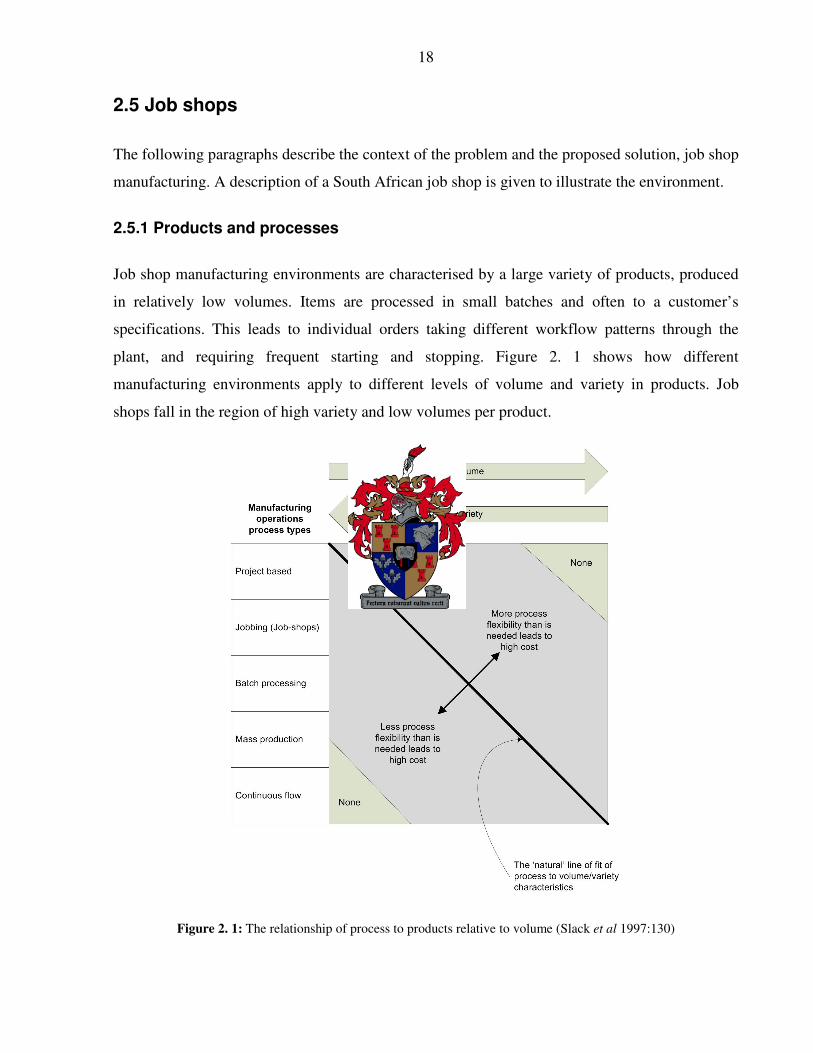
manufacturing environments apply to different levels of volume and variety in products. Job

shops fall in the region of high variety and low volumes per product.

Figure 2. 1: The relationship of process to products relative to volume (Slack et al 1997:130)

19

Similar equipment or functions are normally grouped together in a job shop environment, such as

all lathes in one area or department, all stamping machines in another (Chase & Aquilano

1985:180). Parts that are worked on travel from one functional area to another according to their

process routings. The APICS dictionary (1984:15) defines a job shop as follows (Chase &

Aquilano 1985:580):

‘A job shop is a functional organisation whose departments or work centres are organised around

particular types of equipment or operations, such as drilling, forging, spinning, or assembly.

Products flow through departments in batches corresponding to individual orders – either stock or

individual customer orders.’

Vollmann (1973:398) cite some of the advantages of a job shop layout. The groupings of similar

machines allows for a diversity in manufactured products, as any part can be sent to as few or

many conversion stages as is required. Machines can be utilised somewhat independently of other

machines, which permits a lower investment in equipment. Manpower can be utilised better, and

it allows the development of multiple skills, because people are not tied to a fixed rate of

production and a relatively fixed task. He then goes on to cite some of the problems associated

with job shops, that TOC and DBR was designed to combat: ‘Proper utilisation of manpower and

equipment in job shops, however, requires work-in-process inventories so that each operation can

be quasi-independent of the others; cost of inventories and resultant long manufacturing lead

times need to be traded off against better utilisation of productive capacity.’

20

2.5.2 Aerodyne Aviation Technologies

At this stage it is useful to describe the production environment of the South African company

whose data was used in the rest of this research, Aerodyne Aviation Technologies.

Company overview

Aerodyne Aviation Technologies is located in the Strand Industrial Area in the Western Cape. It

forms part of a group of companies called Aerodyne Technology. Aerodyne Technology was

found in 1983 as a high-tech company that specialises in the design and manufacture of structural

composite parts for the aerospace and defence industries. Today the company consists out of

three separate operating companies, each serving a particular market segment:

1. Aerodyne Aviation Technology (AAT) was formed in 1996. It supplies composite parts

for aircraft interiors, and has been involved in several airline refurbishment contracts,

through its ability to produce more than 3 000 carbon prepreg mouldings a week.

2. Aerodyne Marine Technology is responsible for the Aerodyne range of sailing yachts; all

constructed using advanced wetpreg post cured epoxy technology. The Aerodyne 38

achieved the Boat of the Year: Best in Class award in 2000.

3. Aerodyne Advanced Composites is focused on the supply of carbon composite parts to

the automotive industry, with contracts for German brands in place.

Aerodyne Aviation Technologies (AAT) entered a joint venture with a German company, AIK, in

1998 and since then sold a 70% stake to another German company, Recaro Aircraft Seating, once

one of AAT’ s two major customers. More than 95% of all production is exported to Europe and

the USA. In 2002 AAT employed about 160 people but in 2005 that figure was close to 300.

Turnover in the early days was about R18M; for 2005 it was expected to bring in R60M and for

2006 turnover is expected to be R70M to R75M.

21

Products and services

AAT has achieved ISO 9001:2000 certification for both design and manufacturing. Products and

services offered by AAT include product development expertise, a sustainable moulding capacity

in epoxy, and the company can produce phenolic prepreg of more than 10 000 items a month.

The company manufactures composite backrests for all classes of aircraft seats. The manufacture

of this product type began in 1992 with the development and supply of 800 backrests for the

Concorde. The contract with Concorde has come to an end, but other clients are keeping the

business alive. Lufthansa economy class seats have, for example, been supplied at a rate of a

thousand a week.

Today, more than thirty thousand units produced by AAT are in service on over fifteen

international airlines. The carbon fibre parts of the seat manufactured by AAT include the bucket

structure and headrest, as well as parts and support structures for the armrests and the cushion

formers. Many of the peripheral parts were previously made from thermoplastic or aluminium.

The composite bucket forms a primary seat structure, and the passenger seatbelts attach directly

onto the composite moulding. The bucket is manufactured as a single piece in composite tooling,

using an autoclave for the cure cycle.

Although the company mainly supplies aircraft seats to the airline industry, the products

produced still vary quite widely in terms of design, Bills of Materials and process routings.

Product mixes also vary frequently. Major airlines change the seats of their whole fleet every six

to eight years. KLM, who is considered a smaller airline, ordered parts for twelve thousand seats

early in 2000. Each airline has different requirements, and seats for first, business, and economy

class vary substantially.

22

Manufacturing environment

The manufacturing facility occupies approximately eight thousand square meters of production

floor space. Equipment includes computer numerically controlled (CNC) tool making centres,

CNC prepreg cutting, autoclaves, press-claves, frame presses, ovens and CNC trim routers.

AAT’ s competitive advantage over competing European companies is that although materials are

bought from the same suppliers, these materials can be converted into products and exported at a

lower cost than the competition can offer. This is due to the cheaper infrastructure, cheaper

skilled staff, and cheaper labour.

AAT requires a lot of highly specialised and skilled staff. Most of the skilled personal are trained

and cultivated in-house by promoting from within and running skills-upgrade programmes. The

company’ s two top tool designers were recruited off the factory floor. Even experienced

Engineering graduates will not necessarily have experience in composites or in aviation seating.

It can take six to eighteen months to get them up to speed. Despite its hi-tech nature, composite

production is still labour-intensive. About 70 of AAT’ s 290 employees work in skilled services

such as engineering, quality assurance, stores and tool making. The rest are in production.

Sample data

Separate production lines are set up that manufacture different class seats (First class, Business

Class, Economy, etc.). For the purpose of this research only one line, namely Echo line, was

focused on. Echo produces Economy class airline seats. The reason for only focussing on Echo,

was that at the time that this research was done, AAT had only recently started to implement

TOC. It was decided to run Echo on a S-DBR schedule as a trial run. The S-DBR implementation

on Echo is discussed in Chapter 3.9.4.

The Echo line can still be seen as a job shop environment as it produces a variety of products,

each with a different design, Bill of Material and process routing. Work centres are arranged

according to function. Economy class composite seats are manufactured for Swiss Air, Air

Britannia, British Airways, Taca Air, Niki Air, and Air Berlin. A total of twenty-three variants

are produced on the Echo line, and on average there are five to six active on the line at any given

time.

23

The combined Routing and Bill of Material information for the different variants produced by

AAT’ s Echo line are shown in Appendix G. In his description of an information system, Goldratt

(1990a:169) suggested that the Bill of Materials and Routing files be grouped together in a single

structure. This is done to speed up the computing time of software based scheduling systems.

The concept of combined BOM and routing files is explained further by Stein (1996:56). The

combination is called a Product Flow Diagram (PFD), as it shows the way in which products

flow through the plant. An example of a PFD, and how it relates to the BOM and Routing

information, is shown in Figure 2. 2.

Figure 2. 2: Example Product Flow Diagram (PFD)

The PFD of one of the variants produced on Echo, Taca, is shown in Figure 2. 3:. Refer to

Appendix G for the PFD’ s of all the variants produced on the Echo line.

24

Figure 2. 3: PFD of the Taca variant produced on AAT’ s Echo line

25

Figure 2. 4 PFD of the Taca variant produced on AAT’s Echo line (continued)

26

The production process is relatively generic for all the different products, except that some are

fitted with more rivets and require more drilling operations. A short description of the different

processes follows:

1. Kit Cutting: At the kit cutting station, kits for the front, rear, and cup parts of the

seats are cut from carbon and fibreglass. Different patterns are cut

for different models.

2. Lay-up: At the lay-up station the different layers of carbon and glass are

laid up in moulds. This is a very manual process. The units get

vacuum bagged and a bleeder is used to suck out excess resin.

3. Demoulding: The different parts get removed from their moulds once they have

settled.

4. Trimming: The different seat parts (front, rear, and cup) need to be trimmed to

have a good finishing. This is also a very manual process and a part

may visit this station various times.

5. Drill, Cure, Fit (Rear): The rear part gets fit with helicoils, a hard point and an L-bracket.

6. Painting (Cup): The cup part gets painted with a primer coat. Steps 5 and 6 happen

in parallel. Painting is done by hand.

7. Assembly (bonding): The three different parts are bonded with glue. After it is cured it

gets trimmed and drilled again. The bushes get bonded to the

assembly.

8. Quality Assurance: The first quality check is done after the units have been bonded and

trimmed. If needed, a structural test is also performed. Quality

Assurance checks are also performed various times on each part.

9. Painting and Filling: At this stage the parts go into an iterative painting and filling

sequence. After painting the assembly with a coat, it needs to be

checked for small holes. These holes get filled with powder and re-

painted. After each coat is painted, Quality Assurance is performed.

Sanding, filling, and painting is done by hand.

10. Velcro: The final step before shipping is to apply Velcro strips to the sides

and front, according to customer specifications. The products are

good to send if they pass the QA tests.

27

2.5.3 Job shop scheduling

‘A schedule is a timetable for performing activities, utilising resources, or allocating facilities.

The purpose is to disaggregate the master production schedule (MPS) into time-phased weekly,

daily, or hourly activities – in other words, to specify in precise terms the planned workload on

the productive system in the very short run.’ (Chase & Aquilano 1985:580.)

Optimal job shop schedules should plan for smooth, efficient, low-overall-cost operation with

minimum inventories and no late orders. Work in job shop environments are controlled by work

orders, and most important is accurate order promising and afterwards adherence to these

promised due dates. Job shop schedulers are most frequently used as decision support tools

(Benoy, Dewilde & Voet 1998:44-45).

The typical job-shop scheduling problem involves scheduling any n jobs on m machines. This can

very easily become a complex problem. The scheduling task is one of the most complex tasks in

operations management, as schedulers need to deal with different types of resources with

different capabilities at the same time. The literature contains many solutions that have been

proposed for this problem. As the problem of scheduling is not a solved problem (Smith 2003:10)

the research into new and improved methods is ongoing. Zhang (2003:2.1-2.18) gives a very in-

depth survey of the literature on scheduling.

This study focuses specifically on the TOC solutions to job shop scheduling, and aims to provide

a method of making DBR scheduling easier to implement practically. Although other measures

may provide good solutions, a comparison of the TOC solution to other methods falls outside the

scope of this project.

28

Chapter 3

Drum-Buffer-Rope evolution

3.1 Introduction

This chapter is an in-depth study of Drum-Buffer-Rope (DBR). It investigates how DBR was

developed and how it has been improved. It also introduces the newly developed Simplified

Drum-Buffer-Rope (S-DBR). The purpose of the chapter is to lay the foundation for the

development of the scheduling package and to make certain that the latest trends from industry

are captured in the software design. It also investigates some practical implementations if DBR

and S-DBR to justify them as good solutions for job shops.

3.2 Drum-Buffer-Rope origins

Drum-Buffer-Rope (DBR) is the production logistical solution of the Theory of Constraints. It is

the implementation of the first three Five Focusing Steps on the manufacturing shop floor, to

manage physical resource constraints. DBR was designed with the purpose of increasing

Throughput (T), while simultaneously decreasing Inventory (I), and minimising Operating

Expense (OE). It aims to accomplish these goals by focusing on simplifying and therefore

reducing variability in the production process, and ultimately protecting order due dates against

disruptions.

As the pace of the entire manufacturing system is dictated by the constraint resource, DBR

concentrates on getting the most out of the constraint in order to maximise Throughput. Other

resources are measured against their ability to support the constraint, and to turn goods processed

by the constraint into Throughput. Measuring efficiencies at non-constraint resources are

detrimental in the TOC environment, as it encourages accumulation of unnecessary inventory in

the form of Work in Process (WIP).

29

Drum-Buffer-Rope started out as a software system called “ Optimised Production Timetables”

(OPT) (Spencer, M. S. 1991:22). It was the brainchild of Dr. Eliyahu Goldratt after he applied a

technique for predicting the behaviour of a heated crystalline atom to optimise the large number

of variables of a work schedule in 1979 (Meleton, M. P. 1986:13). Originally a company called

Creative Output Inc. in the United States of America brought it to the market. The name of the

software was later changed to “ Optimised Production Technology” . Although the algorithms of

the software was proprietary information, large companies such as General Electric and General

Motors still bought into it and reported dramatic reductions in lead time and inventories

attributable to OPT and its underlying philosophy (Simons & Simpson 1997:3).

In an attempt to get more publicity for the system, Goldratt published The Goal in 1984 (Goldratt

& Cox 1986). In this book the focus was on the need to change the industry-governing paradigm,

and it actually downplayed the need for a computerised scheduling package (Goldratt 2004). At

this stage, the OPT concepts were implemented in a software package called “ Disaster” . The

reason for calling it “ Disaster” was that Goldratt held firm that a company trying to incorporate

the software without understanding the underlying philosophy would have disastrous results. As

more companies implemented the concepts of The Goal in their own business, Goldratt realised

that companies only implementing the concepts, and not the software, achieved better results,

quicker (Goldratt 2005:1). Goldratt himself shifted his focus from software sales to education,

and the Avram Y Goldratt Institute was established. Unlike OPT the “ Disaster” software was not

proprietary and the concepts were described in many publications (Goldratt 1990a; Schragenheim

& Ronen 1990; Stein, 1996).

The Avram Y. Goldratt Institute eventually split in two, and The TOC Centre was formed

(Simons & Simpson 1997:4). The TOC Centre acquired the rights to the “ Disaster” software and

it was renamed to The Goal System.

30

3.3 Traditional Drum-Buffer-Rope concepts

The following paragraph explains the concepts of DBR as it was originally implemented in the

Goal System algorithm. It is presented to show why S-DBR was developed, and how the three-

buffer system of DBR has been adapted. The DBR concepts implemented in the software

developed in this project are discussed in Chapter 3.6.

Drum-Buffer-Rope is the implementation of the Five-Focusing-Steps of TOC in production. In

the TOC environment a distinction is made between Bottlenecks and Constraints. A constraint is

defined as: ‘Anything that limits a company from reaching its goal’ (Goldratt 1990b:4) while a

bottleneck is defined as: ‘An internal constraint that limits the system from meeting external

demand’ (Srikanth & Umble 1997:117). An example of a bottleneck situation is where the market

is willing to buy more than what some machine or internal process in a company is able to

produce. DBR starts from the outset that only a few resources restrict the whole organisation

from getting everything out of the market, and is therefore focussed on addressing bottlenecks. A

clear distinction needs to be made between Bottleneck resources and Capacity Constrained

Resources. The following definitions were used (Umble & Srikanth 1990:65, 87):

Bottleneck Resource: ‘Any resource whose capacity is equal to or less than the demand

placed upon it’ .

Non-Bottleneck Resource: ‘Any resource whose capacity is greater than the demand

placed upon it’ .

Capacity Constrained Resource: ‘Any resource which, if not properly scheduled and

managed, is likely to cause the actual flow of product through the plant to deviate from

the planned product flow’ .

From these definitions, it is possible for a non-bottleneck resource to become a Capacity

Constrained Resource (CCR) if it is not properly scheduled and managed. By the improper

sequencing of orders, non-bottleneck resources can be loaded in such a way that they are unable

to cope with the demand placed on them for the given capacity. Stein (1996:61) defines the

31

resource constraint, or CCR, as: ‘The resource which, more than any other, threatens the creation

of throughput’ .

Conventional methods of scheduling attempt to avoid bottlenecks by balancing the amount of

work at each work centre across the plant. In a job shop it is however impossible to have a

“ perfectly balanced” plant running at full capacity where the output of one work centre feeds the

next one just at the time when it receives a new unit from an upstream workstation (Chase &

Aquilano 1985:609). The stochastic nature of process times makes it impossible. In a DBR

system the plant must not be balanced. The CCR is strategically placed to dictate the pace of the

plant, and the non-constraint resources must have a measure of protective capacity (called sprint-

capacity) to support the CCR.

According to DBR principles, because the pace of the CCR dictates the pace of the entire plant, it

is not necessary to schedule every single resource. Only the CCR’ s need to be scheduled and the

other non-constraint resources are instructed to work as fast as possible, but only if they have

work (this is called the Road Runner concept). By definition, non-CCR’ s should have enough

excess capacity to catch up to the pace of the CCR if random events cause them to lose

production time. On the other hand, it is also not necessary for non-CCR’ s to work all the time, as

this would lead to unnecessary WIP and stock holding costs. By placing time buffers

strategically, enough time is left for non-CCR’ s to finish their work to feed the CCR, or to get

parts finished by the CCR ready for shipping on time.

Figure 3. 1(Adapted from Schragenheim & Dettmer 2001:113) illustrates the drum, the different

buffers, and the rope. Each component is explained below.

32

Figure 3. 1: Traditional Drum-Buffer-Rope components

The drum is derived from the Master Production Schedule (MPS) after the needed modifications

have been made to ensure that the potential market demand is brought in line with the capacity

and material capabilities of the plant. It therefore sets the pace to which the whole plant is to be

synchronised. Originally the drum was considered to be the constraint resource, which limits the

overall production capabilities of the plant. More recent work on DBR considers the drum to be

the schedule for the Capacity Constrained Resource (CCR), which is derived from the original

MPS and the size of the Shipping Buffer. Time Buffers are defined as (Goldratt 1990:128): ‘The

Time Buffer is the time interval by which we predate the release of work, relative to the date at

which the corresponding constraint’ s consumption is scheduled.’

Time buffers are designed to protect operations against the process variability that is inherent in

every production process. By placing these buffers strategically, the schedules for the key

operations are protected against unplanned disruptions. Three time buffers are used and defined

below (Schragenheim & Dettmer 2001:106):

33

1. Shipping buffer: ‘A liberal estimation of the manufacturing lead time from the CCR

to the completion of an order.’

2. Capacity Constrained Resource Buffer: ‘A liberal estimation of the manufacturing

lead time from the release of raw materials to the site of the Capacity Constrained

Resource.’

3. Assembly Buffer: ‘A liberal estimation of the manufacturing lead time from the

release of raw materials to an assembly point where CCR parts and non-CCR parts are

combined.’

The shipping buffer protects the shipping schedule. It is used to schedule the CCR operations and

the release of materials that are not processed by the CCR. The CCR buffer must protect the

constraint operations, and is used to schedule the release of material that pass through the CCR.

The assembly buffer is used to schedule the release of material on production legs that do not

pass through the CCR, but is assembled with parts from CCR legs. It ensures that parts that have

already passed the CCR do not have to wait at assembly points for parts from non-CCR

operations.

Buffers can easily be misinterpreted to represent work-in-process inventory. The idea however is

not to plan for an amount of work to lie in front of the buffered operation, but to plan for the

preceding operations to be finished processing an order some time before the buffered operation

is scheduled to work on the order. This may result in physical inventory to accumulate in front of

the buffered process.

Production organisations tend to use a uniform buffer size for all products. Time buffers must

protect the schedule against the typical disruptions experienced by the manufacturing plant. The

length of the time buffers is calculated through trial and error and is based on the magnitude of

these disruptions and fluctuations (Schragenheim & Ronen 1990).

Louw (2003:52) developed an analytical formula for calculating the size of buffers, based on an

open queuing model of a flow shop and is given by:

34

Time buffer length = AverageFlowTimeToBufferOrigin + zs(StdDevOfFlowTimeToBufferOrigin)

- SumOfProcessingTimesToBufferOrigin

where zs is the corresponding z-value read from a standard normal table for a certain service

level, s.

Some computerised DBR packages use dynamic buffering. It is only applied to the constraint and

assembly buffers. Dynamic buffering means that the user specifies a fixed part of the buffer,

which only includes estimations of the impact of disruptions and fluctuations. By analysing the

load of a given set of orders, the system will increase the size of the buffer according to the

processing and queue times. This means that the constraint and assembly buffers are

automatically increased if a lack of protective capacity is detected (Stein 1996:115).

The rope is defined as (Schragenheim & Ronen 1990): ‘A “ rope” is a mechanism to force all the

parts of the system to work up to the pace dictated by the drum and no more’ .

According to the DBR methodology the easiest way to ensure that non-constraints work in

synchronisation with the CCR is by forcing the system to contain only material that is scheduled

to be processed on the CCR in the next buffer time frame. Non-CCR operations are therefore

controlled by the timely release of material into the system, and by instructing non-CCR

workstations to work as fast as possible, but only on parts due for orders on the CCR or shipping

schedule. The rope must ensure that material is released into the plant at a rate that is sufficient to

always support the CCR operations without overloading them.

The rope is therefore the material release schedules of all raw materials. The assembly and CCR

buffers are instrumental in the derivation of the rope. If there is no CCR active, the rope is

constructed by means of the shipping buffer.

35

3.4 Drum-Buffer-Rope scheduling steps

DBR scheduling consists out of three steps: identify the resource constraint, exploit the resource

constraint to get the maximum out of it, and then subordinate all the other resources to the

constraint schedule. The fourth step (elevate the constraint) and fifth step (repeat the process) are

strategic actions and do not form part of the operational tasks that DBR addresses. These are the

steps as implemented in the original Goal System software. After production schedules are

released to the shop floor, shop floor control is achieved through buffer management.

3.4.1 Scheduling the plant

The first step in the scheduling process is to identify the primary Capacity Constrained Resource.

This is done by analysing the demand placed on each resource during what is termed the effective

horizon. The effective horizon is simply the planning horizon as specified by the user, plus one

shipping buffer time into the future. For each resource, the loads of all jobs during the effective

horizon are analysed. If there are loads that exceed the capacity of the resource, they are pushed

backwards in time. This may result in what is known as First Day Load (FDL) peaks, meaning

that some resources will have a lot of work scheduled to be started before the start of the effective

horizon. The resource with the largest FDL peak is identified as the primary CCR.

Exploiting the constraint means to develop a detailed finite capacity schedule for the CCR. This

is done through Goldratt’ s backward- forward pass scheduling procedure of the Goal System

Algorithm (explained in detail in Chapter 4). Scheduling the CCR must cause the maximum

available capacity of the CCR to be utilised. Exploitation therefore results in creating the Drum,

which is the detailed work schedule for the CCR.

The subordination part of the scheduling procedure must ensure that all the other non-CCR’ s

work at the pace set by the drum. During subordination a material release schedule is created

based on the CCR schedule, the constraint buffer and the assembly buffer. The subordination

phase establishes the rope. If there is no active CCR for a given set of orders, the drum is the

Master Production Schedule, and material release is offset a shipping time before the specific

order due date.

36

Figure 3. 2 best illustrates the calculation of material release times (Goldratt 1990a:227).

Figure 3. 2: Calculation of material release times by means of time buffers

According to the Goal System algorithm, after the primary resource has been identified and

scheduled, a capacity check on all non-constraint resources should be done again, to identify the

secondary, tertiary, (and so forth) resource constraints, and to schedule them as well. This results

in an identification and scheduling loop, which may result in a number of resources being

scheduled and therefore having to be tightly controlled. The complete Goal System scheduling

algorithm is shown in Figure 3. 3 (adapted from Simons & Simpson 1997:7).

37

Step 1Compute effective horizon = planning horizon + shipping buffer

Step 2Subordinate all resources to the market

Step 5aBuild Drum Schedule (3a - 3d)Consider: Time Rods from fixed Schedule Batch rods for the CCR’s

Step 3cIF processing go into past:Forward pass to achieve feasibility

Step 3bBackward passLevel ruins in line with capacity

Step 3aBuild ruinsOFT = due date - (shipping buffer + rods)

Step 3Build drum schedule for primary constrained resource

Step 2cNo resource constraints go to step 7

Step 2bIdentify resource constraints via FDL peak

Step 2aBackward pass- calculate daily load for each resource =remaining capacity - job requirements

Step 4bDetermine FDL & RL peaksIdentify additional constraints (CCR’s)

Step 4aBackward passCapacity check for nonconstraints:calculate daily load for each resource =remaining capacity - job requirements

Step 4Subordinate nonconstraints to market & drum schedule

Step 3dFix drum schedule in timeReconcile due dates with constraint schedule

Step 5Built schedule for additional drum (CCR Schedule)

Step 4cNo additional constraints constraints go to step 7

Step 5a,cIF processing go into past:Forward pass to achieve feasibility

Step 5a,bBackward passLevel ruins in line with capacity

Step 5a,aBuild ruinsOFT = due date - (shipping buffer + rods)

Step 5a,dFix drum schedule in timeReconcile due dates with constraint schedule

Step 6Drum Loop

Step 7

STOPImplement drum schedules

Step 5cNo drum violations go to step 4

Step 5bIdentify drum violations

Step 6a Rebuild the first fixed Constraint schedule - shift batches later by amount of the drum violation

Step 6cGo to step 4

Step 6bUnfix (eliminate) all additional constraint schedules

Building the Ruins:Place jobs on the time line such that the processing of its final operation would be completed exactly on shipping buffer’s length of time before job due date

Constraint Buffer:

Batch Rod - Time required for other operations between two constraint operations on same job - normally 1/2 constraint buffer

FDL = First Day Load

RL = Red Lane - insufficient capacity on non constraints following constraint once drum schedule is known.

OFT = Operation Finish Time

Shipping Buffer: Period of time allocated for performing operations that must be accomplished following constraint processes but before the job’s due date.

Figure 3. 3: The Goal System scheduling procedure (Simons and Simpson, 1997:7)

38

3.4.2 Shop floor control

After production schedules have been developed, they are released to the shop floor. Control is

then exercised through Buffer Management. Buffer Management is well documented in the TOC

and DBR literature, and only the high level concepts are discussed here (Goldratt 1990a:238;

Stein 1996:141; Gardiner et al. 1992:73). For Buffer Management, the shipping and constraint

buffers are monitored for the work they contain. If one-third of the buffer time has passed and the

material has not arrived at the shipping dock or CCR, it is referred to as “ a hole in region 2” . In

this case the material should be found in the production line and any obstacles to its progress

identified and removed. If the material has not arrived after two thirds of the buffer time has

passed, it is referred to as “ a hole in region 1” . In this case the material should be found and the

order should be expedited to avoid disruptions to the production plan. Buffer Management is

judged as effective if 90% of orders do not have to be expedited. Having to expedite orders more

frequently than this indicates that the buffer is too small. If expediting is very rarely needed, the

buffer size should be reduced. In this way production lead times can continuously be improved

upon and lead times shortened. The desired buffer content profile is illustrated in Figure 3. 4.

Figure 3. 4: Desired buffer content profile (Louw 2003:23)

39

3.5 Simplified Drum-Buffer-Rope

In 2001, Schragenheim and Dettmer published a book called: Manufacturing at Warp Speed

(Schragenheim & Dettmer 2001). In it they claim that the three buffer approach of traditional

DBR has some limitations and certain situations call for a different approach to scheduling. The

main reason for this is that although the company may experience some periods in which there is

an active resource constraint, the market is always the governing system’ s constraint. The

solution they propose is called Simplified Drum-Buffer-Rope (S-DBR) and is similar to the

method followed by traditional DBR when there is no active CCR. In it, only the shipping buffer

is used, and the drum is the Master Production Schedule after capacity limitations have been

considered.

3.5.1 Difficulties with the three buffer system

According to Schragenheim and Dettmer (2001:122) the three buffers implemented by traditional

DBR is in most cases not necessary, and overcomplicates the system. The main reasons for only

using the shipping buffer are as follows:

x� Spreading time buffer: The same reasoning as to why every process in the

manufacturing of a product should not be buffered against variability applies to the three-

buffer system. All the different buffers add up to the total lead-time for manufacturing a

product. Having three buffers weakens the global protection of the plant, because the

portion of the lead-time assigned to one buffer is not usable by the others further down the

line of processing.

x� More buffer time: Three buffers may add more lead-time than is actually needed. By not

adding buffer time to more than one place in the sequence of operations, products can be

delivered more quickly.

x� Superfluous buffer: The argument for having the assembly buffer is to protect the flow

of products to the market after passing the CCR from disruptions, meaning that the

assembly buffer should guard against having parts finished by the CCR waiting for non

CCR parts. In Afrikaans this would be referred to as a “ gejaag na wind”, meaning: “ to be

chasing after the wind” . CCR parts have no value in themselves except when they form

40

part of finished goods that customers pay for. Having orders finished earlier than the

promised due date is in most cases not beneficial as it could lead to unnecessary stock

holding costs. If the client does not necessarily want his orders earlier than the promised

due date, there is no value to be added by delivering before the promised time. The

purpose of DBR is to eliminate variability in delivery dates. This is just as applicable to

delivering early, as it is to delivering late.

A further motivation for having a simpler approach is that it reduces the need for data automation

and having accurate process data. The more detailed the schedules created, the more accurate

data on processing times on operations required. In a job shop environment, products on order

may vary frequently, implying that the sequence of operations and processes may also change

often. Going through an extensive data capturing exercise each time changes are made may not

be feasible.

Another common problem in implementing DBR is that a uniform buffer size is used for all

products. Different products may however have different lead times and different sources of

variation. Having customised buffers for different products in the three-buffer system can become

very cumbersome without the right software support.

3.5.2 Scheduling the plant

In light of the problems posed above, Simplified Drum-Buffer-Rope eliminates all the buffers of

traditional Drum-Buffer-Rope, except the Shipping Buffer. The Shipping Buffer is now defined

as a liberal estimate of the total lead-time of a product. It includes: set-up and run times, move

and queue times, and a pad for normal and excessive variation. S-DBR essentially follows the

same procedure as traditional DBR when there is no CCR. A model for Simplified Drum-Buffer-

Rope is shown in Figure 3. 5.

41

Figure 3. 5: Simplified Drum-Buffer-Rope

The green an red blocks of Figure 3. 5 indicate the portion of the total lead time assigned for red-

line control (explained in paragraph 3.5.3). The start of the red block indicates the Red-Line

value.

Eliminating all but the shipping buffer is based on the assumption that market demand is always

the system’ s constraint. The system’ s constraint is defined as ‘Anything that restricts the system’ s

ability to increase sales’ . The assumption is made that although there might be some resources

that will experience periods of having less available capacity than what is demanded of them, the

market will always be the governing constraint. The CCR usually truly limits company

performance only at times of peak demand, but not at off peak times. This is illustrated in Figure

3. 6 below (adapted from Schragenheim & Dettmer 2001:157).

42

Figure 3. 6: Demand and available capacity of a potential CCR

If the assumption is valid, no resource will ever be scheduled in detail under S-DBR. The only

scheduling that is done is the shipping dates and material release. Deriving the S-DBR schedule

follows the same steps as traditional DBR, but the different steps have different implications.

Identifying the constraint does not imply that the resource which will be explicitly scheduled

must be identified. It rather means that the workload brought on by a specific set of orders needs

to be analysed to see whether there will be resources that will experience difficulty to produce

what is demanded from them. This step therefore involves bringing the MPS in line with the

capacity of the plant, and doing pro-active resource capacity planning and order due date

negotiating to be able to deliver on commitments to the market. According to Schragenheim and

Dettmer (2001:167): ‘…management must fully understand, appreciate and consider the possible

negative impact on marketing’ .

To implement S-DBR, even the potential CCR needs protective capacity of its own. The

sequence followed when scheduling is therefore to first commit to ones customers based on the

limits of available capacity, and then to create a MPS to meet those commitments. In

conventional DBR the MPS is first created, and then the CCR is exploited to be able to meet the

MPS.

Subordination means to simply create a material release schedule based on the MPS and the

shipping buffer. All work orders in the system should be for complete product deliveries.

43

Detailed material requirements must be calculated and unassigned material on the shop floor

assigned to new work orders.

The advantage of equating work orders to customer orders is improving flexibility on the

production floor. It promotes shop floor intelligence in the sense that operators are aware of how

many parts are needed for which orders, and can make sequencing and time saving decisions in

real time. Say for instance there are 100 B parts required for order S001, and 20 for S002. Based

on the actual loads on resources and priorities of due dates, the operators will decide whether to

merge the two requirements and save a set-up, or perform other more important intermediate

operations. By not developing explicit schedules for resources, operators are given the authority

to reprioritise work to give precedence to the most important or pressing jobs.

3.5.3 Shop floor control

To facilitate shop floor control, two new concepts are introduced to the S-DBR environment: Red

Line Control and Planned Load. These control methods are put in place to warn against danger

situations such as an order being late, when the load on a CCR approaches its maximum limit,

and when non-CCR’ s threaten to become CCR’ s.

Red Line Control is a simplified form of traditional Buffer Management. Unlike specifying a

ratio of the complete buffer time for region 1, the red line value is specified as a fixed value. This

means that when the shipping buffer changes, the red line value does not. The red line time is

calculated by determining how long it takes to expedite a medium sized order. When the red line

time for an order is reached, and the order is not ready for shipping, corrective action needs to be

taken. If many red line warnings occur it either signals the emergence of a CCR (in other words

the buffer is too short) or that the red line time is too long. When many orders penetrate the red

line time but there is no need for action, the red line time is also too long. If late deliveries occur

without red line warnings or if corrective action was taken after red line warnings, the red line

time is too short.

In S-DBR red line control is also applied to raw materials. Under traditional DBR conditions it is

often assumed that raw materials are always available. One must however guard against stock-out

of raw materials, if the market constraint is to be effectively exploited. The red line value for raw

44

materials is calculated by multiplying the consumption rate of the most frequently used raw

material with the number of days that it will take the fastest supplier to do an emergency delivery

(Schragenheim & Dettmer 2001:179). If the level of raw-material falls below these levels while

orders keep coming in, an emergency delivery should seriously be considered.

The other control method in S-DBR is called planned load. Planned load is defined as: ‘…the

total hours required of the CCR to complete all work that has been formally released into the

system and has not yet been processed by the CCR’ .

As long as the planned load is less than the quoted lead-time (QLT), orders should be safe. As

soon as the planned load approaches the QLT, the system might be approaching an overload. By

comparing the planned load for each resource with the amount of work waiting in front of the

resource, upstream CCR’ s can be identified.

3.6 The new DBR approach to the buffer system

Eli Schragenheim is the author of literature on the Theory of Constraints and DBR

(Schragenheim & Dettmer 2000; Schragenheim & Dettmer 2001; Schragenheim & Ronen 1990).

He is the developer of several educational simulators that are used to experience the problems in

running manufacturing and projects and the TOC solutions. In 2005 he released an article titled:

“ Buffers in the new GSIM Simulators” . In this article it is argued that the three buffers of

traditional DBR should be reduced to two (the shipping and constraint buffers), and the definition

of the shipping buffer should be somewhat adapted. This article is endorsed by Goldratt and can

be viewed in Appendix A.

The main concerns with the traditional three buffer system are:

1. Shipping buffers for free products (products that do not cross the CCR) should be

different than for CCR products;

2. The assembly buffer is redundant and its purpose is not altogether clear.

The second argument adds on to the argument for not having an assembly buffer in S-DBR. The

assembly buffer should guard against the situation where CCR parts have to wait for non-CCR

45

parts. The assembly buffer effectively causes these materials to be released earlier than needed.

No value is added to the organisation however, if orders that are completed earlier than when

they were promised for do not result in quicker sales, which is often not the case.

The solution to both problems is shown in Figure 3. 7.

Figure 3. 7: The new DBR buffer system (Adapted from Schragenheim 2005:3)

In line with simplifying the DBR system and making it easier to understand and implement, a

simple and effective solution is to discard the assembly buffer, and to define the shipping buffer

as the complete lead time of the product, from material release until shipping. The CCR buffer is

then only a part of the shipping buffer and material for free goods are released based on the

46

shipping buffer. In line with the arguments above, it was decided to adopt the new two buffer

system for the purpose of this research and the development of the associated software.

3.7 Addressing process variability

Drum-Buffer-Rope has undergone some changes since its inception into the manufacturing

environment, but the underlying principle of simplifying the production system by setting its pace

to a single drumbeat and focussing on the end-result instead of local optimums has remained

constant. Goldratt himself perhaps best explains the principle of simplicity in a letter he recently

published to explain his Viable Vision campaign (Goldratt 2004:1): ‘…Examine a given system

and ask yourself, what is the minimum number of points one has to impact in order to impact the

whole system? If the answer is ‘ten points’ then this is a difficult system to manage, it has too

many degrees of freedom.’

And: ‘...But, if the answer is ‘one point’ then this system has only one degree of freedom, it is an

easy system to manage.’

Drum-Buffer-Rope attempts to simplify the manufacturing system by reducing the number of

control points to the minimum, one (the MPS) or two (the MPS and the CCR). By having a lot of

control points in the system, it opens the gateway for process variability to enter. This can be

explained by looking at a simple manufacturing process such as the one in Figure 3. 8.

The figure shows a basic manufacturing line of a part that gets processed by five different

resources (The circles labelled R-1 to R-5). The processing time of each resource is modelled by

an exponential distribution, with 2

1O = 100 to represent a balanced line. The histogram of sixty-

five thousand samples of each process is shown as an Excel graph above each resource (the blue

blocks). The cumulative distribution function of the whole line is shown at the top of the

diagram. It is the histogram of the sum of the processing times of the resources in the line, and

shown as an Excel graph (the red line in each graph).

47

Figure 3. 8: Process variability in a simple production line with finite scheduling

In the normal finite scheduling environment, the capacity of all the workstations would be

balanced as close as possible, and a detailed production schedule would be developed for each

one. The stochastic nature of production processes will cause each process to exhibit some

variation on the actual schedule followed from the planned schedule. As such variation tends to

accumulate (the entire process distribution is given by the convolution of the individual

distributions); the total variation of the whole system would be quite large, causing considerable

disruptions to the planned product flow.

Although it is possible for more than one CCR to be active, management of such situations is

complex and is not really recommended. The Goal System algorithm (Goldratt 1990a, Simons

and Simpson 1997, Stein 1996) handled interactive resource constraints by developing detailed

schedules for secondary and tertiary (etc.) CCR’ s. This in turn leads to the complexity of

scheduling and managing the schedules of resources in a job shop that Drum-Buffer-Rope was

designed to reduce. Furthermore, according to Gardiner et al (1992, p71) ‘Experience with OPT

Frequency

Time

48

demonstrated to Goldratt that real products do not cross two constraints’ . The preferred method is

not to allow the emergence of more than one CCR in the first place, either by adding capacity or

by imposing restrictions on market demand (Schragenheim and Dettmer, 2000). Apart from

heading back towards complex scheduling, scheduling a lot of control points in the plant makes

way for variability to creep back into the system. The norm is therefore to move away from the

old Goal System’ s method of scheduling secondary and tertiary constraints, and keeping the

methodology simple and practical to implement. Figure 3. 9 illustrates the case where Drum-

Buffer-Rope is implemented on the simple production line.

Figure 3. 9: Process variability in a simple production line with DBR scheduling

In Figure 3. 9 R-3 is the CCR (indicated as a red circle) with 2

1O =100. The other resources have

more capacity, and the processing times of the resources are summed before and after the CCR.

The total processing time before R-3 has an exponential distribution with 2

1O =25. The total

Frequency

Time

49

processing time of the resources after R-3 is modelled with the same distribution. Again the total

processing time is modelled with the sum of the three distributions and shown at the top of Figure

3. 9.

In the case where DBR is implemented on the simple line, there are only three sources of

variation from the actual production times with respect to the planned schedules, namely the

material release schedule, the schedule of the CCR (R3 in this case), and at the shipping schedule

of orders. The overall process variability should therefore be less than in the first case, as the

sources of variation are substantially less. This in turn would lead to fewer disruptions in the

planned product flow.

This situation can easily be illustrated by considering exponential distributions. Process times are

often described by exponential distributions (Winston 1994:1111). If a number of processes are

in series, and the service time of each process can be modelled by an exponential distribution, the

total processing time of an object that has to pass through all the processes can be described by

the convolution of all the exponential distributions, which is a Gamma distribution. The Gamma

distribution is described by two variables:

�LV�WKH�QXPEHU�RI�H[SRQHQWLDO�GLVWULEXWLRQV

�LV�WKH�LQ-between arrival waiting time.

The variance of the Gamma distribution is given by:

2)var( DE X

..3. 1

�LV�GHWHUPLQHG�E\�WKH�DYHUDJH�SURFHVVLQJ�WLPHV�RI�WKH�GLIIHUent exponential distributions, where

DV� �LV�GHWHUPLQHG�E\�WKH�QXPEHU�RI�H[SRQHQWLDO�GLVWULEXWLRQV��%\�ORZHULQJ� �WKH�YDULDQFH�RI�WKH�total distribution can be reduced.

The Theory of Constraints starts from the outset that to be successful, one has to remain focused

on the company’ s goal, which is in most cases to make money by selling its products to the end

user. In order for the end user to keep on ordering, the company has to deliver products of the

50

agreed upon quality on time in full. By having a lot of process variability it is extremely difficult

to manage the system, and to deliver on commitments to the market. If the number of control

points is kept to the minimum, the inherent process variability becomes manageable. By having

enough sprint capacity at resources that are not under tight control, lost production time due to

random events can be easily made up for when needed, and the commitments can be fulfilled.

Simplified Drum-Buffer-Rope (S-DBR) takes the above reasoning even further, by making the

assumption that the system constraint (that which limits the system from reaching its goal)

always lies in the market. This assumption then has the implication that the organisation that

wants to implement S-DBR must manage either its commitments to due dates, or its resources

and their capacity in such a way that a Capacity Constrained Resource (CCR) will not emerge.

The focus shifts from control of resources to pro-active planning of the usage of the company’ s

resources. Figure 3. 10 depicts the situation where orders and capacity allocation is managed in

such a way that a CCR does not emerge, and all the resources have enough excess capacity to

make up for lost time due to process variability.

Figure 3. 10: Process variability in a simple production line with S-DBR scheduling

Frequency

Time

51

3.8 What to use when

Simplified Drum Buffer Rope was designed to accommodate most manufacturing environments.

Its simplified method allows for easy implementation without having to rely on complicated

scheduling and planning software. It does however require a sophisticated synchronisation of

marketing and sales with operations. Very efficient pro-active capacity planning is needed for

effective S-DBR implementation, which can be assisted with the correct software tools. S-DBR is

applicable when the constraint lies in the market, and there is spare capacity on all resources. A

market constraint often indicates towards mismanagement or unnecessary policies. If the market

constraint is broken, it may be necessary to move towards the traditional DBR scheduling

environment.

When the constraint however lies with a specific resource, such that the resource does not have

enough capacity to produce what is demanded of it, traditional DBR is more applicable. DBR

addresses physical constraints, or bottlenecks. A bottleneck is an internal constraint that prevents

the manufacturing system from meeting the external demand. If the MPS cannot be adjusted to fit

into the available capacity of the plant, the CCR will have to be scheduled, and for this DBR is to

be used. If the routings of products are such that the CCR is passed more than once, DBR is even

more applicable. Dedicated software is often needed for DBR scheduling as it can quickly

become complex to calculate.

52

3.9 DBR and S-DBR implementations

The literature contains enough accounts of successful DBR implementations not to reject it as a

good solution to the scheduling problems of a job shop environment. There are some common

difficulties however with the practical implementation of the theory. The purpose of this section

is to give evidence from literature that DBR and S-DBR are good solutions for job shop

scheduling, but that there are some potential pitfalls when implementing the methodologies.

Investigating the pitfalls and constructing counter initiatives fall outside the scope of this project.

3.9.1 Successes of DBR implementations:

Although it is not possible to report on all the success stories found in the literature, the following

are a few examples of successful DBR implementations. Common advantages gained are

increased throughput and on-time delivery and reduction in inventory, normally without

increasing or even changing operating expense. The reason for not changing operating expense is

discussed in Paragraph 3.9.2.

Dayton Parts, Inc (DPI) (Harrisburg, Pennsylvania): DPI manufactures and/or distributes

truck and automotive components for the original equipment market and aftermarket with sales to

heavy-, medium-, and light-duty truck and trailer independent companies. The company

experienced an increase in average orders filled from 84.2% in 1992 to 98% in 1995. WIP was

reduced by almost 50%. Average days of products in the shop decreased from 42 in 1992 to a low

of 14 in 1995. (BMP, 1995:10).

Various (7) DBR implementations in Brazil: Corbett and Csillag (2001:17) state that DBR

implementation has been documented in many industries and that it’ s use seems to be increasing,

but the results (although seemingly surprising) are not well documented or disseminated. To

verify whether these kinds of results were replicated by other DBR implementations they studied

seven such cases in Brazil. All the companies had some good results, but only six of the seven

companies continued using the methodology. On average, lead times were reduced, due date

delivery performance was improved, capacity was increased, inventories were decreased, daily

fire fighting in production was decreased, and there was an increase in revenue per employee per

53

year. Some problems were incurred (one company stopped using DBR) which are discussed in

the next section.

FMC Energy Systems (Dunfermline): FMC Energy Systems’ wellhead division makes surface

and sub-sea ‘Christmas trees’ for the offshore oil and gas exploration industry. The ‘Christmas

trees’ are the sets of valve gear and manifolds that sit on top of well heads and control the flow of

hydrocarbon out and injection fluids in – engineered to order, valued at $750,000 to $1,500,000

each, and with build periods of six to 12 months. FMC has a large engineering office, and

manufacturing facility that operates out of an aircraft hangar size 46,000sq ft factory with a suite

of machine tools – seven horizontal boring machines, two large flat bed lathes, numerous CNC

machines and specialist welding – as well as assembly and testing, including a 30ft water test pit

with two 40 tonne cranes for gas integrity testing. In 1998 FMC bought the then ThruPut

Resonance TOC-based ‘Drum Buffer Rope’ APS, following its successful implementation at a

sister plant in Houston, to support redesigned constraint-based manufacturing processes.

Inventory was cut by about $1.4 million and subcontract costs fell by about $1.5 million in that

year – some 10%. Beyond the headlines, FMC had also achieved controlled release of raw

materials and work in progress (WIP) so that WIP and lead times were reduced – these alone

more than paying for the system. The implementation also had some stumbling blocks that will

be commented on in the next section (MCS, 2002b).

3.9.2 Complications with DBR implementations

Most of the literature found in the public domain may be biased towards reporting good results,

as bad results would not necessarily be publicised. During the course of this study very little

could be found on failed implementations. The most obvious case of a failed implementation is

for plant number seven, reported on by Corbett and Csillag (2001:17). Although the company had

some good results after three months into the implementation, the company was not satisfied with

DBR and discontinued the implementation. Their biggest concern was the increase in scrap. The

company had to work with smaller process batches, which increased the scrap rate from 12% to

19%. This had a negative impact on their profitability.

The other companies reported on by Corbett and Csillag also experienced some common

disadvantages with DBR that needed to be countered in order for the implementation to be an

54

overall success. Factors identified by them are that the control of operating expense was relaxed

(because of the primary focus on increasing Throughput), scrap was increased due to smaller

process batches, and that TOC defenders were seen as contestants. The last difficulty arises

because of the way that TOC and DBR challenges conventional measurements (100% efficiency

at all workstations), and the people’ s resistance to change. If a group of people start to

disseminate traditional ways, they can be seen as being in conflict with the current voice and are

regarded as contestants.

Resistance to change is a common difficulty with DBR implementations found in the literature.

In their report, Mabin and Balderstone (2000:2) claim that:’ Even so, some companies failed in

their attempts to adopt OPT, the software package based on Goldratt’ s method. Such failure was

usually diagnosed as an inability or unwillingness by the organisation to discard old traditions,

and embrace the new philosophy and the new measures that were concomitant with successful

adoption.’ If the company that implements DBR comes from an ERP environment, adapting to

the new measurements is even harder: ‘The concepts of DBR sound pretty straightforward and

fairly simple, but in practice it can be counterintuitive. Identifying the constraint is usually not a

problem; just ask the shop supervisor or the production controller. Resisting the temptation to

keep non-constraint resources busy to increase efficiency and utilisation, however, is quite

another matter’ . (Infor 2001)

The FMC Energy Systems implementation went through the same difficulty. The company

implemented a separate DBR scheduling package from the original MPS system. After a while

management realised that the DBR scheduling package was not used frequently, as the

employees were used to the MRP system: ‘…even though it (MRP) might deliver late, it was

‘successful’ , so they were not keen to let it go’ (MCS 2002b). Restructuring the organisation and

creating a separate scheduling division solved the problem. The team was also responsible for

“ cleaning up” the manufacturing information in the MRP database.

Another problem that is commonly experienced during the later stages of successful

implementations is a panic from the shop floor workers. As the plant gets more efficient (as a

whole), inventories dry up and the orders on the backlog gets less workers start to fear for their

jobs (MCS 2002a). Workers also get accustomed to the extra pay associated with working

55

overtime, and when Throughput is improved, overtime is not available anymore. Bal Seal

Engineering Company overcame this issue by paying the workers the same salary as before (with

the overtime). ‘It didn't really cost the company any more than they had been paying for labor

(sic), they got significantly higher throughput for those same labor (sic) dollars, the workers'

take-home pay was preserved, and their quality of life was enhanced considerably - a true win-

win situation.’ (AGI 1999).

3.9.3 Successful S-DBR implementations

At the time that this research was done, there was not a lot of literature available on S-DBR or its

implementation. The available resources were: the book by Schragenheim and Dettmer (2001),

an article by the same authors (Schragenheim & Dettmer 2000), and an article on the

implementation of S-DBR by the US Marine Corps (Srinivasan 2005). This section gives some of

the highlights of the S-DBR implementation at the Maintenance Centre for the Marine Corps

Logistics Base at Albany, Georgia. TOC is finding increasing application within the US navy’ s

maintenance, repair, and overhaul operations (MRO) (Srinivisan 2005).

The Maintenance Centre at Albany is responsible for the regeneration and reconstitution of the

equipment required by the Marine Corps for combat readiness. The Centre undertakes complex

maintenance operations that include rebuilding equipment to original manufacturer’ s

specifications. It repairs and overhauls a wide variety of products that include small arms,

amphibious vehicles, light armoured vehicles, fuel tankers, trucks, earthmoving equipment, and

logistics vehicle systems.

At the time that the maintenance centre decided to implement TOC and S-DBR, it was struggling

to complete equipment repairs on time and was faced with an increasing backlog of work.

Running late on projects and requesting extended time to complete work had become a normal

way of doing business on the centre’ s heavy equipment repair and overhaul lines. ‘For instance,

with the overhaul of the MK-48, a heavy-duty hauler for the Marine Corps, the center (sic) was

only producing 5 units per month against a demand of 10 per month. Customers were threatening

to divert their orders to the private sector’ (Srinivisan 2005:47).

56

Unlike a typical flow shop manufacturing setting where the enterprise knows the sequence of

operations required to complete the finished product, the MRO facility is very much like a pure

job shop facility. In the MRO facility, the work scope of a product that arrives at the facility is

not known unless the product is disassembled and inspected. There is a tremendous variation in

the work scope even for the same type of product, such as the MK-48, and it is difficult to

accurately predict the percentage of parts that must be replaced and the percentage of parts that

should be repaired.

The centre implemented S-DBR scheduling on the MK-48 line as a pilot project by making use

of their current MRP II system. Implementing S-DBR was a result of a Critical Chain

implementation on the whole plant, which identified a policy constraint in terms of how the plant

was being scheduled. Apart from using the MRP II system to create the S-DBR schedules, it also

housed all the needed lead time data for items supplied by vendors.

Implementing S-DBR scheduling on the MK-48 line resulted in repair cycle times for the MK-48

being reduced by a factor of 3, from an average of 167 days to an average of 58 days. The work

in process levels (relative to demand) was also reduced significantly from 5.5 to 1.4. The capacity

for the MK-48 line is now much more flexible, and can work with a rate of anywhere between 10

units per month to as high as 23 units per month. (Srinivisan 2005).

3.9.4 S-DBR implementation at Aerodyne Aviation Technologies

During April of 2005, the management team of AAT attended one of the Goldratt Satellite

programmes on TOC. It was decided to implement TOC at AAT, and to implement S-DBR on

the Echo line (described in Chapter 2) as a test run. S-DBR implementation started on the line in

September 2005. The following information was obtained through personal communication with

the production management team of Aerodyne Aviation Technologies (Meissner, Burgers &

Zelewitz 2006).

The Product Flow Diagrams (PFD) of some of the products manufactured on the Echo line are

shown in Appendix G. The first process in all the product routings is Kit Cutting (R-1). Kit

Cutting is a shared resource, which serves all the lines in the factory. One of the biggest

57

challenges in implementing S-DBR on the line was that Kit Cutting is the release entity of work

on the line, but it does not follow the same schedule as the rest of the line.

S-DBR scheduling is currently done manually on the line. Work orders are defined for every

product on order. To determine day-to-day production priorities, a buffer status is assigned to

each work order. Material is then released into the system, according to the order due date and the

shipping buffer size. Originally the buffer size was set to 240 hours, but has been reduced to 3 to

5 working days since the start of the implementation. Batch sizes are determined by order sizes.

The challenge of the manual process is that problem solving is done in a re-active way. Order

acceptance and scheduling is done based on estimates, without knowing exactly what the load on

the plant is going to be. There is no way to identify problem areas for specific product mixes in

advance, based on process data. Once S-DBR scheduling was implemented on the Echo line, it

was soon realised that the Painting cycle was a resource constraint. This could only be

determined ‘after the fact’ as work in process inventories accumulated in front of the start of the

cycle. In order to perform effective S-DBR scheduling of the Echo line, the capacity of the

painting cycle needed to be brought in line with demand.

The painting cycle refers to parts being painted with different coats: a base coat, a mist coat, a

texture coat, a clear coat, and the top coat. After each coat is painted, a quality check is done. If

the paint job of the specific coat was not done satisfactorily, the part is filled, sanded and painted

again. It was found that first time acceptance of painted parts drastically needed improvement, as

this process was taking up considerable time. Figure 3. 11 shows how the percentage of first time

acceptance of painted parts for the different coats was improved.

The most significant improvement of first-time accepted parts was made after applying the clear

coat (the last coat to be painted). A 100% acceptance figure was obtained during November of

2005 for the first time acceptance of clear coat painted parts. The figure for the other coats was

improved to about 60%. Improving the first time acceptance of painted parts resulted in the

constraint resource being moved from Painting to Kit Cutting. A very expensive Computer

Numerically Controlled (CNC) cutting machine performs the Kit Cutting process. It is therefore

desirable that if the constraint is not in the market, the constraint should be located at Kit Cutting,

and that the CNC machine is the CCR.

58

Figure 3. 11: Ten day moving average for painted parts, July 2005 to December 2005

The manual S-DBR implementation fairly quickly started to show some considerable

improvements to the Echo line. The most drastic improvement was that product lead times were

reduced from one month, to three to five working days. This was mainly due to the reduction in

work in process (WIP) inventory. The inventory levels of assembled parts waiting before the

paint loop for September, October, November, and December 2005 are shown in Figure 3. 12 to

Figure 3. 15. The WIP of assembled parts waiting before Painting was reduced by 36% from

September to December 2005, and peaked with a 57% reduction in November 2005.

The reduction in lead time resulted in the company getting all orders shipped on time for the

close of 2005. A demand of 2209 finished goods due for 15 December 2005 was placed on the

Echo line during a Recaro Aircraft Seating workshop in Germany in September 2005. Recaro

Aircraft Seating is the major shareholder of AAT. This demand meant that Echo had to deliver an

average of 39.15 finished goods per day for twelve weeks. At the time the order was placed, Echo

was only delivering at an average of 30 finished goods per day. The reduction in lead time and

inventories increased Throughput to such an extent that the full order was filled by December 15

2005. An additional 140 finished goods were also delivered, that was the result of expedited order

requests.

59

Figure 3. 12: WIP inventory of assembled parts before painting for September 2005

Figure 3. 13: WIP inventory of assembled parts before painting for October 2005

STARTED MEASURING THE DAILY149 AVERAGE FROM HERE

136

121 121 125

10086 94

74 82 77 7880

46 46 54 52 54 4844 37

21

29 30 31 32 33 34 35 36 37 38 39 40 41 42 43 44 45 46 47 48 4907-Oct 10-Oct 11-Oct 12-Oct 13-Oct 14-Oct 17-Oct 18-Oct 19-Oct 20-Oct 21-Oct 24-Oct 25-Oct 26-Oct 27-Oct 28-Oct 31-Oct

mo tu we th fr mo tu we th fr mo tu we th fr mowk41 wk42 wk 43

DYNAMIC BUFFER MANAGEMENT ---------- GOAL : REDUCE STOCK BUFFER BY THIRDDURING WEEK 41 FROM 120 TO 80

210 213201 200 204 198

189 189

168 167 173 170159 158 156

155 149 146 148

122 124

93

44

6 7 8 9 10 11 12 13 14 15 16 17 18 19 20 21 22 23 24 25 26 27 28

01-Sep 08-Sep 16-Sep 22-Sep 29-SepDAYS

Assembled

Parts

Assembled

Parts

Days

Days

Mean = 162.43 Std Dev = 39.94

Mean = 78.33 Std Dev = 36.06

60

Figure 3. 14: WIP inventory of assembled parts before painting for November 2005

Figure 3. 15: WIP inventory of assembled parts before painting for December 2005

116102 106 102

88 8665 66 71 82

59 64 63 59 6450 55 51 56

42 43 41

50 51 52 53 54 55 56 57 58 59 60 61 62 63 64 65 66 67 68 69 70

01-Nov 02-Nov 03-Nov 04-Nov 07-Nov 08-Nov 09-Nov 10-Nov 11-Nov 14-Nov 15-Nov 16-Nov 17-Nov 18-Nov 21-Nov 22-Nov 23-Nov 24-Nov 25-Nov 28-Nov 29-Nov 30-Nov

tu we th fr mo tu we th fr mo tu we th frwk44

Assembled

Parts

Days

145133

121110 106

10190

79 79 77

01-Dec 02-Dec 05-Dec 06-Dec 07-Dec 08-Dec 09-Dec 12-Dec 13-Dec 14-Dec

I gor Zelewitz:68 Air Berlin rework parts entered system

Assembled

Parts

Days

Mean = 69.59 Std Dev = 21.95

Mean = 104.1 Std Dev = 23.65

61

3.10 The case for a “What If” approach

3.10.1 Proactive measures

The dynamic conditions under which typical job shops operate can make Constraints

Management of the resource constraints a cumbersome task. Wandering bottlenecks can easily

occur due to changes in product mixes and other variables, and can become an obstacle to DBR

implementation (Louw 2003:16). Slack et al (1997:521) describe the problem of wandering

bottlenecks: ‘…as demand, supply, and the process within a manufacturing operation all present

unplanned variations on a dynamic basis, bottle-necks therefore are dynamic, changing their

location and severity.’ They also state that: ‘Similarly, if bottlenecks determine schedules, batch

sizes may alter throughout the plant depending on whether a work centre is a bottleneck or not’ .

Accepting new orders can become difficult if the effect of the order on the plants ability to

deliver on other existing orders cannot be assessed.

By following a “ What If” approach, the effects of emergency orders and other unplanned events

can be accommodated for during the scheduling phases and pro-active measures can be taken to

overcome these obstacles. Modern day computer technology can make this a very efficient

process if the correct software support is available. Such a “ What If” approach would not deliver

optimal schedules and resource allocation, but schedules that are good enough to deliver to

market requirements can be generated fairly quickly, as different scenarios can be analysed and

the effects on the plants can be measured. The scheduler can perform the Identification-,

Exploitation-, and Subordination steps in an interactive manner, allowing problems to be solved

quickly and delivering schedules that are practical and executable.

Danos (2000) reports on the implementation of TOC at a company called Dixie Iron Works. The

company had to integrate three separate software packages (for scheduling, real-time execution,

and accounting) to facilitate DBR scheduling of operations (Danos is vice president of operations

for Dixie Iron Works). Dixie Iron Works specialises in producing custom, high-pressure flow

control equipment for the oil industry. The company operates as a job shop and also produces its

own line of high-pressure oil field plug valves. Danos reports that:

62

‘In the past we were often faced with the choice of turning down emergency orders or

pushing the rest of our schedule backwards, either of which might antagonize

important customers. Now, we simply enter the new job in our schedule and see how it

shakes out. The program highlights the resources that have become constraints under

the new scheduling parameters. Often, this makes it possible to handle the job without

missing any dates through such means as relieving breaks, scheduling breaks or

subcontracting out small jobs on the bottleneck resources.’

The TOC approach to scheduling makes it ideal for a “ What If” approach when implemented

in software. As DBR and S-DBR only finite schedules certain points in the manufacturing

process, calculations can be performed quickly if done in software, making it possible to

analyse various scenarios in a short period of time.

3.10.2 Supporting empowerment efforts

Another benefit of a “ What If” approach to scheduling is that it could be beneficial towards shop

floor empowerment efforts. Empowering employee’ s means to give them authority to make

decisions or take actions on their own (Longenecker et al 2003:455). A definition of

empowerment at work could be given as (www.empowermentillustrated.com): ‘The process of

sharing information, training and allowing employees to manage their jobs in order to obtain

optimum results’ .

Years of shop floor experience give production workers a good feeling and intrinsic knowledge

of the environment they work in. Large international companies such as Unilever and GE give

great value to the capabilities of their work force. The international fast moving consumer goods

company, Unilever PLC, is quoted below (www.unilever.com, 2004): ‘Investing in the personal

and professional development of Unilever’ s people is a high priority for the company. The

benefits of this investment are evident in the skills and motivation of employees and in the

productivity and performance of Unilever’ s operations.’

In support of Unilever’ s statement, according to Ahanotu (1998, p. 181) efforts at General

Electric have shown that ‘…all of the good ideas come from hourly workers’ .

63

By following a “ What If” approach to the scheduling process, the scheduler (which, in SMME’ s

is often not a specialist, but someone with other shop floor duties) can play an interactive role in

developing schedules. In this way he or she can see the results of his/her ideas on the shop floor

situation quickly as immediate feedback is provided. “ What If” scheduling software can be used

to marry the intrinsic knowledge of the scheduler with modern computing technology, to capture

and use this knowledge in the derivation of feasible shop floor schedules, through a “ What If”

approach. The tool will help the scheduler in identifying problems in advance, and to devise

methods to solve problems pro-actively by quickly recalculating and displaying the effects of

changes to the controlling parameters.

Other experienced workers can also take part in problem solving exercises, as their input and

ideas can be fed into the software (if it seems feasible) and the results can be displayed quickly.

In this way ordinary workers can be encouraged to take ownership of the processes they are

assigned to, in order to reduce Operating Expense and increase Throughput, and their input to the

manufacturing process can be analysed pro-actively, before taking the risk of implementing it on

the shop floor. This enables them to use their experience and knowledge of the shop floor to the

benefit of the organisation and ultimately, themselves.

64

Motivation for the shop floor workers

Financial benefits can be gained for the company if it can utilise good ideas from shop floor

workers when scheduling operations. In turn, financial benefits can also be used to motivate shop

floor workers to give their ideas and suggestions.

The simplified value-sharing model as explained by J.L. de Jager, Director of Human Resources

for Tiger Brands South Africa, (personal communication, 13 August, 2005) and adapted for the

TOC framework is used to explain this benefit. The model is shown in Figure 3. 16

Figure 3. 16: Simplified value-sharing model of a company in the TOC framework

The model shows how value is created for the company by selling the products it produces, along

with the parties responsible for each component and how they are rewarded. Apart from a fixed

salary and other benefits, each party is encouraged to deliver by an extra reward. The model

follows a simple formula:

65

Profit = Throughput – Operating Expense.

The directors and other leaders of the company are rewarded at the end of the day by profit

sharing. By getting the maximising Throughput and minimising Operating Expense, the profit

margin is maximised. The sales price is the responsibility of the sales team and is a function of

factors such as the value to the customer, the perceived quality of goods by the market, and the

competition. By maximising the sales price of goods, the sales team is rewarded at the end of the

day by commission. The sales team can only push the price if a good quality product that will be

delivered on time backs them up. This is the responsibility of manufacturing and the shop floor

workers.

Operating Expense is predominantly determined by the labour costs (salaries, wages, overtime,

etc) the quality of work (scrap, rework, etc.), and on time delivery (extra costs of having to

expedite). These are the factors that the ordinary shop floor worker has control over, and should

be motivated to deliver on. It is the responsibility of the leadership team to coordinate the efforts

from manufacturing with the efforts of the sales team, and reward each party fairly for good

performance. The profit margin is a function of the sales price of goods, the number of goods

sold, or Throughput, and the cost of producing them, or Operating Expense. The ordinary shop

floor worker has no control over the sales price, as the sales team determines this. It is not fair to

reward shop floor workers if the company as a whole makes a profit. They should rather be

rewarded with their share of the profit gained by increasing Throughput or decreasing Operating

Expense (indicated by the dotted lines in Figure 3. 16), or Gain Sharing. The focus of TOC is on

maximising Throughput, so production workers should be rewarded for following the so-called

“ road-runner ethic” . Although the focus should not primarily be on minimising expenses,

workers should still be rewarded if they give ideas on decreasing Operating Expense, as it has a

profit benefit for the company. DBR and S-DBR enables the shop floor worker to improve on the

factors they have control over (more sellable goods produced, labour cost, quality, and on-time

delivery) and therefore maximise their gain sharing. It also enables them use their knowledge to

play an active part in making plans on how to further improve on these factors. In order to

encourage them to take part in improving on these areas, they should be rewarded with tangible

rewards if their ideas are used to improve the system as a whole.

66

3.11 Summary

This chapter took an in-depth look at DBR and S-DBR scheduling, clearly showing the difference

in operating principles between the two approaches. S-DBR is applicable when the organisation

is manufacturing under a market constraint where as DBR is applicable to resource or process

constrained organisations. Some cases of DBR and S-DBR implementations were investigated,

and although good results are mostly reported, the lack of effective Change Management can be a

stumbling block in implementing DBR or S-DBR. Peoples resistance to change is an important

issue that needs to be addressed with change management. It was further shown how a “ What If”

approach to scheduling could be advantageous, and a way to motivate employees to take part in

coming up with “ What If” suggestions with financial reward was presented.

67

Chapter 4

DBR and S-DBR scheduling software design and

development

4.1 Introduction

This chapter describes the detailed design and development of the interactive Drum-Buffer-Rope

and Simplified Drum-Buffer-Rope scheduling software, called DBR4JS. As mentioned in

Chapter 1, a Systems Development Life Cycle (SDLC) approach was followed to developing the

software (Kendall & Kendall 2002:11-14). The SDLC embodies a systematic approach to

systems analysis and design, and is represented here in seven phases: (1) Identifying problems,

opportunities, and objectives, (2) Determining information requirements, (3) Analysing system

needs, (4) Designing the recommended system, (5) Developing and documenting software, (6)

Testing and maintaining the system, and (7) Implementing and evaluating the system.

4.2 Identifying problems, opportunities, and objectives

In this phase of the SDLC, the problems, opportunities and objectives of the system are

identified. The objectives of the system were identified in the previous Chapters. The purpose of

developing the DBR4JS software is to create a tool that can be used with live data from an actual

job shop to investigate whether DBR and S-DBR scheduling is possible if a “ What If” approach

is followed. The aim of the scheduling software tool is to marry the intrinsic knowledge of the

scheduler with modern computing technology, to capture and use this knowledge in the

derivation of feasible shop floor schedules, through a “ What If” approach. The tool should help

the scheduler in identifying problems in advance, and to devise methods to solve problems pro-

actively by quickly recalculating and displaying the effects of changes to the controlling

parameters.

68

4.3 Determining information requirements

In this phase the information requirements for the users involved are determined. The ultimate

output of the system must be feasible job shop schedules. As a “ What If” approach is to be

followed, the feasibility of the schedules is the responsibility of the user, rather than that of the

system. The responsibility of the system is to calculate either Drum-Buffer-Rope schedules, or

Simplified Drum-Buffer-Rope schedules, based on the instructions and data given by the user.

The system must give sufficient warning of emerging CCR’ s and possible late orders. It must

then be able to accept changes from the user to the schedule, quickly calculate the effect of the

changes, and display the new schedule to the user, for him to analyse. Once the user is happy

with the schedule, it must be possible to distribute the schedule to the shop floor for execution.

The output of the system is therefore:

x� Identification of the resource constraint, or CCR;

x� Warning of emerging CCR’ s for certain plant loadings;

x� The available capacity of each resource;

x� The capacity used of each resource;

x� Order routings;

x� A finite CCR schedule, in the case of DBR scheduling (setup and processing times);

x� Material release schedule, with dates and quantities per part;

x� A shipping schedule, with dates and quantities per product;

x� Warnings of potentially late orders, according to certain criteria specified by the user;

x� Exporting schedules in a format that is easy to distribute to the shop floor.

4.4 Analysing system needs

In this phase of the SDLC the information needs of the system is analysed to identify the data

needed by the system to deliver the outputs identified in the previous phase. In Chapter 3 an in-

depth look was taken into how DBR and S-DBR works. From the previous chapter it is clear that

for the system to develop finite constraint, material release, and shipping schedules, it needs

detailed data on the following:

69

1. Product information: This is the routing information and Bills of Materials for the

products on order.

2. Order information: This includes the products on order, the quantities on order, and the

order due dates.

3. Inventory information: The number of finished goods in stock, the quantity and location

of work in process (WIP) inventory, and the raw material stock levels are needed to

determine the quantities of finished goods and sub-assemblies that need to be

manufactured to fill orders.

4. Calendar information: The dates and length of shifts in which work can be performed is

needed by the system to calculate available capacity.

5. Resource information: Information is needed on the resources that are available for

manufacturing, i.e. the number of machines available for each shift (this could be people

as well), and the times needed for set-ups and processing for different parts.

6. DBR and S-DBR specific information: This includes the buffer lengths for individual

products or parts, and Red Line control values for S-DBR scheduling. Also included is the

scheduling horizon, that is the time period over which the plant needs to be scheduled.

Most companies use Manufacturing Resource Planning (MRP II, for the purpose of this

document it will be referred to as MRP) or Enterprise Resource Planning (ERP) systems for

production planning and information storage. These systems house the order, product, inventory,

calendar, and resource information of the company, which is critical for accurate scheduling. In

the absence of such a system, most companies have this information stored in some other form,

such as spreadsheets, etc. The question therefore arises as to what the role of MRP or ERP is in

the DBR / S-DBR scheduling system.

4.4.1 The Role of ERP or MRP software

The aim of the software is not to replace a company’ s existing MRP or ERP system, neither to

serve as one in the absence of such a system. In the case where a company is already running an

ERP or MRP system, the idea will be that the scheduling will be done by the DBR4JS software,

and the information needed for scheduling will be obtained from the existing database. Research

has shown that there are a number of benefits in integrating the information stored within a MRP

70

or ERP system with a Drum Buffer Rope Scheduling system (Spencer 1991; Vollman 1986;

Swann 1986).

Swann (1986:30-37) gave an objective analysis of using MRP to emulate MRP. He concludes

that: ‘A company may in fact need both tools: MRP for net requirements and OPT for realistic

shop schedules’ . This is because accurate Bills of Materials and disciplined inventory planning

are still needed, even if a package like OPT is used as a scheduling tool. ‘But MRP is simply not

designed, nor can it be manipulated, to perform the schedule optimisation function that OPT is

uniquely capable of handling’ .

Vollman (1986:38-47) investigated questions such as whether OPT is a replacement for MRP. He

concludes that: ‘…the best way to view OPT, both for understanding and for use, is as an

enhancement to MRP II’ . This is because although OPT provides a good solution for finite

loading of job shops, ‘…very important lessons have been learned in the evolution from MRP to

MRP II which should not be discarded, primarily the linkage between routine material planning

and corporate objectives.’ (Vollman 1986:43).

Spencer (1991) explained how some of the concepts described in Goldratt’ s The Goal could be

incorporated in MRP, from his experience at the John Deere Engine Works. He claims that by

making certain modifications to the lead and queue times, MRP can be used to calculate DBR

schedules. A finite schedule must still however be calculated for the constraint resource by the

master scheduler, along with others: ‘An additional advantage of developing this schedule with a

team is that certain economies can be obtained by recognising things that MRP does not’

(Spencer 1991:24). Shipping buffers are automatically created in most MRP systems ‘…since no

differentiation is made between a week’ s time bucket’ (Spencer 1991:25). This means that the

shipping buffer can be anything from seven days to one day and cannot be customised for

different products. Adding administrative days to the lead times of parts crossing the CCR creates

the CCR buffer. This procedure is therefore according to the old definitions of the shipping and

constraint buffers. The rope is created by making the lead time from the bottleneck to the first

(gating) operation equal to zero. This will give the impression that the first operation is always

past due, and the reason must be conveyed to all managers. This method may provide a workable

solution, but there is no flexibility in the approach. Buffer times are fairly fixed, and it does not

71

allow the scheduler to analyse different scenarios, as this will require making changes directly to

the MRP database.

MRP was designed to accurately capture and manage the net requirements of manufacturing. It is

however not capable of creating finite DBR or S-DBR schedules, with the flexibility needed to

following a “ What If” approach. The system must therefore rather gather the information relevant

to scheduling and planning from the ERP or MRP database, and use this to develop feasible

schedules. The scheduling part of the MRP or ERP system will be completely turned off.

4.4.2 System data flow

The information flow in the system identified in the previous chapters can be modelled with a

Data Flow Diagram (DFD). A Data Flow Diagram is a structured analysis technique that gives a

graphical representation of data processing through the organisation, showing system inputs,

processes, and system outputs. The Gane and Sarson notation for DFD’ s is used (Kendall &

Kendall 2002:274).

Context Diagram

The Context Diagram is the first diagram in the DFD and views the system as a “ black box” . It is

used to indicate the external entities and data sources. The Context Diagram for the DBR4JS

system is shown in Figure 4. 1.

Figure 4. 1: Context Diagram for the DBR4JS system

72

Diagram 0

The context diagram is used to create a logical Diagram 0. In this diagram the process 0 of the

context diagram is broken up into functional sub-processes. From the explanation of how DBR

and S-DBR works in Chapter 3, the context diagram is somewhat different for the case when

DBR scheduling is used to when S-DBR scheduling is used. The Diagram 0 for DBR scheduling

is shown in Figure 4. 2. The context diagram is broken up into five sub-processes: Model the

plant, Identify the CCR, Build the drum (Exploitation), Create the rope (Subordinate), and

Display schedules.

Figure 4. 2: Diagram 0 of the DBR4JS system for DBR Scheduling

73

When S-DBR scheduling is specified, the Exploitation phase of DBR falls away as there is no

CCR. The identification phase is however still performed as verification that there are no

emerging CCR’ s for specific plant loadings. The Diagram 0 for S-DBR therefore only has four

sub-processes: Model the plant, Identify the CCR, Create the rope, and Display schedules. The

Diagram 0 for S-DBR scheduling is displayed in Figure 4. 3.

Figure 4. 3: Diagram 0 of the DBR4JS system for S-DBR scheduling

74

4.5 Designing the recommended system

From the data flow analysis it is clear the system needs some critical information stored in the

MRP or ERP database. The system should however not be dependent on the company storing its

resource and order information in a MRP or ERP system. Part of the design of the system is

therefore to create a storing mechanism that will only house the information critical to

scheduling, and an interface to easily capture the required information. From previous work that

was done (Malherbe 2002), it was decided to develop the system in three separate, stand alone

modules:

1. A Data Mining and Conversion Module (DMCM)

2. A Temporary Database Structure and data files

3. The Drum Buffer Rope Scheduling and Planning Module

Figure 4. 4 depicts the conceptual design of the complete system.

Figure 4. 4: Conceptual design of the complete system

75

4.5.1 Data Mining and Conversion Module (DMCM)

The job of the DMCM is to gather the relevant information from the company’ s MRP or ERP

database, and convert it to a form that the Scheduling and Planning module can use. As every

company that might use the Drum-Buffer-Rope for Job Shops system might use a different MRP

or ERP system or not any system at all, it was decided that the development of the DMCM would

be kept separate, and would form part of the consulting involved with implementing the complete

scheduling system at a specific manufacturing organisation.

4.5.2 Temporary database structure

Software system architecture can be defined by the following (Accpac 2004, p.2): ‘The

fundamental architectural foundation is the separation of core business logic from interface and

database services.’ The intermediate database serves as an interface between the company’ s ERP

or MRP system and the Drum Buffer Rope for Job Shops (DBR4JS) scheduler. It is a temporary

storage place for the data needed to develop schedules. The ERP or MRP system houses the

information that is fundamental to the scheduling process. The aim of the DBR4JS Scheduling

package is to use this information in conjunction with the knowledge of the shop floor worker to

develop feasible DBR or S-DBR schedules. The Data Mining and Conversion Module (DMCM)

will mine this data from the ERP or MRP system. If it is not possible to access the ERP or MRP

database, the information will have to be put in manually by the user. The first interface is then

the intermediate database, and should be separated from the core business logic of the system.

The function of the intermediate database module is to temporarily house the information

captured by the DMCM for the DBR4JS Planning and Scheduling module. It therefore only

contains a subset of the information housed by the MRP database, and is meant to be a snap-shot

of the company’ s situation across the planning horizon over which scheduling is to be done. It

further serves as a buffer to aid in the separate development of the two modules (DMCM and

DBR4JS), and makes it possible to develop independent reporting or even web-based

applications in the future. The concept of the intermediate database is illustrated in Figure 4. 5.

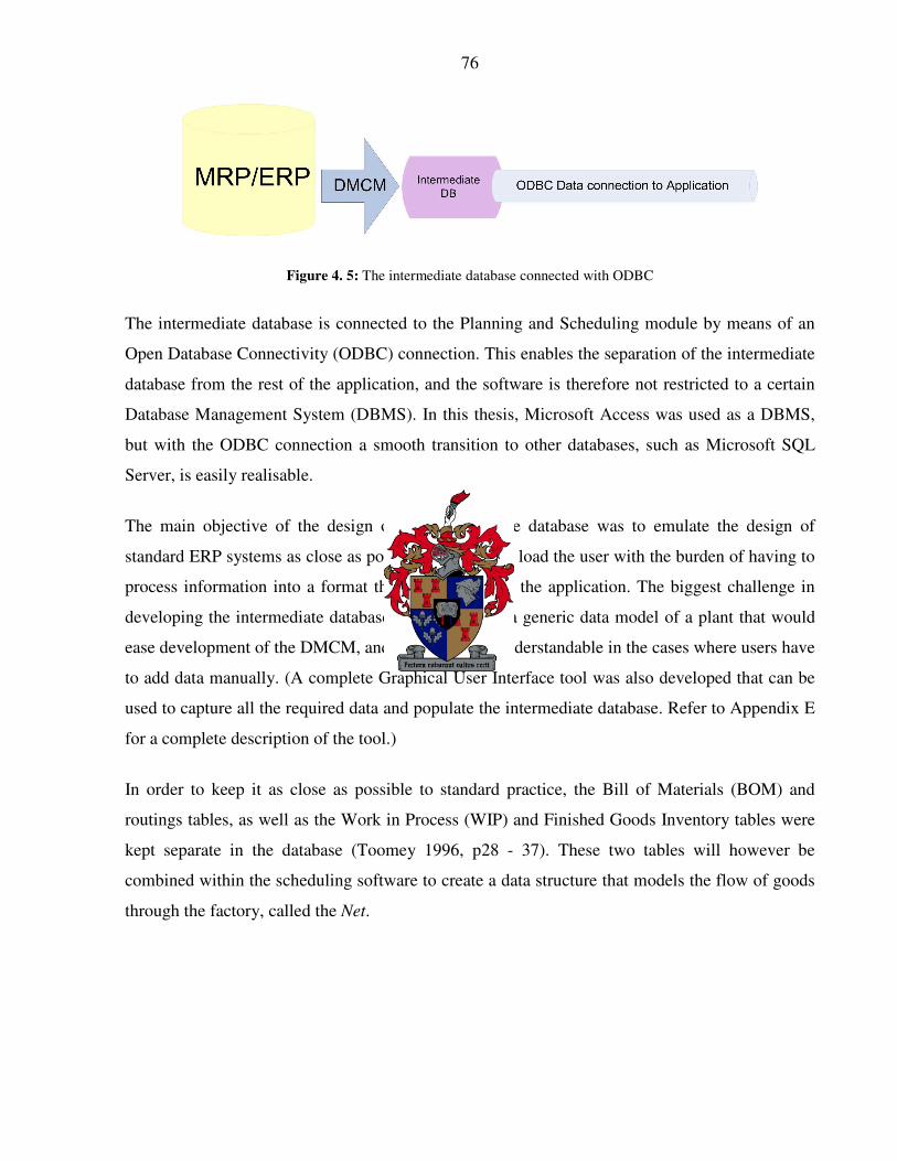
76

Figure 4. 5: The intermediate database connected with ODBC

The intermediate database is connected to the Planning and Scheduling module by means of an

Open Database Connectivity (ODBC) connection. This enables the separation of the intermediate

database from the rest of the application, and the software is therefore not restricted to a certain

Database Management System (DBMS). In this thesis, Microsoft Access was used as a DBMS,

but with the ODBC connection a smooth transition to other databases, such as Microsoft SQL

Server, is easily realisable.

The main objective of the design of the intermediate database was to emulate the design of

standard ERP systems as close as possible, so as not to load the user with the burden of having to

process information into a format that can be read by the application. The biggest challenge in

developing the intermediate database was to develop a generic data model of a plant that would

ease development of the DMCM, and make it easily understandable in the cases where users have

to add data manually. (A complete Graphical User Interface tool was also developed that can be

used to capture all the required data and populate the intermediate database. Refer to Appendix E

for a complete description of the tool.)

In order to keep it as close as possible to standard practice, the Bill of Materials (BOM) and

routings tables, as well as the Work in Process (WIP) and Finished Goods Inventory tables were

kept separate in the database (Toomey 1996, p28 - 37). These two tables will however be

combined within the scheduling software to create a data structure that models the flow of goods

through the factory, called the Net.

77

In order to keep the tool as generic as possible, two assumptions were made concerning data

entry:

x� All times are specified in terms of fractions of hours. Process times are therefore given as,

e.g. 0.25 hours (15 minutes) etc.

x� Due dates are specified by shift dates and it is implied that the order must be shipped at

the end of the specified shift, e.g. at the end of shift 3 on 15 January 2004.

The user must be able to verify the information in the database as correct before scheduling starts.

Furthermore, information such as product routings and shifts that are available for production

must be changeable for the exploitation and subordination phases.

Extended Entity Relationship Diagram

An Entity Relationship Diagram (ERD) is a diagram that pictorially represents entities, the

relationships between them and the attributes used to describe them in a relational data model.

The Extended Entity Relationship Diagram (EERD) of the intermediate database, as implemented

in Microsoft Access, is shown in Figure 4. 6. Refer to Appendix B for the complete Entity

Relationship Diagram (ERD) and EERD, as well as a complete description of each table and the

fields they contain.

78

Figure 4. 6: EERD of the intermediate database as implemented in Microsoft Access

4.5.3 Scheduling parameters and other data

Apart from the subset of data that is normally housed in the MRP or ERP database, certain other

parameters are also needed to develop schedules. This data is however very specific to the DBR

and S-DBR methodologies. It was decided to store this information in a separate location as data

files on the hard disk (parameters.txt, custum_buffers.xls, and custom_redlines.xls).

Parameters that are used for both DBR and S-DBR are the planning horizon and the Resource

Capacity Limit. These values are not stored on disk.

BOM bom_parent_id bom_child_id bom_qunatity

79

1. Planning horizon: The dates and shifts of the start and end of the planning horizon will

have to be specified each time that scheduling is performed. Orders with due dates in the

stretch of time equal to the planning horizon plus one shipping buffer must be scheduled

for. This time period is known as the Effective Horizon.

2. Resource capacity limit: The user can specify a default value to which the capacity used

at each resource must be limited. This value is specified as a percentage and is set as the

limit to which resources are loaded for each shift during the identification and exploitation

phases. For the first identification run a global value is specified and is applied to all

resources. The user can then specify a customised value for each individual resource

during the later phases.

Conventional Drum-Buffer-Rope parameters are different than the parameters for Simplified

Drum-Buffer-Rope, as the constraint buffer, and exploitation phase of the CCR fall away under

S-DBR. Conventional DBR parameters are:

1. Buffer lengths: The user is able to specify default values for the buffers lengths. In

accordance with the latest developments in DBR, only the shipping and constraint buffers

are specified and used. The shipping buffer is a liberal estimate of the complete

production lead time. The constraint buffer is a liberal estimate of the lead time for a part

from material release up to the first time that it is in front of the Capacity Constraint

Resource. Default buffer lengths are stored in the data file, parameters.txt. An advanced

option is to customise the buffer lengths for specific products on order. A record is kept of

products with customised buffer lengths in the custom_buffers.xls file, which is a

Microsoft Excel spreadsheet. The use of a spreadsheet makes it easy for the user to enter

data in the case where there are a lot of products with customised buffer lengths. It will

therefore not be necessary to specify customised buffer lengths every time scheduling is

done. Buffer lengths must be specified as an integer value, in hours.

2. Late order threshold: This value is specified to identify potential late orders during the

exploitation phase. After parts leave the CCR for the last time, the time equal to the

shipping buffer minus the constraint buffer should be available to get orders ready for

shipping before the specific order’ s due date. This time is referred to as the remaining

shipping buffer. The late order threshold is specified as the percentage of the remaining

80

shipping buffer that must be available after the specific part on order has left the CCR for

the last time up to its due date. In other words, if it is specified as 50%, when the CCR

schedule has been formulated, and the time from where a part on order leaves the CCR for

the last time, up to its due date is less than 50% of the remaining shipping buffer, the

order will be flagged as a potential late order. This value is 50% by default and is not

stored on hard disk.

Simplified Drum-Buffer-Rope parameters are the buffer lengths (excluding the shipping buffer)

and Red Line control values:

1. Buffer lengths: In the case where S-DBR is used, default buffer lengths and customised

buffer lengths can still be specified, and is stored in the same location. The only

difference for S-DBR is that only the shipping buffer length is specified.

2. Red Line control: In the case where conventional DBR is used, shop-floor control is

exercised by means of buffer management. The control method used for S-DBR is termed

Red Line control and is specified for order due dates and raw material inventory. Default

Red Line values are stored in the parameters.txt data file on hard disk.

a. Red Line values for order due dates are specified in hours, and is a fixed length

rather than a percentage of the shipping buffer. It is determined by evaluating how

long it takes to expedite a medium sized order.

b. The Red Line value for raw material inventory is specified as a number of parts. It

is calculated by multiplying the consumption rate of the most frequently used

product by the lead time of an emergency delivery by the organisation’ s fastest

supplier. The software allows the user to specify customised Red Line values for

all finished and raw material parts. The customised values are stored in an external

Microsoft Excel spreadsheet (custom_redlines.xls).

4.5.4 DBR and S-DBR planning and scheduling module

The DBR and S-DBR planning and scheduling module forms the heart of the system, and applies

the core business logic, described in Chapter 3, to the input data. This module uses the

information gathered by the DMCM and stored in the intermediate database to create shop floor

schedules according to the adapted Goal System scheduling algorithm, or the Simplified Drum-

81

Buffer-Rope method of scheduling. The module needs to perform the steps of identifying the

constraint, exploit the constraint by scheduling it, and subordinate the other resources by

developing a material release schedule in accordance with the constraint schedule.

One of the main objectives of the planning and scheduling module is to create schedules as

rapidly as possible. To speed up the calculations, the module first creates a model of the plant

according to the input information in computer memory, called The Net, before the identification,

exploitation, and subordination steps begin. This is done to avoid unnecessary computing times

due to disk read and write cycles. The role of the intermediate database is to capture a snapshot of

certain information in the company’ s MRP or ERP database. The idea is to use this data as a

starting point, and investigate the results of adjusting the information to adapt to the company’ s

current circumstances. The DBR4JS software does not to write the data of the intermediate

database back into the MRP or ERP database. The aim is to create feasible DBR or S-DBR

schedules that can be exported to an Excel spreadsheet to be released and distributed to the shop

floor. There is therefore no feedback loop to the MRP or ERP system, except if the software

helps to create enough support to permanently change the data in the database.

The Net is created from the data gathered by the DMCM and stored in the intermediate database

by executing a number of sequel (SQL) queries based on the parameters specified by the user.

The ODBC connection to the intermediate database allows SQL queries to be used, making the

intermediate database independent of the rest of the software. Changing the database

management system of the intermediate database does therefore not compromise the system

functionality.

A what-if approach to scheduling the shop-floor is supported by the Net by allowing the user to

manipulate data in computer memory and quickly see the effects of the changes on the schedule

and the ability of the plant to meet order due dates. It is of the utmost importance to keep a copy

of the validated database, to be able to recreate the Net if the information has been manipulated to

such an extent that a dead end has been reached in the exploitation and subordination efforts. For

this reasons all data manipulation that is done throughout the scheduling, exploitation, and

subordination phases occur within computer memory.

82

The flow diagram of Figure 4. 7 (on the next page) shows how the DBR and S-DBR planning

and scheduling module is to be used to create shop floor schedules.

The end result is exported to formats that are readable by other existing software, to easily

distribute the created schedules on the shop floor. For the purpose of this thesis it was decided to

export schedules to Microsoft Excel, as it is a package that is almost standard in industry today.

83

Figure 4. 7: Flow diagram of the DBR and S-DBR planning and scheduling module

84

4.6 Developing and documenting software

This section describes the detailed development of the scheduling system in computer software.

A full user manual was also developed as part of the software documentation, and can be viewed

in Appendix E.

The borders of development of the Drum-Buffer-Rope for Job Shops (DBR4JS) software were

set as follow:

x� Develop a mechanism to store and maintain the resource and order information needed for

scheduling;

x� Develop a tool that will use this information to assist the scheduler to develop DBR and

S-DBR schedules by following a “ What If” approach to scheduling;

x� Develop a mechanism that will make these schedules available to easily communicate the

developed schedules to the shop floor.

In this project all the above mechanisms were designed in detail and implemented in computer

code to form a completely designed and developed software package. An interface to manage

data entry into the intermediate database also formed part of the development done in this project.

The development of a support tool that will mine the needed information from the existing ERP,

MRP or other manufacturing database (DMCM) is however application specific, and was

therefore falls outside of the scope of development.

The biggest challenge in the development of the scheduling software was to create schedules as

rapidly as possible, and to provide the scheduler with enough features to change input parameters

in order to facilitate an interactive “ What If” approach to creating near optimal DBR and S-DBR

schedules. To make this possible, almost all the necessary information needs to be read into

computer memory before scheduling starts. This was the motivation for using C++ as

development platform for the DBR4JS software, as it allows the developer to take complete

control over memory allocation and allows the creation of very efficient structures to manage

computer memory. Microsoft’ s Visual C++ further has predefined libraries, called the Microsoft

Foundation Classes (MFC), which facilitates rapid development of Graphical User Interfaces

85

(GUI’ s) and database management functions. The software of this thesis, DBR4JS, was

developed using Microsoft Visual Studio 6.0 and MFC.

C++ has the further advantage of being an Object Orientated (OO) programming language. An

Object Oriented Design (OOD) approach was followed in modelling the generic plant, using the

Net. OOD allows the developer to create objects of classes. A class can best be viewed as a

generic framework and objects of specific instances of the class can then be created. An object

model in C++ is simply a set of classes and primitive types that are typically grouped into a

logical hierarchy to model or represent real-world or conceptual objects. In this way, the plant

can be modelled very similar to a physical plant, where there are, for example, objects of specific

resources and orders.

The following few paragraphs describe the algorithms that were developed to implement the

different scheduling steps of Figure 4. 7 in computer software.

4.6.1 Creating The Net

When the user is satisfied that the information in the intermediate database is an accurate

description of the shop floor, the Net can be created. Almost all of the Net’s data structures are

created as “ linked lists” (fourteen such lists are created in total). A linked list is best described as

a chain of small data elements, or objects, linked together with pointers. Each data element

contains a number of fields, almost like a row in a database. The last two fields however are two

pointers, pointing to the previous and next data elements in the list respectively. In this way, the

list can be created in compile time, but can grow and shrink dynamically during execution time.

The concept is shown graphically in Figure 4. 8.

Figure 4. 8: Linked Lists in computer memory

86

The Net consists out of linked lists that store shift-, resource-, inventory-, product and part-

(routings and Bills of Material), and order information. Figure 4. 9 shows how resource

information is stored in the Net.

Figure 4. 9: The resource list in The Net

87

Each Resource object contains three dynamically linked lists, the Capacity List, the Load List,

and the Level List. These lists are used to assign work and available capacity to each resource

during the identification, exploitation and subordination phases. The example of the resource list

is used to illustrate how objects of all the elements in the plant are used to model the whole plant,

products, and orders, etc. The complete Net is formed by the integration of all the various objects.

Attributes of objects are linked to one another relationally. For instance, the capacity of each

resource is dependent on the length of the shifts that the resource is assigned to. By changing the

length of the shift, all the available capacities of all resources are automatically updated, without

having to change each individual resource object. This considerably speeds up computation time.

The integration of the various lists, that form the Net, is shown in Figure 4. 10.

Figure 4. 10: Data structure integration

88

4.6.2 Identifying the constraint

The Master Production Schedule (MPS) is a list of all the orders with their due dates falling in the

effective horizon. The load on the plant is determined by working through the MPS and

determining the load of each order on each resource. To ensure that capacity is always used

backwards in time, the MPS must be sorted with the order with the latest due date first

(Schragenheim and Dettmer 2001, p. 110-112). To further accommodate for the customised

buffer lengths, the due date according to which the MPS is sorted, must be the order due date

minus the order’ s remaining shipping buffer after subtracting the constraint buffer. (For the

purpose of this document, the aforementioned date will be termed the constraint due date.)

Before the identification and scheduling phases can begin, an order specific product flow diagram

has to be created in computer memory for each order on the sorted MPS. This is necessary to

accommodate for order sizes and the inventory on hand. Inventory can now be allocated to

specific orders and is allocated first come, first served, meaning that inventory gets allocated to

orders with the earliest constraint due date first. It is therefore necessary to check each Part

Operation for a specific order, to see how many parts need to be processed while taking the WIP

into consideration. This means that all the processes of making a product may not have to be

followed on specific orders, as some of the parts may already be available from inventory. The

generic Product Flow Diagrams of the different products are used for this process, combined with

the inventory list. The representation of the structure in memory is depicted in Figure 4. 11.

89

Figure 4. 11: Order specific Product Flow Diagrams

The order specific Product Flow Diagrams (PFD) are created by moving down the sorted MPS

and identifying each part that needs to be made. The specific end part is then identified in the list

of generic PFD’ s stored in memory. The first step is to calculate the number of end parts that

need to be made, by comparing the order quantity to the number of the specific part in the

Inventory List. The inventory level of the specific part is also adjusted, if there is any. If there are

not enough parts in inventory to cover the order quantity, a linked list of PartOp objects is

created. The PartOp field of the Order object points at the first PartOp needed to be made, which

is the product on order. The procedure then walks down the generic PFD and creates PartOp

objects of all the operations needed to be performed to create the order. The specific quantity of

each PartOp is calculated by taking into consideration the number of parent parts needed to be

produced, and the number of parts in inventory.

As PFD’ s are stored as one dimensional lists in memory, the hardest part of calculating

production quantities is to keep track of when different legs of assembly operations have been

entered and left. This problem is solved by saving the ID of the current part being visited in

memory. Each time a new part is reached, the current part’ s ID and quantity that needs to be

made is placed on a stack (see class CPlate and CplateStack in the software code). If the new part

90

is a child part, its parent is located from the stack of saved parts. The number needed to be made

for one end part is retrieved from the generic PFD. The production quantity is then calculated as

follows:

gleparentinv

gleparentinv

invgleparentpart qqq

qqq

qqqq

sin

sin

sin **

*0

�t®̄­ �

...[4. 1]

where

partq is the production quantity of the part

parentq is the production quantity of the parent part

invq is the quantity of the specific part in inventory

gleqsin is the quantity needed to make a single parent part

The procedure used to create order specific PFD’ s is shown in Appendix C (Refer to method

IdCompleteMPS() of class CDBR4JSDoc in the software code of Appendix D).

After order specific Product Flow Diagrams have been created, the identification procedure can

be performed. Identifying the CCR involves calculating the load of each order on each resource

for every shift in the effective horizon. Saving on setup times can severely increase the capacity

on a resource. For the purpose of identification, setups are only included once per order. Doing

this levels the playing field to identify possible threats.

Calculating the load of each order on each resource might become a lengthy task in the case

where a company has a lot of resources and a lot of orders in the horizon. To be able to follow a

“ What If” approach to scheduling, computing times have to be kept to the minimum, in order to

see effects of different approaches quickly. For this reason, two different identifying procedures

were implemented. The first is a rough-cut capacity check on each resource. It can be done very

quickly, but should only be used to identify a definite resource constraint. Should the method not

identify a very definite resource constraint, an alternative, more thorough, method is used for the

identification procedure.

91

Rough-cut capacity check

The role of the shipping buffer is to protect the order due dates against statistical fluctuations.

When doing a rough-cut capacity check, it must be taken into consideration that the time between

the finishing time of a load on the constraint, and the due date of the order that the load is for, is

not available to place loads in. Doing a capacity check by simply dividing the capacity by the

demand ignores this. When placing loads on the constraint resource, it must always be done

backwards in time.

The rough-cut capacity check is best described by the overflowing-bucket analogy shown in

Figure 4. 12.

Figure 4. 12: Overflowing bucket analogy

In the representation above, each shift that a resource is assigned to can be seen as a bucket, with

a specified capacity. As work is assigned to the resource, the bucket representing the shift in

which the work is to be done (order due date minus the time: shipping buffer minus constraint

buffer) starts to be filled. When the bucket reaches its limit, the work starts to overflow. As the

purpose of the shipping buffer is to protect order due dates, the work that overflows is assigned to

the bucket before (previous shift). The process is repeated until the very first bucket is reached.

The amount of overflow for each resource indicates the amount of capacity that the resource

lacks to fulfil all order due dates. The resource with the most overflow is labelled as the Capacity

92

Constraint Resource (CCR). The algorithm that was developed to implement the process in

computer memory is shown in Appendix C. (Refer to method IdIdentifyCCR() in class

CDBR4JSDoc of the programme code)

The algorithm is only adequate for identifying resources with a definite lack of capacity for a

given set of production orders. This means that if the algorithm identifies a resource as being the

CCR, the resource will definitely experience difficulty in fulfilling all its due dates. As the

algorithm does not concentrate extensively on the sequencing of orders on a daily resolution, and

it further ignores offsets for rods (see Chapter 7.2.2), a secondary check should be performed in

cases where the algorithm does not definitely identify a resource as a CCR. The advantage of

using the algorithm is that it can be done very quickly, and a detailed analysis of each resource is

not necessary (if it identifies the primary CCR). Further, the literature shows that the OPT

software developed by Goldratt follows a similar rough-cut capacity check procedure to identify

the primary constraint (Meleton 1986, p. 13), (Spencer1991, p.22).

Detailed identification procedure

The detailed identification procedure is in fact the first two steps of the exploitation phase,

executed on every resource in the plant. It takes each resource, one by one, and assumes that it is

the CCR. It then performs the first two steps of the exploitation phase on the resource, to create a

finite backwards schedule for it, based on the processing times stored in the intermediate database

and read into the Net. The way it was implemented in software is to display these calculated

schedule times of each resource to the user. The user can then check to see which resource is

scheduled furthest into the past. The resource scheduled to start working the furthest in the past is

then the CCR.

The first step in the detailed identification procedure is to construct what is termed The Ruins

(Goldratt 1990, p. 204). The Ruins is obtained by placing each load on the investigated resource

at its “ perfect” time, that is the order’ s due date minus the shipping buffer (in the case for S-

DBR) or the due date minus the remainder of the shipping buffer (shipping buffer – constraint

buffer) in the case of DBR. At this stage, capacity limitations are ignored, and only one setup per

order is taken into account. If the constraint has to perform more than one job on the same order,

time has to be allowed for the processes between constraint operations. The concept of “ batch

93

rods” was introduced by Dr Goldratt (1990a, p. 219-220) to address this problem. A batch rod is

an offset of time between jobs on the same constrained resource for the same order. The size of

the batch rod is arbitrarily set to half of the constraint buffer size (Goldratt 1990a, p 218). Placing

a load is illustrated in Figure 4. 13.

Figure 4. 13: Placing loads with rods on a resource

The figure shows the load on the constraint for one order of product G. The routing for the

product is a simple five-step process, and is also shown in the figure. R2 is the CCR and has to

perform two operations on raw material A to produce product G. Between these two operations,

A020 and A040, resource R3 has to perform operation A030. The time allowed for operation

A030 is known as a rod. In the figure, TD is the order due date, TSB is the order due date minus

the shipping buffer (for S-DBR) or the due date minus (the shipping buffer minus the constraint

buffer) for DBR. TS2 is the start time of the second load, and TR is the length of the rod.

The use of “ batch rods” and the calculation of the appropriate placement for a batch rod are

explained by Simons and Simpson (1996, p2406-2407). The basic idea is to let half a CCR-buffer

time between operations performed on the same CCR for the same order. The placement of the

rod between loads is dependent on the processing time per unit. When the processing time per

R1 R2 R3 R2 R4

A G X X

A010 A020 A030 A040 A050

time

TD

A040 A020

TD - TSB

R2

TS2 – TR TS2

94

unit is smallest for the earlier CCR operation, the rod is placed between the scheduled completion

of the first unit of the first CCR operation, and the scheduled start of processing of the first unit

on the second CCR operation (Figure 4. 14(a)). When the opposite is true, i.e. the per unit

processing time for the first CCR operation is largest, the rod is placed between the scheduled

completion of the last unit on the first CCR operation, and the scheduled start of processing of the

last unit on the second CCR operation (Figure 4. 14(b)).

(a) (b)

Figure 4. 14: Placing rods between loads (adapted from Simons & Simpson 1996:2407)

The Ruins is built in the software by taking into consideration due dates, the specific order’ s

shipping buffer, and rod lengths. The algorithm for building The Ruins is shown in Appendix C

(refer to method ExploitBuildRuins() of the CDBR4JSDoc class in the code of Appendix D). In

this algorithm, Load objects are added to the Load List (refer to Chapter 6.3) of each resource.

The biggest challenge in developing the algorithm is to keep track of the location of the

constraint resource in production legs. A stack memory structure (CCCRStack and CCCRPlate)

was used to solve the problem.

The Ruins for eight jobs performed by the CCR is shown in Figure 4. 15 (Rods are not shown in

the following example). At this stage the actual available capacity of the CCR is not taken into

account.

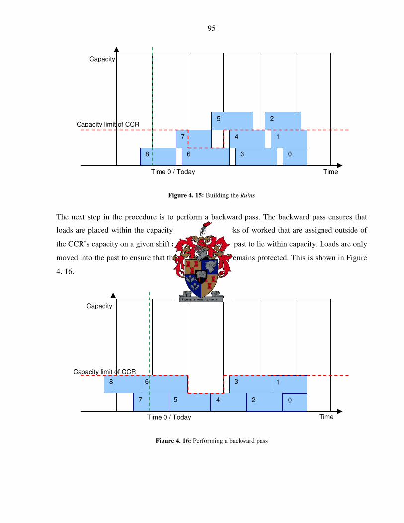
95

Figure 4. 15: Building the Ruins

The next step in the procedure is to perform a backward pass. The backward pass ensures that

loads are placed within the capacity of the CCR. Blocks of worked that are assigned outside of

the CCR’ s capacity on a given shift are moved into the past to lie within capacity. Loads are only

moved into the past to ensure that the shipping buffer remains protected. This is shown in Figure

4. 16.

Figure 4. 16: Performing a backward pass

0

1

2

3

4

6

5 7

8

Time

Capacity

Time 0 / Today

0

1

2

3

4

6

5

7

8

Time

Capacity

Capacity limit of CCR

Time 0 / Today

Capacity limit of CCR

96

The procedure for doing the backward pass (method ExploitBkwdPass() of class CDBR4JSDoc)

also takes the rods between loads into consideration. The flow diagram of the procedure is shown

in Appendix C.

In cases where loads are scheduled to start before time zero, times will be indicated as negative

values. The user can identify the CCR by identifying the resource of which the first load’ s start

time is the most negative. When using DBR scheduling, the software asks the user that the

resource identified as the CCR by the rough-cut capacity check is indeed the resource that should

be scheduled as the CCR. The user then has the opportunity to specify another resource to be

scheduled as the CCR if the detailed identification procedure indicates a CCR.

A screenshot of the outcome of the identification procedure is shown in Figure 4. 17.

Figure 4. 17: Screenshot of the outcome of the identification phase

97

4.6.3 Exploiting the constraint

The following procedure is only applied when the user has chosen to do conventional DBR

scheduling of the production facility.

Exploiting the resource constraint must fulfil three functions:

1. Build the Drum, that is to develop a detailed schedule for the CCR based on order due

dates and the shipping buffer;

2. Inform the master scheduler of orders that are going to miss their due dates due to

capacity constraints in advance;

3. Make it possible to revise the schedule in order to gain even more out of the CCR

through the shop floor worker’ s knowledge of the specific plant.

In cases where there is a definite resource constraint, a detailed schedule must be devised for the

constrained resource in order to exploit it. The method followed in this thesis is the forward-

backward scheduling procedure as suggested by Goldratt (1990a, p. 201-221) and described in

further detail by Stein (1996, p. 82 – 110). The procedure is actually subdivided into three

procedures: building the Ruins, performing a backward pass, and performing a forward pass.

The first two steps of the algorithm, building the Ruins and the backwards pass, has been

explained in Chapter 4.6.2. The only difference is that during the exploitation phase these steps

are only executed on a single resource, the resource identified and confirmed as the CCR by the

user. The next step is to perform the forward pass.

The forward pass moves loads that are scheduled to start in the past (before time zero), after the

backward pass is completed, to be done in the present or future. This is shown in Figure 4. 18.

98

Figure 4. 18: Performing the forward pass

The end result of the forward-backward algorithm is the placement of loads as close as possible

to their ideal time on the CCR, while considering capacity limitations. Although finite scheduling

on the constraint is in fact done in computer memory, the aim is to establish the sequence of

operations according to their ideal completion times.

The forward pass procedure is implemented in the ExploitFwdPass() method of class

CDBR4JSDoc in the software source code. The flow chart of the algorithm used is shown in

Appendix C.

The backward and forward shifting of jobs in the previous steps is more than likely to cause some

jobs to have less than the desired shipping buffer remaining, or even to exceed their order due

dates. The next step in the exploitation phase is therefore to check that all the orders will be

completed on time, and to highlight orders that will experience problems in meeting their due

date requirements. Goldratt (1990a, p. 206) suggests that orders that have less than half a

shipping buffer’ s (or in this case, the shipping buffer minus the constraint buffer) worth of time

left for the remaining operations to be completed after it has left the CCR, is certain to miss its

due date. The DBR4JS software allows the user to specify a threshold time for late orders. The

time is specified as a percentage of the buffer time after the last CCR operation, this being the

shipping buffer minus the constraint buffer. The following example explains this concept:

0

1

2

3

4

6

5 7

8

Capacity

Time 0 / Today Time

Capacity limit of CCR

99

Say the user has specified a shipping buffer of eight hours and a constraint buffer of four hours.

The buffer time after the last CCR operation is then equal to four hours. If a late order threshold

time of 50% has been specified for a specified order, it means that the order will be flagged as a

late order if, after scheduling, there is less than two hours between the scheduled end time of the

last operation on the CCR for the order, and the order due date.

The CCR schedule is presented visually to the user by the DBR4JS software in a graphic similar

to Figure 4. 18. Late orders are flagged by placing a red border around them. A screenshot of the

outcome of the exploitation phase is shown in Figure 4. 19.

Figure 4. 19: Output screen of the exploitation phase

4.6.4 Subordination

The last step in both the DBR and S-DBR scheduling processes is to subordinate the rest of the

resources to the pace set by the drum. In the conventional DBR environment the drumbeat is

given by the CCR schedule. In the S-DBR environment, the validated Master Production

Schedule gives the drumbeat.

The way Subordination was approached in this thesis for both the DBR and S-DBR approaches

was to develop a material release schedule. The schedules developed for each approach are

discussed below.

100

Conventional Drum-Buffer-Rope

Material release schedules are calculated based on the order due date, the constraint date as

calculated by the exploitation procedure, the size of the shipping buffer, and the size of the

constraint buffer. Although finite scheduling is done on the CCR, the end result shown to the user

is only given in terms of the dates and the sequence.

It was decided to base the subordination phase of this thesis on a new, unpublished article by two

of the leaders in the field of the Theory of Constraints, Goldratt and Schragenheim (2005). (The

article is included in Appendix A). In this article it is stated that the notation of three buffers in

DBR has been replaced by only two buffers in the new TOC training material. The implications

are as follows:

x� The assembly buffer falls away;

x� The shipping buffer now relates the entire lead time for producing a product;

x� The constraint buffer is a part of the shipping buffer;

By not using an assembly buffer, material release dates are then calculated as follows:

CCRpassespart

partCCRwithassemblednotisandCCRpassnotdoespart

partCCRwithassembledisbutCCRpassnotdoespart

tt

tt

tt

t

CBCD

SBD

SBD

MR

,

°°°¯

°°°®

­

�

�

�

...[4. 2]

where

MRt is the material release date

Dt is the due date of the order

SBt is the size of the shipping buffer

CDt is the constraint date as calculated in the exploitation phase

CBt is the size of the constraint buffer

101

The schedule is created by moving down the PFD of each order on the MPS and analysing each

Part Operation. If the visited Part Operation is and end product, a shipping schedule entry is

added to the schedule for the order. If the Part Operation is performed on the CCR, a CCR

schedule entry is added, and the load associated with the specific Part Operation is saved on a

stack. When a raw material entry is reached the last CCR load is read from the stack, and the

material release date for the specific material is calculated by creating an offset in time

backwards from the scheduled start date of the retrieved CCR load. If there is no CCR load

stored, the material release date is calculated by creating an offset backwards in time from the

order due date that is the same size as the shipping buffer. Material release cannot be scheduled

past day zero.

The final schedule, as created by the conventional DBR scheduling procedure is shown in Figure

4. 20.

102

Figure 4. 20: Conventional Drum-Buffer-Rope schedule created by the DBR4JS software

103

Simplified Drum-Buffer-Rope

In the S-DBR environment, the material release schedule is simply calculated by subtracting the

shipping buffer length from the order due date. Once again, material release cannot be scheduled

before day zero, the start of the effective horizon.

The control methods of Simplified Drum-Buffer-Rope are Planned Load and Red Line control. It

was decided in this thesis to aid the scheduler with the control methods of S-DBR, as they are

relatively new terms. Planned Load is facilitated for in the Capacity Planning features of the

Identification phase. Red Line control parameters are set at the beginning of the S-DBR

procedure and implemented in the final schedule. Red line values are indicated on the schedule

for every order (Red Line Date) and for every raw material (Red Line Quantity). The number of

raw materials that should be re-ordered, as well as the re-order date is calculated for each usage

of every raw material, based on the Red Line quantity specified, the number in stock, and the lead

time of the specific raw material.

An example of a Simplified DBR schedule, as constructed by the DBR4JS software, is shown in

Figure 4. 21.

104

Figure 4. 21: Simplified Drum-Buffer-Rope schedule created by the DBR4JS software

105

4.7 Testing and maintaining the system

Before the information system could be used it had to be tested. The following paragraphs

describe some of the tests that were performed on the software before populating it with the data

from Aerodyne Aviation Technologies.

4.7.1 Validating the system

The developed DBR4JS software creates DBR and S-DBR schedules by guiding the user through

six steps (and jumping back and forth between them). These steps are:

1. Set up and validate the intermediate database information;

2. Set up the parameters for scheduling and build the Net;

3. Identify the Capacity Constrained Resource;

4. Exploit the CCR (only in the case of traditional DBR);

5. Subordinate material release and shipping;

6. Export the calculated schedule to Microsoft Excel.

The step-wise flow of the programme allowed for modular developing and testing of the

software, after the complete system and all the data structures were designed. The process

followed was to develop a “ step” in the programme, test it thoroughly, and then move on to

developing the next “ step” . Final testing of the complete package was done after all the steps

were integrated into a single system. Along with verifying calculations, a big part of the testing of

each step was to make sure that there was a seamless integration with the previously developed

steps.

To facilitate rapid calculations and scheduling, the management of allocated memory played a

big role in the development of the software. A good example of this is the Load List of each

resource. The Load List is a dynamic linked list created in memory for each resource that stores

the workloads placed on it for a given set of orders. This is created for each resource in the

identification phase. During the exploitation phase each resource’ s list is deleted, except for the

identified CCR. When skipping back to the identification phase, the software must first check

that all the loads have been deleted, and then reconstruct the structure for all resources. Memory

106

that has been released (by deleting the Load List) cannot be referenced, otherwise the programme

will fail. Testing the software involved to follow every possible road in developing schedules,

jumping back and forth between every different step as much as possible to ensure that memory

allocation was done correctly, and the software does not fail.

Apart from the testing performed after each step in the software was developed, various

experimental scenarios were used to validate the calculations of the software. The following is an

example of such a scenario.

Figure 4. 22: Product Flow Diagram of "Product A"

Figure 4. 22 represents the Product Flow Diagram of Product A. It shows the different work

centres (resources) that the parts must visit to form the final product, and the per-unit processing

time spent at each (in minutes). It consists out of two sub-parts, Part E and Part F, which consists

out of raw materials RM-1 and RM-2 respectively. For the sake of the example it is assumed that

setup time is one hour at each work centre. For the example an order for 90 units of Product A is

placed on the fourth shift (having an ID of 050804-01 in this case, meaning the first shift on the

fourth of August 2005). The plant is scheduled to work one eight-hour shift each week day

(Monday to Friday). The shipping buffer for Product A is set to ten hours and the constraint

buffer is five hours.

107

Building the Net

It was mentioned in paragraph 4.6.2 that the Product Flow Diagrams of all the different products

are stored as one-dimensional lists in the computer memory. Functionality was built into the

DBR4JS software to check whether the PFD’s of different products are read into memory

correctly, and whether the number of parts needed to be produced was calculated correctly. The

single-level PFD and production quantities are shown in Figure 4. 23.

Figure 4. 23: Single-level Product Flow Diagram of "Product A"

If the WIP levels are adjusted in the intermediate database to hold 45 units of part F at WC-4, it is

expected that only 45 units need to be processed at WC-3 and WC-1 respectively, and that only

45 units of RM-2 should be released. The results of making the adjustment and re-constructing

the Net are shown in Figure 4. 24.

108

Figure 4. 24: PFD adjusted for Work in Process

Identification

Setup times are only taken into account once for each resource for the purpose of identifying the

CCR. For the given example, one setup per Part/Operation is however taken into account, as

there is only one order in the system. The total processing time calculation for each resource and

the scheduled start time, as calculated in Microsoft Excel, is shown in Table 4. 1.

Setup [hr]

Run Time [hr]

Setup [hr]

Run Time [hr]

WC-PK 1.00 0.133 0.00 0.000 11.97 12.97 3WK-AS 1.00 0.050 0.00 0.000 4.50 5.50 4WC-1 1.00 0.067 1.00 0.067 12.06 14.06 3WC-2 1.00 0.150 0.00 0.000 13.50 14.50 3WC-3 0.00 0.000 1.00 0.233 20.97 21.97 2WC-4 1.00 0.200 1.00 0.100 27.00 29.00 1WC-5 1.00 0.167 1.00 0.167 30.06 32.06 0WC-6 0.00 0.000 0.00 0.000 0.00 0.00 4WC-7 1.00 0.117 0.00 0.000 10.53 11.53 3WC-8 0.00 0.000 1.00 0.167 15.03 16.03 2

Work CenterTotal Run Time

[hr]Total Processing

Time [hr]

Scheduled Start Time

[Shift Index]

Operation 1 Operation 2

Table 4. 1: Identification calculation

109

Product A was stored in the intermediate database by means of the integrated database

management tool, with the processing and setup times as indicated in Table 4. 1. The results of

the identification procedure of the DBR4JS software for these values are shown in Figure 4. 25.

110

Figure 4. 25: Validation of the Identification procedure

111

For the purpose of the example the daily capacity limit of each resource was set to 100%. The

measured results, as calculated by the DBR4JS software, are shown in Table 4. 2.

WC-PK 12.97 3WK-AS 5.50 4WC-1 14.06 3WC-2 14.50 3WC-3 21.97 2WC-4 29.00 1WC-5 32.06 0WC-6 0.00 4WC-7 11.53 3WC-8 16.03 2

Total Hours of Work

Scheduled Start Time

[Shift Index]Work Center

Table 4. 2: Results of the Identification procedure

From the above results it can be seen that resource WC-5 has been correctly identified as the

CCR. If the capacity is limited to 90% each day, an overflow of 3.26 hours into the past for WC-

5 is expected. The result of the detailed overflow calculation in the DBR4JS software when the

daily capacity limit is set to 90% is shown in Figure 4. 26.

Figure 4. 26: Detailed overflow calculation

From Figure 4. 26 the calculated overflow is read as 3.26 hours.

112

Exploitation

Validating the exploitation step involves checking whether the sizes of different loads are

calculated correctly, whether setups are accounted for if needed, whether rod lengths are correct,

etc. For the example described above, it is expected that work on the constraint should be

scheduled to be finished at a time equal to the shipping buffer size minus the constraint buffer

size, which is five hours in this case, before the order due date. The routing for Product A

however indicates that the CCR, WC-5, has to perform two jobs on the order. There is also only

one machine of WC-5 that is scheduled to work for each shift. The DBR4JS software schedules

the CCR by creating a list of available time slots for the resource, and then fits the “ blocks” of

jobs into these time slots as per the Goal System algorithm. Manual calculations of start and

finish times for building the ruins, performing a backward pass, and performing a forward pass

under these restrictions are shown in Table 4. 3.

Shift Hour Min Shift Hour MinF/20 1.000 15.030 4.000 4.000 0.000 2.000 3.000 58.200E/20 1.000 15.030 4.000 4.000 0.000 2.000 3.000 58.200

Shift Hour Min Shift Hour MinF/20 1.000 15.030 2.000 3.000 58.200 -1.000 -4.000 -3.600E/20 1.000 15.030 4.000 4.000 0.000 2.000 3.000 58.200

Shift Hour Min Shift Hour MinF/20 1.000 15.030 3.000 0.000 1.800 1.000 0.000 0.000E/20 1.000 15.030 5.000 0.000 3.600 3.000 0.000 1.800

Part/OpSetup

[hr] Run [hr]

Finish Start

Run [hr]

Part/OpSetup

[hr] Run [hr]

Backward Pass

Forward Pass

Finish StartPart/Op

Setup [hr]

Finish

WC-5Building the Ruins

Start

Table 4. 3: Exploitation calculations

The end result will therefore be that the first operation is to be started immediately, and finishes

at the beginning of the third shift. The second operation will start at the beginning of the third

shift and end at the start of the fifth shift. The due date for the order was set at the end of the

fourth shift. Orders are seen as late in the traditional DBR environment if there is less than half

the shipping buffer minus the constraint buffer time left, after completion of the last CCR

113

operation until the order due date. This order is clearly late and should be indicated as such. The

output of the DBR4JS software for the situation above is shown in Figure 4. 27.

Figure 4. 27: Output of the exploitation phase for an order of "Product A"

From Figure 4. 27 it can be seen that loads are placed as expected from the manual calculations.

The blocks also have a red border, which is the mechanism for indicating late orders. (The

percentage of the buffer time that must be available between the last CCR operation and shipping

can be specified by the user, and was set to 50% for this example.) The detailed scheduling

information for each load is shown in Figure 4. 28 and Figure 4. 29 respectively.

Figure 4. 28: Scheduling information of load F/20 on WC-5

114

Figure 4. 29: Scheduling information of load E/20 on WC-5

The figures above indicate that the start time on the CCR for each load is calculated correctly, as

per the manual calculations of Table 4. 3.

The example above does not validate the rod length calculations. It is still correct however in not

inserting rods between the loads, as the loads are from different production legs of Product A.

Validating the rod length calculations is done by inserting an additional step in the routing of

Product A, to be performed on WC-5. The new product routing and processing times are shown

in Figure 4. 30.

Figure 4. 30: Revised Product A routing to validate rod calculations

115

In order to schedule the revised order, the constraint buffer (and therefore also the shipping

buffer) needs to be adjusted. This is because a rod length of half the constraint buffer needs to be

inserted between the CCR operation on Part A and the CCR operations on Parts E and F. The

constraint buffer is only five hours long, but the processing time of the loads are all roughly

fifteen hours long. By placing the rods as described in paragraph 4.6.2, there will not be enough

time between loads for interspersed operations. To accommodate the order the constraint buffer is

set to thirty-five hours and the shipping buffer to forty hours.

Per unit processing times for the given example are the same for all constraint loads. The

calculation of the length of the rod between loads is therefore given by equation 4.3.

116

� �� �1*2

�� ntc

l pubuff

rod

...[4. 3]

where:

rodl is the length of the rod between loads

buffc is the size of the constraint buffer

put is the per unit processing time

n is the number of parts

By substituting the constraint buffer as thirty-five hours and the per-unit processing time as ten

minutes for ninety units, the rod length is calculated as 1.637 hours. Figure 4. 31 shows a screen

shot of the exploitation phase for the example.

Figure 4. 31: Rod length validation output

The output of Figure 4. 31 also shows how loads are fitted into time slots. The remainder of the

time slot where the first two loads are fitted in is not large enough to fit the third load. It is

therefore carried over to the next time slot. (The user has the freedom to place the load wherever

he or she wants manually). The result of attempting to schedule the third load to start at hour 0 of

shift one is shown in Figure 4. 32.

117

Figure 4. 32: The effect of moving loads with rods attached to them

By trying to move the last load forward in time, the backward rods to the previous loads force

them to move as well, and the minimum required time is kept between loads. When manually

adjusting loads, the time slots constraints can be ignored to facilitate capacity planning. From the

detailed scheduling information for load E/20 (bottom left), the rod length between loads is

calculated as 1.632 hours. The order due date has been adjusted to the end of shift five, so the

order is not flagged as being late.

Subordination

To validate the subordination phase, the scheduled completion dates, scheduled CCR dates,

scheduled material release dates, and the production quantities of orders, as it will appear on the

final schedule needs to be checked. To validate the final schedule the example of Figure 4. 30 is

used again. Material release and the scheduled completion time of orders are calculated by

making use of the constraint buffer and the remainder of the shipping buffer. To illustrate the

calculation of material release the order due date is adjusted to be later in time. The earliest job

on the CCR is scheduled to start at the beginning of the effective horizon. This will result in the

material release time to be before the start of the horizon, which is automatically adjusted to the

118

start of the effective horizon by the software. If the order due date is adjusted to be at the end of

shift number thirteen, the CCR schedule for the order is shown in Figure 4. 33.

Figure 4. 33: CCR schedule with adjusted order due date

Table 4. 4 displays the calculations for the material release and order completion time based on

Figure 4. 33.

Shift Hour Min Shift Hour MinF/20 3.00 6.00 46.00 1.000 15.03 5.000 6.000 48.00E/20 8.00 4.00 18.00 1.000 15.03 10.000 4.000 20.00A/20 10.00 6.00 46.00 1.000 15.03 12.000 6.000 48.00

Start TimeOperation

Finish TimeSetup time [hr]

Run time [hr]

Table 4. 4: Detailed CCR schedule information

Raw materials RM-1 and RM-2 must be released for Part E and Part F respectively. Part A is

scheduled to be finished based on the completion time of PartOp A/20. The calculations for

material release and the scheduled completion times are shown in Table 4. 5.

119

Shift Hour MinF/20 Start Time 3.00 6.00 46.000 Constraint 35.000 RM-2 -1.00 -12 -14.000E/20 Start Time 8.00 4.00 18.000 Constraint 35.000 RM-1 4.00 1 18.000A/20 Finish Time 12.00 6.00 48.000 Remainder of Shipping* 5.000 Completion Time 13.00 3 48.000* ’Remainder of Shipping’ refers to the shipping buffer minus the constraint buffer

Shift Hour MinPart/OpFinish/Start Time Buffer

Length [hr]Buffer Type Calculation

Table 4. 5: Detailed material release and order completion time calculations

The calculations show that strictly speaking, RM-2 should be released some time before the start

of the effective horizon. This time will be pushed forward in time to be exactly on the start of the

effective horizon, in other words shift number one. RM-1 is to be released on shift four, and the

order should be finished no later than shift thirteen. The schedule (conventional DBR Schedule)

from the DBR4JS software for the same example is shown in Figure 4. 34

Figure 4. 34: Conventional DBR schedule for "Product A"

The schedule indicates that the order should not be finished later than at the end of shift number

thirteen (date: 13/08/05 shift nr 1). Raw materials RM-1 and RM-2 should be released on shift

number four (date: 04/08/05 shift nr 1) and shift number one (date: 01/08/05 shift nr 1)

respectively.

The CCR Schedule indicates that CCR operations for the order are on parts F, E, and A. The

CCR (WC-5) should start working on part-operation F/20 on shift number three (date: 03/08/05

shift nr 1). It should start working on part-operation E/20 on shift number eight (date: 08/08/05

shift nr 1) and on part-operation A/20 on shift number ten (date: 10/08/05 shift nr 1).

120

4.7.2 Testing the software

The robustness and ability of the software to handle data from a real manufacturing environment

was done by loading the system with a number of resources, shifts, parts, and orders. The orders

were put in the systems with completely random parts, quantities and due dates. The following

section describes the input data and results of an example test that was performed.

The scheduling horizon was selected for a period of four weeks (August of 2005). The system

contained four different products that orders could be placed for. The Bill of Materials, routings,

setup and processing times, and shipping- and constraint buffer times of the products (Product A,

Product B, Product C, and Product D) are shown in Table 4. 6.

Part A Work Station Setup Time Run Time Part B Work Station Setup Time Run TimeHours Minutes Hours Minutes

WC-PK 0.166666667 0.133333333 8 WC-PK 0.166666667 0.1 6WC-5 0.166666667 0.166666667 10 WC-AS 0.166666667 0.166666667 10WC-AS 0.166666667 0.05 3Part E Work Station Setup Time Run Time Part G Work Station Setup Time Run Time

Hours Minutes Hours MinutesWC-7 0.166666667 0.116666667 7 WC-6 0.166666667 0.25 15WC-5 0.166666667 0.166666667 10 WC-5 0.166666667 0.333333333 20WC-4 0.166666667 0.2 12 WC-4 0.166666667 0.15 9WC-2 0.166666667 0.15 9 WC-2 0.166666667 0.066666667 4WC-1 0.166666667 0.666666667 40 WC-1 0.166666667 0.116666667 7RM-1 RM-3

Part F Work Station Setup Time Run Time Part H Work Station Setup Time Run TimeHours Minutes Hours Minutes

WC-8 0.166666667 0.166666667 10 WC-7 0.166666667 0.066666667 4WC-5 0.166666667 0.166666667 10 WC-4 0.166666667 0.05 3WC-4 0.166666667 1 60 WC-1 0.166666667 0.15 9WC-3 0.166666667 0.233333333 14WC-1 0.166666667 0.066666667 4RM-2 RM-1

40 35 10 5

Part C Work Station Setup Time Run Time Part D Work Station Setup Time Run TimeHours Minutes Hours Minutes

WC-PK 0.166666667 0.166666667 10 WC-PK 0.166666667 0.166666667 10WC-8 0.166666667 0.133333333 8 WC-8 0.166666667 0.216666667 13WC-6 0.166666667 0.083333333 5 WC-6 0.166666667 0.216666667 13WC-5 0.166666667 0.25 15 WC-3 0.166666667 0.166666667 10WC-2 0.166666667 0.15 9 WC-1 0.166666667 0.2 12WC-1 0.166666667 0.166666667 10RM-3 RM-4

10 5 13 5Raw Material 4Raw Material 3

Raw Material 1

Raw Material 2

Raw Material 3

Raw Material 1Shipping Buffer Constraint Buffer Shipping Buffer Constraint Buffer

Shipping Buffer Constraint Buffer Shipping Buffer Constraint Buffer

Table 4. 6: Experimental input data for products on order

Details of the resources used are shown in Table 4. 7.

121

Resource ID Resource Name Nr MachinesWC-1 Work Center 1 5WC-2 Work Center 2 3WC-3 Work Center 3 3WC-4 Work Center 4 3WC-5 Work Center 5 8WC-6 Work Center 6 3WC-7 Work Center 7 2WC-8 Work Center 8 4WC-AS Assembly 2WC-PK Packaging 4

Table 4. 7: Experimental resource information

The software randomly generated one hundred orders for the products. Order sizes were limited

to one hundred parts and due dates were randomly selected between 1 August 2005 and 31

August 2005. A summary of the generated orders is shown in Table 4. 8 (Refer to Appendix F for

a full list of generated orders.

Order Part ID Number of OrdersA 40B 27C 15D 18Total 100

Table 4. 8: Summary of experimental orders

The input data was used to test the DBR4JS software on a personal computer, of which the

system specifications are shown in Table 4. 9.

Computer HP NX9010CPU Pentium 4

3.06 GHzRAM 512MBOperating System Microsoft Windows XP Professional

Version: 2002Service Pack 1

Table 4. 9: Hardware specification of test computer

122

The same experimental data was used to test the ability of the software to calculate both DBR and

S-DBR schedules. The software successfully completed each scheduling step for both methods

with the given input data. The processing times (taken with a hand-held stopwatch) of each step

were recorded and the results are shown in Table 4. 10. The output of the DBR4JS software for

each scheduling step is shown in Appendix F.

Time [minutes]

00:11:04

InstantaneousInstantaneousInstantaneousInstantaneous

Calculate 00:01:95Display Instantaneous

00:00:84InstantaneousInstantaneous

Change Load (with Rods) Start Time (Re-Calculate and Re-Display) InstantaneousInstantaneous

01:55:53

InstantaneousInstantaneousInstantaneousInstantaneous

Calculate 00:01:70Display Instantaneous

Instantaneous01:07:55

Subordinate (Create Schedules and Display)

View Orders (Calculate and Display)

Detailed ID

Add Order (Add and Re-display)

Exploit the CCR (Calculate and Display)View Load InformationChange Order Due Date (Re-Calculate and Display)

Create The Net (Calculate)

Identify the CCR (Calculate and Display)View Orders (Calculate and Display)

View Loadings (Calculate and Display)

Export Schedules to Excel

Process

DBR Scheduling

S-DBR Scheduling

Add Order (Add and Re-display)View Loadings (Calculate and Display)Detailed ID

Subordinate (Create Schedules and Display)

Export Schedules to Excel

Identify the CCR (Calculate and Display)

Table 4. 10: Test results of each process

The time measurements show that the only scheduling steps that really take up a significant

amount of time to perform, is creating the Net and exporting schedules to Microsoft Excel. These

are the only steps in which there is read from or written to computer hard disk by the DBR4JS

software. The actual scheduling and problem solving actions are calculated and displayed rapidly

enough by the software to allow and interactive “ What If” approach to scheduling for the input

data.

123

4.8 Implementing and evaluating the system

In the last phase of the SDLC, the analyst helps implement the information system. This is

mainly the topic of Chapter 5, in which live data from the Echo line at Aerodyne Aviation

Technologies will be implemented in the DBR4JS software. This section will describe the

functionalities of the software that allows it to facilitate a “ What If” approach to scheduling.

4.8.1 Identifying the sonstraint

The identification procedure is executed in both the DBR and S-DBR scheduling algorithms. The

purpose of identifying the CCR for the given set of orders differs however when creating

Simplified DBR schedules than when following the DBR route.

Conventional Drum-Buffer-Rope

The primary capacity constrained resource (CCR) is defined as: ‘The resource which, more than

any other, threatens the creation of throughput’ (Stein 1996, p.61). The CCR determines the

maximum level of throughput obtainable from the manufacturing process. The focus of the entire

plant should therefore be on the CCR. As the schedule for the CCR dictates the pace of the rest of

the manufacturing process, the CCR schedule is referred to as the drum. If there is no active CCR

for a given set of orders, the drum is simply the Master Production Schedule, as dictated by order

due dates.

Having every resource in the plant focussing on the CCR implies that the location of the CCR

should be a strategic decision. In order to maximise control, capacity planning should ensure that

the location of the CCR does not shift with a given set of orders and planned capacity levels. This

movement of the CCR is termed “ wandering bottlenecks” . According to Louw (2003:16): ‘A

common explanation for wandering bottlenecks, especially in job shop environments, is that

changes in product mix cause different work stations to become the bottleneck.’ Wandering

bottlenecks are extremely difficult to manage, as the focus of the entire plant has to move around

continuously. Following good constraint management practice, a specific resource will be

allocated to be the primary CCR and the location of the bottleneck is fixed. This is a strategic

decision based on the costs of capacity expansion and other contributing factors. If wandering

124

bottlenecks do occur, the policies responsible for causing the movement need to be identified and

changed.

The last two steps of the Five Focussing Steps encourage the breaking of constraints (Elevate the

constraint) and re-identification of the constraint (If the constraint has been broken, repeat the

process). The task of the identification function in the conventional Drum-Buffer-Rope

environments is therefore twofold:

1. Identifying the resource that poses the biggest threat to throughput that is the executer of

the drum beat;

2. Confirm that the resource constraint created by a specific set of orders is the resource that

was strategically selected to be the CCR.

Simplified Drum-Buffer-Rope

The Simplified Drum-Buffer-Rope scheduling procedure is derived from the assumption that the

constraint always lies in the market, and that the primary CCR will only experience seasonal

periods of not having enough capacity. Controlling the load on the CCR is then a management

issue, as there are basically two options to dealing with demand: either the number of orders

should be reduced (which will automatically happen if due dates are continually missed), or

commitments to the market should be managed by pro-actively planning the load on the CCR.

This means that before commitments for delivery dates are made, the load on all the resources

brought on by the new order should be checked. If a resource constraint does appear because of

the new order, attempts should be made to bring the load on the resource within its available

capacity by, for instance, negotiating a later delivery date, negotiate a different delivery date for

another order, or plan in advance to have the necessary capacity for the resource on the specific

dates needed.

With the S-DBR approach the focus is on pro-active planning of the loads on resources, and

keeping a close eye on the effect of the loads brought on by new orders on the company’ s

resources. The function of the identification procedure in the S-DBR environment is exactly this,

to see the effect of a given set of orders, with their due dates, on resources, and to monitor that a

CCR does not emerge because of commitments to the market.

125

4.8.2 Capacity planning

In both the DBR and S-DBR scheduling environments it is important to be able to do capacity

planning before proceeding to the exploitation and subordination phases. This is accommodated

for by the software, by giving the user the opportunity to perform the following functions:

x� Change the length of specified shifts in the effective horizon;

x� Set the daily capacity limit of each individual resource;

x� Set the number of available machines of a specific resource for each individual shift in the

effective horizon;

x� Add overtime to specific shifts for specific resources;

x� Add production orders to the MPS;

x� Delete production orders from the MPS;

x� Change the due date of production orders;

x� Change the quantities of production orders;

x� Change the length of the shipping buffer for specific orders;

Apart from the above-mentioned editing features, the user can view the following information to

monitor the effects of changes:

x� The available capacity of each resource for each shift in the effective horizon;

x� The total number of hours worked for each resource during the effective horizon;

x� The average capacity used as a percentage of the total available capacity for each resource

during the effective horizon;

x� The total hours of worked that has over flown into the past (that is the time before day

zero);

x� The capacity used for any resource on any given shift, as a percentage of available

capacity of that resource for the specified shift;

x� The routings of specified orders on the MPS;

All the changes are performed in computer memory by manipulating the dynamically linked lists

of the Net. Every change made causes the rough-cut capacity planning procedure to be executed,

126

and the results are shown on the Graphical User Interface (GUI). Refer to Appendix E for a

complete description of the GUI.

4.8.3 Manual exploitation

If there are orders that will definitely not make their due date requirements, the MPS needs to be

adjusted. This has to be done manually by the user, as certain customers are easier to negotiate

with for postponed orders than others. The responsibility of the system is to quickly calculate the

effects of changes to the MPS on the schedule and communicate it back to the user.

At this stage the knowledge of the shop floor worker needs to be harnessed to exploit the CCR

for all its available capacity. If there are still orders with due dates that are not aligned with the

capacity of the CCR, alternative methods need to be followed to milk every little bit of excess

capacity from the CCR. Some of these methods are suggested by Stein (1996, p. 87-98) and are

listed below:

1. Setup savings: grouping similar jobs to save in between setup times. The danger of

this is that it may force other orders to be late;

2. Overtime: Overtime should be used sparingly as it drives up operating expense. It

should also be used at the right times to ensure that the right orders are completed

earlier;

3. Off-loading: assigning jobs to other resources that are capable of handling them. The

danger of off-loading is that non-CCR resources might become CCR’ s if to much

work is assigned to them;

4. Lot splitting: assigning only a part of the job to another resource. This means that both

resources will now have to perform the same setup. This will increase the total

processing time for the particular order.

The DBR4JS software helps the user in performing these tasks with the following functionalities:

x� Adjusting the Late Order Threshold;

x� Adjusting order due dates;

x� Adjusting the start time of specific loads;

127

The software further performs the following functions automatically:

x� Every time the scheduled start time of a job is changed, the start times of other jobs for

the same order are automatically updated if the batch rods forces time changes;

x� Order due dates and late order thresholds are checked and late orders are flagged with a

red border;

x� Checks whether setups are needed on jobs and adds or removes setup times accordingly.

To aid the user in exploiting the CCR, the following information is continually displayed:

x� All the shifts in the effective horizon, with their lengths adjusted according to the

maximum available capacity specified by the user during the capacity planning phase;

x� The number of machines available on the CCR for each shift;

x� All the different orders with parts that move through the CCR. These orders are colour

coded;

x� Every load placed on the CCR, with its start time, setup time (if any) and run time. Setup

savings are automatically detected and indicated;

It is possible for the user to go back out of the exploitation phase into the Identification and

Capacity planning phases. In this way more machines of the CCR can be assigned to specific

shifts, orders can be added or removed, and all the other capacity expanding features of the

previous steps can be utilised. All these changes are done in computer memory, so as to be able

to quickly re-calculate the effects of changes and reflect them graphically. Routings of orders can

be changed in the intermediate database and the Net can be reconstructed. In this way, offloading

and lot splitting can be accommodated for.

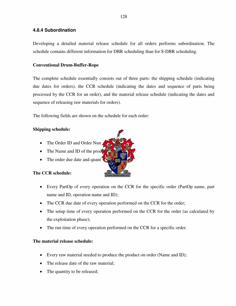
128

4.8.4 Subordination

Developing a detailed material release schedule for all orders performs subordination. The

schedule contains different information for DBR scheduling than for S-DBR scheduling.

Conventional Drum-Buffer-Rope

The complete schedule essentially consists out of three parts: the shipping schedule (indicating

due dates for orders), the CCR schedule (indicating the dates and sequence of parts being

processed by the CCR for an order), and the material release schedule (indicating the dates and

sequence of releasing raw materials for orders).

The following fields are shown on the schedule for each order:

Shipping schedule:

x� The Order ID and Order Number;

x� The Name and ID of the product on order;

x� The order due date and quantity;

The CCR schedule:

x� Every PartOp of every operation on the CCR for the specific order (PartOp name, part

name and ID, operation name and ID);

x� The CCR due date of every operation performed on the CCR for the order;

x� The setup time of every operation performed on the CCR for the order (as calculated by

the exploitation phase);

x� The run time of every operation performed on the CCR for a specific order.

The material release schedule:

x� Every raw material needed to produce the product on order (Name and ID);

x� The release date of the raw material;

x� The quantity to be released;

129

x� The lead time of the raw material.

In the cases where the parts processed for an order do not pass the CCR, the CCR schedule is left

blank.

Simplified Drum-Buffer-Rope

The Simplified schedule is divided into two regions, a shipping schedule and a material release

schedule. The following fields are shown on the schedule for each order

Shipping schedule:

x� The order ID and order number;

x� The product on order: product ID and product name;

x� The order due date and quantity;

x� The order’ s Red Line date, based on the Red Line time specified and the order’ s due date;

Material release schedule:

x� Every needed raw material for the order (Part ID, Part Name);

x� The release date of each raw material needed on the order;

x� The quantity needed to be released of each raw material;

x� The current quantity in stock of each raw material, also considering how much has been

released on other scheduled orders;

x� The Red Line quantity of each raw material;

x� The quantity needed to be re-ordered for each raw material to stay above the Red Line

quantity;

x� The re-order date of each raw material.

130

4.8.5 Exporting schedules

The last feature of the DBR4JS software implemented in this project is to export the developed

schedules to industry standard editing software. In this case, schedules can be exported to a

Microsoft Excel spreadsheet. Exporting schedules to Excel makes it easy to further edit and

format the schedules, distribute it to the shop floor, and to analyse it and draw certain graphs of

the data. Examples of exported schedules are shown in Appendix F.

One of the most important graphs is the Schedule Performance Curve (Umble and Srikanth

1990:153). The Schedule Performance Curve shows the scheduled completion date of orders

against the customer due date. It serves mainly two functions:

1. Illustrate the degree to which customer orders are scheduled to be early or late;

2. Identify the actions that lead to improved customer service performance.

An example of a Schedule Performance Curve is shown in Figure 4. 35.

Figure 4. 35: Schedule Performance Curve (Umble & Srikanth, 1990:153)

131

The Schedule Performance Curve (SPC) will form a straight, forty-five degree line if every order

is scheduled to be completed exactly on its due date. In practice, the SPC should approach, but

not exceed customer due dates. If the SPC shows a complete random pattern, there is likely to be

some serious problems in the system.

Figure 4. 36 shows an example Schedule Performance Curve created by exporting a schedule

created by the DBR4JS software to Microsoft Excel. Refer to Appendix E for a complete

description on creating Schedule Performance Curves in Excel.

Schedule Performance Curve

0

5

10

15

20

25

30

3 5 6 7 10 13 14 17 18 20 21

Order Due Date

Sch

edul

ed C

ompl

etio

n Ti

me

Finish Time IndexDue Date Index

Figure 4. 36: Schedule Performance Curve created by the DBR4JS software

132

Chapter 5

Practical “What If” DBR and S-DBR scheduling

5.1 Introduction

This chapter discusses the implementation of the developed software with live data from one of

the production lines of a South African job shop, Aerodyne Aviation Technologies (AAT). The

software was used to analyse the situation of the Echo line according to the data, and to develop

Simplified Drum-Buffer-Rope schedules by following a “ What If” approach to scheduling. The

purpose of the chapter is to practically illustrate how the software can be used to facilitate a

“ What If” approach to scheduling, and it gives examples of some suggested solutions that can be

tested with the software before implementing them on the shop floor.

5.2 Sample data

The manufacturing environment of the Echo line at Aerodyne Aviation Technologies was

described in Chapter 2.5.2. The sample data was also introduced. Aerodyne supplied the data

with a view of evaluating whether the software could help them improve order delivery. The

production management team specifically wanted to be able to see how much new orders would

load the plant, and to be able to pro-actively identify problem areas and emerging CCR’ s, or

shifting constraints. At the time that this report was written, Aerodyne had reached considerable

success with the manual S-DBR scheduling implementation. The next area for improvement was

to be able to take pro-active measures in breaking emerging resource constraints. The company

had not gone through an extensive time study exercise yet. The data presented here on the

processing times of the various workstations is therefore based on estimates from the production

team, and is not hundred percent accurate. It is however adequate to give a demonstration of the

software and how it can be used, and to justify the effort to collect accurate data. The following

paragraphs will describe the data in more detail.

133

5.2.1 Product information

The Product Flow Diagram (PFD) concept was explained in Chapter 2.5.2. The PFD for one of

the products (the Taca variant) is shown in Figure 5. 1.

The blue boxes in the diagram represent Part / Operations, that is operations that are performed

on specific parts. The ID of the resource performing the operation is indicated at the top of each

box (e.g. R-1). The Part ID is given in the top (lighter) part of the box (e.g. RearSkin). Each time

a new raw material (indicated by the green triangles) is added to a part, a new part ID has to be

defined in the system. The processing time for the specific part at the operation is indicated in the

lower (darker) part of each box.

To simplify the model, similar Part /Operations were grouped together in work groups, and a new

Resource ID was assigned to them. These work groups were treated as single resources. AAT

preferred to follow a top down approach to identifying the constraint. Once a work group has

been identified as being problematic, the resources in the group can be analysed to see exactly

where problems are occurring. The groups of resources are indicated with red dotted-line boxes.

The process names (e.g. Cutting) and new resource ID’ s are indicated in the top part of each box.

Refer to Appendix G for the PFD’ of all the parts manufactured on Echo, and to be delivered

during Quarter 1 of 2006.

134

Figure 5. 1: Product Flow Diagram of the Taca variants

135

Figure 5. 2: Product Flow Diagram of the Taca variants (continued)

136

5.2.2 Order information

AAT’ s order list for products manufactured on the Echo line and to be delivered in the first

quarter of 2006 is displayed in Table 5. 1. The table shows the product description for each part

to be produced, the part ID and when it is to be delivered, with the order quantity.

Total

Description Part 13 20 27 3 10 17 24 3 10 17 24 31Echo Air Berlin Exit Row 139-00-400-42DR 12 12 24Echo Air Berlin LH 139-00-400-35DR 3 3Echo Air Berlin RH 139-00-400-46DR 1 1Echo Back Hapag Lloyd 139-00-400-06BK 12 12 12 6 42Echo Back Niki Exit Row 139-00-400-42JT 1 1Echo Back Swiss 139-00-400-21HQ 68 68Echo Back TACA Std 139-00-400-06BD 0Echo Backrest HL Std LH 139-00-400-38BK 84 84Echo Backrest HL Std RH 139-00-400-47BK 90 90Echo Iberia Exit Row LH 139-00-400-65BK 3 6 3 3 6 21Echo Iberia Exit Row RH 139-00-400-66BK 6 6 3 3 6 24Echo Iberia Ret Exit Row LH 139-00-400-65BKr 20 16 16 16 16 16 100Echo Iberia Ret Std LH 139-00-400-67BKr 45 45 45 45 144 144 144 144 144 900Echo Iberia Std LH 139-00-400-67BK 146 88 75 63 88 460Echo Iberia Std RH 139-00-400-68BK 146 88 78 66 88 466Echo Niki Std LH 139-00-400-35JT 84 84Echo Niki Std RH 139-00-400-46JT 84 84

2452

Jan Feb Mar

Table 5. 1: Echo-line order list for the first quarter of 2006

5.2.3 Inventory information

For the purpose of this exercise, inventory levels for work in process and raw materials were

ignored. It was assumed that there was no work in process, and enough raw materials were

available to fill all orders. It was further assumed that there were no finished goods in the stores.

5.2.4 Calendar information

All resources (men and machines) were assigned to work two shifts a day, five days a week

(Monday through to Friday). When necessary, resources can also be assigned to work two shifts

on Saturdays. Public holidays were ignored. In reality, the workers are split into two groups; one

group is available for the first shift on a day and the other group for the second shift. Standard

shifts are eight hours long. It was assumed that work at the plant would start on 9 January 2006.

137

5.2.5 Resource information

The processing and setup times for resources are displayed with the product / part information.

The software allows the user to define the ‘number of available machines’ for each resource, for

each shift (Refer to Chapter 4.4). Operators (people) are treated by the software as machines.

This function allows the scheduler to assign different capacities for the same resource to different

shifts. As the resources were grouped into functional groups, the ‘number of available machines’

for most resources was defined as one. A single type of resource performs the lay-up processes,

and their quantities were specified as follows: six Rear Lay-ups, four Front Lay-ups, and two Cup

Lay-ups. As resources were grouped into workstations, setup times were ignored and set to zero.

5.2.6 DBR and S-DBR specific information

In this exercise S-DBR scheduling was mostly performed. S-DBR data is as follows:

x� Shipping buffer: 80 hours (10 shifts, or 5 working days)

x� Red Line Control:

��Finished Goods: 32 hours (4 shifts, or 2 days)

��Raw Materials: N/A

x� Planning Horizon: Planning was done in two week time frames across the whole period.

The Effective Horizon is calculated by adding one shipping buffer to the end of the

planning horizon (see Chapter 3). To ensure that work would be scheduled across the

whole first quarter, planning horizons were overlapped. The last week of the first planning

horizon is the same as the first week of the following planning horizon. To cover the

whole period, planning horizons were set out as indicated in Table 5. 2

No Planning Horizon Effective Horizon 1 9 January to 21 January 9 January to 28 January 2 23 January to 11 February 23 January to 18 February 3 13 February to 4 March 13 February to 11 March 4 6 March to 25 March 6 March to 1 April

Table 5. 2: Planning horizons and effective horizons for data analysis

138

x� Resource Capacity Limit: 90%. This is the daily limit set for capacity usage on each

resource.

5.3 Software analysis

The DBR4JS database was populated with the data described above by making use of the

database management tool. S-DBR scheduling was performed with the data supplied. The

following paragraphs show how the software can be used do pro-active planning on how to

increase Throughput, while minimising Operating Expense and Inventory (or investment in more

resources). Some of the solutions posed here might not be practical to implement for AAT, but

they illustrate some “ What If” scenarios that can be analysed.

5.3.1 First Identification run

The results of the Identification procedure of the DBR4JS software, using the data described

above, without any changes, are summarised in Table 5. 3. As the CCR resources are dictating

the pace of the system, only the resources identified as possible CCR’ s are analysed.

Horizon Period CCR Overflow [hrs] 1 9 January to 21 January R-1 CUTTER 536.675 R-12 QA INSPECTOR 515.775 R-2 LAYUP REAR 482.067 R-5 CURE AND DEMOULD 481.108 R-8 PAINTERS 230.3 2 23 January to 11 February R-1 CUTTER 403.31 R-12 QA INSPECTOR 382.278 R-5 CURE AND DEMOULD 345.76 R-8 PAINTERS 96.5 3 13 February to 4 March R-1 CUTTER 219.1 R-5 CURE AND DEMOULD 216.005 R-12 QA INSPECTOR 202.38 4 6 March to 25 March R-1 CUTTER 998.845 R-5 CURE AND DEMOULD 971.183 R-12 QA INSPECTOR 952.161 R-8 PAINTERS 314.5 R-9 CURING 273.217 R-15 FILLER 108.921

Table 5. 3: Results from the first Constraint Identification run with data from AAT’s Echo line

139

Refer to Appendix H for detailed screenshots of the software output for each planning horizon

after the first identification run.

From the data it is clear that workstation R-1, Kit Cutting, is the primary CCR on the Echo line.

Other workstations that continually show difficulty are R-5 (Cure and demould), R-8 (Painter),

and R-12 (Quality inspector). These are the resources that AAT should concentrate on. It was

mentioned earlier that the data presented here is based on estimates from the AAT production

management team. The first suggestion therefore is for AAT to go through an accurate data

collection exercise on these resources to obtain accurate data.

The fact that the Kit Cutting machine is the primary CCR candidate is fairly good, as it is one of

the most expensive resources in the plant. The challenging part of it is that some innovative ways

will have to be presented to add enough capacity to elevate the constraint from Kit Cutting and

into the market, which is desired for S-DBR.

5.3.2 Applying “What If”

From the output of the software it is obvious that AAT will experience some difficulty in

fulfilling their commitments to the market over the presented planning horizons. The purpose of

the software is to facilitate a “ What If” approach to pro-actively identify problem areas and to

give feedback on how suggested solutions will help to improve performance, or not. The

following paragraphs use this functionality of the software to analyse a few “ What If” scenarios

and to create S-DBR schedules for each one of the planning horizons. As the data cannot be seen

as completely accurate, it is assumed that if the overflow of work on a resource is within ten

percent of the total number of hours of work that needs to be completed by the resource, it is

within acceptable range.

Planning Horizon 1: 9 January 2006 to 21 January 2006

From the first identification run for Planning Horizon 1, it can be seen that almost all the

resources will experience difficulty in meeting the demand placed on them. This is because the

factory is only scheduled to start working on 9 January, but there are six orders scheduled to be

140

delivered on 13 January. With the assumption that there is no inventory on hand, these orders

should preferably completed by 9 January already. The first question is:

What if the orders for 13 January 2006 could be completed in December 2005?

By removing the orders for 13 January from the planning horizon (E39, E38, E70, E65, E45, and

E40), the software shows that considerable capacity is added. As a matter of fact, most of the

resources will have no work to do for the first week that the factory is open. This leads to the

question:

What would happen if the plant only started active production a week later?

As most of the resources will be idle, the plant can use the spare time of the first week for other

value adding activities, such as training of multi-skilled staff, machine maintenance, or problem

solving workshops. If the orders for 13 January can be completed in December 2005, the

software shows that the plant can afford not to produce during the first week of 2006.

What if another order was added in January?

The software shows that most of the resources are capable of handling another order for January.

An extra order for 85 units is added with its due date on 26 January. With the new order, the

software shows that it is not feasible for R-1, R-5 and R-12, as these resources show considerable

overflow if they are not able to work in the first week, and another order is added. The following

measures need to be taken to break the resource constraints on these resources, during Planning

Horizon 1:

Order Nr E32 (90 x Hapag Lyod Std RH): The order is postponed for one day, from 20

January to the second shift on 21 January (2 shifts).

Resource R-1 (Kit Cutter): The resource is only scheduled to work during the day shifts of the

first week. The resource is further scheduled to work two hours overtime on shift 13 and 14 (16

January, shift 1 and shift 2) and one hour on shift 15 (17 January).

R-12 (Quality inspector): The first option is to let R-12 work on the day shifts of the first week.

This is not a feasible solution, as the inspection is done on painted parts. If the painters are not

working, there will be no parts to inspect. The second option is to let the resource only start

141

working on the second week, but to appoint two people to perform the quality inspection on

painted parts. This is a potentially good solution, as R-12 is a problematic resource in all the

planning horizons, and its capacity will need to be expanded. An operator from a less critical

resource can be trained during the first week to do quality checks on painted parts.

R-5 (Cure and de-mould): One option for bringing the capacity of R-5 in line with demand is to

apply overtime on the resource for the first few shifts that it is scheduled to operate (week 2).

This will however increase Operating Expense. Another option is to use an oven from the

painting line (R-8) for curing at R-5. As R-8 is not scheduled to work on the first night shift, one

of the ovens is available on that shift for R-5. This is enough to bring R-5’ s capacity in line with

demand.

The output of the Identification step and the resulting S-DBR schedule for Planning Horizon 1, as

calculated by the DBR4JS software, are shown in Appendix H.

Planning Horizon 2: 23 January 2006 to 11 February 2006

The output of the software for the first identification run for Planning Horizon 2 (Appendix H-II)

shows that R-1, R-5, R-8, R-9, R-11, and R-12 will experience difficulty in meeting demand.

Although these resources are fully loaded early in the horizon, there is some lower capacity usage

on all of them during the third week of the planning horizon. Postponing order due dates should

therefore relieve some of the capacity requirements.

What if some orders could be postponed?

Comparing the order due dates of Appendix H-II (Figure H.4) with the periods of less demand in

Planning Horizon 2 (from Figure H.3) shows that the following order adjustments could release

some capacity:

Order Nr Product Quantity Original due date Adjusted due date E75 Niki Std LH 84 10/02/2006-01 14/02/2006-01 E66 Iberia Std LH 88 03/02/2006-01 10/02/2006-01 E71 Iberia Std RH 88 03/02/2006-01 06/02/2006-01 E84 Iberia Ret Std LH 45 10/02/2006-01 15/02/2006-01

Table 5. 4: Postponed orders for Planning Horizon 2

142

Adjusting the order due dates in the software brings the overflow of work on the Curing station

(R-9) down to eleven hours (total hours of work is 186 hours), without applying overtime or

having to work on Saturdays. The curing oven is therefore available for the Painting process over

weekends.

What if the curing oven can be used in the painting process?

If the Painting station works on the Saturday shifts, and the extra oven from the Curing station

(R-9) is used on the first weekend, the software shows that work overflow on R-8 is reduced to

2.3 hours.

The Cure and De-mould station is still experiencing a serious lack in capacity (325 hours of

overflow). The question is asked:

What if another curing oven can be purchased?

Although this might be a serious investment, the situation can be analysed with the software

where another curing oven is purchased, and another operator is assigned to de-moulding. The

software shows that if the capacity of R-5 can be doubled, and the resource works every shift, the

overflow is reduced to 43.36 hours (8% of total amount of work).

Quality assurance is a very manual process, and need not be a CCR if labourers can be taught

multiple skills. Other manual stations such as Drilling and Filling do not have stringent capacity

requirements, and resources from these stations can be utilised for Quality Assurance.

What if more operators can do Quality Assurance?

The software shows that having multiple Quality inspectors will easily break the constraint,

without having to apply excessive overtime. These operators would have had to be paid for a

days work although they would have had a lot of idle time, so no extra Operating Expense would

be incurred by having them perform the Quality Assurance function. From the software it is

shown that the overflow of work in R-12 can be reduced from 359 hours to 7 hours by having the

number of quality inspectors indicated in Table 5. 5.

143

Period Number of inspectors Week 1 (shift1 to 10) 3 Weekend 1 (shift 11 and 12) 2 Week 2 (shift 13 to 18) 3 Week 2 (Shift 19 to 22) 2 Weekend 2 (Shift 23 and 24) 1 Rest of horizon 2

Table 5. 5: Number of Quality Inspectors for Planning Horizon 2

The S-DBR schedule for Planning Horizon 2, with the adjustments above, is shown in

Appendix H-VI. There is however still a problem with R-1, Kit Cutting. Total amount of work

on R-1 is 598.835 hours and the overflow amounts to 346.835 hours.

Planning Horizon 3: 13 February 2006 to 4 March 2006

The first DBR4JS identification run for Planning Horizon 3 shows that only R-1, R-5 and R-12

are over loaded. The other resources are not very occupied, which enables multi-skilled workers

to assist on workstations that need additional capacity.

The previous scenarios showed the benefits of having two Quality Inspectors (R-12) and two

Curing and De-moulding stations (R-5). These measures were implemented across the whole

planning horizon, and the effects on R-5 and R-12 are shown in Figure 5. 3

Figure 5. 3: Resource loading for R-5 (Curing and De-moulding) and R-12 (Quality Assurance)

144

What if another order was added?

An additional order for 150 Taca Std units is added to the system, with a due date of 23 February

(Shift 19). This results in R-1, R-5, R-8 and R-12 emerging as CCR’ s.

The CCR on R-8 is broken simply by limiting the capacity usage on R-8 to 95% (as opposed to

90%) and to assign R-8 to work two shifts on Saturdays. No overtime is needed.

The work overflow on R-5 is brought within 10% of the total work assigned to it (554 hours) by

limiting the capacity usage to 95% as well. Work overflow is then only 22.5 hours (3.9 % of total

work).

The software shows that by assigning three operators to R-12 for the first five shifts, and three

operators every other shift after that for the first week reduces the work overflow on R-12 from

57 hours (9.8% of total work) to 4.57 hours (0.7% of total work).

R-1 is fully loaded across the planning horizon, and has a work overflow of 340 hours (56% of

total work).

The resulting S-DBR schedule for Planning Horizon 3 is shown in Appendix H-VII (Figure H.15,

Figure H.16, and Figure H.17).

Planning Horizon 4: 6 March 2006 to 25 March 2006

The output of the first Identification run of the software shows that the demand of Planning

Horizon 4 is much more than the available capacity. There is a large order (144 units) during

each week (E89, E90, and E91), and a series of small and mid-sized orders in between.

According to the output of the DBR4JS software, it is inevitable that some orders will need to be

cancelled if the company does not want to operate under a true resource constraint.

Apart from Kit Cutting, the two other major constraints for Planning Horizon 4 are R-5 (Curing

and De-moulding) and R-12 (Quality Assurance). In the previous scenarios, it was already shown

that according to the output of the data, the company should consider acquiring another curing

oven, to effectively double the capacity of the Curing and De-moulding station. It was also

suggested that more workers be trained on performing quality inspections of painted parts to

145

increase the capacity of the Quality Assurance station, but it is unlikely that these measures will

completely break the constraints on these resources during Planning Horizon 4.

When AAT started the S-DBR implementation on the Echo line, it was found that Painting (R-8)

was the CCR. The constraint was however moved to Kit Cutting by increasing the percentage of

first time acceptance of painted parts, therefore speeding up the painting process. Taking a deeper

look into the Product Flow Diagrams of Appendix G shows that quality checks are performed six

times on all products. Quality checks are done before the painting cycle to make sure that the

original constraint (Painting) does not work on parts that will be rejected, therefore wasting time.

Three quality checks are done during the cycle, another after the cycle, and another check is done

on finished goods. The three quality checks during the cycle were probably implemented to

increase the first time acceptance of painted parts after each coat was applied. As the constraint

has been shifted, the painting process does not need so much attention any more, if it can be

assumed that the operators will still deliver the same quality of painted parts without being

checked. The question is therefore asked:

What if the number of quality checks on painted parts could be reduced?

The product routings of the products on order during Planning Horizon 4 were adjusted to have

only four quality checks during the painting cycle, the first after Trimming (before the painting

cycle begins), the second after the top coat is applied and the third after the clear coat is applied

(the last step of the painting cycle). Furthermore, the cycle times of the checks on parts Assembly

7 and Assembly 8 are reduced from fifteen minutes to seven minutes, and from ten minutes to

five minutes respectively. The same applies to parts Assembly 13 and Assembly 14, Assembly 20

and Assembly 21, and Assembly 28 and Assembly 29 (Refer to Appendix G).

The amount of work overflow on R-5 (971 hours) is indicative that DBR scheduling will most

likely have to be performed. The scheduler was therefore switched from S-DBR scheduling to

conventional DBR scheduling. The Buffer sizes were set to eighty hours for the shipping buffer,

and forty hours for the constraint buffer. The difference in the way the Identification procedure is

executed for DBR and S-DBR is that job loads are placed on resources on the constraint due date

(Due date – (shipping buffer – constraint buffer)) for DBR scheduling. This has an effect on the

calculation of the work overflow, as loads are placed on resources later in time for DBR

146

scheduling than for S-DBR scheduling. The result of the Identification procedure for R-12 with

the switch to DBR scheduling, and the above-mentioned routing changes implemented, is shown

in Figure 5. 4.

Figure 5. 4: Output of DBR Identification procedure for R-12

The results of the Identification procedure for the other resources are summarised in Table 5. 6.

Horizon Period CCR Overflow [hrs] 4 6 March to 25 March R-1 CUTTER 970.045 R-5 CURE AND DEMOULD 942.383 R-12 QA INSPECTOR 338.75 R-8 PAINTERS 285.7 R-9 CURING 244.417 R-15 FILLER 80.121

Table 5. 6: Results of the DBR Identification procedure for Planning Horizon 4

The demand placed on R-1 and R-5 is quite large, and it will be difficult to bring the capacity of

these resources in line with demand. R-1 is a shared resource with the other lines in the plant, so

it was decided to schedule R-5 as the CCR for the purpose of this exercise. The next step was

therefore to remove the work overflow on the other resources. The biggest impact on resource

loadings will be obtained by removing some of the large orders from the planning horizon.

What if some orders could be postponed?

Postponing all three the large orders for Iberia Std LH (E89, E90, and E91) by one week will

shift the order for 144 Iberia Std LH (E91) out of the planning horizon. This is however not

enough to relieve the other resources, even if all resources are assigned to work every possible

shift, and applying the capacity expansion measures as per the results of the previous scenarios.

The following steps were implemented, along with postponing orders E89, E90, and E91:

147

R-1:

x� Limit the capacity usage to 95%

x� Assign the Cutter to work the Saturday shifts.

R-5:

x� Limit the capacity usage to 95%

x� Assign two Cure and De-mould stations to every shift, including weekends

R-8:

x� Limit the capacity usage to 95%

x� Assign the Painter to work the Saturday shifts.

R-9:

x� Limit the capacity usage to 95%

x� Assign the Curing station to work the Saturday shifts.

R-12:

x� Limit the capacity usage to 95%

x� Assign two Quality Inspectors to work during the week, and one on both Saturday shifts.

The results of the Identification procedure of the DBR4JS software, with the above-mentioned

results implemented, are shown in Figure 5. 5.

148

Figure 5. 5: Results of the DBR Identification procedure after postponing orders E89, E90, and E91

The output shows that additional orders will need to be postponed, to at least have R-5 as the only

CCR (apart from Kit Cutting). R-8 and R-9 are still overloaded with more than 10% of their total

workload.

149

E69 (88 units of Iberia Std LH) and E74 (88 units of Iberia Std RH) are fairly large orders at the

end of the horizon. By postponing them with seven shifts, and E37 (68 units of Swiss seats) with

at least eight shifts, and applying overtime of ten hours per week on both R-8 and R-9, the work

overflow on these resources are brought within ten percent of their total load. The order

adjustments are summarised in Table 5. 7.

Order Nr Product Quantity Original due date Adjusted due date E89 Iberia Ret Std LH 144 17/03/2006-01 24/03/2006-01 E90 Iberia Ret Std LH 144 24/03/2006-01 31/03/2006-01 E91 Iberia Ret Std LH 144 31/03/2006-01 07/04/2006-01 E69 Iberia Std LH 88 31/03/2006-01 11/04/2006-01 E74 Iberia Std RH 88 31/03/2006-01 13/04/2006-01 E37 Swiss 68 31/03/2006-01 11/04/2006-01

Table 5. 7: Order adjustments for Planning Horizon 4

The order postponements allow for some of the measures taken to increase the capacity of R-11,

R-12, and R-15 to be relaxed, in that the daily capacity limit on these resources can be restored to

90%, and they do not have to work over weekends.

The final results of the Identification procedure are shown in Figure 5. 6.

150

Figure 5. 6: Final results of the Identification procedure for Planning Horizon 4

Although R-1 (Kit Cutting) is the real constraint, it was decided to schedule R-5 as the CCR

because R-1 is shared with the rest of the plant. If it is to be scheduled as the CCR, the

requirements of the rest of the plant will also need to be taken into consideration. The complete

DBR schedule for Planning Horizon 4 is shown in Appendix H-VIII. The schedule identifies

specific orders which will have trouble meeting their due dates (indicated in red). This allows the

151

planner to further negotiate due dates, or to keep a close watch on specific orders, to priorities

activities on the shop floor.

5.4 Interpretation of results

The data used in the exercise is based on estimates by the production personnel of Aerodyne

Aviation Technologies. It is adequate to give a first overview of the situation of the plant, but for

detailed analyses more accurate data is needed. The software helped to identify four operations

on which accurate time studies are needed. These operations and their respective resources are

Painting (R-8), Curing and De-moulding (R-5), Kit Cutting (R-1), and Quality Inspection (R-12).

At first glance the plant is seriously lacking capacity to meet demand. Some scenarios were

analysed to see how the capacity of the plant could be brought in line with demand.

Planning Horizon 1

For Planning Horizon 1 it was suggested that Throughput (T) could be increased and Operating

Expense (OE) decreased if certain conditions could be met. If the load on the factory for early

January could be decreased in December, and order E32 could be delivered one day late, an

additional order can be delivered, and the factory can start producing actively one week later,

leaving time during the first week for other value-adding activities such as training and

maintenance. The effect of these actions on the bottom line can be quantified by looking at

Equation 2.2:

OETNP '�' '

The change in T is given by the additional eighty-five units, over the original demand of four

hundred and eighty-eight. The change in OE is given by the decrease in machines having to work

during the first week, and the increase is given by the overtime for R-1. The decrease is

calculated by adding the number of shifts that machines do not have to work (ten shifts multiplied

by fifteen machines plus the five shifts that R-1 does not have to work during the first week),

divided by the total number of shifts that machines would normally work (ten shifts times sixteen

resources times three weeks). The increase in OE is calculated by comparing the total overtime

152

that is assigned (five hours for R-1), over the total overtime that could be assigned (ten hours per

week for three weeks, for sixteen resources). The calculation then looks as follows:

OETNP '�' '

100*4805

480155

100*48885 ¸̧¹

·¨̈©§ ���¹̧

·©̈§

hourshours

shiftsshifts

unitsunits

%668,48

The result does not show the absolute improvement in Net Profit for the line over the period, as

not all the OE and T elements are considered, but it does show that the steps taken could improve

the bottom line results over the specified planning horizon.

Planning Horizon 2

For Planning Horizon 2 it was suggested that some serious investment should be considered to

increase the capacity of the Curing and De-moulding process, by purchasing another curing oven.

Equation 2.3 gives the bottom line impact of investments:

IOET

ROI ''�' '

The change in Return on Investment (ROI) for the whole system is hard to quantify for planning

horizon two, as it can not be said for certain how the Throughput would be impacted. The

software shows that if the investment is not made, R-5 will have considerable work overflow,

which will inevitably lead to late orders. It does however not show which orders specifically will

be impacted by the lack of capacity, and it is therefore not possible to assign a numeric value to

the change in T. If R-5 is a real CCR, doubling its capacity is, according to the input data, needed

to break the constraint, which will lead to increased Throughput and decreased Inventory.

The assumption was also made that if operators from other idle stations could be trained to

perform the Quality Assurance function, the capacity of this workstation could be increased

without incurring additional Operating Expense, as these operators could still be paid the same

wages (if the union agrees).

153

Planning Horizon 3

The numbers of Planning Horizon 3 can quantify the investment in an additional curing oven. T

can be increased with one hundred and fifty units (if an additional order could be obtained). In

order for the Echo line to be able to deliver the additional order, OE needs to be increased by

assigning more resources to R-5, R-8, and R-12. Even if additional OE should be incurred by

having more operators at these workstations, Equation 2.2 still shows a positive impact on NP,

which leads to a positive impact on ROI. The change in T is given by the increase in units (one

hundred and fifty) over the number of units on order for the horizon (five hundred and twenty

three, as order E36 for one Niki Exit Row was accommodated for in Planning Horizon 1). The

change in OE is given by the increase in shifts worked by resources (eight shifts for R-5, six

shifts for R-8, and forty-seven shifts for R-12) over the total number of available shifts (four

hundred and eighty, if weekends are not counted). The calculation is given by:

OETNP '�' '

100*48061

100*523150

¹̧·

©̈§�¹̧

·©̈§

unitsunits

%972,15

If the investment in another curing oven is known as a percentage of the investment in the whole

line, the ROI can be calculated.

Planning Horizon 4

Analysis of Planning Horizon 4 showed the impact that the software can have on evaluating

procedures to break possible policy constraints imposed during previous cycles of the Five

Focusing Steps. The Quality Assurance process on the Echo line was identified as an emerging

CCR for the specified planning horizon. The software helped to set the focus on this process, and

it could further be used to evaluate the situation if the number of quality checks were reduced on

the line.

154

It also showed the value of being able to monitor a S-DBR implementation with every new order

received. S-DBR is most suited if the organisation operates under a market constraint. If an

organisation operates under a true market constraint, it means that there is no internal resource

limiting the Throughput of the system. DBR was designed to handle physical resource

constraints. It was shown that by using the software, the planner is able to see whether there

should be switched over to DBR scheduling during times of peak demand and emerging resource

constraints, or whether counter actions can be taken to break physical constraints pro-actively.

By following the DBR scheduling procedure, a detailed schedule was developed for both material

release and the CCR, R-5. Problem and late orders were highlighted to make it possible for the

production scheduler to make plans on how to deliver specific orders on time.

5.5 Conclusions

The software can be used to quickly see what the load on the plant is for specific orders and

product mixes over a specified time frame, or planning horizon. Improvements can then be

brought about by changing some of the limiting factors and see what the overall effect of

improvement efforts are. The key areas where improvements are needed can also be easily

identified by means of the software. To be truly effective, accurate input data is needed, and the

software helps to identify the areas where data collection is to be prioritised. When the scheduler

is comfortable with the loading on the plant the software quickly calculates the material release

and shipping schedules for orders. These features can help to increase Throughput while

decreasing Operating Expense, by adding capacity only at resources and during times when it is

truly effective in helping to deliver on market commitments. Although the software does not

optimise capacity allocation and schedules, the effects of changes are quickly displayed to

facilitate an approach where the user can try certain options and decide what is the best option to

follow.

155

Chapter 6

Conclusions and recommendations

6.1 Introduction

The purpose of this chapter is to summarise the research and to draw final conclusions.

Recommendations for future research are made.

6.2 Conclusions

The aim of this research was to investigate the feasibility of following a “ What If” approach to

developing Drum-Buffer-Rope or Simplified Drum-Buffer-Rope shop floor schedules for

manufacturers operating in a job shop environment. The argument for following such an

approach is that the experience and knowledge of production schedulers can be utilised in

creating near optimal schedules that are practical to implement on the shop floor. Following such

an approach is helpful towards empowerment efforts in that it involves production workers in the

innovative processes of identifying and breaking constraints, exploiting constraints, and

subordinating the plant to the exploitation decisions. The hypothesis of this study is that if it can

be assumed that DBR and S-DBR provide feasible and good solutions to scheduling the

complexities of a job shop environment, then TOC provides a mechanism, through DBR and S-

DBR, for the scheduler to follow an interactive “ What If” approach to job shop scheduling. To

test the hypothesis, an in-depth study into DBR and S-DBR was made. The following

conclusions can be drawn regarding DBR and S-DBR.

1. DBR was designed to address the scheduling complexities of job shops. It is the

implementation of Constraint Management in manufacturing to address physical resource

constraints. S-DBR was developed to address manufacturing under market constraint

conditions, and to address the difficulties of the three-buffer system of DBR. These

156

difficulties are: the spreading time buffer, more lead time is added than what is needed,

and the superfluous assembly buffer.

2. Concerns with the three-buffer system of DBR resulted in the methodology to be adapted

to only make use of two buffers: the shipping and constraint buffer. The assembly buffer

of original DBR scheduling falls away. This change brings DBR in line with S-DBR,

where only the shipping buffer is used to calculate schedules.

3. DBR protects order due dates by minimising the sources of variation in the production

schedule. The number of control points in the manufacturing line is kept to the minimum,

by only scheduling material release, the CCR operations, and shipping dates. S-DBR

simplifies scheduling even further, by only creating schedules for material release and

shipping dates. The effect on production is that sources of variation are reduced even

more. S-DBR works under the assumption that there is no internal resource constraint.

4. Most of the reported cases of DBR implementations give positive results, with reductions

in product lead times and inventory levels. The literature gives enough evidence for DBR

to be accepted as a good scheduling solution for job shops. A common pitfall with DBR

implementations however is the people’ s resistance to change.

5. At the time that this research was done, there were not a lot of reported cases of S-DBR

implementations in the literature. Only one such case could be found, and good results

were reported. An S-DBR implementation at a South African job shop was investigated,

and it was found that throughput was increased while inventory was decreased.

In order to conduct detailed research into following a “ What If” approach to scheduling at a job

shop, a software tool was developed that will assist users to schedule job shop activities

according to DBR principles. Although the high level principles of Drum-Buffer-Rope are logical

and relatively easy to understand, the implementation at a technical level can quickly become

complex. A detailed study of DBR and its operating principles was made in this project and a

DBR scheduling system was designed and implemented in software. The newly developed

S-DBR was also studied and implemented in the same software.

A concern about implementing DBR or S-DBR scheduling software is the role of the traditional

MRP or ERP system. It was found that MRP or ERP plays an important part in housing the

critical information needed to develop finite DBR or S-DBR schedules. The scheduling part

157

should however be done by a dedicated DBR or S-DBR scheduling module, as MRP and ERP is

not capable of creating finite DBR or S-DBR schedules, with the flexibility needed to following a

“ What If” approach. By utilising both systems, the MRP or ERP system can be focused on

housing critical information regarding the plant, and the DBR or S-DBR scheduling package can

focus on creating feasible shop floor schedules. An ERP or MRP system is not critical to the

success of implementing DBR or S-DBR. It is however a necessity that some sort of database be

maintained that houses the critical information needed for scheduling. This information must

include the products’ Bills of Material, product routings, setup- and run times, the available shifts

and resources, and order quantities and due dates. As inventory levels (WIP and finished goods)

can also have an effect on the load on the plant, this information must also be as accurate as

possible.

In order to test the hypothesis that TOC provides a mechanism, through DBR and S-DBR, for the

scheduler to follow an interactive “ What If” approach to job shop scheduling, actual order and

process data from a South African job shop was implemented in the software. Various scenarios

were tested over different scheduling horizons for a number of orders. The results show that the

effects of capacity expansion efforts can be analysed pro-actively to see if changes in the

controlling variable lead to the improvements that were hoped for. By small changes to process

times and order due dates, the location of the constraint is changed between different resources,

or even shifted to the market. Possible solutions were analysed using the software. DBR and S-

DBR scheduling supports a “ What If” approach to scheduling well, as results are displayed

almost instantly, and different scenarios can be investigated in a short space of time.

Although some of the solutions proposed might not be practical to implement, the study showed

that following a “ What If” approach to scheduling the shop floor could bring about significant

bottom line improvements to the system as a whole. The study further showed that processes on

which accurate data collection is needed can easily be identified, dividing the “ critical few” from

the “ trivial many” . It is concluded that the implementation of the software with actual process

data did not provide enough evidence to disprove the hypothesis. The question however remains

on how effectively the knowledge of experienced shop floor workers can be utilised in the

scheduling process.

158

6.3 Recommendations

6.3.1 Further software development

If the software is to be used to do experimental research into the feasibility of following a “ What

If” approach to DBR and S-DBR job shop scheduling, further development to the software will

be needed to implement it at a manufacturing facility.

x� Graphical user interface:

The focus of the thesis as far as the software development is concerned was to implement the

principles of DBR and S-DBR in software to support shop-floor empowerment efforts.

Development was done to follow the systems architecture definition given in Chapter 1. The

student however only had a basic working knowledge of the C++ development language. It

was therefore essential to separate the core business logic (DBR and S-DBR scheduling) from

the interface layers of the software as to not spend too much time on developing a system

with enhanced graphical support. A graphical representation of the software architecture is

given in Figure 6. 1.

Figure 6. 1: Software architecture

Once the needed scheduling information is imported from the intermediate database, the

functionality of the software is divided into three layers. The DBR4JS Document layer stores

all the relevant information and performs all the calculations. The Net and Utility layer is

159

used to model the physical aspects of the plant. It also contains tools to help the Document

layer perform calculations. The Graphical User Interface layer displays the information of the

document, and gathers input from the user. It is recommended that further development on

the graphical user interface should be done, to enhance the usability and user friendliness of

the software with drag and drop functionality.

x� Material availability

The CCR is scheduled to start working on orders from time zero. If there is not adequate

inventory for the CCR to work on, it will come to a halt while it waits for material, wasting

valuable constraint processing time. To serve as an effective planning and scheduling tool, the

system should at this point highlight orders that are scheduled to be processed but for which

the required material is not available. Goldratt (1990a p. 210) again suggests that orders be re-

sequenced automatically, so that orders with no material has time equal to at least two thirds

of the constraint buffer size, for their material to arrive. Schragenheim and Dettmer (2001,

p111) suggest that the CCR should have work waiting equal to half the CCR buffer time.

It was decided in this research to only highlight orders that will have difficulty in meeting

their due dates. The user is given the opportunity to either overcome the problem through

expediting certain orders or through re-sequencing orders manually, therefore giving control

over the scheduling of the constraint back to the user. The system can support these efforts

further by indicating the status of orders that are scheduled to be processed for which there is

no material. The amount of work necessary in front of the CCR should be adjustable by the

user of the system.

x� Capacity planning

The purpose of the CCR identification phase of the software is not only to identify the CCR,

but also to aid the scheduler in pro-active capacity planning. This is done to either break the

resource constraint completely, or to have the CCR located at the strategically planned

resource. This may lead to a totally different capacity allocation than originally anticipated.

An added feature of the software could be to export the capacity schedule of resources along

160

with the DBR or S-DBR schedule to Microsoft Excel, to give the user a clear indication of the

resource allocation that is needed to support the devised schedule.

6.3.2 Further Research

x� S-DBR in the literature

At the time that this research was done, there was not a lot of literature available on S-DBR or

its implementation. The available resources were the book by Schragenheim and Dettmer

(2001), an article by the same authors (Schragenheim and Dettmer, 2000), and an article on

the implementation of S-DBR by the US Marine Corps (Srinivasan, 2004). Unpublished

literature by Goldratt and Schragenheim (2005) indicate that the DBR environment is heading

towards simplified procedures, making the case for S-DBR stronger. Further research and

literature on S-DBR, its implementations, and results obtained in industry is needed to be able

to judge objectively whether or not it is an improvement over traditional DBR methods.

x� TOC the South African way

Most of the available literature on TOC, DBR and S-DBR is from European and American

production environments. South Africa and Africa is in a unique environment with its own

opportunities and challenges (for instance labour laws). Africa has in fact been identified as a

major area of growth by some of the world’ s top companies, and TOC could be a way for

business to obtain sustained growth. It is recommended that research should be done on how

TOC and its supporting tools (DBR, S-DBR, Critical Chain, etc.) is being implemented in the

African and South African environment, and what challenges are typically being faced.

x� “What If” approach to job shop scheduling

The research done here lays a strong foundation for research into the feasibility of following a

“ What If” approach to job shop scheduling. By implementing the software at a manufacturing

firm, an investigation can be done into how floor knowledge of experienced production

workers can be used to increase throughput and reduce operating expense and inventories

most effectively. Ways and methods of involving the shop floor workers into the innovative

161

processes of scheduling and problem solving exercises can be developed, in order to utilise

the workers’ knowledge without leaving the responsibility of scheduling critical processes

completely in their own hands.

x� Human behaviour

One of the major pitfalls of DBR implementations was identified as resistance to change from

employees. Although the principles make logical sense to most people, adjusting

measurement systems pose some problems. Once the implementation results in less back log

orders and inventories, people get concerned about job security. Valuable research can be

done into how this resistance can be overcome, and how human behaviour should be adjusted

once the DBR or S-DBR system has been implemented and the improvements start to be

realised.

162

References

Accpac International, Inc, 2004. Architecture White Paper. Pleasanton, CA: Accpac.

Advanced Manufacturing Research, Inc. 1996. Advanced Planning and Scheduling Systems: Just

a Fad or Breakthrough in Manufacturing and Supply Chain Management?. Boston: AMR.

Ahanotu, N. D., 1998. Empowerment and production workers: a knowledge-based perspective.

Empowerment in Organizations, 6 (7), 177 – 186.

Avraham Y Goldratt Institute, 1998. TOC Success Story: Boeing. [Online].

Available from: www.tocpractitioner.co.za

[Last Accessed 23 February 2003]

Avraham Y Goldratt Institute, 1999. TOC Success story: Bal Seal Engineering Company,

Productions. [Online].

Available from: www.tocpractitioner.co.za

[Last Accessed 23 February 2003]

AGI see Avraham Y Goldratt Institute

Benoy, M., Dewilde, P. & Voet, M. 1998. Finite Scheduling State-of-the-market: Models for

Scheduling Environments Worldwide Survey of Finite Scheduling Software. Ernest & Young .

Best Manufacturing Practices. Center of Excellence. 1995. Report of Survey Conducted at

Dayton Parts, Inc. Harrisburg.

Burger, M., s.a. Verwysingstegnieke. Universiteit van Suid-Afrika, Pretoria.

BMP see Best Manufacturing Practices

Carstensen, P., Schmidt, K. & Wiil, U.K., 1999. Supporting shop floor intelligence - A CSCW

approach to production planning and control in flexible manufacturing. In: Proceedings of the

International Conference on Group Work, November 1999, Phoenix, AZ: ACM Press.

163

Chang, C.L., Hastings, N. A. J. & White, C, 1993. A Very Fast Production Scheduler.

International Journal of Operations & Production Management, 14 (8):88-101.

Chase, R. B. & Aquilano, N. J., 1985. Production and Operations Management: A Life Cycle

Approach. Homewood, Illinois: Irwin.

Chase R. B., Aquilano, N. J. & Jacobs, F.R., 2001. Operations Management for Competitive

Advantage. 9th ed. New York: McGraw Hill.

Corbett, T. & Csillag, J. M., 2001.Analysis of the Effects of Seven Drum-Buffer-Rope

Implementations. Production and Inventory Management Journal, Third/Fourth Quarter:17-23.

Danos, G. 2000. Three-in-one Solutions Lead to Tripled Profits. Midrange ERP. January:30-34.

Dettmer, H. W., 2000. Constraint Management, in The Complete Guide to the CQM, editor

Thomas Pyzdek. Phoenix: Quality America, Inc:1-27

Gardiner, S. C. Blackstone, J. H. & Gardiner, L.R.., 1992. Drum-Buffer-Rope and Buffer

Management: Impact on Production Management Study and Practices. International Journal of

Operations & Production Management. 13 (6):68-78.

Goldratt, E.M., 1990a. The Haystack Syndrome: Sifting Information Out of The Data Ocean.

Croton-on-Hudson: North River Press.

Goldratt, E. M., 1990b. What is this thing called Theory of Constraints and how should it be

implemented? Massachusetts, USA: North River Press.

Goldratt, E. M., 2004. My Saga to Improve Production [online].

Available form:

http://www.goldratt.co.uk

[Accessed 13 July 2005]

Goldratt, E.M. & Cox, J. 1986. The Goal: a Process of Ongoing Improvement. Revised Edition.

Croton-on-Hudson: North River Press.

164

Goldratt, E.M. and Fox, R.E., 1986. The Race. Great Barrington: North River Press.

Gupta, M., KO, H. J. & Min, H., 2002. TOC-based performance measures and five focusing steps

in a job-shop manufacturing environment. International Journal of Production Research, 40

(4):907 – 930

Infor 2001. Lean Manufacturing in a Make-To-Order Environment: Deconstructing Lean

Methodologies. Hampton.

Kendall, K.E & Kendall, J.E., 2002. Systems Analysis and Design. 5th ed. New Jersey: Prentice

Hall.

Lin, J.T., Wang, F.K. & Lee, W.T., 2004. Capacity-constrained scheduling for a logic IC final

test facility. International Journal of Production Research, (42) 1: 79-99.

Louw, L., 2003 Protective Capacity and Time Buffer Design In Theory Of Constraints Controlled

Discrete Flow Production Systems. Thesis (PhD). Stellenbosch University.

Mabin, V. & Balderstone, S.J., 2000. The World of the Theory of Constraints: A Review of the

International Literature. Boca Raton, FL: St. Lucie Press.

Malherbe J. L., 2003. Scheduling Program Based on the Theory of Constraints. Thesis (M.Eng)

Stellenbosch University.

Manufacturing Computer Solutions, 2002a. Theory of Constraints or Common Sense? April

[online]

Available from www.mcsolutions.co.uk

[Last Accessed 17 October 2004]

Manufacturing Computer Solutions, 2002b. Thing Global, Act Local. July/August [online]

Available from www.mcsolutions.co.uk

[Last Accessed 17 October 2004]

MCS see Manufacturing Computer Solutions

165

Melville, S. & Goddard, W., 1996. Research Methodology: An Introduction for Science &

Engineering Students. Cape Town: Juta & Co. Ltd.

Meleton, M. P., “ OPT – fantasy or breakthrough?” , Production and Inventory Management,

Second Quarter, 1986:13 – 21.

Meissner, W., Burgers, D., & Zelewitz I. 2006. Personal communication. 10 January, Cape

Town.

Pass, S. & Boaz, R., 2004. Management Under Market Constraint in the Hi-tech Industry. SATM:

Current Issues in Technology Management, 2 (8):1-5.

Riggs, J. L., 1970. Production Systems: Planning, Analysis, and Control. USA: John Wiley &

Sons, Inc.

Schragenheim, E. & Dettmer, H. W., 2001. Manufacturing at Warp Speed: Optimizing Supply

Chain Financial Performance. Florida, USA: St. Lucie Press.

Schragenheim, E. & Goldratt, E. M., 2005. Buffers in the new GSIM Simulators. Unpublished

article.

Schragenheim, E & Ronen, B, 1990. Drum-Buffer-Rope Shop Floor Control. Production and

Inventory Management Journal, Third Quarter:18 - 22.

Simons, J. V. & Simpson, W. P., 1997. An Exposition of Multiple Constraint Scheduling as

Implemented in the Goal System (Formerly DisasterTM). Production and Operations

Management, 6 (2):3 - 15.

Simons, J. V. & Simpson, W. P., 1996. Formulation and solution of the drum-buffer-rope

constraint scheduling problem (DBRCSP). International Journal of Production Research, 34

(9):2405 - 2420.

Slack, N., Chambers, S., Harland, C., Harrison, A. & Johnston, R., 1997. Operations

Management, edited by Pycraft, M., Sing, H. & Phihlela, K. South Africa: Pearson Education.

166

Smith, S. F., 2003. Is Scheduling a Solved Problem? [Online]

Available from http://www.cs.cmu.edu/afs/cs/user/sfs/www/mista03/sfs-mista-book.pdf

[Last Accessed 9 December 2005]

Spencer, M. S., 1991. Using “ The Goal” in MRP systems. Production and Operations

Management Journal, Fourth Quarter:22 – 27

Srikanth, M.L. & Umble, M.M., 1997. Synchronous Management: Profit-based manufacturing

for the 21st Century. Guilford, USA: The Spectrum Publishing Co.

Srinivisan, M., Jones, D. & Miller, A., 2005. Corps Capabilities. APICS Magazine. March:46-50.

Stein, R. E., 1996. Re-engineering the manufacturing system: applying the theory of constraints”.

New York: Marcel Dekker, Inc.

Swenseth, S. R., Olson, J. R. & Southard, P. B., 2002. Extending Product Profiling Through

Simulation. International Journal of Operations & Production Management, 22 (9):956-971.

Umble, M. M. & Srikanth, M. L., 1990. Synchronous Manufacturing: Principles of World Class

Excellence. Cincinnati, Ohio: South-Western Publishing Co.

University of South Africa. Bureau of Market Research. 2001. Report Nr 245. Pretoria.

Youngman, K.J., 2005 A Guide to Implementing Theory of Constraints (TOC) [Online] Available

From:

www.dbrmfg.co.nz

[Accessed 4 August 2005]

Zhang, X., 2003. Interactive event-based intelligent scheduling. Thesis (PhD) Randse Afrikaanse

Universiteit.

I

Appendix A

Unpublished TOC article

II

Buffers in the new GSIM Simulators

By Eli Schragenheim

Introduction This document is intended for TOC consultants and practitioners who were used to the notion of three types of buffers within the DBR methodology: Shipping buffer, CCR buffer and Assembly buffer. The new edition of the self-learning kit: Production In The TOC Way by Dr. Eli Goldratt that also uses a new production simulator for Windows, presents a somewhat different approach. This document tries to summarize the approach. Please note, it is assumed that the reader has good knowledge of TOC in general and in DBR in particular. The Three Buffer System

CCR

Customer Order

RM-1 RM2 RM-3 RM-4

The Shipping Buffer provides the time from

the CCR to the completion

The CCR buffer

The Assembly Buffer provides the time to reach assemblies that assemble

CCR parts with non=CCR parts

Assembly Buffer

III

The above figure shows the three buffers defined in most literature on DBR until now. That representation, while still valid had two weaknesses:

1. The shipping buffer for a free product should be quite different than the shipping buffer defined for a product that does go through a CCR.

2. It is not obviously clear what the assembly buffer is buffering against. In the older days I used to hear the following rationale:

As the capacity of the CCR is so precious the parts that have been just processed by the CCR should be rushed to be completed and thus to generate T. It is not conceivable that the precious CCR parts would have to wait for non-CCR parts. As you know in the process of scheduling the CCR, some of the orders are scheduled earlier that what the shipping buffer dictates because several order requires the same time of the CCR. In such a case the materials that go through the CCR have to be released relatively early, but what about the materials that do not go through the CCR ( like RM-4 in the above figure)? How important is it that the order would be completed ahead of time? If we can ship orders early than promised to the client and get the payment earlier, then there is some value in doing it. But, in so many cases the client does not need earlier shipments and the payments would still be linked to the promised date. Note also that there is a definite damage by releasing materials that are processed by non-constrains earlier than needed. We all know the evils of that. The question was posed directly to Eli around 88 when the specifications for Disaster were developed. His decision was: release the materials according to the shipping date. Of course, we could not use the regular shipping-buffer-time alone to determine the release, because that time is enough to cover the operations after that CCR operation, but the materials that do not go through the CCR face many more operations where Murphy can hit any of them. Hence, those materials were released according to the total of the shipping buffer and the assembly buffer times. Thus, in my view, the assembly buffer turned out to be just “ an extension of the shipping buffer in the direction of the non-constrained parts” .

IV

The New Two Buffers System

Viewing the topic again and through the constant strive to present a simple, yet effective, definitions and explanations of the DBR logic, Eli Goldratt has decided to concentrate on just two basic buffers: shipping and CCR. The shipping buffer now relates to the entire lead-time of the product: from material release until completion. The CCR buffer is just a part of the shipping buffer. Now both problems mentioned above are solved and the suggested definitions offer a simpler and more straightforward description. [Goldratt: Eli Shragenheim is giving me too much credit. This elegant solution emerged in our discussion and to the best of my recollection it was suggested by Eli Shragenheim.]

This is how it looks for the above example:

CCR

Customer Order

RM-1 RM2 RM-3 RM-4

The shipping buffer describes the time needed to securely complete the order

The shipping buffer

The CCR buffer is a part of the whole shipping buffer

Parts that go from the CCR face the remaining shipping buffer ahead

Ramifications for Buffer Management The impact of the above to buffer management is what buffer is faced by a part and then based on the actual consumption of the buffer what region is the part right now.

V

Take RM2 in the above example. Once it is released it faces the CCR buffer. Hence, if the CCR buffer is 10 hours and 7 hours have passed and the part is not at the CCR, then RM2 is “ in the red” , meaning in region 1 and should be expedited. Once RM2 is at the CCR or after it faces the remaining shipping buffer. Suppose the shipping buffer is 20 hours. The remaining shipping buffer is 10 hours. 3 hours before the shipping, if the order is not completed, then RM2, wherever it is located, would be declared as “ region 1 hole” and should be expedited. Let’ s now view RM-4. This part does not go through the CCR. Hence, its basic buffer is the full shipping buffer, which equals 20 hours. So, RM-4 is released 20 hours before the due-date. 10 hours later is should appear as being in the Yellow zone. 14 hours later (only 6 hours to completion) is should be “ in the red” – unless it already resides at the assembly where it is assembled with the CCR part. Once RM-4 arrives to the assembly point with the CCR part, it now faces the remaining-shipping-buffer and then the relative consumption of that part of the buffer would determine what region the part is in. Buffer Management in the Simulator The new GSim simulator should reflect the above definitions. In the scheduling

window (reached by clicking on the icon, the second from the left just below the main menu) you would have to define the shipping buffer and the CCR buffer. Note that the shipping buffer should be larger than the CCR buffer (which is now a part of the shipping buffer). The buffer management screen1 shown the relative consumption of the buffer, the missing parts and the total parts. The details provide you with where the last part that belongs to that order is residing. The information is focused on what is truly needed. Information that is not relevant, like what already arrived to the CCR, don’ t show in the buffer management screens.

1 In order to invoke buffer management first click on the icon, the fifth from the left. This would show the “ traffic lights” . When it shows a yellow or red lights, clicking on one of them would show the buffer management screen

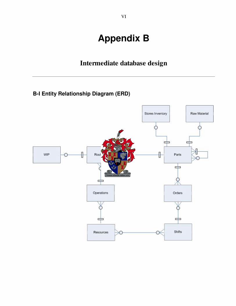
VI

Appendix B

Intermediate database design

B-I Entity Relationship Diagram (ERD)

VII

B-II Extended Entity Relationship Diagram (ERD)

BOM

VIII

B-III Implementation in Microsoft Access

IX

BOM bom_parent_id bom_child_id bom_qunatity

X

B-VI Description of tables and fields

A short description of each table and what it is used for follows:

shifts

x� shift_id (nine character text): the unique ID of each shift. It is a 9-character string literal,

which is the concatenation of the date of the shift, and the number of the shift on that

specific date, e.g. 050314-02 is the second shift on the 14th of March 2005.

x� shift_date (Medium date, e.g. 19-Jan-94): the date of the shift.

x� shift_no (Integer): the number of the shift on the specific date.

x� shift_length (number, two decimal): the length (fraction of hours) of the shift. This allows

the assignment of fractions of shifts for overtime. Say for instance that the working time

on a specific date is specified as 2.5 shifts, it will actually be stored as three shifts, of

which the first two is of the standard length, and the third is only half their length. This

also allows the functionality where the end user can manually add shifts of specified

length to certain dates.

resources:

x� rsrc_id (Text): the unique ID of each resource, e.g. R-4.

x� rsrc_name (Text): the name of the resource, e.g. “ High speed drill” .

x� rsrc_desc (Text): an optional description field.

x� rsrc_yield (Number, percentage): the yield percentage of the resource (default value is 1,

or 100%). This was implemented for later use.

x� rsrc_tot_machines (integer): the total number of available machines.

XI

shifts_resources

x� shift_rsrc_shift_id (nine character text): the unique ID of a specific shift.

x� shift_rsrc_rsrc_id (text): the unique ID of a specific resource.

x� shift_rsrc_machines (integer): the number of the resource used on the specific shift.

This table allows the user to assign certain resources to certain shifts, and to specify how many of

the available machines of each resource should be used on each shift. It allows developing

schedules while considering planned downtime of certain machines.

orders

x� order_id (Autonumber): unique manufacturing order ID.

x� order_nr (Text): what the manufacturing order is for, e.g. Sales Order S/004.

x� order_part_id (Text): the unique ID of the part on order.

x� order_quantity (integer): the number of parts on order.

x� order_shift_id (nine character text): (Due Date) the unique ID of the shift at which the

order is due.

The orders table is for manufacturing orders only, meaning that every order must and can only

have one part specified. For a sales order with multiple parts, separate orders have to be entered

into the table for each part specified.

parts

x� part_id (Text): the unique ID of each part. This Value will be read in from the ERP

database. It has to be a Text field to accommodate all keys.

x� part_name (Text): the name of the part.

x� part_desc (Text): an optional description field.

x� part_make_or_purchase (enumerated, ‘make’ or ‘purchase’): an enumerated field that

states whether a part is made in the plant or purchased from a supplier.

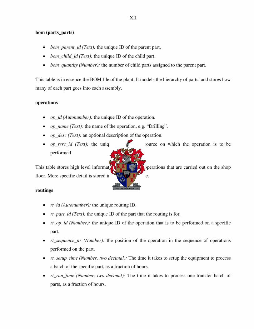
XII

bom (parts_parts)

x� bom_parent_id (Text): the unique ID of the parent part.

x� bom_child_id (Text): the unique ID of the child part.

x� bom_quantity (Number): the number of child parts assigned to the parent part.

This table is in essence the BOM file of the plant. It models the hierarchy of parts, and stores how

many of each part goes into each assembly.

operations

x� op_id (Autonumber): the unique ID of the operation.

x� op_name (Text): the name of the operation, e.g. “ Drilling” .

x� op_desc (Text): an optional description of the operation.

x� op_rsrc_id (Text): the unique ID of the resource on which the operation is to be

performed

This table stores high level information about all the operations that are carried out on the shop

floor. More specific detail is stored in the routings table.

routings

x� rt_id (Autonumber): the unique routing ID.

x� rt_part_id (Text): the unique ID of the part that the routing is for.

x� rt_op_id (Number): the unique ID of the operation that is to be performed on a specific

part.

x� rt_sequence_nr (Number): the position of the operation in the sequence of operations

performed on the part.

x� rt_setup_time (Number, two decimal): The time it takes to setup the equipment to process

a batch of the specific part, as a fraction of hours.

x� rt_run_time (Number, two decimal): The time it takes to process one transfer batch of

parts, as a fraction of hours.

XIII

This table is used to model the routings of each part. It specifies which operation should be

performed on what parts to produce the end product. Further, it contains the processing time

information needed to develop schedules. It is preferable that assembly operations must be the

first operation in the sequence for a specific part. Also, purchased parts should not appear in this

table.

stores_inventory

x� st_inv_id (Autonumber): the unique ID of the inventory record.

x� st_inv_part_id (Text): the unique ID of the finished part that is in the store, as specified in

the parts table.

x� st_inv_quantity (Integer): the number of finished goods on hand.

This table keeps record of the finished parts that are on hand, and therefore do not have to be

produced when they come on order.

wip

x� wip_id (Autonumber): the unique ID of the work in process record.

x� wip_rt_id (Number): the unique ID of the work station in front of which the work in

process is waiting.

x� wip_quantity (Number): the number of wip parts carried in stock.

raw_material

x� rw_mat_id (Autonumber): the unique ID of the raw material.

x� rw_mat_part_id (Text): the unique ID of the parts that is purchased as specified in the

parts table.

x� rw_mat_in_stock_quantity (Number): the number of parts currently on hand.

x� rw_mat_lead_time (Number, integer): the lead time to order new raw material, in terms of

the number of days.

XIV

Appendix C

Selected computer algorithms

C-I Initiating resources

XV

C-II Creating order specific Product Flow Diagrams

XVI

C-III Building the Ruins

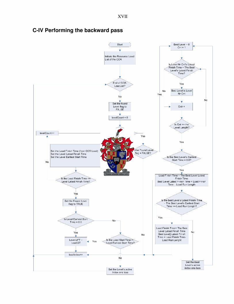
XVII

C-IV Performing the backward pass

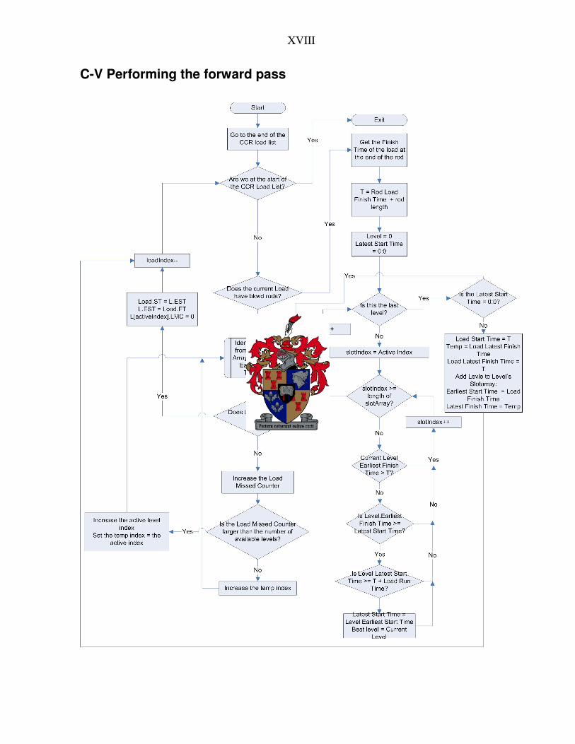
XVIII

C-V Performing the forward pass

XIX

Appendix D

Software code in C++

The complete development code listing can be viewed on the accompanying CD. Individual files

can be viewed with a simple text editor such as Notepad or Wordpad, and the project can be

viewed by installing a copy of Microsoft Visual C++.

XX

Appendix E

DBR4JS user manual

The release version of the software can be found on the attached CD. Installing and operating the

DBR4JS software is described in detail in the User Manual of this Appendix. The software is

started by the dbr4js.exe file in the DBR4JS folder on the CD. In order for the ODBC connection

(the setup is also described in the manual) to work properly, it is recommended that the software

be copied to computer hard disk.

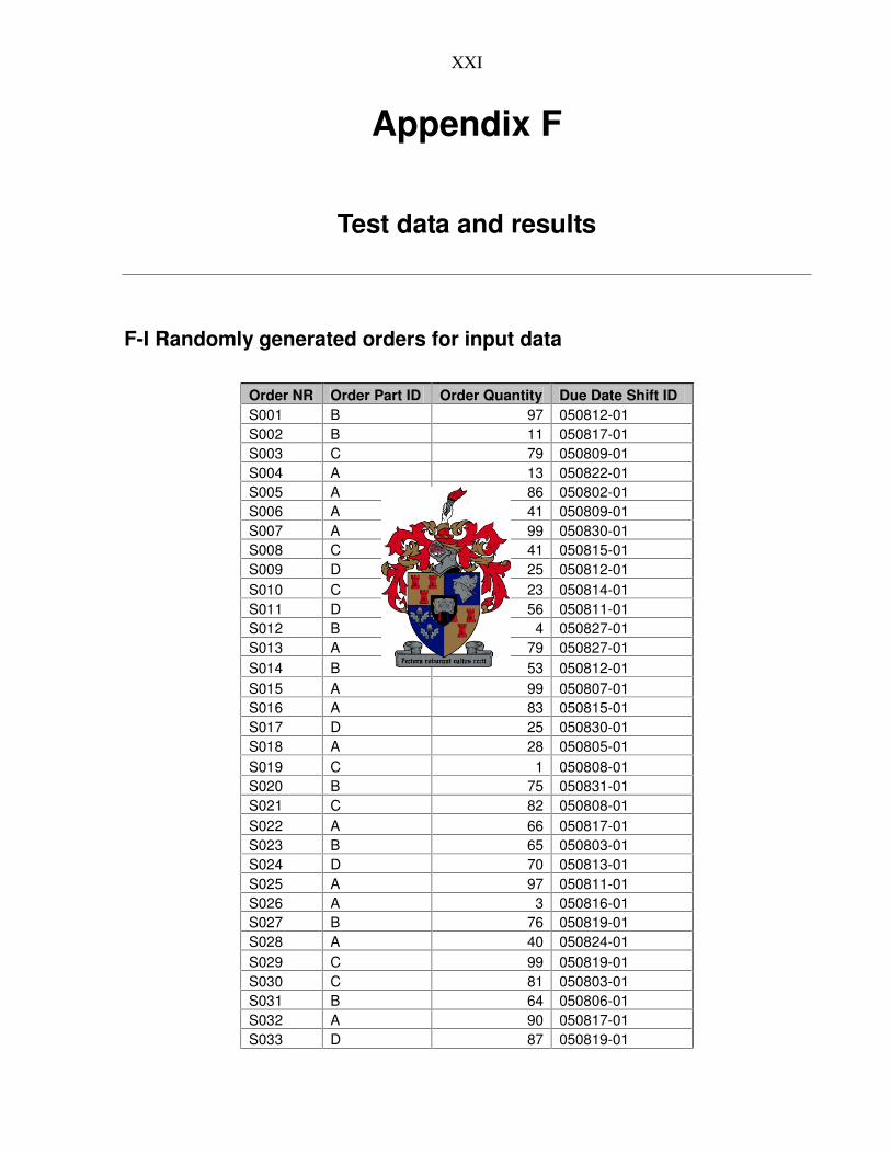
XXI

Appendix F

Test data and results

F-I Randomly generated orders for input data

Order NR Order Part ID Order Quantity Due Date Shift ID S001 B 97 050812-01 S002 B 11 050817-01 S003 C 79 050809-01 S004 A 13 050822-01 S005 A 86 050802-01 S006 A 41 050809-01 S007 A 99 050830-01 S008 C 41 050815-01 S009 D 25 050812-01 S010 C 23 050814-01 S011 D 56 050811-01 S012 B 4 050827-01 S013 A 79 050827-01 S014 B 53 050812-01 S015 A 99 050807-01 S016 A 83 050815-01 S017 D 25 050830-01 S018 A 28 050805-01 S019 C 1 050808-01 S020 B 75 050831-01 S021 C 82 050808-01 S022 A 66 050817-01 S023 B 65 050803-01 S024 D 70 050813-01 S025 A 97 050811-01 S026 A 3 050816-01 S027 B 76 050819-01 S028 A 40 050824-01 S029 C 99 050819-01 S030 C 81 050803-01 S031 B 64 050806-01 S032 A 90 050817-01 S033 D 87 050819-01

XXII

S034 A 8 050830-01 S035 C 19 050810-01 S036 A 72 050813-01 S037 A 40 050823-01 S038 A 70 050819-01 S039 D 44 050830-01 S040 B 6 050825-01 S041 B 38 050816-01 S042 D 45 050815-01 S043 A 58 050817-01 S044 A 65 050818-01 S045 B 72 050811-01 S046 A 21 050825-01 S047 D 61 050806-01 S048 B 27 050813-01 S049 B 97 050821-01 S050 C 28 050826-01 S051 D 82 050822-01 S052 A 47 050810-01 S053 B 86 050802-01 S054 B 35 050822-01 S055 A 63 050821-01 S056 A 94 050802-01 S057 C 19 050815-01 S058 D 100 050821-01 S059 A 98 050804-01 S060 A 69 050804-01 S061 A 77 050823-01 S062 A 65 050818-01 S063 A 33 050808-01 S064 B 45 050813-01 S065 A 3 050830-01 S066 B 67 050829-01 S067 C 67 050809-01 S068 B 47 050802-01 S069 D 24 050827-01 S070 D 66 050813-01 S071 D 37 050802-01 S072 B 88 050803-01 S073 A 16 050820-01 S074 D 35 050801-01 S075 A 91 050807-01 S076 A 4 050830-01 S077 C 37 050824-01 S078 B 100 050827-01 S079 A 60 050805-01 S080 B 97 050808-01 S081 B 88 050826-01 S082 A 66 050808-01

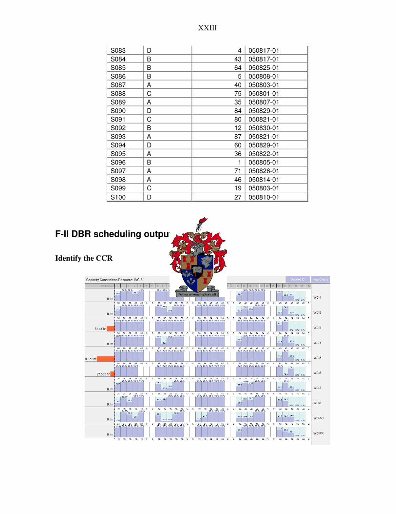
XXIII

S083 D 4 050817-01 S084 B 43 050817-01 S085 B 64 050825-01 S086 B 5 050808-01 S087 A 40 050803-01 S088 C 75 050801-01 S089 A 35 050807-01 S090 D 84 050829-01 S091 C 80 050821-01 S092 B 12 050830-01 S093 A 87 050821-01 S094 D 60 050829-01 S095 A 36 050822-01 S096 B 1 050805-01 S097 A 71 050826-01 S098 A 46 050814-01 S099 C 19 050803-01 S100 D 27 050810-01

F-II DBR scheduling output

Identify the CCR

XXIV

View orders

XXV

Exploit the CCR

XXVI

Subordinate

XXVII

F-III S-DBR scheduling output

Identify the CCR

XXVIII

Subordinate

XXIX

Appendix G

Product routings and Bill of Material information for

products produced on AAT’s Echo line

The blue boxes in the diagrams represent Part / Operations, that is operations that are performed

on specific parts. The ID of the resource performing the operation is indicated at the top of each

box (e.g. R-1). The Part ID is given in the top (lighter) part of the box (e.g. RearSkin). Each time

a new raw material (indicated by the green triangles) is added to a part, a new part ID has to be

defined in the system. The processing time for the specific part at the operation is indicated in the

lower (darker) part of each box.

XXX

G-I Variants: Taca & Hapag

XXXI

G-II Variants: Niki & Air Berlin

XXXII

G-III Variants: Swiss & British Airways

XXXIII

G-IV Variant: Britannia

XXXIV

G-V Variant: Iberia

XXXV

Appendix H

Echo line analyses with DBR4JS

The figures of Appendix H indicate the load on each resource (the first figure of every

table) and the products on order, the order sizes, buffer sizes, and the order due dates (the

second figure of every table). The work overflow of each resource is indicated by a red

square before the first shift of the planning horizon. The capacity usage of each resource

for every shift is also indicated. The second figure indicates the due date for every order

with a blue block. The red block on every order indicates the order due date minus the

shipping buffer for the order. This is the date at which work is placed on every resource

during the identification procedure.

XXXVI

H-I First-run constraint identification for Planning Horizon 1: 9 January to 21 January 2006

Figure H. 1: Resource loading for Planning Horizon: 09 Jan 06 to 21 Jan 06 Figure H. 2: Orders for Planning Horizon: 9 Jan 06 to 21 Jan 06

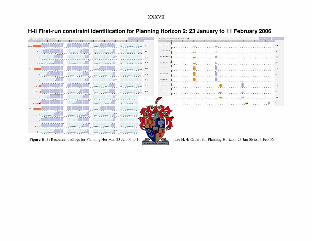
XXXVII

H-II First-run constraint identification for Planning Horizon 2: 23 January to 11 February 2006

Figure H. 3: Resource loadings for Planning Horizon: 23 Jan 06 to 11 Feb 06 Figure H. 4: Orders for Planning Horizon: 23 Jan 06 to 11 Feb 06

XXXVIII

H-III First-run constraint identification for Planning Horizon 3: 13 February to 4 March 2006

Figure H. 5: Resource loadings for Planning Horizon: 13 Feb 06 to 4 March 06 Figure H. 6: Orders for Planning Horizon: 13 Feb 06 to 4 March 06

XXXIX

H-IV First-run constraint identification for Planning Horizon 4: 6 March to 25 March 2006

Figure H. 7: Resource loadings for Planning Horizon: 6 March 06 to 25 March

06

Figure H. 8: Orders for Planning Horizon: 6 March 06 to 25 March 06

XL

H-V S-DBR Schedule for Horizon 1: 9 January to 21 January 2006

Figure H. 9: Resource loadings for Planning Horizon: 9 Jan 06 to 21 Jan 06 Figure H. 10: Orders for Planning Horizon: 9 Jan 06 to 21 Jan 06

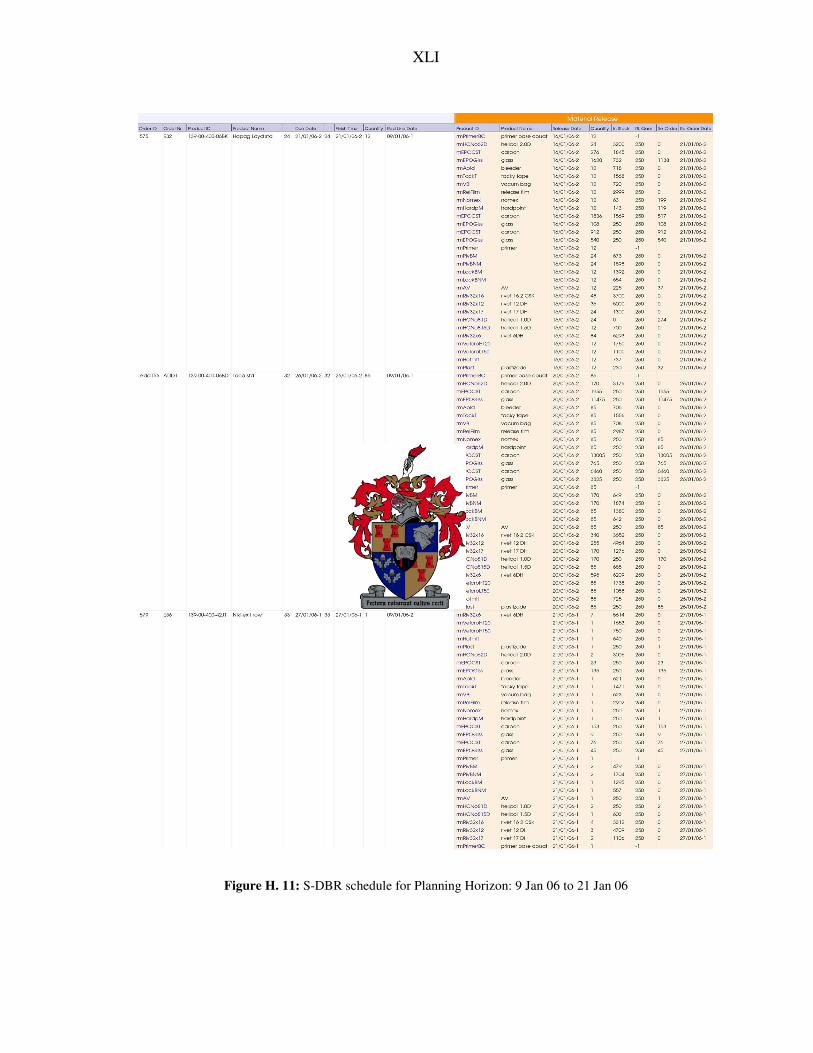
XLI

Figure H. 11: S-DBR schedule for Planning Horizon: 9 Jan 06 to 21 Jan 06

XLII

H-VI S-DBR Schedule for Horizon 2: 23 January to 11 February 2006

Figure H. 12: Resource loadings for Planning Horizon: 23 Jan 06 to 11 Feb 06 Figure H. 13: Orders for Planning Horizon: 23 Jan 06 to 11 Feb 06

XLIII

Figure H. 14: S-DBR schedule for Planning Horizon: 23 Jan 06 to 11 Feb 06

XLIV

Figure H. 14 (continued): S-DBR schedule for Planning Horizon: 23 Jan 06 to 11 Feb 06

XLV

H-VII S-DBR Schedule for Horizon 3: 13 February to 4 March 2006

Figure H. 15: Resource loadings for Planning Horizon: 13 Feb 06 to 4 March 06 Figure H. 16: Orders for Planning Horizon: 13 Feb 06 to 4 March 06

XLVI

Figure H. 17: S-DBR schedule for Planning Horizon: 13 Feb 06 to 4 March 06

XLVII

Figure H. 17 (continued): S-DBR schedule for Planning Horizon: 13 Feb 06 to 4 March 06

XLVIII

H-VIII DBR Schedule for Horizon 4: 6 March to 25 March 2006

Figure H. 18: Resource loadings for Planning Horizon: 6 March 06 to 25 March

06

Figure H. 19: Orders for Planning Horizon: 6 March 06 to 25 March 06