Development of a Vapor Compression Cycle Heat Pump ...

Development of a Vapor Compression Cycle Heat Pump model using EES. Example of application for heat recovery

ESCUELA SUPERTIOR DE TECNOLOGÍA Y CIENCIAS

EXPERIMENTALES

Departamento de Ingeniería Mecánica y Construcción

Directors: Joaquín Navarro Esbrí Francisco Molés Ribera

Final Degree’s Work Grado en Ingeniería Mecánica

Castellón de la Plana, septiembre de 2017

Héctor Torres Emo

Project Documents

Section 1 – Project Report 1 Section 2 – Budget 75 Section 3 – Schedule of conditions 79 Section 4 – Annexes 85 Section 5 – Blueprints 99

1

Section 1 – Project Report

2

Report index 1. INTRODUCTION ................................................................................................................................ 9

1.1. JUSTIFICATION ............................................................................................................................... 11 1.2. OBJECTIVE .................................................................................................................................... 11 1.3. METHODOLOGY ............................................................................................................................. 11

2. BACKGROUND ................................................................................................................................ 12

2.1. HEAT PUMP .................................................................................................................................. 12 2.2. HEAT RECOVERY APPLICATIONS ........................................................................................................ 13 2.3. THERMODYNAMIC CYCLE ................................................................................................................. 17 2.4. MAIN COMPONENTS ...................................................................................................................... 21

2.4.1. Compressor ....................................................................................................................... 21 2.4.2. Expansion device .............................................................................................................. 24 2.4.3. Heat exchanger ................................................................................................................ 24 2.4.4. Safety and control devices ................................................................................................ 26

2.5. WORKING FLUIDS ........................................................................................................................... 26

3. MODEL ........................................................................................................................................... 32

3.1. SYSTEM DESCRIPTION ..................................................................................................................... 32 3.2. STARTING HYPOTHESES .................................................................................................................... 33 3.3. COMPONENTS MODELLING ............................................................................................................... 33

3.3.1. Compressor ....................................................................................................................... 34 3.3.2. Expansion Device .............................................................................................................. 34 3.3.3. Heat Exchangers ............................................................................................................... 34

3.4. PERFORMANCE INDICATORS ............................................................................................................. 42

4. RESULTS AND ANALYSIS ................................................................................................................. 43

4.1. SIMULATION PARAMETERS ............................................................................................................... 43 4.2. RESULTS REPRESENTATION AND ANALYSIS ........................................................................................... 45

4.2.1. Cycle Parameters .............................................................................................................. 45 4.2.2. Components Parameters .................................................................................................. 57

5. CONCLUSIONS ................................................................................................................................ 69

5.1. PROJECT CONCLUSIONS ................................................................................................................... 69 5.2. FURTHER DEVELOPMENTS ................................................................................................................ 71 5.3. PERSONAL CONCLUSIONS ................................................................................................................. 71

6. BIBLIOGRAPHY ............................................................................................................................... 72

3

FIGURE INDEX FIGURE 1 GLOBAL GREENHOUSE GAS EMISSIONS SINCE 1990 ...................................................................................... 9 FIGURE 2 DERIVED HEAT PRODUCTION IN THE EU SINCE 1990. DATA SOURCE: EUROSTAT ............................................... 10 FIGURE 3 HEAT PUMP SCHEME ............................................................................................................................. 12 FIGURE 4 HEAT DEMAND QUALITY AND QUANTITY IN EUROPEAN MARKETS BY INDUSTRY. SOURCE: NELLISSEN AND WOLF, 2015

.............................................................................................................................................................. 14 FIGURE 5 ZNEH SCHEMATIC REPRESENTATION. ........................................................................................................ 15 FIGURE 6 SIMPLE CONFIGURATION ......................................................................................................................... 18 FIGURE 7 INTERNAL HEAT EXCHANGER CONFIGURATION ............................................................................................ 19 FIGURE 8 TWO-STAGE COMPRESSOR CONFIGURATION ............................................................................................... 20 FIGURE 9 CASCADE CONFIGURATION ...................................................................................................................... 21 FIGURE 10 RECIPROCATING COMPRESSOR............................................................................................................... 22 FIGURE 11 SCROLL COMPRESSOR .......................................................................................................................... 22 FIGURE 12 SCREW COMPRESSOR .......................................................................................................................... 22 FIGURE 13 COMPRESSOR TYPES AND RANGE OF OPERATION. ....................................................................................... 23 FIGURE 14 EXPANSION VALVE .............................................................................................................................. 24 FIGURE 15 HEAT EXCHANGERS: SHELL AND TUBE (LEFT) AND PLATE EXCHANGERS (RIGHT). ............................................... 25 FIGURE 16 DIAGRAM OF A CONCENTRIC CYLINDRICAL EXCHANGER .............................................................................. 25 FIGURE 17 SAFETY DEVICES .................................................................................................................................. 26 FIGURE 18 TIMELINE OF REFRIGERANTS DEVELOPMENT .............................................................................................. 28 FIGURE 19 MODEL EVOLUTION ............................................................................................................................. 32 FIGURE 20 MODEL SCHEME ................................................................................................................................. 32 FIGURE 21 CONCENTRIC HEAT EXCHANGER GEOMETRY ............................................................................................. 35 FIGURE 22 HEAT EXCHANGER TEMPERATURE SCHEME ............................................................................................... 36 FIGURE 23 EVAPORATOR STAGES ........................................................................................................................... 39 FIGURE 24 CONDENSER STAGES ............................................................................................................................ 40

TABLE INDEX TABLE 1 COMMERCIAL HEAT PUMP SYSTEMS ............................................................................................................ 14 TABLE 2 HEAT PUMP INDUSTRIAL APPLICATIONS ....................................................................................................... 16 TABLE 3 SAFETY GROUP CLASIFFICATION ................................................................................................................. 28 TABLE 4 FLUIDS PROPERTIES AND INFORMATION. ...................................................................................................... 29 TABLE 5 R134A/R1234YF/R1234ZEE DATA. VALUES FOR CRITICAL PRESSURE AND CRITICAL TEMPERATURE FROM COOLPROP

FLUIDS PROPERTIES, PURE AND PSEUDO-PURE FLUID PROPERTIES. ...................................................................... 30 TABLE 6 SYSTEM MODELLING PARAMETERS ............................................................................................................. 33 TABLE 7 COMPRESSOR MODELLING PARAMETERS...................................................................................................... 34 TABLE 8 EVAPORATOR MODELLING PARAMETERS ...................................................................................................... 39 TABLE 9 CONDENSER MODELLING PARAMETERS ........................................................................................................ 40 TABLE 10 SIMULATION PARAMETERS ..................................................................................................................... 43

4

DIAGRAM INDEX DIAGRAM 1 REVERSE CARNOT CYCLE EXAMPLE FOR R134A ........................................................................................ 17 DIAGRAM 2 IHX CYCLE ........................................................................................................................................ 20 DIAGRAM 3 PT CHART FOR SEVERAL REFRIGERANTS AT SATURATION. DATA SOURCE: COOLPROP ....................................... 29 DIAGRAM 4 R12/R134A/R1234ZE(E)/R1234YF DATA SOURCE: COOLPROP .............................................................. 31 DIAGRAM 5 PRESSURE-ENTHALPY GRAPH FOR R134A/R1234YF/R1234ZEE DATA SOURCE: COOLPROP ........................... 31 DIAGRAM 6 T-S GRAPH OF THE CYCLE WITH SECONDARY FLUIDS. SOURCE: EES ............................................................... 44 DIAGRAM 7 P-H GRAPH OF THE CYCLE. SOURCE: EES ................................................................................................ 44 DIAGRAM 8 COP SIMULATION 1 ........................................................................................................................... 45 DIAGRAM 9 CONDENSER POWER SIMULATION 1....................................................................................................... 46 DIAGRAM 10 COMPRESSOR POWER SIMULATION 1 .................................................................................................. 46 DIAGRAM 11 COP SIMULATION 2 ......................................................................................................................... 47 DIAGRAM 12 CONDENSER POWER SIMULATION 2 .................................................................................................... 47 DIAGRAM 13 COMPRESSOR POWER SIMULATION 2 .................................................................................................. 48 DIAGRAM 14 COP SIMULATION 3 ......................................................................................................................... 48 DIAGRAM 15 CONDENSER POWER SIMULATION 3 .................................................................................................... 49 DIAGRAM 16 COMPRESSOR POWER SIMULATION 3 .................................................................................................. 49 DIAGRAM 17 CR SIMULATION 1 ............................................................................................................................ 50 DIAGRAM 18 VOLUMETRIC FLOW SIMULATION 1 ...................................................................................................... 51 DIAGRAM 19 MASS FLOW SIMULATION 1 ............................................................................................................... 51 DIAGRAM 20 DISCHARGE TEMPERATURE SIMULATION 1 ............................................................................................ 52 DIAGRAM 21 CR SIMULATION 2 ............................................................................................................................ 52 DIAGRAM 22 VOLUMETRIC FLOW SIMULATION 2 ...................................................................................................... 53 DIAGRAM 23 MASS FLOW SIMULATION 2 ............................................................................................................... 53 DIAGRAM 24 DISCHARGE TEMPERATURE SIMULATION 2 ............................................................................................ 54 DIAGRAM 25 CR SIMULATION 3 ............................................................................................................................ 54 DIAGRAM 26 VOLUMETRIC FLOW SIMULATION 3 ...................................................................................................... 55 DIAGRAM 27 MASS FLOW SIMULATION 3 ............................................................................................................... 55 DIAGRAM 28 DISCHARGE TEMPERATURE SIMULATION 3 ............................................................................................ 56 DIAGRAM 29 CONDENSER EXCHANGE AREA SIMULATION 1 ......................................................................................... 57 DIAGRAM 30 EVAPORATOR EXCHANGE AREA SIMULATION 1 ....................................................................................... 58 DIAGRAM 31 IHX EXCHANGE AREA SIMULATION 1 .................................................................................................... 58 DIAGRAM 32 CONDENSER EXCHANGE AREA SIMULATION 2 ......................................................................................... 59 DIAGRAM 33 EVAPORATOR EXCHANGE AREA SIMULATION 2 ....................................................................................... 59 DIAGRAM 34 IHX EXCHANGE AREA SIMULATION 2 .................................................................................................... 60 DIAGRAM 35 CONDENSER EXCHANGE AREA SIMULATION 3 ......................................................................................... 60 DIAGRAM 36 EVAPORATOR EXCHANGE AREA SIMULATION 3 ....................................................................................... 61 DIAGRAM 37 IHX EXCHANGE AREA SIMULATION 3 .................................................................................................... 61 DIAGRAM 38 CONDENSER PRESSURE DROP SIMULATION 1 ......................................................................................... 62 DIAGRAM 39 EVAPORATOR PRESSURE DROP SIMULATION 1 ........................................................................................ 62 DIAGRAM 40 IHX EXTERNAL TUBE PRESSURE DROP SIMULATION 1 ............................................................................... 63 DIAGRAM 41 IHX INTERNAL PRESSURE DROP SIMULATION 1 ....................................................................................... 63 DIAGRAM 42 CONDENSER PRESSURE DROP SIMULATION 2 ......................................................................................... 64 DIAGRAM 43 EVAPORATOR PRESSURE DROP SIMULATION 2 ........................................................................................ 64 DIAGRAM 44 IHX EXTERNAL TUBE PRESSURE DROP SIMULATION 2 ............................................................................... 65 DIAGRAM 45 IHX INTERNAL TUBE PRESSURE DROP SIMULATION 2 ............................................................................... 65 DIAGRAM 46 CONDENSER PRESSURE DROP SIMULATION 3 ......................................................................................... 66 DIAGRAM 47 EVAPORATOR PRESSURE DROP SIMULATION 3 ........................................................................................ 66 DIAGRAM 48 IHX EXTERNAL TUBE PRESSURE DROP SIMULATION 3 ............................................................................... 67 DIAGRAM 49 IHX INTERNAL TUBE PRESSURE DROP SIMULATION 3 ............................................................................... 67

5

EQUATION INDEX EQUATION 1 CARNOT COP WITH TEMPERATURES ..................................................................................................... 17 EQUATION 2 HEAT PUMP COP ............................................................................................................................. 17 EQUATION 3 THERMAL POWER ............................................................................................................................. 18 EQUATION 4 MODEL COP ................................................................................................................................... 34 EQUATION 5 COMPRESSOR POWER ....................................................................................................................... 34 EQUATION 6 VOLUMETRIC CAPACITY OF THE COMPRESSOR ........................................................................................ 34 EQUATION 7 ISENTROPIC PERFORMANCE INTERACTION .............................................................................................. 34 EQUATION 8 HEAT TRANSFER BETWEEN FLUIDS ........................................................................................................ 35 EQUATION 9 LOGARITHMIC MEAN TEMPERATURE AVERAGE ...................................................................................... 35 EQUATION 10 TEMPERATURE DIFFERENCE A ........................................................................................................... 35 EQUATION 11 TEMPERATURE DIFFERENCE B ........................................................................................................... 35 EQUATION 12 GLOBAL HEAT TRANSFER COEFFICIENT ................................................................................................ 36 EQUATION 13 CONVECTION THERMAL RESISTANCE .................................................................................................. 36 EQUATION 14 CONDUCTION THERMAL RESISTANCE .................................................................................................. 36 EQUATION 15 GLOBAL THERMAL RESISTANCE ......................................................................................................... 36 EQUATION 16 RELATIONSHIP BETWEEN LENGTH AND HEAT TRANSFER ........................................................................... 36 EQUATION 17 REYNOLDS NUMBER ........................................................................................................................ 37 EQUATION 18 PRANDTL NUMBER ......................................................................................................................... 37 EQUATION 19 HEAT TRANSFER COEFFICIENT FOR SINGLE PHASE .................................................................................. 37 EQUATION 20 GNIELINSKI CORRELATION FOR NUSSELT NUMBER .................................................................................. 37 EQUATION 21 FRICTION FACTOR ........................................................................................................................... 37 EQUATION 22 DARCY-WEISBACH CORRELATION ....................................................................................................... 38 EQUATION 23 IHX POWER ................................................................................................................................... 38 EQUATION 24 IHX EFFICIENCY PARAMETER ............................................................................................................. 38 EQUATION 25 EVAPORATOR POWER ...................................................................................................................... 39 EQUATION 26 CONDENSER POWER ....................................................................................................................... 40 EQUATION 27 DITTUS-BOELTER CORRELATION ........................................................................................................ 40 EQUATION 28 GUNGOR-WINTERTON CORRELATION ................................................................................................. 41 EQUATION 29 QUALITY INCREASE FACTOR ............................................................................................................... 41 EQUATION 30 QUALITY INCREASE FACTOR MODIFIER ................................................................................................. 41 EQUATION 31 SUPPRESSION FACTOR ...................................................................................................................... 41 EQUATION 32 SUPPRESSION FACTOR MODIFIER ........................................................................................................ 41 EQUATION 33 FROUDE NUMBER ........................................................................................................................... 41 EQUATION 34 BOILING NUMBER ........................................................................................................................... 41 EQUATION 35 SHAH CORRELATION ........................................................................................................................ 41 EQUATION 36 SHAH QUALITY FACTOR .................................................................................................................... 42 EQUATION 37 PIERRE CORRELATION ...................................................................................................................... 42 EQUATION 38 FRICTION FACTOR FOR PHASE CHANGE ................................................................................................ 42 EQUATION 39 FRICTION FACTOR QUALITY MODIFIER ................................................................................................. 42 EQUATION 40 COMPRESSOR RATIO ........................................................................................................................ 43

6

NOMENCLATURE Symbol – Letter Parameter and unit

P Pressure [Pa]

T Temperature [K]

�̇�𝑄 Thermal power [W]

W Compressor power [W]

q Quality [-]

h Enthalpy [J/Kg]

s Entropy [J/Kg·K]

�̇�𝑚 Mass flow rate [Kg/s]

Bo Boiling number [-]

Frlo Froude number [-]

Nu Nusselt number [-]

Re Reynolds number [-]

Pr Prandtl number [-]

G Mass velocity [Kg/s·m2]

g Gravity [m/s2]

D Diameter [m]

L Length [m]

A Area [m2]

cp Specific heat [J/Kg·K]

f Friction factor [-]

V Volume [m3]

v Velocity [m/s]

Δ Increment applied to a parameter [-]

η Performance indicator [-]

α Heat transfer coefficient [W/m2·K]

ρ Density [Kg/m3]

µ Dynamic viscosity [Pa·s]

υ Specific volume [m3/Kg]

ε Efficiency parameter [-]

F Increase factor [-]

S Suppression factor [-]

k Thermal conductivity [W/m·K]

R Thermal resistance [-]

U Global heat transfer coefficient [W/m2·K]

Z Shah coefficient [-]

CR Compression Ratio [-]

7

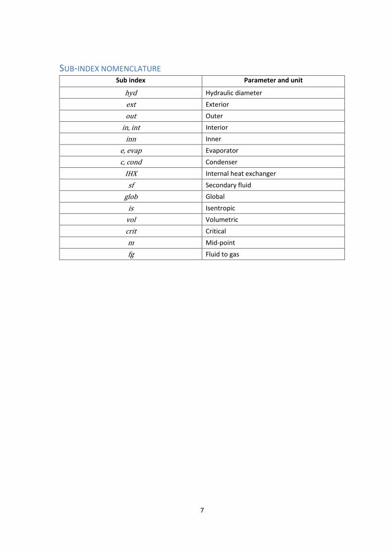
SUB-INDEX NOMENCLATURE Sub index Parameter and unit

hyd Hydraulic diameter

ext Exterior

out Outer

in, int Interior

inn Inner

e, evap Evaporator

c, cond Condenser

IHX Internal heat exchanger

sf Secondary fluid

glob Global

is Isentropic

vol Volumetric

crit Critical

m Mid-point

fg Fluid to gas

9

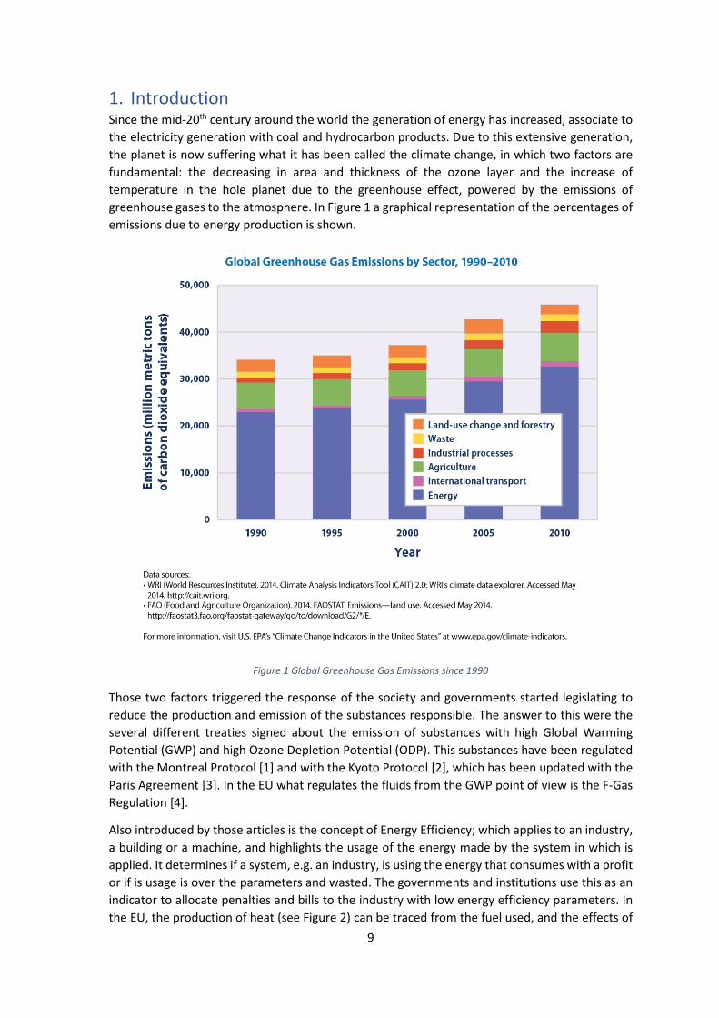
1. Introduction Since the mid-20th century around the world the generation of energy has increased, associate to the electricity generation with coal and hydrocarbon products. Due to this extensive generation, the planet is now suffering what it has been called the climate change, in which two factors are fundamental: the decreasing in area and thickness of the ozone layer and the increase of temperature in the hole planet due to the greenhouse effect, powered by the emissions of greenhouse gases to the atmosphere. In Figure 1 a graphical representation of the percentages of emissions due to energy production is shown.

Figure 1 Global Greenhouse Gas Emissions since 1990

Those two factors triggered the response of the society and governments started legislating to reduce the production and emission of the substances responsible. The answer to this were the several different treaties signed about the emission of substances with high Global Warming Potential (GWP) and high Ozone Depletion Potential (ODP). This substances have been regulated with the Montreal Protocol [1] and with the Kyoto Protocol [2], which has been updated with the Paris Agreement [3]. In the EU what regulates the fluids from the GWP point of view is the F-Gas Regulation [4].

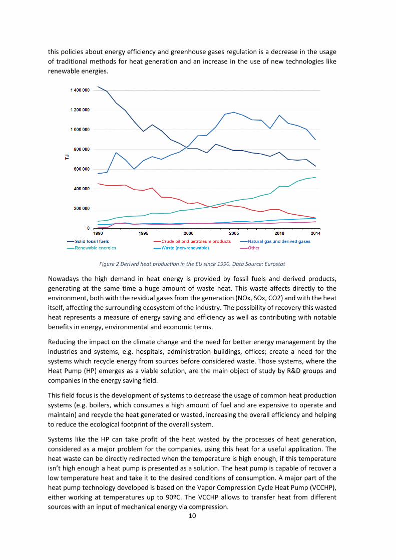
Also introduced by those articles is the concept of Energy Efficiency; which applies to an industry, a building or a machine, and highlights the usage of the energy made by the system in which is applied. It determines if a system, e.g. an industry, is using the energy that consumes with a profit or if is usage is over the parameters and wasted. The governments and institutions use this as an indicator to allocate penalties and bills to the industry with low energy efficiency parameters. In the EU, the production of heat (see Figure 2) can be traced from the fuel used, and the effects of

10

this policies about energy efficiency and greenhouse gases regulation is a decrease in the usage of traditional methods for heat generation and an increase in the use of new technologies like renewable energies.

Figure 2 Derived heat production in the EU since 1990. Data Source: Eurostat

Nowadays the high demand in heat energy is provided by fossil fuels and derived products, generating at the same time a huge amount of waste heat. This waste affects directly to the environment, both with the residual gases from the generation (NOx, SOx, CO2) and with the heat itself, affecting the surrounding ecosystem of the industry. The possibility of recovery this wasted heat represents a measure of energy saving and efficiency as well as contributing with notable benefits in energy, environmental and economic terms.

Reducing the impact on the climate change and the need for better energy management by the industries and systems, e.g. hospitals, administration buildings, offices; create a need for the systems which recycle energy from sources before considered waste. Those systems, where the Heat Pump (HP) emerges as a viable solution, are the main object of study by R&D groups and companies in the energy saving field.

This field focus is the development of systems to decrease the usage of common heat production systems (e.g. boilers, which consumes a high amount of fuel and are expensive to operate and maintain) and recycle the heat generated or wasted, increasing the overall efficiency and helping to reduce the ecological footprint of the overall system.

Systems like the HP can take profit of the heat wasted by the processes of heat generation, considered as a major problem for the companies, using this heat for a useful application. The heat waste can be directly redirected when the temperature is high enough, if this temperature isn’t high enough a heat pump is presented as a solution. The heat pump is capable of recover a low temperature heat and take it to the desired conditions of consumption. A major part of the heat pump technology developed is based on the Vapor Compression Cycle Heat Pump (VCCHP), either working at temperatures up to 90ºC. The VCCHP allows to transfer heat from different sources with an input of mechanical energy via compression.

11

In the recent years of investigation, the VCCHP are bounded to the generation of electricity with renewables sources, e.g. solar panels and batteries, to provide a full system for energy recovery with the minimum impact on the environment. [5]

The development in the energy saving field focused not only on the systems and the components, but also in the working fluids used, which in last terms, are the key of this systems allowing them to operate at different temperatures and limit the geometry and characteristics of the components.

The fields of operation for this technology it’s wide and comprehend a great variety of different fields, each one of it with their needs and specifications. Thus, an extensive range of components and fluids has been created and which need to be tested and analysed before installed, because the heat recovery systems are not a cheap and require an exhaustive study for each application. In order to develop efficient systems, new methods had to be developed due to the quantity of possible iterations for a single application, the increase in the number of working fluids and the range of components available. Data bases has been created with the characteristics of the fluids, which helps to calculate and examine those fluids allowing to model and compare different cycles, systems and components.

1.1. Justification Due to the possibility of use residual energy through a heat pump, it is analysed this technology to apply it in the energy recovery, from waste or natural sources, to enhance efficiency in the heat production.

This technology developed focused on the Heat Pump systems, which allow to make the most of the low temperature residual heat in heat demanding processes and thus reducing the need of traditional heat generation systems.

In this Final Degree’s Work, the Heat Pump system will be treated as a valid method to recover energy from residual heat sources before considered waste. In these terms, the study will also focus on the usage of new low-GWP fluids as substitute for the previous refrigerants.

1.2. Objective The general objective is the study, using models of Vapor Compression Cycle Heat Pump (VCCHP) systems for the recovery of residual heat recovery and the evaluation of Low-GWP working fluids as an alternative.

The specific objectives of the work are:

• Background review. • Heat Pump model for testing. • Analysis of performance parameters from different fluids. • Analysis of components.

1.3. Methodology To achieve the objectives previously set a methodology based on the development of the HP model is proposed. The model will be used to test the different alternative fluids and, therefore, the evaluation and analysis of the results.

12

Thus, the present document is organised:

• Present chapter: Introduction. Stablishing the key factors for the HP technology and the social and economic base where stands.

• Chapter 2: Background. Reviewing the technology conforming the HP system and the components of it as well as the fluids used to operate and the evolution of them.

• Chapter 3: Model. Defining the hypotheses and mathematical methods used in the HP modelling and the starting data and format of the results.

• Chapter 4: Results. Gathering the results given by the model in the simulations and comparing the key performance parameters for the iterations done.

• Chapter 5: Conclusions. Reviewing the results and stablishing connections with the background and applications for the technology studied.

Therefore, the work developed here contributes to help this field of development with an iterative mathematical model for VCCHP systems using Engineering Equation Solver (EES) software [6] and the CoolProp libraries [7] which can simulate under different work conditions several different refrigerants in order to gather data from them and allowing the analysis and comparison.

2. Background 2.1. Heat Pump

The Heat Pump system analysed is based on the vapor compression cycle, using a compressor, a condenser, an expansion valve and an evaporator in the simplest configuration.

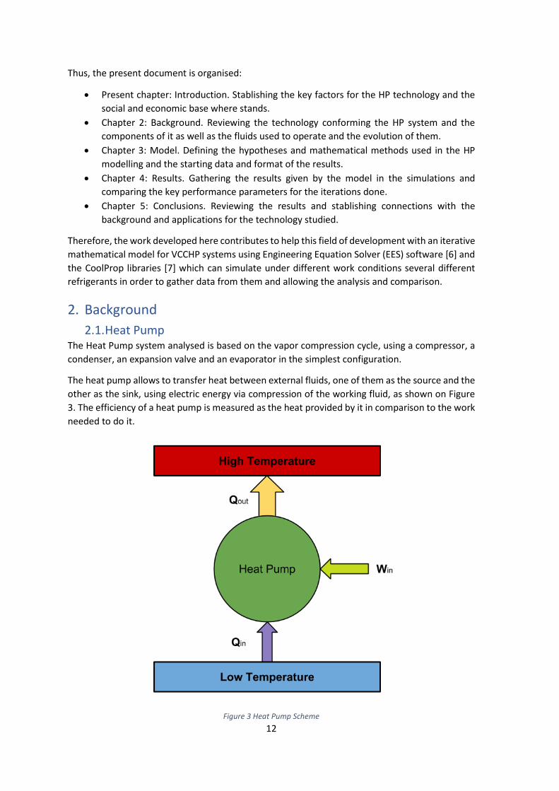
The heat pump allows to transfer heat between external fluids, one of them as the source and the other as the sink, using electric energy via compression of the working fluid, as shown on Figure 3. The efficiency of a heat pump is measured as the heat provided by it in comparison to the work needed to do it.

Figure 3 Heat Pump Scheme

13

The Heat Pump technology has been developed intensively in the past two decades but is application remained in a secondary place as an effective way to provide heat due to initial cost, the system design and the integration in different areas.

With the new environmental-friendly methods to produce electricity and with the greenhouse effect in mind, the heat pump stands as the better option to increase energy efficiency in large-scale systems allowing to recovery energy from sources previously wasted. [8]

In industrial applications the refrigerant used heat pumps is the R134a with high pressure compressors [9], producing heat at temperatures ranges up to 80ºC.

2.2. Heat Recovery Applications The purpose of the heat pump it’s to redirect heat from a waste or a source such as the environment to an application. As a matter of energy efficiency, the heat pump plans a major part as the heat recovery system for industries and in other applications such as water heater for domestic use.

The heat pump plays the key factor in systems where the waste of energy is high, e.g. metal industries or petrochemical industries. The heat recovery from this source, which comes at high temperature, has been the major focus of development and research, although it’s the minor percentage of energy waste.

The major percentage of energy waste is located in low temperature heat sources (under 90ºC), depending on the industry it could range from 20 to 51% of the total heat used in the production process. [10]

The principle of heat recovery in industries and domestic usage has been named as essential by governments and authorities to reduce the consumption of energy in both fields, this statement has become the motor for research and development in the heat pump technologies, so it could be implemented in a great variety of applications with different working fluids to optimise the production and consumption of energy.

The goal of the heat recovery is to provide a system to increase the efficiency in terms of energy consumption in every process where heat is a key factor, and therefore reduce the environmental impact of those processes. Due to the Paris Agreement [3], and prior to that the Montreal Protocol [11], the need for better systems has expanded to every layer of the society where the waste of energy it’s happening. The efforts in R&D are focused on better energy production, via renewable energy e.g. solar panels or windmills, and better energy consumption reducing the energy waste or making a profit out of the waste.

New components and fluids allowed the research, design and modelling of heat pumps for application in several different areas such as petroleum refining, food and beverage production, textiles, wood products and for any industry which requires a heat source in the production line and have a heat waste., although the heat pump it’s not the main heat source but an efficiency-focused system which increases the overall performance.

To perform correctly in the different range of operating temperatures where the Heat Pump technology applies the basic heat pump system it’s modified adding several components originating multiple configurations and iterations with several fluids thus providing flexibility, both in application and available options in the market. The inclusion of renewable energy production

14

in the industry expands the possibilities of the heat pump as a viable solution for energy efficiency increases in heat consumption systems.

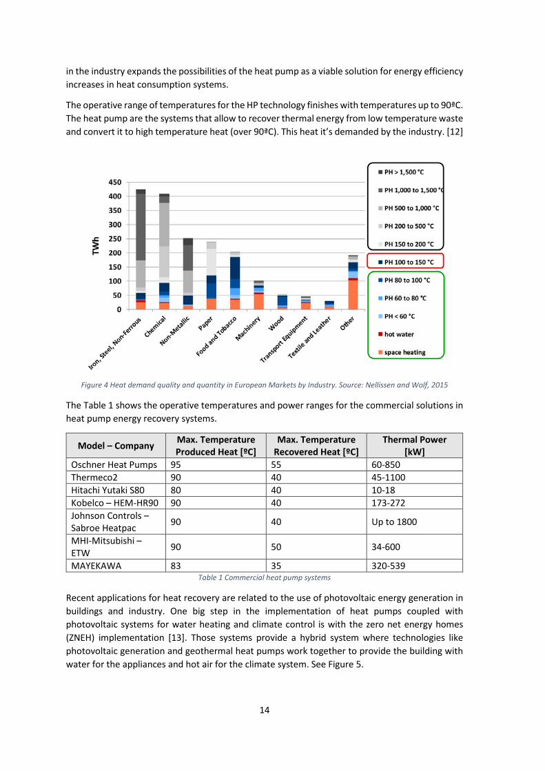
The operative range of temperatures for the HP technology finishes with temperatures up to 90ªC. The heat pump are the systems that allow to recover thermal energy from low temperature waste and convert it to high temperature heat (over 90ªC). This heat it’s demanded by the industry. [12]

Figure 4 Heat demand quality and quantity in European Markets by Industry. Source: Nellissen and Wolf, 2015

The Table 1 shows the operative temperatures and power ranges for the commercial solutions in heat pump energy recovery systems.

Model – Company Max. Temperature Produced Heat [ºC]

Max. Temperature Recovered Heat [ºC]

Thermal Power [kW]

Oschner Heat Pumps 95 55 60-850 Thermeco2 90 40 45-1100 Hitachi Yutaki S80 80 40 10-18 Kobelco – HEM-HR90 90 40 173-272 Johnson Controls – Sabroe Heatpac 90 40 Up to 1800

MHI-Mitsubishi – ETW 90 50 34-600

MAYEKAWA 83 35 320-539 Table 1 Commercial heat pump systems

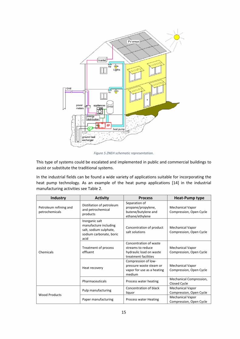
Recent applications for heat recovery are related to the use of photovoltaic energy generation in buildings and industry. One big step in the implementation of heat pumps coupled with photovoltaic systems for water heating and climate control is with the zero net energy homes (ZNEH) implementation [13]. Those systems provide a hybrid system where technologies like photovoltaic generation and geothermal heat pumps work together to provide the building with water for the appliances and hot air for the climate system. See Figure 5.

15

Figure 5 ZNEH schematic representation.

This type of systems could be escalated and implemented in public and commercial buildings to assist or substitute the traditional systems.

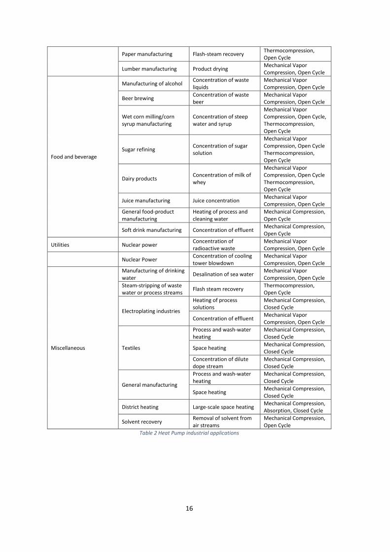
In the industrial fields can be found a wide variety of applications suitable for incorporating the heat pump technology. As an example of the heat pump applications [14] in the industrial manufacturing activities see Table 2.

Industry Activity Process Heat-Pump type

Petroleum refining and petrochemicals

Distillation of petroleum and petrochemical products

Separation of propane/propylene, butene/butylene and ethane/ethylene

Mechanical Vapor Compression, Open Cycle

Chemicals

Inorganic salt manufacture including salt, sodium sulphate, sodium carbonate, boric acid

Concentration of product salt solutions


Treatment of process effluent

Concentration of waste streams to reduce hydraulic load on waste treatment facilities


Heat recovery

Compression of low-pressure waste steam or vapor for use as a heating medium


Pharmaceuticals Process water heating Mechanical Compression, Closed Cycle

Wood Products Pulp manufacturing Concentration of black

liquor Mechanical Vapor Compression, Open Cycle

Paper manufacturing Process water Heating Mechanical Vapor Compression, Open Cycle

16

Paper manufacturing Flash-steam recovery Thermocompression, Open Cycle

Lumber manufacturing Product drying Mechanical Vapor Compression, Open Cycle

Food and beverage

Manufacturing of alcohol Concentration of waste liquids


Beer brewing Concentration of waste beer


Wet corn milling/corn syrup manufacturing

Concentration of steep water and syrup

Mechanical Vapor Compression, Open Cycle, Thermocompression, Open Cycle

Sugar refining Concentration of sugar solution

Mechanical Vapor Compression, Open Cycle Thermocompression, Open Cycle

Dairy products Concentration of milk of whey

Mechanical Vapor Compression, Open Cycle Thermocompression, Open Cycle

Juice manufacturing Juice concentration Mechanical Vapor Compression, Open Cycle

General food-product manufacturing

Heating of process and cleaning water

Mechanical Compression, Open Cycle

Soft drink manufacturing Concentration of effluent Mechanical Compression, Open Cycle

Utilities Nuclear power Concentration of radioactive waste


Nuclear Power Concentration of cooling tower blowdown


Miscellaneous

Manufacturing of drinking water Desalination of sea water Mechanical Vapor

Compression, Open Cycle Steam-stripping of waste water or process streams Flash steam recovery Thermocompression,

Open Cycle

Electroplating industries

Heating of process solutions

Mechanical Compression, Closed Cycle

Concentration of effluent Mechanical Vapor Compression, Open Cycle

Textiles

Process and wash-water heating


Space heating Mechanical Compression, Closed Cycle

Concentration of dilute dope stream


General manufacturing

Process and wash-water heating


Space heating Mechanical Compression, Closed Cycle

District heating Large-scale space heating Mechanical Compression, Absorption, Closed Cycle

Solvent recovery Removal of solvent from air streams

Mechanical Compression, Open Cycle

Table 2 Heat Pump industrial applications

17

2.3. Thermodynamic cycle The cycle corresponds to the vapor compression cycle, it stands as a cycle that allows to transfer heat using the expansion and compression of a fluid under certain conditions of pressure, temperature and flow.

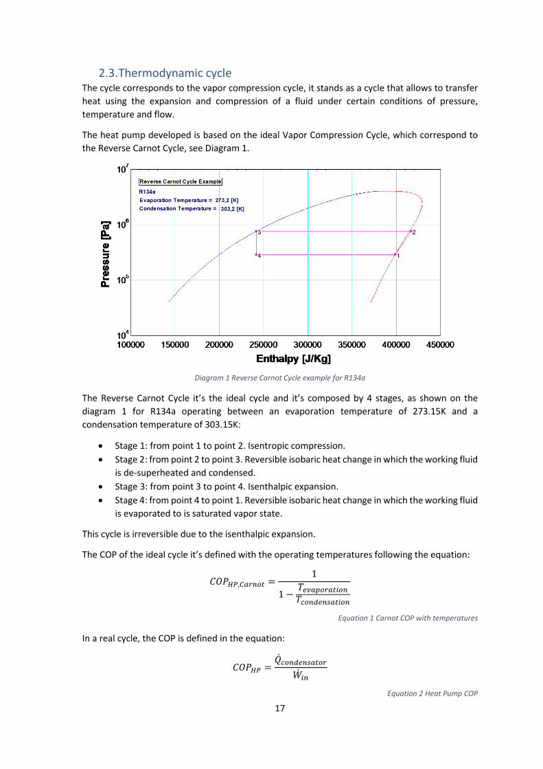
The heat pump developed is based on the ideal Vapor Compression Cycle, which correspond to the Reverse Carnot Cycle, see Diagram 1.

Diagram 1 Reverse Carnot Cycle example for R134a

The Reverse Carnot Cycle it’s the ideal cycle and it’s composed by 4 stages, as shown on the diagram 1 for R134a operating between an evaporation temperature of 273.15K and a condensation temperature of 303.15K:

• Stage 1: from point 1 to point 2. Isentropic compression. • Stage 2: from point 2 to point 3. Reversible isobaric heat change in which the working fluid

is de-superheated and condensed. • Stage 3: from point 3 to point 4. Isenthalpic expansion. • Stage 4: from point 4 to point 1. Reversible isobaric heat change in which the working fluid

is evaporated to is saturated vapor state.

This cycle is irreversible due to the isenthalpic expansion.

The COP of the ideal cycle it’s defined with the operating temperatures following the equation:

𝐶𝐶𝐶𝐶𝐶𝐶𝐻𝐻𝐻𝐻,𝐶𝐶𝐶𝐶𝐶𝐶𝐶𝐶𝐶𝐶𝐶𝐶 =1

1 −𝑇𝑇𝑒𝑒𝑒𝑒𝐶𝐶𝑒𝑒𝐶𝐶𝐶𝐶𝐶𝐶𝐶𝐶𝑒𝑒𝐶𝐶𝐶𝐶𝑇𝑇𝑐𝑐𝐶𝐶𝐶𝐶𝑐𝑐𝑒𝑒𝐶𝐶𝑐𝑐𝐶𝐶𝐶𝐶𝑒𝑒𝐶𝐶𝐶𝐶

Equation 1 Carnot COP with temperatures

In a real cycle, the COP is defined in the equation:

𝐶𝐶𝐶𝐶𝐶𝐶𝐻𝐻𝐻𝐻 =�̇�𝑄𝑐𝑐𝐶𝐶𝐶𝐶𝑐𝑐𝑒𝑒𝐶𝐶𝑐𝑐𝐶𝐶𝐶𝐶𝐶𝐶𝐶𝐶

�̇�𝑊𝑒𝑒𝐶𝐶

Equation 2 Heat Pump COP

18

And the power of the components is defined in the following equation:

�̇�𝑄 = �̇�𝑚 · Δℎ

Equation 3 Thermal Power

Where the Qcondenser it’s the useful heat provided by the system and the Win it’s the total amount of energy consumed from the supply. [15]

The vapor compression cycle it’s applied in refrigeration and in heat pumps, depending on which heat flow it’s the one used to design the system.

There are several types and configurations of heat pumps depending on the components used, the simplest configuration allows to understand and study the general parameters and the correlations involved in the working process however it’s not the best configuration efficiency focused. The main components are always present but a variety of intercoolers, compressors, valves and heat exchangers are added to increase the overall COP of the system.

The optimal configuration it’s based on the demands from the application and the suitability of the components and fluids to work and operate under those conditions.

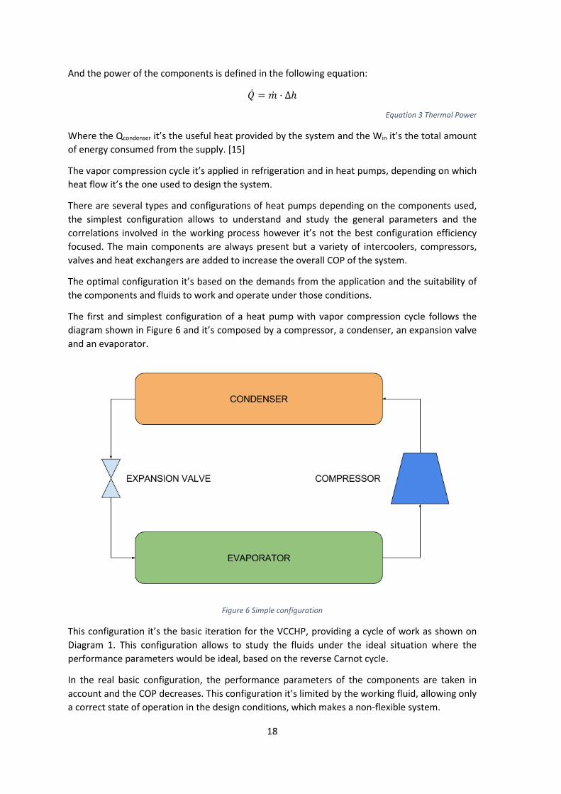
The first and simplest configuration of a heat pump with vapor compression cycle follows the diagram shown in Figure 6 and it’s composed by a compressor, a condenser, an expansion valve and an evaporator.

Figure 6 Simple configuration

This configuration it’s the basic iteration for the VCCHP, providing a cycle of work as shown on Diagram 1. This configuration allows to study the fluids under the ideal situation where the performance parameters would be ideal, based on the reverse Carnot cycle.

In the real basic configuration, the performance parameters of the components are taken in account and the COP decreases. This configuration it’s limited by the working fluid, allowing only a correct state of operation in the design conditions, which makes a non-flexible system.

19

Adding an Internal Heat Exchanger (IHX), as shown on Figure 7to the basic configuration allows to increase the real performance of the HP and allowing the system to adapt to minimal changes of the parameters of work. The IHX exchanges the heat between the superheated liquid fluid at the outlet of the condenser and the subcooled gas fluid at the outlet of the evaporator. This allows the compressor to work in the most efficient way and allowing the system to expand the range of working temperatures.

Figure 7 Internal Heat Exchanger configuration

The cycle for this configuration it’s like the reverse Carnot cycle diagram although incorporating more points to it. See Diagram 2 as an example of the cycle for the IHX configuration. The internal heat exchange occurs between points 5-6 and 9-1.

20

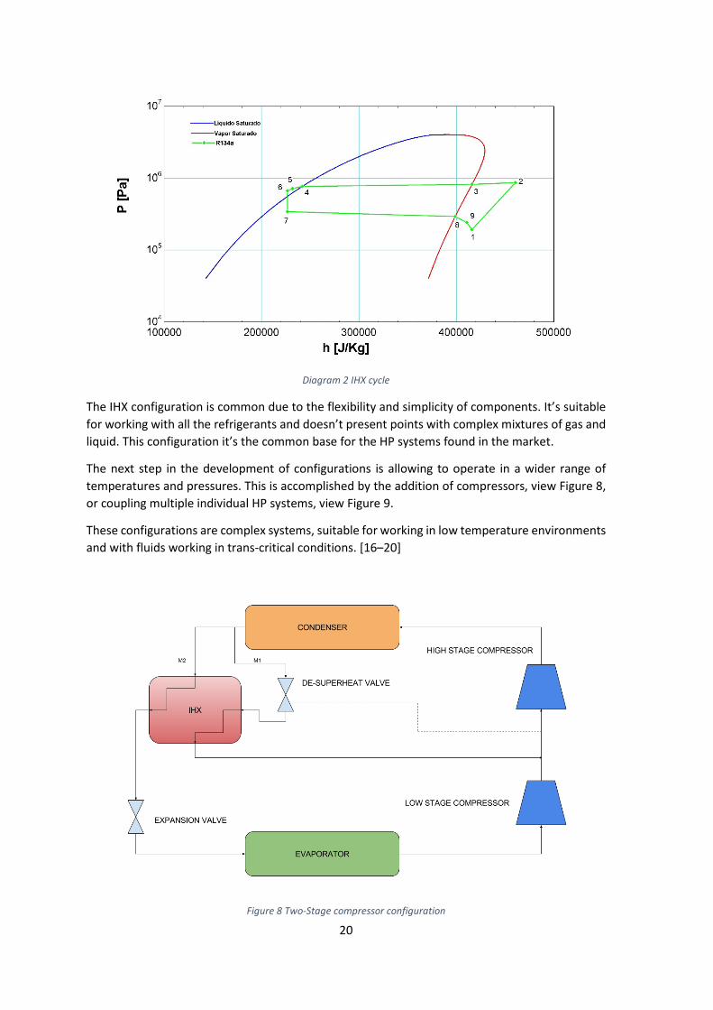
Diagram 2 IHX cycle

The IHX configuration is common due to the flexibility and simplicity of components. It’s suitable for working with all the refrigerants and doesn’t present points with complex mixtures of gas and liquid. This configuration it’s the common base for the HP systems found in the market.

The next step in the development of configurations is allowing to operate in a wider range of temperatures and pressures. This is accomplished by the addition of compressors, view Figure 8, or coupling multiple individual HP systems, view Figure 9.

These configurations are complex systems, suitable for working in low temperature environments and with fluids working in trans-critical conditions. [16–20]

Figure 8 Two-Stage compressor configuration

21

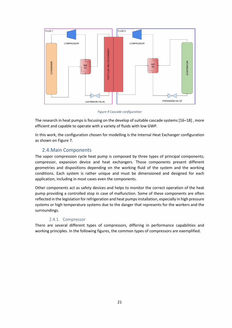
Figure 9 Cascade configuration

The research in heat pumps is focusing on the develop of suitable cascade systems [16–18] , more efficient and capable to operate with a variety of fluids with low GWP.

In this work, the configuration chosen for modelling is the Internal Heat Exchanger configuration as shown on Figure 7.

2.4. Main Components The vapor compression cycle heat pump is composed by three types of principal components; compressor, expansion device and heat exchangers. Those components present different geometries and dispositions depending on the working fluid of the system and the working conditions. Each system is rather unique and must be dimensioned and designed for each application, including in most cases even the components.

Other components act as safety devices and helps to monitor the correct operation of the heat pump providing a controlled stop in case of malfunction. Some of these components are often reflected in the legislation for refrigeration and heat pumps installation, especially in high pressure systems or high temperature systems due to the danger that represents for the workers and the surroundings.

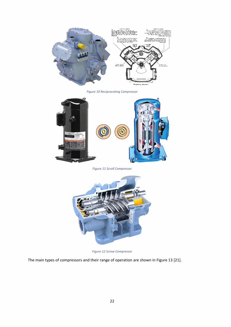
2.4.1. Compressor There are several different types of compressors, differing in performance capabilities and working principles. In the following figures, the common types of compressors are exemplified.

22

Figure 10 Reciprocating Compressor

Figure 11 Scroll Compressor

Figure 12 Screw Compressor

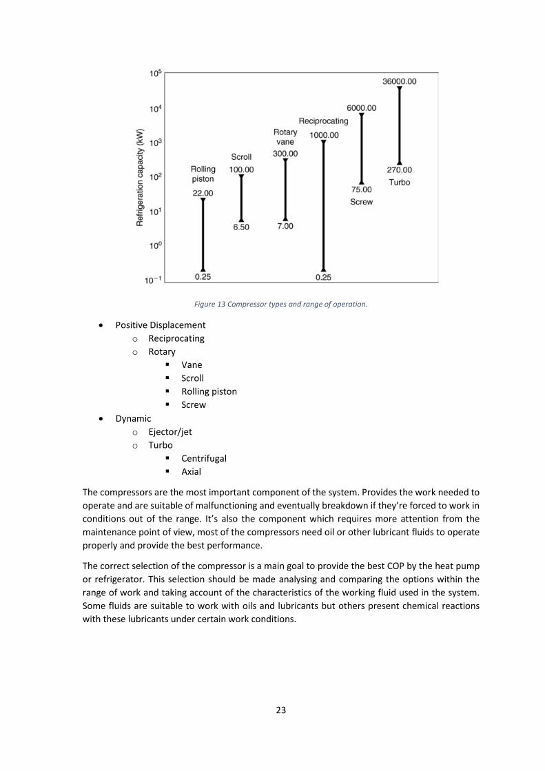
The main types of compressors and their range of operation are shown in Figure 13 [21].

23

Figure 13 Compressor types and range of operation.

• Positive Displacement o Reciprocating o Rotary

Vane Scroll Rolling piston Screw

• Dynamic o Ejector/jet o Turbo

Centrifugal Axial

The compressors are the most important component of the system. Provides the work needed to operate and are suitable of malfunctioning and eventually breakdown if they’re forced to work in conditions out of the range. It’s also the component which requires more attention from the maintenance point of view, most of the compressors need oil or other lubricant fluids to operate properly and provide the best performance.

The correct selection of the compressor is a main goal to provide the best COP by the heat pump or refrigerator. This selection should be made analysing and comparing the options within the range of work and taking account of the characteristics of the working fluid used in the system. Some fluids are suitable to work with oils and lubricants but others present chemical reactions with these lubricants under certain work conditions.

24

2.4.2. Expansion device

Figure 14 Expansion Valve

The expansion device acts as an actuator before the fluid enters the evaporation zone triggering this phase change. Is located in between the high-pressure condensation zone and the low-pressure evaporation zone. Usually the expansion device is a valve, which is regulated to operate at the designated pressure in the cycle. By the variation of the regulation for the trigger pressure of the valve variable temperatures of evaporation are possible always assuring the integrity of the rest of the components in the system. There are other types of expansion devices such as capillary tubes but doesn’t allow any type of regulation. The newest technology in valves allow to control electronically the discharge pressure so the behaviour of the system can be changed to accommodate to different working parameters without the need to replace parts. [22]

In reversible configurations such as the ones found in climate control three-way valves are found, which by switching positions allow the flow to change direction so the system can work as a heat pump or as a refrigeration unit. This only work for certain fluids and components but it’s a common configuration that can be found in domestic installations where the range of temperatures are low.

The expansion valves must assure one direction of flow in the system so there is not fluid returning to the compressor when the system is running, and must be closed, either by itself or by another solenoid valve, when the system is stopped.

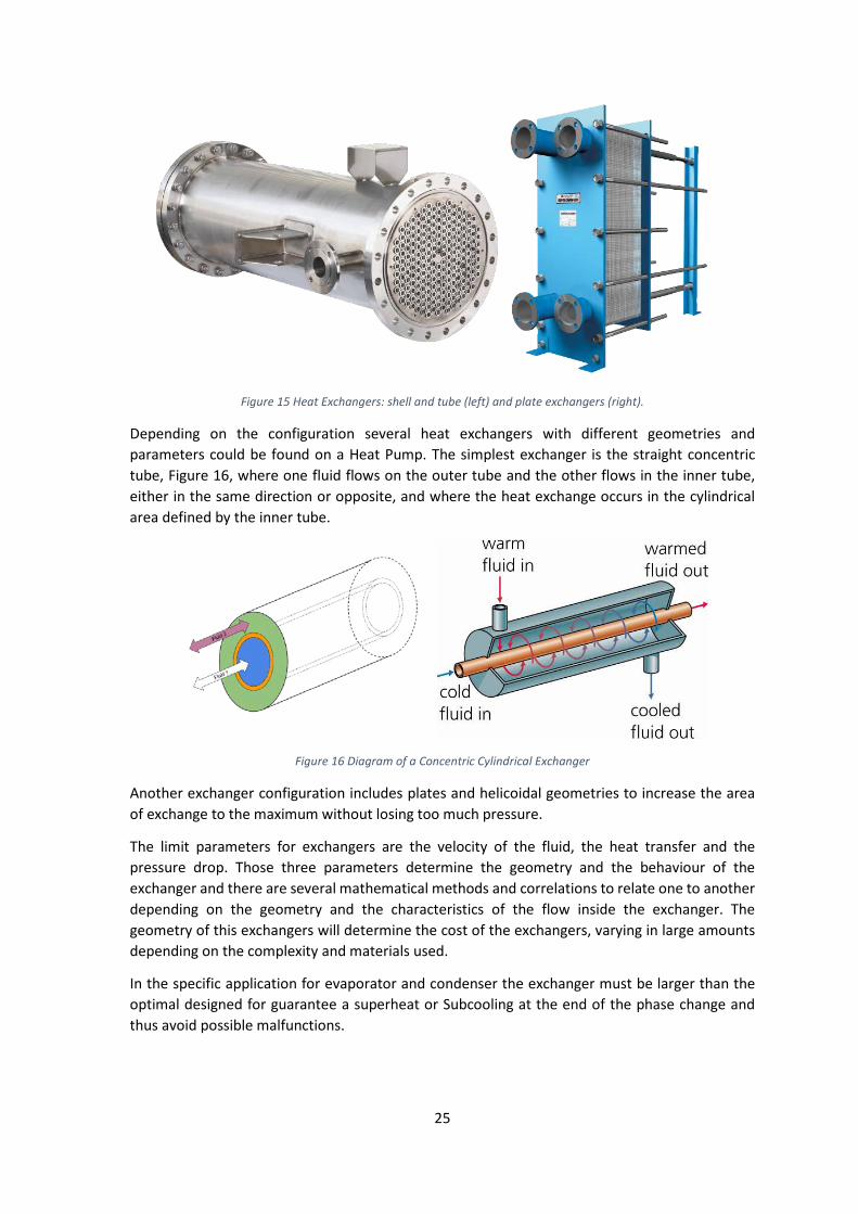
2.4.3. Heat exchanger The heat exchanger is the device where the transmission of heat with the secondary fluid happens, as a minimum there’ll be two heat exchangers, one as a condenser and one as an evaporator. They must assure the complete phase-change inside them, so de geometry and dimensions of each one must be precisely defined in the design. The correct transmission of heat is the final goal of the Heat Pump and the condenser is the exchanger that provides that heat.

25

Figure 15 Heat Exchangers: shell and tube (left) and plate exchangers (right).

Depending on the configuration several heat exchangers with different geometries and parameters could be found on a Heat Pump. The simplest exchanger is the straight concentric tube, Figure 16, where one fluid flows on the outer tube and the other flows in the inner tube, either in the same direction or opposite, and where the heat exchange occurs in the cylindrical area defined by the inner tube.

Figure 16 Diagram of a Concentric Cylindrical Exchanger

Another exchanger configuration includes plates and helicoidal geometries to increase the area of exchange to the maximum without losing too much pressure.

The limit parameters for exchangers are the velocity of the fluid, the heat transfer and the pressure drop. Those three parameters determine the geometry and the behaviour of the exchanger and there are several mathematical methods and correlations to relate one to another depending on the geometry and the characteristics of the flow inside the exchanger. The geometry of this exchangers will determine the cost of the exchangers, varying in large amounts depending on the complexity and materials used.

In the specific application for evaporator and condenser the exchanger must be larger than the optimal designed for guarantee a superheat or Subcooling at the end of the phase change and thus avoid possible malfunctions.

26

2.4.4. Safety and control devices In every heat pump system must be a series of safety and control devices and subsystems to guarantee the perfect performance and prevent critical malfunctioning of the system. Those devices are defined by specific legislation depending on the final application of the heat pump system and the parameters of work of it, e.g. pressure, temperature, flammability of the working fluid, toxicity, possible presence of explosive atmospheres; and this legislation varies in different countries. These regulations should be taken in account in the selection of the components for the system.

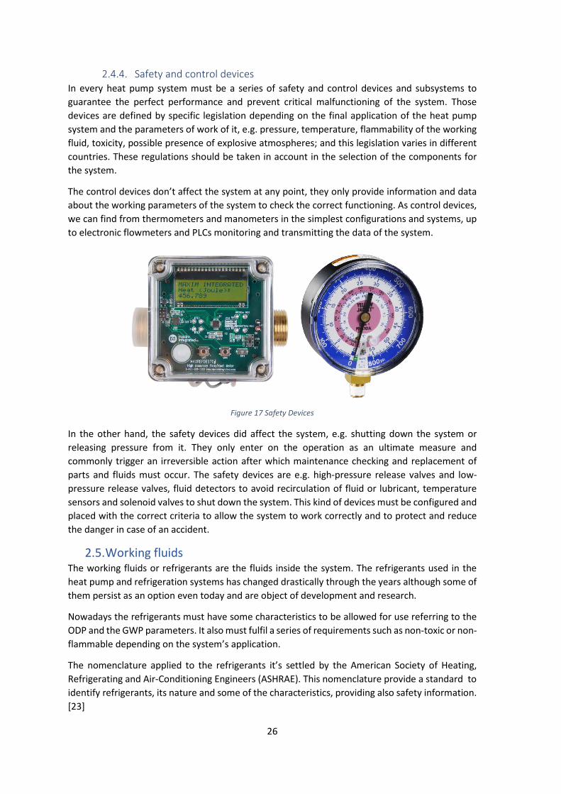
The control devices don’t affect the system at any point, they only provide information and data about the working parameters of the system to check the correct functioning. As control devices, we can find from thermometers and manometers in the simplest configurations and systems, up to electronic flowmeters and PLCs monitoring and transmitting the data of the system.

Figure 17 Safety Devices

In the other hand, the safety devices did affect the system, e.g. shutting down the system or releasing pressure from it. They only enter on the operation as an ultimate measure and commonly trigger an irreversible action after which maintenance checking and replacement of parts and fluids must occur. The safety devices are e.g. high-pressure release valves and low-pressure release valves, fluid detectors to avoid recirculation of fluid or lubricant, temperature sensors and solenoid valves to shut down the system. This kind of devices must be configured and placed with the correct criteria to allow the system to work correctly and to protect and reduce the danger in case of an accident.

2.5. Working fluids The working fluids or refrigerants are the fluids inside the system. The refrigerants used in the heat pump and refrigeration systems has changed drastically through the years although some of them persist as an option even today and are object of development and research.

Nowadays the refrigerants must have some characteristics to be allowed for use referring to the ODP and the GWP parameters. It also must fulfil a series of requirements such as non-toxic or non-flammable depending on the system’s application.

The nomenclature applied to the refrigerants it’s settled by the American Society of Heating, Refrigerating and Air-Conditioning Engineers (ASHRAE). This nomenclature provide a standard to identify refrigerants, its nature and some of the characteristics, providing also safety information. [23]

27

The classification of the fluids is based on a system of families taking account of the nature and the global characteristics, although other classifications are made depending on the criteria selected, e.g. ODP or GWP.

The general classification for refrigerants depending on the type of fluid based on the behaviour is:

• Pure • Mixture

o Zeotropic o Azeotropic o Near-azeotropic o Non-azeotropic

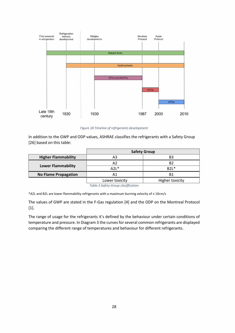
Over the years new parameters define the fluids e.g. safety, durability, ODP or GWP, which determine the usage of the fluids. In Figure 18 a timeline is displayed showing the main families and the main events, remarking the use of natural fluids or hydrocarbons for industrial refrigeration since the early ages of the 19th century, what has been called First Generation Refrigerants. Until 1930, when Thomas Midgley developed the chlorofluorocarbons (CFCs), the refrigeration technology and heat pump was limited only to industry application due to the risk and cost of the systems implemented but with Midgley developments the refrigeration expanded to domestic use thanks to the stability and characteristics of the CFCs and HCFCs, allowing smaller components and working pressures. The evolution of the industrial refrigeration continued using natural refrigerants due to the cost of the new CFCs and HCFCs for big installations, natural refrigerants e.g. Ammonia, were much cheaper than other ones like R-22. Due to the research conducted by Molina and Rowland in the 70s decade, regarding the ozone layer depletion by the CFCs, the Montreal Protocol was pronounced and signed in 1987 regulating the usage of CFCs and HCFCs which have a high ODP coefficient. Few years later the focus was turned to the climate change potential of the refrigerants, and the Kyoto Protocol followed the Montreal Protocol regulating the usage of refrigerants with high GWP. Nowadays CFCs, HCFCs and HFCs refrigerants are in disuse both because of legislation which limits and bans the usage and because of cost of operation. The development and research has returned to natural refrigerants, HFOs, HCs and mixtures. With the development of new configurations and better equipment a performance previously unreachable has been achieved, allowing the usage of them in applications dismissed in the past. [24,25]

28

Figure 18 Timeline of refrigerants development

In addition to the GWP and ODP values, ASHRAE classifies the refrigerants with a Safety Group [26] based on this table:

Safety Group Higher Flammability A3 B3

Lower Flammability A2 B2 A2L* B2L*

No Flame Propagation A1 B1 Lower toxicity Higher toxicity

Table 3 Safety Group clasiffication

*A2L and B2L are lower flammability refrigerants with a maximum burning velocity of ≤ 10cm/s

The values of GWP are stated in the F-Gas regulation [4] and the ODP on the Montreal Protocol [1].

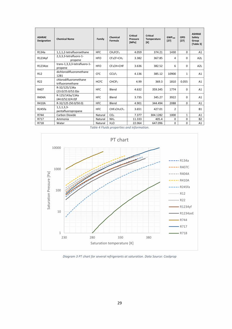
The range of usage for the refrigerants it’s defined by the behaviour under certain conditions of temperature and pressure. In Diagram 3 the curves for several common refrigerants are displayed comparing the different range of temperatures and behaviour for different refrigerants.

29

ASHRAE Designation Chemical Name Family Chemical

Formula

Critical Pressure [MPa]

Critical Temperature [K]

GWP100

[27] OPD [27]

ASHRAE Safety Group [Table 3]

R134a 1,1,1,2-tetrafluoroethane HFC CH2FCF3 4.059 374.21 1430 0 A1

R1234yf 2,3,3,3-tetrafluoro-1-propene HFO CF3CF=CH2 3.382 367.85 4 0 A2L

R1234ze trans-1,3,3,3-tetrafluoro-1-propene HFO CF3CH=CHF 3.636 382.52 6 0 A2L

R12 dichlorodifluoromethane 12B1 CFC CCl2F2 4.136 385.12 10900 1 A1

R22 chlorodifluoromethane trifluoromethane HCFC CHClF2 4.99 369.3 1810 0.055 A1

R407 R-32/125/134a (23.0/25.0/52.0)o HFC Blend 4.632 359.345 1774 0 A1

R404A R-125/143a/134a (44.0/52.0/4.0)f HFC Blend 3.735 345.27 3922 0 A1

R410A R-32/125 (50.0/50.0) HFC Blend 4.901 344.494 2088 0 A1

R245fa 1,1,1,3,3-pentafluoropropane HFC CHF2CH2CF3 3.651 427.01 2 B1

R744 Carbon Dioxide Natural CO2 7.377 304.1282 1000 1 A1 R717 Ammonia Natural NH3 11.333 405.4 0 0 B2 R718 Water Natural H2O 22.064 647.096 0 0 A1

Table 4 Fluids properties and information.

Diagram 3 PT chart for several refrigerants at saturation. Data Source: Coolprop

1

10

100

1000

10000

230 280 330 380

Satu

ratio

n Pr

essu

re [P

a]

Saturation temperature [K]

PT chart

R134a

R407C

R404A

R410A

R245fa

R12

R22

R1234yf

R1234zeE

R744

R717

R718

30

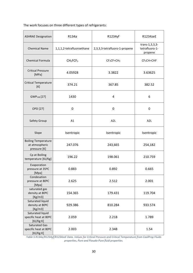
The work focuses on three different types of refrigerants:

ASHRAE Designation R134a R1234yf R1234zeE

Chemical Name 1,1,1,2-tetrafluoroethane 2,3,3,3-tetrafluoro-1-propene trans-1,3,3,3-tetrafluoro-1-

propene

Chemical Formula CH2FCF3 CF3CF=CH2 CF3CH=CHF

Critical Pressure [MPa] 4.05928 3.3822 3.63625

Critical Temperature [K] 374.21 367.85 382.52

GWP100 [27] 1430 4 6

OPD [27] 0 0 0

Safety Group A1 A2L A2L

Slope Isentropic Isentropic Isentropic

Boiling Temperature at atmospheric

pressure [K] 247.076 243,665 254,182

Cp at Boiling temperature [KJ/Kg] 196.22 198.061 210.759

Evaporation pressure at 35ºC

[Mpa] 0.883 0.892 0.665

Condesation pressure at 80ºC

[Mpa] 2.625 2.512 2.001

saturated gas density at 80ºC

[Kg/m3] 154.365 179.431 119.704

Saturated liquid density at 80ºC

[Kg/m3] 929.386 810.284 933.574

Saturated liquid specific heat at 80ºC

[KJ/Kg·K] 2.059 2.218 1.789

Saturated Gas specific heat at 80ºC

[KJ/Kg·K] 2.003 2.348 1.54

Table 5 R134a/R1234yf/R1234zeE Data. Values for Critical Pressure and Critical Temperature from CoolProp Fluids properties, Pure and Pseudo-Pure fluid properties.

31

Diagram 4 R12/R134a/R1234ze(E)/R1234yf Data Source: Coolprop

Diagram 5 Pressure-Enthalpy graph for R134a/R1234yf/R1234zeE Data Source: Coolprop

The R134a is a common refrigerant from the HFC family used in a lot of different applications in low and mid-temperature applications due to is range of operation, which comprehends temperatures between -30 to +20ºC [28] for evaporation.

It was introduced in the industry of refrigeration and heat pumps in the early 1990s as a replacement for R12 (CFC) due to its similar characteristics and the capacity to work under the

30

300

3000

230 250 270 290 310 330 350

Satu

ratio

n Pr

essu

re [K

Pa]

Saturation Temperature [K]

PT chart: CFC - HFC - HFO evolution

R12 R134a R1234zeE R1234yf

0,01

0,1

1

10

0 50 100 150 200 250 300 350 400 450 500

Pres

sure

[MPa

]

Enthalpy [KJ/Kg]

P-h

R134a R1234yf R1234zeE

32

same conditions. It has insignificant ODP but a medium level GWP, which is taxed by the most recent legislation.

The replacement for R134a has been under development with the R1234yf and R1234ze, both from the HFO family of refrigerants. In Diagram 4 is represented the similar behaviour between these refrigerants.

Several researches has been published in the field e.g the work conducted by Nawaz, Shen, Elatar, Baxter and Abdelaziz on the residential water heater application [29].

3. Model The model has been developed in Engineering Equation Solver [6] with the CoolProp Database [7] as a complement to obtain the fluid data. It’s an iterative model which resolves point to point the cycle and calculates the dimensions for the optimal exchangers to perform at the given range of temperatures with the selected fluid.

The model it’s based on the Reverse Carnot Cycle model and evolves into the IHX configuration model as shown on Figure 7, taking account of the performance parameters from the compressor and the pressure losses in the exchangers. In Figure 19 is represented the evolution process of the model.

Figure 19 Model evolution

3.1. System Description The model scheme corresponds to the Figure 20.

Figure 20 Model Scheme

33

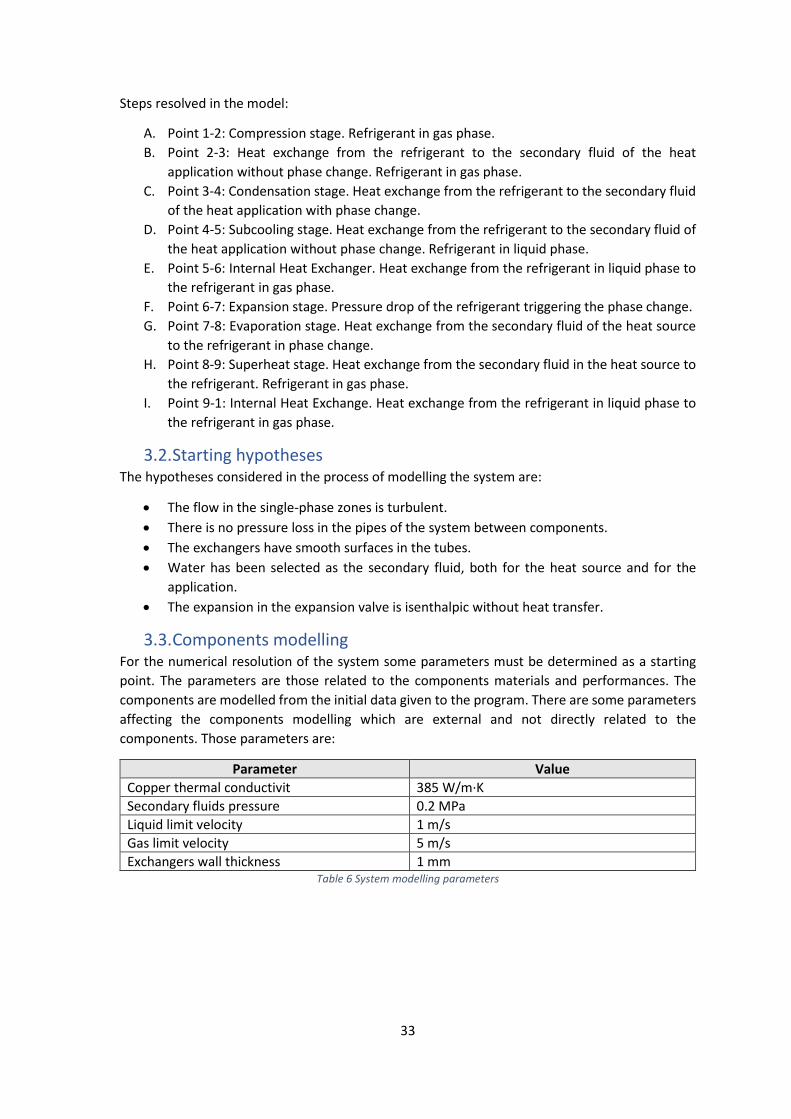
Steps resolved in the model:

A. Point 1-2: Compression stage. Refrigerant in gas phase. B. Point 2-3: Heat exchange from the refrigerant to the secondary fluid of the heat

application without phase change. Refrigerant in gas phase. C. Point 3-4: Condensation stage. Heat exchange from the refrigerant to the secondary fluid

of the heat application with phase change. D. Point 4-5: Subcooling stage. Heat exchange from the refrigerant to the secondary fluid of

the heat application without phase change. Refrigerant in liquid phase. E. Point 5-6: Internal Heat Exchanger. Heat exchange from the refrigerant in liquid phase to

the refrigerant in gas phase. F. Point 6-7: Expansion stage. Pressure drop of the refrigerant triggering the phase change. G. Point 7-8: Evaporation stage. Heat exchange from the secondary fluid of the heat source

to the refrigerant in phase change. H. Point 8-9: Superheat stage. Heat exchange from the secondary fluid in the heat source to

the refrigerant. Refrigerant in gas phase. I. Point 9-1: Internal Heat Exchange. Heat exchange from the refrigerant in liquid phase to

the refrigerant in gas phase.

3.2. Starting hypotheses The hypotheses considered in the process of modelling the system are:

• The flow in the single-phase zones is turbulent. • There is no pressure loss in the pipes of the system between components. • The exchangers have smooth surfaces in the tubes. • Water has been selected as the secondary fluid, both for the heat source and for the

application. • The expansion in the expansion valve is isenthalpic without heat transfer.

3.3. Components modelling For the numerical resolution of the system some parameters must be determined as a starting point. The parameters are those related to the components materials and performances. The components are modelled from the initial data given to the program. There are some parameters affecting the components modelling which are external and not directly related to the components. Those parameters are:

Parameter Value Copper thermal conductivit 385 W/m·K Secondary fluids pressure 0.2 MPa Liquid limit velocity 1 m/s Gas limit velocity 5 m/s Exchangers wall thickness 1 mm

Table 6 System modelling parameters

34

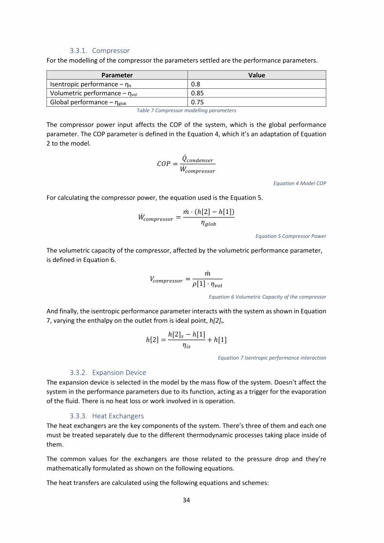
3.3.1. Compressor For the modelling of the compressor the parameters settled are the performance parameters.

Parameter Value Isentropic performance – ηis 0.8 Volumetric performance – ηvol 0.85 Global performance – ηglob 0.75

Table 7 Compressor modelling parameters

The compressor power input affects the COP of the system, which is the global performance parameter. The COP parameter is defined in the Equation 4, which it’s an adaptation of Equation 2 to the model.

𝐶𝐶𝐶𝐶𝐶𝐶 =�̇�𝑄𝑐𝑐𝐶𝐶𝐶𝐶𝑐𝑐𝑒𝑒𝐶𝐶𝑐𝑐𝑒𝑒𝐶𝐶�̇�𝑊𝑐𝑐𝐶𝐶𝑐𝑐𝑒𝑒𝐶𝐶𝑒𝑒𝑐𝑐𝑐𝑐𝐶𝐶𝐶𝐶

Equation 4 Model COP

For calculating the compressor power, the equation used is the Equation 5.

�̇�𝑊𝑐𝑐𝐶𝐶𝑐𝑐𝑒𝑒𝐶𝐶𝑒𝑒𝑐𝑐𝑐𝑐𝐶𝐶𝐶𝐶 =�̇�𝑚 · (ℎ[2] − ℎ[1])

𝜂𝜂𝑔𝑔𝑔𝑔𝐶𝐶𝑔𝑔

Equation 5 Compressor Power

The volumetric capacity of the compressor, affected by the volumetric performance parameter, is defined in Equation 6.

𝑉𝑉𝑐𝑐𝐶𝐶𝑐𝑐𝑒𝑒𝐶𝐶𝑒𝑒𝑐𝑐𝑐𝑐𝐶𝐶𝐶𝐶 =�̇�𝑚

𝜌𝜌[1] · 𝜂𝜂𝑒𝑒𝐶𝐶𝑔𝑔

Equation 6 Volumetric Capacity of the compressor

And finally, the isentropic performance parameter interacts with the system as shown in Equation 7, varying the enthalpy on the outlet from is ideal point, h[2]s.

ℎ[2] =ℎ[2]𝑐𝑐 − ℎ[1]

𝜂𝜂𝑒𝑒𝑐𝑐+ ℎ[1]

Equation 7 Isentropic performance interaction

3.3.2. Expansion Device The expansion device is selected in the model by the mass flow of the system. Doesn’t affect the system in the performance parameters due to its function, acting as a trigger for the evaporation of the fluid. There is no heat loss or work involved in is operation.

3.3.3. Heat Exchangers The heat exchangers are the key components of the system. There’s three of them and each one must be treated separately due to the different thermodynamic processes taking place inside of them.

The common values for the exchangers are those related to the pressure drop and they’re mathematically formulated as shown on the following equations.

The heat transfers are calculated using the following equations and schemes:

35

�̇�𝑄 = 𝑈𝑈 · 𝐴𝐴 · Δ𝑇𝑇𝐿𝐿𝐿𝐿

Equation 8 Heat Transfer between fluids

Where the logarithmic mean temperature average comes defined in the Equation 9

Δ𝑇𝑇𝐿𝐿𝐿𝐿 =Δ𝑇𝑇𝐴𝐴 − Δ𝑇𝑇𝐵𝐵

𝑙𝑙𝑙𝑙 �Δ𝑇𝑇𝐴𝐴Δ𝑇𝑇𝐵𝐵�

Equation 9 Logarithmic Mean Temperature Average

Δ𝑇𝑇𝐴𝐴 = 𝑇𝑇𝑒𝑒𝐶𝐶,1 − 𝑇𝑇𝐶𝐶𝑜𝑜𝐶𝐶,2

Equation 10 Temperature Difference A

Δ𝑇𝑇𝐵𝐵 = 𝑇𝑇𝐶𝐶𝑜𝑜𝐶𝐶,1 − 𝑇𝑇𝑒𝑒𝐶𝐶,2

Equation 11 Temperature Difference B

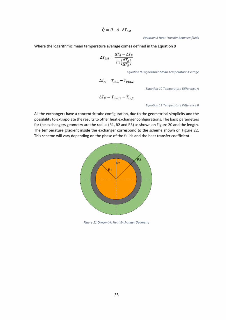
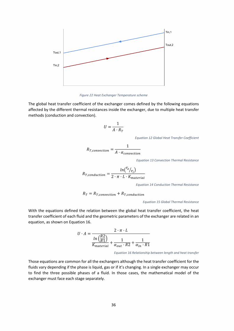
All the exchangers have a concentric tube configuration, due to the geometrical simplicity and the possibility to extrapolate the results to other heat exchanger configurations. The basic parameters for the exchangers geometry are the radius (R1, R2 and R3) as shown on Figure 20 and the length. The temperature gradient inside the exchanger correspond to the scheme shown on Figure 22. This scheme will vary depending on the phase of the fluids and the heat transfer coefficient.

Figure 21 Concentric Heat Exchanger Geometry

36

Figure 22 Heat Exchanger Temperature scheme

The global heat transfer coefficient of the exchanger comes defined by the following equations affected by the different thermal resistances inside the exchanger, due to multiple heat transfer methods (conduction and convection).

𝑈𝑈 =1

𝐴𝐴 · 𝑅𝑅𝑇𝑇

Equation 12 Global Heat Transfer Coefficient

𝑅𝑅𝑇𝑇,𝑐𝑐𝐶𝐶𝐶𝐶𝑒𝑒𝑒𝑒𝑐𝑐𝐶𝐶𝑒𝑒𝐶𝐶𝐶𝐶 =1

𝐴𝐴 · 𝛼𝛼𝑐𝑐𝐶𝐶𝐶𝐶𝑒𝑒𝑒𝑒𝑐𝑐𝐶𝐶𝑒𝑒𝐶𝐶𝐶𝐶

Equation 13 Convection Thermal Resistance

𝑅𝑅𝑇𝑇,𝑐𝑐𝐶𝐶𝐶𝐶𝑐𝑐𝑜𝑜𝑐𝑐𝐶𝐶𝑒𝑒𝐶𝐶𝐶𝐶 =𝑙𝑙𝑙𝑙�𝑟𝑟𝑒𝑒 𝑟𝑟𝑒𝑒� �

2 · 𝜋𝜋 · 𝐿𝐿 · 𝐾𝐾𝑐𝑐𝐶𝐶𝐶𝐶𝑒𝑒𝐶𝐶𝑒𝑒𝐶𝐶𝑔𝑔

Equation 14 Conduction Thermal Resistance

𝑅𝑅𝑇𝑇 = 𝑅𝑅𝑇𝑇,𝑐𝑐𝐶𝐶𝐶𝐶𝑒𝑒𝑒𝑒𝑐𝑐𝐶𝐶𝑒𝑒𝐶𝐶𝐶𝐶 + 𝑅𝑅𝑇𝑇,𝑐𝑐𝐶𝐶𝐶𝐶𝑐𝑐𝑜𝑜𝑐𝑐𝐶𝐶𝑒𝑒𝐶𝐶𝐶𝐶

Equation 15 Global Thermal Resistance

With the equations defined the relation between the global heat transfer coefficient, the heat transfer coefficient of each fluid and the geometric parameters of the exchanger are related in an equation, as shown on Equation 16.

𝑈𝑈 · 𝐴𝐴 =2 · 𝜋𝜋 · 𝐿𝐿

𝑙𝑙𝑙𝑙 �𝑅𝑅2𝑅𝑅1�

𝐾𝐾𝑐𝑐𝐶𝐶𝐶𝐶𝑒𝑒𝐶𝐶𝑒𝑒𝐶𝐶𝑔𝑔+ 1𝛼𝛼𝐶𝐶𝑜𝑜𝐶𝐶 · 𝑅𝑅2 + 1

𝛼𝛼𝑒𝑒𝐶𝐶 · 𝑅𝑅1

Equation 16 Relationship between length and heat transfer

Those equations are common for all the exchangers although the heat transfer coefficient for the fluids vary depending if the phase is liquid, gas or if it’s changing. In a single exchanger may occur to find the three possible phases of a fluid. In those cases, the mathematical model of the exchanger must face each stage separately.

37

Single-phased stages For the analysis of the stages the Reynolds, Prandtl and Nusselt numbers are required, and those numbers vary with the phase of the fluid and the geometry of the conducts.

The Reynolds number is defined in the Equation 17.

𝑅𝑅𝑅𝑅 =𝜌𝜌 · 𝜐𝜐 · 𝐷𝐷

𝜇𝜇

Equation 17 Reynolds Number

The flow pattern it’s defined by the Reynolds number using the following criteria:

• Re < 2300 – Laminar Flow • 2300 < Re < 10000 – Transition • 10000 < Re – Turbulent

The Prandtl number is defined in the Equation 18.

𝐶𝐶𝑟𝑟 = 𝐶𝐶𝑒𝑒 ·𝜇𝜇𝑘𝑘𝑓𝑓

Equation 18 Prandtl Number

The heat transfer coefficient in single phase is defined in the Equation 19.

𝛼𝛼𝑐𝑐𝐶𝐶𝐶𝐶𝑒𝑒𝑒𝑒𝑐𝑐𝐶𝐶𝑒𝑒𝐶𝐶𝐶𝐶 = 𝑁𝑁𝑁𝑁 ·𝑘𝑘𝑓𝑓𝐷𝐷

Equation 19 Heat Transfer Coefficient for single phase

For the calculation of the Nusselt number in single phase this project uses the Gnielinski correlation [34] defined in the Equation 20.

𝑁𝑁𝑁𝑁 =𝑓𝑓8 · (𝑅𝑅𝑅𝑅 − 1000) · 𝐶𝐶𝑟𝑟

1 + 12.7 · �𝑓𝑓8�12�

· �𝐶𝐶𝑟𝑟2 3� − 1�

Equation 20 Gnielinski correlation for Nusselt number

𝑓𝑓 = (0.79 · ln(𝑅𝑅𝑅𝑅)− 1.64)−2

Equation 21 Friction Factor

The conditions of application for the Gnielinski correlation are:

• 0.5 < Pr and 3000 < Re < 106 • 104 < Re < 5·106

38

For the pressure loss in single phase this project uses the Darcy-Weisbach correlation. This pressure loss is due to the friction between the fluid and the surface of the exchanger in contact with it. The Equation 22 and the Equation 21 defines the Darcy-Weisbach correlation and the friction factor respectively.

Δ𝐶𝐶𝑓𝑓𝐶𝐶𝑒𝑒𝑐𝑐𝐶𝐶𝑒𝑒𝐶𝐶𝐶𝐶 = 𝑓𝑓 ·𝐿𝐿𝐷𝐷

·𝜌𝜌 · 𝑁𝑁2

2

Equation 22 Darcy-Weisbach correlation

Internal Heat Exchanger The internal heat exchanger between the points 5-6 and 9-1 in the system only has fluid in single phase. Between 5-6 the fluid is in liquid phase and between the points 9-1 the fluid is in gas phase.

The heat flow of the internal heat exchanger is:

𝑄𝑄𝐼𝐼𝐻𝐻𝐼𝐼̇ = �̇�𝑚 · (ℎ[1] − ℎ[9])

Equation 23 IHX power

The liquid fluid from the condenser (points 5 to 6) will be in the inner tube and the gas fluid from the evaporator (points 9 to 1) will be in the outer tube. The geometry calculation is conducted with the velocity parameters for liquid and gas.

The internal heat exchanger has an efficiency set at 0.85 for the reference point. This efficiency affects and modifies the power transmission as defined by Equation 24

𝜀𝜀𝐼𝐼𝐻𝐻𝐼𝐼 =ℎ[1] − ℎ[9]ℎ𝑐𝑐𝐶𝐶𝑚𝑚 − ℎ[9]

Equation 24 IHX efficiency parameter

Evaporator The evaporator is the heat exchanger where the phase change from fluid to gas and the superheat stage takes place. There’s two stages to calculate, the phase change stage and the single-phase stage. See Figure 23.

39

Figure 23 Evaporator stages

The parameters defined for the evaporator calculation are:

Parameter Value ΔT – temperature increment 10 ºC TG – temperature gap 5 ºC SH – Super Heat temperature 10 ºC Tin,1 – secondary fluid inlet temperature 290 K Q_evaporator – Evaporator power 10000 W or 10 kW

Table 8 Evaporator modelling parameters

The evaporator power is defined in Equation 25, with this equation the mass flow of the system is defined and calculated as a relation with the evaporator power needed in the application.

�̇�𝑄𝑒𝑒𝑒𝑒𝐶𝐶𝑒𝑒𝐶𝐶𝐶𝐶𝐶𝐶𝐶𝐶𝐶𝐶𝐶𝐶 = �̇�𝑚 · (ℎ[9] − ℎ[7])

Equation 25 Evaporator Power

The calculation for the single-phase stage of the evaporator is conducted with the same equations as in the IHX. The phase change stage of the evaporator is calculated using the Gungor-Winterton correlation [35] (Equation 28) and the Pierre correlation modified [36] (Equation 37) for the pressure loss due to the phase change.

The total length of the exchanger and drop pressure would be the combination of the lengths and pressure drops from its stages.

40

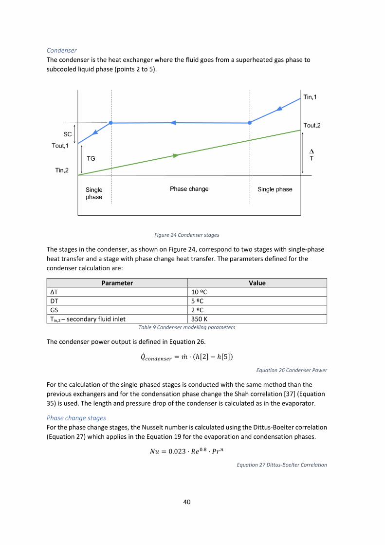
Condenser The condenser is the heat exchanger where the fluid goes from a superheated gas phase to subcooled liquid phase (points 2 to 5).

Figure 24 Condenser stages

The stages in the condenser, as shown on Figure 24, correspond to two stages with single-phase heat transfer and a stage with phase change heat transfer. The parameters defined for the condenser calculation are:

Parameter Value ΔT 10 ºC DT 5 ºC GS 2 ºC Tin,2 – secondary fluid inlet 350 K

Table 9 Condenser modelling parameters

The condenser power output is defined in Equation 26.

�̇�𝑄𝑐𝑐𝐶𝐶𝐶𝐶𝑐𝑐𝑒𝑒𝐶𝐶𝑐𝑐𝑒𝑒𝐶𝐶 = �̇�𝑚 · (ℎ[2] − ℎ[5])

Equation 26 Condenser Power

For the calculation of the single-phased stages is conducted with the same method than the previous exchangers and for the condensation phase change the Shah correlation [37] (Equation 35) is used. The length and pressure drop of the condenser is calculated as in the evaporator.

Phase change stages For the phase change stages, the Nusselt number is calculated using the Dittus-Boelter correlation (Equation 27) which applies in the Equation 19 for the evaporation and condensation phases.

𝑁𝑁𝑁𝑁 = 0.023 · 𝑅𝑅𝑅𝑅0.8 · 𝐶𝐶𝑟𝑟𝐶𝐶

Equation 27 Dittus-Boelter Correlation

41

The conditions of application for the Dittus-Boelter correlation are:

• 0.7 < Pr < 160 • Re > 10000 • L/D > 10

The coefficient n in the Equation 27 has the value 0.3 in the cooling stage and 0.4 in the heating stage.

The Gungor-Winterton correlation for the evaporation stage and its factors are defined from Equation 28 up to Equation 34. It’s a correlation derived from the Equation 19 applying Dittus-Boelter from Equation 27.

𝛼𝛼𝑇𝑇𝐻𝐻,𝑚𝑚 = �𝑆𝑆 · 𝑆𝑆2 + 𝐹𝐹𝑞𝑞 · 𝐹𝐹2� · 𝛼𝛼𝑐𝑐𝐶𝐶𝐶𝐶𝑒𝑒𝑒𝑒𝑐𝑐𝐶𝐶𝑒𝑒𝐶𝐶𝐶𝐶

Equation 28 Gungor-Winterton correlation

In the evaporator inlet (point 7) the quality of the fluid is different than 0 since the evaporation process is triggered in the expansion valve. To correct the Gungor-Winterton correlation and take in account this aspect a factor is introduced as shown on Equation 29.

𝐹𝐹𝑞𝑞 = 1.12 · �𝑞𝑞

1 − 𝑞𝑞�0.75

· �𝜌𝜌𝑔𝑔𝑒𝑒𝑞𝑞𝑜𝑜𝑒𝑒𝑐𝑐𝜌𝜌𝑔𝑔𝐶𝐶𝑐𝑐

�0.41

Equation 29 Quality increase factor

𝐹𝐹2 = 𝐹𝐹𝑟𝑟𝑔𝑔𝐶𝐶0.5

Equation 30 Quality increase factor modifier

𝑆𝑆 = 1 + 3000 · 𝐵𝐵𝐵𝐵0.86

Equation 31 Suppression factor

𝑆𝑆2 = 𝐹𝐹𝑟𝑟𝑔𝑔𝐶𝐶0.1−2·𝐹𝐹𝐶𝐶𝑙𝑙𝑙𝑙

Equation 32 Suppression factor modifier

𝐹𝐹𝑟𝑟𝑔𝑔𝐶𝐶 =𝐺𝐺2

𝜌𝜌𝑔𝑔𝑒𝑒𝑞𝑞𝑜𝑜𝑒𝑒𝑐𝑐2 · 𝑔𝑔 · 𝐷𝐷

Equation 33 Froude Number

𝐵𝐵𝐵𝐵 =�̇�𝑄𝐺𝐺 · 𝜆𝜆

Equation 34 Boiling Number

For condensation the Shah correlation is selected, Equation 35, which depends on the quality factor.

𝛼𝛼𝑇𝑇𝐻𝐻,𝑚𝑚 = 𝛼𝛼𝑐𝑐𝐶𝐶𝐶𝐶𝑒𝑒𝑒𝑒𝑐𝑐𝐶𝐶𝑒𝑒𝐶𝐶𝐶𝐶 · �1 +3.8𝑍𝑍𝑞𝑞0.95�

Equation 35 Shah correlation

42

𝑍𝑍𝑚𝑚 = �1 − 𝑞𝑞𝑞𝑞

�0.8

· 𝐶𝐶𝑟𝑟0.4

Equation 36 Shah quality factor

The pressure losses in the phase change stages in the heat exchangers are determined by the correlations of Darcy-Weisbach and Pierre modified. In single phase, the pressure loss is due to the friction and in the phase change stage the pressure loss is due to the friction and the acceleration of the fluid inside the tube.

The Darcy-Weisbach correlation defines the pressure losses due to friction inside the tubes. Is defined in the Equation 22 and the friction factor it’s been defined previously in the Equation 21.

The Pierre correlation [36] is modified to include the hydraulic diameter and the fluid specific volume, is defined in the Equation 37. The friction factor for phase change is defined by the Equation 38.

Δ𝐶𝐶𝑇𝑇𝐻𝐻 = Δ𝐶𝐶𝑓𝑓𝐶𝐶𝑒𝑒𝑐𝑐𝐶𝐶𝑒𝑒𝐶𝐶𝐶𝐶 + Δ𝐶𝐶𝐶𝐶𝑐𝑐𝑐𝑐𝑒𝑒𝑔𝑔𝑒𝑒𝐶𝐶𝐶𝐶𝐶𝐶𝑒𝑒𝐶𝐶𝐶𝐶 = �𝑓𝑓𝑁𝑁 · 𝐿𝐿 · (𝜈𝜈𝐶𝐶𝑜𝑜𝐶𝐶 + 𝜈𝜈𝑒𝑒𝐶𝐶)

𝐷𝐷+ (𝜈𝜈𝐶𝐶𝑜𝑜𝐶𝐶 − 𝜈𝜈𝑒𝑒𝐶𝐶)� · 𝐺𝐺2

Equation 37 Pierre correlation

𝑓𝑓𝑁𝑁 = 0.00506 · 𝑅𝑅𝑅𝑅−0.0951 · 𝐾𝐾𝑓𝑓0.1554

Equation 38 Friction factor for phase change

𝐾𝐾𝑓𝑓 =ℎ𝑓𝑓𝑔𝑔𝐿𝐿 · 𝑔𝑔

Equation 39 Friction factor quality modifier

3.4. Performance indicators The performance indicators of the system allow the analysis and comparison of the simulations. Those parameters are key in the development of the project in order to analyse and compare the VCCHP modelled with various working fluids.

The main performance indicators of the model are:

• 𝐶𝐶𝐶𝐶𝐶𝐶: Coefficient of Performance of the system. Indicates the performance of the system comparing the power output (via the condenser) with the power input (via the compressor) as defined in Equation 4.

• �̇�𝑄𝐶𝐶𝐶𝐶𝐶𝐶𝑐𝑐𝑒𝑒𝐶𝐶𝑐𝑐𝑒𝑒𝐶𝐶: Power output of the system in terms of heat power able to be applied. • �̇�𝑊𝐶𝐶𝐶𝐶𝑐𝑐𝑒𝑒𝐶𝐶𝑒𝑒𝑐𝑐𝑐𝑐𝐶𝐶𝐶𝐶: Power input of the system in terms of electric power provided to the

compressor. • �̇�𝑚: Mass flow of the system. Indicating the quantity of fluid necessary in the system to

operate.

Other performance parameters analysed:

• �̇�𝑉𝑐𝑐𝐶𝐶𝑐𝑐𝑒𝑒𝐶𝐶𝑒𝑒𝑐𝑐𝑐𝑐𝐶𝐶𝐶𝐶: Volumetric flow in the compressor, needed to select a compressor for the system.

• 𝐶𝐶𝑅𝑅: Compression ratio for the system as show in Equation 40.

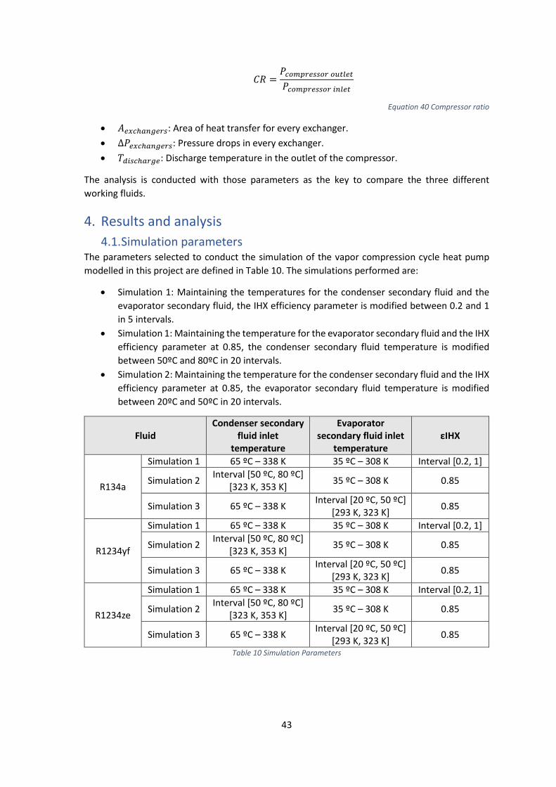
43

𝐶𝐶𝑅𝑅 =𝐶𝐶𝑐𝑐𝐶𝐶𝑐𝑐𝑒𝑒𝐶𝐶𝑒𝑒𝑐𝑐𝑐𝑐𝐶𝐶𝐶𝐶 𝐶𝐶𝑜𝑜𝐶𝐶𝑔𝑔𝑒𝑒𝐶𝐶

𝐶𝐶𝑐𝑐𝐶𝐶𝑐𝑐𝑒𝑒𝐶𝐶𝑒𝑒𝑐𝑐𝑐𝑐𝐶𝐶𝐶𝐶 𝑒𝑒𝐶𝐶𝑔𝑔𝑒𝑒𝐶𝐶

Equation 40 Compressor ratio

• 𝐴𝐴𝑒𝑒𝑚𝑚𝑐𝑐ℎ𝐶𝐶𝐶𝐶𝑔𝑔𝑒𝑒𝐶𝐶𝑐𝑐: Area of heat transfer for every exchanger. • Δ𝐶𝐶𝑒𝑒𝑚𝑚𝑐𝑐ℎ𝐶𝐶𝐶𝐶𝑔𝑔𝑒𝑒𝐶𝐶𝑐𝑐: Pressure drops in every exchanger. • 𝑇𝑇𝑐𝑐𝑒𝑒𝑐𝑐𝑐𝑐ℎ𝐶𝐶𝐶𝐶𝑔𝑔𝑒𝑒: Discharge temperature in the outlet of the compressor.

The analysis is conducted with those parameters as the key to compare the three different working fluids.

4. Results and analysis 4.1. Simulation parameters

The parameters selected to conduct the simulation of the vapor compression cycle heat pump modelled in this project are defined in Table 10. The simulations performed are:

• Simulation 1: Maintaining the temperatures for the condenser secondary fluid and the evaporator secondary fluid, the IHX efficiency parameter is modified between 0.2 and 1 in 5 intervals.

• Simulation 1: Maintaining the temperature for the evaporator secondary fluid and the IHX efficiency parameter at 0.85, the condenser secondary fluid temperature is modified between 50ºC and 80ºC in 20 intervals.

• Simulation 2: Maintaining the temperature for the condenser secondary fluid and the IHX efficiency parameter at 0.85, the evaporator secondary fluid temperature is modified between 20ºC and 50ºC in 20 intervals.

Fluid Condenser secondary

fluid inlet temperature

Evaporator secondary fluid inlet

temperature εIHX

R134a

Simulation 1 65 ºC – 338 K 35 ºC – 308 K Interval [0.2, 1]

Simulation 2 Interval [50 ºC, 80 ºC] [323 K, 353 K] 35 ºC – 308 K 0.85

Simulation 3 65 ºC – 338 K Interval [20 ºC, 50 ºC] [293 K, 323 K] 0.85

R1234yf




R1234ze




Table 10 Simulation Parameters

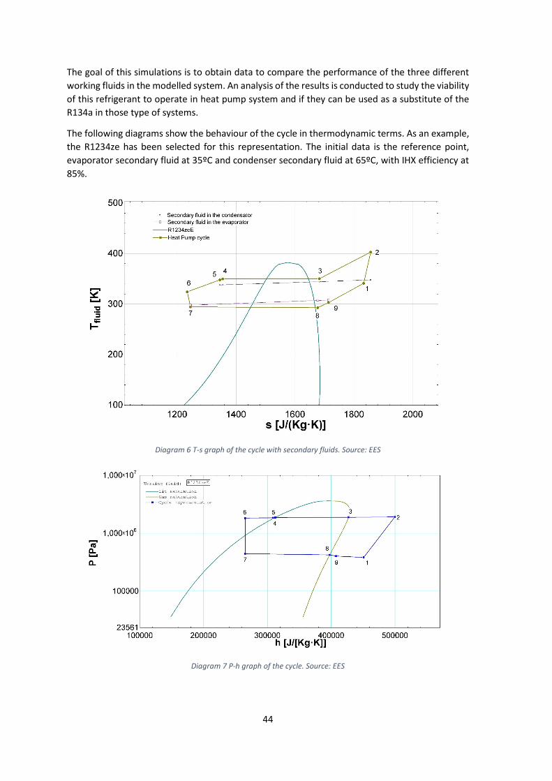
44

The goal of this simulations is to obtain data to compare the performance of the three different working fluids in the modelled system. An analysis of the results is conducted to study the viability of this refrigerant to operate in heat pump system and if they can be used as a substitute of the R134a in those type of systems.

The following diagrams show the behaviour of the cycle in thermodynamic terms. As an example, the R1234ze has been selected for this representation. The initial data is the reference point, evaporator secondary fluid at 35ºC and condenser secondary fluid at 65ºC, with IHX efficiency at 85%.

Diagram 6 T-s graph of the cycle with secondary fluids. Source: EES

Diagram 7 P-h graph of the cycle. Source: EES

45

4.2. Results representation and analysis 4.2.1. Cycle Parameters

In this section, the parameters related to the cycle and the behaviour of the fluids is graphically represented to study and analyse.

The most important parameter for analyse the cycle is the COP and its associated parameters, condenser power and the compressor power, as defined in Equation 4. In the following graphs, the COP is represented for the simulations performed.

For the simulation 1:

Diagram 8 COP simulation 1

2,45

2,5

2,55

2,6

2,65

2,7

2,75

2,8

2,85

2,9

2,95

3

0 0,2 0,4 0,6 0,8 1 1,2

COP

[-]

ε IHX [-]

R134a R1234yf R1234ze

46

Diagram 9 Condenser Power simulation 1

Diagram 10 Compressor Power simulation 1

13300

13400

13500

13600

13700

13800

13900

14000

14100

14200

14300

0 0,2 0,4 0,6 0,8 1 1,2

Qco

nden

ser [

W]

ε IHX [-]

R134a R1234yf R1234ze

4500

4700

4900

5100

5300

5500

5700

5900

0 0,2 0,4 0,6 0,8 1 1,2

Wco

mpr

esso

r [W

]

ε IHX [-]

R134a R1234yf R1234ze

47




1,5

2

2,5

3

3,5

4

320 325 330 335 340 345 350 355

COP

[-]

Condensator secondary fluid inlet temperature [K]

R134a R1234yf R1234ze

11000

11500

12000

12500

13000

13500

14000

14500

15000

15500

16000

320 325 330 335 340 345 350 355

Qco

nden

ser[W

]


R134a R1234yf R1234ze

48




2000

3000

4000

5000

6000

7000

8000

320 325 330 335 340 345 350 355

Wco

mpr

esso

r[W

]


R134a R1234yf R1234ze

1,5

2

2,5

3

3,5

4

4,5

290 295 300 305 310 315 320 325

COP

[-]

Evaporator secondary fluid inlet temperature [K]

R134a R1234yf R1234ze

49



It is appreciable the similarities of behaviour of the fluids under the same conditions.

Analysing the simulation 1 data (Diagram 8, Diagram 9 and Diagram 10) it is appreciable the similar behaviour of the R1234yf and R1234ze, the difference in the values are minimal. The higher COP is given by the R1234ze and lower is given by the R1234yf. The R134a follows a different curve, smoother. The R1234yf is the more affected by the variation of the IHX efficiency.

12000

12500

13000

13500

14000

14500

15000

15500

290 295 300 305 310 315 320 325

Qco

nden

ser[W

]


R134a R1234yf R1234ze

3000

3500

4000

4500

5000

5500

6000

6500

7000

7500

290 295 300 305 310 315 320 325

Wco

mpr

esso

r[W

]


R134a R1234yf R1234ze

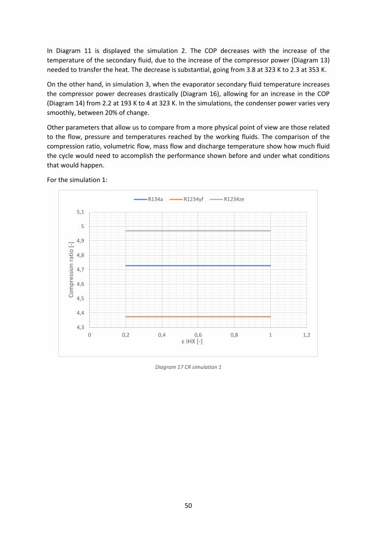
50

In Diagram 11 is displayed the simulation 2. The COP decreases with the increase of the temperature of the secondary fluid, due to the increase of the compressor power (Diagram 13) needed to transfer the heat. The decrease is substantial, going from 3.8 at 323 K to 2.3 at 353 K.

On the other hand, in simulation 3, when the evaporator secondary fluid temperature increases the compressor power decreases drastically (Diagram 16), allowing for an increase in the COP (Diagram 14) from 2.2 at 193 K to 4 at 323 K. In the simulations, the condenser power varies very smoothly, between 20% of change.

Other parameters that allow us to compare from a more physical point of view are those related to the flow, pressure and temperatures reached by the working fluids. The comparison of the compression ratio, volumetric flow, mass flow and discharge temperature show how much fluid the cycle would need to accomplish the performance shown before and under what conditions that would happen.


Diagram 17 CR simulation 1

4,3

4,4

4,5

4,6

4,7

4,8

4,9

5

5,1

0 0,2 0,4 0,6 0,8 1 1,2

Com

pres

sion

ratio

[-]

ε IHX [-]

R134a R1234yf R1234ze

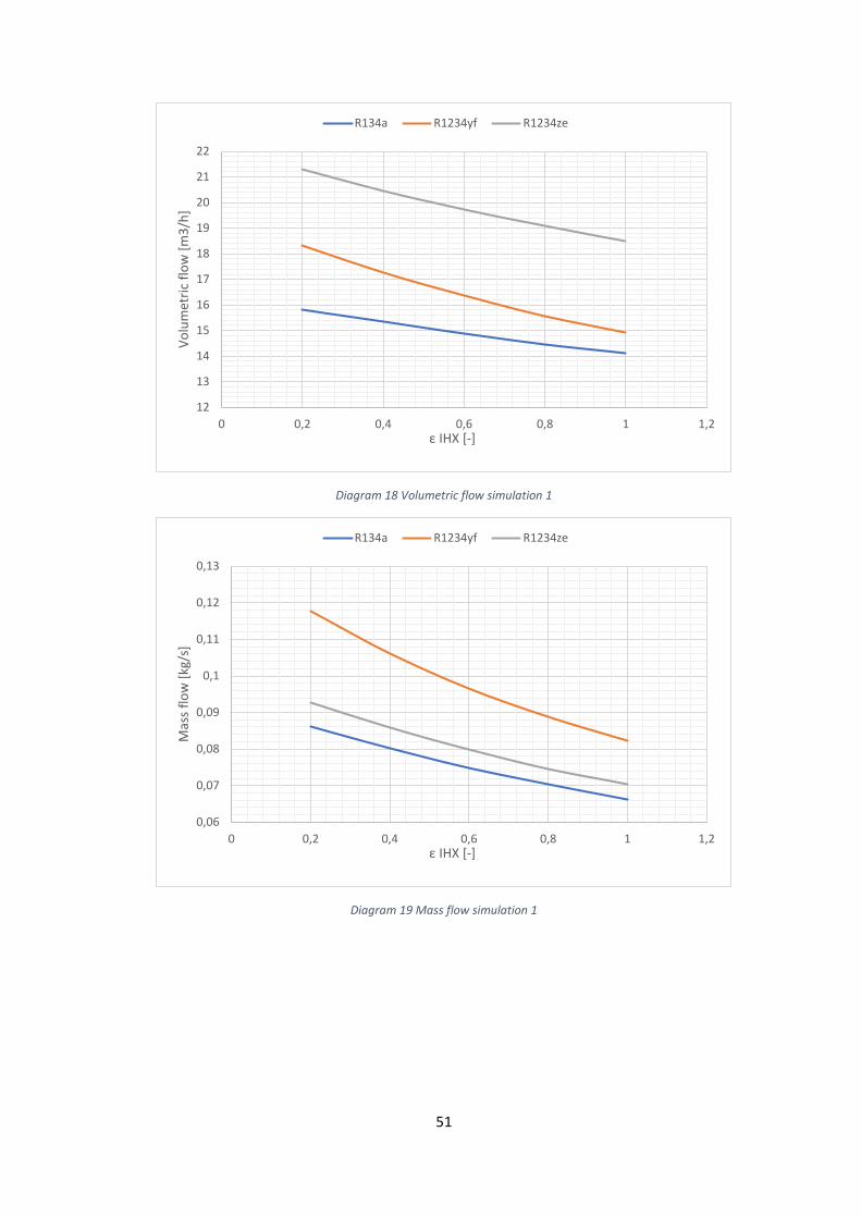
51

Diagram 18 Volumetric flow simulation 1

Diagram 19 Mass flow simulation 1

12

13

14

15

16

17

18

19

20

21

22

0 0,2 0,4 0,6 0,8 1 1,2

Volu

met

ric fl

ow [m

3/h]

ε IHX [-]

R134a R1234yf R1234ze

0,06

0,07

0,08

0,09

0,1

0,11

0,12

0,13

0 0,2 0,4 0,6 0,8 1 1,2

Mas

s flo

w [k

g/s]

ε IHX [-]

R134a R1234yf R1234ze

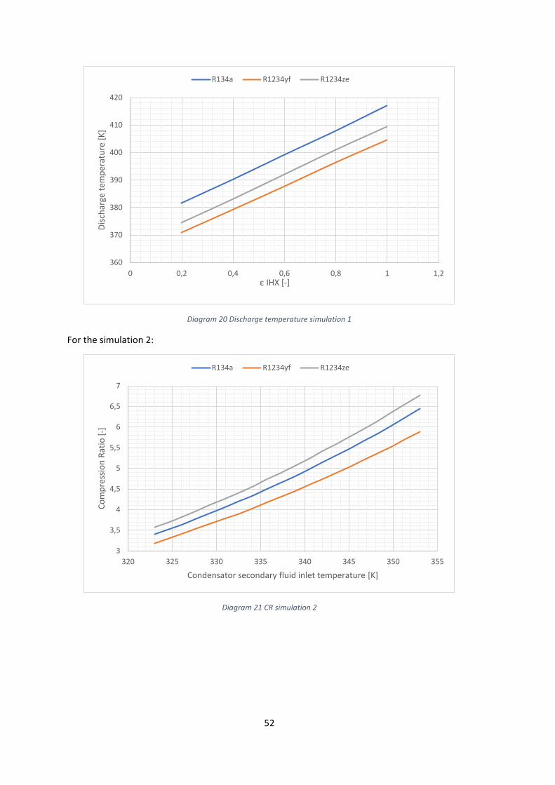
52

Diagram 20 Discharge temperature simulation 1



360

370

380

390

400

410

420

0 0,2 0,4 0,6 0,8 1 1,2

Disc

harg

e te

mpe

ratu

re [K

]

ε IHX [-]

R134a R1234yf R1234ze

3

3,5

4

4,5

5

5,5

6

6,5

7

320 325 330 335 340 345 350 355

Com

pres

sion

Ratio

[-]


R134a R1234yf R1234ze

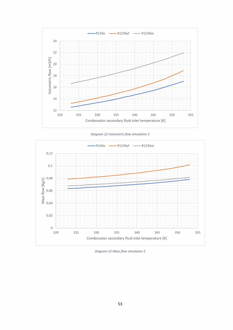
53



12

14

16

18

20

22

24

320 325 330 335 340 345 350 355

Volu

met

ric fl

ow [m

3/h]


R134a R1234yf R1234ze

0

0,02

0,04

0,06

0,08

0,1

0,12

320 325 330 335 340 345 350 355

Mas

s flo

w [K

g/s]


R134a R1234yf R1234ze

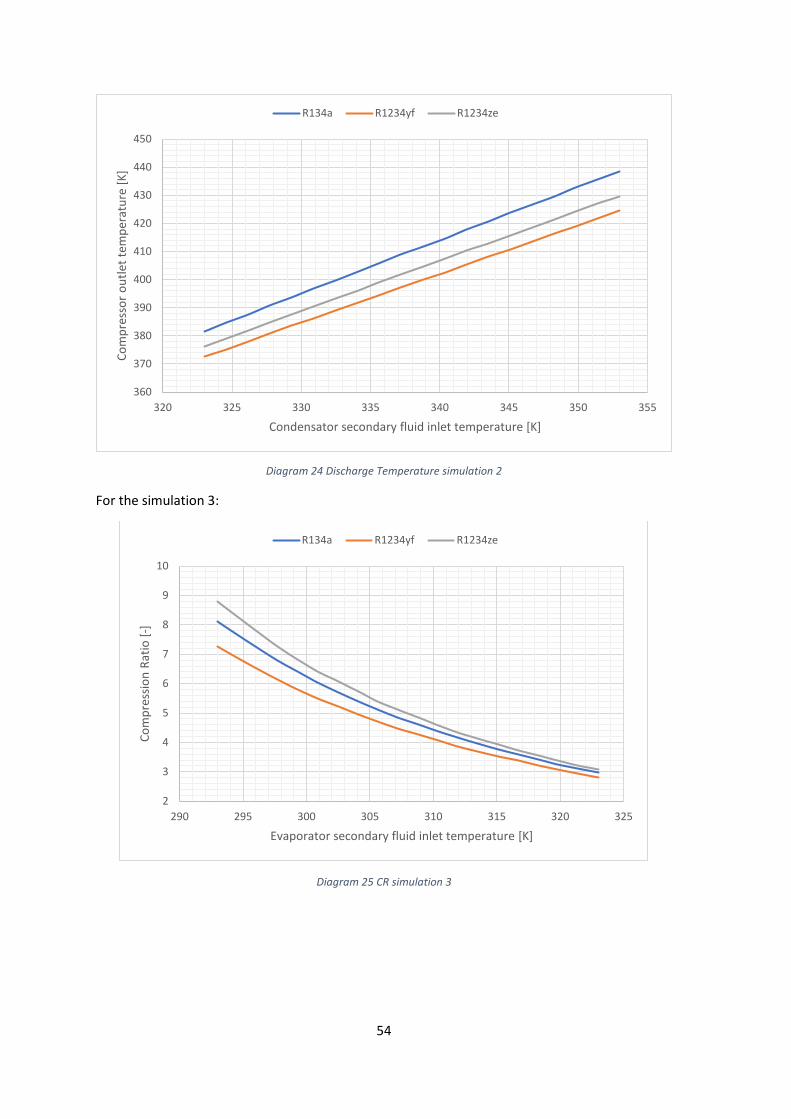
54

Diagram 24 Discharge Temperature simulation 2



360

370

380

390

400

410

420

430

440

450

320 325 330 335 340 345 350 355

Com

pres

sor o

utle

t tem

pera

ture

[K]


R134a R1234yf R1234ze

2

3

4

5

6

7

8

9

10

290 295 300 305 310 315 320 325

Com

pres

sion

Ratio

[-]


R134a R1234yf R1234ze

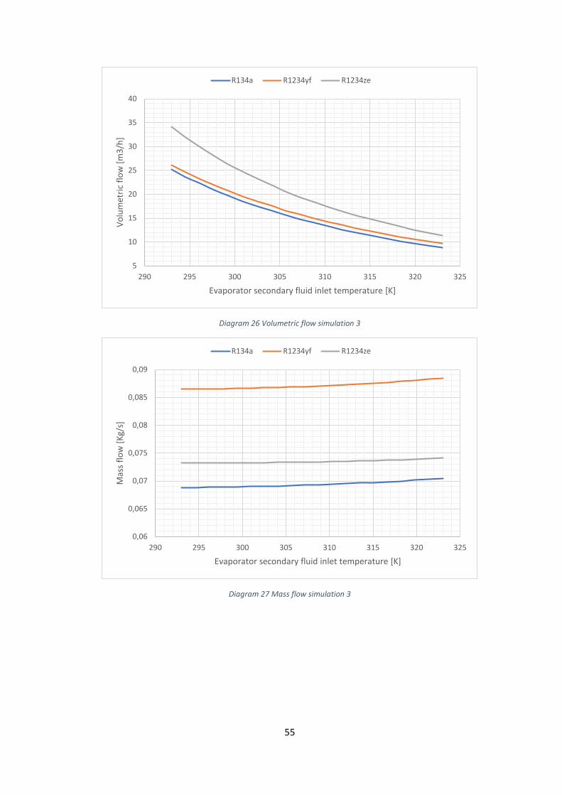
55



5

10

15

20

25

30

35

40

290 295 300 305 310 315 320 325

Volu

met

ric fl

ow [m

3/h]


R134a R1234yf R1234ze

0,06

0,065

0,07

0,075

0,08

0,085

0,09

290 295 300 305 310 315 320 325

Mas

s flo

w [K

g/s]


R134a R1234yf R1234ze

56

Diagram 28 Discharge temperature simulation 3

In these parameters, the differences between fluids start to appear.

In the simulation 1 data, the differences don’t appear so evidently. The compression ratio diagram (Diagram 17) and the discharge temperature diagram (Diagram 20) show, although at different values, the exact same constant progression for the three fluids. The higher compression ratio is for the R1234ze at 4.97, then is the R134a at 4.73 and the R1234yf at 4.37.

In the volumetric flow (Diagram 18) and the mass flow (Diagram 19) data, subtle differences can be detected. The volumetric flow shows a similar behaviour for the R1234yf and the R1234ze in the simulation 1, following both a similar curve. The mass flow relates the R134a and the R1234ze in terms of evolution, where the R1234yf follows a different curve. Despite these, all three fluids show similar behaviour in simulation 1.

The compression ratio diagrams (Diagram 21 and Diagram 25) for the simulations 2 and 3, shows the relation between the discharge pressure and the intake pressure of the compressor (Equation 40) and is appreciable the different evolution between fluids. In Diagram 21 the fluids act similar; being the R1234ze the higher (16.64 at 323K – 21.95 at 353K), then the R1234yf (13.2 at 323K – 18.88 at 353K) and the lower is the R134a (12.5 at 323K – 17.02 at 353K).

In the simulation 3, Diagram 25, is observable a different progression in each fluid, starting at different compression ratios with low temperatures and decreasing rapidly to a convergence point with the temperature set to 323K. The higher one is the R1234ze (8.79 at 293K – 3.07 at 323K), then is the R134a (8.125 at 293K – 2.9 at 323K) and the lower is the R1234yf (7.25 at 293K – 2.88 at 323K)

In terms of volumetric flow, represented in Diagram 22 and Diagram 26, is evident the similarities between the R134a and the R1234yf, giving identical curves. The R1234ze shows a similar behaviour but demand higher volumetric capacities in both cases; also in the simulation 2 case the curve for the evolution of the R1234ze differs from the other 2 fluids.

380

385

390

395

400

405

410

415

420

425

430

435

290 295 300 305 310 315 320 325

Com

pres

sor o

utle

t tem

pera

ture

[K]


R134a R1234yf R1234ze

57

These similarities change in the mass flow diagrams, as can be seen in Diagram 23 and Diagram 27. The fluid requiring a higher mass flow in the cycle is the R1234yf in both simulation cases and the R134a and the R1234ze fluids show similar values, though the difference between them is minimal, less than 0.02 kg/s.

The representation of the discharge temperature parameter, see Diagram 24 and Diagram 28, provide a clear view of the operative temperatures between the fluids. The values differ between them (Diagram 24), being the temperature for the R134a the higher temperature and the temperature for the R1234yf the lower one. This is more pronounced in the simulation 3.

All those parameters help giving information to compare and study the suitability of different fluids for a heat pump application, and analyse the cycle under an interval of conditions allowing to decide which refrigerant suits better the needs of the system in terms of performance and general dimensions.

4.2.2. Components Parameters When deciding which components suits better the cycle the key parameters are exchange area and pressure drops. This information allows to select the geometry and the type of exchanger for every stage in the cycle.

The following graphs represent the variation in those parameters in the different components analysed: condenser, evaporator and internal heat exchanger.


Diagram 29 Condenser exchange area simulation 1

0,25

0,27

0,29

0,31

0,33

0,35

0,37

0,39

0,41

0,43

0 0,2 0,4 0,6 0,8 1 1,2

Cond

ense

r exc

hang

e ar

ea [m

2]

ε IHX [-]

R134a R1234yf R1234ze

58

Diagram 30 Evaporator exchange area simulation 1

Diagram 31 IHX exchange area simulation 1

0,25

1,25

2,25

3,25

4,25

5,25

6,25

0 0,2 0,4 0,6 0,8 1 1,2

Evap

orat

or e

xcha

nge

area

[m2]

ε IHX [-]

R134a R1234yf R1234ze

0

0,1

0,2

0,3

0,4

0,5

0,6

0,7

0,8

0 0,2 0,4 0,6 0,8 1 1,2

IHX

exch

ange

are

a [m

2]

ε IHX [-]

R134a R1234yf R1234ze

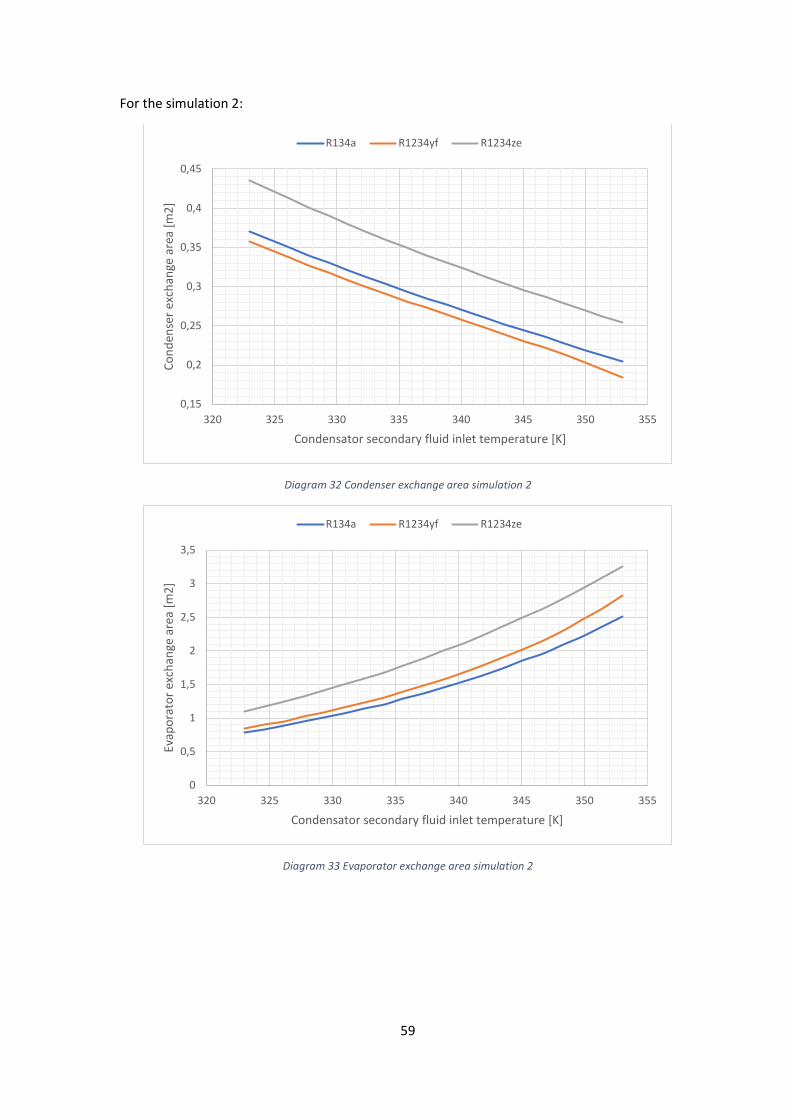
59




0,15

0,2

0,25

0,3

0,35

0,4

0,45

320 325 330 335 340 345 350 355

Cond

ense

r exc

hang

e ar

ea [m

2]


R134a R1234yf R1234ze

0

0,5

1

1,5

2

2,5

3

3,5

320 325 330 335 340 345 350 355

Evap

orat

or e

xcha

nge

area

[m2]


R134a R1234yf R1234ze

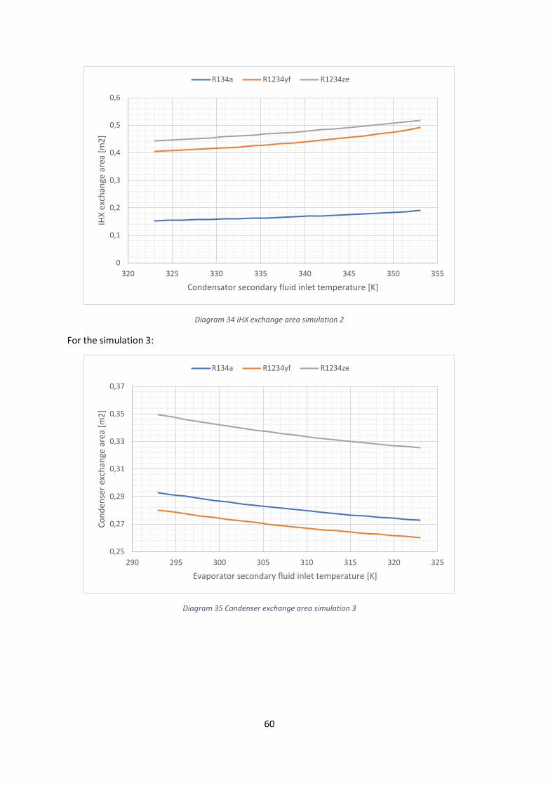
60




0

0,1

0,2

0,3

0,4

0,5

0,6

320 325 330 335 340 345 350 355

IHX

exch

ange

are

a [m

2]


R134a R1234yf R1234ze

0,25

0,27

0,29

0,31

0,33

0,35

0,37

290 295 300 305 310 315 320 325

Cond

ense

r exc

hang

e ar

ea [m

2]


R134a R1234yf R1234ze

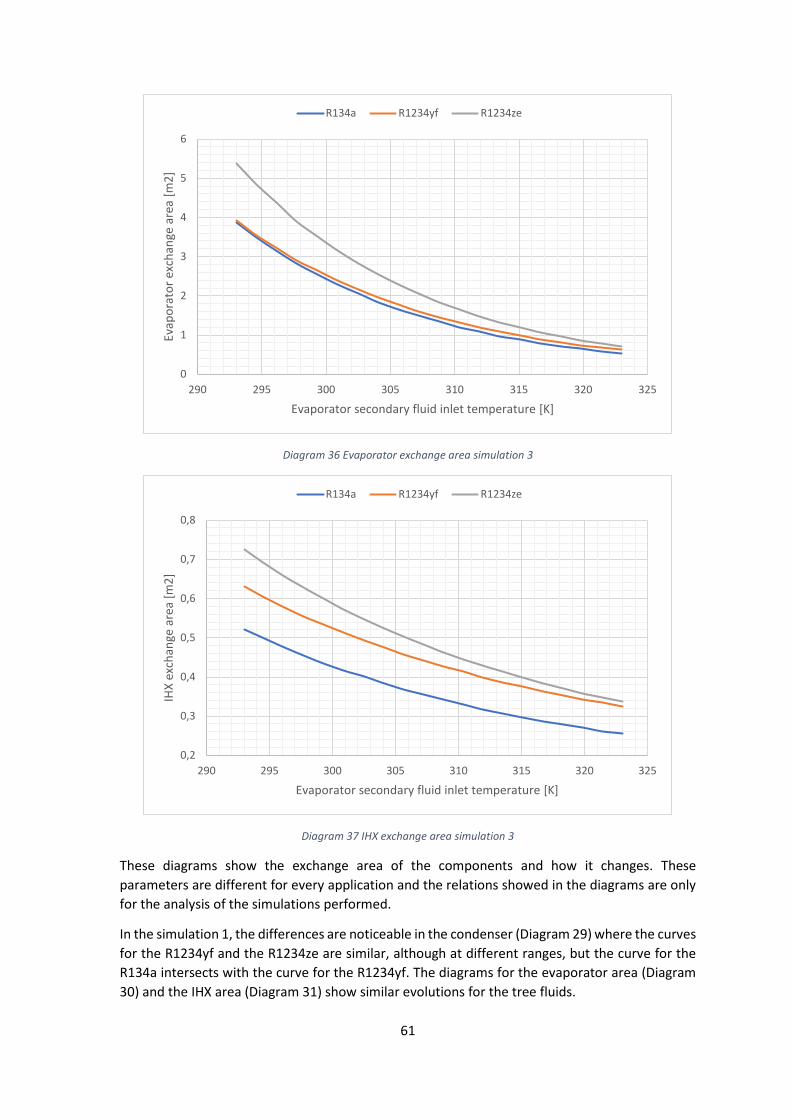
61



These diagrams show the exchange area of the components and how it changes. These parameters are different for every application and the relations showed in the diagrams are only for the analysis of the simulations performed.

In the simulation 1, the differences are noticeable in the condenser (Diagram 29) where the curves for the R1234yf and the R1234ze are similar, although at different ranges, but the curve for the R134a intersects with the curve for the R1234yf. The diagrams for the evaporator area (Diagram 30) and the IHX area (Diagram 31) show similar evolutions for the tree fluids.

0

1

2

3

4

5

6

290 295 300 305 310 315 320 325

Evap

orat

or e

xcha

nge

area

[m2]


R134a R1234yf R1234ze

0,2

0,3

0,4

0,5

0,6

0,7

0,8

290 295 300 305 310 315 320 325

IHX

exch

ange

are

a [m

2]


R134a R1234yf R1234ze

62

In the simulation 1 and 2 the differences only stand in terms of range. The R1234ze data show higher values than the R1234yf and the R134a in all the components. In a particular case for the IHX exchange area in the simulation 1 the R134a show a smaller area than the other two.

The following data graphics refers to the pressure drop parameters inside these components.

The pressure drop inside the components is affected by many different variables, as shown on the components modelling part.


Diagram 38 Condenser pressure drop simulation 1

Diagram 39 Evaporator pressure drop simulation 1

2500

3000

3500

4000

4500

5000

0 0,2 0,4 0,6 0,8 1 1,2

Cond

ense

r pre

ssur

e dr

op [P

a]

ε IHX [-]

R134a R1234yf R1234ze

2000

2100

2200

2300

2400

2500

2600

2700

2800

2900

0 0,2 0,4 0,6 0,8 1 1,2

Evap

orat

or p

ress

ure

drop

[Pa]

ε IHX [-]

R134a R1234yf R1234ze

63

Diagram 40 IHX external tube pressure drop simulation 1

Diagram 41 IHX internal pressure drop simulation 1

0

2000

4000

6000

8000

10000

12000

14000

16000

18000

0 0,2 0,4 0,6 0,8 1 1,2

IHX

exte

rnal

tube

pre

ssur

e dr

op [P

a]

ε IHX [-]

R134a R1234yf R1234ze

0

5000

10000

15000

20000

25000

30000

35000

40000

0 0,2 0,4 0,6 0,8 1 1,2

IHX

inte

rnal

tube

pre

ssur

e dr

op [P

a]

ε IHX [-]

R134a R1234yf R1234ze

64




0

500

1000

1500

2000

2500

3000

3500

4000

4500

320 325 330 335 340 345 350 355

Cond

ense

r pre

ssur

e dr

op [P

a]


R134a R1234yf R1234ze

2200

2250

2300

2350

2400

2450

2500

2550

2600

2650

320 325 330 335 340 345 350 355

Evap

opra

tor p

ress

ure

drop

[Pa]


R134a R1234yf R1234ze

65


Diagram 45 IHX internal tube pressure drop simulation 2

6000

6500

7000

7500

8000

8500

9000

9500

10000

320 325 330 335 340 345 350 355

IHX

exte

rnal

tube

pre

ssur

e dr

op [P

a]


R134a R1234yf R1234ze

0

5000

10000

15000

20000

25000

30000

35000

320 325 330 335 340 345 350 355

IHX

inte

rnal

tube

pre

ssur

e dr

op [P

a]


R134a R1234yf R1234ze

66




0

500

1000

1500

2000

2500

3000

3500

4000

4500

290 295 300 305 310 315 320 325

Cond

ense

r pre

ssur

e dr

op [P

a]


R134a R1234yf R1234ze

2000

2100

2200

2300

2400

2500

2600

2700

2800

2900

3000

290 295 300 305 310 315 320 325

Evap

orat

or p

ress

ure

drop

[Pa]


R134a R1234yf R1234ze

67


Diagram 49 IHX internal tube pressure drop simulation 3

0

2000

4000

6000

8000

10000

12000

14000

16000

290 295 300 305 310 315 320 325

IHX

exte

rnal

tube

pre

ssur

e dr

op [P

a]


R134a R1234yf R1234ze

0

5000

10000

15000

20000

25000

30000

35000

40000

45000

290 295 300 305 310 315 320 325

IHX

inte

rnal

tube

pre

ssur

e dr

op [P

a]


R134a R1234yf R1234ze

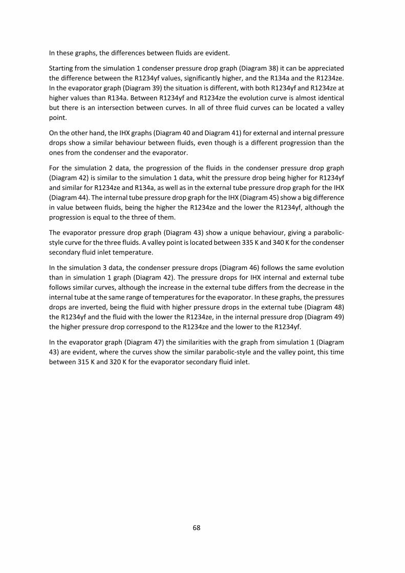
68

In these graphs, the differences between fluids are evident.

Starting from the simulation 1 condenser pressure drop graph (Diagram 38) it can be appreciated the difference between the R1234yf values, significantly higher, and the R134a and the R1234ze. In the evaporator graph (Diagram 39) the situation is different, with both R1234yf and R1234ze at higher values than R134a. Between R1234yf and R1234ze the evolution curve is almost identical but there is an intersection between curves. In all of three fluid curves can be located a valley point.

On the other hand, the IHX graphs (Diagram 40 and Diagram 41) for external and internal pressure drops show a similar behaviour between fluids, even though is a different progression than the ones from the condenser and the evaporator.

For the simulation 2 data, the progression of the fluids in the condenser pressure drop graph (Diagram 42) is similar to the simulation 1 data, whit the pressure drop being higher for R1234yf and similar for R1234ze and R134a, as well as in the external tube pressure drop graph for the IHX (Diagram 44). The internal tube pressure drop graph for the IHX (Diagram 45) show a big difference in value between fluids, being the higher the R1234ze and the lower the R1234yf, although the progression is equal to the three of them.

The evaporator pressure drop graph (Diagram 43) show a unique behaviour, giving a parabolic-style curve for the three fluids. A valley point is located between 335 K and 340 K for the condenser secondary fluid inlet temperature.

In the simulation 3 data, the condenser pressure drops (Diagram 46) follows the same evolution than in simulation 1 graph (Diagram 42). The pressure drops for IHX internal and external tube follows similar curves, although the increase in the external tube differs from the decrease in the internal tube at the same range of temperatures for the evaporator. In these graphs, the pressures drops are inverted, being the fluid with higher pressure drops in the external tube (Diagram 48) the R1234yf and the fluid with the lower the R1234ze, in the internal pressure drop (Diagram 49) the higher pressure drop correspond to the R1234ze and the lower to the R1234yf.

In the evaporator graph (Diagram 47) the similarities with the graph from simulation 1 (Diagram 43) are evident, where the curves show the similar parabolic-style and the valley point, this time between 315 K and 320 K for the evaporator secondary fluid inlet.

69

5. Conclusions In this part, the different resolutions and conclusions originated from the development of the project are gathered.

Based on these resolutions some propositions for further developments based on this project are named.

5.1. Project conclusions The motivation for this project is the need to study heat pump technology as a system for energy recovery in industry and low-GWP fluids able to perform correctly in vapor compression cycle heat pump systems, to integrate those systems in the industry enhancing the energetic efficiency of the production.

The legislation about the use of refrigeration is becoming more restrictive, adding to that the current legislation about the emissions affecting the climate change a new current has appeared in the industry demanding better energy efficient systems.

The final goal of the project is to create a model of a vapor compression cycle heat pump to perform computer assisted analysis instead of the traditional analysis with physical heat pumps, saving in that process time and money. To achieve this goal a study has been conducted analysing the evolution of the heat pump technology and, specially, the development and integration of new working fluids. The main focus of the study it’s been locate which is the actual status, in terms of usage, for the working fluids and which are under development in the present, and try to identify the trends in the heat pump development.

Once the study was completed a second phase of modelling started, based on the internal heat exchanger configuration. This configuration was selected over the simple one because of the flexibility of the system and the performance extracted from it; a simple one is uncommon in the real applications and a system more complex it’s not reliable in terms of extrapolating the results. The IHX configuration gives a good platform for the model and allow to study real applications and to extrapolate the data from the studies conducted. The code has been developed in the EES platform, for two reasons: the first one it’s the simplicity for the equations input and functions, so the code can be updated with additional parameters or components avoiding the need to rewrite the hole script, and the second one it’s the usage of an open source library for the fluids characteristics as is CoolProp.

A secondary goal in the project was the thermodynamic study of different working fluids and is evaluation as a plausible replacement for R134a.

Based on the data gathered in the initial study the selection of refrigerants was conducted, the R134a and its substitutes, R1234yf and R1234ze, were the selected ones. The simulations of the model were conducted for these fluids and the parameters has been exposed in this project. The variables for the simulations were selected based on what can be collected from a real heat pump system, as it would be the temperature of the fluid where the heat is extracted, the evaporator secondary fluid inlet, and the temperature of the fluid where the heat is going to be transferred, the evaporator secondary fluid inlet. Besides those two parameters others can be given, such as is the amount of power for the evaporator or the characteristics of the components like the efficiency or material. The hypotheses stated in the calculations are for simplify of the calculations and reduce possible error sources, thus making the model more flexible and reliable.

70

From all the data gathered and analysed several conclusions are extracted:

• In performance terms, specifically the COP, the three fluids give very similar results verifying that the R1234yf and the R1234ze are substitutes for the R134a. This sets the base for studying the replacement of R134a with R1234yf or R1234ze in already working heat pump systems, and the performance expected with the replacement should be similar.

• The power indicators like the compressor power output show that the R1234yf transfers more heat than the other two in the conditions of the study and the R1234ze transfers almost the same amount of heat as the R134a. The differences between them are minimal and the similar curves show a behaviour already expected from the R134a.

• The system parameters as are the volumetric and mass flow show that a higher quantity of fluid must be needed to operate at the given points, resulting in bigger components or in faster and more powerful compressors. Although this difference is not big enough to discredit the R1234yf and the R1234ze as replacements for the R134a, should be considered in terms of designing new heat pumps or modifying existing ones to operate with the new-generation fluids mentioned. The compression ratio also indicates that the same type of compressor could be used with all three fluids as well as the type of exchangers

• Regarding the components geometric parameters, the exchange area shows the need for bigger exchangers with the new-generation fluids, this affects the selection of components directly and may cause malfunctions in operative heat pumps when replacing the fluid.

• The pressure drops for the R1234yf and R1234ze are also higher, especially for the R1234yf as shown in simulation 1 and 2 results when the fluid is working in the external tubes (condenser, evaporator and IHX external tube). The pressure drop for this this fluid is higher than the R134a one. The R1234ze show a more similar behaviour to R134a nevertheless the pressure drop is higher in most of the cases.

• Overall there isn’t a clear substitute for R134a. Depending on the application and the specifics of each installation R1234yf or R1234ze could be use. Both offer similar performance under the same conditions and the differences between them are easily rectifiable.

From the work conducted to carry out the project several conclusions are extracted:

• There is a need for energy recovery systems in the industry and in the society in general (buildings and public installations) generated both from an economical point of view, reducing the energy bill or at least using that energy more efficiently, and from a legislation point of view, the emissions of high-GWP gases is going to be banned and the restriction to the use of traditional energy sources is expanding all over the world. The industry working with heat demanding processes needs better systems and the ability to develop them fast and commercialize them is going the be a key factor in this research field.

• The trends in refrigerants use show a clear path to the use of low-GWP refrigerants in hybrid systems integrating photovoltaic generation and geothermal technologies to create a zero-emissions system wherever is possible. The implementations of the heat pump in this type of installations is mandatory and the demand is going to increase in the years to come.

71

5.2. Further developments With this project, the bases to develop a full simulation program has been settled. The ways to expand this project are:

• Increase the level of detail adding components to the system such as pipping and more detailed exchangers, so it can be used to create an experimental model to compare and verify the results.

• Incorporate several different correlations to compare different results from a theoretical research point of view.

• Integrate libraries, for the fluids characteristics, able to perform under new design fluids and thus making the model capable to simulate new fluid iterations.

5.3. Personal conclusions In a personal term, this project has allowed me to develop skills such as team work and research to a higher level, as well as work in a professional research environment.

The study has given me a deeper knowledge of the state of the energy technologies state and where and how are they implemented. It also made me work harder in my coding skills, learning a new language like EES and the CoolProp library and analysing the code looking for errors or more efficient writing.

This project has given me a good starting point in the energy engineering field, where I can learn and put my abilities to use, opening new opportunities of work and research.

72

6. Bibliography [1] UNEP. The Montreal Protocol 1987:1–19.

[2] Nations U. Kyoto Protocol To the United Nations Framework Kyoto Protocol To the United Nations Framework. Rev Eur Community Int Environ Law 1998;7:214–7. doi:10.1111/1467-9388.00150.

[3] European Comission. Paris Agreement. Clim Action 2017. http://unfccc.int/files/meetings/paris_nov_2015/application/pdf/paris_agreement_english_.pdf (accessed 16 June 2017).

[4] The European Parliament and the Council of the European Union. Regulation (EU) No 517/2014 of the European Parliament and of the Council of 16 April 2014 on fluorinated greenhouse gases and repealing. 2014.

[5] Iwafune Y, Kanamori J, Sakakibara H. A comparison of the effects of energy management using heat pump water heaters and batteries in photovoltaic -installed houses. Energy Convers Manag 2017;148:146–60. doi:10.1016/j.enconman.2017.05.060.

[6] Klein SA. EES - Engineering Equation Solver 2017.

[7] Bell IH. CoolProp 2016.

[8] Chua KJJ, Chou SKK, Yang WMM. Advances in heat pump systems: A review. Appl Energy 2010;87:3611–24. doi:10.1016/j.apenergy.2010.06.014.

[9] Rijksdienst MS. R & D on Industrial Heat Pumps. 2014.

[10] Bamigbetan O, Eikevik TM, Nekså P, Bantle M. Review of vapour compression heat pumps for high temperature heating using natural working fluids. Int J Refrig 2017;80:197–211. doi:10.1016/j.ijrefrig.2017.04.021.

[11] Buxton G. The Montreal protocol on substances that deplete the ozone layer. vol. 1. 1988. doi:10.1163/15718069620847781.

[12] Nellissen P, Wolf S. Heat pumps in non-domestic applications in Europe: Potential for an energy revolution. 8th EHPA Eur. Heat Pump Forum, 28 May 2015, Brussels, 2015, p. 1–17.

[13] Hepbasli A, Kalinci Y. A review of heat pump water heating systems. Renew Sustain Energy Rev 2009;13:1211–29. doi:10.1016/j.rser.2008.08.002.

[14] McMullan A. Industrial Heat Pumps for Steam and Fuel Savings. 2003.

[15] Bahrami M, Cycle R. The Ideal Vapor - Compression Refrigeration Cycle 2011;461:1–8.

[16] Song Y, Li D, Cao F, Wang X. Theoretical investigation on the combined and cascade CO 2 /R134a heat pump systems for space heating 2017. doi:10.1016/j.applthermaleng.2017.06.014.

[17] Wang G, Chen Z, Li C, Jiang B. Preliminary theoretical analyses of thermal performance and available energy consumption of two-stage cascade cycle heat pump water heater. Int J Refrig 2017. doi:10.1016/j.ijrefrig.2017.06.016.

[18] Minglu Q, Tianrui L, Shiming D, Yanan F, Zhao L. Improving defrosting performance of cascade air source heat pump using thermal energy storage based reverse cycle defrosting method 2017. doi:10.1016/j.applthermaleng.2017.04.146.

[19] Arpagaus C, Bless F, Schiffmann J, Bertsch SS. Multi-temperature heat pumps: A literature review. Int J Refrig 2016;69:437–65. doi:10.1016/j.ijrefrig.2016.05.014.

[20] Cavallini A, Tecnica F, Venezia V, Pd IP. European Seminar – Properties of CO2 as a refrigerant. Carbon N Y 2002.

[21] Grievink J, Swinkels P. Chapter 4 – Compressors. Refrig. Air Cond. Heat Pumps, 2016, p. 1–52. doi:10.1016/B978-0-08-100647-4/00004-8.

73

[22] Trott a. R. Chapter 8 – Expansion Valves. Refrig. Air Cond. Heat Pumps, 2000, p. 93–103. doi:10.1016/B978-075064219-4/50008-X.

[23] Wilson DP, Kujak S, Leary JMO, Kennoy DH, Kusmierz A, Patnaik V, et al. Designation and Safety Classification of Refrigerants. ANSI/ASHRAE Stand 34-2010 2010;4723:9.

[24] Hundy GF, Trott AR, Welch TC, Hundy GF, Trott AR, Welch TC. Chapter 3 – Refrigerants. Refrig. Air Cond. Heat Pumps, 2016, p. 41–58. doi:10.1016/B978-0-08-100647-4.00003-6.

[25] Pavkovic B. Refrigerants – Part 2 : Past , present and future perspectives of refrigerants in air-conditioning applications. REHVA J 2013:28–33.

[26] Reiniche S. ANSI/ASHRAE Addendum ak to ANSI/ASHRAE Standard 34-2007. ASHRAE Stand 2010;4723:5.

[27] Number R. Refrigerants Environmental Data: Ozone Depletion and Global Warming Potential. Ozone Deplet Potential 2007;1:2006–7.

[28] Sarbu I. A review on substitution strategy of non-ecological refrigerants from vapour compression-based refrigeration, air-conditioning and heat pump systems. Int J Refrig 2014;46:123–41. doi:10.1016/j.ijrefrig.2014.04.023.

[29] Nawaz K, Shen B, Elatar A, Baxter V, Abdelaziz O. R-1234yf and R-1234ze(E) as low-GWP refrigerants for residential heat pump water heaters. Int J Refrig 2017. doi:10.1016/j.ijrefrig.2017.06.031.

[30] Saikawa M, Koyama S. Thermodynamic analysis of vapor compression heat pump cycle for tap water heating and development of CO2 heat pump water heater for residential use. Appl Therm Eng 2016;106:1236–43. doi:10.1016/j.applthermaleng.2016.06.105.

[31] Zhang J-F, Qin Y, Wang C-C. Review on CO2 heat pump water heater for residential use in Japan. Renew Sustain Energy Rev 2015;50:1383–91. doi:10.1016/j.rser.2015.05.083.

[32] Baek C, Heo J, Jung J, Cho H, Kim Y. Performance characteristics of a two-stage CO2 heat pump water heater adopting a sub-cooler vapor injection cycle at various operating conditions. Energy 2014;77:570–8. doi:10.1016/j.energy.2014.09.038.

[33] Dai B, Dang C, Li M, Tian H, Ma Y. Thermodynamic performance assessment of carbon dioxide blends with low-global warming potential (GWP) working fluids for a heat pump water heater. Int J Refrig 2015;56:1–14. doi:10.1016/j.ijrefrig.2014.11.009.

[34] V. Gnielinski. New equation for heat transfer in turbulent pipe and channel flow. Int Chem Eng 1976;16:359–68.

[35] Gungor KE, Winterton RHS. Simplified general correlation for saturated flow boiling and comparisons of correlations with data. Chem Eng Res Des 1987;65:148–56.

[36] Choi JY, Kedzierski M a, Domanski P a. Generalized Pressure Drop Correlation for Evaporation and Condensation in Smooth and Micro-Fin Tubes 2001.

[37] Shah M. A general correlation for heat transfer during film condensation inside pipes. Int J Heat Mass Transf 1979;22:547–56.

75

Section 2 – Budget

76

Budget index 1. INTRODUCTION ........................................................................................................................... 77

2. COST OF THE DEVELOPMENT OF THE PROJECT ............................................................................ 77

2.1. PERSONNEL COSTS .......................................................................................................................... 77 2.2. HARDWARE AND SOFTWARE COSTS .................................................................................................... 77

3. TOTAL COST OF THE PROJECT ...................................................................................................... 77

77

1. Introduction The chapter target is to stablish the economic costs associated to the development of the project of a vapor compression cycle heat pump model and is application for analyse working fluids. Due to its role as a research project is impractical the typical economic study, so the budget chapter englobes the cost associated to the man-hours invested and the cost associated with the materials and services used in the development.

2. Cost of the development of the project 2.1. Personnel costs

This chapter an estimation of the personnel cost is conducted based on the pricing of a Mechanical Engineer allocated to the study, data analysis and the conclusion extraction to be able to carry out this project.

The project has been developed in a period of 37 weeks, with 15 hours/week allocated for the project. The total amount of hours ascends to 555 hours.

The coordination of the project conducted by the Director has been done with meetings every week of approximately 30 minutes each. The number of hours ascend to 12 hours.

In following chart, the cost is detailed:

Staff Assignation Hours Price €/h Total € Engineer Documentation 200 20 4.000,00 € Engineer Simulation 250 20 5.000,00 € Engineer Data Analysis 105 20 2.100,00 € Supervisor Coordination 12 40 480,00 €

11.580,00 €

2.2. Hardware and software costs For the amortization of the equipment and services the periods established are 1 year for services purposes and 5 years for equipment.

Concept Price € Amortization Usage Cost € EES 550 1 year 9 months 412,50 € Office 600 1 year 9 months 450,00 € Equipment 1500 5 years 9 months 540,00 €

1.402,50 €

3. Total cost of the project Concept Amount

Personnel 11.580,00 € Equipment 1.402,50 € Total 12.982,50 €

The final amount is twelve thousand nine hundred eighty-two euros with fifty cents.

79

Section 3 – Schedule of conditions

80

Index of schedule of conditions 1. INTRODUCTION ........................................................................................................................... 81

2. GENERAL CONDITIONS ................................................................................................................ 81

2.1. TARGET AND PLACEMENT ................................................................................................................. 81 2.2. PERSONNEL ................................................................................................................................... 81 2.3. RESPONSIBILITIES ........................................................................................................................... 81 2.4. OTHER CONDITIONS UNSPECIFIED ...................................................................................................... 82 2.5. LEGAL AND TECHNICAL DISPOSITIONS ................................................................................................. 82 2.6. INITIAL DATA ................................................................................................................................. 82

3. ADMINISTRATIVE CLAUSES .......................................................................................................... 82

3.1. DOCUMENTATION .......................................................................................................................... 82 3.1.1. Report ............................................................................................................................... 82 3.1.2. Budget .............................................................................................................................. 82 3.1.3. Schedule of conditions ...................................................................................................... 82 3.1.4. Annexes ............................................................................................................................ 82 3.1.5. Blueprints.......................................................................................................................... 82

4. TECHNICAL AND PARTICULAR PRESCRIPTIONS ............................................................................ 83

4.1. SPECIFICATIONS OF ELEMENTS USED IN THE SIMULATIONS ....................................................................... 83 4.1.1. Computers ........................................................................................................................ 83 4.1.2. Software ........................................................................................................................... 83

4.2. SYSTEM IMPLEMENTATION SPECIFICATIONS ......................................................................................... 83 4.3. SYSTEM EXECUTION SPECIFICATIONS................................................................................................... 83

4.3.1. Confidentiality .................................................................................................................. 83 4.3.2. Training ............................................................................................................................ 83

5. FINAL DISPOSITIONS .................................................................................................................... 83

5.1. AUXILIARY ELEMENTS ...................................................................................................................... 83 5.2. SAFETY MEASURES .......................................................................................................................... 83

81

1. Introduction To materialize the project, the following technical, economical, administrative and legal conditions are gathered by means of the present document. Structured in three parts

The prior is composed by a description of the general conditions applied to the work: the target and placement of itself, the personnel in charge of developing it, the legal and technical dispositions applied as well as the initial data.

In second place, the administrative clauses are exposed, where the different parts of the project are stated to form a document available for any demandant whom might ask for it.

In third place, the technical and particular prescriptions are stated, where is stated the definition of the needed technical equipment for the project development and the simulations, as well as the conditions to fulfil so it can be executed.

2. General conditions In this part, the general criteria and the considerations applied to the project are stated. In this schedule of conditions are gathered the execution criteria needed to accomplish the final objectives of the project.

2.1. Target and placement Being the object of this project the development of a vapor compression cycle heat pump model able to be applied in the analysis of working fluids, the actions and requirements to carry out it are under the conditions and orders dictated by the Director expressed underneath.

The composition, simulation and development of this project has been conducted in the ISTENER (Ingeniería de los Sistemas Térmicos y Energéticos) research group from the Mechanical and Construction Engineering Department from Universitat Jaume I.

2.2. Personnel The project staff is composed of a Director, taking control of the coordination, the forms of development and the evaluation of the results and by the successful tenderer of the project that is responsible for carrying out the project under the direction of the Director.

The Director will have full attributions to sanction the suitability of the different alternatives proposed, which would be stated for is inspection, so under his or her judgment could order the redesign of those parts wrongly oriented to the successful conclusion of the project, giving no right to any type of claim from the awardee.

The personnel who’ll advise or help in any manner to the study and optimization of the system must be sufficiently qualified for the tasks.

2.3. Responsibilities The project author will have his own working directories, being accountable for the organization of them, as well as for the data maintenance and for keeping several versions of the same code under several different formats to avoid plausible data losses. The ultimate version would be verified by the Director and would be isolated with their own safety copy.

82

2.4. Other conditions unspecified If during the execution of the project is necessary the modification of any type of the simulations and there are not gathered by this document, the author of the project must execute them under the strict orders given by the Director and in any case accordingly to the procedures given by the expertise and the rules of the good art.

2.5. Legal and technical dispositions The author of the project must adapt it to the rules, specifications and regulations affecting:

• Regulation regarding the protection of the results given by the development and research activities related with heat pump models.

• Regulation of security and hygiene in the workplace. • Specifications attached in the documents of the present project.

2.6. Initial data For the model and analysis of the thermodynamic behaviour of the different working fluids proposed in the project the initial data presented in this document would be used, both in the report of the project as in the Annexes and the budget.

Any type of modification which involves a change of plans in the project would be communicated to the technical direction and approved by them, which would rewrite appropriately the project.

3. Administrative clauses 3.1. Documentation

The author of the project will deliver a copy of it to the Mechanical and Construction Engineering Department of the Universitat Jaume I, being the project since then property of the department and suitable for different uses.

The project would be composed by the following parts:

3.1.1. Report This document details the steps to follow in order to carry out the project. It starts with a brief introduction about the original need starting the project, stating then the expected results with the development. The achieved conclusions are also detailed in the document so are the steps made to get to them.

3.1.2. Budget Collects the economic amount to which the project amounts.

3.1.3. Schedule of conditions Rules the conditions between the promoter of the project and the execution staff.

3.1.4. Annexes Attached is the information that develops, justifies and clarifies any part of the report or document in the project.

3.1.5. Blueprints Includes the graphical information necessary to understand and execute the project correctly.

83

4. Technical and particular prescriptions 4.1. Specifications of elements used in the simulations

To accomplish the simulations which allow to analyse the thermodynamic behaviour of the working fluids the equipment must fulfil the following technical specifications.

4.1.1. Computers The computer specifications for the development and simulations of the project are:

• Processor: Intel Core i7-7700HQ @ 2.8GHz (8 CPUs) Kaby Lake • RAM: 16GB DDR4 2400 MHz • GPU: NVIDIA GTX 1060 6GB VRAM DDR5 • Storage: 128GB SSD + 1 TB HDD • O.S.: Windows 10 Home 64 bits 10.0

4.1.2. Software The software used in the development and simulations of this project is:

• Microsoft Office 365 • EES Software • Coolprop libraries for EES • Sciencedirect database

4.2. System implementation specifications For the implementation of the system the recommendation is to modify the minimum from the original code, only adjusting the parameters necessary for the application to analyse. Keeping the nomenclature avoid further problems with the variables and equations involved.

4.3. System execution specifications 4.3.1. Confidentiality

All the information gathered and the conclusions obtained from the simulations must be saved in privacy due to the confidentiality role.

4.3.2. Training The personnel accountable for the simulations should receive the proper training to allow them to carry out the process.

5. Final dispositions 5.1. Auxiliary elements

The workspace must provide any auxiliary elements needed in the execution of the project, both in terms of staff and equipment.

5.2. Safety measures The manager of the project has the obligation to acknowledge and signal the installations, using for it the correct signs and the proper communications channels to inform the laboratory personnel, taking care of the safety measures needed.

85

Section 4 – Annexes

86

Annex 1: Calculation algorithm

"################ Main code #################" "! ##### FUNCTIONS AND SUBPROGRAMS ####"

"## FLUID DATA CALCULATION FOR GRAPHIC REPRESENTATION ##" Procedure fluiddata(fluid$:P_fluid[1..100];T_fluid[1..100];h_liq[1..100];h_vap[1..100];s_liq[1..100];s_vap[1..100]) i:=2 P_fluid[1]:=propssi('Pcrit';'';0;'';0;fluid$) T_fluid[1]:=propssi('Tcrit';'';0;'';0;fluid$) h_liq[1]:=propssi('H';'P';P_fluid[1];'Q';0;fluid$) s_liq[1]:=propssi('S';'P';P_fluid[1];'Q';0;fluid$) h_vap[1]:=propssi('H';'P';P_fluid[1];'Q';1;fluid$) s_vap[1]:=propssi('S';'P';P_fluid[1];'Q';1;fluid$) n:=100 Repeat P_fluid[i]:=P_fluid[i-1]-(P_fluid[1]/n) T_fluid[i]:=T_fluid[i-1]-(T_fluid[1]/n) h_vap[i]:=propssi('H';'P';P_fluid[i];'Q';1;fluid$) s_vap[i]:=propssi('S';'P';P_fluid[i];'Q';1;fluid$) h_liq[i]:=propssi('H';'P';P_fluid[i];'Q';0;fluid$) s_liq[i]:=propssi('S';'P';P_fluid[i];'Q';0;fluid$) i:=i+1 Until (i>n) End

"!## SUBPROGRAMS FOR HEAT EXCHANGERS ##" "### Single Phase Heat Transfer Coefficient

and friction factor ###" Subprogram single_phase(fluid$;T1;T2;P1;P2;m_dot;D_eq;A:alpha;Vel;rho;f) Tm=(T1+T2)/2 Pm=(P1+P2)/2 Cp=propssi('CPMASS';'T'; Tm;'P';Pm;fluid$) K_f=propssi('L';'T'; Tm;'P';Pm;fluid$) mu=propssi('V';'T'; Tm;'P';Pm;fluid$) rho=propssi('D';'T'; Tm;'P';Pm;fluid$) Vel=(m_dot/rho)/A Re=rho*Vel*D_eq/mu Pr=Cp*mu/K_f "! Gnielinski" Nusselt=((f/8)*(Re-1000)*Pr)/(1+12,7*((f/8)^(1/2))*(Pr^(2/3)-1)) alpha=Nusselt*K_f/D_eq f=(0,79*ln(Re)-1,64)^(-2) End

87

"### Evaporator Heat Transfer Coefficient ###" Procedure evaporation(fluid$;T1;h1;T2;q_in;m_dot;D_eq;A;L:alpha_evap) Tm:=(T1+T2)/2 Cp:=propssi('CPMASS';'T';Tm;'Q';0;fluid$) K_f:=propssi('L';'T';Tm;'Q';0;fluid$) rho_liq:=propssi('D';'T';Tm;'Q';0;fluid$) rho_gas:=propssi('D';'T';Tm;'Q';1;fluid$) hml:=propssi('H';'T';Tm;'Q';0;fluid$) hmg:=propssi('H';'T';Tm;'Q';1;fluid$) mu:=propssi('V';'T';Tm;'Q';0;fluid$) Q:=m_dot*(hmg-h1) Vel:=(m_dot/rho_liq)/A A_t:=pi*D_eq*L Re:=rho_liq*Vel*D_eq/mu "! Reynolds Number" Pr:=Cp*mu/K_f "! Prandtl Number" Nusselt:=0,023*Re^(4/5)*Pr^0,4 "! Nusselt Number via Dittus-Boetler, heating"

"!### Gungor-Winterton ###" alpha_conv:=Nusselt*K_f/D_eq "! Convection Transfer Coefficient" G:=rho_liq*Vel "! Mass velocity" lambda:=hmg-hml "! Latent Heat" q_flow:=Q/A_t "! Thermal Power" Fr_lo:=G^2/(rho_liq^2*9,81*D_eq) "! Froude Number" Bo:=q_in/(G*lambda) "! Boiling Number" S:=1+3000*Bo^0,86 If (Fr_lo<0,05) Then F_2:=Fr_lo^0,5 S_2:=Fr_lo^(0,1-2*Fr_lo) Else F_2:=1 S_2:=1 Endif q:=(1-q_in)/2 F_x:=1,12*(q/(1-q))^0,75*(rho_liq/rho_gas)^0,41 alpha_evap:=(S*S_2+F_x*F_2)*alpha_conv End

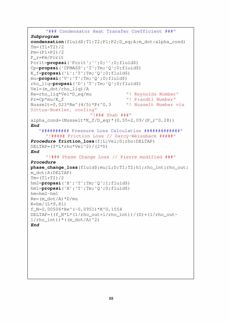
88

"### Condensator Heat Transfer Coefficient ###" Subprogram condensation(fluid$;T1;T2;P1;P2;D_eq;A;m_dot:alpha_cond) Tm=(T1+T2)/2 Pm=(P1+P2)/2 P_r=Pm/Pcrit Pcrit=propssi('Pcrit';'';0;'';0;fluid$) Cp=propssi('CPMASS';'T';Tm;'Q';0;fluid$) K_f=propssi('L';'T';Tm;'Q';0;fluid$) mu=propssi('V';'T';Tm;'Q';0;fluid$) rho_liq=propssi('D';'T';Tm;'Q';0;fluid$) Vel=(m_dot/rho_liq)/A Re=rho_liq*Vel*D_eq/mu "! Reynolds Number" Pr=Cp*mu/K_f "! Prandtl Number" Nusselt=0,023*Re^(4/5)*Pr^0,3 "! Nusselt Number via Dittus-Boetler, cooling"

"!### Shah ###" alpha_cond=(Nusselt*K_f/D_eq)*(0,55+2,09/(P_r^0,28)) End

"########## Pressure Loss Calculation #############" "!##### Friction Loss // Darcy-Weissback #####"

Procedure friction_loss(f;L;Vel;D;rho:DELTAP) DELTAP=(f*L*rho*Vel^2)/(2*D) End

"!### Phase Change Loss // Pierre modified ###" Procedure phase_change_loss(fluid$;mu;L;D;T1;T2;h1;rho_int;rho_out;m_dot;A:DELTAP) Tm=(T1+T2)/2 hm2=propssi('H';'T';Tm;'Q';1;fluid$) hm1=propssi('H';'T';Tm;'Q';0;fluid$) hm=hm2-hm1 Re=(m_dot/A)*D/mu K=hm/(L*9,81) f_N=0,00506*Re^(-0,0951)*K^0,1554 DELTAP=((f_N*L*(1/rho_out+1/rho_int))/(D)+(1/rho_out-1/rho_int))*((m_dot/A)^2) End

89

"### Length Calculation for concentric tube heat exchanger ###"

Subprogram length(R1;R2;alpha_ext;K_mat;alpha_int;Q;T_in1;T_in2;T_out1;T_out2:L) UA=(2*pi*L)/((1/(R2*alpha_ext))+(ln(R2/R1)/K_mat)+(1/(alpha_int*R1))) Q=UA*DTLM DELTA_TA=T_in1-T_out2 DELTA_TB=T_out1-T_in2 DTLM=(DELTA_TA-DELTA_TB)/(ln(DELTA_TA/DELTA_TB)) End

"######### Geometry Calculation ##########" Procedure diameter_in(fluid$;rho;Vel;T;P;m_dot:D_eq;R1;A) A:=(m_dot/rho)/Vel R1:=sqrt(A/pi) D_eq:=2*R1 End Procedure diameter_out(fluid$;rho;Vel;T;P;m_dot;R1;e:D_eq;R2;R3;A) A:=(m_dot/rho)/Vel R2:= R1+e D2:=R2*2 R3:=sqrt(A/PI+R2^2) D3:=R3*2 D_eq:=D3-D2 End

"!### INITIAL DATA AND HYPOTHESES ###" fluid$='R1234zeE' "! Main fluid " T_evap=T_in_e_sf-TG_evap-SH "! Temperature of evaporation " T_cond=T_in_c_sf+TG_cond+SC "! Temperature of condensation " TG_evap=5 [K] TG_cond=10 [K] SH=10 [K] "! Superheat degree of temperature " SC=2 [K] "! Subcooling degree of temperature " eta_is=0,8 [-] "! Compressor performance parameters, isentropic, volumetric and global" eta_vol=0,85 [-] eta_glob=0,75 [-] epsilon_IHX=0,85 "! Internal Heat Exchanger efficiency parameter" Q_evaporator=10000 [W] "! Condensator Heat Exchanged"

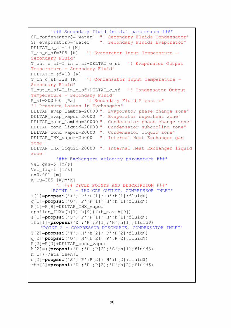
90

"### Secondary fluid initial parameters ###" SF_condensator$='water' "! Secondary Fluids Condensator" SF_evaporator$='water' "! Secondary Fluids Evaporator" DELTAT_e_sf=10 [K] T_in_e_sf=308 [K] "! Evaporator Input Temperature - Secondary Fluid" T_out_e_sf=T_in_e_sf-DELTAT_e_sf "! Evaporator Output Temperature - Secondary Fluid" DELTAT_c_sf=10 [K] T_in_c_sf=338 [K] "! Condensator Input Temperature - Secondary Fluid" T_out_c_sf=T_in_c_sf+DELTAT_c_sf "! Condensator Output Temperature - Secondary Fluid" P_sf=200000 [Pa] "! Secondary Fluid Pressure" "! Pressure Losses in Exchangers" DELTAP_evap_lambda=20000 "! Evaporator phase change zone" DELTAP_evap_vapor=20000 "! Evaporator superheat zone" DELTAP_cond_lambda=20000 "! Condensator phase change zone" DELTAP_cond_liquid=20000 "! Condensator subcooling zone" DELTAP_cond_vapor=20000 "! Condensator liquid zone" DELTAP_IHX_vapor=20000 "! Internal Heat Exchanger gas zone" DELTAP_IHX_liquid=20000 "! Internal Heat Exchanger liquid zone"

"### Exchangers velocity parameters ###" Vel_gas=5 [m/s] Vel_liq=1 [m/s] e=0,001 [m] K_Cu=385 [W/m*K]

"! ### CYCLE POINTS AND DESCRIPTION ###" "POINT 1 - IHX GAS OUTLET, COMPRESSOR INLET"

T[1]=propssi('T';'P';P[1];'H';h[1];fluid$) q[1]=propssi('Q';'P';P[1];'H';h[1];fluid$) P[1]=P[9]-DELTAP_IHX_vapor epsilon_IHX=(h[1]-h[9])/(h_max-h[9]) s[1]=propssi('S';'P';P[1];'H';h[1];fluid$) rho[1]=propssi('D';'P';P[1];'H';h[1];fluid$)

"POINT 2 - COMPRESSOR DISCHARGE, CONDENSATOR INLET" T[2]=propssi('T';'H';h[2];'P';P[2];fluid$) q[2]=propssi('Q';'H';h[2];'P';P[2];fluid$) P[2]=P[3]+DELTAP_cond_vapor h[2]=((propssi('H';'P';P[2];'S';s[1];fluid$)-h[1]))/eta_is+h[1] s[2]=propssi('S';'P';P[2];'H';h[2];fluid$) rho[2]=propssi('D';'P';P[2];'H';h[2];fluid$)

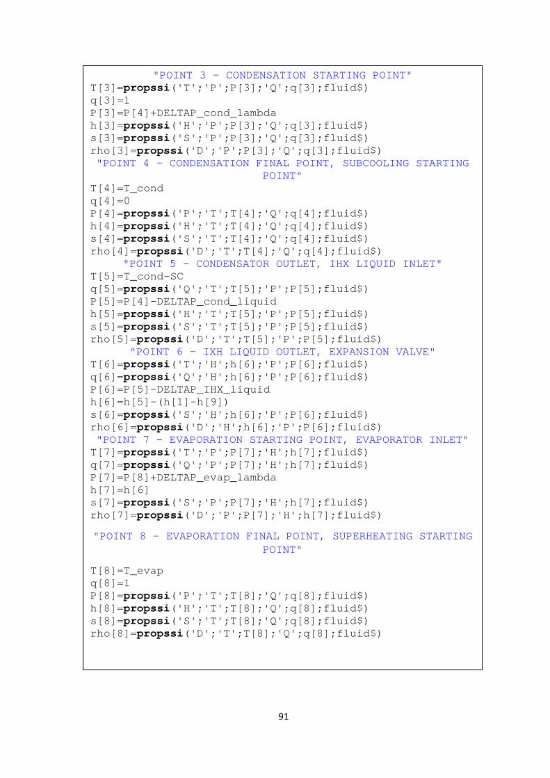
91

"POINT 3 - CONDENSATION STARTING POINT" T[3]=propssi('T';'P';P[3];'Q';q[3];fluid$) q[3]=1 P[3]=P[4]+DELTAP_cond_lambda h[3]=propssi('H';'P';P[3];'Q';q[3];fluid$) s[3]=propssi('S';'P';P[3];'Q';q[3];fluid$) rho[3]=propssi('D';'P';P[3];'Q';q[3];fluid$) "POINT 4 - CONDENSATION FINAL POINT, SUBCOOLING STARTING

POINT" T[4]=T_cond q[4]=0 P[4]=propssi('P';'T';T[4];'Q';q[4];fluid$) h[4]=propssi('H';'T';T[4];'Q';q[4];fluid$) s[4]=propssi('S';'T';T[4];'Q';q[4];fluid$) rho[4]=propssi('D';'T';T[4];'Q';q[4];fluid$)

"POINT 5 - CONDENSATOR OUTLET, IHX LIQUID INLET" T[5]=T_cond-SC q[5]=propssi('Q';'T';T[5];'P';P[5];fluid$) P[5]=P[4]-DELTAP_cond_liquid h[5]=propssi('H';'T';T[5];'P';P[5];fluid$) s[5]=propssi('S';'T';T[5];'P';P[5];fluid$) rho[5]=propssi('D';'T';T[5];'P';P[5];fluid$)

"POINT 6 - IXH LIQUID OUTLET, EXPANSION VALVE" T[6]=propssi('T';'H';h[6];'P';P[6];fluid$) q[6]=propssi('Q';'H';h[6];'P';P[6];fluid$) P[6]=P[5]-DELTAP_IHX_liquid h[6]=h[5]-(h[1]-h[9]) s[6]=propssi('S';'H';h[6];'P';P[6];fluid$) rho[6]=propssi('D';'H';h[6];'P';P[6];fluid$) "POINT 7 - EVAPORATION STARTING POINT, EVAPORATOR INLET" T[7]=propssi('T';'P';P[7];'H';h[7];fluid$) q[7]=propssi('Q';'P';P[7];'H';h[7];fluid$) P[7]=P[8]+DELTAP_evap_lambda h[7]=h[6] s[7]=propssi('S';'P';P[7];'H';h[7];fluid$) rho[7]=propssi('D';'P';P[7];'H';h[7];fluid$)

"POINT 8 - EVAPORATION FINAL POINT, SUPERHEATING STARTING POINT"

T[8]=T_evap q[8]=1 P[8]=propssi('P';'T';T[8];'Q';q[8];fluid$) h[8]=propssi('H';'T';T[8];'Q';q[8];fluid$) s[8]=propssi('S';'T';T[8];'Q';q[8];fluid$) rho[8]=propssi('D';'T';T[8];'Q';q[8];fluid$)

92

"POINT 9 - EVAPORATOR OUTLET, IHX GAS INLET" T[9]=T_evap+SH q[9]=propssi('Q';'T';T[9];'P';P[9];fluid$) P[9]=P[8]-DELTAP_evap_vapor h[9]=propssi('H';'T';T[9];'P';P[9];fluid$) s[9]=propssi('S';'T';T[9];'P';P[9];fluid$) rho[9]=propssi('D';'T';T[9];'P';P[9];fluid$)

"!### GRAPHIC DATA REPRESENTATION ###" Call fluiddata(fluid$:P_fluid[1..100];T_fluid[1..100];h_liq[1..100];h_vap[1..100];s_liq[1..100];s_vap[1..100]) P[10]=P[1] T[10]=T[1] h[10]=h[1] s[10]=s[1] q[10]=q[1] rho[10]=rho[1]

"### Critical Point ###" P_crit=propssi('Pcrit';'';0;'';0;fluid$) T_crit=propssi('Tcrit';'';0;'';0;fluid$) h_crit=propssi('H';'T';T_crit;'P';P_crit;fluid$)

"! ### PERFORMANCE INDICATORS OF THE CYCLE ###" m_dot=Q_condensator/(h[2]-h[5]) Q_evaporator=m_dot*(h[9]-h[7]) W_compressor=(m_dot*(h[2]-h[1]))/eta_glob COP=Q_condensator/W_compressor V_compressor=(m_dot/rho[1]/eta_vol)*convert(m^3/s;m^3/h) CR=P[2]/P[1]

" IHX parametes " h_max=propssi('H';'T';T[5];'P';P[1];fluid$) Q_IHX=m_dot*(h[1]-h[9])

93

"! ### COMPONENTS CALCULATION ###" "! ### Internal Heat Exchanger ###" "### Diameter of the exchanger ###"

Call diameter_in(fluid$;Vel_liq;rho[5];T[5];P[5];m_dot:D_inn_IHX;R1_IHX;A_in_IHX) Call diameter_out(fluid$;Vel_gas;rho[9];T[9];P[9];m_dot;R1_IHX;e:D_hyd_IHX;R2_IHX;R3_IHX;A_out_IHX) "### Heat Coefficient Calculation - Gas outer tube (9-1),

Liquid inner tube (5-6) ###" Call single_phase(fluid$;T[5];T[6];P[5];P[6];m_dot;D_inn_IHX;A_in_IHX:alpha_int_IHX;Vel_int_IHX;rho_int_IHX;f_int_IHX) Call single_phase(fluid$;T[9];T[1];P[9];P[1];m_dot;D_hyd_IHX;A_out_IHX:alpha_ext_IHX;Vel_ext_IHX;rho_ext_IHX;f_ext_IHX)

"### Geometry Parameters ###" Call length(R1_IHX;R3_IHX;alpha_ext_IHX;K_Cu;alpha_int_IHX;Q_IHX;T[5];T[9];T[6];T[1]:L_IHX) Area_IHX=pi*R1_IHX*L_IHX

"### Pressure Loss - Internal and External ###" Call friction_loss(f_int_IHX;L_IHX;Vel_int_IHX;D_inn_IHX;rho_int_IHX:DELTAP_int_IHX) "! Points 5 to 6" Call friction_loss(f_ext_IHX;L_IHX;Vel_ext_IHX;D_hyd_IHX;rho_ext_IHX:DELTAP_ext_IHX) "! Points 9 to 1"

"! ### Evaporator ###" "### Diameter of the exchanger ###"

rho_evap_sf=propssi('D';'T';T_in_e_sf;'P';P_sf;SF_evaporator$) Call diameter_out(fluid$;rho[7];Vel_liq;T[7];P[7];m_dot;R1_evap;e:D_hyd_evap;R2_evap;R3_evap;A_out_evap) "!Outer diameter calculation" Call diameter_in(SF_evaporator$;rho_evap_sf;Vel_liq;T_in_e_sf;P_sf;m_dot_evap_sf:D_inn_evap;R1_evap;A_in_evap) "!Inner diameter calculation"

94

"### Heat Coefficient Calculation - Evaporation outer tube (7-9), secondary fluid inner tube.###"

Tm_evap_sf=(T_in_e_sf+T_out_e_sf)/2 cp_e_sf=propssi('C';'T';Tm_evap_sf;'P';P_sf;SF_evaporator$) Q_evap_1=m_dot*(h[9]-h[8]) Q_evap_2=m_dot*(h[8]-h[7]) Q_evap_1=m_dot_evap_sf*cp_e_sf*(T_in_e_sf-Tm_evap) Q_evap_2=m_dot_evap_sf*cp_e_sf*(Tm_evap-T_out_e_sf)

"### Zone 1: Simple phase - Points 8 to 9 ###" Call single_phase(fluid$;T[8];T[9];P[8];P[9];m_dot;D_hyd_evap;A_out_evap:alpha_ext_evap_1;Vel_ext_evap_1;rho_ext_evap_1;f_ext_evap_1) "! Outer tube" Call single_phase(SF_evaporator$;T_in_e_sf;Tm_evap;P_sf;P_sf;m_dot_evap_sf;D_inn_evap;A_in_evap:alpha_int_evap_1;Vel_int_evap_1;rho_int_evap_1;f_int_evap_1) "! Inner tube"

"### Zone 2: Evaporation - Points 7 to 8 ###" Call evaporation(fluid$;T[7];h[7];T[8];q[7];m_dot;D_hyd_evap;A_out_evap;L_evap_2:alpha_ext_evap_2) "! Outer tube" Call single_phase(SF_evaporator$;Tm_evap;T_out_e_sf;P_sf;P_sf;m_dot_evap_sf;D_inn_evap;A_in_evap:alpha_int_evap_2;Vel_int_evap_2;rho_int_evap_2;f_int_evap_2) "! Inner tube"

"### Geometry Parameters ###" L_evap=L_evap_1+L_evap_2 Call length(R1_evap;R2_evap;alpha_ext_evap_1;K_Cu;alpha_int_evap_1;Q_evap_1;T_in_e_sf;T[8];Tm_evap;T[9]:L_evap_1) Call length(R1_evap;R2_evap;alpha_ext_evap_2;K_Cu;alpha_int_evap_2;Q_evap_2;Tm_evap;T[7];T_out_e_sf;T[8]:L_evap_2) Area_evap=pi*R1_evap*L_evap

"### Pressure Loss ###" D_cont_e=R2_evap*2 Call friction_loss(f_ext_evap_1;L_evap_1;Vel_ext_evap_1;D_cont_e;rho_ext_evap_1:DELTAP_evap_1) rho_ext_evap_2=propssi('D';'T';T[7];'Q';q[7];fluid$) mu_evap=propssi('V';'T';(T[7]+T[8])/2;'Q';q[7];fluid$) Call phase_change_loss(fluid$;mu_evap;L_evap_2;D_cont_e;T[7];T[8];h[7];rho_int_evap_2;rho_ext_evap_2;m_dot;A_out_evap:DELTAP_evap_2) DELTAP_evap=DELTAP_evap_1+DELTAP_evap_2

95

"! ### Condensator ###" "### Diameter of the exchanger ###"

rho_cond_sf=propssi('D';'T';T_in_c_sf;'P';P_sf;SF_condensator$) Call diameter_out(fluid$;rho[2];Vel_gas;T[2];P[2];m_dot;R1_cond;e:D_hyd_cond;R2_cond;R3_cond;A_out_cond) Call diameter_in(SF_condensator$;rho_cond_sf;Vel_liq;T_in_c_sf;P_sf;m_dot_cond_sf:D_inn_cond;R1_cond;A_in_cond)

"### Power parameters ###" Q_cond_1=m_dot*(h[2]-h[3]) Q_cond_2=m_dot*(h[3]-h[4]) Q_cond_3=m_dot*(h[4]-h[5]) Tm_cond_sf=(T_in_c_sf+T_out_c_sf)/2 cp_c_sf=propssi('C';'T';Tm_cond_sf;'P';P_sf;SF_condensator$) Q_cond_1=m_dot_cond_sf*cp_c_sf*(T_out_c_sf-T_m_2_c_sf) Q_cond_3=m_dot_cond_sf*cp_c_sf*(T_m_1_c_sf-T_in_c_sf) Q_cond_2=m_dot_cond_sf*cp_c_sf*(T_m_2_c_sf-T_m_1_c_sf) "### Heat Coefficient Calculation - Condensation outer

tube (2-5), Secondary fluid inner tube ###" "### Zone 1 ###"

Call single_phase(fluid$;T[2];T[3];P[2];P[3];m_dot;D_hyd_cond;A_out_cond:alpha_ext_cond_1;Vel_ext_cond_1;rho_ext_cond_1;f_ext_cond_1) Call single_phase(SF_condensator$;T_in_c_sf;T_m_1_c_sf;P_sf;P_sf;m_dot_cond_sf;D_inn_cond;A_in_cond:alpha_int_cond_1;Vel_int_cond_1;rho_int_cond_1;f_int_cond_1)

"### Zone 2 ###" Call condensation(fluid$;T[3];T[4];P[3];P[4];D_hyd_cond;A_out_cond;m_dot:alpha_ext_cond_2) Call single_phase(SF_condensator$;T_m_1_c_sf;T_m_2_c_sf;P_sf;P_sf;m_dot_cond_sf;D_inn_cond;A_in_cond:alpha_int_cond_2;Vel_int_cond_2;rho_int_cond_2;f_int_cond_2)

"### Zone 3 ###" Call single_phase(fluid$;T[4];T[5];P[4];P[5];m_dot;D_hyd_cond;A_out_cond:alpha_ext_cond_3;Vel_ext_cond_3;rho_ext_cond_3;f_ext_cond_3)

96

Call single_phase(SF_condensator$;T_m_2_c_sf;T_out_c_sf;P_sf;P_sf;m_dot_cond_sf;D_inn_cond;A_in_cond:alpha_int_cond_3;Vel_int_cond_3;rho_int_cond_3;f_int_cond_3)

"### Geometry Parameters ###" L_cond=L_cond_1+L_cond_2+L_cond_3 Call length(R1_cond;R2_cond;alpha_ext_cond_1;K_Cu;alpha_int_cond_1;Q_cond_1;T[2];T_m_2_c_sf;T[3];T_out_c_sf:L_cond_1) Call length(R1_cond;R2_cond;alpha_ext_cond_2;K_Cu;alpha_int_cond_2;Q_cond_2;T[3];T_m_1_c_sf;T[4];T_m_2_c_sf:L_cond_2) Call length(R1_cond;R2_cond;alpha_ext_cond_3;K_Cu;alpha_int_cond_3;Q_cond_3;T[4];T_in_c_sf;T[5];T_m_1_c_sf:L_cond_3) Area_cond=pi*R1_cond*L_cond

"### Pressure Loss ###" mu_cond=propssi('V';'T';(T[3]+T[4])/2;'P';P[3];fluid$) rho_ext_cond_2=propssi('D';'T';(T[3]+T[4])/2;'P';(P[3]+P[4])/2;fluid$) D_cont_c=R2_cond*2 Call friction_loss(f_ext_cond_1;L_cond_1;Vel_ext_cond_1;D_cont_c;rho_ext_cond_1:DELTAP_cond_1) Call phase_change_loss(fluid$;mu_cond;L_cond_2;D_cont_c;T[3];T[4];h[3];rho_int_cond_2;rho_ext_cond_2;m_dot;A_out_cond:DELTAP_cond_2) Call friction_loss(f_ext_cond_3;L_cond_3;Vel_ext_cond_3;D_cont_c;rho_ext_cond_3:DELTAP_cond_3) DELTAP_cond=DELTAP_cond_1+DELTAP_cond_2+DELTAP_cond_3 "!### Graphical representation auxiliar information ###" T_e_sf[1]=T_in_e_sf P_e_sf[1]=P_sf h_e_sf[1]=propssi('H';'T';T_e_sf[1];'P';P_e_sf[1];SF_evaporator$) s_e_sf[1]=s[9] T_e_sf[2]=Tm_evap P_e_sf[2]=P_sf h_e_sf[2]=propssi('H';'T';T_e_sf[2];'P';P_e_sf[2];SF_evaporator$)

97

s_e_sf[2]=s[8] T_e_sf[3]=T_out_e_sf P_e_sf[3]=P_sf h_e_sf[3]=propssi('H';'T';T_e_sf[3];'P';P_e_sf[3];SF_evaporator$) s_e_sf[3]=s[7] T_c_sf[1]=T_in_c_sf P_c_sf[1]=P_sf h_c_sf[1]=propssi('H';'T';T_c_sf[1];'P';P_c_sf[1];SF_condensator$) s_c_sf[1]=s[5] T_c_sf[2]=T_m_1_c_sf P_c_sf[2]=P_sf h_c_sf[2]=propssi('H';'T';T_c_sf[2];'P';P_c_sf[2];SF_condensator$) s_c_sf[2]=s[4] T_c_sf[3]=T_m_2_c_sf P_c_sf[3]=P_sf h_c_sf[3]=propssi('H';'T';T_c_sf[3];'P';P_c_sf[3];SF_condensator$) s_c_sf[3]=s[3] T_c_sf[4]=T_out_c_sf P_c_sf[4]=P_sf h_c_sf[4]=propssi('H';'T';T_c_sf[4];'P';P_c_sf[4];SF_condensator$) s_c_sf[4]=s[2]

99

Section 5 – Blueprints

Development of a Vapor Compression Cycle Heat Pump ...

Documents

Transcript of Development of a Vapor Compression Cycle Heat Pump ...