Development of a High-Speed Rail Model to Study Current and Future High-Speed

Rail Corridors in the United States

Alex J. Vandyke

Thesis submitted to the faculty of the Virginia Polytechnic Institute and State University

in partial fulfillment of the requirements for the degree of

Master of Science

In

Civil Engineering

Antonio A. Trani, Chair

Montasir Abbas

Gerardo W. Flintsch

May 31, 2011

Blacksburg, VA

Keywords: Logit Model, High-Speed Rail, High-Speed Train, Box Cox, Amtrak,

American Travel Survey

Development of a High-Speed Rail Model to Study Current and Future High-Speed

Rail Corridors in the United States

Alex J. Vandyke

ABSTRACT

A model that can be used to analyze both current and future high-speed rail corridors is

presented in this work. This model has been integrated into the Transportation Systems

Analysis Model (TSAM). The TSAM is a model used to predict travel demand between

any two locations in the United States, at the county level. The purpose of this work is to

develop tools that will create the necessary input data for TSAM, and to update the model

to incorporate passenger rail as a viable mode of transportation. This work develops a

train dynamics model that can be used to calculate the travel time and energy

consumption of multiple high-speed train types while traveling between stations. The

work also explores multiple options to determine the best method of improving the

calibration and implementation of the model in TSAM. For the mode choice model, a

standard C logit model is used to calibrate the mode choice model. The utility equation

for the logit model uses the decision variables of travel time and travel cost for each

mode. A modified utility equation is explored; the travel time is broken into an in-vehicle

and out-of-vehicle time in an attempt to improve the model, however the test determines

that there is no benefit to the modification. In addition to the C-logit model, a Box-Cox

transformation is applied to both variables in the utility equation. This transformation

removes some of the linear assumptions of the logit model and thus improves the

performance of the model. The calibration results are implemented in TSAM, where both

existing and projected high-speed train corridors are modeled. The projected corridors

use the planned alignment for modeling. The TSAM model is executed for the cases of

existing train network and projected corridors. The model results show the sensitivity of

travel demand by modeling the future corridors with varying travel speeds and travel

costs. The TSAM model shows the mode shift that occurs because of the introduction of

high-speed rail.

iii

Acknowledgements

I would like to first thank Dr. Antonio Trani for giving me the opportunity to conduct this

research and work toward receiving my degree. This work would not have been possible

without all of his guidance and assistance. I would also like to thank Dr. Montasir Abbas

and Dr. Gerardo Flintsch for serving on the committee and providing valuable input and

information.

I want to extend a special thank you to Nicolas Hinze for all of his assistance in helping

with the development of the computer modeling code. I also want to mention all of the

new friends I have made, both in the Air Transportation Systems Lab and the Civil

Engineering Graduate Program; thanks for all of the good times and memories.

Finally, I would like to parents and grandparents for everything they have done to

provide me an opportunity to complete this work. I would not have been in this position

without all of their support and guidance.

iv

Table of Contents

List of Figures ............................................................................................................. vi

List of Tables ............................................................................................................ viii

Introduction ............................................................................................................... 1

History of American Railroad ......................................................................................... 1 High-Speed Rail Operations Around the World ............................................................. 3

Japan ....................................................................................................................................... 3 France ..................................................................................................................................... 4 China ....................................................................................................................................... 5

Description of Transportation Systems Analysis Model (TSAM) ................................. 6

Literature Review ....................................................................................................... 8

Available Rail Planning/ Analysis Software................................................................... 8 Rail Traffic Controller ............................................................................................................ 8 RAILSIM ................................................................................................................................ 8 TransCAD .............................................................................................................................. 9

Trip Distribution Modeling ........................................................................................... 10 Mode Split Modeling .................................................................................................... 12

Problem Description ................................................................................................. 18

Methodology ............................................................................................................ 19

Train Dynamics Model ................................................................................................. 19 Method .................................................................................................................................. 19 Model Equations ................................................................................................................... 21 Train Types ........................................................................................................................... 24 Energy Consumption ............................................................................................................ 25

Description of American Travel Survey (ATS) Data Set ............................................. 33 Mode Split Analysis - C Logit Model........................................................................... 33

C- Logit Model - Comparison of Weighted vs. Un-weighted Data: ............................. 35 Improvement of C- Logit Coefficient Optimization ..................................................... 37

Skepticism of ATS Weight Factors .............................................................................. 39 Analysis of ATS Weight Factor Effect ......................................................................... 40 Model Comparison Metric ............................................................................................ 45 C- Logit Model - Utility Function Variation ................................................................ 46 Validation of C Logit Coefficient Optimization Code ................................................. 49

Logit Model Improvement - Box Cox Transformation ................................................ 50 Existing Train Network - Station to Station Travel Time and Cost ............................. 51

Future High-Speed Rail Corridor Modeling ................................................................. 54 Alignments ............................................................................................................................ 54 Train Station to Train Station Travel Time and Cost – Future Corridors ............................. 57

County to Train Station Travel Time and Cost – TSAM.............................................. 58 Additional Time and Cost Components – TSAM......................................................... 59

Results ...................................................................................................................... 65

Test of Train Dynamics Model ..................................................................................... 65

v

NEC Corridor Model .................................................................................................... 67

Nationwide Calibration Results .................................................................................... 73 Nationwide Mode Choice Results – 1995 .................................................................... 74 Nationwide Mode Choice Results – 2011 .................................................................... 75

Nationwide Mode Choice Results – 2020 .................................................................... 80 Nationwide Mode Choice Results - 2030 ..................................................................... 82

Summary and Conclusions ........................................................................................ 84

Recommendations .................................................................................................... 87

References ................................................................................................................ 90

Appendix A – Additional Information ........................................................................ 92

Complete List of Amtrak Stations Available in TSAM................................................ 92

Proposed High-Speed Rail Corridor Layouts and Stations......................................... 104 California ............................................................................................................................ 104 Pacific Northwest ................................................................................................................ 105 Florida ................................................................................................................................. 106 Chicago Hub ....................................................................................................................... 107 Southeast ............................................................................................................................. 110 Empire ................................................................................................................................ 111 Northern New England ....................................................................................................... 112 Keystone ............................................................................................................................. 113 South Central ...................................................................................................................... 114 Gulf Coast ........................................................................................................................... 115 Vermont Route.................................................................................................................... 116 Original Northeast Corridor ................................................................................................ 117

Proposed High-Speed Rail Corridors Modeling Assumptions ................................... 118

Nationwide Train Travel Time and Travel Cost Regression Curves .......................... 119 TSAM Lodging Time Penalty .................................................................................... 121 Nationwide Mode Choice Calibration Detailed Results ............................................. 122

TSAM Mode Choice Application Detailed Results.................................................... 125 Baseline Case ...................................................................................................................... 125 Scenario 1 ........................................................................................................................... 126 Scenario 2 ........................................................................................................................... 127 Scenario 3 ........................................................................................................................... 128 Scenario 4 ........................................................................................................................... 130

Appendix B – Source Code....................................................................................... 132

Train Dynamics Model - Matlab Code ....................................................................... 132 Primary File ........................................................................................................................ 132 Train Profile Function ......................................................................................................... 134 Resistive Force Function .................................................................................................... 141 Tractive Effort Function ..................................................................................................... 141 TGV_Resistance Function .................................................................................................. 141

Station to Station Input File Creator ........................................................................... 143 Primary File ........................................................................................................................ 143 Train Station Index Finder Function ................................................................................... 169 Schedule Delay Calculator Function .................................................................................. 170

vi

List of Figures

Figure 1 - Comparison of Linear and Box- Cox Logit Response Curves [21] ................. 17 Figure 2 - Sample Three Phase Velocity Profile .............................................................. 19 Figure 3 - Sample Two Phase Velocity Profile ................................................................ 20

Figure 4 - U.S. Energy Regions used for Consumption Calculations [25] ....................... 26 Figure 5 - Vehicle Tractive Effort Rate vs. Time ............................................................. 30

Figure 6 - Vehicle Energy Consumption Rate vs. Time ................................................... 32 Figure 7 - Vehicle Cumulative Energy Consumed vs. Time ............................................ 32 Figure 8 - Business Trip Distribution of Un-Weighted ATS Data ................................... 40 Figure 9 - Business Trip Distribution Weighted Data ...................................................... 41 Figure 10 - Non Business Trip Distribution of Un-Weighted Data .................................. 41

Figure 11 - Non Business Trip Distribution of Weighted Data ........................................ 42

Figure 12 - Nationwide Train Travel Time Regression Curve ......................................... 52

Figure 13 - Nationwide Train Travel Cost Regression Curve .......................................... 53 Figure 14 - Northeast Corridor Model Analysis Area ...................................................... 70

Figure 15 - Cumulative Percentage of Commercial Air Trips by Distance - Business Trips

- Northeast Corridor Model Only ..................................................................................... 71

Figure 16 - Cumulative Percentage of Commercial Air Trips by Distance - Non-Business

Trips - Northeast Corridor Model Only ............................................................................ 72 Figure 17 - TSAM Mode Choice Results - 2011 - Total Automobile Trips..................... 78

Figure 18 - TSAM Mode Choice Results - 2011 - Total Commercial Air Trips.............. 79 Figure 19 - TSAM Mode Choice Results - 2011 - Total Train Trips ............................... 79

Figure 20 - TSAM Mode Choice Results - 2020 - Total Automobile Trips..................... 80 Figure 21 - TSAM Mode Choice Results - 2020 - Total Commercial Air Trips.............. 81 Figure 22 - TSAM Mode Choice Results - 2020 - Total Train Trips ............................... 81

Figure 23 - TSAM Mode Choice Results - 2030 - Total Automobile Trips..................... 82

Figure 24 - TSAM Mode Choice Results - 2030 - Total Commercial Air Trips.............. 82 Figure 25 - TSAM Mode Choice Results - 2030 - Total Train Trips ............................... 83 Figure 26 - Planned Alignment of California High-Speed Rail Corridor ....................... 104

Figure 27 - Planned Alignment of Pacific Northwest High-Speed Rail Corridor .......... 105

Figure 28 - Planned Alignment of Florida High-Speed Rail Corridor ........................... 106 Figure 29 - Planned Alignment of Chicago Hub High-Speed Rail Corridor - part 1 ..... 107 Figure 30 - Planned Alignment of Chicago Hub High-Speed Rail Corridor - part 2 ..... 108 Figure 31 - Planned Alignment of Chicago Hub High-Speed Rail Corridor - part 3 ..... 108 Figure 32 - Planned Alignment of Southeast High-Speed Rail Corridor ....................... 110

Figure 33 - Planned Alignment of Empire High-Speed Rail Corridor ........................... 111 Figure 34 - Planned Alignment of Northern New England High-Speed Rail Corridor .. 112

Figure 35 - Planned Alignment of High-Speed Rail Corridor ........................................ 113 Figure 36 - Planned Alignment of South Central High-Speed Rail Corridor ................. 114 Figure 37 - Planned Alignment of Gulf Coast High-Speed Rail Corridor ..................... 115 Figure 38 - Planned Alignment of Vermont High-Speed Rail Corridor ......................... 116 Figure 39 - Planned Alignment of Original Northeast Corridor ..................................... 117

Figure 40 - Northeast Corridor Regional Service Travel Time Regression Curve ......... 119 Figure 41 - Northeast Corridor Regional Service Travel Cost Regression Curve .......... 119 Figure 42 - Acela Express Travel Time Regression Curve ............................................ 120

vii

Figure 43 - Acela Express Travel Cost Regression Curve ............................................. 120

viii

List of Tables

Table 1 - Forces Contributing to the Coefficients of the Davis Equation [24] ................. 23 Table 2 - Model Coefficients for Shinkansen Trains ........................................................ 24 Table 3 - Model Coefficients for TGV Trains .................................................................. 25

Table 4 - Energy Generation Percentages for Energy Production Methods [25] ............. 27 Table 5 - Source Energy Factors for Delivered Electricity (Kilowatt-hours of source

energy per Kilowatt- hours of delivered electricity) [25] ................................................ 27 Table 6 - TSAM Income Category Divisions - $(1995) ................................................... 33 Table 7 - Number of ATS Observations in Each Trip Purpose / Income Group Category

........................................................................................................................................... 35 Table 8 - Summary of Coefficients for Un-Weighted ATS Data ..................................... 35

Table 9 - Summary of Coefficients for Weighted ATS Data ........................................... 36

Table 10 - Summary of Coefficients for Random Portion of Un-Weighted Data ............ 37

Table 11 - Summary of Coefficients for Random Portion of Weighted ATS Data .......... 38

Table 12 - Parameters for Kolmogorov-Smirnov Test ..................................................... 44 Table 13 - Comparison of Un-Weighted vs. Weighted Model Predictions ...................... 46 Table 14 - Utility Equation Coefficients for Two Variable Formulation ......................... 47

Table 15 - Utility Equation Coefficients for Three Variable Formulation ....................... 48 Table 16 - Validation of C-logit Optimization Code ........................................................ 49

Table 17 - Calibration Bounds for Box-Cox Coefficients ................................................ 51 Table 18 - Major Cities Along Proposed High-Speed Rail Corridors .............................. 56 Table 19 - Acela Express Train Daily Service Frequency ................................................ 61

Table 20 - Acela Express Train Schedule Delay (hours) .................................................. 62 Table 21 - TSAM Lodging Costs - $(2000)...................................................................... 64

Table 22 - Comparison of Trainset Performance on Original Northeast Corridor Route 66

Table 23 - Comparison of Trainset Performance on Original Northeast Corridor Route

(Stops at Major Cities Only) ............................................................................................. 66 Table 24 - Amtrak Stations Served in Northeast Corridor ............................................... 68

Table 25 - ATS's Reported Driving Distance to Station - Northeast Corridor Only ........ 69 Table 26 - Breakdown of ATS Records in Northeast Corridor Model ............................. 70

Table 27 - Nationwide Mode Choice Calibration vs. ATS Data ...................................... 73 Table 28 - TSAM Mode Choice Results – 1995............................................................... 75 Table 29 - TSAM Mode Choice Results - 2011 - Existing Train Network ...................... 76 Table 30 - TSAM Mode Choice Results – High-Speed Rail Modeling Scenario

Descriptions ...................................................................................................................... 76

Table 31 - TSAM Mode Choice Results - 2011 – Scenario 1 .......................................... 77 Table 32 - TSAM Mode Choice Results - 2011 – Scenario 2 .......................................... 77

Table 33 - TSAM Mode Choice Results - 2011 – Scenario 3 .......................................... 77 Table 34 - TSAM Mode Choice Results - 2011 – Scenario 4 .......................................... 77 Table 35 - Full List of Modeled Train Stations Available in TSAM................................ 92 Table 36 - Modeled Train Stations for California High-Speed Rail Corridor ................ 104 Table 37 - Modeled Train Stations for Pacific Northwest High-Speed Rail Corridor ... 105

Table 38 - Modeled Train Stations for Florida High-Speed Rail Corridor..................... 106 Table 39 - Modeled Train Stations for Chicago Hub High-Speed Rail Corridor – p. 1 . 109 Table 40 - Modeled Train Stations for Chicago Hub High-Speed Rail Corridor – p. 2 . 109

ix

Table 41 - Modeled Train Stations for Southeast High-Speed Rail Corridor ................. 110

Table 42 - Modeled Train Stations for Empire High-Speed Rail Corridor .................... 111 Table 43 - Modeled Train Stations for Northern New England High-Speed Rail Corridor

......................................................................................................................................... 112

Table 44 - Modeled Train Stations for Keystone High-Speed Rail Corridor ................. 113 Table 45 - Modeled Train Stations for South Central High-Speed Rail Corridor .......... 114 Table 46 - Modeled Train Stations for Gulf Coast High-Speed Rail Corridor ............... 115 Table 47 - Modeled Train Stations for Vermont High-Speed Rail Corridor .................. 116 Table 48 – High-Speed Rail Corridor Modeling Assumptions ...................................... 118

Table 49 - TSAM Lodging Time Penalty ....................................................................... 121 Table 50 - Nationwide Mode Choice Calibration - Detailed Results ............................. 122 Table 51 - Nationwide Mode Choice Calibration - Calibration Coefficients ................. 124 Table 52 - TSAM Mode Choice Detailed Results - Baseline Case ................................ 125

Table 53 - TSAM Mode Choice Detailed Results - Scenario 1 ...................................... 126 Table 54 - TSAM Mode Choice Detailed Results - Scenario 2 ...................................... 127

Table 55 - TSAM Mode Choice Detailed Results - Scenario 3 ...................................... 129 Table 56 - TSAM Mode Choice Detailed Results - Scenario 4 ...................................... 130

1

Introduction

History of American Railroad

The development and implementation of the railroad played an important role in the

shaping of the United States. The use of a railroad network for carrying both

passengers and freight helped spur the development of the United States at a critical

point in its existence. The earliest records indicate that the first tracks, approximately

three miles long, were placed in Quincy, Massachusetts. The first cars to operate on

this line were pulled by horses.[1]

Several different carriage powering alternatives were tested in the early years of rail.

The use of horses for power, either attaching them directly to the car for pulling or

placing the horse on a belt that drives the wheels, was the most prevalent. As well,

designer began experimenting with wind power by attaching a sail to the train car; this

design was tested but ultimately failed. However, the most important development for

the railroad was the use of the steam engine to develop a powered car. The

development of the steam engine and even the locomotive had begun long before the

placement of the first rail track; the first steam engine arrived in the U.S. in 1753. The

advent of the steam powered locomotive engine allowed the movement of more people

and freight at a much higher efficiency. The steam engine created an opportunity for

people to utilize the train as a viable, dependable mode of transportation. Individuals

and corporations alike began to operate businesses on the rail lines; one of the first

railroad companies to launch was the Baltimore and Ohio (B&O) railroad that ran west

from Baltimore into Virginia (present day West Virginia).[1]

Another important event in the history of U.S. rail was the completion of the First

Transcontinental Railroad which opened a link between the east and west coasts. The

line was completed on May 10, 1869 at Promontory Summit, Utah. Although rail

operations were already developing heavily, particularly on the east coast, this was an

important event because travel across the country became much quicker and safer. At

2

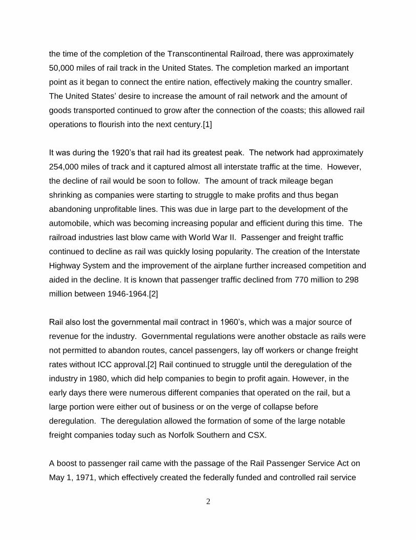
the time of the completion of the Transcontinental Railroad, there was approximately

50,000 miles of rail track in the United States. The completion marked an important

point as it began to connect the entire nation, effectively making the country smaller.

The United States’ desire to increase the amount of rail network and the amount of

goods transported continued to grow after the connection of the coasts; this allowed rail

operations to flourish into the next century.[1]

It was during the 1920’s that rail had its greatest peak. The network had approximately

254,000 miles of track and it captured almost all interstate traffic at the time. However,

the decline of rail would be soon to follow. The amount of track mileage began

shrinking as companies were starting to struggle to make profits and thus began

abandoning unprofitable lines. This was due in large part to the development of the

automobile, which was becoming increasing popular and efficient during this time. The

railroad industries last blow came with World War II. Passenger and freight traffic

continued to decline as rail was quickly losing popularity. The creation of the Interstate

Highway System and the improvement of the airplane further increased competition and

aided in the decline. It is known that passenger traffic declined from 770 million to 298

million between 1946-1964.[2]

Rail also lost the governmental mail contract in 1960’s, which was a major source of

revenue for the industry. Governmental regulations were another obstacle as rails were

not permitted to abandon routes, cancel passengers, lay off workers or change freight

rates without ICC approval.[2] Rail continued to struggle until the deregulation of the

industry in 1980, which did help companies to begin to profit again. However, in the

early days there were numerous different companies that operated on the rail, but a

large portion were either out of business or on the verge of collapse before

deregulation. The deregulation allowed the formation of some of the large notable

freight companies today such as Norfolk Southern and CSX.

A boost to passenger rail came with the passage of the Rail Passenger Service Act on

May 1, 1971, which effectively created the federally funded and controlled rail service

3

Amtrak. The act allowed the federally controlled Amtrak to operate over mostly private

freight tracks, except for the Northeast Corridor (NEC), where the federal government

owns most of the track. The passage of the law also required two things of existing rail

companies, “one time payments, which would eventually total $190 million (from 13

railroads), and/or equipment… In exchange railroads received Amtrak Common Stock.”

In total Amtrak received 300 locomotives and 1200 cars.[3] Amtrak has continued to

grow, despite being underfunded and unprofitable, having reached 25 million

passengers in 2007. Amtrak captures a large number of its riders in the Northeast

Corridor region.

High-Speed Rail Operations Around the World

The following sections discuss some of the countries that are leading the way in the

development and use of high-speed rail. Although high-speed passenger rail is barely

seen in the United States, it is a driving force and desired commodity in many other

countries around the world. This section is by no means all inclusive; other countries

such as Italy, Spain, Germany, India, etc. are either investigating or already using high-

speed rail on a large scale. Spain, despite is relatively small land mass and low

population, currently has the second largest high-speed rail network in the world.

Japan

Japan is considered to be the world leader in terms of high-speed rail technology and its

operation. Japan began operating the world’s first high-speed rail network in 1964

using the Shinkansen trains, known as the bullet trains. The first line connected Tokyo,

Nagoya, Kyoto, and Osaka. The trains initially ran at 200 km/h, but with technological

advances, they can currently operate at 300 km/hr. The Shinkansen network is

currently operating a series of different “lines” through multiple cities. The network has

grown to 1,528 miles of track and serves the islands of Kyushu and Honshu; it connects

to several major cities on each island. The network itself extends from Aomori to

Kagoshima. One of the design features of the network is that there are no at-grade

crossings and the track is fenced off; trespassing is heavily protected by law. These

safeguards enable safe high-speed operations because the trains are not operating on

4

the same lines as the slower freight cars and there are no concerns about vehicles or

pedestrians on the track.

The network operates trains in three different categories. The Nozomi is the

highest/fastest category because it stops only at very important stations, thus producing

the shortest overall travel time. The second category is the Hikari which stops more

frequently than the Nozomi. Due to the additional stops, the Hikari takes about 30

minutes of additional time to travel between Osaka and Tokyo. The last category is the

Kodama which is the slowest category because the train stops at every station along

the route.

There have been many different versions of the trains on the Shinkansen network. The

inaugural train was the Shinkansen Series 0. This train was typically 12 cars long and

operated at speeds around 220 km/hr. Later versions include the 100 series, 300

series, 500 series, and 700 series. Each train featured consumer upgrades and/or

upgraded technology that allowed for faster travel and/or better passenger

accommodations. More information is widely available about each of the different

series of trains. The newest train is the Shinkansen Series N700 which is capable of

traveling 300 km/hr. This train is unique for the Shinkansen in that it has a tilting

mechanism that allows it to tilt one degree during turns; this allows the train to travel

270 km/hr through turns with a design radius of 2,500 meters.[4] Another notable

improvement is that the N700 Series was also able to increase its acceleration

performance by 30% vs. older Shinkansen trains.

France

The French high-speed train network is known as the TGV (Train à Grande Vitesse),

which stands for high-speed train. The project was launched in the late 1960’s with the

first prototype, the TGV 001, being tested in the early 1970’s. Only one TGV 001 was

built as it was used for research and testing of brakes, aerodynamics, traction, etc. The

TGV 001 was powered by a gas turbine and set a world speed record at the time at 318

km/hr. The oil crisis in 1974 led the developers to begin working on an electric powered

5

train. One thing to note is that the trains are designed to be able to operate on the

existing rail network; this allows the trains to connect with many different cities without

adding additional construction costs associated with a new track. As well, it allowed

“high-speed” sections to be built as funding became available. The ultimate goal is to

have protected high-speed sections with no at-grade crossings for long distance travel

and then have the trains run on existing track to connect to various cities.[5]

The first line opened to passenger service on September 27, 1981 between Paris and

Lyon. The network was incredibly successful as it captured most of the air traffic along

the route and was able to pay for itself within 10 years. This initial success led to the

development of the large TGV network that exists today. Today, the current TGV

network is approximately 1250 miles and another 400 miles is currently being built.[6]

This is despite the fact that there are only 18 TGV stations outside of Paris on the six

active lines, which shows the network is currently running only city-city travel.[6] The

TGV network also connects with many of France’s neighboring countries such as

Switzerland, Germany, Belgium, etc.

The rolling stock of the TGV has also evolved. There are currently 7 types of trains

(depending on classification) that are operating on the network. They vary by length of

cars, type of vehicle (single deck or double deck), and seating capacity. The newest of

the trains is the TGV POS (Paris-Ostfrankreich-Süddeutschland : Paris-Eastern France-

Southern Germany), which was developed in 2005 and reaches a top speed of 320

km/hr. One major achievement for the TGV was setting the World Speed Record for

conventional trains. A modified train, named the V150, reached a speed of 574.85

km/hr. on a section of track between Paris and Strasbourg. The train however was

unable to break the top speed record of 581 km/hr. held by a Magnetic Levitation

Train.[7]

China

China is one of the relative newcomers to the high-speed rail market but perhaps they

have the most aggressive goals thus far. China had a very poor performing rail network

6

before it began its series of “Speed-Up” campaigns that began in April 1997 and

concluded in April 2004. This campaign upgraded 7,700 km of existing track, allowing

trains to reach 160 km/hr. on the new track.[8] China has continued to expand its

network; there was approximately 78,000 km of track in 2010. This is currently the

largest rail network in the world. However, China is continuing to expand its network;

they have set an expansion goal of 110,000 km of track by 2012 and 120,000 km in

2020. Of this proposed expansion, 13,000 km will be for high-speed line (220 mph).[9]

The Chinese network is planned to be a network that comprises of both high-speed

lines and moderate speed regional lines. This will allow them to connect a large portion

of their county with rail service while reducing overall costs because the expensive high-

speed track will be placed only along busy corridors. China is making large strides with

their rail program; it will be important for the United States to monitor and learn from

their project. This will provide insight into whether or not high-speed rail can be

successful in the United States because there are similarities between the Chinese

project and the proposed projects in the U.S.

Description of Transportation Systems Analysis Model (TSAM)

The Transportation Systems Analysis Model (TSAM) is a nationwide intercity

transportation planning model that utilizes the traditional four-step planning process. It is

used to predict the travel demand from any one location to any other location in the

United States at the county level. The model was developed as a joint effort between

the Virginia Tech Air Transportation Systems Lab (ATSL) and NASA Langley Research

Center. Later versions of the model have been used by the Federal Aviation

Administration (FAA). The model uses the 1995 American Travel Survey (ATS) as the

basis of the travel choice behavior in the United States.; a more detailed description of

ATS can be found below or on the internet. The model also uses other data sets such

as Woods & Poole socioeconomic data, Airline Origin and Destination Survey (DB1B),

etc. A description of the inputs and modeling process of TSAM can be found in another

work.[10]

7

The model currently focuses on two modes of transportation, automobile and air

(commercial, general aviation, cargo, air taxi). This work will show the development of a

package that will allow passenger train to be included as another viable mode of

transportation in the model.

8

Literature Review

Available Rail Planning/ Analysis Software

There are currently several rail planning software packages that are commercially

available. Each package offers a different array of tools and calculations; some are

used for planning purposes while others specialize in existing network analysis. A

description of a few different commercial packages is available below.

Rail Traffic Controller

Rail Traffic Controller (RTC) is a software package developed by Berkeley Simulation

for the purpose of modeling trains and their interactions on a rail network. This software

works to emulate and improve the role of a human dispatcher on a network. It can

provide the capacity of a network while accounting for delays and re-routing of trains

due to their interactions. It is typically used for the purposes of developing operating

plans, determining locations of bottlenecks, verifying or determining schedule changes

and finding the impact of new trains on a network.

The software includes a vehicle dynamics model that considers different equipment

types, track conditions and constraints, and terrain variations. The software produces

time-distance diagrams, train performance profiles, timetables, etc. As well, it produces

an animation of the traffic flow across the network. This software is commonly employed

by rail analysts in industry. The source of this information as well as additional

information can be found at http://www.berkeleysimulation.com/home.html.[11]

RAILSIM

RAILSIM is a model that is developed by SYSTRA Consulting for the purposes of

existing network analysis of vehicle, network, and energy supply performance. The

package offers multiple modules, each performing a different calculation or simulation.

The Train Performance Calculator is the rail vehicle dynamics model. The inputs are the

track territory to be simulated, train composition, train schedule, and stopping pattern;

the track territory includes the track length, grades, curves, and speed

9

requirements/restrictions in different areas. The output includes trip times and energy

consumption, as well as possible alternatives such as stopping pattern alternatives,

rolling stock alternatives, station dell time alternatives, and rail alignment alternatives.

Other modules include the RAILSIM Editor, which handles the network construction in

the form of a database, the Network Simulator, which is the full model simulation of a

network, the Load Flow Analyzer, which is the tool for all electrical calculations

(predicted consumption costs, grid capacity, demand, and regenerative braking effects).

Others include the Headway Calculator, which is useful in determining if the network is

operating at capacity, the Safe Breaking Calculator, which determines the necessary

“worst case” braking distance for different trains, and Control Line Generator, which is

used to analyze and test train control systems. This package provides many tools that

are useful in analyzing current networks and testing different scenarios with regards to

train types, network schedules, and control systems.

The package has been implemented on projects such as the Northeast Corridor (NEC)

Energy Usage and Capacity Study, Caltrain “Baby Bullet” Express Train Service,

LACMTA Westside Extension Transit Corridor Project, etc. For example, in Northeast

Corridor Energy Usage and Capacity Study, RAILSIM was used to ensure that all

agencies running trains on the NEC were paying their share of the utility bills. As well,

field tests were conducted on motor efficiency, which led Amtrak to implement

regenerative braking. The source of this information is www.railsim.com.[12] More

information about the software and other case studies can be found on the website.

TransCAD

TransCAD is a software package that was developed by Caliper Corporation for the

purpose of modeling, analyzing, and displaying transportation data. It claims to be the

first and only Geographic Information Systems (GIS) software that has been customized

for use by transportation professionals. The software offers a GIS engine, mapping and

analysis tools that have been customized for transportation projects, and multiple

10

calculation modules that perform the calculations and analysis of the transportation

data, examples are travel demand forecasting, public transit modeling, path routing, etc.

The network analysis models are used to solve transportation network problems. This

model contains shortest path routines, traveling salesman models, and network

partitioning. The planning and demand model has tools that analyze the phases of the

four step planning process. This model can handle trip generation, trip attraction, mode

split analysis, and traffic assignment. Other models are available such as a logistics

model, site location and land management, and a transit model.

The transit model allows for shortest path problems as well as determining the attributes

of the path. It also allows multi-modal network integration, such as connecting a

pedestrian network to the transit network. The model can predict the number of

passengers that will utilize the network, based on factors such as user determined

transit fares, surrounding population, level of service, etc.

The benefit of using TransCAD is that provides powerful visualization tools that can be

used to display the results of the analysis that has been conducted. For example, if

calculating flows on streets in a network, TransCAD allows for a GIS type map that will

color the roads based on the traffic flow. This is very beneficial because the visual

presentation of the analysis allows for easy understanding of the situation, can help spot

an error quickly, or can it can be instrumental in the presentation of work to a client or

non-technical audience. The source of this information and additional information can

be found at http://www.caliper.com/tcovu.htm.[13]

Trip Distribution Modeling

Trip distribution is typically the second step in the traditional four-step transportation

planning process. It relies on the results of the trip generation phase, which determines

how many trips are produced in and attracted to each study area or zone. The

distribution phase takes the trip generation results and produces a matrix of the number

11

of trips that occur between each origin and each destination in the study area. For

example, this matrix provides that there are X trips traveling from zone 1 to zone 2 or

there are X trips traveling from household 3 to grocery store 5, depending on the level

which the study area has been divided. There are multiple model types that have been

used for modeling such as growth factor models, gravity models and opportunity

models.[14] The most common model by far is the gravity model.

The transportation gravity model is based on Newton’s Law of Gravitation, which states

“there is a power of gravity pertaining to all bodies, proportional to the several quantities

of matter which they contain, and the force of gravity towards several equal particles of

any body is inversely as the square of the distance of places from the particles.” [14]

The formulation is widely available and can be seen elsewhere.[14] The transportation

planning gravity model is loosely based on Newton’s Law in that is distributes trips

based on the distance between the zones/regions and the “friction” of travel between

the origin and destination zone. The most common formulation of the gravity model is:

∑ ……….... (1)

Where:

This model distributes the trips based on the “friction” of travel to a given zone relative

to the “friction” of traveling to all zones. The friction factor is typically a function of

distance between zones, travel time, socioeconomic characteristics, etc.

The model is also often modified in order to achieve a better fit with the use of a K-

factor. The new model formulation is:

∑ ……….... (2)

Where:

12

This change to the gravity model allows more degrees of freedom and ideally a more

realistic/accurate trip distribution. This formulation uses the F factor as an exclusive

function of travel time between zones. The K factor is then used as an adjustment

factor to account for factors that are not explicitly modeled, such as socioeconomic

factors. This is the trip generation formulation that is utilized in the TSAM Model.[10]

Other models have been used, though far less commonly, for trip distribution modeling,

one such model is the Fratar model. The Fratar model is a typical growth factor model;

it assumes that future trips can be calculated by adjusting base year trips with growth

factors that represent the zone or household. The weakness of this method is that it

does not account for changes in the transportation network or land use characteristics

that changes users behavior; this implies that future projections only vary by a factor

from the base year.[15].

Mode Split Modeling

Mode split is traditionally the third step in the transportation planning process. Although

this step is sometimes called mode choice, it is more accurate to refer to it as mode split

because there may be certain situations where users only have one available mode,

thus there is no choice. Mode split analysis involves “predicting the number of trips from

each origin to each destination which will use each mode of transportation.”[16] For

example, it predicts the number of trips from zone 1 to zone 2 by mode of car given the

demand from zone 1 to zone 2 and the utility (attractiveness) of the car mode relative to

the utility of all other modes. The typical inputs to the mode split analysis are

characteristics about both the transportation system and the users.[16] Characteristics

13

of the transportation system can include travel time, travel cost, time of day, capacity

limitations, etc. Items such as income level, trip purpose, gender, age, employment

status, personal preferences, etc. are all characteristics of the users that can affect the

mode choice split.[17]

The two variations of the transportation planning models with respect to mode choice

are trip end and the trip interchange models. Trip end models are some of the first

transportation planning models that were developed; in these models, the four steps of

the typical planning process are ordered slightly different than the common models

today. Trip end models follow the order of trip generation, mode split, trip distribution,

and traffic assignment. The advantages of this structure is that it preserves

characteristics of trip makers and it can be very accurate in special case, such as short

term analysis, areas of little congestion and areas were public transport is available in

similar ways throughout the study area.[17] Some of the problems that apply to trip end

models are that they try to assign modes before trip destinations have been determined.

Based on the formulation of the model, which relies on the relationships between the

various modes and the economic and social characteristics of the users, future changes

to the system will not be reflected in the mode split. As well, these models are not

transferrable from region to region because of the reliance on relationships instead of

system characteristics.[14]

Trip interchange models are the newer and most frequently used planning models; the

four steps are executed in the order of trip generation, trip distribution, mode split, and

traffic assignment.[15] Trip Interchange models have the advantage in that travel modes

of choice are assigned after trip destinations have been determined, therefore the

model can use characteristics of the modes as well as relevant socioeconomic

characteristics to determine the mode split.[17] The model is sensitive to specific

changes in the system such as time or cost changes. As well, a small dataset is

sufficient for calibration. Some of the disadvantages are that the model uses tradeoffs

between modes to determine the split, which can lead to problems such as the

independence of irrelevant alternatives if not corrected.

14

The most common model for mode split analysis is the multinomial logit model. This

model uses a utility function for each mode (based on characteristics such as travel time

and cost) that determines the benefit the user gets from each mode. The probability of

the user choosing that mode is then typically a ratio of the utility of the given mode

relative to the utility of all the other available modes.[16]. The common formulation of

the logit model is:

( )

∑

……….... (3)

where:

( )

( ) ( )

Logit models are commonly employed in different types of mode split research.

Poorzahedy, Tabatabaee, Kermanshah, Aashtiani, and Toobaei [18] conducted

research on developing a model that will determine whether or not a city has the

necessary characteristics to require a high investment transportation system, as

compared to the average city. The purpose of the work is to use city specific data (GDP,

political system, etc.) to predict whether or not the city has HSR. Once the model is

calibrated, it can be apply to a new city to determine if that new city will invest in high-

speed rail, as would the average city. The work examines the calibration of a logit model

with two different methods; maximum log likelihood and non-linear least squares

regression. The results of the effort show that non-linear regression tends to be more

accurate in its average prediction but it produces a higher standard deviation than

maximum likelihood. Maximum log likelihood was found to be more stable and produce

a lower standard deviation which makes it better suited for applications where certain

data or inputs might be missing because it would be affected less by the missing data.

Yao, Morikawa, Kurauchi, and Tokida [19] have examined the demand for a planned

high-speed rail system in Japan using a forecasting model. A nested logit mode choice

model is calibrated with a combination of revealed preference (RP) and stated

15

preference (SP) data. SP data is typically survey type data where the users state what

their choice or plan would be if they faced a certain situation or decision. RP data is

typically field measured data where users actually choices are monitored and collected

without the users directly knowing of the measurement. By these definitions, RP data is

typically more accurate because it shows the actual choices that users make in a

situation, however it is often difficult and very expensive to collect. SP data is easier to

collect however, it is less reliable because the user’s actual choice to a situation will not

always match their stated choice. This work created two logit models, one for SP and

one for RP, and then combined the models to calculate the maximum log likelihood.

The results found that the combination of RP and SP provided more realistic results

than by using only SP data. While a model with exclusively RP data is preferred, it is

difficult to obtain therefore the RP and SP data model provides a reasonable substitute.

Chen, Mao, Yang, and Zhang [20] verified that there is benefit in acquiring RP data.

This work looks at a nest logit model to determine passenger travel behavior on a

dedicated high-speed rail line in China. The researchers collected both SP and RP data

about users of the rail line and then use maximum likelihood to estimate the parameters

of the model. Their nested logit model consists of two levels, the first level is the

passenger’s travel time preference and the second is the choice between the three

travel modes available. The model also accounts for some socioeconomic factors as

well. The researchers found that is valuable to know the passenger’s actual travel

behavior when trying to study the effects of introducing a new mode of transportation.

The work of Mandel, Gaudry, and Rothengatter [21] proposes the use of Box Cox

transformations for the purpose of improving the logit model prediction rate. The

transformations can be applied to any variable that contains all positive values. The

benefit of the box cox transformation is that it eliminates some of the unrealistic

assumptions behind the logit model such as equal cross elasticities of demand,

exclusion of complementarity among alternatives, a symmetrical response curve, and

the assumption that “coefficients for the constants and for the variables common to all

alternatives are under identified, which means that, for these variables, only differences

16

with respect to an arbitrarily chosen reference can be identified.”[21] The formulation of

the box cox transformation is:

( )= {

(

)

……….... (4)

Once the transformation has been applied, the utility equations for each of the

alternatives can be formulated. Then the logit model can be executed and calibrated

using methods such as log likelihood maximization. The probability equation for a given

mode, after applying the transformation is

( ) ( ∑

)

∑ ( ∑

)

……….... (5)

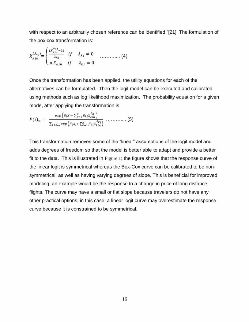
This transformation removes some of the “linear” assumptions of the logit model and

adds degrees of freedom so that the model is better able to adapt and provide a better

fit to the data. This is illustrated in Figure 1; the figure shows that the response curve of

the linear logit is symmetrical whereas the Box-Cox curve can be calibrated to be non-

symmetrical, as well as having varying degrees of slope. This is beneficial for improved

modeling; an example would be the response to a change in price of long distance

flights. The curve may have a small or flat slope because travelers do not have any

other practical options, in this case, a linear logit curve may overestimate the response

curve because it is constrained to be symmetrical.

17

Figure 1 - Comparison of Linear and Box- Cox Logit Response Curves [21]

18

Problem Description

The purpose of this research is to develop tools that can be integrated into the TSAM

model and used to analyze both current and projected future high-speed rail corridors.

The TSAM model uses 1995 as the base year so the updated model should be able to

accurately predict the train trips from the year 1995 forward. As well, many new high-

speed rail lines have been proposed and are in the planning stage. The TSAM model

needs to be able to accurately predict the intermediate/long range trips that will be taken

on the projected corridors. However the model will not be capable of making ridership

projections since TSAM only models “intercity trips”; an intercity trip is defined as a trip

that has a one-way route travel distance of 100 miles or greater.

The model needs to be able to calculate the travel times and travel costs of both the

current and future corridors. The time and cost values will be used to develop a new

calibration that will include train as a mode choice option. As well, a future work will

likely focus on developing a life-cycle cost analysis for high-speed passenger trains that

will be used to make more accurate travel cost predictions. Therefore the model also

needs to be able to determine the energy consumption associated with the trains

because this will be a large portion of the operating costs.

19

Methodology

Train Dynamics Model

Method

A Matlab script is developed for use in calculating travel time and energy consumption

calculations of current and future high-speed rail corridors. The primary calculation in

the script is the calculation of travel times between stations. The velocity profile is

calculated as either a two or three phase profile, depending on the input parameters.

Figure 2 below shows a sample of three phase profile, which includes an acceleration,

cruise and deceleration phase. Figure 3 shows a sample two phase profile, which

includes only the acceleration and deceleration phases. The inputs are the distance

between stations, the type of train to be modeled, maximum desired cruising speed,

deceleration rate, and the integration time step.

Figure 2 - Sample Three Phase Velocity Profile

0 500 1000 1500 2000 2500 3000 3500 4000 4500 50000

5

10

15

20

25

30

35

Distance Traveled (Meters)

Velo

city (

Mete

rs/S

econd)

Acceleration Phase

Cruise Phase

Deceleration Phase

20

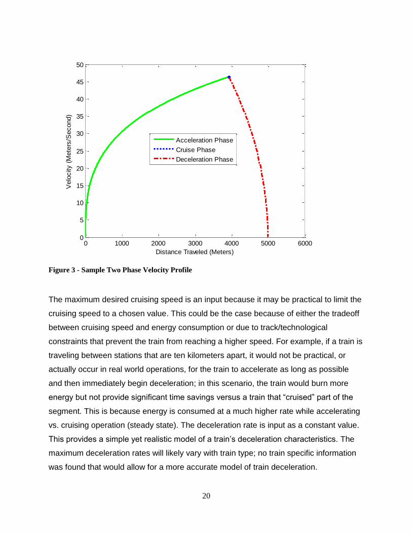
Figure 3 - Sample Two Phase Velocity Profile

The maximum desired cruising speed is an input because it may be practical to limit the

cruising speed to a chosen value. This could be the case because of either the tradeoff

between cruising speed and energy consumption or due to track/technological

constraints that prevent the train from reaching a higher speed. For example, if a train is

traveling between stations that are ten kilometers apart, it would not be practical, or

actually occur in real world operations, for the train to accelerate as long as possible

and then immediately begin deceleration; in this scenario, the train would burn more

energy but not provide significant time savings versus a train that “cruised” part of the

segment. This is because energy is consumed at a much higher rate while accelerating

vs. cruising operation (steady state). The deceleration rate is input as a constant value.

This provides a simple yet realistic model of a train’s deceleration characteristics. The

maximum deceleration rates will likely vary with train type; no train specific information

was found that would allow for a more accurate model of train deceleration.

0 1000 2000 3000 4000 5000 60000

5

10

15

20

25

30

35

40

45

50

Distance Traveled (Meters)

Velo

city (

Mete

rs/S

econd)

Acceleration Phase

Cruise Phase

Deceleration Phase

21

The integration time step is included as an input because the script uses a numerical

integration approach to calculate the velocity profile. This is chosen over a differential

equation method because the distance between stations and the input desired speed

will vary between different O-D pairs, thus an iterative process would be needed to

determine the profile. In the code, at each time step, three items are calculated; the

current speed of the train, total distance traveled, and the distance required for the train

to stop at its current speed. After these calculations, it is then verified that there is ample

distance for the train to be able to stop at the next station. This works by taking the

cumulative distance traveled by the train, at the given time step, and the distance

required for the train to stop at that time step, based on the current velocity of the train,

and ensuring that the sum of the two distances is less than the distance between

stations.

Essentially, the code ensures that the train will be able to accelerate and a come to a

stop at the next train station. For example, if the distance between stations is 5

kilometers and the maximum desired cruising speed is set to 75 m/s, the train cannot

reach 75 m/s and come to a stop in 5 kilometers. Therefore within the code, the train

accelerates as long as possible and then decelerates, while still ensuring that is can

come to a stop at the next station. This example, which is a two-phase profile, is seen in

Figure 3.

Model Equations

The code utilizes Newton’s second law of motion, . This fundamental equation

is used to calculate the acceleration of the vehicle at each time step. The mass is

dependent upon the type and length of train that is modeled, which will be discussed

later. The tractive effort is calculated as:

(

) ……….... (6)

Where:

( )

( )

( )

22

(

)

The tractive effort calculation uses the minimum of the calculated function value and

1,000,000 Newtons because the function approaches infinity as the velocity gets close

to 0. Although the actual tractive effort would be finite, the minimum function ensures

that the equation can be used for modeling ant that at low speeds, the tractive effort is

small enough so that the wheels should not slip.

The resistive forces acting on the train, rolling resistance, aerodynamic resistance, etc.

are calculated with the use of the Davis Equation. The Davis Equation integrates all of

the resistive forces into one equation, which is a function of velocity. The formula that is

used for the modeled Japanese Shinkansen trains is:

……….... (7)

Where:

( )

( )

(

)

(

)

(

) Source: [22]

“Coefficients A and B of the Davis Equation include the mechanical resistances and are

thus mass related. … At higher speeds, the CV2 term becomes dominant since it can

be said to relate to the aerodynamic resistance.”[22] Table 1 shows the major resistance

contributors to each of the three coefficients. A more detailed description and

illustration of some of the different forces listed in Table 1 can be found in another

work.[23]

23

Table 1 - Forces Contributing to the Coefficients of the Davis Equation [24]

A B C

Journal Resistance Flange Friction Head-end Wind Pressure

Rolling Resistance Flange Impact Skin Friction on Side of Train

Track Resistance Rolling Resistance – Wheel/Rail Rear Drag

Wave Action of the Rail Turbulence Between Cars

Yaw Angle of Wind Tunnels

The equation is useful for modeling purposes because it allows the resistance of

different train types to be calculated easily by simply inputting three train specific

coefficients. The Davis Equation is a commonly used equation thus the coefficients for

different train types are typically available.

The TGV trains are modeled with a modified version of the Davis Equation. The

coefficients are calculated as functions of the rolling stock characteristics.[22] The

parameters are calculated using the following formulas:

* (√

)+ ……….... (8)

( ) assumes good quality track, modern rolling stock on bogies

with roller bearings ……….... (9)

[ ( ) (

)] ……….... (10)

Where:

( )

( )

,

( )

( ),

( )

24

( )

Train Types

The code models four different types of high-speed trains; the Japanese Shinkansen

Series 100, Japanese Shinkansen Series 200, French TGV-R, and the French TGV-D.

The train characteristics and coefficients for the Shinkansen Trains can be seen in Table

2 and the information for the TGV Trains is located in Table 3. The source of coefficients

for both train types is [22].

Table 2 - Model Coefficients for Shinkansen Trains

Shinkansen Trains

Parameters Series 100 Series 200

Train Characteristics Mass (kg) 886,000 712,000

Capacity 1,285 720

Tractive Coefficients Power (horsepower) 15,900 15,900

Engine Efficiency Factor 0.75 0.75

Resistive Coefficients

A (Newtons) 11060 8202

B (

) 109.44 105.56

C (

) 15.6168 11.9322

25

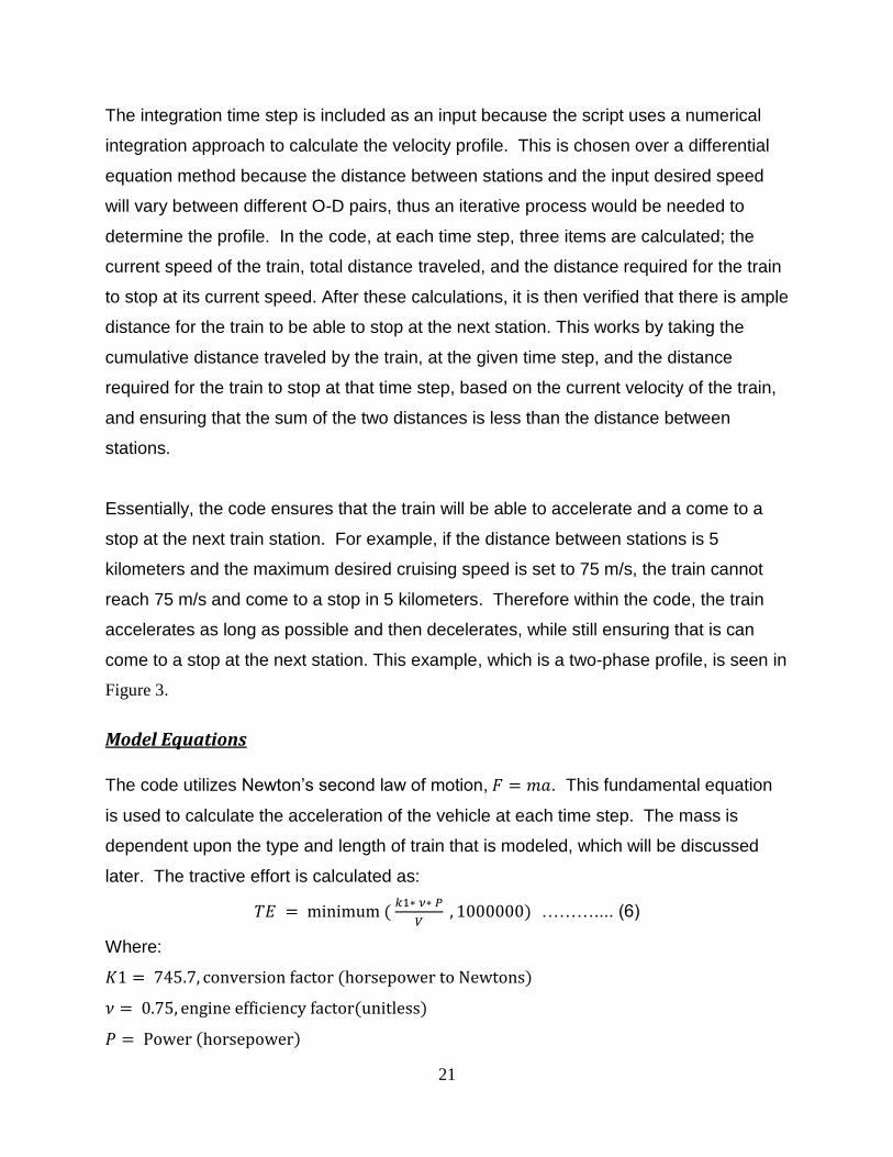
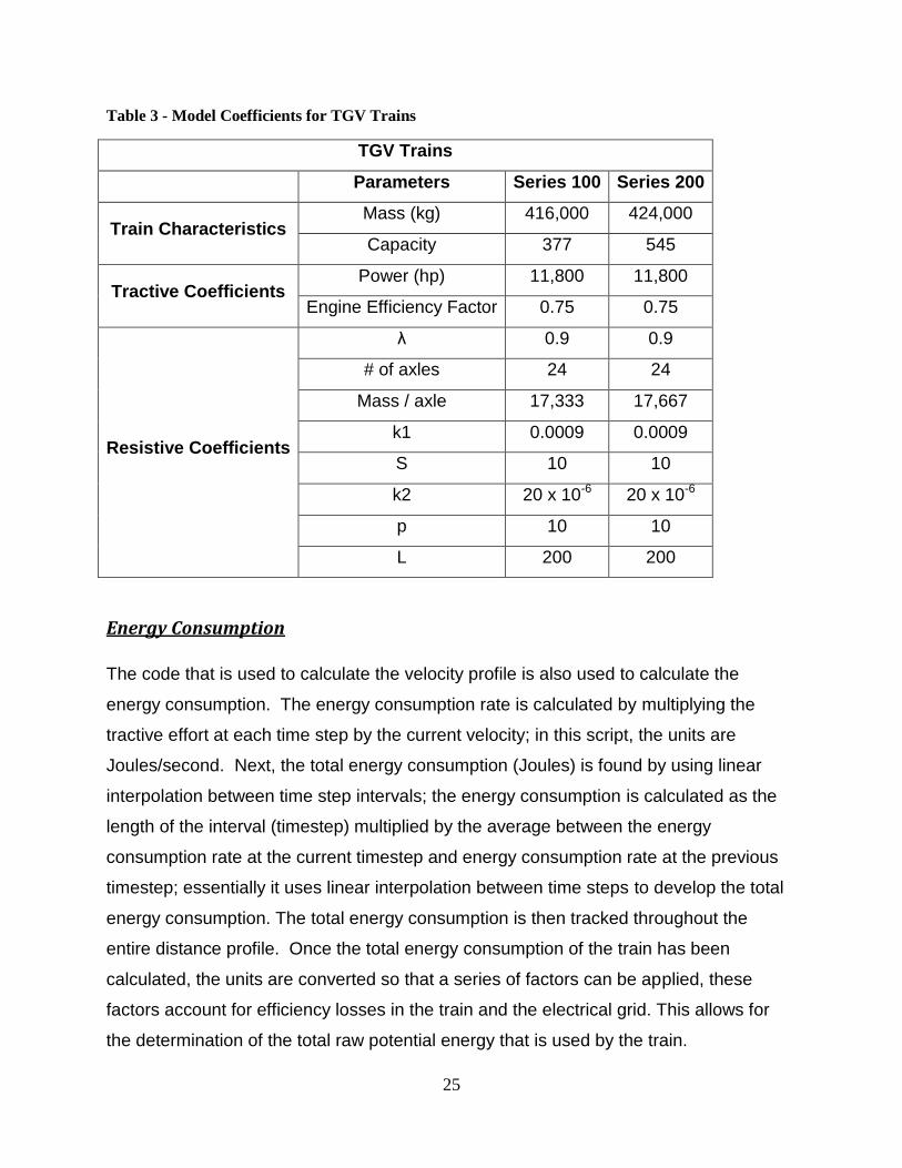
Table 3 - Model Coefficients for TGV Trains

TGV Trains

Parameters Series 100 Series 200

Train Characteristics Mass (kg) 416,000 424,000

Capacity 377 545

Tractive Coefficients Power (hp) 11,800 11,800

Engine Efficiency Factor 0.75 0.75

Resistive Coefficients

λ 0.9 0.9

# of axles 24 24

Mass / axle 17,333 17,667

k1 0.0009 0.0009

S 10 10

k2 20 x 10-6 20 x 10-6

p 10 10

L 200 200

Energy Consumption

The code that is used to calculate the velocity profile is also used to calculate the

energy consumption. The energy consumption rate is calculated by multiplying the

tractive effort at each time step by the current velocity; in this script, the units are

Joules/second. Next, the total energy consumption (Joules) is found by using linear

interpolation between time step intervals; the energy consumption is calculated as the

length of the interval (timestep) multiplied by the average between the energy

consumption rate at the current timestep and energy consumption rate at the previous

timestep; essentially it uses linear interpolation between time steps to develop the total

energy consumption. The total energy consumption is then tracked throughout the

entire distance profile. Once the total energy consumption of the train has been

calculated, the units are converted so that a series of factors can be applied, these

factors account for efficiency losses in the train and the electrical grid. This allows for

the determination of the total raw potential energy that is used by the train.

26

The first factor is an efficiency factor for the pantograph on the train. The pantograph is

the device on the top of the train that contacts the electrical wires and channels the

electricity to the engine. At the time of this research, no empirical measurements about

the energy loss in the pantograph could be found. Thus, it was assumed for the

calculations that the pantograph is 95% efficient.

The other factor is used to account for losses in the generation of electricity and its

transmission through the electrical grid. In order to make meaningful energy

consumption comparisons across different modes of travel, the total raw potential of

each mode must be measured. The loss factor is calculated by the National Renewable

Energy Laboratory and it accounts for transmission and distribution losses, as well as

pre-combustion effects, which includes extraction, processing and transportation of the

fuel source (coal, natural gas, etc.).[25] There are some important assumptions in the

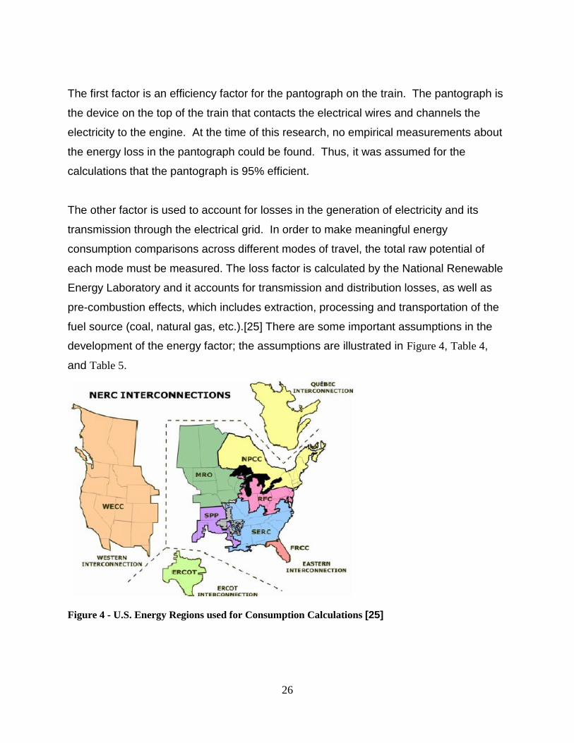
development of the energy factor; the assumptions are illustrated in Figure 4, Table 4,

and Table 5.

Figure 4 - U.S. Energy Regions used for Consumption Calculations [25]

27

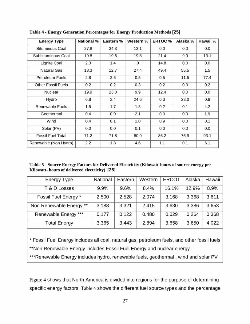
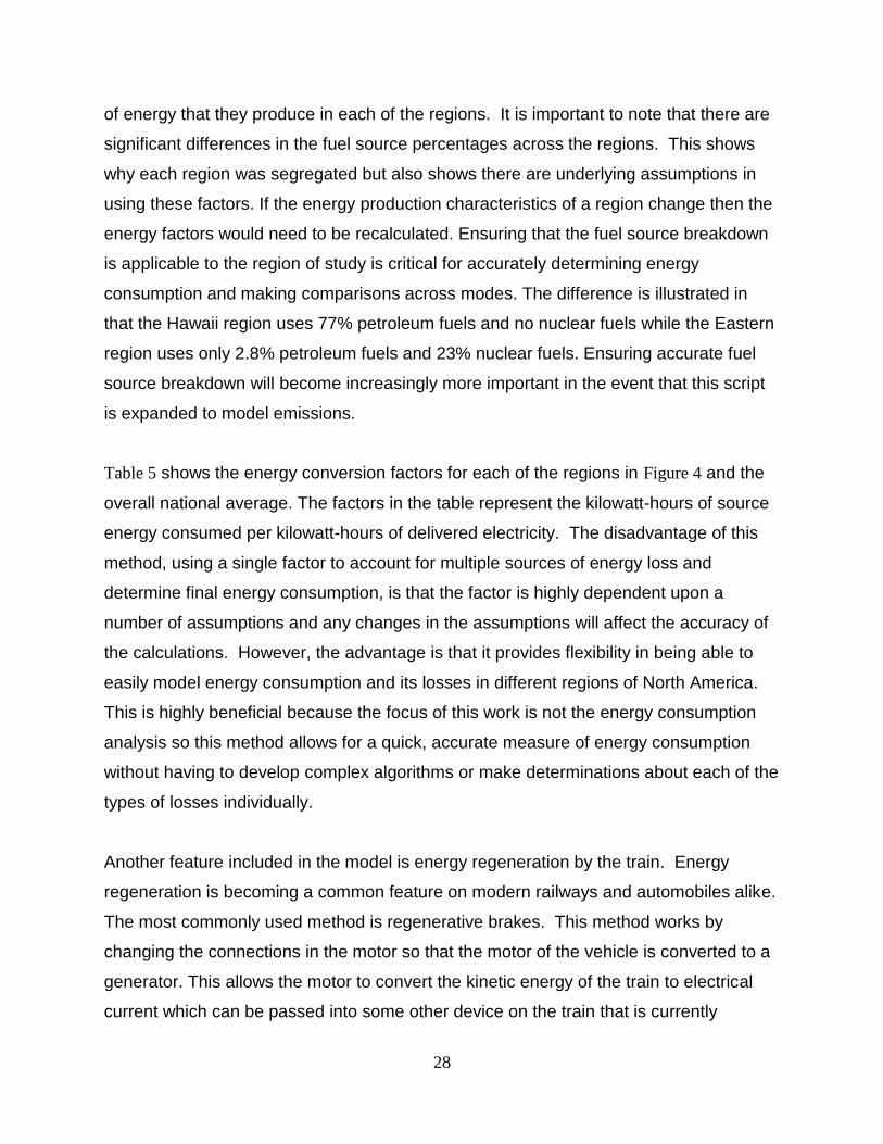
Table 4 - Energy Generation Percentages for Energy Production Methods [25]

Energy Type National % Eastern % Western % ERTOC % Alaska % Hawaii %

Bituminous Coal 27.8 34.3 13.1 0.0 0.0 0.0

Subbituminous Coal 19.8 19.6 19.8 21.4 9.9 13.1

Lignite Coal 2.3 1.4 0 14.8 0.0 0.0

Natural Gas 18.3 12.7 27.4 49.4 55.5 1.5

Petroleum Fuels 2.8 3.6 0.5 0.5 11.5 77.4

Other Fossil Fuels 0.2 0.2 0.3 0.2 0.0 0.2

Nuclear 19.9 23.0 9.9 12.4 0.0 0.0

Hydro 6.8 3.4 24.6 0.3 23.0 0.8

Renewable Fuels 1.5 1.7 1.3 0.2 0.1 4.2

Geothermal 0.4 0.0 2.1 0.0 0.0 1.9

Wind 0.4 0.1 1.0 0.9 0.0 0.1

Solar (PV) 0.0 0.0 0.1 0.0 0.0 0.0

Fossil Fuel Total 71.2 71.8 60.9 86.2 76.9 93.1

Renewable (Non Hydro) 2.2 1.8 4.6 1.1 0.1 6.1

Table 5 - Source Energy Factors for Delivered Electricity (Kilowatt-hours of source energy per

Kilowatt- hours of delivered electricity) [25]

Energy Type National Eastern Western ERCOT Alaska Hawaii

T & D Losses 9.9% 9.6% 8.4% 16.1% 12.9% 8.9%

Fossil Fuel Energy * 2.500 2.528 2.074 3.168 3.368 3.611

Non Renewable Energy ** 3.188 3.321 2.415 3.630 3.386 3.653

Renewable Energy *** 0.177 0.122 0.480 0.029 0.264 0.368

Total Energy 3.365 3.443 2.894 3.658 3.650 4.022

* Fossil Fuel Energy includes all coal, natural gas, petroleum fuels, and other fossil fuels

**Non Renewable Energy includes Fossil Fuel Energy and nuclear energy

***Renewable Energy includes hydro, renewable fuels, geothermal , wind and solar PV

Figure 4 shows that North America is divided into regions for the purpose of determining

specific energy factors. Table 4 shows the different fuel source types and the percentage

28

of energy that they produce in each of the regions. It is important to note that there are

significant differences in the fuel source percentages across the regions. This shows

why each region was segregated but also shows there are underlying assumptions in

using these factors. If the energy production characteristics of a region change then the

energy factors would need to be recalculated. Ensuring that the fuel source breakdown

is applicable to the region of study is critical for accurately determining energy

consumption and making comparisons across modes. The difference is illustrated in

that the Hawaii region uses 77% petroleum fuels and no nuclear fuels while the Eastern

region uses only 2.8% petroleum fuels and 23% nuclear fuels. Ensuring accurate fuel

source breakdown will become increasingly more important in the event that this script

is expanded to model emissions.

Table 5 shows the energy conversion factors for each of the regions in Figure 4 and the

overall national average. The factors in the table represent the kilowatt-hours of source

energy consumed per kilowatt-hours of delivered electricity. The disadvantage of this

method, using a single factor to account for multiple sources of energy loss and

determine final energy consumption, is that the factor is highly dependent upon a

number of assumptions and any changes in the assumptions will affect the accuracy of

the calculations. However, the advantage is that it provides flexibility in being able to

easily model energy consumption and its losses in different regions of North America.

This is highly beneficial because the focus of this work is not the energy consumption

analysis so this method allows for a quick, accurate measure of energy consumption

without having to develop complex algorithms or make determinations about each of the

types of losses individually.

Another feature included in the model is energy regeneration by the train. Energy

regeneration is becoming a common feature on modern railways and automobiles alike.

The most commonly used method is regenerative brakes. This method works by

changing the connections in the motor so that the motor of the vehicle is converted to a

generator. This allows the motor to convert the kinetic energy of the train to electrical

current which can be passed into some other device on the train that is currently

29

drawing power, some type of energy storage system (battery bank, compressed air

tank, flywheel, etc.) or the current can be fed back into the electrical grid, if the train is

connected to the grid and has the necessary equipment.

While regenerative braking does capture a portion of the energy consumed, it should be

noted that it is limited in its application. It is only able to capture a small portion of the

energy used to accelerate the vehicle and the vehicles still require the use of

mechanical brakes. Regenerative braking “force” is related to the speed of the vehicle

since the resistance of the motor (generator) is the braking force; at lower speeds, there

is less braking force therefore mechanical brakes are required to be able to bring the

vehicle to a stop. As well, in emergency situations, more braking force is needed than

the maximum force that can be supplied by the regenerative brake therefore the

regenerative brakes cannot be the only braking system installed.

At the time of this publication, only empirical studies on the amount of energy

regenerated by regenerative braking were found. No method of modeling energy

regeneration is available unless electrical grid modeling is also included in a model. The

studies vary but estimate that the percentage of energy regenerated varies between 5-

20% of the total energy consumed. However, these studies were mostly conducted on

electrical subways and smaller trains therefore the approximation may not directly

apply. As well, the studies do not provide any information about the speeds the

vehicles were traveling and the travel distance over which the analysis occurred. The

best measurement comes from an analysis of the Acela Express regenerative braking

system.[26] This work conducted field measurements on the Acela train and found that

the average energy recovery ratio was 7.65%. This work however does not provide the

travel speeds of the trains. Therefore, this model has conservatively assumes that 5%

of total energy consumption of the rail vehicle can be recaptured. This should be used

with caution because the energy regeneration occurs only during the braking phase

therefore this number can vary largely with the distance between stops. An example

would be a train that runs for 3 hours consecutively (between stops); this train is likely to

recover only a very small portion of the total energy consumed. This is because the

30

great majority of the energy consumed would be used during the cruise phase,

therefore only a small portion of the total energy could be recovered. Therefore, the

energy regeneration would need to be more thoroughly examined in order to make

detailed assessments or comparisons.

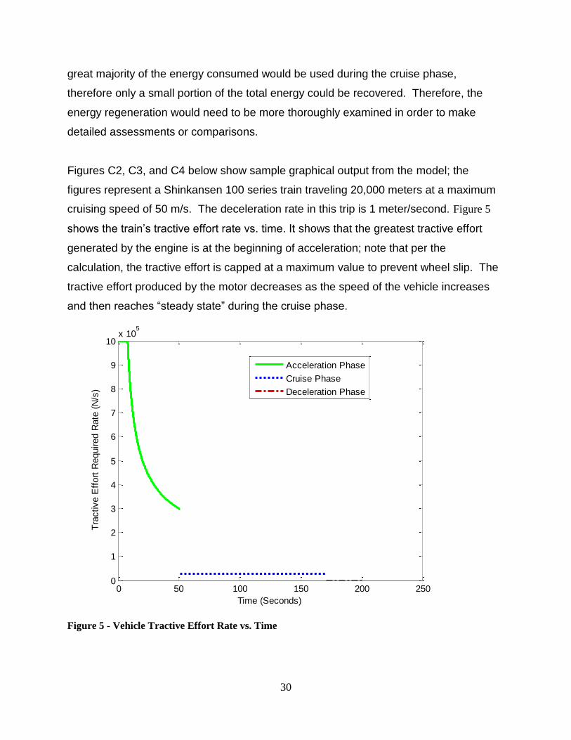
Figures C2, C3, and C4 below show sample graphical output from the model; the

figures represent a Shinkansen 100 series train traveling 20,000 meters at a maximum

cruising speed of 50 m/s. The deceleration rate in this trip is 1 meter/second. Figure 5

shows the train’s tractive effort rate vs. time. It shows that the greatest tractive effort

generated by the engine is at the beginning of acceleration; note that per the

calculation, the tractive effort is capped at a maximum value to prevent wheel slip. The

tractive effort produced by the motor decreases as the speed of the vehicle increases

and then reaches “steady state” during the cruise phase.

Figure 5 - Vehicle Tractive Effort Rate vs. Time

0 50 100 150 200 2500

1

2

3

4

5

6

7

8

9

10x 10

5

Time (Seconds)

Tra

ctive E

ffort

Required R

ate

(N

/s)

Acceleration Phase

Cruise Phase

Deceleration Phase

31

Figure 6 shows the train’s energy consumption rate vs. time. It should be noted that the

energy consumption rate is also greatest at the beginning of acceleration and that the

rate decreases slightly during the acceleration phase, although it is not visible in Figure

6. Once the vehicle reaches cruising speed, the energy consumption drops significantly

therefore showing the advantages in keeping a vehicle in steady state (cruise) mode as

much as possible. One important detail is that the energy created by regenerative

breaking is not modeled in Figure 6 because it is modeled as a percentage of total

energy consumed during acceleration and cruise. However, the regenerated energy is

shown in Figure 7.

Figure 7 shows the cumulative energy consumed by the train vs. time. It is important to

highlight that while the train spends most of the time in cruise mode, the majority of the

consumed energy is used during acceleration. Obviously, this will not always hold true,

particularly on long trips with no stops, however it does highlight the importance of trying

to reduce energy consumption by attempting to minimize stops and perhaps using a

lower cruise speed, particularly on short distance segments. In addition to the graphical

output, the numeric values of total travel time between stations, total energy consumed

by the train, total energy consumed per passenger (based on train capacity and load

factor), total raw potential energy consumed by the train, and the total raw potential

energy consumed per passenger.

32

Figure 6 - Vehicle Energy Consumption Rate vs. Time

Figure 7 - Vehicle Cumulative Energy Consumed vs. Time

0 50 100 150 200 2500

1

2

3

4

5

6

7

8

9x 10

6

Time (Seconds)

Energ

y C

onsum

ption R

ate

(Joule

s/S

econd)

Acceleration Phase

Cruise Phase

Deceleration Phase

0 50 100 150 200 2500

1

2

3

4

5

6x 10

8

Time (Seconds)

Cum

ula

tive E

nerg

y C

onsum

ed (

Joule

s)

Acceleration Phase

Cruise Phase

Deceleration Phase

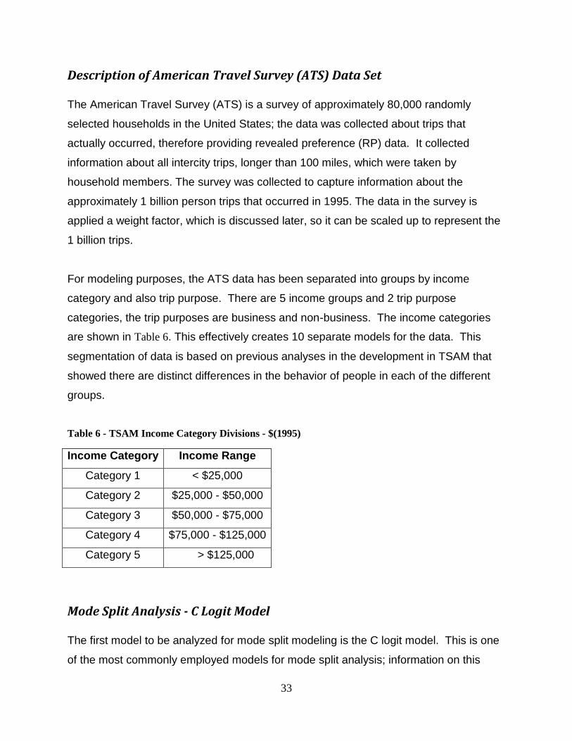
33

Description of American Travel Survey (ATS) Data Set

The American Travel Survey (ATS) is a survey of approximately 80,000 randomly

selected households in the United States; the data was collected about trips that

actually occurred, therefore providing revealed preference (RP) data. It collected

information about all intercity trips, longer than 100 miles, which were taken by

household members. The survey was collected to capture information about the

approximately 1 billion person trips that occurred in 1995. The data in the survey is

applied a weight factor, which is discussed later, so it can be scaled up to represent the

1 billion trips.

For modeling purposes, the ATS data has been separated into groups by income

category and also trip purpose. There are 5 income groups and 2 trip purpose

categories, the trip purposes are business and non-business. The income categories

are shown in Table 6. This effectively creates 10 separate models for the data. This

segmentation of data is based on previous analyses in the development in TSAM that

showed there are distinct differences in the behavior of people in each of the different

groups.

Table 6 - TSAM Income Category Divisions - $(1995)

Income Category Income Range

Category 1 < $25,000

Category 2 $25,000 - $50,000

Category 3 $50,000 - $75,000

Category 4 $75,000 - $125,000

Category 5 > $125,000

Mode Split Analysis - C Logit Model

The first model to be analyzed for mode split modeling is the C logit model. This is one

of the most commonly employed models for mode split analysis; information on this

34

model is widely available. The model utilizes a utility function that uses data about a

specific mode as well as socioeconomic data about the users to capture the benefit that

the user obtains from the mode. The probability of choosing a given mode is calculated

as:

( )

∑

……….... (11)

( )

For this first attempt to calibrate a C logit model, only data for automobile and

commercial air is used, thus since there are only two modes available, the mode with a

probability greater than 0.5 is the mode that the model “chooses” for the corresponding

trip. The model is calibrated by using the log likelihood maximization. Log likelihood

maximization is a commonly used statistical technique that is used to determine the

best statistical fit to the data. Information about log likelihood maximization is widely

available, more information could be found in a choice theory modeling textbook or the

internet.

The C-logit model calibrations that follow have been executed using the program “Mixed

Logit Estimation for Cross-Sectional Data using Maximum Simulated Likelihood” written

by Kenneth E. Train. This code is publicly available at the website

http://elsa.berkeley.edu/~train/software.html.[27] The code has been set up to run as a

standard fixed coefficient logit model. The code is executed in the software Gauss,

Version 9.0. The first model is calibrated using the ATS data, only automobile and air

transportation modes. The utility functions of this initial model are:

……….... (12)

……….... (13)

The number of observations for each of the 10 different categories is listed in Table 7. It

should be noted that for the Business Groups, any trip over 700 miles one way has

been filtered out of the analysis; this is because there are few data points in the longer

35

range trips and thus the distribution becomes inconsistent and unreliable. The

calibration is conducted using both weighted and un-weighted data. The results of these

calibrations are shown in Table 8 and Table 9.

Table 7 - Number of ATS Observations in Each Trip Purpose / Income Group Category

Trip Purpose/ Income Category # of Data Points

Business 1 8663

Business 2 27868

Business 3 20919

Business 4 12135

Business 5 3336

Non Business 1 40736

Non Business 2 84178

Non Business 3 51347

Non Business 4 24217

Non Business 5 18072

C- Logit Model - Comparison of Weighted vs. Un-weighted Data: Table 8 - Summary of Coefficients for Un-Weighted ATS Data

Travel Time

Travel Cost

TT Std. Error

TC Std. Error

Ratio TT/TC Correct

Prediction (%)

Business 1 -0.02657 -0.00902 0.00392 0.00209 2.94524 92.27

Business 2 -0.03692 -0.00861 0.00264 0.00013 4.28838 91.86

Business 3 -0.05406 -0.00585 0.00231 0.00009 9.24248 84.22

Business 4 -0.07446 -0.00571 0.00318 -0.00571 13.04691 85.09

Business 5 -0.10249 -0.00226 0.00608 0.00206 45.28120 80.88

Non-Business 1 -0.04332 -0.00978 0.00118 0.00008 4.43198 92.20

Non-Business 2 -0.04955 -0.01053 0.00081 0.00006 4.70408 93.10

Non-Business 3 -0.05038 -0.00970 0.00106 0.00007 5.19496 91.29

Non-Business 4 -0.06011 -0.00922 0.00180 0.00010 6.51934 90.72

Non-Business 5 -0.07029 -0.00746 0.00423 0.00017 9.41740 88.08

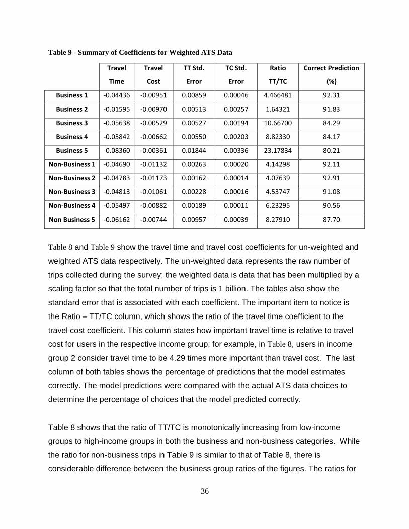
36

Table 9 - Summary of Coefficients for Weighted ATS Data

Travel

Time

Travel

Cost

TT Std.

Error

TC Std.

Error

Ratio

TT/TC

Correct Prediction

(%)

Business 1 -0.04436 -0.00951 0.00859 0.00046 4.466481 92.31

Business 2 -0.01595 -0.00970 0.00513 0.00257 1.64321 91.83

Business 3 -0.05638 -0.00529 0.00527 0.00194 10.66700 84.29

Business 4 -0.05842 -0.00662 0.00550 0.00203 8.82330 84.17

Business 5 -0.08360 -0.00361 0.01844 0.00336 23.17834 80.21

Non-Business 1 -0.04690 -0.01132 0.00263 0.00020 4.14298 92.11

Non-Business 2 -0.04783 -0.01173 0.00162 0.00014 4.07639 92.91

Non-Business 3 -0.04813 -0.01061 0.00228 0.00016 4.53747 91.08

Non-Business 4 -0.05497 -0.00882 0.00189 0.00011 6.23295 90.56

Non Business 5 -0.06162 -0.00744 0.00957 0.00039 8.27910 87.70

Table 8 and Table 9 show the travel time and travel cost coefficients for un-weighted and

weighted ATS data respectively. The un-weighted data represents the raw number of

trips collected during the survey; the weighted data is data that has been multiplied by a

scaling factor so that the total number of trips is 1 billion. The tables also show the

standard error that is associated with each coefficient. The important item to notice is

the Ratio – TT/TC column, which shows the ratio of the travel time coefficient to the

travel cost coefficient. This column states how important travel time is relative to travel

cost for users in the respective income group; for example, in Table 8, users in income

group 2 consider travel time to be 4.29 times more important than travel cost. The last

column of both tables shows the percentage of predictions that the model estimates

correctly. The model predictions were compared with the actual ATS data choices to

determine the percentage of choices that the model predicted correctly.

Table 8 shows that the ratio of TT/TC is monotonically increasing from low-income

groups to high-income groups in both the business and non-business categories. While

the ratio for non-business trips in Table 9 is similar to that of Table 8, there is

considerable difference between the business group ratios of the figures. The ratios for

37

the business group - weighted data are no longer monotonically increasing, and they

have changed significantly from their counterparts in the un-weighed data. This

indicates one of the shortcomings of the ATS data; the method that was used to

determine weighting factors. It is known intuitively and from multiple studies that users

in higher income groups value travel time more than travel cost relative to lower income

groups; this is because they tend to have more discretionary income and are able to

pay additional costs for a travel time benefit. The weighted coefficient values contradict

this fact by implying that users in income group 1 value time more than users in group 2.

Improvement of C- Logit Coefficient Optimization

In the preceding tables, Table 8 and Table 9, the model was calibrated using all of the

ATS data and then the percentage of correct predictions was determined. The correct

predictions in that case is somewhat biased because the model has already been

calibrated against the data. In an effort to add validity to the model, the calibration is

improved by randomly selecting approximately 2/3 of the data for calibration and the

remaining data for the validation. This will allow analysis on data that the model is not

calibrated against, thus providing a more realistic measure of how well the model can

predict trips. The randomization of the data is accomplished by entering the data in

Excel and assigning a random number between 0 and 1 to each data point, then any

data with a random number less than 0.65 is used for calibration and any above 0.65 is

used for validation. Table 10 and Table 11 below summarize the results.

Table 10 - Summary of Coefficients for Random Portion of Un-Weighted Data

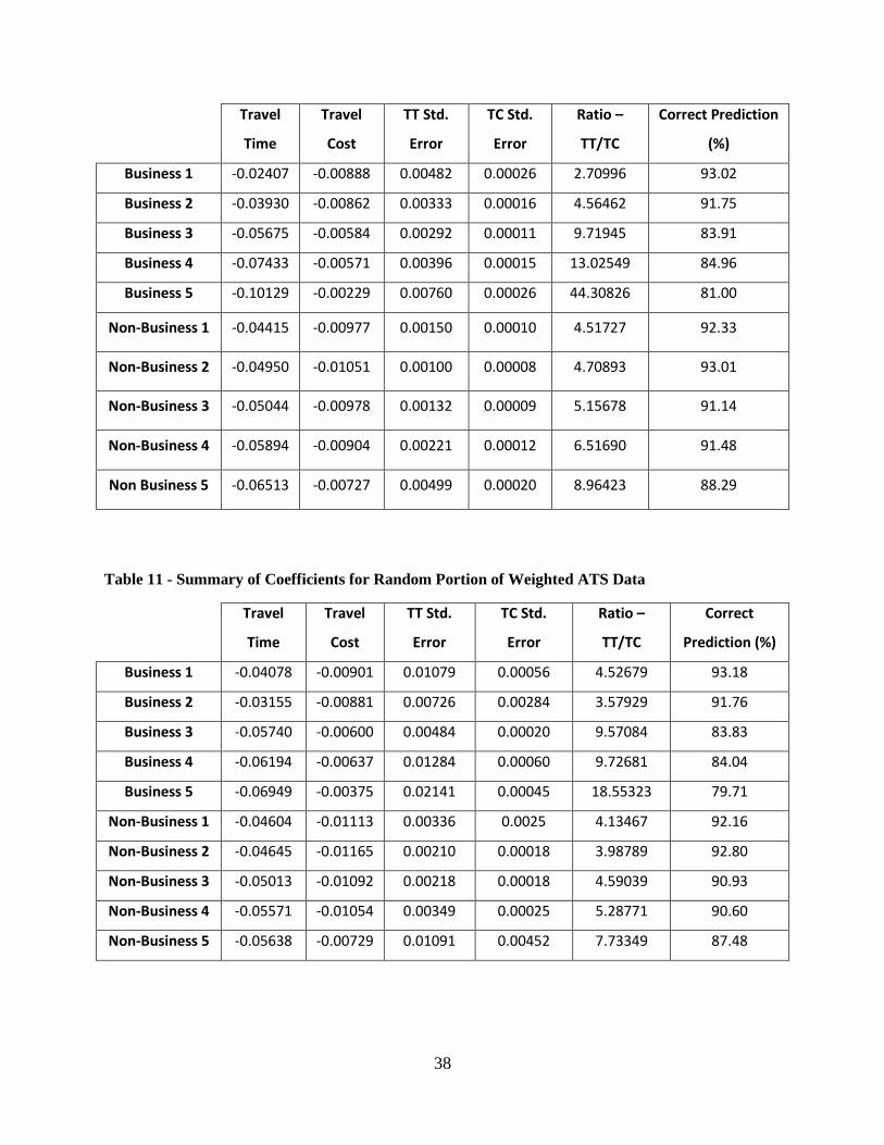
38

Travel

Time

Travel

Cost

TT Std.

Error

TC Std.

Error

Ratio –

TT/TC

Correct Prediction

(%)

Business 1 -0.02407 -0.00888 0.00482 0.00026 2.70996 93.02

Business 2 -0.03930 -0.00862 0.00333 0.00016 4.56462 91.75

Business 3 -0.05675 -0.00584 0.00292 0.00011 9.71945 83.91

Business 4 -0.07433 -0.00571 0.00396 0.00015 13.02549 84.96

Business 5 -0.10129 -0.00229 0.00760 0.00026 44.30826 81.00

Non-Business 1 -0.04415 -0.00977 0.00150 0.00010 4.51727 92.33

Non-Business 2 -0.04950 -0.01051 0.00100 0.00008 4.70893 93.01

Non-Business 3 -0.05044 -0.00978 0.00132 0.00009 5.15678 91.14

Non-Business 4 -0.05894 -0.00904 0.00221 0.00012 6.51690 91.48

Non Business 5 -0.06513 -0.00727 0.00499 0.00020 8.96423 88.29

Table 11 - Summary of Coefficients for Random Portion of Weighted ATS Data

Travel

Time

Travel

Cost

TT Std.

Error

TC Std.

Error

Ratio –

TT/TC

Correct

Prediction (%)

Business 1 -0.04078 -0.00901 0.01079 0.00056 4.52679 93.18

Business 2 -0.03155 -0.00881 0.00726 0.00284 3.57929 91.76

Business 3 -0.05740 -0.00600 0.00484 0.00020 9.57084 83.83

Business 4 -0.06194 -0.00637 0.01284 0.00060 9.72681 84.04

Business 5 -0.06949 -0.00375 0.02141 0.00045 18.55323 79.71

Non-Business 1 -0.04604 -0.01113 0.00336 0.0025 4.13467 92.16

Non-Business 2 -0.04645 -0.01165 0.00210 0.00018 3.98789 92.80

Non-Business 3 -0.05013 -0.01092 0.00218 0.00018 4.59039 90.93

Non-Business 4 -0.05571 -0.01054 0.00349 0.00025 5.28771 90.60

Non-Business 5 -0.05638 -0.00729 0.01091 0.00452 7.73349 87.48

39

Table 10 and Table 11 show that the coefficients for each income/trip purpose group, as

well as the travel time/travel cost ratios, did not change significantly because of the use

of the random portion of data for validation approach. The important result is that the

new model still predicts the mode choice well; the correct prediction percentages of the

new model are similar to those from the previous calibration. This adds validity because

the new model, using “unseen” data, is able to predict equally as well as the original

model, which was calibrated against all of the data. The travel time/travel cost ratios of

the business group for the weighted data have improved; they are closer to

monotonically increasing but they still do not match expectations or the previous model.

This is likely due to the ATS weight factors which are discussed below.

Skepticism of ATS Weight Factors

Again the ATS data was collected in 1995 and recorded data for 550,000 intercity trips

that were taken in the U.S. The weighting factors were applied so that the data set

could be scaled up to the estimated 1 billion intercity trips that occurred that year. The

weighting factors are assigned by dividing the data into groups based on multiple

socioeconomic factors of the surveyed user and then determining how many

people/households in the U.S. had similar characteristics. It is assumed that everyone

within each socioeconomic group will make travel decisions in a similar manner; based

on surveyed users in the socioeconomic group. However, in the ATS data, not all

origin-destination pairs had numerous observations; some pairs had only one

observation. Thus, when these data points receive their weight, a small number of

choices has a large effect on the model, and if the user made a choice that is not

necessarily in line with their income group/ trip purpose/length etc., then this data will

greatly skew the results.

For example, there is only 1 record for travel from Nashville to Atlanta. The surveyed

user chose to drive for this trip, despite the fact that most travelers chose to fly this trip,

so the result is that when the weight factor is applied, the model determines that the

majority of users drive between this origin-destination pair when in actuality, it is the

opposite. This is what causes the irregularities in the coefficients of the weighed data.

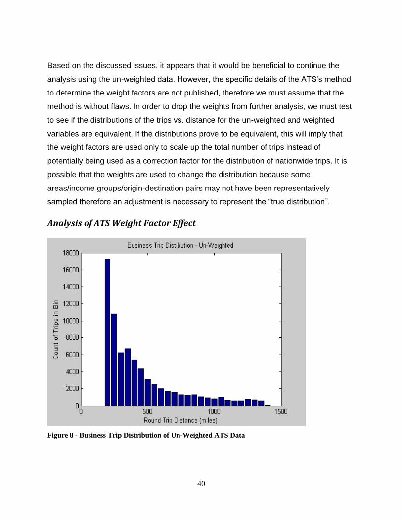
40

Based on the discussed issues, it appears that it would be beneficial to continue the

analysis using the un-weighted data. However, the specific details of the ATS’s method

to determine the weight factors are not published, therefore we must assume that the

method is without flaws. In order to drop the weights from further analysis, we must test

to see if the distributions of the trips vs. distance for the un-weighted and weighted

variables are equivalent. If the distributions prove to be equivalent, this will imply that

the weight factors are used only to scale up the total number of trips instead of

potentially being used as a correction factor for the distribution of nationwide trips. It is

possible that the weights are used to change the distribution because some

areas/income groups/origin-destination pairs may not have been representatively

sampled therefore an adjustment is necessary to represent the “true distribution”.

Analysis of ATS Weight Factor Effect

Figure 8 - Business Trip Distribution of Un-Weighted ATS Data

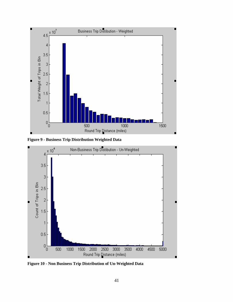
41

Figure 9 - Business Trip Distribution Weighted Data

Figure 10 - Non Business Trip Distribution of Un-Weighted Data

42

Figure 11 - Non Business Trip Distribution of Weighted Data

A visual comparison of Figure 8 vs. Figure 9 and Figure 10 vs. Figure 11 seems to indicate

that the distribution of trips in unchanged by applying the ATS weight factor. The

figures shown above are generated by binning data in 50 mile intervals. Note that trips

in the Business data group that exceeded 700 miles one way were filtered out due to

scarcity of data points for long-range trips.

Two different tests, Chi Square and Kolmogorov-Smirnov, are shown below to test the

hypothesis that the distributions are equivalent. The Chi Square test is executed first;

the formulation for the test is:

∑( )

……….... (14)

where:

43

( )

If the is greater than the critical value, which can be found by using the degrees of

freedom, desired confidence, and a widely available Chi Square table, then you reject

the null hypothesis.

In this case, the null hypothesis is: Ho: Un-weighted Distribution = Weighted Distribution

and H1: Un-weighted Distribution ≠ Weighted Distribution. For this test, the values of the

weighted distribution are treated as the expected value and the un-weighted values are

the observed frequency. The degrees of freedom are calculated as the number of bins -

1. The results for the business and non-business group tests are:

Business Test:

X2 = 560.1

Critical X2 = 36.4 (degrees of freedom = 24; assuming 95% confidence (α=0.05))

560.1 > 36.4 thus reject Ho

Non Business Test:

X2 = 2154.4

Critical X2 = 124 (degrees of freedom = 96; assuming 95% confidence (α=0.05))

2154.4 > 124 thus reject Ho

The results show that for both comparisons, the samples are not from the same

distribution, which would prevent the dropping of the weight factors. In order to validate

the results, the two sample Kolmogorov-Smirnov test was calculated. The two sample

Kolmogorov-Smirnov test is a non-parametric test that can be used to determine if two

samples have the same distribution. The advantage of this test is it is non-parametric;

this implies that the distribution type is not specified by the test. The formulation of the

test is:

44

| ( ) ( )| ……….... (15)

F1,n and F2,n’ are the empirical distribution functions of the sample.

The Null Hypothesis is rejected at level α if:

√

……….... (16)

The critical Kα can be calculated as:

( )√

……….... (17)

Where:

Table 12 - Parameters for Kolmogorov-Smirnov Test

α 0.1 0.05 0.025 0.01 0.005 0.001

c(α) 1.22 1.36 1.48 1.63 1.75 1.95

In Table 12, represents the confidence level. More information about the data in Table

12 is available at www.soest.hawaii.edu/wessel/courses/gg313/Critical_KS.pdf.[28] The

test results for each group are:

Business Test:

Test Value = 6.4526

Critical Value= 0.0050

6.4526 > 0.0050 thus reject Ho

Non Business Test:

Test Value = 13.13

Critical Value = 0.0029

13.13 > 0.0029 thus reject Ho

45

The results of both the business and non-business tests show that the distributions are

not the same in either case. This validates the results of the Chi Square test and

determines that the distribution is statistically different by applying the weight factor.

Therefore the weighting factors will continue to be applied in the model.

Model Comparison Metric

The results of the statistical tests prove the original hypothesis, which states that the

distributions are the same, is false. Based on the results, all analyses will use the weight

factors. As well, direct comparison of the two models shows that they perform similarly.

This comparison is accomplished with the % Correct metric; the calibrations are

optimized using log likelihood values but log likelihood is not easy to interpret and

generally does not allow for comparisons across models, therefore the % Correct metric

is developed in order to provide an easily interpretable comparison metric. In the initial

model, since there are only two alternatives, it is assumed that the alternative with the

highest probability is the one that is “predicted” by the model. This prediction is then

compared to the actual choice that the user made. Then the percentage of the total

trips that are predicted correctly are calculated and used as the metric. This method is

not the most precise, however it provides a quick, easy way to compare the different

models.

46

Table 13 - Comparison of Un-Weighted vs. Weighted Model Predictions

% Correct (Un-weighted) % Correct (Weighted)

Business 1 93.7 93.8

Business 2 92.1 91.2

Business 3 85.7 83.5

Business 4 85.0 82.1

Business 5 79.8 83.7

Non-Business 1 91.9 92.8

Non-Business 2 93.1 93.1

Non-Business 3 91.5 92.0

Non-Business 4 88.5 89.1

Non-Business 5 85.1 86.2

Table 13 shows the percentage of correct predictions for the weighted and un-weighted

models for each of the 10 different categories. It is shown that there is not a significant

difference in how the percentage of correct predictions changes, in most cases the

weighted model predicts more trips correctly than the un-weighted. So, although it has

been shown that there are some flaws with the ATS weight factors, we will continue to

use them for the remaining analysis.

C- Logit Model - Utility Function Variation

In a search to try to achieve a better overall fit from the model, it is postulated that

breaking the total travel time into in-vehicle time and out-of-vehicle time will improve the

model. The theory is that a traveler may perceive out of vehicle time or “idle” time more

negatively than in-vehicle time. If true, then for example, if a traveler faces a choice

between using a private automobile or a bus system to take a trip, with both modes

having equal travel time, the traveler will be more likely to choose the automobile

because there will not as much out-of-vehicle time (transfer time, time waiting on bus to

arrive, security processing time, etc.). This example is assuming that the mode choice

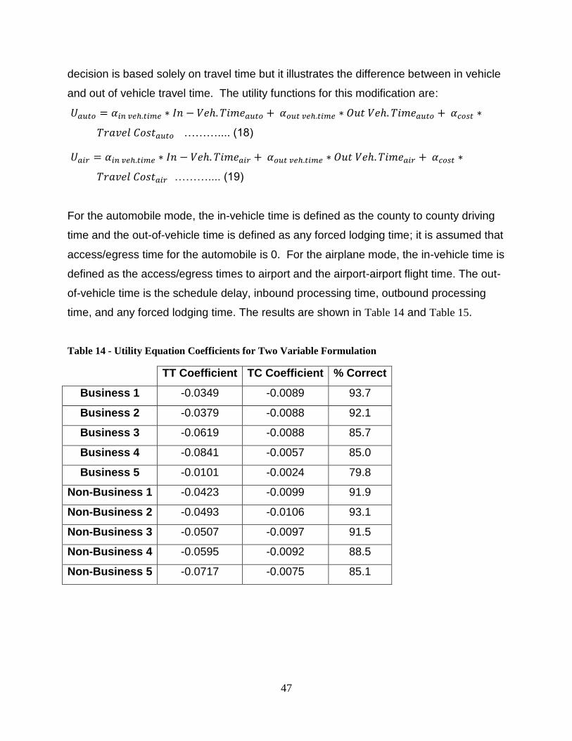
47

decision is based solely on travel time but it illustrates the difference between in vehicle

and out of vehicle travel time. The utility functions for this modification are:

……….... (18)

……….... (19)

For the automobile mode, the in-vehicle time is defined as the county to county driving

time and the out-of-vehicle time is defined as any forced lodging time; it is assumed that

access/egress time for the automobile is 0. For the airplane mode, the in-vehicle time is

defined as the access/egress times to airport and the airport-airport flight time. The out-

of-vehicle time is the schedule delay, inbound processing time, outbound processing

time, and any forced lodging time. The results are shown in Table 14 and Table 15.

Table 14 - Utility Equation Coefficients for Two Variable Formulation

TT Coefficient TC Coefficient % Correct

Business 1 -0.0349 -0.0089 93.7

Business 2 -0.0379 -0.0088 92.1

Business 3 -0.0619 -0.0088 85.7

Business 4 -0.0841 -0.0057 85.0

Business 5 -0.0101 -0.0024 79.8

Non-Business 1 -0.0423 -0.0099 91.9

Non-Business 2 -0.0493 -0.0106 93.1

Non-Business 3 -0.0507 -0.0097 91.5

Non-Business 4 -0.0595 -0.0092 88.5

Non-Business 5 -0.0717 -0.0075 85.1

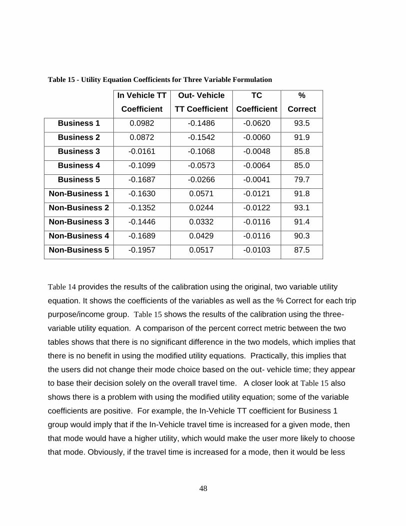
48

Table 15 - Utility Equation Coefficients for Three Variable Formulation

In Vehicle TT

Coefficient

Out- Vehicle

TT Coefficient

TC

Coefficient

%

Correct

Business 1 0.0982 -0.1486 -0.0620 93.5

Business 2 0.0872 -0.1542 -0.0060 91.9

Business 3 -0.0161 -0.1068 -0.0048 85.8

Business 4 -0.1099 -0.0573 -0.0064 85.0

Business 5 -0.1687 -0.0266 -0.0041 79.7

Non-Business 1 -0.1630 0.0571 -0.0121 91.8

Non-Business 2 -0.1352 0.0244 -0.0122 93.1

Non-Business 3 -0.1446 0.0332 -0.0116 91.4

Non-Business 4 -0.1689 0.0429 -0.0116 90.3

Non-Business 5 -0.1957 0.0517 -0.0103 87.5

Table 14 provides the results of the calibration using the original, two variable utility

equation. It shows the coefficients of the variables as well as the % Correct for each trip

purpose/income group. Table 15 shows the results of the calibration using the three-

variable utility equation. A comparison of the percent correct metric between the two

tables shows that there is no significant difference in the two models, which implies that

there is no benefit in using the modified utility equations. Practically, this implies that

the users did not change their mode choice based on the out- vehicle time; they appear

to base their decision solely on the overall travel time. A closer look at Table 15 also

shows there is a problem with using the modified utility equation; some of the variable

coefficients are positive. For example, the In-Vehicle TT coefficient for Business 1

group would imply that if the In-Vehicle travel time is increased for a given mode, then

that mode would have a higher utility, which would make the user more likely to choose

that mode. Obviously, if the travel time is increased for a mode, then it would be less

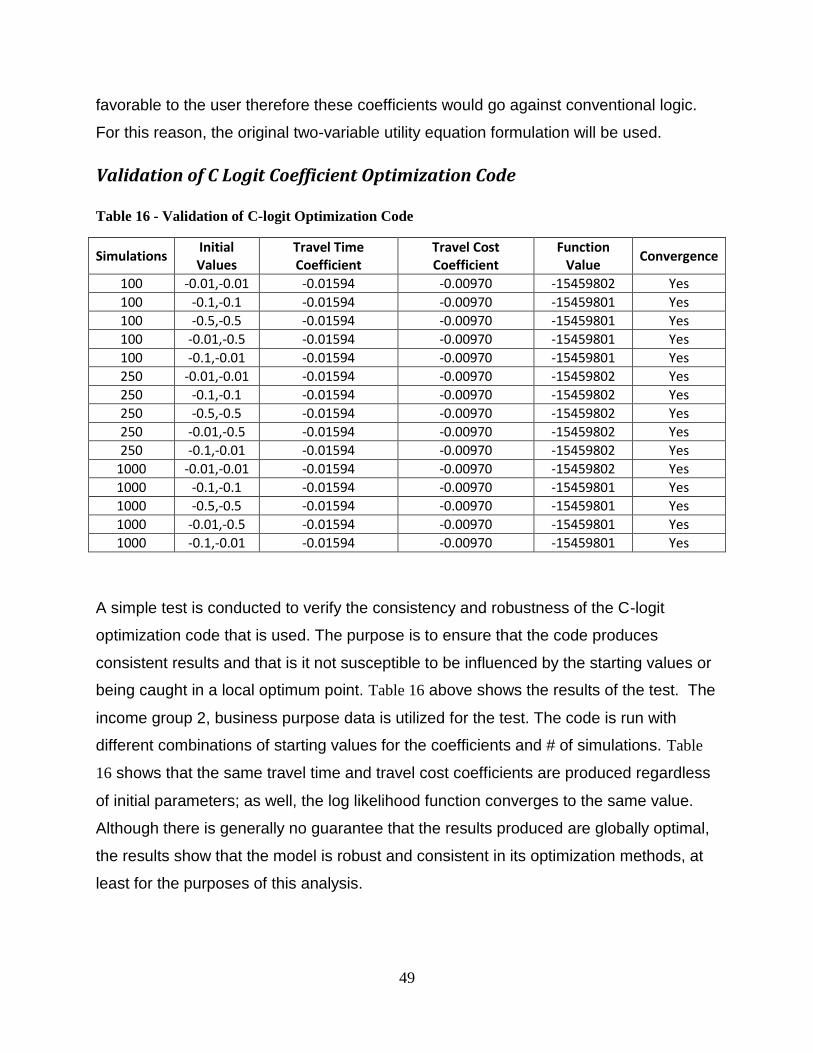
49

favorable to the user therefore these coefficients would go against conventional logic.

For this reason, the original two-variable utility equation formulation will be used.

Validation of C Logit Coefficient Optimization Code Table 16 - Validation of C-logit Optimization Code

Simulations Initial Values

Travel Time Coefficient

Travel Cost Coefficient

Function Value

Convergence

100 -0.01,-0.01 -0.01594 -0.00970 -15459802 Yes

100 -0.1,-0.1 -0.01594 -0.00970 -15459801 Yes

100 -0.5,-0.5 -0.01594 -0.00970 -15459801 Yes

100 -0.01,-0.5 -0.01594 -0.00970 -15459801 Yes

100 -0.1,-0.01 -0.01594 -0.00970 -15459801 Yes

250 -0.01,-0.01 -0.01594 -0.00970 -15459802 Yes

250 -0.1,-0.1 -0.01594 -0.00970 -15459802 Yes

250 -0.5,-0.5 -0.01594 -0.00970 -15459802 Yes

250 -0.01,-0.5 -0.01594 -0.00970 -15459802 Yes

250 -0.1,-0.01 -0.01594 -0.00970 -15459802 Yes

1000 -0.01,-0.01 -0.01594 -0.00970 -15459802 Yes

1000 -0.1,-0.1 -0.01594 -0.00970 -15459801 Yes

1000 -0.5,-0.5 -0.01594 -0.00970 -15459801 Yes

1000 -0.01,-0.5 -0.01594 -0.00970 -15459801 Yes

1000 -0.1,-0.01 -0.01594 -0.00970 -15459801 Yes

A simple test is conducted to verify the consistency and robustness of the C-logit

optimization code that is used. The purpose is to ensure that the code produces

consistent results and that is it not susceptible to be influenced by the starting values or

being caught in a local optimum point. Table 16 above shows the results of the test. The

income group 2, business purpose data is utilized for the test. The code is run with

different combinations of starting values for the coefficients and # of simulations. Table

16 shows that the same travel time and travel cost coefficients are produced regardless

of initial parameters; as well, the log likelihood function converges to the same value.

Although there is generally no guarantee that the results produced are globally optimal,

the results show that the model is robust and consistent in its optimization methods, at

least for the purposes of this analysis.

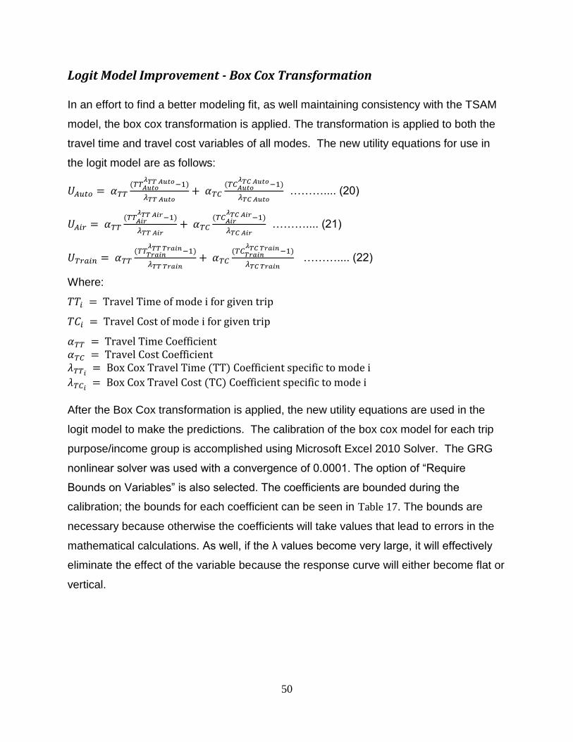
50

Logit Model Improvement - Box Cox Transformation

In an effort to find a better modeling fit, as well maintaining consistency with the TSAM

model, the box cox transformation is applied. The transformation is applied to both the

travel time and travel cost variables of all modes. The new utility equations for use in

the logit model are as follows:

(

)

(

)

……….... (20)

(

)

(

)

……….... (21)

(

)

(

)

……….... (22)

Where:

( )

( )

After the Box Cox transformation is applied, the new utility equations are used in the

logit model to make the predictions. The calibration of the box cox model for each trip

purpose/income group is accomplished using Microsoft Excel 2010 Solver. The GRG

nonlinear solver was used with a convergence of 0.0001. The option of “Require

Bounds on Variables” is also selected. The coefficients are bounded during the

calibration; the bounds for each coefficient can be seen in Table 17. The bounds are

necessary because otherwise the coefficients will take values that lead to errors in the

mathematical calculations. As well, if the λ values become very large, it will effectively

eliminate the effect of the variable because the response curve will either become flat or

vertical.

51

Table 17 - Calibration Bounds for Box-Cox Coefficients

Coefficient Lower Bound Upper Bound

Travel Time

α -10 -0.000001

λ Auto -2 1

λ Air -2 1

λ Train -2 1

Travel Cost

α -10 -0.000001

λ Auto -2 1

λ Air -2 1

λ Train -2 1

Existing Train Network - Station to Station Travel Time and Cost

TSAM currently has rail network data that is representative of the rail network in the

United States in 1995. It includes 464 Amtrak Rail Stations (please see Appendix B,

Table 35 for the full station list), the track distance between stations, and the calculated

schedule delay for travel between each station-station pair. This network was developed

in an earlier work.[29] This data is used as the basis for development of the station-

station travel time and travel cost matrices.

The first step is to develop baseline station-station travel time and travel cost matrices,

the time and cost values will be representative of service conditions in 1995; this is

accomplished using regression equations. The regression data is collected from

Amtrak’s website, www.Amtrak.com, using randomly selected origin-destination pairs

across the United States. It is known that Amtrak’s level of service (travel speed) has

not changed significantly for a large number of years, the northeast corridor is the

exception but a separate regression analysis is used for that corridor, therefore the

travel times presented on the website are representative of the travel times in 1995.

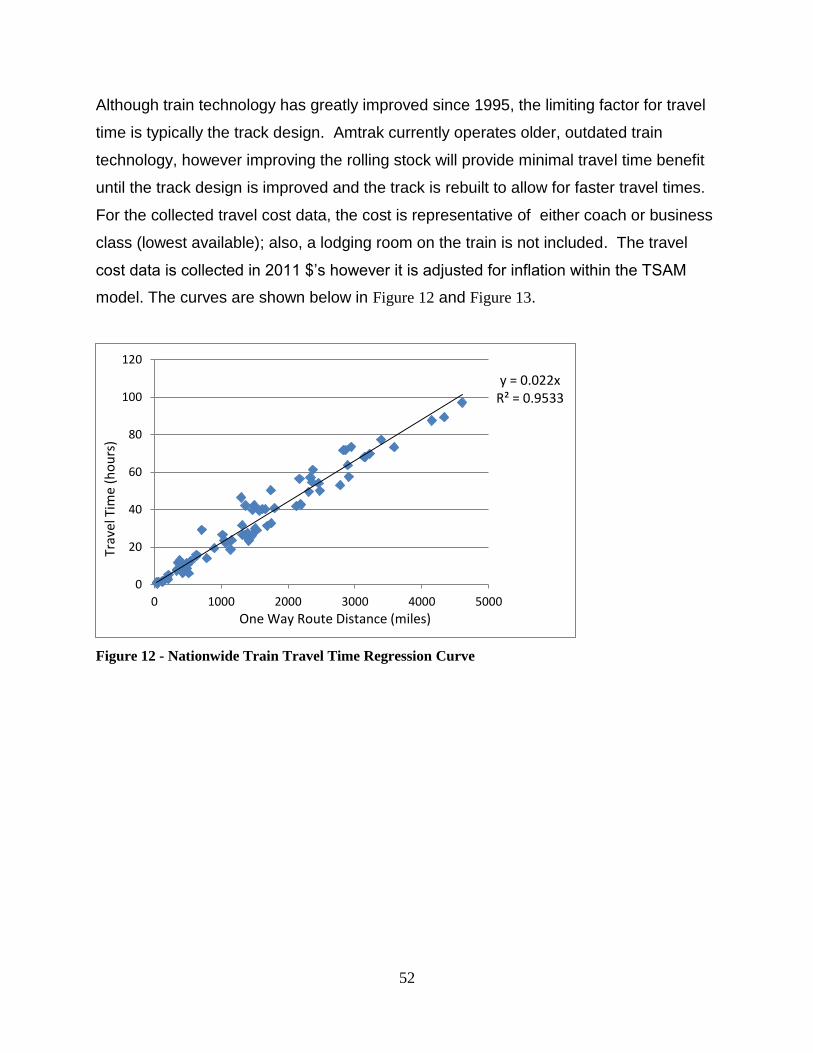
52

Although train technology has greatly improved since 1995, the limiting factor for travel

time is typically the track design. Amtrak currently operates older, outdated train

technology, however improving the rolling stock will provide minimal travel time benefit

until the track design is improved and the track is rebuilt to allow for faster travel times.

For the collected travel cost data, the cost is representative of either coach or business

class (lowest available); also, a lodging room on the train is not included. The travel

cost data is collected in 2011 $’s however it is adjusted for inflation within the TSAM

model. The curves are shown below in Figure 12 and Figure 13.

Figure 12 - Nationwide Train Travel Time Regression Curve

y = 0.022x R² = 0.9533

0

20

40

60

80

100

120

0 1000 2000 3000 4000 5000

One Way Route Distance (miles)

Trav

el T

ime

(ho

urs

)

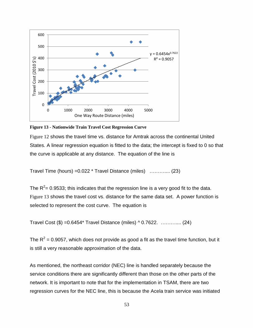
53

Figure 13 - Nationwide Train Travel Cost Regression Curve

Figure 12 shows the travel time vs. distance for Amtrak across the continental United

States. A linear regression equation is fitted to the data; the intercept is fixed to 0 so that

the curve is applicable at any distance. The equation of the line is

Travel Time (hours) =0.022 * Travel Distance (miles) ……….... (23)

The R2= 0.9533; this indicates that the regression line is a very good fit to the data.

Figure 13 shows the travel cost vs. distance for the same data set. A power function is

selected to represent the cost curve. The equation is

Travel Cost ($) =0.6454* Travel Distance (miles) ^ 0.7622. ……….... (24)

The R2 = 0.9057, which does not provide as good a fit as the travel time function, but it

is still a very reasonable approximation of the data.

As mentioned, the northeast corridor (NEC) line is handled separately because the

service conditions there are significantly different than those on the other parts of the

network. It is important to note that for the implementation in TSAM, there are two

regression curves for the NEC line, this is because the Acela train service was initiated

y = 0.6454x0.7622 R² = 0.9057

0

100

200

300

400

500

600

0 1000 2000 3000 4000 5000

One Way Route Distance (miles)

Trav

el C

ost

(2

01

0 $

's)

54

in 2001 therefore the curves for the years 1995-2000 represent service conditions of

Amtrak’s Northeast regional service and curves for years 2001 and forward represent

service conditions of the Acela Express train. The regional service trains continued

operation after the Acela line was introduced, they even maintain steady ridership

because of similar travel times and lower costs than Acela service; however they are

not modeled in TSAM after 2001. For future TSAM improvements, it may be beneficial

to develop some type of route choice model for train ridership so that both the Acela

and the regional service are included in the model.

The regression curves for the regional service can be found in Appendix A, Figure 40

and Figure 41. The regression curves for the Acela express can be found in Appendix A,

Figure 42 and Figure 43. Data for both cases are collected in the same manner as for the

nationwide regression that is discussed above. Again, all cost data was collected in

2010 $’s but the TSAM model accounts for inflation.

Future High-Speed Rail Corridor Modeling

Alignments

The primary purpose of this work is to incorporate the train mode as an option in TSAM.

This includes modeling of both the existing and future networks. At the time of this

work, there are multiple potential high-speed rail corridors that have been proposed.

Many of the technical details are still undetermined (exact alignments, train set type,

station location, etc.). However, there are planned alignments that will be used for

modeling. This work has incorporated twelve of the proposed high-speed rail corridors

into the TSAM model; several corridors are located in the northeast U.S. and will be

joined, however they are modeled separately to provide flexibility for analysis. It is

worth noting that the issue of high-speed rail in America has become a large political

issue due to fears of cost and profitability, several states have declined federal funding

for high-speed rail, so it will be important to watch both the ongoing planning studies as

well as the political landscape to determine if/how the projected corridors may change.

55

Table 18 shows each of the projected corridors that are modeled in TSAM as well as a

list of the major cities that are expected to be served by the corridor. Note that the city

names that are in italics and underlined are not currently modeled in TSAM. There are

no current Amtrak stations in those cities therefore when the station list is expanded,

these cities will need to be included. It is unlikely that the cities in Canada can be

included because the ATS data set is based on travel in the United States only.

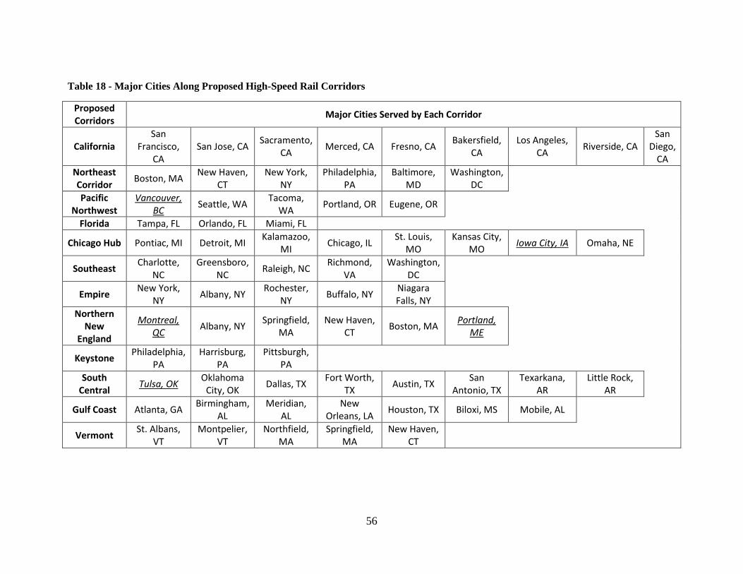
56

Table 18 - Major Cities Along Proposed High-Speed Rail Corridors

Proposed Corridors

Major Cities Served by Each Corridor

California San

Francisco, CA

San Jose, CA Sacramento,

CA Merced, CA Fresno, CA

Bakersfield, CA

Los Angeles, CA

Riverside, CA San

Diego, CA

Northeast Corridor

Boston, MA New Haven,

CT New York,

NY Philadelphia,

PA Baltimore,

MD Washington,

DC

Pacific Northwest

Vancouver, BC

Seattle, WA Tacoma,

WA Portland, OR Eugene, OR

Florida Tampa, FL Orlando, FL Miami, FL

Chicago Hub Pontiac, MI Detroit, MI Kalamazoo,

MI Chicago, IL

St. Louis, MO

Kansas City, MO

Iowa City, IA Omaha, NE

Southeast Charlotte,

NC Greensboro,

NC Raleigh, NC

Richmond, VA

Washington, DC

Empire New York,

NY Albany, NY

Rochester, NY

Buffalo, NY Niagara Falls, NY

Northern New

England

Montreal, QC

Albany, NY Springfield,

MA New Haven,

CT Boston, MA

Portland, ME

Keystone Philadelphia,

PA Harrisburg,

PA Pittsburgh,

PA

South Central

Tulsa, OK Oklahoma

City, OK Dallas, TX

Fort Worth, TX

Austin, TX San

Antonio, TX Texarkana,

AR Little Rock,

AR

Gulf Coast Atlanta, GA Birmingham,

AL Meridian,

AL New

Orleans, LA Houston, TX Biloxi, MS Mobile, AL

Vermont St. Albans,

VT Montpelier,

VT Northfield,

MA Springfield,

MA New Haven,

CT

57

In addition to the stations listed in Table 18, there are additional stations that are

modeled for each corridor; the list of stations modeled for each corridor can be seen in

Appendix A. The additional stations are selected by looking at each projected route and

determining what existing Amtrak stations are nearby. Since the detailed alignment of

each corridor has not been finalized, an attempt is made to determine what additional

stations would be included for each route. No specific criteria was used for the

selection process, if the station was close to the route and/or located in a fairly well

populated area then it was selected. It is known that the alignments will try to pass

through as many heavily populated areas as possible because this will produce higher

potential ridership. This station selection process will also need to be updated as more

details about the corridors emerge.

Train Station to Train Station Travel Time and Cost – Future Corridors

The travel time and cost values are determined by using fixed coefficients. The travel

time is calculated using the overall average travel speed (including stops) and the travel

cost is determined by a fixed price per mile for each corridor. The corridors are still in

the planning stage so detailed cost data or travel speed information is not currently

available. Using fixed values allows for sensitivity runs using different travel speeds and

costs which will show the sensitivity of travelers to both metrics. The train dynamics

model can be used to calculate travel times, however because of the network

connectivity issue in the model (discussed in Recommendations section), it will likely not

provide any improved accuracy because the number of stops and distance between

intermediate stops is not currently available in TSAM. Once the network connectivity

issue is addressed and the speed restrictions on each corridor have been determined,

the train dynamics model will be able to accurately determine the travel time between

stations on the network. However, as the model stands now, the connectivity between

stations is not modeled.

It is important to point out that there are multiple modeled stations along each corridor

that belong to the same greater metropolitan region. For example, looking at the

California Corridor, there are multiple stations that lie within the Los Angeles area; Los

58

Angeles, Irvine, Anaheim, Glendale, etc. It is obvious that not all of these stations will

fall along the high-speed line, however since the final alignment is not yet known, all of

the stations are included so that for modeling purposes, the maximum potential

ridership for the greater Los Angeles area will have access to train. It is assumed that

once the high-speed line has been built, the existing train network will be improved so

that there can be quick access from the outlying stations, such as Pomona, to the

stations along the high-speed line. As well, the TSAM model is interested in only

intercity trips, therefore any trip with a one way distance less than 100 miles is removed

from consideration, so for example, the model would not be estimating trips from

Pomona to Irvine.

In TSAM, the train network is represented as a distance between each O-D station pair;

the number and location of stops between each O-D pair is not included. This inhibits

the ability to utilize the dynamics model because the number and location of each stop

is important because stops can have a large effect on travel time because of the

additional time caused by deceleration, stop time at each station, and acceleration back

to travel speed. As well, the track design of each corridor has yet to be determined;

therefore information about potential speed restrictions caused by the track design is

needed to accurately calculate travel times. If the maximum speed in the dynamics

model is not restricted, the vehicles will accelerate and travel at maximum possible

speed; this is unrealistic because there will potentially be speed restrictions on each

route due to curve radii, grades, and at grade crossings.

County to Train Station Travel Time and Cost – TSAM

The TSAM model predicts travel demand at the county level. Woods and Poole

socioeconomic data is used in the trip generation and trip distribution phases of the

model. This data is also used to determine the population centroid of each county; this

centroid is used for the purposes of determining travel time between O-D pairs. The

calculated driving times between O-D pairs are from county centroid to county centroid.

59

In order for TSAM to be able to predict train ridership, the full travel time between O-D

pairs must be known. Trips that are designated as air or train trips are actually multi-

modal trips in most cases; the method of access to and egress from the stations are

handled by some other form of transportation, mainly automobile. Thus, the travel times

for these trips include several components such as access, processing (origin station),

processing (destination station), schedule delay, and egress time. For each county, the

rail station that is the shortest driving distance away from the county centroid is

considered to the rail station for the corresponding county; thus all train users either

originate or end their trips in the given county will come through the assigned rail station

for that county.

Once each county has been assigned to the closest rail station, the access and egress

times to the rail stations are calculated using Microsoft MapPoint. This is accomplished

by using the latitude-longitude coordinates of both the population centroid of a given

county and the train station. The latitude-longitude coordinates of the train stations

were developed in a previous effort, [29] ,and are currently available in TSAM. As well,

for the projected driving time for all years, a congested driving time is calculated. This

driving time utilizes Travel Time Indices (TTI) to account for congestion, mostly around

cities and large urban areas, while driving. The adjustment of travel times due to the TTI

indices is handled within TSAM.

Additional Time and Cost Components – TSAM

In addition to accounting for congestion penalties for travel times, several other factors

are included in the total travel time and cost values. The first additional component is

the schedule delay. Schedule delay is defined as the time difference between the

desired time of departure and the actual time of departure. Schedule delay typically

only applies to public transportation modes such as commercial air and train; the

schedule for an automobile trip is zero because it is assumed that the traveler can

access their automobile and begin their trip at any time they desire. For example, a

traveler taking a trip by train may desire to leave at 1 pm, however the closest train

departure time may be 2 pm, therefore there is a delay associated with the train mode

60

because the user cannot depart at their desired time. The formula to calculate the

schedule delay is:

……….... (25)

Where:

( )

( )

The schedule delay for the existing nationwide network in the year 1995 is already

incorporated into TSAM. However, the schedule delay for the Acela Express service,

which is modeled starting in the year 2001, has to be calculated. The service frequency

of the Acela express is found by using Amtrak’s published time tables, which can be

found at Amtrak’s website, www.amtrak.com.[30] Table 19 shows a matrix of the service

frequency for the Acela Express train for each of the 16 stations of the Original

Northeast Corridor; the underlined values represent a trip that is traveling Southbound.

The service frequency for this corridor is based on typical weekday operation. Table 20

shows the corresponding schedule delay for the NEC.

61

Table 19 - Acela Express Train Daily Service Frequency

FREQUENCY STM NHV NLC WIL WAS BWI BAL RTE BOS NWK TRE MET NYP PHL PVD BBY

STM 0 8 2 9 9 8 9 8 8 9 1 1 9 9 8 9

NHV 9 0 2 9 9 8 9 8 8 9 1 1 9 9 8 9

NLC 1 1 0 1 1 1 1 2 2 1 1 1 1 1 2 1

WIL 8 8 2 0 9 8 9 9 9 9 1 4 9 9 9 9

WAS 8 8 2 9 0 4 9 9 9 9 1 4 9 9 9 9

BWI 4 4 2 4 8 0 8 4 4 4 1 4 4 4 4 8

BAL 8 8 2 9 9 8 0 9 9 9 1 4 9 9 9 9

RTE 9 9 1 9 9 8 9 0 10 9 1 1 10 9 10 10

BOS 9 9 1 9 9 8 9 10 0 9 1 1 10 9 10 10

NWK 8 8 2 9 9 8 9 9 9 0 1 1 9 9 9 9

TRE 1 1 1 1 1 1 1 1 1 1 0 1 1 1 1 1

MET 4 4 2 1 1 1 1 4 4 4 1 0 4 1 4 1

NYP 8 8 2 9 9 8 9 10 10 9 1 1 0 9 10 10

PHL 8 8 2 9 9 8 9 9 9 9 9 4 9 0 9 9

PVD 9 9 1 9 9 8 9 10 10 9 1 1 10 9 0 10

BBY 8 8 2 9 9 4 9 10 10 9 1 4 10 9 10 0

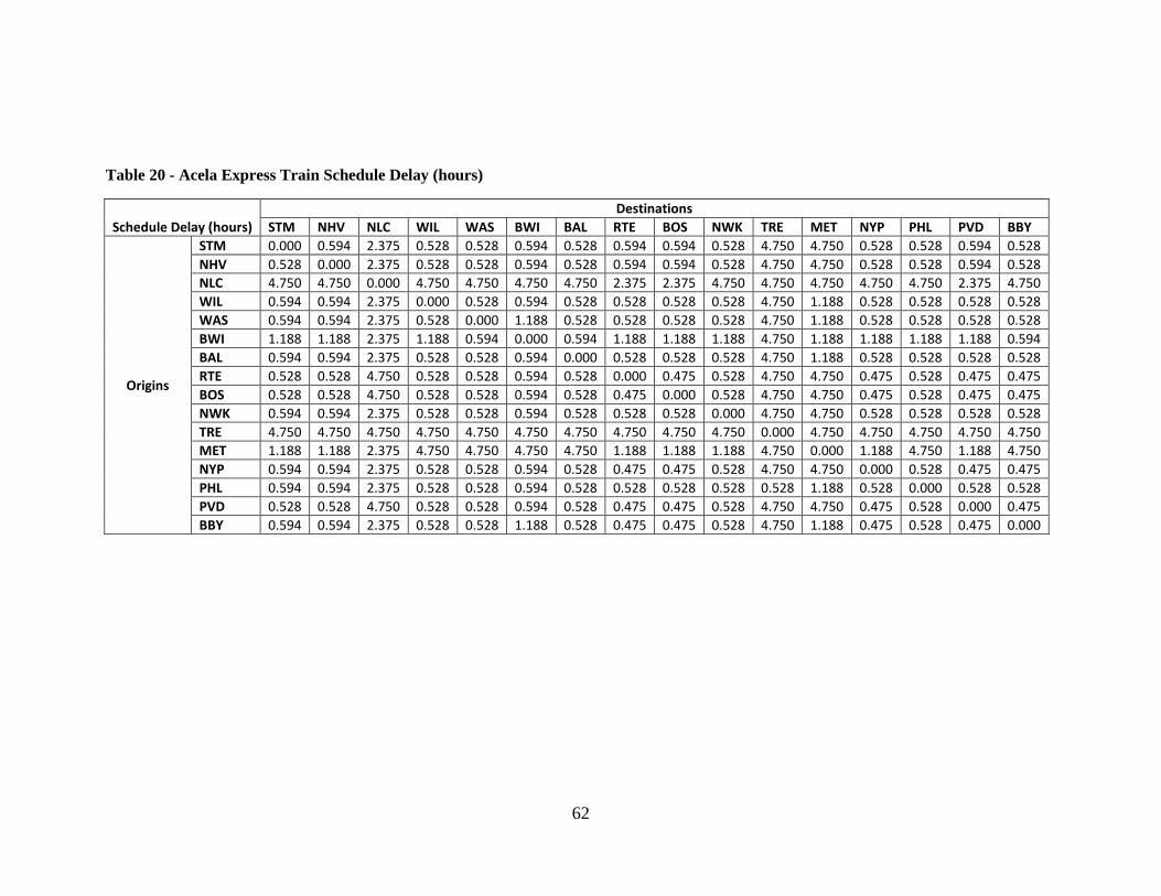
62

Table 20 - Acela Express Train Schedule Delay (hours)

Schedule Delay (hours)

Destinations

STM NHV NLC WIL WAS BWI BAL RTE BOS NWK TRE MET NYP PHL PVD BBY

Origins

STM 0.000 0.594 2.375 0.528 0.528 0.594 0.528 0.594 0.594 0.528 4.750 4.750 0.528 0.528 0.594 0.528

NHV 0.528 0.000 2.375 0.528 0.528 0.594 0.528 0.594 0.594 0.528 4.750 4.750 0.528 0.528 0.594 0.528

NLC 4.750 4.750 0.000 4.750 4.750 4.750 4.750 2.375 2.375 4.750 4.750 4.750 4.750 4.750 2.375 4.750

WIL 0.594 0.594 2.375 0.000 0.528 0.594 0.528 0.528 0.528 0.528 4.750 1.188 0.528 0.528 0.528 0.528

WAS 0.594 0.594 2.375 0.528 0.000 1.188 0.528 0.528 0.528 0.528 4.750 1.188 0.528 0.528 0.528 0.528

BWI 1.188 1.188 2.375 1.188 0.594 0.000 0.594 1.188 1.188 1.188 4.750 1.188 1.188 1.188 1.188 0.594

BAL 0.594 0.594 2.375 0.528 0.528 0.594 0.000 0.528 0.528 0.528 4.750 1.188 0.528 0.528 0.528 0.528

RTE 0.528 0.528 4.750 0.528 0.528 0.594 0.528 0.000 0.475 0.528 4.750 4.750 0.475 0.528 0.475 0.475

BOS 0.528 0.528 4.750 0.528 0.528 0.594 0.528 0.475 0.000 0.528 4.750 4.750 0.475 0.528 0.475 0.475

NWK 0.594 0.594 2.375 0.528 0.528 0.594 0.528 0.528 0.528 0.000 4.750 4.750 0.528 0.528 0.528 0.528

TRE 4.750 4.750 4.750 4.750 4.750 4.750 4.750 4.750 4.750 4.750 0.000 4.750 4.750 4.750 4.750 4.750

MET 1.188 1.188 2.375 4.750 4.750 4.750 4.750 1.188 1.188 1.188 4.750 0.000 1.188 4.750 1.188 4.750

NYP 0.594 0.594 2.375 0.528 0.528 0.594 0.528 0.475 0.475 0.528 4.750 4.750 0.000 0.528 0.475 0.475

PHL 0.594 0.594 2.375 0.528 0.528 0.594 0.528 0.528 0.528 0.528 0.528 1.188 0.528 0.000 0.528 0.528

PVD 0.528 0.528 4.750 0.528 0.528 0.594 0.528 0.475 0.475 0.528 4.750 4.750 0.475 0.528 0.000 0.475

BBY 0.594 0.594 2.375 0.528 0.528 1.188 0.528 0.475 0.475 0.528 4.750 1.188 0.475 0.528 0.475 0.000

63

The next addition relates to the time spent at the origin and destination stations.

When a user takes a train, there will be a certain time period that is devoted to

purchasing a ticket, check in, boarding/un-boarding, security checkpoints, etc.

For the TSAM model, the processing time at the origin station is assumed to be

20 minutes. This assumption will need to be periodically examined to ensure it is

realistic; potential increased security and congestion at train stations would

greatly increase the processing time. The processing time at the destination

station is assumed to be 10 minutes; this accounts for time spent unloading and

departing the train. In addition to processing time, a waiting time at both origin

and destination stations is assigned. The waiting time for both stations is

assumed to be 10 minutes. The waiting time at the origin station accounts for

passengers arriving early to the station so that they do not miss their train. The

waiting time at the destination station accounts for passengers waiting for a

connecting trip; either by connecting taxicab, bus, or time spent loading personal

automobile and exiting the station.

Finally, the TSAM model accounts for lodging times and costs for trips that are

too long to complete in one day; if the round trip travel time exceeds the

maximum daily travel time, then the lodging times and costs are included. The

maximum daily travel time is assumed to be 8 hours for business trips and 10

hours for non-business trips; although this is a user option in the TSAM model.

The time penalty is implemented as a ramp function, the time penalty for each

trip length is shown in Appendix A, Table 49. Although the ramp function may

seem unrealistic, it makes sense for modeling purposes because having a step

function could cause drastic shifts for trips from the same area. For example, if a

step function were implemented, a trip from one location may have no lodging

time included, whereas a trip that originates only a few miles away would have a

full night of lodging time included. This would make the model inconsistent

because users who trips begin and/or end only a few miles apart will likely make

similar travel decisions.

64

The lodging costs are assigned based on trip purpose and income group. It is

assumed that travelers in higher income groups will stay at more expensive

hotels, as well it is assumed that business travelers will spend more on lodging

than non-business travelers. The lodging cost values are based on average

lodging costs in the year 2000 and then are scaled by inflation to match the given

year. The lodging costs are shown in Table 21.

Table 21 - TSAM Lodging Costs - $(2000)

Business Non-Business

Income Group 1 70 50

Income Group 2 80 60

Income Group 3 90 70

Income Group 4 100 80

Income Group 5 120 90

65

Results

Test of Train Dynamics Model

In order to demonstrate the train dynamics model as well as compare the

different train sets that are modeled, a test run along the Northeast Corridor has

been analyzed. Two different scenarios are considered; the first scenario

examines stops at all 16 stations that are modeled on the corridor, see Table 24,

the second scenario considers stops only in the cities of Boston MA, New York

NY, Philadelphia PA, Baltimore MD, and Washington DC. The first scenario

matches current Amtrak operations, the Acela Train stops at nearly every station

along the route. The second scenario models the type of operations that are

commonly seen in Europe; the high-speed trains stop only in the large cities and

commuter trains are used to get passengers into smaller areas.

For both scenarios, stops at stations are modeled as a stop and go only; the time

that would be required for passengers to board/depart the train is not included.

As well, the route is assumed to flat for the entire trip; the detailed gradients of

the track are not available. For both the full NEC route and the major city route,

three different scenarios are included; the first scenario limits the maximum train

speed to 50 m/s (112 mph), the second scenario limits the maximum train speed

to 70 m/s (157 mph), and the last scenario allows the train to travel at its

maximum possible speed. Although it is unlikely that there would ever be a

scenario that the train could travel at its maximum speed with no restrictions, this

will help demonstrate the differences between the train sets and will show how

the travel speed and number of stops can affect the travel time and energy

consumption.

66

Table 22 - Comparison of Trainset Performance on Original Northeast Corridor Route

Shinkansen-

100

Shinkansen-

200

TGV-

R

TGV-

D

Max Speed =

50 m/s

Travel Time (hrs.) 4.77 4.73 4.69 4.69

Energy Use (KW-hrs.) 52993 41993 25199 25442

Max Speed =

70 m/s

Travel Time (hrs.) 3.77 3.66 3.58 3.58

Energy Use (KW-hrs.) 86911 70303 42444 42814

Max Speed =

Unrestricted

Travel Time (hrs.) 3.69 3.4 3.15 3.16

Energy Use (KW-hrs.) 91914 84695 57950 58190

Table 23 - Comparison of Trainset Performance on Original Northeast Corridor Route

(Stops at Major Cities Only)

Shinkansen-

100

Shinkansen-

200

TGV-

R

TGV-

D

Max Speed =

50 m/s

Travel Time (hrs.) 4.54 4.53 4.52 4.52

Energy Use (KW-hrs.) 43905 34400 20751 20908

Max Speed =

70 m/s

Travel Time (hrs.) 3.35 3.32 3.29 3.29

Energy Use (KW-hrs.) 74353 58506 35159 35379

Max Speed =

Unrestricted

Travel Time (hrs.) 3.22 2.93 2.69 2.7

Energy Use (KW-hrs.) 80116 73938 51030 51113

Table 22 shows the travel times and energy consumptions for each of the three

scenarios for the full NEC analysis; Table 23 shows the results for the Major NEC

Cities Analysis. The charts show how each of the different train sets perform in

different scenarios; notice that the two TGV trains perform similarly for all the

scenarios. It is obvious from looking at the charts that as the travel speed

increases, the travel time decreases and the energy use increases. Also, as

expected, reducing the number of stops on the trip will cause the travel time and

energy consumption both to decrease.

67

It is important to note that a significant amount of energy is saved by reducing the

number of stops. This is due to the fact that the train uses energy at a much

higher rate for acceleration when compared to a cruise (steady state) condition.

This demonstrates the importance of proper planning for the future corridor

alignments and station locations. Adding additional stations along a corridor will

provide better access to customers, in turn increasing potential ridership,

however there will be an associated travel time and energy consumption penalty.

The station location process will need to be optimized to maximize ridership while

minimizing costs associated with energy consumption and station operation and

maintenance, especially given the financial climate and the political scrutiny of

high-speed rail.

NEC Corridor Model

The initial TSAM attempt is to calibrate and apply a mode choice model with

three 3 possible modes of transportation (commercial air, auto, and rail) for the

Northeast Corridor (NEC) region only. This is the Amtrak line that runs between

Boston, MA and Washington, DC. The NEC is chosen for several reasons. First,

the NEC is the only section that has true high-speed rail; the NEC is not

considered to have high speed operations when compared to train’s operating

speeds around the world, however when compared to the other sections of the

United States network, it provides the fastest service. The average operating

speed in the NEC is approximately 85 mph.

The NEC also has the highest number of passengers, with approximately 11

million users in 2010.[31] Finally, the ATS is sparse with train records, but

approximately half of the train records are recorded in the NEC, therefore this

provides the best possible corridor for a calibration.

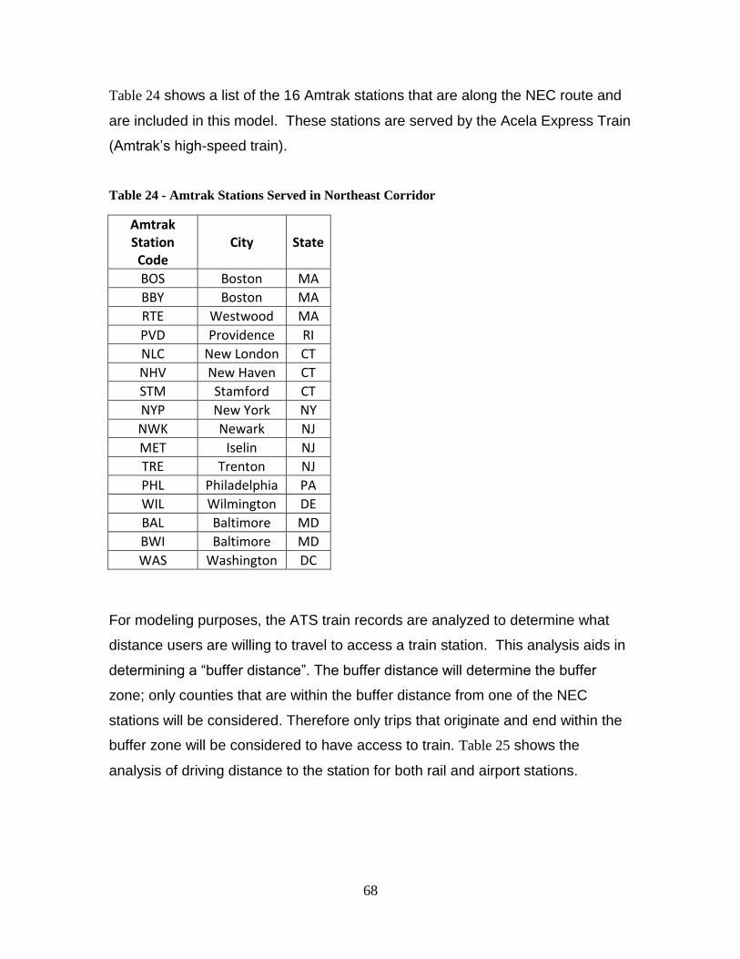
68

Table 24 shows a list of the 16 Amtrak stations that are along the NEC route and

are included in this model. These stations are served by the Acela Express Train

(Amtrak’s high-speed train).

Table 24 - Amtrak Stations Served in Northeast Corridor

Amtrak Station Code

City State

BOS Boston MA

BBY Boston MA

RTE Westwood MA

PVD Providence RI

NLC New London CT

NHV New Haven CT

STM Stamford CT

NYP New York NY

NWK Newark NJ

MET Iselin NJ

TRE Trenton NJ

PHL Philadelphia PA

WIL Wilmington DE

BAL Baltimore MD

BWI Baltimore MD

WAS Washington DC

For modeling purposes, the ATS train records are analyzed to determine what

distance users are willing to travel to access a train station. This analysis aids in

determining a “buffer distance”. The buffer distance will determine the buffer

zone; only counties that are within the buffer distance from one of the NEC

stations will be considered. Therefore only trips that originate and end within the

buffer zone will be considered to have access to train. Table 25 shows the

analysis of driving distance to the station for both rail and airport stations.

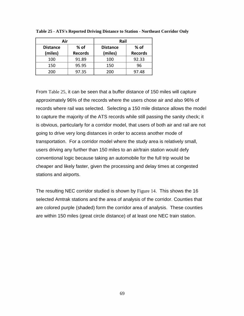
69

Table 25 - ATS's Reported Driving Distance to Station - Northeast Corridor Only

Air Rail

Distance (miles)

% of Records

Distance (miles)

% of Records

100 91.89 100 92.33

150 95.95 150 96

200 97.35 200 97.48

From Table 25, it can be seen that a buffer distance of 150 miles will capture

approximately 96% of the records where the users chose air and also 96% of

records where rail was selected. Selecting a 150 mile distance allows the model

to capture the majority of the ATS records while still passing the sanity check; it

is obvious, particularly for a corridor model, that users of both air and rail are not

going to drive very long distances in order to access another mode of

transportation. For a corridor model where the study area is relatively small,

users driving any further than 150 miles to an air/train station would defy

conventional logic because taking an automobile for the full trip would be

cheaper and likely faster, given the processing and delay times at congested

stations and airports.

The resulting NEC corridor studied is shown by Figure 14. This shows the 16

selected Amtrak stations and the area of analysis of the corridor. Counties that

are colored purple (shaded) form the corridor area of analysis. These counties

are within 150 miles (great circle distance) of at least one NEC train station.

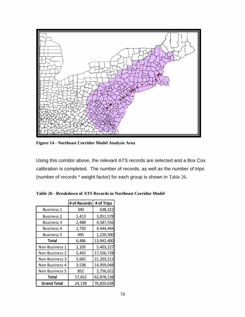
70

Figure 14 - Northeast Corridor Model Analysis Area

Using this corridor above, the relevant ATS records are selected and a Box Cox

calibration is completed. The number of records, as well as the number of trips

(number of records * weight factor) for each group is shown in Table 26.

Table 26 - Breakdown of ATS Records in Northeast Corridor Model

# of Records # of Trips

Business 1 340 638,322

Business 2 1,413 3,051,578

Business 3 2,488 4,587,556

Business 4 1,750 4,444,444

Business 5 495 1,220,500

Total 6,486 13,942,400

Non Business 1 2,105 5,403,227

Non Business 2 5,492 17,556,728

Non Business 3 5,665 21,203,213

Non Business 4 3,538 14,959,048

Non Business 5 852 3,756,022

Total 17,652 62,878,238

Grand Total 24,138 76,820,638

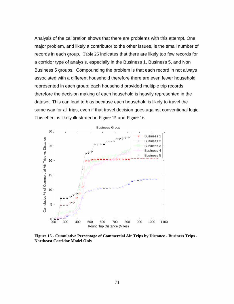
71

Analysis of the calibration shows that there are problems with this attempt. One

major problem, and likely a contributor to the other issues, is the small number of

records in each group. Table 26 indicates that there are likely too few records for

a corridor type of analysis, especially in the Business 1, Business 5, and Non

Business 5 groups. Compounding the problem is that each record in not always

associated with a different household therefore there are even fewer household

represented in each group; each household provided multiple trip records

therefore the decision making of each household is heavily represented in the

dataset. This can lead to bias because each household is likely to travel the

same way for all trips, even if that travel decision goes against conventional logic.

This effect is likely illustrated in Figure 15 and Figure 16.

Figure 15 - Cumulative Percentage of Commercial Air Trips by Distance - Business Trips -

Northeast Corridor Model Only

200 300 400 500 600 700 800 900 1000 11000

5

10

15

20

25

30

Round Trip Distance (Miles)

Cum

ula

tive %

of

Com

merc

ial A

ir T

rips v

s D

ista

nce

Business Group

Business 1

Business 2

Business 3

Business 4

Business 5

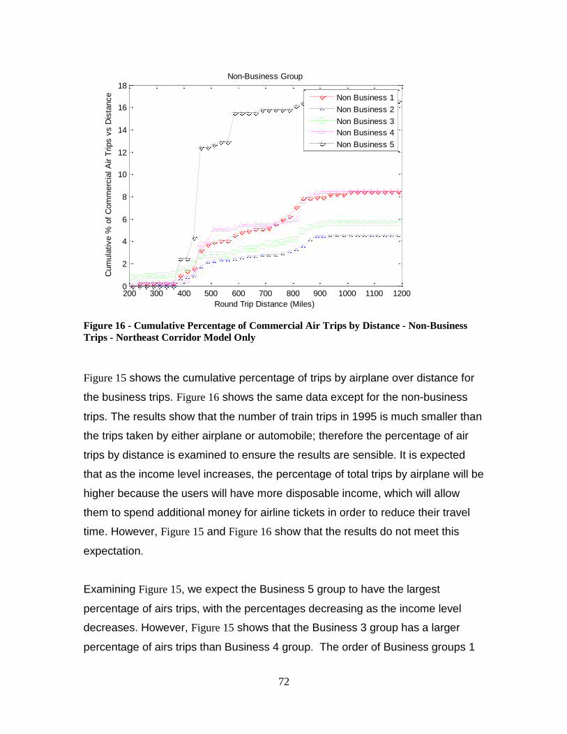
72

Figure 16 - Cumulative Percentage of Commercial Air Trips by Distance - Non-Business

Trips - Northeast Corridor Model Only

Figure 15 shows the cumulative percentage of trips by airplane over distance for

the business trips. Figure 16 shows the same data except for the non-business

trips. The results show that the number of train trips in 1995 is much smaller than

the trips taken by either airplane or automobile; therefore the percentage of air

trips by distance is examined to ensure the results are sensible. It is expected

that as the income level increases, the percentage of total trips by airplane will be

higher because the users will have more disposable income, which will allow

them to spend additional money for airline tickets in order to reduce their travel

time. However, Figure 15 and Figure 16 show that the results do not meet this

expectation.

Examining Figure 15, we expect the Business 5 group to have the largest

percentage of airs trips, with the percentages decreasing as the income level

decreases. However, Figure 15 shows that the Business 3 group has a larger

percentage of airs trips than Business 4 group. The order of Business groups 1

200 300 400 500 600 700 800 900 1000 1100 12000

2

4

6

8

10

12

14

16

18

Round Trip Distance (Miles)

Cum

ula

tive %

of

Com

merc

ial A

ir T

rips v

s D

ista

nce

Non-Business Group

Non Business 1

Non Business 2

Non Business 3

Non Business 4

Non Business 5

73

and 2 is also reversed. The same type of problem occurs in the Non Business

group which is seen in Figure 16. The Non Business 1 group has the second

highest percentage of trips by air which is highly unexpected.

The conclusion from these results is that the projections from a “corridor” model

have too much inconsistency and thus cannot be trusted. This is based on the

inconsistencies of Figure 15 and Figure 16 above as well as the knowledge of the

ATS data set. The ATS data set is relatively sparse and the corridor type analysis

does not capture a large number of records so thus the results are likely biased

and cannot be used for making projections. The next effort will calibrate the

model for the entire continental U.S. (entire ATS data set), since the ATS dataset

was sampled to represent overall travel in the U.S., not for use in specific

corridors.

Nationwide Calibration Results

The corridor type model proves to be inconsistent so the next effort is to calibrate

a nationwide model. The nationwide model uses the box- cox transformation and

is calibrated for the year 1995, since that is the year of the ATS data. The results

of the calibration of the Box Cox model vs. the ATS can be seen in Table 27

below, the detailed calibration results and the calibration coefficients can be seen

in Appendix A, Table 50. The calibration is conducted using the bounds that are

listed in Table 17.

Table 27 - Nationwide Mode Choice Calibration vs. ATS Data

Business Non – Business Total

ATS Calibration ATS Calibration ATS Calibration

Automobile 154,079,520 154,036,233 706,195,897 706,316,064 860,275,417 860,352,297

Commercial

Air 66,050,944 66,227,697 88,742,525 88,486,227 154,793,470 154,713,924

Train 1,359,012 1,225,546 3,890,824 4,026,956 5,249,836 5,252,501

Total 221,489,476 221,489,476 798,829,247 798,829,247 1,020,318,723 1,020,318,723

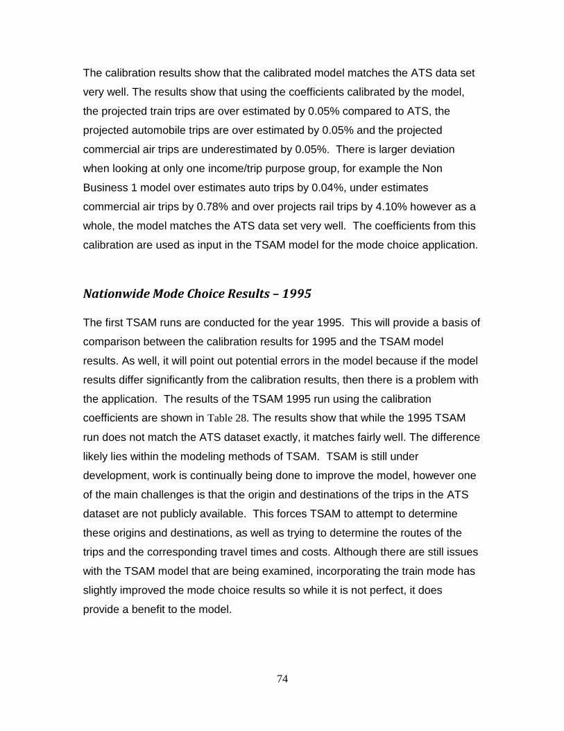
74

The calibration results show that the calibrated model matches the ATS data set

very well. The results show that using the coefficients calibrated by the model,

the projected train trips are over estimated by 0.05% compared to ATS, the

projected automobile trips are over estimated by 0.05% and the projected

commercial air trips are underestimated by 0.05%. There is larger deviation

when looking at only one income/trip purpose group, for example the Non

Business 1 model over estimates auto trips by 0.04%, under estimates

commercial air trips by 0.78% and over projects rail trips by 4.10% however as a

whole, the model matches the ATS data set very well. The coefficients from this

calibration are used as input in the TSAM model for the mode choice application.

Nationwide Mode Choice Results – 1995

The first TSAM runs are conducted for the year 1995. This will provide a basis of

comparison between the calibration results for 1995 and the TSAM model

results. As well, it will point out potential errors in the model because if the model

results differ significantly from the calibration results, then there is a problem with

the application. The results of the TSAM 1995 run using the calibration

coefficients are shown in Table 28. The results show that while the 1995 TSAM

run does not match the ATS dataset exactly, it matches fairly well. The difference

likely lies within the modeling methods of TSAM. TSAM is still under

development, work is continually being done to improve the model, however one

of the main challenges is that the origin and destinations of the trips in the ATS

dataset are not publicly available. This forces TSAM to attempt to determine

these origins and destinations, as well as trying to determine the routes of the

trips and the corresponding travel times and costs. Although there are still issues

with the TSAM model that are being examined, incorporating the train mode has

slightly improved the mode choice results so while it is not perfect, it does

provide a benefit to the model.

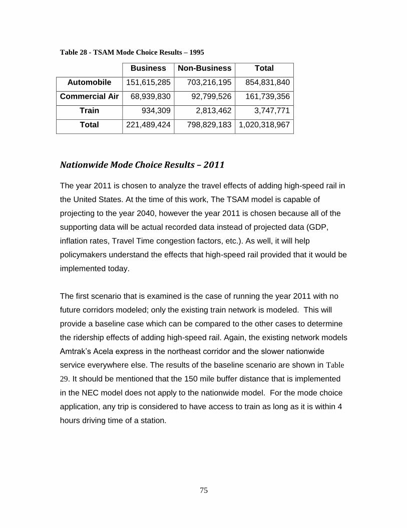
75

Table 28 - TSAM Mode Choice Results – 1995

Business Non-Business Total

Automobile 151,615,285 703,216,195 854,831,840

Commercial Air 68,939,830 92,799,526 161,739,356

Train 934,309 2,813,462 3,747,771

Total 221,489,424 798,829,183 1,020,318,967

Nationwide Mode Choice Results – 2011

The year 2011 is chosen to analyze the travel effects of adding high-speed rail in

the United States. At the time of this work, The TSAM model is capable of

projecting to the year 2040, however the year 2011 is chosen because all of the

supporting data will be actual recorded data instead of projected data (GDP,

inflation rates, Travel Time congestion factors, etc.). As well, it will help

policymakers understand the effects that high-speed rail provided that it would be

implemented today.

The first scenario that is examined is the case of running the year 2011 with no

future corridors modeled; only the existing train network is modeled. This will

provide a baseline case which can be compared to the other cases to determine

the ridership effects of adding high-speed rail. Again, the existing network models

Amtrak’s Acela express in the northeast corridor and the slower nationwide

service everywhere else. The results of the baseline scenario are shown in Table

29. It should be mentioned that the 150 mile buffer distance that is implemented

in the NEC model does not apply to the nationwide model. For the mode choice

application, any trip is considered to have access to train as long as it is within 4

hours driving time of a station.

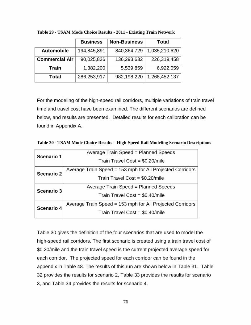
76

Table 29 - TSAM Mode Choice Results - 2011 - Existing Train Network

Business Non-Business Total

Automobile 194,845,891 840,364,729 1,035,210,620

Commercial Air 90,025,826 136,293,632 226,319,458

Train 1,382,200 5,539,859 6,922,059

Total 286,253,917 982,198,220 1,268,452,137

For the modeling of the high-speed rail corridors, multiple variations of train travel

time and travel cost have been examined. The different scenarios are defined

below, and results are presented. Detailed results for each calibration can be

found in Appendix A.

Table 30 - TSAM Mode Choice Results – High-Speed Rail Modeling Scenario Descriptions

Scenario 1 Average Train Speed = Planned Speeds

Train Travel Cost = $0.20/mile

Scenario 2 Average Train Speed = 153 mph for All Projected Corridors

Train Travel Cost = $0.20/mile

Scenario 3 Average Train Speed = Planned Speeds

Train Travel Cost = $0.40/mile

Scenario 4 Average Train Speed = 153 mph for All Projected Corridors

Train Travel Cost = $0.40/mile

Table 30 gives the definition of the four scenarios that are used to model the

high-speed rail corridors. The first scenario is created using a train travel cost of

$0.20/mile and the train travel speed is the current projected average speed for

each corridor. The projected speed for each corridor can be found in the

appendix in Table 48. The results of this run are shown below in Table 31. Table

32 provides the results for scenario 2, Table 33 provides the results for scenario

3, and Table 34 provides the results for scenario 4.

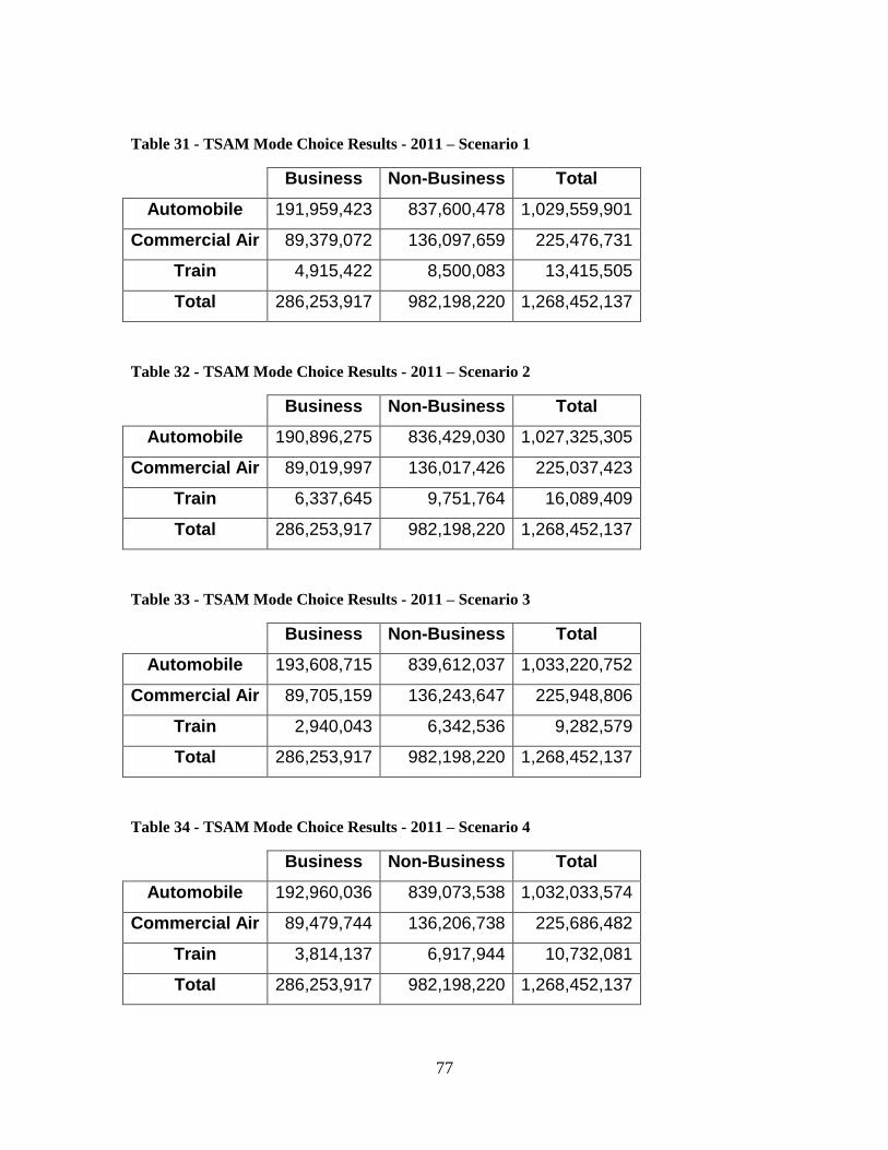
77

Table 31 - TSAM Mode Choice Results - 2011 – Scenario 1

Business Non-Business Total

Automobile 191,959,423 837,600,478 1,029,559,901

Commercial Air 89,379,072 136,097,659 225,476,731

Train 4,915,422 8,500,083 13,415,505

Total 286,253,917 982,198,220 1,268,452,137

Table 32 - TSAM Mode Choice Results - 2011 – Scenario 2

Business Non-Business Total

Automobile 190,896,275 836,429,030 1,027,325,305

Commercial Air 89,019,997 136,017,426 225,037,423

Train 6,337,645 9,751,764 16,089,409

Total 286,253,917 982,198,220 1,268,452,137

Table 33 - TSAM Mode Choice Results - 2011 – Scenario 3

Business Non-Business Total

Automobile 193,608,715 839,612,037 1,033,220,752

Commercial Air 89,705,159 136,243,647 225,948,806

Train 2,940,043 6,342,536 9,282,579

Total 286,253,917 982,198,220 1,268,452,137

Table 34 - TSAM Mode Choice Results - 2011 – Scenario 4

Business Non-Business Total

Automobile 192,960,036 839,073,538 1,032,033,574

Commercial Air 89,479,744 136,206,738 225,686,482

Train 3,814,137 6,917,944 10,732,081

Total 286,253,917 982,198,220 1,268,452,137

78

The results show that the number of trips by each mode is sensitive to both the

travel time and travel cost. Comparing Table 31 and Table 32 shows the sensitivity

of the model to travel speed. Increasing the speed from the planned speeds

(Table 48) to 153 mph average speed for all corridors produces approximately

2.67 million addition trips by train. It is also shown that approximately 2.2 million

of these trips were previously conducted by automobile. As well, the sensitivity

to travel cost is illustrated by comparing Table 31 and Table 33. Increasing the

train’s travel cost from $0.20/mile to $0.40/mile leads to a decrease in total train

trips of approximately 4.2 million trips. These effects are illustrated in Figure 17,

Figure 18, and Figure 19. These figures show the total trips for automobile,

commercial air and train respectively. The predictions using the existing network

are also shown for comparison; the speed on the x-axis does not apply to the

existing network, the regression curves are used.

Figure 17 - TSAM Mode Choice Results - 2011 - Total Automobile Trips

1,022

1,024

1,026

1,028

1,030

1,032

1,034

1,036

Planned 153

Existing Network

$0.20/mile

$0.40/mile

Train Speed (mph)

Inte

rcit

y Tr

ips

(mill

ion

s)

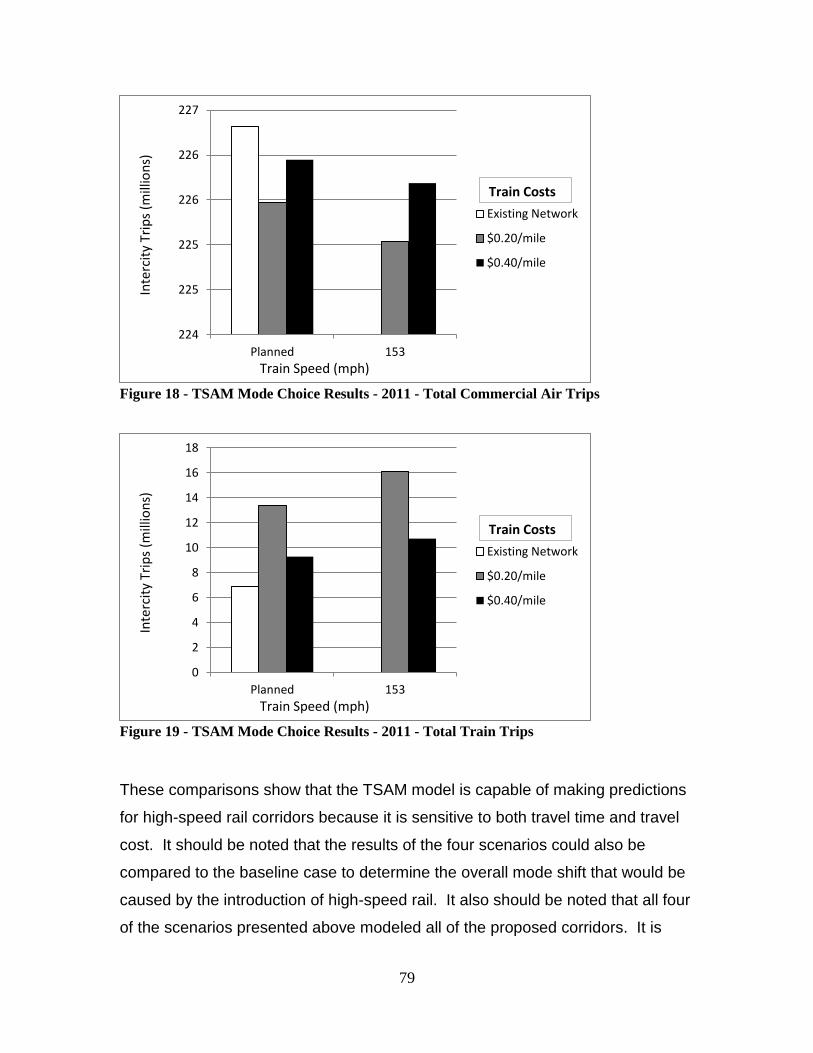
79

Figure 18 - TSAM Mode Choice Results - 2011 - Total Commercial Air Trips

Figure 19 - TSAM Mode Choice Results - 2011 - Total Train Trips

These comparisons show that the TSAM model is capable of making predictions

for high-speed rail corridors because it is sensitive to both travel time and travel

cost. It should be noted that the results of the four scenarios could also be

compared to the baseline case to determine the overall mode shift that would be

caused by the introduction of high-speed rail. It also should be noted that all four

of the scenarios presented above modeled all of the proposed corridors. It is

224

225

225

226

226

227

Planned 153

Existing Network

$0.20/mile

$0.40/mile

Train Speed (mph)

Inte

rcit

y Tr

ips

(mill

ion

s)

Train Costs

0

2

4

6

8

10

12

14

16

18

Planned 153

Existing Network

$0.20/mile

$0.40/mile

Train Speed (mph)

Inte

rcit

y Tr

ips

(mill

ion

s)

Train Costs

80

possible to determine the effect of each proposed corridor individually if needed;

a TSAM run could be executed with only the desired corridor turned on and then

the results could be compared to the baseline case.

Nationwide Mode Choice Results – 2020

In addition to modeling high-speed rail in the year 2011, results for the years

2020 and 2030 have also been presented. For both years, the same scenarios

listed in Table 30 have been calculated. This shows the projected intercity

ridership data and modal shift effects caused by the different high-speed rail

scenarios. As well, the “existing network” case for each year is presented; this

represents the actual network in place in the U.S. in the year 2011, no high

speed rail. This provides ridership results for the case of no implementation of

high speed rail. The results for the future years are based on the current (2011)

projections of population growth, economic growth, inflation index, etc. therefore

they will be sensitive to any changes in those items. The 2020 results are

shown in Figure 20, Figure 21, and Figure 22.

Figure 20 - TSAM Mode Choice Results - 2020 - Total Automobile Trips

1,146

1,148

1,150

1,152

1,154

1,156

1,158

1,160

1,162

Planned 153

Existing Network

$0.20/mile

$0.40/mile

Train Speed (mph)

Inte

rcit

y Tr

ips

(mill

ion

s)

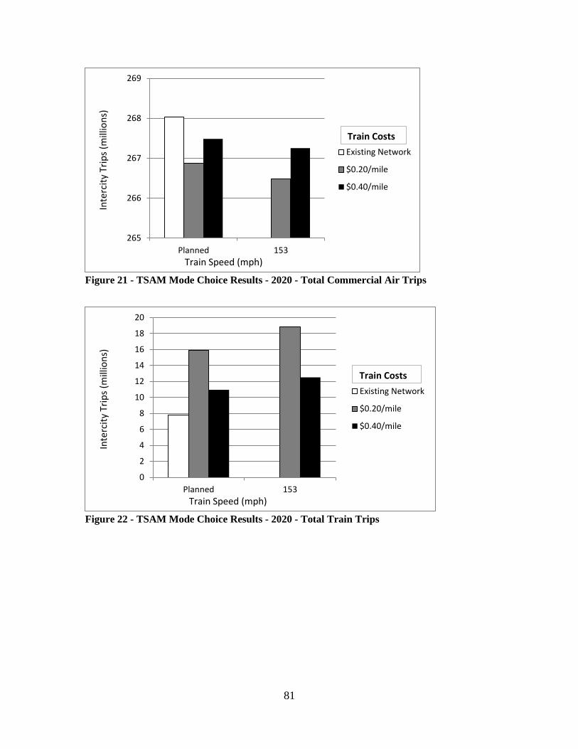
81

Figure 21 - TSAM Mode Choice Results - 2020 - Total Commercial Air Trips

Figure 22 - TSAM Mode Choice Results - 2020 - Total Train Trips

265

266

267

268

269

Planned 153

Existing Network

$0.20/mile

$0.40/mile

Train Speed (mph)

Inte

rcit

y Tr

ips

(mill

ion

s)

Train Costs

0

2

4

6

8

10

12

14

16

18

20

Planned 153

Existing Network

$0.20/mile

$0.40/mile

Train Speed (mph)

Inte

rcit

y Tr

ips

(mill

ion

s)

Train Costs

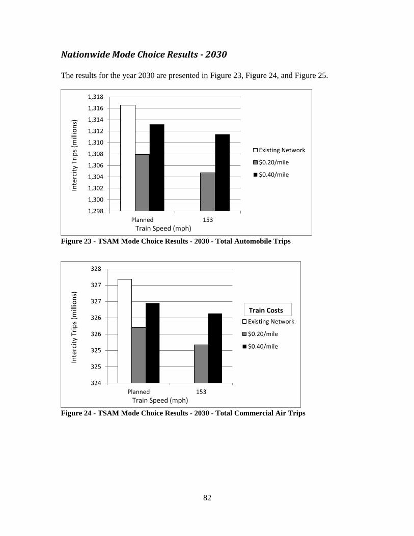
82

Nationwide Mode Choice Results - 2030 The results for the year 2030 are presented in Figure 23, Figure 24, and Figure 25.

Figure 23 - TSAM Mode Choice Results - 2030 - Total Automobile Trips

Figure 24 - TSAM Mode Choice Results - 2030 - Total Commercial Air Trips

1,298

1,300

1,302

1,304

1,306

1,308

1,310

1,312

1,314

1,316

1,318

Planned 153

Existing Network

$0.20/mile

$0.40/mile

Train Speed (mph)

Inte

rcit

y Tr

ips

(mill

ion

s)

324

325

325

326

326

327

327

328

Planned 153

Existing Network

$0.20/mile

$0.40/mile

Train Speed (mph)

Inte

rcit

y Tr

ips

(mill

ion

s)

Train Costs

83

Figure 25 - TSAM Mode Choice Results - 2030 - Total Train Trips

0

5

10

15

20

25

Planned 153

Existing Network

$0.20/mile

$0.40/mile

Train Speed (mph)

Inte

rcit

y Tr

ips

(mill

ion

s)

Train Costs

84

Summary and Conclusions

This thesis developed a high-speed rail model which has been integrated into

TSAM and can now be used to analyze traveler behavior on the basis of three

possible modes of travel (automobile, air, and train). The work examined the use

of the standard logit model for mode choice modeling. Several variations of the

calibration procedure were tested, such as using the full data set for calibration or

using some of the data for calibration and the rest for validation; Maximum log

likelihood was used for optimization of the calibration attempts. The results from

all of the different methods were reasonably good, however knowledge about the

limitations of the logit model and the goal of an improved model led to the

implementation of a box cox transformation. The box cox transformation, which

removes many of the linear assumptions of the standard logit model, is applied to

all of the decision variables.

The trip generation, trip distribution and the mode choice modules in TSAM have

been updated to include train trips; the process of updating the trip generation

and trip distribution modules are part of another work, therefore it is not

discussed in this thesis. The mode choice calibration, using the box cox

transformation and optimizing for maximum log likelihood, matches the base data

very well and is used within TSAM for the mode choice application.

A train vehicle dynamics model has been developed that can be utilized to

calculate travel times and energy consumption. The dynamics model includes

four possible train types since the standards for high-speed rail (rolling stock

type, train length, track design guidelines, etc.) in the United States have yet to

be determined. The dynamics model is also capable of calculating the energy

consumption of the vehicle and could eventually be expanded to calculate

emissions. The dynamics model is tested for a sample run between Boston,

Massachusetts and Washington, DC. Two scenarios are examined, the first

case has the train stop at all 16 stations along the route, and the second case

85

stops at only the 5 major cities; each train is run for three different speeds for

each scenario. The results show the tradeoffs between travel time and energy

consumption; obviously the energy consumption increases at faster speeds and

also increases because of additional stops. As well, the capacity of each trainset

can be used to determine the energy consumption per passenger; which may

also be used for a benefit/cost analysis. This model will help policymakers

determine the number of stations and desired travel speeds by analyzing the

benefit/cost ratio of the travel time/energy consumption cost. Since energy

consumption is likely to be an important factor for decision making, the energy

consumption per passenger could be used to help determine the best trainset for

each corridor; there will be a balance between having enough capacity for

ridership while minimizing the total energy consumption.

The existing nationwide train network and some of the proposed high-speed rail

corridors have been added to the TSAM model. Since many of the proposed

high-speed corridors are still in the planning stage, the current planned

alignments have been used for the model. Each corridor has determined the

major cities that will likely be served, therefore existing Amtrak stations in those

cities, as well as existing stations that may potentially be served by the corridor,

have been modeled as the stations serviced by the corridor. The updates provide

the capability for TSAM to model three modes of transportation; automobile,

commercial air, and train (both current network and proposed corridors). This

allows TSAM to predict the number of intercity trips for all modes on the existing

network, as well as determine the modal shift effects that will be caused by the

introduction of high-speed rail service.

The modal shift effect caused by the introduction of high-speed rail is illustrated

in the results. The results show that if the proposed train corridors were

functioning in 2011, operating at the proposed speeds and having a passenger

cost of $0.20/mile, there are approximately 5.5 million more trips taken by train

compared to the existing network; approximately 850,000 of these additional train

86

trips would be diverted from commercial air. It can be seen that of the trips that

are diverted to high-speed rail, approximately 15-20% of those diverted trips

would have chosen commercial air; the diverted trips is found by comparing the

train trips in a given scenario to the train trips on the existing network. While the

trips diverted from commercial air to train is relatively small compared to the total

number of trips taken, it would provide some congestion relief to the airports that

are along the corridors by reducing the number of annual passengers. This could

potentially allow airports to reduce flights between cities that are served by the

high-speed rail corridors, commonly regional flights, and provide more operating

capacity for the longer range flights. This would be beneficial to the NextGEN

Airspace improvement project, because the airspace could be optimized for the

longer range flights. The high-speed rail corridors could also potentially reduce

congestion on the highway network, specifically major roads; however a more

detailed study would be necessary to test this hypothesis.

It is important to point out that the model is not capable of producing train

ridership estimates because it only considers intercity trips, defined as greater

than 100 mile one way route distance. However it is useful because it can

estimate the impact that high-speed rail will have on the other modes of

transportation, air and automobile. The effect of introducing high speed rail will

be important for planners and policymakers because many airports are operating

near or above their capacity and the condition of the nation’s road network

continues to deteriorate. As travel demand will likely continue to grow, this model

will allow policymakers to determine what benefits high-speed rail will offer and

whether it will be a better transportation investment going forward as compared

to building additional roads and/or airports.

87

Recommendations

This work has developed tools and updated TSAM to model high-speed rail.

However, there are improvements that would be beneficial to the model, some of

which will be necessary as more information about the high-speed rail corridors

becomes available. The improvements are:

1. Improving more complex/accurate methods of calculating energy consumption.

2. Developing a modeling mechanism for train energy regeneration.

3. Adding additional train types to the dynamics model / adding the U.S. trainset to

the model once the standards have been determined.

4. Implementing a link-node style train network in TSAM.

5. Updating the train station list in TSAM

For the first improvement, the current method of calculating energy consumption

provides a quick and easy way to model energy consumption, however it is

dependent upon a large number of assumptions. The method is assuming that

the energy sources of a region retain the same proportions as those listed in the

report. As energy sources vary and continue to shift toward renewable energies,

the current method of modeling energy consumption will no longer be valid,

unless there is a new report that provides the energy source information. The

factors that are used are only valid for the energy source proportions that are

detailed in the report. While the energy consumption modeling is suitable for

planning, a more accurate method of calculation would be necessary to make

detailed energy comparisons between trains or across modes. As well, if the

model is expanded to include emissions, detailed energy consumption

information would be necessary for accurate emission totals.

The second improvement would to be to develop algorithms that could be

implemented in the dynamics model and calculate energy regeneration. As

mentioned in this paper, energy regeneration is currently modeled as a fixed

percentage of the total energy consumed by the train. However, it is obvious to

see that this percentage will change significantly as the trip distances change.

Since the amount of energy regenerated is a function of the velocity of the train

88

prior to braking, the energy regeneration capability is limited. The current

modeling method is likely more accurate for short range trips. It can be seen that

for a very long trip where the train is in “cruise” mode for a large period of time,

the majority of consumed energy cannot be recaptured, thus the longer the trip,

the lower the percentage of total energy consumed that can be regenerated.

The third improvement would be to include more types of train sets in the

dynamics model. The trains included in the model are some of the original high-

speed trains that were in operation. Currently, they are either nearing the end of

their life cycle or already out of service. These trains are still applicable for

modeling because at the time of publication of this work, the United States has

not set the standards for the type of train set that will be operating on the

proposed high-speed lines. While there have been technological improvements

over the currently modeled train sets, the United States certainly will not be

operating trains at the speeds of the European and Asian countries, at least

initially, due to technological limits on the current U.S. rail network (curve radii, at

grade crossings, terrain issues, etc.). Therefore the included train sets provide a

good starting point for modeling high-speed trains in the United States but

eventually the rail network may be improved/developed to the point that some of

the newer train types would be able to achieve a time savings compared to the

older trains therefore modeling additional trains will be necessary as

advancements are made.

The fourth improvement involves updating the station list and applying the correct

station list to the corresponding years in TSAM. The currently available station

list contains 464 stations that were determined to be in the Amtrak network in

1995. At the time of this work, there are 526 stations that are serviced by Amtrak.

The station list needs to be updated for each year to represent the stations that

would have been active in the corresponding year. This would provide more

accurate ridership numbers because the station list for each year would then be

consistent with the actual network of the corresponding year. As well, selected

89

stations from the list of 464 are used to model the projected future corridors. The

projected corridors have determined the major cities that will be served however,

they have not determined the location and number of stations that will be on the

routes, therefore Amtrak stations that are in the major cities are currently used to

model the projected routes. Once the location and number of stations have been

determined, the station list will need to be updated to include the new and/or

relocated stations. This will be very important for ridership projections because

the location of a station within a city will have an effect on the amount of potential

riders.

The fifth improvement, which may provide the greatest benefit to the TSAM

model, is to model the train network as a link-node type network. A network

analysis was conducted in an earlier work, [29], to determine the shortest path

between stations. This analysis provided the track distance between each origin-

destination station pair. However, this analysis will need to be redone when the

station list is updated. The model would benefit by representing the network as a

link-node type network instead of simply using the distance between each origin-

destination station pair. As currently modeled, a trip between any two-station

pairs is only represented by a track distance; there is no information about how

many stations are traveled through during the trip. This limits the model because

the travel time between stations can only be based on an average travel speed,

including stops at stations. If the network is modeled as a link-node type

network, the travel time calculations could be greatly improved because the

number of stops and length of each segment could be calculated as well as

calculating the exact speed of the train on each segment between stops. This

would provide better time calculations, particularly on trips that travel through two

or more corridors because the travel speed could be calculated for each segment

instead of simply an average speed for the entire trip.

90

References 1. Houk, R. Railroad History. 2008 [cited 2010 December 8]; Available from:

http://www.sdrm.org/history/timeline/.

2. American-Rails. The Decline of Passenger Railroading: Three Decades of

Turmoil. 2007 [cited 2010 December 9]; Available from: http://www.american-

rails.com/decline-of-passenger-railroading.html.

3. American-Rails. The Early Years of Amtrak. 2007 [cited 2010 December 9];

Available from: http://www.american-rails.com/early-years-of-amtrak.html.

4. N700 Shinkansen, Japan. [cited 2010 December 9]; Available from:

http://www.railway-technology.com/projects/n700-shinkansen/specs.html.

5. Tiller, C. and Y. Nottara. TGVweb. [cited 2010 December 10]; Available from:

http://www.trainweb.org/tgvpages/tgvindex.html.

6. Infrastructure, U. Up to Speed. 2010 [cited 2010 December 10].

7. Press, A. French Train Hits 357 MPH Breaking World Speed Record. 2007

[cited 2010 December 10]; Available from:

http://www.foxnews.com/story/0,2933,263542,00.html.

8. Learning, M.o. High-Speed Rail in China: History. 2010 [cited 2011 January 5];

Available from: http://www.museumstuff.com/learn/topics/High-

speed_rail_in_China::sub::History.

9. Freemark, Y. High-Speed Rail in China. 2009 [cited 2011 January 5]; Available

from: http://www.thetransportpolitic.com/2009/01/12/high-speed-rail-in-china/.

10. Baik, H., et al., Forecasting model for air taxi, commercial airline, and

automobile demand in the United States. Transportation Research Record,

2008(Compendex): p. 9-20.

11. Simulation, B. Berkeley Simulation Software. [cited 2011 March 1]; Available

from: http://www.berkeleysimulation.com/home.html.

12. Consulting, S. RAILSIM. [cited 2011 February 26]; Available from:

http://www.railsim.com/.

13. Corporation, C. TransCAD. 2011 [cited 2011 March 3]; Available from:

http://www.caliper.com/tcovu.htm.

14. Stopher, P. and A.H. Meyburg, Urban Transportation Modeling and Planning.

1975, Lexington, MA.

15. Hutchinson, B.G., Principals of Urban Transport Systems Planning. 1974,

Washington: Scripta Book.

16. Hanson, S., The Geography of Urban Transportation. 1986, New York: Guilford.

17. Murray-Tuite, P., Travel Demand Theory. 2010: Virginia Tech.

18. Poorzahedy, H., et al., World city mode choice: Choice of rail public

transportation. Scientia Iranica, 2004. 11(Compendex): p. 320-331.

19. Yao, E., et al. A study on nested logit mode choice model for intercity high-speed

rail system with combined RP/SP data. in 3rd International Conference on Traffic

and Transportation Studies, ICTTS 2002, July 23, 2002 - July 25, 2002. 2002.

Guilin, China: American Society of Civil Engineers.

20. Chen, T.-S., et al. A nested logit model for passenger travel behavior of dedicated

passenger railway. in International Conference on Transportation Engineering

2007, ICTE 2007, July 22, 2007 - July 24, 2007. 2007. Chengdu, China:

American Society of Civil Engineers.

91

21. Mandel, B., M. Gaudry, and W. Rothengatter, A disaggregate Box-Cox Logit

mode choice model of intercity passenger travel in Germany and its implications

for high-speed rail demand forecasts. The Annals of regional science, 1997.

31(2): p. 22.

22. Rochard, B.P. and F. Schmid, Review of methods to measure and calculate train

resistances. Proceedings of the Institution of Mechanical Engineers, Part F:

Journal of Rail and Rapid Transit, 2000. 214(Compendex): p. 185-199.

23. Barkan, C., Railroad Transportation Energy Efficiency. 2007

University of Illinois at Urbana-Champaign.

24. Association), A.A.R.E.a.M.-o.-W., AREMA Manual For Railway Engineering.

1999.

25. Deru, M. and P. Torcellini, Source Energy and Emission Factors for Energy Use

in Buildings. 2006: United States. p. 40p.

26. Yu, J.G. and M.B. Ercolino. Measurement and analysis of Acela express

regenerative power recovery. in 2007 ASME/IEEE Joint Rail Conference and the

ASME Internal Combustion Engine Division, Spring Technical Conference,

JRCICE2007, March 13, 2007 - March 16, 2007. 2007. Pueblo, CO, United

states: American Society of Mechanical Engineers.

27. Train, K.A. Kenneth A Train, University of California-Berkeley. [cited 2011 July

15]; Available from: http://elsa.berkeley.edu/~train/software.html.

28. Critical Values for the Two-Sample Kolmogorov-Smirnov Test (2-sided). [cited

2011 December 8]; Available from:

http://www.soest.hawaii.edu/wessel/courses/gg313/Critical_KS.pdf.

29. Joshi, C., Development of a Decision Support Tool for Planning Rail Systems: An

Implementation in TSAM, in Civil Engineering. 2005, Virginia Polytechnic

Institute and State University: Blacksburg. p. 109.

30. Corporation, N.R.P. Amtrak. [cited 2011 June 2]; Available from:

www.amtrak.com.

31. Amtrak, A Vision for High-Speed Rail in the Northeast Corridor. 2010.

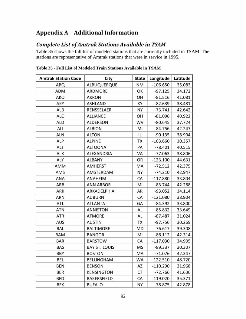
92

Appendix A – Additional Information

Complete List of Amtrak Stations Available in TSAM Table 35 shows the full list of modeled stations that are currently included in TSAM. The

stations are representative of Amtrak stations that were in service in 1995.

Table 35 - Full List of Modeled Train Stations Available in TSAM

Amtrak Station Code City State Longitude Latitude

ABQ ALBUQUERQUE NM -106.650 35.083

ADM ARDMORE OK -97.125 34.172

AKO AKRON OH -81.516 41.081

AKY ASHLAND KY -82.639 38.481

ALB RENSSELAER NY -73.741 42.642

ALC ALLIANCE OH -81.096 40.922

ALD ALDERSON WV -80.645 37.724

ALI ALBION MI -84.756 42.247

ALN ALTON IL -90.135 38.904

ALP ALPINE TX -103.660 30.357

ALT ALTOONA PA -78.401 40.515

ALX ALEXANDRIA VA -77.063 38.806

ALY ALBANY OR -123.100 44.631

AMM AMHERST MA -72.512 42.375

AMS AMSTERDAM NY -74.210 42.947

ANA ANAHEIM CA -117.880 33.804

ARB ANN ARBOR MI -83.744 42.288

ARK ARKADELPHIA AR -93.052 34.114

ARN AUBURN CA -121.080 38.904

ATL ATLANTA GA -84.392 33.800

ATN ANNISTON AL -85.832 33.649

ATR ATMORE AL -87.487 31.024

AUS AUSTIN TX -97.756 30.269

BAL BALTIMORE MD -76.617 39.308

BAM BANGOR MI -86.112 42.314

BAR BARSTOW CA -117.030 34.905

BAS BAY ST. LOUIS MS -89.337 30.307

BBY BOSTON MA -71.076 42.347

BEL BELLINGHAM WA -122.510 48.720

BEN BENSON AZ -110.290 31.968

BER KENSINGTON CT -72.766 41.636

BFD BAKERSFIELD CA -119.020 35.371

BFX BUFALO NY -78.875 42.878

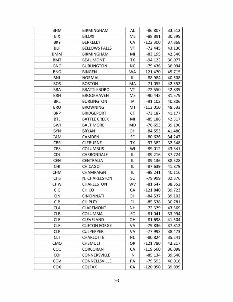
93

BHM BIRMINGHAM AL -86.807 33.512

BIX BILOXI MS -88.891 30.399

BKY BERKELEY CA -122.300 37.868

BLF BELLOWS FALLS VT -72.445 43.136

BMM BIRMINGHAM MI -83.195 42.546

BMT BEAUMONT TX -94.123 30.077

BNC BURLINGTON NC -79.436 36.094

BNG BINGEN WA -121.470 45.715

BNL NORMAL IL -88.984 40.508

BOS BOSTON MA -71.055 42.352

BRA BRATTLEBORO VT -72.550 42.839

BRH BROOKHAVEN MS -90.442 31.579

BRL BURLINGTON IA -91.102 40.806

BRO BROWNING MT -113.010 48.533

BRP BRIDGEPORT CT -73.187 41.177

BTL BATTLE CREEK MI -85.186 42.317

BWI BALTIMORE MD -76.693 39.190

BYN BRYAN OH -84.553 41.480

CAM CAMDEN SC -80.626 34.247

CBR CLEBURNE TX -97.382 32.348

CBS COLUMBUS WI -89.012 43.341

CDL CARBONDALE IL -89.216 37.724

CEN CENTRALIA IL -89.136 38.528

CHI CHICAGO IL -87.639 41.879

CHM CHAMPAIGN IL -88.241 40.116

CHS N. CHARLESTON SC -79.999 32.876

CHW CHARLESTON WV -81.647 38.352

CIC CHICO CA -121.840 39.723

CIN CINCINNATI OH -84.537 39.102

CIP CHIPLEY FL -85.538 30.781

CLA CLAREMONT NH -72.379 43.369

CLB COLUMBIA SC -81.041 33.994

CLE CLEVELAND OH -81.698 41.504

CLF CLIFTON FORGE VA -79.836 37.812

CLP CULPEPPER VA -77.993 38.473

CLT CHARLOTTE NC -80.824 35.241

CMO CHEMULT OR -121.780 43.217

COC CORCORAN CA -119.560 36.098

COI CONNERSVILLE IN -85.134 39.646

COV CONNELLSVILLE PA -79.593 40.018

COX COLFAX CA -120.950 39.099

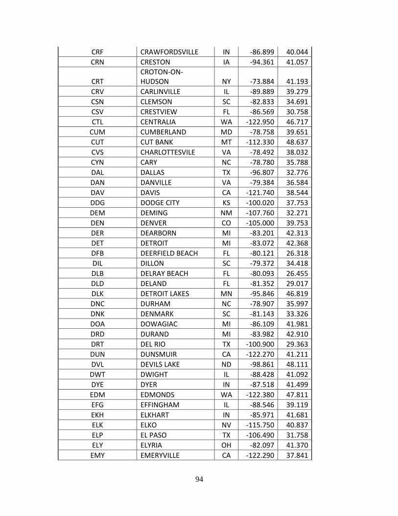
94

CRF CRAWFORDSVILLE IN -86.899 40.044

CRN CRESTON IA -94.361 41.057

CRT CROTON-ON-HUDSON NY -73.884 41.193

CRV CARLINVILLE IL -89.889 39.279

CSN CLEMSON SC -82.833 34.691

CSV CRESTVIEW FL -86.569 30.758

CTL CENTRALIA WA -122.950 46.717

CUM CUMBERLAND MD -78.758 39.651

CUT CUT BANK MT -112.330 48.637

CVS CHARLOTTESVILE VA -78.492 38.032

CYN CARY NC -78.780 35.788

DAL DALLAS TX -96.807 32.776

DAN DANVILLE VA -79.384 36.584

DAV DAVIS CA -121.740 38.544

DDG DODGE CITY KS -100.020 37.753

DEM DEMING NM -107.760 32.271

DEN DENVER CO -105.000 39.753

DER DEARBORN MI -83.201 42.313

DET DETROIT MI -83.072 42.368

DFB DEERFIELD BEACH FL -80.121 26.318

DIL DILLON SC -79.372 34.418

DLB DELRAY BEACH FL -80.093 26.455

DLD DELAND FL -81.352 29.017

DLK DETROIT LAKES MN -95.846 46.819

DNC DURHAM NC -78.907 35.997

DNK DENMARK SC -81.143 33.326

DOA DOWAGIAC MI -86.109 41.981

DRD DURAND MI -83.982 42.910

DRT DEL RIO TX -100.900 29.363

DUN DUNSMUIR CA -122.270 41.211

DVL DEVILS LAKE ND -98.861 48.111

DWT DWIGHT IL -88.428 41.092

DYE DYER IN -87.518 41.499

EDM EDMONDS WA -122.380 47.811

EFG EFFINGHAM IL -88.546 39.119

EKH ELKHART IN -85.971 41.681

ELK ELKO NV -115.750 40.837

ELP EL PASO TX -106.490 31.758

ELY ELYRIA OH -82.097 41.370

EMY EMERYVILLE CA -122.290 37.841

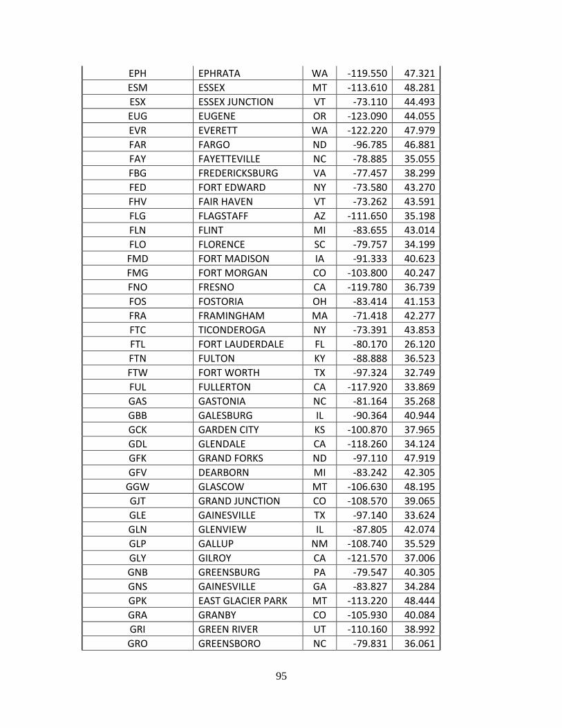
95

EPH EPHRATA WA -119.550 47.321

ESM ESSEX MT -113.610 48.281

ESX ESSEX JUNCTION VT -73.110 44.493

EUG EUGENE OR -123.090 44.055

EVR EVERETT WA -122.220 47.979

FAR FARGO ND -96.785 46.881

FAY FAYETTEVILLE NC -78.885 35.055

FBG FREDERICKSBURG VA -77.457 38.299

FED FORT EDWARD NY -73.580 43.270

FHV FAIR HAVEN VT -73.262 43.591

FLG FLAGSTAFF AZ -111.650 35.198

FLN FLINT MI -83.655 43.014

FLO FLORENCE SC -79.757 34.199

FMD FORT MADISON IA -91.333 40.623

FMG FORT MORGAN CO -103.800 40.247

FNO FRESNO CA -119.780 36.739

FOS FOSTORIA OH -83.414 41.153

FRA FRAMINGHAM MA -71.418 42.277

FTC TICONDEROGA NY -73.391 43.853

FTL FORT LAUDERDALE FL -80.170 26.120

FTN FULTON KY -88.888 36.523

FTW FORT WORTH TX -97.324 32.749

FUL FULLERTON CA -117.920 33.869

GAS GASTONIA NC -81.164 35.268

GBB GALESBURG IL -90.364 40.944

GCK GARDEN CITY KS -100.870 37.965

GDL GLENDALE CA -118.260 34.124

GFK GRAND FORKS ND -97.110 47.919

GFV DEARBORN MI -83.242 42.305

GGW GLASCOW MT -106.630 48.195

GJT GRAND JUNCTION CO -108.570 39.065

GLE GAINESVILLE TX -97.140 33.624

GLN GLENVIEW IL -87.805 42.074

GLP GALLUP NM -108.740 35.529

GLY GILROY CA -121.570 37.006

GNB GREENSBURG PA -79.547 40.305

GNS GAINESVILLE GA -83.827 34.284

GPK EAST GLACIER PARK MT -113.220 48.444

GRA GRANBY CO -105.930 40.084

GRI GREEN RIVER UT -110.160 38.992

GRO GREENSBORO NC -79.831 36.061

96

GRR GRAND RAPIDS MI -85.679 42.956

GRV GREENVILLE SC -82.414 34.857

GSC GLENWOOD SPRINGS CO -107.320 39.548

GUF GULFPORT MS -89.095 30.369

GVB GROVER BEACH CA -120.630 35.122

GWD GREENWOOD MS -90.176 33.518

GZZ GLENS FALLS NY -73.648 43.312

HAM HAMLET NC -79.698 34.883

HAR HARRISBURG PA -76.878 40.262

HAS HASTINGS NE -98.387 40.584

HAV HAVRE MT -109.680 48.554

HAZ HAZELHURST MS -90.394 31.863

HBG HATTIESBURG MS -89.286 31.327

HEM HERMANN MO -91.433 38.707

HER HELPER UT -110.850 39.688

HFD HARTFORD CT -72.682 41.768

HFY HARPERS FERRY WV -77.734 39.325

HGD HUNTINGDON PA -78.012 40.483

HIN HINTON WV -80.889 37.677

HLD HOLDREGE NE -99.371 40.436

HMD HAMMOND LA -90.464 30.512

HMI HAMMOND IN -87.509 41.693

HMN HAMILTON OH -84.560 39.395

HMW HOMEWOOD IL -87.669 41.562

HNF HANFORD CA -119.650 36.326

HOL HOLLYWOOD FL -80.169 26.011

HOM HOLLAND MI -86.098 42.789

HOS HOUSTON TX -95.367 29.767

HPT HIGH POINT NC -80.006 35.958

HUD HUDSON NY -73.798 42.253

HUN HUNTINGTON WV -82.441 38.415

HUT HUTCHINSON KS -97.930 38.056

IDP INDEPENDENCE MO -94.429 39.087

IND INDIANAPOLIS IN -86.160 39.762

IRV IRVINE CA -117.760 33.675

JAN JACKSON MS -90.191 32.301

JAX JACKSONVILLE FL -81.725 30.367

JEF JEFFERSON CITY MO -92.170 38.579

JOL JOLIET IL -88.079 41.525

JSP JESUP GA -81.882 31.606

JST JOHNSTOWN PA -78.922 40.330

97

JXN JACKSON MI -84.400 42.248

KAL KALAMAZOO MI -85.584 42.295

KAN KANNAPOLIS NC -80.622 35.501

KCY KANSAS CITY MO -94.584 39.086

KEL KELSO WA -122.910 46.143

KFS KLAMATH FALLS OR -121.770 42.226

KGC KING CITY CA -121.130 36.204

KIN WEST KINGSTON RI -71.562 41.484

KIS KISSIMMEE FL -81.405 28.293

KKI KANKAKEE IL -87.866 41.119

KNG KINGMAN AZ -114.050 35.188

KTR KINGSTREE SC -79.829 33.664

KWD KIRKWOOD MO -90.408 38.581

LAB LATROBE PA -79.385 40.318

LAF LAFAYETTE IN -86.895 40.421

LAJ LA JUNTA CO -103.540 37.988

LAK LAKELAND FL -81.952 28.046

LAP LA PLATA MO -92.485 40.031

LAU LAUREL MS -89.128 31.692

LAX LOS ANGELES CA -118.240 34.056

LCH LAKE CHARLES LA -93.215 30.238

LCN LINCOLN IL -89.363 40.148

LDB LORDSBURG NM -108.710 32.351

LEC LAKE CITY FL -82.651 30.197

LEE LEES SUMMIT MO -94.378 38.913

LEW LEWISTOWN PA -77.579 40.589

LFT LAFAYETTE LA -92.015 30.227

LIB LIBBY MT -115.550 48.395

LMR LAMAR CO -102.620 38.090

LMY LAMY NM -105.880 35.477

LNC LANCASTER PA -76.308 40.054

LNK LINCOLN NE -96.711 40.815

LNS EAST LANSING MI -84.494 42.719

LPE LAPEER MI -83.306 43.050

LRC LAWRENCE KS -95.232 38.972

LRK LITTLE ROCK AR -92.286 34.750

LSE LA CROSSE WI -91.248 43.834

LSV LAS VEGAS NM -105.210 35.593

LVW LONGVIEW TX -94.725 32.496

LYH LYNCHBURG VA -79.157 37.407

MAL MALTA MT -107.870 48.360

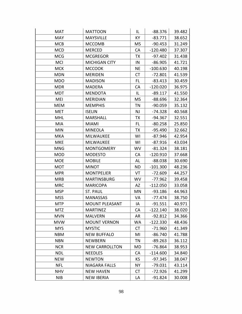
98

MAT MATTOON IL -88.376 39.482

MAY MAYSVILLE KY -83.771 38.652

MCB MCCOMB MS -90.453 31.249

MCD MERCED CA -120.480 37.307

MCG MCGREGOR TX -97.402 31.438

MCI MICHIGAN CITY IN -86.905 41.721

MCK MCCOOK NE -100.630 40.198

MDN MERIDEN CT -72.801 41.539

MDO MADISON FL -83.413 30.459

MDR MADERA CA -120.020 36.975

MDT MENDOTA IL -89.117 41.550

MEI MERIDIAN MS -88.696 32.364

MEM MEMPHIS TN -90.059 35.132

MET ISELIN NJ -74.328 40.568

MHL MARSHALL TX -94.367 32.551

MIA MIAMI FL -80.258 25.850

MIN MINEOLA TX -95.490 32.662

MKA MILWAUKEE WI -87.946 42.954

MKE MILWAUKEE WI -87.916 43.034

MNG MONTGOMERY WV -81.324 38.181

MOD MODESTO CA -120.910 37.668

MOE MOBILE AL -88.038 30.690

MOT MINOT ND -101.300 48.236

MPR MONTPELIER VT -72.609 44.257

MRB MARTINSBURG WV -77.962 39.458

MRC MARICOPA AZ -112.050 33.058

MSP ST. PAUL MN -93.186 44.963

MSS MANASSAS VA -77.474 38.750

MTP MOUNT PLEASANT IA -91.551 40.971

MTZ MARTINEZ CA -122.140 38.020

MVN MALVERN AR -92.812 34.366

MVW MOUNT VERNON WA -122.330 48.436

MYS MYSTIC CT -71.960 41.349

NBM NEW BUFFALO MI -86.740 41.788

NBN NEWBERN TN -89.263 36.112

NCR NEW CARROLLTON MD -76.864 38.953

NDL NEEDLES CA -114.600 34.840

NEW NEWTON KS -97.345 38.047

NFL NIAGARA FALLS NY -79.031 43.114

NHV NEW HAVEN CT -72.926 41.299

NIB NEW IBERIA LA -91.824 30.008

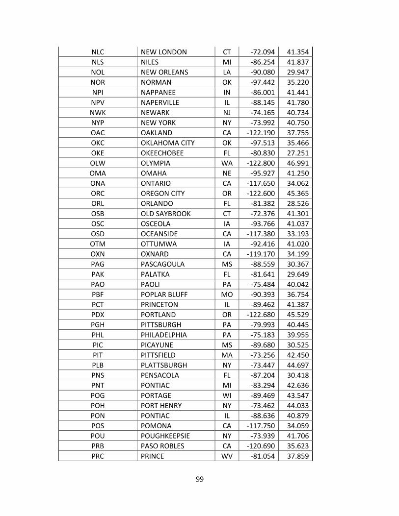
99

NLC NEW LONDON CT -72.094 41.354

NLS NILES MI -86.254 41.837

NOL NEW ORLEANS LA -90.080 29.947

NOR NORMAN OK -97.442 35.220

NPI NAPPANEE IN -86.001 41.441

NPV NAPERVILLE IL -88.145 41.780

NWK NEWARK NJ -74.165 40.734

NYP NEW YORK NY -73.992 40.750

OAC OAKLAND CA -122.190 37.755

OKC OKLAHOMA CITY OK -97.513 35.466

OKE OKEECHOBEE FL -80.830 27.251

OLW OLYMPIA WA -122.800 46.991

OMA OMAHA NE -95.927 41.250

ONA ONTARIO CA -117.650 34.062

ORC OREGON CITY OR -122.600 45.365

ORL ORLANDO FL -81.382 28.526

OSB OLD SAYBROOK CT -72.376 41.301

OSC OSCEOLA IA -93.766 41.037

OSD OCEANSIDE CA -117.380 33.193

OTM OTTUMWA IA -92.416 41.020

OXN OXNARD CA -119.170 34.199

PAG PASCAGOULA MS -88.559 30.367

PAK PALATKA FL -81.641 29.649

PAO PAOLI PA -75.484 40.042

PBF POPLAR BLUFF MO -90.393 36.754

PCT PRINCETON IL -89.462 41.387

PDX PORTLAND OR -122.680 45.529

PGH PITTSBURGH PA -79.993 40.445

PHL PHILADELPHIA PA -75.183 39.955

PIC PICAYUNE MS -89.680 30.525

PIT PITTSFIELD MA -73.256 42.450

PLB PLATTSBURGH NY -73.447 44.697

PNS PENSACOLA FL -87.204 30.418

PNT PONTIAC MI -83.294 42.636

POG PORTAGE WI -89.469 43.547

POH PORT HENRY NY -73.462 44.033

PON PONTIAC IL -88.636 40.879

POS POMONA CA -117.750 34.059

POU POUGHKEEPSIE NY -73.939 41.706

PRB PASO ROBLES CA -120.690 35.623

PRC PRINCE WV -81.054 37.859

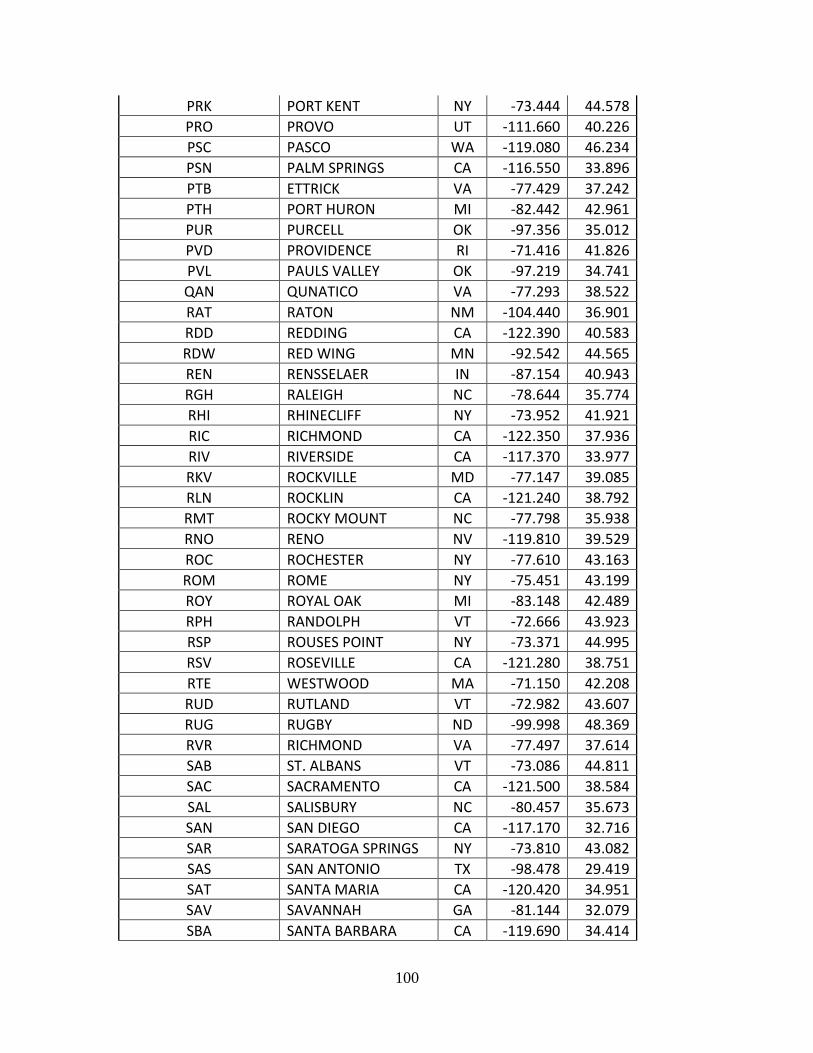
100

PRK PORT KENT NY -73.444 44.578

PRO PROVO UT -111.660 40.226

PSC PASCO WA -119.080 46.234

PSN PALM SPRINGS CA -116.550 33.896

PTB ETTRICK VA -77.429 37.242

PTH PORT HURON MI -82.442 42.961

PUR PURCELL OK -97.356 35.012

PVD PROVIDENCE RI -71.416 41.826

PVL PAULS VALLEY OK -97.219 34.741

QAN QUNATICO VA -77.293 38.522

RAT RATON NM -104.440 36.901

RDD REDDING CA -122.390 40.583

RDW RED WING MN -92.542 44.565

REN RENSSELAER IN -87.154 40.943

RGH RALEIGH NC -78.644 35.774

RHI RHINECLIFF NY -73.952 41.921

RIC RICHMOND CA -122.350 37.936

RIV RIVERSIDE CA -117.370 33.977

RKV ROCKVILLE MD -77.147 39.085

RLN ROCKLIN CA -121.240 38.792

RMT ROCKY MOUNT NC -77.798 35.938

RNO RENO NV -119.810 39.529

ROC ROCHESTER NY -77.610 43.163

ROM ROME NY -75.451 43.199

ROY ROYAL OAK MI -83.148 42.489

RPH RANDOLPH VT -72.666 43.923

RSP ROUSES POINT NY -73.371 44.995

RSV ROSEVILLE CA -121.280 38.751

RTE WESTWOOD MA -71.150 42.208

RUD RUTLAND VT -72.982 43.607

RUG RUGBY ND -99.998 48.369

RVR RICHMOND VA -77.497 37.614

SAB ST. ALBANS VT -73.086 44.811

SAC SACRAMENTO CA -121.500 38.584

SAL SALISBURY NC -80.457 35.673

SAN SAN DIEGO CA -117.170 32.716

SAR SARATOGA SPRINGS NY -73.810 43.082

SAS SAN ANTONIO TX -98.478 29.419

SAT SANTA MARIA CA -120.420 34.951

SAV SAVANNAH GA -81.144 32.079

SBA SANTA BARBARA CA -119.690 34.414

101

SBG SEBRING FL -81.435 27.497

SBY SHELBY MT -111.850 48.505

SCD ST. CLOUD MN -94.148 45.567

SCH SCHRIVER LA -90.813 29.747

SDL SLIDELL LA -89.782 30.278

SDY SCHENECTADY NY -73.943 42.815

SEA SEATTLE WA -122.330 47.599

SED SEDALIA MO -93.228 38.712

SFD SANFORD FL -81.289 28.806

SIM SIMI VALLEY CA -118.690 34.270

SJC SAN JOSE CA -121.900 37.331

SJM ST. JOSEPH MI -86.487 42.107

SKN STOCKTON CA -121.280 37.946

SKY SANDUSKY OH -82.712 41.440

SLC SALT LAKE CITY UT -111.900 40.762

SLM SALEM OR -123.030 44.932

SLO SAN LUIS OBISPO CA -120.650 35.277

SLV SOLVANG CA -120.140 34.596

SMC SAN MARCOS TX -97.936 29.879

SMT SUMMIT IL -87.813 41.792

SNA SANTA ANA CA -117.860 33.753

SNB SAN BERNARDINO CA -117.310 34.104

SNC LEE HALL CA -117.660 33.501

SND SANDERSON TX -102.400 30.140

SNS SALINAS CA -121.660 36.679

SOB SOUTH BEND IN -86.289 41.679

SOD SODA SPRINGS CA -120.370 39.324

SOL SOLANA BEACH CA -117.270 32.992

SOP SOUTHERN PINES NC -79.392 35.174

SPB SPARTANBURG SC -81.936 34.954

SPG SPRINGFIELD MA -72.594 42.106

SPI SPRINGFIELD IL -89.652 39.802

SPK SPOKANE WA -117.410 47.657

SPL STAPLES MN -94.795 46.355

SPM SOUTH SHORE KY -82.964 38.721

SPR SPARKS NV -119.750 39.542

SPT SANDPOINT ID -116.610 48.252

SPX SPARKS NV -119.760 39.534

SSM SELMA NC -78.281 35.532

STA STAUNTON VA -79.073 38.148

STL ST. LOUIS MO -90.205 38.624

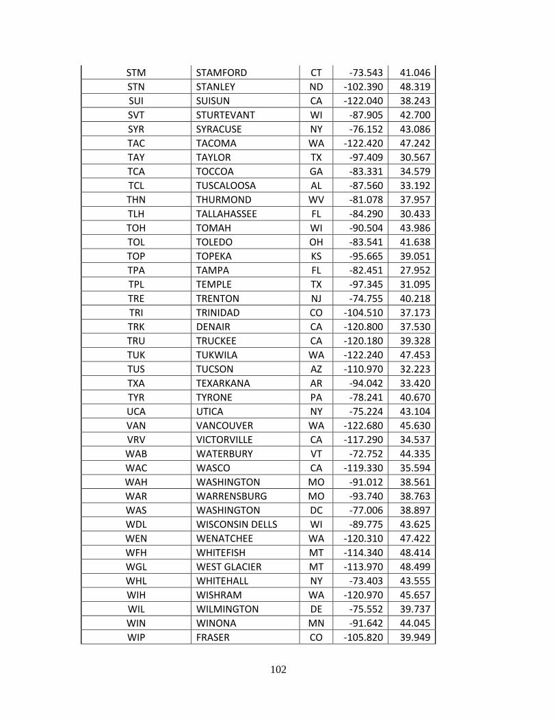
102

STM STAMFORD CT -73.543 41.046

STN STANLEY ND -102.390 48.319

SUI SUISUN CA -122.040 38.243

SVT STURTEVANT WI -87.905 42.700

SYR SYRACUSE NY -76.152 43.086

TAC TACOMA WA -122.420 47.242

TAY TAYLOR TX -97.409 30.567

TCA TOCCOA GA -83.331 34.579

TCL TUSCALOOSA AL -87.560 33.192

THN THURMOND WV -81.078 37.957

TLH TALLAHASSEE FL -84.290 30.433

TOH TOMAH WI -90.504 43.986

TOL TOLEDO OH -83.541 41.638

TOP TOPEKA KS -95.665 39.051

TPA TAMPA FL -82.451 27.952

TPL TEMPLE TX -97.345 31.095

TRE TRENTON NJ -74.755 40.218

TRI TRINIDAD CO -104.510 37.173

TRK DENAIR CA -120.800 37.530

TRU TRUCKEE CA -120.180 39.328

TUK TUKWILA WA -122.240 47.453

TUS TUCSON AZ -110.970 32.223

TXA TEXARKANA AR -94.042 33.420

TYR TYRONE PA -78.241 40.670

UCA UTICA NY -75.224 43.104

VAN VANCOUVER WA -122.680 45.630

VRV VICTORVILLE CA -117.290 34.537

WAB WATERBURY VT -72.752 44.335

WAC WASCO CA -119.330 35.594

WAH WASHINGTON MO -91.012 38.561

WAR WARRENSBURG MO -93.740 38.763

WAS WASHINGTON DC -77.006 38.897

WDL WISCONSIN DELLS WI -89.775 43.625

WEN WENATCHEE WA -120.310 47.422

WFH WHITEFISH MT -114.340 48.414

WGL WEST GLACIER MT -113.970 48.499

WHL WHITEHALL NY -73.403 43.555

WIH WISHRAM WA -120.970 45.657

WIL WILMINGTON DE -75.552 39.737

WIN WINONA MN -91.642 44.045

WIP FRASER CO -105.820 39.949

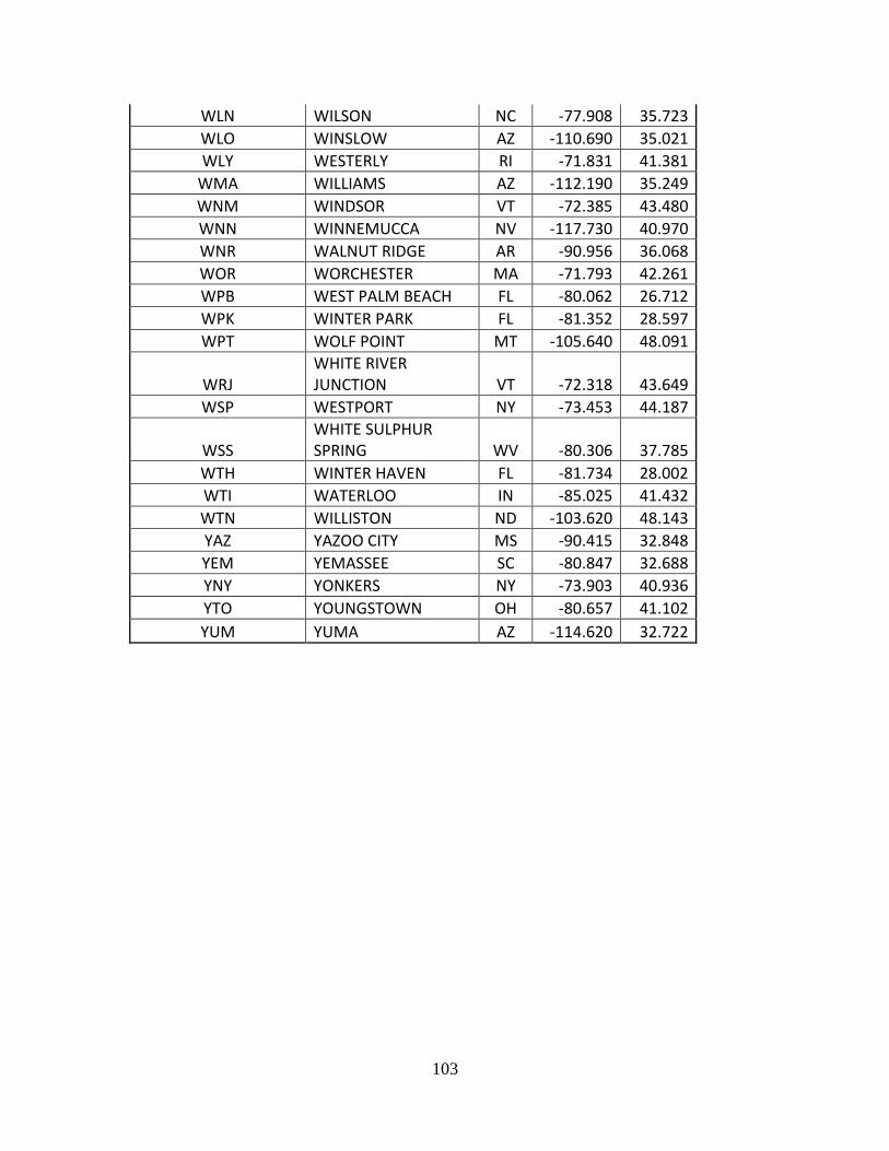
103

WLN WILSON NC -77.908 35.723

WLO WINSLOW AZ -110.690 35.021

WLY WESTERLY RI -71.831 41.381

WMA WILLIAMS AZ -112.190 35.249

WNM WINDSOR VT -72.385 43.480

WNN WINNEMUCCA NV -117.730 40.970

WNR WALNUT RIDGE AR -90.956 36.068

WOR WORCHESTER MA -71.793 42.261

WPB WEST PALM BEACH FL -80.062 26.712

WPK WINTER PARK FL -81.352 28.597

WPT WOLF POINT MT -105.640 48.091

WRJ WHITE RIVER JUNCTION VT -72.318 43.649

WSP WESTPORT NY -73.453 44.187

WSS WHITE SULPHUR SPRING WV -80.306 37.785

WTH WINTER HAVEN FL -81.734 28.002

WTI WATERLOO IN -85.025 41.432

WTN WILLISTON ND -103.620 48.143

YAZ YAZOO CITY MS -90.415 32.848

YEM YEMASSEE SC -80.847 32.688

YNY YONKERS NY -73.903 40.936

YTO YOUNGSTOWN OH -80.657 41.102

YUM YUMA AZ -114.620 32.722

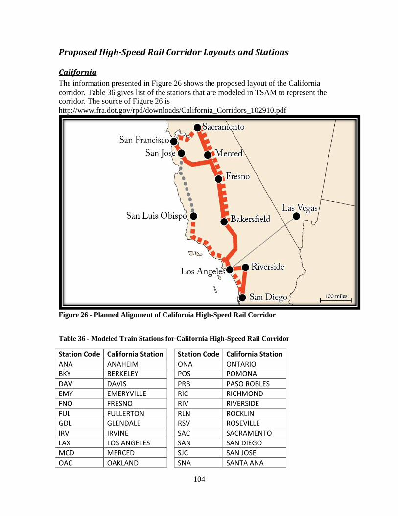
104

Proposed High-Speed Rail Corridor Layouts and Stations

California

The information presented in Figure 26 shows the proposed layout of the California

corridor. Table 36 gives list of the stations that are modeled in TSAM to represent the

corridor. The source of Figure 26 is

http://www.fra.dot.gov/rpd/downloads/California_Corridors_102910.pdf

Figure 26 - Planned Alignment of California High-Speed Rail Corridor

Table 36 - Modeled Train Stations for California High-Speed Rail Corridor

Station Code California Station Station Code California Station

ANA ANAHEIM ONA ONTARIO

BKY BERKELEY POS POMONA

DAV DAVIS PRB PASO ROBLES

EMY EMERYVILLE RIC RICHMOND

FNO FRESNO RIV RIVERSIDE

FUL FULLERTON RLN ROCKLIN

GDL GLENDALE RSV ROSEVILLE

IRV IRVINE SAC SACRAMENTO

LAX LOS ANGELES SAN SAN DIEGO

MCD MERCED SJC SAN JOSE

OAC OAKLAND SNA SANTA ANA

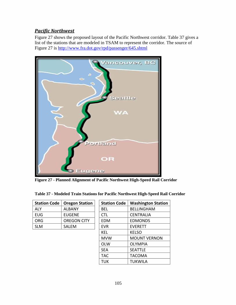
105

Pacific Northwest

Figure 27 shows the proposed layout of the Pacific Northwest corridor. Table 37 gives a

list of the stations that are modeled in TSAM to represent the corridor. The source of

Figure 27 is http://www.fra.dot.gov/rpd/passenger/645.shtml

Figure 27 - Planned Alignment of Pacific Northwest High-Speed Rail Corridor

Table 37 - Modeled Train Stations for Pacific Northwest High-Speed Rail Corridor

Station Code Oregon Station Station Code Washington Station

ALY ALBANY BEL BELLINGHAM

EUG EUGENE CTL CENTRALIA

ORG OREGON CITY EDM EDMONDS

SLM SALEM EVR EVERETT

KEL KELSO

MVW MOUNT VERNON

OLW OLYMPIA

SEA SEATTLE

TAC TACOMA

TUK TUKWILA

106

Florida

Figure 28 shows the proposed layout of the Florida corridor. Table 38 gives a list of the

stations that are modeled in TSAM to represent the corridor. The source of Figure 28 is

http://www.fra.dot.gov/rpd/downloads/Tampa_Orlando_Miami_FINAL_1027.pdf

Figure 28 - Planned Alignment of Florida High-Speed Rail Corridor

Table 38 - Modeled Train Stations for Florida High-Speed Rail Corridor

Station Code Florida Stations Station Code Florida Stations

DFB DEERFIELD BEACH ORL ORLANDO

DLB DELRAY BEACH SFD SANFORD

FTL FORT LAUDERDALE TPA TAMPA

HOL HOLLYWOOD WPB WEST PALM BEACH

KIS KISSIMMEE WPK WINTER PARK

LAK LAKELAND WTH WINTER HAVEN

MIA MIAMI

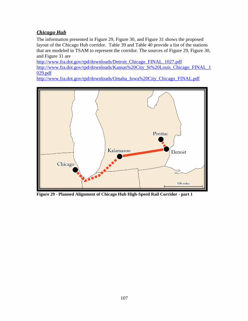
107

Chicago Hub

The information presented in Figure 29, Figure 30, and Figure 31 shows the proposed

layout of the Chicago Hub corridor. Table 39 and Table 40 provide a list of the stations

that are modeled in TSAM to represent the corridor. The sources of Figure 29, Figure 30,

and Figure 31 are

http://www.fra.dot.gov/rpd/downloads/Detroit_Chicago_FINAL_1027.pdf

http://www.fra.dot.gov/rpd/downloads/Kansas%20City_St%20Louis_Chicago_FINAL_1

029.pdf

http://www.fra.dot.gov/rpd/downloads/Omaha_Iowa%20City_Chicago_FINAL.pdf

Figure 29 - Planned Alignment of Chicago Hub High-Speed Rail Corridor - part 1

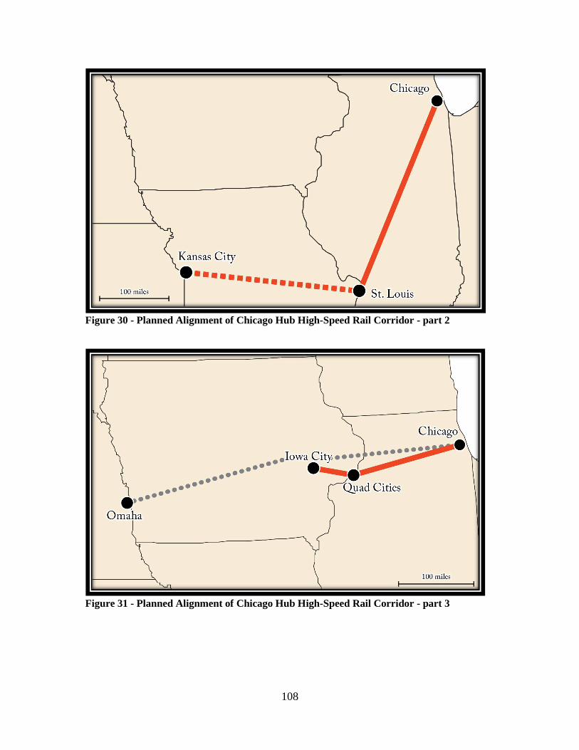
108

Figure 30 - Planned Alignment of Chicago Hub High-Speed Rail Corridor - part 2

Figure 31 - Planned Alignment of Chicago Hub High-Speed Rail Corridor - part 3

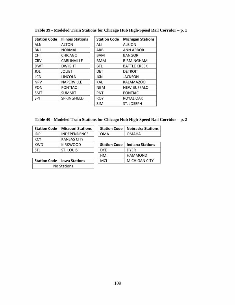
109

Table 39 - Modeled Train Stations for Chicago Hub High-Speed Rail Corridor – p. 1

Station Code Illinois Stations Station Code Michigan Stations

ALN ALTON ALI ALBION

BNL NORMAL ARB ANN ARBOR

CHI CHICAGO BAM BANGOR

CRV CARLINVILLE BMM BIRMINGHAM

DWT DWIGHT BTL BATTLE CREEK

JOL JOLIET DET DETROIT

LCN LINCOLN JXN JACKSON

NPV NAPERVILLE KAL KALAMAZOO

PON PONTIAC NBM NEW BUFFALO

SMT SUMMIT PNT PONTIAC

SPI SPRINGFIELD ROY ROYAL OAK

SJM ST. JOSEPH

Table 40 - Modeled Train Stations for Chicago Hub High-Speed Rail Corridor – p. 2

Station Code Missouri Stations Station Code Nebraska Stations

IDP INDEPENDENCE OMA OMAHA

KCY KANSAS CITY

KWD KIRKWOOD Station Code Indiana Stations

STL ST. LOUIS DYE DYER

HMI HAMMOND

Station Code Iowa Stations MCI MICHIGAN CITY

No Stations

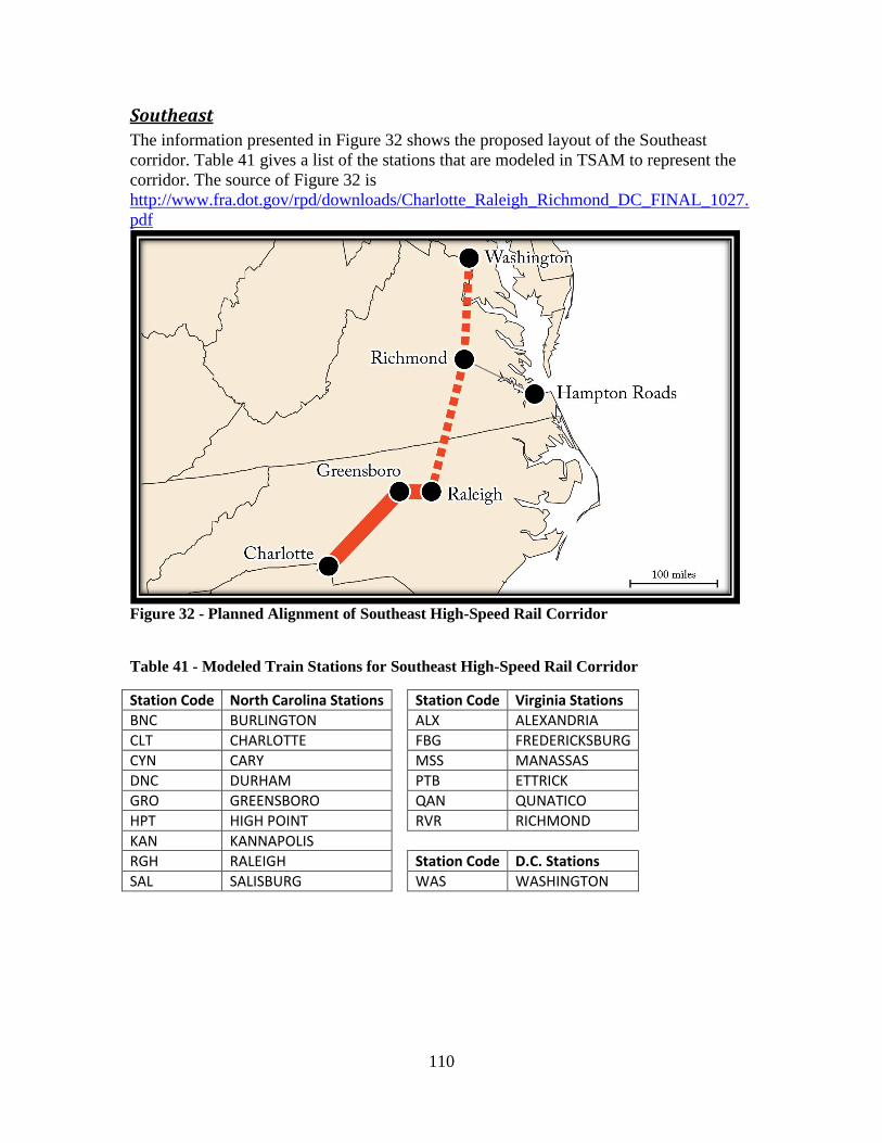
110

Southeast

The information presented in Figure 32 shows the proposed layout of the Southeast

corridor. Table 41 gives a list of the stations that are modeled in TSAM to represent the

corridor. The source of Figure 32 is

http://www.fra.dot.gov/rpd/downloads/Charlotte_Raleigh_Richmond_DC_FINAL_1027.

pdf

Figure 32 - Planned Alignment of Southeast High-Speed Rail Corridor

Table 41 - Modeled Train Stations for Southeast High-Speed Rail Corridor

Station Code North Carolina Stations Station Code Virginia Stations

BNC BURLINGTON ALX ALEXANDRIA

CLT CHARLOTTE FBG FREDERICKSBURG

CYN CARY MSS MANASSAS

DNC DURHAM PTB ETTRICK

GRO GREENSBORO QAN QUNATICO

HPT HIGH POINT RVR RICHMOND

KAN KANNAPOLIS

RGH RALEIGH Station Code D.C. Stations

SAL SALISBURG WAS WASHINGTON

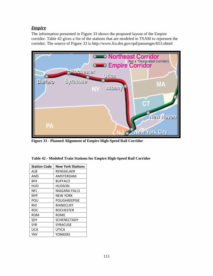
111

Empire

The information presented in Figure 33 shows the proposed layout of the Empire

corridor. Table 42 gives a list of the stations that are modeled in TSAM to represent the

corridor. The source of Figure 33 is http://www.fra.dot.gov/rpd/passenger/653.shtml

Figure 33 - Planned Alignment of Empire High-Speed Rail Corridor

Table 42 - Modeled Train Stations for Empire High-Speed Rail Corridor

Station Code New York Stations

ALB RENSSELAER

AMS AMSTERDAM

BFX BUFFALO

HUD HUDSON

NFL NIAGARA FALLS

NYP NEW YORK

POU POUGHKEEPSIE

RHI RHINECLIFF

ROC ROCHESTER

ROM ROME

SDY SCHENECTADY

SYR SYRACUSE

UCA UTICA

YNY YONKERS

112

Northern New England

The information presented in Figure 34 shows the proposed layout of the Northern New

England corridor. Table 43 gives a list of the stations that are modeled in TSAM to

represent the corridor. The source of Figure 34 is

http://www.fra.dot.gov/rpd/passenger/654.shtml

Figure 34 - Planned Alignment of Northern New England High-Speed Rail Corridor

Table 43 - Modeled Train Stations for Northern New England High-Speed Rail Corridor

Station Code New York Stations Station Code Massachusetts Stations

ALB RENSSELAER BBY BOSTON

FED FORT EDWARD FRA FRAMINGHAM

FTC TICONDEROGA SPG SPRINGFIELD

GZZ GLENS FALL WOR WORCHESTER

PLB PLATTSBURGH

POH PORT HENRY Station Code Connecticut Stations

PRK PORT KENT BER KENSINGTON

RSP ROUSES POINT HFD HARTFORD

WHL WHITEHALL MDN MERIDEN

WSP WESTPORT NHV NEW HAVEN

113

Keystone

The information presented in Figure 35 shows the proposed layout of the Keystone

corridor. Table 44 gives a list of the stations that are modeled in TSAM to represent the

corridor. The source of Figure 35 is http://www.fra.dot.gov/rpd/passenger/652.shtml

Figure 35 - Planned Alignment of High-Speed Rail Corridor

Table 44 - Modeled Train Stations for Keystone High-Speed Rail Corridor

Station Code Pennsylvania Stations

COV CONNELLSVILLE

GNB GREENSBURG

HAR HARRISBURG

LAB LATROBE

PAO PAOLI

PGH PITTSBURGH

PHL PHILADELPHIA

114

South Central

The information presented in Figure 36 shows the proposed layout of the South Central

corridor. Table 45 gives a list of the stations that are modeled in TSAM to represent the

corridor. The source of Figure 36 is http://www.fra.dot.gov/rpd/passenger/647.shtml

Figure 36 - Planned Alignment of South Central High-Speed Rail Corridor

Table 45 - Modeled Train Stations for South Central High-Speed Rail Corridor

Station Code Oklahoma Stations Station Code Texas Stations

ADM ADRMORE AUS AUSTIN

NOR NORMAN CBR CLEBURNE

OKC OKLAHOMA CITY DAL DALLAS

PUR PURCELL FTW FORT WORTH

PVL PAULS VALLEY GLE GAINESVILLE

MCG MCGREGOR

Station Code Arkansas Stations SAS SAN ANTONIO

ARK ARKADELPHIA SMC SAN MARCOS

LRK LITTLE ROCK TAY TAYLOR

MVN MALVERN TPL TEMPLE

TXA TEXARKANA

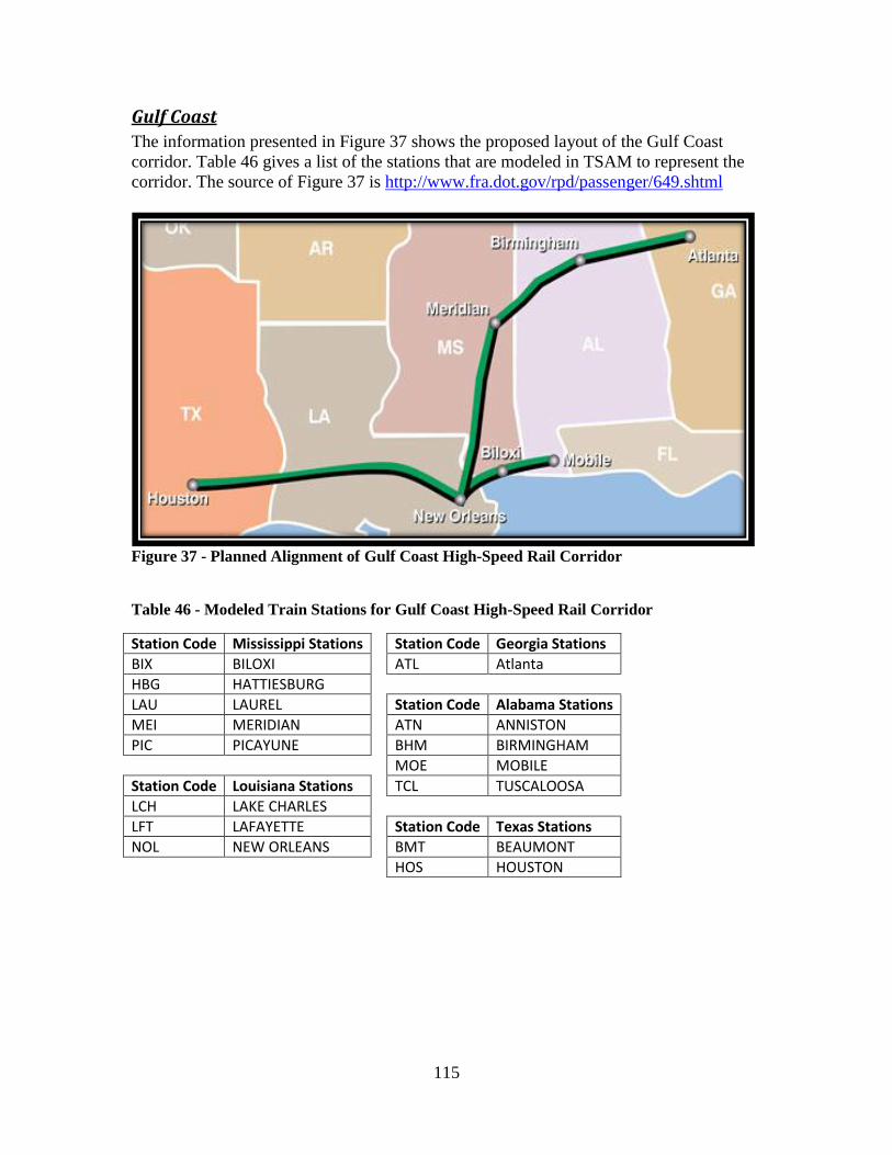
115

Gulf Coast

The information presented in Figure 37 shows the proposed layout of the Gulf Coast

corridor. Table 46 gives a list of the stations that are modeled in TSAM to represent the

corridor. The source of Figure 37 is http://www.fra.dot.gov/rpd/passenger/649.shtml

Figure 37 - Planned Alignment of Gulf Coast High-Speed Rail Corridor

Table 46 - Modeled Train Stations for Gulf Coast High-Speed Rail Corridor

Station Code Mississippi Stations Station Code Georgia Stations

BIX BILOXI ATL Atlanta

HBG HATTIESBURG

LAU LAUREL Station Code Alabama Stations

MEI MERIDIAN ATN ANNISTON

PIC PICAYUNE BHM BIRMINGHAM

MOE MOBILE

Station Code Louisiana Stations TCL TUSCALOOSA

LCH LAKE CHARLES

LFT LAFAYETTE Station Code Texas Stations

NOL NEW ORLEANS BMT BEAUMONT

HOS HOUSTON

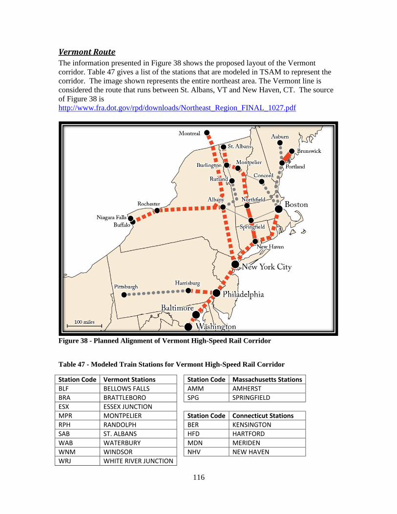
116

Vermont Route

The information presented in Figure 38 shows the proposed layout of the Vermont

corridor. Table 47 gives a list of the stations that are modeled in TSAM to represent the

corridor. The image shown represents the entire northeast area. The Vermont line is

considered the route that runs between St. Albans, VT and New Haven, CT. The source

of Figure 38 is

http://www.fra.dot.gov/rpd/downloads/Northeast_Region_FINAL_1027.pdf

Figure 38 - Planned Alignment of Vermont High-Speed Rail Corridor

Table 47 - Modeled Train Stations for Vermont High-Speed Rail Corridor

Station Code Vermont Stations Station Code Massachusetts Stations

BLF BELLOWS FALLS AMM AMHERST

BRA BRATTLEBORO SPG SPRINGFIELD

ESX ESSEX JUNCTION

MPR MONTPELIER Station Code Connecticut Stations

RPH RANDOLPH BER KENSINGTON

SAB ST. ALBANS HFD HARTFORD

WAB WATERBURY MDN MERIDEN

WNM WINDSOR NHV NEW HAVEN

WRJ WHITE RIVER JUNCTION

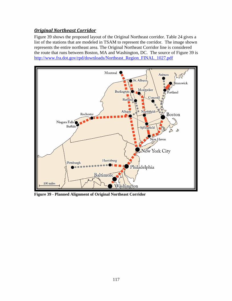
117

Original Northeast Corridor

Figure 39 shows the proposed layout of the Original Northeast corridor. Table 24 gives a

list of the stations that are modeled in TSAM to represent the corridor. The image shown

represents the entire northeast area. The Original Northeast Corridor line is considered

the route that runs between Boston, MA and Washington, DC. The source of Figure 39 is

http://www.fra.dot.gov/rpd/downloads/Northeast_Region_FINAL_1027.pdf

Figure 39 - Planned Alignment of Original Northeast Corridor

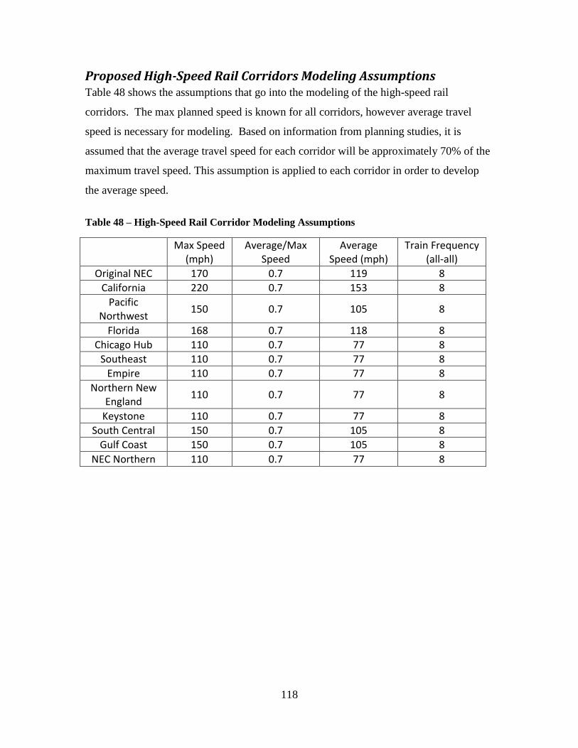
118

Proposed High-Speed Rail Corridors Modeling Assumptions Table 48 shows the assumptions that go into the modeling of the high-speed rail

corridors. The max planned speed is known for all corridors, however average travel

speed is necessary for modeling. Based on information from planning studies, it is

assumed that the average travel speed for each corridor will be approximately 70% of the

maximum travel speed. This assumption is applied to each corridor in order to develop

the average speed.

Table 48 – High-Speed Rail Corridor Modeling Assumptions

Max Speed

(mph) Average/Max

Speed Average

Speed (mph) Train Frequency

(all-all)

Original NEC 170 0.7 119 8

California 220 0.7 153 8

Pacific Northwest

150 0.7 105 8

Florida 168 0.7 118 8

Chicago Hub 110 0.7 77 8

Southeast 110 0.7 77 8

Empire 110 0.7 77 8

Northern New England

110 0.7 77 8

Keystone 110 0.7 77 8

South Central 150 0.7 105 8

Gulf Coast 150 0.7 105 8

NEC Northern 110 0.7 77 8

119

Nationwide Train Travel Time and Travel Cost Regression Curves Figure 40 shows the travel time regression that is used to model the northeast region

service that operates in the Northeast Corridor. This regional service was in place before

the Acela service and continues to operate today, however for the purpose of TSAM, the

regional service is modeled only from 1995 – 2000. Figure 41 shows the travel time

regression curve for the regional service.

Figure 40 - Northeast Corridor Regional Service Travel Time Regression Curve

Figure 41 - Northeast Corridor Regional Service Travel Cost Regression Curve

y = 0.9629x R² = 0.9025

0

100

200

300

400

500

600

0 100 200 300 400 500 600 700

Travel Time vs Distance

One Way Distance (Miles)

Trav

el T

Ime

(Min

ute

s)

y = 5E-07x3 - 0.0007x2 + 0.3392x R² = 0.9334

0

10

20

30

40

50

60

70

80

0 100 200 300 400 500 600 700

Travel Cost vs Distance

One Way Distance (Miles)

Trav

el C

ost

($

)

120

Figure 42 shows the regression analysis that is used to determine the curve that

will be used to estimate the travel time of the Acela Express train. A linear curve

is found to be the best fit; the line is set to have an intercept of 0 so that the

equation is valid for all distances.

Figure 42 - Acela Express Travel Time Regression Curve

Figure 43 shows the regression analysis that is used to determine the curve that

will be used to estimate the travel cost of the Acela Express train. A third order

polynomial is found to be the best fit. The equation of the line and the R2 value is

shown on the chart.

y = 0.0132x R² = 0.9664

0

1

2

3

4

5

6

7

8

9

0 100 200 300 400 500 600 700

Acela Travel Time vs Distance

Travel Distance (Miles)

Trav

el T

ime

(h

rs)

Figure 43 - Acela Express Travel Cost Regression Curve

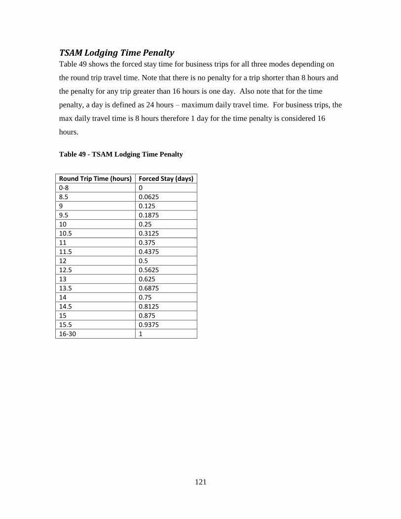
121

TSAM Lodging Time Penalty Table 49 shows the forced stay time for business trips for all three modes depending on

the round trip travel time. Note that there is no penalty for a trip shorter than 8 hours and

the penalty for any trip greater than 16 hours is one day. Also note that for the time

penalty, a day is defined as 24 hours – maximum daily travel time. For business trips, the

max daily travel time is 8 hours therefore 1 day for the time penalty is considered 16

hours.

Table 49 - TSAM Lodging Time Penalty

Round Trip Time (hours) Forced Stay (days)

0-8 0

8.5 0.0625

9 0.125

9.5 0.1875

10 0.25

10.5 0.3125

11 0.375

11.5 0.4375

12 0.5

12.5 0.5625

13 0.625

13.5 0.6875

14 0.75

14.5 0.8125

15 0.875

15.5 0.9375

16-30 1

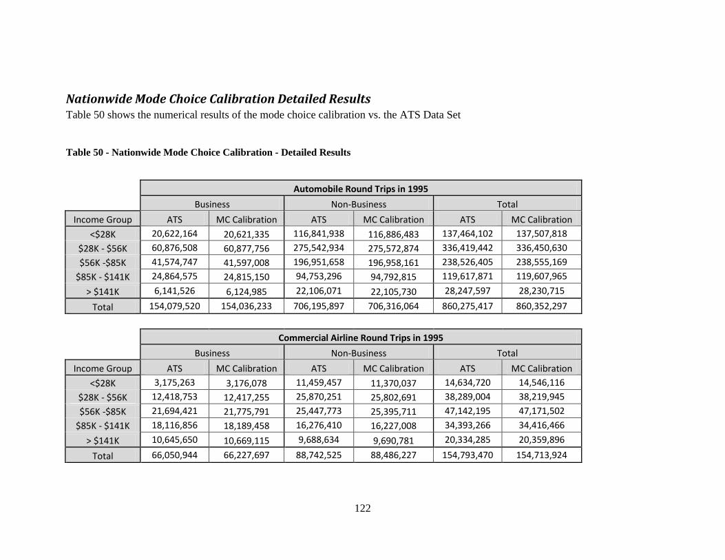
122

Nationwide Mode Choice Calibration Detailed Results Table 50 shows the numerical results of the mode choice calibration vs. the ATS Data Set

Table 50 - Nationwide Mode Choice Calibration - Detailed Results

Automobile Round Trips in 1995

Business Non-Business Total

Income Group ATS MC Calibration ATS MC Calibration ATS MC Calibration

<$28K 20,622,164 20,621,335 116,841,938 116,886,483 137,464,102 137,507,818

$28K - $56K 60,876,508 60,877,756 275,542,934 275,572,874 336,419,442 336,450,630

$56K -$85K 41,574,747 41,597,008 196,951,658 196,958,161 238,526,405 238,555,169

$85K - $141K 24,864,575 24,815,150 94,753,296 94,792,815 119,617,871 119,607,965

> $141K 6,141,526 6,124,985 22,106,071 22,105,730 28,247,597 28,230,715

Total 154,079,520 154,036,233 706,195,897 706,316,064 860,275,417 860,352,297

Commercial Airline Round Trips in 1995

Business Non-Business Total

Income Group ATS MC Calibration ATS MC Calibration ATS MC Calibration

<$28K 3,175,263 3,176,078 11,459,457 11,370,037 14,634,720 14,546,116

$28K - $56K 12,418,753 12,417,255 25,870,251 25,802,691 38,289,004 38,219,945

$56K -$85K 21,694,421 21,775,791 25,447,773 25,395,711 47,142,195 47,171,502

$85K - $141K 18,116,856 18,189,458 16,276,410 16,227,008 34,393,266 34,416,466

> $141K 10,645,650 10,669,115 9,688,634 9,690,781 20,334,285 20,359,896

Total 66,050,944 66,227,697 88,742,525 88,486,227 154,793,470 154,713,924

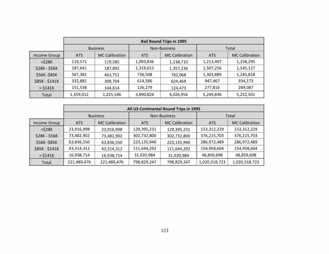
123

Rail Round Trips in 1995

Business Non-Business Total

Income Group ATS MC Calibration ATS MC Calibration ATS MC Calibration

<$28K 119,571 119,585 1,093,836 1,138,710 1,213,407 1,258,295

$28K - $56K 187,641 187,892 1,319,615 1,357,236 1,507,256 1,545,127

$56K -$85K 567,381 463,751 736,508 782,068 1,303,889 1,245,818

$85K - $141K 332,881 309,704 614,586 624,469 947,467 934,173

> $141K 151,538 144,614 126,279 124,473 277,816 269,087

Total 1,359,012 1,225,546 3,890,824 4,026,956 5,249,836 5,252,501

All US Continental Round Trips in 1995

Business Non-Business Total

Income Group ATS MC Calibration ATS MC Calibration ATS MC Calibration

<$28K 23,916,998 23,916,998 129,395,231 129,395,231 153,312,229 153,312,229

$28K - $56K 73,482,902 73,482,902 302,732,800 302,732,800 376,215,703 376,215,703

$56K -$85K 63,836,550 63,836,550 223,135,940 223,135,940 286,972,489 286,972,489

$85K - $141K 43,314,312 43,314,312 111,644,292 111,644,292 154,958,604 154,958,604

> $141K 16,938,714 16,938,714 31,920,984 31,920,984 48,859,698 48,859,698

Total 221,489,476 221,489,476 798,829,247 798,829,247 1,020,318,723 1,020,318,723

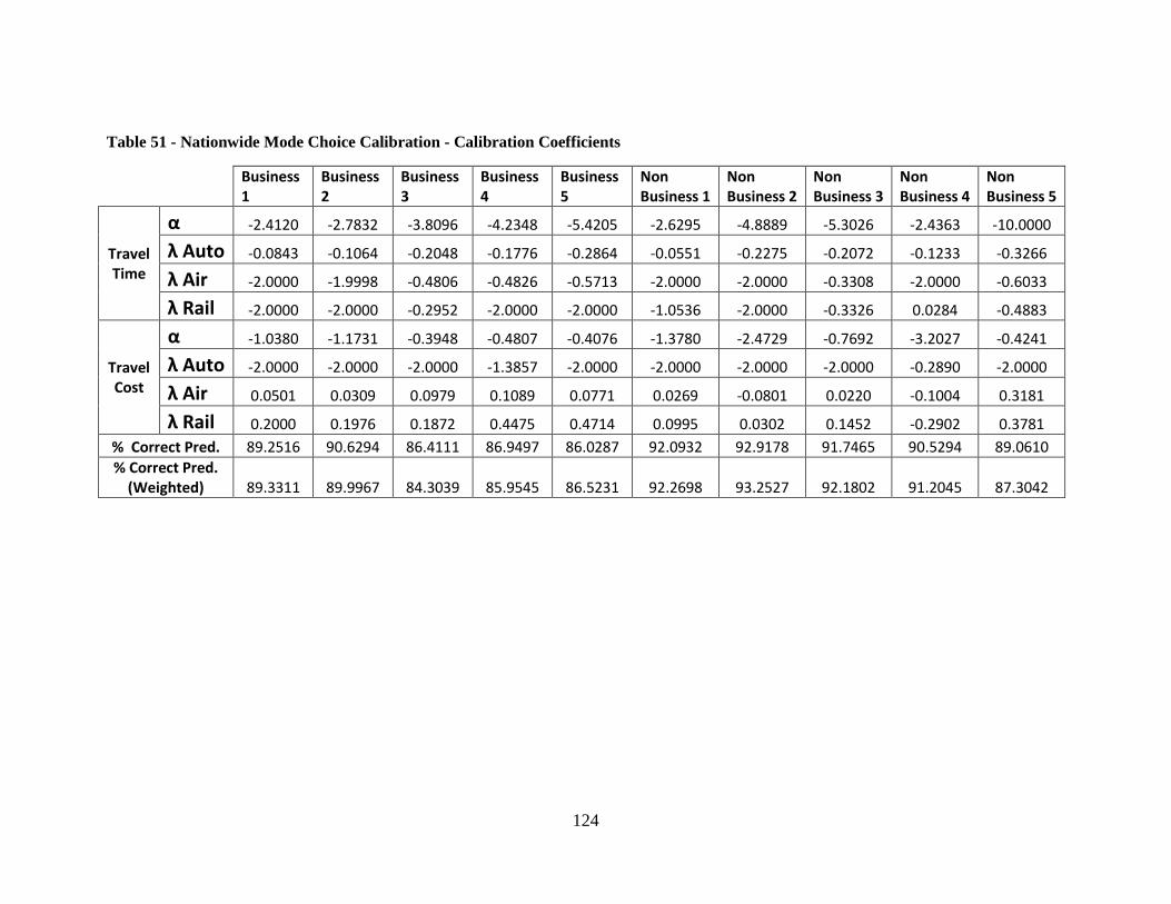
124

Table 51 - Nationwide Mode Choice Calibration - Calibration Coefficients

Business 1

Business 2

Business 3

Business 4

Business 5

Non Business 1

Non Business 2

Non Business 3

Non Business 4

Non Business 5

Travel Time

α -2.4120 -2.7832 -3.8096 -4.2348 -5.4205 -2.6295 -4.8889 -5.3026 -2.4363 -10.0000

λ Auto -0.0843 -0.1064 -0.2048 -0.1776 -0.2864 -0.0551 -0.2275 -0.2072 -0.1233 -0.3266

λ Air -2.0000 -1.9998 -0.4806 -0.4826 -0.5713 -2.0000 -2.0000 -0.3308 -2.0000 -0.6033

λ Rail -2.0000 -2.0000 -0.2952 -2.0000 -2.0000 -1.0536 -2.0000 -0.3326 0.0284 -0.4883

Travel Cost

α -1.0380 -1.1731 -0.3948 -0.4807 -0.4076 -1.3780 -2.4729 -0.7692 -3.2027 -0.4241

λ Auto -2.0000 -2.0000 -2.0000 -1.3857 -2.0000 -2.0000 -2.0000 -2.0000 -0.2890 -2.0000

λ Air 0.0501 0.0309 0.0979 0.1089 0.0771 0.0269 -0.0801 0.0220 -0.1004 0.3181

λ Rail 0.2000 0.1976 0.1872 0.4475 0.4714 0.0995 0.0302 0.1452 -0.2902 0.3781

% Correct Pred. 89.2516 90.6294 86.4111 86.9497 86.0287 92.0932 92.9178 91.7465 90.5294 89.0610

% Correct Pred. (Weighted) 89.3311 89.9967 84.3039 85.9545 86.5231 92.2698 93.2527 92.1802 91.2045 87.3042

125

TSAM Mode Choice Application Detailed Results

Baseline Case

Table 52 below provides the detailed results for the baseline 2011 TSAM run. This run

models only the existing train corridors using the time and cost curves that are presented.

Table 52 - TSAM Mode Choice Detailed Results - Baseline Case

Automobile Trips

Income Group Business Non Business Total

<$28K 18,302,061 101,988,905 120,290,966

$28K - $56K 69,095,049 300,736,295 369,831,344

$56K -$85K 58,692,340 263,065,428 321,757,768

$85K - $141K 38,384,766 136,906,056 175,290,822

> $141K 10,371,675 37,668,045 48,039,720

Total 194,845,891 840,364,729 1,035,210,620

CA Trips

Income Group Business Non Business Total

<$28K 2,871,546 13,075,518 15,947,064

$28K - $56K 13,636,714 35,914,522 49,551,236

$56K -$85K 29,533,071 43,218,409 72,751,480

$85K - $141K 26,576,778 29,556,003 56,132,781

> $141K 17,407,717 14,529,180 31,936,897

Total 90,025,826 136,293,632 226,319,458

Train Trips

Income Group Business Non Business Total

<$28K 54,346 1,156,826 1,211,172

$28K - $56K 91,542 1,827,457 1,918,999

$56K -$85K 717,496 1,041,833 1,759,329

$85K - $141K 334,846 1,364,335 1,699,181

> $141K 183,970 149,408 333,378

Total 1,382,200 5,539,859 6,922,059

126

Total Trips

Income Group Business Non Business Total

<$28K 21,227,953 116,221,249 137,449,202

$28K - $56K 82,823,305 338,478,274 421,301,579

$56K -$85K 88,942,907 307,325,670 396,268,577

$85K - $141K 65,296,390 167,826,394 233,122,784

> $141K 27,963,362 52,346,633 80,309,995

Total 286,253,917 982,198,220 1,268,452,137

Scenario 1

Table 53 below provides the detailed results for the baseline 2011 TSAM run. This run

models the future corridors with a travel cost of $0.20/mile and uses the planned average

travel speeds.

Table 53 - TSAM Mode Choice Detailed Results - Scenario 1

Automobile Trips

Income Group Business Non Business Total

<$28K 18,239,582 101,735,837 119,975,419

$28K - $56K 68,896,646 300,240,084 369,136,730

$56K -$85K 57,953,303 262,274,095 320,227,398

$85K - $141K 37,066,725 135,839,942 172,906,667

> $141K 9,803,167 37,510,520 47,313,687

Total 191,959,423 837,600,478 1,029,559,901

CA Trips

Income Group Business Non Business Total

<$28K 2,868,760 13,058,616 15,927,376

$28K - $56K 13,620,185 35,882,506 49,502,691

$56K -$85K 29,428,061 43,170,634 72,598,695

$85K - $141K 26,310,657 29,469,043 55,779,700

> $141K 17,151,409 14,516,860 31,668,269

Total 89,379,072 136,097,659 225,476,731

127

Train Trips

Income Group Business Non Business Total

<$28K 119,611 1,426,796 1,546,407

$28K - $56K 306,474 2,355,684 2,662,158

$56K -$85K 1,561,543 1,880,941 3,442,484

$85K - $141K 1,919,008 2,517,409 4,436,417

> $141K 1,008,786 319,253 1,328,039

Total 4,915,422 8,500,083 13,415,505

Total Trips

Income Group Business Non Business Total

<$28K 21,227,953 116,221,249 137,449,202

$28K - $56K 82,823,305 338,478,274 421,301,579

$56K -$85K 88,942,907 307,325,670 396,268,577

$85K - $141K 65,296,390 167,826,394 233,122,784

> $141K 27,963,362 52,346,633 80,309,995

Total 286,253,917 982,198,220 1,268,452,137

Scenario 2

Table 54 below provides the detailed results for the baseline 2011 TSAM run. This run

models the future corridors with a travel cost of $0.20/mile and an average travel speed of

153 mph for all projected corridors.

Table 54 - TSAM Mode Choice Detailed Results - Scenario 2

Automobile Trips

Income Group Business Non Business Total

<$28K 18,218,175 101,668,029 119,886,204

$28K - $56K 68,802,074 300,098,999 368,901,073

$56K -$85K 57,848,047 261,919,127 319,767,174

$85K - $141K 36,432,980 135,360,294 171,793,274

> $141K 9,594,999 37,382,581 46,977,580

Total 190,896,275 836,429,030 1,027,325,305

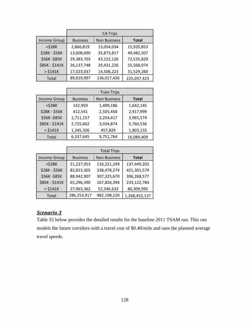
128

CA Trips

Income Group Business Non Business Total

<$28K 2,866,819 13,054,034 15,920,853

$28K - $56K 13,608,690 35,873,817 49,482,507

$56K -$85K 29,383,703 43,152,126 72,535,829

$85K - $141K 26,137,748 29,431,226 55,568,974

> $141K 17,023,037 14,506,223 31,529,260

Total 89,019,997 136,017,426 225,037,423

Train Trips

Income Group Business Non Business Total

<$28K 142,959 1,499,186 1,642,145

$28K - $56K 412,541 2,505,458 2,917,999

$56K -$85K 1,711,157 2,254,417 3,965,574

$85K - $141K 2,725,662 3,034,874 5,760,536

> $141K 1,345,326 457,829 1,803,155

Total 6,337,645 9,751,764 16,089,409

Total Trips

Income Group Business Non Business Total

<$28K 21,227,953 116,221,249 137,449,202

$28K - $56K 82,823,305 338,478,274 421,301,579

$56K -$85K 88,942,907 307,325,670 396,268,577

$85K - $141K 65,296,390 167,826,394 233,122,784

> $141K 27,963,362 52,346,633 80,309,995

Total 286,253,917 982,198,220 1,268,452,137

Scenario 3

Table 55 below provides the detailed results for the baseline 2011 TSAM run. This run

models the future corridors with a travel cost of $0.40/mile and uses the planned average

travel speeds.

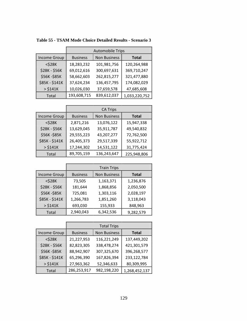
129

Table 55 - TSAM Mode Choice Detailed Results - Scenario 3

Automobile Trips

Income Group Business Non Business Total

<$28K 18,283,232 101,981,756 120,264,988

$28K - $56K 69,012,616 300,697,631 369,710,247

$56K -$85K 58,662,603 262,815,277 321,477,880

$85K - $141K 37,624,234 136,457,795 174,082,029

> $141K 10,026,030 37,659,578 47,685,608

Total 193,608,715 839,612,037 1,033,220,752

CA Trips

Income Group Business Non Business Total

<$28K 2,871,216 13,076,122 15,947,338

$28K - $56K 13,629,045 35,911,787 49,540,832

$56K -$85K 29,555,223 43,207,277 72,762,500

$85K - $141K 26,405,373 29,517,339 55,922,712

> $141K 17,244,302 14,531,122 31,775,424

Total 89,705,159 136,243,647 225,948,806

Train Trips

Income Group Business Non Business Total

<$28K 73,505 1,163,371 1,236,876

$28K - $56K 181,644 1,868,856 2,050,500

$56K -$85K 725,081 1,303,116 2,028,197

$85K - $141K 1,266,783 1,851,260 3,118,043

> $141K 693,030 155,933 848,963

Total 2,940,043 6,342,536 9,282,579

Total Trips

Income Group Business Non Business Total

<$28K 21,227,953 116,221,249 137,449,202

$28K - $56K 82,823,305 338,478,274 421,301,579

$56K -$85K 88,942,907 307,325,670 396,268,577

$85K - $141K 65,296,390 167,826,394 233,122,784

> $141K 27,963,362 52,346,633 80,309,995

Total 286,253,917 982,198,220 1,268,452,137

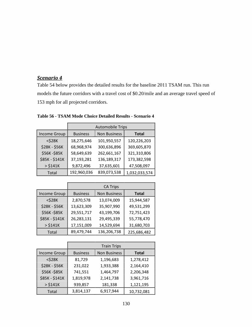
130

Scenario 4

Table 54 below provides the detailed results for the baseline 2011 TSAM run. This run

models the future corridors with a travel cost of $0.20/mile and an average travel speed of

153 mph for all projected corridors.

Table 56 - TSAM Mode Choice Detailed Results - Scenario 4

Automobile Trips

Income Group Business Non Business Total

<$28K 18,275,646 101,950,557 120,226,203

$28K - $56K 68,968,974 300,636,896 369,605,870

$56K -$85K 58,649,639 262,661,167 321,310,806

$85K - $141K 37,193,281 136,189,317 173,382,598

> $141K 9,872,496 37,635,601 47,508,097

Total 192,960,036 839,073,538 1,032,033,574

CA Trips

Income Group Business Non Business Total

<$28K 2,870,578 13,074,009 15,944,587

$28K - $56K 13,623,309 35,907,990 49,531,299

$56K -$85K 29,551,717 43,199,706 72,751,423

$85K - $141K 26,283,131 29,495,339 55,778,470

> $141K 17,151,009 14,529,694 31,680,703

Total 89,479,744 136,206,738 225,686,482

Train Trips

Income Group Business Non Business Total

<$28K 81,729 1,196,683 1,278,412

$28K - $56K 231,022 1,933,388 2,164,410

$56K -$85K 741,551 1,464,797 2,206,348

$85K - $141K 1,819,978 2,141,738 3,961,716

> $141K 939,857 181,338 1,121,195

Total 3,814,137 6,917,944 10,732,081

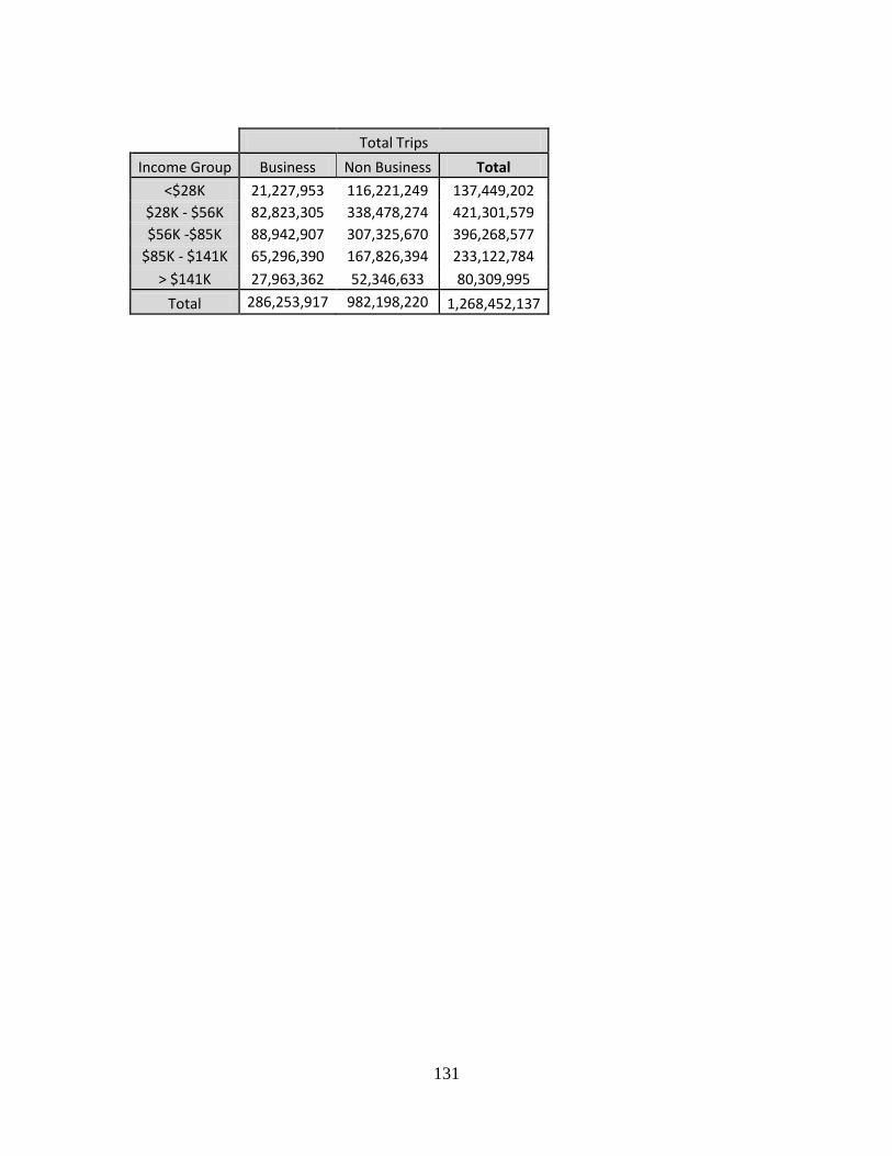
131

Total Trips

Income Group Business Non Business Total

<$28K 21,227,953 116,221,249 137,449,202

$28K - $56K 82,823,305 338,478,274 421,301,579

$56K -$85K 88,942,907 307,325,670 396,268,577

$85K - $141K 65,296,390 167,826,394 233,122,784

> $141K 27,963,362 52,346,633 80,309,995

Total 286,253,917 982,198,220 1,268,452,137

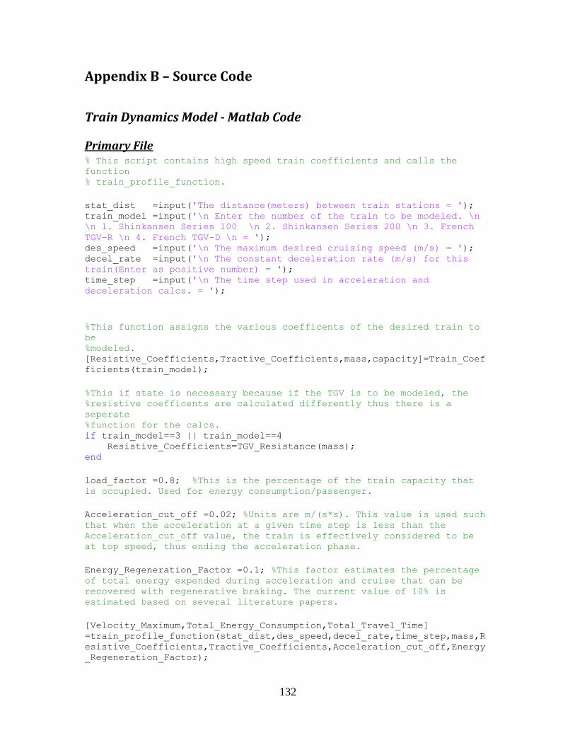
132

Appendix B – Source Code

Train Dynamics Model - Matlab Code

Primary File % This script contains high speed train coefficients and calls the

function % train_profile_function.

stat_dist =input('The distance(meters) between train stations = '); train_model =input('\n Enter the number of the train to be modeled. \n

\n 1. Shinkansen Series 100 \n 2. Shinkansen Series 200 \n 3. French

TGV-R \n 4. French TGV-D \n = '); des_speed =input('\n The maximum desired cruising speed (m/s) = '); decel_rate =input('\n The constant deceleration rate (m/s) for this

train(Enter as positive number) = '); time_step =input('\n The time step used in acceleration and

deceleration calcs. = ');

%This function assigns the various coefficents of the desired train to

be %modeled. [Resistive_Coefficients,Tractive_Coefficients,mass,capacity]=Train_Coef

ficients(train_model);

%This if state is necessary because if the TGV is to be modeled, the %resistive coefficents are calculated differently thus there is a

seperate %function for the calcs. if train_model==3 || train_model==4 Resistive_Coefficients=TGV_Resistance(mass); end

load_factor =0.8; %This is the percentage of the train capacity that

is occupied. Used for energy consumption/passenger.

Acceleration_cut_off =0.02; %Units are m/(s*s). This value is used such

that when the acceleration at a given time step is less than the

Acceleration_cut_off value, the train is effectively considered to be

at top speed, thus ending the acceleration phase.

Energy_Regeneration_Factor =0.1; %This factor estimates the percentage

of total energy expended during acceleration and cruise that can be

recovered with regenerative braking. The current value of 10% is

estimated based on several literature papers.

[Velocity_Maximum,Total_Energy_Consumption,Total_Travel_Time]

=train_profile_function(stat_dist,des_speed,decel_rate,time_step,mass,R

esistive_Coefficients,Tractive_Coefficients,Acceleration_cut_off,Energy

_Regeneration_Factor);

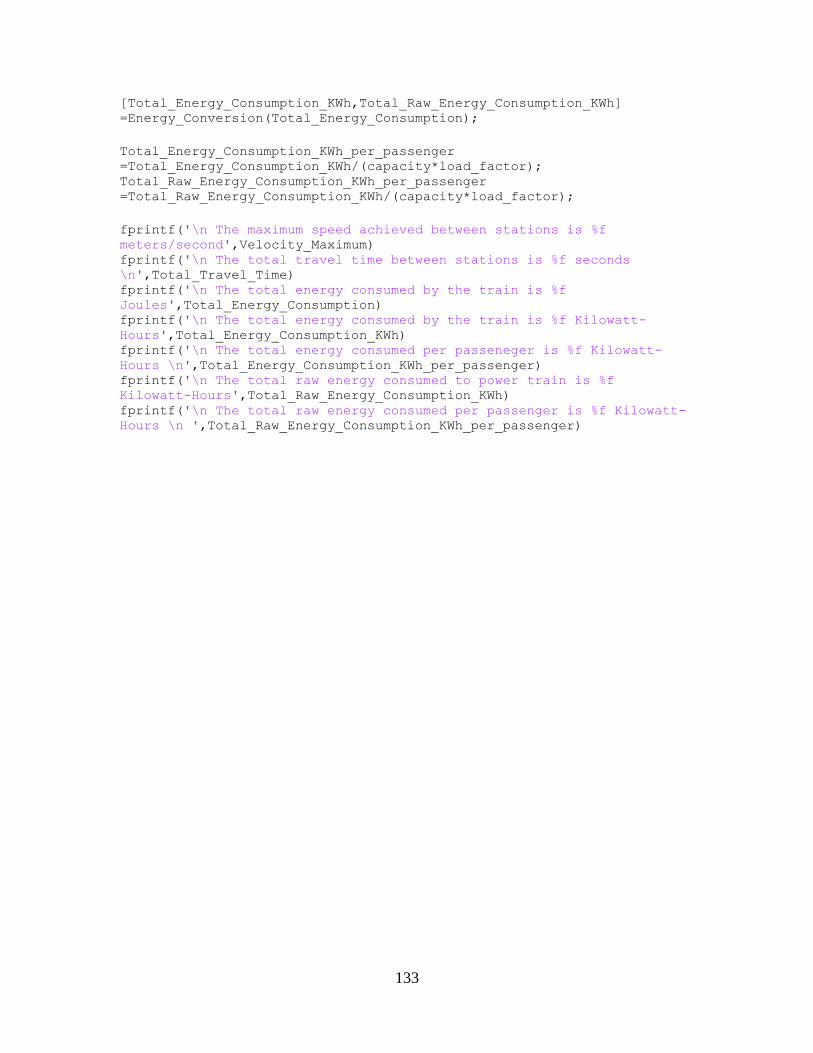
133

[Total_Energy_Consumption_KWh,Total_Raw_Energy_Consumption_KWh]

=Energy_Conversion(Total_Energy_Consumption);

Total_Energy_Consumption_KWh_per_passenger

=Total_Energy_Consumption_KWh/(capacity*load_factor); Total_Raw_Energy_Consumption_KWh_per_passenger

=Total_Raw_Energy_Consumption_KWh/(capacity*load_factor);

fprintf('\n The maximum speed achieved between stations is %f

meters/second',Velocity_Maximum) fprintf('\n The total travel time between stations is %f seconds

\n',Total_Travel_Time) fprintf('\n The total energy consumed by the train is %f

Joules',Total_Energy_Consumption) fprintf('\n The total energy consumed by the train is %f Kilowatt-

Hours',Total_Energy_Consumption_KWh) fprintf('\n The total energy consumed per passeneger is %f Kilowatt-

Hours \n',Total_Energy_Consumption_KWh_per_passenger) fprintf('\n The total raw energy consumed to power train is %f

Kilowatt-Hours',Total_Raw_Energy_Consumption_KWh) fprintf('\n The total raw energy consumed per passenger is %f Kilowatt-

Hours \n ',Total_Raw_Energy_Consumption_KWh_per_passenger)

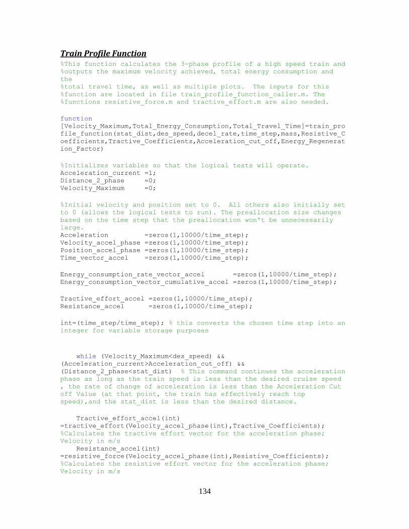
134

Train Profile Function %This function calculates the 3-phase profile of a high speed train and %outputs the maximum velocity achieved, total energy consumption and

the %total travel time, as well as multiple plots. The inputs for this %function are located in file train_profile_function_caller.m. The %functions resistive_force.m and tractive_effort.m are also needed.

function

[Velocity_Maximum,Total_Energy_Consumption,Total_Travel_Time]=train_pro

file_function(stat_dist,des_speed,decel_rate,time_step,mass,Resistive_C

oefficients,Tractive_Coefficients,Acceleration_cut_off,Energy_Regenerat

ion_Factor)

%Initializes variables so that the logical tests will operate. Acceleration_current =1; Distance_2_phase =0; Velocity_Maximum =0;

%Initial velocity and position set to 0. All others also initially set

to 0 (allows the logical tests to run). The preallocation size changes

based on the time step that the preallocation won't be unnecessarily

large. Acceleration =zeros(1,10000/time_step); Velocity_accel_phase =zeros(1,10000/time_step); Position_accel_phase =zeros(1,10000/time_step); Time_vector_accel =zeros(1,10000/time_step);

Energy_consumption_rate_vector_accel =zeros(1,10000/time_step); Energy_consumption_vector_cumulative_accel =zeros(1,10000/time_step);

Tractive_effort_accel =zeros(1,10000/time_step); Resistance_accel =zeros(1,10000/time_step);

int=(time_step/time_step); % this converts the chosen time step into an

integer for variable storage purposes

while (Velocity_Maximum<des_speed) &&

(Acceleration_current>Acceleration_cut_off) &&

(Distance_2_phase<stat_dist) % This command continues the acceleration

phase as long as the train speed is less than the desired cruise speed

, the rate of change of acceleration is less than the Acceleration Cut

off Value (at that point, the train has effectively reach top

speed),and the stat_dist is less than the desired distance.

Tractive_effort_accel(int)

=tractive_effort(Velocity_accel_phase(int),Tractive_Coefficients);

%Calculates the tractive effort vector for the acceleration phase;

Velocity in m/s Resistance_accel(int)

=resistive_force(Velocity_accel_phase(int),Resistive_Coefficients);

%Calculates the resistive effort vector for the acceleration phase;

Velocity in m/s

135

Acceleration(int+1) =(Tractive_effort_accel(int)-

Resistance_accel(int))/mass; % Calculates the acceleration rate

vector during the acceleration phase, Acceleration in m/(s*s) Velocity_accel_phase(int+1) =((Acceleration

(int+1)*time_step)+Velocity_accel_phase(int)); % Calculates the train

velocity for each time step during the acceleration phase and stores as

a vector, Velocity in m/s Position_accel_phase(int+1)

=((((Velocity_accel_phase(int+1)+Velocity_accel_phase(int))/2)*time_ste

p)+Position_accel_phase(int)); %Calculates the train position for each

time step during the acceleration phase and stores as a vector,

Position in m.

Velocity_Maximum =Velocity_accel_phase(int+1); % pulls out

current velocity value and stores as a scalar for use in the comparison

statement above. Acceleration_current =abs(Acceleration(int+1)); % This

stores the absolute value of last value of acceleration for use in the

comparison statement above. The purpose is that once the accelration

drops below the criteria above, then the train has essentianly hit

maximum speed and then must enter the cruise or deceleration phase. Accel_time =int*time_step; % Calculates the time

elasped during the acceleration phase. Time_vector_accel(int+1) =int*time_step; % Stores a vector of time

values from the acceleration phase for plotting purposes.

Energy_consumption_rate_vector_accel(int+1)

=tractive_effort(Velocity_accel_phase(int+1),Tractive_Coefficients)*Vel

ocity_accel_phase(int+1); %calculates the rate of energy consumption at

each time step in the acceleration phase. Energy_consumption_vector_cumulative_accel(int+1)

=((Energy_consumption_rate_vector_accel(int)+Energy_consumption_rate_ve

ctor_accel(int+1))/2)*time_step+(Energy_consumption_vector_cumulative_a

ccel(int)); %computes the cumulative energy consumed for each time step

during the acceleration phase. Energy_consumption_cumulative_end_of_accel

=Energy_consumption_vector_cumulative_accel(int+1); %Finds the total

energy consumed during the acceleration phase.

int =int+(time_step/time_step); % Counter function, allows for

progression of calculations.

Distance_end_of_accel =Position_accel_phase(int); % Finds the

distance covered by the train during the acceleration phase.

%This phase calculates the distance needed for deceleration

assumming a %constant rate decel. Note that distance_end_of_decel is only

distance %for deceleration phase. It is not tied to the acceleration

distance at %this point because the train may have a cruise phase which will

fall

136

%in between.

Decel_time =Velocity_Maximum/decel_rate; % The time

elasped during the deceleration phase Distance_end_of_decel =(-(Velocity_Maximum^2)/(2*-decel_rate))+ 0;

%Finds total distance traveled during deceleration phase using constant

deceleration equation.

Distance_2_phase =Distance_end_of_accel+Distance_end_of_decel; %

The total distance required for the acceleration and deceleration

phases. Used in logical test above such once the distance required for

the train to accelerate to the current value of velocity and then

decelerate exceeds the distance between stations, then the loops ends

and the maximum velocity possible for that station length can be found. Time_2_phase =Accel_time+Decel_time; % Time required for the

train to accelerate and decelerate.

end

if Velocity_Maximum<des_speed %Provides message that train didn't

reach the desired speed for that calculation. fprintf('\n NOTE: The train never reaches the desired cruising

speed!\n The speed is either unattainable or unreachable for the given

station length! \n') end

%Preallocate decel_distance_vector for speed. decel_distance_vector =zeros(1,round(Decel_time/time_step)); decel_velocity_vector =zeros(1,round(Decel_time/time_step)); Time_vector_decel =zeros(1,round(Decel_time/time_step));

%initialize velocity_vector element 1 to cruise velocity for %calculations and plotting. decel_velocity_vector(1)=Velocity_Maximum;

int=(time_step/time_step); % this converts the chosen time step

into an integer for variable storage purposes

timer=0;

while timer<Decel_time %this loop fills out the distance profile

vector of the train during the deceleration phase. It is independent

of distances from acceleration at this point. It is not included in the

while statement above for speed. decel_distance_vector(int+1) =0.5*-

decel_rate*(timer)^2+Velocity_Maximum*(timer)+0; % calculates vector of

distances at eact time step. The j/time_step converts each time step

to an integer for variable storage. decel_velocity_vector(int+1) =(-

decel_rate*(timer))+Velocity_Maximum; Time_vector_decel(int+1) =(timer);

timer =int*time_step; int =int+1;

137

end

%This if-else statement determines if the train will have a cruise

segment, %based on the while statement above. Then depending on whether or

not %there is a cruise segment, cruise time and distance are computed. if (Distance_2_phase<stat_dist)

Cruise_dist =stat_dist-Distance_2_phase; %Determines how much

distance is available for cruise segment. Cruise_time =Cruise_dist/Velocity_Maximum;%Determines time

required for cruise segment based on cruising speed, the cruising

speed is the speed of the train at the end of the acceleration phase.

Total_Travel_Time =Cruise_time+Time_2_phase; % total Travel

time for all 3 phases.

Tractive_effort_cruise_rate

=resistive_force(Velocity_Maximum,Resistive_Coefficients); % The

tractive effort of the train during the cruise segment, this will be a

constant value. This is the tractive effort required because the train

isn't accelerating thus tractive effort only needs to equal resistance. Energy_consumption_end_of_cruise

=Tractive_effort_cruise_rate*Velocity_Maximum*Cruise_time; % Calculates

the total energy consumed during the cruise phase. Tractive_effort_used_rate_vector

=[Tractive_effort_cruise_rate,Tractive_effort_cruise_rate]; %2 element

vector of tractive effort rate during cruise. Used for plotting.

%calculate the position and time at the start of deceleration

phase Position_start_decel =Distance_end_of_accel+Cruise_dist; Time_start_decel =Accel_time+Cruise_time;

else % if there is no cruise segment, then the values are

calculated accordingly. Although there is no cruise segment if this

section is activated, the values are calculated for plotting purposes,

so that no if statements are necessary in the plotting section. Total_Travel_Time =Time_2_phase; Position_start_decel =Distance_end_of_accel; Time_start_decel =Accel_time; Cruise_time =0;

Tractive_effort_cruise_rate =0; Tractive_effort_used_rate_vector

=[Tractive_effort_cruise_rate,Tractive_effort_cruise_rate]; Energy_consumption_end_of_cruise =0; end

% Calculate the vectors for cruise and deceleration phases so that

they

138

% can be plotted. The vectors are all 2 elements because the

cruise % and deceleration phases occur at constant rates. Cruise_time_vector =[Accel_time, Time_start_decel]; Cruise_position_vector

=[Distance_end_of_accel,Position_start_decel]; Cruise_velocity_vector =[Velocity_Maximum, Velocity_Maximum];

Decel_time_vector =Time_vector_decel+Time_start_decel; Decel_position_vector =decel_distance_vector+Position_start_decel;

%calculate the energy consumption vectors for cruise and decel so

they %can be plotted Energy_consumption_vector_cumulative_cruise

=[Energy_consumption_cumulative_end_of_accel,

Energy_consumption_cumulative_end_of_accel+Energy_consumption_end_of_cr

uise]; Energy_consumption_vector_cumulative_decel

=[Energy_consumption_vector_cumulative_cruise(2),

Energy_consumption_vector_cumulative_cruise(2)-

(Energy_consumption_vector_cumulative_cruise(2)*Energy_Regeneration_Fac

tor)];

%Find the last non-zero element in the acceleration phase

variables. %this is necessary because the arrays are preallocated and without %modification, the plot will plot all elements of the arrays,

including the zeros, %which is incorrect for the graph.

Last_element_position_accel =find(Position_accel_phase,1,'last'); Last_element_velocity_accel =find(Velocity_accel_phase,1,'last'); Last_element_time_accel =find(Time_vector_accel,1,'last'); Last_element_energy_accel

=find(Energy_consumption_vector_cumulative_accel,1,'last'); Last_element_tractive_accel =find(Tractive_effort_accel,1,'last');

Tractive_effort_accel(Last_element_tractive_accel+1)=Tractive_effort_ac

cel(Last_element_tractive_accel); % this function makes the tractive

effort vector the same length as the time vector for plotting purposes.

Total_Energy_Consumption=Energy_consumption_vector_cumulative_decel(2);

%------------------------------------------------------------------

---- %The remaining commands generate the various plots that are

produced.

%This series of commands plots the velocity vs distance profile for

the %train.

139

figure

plot(Position_accel_phase(1:Last_element_position_accel),Velocity_accel

_phase(1:Last_element_velocity_accel),'-g') hold on plot(Cruise_position_vector,Cruise_velocity_vector,'-b') plot(Decel_position_vector,decel_velocity_vector,'-r') xlabel('Distance Traveled (Meters)') ylabel('Velocity (Meters/Second)') title('High Speed Train Velocity vs Distance Profile') legend('Acceleration Phase','Cruise Phase','Deceleration Phase') hold off

%This series of commands plots the position vs time profile of the %train. figure

plot(Time_vector_accel(1:Last_element_time_accel),Position_accel_phase(

1:Last_element_position_accel),'-g') hold on plot(Cruise_time_vector,Cruise_position_vector,'-b') plot(Decel_time_vector,Decel_position_vector,'-r') xlabel('Time (Seconds)') ylabel('Distance Traveled (Meters)') title('High Speed Train Distance Traveled vs Time') legend('Acceleration Phase','Cruise Phase','Deceleration Phase') hold off

%This series of commands plots the energy consumption rate vs time %profile of the train. figure

plot(Time_vector_accel(2:Last_element_time_accel),Energy_consumption_ra

te_vector_accel(2:Last_element_energy_accel),'-g') hold on

plot(Cruise_time_vector,[(Energy_consumption_end_of_cruise/Cruise_time)

,(Energy_consumption_end_of_cruise/Cruise_time)],'-b')% the second

vector is the energy consumption rate for the cruise segment. plot(Decel_time_vector,zeros(1,numel(Decel_time_vector)),'-r') %

assume no energy is consumed during the deceleration operation xlabel('Time (Seconds)') ylabel('Energy Consumption Rate (Joules/Second)') title('High Speed Train Energy Consumption Rate vs Time') legend('Acceleration Phase','Cruise Phase','Deceleration Phase') hold off

%This series of commands plots the cumulative energy consumed vs

time profile of %the train figure

140

plot(Time_vector_accel(1:Last_element_time_accel),Energy_consumption_ve

ctor_cumulative_accel(1:Last_element_energy_accel),'-g') hold on

plot(Cruise_time_vector,Energy_consumption_vector_cumulative_cruise,'-

b')

plot([Decel_time_vector(1),Decel_time_vector(numel(Decel_time_vector))]

,Energy_consumption_vector_cumulative_decel,'-r') xlabel('Time (Seconds)') ylabel('Cumulative Energy Consumed (Joules)') title('High Speed Train Energy Consumed vs Time') legend('Acceleration Phase','Cruise Phase','Deceleration Phase') hold off

%This series of commands plots the tractive force uses vs time for

the %train. figure

plot(Time_vector_accel(1:Last_element_time_accel),Tractive_effort_accel

(1:Last_element_tractive_accel+1),'-g'); hold on plot(Cruise_time_vector,Tractive_effort_used_rate_vector,'-b') plot([Time_start_decel, Total_Travel_Time],[0 0],'-r') xlabel('Time (Seconds)') ylabel('Tractive Effort Required Rate (N/s)') title('High Speed Train Tractive Effort Required Rate vs Time') legend('Acceleration Phase','Cruise Phase','Deceleration Phase') hold off

141

Resistive Force Function %This function returns the resistive forces of a high speed train from

the %input of velocity(m/s). function

[Resistive_Force]=resistive_force(Velocity,Resistive_Coefficients) %High Speed Train resistance coefficients. A = Resistive_Coefficients(1); B = Resistive_Coefficients(2); C = Resistive_Coefficients(3);

Resistive_Force=(A+B*Velocity+C*Velocity^2);

Tractive Effort Function %This function returns the tractive effort of a high speed train from

the %input of velocity(m/s). function

[Tractive_Effort]=tractive_effort(Velocity,Tractive_Coefficients) %Coefficients for calculation of tractive effort. k1 = Tractive_Coefficients(1); % conversion factor from HP to

Newtons (Newton m/s) P = Tractive_Coefficients(2); % horsepower (Hp) nu = Tractive_Coefficients(3); % engine efficiency (dim)

Tractive_Effort=min(((k1.*nu.*P)/Velocity),1e6);

TGV_Resistance Function %This function calcuates the resistive coefficents of the French TGV.

All %information was taken from the paper "A Review of Methods to Measure

and %Calculate Train Resistances" by Rochard and Schmid.

%Note that the length, mass, power, and capacity comes from the paper %"Efficiency Comparisons of the Typical High Speed Trains of the in the %World" by Shoji

function [Resistive_Coefficients]=TGV_Resistance(mass)

Lambda =0.9; %The value for lambda should be

between 0.9 and 1.5. The lower values are similar to the high speed

TGV stock. Number_of_axles =24; %This is important because the

calculation of resistive coefficents require mass per axle. Currently

asssumed. Mass_per_axle =mass/Number_of_axles;

k1 =(9*10^-4); % A parameter that depends on shape of train.(Value

listed is for TGV S =10; %Front surface cross sectional area (m^2).

142

k2 =(20*10^-6); %Parameter that depends on condition of surface, pL. p =10; %Partial perimeter of rolling stock down to rail level. L =200; %Length of train (m).

%these are the equations listed in the paper. Each equation has been %multiplied by 1000 to convert the coefficents from kiloNewtons to

Netwons. A =(0.00001*(Lambda*mass*(sqrt(10000/Mass_per_axle))))*1000; B =((3.6*10^-7)*mass)*1000; C =(0.1296*((k1*S)+k2*p*L))*1000;

Resistive_Coefficients=[A B C];

143

Station to Station Input File Creator

Primary File

%This file will create the S2S travel time and S2S travel cost %matrices.

%This file needs the functions: Train_Station_Index Finder, %Schedule_Delay_Calculator

%Travel Cost Equation Values. A cost analysis was conducted on Mar.

23, %2011 for travel on March 9, 2011 on the Amtrak Network Nationwide.

Coach %class with no room. clear all; clc;

for i=2010 %:1:2011

global TrainStation_List Desired_Year = i; %this is the data year that the files are

created for. Cost_Year = 2000; %This should always be 2000 to be

consistent with TSAM. TSAM needs all input cost in 2000 $'s. So the

created table of S2S costs for 1995, or 1996, or 1997, etc. should all

be in 2000 $'s. Regression_Cost_Year = 2010; % THIS HAS TO BE =2010 UNLESS NEW

REGRESSION CURVES ARE DEVELOPED. This is the year of the cost data that

was used to develop regression curves. All curves were developed in

2010 $'s unless noted otherwise.

Very_High_Time_and_Cost='YES'; %If this is yes, the TT and TC are set

to very high values for all O-D pairs. This is used to effectively

elimnate the train mode but still use the 3 mode calibrated

coefficients. Year_Start_High_Speed_Service=2010; %This needs to be year of high

speed initialization for all corridors. If corridors start in different

years, then enter value for each initial year parameter below.

Output_Save_Directory='C:\Users\avandyke\Desktop\S2S_Matlab_Input_Files

\';

disp(['Year:',num2str(Desired_Year)]) %--------------------------------------------------- %This section is used to determine what projected corridor lines are %included in the model. Variables should be 'YES' if the corridor is

to be

144

%modeled. Descriptions of the corridors can be found below. The

initial %year variables are the first year that the given corridor is to be %modeled. These variable should not be less than 2011.

Original_NEC_Route = 'YES'; %this applies only for future

corridor, after year 2010. the route is already modeled for 2001-2010. California_Route = 'YES'; Pacific_Northwest_Route = 'YES'; Florida_Route = 'YES'; Chicago_Hub_Route = 'YES'; Southeast_Route = 'YES'; Empire_Route = 'YES'; Northern_New_England_Route = 'YES'; Keystone_Route = 'YES'; South_Central_Route = 'YES'; Gulf_Coast_Route = 'YES'; Vermont_Route = 'YES'; Cumulative_NEC_Route = 'No'; %IF Cumulative_NEC_Route= YES, this

will combine and overwrite the Original_NEC_Route, Empire_Route,

Northern_New_England_Route, Keystone_Route, and Northern_NEC_Route.

Turn off these corridors to speed the code.

%Initial year of service for each high speed corridor. Original_NEC_Route_Initial_Year =

Year_Start_High_Speed_Service; %This implies the year that the NEC

corridor gets updated (higher speeds). California_Route_Initial_Year =

Year_Start_High_Speed_Service; Pacific_Northwest_Route_Initial_Year =

Year_Start_High_Speed_Service; Florida_Route_Initial_Year =

Year_Start_High_Speed_Service; Chicago_Hub_Route_Initial_Year =

Year_Start_High_Speed_Service; Southeast_Route_Initial_Year =

Year_Start_High_Speed_Service; Empire_Route_Initial_Year =

Year_Start_High_Speed_Service; Northern_New_England_Route_Initial_Year =

Year_Start_High_Speed_Service; Keystone_Route_Initial_Year =

Year_Start_High_Speed_Service; South_Central_Route_Initial_Year =

Year_Start_High_Speed_Service; Gulf_Coast_Route_Initial_Year =

Year_Start_High_Speed_Service; Vermont_Route_Initial_Year =

Year_Start_High_Speed_Service; Cumulative_NEC_Route_Initial_Year =

Year_Start_High_Speed_Service;

%If Acela_Cost_XXXXXX_Route = 'YES' then that corridor is modeled with

145

%the existing Amtrak Acela Cost curve. Otherwise, Cost is currently

based on $/mile. %When new cost function is developed,the code in the double for loop

below %will have to be changed.

%This needs to be in 2010 dollars because Regression_Cost_Year = 2010

Acela_Cost_Original_NEC_Route = 'YES'; Acela_Cost_California_Route = 'YES'; Acela_Cost_Pacific_Northwest_Route = 'YES'; Acela_Cost_Florida_Route = 'YES'; Acela_Cost_Chicago_Hub_Route = 'YES'; Acela_Cost_Southeast_Route = 'YES'; Acela_Cost_Empire_Route = 'YES'; Acela_Cost_Northern_New_England_Route = 'YES'; Acela_Cost_Keystone_Route = 'YES'; Acela_Cost_South_Central_Route = 'YES'; Acela_Cost_Gulf_Coast_Route = 'YES'; Acela_Cost_Vermont_Route = 'YES'; Acela_Cost_Cumulative_NEC_Route = 'YES';

Original_NEC_Route_Average_Cost = 0.60; %This applies only after

high speed rail corridors are turned on. California_Route_Average_Cost = 0.60; Pacific_Northwest_Route_Average_Cost = 0.60; Florida_Route_Average_Cost = 0.60; Chicago_Hub_Route_Average_Cost = 0.60; Southeast_Route_Average_Cost = 0.60; Empire_Route_Average_Cost = 0.60; Northern_New_England_Route_Average_Cost= 0.60; Keystone_Route_Average_Cost = 0.60; South_Central_Route_Average_Cost = 0.60; Gulf_Coast_Route_Average_Cost = 0.60; Vermont_Route_Average_Cost = 0.60; Cumulative_NEC_Route_Average_Cost = 0.60;

%Travel Time is currently based on an average speed across the

corridor. %This speed is the average speed including stops. When new time

functions %are developed, the code in the double for loop below will have to be %changed. The speed is presented in miles/hr. Original_NEC_Route_Average_Speed = 175; %Planned Value = 119.

%This applies only after high speed rail corridors are turned on. California_Route_Average_Speed = 175; %Planned Value = 153 Pacific_Northwest_Route_Average_Speed = 175; %Planned Value = 105 Florida_Route_Average_Speed = 175; %Planned Value = 118 Chicago_Hub_Route_Average_Speed = 175; %Planned Value = 77 Southeast_Route_Average_Speed = 175; %Planned Value = 77 Empire_Route_Average_Speed = 175; %Planned Value = 77 Northern_New_England_Route_Average_Speed= 175; %Planned Value = 77 Keystone_Route_Average_Speed = 175; %Planned Value = 77 South_Central_Route_Average_Speed = 175; %Planned Value = 105 Gulf_Coast_Route_Average_Speed = 175; %Planned Value = 105

146

Vermont_Route_Average_Speed = 175; %Planned Value = 77 Cumulative_NEC_Route_Average_Speed = 175; %Planned Value = 100

%----------------------------------------------------

load('C:\Users\avandyke\Documents\TSAM_GUI_VB_2005\bin\data\mode_choice

\input\TrainStation_List.mat') %This file containts the Amtrak

"TrainStation_List" load('C:\Users\avandyke\Documents\TSAM_GUI_VB_2005\bin\data\mode_choice

\input\PCEP_Index.mat') %This is the inflation index load('C:\Users\avandyke\Documents\TSAM_GUI_VB_2005\bin\data\mode_choice

\input\S2S_Train_ScheduleDelay_HSR.mat') %This loads the original

schedule delay values from TSAM. IT is assumed this is the scheule

delay unless changes are made in the code below. load('C:\Users\avandyke\Documents\TSAM_GUI_VB_2005\bin\data\mode_choice

\input\S2S_Train_Distance_HSR'); %This is the original matrix of

distance between stations. This is the original data and is assumed to

be correct unless specific changes have been noted below.

[~,Number_Stations_Total_Network] = size(TrainStation_List); Station_Index = 1:Number_Stations_Total_Network;

S2S_Train_ScheduleDelay=S2S_Train_ScheduleDelay_HSR; clear S2S_Train_ScheduleDelay_HSR

S2S_Train_Distance=S2S_Train_Distance_HSR(Station_Index,

Station_Index); %this renames the distance matrix. clear S2S_Train_Distance_HSR

if strcmp(Very_High_Time_and_Cost,'YES')==1 S2S_Train_TravelTime=S2S_Train_Distance .* 10; %This means the S2S

travel speed is 1/10 mph. S2S_Train_TravelCost=S2S_Train_Distance .* 5000; %This means the

S2S travel cost is 5000 $/mi. else %------------------------------------------------------------------

-- %ORIGINAL NEC %------------------------------------------------------------------

-- %The code in this section is used to identify the 16 NEC station's

index %numbers. This is the original NEC corridor route, It is modeled

between %2001 and XXXX.

Station_Abbreviation_List =

{'STM','NHV','NLC','WIL','WAS','BWI','BAL','RTE','BOS','NWK','TRE','MET

','NYP','PHL','PVD','BBY'}; %Stations in the NEC. The file

Train_Station_ID_Finder. m can be used to find these codes based on the

desired city. %The Station Abbreviation List is representative of Stamford CT,

New Haven

147

%CT, New London CT, Wilmington DE, Washington DC, Baltimore MD

(airport), %Baltimore MD, Westwood MA, Boston MA, Newark NJ, Trenton NJ,

Metropark NJ, %New York NY, Phidelphia PA, and Providence RI.

[~,Number_Stations] =size(Station_Abbreviation_List); Original_NEC_Station_Index =zeros(1,Number_Stations);

for a=1:1:Number_Stations

Original_NEC_Station_Index(1,a)=Train_Station_Index_Finder(Station_Abbr

eviation_List{1,a}); end

if strcmp(Original_NEC_Route,'YES')==1 &&

Original_NEC_Route_Initial_Year <= Desired_Year Train_Frequency = ones(Number_Stations,Number_Stations)*8;

%This is assigning the frequency of train between all possible

combinations of stations above to be 6 trains. Once an actual schedule

is developed, then a new matrix can be created. Train_Service_Period = 18; %The service period of trains. This

is used for the calculation of schedule delay. Schedule_Delay =

Schedule_Delay_Calculator(Train_Frequency,Train_Service_Period);

%Schedule delay for stations listed above.

S2S_Train_ScheduleDelay(Original_NEC_Station_Index,Original_NEC_Station

_Index)=Schedule_Delay; %Updates the main S2S schedule delay with the

delay calculated for stations listed above.

clear Train_Frequency clear Train_Service_Period clear Schedule Delay end

clear a clear Station_Abbreviation_List clear Number_Stations %------------------------------------------------------------------

---

%------------------------------------------------------------------

--- %CALIFORNIA ROUTE %------------------------------------------------------------------

--- %The code in this section is used to identify the station index %numbers of the California Corridor. if strcmp(California_Route,'YES')==1 &&

California_Route_Initial_Year <= Desired_Year Station_Abbreviation_List =

{'SJC','SAC','MCD','FNO','BFD','LAX','RIV','SAN','ANA','DAV','EMY','FUL

148

','GDL','IRV','OAC','ONA','POS','PRB','RIC','RLN','RSV','SNA'}; %Major

stations end at 'SAN' %The Station Abbreviation List is representative of San Jose,

Sacramento, %Merced, Fresno, Bakersfield, Los Angeles, Riverside, and San

Diego. All %stations are in CA. Other Stations listed are non-major

stations, see %Projected Rail Corridor Data sheet to see where other stations

are %located. [~,Number_Stations] = size(Station_Abbreviation_List); California_Station_Index = zeros(1,Number_Stations);

for a=1:1:Number_Stations

California_Station_Index(1,a)=Train_Station_Index_Finder(Station_Abbrev

iation_List{1,a}); end

Train_Frequency = ones(Number_Stations,Number_Stations)*8;

%This is assigning the frequency of train between all possible

combinations of stations above to be 6 trains. Once an actual schedule

is developed, then a new matrix can be created. Train_Service_Period = 18; %The service period of trains. This

is used for the calculation of schedule delay. Schedule_Delay =

Schedule_Delay_Calculator(Train_Frequency,Train_Service_Period);

%Schedule delay for stations listed above.

S2S_Train_ScheduleDelay(California_Station_Index,California_Station_Ind

ex)=Schedule_Delay; %Updates the main S2S schedule delay with the delay

calculated for stations listed above.

clear a clear Station_Abbreviation_List clear Number_Stations clear Train_Frequency clear Train_Service_Period clear Schedule_Delay end

%------------------------------------------------------------------

--

%------------------------------------------------------------------

-- %PACIFIC NORTHWEST ROUTE %------------------------------------------------------------------

-- %The code in this section is used to identify the station index %numbers of the Pacific Northwest Route. if strcmp(Pacific_Northwest_Route,'YES')==1 &&

Pacific_Northwest_Route_Initial_Year <= Desired_Year

149

Station_Abbreviation_List =

{'SEA','TAC','PDX','EUG','ALY','ORC','SLM','BEL','CTL','EDM','EVR','KEL

','MVW','OLW','TUK'}; %The Station Abbreviation List is representative of Seattle WA,

Tacoma WA, %Portland OR, and Eugene OR. Other Stations listed are non-

major stations, see %Projected Rail Corridor Data sheet to see where other stations

are %located.

[~,Number_Stations] =

size(Station_Abbreviation_List); Pacific_Northwest_Station_Index = zeros(1,Number_Stations);

for a=1:1:Number_Stations

Pacific_Northwest_Station_Index(1,a)=Train_Station_Index_Finder(Station

_Abbreviation_List{1,a}); end

Train_Frequency = ones(Number_Stations,Number_Stations)*8;

%This is assigning the frequency of train between all possible

combinations of stations above to be 6 trains. Once an actual schedule

is developed, then a new matrix can be created. Train_Service_Period = 18; %The service period of trains. This

is used for the calculation of schedule delay. Schedule_Delay =

Schedule_Delay_Calculator(Train_Frequency,Train_Service_Period);

%Schedule delay for stations listed above.

S2S_Train_ScheduleDelay(Pacific_Northwest_Station_Index,Pacific_Northwe

st_Station_Index)=Schedule_Delay; %Updates the main S2S schedule delay

with the delay calculated for stations listed above.

clear a clear Station_Abbreviation_List clear Number_Stations clear Train_Frequency clear Train_Service_Period clear Schedule_Delay end

%------------------------------------------------------------------

-

%------------------------------------------------------------------

- %FLORIDA ROUTE %------------------------------------------------------------------

- %The code in this section is used to identify the station index %numbers of the Florida Route.

150

if strcmp(Florida_Route,'YES')==1 && Florida_Route_Initial_Year <=

Desired_Year Station_Abbreviation_List =

{'TPA','ORL','MIA','DFB','DLB','FTL','HOL','KIS','LAK','SFD','WPB','WPK

','WTH'}; %The Station Abbreviation List is representative of Tampa,

Orlando, Miami. Other Stations listed are non-major stations, see %Projected Rail Corridor Data sheet to see where other stations

are %located.

[~,Number_Stations] = size(Station_Abbreviation_List); Florida_Station_Index = zeros(1,Number_Stations);

for a=1:1:Number_Stations

Florida_Station_Index(1,a)=Train_Station_Index_Finder(Station_Abbreviat

ion_List{1,a}); end

Train_Frequency = ones(Number_Stations,Number_Stations)*8;

%This is assigning the frequency of train between all possible

combinations of stations above to be 6 trains. Once an actual schedule

is developed, then a new matrix can be created. Train_Service_Period = 18; %The service period of trains. This

is used for the calculation of schedule delay. Schedule_Delay =

Schedule_Delay_Calculator(Train_Frequency,Train_Service_Period);

%Schedule delay for stations listed above.

S2S_Train_ScheduleDelay(Florida_Station_Index,Florida_Station_Index)=Sc

hedule_Delay; %Updates the main S2S schedule delay with the delay

calculated for stations listed above.

clear a clear Station_Abbreviation_List clear Number_Stations clear Train_Frequency clear Train_Service_Period clear Schedule_Delay end %------------------------------------------------------------------

-

%------------------------------------------------------------------

- %CHICAGO ROUTE %------------------------------------------------------------------

- %The code in this section is used to identify the station index %numbers of the Chicago Route.

if strcmp(Chicago_Hub_Route,'YES')==1 &&

Chicago_Hub_Route_Initial_Year <= Desired_Year

151

Station_Abbreviation_List =

{'CHI','KCY','STL','OMA','DET','PNT','ALN','BNL','CRV','DWT','JOL','LCN

','NPV','PON','SMT','SPI','IDP','KWD','DYE','HMI','MCI','ALI','ARB','BA

M','BMM','BTL','JXN','KAL','NBM','ROY','SJM'}; %The Station Abbreviation List is representative of Chicago,

Kansas City, St. Louis, Omaha NE, Detroit, Pontiac MI. Other Stations

listed are non-major stations, see %Projected Rail Corridor Data sheet to see where other stations

are. %located.

[~,Number_Stations] = size(Station_Abbreviation_List); Chicago_Hub_Station_Index = zeros(1,Number_Stations);

for a=1:1:Number_Stations

Chicago_Hub_Station_Index(1,a)=Train_Station_Index_Finder(Station_Abbre

viation_List{1,a}); end

Train_Frequency = ones(Number_Stations,Number_Stations)*8;

%This is assigning the frequency of train between all possible

combinations of stations above to be 6 trains. Once an actual schedule

is developed, then a new matrix can be created. Train_Service_Period = 18; %The service period of trains. This

is used for the calculation of schedule delay. Schedule_Delay =

Schedule_Delay_Calculator(Train_Frequency,Train_Service_Period);

%Schedule delay for stations listed above.

S2S_Train_ScheduleDelay(Chicago_Hub_Station_Index,Chicago_Hub_Station_I

ndex)=Schedule_Delay; %Updates the main S2S schedule delay with the

delay calculated for stations listed above.

clear a clear Station_Abbreviation_List clear Number_Stations clear Train_Frequency clear Train_Service_Period clear Schedule_Delay end %------------------------------------------------------------------

-

%------------------------------------------------------------------

- %SOUTHEAST ROUTE %------------------------------------------------------------------

- %The code in this section is used to identify the station index %numbers of the Southeast Route. Other Stations listed are non-

major stations, see %Projected Rail Corridor Data sheet to see where other stations.

152

if strcmp(Southeast_Route,'YES')==1 && Southeast_Route_Initial_Year

<= Desired_Year Station_Abbreviation_List =

{'CLT','GRO','RGH','RVR','WAS','BNC','CYN','DNC','HPT','KAN','SAL','ALX

','FBG','MSS','PTB','QAN'}; %The Station Abbreviation List is representative of Charlotte

NC, %Greensboro NC, Raleigh NC, Richmond VA, and Washington DC.

Other Stations listed are non-major stations, see %Projected Rail Corridor Data sheet to see where other stations

are.

[~,Number_Stations] = size(Station_Abbreviation_List); Southeast_Station_Index = zeros(1,Number_Stations);

for a=1:1:Number_Stations

Southeast_Station_Index(1,a)=Train_Station_Index_Finder(Station_Abbrevi

ation_List{1,a}); end

Train_Frequency = ones(Number_Stations,Number_Stations)*8;

%This is assigning the frequency of train between all possible

combinations of stations above to be 6 trains. Once an actual schedule

is developed, then a new matrix can be created. Train_Service_Period = 18; %The service period of trains. This

is used for the calculation of schedule delay. Schedule_Delay =

Schedule_Delay_Calculator(Train_Frequency,Train_Service_Period);

%Schedule delay for stations listed above.

S2S_Train_ScheduleDelay(Southeast_Station_Index,Southeast_Station_Index

)=Schedule_Delay; %Updates the main S2S schedule delay with the delay

calculated for stations listed above.

clear a clear Station_Abbreviation_List clear Number_Stations clear Train_Frequency clear Train_Service_Period clear Schedule_Delay end %------------------------------------------------------------------

-

%------------------------------------------------------------------

- %EMPIRE ROUTE %------------------------------------------------------------------

- %The code in this section is used to identify the station index %numbers of the Empire Route. if strcmp(Empire_Route,'YES')==1 && Empire_Route_Initial_Year <=

Desired_Year

153

Station_Abbreviation_List =

{'NYP','ROC','BFX','NFL','ALB','AMS','HUD','POU','RHI','ROM','SDY','SYR

','UCA','YNY'}; %The Station Abbreviation List is representative of New York

NY, Rochester %NY, Buffalo NY, ,Niagara Falls NY and Rensselaer NY(Albany).

Other Stations listed are non-major stations, see %Projected Rail Corridor Data sheet to see where other stations

are.

[~,Number_Stations] = size(Station_Abbreviation_List); Empire_Station_Index = zeros(1,Number_Stations);

for a=1:1:Number_Stations

Empire_Station_Index(1,a)=Train_Station_Index_Finder(Station_Abbreviati

on_List{1,a}); end

Train_Frequency = ones(Number_Stations,Number_Stations)*8;

%This is assigning the frequency of train between all possible

combinations of stations above to be 6 trains. Once an actual schedule

is developed, then a new matrix can be created. Train_Service_Period = 18; %The service period of trains. This

is used for the calculation of schedule delay. Schedule_Delay =

Schedule_Delay_Calculator(Train_Frequency,Train_Service_Period);

%Schedule delay for stations listed above.

S2S_Train_ScheduleDelay(Empire_Station_Index,Empire_Station_Index)=Sche

dule_Delay; %Updates the main S2S schedule delay with the delay

calculated for stations listed above.

clear a clear Station_Abbreviation_List clear Number_Stations clear Train_Frequency clear Train_Service_Period clear Schedule_Delay end %------------------------------------------------------------------

-

%------------------------------------------------------------------

- %NORTHERN NEW ENGLAND %------------------------------------------------------------------

- %The code in this section is used to identify the station index %numbers of the Empire Route. if strcmp(Northern_New_England_Route,'YES')==1 &&

Northern_New_England_Route_Initial_Year <= Desired_Year Station_Abbreviation_List =

{'ALB','SPG','NHV','BOS','FED','FTC','GZZ','PLB','POH','PRK','RSP','WHL

','WSP','FRA','WOR','BER','HFD','MDN'};

154

%The Station Abbreviation List is representative of Rensselaer

NY (Albany), %Springfield MA, New Haven CT, Boston MA. Other Stations listed

are non-major stations, see %Projected Rail Corridor Data sheet to see where other stations

are.

[~,Number_Stations] =

size(Station_Abbreviation_List); Northern_New_England_Station_Index =

zeros(1,Number_Stations);

for a=1:1:Number_Stations

Northern_New_England_Station_Index(1,a)=Train_Station_Index_Finder(Stat

ion_Abbreviation_List{1,a}); end

Train_Frequency = ones(Number_Stations,Number_Stations)*8;

%This is assigning the frequency of train between all possible

combinations of stations above to be 6 trains. Once an actual schedule

is developed, then a new matrix can be created. Train_Service_Period = 18; %The service period of trains. This

is used for the calculation of schedule delay. Schedule_Delay =

Schedule_Delay_Calculator(Train_Frequency,Train_Service_Period);

%Schedule delay for stations listed above.

S2S_Train_ScheduleDelay(Northern_New_England_Station_Index,Northern_New

_England_Station_Index)=Schedule_Delay; %Updates the main S2S schedule

delay with the delay calculated for stations listed above.

clear a clear Station_Abbreviation_List clear Number_Stations clear Train_Frequency clear Train_Service_Period clear Schedule_Delay end %------------------------------------------------------------------

-

%------------------------------------------------------------------

- %KEYSTONE ROUTE %The code in this section is used to identify the station index %numbers of the Empire Route. if strcmp(Keystone_Route,'YES')==1 && Keystone_Route_Initial_Year

<= Desired_Year Station_Abbreviation_List =

{'PHL','HAR','PGH','COV','GNB','LAB','PAO'}; %The Station Abbreviation List is representative of

Philadelphia PA, %Harrisburg PA, Pittsburgh PA. Other Stations listed are non-

major stations, see

155

%Projected Rail Corridor Data sheet to see where other stations

are.

[~,Number_Stations] = size(Station_Abbreviation_List); Keystone_Station_Index = zeros(1,Number_Stations);

for a=1:1:Number_Stations

Keystone_Station_Index(1,a)=Train_Station_Index_Finder(Station_Abbrevia

tion_List{1,a}); end

Train_Frequency = ones(Number_Stations,Number_Stations)*8;

%This is assigning the frequency of train between all possible

combinations of stations above to be 6 trains. Once an actual schedule

is developed, then a new matrix can be created. Train_Service_Period = 18; %The service period of trains. This

is used for the calculation of schedule delay. Schedule_Delay =

Schedule_Delay_Calculator(Train_Frequency,Train_Service_Period);

%Schedule delay for stations listed above.

S2S_Train_ScheduleDelay(Keystone_Station_Index,Keystone_Station_Index)=

Schedule_Delay; %Updates the main S2S schedule delay with the delay

calculated for stations listed above.

clear a clear Station_Abbreviation_List clear Number_Stations clear Train_Frequency clear Train_Service_Period clear Schedule_Delay end %------------------------------------------------------------------

-

%------------------------------------------------------------------

- %SOUTH CENTRAL ROUTE %------------------------------------------------------------------

- %The code in this section is used to identify the station index %numbers of the Empire Route. if strcmp(South_Central_Route,'YES')==1 &&

South_Central_Route_Initial_Year <= Desired_Year Station_Abbreviation_List =

{'OKC','AUS','DAL','FTW','SAS','LRK','TXA','ADM','NOR','PUR','PVL','CBR

','GLE','MCG','SMC','TAY','TPL','ARK','MVN'}; %The Station Abbreviation List is representative of Oklahoma

City, Austin TX, Dallas, Ft. Worth TX, San Antonio, Little Rock AR, and

Texarkana AR . Other Stations listed are non-major stations, see %Projected Rail Corridor Data sheet to see where other stations

are.

156

[~,Number_Stations] = size(Station_Abbreviation_List); South_Central_Station_Index = zeros(1,Number_Stations);

for a=1:1:Number_Stations

South_Central_Station_Index(1,a)=Train_Station_Index_Finder(Station_Abb

reviation_List{1,a}); end

Train_Frequency = ones(Number_Stations,Number_Stations)*8;

%This is assigning the frequency of train between all possible

combinations of stations above to be 6 trains. Once an actual schedule

is developed, then a new matrix can be created. Train_Service_Period = 18; %The service period of trains. This

is used for the calculation of schedule delay. Schedule_Delay =

Schedule_Delay_Calculator(Train_Frequency,Train_Service_Period);

%Schedule delay for stations listed above.

S2S_Train_ScheduleDelay(South_Central_Station_Index,South_Central_Stati

on_Index)=Schedule_Delay; %Updates the main S2S schedule delay with the

delay calculated for stations listed above.

clear a clear Station_Abbreviation_List clear Number_Stations clear Train_Frequency clear Train_Service_Period clear Schedule_Delay end %------------------------------------------------------------------

-

%------------------------------------------------------------------

- %GULF COAST ROUTE %------------------------------------------------------------------

- %The code in this section is used to identify the station index %numbers of the Empire Route. if strcmp(Gulf_Coast_Route,'YES')==1 &&

Gulf_Coast_Route_Initial_Year <= Desired_Year Station_Abbreviation_List =

{'ATL','BHM','MOE','BIX','MEI','NOL','HOS','ATN','TCL','HBG','LAU','PIC

','LCH','LFT','BMT'}; %The Station Abbreviation List is representative of Atlanta,

Birmingham AL, Mobile AL, Biloxi MS, Meridian MS, New Orleans, Houston

TX . Other Stations listed are non-major stations, see %Projected Rail Corridor Data sheet to see where other stations

are.

[~,Number_Stations] = size(Station_Abbreviation_List); Gulf_Coast_Station_Index = zeros(1,Number_Stations);

157

for a=1:1:Number_Stations

Gulf_Coast_Station_Index(1,a)=Train_Station_Index_Finder(Station_Abbrev

iation_List{1,a}); end

Train_Frequency = ones(Number_Stations,Number_Stations)*8;

%This is assigning the frequency of train between all possible

combinations of stations above to be 6 trains. Once an actual schedule

is developed, then a new matrix can be created. Train_Service_Period = 18; %The service period of trains. This

is used for the calculation of schedule delay. Schedule_Delay =

Schedule_Delay_Calculator(Train_Frequency,Train_Service_Period);

%Schedule delay for stations listed above.

S2S_Train_ScheduleDelay(Gulf_Coast_Station_Index,Gulf_Coast_Station_Ind

ex)=Schedule_Delay; %Updates the main S2S schedule delay with the delay

calculated for stations listed above.

clear a clear Station_Abbreviation_List clear Number_Stations clear Train_Frequency clear Train_Service_Period clear Schedule_Delay end %------------------------------------------------------------------

-

%------------------------------------------------------------------

- %Vermont ROUTE %------------------------------------------------------------------

- %The code in this section is used to identify the station index %numbers of the NEC Northern ROute. This route goes from New Haven

CT to %St. Albans VT. if strcmp(Vermont_Route,'YES')==1 && Vermont_Route_Initial_Year <=

Desired_Year Station_Abbreviation_List =

{'MPR','SAB','SPG','HFD','NHV','BLF','BRA','ESX','RPH','WAB','WNM','WRJ

','AMM','BER','MDN'}; %The Station Abbreviation List is representative of Montpelier

VT, St. Albans VT, Springfield MA, Hartford CT, New Haven CT. Other

Stations listed are non-major stations, see %Projected Rail Corridor Data sheet to see where other stations

are.

[~,Number_Stations] = size(Station_Abbreviation_List); Vermont_Station_Index = zeros(1,Number_Stations);

158

for a=1:1:Number_Stations

Vermont_Station_Index(1,a)=Train_Station_Index_Finder(Station_Abbreviat

ion_List{1,a}); end

Train_Frequency = ones(Number_Stations,Number_Stations)*8;

%This is assigning the frequency of train between all possible

combinations of stations above to be 6 trains. Once an actual schedule

is developed, then a new matrix can be created. Train_Service_Period = 18; %The service period of trains. This

is used for the calculation of schedule delay. Schedule_Delay =

Schedule_Delay_Calculator(Train_Frequency,Train_Service_Period);

%Schedule delay for stations listed above.

S2S_Train_ScheduleDelay(Vermont_Station_Index,Vermont_Station_Index)=Sc

hedule_Delay; %Updates the main S2S schedule delay with the delay

calculated for stations listed above.

clear a clear Station_Abbreviation_List clear Number_Stations clear Train_Frequency clear Train_Service_Period clear Schedule_Delay end %------------------------------------------------------------------

-

%------------------------------------------------------------------

- %CUMULATIVE NEC ROUTE %------------------------------------------------------------------

-- %- This route combines all of the NEC routes in one %so that the average speed between all the stations are improved. if strcmp(Cumulative_NEC_Route,'YES')==1 &&

Cumulative_NEC_Route_Initial_Year <= Desired_Year Station_Abbreviation_List =

{'STM','NHV','NLC','WIL','WAS','BWI','BAL',...

'RTE','BOS','NWK','TRE','MET','NYP','PHL','PVD','ROC','BFX',...

'NFL','ALB','AMS','HUD','POU','RHI','ROM','SDY','SYR','UCA','YNY',... 'SPG','FED','FTC','GZZ','PLB','POH','PRK','RSP',...

'WHL','WSP','FRA','WOR','BER','HFD','MDN','HAR','PGH','COV',...

'GNB','LAB','PAO','MPR','SAB','SPG','HFD','BLF','BRA','ESX',... 'RPH','WAB','WNM','WRJ','AMM','BER','MDN'}; %The Station Abbreviation List is representative of all

stations that %are in the various NEC Corridors.

159

[~,Number_Stations] = size(Station_Abbreviation_List); Cumulative_NEC_Station_Index = zeros(1,Number_Stations);

for a=1:1:Number_Stations

Cumulative_NEC_Station_Index(1,a)=Train_Station_Index_Finder(Station_Ab

breviation_List{1,a}); end

Train_Frequency = ones(Number_Stations,Number_Stations)*8;

%This is assigning the frequency of train between all possible

combinations of stations above to be 6 trains. Once an actual schedule

is developed, then a new matrix can be created. Train_Service_Period = 18; %The service period of trains. This

is used for the calculation of schedule delay. Schedule_Delay =

Schedule_Delay_Calculator(Train_Frequency,Train_Service_Period);

%Schedule delay for stations listed above.

S2S_Train_ScheduleDelay(Cumulative_NEC_Station_Index,Cumulative_NEC_Sta

tion_Index)=Schedule_Delay; %Updates the main S2S schedule delay with

the delay calculated for stations listed above.

clear a clear Station_Abbreviation_List clear Number_Stations clear Train_Frequency clear Train_Service_Period clear Schedule_Delay end

%disp('All Index Creation is Complete, Calculations of Time and

Cost is occuring now')

%------------------------------------------------------------------

--- %Nationwide Regression Coefficients Currently valid for 1995-2040.

This curve is used as baseline. Other routes have been modified below. %------------------------------------------------------------------

--- % A power function was fit for the Travel Cost regression.

%y=A*x^B. R^2 = 0.9057 for this analysis. A=0.6454; %A=0.6454 for original nationwide regression analysis B=0.7622; %B=0.7622 for original nationwide regression analysis Cost_Factor=1; % Factor=1 for original regression. If ~=1 then a

trial value is used. This factor will increase each cost by the factor

value.

%A linear function was fit for the Travel Time

regression.(Intercept was %set to 0)

160

%y=C*x C=0.022; %C=0.022 for original regression of nationwide times. If

C~=0.022, then it is a trial of a different time. %------------------------------------------------------------------

----

%------------------------------------------------------------------

---- %NORTHEAST CORRIDOR REGRESSION COEFFICIENTS %------------------------------------------------------------------

----

%---------------------------------------- % YEARS 1995-2000

%A 3rd order polynomial function was fit for the Travel Cost in the

NEC %regions. The intercept was fixed at 0. %y=G*X^3 + H*X^2 + I *X G=2E-7; H=-0.0006; I=0.4439;

%A linear function was fit for Travel Time in the NEC. Intercept

was fit to 0. %y=J*x J=0.9629; %This regression was done using minutes therefore in the

equation below, it is divided by 60 %----------------------------------------

%---------------------------------------- %YEARS 2001-2010 Acela Travel Time and Cost Curves %A 3rd order polynomial function was fit for the Travel Cost in the

NEC %(years 2001-2010) %y=G*X^3 + H*X^2 + I *X M=7E-7; N=-0.0015; P=1.0279; Q=20.018;

%A linear function was fit for Travel Time in the NEC (years 2001-

2010).

R=0.0132; %This regression was done using hours. %------------------------------------------------------------------

---

Inflation_Factor=PCEP_Index((Cost_Year-

1994),2)/PCEP_Index((Regression_Cost_Year-1994),2); %This finds the

inflation factor to convert costs from the Cost Year to the Desired

Year.

S2S_Train_TravelTime =

zeros(Number_Stations_Total_Network,Number_Stations_Total_Network);

161

S2S_Train_TravelCost =

zeros(Number_Stations_Total_Network,Number_Stations_Total_Network);

if (Desired_Year>2000 && Desired_Year

<Year_Start_High_Speed_Service) || strcmp(Original_NEC_Route,'YES')==0

%2011 is currently the cutoff because it is hoped that the projected

high speed corridors will be modeled in year 2011. If the Original NEC

HSR route is not modeled, this will revert the schedule delay to that

of the Acela service instead of the regional service.

load('C:\Users\avandyke\Desktop\S2S_Matlab_Input_Files_NEW\S2S_Train_Sc

heduleDelay_NEC_Acela_2001_Forward.mat'); %The stations are in the

order of

{'STM','NHV','NLC','WIL','WAS','BWI','BAL','RTE','BOS','NWK','TRE','MET

','NYP','PHL','PVD','BBY'}. This is the schedule delay of Acela based

on the service frequency in the year 2010.

S2S_Train_ScheduleDelay(Original_NEC_Station_Index,Original_NEC_Station

_Index)=S2S_Train_ScheduleDelay_NEC_Acela_2001_Forward; clear S2S_Train_ScheduleDelay_NEC_Acela_2001_Forward end

for e=1:1:Number_Stations_Total_Network

if mod(e,100)==0

disp([num2str(e),'/',num2str(Number_Stations_Total_Network),' Stations

Processed']) end

for f=1:1:Number_Stations_Total_Network

if S2S_Train_Distance(e,f)<=0 S2S_Train_TravelTime(e,f) = 0; S2S_Train_TravelCost(e,f) = 0;

else %these two lines calculated based on the nationwide

cost %regression. Then if the station pair belongs to one of

the %corridors then it is overwritten with new values. S2S_Train_TravelTime(e,f) =

(C*S2S_Train_Distance(e,f)); %hrs S2S_Train_TravelCost(e,f) =

max(25,((A*(S2S_Train_Distance(e,f))^B)*Cost_Factor))*Inflation_Factor;

% A minimum of 25 dollars is assigned to cost because regression curve

produces negative values for short distances. The $30 is valid for 2011

and it is adjusted for inflation for the desired year.

162

if max(e==Original_NEC_Station_Index(1,:))==1 &&

max(f==Original_NEC_Station_Index(1,:)) %This line determines if both

the origin and destination station are stations in the NEC. If so, the

NEC cost and time functions are used.

if Desired_Year<=2000 S2S_Train_TravelTime(e,f) =

(J*S2S_Train_Distance(e,f))/60; S2S_Train_TravelCost(e,f) =

max(25,((G*(S2S_Train_Distance(e,f)^3))+(H*(S2S_Train_Distance(e,f)^2))

+(I*(S2S_Train_Distance(e,f)))))*Inflation_Factor; % A minimum of 25

dollars is assigned to cost because regression curve produces negative

values for short distances. The $30 is valid for 2011 and it is

adjusted for inflation for the desired year.

elseif Desired_Year>=2001 &&

Desired_Year<Year_Start_High_Speed_Service S2S_Train_TravelTime(e,f) =

(R*S2S_Train_Distance(e,f)); S2S_Train_TravelCost(e,f) =

max(25,((M*(S2S_Train_Distance(e,f)^3))+(N*(S2S_Train_Distance(e,f)^2))

+(P*(S2S_Train_Distance(e,f))+Q)))*Inflation_Factor; % A minimum of 25

dollars is assigned to cost because regression curve produces negative

values for short distances. The $30 is valid for 2011 and it is

adjusted for inflation for the desired year.

elseif strcmp(Original_NEC_Route,'YES')==1 &&

Original_NEC_Route_Initial_Year <= Desired_Year if max(e==Original_NEC_Station_Index(1,:))==1

&& max(f==Original_NEC_Station_Index(1,:)) %This line determines if

both the origin and destination station are stations in the corridor. S2S_Train_TravelTime(e,f) =

(1/Original_NEC_Route_Average_Speed)*S2S_Train_Distance(e,f); %hrs

if

strcmp(Acela_Cost_Original_NEC_Route,'YES')==1 S2S_Train_TravelCost(e,f) =

max(25,((M*(S2S_Train_Distance(e,f)^3))+(N*(S2S_Train_Distance(e,f)^2))

+(P*(S2S_Train_Distance(e,f))+Q)))*Inflation_Factor; % A minimum of 25

dollars is assigned to cost because regression curve produces negative

values for short distances. The $30 is valid for 2011 and it is

adjusted for inflation for the desired year. else S2S_Train_TravelCost(e,f) =

max(25,Original_NEC_Route_Average_Cost*S2S_Train_Distance(e,f))*Inflati

on_Factor; % $. A minimum of 25 dollars is assigned to cost. The cost

is in 2010 $ and then adjusted back to inflation.

end end

else %if the updated high speed rail corridor is

not modeled, then use time and cost data is developed using the Acela

train S2S_Train_TravelTime(e,f) =

(R*S2S_Train_Distance(e,f));

163

S2S_Train_TravelCost(e,f) =

max(25,((M*(S2S_Train_Distance(e,f)^3))+(N*(S2S_Train_Distance(e,f)^2))

+(P*(S2S_Train_Distance(e,f))+Q)))*Inflation_Factor; % A minimum of 25

dollars is assigned to cost because regression curve produces negative

values for short distances. The $30 is valid for 2011 and it is

adjusted for inflation for the desired year.

end %if Desired_Year<=2000 end %max(e==Original_NEC_Station_Index(1,:))==1 &&

max(f==Original_NEC_Station_Index(1,:))

if strcmp(California_Route,'YES')==1 &&

California_Route_Initial_Year <= Desired_Year %determines if California

route is modeled for current year. if max(e==California_Station_Index(1,:))==1 &&

max(f==California_Station_Index(1,:)) %This line determines if both the

origin and destination station are stations in the corridor. S2S_Train_TravelTime(e,f) =

(1/California_Route_Average_Speed)*S2S_Train_Distance(e,f); %hrs

if strcmp(Acela_Cost_California_Route,'YES')==1 S2S_Train_TravelCost(e,f) =

max(25,((M*(S2S_Train_Distance(e,f)^3))+(N*(S2S_Train_Distance(e,f)^2))

+(P*(S2S_Train_Distance(e,f))+Q)))*Inflation_Factor; % A minimum of 25

dollars is assigned to cost because regression curve produces negative

values for short distances. The $30 is valid for 2011 and it is

adjusted for inflation for the desired year. else S2S_Train_TravelCost(e,f) =

max(25,California_Route_Average_Cost*S2S_Train_Distance(e,f))*Inflation

_Factor; % $. A minimum of 25 dollars is assigned to cost. The cost is

in 2010 $ and then adjusted back to inflation. end

end %max(e==California_Station_Index(1,:))==1 &&

max(f==California_Station_Index(1,:)) end %strcmp(California_Route,'YES')==1 &&

California_Route_Initial_Year <= Desired_Year

if strcmp(Pacific_Northwest_Route,'YES')==1 &&

Pacific_Northwest_Route_Initial_Year <= Desired_Year if max(e==Pacific_Northwest_Station_Index(1,:))==1

&& max(f==Pacific_Northwest_Station_Index(1,:)) %This line determines

if both the origin and destination station are stations in the

corridor. S2S_Train_TravelTime(e,f) =

(1/Pacific_Northwest_Route_Average_Speed)*S2S_Train_Distance(e,f); %hrs

if

strcmp(Acela_Cost_Pacific_Northwest_Route,'YES')==1 S2S_Train_TravelCost(e,f) =

max(25,((M*(S2S_Train_Distance(e,f)^3))+(N*(S2S_Train_Distance(e,f)^2))

+(P*(S2S_Train_Distance(e,f))+Q)))*Inflation_Factor; % A minimum of 25

dollars is assigned to cost because regression curve produces negative

values for short distances. The $30 is valid for 2011 and it is

adjusted for inflation for the desired year.

164

else S2S_Train_TravelCost(e,f) =

max(25,Pacific_Northwest_Route_Average_Cost*S2S_Train_Distance(e,f))*In

flation_Factor; % $. A minimum of 25 dollars is assigned to cost. The

cost is in 2010 $ and then adjusted back to inflation. end

end

%max(e==Pacific_Northwest_Station_Index(1,:))==1 &&

max(f==Pacific_Northwest_Station_Index(1,:)) end %strcmp(Pacific_Northwest_Route,'YES')==1 &&

Pacific_Northwest_Route_Initial_Year <= Desired_Year

if strcmp(Florida_Route,'YES')==1 &&

Florida_Route_Initial_Year <= Desired_Year if max(e==Florida_Station_Index(1,:))==1 &&

max(f==Florida_Station_Index(1,:)) %This line determines if both the

origin and destination station are stations in the corridor. S2S_Train_TravelTime(e,f) =

(1/Florida_Route_Average_Speed)*S2S_Train_Distance(e,f); %hrs

if strcmp(Acela_Cost_Florida_Route,'YES')==1 S2S_Train_TravelCost(e,f) =

max(25,((M*(S2S_Train_Distance(e,f)^3))+(N*(S2S_Train_Distance(e,f)^2))

+(P*(S2S_Train_Distance(e,f))+Q)))*Inflation_Factor; % A minimum of 25

dollars is assigned to cost because regression curve produces negative

values for short distances. The $30 is valid for 2011 and it is

adjusted for inflation for the desired year. else S2S_Train_TravelCost(e,f) =

max(25,Florida_Route_Average_Cost*S2S_Train_Distance(e,f))*Inflation_Fa

ctor; % $. A minimum of 25 dollars is assigned to cost. The cost is in

2010 $ and then adjusted back to inflation. end

end %max(e==Florida_Station_Index(1,:))==1 &&

max(f==Florida_Station_Index(1,:)) end %strcmp(Florida_Route,'YES')==1 &&

Florida_Route_Initial_Year <= Desired_Year

if strcmp(Chicago_Hub_Route,'YES')==1 &&

Chicago_Hub_Route_Initial_Year <= Desired_Year if max(e==Chicago_Hub_Station_Index(1,:))==1 &&

max(f==Chicago_Hub_Station_Index(1,:)) %This line determines if both

the origin and destination station are stations in the corridor. S2S_Train_TravelTime(e,f) =

(1/Chicago_Hub_Route_Average_Speed)*S2S_Train_Distance(e,f); %hrs

if

strcmp(Acela_Cost_Chicago_Hub_Route,'YES')==1 S2S_Train_TravelCost(e,f) =

max(25,((M*(S2S_Train_Distance(e,f)^3))+(N*(S2S_Train_Distance(e,f)^2))

+(P*(S2S_Train_Distance(e,f))+Q)))*Inflation_Factor; % A minimum of 25

dollars is assigned to cost because regression curve produces negative

values for short distances. The $30 is valid for 2011 and it is

adjusted for inflation for the desired year.

165

else S2S_Train_TravelCost(e,f) =

max(25,Chicago_Hub_Route_Average_Cost*S2S_Train_Distance(e,f))*Inflatio

n_Factor; % $. A minimum of 25 dollars is assigned to cost. The cost

is in 2010 $ and then adjusted back to inflation. end

end %max(e==Chicago_Hub_Station_Index(1,:))==1 &&

max(f==Chicago_Hub_Station_Index(1,:)) end %strcmp(Chicago_Hub_Route,'YES')==1 &&

Chicago_Hub_Route_Initial_Year <= Desired_Year

if strcmp(Southeast_Route,'YES')==1 &&

Southeast_Route_Initial_Year <= Desired_Year if max(e==Southeast_Station_Index(1,:))==1 &&

max(f==Southeast_Station_Index(1,:)) %This line determines if both the

origin and destination station are stations in the corridor. S2S_Train_TravelTime(e,f) =

(1/Southeast_Route_Average_Speed)*S2S_Train_Distance(e,f); %hrs

if strcmp(Acela_Cost_Southeast_Route,'YES')==1 S2S_Train_TravelCost(e,f) =

max(25,((M*(S2S_Train_Distance(e,f)^3))+(N*(S2S_Train_Distance(e,f)^2))

+(P*(S2S_Train_Distance(e,f))+Q)))*Inflation_Factor; % A minimum of 25

dollars is assigned to cost because regression curve produces negative

values for short distances. The $30 is valid for 2011 and it is

adjusted for inflation for the desired year. else S2S_Train_TravelCost(e,f) =

max(25,Southeast_Route_Average_Cost*S2S_Train_Distance(e,f))*Inflation_

Factor; % $. A minimum of 25 dollars is assigned to cost. The cost is

in 2010 $ and then adjusted back to inflation. end

end %max(e==Southeast_Station_Index(1,:))==1 &&

max(f==Southeast_Station_Index(1,:)) end %strcmp(Southeast_Route,'YES')==1 &&

Southeast_Route_Initial_Year <= Desired_Year

if strcmp(Empire_Route,'YES')==1 &&

Empire_Route_Initial_Year <= Desired_Year if max(e==Empire_Station_Index(1,:))==1 &&

max(f==Empire_Station_Index(1,:)) %This line determines if both the

origin and destination station are stations in the corridor. S2S_Train_TravelTime(e,f) =

(1/Empire_Route_Average_Speed)*S2S_Train_Distance(e,f); %hrs

if strcmp(Acela_Cost_Empire_Route,'YES')==1 S2S_Train_TravelCost(e,f) =

max(25,((M*(S2S_Train_Distance(e,f)^3))+(N*(S2S_Train_Distance(e,f)^2))

+(P*(S2S_Train_Distance(e,f))+Q)))*Inflation_Factor; % A minimum of 25

dollars is assigned to cost because regression curve produces negative

values for short distances. The $30 is valid for 2011 and it is

adjusted for inflation for the desired year. else

166

S2S_Train_TravelCost(e,f) =

max(25,Empire_Route_Average_Cost*S2S_Train_Distance(e,f))*Inflation_Fac

tor; % $. A minimum of 25 dollars is assigned to cost. The cost is in

2010 $ and then adjusted back to inflation. end

end %max(e==Empire_Station_Index(1,:))==1 &&

max(f==Empire_Station_Index(1,:)) end %strcmp(Empire_Route,'YES')==1 &&

Empire_Route_Initial_Year <= Desired_Year

if strcmp(Northern_New_England_Route,'YES')==1 &&

Northern_New_England_Route_Initial_Year <= Desired_Year if

max(e==Northern_New_England_Station_Index(1,:))==1 &&

max(f==Northern_New_England_Station_Index(1,:)) %This line determines

if both the origin and destination station are stations in the

corridor. S2S_Train_TravelTime(e,f) =

(1/Northern_New_England_Route_Average_Speed)*S2S_Train_Distance(e,f);

%hrs

if

strcmp(Acela_Cost_Northern_New_England_Route,'YES')==1 S2S_Train_TravelCost(e,f) =

max(25,((M*(S2S_Train_Distance(e,f)^3))+(N*(S2S_Train_Distance(e,f)^2))

+(P*(S2S_Train_Distance(e,f))+Q)))*Inflation_Factor; % A minimum of 25

dollars is assigned to cost because regression curve produces negative

values for short distances. The $30 is valid for 2011 and it is

adjusted for inflation for the desired year. else S2S_Train_TravelCost(e,f) =

max(25,Northern_New_England_Route_Average_Cost*S2S_Train_Distance(e,f))

*Inflation_Factor; % $. A minimum of 25 dollars is assigned to cost.

The cost is in 2010 $ and then adjusted back to inflation. end

end

%max(e==Northern_New_England_Station_Index(1,:))==1 &&

max(f==Northern_New_England_Station_Index(1,:)) end %strcmp(Northern_New_England_Route,'YES')==1 &&

Northern_New_England_Route_Initial_Year <= Desired_Year

if strcmp(Keystone_Route,'YES')==1 &&

Keystone_Route_Initial_Year <= Desired_Year if max(e==Keystone_Station_Index(1,:))==1 &&

max(f==Keystone_Station_Index(1,:)) %This line determines if both the

origin and destination station are stations in the corridor. S2S_Train_TravelTime(e,f) =

(1/Keystone_Route_Average_Speed)*S2S_Train_Distance(e,f); %hrs

if strcmp(Acela_Cost_Keystone_Route,'YES')==1 S2S_Train_TravelCost(e,f) =

max(25,((M*(S2S_Train_Distance(e,f)^3))+(N*(S2S_Train_Distance(e,f)^2))

+(P*(S2S_Train_Distance(e,f))+Q)))*Inflation_Factor; % A minimum of 25

dollars is assigned to cost because regression curve produces negative

167

values for short distances. The $30 is valid for 2011 and it is

adjusted for inflation for the desired year. else S2S_Train_TravelCost(e,f) =

max(25,Keystone_Route_Average_Cost*S2S_Train_Distance(e,f))*Inflation_F

actor; % $. A minimum of 25 dollars is assigned to cost. The cost is

in 2010 $ and then adjusted back to inflation. end

end %max(e==Keystone_Station_Index(1,:))==1 &&

max(f==Keystone_Station_Index(1,:)) end %strcmp(Keystone_Route,'YES')==1 &&

Keystone_Route_Initial_Year <= Desired_Year

if strcmp(South_Central_Route,'YES')==1 &&

South_Central_Route_Initial_Year <= Desired_Year if max(e==South_Central_Station_Index(1,:))==1 &&

max(f==South_Central_Station_Index(1,:)) %This line determines if both

the origin and destination station are stations in the corridor. S2S_Train_TravelTime(e,f) =

(1/South_Central_Route_Average_Speed)*S2S_Train_Distance(e,f); %hrs

if

strcmp(Acela_Cost_South_Central_Route,'YES')==1 S2S_Train_TravelCost(e,f) =

max(25,((M*(S2S_Train_Distance(e,f)^3))+(N*(S2S_Train_Distance(e,f)^2))

+(P*(S2S_Train_Distance(e,f))+Q)))*Inflation_Factor; % A minimum of 25

dollars is assigned to cost because regression curve produces negative

values for short distances. The $30 is valid for 2011 and it is

adjusted for inflation for the desired year. else S2S_Train_TravelCost(e,f) =

max(25,South_Central_Route_Average_Cost*S2S_Train_Distance(e,f))*Inflat

ion_Factor; % $. A minimum of 25 dollars is assigned to cost. The cost

is in 2010 $ and then adjusted back to inflation. end

end %max(e==South_Central_Station_Index(1,:))==1 &&

max(f==South_Central_Station_Index(1,:)) end %strcmp(South_Central_Route,'YES')==1 &&

South_Central_Route_Initial_Year <= Desired_Year

if strcmp(Gulf_Coast_Route,'YES')==1 &&

Gulf_Coast_Route_Initial_Year <= Desired_Year if max(e==Gulf_Coast_Station_Index(1,:))==1 &&

max(f==Gulf_Coast_Station_Index(1,:)) %This line determines if both the

origin and destination station are stations in the corridor. S2S_Train_TravelTime(e,f) =

(1/Gulf_Coast_Route_Average_Speed)*S2S_Train_Distance(e,f); %hrs

if strcmp(Acela_Cost_Gulf_Coast_Route,'YES')==1 S2S_Train_TravelCost(e,f) =

max(25,((M*(S2S_Train_Distance(e,f)^3))+(N*(S2S_Train_Distance(e,f)^2))

+(P*(S2S_Train_Distance(e,f))+Q)))*Inflation_Factor; % A minimum of 25

dollars is assigned to cost because regression curve produces negative

168

values for short distances. The $30 is valid for 2011 and it is

adjusted for inflation for the desired year. else S2S_Train_TravelCost(e,f) =

max(25,Gulf_Coast_Route_Average_Cost*S2S_Train_Distance(e,f))*Inflation

_Factor; % $. A minimum of 25 dollars is assigned to cost. The cost is

in 2010 $ and then adjusted back to inflation. end

end %max(e==Gulf_Coast_Station_Index(1,:))==1 &&

max(f==Gulf_Coast_Station_Index(1,:)) end %strcmp(Gulf_Coast_Route,'YES')==1 &&

Gulf_Coast_Route_Initial_Year <= Desired_Year

if strcmp(Vermont_Route,'YES')==1 &&

Vermont_Route_Initial_Year <= Desired_Year if max(e==Vermont_Station_Index(1,:))==1 &&

max(f==Vermont_Station_Index(1,:)) %This line determines if both the

origin and destination station are stations in the corridor. S2S_Train_TravelTime(e,f) =

(1/Vermont_Route_Average_Speed)*S2S_Train_Distance(e,f); %hrs

if strcmp(Acela_Cost_Vermont_Route,'YES')==1 S2S_Train_TravelCost(e,f) =

max(25,((M*(S2S_Train_Distance(e,f)^3))+(N*(S2S_Train_Distance(e,f)^2))

+(P*(S2S_Train_Distance(e,f))+Q)))*Inflation_Factor; % A minimum of 25

dollars is assigned to cost because regression curve produces negative

values for short distances. The $30 is valid for 2011 and it is

adjusted for inflation for the desired year. else S2S_Train_TravelCost(e,f) =

max(25,Vermont_Route_Average_Cost*S2S_Train_Distance(e,f))*Inflation_Fa

ctor; % $. A minimum of 25 dollars is assigned to cost. The cost is in

2010 $ and then adjusted back to inflation. end

end %max(e==Vermont_Station_Index(1,:))==1 &&

max(f==Vermont_Station_Index(1,:)) end %strcmp(Vermont_Route,'YES')==1 &&

Vermont_Route_Initial_Year <= Desired_Year

if strcmp(Cumulative_NEC_Route,'YES')==1 &&

Cumulative_NEC_Route_Initial_Year <= Desired_Year if max(e==Cumulative_NEC_Station_Index(1,:))==1 &&

max(f==Cumulative_NEC_Station_Index(1,:)) %This line determines if both

the origin and destination station are stations in the corridor. S2S_Train_TravelTime(e,f) =

(1/Cumulative_NEC_Route_Average_Speed)*S2S_Train_Distance(e,f); %hrs

if

strcmp(Acela_Cost_Cumulative_NEC_Route,'YES')==1 S2S_Train_TravelCost(e,f) =

max(25,((M*(S2S_Train_Distance(e,f)^3))+(N*(S2S_Train_Distance(e,f)^2))

+(P*(S2S_Train_Distance(e,f))+Q)))*Inflation_Factor; % A minimum of 25

dollars is assigned to cost because regression curve produces negative

169

values for short distances. The $30 is valid for 2011 and it is

adjusted for inflation for the desired year. else S2S_Train_TravelCost(e,f) =

max(25,Cumulative_NEC_Route_Average_Cost*S2S_Train_Distance(e,f))*Infla

tion_Factor; % $. A minimum of 25 dollars is assigned to cost. The

cost is in 2010 $ and then adjusted back to inflation. end

end% end

end % if S2S_Train_Distance(e,f)<=0 end % for f=1:1:Number_Stations_Total_Network end %e=1:1:Number_Stations_Total_Network

end %strcmp(Very_High_Time_and_Cost,'YES')==1

save([Output_Save_Directory,'S2S_Train_Distance_',num2str(Desired_Year)

,'.mat'],'S2S_Train_Distance') save([Output_Save_Directory,'S2S_Train_TravelTime_',num2str(Desired_Yea

r),'.mat'],'S2S_Train_TravelTime') save([Output_Save_Directory,'S2S_Train_TravelCost_',num2str(Desired_Yea

r),'.mat'],'S2S_Train_TravelCost') save([Output_Save_Directory,'S2S_Train_ScheduleDelay_',num2str(Desired_

Year),'.mat'],'S2S_Train_ScheduleDelay') clear A clear B clear C clear c clear d clear e clear f clear F clear all

end

Train Station Index Finder Function

%This file finds the index number of a rail station. The city name is

used %for the station, name must be entered in all caps.

function [Station_Index]=Train_Station_Index_Finder(Train_Station_Code) global TrainStation_List %load('C:\Users\Alex\Desktop\TrainStation_List.mat')

170

Station_Index=0;

for i=1:1:464 if strcmp(TrainStation_List(1,i).Station_ID,Train_Station_Code)==1 Station_Index=i; end end

Schedule Delay Calculator Function %This file calculates the schedule delay for service between stations. function

[Schedule_Delay]=Schedule_Delay_Calculator(Train_Frequency,Train_Servic

e_Period) Schedule_Delay=Train_Service_Period./(Train_Frequency .* 4);