Developing and applying a framework for fast-moving ...
173
Developing and applying a framework for fast-moving consumer goods companies to visualize the output of a cost-to-serve analysis E.P. Kamphuis BSc a , Supervisor: Dr. ir. W.J.A. van Heeswijk a , Supervisor: Prof. Dr. M.E. Iacob a , and Supervisor: ir. H. Stevens b a Department of Industrial Engineering & Business Information Systems, University of Twente b Global Supply Chain, Fast Moving Consumer Goods company November 20, 2020
-
Upload
khangminh22 -
Category
Documents
-
view
3 -
download
0
Transcript of Developing and applying a framework for fast-moving ...

Developing and applying a framework for fast-moving consumer
goods companies to visualize the output of a cost-to-serve analysis
E.P. Kamphuis BSca, Supervisor: Dr. ir. W.J.A. van Heeswijka, Supervisor: Prof. Dr.M.E. Iacoba, and Supervisor: ir. H. Stevensb
aDepartment of Industrial Engineering & Business Information Systems, University ofTwente
bGlobal Supply Chain, Fast Moving Consumer Goods company
November 20, 2020

Foreword
Dear reader,
Thank you for taking the time to read my master thesis.
For almost ten months, I have been working on my master thesis, mostly from my room. I spent my firstmonths working from the research company’s office, and even was a part of moving to a new office. Iam glad this short period of working with colleagues allowed me to meet a lot of amazing people. Theirwelcoming attitude made me feel a part of the team for my entire internship period. I would like to thankmy team for their support and the experiences we had together. From this team, I would especiallylike to thank Hadassa, who has always supported me and also pushed me to reach my full potential.Furthermore, I would like to thank Javi. He always took the time to listen to me, and I think he mighteven have taught me a life lesson or two.
From the University of Twente, I want to thank Wouter for supporting me for this long period. Eventhough I did not focus on a subject that is close to his field of expertise, he always managed to provideuseful feedback. I also want to thank Maria for her valuable contributions during the final stages ofwriting my thesis. Without feedback from my two supervisors, I would not have managed to write athesis of this quality. Furthermore, I want to thank all other employees of the University of Twente whohave made it possible for me to have an amazing time as a student, which must now come to an end.
Last, but certainly not least, I want to thank my family, friends, and my girlfriend Marloes for supportingme during these trying times. It was not always easy to work from home in solitude, but in the end, youguys helped me get through it all. In special, I also want to thank all my friends who took the time toprovide me with feedback on this thesis.
Now we will see what the future will bring. When one door closes, a new one always opens. I’m curiousto see where it will lead me.
Eric Kamphuis
i

Management summary
In this thesis, we successfully created a novel framework for Fast-Moving Consumer Goods (FMCG)companies that describes how to use the output of a Cost-To-Serve (CTS) analysis to find businessimprovements. A CTS analysis is an approach to determine what the actual logistics costs are of servinga customer by performing cost allocations. By visualizing the output of a CTS analysis in a tool,FMCG companies can find opportunities for business improvements related to topics such as transportoptimization, warehouse optimization, and network design.
The research took place in the global organization of a large FMCG company that wished to increasethe use of the output from CTS analyses by their operational companies (OpCos). They saw many OpCosthat received a CTS implementation achieve significant business improvements and savings in the past,but only 28 of the 42 CTS OpCos still used a CTS analysis a year later. This situation presented aproblem for the research company because it means OpCos are missing out on potential benefits. Afteranalyzing the problem context in collaboration with the research company, we decided to increase theusefulness of their CTS analysis by emphasizing diagnostic, predictive, and prescriptive insights ratherthan mainly focusing on descriptive insights. Eventually, we created a framework for FMCG companiesto find business improvements using the output of a CTS analysis to solve the problem for the researchcompany.
The framework consists of four phases, which contain various steps based on reviewed literature andpractices of the research company. Figure 1 shows how the Design Science Research Methodology (Pefferset al., 2007), which we followed in this thesis, inspired the phases of the framework. Additionally, wedesigned a generic algorithm that finds root-causes for a high cost-to-serve of a chosen entity as a potentialfeature to develop during the Design and Development phase. This algorithm provides users with similarentities, showing for which variable they differ and what the potential savings are, would the differencebe resolved. The design of the algorithm originated from a requirement of the research company, butother FMCG companies can consider developing this feature in the Define the Objectives of a Solutionphase as well.
Figure 1: The steps of the Design Science Research Methodology (Peffers et al., 2007) followed in thisthesis and included in the framework designed in this thesis
We validated the framework by applying it to the case of the research company, which suppliedthe research company with an improved CTS tool and two secondary deliverables. We created a newCTS tool in MS Power BI that showed a 38% improvement according to the tool-evaluation methodfrom the Evaluation phase of the framework. Furthermore, we created a separate Power BI reportthat visualizes past opportunities found by OpCos after a CTS implementation by applying the stepsof the Demonstration phase of the framework. Most of those opportunities included a measurement ofpotential savings, showing an average cost reduction of 3% per OpCo that the research company canuse to benchmark future CTS implementations. Finally, we created the root-cause analysis methodusing R, but could not include it in the CTS tool due to IT restrictions. Nevertheless, the algorithmshowed great promise by revealing potential savings up to 20% of costs in scope for different data sets,but the performance of underlying models varied between R2 values of 0.17 and 0.93, leaving room forimprovement.
ii

In conclusion, the case study validated that the framework enables FMCG companies to find businessimprovements by using descriptive, diagnostic, predictive, and descriptive features in a tool that visu-alizes the output of a CTS analysis. The case study only revealed four possible improvements we canmake to the framework and showed many potential improvements for the research company. The mainrecommendation for the research company is to start continuously improving its process for visualizingthe output of CTS analyses by using the framework. To support the research company, we created aroadmap with recommendations shown in Figure 2.
Figure 2: The roadmap with recommendations related to the phases of the framework for fast-movingconsumer goods companies to visualize the outcome of a cost-to-serve analysis (the green block indicatesthe research company is currently in the Demonstration phase)
iii

Contents
Foreword . . . . . . . . . . . . . . . . . . . . . . . . . . . . . . . . . . . . . . . . . . . . . . . . i
Management summary . . . . . . . . . . . . . . . . . . . . . . . . . . . . . . . . . . . . . . . . . ii
Contents . . . . . . . . . . . . . . . . . . . . . . . . . . . . . . . . . . . . . . . . . . . . . . . . . vii
Abbreviations . . . . . . . . . . . . . . . . . . . . . . . . . . . . . . . . . . . . . . . . . . . . . . viii
1 Introduction 1
1.1 Background . . . . . . . . . . . . . . . . . . . . . . . . . . . . . . . . . . . . . . . . . . . . 3
1.1.1 The research company . . . . . . . . . . . . . . . . . . . . . . . . . . . . . . . . . . 3
1.1.2 Cost-to-serve implementations . . . . . . . . . . . . . . . . . . . . . . . . . . . . . 3
1.2 Research initiation . . . . . . . . . . . . . . . . . . . . . . . . . . . . . . . . . . . . . . . . 6
1.2.1 Research motivation . . . . . . . . . . . . . . . . . . . . . . . . . . . . . . . . . . . 6
1.2.2 Assignment . . . . . . . . . . . . . . . . . . . . . . . . . . . . . . . . . . . . . . . . 7
1.2.3 Stakeholders . . . . . . . . . . . . . . . . . . . . . . . . . . . . . . . . . . . . . . . 8
1.3 Problem identification . . . . . . . . . . . . . . . . . . . . . . . . . . . . . . . . . . . . . . 8
1.3.1 Problem context . . . . . . . . . . . . . . . . . . . . . . . . . . . . . . . . . . . . . 8
1.3.2 Core problem . . . . . . . . . . . . . . . . . . . . . . . . . . . . . . . . . . . . . . . 11
1.4 Problem approach . . . . . . . . . . . . . . . . . . . . . . . . . . . . . . . . . . . . . . . . 13
1.4.1 Research scope and goal . . . . . . . . . . . . . . . . . . . . . . . . . . . . . . . . . 13
1.4.2 Research questions . . . . . . . . . . . . . . . . . . . . . . . . . . . . . . . . . . . . 14
1.4.3 Research methodology . . . . . . . . . . . . . . . . . . . . . . . . . . . . . . . . . . 16
1.4.4 Report outline . . . . . . . . . . . . . . . . . . . . . . . . . . . . . . . . . . . . . . 17
2 Literature review 19
2.1 Key constructs . . . . . . . . . . . . . . . . . . . . . . . . . . . . . . . . . . . . . . . . . . 19
2.1.1 Opportunities and analytics . . . . . . . . . . . . . . . . . . . . . . . . . . . . . . . 19
iv

2.1.2 Features and requirements . . . . . . . . . . . . . . . . . . . . . . . . . . . . . . . . 20
2.1.3 Frameworks, methods, and roadmaps . . . . . . . . . . . . . . . . . . . . . . . . . 20
2.2 Benefits of cost-to-serve . . . . . . . . . . . . . . . . . . . . . . . . . . . . . . . . . . . . . 21
2.3 Analytics using cost-to-serve . . . . . . . . . . . . . . . . . . . . . . . . . . . . . . . . . . . 22
2.4 Cost drivers . . . . . . . . . . . . . . . . . . . . . . . . . . . . . . . . . . . . . . . . . . . . 24
2.5 Variable selection . . . . . . . . . . . . . . . . . . . . . . . . . . . . . . . . . . . . . . . . . 24
2.6 Model selection . . . . . . . . . . . . . . . . . . . . . . . . . . . . . . . . . . . . . . . . . . 26
2.7 Rating tool performance . . . . . . . . . . . . . . . . . . . . . . . . . . . . . . . . . . . . . 28
3 Framework development 31
3.1 Phase 1: Define objectives of a solution . . . . . . . . . . . . . . . . . . . . . . . . . . . . 33
3.1.1 Review options . . . . . . . . . . . . . . . . . . . . . . . . . . . . . . . . . . . . . . 33
3.1.2 Define requirements . . . . . . . . . . . . . . . . . . . . . . . . . . . . . . . . . . . 38
3.2 Step 2.0: Preparation . . . . . . . . . . . . . . . . . . . . . . . . . . . . . . . . . . . . . . 38
3.2.1 Load data . . . . . . . . . . . . . . . . . . . . . . . . . . . . . . . . . . . . . . . . . 39
3.2.2 Allocate costs . . . . . . . . . . . . . . . . . . . . . . . . . . . . . . . . . . . . . . . 39
3.2.3 Create data model . . . . . . . . . . . . . . . . . . . . . . . . . . . . . . . . . . . . 40
3.3 Phase 2: Design and development . . . . . . . . . . . . . . . . . . . . . . . . . . . . . . . . 41
3.3.1 Review segments and hierarchies . . . . . . . . . . . . . . . . . . . . . . . . . . . . 42
3.3.2 Develop or rework descriptive features . . . . . . . . . . . . . . . . . . . . . . . . . 43
3.3.3 Select variables and fit models . . . . . . . . . . . . . . . . . . . . . . . . . . . . . 43
3.3.4 Root-cause analysis . . . . . . . . . . . . . . . . . . . . . . . . . . . . . . . . . . . 44
3.4 Phase 3: Demonstration . . . . . . . . . . . . . . . . . . . . . . . . . . . . . . . . . . . . . 47
3.4.1 Obtain insights and find opportunities . . . . . . . . . . . . . . . . . . . . . . . . . 47
3.4.2 Map opportunities . . . . . . . . . . . . . . . . . . . . . . . . . . . . . . . . . . . . 48
3.5 Phase 4: Evaluation . . . . . . . . . . . . . . . . . . . . . . . . . . . . . . . . . . . . . . . 49
3.5.1 Measure success . . . . . . . . . . . . . . . . . . . . . . . . . . . . . . . . . . . . . 49
3.5.2 Assess tool performance . . . . . . . . . . . . . . . . . . . . . . . . . . . . . . . . . 50
3.5.3 Assess features . . . . . . . . . . . . . . . . . . . . . . . . . . . . . . . . . . . . . . 51
4 Case study 52
4.1 Performance current situation . . . . . . . . . . . . . . . . . . . . . . . . . . . . . . . . . . 52
v

4.1.1 Phase 3: Demonstration . . . . . . . . . . . . . . . . . . . . . . . . . . . . . . . . . 53
4.1.2 Phase 4: Evaluation . . . . . . . . . . . . . . . . . . . . . . . . . . . . . . . . . . . 54
4.1.3 Differences with the framework . . . . . . . . . . . . . . . . . . . . . . . . . . . . . 57
4.2 Phase 1: Define objectives of a solution . . . . . . . . . . . . . . . . . . . . . . . . . . . . 57
4.2.1 Define goals . . . . . . . . . . . . . . . . . . . . . . . . . . . . . . . . . . . . . . . . 58
4.2.2 Requirements . . . . . . . . . . . . . . . . . . . . . . . . . . . . . . . . . . . . . . . 60
4.2.3 Differences with the framework . . . . . . . . . . . . . . . . . . . . . . . . . . . . . 61
4.3 Phase 2.0: Preparation . . . . . . . . . . . . . . . . . . . . . . . . . . . . . . . . . . . . . . 62
4.3.1 Load data and allocate costs . . . . . . . . . . . . . . . . . . . . . . . . . . . . . . 62
4.3.2 Create the data model . . . . . . . . . . . . . . . . . . . . . . . . . . . . . . . . . . 62
4.3.3 Differences with the framework . . . . . . . . . . . . . . . . . . . . . . . . . . . . . 63
4.4 Phase 2: Design and development . . . . . . . . . . . . . . . . . . . . . . . . . . . . . . . . 63
4.4.1 Tool design . . . . . . . . . . . . . . . . . . . . . . . . . . . . . . . . . . . . . . . . 64
4.4.2 Hierarchies and segments . . . . . . . . . . . . . . . . . . . . . . . . . . . . . . . . 66
4.4.3 Existing features . . . . . . . . . . . . . . . . . . . . . . . . . . . . . . . . . . . . . 67
4.4.4 New features . . . . . . . . . . . . . . . . . . . . . . . . . . . . . . . . . . . . . . . 69
4.4.5 Root-cause analysis . . . . . . . . . . . . . . . . . . . . . . . . . . . . . . . . . . . 69
4.4.6 Differences with the framework . . . . . . . . . . . . . . . . . . . . . . . . . . . . . 72
5 Evaluation 73
5.1 Power BI tool . . . . . . . . . . . . . . . . . . . . . . . . . . . . . . . . . . . . . . . . . . . 73
5.1.1 Requirements . . . . . . . . . . . . . . . . . . . . . . . . . . . . . . . . . . . . . . . 73
5.1.2 Performance new tool . . . . . . . . . . . . . . . . . . . . . . . . . . . . . . . . . . 75
5.1.3 Goals . . . . . . . . . . . . . . . . . . . . . . . . . . . . . . . . . . . . . . . . . . . 77
5.2 Framework evaluation . . . . . . . . . . . . . . . . . . . . . . . . . . . . . . . . . . . . . . 78
6 Conclusions and recommendations 80
6.1 Conclusions . . . . . . . . . . . . . . . . . . . . . . . . . . . . . . . . . . . . . . . . . . . . 80
6.2 Recommendations . . . . . . . . . . . . . . . . . . . . . . . . . . . . . . . . . . . . . . . . 82
6.3 Discussion . . . . . . . . . . . . . . . . . . . . . . . . . . . . . . . . . . . . . . . . . . . . . 84
6.3.1 Validation . . . . . . . . . . . . . . . . . . . . . . . . . . . . . . . . . . . . . . . . . 84
6.3.2 Applicability of the framework . . . . . . . . . . . . . . . . . . . . . . . . . . . . . 85
vi

6.3.3 Limitations and future work . . . . . . . . . . . . . . . . . . . . . . . . . . . . . . . 86
6.3.4 Contribution to theory and practice . . . . . . . . . . . . . . . . . . . . . . . . . . 87
Appendices 92
A Selection of the core problem . . . . . . . . . . . . . . . . . . . . . . . . . . . . . . . . . . 92
B Survey used features and graphs . . . . . . . . . . . . . . . . . . . . . . . . . . . . . . . . 96
C Variables root-cause analysis . . . . . . . . . . . . . . . . . . . . . . . . . . . . . . . . . . 99
D Opportunity typology . . . . . . . . . . . . . . . . . . . . . . . . . . . . . . . . . . . . . . 101
E Opportunities Power BI report . . . . . . . . . . . . . . . . . . . . . . . . . . . . . . . . . 103
F Survey performance current tool . . . . . . . . . . . . . . . . . . . . . . . . . . . . . . . . 109
G Contents of the current tool . . . . . . . . . . . . . . . . . . . . . . . . . . . . . . . . . . . 110
H Survey future analytics . . . . . . . . . . . . . . . . . . . . . . . . . . . . . . . . . . . . . . 121
I Calculated tables, columns, and measures . . . . . . . . . . . . . . . . . . . . . . . . . . . 122
J Power BI tool . . . . . . . . . . . . . . . . . . . . . . . . . . . . . . . . . . . . . . . . . . . 131
K R scripts root-cause analysis . . . . . . . . . . . . . . . . . . . . . . . . . . . . . . . . . . . 140
L Model fitting experiments . . . . . . . . . . . . . . . . . . . . . . . . . . . . . . . . . . . . 158
M Survey performance new tool . . . . . . . . . . . . . . . . . . . . . . . . . . . . . . . . . . 162
vii

Abbreviations
Table 1: Abbreviations used in this report
Abbreviation Description
AHP Analytical Hierarchy ProcessCTS Cost-To-ServeDSRM Design Science Research MethodologyERP Enterprise Resource PlanningFMCG Fast Moving Consumer GoodsKPI Key Performance IndicatorMAE Mean Average ErrorMOQ Minimum Order QuantityNPS Net Promoter ScoreOpCo Operational CompanyOTC Order-To-CashPW Production WarehouseQVD QlikView DataRFE Recursive Feature EliminationRMSE Root Mean Squared ErrorSKU Stock Keeping UnitTPM Total Productive Maintenance
viii
Chapter 1
Introduction
In this master thesis, in the field of Industrial Engineering and Management, we design a framework thatdescribes how to use the output of a cost-to-serve analysis to find business improvements in fast-movingconsumer goods companies. A cost-to-serve analysis is an approach to determine what the actual costis of serving a customer. “The cost-to-serve analysis provides unique insights into the true profitabilityof your key customers” (Freeman et al., 2000). A key indicator in a cost-to-serve analysis is the cost-to-serve per volume-unit, which expresses what the costs are of serving a customer one unit of volume.The considered volume-unit depends on the company or the product. The cost-to-serve approach iscomparable to the Activity-Based Costing method (Turney, 1992) that allocates resources to an activityand the time-driven Activity-Based Costing method (Kaplan and Anderson, 2003) that involves the timerequired to perform an activity. However, cost-to-serve takes a more simplistic approach by allocatingactual process costs and overheads to orders by using a large amount of data. Ultimately, the cost-to-serve method allocates logistics costs in various cost buckets on an order line level, which means eachcustomer-product combination in an order receives costs related to different activities. We perform theresearch at a fast-moving consumer goods company, which we refer to as the research company. Theresearch company applies a hybrid variant combining Activity-Based Costing methods with cost-to-servemethods, using the following cost buckets:
• Inter-company Transport
• Delivery to Customer
• Warehousing
• OTC (Order-To-Cash)
• Overheads
• Trade Terms
• Other
Braithwaite and Samakh (1998) introduced the cost-to-serve analysis around the beginning of thismillennium. The research company has been performing cost-to-serve analyses for the last five years,but until now, the focus was mainly on individual cost-to-serve implementations, paying less attentionto the continuous development of their cost-to-serve analysis as a whole. Figure 1.1 situates the cost-to-serve analysis in the slope of enlightenment, indicating it is fundamental to every business but still underdevelopment (Tohamy, 2020). Currently, there is little guidance in the use of the output of a cost-to-serveanalysis in literature and practice.
1

Figure 1.1: The Gartner Hype Cycle for Supply Chain Strategy, 2020 (Tohamy, 2020)
The artifact used to visualize the output of a cost-to-serve analysis is the cost-to-serve tool. Users ofthis tool can attempt to find business improvements, which can relate to transport optimization, ware-house optimization, network design, or other topics. The framework developed in this thesis, describinghow to use cost-to-serve analysis output to find business improvements in fast-moving consumer goodscompanies, is put to practice by improving the cost-to-serve tool used by the research company.
This chapter describes the process leading up to the research approach. First, Section 1.1 introducesthe research of this master thesis by providing background information related to the study and explainingthe situation at the start of this research. Based on this situation, Section 1.2 presents the requirementof research, which includes the assignment formulated in collaboration with the research company thatserved as a starting point for a thorough problem identification process. Section 1.3 presents the problemidentification and how we choose a core problem based on the assignment. Finally, Section 1.4 definesthe research goal and deliverables. Based on these, we designed steps to solve the core problem, whichwe linked to research questions. At the end of this section, we present the outline of the report, wherewe link chapters to the chosen research methodology.
2

1.1 Background
The purpose of this section is to describe the background of this research. First, Section 1.1.1 intro-duces the research company. Then, Section 1.1.2 explains how the research company performs cost-to-serve implementations, which start with data collection and end with finding opportunities.
1.1.1 The research company
The research company is a large company active in over 100 countries, employing thousands of people,and selling over 300 different types of fast-moving consumer goods internationally. There is a globalorganization, and there are multiple Operational Companies (OpCos). An OpCo consists of one ormultiple production locations and warehouses within a country. The research company has a decentralizedstructure. So, each OpCo is an entity responsible for its performance and can make its own decisions toa certain extent. The level of autonomy differs per OpCo as the research company manages some topicsglobally.
We performed this research from a position in the Global Customer Service team, which is a part ofthe Global Supply Chain department. At the start of this research, the Customer Service team consistedof 11 people, including a manager, five senior leads, four leads, and the researcher. Every member of theteam works on various projects related to capabilities. A capability is a globally developed program thatthe research company can deploy at an OpCo to improve its performance. The Cost-To-Serve (CTS)capability is the focus area of this research.
At the start of the research, there were three people from the Customer Service team working in theCTS team, enabling OpCos to use their data to determine the cost of serving customers. The researchcompany calculates the CTS on an order line level, determining the CTS for products, origins, vehicles,and shipment types. Then, with the allocated costs and other data, OpCos can improve their businessby taking advantage of discovered opportunities through analysis of the output. By making use of theseopportunities, the research company improves on their measure of success for CTS implementations,which is the potential savings found. Currently, the research company has a well-working approachthat allocates costs on an order line level, which we assumed is valid. However, cost allocations do notautomatically provide opportunities for business improvements. Section 1.1.2 explains how the researchcompany performs CTS implementations.
1.1.2 Cost-to-serve implementations
The CTS team has been performing CTS implementations at OpCos since 2015. The CTS capabilityis important, with more than 40 performed implementations at different OpCos over the past years andmore scheduled to come. The steps of a CTS implementation, which did not change much over the years,are as follows:
1. Kick-off, project scoping and tool fit assessment
2. Data collection
3. Data processing and tool calibration
4. User training and Baseline analysis workshop
5. Opportunities assessment
6. The final presentation of results of the opportunities assessment
The kick-off, project scoping, and tool fit assessment do not take much time. The data collection stepstake the most time. Then, there is a sequence of steps depending on software solutions to generateinsights. Figure 1.2 shows these steps.
3
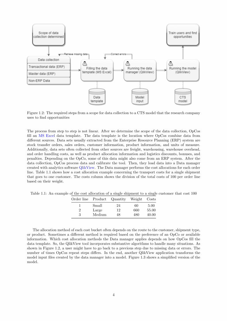
Figure 1.2: The required steps from a scope for data collection to a CTS model that the research companyuses to find opportunities
The process from step to step is not linear. After we determine the scope of the data collection, OpCosfill an MS Excel data template. The data template is the location where OpCos combine data fromdifferent sources. Data sets usually extracted from the Enterprise Resource Planning (ERP) system arestock transfer orders, sales orders, customer information, product information, and units of measure.Additionally, data sets often collected from other sources are freight, warehousing, warehouse overhead,and order handling costs, as well as product allocation information and logistics discounts, bonuses, andpenalties. Depending on the OpCo, some of this data might also come from an ERP system. After thedata collection, OpCos process data and calibrate the tool. Then, they load data into a Data managercreated with analytics software QlikView. The Data manager performs the cost allocations for each orderline. Table 1.1 shows how a cost allocation example concerning the transport costs for a single shipmentthat goes to one customer. The costs column shows the division of the total costs of 100 per order linebased on their weight.
Table 1.1: An example of the cost allocation of a single shipment to a single customer that cost 100
Order line Product Quantity Weight Costs
1 Small 24 60 5.002 Large 12 660 55.003 Medium 48 480 40.00
The allocation method of each cost bucket often depends on the route to the customer, shipment type,or product. Sometimes a different method is required based on the preference of an OpCo or availableinformation. Which cost allocation methods the Data manager applies depends on how OpCos fill thedata template. So, the QlikView tool incorporates substantive algorithms to handle many situations. Asshown in Figure 1.2, a user might have to go back to a previous step due to missing data or errors. Thenumber of times OpCos repeat steps differs. In the end, another QlikView application transforms themodel input files created by the data manager into a model. Figure 1.3 shows a simplified version of themodel.
4
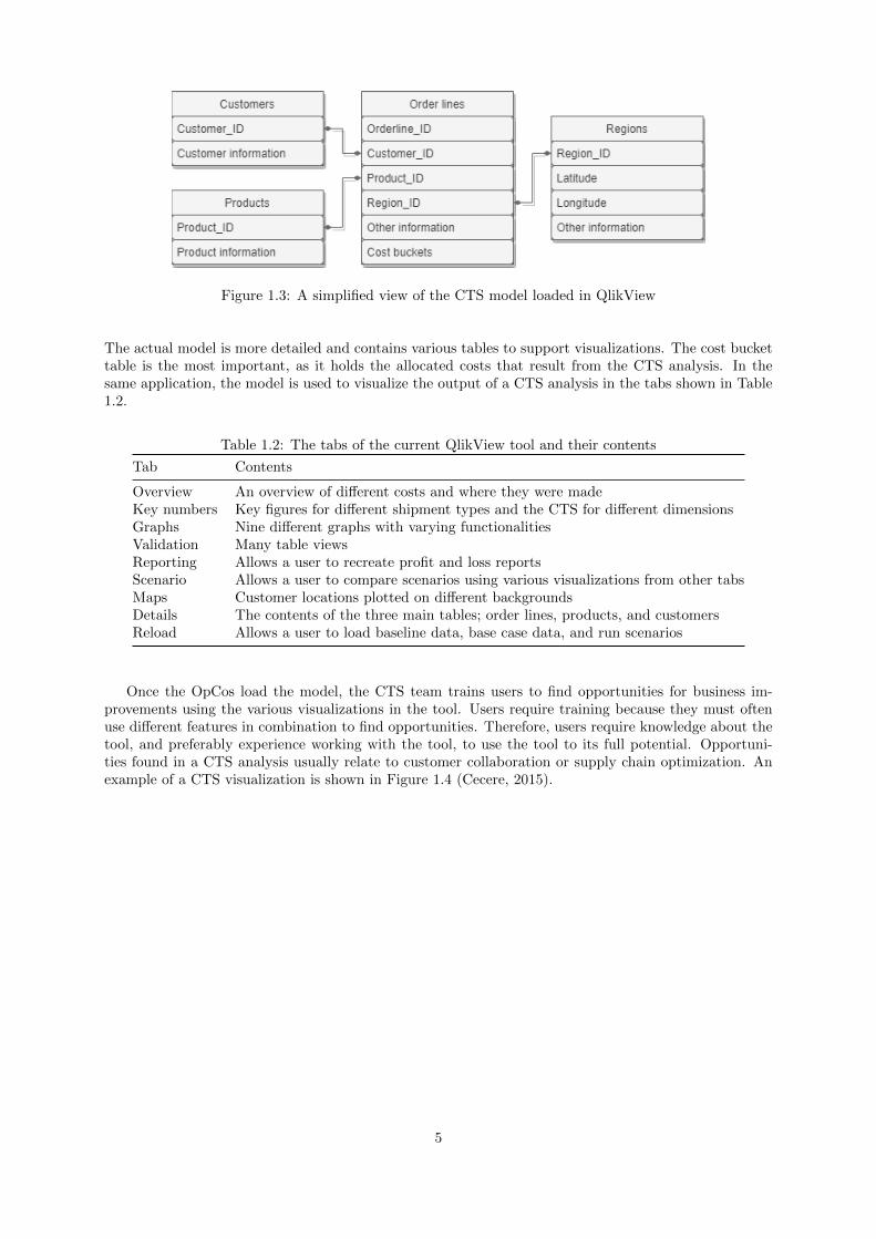
Figure 1.3: A simplified view of the CTS model loaded in QlikView
The actual model is more detailed and contains various tables to support visualizations. The cost buckettable is the most important, as it holds the allocated costs that result from the CTS analysis. In thesame application, the model is used to visualize the output of a CTS analysis in the tabs shown in Table1.2.
Table 1.2: The tabs of the current QlikView tool and their contents
Tab Contents
Overview An overview of different costs and where they were madeKey numbers Key figures for different shipment types and the CTS for different dimensionsGraphs Nine different graphs with varying functionalitiesValidation Many table viewsReporting Allows a user to recreate profit and loss reportsScenario Allows a user to compare scenarios using various visualizations from other tabsMaps Customer locations plotted on different backgroundsDetails The contents of the three main tables; order lines, products, and customersReload Allows a user to load baseline data, base case data, and run scenarios
Once the OpCos load the model, the CTS team trains users to find opportunities for business im-provements using the various visualizations in the tool. Users require training because they must oftenuse different features in combination to find opportunities. Therefore, users require knowledge about thetool, and preferably experience working with the tool, to use the tool to its full potential. Opportuni-ties found in a CTS analysis usually relate to customer collaboration or supply chain optimization. Anexample of a CTS visualization is shown in Figure 1.4 (Cecere, 2015).
5
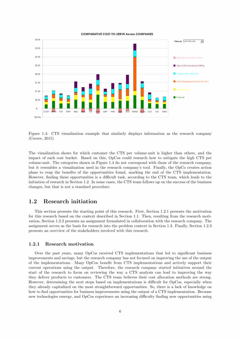
Figure 1.4: CTS visualization example that similarly displays information as the research company(Cecere, 2015)
The visualization shows for which customer the CTS per volume-unit is higher than others, and theimpact of each cost bucket. Based on this, OpCos could research how to mitigate the high CTS pervolume-unit. The categories shown in Figure 1.4 do not correspond with those of the research company,but it resembles a visualization used in the research company’s tool. Finally, the OpCo creates actionplans to reap the benefits of the opportunities found, marking the end of the CTS implementation.However, finding these opportunities is a difficult task, according to the CTS team, which leads to theinitiation of research in Section 1.2. In some cases, the CTS team follows up on the success of the businesschanges, but that is not a standard procedure.
1.2 Research initiation
This section presents the starting point of this research. First, Section 1.2.1 presents the motivationfor this research based on the context described in Section 1.1. Then, resulting from the research moti-vation, Section 1.2.2 presents an assignment formulated in collaboration with the research company. Theassignment serves as the basis for research into the problem context in Section 1.3. Finally, Section 1.2.3presents an overview of the stakeholders involved with this research.
1.2.1 Research motivation
Over the past years, many OpCos received CTS implementations that led to significant businessimprovements and savings, but the research company has not focused on improving the use of the outputof the implementations. Many OpCos benefit from CTS implementations and actively support theircurrent operations using the output. Therefore, the research company started initiatives around thestart of the research to focus on reviewing the way a CTS analysis can lead to improving the waythey deliver products to customers. The CTS team believes their cost allocation methods are strong.However, determining the next steps based on implementations is difficult for OpCos, especially whenthey already capitalized on the most straightforward opportunities. So, there is a lack of knowledge onhow to find opportunities for business improvements using the output of a CTS implementation. Becausenew technologies emerge, and OpCos experience an increasing difficulty finding new opportunities using
6
the tool, the CTS implementation of the research company is at risk of becoming outdated. Therefore,the requirement of the research company to improve the use of CTS analyses motivates this research.
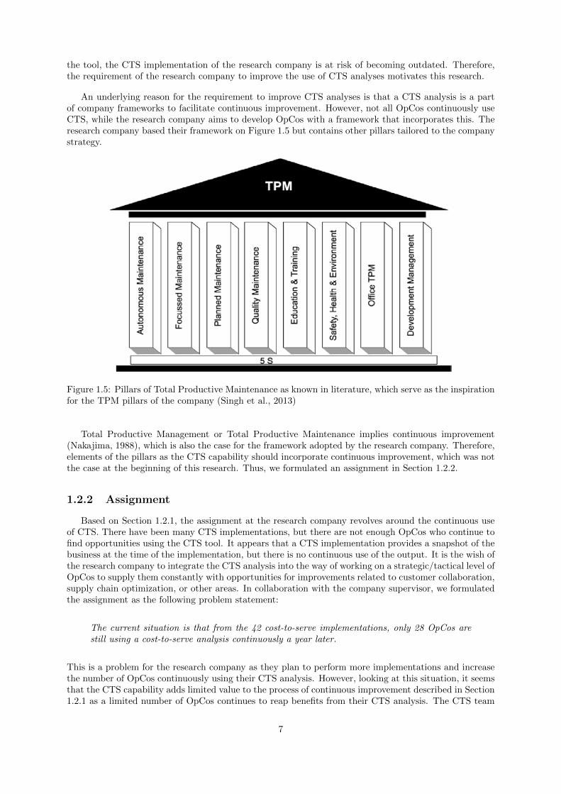
An underlying reason for the requirement to improve CTS analyses is that a CTS analysis is a partof company frameworks to facilitate continuous improvement. However, not all OpCos continuously useCTS, while the research company aims to develop OpCos with a framework that incorporates this. Theresearch company based their framework on Figure 1.5 but contains other pillars tailored to the companystrategy.
Figure 1.5: Pillars of Total Productive Maintenance as known in literature, which serve as the inspirationfor the TPM pillars of the company (Singh et al., 2013)
Total Productive Management or Total Productive Maintenance implies continuous improvement(Nakajima, 1988), which is also the case for the framework adopted by the research company. Therefore,elements of the pillars as the CTS capability should incorporate continuous improvement, which was notthe case at the beginning of this research. Thus, we formulated an assignment in Section 1.2.2.
1.2.2 Assignment
Based on Section 1.2.1, the assignment at the research company revolves around the continuous useof CTS. There have been many CTS implementations, but there are not enough OpCos who continue tofind opportunities using the CTS tool. It appears that a CTS implementation provides a snapshot of thebusiness at the time of the implementation, but there is no continuous use of the output. It is the wish ofthe research company to integrate the CTS analysis into the way of working on a strategic/tactical level ofOpCos to supply them constantly with opportunities for improvements related to customer collaboration,supply chain optimization, or other areas. In collaboration with the company supervisor, we formulatedthe assignment as the following problem statement:
The current situation is that from the 42 cost-to-serve implementations, only 28 OpCos arestill using a cost-to-serve analysis continuously a year later.
This is a problem for the research company as they plan to perform more implementations and increasethe number of OpCos continuously using their CTS analysis. However, looking at this situation, it seemsthat the CTS capability adds limited value to the process of continuous improvement described in Section1.2.1 as a limited number of OpCos continues to reap benefits from their CTS analysis. The CTS team
7

desires that all OpCos that have received a CTS implementation should still use their CTS analysiscontinuously a year later, meaning that the output is regularly updated and reviewed, as is the casefor the 28 OpCos. However, 14 OpCos incidentally consult their CTS analysis or have discontinued theuse of their CTS analysis. So, that 67% of the OpCos that received a CTS implementation still workcontinuously with their CTS analysis is too low, serves as the starting point of the problem identificationin Section 1.3.
1.2.3 Stakeholders
In this research, we distinguish several stakeholders. Stakeholders can be a person, a group of people,or even an entire company. Table 1.3 shows an overview of the involved stakeholders.
Table 1.3: Stakeholders for the master thesis research
Stakeholder Description
First university supervisor Dr. ir. W. J. A. van Heeswijk from the University of TwenteSecond university supervisor Prof. Dr. M. E. Iacob from the University of TwenteCompany supervisor ir. H. Stevens from the Customer Service team, and CTS teamCTS team A team of three people working actively on CTS implementationsCustomer Service team A team of ten people working on Customer Service capabilitiesOpCos A decentralized branch of the research company
All stakeholders play a different role in this research. We consulted University supervisors to maintain athesis worthy of graduating from the master’s of Industrial Engineering and Management. The companysupervisor represents the problem owner of the problem identified in Section 1.3. This stakeholder wasconsulted, informed often, and played a significant role in verifying outcomes. The CTS team is theproblem owner and was involved when requiring more than the single view of the problem owner. Theentire Customer Service team should understand the working of the CTS capability. Therefore, weinformed them of outcomes to ensure they can understand changes made to the CTS tool or process.Last, OpCos receive CTS implementations and are the final users of the CTS tool. CTS implementationsmust aim to answer business questions that OpCos have. Therefore, we took the view of OpCos intoaccount during the research.
1.3 Problem identification
This section analyzes the problem context surrounding the assignment presented in Section 1.2.2.First, Section 1.3.1 describes the problem context by creating a problem cluster and selecting potentialcore problems. Then, Section 1.3.2 evaluates core problems and decides on a focus for this research.
1.3.1 Problem context
The problem context is important in understanding what problems are related to the action problemresulting from the assignment in Section 1.2.2, which is that too few OpCos continuously use a CTSanalysis. A way to visualize the problem context is by creating a problem cluster, which is a part ofthe Managerial Problem-Solving Method described by Heerkens and van Winden (2012). We used thisspecific part of the method for the problem identification performed in this section. Section 1.4.3 presentsthe general research methodology used in this research. Conversations with members of the CTS teamand materials related to the research company led to insights into the problem context and the creationof the problem cluster. The final problem cluster was verified and agreed upon by the members of theCTS team. Figure 1.6 shows the problem cluster, portraying the problem context for the research.
8

Action problem Unchangeable coreproblem
Solvablecore problem
Too few OpCoscontinuously use a
cost-to-serveanalysis
The effort of updatingcontents is too high
The output is notuseful
The tool is too difficultto understand
There are too manytabs/options
Different localrealities requiredifferent options
Unreliable input data
Updating the inputdata costs too much
(time)
Data has to becollected manually
Too much data hasto be based on
estimations
Not all input data isavailable
Knowledge has beenlost
The data collectionprocess has not been
documented
People involvedhave left their
position
The data collectionprocess is different in
each OpCo
There is noautomated data
collection
Finding opportunitiescosts too much time
The output does notmatch expectations
Unclear expectations
OpCos do not havespecific questions
that need answering
The goals of cost-to-serve are unclear
for OpCos
Output on shipmentlevel does not
answer questions
Lack of diagnostic,predictive, and
prescriptive insights
The tool does notdirectly provide
actionable insights
The tool cannothandle multiple
years of data
Users are nottrained well enough
Usefulness: reliable input data, clear goals,and powerful insights
Simplicity: dataautomation
Empowerment:well-trained users
1
3
64
10
9
7
8
11
5
2
Figure 1.6: Problem cluster showing the problem context at the research company
9

The problem cluster visualizes causal relations between problems that occur within the problemcontext. It starts with the action problem at the top of the figure and shows the causes of each problem.When there is no cause for a problem, it is considered a core problem. Core problems are the problemsthat have the highest effect when solved, as solving these problems has a positive influence on all problemsrelated to this problem. Figure 1.6 shows multiple core problems that influence the action problem whichare summarized in Table 1.4. To clarify the problem cluster, we created three main categories. Thefirst category is simplicity, with problems concerning data automation that can severely simplify theCTS implementation process. The second category is usefulness, which concerns reliable input data,clear goals, clear expectations, and handling multiple years of data. So, the tool should provide powerfulinsights that can drive the business forward. The third category is empowerment, which implies that thetools users are fully empowered to make to get the most out of the tool.
Table 1.4: Summary of core problems (Red = Unchangeable core problem, Green = Solvable core problem)Number Problem Explanation
1People involved have left theirposition
People previously involved in CTS haveleft their position, which results in a lossof tacit knowledge.
2There is no automated data col-lection
The absence of an automated data collec-tion leads to an intensive data gatheringprocess.
3 Not all input data is available
Some OpCos cannot provide all the neces-sary input data. Sometimes, the requiredinput data does not exist at all for anOpCo, which decreases the usefulness ofthe tool.
4Too much data has to be basedon estimations
Various estimations are made in the CTSimplementation. However, it is not surewhether they are all valid.
5OpCos do not have specificquestions that need answering
OpCos do not know which problems theywant to solve using CTS. Often they arebaffled by the possibilities.
6The goals of cost-to-serve areunclear for OpCos
OpCos might focus more on obtaining thetool than considering what the generalgoals are of the implementation.
7Output on shipment level doesnot answer questions
The current tool provides data on a ship-ment level. Including data on differentlevels (e.g. invoice or order) could providemore insights.
8The tool cannot handle multi-ple years of data
Because the tool does not allow for multi-ple years of data trend analysis or moni-toring change is not possible.
9Lack of diagnostic, predictive,and prescriptive insights
The current tool mostly displays data de-scriptively. Therefore, it is more difficultto obtain insights quickly.
10Different local realities requiredifferent options
Due to inherent differences between Op-Cos, requirements can differ heavily.
11Users are not trained wellenough
Using the tool requires training. Moretraining would lead to better use of thetool.
Starting from the action problem determined in Section 1.2.2, stating that too few OpCos continuouslyuse a CTS analysis, we found seven solvable core problems. Section 1.3.2 discusses problems that arepotential core problem for this research. In that section, we make a methodological decision regardingwhich problem(s) to focus on based on impact, strategic importance, and effort.
10
We cannot solve four of the potential core problems presented in this research. The first problemthat we cannot solve is Problem 1, that people involved have left their position, as there is no way toinfluence the career path of individuals as a part of this research. The second problem that is not possibleto solve for two reasons is Problem 3, that not all input data is available. First, when an OpCo doesnot have to collect specific data, there is no reason to change this situation. Second, when data shouldbe available, the OpCo should facilitate this locally, as they maintain their own IT systems. The globalorganization can help OpCos to collect specific data, but it is not the focus of this research. The resultingproblem is Problem 4, that too much data relies on estimations, which is considered as a potential coreproblem because the problem connects to Problem 3 by a single relationship. Third, Problem 5, statingthat OpCos do not have specific questions that need answering, presents a circumstance that we cannotinfluence. Last, Problem 10, that different local realities require different options, concerns local factors.It is not within the power of this research to change elements as culture or legislation in countries. So,we do not focus on these issues in this research. Section 1.3.2 presents the problems that we do consider.
1.3.2 Core problem
This section considers the solvable core problems identified in Section 1.3.1, determining which ofthese problems yields the highest impact when solved and is solvable within the time provided for thisresearch. First, we evaluate the solvable problems and choose a focus for the research. Then, we reviewthe understanding of the current reality and the norm for the selected problem.
Selection of the core problem
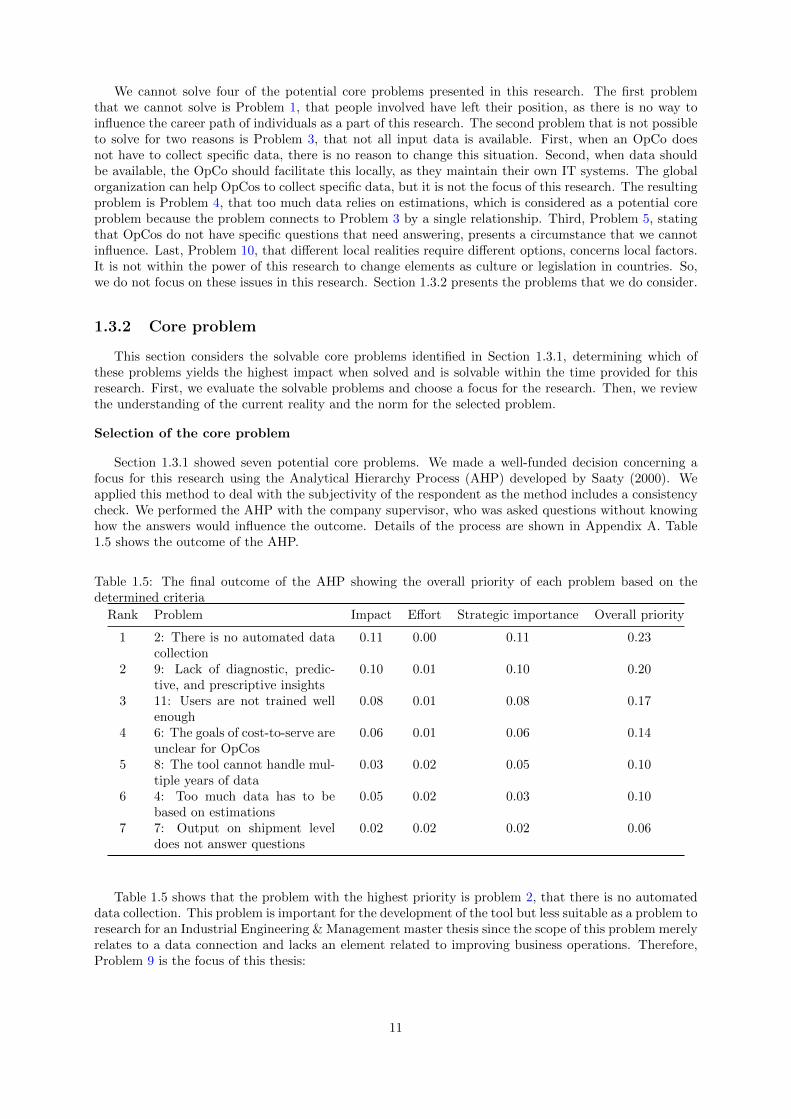
Section 1.3.1 showed seven potential core problems. We made a well-funded decision concerning afocus for this research using the Analytical Hierarchy Process (AHP) developed by Saaty (2000). Weapplied this method to deal with the subjectivity of the respondent as the method includes a consistencycheck. We performed the AHP with the company supervisor, who was asked questions without knowinghow the answers would influence the outcome. Details of the process are shown in Appendix A. Table1.5 shows the outcome of the AHP.
Table 1.5: The final outcome of the AHP showing the overall priority of each problem based on thedetermined criteria
Rank Problem Impact Effort Strategic importance Overall priority
1 2: There is no automated datacollection
0.11 0.00 0.11 0.23
2 9: Lack of diagnostic, predic-tive, and prescriptive insights
0.10 0.01 0.10 0.20
3 11: Users are not trained wellenough
0.08 0.01 0.08 0.17
4 6: The goals of cost-to-serve areunclear for OpCos
0.06 0.01 0.06 0.14
5 8: The tool cannot handle mul-tiple years of data
0.03 0.02 0.05 0.10
6 4: Too much data has to bebased on estimations
0.05 0.02 0.03 0.10
7 7: Output on shipment leveldoes not answer questions
0.02 0.02 0.02 0.06
Table 1.5 shows that the problem with the highest priority is problem 2, that there is no automateddata collection. This problem is important for the development of the tool but less suitable as a problem toresearch for an Industrial Engineering & Management master thesis since the scope of this problem merelyrelates to a data connection and lacks an element related to improving business operations. Therefore,Problem 9 is the focus of this thesis:
11
There is a lack of diagnostic, predictive, and prescriptive insights.
This problem poses as the starting point for the problem approach presented in Section 1.4. By usingthe many features of the research company’s CTS tool, which mainly incorporates descriptive analytics,users can obtain higher-level insights. However, the extent to which this is possible strongly relies onthe expertise of users. So, improving the presence of different types of features can lead to actionableinsights, increase the likelihood that OpCos continue to use the output of their CTS analysis, and therebysolve the action problem. Thus, the focus is on which descriptive, diagnostic, predictive, and prescriptiveanalytics the research company should apply when visualizing the output of a CTS analysis to increaseuser-value, where analytics are underlying mechanisms used in features. The next section explains thedifferences between types of analytics.
Norm and reality
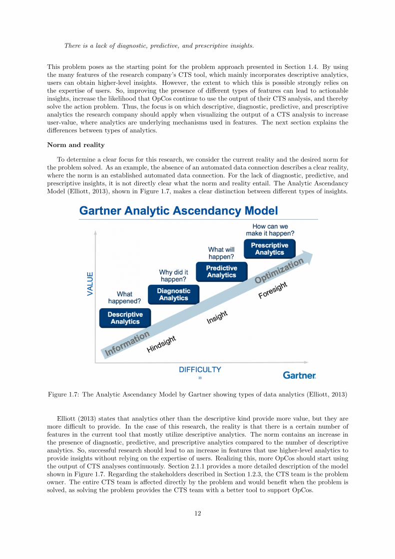
To determine a clear focus for this research, we consider the current reality and the desired norm forthe problem solved. As an example, the absence of an automated data connection describes a clear reality,where the norm is an established automated data connection. For the lack of diagnostic, predictive, andprescriptive insights, it is not directly clear what the norm and reality entail. The Analytic AscendancyModel (Elliott, 2013), shown in Figure 1.7, makes a clear distinction between different types of insights.
Figure 1.7: The Analytic Ascendancy Model by Gartner showing types of data analytics (Elliott, 2013)
Elliott (2013) states that analytics other than the descriptive kind provide more value, but they aremore difficult to provide. In the case of this research, the reality is that there is a certain number offeatures in the current tool that mostly utilize descriptive analytics. The norm contains an increase inthe presence of diagnostic, predictive, and prescriptive analytics compared to the number of descriptiveanalytics. So, successful research should lead to an increase in features that use higher-level analytics toprovide insights without relying on the expertise of users. Realizing this, more OpCos should start usingthe output of CTS analyses continuously. Section 2.1.1 provides a more detailed description of the modelshown in Figure 1.7. Regarding the stakeholders described in Section 1.2.3, the CTS team is the problemowner. The entire CTS team is affected directly by the problem and would benefit when the problem issolved, as solving the problem provides the CTS team with a better tool to support OpCos.
12

1.4 Problem approach
This section presents the approach to solve the core problem identified in Section 1.3.2. First, inSection 1.4.1, we demarcate the scope and formulate the goal of the research. Then, Section 1.4.2presents the main research questions and supportive research questions, and Section 1.4.3 presents theDesign Science Research Methodology as the methodology for this thesis. Finally, Section 1.4.4 outlinesthis report, combining the research questions and the research methodology.
1.4.1 Research scope and goal
This research applies to Fast-Moving Consumer Goods (FMCG) companies that use CTS analyses orwant to start using CTS analyses. We answer several questions in the context of the research company,but because the outcome of the research applies to many OpCos that are individual FMCG companieswith a distinctive local reality, we can generalize findings. Designed solutions fit all OpCos, taking factorssuch as different regions and sizes into account. Furthermore, we took OpCo specific delivery strategies,vehicle types, and other factors influencing the CTS into account. Finally, designed solutions add valueto the Customer Service team. As guidance, features focus on customer-related improvements.
Section 1.3.2 showed that the problem to solve is the lack of diagnostic, predictive, and prescriptiveinsights. So, the focus of this research is on the analytics used to visualize the output of the CTSimplementation. Consequently, we determined the research goal and the main deliverable accordingly.Figure 1.8 shows how, starting from the formulation of the assignment, these were determined.
Figure 1.8: The connection between the assignment, the selected core problem, the research goal, andthe main deliverable of this thesis
As the research in this thesis applies to FMCG companies that want to find business improvements,a generic framework can outline how to visualize the output of a CTS analysis. Findings apply to anyFMCG company regardless of their software or business processes. Thus, the generalized research goalis as follows:
The goal of this research is to design a framework for fast-moving consumer goods companiesto find business improvements using the output of a cost-to-serve analysis.
For the research company, the aim is to increase the number of OpCos that continuously use CTS analyses.The CTS tool visualizes the output of the analysis, but the analytics used in the tool’s features appear
13

insufficient as a large proportion of the OpCos does not continue to use the tool. The framework createdin this thesis includes the development of the CTS tool. By applying the framework to the researchcompany, we created a new CTS tool. The reason to focus on the CTS tool is that it is at the pinnacleof finding opportunities. The main deliverable of the thesis is linked to this and defined as follows:
For the research company, we create a new tool based on the designed framework to findbusiness improvements using the output of a cost-to-serve analysis.
There are two reasons for creating a new tool rather than extending the current CTS tool. Firstly,manufacturers no longer maintain QlikView software. And secondly, the research company selected newtooling software as a company-wide solution.
1.4.2 Research questions
This section presents the main research questions, as well as several supportive questions. Section1.4.4 details which chapters and sections correspond to the questions. We formulated two main researchquestions for this thesis based on the assignment, the core problem, the research goal, and the maindeliverable shown in Figure 1.8. The first main research question, which focuses on the research goal, isas follows:
1 How can fast-moving consumer goods companies find business improvementsby using descriptive, diagnostic, predictive, and descriptive analytics in their toolthat visualizes the output of a cost-to-serve analysis?
Answering the first main research question provides a framework to find business improvements usingthe output of a CTS analysis, which we based on literature and findings related to the research company.Additionally, we formulated a second main research question for the application of the framework inpractice. This research question focuses on the main deliverable, a new CTS tool for the research company,created as a part of a case study. The second main research question is as follows:
2 Can the research company improve the use of the output of cost-to-serve anal-yses by applying the framework designed in this research to create a new tool?
The answer to the second main research question is of value to the research company, as it includesthe creation of a new tool. We answer the research question by applying the framework to the researchcompany in a case study. Besides answering this research question, the case study allows for a validationof the framework. Several research questions support the two main research questions, which we presentin the rest of this section.
Framework development
Answering the first main research question creates a framework. The first supportive research questionto develop the framework is:
1.1 Which descriptive, diagnostic, predictive, and prescriptive features can visualize the outputof a cost-to-serve analysis?
When developing the CTS tool, certain features and analytics add value where others do not. We reviewedliterary sources to understand which features and analytics to apply when visualizing the output of a CTSanalysis, and we assessed how users appreciate parts of the research company’s current tool by surveyingusers in the CTS team and OpCos. Then, we consolidated the results of this research by creating a setof optional features to develop for a CTS tool as a part of the framework to find business improvementsusing the output of a CTS analysis.
14

1.2 How can fast-moving consumer goods companies find a root-cause for a high cost-to-serveper volume-unit based on data used in the cost-to-serve analysis?
Section 4.2.1 argues the development of a feature using diagnostic analytics to find root-causes for ahigh CTS per volume-unit for the research company. This method allows users to select an entity ora combination of entities and find causes for a high CTS per volume unit. An algorithm finds similarentities with a lower CTS per volume-unit, showing where FMCG companies can potentially improveeach entity. The purpose of this research question is to develop a generic method based on literatureregarding input variables, variable selection, and predictive models. This method is applicable in multiplesettings as we applied general techniques that are not only applicable in the case of the research company.
1.3 How can fast-moving consumer goods companies map business improvements obtained withinsights from a cost-to-serve analysis?
The goal of a CTS analysis is to find business improvements. Preferably, FMCG companies can learnfrom past business improvements to strengthen their CTS analysis. To understand how insights canlead to opportunities for business improvements, we performed a literature study and researched pastCTS implementations performed by the research company. Answering this research question provided astructure to map opportunities resulting from obtained insights.
1.4 Which techniques can assess the quality of a tool visualizing the output of a cost-to-serveanalysis?
FMCG companies should measure the effect of changes made to a tool to track improvement. For this,we reviewed the literature concerning technology assessment models, developing a method to evaluatethe performance of tools visualizing the output of a CTS analysis. The resulting method includes ameasurement of success, tool assessment, and feature assessment that FMCG companies should applybefore every iteration that changes to a CTS tool.
Case study: Applying the framework in the research company
After the creation of the framework by answering the first main research question, we validate theframework by applying it to the research company. Consequently, we developed a new tool for the researchcompany. The first research question that supports the second main research question is:
2.1 How is the cost-to-serve implementation of the research company performing?
The purpose of this research question is to understand what type of business improvements the researchcompany found in the past and assess the performance of CTS implementations in the research company.First, related to Research Question 1.3, we validated the structure to map opportunities. We mapped andcollected opportunities found in the research company in the past years, creating an interactive report.Second, related to Research Question 1.4, we validated the method to evaluate the performance of toolsvisualizing the output of a CTS analysis. We assessed the performance of the research company’s CTSimplementations and the current CTS tool by surveying users.
2.2 Which descriptive, diagnostic, predictive, and prescriptive features should the researchcompany use to visualize the output of a cost-to-serve analysis?
The answer to this research question clarifies what to include in the new CTS tool of the research company.Related to Research Question 1.1, we validated the set of options by assessing which features from thecurrent CTS tool should remain and what to develop in the new CTS tool of the research company. Wevalidated decisions made by surveying users of the CTS tool.
15
2.3 How can the research company incorporate the chosen descriptive, diagnostic, predictive,and prescriptive analytics into a new tool?
The purpose of this question is to clarify how we can create a usable CTS tool by presenting the design andcreation of the new CTS tool. We paid attention to the preparation steps required and the developmentof the new CTS tool that contains descriptive analytics from the current CTS tool and analytics thatare new to the research company. Related to Research Question 1.2, we created a modular root-causeanalysis approach that the research company can potentially include in the new CTS tool.
1.4.3 Research methodology
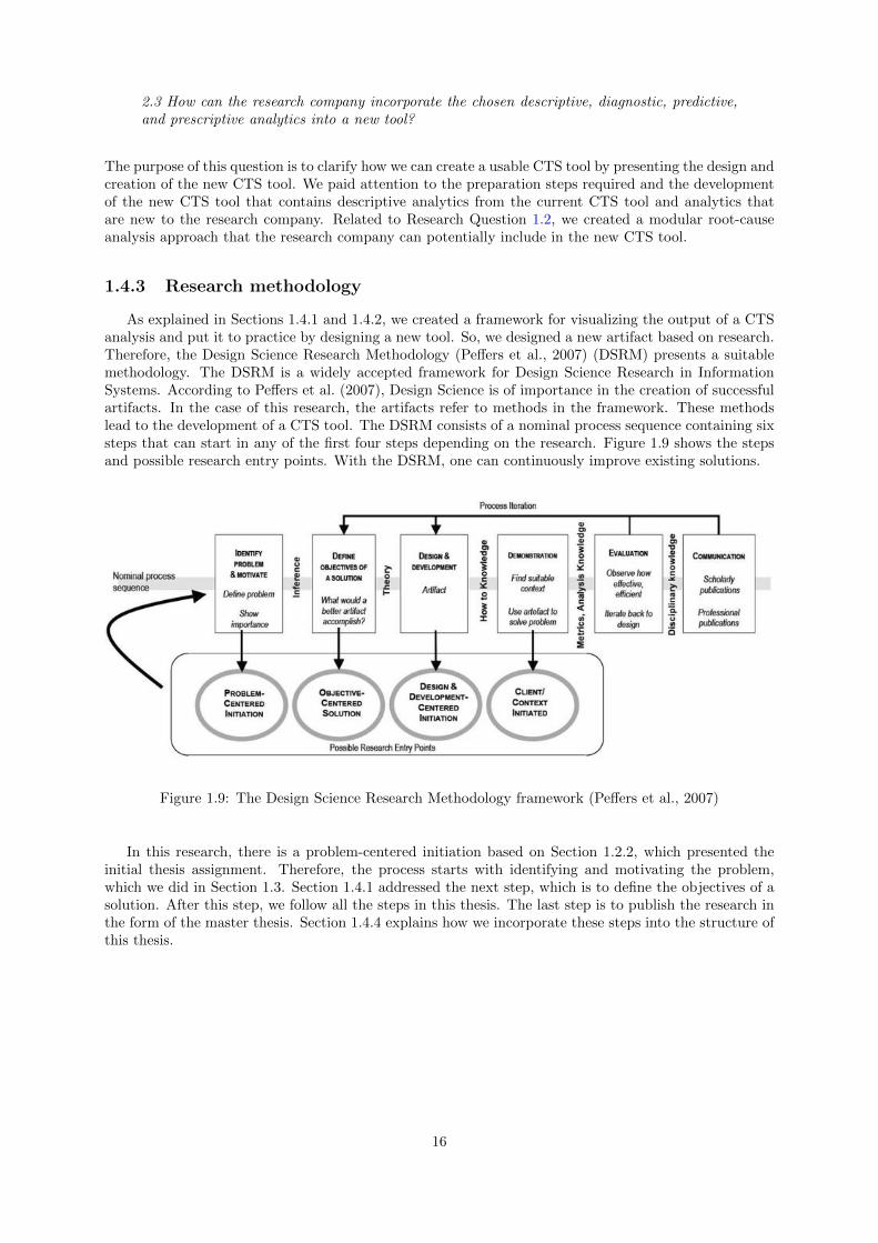
As explained in Sections 1.4.1 and 1.4.2, we created a framework for visualizing the output of a CTSanalysis and put it to practice by designing a new tool. So, we designed a new artifact based on research.Therefore, the Design Science Research Methodology (Peffers et al., 2007) (DSRM) presents a suitablemethodology. The DSRM is a widely accepted framework for Design Science Research in InformationSystems. According to Peffers et al. (2007), Design Science is of importance in the creation of successfulartifacts. In the case of this research, the artifacts refer to methods in the framework. These methodslead to the development of a CTS tool. The DSRM consists of a nominal process sequence containing sixsteps that can start in any of the first four steps depending on the research. Figure 1.9 shows the stepsand possible research entry points. With the DSRM, one can continuously improve existing solutions.
Figure 1.9: The Design Science Research Methodology framework (Peffers et al., 2007)
In this research, there is a problem-centered initiation based on Section 1.2.2, which presented theinitial thesis assignment. Therefore, the process starts with identifying and motivating the problem,which we did in Section 1.3. Section 1.4.1 addressed the next step, which is to define the objectives of asolution. After this step, we follow all the steps in this thesis. The last step is to publish the research inthe form of the master thesis. Section 1.4.4 explains how we incorporate these steps into the structure ofthis thesis.
16
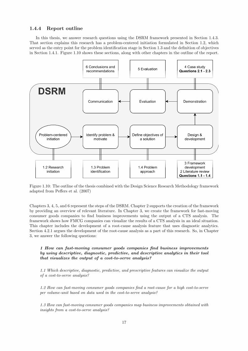
1.4.4 Report outline
In this thesis, we answer research questions using the DSRM framework presented in Section 1.4.3.That section explains this research has a problem-centered initiation formulated in Section 1.2, whichserved as the entry point for the problem identification stage in Section 1.3 and the definition of objectivesin Section 1.4.1. Figure 1.10 shows these sections, along with other chapters in the outline of the report.
Figure 1.10: The outline of the thesis combined with the Design Science Research Methodology frameworkadapted from Peffers et al. (2007)
Chapters 3, 4, 5, and 6 represent the steps of the DSRM. Chapter 2 supports the creation of the frameworkby providing an overview of relevant literature. In Chapter 3, we create the framework for fast-movingconsumer goods companies to find business improvements using the output of a CTS analysis. Theframework shows how FMCG companies can visualize the results of a CTS analysis in an ideal situation.This chapter includes the development of a root-cause analysis feature that uses diagnostic analytics.Section 4.2.1 argues the development of the root-cause analysis as a part of this research. So, in Chapter3, we answer the following questions:
1 How can fast-moving consumer goods companies find business improvementsby using descriptive, diagnostic, predictive, and descriptive analytics in their toolthat visualizes the output of a cost-to-serve analysis?
1.1 Which descriptive, diagnostic, predictive, and prescriptive features can visualize the outputof a cost-to-serve analysis?
1.2 How can fast-moving consumer goods companies find a root-cause for a high cost-to-serveper volume-unit based on data used in the cost-to-serve analysis?
1.3 How can fast-moving consumer goods companies map business improvements obtained withinsights from a cost-to-serve analysis?
17

1.4 Which techniques can assess the quality of a tool visualizing the output of a cost-to-serveanalysis?
In Chapter 4, we applied the framework to the research company in a case study. We validated theframework by showing how it performs in practice and developed a new tool for the research company.So, in this chapter, we answer the following questions:
2 Can the research company improve the use of the output of cost-to-serve anal-yses by applying the framework designed in this research to create a new tool?
2.1 How is the cost-to-serve implementation of the research company performing?
2.2 Which descriptive, diagnostic, predictive, and prescriptive features should the researchcompany use to visualize the output of a cost-to-serve analysis?
2.3 How can the research company incorporate the chosen descriptive, diagnostic, predictive,and prescriptive analytics into a new tool?
Chapter 5 evaluates the implementation of the framework in the research company and the newCTS tool. This evaluation is similar to the assessment of the current situation in Section 4.1. Then,Chapter 6 answers all research questions in the form of conclusions and presents recommendations, whichinclude advice on how the company should structure future developments in light of the implementationof the framework. Finally, the discussion section reviews the applicability of the framework, limitations,opportunities for future research, and the contributions to theory and practice.
18

Chapter 2
Literature review
This chapter reviews literature that supports the answering of the following main research question:
1 How can fast-moving consumer goods companies find business improvementsby using descriptive, diagnostic, predictive, and descriptive analytics in their toolthat visualizes the output of a cost-to-serve analysis?
First, Section 2.1 defines key constructs by explaining important concepts applied in this thesis. Then,Sections 2.2 and 2.3 present the results of literature studies on the benefits of cost-to-serve and potentialanalytics from literature. The first review focuses on what the end goals of a cost-to-serve analysisare, and the second on applicable techniques for visualizing the output of a cost-to-serve analysis. Thefocus is not descriptive analytics, as the research company uses these extensively in the current situationdescribed in Section 4.1. Then, Section 2.4 presents variables that can serve as potential cost drivers fora high cost-to-serve per volume-unit, Section 2.5 presents methods to reduce the number of variables,and Section 2.6 presents literature concerning models to predict a high cost-to-serve per volume-unit.The root cause analysis in Section 3.3.4 uses these variables and models. Finally, Section 2.7 performsresearch into methods to determine the performance of a tool, which are used in Section 3.5.2.
2.1 Key constructs
Throughout this report, we apply various concepts, structures, and research components. The purposeof this section is to shed light on these topics to ensure a clear understanding of their definition. Conceptsexplained in this section support the answering of Research questions 1.1 and 1.4. First, Section 2.1.1presents the different types of analytics referred to throughout this thesis. Then, Section 2.1.2 presents amodel that visualizes requirement engineering for feature development. Finally, Section 2.1.3 defines theconcepts frameworks, methods, and roadmaps.
2.1.1 Opportunities and analytics
In this thesis, various sections mention opportunities for business improvements. An opportunity isan “exploitable set of circumstances with an uncertain outcome, requiring a commitment of resources andinvolving exposure to risk” (BusinessDictionairy.com, 2020). In this research, an opportunity is withinthe scope defined in Section 1.4.1 and found with the CTS tool. A tool refers to an application, whichis “a software program that runs on your computer” (Christensson, 2008) and leads to opportunitiesby providing insights. Section 1.3.2 presented the Gartner Analytic Ascendancy Model (Elliott, 2013),explaining different kinds of analytics supply hindsight, insights, and foresight. These levels of insightsanswer different types of questions (Jong, 2019). Table 2.1 shows the types of questions the differentanalytics answer.
19
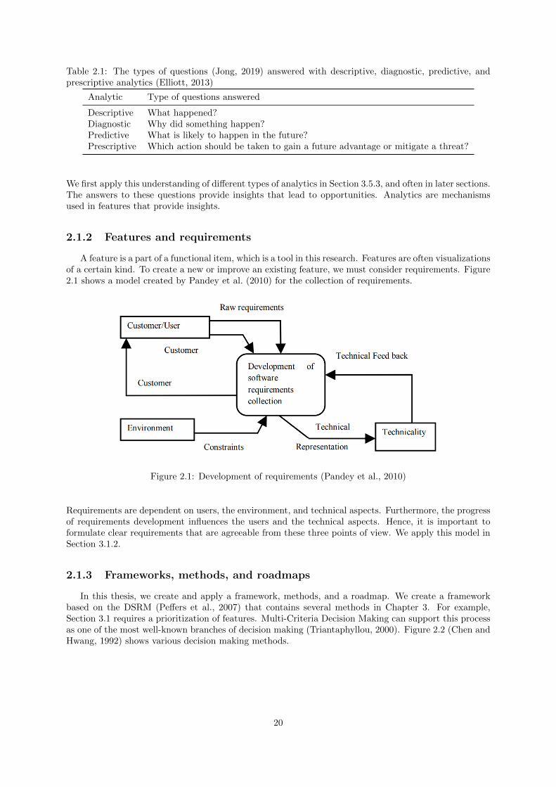
Table 2.1: The types of questions (Jong, 2019) answered with descriptive, diagnostic, predictive, andprescriptive analytics (Elliott, 2013)
Analytic Type of questions answered
Descriptive What happened?Diagnostic Why did something happen?Predictive What is likely to happen in the future?Prescriptive Which action should be taken to gain a future advantage or mitigate a threat?
We first apply this understanding of different types of analytics in Section 3.5.3, and often in later sections.The answers to these questions provide insights that lead to opportunities. Analytics are mechanismsused in features that provide insights.
2.1.2 Features and requirements
A feature is a part of a functional item, which is a tool in this research. Features are often visualizationsof a certain kind. To create a new or improve an existing feature, we must consider requirements. Figure2.1 shows a model created by Pandey et al. (2010) for the collection of requirements.
Figure 2.1: Development of requirements (Pandey et al., 2010)
Requirements are dependent on users, the environment, and technical aspects. Furthermore, the progressof requirements development influences the users and the technical aspects. Hence, it is important toformulate clear requirements that are agreeable from these three points of view. We apply this model inSection 3.1.2.
2.1.3 Frameworks, methods, and roadmaps
In this thesis, we create and apply a framework, methods, and a roadmap. We create a frameworkbased on the DSRM (Peffers et al., 2007) that contains several methods in Chapter 3. For example,Section 3.1 requires a prioritization of features. Multi-Criteria Decision Making can support this processas one of the most well-known branches of decision making (Triantaphyllou, 2000). Figure 2.2 (Chen andHwang, 1992) shows various decision making methods.
20

Figure 2.2: A taxonomy of Multi-Criteria Decision Making Methods (Chen and Hwang, 1992)
The AHP method, applied in Section 1.3.2, is a part of this overview. When deciding what to developin Section 3.1, this technique is applicable. Finally, Section 6.2 includes a roadmap. “A roadmap is astrategic plan that defines a goal or desired outcome and includes the major steps or milestones neededto reach it” (ProductPlan, 2020).
2.2 Benefits of cost-to-serve
This section reviews the obtained benefits from cost-to-serve analyses outside of the research company.We mainly do this to answer the Research question 1.3 How can fast-moving consumer goods companiesmap business improvements obtained with insights from a cost-to-serve analysis?, by identifying maincategories of opportunities found in a cost-to-serve analysis. Section 3.1.1 applies the outcome of thisliterature study to assess benefits held by different potential features, and Section 3.5.1 to determinemeasures of success.
Poole (2017), who performed a study in an FMCG company, states that the goal of a CTS analysisis to support three factors:
• It supports customer service optimization by redesigning processes to make them more efficient.
• It should support collaboration strategies, where actions benefit both the company and the cus-tomer.
• It helps a company to provide the right service at the optimal costs by providing insights into howthey service customers and what the incurred cost was of different activities.
21

In general, Poole describes that a CTS analysis is about improving customer service. Kolarovszki et al.(2016) take a different view by focusing on the relationship between customer profitability and a CTSanalysis through segmenting customers. The focus on profitability often reoccurs. Kone and Karwan(2011) say about a CTS analysis that it “allows companies to monitor their costs and therefore managetheir pricing strategy and profitability.” Findings of a study by Guerreiro et al. (2008) show that mea-suring the CTS enables a more comprehensive customer profitability analysis than the compared studies.Holm et al. (2012) support the research of Guerreiro et al. by stating “the measurement of cost-to-serveprovides specific customer information that enables a more comprehensive CPA than when only mea-suring gross profit from products,” where CPA is referring to a Customer Profitability Analysis. Moststudies do not focus on the customer, contrary to the research company. When reviewing the benefitsmentioned in this section, the main goal is usually profit. Poole (2017) explains that the purpose ofcustomer service optimization is to make processes more efficient, which implies a reduction in costs.Furthermore, customer collaboration means the same but focuses on shared benefits, and a profitablepricing strategy also focuses on increasing profits. Thus, companies should measure obtained profits toassess the performance of a CTS analysis.
Besides profits, customers also hold importance concerning the benefits of CTS. As customers arecritical to the success of FMCG companies, customer satisfaction is also an important indicator. Fur-thermore, performing this research from the Global Customer Service team of the research company,there is an increased interest in customers. A customer is the point of sales for the company. In thecase of an FMCG company, a consumer usually follows the customer. A general method to measurecustomer satisfaction is by asking customers how satisfied they are and dividing the positive responsesby the total number of respondents (Tripathi, 2020). The Net Promoter Score (NPS) is another methodthat measures customer satisfaction that the research company uses. Reichheld (2003) developed thismethod, which relies on customers answering the question: “How likely is it that you would recommendour company to a friend or colleague?” Then, responses returning a 9 or 10 (out of 10) represent pro-moters, responses returning a 7 or 8 represent passives, and responses returning a lower score representdetractors. Respondents that are passives do not influence the NPS score, which Reichheld calculates asfollows:
NPS = PromotersRespondents −
DetractorsRespondents
According to Reichheld (2003), an NPS above 75% indicates world-class customer loyalty. However,the NPS method gained some criticism. Fisher and Kordupleski (2019) claim that the NPS methodperforms poorly and propose a superior Customer Value Management method. Furthermore, Poole(2020) proposes a Value Enhancement Core method that outperforms the predictive accuracy of theNPS concerning customer loyalty. So, there are various rivaling methods available. In general, FMCGcompanies have certain customer satisfaction measures in place. The important factor is that companiesshould measure customer satisfaction in a way and take it into account when evaluating the performanceof CTS analyses.
In conclusion, the main benefits of a CTS analysis relate to profitability and customer satisfaction.Specifically, a CTS analysis provides benefits that relate to customer service optimization, customercollaboration, and a profitable pricing strategy. The measurement of profitability is straightforward,and for customer satisfaction, various measurement techniques are available, which includes the NPSmeasurement.
2.3 Analytics using cost-to-serve
Section 2.2 clarified that a cost-to-serve analysis focuses on increasing company profitability andcustomer satisfaction. Here, we present various analytics based on the output of CTS analyses thatprovide insights that can lead to the mentioned benefits. We mainly do this to answer research question1.1 Which descriptive, diagnostic, predictive, and prescriptive features can visualize the output of acost-to-serve analysis?, by supporting the collection of potential analytics in Section 3.1. Furthermore,the contents of this literature review inspired the importance of a cost allocation step in the frameworkpresented in Section 3.2.2, and the inclusion of hierarchies and segmentation in the framework presented
22

in Section 3.3.1.
Kone and Karwan (2011) focus on predicting the CTS of new customers by clustering customers usingvarious classification attributes. Sun et al. (2015) continue on this with an improved attribute selection,and more recently, Wang et al. (2020) also focus on the estimation of the CTS, concerning the routingcosts for new customers in particular. Wang et al. state that their model is more accurate than theprevious models. Ozener et al. (2013) provides another example of estimating the costs of including anew customer by evaluating customers that use a Vendor Managed Inventory. With a Vendor ManagedInventory, a company can control the inventory levels of its customers. Thus, there are various exampleswhere the focus is on estimating costs for new customers. It is of importance to take into account thatsuch estimations often apply to other dimensions, such as products, as well. Another specific exampleof the use of CTS data is for optimizing third-party logistics service delivery (Ross et al., 2007). Thatresearch focuses on identifying the cost-drivers of third-party-logistics providers within the internal supplychains. So, it is not customer-focused research.
Everaert et al. (2008) focus on improving logistics using a time-driven Activity Based Costing strategy,proving this strategy is more accurate than the regular Activity Based Costing methods. Everaert et al.describe various key-drivers of profitability that mainly focus on the difference between targeted costs,which are theoretically estimated costs, and actual costs. Furthermore, Everaert et al. mention initiativesto enhance profitability, where most efforts relate to negotiating and sales, which are not in the scopeof this research. However, relevant techniques mentioned are introducing minimum order value policies,maximal discount policies, which indicate the discount a company can offer to a customer in exchange forimprovements for the company, optimizing delivery routes, and improving capacity planning. Everaertet al. used simulations to evaluate different scenarios. We could translate these initiatives into analyticsto provide actionable insights using the output of a CTS analysis.
In general, there is not much research available on analytics that could provide useful insights basedon the output of a CTS analysis. Possibilities for analytics can rely on cost buckets used in a CTSanalysis. So, FMCG companies must have a complete set of cost buckets. Often these buckets are valuedusing Activity-Based Costing (Turney, 1992), which assigns resources to activities (Kaplan and Anderson,2003). For example, Kolarovszki et al. (2016) determine the CTS based on the number of visits, distancefrom the customer, and the frequency of contacts. Freeman et al. (2000) take a more comprehensiveapproach by distinguishing many activities related to sales, marketing, and physical distribution. Thekey in all these different approaches is to assign costs to activities and thereby determine the CTS of anorder (line). The mentioned approaches differ in each case and appear tailored to a specific industry orenvironment. Of course, enriching the output of a CTS analysis with general data such as customer orproduct data allows for more possibilities for providing insights through analytics.
To make features more insightful, companies can focus on a group of customers or products that is ofimportance to them, which requires a type of segmentation. Segmentation might not offer direct insights,but it can support other features. Traditionally, a market is segmented based on attributes such asgeography, channel, or demographics (Bolton and Tarasi, 2006). Before this, Bonoma and Shapiro (1984)have already made this concrete by stating five segmentation attributes to use in a nested hierarchy,which are demographics, operating variables, purchasing approach, situational factors, and personalcharacteristics. Companies can also apply nested hierarchies for products, using different attributes(Davis, 2010). By using nested hierarchies, companies can visualize data on different levels, but thisrequires higher data availability. Kolarovszki et al. (2016) describe a three-dimensional model based on acustomer’s relationship value, development potential, and CTS, focusing on customers that are relevant toa company. In the end, segmentation can assign labels to customers or products. Guerreiro et al. (2008)give an example that describes a pyramid model based on the profitability of customers. This modelcontains the smallest group with the most profitable customers at the “platinum” level. The “gold” level,“iron” level, and “lead” level include larger groups of customers with lower profitability. However, usingthis segmentation is difficult, as the largest group of customers represents the most potential savings.However, combining such groupings with features can provide a user with valuable insights.
In conclusion, the literature shows analytics related to estimation methods, methods for predicting theCTS, minimum order value policies, maximal discount policies, and various other analytics. Furthermore,it showed the importance of cost allocations and the usefulness of integrating segmentation approaches.
23

2.4 Cost drivers
Historically, selecting variables is a difficult task. Many people experience difficulties in identifying costdrivers (Pohlen and La Londe, 1994). This section focuses on finding potential variables that could drivea high cost-to-serve per volume-unit because these variables are of importance when creating advancedanalytics. The review in this section supports answering the Research question 1.1 Which descriptive,diagnostic, predictive, and prescriptive features can visualize the output of a cost-to-serve analysis?,serving as input for the assessment of the required data in Section 3.1.2. Furthermore, this literaturereview revealed cost buckets that are supplementary to the cost buckets applied in the research companypresented in Chapter 1, which we use in Section 3.2.2. Finally, we also use the variables for the rootcause analysis in Section 3.3.4.
Stapleton et al. (2004) provide an overview of cost drivers for logistics and marketing. Focusing onthe logistics activities, Stapleton et al. distinguish thee activities:
• Order management activities driven by the number of orders received
• Warehousing and shipping activities driven by the number, size, or weight of units shipped
• Customer service activities driven by the number of returns and complaints.
The last activity is not included in logistics costs in other literature but is very relevant for this researchthat we perform in the Global Customer Service team of an FMCG company. Varila et al. (2007) show theimportance of using multiple cost drivers in combination. Again, mentioning the number and weight ofunits as well as the number of orders. Guerreiro et al. (2008) include previously mentioned distribution,warehousing, and order management costs. Furthermore, Guerreiro et al. use the time and type ofvisits to customers by salespeople and promoters as cost drivers, arguing that visits or calls for logisticspurposes are potential cost drivers.
Up to this point, we saw individual cost drivers for distribution, warehousing, order management,customer service, and activities of representatives. Baykasoglu and Kaplanoglu (2008) introduce a moredetailed split for overhead costs that includes many drivers such as distance, number of vehicles, numberof drivers, amount of freight, and the area used. Baykasoglu and Kaplanoglu show that all these factorsdrive overhead costs, introducing multiple drivers for a single cost bucket. Focusing on distribution,Bokor (2010) extends the work of Stapleton et al. (2004), Varila et al. (2007), and Guerreiro et al. (2008)by including the distance and the number of distribution-related trips as cost drivers leading to multipledrivers for the customer delivery cost bucket.
More recently, van Niekerk and Bean (2019) used various before mentioned cost drivers and appliedthem in a CTS framework. A new cost driver and a new category are introduced by van Niekerk andBean (2019), considering picking activities as relevant cost drivers. When picking requires splittingup a full pallet, this generates more costs due to increased picking times. The new category is theprimary distribution, which considers internal distribution between a production location and a finaldepot. Finally, Kacan (2019) introduces three new dimensions by stating that the origin of a shipment,the utilization of resources, and the supplier used can also drive transportation costs.
In conclusion, the reviewed literature showed that cost drivers in logistics often explain a specific costbucket or activity. There are various general uses of drivers, but the exact selection of drivers appearsto differ depending on the situation, for example, when having to choose between the number, size, orweight of units shipped (Stapleton et al., 2004).
2.5 Variable selection
In this section, we evaluate methods that can reduce the number of variables to fit a predictivemodel. Thereby, we support the answering of Research question 1.2 How can fast-moving consumergoods companies find a root-cause for a high cost-to-serve per volume-unit based on data used in the
24
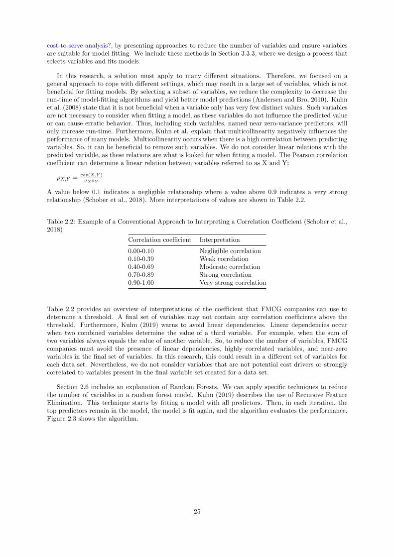
cost-to-serve analysis?, by presenting approaches to reduce the number of variables and ensure variablesare suitable for model fitting. We include these methods in Section 3.3.3, where we design a process thatselects variables and fits models.
In this research, a solution must apply to many different situations. Therefore, we focused on ageneral approach to cope with different settings, which may result in a large set of variables, which is notbeneficial for fitting models. By selecting a subset of variables, we reduce the complexity to decrease therun-time of model-fitting algorithms and yield better model predictions (Andersen and Bro, 2010). Kuhnet al. (2008) state that it is not beneficial when a variable only has very few distinct values. Such variablesare not necessary to consider when fitting a model, as these variables do not influence the predicted valueor can cause erratic behavior. Thus, including such variables, named near zero-variance predictors, willonly increase run-time. Furthermore, Kuhn et al. explain that multicollinearity negatively influences theperformance of many models. Multicollinearity occurs when there is a high correlation between predictingvariables. So, it can be beneficial to remove such variables. We do not consider linear relations with thepredicted variable, as these relations are what is looked for when fitting a model. The Pearson correlationcoefficient can determine a linear relation between variables referred to as X and Y:
ρX,Y = cov(X,Y )σXσY
A value below 0.1 indicates a negligible relationship where a value above 0.9 indicates a very strongrelationship (Schober et al., 2018). More interpretations of values are shown in Table 2.2.
Table 2.2: Example of a Conventional Approach to Interpreting a Correlation Coefficient (Schober et al.,2018)
Correlation coefficient Interpretation
0.00-0.10 Negligible correlation0.10-0.39 Weak correlation0.40-0.69 Moderate correlation0.70-0.89 Strong correlation0.90-1.00 Very strong correlation
Table 2.2 provides an overview of interpretations of the coefficient that FMCG companies can use todetermine a threshold. A final set of variables may not contain any correlation coefficients above thethreshold. Furthermore, Kuhn (2019) warns to avoid linear dependencies. Linear dependencies occurwhen two combined variables determine the value of a third variable. For example, when the sum oftwo variables always equals the value of another variable. So, to reduce the number of variables, FMCGcompanies must avoid the presence of linear dependencies, highly correlated variables, and near-zerovariables in the final set of variables. In this research, this could result in a different set of variables foreach data set. Nevertheless, we do not consider variables that are not potential cost drivers or stronglycorrelated to variables present in the final variable set created for a data set.
Section 2.6 includes an explanation of Random Forests. We can apply specific techniques to reducethe number of variables in a random forest model. Kuhn (2019) describes the use of Recursive FeatureElimination. This technique starts by fitting a model with all predictors. Then, in each iteration, thetop predictors remain in the model, the model is fit again, and the algorithm evaluates the performance.Figure 2.3 shows the algorithm.
25

Figure 2.3: The recursive feature elimination algorithm (Kuhn, 2019)
The optional step of preprocessing the data is not required when using preprocessed input variables.Furthermore, Svetnik et al. (2004) show that the optional step for recalculating the rankings for eachpredictor decreases the performance when it comes to random forests. Alternatively, we can apply Sim-ulated Annealing (Kirkpatrick et al., 1983) by making small changes to the selected subset of predictors.However, this is only beneficial when outcomes differ strongly due to randomness.
In conclusion, FMCG companies may reduce the selection of variables by omitting linear dependencies,highly correlated variables, and near-zero variance predictors to improve the model-fitting performanceof predictive models. The removal of highly correlated variables requires the definition of a suitablethreshold. Furthermore, Recursive Feature Elimination or Simulated Annealing can reduce the numberof variables in Random Forest models.
2.6 Model selection
Here, we present a literature review to support the model fitting process in Section 3.3.3 by supportingthe answering of research question 1.2 How can fast-moving consumer goods companies find a root-causefor a high cost-to-serve per volume-unit based on data used in the cost-to-serve analysis?. In the rootcause analysis in Section 3.3.4, the goal is to fit a model that accurately predicts the cost-to-serve pervolume-unit.
Designed solutions must handle a large amount of data and ensure the applicability to differentsettings. Therefore, we consider basic machine learning techniques, including regression models andrandom forests. In this research, we use known independent and dependent variables. So, as we uselabeled samples to train a model, supervised learning is applied (Ayodele, 2010). Supervised learningcomprises of two learning types, which are classification and regression (GeeksforGeeks, 2020). In thecase of this research, the CTS per volume-unit is a continuous dependent variable. According to Zhou(2018), “in classification, the label indicates the class to which the training example belongs; in regression,the label is a real-value response corresponding to the example”. Brownlee (2017) supports this logicwhen comparing classification and regression techniques. So, the focus of the root cause analysis is onregression.
26

Having determined that we must select a suitable regression model, FMCG companies may test dif-ferent types and choose the best fit. A well-known regression type is a relatively simple Linear Regressionwith multiple independent variables. Sometimes Linear Regression is referred to as Multiple Linear Re-gression (Freedman, 2009), where more than one variable (Xi) has a linear effect (ai) on the outcome ofthe dependent variable (Y ):
Y = a1 ∗X1 + a2 ∗X2 + a3 ∗X3...an ∗Xn + b
There might be no linear relations between independent and dependent variables. In such a case, Poly-nomial Regression might perform better (Seif, 2018). A Polynomial Regression can handle curvature ina way a simple linear regression cannot.
Y = a1 ∗X1 + (a2)2 ∗X2 + (a3)3 ∗X3...(an)n ∗Xn + b
Seif (2018) also presents Lasso and Ridge Regression. These are two regression model types that dealwith collinearity. “When two or more predictors measure the same underlying construct or a facet of suchconstruct, they are said to be collinear (Kock, 2015)”. So, in such a case, there is a linear relationshipbetween two of the independent variables. These regression models deal with collinearity by applyingpenalty functions to ensure collinear variables do not both obtain too high coefficients. The loss function,which regression algorithms minimize, incurs the penalty. Below we see an example of a loss function:
L =∑ni=1(yi − yi)2 + λ
∑mj=1 β
2j
Besides minimizing the squared error between actual and predicted values yi and yi, the model coefficientsβj are squared, multiplied by a factor λ, and added to the loss function. So, the loss function penalizeshigh coefficients. The difference between the Lasso and Ridge Regression is that the Lasso variant takesthe absolute value of the coefficient (Chakon, 2017). ElasticNet Regression presents a hybrid of Lassoand Ridge regression, combining both ways of penalization. However, we can also avoid correlation andcollinearity in the preprocessing phase when variables are selected, as explained in Section 2.5.
Alternatively, we can fit more complex models. An example of such a model is a Random Forestmodel (Breiman, 2001). The Random Forest technique creates a regression tree. Figure 2.4 shows anexample of a regression tree. In such a tree, samples are split based on the value of a certain attribute.As the name random forest indicates, the technique tests random splits and measures the performance.
Figure 2.4: An example of a regression tree, or decision tree (Vala, 2019)
An advantage of this model type is that the model is excellent at handling collinearity between variables.A downside of applying a Random Forest technique is that the model fit makes it difficult to understand
27

the variable importance. Liaw et al. (2002) explain that the importance of a variable is how much theprediction error increases when excluding the variable. Due to sometimes complex interactions with othervariables, it can be difficult to estimate if a variable has a generally positive or negative influence on thepredicted variable.
When fitting more than one model, we must consider how good the model fits are to compare them.The caret package (short for Classification And REgression Training) by Kuhn (2019) includes suitabletechniques to perform a regression analysis in R. The caret package uses the Root Mean Squared Error(RMSE), simple R2 statistic, and the Mean Absolute Error (MAE). The formula for the RMSE is asfollows, considering actual values yi, predicted values yi, and sample size n:
RMSE = [∑ni=1
(yi−yi)2n ]1/2
The R2 statistic has several variants. Kvalseth (1985) compares different measures of the R2 statisticby showing how they differ depending on a model. For this research, we include the squared correlationcoefficient between actual and predicted values, as Kvalseth shows that results do not differ much fordifferent models. Section 2.5 explained this correlation coefficient in more detail. Last, the formula forthe MAE is as follows:
MAE =∑ni=1
|yi−yi|n
In conclusion, FMCG companies can use the five basic regression models mentioned in this sectionand a random forest model to fit a model that predicts a high CTS per volume-unit. To compare models,they can consider several goodness-of-fit measures. For the framework, we include these models andtechniques in the model-fitting process in Section 3.3.3.
2.7 Rating tool performance
This section considers the theory supporting the rating of tool performance to answer the Researchquestion 1.4 Which techniques can assess the quality of a tool visualizing the output of a cost-to-serveanalysis?. Technology acceptance models evaluate a tool’s performance, showing how likely a user is toadopt a certain technology. The adoption of technology is important in this research, as the main goal isto have more continuous users of the cost-to-serve tool after a new implementation. Figure 2.5 shows arecent review of these models by Taherdoost (2018).
Figure 2.5: An overview of adoption/acceptance models (Taherdoost, 2018)
28
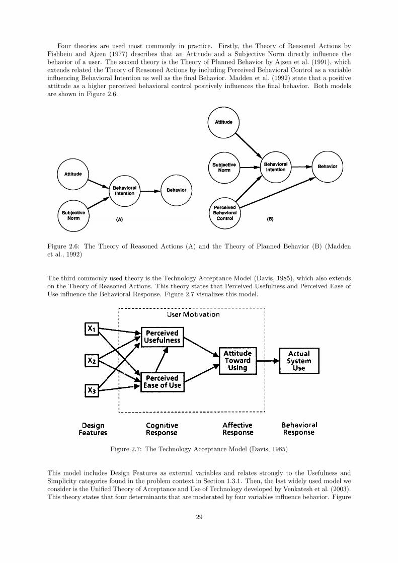
Four theories are used most commonly in practice. Firstly, the Theory of Reasoned Actions byFishbein and Ajzen (1977) describes that an Attitude and a Subjective Norm directly influence thebehavior of a user. The second theory is the Theory of Planned Behavior by Ajzen et al. (1991), whichextends related the Theory of Reasoned Actions by including Perceived Behavioral Control as a variableinfluencing Behavioral Intention as well as the final Behavior. Madden et al. (1992) state that a positiveattitude as a higher perceived behavioral control positively influences the final behavior. Both modelsare shown in Figure 2.6.
Figure 2.6: The Theory of Reasoned Actions (A) and the Theory of Planned Behavior (B) (Maddenet al., 1992)
The third commonly used theory is the Technology Acceptance Model (Davis, 1985), which also extendson the Theory of Reasoned Actions. This theory states that Perceived Usefulness and Perceived Ease ofUse influence the Behavioral Response. Figure 2.7 visualizes this model.
Figure 2.7: The Technology Acceptance Model (Davis, 1985)
This model includes Design Features as external variables and relates strongly to the Usefulness andSimplicity categories found in the problem context in Section 1.3.1. Then, the last widely used model weconsider is the Unified Theory of Acceptance and Use of Technology developed by Venkatesh et al. (2003).This theory states that four determinants that are moderated by four variables influence behavior. Figure
29

2.8 shows the model.
Figure 2.8: The Unified Theory of Acceptance and Use of Technology (Venkatesh et al., 2003)
This model provides an interesting viewpoint on the importance of moderating variables when it comesto technology acceptance. Furthermore, this model replaces the Perceived Usefulness in the TechnologyAcceptance Model by the Performance Expectancy, but the terms appear interchangeable. Both conceptsrelate to the obtainment of cost benefits explained in Section 2.2. Similarly, the Perceived Ease of Useis the Effort Expectancy in the Unified Theory of Acceptance and Use of Technology, implying thattechnology is easy to use. Additionally, the model includes Social Influence and Facilitating Conditions.
In conclusion, there are several suitable models in the reviewed literature for rating tool performance.Putting this literature review to practice, Section 3.5.2 combines and applies the Technology AcceptanceModel and the Unified Theory of Acceptance and Use of Technology.
30

Chapter 3
Framework development
This chapter presents the framework for fast-moving consumer goods companies to visualize the outputof a cost-to-serve analysis. Thereby, we answer the following main research question:
1 How can fast-moving consumer goods companies find business improvementsby using descriptive, diagnostic, predictive, and descriptive analytics in their toolthat visualizes the output of a cost-to-serve analysis?
Figure 3.2 (next page) shows the answer to this question in the form of a framework that combineselements from literature and the research company into a continuous cycle with four different phasesthat contain several steps. The steps inspired by the research company are generic, as related elementsapply to every OpCo regardless of differing characteristics. The framework’s intended users are people inFMCG companies responsible for managing and developing a CTS analysis. Depending on the company,this can be from a global or local position related to customer service or logistics. The starting phase alsodepends on the company. FMCG companies that already perform CTS analyses can commence with anyframework phase, while others must start with the Define Objectives of a Solution phase. The DSRMmethodology shown in Figure 1.9, which we follow in this thesis, inspired the framework phases. Figure3.1 visualizes the relationship between the research methodology of this thesis and the framework.
Figure 3.1: The steps of the Design Science Research Methodology (Peffers et al., 2007) followed in thisthesis and included in the framework designed in this thesis
This chapter presents each part of the framework in detail. First, Section 3.1 presents the DefineObjectives of a Solution phase. Then, Section 3.2 addresses the preparatory steps of the Design andDevelopment phase, which FMCG companies must follow when creating a new tool. Finally, Sections 3.3,3.4, and 3.5 present the Design and Development, Demonstration, and Evaluation phases. In the Designand Development phase, special attention is paid to descriptive and diagnostic analytics as the researchcompany currently mainly incorporates descriptive analytics, whereas diagnostic analytics concern thelevel that follows.
31
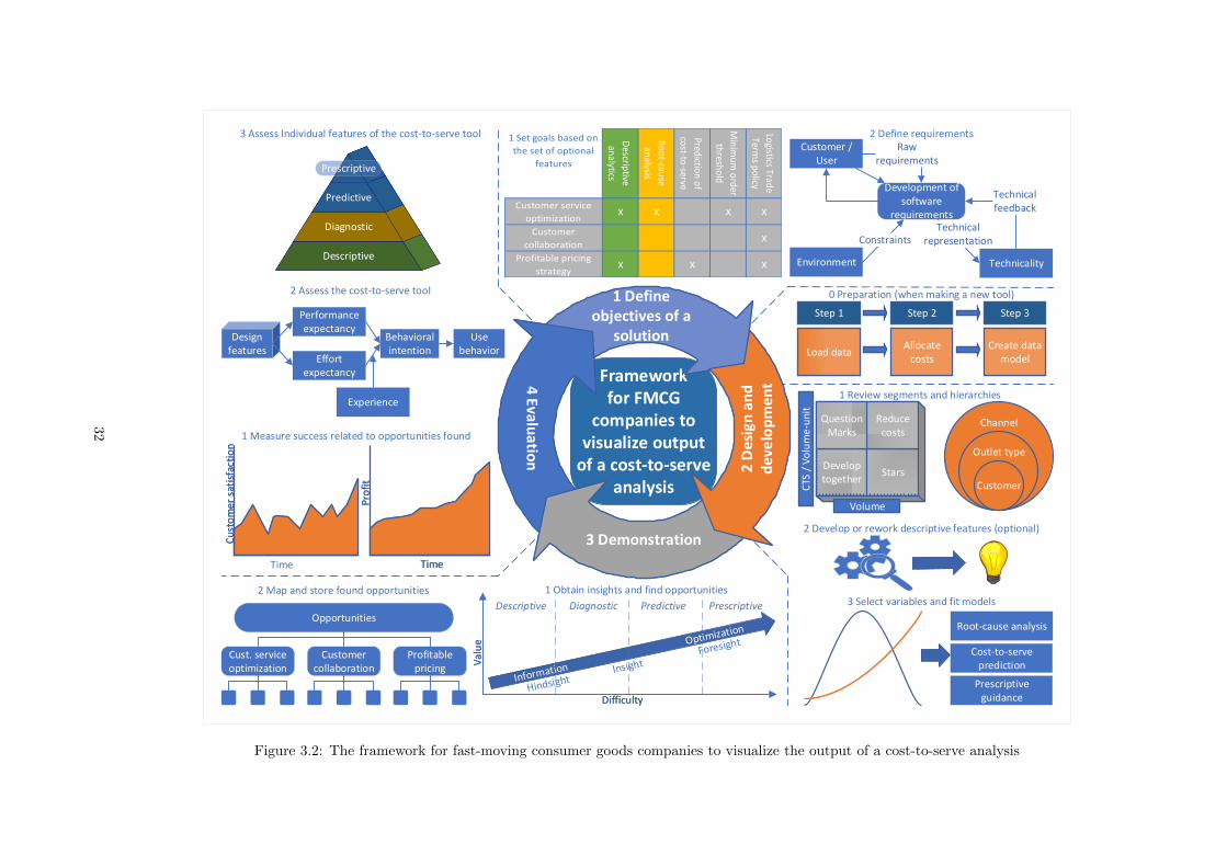
Step 1
Load data
Step 2
Allocate costs
Step 3
Create data model
Step 1
Load data
Step 2
Allocate costs
Step 3
Create data model
Development of software
requirements
Customer / User
Environment Technicality
Design features
Performance expectancy
Effort expectancy
Experience
Behavioral intention
Use behavior
2 Assess the cost-to-serve tool
Pro
fit
Time
Pro
fit
Time
1 Measure success related to opportunities found
2 Define requirements
Frameworkfor FMCG
companies to visualize output
of a cost-to-serve analysis
Channel
Outlet type
Customer
1 Review segments and hierarchies
2 Develop or rework descriptive features (optional)
Develop together
Stars
Reduce costs
CTS
/ V
olu
me
-uni
t
Question Marks
Volume
Develop together
Stars
Reduce costs
CTS
/ V
olu
me
-uni
t
Question Marks
Volume
3 Select variables and fit models
DifficultyDifficulty
Val
ue
Val
ue
Descriptive Diagnostic Predictive Prescriptive
1 Obtain insights and find opportunities
3 Assess Individual features of the cost-to-serve tool
2 Map and store found opportunities
Opportunities
Cust. service optimization
Profitable pricing
Rawrequirements
Technicalfeedback
DescriptiveDescriptive
DiagnosticDiagnostic
PredictivePredictive
Descriptive
Diagnostic
Predictive
ConstraintsTechnical
representation
1 Defineobjectives of a
solution
3 Demonstration
2 D
esig
n a
nd
d
eve
lop
men
t4 Evaluatio
n
Prescriptive
1 Set goals based on
the set of optional
features
Descrip
tive
analytics
Ro
ot-cau
se
analysis
Predictio
n o
f
cost-to
-serve
Min
imu
m o
rder
thresh
old
Logistics Trad
e
Terms p
olicy
Customer service
optimizationX X X X
Customer
collaborationX
Profitable pricing
strategyX X X
Cu
sto
mer
sat
isfa
ctio
nC
ust
om
er s
atis
fact
ion
Customer collaboration
0 Preparation (when making a new tool)
Root-cause analysis
Cost-to-serve prediction
Prescriptive guidance
Time
Figure 3.2: The framework for fast-moving consumer goods companies to visualize the output of a cost-to-serve analysis
32

3.1 Phase 1: Define objectives of a solution
Defining the objectives of a solution includes setting goals and defining requirements. Here, we outlinehow to do this when it comes to visualizing the output of a cost-to-serve analysis, which includes a focuson levels of analytics explained in Section 2.1.1. We answer the following question:
1.1 Which descriptive, diagnostic, predictive, and prescriptive features can visualize the outputof a cost-to-serve analysis?
The input for the Define Objectives of a Solution phase comes from the Evaluation phase. FMCGcompanies can use the success measurements, tool assessment, and feature assessment to make decisions.Figure 3.3 shows the framework’s steps in the Define Objectives of a Solution phase. The output of thisphase is a set of goals, including features to develop with corresponding requirements. FMCG companiesmust perform these steps before the Design and Development phase, as shown in the framework in Figure3.2.
Figure 3.3: The Define objectives of a solution phase of the framework for fast-moving consumer goodscompanies to visualize the output of a cost-to-serve analysis
We explain both steps of the Define Objectives of a Solution phase in this section. First, Section 3.1.1combines previous findings into a set of optional features for FMCG companies to develop as a part oftheir cost-to-serve tool. FMCG companies can use this set of features when setting a goal. Then, Section3.1.2 explains how to define requirements for chosen features with a focus on data requirements.
3.1.1 Review options
Here, we create a set of options that we combine with the types of analytics presented in Section 2.1.1and potential benefits found in Section 2.2. First, we present options from literature. Then, we expandthe set of options by including features from the tool of the research company. We assess the perceivedvalue of features from the research company’s current tool to determine what to include in the set ofoptions. Then, we discuss which tables to include in the set of options, as a table is the most obviousfeature using descriptive analytics. Finally, we combine all potential features into the final set of optionsthat FMCG companies can use to set goals for the Design and Development phase in Section 3.3.
Features from literature
In general, there are not many specific features mentioned in the reviewed literature that appearto provide more than descriptive insights, but Section 2.3 presented a few potential features. Firstly,users should only focus on customers of products that are of importance to them. A segmentationfeature provides this functionality (Bonoma and Shapiro (1984), Bolton and Tarasi (2006), Guerreiroet al. (2008), Davis (2010), Kolarovszki et al. (2016)). On itself, it is not clear how segmentation leadsto insights. However, a CTS tool can combine segmentations with other features. We consider a basicsegmentation as descriptive because it fully depends on user inputs. An advanced segmentation method is
33

diagnostic as it uses techniques that do not rely on users. Secondly, predicting the CTS of a new customercould prove valuable when arranging the pricing for such a customer (Kone and Karwan (2011), Ozeneret al. (2013), Sun et al. (2015), and Wang et al. (2020)). Furthermore, methods are presented that focuson optimizing third-party-logistics service delivery (Ross et al. (2007) and Everaert et al. (2008)) andimprove capacity planning (Everaert et al., 2008), but optimizing delivery routes and improving capacityplanning fall outside of the scope defined in Section 1.4.1. The CTS tool might be the tool to highlightopportunities in this area, but solving these problems is the area of expertise of other teams than theCustomer Service team. Finally, Everaert et al. (2008) introduce minimum order value and maximumdiscount policies. Maximum discount policies relate to Logistic Trade Terms, which are discounts givento the customers when they agree to terms, resulting in more efficiency for the supplying company. Inthe end, the set of options to develop is as follows:
• Descriptive analytics
• A segmentation of customers and products (descriptive or diagnostic)
• Root-cause analysis for a high CTS per volume-unit (diagnostic)
• Estimating the CTS of a new customer or product (predictive)
• Estimating the CTS of a customer or product in the future (predictive)
• Guide in defining a minimum order threshold (prescriptive)
• Guide in defining a discount policy when implementing Logistic Trade Terms (prescriptive)
We included an additional idea for a feature in the set of options inspired by the definition of diagnosticanalytics from Section 2.1.1 that states diagnostic analytics answer the question “Why did somethinghappen?”. A root-cause analysis for a high CTS per volume-unit can answer this question. Furthermore,estimating the CTS of a new customer or product inspired the idea for predicting the CTS of an existingcustomer or existing product to show negative trends. The next two sections detail which descriptivefeatures we included based on the research company’s current tool.
Features from the research company’s tool
We reviewed features from the research company’s current tool, intending to include them in the setof optional features because they are generic features that apply to all OpCos. We sent a survey out toassess how often features are used in the current CTS tool of the research company to include these inthe set of options for the framework. Thereby we apply an Evaluation step presented in Section 3.5.3to the current situation of the research company. The survey, filled by sixteen respondents from OpCosand the Global CTS team, assessed the use of features with a linear scale that awards zero points whenrespondents do not use a feature and three points when they always use a feature. Figure 3.4 shows theoutcome of this survey. Appendix B shows all survey responses referred to in this section.
Figure 3.4: The average score and standard deviation for how often a feature is used by the surveyrespondents (Never 0 - 3 Always)
34
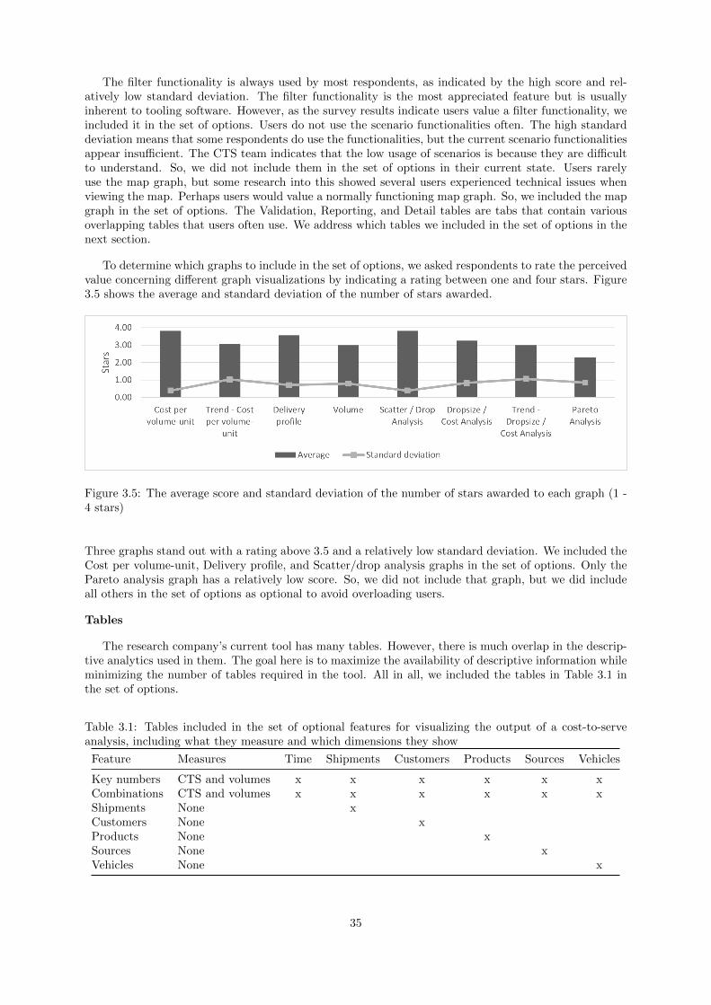
The filter functionality is always used by most respondents, as indicated by the high score and rel-atively low standard deviation. The filter functionality is the most appreciated feature but is usuallyinherent to tooling software. However, as the survey results indicate users value a filter functionality, weincluded it in the set of options. Users do not use the scenario functionalities often. The high standarddeviation means that some respondents do use the functionalities, but the current scenario functionalitiesappear insufficient. The CTS team indicates that the low usage of scenarios is because they are difficultto understand. So, we did not include them in the set of options in their current state. Users rarelyuse the map graph, but some research into this showed several users experienced technical issues whenviewing the map. Perhaps users would value a normally functioning map graph. So, we included the mapgraph in the set of options. The Validation, Reporting, and Detail tables are tabs that contain variousoverlapping tables that users often use. We address which tables we included in the set of options in thenext section.
To determine which graphs to include in the set of options, we asked respondents to rate the perceivedvalue concerning different graph visualizations by indicating a rating between one and four stars. Figure3.5 shows the average and standard deviation of the number of stars awarded.
Figure 3.5: The average score and standard deviation of the number of stars awarded to each graph (1 -4 stars)
Three graphs stand out with a rating above 3.5 and a relatively low standard deviation. We included theCost per volume-unit, Delivery profile, and Scatter/drop analysis graphs in the set of options. Only thePareto analysis graph has a relatively low score. So, we did not include that graph, but we did includeall others in the set of options as optional to avoid overloading users.
Tables
The research company’s current tool has many tables. However, there is much overlap in the descrip-tive analytics used in them. The goal here is to maximize the availability of descriptive information whileminimizing the number of tables required in the tool. All in all, we included the tables in Table 3.1 inthe set of options.
Table 3.1: Tables included in the set of optional features for visualizing the output of a cost-to-serveanalysis, including what they measure and which dimensions they show
Feature Measures Time Shipments Customers Products Sources Vehicles
Key numbers CTS and volumes x x x x x xCombinations CTS and volumes x x x x x xShipments None xCustomers None xProducts None xSources None xVehicles None x
35
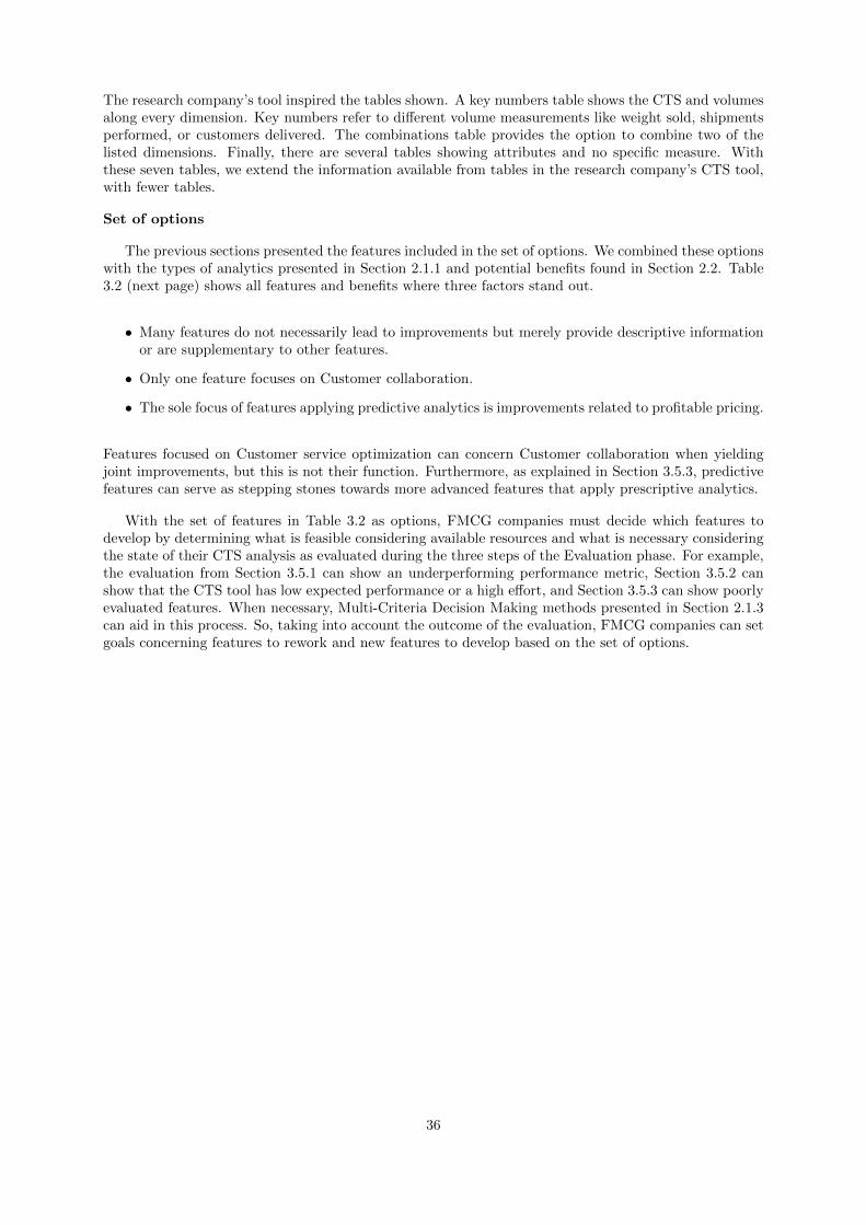
The research company’s tool inspired the tables shown. A key numbers table shows the CTS and volumesalong every dimension. Key numbers refer to different volume measurements like weight sold, shipmentsperformed, or customers delivered. The combinations table provides the option to combine two of thelisted dimensions. Finally, there are several tables showing attributes and no specific measure. Withthese seven tables, we extend the information available from tables in the research company’s CTS tool,with fewer tables.
Set of options
The previous sections presented the features included in the set of options. We combined these optionswith the types of analytics presented in Section 2.1.1 and potential benefits found in Section 2.2. Table3.2 (next page) shows all features and benefits where three factors stand out.
• Many features do not necessarily lead to improvements but merely provide descriptive informationor are supplementary to other features.
• Only one feature focuses on Customer collaboration.
• The sole focus of features applying predictive analytics is improvements related to profitable pricing.
Features focused on Customer service optimization can concern Customer collaboration when yieldingjoint improvements, but this is not their function. Furthermore, as explained in Section 3.5.3, predictivefeatures can serve as stepping stones towards more advanced features that apply prescriptive analytics.
With the set of features in Table 3.2 as options, FMCG companies must decide which features todevelop by determining what is feasible considering available resources and what is necessary consideringthe state of their CTS analysis as evaluated during the three steps of the Evaluation phase. For example,the evaluation from Section 3.5.1 can show an underperforming performance metric, Section 3.5.2 canshow that the CTS tool has low expected performance or a high effort, and Section 3.5.3 can show poorlyevaluated features. When necessary, Multi-Criteria Decision Making methods presented in Section 2.1.3can aid in this process. So, taking into account the outcome of the evaluation, FMCG companies can setgoals concerning features to rework and new features to develop based on the set of options.
36

Table 3.2: The set of features that FMCG companies can develop to visualize the output of a CTS analysis showing the types of analytics and benefits
Analytics type FeatureCustomer service
optimizationCustomer
collaborationProfitable pricing
strategy
Descriptive
Filter functionalityGraph - Cost per volume-unit (CTS per volume-unit bucket and the volume) x xGraph - Scatter / Drop analysis (drops per week and the average dropsize) xGraph - Delivery profile (number of shipments containing a number of pallets) xOptional: Graph - Dropsize / Cost analysis (dropsize and the CTS per volume-unit) xOptional: Graph - Trend - Cost per volume-unit x xOptional: Graph - Volume (volumes of different categories)Optional: Graph - Trend - Dropsize / Cost analysis xTable - Key numbers x xTable - Combinations x xTable - Shipment detailsTable - Customer detailsTable - Product detailsTable - Source detailsTable - Vehicle detailsMap (showing volumes and the CTS per volume-unit) xCustomer and product segmentation (basic)
DiagnosticCustomer and product segmentation (advanced)Root-cause analysis for a high CTS per volume-unit x
PredictiveEstimating the CTS of a new customer or product xEstimating the CTS of a customer or product in the future x
PrescriptiveGuide in defining a minimum order threshold xGuide in defining a discount policy for Logistic Trade Terms x x x
37

3.1.2 Define requirements
After FMCG companies define a goal, and it is clear what to develop, they must define requirements.Section 2.1.2 presented a model by Pandey et al., which shows requirements are dependent on users, theenvironment, and technical aspects. So, the development of features requires clear requirements from auser perspective, and technical aspects play a role in multiple ways, including data availability.
Before-mentioned factors can differ between FMCG companies, but relevant variables might be similar.As applying advanced analytics requires the presence of variables, and we decide to create a feature usingadvanced analytics for the research company in Section 4.2.1, we address data requirements for developingadvanced analytics based on the output of a CTS analysis here. Section 2.4 identified general activitiesand cost drivers as potential variables. However, it also argued that cost drivers are different in eachsituation. In this research, solutions apply to FMCG companies. So, we designed a wide range ofvariables. Table 3.3 shows cost buckets based on a combination of literature from Section 2.4 and themain cost buckets used by the research company as presented in Chapter 1, combined with the activitiesrelated to the cost drivers.
Table 3.3: Combination of activities and cost drivers from literature with cost buckets used currentlywith CTS in the research company
Activity Cost drivers
Inter-company Transport Quantity shipped Origin Utilization SupplierQuantity shipped Volume shipped Weight shipped Distance
Delivery to CustomerNumber of trips Origin Utilization Supplier
Warehousing Quantity shipped Volume shipped Weight shipped Picking timeOrder Management Orders receivedOverheads Distance Vehicles used Quantity shipped Area usedTrade TermsCustomer service Returns Complaints Visits Calls
The cost drivers show some ambiguity that we addressed because the variable selection and model fittingprocess described in Section 3.3.3 requires clear variables. For example, we can evaluate the quantityshipped or the number of trips taken in different ways. Therefore, we designed more specific variablesthat remain generic and that any FMCG company can use. Appendix C shows a complete overview of allthe variables designed to reduce the ambiguity. For Trade Terms, we found no potential cost drivers. Thisoverview of data that FMCG companies should include in their CTS analysis concludes the framework’sphase for defining the objectives of a solution. FMCG companies can set goals using the set of optionscreated and define requirements considering users, technical aspects, and their environment.
3.2 Step 2.0: Preparation
This section outlines the preparation steps of the Design and Development phase for visualizing theoutput of a cost-to-serve analysis. We determined a generalized approach, as steps depend on an FMCGcompany’s view on cost-to-serve and IT infrastructure. FMCG companies must follow these steps whencreating a new cost-to-serve tool. When the goal is to improve an existing cost-to-serve tool, they canskip these steps, but because we develop a new tool for the research company in Section 4.4 we addressthese steps here.
The inputs for the preparation steps of the Design and Development phase are goals and requirementsdefined in the Define Objectives of a Solution phase. Figure 3.6 shows the preparation steps. Theoutput that follows is a data model containing the output of a cost-to-serve analysis and other relevantinformation. FMCG companies must complete these steps before they can continue with the other stepsof the Design and Development phase, as shown in Figure 3.2.
38

Figure 3.6: The preparation steps of the Design and Development phase from the framework for fast-moving consumer goods companies to visualize the output of a cost-to-serve analysis
This section outlines each Preparation step. First, Section 3.2.1 explains how FMCG companiescan load data. Then, Section 3.2.2 presents different methods for cost allocations and a definition ofcost buckets. Finally, Section 3.2.3 shows a data model design for the visualization of output from acost-to-serve analysis.
3.2.1 Load data
The first preparation step is to load the data required to perform a CTS analysis. We based this processon the process to load data into the research company’s CTS tool, as explained in Section 1.1.2. Thedata includes shipments on an order line level and master data regarding various dimensions. Ultimately,OpCos fill a template with a standard layout, which always has the same fields and data types. Therefore,it makes sense to have an automated process, so the data collection only has to occur once. Preferablymodules extract, transform, and load data. Figure 3.7 shows a generic model concerning data loading.
Figure 3.7: The Extract, Transform, and Load process Watts (2017)
This process shows a method to handle the data loading for a CTS analysis in FMCG companies. Afterextracting data, a module transforms data into the desired format, which is ideally the format of thetables required for the data model presented in Section 3.2.3. Finally, the transformed tables are storedin a data warehouse and loaded into visualization software. Ideally, FMCG companies automate thesesteps when loading data for a CTS analysis.
3.2.2 Allocate costs
After loading the data for a CTS analysis, FMCG companies must perform cost allocations. Section2.3 explained that there are different approaches concerning the allocation of cost buckets. However, allapproaches allocate costs on an order line level. FMCG companies might prefer CTS methods, whichallocate actual costs based on drivers, Activity-Based Costing methods (Freeman et al. (2000), Kaplanand Anderson (2003), Kolarovszki et al. (2016)) or a time-driven variant (Everaert et al., 2008). Forexample, Section 2.4 mentions a suitable case for a time-driven approach, stating that picking time is adriver of warehouse costs. So, a time-driven activity-based costing approach involving picking time seems
39
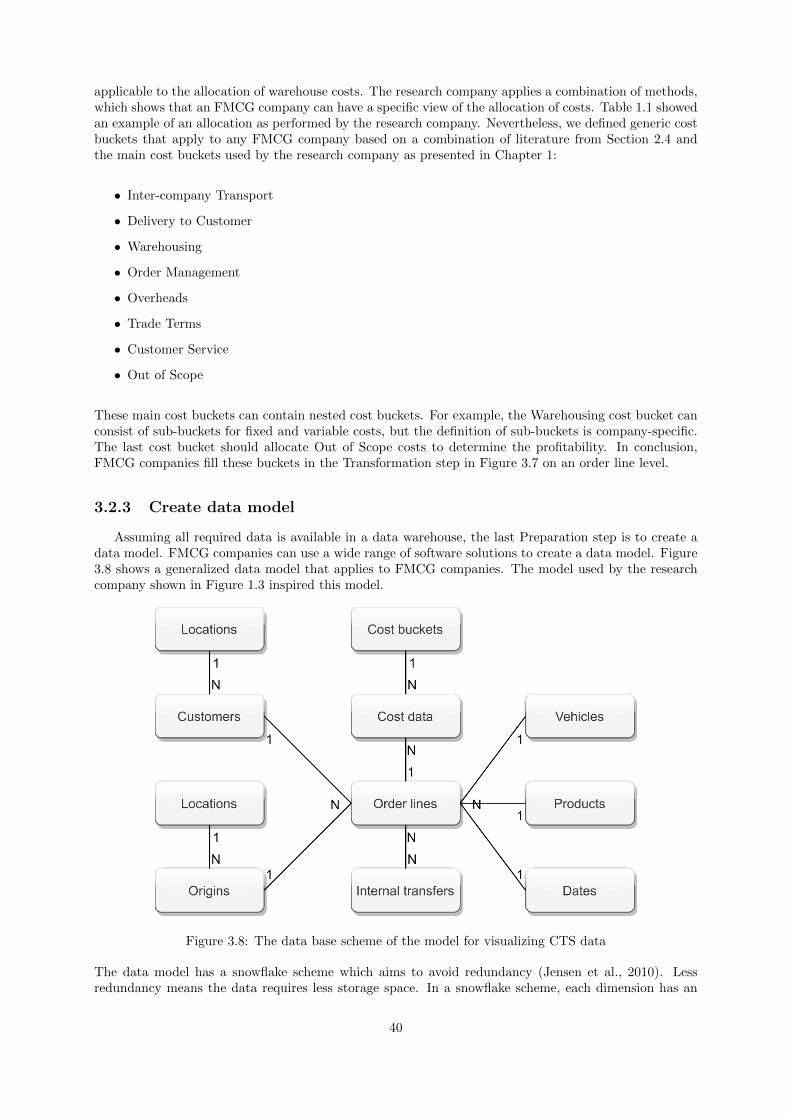
applicable to the allocation of warehouse costs. The research company applies a combination of methods,which shows that an FMCG company can have a specific view of the allocation of costs. Table 1.1 showedan example of an allocation as performed by the research company. Nevertheless, we defined generic costbuckets that apply to any FMCG company based on a combination of literature from Section 2.4 andthe main cost buckets used by the research company as presented in Chapter 1:
• Inter-company Transport
• Delivery to Customer
• Warehousing
• Order Management
• Overheads
• Trade Terms
• Customer Service
• Out of Scope
These main cost buckets can contain nested cost buckets. For example, the Warehousing cost bucket canconsist of sub-buckets for fixed and variable costs, but the definition of sub-buckets is company-specific.The last cost bucket should allocate Out of Scope costs to determine the profitability. In conclusion,FMCG companies fill these buckets in the Transformation step in Figure 3.7 on an order line level.
3.2.3 Create data model
Assuming all required data is available in a data warehouse, the last Preparation step is to create adata model. FMCG companies can use a wide range of software solutions to create a data model. Figure3.8 shows a generalized data model that applies to FMCG companies. The model used by the researchcompany shown in Figure 1.3 inspired this model.
Figure 3.8: The data base scheme of the model for visualizing CTS data
The data model has a snowflake scheme which aims to avoid redundancy (Jensen et al., 2010). Lessredundancy means the data requires less storage space. In a snowflake scheme, each dimension has an
40

individual table and contains keys to underlying dimensions. For example, the model shows tables forcustomer, product, origin, vehicle, and date information. The order lines might be at the center of thedata model. However, the cost data has the lowest level of detail, as each order line has multiple allocatedcost buckets. As explained in Section 3.2.2, cost buckets can incorporate a hierarchy with main bucketsand sub-buckets. Therefore, the storage of the cost bucket names in a separate table is beneficial. Finally,the model includes geographic data concerning customers and sources to determine distances and internaltransfers linked to order lines to enable the visualization of routes to customers. FMCG companies cancreate this data model to visualize the output of a CTS analysis. However, an actual data model likelyincludes additional supportive tables. The creation of a data model concludes the preparation steps ofthe Design and Development phase of the framework, providing a basis for the development of a CTStool.
3.3 Phase 2: Design and development
In this phase, we outline how to rework existing features and develop new features to visualize theoutput of a cost-to-serve analysis. The focus is mainly on descriptive and diagnostic analytics, as theresearch company mostly applies descriptive analytics and diagnostic analytics are the next level. Allfeatures and analytics mentioned here are generic and applicable to any FMCG company. Consequently,we answer the following question in this section:
1.2 How can fast-moving consumer goods companies find a root-cause for a high cost-to-serveper volume-unit based on data used in the cost-to-serve analysis?
The inputs for the Design and Development phase are goals and requirements defined in the DefineObjectives of a Solution phase and the data model from the preparation steps of this phase. Figure 3.9shows the Design and Development phase, which leads to the development of new features. The featuresan FMCG company decides to develop influence the necessary steps taken during this phase. The outputof this phase is a new or revised cost-to-serve tool. The Demonstration phase follows this phase, as shownin the framework in Figure 3.2.
Figure 3.9: The Design an development phase of the framework for fast-moving consumer goods companiesto visualize the output of a cost-to-serve analysis that focus on developing the tool that is used
First, Section 3.3.1 explains how to incorporate segments and hierarchies. Periodically checking theseis important as circumstances change. Then, Section 3.3.2 describes how to review existing features,when this is necessary based on the defined objectives from Section 3.1. Then, Section 3.3.3 explains howto select variables and fit models for the application of diagnostic, predictive, and prescriptive analytics.Finally, Section 3.3.4 develops a generic method find root-causes for a high cost-to-serve per volume-unitthat relies on Section 3.3.3. The root-cause analysis is not a mandatory part of the framework, butSection 4.2.1 argues the requirement for a root-cause analysis for the research company as this lies at thefoundation of more advanced analytics.
41
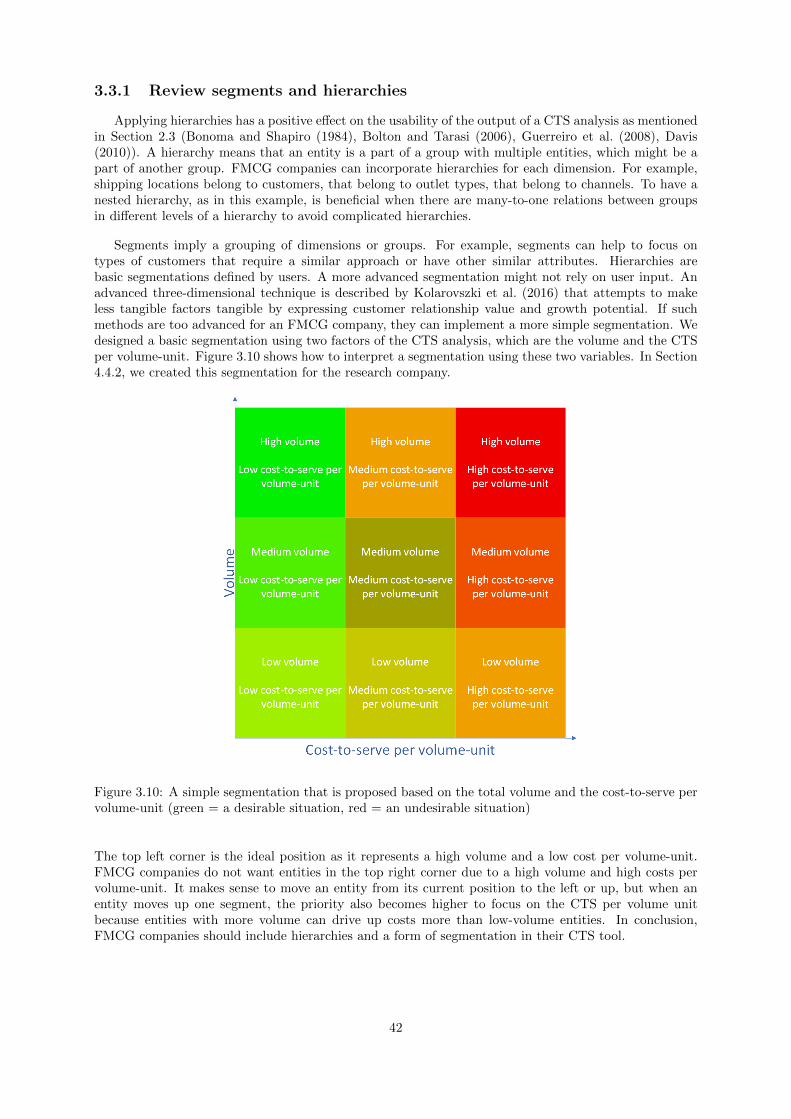
3.3.1 Review segments and hierarchies
Applying hierarchies has a positive effect on the usability of the output of a CTS analysis as mentionedin Section 2.3 (Bonoma and Shapiro (1984), Bolton and Tarasi (2006), Guerreiro et al. (2008), Davis(2010)). A hierarchy means that an entity is a part of a group with multiple entities, which might be apart of another group. FMCG companies can incorporate hierarchies for each dimension. For example,shipping locations belong to customers, that belong to outlet types, that belong to channels. To have anested hierarchy, as in this example, is beneficial when there are many-to-one relations between groupsin different levels of a hierarchy to avoid complicated hierarchies.
Segments imply a grouping of dimensions or groups. For example, segments can help to focus ontypes of customers that require a similar approach or have other similar attributes. Hierarchies arebasic segmentations defined by users. A more advanced segmentation might not rely on user input. Anadvanced three-dimensional technique is described by Kolarovszki et al. (2016) that attempts to makeless tangible factors tangible by expressing customer relationship value and growth potential. If suchmethods are too advanced for an FMCG company, they can implement a more simple segmentation. Wedesigned a basic segmentation using two factors of the CTS analysis, which are the volume and the CTSper volume-unit. Figure 3.10 shows how to interpret a segmentation using these two variables. In Section4.4.2, we created this segmentation for the research company.
Figure 3.10: A simple segmentation that is proposed based on the total volume and the cost-to-serve pervolume-unit (green = a desirable situation, red = an undesirable situation)
The top left corner is the ideal position as it represents a high volume and a low cost per volume-unit.FMCG companies do not want entities in the top right corner due to a high volume and high costs pervolume-unit. It makes sense to move an entity from its current position to the left or up, but when anentity moves up one segment, the priority also becomes higher to focus on the CTS per volume unitbecause entities with more volume can drive up costs more than low-volume entities. In conclusion,FMCG companies should include hierarchies and a form of segmentation in their CTS tool.
42

3.3.2 Develop or rework descriptive features
Cost-to-serve tools will usually include features using descriptive analytics, as these are the mostsimplistic features to develop. However, FMCG companies might want to rework these features. Section1.2 mentioned that the research company wished to review its current solution at the start of the research,which shows an example of an FMCG company wishing to review their current tool. Therefore, weincluded a step to review existing features based on the Define Objectives of a Solution phase presentedin Section 3.1, which FMCG companies can base on the assessment of the state of features from Section3.5.3. Ideally, users appreciate all features of a CTS tool. However, it is important to reconsider the stateof features when this is not the case, which can even result in the removal of certain features. Whenan FMCG company does not yet use descriptive analytics, the FMCG company likely developed goalsrelated to this in Section 3.1.
3.3.3 Select variables and fit models
More recent studies mentioned in Section 2.3 that apply advanced analytics often use predictivemodels to make decisions (Kone and Karwan (2011), Sun et al. (2015), Wang et al. (2020)) rather thanmathematical models (Ross et al. (2007), Ozener et al. (2013)). Predictive models focus on understandinga situation, where mathematical models aim to optimize a certain situation. A wide range of availablevariables and attributes is beneficial for advanced analytics. Ideally, FMCG companies include all vari-ables presented in Section 3.1.2. Then, they can preprocess variables as presented in Section 2.5 andfit models presented in Section 2.6. Figure 3.11 shows steps we designed from creating the variables tofitting a model. We applied these steps for the research company in Section 4.4.5.
Figure 3.11: The process from variable creation to having a final set of variables including values thatusers must define
The process starts with the creation of the variables, where users must choose an entity and level ofdetail. We assume that the variables created do not contain outliers or false inputs. Then, as explainedin Section 2.5, FMCG companies should remove near-zero variables, variables that cause high correlations,or variables they can predict with other variables. For avoiding the correlations, users must determine acutoff value based on Section 2.5. The next step is to scale the variables between zero and one to avoiddifficulties when fitting models due to different magnitudes. Also, scaling makes it easier to derive thevariable importance from weights in many models. Then, we split the data set into a training and testingset for the validation of models. In this step, users determine a training percentage for the data split.Then, FMCG companies must repeat the second, third, and fourth steps because there is a chance thedata splitting led to undesirable values or relations in the training data set. Finally, there is a set ofvariables for model fitting.
The variable set contains independent variables that predict a dependent variable. For many analytics,this is likely the CTS per volume-unit. Section 2.6 presented models that FMCG companies could fit
43
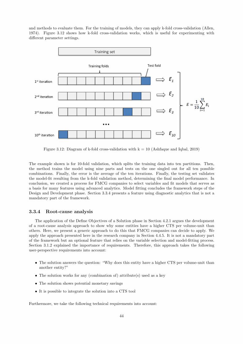
and methods to evaluate them. For the training of models, they can apply k-fold cross-validation (Allen,1974). Figure 3.12 shows how k-fold cross-validation works, which is useful for experimenting withdifferent parameter settings.
Figure 3.12: Diagram of k-fold cross-validation with k = 10 (Ashfaque and Iqbal, 2019)
The example shown is for 10-fold validation, which splits the training data into ten partitions. Then,the method trains the model using nine parts and tests on the one singled out for all ten possiblecombinations. Finally, the error is the average of the ten iterations. Finally, the testing set validatesthe model-fit resulting from the k-fold validation method, determining the final model performance. Inconclusion, we created a process for FMCG companies to select variables and fit models that serves asa basis for many features using advanced analytics. Model fitting concludes the framework steps of theDesign and Development phase. Section 3.3.4 presents a feature using diagnostic analytics that is not amandatory part of the framework.
3.3.4 Root-cause analysis
The application of the Define Objectives of a Solution phase in Section 4.2.1 argues the developmentof a root-cause analysis approach to show why some entities have a higher CTS per volume-unit thanothers. Here, we present a generic approach to do this that FMCG companies can decide to apply. Weapply the approach presented here in the research company in Section 4.4.5. It is not a mandatory partof the framework but an optional feature that relies on the variable selection and model-fitting process.Section 3.1.2 explained the importance of requirements. Therefore, this approach takes the followinguser-perspective requirements into account:
• The solution answers the question: “Why does this entity have a higher CTS per volume-unit thananother entity?”
• The solution works for any (combination of) attribute(s) used as a key
• The solution shows potential monetary savings
• It is possible to integrate the solution into a CTS tool
Furthermore, we take the following technical requirements into account:
44

• Data is available on an order line level
• The variables presented in Section 3.1.2 are available on an order line level
• Software is available that facilitates all computations and the fitting of models
Assuming users take all requirements and constraints into account. The next step is to apply the selectionof variables and fitting of models as explained in Sections 2.5 and 2.4. The output of this process is amodel with the best fit based on the RMSE, R2, and MAE, as explained in Section 2.6. For example, forall attempted model fits, we scale criteria between zero and 1, inversing the R2 as a higher value indicatesa better model fit. Then, the model with the lowest value for the sum of all criteria has a superior fit.Including the fitted model, the root-cause analysis presented here requires the following input data:
• The model
• The data set with variables used by the model
• The unscaled variables, with the volume included
Figure 3.13 (next page) shows the algorithm designed to compare each entity to all other entities basedon this input data. Each entity obtains at most three comparable entities based on three thresholds:
• We exclusively compare entities to other entities with a lower CTS per volume-unit because theend-goal is to find improvements.
• We compare entities to other entities that have an absolute difference concerning the sold volumeof no more than ten percent to safeguard the comparison of similar entities and to speed up thealgorithm.
• We consider entities as similar concerning a variable if the absolute difference between the value forthe two is less than a threshold based on the variable importance in the fitted model.
So, more significant attribute values must be closer to each other to classify as comparable. When thealgorithm finishes, each entity has at most three similar entities, so there are alternatives when it is notclear what business changes to make based on the most similar entity. The output shows actual valuesof both entities, a description on which values the entities differ, and the potential savings corrected forthe MAE of the fitted model to avoid an overestimation of potential savings.
45

Figure 3.13: A flowchart showing the root-cause analysis (round = start/stop, square = process, triangle= decision)
46
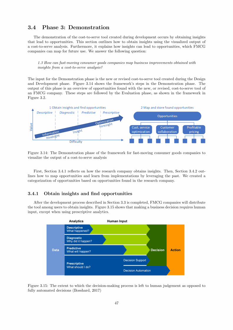
3.4 Phase 3: Demonstration
The demonstration of the cost-to-serve tool created during development occurs by obtaining insightsthat lead to opportunities. This section outlines how to obtain insights using the visualized output ofa cost-to-serve analysis. Furthermore, it explains how insights can lead to opportunities, which FMCGcompanies can map for future use. We answer the following question:
1.3 How can fast-moving consumer goods companies map business improvements obtained withinsights from a cost-to-serve analysis?
The input for the Demonstration phase is the new or revised cost-to-serve tool created during the Designand Development phase. Figure 3.14 shows the framework’s steps in the Demonstration phase. Theoutput of this phase is an overview of opportunities found with the new, or revised, cost-to-serve tool ofan FMCG company. These steps are followed by the Evaluation phase, as shown in the framework inFigure 3.2.
Figure 3.14: The Demonstration phase of the framework for fast-moving consumer goods companies tovisualize the output of a cost-to-serve analysis
First, Section 3.4.1 reflects on how the research company obtains insights. Then, Section 3.4.2 out-lines how to map opportunities and learn from implementations by leveraging the past. We created acategorization of opportunities based on opportunities found in the research company.
3.4.1 Obtain insights and find opportunities
After the development process described in Section 3.3 is completed, FMCG companies will distributethe tool among users to obtain insights. Figure 3.15 shows that making a business decision requires humaninput, except when using prescriptive analytics.
Figure 3.15: The extent to which the decision-making process is left to human judgement as opposed tofully automated decisions (Bosshard, 2017)
47

When a tool that visualizes the output of a CTS analysis only exists of features using prescriptiveanalytics, it always provides clear-cut opportunities, but this is not likely. Therefore, users must learnto combine a CTS tool’s features to find opportunities. Therefore, FMCG companies should considertraining users on how to obtain insights using a CTS tool. For example, Section 1.1.2 explained that theresearch company trains users of the CTS tool through workshops and supports them with setting upaction plans.
3.4.2 Map opportunities
Insights lead to opportunities, which accompany certain benefits. Section 2.2 determined three maintypes of benefits that are obtainable from a CTS analysis. The main benefits relate to customer serviceoptimization, customer collaboration, and a profitable pricing strategy. To be able to judge the effect ofreleasing a new CTS tool, FMCG companies require a method to map the resulting opportunities foundby users. By combining these benefits with research into CTS implementations in the past of the researchcompany, we created a generic opportunity typology for mapping opportunities. We analyzed historicaldata of implementations performed by the research company to discover different opportunity typesrelated to the main benefits. Table 3.4 shows the discovered categories and types with their definitions.
Table 3.4: The definitions of the categories and types used during the collections of potential opportunitiesfound in past CTS implementations
Category Type Definition
Customer service optimization
General Focus on optimizing the supply chainData quality Improve the data qualityNetwork design Change the transportation networkRPM Improve Returnable Products ManagementTransport optimization Optimize transportation activitiesWarehouse optimization Optimize warehousing activities
Customer collaboration
General Focus on collaboration with customersLogistic trade terms Logistics-focused customer discountsOTC Improve the Order To Cash processSLAs Review Service Level Agreements
Profitable pricing strategyGeneral Change prices or discard productsCommercial trade terms Commerce-focused customer discountsProduct portfolio Change the product portfolio
The research into opportunity types confirmed the three main benefits as all types were easily nestedunder one of the benefits. Appendix D shows an overview of the complete typology, including sub-type definitions. The typology was verified with the CTS team and embedded in a simple process forcontinuously evaluating potential opportunities. In other FMCG companies, some types or sub-typesmight not apply or be missing. Then, they can easily remove or add types to improve the typology fortheir situation, but we assume that we found most opportunity types for FMCG companies due to thedifferent nature of the OpCos involved. Figure 3.16 shows the process for mapping opportunities.
Figure 3.16: The steps to map opportunities that have been found
48

In the first row, the process shows how to map opportunities using the typology, which FMCG companiescan extend if necessary. After mapping opportunities, FMCG companies can assess whether they foundnew opportunities. If so, documenting how they found them can potentially pave the way for repeating theprocess in another CTS implementation. Additionally, there is the potential to automate the opportunityand add it to the list of optional features to develop shown in Section 3.1.1. In conclusion, FMCGcompanies must train users based on the user input required to make business decisions and apply theprocess to map opportunities in the Demonstration phase.
3.5 Phase 4: Evaluation
This section outlines how FMCG companies can evaluate the performance of their process and toolto visualize the output of a cost-to-serve analysis, which involves performance measurements as well astool assessments. In this section, we answer the following question:
1.4 Which techniques can assess the quality of a tool visualizing the output of a cost-to-serveanalysis?
The inputs for the Evaluation phase rely on the Design and Development phase and Demonstrationphase. FMCG companies require the created overview of found opportunities from the Demonstrationphase to measure success, and they require the new or revised cost-to-serve tool created in the Design andDevelopment phase to assess it. Figure 3.17 shows the Evaluation phase of the framework. The outputsof this phase are a success measurement, tool evaluation, and feature evaluation. This phase is the last ofthe framework, but the Define Objectives of a Solution phase follows this phase, as shown in Figure 3.2.The output of the Evaluation phase serves as the input for the Define Objectives of a Solution phase.
Figure 3.17: The Evaluation phase of the framework for fast-moving consumer goods companies tovisualize the output of a cost-to-serve analysis
This section explains the Evaluation steps. First, Section 3.5.1 outlines how to measure the successof the cost-to-serve analysis as a whole. The execution of this step can depend on the company or teamKPIs. Then, Section 3.5.2 presents performance variables for a tool assessment and explains how thesevariables can measure the performance of a cost-to-serve tool. Finally, Section 3.5.3 presents a methodto assess the state of features and analytics applied in a cost-to-serve tool.
3.5.1 Measure success
“What gets measured gets done” might be the most famous saying of performance measurement(Behn, 2003). Hence, it is important to measure success. Here, we present KPIs that FMCG companiescan measure to determine the success of CTS implementations. The benefits of CTS, related to potentialmeasurements of success, found in Section 2.2 are Customer service optimization, Customer collaboration,and a Profitable pricing strategy.
Section 2.2 showed that profitability and customer satisfaction measure success related to these ben-efits. When measuring these KPIs, FMCG companies must carefully scope the area of measurement. A
49
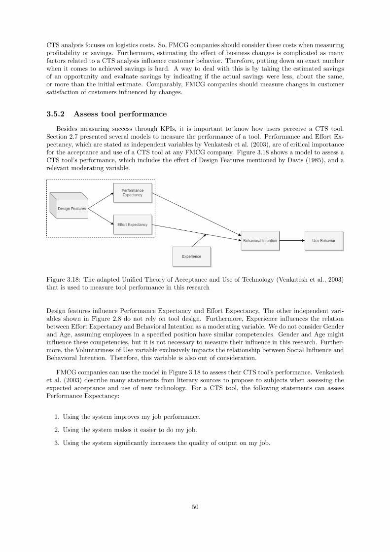
CTS analysis focuses on logistics costs. So, FMCG companies should consider these costs when measuringprofitability or savings. Furthermore, estimating the effect of business changes is complicated as manyfactors related to a CTS analysis influence customer behavior. Therefore, putting down an exact numberwhen it comes to achieved savings is hard. A way to deal with this is by taking the estimated savingsof an opportunity and evaluate savings by indicating if the actual savings were less, about the same,or more than the initial estimate. Comparably, FMCG companies should measure changes in customersatisfaction of customers influenced by changes.
3.5.2 Assess tool performance
Besides measuring success through KPIs, it is important to know how users perceive a CTS tool.Section 2.7 presented several models to measure the performance of a tool. Performance and Effort Ex-pectancy, which are stated as independent variables by Venkatesh et al. (2003), are of critical importancefor the acceptance and use of a CTS tool at any FMCG company. Figure 3.18 shows a model to assess aCTS tool’s performance, which includes the effect of Design Features mentioned by Davis (1985), and arelevant moderating variable.
Figure 3.18: The adapted Unified Theory of Acceptance and Use of Technology (Venkatesh et al., 2003)that is used to measure tool performance in this research
Design features influence Performance Expectancy and Effort Expectancy. The other independent vari-ables shown in Figure 2.8 do not rely on tool design. Furthermore, Experience influences the relationbetween Effort Expectancy and Behavioral Intention as a moderating variable. We do not consider Genderand Age, assuming employees in a specified position have similar competencies. Gender and Age mightinfluence these competencies, but it is not necessary to measure their influence in this research. Further-more, the Voluntariness of Use variable exclusively impacts the relationship between Social Influence andBehavioral Intention. Therefore, this variable is also out of consideration.
FMCG companies can use the model in Figure 3.18 to assess their CTS tool’s performance. Venkateshet al. (2003) describe many statements from literary sources to propose to subjects when assessing theexpected acceptance and use of new technology. For a CTS tool, the following statements can assessPerformance Expectancy:
1. Using the system improves my job performance.
2. Using the system makes it easier to do my job.
3. Using the system significantly increases the quality of output on my job.
50

The following statements can assess the Effort Expectancy:
1. Learning to operate the system was easy for me.
2. Using the system involves too much time doing mechanical operations (e.g., data input).
3. I find it easy to get the system to do what I want it to do.
Scoring these statements to the extent a subject agrees with them provides a performance measure of thetool. FMCG companies can use a scale from 0 (completely disagree) to 5 (completely agree) to measureperformance by assessing answers to the questions concerning the Performance Expectancy, the EffortExpectancy, and the view on the tool as a whole. Furthermore, FMCG companies can apply the methodto a specific part of the CTS tool, such as recently added features.
3.5.3 Assess features
Besides measuring the general performance of the CTS analysis and tool, it is important to be awareof the insights currently provided for users. Section 2.1.1 explains the concept of descriptive, diagnostic,predictive, and prescriptive analytics. FMCG companies can assess if they apply enough analytics of acertain type and whether the focus should be on the next level of analytics. Figure 3.17 indicates thisby the green color of descriptive insights and yellow color of diagnostic insights as an example, whichresembles a case where features applying descriptive analytics are covered, and there is a requirement fordiagnostic analytics. Besides creating a mapping of features used in a CTS tool, FMCG companies caninvolve users to validate assumptions. Then, users must answer two questions:
1. How much value do features in the current tool hold?
2. How much value will the addition of new features add?
When posing these questions, FMCG companies must know what types of analytics features use. Visu-alizing the output of a CTS analysis starts with features applying descriptive analytics that plot valuesagainst various dimensions. The next level, diagnostic analytics, relies on a complete set of descriptiveanalytics to find causes for events or trends, leading users to areas that require attention. Then, predictiveanalytics can focus on these areas to estimate the severity of what might be a trend. Finally, prescriptiveanalytics can drive business decisions directly. Section 3.4.1 explained the extent to which different ana-lytics can drive decisions. Higher-level analytics require less human input in the decision-making process,but features applying higher-level insights require more comprehensive analytics and depend on lowerlevels of analytics. Therefore, FMCG companies should start by making sure lower-level analytics arecomplete and valid before moving to more complicated analytics.
The assessment of features concludes the Evaluation phase of the framework, but the frameworkpresented in this chapter incorporates a continuous cycle. Combining the feature assessment with theperformance of the CTS analysis and tool, FMCG companies can define the objectives of a solutioncorrectly in the next framework phase. So, after the feature assessment, the process restarts with anotherDefine Objectives of a Solution phase, as presented in Section 3.1.
51

Chapter 4
Case study
This chapter presents a case study that applies the framework for fast-moving consumer goods companiesto visualize the output of a cost-to-serve analysis to the research company. Consequently, we answer thefollowing main research question:
2 Can the research company improve the use of the output of cost-to-serve anal-yses by applying the framework designed in this research to create a new tool?
The purpose of this chapter is to present how elements of the framework work in practice and outlinelearnings related to the different phases. Figure 4.1 shows that one section focuses on the current tool,and the others are devoted to the development of a new tool to visualize the output of a cost-to-serveanalysis.
Figure 4.1: The relation between the framework for fast-moving consumer goods companies to visualizethe output of a cost-to-serve analysis and the sections of the case study in this chapter
To ensure we could apply each framework phase to the research company, we applied some phases tothe current situation and others for the development of a new cost-to-serve tool. Each section relates toone or more phases of the framework presented in Chapter 3 and concludes with a comparison betweenthe case study and the intended steps presented in the framework. First, Section 4.1 focuses on thecurrent tool by creating a structure to map opportunities based on framework Phase 3 Demonstration,and evaluating the current performance based on phase 4 Evaluation. Then, Sections 4.2, 4.3, and 4.4present the application of Phases 1 Define objectives of a solution, 2.0 Preparation (when making a newtool), and 2 Design and development to develop a new cost-to-serve tool. In the end, we applied everystep of each framework phase to the research company.
4.1 Performance current situation
This section focuses on the current tool used by the research company. We evaluated the performanceof the research company by applying framework Phase 3 Demonstration and 4 Evaluation in the contextof the company. Thereby we answer the following question:
52
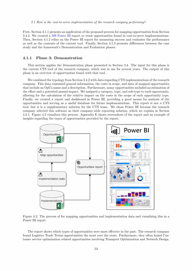
2.1 How is the cost-to-serve implementation of the research company performing?
First, Section 4.1.1 presents an application of the proposed process for mapping opportunities from Section3.4.2. We created a MS Power BI report to track opportunities found in cost-to-serve implementations.Then, Section 4.1.2 relies on the Power BI report for measuring success and evaluates the performanceas well as the contents of the current tool. Finally, Section 4.1.3 presents differences between the casestudy and the framework’s Demonstration and Evaluation phases.
4.1.1 Phase 3: Demonstration
This section applies the Demonstration phase presented in Section 3.4. The input for this phase isthe current CTS tool of the research company, which was in use for several years. The output of thisphase is an overview of opportunities found with that tool.
We combined the typology from Section 3.4.2 with data regarding CTS implementations of the researchcompany. This data contained general information, the costs in scope, and data of mapped opportunitiesthat include an OpCo name and a description. Furthermore, many opportunities included an estimation ofthe effort and a potential annual impact. We assigned a category, type, and sub-type to each opportunity,allowing for the calculation of the relative impact on the costs in the scope of each opportunity type.Finally, we created a report and dashboard in Power BI, providing a good means for analysis of theopportunities and serving as a useful database for future implementations. This report is not a CTStool, but it is a supplementary solution for the CTS team. We chose Power BI because the researchcompany selected this software as their company-wide reporting solution, which we explain in Section4.2.1. Figure 4.2 visualizes this process. Appendix E shows screenshots of the report and an example ofinsights regarding the types of opportunities provided by the report.
Figure 4.2: The process of for mapping opportunities and implementation data and visualizing this in aPower BI report
The report shows which types of opportunities were most effective in the past. The research companyfound Logistics Trade Terms opportunities the most over the years. Furthermore, they often found Cus-tomer service optimization related opportunities involving Transport Optimization and Network Design.
53
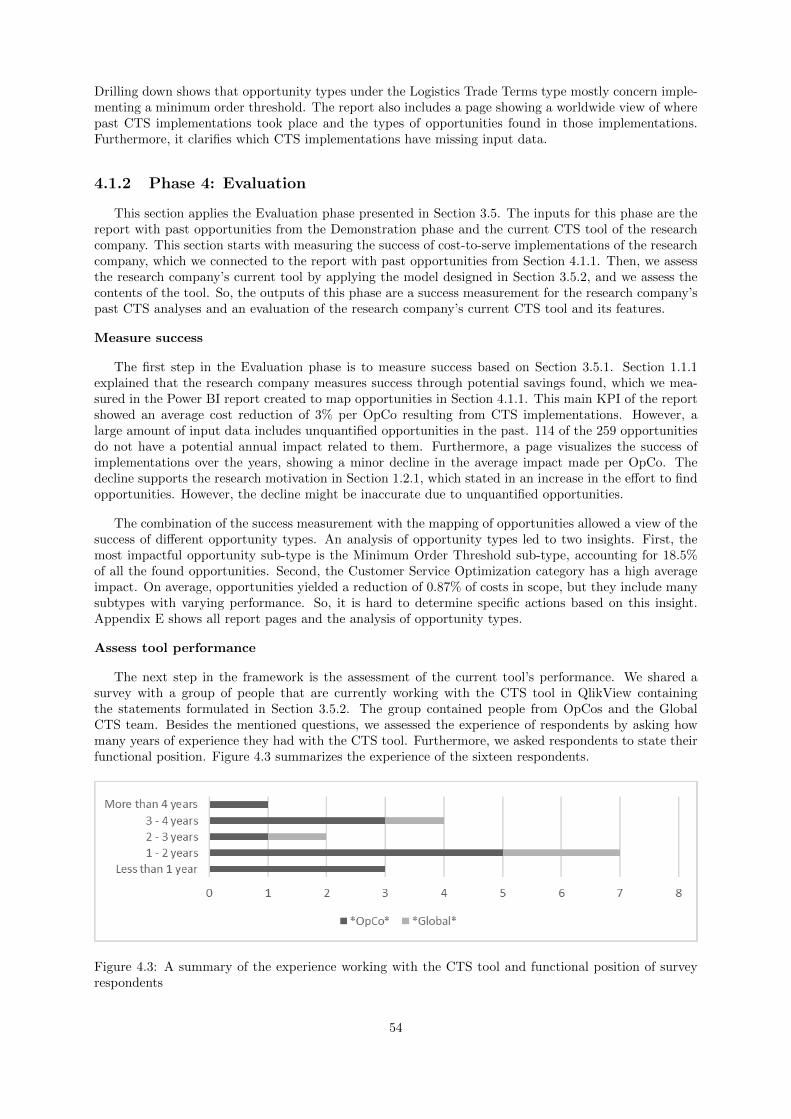
Drilling down shows that opportunity types under the Logistics Trade Terms type mostly concern imple-menting a minimum order threshold. The report also includes a page showing a worldwide view of wherepast CTS implementations took place and the types of opportunities found in those implementations.Furthermore, it clarifies which CTS implementations have missing input data.
4.1.2 Phase 4: Evaluation
This section applies the Evaluation phase presented in Section 3.5. The inputs for this phase are thereport with past opportunities from the Demonstration phase and the current CTS tool of the researchcompany. This section starts with measuring the success of cost-to-serve implementations of the researchcompany, which we connected to the report with past opportunities from Section 4.1.1. Then, we assessthe research company’s current tool by applying the model designed in Section 3.5.2, and we assess thecontents of the tool. So, the outputs of this phase are a success measurement for the research company’spast CTS analyses and an evaluation of the research company’s current CTS tool and its features.
Measure success
The first step in the Evaluation phase is to measure success based on Section 3.5.1. Section 1.1.1explained that the research company measures success through potential savings found, which we mea-sured in the Power BI report created to map opportunities in Section 4.1.1. This main KPI of the reportshowed an average cost reduction of 3% per OpCo resulting from CTS implementations. However, alarge amount of input data includes unquantified opportunities in the past. 114 of the 259 opportunitiesdo not have a potential annual impact related to them. Furthermore, a page visualizes the success ofimplementations over the years, showing a minor decline in the average impact made per OpCo. Thedecline supports the research motivation in Section 1.2.1, which stated in an increase in the effort to findopportunities. However, the decline might be inaccurate due to unquantified opportunities.
The combination of the success measurement with the mapping of opportunities allowed a view of thesuccess of different opportunity types. An analysis of opportunity types led to two insights. First, themost impactful opportunity sub-type is the Minimum Order Threshold sub-type, accounting for 18.5%of all the found opportunities. Second, the Customer Service Optimization category has a high averageimpact. On average, opportunities yielded a reduction of 0.87% of costs in scope, but they include manysubtypes with varying performance. So, it is hard to determine specific actions based on this insight.Appendix E shows all report pages and the analysis of opportunity types.
Assess tool performance
The next step in the framework is the assessment of the current tool’s performance. We shared asurvey with a group of people that are currently working with the CTS tool in QlikView containingthe statements formulated in Section 3.5.2. The group contained people from OpCos and the GlobalCTS team. Besides the mentioned questions, we assessed the experience of respondents by asking howmany years of experience they had with the CTS tool. Furthermore, we asked respondents to state theirfunctional position. Figure 4.3 summarizes the experience of the sixteen respondents.
Figure 4.3: A summary of the experience working with the CTS tool and functional position of surveyrespondents
54
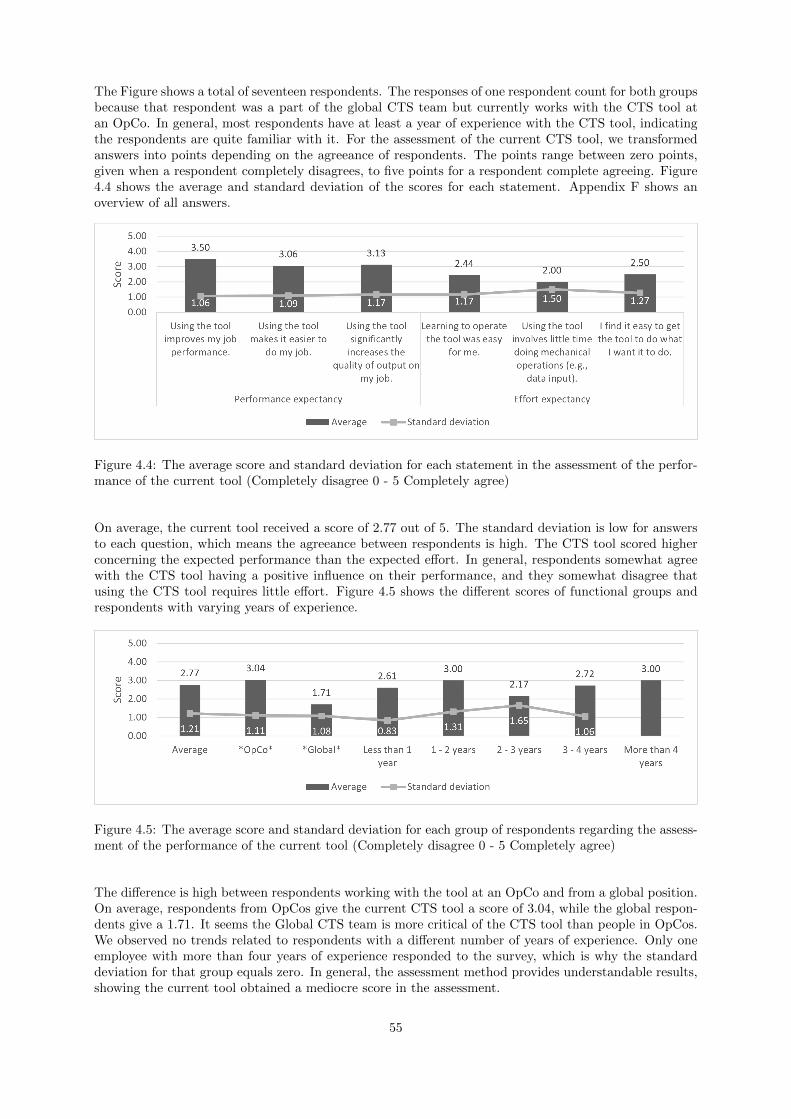
The Figure shows a total of seventeen respondents. The responses of one respondent count for both groupsbecause that respondent was a part of the global CTS team but currently works with the CTS tool atan OpCo. In general, most respondents have at least a year of experience with the CTS tool, indicatingthe respondents are quite familiar with it. For the assessment of the current CTS tool, we transformedanswers into points depending on the agreeance of respondents. The points range between zero points,given when a respondent completely disagrees, to five points for a respondent complete agreeing. Figure4.4 shows the average and standard deviation of the scores for each statement. Appendix F shows anoverview of all answers.
Figure 4.4: The average score and standard deviation for each statement in the assessment of the perfor-mance of the current tool (Completely disagree 0 - 5 Completely agree)
On average, the current tool received a score of 2.77 out of 5. The standard deviation is low for answersto each question, which means the agreeance between respondents is high. The CTS tool scored higherconcerning the expected performance than the expected effort. In general, respondents somewhat agreewith the CTS tool having a positive influence on their performance, and they somewhat disagree thatusing the CTS tool requires little effort. Figure 4.5 shows the different scores of functional groups andrespondents with varying years of experience.
Figure 4.5: The average score and standard deviation for each group of respondents regarding the assess-ment of the performance of the current tool (Completely disagree 0 - 5 Completely agree)
The difference is high between respondents working with the tool at an OpCo and from a global position.On average, respondents from OpCos give the current CTS tool a score of 3.04, while the global respon-dents give a 1.71. It seems the Global CTS team is more critical of the CTS tool than people in OpCos.We observed no trends related to respondents with a different number of years of experience. Only oneemployee with more than four years of experience responded to the survey, which is why the standarddeviation for that group equals zero. In general, the assessment method provides understandable results,showing the current tool obtained a mediocre score in the assessment.
55

Assess features
After we measured the success and assessed the performance of the CTS tool, we assessed the featuresin the tool based on the framework step presented in Section 3.5.3. To get a view of the insights providedby the current tool, we mapped the tool’s features. The mapping of the tool includes all features, theirtype, what they measure, and along which dimensions they can provide insights. Appendix G shows thecomplete mapping of the tool. This framework step includes a survey of how users perceive differentfeatures, which we already presented in Section 3.1.1 to determine optional features to include in theframework’s set of options.
Most features in the CTS tool apply descriptive analytics, showing users what happened, as statedin Section 2.1.1. Users can obtain diagnostic insights, which show why something has happened, butthat requires them to conduct a one-time root-cause analysis. The CTS tool also contains three differentscenarios that users can run, which use predictive analytics, but the tool uses descriptive analytics toshow scenario outcomes. Furthermore, Section 3.1.1 showed that users do not use the scenarios oftenbecause they are difficult to understand. In the rest of this section, we focus on the descriptive analyticsof the CTS tool. Figure 4.6 visualizes what these features measure.
Figure 4.6: The division of what features in the current tool are measuring
Out of the 89 features using descriptive analytics, most features measure volumes, and many featuresmeasure a combination of the CTS and volume KPIs. So, the overall focus is on showing volume KPIs,which is contrary to the savings-focused measurement of success used by the research company in Section4.1.2. Figure 4.7 takes a look at the dimensions used in different features of the tool.
Figure 4.7: The division of dimensions the current tool uses in features
Sources are used as a dimension most frequently, while one would expect to see a focus on customers inthe CTS tool. Additionally, many features in the current CTS tool use overlapping dimensions. In manycases, the CTS tool visualizes data differently, but in some cases, the same table occurs more than once.Table 4.1 shows some features with overlapping dimensions.
56

Table 4.1: Features with similar dimensions that occur more than 5 times in the tool and their measure-ments
Dimensions used CTS CTS and volumes No measures Volume Total
All except CTS buckets and KPIs 1 4 1 2 8Sources 5 3 8
Products 1 4 5Shipments 2 1 2 5
The most striking example of overlap is that five features show the CTS and volumes along a sourcedimension, indicating the degree of overlap in the tool. In conclusion, this assessment shows the focuson descriptive analytics and the overlap between features. Additionally, a new CTS tool could pay moreattention to showing customer dimensions and measuring the CTS.
4.1.3 Differences with the framework
Compared to the typology and process of the Demonstration phase presented in Section 3.4, there arethree differences. Firstly, Internal Optimization refers to Customer Service Optimization, and ProfitablePricing Strategy opportunities are nested under Customer Collaboration because a structure agreed onwith the research company was applied when we created the report. Secondly, we did not consider theautomation of opportunities for the research company because it was the first time the research companyhad an overview of past opportunities, which showed a lot of different types. Perhaps the research com-pany could start automating impactful opportunities using predictive or prescriptive analytics. Thirdly,we made an addition to the framework by creating a Power BI report to visualize past opportunities. Thisreport enables the CTS team to view past opportunities in a user-friendly environment and to obtaininsights regarding their past performance.
There are three differences compared to the framework step on how to measure success from theEvaluation phase. Section 3.5.1 presented profit and customer satisfaction as two indicators of success,but the research company considers savings rather than profit. It was not possible to include profitabilitydue to unavailable data and company policies. However, the savings compared to scoped costs provideda suitable measure of financial success. Regarding customer satisfaction, the research company doesmeasure this, but it was also not possible to include this data. Secondly, we did not include actual valuesbecause the research company only had data concerning estimated savings. Lastly, we measured successon a level of opportunity types due to the connection with the opportunities mapping, allowing the CTSteam to determine which types require more or less attention. The last difference again presents anextension of the Evaluation phase, presented in Section 3.5.
We assessed the tool as intended in the framework step from Section 3.5.2, and we performed mostof the assessment of features used as intended, considering we assessed the value of different the CTStool’s features in Section 3.1.1 to create the set of options for the framework. However, we determinedthe potential value of future analytics in Section 4.2.1 after we set goals concerning what to develop inthe new tool.
4.2 Phase 1: Define objectives of a solution
Here, we focus on the goals and requirements for a new tool for the research company. We evaluatethe performance by applying framework Phase 1 Define objectives of a solution in the context of theresearch company. Thereby we answer the following question:
2.2 Which descriptive, diagnostic, predictive, and prescriptive features should the researchcompany use to visualize the output of a cost-to-serve analysis?
The inputs for this phase are the success measurement, tool assessment, and feature assessment from
57

the Evaluation phase. This section starts with Section 4.2.1 presenting a review of the options presentedin Section 3.1.1. We set a goal stating what to develop as a part of this research. Then, Section 4.2.2outlines requirements and restrictions concerning the selected features. So, the output of this phase is aset of goals, including features to develop with corresponding requirements. Finally, Section 4.2.3 presentsdifferences compared to the framework steps as presented in Section 3.1.
4.2.1 Define goals
As stated in Section 1.2.1, the research company was considering new tooling software around thestart of this research. In the end, they chose Power BI as their standard company-wide reporting solution.Therefore, creating a new tool was in line with company developments.
We made decisions on what descriptive analytics to develop in collaboration with the CTS team. Theselected features included all descriptive analytics from the set of options shown in Table 3.2, except forthe features marked as optional. Furthermore, we could improve the current descriptive analytics byfocusing more on showing relevant data, which we can do by highlighting outliers, showing thresholds,or in other ways. Additionally, we could develop new features relying on descriptive analytics when anopportunity presented itself. So, the first goals defined are as follows:
• Create a new tool in MS Power BI
• Include all non-optional descriptive analytics from Section 3.1.1
• Improve descriptive analytics where possible
• Test new ideas for descriptive analytics that come up during the development
In the next part of this section, we define a goal for a feature using more advanced analytics, based onoptions from Section 3.1.1. Then, we validate this goal by surveying users.
Review options
The assessment in Section 4.1.2 showed that the focus of the old tool was on descriptive analytics.Therefore, the research company should start exploring higher-level analytics. The CTS team wished toexplore the following features from Section 3.1.1:
• Root-cause analysis for a high CTS per volume-unit (diagnostic)
• Estimating the CTS of a new customer or product (predictive)
• Guide in defining a minimum order threshold (prescriptive)
• Guide in defining a discount policy when implementing Logistic Trade Terms (prescriptive)
We did not consider the development of an advanced segmentation method because there was anotherproject in the research company focusing on this. Furthermore, we did not consider an estimation methodfor the CTS of a customer or product in the future, as the CTS team did not require such a feature.
There was a good fit between potential analytics and requirements of the research company. Firstly, aroot-cause analysis for a high CTS per volume-unit is beneficial when understanding the output of a CTSanalysis. We could automate the process where users find the reason for a high CTS per volume-unit.Furthermore, Section 4.1.2 showed types of opportunities found differ per implementation. A root-causeanalysis would reduce the time spent on finding opportunities. Secondly, estimating the CTS of a newcustomer is beneficial when acquiring new customers. Also, estimating the CTS of new products canensure a profitable product launch. However, the research company often relies on single-use solutionsfor such processes. Thirdly, a feature to guide in defining a minimum order threshold would present userswith options for implementing a threshold for a customer or group of customers. Section 4.1.2 showed
58
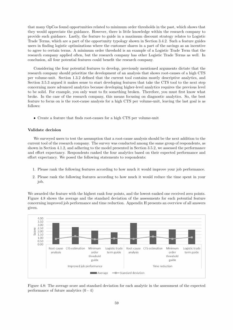
that many OpCos found opportunities related to minimum order thresholds in the past, which shows thatthey would appreciate the guidance. However, there is little knowledge within the research company toprovide such guidance. Lastly, the feature to guide in a maximum discount strategy relates to LogisticTrade Terms, which are a part of the opportunity typology shown in Section 3.4.2. Such a feature guidesusers in finding logistic optimizations where the customer shares in a part of the savings as an incentiveto agree to certain terms. A minimum order threshold is an example of a Logistic Trade Term that theresearch company applied often, but the research company has other Logistic Trade Terms as well. Inconclusion, all four potential features could benefit the research company.
Considering the four potential features to develop, previously mentioned arguments dictate that theresearch company should prioritize the development of an analysis that shows root-causes of a high CTSper volume-unit. Section 1.3.2 defined that the current tool contains mostly descriptive analytics, andSection 3.5.3 argued it makes sense to start developing features that take the CTS tool to the next stepconcerning more advanced analytics because developing higher-level analytics requires the previous levelto be solid. For example, you only want to fix something broken. Therefore, you must first know whatbroke. In the case of the research company, this means focusing on diagnostic analytics. So, the bestfeature to focus on is the root-cause analysis for a high CTS per volume-unit, leaving the last goal is asfollows:
• Create a feature that finds root-causes for a high CTS per volume-unit
Validate decision
We surveyed users to test the assumption that a root-cause analysis should be the next addition to thecurrent tool of the research company. The survey was conducted among the same group of respondents, asshown in Section 4.1.2, and adhering to the model presented in Section 3.5.2, we assessed the performanceand effort expectancy. Respondents ranked the four analytics based on their expected performance andeffort expectancy. We posed the following statements to respondents:
1. Please rank the following features according to how much it would improve your job performance.
2. Please rank the following features according to how much it would reduce the time spent in yourjob.
We awarded the feature with the highest rank four points, and the lowest-ranked one received zero points.Figure 4.8 shows the average and the standard deviation of the assessments for each potential featureconcerning improved job performance and time reduction. Appendix H presents an overview of all answersgiven.
Figure 4.8: The average score and standard deviation for each analytic in the assessment of the expectedperformance of future analytics (0 - 4)
59

The standard deviation is low for the average answers meaning the agreeance between respondents ishigh. Furthermore, the results appear to confirm the requirement of the development of a module thatfinds root-causes of a high CTS per volume-unit. The root-cause analysis scores the highest in bothcategories. When it comes to predictive and prescriptive analytics, the results are less clear. Concerningimproved job performance, respondents prefer predictive analytics rather than prescriptive analytics, butconcerning the expected time reduction, there is no clear preference. We also moderated the experienceand functional groups of respondents. To obtain a more detailed view, Figure 4.9 shows the results fordifferent groups of respondents.
Figure 4.9: The average score and the number of responses for each group of respondents regarding theassessment of future analytics that we could develop (0 - 4)
This again confirms the requirement for the root-cause analysis as only the three respondents with lessthan a year of experience with the tool expect more value from estimating the CTS of a new customeror product over a root-cause analysis. The average response and the responses from OpCos confirmthe assumption that the research company should develop analytics in the specified order. However,the preference is mixed in groups with four respondents or less, but larger groups support the logic tomove from descriptive to diagnostic, to predictive, and finally to prescriptive analytics. So, the researchcompany should develop the features in the order shown in the previous section.
4.2.2 Requirements
Having decided what to develop, we defined requirements based on the framework step in Section3.1.2. This includes, requirements for users, data requirements, and technical constraints that we musttake into account. Regarding the latter, Section 4.2.1 mentioned that Power BI is the preferred softwareand we incorporated the requirements for a root-cause analysis stated in Section 3.13 into the technicalconstraints, which are as follows:
• Create the tool in Power BI
• The tool should work for all OpCos that received a CTS implementation
• The following input files are available:
– The data template (.xlsx)
– Output files from the QlikView tool (.xlsx)
We defined user requirements related to the goals stated in Section 4.2.1. From those goals, we alreadyincluded the creation of a Power BI tool in the constraints. So, the other user requirements are as shownin Table 4.2.
60
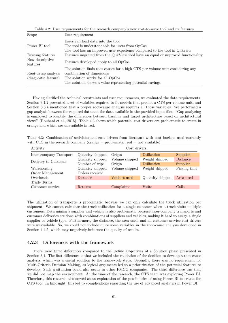
Table 4.2: User requirements for the research company’s new cost-to-serve tool and its features
Scope User requirement
Power BI toolUsers can load data into the toolThe tool is understandable for users from OpCosThe tool has an improved user experience compared to the tool in Qlikview
Existing features Features migrated from the QlikView tool have an equal or improved functionalityNew descriptivefeatures
Features developed apply to all OpCos
Root-cause analysis(diagnostic feature)
The solution finds root causes for a high CTS per volume-unit considering anycombination of dimensionsThe solution works for all OpCosThe solution shows a value representing potential savings
Having clarified the technical constraints and user requirements, we evaluated the data requirements.Section 3.1.2 presented a set of variables required to fit models that predict a CTS per volume-unit, andSection 3.3.4 mentioned that a proper root-cause analysis requires all those variables. We performed agap analysis between the required data and the data available in the provided input files. “Gap analyzingis employed to identify the differences between baseline and target architecture based on architecturalviews” (Rouhani et al., 2015). Table 4.3 shows which potential cost drivers are problematic to create inorange and which are unavailable in red.
Table 4.3: Combination of activities and cost drivers from literature with cost buckets used currentlywith CTS in the research company (orange = problematic, red = not available)
Activity Cost drivers
Inter-company Transport Quantity shipped Origin Utilization SupplierQuantity shipped Volume shipped Weight shipped Distance
Delivery to CustomerNumber of trips Origin Utilization Supplier
Warehousing Quantity shipped Volume shipped Weight shipped Picking timeOrder Management Orders receivedOverheads Distance Vehicles used Quantity shipped Area usedTrade TermsCustomer service Returns Complaints Visits Calls
The utilization of transports is problematic because we can only calculate the truck utilization pershipment. We cannot calculate the truck utilization for a single customer when a truck visits multiplecustomers. Determining a supplier and vehicle is also problematic because inter-company transports andcustomer deliveries are done with combinations of suppliers and vehicles, making it hard to assign a singlesupplier or vehicle type. Furthermore, the distance, the area used, and all customer service cost driverswere unavailable. So, we could not include quite some variables in the root-cause analysis developed inSection 4.4.5, which may negatively influence the quality of results.
4.2.3 Differences with the framework
There were three differences compared to the Define Objectives of a Solution phase presented inSection 3.1. The first difference is that we included the validation of the decision to develop a root-causeanalysis, which was a useful addition to the framework steps. Secondly, there was no requirement forMulti-Criteria Decision Making, as logical arguments led to a prioritization of the potential features todevelop. Such a situation could also occur in other FMCG companies. The third difference was thatwe did not map the environment. At the time of the research, the CTS team was exploring Power BI.Therefore, this research also served as an exploration of the possibilities of using Power BI to create theCTS tool. In hindsight, this led to complications regarding the use of advanced analytics in Power BI.
61
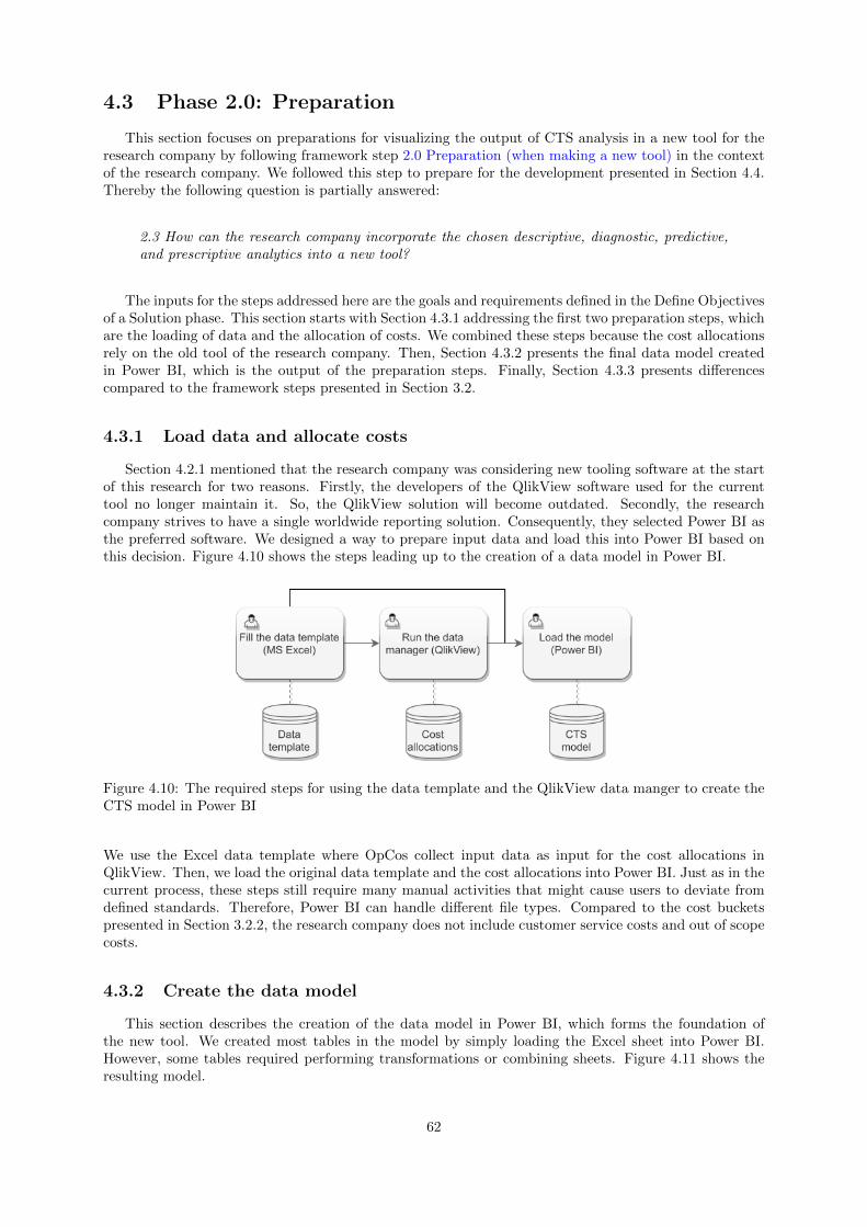
4.3 Phase 2.0: Preparation
This section focuses on preparations for visualizing the output of CTS analysis in a new tool for theresearch company by following framework step 2.0 Preparation (when making a new tool) in the contextof the research company. We followed this step to prepare for the development presented in Section 4.4.Thereby the following question is partially answered:
2.3 How can the research company incorporate the chosen descriptive, diagnostic, predictive,and prescriptive analytics into a new tool?
The inputs for the steps addressed here are the goals and requirements defined in the Define Objectivesof a Solution phase. This section starts with Section 4.3.1 addressing the first two preparation steps, whichare the loading of data and the allocation of costs. We combined these steps because the cost allocationsrely on the old tool of the research company. Then, Section 4.3.2 presents the final data model createdin Power BI, which is the output of the preparation steps. Finally, Section 4.3.3 presents differencescompared to the framework steps presented in Section 3.2.
4.3.1 Load data and allocate costs
Section 4.2.1 mentioned that the research company was considering new tooling software at the startof this research for two reasons. Firstly, the developers of the QlikView software used for the currenttool no longer maintain it. So, the QlikView solution will become outdated. Secondly, the researchcompany strives to have a single worldwide reporting solution. Consequently, they selected Power BI asthe preferred software. We designed a way to prepare input data and load this into Power BI based onthis decision. Figure 4.10 shows the steps leading up to the creation of a data model in Power BI.
Figure 4.10: The required steps for using the data template and the QlikView data manger to create theCTS model in Power BI
We use the Excel data template where OpCos collect input data as input for the cost allocations inQlikView. Then, we load the original data template and the cost allocations into Power BI. Just as in thecurrent process, these steps still require many manual activities that might cause users to deviate fromdefined standards. Therefore, Power BI can handle different file types. Compared to the cost bucketspresented in Section 3.2.2, the research company does not include customer service costs and out of scopecosts.
4.3.2 Create the data model
This section describes the creation of the data model in Power BI, which forms the foundation ofthe new tool. We created most tables in the model by simply loading the Excel sheet into Power BI.However, some tables required performing transformations or combining sheets. Figure 4.11 shows theresulting model.
62
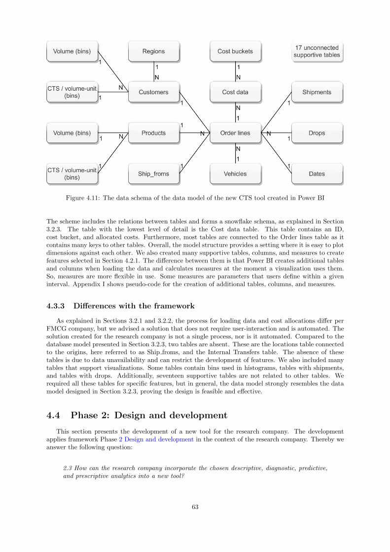
Figure 4.11: The data schema of the data model of the new CTS tool created in Power BI
The scheme includes the relations between tables and forms a snowflake schema, as explained in Section3.2.3. The table with the lowest level of detail is the Cost data table. This table contains an ID,cost bucket, and allocated costs. Furthermore, most tables are connected to the Order lines table as itcontains many keys to other tables. Overall, the model structure provides a setting where it is easy to plotdimensions against each other. We also created many supportive tables, columns, and measures to createfeatures selected in Section 4.2.1. The difference between them is that Power BI creates additional tablesand columns when loading the data and calculates measures at the moment a visualization uses them.So, measures are more flexible in use. Some measures are parameters that users define within a giveninterval. Appendix I shows pseudo-code for the creation of additional tables, columns, and measures.
4.3.3 Differences with the framework
As explained in Sections 3.2.1 and 3.2.2, the process for loading data and cost allocations differ perFMCG company, but we advised a solution that does not require user-interaction and is automated. Thesolution created for the research company is not a single process, nor is it automated. Compared to thedatabase model presented in Section 3.2.3, two tables are absent. These are the locations table connectedto the origins, here referred to as Ship froms, and the Internal Transfers table. The absence of thesetables is due to data unavailability and can restrict the development of features. We also included manytables that support visualizations. Some tables contain bins used in histograms, tables with shipments,and tables with drops. Additionally, seventeen supportive tables are not related to other tables. Werequired all these tables for specific features, but in general, the data model strongly resembles the datamodel designed in Section 3.2.3, proving the design is feasible and effective.
4.4 Phase 2: Design and development
This section presents the development of a new tool for the research company. The developmentapplies framework Phase 2 Design and development in the context of the research company. Thereby weanswer the following question:
2.3 How can the research company incorporate the chosen descriptive, diagnostic, predictive,and prescriptive analytics into a new tool?
63

The inputs for this phase are the goals and requirements defined in the Define Objectives of a Solutionphase and the data model resulting from the preparation steps of this phase. This section starts withSection 4.4.1, which shows how we designed the report to incorporate a desirable user experience. Then,Section 4.4.2 presents the implementation of hierarchies and a basic segmentation method, Section 4.4.3presents the recreation, and sometimes enrichment, of features that existed in the old cost-to-serve tool,Section 4.4.4 introduces new features that we included during the development, and Section 4.4.5 showsthe implementation of the root-cause analysis approach, which we created in Section 3.3.4. The root-cause analysis is optional, but the variable selection and model fitting processes are a mandatory partof the framework. In the end, the outputs of this phase are a new cost-to-serve tool and the root-causeanalysis, which we could not include in the tool. Finally, Section 4.4.6 presents differences compared tothe framework steps as presented in Section 3.3.
In this section, we give an impression of the tool created in Power BI and the root-cause analysissolution, but we do not address all features developed in the new cost-to-serve tool. Appendix J presentsmany features that we do not address in this section.
4.4.1 Tool design
Section 4.2.2 stated two requirements that call for a good design of the new tool. The first requirementwas that the tool should be understandable for users from OpCos. Secondly, the tool should have animproved user experience compared to the tool in Qlikview. This section presents elements that supportthe fulfillment of these requirements. Figure 4.12 shows the main page of the tool.
Figure 4.12: The Main page created in the new Power BI tool using demo data
In the top-left, a selection box shows the volume-units users can choose. When a user changes the volume-unit, the tool shows all values accordingly. Next to the chart, there are two buttons related to differentsections of the CTS tool. Finally, in the top-right, four buttons are visible. The button on the left leadsto the Help page shown in Figure 4.13.
64

Figure 4.13: The Help page created in the new Power BI tool using demo data
The main element of the help page is a figure showing the report structure. After the main page, there aresections with pages to view details, analyze performance, and explore opportunities. The Details sectionfocuses on different dimensions, showing their attributes, key numbers, and allowing users to combinethem, the Analyze Performance section focuses on the current situation of an OpCo, and the ExploreOpportunities section focuses on finding potential business improvements. The help page also shows thehierarchies incorporated throughout the report and several buttons with links to web-pages. Every reportpage has a similar structure to enhance usability. Figure 4.14 shows the page visited when clicking the“Analyze performance” button on the main page.
Figure 4.14: The Page structure created in the new Power BI tool using demo data
65
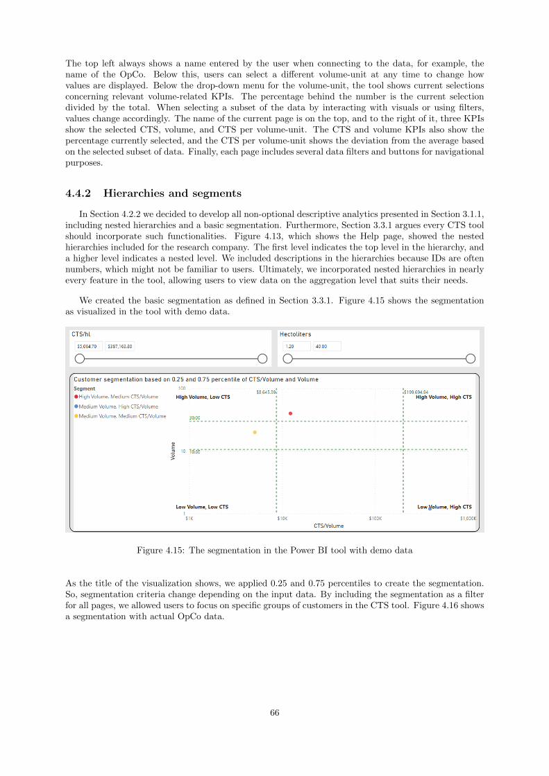
The top left always shows a name entered by the user when connecting to the data, for example, thename of the OpCo. Below this, users can select a different volume-unit at any time to change howvalues are displayed. Below the drop-down menu for the volume-unit, the tool shows current selectionsconcerning relevant volume-related KPIs. The percentage behind the number is the current selectiondivided by the total. When selecting a subset of the data by interacting with visuals or using filters,values change accordingly. The name of the current page is on the top, and to the right of it, three KPIsshow the selected CTS, volume, and CTS per volume-unit. The CTS and volume KPIs also show thepercentage currently selected, and the CTS per volume-unit shows the deviation from the average basedon the selected subset of data. Finally, each page includes several data filters and buttons for navigationalpurposes.
4.4.2 Hierarchies and segments
In Section 4.2.2 we decided to develop all non-optional descriptive analytics presented in Section 3.1.1,including nested hierarchies and a basic segmentation. Furthermore, Section 3.3.1 argues every CTS toolshould incorporate such functionalities. Figure 4.13, which shows the Help page, showed the nestedhierarchies included for the research company. The first level indicates the top level in the hierarchy, anda higher level indicates a nested level. We included descriptions in the hierarchies because IDs are oftennumbers, which might not be familiar to users. Ultimately, we incorporated nested hierarchies in nearlyevery feature in the tool, allowing users to view data on the aggregation level that suits their needs.
We created the basic segmentation as defined in Section 3.3.1. Figure 4.15 shows the segmentationas visualized in the tool with demo data.
Figure 4.15: The segmentation in the Power BI tool with demo data
As the title of the visualization shows, we applied 0.25 and 0.75 percentiles to create the segmentation.So, segmentation criteria change depending on the input data. By including the segmentation as a filterfor all pages, we allowed users to focus on specific groups of customers in the CTS tool. Figure 4.16 showsa segmentation with actual OpCo data.
66

Figure 4.16: The segmentation in the Power BI tool with actual data
The segmentation with actual OpCo data shows approximately 6,000 customers. When a user wouldchoose to focus on a relatively small group with a high volume and CTS per volume-unit, the userwould select the corresponding group in a filter and visit other pages to find opportunities for businessimprovements.
4.4.3 Existing features
In Section 4.2.2 we decided to develop all non-optional descriptive analytics presented in Section 3.1.1.The first feature was the filter functionality. In Power BI, this feature is a part of the user interface withlow customizability. So, the filter functionality included in the tool differs from the filter functionality inthe QlikView tool. Then, we created the three graphs that received high scores in the evaluation of thefeatures of the old tool, in Section 3.1.1. Figure 4.17 shows the Cost per volume-unit graph. Additionally,we created the Scatter/drop analysis, Delivery profile, and map graphs. Appendix J shows those graphs.
Figure 4.17: The Cost per volume-unit graph created in the new Power BI tool
67

In the old CTS tool, users could switch between a view showing the line or showing the stacked column.Here, we combined these functionalities and added labels showing the total CTS/volume-unit, and weincluded buttons above and to the right of the visualization to change the dimension or level of costbuckets. Next, we created the tables suggested by the framework in Section 3.1.1, which are the keynumbers, detail, and combination tables. Figure 4.18 shows the Customer’s key numbers page, andAppendix J shows the others.
Figure 4.18: The Key numbers Customers page created in the new Power BI tool showing demo data
This page shows three tables, which we drilled down to different levels. The first table shows costs ineach cost group for channels, the second table shows volumes and the CTS per volume-unit for outlettypes, and the third table shows the CTS per volume-unit for customers. In the last table, we expandedthe cost groups to reveal the underlying cost-buckets, which only shows the costs for customer deliveries,but other groups are visible when using the horizontal scroll bar. There are also buttons on the rightto switch between the general customer hierarchy or a hierarchy based on attributes specified by users.Furthermore, we derived a feature from the old tool that was not an option in Section 3.1.1. Figure 4.19shows it visualizing volume flows from and to customers based on the old tool’s overview page.
Figure 4.19: The Volume flow feature created in the new Power BI tool showing demo data
68
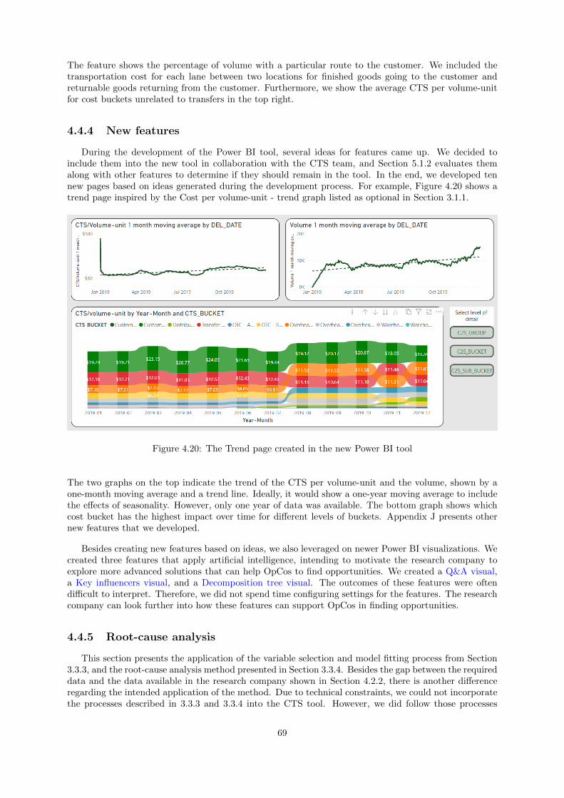
The feature shows the percentage of volume with a particular route to the customer. We included thetransportation cost for each lane between two locations for finished goods going to the customer andreturnable goods returning from the customer. Furthermore, we show the average CTS per volume-unitfor cost buckets unrelated to transfers in the top right.
4.4.4 New features
During the development of the Power BI tool, several ideas for features came up. We decided toinclude them into the new tool in collaboration with the CTS team, and Section 5.1.2 evaluates themalong with other features to determine if they should remain in the tool. In the end, we developed tennew pages based on ideas generated during the development process. For example, Figure 4.20 shows atrend page inspired by the Cost per volume-unit - trend graph listed as optional in Section 3.1.1.
Figure 4.20: The Trend page created in the new Power BI tool
The two graphs on the top indicate the trend of the CTS per volume-unit and the volume, shown by aone-month moving average and a trend line. Ideally, it would show a one-year moving average to includethe effects of seasonality. However, only one year of data was available. The bottom graph shows whichcost bucket has the highest impact over time for different levels of buckets. Appendix J presents othernew features that we developed.
Besides creating new features based on ideas, we also leveraged on newer Power BI visualizations. Wecreated three features that apply artificial intelligence, intending to motivate the research company toexplore more advanced solutions that can help OpCos to find opportunities. We created a Q&A visual,a Key influencers visual, and a Decomposition tree visual. The outcomes of these features were oftendifficult to interpret. Therefore, we did not spend time configuring settings for the features. The researchcompany can look further into how these features can support OpCos in finding opportunities.
4.4.5 Root-cause analysis
This section presents the application of the variable selection and model fitting process from Section3.3.3, and the root-cause analysis method presented in Section 3.3.4. Besides the gap between the requireddata and the data available in the research company shown in Section 4.2.2, there is another differenceregarding the intended application of the method. Due to technical constraints, we could not incorporatethe processes described in 3.3.3 and 3.3.4 into the CTS tool. However, we did follow those processes
69

as intended using Excel, R, and RStudio. We chose R because the research company can, theoretically,embed R scripts in a Power BI report. So, after this research, the research company should be able tointegrate the solutions. Figure 4.21 shows the modular solution that we created. We designed a modularsolution to enhance the potential useability of the root-cause analysis for the research company.
Figure 4.21: The process with subsequently, variable creation, preprocessing, model fitting, and theroot-cause analysis showing intermediate output files
The process requires two input files, the shipment and cost details, that users can extract from theQlikView tool. Then, they set the level of detail in the first file and run the R scripts in the sequenceshown. An advantage of the modular solution is that users can alter the Excel sheets, which serve asinput and output files. Furthermore, users can use the Excel sheets for different reasons than describedin this process. Appendix K shows the code of the R scripts.
The variable selection and model-fitting process designed in Section 3.3.3 mentioned several parame-ters, which are the cutoff value for correlations and the number of repeats and folds for cross-validation.To test the sensitivity of these parameters, we performed two experiments. First, experiments with cutoffvalues for a data set showed the best performance with a value of 0.9, which avoids “very strong” cor-relations based on the interpretation of cutoff values from Section 2.5. Especially the Recursive FeatureElimination random forest model (rfe) showed an improved performance with higher cutoff values, whichis understandable as Section 2.6 explained that this model handles collinearity well. A higher cutoff valuemeans the script removes less correlating variables, which leads to more variables in the final set. Then,we tested the sensitivity of the parameter values for the number of folds and repeats when performing thecross-validation method presented in Section 3.3.3. In this experiment, we did not observe an improvedperformance for higher values, but we observed a high increase in runtime. Therefore, a single run with2-fold cross-validation is the most effective option based on this experiment. Appendix L shows detailedresults and more analysis concerning these experiments.
After determining the values for parameters, we ran the four R scripts for two different OpCos toensure that the solution works for different data sets. For both OpCos, we performed runs for customers,products, and combinations of the two. Table 4.4 summarizes the data sets.
Table 4.4: The data sets for which a root-cause analysis was performed
OpCo Set Customers Products
1Customers 6183Products 11Customers - Products (5118 out of 36103) 727 11
2Customers 269Products 313Customers - Products 269 313
70
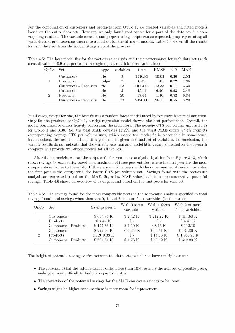
For the combination of customers and products from OpCo 1, we created variables and fitted modelsbased on the entire data set. However, we only found root-causes for a part of the data set due to avery long runtime. The variable creation and preprocessing scripts ran as expected, properly creating allvariables and preprocessing them into a final set for the fitting of models. Table 4.5 shows all the resultsfor each data set from the model fitting step of the process.
Table 4.5: The best model fits for the root-cause analysis and their performance for each data set (witha cutoff value of 0.9 and performed a single repeat of 2-fold cross-validation)
OpCo Set type variables time RMSE Rˆ2 MAE
1Customers rfe 9 1510.83 10.03 0.30 2.53Products ridge 7 0.45 1.45 0.72 1.36Customers - Products rfe 23 11004.02 13.38 0.17 3.34
2Customers rfe 3 45.14 6.96 0.93 2.48Products rfe 20 17.64 1.40 0.82 0.84Customers - Products rfe 33 2420.00 26.11 0.55 3.29
In all cases, except for one, the best fit was a random forest model fitted by recursive feature elimination.Only for the products of OpCo 1, a ridge regression model showed the best performance. Overall, themodel performance differs heavily concerning the indicators. The average CTS per volume-unit is 11.18for OpCo 1 and 3.38. So, the best MAE deviates 12.2%, and the worst MAE differs 97.3% from itscorresponding average CTS per volume-unit, which means the model fit is reasonable in some cases,but in others, the script could not fit a good model given the final set of variables. In conclusion, thevarying results do not indicate that the variable selection and model fitting scripts created for the researchcompany will provide well-fitted models for all OpCos.
After fitting models, we ran the script with the root-cause analysis algorithm from Figure 3.13, whichshows savings for each entity based on a maximum of three peer entities, where the first peer has the mostcomparable variables to the entity. If there are multiple peers with the same number of similar variables,the first peer is the entity with the lowest CTS per volume-unit. Savings found with the root-causeanalysis are corrected based on the MAE. So, a low MAE value leads to more conservative potentialsavings. Table 4.6 shows an overview of savings found based on the first peers for each set.
Table 4.6: The savings found for the most comparable peers in the root-cause analysis specified in totalsavings found, and savings when there are 0, 1, and 2 or more focus variables (in thousands)
OpCo Set Savings peer 1With 0 focus
variablesWith 1 focus
variableWith 2 or morefocus variables
1Customers $ 637.74 K $ 7.42 K $ 212.72 K $ 417.60 KProducts $ 4.47 K $ - $ - $ 4.47 KCustomers - Products $ 122.36 K $ 1.10 K $ 8.16 K $ 113.10
2Customers $ 229.96 K $ 31.79 K $ 66.31 K $ 131.86 KProducts $ 1,979.38 K $ - $ 14.13 K $ 1,965.25 KCustomers - Products $ 681.34 K $ 1.73 K $ 59.62 K $ 619.99 K
The height of potential savings varies between the data sets, which can have multiple causes:
• The constraint that the volume cannot differ more than 10% restricts the number of possible peers,making it more difficult to find a comparable entity.
• The correction of the potential savings for the MAE can cause savings to be lower.
• Savings might be higher because there is more room for improvement.
71
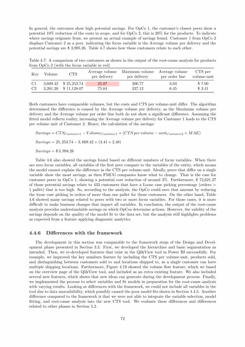
In general, the outcomes show high potential savings. For OpCo 1, the customer’s closest peers show apotential 10% reduction of the costs in scope, and for OpCo 2, this is 20% for the products. To indicatewhere savings originate from, we present an actual example of savings found. Customer 1 from OpCo 2displays Customer 2 as a peer, indicating the focus variable is the Average volume per delivery and thepotential savings are $ 3,995.26. Table 4.7 shows how these customers relate to each other.
Table 4.7: A comparison of two customers as shown in the output of the root-cause analysis for productsfrom OpCo 2 (with the focus variable in red)
Key Volume CTSAverage volume
per deliveryMaximum volume
per deliveryAverage volumeper order line
CTS pervolume-unit
C1 3,609.42 $ 25,253.74 25.07 206.77 3.03 $ 7.00C2 3,261.20 $ 11,128.07 75.84 237.12 6.45 $ 3.41
Both customers have comparable volumes, but the costs and CTS per volume-unit differ. The algorithmdetermined the difference is caused by the Average volume per delivery, as the Maximum volume perdelivery and the Average volume per order line both do not show a significant difference. Assuming thefitted model reflects reality, increasing the Average volume per delivery for Customer 1 leads to the CTSper volume unit of Customer 2. Hence, the calculation of the savings:
Savings = CTSCustomer1 − V olumeCustomer1 × (CTS per volume− unitCustomer2 +MAE)
Savings = 25, 253.74− 3, 609.42× (3.41 + 2.48)
Savings = $ 3, 994.26
Table 4.6 also showed the savings found based on different numbers of focus variables. When thereare zero focus variables, all variables of the first peer compare to the variables of the entity, which meansthe model cannot explain the difference in the CTS per volume-unit. Ideally, peers that differ on a singlevariable show the most savings, as then FMCG companies know what to change. That is the case forcustomer peers in OpCo 1, showing a potential cost reduction of around 3%. Furthermore, $ 72,621.27of those potential savings relate to 433 customers that have a Loose case picking percentage (orders >1 pallet) that is too high. So, according to the analysis, the OpCo could save that amount by reducingthe loose case picking in orders of more than one pallet for those customers. On the other hand, Table4.6 showed many savings related to peers with two or more focus variables. For those cases, it is moredifficult to make business changes that impact all variables. In conclusion, the output of the root-causeanalysis provides understandable savings on which OpCos determine actions. However, the validity of thesavings depends on the quality of the model fit to the data set, but the analysis still highlights problemsas expected from a feature applying diagnostic analytics.
4.4.6 Differences with the framework
The development in this section was comparable to the framework steps of the Design and Devel-opment phase presented in Section 3.3. First, we developed the hierarchies and basic segmentation asintended. Then, we re-developed features that exist in the QlikView tool in Power BI successfully. Forexample, we improved the key numbers feature by including the CTS per volume-unit, products sold,and distinguishing between customers sold to and locations shipped to, as a single customer can havemultiple shipping locations. Furthermore, Figure 4.19 showed the volume flow feature, which we basedon the overview page of the QlikView tool, and included as an extra existing feature. We also includedseveral new features, which shows that new ideas can generate during the development process. Finally,we implemented the process to select variables and fit models in preparation for the root-cause analysiswith varying results. Looking at differences with the framework, we could not include all variables in thetool due to data unavailability, which possibly caused the poor model fits shown in Section 4.4.5. Anotherdifference compared to the framework is that we were not able to integrate the variable selection, modelfitting, and root-cause analysis into the new CTS tool. We evaluate these differences and differencesrelated to other phases in Section 5.2.
72

Chapter 5
Evaluation
In this chapter, we evaluate the framework for fast-moving consumer goods companies to find businessimprovements using the output of a cost-to-serve analysis and the new tool we created for the researchcompany, which resulted from applying the framework in a case study. First, Section 5.1 focuses on theassessment of the new tool, which is similar to the assessment done for the old tool in Section 4.1.2. Then,Section 5.2 evaluates the framework in light of the case study by highlighting differences to determinethe applicability of the framework.
5.1 Power BI tool
This section evaluates the new tool that we created based on the designed framework to find businessimprovements using the outcome of a cost-to-serve analysis. Section 5.1.1 evaluates whether the new toolmeets the requirements set before development. Then, Section 5.1.2 shows the outcomes of the evaluationof the new tool and compares the new and old tools. Finally, Section 5.1.3 evaluates whether we achievedset goals in the creation of the new tool. The first two sections include the results of a survey sent out toassess the new tool. Appendix M shows all answers to this survey.
5.1.1 Requirements
This section focuses on requirements formulated for the development of the new tool by evaluatingtechnical requirements and user requirements. We evaluate the requirements listed in Section 4.2.2.
Technical requirements
Concerning requirements listed in Section 4.2.2, we did not meet the data requirement and the require-ment for a single solution. In general, requirements depend on the company, but Section 3.1.2 presentedvarious potential cost drivers of a high CTS per volume-unit, which FMCG companies should include intheir CTS analysis. The framework requires the availability of these variables for features using descrip-tive analytics and the root-cause analysis presented in Section 4.4.5. However, Section 4.2.2 showed thatit was not possible to include all variables, but we did include all variables from the old tool to avoid aloss of information. To resolve the issue, the research company must expand the data collection duringa CTS implementation.
Section 4.2.2 also mentioned three other requirements. The first requirement was to develop the toolin Power BI. Features that apply descriptive analytics met this requirement, but the root-cause analysisdid not, due to constraints imposed by the IT environment of the research company. IT experts from theresearch company can most likely resolve this issue. The second requirement was that the tool shouldwork for all OpCos that received a CTS implementation, and the third requirement specified the use ofthe data template and output files from the old tool as input files. We tested the new tool with data from
73
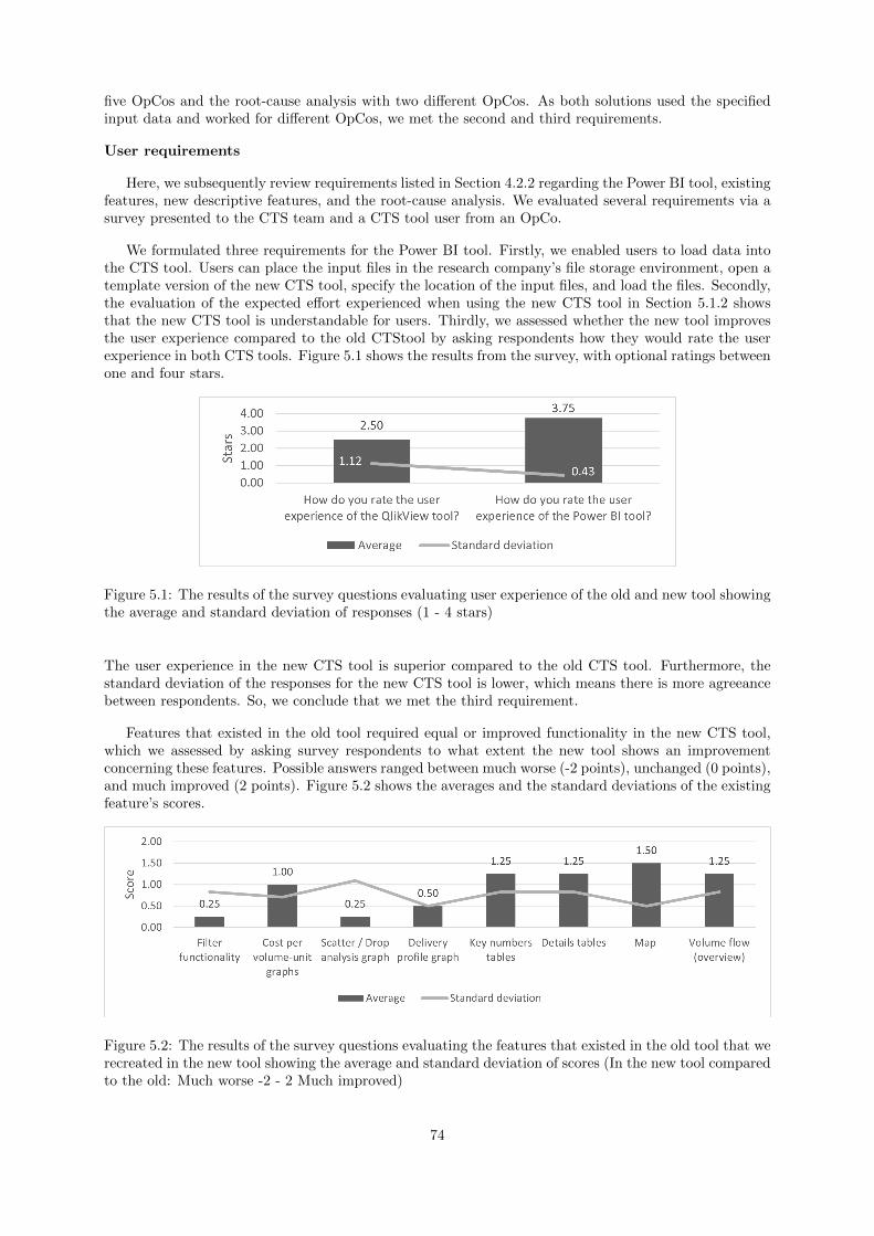
five OpCos and the root-cause analysis with two different OpCos. As both solutions used the specifiedinput data and worked for different OpCos, we met the second and third requirements.
User requirements
Here, we subsequently review requirements listed in Section 4.2.2 regarding the Power BI tool, existingfeatures, new descriptive features, and the root-cause analysis. We evaluated several requirements via asurvey presented to the CTS team and a CTS tool user from an OpCo.
We formulated three requirements for the Power BI tool. Firstly, we enabled users to load data intothe CTS tool. Users can place the input files in the research company’s file storage environment, open atemplate version of the new CTS tool, specify the location of the input files, and load the files. Secondly,the evaluation of the expected effort experienced when using the new CTS tool in Section 5.1.2 showsthat the new CTS tool is understandable for users. Thirdly, we assessed whether the new tool improvesthe user experience compared to the old CTStool by asking respondents how they would rate the userexperience in both CTS tools. Figure 5.1 shows the results from the survey, with optional ratings betweenone and four stars.
Figure 5.1: The results of the survey questions evaluating user experience of the old and new tool showingthe average and standard deviation of responses (1 - 4 stars)
The user experience in the new CTS tool is superior compared to the old CTS tool. Furthermore, thestandard deviation of the responses for the new CTS tool is lower, which means there is more agreeancebetween respondents. So, we conclude that we met the third requirement.
Features that existed in the old tool required equal or improved functionality in the new CTS tool,which we assessed by asking survey respondents to what extent the new tool shows an improvementconcerning these features. Possible answers ranged between much worse (-2 points), unchanged (0 points),and much improved (2 points). Figure 5.2 shows the averages and the standard deviations of the existingfeature’s scores.
Figure 5.2: The results of the survey questions evaluating the features that existed in the old tool that werecreated in the new tool showing the average and standard deviation of scores (In the new tool comparedto the old: Much worse -2 - 2 Much improved)
74

Most features have an average value between one and two, indicating slight or much improvement. Asthose features all have a standard deviation lower than the average, we can argue the respondents ex-perienced the functionality of these features is either unchanged or improved. The Filter functionality,the Scatter/drop analysis graph, and the Delivery profile graph have scores between zero and one witha higher or equal standard deviation, which shows perceptions of respondents differ concerning the im-provement of these features. However, with average values above zero, it is safe to say the functionalityis not worse. Therefore, the existing features met the requirement for improved functionality in the newtool. Furthermore, we stated that new descriptive features should work for all OpCos, which is the casewhen the input data is complete. So, we met this requirement as well.
We formulated three requirements for the root-cause analysis. Firstly, the solution finds root-causesfor a high CTS per volume-unit of any combination of dimensions. In the script where we create variables,users define a key for each order line based on columns available in the shipment details. This key, forwhich the method determines root-causes for a high CTS, can be a single dimension or a combination.Secondly, the solution works for all OpCos. We extracted input data in a standard format from the oldtool for two OpCos. Therefore, the solution works for OpCos that extract data similarly. Thirdly, thesolution shows a value representing potential savings, which we achieved by displaying savings related topeers of an entity. So, we met all requirements concerning the root-cause analysis method and all otheruser requirements formulated for the development of a new tool in this research.
5.1.2 Performance new tool
This section evaluates the performance of the new tool its features. The assessment is similar tothe evaluations performed in Section 4.1.2. First, we assess the performance of the new tool. Then, wecompare the number of features used in the new and old tools.
Tool assessment
The CTS team and a CTS tool user from an OpCo filled the survey presented in this section. Ideally,there would be more respondents from OpCos, as 13 respondents from OpCos assessed the old CTS tool,but as the research company did not yet distribute the new CTS tool among OpCos, we could onlyinvolve a single OpCo. Figure 5.3 shows the results of the assessment of the old and new tools. Whena respondent completely disagreed with a statement, we awarded zero points, and when a respondentcompletely agreed, we awarded five points.
Figure 5.3: The results of the survey questions evaluating the old and new tool showing the average andstandard deviation of responses (Completely disagree 0 - 5 Completely agree)
The new tool outperformed the old version regarding all statements shown. The new tool received anaverage score of 3.83, where the old tool received an average score of 2.77 out of 5. So, in general, the newtool yields an improvement for the research company. The low standard deviation indicates that manyresponses were close to the high average. We also assessed the new features by asking respondents howthey value them by awarding between one and four stars. Figure 5.4 shows the result of this assessment.
75
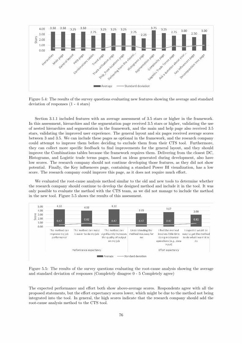
Figure 5.4: The results of the survey questions evaluating new features showing the average and standarddeviation of responses (1 - 4 stars)
Section 3.1.1 included features with an average assessment of 3.5 stars or higher in the framework.In this assessment, hierarchies and the segmentation page received 3.5 stars or higher, validating the useof nested hierarchies and segmentation in the framework, and the main and help page also received 3.5stars, validating the improved user experience. The general layout and six pages received average scoresbetween 3 and 3.5. We can include these pages as optional in the framework, and the research companycould attempt to improve them before deciding to exclude them from their CTS tool. Furthermore,they can collect more specific feedback to find improvements for the general layout, and they shouldimprove the Combinations tables because the framework requires them. Delivering from the closest DC,Histograms, and Logistic trade terms pages, based on ideas generated during development, also havelow scores. The research company should not continue developing those features, as they did not showpotential. Finally, the Key influencers page, containing a standard Power BI visualization, has a lowscore. The research company could improve this page, as it does not require much effort.
We evaluated the root-cause analysis method similar to the old and new tools to determine whetherthe research company should continue to develop the designed method and include it in the tool. It wasonly possible to evaluate the method with the CTS team, as we did not manage to include the methodin the new tool. Figure 5.5 shows the results of this assessment.
Figure 5.5: The results of the survey questions evaluating the root-cause analysis showing the averageand standard deviation of responses (Completely disagree 0 - 5 Completely agree)
The expected performance and effort both show above-average scores. Respondents agree with all theproposed statements, but the effort expectancy scores lower, which might be due to the method not beingintegrated into the tool. In general, the high scores indicate that the research company should add theroot-cause analysis method to the CTS tool.
76
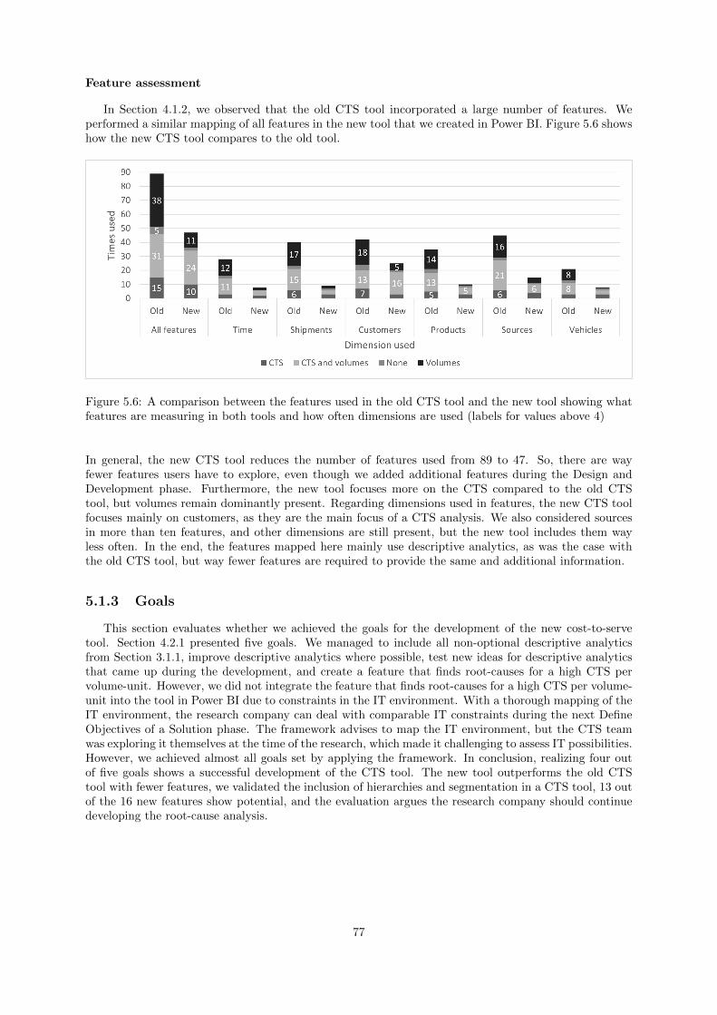
Feature assessment
In Section 4.1.2, we observed that the old CTS tool incorporated a large number of features. Weperformed a similar mapping of all features in the new tool that we created in Power BI. Figure 5.6 showshow the new CTS tool compares to the old tool.
Figure 5.6: A comparison between the features used in the old CTS tool and the new tool showing whatfeatures are measuring in both tools and how often dimensions are used (labels for values above 4)
In general, the new CTS tool reduces the number of features used from 89 to 47. So, there are wayfewer features users have to explore, even though we added additional features during the Design andDevelopment phase. Furthermore, the new tool focuses more on the CTS compared to the old CTStool, but volumes remain dominantly present. Regarding dimensions used in features, the new CTS toolfocuses mainly on customers, as they are the main focus of a CTS analysis. We also considered sourcesin more than ten features, and other dimensions are still present, but the new tool includes them wayless often. In the end, the features mapped here mainly use descriptive analytics, as was the case withthe old CTS tool, but way fewer features are required to provide the same and additional information.
5.1.3 Goals
This section evaluates whether we achieved the goals for the development of the new cost-to-servetool. Section 4.2.1 presented five goals. We managed to include all non-optional descriptive analyticsfrom Section 3.1.1, improve descriptive analytics where possible, test new ideas for descriptive analyticsthat came up during the development, and create a feature that finds root-causes for a high CTS pervolume-unit. However, we did not integrate the feature that finds root-causes for a high CTS per volume-unit into the tool in Power BI due to constraints in the IT environment. With a thorough mapping of theIT environment, the research company can deal with comparable IT constraints during the next DefineObjectives of a Solution phase. The framework advises to map the IT environment, but the CTS teamwas exploring it themselves at the time of the research, which made it challenging to assess IT possibilities.However, we achieved almost all goals set by applying the framework. In conclusion, realizing four outof five goals shows a successful development of the CTS tool. The new tool outperforms the old CTStool with fewer features, we validated the inclusion of hierarchies and segmentation in a CTS tool, 13 outof the 16 new features show potential, and the evaluation argues the research company should continuedeveloping the root-cause analysis.
77
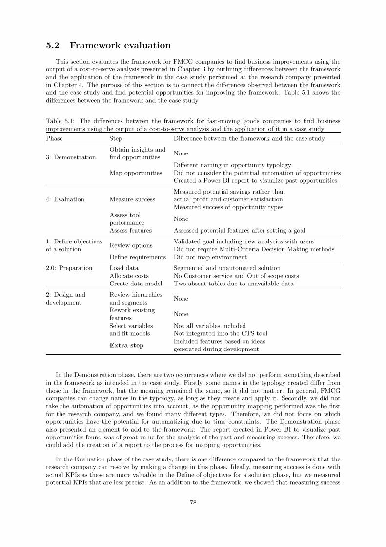
5.2 Framework evaluation
This section evaluates the framework for FMCG companies to find business improvements using theoutput of a cost-to-serve analysis presented in Chapter 3 by outlining differences between the frameworkand the application of the framework in the case study performed at the research company presentedin Chapter 4. The purpose of this section is to connect the differences observed between the frameworkand the case study and find potential opportunities for improving the framework. Table 5.1 shows thedifferences between the framework and the case study.
Table 5.1: The differences between the framework for fast-moving goods companies to find businessimprovements using the output of a cost-to-serve analysis and the application of it in a case study
Phase Step Difference between the framework and the case study
3: DemonstrationObtain insights andfind opportunities
None
Map opportunitiesDifferent naming in opportunity typologyDid not consider the potential automation of opportunitiesCreated a Power BI report to visualize past opportunities
4: Evaluation Measure successMeasured potential savings rather thanactual profit and customer satisfactionMeasured success of opportunity types
Assess toolperformance
None
Assess features Assessed potential features after setting a goal
1: Define objectivesof a solution
Review optionsValidated goal including new analytics with usersDid not require Multi-Criteria Decision Making methods
Define requirements Did not map environment
2.0: Preparation Load data Segmented and unautomated solutionAllocate costs No Customer service and Out of scope costsCreate data model Two absent tables due to unavailable data
2: Design anddevelopment
Review hierarchiesand segments
None
Rework existingfeatures
None
Select variablesand fit models
Not all variables includedNot integrated into the CTS tool
Extra stepIncluded features based on ideasgenerated during development
In the Demonstration phase, there are two occurrences where we did not perform something describedin the framework as intended in the case study. Firstly, some names in the typology created differ fromthose in the framework, but the meaning remained the same, so it did not matter. In general, FMCGcompanies can change names in the typology, as long as they create and apply it. Secondly, we did nottake the automation of opportunities into account, as the opportunity mapping performed was the firstfor the research company, and we found many different types. Therefore, we did not focus on whichopportunities have the potential for automatizing due to time constraints. The Demonstration phasealso presented an element to add to the framework. The report created in Power BI to visualize pastopportunities found was of great value for the analysis of the past and measuring success. Therefore, wecould add the creation of a report to the process for mapping opportunities.
In the Evaluation phase of the case study, there is one difference compared to the framework that theresearch company can resolve by making a change in this phase. Ideally, measuring success is done withactual KPIs as these are more valuable in the Define of objectives for a solution phase, but we measuredpotential KPIs that are less precise. As an addition to the framework, we showed that measuring success
78

is possible for opportunity types, which could be useful to do for other FMCG companies as well.
Three differences between the framework and the case study originated in the Define objectives ofa solution phase. Firstly, we assessed potential features after we defined a goal instead of during theEvaluation phase, which allowed for a more concise assessment and avoided asking users about featuresthe research company might not develop. Thus, the step where FMCG companies assess potential featuresfits better in the Define objectives of a solution phase. Secondly, we did not use Multi-Criteria Decision-Making methods when formulating a goal. We did not require such methods as we could make a decisionbased on logic, but when other FMCG companies could not do the same, such methods could still beuseful. Thirdly, we did not map the IT environment during the definition of requirements. Later, inthe Design and Development phase, we were not able to integrate the steps for variable selection andmodel-fitting into the CTS tool, emphasizing the importance of mapping the IT environment.
In the preparation steps of the Design and Development phase, there are three occurrences where wedid not perform something in the case study as described in the framework. Firstly, the data loadingprocess is segmented and not automated, which leads to users experiencing a high effort when workingwith the CTS tool. However, this does not negatively affect any other phases of the framework. Secondly,the research company does not include Customer Service and Out of Scope costs in their CTS analysis.The absence of customer service elements resulted in a lack of customer satisfaction measurements in theEvaluation phase. Due to the absence of Out of Scope costs, we measured savings rather than profit, butthis did not have negative consequences. Savings can even serve as a suitable alternative for profit in theframework, but including both cost-buckets would strengthen the Evaluation phase of the CTS analysis.Thirdly, two tables from the proposed data model were absent, which led to unincluded variables in theDesign and Development phase. The absence of variables possibly caused the model fitting performanceto vary and restrains the options for the use of analytics.
In the other steps of the Design and Development phase, we decided to include features based onideas generated during development, which presented an extension to the framework. An advantage ofthat step was that we developed more optional features, which we directly evaluated, but Section 5.1.2showed that three of the seven new features lack potential. Therefore, we advised to discard three of themand include the others as optional descriptive features. Furthermore, one of the three standard PowerBI artificial intelligence features scored relatively low, but including these features required little effort.So, we advised continuing the development of that feature. In general, FMCG companies should decidebeforehand how much time to spend on randomly introduced features. The advantage of creating extrafeatures during development is that there are additional features to consider, but the time investmentpresents a disadvantage.
In conclusion, many differences require action from the research company, and five differences providea potential improvement for the framework. These are validating features after defining goals, creatingadditional features during development, creating a report to visualize past opportunities, measuring thesuccess of opportunity types, and the possibility to include savings rather than profit. The number ofdifferences that require the research company to take action, and the improvement made by the new toolshown in Section 5.1, indicate how following the framework can improve the process of visualizing theoutput of a CTS analysis for an FMCG company. Taking the differences presented in this section intoaccount, Section 6.2 shows recommendations for the research company in a roadmap.
79
Chapter 6
Conclusions and recommendations
This chapter presents the conclusions and recommendations of this research. First, Section 6.1 answersthe main research questions.
1 How can fast-moving consumer goods companies find business improvementsby using descriptive, diagnostic, predictive, and descriptive analytics in their toolthat visualizes the output of a cost-to-serve analysis?
2 Can the research company improve the use of the output of cost-to-serve anal-yses by applying the framework designed in this research to create a new tool?
So, we reflect on the creation of the framework for fast-moving consumer goods companies to find businessimprovements using the output of a cost-to-serve analysis and the case study applying this framework inthe research company. Then, Section 6.2 presents recommendations for the research company based onthe case study. Finally, Section 6.3 discusses the findings in this research in the light of validation, theapplicability of the framework, limitations, future work, and the contribution of this research to theoryand practice.
6.1 Conclusions
In this section, we present the conclusions of this research in which we developed and applied aframework for fast-moving consumer goods companies to visualize the output of a cost-to-serve analysis.Chapter 3 presented the framework’s four phases containing various steps, which we summarize here.The framework describes how FMCG companies can find business improvements by using descriptive,diagnostic, predictive, and descriptive analytics in their tool that visualizes the output of a CTS analysis.
Section 3.1 presented the Define Objectives of a Solution phase. We created a set of optional featuresfor a CTS tool by researching which descriptive, diagnostic, predictive, and prescriptive analytics FMCGcompanies can use and which features of the research company’s old CTS tool users value most. Basedon the set of options, FMCG companies can set a goal for development and define requirements based onusers, the environment, and technical aspects. For the data availability, which is a technical requirement,we created a set of variables based on potential cost-drivers that FMCG companies should include intheir CTS analysis.
Section 3.2 presented preparation steps for the Design and Development phase in Section 3.2 thatFMCG companies must follow when creating a new tool. These steps are to load data, allocate costs,and create a data model, which is necessary when creating a new CTS tool. We based those steps onprocesses of the research company, which we supported with reviewed literature. After the preparation
80

steps, the mandatory part of the Design and Development phase in Section 3.3 commences, where wefirstly included the use and review of hierarchies and segmentation techniques in a CTS tool. Secondly,we focused on reworking existing features when the Evaluation phase shows this is necessary. And finally,we explained how to select variables and fit models for features using more advanced analytics, which weapplied in an algorithm that finds root-causes for a high CTS per volume-unit.
Section 3.4 presented the Demonstration phase, where FMCG companies empower users of the CTStool to find potential business improvements. They must decide how much training to provide for usersbased on the amount of human input required to find opportunities, which depends on applied analytics.In this phase, we also researched how to map business improvements obtained with insights from a CTSanalysis, resulting in a process that includes a typology to map found opportunities.
Section 3.5 focused on evaluating the CTS analysis. The Evaluation phase starts by measuring theinfluence CTS analyses have on profitability, and customer satisfaction, which we both derived fromthe benefits of CTS found in the reviewed literature. Then, an evaluation of the tool takes place. Weresearched which techniques can assess the quality of a tool visualizing the output of a CTS analysis,creating a model that applies to CTS tools of FMCG companies. Finally, FMCG companies measure theperformance of different types of analytics used in the features of the CTS tool. After this phase ends, anew cycle begins with the evaluation phase. By going through the mentioned phases and following thesteps, FMCG companies can get the most out of the output from a performed CTS analysis.
In Chapter 4, we applied the framework to find business improvements using the output of a cost-to-serve analysis to the research company to improve the use of results of a CTS analysis and validatethe framework. First, Section 4.1 researched how the CTS implementation of the research company wasperforming by applying the Demonstration and Evaluation phases of the framework. We created anopportunity mapping system, including success measurements that we visualized in a Power BI report.The report includes the research company’s success measurement, showing the average potential savingsper OpCo are 3% of scoped costs. Then, an assessment of the old tool showed that it performs betteron increasing performance than reducing experienced effort, and the feature assessment showed that theresearch company’s CTS tool has many similar descriptive features.
After we assessed the current situation, Section 4.2 presented the Define Objectives of a Solutionphase of the framework where we set goals and define requirements, which included one goal to develop anew tool in Power BI. We researched which descriptive, diagnostic, predictive, and prescriptive analyticsthe research company should use to visualize the output of a CTS analysis by applying the steps to defineobjectives of a solution of the framework. As a result, we decided to develop all the non-optional featuresusing descriptive analytics from the framework’s set of optional features, and we argued the developmentof a root-cause analysis method, based on a prioritization of diagnostic analytics before predictive andprescriptive analytics, which we confirmed via a survey among users of the CTS tool.
Following the Define Objectives of a Solution phase, Section 4.3 addressed the preparation steps of theframework’s Design and Development phase, which was required because we set a goal to develop a newCTS tool. Then, Section 4.4 researched how to incorporate the chosen features into a new tool for theresearch company by following the other steps of the Design and Development phase of the framework.The result was a fully functional Power BI tool with nested hierarchies, a customer segmentation method,a minimized presence of descriptive tables, highly appreciated graphs from the old CTS tool, and featuresusing descriptive analytics designed during the development process. We evaluated the Power BI toolin Section 5.1, showing a 50% more desirable user experience, that all features that were present inthe old CTS tool improved, and that the likelihood to increase performance and reduce effort improvedby 38% despite having fewer features. The hierarchies and segmentation page also received a positiveevaluation, validating the relevance of the corresponding framework step, and six new features basedon ideas generated during development also showed promise. So, FMCG companies could include themin the framework’s optional set of features. Finally, we performed the last steps of the Design andDevelopment phase, concerning the variable selection and fitting of models, in the root-cause analysis.It was not possible to integrate them into the CTS tool. It should be possible, but restrictions relatedto the IT environment of the research company hindered this. Nevertheless, the root-cause analysismethod showed great promise revealing potential savings up to 20% of costs in scope for different datasets and a possible cost reduction of more than 3% by improving a single focus variable for customers in
81
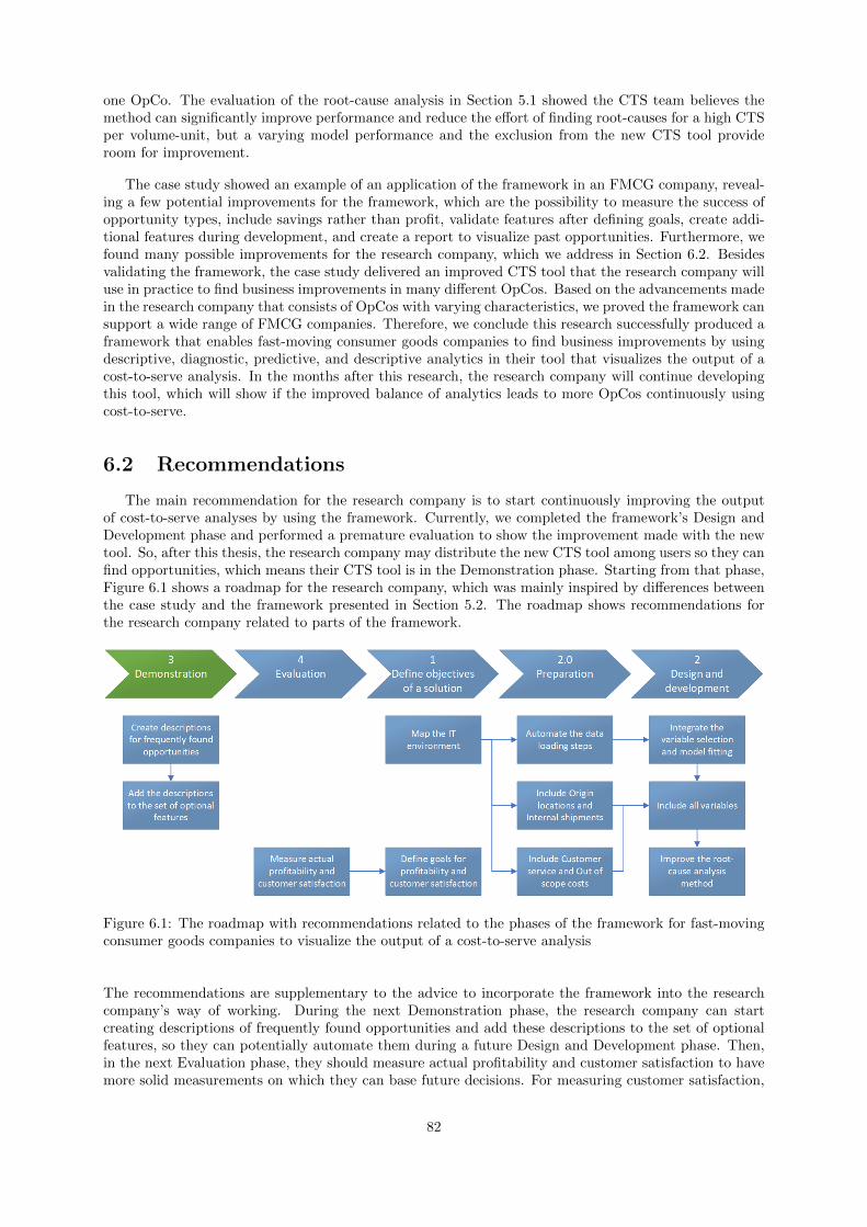
one OpCo. The evaluation of the root-cause analysis in Section 5.1 showed the CTS team believes themethod can significantly improve performance and reduce the effort of finding root-causes for a high CTSper volume-unit, but a varying model performance and the exclusion from the new CTS tool provideroom for improvement.
The case study showed an example of an application of the framework in an FMCG company, reveal-ing a few potential improvements for the framework, which are the possibility to measure the success ofopportunity types, include savings rather than profit, validate features after defining goals, create addi-tional features during development, and create a report to visualize past opportunities. Furthermore, wefound many possible improvements for the research company, which we address in Section 6.2. Besidesvalidating the framework, the case study delivered an improved CTS tool that the research company willuse in practice to find business improvements in many different OpCos. Based on the advancements madein the research company that consists of OpCos with varying characteristics, we proved the framework cansupport a wide range of FMCG companies. Therefore, we conclude this research successfully produced aframework that enables fast-moving consumer goods companies to find business improvements by usingdescriptive, diagnostic, predictive, and descriptive analytics in their tool that visualizes the output of acost-to-serve analysis. In the months after this research, the research company will continue developingthis tool, which will show if the improved balance of analytics leads to more OpCos continuously usingcost-to-serve.
6.2 Recommendations
The main recommendation for the research company is to start continuously improving the outputof cost-to-serve analyses by using the framework. Currently, we completed the framework’s Design andDevelopment phase and performed a premature evaluation to show the improvement made with the newtool. So, after this thesis, the research company may distribute the new CTS tool among users so they canfind opportunities, which means their CTS tool is in the Demonstration phase. Starting from that phase,Figure 6.1 shows a roadmap for the research company, which was mainly inspired by differences betweenthe case study and the framework presented in Section 5.2. The roadmap shows recommendations forthe research company related to parts of the framework.
Figure 6.1: The roadmap with recommendations related to the phases of the framework for fast-movingconsumer goods companies to visualize the output of a cost-to-serve analysis
The recommendations are supplementary to the advice to incorporate the framework into the researchcompany’s way of working. During the next Demonstration phase, the research company can startcreating descriptions of frequently found opportunities and add these descriptions to the set of optionalfeatures, so they can potentially automate them during a future Design and Development phase. Then,in the next Evaluation phase, they should measure actual profitability and customer satisfaction to havemore solid measurements on which they can base future decisions. For measuring customer satisfaction,
82

we advise considering the method used carefully, as Section 2.2 showed that there is criticism towards theNPS method. Then, the research company can also set goals related to these measurements during thenext Define Objectives of a Solution phase. Another recommendation related to that phase is to map theIT environment preceding a reconsideration of the preparation steps of the Design and Development phase.Doing so leads to three other recommendations, which relate to another execution of the preparation stepsof the Design and Development phase:
1. The research company should automate the data loading process.
We advise prioritizing this, as the problem context in Section 1.3.1 showed this was the most relevantproblem. Figure 6.2 illustrates a proposed structure for automating the data loading process.
Figure 6.2: The current data connection process (left) and the proposed data collection process (right)for the research company’s CTS analyses
The structure relies on the development of middleware that supplies the CTS tool in Power BI withthe required source data. When OpCos have comparable data sources, it might even be possible tostandardize the middleware created. Then, they can integrate the variable selection and model-fittingscripts into the tool during the Design and Development phase. By doing this, the research company willhave all features incorporated in a single CTS tool. Additionally, the research company should continueto explore the possibilities in Power BI. As the software continues to develop, it becomes possible to domore with it over time. Perhaps, it becomes possible to perform a variable selection and fit models withinPower BI as well. Then they should focus on the two other recommendations:
2. The research company should include tables with location-data of origins and link a table withinternal shipments to order lines.
3. The research company should include Customer service and Out of Scope costs.
83
With these preparation steps included, the research company should aim to create all variables mentionedin this thesis during the next Design and Development phase. Then, they can review and improve theroot-cause analysis method to ensure it is user-friendly and have everything included in a single CTStool. A final recommendation is to continue developing and reviewing the framework, taking into accountthe evaluation of the framework presented in Section 5.2, which showed potential improvements for theframework.
6.3 Discussion
This section discusses the outcomes of this research. First, Section 6.3.1 outlines how we took intoaccount the validity and reliability of results in this thesis. Then, Section 6.3.2 reflects on the applicabilityof the created framework for the research company, FMCG companies, and other types of companies. Sec-tion 6.3.3 assesses limitations and presents opportunities for future work. Finally, Section 6.3.4 presentsthe contributions of this research to theory and practice.
6.3.1 Validation
Cooper and Schindler (2014) describe validity as the extent to which a test measures what it aimsto, whereas reliability refers to the accuracy of measurements. We often validated matters with the CTSteam, and in some cases, we did this with OpCos. For example, the CTS team validated the problemcluster in Section 1.3.1, showing that it correctly displayed the problem context and was therefore valid.In another example, we ensured a reliable core problem selection using the AHP method with the companysupervisor. The AHP method checks that preferences are consistent, which provides a reliable problemselection. Furthermore, the CTS team verified the opportunity typology created in Section 3.4.2, whichprovided an expert view on potential opportunities, validating the typology for use in practice.
In this thesis, we sent a survey to the CTS team and various tool users from OpCos to assess thevalue of features of the QlikView tool in Section 3.1.1, the performance of the QlikView tool in Section4.1.2, and the desired features using diagnostic, predictive, or prescriptive analytics in Section 4.2.1. Thissurvey had sixteen respondents, including the entire CTS team, which leads to a reliable assessmentwhen taking average values. We applied scales with an even amount of options to force respondentsto express either a negative or positive sentiment, rather than allowing respondents to choose a neutraloption. Hence, decisions made based on the survey are valid as users always expressed their opinionclearly. We also shared another questionnaire with the CTS team and a single OpCo user to assess thePower BI tool in Section 5.1. Due to the low number of respondents, results from this survey are lessreliable, but when we only consider the view of the CTS team, the results are reliable, as the entire teamfilled in both surveys. When we only take the CTS team into account, we see that the tool improvedsignificantly, as the CTS team had a more critical view of the QlikView tool, and the OpCo respondentalso evaluated the new CTS tool positively with a 50% higher score than the old CTS tool. Therefore,we assumed the new tool presented an improvement, but to make future decisions regarding the CTStool, the research company must have more respondents from OpCos assess the CTS tool to increasereliability. Without good reliability, they could make invalid decisions regarding how to improve the CTStool further. Additionally, the comparison of the old and new tools also showed an improvement regardingthe time involved in doing mechanical operations, which does not make sense, as the Power BI tool relieson the QlikView tool to perform the cost allocations in addition to its data loading process. Perhaps,respondents did not consider loading data into the old CTS tool when giving their opinion regarding thatstatement.
The Power BI tool must be reliable to ensure users make business decisions validly. To ensure relia-bility, we compared the values in the Power BI tool with the QlikView tool, assuming values shown inthe QlikView tool are correct. We loaded data from five OpCos into the Power BI tool, which showedsimilar values in overlapping features. So, the Power BI tool is reliable concerning the data and val-ues it shows. We also performed the root-cause analysis for two OpCos to ensure it works in differentsettings and compared the variables created to similar variables shown in the QlikView tool to validateall descriptive information. However, we do not know whether the potential savings resulting from the
84
root-cause analysis, shown in Section 4.4.5, are reliable. Therefore, the research company should attemptto make business changes based on the root-cause analysis and measure actual savings. A better modelfit would also increase the reliability of the savings found. Currently, a difference between entities mightresult from a cost driver that is not a part of the analysis, but in general, the method is reliable as itworks for different OpCos and different dimensions. However, the shown savings are questionable.
6.3.2 Applicability of the framework
Chapter 1 argued the design of a framework for FMCG companies to find business improvements usingthe output of a CTS analysis. We developed this framework to reduce the lack of diagnostic, predictive,and prescriptive insights in the research company’s CTS tool, which we selected as the focus problemtogether with the CTS team. However, the problem context in Section 1.3.1 also showed other problems.In hindsight, the framework relates to all solvable core problems found. For example, in the case study,we saw again that the absence of an automated data collection is a problem, and we solved that the toolcannot handle multiple years of data. Furthermore, the research company could also solve other problemsfound during a phase of the framework. For example, they could focus on improving user-training duringthe Demonstration phase or improve the goal-setting during the Define Objectives of a Solution phase.It appears that the nature of the problem selected for this research caused the focus on the Design andDevelopment phase. When another problem would have resulted from the problem identification, theframework would still provide a good solution, but we might have focused more on another phase.
Chapter 4 showed a successful application of the framework in the research company, which has manyOpCos, and because of the decentralized nature of OpCos, we concluded the framework works for otherFMCG companies as well. The intended users of the framework presented in Chapter 3 are people inFMCG companies that are responsible for managing and developing a CTS analysis. Depending onthe company, this can be from a global or local position related to customer service or logistics. Forexample, the research company manages CTS analyses globally. If the management in the researchcompany would move to a local level, the framework versions of the tool might diverge, and knowledgesharing would inhibit, but the framework would still apply to the research company assuming localmanagement implies that there are multiple local users of the tool. Then, those users take the placethat OpCos have in this thesis. Another difference between FMCG companies can be the scope of theirCTS analysis. The framework includes cost buckets for all logistics costs, but an FMCG company couldalso focus on a segment of the logistics costs. For example, the focus could be on warehousing costs andinclude all relevant cost drivers for those costs. However, a disadvantage of decreasing the scope of theCTS analysis is that it might not measure all effects of changes. Perhaps improvements that positivelyinfluence warehouse costs negatively affect other cost buckets. In general, the scope must not move awayfrom customer-related activities, as these are closely related to the benefits of a CTS analysis, but theframework is still applicable when we do not include one or more of the cost buckets because thosebuckets do not apply to the FMCG company at hand. In conclusion, the framework applies to FMCGcompanies regardless of their organizational structure, but to be sure of this assumption, we should testits applicability in more FMCG companies.
Besides being applicable in FMCG companies, the framework might also apply to other types of com-panies that want to find opportunities related to customer service optimization, customer collaboration,and a profitable pricing strategy. If companies cannot obtain any of these benefits, a CTS implementationbecomes useless, so companies performing a CTS analysis should be able to make changes to the waycustomers are supplied, collaborate with customers, and determine a pricing strategy. Other relevantcharacteristics of an FMCG company are high volumes and a large degree of Make-to-Stock manufac-turing. The combination of those two characteristics can complicate supply chains and make it hard todetermine costs on a customer-level, hence the requirement for a CTS analysis. These characteristicscan also apply to other company types than the FMCG company, such as fashion companies, originalequipment manufacturers, companies selling food, or companies selling flowers. Therefore, the frameworkappears to apply to such companies as well, which we could also test in practice.
The framework requires the availability of reliable input data. Especially when moving to higher-level analytics, this becomes a more critical requirement due to a higher reliance on input data. Thecase study showed that the model-fitting process performed poorly in some cases, which might be due
85
to data unavailability. So, companies applying a CTS analysis should focus on data availability andreliability increasingly when incorporating higher-level analytics. For example, the data handling in theresearch company could improve as it often involves manual work, which might lead to incorrect data.However, if the research company considered it easy to automate data connections and ensure reliabledata input at all times, they would do it. So, change management is required to enable the researchcompany to apply the framework as intended, and this might be the case for other companies as well.Alternatively, companies can strive for solutions that are as good as possible given available data, butgiven the importance of data in a CTS analysis, we could enrich the framework with a data managementarchitecture.
6.3.3 Limitations and future work
The research in this thesis has several limitations, which present opportunities for future work. Theprevious section showed three limitations and opportunities for future work related to the applicabilityof the created framework. Firstly, we applied the framework to a single FMCG company in a casestudy. Due to the nature of the subject of the case study, we argued that the framework applies to otherFMCG companies. However, future work could research whether this assumption is correct by applyingthe framework in several FMCG companies while measuring achieved savings and customer satisfaction.Secondly, the framework is limited to FMCG companies, but we explained that other types of companiescould apply the framework as well. So, when after testing the framework in multiple FMCG companies,future work could research whether the framework applies to other types of companies similar to the casestudy in this thesis. Thirdly, the framework assumes that all input data is available and reliable, whilethe case study showed otherwise. Thus, future work can focus on the IT architecture and possible changemanagement required to incorporate the framework by creating an ideal IT architecture and performinga gap analysis with the architectures of several companies.
In Chapter 4, we applied the framework to an FMCG company that has been performing CTSimplementations for several years, but we would ideally apply it to an FMCG company that does nothave CTS-related processes in place. The successful introduction of CTS analyses in an FMCG companyusing the framework developed in this thesis would provide a strong validation of the framework. InFMCG companies that currently perform CTS analyses, it might be unavoidable to deviate from setstandards due to previously mentioned change management. Therefore, future work could set-up a CTSanalysis in an FMCG company based on the framework and evaluate differences between the frameworkand the case study as done in this thesis in Section 5.2.
Section 3.1.1 shows a set of optional features to develop based on reviewed literature concerningpotential analytics for visualizing the output of a CTS analysis and features from the QlikView tool.However, Section 4.4.4 presented several additional promising features that emerged during development,showing there are more potential features than we found in the literature. In future work, the assessmentof optional features and analytics to develop could focus on other companies that perform CTS analysesbesides referring to the literature to find more features that are valuable for end-users. Furthermore, futurework could focus on the development of new analytics for a CTS analysis, which does not necessarily relateto a limitation in this thesis. However, Section 3.1.1 showed that only a few features focus on customercollaboration but that we can derive these from customer service optimization features. Furthermore,that section showed that there are no predictive features that focus on customer collaboration or customerservice optimization, which presents more possible directions for future work.
In the root-cause analysis in Section 4.4.5, not all data was available, which possibly led to a varyingmodel fitting performance, as explained in Section 6.3.1. Furthermore, we did not integrate the featureinto the CTS tool. Future work can leverage the method designed in this thesis and test it in a casewhere all input data is available to obtain a more stable model fit. Additionally, future work can extendthe range of models experimented with, include monthly variables to ensure seasonality is captured,and include experiments with subsets of variables to predict individual cost buckets, which might allowfor better inclusion of variables showing utilization, supplier attributes, or vehicle attributes. In suchfuture work, validating savings by assessing how many advised changes are feasible in practice wouldalso present a significant improvement compared to the work in this thesis. Another limitation of theroot-cause analysis is that it estimates potential savings for an entity by assuming that if it is comparable
86

to another entity, the CTS per volume-unit will be about the same. However, we could improve thisestimation when there is a good model fit. Future work could build on the root-cause analysis in thisthesis but explore the possibility of estimating savings by predicting a new CTS per volume-unit with thefitted model. All in all, we can potentially improve the root-cause analysis in many ways, which mightpresent a suitable topic for a new graduate intern at the research company.
6.3.4 Contribution to theory and practice
Chapter 1 started by showing that the expectations for CTS are likely to increase in the comingyears. However, there is a gap in the literature explaining how FMCG companies should approach aCTS analysis. In this thesis, we combined many theories related to this subject in a framework. Theconnection of all elements in the framework provides a new basis for FMCG companies to develop theirCTS analyses, creating a holistic overview of what is involved with visualizing the output of a CTSanalysis. We linked reviewed literature from Chapter 2 related to CTS analyses with other literature andsynthesized it in a framework in Chapter 3, including literature on rating tool performance, potentialcost drivers in logistics, and model fitting. The framework also includes the concepts of descriptive,diagnostic, predictive, and prescriptive analytics that can support features that visualize the output ofa CTS analysis. Furthermore, Section 3.4.2 showed potential benefits that result from a CTS analysis,which we supported by creating a typology containing types and sub-types, and Section 4.2.1 validatedthat users prefer diagnostic features rather than predictive or prescriptive features when the current CTStool focuses on features using descriptive analytics. So, FMCG companies should develop lower-levelanalytics in full before focusing on higher-level analytics. We also developed a novel algorithm to findroot-causes using a fitted model in Section 3.13. All in all, we did not find an approach focus on CTSanalyses that compares to the framework developed in this thesis. Therefore, this is the first frameworkfor FMCG companies to support them when visualizing the output of a cost-to-serve analysis.
The future must show whether the improvements made on the use of output a CTS analysis with theframework will lead to more OpCos continuously using CTS in the research company, but regardless ofthe result, we made a high contribution to their work. We implemented a system using the opportunitytypology that visualizes past opportunities found in a CTS implementation in a Power BI report inSection 4.1.1, allowing the CTS team to view and leverage the past. Then, Section 4.2 clarified thatthe research company should focus on diagnostic analytics before moving to more advanced analytics.And finally, we used this and other knowledge to create a new tool in Power BI that visualizes theoutput of a CTS analysis in Sections 4.3 and 4.4. The Power BI tool is going to replace the QlikViewtool used by the research company, and we created the first version of a root-cause analysis methodfor a high CTS per volume-unit for the research company in Section 4.4.5, which the research companycan continue to develop. The framework in itself is also a contribution to the research company. Weproved that the research company could apply the framework, which has led to several improvements andrecommendations for the future. In conclusion, this thesis provides the research company with a structureto follow, supporting processes, and an improved tool to visualize the output of a CTS analysis.
87

Bibliography
Ajzen, I. et al. (1991). The theory of planned behavior. Organizational behavior and human decisionprocesses, 50(2):179–211.
Allen, D. M. (1974). The relationship between variable selection and data agumentation and a methodfor prediction. Technometrics, 16(1):125–127.
Andersen, C. M. and Bro, R. (2010). Variable selection in regression — A tutorial. Journal of chemo-metrics, 24(11-12):728–737.
Ashfaque, J. M. and Iqbal, A. (2019). Introduction to support vector machines and kernel methods.publication at https: // www. researchgate. net/ publication/ 332370436 .
Ayodele, T. O. (2010). Types of machine learning algorithms. New advances in machine learning, 3:19–48.
Baykasoglu, A. and Kaplanoglu, V. (2008). Application of activity-based costing to a land transportationcompany: A case study. International journal of production economics, 116(2):308–324.
Behn, R. D. (2003). Why measure performance? Different purposes require different measures. Publicadministration review, 63(5):586–606.
Bokor, Z. (2010). Cost drivers in transport and logistics. Periodica polytechnica transportation engineer-ing, 38(1):13–17.
Bolton, R. N. and Tarasi, C. O. (2006). Managing customer relationships. Review of marketing research,3(3).
Bonoma, T. V. and Shapiro, B. P. (1984). Evaluating market segmentation approaches. Industrialmarketing management, 13(4):257–268.
Bosshard, T. (2017). Analytics - Does your business need descriptive, diagnostic, predictive, orprescriptive capabilities? https://adviscent.com/blog/analytics-does-your-business-need-
descriptive-diagnostic-predictive-or-prescriptive-capabilities.html. Accessed: 2020-10-05.
Braithwaite, A. and Samakh, E. (1998). The cost-to-serve method. The international journal of logisticsmanagement, 9(1):69–84.
Breiman, L. (2001). Random forests. Machine learning, 45(1):5–32.
Brownlee, J. (2017). Difference between classification and regression in machine learning. https://
machinelearningmastery.com/classification-versus-regression-in-machine-learning/. Ac-cessed: 2020-08-22.
BusinessDictionairy.com (2020). Opportunity. http://www.businessdictionary.com/definition/
opportunity.html. Accessed: 2020-05-15.
Cecere, L. (2015). Seven thoughts to build a customer-centric supply chain organiza-tion. http://www.supplychainshaman.com/demand/demanddriven/seven-thoughts-to-build-a-
customer-centric-supply-chain-organization/. Accessed: 2020-04-02.
88

Chakon, O. (2017). Practical machine learning: Ridge regression vs. lasso. https://hackernoon.com/
practical-machine-learning-ridge-regression-vs-lasso-a00326371ece. Accessed: 2020-09-24.
Chen, S.-J. and Hwang, C.-L. (1992). Fuzzy multiple attribute decision making methods. Springer.
Christensson, P. (2008). Application definition. https://techterms.com/definition/application.Accessed: 2020-05-15.
Cooper, D. and Schindler, P. (2014). Business research methods. The McGraw- Hill Companies.
Davis, F. D. (1985). A technology acceptance model for empirically testing new end-user informationsystems: Theory and results. PhD thesis, Massachusetts institute of technology.
Davis, M. (2010). Case study for supply chain leaders: Dell’s transformative journey through supplychain segmentation. Gartner research. ID number G, 208603.
Elliott, T. (2013). Gartner BI: Analytics moves to the core. Business analytics (blog), February, 14.
Everaert, P., Bruggeman, W., Sarens, G., Anderson, S. R., and Levant, Y. (2008). Cost modeling inlogistics using time-driven ABC. International journal of physical distribution & logistics management.
Fishbein, M. and Ajzen, I. (1977). Belief, attitude, intention, and behavior: An introduction to theoryand research. None.
Fisher, N. I. and Kordupleski, R. E. (2019). Good and bad market research: A critical review of netpromoter score. Applied stochastic models in business and industry, 35(1):138–151.
Freedman, D. A. (2009). Statistical models: Theory and practice. Cambridge university press.
Freeman, B., Haasz, S., Lizzola, S., and Seiersen, N. (2000). Managing your cost-to-serve. Supply chainforum: An international journal, 1:18–28.
GeeksforGeeks (2020). Ml — Types of learning – Supervised learning. https://www.geeksforgeeks.
org/ml-types-learning-supervised-learning/. Accessed: 2020-08-22.
Guerreiro, R., Bio, S. R., and Merschmann, E. V. V. (2008). Cost-to-serve measurement and customerprofitability analysis. The international journal of logistics management.
Heerkens, J. and van Winden, A. (2012). Geen probleem, een aanpak voor alle bedrijfskundige vragen enmysteries. Business school Nederland. Boekredactie.
Holm, M., Kumar, V., and Rohde, C. (2012). Measuring customer profitability in complex environments:an interdisciplinary contingency framework. Journal of the academy of marketing science, 40(3):387–401.
Jensen, C. S., Pedersen, T. B., and Thomsen, C. (2010). Multidimensional databases and data warehous-ing. Synthesis lectures on data management, 2(1):1–111.
Jong, Y. d. (2019). Levels of data analytics. http://www.ithappens.nu/levels-of-data-analytics/.Accessed: 2020-05-15.
Kacan, M. (2019). 5 main drivers of supply chain costs. https://icrontech.com/blog_item/5-main-
drivers-of-supply-chain-costs/. Accessed: 2020-09-05.
Kaplan, R. S. and Anderson, S. R. (2003). Time-driven activity-based costing. Available at SSRN 485443.
Kirkpatrick, S., Gelatt, C. D., and Vecchi, M. P. (1983). Optimization by simulated annealing. science,220(4598):671–680.
Kock, N. (2015). Common method bias in PLS-SEM: A full collinearity assessment approach. Interna-tional journal of e-collaboration (ijec), 11(4):1–10.
Kolarovszki, P., Tengler, J., and Majercakova, M. (2016). The new model of customer segmentation inpostal enterprises. Procedia-social and behavioral sciences, 230:121–127.
89

Kone, E. R. and Karwan, M. H. (2011). Combining a new data classification technique and regressionanalysis to predict the cost-to-serve new customers. Computers & industrial engineering, 61(1):184–197.
Kuhn, M. (2019). The caret package. https://topepo.github.io/caret/. Accessed: 2020-08-23.
Kuhn, M. et al. (2008). Building predictive models in R using the caret package. Journal of statisticalsoftware, 28(5):1–26.
Kvalseth, T. O. (1985). Cautionary note about R 2. The American statistician, 39(4):279–285.
Liaw, A., Wiener, M., et al. (2002). Classification and regression by randomforest. R news, 2(3):18–22.
Madden, T. J., Ellen, P. S., and Ajzen, I. (1992). A comparison of the theory of planned behavior andthe theory of reasoned action. Personality and social psychology bulletin, 18(1):3–9.
Nakajima, S. (1988). Total productive maintenance. Introduction to TPM. Productivity press 1988.
Ozener, O. O., Ergun, O., and Savelsbergh, M. (2013). Allocating cost of service to customers in inventoryrouting. Operations research, 61(1):112–125.
Pandey, D., Suman, U., and Ramani, A. (2010). An effective requirement engineering process model forsoftware development and requirements management. 2010 International conference on advances inrecent technologies in communication and computing, pages 287–291.
Peffers, K., Tuunanen, T., Rothenberger, M. A., and Chatterjee, S. (2007). A design science researchmethodology for information systems research. Journal of management information systems, 24(3):45–77.
Pohlen, T. L. and La Londe, B. J. (1994). Implementing activity-based costing (ABC) in logistics. Journalof business logistics, 15(2):1.
Poole, C. (2017). Supply chain brief: Heinekens journey to improved customer service and collaboration.
Poole, D. (2020). A better way for service to predict future customer loyalty. https://www.gartner.
com/smarterwithgartner/a-better-way-for-service-to-predict-future-customer-loyalty/.
ProductPlan (2020). Roadmap basics. https://www.productplan.com/roadmap-basics/. Accessed:2020-05-15.
Reichheld, F. F. (2003). The one number you need to grow. Harvard business review, 81(12):46–55.
Ross, A., Jayaraman, V., and Robinson, P. (2007). Optimizing 3pl service delivery using a cost-to-serveand action research framework. International journal of production research, 45(1):83–101.
Rouhani, B. D., Mahrin, M. N., Nikpay, F., Ahmad, R. B., and Nikfard, P. (2015). A systematic literaturereview on enterprise architecture implementation methodologies. Information and software technology,62:1–20.
Saaty, T. L. (2000). Fundamentals of decision making and priority theory with the analytic hierarchyprocess, volume 6. RWS publications.
Schober, P., Boer, C., and Schwarte, L. A. (2018). Correlation coefficients: appropriate use and interpre-tation. Anesthesia & Analgesia, 126(5):1763–1768.
Seif, G. (2018). 5 types of regression and their properties. https://towardsdatascience.com/5-types-of-regression-and-their-properties-c5e1fa12d55e. Accessed: 2020-08-22.
Singh, R., Gohil, A. M., Shah, D. B., and Desai, S. (2013). Total productive maintenance (TPM)implementation in a machine shop: A case study. Procedia engineering, 51:592–599.
Stapleton, D., Pati, S., Beach, E., and Julmanichoti, P. (2004). Activity-based costing for logistics andmarketing. Business process management journal.
Sun, L., Karwan, M. H., Gemici-Ozkan, B., and Pinto, J. M. (2015). Estimating the long-term cost toserve new customers in joint distribution. Computers & industrial engineering, 80:1–11.
90

Svetnik, V., Liaw, A., Tong, C., and Wang, T. (2004). Application of Breiman’s random forest to mod-eling structure-activity relationships of pharmaceutical molecules. International workshop on multipleclassifier systems, pages 334–343.
Taherdoost, H. (2018). A review of technology acceptance and adoption models and theories. Procediamanufacturing, 22:960–967.
Tohamy, N. (2020). Hype cycle for supply chain strategy, 2020.
Triantaphyllou, E. (2000). Multi-criteria decision making methods: A comparative study. Springer.
Tripathi, N. (2020). What is customer satisfaction score? https://www.surveysensum.com/blog/what-
is-customer-satisfaction-score-definition-calculation-applications-and-advantages/.Accessed: 2020-10-05.
Turney, P. B. (1992). Activity based costing. Management accounting handbook(4th Edition), edited byC. Drury, Butterworth-Heinemann and CIMA.
Vala, K. (2019). Tree-based methods: Regression trees. https://towardsdatascience.com/tree-
based-methods-regression-trees-4ee5d8db9fe9. Accessed: 2020-09-27.
van Niekerk, H. J. and Bean, W. (2019). Evaluation of the cost drivers and allocation framework inoutbound logistics of the fast-moving consumer goods industry. South African journal of industrialengineering, 30(2):115–130.
Varila, M., Seppanen, M., and Suomala, P. (2007). Detailed cost modelling: A case study in warehouselogistics. International journal of physical distribution & logistics management.
Veness, C. (2020). Calculate distance, bearing and more between latitude/longitude points. https:
//www.movable-type.co.uk/scripts/latlong.html. Accessed: 2020-10-09.
Venkatesh, V., Morris, M. G., Davis, G. B., and Davis, F. D. (2003). User acceptance of informationtechnology: Toward a unified view. MIS quarterly, pages 425–478.
Wang, A., Arbogast, J. E., Bonnier, G., Wilson, Z., and Gounaris, C. E. (2020). Estimation of marginalcost to serve individual customers.
Watts, S. (2017). Etl basics: Extract, Transform & Load. https://www.bmc.com/blogs/what-is-etl-extract-transform-load-etl-explained/. Accessed: 2020-10-02.
Wind, Y. and Saaty, T. L. (1980). Marketing applications of the analytic hierarchy process. Managementscience, 26(7):641–658.
Zhou, Z.-H. (2018). A brief introduction to weakly supervised learning. National science review, 5(1):44–53.
91

Appendices
A Selection of the core problem
Based on the AHP, the following steps have been applied:
1. Build a hierarchy for a decision (goal, criteria, alternatives)
2. Establish a value scale
3. Determine consistent weights for the criterion
4. Score the alternatives
5. Select a problem
We applied the steps in correspondence with the problem owner from the research company, which isthe company supervisor of the researcher. The first step is creating the decision hierarchy that consistsof a goal, criteria, and alternatives are determined based on the problem context and shown in the figurebelow.
The criteria chosen are impact, effort, and strategic importance. These criteria are defined as shownin the table below.
92

Criterion Description
ImpactHow much impact can solving this problem have on the problem; ”Too fewOpCos continuously use cost-to-serve”
Effort How much effort is involved with solving this problem
Strategic importanceWhat is the strategic importance of solving this problem? Taking into accountthe research company, the CS team, and the CTS team.
Second, we determined a value scale to compare criteria. For this, we used the value scale shown inthe table below.
Judgment (preference) Rating
Extremely 9Very-Extremely 8Very strongly 7Strongly-Very 6Strongly 5Moderately-Strongly 4Moderately 3Equally-Moderately 2Equally 1
We compare each criterion, indicating which one holds a preference over the other. The rating is usedin the next step to determine whether the problem owner is consistent. The outcome is that impact andstrategic importance are equally important and are both strongly preferred over effort. The third step isto determine consistent weights for the criteria.
Next, the logic behind checking consistency and determining the weights is shown. All pairs combined,the criteria preferred strongly over the other scores a 5:
Problems Impact Effort Strategic importance
Impact 1 5 1Effort 0.2 1 0.2Strategic importance 1 5 1Sum 2.2 11 2.2
Normalize the table and calculate the priority (or weight) as the average of the row:
Problems NORM Impact Effort Strategic importance Priority
Impact 0.4545 0.4545 0.4545 0.4545Effort 0.0909 0.0909 0.0909 0.0909Strategic importance 0.4545 0.4545 0.4545 0.4545
The α is calculated by dividing the sum of the row by the average:
Problems Impact Effort Strategic importance Sum α
Impact 0.4545 0.4545 0.4545 1.3636 3Effort 0.0909 0.0909 0.0909 0.2727 3Strategic importance 0.4545 0.4545 0.4545 1.3636 3
93
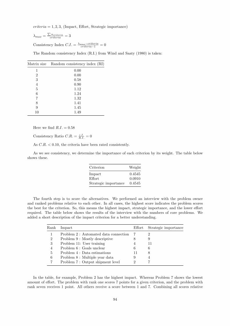
criteria = 1, 2, 3, (Impact, Effort, Strategic importance)
λmax =∑αcriteria
criteria = 3
Consistency Index C.I. = λmax−criteriacriteria−1 = 0
The Random consistency Index (R.I.) from Wind and Saaty (1980) is taken:
Matrix size Random consistency index (RI)
1 0.002 0.003 0.584 0.905 1.126 1.247 1.328 1.419 1.4510 1.49
Here we find R.I. = 0.58
Consistency Ratio C.R. = c.I.R.I. = 0
As C.R. < 0.10, the criteria have been rated consistently.
As we see consistency, we determine the importance of each criterion by its weight. The table belowshows these.
Criterion Weight
Impact 0.4545Effort 0.0910Strategic importance 0.4545
The fourth step is to score the alternatives. We performed an interview with the problem ownerand ranked problems relative to each other. In all cases, the highest score indicates the problem scoresthe best for the criterion. So, this means the highest impact, strategic importance, and the lower effortrequired. The table below shows the results of the interview with the numbers of core problems. Weadded a short description of the impact criterion for a better understanding.
Rank Impact Effort Strategic importance
1 Problem 2 : Automated data connection 7 22 Problem 9 : Mostly descriptive 8 93 Problem 11: User training 4 114 Problem 6 : Goals unclear 6 65 Problem 4 : Data estimations 11 86 Problem 8 : Multiple year data 9 47 Problem 7 : Output shipment level 2 7
In the table, for example, Problem 2 has the highest impact. Whereas Problem 7 shows the lowestamount of effort. The problem with rank one scores 7 points for a given criterion, and the problem withrank seven receives 1 point. All others receive a score between 1 and 7. Combining all scores relative
94

to each other in a matrix, which is then normalized, we calculated the preferred problems based on thedifferent criteria. The table below shows the process.
Problem Impact Effort Strategic importance
2 0.25 0.04 0.254 0.11 0.18 0.076 0.14 0.14 0.147 0.04 0.25 0.048 0.07 0.21 0.119 0.21 0.07 0.2111 0.18 0.11 0.18
Then, we multiply the normalized scores above by previously calculated weights. Finally, the sum foreach problem shows an overall priority.
95

B Survey used features and graphs
Used features
Response Score
Never used 0Rarely used 1Often used 2Always used 3
ID Position Experience Filter func-tionality(being ableto selectspecific di-mensions)
Graphs(the tabwithall thegraphs)
Validationtables(the tabwithtablesrelated tocost allo-cations)
Reportingtables(the tabwithP&Linputdata)
Scenario:Changedeliverylocation
Scenario:MOQ
Scenario:Chang-ingdeliveryday
Scenariographs(the tabvisualizingscenariooutcomes)
Mapgraph(the tabwherethe mapcan beviewed)
Detail ta-bles (thetab withtables onshipments,costs, cus-tomers, andproducts)
1 OpCo 2 - 3years
3 3 2 1 0 0 0 0 1 2
2 OpCo 3 - 4years
3 3 3 3 1 1 1 2 1 3
3 OpCo Morethan 4years
3 3 3 0 1 1 0 1 1 3
4 OpCo 3 - 4years
2 2 1 1 2 1 0 2 0 1
5 OpCo Less than1 year
2 1 2 2 0 0 0 0 0 2
6 Global 1 - 2years
3 3 1 0 1 2 1 2 1 3
7 Global 2 - 3years
2 2 2 2 0 0 0 0 1 2
8 OpCo 1 - 2years
3 3 2 2 3 3 2 2 1 3
96
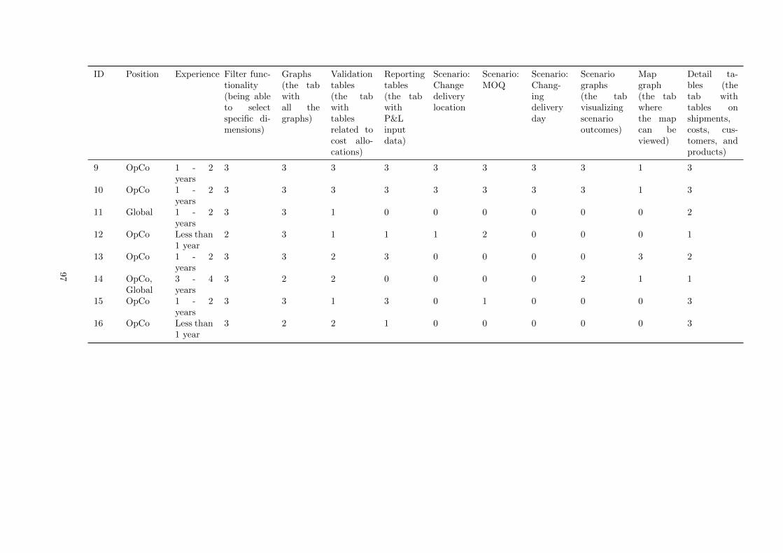
ID Position Experience Filter func-tionality(being ableto selectspecific di-mensions)
Graphs(the tabwithall thegraphs)
Validationtables(the tabwithtablesrelated tocost allo-cations)
Reportingtables(the tabwithP&Linputdata)
Scenario:Changedeliverylocation
Scenario:MOQ
Scenario:Chang-ingdeliveryday
Scenariographs(the tabvisualizingscenariooutcomes)
Mapgraph(the tabwherethe mapcan beviewed)
Detail ta-bles (thetab withtables onshipments,costs, cus-tomers, andproducts)
9 OpCo 1 - 2years
3 3 3 3 3 3 3 3 1 3
10 OpCo 1 - 2years
3 3 3 3 3 3 3 3 1 3
11 Global 1 - 2years
3 3 1 0 0 0 0 0 0 2
12 OpCo Less than1 year
2 3 1 1 1 2 0 0 0 1
13 OpCo 1 - 2years
3 3 2 3 0 0 0 0 3 2
14 OpCo,Global
3 - 4years
3 2 2 0 0 0 0 2 1 1
15 OpCo 1 - 2years
3 3 1 3 0 1 0 0 0 3
16 OpCo Less than1 year
3 2 2 1 0 0 0 0 0 3
97
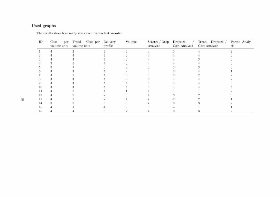
Used graphs
The results show how many stars each respondent awarded.
ID Cost pervolume-unit
Trend - Cost pervolume-unit
Deliveryprofile
Volume Scatter / DropAnalysis
Dropsize /Cost Analysis
Trend - Dropsize /Cost Analysis
Pareto Analy-sis
1 4 2 4 4 4 3 4 22 4 4 4 3 4 4 4 33 4 4 4 3 4 4 3 34 3 3 4 3 4 4 4 35 3 1 3 3 3 3 3 36 4 4 4 2 4 3 4 17 4 3 4 3 4 3 2 28 4 4 4 3 3 4 4 29 4 4 4 4 4 4 4 310 4 4 4 4 4 4 4 411 4 3 4 1 4 1 1 212 4 2 2 3 4 3 2 313 4 3 2 4 4 2 2 114 3 3 3 3 4 3 3 215 4 1 4 3 3 4 1 116 4 4 3 2 4 3 3 2
98

C Variables root-cause analysis
Ordering behavior Average/Min/Max/SD/CV
Weeks of demand Drops/weekWeeks with drops Deliveries/weekWeeks without drops Deliveries/drop
Products/weekProducts/dropProducts/deliveryOrder lines/weekOrder lines/dropOrder lines/deliveryOrder lines/productVolume/weekVolume/dropVolume/deliveryVolume/productVolume/order line
Route to market and distance Average/Min/Max/SD/CV
Percentage of drops per shipping location Shipping locations/weekPercentage of deliveries per shipping location Shipment types/weekPercentage of products per shipping location PWs/weekPercentage of order lines per shipping location PWs/dropPercentage of volume per shipping location PWs/deliveryPercentage of drops per shipment type PWs/productPercentage of deliveries per shipment type Paths/weekPercentage of products per shipment type Paths/dropPercentage of order lines per shipment type Paths/deliveryPercentage of volume per shipment type Paths/productPercentage of order lines per PW Distance/weekPercentage of volume per PW Distance/dropPercentage of order lines PATH Distance/deliveryPercentage of volume PATH Distance/product
Distance/order lineDistance/volume
Picking
Percentage of weeks with loose pickingPercentage of drops with loose pickingPercentage of deliveries with loose pickingPercentage of products with loose pickingPercentage of order lines with loose pickingPercentage of volume with loose pickingLoose case picking percentage in palletsLoose case picking percentage ( >1 pallet)Loose case picking percentage ( >2 pallet)Loose case picking percentage ( >3 pallet)Loose case picking percentage ( >... pallet)
99

Drop days Average/Min/Max/SD/CV
Percentage of drops per drop day Drops per dayTime between drops
Other drivers
OriginOrigin - attributes that can differ per order lineSupplierSupplier - attributes that can differ per order lineVehicleVehicle - attributes that can differ per order lineUtilizationArea used
100
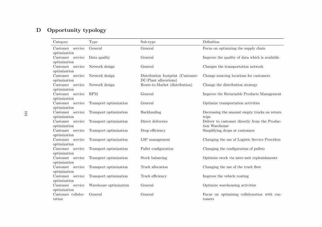
D Opportunity typology
Category Type Sub-type Definition
Customer serviceoptimization
General General Focus on optimizing the supply chain
Customer serviceoptimization
Data quality General Improve the quality of data which is available
Customer serviceoptimization
Network design General Changes the transportation network
Customer serviceoptimization
Network design Distribution footprint (Customer-DC-Plant allocations)
Change sourcing locations for customers
Customer serviceoptimization
Network design Route-to-Market (distribution) Change the distribution strategy
Customer serviceoptimization
RPM General Improve the Returnable Products Management
Customer serviceoptimization
Transport optimization General Optimize transportation activities
Customer serviceoptimization
Transport optimization Backhauling Decreasing the amount empty trucks on returntrips
Customer serviceoptimization
Transport optimization Direct deliveries Deliver to customer directly from the Produc-tion Warehouse
Customer serviceoptimization
Transport optimization Drop efficiency Simplifying drops at customers
Customer serviceoptimization
Transport optimization LSP management Changing the use of Logistic Service Providers
Customer serviceoptimization
Transport optimization Pallet configuration Changing the configuration of pallets
Customer serviceoptimization
Transport optimization Stock balancing Optimize stock via inter-unit replenishments
Customer serviceoptimization
Transport optimization Truck allocation Changing the use of the truck fleet
Customer serviceoptimization
Transport optimization Truck efficiency Improve the vehicle routing
Customer serviceoptimization
Warehouse optimization General Optimize warehousing activities
Customer collabo-ration
General General Focus on optimizing collaboration with cus-tomers
101
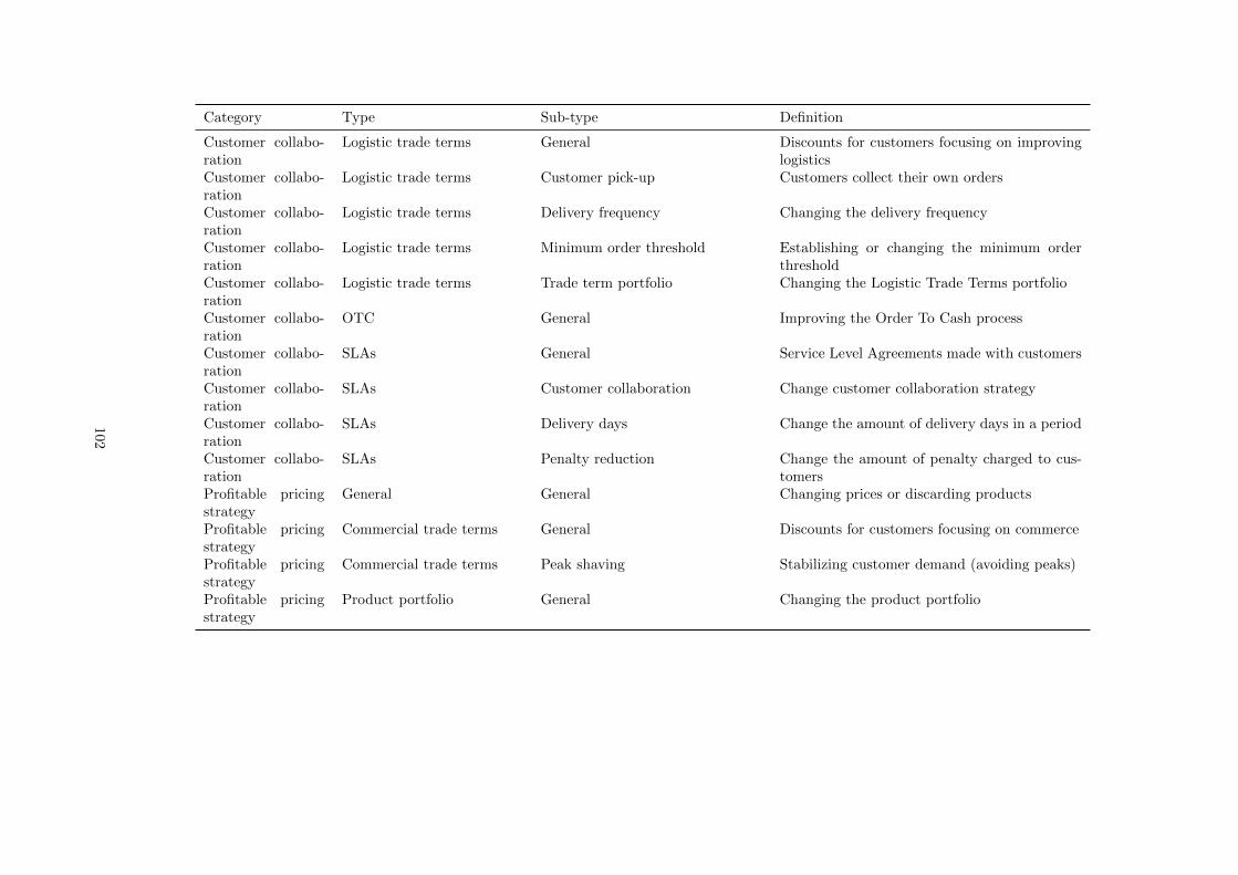
Category Type Sub-type Definition
Customer collabo-ration
Logistic trade terms General Discounts for customers focusing on improvinglogistics
Customer collabo-ration
Logistic trade terms Customer pick-up Customers collect their own orders
Customer collabo-ration
Logistic trade terms Delivery frequency Changing the delivery frequency
Customer collabo-ration
Logistic trade terms Minimum order threshold Establishing or changing the minimum orderthreshold
Customer collabo-ration
Logistic trade terms Trade term portfolio Changing the Logistic Trade Terms portfolio
Customer collabo-ration
OTC General Improving the Order To Cash process
Customer collabo-ration
SLAs General Service Level Agreements made with customers
Customer collabo-ration
SLAs Customer collaboration Change customer collaboration strategy
Customer collabo-ration
SLAs Delivery days Change the amount of delivery days in a period
Customer collabo-ration
SLAs Penalty reduction Change the amount of penalty charged to cus-tomers
Profitable pricingstrategy
General General Changing prices or discarding products
Profitable pricingstrategy
Commercial trade terms General Discounts for customers focusing on commerce
Profitable pricingstrategy
Commercial trade terms Peak shaving Stabilizing customer demand (avoiding peaks)
Profitable pricingstrategy
Product portfolio General Changing the product portfolio
102

E Opportunities Power BI report
Figure 3: A screenshot of the general tab of the opportunities dashboard with marginalized annual impact
103

Figure 4: A screenshot showing the number of opportunities of each type that have been found the most in past years including their average relative impact(right y-axis)
104
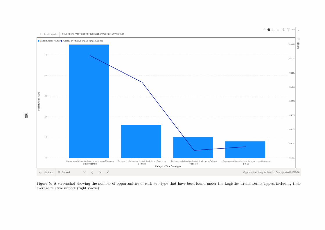
Figure 5: A screenshot showing the number of opportunities of each sub-type that have been found under the Logistics Trade Terms Types, including theiraverage relative impact (right y-axis)
105
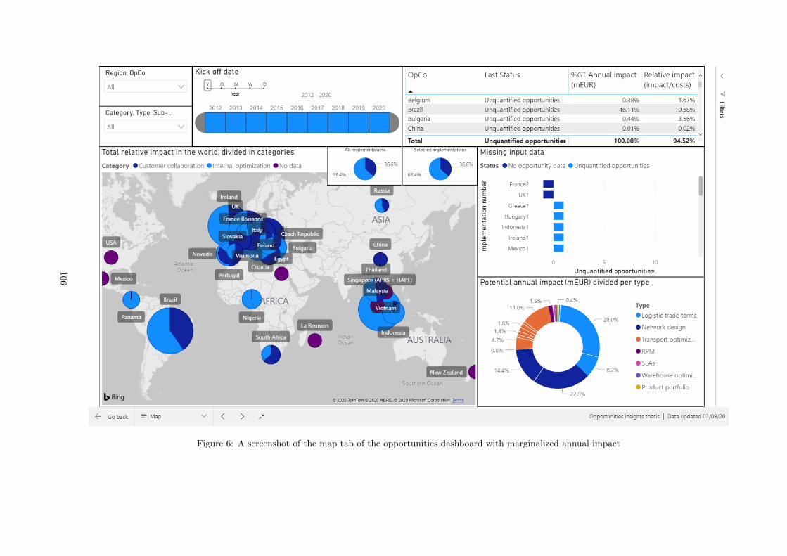
Figure 6: A screenshot of the map tab of the opportunities dashboard with marginalized annual impact
106
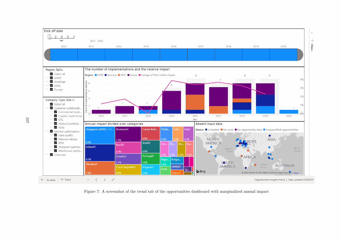
Figure 7: A screenshot of the trend tab of the opportunities dashboard with marginalized annual impact
107

Two opportunity types stand out. Firstly, the research company often found Minimum Order Thresh-old opportunities. Secondly, they found a wide range of Customer Service Optimization opportunitieswith a high average impact. The figure below shows a comparison between the two opportunity types.The Minimum Order Threshold is a sub-type where Customer Service Optimization is a category, but inboth cases a relatively large portion of the opportunities found are being considered.
Figure 8: A comparison between Minimum order threshold and Internal optimization opportunities foundin the research company
Minimum order thresholds opportunities are more specific than Customer service optimization opportu-nities, but the standard deviation of Minimum order threshold opportunities is higher than the mean,indicating that the relative savings vary heavily between opportunities found. Customer Service Opti-mization opportunities made the most impact. Therefore, the figure below takes a close look at the typesand sub-types of the Customer Service Optimization category.
Figure 9: A comparison between the types and sub-types of Customer service optimization opportunitiesfound in the research company
The impact of Customer Service Optimization opportunities varies over different sub-types. Furthermore,the average and standard deviation values for the sub-types differ as well. All in all, it seems that there isa wide range of opportunities in this category. In conclusion, the measurement of success of the researchcompany provided various insights into potential savings, emphasizing the impact differs between typesof opportunities. However, due to the missing input data, it is difficult to determine specific actions.
108
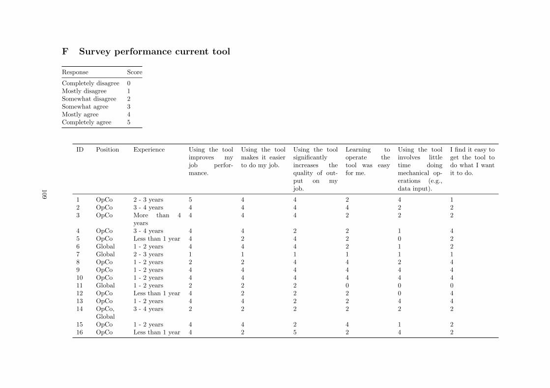
F Survey performance current tool
Response Score
Completely disagree 0Mostly disagree 1Somewhat disagree 2Somewhat agree 3Mostly agree 4Completely agree 5
ID Position Experience Using the toolimproves myjob perfor-mance.
Using the toolmakes it easierto do my job.
Using the toolsignificantlyincreases thequality of out-put on myjob.
Learning tooperate thetool was easyfor me.
Using the toolinvolves littletime doingmechanical op-erations (e.g.,data input).
I find it easy toget the tool todo what I wantit to do.
1 OpCo 2 - 3 years 5 4 4 2 4 12 OpCo 3 - 4 years 4 4 4 4 2 23 OpCo More than 4
years4 4 4 2 2 2
4 OpCo 3 - 4 years 4 4 2 2 1 45 OpCo Less than 1 year 4 2 4 2 0 26 Global 1 - 2 years 4 4 4 2 1 27 Global 2 - 3 years 1 1 1 1 1 18 OpCo 1 - 2 years 2 2 4 4 2 49 OpCo 1 - 2 years 4 4 4 4 4 410 OpCo 1 - 2 years 4 4 4 4 4 411 Global 1 - 2 years 2 2 2 0 0 012 OpCo Less than 1 year 4 2 2 2 0 413 OpCo 1 - 2 years 4 4 2 2 4 414 OpCo,
Global3 - 4 years 2 2 2 2 2 2
15 OpCo 1 - 2 years 4 4 2 4 1 216 OpCo Less than 1 year 4 2 5 2 4 2
109

G Contents of the current tool
To categorize the dimensions, we used the categories shown in the table below. These dimensions often serve as either a row, column, axis, or attribute.Usually, a combination can offer a specific view of the data, but in some cases the CTS of a single dimension is shown.
Table 5: The categories used to map dimensions of analytics in the current tool
Category Description
Time Shows timeShipments Shows information related to shipmentsCustomers Shows customer attributesProducts Shows product attributesSources Shows sourcing characteristicsVehicles Shows vehicle attributesCTS buckets Shows the CTS bucketsKPIs Shows KPIs (e.g. # drops, # shipments)
Often, features are adjustable and can, therefore, show a different axis based on a user preference. Furthermore, features usually measure CTS or volumes.The unit often differs for volumes-measurements.
Tab Feature Type Measures Time Shipments Customers Products Sources Vehicles CTSbuckets
KPIs
All Filters Filter None 1 1 1 1 1 1 0 0All Current
selectionsTable None 1 1 1 1 1 1 1 0
All Key num-bers sum-mary - 1
Table Volumes 0 0 0 0 0 0 0 1
All Key num-bers sum-mary - 2
Table CTS 0 0 0 0 0 0 1 0
Overview Volumeflow
Diagram CTS andvolumes
0 0 0 0 0 0 0 0
Overview Costgroup
Table CTS 0 0 0 0 0 0 1 0
110
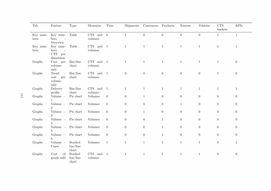
Tab Feature Type Measures Time Shipments Customers Products Sources Vehicles CTSbuckets
KPIs
Key num-bers
Key num-bers -Overview
Table CTS andvolumes
0 1 0 0 0 0 1 1
Key num-bers
Key num-bers -CTS perdimension
Table CTS andvolumes
1 1 1 1 1 1 1 1
Graphs Cost pervolume-unit
Bar/linechart
CTS andvolumes
1 1 1 1 1 1 1 0
Graphs Trend -cost pervolume-unit
Bar/linechart
CTS andvolumes
1 0 0 0 0 0 1 0
Graphs Deliveryprofile
Bar/linechart
CTS andvolumes
1 1 1 1 1 1 1 1
Graphs Volume -1
Pie chart Volumes 0 0 1 0 0 0 0 0
Graphs Volume -2
Pie chart Volumes 0 0 0 0 1 0 0 0
Graphs Volume -3
Pie chart Volumes 0 0 1 0 0 0 0 0
Graphs Volume -4
Pie chart Volumes 0 0 0 1 0 0 0 0
Graphs Volume -5
Pie chart Volumes 0 0 0 1 0 0 0 0
Graphs Volume -6
Pie chart Volumes 0 0 0 1 0 0 0 0
Graphs Volume -Cases
Stackedbar/linechart
Volumes 1 1 1 1 1 1 0 1
Graphs Cost ofgoods sold
Stackedbar/linechart
CTS andvolumes
1 1 1 1 1 1 0 0
111
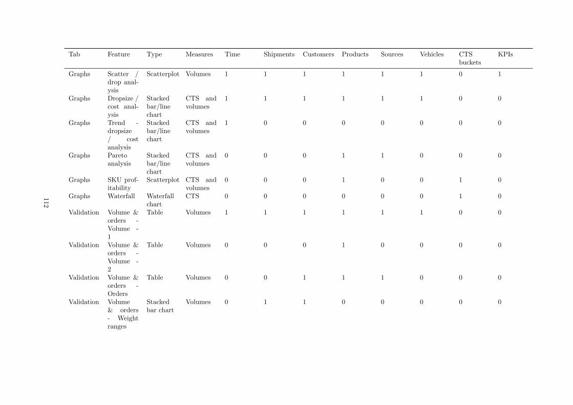
Tab Feature Type Measures Time Shipments Customers Products Sources Vehicles CTSbuckets
KPIs
Graphs Scatter /drop anal-ysis
Scatterplot Volumes 1 1 1 1 1 1 0 1
Graphs Dropsize /cost anal-ysis
Stackedbar/linechart
CTS andvolumes
1 1 1 1 1 1 0 0
Graphs Trend -dropsize/ costanalysis
Stackedbar/linechart
CTS andvolumes
1 0 0 0 0 0 0 0
Graphs Paretoanalysis
Stackedbar/linechart
CTS andvolumes
0 0 0 1 1 0 0 0
Graphs SKU prof-itability
Scatterplot CTS andvolumes
0 0 0 1 0 0 1 0
Graphs Waterfall Waterfallchart
CTS 0 0 0 0 0 0 1 0
Validation Volume &orders -Volume -1
Table Volumes 1 1 1 1 1 1 0 0
Validation Volume &orders -Volume -2
Table Volumes 0 0 0 1 0 0 0 0
Validation Volume &orders -Orders
Table Volumes 0 0 1 1 1 0 0 0
Validation Volume& orders- Weightranges
Stackedbar chart
Volumes 0 1 1 0 0 0 0 0
112
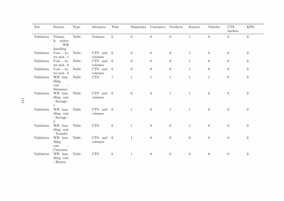
Tab Feature Type Measures Time Shipments Customers Products Sources Vehicles CTSbuckets
KPIs
Validation Volume& orders- WHhandling
Table Volumes 0 0 0 0 1 0 0 0
Validation Cost - in-ter unit - 1
Table CTS andvolumes
0 0 0 0 1 0 0 0
Validation Cost - in-ter unit - 2
Table CTS andvolumes
0 0 0 0 1 0 0 0
Validation Cost - in-ter unit - 3
Table CTS andvolumes
0 0 0 0 1 0 0 0
Validation WH han-dlingcost -Summary
Table CTS 1 1 1 1 1 1 0 0
Validation WH han-dling cost- Storage -1
Table CTS andvolumes
0 0 0 1 1 0 0 0
Validation WH han-dling cost- Storage -2
Table CTS andvolumes
0 1 0 1 1 0 0 0
Validation WH han-dling cost- Transfer
Table CTS 0 1 0 0 1 0 0 0
Validation WH han-dlingcost -Customer
Table CTS andvolumes
0 1 0 0 0 0 0 0
Validation WH han-dling cost- Return
Table CTS 0 1 0 0 0 0 0 0
113

Tab Feature Type Measures Time Shipments Customers Products Sources Vehicles CTSbuckets
KPIs
Validation WH han-dling cost- Con-ditions -1
Table CTS 0 0 0 0 0 0 1 0
Validation WH han-dling cost- Con-ditions -2
Table CTS 0 0 1 1 1 0 1 0
Validation WH han-dling cost- Planthandling
Table CTS andvolumes
0 0 0 0 1 0 0 0
Validation Outboundfreight -Primarydelivery -1
Table CTS andvolumes
0 1 0 0 1 0 0 0
Validation Outboundfreight -Primarydelivery -2
Table CTS andvolumes
0 1 0 0 1 0 0 0
Validation Outboundfreight -Primarydelivery -3
Table Volumes 0 1 0 0 0 0 0 0
Validation Outboundfreight- F&Vdelivery
Table CTS andvolumes
0 1 1 0 1 0 0 0
114
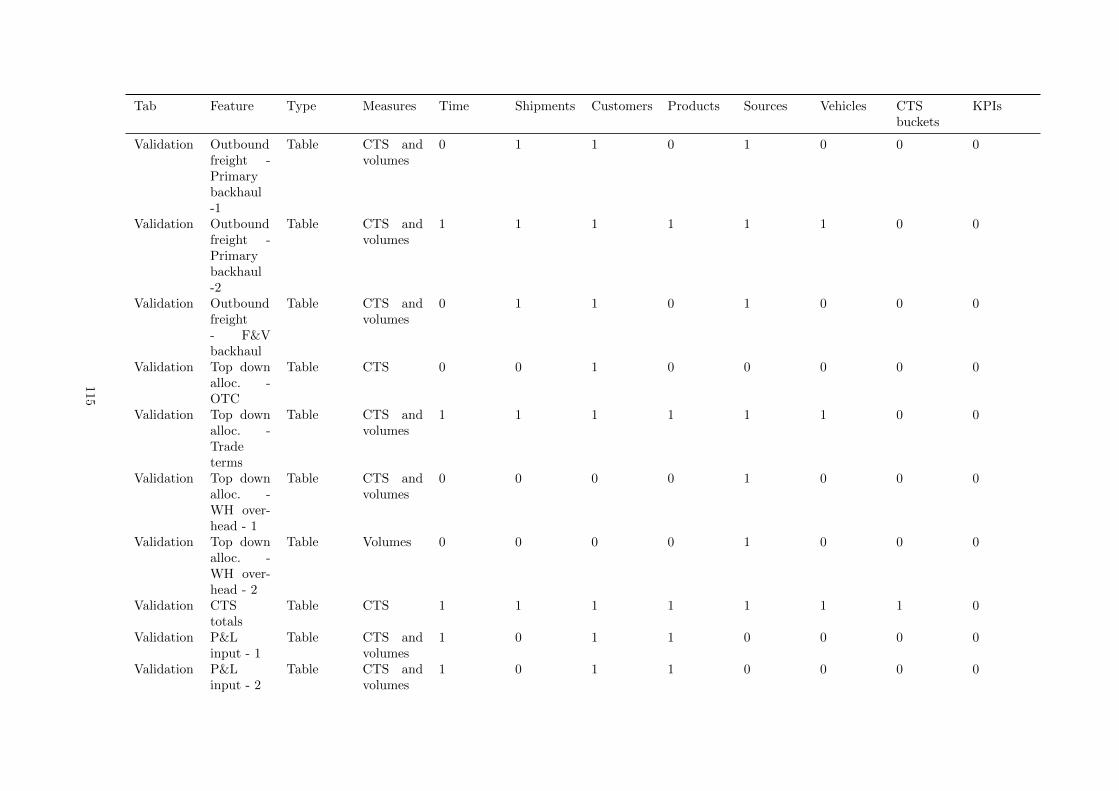
Tab Feature Type Measures Time Shipments Customers Products Sources Vehicles CTSbuckets
KPIs
Validation Outboundfreight -Primarybackhaul-1
Table CTS andvolumes
0 1 1 0 1 0 0 0
Validation Outboundfreight -Primarybackhaul-2
Table CTS andvolumes
1 1 1 1 1 1 0 0
Validation Outboundfreight- F&Vbackhaul
Table CTS andvolumes
0 1 1 0 1 0 0 0
Validation Top downalloc. -OTC
Table CTS 0 0 1 0 0 0 0 0
Validation Top downalloc. -Tradeterms
Table CTS andvolumes
1 1 1 1 1 1 0 0
Validation Top downalloc. -WH over-head - 1
Table CTS andvolumes
0 0 0 0 1 0 0 0
Validation Top downalloc. -WH over-head - 2
Table Volumes 0 0 0 0 1 0 0 0
Validation CTStotals
Table CTS 1 1 1 1 1 1 1 0
Validation P&Linput - 1
Table CTS andvolumes
1 0 1 1 0 0 0 0
Validation P&Linput - 2
Table CTS andvolumes
1 0 1 1 0 0 0 0
115

Tab Feature Type Measures Time Shipments Customers Products Sources Vehicles CTSbuckets
KPIs
Reporting P&Lreport
Table CTS 0 0 1 1 0 0 0 0
Maps Map Map CTS andvolumes
0 0 1 0 1 0 0 0
Maps Hectoliters Table Volumes 0 0 1 0 1 0 0 0Maps Drops Table Volumes 0 1 0 0 0 0 0 0Details Shipment
detailsTable Volumes 1 1 1 1 1 1 0 0
Details Costdetails
Table CTS 0 1 0 0 0 0 0 0
Details Products Table None 0 0 0 1 0 0 0 0Details Customers Table None 0 0 1 0 0 0 0 0
116
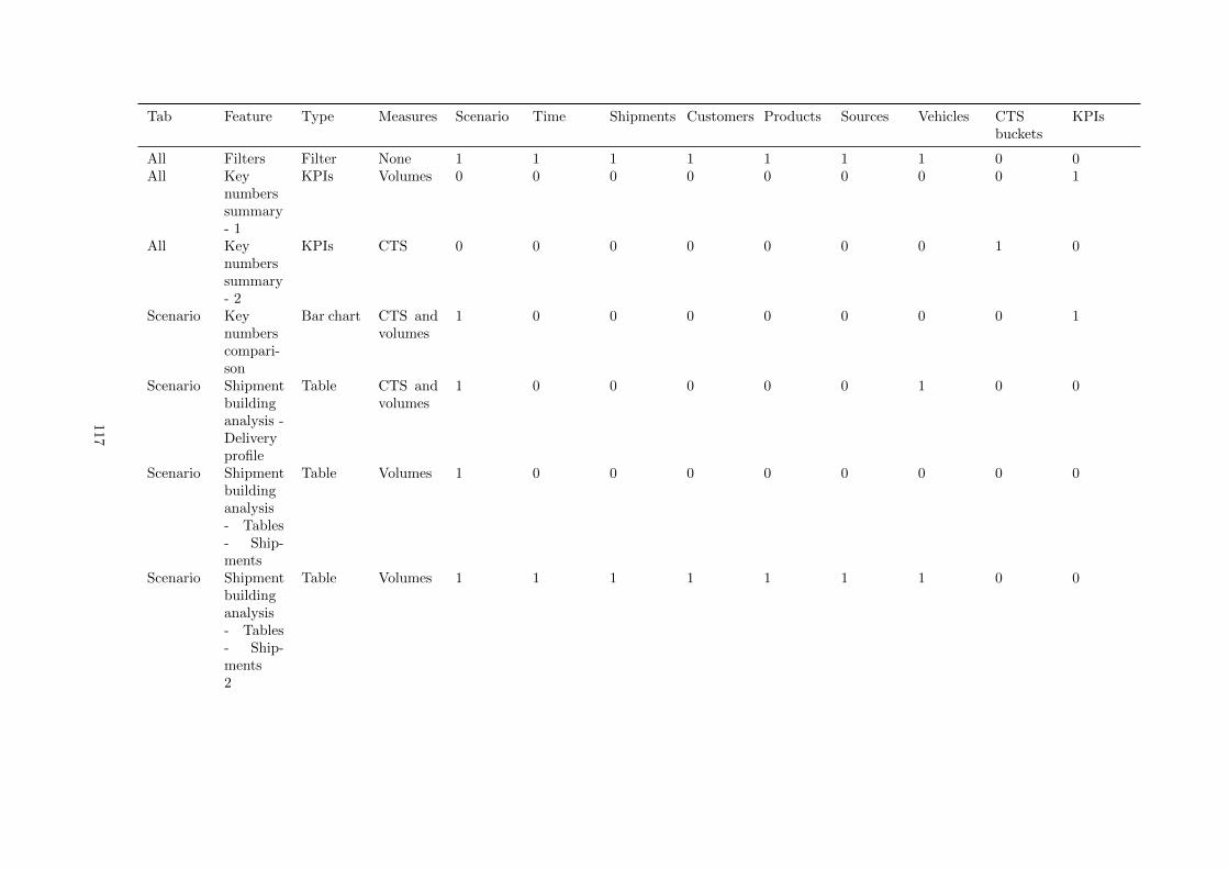
Tab Feature Type Measures Scenario Time Shipments Customers Products Sources Vehicles CTSbuckets
KPIs
All Filters Filter None 1 1 1 1 1 1 1 0 0All Key
numberssummary- 1
KPIs Volumes 0 0 0 0 0 0 0 0 1
All Keynumberssummary- 2
KPIs CTS 0 0 0 0 0 0 0 1 0
Scenario Keynumberscompari-son
Bar chart CTS andvolumes
1 0 0 0 0 0 0 0 1
Scenario Shipmentbuildinganalysis -Deliveryprofile
Table CTS andvolumes
1 0 0 0 0 0 1 0 0
Scenario Shipmentbuildinganalysis- Tables- Ship-ments
Table Volumes 1 0 0 0 0 0 0 0 0
Scenario Shipmentbuildinganalysis- Tables- Ship-ments2
Table Volumes 1 1 1 1 1 1 1 0 0
117

Tab Feature Type Measures Scenario Time Shipments Customers Products Sources Vehicles CTSbuckets
KPIs
Scenario Shipmentbuildinganalysis -Tables -Deliver-ies
Table Volumes 0 0 1 0 0 0 0 0 0
Scenario Shipmentbuildinganalysis -Tables -Drops
Table Volumes 0 0 1 0 0 0 0 0 0
Scenario Shipmentbuildinganalysis- Pershipmen-t/day -1
Bar chart Volumes 1 0 1 1 0 0 0 0 0
Scenario Shipmentbuildinganalysis- Pershipmen-t/day -2
Table Volumes 1 1 0 0 0 0 0 0 0
Scenario Shipmentbuildinganalysis- Nearestneigh-bour -Map
Map Volumes 0 0 0 1 0 0 0 0 0
118

Tab Feature Type Measures Scenario Time Shipments Customers Products Sources Vehicles CTSbuckets
KPIs
Scenario Shipmentbuildinganalysis- Nearestneigh-bour -Ship-ments
Table Volumes 1 1 0 0 0 0 0 0 0
Scenario Shipmentbuildinganalysis- Nearestneigh-bour -Timewindows
Table None 0 0 0 1 0 0 0 0 0
Scenario Shipmentbuildinganalysis- Nearestneigh-bour -Nearestneigh-bour
Table Volumes 0 0 1 0 0 0 0 0 0
Scenario Shipmentbuildinganalysis- Ware-househandling
Table CTS 1 1 1 1 1 1 1 0 0
Scenario Shipmentbuildinganalysis -Volume
Table Volumes 1 1 1 1 1 1 1 0 0
119

Tab Feature Type Measures Scenario Time Shipments Customers Products Sources Vehicles CTSbuckets
KPIs
Scenario Shipmentbuildinganalysis -Details -1
Table Volumes 1 1 1 1 1 1 0 0 0
Scenario Scatterplot- 1
Scatterplot Volumes 1 1 1 1 1 1 1 0 0
Scenario Scatterplot- 2
Differencechart
CTS 1 0 0 0 0 0 0 1 0
Scenario Changingdeliverylocation- 1
Map CTS 1 0 0 1 0 1 0 0 0
Scenario Changingdeliverylocation -ChangedShip from
Table Volumes 1 0 0 0 0 1 0 0 0
Scenario Changingdeliverylocation -ChangedShip to
Table Volumes 1 0 0 1 0 1 0 0 0
Scenario MOQ - 1 Bar chart Volumes 1 0 0 0 0 0 0 0 0Scenario MOQ - 2 Table Volumes 1 0 1 0 0 0 0 0 0Scenario MOQ - 3 Table Volumes 1 1 1 1 1 1 1 0 0Scenario Changing
deliveryday
Bar chart Volumes 1 1 0 0 0 0 0 0 0
Scenario Vehiclethresholdanalysis
Table Volumes 0 0 0 1 0 0 0 0 0
120

H Survey future analytics
Rank Score
1 42 33 24 1
ID Position Experience Improvedjob per-formance:Root-causeanalysis
Improvedjob per-formance:Estimatingthe CTSof a newcustomeror product
Improvedjob per-formance:Guide indefininga mini-mum orderthreshold
Improvedjob perfor-mance: Guidein defininga discountpolicy whenimplementingLogistic TradeTerms
Time re-duction:Root-causeanalysis
Time re-duction:Estimatingthe CTSof a newcustomeror product
Time re-duction:Guide indefininga mini-mum orderthreshold
Time reduc-tion: Guidein defininga discountpolicy whenimplementingLogistic TradeTerms
1 OpCo 2 - 3 years 4 1 3 2 4 1 3 22 OpCo 3 - 4 years 3 4 2 1 4 3 1 23 OpCo More than 4
years4 1 3 2 4 1 2 3
4 OpCo 3 - 4 years 3 4 1 2 3 4 1 25 OpCo Less than 1 year 4 3 1 2 4 3 2 16 Global 1 - 2 years 4 2 1 3 3 1 2 47 Global 2 - 3 years 3 4 2 1 3 1 4 28 OpCo 1 - 2 years 4 3 2 1 4 3 2 19 OpCo 1 - 2 years 3 4 2 1 4 3 2 110 OpCo 1 - 2 years 4 1 3 2 3 1 4 211 Global 1 - 2 years 4 1 2 3 4 1 2 312 OpCo Less than 1 year 1 3 2 4 1 2 3 413 OpCo 1 - 2 years 3 4 2 1 3 4 2 114 OpCo,
Global3 - 4 years 2 1 4 3 2 1 3 4
15 OpCo 1 - 2 years 3 4 2 1 4 1 2 316 OpCo Less than 1 year 4 3 2 1 3 4 2 1
121

I Calculated tables, columns, and measures
Measures are indicated by [Measure] and columns are indicated by Table[Column].
Parameters
Name Value range Step size
Average # SKUs per drop - Weight 0 - 1 0.1CV of cases per week - weight 0 - 1 0.1Loose picking percentage - weight 0 - 1 0.1Truck utilization goal 0 - 1 0.05Weeks with demand - weight 0 - 1 0.1Weeks with no demand in the demand cycle - weight 0 - 1 0.1
CTS / volume-unit bins - customers
d i s t i n c t va lue s Customers [CTS/volume un i t ( b ins ) ]
Calculated columns
Midpoint (CTS / volume−uni t ) =i f bin = maximum bin
( bin value + maximum of Customers [CTS/volume un i t ] ) / 2else
( lower value + upper value ) / 2end i f
CTS / volume-unit bins - products
d i s t i n c t va lue s Products [CTS/uni t ( b ins ) ]
Calculated columns
Midpoint (CTS / volume−uni t ) =i f bin = maximum bin
( bin value + maximum of Products [CTS/volume un i t ] ) / 2else
( lower value + upper value ) / 2end i f
Cost data
Measures
Average Cost to Serve KPI goa l =1.00001 [ Cost to Serve ] / [ Volume ] , i gno r i ng f i l t e r s
Cost to Serve =SUM( ’ Cost data ’ [ Cost ] )
CTS/volume−uni t =[ Cost to Serve ] / [ Volume ]
CTS/volume−uni t 1 month moving average =[CTS/volume−uni t ] , s e l e c t i n g the l a s t month
122

Percentage o f t o t a l Cost to Serve =[ Cost to Serve ] /
[ Cost to Serve ] , i gno r i ng f i l t e r s
Transport c o s t s =[ Cost to Serve ] , where CTS Cost buckets [CTS GROUP] i s Customer d e l i v e r y or
Intercompany t ranspor t
Customers
Calculated columns
Clo s e s t DC =var Lat1 = Regions [ Lat i tude ]var Lon1 = Regions [ Longitude ]return the Ship from [ SHIP FROM ID ] with the lowest va lue for :
var Lat2 = Ship from [ Lat i tude ]var Lon2 = Ship from [ Longitude ]VAR A = 0.5 − COS( ( Lat2 − Lat1 ) ∗ PI / 180) / 2 + COS( Lat1 ∗ PI / 180)
∗ COS( l a t 2 ∗ PI / 180) ∗ (1 − COS( ( Lng2 − Lng1 ) ∗ PI / 180) ) / 212742 ∗ ASIN( (SQRT( A ) ) )
CTS/volume−uni t =[CTS/volume−uni t ]
CTS/volume−uni t ( b ins ) =var b i n s i z e = 0 .95 th p e r c e n t i l e o f Customers [CTS/volume−uni t ] / 20i f Customers [CTS/volume−uni t ] < ROUNDUP( 0 . 9 5 th p e r c e n t i l e o f Customers [CTS/
volume−uni t ] / b i n s i z e ) ∗ b i n s i z evar lower = ROUNDDOWN( Customers [CTS/volume−uni t ] / b i n s i z e ) ∗ b i n s i z elower ” − ” lower + b i n s i z e
elseROUNDUP(0 . 9 5 th p e r c e n t i l e o f Customers [CTS/volume−uni t ] / b i n s i z e ) ∗
b i n s i z e ” +”
Customer =”Customer”
Volume =[ Volume ]
Volume ( b ins ) =var b i n s i z e = 0 .95 th p e r c e n t i l e o f Customers [ Volume ] / 20i f Customers [ Volume ] < ROUNDUP(0 . 9 5 th p e r c e n t i l e o f Customers [ Volume ] /
b i n s i z e ) ∗ b i n s i z evar lower = ROUNDDOWN( Customers [ Volume ] / b i n s i z e ) ∗ b i n s i z elower ” − ” lower + b i n s i z e
elseROUNDUP(0 . 9 5 th p e r c e n t i l e o f Customers [ Volume ] / b i n s i z e ) ∗ b i n s i z e ” +
”
Savings moving to c l o s e s t DC =MAX(SUM( Drops [ Estimated sav ings o f moving drop ] ) , 0) , for drops at the
customer
Segment =
123
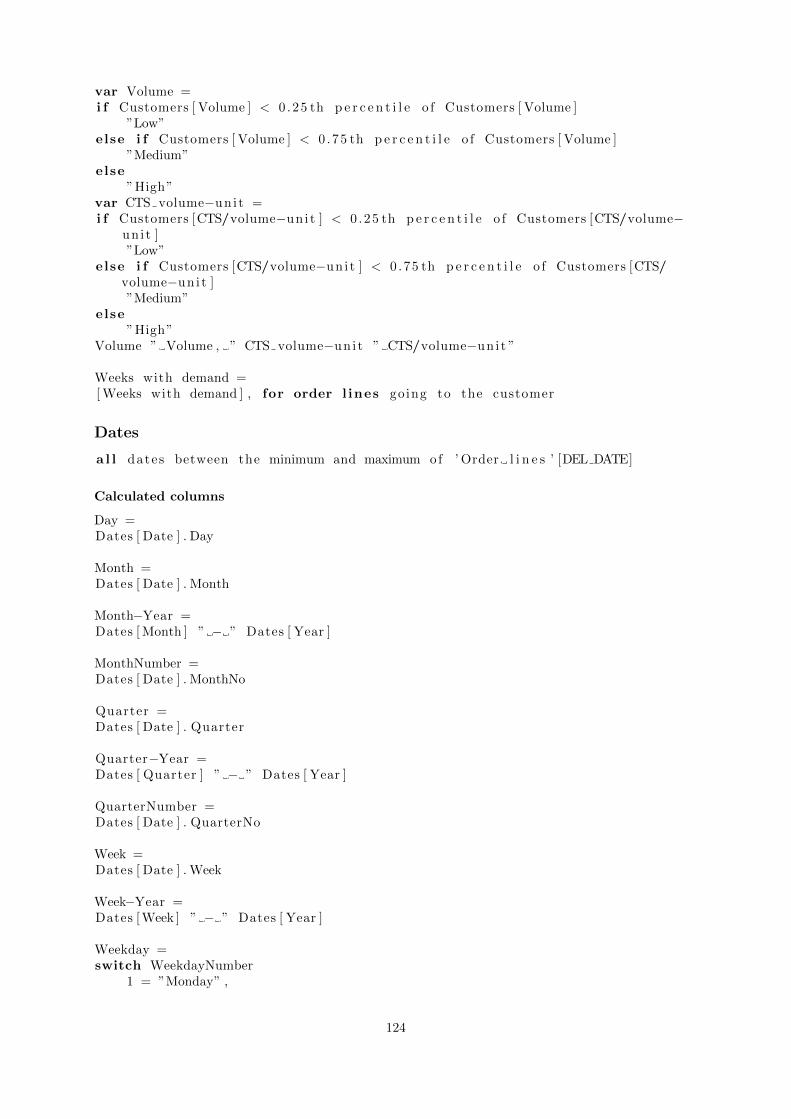
var Volume =i f Customers [ Volume ] < 0 .25 th p e r c e n t i l e o f Customers [ Volume ]
”Low”else i f Customers [ Volume ] < 0 .75 th p e r c e n t i l e o f Customers [ Volume ]
”Medium”else
”High”var CTS volume−uni t =i f Customers [CTS/volume−uni t ] < 0 .25 th p e r c e n t i l e o f Customers [CTS/volume−
uni t ]”Low”
else i f Customers [CTS/volume−uni t ] < 0 .75 th p e r c e n t i l e o f Customers [CTS/volume−uni t ]”Medium”
else”High”
Volume ” Volume , ” CTS volume−uni t ” CTS/volume−uni t ”
Weeks with demand =[ Weeks with demand ] , for order l ines going to the customer
Dates
a l l dates between the minimum and maximum of ’ Order l i n e s ’ [DEL DATE]
Calculated columns
Day =Dates [ Date ] . Day
Month =Dates [ Date ] . Month
Month−Year =Dates [ Month ] ” − ” Dates [ Year ]
MonthNumber =Dates [ Date ] . MonthNo
Quarter =Dates [ Date ] . Quarter
Quarter−Year =Dates [ Quarter ] ” − ” Dates [ Year ]
QuarterNumber =Dates [ Date ] . QuarterNo
Week =Dates [ Date ] . Week
Week−Year =Dates [ Week ] ” − ” Dates [ Year ]
Weekday =switch WeekdayNumber
1 = ”Monday” ,
124

2 = ”Tuesday” ,3 = ”Wednesday” ,4 = ”Thursday” ,5 = ” Friday ” ,6 = ” Saturday ” ,7 = ”Sunday”
WeekdayNumber =weekday ( s t a r t i n g on Monday)
Year =Dates [ Date ] . Year
Drops
d i s t i n c t va lue s ’ Order l i n e s ’ [ Drop ID ]
Calculated columns
CTS/volume−uni t/km =Drops [ Transport c o s t s ] / Drops [ Volume ] / Drops [ Havers ine distance (km) ]
Customers [ C lo s e s t DC] , for a customer in drop
Estimated c o s t s from c l o s e s t DC =i f Drops [ SHIP FROM ID ] <> Drops [ C lo s e s t DC]
var t a r i f f = AVERAGE( Drops [CTS/volume−uni t/km] , where the sh ip froml o c a t i o n i s the c l o s e s t dc for the customer in t h i s drop and theabso lu t e d i f f e r e n c e in volume i s l e s s than 10%
t a r i f f ∗ Drops [ Havers ine distance (km) ] ∗ Drops [ Volume ]
Estimated sav ings o f moving drop =Drops [ Transport c o s t s ] − Drops [ Estimated c o s t s from c l o s e s t DC]
Havers ine distance (km) =var Lat1 = Regions [ Lat i tude ]var Lon1 = Regions [ Longitude ]var Lat2 = Ship from [ Lat i tude ]var Lon2 = Ship from [ Longitude ]VAR A = 0.5 − COS( ( Lat2 − Lat1 ) ∗ PI / 180) / 2 + COS( Lat1 ∗ PI / 180) ∗
COS( l a t 2 ∗ PI / 180) ∗ (1 − COS( ( Lng2 − Lng1 ) ∗ PI / 180) ) / 212742 ∗ ASIN( (SQRT( A ) ) )
Volume =[ Volume ]
SHIP FROM ID =’ Order l i n e s ’ [ SHIP FROM ID ] , for the drop
SHIP TO ID =’ Order l i n e s ’ [ SHIP TO ID ] , for the drop
Transport c o s t s =[ Transport c o s t s ]
Volume bins - customers
125

d i s t i n c t va lue s Customers [ Volume ( b ins ) ]
Calculated columns
Average CTS/volume−uni t =[CTS/volume−uni t ]
Delta Average CTS/volume−uni t =var prev ious = ’ Volume bins − customers ’ [ Average CTS/volume−uni t ] , for the
prev ious row so r t ed descending on ’ Volume bins − customers ’ [ Midpoint (Volume ) ]
’ Volume bins − customers ’ [ Average CTS/volume−uni t ] − prev ious
Midpoint ( Volume ) =i f bin = maximum bin
( bin value + maximum of Customers [ Volume ] ) / 2else
( lower value + upper value ) / 2end i f
Volume bins - products
d i s t i n c t va lue s Products [ Volume ( b ins ) ]
Calculated columns
Average CTS/volume−uni t =[CTS/volume−uni t ]
Delta Average CTS/volume−uni t =var prev ious = ’ Volume bins − products ’ [ Average CTS/volume−uni t ] , for the
prev ious row so r t ed descending on ’ Volume bins − products ’ [ Midpoint (Volume ) ]
’ Volume bins − products ’ [ Average CTS/volume−uni t ] − prev ious
Midpoint ( Volume ) =i f bin = maximum bin
( bin value + maximum of Products [ Volume ] ) / 2else
( lower value + upper value ) / 2end i f
Order lines
Calculated columns
Del ive ry type =i f ’ Order l i n e s ’ [ Route to customer ] = ”PW−CUST” OR ”PW−SELF”
” Direc t d e l i v e r y ( from a PW to the Customer ) ”else
” I n d i r e c t d e l i v e r y ( to the Customer v ia a DC) ”
Drop ID =’ Order l i n e s ’ [SHIPMENT ID ] , ’ Order l i n e s ’ [ SHIP TO ID ]
Extra ca s e s =’ Order l i n e s ’ [DEL QTY] mod Products [CASES PER PALLET]
126

Volume =’ Order l i n e s ’ [DEL QTY] ∗ Products [VOLUME PER CASE]
Kilograms =’ Order l i n e s ’ [DEL QTY] ∗ Products [KILOGRAMS PER CASE]
Other =’ Order l i n e s ’ [DEL QTY] ∗ Products [OTHER PER CASE]
P a l l e t s =’ Order l i n e s ’ [DEL QTY] / Products [CASES PER PALLET]
Route to Customer =var f i r s t part =i f Costs between in te rmed ia te and f i n a l warehouse > 0
”PW−DC−DC−”else i f Costs between product ion and inte rmed ia te warehouse > 0
”PW−DC−”else
”PW−”var second part =i f Shipment type i n d i c a t e s s e l f c o l l e c t i o n
”SELF”else
”CUST”f i r s t part second part
Whole p a l l e t s =ROUNDDOWN( ’ Order l i n e s ’ [ P a l l e t s ] )
YearWeek =YEAR( ’ Order l i n e s ’ [DEL DATE] ) WEEKNUM( ’ Order l i n e s ’ [DEL DATE] )
Products
Calculated columns
CTS/volume−uni t =[CTS/volume−uni t ]
CTS/volume−uni t ( b ins ) =var b i n s i z e = 0 .95 th p e r c e n t i l e o f Products [CTS/volume−uni t ] / 20i f Products [CTS/volume−uni t ] < ROUNDUP(0 . 9 5 th p e r c e n t i l e o f Products [CTS/
volume−uni t ] / b i n s i z e ) ∗ b i n s i z evar lower = ROUNDDOWN( Products [CTS/volume−uni t ] / b i n s i z e ) ∗ b i n s i z elower ” − ” lower + b i n s i z e
elseROUNDUP(0 . 9 5 th p e r c e n t i l e o f Products [CTS/volume−uni t ] / b i n s i z e ) ∗
b i n s i z e ” +”
Volume =[ Volume ]
Volume ( b ins ) =var b i n s i z e = 0 .95 th p e r c e n t i l e o f Products [ Volume ] / 20i f Products [ Volume ] < ROUNDUP( 0 . 9 5 th p e r c e n t i l e o f Products [ Volume ] /
b i n s i z e ) ∗ b i n s i z e
127

var lower = ROUNDDOWN( Products [ Volume ] / b i n s i z e ) ∗ b i n s i z elower ” − ” lower + b i n s i z e
elseROUNDUP(0 . 9 5 th p e r c e n t i l e o f Products [ Volume ] / b i n s i z e ) ∗ b i n s i z e ” +”
Ship from
Calculated columns
Lat i tude =Regions [LATITUDE] , where Regions [ SHIP TO REGION] ID = Ship from [ SHIP FROM
ID ]
Longitude =Regions [LONGITUDE] , where Regions [ SHIP TO REGION] ID = Ship from [ SHIP FROM
ID ]
Shipments
d i s t i n c t va lue s ’ Order l i n e s ’ [SHIPMENT ID ]
Calculated columns
Maximum load =i f Shipment has a v e h i c l e
Veh i c l e s [PAYLOAD] ,else
Shipments [ P a l l e t s ]
P a l l e t s =ROUNDUP(SUM( ’ Order l i n e s ’ [ P a l l e t s ] ) ) , for the shipment
SKUs in shipment =DISTINCTCOUNT( ’ Order l i n e s ’ [MATERIAL] ) , for the shipment
Tons =ROUNDUP(SUM( ’ Order l i n e s ’ [ Kilograms ] / 1000) ) , for each order l i n e in the
shipment
Measures
Truck u t i l i z a t i o n =i f shipment being cons ide r ed > 1
var max load = SUM(MAX( Shipments [Maximum load ] , Shipments [ P a l l e t s ] ) ) ,for each shipment being cons ide r ed
SUM( ’ Order l i n e s ’ [ P a l l e t s ] ) / max loadelse
SUM( ’ Order l i n e s ’ [ P a l l e t s ] ) / SUM( Shipments [Maximum load ] )
Volumes
{Volume−uni t VolumeVolume−uni t KilogramsVolume−uni t P a l l e t sVolume−uni t CasesVolume−uni t Other}
128

Measures
Average # SKUs per drop =AVERAGE(DISTINCTCOUNT( ’ Order l i n e s ’ [MATERIAL] ) ) , for each drop
Complexity =var weeks demand normal ized = ( [ Weeks with demand ] − MIN( [ Weeks with demand
] ) ) / (MAX( [ Weeks with demand ] ) − MIN( [ Weeks with demand ] ) ) , i gno r i ngf i l t e r s
var weeks no demand normal ized = ( [ Weeks with no demand in the demand cycle] − MIN( [ Weeks with no demand in the demand cycle ] ) ) / (MAX( [ Weeks withno demand in the demand cycle ] ) − MIN( [ Weeks with no demand in thedemand cycle ] ) ) , i gno r i ng f i l t e r s
var cv ca s e s week normal ized = ( [CV of ca s e s per week ] − MIN( [CV of ca s e sper week ] ) ) / (MAX( [CV of ca s e s per week ] ) − MIN( [CV of ca s e s per week ] )) , i gno r i ng f i l t e r s
var SKUs drop normal ized = ( [ Average # SKUs per drop ] − MIN( [ Average # SKUsper drop ] ) ) / (MAX( [ Average # SKUs per drop ] ) − MIN( [ Average # SKUs perdrop ] ) ) , i g n o r i n g f i l t e r s
var l o o s e p i ck ing normal ized = ( [ Loose p i ck ing percentage ] − MIN( [ Loosep i ck ing percentage ] ) ) / (MAX( [ Loose p i ck ing percentage ] ) − MIN( [ Loosep i ck ing percentage ] ) ) , i gno r ing f i l t e r s
( [ Weeks with demand − Weight Value ] ∗ (1 − weeks demand normal ized ) +[ Weeks with no demand in the demand cycle − Weight Value ] ∗ weeks no
demand normal ized +[CV of ca s e s per week − Weight Value ] ∗ cv ca s e s week normal ized +[ Average # SKUs per drop − Weight Value ] ∗ SKUs drop normal ized +[ Loose p i ck ing percentage − Weight Value ] ∗ l o o s e p i ck ing normal ized ) /( [ Weeks with demand − Weight Value ] +[ Weeks with no demand in the demand cycle − Weight Value ] +[CV of ca s e s per week − Weight Value ] +[ Average # SKUs per drop − Weight Value ] +[ Loose p i ck ing percentage − Weight Value ] )
Customers so ld to =DISTINCTCOUNT( ’ Order l i n e s ’ [SOLD TO ID ] )
CV of ca s e s per week =STDEV.P( ’ Order l i n e s ’ [DEL QTY] ) / AVERAGE( ’ Order l i n e s ’ [DEL QTY] ) , for each
week in Dates [ Week ]
D e l i v e r i e s =DISTINCTCOUNT( ’ Order l i n e s ’ [DELIVERY ID ] )
Drops =DISTINCTCOUNT( ’ Order l i n e s ’ [ Drop ID ] )
Drops per week =[ Drops ] / [ Weeks between f i r s t and l a s t demand ]
Volume =SUM( ’ Order l i n e s ’ [ Volume ] )
Locat ions shipped to =DISTINCTCOUNT( ’ Order l i n e s ’ [ SHIP TO ID ] )
Loose p i ck ing percentage =1 − SUM( ’ Order l i n e s ’ [ Whole p a l l e t s ] ) / SUM( ’ Order l i n e s ’ [ P a l l e t s ] )
129

Order l ines =DISTINCTCOUNT( ’ Order l i n e s ’ [ Order l ine ID ] )
P a l l e t s =SUM( ’ Order l i n e s ’ [ P a l l e t s ] )
Percentage o f t o t a l volume =[ Volume ] /
[ Volume ] , i gno r i ng f i l t e r s
Products so ld =DISTINCTCOUNT( ’ Order l i n e s ’ [MATERIAL] )
Shipments =DISTINCTCOUNT( ’ Order l i n e s ’ [SHIPMENT ID ] )
Volume =switch Se l e c t ed volume−uni t
”Volume” = SUM( ’ Order l i n e s ’ [ Volume ] ) ,” Kilograms ” = SUM( ’ Order l i n e s ’ [ Kilograms ] ) ,” P a l l e t s ” = SUM( ’ Order l i n e s ’ [ P a l l e t s ] ) ,” Cases ” = SUM( ’ Order l i n e s ’ [ Cases ] ) ,”Other” = SUM( ’ Order l i n e s ’ [ Other ] )
Volume 1 month moving average =[ Volume ] , s e l e c t i n g the l a s t month
Volume−uni t/drop =[ Volume ] / [ Drops ]
Volume−uni t/week =[ Volume ] / [ Weeks between f i r s t and l a s t demand ]
Weeks between f i r s t and l a s t demand =DATEDIFF(MIN( ’ Order l i n e s ’ [DEL DATE] ) , MAX( ’ Order l i n e s ’ [DEL DATE] ) ) + 1
Weeks with demand =MIN(DISTINCTCOUNT( ’ Order l i n e s ’ [ YearWeek ] ) , [ Weeks between f i r s t and l a s t
demand ] )
Weeks with no demand in the demand cycle =[ Weeks between f i r s t and l a s t demand ] − [ Weeks with demand ]
130
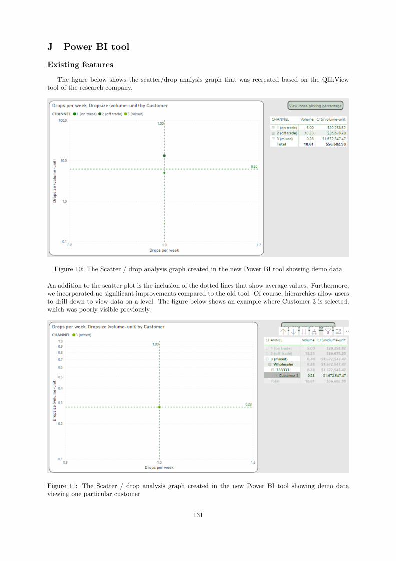
J Power BI tool
Existing features
The figure below shows the scatter/drop analysis graph that was recreated based on the QlikViewtool of the research company.
Figure 10: The Scatter / drop analysis graph created in the new Power BI tool showing demo data
An addition to the scatter plot is the inclusion of the dotted lines that show average values. Furthermore,we incorporated no significant improvements compared to the old tool. Of course, hierarchies allow usersto drill down to view data on a level. The figure below shows an example where Customer 3 is selected,which was poorly visible previously.
Figure 11: The Scatter / drop analysis graph created in the new Power BI tool showing demo dataviewing one particular customer
131

The figure below shows the loose picking percentage view, which users can access through the buttonon the top-right.
Figure 12: The Scatter / drop analysis graph created in the new Power BI tool showing the loose pickingpercentage based on demo data
The loose picking percentage is the percentage of pallets that the OpCo did not ship as a full pallet.For Customer 3, it is 100%, as they did not sell any full pallets to this customer, and Customer 1 has aloose picking percentage of 0%, as the OpCo only sold full pallets to this customer. This graph also doesnot incorporate any significant changes compared to the previous tool besides the dotted lines indicatingaverages. The last graph feature migrated from the QlikView tool to Power BI is the Delivery profilegraph shown in the figure below.
Figure 13: The Delivery profile graph created in the new Power BI tool
132

Compared to the old tool, the feature shown above combines the stacked columns with the line indicatingthe CTS per volume-unit as was done with the Cost per volume-unit graph. Besides this, there are nosignificant improvements compared to the feature in the QlikView tool. Users also have the option toswitch to tons rather than pallets by clicking the button on the left.
The figure below shows the landing page of the Key numbers feature, which is the landing page of anenvironment with various tables.
Figure 14: The Key numbers feature created in the new Power BI tool showing demo data
In the previous tool, the Key numbers were all shown in a table form. In an attempt to make the Keynumbers more appealing, we made two significant changes. First, we always visualize the Key numberson the left side of a page in the new tool, including the percentage of the total currently selected. Second,we created a waterfall chart to show the division among cost buckets. The waterfall chart incorporatesthe cost bucket hierarchy. The figure below shows a drill-down into the Overheads cost group.
Figure 15: The Key numbers feature created in the new Power BI tool showing demo data drilled downon the Overheads CTS GROUP
133
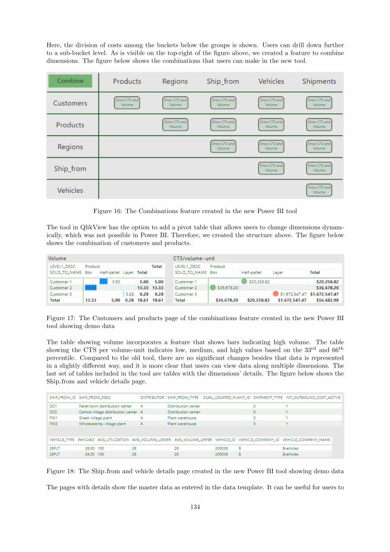
Here, the division of costs among the buckets below the groups is shown. Users can drill down furtherto a sub-bucket level. As is visible on the top-right of the figure above, we created a feature to combinedimensions. The figure below shows the combinations that users can make in the new tool.
Figure 16: The Combinations feature created in the new Power BI tool
The tool in QlikView has the option to add a pivot table that allows users to change dimensions dynam-ically, which was not possible in Power BI. Therefore, we created the structure above. The figure belowshows the combination of customers and products.
Figure 17: The Customers and products page of the combinations feature created in the new Power BItool showing demo data
The table showing volume incorporates a feature that shows bars indicating high volume. The tableshowing the CTS per volume-unit indicates low, medium, and high values based on the 33rd and 66th
percentile. Compared to the old tool, there are no significant changes besides that data is representedin a slightly different way, and it is more clear that users can view data along multiple dimensions. Thelast set of tables included in the tool are tables with the dimensions’ details. The figure below shows theShip from and vehicle details page.
Figure 18: The Ship from and vehicle details page created in the new Power BI tool showing demo data
The pages with details show the master data as entered in the data template. It can be useful for users to
134

be able to export this data without having to go back to the input data. Furthermore, when the researchcompany realizes an automated data connection, they must have this feature as the input data might beunreachable for users. In the old tool, users could only view a customer and product detail page. Then,we included a map feature in the new tool. The figure below shows the map feature.
Figure 19: The Map feature created in the new Power BI tool showing demo data
The map indicates volumes and the CTS per volume-unit. Furthermore, a table shows which customersdo not have geographic information in the input data. In QlikView, the map was no longer working.
New features
We presented the truck utilization as a potential cost driver for a high CTS per volume-unit. Wecreated a measure that calculates the truck utilization along with a page to visualize the truck utilizationrelated to the origins of shipments, which is presented in Appendix I. The figure below shows the page.
Figure 20: The Truck utilization page created in the new Power BI tool
135
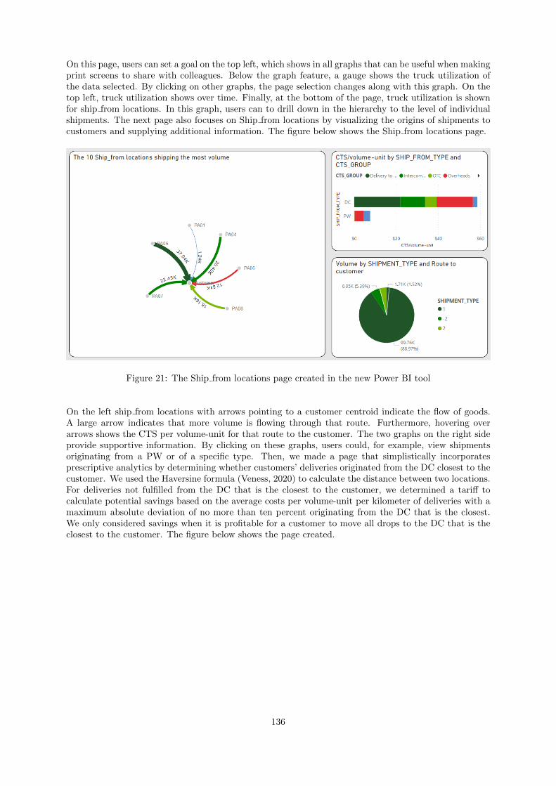
On this page, users can set a goal on the top left, which shows in all graphs that can be useful when makingprint screens to share with colleagues. Below the graph feature, a gauge shows the truck utilization ofthe data selected. By clicking on other graphs, the page selection changes along with this graph. On thetop left, truck utilization shows over time. Finally, at the bottom of the page, truck utilization is shownfor ship from locations. In this graph, users can to drill down in the hierarchy to the level of individualshipments. The next page also focuses on Ship from locations by visualizing the origins of shipments tocustomers and supplying additional information. The figure below shows the Ship from locations page.
Figure 21: The Ship from locations page created in the new Power BI tool
On the left ship from locations with arrows pointing to a customer centroid indicate the flow of goods.A large arrow indicates that more volume is flowing through that route. Furthermore, hovering overarrows shows the CTS per volume-unit for that route to the customer. The two graphs on the right sideprovide supportive information. By clicking on these graphs, users could, for example, view shipmentsoriginating from a PW or of a specific type. Then, we made a page that simplistically incorporatesprescriptive analytics by determining whether customers’ deliveries originated from the DC closest to thecustomer. We used the Haversine formula (Veness, 2020) to calculate the distance between two locations.For deliveries not fulfilled from the DC that is the closest to the customer, we determined a tariff tocalculate potential savings based on the average costs per volume-unit per kilometer of deliveries with amaximum absolute deviation of no more than ten percent originating from the DC that is the closest.We only considered savings when it is profitable for a customer to move all drops to the DC that is theclosest to the customer. The figure below shows the page created.
136
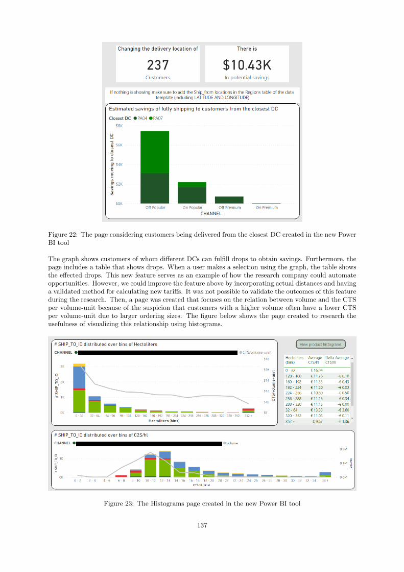
Figure 22: The page considering customers being delivered from the closest DC created in the new PowerBI tool
The graph shows customers of whom different DCs can fulfill drops to obtain savings. Furthermore, thepage includes a table that shows drops. When a user makes a selection using the graph, the table showsthe effected drops. This new feature serves as an example of how the research company could automateopportunities. However, we could improve the feature above by incorporating actual distances and havinga validated method for calculating new tariffs. It was not possible to validate the outcomes of this featureduring the research. Then, a page was created that focuses on the relation between volume and the CTSper volume-unit because of the suspicion that customers with a higher volume often have a lower CTSper volume-unit due to larger ordering sizes. The figure below shows the page created to research theusefulness of visualizing this relationship using histograms.
Figure 23: The Histograms page created in the new Power BI tool
137

The histograms have two applications. First, the top chart shows the change in the CTS per volume-unitbetween buckets. So, users can estimate savings related to an increase in volume. We also visualizedthese differences in the table on the top-right, which can be useful when making decisions for incentivesto increase sales. Second, when a new customer is acquired, users can make a rough estimation regardingexpected logistics costs. We created similar histograms on a product level. The next page focuses oncustomer complexity. In collaboration with the CTS believes factors that increase complexity have beendetermined and plotted for customers. These factors are as follows:
• Weeks with demand (inversed)
• Weeks with no demand in the demand cycle
• Coefficient of Variation of cases per week
• Average # SKUs per drop
• Loose picking percentage
We normalized the values of these variables between zero and one. Then, we multiply each variableby a corresponding weight, which results in a variable score. For each customer, we divide the sum ofthe variables’ scores by the sum of the variables’ weights. Finally, resulting in scores between zero and1, or 0% and 100%. The figure below shows the created page.
Figure 24: The Complexity page created in the new Power BI tool using demo data
The example using demo data shows the concept. The table shows that the customers have the samevalue for the first three variables. For simplicity, we set the weight for these values to 0%. Based onthe set of customers, Customer 3 has the worst values for the two remaining variables and therefore hasa complexity of 100%. Customer 1 has the best values for the two remaining variables resulting in acomplexity of 0%. The purpose of the bottom graph is to visualize the relation between complexity andCTS per volume-unit. We created the next page to visualize indicators to find opportunities for LogisticsTrade Terms, in collaboration with a Logistics Trade Terms expert. The figure below shows the pagethat we created.
138

Figure 25: The Logistics Trade Terms page created in the new Power BI tool using demo data
The table shows KPIs that can aid in finding opportunities. For example, when the loose picking per-centage is high, the research company can offer a discount to reduce this. The idea is that the savingsare higher than the discount given in such a case. Furthermore, the graph on the bottom of the pageshows the distribution of volume on different drop days. Using the functionalities of Power BI, users canview this for a single customer, or a group of customers, by making selections. For example, this couldlead to a Logistic Trade Term that offers a discount when an OpCo does not have to deliver orders on apossibly more expensive day.
139
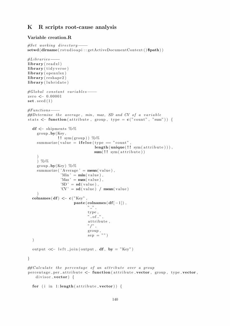
K R scripts root-cause analysis
Variable creation.R
#Set working d i r e c t o r y−−−−setwd (dirname( r s t u d i o a p i : : getActiveDocumentContext ( )$path ) )
#L i b r a r i e s−−−−l ibrary ( r eadx l )l ibrary ( t i d y v e r s e )l ibrary ( openxlsx )l ibrary ( reshape2 )l ibrary ( l u b r i d a t e )
#Globa l cons tant v a r i a b l e s−−−−zero <− 0.00001set . seed (1 )
#Functions−−−−##Determine the average , min , max , SD and CV o f a v a r i a b l es t a t s <− function ( a t t r i bu t e , group , type = c ( ” count ” , ”sum” ) ) {
df <− shipments %>%group by(Key ,
! ! sym( group ) ) %>%summarize ( va lue = i f e l s e ( type == ” count ” ,
length (unique ( ! ! sym( a t t r i b u t e ) ) ) ,sum( ! ! sym( a t t r i b u t e ) )
)) %>%group by(Key) %>%summarize ( ’ Average ’ = mean( va lue ) ,
’Min ’ = min( va lue ) ,’Max ’ = max( va lue ) ,’SD ’ = sd ( va lue ) ,’CV’ = sd ( va lue ) / mean( va lue )
)colnames (df ) <− c ( ”Key” ,
paste (colnames (df [−1]) ,” ” ,type ,” o f ” ,a t t r i bu t e ,”/” ,group ,sep = ”” )
)
output <<− l e f t j o i n ( output , df , by = ”Key” )
}
##C a l c u l a t e the percentage o f an a t t r i b u t e over a grouppercentage per a t t r i b u t e <− function ( a t t r i b u t e vector , group , type vector ,
d i v i s o r vector ) {
for ( i in 1 : length ( a t t r i b u t e vector ) ) {
140

df <− shipments %>%group by(Key ,
! ! sym( group )) %>%summarize ( Values = i f e l s e ( type vector [ i ] == ” count ” ,
length (unique ( ! ! sym( a t t r i b u t e vector [ i ] ) ) ),
sum( ! ! sym( a t t r i b u t e vector [ i ] ) ))) %>%dcast (paste ( ”Key” ,
”˜” ,group ) ,
va lue . var = ” Values ” )colnames (df ) <− c ( ”Key” ,
paste ( ” Percentage o f ” ,d i v i s o r vector [ i ] ,group ,colnames (df [−1])
))###C a l c u l a t e p e r c e n t a g e soutput <<− l e f t j o i n ( output , df , by = ”Key” )output [ ( ncol ( output ) − ncol (df ) + 2) : ncol ( output ) ] <<−
sapply ( output [ ( ncol ( output ) − ncol (df ) + 2) : ncol ( output ) ] , function ( x) x / output [ , d i v i s o r vector [ i ] ] )
}}
##C a l c u l a t e the l o o s e p i c k i n g percentagepercentage l o o s e p i ck ing <− function ( group vector , type vector , d i v i s o r
vector ) {
for ( i in 1 : length ( group vector ) ) {df <− shipments %>%
group by(Key ,Pick ing
) %>%summarize ( Values = i f e l s e ( type vector [ i ] == ” count ” ,
length (unique ( ! ! sym( group vector [ i ] ) ) ) ,sum( ! ! sym( group vector [ i ] ) )
)) %>%dcast (Key ˜ Picking ,
va lue . var = ” Values ”) %>%s e l e c t (Key , ‘ Loose p ick ing ‘ )
colnames (df ) <− c ( ”Key” ,paste ( ” Percentage o f ” ,
d i v i s o r vector [ i ] ,” invo lved l o o s e case p i ck ing ” )
)###C a l c u l a t e percentageoutput <<− l e f t j o i n ( output , df , by = ”Key” )output [ ncol ( output ) ] <<− output [ ncol ( output ) ] / output [ d i v i s o r vector [ i
] ]
141

}}
#Data input−−−−##Shipmentsshipments <− read e x c e l (paste (getwd ( ) ,
”/Shipment d e t a i l s . x l sx ” ,sep = ”” )
)###Check t h a t input i s d i s t i n c t and c r e a t e a d d i t i o n a l v a r i a b l e sshipments <− d i s t i n c t ( shipments ) %>%
mutate ( Drop ID = paste (SHIPMENT ID ,SHIP TO ID) ,
Week = as .numeric ( s t r f t i m e (DEL DATE,format = ”%V” )
) ,p l t l o o s e = p l t o r d e r l i n e − f loor ( p l t o r d e r l i n e ) ,Pick ing = i f e l s e ( p l t l o o s e > 0 ,
” Loose p i ck ing ” ,” Fu l l p a l l e t s ” )
)
##Costsc o s t s <− read e x c e l (paste (getwd ( ) ,
”/Cost d e t a i l s . x l sx ” ,sep = ”” )
)###Check f o r an empty CTS SUB BUCKET v a r i a b l e and remove i f p r e s e n ti f ( ”CTS SUB BUCKET” %in% colnames ( c o s t s ) ) {
c o s t s <− c o s t s %>% s e l e c t (−CTS SUB BUCKET)}###Make sure a l l v a l u e s are numericc o s t s [ ] <− lapply ( cos t s ,
function ( x ) as .numeric ( as . character ( x ) ))###Check t h a t input i s d i s t i n c t and c a l c u l a t e t o t a l c o s t sc o s t s <− d i s t i n c t ( c o s t s ) %>%
mutate (CTS = apply ( c o s t s [ , −1 ] , 1 , sum) )###Add the t o t a l c o s t s to the shipment t a b l edf <− c o s t s %>%
s e l e c t ( Order l ine ID ,CTS)
shipments <− l e f t j o i n ( shipments ,df ,by = ” Order l ine ID” )
##I n c l u d e the path o f an order l i n edf <− shipments %>%
s e l e c t ( Order l ine ID , SHIPMENT TYPE)
###F i r s t par t ( number o f DCs)i f ( ”Primary s h u t t l e from INT to Fina l ” %in% colnames (df ) ) {
df <− l e f t j o i n (df , co s t s , by = ” Order l ine ID” ) %>%mutate ( Path1 = i f e l s e ( ‘ Primary s h u t t l e from INT to Final ‘ > zero ,
”PW−DC−DC−” ,i f e l s e ( ‘ Primary s h u t t l e from PW to Final ‘ > zero ,
”PW−DC−” ,
142

”PW−” ) ) )} else i f ( ”Primary s h u t t l e from PW to Fina l ” %in% colnames (df ) ) {
df <− l e f t j o i n (df , co s t s , by = ” Order l ine ID” ) %>%mutate ( Path1 = i f e l s e ( ‘ Primary s h u t t l e from PW to Final ‘ > zero ,
”PW−DC−” ,”PW−” ) )
} else {df <− l e f t j o i n (df , co s t s , by = ” Order l ine ID” ) %>%
mutate ( Path1 = ”PW−” )}
###Second par t (CUST or SELF)df <− df %>%
mutate ( Path = i f e l s e (SHIPMENT TYPE > zero ,paste ( Path1 , ”CUST” , sep = ”” ) ,paste ( Path1 , ”SELF” , sep = ”” ) ) )
df <− df %>% s e l e c t ( Order l ine ID , Path )shipments <− l e f t j o i n ( shipments , df , by = ” Order l ine ID” )
#Choose the l e v e l o f d e t a i l−−−−##Paste t o g e t h e r a unique Key v a l u eshipments$Key <− paste ( ”P” , shipments$MATERIAL,
sep = ”” )
#Create output s t r u c t u r e−−−−##Add v a l u e s t h a t you want to have in the outputoutput <− shipments %>% s e l e c t (Key , MATERIAL) %>%
arrange (Key) %>%d i s t i n c t ( )
##Add volume and CTSdf <− shipments %>%
group by(Key) %>%summarize ( ’ volume ’ = sum( volume o r d e r l i n e ) ,
’CTS ’ = sum(CTS))
output <− l e f t j o i n ( output , df , by = ”Key” )##I n i t i a l i z e countersoutput i n t r o l en <− length ( output )
#C a l c u l a t e a t t r i b u t e s−−−−##Ordering behavior−−−−df <− shipments %>%
group by(Key) %>%summarize ( ’Weeks with demand ’ = max(Week) − min(Week) + 1 ,
’Weeks ordered ’ = length (unique (Week) ) ,’Week not ordered ’ = max(Week) − min(Week) + 1 − length (unique (
Week) ) ,’ Drops ’ = length (unique ( Drop ID) ) ,’ D e l i v e r i e s ’ = length (unique (DELIVERY ID) ) ,’ Products ’ = length (unique (MATERIAL) ) ,’ Order l i n e s ’ = length (unique ( Order l ine ID) ) ,’ Volume ’ = sum( volume o r d e r l i n e ) )
###Join d foutput <− l e f t j o i n ( output , df , by = ”Key” )
143

##Ordering s t a t s−−−−###Create a data frame with rows t h a t ho ld an a t t r i b u t e , group , and typedf <− data . frame ( a t t r i b u t e = c ( ”Drop ID” ,
”DELIVERY ID” , ”DELIVERY ID” ,”MATERIAL” , ”MATERIAL” , ”MATERIAL” ,” Order l ine ID” , ” Order l ine ID” , ” Order l ine
ID” , ” Order l ine ID” ,”volume o r d e r l i n e ” , ”volume o r d e r l i n e ” , ”
volume o r d e r l i n e ” , ”volume o r d e r l i n e ” , ”volume o r d e r l i n e ” ) ,
group = c ( ”Week” ,”Week” , ”Drop ID” ,”Week” , ”Drop ID” , ”DELIVERY ID” ,”Week” , ”Drop ID” , ”DELIVERY ID” , ”MATERIAL” ,”Week” , ”Drop ID” , ”DELIVERY ID” , ”MATERIAL” , ”
Order l ine ID” ) ,type = c ( ” count ” ,
” count ” , ” count ” ,” count ” , ” count ” , ” count ” ,” count ” , ” count ” , ” count ” , ” count ” ,”sum” , ”sum” , ”sum” , ”sum” , ”sum” ) ,
s t r i ng sAsFac to r s = F)###Run the s t a t s f u n c t i o n f o r each rowfor ( i in 1 :nrow(df ) ) {
s t a t s (df$ a t t r i b u t e [ i ] , df$group [ i ] , df$type [ i ] )}
##Transfers−−−−###Shipping l c o a t i o n sa t t r i b u t e vector <− c ( ”Drop ID” , ”DELIVERY ID” , ”MATERIAL” , ” Order l ine ID” ,
”volume o r d e r l i n e ” )group <− ”SHIP FROM ID”type vector <−c ( ” count ” , ” count ” , ” count ” , ” count ” , ”sum” )d i v i s o r vector = c ( ”Drops” , ” D e l i v e r i e s ” , ” Products ” , ”Order l i n e s ” , ”
Volume” )percentage per a t t r i b u t e ( a t t r i b u t e vector , group , type vector , d i v i s o r
vector )
###Shipment t y p e sgroup <− ”SHIPMENT TYPE”percentage per a t t r i b u t e ( a t t r i b u t e vector , group , type vector , d i v i s o r
vector )
###Production l o c a t i o n sa t t r i b u t e vector <− c ( ” Order l ine ID” , ”volume o r d e r l i n e ” )group <− ”PW ID”type vector <−c ( ” count ” , ”sum” )d i v i s o r vector = c ( ”Order l i n e s ” , ”Volume” )percentage per a t t r i b u t e ( a t t r i b u t e vector , group , type vector , d i v i s o r
vector )
###D e l i v e r y t y p e sgroup <− ”Path”percentage per a t t r i b u t e ( a t t r i b u t e vector , group , type vector , d i v i s o r
vector )rm( a t t r i b u t e vector , group , type vector , d i v i s o r vector )
144

##Transfer s t a t s−−−−df <− data . frame ( ” a t t r i b u t e ” = c ( ”SHIP FROM ID” , ”SHIPMENT TYPE” , ”PW ID” ,
”PW ID” , ”PW ID” , ”PW ID” ,”Path” , ”Path” , ”Path” , ”Path” ) ,
”group” = c ( ”Week” , ”Week” , ”Week” , ”Drop ID” , ”DELIVERYID” , ”MATERIAL” ,
”Week” , ”Drop ID” , ”DELIVERY ID” , ”MATERIAL” ) ,” type ” = c ( ” count ” , ” count ” , ” count ” , ” count ” , ” count ” , ”
count ” ,” count ” , ” count ” , ” count ” , ” count ” ) ,
s t r i ng sAsFac to r s = F)
for ( i in 1 :nrow(df ) ) {s t a t s (df$ a t t r i b u t e [ i ] , df$group [ i ] , df$type [ i ] )
}
##Picking−−−−###Percentages are determined a long t h e s e dimensionspercentage l o o s e p i ck ing (c ( ”Week” , ”Drop ID” , ”DELIVERY ID” , ”MATERIAL” , ”
Order l ine ID” , ”volume o r d e r l i n e ” ) ,c ( ” count ” , ” count ” , ” count ” , ” count ” , ” count ” , ”
sum” ) ,c ( ”Weeks ordered ” , ”Drops” , ” D e l i v e r i e s ” , ”
Products ” , ”Order l i n e s ” , ”Volume” ))###I n i t i a l i z e temperature and t h r e s h o l dtemp <− 1thr e sho ld <− 0###Continue check ing the l o o s e p i c k i n g percentage when > t h r e s h o l d p a l l e t s
are orderedwhile ( temp > 0 . 0 5 ) {
df <− shipments %>%mutate ( l o o s e = i f e lse ( p l t o r d e r l i n e > thresho ld , p l t o r d e r l i n e − f loor
( p l t o r d e r l i n e ) , 0) ) %>%group by(Key) %>%summarize ( ’ Loose p i ck s ’ = sum( l o o s e ) ,
P a l l e t s = sum( p l t o r d e r l i n e ) ) %>%mutate ( ‘ Loose picks ‘ = ‘ Loose picks ‘ / P a l l e t s ) %>%s e l e c t (−P a l l e t s )
colnames (df ) <− c ( ”Key” ,paste ( ” Loose case p i ck ing percentage ( o rde r s > ” ,
thresho ld ,” p a l l e t s ) ” )
)###Join d foutput <− l e f t j o i n ( output , df , by = ”Key” )###Temperature i s the maximum percentagetemp <− max( output [ [ ncol ( output ) ] ] , na .rm = T)###Increment the t h r e s h o l dth r e sho ld <− th r e sho ld + 1
}rm( temp , th r e sho ld )
##Drop days−−−−
145

df <− shipments %>%group by(Key ,
Weekday = c ( ”Sunday” , ”Monday” , ”Tuesday” , ”Wednesday” , ”Thursday” , ” Friday ” , ” Saturday ” ) [ as . POSIXlt ( shipments$DELDATE)$wday + 1 ] ) %>%
summarize ( Value = length (unique ( Drop ID) ) ) %>%dcast (Key ˜ Weekday ,
va lue . var = ”Value” )colnames (df ) <− c ( ”Key” ,
paste ( ” Percentage drop day” ,colnames (df [−1]) ) )
df <− df [ , c (1 , 3 , 7 , 8 , 6 , 2 , 4 , 5) ]###Join d foutput <− l e f t j o i n ( output , df , by = ”Key” )output [ ( ncol ( output ) − 6) : ncol ( output ) ] <− lapply ( output [ ( ncol ( output ) − 6)
: ncol ( output ) ] , function ( x ) x / output$Drops )
##Days between drops−−−−df <− shipments %>%
group by(Key ,DEL DATE) %>%
summarize ( ’ Drops per day ’ = length (unique ( Drop ID) ) )
df <− do . ca l l ( rbind ,lapply ( sp l i t (df , df$Key) ,
function (d) {d$ ‘ Days s i n c e l a s t drop ‘ <− c (NA, d i f f (d$DEL DATE) ) ;
d}) )
###Temporari ly d i s a b l e warnings ( due to customers wi th on ly one drop goingto i n f i n i t y )
defaultW <− getOption ( ”warn” )options ( warn = −1)
df <− df %>%group by(Key) %>%summarize ( ’ Average count o f Drops per day ’ = mean( ‘ Drops per day ‘ ) ,
’Min count o f Drops per day ’ = min( ‘ Drops per day ‘ ) ,’Max count o f Drops per day ’ = max( ‘ Drops per day ‘ ) ,’SD count o f Drops per day ’ = sd ( ‘ Drops per day ‘ ) ,’CV count o f Drops per day ’ = sd ( ‘ Drops per day ‘ ) / mean( ‘ Drops
per day ‘ ) ,’ Average count o f Days s i n c e l a s t drop ’ = mean( ‘ Days s i n c e l a s t
drop ‘ , na .rm = T) ,’Min count o f Days s i n c e l a s t drop ’ = i f e l s e ( i s . i n f i n i t e (min( ‘
Days s i n c e l a s t drop ‘ , na .rm = T) ) ,0 ,min( ‘ Days s i n c e
l a s t drop ‘ , na .rm = T) ) ,
’Max count o f Days s i n c e l a s t drop ’ = i f e l s e ( i s . i n f i n i t e (max( ‘Days s i n c e l a s t drop ‘ , na .rm = T) ) ,
0 ,max( ‘ Days s i n c e
l a s t drop ‘ , na .rm = T) ) ,
’SD count o f Days s i n c e l a s t drop ’ = sd ( ‘ Days s i n c e l a s t drop ‘ ,
146
na .rm = T) ,’CV count o f Days s i n c e l a s t drop ’ = sd ( ‘ Days s i n c e l a s t drop ‘ )
/ mean( ‘ Days s i n c e l a s t drop ‘ ))
###Re−en ab l e warningsoptions ( warn = defaultW )rm( defaultW )###Join d foutput <− l e f t j o i n ( output , df , by = ”Key” )
# ##Cost d i v i s i o n−−−−# df <− shipments %>% s e l e c t ( Order l ine ID ,# Key)# df <− l e f t j o i n ( df ,# cos t s ,# by = ” Order l ine ID”) %>%# s e l e c t (−Order l ine ID) %>%# group by (Key) %>%# summarize a l l (sum)## df [ , c(−1,−nco l ( d f ) ) ] <− l a p p l y ( d f [ , c(−1,−nco l ( d f ) ) ] , f u n c t i o n ( x ) x / d f$
CTS)# df <− d f %>% s e l e c t (−CTS)# colnames ( d f ) <− c (”Key” , p a s t e ( colnames ( d f [−1]) , ”− percentage ”) )# ###Join d f# output <− l e f t j o i n ( output , df , by = ”Key”)
##I n c l u d e CTS/volume−−−−output <− output %>%
mutate ( ‘CTS/volume ‘ = CTS / Volume )
##Output to Excel−−−−output <− output %>%
replace ( i s .na ( . ) , 0)
wb <− createWorkbook ( t i t l e = ” Var iab le s e t . x l sx ” )addWorksheet (wb, ”Output” )writeData (wb, shee t = ”Output” , output , rowNames = F, colNames = T)saveWorkbook (wb, ” Var iab le s e t . x l sx ” , ove rwr i t e = T)rm( l i s t=l s ( ) )
Preprocessing.R
#Set working d i r e c t o r y−−−−setwd (dirname( r s t u d i o a p i : : getActiveDocumentContext ( )$path ) )
#L i b r a r i e s−−−−l ibrary ( r eadx l )l ibrary ( t i d y v e r s e )l ibrary ( openxlsx )l ibrary ( c a r e t )
#Globa l cons tant v a r i a b l e s−−−−zero <− 0.00001set . seed (1 )c u t o f f va lue <− 0 .9t r a i n i n g percentage <− 0 .8
147

#Data input−−−−data <− read e x c e l (paste (getwd ( ) ,
”/Var iab le s e t . x l sx ” ,sep = ”” )
)
#Find in tro−−−−i n t r o length <− 0found <− Fwhile ( found == F) {
i f (colnames (data [ , i n t r o length + 1 ] ) == ”Weeks with demand” ) {found <− Ti n t r o <− data [ , c ( 1 : i n t r o length ) ]data <− data [ ,−c ( 1 : i n t r o length ) ]
}else {
i n t r o length <− i n t r o length + 1}
}rm( i n t r o length , found )
#Near zero v a r i a b l e s in f u l l data se t−−−−data <− data %>%
s e l e c t (−nearZeroVar (data [ ,−ncol (data ) ] ) )
#C o r r e l a t i o n s f u l l data se t−−−−c o r r e l a t i o n s <− cor (data [ ,−ncol (data ) ] ) %>%
replace ( i s .na ( . ) , 0)remove <− f i n d C o r r e l a t i o n ( c o r r e l a t i o n s , c u t o f f = c u t o f f va lue )data <− data %>%
s e l e c t (−remove)
#Linear dependencies f u l l data se t−−−−combinat ions <− f indLinearCombos (data [ ,−ncol (data ) ] )remove <− as .numeric ( combinat ions$remove)data <− data %>%
s e l e c t (−remove)
#Sca le data−−−−data [ ,−ncol (data ) ] <− apply (data [ ,−ncol (data ) ] , MARGIN = 2 , FUN = function (
X) (X − min(X) )/d i f f ( range (X) ) )data <− data %>%
replace ( i s .na ( . ) , 0)
#Data s p l i t t i n g −−−−t ra in Index <− c r ea t eDataPar t i t i on (data$ ‘CTS/volume ‘ ,
p = t r a i n i n g percentage ,l i s t = FALSE,t imes = 1)
dataTrain <− data [ t ra inIndex , ]dataTest<− data[− t ra inIndex , ]
#I f a l l samples are in the t r a i n i n g s e t change the percentage to 50%
148
i f (nrow( dataTest ) == 0) {t ra in Index <− c r ea t eDataPar t i t i on (data$ ‘CTS/volume ‘ ,
p = 0 . 5 ,l i s t = FALSE,t imes = 1)
dataTrain <− data [ t ra inIndex , ]dataTest<− data[− t ra inIndex , ]
}rm( t ra in Index )
#Near zero v a r i a b l e s in t r a i n i n g data se t−−−−remove <− nearZeroVar ( dataTrain [ ,−ncol ( dataTrain ) ] )dataTrain <− dataTrain %>%
s e l e c t (−remove)dataTest <− dataTest %>%
s e l e c t (−remove)data <− data %>%
s e l e c t (−remove)
#C o r r e l a t i o n s t r a i n i n g data se t−−−−c o r r e l a t i o n s <− cor ( dataTrain [ ,−ncol ( dataTrain ) ] ) %>%
replace ( i s .na ( . ) , 0)remove <− f i n d C o r r e l a t i o n ( c o r r e l a t i o n s , c u t o f f = c u t o f f va lue )dataTrain <− dataTrain %>%
s e l e c t (−remove)dataTest <− dataTest %>%
s e l e c t (−remove)data <− data %>%
s e l e c t (−remove)
#Linear dependencies t r a i n i n g data se t−−−−combinat ions <− f indLinearCombos ( dataTrain [ ,−ncol ( dataTrain ) ] )remove <− as .numeric ( combinat ions$remove)dataTrain <− dataTrain %>%
s e l e c t (−remove)dataTest <− dataTest %>%
s e l e c t (−remove)data <− data %>%
s e l e c t (−remove)rm( combinations , c o r r e l a t i o n s , remove)
#Data to Excel−−−−dataTrain <− dataTrain %>%
replace ( i s .na ( . ) , 0)dataTest <− dataTest %>%
replace ( i s .na ( . ) , 0)data <− data %>%
replace ( i s .na ( . ) , 0)i n t r o <− i n t r o %>%
replace ( i s .na ( . ) , 0)
wb <− createWorkbook ( t i t l e = ” Fina l v a r i a b l e s e t . x l sx ” )addWorksheet (wb, ” In t ro ” )writeData (wb, shee t = ” Int ro ” , in t ro , rowNames = F, colNames = T)addWorksheet (wb, ”Data” )writeData (wb, shee t = ”Data” , data , rowNames = F, colNames = T)
149

addWorksheet (wb, ” Train ing ” )writeData (wb, shee t = ” Train ing ” , dataTrain , rowNames = F, colNames = T)addWorksheet (wb, ” Test ing ” )writeData (wb, shee t = ” Test ing ” , dataTest , rowNames = F, colNames = T)saveWorkbook (wb, ” Fina l v a r i a b l e s e t . x l sx ” , ove rwr i t e = T)rm( l i s t=l s ( ) )
Model fitting.R
#Set working d i r e c t o r y−−−−setwd (dirname( r s t u d i o a p i : : getActiveDocumentContext ( )$path ) )
#L i b r a r i e s−−−−l ibrary ( r eadx l )l ibrary ( t i d y v e r s e )l ibrary ( openxlsx )l ibrary ( c a r e t )l ibrary ( l u b r i d a t e )
#Globa l cons tant v a r i a b l e s−−−−zero <− 0.00001
#Data input−−−−dataTrain ing <− read e x c e l (paste (getwd ( ) ,
”/Fina l v a r i a b l e s e t . x l sx ” ,sep = ”” ) ,
shee t = ” Train ing ”)
dataTest ing <− read e x c e l (paste (getwd ( ) ,”/Fina l v a r i a b l e s e t . x l sx ” ,sep = ”” ) ,
shee t = ” Test ing ”)
#Model f i t t i n g −−−−f i t models <− function ( cv number , cv repeat , sa i t e r s , ga i t e r s ) {
set . seed (1 )
v a r i a b l e s <− c ( ”cv number” = cv number ,”cv repeat ” = cv repeat )
##Linear modelstart time <− proc . time ( )
lm control <− t r a inCont ro l ( method = ” repeatedcv ” ,number = cv number ,r epea t s = cv repeat ,v e r b o s e I t e r = T)
lm grid <− expand . grid ( i n t e r c e p t = c (T, F) )
options ( warn = −1)lm model <− t r a i n ( ‘CTS/volume ‘ ˜ . ,
data = as . data . frame ( dataTrain ing ) ,method = ”lm” ,
150

t rContro l = lm control ,tuneGrid = lm grid )
options ( warn = 1) #Suppress warning f o r rank d e f f i c i e n c y
#Create and s t o r e s t a t i s t i c srun time <− proc . time ( ) − start timelm v a r i a b l e s <− c ( ” v a r i a b l e s ” = length (lm model$coefnames ) ) #D i f f e r s per
model , check t h i s !lm time <− c ( ” time ” = run time [ 3 ] )lm p r e d i c t i o n s <− predict (lm model , dataTest ing )lm performance <− postResample (lm p r e d i c t i o n s , dataTest ing$ ‘CTS/volume ‘ )lm <− l i s t (c ( ” type ” = ”lm” , v a r i a b l e s , lm v a r i a b l e s , lm time , lm
performance ) )
output <− data . frame (matrix ( unlist (lm) , nrow=length (lm) , byrow=T) ) #F i r s tmodel goes d i r e c t l y to output
colnames ( output ) <− c ( ” type ” , ”cv number” , ”cv repeat ” , ” v a r i a b l e s ” , ”time ” , ”RMSE” , ”Rˆ2” , ”MAE” )
##Polynomial modelstart time <− proc . time ( )
gaussprPoly control <− t r a inCont ro l ( method = ” repeatedcv ” ,number = cv number ,r epea t s = cv repeat ,v e r b o s e I t e r = T)
#gaussprPoly g r i d <− expand . g r i d ( )
gaussprPoly model <− t r a i n ( ‘CTS/volume ‘ ˜ . ,data = as . data . frame ( dataTrain ing ) ,method = ” gaussprPoly ” ,t rContro l = gaussprPoly control )
#tuneGrid = gaussprPoly g r i d )
#Create and s t o r e s t a t i s t i c srun time <− proc . time ( ) − start timegaussprPoly v a r i a b l e s <− c ( ” v a r i a b l e s ” = length ( gaussprPoly model$
coefnames ) ) #D i f f e r s per model , check t h i s !gaussprPoly time <− c ( ” time ” = run time [ 3 ] )gaussprPoly p r e d i c t i o n s <− predict ( gaussprPoly model , dataTest ing )gaussprPoly performance <− postResample ( gaussprPoly p r e d i c t i o n s ,
dataTest ing$ ‘CTS/volume ‘ )gaussprPoly <− l i s t (c ( ” type ” = ” gaussprPoly ” , v a r i a b l e s , gaussprPoly
v a r i a b l e s , gaussprPoly time , gaussprPoly performance ) )
gaussprPoly <− data . frame (matrix ( unlist ( gaussprPoly ) , nrow=length (gaussprPoly ) , byrow=T) )
colnames ( gaussprPoly ) <− c ( ” type ” , ”cv number” , ”cv repeat ” , ” v a r i a b l e s ” ,” time ” , ”RMSE” , ”Rˆ2” , ”MAE” )
output <− rbind ( output , gaussprPoly )
##E l a s t i c n e t modelstart time <− proc . time ( )
enet control <− t r a inCont ro l ( method = ” repeatedcv ” ,number = cv number ,
151

r epea t s = cv repeat ,v e r b o s e I t e r = T)
#enet g r i d <− expand . g r i d ( )
enet model <− t r a i n ( ‘CTS/volume ‘ ˜ . ,data = as . data . frame ( dataTrain ing ) ,method = ” enet ” ,t rContro l = enet control )
#tuneGrid = enet g r i d )
#Create and s t o r e s t a t i s t i c srun time <− proc . time ( ) − start timeenet v a r i a b l e s <− c ( ” v a r i a b l e s ” = length ( enet model$coefnames ) ) #D i f f e r s
per model , check t h i s !enet time <− c ( ” time ” = run time [ 3 ] )enet p r e d i c t i o n s <− predict ( enet model , dataTest ing )enet performance <− postResample ( enet p r e d i c t i o n s , dataTest ing$ ‘CTS/
volume ‘ )enet <− l i s t (c ( ” type ” = ” enet ” , v a r i a b l e s , enet v a r i a b l e s , enet time ,
enet performance ) )
enet <− data . frame (matrix ( unlist ( enet ) , nrow=length ( enet ) , byrow=T) )colnames ( enet ) <− c ( ” type ” , ”cv number” , ”cv repeat ” , ” v a r i a b l e s ” , ” time ”
, ”RMSE” , ”Rˆ2” , ”MAE” )output <− rbind ( output , enet )
##Ridge modelstart time <− proc . time ( )
r i dg e control <− t r a inCont ro l ( method = ” repeatedcv ” ,number = cv number ,r epea t s = cv repeat ,v e r b o s e I t e r = T)
#r i d g e g r i d <− expand . g r i d ( )
r i dg e model <− t r a i n ( ‘CTS/volume ‘ ˜ . ,data = as . data . frame ( dataTrain ing ) ,method = ” r i dg e ” ,t rContro l = r id ge control )
#tuneGrid = r i d g e g r i d )
#Create and s t o r e s t a t i s t i c srun time <− proc . time ( ) − start timer i dg e v a r i a b l e s <− c ( ” v a r i a b l e s ” = length ( r i dg e model$coefnames ) ) #
D i f f e r s per model , check t h i s !r i dg e time <− c ( ” time ” = run time [ 3 ] )r i dg e p r e d i c t i o n s <− predict ( r i dg e model , dataTest ing )r i dg e performance <− postResample ( r i d g e p r e d i c t i o n s , dataTest ing$ ‘CTS/
volume ‘ )r i dg e <− l i s t (c ( ” type ” = ” r id ge ” , v a r i a b l e s , r i dg e v a r i a b l e s , r i dg e time ,
r i dg e performance ) )
r i dg e <− data . frame (matrix ( unlist ( r i dg e ) , nrow=length ( r i dg e ) , byrow=T) )colnames ( r i dg e ) <− c ( ” type ” , ”cv number” , ”cv repeat ” , ” v a r i a b l e s ” , ” time
” , ”RMSE” , ”Rˆ2” , ”MAE” )
152
output <− rbind ( output , r i d g e )
##Lasso modelstart time <− proc . time ( )
l a s s o control <− t r a inCont ro l ( method = ” repeatedcv ” ,number = cv number ,r epea t s = cv repeat ,v e r b o s e I t e r = T)
#l a s s o g r i d <− expand . g r i d ( )
l a s s o model <− t r a i n ( ‘CTS/volume ‘ ˜ . ,data = as . data . frame ( dataTrain ing ) ,method = ” l a s s o ” ,t rContro l = l a s s o control )
#tuneGrid = l a s s o g r i d )
#Create and s t o r e s t a t i s t i c srun time <− proc . time ( ) − start timel a s s o v a r i a b l e s <− c ( ” v a r i a b l e s ” = length ( l a s s o model$coefnames ) ) #
D i f f e r s per model , check t h i s !l a s s o time <− c ( ” time ” = run time [ 3 ] )l a s s o p r e d i c t i o n s <− predict ( l a s s o model , dataTest ing )l a s s o performance <− postResample ( l a s s o p r e d i c t i o n s , dataTest ing$ ‘CTS/
volume ‘ )l a s s o <− l i s t (c ( ” type ” = ” l a s s o ” , v a r i a b l e s , l a s s o v a r i a b l e s , l a s s o time ,
l a s s o performance ) )
l a s s o <− data . frame (matrix ( unlist ( l a s s o ) , nrow=length ( l a s s o ) , byrow=T) )colnames ( l a s s o ) <− c ( ” type ” , ”cv number” , ”cv repeat ” , ” v a r i a b l e s ” , ” time
” , ”RMSE” , ”Rˆ2” , ”MAE” )output <− rbind ( output , l a s s o )
#Feature s e l e c t i o n RFE−−−−start time <− proc . time ( )
r f e control <− r f eC ont ro l ( f u n c t i o n s = rfFuncs ,method = ” repeatedcv ” ,number = cv number ,r epea t s = cv repeat ,verbose = T)
r f e model <− r f e ( as . matrix ( dataTrain ing [−ncol ( dataTrain ing ) ] ) ,as . vector ( dataTrain ing$ ‘CTS/volume ‘ ) ,s i z e s = c ( 3 : ( ncol ( dataTrain ing ) − 2) ) ,r f eC ont ro l = r f e control )
#Create and s t o r e s t a t i s t i c srun time <− proc . time ( ) − start timer f e v a r i a b l e s <− c ( ” v a r i a b l e s ” = r f e model$ o p t s i z e )r f e time <− c ( ” time ” = run time [ 3 ] )r f e p r e d i c t i o n s <− predict ( r f e model , dataTest ing )r f e performance <− postResample ( r f e p r e d i c t i o n s , dataTest ing$ ‘CTS/volume
‘ )r f e <− l i s t (c ( ” type ” = ” r f e ” , v a r i a b l e s , r f e v a r i a b l e s , r f e time , r f e
performance ) )
153
r f e <− data . frame (matrix ( unlist ( r f e ) , nrow=length ( r f e ) , byrow=T) )colnames ( r f e ) <− c ( ” type ” , ”cv number” , ”cv repeat ” , ” v a r i a b l e s ” , ” time ” ,
”RMSE” , ”Rˆ2” , ”MAE” )output <− rbind ( output , r f e )
#Save the b e s t model f i toutput [ ,−1] <− lapply ( output [ , −1 ] , function ( x ) as .numeric ( as . character ( x )
) )output$best <− output$RMSE / output$ ‘Rˆ2 ‘ #For a low RMSE and Rˆ2model <<− eval (parse ( text = paste ( output$type [ output$best == min( output$
best ) ] ,” model” ,sep = ”” ) ) )
return ( output )
}
#Experiments wi th modelscv repeat <− 1cv number <− 2
i f ( exists ( ” output ” ) ) {output <− rbind ( output , f i t models ( cv number , cv repeat ) )
} else {output <− f i t models ( cv number , cv repeat )
}
save (model , f i l e=”model . Rdata” )
##Output to Excel−−−−output <− output %>%
replace ( i s .na ( . ) , 0)
wb <− createWorkbook ( t i t l e = ”Model f i t output . x l sx ” )addWorksheet (wb, ”Output” )writeData (wb, shee t = ”Output” , output , rowNames = F, colNames = T)saveWorkbook (wb, ”Model f i t output . x l sx ” , ove rwr i t e = T)rm( l i s t=l s ( ) )
Root causes
#Set working d i r e c t o r y−−−−setwd (dirname( r s t u d i o a p i : : getActiveDocumentContext ( )$path ) )
#L i b r a r i e s−−−−l ibrary ( r eadx l )l ibrary ( t i d y v e r s e )l ibrary ( openxlsx )l ibrary ( c a r e t )l ibrary ( l u b r i d a t e )
#Globa l cons tant v a r i a b l e s−−−−zero <− 0.00001
#Load the b e s t performing model and data f i l e
154

load ( ”model . Rdata” )
models <− read e x c e l (paste (getwd ( ) ,”/Model f i t output . x l sx ” ,sep = ”” ) ,
shee t = ”Output”)
i n t r o <− read e x c e l (paste (getwd ( ) ,”/Fina l v a r i a b l e s e t . x l sx ” ,sep = ”” ) ,
shee t = ” Int ro ”)
data <− read e x c e l (paste (getwd ( ) ,”/Fina l v a r i a b l e s e t . x l sx ” ,sep = ”” ) ,
shee t = ”Data”)
output <− read e x c e l (paste (getwd ( ) ,”/Var iab le s e t . x l sx ” ,sep = ”” ) ,
shee t = ”Output”)
i f ( ! i s . null (model [ [ 1 ] ] ) ) {output <− s e l e c t ( output , c (gsub ( ” ‘ ” , ”” , model$coefnames ) , ‘CTS/volume ‘ ) )data <− s e l e c t (data , c (gsub ( ” ‘ ” , ”” , model$coefnames ) , ‘CTS/volume ‘ ) )
} else { #A d i f f e r e n t method i s r e q u i r e d f o r r f eoutput <− s e l e c t ( output , c (model$optVar iab les , ‘CTS/volume ‘ ) )data <− s e l e c t (data , c (model$optVar iab les , ‘CTS/volume ‘ ) )
}
output <− cbind ( in t ro , output )data <− cbind ( in t ro , data )i n t r o length <− ncol ( i n t r o )rm( i n t r o )
#Get the v a r i a b l e importancei f ( ! i s . null (model [ [ 1 ] ] ) ) {
var importance <− t ( varImp (model) [ [ 1 ] ] )} else {
var importance <− t ( as . data . frame (model$ f i t $ importanceSD ) )}
#Check i f we don ’ t have i n c o r r e c t v a r i a b l e svar importance <− t (var importance [ , colnames (data [ ( i n t r o length + 1) : ( ncol
(data ) − 1) ] ) ] )rownames(var importance ) <− c ( ” Importance ” )v a r i a b l e s <− ncol (var importance )
#Set v a r i a b l e t h r e s h o l d f o r when a v a r i a b l e i s comparable wi th a s c a l e from0.01 ( most important ) to 0 .1 ( l e a s t important )
var th r e sho ld <− 0 .1 − (var importance − min(var importance ) ) ∗ 0 .09 / (max(var importance ) − min(var importance ) )
155
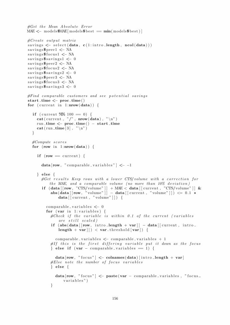
#Get the Mean Abso lu te ErrorMAE <− models$MAE[ models$best == min( models$best ) ]
#Create output matrixsav ing s <− s e l e c t (data , c ( 1 : i n t r o length , ncol (data ) ) )sav ing s$peer1 <− NAsav ings$ f o cus1 <− NAsav ings$ sav ings1 <− 0sav ings$peer2 <− NAsav ings$ f o cus2 <− NAsav ings$ sav ings2 <− 0sav ings$peer3 <− NAsav ings$ f o cus3 <− NAsav ings$ sav ings3 <− 0
#Find comparable customers and see p o t e n t i a l s a v i n g sstart time <− proc . time ( )for ( cur r ent in 1 :nrow(data ) ) {
i f ( cur r ent %% 100 == 0) {cat ( current , ”/” , nrow(data ) , ”\n” )run time <− proc . time ( ) − start timecat ( run time [ 3 ] , ”\n” )
}
#Compute s c o r e sfor (row in 1 :nrow(data ) ) {
i f (row == current ) {
data [ row , ” comparable v a r i a b l e s ” ] <− −1
} else {#Get r e s u l t s Keep rows wi th a lower CTS/volume with a c o r r e c t i o n f o r
the MAE, and a comparable volume ( no more than 10% d e v i a t i o n )i f (data [ [ row , ”CTS/volume” ] ] + MAE < data [ [ current , ”CTS/volume” ] ] &
abs (data [ [ row , ”volume” ] ] − data [ [ current , ”volume” ] ] ) <= 0.1 ∗data [ [ current , ”volume” ] ] ) {
comparable v a r i a b l e s <− 0for (var in 1 : v a r i a b l e s ) {
#Check i f the v a r i a b l e i s w i t h i n 0.1 o f the curren t ( v a r i a b l e sare s t i l l s c a l e d )
i f (abs (data [ [ row , i n t r o length + var ] ] − data [ [ current , i n t r olength + var ] ] ) < var th r e sho ld [ var ] ) {
comparable v a r i a b l e s <− comparable v a r i a b l e s + 1#I f t h i s i s the f i r s t d i f f e r i n g v a r i a b l e put i t down as the f o c u s} else i f (var − comparable v a r i a b l e s == 1) {
data [ row , ” f o cu s ” ] <− colnames (data ) [ i n t r o length + var ]#Else note the number o f f o c u s v a r i a b l e s} else {
data [ row , ” f o cu s ” ] <− paste (var − comparable v a r i a b l e s , ” f o cusv a r i a b l e s ” )
}
156
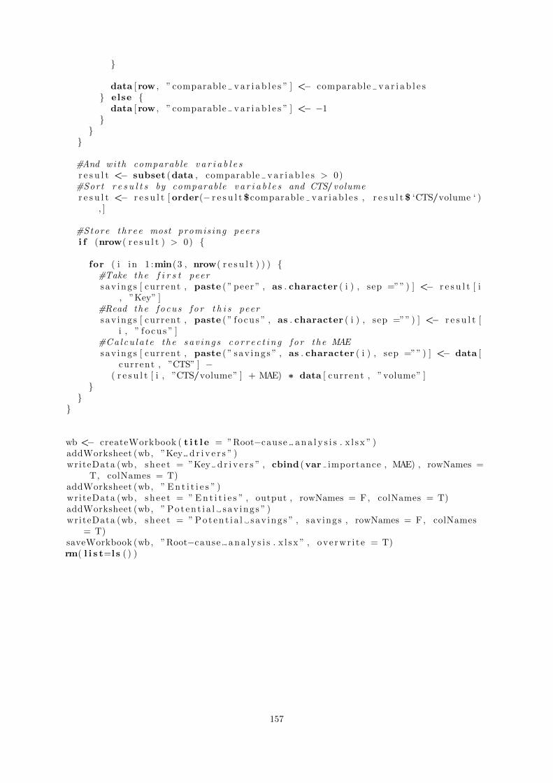
}
data [ row , ” comparable v a r i a b l e s ” ] <− comparable v a r i a b l e s} else {
data [ row , ” comparable v a r i a b l e s ” ] <− −1}
}}
#And with comparable v a r i a b l e sr e s u l t <− subset (data , comparable v a r i a b l e s > 0)
#Sort r e s u l t s by comparable v a r i a b l e s and CTS/volumer e s u l t <− r e s u l t [ order(− r e s u l t $comparable v a r i a b l e s , r e s u l t $ ‘CTS/volume ‘ )
, ]
#Store t h r e e most promising peersi f (nrow( r e s u l t ) > 0) {
for ( i in 1 :min(3 , nrow( r e s u l t ) ) ) {#Take the f i r s t peersav ing s [ current , paste ( ” peer ” , as . character ( i ) , sep =”” ) ] <− r e s u l t [ i
, ”Key” ]#Read the f o c u s f o r t h i s peersav ing s [ current , paste ( ” f o cus ” , as . character ( i ) , sep =”” ) ] <− r e s u l t [
i , ” f o cu s ” ]#C a l c u l a t e the s a v i n g s c o r r e c t i n g f o r the MAEsav ing s [ current , paste ( ” sav ings ” , as . character ( i ) , sep =”” ) ] <− data [
current , ”CTS” ] −( r e s u l t [ i , ”CTS/volume” ] + MAE) ∗ data [ current , ”volume” ]
}}
}
wb <− createWorkbook ( t i t l e = ”Root−cause a n a l y s i s . x l sx ” )addWorksheet (wb, ”Key d r i v e r s ” )writeData (wb, shee t = ”Key d r i v e r s ” , cbind (var importance , MAE) , rowNames =
T, colNames = T)addWorksheet (wb, ” E n t i t i e s ” )writeData (wb, shee t = ” E n t i t i e s ” , output , rowNames = F, colNames = T)addWorksheet (wb, ” Po t en t i a l sav ing s ” )writeData (wb, shee t = ” Po t en t i a l sav ings ” , sav ings , rowNames = F, colNames
= T)saveWorkbook (wb, ”Root−cause a n a l y s i s . x l sx ” , ove rwr i t e = T)rm( l i s t=l s ( ) )
157
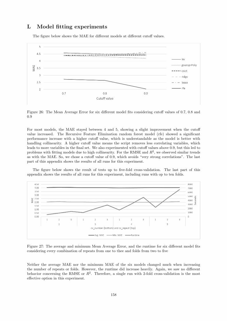
L Model fitting experiments
The figure below shows the MAE for different models at different cutoff values.
Figure 26: The Mean Average Error for six different model fits considering cutoff values of 0.7, 0.8 and0.9
For most models, the MAE stayed between 4 and 5, showing a slight improvement when the cutoffvalue increased. The Recursive Feature Elimination random forest model (rfe) showed a significantperformance increase with a higher cutoff value, which is understandable as the model is better withhandling collinearity. A higher cutoff value means the script removes less correlating variables, whichleads to more variables in the final set. We also experimented with cutoff values above 0.9, but this led toproblems with fitting models due to high collinearity. For the RMSE and R2, we observed similar trendsas with the MAE. So, we chose a cutoff value of 0.9, which avoids “very strong correlations”. The lastpart of this appendix shows the results of all runs for this experiment.
The figure below shows the result of tests up to five-fold cross-validation. The last part of thisappendix shows the results of all runs for this experiment, including runs with op to ten folds.
Figure 27: The average and minimum Mean Average Error, and the runtime for six different model fitsconsidering every combination of repeats from one to thee and folds from two to five
Neither the average MAE nor the minimum MAE of the six models changed much when increasingthe number of repeats or folds. However, the runtime did increase heavily. Again, we saw no differentbehavior concerning the RMSE or R2. Therefore, a single run with 2-fold cross-validation is the mosteffective option in this experiment.
158
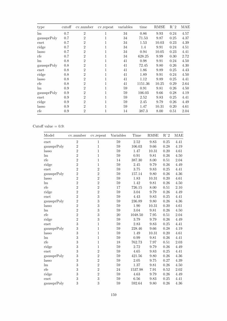
type cutoff cv number cv repeat variables time RMSE Rˆ2 MAE
lm 0.7 2 1 34 0.86 9.93 0.24 4.57gaussprPoly 0.7 2 1 34 71.53 9.87 0.25 4.37enet 0.7 2 1 34 1.53 10.03 0.23 4.39ridge 0.7 2 1 34 1.4 9.91 0.24 4.51lasso 0.7 2 1 34 0.94 10.05 0.23 4.41rfe 0.7 2 1 34 628.25 9.99 0.30 2.72lm 0.8 2 1 41 0.98 9.91 0.24 4.50gaussprPoly 0.8 2 1 41 72.45 9.80 0.26 4.30enet 0.8 2 1 41 1.86 9.89 0.25 4.43ridge 0.8 2 1 41 1.89 9.91 0.24 4.50lasso 0.8 2 1 41 1.12 9.89 0.25 4.41rfe 0.8 2 1 41 1151.36 10.25 0.29 2.64lm 0.9 2 1 59 0.91 9.81 0.26 4.50gaussprPoly 0.9 2 1 59 106.03 9.66 0.28 4.19enet 0.9 2 1 59 2.52 9.83 0.25 4.41ridge 0.9 2 1 59 2.45 9.79 0.26 4.49lasso 0.9 2 1 59 1.47 10.31 0.20 4.61rfe 0.9 2 1 14 387.3 8.00 0.51 2.04
Cutoff value = 0.9:
Model cv number cv repeat Variables Time RMSE Rˆ2 MAE
enet 2 1 59 2.52 9.83 0.25 4.41gaussprPoly 2 1 59 106.03 9.66 0.28 4.19lasso 2 1 59 1.47 10.31 0.20 4.61lm 2 1 59 0.91 9.81 0.26 4.50rfe 2 1 14 387.30 8.00 0.51 2.04ridge 2 1 59 2.45 9.79 0.26 4.49enet 2 2 59 3.75 9.83 0.25 4.41gaussprPoly 2 2 59 157.14 9.80 0.26 4.36lasso 2 2 59 1.83 10.31 0.20 4.61lm 2 2 59 1.42 9.81 0.26 4.50rfe 2 2 17 726.15 8.00 0.51 2.10ridge 2 2 59 3.04 9.79 0.26 4.49enet 2 3 59 4.43 9.83 0.25 4.41gaussprPoly 2 3 59 236.89 9.80 0.26 4.36lasso 2 3 59 1.90 10.31 0.20 4.61lm 2 3 59 3.04 9.81 0.26 4.50rfe 2 3 20 1048.50 7.95 0.51 2.04ridge 2 3 59 3.79 9.79 0.26 4.49enet 3 1 59 2.83 9.83 0.25 4.41gaussprPoly 3 1 59 228.46 9.66 0.28 4.19lasso 3 1 59 1.49 10.31 0.20 4.61lm 3 1 59 0.99 9.81 0.26 4.41rfe 3 1 18 762.73 7.97 0.51 2.03ridge 3 1 59 2.72 9.79 0.26 4.49enet 3 2 59 4.65 9.83 0.25 4.41gaussprPoly 3 2 59 421.56 9.80 0.26 4.36lasso 3 2 59 2.05 9.75 0.27 4.39lm 3 2 59 1.37 9.81 0.26 4.50rfe 3 2 24 1537.98 7.91 0.52 2.02ridge 3 2 59 4.63 9.79 0.26 4.49enet 3 3 59 6.56 9.83 0.25 4.41gaussprPoly 3 3 59 592.64 9.80 0.26 4.36
159

Model cv number cv repeat Variables Time RMSE Rˆ2 MAE
lasso 3 3 59 2.63 9.75 0.27 4.39lm 3 3 59 1.68 9.81 0.26 4.50rfe 3 3 25 2274.92 8.07 0.50 2.07ridge 3 3 59 6.22 9.79 0.26 4.49enet 4 1 59 3.67 9.83 0.25 4.41gaussprPoly 4 1 59 403.10 9.66 0.28 4.19lasso 4 1 59 1.78 9.75 0.27 4.39lm 4 1 59 1.01 9.81 0.26 4.41rfe 4 1 24 1223.68 8.01 0.51 2.06ridge 4 1 59 3.57 9.79 0.26 4.49enet 4 2 59 6.95 9.83 0.25 4.41gaussprPoly 4 2 59 726.67 9.80 0.26 4.36lasso 4 2 59 2.74 9.75 0.27 4.39lm 4 2 59 1.58 9.81 0.26 4.41rfe 4 2 23 2385.81 8.06 0.50 2.04ridge 4 2 59 6.41 9.79 0.26 4.49enet 4 3 59 9.52 9.83 0.25 4.41gaussprPoly 4 3 59 1151.30 9.66 0.28 4.19lasso 4 3 59 3.80 10.31 0.20 4.61lm 4 3 59 2.00 9.81 0.26 4.50rfe 4 3 22 3598.00 7.84 0.53 2.00ridge 4 3 59 8.78 9.79 0.26 4.49enet 5 1 59 5.84 9.83 0.25 4.41gaussprPoly 5 1 59 614.99 9.66 0.28 4.19lasso 5 1 59 2.27 10.31 0.20 4.61lm 5 1 59 1.14 9.81 0.26 4.50rfe 5 1 24 1671.08 8.17 0.49 2.06ridge 5 1 59 5.12 9.79 0.26 4.49enet 5 2 59 8.71 9.83 0.25 4.41gaussprPoly 5 2 59 1153.39 9.80 0.26 4.36lasso 5 2 59 3.34 9.75 0.27 4.39lm 5 2 59 1.89 9.81 0.26 4.50rfe 5 2 23 3382.52 7.95 0.51 2.04ridge 5 2 59 8.09 9.79 0.26 4.49enet 5 3 59 11.92 9.83 0.25 4.41gaussprPoly 5 3 59 1649.50 9.80 0.26 4.36lasso 5 3 59 4.63 9.75 0.27 4.39lm 5 3 59 2.11 9.81 0.26 4.50rfe 5 3 24 5006.28 8.06 0.50 2.10ridge 5 3 59 11.08 9.79 0.26 4.49enet 6 1 59 5.19 9.83 0.25 4.41gaussprPoly 6 1 59 566.90 9.80 0.26 4.36lasso 6 1 59 2.37 9.75 0.27 4.39lm 6 1 59 1.16 9.81 0.26 4.41ridge 6 1 59 4.98 9.79 0.26 4.49enet 7 1 59 5.96 9.83 0.25 4.41gaussprPoly 7 1 59 747.51 9.66 0.28 4.19lasso 7 1 59 2.41 9.75 0.27 4.39lm 7 1 59 1.04 9.81 0.26 4.41ridge 7 1 59 6.90 9.79 0.26 4.49enet 8 1 59 5.64 9.83 0.25 4.41gaussprPoly 8 1 59 946.19 9.80 0.26 4.36lasso 8 1 59 2.28 9.75 0.27 4.39lm 8 1 59 1.12 9.81 0.26 4.41ridge 8 1 59 6.23 9.79 0.26 4.49
160

Model cv number cv repeat Variables Time RMSE Rˆ2 MAE
enet 9 1 59 7.29 9.83 0.25 4.41gaussprPoly 9 1 59 1040.75 9.66 0.28 4.19lasso 9 1 59 2.75 9.75 0.27 4.39lm 9 1 59 1.11 9.81 0.26 4.41ridge 9 1 59 6.72 9.79 0.26 4.49enet 10 1 59 6.80 9.83 0.25 4.41gaussprPoly 10 1 59 1252.03 9.80 0.26 4.36lasso 10 1 59 2.85 9.75 0.27 4.39lm 10 1 59 1.30 9.81 0.26 4.41ridge 10 1 59 6.73 9.79 0.26 4.49
161

M Survey performance new tool
User experience
The results show how many stars each respondent awarded.
ID Position How do you rate the user experience of the QlikView tool? How do you rate the user experience of the Power BI tool?
1 OpCo 3 42 Global 4 43 Global 1 34 Global 2 4
Features old tool
Response Score
Much worse -2Slightly worse -1Unchanged 0Slightly improved 1Much improved 2
ID PositionFilterfunctionality
Cost pervolume-unitgraphs
Scatter/dropanalysisgraph
Deliveryprofilegraph
Keynumberstables
Detailstables
MapVolumeflow(overview)
1 OpCo 1 1 -1 1 2 2 1 12 Global 0 2 0 0 2 2 2 23 Global -1 0 0 0 0 0 1 04 Global 1 1 2 1 1 1 2 2
162

Tool assessment
Response Score
Completely disagree 0Mostly disagree 1Somewhat disagree 2Somewhat agree 3Mostly agree 4Completely agree 5
ID PositionUsing the tool canimprove my jobperformance
Using the tool canmake it easier todo my job
Using the tool cansignificantly increasethe quality of outputon my job
Learning to operatethe tool was easyfor me
Using the tool involveslittle time doingmechanical operations
I find it easy to getthe tool to do whatI want it to do
1 OpCo 4 4 4 3 3 32 Global 5 4 4 4 4 43 Global 4 3 4 5 5 44 Global 4 4 3 3 3 4
New features
The results show how many stars each respondent awarded.
ID Position HierarchiesMainpage
Generallayout
Helppage
Combinationstables
Trendpage
Truckutilizationpage
Ship fromlocationspage
Deliveringfrom theclosest DCpage
Histogramspage
Segmentationpage
1 OpCo 3 3 3 4 3 3 2 3 2 2 42 Global 4 4 4 3 3 3 4 2 4 3 43 Global 4 3 3 4 2 4 3 4 2 2 44 Global 3 4 3 3 3 3 4 4 3 2 3
163

ID Position Complexity page Logistics Trade Terms page Ask a question about your data page Key influencers page Decomposition tree page
1 OpCo 3 4 2 2 42 Global 4 2 4 4 43 Global 3 3 3 2 24 Global 3 2 3 2 2
Root-cause analysis
Response Score
Completely disagree 0Mostly disagree 1Somewhat disagree 2Somewhat agree 3Mostly agree 4Completely agree 5
ID PositionThe method canimprove my jobperformance
The method canmake it easier todo my job
The method cansignificantly increasethe quality of outputon my job
Understanding themethod was easyfor me
I feel the methodinvolves little timedoing mechanicaloperations
I expect it wouldbe easy to get themethod to dowhat I want it to do
1 OpCo2 Global 5 5 5 4 4 43 Global 4 3 4 3 4 24 Global 4 4 4 3 3 3
164