Determination of the magnetic

octupole moment of 173Yb and

a design towards laser - double

resonance methods in an MR -

ToF device

Master’s Thesis, 20.6.2020

Author:

SONJA KUJANPÄÄ

Supervisor:

RUBEN DE GROOTE

c© 2020 Sonja Kujanpää

Julkaisu on tekijänoikeussäännösten alainen. Teosta voi lukea ja tulostaa henkilökohtais-

ta käyttöä varten. Käyttö kaupallisiin tarkoituksiin on kielletty.

This publication is copyrighted. You may download, display and print it for Your own

personal use. Commercial use is prohibited.

Abstract

Kujanpää, Sonja

Determination of the magnetic octupole moment of 173Yb and a design towards laser-

double resonance methods in an MR-ToF device

Master’s thesis

Department of Physics, University of Jyväskylä, 2020, 77 pages.

This thesis consists of two parts.

In the first part, the magnetic octupole moment of stable ytterbium was determined

using collinear laser spectroscopy (CLS) on a fast atomic beam in the Ion-Guide Iso-

tope Separator On-Line (IGISOL) facility at Jyväskylä. The hyperfine constants of the

metastable state in 173Yb were measured using three different dipole transitions. From

the resulting hyperfine spectra, can these constants A, B, and C for dipole, quadrupole,

and octupole, respectively, be extracted. The corresponding nuclear moments µ, Q, and

Ω are determined by combining these hyperfine constants with nuclear theory calcula-

tions. This measurement was performed to validate a previously observed abnormally

large octupole splitting. From our measurement, the hyperfine octupole constant was

determined to be C = 0.02(6) MHz and the corresponding magnetic octupole moment

Ω = −1.3(38) µN b. These values are in significant disagreement with the previous ex-

periment, but agree with the single-particle shell model estimate within the error bars. As

C was zero within our precision, a future measurement using a higher-precision method,

e.g.laser-radiofrequency double-resonance method (LRDR), is needed.

The second part of this thesis was done at CERN, in the Multi Ion Reflection Appara-

tus for CLS (MIRACLS) experiment located in the Isotope Separator On-Line Device

(ISOLDE) facility. MIRACLS uses a Multi Reflection Time-of-Flight (MR-ToF) ion trap

to extend the laser-ion interaction time. Using this method, the population of the hy-

perfine state of interest can be pumped out unintentionally, leading to less fluorescence.

One way to overcome this could be to combine LRDR with MIRACLS: applying an RF

field may repopulate that state, which increases fluorescence and boosts signal. A new

design for the MR-ToF drift tube with an RF electrode was devised. A preliminary test

was performed with a simple RF loop and no drift tube alterations. This test showed no

enhancement due to the applied RF signal. A future design with a coaxial geometry is

planned but not yet tested.

Keywords: collinear laser spectroscopy, ytterbium, magnetic octupole moment, IGISOL,

laser-radiofrequency double-resonance, multi reflection time-of-flight, MR-ToF, CERN,

ISOLDE, MIRACLS

1

2

Tiivistelmä

Kujanpää, Sonja

173Yb:n magneettisen oktupolimomentin määritys ja laserkaksoisresonanssimenetelmän

alustava suunnittelu MR-ToF -laitteeseen

Pro gradu -tutkielma

Fysiikan laitos, Jyväskylän yliopisto, 2020, 77 sivua.

Tämä pro gradu -tutkielma koostuu kahdesta osasta.

Ensimmäisessä osassa stabiilin ytterbiumin magneettinen oktupolimomentti määritetään

kollineaarista laserspektroskopiaa (CLS) ja nopeaa atomisuihkua käyttäen. Mittaus suo-

ritetaan IGISOL-laitteistolla (Ion-Guide Isotope Separator On-Line) Jyväskylän Yliopis-

ton kiihdytinlaboratoriossa. 173Yb:n metastabiilin tilan ylihienokertoimet mitataan käyt-

täen kolmea erilaista optista dipolisiirtymää. Mitatusta ylihienospektristä määritetään

dipoli-, kvadrupoli- ja oktupolikertoimet A, B ja C, joista saadaan vastaavat ytimen mo-

mentit µ, Q ja Ω ydinteorian avulla. Tällä mittauksella pyritään todentamaan aikaisem-

min havaittu epänormaalin suuri oktupolijakautuminen. Nyt tulokseksi saadaan ylihie-

nolle oktupolikertoimelle C = 0.02(6) MHz ja oktupolimomentille Ω = −1.3(38) µN

b. Nämä arvot eroavat huomattavasti edellisestä mittauksesta mutta ovat virheiden ra-

joissa yhdenpitäviä yksihiukkasmallin arvion kanssa. Koska nyt C vastaa virherajoineen

nollaa, tulevaisuudessa mittaus on toistettava tarkemmalla menetelmällä, kuten laser-

radiotaajuuskaksoisresonanssilla (LRDR).

Tutkielman toinen osa tehdään CERN:issä ISOLDE:lla (Isotope Separator On-Line DE-

vice), jossa kehitetään moniheijastavan lentoaikamassaspektrometrin (MR-ToF) ja CLS:an

yhdistävää Multi Ion Reflection Apparatus for CLS (MIRACLS) -laitteistoa. MIRACLS

käyttää MR-ToF:ia ioniloukkuna laserin ja ionien välisen vuorovaikutusajan pidentämi-

seksi. Tästä aiheutuu populaation pumppautuminen pois kiinnostuksen kohteena ole-

valta ylihienotilalta, jolloin havaittu fluoresenssi vähenee. Ratkaisuna on yhdistää LRDR

ja MIRACLS: radiotaajuuden (RF) avulla ajetaan siirtymiä, jotka täyttävät vajaan tilan uu-

delleen johtaen fluoresenssin ja signaalin palautumiseen. Tätä varten MR-ToF-laitteeseen

suunnitellaan uusi keskielektrodi RF-elektrodin kera. Alustava koe tehtiin yksinkertaisel-

la RF-silmukalla ilman muita muutoksia mutta siinä ei havaittu RF-signaalista johtuvaa

parannusta. Seuraavaksi suunniteltiin koaksiaalista keskielektrodia mutta sitä ei kyetty

kokeilemaan käytännössä.

Avainsanat: kollineaarinen laserspekroskopia, ytterbium, magneettinen oktupolimoment-

ti, IGISOL, laser-radiotaajuuskaksoisresonanssi, moniheijastava lentoaikamassaspektro-

metri, MR-ToF, CERN, ISOLDE, MIRACLS

3

4

Preface

Firstly, I would like to express my thanks to my supervisor Ruben de Groote for his enthu-

siasm for this project, support, encouragement, and patience. It has been an educational

experience, and I feel I have learned many new things, even my Python proficiency has

advanced from non-existent to purely atrocious.

Secondly, I would like to express my gratitude to Stephan Malbrunot-Ettenauer for al-

lowing me to continue working with the MIRACLS at ISOLDE-CERN regarding my the-

sis, as well all the team members - special thanks to Simon Sels for his invaluable help,

optimism and efforts during the RF excitation tests and Varvara Lagaki for the much-

appreciated help as well. Thanks also for Mark Bissell for sharing his knowledge and

letting us once again borrow some COLLAPS equipment. Moreover, I want to thank the

Faculty of Mathematics and Science of the University of Jyväskylä for awarding me the

travel grant to go to CERN and complete a part of my thesis there.

I offer thanks also to Iain Moore and Paul Greenlees, without whose reference letters

I sure would have not made it to the CERN Summer Student Programme 2019, which

then lured me into laser spectroscopy and the chosen subject of this thesis (whether for

good or for bad, I’ll leave that to the reader). I am also grateful for Mikael Reponen for

his help with the Finnish translation, which now turned out less badly. Thanks to Henna

Joukainen for the insightful discussions, company, and constructive comments during

these past five years. Thanks also to all my other friends, and family who supported me

during my studies, and for my cat Viiru for always ignoring me when I came home to

visit and then acting as nothing had happened.

Additionally, I acknowledge COVID-19 for making the long-awaited completion of this

thesis possible as sometimes being self-quarantined in your house is all that is needed,

and also unacknowledge it for ruining the other half of my MR-ToF tests. I am also grate-

ful for the spell-check function of Microsoft Word, without whom the word ‘frequency’

would be misspelt differently exactly 93 times.

Kankaanpää, June 2020

S onja Kujanpää

5

6

Contents

Abstract 1

Tiivistelmä 3

Preface 5

1 Introduction 9

1.1 Motivation for 173Yb magnetic octupole . . . . . . . . . . . . . . . . . . . . 10

1.2 Motivation for the development of RF spectroscopy in an MR-ToF . . . . . 12

2 Theoretical background 14

2.1 Nuclear perturbations arising from the atomic structure . . . . . . . . . . . 14

2.1.1 Nuclear ground-state properties from the atomic spectra . . . . . . 14

2.1.2 Fine and hyperfine structure . . . . . . . . . . . . . . . . . . . . . . 15

2.1.3 Spectroscopic notation for labelling the atomic states . . . . . . . . 16

2.1.4 Hyperfine structure shifts due to the nuclear multipole moments . 18

2.2 Lasers and traps in nuclear physics studies . . . . . . . . . . . . . . . . . . 21

2.2.1 Basic operational principle of lasers . . . . . . . . . . . . . . . . . . 22

2.2.2 Linear two-dimensional Paul traps . . . . . . . . . . . . . . . . . . . 24

2.2.3 Multi Reflection Time-of-Flight devices . . . . . . . . . . . . . . . . 26

2.3 Collinear laser spectroscopy . . . . . . . . . . . . . . . . . . . . . . . . . . . 29

2.3.1 Spectral lineshapes and broadening mechanisms . . . . . . . . . . . 31

2.3.2 Optical pumping . . . . . . . . . . . . . . . . . . . . . . . . . . . . . 33

2.4 General concept of MIRACLS . . . . . . . . . . . . . . . . . . . . . . . . . . 33

2.5 Laser-radiofrequency double-resonance method . . . . . . . . . . . . . . . 36

2.5.1 Using LRDR in collinear geometry . . . . . . . . . . . . . . . . . . . 37

3 Study of the magnetic octupole moment of 173Yb 39

3.1 Experimental setup at the IGISOL . . . . . . . . . . . . . . . . . . . . . . . 39

3.1.1 IGISOL-4 facility . . . . . . . . . . . . . . . . . . . . . . . . . . . . . 39

3.1.2 Collinear laser line . . . . . . . . . . . . . . . . . . . . . . . . . . . . 40

3.1.3 Collinear laser spectroscopy of 173Yb . . . . . . . . . . . . . . . . . . 42

3.1.4 Laser system . . . . . . . . . . . . . . . . . . . . . . . . . . . . . . . 43

3.2 Data analysis for the hyperfine constants . . . . . . . . . . . . . . . . . . . 45

3.2.1 Determination of the RFQ cooler voltage offset . . . . . . . . . . . . 47

3.2.2 Systematic uncertainties in the experimental setup . . . . . . . . . 49

3.2.3 Constraining of the overlapping peaks in the spectra . . . . . . . . 51

3.2.4 Stability of the RFQ cooler voltage and the laser frequency . . . . . 52

3.3 Extracted hyperfine constants for the lower and upper states . . . . . . . . 53

3.4 Extraction of the magnetic octupole moment from the experiment . . . . . 56

3.5 Nuclear theory estimates for the octupole moment . . . . . . . . . . . . . . 57

3.6 Interpretation of the obtained results . . . . . . . . . . . . . . . . . . . . . . 58

4 Study of the radiofrequency excitations with Mg+ 60

4.1 Design of the RF electrode and the new drift tube for an MR-ToF device . 60

4.1.1 RF penetrability through different materials . . . . . . . . . . . . . 61

4.1.2 Modified telescopic drift tube design with conducting mesh . . . . 62

4.2 Preliminary tests of the RF excitations at the MIRACLS setup . . . . . . . 63

4.2.1 Laser cooling as a detection method . . . . . . . . . . . . . . . . . . 66

4.3 Redesigned drift tube with a coaxial geometry . . . . . . . . . . . . . . . . 68

4.4 Conclusions about the laser-RF method in an MR-ToF . . . . . . . . . . . . 70

5 Discussion 71

References 72

1 Introduction

Since the landmark experiments towards the comprehension of the atomic and nuclear

structure were done, starting from the discovery of radioactivity by Henri Becquerel

in 1896, the discovery of electron by Joseph Thomson in 1897 and the discovery of the

atomic nucleus by observing the deflection of the alpha particles from gold foil by Ernest

Rutherford, Hans Geiger and Ernest Marsden in 1911, understanding the exact structure

of the nucleus has been of interest for many physicists. In 1913, just two years after the

discovery of the nucleus, the first atomic model was built by Niels Bohr based on Planck’s

theory of quantization of energy, which then gave rise to the atomic shell model in 1949.

Early works focused on studying stable or long-lived isotopes and resulted in enormous

amounts of experimental data - leading to the development of the nuclear shell model to

interpret the underlying nuclear structure. From the experimental data, it was noted that

nuclei with a certain proton (Z) and/or neutron (N) number appeared more stable than

others. These numbers were named the magic numbers (2, 8, 20, 28, 50, 82, and 126) and

they define the number of nucleons that completely fill each shell. [1]

With the construction and development of modern radioactive ion beam (RIB) facilities,

such as Ion-Guide Separator On-Line (IGISOL) at Jyväskylä and the Isotope Separator

On-Line DEvice (ISOLDE) at CERN, it became possible to study short-lived and exotic

radionuclides far from stability. This has led to the discovery of several new nuclear

structure phenomena, some of which challenge the classical shell model picture, such as

the disappearance and emergence of new shell closures [1].

To study the fundamental nuclear properties, one must gather information about the

nucleus. Many methods have been invented over the years. This thesis deals with meth-

ods that investigate the hyperfine structure (HFS) of atoms or ions, which consists of

tiny splittings and changes in the atomic energy levels due to nuclear electromagnetic

properties. The invention of the laser in 1960 [2] and the subsequent laser spectroscopy

techniques enabled the high resolution needed for examining these effects. The earliest

experiment using spectroscopy based on the combination of fast ionic beams and lasers

was done in 1975 by H. Andra [3]. One of the techniques that is nowadays routinely used

in RIB-facilities is collinear laser spectroscopy (CLS), which originated from the theoret-

ical and experimental efforts of W. H. Wing [4] and S. Kaufman [5] in 1976. In CLS, the

laser beam is overlapped with an atom or ion beam to reduce unwanted Doppler broad-

ening of the observed lineshapes. By scanning the laser frequency in the rest frame of the

atoms or ions, it can be tuned into the resonance frequency of the electronic transition

in the atomic shell. When the laser’s frequency corresponds to the energy differences

between the hyperfine levels, the atoms or ions will be excited. After being excited by

the laser, the atoms or ions decay back to their corresponding ground-state, emitting

fluorescence photons. These photons can be detected by a detection system, such as a

9

photomultiplier tube (PMT), placed perpendicularly to the laser/atom beam. By mea-

suring the fluorescence counts as a function of the frequency, the hyperfine splitting and

isotope shifts can be extracted. Since these properties arise from the interaction between

the nucleus and its surrounding electron cloud, it is possible to gain information about

the nuclear properties, such as the nuclear spin, the nuclear multipole moments, and the

nuclear mean-square charge radius [1]. Some pioneering CLS experiments have been

done at ISOLDE-CERN, where currently beamlines COLLAPS [6], CRIS [7], and MIRA-

CLS [8] are in use, and e.g. at the collinear laser line at the IGISOL facility in Jyväskylä.

Most of the measurements in this thesis, whose motivations are detailed in the following

chapters, were done at the IGISOL, in addition to some work conducted at MIRACLS.

1.1 Motivation for 173Yb magnetic octupole

The magnetic dipole moment µ and quadrupole moment Q have been measured in var-

ious different nuclei [9] from the atomic hyperfine structure, yet similar measurements

for the next term in the multipolar expansion, the magnetic octupole constant C and the

corresponding nuclear magnetic octupole moment Ω, have not been conducted nearly

as much. According to the current knowledge, the magnetic octupole splitting has been

previously measured for only 18 elements, such as 45Sc, 83Kr, 151Eu, and 201Hg, all of

which are summarized in table 1.

Due to the lack of experimental data, interpretation of these octupole moments has been

very challenging, and so no meaningful progress in the corresponding nuclear theory

has been made in the past 50 years. For the octupole moments measured, often no un-

certainty for values of Ω is provided in the original works. Especially, good estimates

for theoretical uncertainties of C and Ω are often lacking and in some cases, important

effects like second-order hyperfine mixing are not fully considered. From the experi-

mental point of view, recent years have been very promising: highly precise octupole

moment measurements were done using optical spectroscopy with the D2 line in 133Cs in

2003 [10], and the most accurately determined octupole moment to date was measured

in 2012 using a single trapped 137Ba+ ion [11].

In 2013 yet another octupole measurement was done with atomic 173Yb using the hyper-

fine intervals in the metastable 3P2 state [12]. This measurement was particularly interest-

ing, as a surprisingly large octupole splitting was observed compared to the magnitudes

observed for other elements. This large splitting is intriguing for a couple of reasons:

an effect this large would be measurable with currently used spectroscopic methods at

RIB-facilities [13], and the value of Ω acquired by [12] is significantly larger than the esti-

mated value from the single-particle shell model calculations. This hints that our current

understanding of the nuclear electromagnetic moments could be insufficient and more

theoretical explorations may need to be conducted.

10

Table 1: Summary of some magnetic octupole hyperfine parameters C and the correspondingmagnetic octupole moments Ω. Uncertainties of the C and Ω are as quoted in the literature whereavailable, and µN is the nuclear magneton and b is barn.

Isotope Z N State C [Hz] Ω[µN b] Ref.

35Cl 17 18 2P3/2 -6.95(1.2) -0.0188 a

37Cl 17 20 2P3/2 -5.41(1.2) -0.0146 a

45Sc 21 23 2D5/2 -250(100) 1.6(8) [14]51V 23 27 4D3/2 -1660(140) – [15] b

23 27 4D5/2 -270(80) – [15] b

69Ga 31 38 2P3/2 84(6) 0.107(20) [16]71Ga 31 40 2P3/2 115(7) 0.146(20) [16]79Br 35 44 2P3/2 388(8) 0.116 [17]81Br 35 46 2P3/2 430(8) 0.129 [17]83Kr 36 47 3P2 -790(250 -0.18(6) [18]113In 49 64 2P3/2 1728(45) 0.565(12) [19]115In 49 66 2P3/2 1702(35) 0.574(15) [19]127I 53 74 2P3/2 2450(370) 0.167 [20, 21]

131Xe 54 77 3P2 728(105) 0.048(12) [22]133Cs 55 78 2P3/2 560(70) 0.8(1) [23]137Ba 56 81 2D3/2 36.546 0.05057(54) [11]137Ba 56 81 2D5/2 -12.41(77) 0.0496(37) [24]151Eu 63 88 8,10DJ

c – [25]153Eu 63 90 8,10DJ

c – [25]155Gd 64 91 3D3 -1500(500) -1.6(6) [26]173Yb 70 103 3P2 540(20)·103 -34.4(21) [12]175Lu 71 104 -617(57) – [27]176Lu 71 105 -1377(302) – [27]177Hf 72 105 3F2 170(30) – [28]

72 105 3F3 230(90) – [28]72 105 3F4 500(190) – [28]

179Hf 72 107 3F2 -410(50) – [28]72 107 3F3 -600(250) – [28]72 107 3F4 -1190(500) – [28]

197Au 79 118 2D3/2 212(14) 0.0098(7) [29]79 118 4F9/2 326(10) 0.130 [29]

201Hg 80 121 3P2 -1840(90) -0.130(13) [30]209Bi 83 126 2P3/2 19300(500) 0.55(3)d [31]

83 126 4S3/2 16500(100) 0.43 [32]207Po 84 123 3P2 -12(1) 0.11(1) [33, 34]

a J. H. Holloway, unpublished Ph.D. thesis, Dept. of Phys., MIT, 1956. Values taken from [17].b Only significantly non-zero C-values listed.c Average ratio of C-parameters provided: C(151Eu)/C(153Eu) = 0.87(6).d Value and uncertainty obtained as the average of several theoretical methods.

11

It is important to note that any interpretation of the absolute values of Ω depends essen-

tially on the correct estimations of the associated uncertainties, which originate from both

the experimental measurements and atomic-theory calculations. These theoretical calcu-

lations are required since the effects under study are very small, and corrections for the

mixing of the state of interest with other close-lying states must be considered precisely.

Another reason is the fact that the extraction of Ω from a measurement of C requires a

calculation of the electronic wavefunctions.

In this work, a new measurement is done to validate the results obtained in [12], using

collinear laser spectroscopy at the IGISOL-facility. If a non-zero magnetic octupole con-

stant C is obtained with this method, this will prepare the way for similar measurements

using radioactive ytterbium isotopes in the future.

1.2 Motivation for the development of RF spectroscopy in an MR-ToF

While the most experimental methods currently used in the RIB-facilities provide mea-

surements of the hyperfine splittings with a 1 – 10 MHz precision [13], there are more pre-

cise measurement techniques such as the laser-radiofrequency double resonance (LRDR)

method. LRDR is the descendant of the molecular-beam magnetic-resonance (MBMR)

method, introduced in 1938 [35].

Initially, MBMR was aimed at the determination of the nuclear spins and moments, but

soon after it was adapted to measuring the atomic and molecular hyperfine structure

(HFS) and nuclear g-factors. When tunable single-frequency lasers became available in

the 1970s, they had a massive impact on the development of general spectroscopy and

especially the MRBR method. The most important features in this new laser were its

spectral sharpness, tunability, and efficiency in causing detectable fluorescence. An im-

portant application for this was to use it in a pump-probe configuration to replace in-

homogeneous fields inside the traditional MBMR apparatus. With this arrangement, the

standard MBMR apparatus could be replaced with a shorter and much more efficient

LRDR setup. [36]

The LRDR method relies on the use of radiofrequency (RF) photons to repopulate the

lower hyperfine structure level that was previously depleted by exciting an optical tran-

sition. This repopulation results in a resonant increase in observed fluorescence. The on-

going progress in the development of the higher precision methods and theoretical tools

has much potential to evolve our understanding of the atomic nucleus and its properties.

The aim of this work is to combine the RF excitations from the LRDR method with in-

trap laser spectroscopy technique used in MIRACLS at ISOLDE-CERN. MIRACLS, short

for Multi Ion Reflection Apparatus for Collinear Laser Spectroscopy, relies on the use of

a Multi Reflection Time-of-Flight (MR-ToF) ion trap to increase the laser-ion interaction

12

time. LRDR has been done previously using a Paul trap [37] and a Penning trap [38], but

there is no record of it been done in an MR-ToF device. Thus, this opens new exciting

possibilities for high precision spectroscopy if successful.

For example, Penning traps have been used for high precision Zeeman spectroscopy,

providing long observation times under almost perturbation-free conditions. Normally

resolution can be limited by the finite observation times and line broadening caused by

collisions between particles but with the use of this method these sources can be elimi-

nated. [38]

At MIRACLS the greatest motivation at this time was to overcome the unintentional pop-

ulation depletion in their setup, which is caused by optical pumping. Here the popula-

tion is pumped out of the hyperfine state of interest, which leads to less fluorescence. By

introducing an RF field, this state could be repopulated, leading to an increase in the fluo-

rescence and a boosted signal during the measurements. These RF excitations are already

familiar from the LRDR method, where they are routinely used. The optical detection re-

gion in the MIRACLS setup is located above the MR-ToF device’s central drift tube, so

a new design for the drift tube was also needed to house the desired RF electrodes to

produce the field, along with a control program, and a switch for the RF signal. An initial

investigation of the mechanical design for this modified drift tube was performed during

this thesis and is discussed in chapter 4.2.

13

2 Theoretical background

2.1 Nuclear perturbations arising from the atomic structure

Measurable perturbations of the atomic structure are caused by the non-zero nuclear

spin, the nuclear multipole moments, the radial extent of the charge distribution, and

the distribution of magnetism. The interactions giving rise to these perturbations will be

described in the following chapters.

2.1.1 Nuclear ground-state properties from the atomic spectra

In the absence of external fields, an atom can be depicted as a compact charged nucleus

and an electron cloud arranged in the central Coulomb field produced by the nucleus.

If the electrons have resultant angular momentum, J > 0, and the nucleus has a nuclear

spin, I > 0, further interactions happen between these two systems. [39]

These interactions can be expanded into a multipolar expansion, in which the magnetic

dipole µ, electric quadrupole Q, magnetic octupole Ω, and so on, are nonzero. In an

atomic nucleus with an atomic spin J, a nuclear spin I, and a total angular momen-

tum F = I + J, spectroscopic information on the corresponding nuclear moments can

be obtained roughly in three ways: by observing the transitions between the fine struc-

ture states, or the magnetic transitions which happen within the same atomic state, or in

presence of an external magnetic field, between the magnetic substates labelled with the

projection quantum numbers mJ or mF of these levels [13].

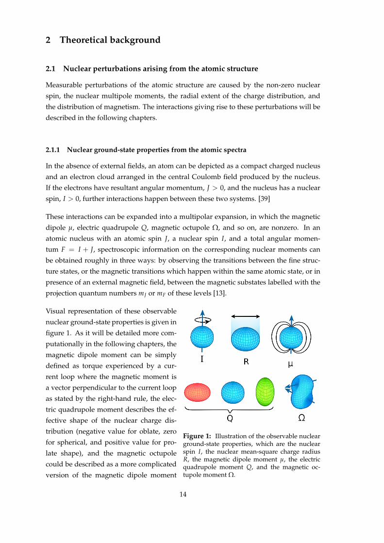
Figure 1: Illustration of the observable nuclearground-state properties, which are the nuclearspin I, the nuclear mean-square charge radiusR, the magnetic dipole moment µ, the electricquadrupole moment Q, and the magnetic oc-tupole moment Ω.

Visual representation of these observable

nuclear ground-state properties is given in

figure 1. As it will be detailed more com-

putationally in the following chapters, the

magnetic dipole moment can be simply

defined as torque experienced by a cur-

rent loop where the magnetic moment is

a vector perpendicular to the current loop

as stated by the right-hand rule, the elec-

tric quadrupole moment describes the ef-

fective shape of the nuclear charge dis-

tribution (negative value for oblate, zero

for spherical, and positive value for pro-

late shape), and the magnetic octupole

could be described as a more complicated

version of the magnetic dipole moment

14

where there are now two angled current loops instead of one, and the magnetic vectors

are facing in- or outwards in the same general direction.

2.1.2 Fine and hyperfine structure

Relativistic effects lead to small splittings of the energy levels in the atom, called the fine

structure. This effect arises when the total orbital momentum L and the spin angular mo-

mentum S of the electrons moving in the Coulomb field of a point-like nucleus couple to

a new angular momentum (spin-orbit coupling) J = S + L [40]. Fine structure splittings

are in the eV scale [13]. The coupling of the electron angular momentum J and nuclear

angular momentum I results in a new angular momentum F = I + J, from which occurs

the splitting of a fine structure level to a hyperfine structure level.

The interaction between the nucleus and the surrounding electromagnetic fields is de-

scribed by the perturbation Hamiltonian [41]

H = ∑k

T(k)e ⊗ T(k)

n , (1)

where T(k)n and T(k)

e are irreducible spherical tensors of rank k describing the electromag-

netic properties of the nucleus and its electric surroundings, respectively. That is, T(k)e

operates in only electronic coordinates and its rank is defined by the interaction of the to-

tal angular momentum operator J of the same space. Similarly, T(k)n operates only in the

coordinates of the nucleons and the terms in the series in equation (1) are the scalar prod-

ucts of these two tensors, marked with ⊗, and thus invariant in the combined space. [39]

Consideration of the parity conservation of the strong and electromagnetic interactions

dictate a general operator T(k)q=0, which consists of negative parity magnetic multipole op-

erators and positive parity electric multipole operators. Thus, it follows that the nucleus

can be described with a series of even-k electric (monopole, quadrupole, . . . ) and odd-kmagnetic (dipole, octupole, . . . ) multipole moments up to order k ≤ 2I. Laser spec-

troscopy techniques, theoretically sensitive to the entire multipole expansion, are typi-

cally limited to measuring moments of order k ≤ 2. This stems from the rapid decrease

in the size of the terms in the expansion compared to the experimental uncertainties. [13]

The atomic hyperfine structure (HFS) arises from the perturbation Hamiltonian in equa-

tion (1), where the electromagnetic tensor is derived from the field caused by the valence

electrons, and the nuclear tensor from the multipole expansions of the nuclear moments.

15

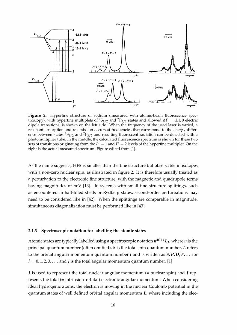
Figure 2: Hyperfine structure of sodium (measured with atomic-beam fluorescence spec-troscopy), with hyperfine multiplets of 2S1/2 and 2P3/2 states and allowed ∆F = ±1, 0 electricdipole transitions, is shown on the left side. When the frequency of the used laser is varied, aresonant absorption and re-emission occurs at frequencies that correspond to the energy differ-ence between states 2S1/2 and 2P3/2 and resulting fluorescent radiation can be detected with aphotomultiplier tube. In the middle, the calculated fluorescence spectrum is shown for these twosets of transitions originating from the F′ = 1 and F′ = 2 levels of the hyperfine multiplet. On theright is the actual measured spectrum. Figure edited from [1].

As the name suggests, HFS is smaller than the fine structure but observable in isotopes

with a non-zero nuclear spin, as illustrated in figure 2. It is therefore usually treated as

a perturbation to the electronic fine structure, with the magnetic and quadrupole terms

having magnitudes of µeV [13]. In systems with small fine structure splittings, such

as encountered in half-filled shells or Rydberg states, second-order perturbations may

need to be considered like in [42]. When the splittings are comparable in magnitude,

simultaneous diagonalization must be performed like in [43].

2.1.3 Spectroscopic notation for labelling the atomic states

Atomic states are typically labelled using a spectroscopic notation n2S+1LJ , where n is the

principal quantum number (often omitted), S is the total spin quantum number, L refers

to the orbital angular momentum quantum number l and is written as S, P, D, F, . . . for

l = 0, 1, 2, 3, . . . , and j is the total angular momentum quantum number. [1]

I is used to represent the total nuclear angular momentum (= nuclear spin) and J rep-

resents the total (= intrinsic + orbital) electronic angular momentum. When considering

ideal hydrogenic atoms, the electron is moving in the nuclear Coulomb potential in the

quantum states of well defined orbital angular momentum L, where including the elec-

16

tronic spin gives a second label S. In principle, it should not matter whether the electronic

states of an ideal atom are labelled using a set of quantum numbers L, mL, S, mS or a set

of L, S, J, mJ . Yet, the spin-orbit interaction which leads to the formation of the fine struc-

ture of the electronic levels, couples L and S in such a way that mL and mS are no longer

well-defined and thus the coupling have to be used to identify the real states. The spin-

orbit interaction can be explained simply by using a semiclassical picture in the reference

frame of the electron, where the nucleus generates a current loop. This creates a magnetic

field at the location of the electron, which interacts with the electrons’ spin magnetic mo-

ment µS giving the spin-orbit contribution to the fine structure. In figure 3 the energy

levels of sodium are illustrated with and without the spin-orbit interaction. [1]

Figure 3: Pictured here are the energy levels in atomic sodium. On the left side of each levelis the electronic configuration, and on the right side is the spectroscopic notation for the atomicstate. The fine structure doublets are labelled with total angular momentum j = l ± 1/2, therelative spacings between the doublets are only consistent for a particular l value i.e. the P- andD-state splittings are not in scale but the decrease of splittings within the P-states is in scale.Figure redrawn from [1].

17

2.1.4 Hyperfine structure shifts due to the nuclear multipole moments

Plenty of information about the magnetic dipole moment µ and the electric quadrupole

moment Q exists for several atomic nuclei [9], but only a little is known about the next

higher moments, i.e. the magnetic octupole Ω and the electric hexadecapole moments.

All of these nuclear moments can be extracted from the atomic HFS measurements and

they are independent of the used nuclear model. This chapter will focus on the nuclear

multipole expansions up to the magnetic octupole moment, as it was of particular interest

for this work.

The (hyper)fine structure of the atoms can be studied via various laser spectroscopy

methods. An atom/ion is optically excited from a lower level |I J, FmF〉 to an upper

level |I′ J′, F′m′F′〉 if the frequency of the laser corresponds to the energy difference of

the transition between the HFS levels. The dipole selection rules dictate that only specific

transitions between the hyperfine states are allowed:

∆F = 0, ± 1 and (2)

F = 0 9 F′ = 0, (3)

where in equation (2) is the allowed transition while in equation (3) the transition is

forbidden [1]. As every atomic state has hyperfine structure, with laser spectroscopic

measurements the hyperfine structure constants A, B (and, potentially also C) are mea-

sured for two states at the same time. These different hyperfine constants will later be

labelled as lower and upper hyperfine constants referring to the upper and lower states,

i.e. Al, Bl, Cl for the lower state and Au, Bu, Cu for the upper state. These two states can

be seen e.g. from figure 3.

When the terms arising from the interaction with the multipole moments are considered,

the first-order expectation for the energy shift of each atomic hyperfine level with respect

to the unperturbed fine structure level can be described by

∆E(1)HFS = ∑

kMk(I, J, F) 〈I I| T(n)

k |I I〉 〈J J| T(e)k |J J〉 , (4)

where I, J, and F are the quantum numbers associated with the corresponding operators

I, J, and F, while Mk gives information about the relative alignment of the atomic and

nuclear momenta and is defined as

Mk(I, J, F) = (−1)I+J+F

I J FJ I k

(

I k I−I 0 I

)(J k J−J 0 J

) , (5)

18

where the factor in the curly brackets is the Wigner 6-j symbol. The different energy

eigenvalues associated with the total angular momenta of the states are described by the

quantum number F = |I − J| ≤ F ≤ I + J. Expanding the equation (4) to the octupole

term (k = 3), it can be written as

∆E(1)HFS =

AK2

+3B4

K(K + 1)− I(I + 1)J(J + 1)(2I(2I − 1)J(2J − 1)

(6)

+5C4

K3 + 4K2 + 45 K(−3I(I + 1)J(J + 1) + I(I + 1) + J(J + 1) + 3)− 4I(I + 1)J(J + 1)

I(I − 1)(2I − 1)J(J − 1)(2J − 1),

where the Wigner 3-j and Wigner 6-j symbols were fully written out in terms of the I, Jand F, and A, B, and C are the hyperfine constants for dipole, quadrupole, and octupole,

respectively, and K = F(F + 1)− I(I + 1)− J(J + 1). The hyperfine constants were de-

fined in the following way:

A = 1I J 〈I I| T(n)

2 |I I〉 〈J J| T(e)1 |J J〉 =

µI

I J〈J J| T(e)

1 |J J〉 , (7)

B = 4 〈I I| T(n)2 |I I〉 〈J J| T(e)

2 |J J〉 = 2eQ 〈J J| T(e)2 |J J〉 , (8)

C = 〈I I| T(n)3 |I I〉 〈J J| T(e)

3 |J J〉 = −Ω 〈J J| T(e)3 |J J〉 , (9)

where in the equation (8) e is the elementary charge and the negative sign for Ω in the

equation (9) is selected to assure that µ and Ω are of the same sign in most cases. [39]

The nuclear magnetic dipole moment µ is then given by the relation

µ = gIµN I, (10)

where gI is the nuclear g-factor and µN the nuclear magneton. Nuclei have smaller mag-

netic moments than electrons, as can be seen from how µN is related to the Bohr magne-

ton µB:

µN = µBme

mp, (11)

where me is the mass of an electron and mp mass of a proton. [40]

The absolute values of the magnetic dipole and electric quadrupole moments can be ob-

tained from a measurement, where a precise calculation of the relevant electromagnetic

fields is conducted. However, a way more prevalent practise is to instead extract the

ratio of the nuclear isotopes from a pair of different isotopes of the same element using

approximated relationships:

AA′' µ

µ′I′

Iand

BB′' Q

Q′, (12)

19

where A′, µ′, I′, B′, and Q′ are the properties related to the reference isotope. [13]

Thus, knowing the moments of a reference isotope, measured using another method,

the moment of interest can be extracted. Note, however, that this procedure represents

an approximation; the differential changes in the nuclear charge and magnetism, while

small, do occur. For magnetic moments, these changes are referred to as anomalies. For

an infinitely small nucleus, equation (12) is valid. In real and especially heavier nuclei,

the finite nuclear extent and relativistic effects affect the electronic wavefunctions and

give rise to corrections that must be considered. These effects are the Breit-Rosenthal

(BR) effect [44] rising from the finite spatial distribution of the nuclear charge, and Bohr-

Weisskopf (BW) effect [45] from the distribution of nuclear magnetism in the nucleus.

These have only a small contribution so they are often accounted for by

A = APOINT(1 + εBW)(1 + εBR), (13)

where APOINT is the hyperfine constant A for a theoretical point-like nucleus [13]. For

quadrupole moments, no experimental reports of hyperfine anomalies exist [46].

So as it can be seen, the extraction of the nuclear moments µ, Q, and Ω from an HFS

measurement requires either the use of a reference nucleus, where the moment was de-

termined in some other way, or the use of atomic calculations to precisely evaluate the

electronic matrix elements. For all moments beyond the quadrupole term (k > 2), only

the latter option is presently applicable.

Additionally, the extraction of the hyperfine constants from the experimental spectra re-

quires the evaluation of the second-order shifts due to the mixing of the close-lying states.

This second-order approximation for the shift of a hyperfine level F due to mixing with

another state that has electronic angular momentum J is defined as

∆E(2)HFS = ∑

J′

1EJ − EJ′

∑k1,k2

F J Ik1 I J′

F J Ik2 I J′

× 〈I||T(n)k1||I〉 〈I||T(n)

k2||I〉 × 〈J′||T(e)

k1||J〉 〈J′||T(e)

k2||J〉,

(14)

where EJ is the energy of an atomic state having an angular momentum J, k1 = 1 for

magnetic dipole transition M1, and k1 = 2 for electric quadrupole transition E2. Note that

the reduced matrix elements (marked with ||) can be related to the full matrix elements

(marked with | ) via the relation

〈J J|Tk|J J〉 =(

J k J−J 0 J

)〈I||Tk||I〉. (15)

20

When the expressions of equation (14) are restricted to M1-M1, M1-E2 and E2-E2 interac-

tions, it can be expressed as follows:

∆E(2)HFS = EM1−M1

HFS + EM1−E2HFS + EE2−E2

HFS (16)

= ∑J′

∣∣∣∣∣

F J I1 I J′

∣∣∣∣∣2

η +

F J I1 I J′

F J I2 I J′

ζ +

∣∣∣∣∣

F J I2 I J′

∣∣∣∣∣2

ε

where η, ζ, and ε are defined as

η =(I + 1)(2I + 1)

Iµ2 |〈J′||T

(1)e ||J〉|2

EJ − EJ′, (17)

ζ =(I + 1)(2I + 1)

I

√2I + 32I − 1

µQ〈J′||T(1)

e ||J〉〈J′||T(2)e ||J〉

EJ − EJ′, (18)

and

ε =(I + 1)(2I + 1)(2I + 3)

I(2I − 1)Q2 |〈J′||T

(2)e ||J〉|2

EJ − EJ′. (19)

In these final expressions, the reduced matrix elements have to be obtained from atomic

theory calculations. [39]

2.2 Lasers and traps in nuclear physics studies

After the laser was first demonstrated in 1960, a wide range of laser applications has

surfaced - many of which would not even be achievable in any other way. Lasers are

the only man-made source that can generate pulses as short as ≤ 10−16 s and be used to

measure absolute frequencies with an accuracy of ∼ 10−15. [2]

The use of lasers has made a major impact on nuclear structure studies since the monochro-

maticity of laser radiation provides excellent spectral resolution. They have a high power

(in continuous waveform mW to W) which leads to enhanced sensitivity and thus opens

possibilities for detecting low atomic densities. For example, 10 mW of laser power at

600 nm is equivalent 5 mA of photons (= 3× 1015 photons/s). Lasers are nowadays also

widely tunable: a wide range of the ultraviolet, visible and infrared spectrum can be con-

tinuously scanned with appropriate sources. Lasers’ phase coherence results in beams

that have narrow divergence so they can be focused to very small spot sizes, making

remarkably large energy densities possible. Lasers can be applied effectively to almost

any conventional hyperfine structure spectroscopy, allowing the measurement of nuclear

moments, sizes, and shapes for nuclei far from stability. [47]

21

2.2.1 Basic operational principle of lasers

This chapter is adapted from the original text by R. Paschotta [2], which is suggested for

further reading to obtain more detailed information about the basic operational principle

of lasers.

The working principle of a laser is based on stimulated emission, which is the process

where excited atoms convert stored energy into light. This usually starts when the ex-

cited atom first produces a photon by spontaneous emission. When this photon reaches

another excited atom, the resulting interaction stimulates that atom to emit a photon as

well. The photons generated from the process have identical properties: wavelength, di-

rection, phase, and polarization. This ability to amplify light when enough excited atoms

are present thus explains the acronym of Light Amplification by Stimulated Emission of

Radiation (LASER).

The heart of the laser system is a laser cavity. A single pass through excited atoms or

molecules is enough to initiate laser action in some high gain devices like excimer (= ex-

cited dimer) lasers, but for most lasers, it is necessary to have multiple passes through

the lasing medium. This is implemented along an optical axis defined by a set of cavity

mirrors producing feedback, and the lasing medium (e.g. crystal, semiconductor, en-

closed gas) is placed on this axis. The axis has a high optical gain and it also becomes the

direction of propagation of the produced laser beam. A very simple cavity has just two

mirrors facing each other: total reflector and partial reflector (reflectance between 30% to

almost 100%) as illustrated in figure 4.

Figure 4: Simple illustration of a general laser, where the gain medium has a long, thin cylindri-cal shape and the cavity is defined by two mirrors with different reflectances. The gain mediumexcitation can be provided with e.g. a another pump laser, a flashlamp, or electric field.

22

Light bounces back and forth within these mirrors and gains intensity with each pass it

makes through the gain medium. Photons that are not emitted into the direction of the

axis are lost and do not contribute to the laser operation. As laser light amplifies, some of

the light will escape the cavity through the partial reflector (called output coupler), but

at the equilibrium state, these losses are fully compensated by the optical gain from the

successive round trip of the photons inside the cavity.

For an ideal laser, all photons in the output beam are identical, which results in perfect

directionality and monochromaticity. These determine the individual coherence and ra-

diance of a laser source. A photon’s energy is determined through relationship E = hc/λ,

where h is Planck’s constant, c is speed of light, and λ is wavelength. An ideal laser

would emit photons with the same energy, thus the same wavelength and so be per-

fectly monochromatic. Many applications depend on monochromaticity even though

real lasers are not perfectly monochromatic due to several broadening mechanisms that

widen the frequency and energy of the emitted photons. The best known of these is the

Doppler broadening, which is determined by the distribution of speeds in a collection of

atoms that form a gas medium.

In addition to sharing the same wavelength, the photons forming the laser beam are in

the same phase and thus coherent, which results in an electric field propagating with

a uniform wavefront. In an ideal presentation, the plane wave propagates with a flat

wavefront along a given direction and each plane that is perpendicular to this direction

experiences the same electric and magnetic field amplitude and phase at a given time.

However, real laser beams slightly deviate from this behaviour, but they remain the best

approximate for a coherent plane wave.

Lasers can be dived into three categories: continuous wave (CW), pulsed, and ultra-

fast lasers. In this section, only CW lasers are discussed, as it was the type used in this

thesis. CW lasers produce a continuous and uninterrupted beam of light which ideally

has a very stable output power. The wavelengths or lines at which light is emitted de-

pend on the characteristic of the laser medium. Each laser wavelength is associated with

a linewidth that depends on several factors, such as the gain bandwidth of the lasing

medium and the design of the optical resonator which can have elements such as fil-

ters and etalons to narrow the linewidth. Some solid-state lasers, like Titanium:Sapphire

lasers, have remarkably broad bandwidth extending to hundreds of nanometres. This

enables the design of tunable and ultrafast lasers.

23

2.2.2 Linear two-dimensional Paul traps

A quadrupole ion trap, also called a radiofrequency (RF) trap, or a Paul trap in honour

of Wolfgang Paul who invented the device in the 1950s [48], uses dynamic electric fields

for trapping charged particles. Earnshaw’s theorem states that it is not possible to create

a static configuration of electric fields to trap a charged particle in all three directions.

However, it is possible to create an average confining force in all three directions by using

time-dependent electric fields. This is done by switching the confining and non-confining

directions at a rate faster than it takes for the particle to escape the trap. From this follows

the name RF trap, as the switching is often done at a radiofrequency. The resulting field

is inhomogenous and thus the average force acting on the particle is non-zero. If the

frequency and amplitude of this quadrupolar electric field are configured precisely, the

field converges towards the centre of the trap, as seen on the right side of figure 5. [49]

The simplest electric field geometry used is the quadrupole, and the electric fields are

generated from the potential on the metal electrodes. A pure quadrupole is created using

hyperbolic electrodes but cylindrical ones are often used since they are easier to manufac-

ture. The electric field remains approximately quadrupolar in the middle of the cylindri-

cal rods. Traps can be classified depending on whether the oscillating field confines the

particles in two or three dimensions. The two-dimensional case, also called a linear Paul

trap, provides confinement in the third direction by using static electric fields. The linear

Paul trap has four quadrupole rods for the radial confinement of the charged particles

and for the axial confinement a static electric potential is applied on the end-plate elec-

trodes, as seen in figure 5, where a harmonically oscillating potential is applied between

the adjacent electrodes [50].

Figure 5: Illustrated on the left is the quadrupolar electrode structure of a typical Paul trap alongwith the field strengths corresponding to each electrode. On the right are the the equipotentiallines for a planar quadrupolar electric field.

24

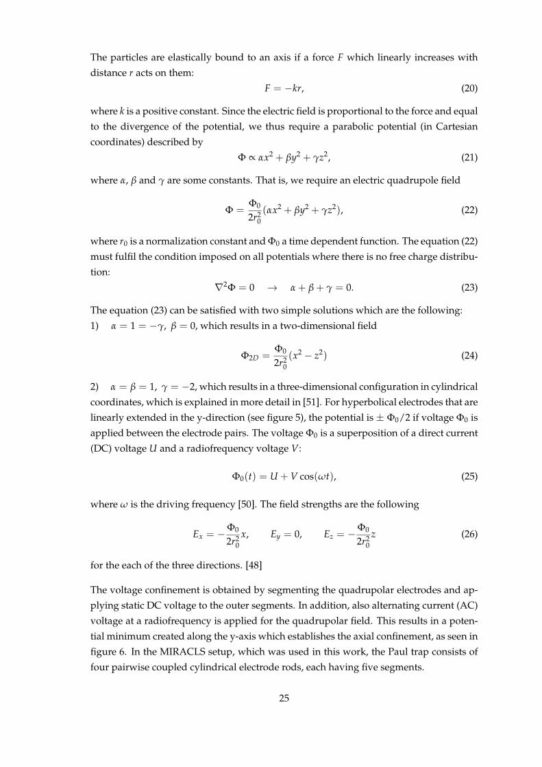
The particles are elastically bound to an axis if a force F which linearly increases with

distance r acts on them:

F = −kr, (20)

where k is a positive constant. Since the electric field is proportional to the force and equal

to the divergence of the potential, we thus require a parabolic potential (in Cartesian

coordinates) described by

Φ ∝ αx2 + βy2 + γz2, (21)

where α, β and γ are some constants. That is, we require an electric quadrupole field

Φ =Φ0

2r20(αx2 + βy2 + γz2), (22)

where r0 is a normalization constant and Φ0 a time dependent function. The equation (22)

must fulfil the condition imposed on all potentials where there is no free charge distribu-

tion:

∇2Φ = 0 → α + β + γ = 0. (23)

The equation (23) can be satisfied with two simple solutions which are the following:

1) α = 1 = −γ, β = 0, which results in a two-dimensional field

Φ2D =Φ0

2r20(x2 − z2) (24)

2) α = β = 1, γ = −2, which results in a three-dimensional configuration in cylindrical

coordinates, which is explained in more detail in [51]. For hyperbolical electrodes that are

linearly extended in the y-direction (see figure 5), the potential is ± Φ0/2 if voltage Φ0 is

applied between the electrode pairs. The voltage Φ0 is a superposition of a direct current

(DC) voltage U and a radiofrequency voltage V:

Φ0(t) = U + V cos(ωt), (25)

where ω is the driving frequency [50]. The field strengths are the following

Ex = −Φ0

2r20

x, Ey = 0, Ez = −Φ0

2r20

z (26)

for the each of the three directions. [48]

The voltage confinement is obtained by segmenting the quadrupolar electrodes and ap-

plying static DC voltage to the outer segments. In addition, also alternating current (AC)

voltage at a radiofrequency is applied for the quadrupolar field. This results in a poten-

tial minimum created along the y-axis which establishes the axial confinement, as seen in

figure 6. In the MIRACLS setup, which was used in this work, the Paul trap consists of

four pairwise coupled cylindrical electrode rods, each having five segments.

25

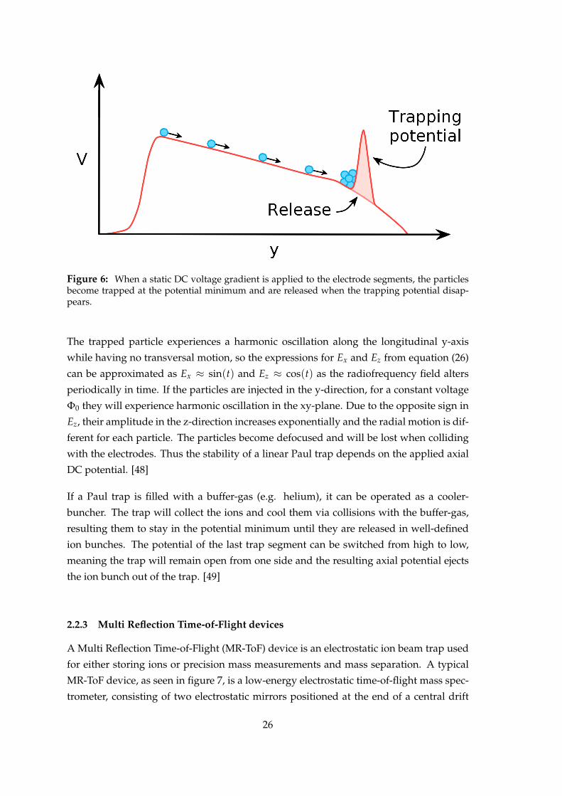
Figure 6: When a static DC voltage gradient is applied to the electrode segments, the particlesbecome trapped at the potential minimum and are released when the trapping potential disap-pears.

The trapped particle experiences a harmonic oscillation along the longitudinal y-axis

while having no transversal motion, so the expressions for Ex and Ez from equation (26)

can be approximated as Ex ≈ sin(t) and Ez ≈ cos(t) as the radiofrequency field alters

periodically in time. If the particles are injected in the y-direction, for a constant voltage

Φ0 they will experience harmonic oscillation in the xy-plane. Due to the opposite sign in

Ez, their amplitude in the z-direction increases exponentially and the radial motion is dif-

ferent for each particle. The particles become defocused and will be lost when colliding

with the electrodes. Thus the stability of a linear Paul trap depends on the applied axial

DC potential. [48]

If a Paul trap is filled with a buffer-gas (e.g. helium), it can be operated as a cooler-

buncher. The trap will collect the ions and cool them via collisions with the buffer-gas,

resulting them to stay in the potential minimum until they are released in well-defined

ion bunches. The potential of the last trap segment can be switched from high to low,

meaning the trap will remain open from one side and the resulting axial potential ejects

the ion bunch out of the trap. [49]

2.2.3 Multi Reflection Time-of-Flight devices

A Multi Reflection Time-of-Flight (MR-ToF) device is an electrostatic ion beam trap used

for either storing ions or precision mass measurements and mass separation. A typical

MR-ToF device, as seen in figure 7, is a low-energy electrostatic time-of-flight mass spec-

trometer, consisting of two electrostatic mirrors positioned at the end of a central drift

26

tube. Here the Earnshaw’s theorem does not apply since the kinetic energy of the ions is

not zero and hence in the ions’ frame of reference, the electric field is not static [52].

The time-of-flight t of the ions is proportional to the square root of their mass-over-charge

ratio:

t ∝√

mq

(27)

and also depends on the ions’ initial conditions which have non-zero distributions for

momentum and position. This initial phase-space spread results in time-spread ∆t of the

arrival times, which can be taken into account and reduced when designing the device -

thus increasing its mass-resolving power which is defined as

R =m

∆m=

t2∆t

. (28)

To obtain higher mass resolving powers, the time-of-flight must be increased. This hap-

pens by either reducing the kinetic energy of the ions or increasing the length of their

flight path [53]. Increasing the flight path can be done by trapping the ions between the

MR-ToF device’s electrostatic mirrors, leading to flight path lengths several times longer

than the physical length of the device. In comparison with a single path spectrometer, an

MR-ToF device can thus reach a mass-resolving power that is larger by several orders of

magnitude (see [53] for more details).

Figure 7: A schematic drawing of an MR-ToF device, where each electrostatic mirror is com-posed of four mirror electrodes and a conducting mesh covers the central drift tube located be-tween the mirrors.

27

Figure 8: Above the MR-ToF cross-section are illustrated the two ejection methods, in-trap po-tential lift and mirror switching. The ion beam is depicted with red, in-trap potential with blueand the electrostatic mirrors’ potentials with grey.

For the axial confinement of the ions, their kinetic energy in the drift tube must be smaller

than the potential of the mirror electrodes. The confinement itself is done by the outer-

most electrodes while the innermost electrodes are used as ion lenses and provide radial

refocusing. There are two techniques [54] to inject and eject the ions from the MR-ToF

device , as illustrated in figure 8:

1. In-trap potential lift, where the mirror potentials stay constant but the ions are

injected with kinetic energy high enough to overcome the mirror potentials. Right

upon the moment when the ions enter the MR-ToF’s drift tube, the lift potential is

switched to the ground so the ions become trapped between the mirror potentials.

The ejection process is similar and includes switching the lift potential back to eject

the ions from the trap.

2. Mirror switching, where the injection mirror is switched down when the ion bunch

reaches the MR-ToF so it can pass into the device. The ejection happens similarly

by switching the ejection mirror down.

The in-trap potential lift is usually a favoured technique as it avoids the switching of

sensitive mirror electrode potentials and so the electric noise and potential fluctuations

remain minimal.

28

2.3 Collinear laser spectroscopy

As illustrated in figure 9, collinear laser spectroscopy (CLS) is performed by overlapping

a narrow-band CW laser beam with a fast ion/neutral atom beam. When the wavelength

of the laser is tuned to match the energy difference of the selected electric transition be-

tween the energy levels, the laser will provide resonant excitation of the ions. After this

they spontaneously decay back to their ground-state, emitting fluorescence photons in

the process.

Depending on the application, a charge-exchange cell (CEC) can be used to neutralize

the ions before they enter the light collection region, where the photons are detected by

photomultiplier tubes (PMTs). The hyperfine structure of the two states involved in the

excitation is obtained by counting the number of observed fluorescence photons as a

function of the scanned laser frequency.

Figure 9: In a collinear geometry, laser (blue) and ion (red) beams are overlapped. The laserexcites the ions to an excited state from where they decay back to the ground-state emitting flu-orescence photons which then can be detected using a photomultiplier tube (PMT). Also shownis a hyperfine spectrum, where each peak corresponds to one transition from a hyperfine mani-fold to another, which is obtained when the photon counts are plotted as a function of the laserfrequency.

29

In the reference frame of the ions the laser frequency vREST experiences a Doppler shift

according to the relativistic Doppler effect [55]

vREST = vLAB1 + β√1− β2

, (29)

where vLAB is the laser frequency measured by the wavemeter and β is the relativistic

Lorentz factor

β =uc=

√1− m2c4

(qV + mc2)2 (30)

where u is velocity of the ions, c is the speed of light, q is the electric charge of the ion, mis the mass of the ion, and V is the total acceleration voltage used. Thus, the frequency

in the reference frame of the ions can be altered by applying an additional, tunable accel-

eration potential to the ions. This is called Doppler tuning, and it allows the locking of a

laser frequency to a precise reference frequency. Some advantages from this method are

the elimination of the systematic uncertainties associated with frequency scanning and

additionally, the acceleration voltage can be changed in a faster and more reliable way

than the laser frequency.

When using a collinear geometry, the laser beam (either counter- or co-propagating with

the ion beam) interacts with the accelerated ion bunches that experience a velocity com-

pression along their axis of motion. This compression is caused by the acceleration to a

well-defined energy E while preserving the original energy-spread δE but reducing the

velocity spread

δv =1√

2mEδE, (31)

where m is the mass of the ion [13]. The longitudinal velocity spread needs to be re-

duced as much as possible to obtain narrow linewidths which are crucial for resolving

the hyperfine structure. This is done by accelerating the beam with 30-60 keV acceleration

voltage before it enters the CLS setup and as a result, the linewidth is reduced to a level

similar to the natural linewidth (Doppler compression), which is some tens of MHz [56].

Due to its high accuracy and precision, CLS is a powerful tool that allows access to the nu-

clear ground-state properties of radionuclides far from stability, and thus provides valu-

able insight into the nuclear shell structure. Nowadays it is routinely used at RIB-facilities

to study properties like the nuclear spin, the electromagnetic multipole moments, and the

mean-square charge radius for a wide range of nuclei [13]. These observables can be ex-

tracted independently of any nuclear model, and thus provide important insight into the

nuclear structure and properties.

30

The experimental sensitivity is improved by using a cooled and bunched ion beam. The

cooling leads to a better laser-ion overlap in the light collection region due to improved

beam quality. Another advantage is the possibility of background suppression. As the

primary source for background in CLS comes from continuous sources, such as the laser

stray light and PMT dark counts [57], it can be reduced significantly by time-gating the

signal from the PMTs on the narrow ion bunch.

2.3.1 Spectral lineshapes and broadening mechanisms

The natural linewidth is the minimal linewidth that the resonance peaks in the hyper-

fine spectrum have due to the Heisenberg’s uncertainty principle. It is described by a

Lorentzian lineshape and determined from the finite lifetime τ of the excited state

Γ =1

2πτ. (32)

The natural linewidth is extremely difficult to obtain experimentally, as several broaden-

ing mechanisms affect the width and shape of the peaks. One of these is the Doppler

broadening, which is the inhomogeneous broadening often much larger than the natural

linewidth when using low beam energies. When an atom is moving with velocity u with

respect to the observer, it experiences a non-relativistic shift for frequency

v = v0

(1± u

c

), (33)

where v0 is the mean optical frequency and the + sign refers to the emitter moving to-

wards the observer, and the − sign for the emitter moving away from the observer. For

atoms with thermal velocity distribution in temperature T, the linewidth resulting from

the Doppler effect is described by a Gaussian profile

∆vD =2v0

c

√2 ln 2

kBTm

, (34)

where kB is the Boltzmann constant. However, this effect can be eliminated by employing

a measurement technique that is insensitive to Doppler broadening. [58]

Another broadening mechanism is a power broadening which originates from the stim-

ulated emission induced by the laser photons. This effect decreases the lifetime of the

excited state compared to the lifetime with only spontaneous decay. Power broadening

can also be described by a Lorentzian lineshape. Yet other mechanisms are a transit-time

broadening caused if the laser-ion interaction time is small compared to the lifetime of

the excited state (negligibly small for CLS), and pressure broadening originating from

the interaction with other particles (usually negligible for CLS due to vacuum condi-

tions). Taking all these different broadening mechanisms into account, the resulting line-

31

shape is described by a Voigt profile, which is convolution of the saturated Gaussian and

Lorentzian profiles. The Gaussian profile can be described by

∆vG =

(1

σ√

2π

)−(x−a)2/2σ2

, (35)

where σ is the standard deviation, a is the mean, and the Gaussian full-width at half

maximum (FWHM) is ΓG = 2σ√

2 ln 2 = 2.355σ. The Lorentzian profile is

∆vL =1π

ΓL/2(x− x0)2 + (ΓL)2 , (36)

where x0 is the centre and ΓL is the Lorentzian FWHM. [59]

The total linewidth of the Voigt profile [60] can be presented as an approximation:

∆vV ≈ 0.53456∆vL

√0.2166∆v2

L + ∆v2G. (37)

A comparison between the lineshapes obtained with the Gaussian, Lorentzian and Voigt

profiles is shown in figure 10.

Figure 10: A comparison between Gaussian, Lorenzian, and Voigt lineshapes with the samefull-width half-maximum (FWHM) and the same normalized integral area.

32

2.3.2 Optical pumping

Optical pumping refers to the act of injecting light into some medium to excite it into the

higher-lying energy levels. It is used both in laser physics and in fundamental physics,

where e.g. several laser cooling methods rely on the optical pumping of the atoms or

ions.

In spectroscopic measurements, the intention can be to selectively populate a certain

state, like some hyperfine sublevel. The selection rules due to the conservation of the

angular momentum play an essential role. This makes it possible to e.g. perform a se-

lective pumping of certain states within a manifold of states. For many cases, such a

process involves several optical pumping steps and spontaneous emission before the tar-

geted states are predominantly populated. Additionally, optical pumping can be used

for isotope separation as different isotopes have somewhat different transition energies,

to resonantly move the population to and from different states, to induce nuclear orien-

tation in radionuclides and thus allow resonance detection when observing the resulting

decay anisotropy, to move populations to states which are more efficient or suit better

for collinear laser spectroscopy purposes, and sequentially move a population to higher

excitation energy until ionization takes place. [13, 58]

Optical pumping can sometimes result in problematic effects, like in the MIRACLS setup

(described in the following chapter) where the population is pumped out from the state

of interest. This is the reason why the use of radiofrequency is explored to possibly re-

populate that state and boost the signal detected in the measurements.

2.4 General concept of MIRACLS

The Multi Ion Reflection Apparatus for Collinear Laser Spectroscopy (MIRACLS) was in-

troduced in 2017 [61] to take better advantage of the exotic radioactive isotopes produced

at ISOLDE-CERN, by probing the same ion many times, thus increasing the observation

time and therefore the experimental sensitivity. Conventional CLS is typically limited to

nuclides whose production yields are relatively high, ranging between 1000 – 10 000 ions

per second. The laser-atom interaction time is of the order of microseconds, while the

half-life of the ions is tens of milliseconds or more. The most exotic nuclides, residing far

from the valley of stability, are produced with low production yields, so new methods

are needed to measure their nuclear properties. One example is to detect ions produced

in a laser ionization process, rather than the photons which are emitted by the atoms.

This method, called Collinear Resonance Ionization Spectroscopy (CRIS), only requires

production rates of the order of 10 ions per second [62].

33

The approach taken by MIRACLS is to utilize the entire lifetime of the exotic radioiso-

topes by using a Multi Reflection Time-of-Flight (MR-ToF) device to trap a bunched ion

beam meanwhile performing CLS on it. When the ions are trapped between the MR-ToF

device’s two electrostatic mirrors, the laser will interact with them at each revolution and

thus effectively increases the interaction time compared to conventional CLS, where the

laser only interacts with the ion beam once. Theoretically, the only efficiency limitation

for MIRACLS is thus the maximal trapping time and the half-life of the ions. This means

the MIRACLS method would allow access to nuclides with very low production yields.

A schematic picture of the MIRACLS Proof-of-Principle (PoP) setup is shown in figure

11. The method is especially suitable for studying closed two-level systems, where the

ions decay directly from the excited state to the initial state without populating other

metastable fine or hyperfine structure states in between. For other systems, this sponta-

neous decay can populate other states, which leads to a reduction in signal as the number

of revolutions increases.

Figure 11: A schematic drawing of the MIRACLS PoP-setup where an offline ion source (1)produces a continuous ion beam, which is injected into a Paul trap (3) and accelerated (4). Then,the ion bunches are trapped in the MR-ToF device (16). The ion beam is depicted by red line andthe laser beam with blue. See the text for details.

34

Typically, CLS is performed at beam energies of about 30 keV to minimize the Doppler

broadening. The MIRACLS PoP-setup is being tested at a lower beam energy of 1.3 keV

using an offline ion source and an MR-ToF device modified for laser spectroscopy, to

demonstrate the feasibility of the method. MIRACLS aims to work with 30 keV kinetic

energies after the PoP-stage when an MR-ToF suitable for 30 keV beam energies will be

designed and constructed.

As illustrated in figure 11, an offline (magnesium) ion source produces a continuous ion

beam which is first collimated and then injected into a buffer-gas (helium) filled linear

Paul trap for cooling, accumulation and bunching. After the time-focused ion bunches

are released from the Paul trap, they are accelerated with the crown-shaped electrodes to-

wards an electrostatic Einzel lens (lens 1) and a pulsed drift tube (lift 1) which is switched

from high voltage (HV) to ground when the ions have reached its centre. The ions gain a

kinetic energy of approximately 2 keV and continue travelling towards the second Einzel

lens (lens 2) and the first electrostatic quadrupole bender (QPB1), which bends the ion

beam 90 onto the MR-ToF axis. Between the QPB1 and MR-ToF, there’s a retractable

MagneToF detector for beam diagnostics. The ion beam is focused by Einzel lenses 3

and 4 before the injection into the MR-ToF device. In the MR-ToF the ions are trapped

for several revolutions, while the laser probes them during each revolution. The laser

provides a resonant optical excitation of the ions: when the laser is held in resonance

with one HFS component of the optical line it excites the ions to the ionic excited state,

from which they will spontaneously decay to several lower levels and emit fluorescence

photons. These photons can then be detected by a PMT in the optical detection region

of the MR-ToF device’s drift tube (also called central drift tube, or lift 2 in figure 11). A

more detailed view of the operation of the MR-ToF is illustrated in figure 8. At the end

of the beamline, there’s another quadrupole bender (QPB2) that bends the beam 90 to-

wards a multichannel plate detector for detection. The laser beam enters and exits the

setup through quartz windows installed at Brewster angles (called Brewster windows)

in order to minimize reflections. Next to these, sets of aperture systems are installed to

minimize the background photon counts.

The MR-ToF device in the MIRACLS PoP-setup consists of two electrostatic mirror elec-

trodes, each composed of four cylindrical electrodes and a central drift tube (two elec-

trodes connected by a fine, conducting mesh). The innermost of the mirror electrode

segments are biased to a negative potential to achieve a radial ion refocusing. The three

outer electrodes provide reflecting potential walls used to confine the ions.

35

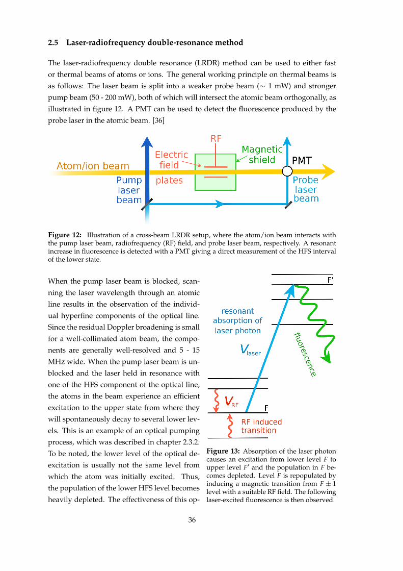
2.5 Laser-radiofrequency double-resonance method

The laser-radiofrequency double resonance (LRDR) method can be used to either fast

or thermal beams of atoms or ions. The general working principle on thermal beams is

as follows: The laser beam is split into a weaker probe beam (∼ 1 mW) and stronger

pump beam (50 - 200 mW), both of which will intersect the atomic beam orthogonally, as

illustrated in figure 12. A PMT can be used to detect the fluorescence produced by the

probe laser in the atomic beam. [36]

Figure 12: Illustration of a cross-beam LRDR setup, where the atom/ion beam interacts withthe pump laser beam, radiofrequency (RF) field, and probe laser beam, respectively. A resonantincrease in fluorescence is detected with a PMT giving a direct measurement of the HFS intervalof the lower state.

Figure 13: Absorption of the laser photoncauses an excitation from lower level F toupper level F′ and the population in F be-comes depleted. Level F is repopulated byinducing a magnetic transition from F ± 1level with a suitable RF field. The followinglaser-excited fluorescence is then observed.

When the pump laser beam is blocked, scan-

ning the laser wavelength through an atomic

line results in the observation of the individ-

ual hyperfine components of the optical line.

Since the residual Doppler broadening is small

for a well-collimated atom beam, the compo-

nents are generally well-resolved and 5 - 15

MHz wide. When the pump laser beam is un-

blocked and the laser held in resonance with

one of the HFS component of the optical line,

the atoms in the beam experience an efficient

excitation to the upper state from where they

will spontaneously decay to several lower lev-

els. This is an example of an optical pumping

process, which was described in chapter 2.3.2.

To be noted, the lower level of the optical de-

excitation is usually not the same level from

which the atom was initially excited. Thus,

the population of the lower HFS level becomes

heavily depleted. The effectiveness of this op-

36

tical pumping is furthermore enhanced if the atoms have a slow (thermal) velocity which

results in longer interaction time with the pump beam. So even the atoms that decay

back to their initial lower state will have sufficient time to absorb another photon before

leaving the pump region. After interacting with the pump beam, the atoms continue un-

til they are irradiated with the probe laser beam. Since the population of the appropriate

lower state HFS was already greatly depleted, the probe beam is not able to cause much

fluorescence. However, if a suitably chosen radiofrequency (RF) transition is applied to

repopulate the depleted level, a resonant increase in the fluorescence can be observed.

This process is also illustrated in figure 13. The linewidth of these double-frequency sig-

nals depends on the transit-time of the atoms in the RF field and is typically ∼ 10 kHz.

Nearly every transition which connects the depleted and the populated level satisfying

the E1 or M1 selection rules can be used. The transition usually ranges from RF to mi-

crowave regimes and arrangement like this allows for the measurement of the lower-state

hyperfine intervals to a precision of 1 kHz or better. [36]

Experimentally, an LRDR measurement is executed by the tuning the laser wavelength

into resonance with a selected HFS component of an optical line, thus allowing the pump

beam to deplete the population in the lower levels. As the laser wavelength is held fixed,

can the frequency of RF be swept repeatedly through a range where resonance is to be

expected, while the fluorescence is observed as a function of the RF frequency. [63]

2.5.1 Using LRDR in collinear geometry

The use of fast beams for optical spectroscopy is preferred since it reduces the Doppler

width and provides excellent overlap between the atom and the laser beam, compared to

a cross-geometry experiment on collimated beams. However, since the linewidth of the

RF resonance depends on the transit time of the ions travelling through the RF region, and

that with a fast beam the transit-time is rather short, the experimental linewidths will be

broad. Illustrated in figure 14 is a collinear LRDR setup for slow ion beams, where the

interaction region consists of three sections: pump region (A), probe region (B), and RF

region (C). To prevent the laser from being in exact resonance with the Doppler-shifted

ions along the collinear beam path, small post-acceleration Faraday cages are included

in A and B regions. When they are kept at a small potential of around a few hundred

volts, the ions and laser are tuned to resonance within these two regions and will not be

in resonance in other sections. Apart from this, the arrangement is fully analogous to the

cross-beam version described above. [64]

The pump and probe regions can be identically constructed resonant absorption regions

where the laser-induced fluorescence occurs. In the pump region, the ions absorb laser

photons resonantly, causing a transition from hyperfine level F of lower state to the hy-

perfine level F′ of the upper state. As a result, the level F becomes depleted. It can be

37

repopulated to some extent by inducing a transition between the neighbouring hyperfine

level F± 1 with the application of a suitable RF field in the C region. The RF resonance

can then be detected by scanning the applied RF, and thus the hyperfine splitting in the

lower level can be measured with high precision. Typical linewidths achieved in the

literature are of the order of 100 kHz. [63, 64]

As compared to the conventional optical collinear laser spectroscopy, the collinear LRDR

comes with the distinct advantage that it offers superior resolution, and therefore yields

more precise hyperfine constants. This precision, in turn, can allow measuring e.g. hy-

perfine anomalies or the higher-order nuclear moments. An important disadvantage is

the reduced efficiency of the method, due to the inherent inefficiencies of e.g. the optical

pumping, the RF excitation process, and the transmission losses due to the larger size of

the apparatus. Furthermore, special care has to be taken to avoid light-shifts in the RF

spectra, since the laser beam is also present in the RF interaction region. In chapter 4,

it will be investigated how to adapt this collinear LRDR geometry into the MIRACLS

concept.

Figure 14: A schematic illustration of a collinear LRDR setup, where A is the pump region, Bis the probe region, and C is the radiofrequency region with an RF electrode. A and B consist ofsimilar open-ended cylindrical Faraday cages.

38

3 Study of the magnetic octupole moment of 173Yb

3.1 Experimental setup at the IGISOL

This chapter will provide a brief introduction to the current IGISOL-4 facility and its

collinear laser spectroscopy line and the relevant equipment located at the Accelerator

Laboratory in the Department of Physics, University of Jyväskylä (JYFL-ACCLAB). The

offline measurements with atomic 173Yb will also be described in detail.

3.1.1 IGISOL-4 facility

The Ion-Guide Isotope Separator On-Line (IGISOL) is a research facility located at JYFL-

ACCLAB. The current version of the IGISOL-setup at JYFL is the fourth in order (IGISOL-

4) and the research mainly focuses on collinear laser spectroscopy, decay spectroscopy

and high-precision mass spectrometry. The IGISOL method was developed in Jyväskylä

in the 1980s to produce radioactive ion beams of exotic nuclei and has since then been

adapted to other facilities as well. The method allows the primary recoils to be mass-

separated on-line and is chemically insensitive allowing the production of radioactive

beams from all elements, also including the refractory elements that are usually difficult

to produce at the ISOL-facilities. The current layout of the entire IGISOL-facility is pre-

sented in figure 15, where most of the equipment is located on the first floor, with the

offline ion sources being on the second floor. [65]

Figure 15: xThe IGISOL-4 facility beamline consists of the following components:

xxxxx1) MCC30/15 cyclotron 6) Focal plane of switchyardxxxxx2) Beamline from K130 cyclotron 7) Decay spectroscopy linexxxxx3) Target chamber and laser 8) RFQ cooler-buncherxxxxx3) ionization in-gas-cell/in-jet 9) Collinear laser spectroscopy linexxxxx4) Offline ion sources 10) Mass spectrometry andxxxxx5) IGISOL separator magnet post-trap spectroscopy

39

At the IGISOL the primary beam can be provided by two cyclotrons: K130 (heavy ions

and high-energy light ions) and MCC30/15 (protons and deuterons). The beam from the

cyclotron is delivered to the ion guide, which is also called the front end, where it im-

pinges to a thin target foil and causes the formation of reaction products that scatter out

of the target material into a gas cell. In their way out, the reaction products lose some of

their energy due to energy-straggling and in the end, they will stop in the target chamber

filled with high-purity helium gas. The products will undergo a charge-exchange with

the helium gas and thermalize, resulting in a high amount of singly charged ions. The

ions are then extracted from the charge-exchange cell (CEC) using a sextupole ion guide

(SPIG) and accelerated to 30 keV in the beamline. A dipole magnet of mass resolving

power m/∆m = 350 (high enough to select the mass number) is used for mass separa-

tion of the extracted ions. Then the ion beam enters the switchyard, which is a vacuum

chamber housing ion optical elements, to be bent to either the decay spectroscopy line or

towards the radiofrequency quadrupole (RFQ) cooler-buncher. In the RFQ, the ions ac-

cumulated, cooled, and bunched. After the extraction from the RFQ, the ions are passed

through a low-energy (800 eV) transfer section, two quadrupole benders each of which

deflects the beam by 90, before being reaccelerated to 30 keV energy. This allows op-

tical access to the central axis of the RFQ by shining laser light through the quadrupole

bender [66]. The produced ion bunches are delivered either to the collinear laser line

or to JYFLTRAP Penning trap for more precise mass separation, mass spectrometry and

post-trap spectroscopy.

Alternatively, the ions of interest can also be produced offline. This happens by replacing

the gas cell with a glow-discharge spark ion source. This ion source is based on a phe-

nomenon called glow-discharge, which can be generated by applying voltage into two

electrodes inside a gas medium. If the gas pressure, the distance between electrodes, and

applied voltage are suitable, a current starts to flow between the two electrodes. When

the conditions are favourable, this results in a glow-discharge reaction that can be even

seen with the naked eye. However, a small current does not result in any visible effects.

The discharge relies on external radiation, such as cosmic radiation or natural radioactiv-

ity, to get started by generating the first ions. [67]

3.1.2 Collinear laser line

A schematic view of the collinear laser line at the IGISOL-4 is illustrated in figure 16.

The 30 keV ion beam enters the collinear beamline from the right side of the figure and

is guided by the XY steerers and focused by the quadrupole triplet before entering the

CEC. This cell consists of a cylinder, fillable with a chosen neutralizing element, and is

mounted on an electrically insulated platform. The platform can be floated to ± 10 kV

and used to Doppler-tune the atom into resonance with the laser. Heating is provided

40

electrically with a variable AC power supply while keeping both ends of the cylinder at

a constant temperature using an oil circulator. The ions that are not neutralized in the

charge-exchange reactions between the gas are deflected from the atom beam using a

pair of electrostatic deflector plates immediately after the cell. After the CEC, there is a

light collection region (LCR) with a segmented PMT. To reduce the amount of scattered

light reaching the PMT, several knife-edge baffles are placed near the LCR. The beamline

also has two Faraday cups and a silicon detector for optimizing the transport efficiency.

A micro-channel plate (MCP) detector is placed off-axis with retractable MagneToF mini

detector for beamtuning and monitoring of the neutralization efficiency. The laser beam

enters the setup from the left in the figure through a telescope system (pictured in figure

18) and the overlap of the ion and laser beam is achieved by tuning both of them through

a removable 0.9 mm aperture. [68]

The signals from the PMT segments are first amplified and then discriminated with a

constant-fraction discriminator. After this, the signals are time-stamped by a time-to-

digital converter. The hyperfine structure of the studied isotope can be scanned by ap-

plying an acceleration/deceleration potential to the ion beam. This potential needs to be

changed with precise reproducibility and short settling time. To do this, a voltage rang-

ing between -4 and 4 V is generated by the analogue output of a data acquisition board

and amplified with a high voltage amplifier. Both devices have large slew rate and fast

settling time enabling the fast voltage sweeps needed. After each scan, a calibration for

the voltage scanning range is carried out by a digital multimeter, which reads out the

scanning voltage after a 1:103 voltage divider. The voltage of the RFQ cooler platform

can be monitored similarly. [68]

Figure 16: xThe ion beam arrives from the right and laser beam from the left into the collinearbeamline at the IGISOL, which consists of the following components:

xxxxxxx1) Micro-channel plate detector 6) Charge-exchange cellxxxxxxx2) MagneToF mini detector 7) Silicon detectorxxxxxxx3) Faraday cup 8) Quadrupole tripletxxxxxxx4) Electrostatic deflector 9) XY steerersxxxxxxx5) Photo multiplier tube

41

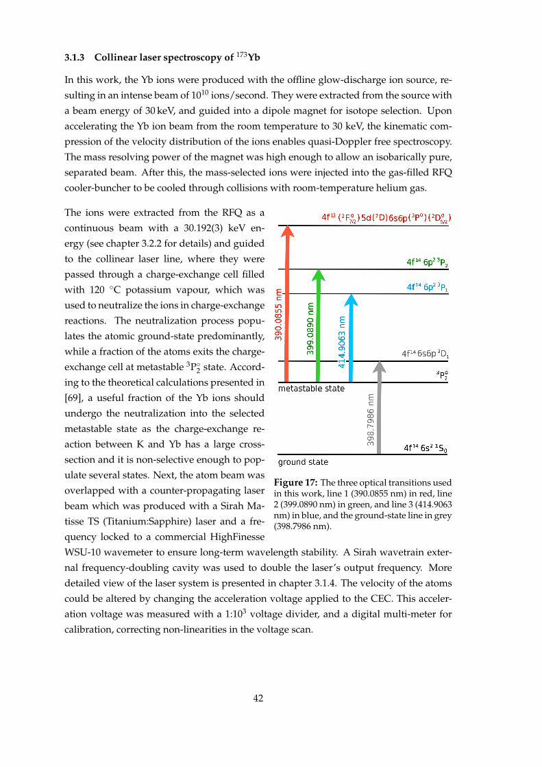
3.1.3 Collinear laser spectroscopy of 173Yb

In this work, the Yb ions were produced with the offline glow-discharge ion source, re-

sulting in an intense beam of 1010 ions/second. They were extracted from the source with

a beam energy of 30 keV, and guided into a dipole magnet for isotope selection. Upon

accelerating the Yb ion beam from the room temperature to 30 keV, the kinematic com-

pression of the velocity distribution of the ions enables quasi-Doppler free spectroscopy.

The mass resolving power of the magnet was high enough to allow an isobarically pure,

separated beam. After this, the mass-selected ions were injected into the gas-filled RFQ

cooler-buncher to be cooled through collisions with room-temperature helium gas.

Figure 17: The three optical transitions usedin this work, line 1 (390.0855 nm) in red, line2 (399.0890 nm) in green, and line 3 (414.9063nm) in blue, and the ground-state line in grey(398.7986 nm).

The ions were extracted from the RFQ as a

continuous beam with a 30.192(3) keV en-

ergy (see chapter 3.2.2 for details) and guided

to the collinear laser line, where they were

passed through a charge-exchange cell filled

with 120 C potassium vapour, which was

used to neutralize the ions in charge-exchange

reactions. The neutralization process popu-

lates the atomic ground-state predominantly,

while a fraction of the atoms exits the charge-

exchange cell at metastable 3P2 state. Accord-

ing to the theoretical calculations presented in

[69], a useful fraction of the Yb ions should

undergo the neutralization into the selected

metastable state as the charge-exchange re-

action between K and Yb has a large cross-

section and it is non-selective enough to pop-

ulate several states. Next, the atom beam was

overlapped with a counter-propagating laser

beam which was produced with a Sirah Ma-

tisse TS (Titanium:Sapphire) laser and a fre-

quency locked to a commercial HighFinesse

WSU-10 wavemeter to ensure long-term wavelength stability. A Sirah wavetrain exter-

nal frequency-doubling cavity was used to double the laser’s output frequency. More

detailed view of the laser system is presented in chapter 3.1.4. The velocity of the atoms

could be altered by changing the acceleration voltage applied to the CEC. This acceler-

ation voltage was measured with a 1:103 voltage divider, and a digital multi-meter for

calibration, correcting non-linearities in the voltage scan.

42

Table 2: Summary of all the transitions from the initial and final states which were used in thiswork, including their wavelengths λ, and wavenumbers ν.

Transition Initial state Final state λ [nm] ν [cm−1]

a 3P2 4f146p2 3P2 399.0890 44760.370

a 3P2 4f13(2F7/2) 5d(2D) 390.0855 45338.530

6s6p(3P) (2D5/2) (J = 2)

a 3P2 4f146p2 3P1 414.9063 43805.420b 4f146s2 1S0 4f146s6p 3D1 398.7986 25068.222c 4f146s2 2S1/2 4f146p 2P1/2 369.4190 27061.820

a Transition from the metastable state.b Transition from the ground-state.c Reference measurements using 171,173Yb+ to calibrate the beam energy.

The hyperfine structure of the atoms was measured by Doppler shifting the laser wave-

length that was observed in the atoms’ rest frame. The spectroscopy itself was performed

using three different optical transitions from the metastable 3P2 state, and one transition

from the ground-state 4f146s2 1S0, as illustrated in figure 17. These transition lines were

at 399.0890 nm, 390.0855 nm, and 414.9063 nm and are detailed in table 2. From these

measurements, the ratio of the atoms in the metastable 3P2 state to the 4f146s2 1S0 ground-

state can be approximated to be 1:104. However, this ratio seems to peculiarly disagree

with the theoretical estimate presented in [69]. Despite this low number of atoms in the

metastable 3P2 state, a clear hyperfine structure spectrum could be achieved in a few

hours. Also, reference measurements of the hyperfine intervals of the ground-states for171Yb+ and 173Yb+ were performed to calibrate the beam energy. This is described in

more detail in chapter 3.2.1.

3.1.4 Laser system

Collinear laser spectroscopy experiments at the IGISOL are nowadays conducted using a

laser laboratory which includes two Sirah Matisse 2 CW lasers pumped by a 20 W Spectra

Physics Millenia eV laser, as illustrated in figure 18. These Matisse lasers are the dye laser

(model DS) and Titanium:Sapphire laser (model TS), and they are used with WaveTrain

2 frequency doubling units.

In this work, the Matisse 2 TS laser was used and its optical layout is shown in figure

19. It is an actively stabilized Titanium:Sapphire ring laser [70]. The ring laser’s res-

onator has the form of a ring and the ring cavity contains e.g. the Titanium:Sapphire gain

medium, etalons, and filters for frequency control, and a unidirectional device. Com-

pared to standing wave (linear) laser resonator, the ring resonator enables two different

43

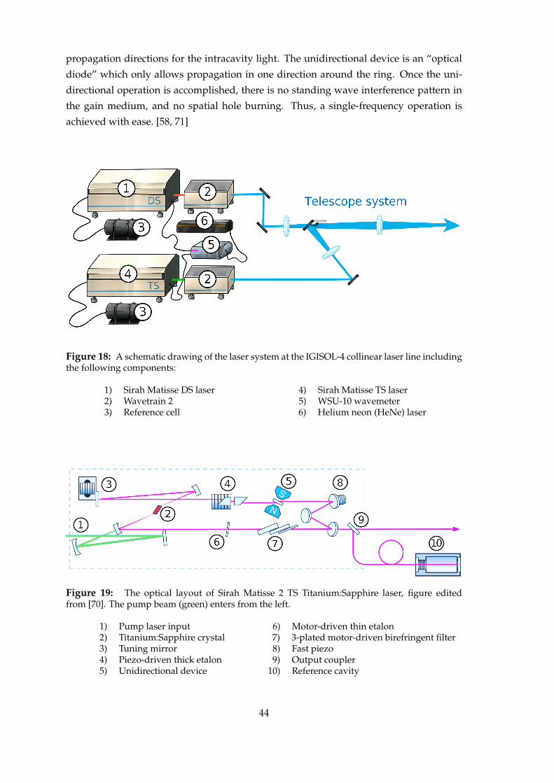
propagation directions for the intracavity light. The unidirectional device is an “optical

diode” which only allows propagation in one direction around the ring. Once the uni-

directional operation is accomplished, there is no standing wave interference pattern in

the gain medium, and no spatial hole burning. Thus, a single-frequency operation is

achieved with ease. [58, 71]

Figure 18: A schematic drawing of the laser system at the IGISOL-4 collinear laser line includingthe following components:

xxxxxxxx1) Sirah Matisse DS laser 4) Sirah Matisse TS laserxxxxxxxx2) Wavetrain 2 5) WSU-10 wavemeterxxxxxxxx3) Reference cell 6) Helium neon (HeNe) laser

Figure 19: xThe optical layout of Sirah Matisse 2 TS Titanium:Sapphire laser, figure editedfrom [70]. The pump beam (green) enters from the left.

xxxxxxx1) Pump laser input 6) Motor-driven thin etalonxxxxxxx2) Titanium:Sapphire crystal 7) 3-plated motor-driven birefringent filterxxxxxxx3) Tuning mirror 8) Fast piezoxxxxxxx4) Piezo-driven thick etalon 9) Output couplerxxxxxxx5) Unidirectional device 10) Reference cavity

44

Each laser has different sets of mirrors coated to correspond to specific wavelength ranges,

thus selecting only part of the full emission spectrum of the lasing medium. Selection of

a single frequency mode is done by scanning the birefringent filter and the thin etalon.

Here the birefringent filter consists of three birefringent plates of varying thicknesses and

the frequency can be selected by rotating the plates.

To accomplish a single-mode operation, two etalons are needed. These are the thin etalon

(a solid-state etalon) which narrows the frequency range, and the piezo-driven thick

etalon to select the final frequency mode. The unidirectional device is used to make

sure that the laser is in a clockwise running mode. Finally, the laser frequency can be

scanned by altering the cavity length with the fast piezo-driven tuning mirror. To es-

tablish short-term stability (i.e. a narrow linewidth), the laser has an external reference

cavity that is coupled to the fast piezo-driven cavity mirror with a feedback loop. For

long-term stability, the reference cavities can be locked into the WSU-10 wavemeter or to

a frequency-stabilized HeNe (helium-neon) laser using a transfer cavity.

For most of the elements studied in this setup, it is required to have frequency-doubled

light. This is achieved by using WaveTrain 2 frequency-doubling units which have trian-

gular enhancement cavity that contains a temperature-stabilized nonlinear crystal. The

crystal generates the second harmonic of the fundamental frequency from the laser. This

frequency-doubled laser light can then be focused into a 1 mm spot in front of the PMT

with the telescope system, and typical background rates due to the scattering of the laser

light are approximately 100 Hz for each 100 µW of laser light [68].

3.2 Data analysis for the hyperfine constants

The experiment was conducted as described in chapter 3.1.3 and the number of photons

was measured with a PMT for each acceleration voltage sweep. A calibrated acceleration

voltage V, as described in equation (30), was used and defined as a sum of the accelera-

tion voltage, and the RFQ cooler platform voltage, respectively:

V = Vacceleration + Vcooler. (38)

An example of the obtained hyperfine spectra is presented in figure 20, where the x-axis is

the frequency of the laser in the atom’s frame of reference, with a large number subtracted

(∼ 12000 cm−1) to see the differences in the frequencies since the hyperfine structure is

about six magnitudes smaller than the frequency of the laser. Each peak corresponds to

a transition from one hyperfine manifold to another; the number of peaks is determined

by nuclear and atomic spins, and the positions of the peaks correspond to the size of the

nuclear moments. The nuclear moments, including the magnetic octupole moment, can

be determined by measuring the distance between the peaks.

45

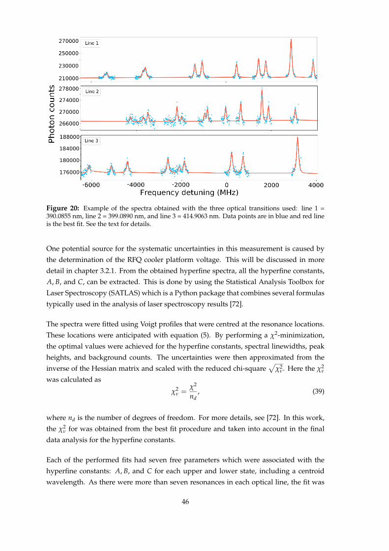
Figure 20: Example of the spectra obtained with the three optical transitions used: line 1 =390.0855 nm, line 2 = 399.0890 nm, and line 3 = 414.9063 nm. Data points are in blue and red lineis the best fit. See the text for details.

One potential source for the systematic uncertainties in this measurement is caused by

the determination of the RFQ cooler platform voltage. This will be discussed in more

detail in chapter 3.2.1. From the obtained hyperfine spectra, all the hyperfine constants,

A, B, and C, can be extracted. This is done by using the Statistical Analysis Toolbox for

Laser Spectroscopy (SATLAS) which is a Python package that combines several formulas

typically used in the analysis of laser spectroscopy results [72].

The spectra were fitted using Voigt profiles that were centred at the resonance locations.

These locations were anticipated with equation (5). By performing a χ2-minimization,

the optimal values were achieved for the hyperfine constants, spectral linewidths, peak

heights, and background counts. The uncertainties were then approximated from the

inverse of the Hessian matrix and scaled with the reduced chi-square√

χ2ν. Here the χ2

ν

was calculated as

χ2ν =

χ2

nd, (39)

where nd is the number of degrees of freedom. For more details, see [72]. In this work,

the χ2ν for was obtained from the best fit procedure and taken into account in the final

data analysis for the hyperfine constants.

Each of the performed fits had seven free parameters which were associated with the

hyperfine constants: A, B, and C for each upper and lower state, including a centroid

wavelength. As there were more than seven resonances in each optical line, the fit was

46

over-determined. This over-determination reduces the statistical uncertainties, which

results in precise values for the hyperfine constants although the signal-to-background

ratio was somewhat poor in some of the scans. To determine the final values for each

set of extracted hyperfine constants, their weighted mean was calculated including the

standard error of the weighted mean as the uncertainty.

To calculate the weighted mean for a data set of elements xi, the weight wi for each ele-

ment can be determined as a reciprocal of the variance σi:

wi =1σ2

i, (40)

when the weighted mean itself is defined as

x =

n∑

i=1wixi

n∑

i=1wi

. (41)

Typically, there exists some error in the variance of each individual data point, e.g. arising

from the fact that experimental errors may be underestimated if some error source is

forgotten, or if there is error in the calculation of the variance for each data point. In this

case, a correction must be made in the variance of the weighted mean:

σ2x = σ2

x χ2ν, (42)

where χ2ν is the reduced chi-squared and the square root of σx is the standard error of the

weighted mean, while σx is defined as

σx =

(√n

∑i=1

wi

)−1

, (43)

with the variance weights included. [73]

3.2.1 Determination of the RFQ cooler voltage offset

A source for systematic uncertainty of the hyperfine constants arises from the uncer-

tainty of the ion beam energy. If incorrect beam energy is assumed during the analysis,

the frequency scale of the hyperfine structure in the rest frame of the atoms experiences

a small stretching which might result in some distortion in the extracted hyperfine inter-

vals. Though, not much effect from this is expected for the value of the octupole constant

C, as the non-zero C is only manifested as a small perturbation on top of the consider-

ably larger dipole and quadrupole splittings. Regardless, this effect was carefully consid-

ered and removed by performing an ion beam energy calibration. This calibration relies

47

on reference measurements for the hyperfine intervals of the singly-charged 171Yb+ and173Yb+. Since these particular intervals have been measured extremely precisely, could

the beam energy calibration be performed [68].

To study this ionic ground-state, the temperature of the charge-exchange cell was brought

to room temperature and thus the ion beam no longer experienced neutralization. Thus,

CLS could be performed using the ionic 369.4190 nm line from the 4f146s2 2S1/2 state to

the 4f146p 2P1/2 state at 27061.820 cm−1. In total, three scans were taken for both 171Yb+

and 173Yb+.

To understand how much the deviation in the RFQ cooler voltage would affect on the

obtained values of the hyperfine constants, the results from the 171Yb+ and 173Yb+ data

analysis were plotted as in figure 21. On the y-axis is the difference between the weighted

mean of the extracted hyperfine constant Al and the corresponding literature value, which

are presented in table 3. The values for 173Yb+ were multiplied by three, so the values for

both isotopes scale similarly with the cooler voltage offset, accounting for the different

nuclear spins of the two isotopes.

Figure 21: Demonstrated here is how much the different cooler voltage offsets affect the hyper-fine constant Al for 171Yb+ and 173Yb+. The red and blue lines include errors, and were calculatedas a difference from the corresponding literature values.

Table 3: Summary of the extracted values for the hyperfine constants Al with the energy cali-bration, and their corresponding literature values, which were used to make the figure 21. Notethat the error bars here are purely statistical, and do not include a systematic uncertainty due tothe acceleration voltage.

Isotope Weighted mean of Al [MHz] Literature value of Al [MHz] Ref.

171Yb+ 12641.89(45) 12642.8121184682(4) [74]173Yb+ -3497.36(23) -3497.24007985(3) [75]

48

Figure 22: On the left, 171Yb+ is plotted and on the right is 173Yb+. Linear fit was done for thedatapoints using Origin Pro 2020, and from the resulting equation the values for the voltage offsetto obtain the literature value were solved. These offset voltage values were V171

off = 30.3298 V andV173

off = 37.2166 V.

The hyperfine constant Al obtained from each of these as a function of a voltage offset

range is plotted in figure 22. This figure also shows the linear fit used to determine the

voltage offset required to match the literature values listed in table 3. This procedure

was followed for both 171Yb+ and 173Yb+. Then, a weighted arithmetic mean was taken,

yielding ≈ 35.3 V. Note that the datapoints used in this fit were independent, and thus

the errors given by the linear fit are very small and therefore cannot be used. Instead, the

uncertainty on the offset voltage was obtained by propagating the mean uncertainty on

the experimental hyperfine Al constants. This value was further scaled by the reduced

chi-square [73]:

χ2ν =

1(n− 1)

n

∑i=1

(xi − x)2

σ2i

, (44)

where n = 2 for this case, and σi was the the standard error of the weighted mean from ta-

ble 3. Following this procedure, the final value for the voltage offset was Voffset = 35.3(34),

and it was added to the calibrated total ion beam energy for the final data analysis:

V = Vacceleration + Vcooler + Voffset. (45)

3.2.2 Systematic uncertainties in the experimental setup

The beam energy was assumed to have a 3 V uncertainty whose effect on the hyperfine

constants was approximated by refitting the spectra with -3 and +3 V offset to the beam

energy. The hyperfine constant values from these spectra were subtracted from the values

given in table 6. From the obtained values for ± 3 V spectra, means were taken to get the

final values, which are presented in table 4. It can be concluded that 3 V systematic

49

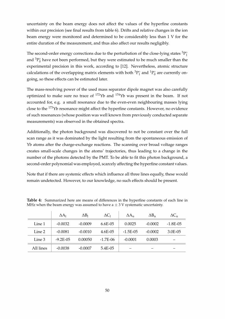
uncertainty on the beam energy does not affect the values of the hyperfine constants

within our precision (see final results from table 6). Drifts and relative changes in the ion

beam energy were monitored and determined to be considerably less than 1 V for the

entire duration of the measurement, and thus also affect our results negligibly.

The second-order energy corrections due to the perturbation of the close-lying states 3P1and 3P0 have not been performed, but they were estimated to be much smaller than the

experimental precision in this work, according to [12]. Nevertheless, atomic structure

calculations of the overlapping matrix elements with both 3P1 and 1P0 are currently on-

going, so these effects can be estimated later.

The mass-resolving power of the used mass separator dipole magnet was also carefully

optimized to make sure no trace of 172Yb and 174Yb was present in the beam. If not

accounted for, e.g. a small resonance due to the even-even neighbouring masses lying

close to the 173Yb resonance might affect the hyperfine constants. However, no evidence

of such resonances (whose position was well known from previously conducted separate

measurements) was observed in the obtained spectra.

Additionally, the photon background was discovered to not be constant over the full

scan range as it was dominated by the light resulting from the spontaneous emission of

Yb atoms after the charge-exchange reactions. The scanning over broad voltage ranges

creates small-scale changes in the atoms’ trajectories, thus leading to a change in the

number of the photons detected by the PMT. To be able to fit this photon background, a

second-order polynomial was employed, scarcely affecting the hyperfine constant values.

Note that if there are systemic effects which influence all three lines equally, these would

remain undetected. However, to our knowledge, no such effects should be present.

Table 4: Summarized here are means of differences in the hyperfine constants of each line inMHz when the beam energy was assumed to have a ± 3 V systematic uncertainty.

∆Al ∆Bl ∆Cl ∆Au ∆Bu ∆Cu

Line 1 -0.0032 -0.0009 6.6E-05 0.0025 -0.0002 -1.8E-05

Line 2 -0.0081 -0.0010 4.6E-05 -1.5E-05 -0.0002 3.0E-05

Line 3 -9.2E-05 0.00050 -1.7E-06 -0.0001 0.0003 –

All lines -0.0038 -0.0007 5.4E-05 – – –

50

3.2.3 Constraining of the overlapping peaks in the spectra

In some of the spectra partially overlapping resonances were detected. However, for

these overlapping peaks their ratio of amplitudes can be constrained by using a ratio of

the absolute theoretical intensities [13]:

IFF′ ∝ (2F + 1)(2F′ + 1)

F F′ 1

J J′ I

2

FJ J′ , (46)

where the factor in the curly brackets is the Wigner 6-j symbol and FJ J′ is the unperturbed

fine structure transition. The use of this ensures the convergence of the fit while also pre-

venting the convergence of non-physically small amplitudes for one of the components.

The peaks which were constrained are listed in table 5 and visually presented in figure 23.

Table 5: Summary of the constrained peaks for each line used. Depicted on the horizontallines are the peak pairs whose amplitudes were constrained as they were slightly overlapping, orconverging to zero amplitude.

Peak on left Location [MHz] Peak on right Location [MHz]

Line 1 1.2_1.2 -5405.31 1.2_3.2 -5291.463.2_3.2 -3575.65 3.2_5.2 -3551.65

Line 2 1.2_1.2 -3690.61 3.2_5.2 -3469.405.2_5.2 -944.53 7.2_9.2 -842.785

Line 3 5.2_7.2 -2099.53 5.2_3.2 -1883.53

Figure 23: The peaks shaded with blue were slightly overlapping or their amplitudes wereconverging to zero in some of the scans and thus needed to be constrained. More informationabout the peaks can be found in table 5.

51

3.2.4 Stability of the RFQ cooler voltage and the laser frequency

The RFQ cooler platform voltage and the laser frequency were monitored during the

measurement, and presented in figures 24 and 25, respectively. As can be seen, the cooler

voltage was lowered by about 10 V before the last four scans of the measurement, to

optimize the cooler transmission efficiency. To get a hold of the significance of this offset,

a 10 V offset in the beam energy would correspond to ∼ 2 MHz offset in the extracted

values of the hyperfine constants compared to their literature values. However, the laser

frequency only experienced very minor fluctuations (maximum of about 1.6 MHz) in

frequency during the whole measurement, so the effect from it should be very small.

Figure 24: The shaded red area is the error for the calibrated RFQ cooler voltage. There wasabout a 10 V drop in the RFQ cooler voltage during the last part of the measurement. The calibra-tion of the voltage is explained in chapter 3.2.1.

Figure 25: Shown here on the y-axis is the laser frequency in THz with a large number sub-tracted. These numbers were: line 1 (375.25471 THz), line 2 (383.91566 THz), and line 3 (360.94972THz).

52

3.3 Extracted hyperfine constants for the lower and upper states

Data from the used three different lines seemed to provide consistent values, thus pre-

senting a measure of confidence for the final hyperfine constants which are presented in

table 6. The constants are also compared to the existing literature values in table 7. The

constants of the upper states (Au, Bu, Cu) have no known literature values the so a com-

parison there was not possible. The uncertainties of the hyperfine constants are presented

in the brackets and are purely statistical.

As it can be seen, a satisfactory agreement for the hyperfine constant Al is obtained,

but the value for Bl has a bit larger deviation and Cl differs greatly from the literature.

And as an interesting note, the hyperfine constant Au of the 4f146p2 3P1 state would be

zero within the uncertainties of this measurement. The hyperfine constants Al, Bl, Cl are

plotted in figures 26, 27, and 28, and the constants Au, Bu, Cu in figures 29, 30, and 31,

respectively. For the metastable 3P2 state, the hyperfine constant Cl is zero within one

standard deviation for each line.

Table 6: Summary of the hyperfine constants extracted in these measurements. The uncertainties(one standard deviation) are given in brackets and they are calculated as the standard error of theweighted mean from the values which were obtained for each measurement scan.

Al [MHz] Bl [MHz] Cl [MHz] Au [MHz] Bu [MHz] Cu [MHz]

399.0890 nm -741.9(3) 1343.9(23) 0.08(17) -123.3(2) -628.8(24) 0.10(17)-741.7(2) 1346.7(18) 0.16(13) -123.4(2) -629.1(17) 0.05(12)-742.3(2) 1347.5(19) -0.06(14) -123.4(2) -631.3(18) 0.27(13)-742.3(2) 1350.8(23) -0.19(16) -123.5(2) -628.7(20) -0.07(14)-741.7(5) 1346.1(47) -0.20(32) -123.7(5) -631.6(39) 0.01(28)

Weight. mean -742.0(1) 1347.2(10) -0.01(7) -123.4(10) -629.8(9) 0.08(7)

390.0855 nm -741.9(3) 1350.3(29) 0.12(22) -347.7(3) 121.4(26) -0.15(20)-741.7(6) 1346.4(50) -0.01(35) -347.9(5) 115.5(45) -0.35(34)-741.6(6) 1351.7(47) -0.13(26) -347.6(7) 112.7(66) 0.46(49)-741.8(4) 1346.0(39) 0.48(28) -347.4(39) 122.3(35) -0.22(28)

Weight. mean -741.8(2) 1348.9(19) 0.12(13) -347.6(2) 120.0(18) -0.15(14)

414.9063 nm -742.0(4) 1343.8(36) -0.12(26) 0.06(68) 483.4(18) –-742.1(5) 1346.6(36) 0.21(28) -0.64(83) 484.1(21) –-742.1(7) 1350.9(61) -0.38(43) -0.05(106) 485.8(28) –-741.0(9) 1338.8(75) 0.45(43) 1.51(140) 483.5(37) –

Weight. mean -742.0(3) 1345.4(23) 0.01(17) -0.01(45) 484.0(12) –

All lines -741.98(9) 1347.3(8) 0.02(6) – – –

53

Table 7: Comparison between the weighted mean of the all lines used in this work and twodifferent literature values.

Reference Year Al [MHz] Bl [MHz] Cl [MHz]

This work 2020 -741.98(9) 1347.3(8) 0.02(6)

[12] 2013 -742.11(2) 1339.2(2) 0.54(2)

[76] 1991 -742(5) 1342(38) –

To be noted that at least one peak in the observed HFS spectra was smaller than the

background noise but still visible in some of the scans, however constraining it did not

affect any of the values of the extracted hyperfine constants within the uncertainties of

this measurement.

Using all 13 scans measured, the weighted mean of the constants Cl from the metastable3P2 state is zero at the 1σ (68%) confidence level. This value of 0.02(6) MHz considerably

differs from the 0.54(2) MHz value obtained by using the 769.9487 nm line in [12]. So far,

the cause for this deviation remains unclear. Using our current setup, it was not possible

to conduct measurement using this line as the wavelength of the spontaneously emitted

light from the atoms lies outside the sensitivity range of the used photomultiplier tube.

Thus, further research using the 769.9487 nm line might shed light on this matter.

Figure 26: All the values which were extracted for hyperfine constant Al in this measurement,where the shaded areas represent the weighted mean of each line. On the right, the weightedmean of these 13 scans is compared to the value obtained in [12].

54

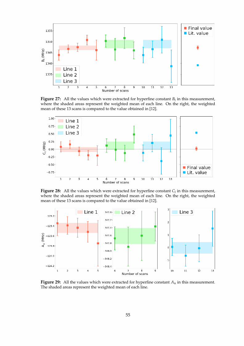
Figure 27: All the values which were extracted for hyperfine constant Bl in this measurement,where the shaded areas represent the weighted mean of each line. On the right, the weightedmean of these 13 scans is compared to the value obtained in [12].

Figure 28: All the values which were extracted for hyperfine constant Cl in this measurement,where the shaded areas represent the weighted mean of each line. On the right, the weightedmean of these 13 scans is compared to the value obtained in [12].

Figure 29: All the values which were extracted for hyperfine constant Au in this measurement.The shaded areas represent the weighted mean of each line.

55

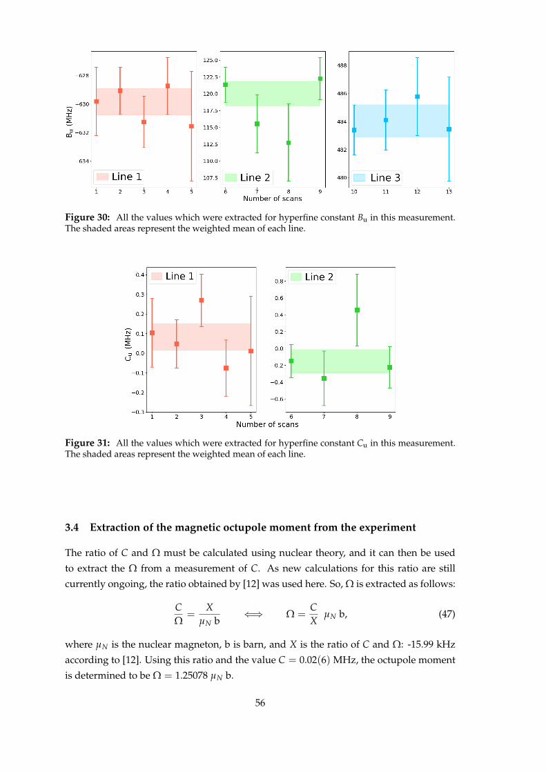
Figure 30: All the values which were extracted for hyperfine constant Bu in this measurement.The shaded areas represent the weighted mean of each line.

Figure 31: All the values which were extracted for hyperfine constant Cu in this measurement.The shaded areas represent the weighted mean of each line.

3.4 Extraction of the magnetic octupole moment from the experiment

The ratio of C and Ω must be calculated using nuclear theory, and it can then be used

to extract the Ω from a measurement of C. As new calculations for this ratio are still

currently ongoing, the ratio obtained by [12] was used here. So, Ω is extracted as follows:

CΩ

=X

µN b⇐⇒ Ω =

CX

µN b, (47)

where µN is the nuclear magneton, b is barn, and X is the ratio of C and Ω: -15.99 kHz

according to [12]. Using this ratio and the value C = 0.02(6) MHz, the octupole moment

is determined to be Ω = 1.25078 µN b.

56

The error for this value is calculated using the propagation of uncertainty [73]:

s f =

√(∂ f∂x

)2

s2x +

(∂ f∂y

)2

s2y +

(∂ f∂z

)2

s2z + · · ·, (48)

where s f is the standard deviation for function f , ∂ is the partial derivative, and sx,y,z,...

represents the standard deviation for x, y, x, ... Thus, for octupole moment, the error is

calculated as

sΩ =

√(1X

)2

s2C, (49)

where sC is the uncertainty of the hyperfine constant C. The final value for the experi-

mentally extracted octupole moment from this work is then Ω = −1.3(38) µN b.

3.5 Nuclear theory estimates for the octupole moment

The hyperfine interaction can be represented in terms of the multipole expansion of

the field potential when considering the classical electromagnetic interactions between

atomic electrons and the nucleus. The magnetic octupole expectation value can thus be

calculated using the single-particle model [39]:

ΩµN 〈r2〉 =

32

2I − 1(2I + 4)(2I + 2)

×

(I + 2)[(I − 32 )gl + gs], I = l + 1

2

(I − 1)[(I + 52 )gl − gs], I = l − 1

2

(50)

where⟨r2⟩ is the mean-squared radius of the valence nucleon orbital, and gl and gs are

the nuclear g-factors for orbital and spin angular momentum, respectively. The g-factors

are defined as [1]

gl = 1, gs = 5.5856912(22) for free protons, and (51)

gl = 0, gs = −3.8260837(18) for free neutrons. (52)

However, from the systematics of the magnetic dipole moments, it is known that these g-

factor values for free nucleons are not able to provide a sufficient enough approximation

for the majority of nuclei. Thus, quenched values are often used and defined as gqs =

0.6 gs. In principle, to obtain values for⟨r2⟩, theoretical calculations would be required.

As an approximation, data on the total nuclear charge radius was used from [77], where

R =⟨r2⟩1/2 = 5.3046(59) fm so

⟨r2⟩ = 28.1388 fm2. This is the mean-squared radius of the

valence nucleon, so to make an approximation here the total mean-squared radius is used

instead. To obtain the value for only the valence nucleon, nuclear theory calculations will

be required but their derivation is currently in progress.

57

For 17370 Yb103 (I = 5/2−), according to the single-particle shell model, the unpaired neu-

tron will occupy the f5/2 = l − 1/2 orbital as the nuclear spin is of negative parity. Thus,

the equation (50) simplifies asΩ

µN 〈r2〉 = − gs

7(53)

for ytterbium, and results in Ω f = 0.546583 and Ωq = 0.327950 for the free and quenched

single-particle shell model values, respectively. To convert the result from the equation

(53) to the same units with the experimental octupole moment, it must be multiplied with

µN⟨r2⟩. These values, along with a comparison between all three theoretical models and

experimental values used here, are presented in table 8.

The extreme single-particle model described above has limits similar to the Schmidt lines,

and does not characterize the octupole moments sufficiently enough. However, by us-

ing an axially-symmetric collective model in strong coupling, can the octupole moments

of odd-A nuclei with reasonably well-known energy levels be described. To calculate

the expectation value of the magnetic octupole moment using the collective model, the

following equation can be used

Ω =2I(2I − 1)(2I − 2)

(2I + 1)(2I + 2)(2I + 3)× µN

[67

gcR20 + g(3)

wω0

G(I, N, β)

], (54)

where gc depends on the electric charge density and the gradient of mass density, R0 is

the radius of a sphere with same volume as the deformed nucleus, g(3) is "total" particle

gyromagnetic ratio for the octupole term,√/mω0 is the intrinsic oscillator length, and

G[I, N, β] is a complicated function of I, N, and β which is given in [78].

3.6 Interpretation of the obtained results

The values obtained for the hyperfine constants are consistent for each scan and also

agree with the literature values well regarding to Al but deviate a little for Bl, as seen in

tables 6 and 7. It can also be noted, that for the 390.0855 nm line the values of Bl and

Cl seem to vary more compared to other lines, along with the Bu values within that line.

This might have something to do with the deviation between the obtained value of Bl

and its literature value. However, as the uncertainties are quite large here, at least for Cl

the effect would not have been notable and our value is still considerably smaller than

the previously obtained one, though here different lines were used. The reason for this

deviation is currently unknown.

As it can be seen from figure 32 and table 8, the experimentally determined octupole

moment from our measurement agrees with all the theoretical estimates within its error

bars which, however, are quite large. Notably, these theory values differ in sign with our

58

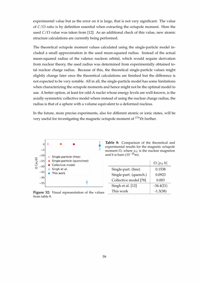
experimental value but as the error on it is large, that is not very significant. The value

of C/Ω ratio is by definition essential when extracting the octupole moment. Here the

used C/Ω value was taken from [12]. As an additional check of this value, new atomic

structure calculations are currently being performed.

The theoretical octupole moment values calculated using the single-particle model in-

cluded a small approximation in the used mean-squared radius. Instead of the actual

mean-squared radius of the valence nucleon orbital, which would require derivation

from nuclear theory, the used radius was determined from experimentally obtained to-

tal nuclear charge radius. Because of this, the theoretical single-particle values might

slightly change later once the theoretical calculations are finished but the difference is

not expected to be very notable. All in all, the single-particle model has some limitations

when characterizing the octupole moments and hence might not be the optimal model to

use. A better option, at least for odd-A nuclei whose energy levels are well-known, is the

axially-symmetric collective model where instead of using the nuclear charge radius, the

radius is that of a sphere with a volume equivalent to a deformed nucleus.

In the future, more precise experiments, also for different atomic or ionic states, will be

very useful for investigating the magnetic octupole moment of 173Yb further.

Figure 32: Visual representation of the valuesfrom table 8.

Table 8: Comparison of the theoretical andexperimental results for the magnetic octupolemoment Ω, where µN is the nuclear magnetonand b is barn (10−28m).

Ω [µN b]

Single-part. (free) 0.1538Single-part. (quench.) 0.0923Collective model [78] 0.003Singh et al. [12] -34.4(21)This work -1.3(38)

59

4 Study of the radiofrequency excitations with Mg+

In this chapter, the combination of the collinear LRDR and the MIRACLS method is at-

tempted, and a preliminary test is conducted. Some designs and ideas will be presented

to answer the possible challenges and difficulties arising from this kind of project.

4.1 Design of the RF electrode and the new drift tube for an MR-ToF device

This section provides details of the testing of RF penetrability, and the designs for the RF

electrodes and modified drift tubes for the MR-ToF device.

The original tube consists of two types of fine conducting mesh to allow the fluorescence

photon detection as the PMT is located right above it. This had to be taken into account

when designing a new tube to house the desired RF electrodes. Additionally, there is not

much extra space near the drift tube area because of the surrounding straylight shield and

the three passing support rods, and the electrostatic mirrors and associated cables have

high voltage through them. The surrounding area inside the MR-ToF device is shown in

figure 37 and the HV cables and drift tube mesh in figure 33.

Figure 33: At the top is shown the entire MR-ToF device and the corresponding HV cables. Atbottom left is a close-up from the cables leading to the mirror electrodes and at bottom right is aclose-up of the two meshes that form the drift tube itself.

60

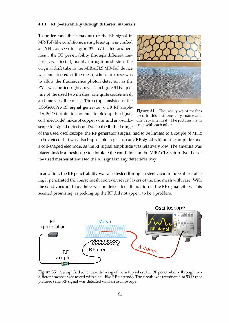
4.1.1 RF penetrability through different materials

Figure 34: The two types of meshesused in this test, one very coarse andone very fine mesh. The pictures are inscale with each other.

To understand the behaviour of the RF signal in

MR-ToF-like conditions, a simple setup was crafted

at JYFL, as seen in figure 35. With this arrange-

ment, the RF penetrability through different ma-

terials was tested, mainly through mesh since the

original drift tube in the MIRACLS MR-ToF device

was constructed of fine mesh, whose purpose was

to allow the fluorescence photon detection as the

PMT was located right above it. In figure 34 is a pic-

ture of the used two meshes: one quite coarse mesh

and one very fine mesh. The setup consisted of the

DSSG600Pro RF signal generator, 6 dB RF ampli-

fier, 50 Ω terminator, antenna to pick up the signal,

coil "electrode" made of copper wire, and an oscillo-

scope for signal detection. Due to the limited range

of the used oscilloscope, the RF generator’s signal had to be limited to a couple of MHz

to be detected. It was also impossible to pick up any RF signal without the amplifier and

a coil-shaped electrode, as the RF signal amplitude was relatively low. The antenna was

placed inside a mesh tube to simulate the conditions in the MIRACLS setup. Neither of

the used meshes attenuated the RF signal in any detectable way.

In addition, the RF penetrability was also tested through a steel vacuum tube after notic-

ing it penetrated the coarse mesh and even seven layers of the fine mesh with ease. With

the solid vacuum tube, there was no detectable attenuation in the RF signal either. This

seemed promising, as picking up the RF did not appear to be a problem.

Figure 35: A simplified schematic drawing of the setup where the RF penetrability through twodifferent meshes was tested with a coil-like RF electrode. The circuit was terminated to 50 Ω (notpictured) and RF signal was detected with an oscilloscope.

61

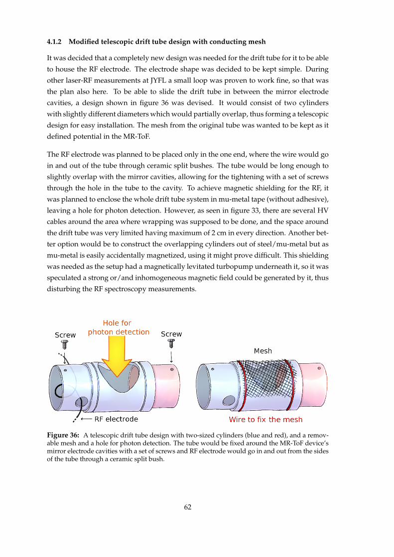
4.1.2 Modified telescopic drift tube design with conducting mesh

It was decided that a completely new design was needed for the drift tube for it to be able

to house the RF electrode. The electrode shape was decided to be kept simple. During

other laser-RF measurements at JYFL a small loop was proven to work fine, so that was

the plan also here. To be able to slide the drift tube in between the mirror electrode

cavities, a design shown in figure 36 was devised. It would consist of two cylinders

with slightly different diameters which would partially overlap, thus forming a telescopic

design for easy installation. The mesh from the original tube was wanted to be kept as it

defined potential in the MR-ToF.

The RF electrode was planned to be placed only in the one end, where the wire would go

in and out of the tube through ceramic split bushes. The tube would be long enough to

slightly overlap with the mirror cavities, allowing for the tightening with a set of screws

through the hole in the tube to the cavity. To achieve magnetic shielding for the RF, it

was planned to enclose the whole drift tube system in mu-metal tape (without adhesive),

leaving a hole for photon detection. However, as seen in figure 33, there are several HV

cables around the area where wrapping was supposed to be done, and the space around

the drift tube was very limited having maximum of 2 cm in every direction. Another bet-

ter option would be to construct the overlapping cylinders out of steel/mu-metal but as

mu-metal is easily accidentally magnetized, using it might prove difficult. This shielding

was needed as the setup had a magnetically levitated turbopump underneath it, so it was

speculated a strong or/and inhomogeneous magnetic field could be generated by it, thus

disturbing the RF spectroscopy measurements.

Figure 36: A telescopic drift tube design with two-sized cylinders (blue and red), and a remov-able mesh and a hole for photon detection. The tube would be fixed around the MR-ToF device’smirror electrode cavities with a set of screws and RF electrode would go in and out from the sidesof the tube through a ceramic split bush.

62

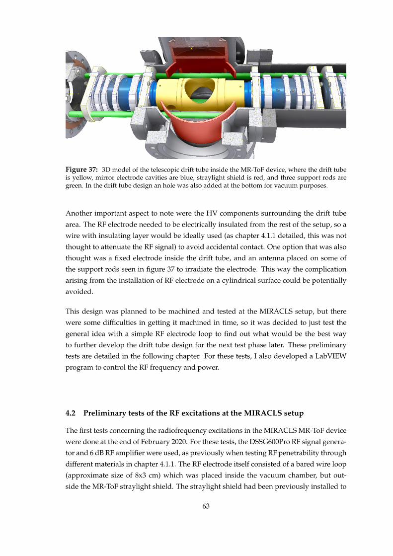
Figure 37: 3D model of the telescopic drift tube inside the MR-ToF device, where the drift tubeis yellow, mirror electrode cavities are blue, straylight shield is red, and three support rods aregreen. In the drift tube design an hole was also added at the bottom for vacuum purposes.

Another important aspect to note were the HV components surrounding the drift tube

area. The RF electrode needed to be electrically insulated from the rest of the setup, so a

wire with insulating layer would be ideally used (as chapter 4.1.1 detailed, this was not

thought to attenuate the RF signal) to avoid accidental contact. One option that was also

thought was a fixed electrode inside the drift tube, and an antenna placed on some of

the support rods seen in figure 37 to irradiate the electrode. This way the complication

arising from the installation of RF electrode on a cylindrical surface could be potentially

avoided.

This design was planned to be machined and tested at the MIRACLS setup, but there

were some difficulties in getting it machined in time, so it was decided to just test the

general idea with a simple RF electrode loop to find out what would be the best way

to further develop the drift tube design for the next test phase later. These preliminary

tests are detailed in the following chapter. For these tests, I also developed a LabVIEW

program to control the RF frequency and power.

4.2 Preliminary tests of the RF excitations at the MIRACLS setup

The first tests concerning the radiofrequency excitations in the MIRACLS MR-ToF device

were done at the end of February 2020. For these tests, the DSSG600Pro RF signal genera-

tor and 6 dB RF amplifier were used, as previously when testing RF penetrability through

different materials in chapter 4.1.1. The RF electrode itself consisted of a bared wire loop

(approximate size of 8x3 cm) which was placed inside the vacuum chamber, but out-

side the MR-ToF straylight shield. The straylight shield had been previously installed to

63

reduce the background photon counts. This simplified test setup was used to avoid tech-

nical complications, such as isolating the electrode from the rest of the setup, disturbing

electric fields and voltage switching complications, associated with placing the RF elec-

trode inside the actual drift tube. A simplified schematic drawing of this placement and

the relevant measurement setup is illustrated in figure 38.

BNC and SMA cables were used to connect the RF electrode and the RF generator outside

the vacuum. A LabVIEW program I wrote at JYFL was integrated into the existing MIR-

ACLS laser scanning program and was proven to work as expected. After optimizing the

ion beam transport and the operational parameters of the MR-ToF, the first resonances on24,25,26Mg could be obtained.

Once this was achieved, an RF signal with frequency of 1788.763 MHz was applied. How-

ever, after several measurements, no evidence of an enhancement in the photon rate due

to the RF excitation could be observed, as seen in figure 39. In this figure, there are bursts

of photons when the ions are in front of the PMT and then the signal drops due to the op-

tical pumping into the other HFS level. The purpose of the RF signal is to excite the ions

back to the HFS level of interest as explained in figure 13 and therefore it was expected

that the red (RF on) signal’s height wouldn’t have decayed away as fast as it did.

Figure 38: A simple schemetic drawing of the setup and RF electrode (pink) placement at theMIRACLS setup, where controlling of the RF was done with a LabVIEW program integrated intothe existing laser frequency scanning program.

64

Figure 39: Presented here is the the sum on 4 measurements with RF on (red) and sum of 4measurements with RF off (blue), with RF frequency of 1788.763 MHz. As it can be seen, thereseems to be no clear RF enhancement visible.

Various additional checks and tests were performed. The loading time of the MR-ToF was

increased to enhance the signal strength. The RF frequency was changed to a Doppler-

shifted value. After still having not observed any signal, the RF generator and ampli-

fier were replaced by a Rohde & Schwarz triggerable generator, which allowed for a

frequency-modulation of the RF signal. This was done in case the exact RF frequency

was missed or an external magnetic field had shifted the transition frequency. The RF

output was triggered on after 300 µs from switching down the lift 2. The results from

the measurements with the modulated RF signal and 300 µs triggering can be seen in

figure 40.

An additional step that could have been taken would have been to modulate the laser

intensity using a Pockels cell, but there was no time to investigate this option. An-

other option would have been to take out the whole RF electrode in hopes of trying to

make it better, which would have required breaking the vacuum, all while also having

to impedance-match it to 50 Ω. Furthermore, a larger-gain amplifier might have helped

in case the RF-field was too small to induce significant excitations. However, no such

amplifier was available at the time.

65

Figure 40: Here the RF was triggered exactly 300 µs (red line) after switching lift 2 down whilealso modulating the RF signal over the range of 1.5 MHz to cover all the magnetic substates.On the right, the green is the subtraction between the RF on and off measurements. There’s asmall offset in the background, most likely due to the laser power dropping after two hours ofmeasuring. However, it seems there is no signal enhancement at 300 µs as it was expected.

4.2.1 Laser cooling as a detection method

As an alternative approach to realizing in-trap RF spectroscopy, an RF signal was applied

to one of the segments of the linear Paul trap (see figure 5) which cools and bunches the

ions prior to their injection into the MR-ToF. The CW laser beam was, in this case, directed

also into the Paul trap. For even-even isotopes, tuning the frequency of the laser to a few

100 MHz below the transition frequency leads to laser cooling, which dampens the ion

motion in all directions.

When the laser frequency is tuned slightly below the resonant frequency of the ion, it

absorbs more photons when it moves towards the laser beam than it does when moving

away from it due to the Doppler effect. In the frame of the moving ion, when a counter-

propagating laser beam with a frequency below the ion’s resonance frequency is applied,

it leads to a Doppler shift that increases the frequency of the laser beam as observed by the

ion. This Doppler shift then causes the laser light to come closer to resonance with the ion,

and thus increases the rate of absorption from the beam. When these ions de-excite, they

emit photons isotropically, thus resulting in a net momentum kick which slows down

the ions. To cool the ions’ motion in all three directions, the radiative force must have

a component along with the direction corresponding to each degree of freedom, that is

the laser beam must not get through the trap along any of the axes of symmetry. Since

the ions will return from the excited hyperfine state to the ground-state after a time of

some nanoseconds, this absorption-emission process is repeated very quickly and results

in effective cooling of the ions. [40, 79]

66

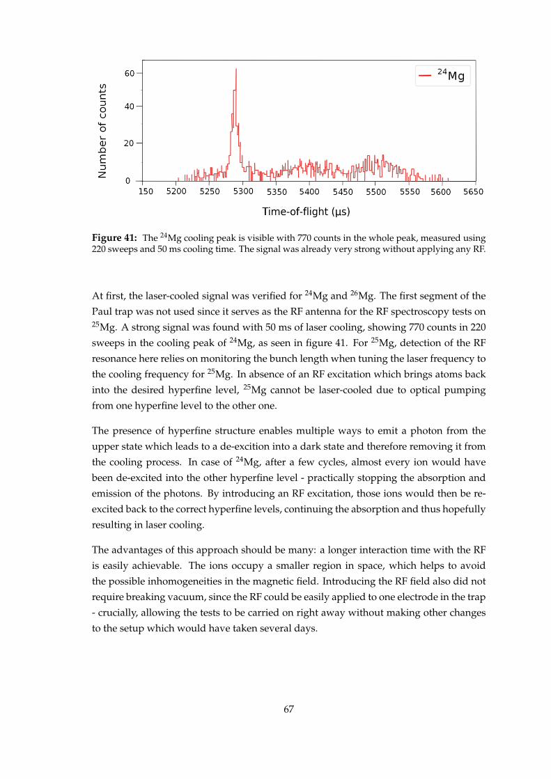
Figure 41: The 24Mg cooling peak is visible with 770 counts in the whole peak, measured using220 sweeps and 50 ms cooling time. The signal was already very strong without applying any RF.

At first, the laser-cooled signal was verified for 24Mg and 26Mg. The first segment of the

Paul trap was not used since it serves as the RF antenna for the RF spectroscopy tests on25Mg. A strong signal was found with 50 ms of laser cooling, showing 770 counts in 220

sweeps in the cooling peak of 24Mg, as seen in figure 41. For 25Mg, detection of the RF

resonance here relies on monitoring the bunch length when tuning the laser frequency to

the cooling frequency for 25Mg. In absence of an RF excitation which brings atoms back

into the desired hyperfine level, 25Mg cannot be laser-cooled due to optical pumping

from one hyperfine level to the other one.

The presence of hyperfine structure enables multiple ways to emit a photon from the

upper state which leads to a de-excition into a dark state and therefore removing it from

the cooling process. In case of 24Mg, after a few cycles, almost every ion would have

been de-excited into the other hyperfine level - practically stopping the absorption and

emission of the photons. By introducing an RF excitation, those ions would then be re-

excited back to the correct hyperfine levels, continuing the absorption and thus hopefully

resulting in laser cooling.

The advantages of this approach should be many: a longer interaction time with the RF

is easily achievable. The ions occupy a smaller region in space, which helps to avoid

the possible inhomogeneities in the magnetic field. Introducing the RF field also did not

require breaking vacuum, since the RF could be easily applied to one electrode in the trap

- crucially, allowing the tests to be carried on right away without making other changes

to the setup which would have taken several days.

67

Figure 42: The laser cooled peaks of 24Mg (upper) and 26Mg (lower) can be seen in blue, and redcolour indicates the place where 25Mg peak should have shown up. As it can be seen, the countrate was very low and 25Mg was conspicuously absent.

Now the RF generator was floated to the DC voltage of the Paul trap’s segment and lasers

were tuned to cool 25Mg after a reference measurements on 24Mg and 26Mg to calibrate

the time-of-flight. After a very long measurement with a low count rate, where the RF

frequency was tuned to the resonance frequency of 1778 MHz, no signal was observed at

the time-of-flight of 25Mg, as seen in figure 42.

4.3 Redesigned drift tube with a coaxial geometry

From the preliminary tests, it became clear that a more complex drift tube modifications

are needed in order to obtain a detectable RF signal and cause the excitations. It has been

previously demonstrated in collinear laser-radiofrequency literature [80] that coaxial ge-

ometry is often used, thus it could be adapted to the MR-ToF device as well. This could

be done as follows: the drift tube itself would serve as the outer part of the coaxial elec-

trode geometry, and an inner conductor would be added along the whole length of the

drift tube, as envisioned in figure 43. This just a rough idea though, as there are numer-

ous aspects to this design that need careful consideration and planning, so they are not

discussed in this thesis.

68

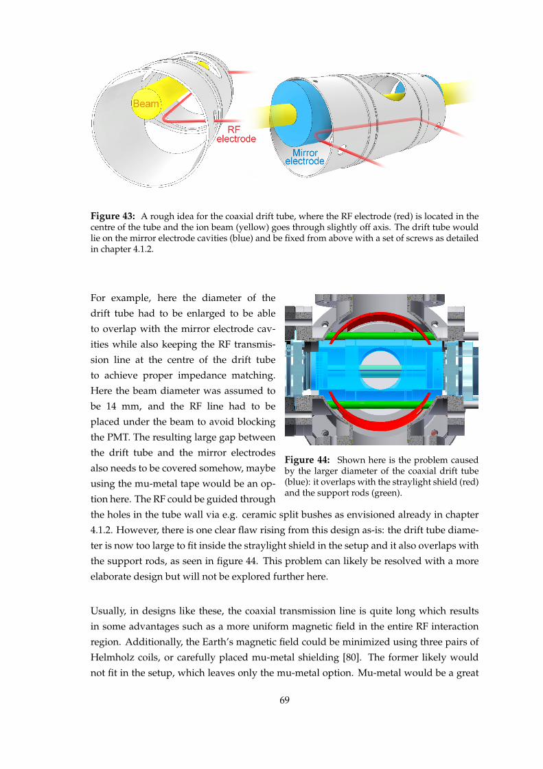
Figure 43: A rough idea for the coaxial drift tube, where the RF electrode (red) is located in thecentre of the tube and the ion beam (yellow) goes through slightly off axis. The drift tube wouldlie on the mirror electrode cavities (blue) and be fixed from above with a set of screws as detailedin chapter 4.1.2.

Figure 44: Shown here is the problem causedby the larger diameter of the coaxial drift tube(blue): it overlaps with the straylight shield (red)and the support rods (green).

For example, here the diameter of the

drift tube had to be enlarged to be able

to overlap with the mirror electrode cav-

ities while also keeping the RF transmis-

sion line at the centre of the drift tube

to achieve proper impedance matching.

Here the beam diameter was assumed to

be 14 mm, and the RF line had to be

placed under the beam to avoid blocking

the PMT. The resulting large gap between

the drift tube and the mirror electrodes

also needs to be covered somehow, maybe

using the mu-metal tape would be an op-

tion here. The RF could be guided through

the holes in the tube wall via e.g. ceramic split bushes as envisioned already in chapter

4.1.2. However, there is one clear flaw rising from this design as-is: the drift tube diame-

ter is now too large to fit inside the straylight shield in the setup and it also overlaps with

the support rods, as seen in figure 44. This problem can likely be resolved with a more

elaborate design but will not be explored further here.

Usually, in designs like these, the coaxial transmission line is quite long which results

in some advantages such as a more uniform magnetic field in the entire RF interaction

region. Additionally, the Earth’s magnetic field could be minimized using three pairs of

Helmholz coils, or carefully placed mu-metal shielding [80]. The former likely would

not fit in the setup, which leaves only the mu-metal option. Mu-metal would be a great

69

candidate for magnetic shielding due to its highly permeable properties. To shield from

high-frequency (> 100 kHz) RF fields, materials such as copper, aluminium, and metal-

lized plastics could be used.

However, due to the current situation with the pandemic and the arisen technical diffi-

culties in the integration of the RF, no detailed study of the feasibility of this design was

undertaken but is planned for the future.

4.4 Conclusions about the laser-RF method in an MR-ToF

Due to the pandemic situation, final tests with a fully constructed drift tube design were

not possible so it remains unclear if this would have worked. However, the RF integration

into the MR-ToF device was deemed a more complicated task than initially thought, so

perhaps some simulations about the RF field in the MR-ToF-like conditions would also

prove beneficial in the future. The MR-ToF could also be used in mirror switching mode

instead of the in-trap potential lift to potentially help with the technical complications

associated with the voltage switching in the drift tube. To make sure the RF-field was

sufficient enough, a large-gain amplifier should also be tested along with the suitably

modified drift tube.

As it has been previously described in the literature, a coaxial drift tube geometry might

also be the best option here, since it would provide a more uniform magnetic field in the

RF interaction region. The effect from Earth’s magnetic field also needs to be considered,

and the RF region appropriately shielded from it. Shielding this region fully might prove

somewhat challenging, as the optical detection region with the PMT is located right above

the centre of the drift tube and thus cannot be blocked.

As demonstrated in [37, 38], the use of RF spectroscopy is possible in at least Paul and

Penning traps, and that it is possible for complicated species such as singly-charged eu-

ropium even when the species are not cooled beyond simple buffer-gas cooling. Many

of the advantages of working in these traps will hopefully also translate into the use of

the MR-ToF device in the future, opening new exciting possibilities for high precision

spectroscopy.

70

5 Discussion

Currently, there are only 18 elements with an experimentally measured magnetic oc-

tupole moment. More measurements for a larger variety of elements would thus prove

beneficial to understand the higher-order effects in different nuclei. A very large value of

the hyperfine C constant of 173Yb reported in the literature was interesting for two rea-

sons. Firstly, if correct, it would indicate a severe problem in our understanding of the

magnetic octupole moments. Secondly, the value is such that experimental studies on ra-

dioactive ytterbium isotopes would have been possible with currently available methods

at the IGISOL. The measurements presented in this thesis do not confirm the strikingly

large value of the 173Yb octupole moment reported in the literature but instead yield a

value which is zero within the experimental uncertainty, and closer to the typical val-

ues obtained for other elements. This work shows that higher-precision methods will be

needed for further octupole moment studies in the future.

This work brings the experimental value in agreement with both free and quenched

single-particle model, and the collective model. This thesis will, in any case, serve as

a motivation for future octupole measurements and theoretical investigations for stable

and radioactive elements. From the analysis process, it also can be concluded that careful

analysis and peak constraining are crucial for the final values of the hyperfine constants,

as they can have a significant effect on especially for the octupole constant if not done

in a thorough manner. No earlier measurements of the upper state hyperfine constants

Au, Bu, and Cu of the lines used here were found in the literature. This thesis thus pro-

vides the first values for these constants as well.

This thesis has also made the first steps in a bigger project which aims to implement the

laser-RF techniques in an MR-TOF device. While no positive results could be obtained,

several important lessons were learnt while constructing and using the first rudimentary

setup. It is clear, that the combination of MIRACLS and LRDR needs more work and

there are several complications which need to be addressed in the future. Some simu-

lations could be useful here, and it would help to know if there is some magnetic field

present inside the MR-ToF as this would induce a wide range of splittings in the mF lev-

els which cannot be easily covered. If the combination of these two methods succeeds

in the future, it will undoubtedly have great potential to improve our understanding of

the atomic nucleus and its properties due to the superior resolution typical to LRDR. The

more precise determination of the hyperfine constants will enable measurements of e.g.

the hyperfine anomalies or the higher-order nuclear moments. All things considered,

perhaps it would be most effective to construct an entirely new MR-ToF with the RF ex-

citation region in mind in order to avoid the multiple complications encountered here.

Nevertheless, many obstacles need to be overcome before a successful result is obtained,

as is often the case when trying new things.

71

References

[1] Kenneth S. Krane. Introductory Nuclear Physics. Wiley, 1988.

[2] R. Paschotta. Lasers: Understanding the basics. RP. Photonics Encyclopedia. https:

//www.photonics.com/Articles/Lasers_Understanding_the_Basics/a25161, ac-

cessed 15.5.2020.

[3] H. J. Andra. Proceedings of the Fourth International Conference on Atomic Physics.

Atomic Physics, 4:635, 1975.

[4] William H. Wing, George A. Ruff, Willis E. Lamb, and Joseph J. Spezeski. Observa-

tion of the infrared spectrum of the hydrogen molecular ion HD+. Phys. Rev. Lett.,36:1488–1491, 1976.

[5] S.L. Kaufman. High-resolution laser spectroscopy in fast beams. Optics Communica-

tions, 17(3):309 – 312, 1976.

[6] R. Neugart, J. Billowes, M. L. Bissell, and K. Blaum et al. Collinear laser spectroscopy

at ISOLDE: new methods and highlights. Journal of Physics G: Nuclear and ParticlePhysics, 44(6):064002, 2017.

[7] T.E. Cocolios, R.P. de Groote, J. Billowes, and M.L. Bissell et al. High-resolution laser

spectroscopy with the Collinear Resonance Ionisation Spectroscopy (CRIS) experi-

ment at CERN-ISOLDE. Nuclear Instruments and Methods in Physics Research SectionB: Beam Interactions with Materials and Atoms, 376:284 – 287, 2016.

[8] Simon Sels, P. Fischer, and H. Heylen et al. First steps in the development of the

multi ion reflection apparatus for collinear laser spectroscopy. Nuclear Instrumentsand Methods in Physics Research Section B: Beam Interactions with Materials and Atoms,

2019.

[9] T.J. Mertzimekis, K. Stamou, and A. Psaltis. An online database of nuclear electro-

magnetic moments. Nuclear Instruments and Methods in Physics Research Section A:Accelerators, Spectrometers, Detectors and Associated Equipment, 807:56–60, 2016.

[10] Vladislav Gerginov, Andrei Derevianko, and Carol E. Tanner. Observation of the

nuclear magnetic octupole moment of 133Cs. Phys. Rev. Lett., 91:072501, 2003.

[11] Nicholas C. Lewty, Boon Leng Chuah, Radu Cazan, B. K. Sahoo, and M. D. Barrett.

Spectroscopy on a single trapped 137Ba+ ion for nuclear magnetic octupole moment

determination. Opt. Express, 20(19):21379–21384, 2012.

[12] Alok K. Singh, D. Angom, and Vasant Natarajan. Observation of the nuclear mag-

72

netic octupole moment of 173Yb from precise measurements of the hyperfine struc-

ture in the 3P2 state. Phys. Rev. A, 87:012512, 2013.

[13] P. Campbell, I.D. Moore, and M.R. Pearson. Laser spectroscopy for nuclear structure

physics. Progress in Particle and Nuclear Physics, 86:127 – 180, 2016.

[14] R. P. de Groote, J. Moreno, J. Dobaczewski, I. Moore, M. Reponen, B. K. Sahoo, and

C. Yuan. Measurement of an unusually large magnetic octupole moment in 45Sc

challenges state-of-the-art nuclear-structure theory. 2020.

[15] W. J. Childs, O. Poulsen, L. S. Goodman, and H. Crosswhite. Laser-rf double-

resonance studies of the hyperfine structure of 51V. Phys. Rev. A, 19:168–176, 1979.

[16] R. T. Daly and J. H. Holloway. Nuclear magnetic octupole moments of the stable

gallium isotopes. Phys. Rev., 96:539–540, 1954.

[17] Howard Howland Brown and John G. King. Hyperfine structure and octopole in-

teraction in stable bromine isotopes. Phys. Rev., 142:53–59, 1966.

[18] W. L. Faust and L. Y. Chow Chiu. Hyperfine structure of the metastable (4p)5(5s)3 p2

state of 36Kr83. Phys. Rev., 129:1214–1220, 1963.

[19] T. G. Eck and P. Kusch. Hfs of the 52 p 32

state of In115 and In113: Octupole interactions

in the stable isotopes of indium. Phys. Rev., 106:958–964, 1957.

[20] V. Jaccarino, J. G. King, R. A. Satten, and H. H. Stroke. Hyperfine structure of I127.

nuclear magnetic octupole moment. Phys. Rev., 94:1798–1799, 1954.

[21] M. J. Amoruso and W. R. Johnson. Relativistic one-electron calculations of shielded

atomic hyperfine constants. Phys. Rev. A, 3:6–12, 1971.

[22] W. L. Faust and M. N. McDermott. Hyperfine structure of the (5p)5(6s)3 p2 state of

54Xe129 and 54Xe131. Phys. Rev., 123:198–204, 1961.

[23] Vladislav Gerginov, Andrei Derevianko, and Carol E. Tanner. Observation of the

nuclear magnetic octupole moment of 133Cs. Phys. Rev. Lett., 91:072501, 2003.

[24] Nicholas C. Lewty, Boon Leng Chuah, Radu Cazan, Murray D. Barrett, and B. K.

Sahoo. Experimental determination of the nuclear magnetic octupole moment of137Ba+ ion. Phys. Rev. A, 88:012518, 2013.

[25] W. J. Childs. M1, e2, and m3 hyperfine structure and nuclear moment ratios for151,153Eu. Phys. Rev. A, 44:1523–1530, 1991.

[26] P. J. Unsworth. Nuclear dipole, quadrupole and octupole moments of 155Gd by

73

atomic beam magnetic resonance. Journal of Physics B: Atomic and Molecular Physics,

2(1):122–133, 1969.

[27] T. Brenner, S. Büttgenbach, W. Rupprecht, and F. Träber. Nuclear moments of the low

abundant natural isotope 176Lu and hyperfine anomalies in the lutetium isotopes.

Nuclear Physics A, 440(3):407 – 423, 1985.

[28] W. G. Jin, M. Wakasugi, T. T. Inamura, T. Murayama, T. Wakui, H. Katsuragawa,

T. Ariga, T. Ishizuka, and I. Sugai. Laser-rf double-resonance spectroscopy of177,179Hf. Phys. Rev. A, 52:157–164, 1995.

[29] Arthur G. Blachman, Donald A. Landman, and Allen Lurio. Hyperfine structure

and gJ value of the 2d 32

and of the 4 f 92

states of Au197. Phys. Rev., 161:60–67, 1967.

[30] Mark N. McDermott and William L. Lichten. Hyperfine structure of the 63 p2 state of

80Hg199 and 80Hg201. properties of metastable states of mercury. Phys. Rev., 119:134–

143, 1960.

[31] Donald A. Landman and Allen Lurio. Hyperfine structure of the (6p)3 configuration

of Bi209. Phys. Rev. A, 1:1330–1338, 1970.

[32] Robert J. Hull and Gilbert O. Brink. Hyperfine structure of 209Bi. Physical Review A,

1(3):685, 1970.

[33] C. M. Olsmats, S. Axensten, and G. Liljegren. Hyperfine structure investigation of205Po and 207Po. Arkiv Fysik, 19, 1961.

[34] Gladys H. Fuller. Nuclear spins and moments. Journal of Physical and Chemical Refer-ence Data, 5(4):835–1092, 1976.

[35] I. I. Rabi, J. R. Zacharias, S. Millman, and P. Kusch. A new method of measuring

nuclear magnetic moment. Phys. Rev., 53:318–318, Feb 1938.

[36] W. J. Childs. Overview of Laser-Radiofrequency Double-Resonance Studies of Atomic,Molecular, and Ionic Beams. PHYSICS REPORTS (Review Section of Physics Letters)

211. No. 3(1992) 113—165., 1992.

[37] O. Becker, K. Enders, G. Werth, and J. Dembczynski. Hyperfine-structure measure-

ments of the 151,153Eu+ ground state. Phys. Rev. A, 48:3546–3554, Nov 1993.

[38] Trapp, S., Tommaseo, G., Revalde, G., Stachowska, E., Szawiola, G., and Werth, G.

Ion trap nuclear resonance on 151eu+. Eur. Phys. J. D, 26(3):237–244, 2003.

[39] Charles Schwartz. Theory of hyperfine structure. Phys. Rev., 97:380–395, Jan 1955.

[40] C.J. Foot. Atomic Physics. Oxford Master Series in Physics, OUP Oxford, 2005.

74

[41] G. Drake. Springer handbook of Atomic, molecular and Optical physics. Springer, 2005.

[42] M.L. Bissell et al. Model independent determination of the spin of the 180Ta naturally

occurring isomer. Phys. Rev. C, 74:047301, 2006.

[43] C. Schulz, E. Arnold, W. Borchers, W. Neu, R. Neugart, M. Neuroth, E. W. Otten, and

et al. Resonance ionization spectroscopy on a fast atomic ytterbium beam. Journal ofPhysics B: Atomic, Molecular and Optical Physics, 24(22):4831–4844, 1991.

[44] Jenny E. Rosenthal and G. Breit. The isotope shift in hyperfine structure. Phys. Rev.,41:459–470, 1932.

[45] Aage Bohr and V. F. Weisskopf. The influence of nuclear structure on the hyperfine

structure of heavy elements. Phys. Rev., 77:94–98, 1950.

[46] J.R. Persson. Table of hyperfine anomaly in atomic systems. Atomic Data and NuclearData Tables, 99(1):62–68, Jan 2013.

[47] Daniel E. Murnick and Michael S. Feld. Applications of lasers to nuclear physics.

Ann. Rev. Nucl. Part. Sci. 29: 41 1-54, 1979.

[48] Wolfgang Paul. Electromagnetic traps for charged and neutral particles. Rev. Mod.Phys., 62:531–540, 1990.

[49] F. Herfurth and H. K. Blaum. Trapped Charged Particles and Fundamental Interactions.

Springer, Berlin Heidelberg, 2008.

[50] Donald J. Douglas, Aaron J. Frank, and Dunmin Mao. Linear ion traps in mass

spectrometry. Mass Spectrometry Reviews, 24(1):1–29, 2005.

[51] V.N. Gheorghe F.G. Major and G. Werth. Charged particle traps: Physics and tech-

niques of charged particle field confinement. Springer Series on Atomic, Optical, andPlasma Physics, 2006.

[52] D. Zajfman, O. Heber, L. Vejby-Christensen, I. Ben-Itzhak, M. Rappaport, R. Fish-

man, and M. Dahan. Electrostatic bottle for long-time storage of fast ion beams.

Phys. Rev. A, 55:R1577–R1580, 1997.

[53] F. Wienholtz, S. Kreim, M. Rosenbusch, L. Schweikhard, and R.N. Wolf. Mass-

selective ion ejection from multi-reflection time-of-flight devices via a pulsed in-trap

lift. International Journal of Mass Spectrometry, 421:285 – 293, 2017.

[54] Wolfgang Plaß, T. Dickel, and Christoph Scheidenberger. Multiple-reflection time-

of-flight mass spectrometry. International Journal of Mass Spectrometry, 349-350:134–

144, 2013.

75

[55] Klaus Blaum, Jens Dilling, and Wilfried Nörtershäuser. Precision atomic physics

techniques for nuclear physics with radioactive beams. Physica Scripta Volume T,

T152, 10 2012.

[56] B. Cheal and K. T. Flanagan. TOPICAL REVIEW: Progress in laser spectroscopy at

radioactive ion beam facilities. Journal of Physics G Nuclear Physics, 37(11):113101,

November 2010.

[57] W. Nörtershäuser and C. Geppert. Nuclear Charge Radii of Light Elements and

Recent Developments in Collinear Laser Spectroscopy. . Scheidenberger C., PfütznerM. (eds) The Euroschool on Exotic Beams, Vol. IV. Lecture Notes in Physics, vol 879, 2014.

[58] R. Paschotta. Encyclopedia of Laser Physics and Technology. 1. edition , Wiley-VCH,

ISBN 978-3-527-40828-3, 2008.

[59] P.F. Bernath. Spectra of Atoms and Molecules. Oxford University Press, 2016.

[60] J.J. Olivero and R.L. Longbothum. Empirical fits to the Voigt line width: A brief

review. Journal of Quantitative Spectroscopy and Radiative Transfer, 17(2):233 – 236,

1977.

[61] Blaum K. Nörtershäuser W. Schweikhard L. Wienholtz F. Malbrunot-Ettenauer, S.

Benchmarking of a multi ion reflection apparatus for collinear laser spectroscopy of

radionuclides. Letter of Intent to the ISOLDE and Neutron Time-of-Flight Committee,

2017.

[62] R. P. de Groote, Jon Billowes, Corry L Binnersley, Mark L. Bissell, Thomas Elias

Cocolios, T. Day Goodacre, Gregory James Farooq-Smith, and et al. Measurement

and microscopic description of odd–even staggering of charge radii of exotic copper

isotopes. Nature Physics, pages 1–5, 2020.

[63] Wolfgang Demtröder. Laser Spectroscopy: Vol 2: Experimental Techniques. Springer, 4

edition, 2008.

[64] A. Sen, L. S. Goodman, and W. J. Childs. Collinear laser and slow-ion-beam appa-

ratus for high-precision laser-rf double-resonance spectroscopy. Rev. Sci. Instrum.;(United States), 59:1, 1 1988.

[65] Tommi Eronen, V. Kolhinen, V.-V Elomaa, Dmitry Gorelov, Ulrike Hager, and et al.

JYFLTRAP: a Penning trap for precision mass spectroscopy and isobaric purification.

Three Decades of Research Using IGISOL Technique at the University of Jyväskylä, pages

61–81, 2014.

[66] Bradley Cheal and D. Forest. Collinear laser spectroscopy at the new IGISOL-4 fa-

cility. Hyperfine Interactions, 223, 2012.

76

[67] Yuri P. Raizer. Gas Discharge Physics. Springer, 2001.

[68] R.P. de Groote, A. de Roubin, P. Campbell, B. Cheal, C.S. Devlin, T. Eronen, S. Geld-

hof, and I.D. Moore et al. Upgrades to the collinear laser spectroscopy experiment

at the IGISOL. Nuclear Instruments and Methods in Physics Research Section B: BeamInteractions with Materials and Atoms, 463:437 – 440, 2020.

[69] A.R. Vernon, J. Billowes, C.L. Binnersley, M.L. Bissell, and T.E. Cocolios et al. Sim-

ulation of the relative atomic populations of elements 1 < Z < 89 following charge

exchange tested with collinear resonance ionization spectroscopy of indium. Spec-trochimica Acta Part B: Atomic Spectroscopy, 153:61 – 83, 2019.

[70] Sirah. Datasheet Matisse 2 TS. http://www.sirah.com/wp-content/uploads/pdfs/

Matisse-2-TS.pdf, accessed 18.5.2020.

[71] Anthony E. Siegman. Lasers. University Science Books, 1990.

[72] Wouter Gins, Ruben P. de Groote, and M. L. et al. Bissell. Analysis of counting data:

Development of the SATLAS Python package. Comput. Phys. Comm., 222:286–294,

2018.

[73] John R. Taylor. An introduction to error analysis. University Science Books, 2 edition,

1997.

[74] Piyaphat Phoonthong, Michiaki Mizuno, Kohta Kido, and Nobuyasu Shiga. De-

termination of the absolute microwave frequency of laser-cooled 171Yb+. AppliedPhysics B: Lasers and Optics, page 135, 2014.

[75] A. Münch, M. Berkler, Ch. Gerz, D. Wilsdorf, and G. Werth. Precise ground-state

hyperfine splitting in 173ii. Phys. Rev. A, 35:4147–4150, May 1987.

[76] Kischkel C. S. Maier, J. and M. Baumann. Hyperfine structure and isotope shift of

some even parity levels in the YbI spectrum, 1991.

[77] I. Angeli and K.P. Marinova. Table of experimental nuclear ground state charge

radii: An update. Atomic Data and Nuclear Data Tables, 99(1):69 – 95, 2013.

[78] S. A. Williams. Magnetic octupole moments of axially symmetric deformed nuclei.

Phys. Rev., 125:340–346, 1962.

[79] W.D. Phillips and H.J. Metcalf. Cooling and trapping atoms. Scientific American,

page 50, 1987.

[80] Silverans Roger E. Van Hove, Marleen E. Fast beam collinear laser-rf double reso-

nance. Hyperfine Interactions, 38:773–792, 1987.

77