UNIVERSITY OF MALAWI

CHANCELLOR COLLEGE

FACULTY OF SCIENCE

MATHEMATICAL SCIENCES DEPARTMENT

Project Report

Determinants of Gender Based Violence Amongst Pregnant Women in Malawi

By

PATRICK JOEL MWALE

Supervisor

MRS H. MDALA

A Dissertation Submitted to Mathematical Science Department, Faculty of Science,

in Partial Fulfillment of the Requirement for the Degree of Bachelor of Science

AUGUST, 2014

Declaration

I, the undersigned, here by declare that this dissertation is my own work which has not been

submitted to any other institution for similar purposes. Where other peoples work has been used

acknowledgments have been made.

Name: Patrick Joel Mwale

Signature...............................

Date .......................

i

Certification

The undersigned certify that this dissertation represents the student’s own work of effort and has

been submitted with my approval.

Signature: ........................ Date:...........................

Mrs H. Mdala (BSc, Instructor in statistics),

Supervisor.

ii

Dedication

I dedicate this paper to my parents Mr. and Mrs J Mwale and to my family. Thank you for

everything. I love you and God bless you

iii

Acknowledgements

I thank God for the wonderful Blessings He has showered upon my life. I thank Him for the Wis-

dom, Intelligence, Courage, strength that kept me going when situations seemed tough. I thank

Him for His grace and Holy Spirit, this was indeed sufficient for me.

I extend my gratitude and appreciation to my supervisor, Mrs. H. Twabi for her constant sup-

port, constructive corrections, care and understanding. Your numerous comments that filled my

drafts have really paid off; this paper could not have come out like this without your help. I further

extend my gratitude to Mr. T. Kaombe and Dr. J.J. Namangale for the great statistical foundation

they built in me. Special thanks also should go to Mr J. simbeye who also helped in enlightening

up my project. God bless you all.

Very special thanks to my parents, Mr. and Mrs. J Mwale for the moral, physical, academic

and spiritual support, for the unconditional love and care you have always given me. To my broth-

ers and sisters; Chrispin, Nesta, Doreen, Caroline and Leonard I love you guys and God bless you.

To my late brother (Alfred) and sisters (Grolia and Clara) will always remember you.

Lastry to Edward, Mudaniso, Alex, Chimwemwe, Duncan, Noah, Panji, Khumbo, Moffat, Don-

ald, Godwin, Eric, Davie, Brewster, Bertha, Jessie, Mayamiko, Jucee, Calvin, Kettie, Emmanuel,

Chawa, Bvutan, keith, Geoffrey and all my statistics, Mathematics and geography classmates for

being there for me in different dimensions of my life at Chanco, you were like family. God bless you

all.

iv

Abstract

GBV is a global problem which highly occurs in the developing nations (13%), and Malawi is one

of them with an estimate of about 28% of its women being abused in one way or the other. 5% of

pregnant women in the country are also affected by GBV, hence putting them at higher risk of having

pregnancy complications. The Malawi Government, after the 2004 MDHS report on GBV put in

place a lot of efforts to control the problem. However there is still limited knowledge concerning the

determinants of the problem (especially amongst pregnant women), which might be due to luck of

published data on the subject and awareness to bridge the knowledge gap.

As such this study assessed the determinants triggering GBV amongst pregnant women in the coun-

try. This was done using the 2010 MDHS data, which collected information from 2,3020 women in

the reproductive age group (15-49 years). The analysis of the study was done in three levels, uni-

variate, bi-variate and multivariate analysis. The uni-variate was used to examine the frequency

of occurrence of GBV, the bi-variate to measure the association of each factor against GBV, this

was done using Chi-square tests of associations and Cramer’s V which measures the strength of

association. Thirdly predictors of GBV were found using a logistic regression model. Data entry,

analysis and model fitting was done using STATA (version 12) and all tests were compared at a 5%

significant level.

The results showed that 3.26% of pregnant women in Malawi are hurt either by their husband or

partner. The factors found to be associated with GBV were as follows; jealousy, hurt before preg-

nancy, alcohol consumption, ethnicity, has radio, number of wives, social support, and occupation.

The logistic regression model showed that women who had a jealousy husband were 16 times more

likely to be abused than those without one (p − value < 0.001), women who had a radio in their

homes were 62% less likely to be abused than those who did not (p − value = 0.011) and women

who had a partner who at oftentimes drinks alcohol were 7 times more likely to be abused than those

whose husband don’t drink (p− value = 0.036).

v

Contents

1 INTRODUCTION 1

1.1 Background Information . . . . . . . . . . . . . . . . . . . . . . . . . . . . . . . . . 1

1.2 Problem Statement / Justification . . . . . . . . . . . . . . . . . . . . . . . . . . . . 2

1.3 Study Objectives . . . . . . . . . . . . . . . . . . . . . . . . . . . . . . . . . . . . . 4

1.3.1 General Objective . . . . . . . . . . . . . . . . . . . . . . . . . . . . . . . . . 4

1.3.2 Specific Objections . . . . . . . . . . . . . . . . . . . . . . . . . . . . . . . . 4

2 LITERATURE REVIEW 5

2.1 Social-Demographic and Economic Studies . . . . . . . . . . . . . . . . . . . . . . . 5

3 METHODOLOGY 9

3.1 Study Locale and Design . . . . . . . . . . . . . . . . . . . . . . . . . . . . . . . . . 9

3.1.1 Target Population . . . . . . . . . . . . . . . . . . . . . . . . . . . . . . . . . 9

3.1.2 Sample Size and Sampling Procedure . . . . . . . . . . . . . . . . . . . . . . 9

3.2 Suggested Models and Analysis . . . . . . . . . . . . . . . . . . . . . . . . . . . . . 11

3.2.1 Key Variables . . . . . . . . . . . . . . . . . . . . . . . . . . . . . . . . . . . 11

3.2.2 Analytical technic . . . . . . . . . . . . . . . . . . . . . . . . . . . . . . . . 11

3.2.3 Uni-variate Statistics . . . . . . . . . . . . . . . . . . . . . . . . . . . . . . . 11

3.2.4 Inferential Analysis . . . . . . . . . . . . . . . . . . . . . . . . . . . . . . . . 11

3.2.5 Data Entry and Analysis . . . . . . . . . . . . . . . . . . . . . . . . . . . . . 15

3.3 Ethical Consideration . . . . . . . . . . . . . . . . . . . . . . . . . . . . . . . . . . . 15

3.4 Limitations . . . . . . . . . . . . . . . . . . . . . . . . . . . . . . . . . . . . . . . . 15

4 RESEARCH FINDINGS 16

4.1 Interpretation of Results . . . . . . . . . . . . . . . . . . . . . . . . . . . . . . . . . 16

4.1.1 Descriptive statistics . . . . . . . . . . . . . . . . . . . . . . . . . . . . . . . 16

vi

4.1.2 Bi-variate statistics . . . . . . . . . . . . . . . . . . . . . . . . . . . . . . . . 19

4.1.3 Multivariate Analysis . . . . . . . . . . . . . . . . . . . . . . . . . . . . . . . 21

5 DISCUSSION OF RESULTS 24

6 CONCLUSION AND RECOMMENDATIONS 30

6.1 Conclusion . . . . . . . . . . . . . . . . . . . . . . . . . . . . . . . . . . . . . . . . . 30

6.2 Recommendations . . . . . . . . . . . . . . . . . . . . . . . . . . . . . . . . . . . . . 31

6.3 Appendix 1: Summary of Descriptive Statistics . . . . . . . . . . . . . . . . . . . . 34

6.3.1 Table 4: Frequencies and percentages of women in different background char-

acteristic variables on GBV . . . . . . . . . . . . . . . . . . . . . . . . . . . 34

6.3.2 Table 5: Frequencies and percentages of women in different background char-

acteristic variables on Place of Residence . . . . . . . . . . . . . . . . . . . . 36

vii

List of Tables

Table 1: Acronyms

Table 2: Results of Chi-square tests of associations and Cramer’s V

Table 3: Binary Logistic Regression Analysis

Table 4: Frequencies and percentages of women in different background characteristic variables on

GBV

Table 5: Frequencies and percentages of women in different background characteristic variables on

Place of Residence

List of figures

Figure 1: A pie chart showing the proportion of abused pregnant women in Malawi

Figure 2: A bar graph showing the distribution of woman’s age on GBV

Figure 3: A bar graph showing the distribution of violence amongst women with a jealousy partner

viii

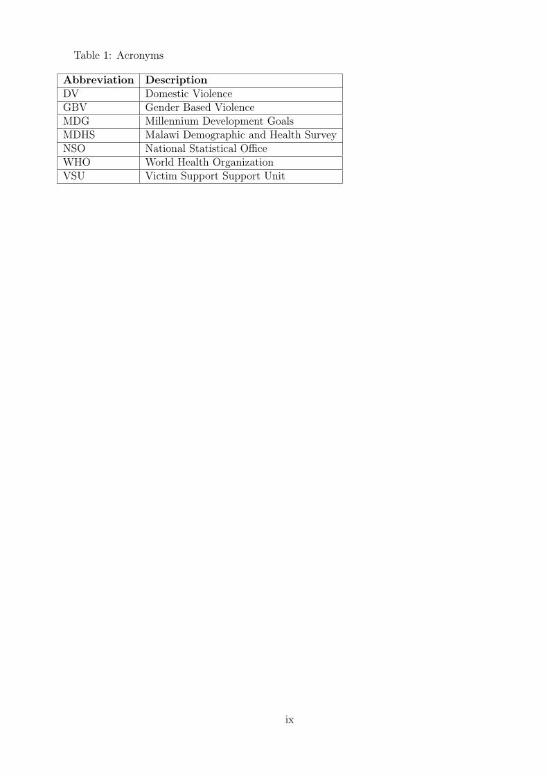
Table 1: Acronyms

Abbreviation DescriptionDV Domestic ViolenceGBV Gender Based ViolenceMDG Millennium Development GoalsMDHS Malawi Demographic and Health SurveyNSO National Statistical OfficeWHO World Health OrganizationVSU Victim Support Support Unit

ix

Chapter 1

INTRODUCTION

1.1 Background Information

Gender based violence (GBV) is defined as any act of violence that results in, or likely to result in,

physical, sexual or psychological harm, or suffering to women, or men (though at a lesser degree)

including threats of such acts coercion or arbitrary deprivations of liberty, where occurring in public

or private life (UN, 1993).

GBV occur in many forms, including but not limited to intimate partner violence (IPV), sexual

violence and femicide or the killing of women because of their gender by males. The frequency and

variety of GBV varies across countries and continents, but the negative impact it has on individuals

and on families is universal, and has direct links to health problems (UNFPA, 1998).

Domestic violence is recognized as a major public health concern (Donohoe M, 2003) and vio-

lation of human rights that is faced by all societies around the world, with one woman in every four

being abused during pregnancy worldwide (Kidman N, 2010, Unifem., 2010). In various countries,

studies have shown that people believe that husbands are justified in beating their wives if they

disobeyed them or refuse sex.

Pregnant women have been found to be at high risk of being abused (Unifem, 2008). Earlier

studies have estimated that 4% to 15% of pregnant women around the world have experienced vio-

lence (WHO, 2005). The same study also found that an astonishing one out of every four pregnant

women in rural Peru, experienced GBV. Factors like social support, woman occupation, woman’s

1

place of residence etc. were found to be associated with GBV amongst pregnant women (Khosla

A.H et al, 2005).

About 13% of women experience Domestic violence during pregnancy in developing countries

(Unifem., 2008). Other studies have indicated that more than 40% of women have experienced

GBV, and 56% for young girls between the ages of 15 to 19, pregnant women showing more than

10% (Uganda DHS, 2006, DRC DHS, 2007).

Here in Malawi, nearly 3 in every 10 women (28%) and 1 out of 16 pregnant women (6.2%) get

abused annually, and one in every four women have ever experienced sexual violence (NSO, 2011).

Domestic violence during pregnancy has been identified as one of the risk factors for low birth

weight, ante partum hospitalization, induced and spontaneous abortions and other injuries (Kaye

D. et al, 2005).

1.2 Problem Statement / Justification

The Government of Malawi not only recognizes GBV, especially violence against women, as a severe

impendent to poverty reduction, but also recognizes its impact on vulnerable groups. It has made

a lot of efforts in trying to eliminate GBV such as enacting the prevention of DV Act in 2006 and

the National response to combat GBV, 2008-2013.It also created institutions known as victim sup-

port units, based at police stations where victims are encouraged to report cases whenever abused

(Chasweka R. et al., 2012).

Despite the above mentioned efforts, in comparison of the 2004 and the 2010 MDHS report, there

was an indication of some percentage increase in violence according to woman’s background char-

acteristics i.e. age (4% - 9%), marital status (4% - 7%) and place of residence (4% - 8%). Another

study on magnitude of domestic violence amongst pregnant women at Nsanje District Hospital in

2012, found that the percentage of women who have ever experienced physical violence since attain-

ing 15 years of age in Nsanje was about 32% and 19% experienced physical violence the previous

year preceding the 2010 MDHS (Chasweka R. et al., 2012). Most studies conducted on GBV mostly

focus on women, children and the elderly.

2

Consequently knowledge on risk factors of GBV amongst pregnant women is still limited in the

country, since a few studies on the issue and awareness campaigns on the risk factors of GBV have

been done. Consequences of the act like; low birth weight, infant illness, premature labor, miscar-

riage and under−2 mortality is little known especially in the rural areas (Turan J. et al., 2012).

All this clearly show that though people know about GBV, it is still being practiced at a higher rate

in the country. Hence indicating Malawi’s poor human rights indicators, which negatively affects

the women livelihood. It also shows that Malawi is failing to meet its Millennium Development

Goal of empowering women.

It is therefore the aim of this study to examine the determinants of GBV amongst pregnant women

in Malawi and analyze the significance of each of these determinants to GBV, since apart from the

MDHS a few studies have been done in the country concerning the same. Hence the study shall

review the determinants of GBV amongst pregnant women using a quantitative study approach.

In so doing sensitizing the people on the risk factors as well as dangers of violence to a pregnant

woman, which in the end will empower these women and help the Government meet the millennium

development goals. It could also be used in reviewing the determinants and proportion of GBV

amongst pregnant women in the country in future academic writing.

3

1.3 Study Objectives

1.3.1 General Objective

• To measure the demographic and social economic features which put pregnant women at high

risk for domestic violence.

1.3.2 Specific Objections

• Measure the prevalence of partner violence during pregnancy.

• Identify the association between GBV amongst pregnant women and the determining factors.

• Measure the strength of association for each determining factor

4

Chapter 2

LITERATURE REVIEW

2.1 Social-Demographic and Economic Studies

Of all the human rights violations, gender based violence is perhaps the most widespread and so-

cially tolerant (Glaser. et al., 1967). Globally it kills and disables more women in the child bearing

age than does cancer.

Literature of GBV especially on pregnant women is scarce here in Malawi. The risk factors and

effect associated with the problem is little known especially in the rural areas. This is the case since

the condition is associated with shame and disrespect with some cultures taking such as punishment

to teach women how to respect their husbands. As a result many victims give in accurate reports

or under report the problem

GBV during pregnancy brings more danger to the life of both the woman and the unborn ba-

bies. And according to studies, the practice can result in miscarriage, premature labor, low-birth

weight, infant illness and under−2 mortality (Turan J. et al., 2012).

Discussed below are some of the studies done around the world, which have reported Social-

Demographic and Economic conditions as factors reading to GBV amongst pregnant women.

The 2008 USAID Health Sector Program, reported that a number of cross sectional studies by

the World Health Organization found that men who witnessed violence as children, are at a higher

risk of violating their wives when they get married. The studies also show that women married to

5

or in a relationship with men who drink or use drugs are at a higher risk of being abused compared

to those married to men who don’t drink. However most of these studies could neither determine

whether the risk factor preceded the violence nor provide qualitative insight into complex social

dynamics. These studies also indicated an increase of DV in communities as a result of education

and economic empowerment of women, at least until attaining high enough status to be projected

from backslash against such changes (Kug E.G. et al., 2002).

Different studies that used DHS results from different countries have indicated the following; In

Zambia 27% of ever married women reported being beaten by their partners. 33% of these women

belonging to 15-19 age group, 35% from 20-24 age group the remaining to other age groups (Kishor

S. et al., 2004). In South Africa 7% of 15-19 years had been assaulted, while 10% had been sexually

abused by their partners (Jewkes R. et al). Kenya reported 43% of 15-49 year old women being

abused in their life time, 16% reported ever been sexually abused (Kenya DHS., 2005).

Other studies by WHO reported that, in rural Ethiopia, 49% of ever partnered women had ever

experienced physical violence by their partner, rising to 59% ever experiencing sexual violence. 47%

of ever partnered women in rural Tanzania have ever experienced physical violence and 31% had

experienced sexual violence (WHO., 2005).

A prospective study (Khosla A. et al., 2005) on DV in pregnant women in Northern India, with

a sample of 991 married pregnant women reported 28.4% of abuse during pregnancy. The study

which only used chi-square of association and odds ratio, found that abuse was higher in families

with husbands who drink or smoke and in families where husbands had low education (OR: 2.07

95% CI ; 1.54-2.79), this was similar to a study by (Bacchus L. et al., 2004) and (Leung WC. et al

1999). The study also found high levels in women with lack of social support (OR: 98.9) as against

OR of 1.8 in another study from India by (Peedlcayll A. et al., 2004). However the study found

same levels of abuse in rural women compared to women in urban areas, and same levels of abuse in

women with low levels of education compared to those with high education level which is contrary

to most studies.

Such differences could have come about as a result of errors in sample correction since the study

only assessed women who were admitted that time, which was not a representative sample for

6

the whole country. The use of chi-square test for association alone without using logistic regression

can also bring bring about errors in interpreting the effectiveness of each factor on domestic violence.

A study on intimate partner violence (IPV) (Bazargan-Hejazi Sh. et al., 2013) which used chi-

square test (bivariate statistic), boneferron correction to reduce Type I error and multivariate lo-

gistic regression (multivariate statistics) and was based on the MDHS, found that physical violence

increases with age (9 - 13%) with (OR = 1.35; 95% CI: 1.05-1.73), while sexual violence decreases

with age (14 - 11%) with (OR = 1.4; 95% CI: 1.03-1.90) of the woman. Women with low levels of

education reported highest level of physical abuse (16 22%), sexual abuse (10 15%) and emotional

(11 13%) with (OR = 0.70; 95% CI: 0.49-0.99). Those with higher education had lower levels

compared to those with low education; physical 7%, sexual violence 5% and emotional violence

19%. Women who could not read at all were less likely to report sexual IPV than women who

could read a full sentence (OR = 0.76: 95% CI; 1.03-1.90). The study did not find any significant

difference in reporting IPV of any type between woman’s place of residence.

However other studies (Anderson N. et al., 2007) which used primary data, with a sample of 20,639

women from 8 different African countries including Malawi, indicated a higher prevalence as well

as a more accepting attitude of IPV in rural areas. but this study was qualitative and didn’t use

statistical significant evidence, as such it can have a lot of errors as well.

A descriptive study on Magnitude of Domestic Violence against Pregnant Women in Malawi (Chasweka

R. et al., 2012), which used the administration of structured questionnaires for data collection and

used chi-square test for analysis with a sample size of 292 pregnant women, found 58.6% of these

women abused by their marriage partners. Among these, 28% had been sexually abused. The

study also found that in all age categories women were abused, contrally to the 2011 NSO findings

that Domestic Violence (DV) was more prevalent among young pregnant women. This might be

the case as a result of lack of reporting among old couples in the MDHS data, compared to young

abused pregnant women (Chasweka R. et al., 2012). The study had a majority of women who did

not go beyond primary school, therefore the comparative group was a minority that could not have

had any significant influence on the results, as such it showed abuse despite education levels. This

agreed with Lammechnane’s findings (Lammechnane P. et al., 2011). However studies by (Khosla A.

et al., 2005) and (Audi C et al., 2008), found that high incidence of DV among low-educated women.

7

The study also found an association between low income and women being abused during preg-

nancy. Some errors might come up in the study since it only used chi-square of association instead

of testing the significance of each explanatory variable against DV using the logistic regression.

8

Chapter 3

METHODOLOGY

3.1 Study Locale and Design

The study used data obtained from the 2010 Malawi Demographic Health Survey. As such the

study has used quantitative data only.

3.1.1 Target Population

The study consisted of women between the ages of 15 to 49, who had ever been abused while

pregnant.

3.1.2 Sample Size and Sampling Procedure

The data of this study was obtained from the 2010 Malawi Demographic Health Survey

(http://www.measuredhs.com/data/Using-Datasets-for-Analysis), which used a cross sectional study

and used a cluster sampling to collect data from the individuals in the sample frame defined. The

sample included 849 clusters, 158 in urban areas and 691 in rural areas. A woman’s questionnaire

was used to collect information from all women aged 15-49.

A nationally representative sample of 23,020 interviews of women in this age group were called

for and a domestic violence question during pregnancy before and during the interview was asked,

which is the target population of this study.

So this study analyzed responses from these women to find the risk factors associated with the

problem.

9

Key Issues Investigated

The main interest was on specific questions that addressed the specific objectives of this study. The

questions were as follows;

• What are the factors that influence GBV amongst pregnant women and how significant are

they?

• What is the relationship between each factor identified and violence amongst pregnant women?

• What is the occurrence/rate of GBV amongst pregnant women in Malawi?

10

3.2 Suggested Models and Analysis

3.2.1 Key Variables

• Response Variable: Hurt during pregnancy by husband or partner

• Explanatory Variable: Age, Marital Status, Place Of Residence, Education Level, Wealth,

occupation, partner or husband who drinks, ethnicity, jealousy e.t.c.

3.2.2 Analytical technic

The study tried to identify the determinants of gender based violence amongst pregnant women

in Malawi. The analysis was done at three levels; uni-variate, bi-variate and multivariate analysis.

The dependent variable was whether a woman was hurt during pregnancy or not, which is binary

response. The response variable; hurt during pregnancy was coded with values: 0 for not hurt and 1

for being hurt. The explanatory variables were in discrete form except age (continuous) from which

another variable (age categories) was generated. The ages were categorized into young (15-24),

middle (25-34) and old (35-49).

3.2.3 Uni-variate StatisticsThis part looked at the descriptive statistics for both the Socio-demographic and economic fac-

tors used in the study. As such frequency and the percentages of GBV among pregnant women inMalawi were obtained.

3.2.4 Inferential Analysis

To test the general hypothesis, different statistical methods were used to identify any relationship

between the dependent and independent variables. All the test were curried at a 5% significance

level. If the calculated p-value was less than the significance level, the null hypothesis was rejected

in favor of the alternative hypothesis. The statistical methods were as follows;

(a) Bi-variate Analysis This analysis used a chi-square test (χ2) to test the association between

the response variable (hurt during pregnancy) and each explanatory variable or factor (age, marital

status, place of residence, education level, wealth, occupation e.t.c). The hypothesis tested were as

follows;

11

• H0: There is no association between socio-demographic factors and GBV amongst pregnant

women in Malawi.

• H1: There exist an association between economic conditions and GBV amongst pregnant

women in Malawi.

The formula for chi-square statistics is

χ2 = Σ(Oij − Eij)

2

Eij

and follows a χ2 with (r-1) (c-1) degrees of freedom. Where

• Oij is the observed counts in cell ij; i = 1, 2, 3..r and j = 1, 2, 3..c where r is the number of

rows and c is the number of columns in an rc contingency table.

• Eij the expected counts in cell ij; i = 1, 2, 3..r and j = 1, 2, 3..c where r is the number of

rows and c is the number of columns in an rc contingency table.

However, in most cases, the χ2 test in a contingency table is not robust as it can be affected by

the sample size and also by the number of rows and columns which when they increase, in most

cases we tend to reject H0. As such Cramers V, a measure of strength of association between

two nominal variables, giving a value between 0 and +1 (inclusive) was used. Cramers V which

is a variant of chi-square, based on Pearsons chi-square statistic to test the strength of association

between the individual covariates and GBV. Cramers V is given by;

V =√

χ2

N(q−1)

Where: χ2 is the chi-square statistic; N is the total sample size and q is the number of rows or the

number of columns, whichever is less.

Cramers V is a symmetrical measure, it does not matter which variable we place in the column

and which in the rows. Also the order of rows or columns does not matter, so Cramers V may be

used with nominal data types or higher. Cramers V varies from 0 (corresponding to no association

between the variables) to 1 (complete association) and can reach 1 only when the two variables are

equal to each other.

12

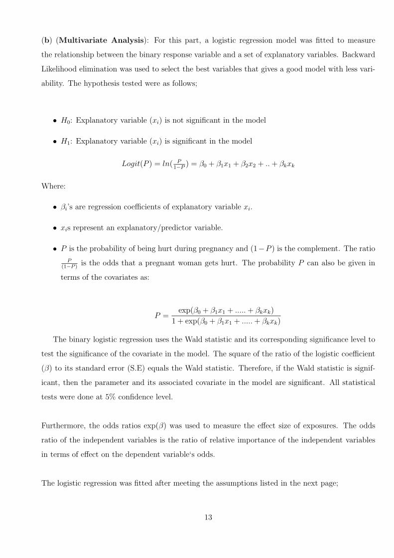
(b) (Multivariate Analysis): For this part, a logistic regression model was fitted to measure

the relationship between the binary response variable and a set of explanatory variables. Backward

Likelihood elimination was used to select the best variables that gives a good model with less vari-

ability. The hypothesis tested were as follows;

• H0: Explanatory variable (xi) is not significant in the model

• H1: Explanatory variable (xi) is significant in the model

Logit(P ) = ln( P1−P ) = β0 + β1x1 + β2x2 + ..+ βkxk

Where:

• βi’s are regression coefficients of explanatory variable xi.

• xis represent an explanatory/predictor variable.

• P is the probability of being hurt during pregnancy and (1−P ) is the complement. The ratio

P(1−P )

is the odds that a pregnant woman gets hurt. The probability P can also be given in

terms of the covariates as:

P =exp(β0 + β1x1 + .....+ βkxk)

1 + exp(β0 + β1x1 + .....+ βkxk)

The binary logistic regression uses the Wald statistic and its corresponding significance level to

test the significance of the covariate in the model. The square of the ratio of the logistic coefficient

(β) to its standard error (S.E) equals the Wald statistic. Therefore, if the Wald statistic is signif-

icant, then the parameter and its associated covariate in the model are significant. All statistical

tests were done at 5% confidence level.

Furthermore, the odds ratios exp(β) was used to measure the effect size of exposures. The odds

ratio of the independent variables is the ratio of relative importance of the independent variables

in terms of effect on the dependent variable‘s odds.

The logistic regression was fitted after meeting the assumptions listed in the next page;

13

• The dependent variable was binary (hurt during pregnancy) coded as shown below;

1. 0 for no

2. 1 for yes

• The data was not normally distributed

• No linear relationship between the independent variables

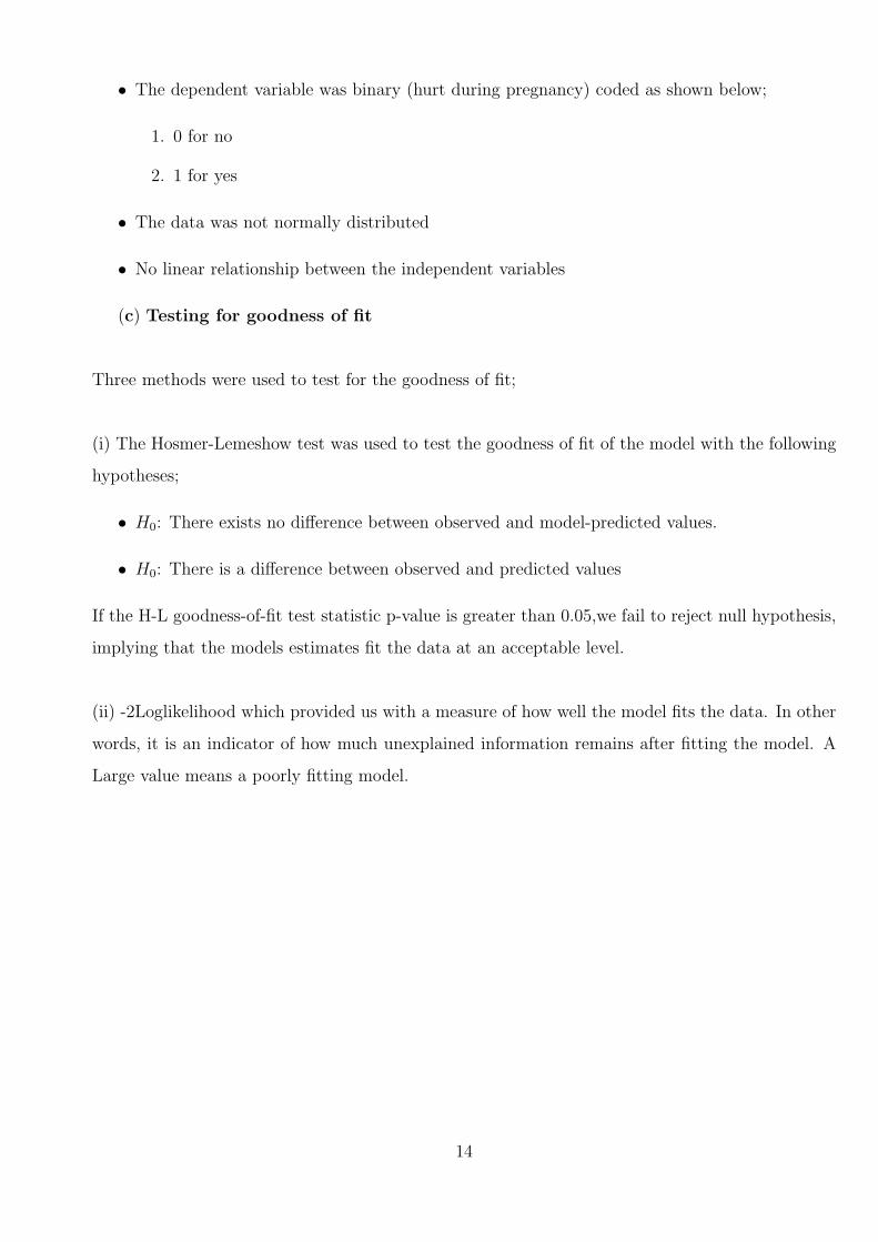
(c) Testing for goodness of fit

Three methods were used to test for the goodness of fit;

(i) The Hosmer-Lemeshow test was used to test the goodness of fit of the model with the following

hypotheses;

• H0: There exists no difference between observed and model-predicted values.

• H0: There is a difference between observed and predicted values

If the H-L goodness-of-fit test statistic p-value is greater than 0.05,we fail to reject null hypothesis,

implying that the models estimates fit the data at an acceptable level.

(ii) -2Loglikelihood which provided us with a measure of how well the model fits the data. In other

words, it is an indicator of how much unexplained information remains after fitting the model. A

Large value means a poorly fitting model.

14

3.2.5 Data Entry and Analysis

Since the study utilized secondary data whose entry and editing were accomplished using CSPro,

the data was imported into Statistical Package for Social Scientists (SPSS). Despite the data set

being imported into a statistical package (SPSS), SPSS was only used to transform the data into

STATA compatible format. All analyses were done using STATA (version 10). STATA was preferred

in analysis for its ability to easily clean the data set.

3.3 Ethical Consideration

The secondary data used in the study was obtained from www.measuredhs.org by writing an e-

mail asking for approval to use the requested data. For the confidentiality and privacy, the obtained

data was not accessed by anyone else but me and was used only to serve the purposes of the project.

3.4 Limitations

The use of secondary data my somehow give biased results as women who were not home during

the time of the interviews were not followed up.

It might also be possible that during the MDHS data collection, some women that might been

abused did not speak out because GBV is a sensitive issue that’s taken to be a private matter

between husband and wife. Some women may not have disclosed their experience of abuse to avoid

shame and embarrassment. These limitations can bring errors in our study.

The proposed study was supposed to use data from both the 2010 Malawi Demographic Health

Survey and the Zomba Police Victim Support Unit, however this was not possible since the data

from the victim support unit did not indicate whether the victim was pregnant or not. The sample

size for Zomba district was 142, and upon dropping missing values in other variables the sample

reduced to 33 which would not be a well representative of the population. It also brought problems

especially when running the regression model as the data had a lot of missing values, hence causing

complete separation. As such, only the 2010 MDHS data was used and the study locale was changed

to the whole country.

15

Chapter 4

RESEARCH FINDINGS

4.1 Interpretation of Results

This chapter gives the results of the study on GBV amongst pregnant women in Malawi which

used the 2010 MDHS data. The analysis was done at three levels; uni-variate, bi-variate and multi

variate analysis. Thus looking at the frequency of occurrence of GBV, the association between

the background characteristic variables and GBV but also the significance of these background

characteristics on the occurrence of GBV. Two methods were also used to measure the goodness of

fit namely -2loglikelihood and Hosmer Lemeshow. Both methods describes how well the model fits

the data.

4.1.1 Descriptive statistics

Respondent’s Socio-Demographic Characteristics

This part shows the combined results of both uni-variate and bi-variate analysis, thus showing

the frequencies of occurrence of GBV against each explanatory variable as well as showing which

variables were associated with GBV. The test of association was done using χ2 test (Clamer’s V),

which was tested at 5% significance level.

The descriptive results include the frequencies and the percentages of the women in each explana-

tory variable in relation to GBV (see Appendix 1 for descriptive results). Amongst the respondents

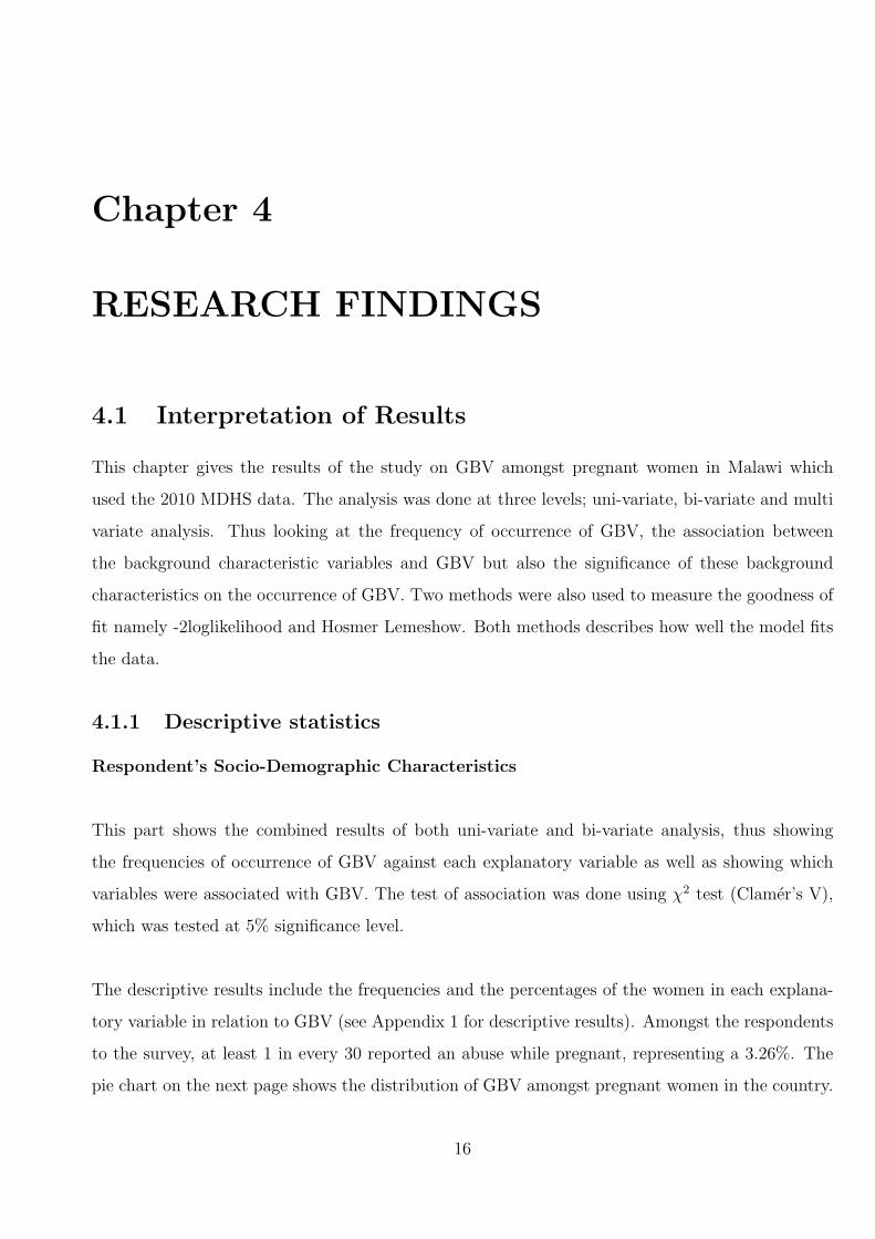
to the survey, at least 1 in every 30 reported an abuse while pregnant, representing a 3.26%. The

pie chart on the next page shows the distribution of GBV amongst pregnant women in the country.

16

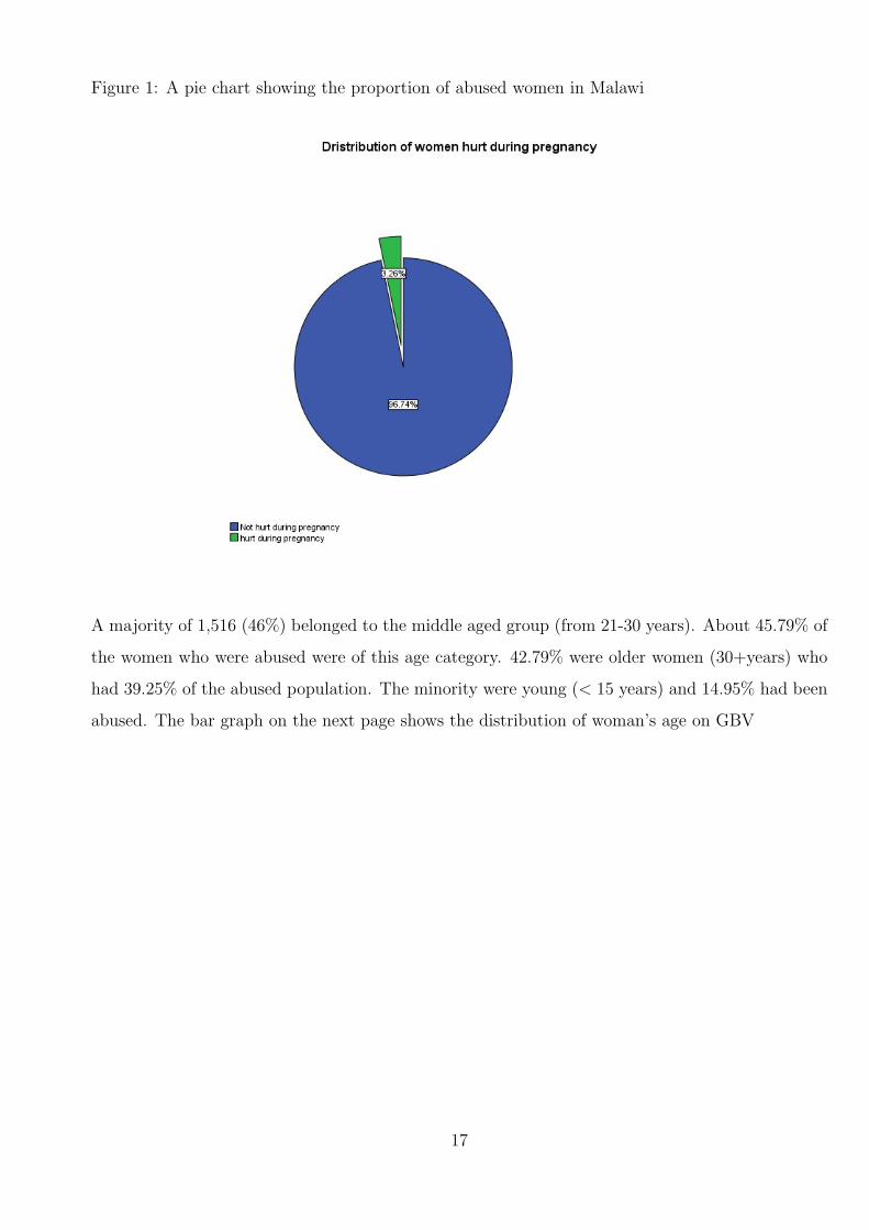
Figure 1: A pie chart showing the proportion of abused women in Malawi

A majority of 1,516 (46%) belonged to the middle aged group (from 21-30 years). About 45.79% of

the women who were abused were of this age category. 42.79% were older women (30+years) who

had 39.25% of the abused population. The minority were young (< 15 years) and 14.95% had been

abused. The bar graph on the next page shows the distribution of woman’s age on GBV

17

Figure 2: A bar graph showing the distribution of woman’s age on GBV

2,938 (89.38%) of the population came from the rural areas while 349 (10.62%) were from the

urban areas, and 87.85% of the 107 of the abused women were from the rural areas. The majority

of the group 1,105 (41.37%) belonging to the Chewa ethnic group, and had the highest percentage

of abuse compared to the other tribes.

On the levels of education of these respondents, 556 (16.97%) had no education while 2,287 (69.81%)

attended primary, 415 (12.67%) had secondary education and only 18 (0.55%) had tertiary edu-

cation. Those with primary education had the highest rate of abuse (76.64%), followed by those

without any education (12.15%), then those with secondary and lastly who had tertiary educa-

tion. 2,859 respondents were married, 84.11% of the abused women reported to be married while

15.89% were living together. 1,900 (57.93%) of the respondents were employed while the other

42.07% were not, and of those who were not employed 58.33% were hurt during pregnancy. 1,185

(36.16%) of these respondents had no radio in their homes and 53.26% of the abused respondents,

had no radio in their homes. However 63% of these women belonged to the middle and poor families.

18

Women whose husbands drink alcohol were atleast 93.35% and over 98% of the women who re-

ported an abuse had a husband who drinks. 433 (41.55%) of these women had a husband who

Was jealous when seen talking to another man and 102 (35.29%) had been hurt before they got

pregnant. Below is a graph showing the distribution of abuse against jealousy husband;

Figure 3: A bar graph showing the distribution of violence amongst women with a jealousy partner

Only 42 (4.03%) of the 1,041 Respondents sought police help and these showed a lower rate of

abuse compared to those who dont. Finally 267 (8.8%) of the group had a husband who had more

than one wife.

4.1.2 Bi-variate statistics

This part shows the results of bi-variate analysis, thus showing the variables which were associated

with GBV as well as the strength of association. The test of association was done using χ2 test

(Clamer’s V), which was tested at 5% significance level.

Based on the output in table 1 on the next page, it can be clearly seen that variables; jeal-

19

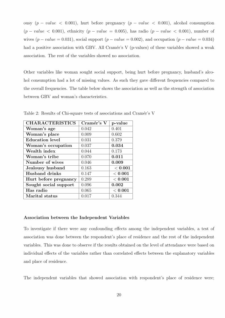
ousy (p − value < 0.001), hurt before pregnancy (p − value < 0.001), alcohol consumption

(p − value < 0.001), ethnicity (p − value = 0.005), has radio (p − value < 0.001), number of

wives (p− value = 0.031), social support (p− value = 0.002), and occupation (p− value = 0.034)

had a positive association with GBV. All Cramer’s V (p-values) of these variables showed a weak

association. The rest of the variables showed no association.

Other variables like woman sought social support, being hurt before pregnancy, husband’s alco-

hol consumption had a lot of missing values. As such they gave different frequencies compared to

the overall frequencies. The table below shows the association as well as the strength of association

between GBV and woman’s characteristics.

Table 2: Results of Chi-square tests of associations and Cramer’s V

CHARACTERISTICS Cramer’s V p-valueWoman’s age 0.042 0.401Woman’s place 0.009 0.602Education level 0.031 0.379Woman’s occupation 0.037 0.034Wealth index 0.044 0.173Woman’s tribe 0.070 0.011Number of wives 0.046 0.009Jealousy husband 0.163 < 0.001Husband drinks 0.147 < 0.001Hurt before pregnancy 0.289 < 0.001Sought social support 0.096 0.002Has radio 0.065 < 0.001Marital status 0.017 0.344

Association between the Independent Variables

To investigate if there were any confounding effects among the independent variables, a test of

association was done between the respondent’s place of residence and the rest of the independent

variables. This was done to observe if the results obtained on the level of attendance were based on

individual effects of the variables rather than correlated effects between the explanatory variables

and place of residence.

The independent variables that showed association with respondent’s place of residence were;

20

woman’s education level (p-value<0.001) having a radio(p-value<0.001), sought social support (p-

value<0.001), number of wives (p-value<0.001), woman’s tribe (p-value<0.001), wealth index (p-

value<0.001) and occupation of the respondent (p-value=0.045) in the study (see Appendix 1 for

descriptive results). This association might affect the significance of the results when looking at

association between the factors and GBV amongst pregnant women, since the results also included

the association that exists between the variables. The results on place of residence gave some bias-

ness because a majority of the respondents were from the rural areas, thus the results showed some

inconsistency on analysis done on place of residence.

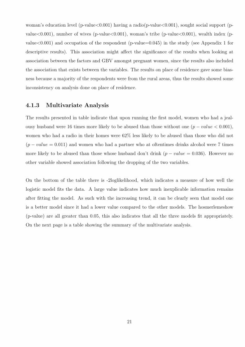
4.1.3 Multivariate Analysis

The results presented in table indicate that upon running the first model, women who had a jeal-

ousy husband were 16 times more likely to be abused than those without one (p− value < 0.001),

women who had a radio in their homes were 62% less likely to be abused than those who did not

(p − value = 0.011) and women who had a partner who at oftentimes drinks alcohol were 7 times

more likely to be abused than those whose husband don’t drink (p − value = 0.036). However no

other variable showed association following the dropping of the two variables.

On the bottom of the table there is -2loglikelihood, which indicates a measure of how well the

logistic model fits the data. A large value indicates how much inexplicable information remains

after fitting the model. As such with the increasing trend, it can be clearly seen that model one

is a better model since it had a lower value compared to the other models. The hosmerlemeshow

(p-value) are all greater than 0.05, this also indicates that all the three models fit appropriately.

On the next page is a table showing the summary of the multivariate analysis.

21

Table 3:Binary Logistic Regression Analysis

Model 1 Model 2 Model 3Variable OR.(S.E)[P-value] OR.(S.E)[P-value] OR.(S.E)[P-value]Jealousy 15.5343(9.4532)[0.000]* 14.85128(9.01229)[0.000]* 15.16957(9.182423)[0.000]*husbandNumber of [0.147] [0.177] [0.461]WivesOne(RC)Two 1.97206(0.9228721)[0.147] 1.861512(0.85617)[0.177] 1.873374(0.860758)[0.172]Woman’s 1.194328(0.416961)[0.611] 1.181639(0.40930)[0.630] Dropped From The ModeloccupationHave radio 0.388909(0.143723)[0.011]* 0.435221(0.14341)[0.012]* 0.434786(0.143285)[0.011]*Wealth [0.161] Dropped From The Model Dropped From The ModelPoorer(RC)Poor 0.913113(0.418955)[0.843]Middle 0.576718(0.317351)[0.317]Rich 0.748035(0.419608)[0.605]Richer 2.271971(1.230233)[0.130]Husband 0.561491(0.155341)[0.037]* 0.562544(0.15431)[0.036]* 0.565194(0.154558)[0.037]*drinksNon (RC)Often 6.742474(6.910517)[0.063] 6.700458(6.90034)[0.060] 6.695194(6.899458)[0.062]Sometimes 1.857692(1.913182)[0.548] 1.79958(1.87645)[0.0562] 1.800724(1.901873)[0.510]Tribe [0.0.097] [0.133] [0.121]Chewa(RC)Tumbuka 2.737817(1.324238)[0.037]* 2.73326(1.300266)[0.035]* 2.756627(1.310190)[0.033]*Yao 3.069475(1.418560)[0.015]* 2.80586(1.275222)[0.023]* 2.843053(1.290358)[0.021]*Lomwe 1.844763(1.580250)[0.475] 1.98562(1.634359)[0.405] 2.013123(1.655637)[0.395]Ngoni 3.003000(1.447622)[0.023] 2.71416(1.291174)[0.036]* 2.767832(1.312089)[0.032]*Const 0.009928(0.007986)[0.000]* 0.00999(0.007771)[0.000]* 0.010751(0.008173)[0.000]*-2LL 142.66 145.795566 145.9133H-L 0.9704 0.7577 0.7391

Two tailed test: p− value < 0.05,RC: Reference Category,-2LL: -2Loglikehood,H-L: Hosmerlemeshow

22

Table 3 shows the impact of the independent variables that had shown positive association

during the chi-square test, including wealth which though did not show association but had shown

association in other studies done around the world. Variables like hurt before pregnancy, radio,

seek police support which also indicated positive association, were not included in the models since

they had a lot of missing values as such they were causing complete separation also known as quasi-

complete separation. This happens when you have a very small sample or a lot of missing values ,

as such these variables were not included.

23

Chapter 5

DISCUSSION OF RESULTS

The 2010 MDHS reported that 6.2% of pregnant women in the country experience abuse in one

way or the other during pregnancy in the country annually. The study found that one out of every

thirty pregnant women get physically hurt either buy her husband or partner. This represents 3.2%

of abused pregnant women, which was close to the 4%-15% 2005 estimate by the world health or-

ganization. The percentage difference might be because of missing values in the 2010 MDHS data.

After performing the three analysis; descriptive, bi-variate and multivariate the study reviewed the

following according to the demographic characteristics;

WOMAN’S AGE

Though without any association to violence during pregnancy, the study showed high levels of

abuse (45.79%) among middle aged women (20-30 years old) compared to the other age categories.

This was similar to the MDHS report, however contrary to Chasweka s findings who found equal

levels of abuse in all age categories. Such a difference can come about as a result of misrepresenta-

tion of other age categories in the DHS data. Though there was a difference both studies found no

association between ages of the respondents and violence amongst pregnant women. As such the

variable was not included in the logistic regression model.

WOMAN’S PLACE OF RESIDENCE

The study agreed with a studies by Khosla (2005), Bazargan (2013) and the MDHS (2010) which

found high prevalence of domestic violence amongst women from rural areas (87.85%) compared to

those living in urban areas. Most women from rural areas in the country put their trust in customs

24

which encourage them to endure when ever they have been abused in their families, as such acts

of abuse are not reported some do not report such acts only because of shame as they believe that

family matters should not involve the public. Nevertheless the study did not find any association

between place of residence and violence during pregnancy which was different to the results by

Bazargan and Khosla. Such a case could be as the DHS data had a high representation of women

from the rural areas which could lead to bias. Hence this variable was not included in the logistic

regression as well.

WOMAN’S LEVEL OF EDUCATION

On the levels of education the study agreed with other studies by Audi. F (2008), Nasir. K

(2003) and Khosla (2005), who also found high levels of abuse amongst pregnant women especially

those who only attended primary. Since uneducated women depend a lot on their husbands, men

take advantage of this and abuse their wives knowing that there is nothing else they can do without

them. Such women are also vulnerable to abuse since most of them do not know their rights, as

such they do nothing but endure when ever abused. The study did not find a positive association

between the levels of education and violence during pregnancy, however Nasir and Khosla found an

association between the two. This might be because of misrepresentation of respondents especially

those with higher education in the DHS data. Thus the variable was not included in the logistic

model as well.

WOMAN’S OCCUPATION

On occupation the study differed from both studies by Khosla and Audi. The results showed

high levels of abuse among women who were not working compared to those who had a job. How-

ever Khosla found equal levels of abuse regardless of the woman’s occupation. This might be the

case since social norms in India prevent even economically independent women to stand up to

abuse (Khosla, et al. 2005). Audi reported a greater number of abuse in women who assume

non-traditional roles or when they start to work. The case is different here in Malawi since women

who are employed feel that they can afford to provide for their family even without help from a

husband, as such men fail to abuse women who are working in fear of being left alone. After fitting

a regression model, the variable work (OR: 1.194, P − value : 0.611, CI: 0.6128, 2.4048) indicates

25

that the odds of being abused for women who don’t have a job are 19.4% higher compared to those

who had a job. But with a p-value of 0.611 the variable was regarded insignificant to the model.

HUSBAND DRINKS ALCOHOL

The study also revealed high levels of abuse among respondents who had a husband or partner

who drink alcohol. This was also the case with studies by both Nasir and Audi who also found

high levels of abuse among pregnant women who had partners who drink. Mostly men drink alcohol

whenever they have something troubling them, as such its the wife who gets the beating even though

she did not do wrong. This being the case they pretend as it was the influence of the alcohol though

they did know what they were doing. A positive association was also found between alcohol con-

sumption and abuse. After fitting a regression model, variable drink (OR: 0.544, P − value : 0.025,

CI: 0.31953, 0.92654) indicated that women who had a husband who does not drink were 56% less

likely to be abused compared to those whose husband drink. The confidence interval indicates that

the variable has a negative association in the model.

WOMAN SOUGHT SOCIAL SUPPORT

The study also revealed that women who sought help from the police, reported to have lower

levels of abuse compared to those who dont. This was also the case with Khoslas study which also

found low levels of abuse in women who had social support. This might be the case as men fear

arrests if reported to the police whenever they abuse their partners. The study also found positive

association between social support and violence amongst pregnant women. However the model was

not included in the regression model since it had a lot of missing values which was causing the

quasi-complete separation.

WOMAN ABUSED BEFORE PREGNANCY

Women who reported abuse before pregnancy, also reported a high level of abuse during preg-

nancy compared to those who weren’t. An association between the two was also found which

agreed with Chaswekas study. He reported that most women think that reporting violence would

be viewed as revealing family secrets which brings shame and embarrassment to the family. As such

26

men get used to beating their wives no matter how small the issue is. Though with an association

the variable was not included in the regression model since it had a lot of missing values hence

causing quasi-complete separation.

WOMAN’S WEALTH INDEX

Women who were from poor families reported a great number of abuse than those from middle

and rich families. This was also the case in most studies for instance Khosla (2005), Audi (2008),

Nasir (2003) and Faruqi (1996) who also found an association between the variables but this study

did not find any association. This difference might be as a result of lack of reporting among women

from rich families in the MDHS data, as such though without association the variable was included

in the regression model to check whether it was significant to the model or not. However with (OR:

1.172684, P − value : 0.221, CI: 0.985924, 1.513537), wealth index proved to be not significant to

the model and was dropped in both models one and two. The output indicated that the odds of

being abused for women from poorest families were 17% higher compared to those from rich families.

JEALOUSY HUSBAND

Most men feel insecure whenever they see their wives talk to another man, so as a way of protecting

their marriages or relationships they beat their wives so that they should not talk to other men as

such the study showed that women who had a jealous partner (OR: 15.5343, P − value < 0.001,

CI: 4.713282, 51.20073) were at least 16 times more likely to be abused compared to those whose

husband was not jealous. A study by Nasir (2003), also found jealousy to be highly associated with

domestic violence amongst pregnant women.

No other studies were found that dealt with factors; respondent’s marital status, number of wives,

having a radio in the house or respondent’s ethnicity. This study found an association between

both factors and violence amongst pregnant women.

WOMAN’S STATUS

On marital status, the respondents who were married reported high levels of abuse compared to

27

those who were only living together. Since most men feel assured that the wife will never leave

them especially because of cultural values they abuse their wives knowing that they can never leave

them while those who are just leaving together fear that they might lose their partner as most of

these families are still young. The status of the woman showed no association with abuse, as such

it was not included in the regression model.

HUSBAND’S NUMBER OF WIVES

The number wives also proved to be associated with abuse amongst pregnant women. Men with two

or more wives (OR: 1.97206, p− value : 0.147, CI: 0.7880983, 4.934691) were two times more likely

to hurt their wives than men who only had one wife. However the DHS showed a misrepresentation

of respondents especially those with a husband who had two wives (8.2%). This could lead to biased

results as the concentration of respondents was high on women who had a husband with only one

wife.

FAMILY HAS A RADIO

Women who had a radio in their homes reported low levels of abuse compared to those who had

no radio. This might be so since women who listen to radio programs know more about their

rights and know where to report whenever their rights have been violated. Both partners in the

house could be aware of the dangers of abusing a pregnant woman and the imprecations it might

bring on the pregnancy through the radio programs. Upon fitting the regression model having

a radio (OR: 0.38084, P − value : 0.007, CI: 0.189164, 0.7766725), reported that the odds of be-

ing abused for women who had no radio in their homes were 62% higher than those who had a radio.

WOMAN’S TRIBE

On womens ethnicity, the Chewa tribe had the highest level of abuse compared to the other tribes.

This might be as a result of some cultural norms as they have a saying in Chichewa banja ndi

kupilila” that encourage to endure pain in families. As such experiencing more abuse than the

other tribes. Other tribes like Tumbuka who practice ”lobola” put the women high risk of abuse as

the husband feel they own their wives since they paid money for the marriage hence they can abuse

28

their wives. After fitting the regression model, ethnicity (OR: 1.098, P − value : 0.110, CI: 0.97891,

1.23158), revealed that the odds of abuse were almost 3 times higher in Tumbuka, Yao and Ngoni

women and 2 times more in Lomwe women compared to Chewa women.

29

Chapter 6

CONCLUSION AND

RECOMMENDATIONS

6.1 Conclusion

Despite the introduction and in-acting of the prevention of DV Act in 2006, the national response

to combat GBV; 2008 to 2013 and the victim support units in the police stations, the rate of DV

in the country has not changed that much.

The study which used the 2010 DHS data revealed that 3.26% of pregnant women in the coun-

try gets hurt either by their husband or partner. The study also revealed some determinant factors

associated with DV amongst pregnant women in Zomba which were jealousy, having a radio and

alcohol consumption. Women who had a jealous husband were more likely to be abused compared

to those who did not, the same was with women who had no radio in their homes and those who

had partner who drinks.

However, the results to this study can not be that conclusive, since the data had a lot of miss-

ing values. As such chances are high that the results might be somehow biased and might favor

other factors. Never the less though this is a limitation, the study provides a baseline for further

research and development of policies and strategies to decrease DV amongst pregnant women.

30

6.2 Recommendations

• Awareness campaigns should be launched and conducted in the country to teach the nation

on the causes and the impacts of DV amongst pregnant women.

• Introduction of more radio programs concerning issues of women’s rights that can help in

empowering them.

• Further research should be done across the nation to determine more factors of DV amongst

pregnant women and ways of reducing the cases of DV.

31

Reference

Anderson N. et al. (2007) Risk Factors for Domestic Violence: National Cross- Sectional

Household Surveys in eight southern African Countries.

Audi C, Segall-Correa A Santiago S, Andrade M, Peraz-Escamilla R. (2008) ”Violence

Against Pregnant Women: prevalence and association factors”.

Bazargan-Hejazi Sh., Medeiros S., Mohammad R., Lin J., Dalal K., (2005) Partner

Violence: A study of female victims in Malawi. J inj, Violence Res. 2013 jan; 5(1) :

38 − 50 Central Bureau of Statistics and Ministry of Health, Measure DHS (ORC

Macro), Kenya Demographic and Health Survey (Nairobi).

Bacchus L, Mezey G, Bewley S, Hawith A. (2004) Prevalence of Domestic Violence when

midwives routinery enquire in pregnancy. BJOG ; 3:444-5

Chasweka R, Chimwanza A, Maluwa A, Odland O. J., (2007) Magnitude of Domestic

Violence against pregnant Women in Malawi. J. res. Nurs. Midwifery. 2012 july

vol.1(2); 17− 21 DHS Data for Uganda, (2006) and for DRC (2007)

Donohoe M, (2003). Violence and Human Rights Abuse against Women in the Devel-

oping World. Medscope Ob/Gyn and Womens Health, 2003; 8(2)

Ellsberg M., Heise L., Gottemveller.( 2008) Ending Violence against Women and Guedes

A. Addressing Gender-Based Violence through USAIDs Health programs (2nded),

IGWG,

Glaser, Barney G. and Strauss, Anselm L. (1967)The Discovery of Grounded Theory

Strategies for Qualitative Research

Kaye D, Mirembe F, Bantebya G, Johansson A, Ekstrom A (2005). Domestic Violence

During Pregnancy and Risk of Low Birth Weight and Maternal Complications : a

prospective cohort study at Mulago Hospital, Uganda. East Africa Med. J. 2005

Nov; 82(11): 579-87

Kidman N. (2008) A Life Free of Violence is Every Womans Right.(2010)

Kishor, S., and K. Johnson. (2004) profiling Domestic Violence-A Multi-Country study.

Calverton, Maryland: ORC Macro.

Khosla A, Dua D, Devi L, Sud S (2005). Domestic Violence in Pregnancy in North

Indian Women. Indian J. med. Sci; 59: 195-9

Kug E.G., L.L Dahlberg, J.A Mercy, A.B Zwian, R Lozano. (2002) ”World Report on

Violence and Health”. Geneva: World Health Organization.

32

Lamichhane P, Puri M, Tamang J, Dulai B (2011). Womens status and violence against

young married women in rural Nepal

Leung W.C, Leung T.W, Lam Y.Y.J, Ho P.C. (1999) The Prevalence of Domestic Vi-

olence Against Pregnant Women in Chinese Community. In J Obst Gyneccol ; 66:

23-30

Loan P. (2006) ”Perception toward Domestic Violence against Women of Health Providers

of the Thanh Nhan general Hospital in Hanoi, Vietnam”.

Malawi Demographic and Health Survey 2010. Zomba, Malawi: NSO and ICF Macro.

National Statistical Office (NSO) and ICF Macro (2011). Malawi Demographic and

Health Survey, 2010. Zomba, Malawi and Calverton, Maryland, USA: NSO and ICF

Macro

Peedicayil A, Sadowshi L.S, Jeyaseelan L, Shankar V, Jain D, Suresh S. (2004) Spousal

Violence against Women During Pregnancy. BJOG ; 3:682-7

R. Jewkes, K. Dunkle, M. Nduna, and N. Shai, Intimate Partner Violence, Relationship

Gender Power Inequity, and Incidence of HIV Infection in Young Women in South

Africa: A Cohort Study,

Turan J, Hatcher A, Medema J, et al., (2012) Effects of Perception of HIV/AIDS stigma

on Utilization of Skilled Childbirth Service in Rural Kenya a Mixed Methods Study.

Plos Medicine. Aug

UNIFEM. (2008) Violence against Women: Facts and Figures,

UNIFEM. (2010) Gender justice and ending description for the Millennium Development

Goals,

United Nations General Assembly. (1993) Declaration on the Elimination of Violence

against Women. United Nation Department of Public information,

United Nations Population Fund (UNFPA). (1998) Violence against Girls and Women:

A public Health priority. UNFPA Gender Theme Group

USAID under the BRIDGE Project (Cooperative Agreement), 2008

WHO (2005) Multi-country study on womens health and domestic violence,

World Health Organization. (2006) Mortality country fact sheet for Thailand,

33

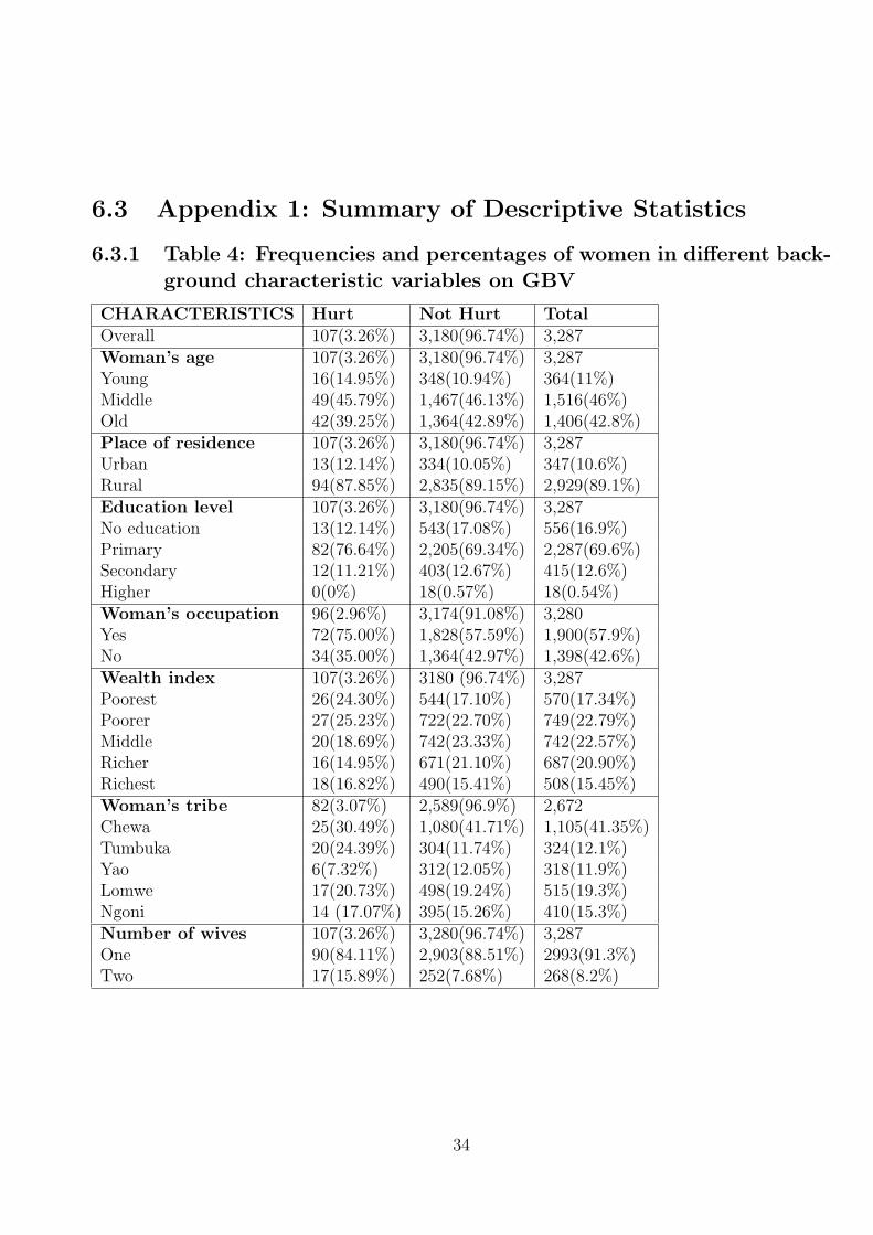
6.3 Appendix 1: Summary of Descriptive Statistics

6.3.1 Table 4: Frequencies and percentages of women in different back-ground characteristic variables on GBV

CHARACTERISTICS Hurt Not Hurt TotalOverall 107(3.26%) 3,180(96.74%) 3,287Woman’s age 107(3.26%) 3,180(96.74%) 3,287Young 16(14.95%) 348(10.94%) 364(11%)Middle 49(45.79%) 1,467(46.13%) 1,516(46%)Old 42(39.25%) 1,364(42.89%) 1,406(42.8%)Place of residence 107(3.26%) 3,180(96.74%) 3,287Urban 13(12.14%) 334(10.05%) 347(10.6%)Rural 94(87.85%) 2,835(89.15%) 2,929(89.1%)Education level 107(3.26%) 3,180(96.74%) 3,287No education 13(12.14%) 543(17.08%) 556(16.9%)Primary 82(76.64%) 2,205(69.34%) 2,287(69.6%)Secondary 12(11.21%) 403(12.67%) 415(12.6%)Higher 0(0%) 18(0.57%) 18(0.54%)Woman’s occupation 96(2.96%) 3,174(91.08%) 3,280Yes 72(75.00%) 1,828(57.59%) 1,900(57.9%)No 34(35.00%) 1,364(42.97%) 1,398(42.6%)Wealth index 107(3.26%) 3180 (96.74%) 3,287Poorest 26(24.30%) 544(17.10%) 570(17.34%)Poorer 27(25.23%) 722(22.70%) 749(22.79%)Middle 20(18.69%) 742(23.33%) 742(22.57%)Richer 16(14.95%) 671(21.10%) 687(20.90%)Richest 18(16.82%) 490(15.41%) 508(15.45%)Woman’s tribe 82(3.07%) 2,589(96.9%) 2,672Chewa 25(30.49%) 1,080(41.71%) 1,105(41.35%)Tumbuka 20(24.39%) 304(11.74%) 324(12.1%)Yao 6(7.32%) 312(12.05%) 318(11.9%)Lomwe 17(20.73%) 498(19.24%) 515(19.3%)Ngoni 14 (17.07%) 395(15.26%) 410(15.3%)Number of wives 107(3.26%) 3,280(96.74%) 3,287One 90(84.11%) 2,903(88.51%) 2993(91.3%)Two 17(15.89%) 252(7.68%) 268(8.2%)

34

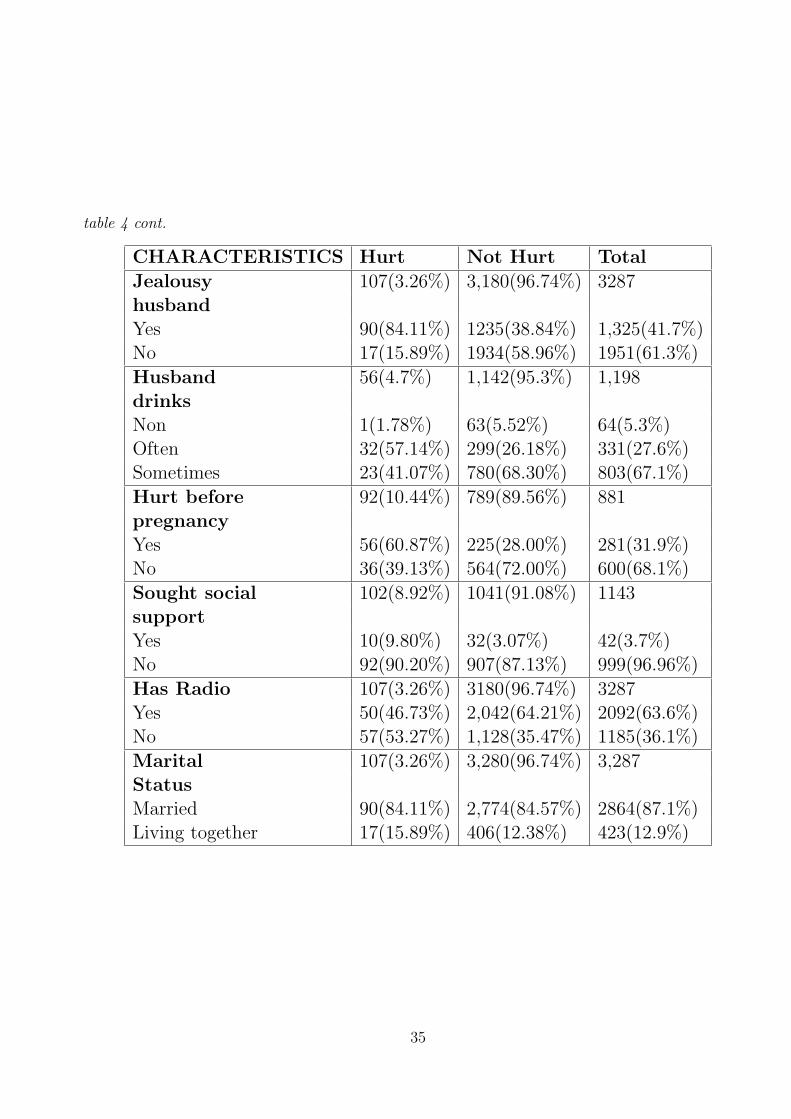
table 4 cont.

CHARACTERISTICS Hurt Not Hurt Total

Jealousy 107(3.26%) 3,180(96.74%) 3287husbandYes 90(84.11%) 1235(38.84%) 1,325(41.7%)No 17(15.89%) 1934(58.96%) 1951(61.3%)

Husband 56(4.7%) 1,142(95.3%) 1,198drinksNon 1(1.78%) 63(5.52%) 64(5.3%)Often 32(57.14%) 299(26.18%) 331(27.6%)Sometimes 23(41.07%) 780(68.30%) 803(67.1%)

Hurt before 92(10.44%) 789(89.56%) 881pregnancyYes 56(60.87%) 225(28.00%) 281(31.9%)No 36(39.13%) 564(72.00%) 600(68.1%)

Sought social 102(8.92%) 1041(91.08%) 1143supportYes 10(9.80%) 32(3.07%) 42(3.7%)No 92(90.20%) 907(87.13%) 999(96.96%)

Has Radio 107(3.26%) 3180(96.74%) 3287Yes 50(46.73%) 2,042(64.21%) 2092(63.6%)No 57(53.27%) 1,128(35.47%) 1185(36.1%)

Marital 107(3.26%) 3,280(96.74%) 3,287StatusMarried 90(84.11%) 2,774(84.57%) 2864(87.1%)Living together 17(15.89%) 406(12.38%) 423(12.9%)

35

6.3.2 Table 5: Frequencies and percentages of women in different back-ground characteristic variables on Place of Residence

CHARACTERISTICS Urban RuralOverall 415 (11.03%) 3,349 (88.97%)Woman’s ageYoung 16 (14.95%) 348 (10.95%)Middle 49 (45.79%) 1,467 (46.15%)Old 42 (39.25%) 1,364 (42.91%)Education levelNo education 34 (8.19%) 614 (18.34%)Primary 219 (52.77%) 2,387 (71.30%)Secondary 145 (34.94%) 335 (10.01%)Higher 17 (4.10%) 12 (0.36%)Woman’s occupationYes 224 (54.11%) 1,980 (59.25%)No 190 (45.89%) 1561,362 (40.75%)Wealth indexPoorest 10 (2.41%) 617 (18.43%)Poorer 21 (5.06%) 818 (24.43%)Middle 35 (8.43%) 831 (24.82%)Richer 98 (23.61%) 695 (20.76%)Richest 251 (60.48%) 387 (11.56%)Woman’s tribeChewa 104 (30.68%) 1,141 (42.17%)Tumbuka 50 (14.75%) 327 (12.08%)Yao 50 (14.75%) 307 (11.35%)Lomwe 68 (20.06%) 515 (19.03%)Ngoni 67 (19.76%) 416 (15.37%)Number of wivesOne 398 (97.07%) 2,999 (90.55%)Two 12 (2.93%) 313 (9.45%)Jealousy husbandYes 137 (38.38%) 1,223 (40.77%)No 220 (61.62%) 1934 (54.23%)Husband drinksNon 8 (5.93%) 60 (5.52%)Often 36 (26.67%) 300 (27.60%)Sometimes 91 (67.41%) 727 (66.88%)Hurt before pregnancyYes 41 (39.05%) 244 (30.77%)No 64 (60.95%) 549 (69.23%)Sought social supportYes 13 (10.40%) 30 (3.25%)No 112 (89.60%) 894 (96.75%)Has radioYes 306 (73.73%) 2,110 (63.31%)No 109 (26.27%) 1,223 (36.69%)Marital StatusMarried 355 (85.54%) 2,915 (87.07%)Living together 2,915 (87.07%) 433 (12.93%)

36