Give to AgEcon Search

The World’s Largest Open Access Agricultural & Applied Economics Digital Library

This document is discoverable and free to researchers across the globe due to the work of AgEcon Search.

Help ensure our sustainability.

AgEcon Search http://ageconsearch.umn.edu

aesearch@umn.edu

Papers downloaded from AgEcon Search may be used for non-commercial purposes and personal study only. No other use, including posting to another Internet site, is permitted without permission from the copyright owner (not AgEcon Search), or as allowed under the provisions of Fair Use, U.S. Copyright Act, Title 17 U.S.C.

1

Determinants of China’s seafood trade patterns

Bixuan Yang, University of Florida, yangbixuan@ufl.edu

Frank Asche, University of Florida, frank.asche@ufl.edu

James L. Anderson, University of Florida, james.anderson@ufl.edu

Selected Paper prepared for presentation at the Southern Agricultural Economics Association (SAEA) Annual Meeting, Birmingham, Alabama, February 2-5, 2019

Copyright 2019 by [Yang, Asche, and Anderson]. All rights reserved. Readers may make verbatim copies of this document for non-commercial purposes by any means, provided that this copyright notice appears on all such copies.

2

Determinants of China’s seafood trade patterns

Abstract

China is the world’s largest seafood exporter, with rapidly increasing exports primarily

based on an increasing aquaculture production. Hence, analyzing patterns for China’s

seafood trade are of great importance. In this study, gravity models were estimated for

various product forms to investigate the impact of economic factors such as GDP, income,

distances, per capita seafood consumption, regional trade agreements (RTA), and

continental locations on seafood trade. The results of the model indicate that there is

substantial variation in trade patterns across product categories. Furthermore, the forms

of live and fresh seafood are a separate group for which trade is significantly affected by

distance, income, and status of “developed country,” while GDP and continental dummies

play an essential role in the trade of products in other forms.

Keywords: seafood trade, augmented gravity model, China, various product forms, trade

polices

1. Introduction

Seafood is one of the most traded food products, accounting for about 9% of global

agricultural food exports. In 2015, the global trade of seafood reached 36.9 million tonnes

with a value of $133.3 billion (FAO, 2016), and it is estimated that 78% of seafood

products are exposed to international trade competition (Tveteras et al., 2012). China is

the world’s largest producer and exporter of seafood. In 2015, Chinese exports accounted

for 15% of global seafood exports with a value of $19.9 million, which was shipped to

over 160 countries. The seafood exports are also important for China, as seafood products

ranked first by value among all food products (China fishery statistical yearbook, 2016).

China’s seafood exports are heterogeneous, composed of multiple species and product

forms, varying from unprocessed products such as frozen whole fish to value-added

3

processed products such as fish fillets and prepared fish, crustaceans, and molluscs. The

trade patterns have changed in recent decades, as growth rates differ across product forms.

In particular, the export value of processed products remained stable, while that of frozen

whole fish was expanding at the very high annual growth rate of 19.5%. As a

consequence, the share of processed products decreased from 73.9% to 53.6%.

This paper investigates the development in Chinese trade patterns of seafood by

estimating gravity models for various product forms. The gravity model is the workhorse

in the international trade literature when investigating trade patterns. There are numerous

examples of applications of this model to analyze trade patterns for other food products

(Sarker and Jayasinghe, 2007; Emlinger et al., 2008; Karemera et al., 2009; Cardamone,

2011; Haq et al., 2012). However, despite the importance of trade in the seafood market,

there are few applications to seafood. The few exceptions primarily investigate two types

of questions regarding seafood trade: 1) Determinants of trade on some specific species

such as shrimp (He et al. 2013) and catfish, basa, and tra fish (Rabbani et al. 2011), or 2)

the impact of food safety standards and non-tariff measures on trade flows (Anders et al.

2006; Nguyen and Wilson, 2009; Liu et al., 2011; Tran et al., 2013; Shepotylo, 2016).

The gravity model also allows the investigation of the impact of factors such as

transportation costs, size of economy and wealth level on China’s seafood exports. This is

potentially important as there is an indication of a preference for high-value and

high-quality seafood in developed countries (Swartz et al., 2010; Asche et al., 2015),

while people in poor countries have tend to import more affordable low-value seafood

(Beveridge et al., 2013).

The rest of this paper is organized as follows. Section 2 introduces the data used and

presents descriptive statistics of trade flows. Section 3 gives a brief literature review of

China’s seafood industry and discusses model specifications. Section 4 reports the

4

empirical results. Section 5 draws some conclusions.

2. Industry and data

The export value of Chinese seafood has doubled during the last decade (Figure 1),

largely associated with a fast growth in production. China's seafood production increased

from 56.1 million tonnes in 2007 to 79.4 million tonnes in 2015. Around 90% of the

expansion of production is contributed by aquaculture (Figure 2), while capture

production has remained almost constant during this period.

Figure 1

Exports value of fish and shellfish (billion US$), 2007-2015.

Source: FAOSTAT Database.

Note: The export value is deflated by the U.S. CPI.

Figure 2

China’s seafood production by production source in quantity (tonnes), 2007-2015.

5

Source: FAOSTAT Database.

Data for China's seafood exports for period 2007-2015 is obtained from the UN

COMTRADE database. This database provides information on the destination country,

quantity, and value (in US$ at current prices) for each commodity classified according to

the Harmonized System (HS) 2007 nomenclature at six digits in each year1. We deflate

export values by the U.S. CPI, which comes from the World Bank. Seafood products in

this study are collected at the two-digit HS level from section 03 (Fish and crustaceans,

molluscs and other aquatic invertebrates) and four-digit HS code section 1604 (Prepared

or preserved fish; caviar and caviar substitutes prepared from fish eggs) and 1605

(Crustaceans, molluscs and other aquatic invertebrates, prepared or preserved).2 The

1 HS codes have been revised in 2012. UN COMTRADE database converts data that is

recorded in HS 2012 to HS 2007. 2. Ornamental fish and by-products including livers, roes, caviar, caviar substitutes, and

6

sample used in this study covers 13,676 observations and 198 trading partners. Figure 1

presents export values of respectively fish and shellfish in period 2007-2015. The figure

clearly shows a strong increasing trend in exports for both categories. Export values of

fish reached 10.76 billion USD in 2015, compared to 5.70 billion USD in 2007. Export

values of shellfish rose to 8.58 billion USD in 2015, which is more than double of the

amount in 2007.

Fishery products are classified into five main product forms: live, fresh, frozen, prepared,

and dried, salted, smoked; crustaceans are classified into three product forms: prepared,

frozen, and fresh3. Similarly, molluscs are classified into three product forms: prepared,

conserved, and live, fresh or chilled. Frozen, dried, salted or in brine, and smoked

molluscs are grouped and defined as conserved molluscs. The composition of two

processing categories, prepared and dried, smoked, salted, are somewhat more complex

than others. Firstly, there are various methods of preparation and preservation of seafood

such as breading, battering, canning, etc., leading to a wide range of product values. The

dried, salted, smoked fish category is also a mixture of both high-value (e.g., smoked

salmon) and low-value products (e.g., salted anchovies). Current dataset employed by our

study does not allow us to differentiate them at a very detailed level, while the results will

still fairly shed light on how factors affect trade across product forms.

Figure 3

Exports value of fish by product form (billion USD), 2007-2015.

fish meal are excluded in this study. 3 The category of fresh crustaceans includes live, fresh, dried, smoked, and salted

crustaceans.

7

Figure 4

Exports value of shellfish by product form (billion USD), 2007-2015.

Figure 3 and 4 present export values of fish and shellfish by product form respectively.

Figure 3 indicates that the frozen is the most important product form, accounting for over

60 percent of the fish exports. The export of frozen fish has more than doubled from 2007

to 2015, making a significant contribution to the total growth of fish exports. For shellfish,

8

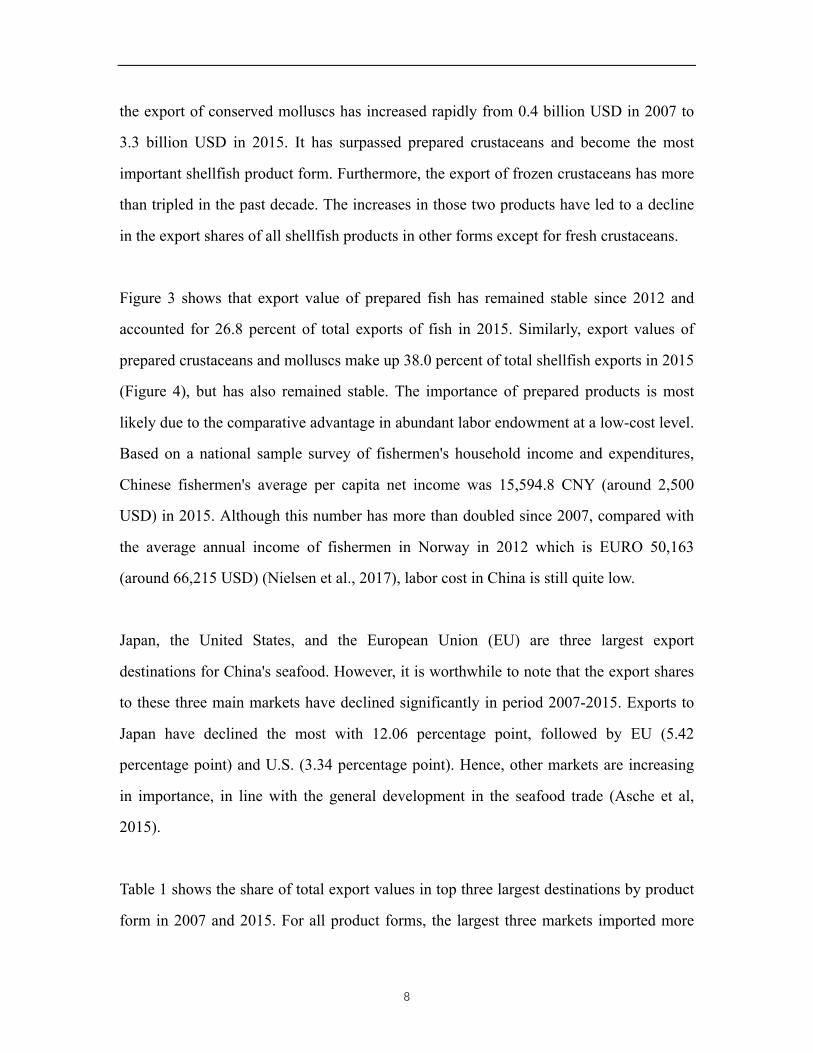
the export of conserved molluscs has increased rapidly from 0.4 billion USD in 2007 to

3.3 billion USD in 2015. It has surpassed prepared crustaceans and become the most

important shellfish product form. Furthermore, the export of frozen crustaceans has more

than tripled in the past decade. The increases in those two products have led to a decline

in the export shares of all shellfish products in other forms except for fresh crustaceans.

Figure 3 shows that export value of prepared fish has remained stable since 2012 and

accounted for 26.8 percent of total exports of fish in 2015. Similarly, export values of

prepared crustaceans and molluscs make up 38.0 percent of total shellfish exports in 2015

(Figure 4), but has also remained stable. The importance of prepared products is most

likely due to the comparative advantage in abundant labor endowment at a low-cost level.

Based on a national sample survey of fishermen's household income and expenditures,

Chinese fishermen's average per capita net income was 15,594.8 CNY (around 2,500

USD) in 2015. Although this number has more than doubled since 2007, compared with

the average annual income of fishermen in Norway in 2012 which is EURO 50,163

(around 66,215 USD) (Nielsen et al., 2017), labor cost in China is still quite low.

Japan, the United States, and the European Union (EU) are three largest export

destinations for China's seafood. However, it is worthwhile to note that the export shares

to these three main markets have declined significantly in period 2007-2015. Exports to

Japan have declined the most with 12.06 percentage point, followed by EU (5.42

percentage point) and U.S. (3.34 percentage point). Hence, other markets are increasing

in importance, in line with the general development in the seafood trade (Asche et al,

2015).

Table 1 shows the share of total export values in top three largest destinations by product

form in 2007 and 2015. For all product forms, the largest three markets imported more

9

than half of total exports in 2007, while export shares to the main markets have declined

particularly in frozen fish, conserved molluscs, and frozen crustaceans. The regional

patterns of some products such as frozen fish, prepared fish, dried, salted, smoked fish,

and prepared crustaceans are fairly stable. The EU, Japan, and the U.S. remain to be the

largest markets for frozen fish and prepared crustaceans, while Japan and the U.S are two

important markets for prepared fish. Korea, the U.S., and the EU are the main partners for

dried, salted, smoked fish exports. However, the regional patterns have changed, and new

partners have emerged for other categories including conserved molluscs, prepared

molluscs, and frozen crustaceans. Thailand has taken over Japan and become the largest

importer of conserved molluscs with a share of 20.01%. The imported conserved

molluscs including squid, cuttlefish, scallop, etc. are used both for local consumption and

as raw materials for re-processing (Infofish, 2013). Low labor cost in Thailand

contributes to the development of processing industry and allows low-value products to

be processed into high-value products for re-export. Hong Kong and Unspecified Asian

countries have taken over the U.S. and Korea for prepared molluscs and taken over Korea

and the EU for frozen crustaceans, then become main trading partners.

The export values of live and fresh seafood (Figure 3 and Figure 4) have shown an

increasing trend. It is associated with the expansion of preferences for high-quality

seafood with freshness being a significant factor (Roheim et al., 2007). Over 90% of live

and fresh fish are exported to Hong Kong, Korea, Japan, and Unspecified Asian countries,

which are wealthy and located in close geographic proximity with China. A similar trade

pattern could also be applied to live, fresh or chilled molluscs and fresh crustaceans. For

other major destination of China's seafood such as the United States, air transport is

employed as the only suitable mode of transportation for live and fresh seafood, making

China less competitive compared with Latin American countries due to high

transportation costs (Asche, 2008).

10

Table 1

Share of total export value in largest destinations by product form (%).

Product form Largest markets 2007 Total

share

Largest markets 2015 Total

share

Fish

Frozen fish EU 31.14 71.45 EU 18.56 52.09

United States 22.13

United States 18.37

Japan 18.18

Japan 15.16

Prepared fish Japan 42.87 72.89 Japan 31.23 58.07

United States 22.04

United States 20.37

Russian

Federation

7.98

Hong Kong 6.47

Live fish Korea, Rep. 43.11 97.20 Hong Kong 43.78 96.18 Japan 32.47

Korea, Rep. 26.67

Hong Kong 21.61

Japan 25.74

Dried, salted,

smoked fish

United States 22.46 63.61 Korea, Rep. 19.44 51.34

EU 21.67

United States 17.60

Korea, Rep. 19.48

EU 14.30

Fresh fish Hong Kong 39.10 95.45 Hong Kong 63.19 91.67 Japan 30.60

Unspecified Asia 24.31

Korea, Rep. 25.74

Korea, Rep. 4.17

Shellfish

Conserved

molluscs

Japan 26.77 66.57 Thailand 20.01 43.53

United States 22.57

United States 12.00

Korea, Rep. 17.23

Hong Kong 11.52

Prepared

crustaceans

United States 23.54 57.29 United States 29.96 51.73

Japan 20.66

Japan 10.94

11

EU 13.10

EU 10.83

Prepared mollucs Japan 54.23 75.69 Japan 31.13 58.12

United States 11.78

Unspecified Asia 14.48

Korea, Rep. 9.69

Hong Kong 12.51

Frozen

crustaceans

Japan 30.39 78.38 Hong Kong 22.12 51.04

Korea, Rep. 25.35

Japan 15.23

EU 22.64

Unspecified Asia 13.69

Live, fresh or

chilled molluscs

Japan 47.18 93.03 Korea, Rep. 64.65 91.63

Korea, Rep. 41.57

Japan 17.32

Hong Kong 4.28

Hong Kong 9.66

Fresh

crustaceans

Hong Kong 43.67 78.70 Hong Kong 31.95 79.29

Japan 18.09

Unspecified Asia 25.96

Korea, Rep. 16.94

Korea, Rep. 21.39

Figure 5

Distribution of fish exports over destination markets, 2007-2015.

12

Figure 6

Distribution of shellfish exports over destination markets, 2007-2015.

13

Figure 5 and 6 report distribution of fish and shellfish over destination markets by

product form respectively. Overall, Asia is the most significant destination market with an

export share of 55.94 percent, while America and Europe rank as the second and third

leading destination markets with a share of 23.06 percent and 17.17 percent over the

sample period. Exports to Africa and Australia only account for 2.06 percent and 1.79

percent respectively.

Exports of live and fresh products are exceptionally highly concentrated with over 95

percent of those goods exported to Asian countries, indicating the importance of distance

for these product categories, possibly together with cultural preference. The U.S. seems

to play a more significant role in importing conserved fish products, as well as prepared

crustaceans than at the aggregation level. Shares of frozen fish, dried, salted, smoked fish,

and frozen crustaceans received by the EU are higher than at the aggregation level.

14

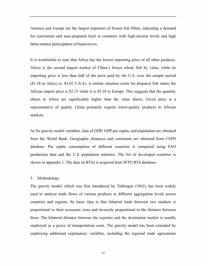
America and Europe are the largest importers of frozen fish fillets, indicating a demand

for convenient and easy-prepared food in countries with high-income levels and high

labor-market participation of housewives.

It is worthwhile to note that Africa has the lowest importing price of all other products.

Africa is the second largest market of China’s frozen whole fish by value, while its

importing price is less than half of the price paid by the U.S. over the sample period

($1.38 in Africa vs. $3.02 U.S.A). A similar situation exists for prepared fish where the

African import price is $2.15 while it is $5.39 in Europe. This suggests that the quantity

shares to Africa are significantly higher than the value shares. Given price is a

representative of quality, China primarily exports lower-quality products to African

markets.

As for gravity model variables, data of GDP, GDP per capita, and population are obtained

from the World Bank. Geographic distances and continents are obtained from CEPII

database. Per capita consumption of different countries is computed using FAO

production data and the U.S. population statistics. The list of developed countries is

shown in appendix 1. The data on RTAs is acquired from WTO RTA database.

3. Methodology

The gravity model, which was first introduced by Tinbergen (1962), has been widely

used to analyze trade flows of various products at different aggregation levels across

countries and regions. Its basic idea is that bilateral trade between two markets is

proportional to their economic sizes and inversely proportional to the distance between

them. The bilateral distance between the exporter and the destination market is usually

employed as a proxy of transportation costs. The gravity model has been extended by

employing additional explanatory variables, including the regional trade agreements

15

(RTAs) (Frankel and Rose, 2002; Feenstra et al., 2001), per capita GDP (Rose, 2000;

Breuss and Egger, 1999), continent dummies (Magerman et al, 2016), etc. Kepaptsoglou

et al. (2010) conduct a comprehensive summary with a list of the variables that have been

applied to the gravity model. They also find that the gravity model is successful in

investigating trade flows due to its empirical robustness. The gravity model has been

applied to a wide variety of food products (Sarker and Jayasinghe, 2007; Karemera et al.,

2009; Natale et al., 2015; Cardamone, 2011; Emlinger et al., 2008; Haq et al., 2012).

For the studies regarding seafood trade, He et al. (2013) examine the determinants of the

U.S. shrimp imports from China, Thailand, Indonesia, and Vietnam using the augmented

gravity model. They find that imports of shrimp in the U.S. depend on the tariff, GDP,

and exchange rate. Rabbani et al. (2011) employs the augmented gravity model and study

the determinants of catfish, basa and tra imports to the U.S. They conclude that per capita

GDP, population, and import prices affect import values, while significance and

magnitude of effects are varied across the country of origin. Tran et al. (2013) assess the

impacts of food safety (chemical) standards on seafood exports to Japan, EU, and the U.S.

with the gravity model. Increasing the stringency of regulations is found to have negative

impacts on trade flows. They compare different specifications of gravity model but

conclude which approach is the best one remains inconclusive. Natale et al. (2015)

investigate the determinants of global seafood trade by applying the gravity model to

different aggregation levels of commodities. Their results show that seafood exports are

driven by high seafood preferences or advantages in low labor cost for further processing.

They also attribute seafood expansion to aquaculture production growth and trade for

re-processing. Shepotylo (2016) explores the extensive and intensive margins of global

seafood exports for the period 1996-2011. He finds that standard gravity-type variables

such as shipping costs, GDP, and RTAs have a significant impact on exports with

expected signs. He emphasizes the heterogeneous effects of non-tariff measures and the

16

different magnitude of effects across products.4

As indicated above, it is increasingly common to augment the gravity model with

variables capturing specific features relevant for the specific case one are addressing, and

that is also of importance in this paper. Per capita GDP is included in the model as a

proxy for the wealth level in the destination market. This is nuanced by also adding an

interaction term of developed country and per capita GDP to distinguish the impact of

wealth in developed and developing countries. The variable per capita consumption of

seafood is used to capture the strength of preference for seafood consumption traditions

in the destination market.

RTAs are reciprocal trade agreements between two or more partners, including free trade

agreements and customs unions. A binary variable RTA is employed in the gravity model

to capture the difference in China’s trade with RTA members and non-members. Some

authors claim that RTAs between China and importing countries could promote bilateral

agricultural trade by improving resource allocation efficiencies and reducing trade

barriers (Yang and Martinez-Zarzozo, 2014; Qiu et al., 2007). However, there is less

consensus in previous studies on the significance and magnitude of such effect since

RTAs have different characteristics and cover various groups of commodities. A set of

continental dummies are used to measure the border effect which is also a proxy of trade

costs. The empirical literature on border effects finds that the direction and magnitude of

border effects are sensitive to the estimation methods and also change gradually.

Anderson and van Wincoop (2003) find the border effect is always negative. In contrast,

Magerman et al. (2016) indicate that some open economies like Europe trade more with

global markets than with intra-continental countries, while Australia trades more inside

4 Although not quite a gravity mode, Straume (2017) use the gravity variables to explain trade duration.

17

than with global markets. As we will discussed in detail in section two, trades of live fish,

fresh fish, fresh crustaceans, and fresh molluscs are highly concentrated in Asia.

Therefore, continental dummies are not included in regressions of those four categories.

The augmented gravity models estimated in this paper has the following specification:

ln#𝑋%&' = 𝛽* + 𝛽, ln#𝐺𝐷𝑃%&' + 𝛽0 ln#𝑑𝑖𝑠𝑡%' + 𝛽5 ln#𝐺𝐷𝑃/𝑐𝑎𝑝𝑖𝑡𝑎%&' + 𝛽:𝐷𝐸 ∗

ln#𝐺𝐷𝑃/𝑐𝑎𝑝𝑖𝑡𝑎%&' + 𝛽= ln#𝑐𝑜𝑛𝑠/𝑐𝑎𝑝𝑖𝑡𝑎%&' + 𝛽@𝑅𝑇𝐴%& + 𝛽D𝐸𝑢𝑟𝑜𝑝𝑒 + 𝛽H𝐴𝑚𝑒𝑟𝑖𝑐𝑎 +

𝛽J𝐴𝑢𝑠𝑡𝑟𝑎𝑙𝑖𝑎 + 𝛽,*𝐴𝑓𝑟𝑖𝑐𝑎 + ∑ 𝛾&& 𝐷& + 𝜖%&………………….(1)

where 𝑋%& is the export value of seafood from China to the destination market j in period

t. The definition of the variables can be found in Table 2.

Table 2

A description of independent variables included in the gravity model.

Explanatory variables Description

𝐺𝐷𝑃% (Real) Gross domestic product (GDP) of the

importing country j

𝑑𝑖𝑠𝑡% Bilateral distance between China and the importing

country j (kilometers)5

𝐺𝐷𝑃/𝑐𝑎𝑝𝑖𝑡𝑎% (Real) GDP per capita in the importing country j6

𝐷𝐸 Binary variable, equals 1 if country j is a developed

country

𝑐𝑜𝑛𝑠/𝑐𝑎𝑝𝑖𝑡𝑎% Per capita consumption of seafood in the importing

5 Bilateral distances are calculated with the great circle formula, which uses latitudes and

longitudes of the most important cities of two countries in terms of population. 6 Real GDP and GDP per capita are denominated in constant US$ (2010).

18

country j (kg per capita)

𝑅𝑇𝐴%& Binary variable, equals 1 if country j is a member of

China’s regional trade agreements

Europe Binary variable, equals 1 if country j is located in

Europe

America Binary variable, equals 1 if country j is located in

North America or South America

Australia Binary variable, equals 1 if country j is located in

Australia

Africa Binary variable, equals 1 if country j is located in

Africa

𝐷& Dummy variable of the year

In recent years, the fact that there are zero trade flows in many potential trade

relationships has received particular attention. Silva and Tenreyro (2006) emphasize that

heteroskedastic residuals and zero trade flows could lead to severely-biased estimates for

parameters. There are several methods proposed in to deal with zero observations: 1.

Ignoring all zero trade flows (Frankel and Rose, 2002; Anderson and Van Wincoop, 2003);

2. replacing the zero with a small number (Van Bergeijk and Oldersma, 1990; Wang and

Winters, 1991; Raballand, 2003); 3. Using the Tobit model (Eaton et al. 1994; Soloaga

and Winters, 2001); 4. Using Poisson family regressions (Silva and Tenreyro, 2006;

Burger et al., 2009); 5. using the Heckman sample selection model (Wooldridge, 2002;

Helpman, Melitz & Rubinstein, 2008). Based on formal statistical tests, Martin and Pham

(2008) and Burger et al. (2009) conclude that the choice of the best model specification to

treat zero trade flows and heteroskedastic issues is inconclusive. In this study, Poisson

Pseudo Maximum Likelihood (PPML) is employed to estimate the gravity model. Year

dummies are included in the model to capture all the time-variant effects of China that are

19

omitted from model specifications, such as China’s seafood production and economic

conditions. Therefore, I specify the empirical model as:

𝑋%& = expU𝛽* + 𝛽, 𝑙𝑛#𝐺𝐷𝑃%&' + 𝛽0 𝑙𝑛#𝑑𝑖𝑠𝑡%' + 𝛽5 𝑙𝑛#𝐺𝐷𝑃/𝑐𝑎𝑝𝑖𝑡𝑎%&' + 𝛽:𝐷𝐸 ∗

𝑙𝑛#𝐺𝐷𝑃/𝑐𝑎𝑝𝑖𝑡𝑎%&' + 𝛽= 𝑙𝑛#𝑐𝑜𝑛𝑠/𝑐𝑎𝑝𝑖𝑡𝑎%&' + 𝛽@𝑅𝑇𝐴%& + 𝛽D𝐸𝑢𝑟𝑜𝑝𝑒 + 𝛽H𝐴𝑚𝑒𝑟𝑖𝑐𝑎 +

𝛽J𝐴𝑢𝑠𝑡𝑟𝑎𝑙𝑖𝑎 + 𝛽,*𝐴𝑓𝑟𝑖𝑐𝑎 + ∑ 𝛾&& 𝐷& + 𝜖%&V………………….(2)

4. Empirical results

Table 3 and 4 present the results from the gravity models grouped by product form. As

one can see, with the exception of frozen fish all regressions have an 𝑅0 higher than 0.4,

suggesting a relatively good fit.7 The relatively low𝑅0 of frozen fish is most likely

attributed to the large number of heterogeneous products within this category. To get a

better understanding of the trade pattern for the frozen fish category, separate regressions

are conducted according to their processing stages, and results are reported in table 5

bellow. Most of the parameters in tables 3 and 4 are statistically significant and have

expected signs. Moreover, the impacts of most variables vary with product form,

providing a clear indication that trade patterns are not identical across product forms.

The magnitude of distance parameters ranges from -0.680 to -2.423 for fish and from

-0.238 to -3.330 for shellfish. Distance is particularly important for live and fresh fish,

fresh molluscs and fresh crustaceans. Hence, high transportation costs of live and fresh

products can to a large extent explain their small proportions in total exports and high

concentration in East Asia. Lower values on the distance variable are reported for other

7. Multicollinearity was tested by computing variance inflation factor (VIF). All VIF

values are below 5 with the exception of GDP per capita (6.05) and the interaction term (5.04). But it is still within the limit of 10, suggesting this model is not suffering serious multicollinearity issues.

20

fish products, frozen crustaceans, and prepared molluscs, indicating that distance is less

important for these products. Finally, insignificant coefficients for conserved molluscs

and prepared crustaceans indicate that exports of those products do not seem to be

affected by distance. The sign of coefficients for GDP is positive and statistically

significant in all cases, which is in line with the assumption that larger economies trade

more. The magnitude of the relationship is relatively smaller for live and fresh products

compared with other commodities.

The role of the income level in a country also varies significantly. Most trade flows

increase with increased income, but to varying degrees. Interestingly, dried, salted and

smoked fish has a negative parameter while the effect is statistically insignificant for

frozen fish. The significant negative impact of income on exports of dried, salted, smoked

fish could be attributed to the fact that dried fish, which accounts for a significant

proportion of exports in this category, are more consumed by poor countries due to its

low-value characteristics (Dey et al., 2008). Also here, live and fresh fish and crustaceans

are much more sensitive than the other variables, indicating that the main markets for

these products are wealthy countries with a short distance from China. These results are

in line with the findings of Asche et al. (2015) that people in wealthier countries have a

preference for high-quality and high-value seafood.

The coefficients of per capita seafood consumption for all products are positive and

statistically significant except for fresh molluscs. The impacts of RTA are ambiguous.

They increase exports for live fish, fresh fish, frozen fish, and all shellfish with the

exception of live and fresh molluscs, while there are negative effects of RTA on prepared

fish. The relative effects of RTA are particularly high for live and fresh fish and fresh

crustaceans.

21

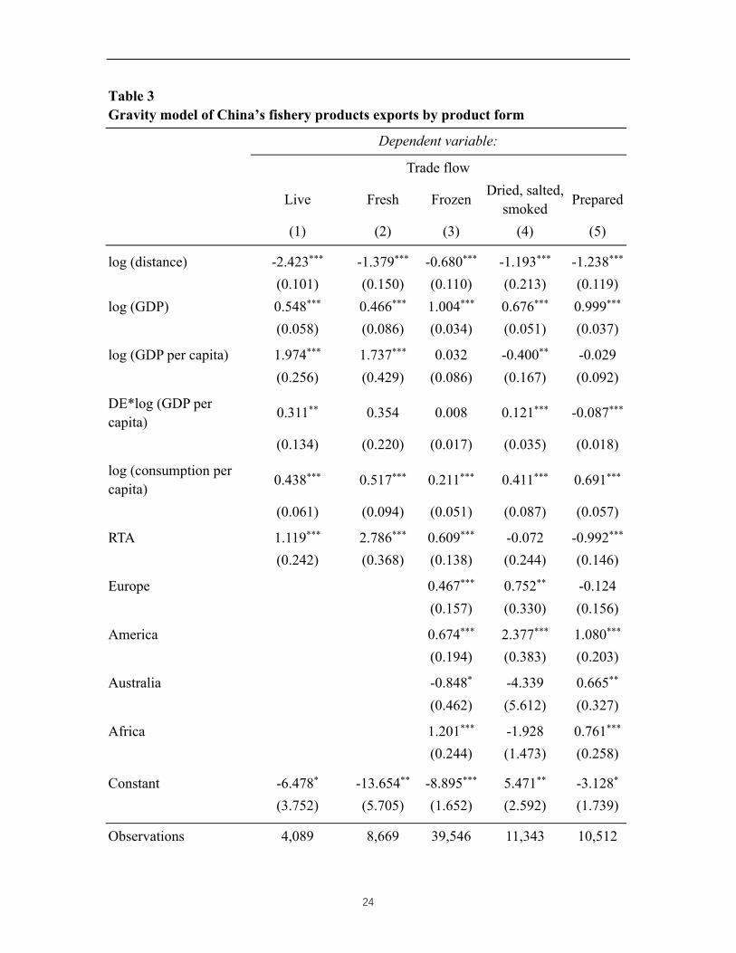
Disregarding live and fresh fish, the continental dummies show that America seems to

import more fish, whatever the level of processing, than Asia. The same applies to Europe

with the exception of prepared fish. In the case of shellfish (excluding fresh crustaceans

and fresh molluscs), the negative coefficients of Europe dummies indicate that exports of

all shellfish face a border effect when entering the European market. For frozen

crustaceans and conserved molluscs, a border effect also exists to the US. This is not too

surprising given the trade tensions for shrimp (Keithley and Poudel, 2008).

As noted above, frozen fish has a low 𝑅0, a feature that may be due to this being a large

category containing several important subcategories. The data allows us to break down

the frozen category by degree of conservation; that is into whole frozen, frozen fillets and

frozen fish meat. The results from the gravity model in equation (2) estimated on these

categories are reported in Table 5. As one can see, the R2 are all improved relatively to

the aggregated model, and there is substantial variation between parameters in the

different categories. Of particular interest is it that the coefficient of Africa for whole

frozen fish is significant and positive, indicating that whole frozen fish are much more

important for Africa. It can be explained by Africa importing low-value whole frozen fish

as affordable sources of protein. Africa’s unit price in this product category is much lower

than for the other continents. There is a positive and significant effect of income for

frozen fish fillets, while the effect is significantly negative for whole frozen fish and

frozen fish meat. The results indicate that frozen fish fillets are considered to be more

valuable, thus are preferred by Europe and the United States. Given that frozen whole

fish are imported and used for reprocessing by some importers, a lower income level

reflects a comparative advantage in cheap labor, which enables those countries to process

low-value frozen whole fish into higher-value products such as fillets.

5. Conclusion

22

This study investigated the determinants of China’s seafood exports by estimating

augmented gravity models for various product forms. As proposed by Silva and Tenreyro

(2006), PPML is applied to solve the issues of zero trade flow and heteroskedastic

residuals. Most of the parameters are statistically significant and have expected signs.

Moreover, there is significant variation in trade patterns between the product categories.

The results indicate that transportation costs and wealth level seem to be much more

important for products with higher perishability, while the impacts are insignificant on

some other products (e.g. conserved molluscs and prepared crustaceans). Furthermore,

most trade flows are driven by increased income but with highly varied degrees. Of

particular interest is it that dried and smoked fish has a negative income parameter,

suggesting that these products are “inferior”, and are primarily being exported to poor

countries with limited ability to pay.

In general, the product forms live and fresh seafood are a separate group of which trade is

significantly affected by distance and income level. This has significant implications for

future marketing strategies as it suggests that wealthy Asian countries will hold the

leading role in importing live and fresh seafood. Furthermore, the lower impact of GDP

also suggests that demand for high-value seafood is not significantly driven by the size of

the economy.

The role of continental locations is different across product categories. Europe and

America provide China with more opportunities and larger markets for a number of fish

products (e.g. frozen fish fillets and dried, smoked, salted fish), while they also face

border effects for some other products. It is worthwhile to point out that low-value whole

frozen fish is much more important for Africa than other continents as affordable sources

of protein.

23

In contrast to the strong growth of frozen products exports, China’s exports of processed

products have remained stable in the past decade, suggesting that its role in re-exporting

seafood is becoming less important.8 It can be attributed to the fact that seafood

processing industry is increasingly challenged by increases in labor and environmental

costs (USDA, 2017). Therefore, there is a trend that China has limited potentials of

processing seafood, although it has potentials of producing seafood as global demand

growth. Meanwhile, countries with low labor cost, such as Thailand and Vietnam, has

experienced a development of processing industry in the past decade.

8 China took the lead in re-exporting seafood when freezing technology became good

enough to allow seafood to be thawed and refrozen several times without a strong reduction in product quality, largely due to low labor cost and economies of scale (Anderson et al, 2017).

24

Table 3 Gravity model of China’s fishery products exports by product form Dependent variable: Trade flow

Live Fresh Frozen Dried, salted, smoked Prepared

(1) (2) (3) (4) (5)

log (distance) -2.423*** -1.379*** -0.680*** -1.193*** -1.238*** (0.101) (0.150) (0.110) (0.213) (0.119) log (GDP) 0.548*** 0.466*** 1.004*** 0.676*** 0.999*** (0.058) (0.086) (0.034) (0.051) (0.037)

log (GDP per capita) 1.974*** 1.737*** 0.032 -0.400** -0.029 (0.256) (0.429) (0.086) (0.167) (0.092)

DE*log (GDP per capita) 0.311** 0.354 0.008 0.121*** -0.087***

(0.134) (0.220) (0.017) (0.035) (0.018)

log (consumption per capita) 0.438*** 0.517*** 0.211*** 0.411*** 0.691***

(0.061) (0.094) (0.051) (0.087) (0.057)

RTA 1.119*** 2.786*** 0.609*** -0.072 -0.992*** (0.242) (0.368) (0.138) (0.244) (0.146)

Europe 0.467*** 0.752** -0.124 (0.157) (0.330) (0.156)

America 0.674*** 2.377*** 1.080*** (0.194) (0.383) (0.203)

Australia -0.848* -4.339 0.665** (0.462) (5.612) (0.327)

Africa 1.201*** -1.928 0.761*** (0.244) (1.473) (0.258)

Constant -6.478* -13.654** -8.895*** 5.471** -3.128* (3.752) (5.705) (1.652) (2.592) (1.739)

Observations 4,089 8,669 39,546 11,343 10,512

25

R2 0.78 0.59 0.38 0.45 0.56 Year dummies Yes Yes Yes Yes Yes

Note: *p**p***p<0.01

26

Table 4 Gravity model of China’s shellfish exports by product form

Dependent variable: Trade flow

Fresh Live and fresh Frozen Conserved Prepared Prepared

crustaceans molluscs crustaceans molluscs crustaceans molluscs

log (distance) -1.282*** -3.330*** -0.238* -0.169 -0.056 -0.776*** (0.080) (0.182) (0.126) (0.110) (0.121) (0.163) log (GDP) 0.378*** 0.695*** 0.908*** 0.810*** 0.814*** 1.014*** (0.043) (0.095) (0.050) (0.039) (0.037) (0.064)

log (GDP per capita) 1.166*** 1.504*** 0.638*** 0.214** 0.489*** 0.705***

(0.167) (0.353) (0.106) (0.090) (0.098) (0.141)

DE*log (GDP per capita) 0.126*** 0.120 -0.061*** 0.047** 0.012 -0.072**

(0.036) (0.084) (0.023) (0.022) (0.021) (0.030)

log (consumption per capita)

0.397*** 0.117 0.636*** 0.474*** 0.414*** 0.612***

(0.054) (0.147) (0.055) (0.054) (0.054) (0.080)

RTA 2.353*** 0.190 1.296*** 1.220*** 1.059*** 0.482** (0.177) (0.389) (0.169) (0.137) (0.139) (0.222)

Europe -0.550*** -1.131*** -1.227*** -1.151*** (0.194) (0.183) (0.192) (0.241)

America -0.904*** -0.462** 0.241 -0.399 (0.246) (0.204) (0.208) (0.296)

Australia -0.174 -0.331 0.039 -0.454 (0.315) (0.267) (0.252) (0.439)

Africa -0.167 0.118 -1.526** 0.080 (0.512) (0.334) (0.709) (0.611)

Constant -2.809 3.693 -17.094*** -10.898*** -12.586*** -13.372*** (2.643) (5.914) (2.378) (1.808) (1.777) (3.130)

27

Observations 5,428 6,416 6,570 9,198 5,256 1,314 R2 0.68 0.78 0.50 0.54 0.61 0.85 Year dummies Yes Yes Yes Yes Yes Yes

Note: *p**p***p<0.01

28

Table 5 Gravity model of China’s frozen fish exports by product form Dependent variable: Trade flow Frozen fillets Frozen whole Frozen meat

log (distance) -1.163*** -0.868*** -0.223 (0.166) (0.102) (0.240) log (GDP) 1.084*** 0.790*** 0.872*** (0.037) (0.031) (0.074)

log (GDP per capita) 0.345*** -0.136** -0.470** (0.130) (0.063) (0.185)

DE*log (GDP per capita) -0.014 -0.040** 0.139*** (0.021) (0.018) (0.047)

log (consumption per capita) -0.190*** 0.777*** 0.578*** (0.061) (0.051) (0.112)

RTA -0.794*** 0.885*** 0.052 (0.215) (0.122) (0.277)

Europe 1.114*** -0.935*** -1.367*** (0.196) (0.197) (0.361)

America 1.318*** 0.077 -1.189*** (0.267) (0.195) (0.436)

Australia -0.610 -0.278 -1.531* (0.542) (0.393) (0.783)

Africa -0.545 1.805*** -2.215** (0.701) (0.178) (1.068)

Constant -6.595*** -2.757** -6.319* (2.227) (1.295) (3.499)

Observations 2,785 33,512 3,249 R2 0.72 0.40 0.59 Year dummies Yes Yes Yes

Note: *p**p***p<0.01

29

Appendix 1

List of developed countries

Country ISO3 Country ISO3

Australia AUS Lithuania LTU

Austria AUT Luxembourg LUX

Belgium BEL Macau MAC

Canada CAN Malta MLT

Cyprus CYP Netherlands NLD

Czech Republic CZE New Zealand NZL

Denmark DNK Norway NOR

Estonia EST Portugal PRT

Finland FIN Puerto Rico PRI

France FRA San Marino SMR

Germany DEU Singapore SGP

Greece GRC Slovakia SVK

Hong Kong HKG Slovenia SVN

Iceland ISL South Korea KOR

Ireland IRL Spain ESP

Israel ISR Sweden SWE

Italy ITA Switzerland CHE

Japan JPN United Kingdom GBR

Latvia LVA United States USA

30

Reference

Anders, S., Caswell, J.A., 2006. "Assessing the Impact of Stricter Food Safety Standards

on Trade: HACCP in U.S. Seafood Trade with the Developing World," 2006 Annual

meeting, July 23-26, Long Beach, CA 21338, American Agricultural Economics

Association (New Name 2008: Agricultural and Applied Economics Association).

Anderson, J.E., van Wincoop, E., 2003. Gravity with Gravitas: A Solution to the Border

Puzzle. American Economic Review 93, 170–192.

https://doi.org/10.1257/000282803321455214

Anderson, J.L., F. Asche, T. Garlock and J. Chu (2017) Aquaculture: It's Role in the

Future of Food. In A. Schmitz, P.L. Kennedy and T.G. Schmitz (ed.). World

Agricultural Resources and Food Security (Frontiers of Economics and Globalization,

Vol. 17). Emerald Publishing, pp- 159-173.

Asche, F. 2008. Farming the Sea. Marine Resource Economics 23(4):527–47.

https://doi.org/10.1086/mre.23.4.42629678

Asche, F., Bellemare, M.F., Roheim, C., Smith, M.D., Tveteras, S., 2015. Fair Enough?

Food Security and the International Trade of Seafood. World Development 67, 151–

160. https://doi.org/10.1016/j.worlddev.2014.10.013

Beveridge, M.C.M., Thilsted, S.H., Phillips, M.J., Metian, M., Troell, M., Hall, S.J., 2013.

Meeting the food and nutrition needs of the poor: the role of fish and the

opportunities and challenges emerging from the rise of aquaculture a: aquaculture and

food and nutrition security. Journal of Fish Biology n/a-n/a.

https://doi.org/10.1111/jfb.12187

Breuss, F., Egger, P., 1999. How Reliable Are Estimations of East-West Trade Potentials

Based on Cross-Section Gravity Analyses? Empirica 26, 81–94.

https://doi.org/10.1023/A:1007011329676

31

Burger, M., van Oort, F., Linders, G.-J., 2009. On the Specification of the Gravity Model

of Trade: Zeros, Excess Zeros and Zero-inflated Estimation. Spatial Economic

Analysis 4, 167–190. https://doi.org/10.1080/17421770902834327

Cardamone, P., 2011. The effect of preferential trade agreements on monthly fruit exports

to the European Union. Eur Rev Agric Econ 38, 553–586.

https://doi.org/10.1093/erae/jbq052

China Agriculture Press (2016) China Fishery Statistical Yearbook (China Agriculture

Press, Beijing). Chinese.

Dey, M.M., Garcia, Y.T., Praduman, K., Piumsombun, S., Haque, M.S., Li, L., Radam, A.,

Senaratne, A., Khiem, N.T., Koeshendrajana, S., 2008. Demand for fish in Asia: a

cross-country analysis*. Australian Journal of Agricultural and Resource Economics

52, 321–338. https://doi.org/10.1111/j.1467-8489.2008.00418.x

Eaton, Jonathan, and Akiko Tamura. "Bilateralism and regionalism in Japanese and US

trade and direct foreign investment patterns." Journal of the Japanese and

international economies 8, no. 4 (1994): 478-510.

Emlinger, C., Jacquet, F., Lozza, E.C., 2008. Tariffs and other trade costs: assessing

obstacles to Mediterranean countries’ access to EU-15 fruit and vegetable markets.

European Review of Agricultural Economics 35, 409–438.

https://doi.org/10.1093/erae/jbn031

FAO, The State of World Fisheries and Aquaculture 2016 (SOFIA): Contributing to food

security and nutrition for all, Rome: Food and Agriculture Organization, 2016, pp.

200.

Feenstra, R.C., 2015. Advanced International Trade: Theory and Evidence - Second

Edition. Princeton University Press.

Frankel, J., Rose, A., 2002. An Estimate of the Effect of Common Currencies on Trade

and Income. Quarterly Journal of Economics 117, 437–466.

https://doi.org/10.1162/003355302753650292

32

Haq, Z.U., Meilke, K., Cranfield, J., 2013. Selection bias in a gravity model of agrifood

trade. Eur Rev Agric Econ 40, 331–360. https://doi.org/10.1093/erae/jbs028

He, C., Quagrainie, K.K., Wang, H.H., 2013. Determinants of shrimp importation into the

USA: an application of an augmented gravity model. Journal of Chinese Economic

and Business Studies 11, 219–228. https://doi.org/10.1080/14765284.2013.814466

Helpman, E., Melitz, M., Rubinstein, Y., 2008. Estimating Trade Flows: Trading Partners

and Trading Volumes*. The Quarterly Journal of Economics 123, 441–487.

https://doi.org/10.1162/qjec.2008.123.2.441

INFOFISH (2013).Thailand Seafood Market and Potentials for Peruvian Products,

October 2013. Accessed online at

http://www.siicex.gob.pe/siicex/resources/sectoresproductivos/Thailand%20Report%

20Market%20Review.pdf

Karemera, D., Managi, S., Reuben, L., Spann, O., 2011. The impacts of exchange rate

volatility on vegetable trade flows. Applied Economics 43, 1607–1616.

https://doi.org/10.1080/00036840802600137

Keithly, W.R., Poudel, P., 2008. The Southeast U.S.A. Shrimp Industry: Issues Related to

Trade and Antidumping Duties. Marine Resource Economics 23, 459–483.

https://doi.org/10.1086/mre.23.4.42629675

Kepaptsoglou, K., Karlaftis, M.G., Tsamboulas, D., 2010. The Gravity Model

Specification for Modeling International Trade Flows and Free Trade Agreement

Effects: A 10-Year Review of Empirical

Studies~!2009-07-09~!2010-01-28~!2010-04-22~! The Open Economics Journal 3,

1–13. https://doi.org/10.2174/1874919401003010001

Liu, H., Kerr, W.A., Hobbs, J.E., 2012. A review of Chinese food safety strategies

implemented after several food safety incidents involving export of Chinese aquatic

products. British Food Journal 114, 372–386.

https://doi.org/10.1108/00070701211213474

33

Magerman, G., Studnicka, Z., Van Hove, J., 2016. Distance and Border Effects in

International Trade: A Comparison of Estimation Methods. Economics: The

Open-Access, Open-Assessment E-Journal.

https://doi.org/10.5018/economics-ejournal.ja.2016-18

Martin W, Pham CS. 2008. Estimating the gravity equation when zero trade flows are

frequent. MPRA Pap. 9453, Univ. Libr. Munich, Ger.

Nguyen, A.V.T., and Wilson, N.L.W. 2009. “Effects of Food Safety Standards on Seafood

Exports to US, EU and Japan,” Southern Agricultural Economics Association Annual

Meeting.

Qiu, H., Yang, J., Huang, J., Chen, R., 2007. Impact of China‐ASEAN Free Trade Area

on China’s International Agricultural Trade and Its Regional Development. China &

World Economy 15. https://doi.org/10.1111/j.1749-124X.2007.00083.x

Raballand, G., 2003. Determinants of the Negative Impact of Being Landlocked on Trade:

An Empirical Investigation Through the Central Asian Case. Comparative Economic

Studies 45, 520–536. https://doi.org/10.1057/palgrave.ces.8100031

Rabbani, A.G., Dey, M.M., Singh, K., 2011. Determinants of catfish, basa and tra

importation into the USA: an application of an augmented gravity model. Aquaculture

Economics & Management 15, 230–244.

https://doi.org/10.1080/13657305.2011.598215

Roheim, C.A., Gardiner, L., Asche, F., 2007. Value of Brands and Other Attributes:

Hedonic Analysis of Retail Frozen Fish in the UK. Marine Resource Economics 22,

239–253. https://doi.org/10.1086/mre.22.3.42629557

Rose, A.K., 2000. One money, one market: the effect of common currencies on trade.

Economic Policy 15, 8–0. https://doi.org/10.1111/1468-0327.00056

Sarker, R., Jayasinghe, S., 2007. Regional trade agreements and trade in agri‐food

products: evidence for the European Union from gravity modeling using

34

disaggregated data. Agricultural Economics 37, 93–104.

https://doi.org/10.1111/j.1574-0862.2007.00227.x

Shepotylo, O., 2016. Effect of non-tariff measures on extensive and intensive margins of

exports in seafood trade. Marine Policy 68, 47–54.

https://doi.org/10.1016/j.marpol.2016.02.014

Silva, J.M.C.S., Tenreyro, S., 2006. The Log of Gravity. The Review of Economics and

Statistics 88, 641–658. https://doi.org/10.1162/rest.88.4.641

Soloaga, I., Alan Wintersb, L., 2001. Regionalism in the nineties: what effect on trade?

The North American Journal of Economics and Finance 12, 1–29.

https://doi.org/10.1016/S1062-9408(01)00042-0

Straume, H.-M.,2017. Here today, gone tomorrow: The duration of Norwegian salmon

exports. Aquaculture Economics and Management, 21(1), 88-104

http://dx.doi.org/10.1080/13657305.2017.1262477

Swartz, W., Rashid Sumaila, U., Watson, R., Pauly, D., 2010. Sourcing seafood for the

three major markets: The EU, Japan and the USA. Marine Policy 34, 1366–1373.

https://doi.org/10.1016/j.marpol.2010.06.011

Tinbergen, J., 1962. Shaping the world economy: Suggestions for an international

economics policy, The Twentieth Century Fund, New York.

Tran, N., Wilson, N., and Hite, D., (2012). Choosing the best model in the presence of

zero trade: a fish product analysis. WorldFish, Penang, Malaysia. Working Paper:

2012-50.

Tveterås, S., Asche, F., Bellemare, M.F., Smith, M.D., Guttormsen, A.G., Lem, A., Lien,

K., Vannuccini, S., 2012. Fish Is Food - The FAO’s Fish Price Index. PLoS ONE 7,

e36731. https://doi.org/10.1371/journal.pone.0036731

USDA, 2017. China's Fishery Annual, USDA foreign agricultural service report

35

Van Bergeijk, P.A.G. and H. Oldersma, 1990. Detente, Market-Oriented Reform and

German Unification: Potential Consequences for the World Trade System, Kyklos, 43,

599–609. https://doi.org/10.1111/j.1467-6435.1990.tb02239.x

Wang, Z.K. and Winters, L.A., 1992. The trading potential of Eastern Europe. Journal of

Economic Integration, pp.113-136.

Wooldridge, J.M., 2002. Inverse probability weighted M-estimators for sample selection,

attrition, and stratification. Portuguese Economic Journal 1, 117–139.

https://doi.org/10.1007/s10258-002-0008-x

Yang, S., Martinez-Zarzoso, I., 2014. A panel data analysis of trade creation and trade

diversion effects: The case of ASEAN–China Free Trade Area. China Economic

Review 29, 138–151. https://doi.org/10.1016/j.chieco.2014.04.002