Characterising metabolic deficits in sporadic and familial ...
Upload
khangminh22Category
view
2download
0
© Copyright by Brendan Tonson-Older 2020. All Rights Reserved.
Detection of higher visual function deficits and
validation of multifocal pupillography in
stroke, chiasmal compression and anterior
ischemic optic neuropathy.
A thesis submitted for the degree of Doctor of Philosophy
of The Australian National University.
Dr Brendan Tonson-Older
Submitted for examination February 20, 2020

ii

iii
Declaration
I declare that this thesis is entirely my own original work, and that no component has previously
been submitted to any university for any award or qualification. I have been the major
contributor involved in all aspects in the production of this thesis including: design, data
collection, analysis and writing. A portion of the data for the second experimental chapter was
collected by persons other than myself to provide the opportunity for reanalysis in combination
with my data, but all other analysis and collection of experimental data was carried out by
myself. To the best of my knowledge, no component has been previously written or published
prior to submission without due acknowledgement.
____________________________
Brendan Tonson-Older
20th February, 2020

iv

v
Acknowledgements
Firstly I would like to acknowledge the support of my supevisors, Prof. Ted Maddess for
introducing me to the world of ophthalmology and the generous use of his lab and equipment
which made this project possible. To my chair Prof. Christian Lueck, who was always there to
lend an ear, and whose advise was invaluable both inside and outside of research. To Assoc
Prof. Jason Bell, who kindly designed the kinematogram with me, and who I could always rely
on to have an open discussion and practical advice. To Dr Corinne Carle, who has invested
much of her time helping me to where I am now, teaching me, and showing me the ropes of
working in this lab, I also would not be here without your considerable support.
I would also like to especially thank Assoc Prof. Krisztina Valter-Kocsi, who supported me
through both my PhD and medical school, through some of my darkest times.
To Diana Perriman and Ms Amelia Maddock, who had helped with numerous questions and
concerns, and ensured my financial stability.
To those clinical staff who work on this project:
Emilie Rohan help with slitlamp exams, running the clinical suite, and always with a smile.
Dr Kate Reid, who was kind enough to refer many of the test subjects, and assess all the clinical
information to rule out ocular disorders.
Dr Jocelyne Rivero, who first showed me how to use an OCT and the Humphrey devices, and
showed me the basics of clinical assessment before the project began.
Dr Shaun Zhai – who referred stroke patients, and assessed neurological deficits in many of
the subjects.

vi
Dr Faran Sabeti and Ms Maria Kolic – who showed me many of the devices used in the clinical
suite, and aided with my training.
To the various clinical and ANU departments who have supported me along this journey:
Canberra Hospital neurology department, Eye clinic, Calvary stroke ward, and Canberra eye
hospital, for all the referrals and advice.
The ANU medical school for training me as a doctor, and supporting my PhD, and for the
financial support in stipend and scholarship which allowed me to come here.
I would also like to recognise the excpetional work provided by the professional copy editor
Dr Andrew Bell, who helped ensure the quality and continuity of my work.
To my family, especially my mother Jaqui Tonson and my aunt Barbara Tonson, who have
always been there to talk and support me through the high and lows.
To my friends who have supported me through this long journey, especially Maree Silling who
has kept me level headed and calm in periods of stress, and Hayley Fancourt, who has always
been a ear to listen and the shoulder to cry on, and the person who has brought joy to my life
just when I need it most.
vii
Abstract
It is well established that neural damage can result in visual dysfunction, both visual field loss
and in higher visual function (HVF) loss such as perceptions of depth, colour, motion and faces.
This thesis examines these visual deficits in the common neurological diseases of stroke,
chiasmal compression, and anterior ischemic optic neuropathy (AION).
While it is established that isolated complete HVF deficits do occur in stroke, they are also
known to be rare. However, as HVFs are not routinely tested in clinical practice, it is unknown
how common more subtle defects are, and what tools are effective in detecting these. Chapter
3 explores these questions, outlining that colour and depth perceptions are the most commonly
affected, that Ishihara (colour) and stereofly and randot (depth), are the most useful tests, and
outlines recommendations for improvement in some of these tools.
The relatively new invention of multifocal pupillographic objective perimetry (mfPOP)
provides a number of benefits from other forms of perimetry. It measures both eyes at once,
allowing measures of direct and consensual responses, it is objective, and it allows repeat
measures of each region giving a measure of error. This advancement opens up new
opportunities to investigate pupillary physiology in neurological disorders and adds new
challenges in how to combine these signals into a single meaningful measure. Chapter 4
investigates the physiology of the pupil in stroke, chiasmal compression, and AION, and
investigates how these components can be appropriately combined into a single measure.
Results show naso-temporal differences are consistent with known physiology in control
subjects and provides evidence that denser nasal retinal input may underpin the greater
contraction anisocoria seen in temporal fields than in nasal fields.
viii
With the intention that mfPOP be used in clinical practice, it must demonstrate it can perform
as well as traditional perimetry, such as Humphrey and Matrix devices, in a wide range of
disorders. Currently mfPOP testing neurological disorders has been very limited, and this
represents a large gap in the literature. Chapter 5 compares mfPOP to Humphrey and Matrix
perimeters, showing they mfPOP does not correlate well with these devices, and compares their
utility in neurological disease. It shows that Humphrey appears the most useful device overall,
with Matrix being exceptionally good in chiasmal compression, while mfPOP does not appear
effective in these disorders.
With the first mfPOP approach having limitations in its diagnostic ability, a second stimulus
protocol was designed using colour opponency with the measure of response latency (rather
than amplitude), thought to preferentially stimulate cortical input to the pupil response, and
may allow detection of cortical lesions. Chapter 6 investigates this new colour exchange
protocol and latency measure, contrasting with the more common luminance approach used in
chapter 5. It shows that the colour protocol shows a number of subtle differences compared to
the luminance protocol, but does not show any greater utility in neurological disease. It reveals
that latency and amplitude appear to have a weak positive relationship, and that mfPOP repeats
appear to correlate well, but all measures have substantial variation.
These finding open up a number of future directions, from a larger and more focused HVF
study into colour and depth perception, to considering retinal density as contributing towards
biases in pupillary components, exploring hemifield ratios as a measure of early detection of
chiasmal compression, and trialling other mfPOP methods to determine whether neurological
disorders can be detected through pupillometry.

ix
Table of Contents
2 Chapter 2: General Methods ................................................... Error! Bookmark not defined.
2.1. Recruitment ........................................................................ Error! Bookmark not defined.
2.1.1. Sources of potential subjects ........................................... Error! Bookmark not defined.
2.1.2. Selection criteria .............................................................. Error! Bookmark not defined.
2.1.3. Exclusion criteria .............................................................. Error! Bookmark not defined.
2.1.4. Contact ............................................................................. Error! Bookmark not defined.
2.1.5. Consent ............................................................................ Error! Bookmark not defined.
2.2. Medical History ................................................................... Error! Bookmark not defined.
2.2.1. Questionnaire .................................................................. Error! Bookmark not defined.
2.2.2. Hospital records ............................................................... Error! Bookmark not defined.
2.3. Screening for pre-existing conditions ................................... Error! Bookmark not defined.
2.3.1. Acuity ............................................................................... Error! Bookmark not defined.
2.3.2. Cataracts .......................................................................... Error! Bookmark not defined.
2.3.3. Retinal disorders .............................................................. Error! Bookmark not defined.
2.3.4. Visual neglect ................................................................... Error! Bookmark not defined.
2.4. Higher Visual Function Tests ................................................ Error! Bookmark not defined.
2.4.1. Stereopsis ......................................................................... Error! Bookmark not defined.
2.4.2. Colour vision..................................................................... Error! Bookmark not defined.
2.4.3. Global motion detection .................................................. Error! Bookmark not defined.
2.4.4. Facial recognition ............................................................. Error! Bookmark not defined.
2.5. Perimetry ............................................................................ Error! Bookmark not defined.
2.5.1. Humphrey Field Analyser (HFA) ....................................... Error! Bookmark not defined.
2.5.2. Matrix Field Analyser (MFA) ............................................ Error! Bookmark not defined.
2.5.3. Multifocal pupillographic objective perimetry (mfPOP) .. Error! Bookmark not defined.
2.6. MRI ..................................................................................... Error! Bookmark not defined.
References ......................................................................................... Error! Bookmark not defined.
Appendix A: Line Bisection Test .......................................................... Error! Bookmark not defined.
Appendix B: Star Cancellation Test ..................................................... Error! Bookmark not defined.
x
Glossary: abbreviations
AION Anterior ischemic optic neuropathy
AMD Age-related macular degeneration
Amp Peak amplitude (pupillary response)
ARK-1 Autorefractor and keratometer (Brand name)
AUC Area under the curve
BCVA Best corrected visual acuity
BFRT Benton facial recognition test
BM Basement membrane
CCC Central corneal curvature
CCI Colour confusion index (Farnsworth-Munsell)
CFMT Cambridge facial memory test
CI Confidence interval
CIELAB International Commission of Illumination colour scale
CNIII Cranial nerve number 3 (Occulomotor nerve)
Con Consensual pupil response
CT Computed tomography
D15 Farnsworth-Munsell Dichotomous 15-well test
Dir Direct pupil response
DTI Diffusion tensor imaging (Magnetic resonance scan)
DWI Diffusion weighted imaging
EEG Electroencephalogram
ETDRS Early treatment of diabetic retinopathy study (Type of visual acuity chart)
EWN Edinger-Westphal nuceli
FDT Frequency doubling technology
FLAIR Fluid attenuated inversion recovery (Magnetic resonance scan)
FM Farnsworth-Munsell
FM100 Farnsworth-Munsell Dichotomous 100-well test
FPR False positive ration
G/R Bright green stimuli on dim red background
GCA Giant cell arteritis
GCL Ganglion cell layer
HFA Humphrey field analyser
HH Homonymous hemianopia
HVF Higher visual function
ICC Intraclass correlation coeffcient
ICH Intracranial haemorrhage
ILM Internal limiting membrane
INL Inner nuclear layer
IOP Intraocular pressure
IPL Inner plexiform layer
ipRGC intriniscally photoreceptive retinal ganglion cells
IS Inner segment
Ishi Ishihara 24-plate set
xi
IT Inferior temporal
K-cells Koniocellular cells
Km Kinematogram
LB Line bisection (3x horizontal lines)
L-cone Longwave cone (red)
LGN Lateral geniculate nucleus
M-cells Magnocellular cells
M-cone Mediumwave cone (yellow)
MFA Humphrey-Matrix field analyser
mfPOP Multifocal pupillogrpahic objective perimetry
mfVEP Multifocal visual evoked potentials
MLA Maximum liklihood analysis
MRI Magnetic resonance imaging
MT Middle temporal region
NA-AION Non-arteritic anterior ischemic optic neuropathy
OCT Optical coherence tomography
ONH Optic nerve head
ONL Outer nuclear layer
OPL Outer plexiform layer
Opn4 Melanopsin
ORA Ocular response analyser
OS Outer segment
P.pole Posterior pole (Fundoscopy)
PCA Principal component analysis
P-cells Parvocellular cells
PON Pretectal olivery nucleus
PWI Perfusion weighted imaging
R&R Relaxing and remitting (Multiple sclerosis)
Randot Random Dot 3 (Stereoacuity test)
RD Randot 3 with lea symbols
RDK Random dot kinematogram
RGC Retinal ganglion cells
RHT Retinohypothalamic tract
RMF Recognition memory test for faces
RNFL Retinal nerve fibre layer
ROC Receiver operator characteristics
RPE Retinal pigment epithelium
SCN Suprachiasmatic nucleus
S-cone Shortwave cone (blue)
SD Standard deviation
SE Standard error
SF Stereofly with lea symbols
SITA Swedish interactive thresholding algorithms
SNR Signar to noise ratio
Spectralis Spectral domain optical coherence tomography (Brand name)
TCDS Total colour difference score (Farnsworth-Munsell)

xii
TTP Time to peak (pupillary response)
V1 Primary visual cortex
V2-V8 Secondary visual cortices
VEP Visual evoked potentials
VFD Visual field defect
VFL Visual field loss
Y/Y Bright yellow stimuli on dim yellow background
ZEST Zippy estimation of sequential testing

13
1 Chapter 1: Introduction
1.1. Statement of Purpose
It is well established that neural damage can result in visual dysfunction, both visual field loss
and higher visual function1 (HVF) loss which include facial recognition, motion, and depth and
colour perception. While pure and complete HVF losses are rare, patients may also present
with more subtle deficits and there is no measure of how commonly these deficits occur in
stroke patients, nor which tests are most effective in detecting them. As they are not typically
assessed in current clinical practice, they may frequently go undiagnosed, leading to slower
recoveries, impaired quality of life, and potentially serious accidents.
The first part of this study is a pilot study investigating higher visual loss in stroke patients to
ascertain if any deficits are sufficiently common to warrant further investigation and which
tests provide the greatest utility in detection of these disorders.
Another form of visual impairment is visual field loss, which is typically assessed with
perimetry. To increase consistency, there has been a transition over the last 25 years from
traditional manual perimetry into automated perimetry, with the Humphrey field analyser and
Matrix being two of the more commonly used perimeters. Both these machines require users
to consciously respond to stimuli, making the test intrinsically subjective. Patients often do not
respond appropriately, or in the case of stroke patients, they may have other limitations which
prevent reliable testing. To address this, pupillographic perimetry was developed to eliminate
1 Visial perception which is processed outside of the primary visual cortex. These include all manner of processing
of the basic image to include colour, form, motion, recognition, and interpretation.
Chapter 1: Statement of purpose
14
subjective patient responses and replace them with autonomic pupil responses. Given that it
uses the pupil reflex (hundreds of milliseconds) – compared to perception, recognition, and
motor output (seconds) – it also means regions can be tested much faster. More recently
pupillographic perimetry has been further developed through multifocal methods which allow
multiple stimuli to be presented simultaneously, increasing the number of presentations
possible in a given time. This multifocal pupillographic objective perimetry (mfPOP)
technology has been shown to be useful in a number of retinal disorders, but there has only
been limited testing in neural disorders.
The second part of this study aims to investigate how damage to various parts of the visual
pathway – anterior (anterior ischemic optic neuropathy, AION), chiasmal (chiasmal
compression), and posterior (cortical stroke) – affect mfPOP measures. First, direct and
consensual responses are compared to highlight the underlying physiology and determine
appropriate means to amalgamate these signals. Secondly, to determine if mfPOP is sensitive
enough to neural damage in these conditions, compared to existing Humphrey and Matrix
devices, so as to be useful clinically. Lastly, to compare different stimuli protocols and
measures to evaluate which approach is most useful and whether any additional information
can be gleaned from alternative approaches. In particular, the aim is to determine whether post-
lateral geniculate nucleus (LGN) damage (posterior to subcortical pupillary branch point) can
be detected by mfPOP, and whether this is best measured with luminance only or colour-
exchange protocols, using either size (amplitude) or time (latency) measures.
Chapter 1: Overview of chapter
15
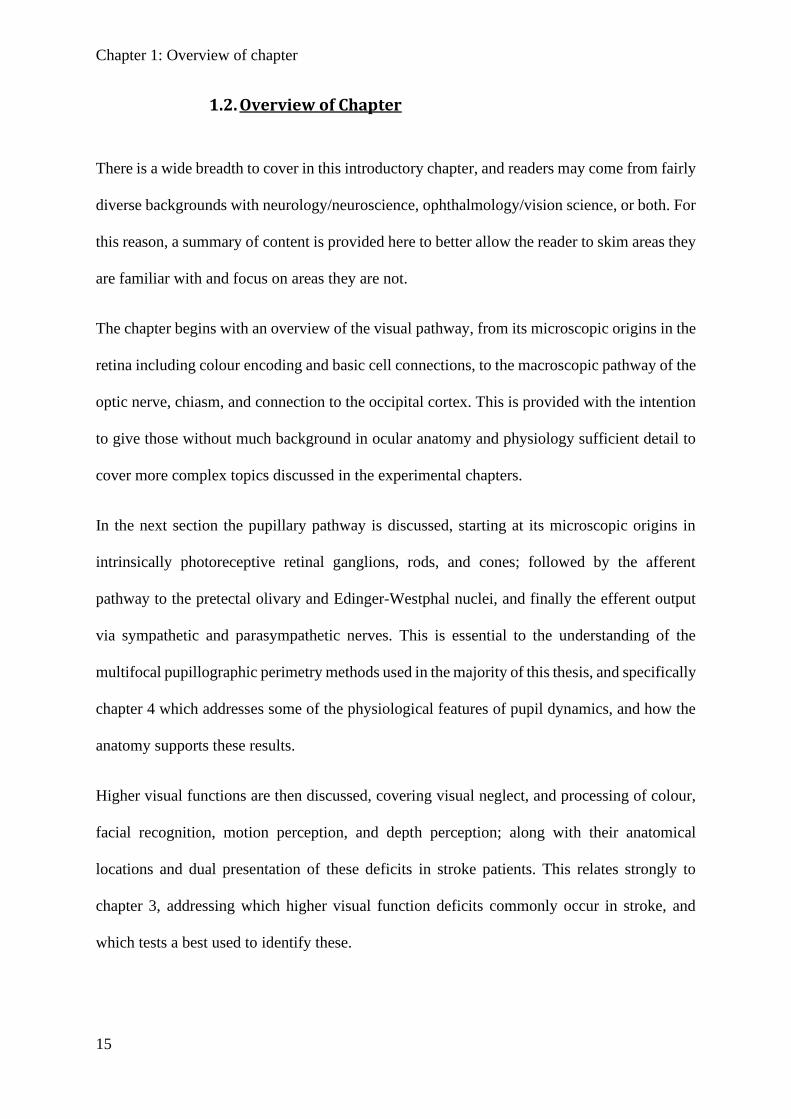
1.2. Overview of Chapter
There is a wide breadth to cover in this introductory chapter, and readers may come from fairly
diverse backgrounds with neurology/neuroscience, ophthalmology/vision science, or both. For
this reason, a summary of content is provided here to better allow the reader to skim areas they
are familiar with and focus on areas they are not.
The chapter begins with an overview of the visual pathway, from its microscopic origins in the
retina including colour encoding and basic cell connections, to the macroscopic pathway of the
optic nerve, chiasm, and connection to the occipital cortex. This is provided with the intention
to give those without much background in ocular anatomy and physiology sufficient detail to
cover more complex topics discussed in the experimental chapters.
In the next section the pupillary pathway is discussed, starting at its microscopic origins in
intrinsically photoreceptive retinal ganglions, rods, and cones; followed by the afferent
pathway to the pretectal olivary and Edinger-Westphal nuclei, and finally the efferent output
via sympathetic and parasympathetic nerves. This is essential to the understanding of the
multifocal pupillographic perimetry methods used in the majority of this thesis, and specifically
chapter 4 which addresses some of the physiological features of pupil dynamics, and how the
anatomy supports these results.
Higher visual functions are then discussed, covering visual neglect, and processing of colour,
facial recognition, motion perception, and depth perception; along with their anatomical
locations and dual presentation of these deficits in stroke patients. This relates strongly to
chapter 3, addressing which higher visual function deficits commonly occur in stroke, and
which tests a best used to identify these.
Chapter 1: Overview of chapter
16
With the visual pathway being covered, including deficits from damage to the cortex, an
overview of cortical stroke is first covered, followed by the subcortical diseases used in this
research (chiasmal compression and anterior ischemic optic neuropathy). Collectively these
represent anterior damage at the optic disc, damage in the middle at the optic radiation, and
damage posteriorly in the cortex; allowing a comparison between damage affecting the
subcortical pupillary pathway and damage to the cortical input to the pupillary system. This
relates to a key element of this research – to determine if multifocal pupillographic perimetry
can detect subcortical and cortical damage utilising the pupil response (chapters 5 and 6). Each
of these sections also outline their typical visual field loss and progression, to better inform
decisions made in methods and analysis, particularly the hemifield ratios used in the analysis
of chapter 5.
Visual field testing is then addressed. This section covers confrontational testing and its
limitations, the invention of manual Goldmann perimetry, the invention and refinement of both
automated Humphrey perimetry and automated Matrix perimetry, and the multifocal methods
of visual evoked potentials which led to the development of automated multifocal
pupillographic objective perimetry (mfPOP). This history is covered because it is crucial to
understanding how and why various aspect of mfPOP were designed they way they are, and
because Humphrey and Matrix are directly compared with mfPOP in chapter 5. A more
extensive section on mfPOP is then covered, outlining experiments using this technology and
refinement of its methods into what is used for these experiments. This is most pertinent to
chapter 6, which utilises some new alternative methods informed by previous experiments.
Lastly, a summary of experimental results published following commencement of this study
are provided to give a sense of where this work fits into the literature.
At the end of the chapter is a summary section, to provide links between the key concepts
covered in the introduction and why this led to the research being completed.
Chapter 1: Visual pathways
17
1.3. Visual Pathways
1.3.1. Retinal function
Light initially enters the eye through the cornea, which contributes most of the refraction. The
iris blocks out extraneous light, allowing the remaining light to be sharply focused on the retina
by the variable refractive capacity of the lens. The retina functions to phototransduce light into
electrical currents and organise these into a structural framework which can be transmitted and
interpreted by the neural networks of the visual cortex and subcortical nuclei.
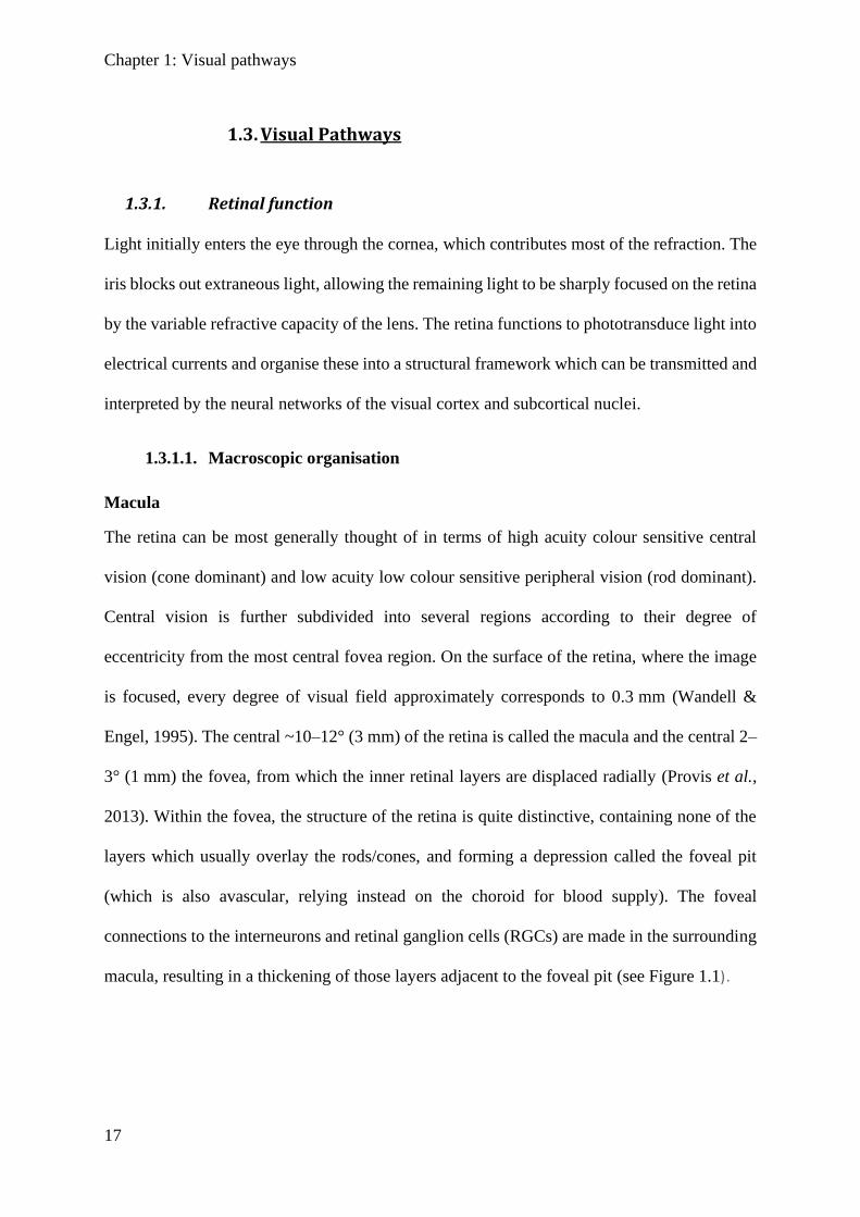
1.3.1.1. Macroscopic organisation
Macula
The retina can be most generally thought of in terms of high acuity colour sensitive central
vision (cone dominant) and low acuity low colour sensitive peripheral vision (rod dominant).
Central vision is further subdivided into several regions according to their degree of
eccentricity from the most central fovea region. On the surface of the retina, where the image
is focused, every degree of visual field approximately corresponds to 0.3 mm (Wandell &
Engel, 1995). The central ~10–12° (3 mm) of the retina is called the macula and the central 2–
3° (1 mm) the fovea, from which the inner retinal layers are displaced radially (Provis et al.,
2013). Within the fovea, the structure of the retina is quite distinctive, containing none of the
layers which usually overlay the rods/cones, and forming a depression called the foveal pit
(which is also avascular, relying instead on the choroid for blood supply). The foveal
connections to the interneurons and retinal ganglion cells (RGCs) are made in the surrounding
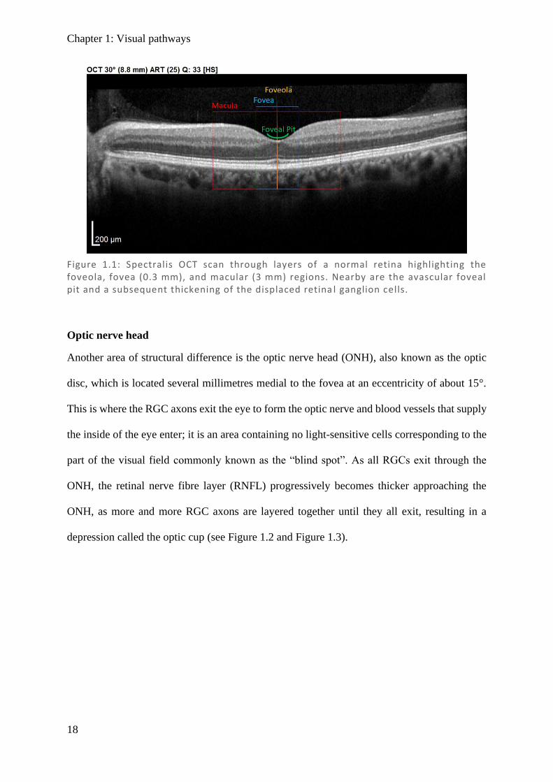
macula, resulting in a thickening of those layers adjacent to the foveal pit (see Figure 1.1).
Chapter 1: Visual pathways
18
Optic nerve head
Another area of structural difference is the optic nerve head (ONH), also known as the optic
disc, which is located several millimetres medial to the fovea at an eccentricity of about 15°.
This is where the RGC axons exit the eye to form the optic nerve and blood vessels that supply
the inside of the eye enter; it is an area containing no light-sensitive cells corresponding to the
part of the visual field commonly known as the “blind spot”. As all RGCs exit through the
ONH, the retinal nerve fibre layer (RNFL) progressively becomes thicker approaching the
ONH, as more and more RGC axons are layered together until they all exit, resulting in a
depression called the optic cup (see Figure 1.2 and Figure 1.3).
Figure 1.1: Spectralis OCT scan through layers of a normal retina highlighting the foveola, fovea (0.3 mm), and macular (3 mm) regions. Nearby are the avascular foveal pit and a subsequent thickening of the displaced retina l ganglion cells.
Chapter 1: Visual pathways
19
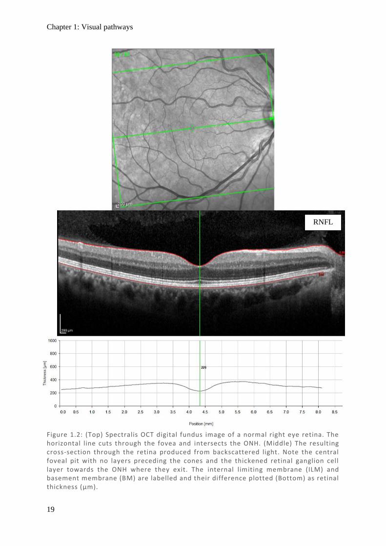
Figure 1.2: (Top) Spectralis OCT digital fundus image of a normal right eye retina. The horizontal line cuts through the fovea and intersects the ONH. (Middle) The resulting cross-section through the retina produced from backscattered light. Note the central foveal pit with no layers preceding the cones and the thickened retinal ganglion cell layer towards the ONH where they exit. The internal limiting membrane (ILM) and basement membrane (BM) are labelled and their difference plotted (Bottom) as retinal thickness (µm).
RNFL
Chapter 1: Visual pathways
20
1.3.1.2. Microscopic organisation
Light passes through all the layers of the retina before hitting the rods and cones which have
light sensitive photopigments (retinal) attached to plasma membrane proteins (opsins). When
light strikes retinal it changes conformation, activating a signal cascade using cGMP which
results in closure of Na-channels and hyperpolarisation, closing voltage-gated Ca-channels and
thus preventing the release of neurotransmitter glutamate (Hurley, 2009) and signalling the
postsynaptic cell. The timing of this activation contributes to the delay in pupillary response
after a stimulus by as much as 100 ms of its ~500-600 ms latency (Arshavsky & Wensel, 2013)
with the larger bulk of the timing in iris constriction. The response of the postsynaptic cell can
be stimulatory or inhibitory, there are a great diversity of RGC receiving different input, and
with different extent of dendritic lamination, this facilitates the complex input signals involved
in each aspect of vision (Dacey et al., 2003).
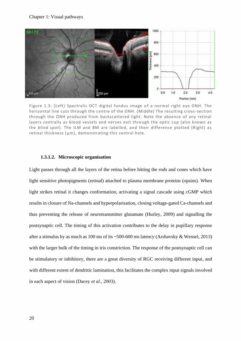
Figure 1.3: (Left) Spectralis OCT digital fundus image o f a normal right eye ONH. The horizontal l ine cuts through the centre of the ONH. (Middle) The resulting cross -section through the ONH produced from backscattered light. Note the absence of any retinal layers centrally as blood vessels and nerves exit thro ugh the optic cup (also known as the blind spot). The ILM and BM are labelled, and their difference plotted (Right) as retinal thickness (µm), demonstrating this central hole.
Chapter 1: Visual pathways
21
Retinal layers
The rod and cones span several layers (see Figure 1.4): the opsin-photopigment compartment
within the outer segment (OS), the cell organelles within the inner segment (IS), the outer
nuclear layer (ONL) containing the cell bodies, and the outer plexiform layer (OPL) where
connections are made with interneurons. Within the inner plexiform layer (IPL) and inner
nuclear layer (INL) are the axons and cell bodies of interneurons (amacrine, bipolar, and
horizontal cells), which integrate and refine signals from rods/cones and eventually connect
through to the RGC in the ganglion cell layer (GCL) (Kolb, 1995). While the complexity of
these connections cannot be understated, with numerous subdivisions of cells, generally the
rods/cones transmit their signal via bipolar cells to the RGC, while horizontal cells in the OPL
integrate a large number of inputs as they are communicated to bipolar cells, and amacrine cells
in the IPL integrate a number of bipolar cell outputs as they communicate to the RGC.
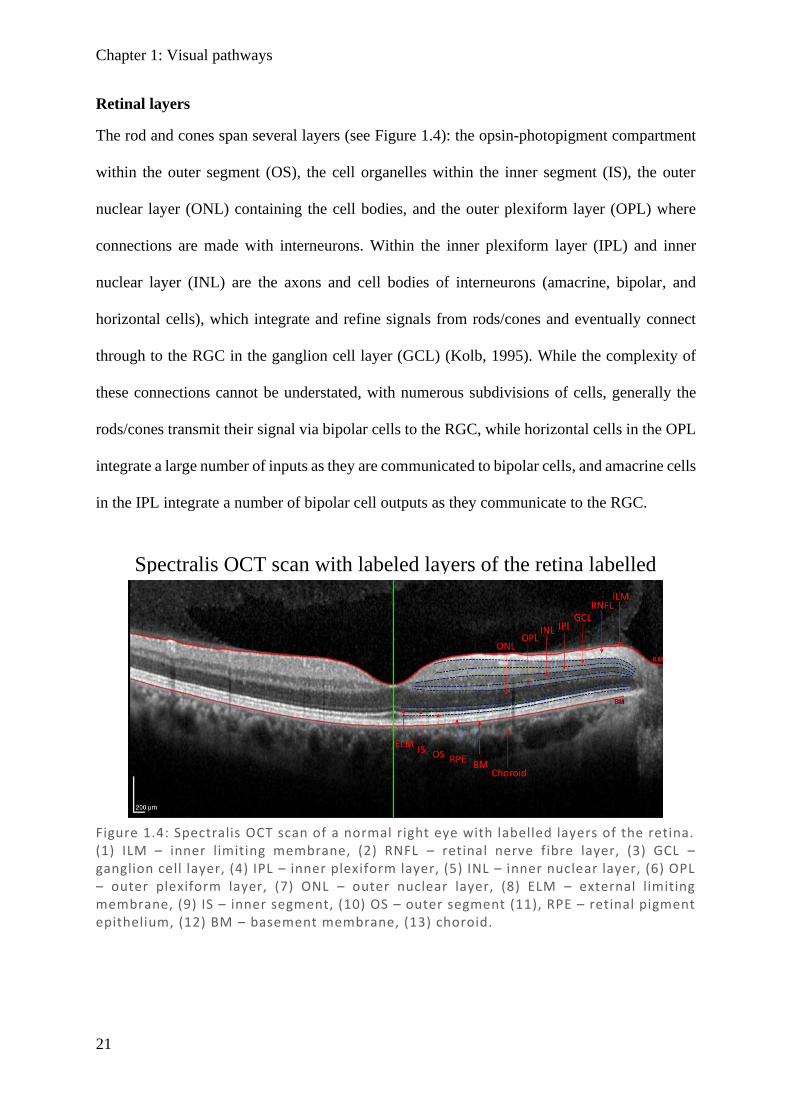
Figure 1.4: Spectralis OCT scan of a normal right eye with labelled layers of the retina. (1) ILM – inner limiting membrane, (2) RNFL – retinal nerve fibre layer, (3) GCL – ganglion cell layer, (4) IPL – inner plexiform layer, (5) INL – inner nuclear layer, (6) OPL – outer plexiform layer, (7) ONL – outer nuclear layer, (8) ELM – external limiting membrane, (9) IS – inner segment, (10) OS – outer segment (11), RPE – retinal pigment epithelium, (12) BM – basement membrane, (13) choroid.
Spectralis OCT scan with labeled layers of the retina labelled
Chapter 1: Visual pathways
22
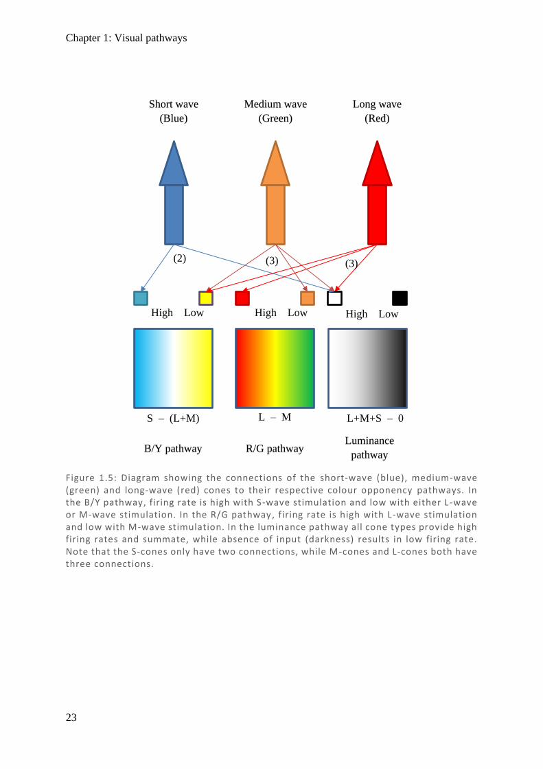
Colour Opponency
As there are approximately 100-fold less RGC than photoreceptor cells, there is a large degree
of integration, with multiple bipolar cells signalling a single RGC. This difference in RGC–
photoreceptor ratio is most prominent in the rod system, while in the cone system it is closer
to 1:1 and cones typically connect to multiple RGC via the colour opponent system (Schein,
1988; Wassle et al., 1989). Neural integration of cones involves an offset of two colour systems
and a luminance pathway (see Figure 1.5), with red/green sensitivity being recorded as L – M
[long wave (red) minus medium wave (green)], and blue/yellow sensitivity being recorded as
S – (L+M) [short wave (blue) minus combination of medium and long (yellow)]. Luminance
on the other hand is an integration of all cone types [L+M+S] and is achromatic with a lower
resolution, thereby only sampling input from the field it represents (Shevell & Martin, 2017).
Given this connectivity in encoding colour, each L-cone (red) and each M-cone (green) need
to connect to at least two bipolar neurons, while S-cones (blue) only require one (excluding the
luminance pathway). Interestingly, as one progresses from peripheral vision to more central
locations, there is an increase in the ratio of RGC to photoreceptor cells, with ~2 RGC per cone
at 2.5˚ (Schein, 1988) increasing to >3 RGC in the central 550 µm (Wassle et al., 1989).
Centrally, rods are sparse, and while there is a higher density of cones and ganglion cells, there
are more than twice as many pedicels2 as RGC (Wassle et al., 1989), resulting in displacement
of the RGC with respect to their associated cone input (Figure 1.6). This particularly high cone
density results in significantly higher resolution of central vision in daylight. Additionally, the
absence of RGC in the foveal pit, combined with the displacement with respect to their
connected cones, results in elongated connections and the apparent thickening of the macula
alluded to earlier.
2 Cone axon terminal where cone synapses with retinal ganglion cell.
Chapter 1: Visual pathways
23
Long wave
(Red)
Medium wave
(Green)
Short wave
(Blue)
S – (L+M) L – M L+M+S – 0
High Low High Low High Low
(2) (3) (3)
B/Y pathway R/G pathway Luminance
pathway
Figure 1.5: Diagram showing the connections of the short-wave (blue), medium-wave (green) and long-wave (red) cones to their respective colour opponency pathways. In the B/Y pathway, firing rate is high with S-wave stimulation and low with either L -wave or M-wave stimulation. In the R/G pathway, firing rate is high with L-wave stimulation and low with M-wave stimulation. In the luminance pathway all cone types provide high firing rates and summate, while absence of input (darkness) results in low firing rate. Note that the S-cones only have two connections, while M-cones and L-cones both have three connections.

Chapter 1: Visual pathways
24
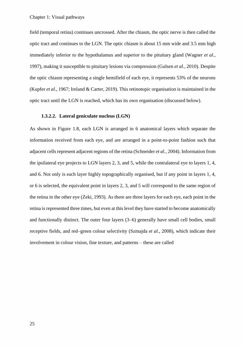
1.3.2. Visual pathway
Signals received by the RGC continue in parallel as the optic nerve until they reach the optic
chiasm. Here nasal fibres decussate and continue as the contralateral optic tract through the
optic radiations to the primary visual cortex (striate cortex) (Walsh, 1990) (See Figure 1.7).
1.3.2.1. Chiasm and optic tract
The optic nerve is highly organised and is separated by hemifield. Fibres which represent the
temporal field (nasal retina) decussates at the optic chiasm, while fibres that represent the nasal
Figure 1.6: Rod and cone densities across the visual field. Cone density sharply peaks in the central foveal region where rods are absent. Rods peak around 18 ° in the nasal region, while they are slightly offset in the temporal region due to the optic disc and peak at around 22° eccentricity. Relative size of the rods (purple) and cones (green) can also be seen in the top row, highlighting the change in diameter of both rods/cones. Cones are ~3.3 µm in fovea and increase in size to ~10 µm at the extreme periphery. Rods have a size of ~3 µm at peak density and more subtly increase in size to 5.5 µm in the periphery (Jonas et al., 1992; Purves et al., 2001). Reproduced with permission from purves et al., 2001.
Chapter 1: Visual pathways
25
field (temporal retina) continues uncrossed. After the chiasm, the optic nerve is then called the
optic tract and continues to the LGN. The optic chiasm is about 15 mm wide and 3.5 mm high
immediately inferior to the hypothalamus and superior to the pituitary gland (Wagner et al.,
1997), making it susceptible to pituitary lesions via compression (Gulsen et al., 2010). Despite
the optic chiasm representing a single hemifield of each eye, it represents 53% of the neurons
(Kupfer et al., 1967; Ireland & Carter, 2019). This retinotopic organisation is maintained in the
optic tract until the LGN is reached, which has its own organisation (discussed below).
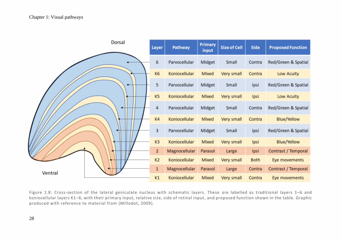
1.3.2.2. Lateral geniculate nucleus (LGN)
As shown in Figure 1.8, each LGN is arranged in 6 anatomical layers which separate the
information received from each eye, and are arranged in a point-to-point fashion such that
adjacent cells represent adjacent regions of the retina (Schneider et al., 2004). Information from
the ipsilateral eye projects to LGN layers 2, 3, and 5, while the contralateral eye to layers 1, 4,
and 6. Not only is each layer highly topographically organised, but if any point in layers 1, 4,
or 6 is selected, the equivalent point in layers 2, 3, and 5 will correspond to the same region of
the retina in the other eye (Zeki, 1993). As there are three layers for each eye, each point in the
retina is represented three times, but even at this level they have started to become anatomically
and functionally distinct. The outer four layers (3–6) generally have small cell bodies, small
receptive fields, and red–green colour selectivity (Szmajda et al., 2008), which indicate their
involvement in colour vision, fine texture, and patterns – these are called
Chapter 1: Visual pathways
26
Figure 1.7: Visual pathway from retinal origins, crossing at the optic chiasm, and continuing to the lateral geniculate nucleus (LGN). Highlights branch point off the visual pathway to the subcortical pupillary pathway, leading to the pretectal olivary nucelus (PON) and integrating both fields at the Edinger-Westphal nucleus (EWN) which then innvervates the pupils.
Chapter 1: Visual pathways
27
parvocellular cells (P-cells) and receive extensive input from midget RGC. The inner two
layers (1 and 2) contain cells with larger cell bodies which have large receptive fields, are
contrast sensitive but insensitive to colour, and are responsible for motion detection – these are
called magnocellular cells (M-cells) and receive extensive input from parasol RGCs (Szmajda
et al., 2008).
Between each of the 6 layers are a third type of cell called koniocellular cells (K-cells) which
have very small cell bodies. The function of K-cells and what defines a koniocellular neuron
are still up for debate. Evidence from macaques suggests input from both peripheral and central
retina (Percival et al., 2013), with three pairs of distinct layers in each LGN: dorsal layer for
low-acuity information, middle layer for short-wave (blue) cone sensitivity, and ventral layer
tied to the superior colliculus (Hendry & Reid, 2000; Szmajda et al., 2008). A small population
of K-cells and P-cells have even been shown to bypass the standard visual pathway and branch
off directly to the middle temporal (MT) region which processes motion (Sincich et al., 2004)
and, based on evidence in primates, connects directly to V1 (layers 1 and 3B) of the primary
visual cortex (Berson et al., 2002).
Taking all this into consideration, it is important to recognise that, despite there only being
three types of cone and three apparent anatomical layers in the LGN, there are more than 20
types of RGC, numerous subtypes of interneurons, and complex connectivity from the LGN to
other areas of the brain. As pointed out by Kaplan in his updated review of the visual pathways,
it would seem remiss to cling to the idea of a simple three-stream pathway when we are
consistently presented with evidence that perceptual processing is simply more complex than
that (Kaplan, 2013).
Chapter 1: Visual pathways
28
Figure 1.8: Cross-section of the lateral geniculate nucleus with schematic layers. These are labelled as traditional layers 1–6 and koniocellular layers K1–6, with their primary input, relative size, side of retinal input , and proposed function shown in the table. Graphic produced with reference to material from (Millodot, 2009).
Chapter 1: Visual pathways
29
1.3.2.3. Visual cortex
The primary visual cortex (V1) is represented in both hemispheres, receiving input from
ipsilateral LGN and therefore the contralateral hemifield from both eyes. Similar to the LGN,
it is highly retinotopically organised so that nearby points in the cortex map to nearby visual
fields. Notably this is not linear – the central 2% of the visual field accounts for 50% of V1
(Adams & Horton, 2003), and the increased density of photoreceptors in the macula only
partially accounts for this, as it also shows cortical magnification (Wandell & Engel, 1995).
This means that damage to V1 or its immediate input from LGN result in homonymous visual
field damage to the contralateral field – that is, damage in the same region on the same side of
both eyes but opposite to the side of the lesion. Where damage is incomplete there is frequently
a degree of macular sparing, given that it is unlikely to have completely knocked out the entire
central vision representation. After V1, information is parcelled out into specialised cortical
areas for further analysis of specific aspects of visual information such as colour, motion,
spatial location, form and identity (Zeki, 1993), which are further discussed in Section 1.3
(Higher visual functional deficits) below.
1.3.3. Pupillary pathway
In the traditional understanding of the pupillary response, some RGC axons branch off the optic
tract prior to the LGN to reach the pretectal olivary nucleus (PON) (Walsh, 1990; Tsujimura
& Tokuda, 2011). Each of the two PON then project into both oculomotor nuclei to the adjacent
Edinger–Westphal Nuclei (EWN), such that despite the earlier separation of the visual field
down the two tracts, the full visual field is represented in both the EWN (Carle et al., 2011b;
Kozicz et al., 2011). The EWN then produces parasympathetic output, which projects
anteriorly through the oculomotor nerves (CNIII) to the ciliary ganglia and, finally, via short
ciliary nerves to the iris sphincter muscle to cause pupil constriction. In addition to this standard
pupil response, a separate pathway involving colour processing in the cortex has been
Chapter 1: Visual pathways
30
postulated to contribute to the pupillary responses (Young & Alpern, 1980). This is further
discussed under the multifocal pupillographic objective perimetry (mfPOP) heading (Section
1.5.4.2).
1.3.3.1. Afferent pupillary input
Intrinsically photoreceptive retinal ganglion cells (ipRGC)
Inside the retina there is a recently discovered subpopulation of ~0.2% of RGCs that do not
just transmit photoreceptor derived signals, but are intrinsically photosensitive themselves
(Fukuda et al., 2012; Munch et al., 2012; Pickard & Sollars, 2012; Munch & Kawasaki, 2013).
These intrinsically photoreceptive RGC (ipRGC) express the photopigment melanopsin
(Opn4), which is most sensitive to short–medium wavelength light, peaking at ~480 nm (blue)
(Pickard & Sollars, 2012; Sand et al., 2012; Munch & Kawasaki, 2013). The ipRGC response
to light is relatively slow, taking seconds to build up to maximal response, which is an order of
magnitude slower than rods and cones, and it may also persist for minutes after the stimulus
has ended (Pickard & Sollars, 2012; Sand et al., 2012). Interestingly though, electron
micrographs show that ipRGC also receive input from cones of the retina via amacrine and
bipolar cells (Pickard & Sollars, 2012; Sand et al., 2012; Munch & Kawasaki, 2013), allowing
a rapid response too.
In determining ipRGC function, it was discovered that they are required for photoentrainment
of the circadian rhythm. This was proven by some elegant studies using knockout mice that
showed either melanopsin or cones were sufficient, but ipRGC were necessary, for
photoentrainment (Pickard & Sollars, 2012; Sand et al., 2012). The pathway was found to
travel via the retinohypothalamic tract (RHT) to the suprachiasmatic nucleus (SCN) above the
optic chiasm (Munch et al., 2012; Nissila et al., 2012; Pickard & Sollars, 2012; Sand et al.,
2012). ipRGC were also implicated in pineal melatonin regulation of the sleep–wake cycle,
and in mediating the pupil response (Munch et al., 2012; Pickard & Sollars, 2012; Sand et al.,
Chapter 1: Visual pathways
31
2012; Carle et al., 2013), either grossly throughout the day (predominantly via melanopsin) or
acutely via cone input when a bright flash occurs (Pickard & Sollars, 2012). Animal studies
have shown ipRGC branch both directly to the SCN via RHT and also to the intergeniculate
leaflet which leads to the SCN via the geniculohypothalamic tract (Morin et al., 2003). In doing
these experiments, projections to the pretectal olivary nuclei (PON) were discovered, which is
known to regulate the light reflex (Edelstein & Amir, 1999; Pickard & Sollars, 2012). Many
more locations were also reported, including ventral subparaventricular zone, lateral preoptic
nucleus, medial amygdala, lateral habenula, superior colliculus, and periaqueductal gray
matter, which suggest other functional roles which are not yet understood (Pickard & Sollars,
2012).
In macaque retinas, ipRGC were shown to comprise just 0.2% of the RGC (Dacey et al., 2005)
with overlapping mesh and very large dendritic fields, particularly in the periphery where they
may approach 1 mm (Do & Yau, 2010). Despite being a relatively uncommon RGC type,
subtypes have been proposed as M1, M2, and M3. In rodents M1 and M2 appear similar in
number at ~45% of total ipRGC each, while M3 comprises only 10% (Berson et al., 2010).
Very recently M1 has been further subdivided by expression of a transcription factor (Brn3b),
where M1 ipRGC which are Brn3b+ project to the PON and are necessary for the pupillary
light reflex, whereas Brn3b– project to the SCN and are sufficient for photoentrainment (Li &
Schmidt, 2018). Differences in myelination between ipRGC projecting to SCN and PON
showed heavy myelination of PON-projecting neurons, consistent with the necessary time-
scales of their responses (Kim et al., 2019).
Rod/Cone
As ipRGC drive the pupillary reflex, rod and cones may only influence pupil response via this
pathway. In terms of the intrinsic input (melanopsin) from ipRGC, it contributes significantly
to maintenance of pupil constriction in response to light stimuli ≥ 30 seconds in duration, even
Chapter 1: Visual pathways
32
when only of small luminance (McDougal & Gamlin, 2010; Lee et al., 2019). Cones contribute
over very short durations and quickly adapt, contributing relatively minimally after 30 seconds.
Rods are also involved, but do not adapt as much as cones and contribute to steady-state
responses at smaller luminances below the threshold at which melanopsin reacts (Lall et al.,
2010; McDougal & Gamlin, 2010). Variation in colour input in terms of both wavelength and
intensity appears able to selectively target melanopsin (blue), rods (low intensity), or cones
(red) (Kardon et al., 2009). It should be noted the final pupil response may include the
subcortical, ipRGC-driven pupillary light reflex in addition to cortical inputs to the PON and
EWN.
1.3.3.2. Subcortical nuclei
Pretectal olivary nucleus
The pretectal olivary nucleus (PON) receives the retinal input from ipRGC, with the PON firing
rate directly related to the intensity of photopic stimulation of the retina (Pintor, 2009). Due to
decussation of nasal retinal fibres (temporal field) at the optic chiasm, input to each PON
comprises temporal hemiretina from the ipsilateral side and nasal hemiretina from the
contralateral side (Carle et al., 2011b). As mentioned earlier, this input is not entirely even,
with nasal hemiretina having a greater density of cones (Curcio & Allen, 1990). Primate studies
show differences as large as 58% decussate while only 42% do not (Horton & Hocking, 1996;
Horton, 1997), and a study of a single human retina showed 53% decussate versus 47% do not
(Kupfer et al., 1967; Ireland & Carter, 2019). Recent evidence suggests that this difference is
small relative to the differences in PON connection with the Edinger–Westphal nucleus (Carle
et al., 2019) (discussed below).
Edinger–Westphal Nucleus (EWN)
There is bilateral input from both PON to both EWN, so this is the first point at which the full
retinal input is represented in a single region. Interestingly, there is not equal input from

Chapter 1: Visual pathways
33
ipsilateral and contralateral PON. In primate studies a notable bias towards contralateral input
has been demonstrated (Tigges & O'Steen, 1974; Hutchins & Weber, 1985; Gamlin & Clarke,
1995; Gamlin et al., 1995). This would result in greater direct than consensual responses in the
nasal retina (temporal field) and equally greater consensual than direct in the temporal retina
(nasal field). Most studies seem consistent in showing that the nasal retina (temporal field) has
greater direct responses, while for the temporal retina (nasal field) the results are mixed, with
some studies showing marginally greater consensual responses (Cox & Drewes, 1984; Martin
et al., 1991) while others show no difference (Smith & Smith, 1980; Wyatt & Musselman,
1981; Schmid et al., 2000; Carle et al., 2011b). This has been suggested to be due to stimulus
intensity affecting this anisocoria, with a model proposed to account for this (Carle et al.,
2011b). In investigating retinal, PON, and EWN levels for contribution for anisocoria, the level
of the PON connection to EWN was highlighted as most influential (Carle et al., 2019).
Chapter 1: Visual pathways
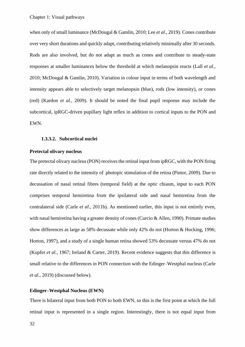
34
Figure 1.9: Cross-section of midbrain at the level of the superior colliculus. Right side labels show major tracts and nuclei; left side labels show pupillary pathway in order labelled 1 –7. (1) Due to decussation at the optic chiasm, the optic tract rec eives retinal fibres direct from the ipsilateral eye, representing the nasal field, combined with indirect fibres of the contralateral eye representing the temporal field. The large majority of fibres terminate in the lateral geniculate nucleus. (2) Brachi um and (3) stratum of the superior colliculus are the continuation of the branch from the optic tract of fibres involved in the pupillary response which termina te in the (4) pretectal olivary nucleus (PON). The PON fibres then bilaterally terminate on both (5) Edinger–Westphal nuclei (EWN), now representing full integration of both streams of visual information. The EWN continues through the (6) oculomotor nucleus where it forms i nto the parasympathetic component of the pupillary light response and follows the fibres of the (7) oculomotor nerve. Graphic produced with reference to material from (DeArmond et al., 1976).
Chapter 1: Visual pathways
35
1.3.3.3. Efferent pupillary output
The iris is comprised of two key components: outer radial muscle that dilates the pupil
(controlled by the sympathetic system) and the inner circular muscles that constrict the pupil
(parasympathetic control) (McDougal & Gamlin, 2015). These muscles are modulated by the
sum of the pupil light response (with greater amounts of light causing constriction of the pupil),
the accommodation and convergence response (with near objects resulting in pupil
constriction), and arousal from adrenergic responses (causing dilation). The integration of these
pathways is what gives rise to the overall pupillary response.
Parasympathetic
The parasympathetic division of the pupillary response begins in the EWN after receiving
bilateral input from the PON. Nerves exit the EWN and continue as part of the oculomotor
nerve in the dorsal sheath to reach the ciliary ganglion, where neurons synapse and continue as
postganglionic neurons to innervate the sphincter pupillae muscle of the iris to cause
constriction (McMinn, 1998).
Sympathetic
The sympathetic component of the pupillary response begins in the posterolateral
hypothalamus. Neurons exit the hypothalamus, traverse the brainstem laterally adjacent to the
spinal lemniscus, and descend the spinal column to the level of T1. Here they exit the lateral
horn and enter the sympathetic chain via the white ramus communicans and ascend to the
superior cervical ganglion. They then synapse and become postganglionic neurons, which enter
the skull with the internal carotid and branch into the pupillary and eyelid components. The
pupillary component enters the ophthalmic branch of the trigeminal nerve and is finally
distributed to the eye via the nasociliary and long ciliary branches to innervate the dilator
pupillae muscle of the iris (McMinn, 1998).
Chapter 1: Higher visual functional deficits
36
1.4. Higher Visual Functional Deficits
Higher visual functions (HVFs) are visual processes that rely on complex integration of visual
information to generate perception beyond that of the raw image itself. They include
extrastriate vision that includes things like colour perception, depth perception, motion, and
facial recognition. These functional processes are often taken for granted and may occur
without the person themselves even being aware of their deficit (anosognosia). Due their
specialised nature, they tend not to be tested in clinical settings. There are a variety of case
studies presenting various degrees of HVF deficits (presented below), which tend to represent
the more severe end of the spectrum. Pure HVF deficits rather rare, but more subtle defects
may occur, and without standard clinical testing it is hard to know if they also have a low
incidence or rather a low detection rate due to infrequent testing. To try and assess this question,
we have noted a range of tests which attempt to assess HVF deficits: visual neglect3,
achromatopsia4, prosopagnosia5, akinetopsia6, and astereopsis7. This study does not attempt to
definitively define the prevalence of these in the stroke population, but rather to act as a pilot
to suggest which might be worth pursuing in future studies, and which tests appear useful. For
the detailed list of tests, reasoning for selection, and their administration – please refer to the
General Methods (Chapter 2).
3 Visual pathway remains intact, but does not consciously acknowledge items on side contralateral to lesion unless
particular attention is drawn to it (inattention). 4 Inability to recognise colours, seeing the world in grey, following a cortical lesion. More subtle defects may
diminish colour sensitivity without being blind to colour. 5 Inability to recognise faces and unique features of faces, following a cortical lesion. In the most severe cases,
they cannot recognise their own face, while more subtle defects may make discerning between faces difficult. 6 Inability to decern motion either generally (seeing all motion as series of static images) or in motion coherence
(cannot detect cohesive motion from noise). 7 Inability to use binocular vision to produce three-dimensional percept. May reply on other feautres or in severe
cases perceive the world as flat.
Chapter 1: Higher visual functional deficits
37
1.4.1. Extrastriate visual areas
There are many reported areas of visual processing in the brain, with an even more variable set
of mapping to cortices. While this is not the focus on this study, a brief overview of these seems
fitting before discussing deficits which refer to these regions. As discussed in the sections
below – there are numerous cases of those with selective deficits, which would strongly imply
selective processing areas of the cortex. Perhaps what make this less clear is that multiple areas
are frequently reported as having similar activity when presented with selective stimuli – for
example motion stimuli have reported activity in V1, V2, V3, and V5 (McKeefry et al., 1997;
Furlan & Smith, 2016), and numerous connections have been described (Vanni et al., 2020).
Perhaps a more balanced view is to say that multiple areas partake in processing of visual
features, while more selective areas are necessary to consciously produce the final visual
percept. This would allow for a more subtle range of deficits to present, where any processing
region is impaired, while selective loss of perception entirely remains rare (Vaina, 1995). With
this in mind, the areas which appear necessary for perception are discussed, along with their
anatomical locations, although they may not be the only regions involved in these precepts. To
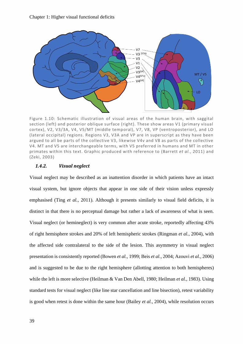
aim with visualisation, a schematic diagram of the visual association areas is included as Figure
1.10.
The primary visual cortex, or striate cortex (V1), is a well mapped area at the occipital pole
enveloping inwards. It is necessary for visual field, and while limited perception has been
demonstrated in its absence (‘blindsight’) (Vaina, 1995; Vakalopoulos, 2005; Smits et al.,
2019), there is minimal visual perception in areas where this has been damaged. Encapsulating
and surrounding V1 is V2, which is implicated in higher order contour, shape and form (Roe
& Ts'o, 2015). V3 and VP (ventroposterior) have been described superior and inferior
(respectively) to V2, each with input from only quarter of a hemifield (Burkhalter & Van Essen,
1986). This has been challenged as actually being two sides of V3 (Sereno et al., 1995; DeYoe
Chapter 1: Higher visual functional deficits
38
et al., 1996; Lyon & Kaas, 2001) based on similar function selectivity and mirror images of
retinotopic maps in humans (Shipp et al., 1995; Zeki, 2003), which certainly seems the stronger
argument. More recently it has been suggested that both V3 and V4 play a critical role in
transmitting information to higher order areas (Arcaro & Kastner, 2015), such that ventral V3
(VP) has greater colour selectivity (Burkhalter & Van Essen, 1986) in heading towards the
colour centre, and that posterior V3 (V3A) has greater motion selectivity (Tootell et al., 1997)
in heading toward the motion centre. In a similar set of logic to dividing V3, the colour centre
V4 was proposed to be comprised of V4v (Sereno et al., 1995; Tootell et al., 1996) and newly
found area V8 (Hadjikhani et al., 1998), which appeared to actually be overlapping with the
previously defined V4 (Zeki et al., 1991; McKeefry & Zeki, 1997; Wade et al., 2002; Zeki,
2003). This may correspond closely to the posterior aspect of the interior temporal (IT) region
which has also been suggested as the colour processing centre (Heywood et al., 1998; Conway
& Tsao, 2009), while others have suggested it relates to colour learning (Cowey et al., 2001).
The middle temporal (MT) visual area was coined in owl monkeys (Allman & Kaas, 1971)
while the same area was concurrently discovered in macaques and coined V5 (Dubner & Zeki,
1971), hence the persistent use of both terms which can be considered interchangeable.
Continued work described V5 in humans, with understanding of V5 has evolved through the
years, being sensitive to motion in an integrative sense, focusing on cohesion in noise and
filtering objects from background scenery (Born & Bradley, 2005). The V7 and LO (lateral
occipital) has not been associated with distinct clinical syndromes, and so are of limited
relevance in this context.
Chapter 1: Higher visual functional deficits
39
1.4.2. Visual neglect
Visual neglect may be described as an inattention disorder in which patients have an intact
visual system, but ignore objects that appear in one side of their vision unless expressly
emphasised (Ting et al., 2011). Although it presents similarly to visual field deficits, it is
distinct in that there is no perceptual damage but rather a lack of awareness of what is seen.
Visual neglect (or hemineglect) is very common after acute stroke, reportedly affecting 43%
of right hemisphere strokes and 20% of left hemispheric strokes (Ringman et al., 2004), with
the affected side contralateral to the side of the lesion. This asymmetry in visual neglect
presentation is consistently reported (Bowen et al., 1999; Beis et al., 2004; Azouvi et al., 2006)
and is suggested to be due to the right hemisphere (allotting attention to both hemispheres)
while the left is more selective (Heilman & Van Den Abell, 1980; Heilman et al., 1983). Using
standard tests for visual neglect (like line star cancellation and line bisection), retest variability
is good when retest is done within the same hour (Bailey et al., 2004), while resolution occurs
Figure 1.10: Schematic illustration of visual areas of the human brain, with saggital section (left) and posterior oblique surface (right). These show areas V1 (primary visual cortex), V2, V3/3A, V4, V5/MT (middle temporal), V7, V8, VP (ventroposterior), and LO (lateral occipital) regions. Regions V3, V3A and VP are in superscript as they have been argued to all be parts of the collective V3, likewise V4v and V8 as parts of the collective V4. MT and V5 are interchangeable terms, with V5 preferred in humans and MT in other primates within this text. Graphic produced with reference to (Barrett et al., 2011) and (Zeki, 2003)
Chapter 1: Higher visual functional deficits
40
in the majority of cases over the following weeks to months (Jehkonen et al., 2000; Lundervold
et al., 2005)
1.4.3. Achromatopsia
Damage to cortical areas beyond V1 may not damage the visual field but can result in selective
loss of the ability to process features such as colour perception, motion perception, depth
perception, and facial recognition. Cases of cerebral achromatopsia have been described from
as early as the 1800s (Zeki, 1990), with many case reports continuing in the modern literature
(Setala & Vesti, 1994; Cowey et al., 2008; von Arx et al., 2010; Pagani et al., 2012; Carota &
Calabrese, 2013; Bartolomeo et al., 2014; Zhou et al., 2018). Reports demonstrate that lesions
tend to occur in the inferior occipital–temporal cortex near the reported V4, which has been
confirmed in a meta-analysis of the overlapping damaged regions in 92 cases of cerebral
achromatopsia (Bouvier & Engel, 2006).
1.4.4. Prosopagnosia
Prosopagnosia is the inability to recognise the distinct features of a person’s face that allow
that person to be identified. Cerebral deficits in facial recognition have been demonstrated in
the modern literature (Lu et al., 2005; Lang et al., 2006; Fox et al., 2011; Heutink et al., 2012),
with a meta-analysis of 100 cases showing the commonly reported region being adjacent to
V4. Given the regions for prosopagnosia and achromatopsia are so close, it is not surprising
that roughly half of achromatopsia patients have prosopagnosia and half of prosopagnosia
patients have achromatopsia (Bouvier & Engel, 2006).
1.4.5. Akinetopsia
Compared to colour and facial recognition, descriptions of cerebral deficits in motion
perception are more recent, with the first case of isolated motion impariement without field
defects (as a consequence of a cerebral lesion) published in 1983 (Zihl et al., 1983). Unlike the
Chapter 1: Higher visual functional deficits
41
colour centre in achromatopsia, which took many years to be accepted, a motion centre was
readily accepted, with the term akinetopsia being coined (Zeki, 1991) – although it should be
noted that the term akinetopsia refers to impairment or loss of any of the motion domains rather
than complete loss of all motion perception. Since then akinetopsia has been described in a
number of patients (Shipp et al., 1994; Rizzo et al., 1995; Barton et al., 1996; Vaina et al.,
2001; Pelak & Hoyt, 2005; Vaina et al., 2010; Cooper et al., 2012; Otsuka-Hirota et al., 2014).
As to the location of the damage, V5 has been suggested - based on transcranial magnetic
stimulation (Zihl & Heywood, 2015), and lesions demonstrating an inability to determine the
direction of global dot motion stimuli when noise is added (random dot kinematograms) (Shipp
et al., 1994; Vaina et al., 2010), or to track motion (Cooper et al., 2012). Further, in a larger
group of 57 stroke patients, it was demonstrated that many had enduring motion deficits, with
damage in V5 (n = 10) resulting in markedly decreased ability to detect motion coherence
ipsilaterally or contralaterally, although more substantially contralaterally (Vaina et al., 2010).
1.4.6. Astereopsis
Astereopsis is the inability to judge depth from the disparity between images projected onto
both retinas, with affected persons forced to rely upon other less sensitive monocular cues to
judge depth; some individuals are unable to perceive depth at all. A description of ‘seeing the
world as flat’ was published in the early 1900s in which a complete loss of stereovision
perception was described (Holmes, 1918, 1919; Holmes & Horrax, 1919). More recent
literature has also described stereoscopic damage from lesions (Ross, 1983; Takayama &
Sugishita, 1994; Miller et al., 1999; Schaadt et al., 2014); MRI imaging has highlighted activity
in the area immediately posterior to V5 during motion tasks (Senior et al., 2000).
Interestingly, many of those with damage to V5 (and who lack motion sensitivity) also lack
depth perception (40%), while damage to the nearby occipitoparietal region gave rise to 65%
of patients having depth perception (stereopsis) affected (Vaina et al., 2010).
Chapter 1: Diseases of the visual pathways
42
1.5. Diseases of the Visual Pathways
1.5.1. Anterior ischemic optic neuropathy (AION)
AION typically presents as a relatively sudden loss of vision in a single eye, associated with
oedema of the optic disc and evolving over several months into optic atrophy with a permanent
visual field defect (VFD) (Hayreh, 1974). AION is the most common acute optic nerve disease
in those aged over 50, with a reported incidence of 2.3–10.3 per 100,000 (Johnson & Arnold,
1994; Hattenhauer et al., 1997; Kerr et al., 2009; Lee et al., 2011b; Arda et al., 2013). It results
from disruption of blood flow to one or more of the short posterior ciliary arteries which
progress anteriorly from their branch off the ophthalmic artery and pass into the back of the
eye, surrounding the optic nerve and optic disc (Kerr et al., 2009). Ischemia of the optic nerve
gives rise to inflammation causing swelling, compression, and hypoxic damage (Matson &
Fujimoto, 2011). AION most commonly presents with an altitudinal defect predominantly
affecting either the superior or inferior field of a single eye (depending on which ciliary artery
is affected). In classifying AION, it may be described as either arteritic or non-arteritic.
1.5.1.1. Arteritic AION
The pathogenesis of the less common arteritic form (Johnson & Arnold, 1994) is well
understood and is almost exclusively caused by giant cell arteritis (GCA) (Matson & Fujimoto,
2011). GCA is a form of systemic vasculitis in which medium to large arteries become inflamed
with macrophages and giant multinuclear cells, causing thickening of the wall and narrowing
of the lumen which may result in disruption to blood flow. Arteritic AION is considered a
ocular emergency because further visual field loss (VFL) may be prevented by treating with
corticosteroids (Hayreh, 2009; Matson & Fujimoto, 2011).
1.5.1.2. Non-arteritic AION
Chapter 1: Diseases of the visual pathways
43
The exact pathogenesis of non-arteritic AION (NA-AION) has been suggested as lacking by
some (Matson & Fujimoto, 2011; Punjabi et al., 2011; Arda et al., 2013). However, extensive
work by Hayreh over the last 40 years (who incidentally named AION), suggests that the cause
is complex and multifactorial in nature (Hayreh, 1974, 2001b, a, 2009, 2011). Some
contributing factors include intraocular pressure, crowded optic discs, vascular resistance, and
impaired vessel autoregulation, in addition to the more traditional vascular risk factors such as
hyperlipidaemia, hypertension, diabetes, and obstructive sleep apnoea (Hayreh, 2009; Kerr et
al., 2009; Matson & Fujimoto, 2011; Arda et al., 2013).
Once a patient has presented with AION in a single eye, the risk of recurrence in the same eye
is relatively low (5.8% at 2 years) (Hayreh et al., 2001). This has been proposed to be due to a
thinning of the nerve fibre layer, making more space available within the optic disc, so there is
less crowding and room for expansion in future ischemic events. However, this is still in
contention. That being said, having NA-AION in a single eye puts a patient at high risk of an
event in the fellow eye (15–24% over 5 years) (Beck et al., 1997). This is likely due to having
the same risk factors and structural commonalities that predisposed the first eye, and this risk
is further compounded in the arteritic group to almost double that of NA-AION (Beri et al.,
1987). Systematically reducing and eliminating the risk factors appears to be the main option
in minimising risk of recurrence.
1.5.2. Pituitary tumours
Each optic nerve passes through their respective optic foramen and converges at the optic
chiasm just posterior to the bone of the tuberculum sellae. The chiasmic tract continues directly
superior to the pituitary gland and tilts upward 45o to the lamina terminalis, forming an indent
in the third ventricle called the anterior optic recess (Walsh, 1990). The pituitary gland
(hypophysis) is a small endocrine gland about the size of a pea found inferior to the optic
chiasm within the bone cavity of the sella turcica. It is a very common place for tumours to
Chapter 1: Diseases of the visual pathways
44
develop, with pituitary adenomas accounting for 12–17% of all intracranial tumours (Okamoto
et al., 2008; Wang et al., 2008; Kasputyte et al., 2013), with a prevalence in autopsy studies as
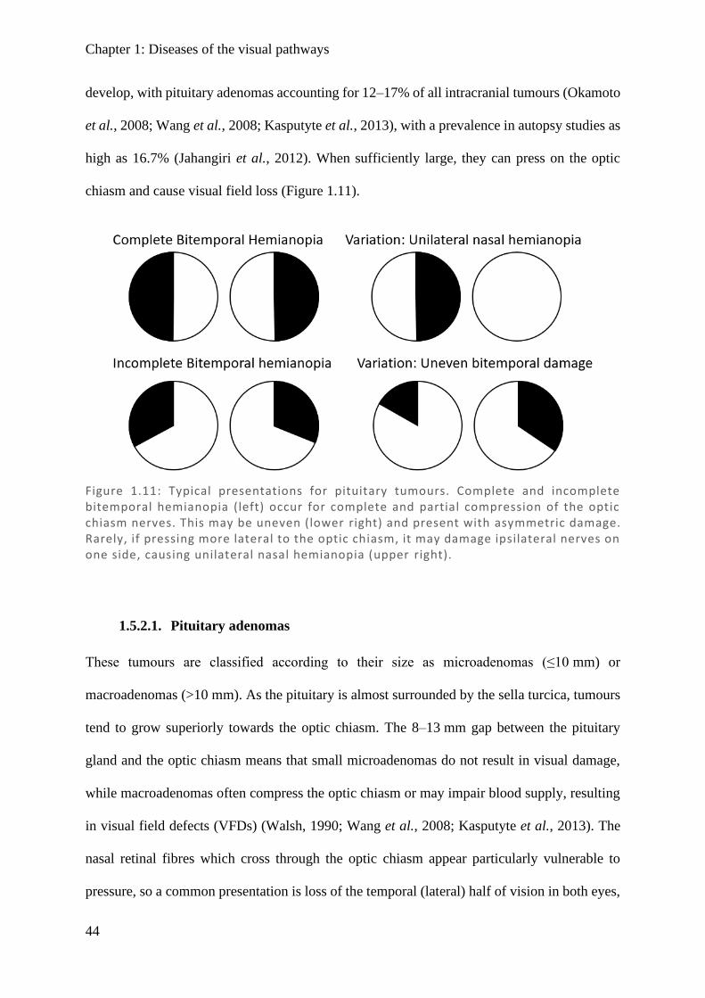
high as 16.7% (Jahangiri et al., 2012). When sufficiently large, they can press on the optic
chiasm and cause visual field loss (Figure 1.11).
1.5.2.1. Pituitary adenomas
These tumours are classified according to their size as microadenomas (≤10 mm) or
macroadenomas (>10 mm). As the pituitary is almost surrounded by the sella turcica, tumours
tend to grow superiorly towards the optic chiasm. The 8–13 mm gap between the pituitary
gland and the optic chiasm means that small microadenomas do not result in visual damage,
while macroadenomas often compress the optic chiasm or may impair blood supply, resulting
in visual field defects (VFDs) (Walsh, 1990; Wang et al., 2008; Kasputyte et al., 2013). The
nasal retinal fibres which cross through the optic chiasm appear particularly vulnerable to
pressure, so a common presentation is loss of the temporal (lateral) half of vision in both eyes,
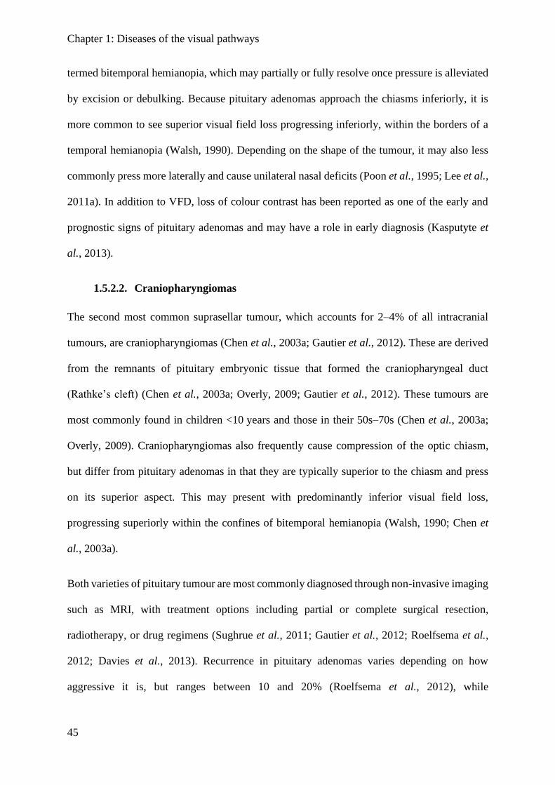
Figure 1.11: Typical presentations for pituitary tumours. Complete and incomplete bitemporal hemianopia (left) occur for complete and partial compression of the optic chiasm nerves. This may be uneven (lower right) and present with asymmetric damage. Rarely, if pressing more lateral to the optic chiasm, it may damage ipsilateral nerves on one side, causing unilateral nasal hemianopia (upper right).
Chapter 1: Diseases of the visual pathways
45
termed bitemporal hemianopia, which may partially or fully resolve once pressure is alleviated
by excision or debulking. Because pituitary adenomas approach the chiasms inferiorly, it is
more common to see superior visual field loss progressing inferiorly, within the borders of a
temporal hemianopia (Walsh, 1990). Depending on the shape of the tumour, it may also less
commonly press more laterally and cause unilateral nasal deficits (Poon et al., 1995; Lee et al.,
2011a). In addition to VFD, loss of colour contrast has been reported as one of the early and
prognostic signs of pituitary adenomas and may have a role in early diagnosis (Kasputyte et
al., 2013).
1.5.2.2. Craniopharyngiomas
The second most common suprasellar tumour, which accounts for 2–4% of all intracranial
tumours, are craniopharyngiomas (Chen et al., 2003a; Gautier et al., 2012). These are derived
from the remnants of pituitary embryonic tissue that formed the craniopharyngeal duct
(Rathke’s cleft) (Chen et al., 2003a; Overly, 2009; Gautier et al., 2012). These tumours are
most commonly found in children <10 years and those in their 50s–70s (Chen et al., 2003a;
Overly, 2009). Craniopharyngiomas also frequently cause compression of the optic chiasm,
but differ from pituitary adenomas in that they are typically superior to the chiasm and press
on its superior aspect. This may present with predominantly inferior visual field loss,
progressing superiorly within the confines of bitemporal hemianopia (Walsh, 1990; Chen et
al., 2003a).
Both varieties of pituitary tumour are most commonly diagnosed through non-invasive imaging
such as MRI, with treatment options including partial or complete surgical resection,
radiotherapy, or drug regimens (Sughrue et al., 2011; Gautier et al., 2012; Roelfsema et al.,
2012; Davies et al., 2013). Recurrence in pituitary adenomas varies depending on how
aggressive it is, but ranges between 10 and 20% (Roelfsema et al., 2012), while
Chapter 1: Diseases of the visual pathways
46
craniopharyngioma recurrence is reportedly even higher (35.7%) (Gautier et al., 2012). It is
therefore common to arrange for periodic radiological images to monitor for regrowth.
1.5.3. Stroke
Stroke is Australia’s second highest cause of death and a leading cause of disability, affecting
an estimated 375,000 Australians (Wang et al., 2012). Most fundamentally, stroke is a lack of
blood flow to the brain, resulting in death of neural tissue. There are two kinds of stroke:
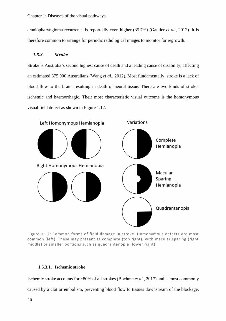
ischemic and haemorrhagic. Their most characteristic visual outcome is the homonymous
visual field defect as shown in Figure 1.12.
1.5.3.1. Ischemic stroke
Ischemic stroke accounts for ~80% of all strokes (Boehme et al., 2017) and is most commonly
caused by a clot or embolism, preventing blood flow to tissues downstream of the blockage.
Figure 1.12: Common forms of field damage in stroke. Homonymous defects are most common (left). These may present as complete (top right), with macular sparing (right middle) or smaller portions such as quadrantanopia (lower right).
Chapter 1: Diseases of the visual pathways
47
Any part of the visual pathway may be affected depending on the location of the infarct. When
anterior pre-chiasmal optic nerve(s) are affected due to ciliary artery blood flow disruption,
this is classified as AION. The optic nerve is supplied by the ophthalmic artery and internal
carotid pial vessels, and the optic chiasm by the circle of Willis; these may present unilateral
or bitemporal damage, however both these presentations are rare (Pula & Yuen, 2017).
Congruous homonymous hemianopia8 (HH) is the most common form of field loss following
stroke (Rowe et al., 2013; Glisson, 2014) with Rowe et al. reporting complete and partial HH
in 73.5% of stroke patients with field loss, and quadrantanopias9 in another 15.2%. HH is
predominantly caused from occipital lobe lesions (54%), optic radiations (33%), or the optic
tract (6%) (Rowe et al., 2013). These are supplied by the posterior cerebral artery, which may
also have collateral supply from the temporo-occipital sylvian artery (Pula & Yuen, 2017).
1.5.3.2. Haemorrhagic stroke
Haemorrhagic stroke makes up the remaining ~20% of presentations, with a variety of types
depending on the layer of the bleed. The most common types are intracerebral haemorrhage
(ICH) (~10–15%) and subarachnoid haemorrhage (~5%) (Qureshi et al., 2001; de Rooij et al.,
2007; An et al., 2017). Risk factors are those similar to that of ischemic stroke: hypertension,
smoking, excessive alcohol intake, old age, and male sex – but also Asian ethnicity and
anticoagulants (An et al., 2017). ICH is mostly caused by long-standing hypertension resulting
in degeneration of blood vessels and aneurisms, which then rupture. Haemorrhagic stroke has
poorer outcomes than other strokes, with a 1-month mortality rate of 40% and 1-year of ~60%
(Qureshi et al., 2001; An et al., 2017). Unlike ischemic stroke, peripheral damage may occur
8 Complete visual field loss covering half the field but not crossing the vertical meridian, affecting the same side
of both eyes. Some fields may not affect the whole hemifield, but the damage in one eye matches the other, which
are said to have homonrmous field loss, but are not hemianopias. 9 Visual field loss that is homonymous (see above footnote), but only affects approximately a quarter wedge of
the vision in each eye.
Chapter 1: Diseases of the visual pathways
48
due to mass-effect and compression of surrounding structures; therefore almost any region can
be affected and result in visual impairment.
1.5.3.3. Imaging
While clinical signs are well known, given the opposing natures of treatment for ischemic and
haemorrhagic stroke, imaging is often necessary. According to the American Academy of
Neurology, a computed tomography (CT) scan should usually done to distinguish between
ischemic and haemorrhagic because it is quick, cheap, and readily available. Magnetic
resonance imaging (MRI) may be done later and it can better define the stroke, can detect
ischemic regions, and predict infarct more accurately – either acutely using diffusion or
perfusion weighted images (DWI, PWI), or chronically using fluid attenuated inversion
recovery (FLAIR) to visualise past strokes (Schellinger et al., 2010). While mostly used in the
research currently, diffusion tensor imaging (DTI) can also provide information about the
particular tracts which are damaged.
1.5.3.4. Visual impairment after stroke
Stroke can affect any part of the body – including movement, sensation, and perception. Visual
impairment in stroke patients is very common with an estimated prevalence of 20–74% (Rowe
et al., 2009; Pollock et al., 2011b; Hayes et al., 2012; Ali et al., 2013). Persistent visual
impairment is particularly significant as it can be associated with loss of mobility, reading
deficits, inability to drive, depression, anxiety, social isolation, and falls (Jones & Shinton,
2006; Hayes et al., 2012; Sand et al., 2013). Visual deficits have also been correlated with
impaired rehabilitation of other functional deficits (Shrestha et al., 2012). The more commonly
detected impairments are visual field defects and eye-movement disorders, although it is also
possible for stroke to cause disorders of higher-order functions of perception such as colour
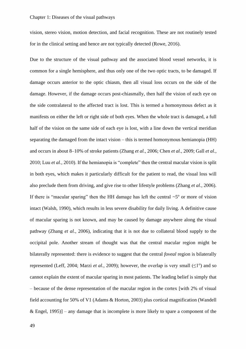
Chapter 1: Diseases of the visual pathways
49
vision, stereo vision, motion detection, and facial recognition. These are not routinely tested
for in the clinical setting and hence are not typically detected (Rowe, 2016).
Due to the structure of the visual pathway and the associated blood vessel networks, it is
common for a single hemisphere, and thus only one of the two optic tracts, to be damaged. If
damage occurs anterior to the optic chiasm, then all visual loss occurs on the side of the
damage. However, if the damage occurs post-chiasmally, then half the vision of each eye on
the side contralateral to the affected tract is lost. This is termed a homonymous defect as it
manifests on either the left or right side of both eyes. When the whole tract is damaged, a full
half of the vision on the same side of each eye is lost, with a line down the vertical meridian
separating the damaged from the intact vision – this is termed homonymous hemianopia (HH)
and occurs in about 8–10% of stroke patients (Zhang et al., 2006; Chen et al., 2009; Gall et al.,
2010; Luu et al., 2010). If the hemianopia is “complete” then the central macular vision is split
in both eyes, which makes it particularly difficult for the patient to read, the visual loss will
also preclude them from driving, and give rise to other lifestyle problems (Zhang et al., 2006).
If there is “macular sparing” then the HH damage has left the central ~5o or more of vision
intact (Walsh, 1990), which results in less severe disability for daily living. A definitive cause
of macular sparing is not known, and may be caused by damage anywhere along the visual
pathway (Zhang et al., 2006), indicating that it is not due to collateral blood supply to the
occipital pole. Another stream of thought was that the central macular region might be
bilaterally represented: there is evidence to suggest that the central foveal region is bilaterally
represented (Leff, 2004; Marzi et al., 2009); however, the overlap is very small (≤1o) and so
cannot explain the extent of macular sparing in most patients. The leading belief is simply that
– because of the dense representation of the macular region in the cortex [with 2% of visual
field accounting for 50% of V1 (Adams & Horton, 2003) plus cortical magnification (Wandell
& Engel, 1995)] – any damage that is incomplete is more likely to spare a component of the
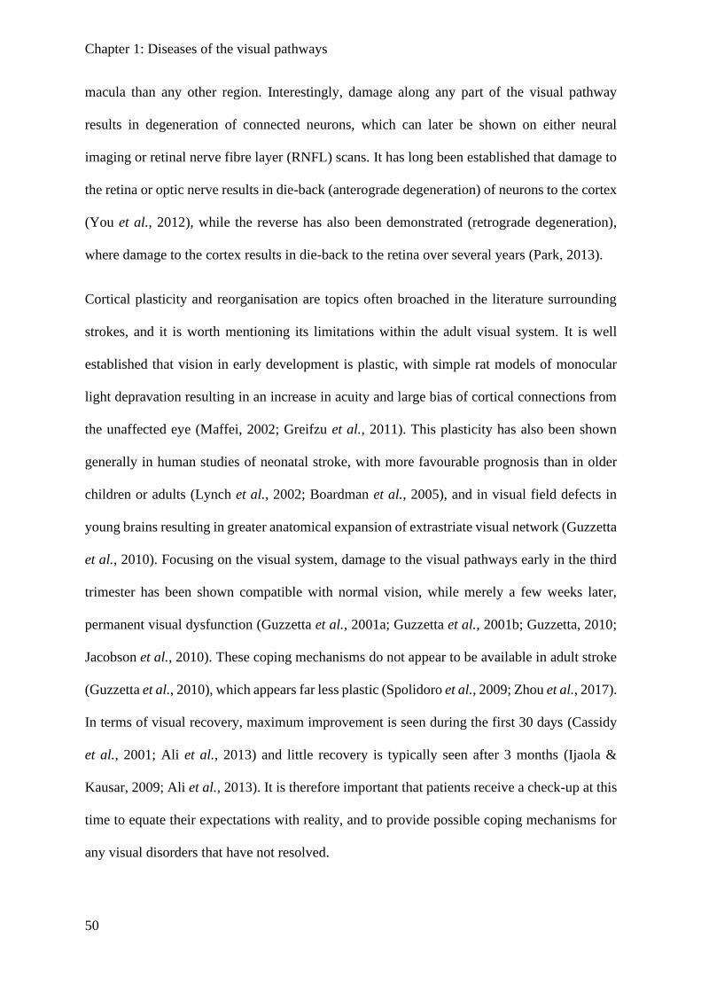
Chapter 1: Diseases of the visual pathways
50
macula than any other region. Interestingly, damage along any part of the visual pathway
results in degeneration of connected neurons, which can later be shown on either neural
imaging or retinal nerve fibre layer (RNFL) scans. It has long been established that damage to
the retina or optic nerve results in die-back (anterograde degeneration) of neurons to the cortex
(You et al., 2012), while the reverse has also been demonstrated (retrograde degeneration),
where damage to the cortex results in die-back to the retina over several years (Park, 2013).
Cortical plasticity and reorganisation are topics often broached in the literature surrounding
strokes, and it is worth mentioning its limitations within the adult visual system. It is well
established that vision in early development is plastic, with simple rat models of monocular
light depravation resulting in an increase in acuity and large bias of cortical connections from
the unaffected eye (Maffei, 2002; Greifzu et al., 2011). This plasticity has also been shown
generally in human studies of neonatal stroke, with more favourable prognosis than in older
children or adults (Lynch et al., 2002; Boardman et al., 2005), and in visual field defects in
young brains resulting in greater anatomical expansion of extrastriate visual network (Guzzetta
et al., 2010). Focusing on the visual system, damage to the visual pathways early in the third
trimester has been shown compatible with normal vision, while merely a few weeks later,
permanent visual dysfunction (Guzzetta et al., 2001a; Guzzetta et al., 2001b; Guzzetta, 2010;
Jacobson et al., 2010). These coping mechanisms do not appear to be available in adult stroke
(Guzzetta et al., 2010), which appears far less plastic (Spolidoro et al., 2009; Zhou et al., 2017).
In terms of visual recovery, maximum improvement is seen during the first 30 days (Cassidy
et al., 2001; Ali et al., 2013) and little recovery is typically seen after 3 months (Ijaola &
Kausar, 2009; Ali et al., 2013). It is therefore important that patients receive a check-up at this
time to equate their expectations with reality, and to provide possible coping mechanisms for
any visual disorders that have not resolved.
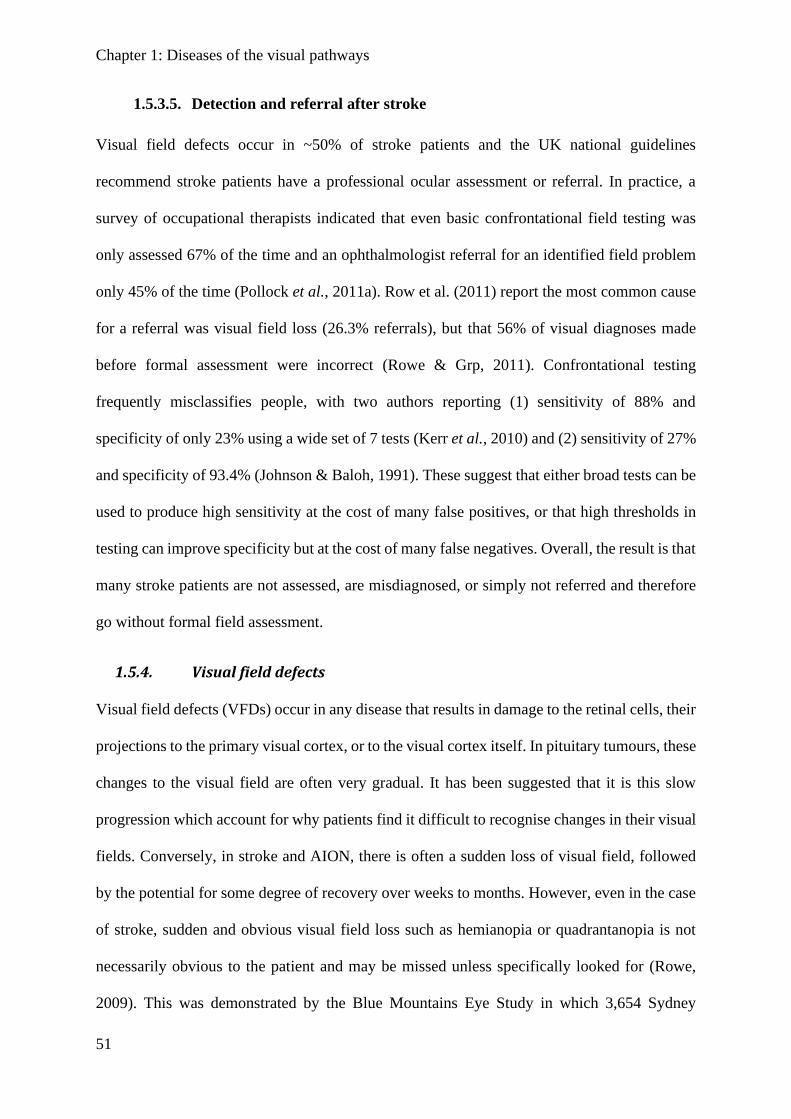
Chapter 1: Diseases of the visual pathways
51
1.5.3.5. Detection and referral after stroke
Visual field defects occur in ~50% of stroke patients and the UK national guidelines
recommend stroke patients have a professional ocular assessment or referral. In practice, a
survey of occupational therapists indicated that even basic confrontational field testing was
only assessed 67% of the time and an ophthalmologist referral for an identified field problem
only 45% of the time (Pollock et al., 2011a). Row et al. (2011) report the most common cause
for a referral was visual field loss (26.3% referrals), but that 56% of visual diagnoses made
before formal assessment were incorrect (Rowe & Grp, 2011). Confrontational testing
frequently misclassifies people, with two authors reporting (1) sensitivity of 88% and
specificity of only 23% using a wide set of 7 tests (Kerr et al., 2010) and (2) sensitivity of 27%
and specificity of 93.4% (Johnson & Baloh, 1991). These suggest that either broad tests can be
used to produce high sensitivity at the cost of many false positives, or that high thresholds in
testing can improve specificity but at the cost of many false negatives. Overall, the result is that
many stroke patients are not assessed, are misdiagnosed, or simply not referred and therefore
go without formal field assessment.
1.5.4. Visual field defects
Visual field defects (VFDs) occur in any disease that results in damage to the retinal cells, their
projections to the primary visual cortex, or to the visual cortex itself. In pituitary tumours, these
changes to the visual field are often very gradual. It has been suggested that it is this slow
progression which account for why patients find it difficult to recognise changes in their visual
fields. Conversely, in stroke and AION, there is often a sudden loss of visual field, followed
by the potential for some degree of recovery over weeks to months. However, even in the case
of stroke, sudden and obvious visual field loss such as hemianopia or quadrantanopia is not
necessarily obvious to the patient and may be missed unless specifically looked for (Rowe,
2009). This was demonstrated by the Blue Mountains Eye Study in which 3,654 Sydney
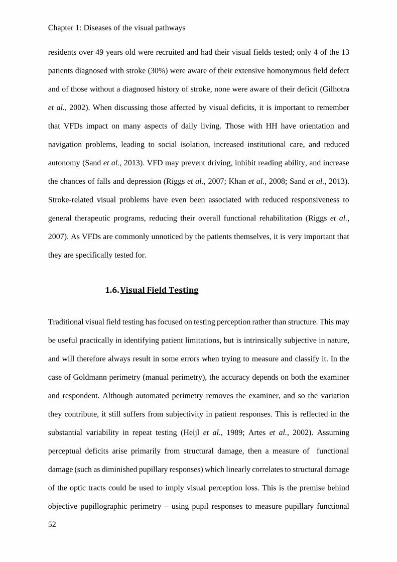
Chapter 1: Diseases of the visual pathways
52
residents over 49 years old were recruited and had their visual fields tested; only 4 of the 13
patients diagnosed with stroke (30%) were aware of their extensive homonymous field defect
and of those without a diagnosed history of stroke, none were aware of their deficit (Gilhotra
et al., 2002). When discussing those affected by visual deficits, it is important to remember
that VFDs impact on many aspects of daily living. Those with HH have orientation and
navigation problems, leading to social isolation, increased institutional care, and reduced
autonomy (Sand et al., 2013). VFD may prevent driving, inhibit reading ability, and increase
the chances of falls and depression (Riggs et al., 2007; Khan et al., 2008; Sand et al., 2013).
Stroke-related visual problems have even been associated with reduced responsiveness to
general therapeutic programs, reducing their overall functional rehabilitation (Riggs et al.,
2007). As VFDs are commonly unnoticed by the patients themselves, it is very important that
they are specifically tested for.
1.6. Visual Field Testing
Traditional visual field testing has focused on testing perception rather than structure. This may
be useful practically in identifying patient limitations, but is intrinsically subjective in nature,
and will therefore always result in some errors when trying to measure and classify it. In the
case of Goldmann perimetry (manual perimetry), the accuracy depends on both the examiner
and respondent. Although automated perimetry removes the examiner, and so the variation
they contribute, it still suffers from subjectivity in patient responses. This is reflected in the
substantial variability in repeat testing (Heijl et al., 1989; Artes et al., 2002). Assuming
perceptual deficits arise primarily from structural damage, then a measure of functional
damage (such as diminished pupillary responses) which linearly correlates to structural damage
of the optic tracts could be used to imply visual perception loss. This is the premise behind
objective pupillographic perimetry – using pupil responses to measure pupillary functional
Chapter 1: Visual field testing
53
deficits to the visual pathway and imply that damage to visual field perception concurrently
occurs due to both relying on the same underlying structures.
In the context of neurological disease, it is frequently necessary to assess visual fields.
Traditionally this was done with confrontational testing, a relatively crude method where a
clinician assesses visual fields by the bedside. While the study of perimetry appears to have
started with Hermann Aubert (Aubert & Foerster, 1857), it has opened a broad and extensive
domain of investigation. Advances in technology have refined these devices, with more modern
devices adopting two testing approaches: manual or automated. In each case, two stimuli can
be used: fixed (static) or moving (kinetic). Goldmann perimetry is a form of manual kinetic
perimetry which became widely accepted after invention of the Goldmann device (Goldmann,
1946). Goldmann perimetry remains in use today, and in the hands of an experienced
professional can be faster and more dynamic than automated perimetry, as the test locations
are not fixed. However, manual perimetry does suffer from the intrinsic issue of variability
between assessors; it also requires an experience technician to complete, and, being hand-
drawn, it is hard to directly compare between cases or sequential visits. Automated perimetry,
in the context of readily accessible computers, was designed to address these consistency
problems and create a standardised approach where the assessor may complete testing with
minimal training. Recently, automated perimetry has become the standard (Johnson et al.,
2011). There is substantial variation in which perimeter device or assessment is selected for
each ocular or neurological disease; however, a literature review of devices used for conditions
in this study revealed the Humphrey perimeter was the most commonly used in cases of stroke,
chiasmal compression, and optic neuropathy (Hepworth & Rowe, 2018). While substantially
less commonly used, frequency doubling perimetry (also known as Matrix perimetry) has also
been used in these conditions (Hepworth & Rowe, 2018). Multifocal pupillographic objective
perimetry (mfPOP) is a relatively new technology originating from work on visual evoked
Chapter 1: Visual field testing
54
potentials; it attempts to provide the benefits of automated perimetry while addressing some of
their flaws – notably the subjectivity of patient responses to stimuli. Patient response are
eliminated by utilising their autonomic pupillary light reflex and measuring its amplitude and
latency.
Each of these visual field devices, their approach, and adaptations over time are discussed
below.
1.6.1. Confrontational testing
Confrontational testing is considered a routine part of the neurological assessment, where the
clinician compares their own visual field with that of the patient (Elliott et al., 1997). While
there are many variants (Pandit et al., 2001; Connolly & Oczkowski, 2010), in practice this
commonly involves having the clinician and patient close one eye; the clinician then either
wiggles a finger and asks if the patient can see the movement (kinetic), or raises a select number
of fingers and asks the patient to report how many they see (static) in each of four quadrants.
While especially quick and easy, this test was soon recognised to have significant limitations,
with “wiggling finger” movement said to be easily detectable even in the presence of moderate
field suppression (Reader & Harper, 1976). Next is the concern with only testing a very crude
and inconsistent set of regions. While large defects like hemianopias (such as stroke and
chiasmal defects) may have a sensitivity of 42–75% (Trobe et al., 1981; Johnson & Baloh,
1991; Shahinfar et al., 1995), for smaller arcuate lesions this drops markedly to 20%
(Shahinfar et al., 1995), and for irregular defects such as in optic nerve damage to <11% (Trobe
et al., 1981) with a high rate of false negatives. Any of the common confrontational approaches
(individually or in combination) continue to have either low sensitivity or low specificity, such
that none are particularly effective (Connolly & Oczkowski, 2010; Kerr et al., 2010; Danesh-
Meyer & Gamble, 2011; Prasad & Cohen, 2011). An adaptation using automated
confrontational testing was trialled, using eight coloured test regions: this was shown in
Chapter 1: Visual field testing
55
glaucoma to have higher sensitivity than finger-counting confrontation (Bass et al., 2007),
which principally is just a simpler form of automated perimetry. The point here is that
confrontational testing is not good enough in neurological disorders where visual field defects
are likely, meaning formal perimetry becomes necessary. Despite the often low sensitivity of
confrontational testing, it remains a quick and easy screening tool and, provided its limitations
are understood, it may be useful in some cases where stroke-related disabilities prevent patients
from undertaking the higher sensitivity automated perimetry (Sand et al., 2013).
1.6.2. Goldmann perimetry
For many years Goldmann perimetry was the gold standard, only challenged by the invention
of standard automated perimetry in the form of the Humphrey perimeter. When the two were
initially compared, it was found that the devices showed similar results for the majority of
fields. Although Humphrey tended to suggest marginally worse fields than Goldmann, it had a
higher rate of inadequate fixation (Beck et al., 1985), and 25% longer test time in glaucoma
patients (Trope & Britton, 1987). While patients tended to prefer Goldmann to Humphrey ~3:1,
technicians heavily preferred Humphrey over Goldmann 5:1 (Trope & Britton, 1987), so
Humphrey naturally began to gain traction. In terms of application to neurological deficits,
discussion comparing the older version of Humphrey to Goldmann has mixed results, with
some suggesting concordance and other suggesting inability to localise the blind spot may have
resulted in unrepresentative fields for some patients (Wong & Sharpe, 2000; Coyle, 2001;
Kuritzky, 2001). While manual Goldmann perimetry is still in use for neurological disorders,
it has become less popular compared to automated perimetry (Hepworth & Rowe, 2018). More
modern iterations of Humphrey have made significant improvements, suggesting it now
performs similarly or better to Goldmann perimetry and is a promising successor (Bevers et
al., 2019). It should be noted that in rare cases, some individuals show blind visual fields to
static perimetry (as used in Humphrey) but not to kinetic stimuli (as used in Goldmann), so-
Chapter 1: Visual field testing
56
called statokinetic dissociation (Riddoch Phenomenon) (Zappia et al., 1971; Hayashi et al.,
2017). While this effect may account for some of the differences noted between devices, in
terms of practical function, they remain functionally blind.
1.6.3. Automated perimetry
There are a range of automated perimetry devices on the market, including the Humphrey (Carl
Zeiss AG, Germany) and Octopus (Haag Streit International, Switzerland) devices which use
luminance stimuli, and the Humphrey-Matrix (Carl Zeiss Meditec, Dublin CA) devices which
use contrast gratings. In this study, Humphrey II (HFA) and Humphrey-Matrix (MFA) devices
were used, so discussion will be limited to these devices.
1.6.3.1. Humphrey
The Humphrey Field Analyser II (HFA) (Carl Zeiss Meditech AG, Jena, Germany) is one of
the most commonly used automated visual field machines for all manner of visual field
assessments, and is the most commonly used visual field device for the visual assessment of
stroke, chiasmal compression, and optic neuropathy (Hepworth & Rowe, 2018), with a third
model recently being released. All Humphrey models use Goldmann size III stimuli (0.43°) on
a stimulus grid with equally spaced points 6° apart and use the Weber formula of contrast ((Lmax
– Lback) / (Lback)) where the background luminance is 10 cd/m2 and the minimal luminance
above background 0.0255cd/m2 up to maximum above background of 3178 cd/m2, providing
5.1 log units of range. These are then converted into dB using 10*log10(Contrast) (Fredette et
al., 2015) and reported as stimulus attenuation from the largest contrast possible (in dB). Thus,
the poorest response is where a person does not detect the stimulus at Lmax, resulting in 0 dB
score, and the best response is where a person detects minimal background change, resulting
in a 51 dB score, while in practice this is limited to ~40 dB.
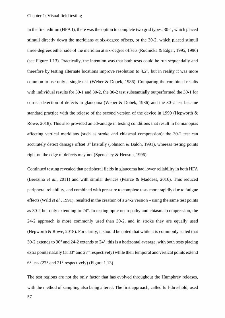
Chapter 1: Visual field testing
57
In the first edition (HFA I), there was the option to complete two grid types: 30-1, which placed
stimuli directly down the meridians at six-degree offsets, or the 30-2, which placed stimuli
three-degrees either side of the meridian at six-degree offsets (Rudnicka & Edgar, 1995, 1996)
(see Figure 1.13). Practically, the intention was that both tests could be run sequentially and
therefore by testing alternate locations improve resolution to 4.2°, but in reality it was more
common to use only a single test (Weber & Dobek, 1986). Comparing the combined results
with individual results for 30-1 and 30-2, the 30-2 test substantially outperformed the 30-1 for
correct detection of defects in glaucoma (Weber & Dobek, 1986) and the 30-2 test became
standard practice with the release of the second version of the device in 1990 (Hepworth &
Rowe, 2018). This also provided an advantage in testing conditions that result in hemianopias
affecting vertical meridians (such as stroke and chiasmal compression): the 30-2 test can
accurately detect damage offset 3° laterally (Johnson & Baloh, 1991), whereas testing points
right on the edge of defects may not (Spenceley & Henson, 1996).
Continued testing revealed that peripheral fields in glaucoma had lower reliability in both HFA
(Berezina et al., 2011) and with similar devices (Pearce & Maddess, 2016). This reduced
peripheral reliability, and combined with pressure to complete tests more rapidly due to fatigue
effects (Wild et al., 1991), resulted in the creation of a 24-2 version – using the same test points
as 30-2 but only extending to 24°. In testing optic neuropathy and chiasmal compression, the
24-2 approach is more commonly used than 30-2, and in stroke they are equally used
(Hepworth & Rowe, 2018). For clarity, it should be noted that while it is commonly stated that
30-2 extends to 30° and 24-2 extends to 24°, this is a horizontal average, with both tests placing
extra points nasally (at 33° and 27° respectively) while their temporal and vertical points extend
6° less (27° and 21° respectively) (Figure 1.13).
The test regions are not the only factor that has evolved throughout the Humphrey releases,
with the method of sampling also being altered. The first approach, called full-threshold, used

Chapter 1: Visual field testing
58
a starting value determined from normative data, and then varied stimuli by 4 dB until there
was a response reversal; thereafter the variation was 2 dB with the last recognised stimulus
used as the final threshold estimate (Spenceley & Henson, 1996; Artes et al., 2002). This
approach has provided some redundancy, such that if the starting test position (based on
normalised data) is far from the patient’s true value, or there is a single response error for a
given test point, it does not produce any greater error in the result (although it does take longer
to complete the test) (Johnson et al., 1992). This makes the test fairly robust, but at the expense
of long test durations, which then have the potential problem of enhanced fatigue effects (Wild
et al., 1991). A newer more complex algorithm called Swedish Interactive Thresholding
Algorithms (SITA) was trialled to provide shorter test times, with the SITA-standard reducing
30-2 test times by up to 50% (Bengtsson et al., 1998), and the SITA-fast being even shorter
(Bengtsson & Heijl, 1998). It achieves this by Bayesian inference and removal of false positive
catch trials (Schiefer et al., 2009). SITA-standard showed similar or better detection in
glaucomatous fields, similar mean defects (Musch et al., 2005), reduced test–retest variability
(Artes et al., 2002), and reduced learning effects (Yenice & Temel, 2005), although it may
underestimate false positives as they are no longer formally tested (Newkirk et al., 2006). When
SITA-standard was compared to full threshold in optic neuropathies and hemianopias typical
of stroke or pituitary lesions, SITA-standard performed at least as well (Wall et al., 2001).
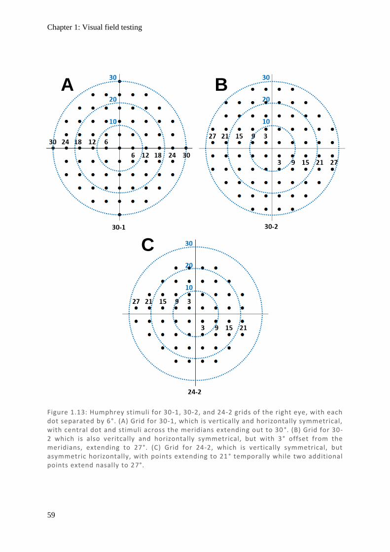
Chapter 1: Visual field testing
59
Figure 1.13: Humphrey stimuli for 30-1, 30-2, and 24-2 grids of the right eye, with each dot separated by 6°. (A) Grid for 30-1, which is vertically and horizontally symmetrical, with central dot and stimuli across the meridians extending out to 30 °. (B) Grid for 30-2 which is also veritcally and horizontally symmetrical, but with 3° offset from the meridians, extending to 27°. (C) Grid for 24-2, which is vertically symmetrical, but asymmetric horizontally, with points extending to 21 ° temporally while two additional points extend nasally to 27°.
A B
C
Chapter 1: Visual field testing
60
1.6.3.2. Matrix
MFA is a less commonly used perimeter (Hepworth & Rowe, 2018), using frequency doubling
technology: low spatial frequency sinusoidal gratings flickering at high temporal frequency
give the illusion of a doubling of the spatial frequency (Anderson & Johnson, 2002). It was
developed with the intention on improving on a weakness in HFA regarding its highly variable
glaucomatous fields. The belief was that there was preferential stimulation of magnocellular
(M) cells and specifically a subpopulation (My cells) (Maddess & Henry, 1992), and that with
fewer M-cells distributed in the retina, it might be more sensitive to glaucomatous loss with
less redundancy (Johnson, 1994; Johnson & Samuels, 1997; Wall et al., 2002; Yoon et al.,
2012). While the frequency doubling effect has been demonstrated to occur at frequencies and
contrast levels utilised by the MFA (Maddess & Kulikowski, 1999; McKendrick et al., 2003),
it does not rely on the apparent frequency in any way, only asking subjects to identify if the
stimulus is visualised or not. It was later proposed that the effect was mediated by multiple
cells (White et al., 2002), although the stimuli were not the only modifications made. Several
changes from the HFA design make it more similar to mfPOP, and therefore of interest. As
mentioned earlier, HFA had poor reproducibility over glaucomatous fields (Heijl et al., 1989;
Artes et al., 2002), particularly peripherally (Berezina et al., 2011). Another suggestion for this
has been the relatively small stimuli (0.43°) and a relatively small cap in the maximal
luminance the display can produce, leading to a small dynamic range for the device, which is
also shown to improve when larger stimuli are used (Wall et al., 2013; Gardiner et al., 2015;
Numata et al., 2017). Further, the technique has relatively wide spacing (6°) between stimuli,
resulting in under-sampling and aliasing (Weber & Dobek, 1986; Maddess, 2011, 2014). The
size issue was addressed in the first iteration of Matrix (C-20 FDT) in which the central 40° of
field was measured using much larger stimuli 10° in diameter but with only 17 test locations
(4 in each quadrant and 1 centrally) (Yoon et al., 2012). This approach had success in detecting
Chapter 1: Visual field testing
61
anterior pathway damage with both AION and chiasmal compression, showing similar
sensitivities to HFA (Wall et al., 2002; Girkin et al., 2004; Monteiro et al., 2007). However it
also suffered from some of the same drawbacks as the 30-1 HFA in that targets were along the
meridian and so performed poorly in hemianopias (Wall et al., 2002; Noval et al., 2005).
Likewise, while the stimuli are much larger, the number of regions tested is much smaller,
meaning under-sampling remained an issue. The second iteration solved these issues by halving
the stimuli size to 5° and adopting the same 30-2 (68 test locations) and 24-2 (54 test locations)
approach as HFA, while additionally retaining its central test region (Yoon et al., 2012). The
method for threshold detection was also upgraded from its modified binary search strategy
(Tyrrell & Owens, 1988) to Zippy Estimation by Sequential Testing (ZEST) which showed
promise on early testing (Anderson & Johnson, 2006) but causes all results to converge on only
15 unevenly spaced values (Fredette et al., 2015), which may contribute to its reduced
variability. When the modern versions of both devices were compared against each other in
homonymous hemianopic fields typical of stroke (Biousse et al., 2005) using a 24-2 map, there
was no statistically significant difference between MFA and HFA in terms of sensitivity or
specificity (Taravati et al., 2008). However, it should be noted that HFA did have higher
sensitivity, reportedly due to MFA presenting with a greater number of scattered abnormal field
defects incongruent with expectations of the disease. When chiasmal compression damage
measured by MFA was compared to prior diagnosis from HFA, it only detected 75% of
bitemporal hemianopias (Noval et al., 2005).
1.6.4. Multifocal methods
Multifocal pupillographic object perimetry (mfPOP) evolved from multifocal visual evoked
potentials (mfVEP) over the last 20 years and so it seems appropriate to cover advances in
mfVEP which lead to mfPOP.
1.6.4.1. Multifocal visual evoked potentials
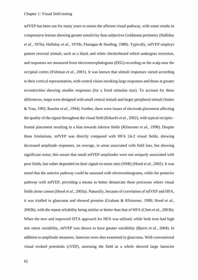
Chapter 1: Visual field testing
62
mfVEP has been use for many years to assess the afferent visual pathway, with some results in
compressive lesions showing greater sensitivity than subjective Goldmann perimetry (Halliday
et al., 1976a; Halliday et al., 1976b; Flanagan & Harding, 1988). Typically, mfVEP employs
pattern reversal stimuli, such as a black and white checkerboard which undergoes inversion,
and responses are measured from electroencephalogram (EEG) recording on the scalp near the
occipital cortex (Fishman et al., 2001). It was known that stimuli responses varied according
to their cortical representation, with central vision invoking large responses and those at greater
eccentricities showing smaller responses (for a fixed stimulus size). To account for these
differences, maps were designed with small central stimuli and larger peripheral stimuli (Sutter
& Tran, 1992; Baseler et al., 1994). Further, there were issues of electrode placement affecting
the quality of the signal throughout the visual field (Kikuchi et al., 2002), with typical occipito–
frontal placement resulting in a bias towards inferior fields (Klistorner et al., 1998). Despite
these limitations, mfVEP was directly compared with HFA 24-2 visual fields, showing
decreased amplitude responses, on average, in areas associated with field loss, but showing
significant noise; this meant that small mfVEP amplitudes were not uniquely associated with
poor fields, but rather depended on their signal-to-noise ratio (SNR) (Hood et al., 2002). It was
noted that the anterior pathway could be assessed with electroretinograms, while the posterior
pathway with mfVEP, providing a means to better demarcate these processes where visual
fields alone cannot (Hood et al., 2003a). Naturally, because of correlation of mfVEP and HFA,
it was trialled in glaucoma and showed promise (Graham & Klistorner, 1999; Hood et al.,
2003b), with the repeat reliability being similar or better than that of HFA (Chen et al., 2003b).
When the new and improved SITA approach for HFA was utilised, while both tests had high
test–retest variability, mfVEP was shown to have greater variability (Bjerre et al., 2004). In
addition to amplitude measures, latencies were also examined in glaucoma. With conventional
visual evoked potentials (cVEP), assessing the field as a whole showed large latencies
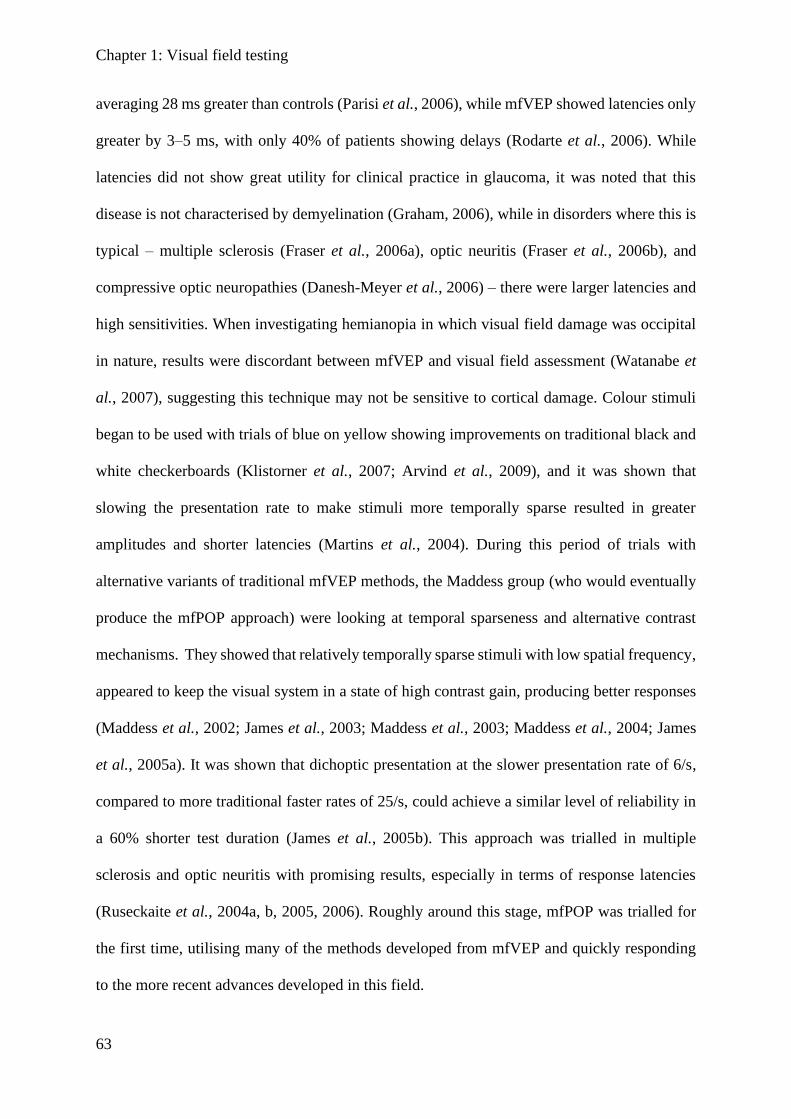
Chapter 1: Visual field testing
63
averaging 28 ms greater than controls (Parisi et al., 2006), while mfVEP showed latencies only
greater by 3–5 ms, with only 40% of patients showing delays (Rodarte et al., 2006). While
latencies did not show great utility for clinical practice in glaucoma, it was noted that this
disease is not characterised by demyelination (Graham, 2006), while in disorders where this is
typical – multiple sclerosis (Fraser et al., 2006a), optic neuritis (Fraser et al., 2006b), and
compressive optic neuropathies (Danesh-Meyer et al., 2006) – there were larger latencies and
high sensitivities. When investigating hemianopia in which visual field damage was occipital
in nature, results were discordant between mfVEP and visual field assessment (Watanabe et
al., 2007), suggesting this technique may not be sensitive to cortical damage. Colour stimuli
began to be used with trials of blue on yellow showing improvements on traditional black and
white checkerboards (Klistorner et al., 2007; Arvind et al., 2009), and it was shown that
slowing the presentation rate to make stimuli more temporally sparse resulted in greater
amplitudes and shorter latencies (Martins et al., 2004). During this period of trials with
alternative variants of traditional mfVEP methods, the Maddess group (who would eventually
produce the mfPOP approach) were looking at temporal sparseness and alternative contrast
mechanisms. They showed that relatively temporally sparse stimuli with low spatial frequency,
appeared to keep the visual system in a state of high contrast gain, producing better responses
(Maddess et al., 2002; James et al., 2003; Maddess et al., 2003; Maddess et al., 2004; James
et al., 2005a). It was shown that dichoptic presentation at the slower presentation rate of 6/s,
compared to more traditional faster rates of 25/s, could achieve a similar level of reliability in
a 60% shorter test duration (James et al., 2005b). This approach was trialled in multiple
sclerosis and optic neuritis with promising results, especially in terms of response latencies
(Ruseckaite et al., 2004a, b, 2005, 2006). Roughly around this stage, mfPOP was trialled for
the first time, utilising many of the methods developed from mfVEP and quickly responding
to the more recent advances developed in this field.
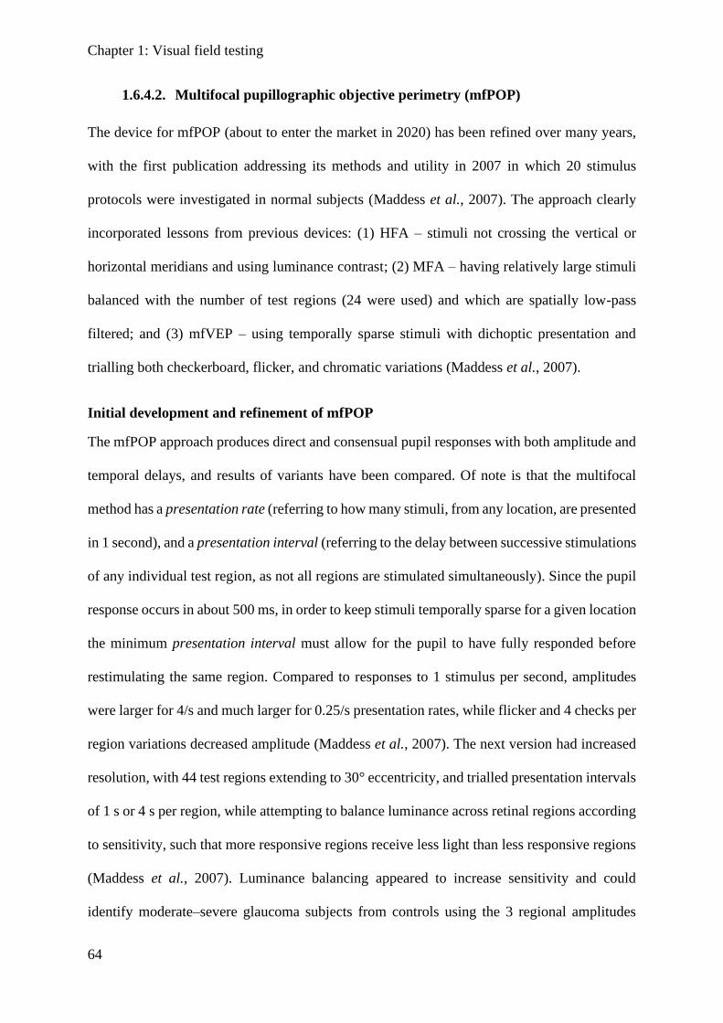
Chapter 1: Visual field testing
64
1.6.4.2. Multifocal pupillographic objective perimetry (mfPOP)
The device for mfPOP (about to enter the market in 2020) has been refined over many years,
with the first publication addressing its methods and utility in 2007 in which 20 stimulus
protocols were investigated in normal subjects (Maddess et al., 2007). The approach clearly
incorporated lessons from previous devices: (1) HFA – stimuli not crossing the vertical or
horizontal meridians and using luminance contrast; (2) MFA – having relatively large stimuli
balanced with the number of test regions (24 were used) and which are spatially low-pass
filtered; and (3) mfVEP – using temporally sparse stimuli with dichoptic presentation and
trialling both checkerboard, flicker, and chromatic variations (Maddess et al., 2007).
Initial development and refinement of mfPOP
The mfPOP approach produces direct and consensual pupil responses with both amplitude and
temporal delays, and results of variants have been compared. Of note is that the multifocal
method has a presentation rate (referring to how many stimuli, from any location, are presented
in 1 second), and a presentation interval (referring to the delay between successive stimulations
of any individual test region, as not all regions are stimulated simultaneously). Since the pupil
response occurs in about 500 ms, in order to keep stimuli temporally sparse for a given location
the minimum presentation interval must allow for the pupil to have fully responded before
restimulating the same region. Compared to responses to 1 stimulus per second, amplitudes
were larger for 4/s and much larger for 0.25/s presentation rates, while flicker and 4 checks per
region variations decreased amplitude (Maddess et al., 2007). The next version had increased
resolution, with 44 test regions extending to 30° eccentricity, and trialled presentation intervals
of 1 s or 4 s per region, while attempting to balance luminance across retinal regions according
to sensitivity, such that more responsive regions receive less light than less responsive regions
(Maddess et al., 2007). Luminance balancing appeared to increase sensitivity and could
identify moderate–severe glaucoma subjects from controls using the 3 regional amplitudes
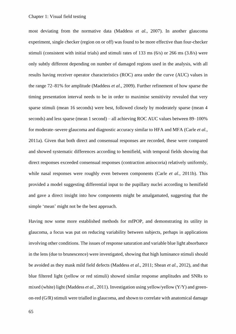
Chapter 1: Visual field testing
65
most deviating from the normative data (Maddess et al., 2007). In another glaucoma
experiment, single checker (region on or off) was found to be more effective than four-checker
stimuli (consistent with initial trials) and stimuli rates of 133 ms (6/s) or 266 ms (3.8/s) were
only subtly different depending on number of damaged regions used in the analysis, with all
results having receiver operator characteristics (ROC) area under the curve (AUC) values in
the range 72–81% for amplitude (Maddess et al., 2009). Further refinement of how sparse the
timing presentation interval needs to be in order to maximise sensitivity revealed that very
sparse stimuli (mean 16 seconds) were best, followed closely by moderately sparse (mean 4
seconds) and less sparse (mean 1 second) – all achieving ROC AUC values between 89–100%
for moderate–severe glaucoma and diagnostic accuracy similar to HFA and MFA (Carle et al.,
2011a). Given that both direct and consensual responses are recorded, these were compared
and showed systematic differences according to hemifield, with temporal fields showing that
direct responses exceeded consensual responses (contraction anisocoria) relatively uniformly,
while nasal responses were roughly even between components (Carle et al., 2011b). This
provided a model suggesting differential input to the pupillary nuclei according to hemifield
and gave a direct insight into how components might be amalgamated, suggesting that the
simple ‘mean’ might not be the best approach.
Having now some more established methods for mfPOP, and demonstrating its utility in
glaucoma, a focus was put on reducing variability between subjects, perhaps in applications
involving other conditions. The issues of response saturation and variable blue light absorbance
in the lens (due to brunescence) were investigated, showing that high luminance stimuli should
be avoided as they mask mild field defects (Maddess et al., 2011; Shean et al., 2012), and that
blue filtered light (yellow or red stimuli) showed similar response amplitudes and SNRs to
mixed (white) light (Maddess et al., 2011). Investigation using yellow/yellow (Y/Y) and green-
on-red (G/R) stimuli were trialled in glaucoma, and shown to correlate with anatomical damage

Chapter 1: Visual field testing
66
in the form of retinal nerve fibre layer (RNFL) thinning based on optical coherence tomography
(OCT) scans (Chain et al., 2012; Kolic et al., 2013), implying it may be useful in other retinal
disorders which cause retinal thinning.
Trials of mfPOP in age-related macular degeneration (AMD) revealed smaller constriction
amplitudes and high ROC AUC values of 0.84–0.96 for moderate to severe damage (Sabeti et
al., 2011; Rosli et al., 2012). Trials in diabetic retinopathy showed reasonable ROC AUC
values between 87–95% in diabetics with damage for >10 years, whereas notably poorer values
(49–72%) were found in those who had had diabetes for shorter durations (0–10 years) (Bell
et al., 2010).
With many of the parameters now constant, including stimulus location and luminance
balancing, there still remained some variability in methodology – namely in stimulus duration,
brightness, and mean interval between stimuli. An experiment addressing these variables was
performed, demonstrating that larger mean intervals (4 seconds), smaller luminance (150
cd/m2), and duration of 133 ms were optimal (James et al., 2012). A final seminal paper which
was published prior to commencing my study which heavily influenced its design took a more
comprehensive look at the difference between stimuli of various colours. This showed that (1)
isoluminant colour exchange produces a response with either red-on-green (R/G) or green-on-
red (G/R) stimuli, although larger responses are noted in the G/R; and (2) that a greater colour
component with a smaller luminance component results in longer latencies with differences as
large as 60 ms (Carle et al., 2013). While it might be intuitive to think a smaller luminance
component with its smaller amplitudes might simply have a greater time to peak (latency)
because its waveform has a slow velocity, this is not the case. While pupillary response velocity
scales with amplitude (Bremner, 2012), the waveform is isomorphically scaled – that is, every
component of its shape remains constant (Semmlow & Stark, 1973; Semmlow et al., 1975;
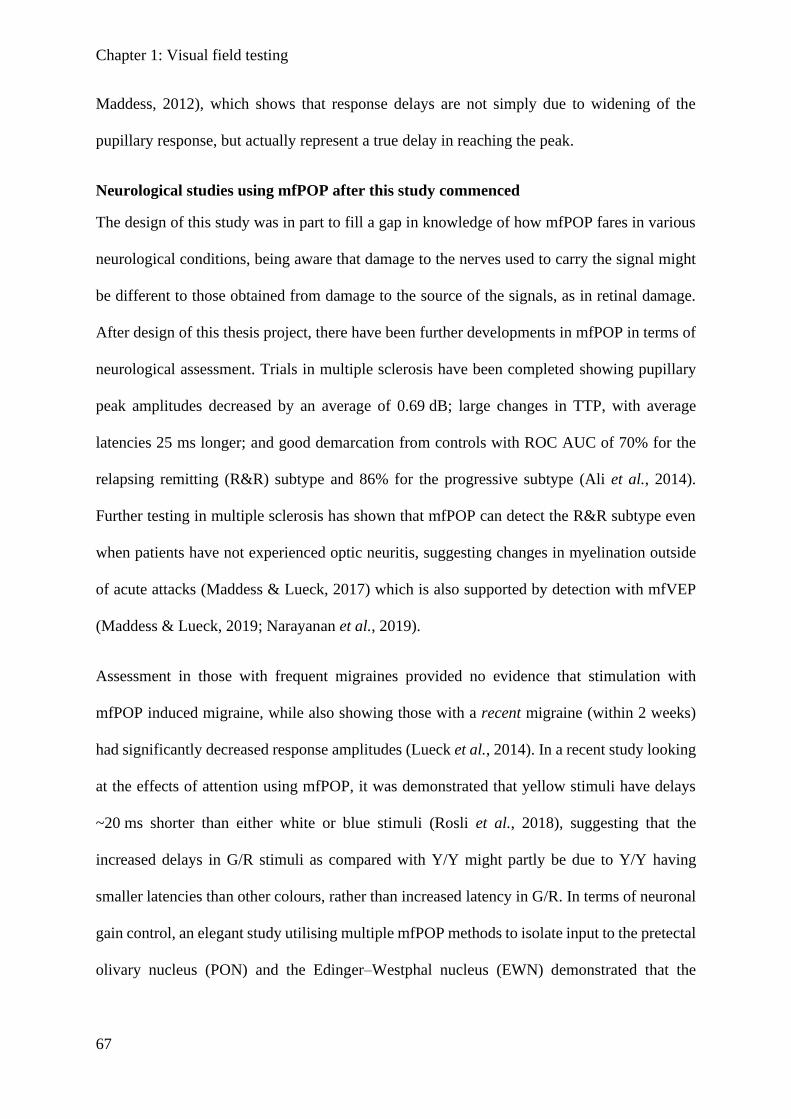
Chapter 1: Visual field testing
67
Maddess, 2012), which shows that response delays are not simply due to widening of the
pupillary response, but actually represent a true delay in reaching the peak.
Neurological studies using mfPOP after this study commenced
The design of this study was in part to fill a gap in knowledge of how mfPOP fares in various
neurological conditions, being aware that damage to the nerves used to carry the signal might
be different to those obtained from damage to the source of the signals, as in retinal damage.
After design of this thesis project, there have been further developments in mfPOP in terms of
neurological assessment. Trials in multiple sclerosis have been completed showing pupillary
peak amplitudes decreased by an average of 0.69 dB; large changes in TTP, with average
latencies 25 ms longer; and good demarcation from controls with ROC AUC of 70% for the
relapsing remitting (R&R) subtype and 86% for the progressive subtype (Ali et al., 2014).
Further testing in multiple sclerosis has shown that mfPOP can detect the R&R subtype even
when patients have not experienced optic neuritis, suggesting changes in myelination outside
of acute attacks (Maddess & Lueck, 2017) which is also supported by detection with mfVEP
(Maddess & Lueck, 2019; Narayanan et al., 2019).
Assessment in those with frequent migraines provided no evidence that stimulation with
mfPOP induced migraine, while also showing those with a recent migraine (within 2 weeks)
had significantly decreased response amplitudes (Lueck et al., 2014). In a recent study looking
at the effects of attention using mfPOP, it was demonstrated that yellow stimuli have delays
~20 ms shorter than either white or blue stimuli (Rosli et al., 2018), suggesting that the
increased delays in G/R stimuli as compared with Y/Y might partly be due to Y/Y having
smaller latencies than other colours, rather than increased latency in G/R. In terms of neuronal
gain control, an elegant study utilising multiple mfPOP methods to isolate input to the pretectal
olivary nucleus (PON) and the Edinger–Westphal nucleus (EWN) demonstrated that the

Chapter 1: Visual field testing
68
majority of gain control occurs at the level of the EWN where the signal is integrated from
input of both eyes (Carle et al., 2019).
Retinal studies using mfPOP after this study commenced
Regarding retinal advances in mfPOP after this study commenced, additional studies in AMD,
diabetic retinopathy, and glaucoma have been published and are briefly summarised below. In
AMD, mfPOP was able to demonstrate a significant change in sensitivity with progression,
with the reassuring result that central rings showed the greatest losses, consistent with disease
pathology. Comparing Age-Related Eye Disease Study (AREDS) classifications 1–4, the study
showed ROC AUC values of 43%, 60%, 60%, and 92% (within eye) and 62%, 74%, 81%, and
100% (between eye) for the best protocol (Sabeti et al., 2014), on par with previous studies in
AMD (Sabeti et al., 2011; Rosli et al., 2012). Examination of diabetic retinopathy patients
showed mfPOP mean amplitude was smaller in subjects with retinopathy, while surprisingly
the longest delays (latency) were in patients without retinopathy. By comparing asymmetry
between eyes for TTP (latency), sensitivity reached 100% at 0% FPR in separating diabetes
(with or without retinopathy) from controls (Sabeti et al., 2015), a notable improvement from
previous work (Bell et al., 2010). In glaucoma, testing the intrinsic component of intrinsically
photoreceptive retinal ganglion cells (ipRGC) (blue wavelength sensitivity) compared to their
cone input (yellow), showed similar diagnostic accuracy but with blue light being more
variable in advanced disease and less sensitive to scotomas (Carle et al., 2015). This is
consistent with previous studies involving brunescence, which contributes to variability
between individuals (Maddess et al., 2011; Shean et al., 2012). A study of the effects of the
dilating agent tropicamide (frequently used in ophthalmic examinations) revealed both
pupillary delays and amplitude decreased initially, with pupil delays fully recovered after 8 h,
while amplitudes were aberrant for 48 h (Rai et al., 2019).
Chapter 1: Summary – addressing gaps in literature
69
1.7. Summary – addressing gaps in the literature
1.7.1. Chapter 3 – Higher visual function loss and it assessment in stroke
This introduction has covered the visual pathways from the retina to the visual cortex and its
distribution into other cortical centres, any of which may be damaged by disease. Extrastriate
visual areas were shown to have areas of specialised processing, with cortical damage resulting
in a range of deficits of higher visual function (HVF). It was established that pure higher visual
function (HVF) deficits are rare, but that more subtle defects largely go unreported, leaving it
unclear whether subtle HVF deficits occur commonly, which tests are most appropriate, and
whether these warrants standard testing in clinical practice. Chapter 3 begins this discussion by
piloting a study of heterogenous stroke patients who completed a range of HVF testing using
multiple measures, and reporting which deficits appear to be worth further investigating and
which tests appear most useful.
1.7.2. Chapter 4 – Pupillometry direct and consensual responses in stroke,
chiasmal compression and AION
The origin of the pupil response in intrinsically photoreceptive retinal ganglion cells (ipRGC)
and their combined intrinsic and cone inputs were discussed, along with their afferent
pathways, and input to pupillary nuclei. The direct and consensual pupillary outputs were
discussed, specifically covering their differences in the nasal and temporal fields. These
features have been reported multiple times in control patients, but have not been reported in
neurological disease. Chapter 4 compared direct and consensual pupillary outputs in stroke,
chiasmal compression, and AION; addressing whether the same features are controls exist, or
whether they may be characteristic differences which can better differentiate these conditions.
Further, to enable a direct point-to-point comparison between visual field devices, direct and
Chapter 1: Summary – addressing gaps in literature
70
consensual signals must be combined, and this chapter considered how best to combine these
without bias.
1.7.3. Chapter 5 – Visual field comparison of standard automated perimetry
and pupillomgrey in stroke, chiasmal compression and AION.
The introduction covered the history and developments of standard automated perimetry
devices (HFA and MFA), covering their strengths, weaknesses, and output format. Likewise
the history and development of mfPOP was covered in detail, leading up to the protcols used
in these experiements. While mfPOP has been tested in a number of retinal disorders, its testing
in neurological disorders remains limited, and it has not been tested in stroke, pituitary tumour,
or AION conditions. As disucssed – these are common conditions and it is important that field
devices can accurately identify and characterise damage, which may inform treatment or
suggest limitations on activities that have becomes dangerous, such as driving. If mfPOP is to
be used in clinical practice, it is important to assess how well it performs against devices which
are used in clinical practice. This chapter compares HFA, MFA and mfPOP and assesses their
relative effectiveness.
1.7.4. Chapter 6 – Analysis of pupillometry response waveform time-to-peak
and comparison with amplitude in stroke, chiasmal compression and AION
A range of mfPOP protocols were discussed, including different output measures such as
amplitude and time-to-peak (latency) of the response waveform. These previous experiments
inform the new protocol used in this chapter, using green on red (G/R) stimuli and yellow on
yellow (Y/Y) stimuli, with amplitude and latency measures. These are further justified within
the chapter, but follow from the seminal paper by Carle et al., 2013 discussed above. As delays
have been demonstrated in G/R colour-exchange stimuli consistent with cortical processing, it
was thought that a G/R may be a more sensitive measure to cortical damage in stroke. This

Chapter 1: Summary – addressing gaps in literature
71
chapter explores that possibility, while also discussing outcomes in chiasmal compression and
AION.
72
References
Adams DL & Horton JC. (2003). A precise retinotopic map of primate striate cortex
generated from the representation of angioscotomas. J Neurosci 23, 3771-3789.
Ali EN, Maddess T, James AC, Voicu C & Lueck CJ. (2014). Pupillary response to sparse
multifocal stimuli in multiple sclerosis patients. Mult Scler 20, 854-861.
Ali M, Hazelton C, Lyden P, Pollock A, Brady M & Collaboration V. (2013). Recovery from
poststroke visual impairment: Evidence from a clinical trials resource. Neurorehab
Neural Re 27, 133-141.
Allman JM & Kaas JH. (1971). A representation of the visual field in the caudal third of the
middle tempral gyrus of the owl monkey (aotus trivirgatus). Brain Res 31, 85-105.
An SJ, Kim TJ & Yoon BW. (2017). Epidemiology, risk factors, and clinical features of
intracerebral hemorrhage: An update. J Stroke 19, 3-10.
Anderson AJ & Johnson CA. (2002). Mechanisms isolated by frequency-doubling technology
perimetry. Invest Ophthalmol Vis Sci 43, 398-401.
Anderson AJ & Johnson CA. (2006). Comparison of the asa, mobs, and zest threshold
methods. Vision Res 46, 2403-2411.
Arcaro MJ & Kastner S. (2015). Topographic organization of areas v3 and v4 and its relation
to supra-areal organization of the primate visual system. Vis Neurosci 32, E014.
Arda H, Birer S, Aksu M, Ismailogullari S, Karakucuk S, Mirza E, Gumus K & Oner A.
(2013). Obstructive sleep apnoea prevalence in non-arteritic anterior ischaemic optic
neuropathy. Brit J Ophthalmol 97, 206-209.
Arshavsky VY & Wensel TG. (2013). Timing is everything: Gtpase regulation in
phototransduction. Invest Ophthalmol Vis Sci 54, 7725-7733.
Artes PH, Iwase A, Ohno Y, Kitazawa Y & Chauban BC. (2002). Properties of perimetric
threshold estimates from full threshold, sita standard, and sita fast strategies. Invest
Ophth Vis Sci 43, 2654-2659.

Chapter 1: References
73
Arvind H, Graham S, Leaney J, Grigg J, Goldberg I, Billson F & Klistorner A. (2009).
Identifying preperimetric functional loss in glaucoma: A blue-on-yellow multifocal
visual evoked potentials study. Ophthalmology 116, 1134-1141.
Aubert H & Foerster R. (1857). Untersuchungen über den raumsinn der retina. Archiv für
Ophthalmologie 3, 1-37.
Azouvi P, Bartolomeo P, Beis JM, Perennou D, Pradat-Diehl P & Rousseaux M. (2006). A
battery of tests for the quantitative assessment of unilateral neglect. Restor Neurol
Neurosci 24, 273-285.
Bailey MJ, Riddoch MJ & Crome P. (2004). Test-retest stability of three tests for unilateral
visual neglect in patients with stroke: Star cancellation, line bisection, and the baking
tray task. Neuropsychol Rehabil 14, 403-419.
Barrett KE, Barman SM, Biotano S & Brooks HL. (2011). Ganong's review of medical
physiology. McGraw-Hill Education, USA.
Bartolomeo P, Bachoud-Levi AC & Thiebaut de Schotten M. (2014). The anatomy of
cerebral achromatopsia: A reappraisal and comparison of two case reports. Cortex 56,
138-144.
Barton JJS, Sharpe JA & Raymond JE. (1996). Directional defects in pursuit and motion
perception in humans with unilateral cerebral lesions. Brain 119, 1535-1550.
Baseler HA, Sutter EE, Klein SA & Carney T. (1994). The topography of visual evoked
response properties across the visual field. Electroencephalogr Clin Neurophysiol 90,
65-81.
Bass SJ, Cooper J, Feldman J & Horn D. (2007). Comparison of an automated confrontation
testing device versus finger counting in the detection of field loss. Optometry 78, 390-
395.
Beck RW, Bergstrom TJ & Lichter PR. (1985). A clinical comparison of visual field testing
with a new automated perimeter, the humphrey field analyzer, and the goldmann
perimeter. Ophthalmology 92, 77-82.
Beck RW, Hayreh SS, Podhajsky PA, Tan ES & Moke PS. (1997). Aspirin therapy in
nonarteritic anterior ischemic optic neuropathy. Am J Ophthalmol 123, 212-217.
Beis JM, Keller C, Morin N, Bartolomeo P, Bernati T, Chokron S, Leclercq M, Louis-
Dreyfus A, Marchal F, Martin Y, Perennou D, Pradat-Diehl P, Prairial C, Rode G,
Chapter 1: References
74
Rousseaux M, Samuel C, Sieroff E, Wiart L, Azouvi P & French Collaborative Study
Group on Assessment of Unilateral N. (2004). Right spatial neglect after left
hemisphere stroke: Qualitative and quantitative study. Neurology 63, 1600-1605.
Bell A, James AC, Kolic M, Essex RW & Maddess T. (2010). Dichoptic multifocal
pupillography reveals afferent visual field defects in early type 2 diabetes. Invest
Ophth Vis Sci 51, 602-608.
Bengtsson B & Heijl A. (1998). Sita fast, a new rapid perimetric threshold test. Description
of methods and evaluation in patients with manifest and suspect glaucoma. Acta
Ophthalmol Scand 76, 431-437.
Bengtsson B, Heijl A & Olsson J. (1998). Evaluation of a new threshold visual field strategy,
sita, in normal subjects. Swedish interactive thresholding algorithm. Acta Ophthalmol
Scand 76, 165-169.
Berezina TL, Khouri AS, Kolomeyer AM, Clancy PS & Fechtner RD. (2011). Peripheral
visual field thresholds using humphrey field analyzer program 60-4 in normal eyes.
Eur J Ophthalmol 21, 415-421.
Beri M, Klugman MR, Kohler JA & Hayreh SS. (1987). Anterior ischemic optic neuropathy
.7. Incidence of bilaterality and various influencing factors. Ophthalmology 94, 1020-
1028.
Berson DM, Castrucci AM & Provencio I. (2010). Morphology and mosaics of melanopsin-
expressing retinal ganglion cell types in mice. J Comp Neurol 518, 2405-2422.
Berson DM, Dunn FA & Takao M. (2002). Phototransduction by retinal ganglion cells that
set the circadian clock. Science 295, 1070-1073.
Bevers C, Blanckaert G, Van Keer K, Fils JF, Vandewalle E & Stalmans I. (2019). Semi-
automated kinetic perimetry: Comparison of the octopus 900 and humphrey visual
field analyzer 3 versus goldmann perimetry. Acta Ophthalmol 97, e499-e505.
Biousse V, Kedar S, Zhang XJ, Lynn M & Newman NJ. (2005). Homonymous hemianopia in
stroke. Neurology 64, A14-A14.
Bjerre A, Grigg JR, Parry NR & Henson DB. (2004). Test-retest variability of multifocal
visual evoked potential and sita standard perimetry in glaucoma. Invest Ophthalmol
Vis Sci 45, 4035-4040.

Chapter 1: References
75
Boardman JP, Ganesan V, Rutherford MA, Saunders DE, Mercuri E & Cowan F. (2005).
Magnetic resonance image correlates of hemiparesis after neonatal and childhood
middle cerebral artery stroke. Pediatrics 115, 321-326.
Boehme AK, Esenwa C & Elkind MS. (2017). Stroke risk factors, genetics, and prevention.
Circ Res 120, 472-495.
Born RT & Bradley DC. (2005). Structure and function of visual area mt. Annu Rev Neurosci
28, 157-189.
Bouvier SE & Engel SA. (2006). Behavioral deficits and cortical damage loci in cerebral
achromatopsia. Cereb Cortex 16, 183-191.
Bowen A, McKenna K & Tallis RC. (1999). Reasons for variability in the reported rate of
occurrence of unilateral spatial neglect after stroke. Stroke 30, 1196-1202.
Bremner FD. (2012). Pupillometric evaluation of the dynamics of the pupillary response to a
brief light stimulus in healthy subjects. Invest Ophthalmol Vis Sci 53, 7343-7347.
Burkhalter A & Van Essen DC. (1986). Processing of color, form and disparity information
in visual areas vp and v2 of ventral extrastriate cortex in the macaque monkey. J
Neurosci 6, 2327-2351.
Carle CF, James AC, Kolic M, Essex RW & Maddess T. (2015). Blue multifocal
pupillographic objective perimetry in glaucoma. Invest Ophthalmol Vis Sci 56, 6394-
6403.
Carle CF, James AC, Kolic M, Loh YW & Maddess T. (2011a). High-resolution multifocal
pupillographic objective perimetry in glaucoma. Invest Ophth Vis Sci 52, 604-610.
Carle CF, James AC & Maddess T. (2013). The pupillary response to color and luminance
variant multifocal stimuli. Invest Ophth Vis Sci 54, 467-475.
Carle CF, James AC, Rosli Y & Maddess T. (2019). Localization of neuronal gain control in
the pupillary response. Frontiers in neurology 10, 203.
Carle CF, Maddess T & James AC. (2011b). Contraction anisocoria: Segregation,
summation, and saturation in the pupillary pathway. Invest Ophth Vis Sci 52, 2365-
2371.
Chapter 1: References
76
Carota A & Calabrese P. (2013). The achromatic 'philosophical zombie', a syndrome of
cerebral achromatopsia with color anopsognosia. Case Rep Neurol 5, 98-103.
Cassidy TP, Bruce DW & Gray CS. (2001). Visual field loss after stroke: Confrontation and
perimetry in the assessment of recovery. J Stroke Cerebrovasc Dis 10, 113-117.
Chain AYH, Carle CF, James AC & Maddess T. (2012). Multifocal pupillographic perimetry
and ocular coherence tomography measurements in glaucoma. Clin Exp Ophthalmol
40, 136-137.
Chen C, Okera S, Davies PE, Selva D & Crompton JL. (2003a). Craniopharyngioma: A
review of long-term visual outcome. Clin Exp Ophthalmol 31, 220-228.
Chen CS, Hood DC, Zhang X, Karam EZ, Liebmann JM, Ritch R, Thienprasiddhi P &
Greenstein VC. (2003b). Repeat reliability of the multifocal visual evoked potential in
normal and glaucomatous eyes. J Glaucoma 12, 399-408.
Chen CS, Lee AW, Clarke G, Hayes A, George S, Vincent R, Thompson A, Centrella L,
Johnson K, Daly A & Crotty M. (2009). Vision-related quality of life in patients with
complete homonymous hemianopia post stroke. Top Stroke Rehabil 16, 445-453.
Connolly B & Oczkowski W. (2010). Individual and combined confrontation visual field
tests performed poorly as a screen for visual field abnormalities. Ann Intern Med 153.
Conway BR & Tsao DY. (2009). Color-tuned neurons are spatially clustered according to
color preference within alert macaque posterior inferior temporal cortex. Proc Natl
Acad Sci U S A 106, 18034-18039.
Cooper SA, Joshi AC, Seenan PJ, Hadley DM, Muir KW, Leigh RJ & Metcalfe RA. (2012).
Akinetopsia: Acute presentation and evidence for persisting defects in motion vision.
J Neurol Neurosur Ps 83, 229-230.
Cowey A, Alexander I, Heywood C & Kentridge R. (2008). Pupillary responses to coloured
and contourless displays in total cerebral achromatopsia. Brain 131, 2153-2160.
Cowey A, Heywood CA & Irving-Bell L. (2001). The regional cortical basis of
achromatopsia: A study on macaque monkeys and an achromatopsic patient. Eur J
Neurosci 14, 1555-1566.
Cox TA & Drewes CP. (1984). Contraction anisocoria resulting from half-field illumination.
Am J Ophthalmol 97, 577-582.

Chapter 1: References
77
Coyle JT. (2001). Goldmann vs. Humphrey perimetry for occipital lobe lesions.
Ophthalmology 108, 241-242.
Curcio CA & Allen KA. (1990). Topography of ganglion cells in human retina. J Comp
Neurol 300, 5-25.
Dacey DM, Liao HW, Peterson BB, Robinson FR, Smith VC, Pokorny J, Yau KW & Gamlin
PD. (2005). Melanopsin-expressing ganglion cells in primate retina signal colour and
irradiance and project to the lgn. Nature 433, 749-754.
Dacey DM, Peterson BB, Robinson FR & Gamlin PD. (2003). Fireworks in the primate
retina: In vitro photodynamics reveals diverse lgn-projecting ganglion cell types.
Neuron 37, 15-27.
Danesh-Meyer HV, Carroll SC, Gaskin BJ, Gao A & Gamble GD. (2006). Correlation of the
multifocal visual evoked potential and standard automated perimetry in compressive
optic neuropathies. Invest Ophthalmol Vis Sci 47, 1458-1463.
Danesh-Meyer HV & Gamble GD. (2011). Diagnostic accuracy of confrontation visual field
tests reply from the authors. Neurology 76, 1193-1193.
Davies JM, Trinh VT, Sneed PK & McDermott MW. (2013). Radiotherapy for recurrent
epidermoid cyst. J Neuro-Oncol 112, 307-313.
de Rooij NK, Linn FH, van der Plas JA, Algra A & Rinkel GJ. (2007). Incidence of
subarachnoid haemorrhage: A systematic review with emphasis on region, age,
gender and time trends. J Neurol Neurosurg Psychiatry 78, 1365-1372.
DeArmond SJ, Fusco MM & Dewey MM. (1976). Structure of the human brain: A
photographic atlas. Oxford University Press, USA.
DeYoe EA, Carman GJ, Bandettini P, Glickman S, Wieser J, Cox R, Miller D & Neitz J.
(1996). Mapping striate and extrastriate visual areas in human cerebral cortex. Proc
Natl Acad Sci U S A 93, 2382-2386.
Do MT & Yau KW. (2010). Intrinsically photosensitive retinal ganglion cells. Physiol Rev
90, 1547-1581.
Dubner R & Zeki SM. (1971). Response properties and receptive fields of cells in an
anatomically defined region of the superior temporal sulcus in the monkey. Brain Res
35, 528-532.

Chapter 1: References
78
Edelstein K & Amir S. (1999). The role of the intergeniculate leaflet in entrainment of
circadian rhythms to a skeleton photoperiod. J Neurosci 19, 372-380.
Elliott DB, North I & Flanagan J. (1997). Confrontation visual field tests. Ophthal Physl Opt
17, S17-S24.
Fishman GA, Birch DG, Holder GE & Brigell MG. (2001). Electrophysiologic testing in
disorders of the retina, optic nerve, and visual pathway. American academy of
ophthalmology, San Francisco.
Flanagan JG & Harding GF. (1988). Multi-channel visual evoked potentials in early
compressive lesions of the chiasm. Doc Ophthalmol 69, 271-281.
Fox CJ, Hanif HM, Iaria G, Duchaine BC & Barton JJS. (2011). Perceptual and anatomic
patterns of selective deficits in facial identity and expression processing.
Neuropsychologia 49, 3188-3200.
Fraser C, Klistorner A, Graham S, Garrick R, Billson F & Grigg J. (2006a). Multifocal visual
evoked potential latency analysis: Predicting progression to multiple sclerosis. Arch
Neurol 63, 847-850.
Fraser CL, Klistorner A, Graham SL, Garrick R, Billson FA & Grigg JR. (2006b). Multifocal
visual evoked potential analysis of inflammatory or demyelinating optic neuritis.
Ophthalmology 113, 323 e321-323 e322.
Fredette MJ, Giguere A, Anderson DR, Budenz DL & McSoley J. (2015). Comparison of
matrix with humphrey field analyzer ii with sita. Optometry and vision science :
official publication of the American Academy of Optometry 92, 527-536.
Fukuda Y, Higuchi S, Yasukouchi A & Morita T. (2012). Distinct responses of cones and
melanopsin-expressing retinal ganglion cells in the human electroretinogram. J
Physiol Anthropol 31.
Furlan M & Smith AT. (2016). Global motion processing in human visual cortical areas v2
and v3. J Neurosci 36, 7314-7324.
Gall C, Franke GH & Sabel BA. (2010). Vision-related quality of life in first stroke patients
with homonymous visual field defects. Health Qual Life Out 8.
Gamlin PD & Clarke RJ. (1995). The pupillary light reflex pathway of the primate. J Am
Optom Assoc 66, 415-418.
Chapter 1: References
79
Gamlin PD, Zhang H & Clarke RJ. (1995). Luminance neurons in the pretectal olivary
nucleus mediate the pupillary light reflex in the rhesus monkey. Exp Brain Res 106,
169-176.
Gardiner SK, Demirel S, Goren D, Mansberger SL & Swanson WH. (2015). The effect of
stimulus size on the reliable stimulus range of perimetry. Transl Vis Sci Technol 4, 10.
Gautier A, Godbout A, Grosheny C, Tejedor I, Coudert M, Courtillot C, Jublanc C, De
Kerdanet M, Poirier JY, Riffaud L, Sainte-Rose C, Van Effenterre R, Brassier G,
Bonnet F, Touraine P & Grp CS. (2012). Markers of recurrence and long-term
morbidity in craniopharyngioma: A systematic analysis of 171 patients. J Clin Endocr
Metab 97, 1258-1267.
Gilhotra JS, Mitchell P, Healey PR, Cumming RG & Currie J. (2002). Homonymous visual
field defects and stroke in an older population. Stroke 33, 2417-2420.
Girkin CA, McGwin G, Jr. & DeLeon-Ortega J. (2004). Frequency doubling technology
perimetry in non-arteritic ischaemic optic neuropathy with altitudinal defects. The
British journal of ophthalmology 88, 1274-1279.
Glisson CC. (2014). Visual loss due to optic chiasm and retrochiasmal visual pathway
lesions. Continuum (Minneap Minn) 20, 907-921.
Goldmann H. (1946). Demonstration unseres neuen projektionskugelperimeters samt
theoretischen und klinischen bemerkungen über perimetrie. Ophthalmologica 111,
187-192.
Graham SL. (2006). The effects of glaucoma on the latency of the multifocal visual evoked
potential. The British journal of ophthalmology 90, 1077-1078.
Graham SL & Klistorner A. (1999). The diagnostic significance of the multifocal pattern
visual evoked potential in glaucoma. Curr Opin Ophthalmol 10, 140-146.
Greifzu F, Schmidt S, Schmidt KF, Kreikemeier K, Witte OW & Lowel S. (2011). Global
impairment and therapeutic restoration of visual plasticity mechanisms after a
localized cortical stroke. Proc Natl Acad Sci U S A 108, 15450-15455.
Gulsen S, Dinc AH, Unal M, Canturk N & Altinors N. (2010). Characterization of the
anatomic location of the pituitary stalk and its relationship to the dorsum sellae,
tuberculum sellae and chiasmatic cistern. J Korean Neurosurg Soc 47, 169-173.

Chapter 1: References
80
Guzzetta A. (2010). Plasticity of the visual system after congenital brain damage: A few
weeks can matter. Dev Med Child Neurol 52, 699.
Guzzetta A, Cioni G, Cowan F & Mercuri E. (2001a). Visual disorders in children with brain
lesions: 1. Maturation of visual function in infants with neonatal brain lesions:
Correlation with neuroimaging. European journal of paediatric neurology : EJPN :
official journal of the European Paediatric Neurology Society 5, 107-114.
Guzzetta A, D'Acunto G, Rose S, Tinelli F, Boyd R & Cioni G. (2010). Plasticity of the
visual system after early brain damage. Dev Med Child Neurol 52, 891-900.
Guzzetta A, Fazzi B, Mercuri E, Bertuccelli B, Canapicchi R, van Hof-van Duin J & Cioni G.
(2001b). Visual function in children with hemiplegia in the first years of life. Dev
Med Child Neurol 43, 321-329.
Hadjikhani N, Liu AK, Dale AM, Cavanagh P & Tootell RB. (1998). Retinotopy and color
sensitivity in human visual cortical area v8. Nat Neurosci 1, 235-241.
Halliday AM, Halliday E, Kriss A, McDonald WI & Mushin J. (1976a). The pattern-evoked
potential in compression of the anterior visual pathways. Brain 99, 357-374.
Halliday AM, Halliday L, Kriss A, McDonald WI & Mushin J. (1976b). Abnormalities of the
pattern evoked potential in compression of the anterior visual pathways. Trans
Ophthalmol Soc N Z 28, 37-40.
Hattenhauer MG, Leavitt JA, Hodge DO, Grill R & Gray DT. (1997). Incidence of
nonarteritic anterior ischemic optic neuropathy. Am J Ophthalmol 123, 103-107.
Hayashi R, Yamaguchi S, Narimatsu T, Miyata H, Katsumata Y & Mimura M. (2017).
Statokinetic dissociation (riddoch phenomenon) in a patient with homonymous
hemianopsia as the first sign of posterior cortical atrophy. Case Rep Neurol 9, 256-
260.
Hayes A, Chen CS, Clarke G & Thompson A. (2012). Functional improvements following
the use of the nvt vision rehabilitation program for patients with hemianopia
following stroke. Neurorehabilitation 31, 19-30.
Hayreh SS. (1974). Anterior ischemic optic neuropathy .1. Terminology and pathogenesis.
Brit J Ophthalmol 58, 955-963.
Hayreh SS. (2001a). Blood flow in the optic nerve head and factors that may influence it.
Prog Retin Eye Res 20, 595-624.

Chapter 1: References
81
Hayreh SS. (2001b). The blood supply of the optic nerve head and the evaluation of it - myth
and reality. Prog Retin Eye Res 20, 563-593.
Hayreh SS. (2009). Ischemic optic neuropathy. Prog Retin Eye Res 28, 34-62.
Hayreh SS. (2011). Treatment of non-arteritic anterior ischaemic optic neuropathy. Brit J
Ophthalmol 95, 1617-1618.
Hayreh SS, Podhajsky PA & Zimmerman B. (2001). Ipsilateral recurrence of nonarteritic
anterior ischemic optic neuropathy. Am J Ophthalmol 132, 734-742.
Heijl A, Lindgren A & Lindgren G. (1989). Test-retest variability in glaucomatous visual-
fields. Am J Ophthalmol 108, 130-135.
Heilman KM & Van Den Abell T. (1980). Right hemisphere dominance for attention: The
mechanism underlying hemispheric asymmetries of inattention (neglect). Neurology
30, 327-330.
Heilman KM, Watson RT, Bower D & Valenstein E. (1983). [right hemisphere dominance
for attention]. Rev Neurol (Paris) 139, 15-17.
Hendry SHC & Reid RC. (2000). The koniocellular pathway in primate vision. Annu Rev
Neurosci 23, 127-153.
Hepworth LR & Rowe FJ. (2018). Programme choice for perimetry in neurological
conditions (popin): A systematic review of perimetry options and patterns of visual
field loss. Bmc Ophthalmol 18, 241.
Heutink J, Brouwer WH, Kums E, Young A & Bouma A. (2012). When family looks strange
and strangers look normal: A case of impaired face perception and recognition after
stroke. Neurocase 18, 39-49.
Heywood CA, Nicholas JJ, LeMare C & Cowey A. (1998). The effect of lesions to cortical
areas v4 or ait on pupillary responses to chromatic and achromatic stimuli in
monkeys. Exp Brain Res 122, 475-480.
Holmes G. (1918). Disturbances of visual orientation. The British journal of ophthalmology
2, 506-516.
Holmes G. (1919). Disturbances of visual space perception. Brit Med J 2, 230-233.

Chapter 1: References
82
Holmes G & Horrax G. (1919). Disturbances of spatial orientation and visual attention with
loss of stereoscopic vision. Arch Neuro Psychiatr 1, 385-407.
Hood DC, Greenstein VC, Odel JG, Zhang X, Ritch R, Liebmann JM, Hong JE, Chen CS &
Thienprasiddhi P. (2002). Visual field defects and multifocal visual evoked potentials:
Evidence of a linear relationship. Arch Ophthalmol 120, 1672-1681.
Hood DC, Odel JG & Winn BJ. (2003a). The multifocal visual evoked potential. Journal of
neuro-ophthalmology : the official journal of the North American Neuro-
Ophthalmology Society 23, 279-289.
Hood DC, Zhang X & Winn BJ. (2003b). Detecting glaucomatous damage with multifocal
visual evoked potentials: How can a monocular test work? J Glaucoma 12, 3-15.
Horton JC. (1997). Wilbrand's knee of the primate optic chiasm is an artefact of monocular
enucleation. Trans Am Ophthalmol Soc 95, 579-609.
Horton JC & Hocking DR. (1996). Intrinsic variability of ocular dominance column
periodicity in normal macaque monkeys. J Neurosci 16, 7228-7239.
Hurley JB. (2009). Encyclopedia of neuroscience. In Phototransduction, ed. Squire LR.
Elsevier.
Hutchins B & Weber JT. (1985). The pretectal complex of the monkey: A reinvestigation of
the morphology and retinal terminations. J Comp Neurol 232, 425-442.
Ijaola FO & Kausar SA. (2009). Visual impairment following stroke: Do stroke patients
require vision assessment ? Age Ageing 38, 629-630.
Ireland AC & Carter BI. (2019). Neuroanatomy, optic chiasm. StatPearls Publishing,
Treasure Island, Florida.
Jacobson L, Rydberg A, Eliasson AC, Kits A & Flodmark O. (2010). Visual field function in
school-aged children with spastic unilateral cerebral palsy related to different patterns
of brain damage. Dev Med Child Neurol 52, e184-187.
Jahangiri A, Lamborn KR, Blevins L, Kunwar S & Aghi MK. (2012). Factors associated with
delay to pituitary adenoma diagnosis in patients with visual loss. J Neurosurg 116,
283-289.
Chapter 1: References
83
James AC, Kolic M, Bedford SM & Maddess T. (2012). Stimulus parameters for multifocal
pupillographic objective perimetry. J Glaucoma 21, 571-578.
James AC, Maddess T & Bowman E. (2003). Effect of presentation rate and pulse duration
on the pattern-pulse multifocal visual evoked potential (ppmvep). Invest Ophth Vis Sci
44, U445-U445.
James AC, Maddess T, Goh XL & Winkles N. (2005a). Spatially sparse pattern-pulse
stimulation enhances multifocal visual evoked potential analysis. Invest Ophth Vis Sci
46.
James AC, Ruseckaite R & Maddess T. (2005b). Effect of temporal sparseness and dichoptic
presentation on multifocal visual evoked potentials. Visual Neurosci 22, 45-54.
Jehkonen M, Ahonen JP, Dastidar P, Koivisto AM, Laippala P, Vilkki J & Molnar G. (2000).
Visual neglect as a predictor of functional outcome one year after stroke. Acta Neurol
Scand 101, 195-201.
Johnson CA. (1994). Selective versus nonselective losses in glaucoma. J Glaucoma 3 Suppl
1, S32-44.
Johnson CA, Chauhan BC & Shapiro LR. (1992). Properties of staircase procedures for
estimating thresholds in automated perimetry. Invest Ophthalmol Vis Sci 33, 2966-
2974.
Johnson CA & Samuels SJ. (1997). Screening for glaucomatous visual field loss with
frequency-doubling perimetry. Invest Ophthalmol Vis Sci 38, 413-425.
Johnson CA, Wall M & Thompson HS. (2011). A history of perimetry and visual field
testing. Optometry and vision science : official publication of the American Academy
of Optometry 88, E8-15.
Johnson LN & Arnold AC. (1994). Incidence of nonarteritic and arteritic anterior ischemic
optic neuropathy - population-based study in the state of missouri and los-angeles-
county, california. J Neuro-Ophthalmol 14, 38-44.
Johnson LN & Baloh FG. (1991). The accuracy of confrontation visual-field test in
comparison with automated perimetry. J Natl Med Assoc 83, 895-898.
Jonas JB, Schneider U & Naumann GO. (1992). Count and density of human retinal
photoreceptors. Graefe's archive for clinical and experimental ophthalmology =

Chapter 1: References
84
Albrecht von Graefes Archiv fur klinische und experimentelle Ophthalmologie 230,
505-510.
Jones SA & Shinton RA. (2006). Improving outcome in stroke patients with visual problems.
Age Ageing 35, 560-565.
Kaplan E. (2013). The m, p and k pathways of the primate visual system revisited. In The
new visual neuroscience, ed. Werner JS & Chalupa LM, pp. 215-227.
Kardon R, Anderson SC, Damarjian TG, Grace EM, Stone E & Kawasaki A. (2009).
Chromatic pupil responses: Preferential activation of the melanopsin-mediated versus
outer photoreceptor-mediated pupil light reflex. Ophthalmology 116, 1564-1573.
Kasputyte R, Slatkeviciene G, Liutkeviciene R, Glebauskiene B, Bernotas G & Tamasauskas
A. (2013). Changes of visual functions in patients with pituitary adenoma. Med Lith
49, 132-137.
Kerr NM, Chew SSL, Eady EK, Gamble GD & Danesh-Meyer HV. (2010). Diagnostic
accuracy of confrontation visual field tests. Neurology 74, 1184-1190.
Kerr NM, Chew SSSL & Danesh-Meyer HV. (2009). Non-arteritic anterior ischaemic optic
neuropathy: A review and update. J Clin Neurosci 16, 994-1000.
Khan S, Leung E & Jay WM. (2008). Stroke and visual rehabilitation. Top Stroke Rehabil 15,
27-36.
Kikuchi Y, Yoshii M, Yanashima K, Enoki T, Ide T, Sakemi F & Okisaka S. (2002).
Multifocal visual evoked potential is dependent on electrode position. Jpn J
Ophthalmol 46, 533-539.
Kim KY, Rios LC, Le H, Perez AJ, Phan S, Bushong EA, Deerinck TJ, Liu YH, Ellisman
MA, Lev-Ram V, Ju S, Panda SA, Yoon S, Hirayama M, Mure LS, Hatori M,
Ellisman MH & Panda S. (2019). Synaptic specializations of melanopsin-retinal
ganglion cells in multiple brain regions revealed by genetic label for light and electron
microscopy. Cell Rep 29, 628-644 e626.
Klistorner A, Graham SL, Martins A, Grigg JR, Arvind H, Kumar RS, James AC & Billson
FA. (2007). Multifocal blue-on-yellow visual evoked potentials in early glaucoma.
Ophthalmology 114, 1613-1621.

Chapter 1: References
85
Klistorner AI, Graham SL, Grigg JR & Billson FA. (1998). Multifocal topographic visual
evoked potential: Improving objective detection of local visual field defects. Invest
Ophthalmol Vis Sci 39, 937-950.
Kolb H. (1995). Webvision: The organisation of the retina and visual system, ed. Kolb H,
Nelson R, Fernandez E & Jones B. University of Utah Health Sciences Center, Salt
lake city, Utah.
Kolic M, Chain A, James A, Maddess T & Carle C. (2013). Structure and function in
multifocal pupillographic objective perimetry (mfpop). Invest Ophth Vis Sci 54.
Kozicz T, Bittencourt JC, May PJ, Reiner A, Gamlin PDR, Palkovits M, Horn AKE, Toledo
CAB & Ryabinin AE. (2011). The edinger-westphal nucleus: A historical, structural,
and functional perspective on a dichotomous terminology. J Comp Neurol 519, 1413-
1434.
Kupfer C, Chumbley L & Downer JC. (1967). Quantitative histology of optic nerve, optic
tract and lateral geniculate nucleus of man. J Anat 101, 393-401.
Kuritzky S. (2001). Goldmann vs. Humphrey perimetry for occipital lobe lesions.
Ophthalmology 108, 242.
Lall GS, Revell VL, Momiji H, Al Enezi J, Altimus CM, Guler AD, Aguilar C, Cameron
MA, Allender S, Hankins MW & Lucas RJ. (2010). Distinct contributions of rod,
cone, and melanopsin photoreceptors to encoding irradiance. Neuron 66, 417-428.
Lang N, Baudewig J, Kallenberg K, Antal A, Happe S, Dechent P & Paulus W. (2006).
Transient prosopagnosia after ischemic stroke. Neurology 66, 916-916.
Lee JP, Park IW & Chung YS. (2011a). The volume of tumor mass and visual field defect in
patients with pituitary macroadenoma. Korean J Ophthalmol 25, 37-41.
Lee MS, Grossman D, Arnold AC & Sloan FA. (2011b). Incidence of nonarteritic anterior
ischemic optic neuropathy: Increased risk among diabetic patients. Ophthalmology
118, 959-963.
Lee SK, Sonoda T & Schmidt TM. (2019). M1 intrinsically photosensitive retinal ganglion
cells integrate rod and melanopsin inputs to signal in low light. Cell Rep 29, 3349-
3355 e3342.
Chapter 1: References
86
Leff A. (2004). A historical review of the representation of the visual field in primary visual
cortex with special reference to the neural mechanisms underlying macular sparing.
Brain Lang 88, 268-278.
Li JY & Schmidt TM. (2018). Divergent projection patterns of m1 iprgc subtypes. J Comp
Neurol 526, 2010-2018.
Lu XS, Ye J, Zhou S, Lu BX & Chen XH. (2005). Unilateral spatial neglect, global
processing deficit and prosopagnosia following right hemisphere stroke: A case
report. Chinese Med J-Peking 118, 1846-1848.
Lueck C, Ali E, Carle C & Maddess T. (2014). Effects of stimulating melanopsin-containing
retinal ganglioncells in migraine patients using multifocal objective pupillometry. J
Clin Neurosci 21, 2048.
Lundervold AJ, Bergmann N & Wootton C. (2005). Visual neglect in the first weeks after a
stroke in the right hemisphere. Scand J Psychol 46, 297-303.
Luu S, Lee AW, Daly A & Chen CS. (2010). Visual field defects after stroke a practical
guide for gps. Aust Fam Physician 39, 499-503.
Lynch JK, Hirtz DG, DeVeber G & Nelson KB. (2002). Report of the national institute of
neurological disorders and stroke workshop on perinatal and childhood stroke.
Pediatrics 109, 116-123.
Lyon DC & Kaas JH. (2001). Connectional and architectonic evidence for dorsal and ventral
v3, and dorsomedial area in marmoset monkeys. J Neurosci 21, 249-261.
Maddess T. (2011). The influence of sampling errors on test-retest variability in perimetry.
Invest Ophthalmol Vis Sci 52, 1014-1022.
Maddess T. (2012). Pupil dynamics and response amplitude: Only size matters. Invest Ophth
Vis Sci 53, 7644-7644.
Maddess T. (2014). Modeling the relative influence of fixation and sampling errors on retest
variability in perimetry. Graefe's archive for clinical and experimental ophthalmology
= Albrecht von Graefes Archiv fur klinische und experimentelle Ophthalmologie 252,
1611-1619.
Maddess T, Bedford SM, Goh XL & James AC. (2009). Multifocal pupillographic visual
field testing in glaucoma. Clin Exp Ophthalmol 37, 678-686.
Chapter 1: References
87
Maddess T, Goh XL & James AC. (2007). Luminance and chromatic multifocal
pupillographic perimetry. In ARVO annual meeting, pp. 1628. Investigative
ophthalmology and visual science.
Maddess T & Henry GH. (1992). Performance of nonlinear visual units in ocular
hypertension and glaucoma. Clin Vision Sci 7, 371-383.
Maddess T, Ho YL, Wong SS, Kolic M, Goh XL, Carle CF & James AC. (2011). Multifocal
pupillographic perimetry with white and colored stimuli. J Glaucoma 20, 336-343.
Maddess T, James AC & Bowman EA. (2004). Contrast responses of dichoptic multifocal
visual evoked potential responses to contrast reversing and temporally sparse stimuli.
Invest Ophth Vis Sci 45, U155-U155.
Maddess T, James AC, Ruseckaite R & Bowman EA. (2003). Hierarchical decomposition of
multifocal visual evoked potential responses to dichoptic contrast reversing and
temporally sparse stimuli. Invest Ophth Vis Sci 44, U465-U465.
Maddess T & Kulikowski JJ. (1999). Apparent fineness of stationary compound gratings.
Vision Res 39, 3404-3416.
Maddess T & Lueck CJ. (2017). Multiple sclerosis seen through new eyes. Clin Exp
Ophthalmol 45, 9-11.
Maddess T & Lueck CJ. (2019). Correlating structure with visual function in patients with
multiple sclerosis: Where is this leading? Clin Neurophysiol 130, 157-159.
Maddess T, Ruseckaite R & James AC. (2002). Effect of sparseness and dichoptic
presentation on multifocal visual evoked potentials. Invest Ophth Vis Sci 43, U1337-
U1337.
Maffei L. (2002). Plasticity in the visual system: Role of neurotrophins and electrical activity.
Arch Ital Biol 140, 341-346.
Martin TI, Kardon RI & Thompson HS. (1991). Unequal direct and consensual pupillary
responses to hemiretinal stimuli. Invest Ophth Vis Sci 32, 1124.
Martins A, Klistorner A, Graham S & Billson F. (2004). Effect of check size and stimulation
rate on blue-yellow multifocal visual evoked potentials. Clin Exp Ophthalmol 32,
270-274.

Chapter 1: References
88
Marzi CA, Mancini F, Sperandio I & Savazzi S. (2009). Evidence of midline retinal
nasotemporal overlap in healthy humans: A model for foveal sparing in hemianopia?
Neuropsychologia 47, 3007-3011.
Matson M & Fujimoto L. (2011). Bilateral arteritic anterior ischemic optic neuropathy.
Optometry 82, 622-631.
McDougal DH & Gamlin PD. (2010). The influence of intrinsically-photosensitive retinal
ganglion cells on the spectral sensitivity and response dynamics of the human
pupillary light reflex. Vision Res 50, 72-87.
McDougal DH & Gamlin PD. (2015). Autonomic control of the eye. Compr Physiol 5, 439-
473.
McKeefry DJ, Watson JDG, Frackowiak RSJ, Fong K & Zeki S. (1997). The activity in
human areas v1/v2, v3, and v5 during the perception of coherent and incoherent
motion. Neuroimage 5, 1-12.
McKeefry DJ & Zeki S. (1997). The position and topography of the human colour centre as
revealed by functional magnetic resonance imaging. Brain 120 ( Pt 12), 2229-2242.
McKendrick AM, Anderson AJ, Johnson CA & Fortune B. (2003). Appearance of the
frequency doubling stimulus in normal subjects and patients with glaucoma. Invest
Ophthalmol Vis Sci 44, 1111-1116.
McMinn RMH. (1998). Last's anatomy regional and applied. Elsivier: Churchill Livingstone,
Edinburgh, United Kingdom.
Miller LJ, Mittenberg W, Carey VM, McMorrow MA, Kushner TE & Weinstein JM. (1999).
Astereopsis caused by traumatic brain injury. Arch Clin Neuropsych 14, 537-543.
Millodot M. (2009). Dictionary of optometry and visual science. Butterworth-Heinemann -
elsevier, United Kingdom.
Monteiro ML, Moura FC & Cunha LP. (2007). Frequency doubling perimetry in patients
with mild and moderate pituitary tumor-associated visual field defects detected by
conventional perimetry. Arq Bras Oftalmol 70, 323-329.
Morin LP, Blanchard JH & Provencio I. (2003). Retinal ganglion cell projections to the
hamster suprachiasmatic nucleus, intergeniculate leaflet, and visual midbrain:
Bifurcation and melanopsin immunoreactivity. J Comp Neurol 465, 401-416.
Chapter 1: References
89
Munch M & Kawasaki A. (2013). Intrinsically photosensitive retinal ganglion cells:
Classification, function and clinical implications. Curr Opin Neurol 26, 45-51.
Munch M, Leon L, Crippa SV & Kawasaki A. (2012). Circadian and wake-dependent effects
on the pupil light reflex in response to narrow-bandwidth light pulses. Invest Ophth
Vis Sci 53, 4546-4555.
Musch DC, Gillespie BW, Motyka BM, Niziol LM, Mills RP & Lichter PR. (2005).
Converting to sita-standard from full-threshold visual field testing in the follow-up
phase of a clinical trial. Invest Ophthalmol Vis Sci 46, 2755-2759.
Narayanan D, Cheng H, Tang RA & Frishman LJ. (2019). Multifocal visual evoked
potentials and contrast sensitivity correlate with ganglion cell-inner plexiform layer
thickness in multiple sclerosis. Clin Neurophysiol 130, 180-188.
Newkirk MR, Gardiner SK, Demirel S & Johnson CA. (2006). Assessment of false positives
with the humphrey field analyzer ii perimeter with the sita algorithm. Invest Ophth Vis
Sci 47, 4632-4637.
Nissila J, Manttari S, Tuominen H, Sarkioja T, Takala T, Saarela S & Timonen M. (2012).
The abundance and distribution of melanopsin (opn4) protein in human brain. Eur
Psychiat 27.
Noval S, Contreras I, Rebolleda G, Munoz-Negrete FJ & Ruiz de Zarate B. (2005). A
comparison between humphrey and frequency doubling perimetry for chiasmal visual
field defects. Eur J Ophthalmol 15, 739-745.
Numata T, Maddess T, Matsumoto C, Okuyama S, Hashimoto S, Nomoto H & Shimomura
Y. (2017). Exploring test-retest variability using high-resolution perimetry. Transl Vis
Sci Technol 6, 8.
Okamoto Y, Okamoto F, Hiraoka T, Yamada S & Oshika T. (2008). Vision-related quality of
life in patients with pituitary adenoma. Am J Ophthalmol 146, 318-322.
Otsuka-Hirota N, Yamamoto H, Miyashita K & Nagatsuka K. (2014). Invisibility of moving
objects: A core symptom of motion blindness. BMJ Case Rep 2014.
Overly C. (2009). Bitemporal hemianopia arising from a suprasellar craniopharyngioma.
Optometry 80, 621-629.

Chapter 1: References
90
Pagani R, Bosco G, Dalla Valle E, Capitani E & Laiacona M. (2012). The assessment of
colour perception, naming and knowledge: A new test device with a case study.
Neurol Sci 33, 801-809.
Pandit RJ, Gales K & Griffiths PG. (2001). Effectiveness of testing visual fields by
confrontation. Lancet 358, 1339-1340.
Parisi V, Miglior S, Manni G, Centofanti M & Bucci MG. (2006). Clinical ability of pattern
electroretinograms and visual evoked potentials in detecting visual dysfunction in
ocular hypertension and glaucoma. Ophthalmology 113, 216-228.
Park HP, YG. Cho, AH. Park, CK. (2013). Transneuronal retrograde degeneration of the
retinal ganglion cells in patients with cerebral infarction. Ophthalmology 120, 1292-
1299.
Pearce JG & Maddess T. (2016). Retest variability in the medmont m700 automated
perimeter. Optometry and vision science : official publication of the American
Academy of Optometry 93, 272-280.
Pelak VS & Hoyt WF. (2005). Symptoms of akinetopsia associated with traumatic brain
injury and alzheimer's disease. Neuro-Ophthalmology 29, 137-142.
Percival KA, Martin PR & Grunert U. (2013). Organisation of koniocellular-projecting
ganglion cells and diffuse bipolar cells in the primate fovea. Eur J Neurosci 37, 1072-
1089.
Pickard GE & Sollars PJ. (2012). Intrinsically photosensitive retinal ganglion cells. Rev
Physiol Bioch P 162, 59-90.
Pintor J. (2009). Autonomic nervous system: Ophthalmic control. In Encyclopedia of
neuroscience, ed. Squire LR. Academic Press.
Pollock A, Hazelton C & Brady M. (2011a). Visual problems after stroke: A survey of
current practice by occupational therapists working in uk stroke inpatient settings. Top
Stroke Rehabil 18, 643-651.
Pollock A, Hazelton C, Henderson CA, Angilley J, Dhillon B, Langhorne P, Livingstone K,
Munro FA, Orr H, Rowe FJ & Shahani U. (2011b). Interventions for visual field
defects in patients with stroke. Cochrane Database Syst Rev, CD008388.
Poon A, McNeill P, Harper A & O'Day J. (1995). Patterns of visual loss associated with
pituitary macroadenomas. Aust N Z J Ophthalmol 23, 107-115.

Chapter 1: References
91
Prasad S & Cohen AB. (2011). Diagnostic accuracy of confrontation visual field tests.
Neurology 76, 1192-1193.
Provis JM, Dubis AM, Maddess T & Carroll J. (2013). Adaptation of the central retina for
high acuity vision: Cones, the fovea and the avascular zone. Prog Retin Eye Res 35,
63-81.
Pula JH & Yuen CA. (2017). Eyes and stroke: The visual aspects of cerebrovascular disease.
Stroke Vasc Neurol 2, 210-220.
Punjabi OS, Tanna AP & Rosenberg MA. (2011). Optic disk excavation in nonarteritic
anterior ischemic optic neuropathy. J Glaucoma 20, 71-73.
Purves D, Augustine GJ, D. F, Katz LC, LaMantia AS, McNamara JO & Williams SM.
(2001). Neuroscience. Sinaurer Associates, Sunderland (MA).
Qureshi AI, Tuhrim S, Broderick JP, Batjer HH, Hondo H & Hanley DF. (2001).
Spontaneous intracerebral hemorrhage. N Engl J Med 344, 1450-1460.
Rai BB, Sabeti F, Carle CF, Rohan EMF, Sarac O, van Kleef J & Maddess T. (2019).
Recovery dynamics of multifocal pupillographic objective perimetry from
tropicamide dilation. Graefe's archive for clinical and experimental ophthalmology =
Albrecht von Graefes Archiv fur klinische und experimentelle Ophthalmologie.
Reader AL & Harper DG. (1976). Confrontation visual-field testing. Jama-J Am Med Assoc
236, 250-250.
Riggs RV, Andrews K, Roberts P & Gilewski M. (2007). Visual deficit interventions in adult
stroke and brain injury - a systematic review. Am J Phys Med Rehab 86, 853-860.
Ringman JM, Saver JL, Woolson RF, Clarke WR & Adams HP. (2004). Frequency, risk
factors, anatomy, and course of unilateral neglect in an acute stroke cohort. Neurology
63, 468-474.
Rizzo M, Nawrot M & Zihl J. (1995). Motion and shape perception in cerebral akinetopsia.
Brain 118, 1105-1127.
Rodarte C, Hood DC, Yang EB, Grippo T, Greenstein VC, Liebmann JM & Ritch R. (2006).
The effects of glaucoma on the latency of the multifocal visual evoked potential. The
British journal of ophthalmology 90, 1132-1136.

Chapter 1: References
92
Roe AW & Ts'o DY. (2015). Specificity of v1-v2 orientation networks in the primate visual
cortex. Cortex 72, 168-178.
Roelfsema F, Biermasz NR & Pereira AM. (2012). Clinical factors involved in the recurrence
of pituitary adenomas after surgical remission: A structured review and meta-analysis.
Pituitary 15, 71-83.
Rosli Y, Bedford SM, James AC & Maddess T. (2012). Photopic and scotopic multifocal
pupillographic responses in age-related macular degeneration. Vision Res 69, 42-48.
Rosli Y, Carle CF, Ho Y, James AC, Kolic M, Rohan EMF & Maddess T. (2018).
Retinotopic effects of visual attention revealed by dichoptic multifocal pupillography.
Sci Rep 8, 2991.
Ross JE. (1983). Disturbance of stereoscopic vision in patients with unilateral stroke. Behav
Brain Res 7, 99-112.
Rowe F. (2009). Letters to the editor: Visual impairment following stroke do stroke patients
require visual assessment? Age Ageing 35, 560-565.
Rowe F. (2016). Visual effects and rehabilitation after stroke. Community Eye Health 29, 75-
76.
Rowe F, Brand D, Jackson CA, Price A, Walker L, Harrison S, Eccleston C, Scott C,
Akerman N, Dodridge C, Howard C, Shipman T, Sperring U, MacDiarmid S &
Freeman C. (2009). Visual impairment following stroke: Do stroke patients require
vision assessment? Age Ageing 38, 188-193.
Rowe FJ & Grp V. (2011). Accuracy of referrals for visual assessment in a stroke population.
Eye 25, 161-167.
Rowe FJ, Wright D, Brand D, Jackson C, Harrison S, Maan T, Scott C, Vogwell L, Peel S,
Akerman N, Dodridge C, Howard C, Shipman T, Sperring U, Macdiarmid S &
Freeman C. (2013). A prospective profile of visual field loss following stroke:
Prevalence, type, rehabilitation, and outcome. BioMed research international 2013,
719096.
Rudnicka AR & Edgar DF. (1995). Automated static perimetry in myopes with peripapillary
crescents--part i. Ophthalmic Physiol Opt 15, 409-412.
Chapter 1: References
93
Rudnicka AR & Edgar DF. (1996). Automated static perimetry in myopes with peripapillary
crescents--part ii. Ophthalmic Physiol Opt 16, 416-429.
Ruseckaite R, Maddess T & James AC. (2004a). Comparing multifocal binocular pattern
pulse visual evoked potentials in normal and multiple sclerosis patients. Perception
33, 129-129.
Ruseckaite R, Maddess T & James AC. (2004b). Comparing multifocal frequency-doubling
illusion, visual evoked potentials, and automated perimetry in normal and optic
neuritis patients. Perception 33, 128-128.
Ruseckaite R, Maddess T & James AC. (2005). New methods to detect multiple sclerosis.
Unveiling the Mystery of the Brain: Neurophysiological Investigation of the Brain
Function 1278, 49-52.
Ruseckaite R, Maddess T & James AC. (2006). Monocular and binocular multifocal visual
evoked potentials in normal and multiple sclerosis subjects. Mult Scler 12, S166-
S166.
Sabeti F, Maddess T, Essex RW & James AC. (2011). Multifocal pupillographic assessment
of age-related macular degeneration. Optometry Vision Sci 88, 1477-1485.
Sabeti F, Maddess T, Essex RW, Saikal A, James AC & Carle CF. (2014). Multifocal
pupillography in early age-related macular degeneration. Optometry and vision
science : official publication of the American Academy of Optometry 91, 904-915.
Sabeti F, Nolan CJ, James AC, Jenkins A & Maddess T. (2015). Multifocal pupillography
identifies changes in visual sensitivity according to severity of diabetic retinopathy in
type 2 diabetes. Invest Ophthalmol Vis Sci 56, 4504-4513.
Sand A, Schmidt TM & Kofuji P. (2012). Diverse types of ganglion cell photoreceptors in the
mammalian retina. Prog Retin Eye Res 31, 287-302.
Sand KM, Midelfart A, Thomassen L, Melms A, Wilhelm H & Hoff JM. (2013). Visual
impairment in stroke patients - a review. Acta Neurol Scand 127, 52-56.
Schaadt AK, Schmidt L, Reinhart S, Adams M, Garbacenkaite R, Leonhardt E, Kuhn C &
Kerkhoff G. (2014). Perceptual relearning of binocular fusion and stereoacuity after
brain injury. Neurorehabil Neural Repair 28, 462-471.
Schein SJ. (1988). Anatomy of macaque fovea and spatial densities of neurons in foveal
representation. J Comp Neurol 269, 479-505.
Chapter 1: References
94
Schellinger PD, Bryan RN, Caplan LR, Detre JA, Edelman RR, Jaigobin C, Kidwell CS,
Mohr JP, Sloan M, Sorensen AG, Warach S, Therapeutics & Technology Assessment
Subcommittee of the American Academy of N. (2010). Evidence-based guideline:
The role of diffusion and perfusion mri for the diagnosis of acute ischemic stroke:
Report of the therapeutics and technology assessment subcommittee of the american
academy of neurology. Neurology 75, 177-185.
Schiefer U, Pascual JP, Edmunds B, Feudner E, Hoffmann EM, Johnson CA, Lagreze WA,
Pfeiffer N, Sample PA, Staubach F, Weleber RG, Vonthein R, Krapp E & Paetzold J.
(2009). Comparison of the new perimetric gate strategy with conventional full-
threshold and sita standard strategies. Invest Ophthalmol Vis Sci 50, 488-494.
Schmid R, Wilhelm B & Wilhelm H. (2000). Naso-temporal asymmetry and contraction
anisocoria in the pupillomotor system. Graef Arch Clin Exp 238, 123-128.
Schneider KA, Richter MC & Kastner S. (2004). Retinotopic organization and functional
subdivisions of the human lateral geniculate nucleus: A high-resolution functional
magnetic resonance imaging study. J Neurosci 24, 8975-8985.
Semmlow J, Hansmann D & Stark L. (1975). Variation in pupillomotor responsiveness with
mean pupil size. Vision Res 15, 85-90.
Semmlow J & Stark L. (1973). Pupil movements to light and accommodative stimulation: A
comparative study. Vision Res 13, 1087-1100.
Senior C, Barnes J, Giampietro V, Simmons A, Bullmore ET, Brammer M & David AS.
(2000). The functional neuroanatomy of implicit-motion perception or
representational momentum. Curr Biol 10, 16-22.
Sereno MI, Dale AM, Reppas JB, Kwong KK, Belliveau JW, Brady TJ, Rosen BR & Tootell
RB. (1995). Borders of multiple visual areas in humans revealed by functional
magnetic resonance imaging. Science 268, 889-893.
Setala K & Vesti E. (1994). Acquired cerebral achromatopsia - a case-report. Neuro-
Ophthalmology 14, 31-36.
Shahinfar S, Johnson LN & Madsen RW. (1995). Confrontation visual-field loss as a function
of decibel sensitivity loss on automated static perimetry - implications on the accuracy
of confrontation visual-field (cvf) testing. Invest Ophth Vis Sci 36, S454-S454.

Chapter 1: References
95
Shean CJW, James AC, Kolic M, Maddess T & Carle CF. (2012). Signal and noise of
multifocal pupillographic stimulus response functions. Clin Exp Ophthalmol 40, 122-
122.
Shevell SK & Martin PR. (2017). Color opponency: Tutorial. Journal of the Optical Society
of America A, Optics, image science, and vision 34, 1099-1108.
Shipp S, de Jong BM, Zihl J, Frackowiak RS & Zeki S. (1994). The brain activity related to
residual motion vision in a patient with bilateral lesions of v5. Brain 117 ( Pt 5),
1023-1038.
Shipp S, Watson JD, Frackowiak RS & Zeki S. (1995). Retinotopic maps in human prestriate
visual cortex: The demarcation of areas v2 and v3. Neuroimage 2, 125-132.
Shrestha GS, Upadhyaya S, Sharma AK & Gajurel BP. (2012). Ocular-visual defect and
visual neglect in stroke patients - a report from kathmandu, nepal. Journal of
Optometry 5, 43-49.
Sincich LC, Park KF, Wohlgemuth MJ & Horton JC. (2004). Bypassing v1: A direct
geniculate input to area mt. Nat Neurosci 7, 1123-1128.
Smith SA & Smith SE. (1980). Contraction anisocoria: Nasal versus temporal illumination.
The British journal of ophthalmology 64, 933-934.
Smits AR, Seijdel N, Scholte HS, Heywood CA, Kentridge RW & de Haan EHF. (2019).
Action blindsight and antipointing in a hemianopic patient. Neuropsychologia 128,
270-275.
Spenceley SE & Henson DB. (1996). Visual field test simulation and error in threshold
estimation. The British journal of ophthalmology 80, 304-308.
Spolidoro M, Sale A, Berardi N & Maffei L. (2009). Plasticity in the adult brain: Lessons
from the visual system. Exp Brain Res 192, 335-341.
Sughrue ME, Yang I, Kane AJ, Fang S, Clark AJ, Aranda D, Barani IJ & Parsa AT. (2011).
Endocrinologic, neurologic, and visual morbidity after treatment for
craniopharyngioma. J Neuro-Oncol 101, 463-476.
Sutter EE & Tran D. (1992). The field topography of erg components in man--i. The photopic
luminance response. Vision Res 32, 433-446.

Chapter 1: References
96
Szmajda BA, Grunert U & Martin PR. (2008). Retinal ganglion cell inputs to the
koniocellular pathway. J Comp Neurol 510, 251-268.
Takayama Y & Sugishita M. (1994). Astereopsis induced by repetitive magnetic stimulation
of occipital cortex. J Neurol 241, 522-525.
Taravati P, Woodward KR, Keltner JL, Johnson CA, Redline D, Carolan J, Huang CQ &
Wall M. (2008). Sensitivity and specificity of the humphrey matrix to detect
homonymous hemianopias. Invest Ophth Vis Sci 49, 924-928.
Tigges J & O'Steen WK. (1974). Termination of retinofugal fibers in squirrel monkey: A re-
investigation using autoradiographic methods. Brain Res 79, 489-495.
Ting DSJ, Pollock A, Dutton GN, Doubal FN, Ting DSW, Thompson M & Dhillon B.
(2011). Visual neglect following stroke: Current concepts and future focus. Surv
Ophthalmol 56, 114-134.
Tootell RB, Dale AM, Sereno MI & Malach R. (1996). New images from human visual
cortex. Trends Neurosci 19, 481-489.
Tootell RB, Mendola JD, Hadjikhani NK, Ledden PJ, Liu AK, Reppas JB, Sereno MI & Dale
AM. (1997). Functional analysis of v3a and related areas in human visual cortex. J
Neurosci 17, 7060-7078.
Trobe JD, Acosta PC, Krischer JP & Trick GL. (1981). Confrontation visual-field techniques
in the detection of anterior visual pathway lesions. Ann Neurol 10, 28-34.
Trope GE & Britton R. (1987). A comparison of goldmann and humphrey automated
perimetry in patients with glaucoma. The British journal of ophthalmology 71, 489-
493.
Tsujimura S & Tokuda Y. (2011). Delayed response of human melanopsin retinal ganglion
cells on the pupillary light reflex. Ophthal Physl Opt 31, 469-479.
Tyrrell RA & Owens DA. (1988). A rapid technique to assess the resting states of the eyes
and other threshold phenomena: The modified binary search (mobs). Behavior
Research Methods, Instruments, & Computers 20, 137-141.
Vaina LM. (1995). Akinetopsia, achromatopsia and blindsight: Recent studies on perception
without awareness. Synthese 105, 253-271.

Chapter 1: References
97
Vaina LM, Cowey A, Eskew RT, LeMay M & Kemper T. (2001). Regional cerebral
correlates of global motion perception - evidence from unilateral cerebral brain
damage. Brain 124, 310-321.
Vaina LM, Sikoglu EM, Soloviev S, LeMay M, Squatrito S, Pandiani G & Cowey A. (2010).
Functional and anatomical profile of visual motion impairments in stroke patients
correlate with fmri in normal subjects. J Neuropsychol 4, 121-145.
Vakalopoulos C. (2005). A theory of blindsight - the anatomy of the unconscious: A proposal
for the koniocellular projections and intralaminar thalamus. Med Hypotheses 65,
1183-1190.
Vanni S, Hokkanen H, Werner F & Angelucci A. (2020). Anatomy and physiology of
macaque visual cortical areas v1, v2, and v5/mt: Bases for biologically realistic
models. Cereb Cortex.
von Arx SW, Muri RM, Heinemann D, Hess CW & Nyffeler T. (2010). Anosognosia for
cerebral achromatopsia-a longitudinal case study. Neuropsychologia 48, 970-977.
Wade AR, Brewer AA, Rieger JW & Wandell BA. (2002). Functional measurements of
human ventral occipital cortex: Retinotopy and colour. Philos Trans R Soc Lond B
Biol Sci 357, 963-973.
Wagner AL, Murtagh FR, Hazlett KS & Arrington JA. (1997). Measurement of the normal
optic chiasm on coronal mr images. AJNR Am J Neuroradiol 18, 723-726.
Wall M, Doyle CK, Zamba KD, Artes P & Johnson CA. (2013). The repeatability of mean
defect with size iii and size v standard automated perimetry. Invest Ophthalmol Vis
Sci 54, 1345-1351.
Wall M, Neahring RK & Woodward KR. (2002). Sensitivity and specificity of frequency
doubling perimetry in neuro-ophthalmic disorders: A comparison with conventional
automated perimetry. Invest Ophth Vis Sci 43, 1277-1283.
Wall M, Punke SG, Stickney TL, Brito CF, Withrow KR & Kardon RH. (2001). Sita standard
in optic neuropathies and hemianopias: A comparison with full threshold testing.
Invest Ophthalmol Vis Sci 42, 528-537.
Walsh TJ. (1990). Visual fields: Examination and interpretation. Oxford University Press,
Oxford, United Kingdom.

Chapter 1: References
98
Wandell BA & Engel SA. (1995). Fmri measurements of the neural image in area-v1. Invest
Ophth Vis Sci 36, S612-S612.
Wang HB, Sun W, Fu Z, Si ZC, Zhu YF, Zhai GD, Zhao GY, Xu SC & Pang Q. (2008). The
pattern of visual impairment in patients with pituitary adenoma. J Int Med Res 36,
1064-1069.
Wang L, Guo XL, Sun JF, Jin Z & Tong SB. (2012). Cortical networks of hemianopia stroke
patients: A graph theoretical analysis of eeg signals at resting state. Ieee Eng Med Bio,
49-52.
Wassle H, Grunert U, Rohrenbeck J & Boycott BB. (1989). Cortical magnification factor and
the ganglion cell density of the primate retina. Nature 341, 643-646.
Watanabe K, Shinoda K, Kimura I, Mashima Y, Oguchi Y & Ohde H. (2007). Discordance
between subjective perimetric visual fields and objective multifocal visual evoked
potential-determined visual fields in patients with hemianopsia. Am J Ophthalmol
143, 295-304.
Weber J & Dobek K. (1986). What is the most suitable grid for computer perimetry in
glaucoma patients? Ophthalmologica 192, 88-96.
White AJ, Sun H, Swanson WH & Lee BB. (2002). An examination of physiological
mechanisms underlying the frequency-doubling illusion. Invest Ophthalmol Vis Sci
43, 3590-3599.
Wild JM, Searle AE, Dengler-Harles M & O'Neill EC. (1991). Long-term follow-up of
baseline learning and fatigue effects in the automated perimetry of glaucoma and
ocular hypertensive patients. Acta Ophthalmol (Copenh) 69, 210-216.
Wong AM & Sharpe JA. (2000). A comparison of tangent screen, goldmann, and humphrey
perimetry in the detection and localization of occipital lesions. Ophthalmology 107,
527-544.
Wyatt HJ & Musselman JF. (1981). Pupillary light reflex in humans: Evidence for an
unbalanced pathway from nasal retina, and for signal cancellation in brainstem. Vision
Res 21, 513-525.
Yenice O & Temel A. (2005). Evaluation of two humphrey perimetry programs: Full
threshold and sita standard testing strategy for learning effect. Eur J Ophthalmol 15,
209-212.

Chapter 1: References
99
Yoon MK, Hwang TN, Day S, Hong J, Porco T & McCulley TJ. (2012). Comparison of
humphrey matrix frequency doubling technology to standard automated perimetry in
neuro-ophthalmic disease. Middle East Afr J Ophthalmol 19, 211-215.
You Y, Gupta VK, Graham SL & Klistorner A. (2012). Anterograde degeneration along the
visual pathway after optic nerve injury. Plos One 7, e52061.
Young RSL & Alpern M. (1980). Pupil responses to foveal exchange of monochromatic
lights. J Opt Soc Am 70, 697-706.
Zappia RJ, Enoch JM, Stamper R, Winkelman JZ & Gay AJ. (1971). The riddoch
phenomenon revealed in non-occipital lobe lesions. The British journal of
ophthalmology 55, 416-420.
Zeki S. (1990). A century of cerebral-achromatopsia. Brain 113, 1721-1777.
Zeki S. (1991). Cerebral akinetopsia (visual-motion blindness) - a review. Brain 114, 811-
824.
Zeki S. (1993). A vision of the brain. Blackwell Scientific Publications, Oxford.
Zeki S. (2003). Improbable areas in the visual brain. Trends Neurosci 26, 23-26.
Zeki S, Watson JD, Lueck CJ, Friston KJ, Kennard C & Frackowiak RS. (1991). A direct
demonstration of functional specialization in human visual cortex. J Neurosci 11,
641-649.
Zhang XJ, Kedar S, Lynn MJ, Newman NJ & Biousse V. (2006). Homonymous hemianopia
in stroke. J Neuro-Ophthalmol 26, 180-183.
Zhou C, He Y & Li X. (2018). Cerebral achromatopsia secondary to ischemic stroke. Neurol
India 66, 573-575.
Zhou J, Liu Z, Clavagnier S, Reynaud A & Hou F. (2017). Visual plasticity in adults. Neural
Plasticity 2017, 8469580.
Zihl J & Heywood CA. (2015). The contribution of lm to the neuroscience of movement
vision. Front Integr Neurosci 9, 6.
Zihl J, von Cramon D & Mai N. (1983). Selective disturbance of movement vision after
bilateral brain damage. Brain 106 (Pt 2), 313-340.
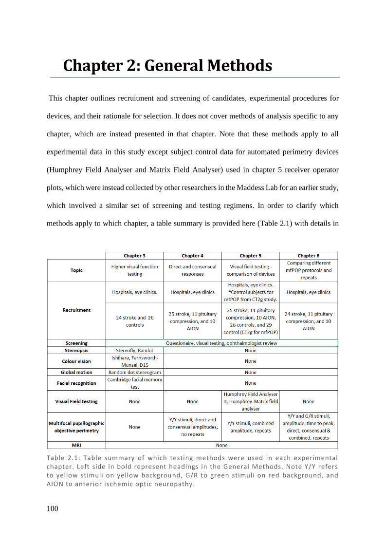
100
2 Chapter 2: General Methods
This chapter outlines recruitment and screening of candidates, experimental procedures for
devices, and their rationale for selection. It does not cover methods of analysis specific to any
chapter, which are instead presented in that chapter. Note that these methods apply to all
experimental data in this study except subject control data for automated perimetry devices
(Humphrey Field Analyser and Matrix Field Analyser) used in chapter 5 receiver operator
plots, which were instead collected by other researchers in the Maddess Lab for an earlier study,
which involved a similar set of screening and testing regimens. In order to clarify which
methods apply to which chapter, a table summary is provided here (Table 2.1) with details in
Table 2.1: Table summary of which testing methods were used in each experimental chapter. Left side in bold represent headings in the General Methods. Note Y/Y refers to yellow stimuli on yellow background, G/R to green stimuli on red background, and AION to anterior ischemic optic neuropathy.
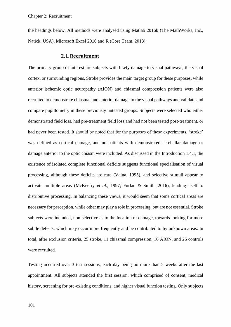
Chapter 2: Recruitment
101
the headings below. All methods were analysed using Matlab 2016b (The MathWorks, Inc.,
Natick, USA), Microsoft Excel 2016 and R (Core Team, 2013).
2.1. Recruitment
The primary group of interest are subjects with likely damage to visual pathways, the visual
cortex, or surrounding regions. Stroke provides the main target group for these purposes, while
anterior ischemic optic neuropathy (AION) and chiasmal compression patients were also
recruited to demonstrate chiasmal and anterior damage to the visual pathways and validate and
compare pupillometry in these previously untested groups. Subjects were selected who either
demonstrated field loss, had pre-treatment field loss and had not been tested post-treatment, or
had never been tested. It should be noted that for the purposes of these experiments, ‘stroke’
was defined as cortical damage, and no patients with demonstrated cerebellar damage or
damage anterior to the optic chiasm were included. As discussed in the Introduction 1.4.1, the
existence of isolated complete functional deficits suggests functional specialisation of visual
processing, although these deficits are rare (Vaina, 1995), and selective stimuli appear to
activate multiple areas (McKeefry et al., 1997; Furlan & Smith, 2016), lending itself to
distributive processing. In balancing these views, it would seem that some cortical areas are
necessary for perception, while other may play a role in processing, but are not essential. Stroke
subjects were included, non-selective as to the location of damage, towards looking for more
subtle defects, which may occur more frequently and be contributed to by unknown areas. In
total, after exclusion criteria, 25 stroke, 11 chiasmal compression, 10 AION, and 26 controls
were recruited.
Testing occurred over 3 test sessions, each day being no more than 2 weeks after the last
appointment. All subjects attended the first session, which comprised of consent, medical
history, screening for pre-existing conditions, and higher visual function testing. Only subjects

Chapter 2: Recruitment
102
within the stroke, chiasmal compression and AION groups continued to sessions 2 and 3, which
comprised of testing visual fields. In session 2, Humphrey and two mfPOP version were tested,
while in session 3, Matrix and repeats of the mfPOP versions were tested (details in 2.5.
Perimetry). One subject in the stroke group, and two subjects in the chiasmal compression
group, did not complete session 3 and so have no Matrix reports. Data for these subjects was
used where possible, but in producing averages and for direct comparisons, absent results were
omitted from the calculation. A demographic breakdown of all included subjects is provided
here for reference (Table 2.2).
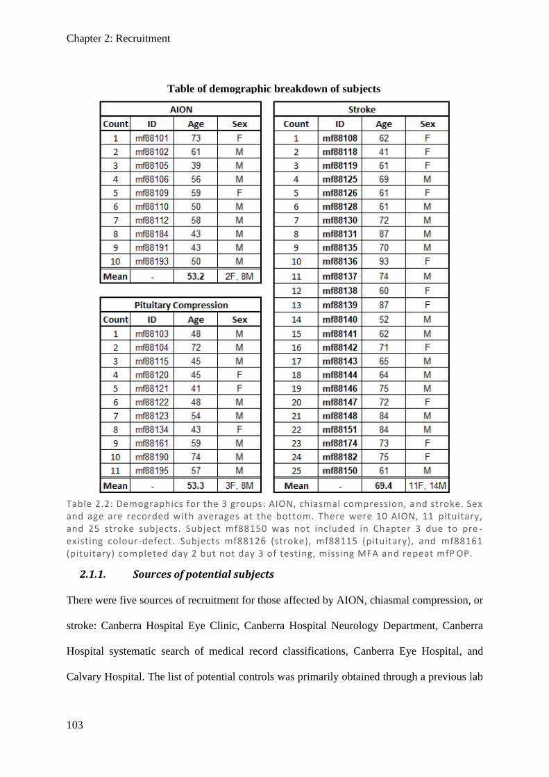
Chapter 2: Recruitment
103
2.1.1. Sources of potential subjects
There were five sources of recruitment for those affected by AION, chiasmal compression, or
stroke: Canberra Hospital Eye Clinic, Canberra Hospital Neurology Department, Canberra
Hospital systematic search of medical record classifications, Canberra Eye Hospital, and
Calvary Hospital. The list of potential controls was primarily obtained through a previous lab
Table of demographic breakdown of subjects
Table 2.2: Demographics for the 3 groups: AION, chiasmal compression, a nd stroke. Sex and age are recorded with averages at the bottom. There were 10 AION, 11 pituitary, and 25 stroke subjects. Subject mf88150 was not included in Chapter 3 due to pre -existing colour-defect. Subjects mf88126 (stroke), mf88115 (pituitary), and mf88161 (pituitary) completed day 2 but not day 3 of testing, missing MFA and repeat mfP OP.

Chapter 2: Recruitment
104
study completed two years previously that had already assessed these subjects’ vision as being
normal at the time and had consented to be contacted for future studies.
2.1.1.1. Canberra Hospital Eye Clinic
A list of potential subjects was obtained from a search of optometrist referral letters to
ophthalmologist Dr Kate Reid at The Canberra Hospital Eye Clinic spanning the previous 2
years. Searches used the following keywords: AION, pituitary, stroke, optic neuropathy, and
visual field loss. Letters were then assessed and a point score system used to shortlist potential
candidates taking into consideration: whether a diagnosis was only suspected or confirmed,
whether visual fields had been completed, whether they had sufficient visual acuity for
inclusion, and whether they had other diseases that might affect vision. Each case was
considered for inclusion given the information provided, excluding those who had visual field
testing with normal fields, poor visual acuity, and those with other ocular pathology. This was
the source of recruitment for all three disease types. Addresses and phone numbers for these
patients were obtained through the ACT Health Medical Records Department.
2.1.1.2. Canberra Hospital Neurology Department
A presentation was given to the neurology staff, outlining the basic inclusion criteria for
recruitment which encompassed known or suspected occipital stroke, but with adequate level
of cognition and motor skills to complete testing requirements. Suitable subjects were then
referred by clinicians including neuro-ophthalmologists, neurologists, and neurosurgeons. This
was primarily the source for stroke and pituitary tumour patients. Address and phone numbers
for these patients were obtained through the Medical Records Department.
2.1.1.3. Canberra Hospital systematic search of medical records
Regular searches spanning Jan 2011 – July 2014 were completed according to the medical
records classification codes. This systematic search included all three patient groups with codes

Chapter 2: Recruitment
105
I60/1/2/3/4 (stroke: ischemic and haemorrhagic), D35.2/3 (pituitary: adenoma and
craniopharyngioma), and H47 (AION: other disorders of optic nerve). All shortlisted patients
then had their medical records screened for suitability and the refined shortlist of addresses and
phone numbers were then obtained from Medical Records.
2.1.1.4. Canberra Eye Hospital
Canberra Eye Hospital is a private specialist treatment centre providing outpatient care for a
wide community. In another larger study previously completed by our lab group, participants
had been recruited through the Canberra Eye Hospital records. By sorting through the notes
from the previous study, a series of potential recruits were shortlisted. Approval to contact was
given by their treating physician. They were then screened for applicability through the
Canberra Hospital medical records system where such a record existed. Addresses and phone
numbers were obtained from both the Canberra Eye Hospital and Canberra Hospital records
and the most recent contact details used.
2.1.1.5. Calvary Hospital
During the testing period, a new stroke ward was formed at Calvary hospital in the ACT. To
maximise recruitment, the project and its selection criteria were discussed with Dr Shaun Zhai,
a registrar working on the Calvary stroke ward. Referrals were sent from the three-month post-
stroke follow up clinics, exclusively referring stroke patients. Addresses and phone number
were obtained from the physician via Calvary Hospital medical records.
2.1.1.6. Recruitment of controls
Controls were primarily recruited from a previous study list where subjects had been confirmed
to have normal vision two years prior and were therefore likely to have maintained normal
vision. This study included in its consent form the willingness to be contacted for future studies.
40 potential control subjects were extracted from the original study and their contact details
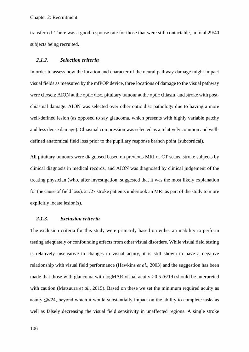
Chapter 2: Recruitment
106
transferred. There was a good response rate for those that were still contactable, in total 29/40
subjects being recruited.
2.1.2. Selection criteria
In order to assess how the location and character of the neural pathway damage might impact
visual fields as measured by the mfPOP device, three locations of damage to the visual pathway
were chosen: AION at the optic disc, pituitary tumour at the optic chiasm, and stroke with post-
chiasmal damage. AION was selected over other optic disc pathology due to having a more
well-defined lesion (as opposed to say glaucoma, which presents with highly variable patchy
and less dense damage). Chiasmal compression was selected as a relatively common and well-
defined anatomical field loss prior to the pupillary response branch point (subcortical).
All pituitary tumours were diagnosed based on previous MRI or CT scans, stroke subjects by
clinical diagnosis in medical records, and AION was diagnosed by clinical judgement of the
treating physician (who, after investigation, suggested that it was the most likely explanation
for the cause of field loss). 21/27 stroke patients undertook an MRI as part of the study to more
explicitly locate lesion(s).
2.1.3. Exclusion criteria
The exclusion criteria for this study were primarily based on either an inability to perform
testing adequately or confounding effects from other visual disorders. While visual field testing
is relatively insensitive to changes in visual acuity, it is still shown to have a negative
relationship with visual field performance (Hawkins et al., 2003) and the suggestion has been
made that those with glaucoma with logMAR visual acuity >0.5 (6/19) should be interpreted
with caution (Matsuura et al., 2015). Based on these we set the minimum required acuity as
acuity ≤6/24, beyond which it would substantially impact on the ability to complete tasks as
well as falsely decreasing the visual field sensitivity in unaffected regions. A single stroke

Chapter 2: Recruitment
107
patient was included for visual field analysis, but not higher visual function (HVF) testing, due
to a pre-existing red–green colour defect.
Any subject with a pre-existing eye condition that may affect the visual field, such as glaucoma,
significant cataracts, age-related macular degeneration, or retinitis, was excluded from the
study. As not all the subjects were able to undergo a comprehensive medical records screen
prior to testing, this meant some participants were excluded post-testing. Likewise, if any of
the participants had eye conditions that would exclude them from a particular component of
the HVF testing, such as having only one eye (lack of depth perception), or pre-existing red–
green defect (poor colour perception), then their data for that particular test was omitted;
however, they were permitted to complete other aspects of the research that would not be
dramatically impacted (such as motion and facial recognition). No participants with a single
functional eye were included for visual field analysis. Subjects were additionally excluded if
they had any underlying neural disorder that may affect conduction speed and pupillary
response to light. Given that pupillary responses in Alzheimer’s disease (Chougule et al., 2019)
and Parkinson’s (Micieli et al., 1991) show decreased constriction amplitude and increase
latency, patients with concurrent dementia were excluded and were specifically asked if they
had any of the following: Parkinson’s, Alzheimer’s, Huntington’s, or any form of dementia.
Similarly, due to potential for confounding effects, those with concurrent multiple sclerosis or
amyotrophic lateral sclerosis were also excluded as a precaution. For safety reasons current
epilepsy was an exclusion, since flashing lights are used, although there is some evidence
suggesting mfPOP does not appear to be a trigger for episodes (Ali et al., 2015). Those who
were pregnant were also excluded, as this has been shown to result in increased photopic pupil
diameter (Altay et al., 2016), and may involve unknown changes to the pupillary response. No
subjects were included who concurrently had multiple test conditions (stroke, pituitary tumour,
and AION). Those unable, due to field loss, to fixate on the central fixation light when

Chapter 2: Recruitment
108
completing a visual field test were considered to have a single functional eye and their fields
were omitted.
2.1.4. Contact
After obtaining preliminary lists of potential subjects from the sources listed above, they were
systematically contacted. First contact involved mailing out copies of the information and
consent forms, along with a cover letter from their clinician when appropriate. Two weeks later,
subjects were called and asked if they were interested in being involved in the study. Candidates
who declined were not contacted further, and no privacy complaints have been raised. Those
indicating interest were booked in for testing. All were volunteers and no incentive (monetary
or other) was used to encourage participation in this study.
2.1.5. Consent
Study approved by ACT Health Human Research Ethics Committee (ETH.5.13.100) and ANU
Human Research Ethics Committee (2013/343). Study abides by the principles outlined in the
Declaration of Helsinki.
Information and consent forms were included in the approved information pack for subjects to
read and sign prior to attending their first appointment and a contact phone number was
provided to allow clarification of any points. All consent forms included signature of the
investigator, participant, and a witness. Consent detailed that they should not have been
involved in any clinical trial or other interventional research within the last 3 months and
included consent to view medical records which pertained to this project, allowing review of
their medical history.
2.2. Medical History
A questionnaire was completed at the beginning of the first test session to ascertain any ocular
conditions or background conditions that may confound the measures made in this research. In

Chapter 2: Medical history
109
addition to the patient’s reported history, a comprehensive summary of their previous medical
records held by Canberra Hospital was also made (but omitted from this dissertation so as to
maintain confidentiality – see 2.2.2 Hospital ).
2.2.1. Questionnaire
A basic medical history for the patients was taken, including both a general history of ocular
disorders and a list of specific questions to exclude disorders. Specific questions included
presence or absence of: diabetes, cancer, dementia, multiple sclerosis, epilepsy, pregnancy,
glaucoma, cataracts, age-related macular degeneration, retinitis, colour vision defects, eye
surgery, eye injections, and contacts. This was taken in addition to a structured general history
comprising: any diagnosed eye conditions, previous ocular complaints or treatments, family
history, full list of medications, and characteristics of the presenting disorder for this study
including treatments and investigations sought for this disorder. For demographic and
statistical purposes, age, gender, ethnicity, dominant eye, and handedness were also noted.
Any eye condition or ocular history which might cause visual impairment was flagged, and the
list of medications was screened by a medical professional for any drugs which may impair
normal vision or the pupil response, including interactions that may confound testing.
2.2.2. Hospital records
Permission to access state medical records from Australian Capital Territory Health (ACT
health) was included as part of the consent form. Medical records were systematically assessed
including all visits to ophthalmology, neurology, neurosurgery, or cardiology wards and any
related visits to radiology, emergency department, endocrinology, rehabilitation, or
occupational therapy. For each visit, the date and a summary of key information for that visit
is provided, including any information received from referrals. All available visual field and
optical coherence tomography (OCT) results were included in the summaries. This

Chapter 2: Medical history
110
supplementary information has sufficient personal information to be considered confidential,
and so is not presented as part of this thesis.
2.3. Screening for pre-existing conditions
To ensure any discovered abnormalities in visual function were not caused by another
underlying condition, such as retinal disease, all patients were initially screened. This was
completed through the set of tests listed below, with their associated chapter section:
- logMAR acuity measured using an ETDRS chart (Kinyoun et al., 1989) (2.3.1.2).
- Intraocular pressure (IOP) with Ocular Response Analyser (Reichert, USA) (2.3.3.2).
- Retroillumination with ARK-1 (Marco, USA) and/or slit lamp examination (2.3.2.1).
- Fundus photo, posterior pole (P.pole), optic nerve head (ONH), and retinal nerve fibre
layer (RNFL) scan using Spectralis OCT (Heidelberg Engineering GmbH, Germany)
(2.3.3.1).
All results were then assessed by Dr Kate Reid, a senior neuro-ophthalmologist at Canberra
Hospital Eye Clinic, for any evidence of retinal disease that might affect the visual field. While
the majority of excluded subjects were excluded prior to testing based on medical records and
questionnaire, a total of 84 subjects were assessed by Dr Reid and a further 10 subjects were
excluded. This gave the final figure of 25 stroke, 11 chiasmal compression, 10 AION, and 26
controls, noting that one stroke patient was only available for visual field testing but not HVF,
due to having a pre-existing red-green colour defect and was excluded from Chapters 3 and 6.
2.3.1. Acuity
2.3.1.1. Refraction
Participants that regularly wear reading or distance glasses had their prescription measured
with a vertometer and their visual acuity was tested both with and without glasses. The optical
prescription was noted for correction of visual myopia, presbyopia, and astigmatism. For those

Chapter 2: Screening for pre-existing conditions
111
with acuity worse than 6/12 with glasses, pinhole acuity was also included. The best corrected
visual acuity (BCVA) noted through these three assessments was used. A minimum threshold
BCVA of 6/24 was used as an exclusion criterion.
2.3.1.2. ETDRS chart
While both Snellen chart and Early Treatment of Diabetic Retinopathy Study (ETDRS) chart
report similar acuity in those with mild-to-moderately lowered acuity (Kaiser, 2008), ETDRS
acuity at 4 m was chosen as it offers some advantages over the Snellen chart. ETDRS has the
same number of optotype letters on each line with approximately the same reading difficulty,
increasing its accuracy and reproducibility (Shamir et al., 2016). For consistency, all measures
were made by a single assessor, with 3/5 correct in a line considered sufficient to meet that
level of acuity. Subjects had one eye covered and were asked to start on the lowest line that
they can easily read and then progress down until they either failed the line or were unable to
read the line. The right eye was always tested first, and when testing the left eye, they were
asked to read the letters in reverse (right to left), to try and minimise their ability to recall letters
when reading the same line.
2.3.2. Cataracts
Cataracts are very common, particularly in the elderly population, and can cause dimming of
visual fields that are neither of retinal nor neural origin (Lam et al., 1991). As visual fields are
a primary focus, it was therefore very important that anyone with a substantial cataract be
excluded from the study.
2.3.2.1. ARK-1 retroillumination and slit lamp
To check for cataracts, the ARK-1 autorefractor and keratometer was used as a screening
device using its retroillumination test to detect opacities in the optical media of the eye. When
the patient reported a history of cataracts or the ARK-1 screening appeared abnormal, a slit
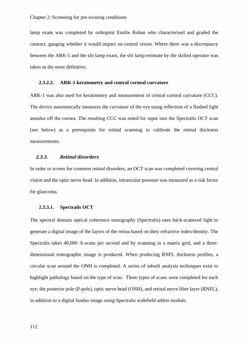
Chapter 2: Screening for pre-existing conditions
112
lamp exam was completed by orthoptist Emilie Rohan who characterised and graded the
cataract, gauging whether it would impact on central vision. Where there was a discrepancy
between the ARK-1 and the slit lamp exam, the slit lamp estimate by the skilled operator was
taken as the more definitive.
2.3.2.2. ARK-1 keratometry and central corneal curvature
ARK-1 was also used for keratometry and measurement of central corneal curvature (CCC).
The device automatically measures the curvature of the eye using reflection of a flashed light
annulus off the cornea. The resulting CCC was noted for input into the Spectralis OCT scan
(see below) as a prerequisite for retinal scanning to calibrate the retinal thickness
measurements.
2.3.3. Retinal disorders
In order to screen for common retinal disorders, an OCT scan was completed covering central
vision and the optic nerve head. In addition, intraocular pressure was measured as a risk factor
for glaucoma.
2.3.3.1. Spectralis OCT
The spectral domain optical coherence tomography (Spectralis) uses back-scattered light to
generate a digital image of the layers of the retina based on their refractive index/density. The
Spectralis takes 40,000 A-scans per second and by scanning in a matrix grid, and a three-
dimensional tomographic image is produced. When producing RNFL thickness profiles, a
circular scan around the ONH is completed. A series of inbuilt analysis techniques exist to
highlight pathology based on the type of scan. Three types of scans were completed for each
eye: the posterior pole (P-pole), optic nerve head (ONH), and retinal nerve fibre layer (RNFL),
in addition to a digital fundus image using Spectralis widefield addon module.
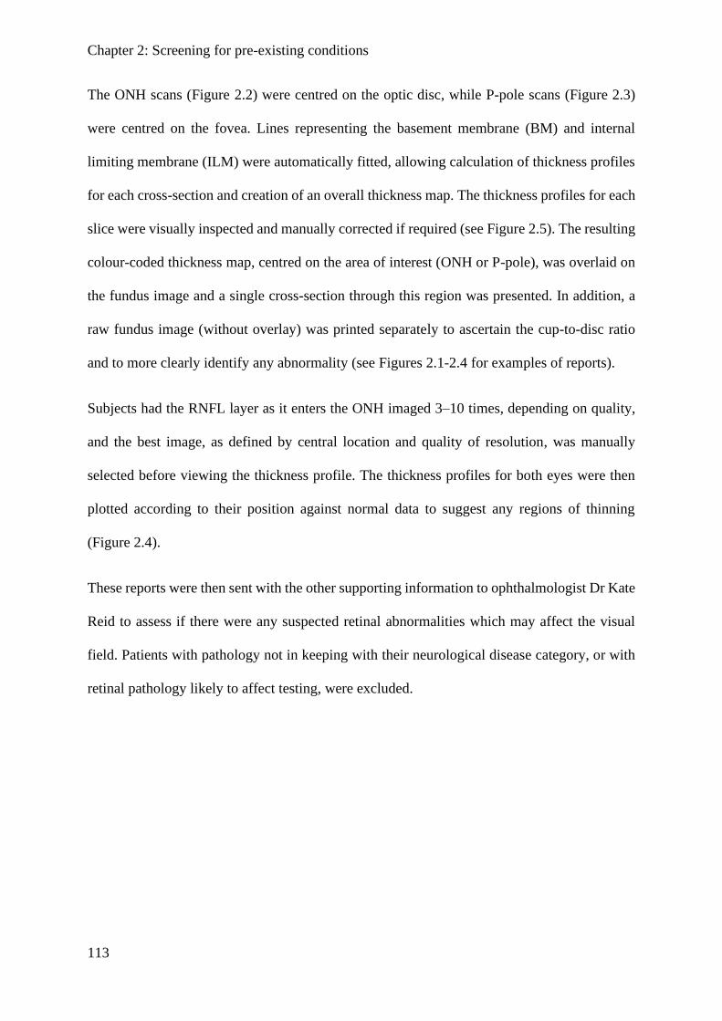
Chapter 2: Screening for pre-existing conditions
113
The ONH scans (Figure 2.2) were centred on the optic disc, while P-pole scans (Figure 2.3)
were centred on the fovea. Lines representing the basement membrane (BM) and internal
limiting membrane (ILM) were automatically fitted, allowing calculation of thickness profiles
for each cross-section and creation of an overall thickness map. The thickness profiles for each
slice were visually inspected and manually corrected if required (see Figure 2.5). The resulting
colour-coded thickness map, centred on the area of interest (ONH or P-pole), was overlaid on
the fundus image and a single cross-section through this region was presented. In addition, a
raw fundus image (without overlay) was printed separately to ascertain the cup-to-disc ratio
and to more clearly identify any abnormality (see Figures 2.1-2.4 for examples of reports).
Subjects had the RNFL layer as it enters the ONH imaged 3–10 times, depending on quality,
and the best image, as defined by central location and quality of resolution, was manually
selected before viewing the thickness profile. The thickness profiles for both eyes were then
plotted according to their position against normal data to suggest any regions of thinning
(Figure 2.4).
These reports were then sent with the other supporting information to ophthalmologist Dr Kate
Reid to assess if there were any suspected retinal abnormalities which may affect the visual
field. Patients with pathology not in keeping with their neurological disease category, or with
retinal pathology likely to affect testing, were excluded.
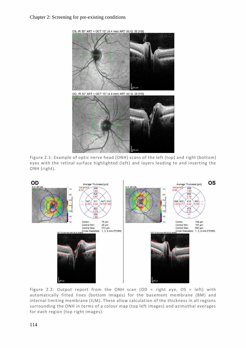
Chapter 2: Screening for pre-existing conditions
114
Figure 2.1: Example of optic nerve head (ONH) scans of the left (top) and right (bottom) eyes with the retinal surface highlighted (left) and layers leading to and inserting the ONH (right).
Figure 2.2: Output report from the ONH scan (OD = right eye, OS = left) with automatically fitted lines (bottom images) for the bas ement membrane (BM) and internal limiting membrane (ILM). These allow calculation of the thickness in all regions surrounding the ONH in terms of a colour map (top left images) and azimuthal averages for each region (top right images).
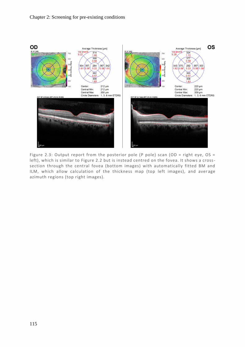
Chapter 2: Screening for pre-existing conditions
115
Figure 2.3: Output report from the posterior pole (P pole) scan (OD = right eye, OS = left), which is similar to Figure 2.2 but is instead centred on the fovea. It shows a cross -section through the central fovea (bottom images) with automatically fitted BM and ILM, which allow calculation of the thickness map (top left images), and aver age azimuth regions (top right images).
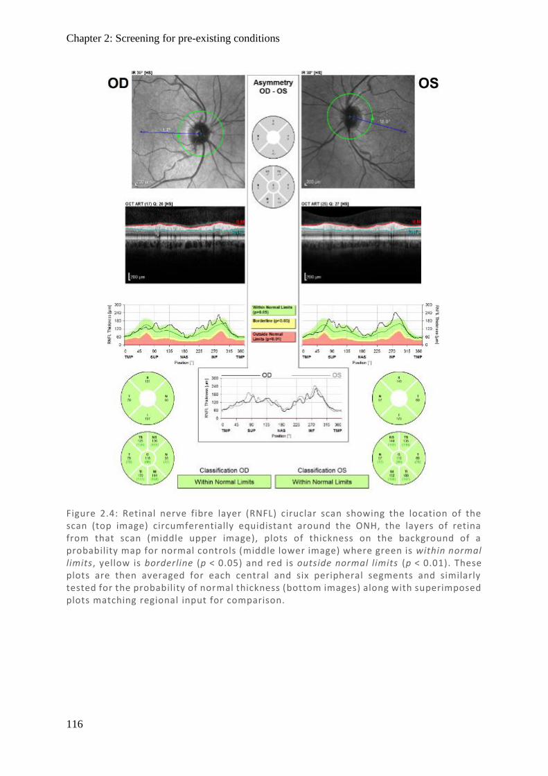
Chapter 2: Screening for pre-existing conditions
116
Figure 2.4: Retinal nerve fibre layer (RNFL) ciruclar scan showing the location of the scan (top image) circumferentially equidistant around the ONH, the layers of retina from that scan (middle upper image), plots of thickness on the background of a probability map for normal controls (middle lower image) where green is within normal limits, yellow is borderline (p < 0.05) and red is outside normal limits (p < 0.01). These plots are then averaged for each central and six peripheral segments and similarly tested for the probability of normal thickness (bottom images) along with superimposed plots matching regional input for comparison.
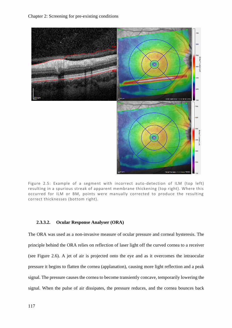
Chapter 2: Screening for pre-existing conditions
117
2.3.3.2. Ocular Response Analyser (ORA)
The ORA was used as a non-invasive measure of ocular pressure and corneal hysteresis. The
principle behind the ORA relies on reflection of laser light off the curved cornea to a receiver
(see Figure 2.6). A jet of air is projected onto the eye and as it overcomes the intraocular
pressure it begins to flatten the cornea (applanation), causing more light reflection and a peak
signal. The pressure causes the cornea to become transiently concave, temporarily lowering the
signal. When the pulse of air dissipates, the pressure reduces, and the cornea bounces back
Figure 2.5: Example of a segment with incorrect auto -detection of ILM (top left) resulting in a spurious streak of apparent membrane thickening (top right). Where this occurred for ILM or BM, points were manually corrected to produce the resulting correct thicknesses (bottom right).

Chapter 2: Screening for pre-existing conditions
118
causing a second peak. Based on these measures one can calculate the intraocular pressure and
effective elasticity of the cornea, inelasticity being measured by the rate of corneal hysteresis
(Radcliffe, 2014). Through extensive evidence that corneal thickness alters the pressure as
measured by tonometry (Whitacre et al., 1993; Wolfs et al., 1997; Stodtmeister, 1998; Shah et
al., 1999; Bhan et al., 2002), one can calculate a corneal corrected pressure (IOPcc) and a non-
corneal adjusted value that correlates with Goldmann tonometry (IOPg), as well as two
measures of elasticity, corneal hysteresis (CH) and corneal resistance factor (CRF). During
testing, subjects were asked to place their forehead on the forehead rest and look straight ahead.
Four red lights in the shape of a diamond with a green dot in the centre are present when the
subject is in the correct position. The process was explained to the subject and they were asked
to open wide and refrain from squinting as the eye piece moves forward to generate the burst
Figure 2.6: Diagram of hysteresis showing the pressure wave (in green) produced by a shot of air, with a smooth increase peaking at 10 -15 ms followed by a smooth decrease. In red is the signal from light reflected off the cornea. As ai r pressure exceeds intraocular pressure (IOP) the cornea flattens resulting in better reflection and a peak in the signal (applanation pressure 1), followed by a period of inversion and, as pressure drops, another peak in signal (applanation pressure 2). H ysteresis is defined as the difference between the pressure at which the airjet applanates the cornea inwards and that at which it applanates outwards, which quantifies the elasticity of the cornea. Produced with reference to (Radcliffe, 2014).
Chapter 2: Screening for pre-existing conditions
119
of air. A total of four measures were taken and the recording with the highest quality (as
determined by the ORA) was recorded.
2.3.4. Visual neglect
Visual neglect (hemineglect) describes a condition in which there is nothing structurally wrong
with the visual system, but patients unconsciously ignore vision on one side unless attention is
expressly drawn there. Visual neglect is relatively common immediately after a stroke, with
rates reported as 65–82% (depending on side) at 2–3 days post-stroke (Stone et al., 1993) and
is also associated with visual field deficits, although double dissociation10 may occur (Halligan
et al., 1990). The difficulty with visual neglect is that patients may not be able to respond to
stimuli within the visual field on the affected side. When devices are used that require a
perceptual response, such as Humphrey and Matrix field analysers, it is difficult to distinguish
it from a true visual field defect (Kooistra & Heilman, 1989). To address this issue, we have
both extended the acceptable post-stroke recovery time for inclusion in this study (during which
most hemineglect resolves) and have also screened directly using neglect-specific tests. Rates
of visual neglect at 3 weeks post stroke are reported to be 8–11%, and significant neglect is
rarely observed at 6 months (Sunderland et al., 1987); similarly, a large study of 1281 acute
stroke patients found that neglect was markedly reduced at 3 months (Ringman et al., 2004).
For our studies, subjects were not recruited until they were allowed a minimum of 3 months
recovery time, with many patients well exceeding that period. A number of tests have been
devised which allow visual neglect and visual field damage to be distinguished, two of the most
common being the line bisection and star cancellation tests (Ferber & Karnath, 2001; Li &
Malhotra, 2015).
10 When two related mental processes present independently of eachother.

Chapter 2: Screening for pre-existing conditions
120
2.3.4.1. Line bisection and star cancellation
The line bisection test has three horizontal 19 cm long lines printed on a landscape A4 sheet
with the top line placed to the right, the middle line centrally, and the lower line to the left (see
Appendix A: Line Bisection Test). Subjects were asked to look at each line in turn and make a
mark with a pen where they believed the centre of each line was. The premise behind this test
is that those with visual neglect ignore part of the line and so believe it to be shorter, bisecting
the line far from the true centre and away from the side with neglect. In comparison, those with
a visual field defect, despite not being able to see on one side, realise that the line doesn’t end
within their vision and they turn their head to make use of their peripheral vision to read the
true length of the line. Thus, while those with field defects may perform slightly worse than
controls due to peripheral blurring, this is separate from the large consistent bias frequently
demonstrated in visual neglect. The output measure for the test is how far the average distance
from the true centre is, where left is positive and right is negative. If a bias is made to the left
on one line and to the right in another, they will offset each other, resulting in a low mean bias
and will not be assessed as having visual neglect (which is characteristically unilateral).
The star cancellation test involves a mixture of a randomly ordered set of 56 small stars, 52
large stars, 13 letters, and 10 words which span an entire A4 sheet (see Appendix B: Star
Cancellation Test ). The task requires the subject to find and cross out all 56 small stars on the
sheet, with the first two stars in the centre being crossed off as part of the initial explanation.
The premise is that those with visual neglect will ignore the small stars on one side of the page,
while those with an equivalent visual field defect will realise that there is more to the page than
they can immediately see and turn their head to ensure they have checked the entire page. The
measured output for this test is the degree of laterality, expressed as a fraction of those missed
on the left compared with those missed on the right.

Chapter 2: Screening for pre-existing conditions
121
When comparing the effectiveness of the line bisection and star cancellation tests, it is first
useful to identify a threshold for abnormality. Threshold scores for presence of neglect have
been reported as >3 stars on a single side for the star cancellation test, and >14 mm to left or
right in the line bisection test (Bailey et al., 2004). Line bisection has a relatively low sensitivity
of 53–60% (Halligan et al., 1989; Ferber & Karnath, 2001), which might reflect the fact that a
bias also exists in the general population (so-called pseudoneglect) (McCourt & Olafson, 1997;
McCourt & Jewell, 1999). Factor analysis of commonly used visual neglect strategies still
reveal a relatively high loading factor of 0.85 for a 6-test battery despite a low overall
sensitivity of 53%, with star-cancellation having the highest load factor of 0.90 and sensitivity
100% (Halligan et al., 1989). One might conclude that star cancellation is the better option;
however, the line bisection and star cancellation tests assess different cognitive skills and may
dissociate from each other (Ferber & Karnath, 2001; Rorden & Karnath, 2010), meaning the
combination may give better coverage as a screening tool.
2.4. Higher Visual Function Tests
Higher visual functions (HVFs) are visual perceptions which are processed outside of the
primary visual cortex. As there are many case studies describing prosopagnosia, akinetopsia,
astereopsis, and achromatopsia, but little literature on how commonly more subtle defects
present, all these four HVF were explored. Since perception is subjective, there are a range of
tests which may assess each HVF. These are described below in more detail, elaborating on
why one was chosen over the other options.
2.4.1. Stereopsis
Depth perception can be attributed to several forms of visual processing including both
monocular and binocular cues. Monocular cues include motion parallax, optic expansion, and
familiar/relative size, some of which incorporate prior known characteristics about the object.
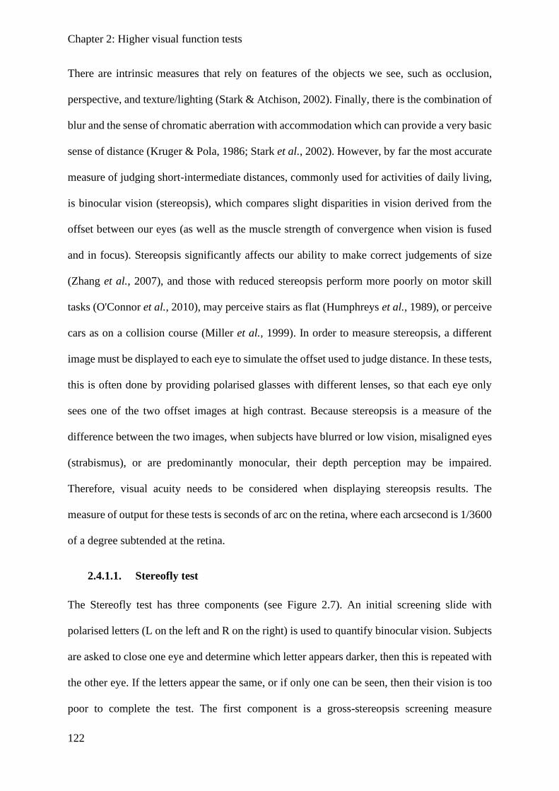
Chapter 2: Higher visual function tests
122
There are intrinsic measures that rely on features of the objects we see, such as occlusion,
perspective, and texture/lighting (Stark & Atchison, 2002). Finally, there is the combination of
blur and the sense of chromatic aberration with accommodation which can provide a very basic
sense of distance (Kruger & Pola, 1986; Stark et al., 2002). However, by far the most accurate
measure of judging short-intermediate distances, commonly used for activities of daily living,
is binocular vision (stereopsis), which compares slight disparities in vision derived from the
offset between our eyes (as well as the muscle strength of convergence when vision is fused
and in focus). Stereopsis significantly affects our ability to make correct judgements of size
(Zhang et al., 2007), and those with reduced stereopsis perform more poorly on motor skill
tasks (O'Connor et al., 2010), may perceive stairs as flat (Humphreys et al., 1989), or perceive
cars as on a collision course (Miller et al., 1999). In order to measure stereopsis, a different
image must be displayed to each eye to simulate the offset used to judge distance. In these tests,
this is often done by providing polarised glasses with different lenses, so that each eye only
sees one of the two offset images at high contrast. Because stereopsis is a measure of the
difference between the two images, when subjects have blurred or low vision, misaligned eyes
(strabismus), or are predominantly monocular, their depth perception may be impaired.
Therefore, visual acuity needs to be considered when displaying stereopsis results. The
measure of output for these tests is seconds of arc on the retina, where each arcsecond is 1/3600
of a degree subtended at the retina.
2.4.1.1. Stereofly test
The Stereofly test has three components (see Figure 2.7). An initial screening slide with
polarised letters (L on the left and R on the right) is used to quantify binocular vision. Subjects
are asked to close one eye and determine which letter appears darker, then this is repeated with
the other eye. If the letters appear the same, or if only one can be seen, then their vision is too
poor to complete the test. The first component is a gross-stereopsis screening measure

Chapter 2: Higher visual function tests
123
presenting a large image of a fly, with each aspect of the fly having an offset of 4800–3000
arcsec. If they do perceive the three-dimensional effect in these more gross examples, then they
can proceed to more refined tests on the following test pages. These pages include three lines,
each with a series of four basics shapes progressing from 400 down to 100 arcsec. This section
of the test is often used to assess children, although it also provides an excellent secondary
measure to cover intermediate range stereopsis. In the final section there are ten diamonds,
each comprised of four dots (top, bottom, left, right) with only a single circle being the
stereopsis stimulus. Participants are asked to identify which circle appears three-dimensional
in each example, which progressively become more subtle from 400 to 20 arcsec (fine
stereopsis). When a subject can no longer detect any difference or after getting two incorrect,
the last correct answer is taken as their threshold. If a subject gets one wrong and then gets at
least two correct answers, this is considered an innocent mistake and they are allowed to
continue.
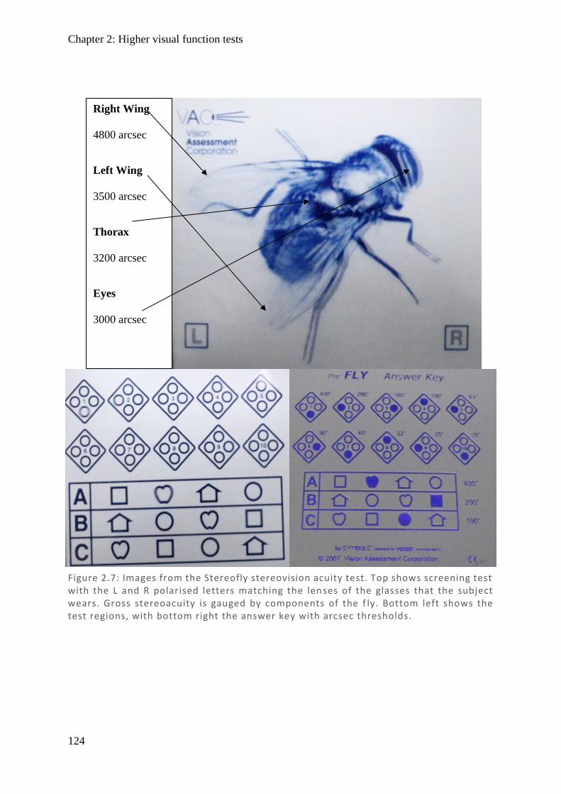
Chapter 2: Higher visual function tests
124
Right Wing
4800 arcsec
Left Wing
3500 arcsec
Thorax
3200 arcsec
Eyes
3000 arcsec
Figure 2.7: Images from the Stereofly stereovision acuity test. Top shows screening test with the L and R polarised letters matching the len ses of the glasses that the subject wears. Gross stereoacuity is gauged by components of the f ly. Bottom left shows the test regions, with bottom right the answer key with arcsec thresholds.

Chapter 2: Higher visual function tests
125
2.4.1.2. Randot test
Random dot stereograms were invented by Béla Julesz and stemmed from work on depth
perception. The stereogram does not have familiar cues or visible offsets when viewed
monocularly (Julesz, 1964, 1965) and were developed from computer-generated patterns
(Julesz, 1960) that form the basis of the modern Random Dot 3 (Randot) booklet. The Randot
test is similar in principle to the Stereofly test, and also contains three sections, with images
for each eye being offset to generate a 3D effect (see Figure 2.8). The difference is that the
background is comprised of random dot noise, which encode the offset when polarised glasses
are worn. This was designed to address a potential flaw in the Stereofly test, which is that the
visual offset of the images can be seen by those with good acuity without wearing the glasses,
and hence without using stereoscopic vision at all.
The random dots mask this offset, so one cannot clearly make out images within the
background without wearing the polarised glasses, although the trade-off is that these shapes
may be harder to visualise. On the first screening page are four basic shapes ranging from 900
to 300 arcsec and subjects must identify which shape is present within each, the first of which
has more obvious contrast and can be seen without glasses. In the second section there are three
rows, each with four basic shapes within them ranging from 300 to 100 arcsec. To answer a
line correctly, subjects must get at least three of the four shapes correct. In the final section,
there are ten diamond shapes each with four circles (top, bottom, left, and right), three of which
appear to go into the page and one which comes out of the page. Many subjects had difficulty
seeing the circles at all, and so were asked to mention if they noticed anything that appeared
different in any of the four directions. This tested stereoacuity in the range 160–12.5 arcsec,
covering finer resolution than Stereofly. The same rules as for the Stereofly were applied: after
getting two incorrect, the last correct answer was taken as threshold. If two correct answers are
made after an incorrect one, it is ignored, and they are allowed to continue.

Chapter 2: Higher visual function tests
126
Figure 2.8: Images of the Random Dot 3 (Randot) stereovision acuity test. Top left shows gross stereoacuity by shape identification. Top right shows intermediate (shape) and fine stereoacuity (direction) tests. Bottom shows the test regions and answer key with arcsec thresholds.
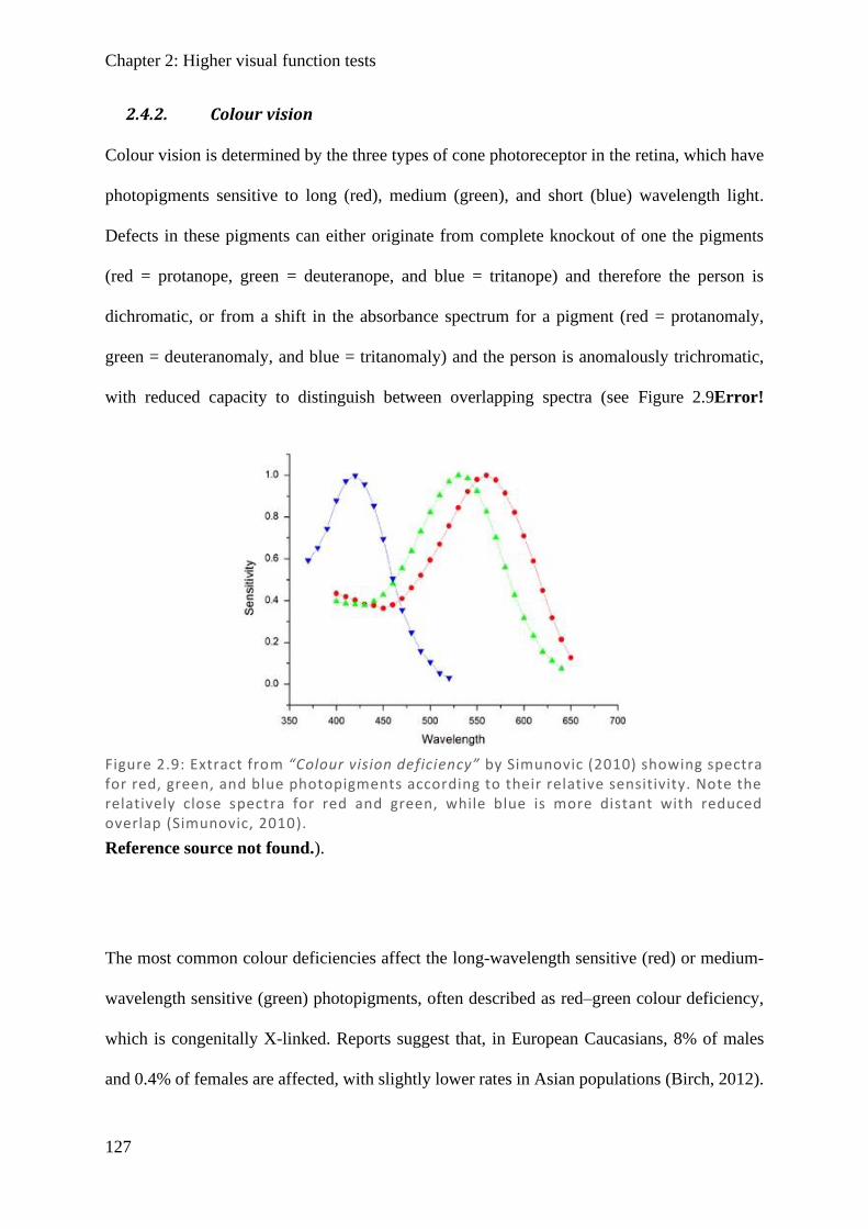
Chapter 2: Higher visual function tests
127
2.4.2. Colour vision
Colour vision is determined by the three types of cone photoreceptor in the retina, which have
photopigments sensitive to long (red), medium (green), and short (blue) wavelength light.
Defects in these pigments can either originate from complete knockout of one the pigments
(red = protanope, green = deuteranope, and blue = tritanope) and therefore the person is
dichromatic, or from a shift in the absorbance spectrum for a pigment (red = protanomaly,
green = deuteranomaly, and blue = tritanomaly) and the person is anomalously trichromatic,
with reduced capacity to distinguish between overlapping spectra (see Figure 2.9Error!
Reference source not found.).
The most common colour deficiencies affect the long-wavelength sensitive (red) or medium-
wavelength sensitive (green) photopigments, often described as red–green colour deficiency,
which is congenitally X-linked. Reports suggest that, in European Caucasians, 8% of males
and 0.4% of females are affected, with slightly lower rates in Asian populations (Birch, 2012).
Figure 2.9: Extract from “Colour vision deficiency” by Simunovic (2010) showing spectra for red, green, and blue photopigments according to their relative sensitivity. Note the relatively close spectra for red and green, while blue is more distant with reduced overlap (Simunovic, 2010).

Chapter 2: Higher visual function tests
128
In an older Australia optometric population of 7000 sequential patients screened with Ishihara
plates, 6.32% of males and 0.28% of females showed congenital red–green defects (Steward
& Cole, 1989). These rates are further broken down into their component disorders in Table
2.3.
Given how common red–green deficiencies are, it was important to include a measure that
specifically tested for these disorders, the Ishihara (Ishihara, 1918) being one of the more
commonly used tools. More generally, for detecting any kind of colour deficiency the
Farnsworth–Munsell test (Farnsworth, 1943) is a very popular tool. The classic version of the
Farnsworth–Munsell is the 100-hue, having 100 wells containing coloured tiles which must be
ordered according to colour gradient. While the 100-hue is very accurate, with wells
approaching the minimum that a normal observer can distinguish, its limitation is that it is time
consuming and fatiguing, making it impractical for routine clinical use (Neitz et al., 2008),
especially in those who are elderly or have difficulty concentrating such as stroke patients. The
smaller Farnsworth–Munsell D15 is a much quicker and convenient test designed for routine
clinical use, as the subject need only order 15 wells, the trade-off being it is relatively
insensitive to mild colour deficiencies (Neitz et al., 2008). As we are focused on acquired
cerebral colour deficiencies as a result of cortical damage from stroke, damage would typically
be substantial if not complete (Zeki, 1990; Zhou et al., 2018), although selective losses have
also been reported (Wooten, 1981). The D15 set was chosen, as it can pick up moderate–severe
colour deficiencies and is conducive to clinical application.
It should be noted that there are also reports of hemiachromatopsia (Kolmel, 1988; Paulson et
al., 1994; Short & Graff-Radford, 2001; Bouvier & Engel, 2006), where only half of the visual
field is affected, and as Ishihara and Farnsworth-Munsell tests use both hemifields, they may

Chapter 2: Higher visual function tests
129
be insensitive to this group. That being said, Ishihara and Farnsworth-Munsell are two of the
most commonly used tests to assess achromatopsia (Bouvier & Engel, 2006), while also
providing rapid and easy testing that might be applied to a clinical environment.
2.4.2.1. Ishihara
The Ishihara test is comprised of 17 plates (images), each with a number formed by dots of a
similar hue (such as red/pink/orange) on a background of distractor colours which have
dissimilar hues. While those with normal trichromatic vision clearly see the outline of the
numbers, those with colour defects (especially red–green) can find it difficult to demarcate
between target and background. In addition, some frames encode a second number with less-
overtly related colours, which may add to the uncertainty of those without normal colour vision.
This makes the test very sensitive to shifts in red (protanope) and green (deuteranope), with
only minimal testing of the less common blue (tritanope) deficiencies. The first frame is a
control and should be detected even by those with no colour vision, and two frames throughout
the test show numbers that are not identified by those with normal vision but may be detected
by those with red–green defects. When marking this test, subject answers are compared against
the correct number for a normal-vision respondent, and any answer other than the correct one
(or the absence of a number) is taken as incorrect. While testing in this thesis focuses on
continuous measures for making a categorisation between normal and abnormal, a threshold
for Ishihara of >3 errors is typically treated as abnormal, with a 98.4% sensitivity reported
(Birch, 2010).
2.4.2.2. Farnsworth–Munsell D15
The D15 is comprised of a base reference well and 15 wells that are spaced across the colour
spectrum. When completing the test, the reference well is place in the container, and all the
other colour wells are randomly arranged outside the container (see Figure 2.10). The subject

Chapter 2: Higher visual function tests
130
must choose the colour they believe is closest to the reference well and place it next to it, then
sequentially repeat this process until all the wells have been placed. Subjects are free to remove
or rearrange the well order within they container as they see fit. Subjects were notified that they
would be timed for the test, but they should prioritise making sure the well order is correct over
completing quickly. Once the subject completed the test, they were asked to have a final look
at the order they had chosen to ensure they were happy with it. Once confirmed, the wells were
turned upside down to reveal the numbers on their bases and the well order was noted. To
assess the extent of colour vision deficiency associated with this test, the methods described by
(Bowman, 1982) were used. In this method, each well is assigned a colour value according to
the CIELAB colour space using the measures L* as lightness (black to white), a* as green to
red, and b* as blue to yellow, matching the colour encoding pathways of the visual system.
The difference between wells was then calculated using the formula
𝛥𝐸𝑎𝑏∗ = √(𝛥𝐿∗)2 + (𝛥𝑎∗)2 + (𝛥𝑏∗)2 .
Values for each difference between wells were recorded from this paper and the sum of the
differences between wells was calculated (see Table 2.4). The correct order minimises the total
colour difference score between wells (minimum is 117). From this a colour confusion index
(CCI) was created by the ratio of the total colour difference score over the minimum score,
making a perfect well order (normal) 1.00. The larger the number, the larger the abnormality
up to a maximum of 5.33 if the wells are maximally different.
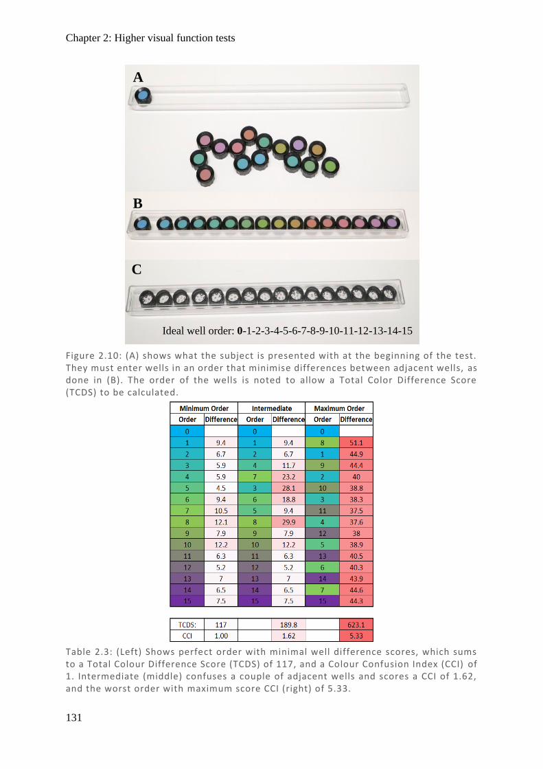
Chapter 2: Higher visual function tests
131
Figure 2.10: (A) shows what the subject is presented with at the beginning of the test. They must enter wells in an order that minimise differences between adjacent wells, as done in (B). The order of the wells is noted to allow a Total Color Difference Score (TCDS) to be calculated.
A
B
C
Ideal well order: 0-1-2-3-4-5-6-7-8-9-10-11-12-13-14-15
Table 2.3: (Left) Shows perfect order with minimal well difference scores, which sums to a Total Colour Difference Score (TCDS) of 117, and a Colour Confusion Index (CCI) of 1. Intermediate (middle) confuses a couple of adjacent wells and scores a CCI of 1.62, and the worst order with maximum score CCI (right) of 5.33.
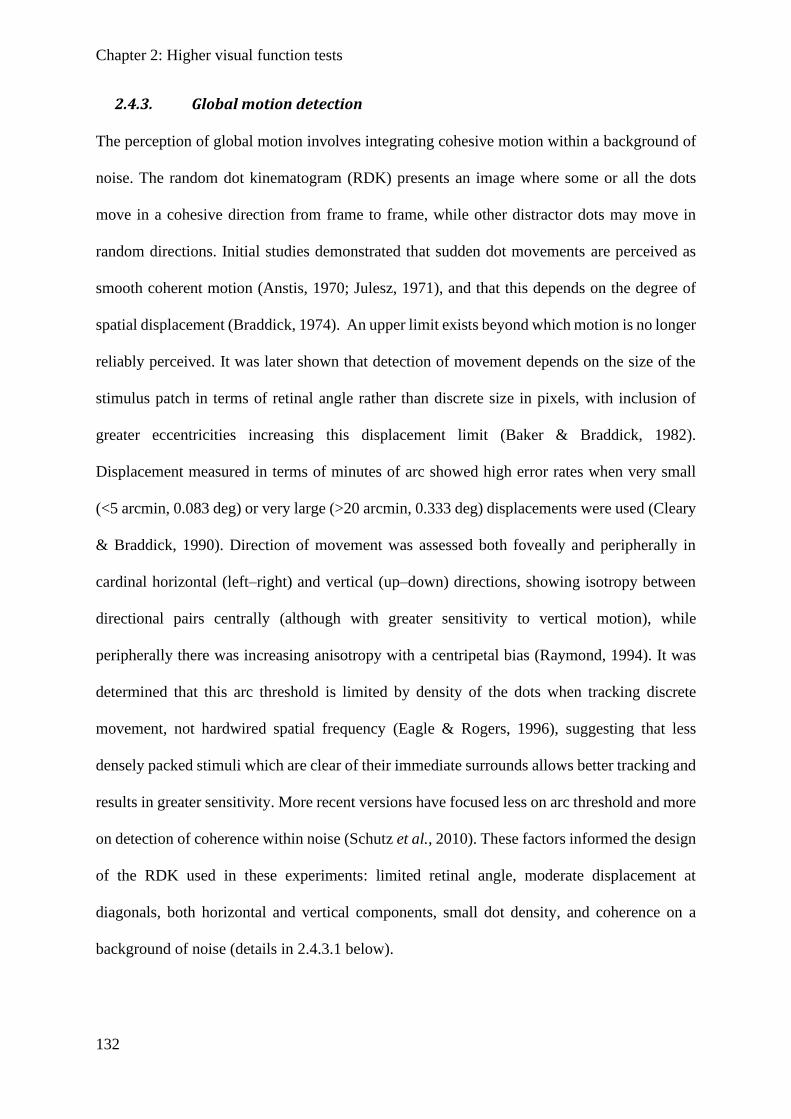
Chapter 2: Higher visual function tests
132
2.4.3. Global motion detection
The perception of global motion involves integrating cohesive motion within a background of
noise. The random dot kinematogram (RDK) presents an image where some or all the dots
move in a cohesive direction from frame to frame, while other distractor dots may move in
random directions. Initial studies demonstrated that sudden dot movements are perceived as
smooth coherent motion (Anstis, 1970; Julesz, 1971), and that this depends on the degree of
spatial displacement (Braddick, 1974). An upper limit exists beyond which motion is no longer
reliably perceived. It was later shown that detection of movement depends on the size of the
stimulus patch in terms of retinal angle rather than discrete size in pixels, with inclusion of
greater eccentricities increasing this displacement limit (Baker & Braddick, 1982).
Displacement measured in terms of minutes of arc showed high error rates when very small
(<5 arcmin, 0.083 deg) or very large (>20 arcmin, 0.333 deg) displacements were used (Cleary
& Braddick, 1990). Direction of movement was assessed both foveally and peripherally in
cardinal horizontal (left–right) and vertical (up–down) directions, showing isotropy between
directional pairs centrally (although with greater sensitivity to vertical motion), while
peripherally there was increasing anisotropy with a centripetal bias (Raymond, 1994). It was
determined that this arc threshold is limited by density of the dots when tracking discrete
movement, not hardwired spatial frequency (Eagle & Rogers, 1996), suggesting that less
densely packed stimuli which are clear of their immediate surrounds allows better tracking and
results in greater sensitivity. More recent versions have focused less on arc threshold and more
on detection of coherence within noise (Schutz et al., 2010). These factors informed the design
of the RDK used in these experiments: limited retinal angle, moderate displacement at
diagonals, both horizontal and vertical components, small dot density, and coherence on a
background of noise (details in 2.4.3.1 below).
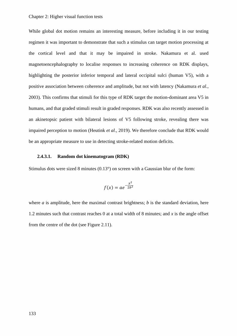
Chapter 2: Higher visual function tests
133
While global dot motion remains an interesting measure, before including it in our testing
regimen it was important to demonstrate that such a stimulus can target motion processing at
the cortical level and that it may be impaired in stroke. Nakamura et al. used
magnetoencephalography to localise responses to increasing coherence on RDK displays,
highlighting the posterior inferior temporal and lateral occipital sulci (human V5), with a
positive association between coherence and amplitude, but not with latency (Nakamura et al.,
2003). This confirms that stimuli for this type of RDK target the motion-dominant area V5 in
humans, and that graded stimuli result in graded responses. RDK was also recently assessed in
an akinetopsic patient with bilateral lesions of V5 following stroke, revealing there was
impaired perception to motion (Heutink et al., 2019). We therefore conclude that RDK would
be an appropriate measure to use in detecting stroke-related motion deficits.
2.4.3.1. Random dot kinematogram (RDK)
Stimulus dots were sized 8 minutes (0.13°) on screen with a Gaussian blur of the form:
𝑓(𝑥) = 𝑎ⅇ−
𝑥2
2𝑏2
where a is amplitude, here the maximal contrast brightness; b is the standard deviation, here
1.2 minutes such that contrast reaches 0 at a total width of 8 minutes; and x is the angle offset
from the centre of the dot (see Figure 2.11).
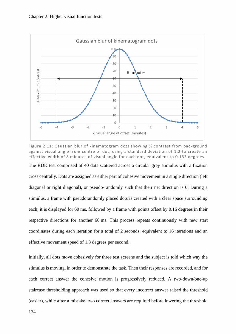
Chapter 2: Higher visual function tests
134
The RDK test comprised of 40 dots scattered across a circular grey stimulus with a fixation
cross centrally. Dots are assigned as either part of cohesive movement in a single direction (left
diagonal or right diagonal), or pseudo-randomly such that their net direction is 0. During a
stimulus, a frame with pseudorandomly placed dots is created with a clear space surrounding
each; it is displayed for 60 ms, followed by a frame with points offset by 0.16 degrees in their
respective directions for another 60 ms. This process repeats continuously with new start
coordinates during each iteration for a total of 2 seconds, equivalent to 16 iterations and an
effective movement speed of 1.3 degrees per second.
Initially, all dots move cohesively for three test screens and the subject is told which way the
stimulus is moving, in order to demonstrate the task. Then their responses are recorded, and for
each correct answer the cohesive motion is progressively reduced. A two-down/one-up
staircase thresholding approach was used so that every incorrect answer raised the threshold
(easier), while after a mistake, two correct answers are required before lowering the threshold
Figure 2.11: Gaussian blur of kinematogram dots showing % contrast from background against visual angle from centre of dot, using a standard deviation of 1.2 to create an effective width of 8 minutes of visual angle for each dot, equivalent to 0.133 degrees.
0
10
20
30
40
50
60
70
80
90
100
-5 -4 -3 -2 -1 0 1 2 3 4 5
% M
axim
um
Co
ntr
ast
x, visual angle of offset (minutes)
Gaussian blur of kinematogram dots
8 minutes

Chapter 2: Higher visual function tests
135
(harder). This means random answers lead to steps up towards complete cohesive motion,
making it statistically improbable to progress very far without having the capacity to recognise
the stimulus direction. A reversal is said to occur each time there is a change from a series of
steps down to a step up, or steps up to a step down (see Figure 2.12). In total, the test comprises
the lesser of 10 reversals or 45 responses, after which the last 4 reversals are taken and averaged
as the subject’s threshold.
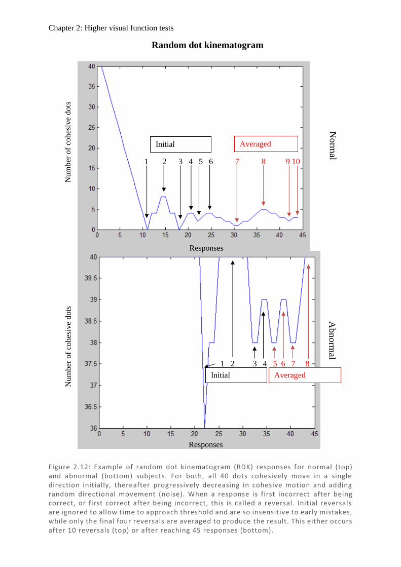
Chapter 2: Higher visual function tests
136
Responses
Responses
Num
ber
of
coh
esiv
e dots
N
um
ber
of
coh
esiv
e dots
Initial
1 2 3 4 5 6 7 8 9 10
Averaged
Norm
al A
bno
rmal
1 2 3 4 5 6 7 8
Initial Averaged
Random dot kinematogram
Figure 2.12: Example of random dot kinematogram (RDK) responses f or normal (top) and abnormal (bottom) subjects. For both, all 40 dots cohesively move in a single direction initially, thereafter progressively decreasing in cohesive motion and adding random directional movement (noise). When a response is first incorrect after being correct, or first correct after being incorrect, this is called a reversal. Initial reversals are ignored to allow time to approach threshold and are so insensitive to early mistakes, while only the final four reversals are averaged to produce the result. This either occurs after 10 reversals (top) or after reaching 45 responses (bottom).
Chapter 2: Higher visual function tests
137
2.4.4. Facial recognition
Facial recognition is an important part of everyday living that is often overlooked. It allows us
to recognise friends and family from strangers and to interact with people. Practically, it is not
only the ability to recognise a face that matters, but the ability to remember and recall that face,
which has guided the production of standardised tests. Two of the standardised tests, the Benton
Facial Recognition Test (BFRT) (Benton & Van Allen, 1968) and the Recognition Memory
Test for Faces (RMF) (Warrington, 1984) have shown serious shortcomings, largely to do with
facial matching being possible without facial identification. BFRT presents target and test faces
simultaneously with unlimited duration, allowing a feature-matching strategy, while RMF
images include substantial non-face information such as hair and clothes. In both tests, a
substantial proportion of normal subjects are able to score in the normal range even when the
face is occluded (Duchaine & Weidenfeld, 2003). It also appears insensitive to prosopagnosia
detection, with many such patients scoring normally on BFRT (Nunn et al., 2001; Duchaine &
Nakayama, 2004). In response, a test with only facial information and with images presented
separately was developed, the Cambridge Facial Memory Test (CFMT). The CFMT appears
to have higher detection rates when the standard psychophysical threshold (2-standard
deviations below the mean, or the lowest 5 percentile) is used (Duchaine & Nakayama, 2006).
We have therefore chosen CFMT as one of the more widely used modern variants (McKone et
al., 2011; Croydon et al., 2014; Cho et al., 2015; Albonico et al., 2017; Gray et al., 2017;
McKone et al., 2017).
2.4.4.1. Cambridge Facial Memory Test (CFMT)
The CFMT was designed to assess the ability to recognise and remember a person’s face. Those
with impaired facial recognition are unable to detect those unique features of a person’s face
which make them recognisable and so they perform poorly on the test. However there is also a
memory component, which means that elderly people tend to get lower scores and there is a
Chapter 2: Higher visual function tests
138
substantial trend of declining score with age (Bowles et al., 2009). To address this issue, the
same group assessed a range of age groups, developed a formula that adjusts for age, and
calculated a figure according to which those below the 5th percentile had prosopagnosia, i.e.
impaired facial recognition (Bowles et al., 2009). With a commonly accepted threshold of the
5th percentile, 5% percent of the general population will fall into this range. Within this group
are those who have congenital deficiencies, suggested to be as high as ~2.5% (Kennerknecht
et al., 2006), which appear to run in families (Kennerknecht et al., 2007). It remains unknown
how many of these people have cerebral deficiencies.
It has been demonstrated that CFMT reveals small differences depending on ethnicity, age, and
sex (Bowles et al., 2009), which is perhaps not surprising given that the test exclusively uses
faces of young males from the Boston region. While there is some suggestion that gender bias
is minimal (Scherf et al., 2017), the ethnicity difference is notable, with newer versions
including Australian-specific (McKone et al., 2011) and East Asian-specific (McKone et al.,
2017) versions. It was a limitation of our design that the Australian-specific version was not
available at the time of testing, although we highly recommend that location-specific versions
be used in future.
In terms of practical implementation of the test, procedures were explained to the subjects
beforehand. Each section of the test comprises a presentation section where subjects are asked
to learn the face(s), and a testing section where they must recall the face(s) from a three-option
forced choice (details in Figures 2.13 –2.14 ). The practice section using cartoons was not
scored and was only used to demonstrate how to complete the tasks. Section one presents a
single face from three angles in sequence, and then has three sets of three-way forced choice
selections, with each answer being an exact matching photo to one angle of the presented face.
This process is then repeated with new faces, until in total six faces are presented with 18
responses. Section two consists of simultaneous presentation of the same six faces used in

Chapter 2: Higher visual function tests
139
section one, followed by 30 sets of thee-way forced choice selections, with each answer being
a similar but novel image of any of the six presented faces (totalling five from each face).
Section three consists of the same simultaneous presentation of six faces used in section two,
followed by 24 sets of three-way force choice selections, with each answer being a similar but
novel image with added noise from any of the six presented faces (totalling four from each
face). The test comprises a total of 72 responses (section one, 18; section two, 30; section three,
24), with six target faces and 50 distractor faces.

Chapter 2: Higher visual function tests
140
Figure 2.13: CFMT practice and section one test sequences. Left (A –G): the practice sequence outlining how to complete tasks, while the the same instructions (A) are then shown for the actual test sequence (H–M) for section one (of three). Subjects are shown a single face from three angles sequentially, then given sets of three faces containing an idental image from that set and two distractors, they are asked to identify which face was the one initially shown. Section 1 repeats this process with a total of six faces, comprising 18 results.
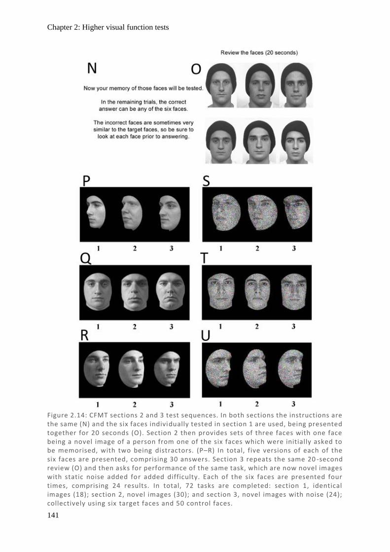
Chapter 2: Higher visual function tests
141
Figure 2.14: CFMT sections 2 and 3 test sequences. In both sections the instructions are the same (N) and the six faces individually tested in section 1 are used, being presented together for 20 seconds (O). Section 2 then provides sets of three faces with one face being a novel image of a person from one of the six faces which were initially asked to be memorised, with two being distractors. (P–R) In total, five versions of each of the six faces are presented, comprising 30 answers. Section 3 repeats the same 20 -second review (O) and then asks for performance of the same task, which are now novel images with static noise added for added difficulty. Each of the six faces are presented four times, comprising 24 results. In total, 72 tasks are completed: section 1, identical images (18); section 2, novel images (30); and section 3, novel images with noise (24); collectively using six target faces and 50 control faces.
Chapter 2: Perimetry
142
2.5. Perimetry
The multifocal pupillographic objective perimetry (mfPOP) device objectiveFIELD analyser
(Konan Medical USA Inc, Irvine CA) presents a novel approach to using rapid light stimuli to
measure pupil diameter responses. It shows promise in retinal disorders but there has only been
limited testing with neurological disorders. For a full discussion of the history or perimeters
and their comparison, see the introduction section ‘Automated Perimetry’. Here only the
selected devices will be discussed and will cover stimuli, test procedures, and output measures.
2.5.1. Humphrey Field Analyser (HFA)
Humphrey Field Analyser II (HFA) (Carl Zeiss Meditech AG, Jena, Germany) is the most
commonly used device for field testing in neurological disease (Hepworth & Rowe, 2018),
using small light stimuli (Goldmann Size 3). For this study testing was done with the
achromatic 24-2 SITA threshold values (see next section).
2.5.1.1. Stimuli
With the invention of the HFA II device, the common approach was to use the 30-2 pattern of
grid points. This same grid format could be used for the wide field of 30-2, covering 3–33
degrees eccentricity, or the smaller but faster 24-2, covering 3–27 degrees. In comparing these
approaches in neurological diseases, 24-2 has greater reliability than 30-2 (Wild et al., 1991;
Khoury et al., 1999) and is quicker and so was selected for this study. There are 54 regions in
the 24-2 test grid 6 degrees apart with 3 degree offset from the meridians, extending to 21
degrees in each of the superior, inferior, temporal regions and two points at 27 degrees nasally
(Figure 2.15).
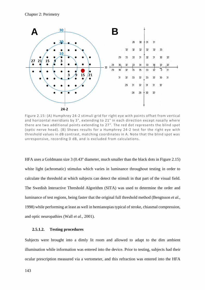
Chapter 2: Perimetry
143
HFA uses a Goldmann size 3 (0.43o diameter, much smaller than the black dots in Figure 2.15)
white light (achromatic) stimulus which varies in luminance throughout testing in order to
calculate the threshold at which subjects can detect the stimuli in that part of the visual field.
The Swedish Interactive Threshold Algorithm (SITA) was used to determine the order and
luminance of test regions, being faster that the original full threshold method (Bengtsson et al.,
1998) while performing at least as well in hemianopias typical of stroke, chiasmal compression,
and optic neuropathies (Wall et al., 2001).
2.5.1.2. Testing procedures
Subjects were brought into a dimly lit room and allowed to adapt to the dim ambient
illumination while information was entered into the device. Prior to testing, subjects had their
ocular prescription measured via a vertometer, and this refraction was entered into the HFA
Figure 2.15: (A) Humphrey 24-2 stimuli grid for right eye with points offset from vertical and horizontal meridians by 3°, extending to 21° in each direction except nasally where there are two additional points extending to 27 °. The red dot represents the blind spot (optic nerve head). (B) Shows results for a Humphrey 24-2 test for the right eye with threshold values in dB contrast, matching coordinates in A. Note that the blind spot was unresponsive, recording 0 dB, and is excluded from calculations.
A B

Chapter 2: Perimetry
144
device, which then suggests a set of trial lenses. Subjects were instructed to place their chin on
the chinrest and lean forwards to touch the headrest, then focus on the central fixation dot
throughout testing. It was explained that they should press the button whenever they can see a
dot appear on the screen, and that they could blink freely. At the beginning of testing, gaze
tracking was turned on for all subjects (where tracking was possible), and the pupil was centred
on a reference marker. The right eye was always tested first. During testing, small alterations
in position were corrected periodically by small alterations in the chinrest to keep the reference
marker centred on the pupil. If there were large deviations from the reference marker, slumping
away from the headrest, repeated saccades off centre, significant drooping of the eyes, or severe
fatigue, the test was paused, corrected, and recommenced if possible. Alternatively, if it was
thought that the problem had caused a significant effect, testing was stopped and repeated. Any
test with poor validity markers (according to device parameters of fixation loss >20% or false
positive values of >33%) meant that the test for that eye was repeated following instruction to
the subject.
2.5.1.3. Output measures
Threshold values were calculated from contrast according to the Weber formula ((Lmax – Lback)
/ (Lback)), where the background luminance is 10 cd/m2 and the maximum luminance is as large
as 3178 cd/m2 which are then converted into dB as 10*log10(Lmax – Lthreshold) (Fredette et al.,
2015). Thus, the poorest response is where a person does not detect the stimulus at Lmax
resulting in a 0 dB score, and the best response is where a person detects minimal background
change, resulting in a 35 dB score. While other measures, including total deviation, pattern
deviation, and probability maps, were collected, they were not used in this analysis and are not
discussed here.
Chapter 2: Perimetry
145
2.5.2. Matrix Field Analyser (MFA)
The Humphrey-Matrix (Carl Zeiss Meditec, Dublin CA) or Matrix field analyser (MFA) is
another perimetry device which is less commonly used (Hepworth & Rowe, 2018), but has
larger test regions and uses contrast-reversing grating stimuli. It was selected due to the larger
test regions being a closer approximation to mfPOP stimuli, and so may provide a more suitable
comparison.
2.5.2.1. Stimuli
The Matrix visual field test is based upon frequency doubling technology (FDT) perimetry.
This relies on the spatial frequency doubling effect – when a low spatial frequency sinusoidal
grating (<2 cycles/degree) is counter-phase flickered at a high temporal frequency (>15 Hz),
the grating appears to have a spatial frequency twice that of its actual frequency (Taravati et
al., 2008). The effect is also seen well for transient onset stimuli (Maddess & Kulikowski,
1999). FDT reportedly preferentially stimulate the magnocellular pathway, targeting a cell type
with less redundancy, and so greater sensitivity to early loss (originally designed for glaucoma
fields) – for further discussion see Introduction section 1.6.3.2 Matrix.
In order to allow direct comparison, a similar 24-2 field map was used as for HFA, with stimuli
still spaced 6 degrees apart, but with much larger stimuli 5° in diameter such that the majority
of the gap is filled by stimuli but without any overlap. In addition, there is a single central test
region where meridians meet, which was discarded for the purposes of comparisons as there is
no analogous region in either of the two other devices. Stimuli are presented as a contrast
sinusoidal grating eliciting the frequency doubling illusion (Anderson & Johnson, 2002).
Similar to HFA, stimulus contrast is varied to calculate the threshold at which a subject can
detect it and a thresholding algorithm is used. In this case the Zippy Estimation by Sequential
Testing (ZEST) thresholding strategy is used, which showed promised in early testing
Chapter 2: Perimetry
146
(Anderson & Johnson, 2006), although it has been shown to converge on only 15 unevenly
spaced values (Fredette et al., 2015). Despite this, MFA has been compared to HFA in
hemianopias and has shown similar performance (Taravati et al., 2008).
2.5.2.2. Testing procedures
MFA subjects with ocular prescriptions < ±3 dioptres could be assessed without glasses, while
anyone else was asked to wear their glasses for testing. This is consistent with manufacturer
recommendations and is supported by the apparent tolerance to blur of the frequency doubling
technology (Campbell & Green, 1965; Legge et al., 1987). Prior to testing subjects were
instructed to place their chin on the chinrest and lean forwards to touch the headrest, focus on
a central cross during testing, and press the button when they saw a modulating grating on the
screen; they could blink whenever necessary. A short demonstration was completed for
<30 seconds at the beginning to confirm understanding of expectations. The right eye was
always tested first. During testing, small subject movements off-centre were tolerated provided
the pupil remained within the 3 mm reference marker originally centred on the pupil, and if
this was exceeded the test was paused and the subject repositioned before recommencing.
Where there was slumping away from the headrest, repeated saccades off-centre, significant
eyelid droop, or severe fatigue, the test was paused and the subject re-instructed and the test
recommenced if possible. If problems were thought to have caused a significant impact on
testing, the test was stopped and redone. Any test with poor validity markers (with fixation loss
>20% or false positive values of >33%, as per manufacturer guidelines) was repeated for that
eye.
2.5.2.3. Output measures
Threshold stimuli for MFA uses a different methods for calculation of contrast to the HFA.
Contrast is calculated according to the Michaelson formula ((Lmax – Lmin) / (Lmax + Lmin)) for a
Chapter 2: Perimetry
147
background Lback (100 cd/m2) of the average of Lmax (200 cd/m2) and Lmin (0 cd/m2); dB values
are calculated as –20*log(contrast) (Fredette et al., 2015). Thus, the poorest response is where
a person does not detect a maximal contrast of 0 contrasted with 200 cd/m2 (100% contrast)
resulting is 0 dB score, and the best response is where a person detects minimal change of 0
contrasted with 5 cd/m2 (1.27% contrast) resulting in a score of 38 dB. In principle, this means
HFA and MFA are equivalent at ~35–38 dB and a 1 dB loss in HFA is equivalent to a 2 dB
loss in MFA (Fredette et al., 2015). Despite the range extending to 38 dB, because of the ZEST
testing algorithm making only 15 results accessible, and those results being unevenly
distributed, there are often large gaps between values. Similar to HFA, other measures were
collected including total deviation, pattern deviation, and probability maps, but they were not
used in this analysis and are not discussed here.
2.5.3. Multifocal pupillographic objective perimetry (mfPOP)
Multifocal pupillographic objective perimetry (mfPOP) provides a new approach compared to
previous automated perimetry. It presents multiple stimuli and measures the response via the
autonomic system, bypassing the need for a subjective response.
2.5.3.1. Stimuli
Two sorts of stimuli were used: bright yellow stimuli on a dim yellow background (Y/Y),
(C.I.E x,y coordinates 0.377, 0.464 bright yellow on 0.408, 0.515 dim yellow background)
termed luminance only, and bright green stimuli on a dim red background (G/R) (x,y 0.291,
0.612 bright green on 0.551, 0.343 dim red), termed colour exchange (including colour and
luminance components). In all other respects, these protocols are identical. As the G/R protocol
is only used for chapter 6, the methods specific to that protocol will be presented there, while
all general methods applicable to both protocols are presented here.
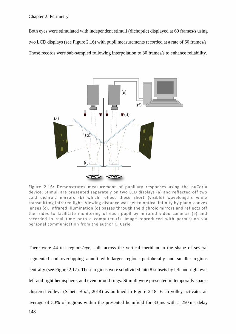
Chapter 2: Perimetry
148
Both eyes were stimulated with independent stimuli (dichoptic) displayed at 60 frames/s using
two LCD displays (see Figure 2.16) with pupil measurements recorded at a rate of 60 frames/s.
Those records were sub-sampled following interpolation to 30 frames/s to enhance reliability.
There were 44 test-regions/eye, split across the vertical meridian in the shape of several
segmented and overlapping annuli with larger regions peripherally and smaller regions
centrally (see Figure 2.17). These regions were subdivided into 8 subsets by left and right eye,
left and right hemisphere, and even or odd rings. Stimuli were presented in temporally sparse
clustered volleys (Sabeti et al., 2014) as outlined in Figure 2.18. Each volley activates an
average of 50% of regions within the presented hemifield for 33 ms with a 250 ms delay
Figure 2.16: Demonstrates measurement of pupillary responses using the nuCoria device. Stimuli are presented separately on two LCD displays (a) and reflected off two cold dichroic mirrors (b) which reflect these short (visible) wavelengths while transmitting infrared light. Viewing distance was set to optical infinity by plano -convex lenses (c). Infrared illumination (d) passes through the dichroic mirrors and reflects off the irides to facilitate monitoring of each pupil by infrared video cameras (e) and recorded in real time onto a computer (f). Image reproduced with permission via personal communication from the author C. Carle.

Chapter 2: Perimetry
149
between onsets of each volley, sequentially rotating through presentations in each of the 8
subsets. Stimuli in each test region were presented on average every 4 seconds for a total of
approximately 90 presentations per region throughout the test period of 360 seconds.
The two protocols (Y/Y and G/R) were completed on each visit for two visits (2 repeats of each
protocol), with random allocation as to order of testing on the first occasion and the reverse
order on repeat. Both protocols had a background luminance of 10 cd/m2 and stimuli of
maximum luminance of 150 cd/m2. Due to intrinsic differences in sensitivity across the retina,
both protocols employed luminance balancing across the field to maximise total signal to noise
ratio, as described elsewhere (Maddess et al., 2009).
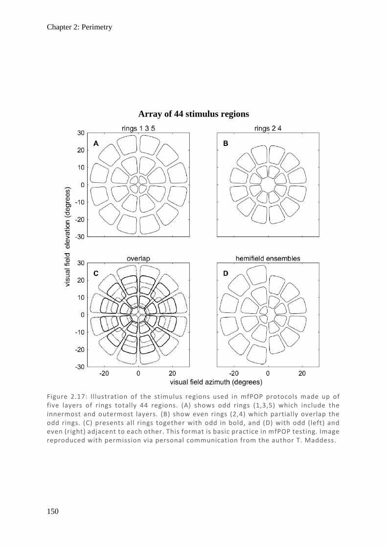
Chapter 2: Perimetry
150
Figure 2.17: Illustration of the stimulus regions used in mfPOP protocols made up of five layers of rings totally 44 regions. (A) shows odd rings (1,3,5) which include the innermost and outermost layers. (B) show even rings (2,4) which partially overlap the odd rings. (C) presents all rings together with odd in bold, and (D) with odd (left) and even (right) adjacent to each other. This format is basic practice in mfPOP testing. Image reproduced with permission via personal communication from the author T. Maddess.
Array of 44 stimulus regions
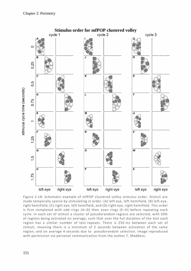
Chapter 2: Perimetry
151
Figure 2.18: Schematic example of mfPOP clustered volley stimulus order. Stimuli are made temporally sparse by stimulating in order: (A) left eye, left hemifield, (B) left eye, right hemifield, (C) right eye, left hemifield, and (D) ri ght eye, right hemifield. This order is first completed with odd rings (A–D) then even rings (E–H) before repeating each cycle. In each set of stimuli a cluster of pseudorandom regions are selected, with 50% of regions being activated on average, such that over the full duration of the test each region has a similar number of test -repeats. There is 250 ms between each set of stimuli, meaning there is a minimum of 2 seconds between activation of the same region, and on average 4 seconds due to pseudorandom selection. Image reproduced with permission via personal communication from the author T. Maddess.
Stimulus order for mfPOP clustered volley

Chapter 2: Perimetry
152
2.5.3.2. Testing procedures
While mfPOP is insensitive to blur, its software includes an algorithm to keep trial lenses as
similar as possible to reduce the effects of excessive blur. This is required as the trial lenses are
not exactly at the spectacle distance. Ocular prescription was entered, automatically converted
to spherical equivalent, and rounded to the nearest available lens: –9, –6, –3, 0, +3, +6, or +9
spherical dioptres. The stimuli had no spatial frequencies above 2 cycle/deg and so were little
demodulated by refractive errors < 2 D (Phillips & Stark, 1977; Sabeti et al., 2015). Prior to
testing, subjects had their horizontal vergence aligned by presenting a large X in one eye and a
plus-sign in the other; the horizontal alignment of the displays was then adjusted until these
objects were fused at optical infinity. Subjects were instructed to fixate a smaller central plus-
sign sustained throughout testing, and informed that they could blink as necessary but should
attempt to keep this to a minimum except during breaks. In a routine test there were 9 segments
each comprising ~40 seconds of test time with ~7 second breaks between each segment. The
ambient light level of the test-room was recorded, and lights adjusted when necessary to keep
constant at ~450 lux measured next to the mfPOP eye-pieces with a light-adaptation period of
3–5 minutes allowed prior to testing. Both eyes were tested simultaneously. Where subjects
had drooping eye-lids affecting pupil diameter measures, teary eyes, or requested to stop, that
segment was paused, and the duration of the break was noted before recommencement. Where
there was substantial eye movement, or poor-quality signal due to excess blinking or drooping
lids obscuring pupil measurement and causing data acquisition to fall below 85%, that segment
was repeated. Where a second testing protocol was to follow, a minimum rest period of 3
minutes was allowed before commencing.
2.5.3.3. Output measures
Raw pupillary measures were divided by the average pre-stimulus pupil diameter through all
segments and multiplied by the average diameter of 3.5 mm to produce magnitudes
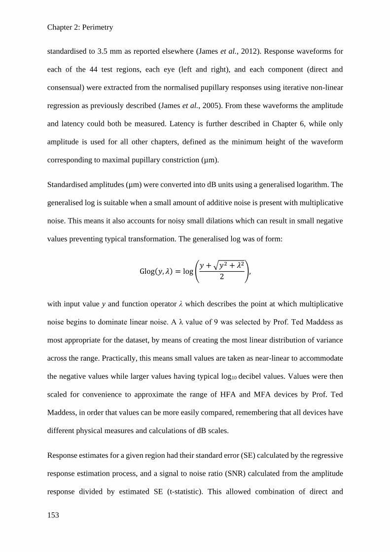
Chapter 2: Perimetry
153
standardised to 3.5 mm as reported elsewhere (James et al., 2012). Response waveforms for
each of the 44 test regions, each eye (left and right), and each component (direct and
consensual) were extracted from the normalised pupillary responses using iterative non-linear
regression as previously described (James et al., 2005). From these waveforms the amplitude
and latency could both be measured. Latency is further described in Chapter 6, while only
amplitude is used for all other chapters, defined as the minimum height of the waveform
corresponding to maximal pupillary constriction (µm).
Standardised amplitudes (µm) were converted into dB units using a generalised logarithm. The
generalised log is suitable when a small amount of additive noise is present with multiplicative
noise. This means it also accounts for noisy small dilations which can result in small negative
values preventing typical transformation. The generalised log was of form:
Glog(𝑦, 𝜆) = log (𝑦 + √𝑦2 + 𝜆2
2),
with input value y and function operator λ which describes the point at which multiplicative
noise begins to dominate linear noise. A λ value of 9 was selected by Prof. Ted Maddess as
most appropriate for the dataset, by means of creating the most linear distribution of variance
across the range. Practically, this means small values are taken as near-linear to accommodate
the negative values while larger values having typical log10 decibel values. Values were then
scaled for convenience to approximate the range of HFA and MFA devices by Prof. Ted
Maddess, in order that values can be more easily compared, remembering that all devices have
different physical measures and calculations of dB scales.
Response estimates for a given region had their standard error (SE) calculated by the regressive
response estimation process, and a signal to noise ratio (SNR) calculated from the amplitude
response divided by estimated SE (t-statistic). This allowed combination of direct and
Chapter 2: Perimetry
154
consensual components to be combined into a single measure by weighting according to their
SNR (reasoning and details in Chapter 4). Recall that since both eyes are stimulated and both
pupils recorded there are 44 responses per eye and per pupil.
Finally, conversion from the 44-test region mfPOP map to the 54-region 24-2 format was done
by weighted averages according to the relative contribution of the overlapping areas
(Ruseckaite et al., 2006). This allowed direct point-to-point comparison of the three devices all
in dB, even though all three dB scales and input measures are entirely different.
2.6. MRI
In the TCH Neurology Department, it is standard practice to have a CT done on suspected
stroke patients to confirm stroke and determine whether is it ischemic or haemorrhagic. While
this may be effective at highlighting any bleeding, it is not particularly effective at highlighting
ischemic damage or localising the damaged region. Consequently, some patients never have
an MRI scan and diagnosis must rely solely on the CT for positional information of the lesion.
As the penumbra region may show up on CT/MRI scans acutely, the final damaged post-stroke
region may be smaller and of a different size/shape than originally demonstrated. Even with
MRI, scan protocols vary in how effective they are at detecting new or old infarcts. For these
reasons, an MRI was acquired for all stroke patients willing and able to do so in order to provide
a more accurate description of their stroke infarct region. The protocol decided on was 3D fluid
attenuated inversion recovery (FLAIR) scan, which is effective at highlighting post-stroke
damage after the initial acute damage has dissipated. In addition, diffusion tensor imaging
(DTI) was done with the aim of measuring tract damage. While this data was collected as
part of these experiments, they were not able to be analysed due to specialist staff and
time constraints, but may be reviewed for future publications.
155
References
Albonico A, Malaspina M & Daini R. (2017). Italian normative data and validation of two
neuropsychological tests of face recognition: Benton facial recognition test and
cambridge face memory test. Neurol Sci 38, 1637-1643.
Ali EN, Maddess TL, Martin K, Borbelj A & Lueck CJ. (2015). Pupillary response to sparse
multifocal stimuli in epilepsy patients. In 4th annual saudi epilepsy society
conference, ed. Al-Baradie RS, pp. 74-78. Neurosciences, Riyadh.
Altay Y, Altay MM, Demirok G, Balta O & Bolu H. (2016). Measurements of pupillary
diameter and wavefront aberrations in pregnant women. Scientifica (Cairo) 2016,
4129524.
Anderson AJ & Johnson CA. (2002). Mechanisms isolated by frequency-doubling technology
perimetry. Invest Ophthalmol Vis Sci 43, 398-401.
Anderson AJ & Johnson CA. (2006). Comparison of the asa, mobs, and zest threshold
methods. Vision Res 46, 2403-2411.
Anstis SM. (1970). Phi movement as a subtraction process. Vision Res 10, 1411-1430.
Bailey MJ, Riddoch MJ & Crome P. (2004). Test-retest stability of three tests for unilateral
visual neglect in patients with stroke: Star cancellation, line bisection, and the baking
tray task. Neuropsychol Rehabil 14, 403-419.
Baker CL, Jr. & Braddick OJ. (1982). The basis of area and dot number effects in random dot
motion perception. Vision Res 22, 1253-1259.
Bengtsson B, Heijl A & Olsson J. (1998). Evaluation of a new threshold visual field strategy,
sita, in normal subjects. Swedish interactive thresholding algorithm. Acta Ophthalmol
Scand 76, 165-169.
Benton AL & Van Allen MW. (1968). Impairment in facial recognition in patients with
cerebral disease. Trans Am Neurol Assoc 93, 38-42.
Bhan A, Browning AC, Shah S, Hamilton R, Dave D & Dua HS. (2002). Effect of corneal
thickness on intraocular pressure measurements with the pneumotonometer,
Chapter 2: References
156
goldmann applanation tonometer, and tono-pen. Invest Ophthalmol Vis Sci 43, 1389-
1392.
Birch J. (2010). Identification of red-green colour deficiency: Sensitivity of the ishihara and
american optical company (hard, rand and rittler) pseudo-isochromatic plates to
identify slight anomalous trichromatism. Ophthalmic Physiol Opt 30, 667-671.
Birch J. (2012). Worldwide prevalence of red-green color deficiency. Journal of the Optical
Society of America A, Optics, image science, and vision 29, 313-320.
Bouvier SE & Engel SA. (2006). Behavioral deficits and cortical damage loci in cerebral
achromatopsia. Cereb Cortex 16, 183-191.
Bowles DC, McKone E, Dawel A, Duchaine B, Palermo R, Schmalzl L, Rivolta D, Wilson
CE & Yovel G. (2009). Diagnosing prosopagnosia: Effects of ageing, sex, and
participant-stimulus ethnic match on the cambridge face memory test and cambridge
face perception test. Cogn Neuropsychol 26, 423-455.
Bowman KJ. (1982). A method for quantitative scoring of the farnsworth panel d-15. Acta
Ophthalmol 60, 907-916.
Braddick O. (1974). A short-range process in apparent motion. Vision Res 14, 519-527.
Campbell FW & Green DG. (1965). Optical and retinal factors affecting visual resolution. J
Physiol 181, 576-593.
Cho SJ, Wilmer J, Herzmann G, McGugin RW, Fiset D, Van Gulick AE, Ryan KF &
Gauthier I. (2015). Item response theory analyses of the cambridge face memory test
(cfmt). Psychol Assess 27, 552-566.
Chougule PS, Najjar RP, Finkelstein MT, Kandiah N & Milea D. (2019). Light-induced
pupillary responses in alzheimer's disease. Frontiers in neurology 10, 360-360.
Cleary R & Braddick OJ. (1990). Direction discrimination for band-pass filtered random dot
kinematograms. Vision Res 30, 303-316.
Croydon A, Pimperton H, Ewing L, Duchaine BC & Pellicano E. (2014). The cambridge face
memory test for children (cfmt-c): A new tool for measuring face recognition skills in
childhood. Neuropsychologia 62, 60-67.

Chapter 2: References
157
Duchaine B & Nakayama K. (2006). The cambridge face memory test: Results for
neurologically intact individuals and an investigation of its validity using inverted
face stimuli and prosopagnosic participants. Neuropsychologia 44, 576-585.
Duchaine BC & Nakayama K. (2004). Developmental prosopagnosia and the benton facial
recognition test. Neurology 62, 1219-1220.
Duchaine BC & Weidenfeld A. (2003). An evaluation of two commonly used tests of
unfamiliar face recognition. Neuropsychologia 41, 713-720.
Eagle RA & Rogers BJ. (1996). Motion detection is limited by element density not spatial
frequency. Vision Res 36, 545-558.
Farnsworth D. (1943). The farnsworth-munsell 100-hue and dichotomous tests for color
vision. J Opt Soc Am 33, 568-578.
Ferber S & Karnath HO. (2001). How to assess spatial neglect--line bisection or cancellation
tasks? J Clin Exp Neuropsychol 23, 599-607.
Fredette MJ, Giguere A, Anderson DR, Budenz DL & McSoley J. (2015). Comparison of
matrix with humphrey field analyzer ii with sita. Optometry and vision science :
official publication of the American Academy of Optometry 92, 527-536.
Furlan M & Smith AT. (2016). Global motion processing in human visual cortical areas v2
and v3. J Neurosci 36, 7314-7324.
Gray KL, Bird G & Cook R. (2017). Robust associations between the 20-item prosopagnosia
index and the cambridge face memory test in the general population. R Soc Open Sci
4, 160923.
Halligan PW, Marshall JC & Wade DT. (1989). Visuospatial neglect: Underlying factors and
test sensitivity. Lancet 2, 908-911.
Halligan PW, Marshall JC & Wade DT. (1990). Do visual field deficits exacerbate visuo-
spatial neglect? J Neurol Neurosurg Psychiatry 53, 487-491.
Hawkins AS, Szlyk JP, Ardickas Z, Alexander KR & Wilensky JT. (2003). Comparison of
contrast sensitivity, visual acuity, and humphrey visual field testing in patients with
glaucoma. J Glaucoma 12, 134-138.
Chapter 2: References
158
Hepworth LR & Rowe FJ. (2018). Programme choice for perimetry in neurological
conditions (popin): A systematic review of perimetry options and patterns of visual
field loss. Bmc Ophthalmol 18, 241.
Heutink J, de Haan G, Marsman JB, van Dijk M & Cordes C. (2019). The effect of target
speed on perception of visual motion direction in a patient with akinetopsia. Cortex
119, 511-518.
Humphreys GW, Quinlan PT & Riddoch MJ. (1989). Grouping processes in visual search:
Effects with single- and combined-feature targets. J Exp Psychol Gen 118, 258-279.
Ishihara S. (1918). Tests for color blindness. Am J Ophthalmol 1, 457.
James AC, Kolic M, Bedford SM & Maddess T. (2012). Stimulus parameters for multifocal
pupillographic objective perimetry. J Glaucoma 21, 571-578.
James AC, Ruseckaite R & Maddess T. (2005). Effect of temporal sparseness and dichoptic
presentation on multifocal visual evoked potentials. Visual Neurosci 22, 45-54.
Julesz B. (1960). Binocular depth perception of computer-generated patterns. Bell system
technical journal 39, 1125-1162.
Julesz B. (1964). Binocular depth perception without familiarity cues. Science 145, 356-362.
Julesz B. (1965). Texture and visual perception. Sci Am 212, 38-48.
Julesz B. (1971). Foundations of cyclopean perception. The University of Chicago Press,
Chicago.
Kaiser PK. (2008). Comparison of snellen versus etdrs protocol visual acuities performed by
certified vision examiners. In Association for Research in Vision and Ophthalmology.
Investigative Ophthalmology & Visual Science.
Kalloniatis M & Luu C. (2005). The perception of color. In The organisation of the retina
and the visual system, ed. Kolb H, Fernandez E & Nelson R. University of Utah
Health Science Center, Salt Lake City, Utah.
Kennerknecht I, Grueter T, Welling B, Wentzek S, Horst J, Edwards S & Grueter M. (2006).
First report of prevalence of non-syndromic hereditary prosopagnosia (hpa). Am J
Med Genet A 140, 1617-1622.

Chapter 2: References
159
Kennerknecht I, Plumpe N, Edwards S & Raman R. (2007). Hereditary prosopagnosia (hpa):
The first report outside the caucasian population. J Hum Genet 52, 230-236.
Khoury JM, Donahue SP, Lavin PJ & Tsai JC. (1999). Comparison of 24-2 and 30-2
perimetry in glaucomatous and nonglaucomatous optic neuropathies. Journal of
neuro-ophthalmology : the official journal of the North American Neuro-
Ophthalmology Society 19, 100-108.
Kinyoun J, Barton F, Fisher M, Hubbard L, Aiello L & Ferris F, 3rd. (1989). Detection of
diabetic macular edema. Ophthalmoscopy versus photography--early treatment
diabetic retinopathy study report number 5. The etdrs research group. Ophthalmology
96, 746-750; discussion 750-741.
Kolmel HW. (1988). Pure homonymous hemiachromatopsia. Findings with neuro-
ophthalmologic examination and imaging procedures. Eur Arch Psychiatry Neurol Sci
237, 237-243.
Kooistra CA & Heilman KM. (1989). Hemispatial visual inattention masquerading as
hemianopia. Neurology 39, 1125-1127.
Kruger PB & Pola J. (1986). Stimuli for accommodation: Blur, chromatic aberration and size.
Vision Res 26, 957-971.
Lam BL, Alward WL & Kolder HE. (1991). Effect of cataract on automated perimetry.
Ophthalmology 98, 1066-1070.
Legge GE, Mullen KT, Woo GC & Campbell FW. (1987). Tolerance to visual defocus. J Opt
Soc Am A 4, 851-863.
Li K & Malhotra PA. (2015). Spatial neglect. Pract Neurol 15, 333-339.
Maddess T & Kulikowski JJ. (1999). Apparent fineness of stationary compound gratings.
Vision Res 39, 3404-3416.
Maddess TL, Kolic M, Essex RW & James AC. (2009). Balanced luminance multifocal
pupillographic perimetry. In Invest Ophthalmol Vis Sci, pp. 5281.
Matsuura M, Hirasawa K, Murata H & Asaoka R. (2015). The relationship between visual
acuity and the reproducibility of visual field measurements in glaucoma patients.
Invest Ophthalmol Vis Sci 56, 5630-5635.

Chapter 2: References
160
McCourt ME & Jewell G. (1999). Visuospatial attention in line bisection: Stimulus
modulation of pseudoneglect. Neuropsychologia 37, 843-855.
McCourt ME & Olafson C. (1997). Cognitive and perceptual influences on visual line
bisection: Psychophysical and chronometric analyses of pseudoneglect.
Neuropsychologia 35, 369-380.
McKeefry DJ, Watson JDG, Frackowiak RSJ, Fong K & Zeki S. (1997). The activity in
human areas v1/v2, v3, and v5 during the perception of coherent and incoherent
motion. Neuroimage 5, 1-12.
McKone E, Hall A, Pidcock M, Palermo R, Wilkinson RB, Rivolta D, Yovel G, Davis JM &
O'Connor KB. (2011). Face ethnicity and measurement reliability affect face
recognition performance in developmental prosopagnosia: Evidence from the
cambridge face memory test-australian. Cogn Neuropsychol 28, 109-146.
McKone E, Wan L, Robbins R, Crookes K & Liu J. (2017). Diagnosing prosopagnosia in east
asian individuals: Norms for the cambridge face memory test-chinese. Cogn
Neuropsychol 34, 253-268.
Micieli G, Tassorelli C, Martignoni E, Pacchetti C, Bruggi P, Magri M & Nappi G. (1991).
Disordered pupil reactivity in parkinson's disease. Clin Auton Res 1, 55-58.
Miller LJ, Mittenberg W, Carey VM, McMorrow MA, Kushner TE & Weinstein JM. (1999).
Astereopsis caused by traumatic brain injury. Arch Clin Neuropsych 14, 537-543.
Nakamura H, Kashii S, Nagamine T, Matsui Y, Hashimoto T, Honda Y & Shibasaki H.
(2003). Human v5 demonstrated by magnetoencephalography using random dot
kinematograms of different coherence levels. Neurosci Res 46, 423-433.
Neitz M, G. GD & Neitz J. (2008). Visual acuity, color vision, and adaptation. In Albert &
jakobiec's principles and practice of ophthalmology, 3rd edn, ed. Albert DM, Miller
JW, Azar DT & Boldi BA. Saunders, Philadelphia.
Nunn JA, Postma P & Pearson R. (2001). Developmental prosopagnosia: Should it be taken
at face value? Neurocase 7, 15-27.
O'Connor AR, Birch EE, Anderson S, Draper H & Grp FR. (2010). The functional
significance of stereopsis. Invest Ophth Vis Sci 51, 2019-2023.
Paulson HL, Galetta SL, Grossman M & Alavi A. (1994). Hemiachromatopsia of unilateral
occipitotemporal infarcts. Am J Ophthalmol 118, 518-523.

Chapter 2: References
161
Phillips S & Stark L. (1977). Blur - sufficient accommodative stimulus. Doc Ophthalmol 43,
65-89.
Radcliffe NM. (2014). Hysteresis: A powerful tool for glaucoma care. Review
Ophthalmology 21, 50-57.
Raymond JE. (1994). Directional anisotropy of motion sensitivity across the visual field.
Vision Res 34, 1029-1037.
Ringman JM, Saver JL, Woolson RF, Clarke WR & Adams HP. (2004). Frequency, risk
factors, anatomy, and course of unilateral neglect in an acute stroke cohort. Neurology
63, 468-474.
Rorden C & Karnath HO. (2010). A simple measure of neglect severity. Neuropsychologia
48, 2758-2763.
Ruseckaite R, Maddess T & James AC. (2006). Monocular and binocular multifocal visual
evoked potentials in normal and multiple sclerosis subjects. Mult Scler 12, S166-
S166.
Sabeti F, Maddess T, Essex RW, Saikal A, James AC & Carle CF. (2014). Multifocal
pupillography in early age-related macular degeneration. Optometry and vision
science : official publication of the American Academy of Optometry 91, 904-915.
Sabeti F, Nolan CJ, James AC, Jenkins A & Maddess T. (2015). Multifocal pupillography
identifies changes in visual sensitivity according to severity of diabetic retinopathy in
type 2 diabetes. Invest Ophthalmol Vis Sci 56, 4504-4513.
Scherf KS, Elbich DB & Motta-Mena NV. (2017). Investigating the influence of biological
sex on the behavioral and neural basis of face recognition. eNeuro 4.
Schutz AC, Braun DI, Movshon JA & Gegenfurtner KR. (2010). Does the noise matter?
Effects of different kinematogram types on smooth pursuit eye movements and
perception. J Vision 10.
Shah S, Chatterjee A, Mathai M, Kelly SP, Kwartz J, Henson D & McLeod D. (1999).
Relationship between corneal thickness and measured intraocular pressure in a
general ophthalmology clinic. Ophthalmology 106, 2154-2160.

Chapter 2: References
162
Shamir RR, Friedman Y, Joskowicz L, Mimouni M & Blumenthal EZ. (2016). Comparison
of snellen and early treatment diabetic retinopathy study charts using a computer
simulation. Int J Ophthalmol-Chi 9, 119-123.
Short RA & Graff-Radford NR. (2001). Localization of hemiachromatopsia. Neurocase 7,
331-337.
Simunovic MP. (2010). Colour vision deficiency. Eye (Lond) 24, 747-755.
Stark LR & Atchison DA. (2002). Monocular accommodation response for totally occluded
objects. Optometry and vision science : official publication of the American Academy
of Optometry 79, 658-666.
Stark LR, Lee RS, Kruger PB, Rucker FJ & Ying Fan H. (2002). Accommodation to
simulations of defocus and chromatic aberration in the presence of chromatic
misalignment. Vision Res 42, 1485-1498.
Steward JM & Cole BL. (1989). Incidence of congential colour vision defects in an australian
optometric population. In Colour vision deficiencies IX, ed. Drum B & Verriest G, pp.
109-111. Springer, Dordrecht.
Stodtmeister R. (1998). Applanation tonometry and correction according to corneal thickness.
Acta Ophthalmol Scand 76, 319-324.
Stone SP, Halligan PW & Greenwood RJ. (1993). The incidence of neglect phenomena and
related disorders in patients with an acute right or left hemisphere stroke. Age Ageing
22, 46-52.
Sunderland A, Wade DT & Langton Hewer R. (1987). The natural history of visual neglect
after stroke. Indications from two methods of assessment. Int Disabil Stud 9, 55-59.
Taravati P, Woodward KR, Keltner JL, Johnson CA, Redline D, Carolan J, Huang CQ &
Wall M. (2008). Sensitivity and specificity of the humphrey matrix to detect
homonymous hemianopias. Invest Ophth Vis Sci 49, 924-928.
Vaina LM. (1995). Akinetopsia, achromatopsia and blindsight: Recent studies on perception
without awareness. Synthese 105, 253-271.
Wall M, Punke SG, Stickney TL, Brito CF, Withrow KR & Kardon RH. (2001). Sita standard
in optic neuropathies and hemianopias: A comparison with full threshold testing.
Invest Ophthalmol Vis Sci 42, 528-537.

Chapter 2: References
163
Warrington EK. (1984). Recognition memory test: Manual. NFER-Nelson, Berkshire, UK.
Whitacre MM, Stein RA & Hassanein K. (1993). The effect of corneal thickness on
applanation tonometry. Am J Ophthalmol 115, 592-596.
Wild JM, Searle AE, Dengler-Harles M & O'Neill EC. (1991). Long-term follow-up of
baseline learning and fatigue effects in the automated perimetry of glaucoma and
ocular hypertensive patients. Acta Ophthalmol (Copenh) 69, 210-216.
Wolfs RC, Klaver CC, Vingerling JR, Grobbee DE, Hofman A & de Jong PT. (1997).
Distribution of central corneal thickness and its association with intraocular pressure:
The rotterdam study. Am J Ophthalmol 123, 767-772.
Wooten BR. (1981). Partial cerebral achromatopsia with selective hue loss. In International
research group on colour vision deficiencies symposium, ed. Verriest G. Dr W. Junk
Publishers, Berlin.
Zeki S. (1990). A century of cerebral-achromatopsia. Brain 113, 1721-1777.
Zhang Q, Shi J, Luo Y, Liu S, Yang J & Shen M. (2007). Effect of task complexity on
intelligence and neural efficiency in children: An event-related potential study.
Neuroreport 18, 1599-1602.
Zhou C, He Y & Li X. (2018). Cerebral achromatopsia secondary to ischemic stroke. Neurol
India 66, 573-575.
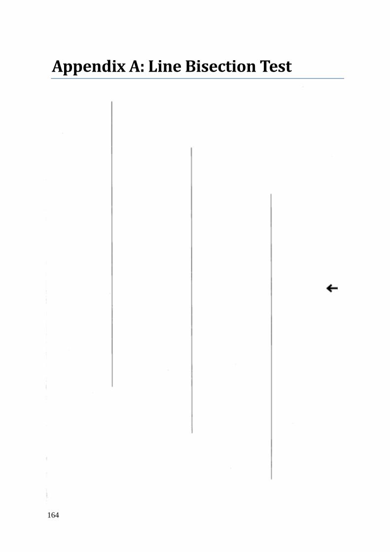
164
Appendix A: Line Bisection Test
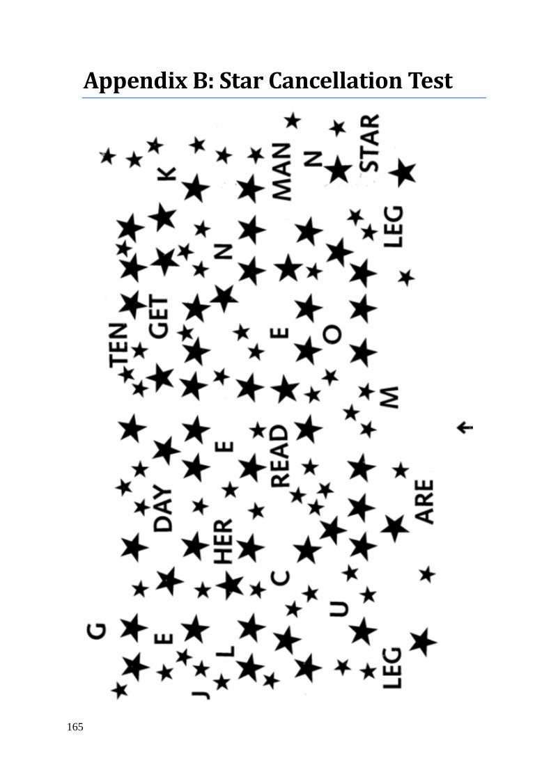
165
Appendix B: Star Cancellation Test
166
3 Chapter 3: Higher visual function loss and its assessment in stroke
3.1. Abstract
3.1.1. Purpose
This study investigated higher visual function deficits in perception of colour, facial
recognition, stereopsis, and coherent global motion, as a pilot to determine if subtle deficits are
common in stroke patients and which methods are most effective in detecting them.
3.1.2. Methods
Stroke patients (n = 24) and controls (n = 26) were tested using a test battery of Ishihara,
Farnsworth–Munsell D15, Cambridge Facial Memory Test, stereofly, randot, and random dot
kinematogram as outlined in the general methods section. Receiver operator characteristics
with bootstrap were produced to calculate appropriate threshold values, their rates of
presentation, and area under curve (AUC) was calculated to indicate which tests were most
valuable. Principal component and mean likelihood analysis with scree plots were also used to
indicate tests which account for the most variability in responses, providing other measures of
test diagnostic value and indicating which tests groups measure the same component.
3.1.3. Results
Stereofly, randot and Ishihara reached significance (p < 0.01) for AUC with means and SD of
0.79 ± 0.08, 0.76 ± 0.09, and 0.73 ± 0.08 respectively. No other variables reached significance.
At false positive ratios (FPRs) of 5%, 10%, and 20%, stereofly, Ishihara, and randot had the
highest sensitivities with values of 20–30%, 35–40%, and 60%. At very low FPRs of 2% and
5%, Farnsworth–Munsell performed equal or better to these test variables. Principal component
scree plots suggested two or three components, representing 48% and 63% variance. Both were
Chapter 3: Abstract
167
examined, revealing that the primary component was predominantly stereofly and randot, while
the secondary component was CFMT with Farnsworth–Munsell.
3.1.4. Conclusions
Stereovision as measured by stereofly or randot shows significant deficits in stroke patients
compared to controls, with stereofly having marginally better sensitivities across the useful
range. Combining tests would be of limited usefulness given they both load onto the same
factor. Colour vision as measured by Ishihara also shows significant deficits. While the other
colour vision test (Farnsworth–Munsell) provides some utility, it did not reach significance
alone. Given that colour vision does appear to be affected, and that Farnsworth–Munsell D15
approached significance, there may be some utility in using the larger more robust FM100.
Combination of CFMT with FM appears likely to be due to close localisation anatomically, in
contrast to SF and RD which are functionally similar.
Chapter 3: Introduction
168
3.2. Introduction
Based on many case reports following stroke, it is well established that deficits in higher visual
function occur – such as visual neglect11 (Cherney & Halper, 2001; Pollock et al., 2011),
achromatopsia12 (Setala & Vesti, 1994; Bartolomeo et al., 1997; Duvelleroy-Hommet et al.,
1997; Cowey et al., 2008; von Arx et al., 2010; Pagani et al., 2012; Carota & Calabrese, 2013;
Bartolomeo et al., 2014; Zhou et al., 2018), prosopagnosia13 (Lander et al., 2004; Lu et al.,
2005; Lang et al., 2006; Fox et al., 2011; Heutink et al., 2012), akinetopsia14 (Vaina, 1994;
Rizzo et al., 1995; Barton et al., 1996; Vaina et al., 2001; Cooper et al., 2012), and astereopsis15
(Ross, 1983; Schaadt et al., 2014; Schaadt et al., 2015; Schow et al., 2016). However, little
work has been done in identifying less overt deficits and the relative frequency of these
conditions in the stroke population.
This study investigated higher visual function deficits in perception of colour (using Ishihara
and Farnsworth–Munsell), facial recognition (using the Cambridge Face Memory Test
[CFMT]), stereopsis (using stereofly & randot), cohesive motion (kinematogram) and visual
neglect (line bisection and star cancellation). We used them to identify whether any deficits are
common in stroke patients and to determine which methods are most effective in detecting
impairment. Given the heterogeneity of stroke presentation, and the relatively small sample
size of 24 (against 26 controls), this was only intended as a pilot to test a broad range of methods
11 Visual pathway remains intake, but does not conciously acknowledge items on side contralateral to lesion. 12 Inability to recognise colours, seeing the world in grey, following a cortical lesion. More subtle defects may
diminish colour sensitivity without being blind to colour. 13 Inability to recognise faces and unique features of faces, following a cortical lesion. In the most severe cases,
they cannot recognise their own face, while more subtle defects may make discerning between faces difficult. 14 Inability to decern motion either generally (seeing all motion as series of static images) or in motion coherence
(cannot detect cohesive motion from noise). 15 Inability to use binocular vision to produce three-dimensional percept. May reply on other feautres or in severe
cases perceive the world as flat.
Chapter 3: Introduction
169
which might then be refined in a larger study, one less demanding of subject test-time and
having more definitive outcomes.
3.3. Methods
Full methods, including recruitment, reasoning for test selection, and their administration can
be found in General Methods (Chapter 2). Only a summary is provided here for convenience.
As outlined in General Methods 2.1, there is evidence for both the functional specialisation of
cortical processing based on isolated deficits, although rare (Vaina, 1995), and distributive
model of cortical processing, based on selective stimuli activating many cortical areas
(McKeefry et al., 1997; Furlan & Smith, 2016). This study recruited stroke subjects without
consideration of cortical location, because we already know that isolated deficits are rare, but
do not know the extent of more subtle deficits, which do not have established locations.
A total of 24 stroke subjects (non-selective to location) were recruited, along with 26 control
subjects. Both groups were screened for visual impairment due to retinal disorders using both
a questionnaire and ophthalmic equipment, and they met the acuity criteria of best-corrected
visual acuity of logMAR >0.5 (6/19). All subjects then completed a series of higher visual
function tests outlined below.
3.3.1. Higher visual function tests
The HVF tests are listed below. In order to complete a principal component analysis (PCA), a
single measure is required for each test, and so summary variables were made for tests with
multiple measures – these are summarised in Table 3.1Error! Not a valid bookmark self-
reference. along with the abbreviation code used in graphing.

Chapter 3: Methods
170
Table 3.1: Higher visual function tests, summary variables , and short-codes.
Short code Test Summary variable
LB Line bisection: 3 × 19 cm lines
from behavioural inattention test
(Wilson et al., 1987)
Average error from 3 lines (mm)
Ishi Ishihara 24-plate set (Ishihara,
1918) Sum of correct answers (both eyes)
FM Farnsworth-Munsell D-15
dichotomous test (Farnsworth,
1947)
Colour confusion index: sum of the
hue difference of selected well order
over ideal well order (Bowman, 1982).
CFMT Cambridge Facial Memory Test
(Duchaine & Nakayama, 2006) Sum of correct answers (all 3 sections)
RD Randot dot 3 with Lea symbols
(Vision Assessment Corporation,
2012, Illinois USA)
Minimum threshold achieved in test
SF
The fly stereo acuity test with Lea
symbols
(Vision Assessment Corporation,
2007, Illinois USA)
Minimum threshold achieved in test
Km Kinematogram
(custom design) Minimum threshold achieved in test
3.3.1.1. Reliability of higher visual function tests
The sensitivities of these tests are unknown in the stroke population, which is the purpose in
comparing with controls in this study. While sensitivity may be unknown, the reliability of
many of these tests has been previously reported, which may inform if they are likely to be
internally consistent.
Line bisection in terms of the Schenkenberg line bisection test showed intraclass correlation
coefficients for intra-rater reliability between 0.82-1 (Stone et al., 2019), although it should be
acknowledged that the standard line bisection test used for this study has fewer lines to bisect.
Chapter 3: Methods
171
A report of the quantitative reliability of the Ishihara for normal controls could not be found,
although it has been qualitatively reported as having high test-retest reliability with 102 normal
subjects scoring ≤3 errors on both of two attempts (Johnson, 1992). The Farnsworth-Munsell
D15 assessed using the same colour-confusion index (CCI) as this study, showed the mean
difference between test and retest of -0.02 ± 0.128 which is a small difference but with
substantial variability. The resulting intraclass correlation coefficient was 0.56 (95%
confidence interval 0.43-0.67) which shows questionable reliability (Good et al., 2005).
Various groups report a CFMT Cronbach’s alpha reliability between 0.83-0.88 (Herzmann et
al., 2008; Bowles et al., 2009; Wilmer et al., 2010), considered high by the standard of
cognitive tasks. The randot stereovision test is more commonly administered in children, with
reliability in those aged 4-10 years showing within-subject variation of 1.57 (95% CI 1.44-
1.71) randot plates (Adler et al., 2012), with those in the older age groups showing greater
stability between testing. In adults with stable strabismus, stereoacuity measured on
consecutive visits showed differences of 0.59 log arcsec equating to 1.95 octave steps of
difference (Adams et al., 2009). Together these suggest that the randot stereovision test is
moderately stable in those without visual impairment, but likely has greater test-retest
variability in those with impaired stereopsis. Similar results were demonstrated in stereofly
stereo acuity test, suggesting those with impaired stereopsis (>160 arcsec) become increasingly
variable in their responses (Fawcett & Birch, 2003). As the random dot kinematogram is an
original test, there is no reported reliability measure, although anecdotally unaffected staff
members showed similar results on repeats prior to study commencing, while during the study
it was noted a few subjects scored substantially differently on repeat, leaving reliability
uncertain.
Chapter 3: Methods
172
3.3.2. Receiver operator characteristics and thresholds
In clinical practice, tests routinely require a ‘normal range’ or ‘threshold’ to allow
categorisation into normal or abnormal for diagnosis and treatment purposes. The aim is to
distinguish between two distributions: ‘normal’ patients who do not have the disease, and
‘abnormal’ patients who do (Nettleman, 1988; Junge & Dettori, 2018).
In this study, the equivalent groups are ‘control’ and ‘stroke’, where their diagnostic status is
already known, while the sensitivity and specificity of the psychophysical tests we are trialling
are not. Naturally, sensitivity and specificity depend on what threshold is used to demarcate
between normal and abnormal, and one way of measuring how well a test performs at all
possible thresholds is using a receiver operator characteristic (ROC) plot, with its overall
quantitative performance being reflected in its area under the curve (AUC) (Nettleman, 1988;
Junge & Dettori, 2018). This study is not interested in the diagnostic capacity of HVF tests to
detect stroke, but rather whether HVF deficits exist in the stroke population (as compared to
controls). As the threshold for demarcating between a ‘normal’ and an ‘abnormal’ is not well
established, ROC plots provide a means to assess relative diagnostic power.
To illustrate this, Figure 3.1 shows a range of possible distributions, from perfect score for
AUC of 1, to a minimal (chance) score of 0.5. A perfect test has a sensitivity of 100% (all
stroke patients have abnormal result) with a false-positive ratio (FPR) of 0% (no controls have
abnormal result). In comparison, a test which had no power to discern between groups (chance
level) would have a sensitivity of 50% and a FPR of 50%, indicating a person from either group
would be equally likely to be classified as having an abnormal result. The beauty of this
technique is that all potential thresholds are attempted, allowing the user to select an
appropriate sensitivity or specificity which is appropriate to the context.
Chapter 3: Methods
173
In practice where the result may prompt an invasive clinical decision, there is generally a low
threshold for false positives, while in screening where follow-up is not invasive, keeping
sensitivity high may be more important. The context often determines what an appropriate
value is, and for these purposes the ROC provides information about all possible values across
every possible threshold, while also providing a quantitative measure of overall diagnostic
performance.
In this study, it is not known how common a deficit is in the stroke population or in the normal
population; however it would be fair to assume that to identify a deficit due to stroke, it would
have to be sufficiently different to the normal population. In psychophysical tests like this, a
threshold which categorises the lowest scoring 5% of the population as abnormal is commonly
used, and will be presented alongside the recommended threshold. On a ROC curve, this
corresponds to a FPR of 5%, and the sensitivity at this threshold represents how common a
deficit is in the stroke population.
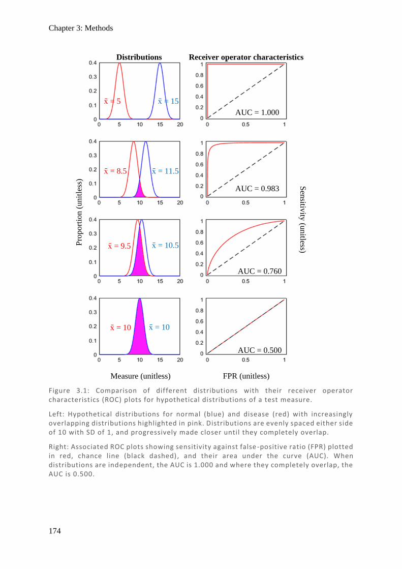
Chapter 3: Methods
174
Figure 3.1: Comparison of different distributions with their receiver operator characteristics (ROC) plots for hypothetical distributions of a test measure.
Left: Hypothetical distributions for normal (blue) and disease (red) with increasingly overlapping distributions highlighted in pink. Distributions are evenly spaced either side of 10 with SD of 1, and progressively made closer until they completely overlap.
Right: Associated ROC plots showing sensitivity against false -positive ratio (FPR) plotted in red, chance line (black dashed) , and their area under the curve (AUC). When distributions are independent, the AUC is 1.000 and where they completely overlap, the AUC is 0.500.
x̄ = 5 x̄ = 15
x̄ = 8.5 x̄ = 11.5
x̄ = 9.5 x̄ = 10.5
x̄ = 10 x̄ = 10
AUC = 1.000
AUC = 0.983
AUC = 0.760
AUC = 0.500
FPR (unitless)
Sen
sitivity
(unitless)
Pro
port
ion (
unit
less
)
Measure (unitless)
Distributions Receiver operator characteristics
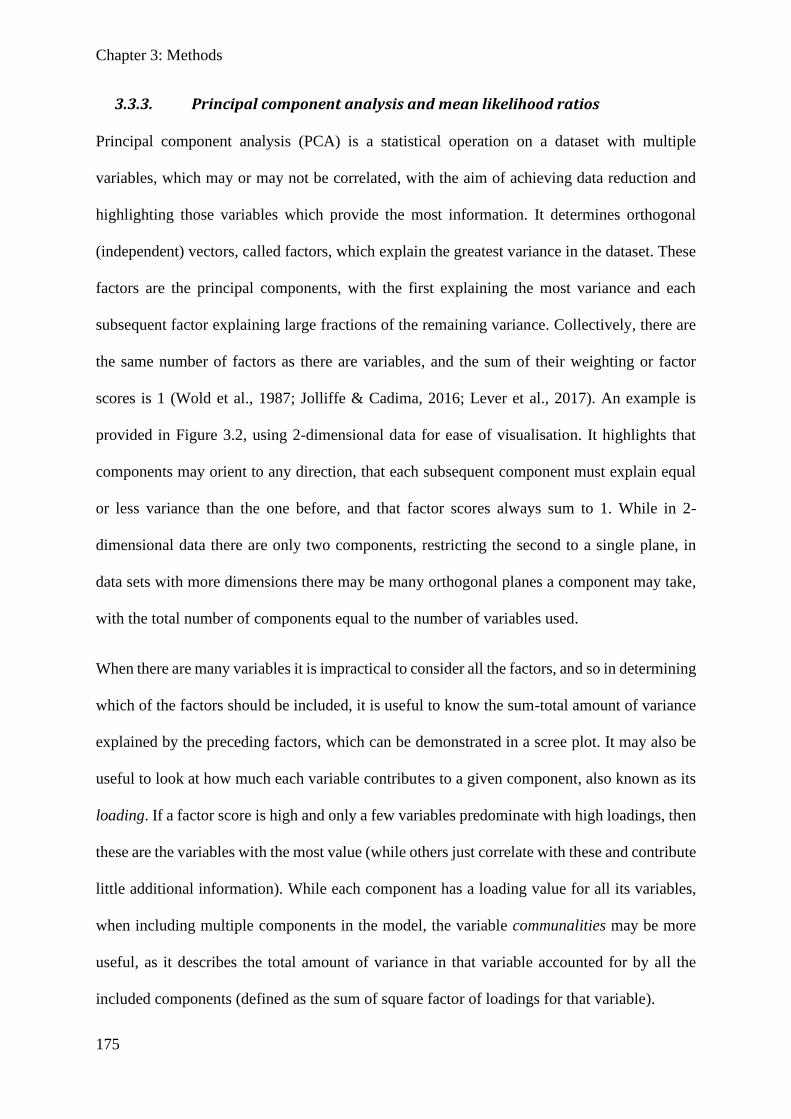
Chapter 3: Methods
175
3.3.3. Principal component analysis and mean likelihood ratios
Principal component analysis (PCA) is a statistical operation on a dataset with multiple
variables, which may or may not be correlated, with the aim of achieving data reduction and
highlighting those variables which provide the most information. It determines orthogonal
(independent) vectors, called factors, which explain the greatest variance in the dataset. These
factors are the principal components, with the first explaining the most variance and each
subsequent factor explaining large fractions of the remaining variance. Collectively, there are
the same number of factors as there are variables, and the sum of their weighting or factor
scores is 1 (Wold et al., 1987; Jolliffe & Cadima, 2016; Lever et al., 2017). An example is
provided in Figure 3.2, using 2-dimensional data for ease of visualisation. It highlights that
components may orient to any direction, that each subsequent component must explain equal
or less variance than the one before, and that factor scores always sum to 1. While in 2-
dimensional data there are only two components, restricting the second to a single plane, in
data sets with more dimensions there may be many orthogonal planes a component may take,
with the total number of components equal to the number of variables used.
When there are many variables it is impractical to consider all the factors, and so in determining
which of the factors should be included, it is useful to know the sum-total amount of variance
explained by the preceding factors, which can be demonstrated in a scree plot. It may also be
useful to look at how much each variable contributes to a given component, also known as its
loading. If a factor score is high and only a few variables predominate with high loadings, then
these are the variables with the most value (while others just correlate with these and contribute
little additional information). While each component has a loading value for all its variables,
when including multiple components in the model, the variable communalities may be more
useful, as it describes the total amount of variance in that variable accounted for by all the
included components (defined as the sum of square factor of loadings for that variable).
Chapter 3: Methods
176
Maximum likelihood analysis (MLA) is an alternative form of principal component analysis
with less restrictive criteria as to the orthogonal nature of sequential components, and which
may uncover factors that are more natural. It uses a different approach to optimisation but
provides similar output measures. In considering which better explains the data, both PCA and
MLA can be compared, using their mean communalities for an equal number of components.
3.4. Results
3.4.1. Receiver operator characteristics
Below are separately presented results for all seven test variables using ROC and Thresholds
for stroke patients, compared to controls. In each graph the bootstrap randomly sampled (with
Figure 3.2: Examples of 2-dimensional data with its primary (red) and secondary (blue) principal components.
(A) Equal variance in all directions – so the primary principal component may be in any direction; however its secondary component must be orthogonal. Due to equal variance throughout, both components will explain the same amount of variance and their loadings with be equal (i.e. 1o = 0.5 and 2o = 0.5).
(B) Greater variance diagonally – so the direction of the primary principal component aligns with greatest variability (angled upwards) and explains almost twice the variance, so it will have a weighting twice as large as the second component (i.e. 1 o = 0.66 and 2o = 0.33).
(C) Larger variability diagonally – again the direction of the primary component aligns with greatest variability (angled downwards). This that highlights the component may be in any direction. Here the primary component explains markedly more variability than the second and will be many times larger (i.e. 1 o = 0.8 and 2o = 0.2).
A B C
Measure 1 (unitless)
Mea
sure
2
(u
nit
less
)
Mea
sure
2
(u
nit
less
)
Mea
sure
2
(u
nit
less
)
Measure 1 (unitless) Measure 1 (unitless)

Chapter 3: Results
177
replacement) from the 24 stroke subjects 24 times (and the 26 control subjects 26 times) to
generate a new population each time, producing subtly different ROC plots, allowing the
possibility that the same sample might be selected multiple times and create a more varied ROC
plot. When repeated many times, and all varied ROC plots are combined, it generates a
distribution of values allowing an unbiased measure of mean and standard deviation across the
entire range, providing a smooth curve and a measure of error. The larger the number of
bootstrap repeats, the more stable the final mean values. Repeated trials showed bootstrap
values of 100,000 were sufficient for the area under curve (AUC) to be accurate to the nearest
two decimal places, but due to ease of calculation 1,000,000 repeats better pictorially
demonstrated the method with smoother curves, and so was used in the final calculations. All
graphs have been standardised in this presentation:
Top Left: Shows a 2D histogram heatmap of all bootstrapped ROC plots with logarithmic
scales such that bright values show areas of relative density and darker areas low density. Due
to there being 24 patients and 26 controls, there are 24 possible changes in the sensitivity and
26 in the FPR, resulting in a pixilation effect. This shows the full range and relative count of
how common each ROC bootstrap was with a calculation of the mean and standard deviation
of the data set.
Bottom Left: Shows the mean (full line), ± 1 standard deviation (dotted lines) based on the
ROC heatmap. The dashed diagonal line represents chance. Values for the area under the curve
(AUC) for each test are presented in a table following the ROC plots.
Top Right: Shows a 2D histogram heatmap of all bootstrapped threshold plots on a logarithmic
scale. While threshold should be a continuous measure, due to the sample size or test
construction, there are values for which there is no response, resulting in some of the binned
Chapter 3: Results
178
values showing up as horizontal gaps in the data. Where this occurs, data is extrapolated to the
next valid data point.
Bottom Right: Shows the mean (full line) ± 1 standard deviation (dotted lines) based on the
threshold heatmap. This can be directly compared with ROC maps at areas with the same FPR
value and outlines what the reference threshold is for each ROC value. It also indicates the
relative distribution of respondents, with a shallow slope representing many respondents and a
steep slope representing relatively few.
Line bisection (Figure 3.3) and kinematogram (Figure 3.6) both performed below chance,
suggesting stroke subjects marginally outperformed controls. This suggests damage in these
visual functions is either very minimal, or that the tests used are not effective in detecting visual
deficits. Line bisection and kinematogram also both has evening distributed results over their
lower range (normal scores), with relatively few results in the upper range (abnormal scores).
Farnsworth-Munsell (FM; Figure 3.8) and Cambridge Facial Memory Test (CFMT; Figure 3.9)
both scored marginally above chance, although for very different reasons. FM had a large
number of subjects with perfect scores (CCI 1.0), including 81% of controls and 64% of stroke
subjects, meaning there is no data for high FPR scores, as it is not possible to differentiate
between identical scores. The result was FM did not have much power to resolve difference
between stroke and control subjects. A more challenging test with greater well number and
finer colour differences may improve ability to demarcate between groups. CFMT, on the other
hand, suffered from many controls having poor scores, therefore not being able to clearly
differentiate between low scoring individuals. This is somewhat surprising, but with an elderly
population having reduced working memory, this may explain why results are below
expectations. The test may be improved by either making the test easier or lowering the
minimum chance score. Using the newer Australian CFMT, rather than the version used here
Chapter 3: Results
179
(faces from Boston residents), may improve scores as Australian test subjects have been shown
to score better on Australian faces (McKone et al., 2011). Likewise, the minimum chance score
could be reduced by including more distractor faces, such that rather than a force 3-person
forced choice (33% chance), there is a 5-person forced choice (20% chance).
Randot (Figure 3.4), stereofly (Figure 3.5), and Ishihara (Figure 3.7) all performed well above
chance. Interestingly, both measure of stereovision (randot and stereofly) have very similar
ROC plots and threshold shapes, although subjects scored much lower thresholds on stereofly
than randot, suggesting stereofly is an easier test of stereovision. Ishihara also suffered from
some similar effects to that of FM, in that many subjects scored very highly, so reducing the
dynamic range of the test. However, Ishihara still performed well in differentiating stroke and
control subjects, with subtle but consistently lower scores in the stroke group.
Overall, the best shaped plots were randot, stereofly, and Ishihara. FM and CFMT tests showed
some potential but need modification to test closer to the middle of their range. Line bisection
and kinematogram show little utility. To better summarise and compare results, a table
summary is provided with calculation of the AUC, SD, and p-values (Table 3.2).
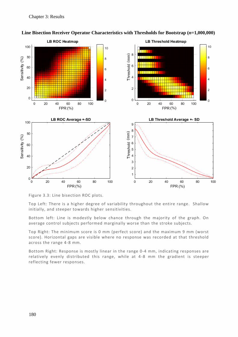
Chapter 3: Results
180
Line Bisection Receiver Operator Characteristics with Thresholds for Bootstrap (n=1,000,000)
Figure 3.3: Line bisection ROC plots.
Top Left: There is a higher degree of variability throughout the entire range. Shallow initially, and steeper towards higher sensitivities.
Bottom left: Line is modestly below chance through the majority of the graph. On average control subjects performed marginally worse than the stroke subjects.
Top Right: The minimum score is 0 mm (perfect score) and the maximum 9 mm (worst score). Horizontal gaps are visible where no response was recorded at that threshold across the range 4-8 mm.
Bottom Right: Response is mostly linear in t he range 0-4 mm, indicating responses are relatively evenly distributed this range, while at 4 -8 mm the gradient is steeper reflecting fewer responses.
(%)
(%)
(mm
) (m
m)
(%)
(%)
(%)
(%)
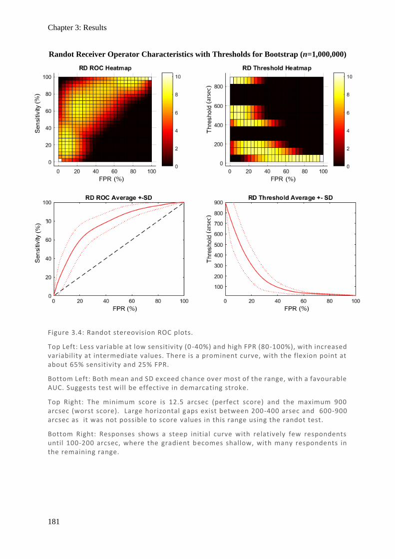
Chapter 3: Results
181
Figure 3.4: Randot stereovision ROC plots.
Top Left: Less variable at low sensitivity (0 -40%) and high FPR (80-100%), with increased variability at intermediate values. There is a prominent curve, with the flexion point at about 65% sensitivity and 25% FPR.
Bottom Left: Both mean and SD exceed chance over most of the range, with a favourable AUC. Suggests test will be effective in demarcating stroke.
Top Right: The minimum score is 12.5 arcsec (perfect score) and the maximum 900 arcsec (worst score). Large horizontal gaps exist between 200-400 arsec and 600-900 arcsec as it was not possible to score values in this range using the randot test.
Bottom Right: Responses shows a steep initial curve with relatively few respondents until 100-200 arcsec, where the gradient becomes shallow, with many respondents in the remaining range.
Randot Receiver Operator Characteristics with Thresholds for Bootstrap (n=1,000,000)
(%)
(%)
(ars
ec)
(ars
ec)
(%)
(%)
(%)
(%)
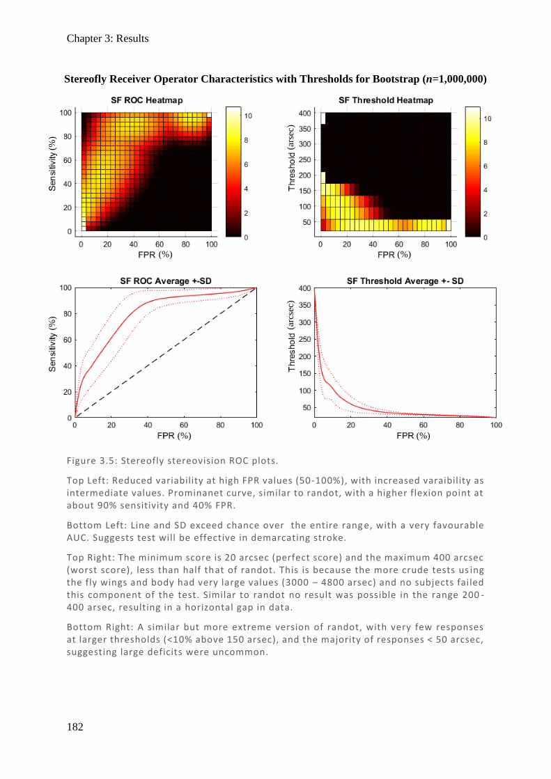
Chapter 3: Results
182
Figure 3.5: Stereofly stereovision ROC plots.
Top Left: Reduced variability at high FPR values (50-100%), with increased varaibility as intermediate values. Prominanet curve, similar to randot, with a higher flexion point at about 90% sensitivity and 40% FPR.
Bottom Left: Line and SD exceed chance over the entire rang e, with a very favourable AUC. Suggests test will be effective in demarcating stroke.
Top Right: The minimum score is 20 arcsec (perfect score) and the maximum 400 arcsec (worst score), less than half that of randot. This is because the more crude tests us ing the fly wings and body had very large values (3000 – 4800 arsec) and no subjects failed this component of the test. Similar to randot no result was possible in the range 200 -400 arsec, resulting in a horizontal gap in data.
Bottom Right: A similar but more extreme version of randot, with very few responses at larger thresholds (<10% above 150 arsec), and the majority of responses < 50 arcsec, suggesting large deficits were uncommon.
Stereofly Receiver Operator Characteristics with Thresholds for Bootstrap (n=1,000,000)
(%)
(%)
(ars
ec)
(arc
sec)
(%)
(%)
(%)
(%)
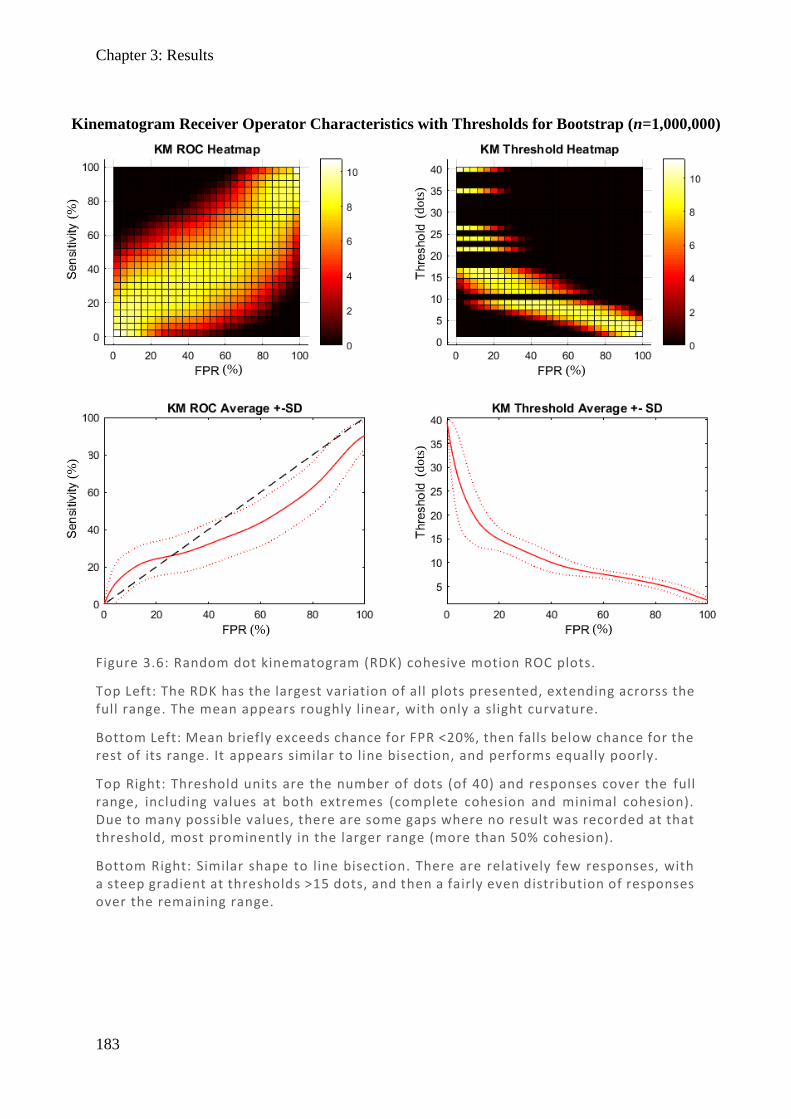
Chapter 3: Results
183
Figure 3.6: Random dot kinematogram (RDK) cohesive motion ROC plots.
Top Left: The RDK has the largest variation of all plots presented, extending acrorss the full range. The mean appears roughly linear, with only a slight curvature.
Bottom Left: Mean briefly exceeds chance for FPR <20%, then falls below chance for the rest of its range. It appears similar to line bisection, and performs equally poorly.
Top Right: Threshold units are the number of dots (of 40) and responses cover the full range, including values at both extremes (complete cohesion and minimal cohesion). Due to many possible values, there are some gaps where no result was recorded at that threshold, most prominently in the larger range (more than 50% cohesion).
Bottom Right: Similar shape to line bisection. There are relatively few responses, with a steep gradient at thresholds >15 dots, and then a fairly even distribution of responses over the remaining range.
(%)
(%)
(do
ts)
(do
ts)
(%)
(%)
(%)
(%)
Kinematogram Receiver Operator Characteristics with Thresholds for Bootstrap (n=1,000,000)
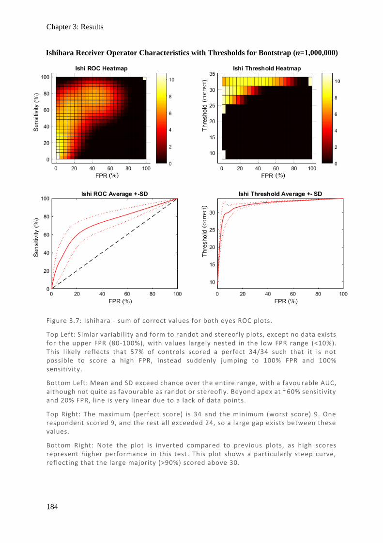
Chapter 3: Results
184
Figure 3.7: Ishihara - sum of correct values for both eyes ROC plots.
Top Left: Simlar variability and form to randot and stereofly plots, except no data exists for the upper FPR (80-100%), with values largely nested in the low FPR range (<10%). This likely reflects that 57% of controls scored a perfect 34/34 such that it is not possible to score a high FPR, instead suddenly jumping to 100% FPR and 100% sensitivity.
Bottom Left: Mean and SD exceed chance over the entire range, with a favou rable AUC, although not quite as favourable as randot or stereofly. Beyond apex at ~60% sensitivity and 20% FPR, line is very linear due to a lack of data points.
Top Right: The maximum (perfect score) is 34 and the minimum (worst score) 9. One respondent scored 9, and the rest all exceeded 24, so a large gap exists between these values.
Bottom Right: Note the plot is inverted compared to previous plots, as high scores represent higher performance in this test. This plot shows a particularly steep curve, reflecting that the large majority (>90%) scored above 30.
Ishihara Receiver Operator Characteristics with Thresholds for Bootstrap (n=1,000,000)
(%)
(%)
(co
rrec
t)
(co
rrec
t)
(%)
(%)
(%)
(%)
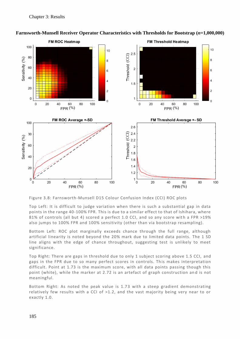
Chapter 3: Results
185
Figure 3.8: Farnsworth-Munsell D15 Colour Confusion Index (CCI) ROC plots
Top Left: It is difficult to judge variation when there is such a substantial gap in data points in the range 40-100% FPR. This is due to a similar effect to that of Ishihara, where 81% of controls (all but 4) scored a perfect 1.0 CCI, and so any score wit h a FPR >19% also jumps to 100% FPR and 100% sensitivity (other than via bootstrap resampling).
Bottom Left: ROC plot marginally exceeds chance through the full range, although artificial linearity is noted beyond the 20% mark due to limited data points. The 1 SD line aligns with the edge of chance throughout, suggesting test is unlikely to meet significance.
Top Right: There are gaps in threshold due to only 1 subject scoring above 1.5 CCI, and gaps in the FPR due to so many perfect scores in controls. Th is makes interpretation difficult. Point at 1.73 is the maximum score, with all data points passing though this point (white), while the marker at 2.72 is an artefact of graph construction an d is not meaningful.
Bottom Right: As noted the peak value is 1.7 3 with a steep gradient demonstrating relatively few results with a CCI of >1.2, and the vast majority being very near to or exactly 1.0.
Farnsworth-Munsell Receiver Operator Characteristics with Thresholds for Bootstrap (n=1,000,000)
(%)
(%)
(CC
I)
(CC
I)
(%)
(%)
(%)
(%)
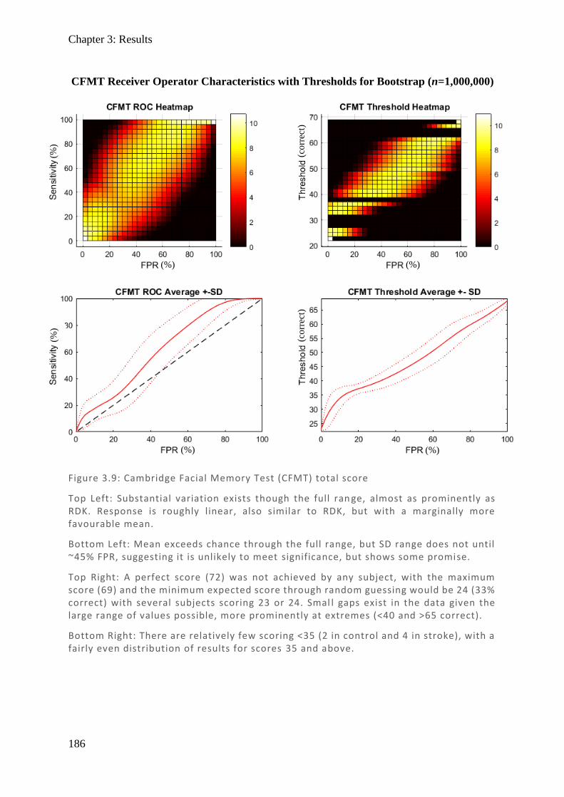
Chapter 3: Results
186
Figure 3.9: Cambridge Facial Memory Test (CFMT) total score
Top Left: Substantial variation exists though the full ran ge, almost as prominently as RDK. Response is roughly linear, also similar to RDK, but with a marginally more favourable mean.
Bottom Left: Mean exceeds chance through the full range, but SD range does not until ~45% FPR, suggesting it is unlikely to meet significance, but shows some promise.
Top Right: A perfect score (72) was not achieved by any subject, with the maximum score (69) and the minimum expected score through random guessing would be 24 (33% correct) with several subjects scoring 23 or 24. Smal l gaps exist in the data given the large range of values possible, more prominently at extremes (<40 and >65 correct).
Bottom Right: There are relatively few scoring <35 (2 in control and 4 in stroke), with a fairly even distribution of results for scores 35 and above.
CFMT Receiver Operator Characteristics with Thresholds for Bootstrap (n=1,000,000)
(%)
(%)
(co
rrec
t)
(co
rrec
t)
(%)
(%)
(%)
(%)
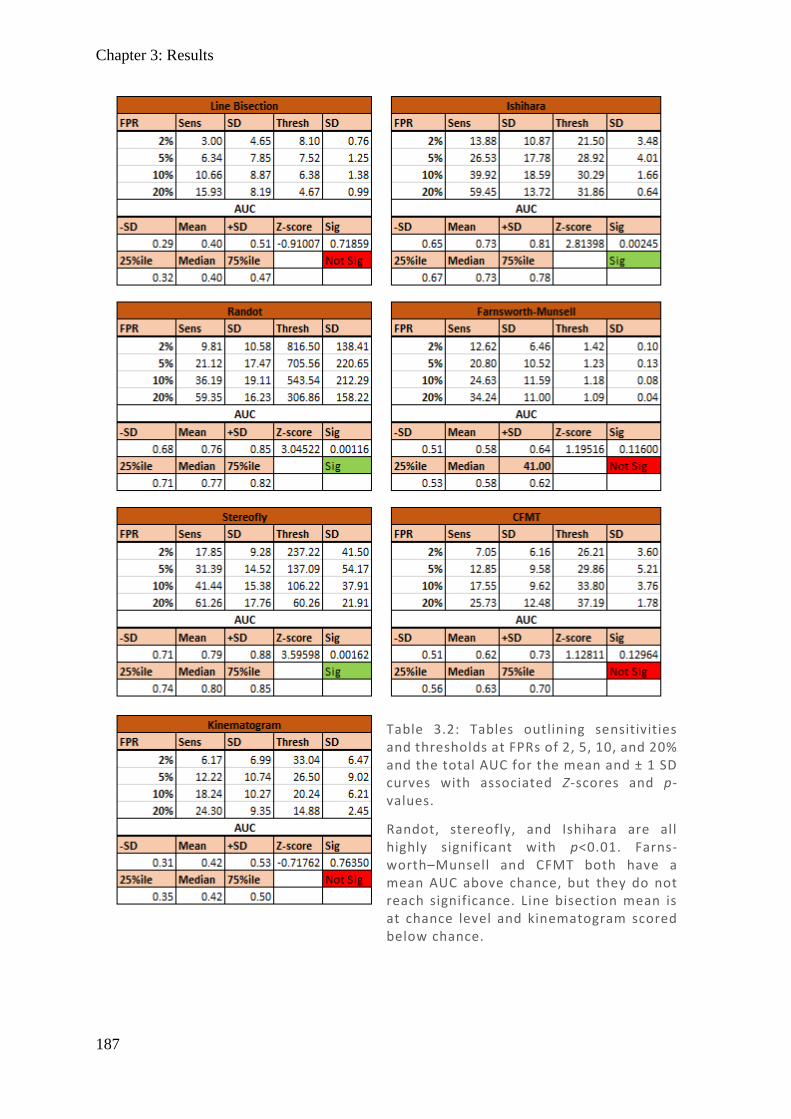
Chapter 3: Results
187
Table 3.2: Tables outlining sensitivities and thresholds at FPRs of 2, 5, 10, and 20% and the total AUC for the mean and ± 1 SD curves with associated Z-scores and p-values.
Randot, stereofly, and Ishihara are all highly significant with p<0.01. Farns-worth–Munsell and CFMT both have a mean AUC above chance, but they do not reach significance. Line bisection mean is at chance level and kinematogram scored below chance.
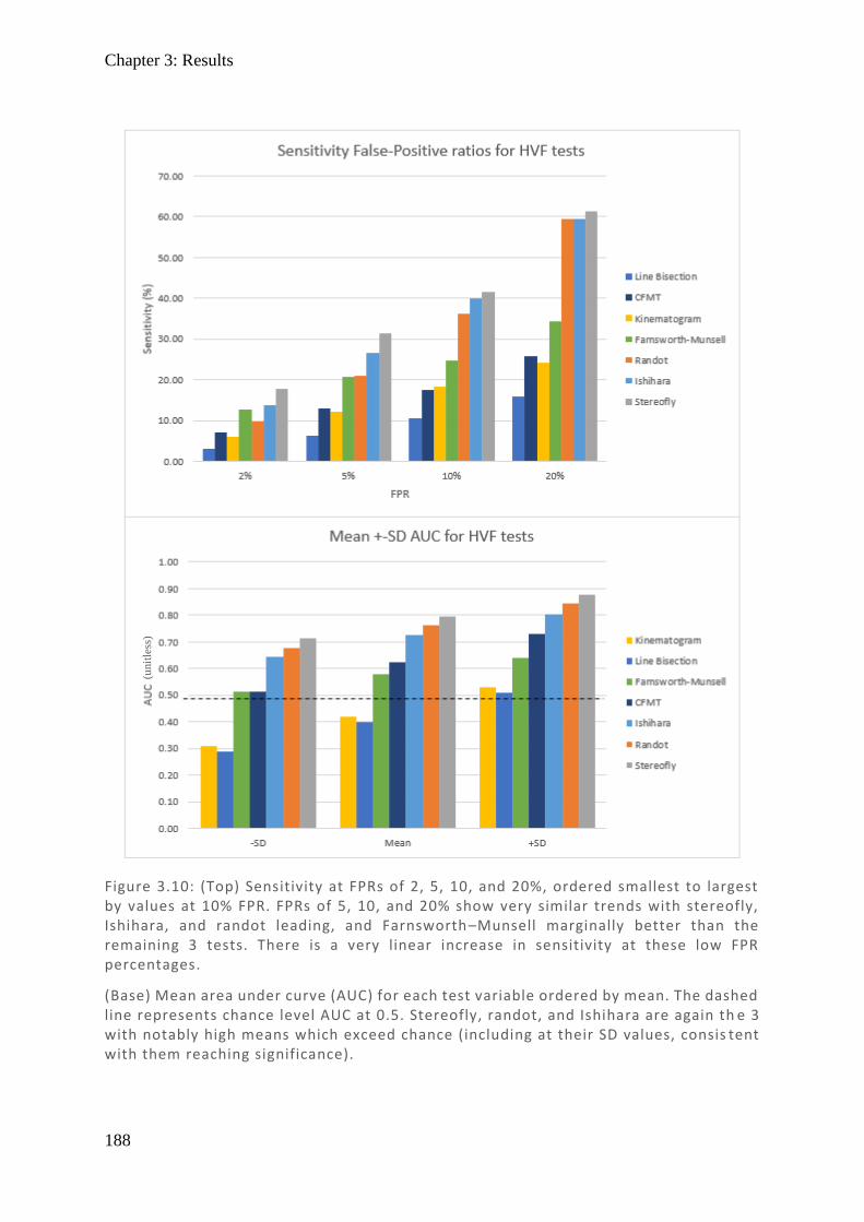
Chapter 3: Results
188
(%)
Figure 3.10: (Top) Sensitivity at FPRs of 2, 5, 10, and 20%, ordered smallest to largest by values at 10% FPR. FPRs of 5, 10, and 20% show very similar trends with stereofly, Ishihara, and randot leading, and Farnsworth–Munsell marginally better than the remaining 3 tests. There is a very linear increase in sensitivity at these low FPR percentages.
(Base) Mean area under curve (AUC) for each test variable ordered by mean. The dashed line represents chance level AUC at 0.5. Stereofly, randot, and Ishihara are again th e 3 with notably high means which exceed chance (including at their SD values, consis tent with them reaching significance).
(unit
less
)
Chapter 3: Results
189
The tests with the largest AUC were randot, stereofly, and Ishihara, which show clearly
significant responses, while FM and CFMT approach significance, and LB and KM appear at
or below chance (see Table 3.2). To confirm significance of indeterminate variables, the mean
and SD for AUC were calculated to provide Z-scores and p-values in Table 3.2 and were
graphed in Figure 3.10, highlighting that the lower SD for CFMT and FM was marginally
above chance, but that they were not significant at the 5% level.
In order to better compare these tests over a clinically useful range, the sensitivities and
thresholds for FPR values of 2%, 5%, 10% and 20% were also produced in Table 3.2 and
graphed in Figure 3.10. While overall the same three tests are highlighted as most effective –
SF, RD, and Is – at 2–5% FPR levels FM performs equal to or better than RD. This is important
given that 5% is a commonly used threshold for FPR in psychophysical testing, so FM should
therefore also be considered a useful measure. This then highlights that the two stereoscopic
measures (SF and RD) and the two colour measures (Is and FM) appear to be the most useful
tests and that stereopsis and colour are the domains most worth testing post-stroke.
3.4.2. Principal components
Having produced ROC plots which highlight which tests appear effective in detecting stroke,
we wanted to determine if these are independent measures or if some of these tests correlate
and are measuring only a single underlying measure. In order to clarify this, a principal
component analysis (PCA) was done on the seven summary variables generated from the
testing panel, with the following abbreviations: line bisection (LB), Ishihara (Is), Farnsworth–
Munsell (FM), CFMT (Ct), randot (RD), stereofly (SF), and kinematogram (Km). Principal
curves were generated from data from stroke and control subjects only.
3.4.2.1. Scree plot: selecting number of factors

Chapter 3: Results
190
The first step in this analysis was to determine how many components should be considered,
which may be observed from the scree plot in Figure 3.11. This shows how much of the total
variance is accounted for by each variable, ordered from most to least (red), and their
cumulative variance (green). In PCA, three common practices are used in determining the
number of components to include (Tabachnick, 1996):
1. The total number of variables ≥1 [in this case three];
2. The point at which a curve begins to level off [in this case two];
3. When a suitable amount of total variance has been explained [unclear].
We therefore conclude that two or three components was an appropriate number and completed
the analysis with both two factors and three factors, with the three-factor analysis figures
omitted due to gross similarity to the two-factor analysis.
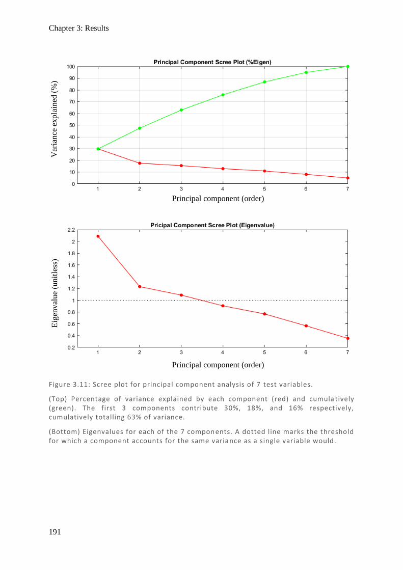
Chapter 3: Results
191
Figure 3.11: Scree plot for principal component analysis of 7 test variables.
(Top) Percentage of variance explained by each component (red) and cumula tively (green). The first 3 components contribute 30%, 18%, and 16% respectively, cumulatively totalling 63% of variance.
(Bottom) Eigenvalues for each of the 7 components. A dotted line marks the threshold for which a component accounts for the same varia nce as a single variable would.
Var
iance
expla
ined
(%
) E
igen
val
ue
(unit
less
)
Principal component (order)
Principal component (order)
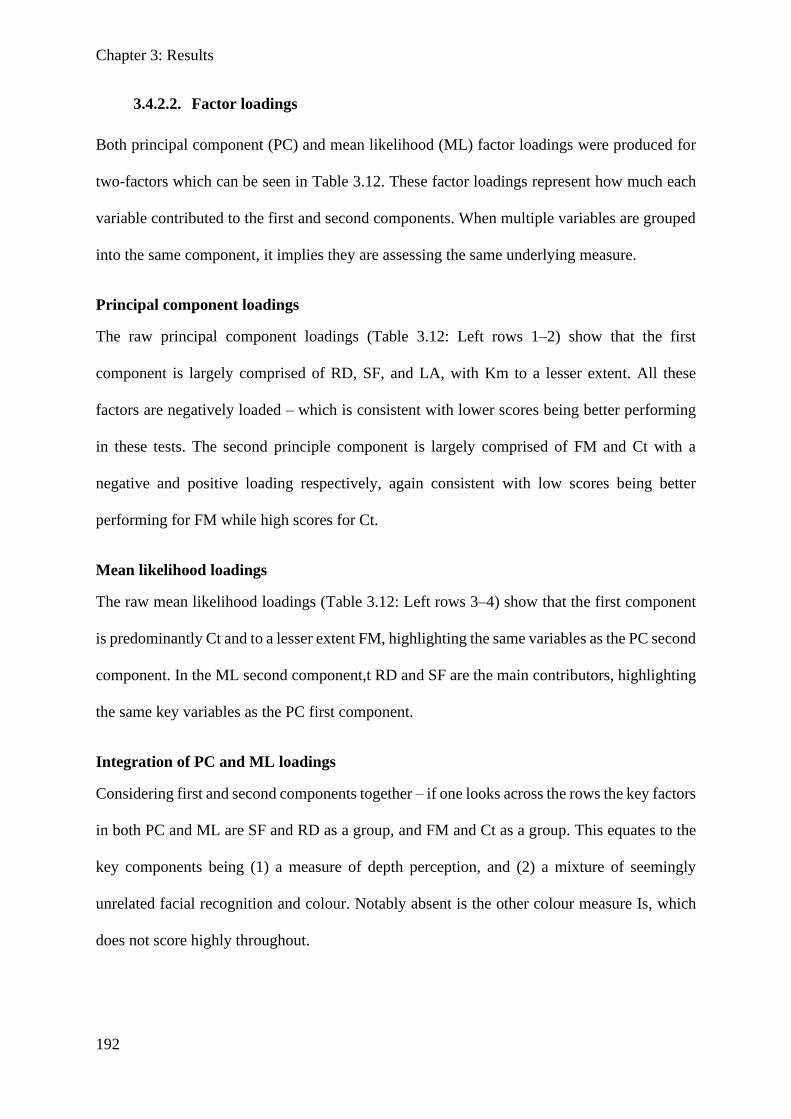
Chapter 3: Results
192
3.4.2.2. Factor loadings
Both principal component (PC) and mean likelihood (ML) factor loadings were produced for
two-factors which can be seen in Table 3.12. These factor loadings represent how much each
variable contributed to the first and second components. When multiple variables are grouped
into the same component, it implies they are assessing the same underlying measure.
Principal component loadings
The raw principal component loadings (Table 3.12: Left rows 1–2) show that the first
component is largely comprised of RD, SF, and LA, with Km to a lesser extent. All these
factors are negatively loaded – which is consistent with lower scores being better performing
in these tests. The second principle component is largely comprised of FM and Ct with a
negative and positive loading respectively, again consistent with low scores being better
performing for FM while high scores for Ct.
Mean likelihood loadings
The raw mean likelihood loadings (Table 3.12: Left rows 3–4) show that the first component
is predominantly Ct and to a lesser extent FM, highlighting the same variables as the PC second
component. In the ML second component,t RD and SF are the main contributors, highlighting
the same key variables as the PC first component.
Integration of PC and ML loadings
Considering first and second components together – if one looks across the rows the key factors
in both PC and ML are SF and RD as a group, and FM and Ct as a group. This equates to the
key components being (1) a measure of depth perception, and (2) a mixture of seemingly
unrelated facial recognition and colour. Notably absent is the other colour measure Is, which
does not score highly throughout.

Chapter 3: Results
193
Communalities
Both principal component and mean likelihood communalities were produced for the two
factors (Figure 3.13). These represent how well each variable is explained by the two-factor
model.
Principal component communalities
The best explained variables with >50% communalities were RD (70%), Ct (61%), FM (59%),
SF (58%), and LA (53%). Km and Is are poorly explained with scores of 25% and 7%
respectively.
Mean likelihood communalities
The best explained variables with >50% communalities were RD (89%) and Ct (85%) with
very high scores exceeding those in PC. However, the other variables were more poorly
explained with SF (44%), FM (18%), and all other variables <10%.
Integrating PC and ML communalities
Table 3.12: Principal component and mean likelihood rotated loadings for the first and second components. (Left) Raw weighted loadings; (Right) Absolute values of the weighted loadings to more clearly demonstrate magnitude of contribution. The table is colour-coded so that larger weightings are more red while smaller ones a re more white. Variables are ordered descending by first principal component.
Principal Component (PC) and Mean Likelihood (ML) rotated loandings
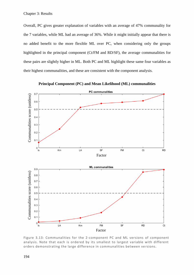
Chapter 3: Results
194
Overall, PC gives greater explanation of variables with an average of 47% communality for
the 7 variables, while ML had an average of 36%. While it might initially appear that there is
no added benefit to the more flexible ML over PC, when considering only the groups
highlighted in the principal component (Ct/FM and RD/SF), the average communalities for
these pairs are slightly higher in ML. Both PC and ML highlight these same four variables as
their highest communalities, and these are consistent with the component analysis.
Figure 3.13: Communalities for the 2-component PC and ML versions of component analysis. Note that each is ordered by its smallest to largest variable with different orders demonstrating the large difference in communalities between ve rsions.
Principal Component (PC) and Mean Likelihood (ML) communalities
Factor
Factor
Com
munal
itie
s sc
ore
(unit
less
) C
om
munal
itie
s sc
ore
(unit
less
)
Chapter 3: Discussion
195
3.5. Discussion
This study examined domains of higher visual function loss not routinely tested in clinical
practice: stereovision (stereofly, randot), colour vision (Ishihara, Farnsworth–Munsell), facial
recognition (CFMT), motion perception (kinematogram), and visual neglect (line bisection).
Each test was analysed with receiver operator characteristics (ROC) plots of sensitivity (Sens)
against false positive ratio (FPR), followed by principal component analysis using both
principal component (PC) and mean likelihood (ML) approaches.
ROC plots suggested stereovision and colour as the more useful tests, with stereofly, randot,
Ishihara, and Farnsworth–Munsell (FM) being the tests with the highest sensitivity at
reasonable FPR values (2%, 5%, 10%, and 20%). When considering the entire graph, the total
AUC was highly significant p<0.01 in stereofly, randot, and Ishihara. Although both CFMT
and FM also had their AUC means modestly exceeding chance and approaching significance,
they were non-significant. The worst performing tests – line bisection and kinematogram – had
AUC values which were below chance. Collectively this demonstrates that stereovision and
colour were the most useful measures in distinguishing between stroke and control populations.
Comparing the top scoring tests, stereofly appeared to have marginally better sensitivity and
marginally larger AUC compared to its counterpart randot. While Ishihara had marginally
lower AUC compared to both stereofly and randot, it did manage to out-perform randot in
sensitivity at FPR <20%. This is important given that psychophysical tests typically use a FPR
of 5% as an appropriate threshold to demarcate between normal and abnormal (a level which
equates to the lowest scoring 5% of the general population).
For colour vision, Ishihara has consistently higher sensitivity and a larger significant AUC,
while Farnsworth–Munsell did not reach significance. This is unexpected given that the
Ishihara test is largely designed to identify red–green colour defects, while Farnsworth–
Chapter 3: Discussion
196
Munsell is considered an unbiased test of the full colour range. However, it has been
demonstrated that those with cerebral achromatopsia perform randomly on the FM 100-hue
test and Ishihara at normal reading distance (Cowey et al., 2008). Given that the large bulk of
Ishihara responses were not random, but instead were marginally decreased or normal, if a
colour deficit is present it is likely to be quite subtle. Therefore using the D15 set (the smaller
15-hue subset of the 100-hue set) which is designed for very crude deficits may not have been
as effective as using the larger FM100 set (Bassi et al., 1993; Lopez et al., 2000), with more
subtle differences between wells, and so including FM100 in future testing may be worthwhile.
CFMT ROC plots were modestly above chance, but still did not achieve significance, which
was surprising given that the principal component analysis highlighted it as very important in
both PC and ML factors. CFMT is known to have a substantial age effect (Bowles et al., 2009)
and given that many of our test group were in the older range, this would have reduced the
ability to demarcate between controls and stroke groups; in other words it is possible that with
a younger group CFMT might achieve significance. Using the Australian version of the CFMT
on our Australian subjects would eliminate racial bias demonstrated between countries (Bowles
et al., 2009; McKone et al., 2011; McKone et al., 2017), and may allow higher scores in the
control group, thereby reducing false positive scores and increasing AUC. The other approach
would be to expand the dynamic range by lowering the expected outcome from random
guessing. Currently in a 3-way forced choice, 33% of answers are correct even when the subject
is guessing. This results in many of the older population, who have lower scores, falling below
chance level. If the test were modified to a 5-way force choice, then each correct answer would
have more meaning, and the expected outcome would drop to 20%, perhaps providing some
additional range which is needed to test elderly subjects.
Regarding the non-significance of KM, another study focusing on motion detection did provide
some evidence that occipito–parietal stroke may result in reduced sensitivity to coherence,
Chapter 3: Discussion
197
although occipital–temporal and frontal did not (Vaina et al., 2010). The lack of significance
for LB was not unexpected given that the design of the study required that patients had
recovered for at least 3 months and that visual neglect typically resolves within this timeframe
(Ijaola & Kausar, 2009; Ali et al., 2013).
Principal component scree plots were produced to help define the appropriate number of
components to include. It was clear that the first component eigenvalue (2.09) was notably
larger than the other components – and almost double that of the second (1.23) or third (1.09)
components, which were only marginally above the threshold of 1. One approach to selecting
factors is taking the first point where values begin to plateau (two values), and the other
approach is eigenvalues ≥1 (three values); both were explored, although for ease of
interpretation only the two-component results were presented. In the two-factor analysis, one
factor appeared to be stereovision including RD and SF, while the other grouped together
colour and facial recognition (FM and Ct). Addition of a third component produced similar
relationships as with two components: RD and SF and FM and Ct were both grouped together
with the new addition of Km and Is as the new component in PC, while Km alone in the ML
components. Given the comparatively low eigenvalue for the third component – near the
threshold of 1, and the below the chance AUC for the ROC plot of Km – this may be a result
of over-analysis of a small data set and is unlikely to be meaningful. It is also noted that PC
and ML are better used for large populations, and with a relatively small subject pool, collection
of a larger data set may allow clearer results from this type of analysis.
Through all ROC and PCA plots, stereovision was a key factor. In considering potential
confounders, the effectiveness of stereovision could quite reasonably be explained by there
being a greater burden of blurry vision in the stroke population (Rowe et al., 2009) and that
blurry vision directly affects the ability to distinguish fine stereovision. This potential
relationship was investigated by assessing best corrected visual acuity (BCVA) from the worst

Chapter 3: Discussion
198
eye – given that stereoscopic vision relies on a difference between the eyes and should therefore
be limited by the eye with the lowest BCVA. A scatter plot of worst eye BCVA in both stroke
and controls combined against stereofly and randot produced somewhat linear trendlines with
poor to moderate R-values. This suggests that VA may explain a component but not all the
sensitivity noted on ROC curves. Interestingly, those with cerebral achromatopsia have been
demonstrated as able to discern colour differences when colours are abutting by edge detection,
but not when spaced (Heywood et al., 1991) so that when Ishihara is viewed at >2 m or with
blur, they may become discernible (Cowey et al., 2008). Given that blurry vision may not only
affect stereovision, but also the effectiveness of Ishihara, it is essential that any correctable
acuity be done prior to testing.
Other than stereovision, colour appeared to be affected with Ishihara being significant in ROC
plots, and FM being highlighted in conjunction with CFMT in principal component analysis.
It was initially surprising that the two colour measures were not grouped together, but rather
that FM was paired with CFMT. While colour certainly plays a role in facial identification, the
CFMT itself is achromatic and so any colour deficit would not put them at disadvantage in
facial recognition. However, in a study looking at acquired prosopagnosia, 6 of the 12 subjects
also had dyschromatopsia (Moroz et al., 2016), with a suggestion that this relates to damage to
the fusiform gyri, consistent with PET and MRI imaging of achromatopsic patients (Lueck et
al., 1989; Heywood et al., 1991; Bartolomeo et al., 2014). In other words, facial recognition
and colour perception may not be functionally related, but rather in structurally adjacent
regions on the ventral surface of the brain, so that damage to one commonly results in damage
to the other. Establishment of a plausible explanation for this linkage certain strengthens the
case that these measures are true deficits arising from stroke lesions.
Overall there is good evidence that stereovision is the most useful domain measured, with
stereofly being the test of choice based on AUC and sensitivities at low FPR. Stereofly was

Chapter 3: Discussion
199
also subjectively a better test to measure patients since instructions were more easily
understood than in randot, where the image with background noise appeared to confuse some
participants. Despite this, randot also performed well overall, with only marginally less AUC
and sensitivities, and the principal component analysis suggests they are indeed measuring the
same thing, which is reassuring. It may be appropriate in further studies to assess ocular
alignment in order to ascertain whether stereoacuity is centrally or peripherally impaired,
towards providing either intervention or harm minimisation. Colour vision is the other measure
with potential utility, particularly the Ishihara, which performed well in AUC and sensitivities.
It quite substantially beat the other colour test (Farnsworth–Munsell) and they were not
grouped together highly in the principal component analysis. Using the ROC 5% FPR as
representative of how common deficits might be expected to be in the stroke population, the
stereovision deficit appeared to be 20–30%, depending on the test used, and colour vision
deficit of 20–25%, again depending on the test used. With the short test duration of these
measures, it may be possible to further expand or combine tests to provide higher sensitivities
– especially in the colour domain, where tests appeared to be measuring different things (noting
they were not grouped together in principal components). Deficits in colour were not
substantial in most instances, and it should be carefully weighed up if testing is necessary –
given there is very limited capacity to treat, and it is unlikely to cause significant morbidity.
Stereovision deficits on the other hand were often relatively severe, with many participants
being unable to detect the crudest stimuli. Given that there appears to be a weak relationship
between BCVA and stereovision, it is hard to say how much of these deficits are blur and how
much is actual stereoscopic deficit. However, whether through primary damage or through
secondary effects of lowered visual acuity, it has the potential to be clinically meaningful in
the context of minimising future harm (through avoiding household collisions, losing balance,
or competently driving). It may be useful to develop other tests to use in combination, given
Chapter 3: Discussion
200
that stereofly and randot largely use the same principles and do not appear to provide much
more utility when their measures are combined.
A future direction may be to include analysis of HVF loss in other forms of visual impairment,
in order to ascertain if these deficits occur as a result of true cortical damage, or merely due to
impaired quality of vision. Similarly, characterisation of stroke damage would be useful. While
MRI data was collected for the majority of stroke patients, analysis of this data has not yet been
possible. It was mentioned in the introduction that there is the potential for both functional
specialisation and distributive processing of visual percepts, so imaging studies of those with
subtle defects would be of interest in contributing to that discussion. Subsequent studies can
analyse this MRI data, and with larger numbers, correlate abnormalities with location, towards
a broader undertaking of visual processing.
3.6. Conclusion
Stereovision deficits occur relatively common in stroke patients and are associated with the
potential for intervention and harm minimisation. Both stereofly and randot are useful and
moderately effective for this purpose, with stereofly being the test of choice in terms of
sensitivity and useability. Colour vision deficits appear commonly as well, with Ishihara being
moderately effective in detecting deficits, while Farnsworth–Munsell has a limited capacity to
identify them. Deficits in colour vision do not appear substantial and may not require
intervention in many instances. This study had a small mixed stroke patient population and was
only intended as a pilot, so a larger study with more restrictive criteria on stroke patient
inclusion would be useful, with a focus on stereovision and colour likely to be most worthwhile.
It is also recommended to consider the full FM100, or a set between the D15 and FM100 with
more than 15 hues, which may provide the extra sensitivity required to make the Farnsworth–
Munsell test competitive with Ishihara and useful in identifying colour deficits.

201
References
Adams WE, Leske DA, Hatt SR & Holmes JM. (2009). Defining real change in measures of
stereoacuity. Ophthalmology 116, 281-285.
Adler P, Scally AJ & Barrett BT. (2012). Test--retest variability of randot stereoacuity
measures gathered in an unselected sample of uk primary school children. The British
journal of ophthalmology 96, 656-661.
Ali M, Hazelton C, Lyden P, Pollock A, Brady M & Collaboration V. (2013). Recovery from
poststroke visual impairment: Evidence from a clinical trials resource. Neurorehab
Neural Re 27, 133-141.
Bartolomeo P, Bachoud-Levi AC & Denes G. (1997). Preserved imagery for colours in a
patient with cerebral achromatopsia. Cortex 33, 369-378.
Bartolomeo P, Bachoud-Levi AC & Thiebaut de Schotten M. (2014). The anatomy of
cerebral achromatopsia: A reappraisal and comparison of two case reports. Cortex 56,
138-144.
Barton JJS, Sharpe JA & Raymond JE. (1996). Directional defects in pursuit and motion
perception in humans with unilateral cerebral lesions. Brain 119, 1535-1550.
Bassi CJ, Galanis JC & Hoffman J. (1993). Comparison of the farnsworth-munsell 100-hue,
the farnsworth d-15, and the lanthony d-15 desaturated color tests. Arch Ophthalmol-
Chic 111, 639-641.
Bowles DC, McKone E, Dawel A, Duchaine B, Palermo R, Schmalzl L, Rivolta D, Wilson
CE & Yovel G. (2009). Diagnosing prosopagnosia: Effects of ageing, sex, and
participant-stimulus ethnic match on the cambridge face memory test and cambridge
face perception test. Cogn Neuropsychol 26, 423-455.
Bowman KJ. (1982). A method for quantitative scoring of the farnsworth panel d-15. Acta
Ophthalmol 60, 907-916.
Carota A & Calabrese P. (2013). The achromatic 'philosophical zombie', a syndrome of
cerebral achromatopsia with color anopsognosia. Case Rep Neurol 5, 98-103.
Cherney LR & Halper AS. (2001). Unilateral visual neglect in right-hemisphere stroke: A
longitudinal study. Brain Injury 15, 585-592.

Chapter 3: References
202
Cooper SA, Joshi AC, Seenan PJ, Hadley DM, Muir KW, Leigh RJ & Metcalfe RA. (2012).
Akinetopsia: Acute presentation and evidence for persisting defects in motion vision.
J Neurol Neurosur Ps 83, 229-230.
Cowey A, Alexander I, Heywood C & Kentridge R. (2008). Pupillary responses to coloured
and contourless displays in total cerebral achromatopsia. Brain 131, 2153-2160.
Duchaine B & Nakayama K. (2006). The cambridge face memory test: Results for
neurologically intact individuals and an investigation of its validity using inverted
face stimuli and prosopagnosic participants. Neuropsychologia 44, 576-585.
Duvelleroy-Hommet C, Gillet P, Cottier JP, de Toffol B, Saudeau D, Corcia P & Autret A.
(1997). [cerebral achromatopsia without prosopagnosia, alexia, object agnosia]. Rev
Neurol (Paris) 153, 554-560.
Farnsworth D. (1947). Investigation on corrective training of color blindness. Sight Sav Rev
17, 194-200.
Fawcett SL & Birch EE. (2003). Validity of the titmus and randot circles tasks in children
with known binocular vision disorders. J Aapos 7, 333-338.
Fox CJ, Hanif HM, Iaria G, Duchaine BC & Barton JJS. (2011). Perceptual and anatomic
patterns of selective deficits in facial identity and expression processing.
Neuropsychologia 49, 3188-3200.
Furlan M & Smith AT. (2016). Global motion processing in human visual cortical areas v2
and v3. J Neurosci 36, 7314-7324.
Good GW, Schepler A & Nichols JJ. (2005). The reliability of the lanthony desaturated d-15
test. Optometry and vision science : official publication of the American Academy of
Optometry 82, 1054-1059.
Herzmann G, Danthiir V, Schacht A, Sommer W & Wilhelm O. (2008). Toward a
comprehensive test battery for face cognition: Assessment of the tasks. Behav Res
Methods 40, 840-857.
Heutink J, Brouwer WH, Kums E, Young A & Bouma A. (2012). When family looks strange
and strangers look normal: A case of impaired face perception and recognition after
stroke. Neurocase 18, 39-49.

Chapter 3: References
203
Heywood CA, Cowey A & Newcombe F. (1991). Chromatic discrimination in a cortically
colour blind observer. Eur J Neurosci 3, 802-812.
Ijaola FO & Kausar SA. (2009). Visual impairment following stroke: Do stroke patients
require vision assessment ? Age Ageing 38, 629-630.
Ishihara S. (1918). Tests for color blindness. Am J Ophthalmol 1, 457.
Johnson DD. (1992). The ishihara test: On the prevention of job discrimination. J Am Optom
Assoc 63, 352-360.
Jolliffe IT & Cadima J. (2016). Principal component analysis: A review and recent
developments. Philos Trans A Math Phys Eng Sci 374, 20150202.
Junge MRJ & Dettori JR. (2018). Roc solid: Receiver operator characteristic (roc) curves as a
foundation for better diagnostic tests. Global Spine J 8, 424-429.
Lander K, Humphreys G & Bruce V. (2004). Exploring the role of motion in prosopagnosia:
Recognizing, learning and matching faces. Neurocase 10, 462-470.
Lang N, Baudewig J, Kallenberg K, Antal A, Happe S, Dechent P & Paulus W. (2006).
Transient prosopagnosia after ischemic stroke. Neurology 66, 916-916.
Lever J, Krzywinski M & Altman N. (2017). Principal component analysis. Nature Methods
14, 641.
Lopez P, Caruso RC & Kaiser-Kupfer MI. (2000). A comparison of lanthony's desaturated 15
hue test with the farnsworth-munsell 100 hue test for the quantification of color vision
deficiencies. Invest Ophth Vis Sci 41, S356-S356.
Lu XS, Ye J, Zhou S, Lu BX & Chen XH. (2005). Unilateral spatial neglect, global
processing deficit and prosopagnosia following right hemisphere stroke: A case
report. Chinese Med J-Peking 118, 1846-1848.
Lueck CJ, Zeki S, Friston KJ, Deiber MP, Cope P, Cunningham VJ, Lammertsma AA,
Kennard C & Frackowiak RS. (1989). The colour centre in the cerebral cortex of man.
Nature 340, 386-389.
McKeefry DJ, Watson JDG, Frackowiak RSJ, Fong K & Zeki S. (1997). The activity in
human areas v1/v2, v3, and v5 during the perception of coherent and incoherent
motion. Neuroimage 5, 1-12.

Chapter 3: References
204
McKone E, Hall A, Pidcock M, Palermo R, Wilkinson RB, Rivolta D, Yovel G, Davis JM &
O'Connor KB. (2011). Face ethnicity and measurement reliability affect face
recognition performance in developmental prosopagnosia: Evidence from the
cambridge face memory test-australian. Cogn Neuropsychol 28, 109-146.
McKone E, Wan L, Robbins R, Crookes K & Liu J. (2017). Diagnosing prosopagnosia in east
asian individuals: Norms for the cambridge face memory test-chinese. Cogn
Neuropsychol 34, 253-268.
Moroz D, Corrow SL, Corrow JC, Barton ARS, Duchaine B & Barton JJS. (2016).
Localization and patterns of cerebral dyschromatopsia: A study of subjects with
prospagnosia. Neuropsychologia 89, 153-160.
Nettleman MD. (1988). Receiver operator characteristic (roc) curves. Infect Control Hosp
Epidemiol 9, 374-377.
Pagani R, Bosco G, Dalla Valle E, Capitani E & Laiacona M. (2012). The assessment of
colour perception, naming and knowledge: A new test device with a case study.
Neurol Sci 33, 801-809.
Pollock A, Hazelton C & Brady M. (2011). Visual problems after stroke: A survey of current
practice by occupational therapists working in uk stroke inpatient settings. Top Stroke
Rehabil 18, 643-651.
Rizzo M, Nawrot M & Zihl J. (1995). Motion and shape perception in cerebral akinetopsia.
Brain 118, 1105-1127.
Ross JE. (1983). Disturbance of stereoscopic vision in patients with unilateral stroke. Behav
Brain Res 7, 99-112.
Rowe F, Brand D, Jackson CA, Price A, Walker L, Harrison S, Eccleston C, Scott C,
Akerman N, Dodridge C, Howard C, Shipman T, Sperring U, MacDiarmid S &
Freeman C. (2009). Visual impairment following stroke: Do stroke patients require
vision assessment ? Age Ageing 38, 188-193.
Schaadt AK, Brandt SA, Kraft A & Kerkhoff G. (2015). Holmes and horrax (1919) revisited:
Impaired binocular fusion as a cause of "flat vision" after right parietal brain damage -
a case study. Neuropsychologia 69, 31-38.
Schaadt AK, Schmidt L, Reinhart S, Adams M, Garbacenkaite R, Leonhardt E, Kuhn C &
Kerkhoff G. (2014). Perceptual relearning of binocular fusion and stereoacuity after
brain injury. Neurorehabil Neural Repair 28, 462-471.

Chapter 3: References
205
Schow T, Harris P, Teasdale TW & Rasmussen MA. (2016). Evaluation of a four month
rehabilitation program for stroke patients with balance problems and binocular visual
dysfunction. Neurorehabilitation 38, 331-341.
Setala K & Vesti E. (1994). Acquired cerebral achromatopsia - a case-report. Neuro-
Ophthalmology 14, 31-36.
Stone A, Cooke D, Morton D & Steele M. (2019). Reliability of revised scoring methods for
the schenkenberg line bisection test with adults following stroke: Preliminary
findings. Brit J Occup Ther 82, 750-758.
Tabachnick BGF, L.S. (1996). Using multivariate statistics. Harper Collins, New York.
Vaina LM. (1994). Functional segregation of color and motion processing in the human
visual-cortex - clinical-evidence. Cereb Cortex 4, 555-572.
Vaina LM. (1995). Akinetopsia, achromatopsia and blindsight: Recent studies on perception
without awareness. Synthese 105, 253-271.
Vaina LM, Cowey A, Eskew RT, LeMay M & Kemper T. (2001). Regional cerebral
correlates of global motion perception - evidence from unilateral cerebral brain
damage. Brain 124, 310-321.
Vaina LM, Sikoglu EM, Soloviev S, LeMay M, Squatrito S, Pandiani G & Cowey A. (2010).
Functional and anatomical profile of visual motion impairments in stroke patients
correlate with fmri in normal subjects. J Neuropsychol 4, 121-145.
von Arx SW, Muri RM, Heinemann D, Hess CW & Nyffeler T. (2010). Anosognosia for
cerebral achromatopsia-a longitudinal case study. Neuropsychologia 48, 970-977.
Wilmer JB, Germine L, Chabris CF, Chatterjee G, Williams M, Loken E, Nakayama K &
Duchaine B. (2010). Human face recognition ability is specific and highly heritable.
Proc Natl Acad Sci U S A 107, 5238-5241.
Wilson B, Cockburn J & Halligan P. (1987). Development of a behavioral-test of visuospatial
neglect. Arch Phys Med Rehab 68, 98-102.
Wold S, Esbensen K & Geladi P. (1987). Principal component analysis. Chemometr Intell
Lab 2, 37-52.

Chapter 3: References
206
Zhou C, He Y & Li X. (2018). Cerebral achromatopsia secondary to ischemic stroke. Neurol
India 66, 573-575.
207
4 Chapter 4: Pupillometry – direct and consensual responses in stroke, chiasmal compression, and AION
4.1. Abstract
4.1.1. Purpose
mfPOP records both direct and consensual responses to stimuli presented concurrently to either
eye. Pictorial perimetry reports may use direct responses, consensual responses, or a
combination of the two. In order to determine which method is most appropriate, the
relationship between direct and consensual needs to be explored.
4.1.2. Methods
Scatter plots of each visual field region’s direct and consensual response amplitude were
plotted for each of the groups (stroke n = 25, pituitary n = 11, and AION n = 10) split by
nasal/temporal region with trendline and correlation coefficient (r-scores) for each to
demonstrate their relationship. Bland–Altman plots of the same were produced to highlight
their differences. Fields for each subject were produced for: direct, consensual, their difference
(Dir – Con) and their ratio (Dir / Con) the group averages are presented here to test whether
there are any spatial differences in pupillary response. Signal-to-noise ratio (SNR) plots for
direct and consensual were used for appropriate amalgamation into a single measure for
production of reports.
4.1.3. Results
Scatterplots demonstrate a high degree of correlation between direct and consensual response
in stroke, pituitary, and AION, both nasally (r-scores of 0.93, 0.88, and 0.95 respectively) and
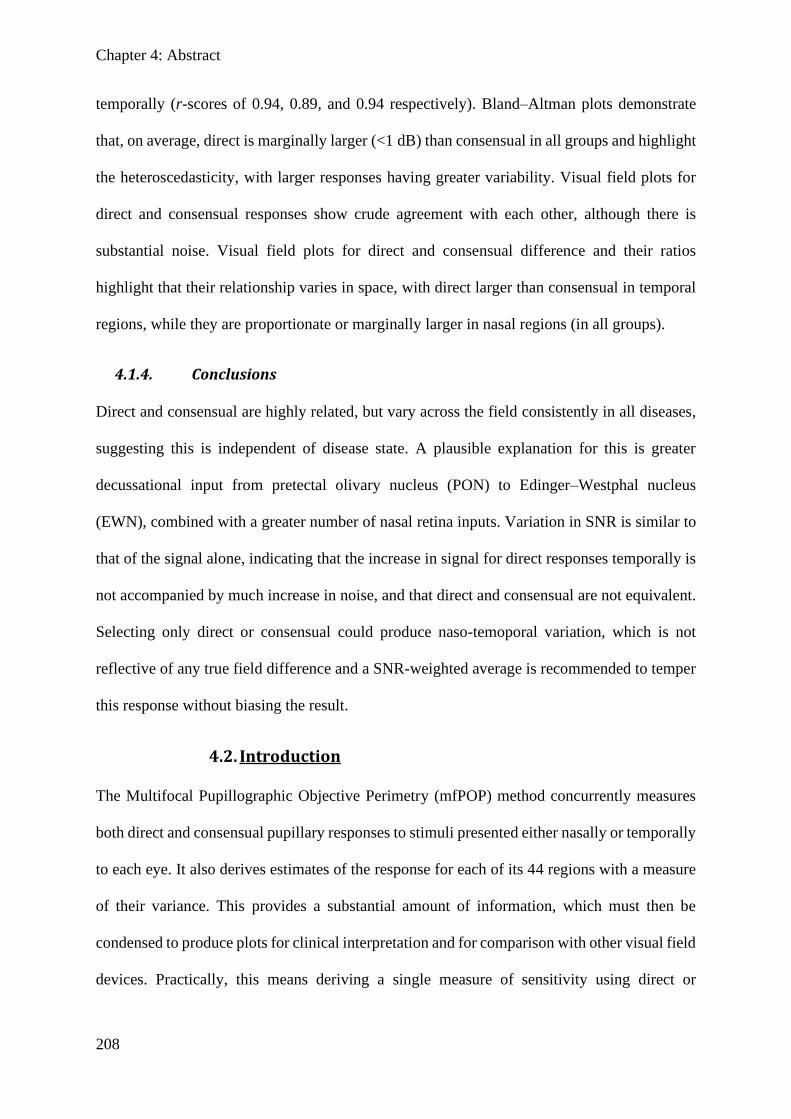
Chapter 4: Abstract
208
temporally (r-scores of 0.94, 0.89, and 0.94 respectively). Bland–Altman plots demonstrate
that, on average, direct is marginally larger (<1 dB) than consensual in all groups and highlight
the heteroscedasticity, with larger responses having greater variability. Visual field plots for
direct and consensual responses show crude agreement with each other, although there is
substantial noise. Visual field plots for direct and consensual difference and their ratios
highlight that their relationship varies in space, with direct larger than consensual in temporal
regions, while they are proportionate or marginally larger in nasal regions (in all groups).
4.1.4. Conclusions
Direct and consensual are highly related, but vary across the field consistently in all diseases,
suggesting this is independent of disease state. A plausible explanation for this is greater
decussational input from pretectal olivary nucleus (PON) to Edinger–Westphal nucleus
(EWN), combined with a greater number of nasal retina inputs. Variation in SNR is similar to
that of the signal alone, indicating that the increase in signal for direct responses temporally is
not accompanied by much increase in noise, and that direct and consensual are not equivalent.
Selecting only direct or consensual could produce naso-temoporal variation, which is not
reflective of any true field difference and a SNR-weighted average is recommended to temper
this response without biasing the result.
4.2. Introduction
The Multifocal Pupillographic Objective Perimetry (mfPOP) method concurrently measures
both direct and consensual pupillary responses to stimuli presented either nasally or temporally
to each eye. It also derives estimates of the response for each of its 44 regions with a measure
of their variance. This provides a substantial amount of information, which must then be
condensed to produce plots for clinical interpretation and for comparison with other visual field
devices. Practically, this means deriving a single measure of sensitivity using direct or
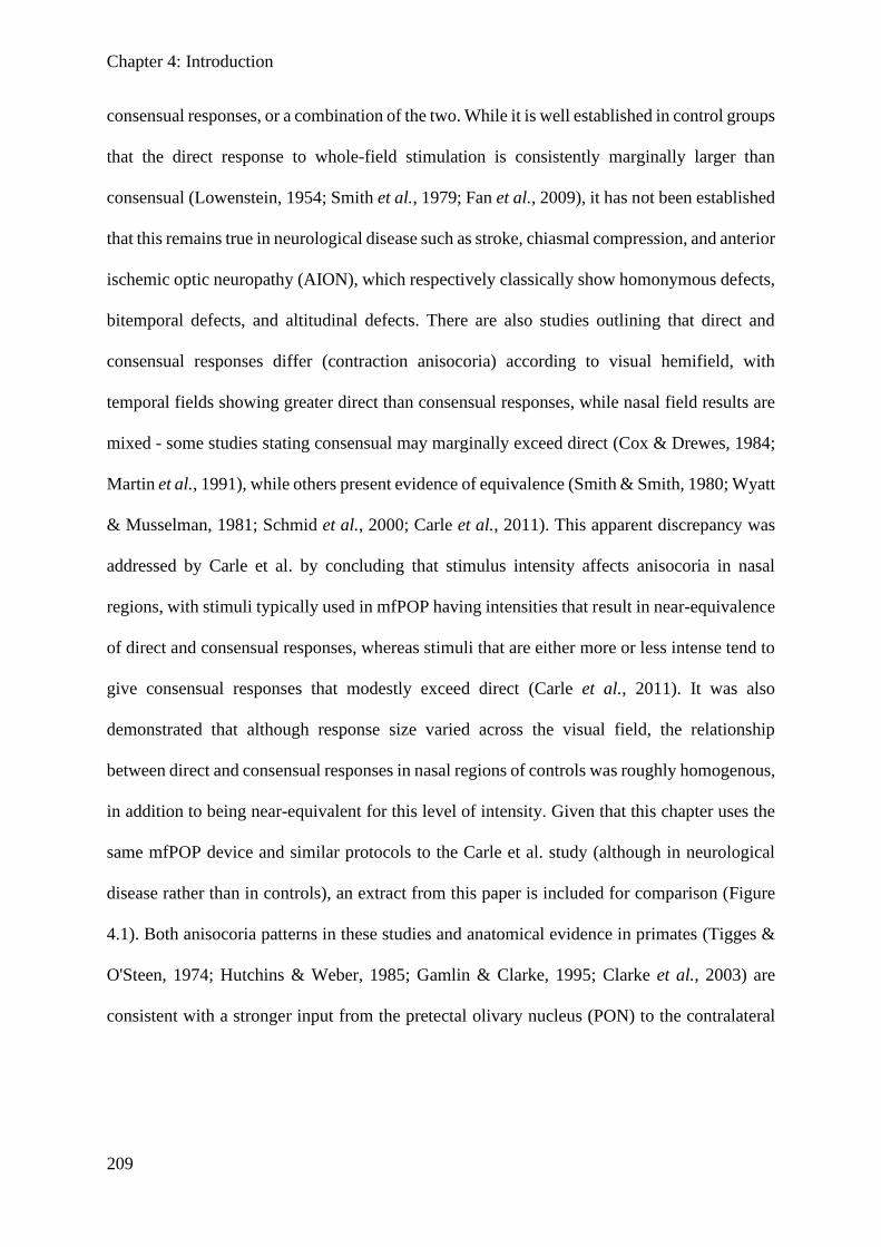
Chapter 4: Introduction
209
consensual responses, or a combination of the two. While it is well established in control groups
that the direct response to whole-field stimulation is consistently marginally larger than
consensual (Lowenstein, 1954; Smith et al., 1979; Fan et al., 2009), it has not been established
that this remains true in neurological disease such as stroke, chiasmal compression, and anterior
ischemic optic neuropathy (AION), which respectively classically show homonymous defects,
bitemporal defects, and altitudinal defects. There are also studies outlining that direct and
consensual responses differ (contraction anisocoria) according to visual hemifield, with
temporal fields showing greater direct than consensual responses, while nasal field results are
mixed - some studies stating consensual may marginally exceed direct (Cox & Drewes, 1984;
Martin et al., 1991), while others present evidence of equivalence (Smith & Smith, 1980; Wyatt
& Musselman, 1981; Schmid et al., 2000; Carle et al., 2011). This apparent discrepancy was
addressed by Carle et al. by concluding that stimulus intensity affects anisocoria in nasal
regions, with stimuli typically used in mfPOP having intensities that result in near-equivalence
of direct and consensual responses, whereas stimuli that are either more or less intense tend to
give consensual responses that modestly exceed direct (Carle et al., 2011). It was also
demonstrated that although response size varied across the visual field, the relationship
between direct and consensual responses in nasal regions of controls was roughly homogenous,
in addition to being near-equivalent for this level of intensity. Given that this chapter uses the
same mfPOP device and similar protocols to the Carle et al. study (although in neurological
disease rather than in controls), an extract from this paper is included for comparison (Figure
4.1). Both anisocoria patterns in these studies and anatomical evidence in primates (Tigges &
O'Steen, 1974; Hutchins & Weber, 1985; Gamlin & Clarke, 1995; Clarke et al., 2003) are
consistent with a stronger input from the pretectal olivary nucleus (PON) to the contralateral
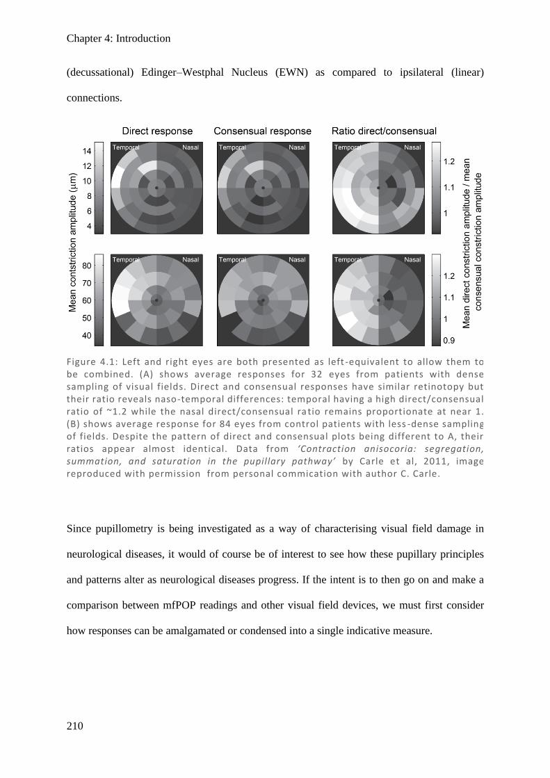
Chapter 4: Introduction
210
(decussational) Edinger–Westphal Nucleus (EWN) as compared to ipsilateral (linear)
connections.
Since pupillometry is being investigated as a way of characterising visual field damage in
neurological diseases, it would of course be of interest to see how these pupillary principles
and patterns alter as neurological diseases progress. If the intent is to then go on and make a
comparison between mfPOP readings and other visual field devices, we must first consider
how responses can be amalgamated or condensed into a single indicative measure.
Figure 4.1: Left and right eyes are both presented as left -equivalent to allow them to be combined. (A) shows average responses for 32 eyes from patients with dense sampling of visual fields. Direct and consensual responses have similar retinotopy but their ratio reveals naso-temporal differences: temporal having a high direct/consensual ratio of ~1.2 while the nasal direct/consensual ra tio remains proportionate at near 1. (B) shows average response for 84 eyes from control patients with less -dense sampling of fields. Despite the pattern of direct and consensual plots being different to A, their ratios appear almost identical. Data from ‘Contraction anisocoria: segregation, summation, and saturation in the pupillary pathway’ by Carle et al, 2011, image reproduced with permission from personal commication with author C. Carle.

Chapter 4: Results
211
4.3. Methods
4.3.1. Subjects and screening
A history of mfPOP and the reasoning for the test parameters used can be found in the
Introduction chapter (1.6.4. Multifocal methods). Full descriptions are presented in the General
Methods, including recruitment (section 2.1), screening (section 2.2), mfPOP stimuli,
procedures, and output measures (section 2.5.3). For brevity, here an overview is presented.
Subjects were recruited from multiple hospital and eye clinic sources and informed consent
was obtained. Subjects were screened for pre-existing ocular conditions, both via questionnaire
and clinical assessment and included: best corrected visual acuity of 6/24 or better, cataract
screening, intraocular pressure measurement, fundus photo, and OCT scan of posterior pole
and optic nerve head. Groups consisted of stroke (heterogenous cortical lesions) (n = 25),
chiasmal compression (n = 11), and AION (n = 10).
4.3.2. Multifocal Pupillographic Objective Perimetry (mfPOP)
Pupil diameter was assessed using mfPOP objectiveFIELD analyser (Konan Medical USA Inc,
Irvine CA) which uses rapidly presented stimuli with a fixed luminance and measures the pupil
response, obtaining data for 44 test regions extending out to 20° eccentricity in each direction.
A total of four tests were completed using mfPOP.
4.3.2.1. Testing protocol and settings
Ambient light was kept constant and the device hood acted to minimise effects of background
luminance. Lenses nearest the subject’s prescription glasses were used rounded to the nearest
3 spherical dioptres, since mfPOP is insensitive to moderate blur. Vergence was aligned at
optical infinity. Patients were instructed to maintain focus on a central marker, that they can
blink at any time but should minimise it during testing (9 × 45 s segments), instead utilising
the breaks (7 s between segments).
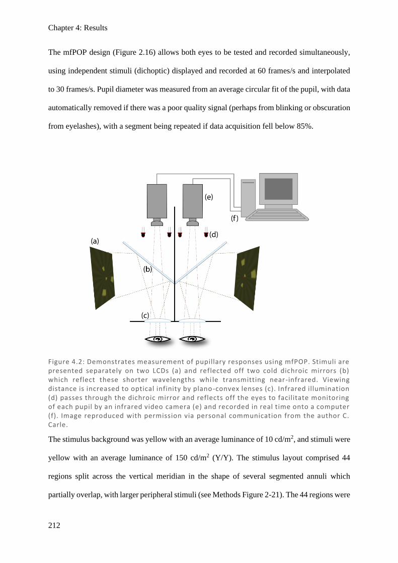
Chapter 4: Results
212
The mfPOP design (Figure 2.16) allows both eyes to be tested and recorded simultaneously,
using independent stimuli (dichoptic) displayed and recorded at 60 frames/s and interpolated
to 30 frames/s. Pupil diameter was measured from an average circular fit of the pupil, with data
automatically removed if there was a poor quality signal (perhaps from blinking or obscuration
from eyelashes), with a segment being repeated if data acquisition fell below 85%.
The stimulus background was yellow with an average luminance of 10 cd/m2, and stimuli were
yellow with an average luminance of 150 cd/m2 (Y/Y). The stimulus layout comprised 44
regions split across the vertical meridian in the shape of several segmented annuli which
partially overlap, with larger peripheral stimuli (see Methods Figure 2-21). The 44 regions were
Figure 4.2: Demonstrates measurement of pupillary responses using mfPOP. Stimuli are presented separately on two LCDs (a) and reflected off two cold dichroic mirrors (b) which reflect these shorter wavelengths whi le transmitting near-infrared. Viewing distance is increased to optical infinity by plano-convex lenses (c). Infrared illumination (d) passes through the dichroic mirror and reflects off the eyes to facilitate monitoring of each pupil by an infrared video camera (e) and recorded in real time onto a computer (f). Image reproduced with permission via personal communication from the author C. Carle.
Chapter 4: Results
213
divided into 8 sections comprising left and right eye, left and right hemifield, and odd or even
rings. Presentations were in clustered volleys (Sabeti et al., 2014), which were temporally
sparse but could be spatially near (see Methods Figure 2-22). Each volley consists of activation
of, on average, 50% of regions within a subset for 33 ms, with a 250 ms delay between the
onsets of each volley, sequentially rotating through presentations in each of 8 subsets. This
means that, in total, each region is presented on average every 4 seconds for a total of around
90 presentations throughout the total test duration of 360 seconds.
4.3.2.2. Signal extraction and processing
Following continuous collection of data during the testing period, all data was processed. The
output signal was converted into response amplitudes using a multiple linear regression method
described elsewhere (James, 2003; James et al., 2005; Ruseckaite et al., 2005). Responses were
normalised to an average diameter of 3.5 mm to account for differences in resting pupil
diameter between subjects (James et al., 2012).
Amplitudes (µm) were converted into dB units using a generalised logarithmic transform which
stabilises the variance and removes small dilations that would result in negative values
preventing dB transformation. The generalised logarithmic transform was of the form:
Glog(𝑦, 𝜆) = log (𝑦 + √𝑦2 + 𝜆2
2)
with λ set to 9 based on appropriateness to the dataset. Data was then linearly scaled to
conveniently match the HFA range. Conversion from the 44 region map of the mfPOP stimuli
to the 54-region HFA 24-2 format was done by weighting averages in accordance with their
overlap.
In this chapter both direct and consensual responses are set out separately; how they might be
combined most effectively is considered below. Testing of the Y/Y protocol was done on two
Chapter 4: Results
214
visits by each subject, and analysis of differences between visits is addressed in Chapter 6. As
it is expected that clinicians would only test a subject on a single occasion, it is important that
any method used to combine direct and consensual is appropriate to the variability present in a
single unaveraged test. For this reason, only the first test is considered in this chapter, while
other chapters average over repeats.
To investigate the relationship and similarities between direct and consensual pupillary
response for the 3 neurological diseases, simple scatter plots of direct and consensual responses
of all visual field locations from subjects within a patient-group were produced, with a
correlation coefficient (Pearson’s r) to show the trend and relationship.
Bland–Altman plots were produced to display means across direct and consensual responses
against differences between direct and consensual responses, a way of highlighting and
quantifying differences (Bland & Altman, 1999; Zaki et al., 2012; Giavarina, 2015). The
overall mean and 95% confidence intervals (defined by 1.96 SD from the mean) were used to
describe the variability between direct and consensual (on the ordinate) with respect to the base
signal (the average of direct and consensual, abscissa).
Visual field plots of pupil responses for both eyes using the 24-2 format are presented in
greyscale. Using the generalised log-transform, 0 dB represents no response (black) and
maximum response amplitudes (in the 25–30 dB range) are shown in white. Average visual
fields for each patient group were produced by taking the mean of each visual field location
across all patients for each eye. Plots of direct, consensual, their difference (Dir – Con), and
their ratio (Dir / Con) were used to investigate naso-temporal differences, with a colour scale
used such that no difference (0) is shown as white, direct exceeding consensual as increasingly
more red, and as consensual exceeding direct as increasingly more blue.
Chapter 4: Results
215
Signal-to-noise ratio (SNR) was investigated with signal represented by response amplitude
and noise by the SE of the raw amplitude. The multifocal analysis method used multiple
recorded responses (effectively one for each stimulus presentation) to measure each test point,
allowing calculation of an estimated SE for that response.
In combining SNR for each point, signal was averaged prior to dB conversion in order to allow
linear summing, while noise was averaged as the root mean square (RMS) due to conversion
of SE into variance before linear summing is possible.
All calculations and graphs were produced using Matlab version 2016B (The MathWorks, Inc.,
Natick, USA) and Microsoft Excel 2016.
4.4. Results
Figures 4.3– 4.5 show that patient groups in all three neurological groups showed highly linear
relationships between direct and consensual responses, with a high degree of correlation and
near-zero y-intercepts. In the larger range, all three also appear to have trendlines shallower
than perfect linear correlations (greater direct than consensual responses). This effect appears
most prominently in the temporal visual field test regions, while nasal test regions are closer to
the line of equivalence, especially in chiasmal compression and AION, and which become
slightly above equivalence before the majority of the data points (greater consensual than
direct). In stroke, there does not appear to be any heteroscedasticity, while in the pituitary and
AION groups there is quite definitely an increase in variability at larger responses.
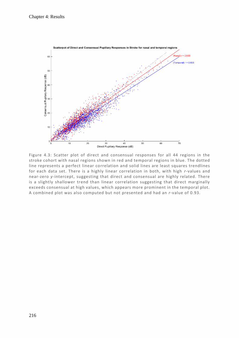
Chapter 4: Results
216
Figure 4.3: Scatter plot of direct and consensual responses for all 44 regions in the stroke cohort with nasal regions shown in red and temporal regions in blue. The dotted line represents a perfect linear correlation and solid lines are least squares trendlines for each data set. There is a highly linear correlation in both, with high r-values and near-zero y-intercept, suggesting that direct and consensual are highly related. There is a slightly shallower trend than linear correlation suggesting that direct marginally exceeds consensual at high values, which appears more prominent in the temporal plot. A combined plot was also computed but not presented and had an r-value of 0.93.
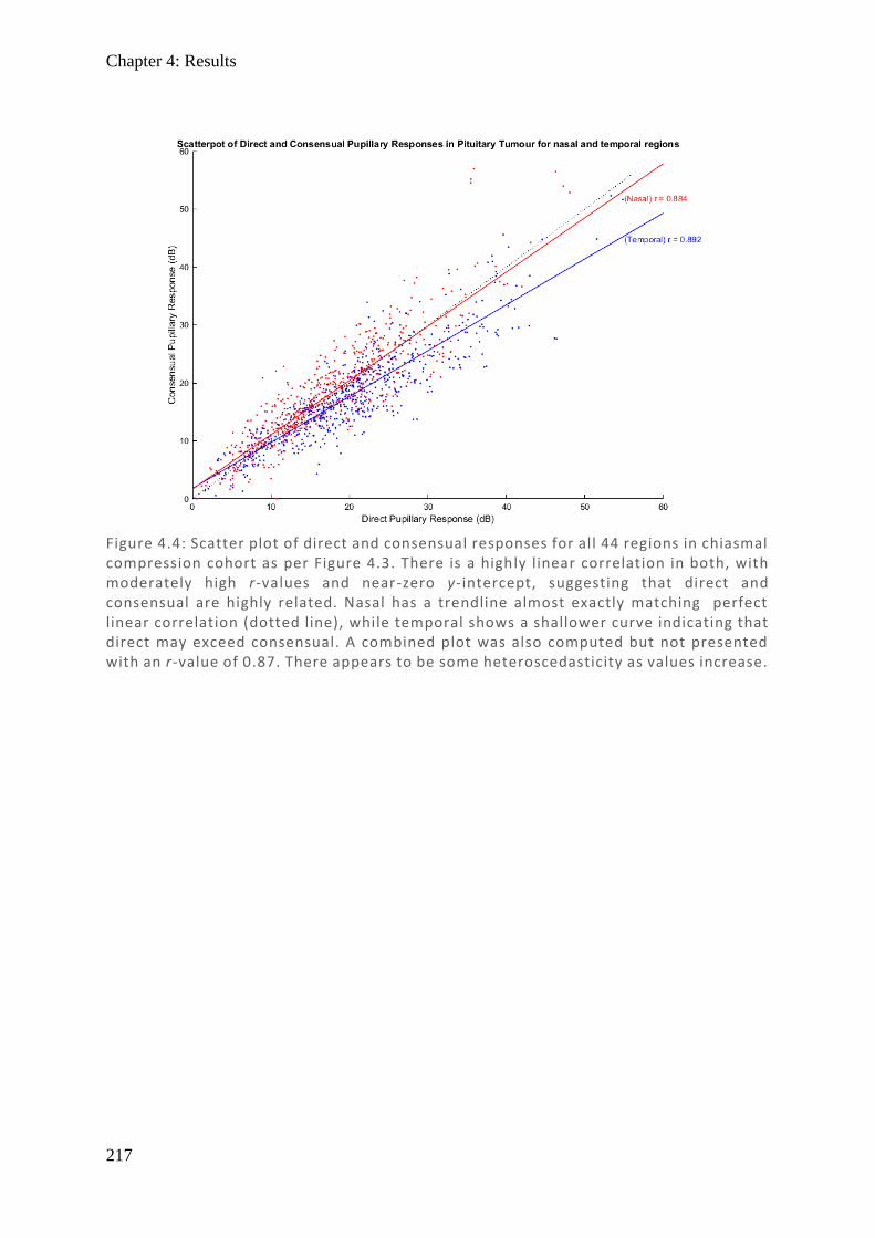
Chapter 4: Results
217
Figure 4.4: Scatter plot of direct and consensual responses for all 44 regions in chiasmal compression cohort as per Figure 4.3. There is a highly linear correlation in both, with moderately high r-values and near-zero y-intercept, suggesting that direct and consensual are highly related. Nasal has a trendline almost exactly matching perfect linear correlation (dotted line), while temporal shows a shallower curve indicating that direct may exceed consensual. A combined plot was also computed but not presented with an r-value of 0.87. There appears to be some heteroscedasticity as values increase.
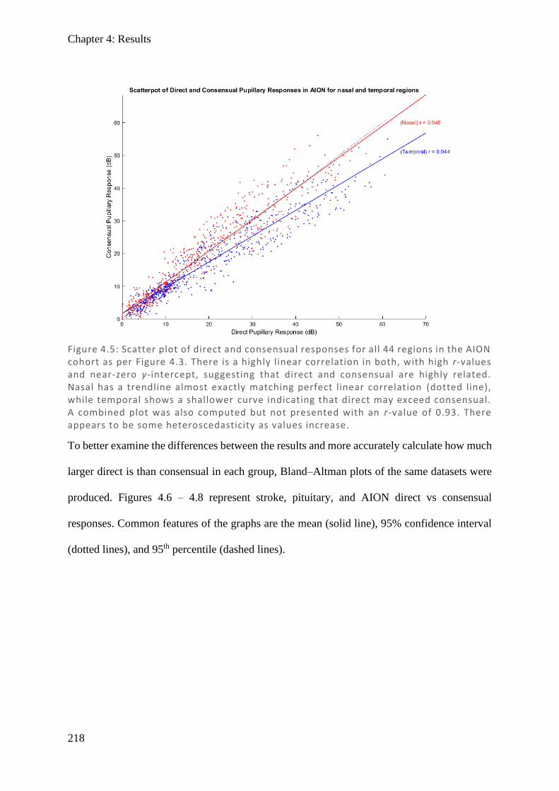
Chapter 4: Results
218
To better examine the differences between the results and more accurately calculate how much
larger direct is than consensual in each group, Bland–Altman plots of the same datasets were
produced. Figures 4.6 – 4.8 represent stroke, pituitary, and AION direct vs consensual
responses. Common features of the graphs are the mean (solid line), 95% confidence interval
(dotted lines), and 95th percentile (dashed lines).
Figure 4.5: Scatter plot of direct and consensual responses for all 44 regions in the AION cohort as per Figure 4.3. There is a highly linear correlation in both, with high r-values and near-zero y-intercept, suggesting that direct and consensual are highly related. Nasal has a trendline almost exactly matching perfect linear correlation (dotted line), while temporal shows a shallower curve indicating that direct may exceed consensual. A combined plot was also computed but not presented with an r-value of 0.93. There appears to be some heteroscedasticity as values increase.
Chapter 4: Results
219
Figures 4.6 – 4.8 demonstrate that the mean direct response is significantly larger than the mean
consensual in temporal regions of all groups by a margin of ~2 dB, while the consensual
significantly exceeded temporal in chiasmal compression and AION by <1 dB, with stroke
having a non-significant difference. There is heteroscedasticity in the AION and pituitary
groups which was notably absent in the stroke group, likely explaining why stroke has the
smallest range (maximum difference between direct and consensual). The large density of
responses in all groups were those with means <25 dB, which were most dense near zero
difference and only rarely extend beyond a 10 dB difference. With means below 25 dB,
differences of 10 dB represent a substantial amount of variation, nearly 50% of their average.
While there are certainly average linear trends in the scatter plots, the variability in Bland–
Altman analyses suggests that substantial differences remain between direct and consensual
responses, particularly at large amplitudes, which warrants further investigation. Given that
direct and consensual responses have been noted to differ systematically throughout the visual
field in control patients, that this may also be true in these conditions. To investigate this,
average visual field responses for each visual field point in each condition were generated for
direct only, consensual only, direct – consensual difference, and direct / consensual ratios,
pictorially displaying the average fields as if they were a single person’s responses. This allows
similarities and differences to be organised according to spatial location.
Graphs are displayed in 24-2 format with direct and consensual responses being in greyscale
(with the smallest average responses in black and the largest in white). Differences and ratios
are presented in a colour-scale, with no-difference or ratio of 1 being white, direct exceeding
consensual in red, and the reverse in blue. To allow comparison, direct and consensual are
presented on the same scale. Units for direct, consensual, and their difference are in dB, while
ratios are unitless. On the axes, degrees of eccentricity are displayed as a guide to relative extent
of the visual field range.
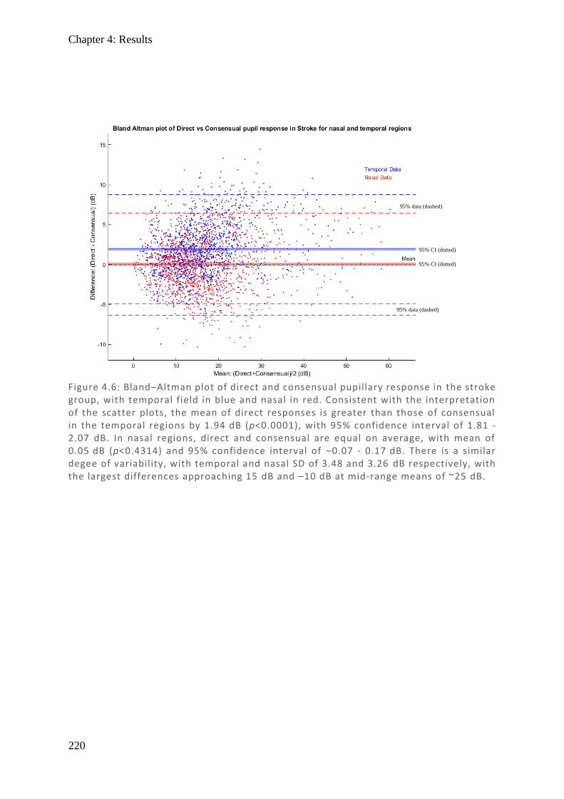
Chapter 4: Results
220
Figure 4.6: Bland–Altman plot of direct and consensual pupillary response in the stroke group, with temporal field in blue and nasal in red. Consistent with the interpretation of the scatter plots, the mean of direct responses is greater than those of consensual in the temporal regions by 1.94 dB (p<0.0001), with 95% confidence interval of 1.81 - 2.07 dB. In nasal regions, direct and consensual are equal on average, with mean of 0.05 dB (p<0.4314) and 95% confidence interval of –0.07 - 0.17 dB. There is a similar degee of variability, with temporal and nasal SD of 3.48 and 3.26 dB respectively, with the largest differences approaching 15 dB and –10 dB at mid-range means of ~25 dB.
95% data (dashed)
95% CI (dotted)
95% CI (dotted)
95% data (dashed)
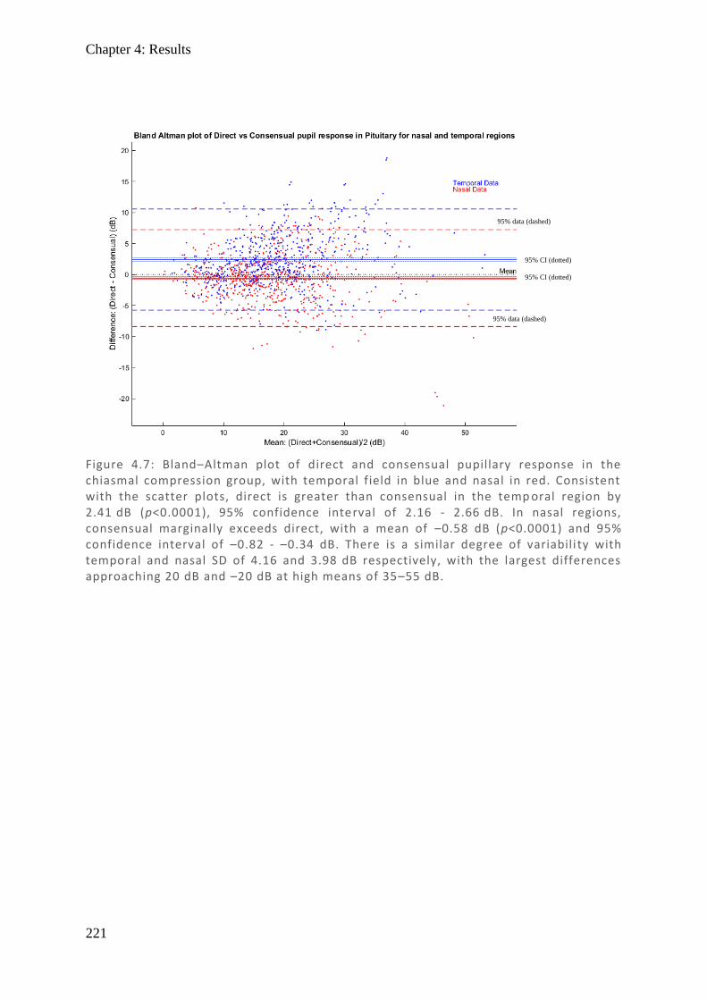
Chapter 4: Results
221
Figure 4.7: Bland–Altman plot of direct and consensual pupillary response in the chiasmal compression group, with temporal field in blue and nasal in red. Consistent with the scatter plots, direct is greater than consensual in the temp oral region by 2.41 dB (p<0.0001), 95% confidence interval of 2.16 - 2.66 dB. In nasal regions, consensual marginally exceeds direct, with a mean of –0.58 dB (p<0.0001) and 95% confidence interval of –0.82 - –0.34 dB. There is a similar degree of variabili ty with temporal and nasal SD of 4.16 and 3.98 dB respectively, with the largest differences approaching 20 dB and –20 dB at high means of 35–55 dB.
95% CI (dotted)
95% data (dashed)
95% CI (dotted)
95% data (dashed)
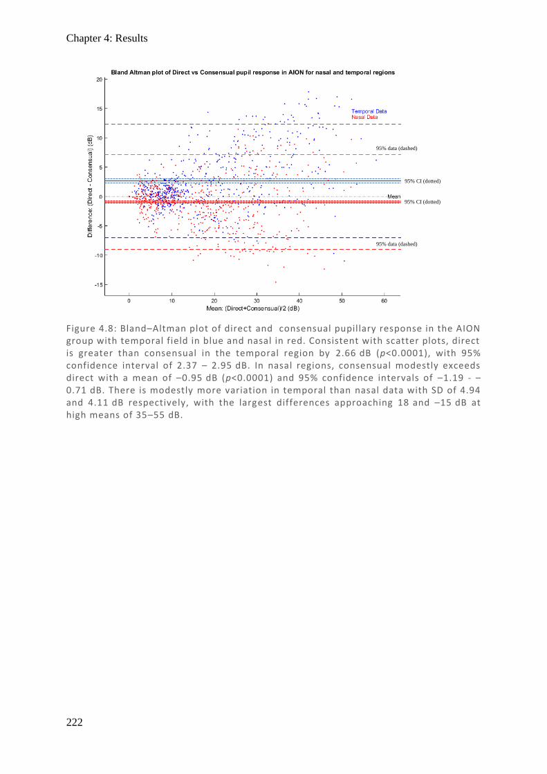
Chapter 4: Results
222
Figure 4.8: Bland–Altman plot of direct and consensual pupillary response in the AION group with temporal field in blue and nasal in red. Consistent with scatter plots, direct is greater than consensual in the temporal region by 2.66 dB (p<0.0001), with 95% confidence interval of 2.37 – 2.95 dB. In nasal regions, consensual modestly exceeds direct with a mean of –0.95 dB (p<0.0001) and 95% confidence intervals of –1.19 - –0.71 dB. There is modestly more variation in temporal than nasal data with SD of 4.94 and 4.11 dB respectively, with the largest differences approaching 18 and –15 dB at high means of 35–55 dB.
95% CI (dotted)
95% data (dashed)
95% CI (dotted)
95% data (dashed)
Chapter 4: Results
223
Figure 4.9 shows a comparison of direct and consensual for the stroke group. Visual inspection
reveals direct and consensual are well aligned, but with clearly visible variation. There is a
notable hemifield difference approximating a modest right-sided hemianopia, which is more
prominent in the left eye and persists in both direct and consensual responses. While this could
be caused by a greater number of right-sided hemianopias in the stroke group, there is actually
more left-sided hemianopias, and the effect persisted in the pituitary and AION groups. This is
most likely an artefact due to gain control, being based on order of stimulation, an issue which
is covered in the Discussion below.
In reviewing the mean difference, there are modest differences of –2 to 4 dB, highlighting that
there are a few regions nasally where consensual exceeds direct, while in most temporal
regions, direct exceeds consensual. Ratios reflect a similar response, with most temporal
regions showing a 10–20% larger direct response, while nasally the responses average out as
nearly the same. Figure 4.10 shows a comparison of direct and consensual for the chiasmal
compression group. Results are remarkably similar to the stroke group, with moderate
alignment of direct and consensual, temporal regions with greater direct responses, and nasal
regions with some consensual responses exceeding direct. The main difference appears to be
that the temporal bias towards the direct component is less pronounced and the nasal bias is a
little more pronounced, with the net difference now showing that consensual modestly exceeds
temporal nasally.
Figure 4.11 shows a comparison of direct and consensual for the AION group and is much the
same as with the stroke and chiasmal compression groups. There is perhaps better alignment
with the chiasmal compression group than the stroke group, in that there is quite definitively a
nasal bias towards consensual exceeding direct, while the temporal region appears consistent
in all diseases. The key difference in this group is a notably larger difference in the left eye
temporal region than in the right.

Chapter 4: Results
224
Overall, Figures 4.9 – 4.11 demonstrate that direct and consensual responses by region grossly
match, but with significant noise, consistent with the Bland–Altman plots. But perhaps more
interestingly, while not clearly evident in visual inspection of direct and consensual responses,
there are consistent small differences naso-temporally. In all conditions, direct exceeded
consensual in temporal regions, while in nasal regions they were either equivalent or had
consensual modestly exceed direct. Temporal differences were more pronounced than nasal,
and this might explain why larger responses were more variable and why direct has an average
response greater than consensual in Bland–Altman.
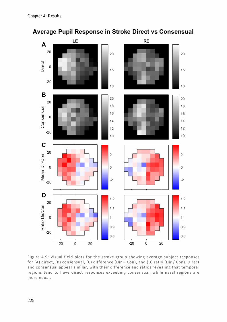
Chapter 4: Results
225
Figure 4.9: Visual field plots for the stroke group showing avera ge subject responses for (A) direct, (B) consensual, (C) difference (Dir – Con), and (D) ratio (Dir / Con). Direct and consensual appear similar, with their difference and ratios revealing that tempora l regions tend to have direct responses exceeding conse nsual, while nasal regions are more equal.
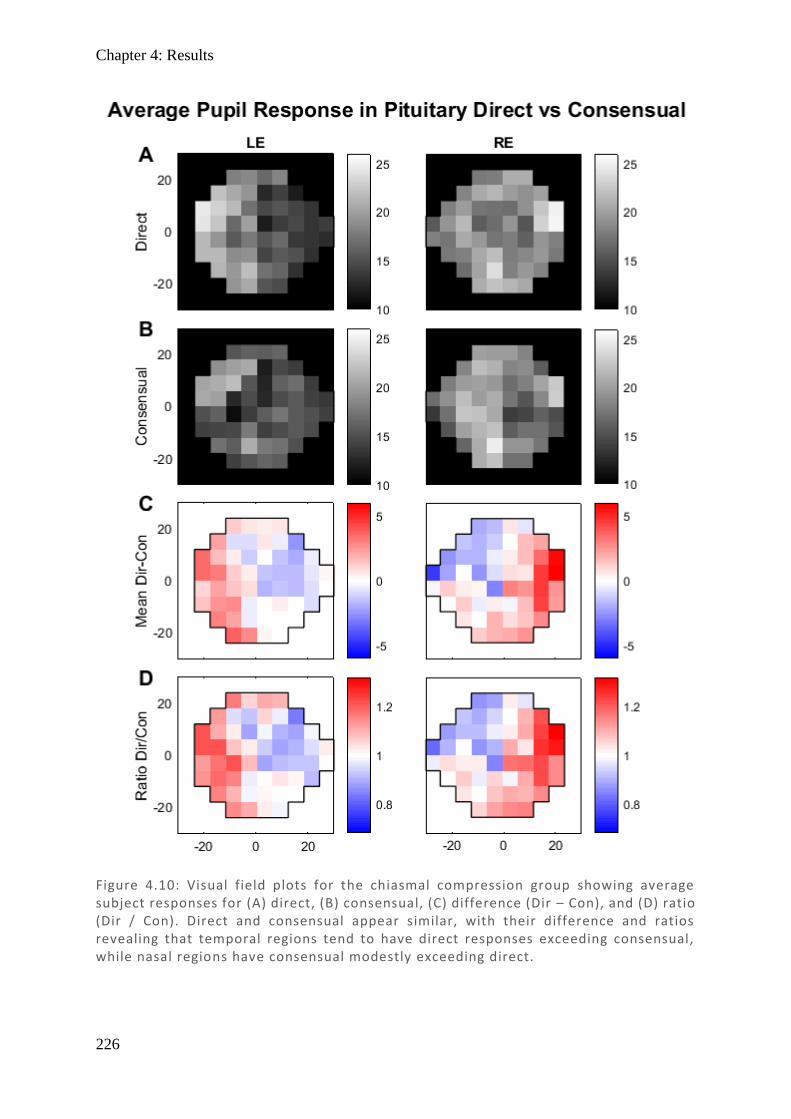
Chapter 4: Results
226
Figure 4.10: Visual field plots for the chiasmal compression group showing average subject responses for (A) direct, (B) consensual, (C) difference (Dir – Con), and (D) ratio (Dir / Con). Direct and consensual appear similar, with their difference and ratios revealing that temporal regions tend to have direct responses exceeding consensual, while nasal regions have consensual modestly exceeding direct.
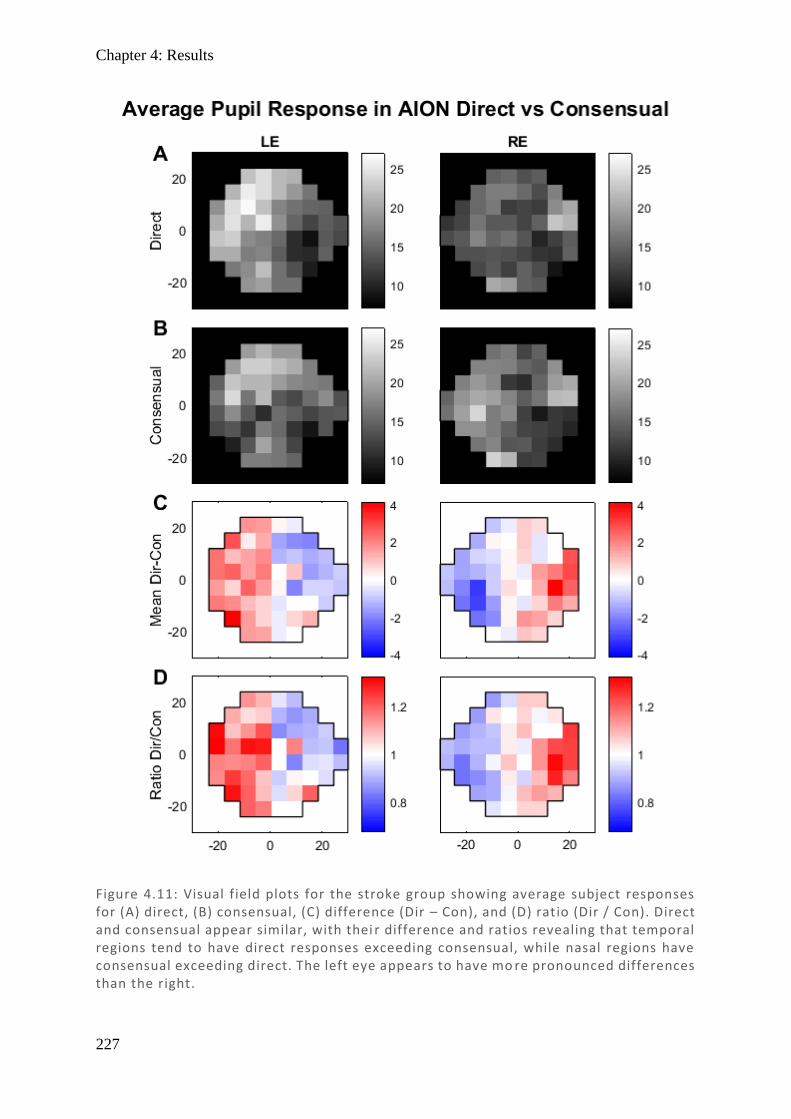
Chapter 4: Results
227
Figure 4.11: Visual field plots for the stroke group showing average subject responses for (A) direct, (B) consensual, (C) difference (Dir – Con), and (D) ratio (Dir / Con). Direct and consensual appear similar, with thei r difference and ratios revealing that temporal regions tend to have direct responses exceeding consensual, while nasal regions have consensual exceeding direct. The left eye appears to have mo re pronounced differences than the right.
Chapter 4: Results
228
With larger direct / consensual ratios occurring temporally, it follows that the direct signal is
larger than consensual in the temporal visual field, but this does not consider the noise
component, and this component may also be larger based on the apparent heteroscedasticity in
the scatter plots. A larger signal is not a necessarily a better signal unless its noise is
proportionally smaller, and so SNR is a measure of how confident one is that a signal is
noticeably different to background noise. To explore whether the SNR for direct and
consensual responses also vary naso-temporally and to quantify this difference, Bland–Altman
plots of direct and consensual for nasal and temporal regions were produced separately.
Averages were taken of the entire nasal region amplitudes (signal) and standard deviations for
each point (noise) were averaged by calculating the root mean square (RMS). To gauge the
variability in direct and consensual SNR generally, a plot of non-averaged points for nasal and
temporal together was also produced.
Similar plots were produced for AION and pituitary, but with very similar results - they are
omitted here. Figure 4.12 highlights that the average direct and consensual SNRs are the same
in nasal regions, consistent with the equivalent signal demonstrated in Figure 4.9. Also, in
keeping with previous results, Figure 4.13 demonstrates that in temporal regions the average
SNR for direct is greater than consensual. In contrasting the two, not only are the means
different, but there are larger confidence intervals in the temporal region showing greater
variation in SNR. Along the x-axis it can be seen that results typically have a SNR of between
2 and 7, such that with differences as large as 1.9, there is quite substantial variation among
some points. When the same plot is produced without averaging the points, individual point
variation along the x-axis was as small as 0.01 and as large as 12.2 and y-axis differences as
large as 4.4. This demonstrates that individual variation between points is quite large and that,
despite an average favouring direct overall, many of the points (particularly those in nasal
regions) have higher SNR in consensual. Neither direct or consensual alone is individually

Chapter 4: Results
229
accurate enough to replace the other, and so potential ways to combine the two should be
considered where the SNR is factored in and neither is discarded, such as an SNR-weighted
mean.
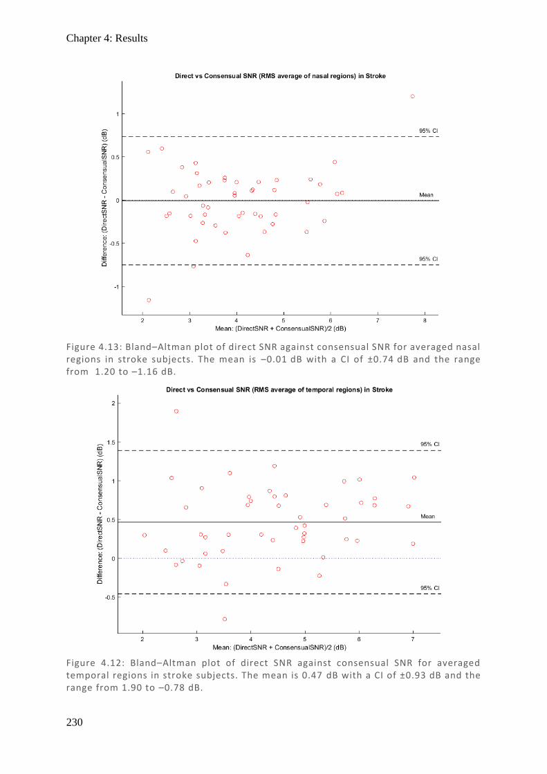
Chapter 4: Results
230
Figure 4.13: Bland–Altman plot of direct SNR against consensual SNR for averaged nasal regions in stroke subjects. The mean is –0.01 dB with a CI of ±0.74 dB and the range from 1.20 to –1.16 dB.
Figure 4.12: Bland–Altman plot of direct SNR against consensual SNR for averaged temporal regions in stroke subjects. The mean is 0.47 dB with a CI of ±0.93 dB and the range from 1.90 to –0.78 dB.
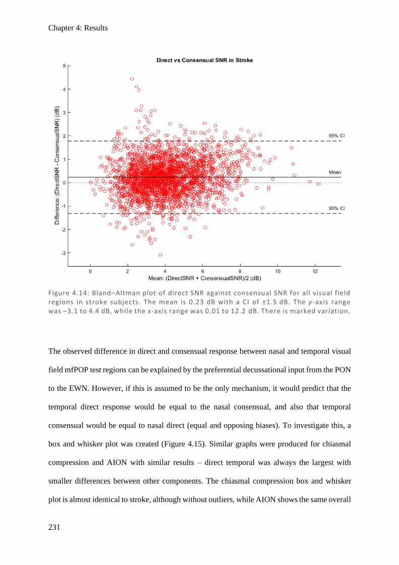
Chapter 4: Results
231
The observed difference in direct and consensual response between nasal and temporal visual
field mfPOP test regions can be explained by the preferential decussational input from the PON
to the EWN. However, if this is assumed to be the only mechanism, it would predict that the
temporal direct response would be equal to the nasal consensual, and also that temporal
consensual would be equal to nasal direct (equal and opposing biases). To investigate this, a
box and whisker plot was created (Figure 4.15). Similar graphs were produced for chiasmal
compression and AION with similar results – direct temporal was always the largest with
smaller differences between other components. The chiasmal compression box and whisker
plot is almost identical to stroke, although without outliers, while AION shows the same overall
Figure 4.14: Bland–Altman plot of direct SNR against consensual SNR for all visual field regions in stroke subjects. The mean is 0.23 dB with a CI of ±1.5 dB. The y-axis range was –3.1 to 4.4 dB, while the x-axis range was 0.01 to 12.2 dB. There is marked variation.
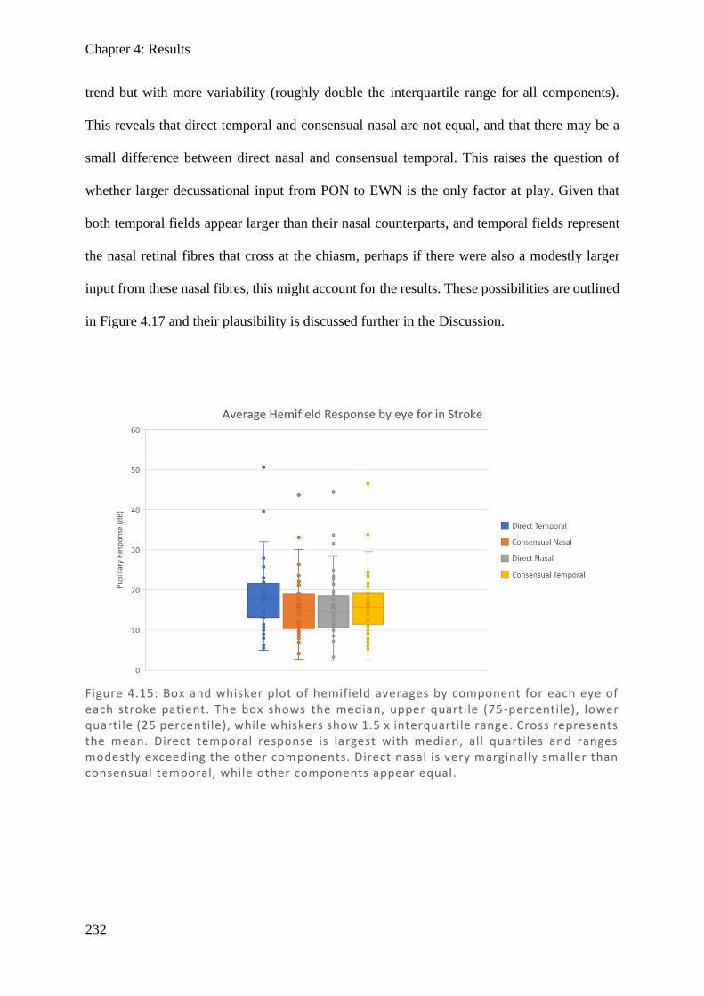
Chapter 4: Results
232
trend but with more variability (roughly double the interquartile range for all components).
This reveals that direct temporal and consensual nasal are not equal, and that there may be a
small difference between direct nasal and consensual temporal. This raises the question of
whether larger decussational input from PON to EWN is the only factor at play. Given that
both temporal fields appear larger than their nasal counterparts, and temporal fields represent
the nasal retinal fibres that cross at the chiasm, perhaps if there were also a modestly larger
input from these nasal fibres, this might account for the results. These possibilities are outlined
in Figure 4.17 and their plausibility is discussed further in the Discussion.
Figure 4.15: Box and whisker plot of hemifield averages by component for each eye of each stroke patient. The box shows the median, upper quartile (75-percentile), lower quartile (25 percentile), while whiskers show 1.5 x interquartile range. Cross represents the mean. Direct temporal response is largest with median, all quartiles and ranges modestly exceeding the other components. Direct nasal is very marginally smaller than consensual temporal, while other components appear equal.
Chapter 4: Discussion
233
4.5. Discussion
There was a highly linear correlation between direct and consensual, supporting the idea that
they may be equivalent, but results from Bland–Altman suggest consistent differences. Direct
was shown to be modestly greater than consensual on average in all conditions, consistent with
previous studies of control patients who demonstrated the same (Lowenstein, 1954; Smith et
al., 1979; Fan et al., 2009). This overall difference was then highlighted to be due almost
entirely to nasal–temporal differences, with temporal hemifields having larger direct responses
and nasal hemifields having similar or modestly greater consensual responses. As discussed in
the introduction, it is a common finding that temporal hemifields have larger direct responses
(more prominent), while results for nasal fields were mixed – some showing, as we did, that
consensual exceeds direct (Cox & Drewes, 1984; Martin et al., 1991), while other show
equivalence (Smith & Smith, 1980; Wyatt & Musselman, 1981; Schmid et al., 2000; Carle et
al., 2011).
A comparison to the closely related results from (Carle et al., 2011), who used the same device
with the same background luminance (10 cd/m2) but brighter stimuli (290 cd/m2 compared to
our 150 cd/m2), reveals that Carle et al. found near-equivalence of direct and consensual in the
nasal field, whereas we found that consensual was larger. This earlier work addressed factors
which may explain how these discrepant results might originate – that they may depend on
stimulus intensity – such that less intense stimuli (like ours) will show a consensual bias, while
more intense stimuli will plateau at equivalence for the ranges typical in testing, with a
theoretical model predicting modest consensual bias for even more intense stimuli (Carle et al.,
2011). This model is based on equal input to the PON and greater contralateral input to the
EWN, giving potential for saturation, and our results seem to support this model, although the
results can only address the less intense range.
Chapter 4: Discussion
234
If the proposed PON bias towards contralateral input to EWN (crudely estimated at 15%) were
the only factor considered, and pupillary input from nasal and temporal fibres is presumed
even, then this would explain the temporal field bias (direct > consensual) and would predict
that the nasal field would be equally and oppositely biased (consensual > direct) (Figure 4.17,
part C). However, both our results and results from the multiple studies listed above, all report
that the temporal field shows the greater bias, with small or no bias in the nasal region. In
considering why this might be, it is interesting to note there are known differences in the fibres
which supply the PON. There is a higher density of nasal retinal fibres extending laterally
within the 30° eccentricity tested using mfPOP (see Figure 4.16), and there are also more nasal
retinal fibres that decussate at the optic chiasm, compared to fibres from the temporal retina
which continue uncrossed. Studies in primates based on the relative quantity of cortical layer
IVc occupied by the ipsilateral and contralateral eyes suggest that 58% decussate and 42%
remain uncrossed (Horton & Hocking, 1996; Horton, 1997), while in a human histology study
of a single person, 53% of the fibres decussated and 47% did not (Kupfer et al., 1967). If this
bias between visual pathways is considered in isolation, with no effect of PON to EWN bias,
this would produce stronger nasal retina (temporal field) responses, although it predicts the
direct and consensual responses would be about even (Figure 4.17, part B). However, if both
effects are considered together (bias towards chiasmal decussation and bias from PON to
contralateral EWN), this prediction more closely matches the results, with direct exceeding
consensual in the temporal field, consensual exceeding direct in the nasal field, and temporal
field effects being of larger magnitude (Figure 4.17, part D).
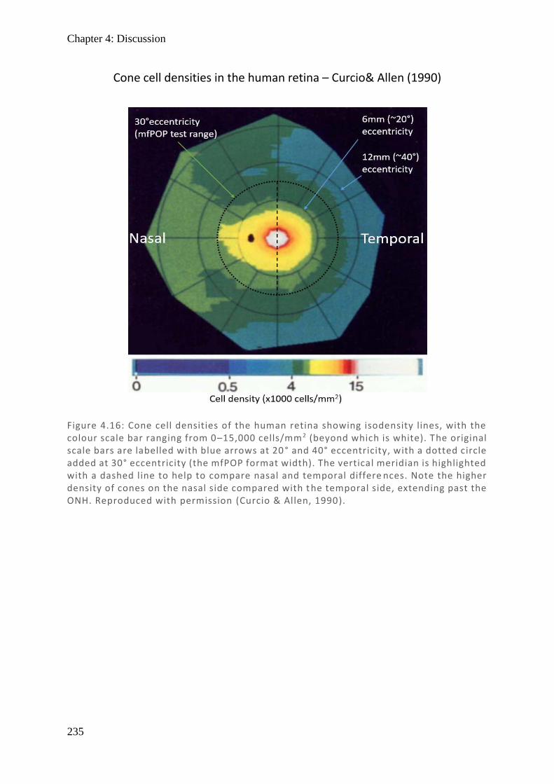
Chapter 4: Discussion
235
Figure 4.16: Cone cell densities of the human retina showing isodensity lines, with the colour scale bar ranging from 0–15,000 cells/mm2 (beyond which is white). The original scale bars are labelled with blue arrows at 20 ° and 40° eccentricity, with a dotted circle added at 30° eccentricity (the mfPOP format width). The vertical meridian is highlighted with a dashed line to help to compare nasal and temporal differe nces. Note the higher density of cones on the nasal side compared with t he temporal side, extending past the ONH. Reproduced with permission (Curcio & Allen, 1990).
Cone cell densities in the human retina – Curcio& Allen (1990)

Chapter 4: Discussion
236
Figure 4.17: Theoretical models of the visual pathways with retinal input from right temporal (light blue), right nasal (orange), left nasal (red), and left temporal (dark blue) with their relative predicted pupil responses. For clarity, these are also presented for the visual field in the tables with key T = temporal, N = nasal, D = direct, and C = consensual. Numbers are only to indicate relative response to allow co mparison based on experimental bias at the PON–EWN and nasal–temporal levels. (A) Pathway with no bias – equal input. (B) Preferential nasal/optic chiasms bias (53% of fibres). (C) PON to EWN preferential bias towards contralateral input (15% larger). (D) Combined bias of (B) and (C) including retinal and nuclei bias.
Chapter 4: Discussion
237
Comparing chiasmal compression direct and consensual bias to that of stroke, bias in the
temporal fields was less pronounced, while bias in the nasal fields was more pronounced.
Chiasmal compression typically results in bitemporal visual field lesions, and so it was
considered whether this might explain the differences. However, as damage to the chiasm
would affect all temporal output, and so should equally affect direct and consensual responses
(as they separate at the PON), this would seem unlikely. Additionally, similar results were
noted in AION, which has no grounds for these differences to have occurred.
A feature highlighted in the results for both direct and consensual across all disease states was
the appearance of a mild right homonymous hemianopia, more prominent in the left eye. Given
its presence in all disease types, it would appear that this is an artefact of the device itself. It is
most simply explained by noting that there is gain control in the pupillary system, which has
recently been suggested to be at the EWN level (Carle et al., 2019). The sequence of stimuli in
these experiments is to present to the left eye first (left hemifield then right hemifield), followed
by the right eye (left hemifield then right hemifield). As the first presentation (left eye, left
hemifield) in each segment is the most responsive, and the first presentation in the right eye
(right eye, left hemifield) is also more responsive, this would explain both the notable left–
right hemifield bias, and why the right eye hemifield bias is less pronounced. As integration
has been suggested at the EWN, both pupillary inputs are represented at the EWN, and so it
makes sense that gain control may exist between eyes as well as within eyes. While
randomisation of stimuli sequence should eliminate this bias, gaps between stimuli would have
to be added to maintain temporally sparse stimuli, and this would substantially lengthen test
duration. Alternatively, alternating testing order between segments might also provide reduced
bias, without altering test duration. This may be explored in future studies.
Variability was highlighted early in the analysis as substantial, with Bland–Altman plots of
direct vs consensual revealing it was not uncommon for variation in direct and consensual

Chapter 4: Discussion
238
responses to be near 50% of their average. In pictorial displays of the averaged visual field,
direct and consensual visual fields certainly showed some correlation, but still had marked
variation between them, despite them being averages of the group. This was also maintained
in SNR plots, showing similar degrees of variation to direct and consensual responses. In
assessing how one should amalgamate the direct and consensual responses, this result suggests
that while there is a correlation, the responses are not interchangeable, and they vary quite
substantially in their SNR. While direct is marginally larger in both signal and SNR, this is
only because of the temporal field and so to select only direct would discard a lot of valid data,
some of which has better SNR (particularly in the nasal field). A simple average does not
account for the amount of variation in SNR, or the naso–temporal differences. Using the largest
SNR of the pair would certainly be worth considering, but given that the point of the test is to
highlight damaged regions (which will have intrinsically low signal), this may under-represent
the true amount of damage and give a positive bias. Therefore, the most appropriate
combination based on this data is to complete an average of direct and consensual weighted by
SNR. This approach accounts for the naso–temporal differences (since temporally wherever
direct exceeds consensual it will have a greater SNR and be proportionately more weighted),
while the same is true for consensual nasally. This technique does not discard any data, and
should minimise any positive bias.
4.6. Conclusion
Direct and consensual pupillary response amplitudes correlate, but with substantial noise,
indicating they are not entirely equivalent. On average, the direct response is greater than the
consensual in temporal regions, but it is equivalent or marginally smaller in nasal regions,
consistent with controls in previous studies. This effect persisted across all disease types
suggesting it is an innate physiological difference. These differences may be explained by
larger decussational input from PON to EWN and a greater number of nasal fibres. Similar

Chapter 4: Discussion
239
degrees of variability in response amplitude and SNR point to neither component being totally
superior to the other. In order to combine measures, with the intention of accounting for spatial
differences, but without causing positive bias, a combination using an SNR-weighted average
is the most suitable.

240
References
Bland JM & Altman DG. (1999). Measuring agreement in method comparison studies. Stat
Methods Med Res 8, 135-160.
Carle CF, James AC, Rosli Y & Maddess T. (2019). Localization of neuronal gain control in
the pupillary response. Frontiers in neurology 10, 203.
Carle CF, Maddess T & James AC. (2011). Contraction anisocoria: Segregation, summation,
and saturation in the pupillary pathway. Invest Ophthalmol Vis Sci 52, 2365-2371.
Clarke RJ, Blanks RH & Giolli RA. (2003). Midbrain connections of the olivary pretectal
nucleus in the marmoset (callithrix jacchus): Implications for the pupil light reflex
pathway. Anat Embryol (Berl) 207, 149-155.
Cox TA & Drewes CP. (1984). Contraction anisocoria resulting from half-field illumination.
Am J Ophthalmol 97, 577-582.
Curcio CA & Allen KA. (1990). Topography of ganglion cells in human retina. J Comp
Neurol 300, 5-25.
Fan X, Miles JH, Takahashi N & Yao G. (2009). Sex-specific lateralization of contraction
anisocoria in transient pupillary light reflex. Invest Ophthalmol Vis Sci 50, 1137-1144.
Gamlin PD & Clarke RJ. (1995). The pupillary light reflex pathway of the primate. J Am
Optom Assoc 66, 415-418.
Giavarina D. (2015). Understanding bland altman analysis. Biochem Med (Zagreb) 25, 141-
151.
Horton JC. (1997). Wilbrand's knee of the primate optic chiasm is an artefact of monocular
enucleation. Trans Am Ophthalmol Soc 95, 579-609.
Horton JC & Hocking DR. (1996). Intrinsic variability of ocular dominance column
periodicity in normal macaque monkeys. J Neurosci 16, 7228-7239.
Hutchins B & Weber JT. (1985). The pretectal complex of the monkey: A reinvestigation of
the morphology and retinal terminations. J Comp Neurol 232, 425-442.

Chapter 4: References
241
James AC. (2003). The pattern-pulse multifocal visual evoked potential. Invest Ophth Vis Sci
44, 879-890.
James AC, Kolic M, Bedford SM & Maddess T. (2012). Stimulus parameters for multifocal
pupillographic objective perimetry. J Glaucoma 21, 571-578.
James AC, Ruseckaite R & Maddess T. (2005). Effect of temporal sparseness and dichoptic
presentation on multifocal visual evoked potentials. Visual Neurosci 22, 45-54.
Kupfer C, Chumbley L & Downer JC. (1967). Quantitative histology of optic nerve, optic
tract and lateral geniculate nucleus of man. J Anat 101, 393-401.
Lowenstein O. (1954). Alternating contraction anisocoria; a pupillary syndrome of the
anterior midbrain. AMA Arch Neurol Psychiatry 72, 742-757.
Martin TI, Kardon RI & Thompson HS. (1991). Unequal direct and consensual pupillary
responses to hemiretinal stimuli. Invest Ophth Vis Sci 32, 1124.
Ruseckaite R, Maddess T, Danta G, Lueck CJ & James AC. (2005). Sparse multifocal stimuli
for the detection of multiple sclerosis. Ann Neurol 57, 904-913.
Sabeti F, Maddess T, Essex RW, Saikal A, James AC & Carle CF. (2014). Multifocal
pupillography in early age-related macular degeneration. Optometry and vision
science : official publication of the American Academy of Optometry 91, 904-915.
Schmid R, Wilhelm B & Wilhelm H. (2000). Naso-temporal asymmetry and contraction
anisocoria in the pupillomotor system. Graef Arch Clin Exp 238, 123-128.
Smith SA, Ellis CJ & Smith SE. (1979). Inequality of the direct and consensual light reflexes
in normal subjects. The British journal of ophthalmology 63, 523-527.
Smith SA & Smith SE. (1980). Contraction anisocoria: Nasal versus temporal illumination.
The British journal of ophthalmology 64, 933-934.
Tigges J & O'Steen WK. (1974). Termination of retinofugal fibers in squirrel monkey: A re-
investigation using autoradiographic methods. Brain Res 79, 489-495.
Wyatt HJ & Musselman JF. (1981). Pupillary light reflex in humans: Evidence for an
unbalanced pathway from nasal retina, and for signal cancellation in brainstem. Vision
Res 21, 513-525.

Chapter 4: References
242
Zaki R, Bulgiba A, Ismail R & Ismail NA. (2012). Statistical methods used to test for
agreement of medical instruments measuring continuous variables in method
comparison studies: A systematic review. Plos One 7, e37908.
243
5 Chapter 5: Visual field comparison of standard automated perimetry and pupillometry in stroke, chiasmal compression, and AION
5.1. Abstract
5.1.1. Purpose
The Humphrey and Matrix field analysers (HFA, MFA) are routinely used in clinical practice
to assess visual fields. While there is a lot of research into comparisons in glaucoma, there is
limited research on comparisons in stroke, pituitary tumour, and AION. Multifocal
pupillographic objective perimetry (mfPOP) is a novel perimeter under development which has
many potential advantages over traditional testing, including simultaneous testing of the two
eyes, both response amplitude and delay, standard errors of the field data, and objectivity.
While mfPOP has been shown useful in a number of retinal disorders, it has not yet been tested
in neurological disorders, which are of particular interest given it utilises pupillary responses
which are neurally encoded. The aims of this study are to investigate relationships between
these devices and compare their diagnostic ability in order to suggest which device(s) are most
effective. Of particular interest is whether post-geniculate lesions appear in mfPOP, as in
standard automated perimetry.
5.1.2. Methods
There were 25 stroke, 11 pituitary tumour, and 10 AION patients who were recruited and
screened for retinal disorders with a test set including OCT scan, IOP measure, and BCVA.
Subjects were tested using Humphrey 24-2 SITA-Full perimetry (HFA), Matrix frequency
Chapter 5: Abstract
244
doubling 24-2 perimetry (MFA), and an mfPOP yellow/yellow protocol. Control data was used
from a previous study using the same protocol. Threshold values in dB were used for HFA and
MFA devices. The mfPOP data had pupillary response measures extracted by region using
iterative nonlinear regression. Direct and consensual signals were combined by SNR-weighted
means, converted in dB using the generalised logarithm, and interpolated onto a 24-2 grid.
Comparisons were made with scatter plots (using principal curves with and without 0 dB points
included), Bland–Altman plots, and intraclass correlation coefficients using hemifield ratios.
Diagnostic ability was assessed using area under receiver operator characteristics plots (with
bootstrap based upon the hemifield ratio signal).
5.1.3. Results
Principal curves for scatterplots (with 0 dB points removed) show a somewhat linear
relationship between HFA and MFA and a non-linear logarithmic-like relationship with
mfPOP. Bland–Altman plots demonstrated the most linear relationship between HFA and MFA
over their upper range in all conditions, with small mean differences and 95% CIs when the
devices were compared. Bland–Altman plots for HFA and mfPOP showed very limited
agreement, with large mean difference and 95% CI; MFA and mfPOP also showed limited
agreement with intermediate mean difference and large 95% CI. Hemifield ROC plots for HFA,
MFA, and mfPOP showed AUC of 0.842*, 0.844*, and 0.531 for stroke (* = significant); AUC
of 0.724*, 0.966*, and 0.545 for chiasmal compression; and 0.912*, 0.885*, and 0.533 for
AION. The ICC for HFA vs MFA were 0.985 for stroke, 0.923 for pituitary, and 0.962 for
AION (all highly significant), while correlations between HFA and mfPOP or MFA and
mfPOP were all non-significant or marginally significant.
5.1.4. Conclusions
HFA and MFA correlate very well with each other in all conditions, while mfPOP did not
correlate well with either HFA or MFA, but marginally better with MFA. This may be due to
Chapter 5: Abstract
245
mfPOP more linearly correlating with structural loss (RNFL thickness) while HFA and MFA
show more logarithmic relationships to structure. HFA and MFA performed well at detection
of conditions using hemifield ratios, with HFA slightly out-performing MFA in stroke and
AION, while MFA substantially out-performed HFA in chiasmal compression. mfPOP was not
effective at distinguishing disease state based on hemifield ratios. Visual inspection suggested
that mfPOP demonstrated some correlation in complete/near-complete homonymous
hemianopia, which suggests detection of post-LGN damage; a likely hypothesis is retrograde
degeneration, which is only noted in hemianopia but not quadrantanopia or smaller. Further
investigation is necessary using MRI data to confirm this hypothesis.
Chapter 5: Introduction
246
5.2. Introduction
In the assessment of visual fields, standard automated perimetry (SAP) has become the
mainstay of clinical practice; it is a standardised approach that is minimally dependent upon
the person administering the test. Different approaches can be used such as the Humphrey Field
Analyser (HFA) which uses Goldmann size III (0.43° diameter) stimuli with varying
luminance, and the Matrix Field Analyser (MFA), which uses larger contrast-reversing grating
stimuli whose varying contrast produces a frequency-doubling effect. Each of these devices
has its own limitations, with HFA being demonstrated in glaucomatous fields to have poor
reproducibility over most of its range (Heijl et al., 1989; Artes et al., 2002) and greater
peripheral variability (Berezina et al., 2011) consistent with other similar devices (Pearce &
Maddess, 2016). The small stimulus size of these devices is suggested to be a strong contributor
to these effects (Wall et al., 2013; Gardiner et al., 2015; Numata et al., 2017), as is
undersampling (Weber & Dobek, 1986; Maddess, 2011b, 2014). MFA attempts to correct some
of these deficits with larger stimuli, which do appear to have reduced variability (Chauhan &
Johnson, 1999; Artes et al., 2005; Horani et al., 2007; Wall et al., 2009; Wall et al., 2010). A
new Mean Likelihood (ML) algorithm was also used for estimation, replacing the Swedish
Interactive Thresholding Algorithm (SITA) used in HFA with the Zippy Estimation of
Sequential Testing (ZEST). ZEST showed promise on early testing (Anderson & Johnson,
2006) but causes all results to converge on only 15 unevenly spaced values (Fredette et al.,
2015), which may contribute to the reduced variability. Different contrast definitions are also
used: HFA uses the Weber formula, while Matrix uses the Michelson formula. There are also
different calculations of log units, with HFA using 10*log(Amplitude) and MFA using
20*log(Amplitude), meaning no direct correlation of units is possible between machines
despite having a procedurally similar approach and coincidently similar values (Fredette et al.,
2015).
Chapter 5: Introduction
247
While it would seem that MFA has the edge in early glaucoma detection (Medeiros et al., 2004;
Kim et al., 2007), in optic nerve and chiasmal damage they are reportedly similar clinically
(Huang et al., 2008). In detection of post-LGN lesions producing homonymous field defects
(typical in stroke), HFA out performs MFA but not to statistical significance (Taravati et al.,
2008). In practice, HFA is by far the most commonly used device for testing of neurological
conditions (Hepworth & Rowe, 2018).
Multifocal pupillographic objective perimetry (mfPOP) provides an entirely new approach to
assessing field damage by removing the subjective patient response to stimuli and replacing it
with an objective autonomic response of pupil constriction to light. It also takes into
consideration lessons from the HFA and MFA in terms of having large stimuli to reduce test–
retest variability, and increasingly larger stimuli peripherally to counter the increased
peripheral variability seen in HFA and compensate to some extent for the smaller retinal
magnification (Holden & Fitzke, 1988). It has veered away from both the SITA and ZEST
approximations, which are both based on varying stimulus intensity with a binary response, in
favour of using fixed contrast stimuli while measuring the amplitude response. By presenting
multiple stimuli simultaneously (multifocally) and then extracting component signals, this also
allows both eyes to be tested at once, a faster test time, and multiple tests of a single field
location, allowing less variability and more consistency (Maddess et al., 2009). It has been
trialled and shown promise in a number of common retinal diseases including early detection
of diabetic retinopathy (Bell et al., 2010; Coombes et al., 2012; Sabeti et al., 2015), early
detection of age-related macular degeneration (AMD) (Sabeti et al., 2011; Sabeti et al., 2013;
Sabeti et al., 2014; Sabeti et al., 2017), and similar diagnostic accuracy to SAP in glaucoma
(Maddess et al., 2009; Carle et al., 2011a; Maddess et al., 2013; Carle et al., 2015). For
neurological conditions, there also appears to be some promising results in migraine (Lueck et
al., 2014) and epilepsy (Ali et al., 2015). Testing of neurologically based conditions which
Chapter 5: Introduction
248
affect visual field loss is limited, with multiple sclerosis being assessed (Maddess et al., 2012a;
Ali et al., 2014). However, conditions such as anterior ischemic optic neuropathy (AION),
chiasmal compression, and stroke have been largely unexplored. Neurological testing with
mfPOP is of particular interest, given it objectively measures neurological pathways via the
pupillary response and that completion of complex tasks like SAP may be difficult and
exhausting for those with neurological deficits. It would be interesting to identify whether any
differences can be detected and whether they correlate with the locations identified in
traditional field testing. AION manifests as anterior damage at the optic disc, chiasmal
compression as an intermediate at the optic chiasm, and occipital stroke as a more posterior
damage post-LGN, which is notably after the subcortical pupillary response branch point.
Significant cortical input from both striate and extrastriate vision areas to the pretectal olivary
nucleus (PON) has been demonstrated in monkeys (Gamlin, 2006). These include input from
occipital cortex (V1) (Benevento & Rezak, 1976; Benevento et al., 1977; Distler & Hoffmann,
1989), visual association cortices V2-5 (Benevento & Davis, 1977; Benevento et al., 1977;
Dineen & Hendrickson, 1983), and the inferior temporal region (Steele & Weller, 1993).
However, with anatomical evidence of input to PON, the question becomes: does the pupillary
system have meaningful responses to cortical input? Practically, it is well established that
pupils respond to arousal and cognitive state (Cash-Padgett et al., 2018), and pupillary response
delays in isoluminant colour exchange (Young & Alpern, 1980; Carle et al., 2013) imply
notable cortical input from colour integration. Finally the question has been quite elegantly
answered by Heywood et al. who demonstrated that cortical lesion to the inferior temporal
region of a monkey abolishes isoluminant chromatic exchange response but not luminant
achromatic response, demonstrating that cortical lesions may indeed be detected by the
pupillary pathway with selective stimuli (Heywood et al., 1998). Given there is strong evidence
in monkeys for pupillary detection of a specific cortical lesion, it would be interesting to

Chapter 5: Introduction
249
ascertain if this is true in human stroke patients, who may have more varying damage affecting
analogous regions in addition to other cortical input pathways.
This project aims to explore visual field responses in stroke, pituitary tumour, and AION using
two traditional perimeters: HFA and MFA, and compare them to novel mfPOP responses in
terms of assessing consistency and diagnostic ability, while also exploring the possibility that
the subcortical pupillary response pathway receives cortical input.
5.3. Methods
The history of mfPOP and the reasons for its test parameters can be found in the Introduction
(1.6.4 Multifocal methods). Full methods including recruitment (section 2.1), screening
(section 2.2), and mfPOP stimuli, procedures, and output measures (section 2.5.3) are detailed
in the General Methods. Here for brevity only an overview of these will be presented. Noting
that 1 subject from the stroke group and two from the chiasmal compression group did not
complete day 3 of testing, and so do not have Matrix fields or repeat mfPOP reports. Where
possible these subjects were still included in the data set, but removed where data was absent
or necessary for comparison.
5.3.1. Subjects and screening
Subjects were recruited from multiple hospital and eye clinic sources and informed consent
obtained. Subjects were screened for pre-existing ocular conditions, both via questionnaire and
clinical assessment. The latter included best corrected visual acuity 6/24 or better, cataract
screening, intraocular pressure measurement, fundus photo, and OCT scans of posterior pole
and optic nerve head. Groups consisted of stroke (heterogenous cortical lesions) (n = 25),
chiasmal compression (n = 11), and AION (n = 10).

Chapter 5: Methods
250
5.3.2. Visual field assessment
All subjects completed the 24-2 pattern of the Humphrey Field Analyser [HFA II] (Carl Zeiss
Meditec Inc., Dublin, CA; Achromatic SITA-Full perimetry), 24-2 pattern of the Humphrey
Matrix frequency-doubling perimeter [MFA II] (Carl Zeiss Meditec, Inc. Dublin, CA), and
multifocal pupillographic objective perimetry (mfPOP) on a prototype FDA-cleared
ObjectiveFIELD (Konan Medical USA Inc, Irvine CA) with yellow stimuli on yellow
background (Y/Y) which measured maximum amplitude of the pupillary response waveform.
Subjects had their visual fields tested over 2 days within 2 weeks of each other. On their first
day, subjects had HFA and both mfPOP protocols (Y/Y and G/R) tested, and on their second
day had MFA and a repeat of both mfPOP protocols. The order of testing was randomised such
that standard automated perimetry (SAP; HFA or MFA) was tested first on one of the days and
mfPOP on the other. The analysis for this chapter only uses the more established Y/Y stimuli,
as the G/R protocol was of novel design and control data was unavailable (instead G/R is
explored in Chapter 6).
5.3.3. Humphrey Field Analyser (HFA)
Methods for conducting HFA are as described in General Methods (2.5.1 Humphrey Field
Analyser (HFA)). This comprised testing of the 24-2 format, which tests points 3° either side
of the meridians and extends to 21° in every direction, with two additional points nasally to
27°. Goldmann size 3 (0.43° diameter) white light stimuli are used, and the order of
presentation was determined by the Swedish Interactive Threshold Algorithm (SITA).
Standard operating procedures were used according to the HFA manual. Subjects had their
ocular prescription measured by vertometer, and entered into HFA device, which
recommended trial lenses used during testing. The right eye was always tested first. Subjects
were instructed how to complete testing and asked to fixate on central fixation dot. Gaze
tracking was initiated prior to testing where possible, and pupil was centred on reference
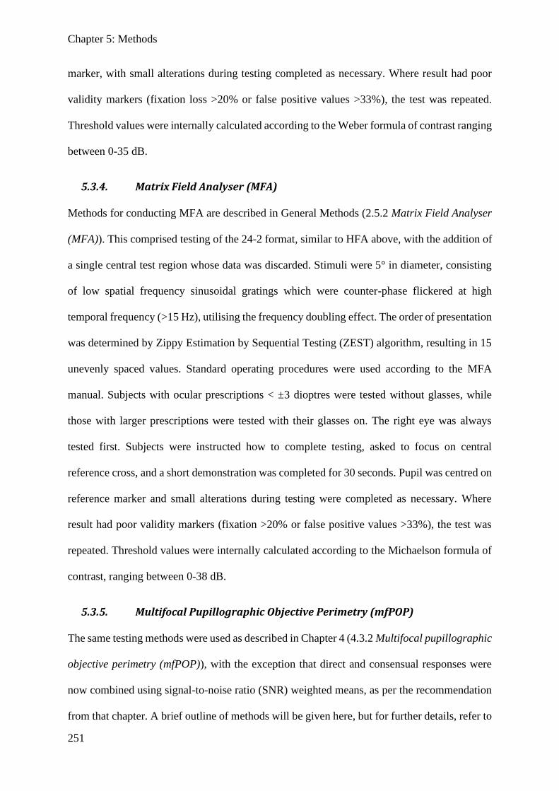
Chapter 5: Methods
251
marker, with small alterations during testing completed as necessary. Where result had poor
validity markers (fixation loss >20% or false positive values >33%), the test was repeated.
Threshold values were internally calculated according to the Weber formula of contrast ranging
between 0-35 dB.
5.3.4. Matrix Field Analyser (MFA)
Methods for conducting MFA are described in General Methods (2.5.2 Matrix Field Analyser
(MFA)). This comprised testing of the 24-2 format, similar to HFA above, with the addition of
a single central test region whose data was discarded. Stimuli were 5° in diameter, consisting
of low spatial frequency sinusoidal gratings which were counter-phase flickered at high
temporal frequency (>15 Hz), utilising the frequency doubling effect. The order of presentation
was determined by Zippy Estimation by Sequential Testing (ZEST) algorithm, resulting in 15
unevenly spaced values. Standard operating procedures were used according to the MFA
manual. Subjects with ocular prescriptions < ±3 dioptres were tested without glasses, while
those with larger prescriptions were tested with their glasses on. The right eye was always
tested first. Subjects were instructed how to complete testing, asked to focus on central
reference cross, and a short demonstration was completed for 30 seconds. Pupil was centred on
reference marker and small alterations during testing were completed as necessary. Where
result had poor validity markers (fixation >20% or false positive values >33%), the test was
repeated. Threshold values were internally calculated according to the Michaelson formula of
contrast, ranging between 0-38 dB.
5.3.5. Multifocal Pupillographic Objective Perimetry (mfPOP)
The same testing methods were used as described in Chapter 4 (4.3.2 Multifocal pupillographic
objective perimetry (mfPOP)), with the exception that direct and consensual responses were
now combined using signal-to-noise ratio (SNR) weighted means, as per the recommendation
from that chapter. A brief outline of methods will be given here, but for further details, refer to
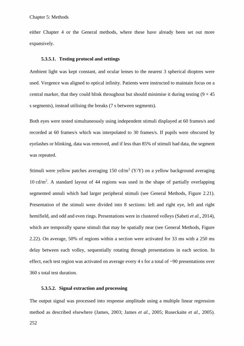
Chapter 5: Methods
252
either Chapter 4 or the General methods, where these have already been set out more
expansively.
5.3.5.1. Testing protocol and settings
Ambient light was kept constant, and ocular lenses to the nearest 3 spherical dioptres were
used. Vergence was aligned to optical infinity. Patients were instructed to maintain focus on a
central marker, that they could blink throughout but should minimise it during testing (9 × 45
s segments), instead utilising the breaks (7 s between segments).
Both eyes were tested simultaneously using independent stimuli displayed at 60 frames/s and
recorded at 60 frames/s which was interpolated to 30 frames/s. If pupils were obscured by
eyelashes or blinking, data was removed, and if less than 85% of stimuli had data, the segment
was repeated.
Stimuli were yellow patches averaging 150 cd/m2 (Y/Y) on a yellow background averaging
10 cd/m2. A standard layout of 44 regions was used in the shape of partially overlapping
segmented annuli which had larger peripheral stimuli (see General Methods, Figure 2.21).
Presentation of the stimuli were divided into 8 sections: left and right eye, left and right
hemifield, and odd and even rings. Presentations were in clustered volleys (Sabeti et al., 2014),
which are temporally sparse stimuli that may be spatially near (see General Methods, Figure
2.22). On average, 50% of regions within a section were activated for 33 ms with a 250 ms
delay between each volley, sequentially rotating through presentations in each section. In
effect, each test region was activated on average every 4 s for a total of ~90 presentations over
360 s total test duration.
5.3.5.2. Signal extraction and processing
The output signal was processed into response amplitude using a multiple linear regression
method as described elsewhere (James, 2003; James et al., 2005; Ruseckaite et al., 2005).
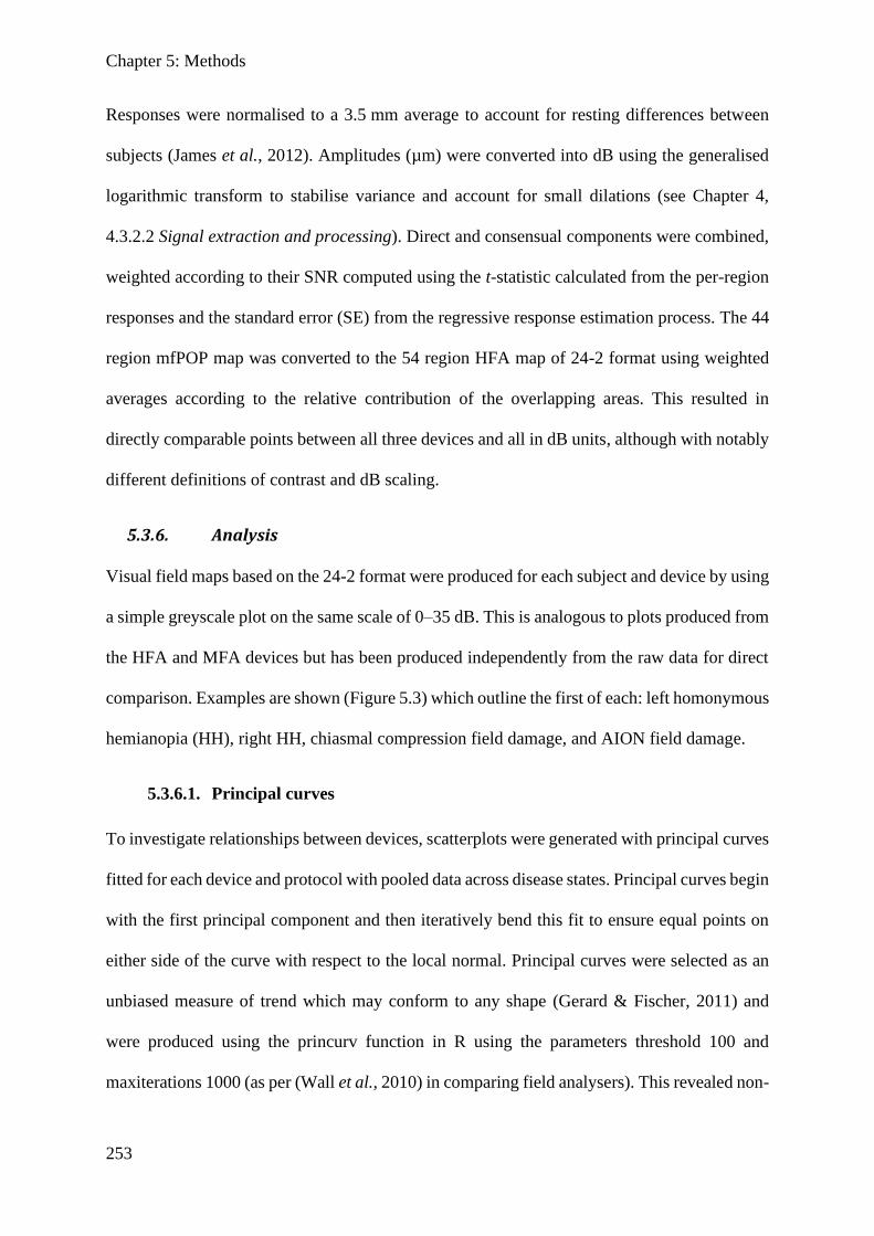
Chapter 5: Methods
253
Responses were normalised to a 3.5 mm average to account for resting differences between
subjects (James et al., 2012). Amplitudes (µm) were converted into dB using the generalised
logarithmic transform to stabilise variance and account for small dilations (see Chapter 4,
4.3.2.2 Signal extraction and processing). Direct and consensual components were combined,
weighted according to their SNR computed using the t-statistic calculated from the per-region
responses and the standard error (SE) from the regressive response estimation process. The 44
region mfPOP map was converted to the 54 region HFA map of 24-2 format using weighted
averages according to the relative contribution of the overlapping areas. This resulted in
directly comparable points between all three devices and all in dB units, although with notably
different definitions of contrast and dB scaling.
5.3.6. Analysis
Visual field maps based on the 24-2 format were produced for each subject and device by using
a simple greyscale plot on the same scale of 0–35 dB. This is analogous to plots produced from
the HFA and MFA devices but has been produced independently from the raw data for direct
comparison. Examples are shown (Figure 5.3) which outline the first of each: left homonymous
hemianopia (HH), right HH, chiasmal compression field damage, and AION field damage.
5.3.6.1. Principal curves
To investigate relationships between devices, scatterplots were generated with principal curves
fitted for each device and protocol with pooled data across disease states. Principal curves begin
with the first principal component and then iteratively bend this fit to ensure equal points on
either side of the curve with respect to the local normal. Principal curves were selected as an
unbiased measure of trend which may conform to any shape (Gerard & Fischer, 2011) and
were produced using the princurv function in R using the parameters threshold 100 and
maxiterations 1000 (as per (Wall et al., 2010) in comparing field analysers). This revealed non-
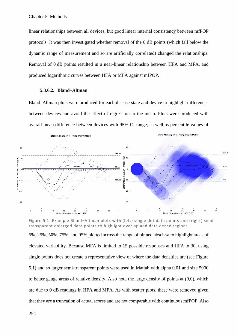
Chapter 5: Methods
254
linear relationships between all devices, but good linear internal consistency between mfPOP
protocols. It was then investigated whether removal of the 0 dB points (which fall below the
dynamic range of measurement and so are artificially correlated) changed the relationships.
Removal of 0 dB points resulted in a near-linear relationship between HFA and MFA, and
produced logarithmic curves between HFA or MFA against mfPOP.
5.3.6.2. Bland–Altman
Bland–Altman plots were produced for each disease state and device to highlight differences
between devices and avoid the effect of regression to the mean. Plots were produced with
overall mean difference between devices with 95% CI range, as well as percentile values of
5%, 25%, 50%, 75%, and 95% plotted across the range of binned abscissa to highlight areas of
elevated variability. Because MFA is limited to 15 possible responses and HFA to 30, using
single points does not create a representative view of where the data densities are (see Figure
5.1) and so larger semi-transparent points were used in Matlab with alpha 0.01 and size 5000
to better gauge areas of relative density. Also note the large density of points at (0,0), which
are due to 0 dB readings in HFA and MFA. As with scatter plots, these were removed given
that they are a truncation of actual scores and are not comparable with continuous mfPOP. Also
Figure 5.1: Example Bland–Altman plots with (left) single dot data points and (righ t) semi-transparent enlarged data points to highlight overlap and data dense regions.

Chapter 5: Methods
255
note the diagonal lines of data, which exist due to a result for one device (for example HFA 0
dB) having many possible results in the other device (for example MFA 0, 2, 3, 6, 7, 10, 12,
13, 18 dB), which when plotting their average against their difference will result in diagonal
placements of points as seen in Figure 5.1.
5.3.6.3. Hemifield ratios
As it is well established in stroke that post-LGN damage typically presents with homonymous
field damage (with the most extreme form being homonymous hemianopia), homonymous
defects are a classic and effective means to identify post-chiasmal stroke. All three perimeters
produce fields with different contrast and ranges, which might make homonymous field
identification challenging. In order to compare a machine’s ability to identify stroke, a
hemifield ratio may be calculated by comparing either the left hemifields of both eyes over the
right hemifields or vice versa, depending on the side of damage. To account for either
possibility, the minimum of both options was taken, which represents the ratio showing the
most damage (see Figure 5.2 top). This was in part done because we did not know with
confidence which field was expected to show a hemianopic defect, especially where the field
damage due to the stroke was mild. Also, some of the patients had suffered multiple strokes
and so strokes were not necessarily confined to a particular half of the posterior pole of the
cortex.
A full and complete hemianopia will have a hemifield ratio of 0, and a completely normal field
where there is no field damage will have a ratio of 1. This ratio can then be used in receiver
operator characteristics (ROC) plots (heading 5.3.6.4) to highlight which devices are most
effective at detecting hemifield damage, and in an intraclass correlation coefficients (ICC) table
(heading 5.3.6.5) to compare correlation between devices.

Chapter 5: Methods
256
While not as well defined as stroke, this principle can be extended to typical field damage in
pituitary tumour, which is stereotypically bitemporal or unilateral temporal, and AION which
is typically unilateral altitudinal. Therefore, using these assumptions, hemifield ratios can be
calculated for chiasmal compression and AION as well (Figure 5.2).
5.3.6.4. Receiver operator characteristics (ROC)
The same approach as detailed in Chapter 3 (3.3.2 Receiver operator characteristics and
thresholds) was used utilising the same program and output format, except using the hemifield
ratio as the measure. ROC plots sensitivity against false positive ratio (FPR; 1 – specificity)
A B C D
Minimum of:
Stroke Hemifield Ratio:
A
B
C
D
Minimum of:
AION Hemifield Ratio:
A B C D
Pituitary Hemifield Ratio:
Figure 5.2: Hemifield ratio calculations for stroke (top), chiasmal compression (middle), and AION (bottom). Each ratio assumes typical field damage based on the anatomical location of the damage, with stroke result ing in either right of left homonymous hemianopic damage, chiasmal compression with bitemporal hemianopic damage, and AION with either superior or inferior loss in a single eye. Where more than one possibility is possible, the minimim of the possible ratio s is used, which represents the one which explains the most damage.
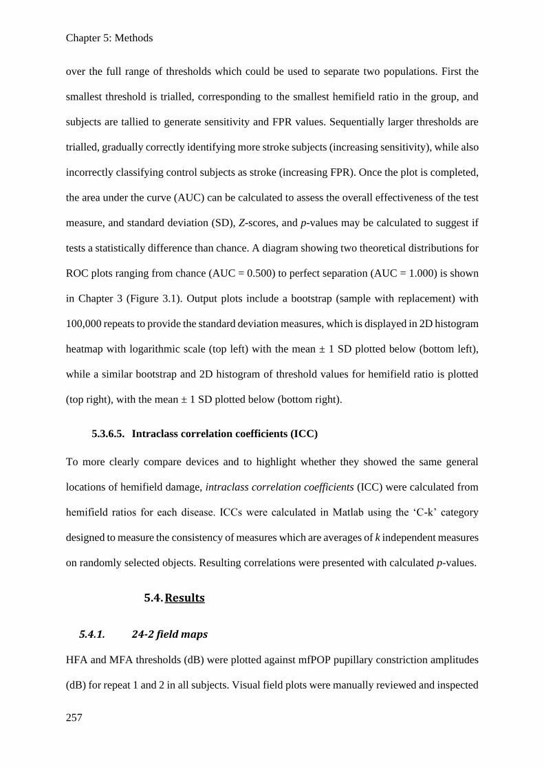
Chapter 5: Methods
257
over the full range of thresholds which could be used to separate two populations. First the
smallest threshold is trialled, corresponding to the smallest hemifield ratio in the group, and
subjects are tallied to generate sensitivity and FPR values. Sequentially larger thresholds are
trialled, gradually correctly identifying more stroke subjects (increasing sensitivity), while also
incorrectly classifying control subjects as stroke (increasing FPR). Once the plot is completed,
the area under the curve (AUC) can be calculated to assess the overall effectiveness of the test
measure, and standard deviation (SD), Z-scores, and p-values may be calculated to suggest if
tests a statistically difference than chance. A diagram showing two theoretical distributions for
ROC plots ranging from chance (AUC = 0.500) to perfect separation (AUC = 1.000) is shown
in Chapter 3 (Figure 3.1). Output plots include a bootstrap (sample with replacement) with
100,000 repeats to provide the standard deviation measures, which is displayed in 2D histogram
heatmap with logarithmic scale (top left) with the mean ± 1 SD plotted below (bottom left),
while a similar bootstrap and 2D histogram of threshold values for hemifield ratio is plotted
(top right), with the mean ± 1 SD plotted below (bottom right).
5.3.6.5. Intraclass correlation coefficients (ICC)
To more clearly compare devices and to highlight whether they showed the same general
locations of hemifield damage, intraclass correlation coefficients (ICC) were calculated from
hemifield ratios for each disease. ICCs were calculated in Matlab using the ‘C-k’ category
designed to measure the consistency of measures which are averages of k independent measures
on randomly selected objects. Resulting correlations were presented with calculated p-values.
5.4. Results
5.4.1. 24-2 field maps
HFA and MFA thresholds (dB) were plotted against mfPOP pupillary constriction amplitudes
(dB) for repeat 1 and 2 in all subjects. Visual field plots were manually reviewed and inspected
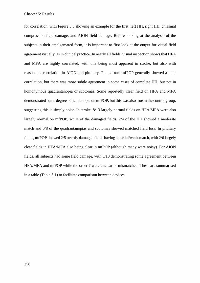
Chapter 5: Results
258
for correlation, with Figure 5.3 showing an example for the first: left HH, right HH, chiasmal
compression field damage, and AION field damage. Before looking at the analysis of the
subjects in their amalgamated form, it is important to first look at the output for visual field
agreement visually, as in clinical practice. In nearly all fields, visual inspection shows that HFA
and MFA are highly correlated, with this being most apparent in stroke, but also with
reasonable correlation in AION and pituitary. Fields from mfPOP generally showed a poor
correlation, but there was more subtle agreement in some cases of complete HH, but not in
homonymous quadrantanopia or scotomas. Some reportedly clear field on HFA and MFA
demonstrated some degree of hemianopia on mfPOP, but this was also true in the control group,
suggesting this is simply noise. In stroke, 8/13 largely normal fields on HFA/MFA were also
largely normal on mfPOP, while of the damaged fields, 2/4 of the HH showed a moderate
match and 0/8 of the quadrantanopias and scotomas showed matched field loss. In pituitary
fields, mfPOP showed 2/5 overtly damaged fields having a partial/weak match, with 2/6 largely
clear fields in HFA/MFA also being clear in mfPOP (although many were noisy). For AION
fields, all subjects had some field damage, with 3/10 demonstrating some agreement between
HFA/MFA and mfPOP while the other 7 were unclear or mismatched. These are summarised
in a table (Table 5.1) to facilitate comparison between devices.
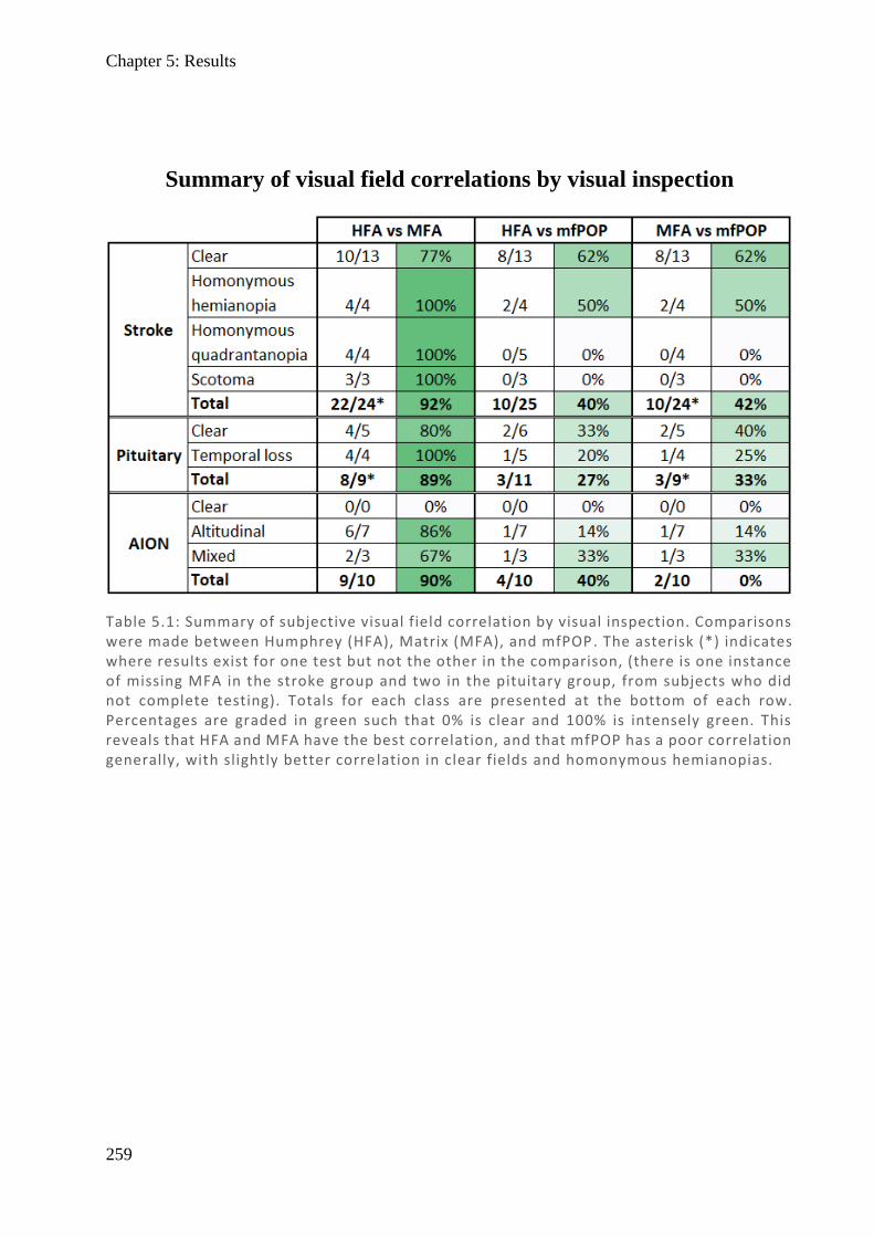
Chapter 5: Results
259
Table 5.1: Summary of subjective visual field correlation by visual inspection. Comparisons were made between Humphrey (HFA), Matrix (MFA), and mfPOP. The asterisk (*) indicates where results exist for one test but not the other in the comparison, (there is one instance of missing MFA in the stroke group and two in the pituitary group, from subjects who did not complete testing). Totals for each class are presented at the bottom of each row. Percentages are graded in green such that 0% is clear and 100% is intensely green. This reveals that HFA and MFA have the best correlation, and that mfPOP has a poor correlation generally, with slightly better corre lation in clear fields and homonymous hemianopias.
Summary of visual field correlations by visual inspection
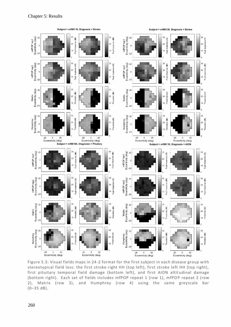
Chapter 5: Results
260
Figure 5.3: Visual fields maps in 24-2 format for the first subject in each disease group with stereotypical field loss: the first stroke right HH (top left), first stroke left HH (top right), first pituitary temporal field damage (bottom left), and first AION altit udinal damage (bottom right). Each set of fields includes mfPOP repeat 1 (row 1), mfPO P repeat 2 (row 2), Matrix (row 3), and Humphrey (row 4) using the same greyscale bar (0–35 dB).
Chapter 5: Results
261
5.4.2. Principal curve scatter plots
Figure 5.4 directly compares 24-2 points between devices by producing scatter plots of all field
points, using a dB scale (noting that scales and contrast differ between devices). HFA, MFA,
and mfPOP by repeat are compared, with associated principal curves (PC). The principal curve
is a non-bias fit which iteratively flexes to ensure the same number of points map to each side.
The graph includes all data points, including 0 dB results which represent the maximum
contrast capability of HFA and MFA devices, while mfPOP is not limited by such constraints.
The left column (A, B) show HFA against mfPOP repeat 1 and 2. There are similar trends
between HFA and both mfPOP repeats, with a logarithmic-like shape. Looking at the data there
are two prominent areas of density: one in the range 25–35 dB HFA which represent largely
normal results spread over most of the mfPOP range (10–40 dB), and another along the bottom
at 0 dB HFA representing complete field loss covering much of the mfPOP range. It is clear
there is a poor correlation, with the principal curve indicating that mfPOP has variety whereas
there is little in HFA. There is a sudden change where HFA trends towards 0, where many of
its points reside, while the mfPOP spread is only marginally reduced. The hyperflex of the PC
is probably spurious due to the limited number of data points in this range.
The right column (D, E) show MFA against mfPOP repeat 1 and 2. The generalised shape is
very similar to that in HFA (sharp curve) but is slightly more linear. There is less pooling of
the data into two domains, with greater spread in MFA than in HFA, although the apparent
horizontal banding is due to results in MFA being limited to only 15 possibilities.
The bottom row (C, F) compares HFA vs MFA and shows a complex sigmoidal relationship.
Initially there is a roughly linear relationship at high values until ~20 dB, after which there is
greater variation in HFA, before both trend towards 0. This may be due to the large number of

Chapter 5: Results
262
values at 0 dB in both devices. While not the focus of these comparisons, mfPOP repeat 1 was
compared to repeat 2, and showed a highly linear correlation, which is further investigated in
Chapter 6.
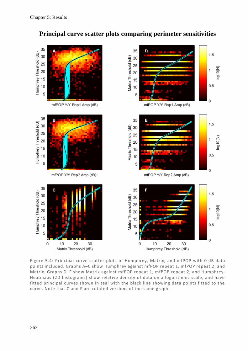
Chapter 5: Results
263
Figure 5.4: Principal curve scatter plots of Humphrey, Matrix, and mfPOP with 0 dB data points included. Graphs A–C show Humphrey against mfPOP repeat 1, mfPOP repeat 2, and Matrix. Graphs D–F show Matrix against mfPOP repeat 1, mfPOP repeat 2, and Humphrey. Heatmaps (2D histograms) show relative density of data on a logorithmic scale, and have fitted principal curves shown in teal with the black line showing data points fitted to the curve. Note that C and F are rotated versions of the same graph.
Principal curve scatter plots comparing perimeter sensitivities
Chapter 5: Results
264
Due to the large effect of 0 dB points on the data, and the consideration that these are not true
0-dB points, but rather a result of clipping the range of these machines, it is worth investigating
whether removal of these points reveals different trends between the machines.
Accordingly, Figure 5.5 shows similar scatter plots to Figure 5.4, with the 0 dB points removed.
Scatter plots of HFA, MFA, and mfPOP repeats with associated principal curves are displayed.
The left column (A, B) compares HFA against both mfPOP repeats. Removal of the 0 dB points
appears to have quite substantially altered the shape of the curve so that it is no longer anchored
at 0 dB. However, it still maintains the general logarithmic shape, which is more modest and
appears to give a better fit. At HFA of ~25 dB, the mfPOP covers most of its range of 10–
40 dB with a gradient of near zero showing no correlation before arcing downward with a large
change in HFA at lower thresholds and having a y-intercept at ~12 dB. This shape shows that
as mfPOP decreases, HFA remains constant until about 10 dB, after which there is rapid
deterioration in HFA scores. If both devices were assumed to be measuring underlying damage,
this would be consistent with HFA having input from overlapping retinal cells with redundancy
(all RGC), while mfPOP input (ipRGC) has less redundancy, such that small amounts of
damage affect mfPOP but do not affect HFA – until no redundancy remains and there is a steep
decline. This possibility is further explored in the discussion.
The right column (D, E) compares MFA against both mfPOP repeats. Removal of the 0 dB
points has more modestly affected MFA so that its gradients are less steep, and it now closely
approximates the general shape of HFA and mfPOP. While HFA is very flat at 25 dB over the
mfPOP range of 10–40 dB, MFA has a modest shallow linear gradient before also arcing
downwards with an intercept near the origin (0,0). This adds weight to the consideration of
redundancy, given that the MFA is said to target My cells more sensitive to cellular loss and
with less overlapping fields (less redundancy). A key difference between HFA and MFA is that

Chapter 5: Results
265
there is a greater range of data below 20 dB in MFA, which likely accounts for the steeper arc
and which makes sense given that the MFA uses the Michelson formula with dB conversion
which is effectively mathematically double that of the HFA which uses the Weber formula for
contrast.
The bottom rows (C, F) compare HFA and MFA, revealing that there is a much more linear
correlation when the 0 dB points are removed. At the higher end of the thresholds, the curve
has a 1:2 linear relationship, with HFA falling from 35 to 25 dB (a 10 dB range), while MFA
has fallen from 40 to 20 dB (a 20 dB range), consistent with the Michelson and Weber contrast
calculations, then shifting to a steeper gradient closer to a 1.3 : 1 ratio (HFA : MFA).
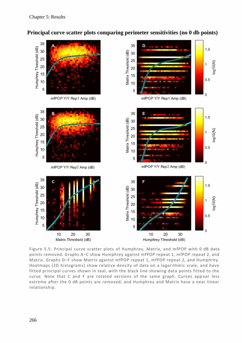
Chapter 5: Results
266
Figure 5.5: Principal curve scatter plots of Humphrey, Matrix, and mfPOP with 0 dB data points removed. Graphs A–C show Humphrey against mfPOP repeat 1, mfPOP repeat 2, and Matrix. Graphs D–F show Matrix against mfPOP repeat 1, mfPOP repeat 2, and Humphrey. Heatmaps (2D histograms) show relative density of data on a logorithmic scale, and have fitted principal curves shown in teal, with the black line showing data points fitted to the curve. Note that C and F are rotated versions of the same graph. Curves app ear less extreme after the 0 dB points are removed, and Humphrey and Matrix have a near linear relationship.
Principal curve scatter plots comparing perimeter sensitivities (no 0 db points)
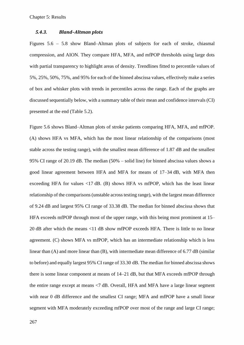
Chapter 5: Results
267
5.4.3. Bland–Altman plots
Figures 5.6 – 5.8 show Bland–Altman plots of subjects for each of stroke, chiasmal
compression, and AION. They compare HFA, MFA, and mfPOP thresholds using large dots
with partial transparency to highlight areas of density. Trendlines fitted to percentile values of
5%, 25%, 50%, 75%, and 95% for each of the binned abscissa values, effectively make a series
of box and whisker plots with trends in percentiles across the range. Each of the graphs are
discussed sequentially below, with a summary table of their mean and confidence intervals (CI)
presented at the end (Table 5.2).
Figure 5.6 shows Bland–Altman plots of stroke patients comparing HFA, MFA, and mfPOP.
(A) shows HFA vs MFA, which has the most linear relationship of the comparisons (most
stable across the testing range), with the smallest mean difference of 1.87 dB and the smallest
95% CI range of 20.19 dB. The median (50% – solid line) for binned abscissa values shows a
good linear agreement between HFA and MFA for means of 17–34 dB, with MFA then
exceeding HFA for values <17 dB. (B) shows HFA vs mfPOP, which has the least linear
relationship of the comparisons (unstable across testing range), with the largest mean difference
of 9.24 dB and largest 95% CI range of 33.38 dB. The median for binned abscissa shows that
HFA exceeds mfPOP through most of the upper range, with this being most prominent at 15–
20 dB after which the means <11 dB show mfPOP exceeds HFA. There is little to no linear
agreement. (C) shows MFA vs mfPOP, which has an intermediate relationship which is less
linear than (A) and more linear than (B), with intermediate mean difference of 6.77 dB (similar
to before) and equally largest 95% CI range of 33.30 dB. The median for binned abscissa shows
there is some linear component at means of 14–21 dB, but that MFA exceeds mfPOP through
the entire range except at means <7 dB. Overall, HFA and MFA have a large linear segment
with near 0 dB difference and the smallest CI range; MFA and mfPOP have a small linear
segment with MFA moderately exceeding mfPOP over most of the range and large CI range;
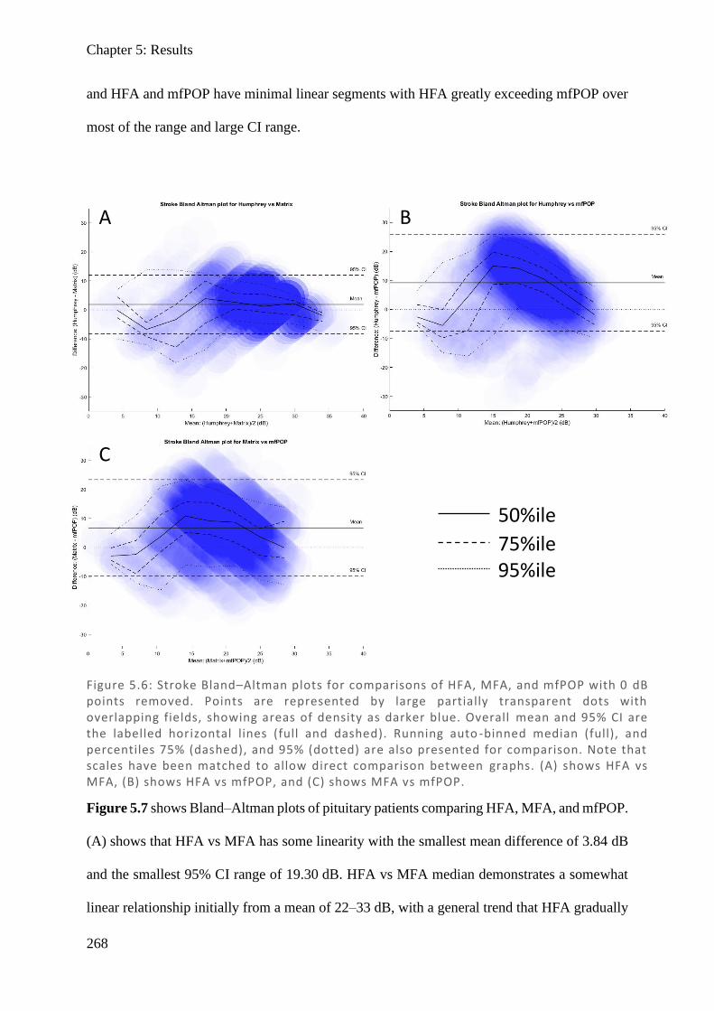
Chapter 5: Results
268
and HFA and mfPOP have minimal linear segments with HFA greatly exceeding mfPOP over
most of the range and large CI range.
Figure 5.7 shows Bland–Altman plots of pituitary patients comparing HFA, MFA, and mfPOP.
(A) shows that HFA vs MFA has some linearity with the smallest mean difference of 3.84 dB
and the smallest 95% CI range of 19.30 dB. HFA vs MFA median demonstrates a somewhat
linear relationship initially from a mean of 22–33 dB, with a general trend that HFA gradually
Figure 5.6: Stroke Bland–Altman plots for comparisons of HFA, MFA, and mfPOP with 0 dB points removed. Points are represented by large partially transparent dots with overlapping fields, showing areas of density as darker blue. Overall mean and 95% CI are the labelled horizontal lines (full and dashed). Running auto -binned median (full), and percentiles 75% (dashed), and 95% (dotted) are also presented for comparison. Note that scales have been matched to allow direct comparison between graphs. (A) shows HFA vs MFA, (B) shows HFA vs mfPOP, and (C) shows MFA vs mfPOP.
A B
C
50%ile
75%ile
95%ile
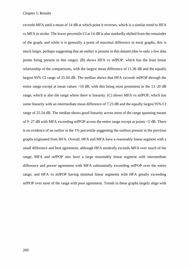
Chapter 5: Results
269
exceeds MFA until a mean of 14 dB at which point it reverses, which is a similar trend to HFA
vs MFA in stroke. The lower percentile CI at 14 dB is also markedly shifted from the remainder
of the graph, and while it is generally a point of maximal difference in most graphs, this is
much larger, perhaps suggesting that an outlier is present in this dataset (due to only a few data
points being present in this range). (B) shows HFA vs mfPOP, which has the least linear
relationship of the comparisons, with the largest mean difference of 11.36 dB and the equally
largest 95% CI range of 25.04 dB. The median shows that HFA exceeds mfPOP through the
entire range except at mean values <10 dB, with this being most prominent in the 13–20 dB
range, which is also the range where there is linearity. (C) shows MFA vs mfPOP, which has
some linearity with an intermediate mean difference of 7.23 dB and the equally largest 95% CI
range of 25.54 dB. The median shows good linearity across most of the range spanning means
of 9–27 dB with MFA exceeding mfPOP across the entire range except at points <5 dB. There
is no evidence of an outlier in the 1% percentile suggesting the outliers present in the previous
graphs originated from HFA. Overall, HFA and MFA have a reasonably linear segment with a
small difference and best agreement, although HFA modestly exceeds MFA over much of the
range; MFA and mfPOP also have a large reasonably linear segment with intermediate
difference and poorer agreement with MFA substantially exceeding mfPOP over the entire
range; and HFA vs mfPOP having minimal linear segments with HFA greatly exceeding
mfPOP over most of the range with poor agreement. Trends in these graphs largely align with
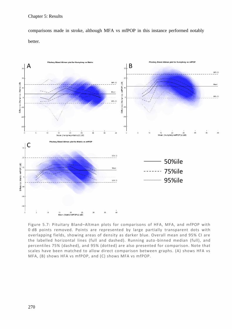
Chapter 5: Results
270
comparisons made in stroke, although MFA vs mfPOP in this instance performed notably
better.
Figure 5.7: Pituitary Bland–Altman plots for comparisons of HFA, MFA, and mfPOP with 0 dB points removed. Points are represented by large partially transparent dots with overlapping fields, showing areas of density as darker blue. Overall mean and 95% CI are the labelled horizontal lines (full and dashed). Running auto -binned median (full), and percentiles 75% (dashed), and 95% (dotted) are also presented for comparison. Note that scales have been matched to allow direct comparison between graphs. (A) shows HFA vs MFA, (B) shows HFA vs mfPOP, and (C) shows MFA vs mfPOP.
A B
C
50%ile
75%ile
95%ile

Chapter 5: Results
271
Figure 5.8 shows Bland–Altman plots of AION patients comparing HFA, MFA, and mfPOP.
(A) shows HFA vs MFA, which has the most linear relationship of the comparisons with a
small mean difference of 4.30 dB and smallest 95% CI range of 24.90 dB. The median shows
good agreement between HFA and MFA for means over most of the range, with HFA
exceeding MFA modestly over the range except at extremes of <4 dB and >32 dB. (B) shows
HFA vs mfPOP, which has a nonlinear relationship with the largest mean difference of 8.82 dB
and the largest 95% CI range of 39.69 dB. The median shows there is minimal linearity and
poor agreement, with HFA substantially exceeding mfPOP over the central range of means of
12–23 dB and mfPOP modestly exceeding HFA at the extremes. Notably, there is a very large
5% percentile range dipping to –15 dB despite the median being 17 dB, suggesting that while
HFA generally exceeds mfPOP there is quite substantial variation, and this is consistent with
having the equally largest 95% CI of all comparisons in all graphs. (C) shows MFA vs mfPOP,
which has a similarly poor relationship to (B) with a nonlinear relationship, small mean
difference of 4.12 dB, and an equally large CI range of 40.27 dB. The median shows there is
minimal linearity and poor agreement, with MFA substantially exceeding mfPOP over the
central range of means of 8–20 dB and mfPOP modestly exceeding MFA at the extremes. There
are also particularly wide scores at 95% and 5%, similar to (B). Overall, HFA and MFA have
linearity over most of the range with the smallest difference and CI range; MFA and mfPOP
as well as HFA and mfPOP have minimal linear segments; and HFA and MFA exceed mfPOP
over much of the range with larger differences and very large CI ranges. Trends in AION
largely concur with those in stroke and pituitary, highlighting that HFA and MFA have good
overall agreement, that MFA and mfPOP have poor agreement, and that HFA and mfPOP have
very poor agreement.
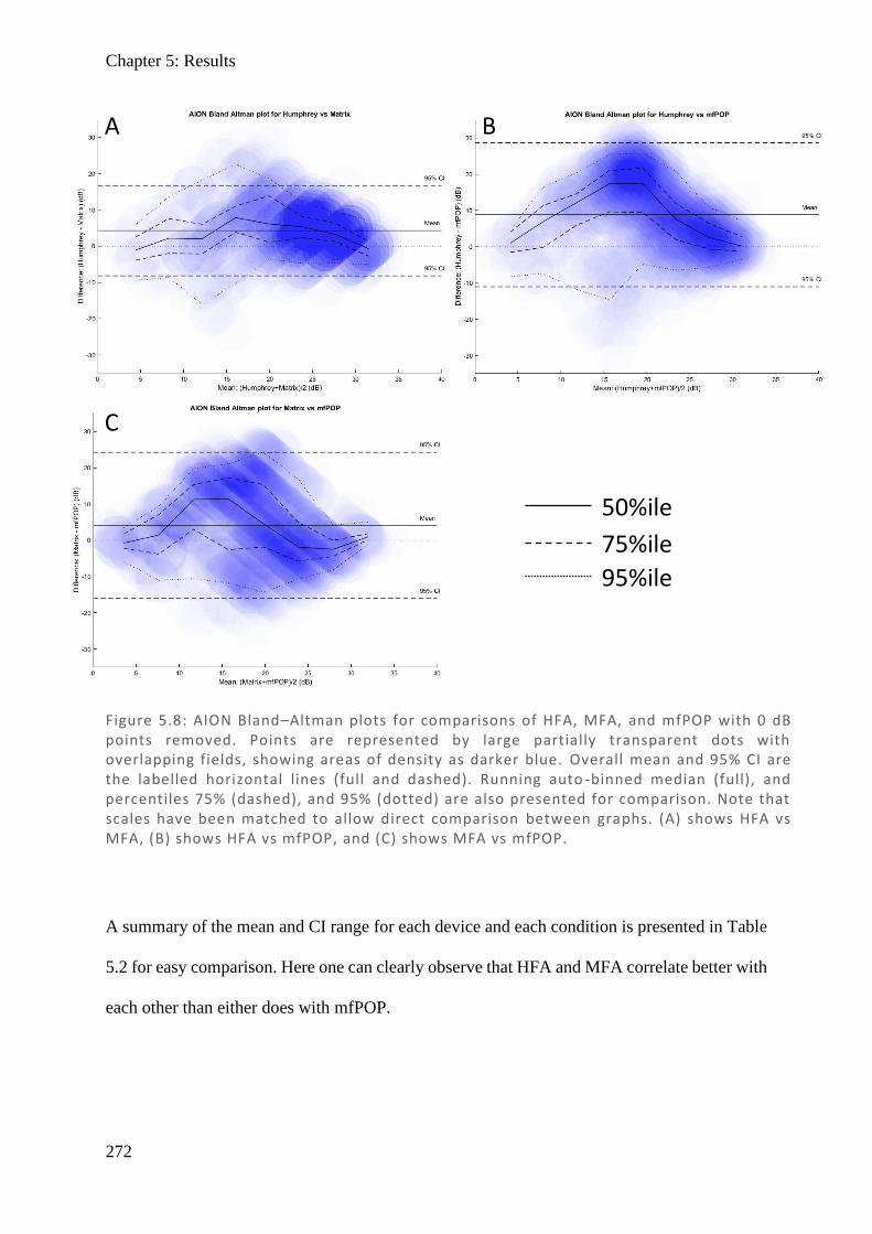
Chapter 5: Results
272
A summary of the mean and CI range for each device and each condition is presented in Table
5.2 for easy comparison. Here one can clearly observe that HFA and MFA correlate better with
each other than either does with mfPOP.
Figure 5.8: AION Bland–Altman plots for comparisons of HFA, MFA, and mfPOP with 0 dB points removed. Points are represented by large partially transparent dots with overlapping fields, showing areas of density as darker blue. Overall mean and 95% CI are the labelled horizontal lines (full and dashed). Running auto -binned median (full), and percentiles 75% (dashed), and 95% (dotted) are also presented for comparison. Note that scales have been matched to allow direct comparison between graphs. (A) shows HFA vs MFA, (B) shows HFA vs mfPOP, and (C) shows MFA vs mfPOP.
A B
C
50%ile
75%ile
95%ile
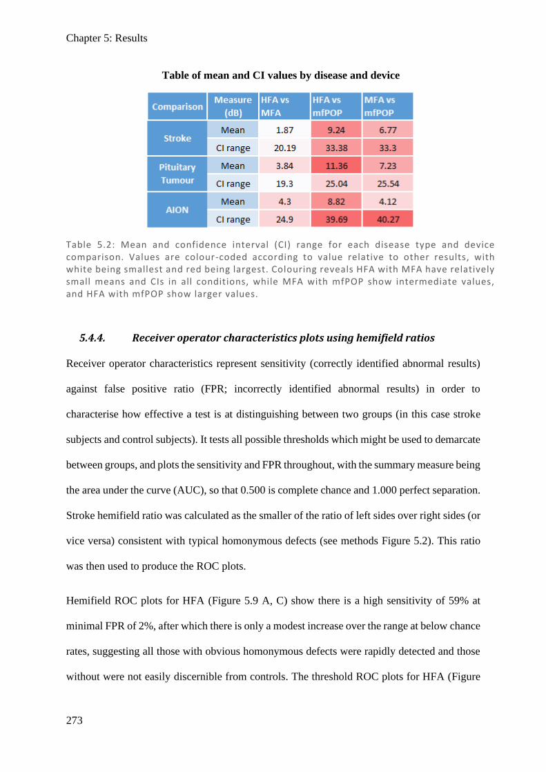
Chapter 5: Results
273
5.4.4. Receiver operator characteristics plots using hemifield ratios
Receiver operator characteristics represent sensitivity (correctly identified abnormal results)
against false positive ratio (FPR; incorrectly identified abnormal results) in order to
characterise how effective a test is at distinguishing between two groups (in this case stroke
subjects and control subjects). It tests all possible thresholds which might be used to demarcate
between groups, and plots the sensitivity and FPR throughout, with the summary measure being
the area under the curve (AUC), so that 0.500 is complete chance and 1.000 perfect separation.
Stroke hemifield ratio was calculated as the smaller of the ratio of left sides over right sides (or
vice versa) consistent with typical homonymous defects (see methods Figure 5.2). This ratio
was then used to produce the ROC plots.
Hemifield ROC plots for HFA (Figure 5.9 A, C) show there is a high sensitivity of 59% at
minimal FPR of 2%, after which there is only a modest increase over the range at below chance
rates, suggesting all those with obvious homonymous defects were rapidly detected and those
without were not easily discernible from controls. The threshold ROC plots for HFA (Figure
Table 5.2: Mean and confidence interval (CI) range for each disease type and device comparison. Values are colour-coded according to value relative to other results, with white being smallest and red being largest. Colouring reveals HFA with MFA have relatively small means and CIs in all conditions, while MFA with mfPOP show intermediate values, and HFA with mfPOP show larger values.
Table of mean and CI values by disease and device
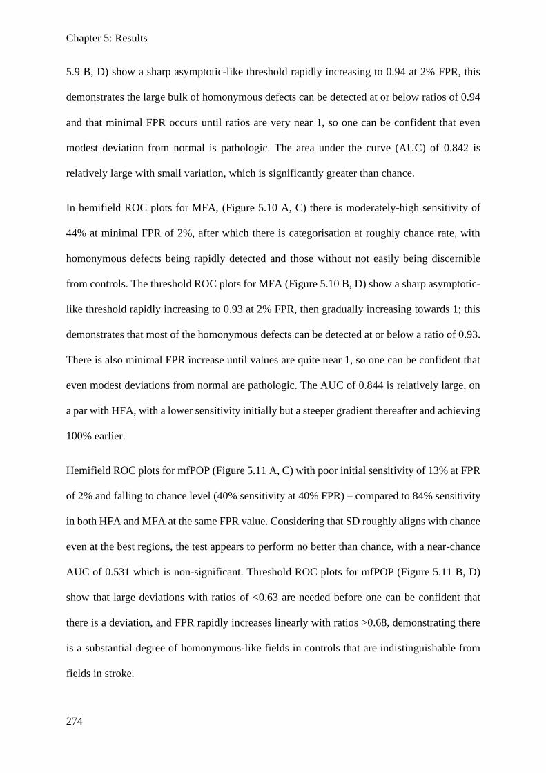
Chapter 5: Results
274
5.9 B, D) show a sharp asymptotic-like threshold rapidly increasing to 0.94 at 2% FPR, this
demonstrates the large bulk of homonymous defects can be detected at or below ratios of 0.94
and that minimal FPR occurs until ratios are very near 1, so one can be confident that even
modest deviation from normal is pathologic. The area under the curve (AUC) of 0.842 is
relatively large with small variation, which is significantly greater than chance.
In hemifield ROC plots for MFA, (Figure 5.10 A, C) there is moderately-high sensitivity of
44% at minimal FPR of 2%, after which there is categorisation at roughly chance rate, with
homonymous defects being rapidly detected and those without not easily being discernible
from controls. The threshold ROC plots for MFA (Figure 5.10 B, D) show a sharp asymptotic-
like threshold rapidly increasing to 0.93 at 2% FPR, then gradually increasing towards 1; this
demonstrates that most of the homonymous defects can be detected at or below a ratio of 0.93.
There is also minimal FPR increase until values are quite near 1, so one can be confident that
even modest deviations from normal are pathologic. The AUC of 0.844 is relatively large, on
a par with HFA, with a lower sensitivity initially but a steeper gradient thereafter and achieving
100% earlier.
Hemifield ROC plots for mfPOP (Figure 5.11 A, C) with poor initial sensitivity of 13% at FPR
of 2% and falling to chance level (40% sensitivity at 40% FPR) – compared to 84% sensitivity
in both HFA and MFA at the same FPR value. Considering that SD roughly aligns with chance
even at the best regions, the test appears to perform no better than chance, with a near-chance
AUC of 0.531 which is non-significant. Threshold ROC plots for mfPOP (Figure 5.11 B, D)
show that large deviations with ratios of <0.63 are needed before one can be confident that
there is a deviation, and FPR rapidly increases linearly with ratios >0.68, demonstrating there
is a substantial degree of homonymous-like fields in controls that are indistinguishable from
fields in stroke.
Chapter 5: Results
275
Figure 5.9: Stroke HFA ROC plots using hemifield ratio, with 100,000 repeat bootstrap. Dashed line represents chance (where a test has no diagnostic capacity). (A) shows log -scale heatmap of the ROC with bootstrap demonstrating variability and general trend, with (C) showing the resulting mean ± SD allowing calculation of area under the curve (AUC). (B) shows threshold heatmap highlighting what threshold is used for calculation of the sensitivity/FPR values, together with (D) using the mean and ±SD.
Humphrey Field Analyser
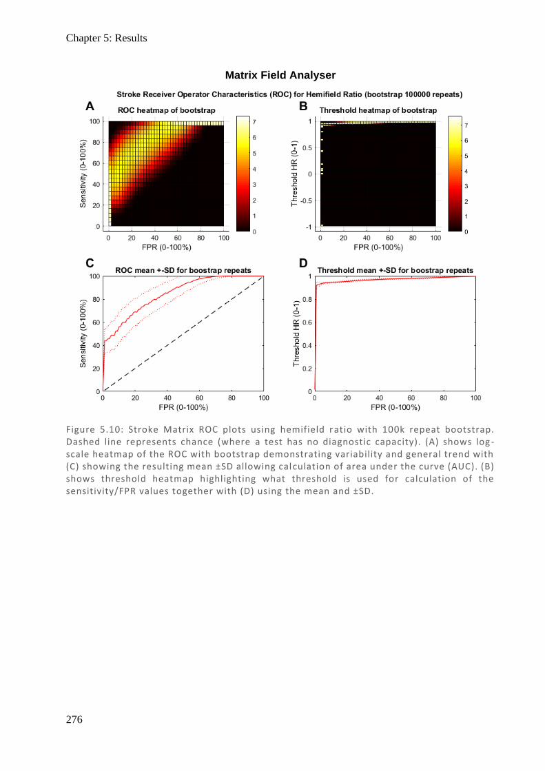
Chapter 5: Results
276
Figure 5.10: Stroke Matrix ROC plots using hemifield ratio with 100k repeat bootstrap. Dashed line represents chance (where a test has no diagnostic capacity). (A) shows log -scale heatmap of the ROC with bootstrap demonstrating variability and general trend with (C) showing the resulting mean ±SD allowing calculation of area under the curve (AUC). (B) shows threshold heatmap highlighting what threshold is used for calculation of the sensitivity/FPR values together with (D) using the mean and ±SD.
Matrix Field Analyser
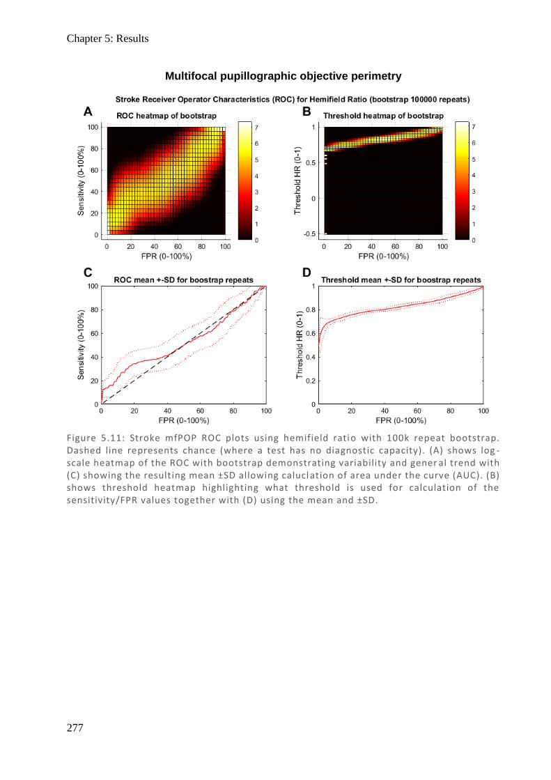
Chapter 5: Results
277
Figure 5.11: Stroke mfPOP ROC plots using hemifield ratio with 100k repeat bootstrap. Dashed line represents chance (where a test has no diagnostic capacity). (A) shows log -scale heatmap of the ROC with bootstrap demonstrating variability and gener al trend with (C) showing the resulting mean ±SD allowing calucl ation of area under the curve (AUC). (B) shows threshold heatmap highlighting what threshold is used for calculation of the sensitivity/FPR values together with (D) using the mean and ±SD.
Multifocal pupillographic objective perimetry
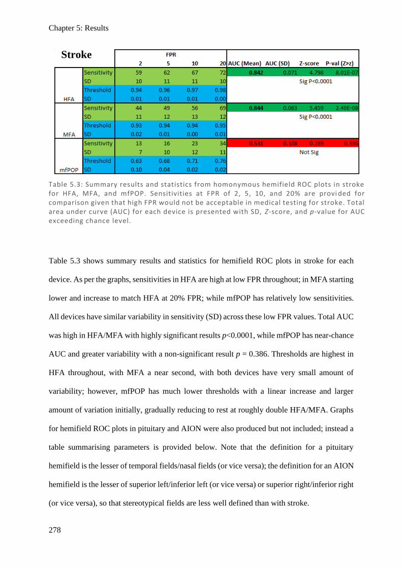
Chapter 5: Results
278
Table 5.3 shows summary results and statistics for hemifield ROC plots in stroke for each
device. As per the graphs, sensitivities in HFA are high at low FPR throughout; in MFA starting
lower and increase to match HFA at 20% FPR; while mfPOP has relatively low sensitivities.
All devices have similar variability in sensitivity (SD) across these low FPR values. Total AUC
was high in HFA/MFA with highly significant results p<0.0001, while mfPOP has near-chance
AUC and greater variability with a non-significant result p = 0.386. Thresholds are highest in
HFA throughout, with MFA a near second, with both devices have very small amount of
variability; however, mfPOP has much lower thresholds with a linear increase and larger
amount of variation initially, gradually reducing to rest at roughly double HFA/MFA. Graphs
for hemifield ROC plots in pituitary and AION were also produced but not included; instead a
table summarising parameters is provided below. Note that the definition for a pituitary
hemifield is the lesser of temporal fields/nasal fields (or vice versa); the definition for an AION
hemifield is the lesser of superior left/inferior left (or vice versa) or superior right/inferior right
(or vice versa), so that stereotypical fields are less well defined than with stroke.
Table 5.3: Summary results and statistics from homonymous hemifield ROC plots in stroke for HFA, MFA, and mfPOP. Sensitivities at FPR of 2, 5, 10, and 20% are provi ded for comparison given that high FPR would not be acceptable in medical testing for stroke. Total area under curve (AUC) for each device is presented with SD, Z-score, and p-value for AUC exceeding chance level.
Stroke
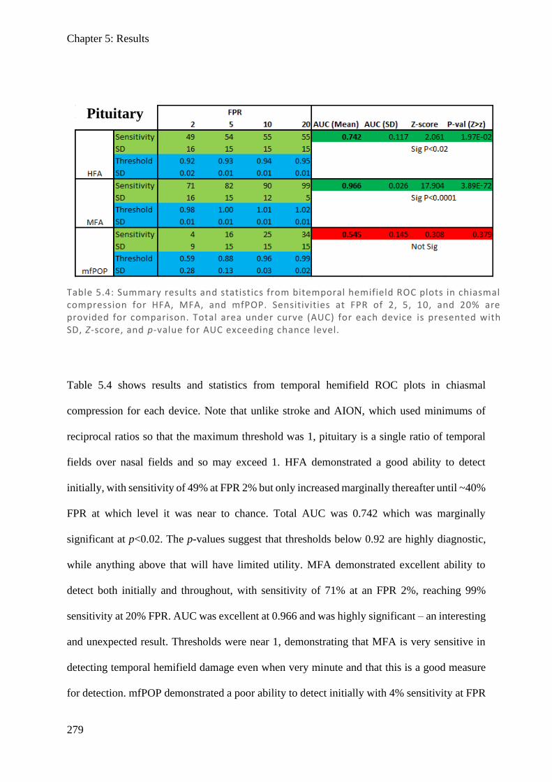
Chapter 5: Results
279
Table 5.4 shows results and statistics from temporal hemifield ROC plots in chiasmal
compression for each device. Note that unlike stroke and AION, which used minimums of
reciprocal ratios so that the maximum threshold was 1, pituitary is a single ratio of temporal
fields over nasal fields and so may exceed 1. HFA demonstrated a good ability to detect
initially, with sensitivity of 49% at FPR 2% but only increased marginally thereafter until ~40%
FPR at which level it was near to chance. Total AUC was 0.742 which was marginally
significant at p<0.02. The p-values suggest that thresholds below 0.92 are highly diagnostic,
while anything above that will have limited utility. MFA demonstrated excellent ability to
detect both initially and throughout, with sensitivity of 71% at an FPR 2%, reaching 99%
sensitivity at 20% FPR. AUC was excellent at 0.966 and was highly significant – an interesting
and unexpected result. Thresholds were near 1, demonstrating that MFA is very sensitive in
detecting temporal hemifield damage even when very minute and that this is a good measure
for detection. mfPOP demonstrated a poor ability to detect initially with 4% sensitivity at FPR
Table 5.4: Summary results and statistics from bitemporal hemifield ROC plots in chiasmal compression for HFA, MFA, and mfPOP. Sensitivities at FPR of 2, 5, 10, and 20% are provided for comparison. Total area under curve (AUC) for each device is presented with SD, Z-score, and p-value for AUC exceeding chance level.
Pituitary
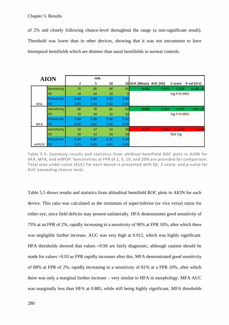
Chapter 5: Results
280
of 2% and closely following chance-level throughout the range (a non-significant result).
Threshold was lower than in other devices, showing that it was not uncommon to have
bitemporal hemifields which are dimmer than nasal hemifields in normal controls.
Table 5.5 shows results and statistics from altitudinal hemifield ROC plots in AION for each
device. This ratio was calculated as the minimum of super/inferior (or vice versa) ratios for
either eye, since field deficits may present unilaterally. HFA demonstrates good sensitivity of
75% at an FPR of 2%, rapidly increasing to a sensitivity of 90% at FPR 10%, after which there
was negligible further increase. AUC was very high at 0.912, which was highly significant.
HFA thresholds showed that values <0.90 are fairly diagnostic, although caution should be
made for values >0.93 as FPR rapidly increases after this. MFA demonstrated good sensitivity
of 68% at FPR of 2%, rapidly increasing to a sensitivity of 81% at a FPR 10%, after which
there was only a marginal further increase – very similar to HFA in morphology. MFA AUC
was marginally less than HFA at 0.885, while still being highly significant. MFA thresholds
Table 5.5: Summary results and statistics from altidinal hemifield ROC plots in AION for HFA, MFA, and mfPOP. Sensitivities at FPR of 2, 5, 10, and 20% are provided for comparison. Total area under curve (AUC) for each device is presented with SD, Z-score, and p-value for AUC exceeding chance level.
AION
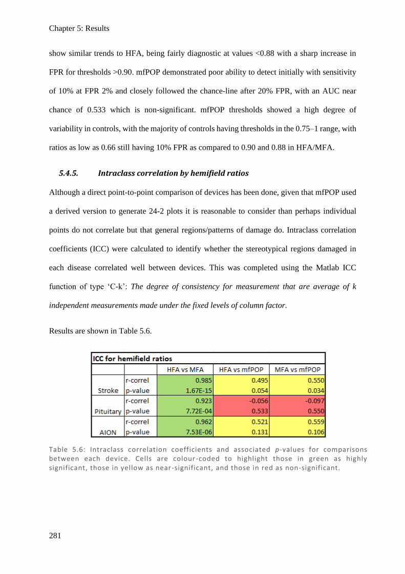
Chapter 5: Results
281
show similar trends to HFA, being fairly diagnostic at values <0.88 with a sharp increase in
FPR for thresholds >0.90. mfPOP demonstrated poor ability to detect initially with sensitivity
of 10% at FPR 2% and closely followed the chance-line after 20% FPR, with an AUC near
chance of 0.533 which is non-significant. mfPOP thresholds showed a high degree of
variability in controls, with the majority of controls having thresholds in the 0.75–1 range, with
ratios as low as 0.66 still having 10% FPR as compared to 0.90 and 0.88 in HFA/MFA.
5.4.5. Intraclass correlation by hemifield ratios
Although a direct point-to-point comparison of devices has been done, given that mfPOP used
a derived version to generate 24-2 plots it is reasonable to consider than perhaps individual
points do not correlate but that general regions/patterns of damage do. Intraclass correlation
coefficients (ICC) were calculated to identify whether the stereotypical regions damaged in
each disease correlated well between devices. This was completed using the Matlab ICC
function of type ‘C-k’: The degree of consistency for measurement that are average of k
independent measurements made under the fixed levels of column factor.
Results are shown in Table 5.6.
Table 5.6: Intraclass correlation coefficients and associated p-values for comparisons between each device. Cells are colour -coded to highlight those in green as highly significant, those in yellow as near-significant, and those in red as non-significant.

Chapter 5: Results
282
ICCs for HFA vs MFA were high in all disease states, with stroke being the most highly
correlated followed closely by AION and pituitary, with all results being highly significant.
For HFA vs mfPOP, results were mixed with moderate correlation in stroke and AION with
near-significant results, while pituitary was negatively correlated and was non-significant. For
MFA vs mfPOP, results were similar to HFA but slightly more favourable, with stroke and
AION being near-significant and marginally significant, and pituitary again being negatively
correlated with a non-significant result. These are generally consistent with point-to-point
comparisons and further support that there is a good correlation between HFA and MFA,
whereas mfPOP does not correlate well with either, although marginally better in MFA.
Chapter 5: Discussion
283
5.5. Discussion
While an analysis on the population scale would be absolutely worth doing, the 24-2 raw field
maps provide a good measure of what clinicians might see in practice when looking at
individual patients, and so visual inspection is an important part of deciding which devices
work well.
Visually, HFA and MFA have very good agreement with respect to damage location and
morphology through all conditions, although there were a couple of instances of mismatch
where one demonstrated something the other did not. mfPOP showed some general hemianopic
trends to side matching HFA/MFA in stroke when there was complete/near-complete
homonymous hemianopia, but otherwise did not correlate well with quadrantanopias or smaller
damaged areas in any condition. It was however noticed that in many of the fields where some
damage was apparent on HFA/MFA, that mfPOP showed a noisy reduction in the entire field,
although it was often difficult to discern given the high level of noise.
This is an interesting result given that the traditional subcortical pupillary pathway branches
before the LGN and therefore would not be expected to detect post-LGN damage without
cortical input. Anatomical studies show there is cortical input to the pretectal olivary nucleus
within the pretectum (Gamlin, 2006), it has been demonstrated that removal of the cortex in
macaques can affect pupil dynamics (Heywood et al., 1998), and response delays in
isoluminant colour exchange (Carle et al., 2013; Rosli et al., 2018) suggest mfPOP may be
affected by cortical input. However, results in this study using the mfPOP Y/Y protocol did not
demonstrate this. The inconsistency in mfPOP to show pupillary changes in hemianopias, the
absence of any correlation in quadrantanopias, and the at-chance AUC values from ROC show
that cortical stroke is only minimally detected by this test. It would then seem that perhaps
pupil fields and visual fields might be dissociated in these disorders, as has been reported in
Chapter 5: Discussion
284
other ocular diseases like Leber hereditary optic neuropathy , which shows complete retention
of pupil response despite the visual field loss due to minimal damage to ipRGC (Bremner et
al., 1999; Bremner et al., 2001; Nissen et al., 2015). However, since a several hemianopia
subjects did show a degree of correlation, there must be some means by which damage is
detectable in this system. Another study looking at pupillometry in response to a single large
stimulus (10 degrees diameter) presented in the damaged field of stroke patients also revealed
mixed results. Some stroke patients showed pupillary responses, while others showed minimal
responses, with no obvious reason for this division (Sahraie et al., 2013). Certainly, a simple
argument that different cortical strokes result in different loss of cortical input is a likely
possibility, but perhaps doesn’t explain why same sided hemianopias between patients do not
show similar patterns, or why no quandrantanopias show concordance with automated
perimetry.
One consideration is that the stimuli employed in this study have sufficiently large contrast to
induce a pupil response of the blind hemifield, while not being consciously aware of stimuli.
Several studies addressing blindsight in a patient with a cortical lesions resulting in hemianopia
have demonstrated that large stimuli presented for long periods can be detectable by the patient
and result in pupillary constriction, especially where flicker is employed (Weiskrantz et al.,
1991; Barbur et al., 1994). While this is intriguing, there are several key differences between
their approach and mfPOP, most notable stimuli were presented for 500ms compared to only
33ms in mfPOP, and flicker was employed, while mfPOP does not use flicker. While these
may not be directly comparable, it may still be worth investigating if smaller sized stimuli with
lower contrast may show better attenuation of signal in blind hemifields.
Another further possibility is as subcortical pathways remain intact after stroke initially,
pupillometry may not align with the field defects, but after atrophy to retinal pathways back to
the retina following stroke, retinal input to ipRGC may be affected. This would result in
Chapter 5: Discussion
285
pupillometry being diminished in blind hemifields, and that this might explain the variable
extent of alignment of pupillometry with visual field damage. Removal of striate cortex has
been demonstrated to have a time-course related to the atrophy of the LGN in monkeys (Cowey,
1974; Cowey et al., 1999; Johnson & Cowey, 2000) and lesions in occipital cortex of humans
using MRI have demonstrated shrinkage of the optic tract (Bridge et al., 2011; Cowey et al.,
2011) and even thinning of the retinal nerve fibre layer (RNFL) on OCT scans (Jindahra et al.,
2009). It is therefore theoretically possuble that this degeneration might include cells with input
to the pupillary pathway, and thereby perturb the subcortical pupillary response sufficiently to
facilitate crude detection on mfPOP. Results from a recent study looking at the time course of
human retrograde degeneration in homonymous hemianopia demonstrated an initial sharp
decrease in the first two years followed by linear thinning thereafter, while in quadrantanopias
or smaller, there was no discernible thinning at all (Jindahra et al., 2012). Continuing with the
hypothesis that this degeneration affects pupillary input, this then provides a strong argument
for why mfPOP might be able to similarly detect some HH damage, although it might not detect
quadrantanopias or smaller defects. While this issue was not addressed in these studies, brain
MRIs, including diffusion tensor imaging of cortical tracts, was performed on our subjects and
future analysis of these might provide further insight into the hypothesis.
Principal curves were explored for relationships between devices. In the first iteration which
included all data points, HFA had a complex curve relationship with mfPOP, hyperflexing back
on itself, which does not intuitively make sense. Looking more closely at the scatter plot, there
were two areas of dense data – one being at the HFA’s upper range of 25–35 dB spread over
the entire mfPOP range, and another at HFA’s lower range at 0 dB, again with a substantial
spread in mfPOP, and these appear to be the factors causing this flex. This was confirmed by
the second iteration with 0 dB data points removed, showing a relationship with no correlation
initially at high normal HFA values, and then a sharp decline in HFA over a small mfPOP
Chapter 5: Discussion
286
range. Given that HFA thresholds are calculated using the maximal luminance it can display
(3178 cd/m2) as 0 dB (Fredette et al., 2015), it is clear that a 0 dB score is not a true null
response, as more intense lights might still allow detection of the stimulus. There is thus a floor
effect, at which true thresholds are grouped into 0 dB as the limit of the testing range is reached.
It is then reasonable to only compare tests within their range and exclude points affected by
this floor (i.e. 0 dB points). In looking at MFA with mfPOP, in the first iteration there was
again a pooling of data at the 0 dB range, but otherwise the data was more widely spread
throughout the MFA range (albeit striated due to a limitation of 15 output thresholds). After
removing the 0 dB data points in the second iteration, the relationship was less dramatically
shifted than in HFA, but modestly less steep and in good alignment with HFA trends. In
comparing HFA vs MFA with all data, there was a sigmoidal relationship which appears to be
due to 0-points in MFA all being 0 dB points in HFA, but HFA having many 0 dB points which
are spread over the MFA range. While they both have floor effects, it is well established that
MFA has a greater dynamic range than HFA in glaucoma (Wall et al., 2009), and this result
suggests the same is true of neurological disease. Once 0 dB points are removed, they show a
nearly linear relationship, with a slight flexion at 20 dB HFA / 15 dB MFA. The gradient is
initially roughly 2:1 for MFA:HFA, which is consistent with the different dB conversion rates
of 20*log(contrast) vs 10*log(attenuation), thereafter becoming closer to 1:1, perhaps due to
the HFA’s smaller dynamic range. Considering that mfPOP has been correlated with RNFL
thickness (structural damage) (Kolic et al., 2013), and that both HFA and MFA are known to
measure threshold for detection (functional damage), this may explain the shape of their
relationship. It is known that there are many overlapping fields in the retina (Wassle & Boycott,
1991; Gauthier et al., 2009; Soo et al., 2011), with the coverage factor suggesting dendritic
overlap of 3–4 cells for a given region (Wassle, 2004), such that damage to a single cell does
not result in field loss (redundancy). However, every cell lost would result in a decrease in
Chapter 5: Discussion
287
RNFL thickness once its axon degenerates, creating a structural loss. It follows that if one were
to plot RNFL thickness against perception, one might see structural damage occurring while
the perceptual signal remained constant – until a critical point was reached where no
redundancy remains and perception rapidly declined (Hart & Becker, 1982; Kerrigan-
Baumrind et al., 2000). This may explain the sharply curved relationship between mfPOP and
HFA, as HFA is a perceptual measure with redundancy and mfPOP has been shown to have a
more linear relationship with RNFL (Kolic et al., 2013). Likewise, it may also underpin why
MFA has a similar relationship with mfPOP as with HFA, although with more linearity – that
is, MFA remains a perceptual measure with some redundancy, but it was originally created to
target My said to have less redundancy (Maddess & Henry, 1992; Johnson, 1994; Johnson &
Samuels, 1997; Wall et al., 2002; Yoon et al., 2012).
Bland–Altman plots collectively demonstrated similar finding to the scatter plots, with HFA
and MFA having the most agreement and smallest mean difference, while HFA and mfPOP
showed the worst agreement and largest mean difference, with MFA and mfPOP having
marginal agreement and intermediate mean differences. Between diseases, pituitary appeared
to have the least variability overall, but may have been confounded by the relatively few data
points having heavy field damage. This also explains its particularly large 1% CI at means of
10–15 dB as an outlier in a small dataset. Stroke had a similar degree of variation to pituitary
but with more data points, and AION showed much wider confidence intervals and greater
variability. Greatest variability in HFA vs MFA for all diseases was in the 12–15 dB range,
which roughly aligns with the flexion point on their principal curve plots. In HFA or MFA
plots against mfPOP, there was no consistent point of maximal variation, with generally large
variation throughout. In terms of means, HFA > MFA > mfPOP for all conditions, which would
make sense given the pooling of data at the upper range in the scatter plots while MFA and
mfPOP were both more evenly spread throughout their range. It should be noted that in stroke
Chapter 5: Discussion
288
it is common to see a fairly sharp demarcation between normal and complete deficit, thereby
generating two distinct data pools – as opposed to say AION or glaucoma which have many
grey-intermediate damage regions which give a spread of data.
In assessing which device is most effective at detecting a disorder, it can be difficult when there
is no gold standard to compare against, but one method is to reduce each field to a single
number and generate a ROC curve. While Mean Defect (MD) has been used repeatedly in HFA
and MFA, it does not take into account if the shape of the field defect is typical for that disease
nor does it control for the possibility that the person has brighter or dimmer fields generally.
Hemifield ratios provide an interesting in between case which only considers field damage
typical of the disease and is naturally normalised to the person’s unaffected regions (because it
is a ratio of one side to the other). HFA and MFA demonstrated a high and significant AUC,
demonstrating that even small deviations (6–7%) from equality between hemifields is highly
diagnostic. In terms of selecting which would be more appropriate, although MFA is very
marginally better than HFA in terms of total AUC, for FPR values which are be likely to be
acceptable (<20%), HFA demonstrates a better profile, reaching 59% sensitivity at an FPR of
2%, compared to MFA’s 44%. mfPOP, on the other hand, did not perform so favourably, with
an AUC marginally above chance and a non-significant result. Looking at a graph of
thresholds, mfPOP demonstrates that many of the control subjects have partial HH-like fields,
meaning this noise makes it very difficult to pick up damaged fields. In complete or near-
complete HH, there were fields which were discernible in mfPOP, and this explains the initial
increase in ROC curves above baseline, but, similar to visual inspection, there was limited
ability to correctly identify any damage in those with smaller defects seen on HFA or MFA.
ROC plots using hemifield ratios for pituitary revealed that while HFA performed fine with a
significant result, MFA quite dramatically outperformed HFA with an AUC of 0.966 reaching
99% sensitivity at 20% FPR. mfPOP again performed at chance level with a non-significant
Chapter 5: Discussion
289
result. It was very interesting to note that MFA sensitivity here even outperformed visual
inspection, with approximately half the subjects having no apparent damage on Matrix field.
Most of the subjects had been identified as having a pituitary tumour through visual field testing
and had demonstrated field deficits prior to surgery, after which many completely resolved.
This suggests that perhaps there was retained subtle damage and that MFA, in combination
with hemifield ratios, is very sensitive to these subtle differences and so may permit earlier
detection. In attempting to explain why MFA performed so well in this test, it is worth thinking
about its design. Matrix was reported to stimulate a subset of magnocellular cells called My
(Maddess & Henry, 1992; Johnson & Samuels, 1997). My comprise 15–25% of the
magnocellular response, are large in diameter, and have minimal coverage factor (Crook et al.,
1988), being suggested to be sensitive to glaucomatous damage and insensitive to other
neurological disease (Maddess & Henry, 1992). While this premise has been challenged
(Anderson & Johnson, 2002; White et al., 2002), it continues to be debated (Maddess, 2011a).
Whether My cells are the population of interest or not, the principle that the MFA stimulus
targets a cell type which has a low convergence factor might well explain why MFA appears
to detect subtle differences which HFA is insensitive to.
ROC plots using hemifield ratios for AION revealed that HFA and MFA perform well with
high AUC for both devices, with significant results. HFA performed slightly better than MFA,
with larger AUC and larger sensitivities over a useful FPR range, initially reaching 75%
sensitivity at 2% FPR compared with MFA’s 68%. mfPOP performed on a par with previous
diseases, with no significant difference from chance.
Overall, the ROC plots reveal that HFA is likely to be the most useful in stroke and AION,
while MFA has excellent sensitivity and is most useful in chiasmal compression. mfPOP was
not able to discern disease states using hemifield ratios, and thresholds show substantial noise
which could mislead clinicians to false conclusions.
Chapter 5: Discussion
290
While agreement between the devices was determined with point-to-point correlations, the
general location of field damage had not been compared. Using the same hemifield ratios
utilised in ROC plots, the mfPOP device was compared with other devices using intraclass
correlation coefficients (ICCs). Results were consistent with pointwise analysis, with HFA and
MFA having excellent correlation in stroke and AION, and very good correlation in chiasmal
compression; while mfPOP comparisons were not well correlated, although marginally better
against MFA than HFA. While one of the results for MFA vs mfPOP did reach significance at
the 5% level, this was marginal and, considering the degree of correlation between the other
two devices, this should not be overanalysed. It is also perhaps worth noting that the slightly
lower correlation in HFA vs MFA for the 1 group is consistent with the biggest difference in
AUC for these machines, likely due to the exceptional performance MFA demonstrated in
pituitary detection.
It is interesting to note that mfPOP performed so poorly in the subcortical damage groups of
AION and chiasmal compression, when it has been reported effective in damage to the retina
in glaucoma (Carle et al., 2011b; Carle et al., 2015), age-related macular degeneration (Sabeti
et al., 2011; Maddess et al., 2012b; Rosli et al., 2012), and diabetic retinopathy (Sabeti et al.,
2015). The first consideration would be if the anterior damage groups in this study were not
severe enough to demonstrate damage. However, given damage was demonstrated on SAP
devices, and they were wound effective in separating from controls, this does not seem
adequate to explain the findings. Another reason this might be is the diseases AION and
chiasmal compression both result in damage to the optic nerve, as opposed to predominantly
retinal damage. However, success in glaucoma would imply such damage might be detectable.
The other key different is using a method able to consider the location of the damage, rather
than simply presence of damage. To date mfPOP studies have largely used the ‘worst n regions’
in ROC plots to demonstrate effectiveness, where n has varied considerably between studies.

Chapter 5: Discussion
291
This approach is limited, as it only shows whether your vision is worse than controls, not
whether the pattern of field loss is consistent with the disease being assessed. It therefore may
provide excellent ROC results for separating diseases from control groups, but would not be
effective in separating between the mixed ocular disorders which present to clinicians. Given
stroke patients have more typical patterns of field loss, the approach in this study has instead
been to assess whether typical field loss is demonstrated in affected patients. This has revealed
that mfPOP does not show patterns of loss consistent with stroke, but does appear to show
generally dimmer responses in some patients. This can likely explain why this study has not
shown as favourable results as in other diseases assessed using mfPOP, and provides a
challenge for mfPOP to overcome to be useful in clinical practice.
A limitation in this study is the relatively small numbers of subjects in each group, some of
which do not have overt field damage. While this has hindered more definitive conclusions,
measuring the same cohort with other devices has allowed a fair comparison despite a
heterogenous population. It would have been interesting to note how well the other mfPOP
protocol (green stimuli on red background, G/R) performed if control data were collected,
given that colour components have been demonstrated to be abolished by a specific cortical
lesion in macaques (Heywood et al., 1998). If there was more time, collection of G/R data
would facilitate this analysis. Likewise, MRI data was collected but was not able to be analysed
at this time. A future direction might be to investigate how structural damage varied between
those that appeared to show some mfPOP correlation and those that did not.
5.6. Conclusion
HFA and MFA correlate very well with each other in all conditions, while mfPOP did not
correlate well with either HFA or MFA, although marginally better with MFA. This may be
due to mfPOP measuring structural damage while HFA and MFA measure perceptual damage.
Chapter 5: Discussion
292
HFA and MFA performed well at detecting conditions using hemifield ratios, with HFA
slightly out-performing MFA in stroke and AION, whereas MFA substantially out-performed
HFA in pituitary. mfPOP was not effective at distinguishing disease states based on hemifield
ratios, and as things currently stand, cannot contribute to the diagnosis of stroke, chiasmal
compression, or AION. Visual inspection suggested that mfPOP demonstrated some
correlation in complete/near-complete homonymous hemianopia, which suggests some
detection of post-LGN damage, with a likely hypothesis being retrograde degeneration, which
can only be seen in hemianopia but not in quadrantanopia or smaller. Further investigation is
necessary using MRI data to confirm this hypothesis.

293
References
Ali EN, Maddess T, James AC, Voicu C & Lueck CJ. (2014). Pupillary response to sparse
multifocal stimuli in multiple sclerosis patients. Mult Scler 20, 854-861.
Ali EN, Maddess TL, Martin K, Borbelj A & Lueck CJ. (2015). Pupillary response to sparse
multifocal stimuli in epilepsy patients. In 4th annual saudi epilepsy society
conference, ed. Al-Baradie RS, pp. 74-78. Neurosciences, Riyadh.
Anderson AJ & Johnson CA. (2002). Mechanisms isolated by frequency-doubling technology
perimetry. Invest Ophthalmol Vis Sci 43, 398-401.
Anderson AJ & Johnson CA. (2006). Comparison of the asa, mobs, and zest threshold
methods. Vision Res 46, 2403-2411.
Artes PH, Hutchison DM, Nicolela MT, LeBlanc RP & Chauhan BC. (2005). Threshold and
variability properties of matrix frequency-doubling technology and standard
automated perimetry in glaucoma. Invest Ophth Vis Sci 46, 2451-2457.
Artes PH, Iwase A, Ohno Y, Kitazawa Y & Chauban BC. (2002). Properties of perimetric
threshold estimates from full threshold, sita standard, and sita fast strategies. Invest
Ophth Vis Sci 43, 2654-2659.
Barbur JL, Harlow AJ & Weiskrantz L. (1994). Spatial and temporal response properties of
residual vision in a case of hemianopia. Philos Trans R Soc Lond B Biol Sci 343, 157-
166.
Bell A, James AC, Kolic M, Essex RW & Maddess T. (2010). Dichoptic multifocal
pupillography reveals afferent visual field defects in early type 2 diabetes. Invest
Ophth Vis Sci 51, 602-608.
Benevento LA & Davis B. (1977). Topographical projections of the prestriate cortex to the
pulvinar nuclei in the macaque monkey: An autoradiographic study. Exp Brain Res
30, 405-424.
Benevento LA & Rezak M. (1976). The cortical projections of the inferior pulvinar and
adjacent lateral pulvinar in the rhesus monkey (macaca mulatta): An autoradiographic
study. Brain Res 108, 1-24.

Chapter 5: References
294
Benevento LA, Rezak M & Santos A. (1977). An autoradiographic study of the projections of
the pretectum in the rhesus monkey (macaca mulatta): Evidence for sensorimotor
links to the thalamus and oculomotor nuclei. Brain Res 127, 197-218.
Berezina TL, Khouri AS, Kolomeyer AM, Clancy PS & Fechtner RD. (2011). Peripheral
visual field thresholds using humphrey field analyzer program 60-4 in normal eyes.
Eur J Ophthalmol 21, 415-421.
Bremner FD, Shallo-Hoffmann J, Riordan-Eva P & Smith SE. (1999). Comparing pupil
function with visual function in patients with leber's hereditary optic neuropathy.
Invest Ophthalmol Vis Sci 40, 2528-2534.
Bremner FD, Tomlin EA, Shallo-Hoffmann J, Votruba M & Smith SE. (2001). The pupil in
dominant optic atrophy. Invest Ophthalmol Vis Sci 42, 675-678.
Bridge H, Jindahra P, Barbur J & Plant GT. (2011). Imaging reveals optic tract degeneration
in hemianopia. Invest Ophthalmol Vis Sci 52, 382-388.
Carle CF, James AC, Kolic M, Essex RW & Maddess T. (2015). Blue multifocal
pupillographic objective perimetry in glaucoma. Invest Ophthalmol Vis Sci 56, 6394-
6403.
Carle CF, James AC, Kolic M, Loh YW & Maddess T. (2011a). High-resolution multifocal
pupillographic objective perimetry in glaucoma. Invest Ophthalmol Vis Sci 52, 604-
610.
Carle CF, James AC, Kolic M, Loh YW & Maddess T. (2011b). High-resolution multifocal
pupillographic objective perimetry in glaucoma. Invest Ophth Vis Sci 52, 604-610.
Carle CF, James AC & Maddess T. (2013). The pupillary response to color and luminance
variant multifocal stimuli. Invest Ophth Vis Sci 54, 467-475.
Cash-Padgett T, Azab H, Yoo SBM & Hayden BY. (2018). Opposing pupil responses to
offered and anticipated reward values. Anim Cogn 21, 671-684.
Chauhan BC & Johnson CA. (1999). Test-retest variability of frequency-doubling perimetry
and conventional perimetry in glaucoma patients and normal subjects. Invest
Ophthalmol Vis Sci 40, 648-656.
Coombes C, Sabeti F, Baker L, Cheung V, Chiou M, Kolic M, James A, Nolan C & Maddess
T. (2012). Clinical utility of multifocal pupillographic objective perimetry in type 1
diabetes. Clin Exp Ophthalmol 40, 108-108.

Chapter 5: References
295
Cowey A. (1974). Atrophy of retinal ganglion cells after removal of striate cortex in a rhesus
monkey. Perception 3, 257-260.
Cowey A, Alexander I & Stoerig P. (2011). Transneuronal retrograde degeneration of retinal
ganglion cells and optic tract in hemianopic monkeys and humans. Brain 134, 2149-
2157.
Cowey A, Stoerig P & Williams C. (1999). Variance in transneuronal retrograde ganglion
cell degeneration in monkeys after removal of striate cortex: Effects of size of the
cortical lesion. Vision Res 39, 3642-3652.
Crook JM, Lange-Malecki B, Lee BB & Valberg A. (1988). Visual resolution of macaque
retinal ganglion cells. J Physiol 396, 205-224.
Dineen JT & Hendrickson A. (1983). Overlap of retinal and prestriate cortical pathways in
the primate pretectum. Brain Res 278, 250-254.
Distler C & Hoffmann KP. (1989). The pupillary light reflex in normal and innate
microstrabismic cats, ii: Retinal and cortical input to the nucleus praetectalis olivaris.
Vis Neurosci 3, 139-153.
Fredette MJ, Giguere A, Anderson DR, Budenz DL & McSoley J. (2015). Comparison of
matrix with humphrey field analyzer ii with sita. Optometry and vision science :
official publication of the American Academy of Optometry 92, 527-536.
Gamlin PDR. (2006). The pretectum: Connections and oculomotor-related roles. Prog Brain
Res 151, 379-405.
Gardiner SK, Demirel S, Goren D, Mansberger SL & Swanson WH. (2015). The effect of
stimulus size on the reliable stimulus range of perimetry. Transl Vis Sci Technol 4, 10.
Gauthier JL, Field GD, Sher A, Shlens J, Greschner M, Litke AM & Chichilnisky EJ. (2009).
Uniform signal redundancy of parasol and midget ganglion cells in primate retina. J
Neurosci 29, 4675-4680.
Gerard B & Fischer A. (2011). Parameter selection for principal curves. HAL archives-
ouvertes.
Hart WM, Jr. & Becker B. (1982). The onset and evolution of glaucomatous visual field
defects. Ophthalmology 89, 268-279.

Chapter 5: References
296
Heijl A, Lindgren A & Lindgren G. (1989). Test-retest variability in glaucomatous visual
fields. Am J Ophthalmol 108, 130-135.
Hepworth LR & Rowe FJ. (2018). Programme choice for perimetry in neurological
conditions (popin): A systematic review of perimetry options and patterns of visual
field loss. Bmc Ophthalmol 18, 241.
Heywood CA, Nicholas JJ, LeMare C & Cowey A. (1998). The effect of lesions to cortical
areas v4 or ait on pupillary responses to chromatic and achromatic stimuli in
monkeys. Exp Brain Res 122, 475-480.
Holden AL & Fitzke FW. (1988). Image size in the fundus: Structural evidence for wide-field
retinal magnification factor. The British journal of ophthalmology 72, 228-230.
Horani A, Frenkel S & Blumenthal EZ. (2007). Test-retest variability in visual field testing
using frequency doubling technology. Eur J Ophthalmol 17, 203-207.
Huang CQ, Carolan J, Redline D, Taravati P, Woodward KR, Johnson CA, Wall M &
Keltner JL. (2008). Humphrey matrix perimetry in optic nerve and chiasmal
disorders: Comparison with humphrey sita standard 24-2. Invest Ophthalmol Vis Sci
49, 917-923.
James AC. (2003). The pattern-pulse multifocal visual evoked potential. Invest Ophth Vis Sci
44, 879-890.
James AC, Kolic M, Bedford SM & Maddess T. (2012). Stimulus parameters for multifocal
pupillographic objective perimetry. J Glaucoma 21, 571-578.
James AC, Ruseckaite R & Maddess T. (2005). Effect of temporal sparseness and dichoptic
presentation on multifocal visual evoked potentials. Visual Neurosci 22, 45-54.
Jindahra P, Petrie A & Plant GT. (2009). Retrograde trans-synaptic retinal ganglion cell loss
identified by optical coherence tomography. Brain 132, 628-634.
Jindahra P, Petrie A & Plant GT. (2012). The time course of retrograde trans-synaptic
degeneration following occipital lobe damage in humans. Brain 135, 534-541.
Johnson CA. (1994). Selective versus nonselective losses in glaucoma. J Glaucoma 3 Suppl
1, S32-44.

Chapter 5: References
297
Johnson CA & Samuels SJ. (1997). Screening for glaucomatous visual field loss with
frequency-doubling perimetry. Invest Ophthalmol Vis Sci 38, 413-425.
Johnson H & Cowey A. (2000). Transneuronal retrograde degeneration of retinal ganglion
cells following restricted lesions of striate cortex in the monkey. Exp Brain Res 132,
269-275.
Kerrigan-Baumrind LA, Quigley HA, Pease ME, Kerrigan DF & Mitchell RS. (2000).
Number of ganglion cells in glaucoma eyes compared with threshold visual field tests
in the same persons. Invest Ophthalmol Vis Sci 41, 741-748.
Kim TW, Zangwill LM, Bowd C, Sample PA, Shah N & Weinreb RN. (2007). Retinal nerve
fiber layer damage as assessed by optical coherence tomography in eyes with a visual
field defect detected by frequency doubling technology perimetry but not by standard
automated perimetry. Ophthalmology 114, 1053-1057.
Kolic M, Chain A, James A, Maddess T & Carle C. (2013). Structure and function in
multifocal pupillographic objective perimetry (mfpop). Invest Ophth Vis Sci 54.
Lueck C, Ali E, Carle C & Maddess T. (2014). Effects of stimulating melanopsin-containing
retinal ganglioncells in migraine patients using multifocal objective pupillometry. J
Clin Neurosci 21, 2048.
Maddess T. (2011a). Frequency-doubling technology and parasol cells. Invest Ophth Vis Sci
52, 3759-3759.
Maddess T. (2011b). The influence of sampling errors on test-retest variability in perimetry.
Invest Ophthalmol Vis Sci 52, 1014-1022.
Maddess T. (2014). Modeling the relative influence of fixation and sampling errors on retest
variability in perimetry. Graefe's archive for clinical and experimental ophthalmology
= Albrecht von Graefes Archiv fur klinische und experimentelle Ophthalmologie 252,
1611-1619.
Maddess T, Ali E, James A, Voicu C, Janke A & Lueck C. (2012a). The application of
pupillary response to sparse multifocal stimuli in monitoring multiple sclerosis
patients. Neurology 78.
Maddess T, Bedford SM, Goh XL & James AC. (2009). Multifocal pupillographic visual
field testing in glaucoma. Clin Exp Ophthalmol 37, 678-686.

Chapter 5: References
298
Maddess T, Essex RW, Kolic M, Carle CF & James AC. (2013). High- versus low-density
multifocal pupillographic objective perimetry in glaucoma. Clin Exp Ophthalmol 41,
140-147.
Maddess T & Henry GH. (1992). Performance of nonlinear visual units in ocular
hypertension and glaucoma. Clin Vision Sci 7, 371-383.
Maddess T, Saikal A, Kolic M, Carle CF, Essex RW, James AC & Sabeti F. (2012b).
Diagnostic accuracy of multifocal pupillographic objective perimetry (mfpop) in early
age-related macular degeneration. Clin Exp Ophthalmol 40, 129-129.
Medeiros FA, Sample PA & Weinreb RN. (2004). Frequency doubling technology perimetry
abnormalities as predictors of glaucomatous visual field loss. Am J Ophthalmol 137,
863-871.
Nissen C, Ronnback C, Sander B, Herbst K, Milea D, Larsen M & Lund-Andersen H. (2015).
Dissociation of pupillary post-illumination responses from visual function in
confirmed opa1 c.983a > g and c.2708_2711delttag autosomal dominant optic
atrophy. Frontiers in neurology 6, 5.
Numata T, Maddess T, Matsumoto C, Okuyama S, Hashimoto S, Nomoto H & Shimomura
Y. (2017). Exploring test-retest variability using high-resolution perimetry. Transl Vis
Sci Technol 6, 8.
Pearce JG & Maddess T. (2016). Retest variability in the medmont m700 automated
perimeter. Optometry and vision science : official publication of the American
Academy of Optometry 93, 272-280.
Rosli Y, Bedford SM, James AC & Maddess T. (2012). Photopic and scotopic multifocal
pupillographic responses in age-related macular degeneration. Vision Res 69, 42-48.
Rosli Y, Carle CF, Ho Y, James AC, Kolic M, Rohan EMF & Maddess T. (2018).
Retinotopic effects of visual attention revealed by dichoptic multifocal pupillography.
Sci Rep 8, 2991.
Ruseckaite R, Maddess T, Danta G, Lueck CJ & James AC. (2005). Sparse multifocal stimuli
for the detection of multiple sclerosis. Ann Neurol 57, 904-913.
Sabeti F, James AC, Carle CF, Essex RW, Bell A & Maddess T. (2017). Comparing
multifocal pupillographic objective perimetry (mfpop) and multifocal visual evoked
potentials (mfvep) in retinal diseases. Sci Rep 7, 45847.

Chapter 5: References
299
Sabeti F, James AC, Essex RW & Maddess T. (2013). Multifocal pupillography identifies
retinal dysfunction in early age-related macular degeneration. Graefe's archive for
clinical and experimental ophthalmology = Albrecht von Graefes Archiv fur klinische
und experimentelle Ophthalmologie 251, 1707-1716.
Sabeti F, Maddess T, Essex RW & James AC. (2011). Multifocal pupillographic assessment
of age-related macular degeneration. Optometry Vision Sci 88, 1477-1485.
Sabeti F, Maddess T, Essex RW, Saikal A, James AC & Carle CF. (2014). Multifocal
pupillography in early age-related macular degeneration. Optometry and vision
science : official publication of the American Academy of Optometry 91, 904-915.
Sabeti F, Nolan CJ, James AC, Jenkins A & Maddess T. (2015). Multifocal pupillography
identifies changes in visual sensitivity according to severity of diabetic retinopathy in
type 2 diabetes. Invest Ophthalmol Vis Sci 56, 4504-4513.
Sahraie A, Trevethan CT, MacLeod MJ, Urquhart J & Weiskrantz L. (2013). Pupil response
as a predictor of blindsight in hemianopia. Proc Natl Acad Sci U S A 110, 18333-
18338.
Soo FS, Schwartz GW, Sadeghi K & Berry MJ, 2nd. (2011). Fine spatial information
represented in a population of retinal ganglion cells. J Neurosci 31, 2145-2155.
Steele GE & Weller RE. (1993). Subcortical connections of subdivisions of inferior temporal
cortex in squirrel monkeys. Vis Neurosci 10, 563-583.
Taravati P, Woodward KR, Keltner JL, Johnson CA, Redline D, Carolan J, Huang CQ &
Wall M. (2008). Sensitivity and specificity of the humphrey matrix to detect
homonymous hemianopias. Invest Ophthalmol Vis Sci 49, 924-928.
Wall M, Doyle CK, Zamba KD, Artes P & Johnson CA. (2013). The repeatability of mean
defect with size iii and size v standard automated perimetry. Invest Ophthalmol Vis
Sci 54, 1345-1351.
Wall M, Neahring RK & Woodward KR. (2002). Sensitivity and specificity of frequency
doubling perimetry in neuro-ophthalmic disorders: A comparison with conventional
automated perimetry. Invest Ophth Vis Sci 43, 1277-1283.
Wall M, Woodward KR, Doyle CK & Artes PH. (2009). Repeatability of automated
perimetry: A comparison between standard automated perimetry with stimulus size iii
and v, matrix, and motion perimetry. Invest Ophthalmol Vis Sci 50, 974-979.

Chapter 5: References
300
Wall M, Woodward KR, Doyle CK & Zamba G. (2010). The effective dynamic ranges of
standard automated perimetry sizes iii and v and motion and matrix perimetry. Arch
Ophthalmol 128, 570-576.
Wassle H. (2004). Parallel processing in the mammalian retina. Nat Rev Neurosci 5, 747-757.
Wassle H & Boycott BB. (1991). Functional architecture of the mammalian retina. Physiol
Rev 71, 447-480.
Weber J & Dobek K. (1986). What is the most suitable grid for computer perimetry in
glaucoma patients? Ophthalmologica 192, 88-96.
Weiskrantz L, Harlow A & Barbur JL. (1991). Factors affecting visual sensitivity in a
hemianopic subject. Brain 114 ( Pt 5), 2269-2282.
White AJ, Sun H, Swanson WH & Lee BB. (2002). An examination of physiological
mechanisms underlying the frequency-doubling illusion. Invest Ophthalmol Vis Sci
43, 3590-3599.
Yoon MK, Hwang TN, Day S, Hong J, Porco T & McCulley TJ. (2012). Comparison of
humphrey matrix frequency doubling technology to standard automated perimetry in
neuro-ophthalmic disease. Middle East Afr J Ophthalmol 19, 211-215.
Young RSL & Alpern M. (1980). Pupil responses to foveal exchange of monochromatic
lights. J Opt Soc Am 70, 697-706.
301
6 Chapter 6: Analysis of time-to-peak response in pupillometry waveforms, and comparison with response amplitude in stroke, chiasmal compression, and AION
6.1. Abstract
6.1.1. Purpose
Multifocal pupillographic objective perimetry (mfPOP) uses changes in pupil diameter in
response to light stimuli to measure sensitivity of the visual field. This results in a pupil
response waveform for each region measured across 2 seconds, and the waveform is then used
to derive measures that can be used to assess the visual field. In previous experiments the
amplitude of this waveform was called the peak response. It is also possible to measure the
latency of this peak response, called the time-to-peak (TTP). While amplitude is perhaps the
most intuitive measure, there may also be useful information in the TTP.
In previous experiments, yellow stimuli on a yellow background (Y/Y) were used, giving
purely luminance-based stimuli, while another protocol is presented here, with green stimuli
on a red background (G/R) with a mixed luminance and colour exchange signal. While both
colour and luminance pupil responses receive cortical input, it appears cortical input dominates
in isoluminant colour exchange, whereas subcortical input dominates in luminance-only
responses. Thus, the G/R protocol provides a plausible means for detecting stroke damage,
whereas Y/Y was ineffectual (see Chapter 5). The extent of colour exchange compared to
luminance has also been associated with increased TTP, suggesting that this measure might
Chapter 6: Abstract
302
provide additional utility for detecting cortical damage. This chapter compares amplitude
(Amp) and TTP measures across both protocols of Y/Y and G/R, testing whether there are any
useful relationships and notable features. Additionally, given the large degree of noise in results
presented in Chapter 5, repeat sessions will be evaluated as a measure of internal consistency
and reproducibility.
6.1.2. Methods
Subjects with complete data sets for groups [stroke (n = 24), pituitary (n = 11), and AION (n =
10)] were tested using multifocal pupillographic objective perimetry (mfPOP) with either
yellow stimuli on a yellow background (Y/Y) or green stimuli on a red background (G/R), with
average stimuli luminance of 150 cd/m2 and average background 10 cd/m2. Pupillary responses
had their peak amplitude measured (Amp) and their latency measured as time-to-peak (TTP;
latency). Amp was converted from absolute measures (µm) to relative measures of dB to allow
comparison with the Humphrey Field Analyser (HFA) results. Pupillary responses had direct
and consensual components combined in terms of signal-to-noise-ratio weighted means. Means
across repeats were taken where appropriate and converted from 44-region mfPOP fields into
54-region HFA 24-2 format by proximity weighting. Results were plotted on visual field maps
with a colour- or grey-scale map.
6.1.3. Results
In stroke patients, G/R showed response amplitudes 2.2 dB smaller and TTP values 11.2 ms
greater than Y/Y, with similar trends in chiasmal compression and AION. Comparing direct
and consensual, both Y/Y and G/R protocols showed that direct exceeded consensual
temporally, and consensual exceeded direct nasally (except for Y/Y in stroke where nasal
regions were equivalent). TTP showed relatively smaller proportional differences between
direct and consensual responses, which had whole fields (from one eye) showing a bias towards
either direct or consensual in 60–63% of eyes (and frequently being reciprocal between fellow
Chapter 6: Abstract
303
eyes). There were moderate–strong relationships between Y/Y and G/R for Amp and TTP
across all disease types, with Pearson correlation coefficients in the range 0.530–0.849.
Aggregate results comparing Amp and TTP for each protocol showed curvilinear response with
no correlation (r2 < 0.06), but individual plots showed positive linear correlations in 21/24 for
Y/Y stroke and 19/24 for G/R stroke. Results for pituitary and AION were similar, with Y/Y
showing greater Pearson scores than in G/R generally. Repeats showed high correlations for
all protocols, measures, and conditions (r ≥ 0.7, except G/R TTP in stroke with r = 0.491).
6.1.4. Conclusions
Pupil responses from G/R correlate well with Y/Y stimuli in terms of Amp and TTP, with
marginally smaller amplitude and greater latency on average. Contraction anisocoria varies
according to hemifield in both Y/Y and G/R, with temporal fields showing direct > consensual
and nasal fields with consensual > direct. Differences between direct and consensual in terms
of latency are small and tend to affect the whole field of any eye, often with reciprocal results
in the fellow eye, which is likely due to anatomical variation. There is a positive correlation
between Amp and TTP in the majority of subjects, suggesting damaged regions show smaller
amplitudes and increased latency. Repeats show a mostly high degree of correlation, with Y/Y
outperforming G/R. No approach appears to have good visual correlation with HFA results.

Chapter 6: Introduction
304
6.2. Introduction
In chapter 5, the traditional visual field devices, the Humphrey Field Analyser (HFA) and the
Matrix Field Analyser (MFA), were compared to multifocal pupillographic objective perimetry
(mfPOP) using the most straightforward protocol and measure – the standardised amplitude
(Amp) of pupil constrictions in response to a luminance-only based protocol comprising bright
yellow stimuli on a dimmer yellow background (Y/Y). Chapter 5 revealed that neither HFA
nor MFA sensitivities appeared to correlate well with responses to the mfPOP protocol, that it
had limited utility in predicting stroke, and suggested that these devices may be measuring
different things. It was suggested that HFA and MFA measure perception, which is sensitive
to any damage to processes that input to the cortex (or to the cortex itself), whereas the mfPOP
Y/Y protocol appears to measure structural damage predominantly within the subcortical
pupillary pathway (in which afferent components project to the pretectum prior to the LGN),
making it relatively insensitive to cortical or posterior pathway damage.
As previously mentioned, in monkeys there is extensive anatomical evidence that there is input
from both striate and extrastriate vision areas to the pretectal olivary nucleus (PON), as
reviewed by Gamlin (Gamlin, 2006). This includes input from occipital cortex (V1)
(Benevento & Rezak, 1976; Benevento et al., 1977; Distler & Hoffmann, 1989), visual
association cortices V2–5 (Benevento & Davis, 1977; Benevento et al., 1977; Dineen &
Hendrickson, 1983), and the inferior temporal region (Steele & Weller, 1993). It would
therefore seem plausible that stroke damage may affect the pupillary response, despite the poor
sensitivity of the Y/Y protocol using Amp.
It is known that changing colour at the same luminance (isoluminant colour exchange) evokes
a bidirectional pupillary constriction, such that a red stimulus on a green background (R/G) or
a green stimulus on a red background (G/R) both result in constriction (Young & Alpern, 1980;
Chapter 6: Introduction
305
Barbur et al., 1992; Barbur et al., 1998; Carle et al., 2013). Further, it was shown that these
typically have a peak response ~40–50 ms later than with luminance protocols (Gamlin et al.,
1998; Carle et al., 2011).
The reported delay between activity in primary visual cortex (V1) and association cortex (V4)
appears to be in the order of 20–30 ms (McClurkin & Optican, 1996; McClurkin et al., 1996).
Such an activation time between V1 and V4 is in a similar range to that of the increased latency
observed in colour exchange, and it has been suggested that this delay might represent cortical
processing of colour (Gamlin et al., 1998; Carle et al., 2011). Further, Heywood et al.
demonstrated that a cortical lesion can abolish the isoluminant colour exchange response
without damaging the luminant achromatic response (Heywood et al., 1998). A stimulus with
a colour component might then provide useful information not apparent with a pure luminance
stimulus, and response delays might provide an alternative way to detect differences not
apparent in the response’s amplitude.
Input to intrinsically photoreceptive retinal ganglion cells (ipRGC) comes both from intrinsic
sensitivity predominantly in the blue part of the spectrum (slow, tens of seconds) and cone
input (rapid, <2 seconds) from all cone types (Pickard & Sollars, 2012; Sand et al., 2012). This
essentially makes ipRGC sensitive to changes in red/green/yellow, especially for rapid
responses. In that sense Y/Y stimuli involve only luminance changes and probably focus only
on subcortical input, while isoluminant colour exchange stimuli involve colour changes only
and focus on cortical pathways.
Naturally, there is pupil constriction to a pure increase in luminance, such as with a yellow
stimulus on a yellow background (Y/Y). Where there are larger increases in luminance, there
are larger pupillary constrictions, and very large differences in luminance (order of ~2 log
units) can result in shorter latencies of response (Bergamin & Kardon, 2003). The addition of
Chapter 6: Introduction
306
colour exchange to luminance stimuli marginally increases amplitudes, but what is interesting
is that the latency of response measured by time-to-peak (TTP) appears to also be greater when
there is more colour-exchange component and less luminance component (Barbur et al., 1992;
Barbur et al., 1998; Carle et al., 2013). It has also been noted that while there is a bidirectional
response, both the amplitude response and latency are larger when presenting G/R compared
to R/G (Carle et al., 2013). It can therefore be understood why the same paper suggested that
a suitable candidate for assessing the combined function of cortical and subcortical pathways
might be a mixed component comprised of relatively high luminance green stimuli on a
relatively lower luminance red background (Carle et al., 2013).
In this study G/R is defined as a bright green stimulus of average 150 cd/m2 on a dim red
background of average 10 cd/m2, thereby combining both colour and luminance. This
compares to the Y/Y protocol used in earlier chapters, where there was a similarly bright yellow
stimulus (150 cd/m2) on a similarly dim yellow background (10 cd/m2), representing luminance
change, but without any colour exchange component. The G/R protocol was used (in addition
to the Y/Y protocol utilised in earlier chapters) in order that we might compare potential
changes in Amp and TTP due to damage within the subcortical pathway (such as from chiasmal
compression and AION) or the cortical pathway (stroke). In addition, we wanted to explore
whether the protocols (Y/Y and G/R) and measures (Amp and TTP) had any significant
relationships or notable features.
It is expected that, due to cortical colour processing, the G/R protocol might have longer
latencies than Y/Y, and might better reflect cortical damage in the stroke cohort. It would be
reasonable to infer that cortical damage might result in decreased amplitude due to smaller
pupillary input, and reduced latency due to a smaller colour component input, thus relying more
heavily on the faster luminance component. Here, this aspect will be investigated in two ways:

Chapter 6: Introduction
307
by producing visual field plots for all subjects and visually inspecting them; and by comparing
amalgamated visual field plots, box and whisker plots, and scatter plots.
In the pituitary and AION groups, damage is anterior and is expected to affect both subcortical
and cortical pathways. While long latencies are still expected in the G/R protocol compared to
Y/Y, it is expected that damage will result in decreased amplitude but minimal changes in TTP
(given that the input from colour and luminance might be equally reduced but still
proportionate). Throughout, results for chiasmal compression and AION will be presented
along with stroke for comparison purposes.
6.3. Methods
A history of mfPOP and reasoning for test parameters can be found in the Introduction chapter:
Multifocal methods heading. Full methods including recruitment (section 2.1), screening
(section 2.2) and mfPOP stimuli, procedures and output measures (section 2.5.3) are detailed
in General Methods. As all procedures are unchanged from previous chapters, this section will
focus only on the novel G/R protocol and analyses used in this chapter.
It is first worth reiterating the three groups involved here: each subject within each disease
group for which there was a complete data set (stroke, n = 24; pituitary, n = 11; and AION,
n = 10). Stroke was defined (according to General Methods) as cortical damage, and no subject
with demonstrated cerebellar damage or damage anterior to the optic chiasm was included. The
stroke group is otherwise a heterogenous population, preferentially but not exclusively selected
for occipital lesions. The pituitary group demonstrate chiasmal compression on the optic nerve
(shown either through MRI or visual field testing consistent with disorder) which may or may
not have resolved post-treatment. AION is defined according to the best clinical judgement of
the treating ophthalmologist, and may involve a single eye or both eyes.
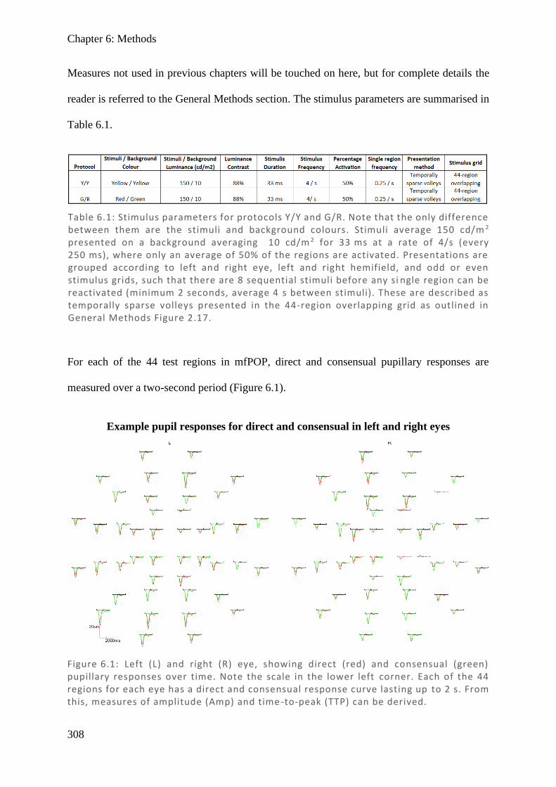
Chapter 6: Methods
308
Measures not used in previous chapters will be touched on here, but for complete details the
reader is referred to the General Methods section. The stimulus parameters are summarised in
Table 6.1.
For each of the 44 test regions in mfPOP, direct and consensual pupillary responses are
measured over a two-second period (Figure 6.1).
Table 6.1: Stimulus parameters for protocols Y/Y and G/R. Note that the only difference between them are the stimuli and background colours. Stimuli average 150 cd/m 2 presented on a background averaging 10 cd/m 2 for 33 ms at a rate of 4/s (every 250 ms), where only an average of 50% of the regions are activated. Presentations are grouped according to left and right eye, left and right hemifield, and odd or even stimulus grids, such that there are 8 sequential stimuli before any si ngle region can be reactivated (minimum 2 seconds, average 4 s between stimuli). These are described as temporally sparse volleys presented in the 44-region overlapping grid as outlined in General Methods Figure 2.17.
Figure 6.1: Left (L) and right (R) eye, showing direct (red) and consensual (green) pupillary responses over time. Note the scale in the lower left corner. Each of the 44 regions for each eye has a direct and consensual response curve lasting up to 2 s. From this, measures of amplitude (Amp) and time -to-peak (TTP) can be derived.
Example pupil responses for direct and consensual in left and right eyes
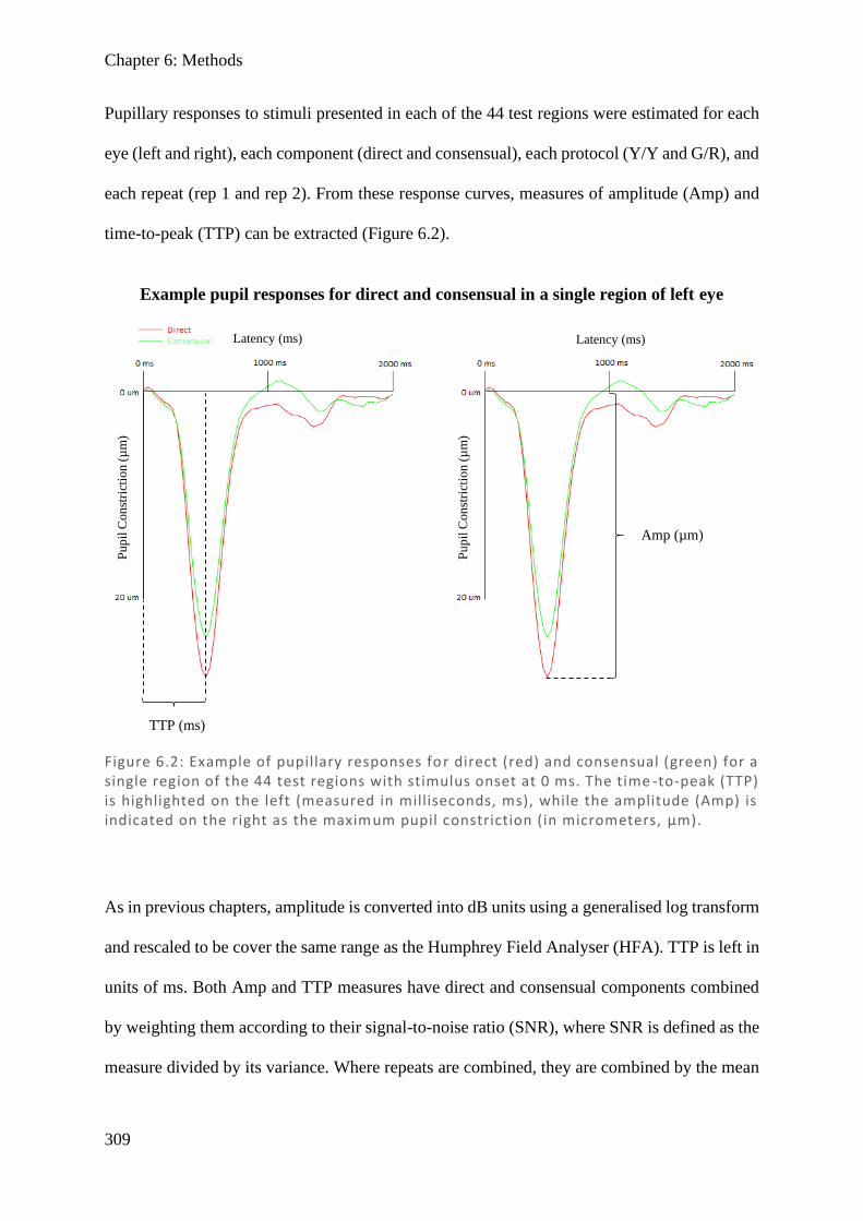
Chapter 6: Methods
309
Pupillary responses to stimuli presented in each of the 44 test regions were estimated for each
eye (left and right), each component (direct and consensual), each protocol (Y/Y and G/R), and
each repeat (rep 1 and rep 2). From these response curves, measures of amplitude (Amp) and
time-to-peak (TTP) can be extracted (Figure 6.2).
As in previous chapters, amplitude is converted into dB units using a generalised log transform
and rescaled to be cover the same range as the Humphrey Field Analyser (HFA). TTP is left in
units of ms. Both Amp and TTP measures have direct and consensual components combined
by weighting them according to their signal-to-noise ratio (SNR), where SNR is defined as the
measure divided by its variance. Where repeats are combined, they are combined by the mean
Figure 6.2: Example of pupillary responses for direct (red) and consensual (green) for a single region of the 44 test regions with stimulus onset at 0 ms. The time -to-peak (TTP) is highlighted on the left (measured in milliseconds, ms), while the amplitude (Amp) is indicated on the right as the maximum pupil constriction (in micrometers, µm).
Example pupil responses for direct and consensual in a single region of left eye
TTP (ms)
Amp (µm)
Latency (ms) Latency (ms)
Pu
pil
Con
stri
ctio
n (
µm
)
Pu
pil
Con
stri
ctio
n (
µm
)

Chapter 6: Methods
310
of the two repeats. Lastly, the 44 region mfPOP results are translated by area-weighted means
into the 54 region 24-2 design of the HFA. Where averages of the cohort are given, they are
after the preliminary data processing mentioned above and relate only to a single disease.
Results for these regions are presented as fields which show the 54 regions according to
eccentricity, in either linear grayscale, in colour with 128 degrees of colour difference, or in
the case of ratios, as a colour scale in 64 shades of red (larger direct than consensual) and in 64
shades of blue (larger consensual than direct). In the case of ratios, a value of 1 is represented
by white and darker colours represent more extreme ratios. Unless otherwise stated, graphs of
averages clip the scale according to the maximum and minimum values presented in that plot
only and thus cover the full range, while when individual subject plots are given, the scales are
clipped to the maximum and minimum values for that entire disease cohort and so may not
cover the entire range, but allow comparison between subjects.
For direct and consensual ratios measuring TTP, differences occurred between eyes. To better
quantify this, a threshold percentage of regions where direct > consensual (or vice versa) was
calculated to allow an eye to be considered ‘polarised’ rather than simply showing random
noise. A binomial distribution was used to calculate the threshold using the following
technique: 50% probability of success (direct/consensual ratio could only be above 1 or below
1) based on 54 trials (number of regions in field) and a cumulative probability of <0.01 as an
acceptable α-value. This calculation gave the threshold as ≥36 (more than two-thirds of the 54
points) for an eye to be considered polarised. Using this threshold, tables were produced
showing the number of polarised fields.
Chapter 6: Results
311
6.4. Results
6.4.1. Individual field plots for both protocols and measures
Initially, to investigate gross trends in the data, visual field plots comparing Amplitude (Amp)
and time-to-peak (TTP) across the protocols Y/Y and G/R were created, alongside those for
the Humphrey Field Analyser (HFA), for the three disease states – stroke, pituitary tumour,
and AION. An example set showing the first-tested stroke subject with left hemianopia, the
first stroke subject with right hemianopia, and the first pituitary and AION subjects with field
damage according to HFA are shown in Figure 6.3 (equivalent to the subjects used in Chapter
5).
Chapter 5 indicated that mfPOP Amp Y/Y correlated poorly with HFA, so the Y/Y results are
displayed here only for comparison. In terms of Amp, it appears that Y/Y and G/R are relatively
similar, which is expected given they both have the same difference in luminance between
stimulus and background, and luminance appears to be the main driver of changes in Amp.
TTP values for Y/Y and G/R agree only crudely, but G/R appears to have greater latencies
(darker in figure), which is consistent with the G/R protocol involving more synapses and a
longer pathway (due to cortical processing of colour). An interesting and notable feature is that
in some stroke patients, pupillary responses to G/R mfPOP stimuli in regions which had lower
sensitivity on HFA exhibit smaller constriction amplitudes (darker) as well as shorter TTPs
(darker), consistent with the expectation that cortical damage results in loss of colour input.
6.4.2. Average data by disease: field plots and box and whisker plots
This initial look at the data suggests some extra interesting comparisons. It would be useful to
see if the apparent trends in Y/Y and G/R protocols show up consistently in the amalgamated
dataset. Averages for stroke (n = 24), pituitary (n = 11), and AION (n = 10) are shown in
Figures 6.4–6.6. Y/Y Amp appears to have marginally larger responses than G/R Amp across
Chapter 6: Results
312
both eyes and all three disease types. Although the individual points do not match especially
well, general regions such as quadrants appear to show similar gradients of light and dark
regions, indicating there is some signal within the background noise. G/R TTP appears to have
longer delays than Y/Y TTP, consistent with individual results. Comparing patterns, they
crudely align, with similar gradients of light visible when quadrants are compared. Comparing
both measures (Amp and TTP) from either protocol, some selected subjects in the stroke cohort
(such as mf88130 below) appear to show marginally smaller latency (darker) in regions where
Amp is smaller (darker), although this is very noisy and shows inconsistencies. The G/R
protocol also appears to have smaller amplitudes (darker Amp) and larger latency (brighter
TTP) than its Y/Y equivalents throughout all three disease types. To confirm these
relationships, box and whisker plots of Amp and TTP measures for Y/Y and G/R were
produced (see Figure 6.7).
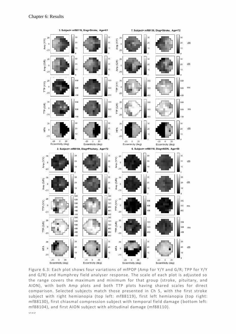
Chapter 6: Results
313
Figure 6.3: Each plot shows four variations of mfPOP (Amp f or Y/Y and G/R; TPP for Y/Y and G/R) and Humphrey field analyser response. The scale of each plot is adjusted so the range covers the maximum and minimum for that group (stroke, pituitary, and AION), with both Amp plots and both TTP plots having shared sca les for direct comparison. Selected subjects match those presented in Ch 5, with the first stroke subject with right hemianopia (top left: mf88119), first left hemianopia (top ri ght: mf88130), first chiasmal compression subject with temporal field damage ( bottom left: mf88104), and first AION subject with altitudinal damage (mf88110).
dB
dB
dB
ms
ms
dB
dB
dB
ms
ms
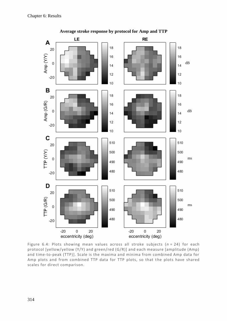
Chapter 6: Results
314
Figure 6.4: Plots showing mean values across all stroke subjects (n = 24) for each protocol [yellow/yellow (Y/Y) and green/red (G/R)] and each measure [amplitude (Amp) and time-to-peak (TTP)]. Scale is the maxima and minima from combined Amp data for Amp plots and from combined TTP data for TTP plots, so that t he plots have shared scales for direct comparison.
Average stroke response by protocol for Amp and TTP
dB
ms
dB
ms
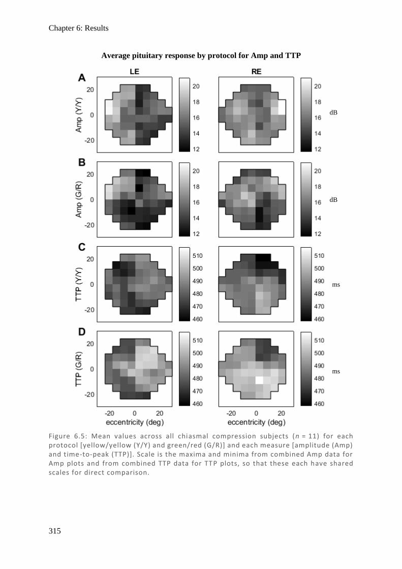
Chapter 6: Results
315
Figure 6.5: Mean values across all chiasmal compression subjects (n = 11) for each protocol [yellow/yellow (Y/Y) and green/red (G/R)] and each measure [amplitude (Amp) and time-to-peak (TTP)]. Scale is the maxima and minima from combined Amp data for Amp plots and from combined TTP data for TTP plots, so that these each have shared scales for direct comparison.
Average pituitary response by protocol for Amp and TTP
dB
ms
dB
ms
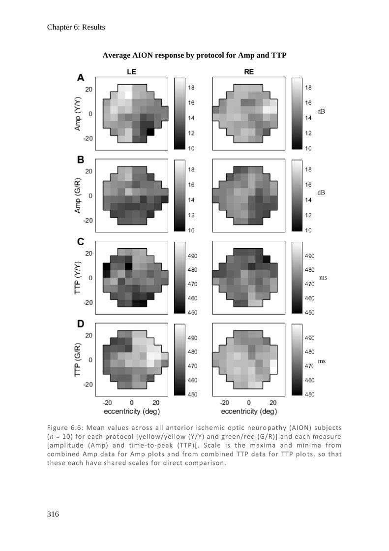
Chapter 6: Results
316
Figure 6.6: Mean values across all anterior ischemic optic neuro pathy (AION) subjects (n = 10) for each protocol [yellow/yellow (Y/Y) and green/red (G/R)] and each measure [amplitude (Amp) and time-to-peak (TTP)[. Scale is the maxima and minima from combined Amp data for Amp plots and from combined TTP data for TTP plo ts, so that these each have shared scales for direct comparison.
Average AION response by protocol for Amp and TTP
dB
ms
dB
ms
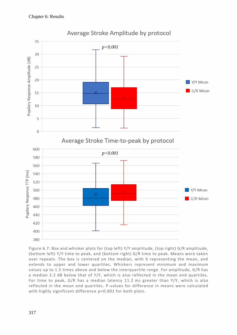
Chapter 6: Results
317
Figure 6.7: Box and whisker plots for (top left) Y/Y amplitude, (top right) G/R amplitude, (bottom left) Y/Y time to peak, and (bottom right) G/R time to peak. Means were taken over repeats. The box is centered on the median, with X representing the mean, and extends to upper and lower quartiles. Whiskers repre sent minimum and maximum values up to 1.5 times above and below the interquartile range. For amplitude, G/R has a median 2.2 dB below that of Y/Y, which is also reflected in the mean and quartiles. For time to peak, G/R has a median latency 11.2 ms greater than Y/Y, which is also reflected in the mean and quartiles. P -values for difference in means were calculated with highly significant difference p<0.001 for both plots.
p<0.001
p<0.001
Chapter 6: Results
318
The results from the box and whisker plots match observations from visual inspection of
individual and amalgamated field plots: the G/R protocol has marginally smaller responses
(–2.2 dB median difference) and marginally greater latency (11.2 ms median difference)
compared to their Y/Y counterparts. The greater latency is expected and consistent with
controls tested previously, but the decreased amplitude is novel, since controls previously
showed marginally greater amplitudes. This might be explained by G/R detecting some stroke
damage in selected subjects, so that individual results suggest decreased Amp and shorter TTP,
which is also reflected in the average results (a reduction in Amp and TTP compared to
controls). Because controls showed only slightly larger Amp values in G/R compared to Y/Y,
any damage is readily reflected as a smaller Amp. Controls for TTP had larger differences
between G/R and Y/Y, so while these differences appear reduced in the stroke population, their
G/R remains longer than Y/Y in terms of latency.
Results for chiasmal compression and AION show similar trends, with median differences for
Amp of –1.3 dB for Y/Y and –1.7 dB for G/R, while the corresponding figures for TTP are
12.2 ms and 5.1 ms. As these groups would not be expected to have cortical damage, this
suggests that perhaps the decreased latency is not due to lack of cortical input, but may relate
to an intrinsically longer latency in the G/R protocol.
6.4.3. Direct and consensual components
When investigating direct and consensual amplitude responses in Chapter 3, it was found that
direct and consensual varied throughout the field, and it was demonstrated that SNR-weighted
means were an appropriate way of fairly amalgamating these components. Given that there is
also a difference between the Y/Y and G/R protocols, it seems worthwhile to investigate
whether any prominent differences in direct and consensual responses occur in the G/R
protocol and in TTP measures. For the stroke group, graphs of fields for Y/Y and G/R, direct
and consensual, are plotted for Amp in Figure 6.8 and for TTP in Figure 6.9.
Chapter 6: Results
319
When Y/Y Amp is broken into direct and consensual components, results are subtle, but again
they show features previously highlighted in Chapter 3: that direct exceeds consensual
temporally and consensual marginally exceeds direct nasally (further investigated as ratios
next). Also note the larger response on the left side of both fields, which is a consequence of
the order of stimulus presentation, showing larger responses to the first presentation within
each eye due to gain control. These effects persist through all three disease types and across
both protocols – although they are more apparent in the Y/Y protocol. It should be made clear
this effect is independent and distinct to any differences noted between direct and consensual
components, and this is further covered in the discussion.
Neither Y/Y or G/R show the same features using TTP for direct and consensual, nor do they
have any obvious patterns, other than to say direct and consensual appear to align well. Plots
from pituitary and AION did not show any additional information and so were omitted in
favour of the direct consensual ratios which demonstrate these features more clearly.
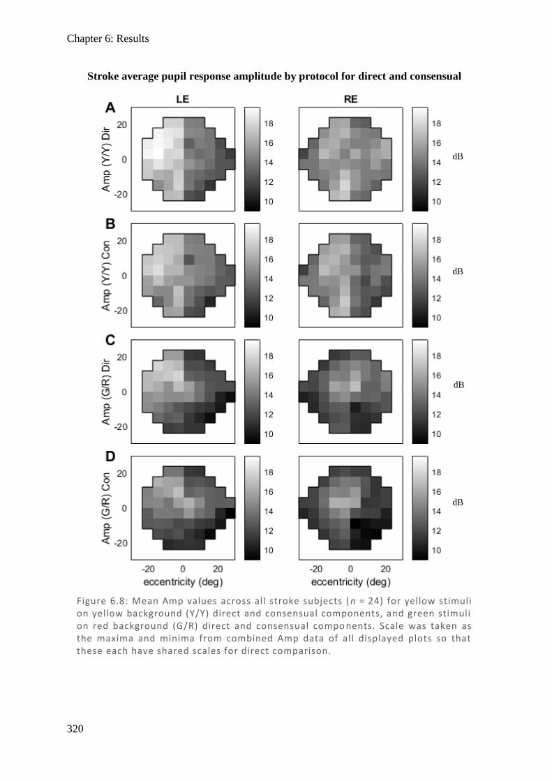
Chapter 6: Results
320
Stroke average pupil response amplitude by protocol for direct and consensual
Figure 6.8: Mean Amp values across all stroke subjects ( n = 24) for yellow stimuli on yellow background (Y/Y) direct and consensual components, and green stimuli on red background (G/R) direct and consensual compo nents. Scale was taken as the maxima and minima from combined Amp data of all displayed plots so that these each have shared scales for direct comparison.
dB
dB
dB
dB
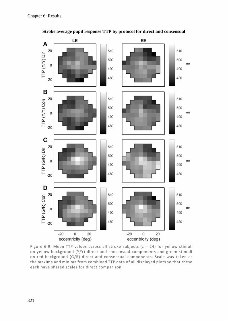
Chapter 6: Results
321
Stroke average pupil response TTP by protocol for direct and consensual
Figure 6.9: Mean TTP values across all stroke subjects ( n = 24) for yellow stimuli on yellow background (Y/Y) direct and consensual components and green stimuli on red background (G/R) direct and consensual componen ts. Scale was taken as the maxima and minima from combined TTP data of all displayed plots so that these each have shared scales for direct comparison.
ms
ms
ms
ms
Chapter 6: Results
322
With features again showing a difference between direct and consensual according to
hemifield, it is worth viewing the direct / consensual ratios, which previously highlighted the
hemifield differences in the Y/Y Amp protocol. Fields with plotted ratios for Y/Y and G/R
using both measures of AMP and TTP, with shared scale across all four variants were produced
for each disease type in Figures 6.10–6.12.
As shown previously for the Y/Y Amp results, in the all groups direct exceeds consensual in
temporal regions, while in nasal regions, for the stroke group consensual and direct are roughly
equal; however, in the pituitary and AION groups consensual exceeds direct.
For the G/R Amp results we see that very similar features are highlighted, with slightly
enhanced contraction anisocoria reflecting the marginally larger differences between direct and
consensual in both temporal and nasal regions. In the stroke group, the nasal region now
matches the other disease groups with consensual exceeding direct nasally.
Looking at the TTP values across all groups, the ratios are proportionately much smaller than
those in Amp, showing only very subtle differences of 2–3% above or below equivalence,
while Amp shows differences as great as 20%. To better examine whether any trends exist
within the TTP data, the contrast was enhanced by producing separate scales for these results,
which are reiterated in Figures 6.14–6.15. The subtle differences in TTP results do not align
with Amp at all, and appear to poorly correlate between protocols. Stroke TTP results seem
close to random noise, although the Y/Y appears to show that for the left eye many results have
direct > consensual, while the fellow right eye shows consensual > direct; the issue is unclear
in G/R. Conversely, in chiasmal compression both protocols show consensual > direct for the
left eye, while the right eye shows direct > consensual. For AION, only the G/R protocol shows
this effect, while it is unclear in the Y/Y. It would appear there are some underlying effects
causing differences between eyes, but these appear inconsistent between the groups.
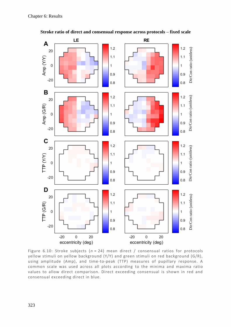
Chapter 6: Results
323
Figure 6.10: Stroke subjects (n = 24) mean direct / consensual ratios for protocols yellow stimuli on yellow background (Y/Y) and green stimuli on red background (G/R), using amplitude (Amp), and time-to-peak (TTP) measures of pupillary response. A common scale was used across all plots according to the minima and maxima ratio values to allow direct comparison. Direct exceeding consensual is shown in red and consensual exceeding direct in blue.
Stroke ratio of direct and consensual response across protocols – fixed scale
Dir
/Co
n r
atio
(u
nit
less
) D
ir/C
on
rat
io (
un
itle
ss)
Dir
/Co
n r
atio
(u
nit
less
) D
ir/C
on
rat
io (
un
itle
ss)
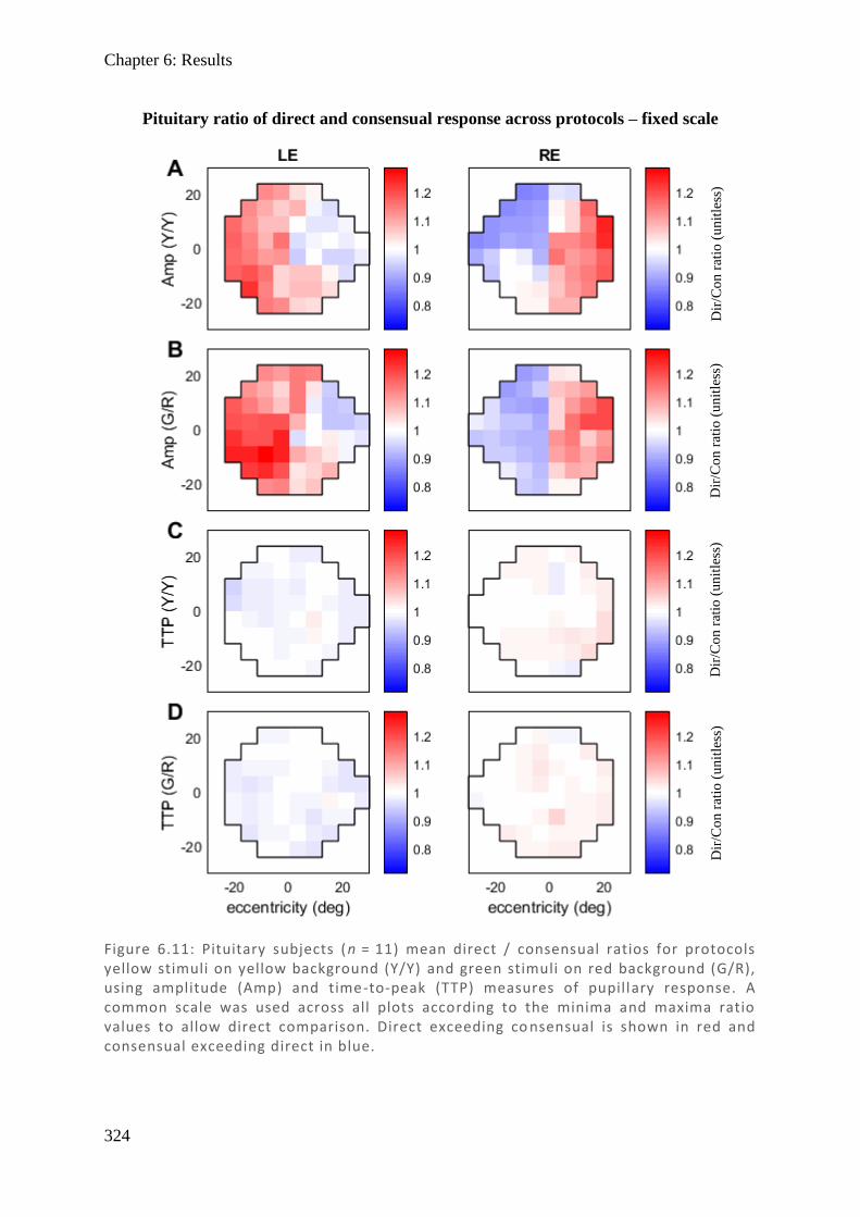
Chapter 6: Results
324
Figure 6.11: Pituitary subjects (n = 11) mean direct / consensual ratios for protocols yellow stimuli on yellow background (Y/Y) and green stimuli on red background (G/R), using amplitude (Amp) and time-to-peak (TTP) measures of pupillary response. A common scale was used across all plots according to the minima and maxima ratio values to allow direct comparison. Direct exceeding co nsensual is shown in red and consensual exceeding direct in blue.
Pituitary ratio of direct and consensual response across protocols – fixed scale
Dir
/Co
n r
atio
(u
nit
less
) D
ir/C
on
rat
io (
un
itle
ss)
Dir
/Co
n r
atio
(u
nit
less
) D
ir/C
on
rat
io (
un
itle
ss)
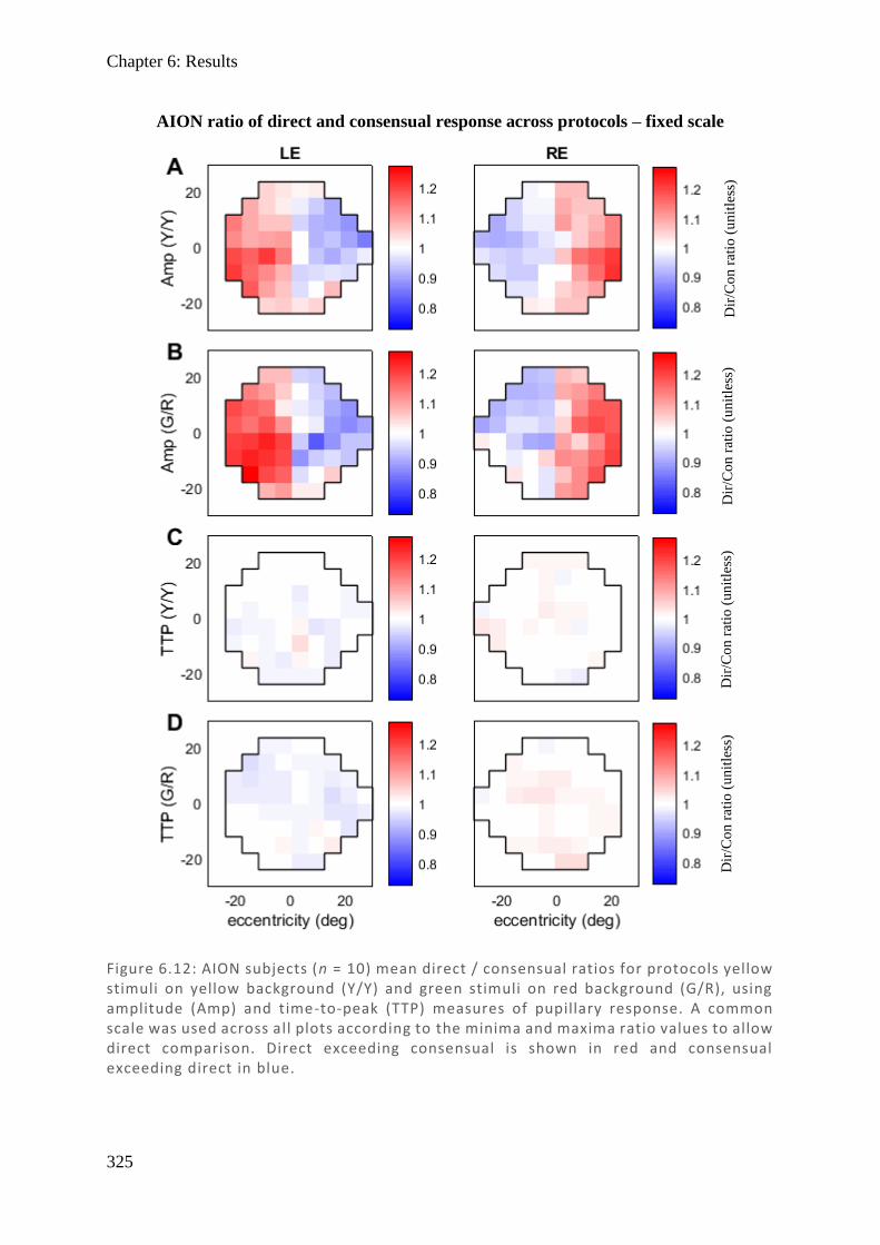
Chapter 6: Results
325
Figure 6.12: AION subjects (n = 10) mean direct / consensual ratios for protocols yellow stimuli on yellow background (Y/Y) and green stimuli on red background (G/R), using amplitude (Amp) and time-to-peak (TTP) measures of pupillary response. A common scale was used across all plots according to the minima and maxima ratio values to allow direct comparison. Direct exceeding consensual is shown in red and consensual exceeding direct in blue.
AION ratio of direct and consensual response across protocols – fixed scale
Dir
/Co
n r
atio
(u
nit
less
) D
ir/C
on
rat
io (
un
itle
ss)
Dir
/Co
n r
atio
(u
nit
less
) D
ir/C
on
rat
io (
un
itle
ss)
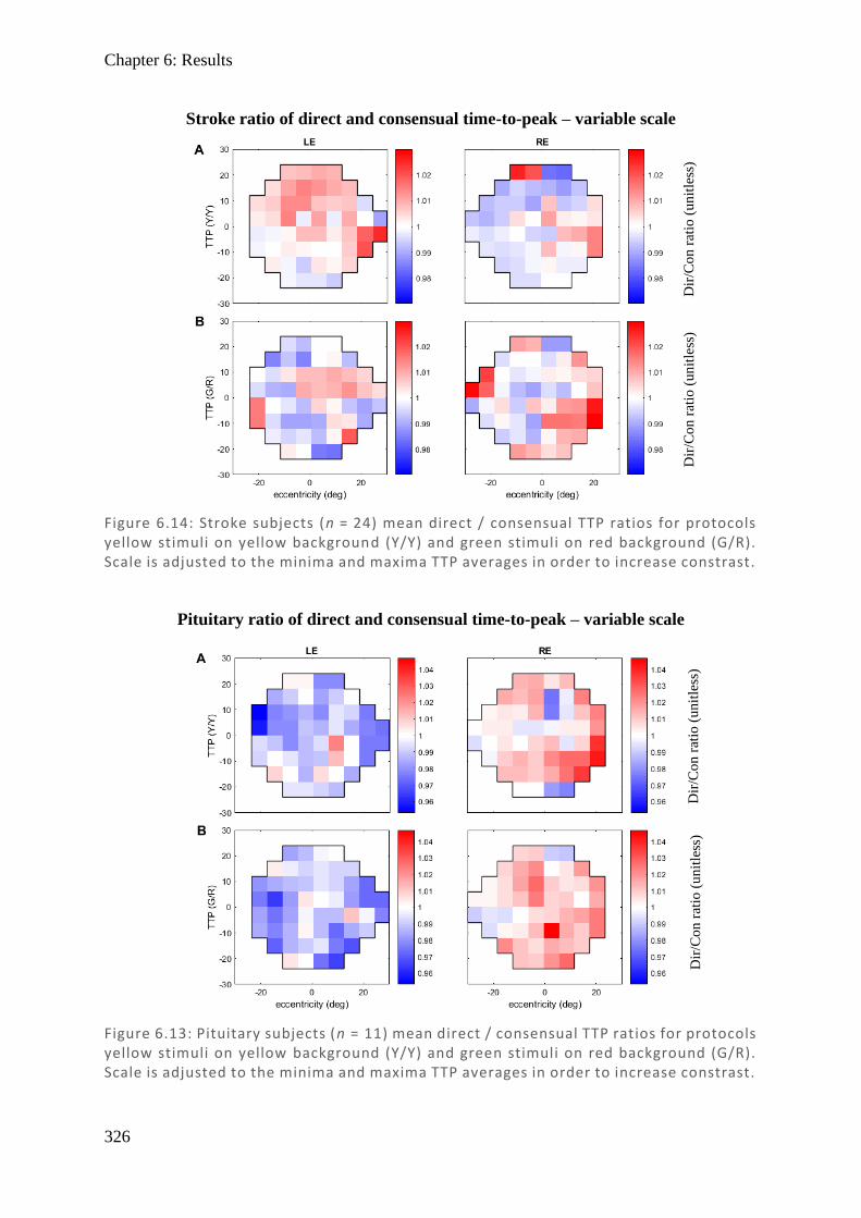
Chapter 6: Results
326
Figure 6.14: Stroke subjects (n = 24) mean direct / consensual TTP ratios for protocols yellow stimuli on yellow background (Y/Y) and green stimuli on red background (G/R). Scale is adjusted to the minima and maxima TTP averages in order to increase constrast.
Stroke ratio of direct and consensual time-to-peak – variable scale
Dir
/Co
n r
atio
(u
nit
less
) D
ir/C
on
rat
io (
un
itle
ss)
Figure 6.13: Pituitary subjects (n = 11) mean direct / consensual TTP ratios for protocols yellow stimuli on yellow background (Y/Y) and green stimuli on red background (G/R). Scale is adjusted to the minima and maxima TTP averages in order to increase constrast.
Pituitary ratio of direct and consensual time-to-peak – variable scale
Dir
/Co
n r
atio
(u
nit
less
) D
ir/C
on
rat
io (
un
itle
ss)
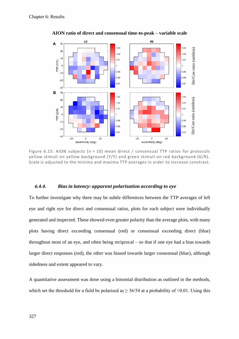
Chapter 6: Results
327
6.4.4. Bias in latency: apparent polarisation according to eye
To further investigate why there may be subtle differences between the TTP averages of left
eye and right eye for direct and consensual ratios, plots for each subject were individually
generated and inspected. These showed even greater polarity than the average plots, with many
plots having direct exceeding consensual (red) or consensual exceeding direct (blue)
throughout most of an eye, and often being reciprocal – so that if one eye had a bias towards
larger direct responses (red), the other was biased towards larger consensual (blue), although
sidedness and extent appeared to vary.
A quantitative assessment was done using a binomial distribution as outlined in the methods,
which set the threshold for a field be polarised as ≥ 36/54 at a probability of <0.01. Using this
Figure 6.15: AION subjects (n = 10) mean direct / consensual TTP ratios for protocols yellow stimuli on yellow background (Y/Y) and green stimuli on red background (G/R). Scale is adjusted to the minima and maxima TTP averages in order to increase constrast.
AION ratio of direct and consensual time-to-peak – variable scale
Dir
/Co
n r
atio
(un
itle
ss)
Dir
/Co
n r
atio
(un
itle
ss)
Chapter 6: Results
328
threshold, tables were produced for showing the number of polarised fields for each of the three
conditions and these are presented below as Tables 6.2–6.4.
Results show that fields are polarised in 60–63% of eyes, and they were not overtly affected
by protocol (Y/Y or G/R), type of polarisation (dir > con [red] or con > dir [blue]), or the
affected eye.
Comparing stroke bias for direct and consensual TTP in Table 6.2 for individuals to the average
bias in Figure 6.10, provides a suggestion as to why the averages were less clear: because
polarisation might occur in either direction in a given subject, these frequently cancel out,
leaving the amalgamated results less polarised than the individual subject results. Investigating
repeats, it was found that the vast majority of those which showed polarisation in first testing
also showed the same polarisation in repeat testing, suggesting it is unlikely to be noise. These
results were compared to apparent field damage from the HFA and seemed to be independent
of damage and disease type. It is unknown why this polarisation occurs, but it could relate to
asymmetrical sympathetic input to the EWN.
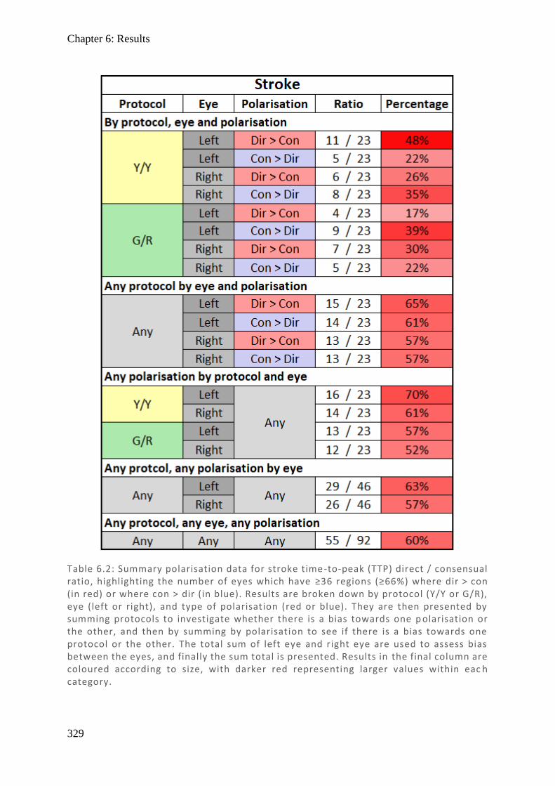
Chapter 6: Results
329
Table 6.2: Summary polarisation data for stroke time -to-peak (TTP) direct / consensual ratio, highlighting the number of eyes which have ≥36 regions (≥66%) where dir > con (in red) or where con > dir (in blue). Results are broken down by protocol (Y/Y or G/R), eye (left or right), and type of polarisation (red or blue). They are then presented by summing protocols to investigate whether there is a bias towards one p olarisation or the other, and then by summing by polarisation to see if there is a bias towards one protocol or the other. The total sum of left eye and right eye are used to assess bias between the eyes, and finally the sum total is presented. Results in the final column are coloured according to size, with darker red representing larger values within eac h category.
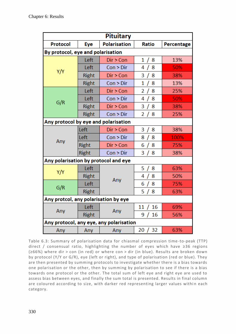
Chapter 6: Results
330
Table 6.3: Summary of polarisation data for chiasmal compression time -to-peak (TTP) direct / consensual ratio, highlighting the number of eyes which have ≥36 regions (≥66%) where dir > con (in red) or where con > dir (in blue). Results are broken down by protocol (Y/Y or G/R), eye (left or right), and type of polarisation (red or blue). They are then presented by summing protocols to investigate whether there is a bias towards one polarisation or the other, then by summing by polarisation to see if there is a bias towards one protocol or the other. The total sum of left eye and right eye are used to assess bias between eyes, and finally the sum total is presented. Results in final column are coloured according to size, with darker red representing larger values withi n each category.
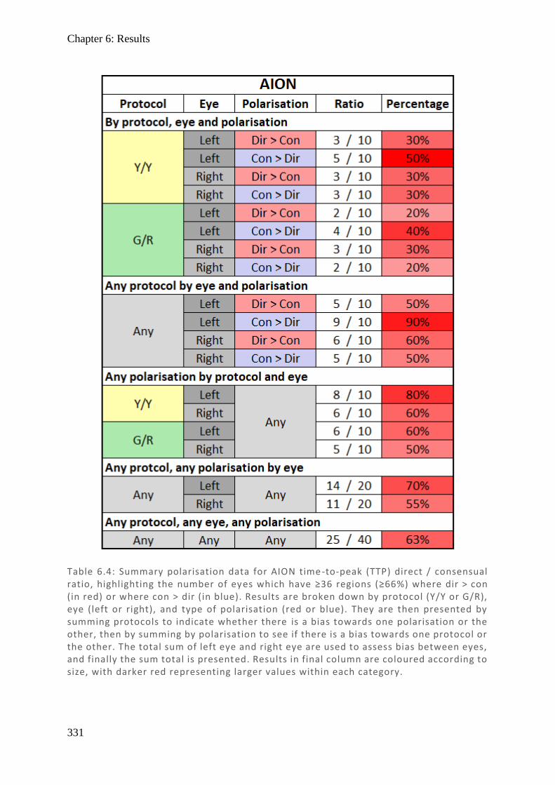
Chapter 6: Results
331
Table 6.4: Summary polarisation data for AION time-to-peak (TTP) direct / consensual ratio, highlighting the number of eyes which have ≥36 regions (≥66%) where dir > con (in red) or where con > dir (in blue). Results are broken down by protocol (Y/Y or G/R), eye (left or right), and type of polarisation (red or blue). They are then presented by summing protocols to indicate whether there is a bias towards one polarisation or the other, then by summing by polarisation to see if there is a bias towards one protocol or the other. The total sum of left eye and right eye are used to assess bias between eyes, and finally the sum total is presented. Results in final column are coloured according to size, with darker red representing larger values within each category.
Chapter 6: Results
332
6.4.5. Correlation between protocols (Y/Y and G/R)
Now that the key differences in direct and consensual responses between protocols have been
highlighted, it is interesting to look for correlation between protocols. Recall that both protocols
(Y/Y and G/R) using Amp appeared to broadly align, although G/R had smaller mean
amplitudes, and that using TTP they also appeared to align, although G/R had larger mean
latencies. These relationships will now be formally reviewed in scatter plots (Figures 6.16–
6.19). In comparing stroke protocols Y/Y (ordinate) and G/R (abscissa) using Amp, a Pearson
correlation coefficient of r = 0.762 demonstrates a strong relationship, with a linear fit
appearing suitable and with the trendline mostly below unity for the majority of points. This is
consistent with G/R having smaller responses than Y/Y. The stroke Y/Y (ordinate) and G/R
(abscissa) for TTP has a moderate correlation (r = 0.530), which appears to be mostly linear
but is skewed by several more extreme points in the range 550–800 ms on the Y/Y protocol
corresponding to much smaller G/R points in the 300–500 ms range. This was investigated and
found to be largely due to a single subject with discordant results – if the graph is replotted
with that subject removed, the Pearson correlation improves dramatically to r = 0.647 and a
more linear correlation appears, consistent with results from chiasmal compression (r = 0.699)
and AION (r = 0.849) shown in Figure 6.17. For all conditions, the trendline has a gradient less
than unity, but this trendline crosses unity after the bulk of the data points. This is therefore
consistent with the bulk of points having greater latencies in G/R, particularly at smaller values,
while at the larger end of values the G/R has marginally smaller latencies.
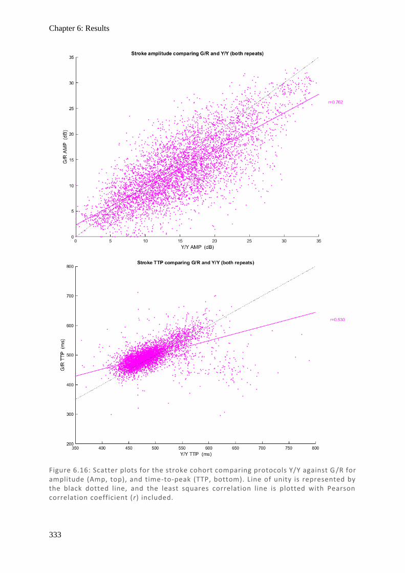
Chapter 6: Results
333
Figure 6.16: Scatter plots for the stroke cohort comparing protocols Y/Y against G /R for amplitude (Amp, top), and time-to-peak (TTP, bottom). Line of unity is represented by the black dotted line, and the least squares correlation line is plotted with Pearson correlation coefficient (r) included.
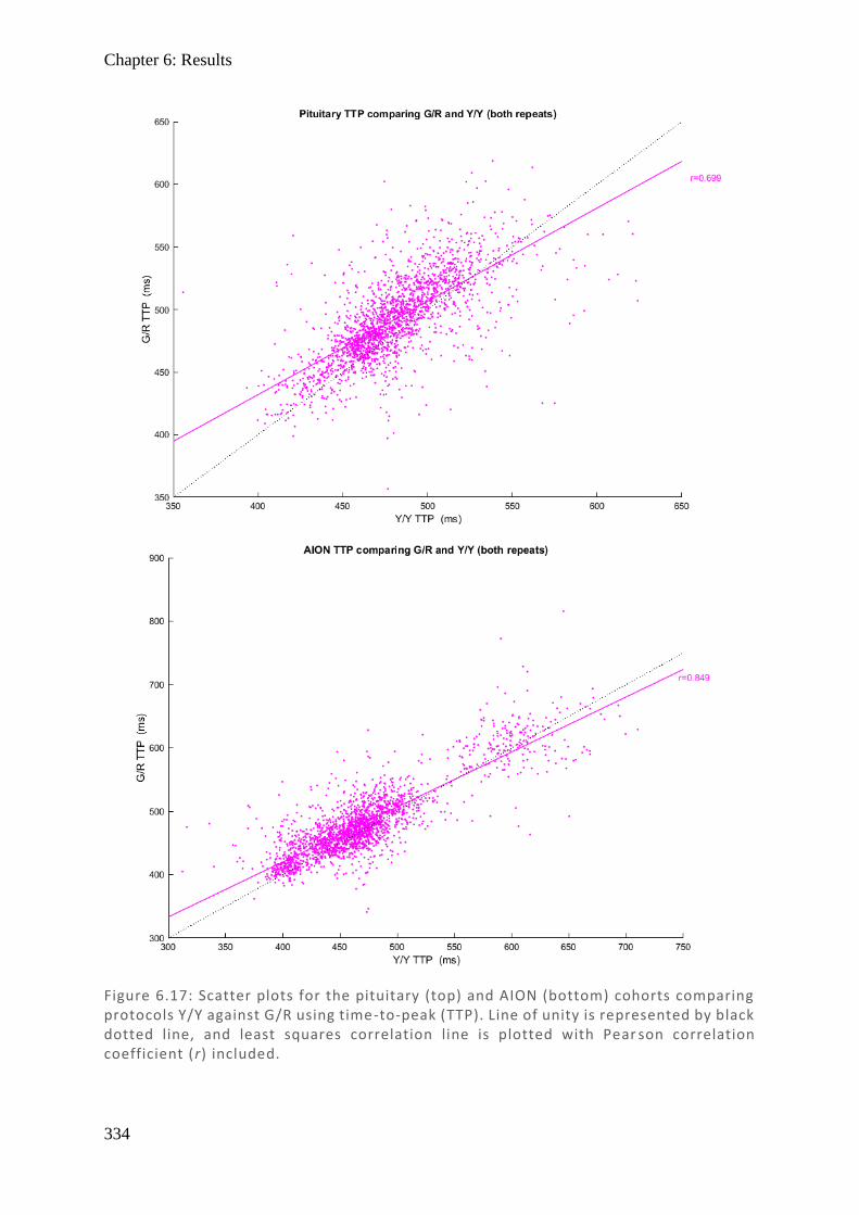
Chapter 6: Results
334
Figure 6.17: Scatter plots for the pituitary (top) and AION (bottom) cohorts comparing protocols Y/Y against G/R using time-to-peak (TTP). Line of unity is represented by black dotted line, and least squares correlation line is plotted with Pear son correlation coefficient (r) included.
Chapter 6: Results
335
6.4.6. Correlation between measures (Amp and TTP)
The other feature that was noted on visual inspection was that some areas showing smaller
Amp responses appeared to show some decreased latency (albeit small) in selected stroke
subjects, while there was small increase in latency for selected pituitary subjects – although
noise might have been the explanation. Therefore, it is interesting to investigate whether these
relationships are formally true within the larger cohort. Figure 6.18 presents a scatter plot for
stroke subjects comparing Amp (ordinate) and TTP (abscissa) for Y/Y and for G/R protocols.
A quadratic fit appeared to show a very poor relationship, with correlation coefficients r2 =
0.050 for Y/Y and r2 = 0.055 for G/R, suggesting TTP is independent of Amp. Since this was
not consistent with individual results, this was further explored by producing scatter plots for
each subject individually (see Table 6.5) which tells a very different story. Individually, 21 of
24 subjects show positive linear correlation, mostly in the r = 0.2–0.4 range, with only 2
showing a negative correlation. What becomes apparent on inspection is that there is substantial
variation between people, and that this can cause spurious associations when plotted in
aggregate. The G/R protocol was analysed in the same way (see Table 6.6) with overall poorer
correlations (but still overwhelmingly positive), with 19 of 24 subjects having a positive
correlation mostly in the range r = 0.1–0.3. Results for chiasmal compression and AION were
also completed but for brevity not included – these showed similar trends to the stroke group,
with the majority of correlations positive and the Y/Y protocol showing, overall, higher
Pearson correlation values than G/R. This new evidence suggests that there is a positive linear
association between Amp and TTP for most subjects, although the extent of this relationship
varies between subjects.
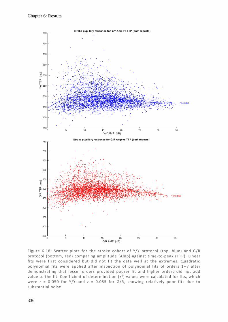
Chapter 6: Results
336
Figure 6.18: Scatter plots for the stroke cohort of Y/Y protocol (top, blue) and G/R protocol (bottom, red) comparing amplitude (Amp) against time-to-peak (TTP). Linear fits were first considered but did not fit the data well at the extremes. Quadratic polynomial fits were applied after inspection of polynomial fits of orders 1 –7 after demonstrating that lesser orders provided poorer fit and higher orders did not add value to the fit. Coefficient of determination ( r2) values were calculated for fits, which were r = 0.050 for Y/Y and r = 0.055 for G/R, showing relatively poor fits due to substantial noise.
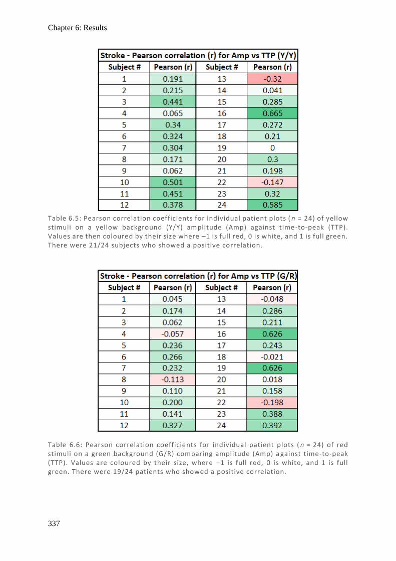
Chapter 6: Results
337
Table 6.5: Pearson correlation coefficients for individual patient plots ( n = 24) of yellow stimuli on a yellow background (Y/Y) amplitude (Amp) against time-to-peak (TTP). Values are then coloured by their size where –1 is full red, 0 is white, and 1 is full green. There were 21/24 subjects who showed a positive correlation.
Table 6.6: Pearson correlation coefficients for individual patient plots ( n = 24) of red stimuli on a green background (G/R) comparing amplitude (Amp) a gainst time-to-peak (TTP). Values are coloured by their size, where –1 is full red, 0 is white, and 1 is full green. There were 19/24 patients who showed a positive correlation.

Chapter 6: Results
338
6.4.7. Correlation between repeats (Rep 1 and Rep 2)
The final comparison which needs to be explored is between repeats, giving a measure of
internal consistency. Both Y/Y repeats for Amp and G/R repeats for Amp show strong
correlation, with high Pearson coefficients r = 0.821 and r = 0.794 respectively (Figure 6.19).
Both have gradients below unity, but with the intersection occurring roughly in the middle of
the data so that between repeats there is a similar number of points above and below unity. For
the Y/Y repeats for TTP, a tight linear correlation close to unity was found, with strong
correlation r = 0.800 (Figure 6.20). G/R repeats using TTP did not fare so well, being plagued
by outlier points in repeat 1 which had substantially higher latencies than the second repeat
(even when subjects with the most extreme results were removed) and showed only moderate
correlation r = 0.491. Overall, repeats did show correlation, but with quite a lot of noise, so
that if a single test is to be reliable, this aspect will need further reduction, particularly in the
G/R protocol.
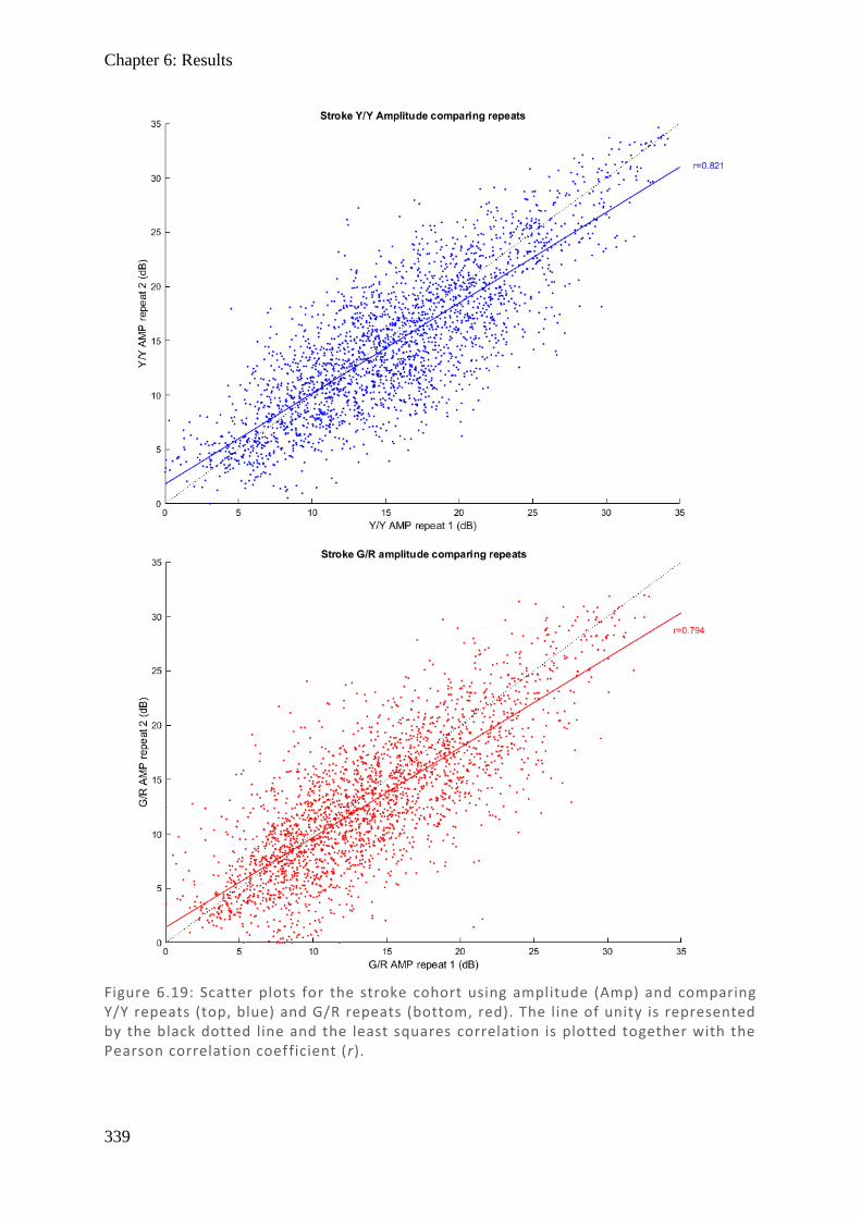
Chapter 6: Results
339
Figure 6.19: Scatter plots for the stroke cohort using amplitude (Amp) and comparing Y/Y repeats (top, blue) and G/R repeats (bottom, red). The line of unity is represented by the black dotted line and the least squares correlation is plotted together with the Pearson correlation coefficient (r).
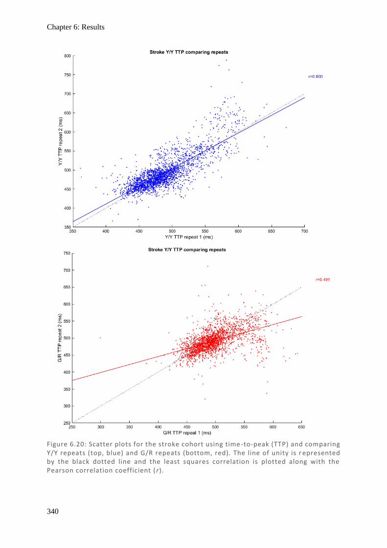
Chapter 6: Results
340
Figure 6.20: Scatter plots for the stroke cohort using time -to-peak (TTP) and comparing Y/Y repeats (top, blue) and G/R repeats (bottom, red). The line of unity is r epresented by the black dotted line and the least squares correlation is plotted along with the Pearson correlation coefficient ( r).
Chapter 6: Discussion
341
6.5. Discussion
Initial inspection of individual subjects (examples in Figure 6.3) and their amalgamated
results (Figures 6.4–6.6) showed that the G/R protocol produced smaller amplitudes and
greater latencies compared with Y/Y. This was confirmed in box and whisker plots of stroke
patients (Figure 6.7), revealing differences in median amplitude of 2.2 dB and in median TTP
of 11.2 ms, with similar trends in pituitary and AION plots. Comparing these findings with
the literature, results here used a background luminance of 10 cd/m2 and stimuli of 150 cd/m2
for both Y/Y and G/R protocols, while the nearest comparison used stimuli of 290 cd/m2 on
either a background of 115 cd/m2 (Y-hi/Y-mid) or 10 cd/m2 (Y-hi/Y-lo) (Carle et al., 2013).
Y-hi/Y-mid uses different luminance values for both stimuli and background, but with a
similar absolute difference between stimuli and background (Δ = +175 cd/m2) compared to
ours (Δ = +140 cd/m2), while Y-hi/Y-lo uses the same background but with a stronger
stimulus (Δ = +280 cd/m2). In this instance it is not the absolute luminance difference which
matters, but rather the contrast of the stimulus with the background which induces pupillary
constriction. Luminance contrast can be calculated using the Michaelson formula:
C = (Lmax – Lmin) / (Lmax + Lmin) often used for gratings or where there are an even number of
high and low contrast areas, or the Weber formula C = (Lmax – Lmin) / Lbackground used for
bright stimuli on an extensive background (MacIntyre & Cowan, 1992; Pelli & Bex, 2013).
As stimuli are active in up to 50% of possible regions at a given time either contrast formula
might be appropriate, although Weber may be preferable in this instance as there are
frequently less than 50% active. Comparing protocols (Table 6.7) reveals that Y-hi/Y-lo is
the closest match for comparison.
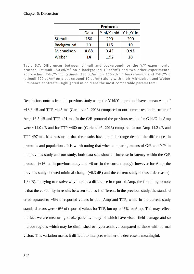
Chapter 6: Discussion
342
Results for controls from the previous study using the Y-hi/Y-lo protocol have a mean Amp of
~13.6 dB and TTP ~445 ms (Carle et al., 2013) compared to our current results in stroke of
Amp 16.5 dB and TTP 491 ms. In the G/R protocol the previous results for G-hi/G-lo Amp
were ~14.0 dB and for TTP ~460 ms (Carle et al., 2013) compared to our Amp 14.2 dB and
TTP 497 ms. It is reassuring that the results have a similar range despite the differences in
protocols and populations. It is worth noting that when comparing means of G/R and Y/Y in
the previous study and our study, both data sets show an increase in latency within the G/R
protocol (+16 ms in previous study and +6 ms in the current study); however for Amp, the
previous study showed minimal change (+0.3 dB) and the current study shows a decrease (–
1.8 dB). In trying to resolve why there is a difference in reported Amp, the first thing to note
is that the variability in results between studies is different. In the previous study, the standard
error equated to ~6% of reported values in both Amp and TTP, while in the current study
standard errors were ~6% of reported values for TTP, but up to 45% for Amp. This may reflect
the fact we are measuring stroke patients, many of which have visual field damage and so
include regions which may be diminished or hypersensitive compared to those with normal
vision. This variation makes it difficult to interpret whether the decrease is meaningful.
Table 6.7: Differences between stimuli and background for the Y/Y experimen tal protocol (stimuli 150 cd/m2 on a background 10 cd/m2) and two other experimental approaches: Y-hi/Y-mid (stimuli 290 cd/m2 on 115 cd/m2 background) and Y-hi/Y-lo (stimuli 290 cd/m2 on a background 10 cd/m2) along with their Michaelson and Weber luminance contrasts. Highlighted in bold are the most comparable parameters.
Chapter 6: Discussion
343
An initial review of individual results appeared to show regions appearing damaged on HFA
showed some decreased Amp and TTP values. While this was hidden in the amalgamated
results, individual correlations support this observation, showing a positive correlation between
Amp and TTP in the large majority, particularly for the G/R protocol. A tentative explanation
might be that shallower amplitudes have slower constriction velocities and so their TTP is
wider. However, although pupillary response velocity does scale with amplitude (Bremner,
2012), the pupillary response waveform has been shown to be isomorphically scaled – that is
every component of its shape remains constant (Semmlow & Stark, 1973; Semmlow et al.,
1975; Maddess, 2012), demonstrating that delays in TTP are real and not simply an artefact of
wider pupillary responses. Comparing this positive Amp and TTP relationship to the original
expectation – that cortical damage would result in both decreased Amp and TTP – appears to
support this. Likewise, it was considered that G/R likely utilises a greater cortical input than
Y/Y, which is again supported by a greater proportion and stronger correlations in the G/R
protocol. But equally, the results for Y/Y should not be overlooked, because applying the same
argument, it would suggest that there is also a cortical component to this ‘luminance pathway’.
Comparing G/R and Y/Y can then be thought of in a less absolute way: it is not ‘subcortical
luminance’ and ‘cortical colour exchange’ but rather a matter of shifting the balance of the
cortical and subcortical components they both produce, either more towards cortical in G/R or
more towards subcortical in Y/Y.
Direct and consensual components were explored across both protocols and measures (Figures
6.10–6.12). The previously noted Amp Y/Y contraction anisocoria from Chapter 3 (in which
there are hemifield differences) was also demonstrated in the Amp G/R protocol, with broadly
similar distribution and a marginally more prominent magnitude. For G/R, the relationship of
direct > consensual temporally and consensual > direct nasally was demonstrated across all
diseases, and similarly for Y/Y except for the nasal regions of stroke (which were nearly equal).
Chapter 6: Discussion
344
This is consistent with the literature in which temporal contraction anisocoria is consistent
across studies while nasal fields vary (Smith & Smith, 1980; Wyatt & Musselman, 1981; Cox
& Drewes, 1984; Martin et al., 1991; Schmid et al., 2000; Carle et al., 2011). TTP did not
follow this trend, which intuitively makes sense, given that the difference between direct and
consensual responses is predominantly due to differential input from the pretectal olivary
nucleus (PON) to the Edinger–Westphal Nucleus (EWN) but does not involve any additional
pathways or synapses. TTP showed only very small deviations from direct and consensual
equivalence throughout all tested fields, having ratios that were in the range 0.96–1.04 and
mostly near 1, whereas the Amp ratios were in the range 0.8–1.2. When the scales were adjusted
to make clearer these finer degrees of latency difference (Figures 6.14–6.15), it was found that
a large number were polarised (whole field having ratios above 1 or ratios below 1) within a
single eye. Eyes would mostly have longer latencies for direct in one eye and longer latencies
for consensual in the other, with the direction seemingly at random. On the whole, 60–63% of
eyes were polarised through all three disease states and both protocols (Tables 6.2–6.4). While
it should be noted these are only small changes in TTP (mostly <30 ms), with so many subjects
showing polarisation, and consistency between repeats on different days, it would appear this
effect is real. It does not appear to be attributable to the device settings, given the variation in
sidedness and extent, nor does it seem to correlate to a protocol, eye, or visual field damage as
shown by HFA, but rather it seems likely to be due to intrinsic differences between subjects.
While differences between eyes has been reported for combined pupillary components, a
difference between eyes for direct and consensual latency does not appear to have been reported
by others. A difference in the inter-eye latency for time of onset of pupillary response has been
shown in normal subjects to be about 5–10 ms, while there are larger responses in the range
20–60 ms for those with optic neuritis, with larger intensity stimuli having smaller differences
(Bergamin & Kardon, 2003). In the stroke group, the average inter-eye latency was 6.8 ms,
Chapter 6: Discussion
345
falling in the middle of the expected range. Differences between direct and consensual for a
single eye averaged over all regions were very variable between subjects and were as large as
30 ms in some eyes; averaging these differences across subjects resulted in a right eye mean
difference for direct and consensual of 8.2 ms and a left eye mean difference of 7.6 ms. This
suggests that the bulk of the difference in latency between eyes appears to be due to differences
in the direct and consensual responses between eyes, giving rise to the commonly observed
reciprocal nature of the difference between eyes. While these differences in latency could be
due to variable degrees of myelination affecting conduction velocity, their often reciprocal
nature suggests anatomical differences such that when one pathway becomes longer, the other
becomes shorter.
Consistent with the individual results, correlation between repeats for each protocol (Y/Y and
G/R) showed a strong relationship across all conditions (stroke, chiasmal compression, and
AION) using both measures (Amp and TTP), except there was only moderate correlation in
TTP for the stroke group (Figures 6.19–6.20). This appeared to be due to a number of aberrant
results far from the main pool of data where G/R repeat 1 greatly exceeded G/R repeat 2. In
investigating the source of this anomaly, a single subject was shown to contribute most of these
points, and correlation improved notably if replotted without this subject’s results (although no
valid reason to exclude them was found). Despite this, the lower correlation coefficients for
G/R suggest it is a slightly less reliable measure than its Y/Y counterpart.
It would have been useful to create a G/R receiver operating characteristic (ROC) curve for
detection of each of the disease states (as done for Y/Y in Chapter 5), but unfortunately there
is no control data to permit this. Although this data could still be collected, the methods used
in this current study for Amp analysis seem unlikely to be useful – because there is a strong
correlation between Y/Y and G/R amplitude and Y/Y is poor in detecting any of these diseases.
The TTP results show much less correlation with Amp (in both protocols), but they also showed
Chapter 6: Discussion
346
a poor visual correlation with the HFA results, and so it would be surprising if they were to
perform well in an ROC analysis.
Considering that there were indeed longer delays in the G/R protocol than the Y/Y, it is worth
reviewing the results of an experiment done previously comparing G/R and R/G. Carle et al.
tested equiluminant R/G and G/R protocols with luminances of 90, 115, and 140 cd/m2 and
measured Amp and TTP values (Carle et al., 2013). Results demonstrated that the G/R protocol
had consistently larger responses and longer latencies – demonstrating that there is a bi-
directional response heavily biased towards G/R. The authors suggested that this could be due
to chromatic adaptation of cone photoreceptors, so that due to the wavelengths of the tested
colours, a green background would enhance activation of red stimuli rather than the reverse.
What they did not consider was how this same effect might impact the increased latency noted
in G/R compared to R/G. There is a fixed delay in opsin activation which depends on a protein
cascade ending in cell hyperpolarisation, a process which occurs in the order of ~20-50ms in
cones (van Hateren & Lamb, 2006) and ~100ms in rods to reach peak hyperpolarisation
(Arshavsky & Wensel, 2013) after which neurotransmitter release ceases and signal
transduction is complete. Intuitively, it then follows that a Y/Y stimulus already has these
mechanisms partially activated through the background luminance, so the time required for
activation is reduced compared to a G/R protocol (where predominantly new cones need to be
activated from rest). However, the much larger portion of the 500-600ms time until peak
pupillary constriction is due to delays in iris constriction. The prediction is that the greater the
luminance component, the more cross-activation of cones at rest, and the faster the response.
Likewise, while less background activation occurs in any colour exchange stimuli, R/G has
greater background activation than G/R, and so would be predicted to have shorter delays in
activation. This would account for the longer delays we observed in G/R compared to Y/Y. It
would also account for the findings of Carle et al. which suggest that greater colour opponency
Chapter 6: Discussion
347
and reduced luminance result in greater delays, and also why G/R is more responsive in
amplitude and has longer latencies than R/G. Further investigation with other colour varieties
may confirm if this is in fact the case.
In this context, it is worth considering here the results from Chapter 4, which discussed higher
visual function (HVF) deficits, since colour was highlighted as one of the two common deficits.
Given that colour provides input to the pupillary response (Heywood et al., 1998), and that the
previous chapter suggested colour vision was commonly impaired in the same cohort of
subjects for which we now see pupillary impairment (decreased Amp and TTP), it is reasonable
to suppose that colour impairment and pupillary impairment may be related. Further,
associations of TTP with areas of field damage were more obvious in the G/R group,
reinforcing the idea that the G/R protocol has greater cortical involvement. If the colour centre
were damaged, the question as to why no subject had complete colour loss (achromatopsia) in
HVF arises, but it is true that many had more subtle impairments. Since visual field damage
naturally prevents testing of colour vision in that region, and damage to the colour centre
without field defects is uncommon, it is strange that colour has been affected so commonly in
the seeing field. If colour is considered to be processed bilaterally, then unilateral damage
might impair colour in the seeing field; however, this does not make sense when unilateral
damage generally causes hemiachromatopsia (colour loss on a single side of homonymous
fields) contralaterally (similar to field loss) (Damasio & Damasio, 1986; Kolmel, 1988;
Paulson et al., 1994; Short & Graff-Radford, 2001). Alternatively, if one thinks of areas which
are necessary for colour, such as posterior aspect of inferior temporal (IT) which when
damaged appears to cause cerebral achromatopsia, and others that contribute to colour quality,
then perhaps this might better explain what these results demonstrate. Noting the heterogeneity
of the stroke cohort also might explain the variation in responses: why some subjects show
Chapter 6: Discussion
348
damage in Amp and TTP somewhat congruent with visual field damage, while others show no
such relationship.
The original premise behind these experiments was that the pupils receive input from the cortex
and that cortical damage may be able to be detected using appropriate pupillary stimuli. Some
evidence for cortical input to pupillary mechanisms was presented in the introduction, with one
elegant paper from Heywood and colleagues unequivocally demonstrating this. Their paper
showed that removal of the rostral inferior temporal (IT) cortex of a rhesus monkey removed
chromatic pupillary response but spared luminance response (Heywood et al., 1998). Further,
they demonstrated that removal of a different region of visual association cortex (V4) did not
cause changes to either type of stimuli. The point here is that while there is cortical input to the
pupillary response, this cortical input appears to be specialised information from particular
regions, such as colour exchange from IT cortex. While a colour exchange protocol may be
useful in detecting those with damage to a single area providing colour input to the pupil
response, there is no evidence that it can detect damage to other cortical areas. Further,
combining colour exchange with luminance (as done in our protocol) means that even if the
appropriate cortical region were damaged and the colour component abolished, the luminance
component would remain, making it harder to distinguish the response from what is already a
noisy response compared to standard automated perimetry.
In summary, the results from Chapter 5 exploring Y/Y Amp and correlating it with visual field
damage showed that this was not a good measure; hence a potentially better candidate, G/R
TTP, was tested. This definitely showed that a few subjects had decreased TTP which aligned
with field damage; however, the majority did not have this pattern, and even in those which
did, there was a high degree of noise, making this relationship difficult to establish. There is a
large amount of data processing involved in extracting mfPOP raw data and adapting it into a
useable form comparable with the Humphrey and Matrix devices, and some steps of this
Chapter 6: Discussion
349
processing seem likely to add noise – for example, in using weighted means to translate 44
regions into 54 regions. Likewise, the combination of luminance and colour exchange
pathways makes it harder to isolate what the causes of changes in responses noted in the stroke
group. In future analyses, it may be worth performing isoluminant colour exchange and
luminance-only testing, and less heavily processing the data, to see whether this gives less
background noise and better performance.
6.6. Conclusion
Pupillary responses from G/R stimuli correlate well with Y/Y stimuli in terms of Amp and
TTP, with marginally smaller amplitude and greater latency overall. Trends in direct and
consensual responses for both Y/Y and G/R protocols show contraction anisocoria according
to hemifield using amplitude measures, but these are not reflected in TTP measures. TTP
appears to show, in 60–63% of eyes, subtle differences in direct and consensual responses
throughout a significant (p<0.01) number of regions within a single eye, and often with a
reciprocal relationship in the fellow eye. These trends in TTP were not associated with either
eye or protocol and appear to be anatomical differences between subjects.
Aggregate results comparing Amp against TTP did not show a relationship, but assessment of
individual subjects showed that the vast majority had a moderate–strong correlation for Y/Y
and a weak–moderate correlation for G/R. Repeats for each protocol and measure generally
showed high Pearson values in the range 0.7–0.8 (except for G/R TTP in stroke, which was
much smaller at 0.49). The additional G/R protocol and measures of TTP do not, appear to
correlate well visually with HFA fields; a few subjects do show a weak relationship, although
it is very noisy. The G/R protocol in its current form appears unlikely to have much better
utility in identifying stroke than its Y/Y Amp counterpart, although it might have potential if
the stimuli were further refined and data processing was streamlined.

350
References
Arshavsky VY & Wensel TG. (2013). Timing is everything: Gtpase regulation in
phototransduction. Invest Ophthalmol Vis Sci 54, 7725-7733.
Barbur JL, Harlow AJ & Sahraie A. (1992). Pupillary responses to stimulus structure, colour
and movement. Opthalmic and Physiological Optics 12, 137-141.
Barbur JL, Wolf J & Lennie P. (1998). Visual processing levels revealed by response
latencies to changes in different visual attributes. Proc Biol Sci 265, 2321-2325.
Benevento LA & Davis B. (1977). Topographical projections of the prestriate cortex to the
pulvinar nuclei in the macaque monkey: An autoradiographic study. Exp Brain Res
30, 405-424.
Benevento LA & Rezak M. (1976). The cortical projections of the inferior pulvinar and
adjacent lateral pulvinar in the rhesus monkey (macaca mulatta): An autoradiographic
study. Brain Res 108, 1-24.
Benevento LA, Rezak M & Santos A. (1977). An autoradiographic study of the projections of
the pretectum in the rhesus monkey (macaca mulatta): Evidence for sensorimotor
links to the thalamus and oculomotor nuclei. Brain Res 127, 197-218.
Bergamin O & Kardon RH. (2003). Latency of the pupil light reflex: Sample rate, stimulus
intensity, and variation in normal subjects. Invest Ophthalmol Vis Sci 44, 1546-1554.
Bremner FD. (2012). Pupillometric evaluation of the dynamics of the pupillary response to a
brief light stimulus in healthy subjects. Invest Ophthalmol Vis Sci 53, 7343-7347.
Carle CF, James AC & Maddess T. (2013). The pupillary response to color and luminance
variant multifocal stimuli. Invest Ophth Vis Sci 54, 467-475.
Carle CF, Maddess T & James AC. (2011). Contraction anisocoria: Segregation, summation,
and saturation in the pupillary pathway. Invest Ophthalmol Vis Sci 52, 2365-2371.
Cox TA & Drewes CP. (1984). Contraction anisocoria resulting from half-field illumination.
Am J Ophthalmol 97, 577-582.
Chapter 6: References
351
Damasio AR & Damasio H. (1986). Hemianopia, hemiachromatopsia and the mechanisms of
alexia. Cortex 22, 161-169.
Dineen JT & Hendrickson A. (1983). Overlap of retinal and prestriate cortical pathways in
the primate pretectum. Brain Res 278, 250-254.
Distler C & Hoffmann KP. (1989). The pupillary light reflex in normal and innate
microstrabismic cats, ii: Retinal and cortical input to the nucleus praetectalis olivaris.
Vis Neurosci 3, 139-153.
Gamlin PDR. (2006). The pretectum: Connections and oculomotor-related roles. Prog Brain
Res 151, 379-405.
Gamlin PDR, Zhang HY, Harlow A & Barbur JL. (1998). Pupil responses to stimulus color,
structure and light flux increments in the rhesus monkey. Vision Res 38, 3353-3358.
Heywood CA, Nicholas JJ, LeMare C & Cowey A. (1998). The effect of lesions to cortical
areas v4 or ait on pupillary responses to chromatic and achromatic stimuli in
monkeys. Exp Brain Res 122, 475-480.
Kolmel HW. (1988). Pure homonymous hemiachromatopsia. Findings with neuro-
ophthalmologic examination and imaging procedures. Eur Arch Psychiatry Neurol Sci
237, 237-243.
MacIntyre B & Cowan WB. (1992). A practical approach to calculating luminance contrast
on a crt. ACM Trans Graph 11, 336–347.
Maddess T. (2012). Pupil dynamics and response amplitude: Only size matters. Invest Ophth
Vis Sci 53, 7644-7644.
Martin TI, Kardon RI & Thompson HS. (1991). Unequal direct and consensual pupillary
responses to hemiretinal stimuli. Invest Ophth Vis Sci 32, 1124.
McClurkin JW & Optican LM. (1996). Primate striate and prestriate cortical neurons during
discrimination. I. Simultaneous temporal encoding of information about color and
pattern. J Neurophysiol 75, 481-495.
McClurkin JW, Zarbock JA & Optican LM. (1996). Primate striate and prestriate cortical
neurons during discrimination. Ii. Separable temporal codes for color and pattern. J
Neurophysiol 75, 496-507.
Chapter 6: References
352
Paulson HL, Galetta SL, Grossman M & Alavi A. (1994). Hemiachromatopsia of unilateral
occipitotemporal infarcts. Am J Ophthalmol 118, 518-523.
Pelli DG & Bex P. (2013). Measuring contrast sensitivity. Vision Res 90, 10-14.
Pickard GE & Sollars PJ. (2012). Intrinsically photosensitive retinal ganglion cells. Rev
Physiol Bioch P 162, 59-90.
Sand A, Schmidt TM & Kofuji P. (2012). Diverse types of ganglion cell photoreceptors in the
mammalian retina. Prog Retin Eye Res 31, 287-302.
Schmid R, Wilhelm B & Wilhelm H. (2000). Naso-temporal asymmetry and contraction
anisocoria in the pupillomotor system. Graef Arch Clin Exp 238, 123-128.
Semmlow J, Hansmann D & Stark L. (1975). Variation in pupillomotor responsiveness with
mean pupil size. Vision Res 15, 85-90.
Semmlow J & Stark L. (1973). Pupil movements to light and accommodative stimulation: A
comparative study. Vision Res 13, 1087-1100.
Short RA & Graff-Radford NR. (2001). Localization of hemiachromatopsia. Neurocase 7,
331-337.
Smith SA & Smith SE. (1980). Contraction anisocoria: Nasal versus temporal illumination.
The British journal of ophthalmology 64, 933-934.
Steele GE & Weller RE. (1993). Subcortical connections of subdivisions of inferior temporal
cortex in squirrel monkeys. Vis Neurosci 10, 563-583.
van Hateren JH & Lamb TD. (2006). The photocurrent response of human cones is fast and
monophasic. BMC Neuroscience 7, 34.
Wyatt HJ & Musselman JF. (1981). Pupillary light reflex in humans: Evidence for an
unbalanced pathway from nasal retina, and for signal cancellation in brainstem. Vision
Res 21, 513-525.
Young RSL & Alpern M. (1980). Pupil responses to foveal exchange of monochromatic
lights. J Opt Soc Am 70, 697-706.
353
7 Chapter 7: Integrative discussion
Chapter 1 provided a background to the visual pathways, processing in higher visual centres,
how neurological disease affects these pathways, and introduced both traditional visual field
testing and multifocal pupillographic objective perimetry. The topic of functional
specialisation of visual association cortices was covered, with isolated deficits in a range of
visual functions being highly suggestive of processing in this way (see Chapter 3 introduction
for a list of over 20 such examples). Despite many such reports, completely isolated functional
deficits remain rare (Vaina, 1995). The distributive model of processing – that multiple areas
take part in visual processing – would also appear to have some weight, with selective stimuli
activating many cortical areas (McKeefry et al., 1997; Furlan & Smith, 2016). Combining both
these concepts, it is a logical progression to believe that multiple areas are involved in
processing but that one final area is necessary for perception. If this is the case, the question
becomes: does damage to such processing areas result in more subtle defects, which are not
examined during routine clinical practice? (Rowe, 2016). This question was addressed in
Chapter 1, revealing that it appears to be the case, with depth perception and colour being the
primary measures affected. Receiver operator characteristics plots and principal component
analysis both suggested that stereofly, randot, and Ishihara were the most useful tests, noting
that stereofly and randot appear to measure the same thing and so only one is necessary. It also
addressed potential improvements in the current testing regimens, such as larger well
Farnsworth–Munsell and a wider dynamic range for Cambridge Facial Memory Test.
A visual deficit known to be common in neurological disease is visual field loss, both in stroke
(Zhang et al., 2006; Chen et al., 2009; Gall et al., 2010; Luu et al., 2010; Rowe et al., 2013;
Glisson, 2014) and other subcortical diseases like chiasmal compression (Walsh, 1990; Wang
Chapter 7: Integrative discussion
354
et al., 2008; Kasputyte et al., 2013) and AION (Hayreh & Zimmerman, 2008; Cullen & Chung,
2012; Pahor & Pahor, 2016). To assess these, perimetry is commonly used. In covering the
history behind these perimetry devices, common use has progressed from simple
confrontational testing (Reader & Harper, 1976), to manual perimetry (Goldmann) (Trope &
Britton, 1987), through to automated perimetry with multiple iterations (Johnson et al., 2011;
Hepworth & Rowe, 2018; Bevers et al., 2019). In parallel to the more recent iterations of
perimetry, the extensive work on multifocal visual evoked potentials ultimately led to the
development of multifocal pupillography (for review see Chapter 1, section 1.6.4 Multifocal
methods). Two key areas of mfPOP development have been its use to non-invasively probe
human physiology and its use in ocular disease, both of which are addressed in Chapters 4 and
5 respectively.
Early work with other devices noted that pupil responses in direct were greater than consensual
(Lowenstein, 1954; Smith et al., 1979; Fan et al., 2009). Further exploration led to the
conclusion that direct consistently exceeded consensual in the temporal field, but results were
mixed nasally, some showing consensual marginally exceeding direct (Cox & Drewes, 1984;
Martin et al., 1991) while others have shown equivalence (Smith & Smith, 1980; Wyatt &
Musselman, 1981; Schmid et al., 2000; Carle et al., 2011b). Investigation with mfPOP has not
only produced similar results, but has gone on to produce a model of how these differences
occur, proposing it relates to luminance of the stimuli (Carle et al., 2011b) and, more recently,
that the majority of the gain control exists at the EWN (Carle et al., 2019). While this finding
was investigated in controls, it remained untested in neurological disease. This thesis has
investigated stroke, chiasmal compression, and AION, and reveals that these naso-temporal
differences in pupillary components persist. It further raises the possibility that the higher
density input from the nasal retina (temporal field) explains why the bias towards direct in the
temporal field is larger than the bias towards consensual in the nasal field.
Chapter 7: Integrative discussion
355
In terms of mfPOP use in ocular disease, the device appears to function well in a range of
retinal disorder including glaucoma (Maddess et al., 2007; Maddess et al., 2009), AMD (Carle
et al., 2011a; Sabeti et al., 2011; Rosli et al., 2012; Sabeti et al., 2014), and diabetic retinopathy
(Bell et al., 2010; Carle et al., 2015; Sabeti et al., 2015). Some initial tests with multiple
sclerosis (Ali et al., 2014; Maddess & Lueck, 2017) and migraine (Lueck et al., 2014) also
show some promise.
If mfPOP is to be the future replacement for standard automated perimetry such as Humphrey
perimetry, it must first demonstrate it is at least as good as these devices in the full range of
conditions for which perimetry is currently used. It is therefore essential to determine the
performance of mfPOP in some of the more common neurological disorders which produce
visual field deficits (specifically stroke, chiasmal compression, and AION). Chapter 5
addressed this question, with results demonstrating that the Humphrey and Matrix devices
highly correlate, while neither correlate well with mfPOP. Further, in assuming typical field
loss for each disease, Humphrey and Matrix were able to detect these disorders, while mfPOP
was not. Large variations even in control fields made differentiation very difficult with the
mfPOP approach.
It is then worth considering other approaches to using mfPOP which might better detect cortical
changes. As there is evidence from anatomical studies of cortical input to the pupillary system
at the PON (Benevento & Rezak, 1976; Benevento & Davis, 1977; Benevento et al., 1977;
Dineen & Hendrickson, 1983; Distler & Hoffmann, 1989; Steele & Weller, 1993; Gamlin,
2006), which demonstrate that colour exchange induces pupillary constriction (Barbur et al.,
1992; Barbur et al., 1998; Carle et al., 2013) and that colour-exchange has delayed responses
(Gamlin et al., 1998; Carle et al., 2011b), it has been proposed that colour exchange may
preferentially utilise cortical input to the pupillary system. This is further supported by direct
evidence in macaques that a cortical lesion can induce colour-exchange-specific deficits while
Chapter 7: Integrative discussion
356
retaining luminance responses (Heywood et al., 1998). These studies, and a closely related
study using isoluminant colour exchange (Carle et al., 2013), informed the design of Chapter
6, which addressed whether coloured stimuli (G/R), and the alternative measure of time-to-
peak (latency) gave any promising differences from the luminance-only approach (Y/Y) used
in Chapter 5. The population as a whole revealed that the G/R protocol had smaller responses
and longer latencies compared to the Y/Y, consistent with the concept that cortical damage
lessens cortical input to the pupillary system (thereby reducing amplitude and shifting the
balance of input towards the faster subcortical luminance pathway). However, this line of
argument is questionable, given similar results found with both chiasmal compression and
AION, which are subcortical lesions. While a more definitive repeat analysis using receiver
operator curves for the G/R protocol was not possible (because no control dataset was
available), visual comparison with Humphrey fields also did not show promise, with mfPOP
showing that only a couple of subjects with full hemianopias had mildly congruent damage.
While alternative approaches and methods may reveal more sensitive measures, we are forced
to conclude that the studies here were unable to demonstrate that mfPOP was effective in
stroke, chiasmal compression, or AION.
Nevertheless, comparing results between chapters, some understanding has emerged. It is first
worth considering how the higher visual function (HVF) deficits in Chapter 3 relate to the
visual field defects in Chapter 5. While the degree of visual field deficits did not prevent
appropriate completion of HVF tasks, it is questionable whether in real situations where rapid
decision-making is necessary (such as stepping down stairs), that visual field damage might
add to the lack of visual information. Interaction of deficits would be consistent with prolonged
and reduced functional rehabilitation in those with visual field defects (Riggs et al., 2007).
These combined deficits also seem probable, given the proximity of the primary visual cortex
to the association cortices (Zeki, 2003). Combined deficits in HVF have also been reported,
Chapter 7: Integrative discussion
357
frequently grouping colour vision deficits and facial recognition deficits (Bouvier & Engel,
2006), and also suggesting that those with loss of motion sensitivity also have decreased
stereopsis (Vaina et al., 2010). This is consistent with the concept of two pathways of
processing: dorsal (superiorly towards V5) and ventral (inferiorly towards V4). While the small
numbers in this study make it difficult to say, this was evident in the principal component
analysis, where the first principal components grouped stereovision tests (stereofly and randot)
most closely with motion (kinematogram) [dorsal pathway], and the second grouped colour
(Farnsworth–Munsell) with facial recognition (CFMT) [ventral pathway]. The intention of
Chapter 3 was to investigate subtotal HVF deficits under the premise that such deficits may be
more diffusely located than the functionally specialised regions reported in complete deficits.
Since subtle defects were grouped similarly to complete deficits, this implies (perhaps weakly)
that these diffuse regions may affect the dorsal and ventral processing pathways, such that
damage in a given pathway might subtlety impair function in both domains. It would be
interesting to explore this concept further in future analysis of the MRI data collected, and more
definitively with a larger study that can use the suggestions from this pilot and provide the
resolution necessary for firmer evidence.
The results in Chapter 4 regarding the effect of naso-temporal differences on pupillary
components was similar to controls, even in chiasmal compression. This is surprising given
that chiasmal compression is expected to reduce responses bitemporally. In this chapter it was
noted that not many of the subjects in the pituitary group had overt field deficits on Humphrey
field testing, and that this might relate to the lack of evidence for damage to pupillary
components. However, in Chapter 5, it was shown that Matrix was exceptionally effective in
detecting chiasmal compression, despite there being no obvious field loss. This means that
more subtle loss is likely to be present, which mfPOP was unable to detect, as discussed in
Chapter 5. So perhaps the persistence of naso-temporal differences is a reflection of mfPOP
Chapter 7: Integrative discussion
358
not being sensitive to loss rather than to absence of damage. This would make sense in the
context of blind-sight, where the person is functionally blind but appears to have subconscious
capacity to respond to stimuli they are unable to see. It has been reported that cells which may
be involved in this subconscious visual ability are the ipRGC (Van Gelder, 2008), which are
also involved in the pupillary response. If these ipRGC persist through substantial retinal loss,
as blind-sight suggests they do, then this might explain why the pupillary response was
insensitive to both pituitary and AION damage. It at least poses the question: to what extent
are ipRGC affected in neurological disorders? Certainly in cortical stroke, it has been
established that there is retrograde degeneration to the retina due to lack of feedback (Jindahra
et al., 2012), but as ipRGC project subcortically, this cell population may be unaffected. It
would be worth studying the behaviour of ipRGC in both retinal and neurological diseases to
clarify why mfPOP appears effectual in some conditions and not others.
Chapter 5 directly compared perimeter devices and assessed their effectiveness in
differentiating stroke, chiasmal compression, and AION using the typical pattern of field loss
expected for these conditions. This is a different approach than has been used previously in
mfPOP studies, where often the ‘worst n regions’ has been used in receiver operator
characteristics, where n has ranged considerably between studies (Maddess et al., 2009; Bell
et al., 2010; Sabeti et al., 2011, 2012; Maddess et al., 2013; Carle et al., 2015). While this
parameter appears quite effective at differentiating between various retinal conditions and
controls, and may even show up progression, this approach is limited. The reason is that it is
only a binary differentiator, in other words all conditions lead to worsening of the worst n
regions, meaning it has great difficulty (or impossibility) in differentiating between conditions,
since the pattern of field loss is not considered. Clinically, this is extremely important, given
that not all patients present for follow-up of a known condition; rather, many present with an
unknown disease which requires diagnosis. In future analysis, it would be informative to review
Chapter 7: Integrative discussion
359
the results in these chapters using the n-worst regions. Likewise it would be worth reviewing
data for a mixed disease population, perhaps employing typical patterns of loss as was
presented here, to determine if mfPOP might be used to differentiate between diseases (in
addition to its established role in differentiating between disease and controls).
Chapter 6 explored alternative mfPOP stimuli and measures, employing G/R stimuli with both
colour and luminance components. The principle at work here was that colour change might
preferentially stimulate cortical pupillary input. Taking into consideration the results from
Chapter 3, which revealed colour to be one of the more prominently affected functions in
stroke, it is worth considering how G/R stimuli might be affected by this. As discussed earlier,
removal of a particular section of macaque cortex analogous to the human inferior temporal
(IT; thought to process colour) selectively impaired chromatic responses but not achromatic
luminance changes, while similar experiments with V4 did not (Heywood et al., 1998). It
would seem that a complete lesion to IT can dramatically affect pupillary response, while lesion
of an adjacent area in the same ventral pathway does not. Considering that colour defects in
this cohort was mostly subtle, it does not appear as if there were an isolated IT lesion in this
cohort, although, as discussed above, grouping according to dorsal and ventral pathways does
seem likely. It then follows that any damage that does not lesion the IT is unlikely to result in
pupillary changes. While several subjects with full homonymous hemianopias who completed
G/R mfPOP testing did show some alignment with Humphrey fields, quadrantanopias and
scotomas (which were more frequent) did not. It would be indeed worthwhile to analyse the
MRI data from these selected subjects, in order to determine if the IT region was affected, and
whether this might support pupillary changes in response to cortical lesions in humans.
360
Conclusion
This thesis set out to explore testing visual deficits in neurological disease, and to address the
lack of information in the literature surrounding subtle HVF in stroke and visual field
assessment using pupillometry in common neurological diseases.
Chapter 3 sought to pilot a study screening for common HVF, and determine which HVF (if
any) show deficits, which tests are effective in measuring these, and how those tests might be
improved towards a larger and more concrete study in the future. The chapter reveals that there
are common HVF deficits in stereopsis and colour, which can be detected using Ishihara,
stereofly, and randot. Several improvements were suggested, including selection of stereofly
over randot, larger well set for Farnsworth-Munsell, and more sensitive CFMT by using
racially specific versions and more distractor images.
Chapter 4 sought to determine if direct and consensual pupil components retained naso-
temporal differences in neurological diseases, explore the physiology behind these differences,
and investigate how they might be combined into a single measure for clinical practice. The
chapter reveals that naso-temporal differences are retained in stroke, chiasmal compression,
and AION, suggests that temporal bias appears greater than nasal bias due to density of retinal
input, and shows that SNR weighted means are an appropriate means to combine signals
without discarding data and with minimal bias.
Chapter 5 sought to compare the perimetry devices of Humphrey, Matrix, and mfPOP, correlate
their fields, seek an understanding of why any differences exist, and determine which are most
effective in detection of stroke, chiasmal compression, and AION. The chapter reveals that
Humphrey and Matrix correlate well, while mfPOP does not correlate with either of the other
two devices. It appears this may relate to mfPOP measuring structural damage to ipRGC which
Chapter 7: Conclusion
361
may be resistant to damage, while standard automated perimetry measure perceptual damage.
Both Humphrey and Matrix were effective in detection of all tested neurological disorders,
with Humphrey being marginally better in pituitary and AION, while Matrix was exquisitely
sensitive to chiasmal compression, while mfPOP was poor throughout. Results from this study
have not been promising, and suggest that mfPOP is inferior to current methods in detection of
visual field loss in stroke, chiasmal compression, and AION.
Chapter 6 sought to determine if an alternate mfPOP approach using colour exchange stimuli
(G/R), or the alternate measure of pupillary latency (time-to-peak; TTP) reveal any differences
compared to the traditional testing of luminance only (Y/Y). The chapter reveals that G/R
protocol has marginally smaller Amps and marginally larger TTP, but otherwise correlate well
with each other. It notes there are biases in direct and consensual responses between eyes that
are largely reciprocal in nature, and that individuals appear to show a positive relationship
between Amp and TTP in all conditions. Lastly it shows the there is moderate-strong
correlation between repeats, although with substantial noise.
Overall this thesis has substantially contributed to the knowledge of visual impairment in
neurological diseases, and suggested some interesting new topics to explore. Notably, whether
colour and depth should be routinely tested in clinical practice, whether retinal density plays a
role in pupillary component naso-temporal bias, whether hemifield ratios might be an effective
means for early detection of chiasmal compression, and whether G/R delays are actually caused
by cortical processing.

362
References
Ali EN, Maddess T, James AC, Voicu C & Lueck CJ. (2014). Pupillary response to sparse
multifocal stimuli in multiple sclerosis patients. Mult Scler 20, 854-861.
Barbur JL, Harlow AJ & Sahraie A. (1992). Pupillary responses to stimulus structure, colour
and movement. Opthalmic and Physiological Optics 12, 137-141.
Barbur JL, Wolf J & Lennie P. (1998). Visual processing levels revealed by response
latencies to changes in different visual attributes. Proc Biol Sci 265, 2321-2325.
Bell A, James AC, Kolic M, Essex RW & Maddess T. (2010). Dichoptic multifocal
pupillography reveals afferent visual field defects in early type 2 diabetes. Invest Ophth Vis
Sci 51, 602-608.
Benevento LA & Davis B. (1977). Topographical projections of the prestriate cortex to the
pulvinar nuclei in the macaque monkey: An autoradiographic study. Exp Brain Res 30, 405-
424.
Benevento LA & Rezak M. (1976). The cortical projections of the inferior pulvinar and
adjacent lateral pulvinar in the rhesus monkey (macaca mulatta): An autoradiographic study.
Brain Res 108, 1-24.
Benevento LA, Rezak M & Santos A. (1977). An autoradiographic study of the projections of
the pretectum in the rhesus monkey (macaca mulatta): Evidence for sensorimotor links to the
thalamus and oculomotor nuclei. Brain Res 127, 197-218.
Bevers C, Blanckaert G, Van Keer K, Fils JF, Vandewalle E & Stalmans I. (2019). Semi-
automated kinetic perimetry: Comparison of the octopus 900 and humphrey visual field
analyzer 3 versus goldmann perimetry. Acta Ophthalmol 97, e499-e505.
Bouvier SE & Engel SA. (2006). Behavioral deficits and cortical damage loci in cerebral
achromatopsia. Cereb Cortex 16, 183-191.
Chapter 7: References
363
Carle CF, James AC, Kolic M, Essex RW & Maddess T. (2015). Blue multifocal
pupillographic objective perimetry in glaucoma. Invest Ophthalmol Vis Sci 56, 6394-6403.
Carle CF, James AC, Kolic M, Loh YW & Maddess T. (2011a). High-resolution multifocal
pupillographic objective perimetry in glaucoma. Invest Ophth Vis Sci 52, 604-610.
Carle CF, James AC & Maddess T. (2013). The pupillary response to color and luminance
variant multifocal stimuli. Invest Ophth Vis Sci 54, 467-475.
Carle CF, James AC, Rosli Y & Maddess T. (2019). Localization of neuronal gain control in
the pupillary response. Frontiers in neurology 10, 203.
Carle CF, Maddess T & James AC. (2011b). Contraction anisocoria: Segregation,
summation, and saturation in the pupillary pathway. Invest Ophthalmol Vis Sci 52, 2365-
2371.
Chen CS, Lee AW, Clarke G, Hayes A, George S, Vincent R, Thompson A, Centrella L,
Johnson K, Daly A & Crotty M. (2009). Vision-related quality of life in patients with
complete homonymous hemianopia post stroke. Top Stroke Rehabil 16, 445-453.
Cox TA & Drewes CP. (1984). Contraction anisocoria resulting from half-field illumination.
Am J Ophthalmol 97, 577-582.
Cullen JF & Chung SH. (2012). Non-arteritic anterior ischaemic optic neuropathy (na-aion):
Outcome for visual acuity and visual field defects, the singapore scene 2. Singapore Med J
53, 88-90.
Dineen JT & Hendrickson A. (1983). Overlap of retinal and prestriate cortical pathways in
the primate pretectum. Brain Res 278, 250-254.
Distler C & Hoffmann KP. (1989). The pupillary light reflex in normal and innate
microstrabismic cats, ii: Retinal and cortical input to the nucleus praetectalis olivaris. Vis
Neurosci 3, 139-153.
Fan X, Miles JH, Takahashi N & Yao G. (2009). Sex-specific lateralization of contraction
anisocoria in transient pupillary light reflex. Invest Ophthalmol Vis Sci 50, 1137-1144.
Chapter 7: References
364
Furlan M & Smith AT. (2016). Global motion processing in human visual cortical areas v2
and v3. J Neurosci 36, 7314-7324.
Gall C, Franke GH & Sabel BA. (2010). Vision-related quality of life in first stroke patients
with homonymous visual field defects. Health Qual Life Out 8.
Gamlin PDR. (2006). The pretectum: Connections and oculomotor-related roles. Prog Brain
Res 151, 379-405.
Gamlin PDR, Zhang HY, Harlow A & Barbur JL. (1998). Pupil responses to stimulus color,
structure and light flux increments in the rhesus monkey. Vision Res 38, 3353-3358.
Glisson CC. (2014). Visual loss due to optic chiasm and retrochiasmal visual pathway
lesions. Continuum (Minneap Minn) 20, 907-921.
Hayreh SS & Zimmerman MB. (2008). Nonarteritic anterior ischemic optic neuropathy:
Natural history of visual outcome. Ophthalmology 115, 298-305 e292.
Hepworth LR & Rowe FJ. (2018). Programme choice for perimetry in neurological
conditions (popin): A systematic review of perimetry options and patterns of visual field loss.
Bmc Ophthalmol 18, 241.
Heywood CA, Nicholas JJ, LeMare C & Cowey A. (1998). The effect of lesions to cortical
areas v4 or ait on pupillary responses to chromatic and achromatic stimuli in monkeys. Exp
Brain Res 122, 475-480.
Jindahra P, Petrie A & Plant GT. (2012). The time course of retrograde trans-synaptic
degeneration following occipital lobe damage in humans. Brain 135, 534-541.
Johnson CA, Wall M & Thompson HS. (2011). A history of perimetry and visual field
testing. Optometry and vision science : official publication of the American Academy of
Optometry 88, E8-15.
Chapter 7: References
365
Kasputyte R, Slatkeviciene G, Liutkeviciene R, Glebauskiene B, Bernotas G & Tamasauskas
A. (2013). Changes of visual functions in patients with pituitary adenoma. Med Lith 49, 132-
137.
Lowenstein O. (1954). Alternating contraction anisocoria; a pupillary syndrome of the
anterior midbrain. AMA Arch Neurol Psychiatry 72, 742-757.
Lueck C, Ali E, Carle C & Maddess T. (2014). Effects of stimulating melanopsin-containing
retinal ganglioncells in migraine patients using multifocal objective pupillometry. J Clin
Neurosci 21, 2048.
Luu S, Lee AW, Daly A & Chen CS. (2010). Visual field defects after stroke a practical
guide for gps. Aust Fam Physician 39, 499-503.
Maddess T, Bedford SM, Goh XL & James AC. (2009). Multifocal pupillographic visual
field testing in glaucoma. Clin Exp Ophthalmol 37, 678-686.
Maddess T, Essex RW, Kolic M, Carle CF & James AC. (2013). High- versus low-density
multifocal pupillographic objective perimetry in glaucoma. Clin Exp Ophthalmol 41, 140-
147.
Maddess T, Goh XL & James AC. (2007). Luminance and chromatic multifocal
pupillographic perimetry. In ARVO annual meeting, pp. 1628. Investigative ophthalmology
and visual science.
Maddess T & Lueck CJ. (2017). Multiple sclerosis seen through new eyes. Clin Exp
Ophthalmol 45, 9-11.
Martin TI, Kardon RI & Thompson HS. (1991). Unequal direct and consensual pupillary
responses to hemiretinal stimuli. Invest Ophth Vis Sci 32, 1124.
McKeefry DJ, Watson JDG, Frackowiak RSJ, Fong K & Zeki S. (1997). The activity in
human areas v1/v2, v3, and v5 during the perception of coherent and incoherent motion.
Neuroimage 5, 1-12.

Chapter 7: References
366
Pahor A & Pahor D. (2016). [clinical findings in patients with non-arteritic anterior ischemic
optic neuropathy (na-aion) under 50 years of age]. Klin Monbl Augenheilkd 233, 66-71.
Reader AL & Harper DG. (1976). Confrontation visual-field testing. Jama-J Am Med Assoc
236, 250-250.
Riggs RV, Andrews K, Roberts P & Gilewski M. (2007). Visual deficit interventions in adult
stroke and brain injury - a systematic review. Am J Phys Med Rehab 86, 853-860.
Rosli Y, Bedford SM, James AC & Maddess T. (2012). Photopic and scotopic multifocal
pupillographic responses in age-related macular degeneration. Vision Res 69, 42-48.
Rowe F. (2016). Visual effects and rehabilitation after stroke. Community Eye Health 29, 75-
76.
Rowe FJ, Wright D, Brand D, Jackson C, Harrison S, Maan T, Scott C, Vogwell L, Peel S,
Akerman N, Dodridge C, Howard C, Shipman T, Sperring U, Macdiarmid S & Freeman C.
(2013). A prospective profile of visual field loss following stroke: Prevalence, type,
rehabilitation, and outcome. BioMed research international 2013, 719096.
Sabeti F, Maddess T, Essex RW & James AC. (2011). Multifocal pupillographic assessment
of age-related macular degeneration. Optometry Vision Sci 88, 1477-1485.
Sabeti F, Maddess T, Essex RW & James AC. (2012). Multifocal pupillography identifies
ranibizumab-induced changes in retinal function for exudative age-related macular
degeneration. Invest Ophthalmol Vis Sci 53, 253-260.
Sabeti F, Maddess T, Essex RW, Saikal A, James AC & Carle CF. (2014). Multifocal
pupillography in early age-related macular degeneration. Optometry and vision science :
official publication of the American Academy of Optometry 91, 904-915.
Sabeti F, Nolan CJ, James AC, Jenkins A & Maddess T. (2015). Multifocal pupillography
identifies changes in visual sensitivity according to severity of diabetic retinopathy in type 2
diabetes. Invest Ophthalmol Vis Sci 56, 4504-4513.

Chapter 7: References
367
Schmid R, Wilhelm B & Wilhelm H. (2000). Naso-temporal asymmetry and contraction
anisocoria in the pupillomotor system. Graef Arch Clin Exp 238, 123-128.
Smith SA, Ellis CJ & Smith SE. (1979). Inequality of the direct and consensual light reflexes
in normal subjects. The British journal of ophthalmology 63, 523-527.
Smith SA & Smith SE. (1980). Contraction anisocoria: Nasal versus temporal illumination.
The British journal of ophthalmology 64, 933-934.
Steele GE & Weller RE. (1993). Subcortical connections of subdivisions of inferior temporal
cortex in squirrel monkeys. Vis Neurosci 10, 563-583.
Trope GE & Britton R. (1987). A comparison of goldmann and humphrey automated
perimetry in patients with glaucoma. The British journal of ophthalmology 71, 489-493.
Vaina LM. (1995). Akinetopsia, achromatopsia and blindsight: Recent studies on perception
without awareness. Synthese 105, 253-271.
Vaina LM, Sikoglu EM, Soloviev S, LeMay M, Squatrito S, Pandiani G & Cowey A. (2010).
Functional and anatomical profile of visual motion impairments in stroke patients correlate
with fmri in normal subjects. J Neuropsychol 4, 121-145.
Van Gelder RN. (2008). Non-visual photoreception: Sensing light without sight. Curr Biol
18, R38-39.
Walsh TJ. (1990). Visual fields: Examination and interpretation. Oxford University Press,
Oxford, United Kingdom.
Wang HB, Sun W, Fu Z, Si ZC, Zhu YF, Zhai GD, Zhao GY, Xu SC & Pang Q. (2008). The
pattern of visual impairment in patients with pituitary adenoma. J Int Med Res 36, 1064-
1069.
Wyatt HJ & Musselman JF. (1981). Pupillary light reflex in humans: Evidence for an
unbalanced pathway from nasal retina, and for signal cancellation in brainstem. Vision Res
21, 513-525.

Chapter 7: References
368
Zeki S. (2003). Improbable areas in the visual brain. Trends Neurosci 26, 23-26.
Zhang XJ, Kedar S, Lynn MJ, Newman NJ & Biousse V. (2006). Homonymous hemianopia
in stroke. J Neuro-Ophthalmol 26, 180-183.
Copyright © 2022 FDOKUMEN