Design of international assembly systems and their supply chains under NAFTA

www.elsevier.com/locate/tre

Transportation Research Part E 41 (2005) 467–493

Design of international assembly systems and their supplychains under NAFTA

Wilbert Wilhelm *, Dong Liang, Brijesh Rao, Deepak Warrier,Xiaoyan Zhu, Sharath Bulusu

Department of Industrial Engineering, Texas A&M University, TAMUS 3131, College Station, TX 77843-3131, USA

Abstract

The purpose of this paper is to provide a decision support aid for the strategic design of an assemblysystem in the international business environment created by NAFTA. The strategic design problem is toprescribe a set of facilities, including their locations, technologies, and capacities, as well as strategic aspectsof the supply chain, selecting suppliers; locating distribution centers; planning transportation modes; andallocating target levels (i.e., amounts) for production, assembly, and distribution. The objective is tomaximize after-tax profits. This paper presents a mixed integer programming model that represents thecomplexities of the international design problem as well as relevant enterprise-wide decisions in theUS–Mexico business environment under NAFTA. It deals with a broad set of design issues (e.g., bill-of-material restrictions, international financial considerations, and material flow through the entire supplychain) using effective modeling devices (e.g., linearizing non-linearities that arise in modeling transfer pricesand allocating transportation charges). Examples demonstrate how managers might use the model as adecision support aid.� 2005 Elsevier Ltd. All rights reserved.

Keywords: Designing international assembly systems; Designing international supply chains; Strategic planning underNAFTA; Modeling international business considerations; Mixed integer programming

1366-5545/$ - see front matter � 2005 Elsevier Ltd. All rights reserved.doi:10.1016/j.tre.2005.06.002

* Corresponding author. Tel.: +1 979 845 5493; fax: +1 979 847 9005.E-mail address: [email protected] (W. Wilhelm).

mailto:[email protected]

468 W. Wilhelm et al. / Transportation Research Part E 41 (2005) 467–493

1. Introduction

Global competition is increasing the need for enterprises to internationalize, using the produc-tion sharing strategy to locate operations in countries that offer comparative advantages. Tradeallows countries to allocate natural, labor, and capital resources more efficiently, resulting in pro-ductivity increases and economic gains that improve income and living standards. According to aWall Street Journal editorial (Editorial, 2004) ‘‘The point of free trade isn�t to create jobs per sebut to allow resources to find their most efficient use and re-deploy workers to better paying jobs.Manufacturing networks incorporating the comparative advantages of all three NAFTA mem-bers have made North America an attractive investment for global capital’’. In particular, theNorth American Free Trade Agreement (NAFTA) (The NAFTA Secretariat) has encouragedUS-based companies to locate assembly operations in Mexico. No widely accepted tools providedecision support for the strategic design of an assembly system in this international environment.The purpose of this paper is to address this need.The strategic design problem is to prescribe a set of facilities, including their locations, technol-

ogies, and capacities, as well as strategic aspects of the supply chain, selecting suppliers; locatingdistribution centers; planning transportation modes; and allocating target levels (i.e., amounts)for production, assembly, and distribution. Strategic decisions design the system and its capacityfor a relatively long horizon (e.g., 2–10 years) with the objective of maximizing after-tax profits.The objectives of this paper are a model that represents the complexities of the international designproblem, integrating relevant enterprise-wide decisions in the US–Mexico business environmentunder NAFTA, and examples that demonstrate how managers might use the model as a decisionsupport aid.Initiated in 1993, NAFTA (The NAFTA Secretariat) furthered relationships between the US

and Mexico, the world�s 1st and 10th largest economies. Trade between the US and Mexicojumped 74% from 1994 to 1999 to over $41 billion (Brezosky, 2003). The 1250-mile Texas–Mexicoborder fosters close socio-economic ties. The Texas Border Region (TBR) comprises four counties(Cisneros, 2001) with six cities, each of which has a ‘‘sister city’’ across the border. Both Texas andMexico BRs participate extensively in production sharing under NAFTA. With low levels of edu-cation and worker skill, and high levels of unemployment and immigration, the TBR has histor-ically been economically challenged (Yucel, 2001); ‘‘There are few places in the United States asdesperate for economic development as the impoverished communities of the Rio Grande valley’’(Pinkerton, 2001). Trade with Mexico promises new economic opportunities in the TBR.Before NAFTA, much of the trade between the US and Mexico was conducted under the

Maquiladora Program (MP), which began in 1965. Comprised of low-cost, labor-intensive assem-bly plants that employed only unskilled labor (Vargas, 1998a,b, 2000), it has allowed US compa-nies to assemble products that are priced competitively in the world marketplace. Maquiladoraimport parts from the US, assemble them, and return end products to the US where distributioncenters (DCs) typically offer better insurance coverage, protection against pilferage, and hedgingagainst changes in exchange rates. Shipments into Mexico incur no tariffs, and the US shipperpays duties only on the value added in Mexico, stimulating job growth in the Maquiladora butdiscouraging use of suppliers in Mexico. Second-generation operations, which involve higher lev-els of technology using modern management techniques (e.g., just-in-time (JIT)), began in the1980s. More recently, third-generation operations (Buitelaar and Perez, 2000) have involved

W. Wilhelm et al. / Transportation Research Part E 41 (2005) 467–493 469

capital-intensive, state-of-the-art manufacturing techniques and more highly skilled labor. Maqui-ladoras continue to thrive under NAFTA, accounting in 2000 for 29% of the manufacturingjobs in Mexico and exports valued at over $79 billion, 47.7% of Mexico�s total exports (Vargas,2000).One in five Texans live in the TBR (Brezosky, 2003). The population of one pair of sister cities,

Laredo and Nuevo Laredo, has grown 48% over the last decade. Daily northbound vehicle cross-ings at Laredo increased from 2.7 million in 1994 to 4.3 million in 2001. Each day, some 15,000trucks cross the border. In 1999, $30 billion of US exports and $35 billion of US imports camethrough Laredo, stimulating transportation and distribution industries (Phillips and Manzanares,2001). Typically, a carrier transports parts from a plant in the US to a warehouse in Laredo wherethey are cross-docked to a drayage carrier that takes them through customs and across the borderwhere they are cross-docked to a Mexican carrier for transport to an assembly plant. Finishedproducts retrace this route to a DC in Laredo for subsequent distribution.The Texas–Mexico business environment will change markedly over the next decade, presenting

new needs that this paper addresses. The recent recession combined with competition—especiallyfrom China, which offers low labor rates—led to some downsizing in the Maquiladora. Variouscountries around the world (Canas and Coronado, 2002) now compete in production sharing. Thefuture holds more challenges to deal with increasing labor costs, educating workers, and evolvingMexican fiscal policies. Nevertheless, Mexico offers low cost and is expected to maintain a com-petitive edge, especially in assembly (Buitelaar and Perez, 2000). Environmental concerns must beaddressed, NAFTA will allow duty-free trade by 2010 (Buitelaar and Perez, 2000), labor rates willincrease with the education of the workforce, and the Mexican market will grow substantially.Supply chain design will change markedly (Alarcon and Sepeda, 1998). Only 3% of inputs are pro-duced in Mexico while 80–85% are produced in the US and 12–17% are from global sources (Alar-con and Sepeda, 1998). Maquiladoras operating with the JIT system are encouraging—if notrequiring—suppliers to locate nearby. Over the next decade, it appears that more operationsinvolving higher levels of technology and more suppliers will be located in Mexico and more man-ufacturing facilities and DCs will be located in the TBR to exploit proximity, enhancing JIT capa-bilities. Mexican (US) trucks may deliver directly to destinations in the US (Mexico), perhapsaffecting the distribution industry in Laredo. As a positive example of growth in the border re-gion, Toyota will build a new $800 million plant in San Antonio, TX, to assemble Tundra trucks(Houston Chronicle, 2003) and a $140 million plant in Tijuana, MX, to make Tacoma trucks andtruck beds, which will be transported to their plant in Fremont, CA, for assembly into trucks.Operations of these magnitudes will attract suppliers to locate in proximity on both sides ofthe border. The Texas–Mexico business environment (Yucel, 2001) involves these unique issues(e.g., NAFTA terms, supplier location, proximity, transportation, warehousing) as well as issuesthat are common to all international operations (O�Connor, 1997) (e.g., local-content rules, bor-der-crossing costs, transfer prices, income taxes, exchange rates) but with parameter values thatdepend upon NAFTA terms and country-specific laws.Products must meet NAFTA-imposed rules of origin (The NAFTA Secretariat, Chapter 4) to

qualify for preferential tariffs as they move across the border between member countries. Theselocal-content rules require that a minimum content (i.e., proportion of constituent material andvalue added) originate within the NAFTA countries. The proportion of ‘‘originating material’’can be measured relative to either the transaction value or the net product cost. Article 405


(The NAFTA Secretariat, Ch 4), known as the De Minimis rule, relaxes local-content rules, allow-ing most products to comprise up to 7% of non-originating material.Transports from one country to another may incur ‘‘border-crossing’’ costs, including tariffs,

duties, and monetary exchange losses. In addition, cross docking expenses must be incurred ifrules allow only carriers that are based in a country to transport in that country.If an enterprise ships material from one of its facilities in one country to another of its facilities

in a second country, the receiving facility must pay a transfer price for the material. Tariffs, duties,and income taxes are based on transfer price (e.g., Brezosky, 2003; Canas and Coronado, 2002;Phillips and Manzanares, 2001; Vargas, 1998a,b; Vidal and Goetschalckx, 2001), which can beused to allocate a disproportionate share of profits to facilities in countries with lower incometax rates to increase the after-tax profit of the parent company. To prevent fiscal malpractice,countries enact laws to restrict transfer prices. A principle commonly adopted—the ‘‘arm�s-length’’ standard—invokes a market-based valuation for setting transfer prices, requiring that atransfer price between related facilities (i.e., those belonging to one enterprise) must be compara-ble to market prices used in transactions between unrelated facilities. The US Internal RevenueCode recognizes several methods for determining transfer prices, including comparable uncon-trolled price (CUP), resale price, cost plus, comparable profits, and profit split. Transfer pricesmay be determined based on any acceptable method—or combination of them—as long as thearm�s-length standard is met. Our model incorporates the CUP method by restricting each trans-fer price to a range that represents market prices charged to unrelated facilities. Transfer pricesgenerally do not include transportation charges but a firm can also manipulate them to reducetaxes, so our model also allocates transportation charges according to applicable laws.A special case arises if one facility transfers the same component to a number of related facil-

ities. Vidal and Goetschalckx (2001) required all transfer prices in such a case to be equal, but thisled to a non-linear model that they solved with a heuristic. In contrast, we follow Barfield et al.(2002): ‘‘Multinational companies may use one transfer price when a product is sent to or receivedfrom a company and a totally different transfer price for the same product when it is sent to orreceived from another.’’ We adopt this view to craft a linear, instead of a non-linear, formulationto facilitate solution.Exchange rate fluctuations present financial risks in international transactions. Disparities be-

tween buying and selling prices caused by exchange rates can cause significant changes to the rev-enue streams. Such risks may be dealt with by hedging policies and arbitrage transactions(O�Connor, 1997).Finally, some design issues are common to both international and domestic enterprises. For

example, dealing with bill-of-material (BOM) flows poses special problems in assembly systems.At a node representing an assembly operation, incoming arcs carry flows of different components;and the outgoing arc, flow of the assembly. Such multi-commodity flows do not conform to theclassical flow balance associated with minimum-cost network-flow problems. Related issues ariseif a component is assembled into several end products, if one component can be incorporated inseveral assemblies that comprise one end product, and if facilities are flexible so that one compo-nent may be manufactured in several facilities or one facility can manufacture severalcomponents.The body of this paper comprises five sections. The first section reviews relevant literature, the

second presents our model, and the third section discusses our model in detail. The fourth section


exemplifies how managers might use our model as a decision support aid in a hypothetical settingthat involves an enterprise that manufactures two types of laptop computers. ‘‘What if’’ cases ex-plore centralized design, decentralized design, vertical integration, outsourcing, sub-contractingall manufacturing operations, economies of scale, sensitivity to alternative bounds on transferprices, sensitivity to exchange rates, and the effects of governmental inducements. The fifth sectionrelates conclusions and recommendations for future research.

2. Literature review

Interest in international operations is growing rapidly with the global economy. Recent reviews(Geunes and Pardalos, 2003; Sarmiento and Nagi, 1999; Vidal and Goetschalckx, 1997), books(Tayur et al., 1999), and special issues describe the state-of-the-art relative to designing interna-tional production/distribution (P/D) systems. Bitran and Tirupati (1993) described the strategicproblem. A substantial literature has addressed strategic decisions (Goetschalckx et al., 1996)but the typical paper has addressed a subset of relevant factors, such as production/distribution(Erenguc et al., 1999; Schmidt and Wilhelm, 2000), locating facilities and warehouses (Kouveliset al., 2004; Owen and Daskin, 1998; Revelle and Laporte, 1996; Verter and Dincer, 1995a), sup-ply chain (Schmidt and Wilhelm, 2000), global sourcing (Vidal and Goetschalckx, 2002), andcapacity expansion (Verter and Dincer, 1995a, 1992).Most models have been (deterministic) mixed integer programs (MIPs). Some addressing lim-

ited aspects of domestic P/D systems have been extended to the global setting (e.g., Bartmess andCerny, 1993; Kouvelis and Rosenblatt, 1997). MIPs have been used to prescribe facility configu-ration as well as production, distribution, and investment decisions (Bhutta et al., 2003); to designglobal logistics networks, focusing on policies countries adopt to attract international trade (e.g.,taxation, subsidized financing, and local-content rules) (Kouvelis and Rosenblatt, 1997); to coor-dinate procurement, manufacturing, and distribution in global supply chains (Cohen et al., 1989);and to demonstrate supply chain sensitivity to exchange rates and supplier reliability (Vidal andGoetschalckx, forthcoming). In particular, Cohen et al., 1989) addressed financial considerations(e.g., transfer prices, exchange rates, and overhead allocation), which introduced non-linearities,in a three-level network, neglecting assembly and plant-to-plant transfers. Vidal and Goetschalckx(forthcoming) classified factors as those that can be modeled with a high degree of accuracy, thosethat can be modeled adequately by invoking assumptions, and those that are very difficult to mod-el. Factors that can be modeled accurately include BOM constraints; capacities of vendors, facil-ities, and transportation channels; conservation of product flows; and fixed costs associated withvendors and transportation channels. Factors that can be modeled adequately by invokingassumptions include customer demand satisfaction, which requires the assumption that demandis deterministic; and production and transportation costs, each of which requires the assumptionof a linear structure. Factors that are difficult to model include the reliability of vendors and trans-portation channels, fluctuations of tax and currency-exchange rates, and stochastic lead times anddemands.MacCormack et al. (1994) favored locations in developing markets with adequate infrastruc-

tures, emphasizing core competencies (e.g., product quality, technological leadership, and processattributes). They suggested that future global networks will be decentralized, incorporating


smaller, more flexible facilities located according to infrastructure and labor skills rather thancosts. Bartmess and Cerny (1993) recommended that locations reflect core competencies of a firm.Their model considered exchange rates, political impacts, taxes, transfer prices, and costs, but didnot prescribe optimal designs. Vidal and Goetschalckx (2001) presented a detailed model to max-imize after-tax profits, considering transfer prices and transportation charges, and a heuristic fortheir non-convex model.Interfaces between strategic and tactical decisions in global supply chains have been studied

(Goetschalckx et al., 2002; Vidal and Goetschalckx, 2002) and several papers have addressedmaterial flow control and integration (Cohen and Moon, 1991; Erenguc et al., 1999), especiallyin P/D (Beamon, 1998; Mohamed, 1999; Vidal and Goetschalckx, 2001). Talluri and Baker(2002) proposed a multi-phase supply-chain design methodology in which they configured thesupply chain network first and then specified tactical and operational decisions for it.Some studies have addressed uncertainty explicitly. Most of this research has studied limited

aspects, such as facility location (Hodder and Dincer, 1986; Hodder and Jucker, 1985) and ex-change rates (Hodder and Jucker, 1985). Models that deal with broader issues have been proposedby (Alonso-Ayuso et al., 2003; Huchzermeier, 1991; Santoso et al., 2004), making some progressin dealing quantitatively with uncertainty. However, stochastic programming capabilities are stillevolving, especially in application to large-scale systems, so that deterministic models remain animportant focus.Existing MIP models suffer from a number of shortcomings. None deal specifically with the

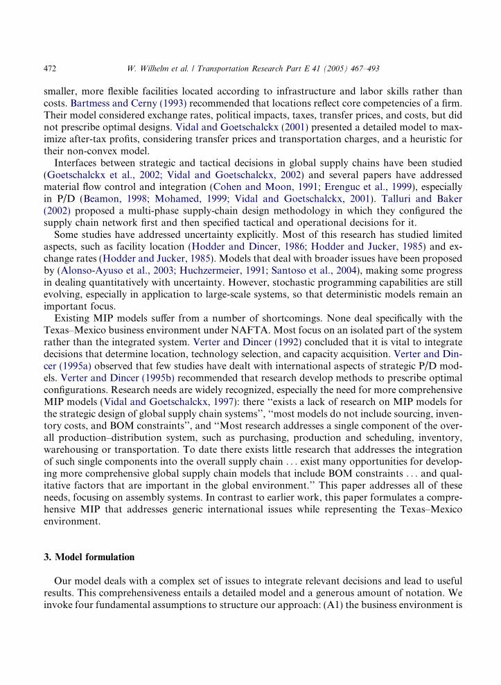
Texas–Mexico business environment under NAFTA. Most focus on an isolated part of the systemrather than the integrated system. Verter and Dincer (1992) concluded that it is vital to integratedecisions that determine location, technology selection, and capacity acquisition. Verter and Din-cer (1995a) observed that few studies have dealt with international aspects of strategic P/D mod-els. Verter and Dincer (1995b) recommended that research develop methods to prescribe optimalconfigurations. Research needs are widely recognized, especially the need for more comprehensiveMIP models (Vidal and Goetschalckx, 1997): there ‘‘exists a lack of research on MIP models forthe strategic design of global supply chain systems’’, ‘‘most models do not include sourcing, inven-tory costs, and BOM constraints’’, and ‘‘Most research addresses a single component of the over-all production–distribution system, such as purchasing, production and scheduling, inventory,warehousing or transportation. To date there exists little research that addresses the integrationof such single components into the overall supply chain . . . exist many opportunities for develop-ing more comprehensive global supply chain models that include BOM constraints . . . and qual-itative factors that are important in the global environment.’’ This paper addresses all of theseneeds, focusing on assembly systems. In contrast to earlier work, this paper formulates a compre-hensive MIP that addresses generic international issues while representing the Texas–Mexicoenvironment.

3. Model formulation

Our model deals with a complex set of issues to integrate relevant decisions and lead to usefulresults. This comprehensiveness entails a detailed model and a generous amount of notation. Weinvoke four fundamental assumptions to structure our approach: (A1) the business environment is


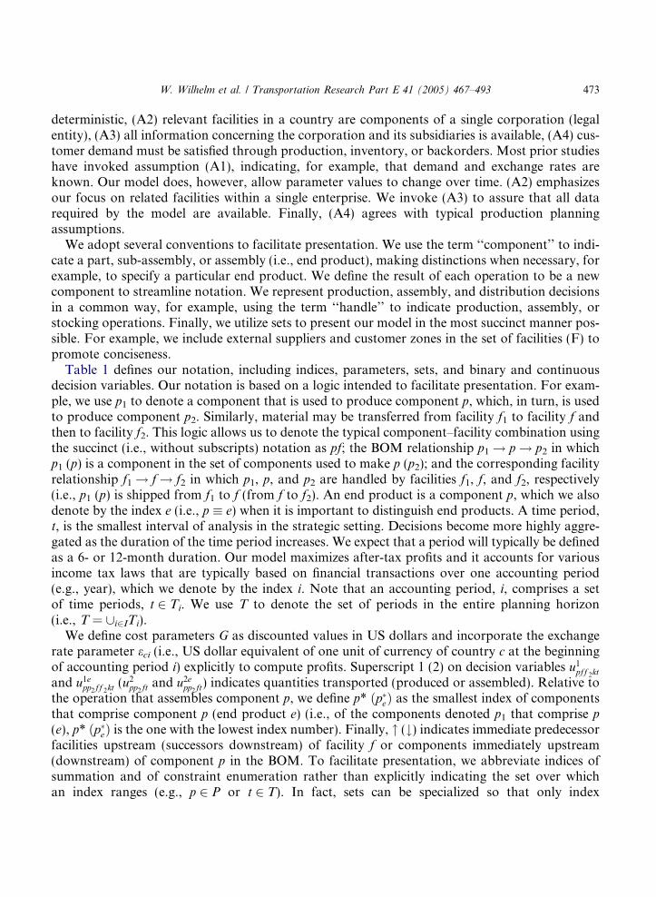
deterministic, (A2) relevant facilities in a country are components of a single corporation (legalentity), (A3) all information concerning the corporation and its subsidiaries is available, (A4) cus-tomer demand must be satisfied through production, inventory, or backorders. Most prior studieshave invoked assumption (A1), indicating, for example, that demand and exchange rates areknown. Our model does, however, allow parameter values to change over time. (A2) emphasizesour focus on related facilities within a single enterprise. We invoke (A3) to assure that all datarequired by the model are available. Finally, (A4) agrees with typical production planningassumptions.We adopt several conventions to facilitate presentation. We use the term ‘‘component’’ to indi-

cate a part, sub-assembly, or assembly (i.e., end product), making distinctions when necessary, forexample, to specify a particular end product. We define the result of each operation to be a newcomponent to streamline notation. We represent production, assembly, and distribution decisionsin a common way, for example, using the term ‘‘handle’’ to indicate production, assembly, orstocking operations. Finally, we utilize sets to present our model in the most succinct manner pos-sible. For example, we include external suppliers and customer zones in the set of facilities (F) topromote conciseness.Table 1 defines our notation, including indices, parameters, sets, and binary and continuous

decision variables. Our notation is based on a logic intended to facilitate presentation. For exam-ple, we use p1 to denote a component that is used to produce component p, which, in turn, is usedto produce component p2. Similarly, material may be transferred from facility f1 to facility f andthen to facility f2. This logic allows us to denote the typical component–facility combination usingthe succinct (i.e., without subscripts) notation as pf; the BOM relationship p1 ! p! p2 in whichp1 (p) is a component in the set of components used to make p (p2); and the corresponding facilityrelationship f1 ! f! f2 in which p1, p, and p2 are handled by facilities f1, f, and f2, respectively(i.e., p1 (p) is shipped from f1 to f (from f to f2). An end product is a component p, which we alsodenote by the index e (i.e., p � e) when it is important to distinguish end products. A time period,t, is the smallest interval of analysis in the strategic setting. Decisions become more highly aggre-gated as the duration of the time period increases. We expect that a period will typically be definedas a 6- or 12-month duration. Our model maximizes after-tax profits and it accounts for variousincome tax laws that are typically based on financial transactions over one accounting period(e.g., year), which we denote by the index i. Note that an accounting period, i, comprises a setof time periods, t 2 Ti. We use T to denote the set of periods in the entire planning horizon(i.e., T = [i2ITi).We define cost parameters G as discounted values in US dollars and incorporate the exchange

rate parameter eci (i.e., US dollar equivalent of one unit of currency of country c at the beginningof accounting period i) explicitly to compute profits. Superscript 1 (2) on decision variables u1pff 2ktand u1epp2ff 2kt (u

2pp2ft

and u2epp2ft) indicates quantities transported (produced or assembled). Relative tothe operation that assembles component p, we define p* ðp�eÞ as the smallest index of componentsthat comprise component p (end product e) (i.e., of the components denoted p1 that comprise p(e), p* ðp�eÞ is the one with the lowest index number). Finally, " (#) indicates immediate predecessorfacilities upstream (successors downstream) of facility f or components immediately upstream(downstream) of component p in the BOM. To facilitate presentation, we abbreviate indices ofsummation and of constraint enumeration rather than explicitly indicating the set over whichan index ranges (e.g., p 2 P or t 2 T). In fact, sets can be specialized so that only index

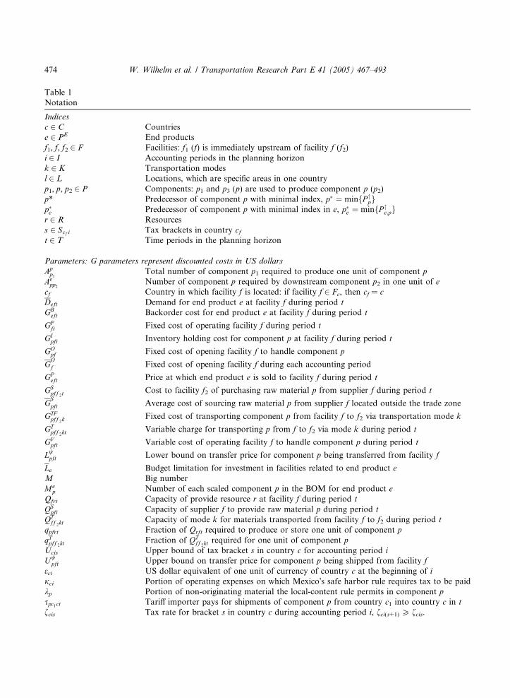
Table 1Notation

Indices

c 2 C Countriese 2 PE End productsf1, f, f2 2 F Facilities: f1 (f) is immediately upstream of facility f (f2)i 2 I Accounting periods in the planning horizonk 2 K Transportation modesl 2 L Locations, which are specific areas in one countryp1, p, p2 2 P Components: p1 and p3 (p) are used to produce component p (p2)p* Predecessor of component p with minimal index, p� ¼ minfP "

pgp�e Predecessor of component p with minimal index in e, p�e ¼ minfP "

e;pgr 2 R Resourcess 2 Scf i Tax brackets in country cft 2 T Time periods in the planning horizon

Parameters: G parameters represent discounted costs in US dollars

App1 Total number of component p1 required to produce one unit of component pAepp2 Number of component p required by downstream component p2 in one unit of ecf Country in which facility f is located: if facility f 2 Fc, then cf = cDeft Demand for end product e at facility f during period tGBeft Backorder cost for end product e at facility f during period t

GFft Fixed cost of operating facility f during period t

GIpft Inventory holding cost for component p at facility f during period t

GOpf Fixed cost of opening facility f to handle component p

GOf Fixed cost of opening facility f during each accounting period

GPeft Price at which end product e is sold to facility f during period t

GSpff 2t Cost to facility f2 of purchasing raw material p from supplier f during period t

GSpft Average cost of sourcing raw material p from supplier f located outside the trade zone

GTFpff 2k Fixed cost of transporting component p from facility f to f2 via transportation mode k

GTpff 2kt Variable charge for transporting p from f to f2 via mode k during period t

GVpft Variable cost of operating facility f to handle component p during period t

Lwpft Lower bound on transfer price for component p being transferred from facility f

Le Budget limitation for investment in facilities related to end product eM Big numberMep Number of each scaled component p in the BOM for end product e

Qfrt Capacity of provide resource r at facility f during period tQSpft Capacity of supplier f to provide raw material p during period tQTff 2kt Capacity of mode k for materials transported from facility f to f2 during period tqpfrt Fraction of Qrft required to produce or store one unit of component pqTpff 2kt Fraction of QTff 2kt required for one unit of component pUcis Upper bound of tax bracket s in country c for accounting period iUwpft Upper bound on transfer price for component p being shipped from facility f

eci US dollar equivalent of one unit of currency of country c at the beginning of ijci Portion of operating expenses on which Mexico�s safe harbor rule requires tax to be paidkp Portion of non-originating material the local-content rule permits in component pspc1ct Tariff importer pays for shipments of component p from country c1 into country c in tfcis Tax rate for bracket s in country c during accounting period i, fci(s+1) P fcis.


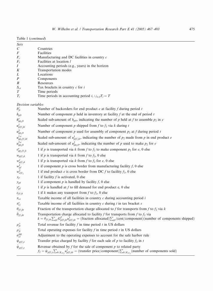
Table 1 (continued)

Sets

C CountriesF FacilitiesFc Manufacturing and DC facilities in country cFl Facilities at location lI Accounting periods (e.g., years) in the horizonK Transportation modesL LocationsP ComponentsR ResourcesSci Tax brackets in country c for iT Time periodsTi Time periods in accounting period i, [i2ITi = T

Decision variables

beft Number of backorders for end product e at facility f during period t

hpft Number of component p held in inventory at facility f at the end of period t

hepp2ft Scaled sub-amount of hpft, indicating the number of p held at f to assemble p2 in e

u1pff 2kt Number of component p shipped from f to f2 via k during t

u2pp2ft Number of component p used for assembly of component p2 at f during period t

u1;epp2ff 2kt Scaled sub-amount of u1pff 2kt, indicating the number of p2 made from p in end product e

u2;epp2ft Scaled sub-amount of u2pp2ft, indicating the number of p used to make p2 for e

vepp2ff 2k 1 if p is transported via k from f to f2 to make component p2 for e, 0 else

wpff 2k 1 if p is transported via k from f to f2, 0 else

wepff 2k 1 if p is transported via k from f to f2 for e, 0 else

w1pf 1 if component p is cross border from manufacturing facility f, 0 else

w2eff 2

1 if end product e is cross border from DC f to facility f2, 0 else

xf 1 if facility f is activated, 0 else

ypf 1 if component p is handled by facility f, 0 else

yepf 1 if p is handled at f to fill demand for end product e, 0 else

zff 2k 1 if k makes any transport from f to f2, 0 else

pci Taxable income of all facilities in country c during accounting period i

psci Taxable income of all facilities in country c during i in tax bracket s

hff 2kt Fraction of the transportation charge allocated to f for transports from f to f2 via k

hff 2kt Transportation charge allocated to facility f for transports from f to f2 viak ¼ hff 2kt

Ppf G

Tpff 2kt

u1pff 2kt ¼ ðfraction allocatedÞP

pf ðcost=componentÞðnumber of components shippedÞqþft Total revenue for facility f in time period t in US dollars

q�ft Total operating expenses for facility f in time period t in US dollars

rSHct Adjustment to the operating expenses to account for the safe harbor rule

wpff 2 t Transfer price charged by facility f for each sale of p to facility f2 in t

wpff 2 t Revenue obtained by f for the sale of component p to related partyf2 ¼ wpff 2 t

Pk2Kff2

u1pff 2kt ¼ ðtransfer price=componentÞP

k2Kff 2ðnumber of components soldÞ



combinations that have meaning are defined, making the model as concise as possible. We nowpresent our model.

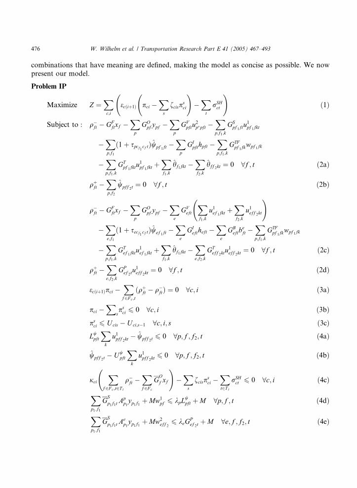
Problem IP

Maximize Z ¼Xc;i

ecðiþ1Þ pci �Xs

fcispsci

!�Xt

rSHct

!ð1Þ

Subject to : q�ft � GFftxf �

Xp

GOpf ypf �Xp

GVpftu2p�pft �

Xp;f1;k

GSpf 1ftu1pf 1fkt

�Xp;f1

ð1þ spcf1cf tÞwpf 1ft �Xp

GIpfthpft �Xp;f1;k

GTFpf 1fkwpf 1fk

�Xp;f1;k

GTpf 1fktu1pf 1fkt

þXf1;k

hf1fkt �Xf2;k

hff 2kt ¼ 0 8f ; t ð2aÞ

qþft �

Xp;f2

wpff 2t¼ 0 8f ; t ð2bÞ

q�ft � GFftxf �

Xp

GOpf ypf �Xe

GVeftXf1;k

u1ef 1fkt þXf2;k

u1eff 2kt

!

�Xe;f1

ð1þ secf1 cf tÞwef 1ft�Xe

GIeftheft �Xe

GBeftbeft �

Xp;f1;k

GTFpf 1fkwpf 1fk

�Xp;f1;k

GTef 1fktu1ef 1fkt

þXf1;k

hf1fkt �Xe;f2;k

GTeff 2ktu1eff 2kt

¼ 0 8f ; t ð2cÞ

qþft �

Xe;f2;k

GPef 2tu1eff 2kt

¼ 0 8f ; t ð2dÞ

ecðiþ1Þpci �Xf2F c;t

ðqþft � q�

ftÞ ¼ 0 8c; i ð3aÞ

pci �X

spsci 6 0 8c; i ð3bÞ

psci 6 Ucis � Uci;s�1 8c; i; s ð3cÞ

Lwpft

Xk

u1pff 2kt � wpff 2t6 0 8p; f ; f2; t ð4aÞ

wpff 2t � Uwpft

Xk

u1pff 2kt 6 0 8p; f ; f2; t ð4bÞ

jciX

f2F c;t2T iq�ft �

Xf2F c

GOf xf

!�Xs

fcispsci �

Xt2T i

rSHct 6 0 8c; i ð4cÞ

Xp1;f1

GSp1f1t

App1yp1f1 þMw1pf 6 kpL

wpft þM 8p; f ; t ð4dÞ

Xp1;f1

GSp1f1t

Aep1yp1f1 þMw2eff 2

6 keGPef 2t

þM 8e; f ; f2; t ð4eÞ


hff 2kt �Xp

GTpff 2ktu1pff 2kt

6 0 8f ; f2; k; t ð4fÞ

yepf � ypf 6 0 8e; p; f ð5aÞ

ypf �Xe

yepf 6 0 8p; f ð5bÞ

wepff 2k � wpff 2k 6 0 8e; p; f ; f2; k ð5cÞ

wpff 2k �Xe

wepff 2k 6 0 8p; f ; f2; k ð5dÞ

ypf � xf 6 0 8p; f ð5eÞ

xf �Xp

ypf 6 0 8f ð5fÞ

wpff 2k � zff 2k 6 0 8p; f ; f2; k ð5gÞ

zff 2k �Xp

wpff 2k 6 0 8f ; f2; k ð5hÞ

wpff 2k þ wpf 2fk 6 1 8p; f ; f2; k ð5iÞ

w1pf �

Xf2;k

wpff 2k 6 0 8p; f ð5jÞ

wpff 2k � w1pf 6 0 8p; f ; f2; k ð5kÞX

k;t

u1eff 2kt �Xt

Def 2tw2eff 2

6 0 8e; f ; f2 ð5lÞ

Xf2F l

xf 6 1 8l ð5mÞ

Xf

ypf ¼ 1 8p ð5nÞ

Xp

qpfrtu2p�pft � Qfrtxf 6 0 8f ; r; t ð6aÞ

Xe;f2;k

qefrtu1eff 2kt

� Qfrtxf 6 0 8f ; r; t ð6bÞ

qpfrtu2p�pft � Qfrtypf 6 0 8p; f ; r; t ð6cÞX

f2;k

qefrtu1eff 2kt

� Qfrtyef 6 0 8e; f ; r; t ð6dÞ

Xf2;k

u1pff 2kt � QSpftypf 6 0 8p; f ; t ð6eÞ

Xp

qTpff 2ktu1pff 2kt

� QTff 2ktzff 2k 6 0 8f ; f2; k; t ð6fÞ


qTpff 2ktu1pff 2kt

� QTff 2ktwpff 2k 6 0 8f ; f2; k; t ð6gÞ

ð0.5ÞXe

qefrtðhef ðt�1Þ þ heftÞ � Qfrtxf 6 0 8f ; r; t ð6hÞXe;p2

Aepp2u1;epp2ff 2kt

� u1pff 2kt ¼ 0 8p; f ; f2; k; t ð7aÞ

Xe

Aepp2u2;epp2ft

� u2pp2ft ¼ 0 8p; p2; f ; t ð7bÞXe;p2

Aepp2hepp2ft

� hpft ¼ 0 8p; f ; t ð7cÞ

u2;ep�epft � u2;ep1pft

¼ 0 8e; p; p1; f ; t ð7dÞXf2;k;t12f1...tg

u1pff 2kt1 �X

t12f1...tgu2p�pft1 6 0 8p; f ; t ð7eÞ

Xf

yepf ¼ 1 8e; p ð8a;b; cÞ

vepp2ff 2k � yepf 6 0 8e; p; p2; f ; f2; k ð8dÞ

vepp2ff 2k � yep2f2

6 0 8e; p; p2; f ; f2; k ð8eÞ

yepf þ yep2f2 �Xk

vepp2ff 2k 6 1 8e; p; p2; f ; f2 ð8fÞ

vepp2ff 2k � wepff 2k

6 0 8e; p; p2; f ; f2; k ð8gÞ

wepff 2k �Xp2

vepp2ff 2k 6 0 8e; p; f ; f2; k ð8hÞ

Xp;f

GOpf yepf þ

Xp;f ;f2;k

GTFpff 2kwepff 2k

6 Le 8e ð8iÞ

Xp2;f ;f2;k;t

u1;epp2ff 2kt ¼ Mep

Xft

Deft 8e; p ð9aÞ

Xf1;k

u1;epp2f1fkt þ hepp2f ðt�1Þ � h

epp2ft

� u2;epp2ft ¼ 0 8e; p; p2; f ; t ð9bÞ

u2;ep�epft þXp2;f1;k

u1;epp2f1fkt þXp2

ðhepp2f ðt�1Þ � hepp2ft

Þ

�Xp2

u2;epp2ft �Xp2;f2;k

u1;epp2ff 2kt ¼ 0 8e; p; f ; t ð9cÞ

Xf1;k

u1;epp2f1fkt þ hepp2f ðt�1Þ � h

epp2ft

� beft þ bef ðtþ1Þ �Xf2;k

u1;epp2ff 2kt ¼ 0 8e; p; p2; f ; t ð9dÞ

Xf1;k

u1;epp2f1fkt ¼ Deft 8e; p; p2; f ; t ð9eÞ

Xf ;t
u2;ep1pft ¼Xft

Deft 8e; p; p1 ð9fÞ

vepp2ff 2k;wpff 2k;wepff 2k

;w1pf ;w

2eff 2

; xf ; ypf ; yepf ; zff 2k 2 f0; 1g ð10Þ

beft; hpft; hepp2ft

; u1pff 2kt; u2pp2ft

; u1;epp2ff 2kt; u2;epp2ft

; hff 2kt;qþft ; q

�ft ;r

SHct ; wpff 2t

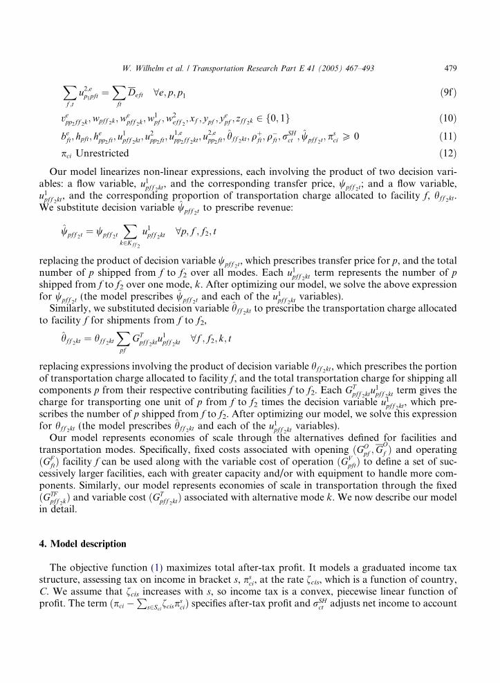
; psci P 0 ð11Þpci Unrestricted ð12Þ

Our model linearizes non-linear expressions, each involving the product of two decision vari-ables: a flow variable, u1pff 2kt, and the corresponding transfer price, wpff 2t

; and a flow variable,u1pff 2kt, and the corresponding proportion of transportation charge allocated to facility f, hff 2kt.We substitute decision variable wpff 2t to prescribe revenue:

wpff 2t ¼ wpff 2t

Xk2Kff 2

u1pff 2kt 8p; f ; f2; t

replacing the product of decision variable wpff 2t, which prescribes transfer price for p, and the total

number of p shipped from f to f2 over all modes. Each u1pff 2kt term represents the number of pshipped from f to f2 over one mode, k. After optimizing our model, we solve the above expressionfor wpff 2t (the model prescribes wpff 2t and each of the u1pff 2kt variables).Similarly, we substituted decision variable hff 2kt to prescribe the transportation charge allocated

to facility f for shipments from f to f2,

hff 2kt ¼ hff 2ktXpf

GTpff 2ktu1pff 2kt

8f ; f2; k; t

replacing expressions involving the product of decision variable hff 2kt, which prescribes the portionof transportation charge allocated to facility f, and the total transportation charge for shipping allcomponents p from their respective contributing facilities f to f2. Each G

Tpff 2kt

u1pff 2kt term gives thecharge for transporting one unit of p from f to f2 times the decision variable u1pff 2kt, which pre-scribes the number of p shipped from f to f2. After optimizing our model, we solve this expressionfor hff 2kt (the model prescribes hff 2kt and each of the u1pff 2kt variables).Our model represents economies of scale through the alternatives defined for facilities and

transportation modes. Specifically, fixed costs associated with opening ðGOpf ;GOf Þ and operating

ðGFftÞ facility f can be used along with the variable cost of operation ðGVpftÞ to define a set of suc-cessively larger facilities, each with greater capacity and/or with equipment to handle more com-ponents. Similarly, our model represents economies of scale in transportation through the fixedðGTFpff 2kÞ and variable cost ðG

Tpff 2kt

Þ associated with alternative mode k. We now describe our modelin detail.

4. Model description

The objective function (1) maximizes total after-tax profit. It models a graduated income taxstructure, assessing tax on income in bracket s, psci, at the rate fcis, which is a function of country,C. We assume that fcis increases with s, so income tax is a convex, piecewise linear function ofprofit. The term ðpci �

Ps2Scifcisp

sciÞ specifies after-tax profit and rSHct adjusts net income to account


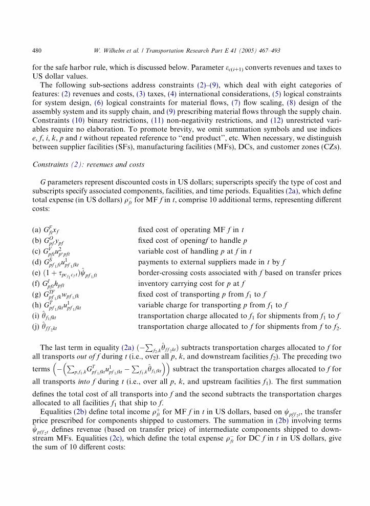
for the safe harbor rule, which is discussed below. Parameter ec(i+1) converts revenues and taxes toUS dollar values.The following sub-sections address constraints (2)–(9), which deal with eight categories of

features: (2) revenues and costs, (3) taxes, (4) international considerations, (5) logical constraintsfor system design, (6) logical constraints for material flows, (7) flow scaling, (8) design of theassembly system and its supply chain, and (9) prescribing material flows through the supply chain.Constraints (10) binary restrictions, (11) non-negativity restrictions, and (12) unrestricted vari-ables require no elaboration. To promote brevity, we omit summation symbols and use indicese, f, i, k, p and t without repeated reference to ‘‘end product’’, etc. When necessary, we distinguishbetween supplier facilities (SFs), manufacturing facilities (MFs), DCs, and customer zones (CZs).

Constraints (2): revenues and costs

G parameters represent discounted costs in US dollars; superscripts specify the type of cost andsubscripts specify associated components, facilities, and time periods. Equalities (2a), which definetotal expense (in US dollars) q�

ft for MF f in t, comprise 10 additional terms, representing differentcosts:

(a) GFftxf fixed cost of operating MF f in t

(b) GOpf ypf fixed cost of openingf to handle p

(c) GVpftu2p�pft variable cost of handling p at f in t

(d) GSpf 1ftu1pf 1fkt

payments to external suppliers made in t by f

(e) ð1þ spcf1cf tÞwpf 1ft border-crossing costs associated with f based on transfer prices

(f) GIpfthpft inventory carrying cost for p at f

(g) GTFpf 1fkwpf 1fk fixed cost of transporting p from f1 to f

(h) GTpf 1fktu1pf 1fkt

variable charge for transporting p from f1 to f

(i) hf1fkt transportation charge allocated to f1 for shipments from f1 to f

(j) hff 2kt transportation charge allocated to f for shipments from f to f2.

The last term in equality (2a) ð�P

f2;khff 2ktÞ subtracts transportation charges allocated to f for

all transports out of f during t (i.e., over all p, k, and downstream facilities f2). The preceding two

terms �P

p;f1;kGTpf 1fktu

1pf 1fkt

�P

f1;khf1fkt

� �� subtract the transportation charges allocated to f for

all transports into f during t (i.e., over all p, k, and upstream facilities f1). The first summation

defines the total cost of all transports into f and the second subtracts the transportation chargesallocated to all facilities f1 that ship to f.Equalities (2b) define total income qþ

ft for MF f in t in US dollars, based on wpff 2t, the transferprice prescribed for components shipped to customers. The summation in (2b) involving termswpff 2t defines revenue (based on transfer price) of intermediate components shipped to down-stream MFs. Equalities (2c), which define the total expense q�

ft for DC f in t in US dollars, givethe sum of 10 different costs:

(a) GFftxf fixed cost of operating f in t

(b) GOpf ypf fixed cost of operating DC f to handle p, charged to t = 1

(c) GVeftP

f1;ku1ef 1fkt

þP

f2;ku1eff 2kt

� �variable cost of handling e entering and departing DC f in t

(d) ð1þ secf1cf tÞwef 1ft border-crossing costs allocated to f for shipments fromrelated facilities

(e) GIeftheft inventory holding cost for e at DC f at the end of t

(f) GBeftbeft backorder cost for e at DC f at the end of t

(g) GTFef 1fkwef 1fk fixed cost of transporting e from f1 to f in t

(h) GTef 1fktu1ef 1fkt

variable charge for transporting amount u1ef 1fkt of efrom f1 to f in t

(i) hf1fkt transportation charges allocated to f for componentsshipped from f1 to f

(j) GTeff 2ktu1eff 2kt

charge for transporting amount u1eff 2kt of e from f1 to f in t.


Equalities (2d) define the total income qþft for DC f in t, considering the quantity of e sold,

u1eff 2kt.

Constraints (3): income taxes

Equalities (3a) define total taxable income earned in country c, pci, in i as the difference betweenrevenue and cost associated with facilities f in c for all t that comprise i,

Pf2F c;tðq

þft � q�

ftÞ. Totalincome pci can be positive, zero, or negative; if it is positive, equalities (3b) partition it intocomponents psci associated with graduated income tax brackets in c (i.e., s 2 Sci). Inequalities(3c) impose upper bounds on decision variables based on the range of each tax bracket. Con-straints (11) require that psci be non-negative. This (sub)set of constraints (i.e., (3), (11), and(12)) defines the amount of income in tax bracket s, psci, which is taxed at rate fcis in (1). Because(2) and (3a) are equalities, they could be used to substitute decision variables in (1), reducing thesize of the model. However, the current formulation allows us to easily highlight all costcomponents.

Constraints (4): international considerations

We model the generic international environment by incorporating typical considerations suchas transfer pricing (4a) and (4b), the safe harbor rule (4c), local-content rules (4d) and (4e), andtransportation-charge allocation (4f). Constraints (2a) and (2c) impose border-crossing fees. Thissection discusses these issues in relationship to the US–Mexico environment.

Constraints (4a) and (4b): transfer pricesInequalities (4a) and (4b) model the CUP method by setting lower Lw

pft and upper Uwpft bounds

on transfer prices, wpff 2t. Since we use revenue wpff 2t to linearize terms involving transfer price


wpff 2t, (4a) and (4b) employ revenue wpff 2tto set bounds for the sum of transfers u1pff 2kt between

MF f and f2, where f2 is either a MF or a DC downstream of f.

Constraints (4c): safe harbor ruleSafe harbor rules are used to exempt Maquiladora operations from permanent establishment

rules. A permanent establishment must pay an additional ‘‘asset tax’’ of 1.8% of the total valueof its assets. Under current Hacienda (Mexican tax authority) rules, a Maquiladora created priorto 2001 must meet the following safe harbor rule: It must declare taxable revenue equal to 6.5% ofits ordinary operating expenses or 6.9% of the value of the assets employed in the operation,whichever is higher. Alternatively, it can negotiate an advanced pricing agreement (APA) withthe Mexican tax authorities. Maquiladoras created after 2001, ‘‘Maquiladoras of new creation’’,have to meet only the ‘‘6.5% of operating expenses’’ rule. The objective function computes profitsaccordingly—if the actual taxable revenue is less than 6.5% of the operating expenses, the corpo-ration must pay tax on the difference, thereby reducing profit but maintaining exemption frompermanent establishment rules. Inequalities (4c) invoke safe harbor rules and the rSHct term inobjective function (1) adjusts after-tax income so that the tax paid to Mexico is not less than

jci (i.e., 0.065) portion of operating expenses. In (4c),P

f2F c;t2T iq�ft �

Pf2F cG

Of xf

� �defines vari-

able cost (i.e., sum of all operating expenses minus fixed cost) for the legal entity in Mexico, which,when multiplied by the safe harbor portion, jci, defines the tax required to satisfy the safe har-bor rule. Subtracting taxes paid,

Psfcisp

sci, yields a difference that, if positive, indicates that addi-

tional taxP

t2T irSHct must be paid to satisfy the safe harbor rule and, if negative, indicates that tax

paid on transactions is sufficient to satisfy the safe harbor rule so that no additional tax must bepaid.The safe harbor rule for Maquiladora operations in Mexico provides the only exception to the

graduated tax rates in Mexico, assessing a minimum tax of 6.5% of operating expenses. If a Mex-ican subsidiary pays less than this minimum tax, it loses its Maquiladora status.

Constraints (4d) and (4e): local-content rulesInequalities (4d) and (4e) impose local-content requirements for manufacturing facilities and

DCs, respectively, by placing upper bounds on the value of non-NAFTA material incorporatedin each component shipped across the border between two NAFTA countries. The value of thisnon-NAFTA content cannot exceed kp portion of the transaction value.If MF f ships p across a border between two NAFTA countries, w1

pf ¼ 1 and (4d) is activated(otherwise, w1

pf ¼ 0 and (4d) is redundant). Inequality (4d) requires that the non-NAFTA contentof such a shipment not exceed the upper bound, kpL

wpft, where L

wpft is the lower bound on the trans-

fer price that can be charged in the transaction. Since we incorporate the transfer price wpff 2tin

decision variable wpff 2tto avoid non-linearities, it is not available for use in this constraint. This

upper bound on non-NAFTA content is conservative (because transfer price can be prescribed avalue larger than its lower bound) and, we expect, will lead to acceptable solutions in practice.Summing terms G

Sp1ftApp1yp1f1 gives the total cost of materials in p prescribed (by decision variables

yp1f1) to originate in non-NAFTA countries. If a supplier does not offer the same price to allrelated facilities that it supplies, G

Sp1ft

must represent the average of these prices because it isnot possible to identify which facility purchased the material after an assembly operation in the


multi-echelon network. A unique local content can be specified for each p, if necessary, by spec-ifying kp. Similarly, constraints (4e) deal with shipments from DCs to customers.

Constraints (4f): transportation-charge allocationThe charge for transporting from f to f2 via k is allocated among f and f2. Inequality (4f) uses

the summation of transportation charges as an upper bound on the cash value of these transports,hff 2kt. Decision variables zff 2k reflect alternative transportation modes, including direct, point-to-point shipments as well as cross docking by third-party providers. Similarly, decision variables xfrepresent DC alternatives in the US or Mexico. Currently, DC locations in the US are preferredbecause they offer lower cost (e.g., related to insurance and pilferage).

Constraints (5): logical constraints for system design

Constraints (5) and (8) design the assembly system and its supply chain. Inequalities (5a) and(5b) define ypf = 1 if p is handled at f to eventually fill demand for e: (5a) assures that ypf = 1 if p ishandled at f in association with e (i.e., if any yepf ¼ 1) while (5b) requires ypf = 0 if no p is handledat f in association with any e (i.e., the sum of yepf over all e is 0). Similarly, inequalities (5c)–(5d),(5e)–(5f), (5g)–(5h), (5j)–(5k) and (5l) define wpff 2k, xf, zff 2k, w

1pf , and w

2eff 2

, respectively. Inequality(5i) assures that no component is transported back and forth between two facilities; inequality(5m), that the model prescribes at most one facility from the set of alternatives located at site l,Fl; equality (5n), that the model selects one supplier for each raw material.Inequality (5i) is needed to prevent shipping the same p back and forth between f and f2 in a

special case. Production requirements are satisfied as p first flows from f to f2 so that additionalshipments incur only variable transportation cost. If f and f2 can both handle (e.g., assemble) pand p2 and are in different countries that assess different income tax rates, it is possible that trans-fer prices can be prescribed so that the company makes a net profit by making shipments of p thatreduce income taxes more than they increase transportation charges. Inequality (5i) prevents suchwindfalls.

Constraints (6): logical constraints on material flows

Constraints (6a)–(6g) impose variable upper-bounds, relating decision variables that design thesystem to those that prescribe flow in it. We assume that f employs resource r with capacity Qfrt int. Inequalities (6a) impose capacity Qfrt at MF f during t, limiting the flows of associated productsu2p�pft according to the amount of r each requires, qpfrt. Similarly, inequalities (6b) and (6e)–(6f)impose capacities: (6b) of DC f, (6e) SF f, and (6f) k. Inequalities (6c), (6d) and (6g) impose capac-ity relative to disaggregated flow of one p: (6c) at MF f, (6d) at DC f, and (6g) on k. Inequalities(6h) limit the average inventory held at DC f. If a supplier, mode, or facility is not selected (ypf,zff 2k, or xf = 0), the associated flow must be zero.

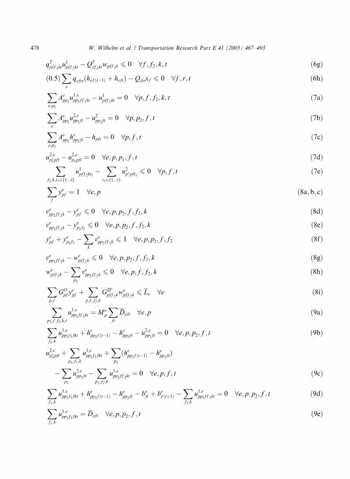
Constraints (7): flow scaling

Constraints (7) and (9) model the flow of materials through the supply chain. Equalities (7a)–(7c) scale flows for e. Rather than dealing with multi-commodity flow, for which each component


is treated as a unique commodity, we define the flow on each arc, which represents production,assembly, or distribution of a particular component in a time period, in terms of the numberof end products it represents, essentially converting all flow to that of a single commodity, e.Equalities (7a) define the total amount of component p transported, u1pff 2kt, as the sum of the num-ber of p made for each immediate successor p2 in each e, Aepp2u

1;epp2ff 2kt

. Similarly, equalities (7b) de-fine the total amount of p manufactured, u2pp2ft, as the sum of the number of p made for eachimmediate successor p2 in each e, A

epp2u2;epp2ft. A component used in several end products is incorpo-

rated in the network associated with each and the total transportation flow and production of thecomponent appear in constraints (2), (4), and (6). Equalities (7c) define the inventory of p held atf, hpft, as the sum of the number of p held for each immediate successor p2, in each e, Aepp2h

epp2ft

.Equalities (7a), (7b) and (7c) can be used to substitute for u1pff 2kt, u

2pp2ft

, and hpft, respectively, mak-ing the model smaller and easier to solve; we include them to clarify our presentation. Equalities(7d) assure that the correct number of each component is used in each assembly operation (seealso the discussion of (9)). Inequalities (7e) assure that the amount of p transported out of f overthe first t periods,

Pf2;k;t12f1...tgu

1pff 2kt1

, is less than or equal to the amount produced in f over that

series of periods,P

t12f1...tgu2p�pft1

.

Constraints (8) design of the assembly system and its supply chain

Our model prescribes a system design by selecting a subset of alternative facilities, which rep-resent suppliers of each ‘‘raw’’ component; the location, technology and capacity for each produc-tion, assembly, and DC operation; and by selecting the transportation mode for each shipment.Inequalities (8) reflect the BOM for each end product e. Summing f over the appropriate set of

facilities, equality (8a) assures that one supplier sources raw material p; (8b), that one facility man-ufactures component p; and (8c), that one DC distributes e. Inequalities (8d)–(8h) allow the ship-ment of p from f to f2 using k only if p is produced at f and at least one component immediatelydownstream of p is assembled at f2. Inequality (8i) invokes a budget limitation, assuring that thetotal fixed cost associated with prescribing facilities and transportation modes for e does not ex-ceed Le dollars. This budget limitation is appropriate because each e may be viewed as a profitcenter that serves a unique market segment. Our model also deals with related cases (one p usedin several e (7a), one p used in several p2 of one e) and facility flexibility (e.g., one p may be man-ufactured in several f (9b) and one f may manufacture several p (6)).

Constraints (9): prescribing material flows through the supply chain

At a node representing an assembly operation, the scaled flow on each incoming arc is the sameas the flow on the outgoing arc. For each assembly operation, we redirect each input arc—exceptthe one of lowest index number—to a sink node, allowing flow to conform to classical network-flow balance at all nodes. We set the demand at each sink node to assure flow of the number ofcomponents needed in all end products demanded.Equalities (9a) enforce flow balance at source nodes (i.e., suppliers of raw materials), assuring

that the sum of all flows out, u1;epp2ff 2t, equals the total demand plus the requirement of the sinknode, Me

p

Pf ;tDeft. The BOM need not be a tree; for example, p could be incorporated in several


sub-assemblies p2 to make one end product e. Aepp2

defines the number of p used to manufacture p2for e and Me

p indicates the number of different sub-assemblies, denoted individually using p2, thatincorporate p.Equalities (9b) enforce flow balance for component p, which is transported from other facilities

f1 to MF f, considering the sum of shipments u1;epp2f1fkt; inventory changes at f, hepp2f ;ðt�1Þ � h

epp2ft

; andflow out to manufacture p2, u

2;epp2ft

. We invoke equalities (9b) only relative to the arc of lowest indexnumber, p�e . Flow balance equalities (7d) assure that all flows incoming to the assembly operation,u2;ep�epft and u

2;ep1pft

, are equal to each other (i.e., the flow of components on each arc incoming to anassembly operation must equal the flow on the departing arc).Equalities (9c) enforce flow balance of p at f considering manufacturing inputs u2;ep�epft, the sum of

shipments u1;epp2f1fkt from each other f1 to f, the sum of inventory changes ðhepp2f ðt�1Þ � hepp2ft

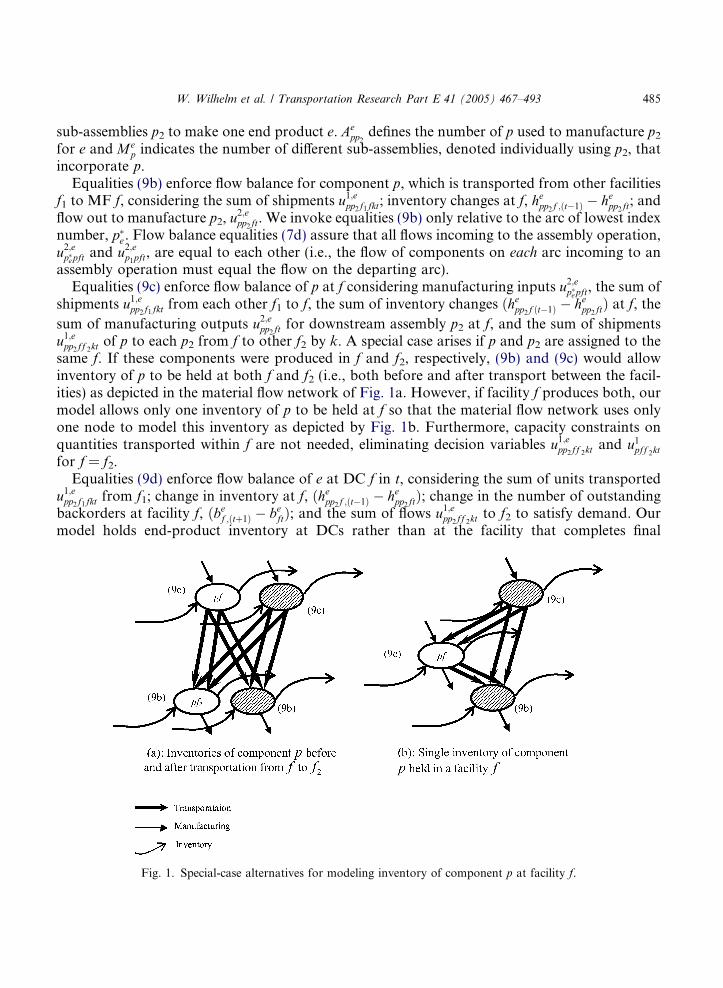
Þ at f, thesum of manufacturing outputs u2;epp2ft for downstream assembly p2 at f, and the sum of shipmentsu1;epp2ff 2kt of p to each p2 from f to other f2 by k. A special case arises if p and p2 are assigned to thesame f. If these components were produced in f and f2, respectively, (9b) and (9c) would allowinventory of p to be held at both f and f2 (i.e., both before and after transport between the facil-ities) as depicted in the material flow network of Fig. 1a. However, if facility f produces both, ourmodel allows only one inventory of p to be held at f so that the material flow network uses onlyone node to model this inventory as depicted by Fig. 1b. Furthermore, capacity constraints onquantities transported within f are not needed, eliminating decision variables u1;epp2ff 2kt and u

1pff 2kt

for f = f2.Equalities (9d) enforce flow balance of e at DC f in t, considering the sum of units transported

u1;epp2f1fkt from f1; change in inventory at f, ðhepp2f ;ðt�1Þ � hepp2ft

Þ; change in the number of outstandingbackorders at facility f, ðbef ;ðtþ1Þ � beftÞ; and the sum of flows u1;epp2ff 2kt to f2 to satisfy demand. Ourmodel holds end-product inventory at DCs rather than at the facility that completes final

Fig. 1. Special-case alternatives for modeling inventory of component p at facility f.


assembly. Equalities (9e) ensure the sum all flows u1;epp2f1fkt of e handled at DC f1 and transported toCZ f using k satisfies the demand for e at CZ f in t, Deft. Note that equalities (9d) and (9e) hold forend product e. In order to use an index consistently in variable u1;epp2f1fkt to represent the componenttransported, if p = e we define p2 = p = e. Equalities (9f) ensure flow balance at sink nodes, requir-ing inflows, u2;ep1pft, to equal the sum of demands Deft.

5. Example application

This section exemplifies how managers might use our model as a decision support aid. Thehypothetical setting involves an enterprise that manufactures two types of laptop computers,one for the high-end market segment and one for the low-end. Three operations complete assem-bly: the first and second assemble the base and screen assemblies, respectively; and the third, theend product.Assembly operations occur in related facilities, while most components are purchased from spe-

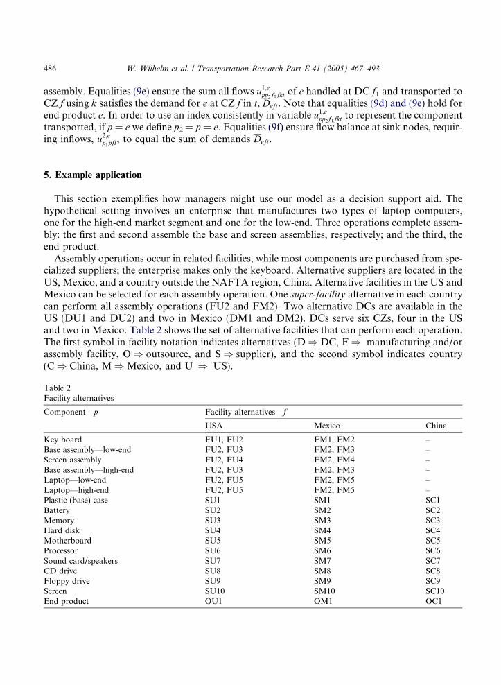
cialized suppliers; the enterprise makes only the keyboard. Alternative suppliers are located in theUS, Mexico, and a country outside the NAFTA region, China. Alternative facilities in the US andMexico can be selected for each assembly operation. One super-facility alternative in each countrycan perform all assembly operations (FU2 and FM2). Two alternative DCs are available in theUS (DU1 and DU2) and two in Mexico (DM1 and DM2). DCs serve six CZs, four in the USand two in Mexico. Table 2 shows the set of alternative facilities that can perform each operation.The first symbol in facility notation indicates alternatives (D) DC, F) manufacturing and/orassembly facility, O) outsource, and S) supplier), and the second symbol indicates country(C) China, M)Mexico, and U ) US).

Table 2Facility alternatives

Component—p Facility alternatives—f

USA Mexico China

Key board FU1, FU2 FM1, FM2 –Base assembly—low-end FU2, FU3 FM2, FM3 –Screen assembly FU2, FU4 FM2, FM4 –Base assembly—high-end FU2, FU3 FM2, FM3 –Laptop—low-end FU2, FU5 FM2, FM5 –Laptop—high-end FU2, FU5 FM2, FM5 –Plastic (base) case SU1 SM1 SC1Battery SU2 SM2 SC2Memory SU3 SM3 SC3Hard disk SU4 SM4 SC4Motherboard SU5 SM5 SC5Processor SU6 SM6 SC6Sound card/speakers SU7 SM7 SC7CD drive SU8 SM8 SC8Floppy drive SU9 SM9 SC9Screen SU10 SM10 SC10End product OU1 OM1 OC1

Table 3Initiating values of cost parameters

Facilities Fixed opening costsin $ million ($m)

Fixed annualoperating costs in$m

Variable operatingcost/unit in $/unit

Country USA Mexico USA Mexico US MexicoManufacturing and assembly 10 4 5 2 100 15Distribution centers 5 2 1 4 10 1.5

Table 4Demand (in thousands of units)

End-product Year 1 Year 2 Year 3

US Mexico US Mexico US Mexico

Low-end 60 6 80 8 60 6High-end 40 4 60 6 40 4


We defined a planning horizon comprising three time periods, each representing one year andgenerated cost parameters randomly based on initiating parameters, which are given in Table 3.Our discussions and conclusions are based on the parameters input to our model, including thosein Table 3. Generally, the costs in Mexico are less than those in the US However, we initiated thefixed annual cost of operating a DC in Mexico to be much higher than the corresponding cost inthe US to reflect the higher indirect costs of operating a DC in Mexico. We generated cost param-eter values by scaling the initiating values in proportion to the capacity of a facility and the num-ber of operations that it can perform and then adding a uniformly distributed random variate withrange based on the resulting mean value. Table 4 gives the values of demand for both high-endand low-end laptops.We investigated a set of cases to demonstrate how managers might apply our model as a deci-

sion support aid: Case 1 is the basic case, which results in a centralized design to exploit economiesof scale; Case 2 considers a decentralized system design; Case 3 investigates increased vertical inte-gration in which the enterprise assembles the motherboard instead of buying it; Case 4 considersoutsourcing the screen assembly, Case 5 outsources the entire laptop; Case 6 evaluates an addi-tional super facility with higher capacity; Cases 7 and 8 assess sensitivity relative to bounds onthe transfer prices; Case 9 reports the exchange rate that would make it attractive for a facilityin the US to replace one in Mexico, and Case 10 studies the effects of governmental inducementsto attract facilities. Case 11 evaluates the sensitivity of system design to the cost of transportationbetween FM2 and FM5, the only two manufacturing facilities in the Case 1 solution. Table 5summarizes results, detailing the system design our model prescribes and the profit obtained ineach case.In Case 1, our model prescribes the super facility in Mexico (FM2) and supplements it with an-

other facility (FM5). As a super facility, FM2 can perform all manufacturing and assembly oper-ations but its capacity must be augmented by FM5, which can perform only final assemblyoperations. Our model prescribes 11 suppliers (SM1, SC1, SM2, SC3, SM4, SM5, SC6, SM7,SC8, SM9 and SC10); six in Mexico and five in China, reflecting local-content rules. Our model

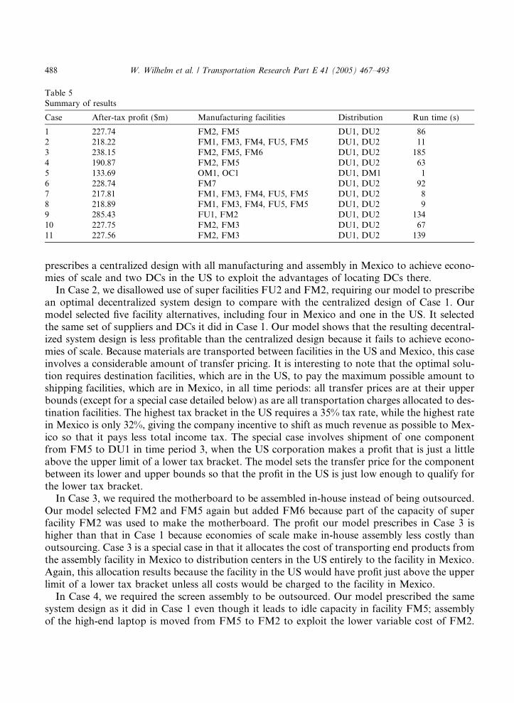
Table 5Summary of results

Case After-tax profit ($m) Manufacturing facilities Distribution Run time (s)

1 227.74 FM2, FM5 DU1, DU2 862 218.22 FM1, FM3, FM4, FU5, FM5 DU1, DU2 113 238.15 FM2, FM5, FM6 DU1, DU2 1854 190.87 FM2, FM5 DU1, DU2 635 133.69 OM1, OC1 DU1, DM1 16 228.74 FM7 DU1, DU2 927 217.81 FM1, FM3, FM4, FU5, FM5 DU1, DU2 88 218.89 FM1, FM3, FM4, FU5, FM5 DU1, DU2 99 285.43 FU1, FM2 DU1, DU2 13410 227.75 FM2, FM3 DU1, DU2 6711 227.56 FM2, FM3 DU1, DU2 139


prescribes a centralized design with all manufacturing and assembly in Mexico to achieve econo-mies of scale and two DCs in the US to exploit the advantages of locating DCs there.In Case 2, we disallowed use of super facilities FU2 and FM2, requiring our model to prescribe

an optimal decentralized system design to compare with the centralized design of Case 1. Ourmodel selected five facility alternatives, including four in Mexico and one in the US. It selectedthe same set of suppliers and DCs it did in Case 1. Our model shows that the resulting decentral-ized system design is less profitable than the centralized design because it fails to achieve econo-mies of scale. Because materials are transported between facilities in the US and Mexico, this caseinvolves a considerable amount of transfer pricing. It is interesting to note that the optimal solu-tion requires destination facilities, which are in the US, to pay the maximum possible amount toshipping facilities, which are in Mexico, in all time periods: all transfer prices are at their upperbounds (except for a special case detailed below) as are all transportation charges allocated to des-tination facilities. The highest tax bracket in the US requires a 35% tax rate, while the highest ratein Mexico is only 32%, giving the company incentive to shift as much revenue as possible to Mex-ico so that it pays less total income tax. The special case involves shipment of one componentfrom FM5 to DU1 in time period 3, when the US corporation makes a profit that is just a littleabove the upper limit of a lower tax bracket. The model sets the transfer price for the componentbetween its lower and upper bounds so that the profit in the US is just low enough to qualify forthe lower tax bracket.In Case 3, we required the motherboard to be assembled in-house instead of being outsourced.

Our model selected FM2 and FM5 again but added FM6 because part of the capacity of superfacility FM2 was used to make the motherboard. The profit our model prescribes in Case 3 ishigher than that in Case 1 because economies of scale make in-house assembly less costly thanoutsourcing. Case 3 is a special case in that it allocates the cost of transporting end products fromthe assembly facility in Mexico to distribution centers in the US entirely to the facility in Mexico.Again, this allocation results because the facility in the US would have profit just above the upperlimit of a lower tax bracket unless all costs would be charged to the facility in Mexico.In Case 4, we required the screen assembly to be outsourced. Our model prescribed the same

system design as it did in Case 1 even though it leads to idle capacity in facility FM5; assemblyof the high-end laptop is moved from FM5 to FM2 to exploit the lower variable cost of FM2.


Our model shows that the cost of outsourcing (Case 4) is greater than the cost of in-house assem-bly (Case 1).In Case 5, we required both end products to be outsourced. Our model selected one outsourcer

in Mexico (OM1) and one in China (OC1), along with one DC in Mexico and one in the US. Ourmodel shows that the cost of outsourcing (Case 5) is much higher than the cost of in-house assem-bly, reducing profit in comparison with Case 1. This case is interesting because the local-contentrules play an important role, causing the model to prescribe an outsourcer in Mexico as well as aDC in Mexico. The outsourcer in China ships directly to both DCs, which do not transship prod-ucts so the local-content rules do not apply for these products. The outsourcer in Mexico alsoships directly to both DCs; products that cross the border into the US satisfy local-content restric-tions because they are made in the NAFTA zone.In Case 6, we defined an additional super facility (FM7) at the site where FM2 would be lo-

cated. FM7 can perform all manufacturing and assembly operations and has a higher capacitythan FM2. Our model prescribes this single facility to obtain economies of scale that exceededthose achieved in Case 1.In Cases 7 and 8, we investigated the sensitivity of profit to changes in the bounds on transfer

prices. Compared with Case 2, in which we bounded transfer prices to be within ±10% of marketprice, these cases imposed bounds of ±20% and ±5%, respectively. Our model prescribed systemdesigns that obtained profits in direct relationship to these bounds, achieving higher profit in thecase with greater flexibility in setting transfer prices (i.e., in order ±20%, ±10%, ±5%).In Case 9, we studied the sensitivity of our model with respect to the dollar–peso exchange

rates. Our model did not prescribe a manufacturing facility in the US until the current exchangerate of 0.096 ($/peso) increased to 0.45.In Case 10, we investigated the impact of subsidies from local authorities on facility location by

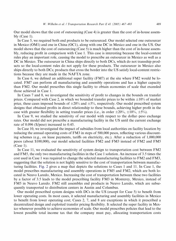
reducing the annual operating costs of FM3 in steps of 500,000 pesos, reflecting various discount-ing schemes (e.g., on lease payments, tariffs on electricity, etc.). After a reduction of 1,000,000pesos (about $100,000), our model selected facilities FM2 and FM3 instead of FM2 and FM5(Case 1).In Case 11, we evaluated the sensitivity of system design to transportation cost between FM2

and FM5, the only two manufacturing facilities in the Case 1 solution. An increase of 3.5 times thecost used in Case 1 was required to change the selected manufacturing facilities to FM2 and FM3,suggesting that the solution is not highly sensitive to the cost of transportation between manufac-turing facilities. Fig. 2 gives a map that depicts the solutions to Cases 1 and 11. In Case 1, themodel prescribes manufacturing and assembly operations in FM5 and FM2, which are both lo-cated in Neuvo Laredo, Mexico. Increasing the cost of transportation between these two facilitiesby a factor of 3.5 leads to the model prescribing facility FM3 in Monterey, Mexico, instead ofFM5 in Neuvo Laredo. FM2 still assembles end products in Neuvo Laredo, which are subse-quently transported to distribution centers in Austin and Columbus.Our model prescribed system designs with DCs in the US (except for Case 5) to benefit from

lower operating costs. In most cases, it selected manufacturing and assembly facilities in Mexicoto benefit from lower operating cost; Cases 2, 7, and 8 are exceptions in which it prescribed adecentralized design and exploited transfer pricing flexibility. It selected the super facility in Mex-ico whenever possible to achieve economies of scale. Our model prescribes policies that lead to thelowest possible total income tax that the company must pay, allocating transportation costs

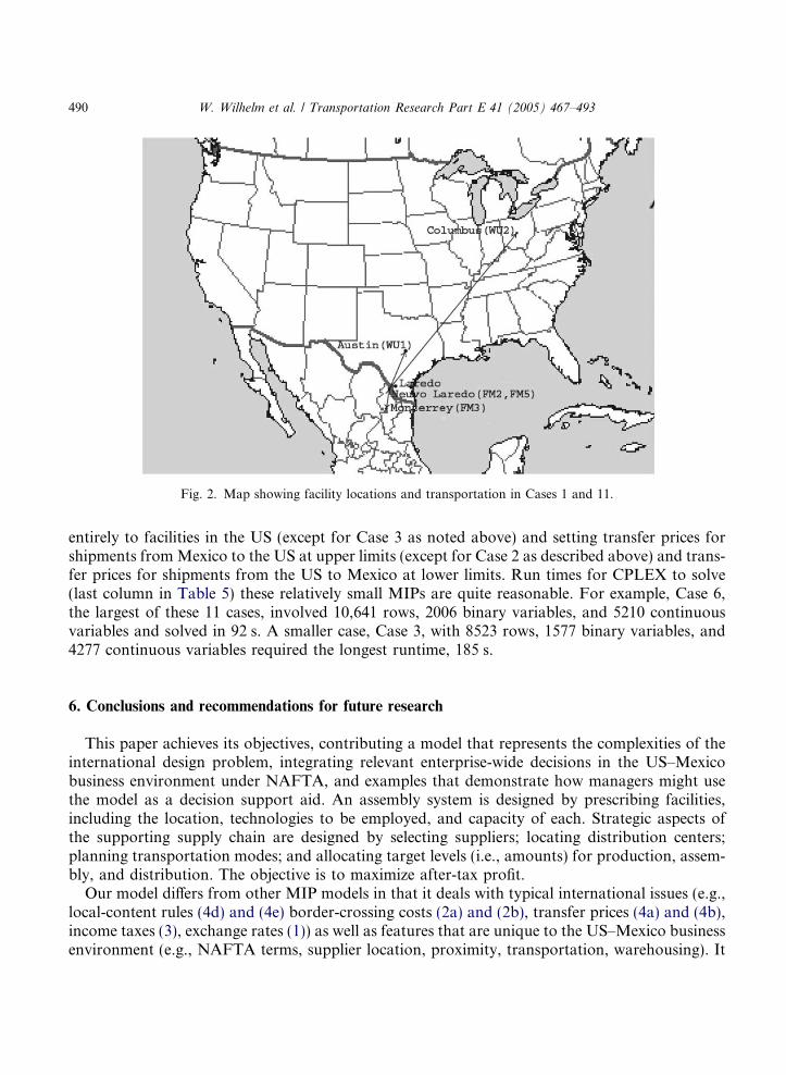
Fig. 2. Map showing facility locations and transportation in Cases 1 and 11.


entirely to facilities in the US (except for Case 3 as noted above) and setting transfer prices forshipments fromMexico to the US at upper limits (except for Case 2 as described above) and trans-fer prices for shipments from the US to Mexico at lower limits. Run times for CPLEX to solve(last column in Table 5) these relatively small MIPs are quite reasonable. For example, Case 6,the largest of these 11 cases, involved 10,641 rows, 2006 binary variables, and 5210 continuousvariables and solved in 92 s. A smaller case, Case 3, with 8523 rows, 1577 binary variables, and4277 continuous variables required the longest runtime, 185 s.

6. Conclusions and recommendations for future research

This paper achieves its objectives, contributing a model that represents the complexities of theinternational design problem, integrating relevant enterprise-wide decisions in the US–Mexicobusiness environment under NAFTA, and examples that demonstrate how managers might usethe model as a decision support aid. An assembly system is designed by prescribing facilities,including the location, technologies to be employed, and capacity of each. Strategic aspects ofthe supporting supply chain are designed by selecting suppliers; locating distribution centers;planning transportation modes; and allocating target levels (i.e., amounts) for production, assem-bly, and distribution. The objective is to maximize after-tax profit.Our model differs from other MIP models in that it deals with typical international issues (e.g.,

local-content rules (4d) and (4e) border-crossing costs (2a) and (2b), transfer prices (4a) and (4b),income taxes (3), exchange rates (1)) as well as features that are unique to the US–Mexico businessenvironment (e.g., NAFTA terms, supplier location, proximity, transportation, warehousing). It


deals effectively with design issues such as BOM restrictions (e.g., assembly operations, one com-ponent used in several end products (see discussion related to (7)), and one component used inseveral sub-assemblies on one end product (see discussion describing (6)), component usage,and facility flexibility (e.g., one component may be manufactured in several facilities (see discus-sion related to (9)) and one facility can manufacture several components (see discussion regarding(8)). It linearizes non-linearities that arise in modeling transfer prices and allocating transporta-tion charges (see the discussion immediately following the model) and addresses strategic aspectsof transportation and distribution. It addresses relevant financial considerations, prescribingtransfer price and transportation-cost allocations (2), (4f), invoking safe harbor rules (4c), mod-eling graduated income tax rates (3), and incorporating exchange rates (1). It allows inventory andbackorders to be incurred at each stage in the production/distribution process and it integratesmaterial flow through the entire supply chain (i.e., suppliers, production, assembly, distribution,transportation, customers).Examples demonstrate that our model can be applied to analyze a number of trade-offs, for

example, centralization versus decentralization, make versus buy, outsourcing versus in-houseassembly, flexible versus dedicated technologies, and economies of scale versus economies of pro-cess. It can also be used to evaluate a variety of factors such as limitations on transfer prices, facil-ity locations, tariff impacts, exchange rate impacts, tax impacts, dollar valuation, local-contentrules, and the costs of transportation and distribution.Future research could expand the set of considerations represented by the model, for example,

to model prices as a function of quantity produced or transportation cost as a function of thequantity shipped. Future research can also exploit the structures embedded in our model to devisea specialized solution method for application to large-scale instances. In addition, future researchcan devise an effective approach to optimize stochastic versions of the problem, for example, incases for which it is important to treat demand-and/or-exchange-rate uncertainty explicitly.Our research is continuing along these lines.

Acknowledgement

This material is based in part upon work supported by the Texas Advanced Technology Pro-gram under Grant Number 000512-0248-2001. The authors are indebted to Arturo Garcia of theLaredo Development Foundation; to Nicolas Ferrara, Director of the Department of EconomicDevelopment in Nuevo Laredo, Mexico; and to other collaborators—too numerous to enumer-ate—in the Federal Reserve Bank of Dallas and other organizations in Laredo and Nuevo Lar-edo. We also acknowledge the able programming assistance of Kalyan Balasubramaniam andGuhan Subbarayan. Finally, we note our appreciation of the comments provided by two anony-mous referees and a guest editor that allowed us to strengthen an earlier version of this paper.

References

Alarcon, D., Sepeda, E., 1998. Employment trends in the Mexican manufacturing sector. The North American Journalof Economics and Finance 9, 125–145.


Alonso-Ayuso, A., Escudero, L.F., Garın, A., Ortuno, M.T., Perez, G., 2003. An approach for strategic supplyplanning under uncertainty based on stochastic 0–1 programming. Journal of Global Optimization 26, 97–124.

Barfield, J.T., Raiborn, C.A., Kinney, M.R., 2002. Cost Accounting: Traditions & Innovations. South-Western CollegePublishing, Mason, OH.

Bartmess, A., Cerny, K., 1993. Building competitive advantage through a global network of capabilities. CaliforniaManagement Review (Winter), 78–103.

Beamon, B.M., 1998. Supply chain design and analysis: models and methods. International Journal of ProductionEconomics 55, 281–294.

Bhutta, K.S., Huq, F., Frazier, G., Mohamed, Z., 2003. An integrated location, production, distribution andinvestment model for a multinational corporation. International Journal of Production Economics 86, 201–216.

Bitran, G.R., Tirupati, D., 1993. Hierarchical production planning. In: Graves, S.C., Rinnooy-Kan, A.H.G., Zipkin,P.H. (Eds.), Logistics of production and inventory. North-Holland, Amsterdam, pp. 523–568.

Brezosky, L., 2003. Texas legislators face challenges: lawmaker�s report highlights border woes. Houston Chronicle A7(January 2), A10.

Buitelaar, R.M., Perez, R.P., 2000. Maquila, economic reform and corporate strategies. World Development 28 (9),1627–1642.

Canas, J., Coronado, R., 2002. Maquiladora industry: past, present and future. El Paso Business Frontier, FederalReserve Bank of Dallas, El Paso Branch, Issue 2, 1–6.

Cisneros, A., 2001. Texas colonias: housing and infrastructure issues. The Border Economy, Federal Reserve Bank ofDallas, June 19–21.

Cohen, M.A., Moon, S., 1991. An integrated plant loading model with economies of scale and scope. European Journalof Operational Research 50 (3), 266–279.

Cohen, M.A., Fisher, M., Jaikumar, R., 1989. International manufacturing and distribution networks: a normativemodel framework. In: Ferdow, K. (Ed.), Managing International Manufacturing. Elsevier Science Publishers, NorthHolland, pp. 67–93.

Editorial, 2004. Review and outlook: triumph of NAFTA, Wall Street Journal, January 12, A14.Erenguc, S. Selcuk, Simpson, N.C., Vakharia, A.J., 1999. Integrated production/distribution planning in supply chains:

an invited review. European Journal of Operational Research 115, 219–236.Geunes, J., Pardalos, P.M., 2003. Network optimization in supply chain management and financial engineering: an

annotated bibliography. Networks 42 (2), 66–84.Goetschalckx, M., Cole, M.H., Dogan, K., Wei, R.P., 1996. A Generic Model for the Strategic Design of Production–

Distribution Systems. Georgia Institute of Technology, Atlanta, GA.Goetschalckx, M., Vidal, C.J., Dogan, K., 2002. Modeling and design of global logistics systems: a review of integrated

strategic and tactical models and design algorithms. European Journal of Operational Research 143, 1–18.Hodder, J.E., Dincer, M.C., 1986. A multi-factor model for international plant location and financing under

uncertainty. Computer and Operations Research 13 (5), 601–609.Hodder, J.E., Jucker, J.V., 1985. International plant location under price and exchange rate uncertainty. Engineering

Costs and Production Economics 9, 225–229.Houston Chronicle, 2003. Toyota work force takes shape in San Antonio, Houston, TX, Business Section, March 9, 1.Huchzermeier, A.H., 1991. Global manufacturing strategic planning under exchange rate uncertainty. Ph.D.

dissertation, University of Pennsylvania, Philadelphia, PA.Kouvelis, P., Rosenblatt, M.J., 1997. Development of International Facility Networks with Financing, Trade Tariff and

Tax Considerations, John M. Olin School of Business, Washington University, St. Louis, MO.Kouvelis, P., Rosenblatt, M.J., Munson, C.L., 2004. A mathematical programming model for global plant location

problems: analysis and insights. IIE Transactions 36, 127–144.Mohamed, Z.M., 1999. An integrated production–distribution model for a multi-national company operating under

varying exchange rates. International Journal of Production Economics 58, 81–92.MacCormack, A.D., Newman III, L.J., Rosenfield, D.B., 1994. The new dynamics of global manufacturing site

location. Sloan Management Review (Summer), 69–80.O�Connor, W., 1997. International transfer pricing. In: Choi, F.D.S. (Ed.), International Accounting and Finance

Handbook, second ed. John Wiley and Sons, New York, NY.


Owen, S.H., Daskin, M.S., 1998. Strategic facility location: a review. European Journal of Operations Research 111,423–447.

Phillips, K., Manzanares, C., 2001. Transportation: infrastructure and the border economy. The Border Economy,Federal Reserve Bank of Dallas, June, 11–14.

Pinkerton, J., 2001. Borderline hope. Houston Chronicle A1 (August 5). A20–1.Revelle, C.S., Laporte, G., 1996. The plant location problem: new models and research prospects. Operations Research

44 (6), 864–874.Santoso, T., Ahmed, S., Goetschalckx, M., Shapiro, A., 2004. A stochastic programming approach for supply chain

network design under uncertainty. School of Industrial and Systems Engineering, Georgia Institute of Technology,February 4.

Sarmiento, A.M., Nagi, R., 1999. A review of integrated analysis of production–distribution systems. IIE Transactions31, 1061–1074.

Schmidt, G., Wilhelm, W.E., 2000. Strategic, tactical, and operational decisions related to multi-national logisticsnetworks: a review and discussion of modeling issues. International Journal of Production Research 38 (7), 1501–1523.

Talluri, S., Baker, R.C., 2002. A multi-phase mathematical programming approach for effective supply chain design.European Journal of Operational Research 141, 544–558.

Tayur, S., Ganeshan, R., Magazine, M. (Eds.), 1999. Quantitative Models for Supply Chain Management. KluwerInternational Series. Kluwer Academic Publishers, Boston, MA, pp. 669–702.

The NAFTA Secretariat. Available from: <http://www.nafta-sec-alena.org>.Vargas, L., 1998a. The Maquladora industry in historical perspective (Part 1). Business Frontier, Federal Reserve Bank

of Dallas, El Paso Branch, Issue 3.Vargas, L., 1998b The Maquladora industry in historical perspective (Part 2). Business Frontier, Federal Reserve Bank

of Dallas, El Paso Branch, Issue 4.Vargas, L., 2000. Maquiladoras 2000: still growing. El Paso Business Frontier, Federal Reserve Bank of Dallas, El Paso

Branch, Issue 3.Verter, V., Dincer, M.C., 1992. An integrated evaluation of location, capacity acquisition, and technology selection for

designing global manufacturing strategies. European Journal of Operational Research 60, 1–18.Verter, V., Dincer, M.C., 1995a. Facility location and capacity acquisition: an integrated approach. Naval Research

Logistics Quarterly 42, 1141–1160.Verter, V., Dincer, M.C., 1995b. Global manufacturing strategy. In: Drezner, Z. (Ed.), Facility Location: A Survey of

Applications and Methods. Springer-Verlag, New York, NY.Vidal, C.J., Goetschalckx, M., 1997. Strategic production—distribution models: a critical review with emphasis on

global supply chain models. European Journal of Operational Research 98, 1–18.Vidal, C.J., Goetschalckx, M., 2001. A global supply chain model with transfer pricing and transportation cost

allocation. European Journal of Operations Research 129, 134–158.Vidal, C., Goetschalckx, M., 2002. Modeling and design of global logistics systems: a review of integrated strategic and

tactical models and design algorithms. European Journal of Operational Research 143, 1–18.Vidal, C.J., Goetschalckx, M., forthcoming. The role and limitations of quantitative techniques in the strategic design

of global logistics systems. Special Issue on Manufacturing in the Global Economy, Technological and Forecastingand Social Change.

Yucel, M., 2001. The border economy: introduction. The Border Economy, Federal Reserve Bank of Dallas, June 1.

http://www.nafta-sec-alena.org

Design of international assembly systems and their supply chains under NAFTA

Documents

Transcript of Design of international assembly systems and their supply chains under NAFTA