
Characterization of Pseudomonas syringae pv. syringae from ...
Upload
khangminh22Category
view
1download
0
Universitat Politecnica de Catalunya
Escola Tecnica Superior d’Enginyeria Industrialde Barcelona. ETSEIB
Design, modeling andsimulation of a PV power
plant.
Bachelor’s final project
Autor: Pablo Poza Ferragut
Supervisor: Oriol Gomis Bellmunt
Junio 2020

Summary
The rise of the photovoltaic energy during the last decades and mainly during the lastyears has many indicators; the fast growth of the global production capacity, the inno-vations related to the solar energy technologies or the continuous adaptation of the lawcode to fit a wider variety of scenarios and conditions.
Additionally the recent improvements have given Large Scale PV power plant (LS-PVPP)the capability to work as baseload power plants relieving dirtier sources of energies. How-ever one of the biggest disadvantages in front of conventional energy sources is the cost.In the last years PV technologies have achieved higher cost-effective ratio and now areable to compete against non-renewable production methods.
For this reason the present work is centered in the development of a tool for integrationof LS-PVPP in the actual energy distribution system that allows the user to optimizeand study the design and functionality of the plant.
A MATLAB based program and different functions have been developed to perform apower flow analysis. Different grid codes requirements have been analyzed for LS-PVPP.Approaches from different years are taken into account and the tendency of unifyingsome parts of these grid codes to achieve higher levels of energy share is discussed too.Examples of control implementation to meet these requirements are also included.
The example used to test the Power flow equations (PFE) solver is composed of centralinverters. According to [2] this configuration is the most cost-effective nowadays despitethe string inverters are close and present a series of benefits related with the versatilityand control.

Contents
1 Prefase 8
1.1 Objective . . . . . . . . . . . . . . . . . . . . . . . . . . . . . . . . . . . . 8
1.2 Motivation . . . . . . . . . . . . . . . . . . . . . . . . . . . . . . . . . . . 8
2 Power flow analysis 9
2.1 Procedure . . . . . . . . . . . . . . . . . . . . . . . . . . . . . . . . . . . . 9
2.2 Power flow equation basis . . . . . . . . . . . . . . . . . . . . . . . . . . . 10
2.3 Formulation . . . . . . . . . . . . . . . . . . . . . . . . . . . . . . . . . . . 11
2.3.1 Bus admittance matrix . . . . . . . . . . . . . . . . . . . . . . . . 11
2.4 Limitations and considerations . . . . . . . . . . . . . . . . . . . . . . . . 12
2.5 Solution methods. . . . . . . . . . . . . . . . . . . . . . . . . . . . . . . . 12
2.6 Definitions . . . . . . . . . . . . . . . . . . . . . . . . . . . . . . . . . . . . 13
2.6.1 Slack bus. . . . . . . . . . . . . . . . . . . . . . . . . . . . . . . . . 13
2.6.2 Load bus; PQ type. . . . . . . . . . . . . . . . . . . . . . . . . . . 14
2.6.3 Voltage controlled bus; PV type. . . . . . . . . . . . . . . . . . . . 14
2.7 The Newton-Raphson power flow solution. . . . . . . . . . . . . . . . . . . 14
2.7.1 Problem general form . . . . . . . . . . . . . . . . . . . . . . . . . 14
2.7.2 Multi-Variable NRA . . . . . . . . . . . . . . . . . . . . . . . . . . 15
2.8 Load flows of the system . . . . . . . . . . . . . . . . . . . . . . . . . . . . 17
3 Validating the results 18
3.1 Considerations. . . . . . . . . . . . . . . . . . . . . . . . . . . . . . . . . . 18
3.1.1 Limitations . . . . . . . . . . . . . . . . . . . . . . . . . . . . . . . 18
3.1.2 Distribution system limitations . . . . . . . . . . . . . . . . . . . . 19
1
3.1.3 Parameters under study. . . . . . . . . . . . . . . . . . . . . . . . . 19
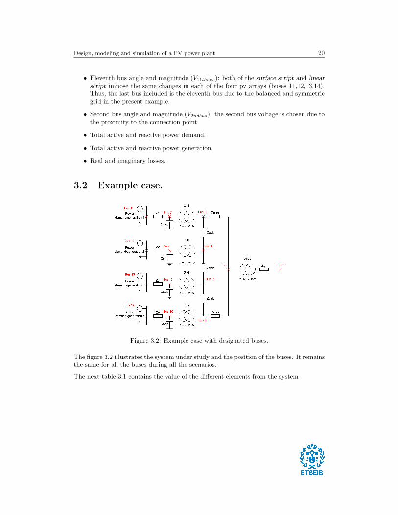
3.2 Example case. . . . . . . . . . . . . . . . . . . . . . . . . . . . . . . . . . . 20
3.2.1 Per unit values . . . . . . . . . . . . . . . . . . . . . . . . . . . . . 21
3.2.2 Initial values and suppositions . . . . . . . . . . . . . . . . . . . . 21
3.3 Result comparison versus MATPOWER . . . . . . . . . . . . . . . . . . . 23
3.3.1 First comparison: Active and reactive power demand variation withPQ buses. . . . . . . . . . . . . . . . . . . . . . . . . . . . . . . . . 23
3.3.2 Second comparison: Active and reactive power generation variationwith PQ buses. . . . . . . . . . . . . . . . . . . . . . . . . . . . . . 26
3.3.3 Third comparision: Active power generation and grid voltage vari-ation with PV buses. . . . . . . . . . . . . . . . . . . . . . . . . . . 28
3.4 Analysis of maximum and minimum voltage deviations and loses. . . . . . 30
3.4.1 Particular case: different values for each converter output . . . . . 30
4 Grid code requirements 33
4.1 Introduction . . . . . . . . . . . . . . . . . . . . . . . . . . . . . . . . . . . 33
4.2 Static regulation . . . . . . . . . . . . . . . . . . . . . . . . . . . . . . . . 35
4.2.1 Power factor regulation . . . . . . . . . . . . . . . . . . . . . . . . 35
4.2.2 Power Curtailment . . . . . . . . . . . . . . . . . . . . . . . . . . . 36
4.2.3 Active power reserves . . . . . . . . . . . . . . . . . . . . . . . . . 36
4.2.4 Voltage range and Control . . . . . . . . . . . . . . . . . . . . . . . 37
4.2.5 Remote Voltage Control . . . . . . . . . . . . . . . . . . . . . . . . 37
4.2.6 Frequency . . . . . . . . . . . . . . . . . . . . . . . . . . . . . . . . 37
4.2.7 Flicker . . . . . . . . . . . . . . . . . . . . . . . . . . . . . . . . . . 38
4.3 Grid support; reactive power compensation . . . . . . . . . . . . . . . . . 38
5 Environmental impact analysis 42
5.1 Large scale PV power plant . . . . . . . . . . . . . . . . . . . . . . . . . . 42
5.1.1 Construction . . . . . . . . . . . . . . . . . . . . . . . . . . . . . . 43
5.1.2 Operation . . . . . . . . . . . . . . . . . . . . . . . . . . . . . . . . 43
5.1.3 Decommission . . . . . . . . . . . . . . . . . . . . . . . . . . . . . . 44
5.1.4 Potential environmental consequences . . . . . . . . . . . . . . . . 44
5.1.5 Potential ecological consequences . . . . . . . . . . . . . . . . . . . 44
5.1.6 Transmission system impact . . . . . . . . . . . . . . . . . . . . . . 45
5.1.7 Conclusions . . . . . . . . . . . . . . . . . . . . . . . . . . . . . . . 45
2

6 Projects budget 47
6.1 Large Scale PV power plant . . . . . . . . . . . . . . . . . . . . . . . . . . 47
6.2 Ancillary services . . . . . . . . . . . . . . . . . . . . . . . . . . . . . . . . 48
6.3 Introduction . . . . . . . . . . . . . . . . . . . . . . . . . . . . . . . . . . . 51
6.4 Scripts . . . . . . . . . . . . . . . . . . . . . . . . . . . . . . . . . . . . . . 51
6.5 First comparison power flow results . . . . . . . . . . . . . . . . . . . . . . 52
6.6 Second comparison power flow results . . . . . . . . . . . . . . . . . . . . 54
6.7 Third comparison power flow results . . . . . . . . . . . . . . . . . . . . . 55
3

List of Figures
2.1 Example of a 5 bus system with the impedance of the lines. . . . . . . . . 10
3.1 Relation between the Pdc and Vdc and main points to analyze. . . . . . . . 19
3.2 Example case with designated buses. . . . . . . . . . . . . . . . . . . . . . 20
3.3 Eleventh bus values (1st case) . . . . . . . . . . . . . . . . . . . . . . . . . 25
3.4 Second bus values (1st case) . . . . . . . . . . . . . . . . . . . . . . . . . . 25
3.5 Seventh bus values (1st case) . . . . . . . . . . . . . . . . . . . . . . . . . 25
3.6 Eleventh bus values (2nd case) . . . . . . . . . . . . . . . . . . . . . . . . 27
3.7 Second bus values (2nd case) . . . . . . . . . . . . . . . . . . . . . . . . . 27
3.8 Seventh bus values (2nd case) . . . . . . . . . . . . . . . . . . . . . . . . . 27
3.9 Eleventh bus values (3rd case) . . . . . . . . . . . . . . . . . . . . . . . . 29
3.10 Second bus values (3rd case) . . . . . . . . . . . . . . . . . . . . . . . . . 29
3.11 Seventh bus values (3rd case) . . . . . . . . . . . . . . . . . . . . . . . . . 29
3.12 Example scheme with voltage magnitude and phase values . . . . . . . . . 31
3.13 Example scheme with voltage magnitude and phase values . . . . . . . . . 31
3.14 Real and Imaginary losses changing the grid voltage from 0.9 to 1.1 . . . 32
4.1 Power installed in Spain from 2007 to 2018. . . . . . . . . . . . . . . . . . 34
4.2 Summary of the total energy managed by the ancillary services in thespanish peninsula. . . . . . . . . . . . . . . . . . . . . . . . . . . . . . . . 34
4.3 Reactive power requirements for Puerto Rico, South Africa and China,Germany and Romania. . . . . . . . . . . . . . . . . . . . . . . . . . . . . 35
4.4 Power curtailment requirements . . . . . . . . . . . . . . . . . . . . . . . . 36
4.5 Summary of grid codes requirements for LS-PVPP . . . . . . . . . . . . . 38
4.6 Scheme of the connection points contextualized in the current example . . 39
4

4.7 From left to right; output PoC and grid PoC phasor diagrams when PF isset to unity. . . . . . . . . . . . . . . . . . . . . . . . . . . . . . . . . . . . 40
6.1 Breakdown of ancillary services cost in the average final price of energy inthe peninsular system . . . . . . . . . . . . . . . . . . . . . . . . . . . . . 49
6.2 Active and reactive power demand (1st case) . . . . . . . . . . . . . . . . 52
6.3 Active and reactive power generation (1st case) . . . . . . . . . . . . . . . 52
6.4 Imaginary and real losses (1st case) . . . . . . . . . . . . . . . . . . . . . . 53
6.5 Active and reactive power demand (2nd case) . . . . . . . . . . . . . . . . 54
6.6 Active and reactive power generation (2nd case) . . . . . . . . . . . . . . 54
6.7 Active and reactive power generation (2nd case) . . . . . . . . . . . . . . 54
6.8 Active and reactive power demand (3rd case) . . . . . . . . . . . . . . . . 55
6.9 Active and reactive power generation (3rd case) . . . . . . . . . . . . . . . 55
6.10 Active and reactive power generation (3rd case) . . . . . . . . . . . . . . . 55
5

List of Tables
3.1 Present work system parameters. . . . . . . . . . . . . . . . . . . . . . . . 21
3.2 Example’s parameters in pu. . . . . . . . . . . . . . . . . . . . . . . . . . 21
3.3 Required parameters for each bus. . . . . . . . . . . . . . . . . . . . . . . 22
3.4 Required parameters for each bus. . . . . . . . . . . . . . . . . . . . . . . 22
3.5 Selected variables and ranges . . . . . . . . . . . . . . . . . . . . . . . . . 24
3.6 Selected variables and ranges . . . . . . . . . . . . . . . . . . . . . . . . . 26
3.7 Selected variables and ranges . . . . . . . . . . . . . . . . . . . . . . . . . 28
3.8 Initial values for the converter output buses. . . . . . . . . . . . . . . . . . 30
5.1 Comparison of life cycle emissions for solar technologies and conventionalcarbon-intensive systems . . . . . . . . . . . . . . . . . . . . . . . . . . . . 43
6.1 PV plant CAPEX costs and current project budget . . . . . . . . . . . . . 48
6.2 PV plant OPEX . . . . . . . . . . . . . . . . . . . . . . . . . . . . . . . . 48
6

Acronyms
DES Distributed energy sistems. 19, 36, 37
ENSTO-E European Network for Transmission System Operators for Electricity. 33
eSCR Equivalent short circuit ratio. 40
LS-PVPP Large Scale PV power plant. 1, 4, 34, 37–40, 42–45, 47
MPP maximum power point. 19
MPPT Maximum power point tracker. 30
NRA Newthon-Raphson algorithm. 14, 16, 17, 24, 26, 51
PF Power factor. 5, 35, 38, 40
PFC Power factor control. 39
PFE Power flow equations. 1, 23, 28, 34
PoC point of connection. 5, 38–41
RfG Network Code on Requirements for Grid Connection applicable to all Generators.33
SCR Short circuit ratio. 39, 40
TSO Transmission system operator. 33, 36
7

Chapter 1
Prefase
1.1 Objective
This work focuses of understanding and studying the collection grid and the energy distri-bution of solar photovoltaic plants (PV) in MATLAB. The main idea is to add a moduleto calculate the phenomena happening from the inverter to the point of couple to the grid.The present work starts from the results obtained by the model developed by GabrieleCatalano [1] and evolved by Eduard Foved [2].
1.2 Motivation
The present project follows the work done by Gabriele Catalano [1] and Eduard Foved [2]during their Master Thesis. Both of the mentioned projects are centered in the module toinverter part leading to black box models in the definition of other components functionssuch as the transformer or the grid itself. This work is an effort to develop a model toset optimal values and configurations for a better performance when exchanging energywith the transmission system and consumption centers.
The present work is an effort to review the state of art of the PV technologies andits integration in the different energy systems and in particular, the Spanish situation.The scope of the projects aims to cover the energy management requirements and theirtendencies to introduce PV energy as a reliable source in the market.
Nowadays in a world of fast changes and climatic issues the environmental impact of thesociety should be taken seriously, consequently a deep research on the known effects ofusing PV technologies in a utility-scale is included in the project.
8

Chapter 2
Power flow analysis
The tool used in this work to analyse the parameters of all the buses and define the currentflow are the power flow equations. For a given power network where the net apparentpower and some other limitations or restrictions on voltages and power generations, solvefor unknown bus voltages and generation and for the complex power flow in all of thenetwork components.
2.1 Procedure
In the next section the steps followed to develop a power flow study for a generic networkset by the user are discussed:
1. Obtain or determine the values of the passive network elements such as cableimpedance parameters.
2. Set the location, measure the distances between members and find out the valuesof the complex power loads using tools as wattmeters.
3. Study every operator in order to set the generation specifications and constraints.
4. Design a mathematical model to model the power flow in the network.
5. Solve for the voltage of the network.
6. Solve for power flows as well as losses in the network.
7. Make sure the constraints set on the third step are not violated.
The fourth step is where the importance of power flow equations gains importance, theydefine the power flows of the systems and the resulting bus voltages, those are discussedin the following sections. As long as the system resulting from applying the equations isa nonlinear system with complex coefficients with as many unknowns as buses, the use ofiterative methods or closed form techniques is mandatory.
9

Design, modeling and simulation of a PV power plant 10
2.2 Power flow equation basis
In this section the development of the power flow equations are briefly described to in-troduce the formulation that is explained in next section. The example where a numbern of buses separated a distance by cables that introduce an impedance between them isused as a context to the development and is illustrated in figure (2.1).
Figure 2.1: Example of a 5 bus system with the impedance of the lines.
The lines and the impedance of the buses are known and taking into account that theadmittance is defined as:
Y = Z−1 (2.1)
the bus admittance matrix is conformed. The detailed description is commented in section2.3.
The Kirchhoff law is applied in every node yield resulting in expressions that describe thecorrelation between currents, obtaining equation (2.2) that can be applied in each node:
Ii = ViYi0 +
n∑i=1,i 6=j
(Vi − Vj)Yij (2.2)
Therefore expressed in a matrix environment the following relation results in:
[Inode] = [Ynode][Vnode] (2.3)
Where [Y ] is the admittance matrix, [I] and [V ] are vector expressing current and voltagerespectively for each node.

Design, modeling and simulation of a PV power plant 11
[I] =
I1I2...In
(2.4)
[V ] =
V1V2...Vn
(2.5)
Introducing the relation expressed in (2.2) in the Gauss Power flow I that describesthe apparent power as the voltage multiplied by the conjugate of the current and lastlyregrouping terms the voltage can be described as
Vi =1
Yii
S∗iV ∗i−
n∑j=1j 6=i
YijVj
(2.6)
Finally considering that the apparent net power is defined by result of the power generatedinside the bus and the power consumed by the load and the respective losses.
S∗i = S∗gen−i − S∗load−i (2.7)
And if it is equaled to the Gauss Power Flow:
S∗gen−i − S∗load−i = V ∗i
n∑k=1
YikVk (2.8)
The combination gives us a nonlinear equation system with implied difficulties, limitationsand considerations that will be discussed later in this document.
2.3 Formulation
2.3.1 Bus admittance matrix
The Y matrix is defined by the admittance of the buses in the next configuration:
• The (k, k) elements are the result of the sum of the admittance of the elementspresent in the connection between node k and reference (Ground admittance B/2and the admittance of the elements connected between nodes, the line admittance.
ISi = ViI∗i where i is the current node

Design, modeling and simulation of a PV power plant 12
• The (j, k) and (k, j) terms are defined by the negative of the admittance betweenrespective j and k nodes.
A generic bus admittance matrix of a 3 bus network is shown in the next example:
[Y ] =
Y11 Y12 Y13Y21 Y22 Y23Y31 Y32 Y33
(2.9)
Examples of a (k ,k) and (j, k) components are shown next:
Yii = Yi0II +
n∑j=1i6=j
Yij (2.10)
Yij = −Yij (2.11)
2.4 Limitations and considerations
This context introduce a number of difficulties in the calculations which are discussednext. The complex power outputs can be modified as long as the generation equals to theload in every bus. In fact the last generator calculated must be calculated last because ithas to compensate all the uncalculated network losses, this is named the Slack bus. Atthe same time the losses are unknown until the voltages are calculated. In addition theflow is only valid for an arbitrary phase angle reference and it is not possible to solve thesystem for absolute values of angle or voltage.
For a example; for a four bus systems, in which one of the buses is the slack bus, theunknowns are voltages of all the buses plus the apparent net power of the slack generator.Therefore including the equation 2.8 evaluated for each bus it results in a system composedof four nonlinear equations with complex coefficients and five unknowns.
In order to solve the system using the mentioned iterative methods the slack bus voltageis specified. This way the number of unknown is reduced by one and the complex powergeneration is able to to fit the changes in both real and reactive power losses. The slackbus is also used as a phase reference with a limited magnitude. The next section willintroduce the solution methods available as well as the procedure it follows.
2.5 Solution methods.
This section introduces the development of a correct solution as well as the differentsolutions proposed by the literature. In the present context there are four parameters ofinterest to know for each bus.
• Real power, associated from now with P .
IIYi0 is the admittance of the elements between node and reference or the i node.
Design, modeling and simulation of a PV power plant 13
• Reactive power; Q.
• Voltage module; V .
• Voltage phase; δ.
As it has been commented in every bus tools such as wattmeters are used to measure thevalues of the apparent net power S, therefore the P and Q values. The buses are classifiedin terms of the two known parameters, introducing the PV and PQ buses. Those arediscussed in the definitions section.
The result of the application of the power flow equations in a real environment is a non-linear systems where the bus voltages and apparent power of the slack bus are unknowns.Different methods to solve nonlinear equations can be found in specialized literature,these are some:
• Gauss Seidel.
• Newton Raphson
• Fast Decoupled
There are some considerations to take into account; firstly these methods need guessesto start iterating and it is important to have good approximations. In order to evaluatethe behaviour of the approximations a process is set and it is implemented in two stages;the first one calculates the approximate angles and the second the approximated voltagemodules.
However the Gauss-Seidel is commonly used because the simplicity of the implementationand a better performance in front of the Gauss method, in this work the Newton-Raphsonsolution is chosen. The reasons are a fast convergence with a good initial guesses and alarge range of convergence. Some disadvantages are the difficulties that the implemen-tation brings implicit and the computing requirements resulting in an increment of theiteration step time. Newton-Raphson is a widely used method in the power flow analysis.
2.6 Definitions
In this section the items and concepts commented before are discussed in detail.
2.6.1 Slack bus.
A single bus for which the voltage and phase are specified designated to supply theunknown real and reactive losses, in consequence these values are unknowns. The selectionof the slack bus depends manly on experience with the system under study because thisbus must change to follow the variation in the losses to take up the slack. These decisionhas a significant influence in the results obtained.
Design, modeling and simulation of a PV power plant 14
2.6.2 Load bus; PQ type.
This classification refers to the buses where the real and reactive power are specified. Itis recommended to designate any bus with injected complex power as a load bus. Thevoltage magnitude and angle adapt to the situations created by the power injections.It has to be mentioned that the voltages have limitations to ensure smooth and securevoltage ranges for the devices connected to the grid. Usually these ranges go from 90 to110% of the nominal voltage.
2.6.3 Voltage controlled bus; PV type.
As its name describes the voltage is controlled adding a voltage controller module thatsets the voltage in a narrow range that can be understood as constant. In addition the realpower is also specified. Consequently the reactive power is a variable with a limitationswith upper and lower bounds. In a real situation a PV bus always have a generator thatmeets the requirements to be a variable source of reactive power.
2.7 The Newton-Raphson power flow solution.
2.7.1 Problem general form
In this section the Newton-Raphson algorithm is described; in the first part the presen-tation and general form of the problem are introduced. In the second part the matricidalpower flow solution is discussed.
In practice, the bus apparent net power Si is a parameter more accessible than thebus currents Ii therefore NRA reorganizes the equations following the next procedure.Regrouping terms the generic admittance expression is obtained:
Yij = |Yij |∠θij = |Yij | cos θij + j|Yij | sin θij = Gij + jBij (2.12)
Using the Gauss power flow (2.8) S∗i can be expressed as:
S∗i = V ∗i Ii = V ∗i
n∑j=1
(YijVj) (2.13)
Now reorganizing equation (2.8) in correlation with the generic admittance reorganization(2.12) and the apparent power conjugate S∗i equation (2.13) results the next expression:
S∗i = Pi − jQi =
n∑j=1
|YijViVj |∠(θij + δj − δi) (2.14)
Finally 2n equations are obtained following the generic form of:
Pi = |Vi|2Gii +
n∑j=1,j 6=i
|YijViVj | cos (θij + δj − δi) (2.15)

Design, modeling and simulation of a PV power plant 15
Qi = |Vi|2Bii +
n∑j=1,j 6=i
|YijViVj | sin (θij + δj − δi) (2.16)
The key idea behind the Newton-Raphson algorithm is to use a sequential linearizationwhere function depending on x is equaled to zero. Starting from the initial guess everystep an increment of ∆x is defined:
f(x) = 0 (2.17)
∆x(v)III = x− x(v) (2.18)
Representing f(x) by a Taylor series where the components or 2nd order or higher areneglected. This can be done and performs well because the equation equals to zero. Theexpressions remains now as:
f(x) = f(x(v)) +df(x(v))
dx∆x(v) (2.19)
Finally it can be solved for ∆x(v) and start a new iteration setting the value of x(v+1) asthe new one.
∆x(v) = −[df(x(v))
dx
]−1f(x(v)) (2.20)
This algorithm has a quadratic convergence meaning the error decreases quickly whenapproaching the solution and the result depends on the initial guesses that can be set forthe voltages. Two are considered; x(0) = 0 or x(0) = −1. The iteration stop when theabsolute value of the function with the current x(n) is lower than a tolerance, ε set by theuser.
2.7.2 Multi-Variable NRA
The first change to notice is that in the multi-variable case the variables and functions x,f(x) and therefore the increment ∆x become vectors containing the parameters for eachbus. In addition the derivative component is now a matrix known as the Jacobian. Thismatrix contains the partial derivative of each function f(x) for every variable xn.
J(x) =
∂f1(x)∂x1
∂f1(x)∂x2
. . . ∂f1(x)∂xn
∂f2(x)∂x1
∂f2(x)∂x2
. . . ∂f2(x)∂xn
......
. . ....
∂fn(x)∂x1
∂fn(x)∂x2
. . . ∂fn(x)∂xn
(2.21)
The system has a matrix structure therefore the operations must be performed in accor-dance. Following the solution scheme of previous sections the jacobian is inverted to solvefor the increment ∆x.
IIIv: represents the current step

Design, modeling and simulation of a PV power plant 16
The NRA application to power flow need a reformulation for the power equations associ-ated to each bus. Taking in to account the equations (2.12) and the conjugate of (2.14)and defining the next expressions:
Vi = |Vi|ejθi = |Vi|∠θi
ejθ = cos θ + j sin θ
θij = θi − θjThe following equation can be obtained:
Si =
n∑j=1
|Vi||Vj |ejθij (Gij − jBij) (2.22)
And resolving into the real and imaginary parts the equations used in the algorithm canbe found.
Pi =
n∑j=1
|Vi||Vj | (Gij cos θij +Bij sin θij) = PGi − PDi (2.23)
Qi =
n∑j=1
|Vi||Vj | (Gij sin θij −Bij cos θij) = QGi −QDi (2.24)
With the first bus designated as the slack bus and setting its voltage magnitude and anglethe rest of the voltages and phases are found following the next scheme:
x =
θ2...θn|V2|
...|Vn
f(x) =
P2(x)− PG2 + PD2
...Pn(x)− PGn + PDnQ2(x)−QG2 +QD2
...Qn(x)−QGn +QDn
At the beginning of the iteration the number of steps is set to 0, v = 0 and the initialguesses are introduced. Each step the number is increasing in one, v = v+1 The stoppingcriteria is the same as seen before for a given tolerance, ε.

Design, modeling and simulation of a PV power plant 17
PV cases
As long as the PV buses are fixed in voltage magnitude there’s no need to include theunknown in the system or write the reactive power balance equations; it varies to maintainthe fixed voltage within a reasonable limits. However those can be included writing thevoltage constraint as |Vi|−Visetpoint = 0. If they are not included in the system the scriptused in this work contains a simple limit violation test. It checks if the limits introducedin the bus data are violated. If the bounds are overpassed the program displays a messageindicating which bus is having issues and the magnitude of these.
2.8 Load flows of the system
Once the NRA converged the Voltage magnitudes and angles are known and the line flowsand losses are obtained.
First of all the Line Current Flows are calculated in each branch using Ohm’s law in bothdirections of the branch. The resulting expressions are shown next: The from bus-to buscurrent expression is obtained:
Iij = −(Vi − Vjabranch)Yij/a2branch + bbranch/a
2branchVi (2.25)
and the reverse direction expression results in:
Iji = −(Vj − Viabranch)Yji/a2branch + bbranchVj (2.26)
Where a is the tap setting and is set to 1 for all simulations. This tap setting is afunctionality found in some transformers. It allows the transformer to have variable turnratios to keep the changes of the primary side. The ground admittance is represented byb. In this work the ground admittance is the half of the susceptance present in any ofthe two buses conforming the line. Secondly, the Line Power Flows in MVA and the linelosses are obtained using the apparent power equations:
Sij = ViI∗ij ∗ Sbase (2.27)
Lij = Sij + Sji (2.28)
Finally, the Bus Power Injections result from applying the equation (2.27) in addition tothe initial bus current apparent power.
S∗i =
Busn∑j=1
V ∗i VjYij (2.29)
Where the real part is the active power Pi = real(Si) and the imaginary is the reactivepower Qi = −imag(Si).

Chapter 3
Validating the results
3.1 Considerations.
In this chapter the process to validate the results is described and results of different casesare discussed.
The process of validating consist in considering different cases and running them in aconsolidated power flow algorithm. In this work MATPOWER is set as the reference.The differences between the final results in both programs are discussed with the purposeof explaining them.
Once the reliability of the present work’s program is set different scenarios are testedfocusing on describing the behaviour of the system. The methodology for the analysis isbased on varying the value of significant parameters of the system in a range that includerealistic and common situations and observe the reaction of the power flows of the system.
The script contains different limitations that are commented in the next sections. Someof them are the reactive power limitation (Qmax, Qmin) when working with PV buses orthe capability curve of the converters.
3.1.1 Limitations
In real situations there are a lot of physical limitations that can be easily missconsidered.The aim of this section is to cite all the limitations that have been taken into accountand if it is possible define a procedure to deal with each one.
Capability curve of the converter
In the paper [2] the dependency of the inverter’s capability curve on ambient temperature,solar irradiance, the dc voltage variation and the inverter operation. The converter usedto perform the analysis found in [2] is an inverter formed by two stages; the first one is
18

Design, modeling and simulation of a PV power plant 19
a dc-dc stage used to step up the voltage to keep working on the maximum power point(MPP). The second one make the proper conversion to an ac signal.
The first two parameters, ambient temperature and solar irradiance, are environmentaldue to it the values can not be chosen. The rest of the parameters are electrical andcan be modified with robust procedures. The dc voltage variation is limited in the lowerlimitation (Vmin) by the minimum voltage to keep the ac side under the nominal values.These nominal values are dictated by the grid code applied. The upper limitation (Vmax)in set by the open circuit voltage of each panel times the number of panels connected inseries. In the figure (3.1) the relation between the Vdc and Pdc and the main points understudy are represented.
Figure 3.1: Relation between the Pdc and Vdc and main points to analyze.
3.1.2 Distribution system limitations
To ensure a correct and smooth penetration of the DES, especially solar energy basedgeneration systems, many limitations are imposed. Depending on the definition of thebuses, PQ or PV the remaining parameters have limitations. In first case the PQ achievethe given power values by regulating the voltage angle and magnitude. The boundariesand their strictness are set depending on the local point of the system and its possibleimplications on the devices connected to it. In section 4 the regulation and the examplesof some grid codes can be found. In second case and analogously the PV buses maintainthe voltage constant by regulating the reactive power. Thus, those are attached to thereactive power limitations that are explained in section 4
3.1.3 Parameters under study.
The indicators chosen to study and validate this work’s results are listed next.
• Seventh bus angle and magnitude (V7thbus): the capacitor is connected between theground and the seventh bus therefore it is included is the analysis.
Design, modeling and simulation of a PV power plant 20
• Eleventh bus angle and magnitude (V11thbus): both of the surface script and linearscript impose the same changes in each of the four pv arrays (buses 11,12,13,14).Thus, the last bus included is the eleventh bus due to the balanced and symmetricgrid in the present example.
• Second bus angle and magnitude (V2ndbus): the second bus voltage is chosen due tothe proximity to the connection point.
• Total active and reactive power demand.
• Total active and reactive power generation.
• Real and imaginary losses.
3.2 Example case.
Figure 3.2: Example case with designated buses.
The figure 3.2 illustrates the system under study and the position of the buses. It remainsthe same for all the buses during all the scenarios.
The next table 3.1 contains the value of the different elements from the system

Design, modeling and simulation of a PV power plant 21
Table 3.1: Present work system parameters.
Element Value
Rc 8E-03 ohmsXc (4,28E-05 H) 1,345E-2 ohmsXcap1 (4,20E-04 F) 7,5788 ohmsRcab 1,475E-02 ohmsXcab (1,42E-04 H) 4,446E-2 ohmsRtr 1,60E-05 ohmsLtr (1,45E-04 H) 4,5553E-02 ohmsRtrhi 0,01 ohmsLtrhi (9,55E-05 H) 3E-2 ohmsRg 5,33E-02 ohmsLg (1,697653E-03 H) 5,33E-1 ohms
3.2.1 Per unit values
The existence of transformers which have different ratio in the system make per unitvalues a great tool to work with. In order to change the values to per unit the base valuesshall be defined. The base apparent power remains the same in all the transformer sides.The base voltage is the one set by the transformer side where the impedance is located.Finally the relation between this base parameters and the current and impedance basesis set by the Ohm’s law which is represented next:
Sbase = VbaseIbase =V 2base
Zbase(3.1)
With the base values the conversionI of all the values is performed resulting in the nexttable:
Table 3.2: Example’s parameters in pu.
Zbase1 Zc (0,2 + 0,33615j) puZcap (-5,2778E-03j) puZtri (1,6E-07 + j4,5553E-04) pu
Zbase2 Zcab (1,475E-04 + j4,461E-04) puZthri (1E-04 + j1,152E-04) pu
Zbase3 Zg (5,333E-06 + j5,3333E-04) pu
3.2.2 Initial values and suppositions
As it is discussed in the Power Flow analysis section the script need some of the parametersto start a new case. In one hand in terms of the bus data the requirements are listed in
IZbase1 = 0, 04 ohms, Zbase2 = 100 ohms and Zbase3 = 10 kohms.

Design, modeling and simulation of a PV power plant 22
table (3.3).
Table 3.3: Required parameters for each bus.
Bus Bus id
Type 1- Slack bus, 2- PV bus and 3- PQ bus.Vsp Voltage specified at the beginning for bus i.theta The V phase of bus i.PGi Real power generated at each bus.QGi Reactive power generated at bus i.PLi Active power as load in bus i.QLi Reactive power as load in bus i.Qmin Inferior limits for reactive power.Qmax Superior limit for reactive power.
In the first cases the following suppositions are assumed:
• The surface script is a method for validating the results against MATPOWER andthere are no final conclusions extracted.
• The first bus is always the slack bus. In the current situation the grid bus is set asbus 1 and set as angle reference.
In the other hand the value of the lines is required. The parameters included are shownin table 3.4.
Table 3.4: Required parameters for each bus.
From bus Bus id of the beginning of the line
To bus Bus id of the end of the lineR [pu] Resistance of the line.X [pu] Reluctance of the line.B/2 Ground admittanceX’mer TAP tap value.
The suppositions for the line parameters are:
• The Qmax and Qmin, in case of choosing PV buses, are set to -99 MVAr and 99MVAr respectively that mean there are no limitations or those are considered wideenough for the systems power magnitude.
• The tap valueII used to adjust the reactive power in the bus terminals is alwaysequal to 1 in order to simplify the initial verifying operations and the existence ofpower electronics.
IIthe tap value is a capability some transformers have to change the turns ratio. It is used to managethe reactive power. Nowadays the power electronics are more efficient and much less cost-effective.

Design, modeling and simulation of a PV power plant 23
• The ground admittance referred to the admittance of the shunt elements connectedto the bus. The value refers to the half of the total susceptance (B) of the node dueto the value is repeated in the two branches that include the particular bus.
3.3 Result comparison versus MATPOWER
With the aim of validating that the present work’s PFE script is robust enough to extractconclusions of it, different cases are tested. Two MATLAB based programs are includedin this work: the surface script and the linear script.
The linear script performs multiple simulations in both programs; PFE and MATPOWERchanging one of the initial parameters and plots the results of the variables of interestdiscussed in section 3.1.3 in a 2D graphic. It is used to evaluate the effects of changingone of the inputs of the system with the aim of finding out its behaviour.
The surface script performs multiple simulations changing two of the initial values andplots surfaces representing all the combinations for a particular range of the two variables.It is used to validate the results versus MATPOWER. Both of them are limited due tothe impossibility of applying different conditions on each PV array. However some caseswill be performed manually, applying different conditions in some of the PV arrays (buses11, 12, 13, 14). The surface script is useful to identify interest points such as minimumor maximum values depending on the two variables changing.
In the next sections a summary of the cases and the results for each program are discussedfollowing the same structure:
1. Particular case initial values and considerations.
2. Result comparison.
3.3.1 First comparison: Active and reactive power demand vari-ation with PQ buses.
Initial values and considerations
The reason for choosing the following parameters is discussed in the section 3.1.3. Thiscase is conformed to test the capability of the PFE solver to work with PQ buses.
The values used for the simulation are shown in the next table and are referenced to thebuses 11, 12, 13 and 14. In the real system these buses represent the PV arrays into thecollection grid:
Results
Firstly the results for the voltage and angle of the buses of interest are displayed in figures3.3, 3.4, 3.5. The original colors are black with 60% of opacity and green. As the results

Design, modeling and simulation of a PV power plant 24
Table 3.5: Selected variables and ranges
Variable Range
Active power demand [MW] (Pl) [0.2, 0.6]Reactive power demand [MVAr] (Ql) [0.1, 0.3]
are exactly the same the surfaces are overlapped and the resulting color is a mixturebetween them.
Once the values for voltage from the NRA are validated the load-flow solution is performedin both programs. The result comparison can be found in section 6.5.

Design, modeling and simulation of a PV power plant 25
(a) 11th Bus magnitude (b) 11th Bus angle
Figure 3.3: Eleventh bus values (1st case)
(a) 2nd Bus magnitude [p.u.] (b) 2nd Bus angle [o]
Figure 3.4: Second bus values (1st case)
(a) 7th Bus magnitude (b) 7th Bus angle
Figure 3.5: Seventh bus values (1st case)
Design, modeling and simulation of a PV power plant 26
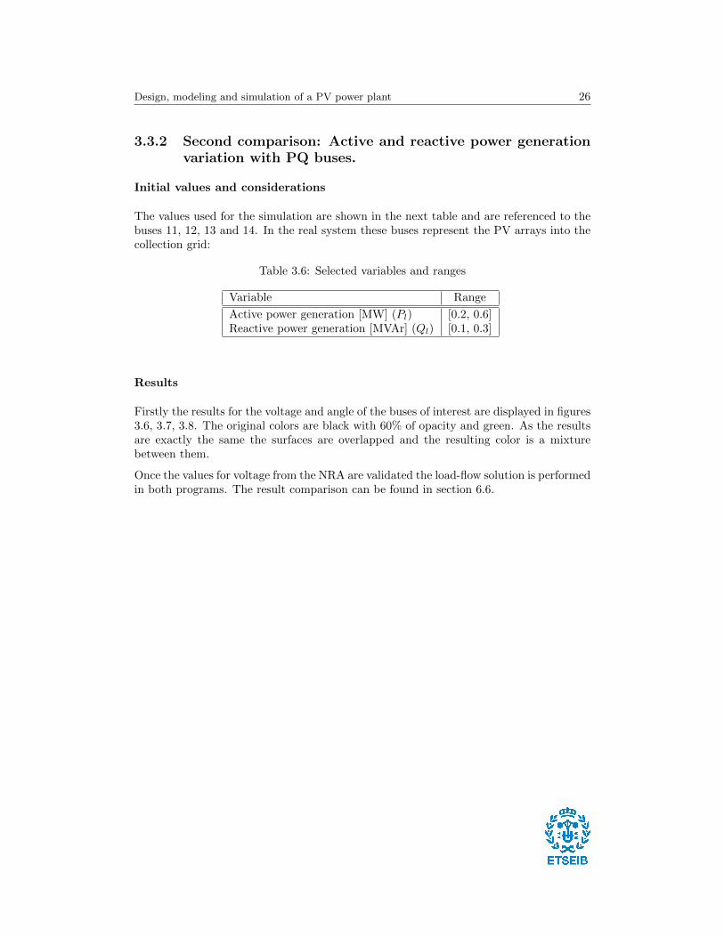
3.3.2 Second comparison: Active and reactive power generationvariation with PQ buses.
Initial values and considerations
The values used for the simulation are shown in the next table and are referenced to thebuses 11, 12, 13 and 14. In the real system these buses represent the PV arrays into thecollection grid:
Table 3.6: Selected variables and ranges
Variable Range
Active power generation [MW] (Pl) [0.2, 0.6]Reactive power generation [MVAr] (Ql) [0.1, 0.3]
Results
Firstly the results for the voltage and angle of the buses of interest are displayed in figures3.6, 3.7, 3.8. The original colors are black with 60% of opacity and green. As the resultsare exactly the same the surfaces are overlapped and the resulting color is a mixturebetween them.
Once the values for voltage from the NRA are validated the load-flow solution is performedin both programs. The result comparison can be found in section 6.6.
Design, modeling and simulation of a PV power plant 27
(a) 11th Bus magnitude (b) 11th Bus angle
Figure 3.6: Eleventh bus values (2nd case)
(a) 2nd Bus magnitude [p.u.] (b) 2nd Bus angle [o]
Figure 3.7: Second bus values (2nd case)
(a) 7th Bus magnitude (b) 7th Bus angle
Figure 3.8: Seventh bus values (2nd case)

Design, modeling and simulation of a PV power plant 28
3.3.3 Third comparision: Active power generation and grid volt-age variation with PV buses.
Initial values and considerations
This test is performed to test the capability of the PFE solver to work with PV buses.
The values used for the simulation are shown in the next table and are referenced to thebuses 11, 12, 13 and 14. In the real system these buses represent the PV arrays into thecollection grid:
Table 3.7: Selected variables and ranges
Variable Range
Active power demand [MW] (Pl) [0.2, 0.6]Grid voltage [p.u.] (V1) [0.95, 1.15]
Results
Firstly the results for the voltage and angle of the buses of interest are displayed infigures 3.9, 3.10, 3.11. The original colors are black with 60% of opacity and green. Asthe results are exactly the same the surfaces are overlapped and the resulting color is amixture between them.
The specified voltage for the PV buses (buses 11, 12, 13 and 14) is 1 as it can be confirmedin figure 3.9a.
Once the values of the iteration are confirmed the load-flow solution is performed in bothprograms. The results can be found in section 6.7.

Design, modeling and simulation of a PV power plant 29
(a) 11th Bus magnitude (b) 11th Bus angle
Figure 3.9: Eleventh bus values (3rd case)
(a) 2nd Bus magnitude [p.u.] (b) 2nd Bus angle [o]
Figure 3.10: Second bus values (3rd case)
(a) 7th Bus magnitude (b) 7th Bus angle
Figure 3.11: Seventh bus values (3rd case)

Design, modeling and simulation of a PV power plant 30
3.4 Analysis of maximum and minimum voltage devi-ations and loses.
In this section individual simulations and are performed with the aim of defining thebehaviour of the system. For the next simulations all the converter outputs are set asPV type buses as the majority of devices need a range of voltages to work correctly andthe magnitude of the changes in the system’s voltages are commonly wider than thoseranges. In section 4.3 a new type of bus is defined where the reactive power is a functionof the voltage with the aim of reducing the losses and therefore the stress of the systemamong other benefits.
3.4.1 Particular case: different values for each converter output
In this case the voltage of the converters (buses 11, 12, 13 ,14) are set to different valuesto simulate a real situation where the differences between components and conditions setdifferent efficiencies in each PV array. For example; different dust densities in the panelsor shades that reduce the efficiency of the Maximum power point tracker (MPPT)III.The initial data for the buses is summarized in the table 3.8 Using the script Individual
Table 3.8: Initial values for the converter output buses.
Bus id Voltage [p.u.] P demand [MW] P generation [MW]
11 1.02 0.65 0.4312 1.01 0.59 0.4413 1.03 0.62 0.4114 1.09 0.66 0.40
case the results are obtained and represented in figure 3.12. It can be observed that themaximum voltage deviation in per unit, excepting the voltage regulated buses, is foundin bus 5 with an increment of 0,0161% which transformed to real values is an incrementof 322 V. The minimum voltage deviation is found in bus 2 with a per unit increment of0,0094% and real value of 188 V.
The losses and injected apparent powers in each bus are illustrated in figure 3.13. Thereal and imaginary losses are similar to the magnitudes of thesurface script for the samegrid voltage value and active power generation figure 6.10. In fact if the linear script isused to evaluate the relation between the grid voltage and both imaginary and real lossesusing the same initial data. The results from figure 3.14 correspond to a variation in gridvoltage from 0.9 to 1.1 p.u. It can be concluded that both losses present a minimum whenthe grid voltage is 1.
IIIMPPT: is a device that set the voltage in the array to meet the maximum active power output. Ithas to work with the lower voltage on the array therefore if one panel is performing poorly the rest ofthe array is affected. It is considered as a type of loss.

Design, modeling and simulation of a PV power plant 31
Figure 3.12: Example scheme with voltage magnitude and phase values
Figure 3.13: Example scheme with voltage magnitude and phase values

Design, modeling and simulation of a PV power plant 32
Figure 3.14: Real and Imaginary losses changing the grid voltage from 0.9 to 1.1
Chapter 4
Grid code requirements
4.1 Introduction
A Grid Code is a technical document containing the rules governing the operation, mainte-nance and development of the transmission system. It is necessary due to the existence ofdifferent energy suppliers that work with the same Transmission system operator (TSO).In the grid code all the requirements are specified and discussed to ensure stability andquality of electrical systems in continuous operation as well as during fault’s or extraor-dinary events. Grid codes are different and depend on the country they are conformed.Each country elaborates one and the differences between them are motivated by the char-acteristics of the country and the particular needs created by the local electrical system.However according to [7] there is a tendency to harmonize grid codes in different EUcountries with documents such as: Network Code on Requirements for Grid Connectionapplicable to all Generators (RfG) drafted by European Network for Transmission Sys-tem Operators for Electricity (ENSTO-E). These documents are used as framework whiledeveloping grid codes.
The increasing penetration of renewable energies during the last decades have forced im-provements in the technology and system’s behaviour control. These changes are mainlymotivated by the intrinsic characteristics of renewable energies, such as the dependencyon the environment and the intermittent behaviour of the natural energy resources. Thesevariations can conclude in undesired faults creating damages to the transmission systemelements and all the equipment connected to the network. The grid codes are constantlyupdated to ensure smooth and correct functioning in all situations.
For example the grid code of a large country with a good number of sources and alow penetration of renewable energies must have less strict conditions for transmissionsystem frequency than a little island which has an equal proportion of renewable andnon-renewable energy sources.
There are two types of requirements: static and dynamic. Static requirements refer tothe continuous operation state and the dynamic collect the procedures to follow duringfault sequences and disturbances. The grid codes include worst case scenarios to cover
33

Design, modeling and simulation of a PV power plant 34
all the possible events that can take place including strict measures as the completedisconnection.
The renewable energies present a big flexibility to penetrate in the market as they can beintroduced as wind farms, PV plants, Hydro-powered stations... The solar energy is oneof the resources that are experiencing a fast growth during the last decades. In the paper[6] presented in MPDI journal it is exposed that the power installed capacity in Spainfor solar energy increased over a 5 GW from 2007 to 2018 with a positive tendency. Theevolution is represented in figure 4.1.
Figure 4.1: Power installed in Spain from 2007 to 2018.
In the present work the grid code requirements for a Large Scale PV power plant (LS-PVPP) are discussed and contextualized for different grid codes. The particular solutionpresented in [8] for compensating reactive power is introduced in the present work PFEsolver.
According to [11] the amount of energy managed via the peninsular system’s ancillaryservices in GWh is illustrated in figure 4.2.
Figure 4.2: Summary of the total energy managed by the ancillary services in the spanishpeninsula.

Design, modeling and simulation of a PV power plant 35
4.2 Static regulation
In general the static regulation for renewable energies depend on the resource used andits intrinsic characteristics. For example for solar and wind sources power curtailment isneeded due to the unpredictable availability and the fast and wide variations they cansuffer due to environmental conditions. Power curtailment limits the power extraction intwo different situations: when the power extracted is greater than the nominal value ofthe plant in peak generation events or when the demand is lower than the production.
In [4] an analysis of the connection requirements of wind power generation units for sixgrid codes is carried out.
4.2.1 Power factor regulation
The power factor is the ratio of reactive to apparent power consumption, thus its require-ments and the reactive power are similar in the different Grid Codes. Any inductancewith no capacitors attached consumes reactive power. Consequently this reactive powerconsumption must be produced somewhere in the grid. One thing to consider is that thedistribution of reactive power is cost intensive and the reactive power is not profitablealthough it is used in some cases to support the grid during particular events. In [5] anexample of different Grid Codes power factor/reactive power requirements is presented:
Figure 4.3: Reactive power requirements for Puerto Rico, South Africa and China, Ger-many and Romania.
The most restrictive PF requirement in figure (4.3) is the red line referring the Grid codefrom South Africa. From 100% to 20% of production the maximum PF are 0.975 leadingand 0.975 lagging.
One of the limitations commented in section 3.1.1 are the reactive power bounds for PVbuses. Those limitations should be established in order to meet the Grid Code guidelines

Design, modeling and simulation of a PV power plant 36
of reactive power consumption.
4.2.2 Power Curtailment
Power curtailment introduces the possible reduction of generated active power dependingon grid requirements. Two common situations where power curtailment is effective are:
• The possible overloading at peak generation hours for natural resources as wind orsolar energy. Due to the inherent characteristics of those.
• When the demand is lower than the generated active power without power curtail-ment.
The overloading is regulated by the TSO because it would cause an increment of thefrequency, therefore an increment in the inertia of the transmission system.
The power curtailment is not outlined precisely in most of the Grid Codes and it de-pends on environmental conditions, installed capacity and economics. According to [4]an indicator to apply this requirement is the frequency surplus. In European countries,with a grid frequency of 50 Hz, the bound to start applying power curtailment was 50,5Hz. When the frequency deviation decreases the reestablishment of the active power hasits own limitations. It should be less than the 10% of the network capacity per minute.Figure 4.4 extracted from [4] illustrates the operation conditions when the network isoverloading.
Figure 4.4: Power curtailment requirements
4.2.3 Active power reserves
The tendency of introducing more and more Distributed energy sistems (DES) basedon renewable energies in existing distribution networks generates new problems. Thedifficulty of prediction and intermittency of renewable energy sources in addition to thehigh density of DES lead to voltage and frequency issues in the distribution network.For example the proximity of PV plants due to the land restrictions submit them all tothe same environmental conditions. It has to be noticed that the most common peaks ofsolar production are found in the middle of the day where the demand is low. The energysurplus is redirected into the grid however in a distribution network with a high density

Design, modeling and simulation of a PV power plant 37
of DES it can conclude in bidirectional power flows, overloads or over voltages on somebranches or transformers.
To fix this issues and ensure a smooth penetration of the DES in the distribution networkstwo solutions are found. The first one is the use of batteries as energy storage systemsto supply the active power demand in compromised situations. Although it has beenexperimentally implemented presenting good results it is still cost-prohibitive and is notcost-competitive if compared with other sources. The main problem is the current energystorage technology that presents a low efficiency and a high maintenance and productioncosts at this power ratings. The alternative method is the active power regulation. It isbased on the power curtailment. In a situation where the energy production can reachthe nominal values the active power output is regulated to offer around an percentageof the maximum capacity. The remaining capacity is set as active power reserves. Thisapproach is easier to implement but it causes a reduction in the efficiency of the plant.
4.2.4 Voltage range and Control
The PV plant must be able to run at rated voltage plus the specified voltage range. Therated voltage and the voltage range varies depending on the transmission system, whichdepends on the country. The voltage ranges at the different rated values, for limitedperiods of time during fault or particular events, are also specified. According to [4] therequirement for all nominal values in continuous operation varies around ±10% of thenominal value.
4.2.5 Remote Voltage Control
Additionally in most of the grid codes it is required that the LS-PVPP or power stationcontains a closed loop voltage regulation system.
The voltage regulation follow the basis of the PV bus definition where a voltage set pointis specified and regulated by continuously modulating the reactive power output in theacceptable ranges. In addition the voltage set point shall be within the limits.
The time response of the voltage regulation system is also specified in some of the gridcodes analyzed in [4].
4.2.6 Frequency
The generator’s plant must be capable of working in accordance with specified frequencyranges. The majority of the grid codes presented [4] must be able to run continuousoperation in frequencies between 47,5 Hz and 52 Hz. Time delays might be necessary insome range of frequencies. The procedure in case of breaking the limits is to reduce theactive power output and remain connected. Disconnection is only permitted at frequenciesbelow 47 Hz and above 53 Hz and with no time delay.

Design, modeling and simulation of a PV power plant 38
4.2.7 Flicker
A flicker is a single, rapid change of the root mean square voltage. The connection ofdifferent elements such as capacitors, lines, cables, transformers and other elements maycause transmission system step changes.
It must be mentioned that a lot of grid codes do not mention flicker’s, according to [4]the Danish grid code specifies the next procedure.
Different thresholds are set depending on the time interval where the flicker magnitudeis evaluated. The short term flicker is a weighted average of the flicker contribution overten minutes. The long term flicker is defined over 2 hour.
Finally in figure 4.5, extracted from [5], a summary of the requirements for a LS-PVPPis illustrated for a better understanding.
Figure 4.5: Summary of grid codes requirements for LS-PVPP
4.3 Grid support; reactive power compensation
As the present work is centered in renewable energies and they are based on naturalresources usually the generation plants are located in remote areas. Consequently thetransmission lengths are long enough to consider the transmission line impedance signif-icant. As the transmission lines are mostly composed of inductance elements, which arepart of the imaginary domain, and transformers.
The inverter is synchronized to a point of connection (PoC) and the feedback measure-ments are taken at this point. As the current fed to the PoC flows through the gridimpedance a quantity of reactive power is created although the inverter is working atunity PF. Thus, the active power of the PV inverter becomes coupled with the reac-tive power seen by the grid. This undesired reactive power causes a bad behaviour thatincludes an increase in transmission losses and consequently reduces the maximum trans-mission capacity, compromises system stability and strains the grid.
The undesired reactive power depends on the grid current and grid impedance. If theimpedance is high the PoC current has a significant impact on the local voltages. A grid
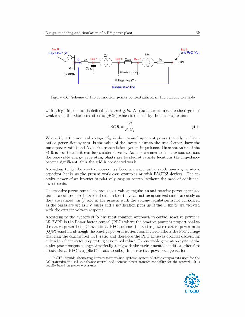
Design, modeling and simulation of a PV power plant 39
Figure 4.6: Scheme of the connection points contextualized in the current example
with a high impedance is defined as a weak grid. A parameter to measure the degree ofweakness is the Short circuit ratio (SCR) which is defined by the next expression:
SCR =V 2n
SnZg(4.1)
Where Vn is the nominal voltage, Sn is the nominal apparent power (usually in distri-bution generation systems is the value of the inverter due to the transformers have thesame power ratio) and Zg is the transmission system impedance. Once the value of theSCR is less than 5 it can be considered weak. As it is commented in previous sectionsthe renewable energy generating plants are located at remote locations the impedancebecome significant, thus the grid is considered weak.
According to [8] the reactive power has been managed using synchronous generators,capacitor banks as the present work case examples or with FACTSI devices. The re-active power of an inverter is relatively easy to control without the need of additionalinvestments.
The reactive power control has two goals: voltage regulation and reactive power optimiza-tion or a compromise between them. In fact they can not be optimized simultaneously asthey are related. In [8] and in the present work the voltage regulation is not consideredas the buses are set as PV buses and a notification pops up if the Q limits are violatedwith the current voltage setpoint.
According to the authors of [8] the most common approach to control reactive power inLS-PVPP is the Power factor control (PFC) where the reactive power is proportional tothe active power feed. Conventional PFC assumes the active power-reactive power ratio(Q/P) constant although the reactive power injection from inverter affects the PoC voltagechanging the commented Q/P ratio and therefore the PFC achieves optimal decouplingonly when the inverter is operating at nominal values. In renewable generation systems theactive power output changes drastically along with the environmental conditions thereforeif traditional PFC is applied it leads to suboptimal reactive power compensation.
IFACTS: flexible alternating current transmission system: system of static components used for theAC transmission used to enhance control and increase power transfer capability for the network. It isusually based on power electronics.

Design, modeling and simulation of a PV power plant 40
In [8] a method for autonomous compensation of undesired reactive power flow from thetransmission line reactance is presented. It includes a continuous-real time impedancemeasurement is used to estimate the transmission reactance. Based on the outputs andthe commented estimation the undesired reactive power is compensated and consequentlythe active power from the PV inverter is decoupled from the reactive power seen by thegrid. It allows the reactive power of the inverter to be controlled and still set the reactivepower value to 0 in the grid side. In the present work the estimation of the impedanceis not used as the grid parameters are known; for more information in [8] the estimationmethod is widely discussed. In conclusion the present work’s goal for grid support is todecouple the reactive power drawn from the grid that decreases the PF.
An image extracted from [8] illustrates the differences between the phasor at the differentpoints of connection:
Figure 4.7: From left to right; output PoC and grid PoC phasor diagrams when PF is setto unity.
As it is noticed when connecting to the output PoC with the inverter working at unity PFthe output current is in phase with the output voltage. On the grid side and after passingthrough the transmission impedance the current and output voltage are shifted, thus thegrid side PF is reduced. The reactive power compensation can be performed directly byadjusting the output’s voltage angle to match the grid voltage angle. In conclusion if thecompensation is applied the grid’s PF shall be equal to unity.
The wide and fast fluctuations of the renewable resources cause changes in the activepower which result in a variance of the reactive power consumption related with thetransmission system. In the present work the LS-PVPP are supposed to be weak grids,thus these active power variations can cause an undesired reactive power flow; increasingtransmission losses and limiting the active power of the line. These events can conclude incompromising the system stability. If the reactive power changes the power angle beyonda limit the equilibrium point no longer exists and the system becomes unstable.
In the context of the renewable energies another indicator for evaluating the stiffness ofthe grid is set. The Equivalent short circuit ratio (eSCR) follows the same concept thanthe SCR but it takes the instantaneous power instead of the nominal. With this changebeing applied the fluctuating nature of the active power is covered.

Design, modeling and simulation of a PV power plant 41
Compensation of the unintended reactive power.
The unintended reactive power flow can be compensated by forcing the inverter’s outputcurrent angle to match the grid PoC voltage angle. According to [8] the transmissionline consumes a reactive power of Qg with a total transmission reactance Xg while thecapacitive filter used to compensate produces a reactive power of Qc. Thus the totalreactive power Qtotal follows the next expression for one line:
Qtotal = Qg +Qc = I2oXg −V 2o
Xc(4.2)
Where Io and Vo are the current and voltage outputs of the converter.
Chapter 5
Environmental impact analysis
In this section the environmental effects of a LS-PVPP and its distribution system, itscomponents and the control methodology are discussed. The object of the study triesto focus on renewable energies as generators due to the restrictions they are attached interms of location and availability of the natural resource. In the scope of this projectare included the impact on the landscape, the side-effects suffered by the wildlife and thepossible impacts on the society.
The present project is centered in solar energy and the conclusions are particularized forthis natural resource. However many of the conclusions can be extracted for other energygeneration methods. The analysis is divided by areas. Each area is centered in a periodof the lifetime of the PV plant. Usually a LS-PVPP has a functional period that variesbetween 25 and 40 years.
As it is discussed in [9] there are diverse benefits of solar energy implementation ina particular location. Those include the reduction of the greenhouse effect gases, thestabilization of the degraded land and the increase of energy independence among others.It is important to notice that the creation of a PV power plant introduces social benefitsas well, the acceleration of rural electrification and the creation of job opportunities.
5.1 Large scale PV power plant
Solar energy is one of the best looking alternatives to fossil fuels in terms of fighting theclimate change. The table 5.1 contains values extracted from [9] comparing solar energytechnologies and conventional production systems. The photovoltaic systems present tentimes less contribution to the climate change than a conventional carbon-intensive system.Indeed a breakdown of the generation structure of the peninsular system extracted from[12] shows the tendency to substitute dirty sources of energy. Between 2017 and 2018 thetotal generation percentage of the peninsular system went from 33.7% to 40% with a 3%of solar energy share.
42

Design, modeling and simulation of a PV power plant 43
Table 5.1: Comparison of life cycle emissions for solar technologies and conventionalcarbon-intensive systems
Conventional systems Renewable systems
Production system g-CO2/kWh Production system g-CO2/kWh
Coal 975 Crystalline-silicon 45Gas 608 Thin-film amorphous silicon 45Oil 742 Thin-film cadmium telluride 14
Nuclear 42
Solar energy land use is smaller than average land use presented by other energy systemsincluding renewable sources as wind. Furthermore the changes introduced by solar ener-gies are less intense. In fact solar energy brings with it co-benefit opportunities. Someof them are the utilization of degraded lands, the mixture between solar panels locationand agriculture or hybrid power systems.
In the following sections some of the possible effects of the solar energy implementationare discussed. Firstly classified depending on the stages of the life cycle of a PV powerplant and then depending on the affected medium.
5.1.1 Construction
The magnitude of the demand of a utility-scale PV plant is usually around megawatts,consequently a wide area is needed to achieve that power generation. At first sight it canseem a minor inconvenient but the land restrictions, applied in order to protect the naturalenvironment and reduce the landscape impact, in addition to the inherent characteristicsof solar energy such as the inttermitency and the local availability of the resource reducedrastically the available terrain.
The construction stage includes actions as vegetation removal and complementary op-erations such as the creation of new roads, corridors and the transmission lines. Theseoperations can have negative effects in the environment due to the landscape impact andnoise and light pollution that can affect to the biodiversity in a wide spectrum of ways.
5.1.2 Operation
In this stage different maintenance operations are performed. The dust affects directly inthe efficiency of the PV panels therefore a cleaning routine needs to be done. The roadsused to access the panels and perform the different operations are already built. It isimportant to notice that LS-PVPP needs energy to start generating and this energy cancome from non renewable sources. Thus, this energy can be summarized in equivalentCO2 emissions.

Design, modeling and simulation of a PV power plant 44
5.1.3 Decommission
In the decommission stage the PV cells shall be recycled in order to avoid toxic substancesincluding cadmium, arsenic, silica dust and chemical products such as dust suppressants,coolant liquids and herbicides among others. Those substances are very toxic and in caseof inappropriate handling can pollute surface ground, superficial water accumulations andaquifers.
5.1.4 Potential environmental consequences
The use of environmental toxicants and flammable products is constant during all thestages. A procedure to neutralize those substances needs to be established if possible.The vehicular activity and soil disturbance are permanent effects during the lifespan ofthe PV plant.
Different environmental implications are related with the installation of PV power plants.Some of the more significant changes in the environment are commented next. Thechanges in albedo along the PV panels consumption lead to changes in the surface tem-perature and the precipitation regime which can be summarized in changes in the micro-climate and local hydrology. More information can be found in [9].
5.1.5 Potential ecological consequences
Land level effects
All the changes commented before can lead to a ecological response that includes a wideimpact on the biodiversity and soil nutrients dynamics. Usually LS-PVPP are located inremote areas where there is a wide biodiversity and the related footprint changes com-pletely the environment during the lifetime of the plant. The removed vegetation servesas air filter in many scenarios especially in arid terrains; it retains dust and sedimentstraveling with the wind, from dispersing around. Those sediments directly affect the ef-ficiency of the PV plants by simply accumulating in the PV panels or absorbing some ofthe irradiance coming from the Sun while suspended in the atmosphere.
The PV panels operational maintenance includes panel washing in order to maximize theefficiency. The process of cleaning the panels is manly based in water which can be anissue in some arid territories or places where water is an scarce resource.
The wide area occupied by the LS-PVPP create barriers to the genes spreading of certainspecies with little-range movement patterns that are not able to circumvent the installa-tion. Repatriation and translocation programs consist in collect the affected species andrelease them in different areas. However, according to [9], those methodologies have a lowsuccess rate close to 20% due to the complications of some species to adapt and overcomein new environments with an existent ecosystem. Another mitigation methodologies havebeen tested but the cost and the individual requirements of each specie do not guaranteebenefits. In addition some species as birds can not be controlled and they suffer accidents

Design, modeling and simulation of a PV power plant 45
related with the infrastructure. Changes in the land distribution, vegetation and biodi-versity in addition with the creation of roads which increments accessibility allow invasorspecies to move in.
Land-atmosphere synergies
PV panels have an effective albedo between 0,18 and 0,23 that is above the average albedofor the rural areas where the LS-PVPP are located. It concludes in an increase of the soilsurface temperature that can affect environmentally sensitive ecosystems. A high densityof PV generation can cause a change in the radiative balance that can not be understated.
5.1.6 Transmission system impact
The need of long transmission lines to transport the energy generated at the power plantsto the population centers where the consumption occurs as a big environmental impact.The major problem is centered in the land use; for example in [9] is said that only in 2007more than 300 km of high-voltage transmission lines where constructed in the UnitedStates. Nowadays, in an energy market that is constantly growing and diversifying, newopportunities related with more efficient and robust renewable technologies this numberis just increasing. The creation of transmission corridors in natural habitats can have aneffect on biodiversity similar to the PV power plant itself. In short term the corridorsare used by new communities to reach new territories and it can be an issue. Howeverin a mid-late term some places have presented great side effects on native biodiversity.In conclusion the environmental effects of the transmission lines are strongly correlatedwith the location and can be mitigated.
According to [10] the spanish transmission system in 2016 had 43.800km of circuits and5.609 substation bays accounting a total power of 85.144 MVA. The tendency is to growwith values between 0 and 1%. As a example in the 2018 review of Red Electrica deEspana ([12]) the total length of the transmission system is 44.243km.
In high capacity transmission systems the losses can affect directly to the climate change.In average the losses represent up to 3% of the total energy flow. This can represent ahigh volume of energy flowing to the environment leading to local temperature changes.
A lot of components used to conform the transmission lines and the interaction elementsof the grids, such as oil from transformers, contain environmental harassing substancesthat shall be recycled properly in order to mitigate their negative effects.
5.1.7 Conclusions
In general, positive impacts outweigh negative ones. At first sight the relief of the conven-tional generation plants in favour of solar energies is a good deal due to the reduction inCO2 and gas emissions. However many things need to be taken account to mitigate thepossible side effects of solar energies. For example if a LS-PVPP is located in a environ-mentally sensitive ecosystem the biodiversity would be strongly affected. In conclusion a

Design, modeling and simulation of a PV power plant 46
deep study on the location, a mitigation plan and a correct law code that protects themore sensitive areas can conclude in many environmental and social benefits.

Chapter 6
Projects budget
The present work is centered in the optimization of a PV plant by including a toolthat allows the user to take advantage of real time information to reduce losses andchoose the best settings at each situation. The cost of implementation is relatively lowin comparison to the total budget of creating an entire PV power plant and it can havepositive economic effects as consequences. Different conception costs per energy unit arepresented. In first place the CAPEXI (capital expenditure, table 6.1) data for a LS-PVPP project are presented. In second place OPEXII (Operational expenditures, table6.2) derived from the continuous operation of the PV plant are tabulated. Finally a smallreview of the economic impact of the ancillary services is presented according to RedElectrica de Espana.
6.1 Large Scale PV power plant
The prices shown on table 6.1 are extracted from [2]. The data is extracted fromBloomberg New Energy Finance which is a reliable energy related database. The batterysystem commented in section 4 is included to illustrate the high cost per kWh of thismethodology. The miscellaneous cost include an average land prince and the engineering,the derived cost of legal permissions and the construction among others.
Where EUR/Wn is the cost per watt of nominal power. The Balance of the system (BOS)encompasses all the components of a photovoltaic system other than photovoltaic panelsand the inverters. This concept includes wiring, switches, mounting system and somemechanism used to increase the efficiency of the PV power plant such as the maximumpower point tracker (MPPT) or the GPS solar tracker that changes the orientation of thepanels depending on the position of the Sun.
In the table 6.2 the continuous operations cost for a year of production is presented. ThePV technologies need energy to start converting energy and the intermittency of the solar
ICAPEX; the inversion cost to start running the PV plant.IIOPEX; the operation and maintenance cost of running the PV plant.
47

Design, modeling and simulation of a PV power plant 48
Table 6.1: PV plant CAPEX costs and current project budget
CAPEX component Cost per Watt Current project
Modules 0,31 EUR/Wn 1,24 M. EURCentral inverters 0,03 EUR/WAC 0,12 M. EURBalance of the system 0,17 EUR/WAC 0,68 M. EURMiscellaneous cost 0,30 EUR/WAC 1,2 M. EURPower curtailment with batteries (optional) 400 EUR/kWh -
source or the night periods create situations where the consumed energy is higher thanthe production. The dust removal, panel cleaning, maintenance products and salaries areincluded. The tracker system operation cost is isolated to illustrate the associated costof implementing a solar tracking system.
Table 6.2: PV plant OPEX
OPEX component Cost per MW
OPEX PV plant operation 9500 EUR/MWOPEX tracker operation (if included) 900 EUR/MW
6.2 Ancillary services
The grid codes requirements have an impact on the average final price of energy. In thereport of Red Electrica de Espana of 2018 about the ancillary services [11] a breakdownof the components conforming that price is performed. The figure 6.1 illustrates it. Thegrid support requirements seen in section 4 introduce a reduction on the final price. Themagnitude of its reduction is small in comparison with the final price but the advantagesin energy management in terms of reliability and security make their application essential.

Design, modeling and simulation of a PV power plant 49
Figure 6.1: Breakdown of ancillary services cost in the average final price of energy in thepeninsular system

Conclusions and further work
During the last years solar energy has penetrated in the energy market as an alternativeto fossil fuel-based energy. It has been possible due to the advances in power electronicsmixed with the automatic control methodologies that permitted the mitigation of theunintended behaviour of renewable energies. The balance of the environmental effectsbrought by these renewable energies is mostly positive however in section 5 is shownthat the effects on the environment are diverse and strongly dependent on the situationand the ecosystem sensibility. In some cases those consequences are unknown and canconclude in a permanent change in the surroundings of the installation with importantlosses in biodiversity and natural wealth. In consequence a deep study on the biodiversityand present ecosystem shall be performed in order to mitigate those negative effects. Thesoil and physic environment are also affected as a part of the energy they were usuallyreceiving to develop natural processes is used to produce energy for human consumptioncausing changes in the local temperature and soil nutrients development.
In the current work a program based on [3] to solve the power flows of a given systemis developed and validated versus MATPOWER. It models the buses using traditionalmethods as PQ and PV buses. A summary of the most common static regulation presentin most of the grid codes is included. A particular solution to mitigate the negative effectsof the unintended reactive power on large distribution systems based on regulating theamount of reactive power as a function of the voltage is also included. In further work theimplementation of that bus model and more grid code requirements can be performed.
Although the good results achieved by energy storage systems and the new developmentsthe implementation cost is still high in order to be competitive. Thus, the active powerreserves methodology discussed in section 4.2.3 leads to a efficiency decrease.
50

Annex
6.3 Introduction
In this chapter different images and script information from this work can be found.
6.4 Scripts
A brief description of the scripts used in the present project is included next. The scriptscan be found in the .zip file annexed to this project.
• The scripts named busdatas and linedatas are extracted from [3] and are used tointroduce each case initial data. The information about the data introduction isdiscussed in section 3.2.2.
• ymatrix is used to create the admittance matrix.
• pfeq and pfeq2 are the core of the NRA. Their results are the voltage and phasevalues of the buses. The difference between them is the way of displaying the results.
• loadflows1 and loadflows2 are used to perform the load flow analysis. They arecalled from pfeq and pfeq2 respectively.
• The Surface script is used to validate the results against MATPOWER and identifyparticular points if needed. It varies two parameters of the system and plot theresults in different surfaces for both programs. The different parameters that canbe changed are: active and reactive power demand (Pl, Ql), active and reactivepower generation (Pg, Qg), all converters voltage at the same rate (only PV buses;V11, V12, V13 and V14) and the grid voltage (V1).
• The linear script is made for a two dimension comparison to study the behaviourin a more isolated manner than in the Surface script.
• The linear pfe script perform simulations of changing one parameter and plots theresults in two dimension graphics. The available parameters to change are the samefrom surface script.
51

Design, modeling and simulation of a PV power plant 52
• The individual case script perform one simulation of the selected case and displaysan accurate summary of the values of the system. A breakdown of the branchesand buses values as well as the totals are included. In addition in cases includingPV buses the limit violations are also displayed.
6.5 First comparison power flow results
(a) Active power demand in KW (b) Reactive power demand in KVAr
Figure 6.2: Active and reactive power demand (1st case)
(a) Active power generation in KW (b) Reactive power generation in KVAr
Figure 6.3: Active and reactive power generation (1st case)

Design, modeling and simulation of a PV power plant 53
(a) Real losses in KW (b) Imaginary losses in kVAr
Figure 6.4: Imaginary and real losses (1st case)

Design, modeling and simulation of a PV power plant 54
6.6 Second comparison power flow results
(a) Active power demand in KW (b) Reacive power demand in KVAr
Figure 6.5: Active and reactive power demand (2nd case)
(a) Active power generation in KW (b) Reacive power generation in KVAr
Figure 6.6: Active and reactive power generation (2nd case)
(a) Real losses (b) Imaginary losses in kVAr
Figure 6.7: Active and reactive power generation (2nd case)

Design, modeling and simulation of a PV power plant 55
6.7 Third comparison power flow results
(a) Active power demand in KW (b) Reactive power demand in KVAr
Figure 6.8: Active and reactive power demand (3rd case)
(a) Active power generation in KW (b) Reactive power generation in KVAr
Figure 6.9: Active and reactive power generation (3rd case)
(a) Real losses (b) Imaginary losses
Figure 6.10: Active and reactive power generation (3rd case)

Bibliography
[1] Gabriele Catalano, Oriol Gomis Bellmunt. Development of a model to simulate solarPV plants in MATLAB with a study on the effects of undersizing the inverter Masterthesis from ETSEIB, UPC. September 2018.
[2] Eduard Foved Johe, Oriol Gomis Bellmunt. Design and optimisation of the architec-ture and the orientation of utility-scale photovoltaic power plants Master thesis fromETSEIB, UPC. April 2019.
[3] Praviraj PG (2020). Newton-Raphson Loadflow(https://www.mathworks.com/matlabcentral/fileexchange/21059-newton-raphson-loadflow) , MATLAB Central FileExchange. Retrieved May 24, 2020.
[4] Willi Christiansen and David T. Jonhsen Analysis of requirements in selected GridCodes Ørsted•DTU, Section of Electric power Engineering, Technical University ofDenmark (DTU). 20 January 2006.
[5] Ana Cabrera-Tobar, Eduard Bullich-Massague, Monica Aragues-Penalba and OriolGomis-Bellmunt. Active and Reactive Power Control of a PV Generator for GridCode Compliance Energies. 12. 3872. 10.3390/en12203872.
[6] Raquel Fernandez-Gonzalez, Andres Suarez-Garcıa, Miguel Angel AlvarezFeijoo,Elena Arce and Montserrat Dıez-Mediavilla. Spanish Photovoltaic So-lar Energy: Institutional Change, Financial Effects, and the Business Sec-tor (www.mdpi.com/journal/sustainability) Sustainability 2020, 12, 1892;doi:10.3390/su12051892
[7] Atsede G. Endegnanew, Salvatore D’Arco, Atsede G. Endegnanew, Raymundo E.Torres-Olguin, Jorun Irene Marvik and Elisabetta Tedeschi. Collocation of Europeangrid codes Work Package Partners, doc ref: MARINET-D2.26.
[8] Henrik Alenius, Roni Luhtala, Tuomas Messo, Tomi Roinila. Autonomous reactivepower support for smart photovoltaic inverter based on real-time grid-impedance mea-surements of a weak grid doc ref: https://doi.org/10.1016/j.epsr.2020.106207. 2020May.
[9] R.R. Hernandez, S.B.Easter, M.L.Murphy-Mariscal, F.T.Maestre, M.Tavassoli, E.B.Allen, C.W.Barrows, J.Belnap, R.Ochoa-Hueso, S.Ravi, M.F.Allen. Environmentalimpacts of utility-scale solar energy Renewable and Sustainable Energy Reviews Vol-ume 29, January 2014, Pages 766-779. https://doi.org/10.1016/j.rser.2013.08.041
56

Design, modeling and simulation of a PV power plant 57
[10] Red Electrica de Espana The Spanish Electricity System 2016 ONLINE: Review ofthe Spanish electricity system from 2016.
[11] Red Electrica de Espana Ancillary services and International exchanges ONLINE:PRELIMINARY REPORT: Commited to Intelligent Energy 2018
[12] Red Electrica de Espana Red Electrica Infografia Sector Electrico ONLINE Poster2018
Copyright © 2022 FDOKUMEN