design, implementation and control of scara robot

Design, Implementation And

Control Of

SCARA ROBOT

Acknowledgment

2

Acknowledgment

3

Design, Implementation And

Control Of

SCARA ROBOT

Sinai University

Mechanic department

Mechatronics

By:

Ahmed Saleh Ahmed

Mohammed Alnajjar

Hossam Eltanany

Prof.Dr. Saber Abdrabbo

Acknowledgment

4

Acknowledgment

5

Acknowledgment

It is our proud privilege to release the feeling of our gratitude to several persons who

helped us directly or indirectly to conduct this project work. We express our heart full

indebtedness and owe a deep sense of gratitude to our professor

Prof. Dr. Saber Abdrabbo

For his science guidance and inspiration in completing this project.

We are extremely thankful to the

Prof.Dr. Mohammed Abdelsalam.

Dean of the Faculty of Engineering

Prof.Dr. Abdelhamid Abdo.

Director of Faculty of Engineering

And all faculty member of PGDM for their coordination and cooperation and for

their kind guidance and encouragement.

We also deliver special thank you to mechanical department for and it

staff for their great help to complete our project, also electrical department has

its guidance rule on this project

Acknowledgment

6

Acknowledgment

7

For our parent who support us till we stand here today

with this project

For special people in our lives gave us hope to continue till

last step

Acknowledgment

8

Contents

9

Contents

Acknowledgment ....................................................................................................................................................... 5

Contents .................................................................................................................................................................... 9

Tables ....................................................................................................................................................................... 11

Figures ..................................................................................................................................................................... 12

Introduction ............................................................................................................................................................. 13

Chapter.1 Robotics Basic Concepts .................................................................................................................. 14

1.1 Definition of robot and industrial robot (1) .............................................................................................. 15

1.2 Robot Arm Configurations (2) ................................................................................................................... 16

1.2.1 Cartesian (3P) .................................................................................................................................. 17

1.2.2 Cylindrical (R2P) ............................................................................................................................... 17

1.2.3 Spherical (Polar) (2 RP) .................................................................................................................... 18

1.2.4 Articulated Arm (3R) ........................................................................................................................ 18

1.2.5 SCARA .............................................................................................................................................. 18

1.3 Sensors (3) ................................................................................................................................................. 19

1.4 Sensor classification ................................................................................................................................ 23

1.4.1 Binary Sensor ................................................................................................................................... 26

1.4.2 Analog versus Digital Sensors: ......................................................................................................... 27

1.4.3 Shaft Encoder................................................................................................................................... 28

1.4.4 A/D Converter .................................................................................................................................. 29

1.4.5 Position Sensitive Device ................................................................................................................. 30

1.4.6 Accelerometer: ................................................................................................................................ 33

1.5 MOTORS AND ACTUATORS: .................................................................................................................... 33

1.5.1 AC Motors ........................................................................................................................................ 33

1.5.2 DC Motors ........................................................................................................................................ 34

1.5.3 Exotic Motors ................................................................................................................................... 37

1.5.4 Stepper Motors (4) ............................................................................................................................ 38

1.5.5 Servos .............................................................................................................................................. 39

1.6 CRITERIA FOR SELECTION (6)..................................................................................................................... 40

1.6.1 REASONS FOR APPLYING ROBOTICS AND ARTIFICIAL INTELLIGENCE.............................................. 40

Contents

10

1.6.2 COMBINING SHORT-TERM AND LONG-TERM OBJECTIVES ............................................................. 41

1.6.3 APPLICATIONS OF ROBOTICS AND ARTIFICIAL INTELLIGENCE ........................................................ 42

1.6.4 PLANNING FOR GROWTH ................................................................................................................ 42

Chapter.2 Robot Control .................................................................................................................................. 43

2.1 SCARA Manipulator (RRP)........................................................................................................................ 44

2.2 Forward Kinematics: ................................................................................................................................ 45

2.2.1 Mathematical model: ...................................................................................................................... 45

2.2.2 Mat lab code for forward kinematics of scara robot: ...................................................................... 49

2.3 Inverse Kinematics ................................................................................................................................... 49

2.3.1 Mathematical model ....................................................................................................................... 49

2.3.2 Mat lab code for Inverse Kinematics ............................................................................................... 54

2.4 Why we use Mat lab? .............................................................................................................................. 54

2.5 Full modeling of scara robot on mat lab: ................................................................................................ 55

Chapter.3 Mechanical design ........................................................................................................................... 71

3.1 Programs used on mechanical design: .................................................................................................... 71

3.2 Consideration before design robot: ........................................................................................................ 72

3.3 Material selection .................................................................................................................................... 73

Chapter.4 Microcontroller ................................................................................................................................ 79

4.1 What is microcontroller? ......................................................................................................................... 80

4.2 Types of microcontroller: ........................................................................................................................ 82

4.3 Program used on scara robot .................................................................................................................. 85

Conclusion ............................................................................................................................................................... 88

References ............................................................................................................................................................... 89

11

Tables

Table 1specification ................................................................................................................................................. 25

Table 2 sensor material ........................................................................................................................................... 25

Table 3 detection means used in sensor ................................................................................................................. 26

Table 2.4 Joint parameters for SCARA ..................................................................................................................... 48

Figures

12

Figures

Figure 1-1 Level-control system. ............................................................................................................................. 19

Figure 1-2 A sensor may incorporate several transducers. ..................................................................................... 21

Figure 1-3Positions of sensors in a data acquisition system. .................................................................................. 23

Figure 1-4Interfacing a tactile sensor ...................................................................................................................... 26

Figure 1-5 Signal timing for synchronous serial interface ....................................................................................... 27

Figure 1-6 Optical encoders, incremental versus absolute (Gray code) ................................................................ 28

Figure 1-7 A/D converter interfacing ....................................................................................................................... 30

Figure 1-8 sonar sensor ........................................................................................................................................... 31

Figure 1-9 infrared sensor ....................................................................................................................................... 32

Figure 1-10 stepper motor schematic ..................................................................................................................... 38

Figure 1-11 servo control ........................................................................................................................................ 39

Figure2-1 The SCARA (Selective Compliant Articulated Robot for Assembly). ...................................................... 44

Figure2-2 Workspace of the SCARA manipulator. ................................................................................................... 45

Figure 2-3 Coordinate frames for two-link planar robot. ........................................................................................ 46

Figure2-4 DH coordinate frame assignment for the SCARA manipulator ............................................................... 47

Figure2-5 Multiple inverse kinematic solutions. ..................................................................................................... 50

Figure2-6 Solving for the joint angles of a two-link planar arm. ............................................................................. 50

Figure2-7scara manipulator .................................................................................................................................... 53

Figure 2-8 3D plotting for scara robot ..................................................................................................................... 69

Figure 2-9 Rendering of scara robot ........................................................................................................................ 69

Figure 3-1 comparison between inventor and solid work ...................................................................................... 72

Figure 3-2 base ........................................................................................................................................................ 74

Figure 3-3section on base........................................................................................................................................ 74

Figure 3-4 forearm ................................................................................................................................................... 75

Figure 3-5 section on forearm ................................................................................................................................. 75

Figure 3-6 top .......................................................................................................................................................... 76

Figure 3-7 section on top ......................................................................................................................................... 76

Figure 3-8 full design ............................................................................................................................................... 77

Figure 3-9 full design 3d .......................................................................................................................................... 78

Figure 4-1 microcontroller ....................................................................................................................................... 79

Figure 4-2 pic microcontroller ................................................................................................................................. 82

Figure 4-3 Arduino ................................................................................................................................................... 83

Introduction

13

Introduction

More robots bite the dust for a lack of management discipline than any other reason.

Building robots is much like going into battle.

You can do great damage coming straight out of the gate and swinging swords, but it

takes planning to make sure only the enemy gets cut. Robots are not built; they are born.

With forethought and preparation, the process can be much less painful. And lest we forget,

the project depends on people. Motivation and management, of self and others, are required

for success

Robotics has achieved its greatest success to date in the world of industrial

manufacturing. Robot arms, or manipulators, comprise a 2 billion dollar industry.

Bolted at its shoulder to a specific position in the assembly line, the robot arm can move

with great speed and accuracy to perform repetitive tasks such as spot welding and

painting. In the electronics industry, manipulators place surface-mounted components with

superhuman precision, making the portable telephone and laptop computer possible.

At this project we try to introduce good prototype for manufacturing scara robot

hoping it will lead others on their way to learn and build scara robots on the future .

Robotics Basic Concepts

14

Chapter.1 Robotics Basic Concepts

Before we start manufacture robots we should study basics of robotics science to

understand concepts of design and control robot and its accessories which includes input

devices like sensors ( types, how it work and how to control it) and output devices like

actuators ( types, how it work and how to control it ).


15

1.1 Definition of robot and industrial robot (1)

The distinction of robots lies somewhere in the sophistication of the

programmability of the device – a numerically controlled (NC) milling machine is not an

industrial robot.

As says, “If a mechanical device can be programmed to perform a wide variety of

applications, it is probably an industrial robot”. The essential difference between an

industrial robot and an NC machine is the versatility of the robot, that it is provided with

tools of different types and has a large workspace compared to the volume of the robot

itself. The NC machine is dedicated to a special task, although in a fairly flexible way,

which gives a system built after fixed and limited specifications.

The study and control of industrial robots is not a new science, rather a mixture of

“classical fields”. From mechanical engineering the machine is studied in static and

dynamic situations. By means of mathematics the spatial motions can be described.

Tools for designing and evaluating algorithms to achieve the desired motion are

provided by control theory. Electrical engineering are helpful when designing sensors and

interfaces for industrial robots. Last but not least, computer science provides for

programming the device to perform a desired task.

The term robotics has recently been defined as the science studying “the intelligent

connection of perception to action”. Industrial robotics is a discipline concerning robot

design, control and applications in industry and the products are now reaching the level of

a mature technology.

The status of robotics technology can be reflected by the definition of a robot

originating from the Robot Institute of America. The institute uses the definition that “a

robot is a reprogrammable multifunctional manipulator designed to move materials, parts,

tools or specialized devices through variable programmed motions for the performance of

a variety of tasks”. The key element in the definition is the word reprogrammable, which

gives the robot characteristics as utility and adaptability.


16

Sometimes the word robotics revolution is mentioned, but it is in fact a part of the

much larger computer revolution.

Most of the organizations nowadays agree more or less to the definition of industrial

robots, formulated by the International Organization for Standardization, ISO.

• “Manipulating industrial robot is an automatically controlled, reprogrammable,

multi-purpose, manipulative machine with several degrees of freedom, which may be

either fixed in place or mobile for use in industrial automation applications”.

• “Manipulator is a machine, the mechanism of which usually consists of a series of

segments jointed or sliding relative to one another, for the purpose of grasping and/or

moving objects (pieces or tools) usually in several degrees of freedom”.

From this definition, it can be seen that the word manipulator is used for the arm of

the robot. The definition of industrial robot, it can be interpreted as follows. A robot shall

easily be reprogrammable without physically rebuilding the machine. It shall also have

memory and logic to be able to work independently and automatically. Its mechanical

structure shall be able to be used in several working tasks, without any larger mechanical

operations of the structure.

Another definition comes from Japan Industrial Robot Association (JIRA), where

they divide robots into six different classes. They also incorporate tele-manipulators and

simple automatons, which is one of the reasons to why Japan often have hundreds of

thousands of installed robots. Approximately 25% of the installed robots can be counted

as industrial robots from our point of view, which however still makes Japan the leading

robot user.

1.2 Robot Arm Configurations (2)

• Cartesian (3P)

• Cylindrical (R2P)

• Spherical (Polar) (2 RP)

• Articulated (3R)

• SCARA (2R in horizontal + 1P in vertical plane)


17

1.2.1 Cartesian (3P)

• Due to their rigid structure they can manipulate high loads so they are commonly used

for pick-and-place operations, machine tool loading, in fact any application that uses a lot

of moves in the X, Y, Z planes.

• These robots occupy a large space, giving a low ratio of robot size to operating volume.

They may require some form of protective covering.

1.2.2 Cylindrical (R2P)

• They have a rigid structure, giving them the capability to lift heavy loads through a

large working envelope, but they are restricted to area close to the vertical base or the

floor.

• This type of robot is relatively easy to program for loading and unloading of palletized

stock, where only the minimum number of moves is required to be programmed.


18

1.2.3 Spherical (Polar) (2 RP)

• These robots can generate a large working envelope.

• The robots can allow large loads to be lifted.

• The semi-spherical operating volume leaves a considerable space near to the base that

cannot be reached.

• This design is used where a small number of vertical actions is adequate: the loading

and unloading of a punch press is a typical application.

1.2.4 Articulated Arm (3R)

• This is the most widely used arm configuration because of its flexibility in reaching any

part of the working envelope.

• This configuration flexibility allows such complex applications as spray painting and

welding to be implemented successfully.

1.2.5 SCARA

• Although originally designed specifically for assembly work, these robots are now

being used for welding, drilling and soldering operations because of their repeatability

and compactness.

• They are intended for light to medium loads and the working volume tends to be

restricted as there is limited vertical movement

And that last type that we choose to work on at our graduation project this year


19

1.3 Sensors (3)

A sensor is often defined as a device that receives and responds to a signal or

stimulus. This definition is broad. In fact, it is so broad that it covers almost everything

from a human eye to a trigger in a pistol. Consider the level-control system shown in Fig

(1).

Figure 1-1 Level-control system.

The operator adjusts the level of fluid in the tank by manipulating its valve.

Variations in the inlet flow rate, temperature changes (these would alter the fluid’s

viscosity and, consequently, the flow rate through the valve), and similar disturbances must

be compensated for by the operator. Without control, the tank is likely to flood, or run dry.

To act appropriately, the operator must obtain information about the level of fluid in the

tank on a timely basis. In this example, the information is perceived by the sensor, which

consists of two main parts: the sight tube on the tank and the operator’s eye, which

generates an electric response in the optic nerve. The sight tube by itself is not a sensor,

and in this particular control system, the eye is not a sensor either. Only the combination

of these two components makes a narrow-purpose sensor (detector), which is selectively


20

sensitive to the fluid level. If a sight tube is designed properly, it will very quickly reflect

variations in the level, and it is said that the sensor has a fast speed response. If the internal

diameter of the tube is too small for a given fluid viscosity, the level in the tube may lag

behind the level in the tank. Then, we have to consider a phase characteristic of such a

sensor. In some cases, the lag may be quite acceptable, whereas in other cases, a better

sight tube design would be required. Hence, the sensor’s performance must be assessed

only as a part of a data acquisition system.

This world is divided into natural and man-made objects. The natural sensors, like

those found in living organisms, usually respond with signals, having an electrochemical

character; that is, their physical nature is based on ion transport, like in the nerve fibers

(such as an optic nerve in the fluid tank operator). In man-made devices.

Information is also transmitted and processed in electrical form—however, through

the transport of electrons. Sensors that are used in artificial systems must speak the same

language as the devices with which they are interfaced. This language is electrical in its

nature and a man-made sensor should be capable of responding with signals where

information is carried by displacement of electrons, rather than ions.

Thus, it should be possible to connect a sensor to an electronic system through

electrical wires, rather than through an electrochemical solution or a nerve fiber. Hence, in

this book, we use a somewhat narrower definition of sensors, which may be phrased as

A sensor is a device that receives a stimulus and responds with an

electrical signal.

The term stimulus is used throughout this book and needs to be clearly understood.

The stimulus is the quantity, property, or condition that is sensed and converted into

electrical signal. Use a different term, measured, which has the same meaning, however

with the stress on quantitative characteristic of sensing.

The purpose of a sensor is to respond to some kind of an input physical property

(stimulus) and to convert it into an electrical signal which is compatible with electronic

circuits. We may say that a sensor is a translator of a generally nonelectrical value into an

electrical value. When we say “electrical,” we mean a signal which can be channeled,

amplified, and modified by electronic devices. The sensor’s output signal may be in the

form of voltage, current, or charge. These may be further described in terms of amplitude,


21

frequency, phase, or digital code. This set of characteristics is called the output signal

format. Therefore, a sensor has input properties (of any kind) and electrical output

properties.

Any sensor is an energy converter. No matter what you try to measure, you always

deal with energy transfer from the object of measurement to the sensor. The process of

sensing is a particular case of information transfer, and any transmission of information

requires transmission of energy. Of course, one should not be confused by an obvious fact

that transmission of energy can flow both ways—it may be with a positive sign as well as

with a negative sign; that is, energy can flow either from an object to the sensor or from

the sensor to the object. A special case is when the energy is zero, and it also carries

information about existence of that particular case. For example, a thermopile infrared

radiation sensor will produce a positive voltage when the object is warmer than the sensor

(infrared flux is flowing to the sensor) or the voltage is negative when the object is cooler

than the sensor (infrared flux flows from the sensor to the object). When both the sensor

and the object are at the same temperature, the flux is zero and the output voltage is zero.

This carries a message that the temperatures are the same.

The term sensor should be distinguished from transducer. The latter is a converter

of one type of energy into another, whereas the former converts any type of energy into

electrical. An example of a transducer is a loudspeaker which converts an electrical signal

into a variable magnetic field and, subsequently, into acoustic waves.2 this is nothing to

do with perception or sensing. Transducers may be used as actuators in various systems.

An actuator may be described as opposite to a sensor—it converts electrical signal into

generally nonelectrical energy. For example, an electric motor is an actuator—it converts

electric energy into mechanical action.

Figure 1-2 A sensor may incorporate several transducers.


22

Transducers may be parts of complex sensors (Fig. 1.2). For example, a chemical

sensor may have a part which converts the energy of a chemical reaction into heat

(transducer) and another part, a thermopile, which converts heat into an electrical signal.

The combination of the two makes a chemical sensor—a device which produces an

electrical signal in response to a chemical reaction. Note that in the above example, a

chemical sensor is a complex sensor; it is comprised of a transducer and another sensor

(heat). This suggests that many sensors incorporate at least one direct-type sensor and a

number of transducers. The direct sensors are those that employ such physical effects that

make a direct energy conversion into electrical signal generation or modification.

Examples of such physical effects are photo effect and See beck effect.

In summary, there are two types of sensors: direct and complex. A direct sensor

converts a stimulus into an electrical signal or modifies an electrical signal by using an

appropriate physical effect, whereas a complex sensor in addition needs one or more

transducers of energy before a direct sensor can be employed to generate an electrical

output.

A sensor does not function by itself; it is always a part of a larger system that may

incorporate many other detectors, signal conditioners, signal processors, memory devices,

data recorders, and actuators. The sensor’s place in a device is either intrinsic or extrinsic.

It may be positioned at the input of a device to perceive the outside effects and to signal

the system about variations in the outside stimuli. Also, it may be an internal part of a

device that monitors the devices’ own state to cause the appropriate performance. A sensor

is always a part of some kind of a data acquisition system. Often, such a system may be a

part of a larger control system that includes various feedback mechanisms.

To illustrate the place of sensors in a larger system, Fig. 1.3 shows a block diagram

of a data acquisition and control device. An object can be anything: a car, space ship,

animal or human, liquid, or gas. Any material object may become a subject of some kind

of a measurement. Data are collected from an object by a number of sensors. Some of them

(2, 3, and 4) are positioned directly on or inside the object. Sensor 1 perceives the object

without a physical contact and, therefore, is called a noncontact sensor. Examples of such

a sensor is a radiation detector and a TV camera. Even if we say “noncontact”, we

remember that energy transfer always occurs between any sensor and an object.


23

Figure 1-3Positions of sensors in a data acquisition system.

Sensor 1 is noncontact, sensors 2and 3 are passive, sensor 4 is active, and sensor 5

is internal to a data acquisition system.

Sensor 5 serves a different purpose. It monitors internal conditions of a data

acquisition system itself. Some sensors (1 and 3) cannot be directly connected to standard

electronic circuits because of inappropriate output signal formats. They require the use of

interface devices (signal conditioners). Sensors 1, 2, 3, and 5 are passive. They generate

electric signals without energy consumption from the electronic circuits. Sensor 4 is active.

It requires an operating signal, which is provided by an excitation circuit. This signal is

modified by the sensor in accordance with the converted information. An example of an

active sensor is a thermistor, which is a temperature-sensitive resistor. It may operate with

a constant-current source, which is an excitation circuit. Depending on the complexity of

the system, the total number of sensors may vary from as little as one (a home thermostat)

to many thousands (a space shuttle).

1.4 Sensor classification

Sensor classification schemes range from very simple to the complex. Depending

on the classification purpose, different classification criteria may be selected. Here, we

offer several practical ways to look at the sensors.

All sensors may be of two kinds: passive and active. A passive sensor does not

need any additional energy source and directly generates an electric signal in response to


24

an external stimulus; that is, the input stimulus energy is converted by the sensor into the

output signal. The examples are a thermocouple, a photodiode, and a piezoelectric sensor.

Most of passive sensors are direct sensors as we defined them earlier. The active sensors

require external power for their operation, which is called an excitation signal. That signal

is modified by the sensor to produce the output signal. The active sensors sometimes are

called parametric because their own properties change in response to an external effect

and these properties can be subsequently converted into electric signals. It can be stated

that a sensor’s parameter modulates the excitation signal and that modulation carries

information of the measured value. For example, a thermistor is a temperature-sensitive

resistor. It does not generate any electric signal, but by passing an electric current through

it (excitation signal), its resistance can be measured by detecting variations in current

and/or voltage across the thermistor. These variations (presented in ohms) directly relate

to temperature through a known function. Another example of an active sensor is a resistive

strain gauge in which electrical resistance relates to a strain. To measure the resistance of

a sensor, electric current must be applied to it from an external power source.

Depending on the selected reference, sensors can be classified into absolute and

relative. An absolute sensor detects a stimulus in reference to an absolute physical scale

that is independent on the measurement conditions, whereas a relative sensor produces a

signal that relates to some special case. An example of an absolute sensor is a thermistor:

a temperature-sensitive resistor. Its electrical resistance directly relates to the absolute

temperature scale of Kelvin. Another very popular temperature sensor—a thermocouple—

is a relative sensor. It produces an electric voltage that is function of a temperature gradient

across the thermocouple wires. Thus, a thermocouple output signal cannot be related to

any particular temperature without referencing to a known baseline. Another example of

the absolute and relative sensors is a pressure sensor.

An absolute-pressure sensor produces signal in reference to vacuum—an absolute zero

on a pressure scale. A relative-pressure sensor produces signal with respect to a selected

baseline that is not zero pressure (e.g., to the atmospheric pressure).

Another way to look at a sensor is to consider all of its properties, such as what it

measures (stimulus), what its specifications are, what physical phenomenon it is sensitive

to, what conversion mechanism is employed, what material it is fabricated from, and what

its field of application is. Tables 1. Represent such a classification scheme, which is pretty

much broad and representative. If we take for the illustration a surface acoustic-wave

oscillator accelerometer, the table entries might be as follows:


25

Stimulus Acceleration

Specifications:

Sensitivity in frequency shift per

gram of acceleration, short- and long-term

stability in Hz per unit time, etc.

Detection means: Mechanical

Conversion phenomenon Elastoelectric

Material Inorganic insulator

Field Automotive, marine, space, and scientific

Measurement

Table 1specification

Table 2 sensor material


26

Table 3 detection means used in sensor

1.4.1 Binary Sensor

Binary sensors are the simplest type of sensors. They only return a single bit of

information, either 0 or 1. A typical example is a tactile sensor on a robot, for example

using a micro switch. Interfacing to a microcontroller can be achieved very easily by using

a digital input either of the controller or a latch. Figure (4) shows how to use a resistor to

link to a digital input. In this case, a pull-up resistor will generate a high signal unless the

switch is activated. This is called an “active low” setting.

Figure 1-4Interfacing a tactile sensor


27

1.4.2 Analog versus Digital Sensors:

A number of sensors produce analog output signals rather than digital signals. This

means an A/D converter is required to connect such a sensor to a microcontroller. Typical

examples of such sensors are:

• Microphone

• Analog infrared distance sensor

• Analog compass

• Barometer sensor

Digital sensors on the other hand are usually more complex than analog sensors and often

also more accurate. In some cases the same sensor is available in either analog or digital

form, where the latter one is the identical analog sensor packaged with an A/D converter.

The output signal of digital sensors can have different forms. It can be a parallel interface

(for example 8 or 16 digital output lines), a serial interface (for example following the

RS232 standard) or a “synchronous serial” interface. The expression “synchronous serial”

means that the converted data value is read bit by bit from the sensor. After setting the

chip-enable line for the sensor, the CPU sends pulses via the serial clock line and at the

same time reads 1 bit of information from the sensor’s single bit output line for every pulse

(for example on each rising edge). See Figure (5) for an example of a sensor with a 6bit

wide output word.

Figure 1-5 Signal timing for synchronous serial interface


28

1.4.3 Shaft Encoder

Encoders are required as a fundamental feedback sensor for motor control. There

are several techniques for building an encoder. The most widely used ones are either

magnetic encoders or optical encoders. Magnetic encoders use a Hall-effect sensor and a

rotating disk on the motor shaft with a number of magnets mounted in a circle. Every

revolution of the motor shaft drives the magnets past the Hall sensor and therefore results

in 16 pulses or “ticks” on the encoder line. Standard optical encoders use a sector disk with

black and white segments (see Figure 2.3, left) together with an LED and a photo-diode.

The photo-diode detects reflected light during a white segment, but not during a black

segment. So once again, if this disk has 16 white and 16 black segments, the sensor will

receive 16 pulses during one revolution. Encoders are usually mounted directly on the

motor shaft (that is before the gear box), so they have the full resolution compared to the

much slower rotational speed at the geared-down wheel axle. For example, if we have an

encoder which detects 16 ticks per revolution and a gearbox with a ratio of 100:1 between

the motor and the vehicle’s wheel, then this gives us an encoder resolution of 1,600 ticks

per wheel revolution. Both encoder types described above are called incremental, because

they can only count the number of segments passed from a certain starting point. They are

not sufficient to locate a certain absolute position of the motor shaft. If this is required, a

Gray-code disk (Figure 6, right) can be used in combination with a set of sensors.

Figure 1-6 Optical encoders, incremental versus absolute (Gray code)

The number of sensors determines the maximum resolution of this encoder type (in

the example there are 3 sensors, giving a resolution of 23 = 8 sectors). Note that for any


29

transition between two neighboring sectors of the Gray code disk only a single bit changes

(e.g. between 1 = 001 and 2 = 011). This would not be the case for a standard binary

encoding (e.g. 1 = 001 and 2 = 010, which differ by two bits).

This is an essential feature of this encoder type, because it will still give a proper

reading if the disk just passes between two segments. (For binary encoding the result would

be arbitrary when passing between 111 and 000.) As has been mentioned above, an encoder

with only a single magnetic or optical sensor element can only count the number of

segments passing by. But it cannot distinguish whether the motor shaft is moving

clockwise or counterclockwise.

This is especially important for applications such as robot vehicles which should be

able to move forward or backward. For this reason most encoders are equipped with two

sensors (magnetic or optical) that are positioned with a small phase shift to each other.

With this arrangement it is possible to determine the rotation direction of the motor shaft,

since it is recorded which of the two sensors first receives the pulse for a new segment. If

in Figure (6) Enc1 receives the signal first, then the motion is clockwise; if Enc2 receives

the signal first, then the motion is counter-clockwise.

Since each of the two sensors of an encoder is just a binary digital sensor, we could

interface them to a microcontroller by using two digital input lines. However, this would

not be very efficient, since then the controller would have to constantly poll the sensor data

lines in order to record any changes and update the sector count.

1.4.4 A/D Converter An A/D converter translates an analog signal into a digital value. The characteristics of

an A/D converter include:

• Accuracy expressed in the number of digits it produces per value (for example

10bit A/D converter)

• Speed expressed in maximum conversions per second (for example 500

conversions per second)

• Measurement range expressed in volts (for example 0.5V) A/D converters come in

many variations. The output format also varies.

Typical are either a parallel interface (for example up to 8 bits of accuracy) or a

synchronous serial interface (see Section 2.3). The latter has the advantage that it does not

impose any limitations on the number of bits per measurement, for example 10 or 12bits


30

of accuracy. Figure (7) shows a typical arrangement of an A/D converter interfaced to a

CPU.

Figure 1-7 A/D converter interfacing

Many A/D converter modules include a multiplexer as well, which allows the

connection of several sensors, whose data can be read and converted subsequently. In this

case, the A/D converter module also has a 1bit input line, which allows the specification

of a particular input line by using the synchronous serial transmission (from the CPU to

the A/D converter).

1.4.5 Position Sensitive Device

Sensors for distance measurements are among the most important ones in robotics.

For decades, mobile robots have been equipped with various sensor types for measuring

distances to the nearest obstacle around the robot for navigation purposes. Sonar sensors

in the past, most robots have been equipped with sonar sensors (often Polaroid sensors).

Because of the relatively narrow cone of these sensors, a typical configuration to

cover the whole circumference of a round robot required 24 sensors, mapping about 15°

each. Sonar sensors use the following principle: a short acoustic signal of about 1ms at an

ultrasonic frequency of 50 kHz to 250 kHz is emitted and the time is measured from signal

emission until the echo returns to the sensor.

The measured time-of-flight is proportional to twice the distance of the nearest

obstacle in the sensor cone. If no signal is received within a certain time limit, then no

obstacle is detected within the corresponding distance. Measurements are repeated about

20 times per second, which gives this sensor its typical clicking sound (see Figure 8)


31

Figure 1-8 sonar sensor

Sonar sensors have a number of disadvantages but are also a very powerful sensor system,

as can be seen in the vast number of published articles dealing with them [Barshan, Ayrulu,

Utete 2000], [Kuc 2001]. The most significant problems of sonar sensors are reflections

and interference. When the acoustic signal is reflected, for example off a wall at a certain

angle, then an obstacle seems to be further away than the actual wall that reflected the

signal. Interference occurs when several sonar sensors are operated at once (among the 24

sensors of one robot, or among several independent robots). Here, it can happen that the

acoustic signal from one sensor is being picked up by another sensor, resulting in

incorrectly assuming a closer than actual obstacle. Coded sonar signals can be used to

prevent this, for example using pseudo random codes [Jorge, Berg 1998].

Laser sensors today, in many mobile robot systems, sonar sensors have been replaced

by either infrared sensors or laser sensors. The current standard for mobile robots is laser

sensors (for example Sick Auto Indent [Sick 2006]) that return an almost perfect local 2D

map from the viewpoint of the robot, or even a complete 3D distance map. Unfortunately,

these sensors are still too large and heavy (and too expensive) for small mobile robot

systems. This is why we concentrate on infrared distance sensors.


32

Figure 1-9 infrared sensor

Infrared (IR) distance sensors do not follow the same principle as sonar sensors, since

the time-of-flight for a photon would be much too short to measure with a simple and cheap

sensor arrangement. Instead, these systems typically use a pulsed infrared LED at about 40

kHz together with a detection array (see Figure 9). The angle under which the reflected

beam is received changes according to the distance to the object and therefore can be used

as a measure of the distance. The wavelength used is typically 880nm. Although this is

invisible to the human eye, it can be transformed to visible light either by IR detector cards

or by recording the light beam with an IR-sensitive camera. Figure 2.7 shows the Sharp

sensor GP2D02 [Sharp 2006] which is built in a similar way as described above. There are

two variations of this sensor:

• Sharp GP2D12 with analog output

• Sharp GP2D02 with digital serial output

The analog sensor simply returns a voltage level in relation to the measured distance

(unfortunately not proportional, see Figure 2.7, right, and text below). The digital sensor

has a digital serial interface. It transmits an 8bit measurement value bit-wise over a single

line, triggered by a clock signal from the CPU as shown, the relationship between digital

sensor read-out (raw data) and actual distance information can be seen. From this diagram

it is clear that the sensor does not return a value linear or proportional to the actual distance,

so some post-processing of the raw sensor value is necessary. The simplest way of solving

this problem is to use a lookup table which can be calibrated.

For each individual sensor. Since only 8 bits of data are returned, the lookup table

will have the reasonable size of 256 entries. Such a lookup table is provided in the hardware

description table (HDT) of the Rob IOS operating system. With this concept, calibration is

only required once per sensor and is completely transparent to the application program.


33

1.4.6 Accelerometer:

All these simple sensors have a number of drawbacks and restrictions. Most of them

cannot handle jitter very well, which frequently occurs in driving or especially walking

robots. As a consequence, some software means have to be taken for signal filtering. A

promising approach is to combine two different sensor types like a gyroscope and an

inclinometer and perform sensor fusion in software.

A number of different accelerometer models are available from Analog

Devices, measuring a single or two axes at once. Sensor output is either analog or a PWM

signal that needs to be measured and translated back into a binary value by the CPU’s

timing processing unit.

The acceleration sensors we tested were quite sensitive to positional noise (for

example servo jitter in walking robots). For this reason we used additional low-pass filters

for the analog sensor output or digital filtering for the digital sensor output.

1.5 MOTORS AND ACTUATORS:

Motors are simply devices that take in power and generate movement. Most motors

convert the power to a magnetic field using coils. A few motors do not use coils, and we’ll

discuss them later.

The power fed in to the motor coils can come from the AC power mains, DC power

supplies, or from controllers that control the coils for specific purposes. Motors are divided

into classes based on the type of power they use.

1.5.1 AC Motors

Most motors in use today are AC motors designed for medium to heavy-duty

work. They are present in most motorized appliances that use AC power. They are

inexpensive because they do not require complicated construction and because they are


34

built in large quantities. Motors differ in their construction, speed control, cooling

methods, control systems, size, and weight.

Construction AC motors have the coils built in to the outside casing (the stator)

and magnets that spin in the middle (on the rotor).

Speed The number of windings and the frequency of the power fed to the coils fix

the speed of the motor. The speed of AC motors is basically constant. As such, they may

not be the best for robots. Let’s consider just 60 Hz of power for these examples. If just

three windings form a single rotating field (one pole), the motor spins at 60 Hz or 3,600

revolutions per minute (RPM). As three more winding coils are added, the number of poles

goes to 2 and the RPMs go down to 1800.

The following equation is used to determine the RPM, where p is the number of

three winding coils (poles), f is the frequency of the power, and so is the speed of the motor

in 4 RPM:

_ cooling the windings are on the outside case, where they can be cooled easier.

Furthermore, with no brushes, the casing can be wide open to admit air for cooling.

_ Controls AC motors are not easy to control, in either speed or position. It is

possible to build an electronic controller to trim the speed and power consumption of an

AC motor, but it is best used in situations where only gross mechanical power is needed,

especially for constant speed applications.

_ Portability Given that a portable robot probably is running off batteries, AC

motors may not be the right choice. Along with the difficulties of controlling the speed and

position of an AC motor, it’s fair to conclude they may not be a good choice in a robot.

1.5.2 DC Motors

DC motors come in many different styles. AC motors only have fewer styles

because their architecture attempts to take advantage of the existing movement (waveform)

of the AC power. Like most motors, DC motors generate movement by creating magnetic

fields within the motor that attract one another. By and large, DC motors have permanent

magnets in the stator and the rotor has the coils (the reverse of AC motors). But since DC

power has no movement (waveform) of its own, the motor electronics must create a change

in the DC waveform as the motor rotates. This can happen in several ways.


35

DC MOTORS WITH BRUSHES

_ Construction The rotor would stop spinning if the DC field in the rotor coils never

changed. By altering the polarity of the DC voltage on the coil as it rotates, we can

continually make its field attract the next magnet in the stator. As the rotor rotates, a set of

position-dependent switches in the rotor switch the field on the rotor coils. The switches

are implemented with a stationary, partitioned slip ring on the rotor bearing (for incoming

power) and brushes that drag around the ring to power the coils. After the rotor rotates

enough, the brushes move to the other part of the slip ring and reverse the polarity on the

coils. It’s a little like keeping a carrot in front of a horse. This structure, however, has some

clear disadvantages:

_ Electrical noise the brushes create sparks, which emit a great deal of electrical

radiation. Further, since the voltages change abruptly, the power supply noise can be

severe.

_ Fire hazard Sparks can touch off explosions.

_ Reliability Brushes can wear out and get clogged with dirt. After a while, motors may

need replacement brushes.

_ Speed DC motors are controlled by varying the voltage on the DC power supply.

Higher-voltage motors are generally more powerful.

_ Cooling is a little more of a problem with DC brushed motors since the electrical

coils are inside on the rotor. Furthermore, since the speed is controlled by linearly varying

the power to the coils, the dissipation in the power supply can become a problem.

_ Controls By controlling the voltage and current through the coils, both speed and

torque can be controlled. By and large, most DC motor controllers use a chopping

waveform to control the average DC voltage (as opposed to a linear regulator). By turning

the DC coil voltage off and on (to full voltage) very rapidly, the average DC voltage on the

coil can be controlled by means of a duty cycle. Such motor drives are more efficient.

_ Portability DC motors tend to take up more room than AC motors of similar power

because of the brushes and coils on the rotor. Further, since the coils are on the rotor, they

have a considerable gyroscopic effect. A lot of spinning mass exists on the rotor.

BRUSHLESS DC MOTORS

_ Construction Brushless DC motors have much the same construction as AC motors.

The rotor has permanent magnets, and the coils are on the case (stator). By altering the

polarity of the DC voltage on the stator coils as the rotor rotates we can continually make


36

its field attract the next magnet in the rotor. As the rotor rotates, electrical controls switch

the field on the stator coils. This structure has some clear advantages:

_ Electrical noise Much less electrical noise exists than with brushed DC motors.

_ Fire hazard No sparks are made.

_ Reliability No brushes are used that could wear out. Further, far less mass takes

place on the rotor.

_ Speed DC motors are controlled by varying the voltage on the DC power supply.

Higher-voltage motors are generally more powerful.

_ Cooling is easy since the coils are on the casing, but because the speed is controlled

by linearly varying the power to the coils, the dissipation in the power supply can become

a problem.

_ Controls Brushless DC motors can be controlled with a similar type of chopped

waveform control that the brushed DC motors use (with accommodations for the

interference from the brushes). Since no brushes are used, the controller must also sense

the motor position. This makes the controller much more expensive.

_ Portability Brushless DC motors are fairly lightweight, but the controller can be

complex. Further, make sure the motor does not have delicate sensing wires (to sense

position). Try to get the kind where the controller senses the motor position automatically.

It makes the controller more expensive, but the motor will be more mechanically reliable.

DC STEPPER MOTORS

_ Construction Stepper motors have much the same construction as AC motors and

DC brushless motors. The rotor has permanent magnets, and the coils are on the case

(stator). By altering the polarity of the DC voltage on the stator coils as the rotor rotates,

we can continually make its field attract the next magnet in the rotor. As the rotor rotates,

electrical controls switch the field on the stator coils.


37

Some clear differences exist between steppers and DC brushless motors:

_ Stepping speed Stepping motors are designed with more rotational positions and

tend to step from position to position faster. They’re more like a digital system and the DC

brushless motors are more like an analog system.

_ Stopping Steppers are designed to stop on a dime and hold their position. For this

reason, they tend to have less rotational mass. DC motors can perform the same feat but

must have carefully designed servo systems to sense and hold their position. Steppers hold

the position that is defined by the motor geometry.

_ Speed Steppers are not necessarily designed for speed. If they go too fast, they

may lose their position by slipping over one too many poles. They have to move

deliberately. They are also not well geared for changing loads; they can lose track of their

position if the load varies in a sudden manner.

_ Cooling Steppers can be fairly open and easy to cool. If they remain stationary for

some time, the current in the coil can be reduced. A good controller will do that

automatically.

_ Controls Steppers have relatively complex controllers. They are generally

computerized since the computer must keep track of the position and momentum of the

motor. More complex controllers have more than just on-off control of the coil voltage and

current.

_ Portability Steppers tend to be lightweight and fairly sturdy. They are not

particularly good with large or varying loads, but they function reliably in most

applications.

1.5.3 Exotic Motors

PIEZO-ELECTRIC MOTORS

Piezo-electric materials are ceramics that change shape when an electric field is

applied across them. Watch alarms and phone ringers are the most common applications

of such materials. They don’t move much, but they can move often. They are used for

small motions like creeping and fine adjustments. If the robot must have very fine, accurate

positioning, piezo-electrics can provide the movements. They can move large loads, albeit

slowly.


38

ORGANICS

Some organic crystals expand and contract when a current is passed through them.

No simpler motor exists. Unfortunately, these tend to be very fragile.

1.5.4 Stepper Motors (4)

There are two motor designs which are significantly different from standard DC

motors. These are stepper motors discussed in this section and servos, introduced in the

following section. Stepper motors differ from standard DC motors in such a way that they

have two independent coils which can be independently controlled. As a result, stepper

motors can be moved by impulses to proceed exactly a single step forward for backward,

instead of a smooth continuous motion in a standard DC motor. A typical number of steps

per revolution is 200, resulting in a step size of 1.8°. Some stepper motors allow half steps,

resulting in an even finer step size. There is also a maximum number of steps per second,

depending on load, which limits a stepper motor’s speed.

Figure 1-10 stepper motor schematic

Figure (10) demonstrates the stepper motor schematics. Two coils are independently

controlled by two H-bridges (here marked A, A and B, B). Each four-step cycle advances

the motor’s rotor by a single step if executed in order 1...4. Executing the sequence in

reverse order will move the rotor one step back. Note that the switching sequence pattern

resembles a gray code. For details on stepper motors and interfacing.

Stepper motors seem to be a simple choice for building mobile robots, considering

the effort required for velocity control and position control of standard DC motors.

However, stepper motors are very rarely used for driving mobile robots, since they lack

any feedback on load and actual speed (for example a missed step execution). In addition

to requiring double the power electronics, stepper motors also have a worse

weight/performance ratio than DC motors.


39

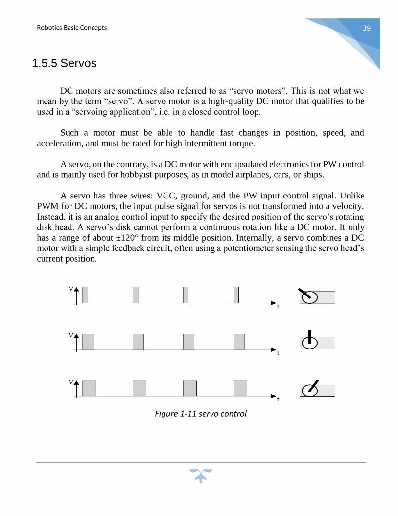
1.5.5 Servos

DC motors are sometimes also referred to as “servo motors”. This is not what we

mean by the term “servo”. A servo motor is a high-quality DC motor that qualifies to be

used in a “servoing application”, i.e. in a closed control loop.

Such a motor must be able to handle fast changes in position, speed, and

acceleration, and must be rated for high intermittent torque.

A servo, on the contrary, is a DC motor with encapsulated electronics for PW control

and is mainly used for hobbyist purposes, as in model airplanes, cars, or ships.

A servo has three wires: VCC, ground, and the PW input control signal. Unlike

PWM for DC motors, the input pulse signal for servos is not transformed into a velocity.

Instead, it is an analog control input to specify the desired position of the servo’s rotating

disk head. A servo’s disk cannot perform a continuous rotation like a DC motor. It only

has a range of about ±120° from its middle position. Internally, a servo combines a DC

motor with a simple feedback circuit, often using a potentiometer sensing the servo head’s

current position.

Figure 1-11 servo control


40

The PW signal used for servos always has a frequency of 50Hz, so pulses are

generated every 20ms. The width of each pulse now specifies the desired position of the

servo’s disk (Figure 3.10).

For example, a width of 0.7ms will rotate the disk to the leftmost position (–120°),

and a width of 1.7ms will rotate the disk to the rightmost position (+120°). Exact values of

pulse duration and angle depend on the servo brand and model.

Like stepper motors, servos seem to be a good and simple solution for robotics tasks.

However, servos have the same drawback as stepper motors: they do not provide any

feedback to the outside. When applying a certain PW signal to a servo, we do not know

when the servo will reach the desired position or whether it will reach it at all, for example

because of too high a load or because of an obstruction.

1.6 CRITERIA FOR SELECTION (6)

The committee spent a great deal of time developing criteria for the selection of

Army applications of robotics and artificial intelligence. These criteria were essential in

guiding the work of the committee; but beyond that, they are more broadly applicable to

future decisions by the Army as well as by others. The criteria for selecting applications

reflect both the immediate technological benefits and the attitudinal and managerial

considerations that will affect the ultimate widespread acceptance of the technology.

1.6.1 REASONS FOR APPLYING ROBOTICS AND

ARTIFICIAL INTELLIGENCE

The introduction of robotics and artificial intelligence technology into the Army can

result in a number of benefits, among them the following:

improved combat capabilities,

increased mission flexibility,

increased system reliability

reduced unit/life-cycle costs,

reduced manpower requirements,

Simplified training.


41

In selecting applications from the much larger list of possibilities, the committee not

only looked for opportunities to achieve those benefits but also sought affirmative answers

to the following questions:

Will it perform, in the near term, an essential task for the Army?

Can its initial version be implemented in 2 to 3 years?

Can it be readily upgraded as more sophisticated technology becomes available?

Does it tie in with existing, related programs, including programs of the other

services?

Will it use the best technology available in the scientific community?

These considerations should help to ensure initial acceptance and continuing success

with these

Promising developing technologies.

1.6.2 COMBINING SHORT-TERM AND LONG-TERM

OBJECTIVES

Initial short-term implementation should provide a basis for future upgrading and

growth as the user gains experience and confidence in working with equipment using

robotics and AI technology. To this end the Army's program should be carefully integrated

and include short term, achievable objectives with growth projected to meet long-term

requirements.

As a result; some of the applications chosen may at first appear to be implementable

in the short term by other existing technologies with lower cost and ease. However, such

short-term expediency may cause unwarranted and unintended delay in the ultimately more

cost-effective application of new developing robot technologies. To prevent this problem,

short-term applications should be

applied to existing, highly visible systems,

reasonably afforded within the Army's projected budget,

within the state of the art, requiring development and engineering rather than

invention or research,

able to demonstrate an effective solution to a critical Army need,

achievable within 2 to 3 years,

Not redundant with efforts in DARPA or the other services.


42

1.6.3 APPLICATIONS OF ROBOTICS AND ARTIFICIAL

INTELLIGENCE

On the other hand, the committee considered long-term applications to be important

vehicles for advancing research in these technologies and, in some cases, for introducing

useful applications of robotics and artificial intelligence. These more advanced

applications would ultimately, at reduced cost, assist in meeting the changing requirements

of the modern battlefield envisioned in the Army's Air Land Battle 2000 concept.

The principle that guided the committee's selection of applications, therefore, was

to combine short-term and long-term benefits; that is, to select applications that can be

implemented quickly to meet a current need and, in addition, can be upgraded over the next

10 years in ways that advance the state of the art and perform more complex functions for

the Army.

1.6.4 PLANNING FOR GROWTH

For the near term, using state of the art technology and assuming that a

demonstration program starts in 1 1/2 to 2 years and continues for 2 years, the committee

recommends that projects be selected based not only on what is commercially available

now but also on technology that is likely to become available within the next 2 years.

During the next 4 to 5 years, while the Army is developing its demonstration

systems, annual expenditures by university, industrial, government, and nonprofit

laboratories for R&D and for initial applications will probably exceed several hundred

million dollars per year worldwide. To be timely and cost effective, Army demonstration

systems should be designed in such a way that these developments can be incorporated

without discarding earlier versions.

It is therefore of the utmost importance to specify, at the outset, maximum feasible

computer processor (and memory) power for each application. Industry experience has

shown that the major deterrent to updating and improving performance and functions has

been the choice of the "smallest" processor to meet only the initial functional and

performance objectives.

It is at least as important to ensure that this growth potential be protected during

development of the initial applications both industry and the Army have known

programmers with a propensity to expand operating and other systems until they occupy

the entire capacity of design processor and memory.

Robot Control

43

Chapter.2 Robot Control

Although there are many possible ways use prismatic and revolute joints to construct

kinematic chains, in practice only a few of these are commonly used in industry

applications and prove its efficiency, one of them is scara robot which we going to study

how to calculate DH matrix for it and how to simulate the robot on matlab.

Robot Control

44

2.1 SCARA Manipulator (RRP)

Figure2-1 The SCARA (Selective Compliant Articulated Robot for Assembly).

The SCARA arm (for Selective Compliant Articulated Robot for Assembly) shown in

Figure 2.1 is a popular manipulator, which, as its name suggests, is tailored for assembly

operations. Although the SCARA has an RRP structure, it is quite different from the

spherical manipulator in both appearance and in its range of applications. Unlike the

spherical design, which has z0 perpendicular to z1, and z1 perpendicular to z2, the SCARA

has z0, z1, and z2 mutually parallel.

Robot Control

45

Figure2-2 Workspace of the SCARA manipulator.

2.2 Forward Kinematics:

2.2.1 Mathematical model:

The first problem encountered is to describe both the position of the tool and the

locations A and B (and most likely the entire surface S) with respect to a common

coordinate system.

Typically, the manipulator will be able to sense its own position in some manner using

internal sensors (position encoders located at joints 1 and 2) that can measure directly the

joint angles θ1 and θ2. We also need therefore to express the positions A and B in terms of

these joint angles. This leads to the forward kinematics problem studied in Chapter 3,

which is to determine the position and orientation of the end-effector or tool in terms of

the joint variables.

Robot Control

46

It is customary to establish a fixed coordinate system, called the world or base frame

to which all objects including the manipulator are referenced. In this case we establish the

base coordinate frame o0x0y0 at the base of the robot,

Figure 2-3 Coordinate frames for two-link planar robot.

As shown in Figure 2.3. The coordinates (x, y) of the tool are expressed in this

coordinate frame as

x = x2 = α1 cos θ1 + α2 cos (θ1 + θ2) (2.1)

y = y2 = α1 sin θ1 + α2 sin(θ1 + θ2) (2.2)

In which α1 and α2 are the lengths of the two links, respectively. Also the orientation of

the tool frame relative to the base frame is given by the direction cosines of the x2 and y2

axes relative to the x0 and y0 axes, that is,

x2 · x0 = cos (θ1 + θ2); x2 · y0 = − sin (θ1 + θ2)

y2 · x0 = sin(θ1 + θ2); y2 · y0 = cos(θ1 + θ2)

Which we may combine into an orientation matrix

(2.3)

Robot Control

47

Equations (2.1), (2.2) and (2.3) are called the forward kinematic equations for this

arm. For a six degree-of-freedom robot these equations are quite complex and cannot be

written down as easily as for the two-link manipulator.

Consider the SCARA manipulator of Figure 2.4. This manipulator, consists of an

RRP arm and a one degree-of-freedom wrist, whose motion is a roll about the vertical axis.

The first step is to locate and label the joint axes as shown. Since all joint axes are parallel

we have some freedom in the placement of the origins. The origins are placed as shown

for convenience. We establish the x0 axis in the plane of the page as shown. This is

completely arbitrary and only affects the zero configuration of the manipulator, that is, the

position of the manipulator when θ1 = 0.

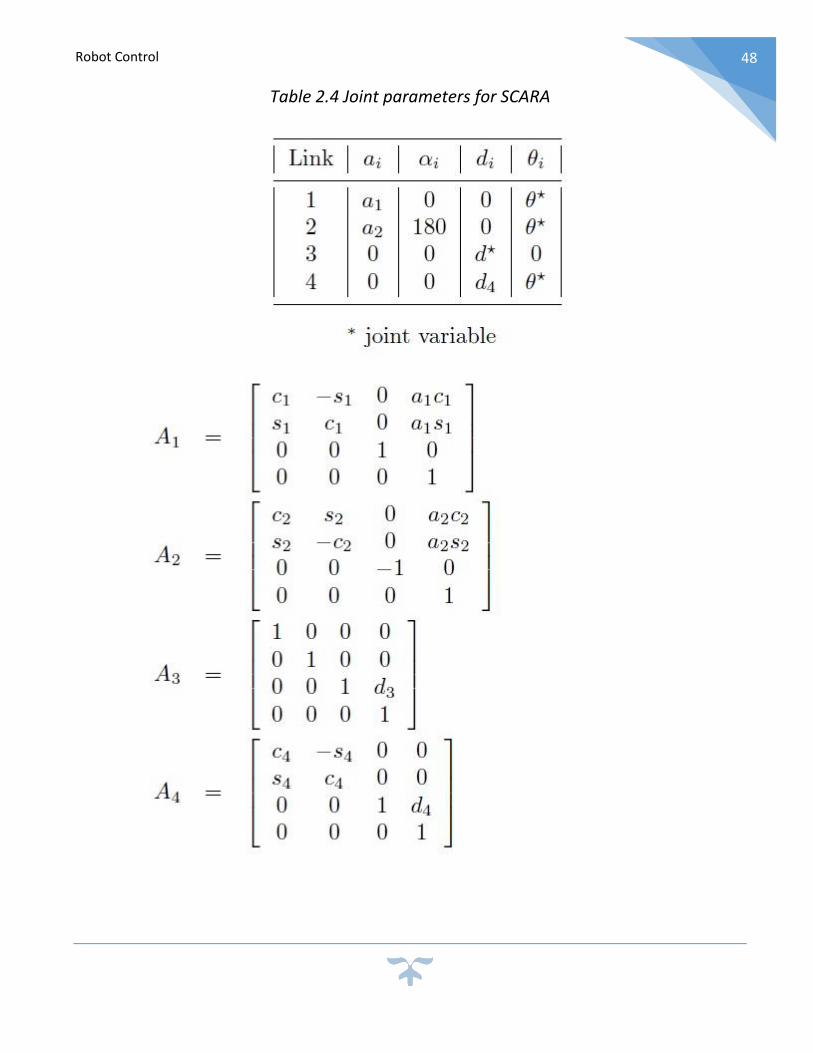
Figure2-4 DH coordinate frame assignment for the SCARA manipulator

The joint parameters are given in Table 3.5, and the A-matrices are as follows

Robot Control

48

Table 2.4 Joint parameters for SCARA

Robot Control

49

The forward kinematic equations are therefore given by:

2.2.2 Mat lab code for forward kinematics of scara robot:

Write this code on mat lab to calculate forward kinematics for scara robot:

function [R, O]=Forward_SCARA(theta,d3,d4,a1,a2)

th1=theta(0,90);

th2=theta(0,90);

th4=theta(0,90);

alpha=th1+th2-th4;

R=[cos(alpha),sin(alpha),0;sin(alpha),-cos(alpha),0;0,0,-1];

O=[((a1*cos(th1))+(a2*cos(th1+th2)));((a1*sin(th1))+(a2*sin(th1+th2))

);(-d3-d4)];

2.3 Inverse Kinematics

2.3.1 Mathematical model

Now, given the joint angles θ1, θ2 we can determine the end-effector coordinates x

and y. In order to command the robot to move to location a we need the inverse; that is, we

need the joint variables θ1, θ2 in terms of the x and y coordinates of A. This is the problem

of inverse kinematics. In other words, given x and y in the forward kinematic Equations

Robot Control

50

(2.1) and (2.2), we wish to solve for the joint angles. Since the forward kinematic equations

are nonlinear, a solution may not be easy to find, nor is there a unique solution in general.

We can see in the case of a two-link planar mechanism that there may be no solution,

for example if the given (x, y) coordinates are out of reach of the manipulator. If the given

(x, y) coordinates are within the manipulator’s reach there may be two solutions as shown

in Figure 2. 5 , the so-called elbow up and elbow down configurations, or there may be

exactly one solution if the manipulator must be fully extended to reach the point.

Figure2-5 Multiple inverse kinematic solutions.

There may even be an infinite number of solutions in some cases. Consider the diagram

of Figure 2.6.

Figure2-6 Solving for the joint angles of a two-link planar arm.

Robot Control

51

Using the Law of Cosines we see that the angle θ2 is given by:

We could now determine θ2 as

θ2 = cos−1 (D) (2.5)

However, a better way to find θ2 is to notice that if cos (θ2) is given by Equation

(2.4) then sin (θ2) is given as

Sin (θ2) = ±√1 − 𝐷2 (2.6)

And, hence, θ2 can be found by

θ2 = 𝑡𝑎𝑛−1 ±√1−𝐷2

𝐷 (2.7)

The advantage of this latter approach is that both the elbow-up and elbow down

solutions are recovered by choosing the positive and negative signs in Equation (2.7),

respectively.

Θ1 is now given as

θ2 = 𝑡𝑎𝑛−1 (𝑦

𝑥⁄ ) − 𝑡𝑎𝑛−1 (𝛼2𝑠𝑖𝑛θ2

𝛼1+ 𝛼2𝑐𝑜𝑠θ2) (2.8)

Notice that the angle θ1 depends on θ2. This makes sense physically since we

would expect to require a different value for θ1, depending on which solution is chosen

for θ2.

(2.4)

Robot Control

52

The inverse kinematics solution is then given as the set of solutions of the equation

𝑇41 = [

𝑅 00 1

]

= [

𝑐12𝑐4 + 𝑠12𝑠4 𝑠12𝑐4 − 𝑐12𝑠4 0 𝑎1𝑐1 + 𝑎2𝑐12

s12c4 − c12s4 −c12c4 − s12s4 0 a1s1 + a22s12

0 0 −1 −d3 − d4

0 0 0 1

] (2.9)

We first note that, since the SCARA has only four degrees-of-freedom, not every

possible H from SE (3) allows a solution of (2.9). In fact we can easily see that there is no

solution of (2.9) unless R is of the form

𝑅 = [𝑐𝛼 𝑠𝛼 0𝑠𝛼 −𝑐𝛼 00 0 −1

] (2.10)

And if this is the case, the sum θ1 + θ2 − θ4 is determined by

𝜃1 + 𝜃2 − 𝜃4 = 𝛼 = atan2 (𝑟11 , 𝑟12 ) (2.11)

Projecting the manipulator configuration onto the x0 − y0 plane immediately yields

the situation of Figure 2.17.

Robot Control

53

Figure2-7scara manipulator

We see from this that

𝜃2 = 𝑎𝑡𝑎𝑛2 (𝑐2, ±√1 − 𝑐2) (2.12)

Where

𝑐2 = 𝑜𝑥

2+ 𝑜𝑦2−𝑎1

2− 𝑎22

2𝑎1𝑎2 (2.13)

𝜃1 = 𝑎𝑡𝑎𝑛2 ( 𝑜𝑥, 𝑜𝑦) − 𝑎𝑡𝑎𝑛2 (𝑎1 + 𝑎2𝑐2, 𝑎2𝑠2) (2.14)

We may then determine θ4 from (2.11) as

𝜃4 = 𝜃1 + 𝜃2 − 𝛼 (2.15)

= 𝜃1 + 𝜃2 − 𝑎𝑡𝑎𝑛2 ( 𝑟11, 𝑟12)

Finally d3 is given as

Robot Control

54

𝑑3 = 𝑜𝑧 + 𝑑4 (2.16)

2.3.2 Mat lab code for Inverse Kinematics

Write this mat lab code to calculate inverse kinematics for scara robot:

function [theata, d3]=Inv_SCARA(O,R,a1,a2,d4)

alpha=atan2(R(1,2),R(1,1));

C2=((O(1,1)^2)+(O(2,1)^2)-(a1^2)-(a2^2))/(2*a1*a2);

S2=sqrt(1-(C2^2));

theata2=atan2(S2,C2);

theata1=(atan2(O(2,1),O(1,1)))-

atan2((a2*sin(theata2)),(a1+a2*cos(theata2)));

theata4=theata1+theata2-alpha;

theata1=(theata1*180/pi);



theata=[theata1,theata2,theata4];

d3=d1-O(3,1)-d4;

2.4 Why we use Mat lab?

The language provided by Sankyo (SSL/E language), is a very specific language with many

limitations. For instance, the possibility of modular programming are very limited, the

mathematics tools are not so powerful, and programming is quite uncomfortable.

Furthermore, the robot controller has hardware limitations in terms of I/0 communications

ports. These aspects can be resolved if the user could program the robot from a PC where

a more structured programming language like C, C++, Java, or Mat lab is installed. In this

case, an interpreter should perform a translation operation. As will be explained in this

Robot Control

55

document, the interpreter is a program written in the robot native language (SSL/E

language), which is running on the robot controller. The user who wants to control the

robot, will write an operative program in Mat lab that is installed on a PC of the lab.

Mat lab is a very versatile software environment developed by Math Works used in

many fields and it is known by almost every engineering student. The reasons that led the

choice of Mat lab instead of other high-level programming languages are:

easy communication with external devices via all the main communication protocols

(GPIB, serial, TCP/IP, and UDP) by using the Mat lab Instrument Control Toolbox

functions;

easy implementation of GUIs (Graphical User Interfaces);

possibility of developing a virtual model of the robot by using the Mat lab integrated

software Simulink;

easy image and video acquisition and processing by using the Mat lab Image

Acquisition Toolbox and Image Processing Toolbox;

control, simulation, and visual control integrated in the same software;

Mat lab Help, Math Works on-line support, and many examples of code on the

Internet make Mat lab programming suitable for didactic applications with the robot.

2.5 Full modeling of scara robot on mat lab:

To design full model of scara robot using mat lab to predict and calculate how scara

robot will move from point to another according to our given data which we will supply it

with, we need mat lab codes to:

1- Forward kinematic which is:

function [R, O]=Forward_SCARA(theta,d3,d4,a1,a2)

th1=theta(0,90);

th2=theta(0,90);

th4=theta(0,90);

alpha=th1+th2-th4;

R=[cos(alpha),sin(alpha),0;sin(alpha),-cos(alpha),0;0,0,-1];

O=[((a1*cos(th1))+(a2*cos(th1+th2)));((a1*sin(th1))+(a2*sin(th1+th2

)));(-d3-d4)];

Robot Control

56

2- Inverse kinematics which is:

function [theata, d3]=Inv_SCARA(O,R,a1,a2,d4)

alpha=atan2(R(1,2),R(1,1));

C2=((O(1,1)^2)+(O(2,1)^2)-(a1^2)-(a2^2))/(2*a1*a2);

S2=sqrt(1-(C2^2));

theata2=atan2(S2,C2);

theata1=(atan2(O(2,1),O(1,1)))-

atan2((a2*sin(theata2)),(a1+a2*cos(theata2)));

theata4=theata1+theata2-alpha;




theata=[theata1,theata2,theata4];

d3=d1-O(3,1)-d4;

3- Path planning which is:

function Path_PLaning(OI,OF,TH4) % function take as input initial and

% final position and orientation

a1=1;

a2=1;

d1=1; % definition of robot parameters

d2=.1;

d=.1;

L=.3;

Xi=OI(1,1);

Yi=OI(2,1); % definition of initial position

Zi=OI(3,1);

flag=0; % make signal flag to 0 value

Xf=OF(1,1);

Yf=OF(2,1); % definition of final position

Robot Control

57

Zf=OF(3,1);

if sqrt(((Xi)^2)+((Yi)^2))>2 % test of initial position in or out

% work space

fprintf('Out of work space')

flag=1; % if yes make signal flag=1

end

if sqrt(Xf^2+Yf^2)>2 % test of final position in or out

% work space


flag=1; % if yes make signal flag=1

end

if flag==0 % if flag=0 in this case we are in work

% space

[T1, T2 , ~, d3]=Scara_Inverse(Xi,Yi,Zi,d1,d2,a1,a2); %call function

%Scara_Inverse

% returning T1 T2 T4 d3

% for initial point

J=Jacobian(T1,T2); %call function jacobian to test

% singularity of initial point

J11=[J(1:3,1:3)];

S=det(J11);

if S==0

flag=1;

fprintf('Singularity')

end

[T1f, T2f, T4, d3]=Scara_Inverse(Xf,Yf,Zf,d1,d2,a1,a2); %call

function

%Scara_Inverse

% returning T1 T2 T4 d3

% for initial point

J=Jacobian(T1f,T2f); %call function jacobian to test

% singularity of final point

J11=[J(1:3,1:3)];

S=det(J11);

if S==0

flag=1;

fprintf('Singularity')

end

Robot Control

58

end

%

if flag==0

slope = (Yf-Yi)/(Xf-Xi); % we make calculation of slope of

% second portion of path

inc=.01;

for Z=0:inc:Zi % begin of first portion of path,

% make the value of inc=0.01

% in this portion we maintain the

% value of X and Y and the only

% variation is in Z axis

d3=d1-Z-d2;

SCARA_plot(T1,T2,T4,a1,a2,d1,d3,d2,L,d)

hold on

plot3([Xi Xi],[Yi Yi],[0 Zi],'red','linewidth',2) %plotting first

% portion of path

hold on

plot3([Xi Xf],[Yi Yf],[Zi Zi],'red','linewidth',2) %plotting second

% portion of path

hold on

plot3([Xf Xf],[Yf Yf],[Zi Zf],'red','linewidth',2) %plotting third

% portion of path

hold off

pause(.01)

end

if Xi>Xf % if the desired position is < the

% initial position we decrement xi by

% -0.01

inc=-.01;

else

inc=.01; % if the desired position is > the

% initial position we increment xi by

% +0.01

end

Robot Control

59

for X=Xi:inc:Xf % for any new value of X and Y we calculate

% [T1 T2 T4 d2] by call of function

% Scara_Inverse

Y=slope*(X-Xf)+Yf;

[T1, T2, T4, d3]=Scara_Inverse(X,Y,Zi,d1,d2,a1,a2);


% portion of path

hold on

plot3([Xi Xf],[Yi Yf],[Zi Zi],'red','linewidth',2)%plotting second

% portion of path

hold on


% portion of path

hold on

SCARA_plot(T1,T2,T4,a1,a2,d1,d3,d2,L,d) % ploting the motion of

% robot on the path

pause(.01)

end

inc=-.01; % begin of third portion of path,

% make the value of inc=-0.01

% in this portion we maintain the

% value of X and Y and the only

% variation is in Z axis

for Z=Zi:inc:Zf

d3=d1-Z-d2; % we go down by decrementing Zi


% robot on the path

hold on


% portion of path

hold on


% portion of

path

hold on

Robot Control

60


% portion of path

hold off

pause(.01)

end

for T4=0:1:TH4 % adjustement and orientation of end

% effector

hold on


% portion of path


% portion of path


% portion of path

hold off


% robot on the path

hold on


% portion of path


% portion of path


% portion of path

pause(.01)

end

hold off

end

4- Plotting scara robot which is:

function plotSCARA=SCARA_plot(T1,T2,T4,a1,a2,d1,d2,d3,L,d)

if T1<0;

T1=T1+360;

end

if T2<0;

Robot Control

61

T2=T2+360;

end

if T4<0;

T4=T4+360;

end

if T4>180

T4=T4-180;

end

%%%%%%%%for a1

X_1=a1*cosd(T1);

Y_1=a1*sind(T1);

plot3([0 X_1],[0 Y_1],[d1 d1],'b','linewidth',7)

%%%%%%%%for a2

X_2=X_1+(a2*cosd(T1+T2));

Y_2=Y_1+(a2*sind(T1+T2));

hold on

plot3([X_2 X_1],[Y_2 Y_1],[d1 d1],'r','linewidth',7)

%%%%%%%%%%%%%%%%%%% for d1

hold on

plot3([0 0],[0 0],[0 d1],'black','linewidth',8)

%%%%%%%%%%%%%%%%%%%%% for d2

hold on

plot3([X_2 X_2],[Y_2 Y_2],[d1 d1-d2],'black','linewidth',5)

% plot3([X_2 X_2],[Y_2 Y_2],[d1 d1+.4],'blue','linewidth',7) %

tube

%%%%%%%%%%%% End effector

hold on

if (T4 < 90)

XP=[min(X_2-(L/2)*cosd(T4),X_2+(L/2)*cosd(T4)),max(X_2-

(L/2)*cosd(T4),X_2+(L/2)*cosd(T4))];

YP=[min(Y_2-(L/2)*sind(T4),Y_2+(L/2)*sind(T4)),max(Y_2-

(L/2)*sind(T4),Y_2+(L/2)*sind(T4))];

plot3([XP(1),XP(2)],[YP(1),YP(2)],[d1-d2 d1-d2],'linewidth',5)

hold on

XP=[min(X_2-(d/2)*cosd(T4),X_2+(d/2)*cosd(T4)),max(X_2-

(d/2)*cosd(T4),X_2+(d/2)*cosd(T4))];

YP=[min(Y_2-(d/2)*sind(T4),Y_2+(d/2)*sind(T4)),max(Y_2-

(d/2)*sind(T4),Y_2+(d/2)*sind(T4))];

plot3([XP(1),XP(1)],[YP(1),YP(1)],[d1-d2 d1-d2-d3])

hold on


else

Robot Control

62

XP=[min(X_2-(L/2)*cosd(T4),X_2+(L/2)*cosd(T4)),max(X_2-

(L/2)*cosd(T4),X_2+(L/2)*cosd(T4))];

YP=[max(Y_2-(L/2)*sind(T4),Y_2+(L/2)*sind(T4)),min(Y_2-

(L/2)*sind(T4),Y_2+(L/2)*sind(T4))];

plot3([XP(1),XP(2)],[YP(1),YP(2)],[d1-d2 d1-d2],'linewidth',5)

hold on

XP=[min(X_2-(d/2)*cosd(T4),X_2+(d/2)*cosd(T4)),max(X_2-

(d/2)*cosd(T4),X_2+(d/2)*cosd(T4))];

YP=[max(Y_2-(d/2)*sind(T4),Y_2+(d/2)*sind(T4)),min(Y_2-

(d/2)*sind(T4),Y_2+(d/2)*sind(T4))];


hold on



hold on

end

% %%%%%%%%%%%%%%%%%%%% Joints

% hold on

% plot3([0 0],[0 0],[d1*.98 d1*1.02],'black','linewidth',5.5)

% figure

% plot([0 X_1],[0 Y_1])

% hold on

% plot([X_2 X_1],[Y_2 Y_1])

axis([-(a1+a2) (a1+a2) -(a1+a2) (a1+a2) 0 d1])

hold off

5- vr plotting of scara robot which is:

function plotVR=SCARA_VR_PLOT(T1,T2,T4,d4b,dist)

SCARA30 = vrworld('SCARA30.wrl');

open(SCARA30)

radian=T1*pi/180;

SCARA30.a1.rotation = [1, 0, 0, radian];

radian=-T2*pi/180;

SCARA30.a2.rotation = [1, 0, 0, radian];

radian=T4*pi/180;

SCARA30.d4b.rotation = [0, 1, 0, radian];

SCARA30.d4b.translation = [0, d4b, 0];

Robot Control

63

EndV1=SCARA30.EndV1.translation;

EndV2=SCARA30.EndV2.translation;

x1=EndV1(1);

x2=EndV2(1);

% y1=EndV1(2);

% y2=EndV2(2);

% sighn=sign([y1 y2]);

% y1f=.5*sighn(1)*dist

% y2f=.5*sighn(2)*dist

y1=-.5*dist;

y2=.5*dist;

SCARA30.EndV1.translation = [x1, y1, 0];

SCARA30.EndV2.translation = [x2, y2, 0];

6- Trajectory planning which is:

function Trajectory_PLaning(OI,OF,to,tf,TH4)

a1=1;

a2=1;

d1=1;

d2=.1;

d=.1;

L=.3;

Xi=OI(1,1);

Yi=OI(2,1);

Zi=OI(3,1);

flag=0;

Xf=OF(1,1);

Yf=OF(2,1);

Zf=OF(3,1);

Vo=0;

Vf=0;

ao=0;

af=0;

if sqrt(Xi^2+Yi^2)>2


flag=1;

end

if sqrt(Xf^2+Yf^2)>2

Robot Control

64


flag=1;

end

[q1i, q2i , ~, d3]=Scara_Inverse(Xi,Yi,Zi,d1,d2,a1,a2);

[q1f, q2f , ~, d3]=Scara_Inverse(Xf,Yf,Zi,d1,d2,a1,a2);

A=[1,to,((to)^2),((to)^3),((to)^4),((to)^5);

0,1,2*to,3*((to)^2),4*((to)^3),5*((to)^4);

0,0,2,6*to,12*((to)^2),20*((to)^3);

1,tf,((tf)^2),((tf)^3),((tf)^4),((tf)^5);

0,1,2*tf,3*((tf)^2),4*((tf)^3),5*((tf)^4);

0,0,2,6*tf,12*((tf)^2),20*((tf)^3)];

B1=[q1i;Vo;ao;q1f;Vf;af];

B2=[q2i;Vo;ao;q2f;Vf;af];

C1=inv(A)*B1;

C2=inv(A)*B2;

T=[];

Q1=[];

Q2=[];

X=[];

Y=[];

V1=[];

V2=[];

AC1=[];

AC2=[];

for t=to:.01:tf-.01

q1=C1(1,1)+C1(2,1)*t+C1(3,1)*t^2+

C1(4,1)*t^3+C1(5,1)*t^4+C1(6,1)*t^5;

q2=C2(1,1)+C2(2,1)*t+C2(3,1)*t^2+

C2(4,1)*t^3+C2(5,1)*t^4+C2(6,1)*t^5;

v1=C1(2,1)+(2*C1(3,1)*t)+

(3*C1(4,1)*t^2)+(4*C1(5,1)*t^3)+(5*C1(6,1)*t^4);

v2=C2(2,1)+(2*C2(3,1)*t)+

(3*C2(4,1)*t^2)+(4*C2(5,1)*t^3)+(5*C2(6,1)*t^4);

ac1=(2*C1(3,1))+ (6*C1(4,1)*t)+(12*C1(5,1)*t^2)+(20*C1(6,1)*t^3);

ac2=(2*C2(3,1))+ (6*C2(4,1)*t)+(12*C2(5,1)*t^2)+(20*C2(6,1)*t^3);

x=a1*cosd(q1)+a2*cosd(q1+q2);

y=a1*sind(q1)+a2*sind(q1+q2);

X=[X x];

Y=[Y y];

Q1=[Q1,q1];

Q2=[Q2,q2];

V1=[V1 v1];

Robot Control

65

V2=[V2 v2];

AC1=[AC1 ac1];

AC2=[AC2 ac2];

T=[T t];

end

SCARA30 = vrworld('SCARA30.wrl');

open(SCARA30)

view(SCARA30);

% plot(T,Q1)

% title('position of the First JOINT')

% figure

% plot(T,Q2)

% title('position of the Second JOINT')

% figure

% plot(T,V1)

% title('Velocity of the First JOINT')

% figure

% plot(T,V2)

% title('Velocity of the Second JOINT')

% figure

% plot(T,AC1)

% title('Accelaration of the First JOINT')

% figure

% plot(T,AC2)

% title('Accelaration of the Second JOINT')

figure

Zl=Zi*ones(1,length(X));

plot3(X,Y,Zl,'red','linewidth',2)

inc=.01;

for Z=0:inc:Zi

d3=d1-Z-d2;

SCARA_plot(Q1(1),Q2(1),0,a1,a2,d1,d3,d2,L,d)

SCARA_VR_PLOT(Q1(1),Q2(1),0,-d3,d)

hold on

plot3([Xi Xi],[Yi Yi],[0 Zi],'red','linewidth',2)


plot3([Xf Xf],[Yf Yf],[Zi Zf],'red','linewidth',2)

hold off

Robot Control

66

pause(.01)

end

Z=Zi*ones(1,length(X));

plot3(X,Y,Z,'red','linewidth',2)


for i=1:1:length(Q1)


hold on


hold on

plot3(X,Y,Z,'red','linewidth',2)

hold on

SCARA_plot(Q1(i),Q2(i),0,a1,a2,d1,d3,d2,L,d)

SCARA_VR_PLOT(Q1(i),Q2(i),0,-d3,d)

pause(.01)

hold off

end

inc=-.01;

for Z=Zi:inc:Zf

d3=d1-Z-d2;


hold on


hold on


SCARA_plot(Q1(length(Q1)),Q2(length(Q1)),0,a1,a2,d1,d3,d2,L,d)

SCARA_VR_PLOT(Q1(length(Q1)),Q2(length(Q1)),0,-d3,d)

pause(.01)

hold off

end

for T4=0:1:TH4


hold on


Robot Control

67

hold on


SCARA_plot(Q1(length(Q1)),Q2(length(Q1)),T4,a1,a2,d1,d3,d2,L,d)

SCARA_VR_PLOT(Q1(length(Q1)),Q2(length(Q1)),T4,-d3,d)

pause(.01)

end

hold off

end

The final result will be:

Write this code:

OI=[0.3 0.3 0.2]';

OF=[-1 -1 0.4]';

Angle=-20;

Trajectory_PLaning(OI,OF,0,5,Angle)

Then simulation will start with this results:

q1i =

-32.7527

q2i =

155.5054

T4 =

0

d3 =

0.7000

q1f =

-180

q2f =

90

T4 =

0

d3 =

0.7000

Robot Control

68

A =

1 0 0 0 0 0

0 1 0 0 0 0

0 0 2 0 0 0

1 5 25 125 625 3125

0 1 10 75 500 3125

0 0 2 30 300 2500

B1 =

-32.7527

0

0

-180.0000

0

0

B2 =

155.5054

0

0

90.0000

0

0

C1 =

-32.7527

0

0

-11.7798

3.5339

-0.2827

C2 =

155.5054

0

0

-5.2404

1.5721

-0.1258

inc =

0.0100

Robot Control

69

Figure 2-8 3D plotting for scara robot

Figure 2-9 Rendering of scara robot

Robot Control

70

Mechanical design

71

Chapter.3 Mechanical design

3.1 Programs used on mechanical design:

There are two main streams in mechanical engineering when it comes about software

they are:

CAD & CAM

CAD and CAM are having different applications CAD is for part designing or even a

machine designing and many other features and applications are from aerospace to show

making.

CAM is for generating NC programs for CNC machines so that a particularly modeled

part can be machined and can be used out in a tank, an aero plane or a satellite.

On the other hand the most powerful designing software are:

1. Inventor

2. Solid work

3. Catia

4. Pro engineer

There is small difference between inventor, solid work, and Catia:

1. Autodesk Inventor is easy to learn and use. But it is perfect for machine design kind of

work. No surfacing available in Inventor. Best suitable for Novice/Beginners for 3D

CAD.

2. Solid works is good & has surfacing option too, easy to learn also. Excellent tool to

work with great support. Best suitable for Moderate users with some basic CAD

knowledge.

Mechanical design

72

3. Catia- Best & one of the Complicated tools available out there. Best suitable for

advanced users. Mostly used in Automobile Design Industries. Highly complicated

profiles & models can be done.

The most commonly software on Egypt and all company use them on their design is

Inventor and solid work

Figure 3-1 comparison between inventor and solid work

We use Autodesk Inventor to finish our design for scara robot

3.2 Consideration before design robot:

Robots are designed to be highly accurate, precise and flexible machines. Robots in

general and SCARA robots in particular, are used as replacements for human operators.

This can be for a variety of reasons, but an important feature of using robots is that they

almost always do the job better than a human operator. In order to achieve this important

Mechanical design

73

goal, the robot needs to conform to certain minimum standards of performance. To give an

idea, some of the specifications of the Adept One XL SCARA robot are described below.

This particular robot was chosen because it enjoys wide commercial success.

The SCARA is a standard configuration among robots. Furthermore we did not design

the robot strictly for a specific application. Hence at the preliminary phase, we only had

the following points in mind:

The robot should be as light and rigid as possible, within our economic constraints.

Load capacity of 3 kg.

A reach of 0.5 m.

A control resolution of 0.5 mm.

Maximum tip velocity of.

Maximum tip acceleration of.

Also, we intend the robot to be used for more than just assembly tasks. This necessitates

analog control of the prismatic axis. Hence, against the industrial norm of using pneumatic

actuators, we opted for a ball-screw as the joint actuator.

3.3 Material selection

Economy was the prime concern here. The material selected should be low in cost (per

kg basis), readily available in the desired shapes and sizes and the procurement time and

procurement cost should be low. We initially had a choice of two materials, wood and Mild

Steel. Wood provides the necessary rigidity at a low weight. And low cost than MS, beside

it do same function of MS for this prototype.

Scara robot parts:

Our robot consists of 4 parts:

1- Base

2- Forearm

3- Top

4- Shaft

Mechanical design

74

Figure 3-2 base

Figure 3-3section on base

Mechanical design

75

Figure 3-4 forearm

Figure 3-5 section on forearm

Mechanical design

76

Figure 3-6 top

Figure 3-7 section on top

Mechanical design

77

Figure 3-8 full design

Mechanical design

78

Figure 3-9 full design 3d

Microcontroller

79

Chapter.4 Microcontroller

Figure 4-1 microcontroller

Microcontrollers are hidden inside a surprising number of products these days. If your

microwave oven has an LED or LCD screen and a keypad, it contains a microcontroller.

All modern automobiles contain at least one microcontroller, and can have as many as six

or seven: The engine is controlled by a microcontroller, as are the anti-lock brakes,

the cruise control and so on. Any device that has a remote control almost certainly contains

a microcontroller: TVs, VCRs and high-end stereo systems all fall into this category.

Nice SLR and digital cameras, cell phones, camcorders, answering machines, laser

printers, telephones (the ones with caller ID, 20-number memory, etc.), pagers, and feature-

laden refrigerators, dishwashers, washers and dryers (the ones with displays and

keypads)... You get the idea. Basically, any product or device that interacts with its user

has a microcontroller buried inside. (7)

http://electronics.howstuffworks.com/led.htm

http://electronics.howstuffworks.com/lcd.htm

http://auto.howstuffworks.com/engine.htm

http://auto.howstuffworks.com/auto-parts/brakes/brake-types/anti-lock-brake.htm

http://auto.howstuffworks.com/cruise-control.htm

http://electronics.howstuffworks.com/tv.htm

http://electronics.howstuffworks.com/vcr.htm

http://electronics.howstuffworks.com/camera.htm

http://electronics.howstuffworks.com/cameras-photography/digital/digital-camera.htm

http://electronics.howstuffworks.com/cell-phone.htm

http://electronics.howstuffworks.com/camcorder.htm

http://electronics.howstuffworks.com/question21.htm

http://computer.howstuffworks.com/laser-printer.htm

http://computer.howstuffworks.com/laser-printer.htm

http://electronics.howstuffworks.com/telephone.htm

http://home.howstuffworks.com/refrigerator.htm

http://home.howstuffworks.com/washer.htm

http://home.howstuffworks.com/dryer.htm

Microcontroller

80

4.1 What is microcontroller?

A microcontroller is a computer. All computers -- whether we are talking about a

personal desktop computer or a large mainframe computer or a microcontroller -- have

several things in common:

All computers have a CPU (central processing unit) that executes programs. If you

are sitting at a desktop computer right now reading this article, the CPU in that

machine is executing a program that implements the Web browser that is displaying

this page.

The CPU loads the program from somewhere. On your desktop machine, the

browser program is loaded from the hard disk.

The computer has some RAM (random-access memory) where it can store

"variables."

And the computer has some input and output devices so it can talk to people. On

your desktop machine, the keyboard and mouse are input devices and

the monitor and printer are output devices. A hard disk is an I/O device -- it handles

both input and output.

The desktop computer you are using is a "general purpose computer" that can run any of

thousands of programs. Microcontrollers are "special purpose computers."

Microcontrollers do one thing well. There are a number of other common characteristics

that define microcontrollers. If a computer matches a majority of these characteristics, then

you can call it a "microcontroller":

Microcontrollers are "embedded" inside some other device (often a consumer

product) so that they can control the features or actions of the product. Another name

for a microcontroller, therefore, is "embedded controller."

Microcontrollers are dedicated to one task and run one specific program. The

program is stored in ROM (read-only memory) and generally does not change.

Microcontrollers are often low-power devices. A desktop computer is almost

always plugged into a wall socket and might consume 50 watts of electricity. A

battery-operated microcontroller might consume 50 mill watts.

A microcontroller has a dedicated input device and often (but not always) has a

small LED or LCD display for output. A microcontroller also takes input from the

device it is controlling and controls the device by sending signals to different

components in the device. For example, the microcontroller inside a TV takes input

from the remote control and displays output on the TV screen. The controller

controls the channel selector, the speaker system and certain adjustments on the

picture tube electronics such as tint and brightness. The engine controller in a car

http://computer.howstuffworks.com/pc.htm

http://computer.howstuffworks.com/10-types-of-computers.htm

http://computer.howstuffworks.com/microprocessor.htm

http://computer.howstuffworks.com/hard-disk.htm

http://computer.howstuffworks.com/ram.htm

http://computer.howstuffworks.com/keyboard.htm

http://computer.howstuffworks.com/mouse.htm

http://computer.howstuffworks.com/monitor.htm

http://computer.howstuffworks.com/inkjet-printer.htm

http://computer.howstuffworks.com/rom.htm

http://electronics.howstuffworks.com/inside-rc.htm

http://electronics.howstuffworks.com/speaker.htm

http://auto.howstuffworks.com/under-the-hood/trends-innovations/car-computer1.htm

Microcontroller

81

takes input from sensors such as the oxygen and knock sensors and controls things

like fuel mix and spark plug timing. A microwave oven controller takes input from

a keypad, displays output on an LCD display and controls a relay that turns the

microwave generator on and off.

A microcontroller is often small and low cost. The components are chosen to

minimize size and to be as inexpensive as possible.

A microcontroller is often, but not always, ruggedized in some way. The

microcontroller controlling a car's engine, for example, has to work in temperature

extremes that a normal computer generally cannot handle. A car's microcontroller in

Alaska has to work fine in -30 degree F (-34 C) weather, while the same

microcontroller in Nevada might be operating at 120 degrees F (49 C). When you

add the heat naturally generated by the engine, the temperature can go as high as

150 or 180 degrees F (65-80 C) in the engine compartment. On the other hand, a

microcontroller embedded inside a VCR hasn't been ruggedized at all.

The actual processor used to implement a microcontroller can vary widely. For

example, the cell phone shown on Inside a Digital Cell Phone contains a Z-80 processor.

The Z-80 is an 8-bit microprocessor developed in the 1970s and originally used in home

computers of the time. The Garmin GPS shown in How GPS Receivers Work contains a

low-power version of the Intel 80386, I am told. The 80386 was originally used in desktop

computers.

In many products, such as microwave ovens, the demand on the CPU is fairly low and

price is an important consideration. In these cases, manufacturers turn to dedicated

microcontroller chips -- chips that were originally designed to be low-cost, small, low-

power, embedded CPUs. The Motorola 6811 and Intel 8051 are both good examples of

such chips. There is also a line of popular controllers called "PIC microcontrollers" created

by a company called Microchip. By today's standards, these CPUs are incredibly

minimalistic; but they are extremely inexpensive when purchased in large quantities and

can often meet the needs of a device's designer with just one chip.

A typical low-end microcontroller chip might have 1,000 bytes of ROM and 20 bytes of

RAM on the chip, along with eight I/0 pins. In large quantities, the cost of these chips can

sometimes be just pennies. You certainly are never going to run Microsoft Word on such

a chip -- Microsoft Word requires perhaps 30 megabytes of RAM and a processor that can

run millions of instructions per second. But then, you don't need Microsoft Word to control

a microwave oven, either. With a microcontroller, you have one specific task you are trying

to accomplish, and low-cost, low-power performance is what is important. (7)

http://home.howstuffworks.com/microwave.htm

http://electronics.howstuffworks.com/relay.htm

http://auto.howstuffworks.com/engine.htm

http://electronics.howstuffworks.com/inside-cell-phone.htm

http://www.geocities.com/SiliconValley/Peaks/3938/z80arki.htm

http://electronics.howstuffworks.com/gadgets/travel/gps.htm

http://www.cs.ucr.edu/~dalton/i8051/

http://www.microchip.com/

http://computer.howstuffworks.com/bytes.htm

Microcontroller

82

4.2 Types of microcontroller:

The most famous microcontroller used this days is:

1- Pic microcontroller

2- Arduino

1- Pic microcontroller

Figure 4-2 pic microcontroller

PIC microcontrollers are a family of specialized microcontroller chips produced by

Microchip Technology in Chandler, Arizona. The acronym PIC stands for "peripheral

interface controller," although that term is rarely used nowadays. A microcontroller is a

compact microcomputer designed to govern the operation of embedded systems in motor

vehicles, robots, office machines, medical devices, mobile radios, vending machines, home

appliances, and various other devices. A typical microcontroller includes a processor,

memory, and peripherals.

The PIC microcontrollers appeal to hobbyists and experimenters, especially in the

fields of electronics and robotics. Key features include wide availability, low cost, ease of

reprogramming with built-in EEPROM (electrically erasable programmable read-only

memory), an extensive collection of free application notes, abundant development tools,

and a great deal of information available on the Internet. The PIC microcontrollers often

appear under the brand name PIC micro.

http://whatis.techtarget.com/definition/microcontroller

http://whatis.techtarget.com/definition/microcomputer

http://whatis.techtarget.com/definition/microcomputer

http://searchenterpriselinux.techtarget.com/definition/embedded-system

http://searchcio-midmarket.techtarget.com/definition/robot

http://searchcio-midmarket.techtarget.com/definition/processor

http://searchmobilecomputing.techtarget.com/definition/memory

http://searchmobilecomputing.techtarget.com/definition/peripheral

http://searchcio-midmarket.techtarget.com/definition/EEPROM

Microcontroller

83

Every PIC microcontroller has a set of registers that also function as RAM (random

access memory). Special purpose control registers for on-chip hardware resources are also

mapped into the data space. Every PIC has a stack that saves return addresses. The stack

was not software-accessible on the earlier versions of the PIC, but this limitation was

removed in later devices.

2- Arduino

Figure 4-3 Arduino

Arduino is a tool for making computers that can sense and control more of the physical

world than your desktop computer. It's an open-source physical computing platform based

on a simple microcontroller board, and a development environment for writing software

for the board.

Arduino can be used to develop interactive objects, taking inputs from a variety of

switches or sensors, and controlling a variety of lights, motors, and other physical outputs.

Arduino projects can be stand-alone, or they can communicate with software running on

your computer (e.g. Flash, Processing, and Max MSP.) The boards can be assembled by

hand or purchased preassembled; the open-source IDE can be downloaded for free.

The Arduino programming language is an implementation of Wiring, a similar physical

computing platform, which is based on the Processing multimedia programming

environment.

http://whatis.techtarget.com/definition/register

http://searchmobilecomputing.techtarget.com/definition/RAM

http://searchcio-midmarket.techtarget.com/definition/stack

http://searchsoa.techtarget.com/definition/software

Microcontroller

84

There are many other microcontrollers and microcontroller platforms available for

physical computing. Parallax Basic Stamp, Net media’s BX-24, Phidgets, MIT's Handy

board, and many others offer similar functionality. All of these tools take the messy details

of microcontroller programming and wrap it up in an easy-to-use package. Arduino also

simplifies the process of working with microcontrollers, but it offers some advantage for

teachers, students, and interested amateurs over other systems:

Inexpensive - Arduino boards are relatively inexpensive compared to other

microcontroller platforms. The least expensive version of the Arduino module can be

assembled by hand, and even the pre-assembled Arduino modules cost less than $50

Cross-platform - The Arduino software runs on Windows, Macintosh OSX, and Linux

operating systems. Most microcontroller systems are limited to Windows.

Simple, clear programming environment - The Arduino programming environment is

easy-to-use for beginners, yet flexible enough for advanced users to take advantage of

as well. For teachers, it's conveniently based on the Processing programming

environment, so students learning to program in that environment will be familiar with

the look and feel of Arduino

Open source and extensible software- The Arduino software is published as open

source tools, available for extension by experienced programmers. The language can

be expanded through C++ libraries, and people wanting to understand the technical

details can make the leap from Arduino to the AVR C programming language on which

it's based. Similarly, you can add AVR-C code directly into your Arduino programs if

you want to.

Open source and extensible hardware - The Arduino is based on

Atmel's ATMEGA8 and ATMEGA168 microcontrollers. The plans for the modules

are published under a Creative Commons license, so experienced circuit designers can

make their own version of the module, extending it and improving it. Even relatively

inexperienced users can build the breadboard version of the module in order to

understand how it works and save money.

For this reason we choose to work with Arduino on our project “scara robot”

Microcontroller

85

4.3 Program used on scara robot

Our scara robot contains of 3 servo motors ( 2 servo motor for joints and one for effect

hand ) and one stepper motor so when we use Arduino we need to write code that contain

of three basic steps :

1- Move joints ( scara robot ) to reach destination

2- Move shaft (stepper motor ) to enable effect hand pick or left subjects

3- Move effect hand ( servo motor ) to hold subject or release it

And they should move by order not before or after,

First we write code for joints to move to specific location, the code is:

#include <Servo.h> Servo myservo; Servo mservo; int pos = 0; int ps=0; void setup() { myservo.attach(9); mservo.attach(5); } void loop() { for(pos = 0; pos <= 180; pos += 1) { myservo.write(pos); delay(10); } delay(1000); for(ps = 0; ps<=100; ps+=1) { mservo.write(ps); delay(15); } delay(1000); for(ps = 100; ps >=0; ps -= 1) { mservo.write(ps); delay(15); } delay(1000);

Microcontroller

86

for(pos = 180; pos>=0; pos-=1) { myservo.write(pos); delay(10); } delay(3000); }

Then it turn of shaft to move up and down to enable hand effect to hold subject, on

this code we make something different by giving pulses to stepper motor instead of

let Arduino did it, and it works effectively and give us best results than normal code,

code for shaft is:

#include <Stepper.h> const int stepsPerRevolution = 200; Stepper myStepper(stepsPerRevolution, 8,9,10,11); void setup() { myStepper.setSpeed(60); Serial.begin(9600); } void loop() { Serial.println("clockwise"); myStepper.step(stepsPerRevolution); delay(500); Serial.println("counterclockwise"); myStepper.step(-stepsPerRevolution); delay(500); }

Last move will made by effect hand to hold subjects or left it, this code is: #include <Servo.h> Servo myservo; int pos = 0; void setup() { myservo.attach(9); } void loop() { for(pos = 0; pos <= 180; pos += 1) { myservo.write(pos);

Microcontroller

87

delay(15); } for(pos = 180; pos>=0; pos-=1) { myservo.write(pos); delay(15); } }

Movement at this sequence will be repeated for pick and left subjects from one place

to another.

Conclusion

88

Conclusion

Manufacturing robots are quit complicated industry, it develop every day and new

generation appears with more enhancement to make work on hard environment is easier.

We produce away to manufacture scara robot includes its programming and simulation on

mat lab and how we calculate DH matrix for it then mechanical design on inventor and we

finish with controlling scara robot with Arduino.

We are of the belief that real engineers should have wide interdisciplinary knowledge,

this project involved a substantial amount of mechanical, electronics, computer and control

engineering. Tackling it has exponentially increased our knowledge base.

Both of us are fascinated by machine automation and robotics, and making our very

own robot has been a long standing dream. It is gratifying to see it converted to reality,

working on the robot has been a source of joy and inspiration to us throughout the year, so

much so, that we are almost sorry that the project is over. It was one of those rare instances,

where not only the result, but also the process was a source of continued pleasure.

However, in conclusion, we can only say that building the robot tested our design skills

to the limit. Its success, therefore, is our greatest reward.

References

89

References

1- Anon., n.d. robotics. [Online]

Available at: http://www.robotbasics.com/robot-arm-configurations

[Accessed 4 2015].

2- BERGREN, C. M., 2003. ANATOMY OF A ROBOT. s.l.:s.n.

3- Bräunl, T., 1998. EMBEDDED ROBOTICS Mobile Robot Design and Applications

with Embedded Systems. s.l.:s.n.

4- FRADEN, J., 2004. HANDBOOK OF MODERN SENSORS PHYSICS, DESIGNS, and

APPLICATIONS. clifornia : s.n.

5- Mark W. Spong, S. H. a. M. V., n.d. Robot modeling and control. first ed. s.l.:s.n.

6- Wallén, J., 2008. The history of the industrial robot, s.l.: s.n.

7- Brain, M., 2000. how stuff works. [Online]

Available at: http://electronics.howstuffworks.com/microcontroller.htm

[Accessed 1 june 2015].

References

90

References

91

Notes

92

Notes

design, implementation and control of scara robot

Documents

Transcript of design, implementation and control of scara robot