Design and simulation of a small cold storage with NH3 ...
174
Tom André Bredesen NTNU Norwegian University of Science and Technology Faculty of Engineering Department of Energy and Process Engineering Master’s thesis Tom André Bredesen Design and simulation of a small cold storage with NH 3 refrigeration system and CO 2 as indirect cooling loop for storing of fresh fruits and vegetables Master’s thesis in Energy and Environmental Engineering Supervisor: Trygve Magne Eikevik July 2019
-
Upload
khangminh22 -
Category
Documents
-
view
0 -
download
0
Transcript of Design and simulation of a small cold storage with NH3 ...

Tom A
ndré Bredesen
NTN
UN
orw
egia
n U
nive
rsity
of S
cien
ce a
nd T
echn
olog
yFa
cult
y of
Eng
inee
ring
Dep
artm
ent o
f Ene
rgy
and
Pro
cess
Eng
inee
ring
Mas
ter’
s th
esis
Tom André Bredesen
Design and simulation of a small coldstorage with NH3 refrigeration systemand CO2 as indirect cooling loop forstoring of fresh fruits and vegetables
Master’s thesis in Energy and Environmental EngineeringSupervisor: Trygve Magne Eikevik
July 2019


Tom André Bredesen
Design and simulation of a small coldstorage with NH3 refrigeration systemand CO2 as indirect cooling loop forstoring of fresh fruits and vegetables
Master’s thesis in Energy and Environmental EngineeringSupervisor: Trygve Magne EikevikJuly 2019
Norwegian University of Science and TechnologyFaculty of EngineeringDepartment of Energy and Process Engineering


Preface
Preface
This Master Thesis has been completed at the Norwegian University of Science and Tech-
nology during the spring semester of 2019. In relation to the thesis, a stay at the Indian
Institute of Technology Kharagpur in India from 22.01.2019 to 05.04.2019 was performed.
The thesis consists of a literature study on Indian food cold chains and refrigeration sys-
tems, in addition to an investigation of typical existing food products and cold chains.
The results of a survey conducted at IIT Kharagpur is presented and a thesis problem
statement is decided. The use of a small cold storage for fruits and vegetables at the
Indian mandis is investigated. The refrigeration systems considered and compared are a
single stage NH3 refrigeration system with and without a CO2 based natural circulation
loop.
The Master Thesis is done in cooperation with SINTEF Ocean and IIT Kharagpur, as a
part of the Re-FOOD project, which is an international partnership between Norway and
India to strengthen the global bioeconomy.
I wish to extend a huge thank you to my supervisor, Prof. Trygve Magne Eikevik, for the
help provided. My co-supervisor, Dr. Ignat Tolstorebrov, deserves a thank for the tech-
nical assistance. I would also like to extend a thank to my supervisor at IIT Kharagpur,
Prof. Maddali Ramgopal, for assisting me with my work in India. Dr. Kristina Norne
Widell also deserves a thank for assisting me with supporting material and guidance prior
to travelling to India. A great thank to Prof. Armin Hafner and Norsk Kjøleteknisk
Forening is also extended, for trusting me with the Gustav Lorentzen Grant to support
my stay in India. At last, I would like to show gratitude to all who assisted me with my
thesis and my stay at IIT Kharagpur.
Simulation models were made and some key results are presented.
Tom Andre Bredesen
I
Abstract
Abstract
The objective of this Master Thesis is to investigate Indian food cold chains for fruits
and vegetables and try to improve the cold chains with a small cold storage using a
NH3 refrigeration system with CO2 in a Natural Circulation Loop (NCL). Performance
of the NH3 system with and without the NCL are compared. The fruits investigated are
mangoes, grapes, apples, oranges and bananas. The vegetables investigated are potatoes,
onions, tomatoes, cauliflowers, cabbages and okras. By studying how the monthly average
wholesale prices for each product change, apples, mangoes and grapes are considered most
suited for storage in terms of storage life and expected profit. The domestic and export
cold chain, and the commodity flow through the Indian mandis, are investigated. The
main findings are that lack of refrigerated transport and pre-cooling are major challenges
in both cold chains. The domestic cold chain additionally need about twice the current
cold storage capacity. The high number of intermediates in the mandis flow chain are
highlighted as an issue, in addition to the total absence of refrigeration and cold storages.
The Indian mandis is considered the weakest link and a cold storage is designed for use
at mandis’ or small markets. The results from a field investigation at IIT Kharagpur in
India confirms the discussed conditions.
To design the evaporator, an I,x-diagram for moist air is used to decide maximum tem-
perature difference and the resulting heat transfer area is 64.8 m2. After investigating the
effects of changing temperature difference in the intermediate heat exchanger (IHX), the
resulting area is set to 0.97 m2. To model the NCL, pressure losses through the entire loop
are calculated. All investigated heights and circulation rates result in a positive driving
force. For practical reasons, a height of 1 m and circulation rate of 2 are chosen. Refrig-
eration loads through an entire year are used to estimate the performance of the systems.
The standard system operates with an average SCOP of about 6.5 during one year, while
the NCL system operates with an average SCOP of about 5.6. Annual operating profits
are estimated to be between 474 thousand and 479 thousand INR, depending on system
configuration and electricity rate. In conclusion, both system solutions are considered
competitive and feasible.
II

Abstrakt
Abstrakt
Malet med denne Masteroppgaven er a studere indiske kuldekjeder for frukt og grønnsaker,
for a foresla hvordan disse kan forbedres med et lite kuldelager som benytter seg av et
NH3 kjølesystem med CO2 i ei naturlig sirkulasjonsløkke (NCL). Driftsytelse for NH3 sys-
temet med, og uten, NCLen sammenlignes. De undersøkte fruktene er mango, drue, eple,
appelsin og banan. De undersøkte grønnsakene er potet, løk, tomat, blomkal, hodekal
og okra. Ved a studere hvordan den manedlige markedsprisen for hvert produkt en-
drer seg, samtidig som mulig lagringstid og profitt tas i betraktning, blir eple, mango
og druer vurdert som mest gunstige for kjølelagring. Kuldekjeden for innenlands salg
og eksport, i tillegg til produktstrømmen gjennom den indiske mandien, er undersøkt.
Hovedfunnene er at mangel pa termobiler og forkjøling av mat er de største utfordrin-
gene i begge kuldekjedene. I tillegg er det behov for omtrent dobbel kapasitet av dagens
kjølelagre i innenlands kuldekjeder. Antallet mellommenn og ledd i produktstrømmen
gjennom mandien fremheves som et stort problem, i tillegg til den enorme mangelen pa
kjøling og kuldelagre. Den indiske mandien vurderes til a være det svakeste leddet og et
kuldelager for bruk pa mandiene eller andre sma marked blir designet. Resultater fra en
undersøkelse utført pa IIT Kharagpur i India bekrefter mange av de diskuterte forholdene.
Nar fordamperen designes, blir et I,x-diagram for fuktig luft brukt til a bestemme den
maksimale temperaturforskjellen. Det resulterende varmeoverføringsarealet er 64.8 m2.
Ved a undersøke virkningene av endret temperaturforskjell i den mellomliggende varmevek-
sleren (IHX), blir det resulterende arealet satt til 0.97 m2. For a modellere NCLen blir
trykktapene gjennom hele løkka beregnet. Alle undersøkte høyder og sirkulasjonsrater
resulterer i en positiv drivkraft. Av praktiske grunner blir en høyde pa 1 m og en sirku-
lasjonsrate pa 2 valgt. For a beregne driftsytelsen til systemene, blir kjølelasten gjennom
hele aret beregnet og brukt. Standardsystemet forventes a operere med en gjennomsnittlig
SCOP pa omtrent 6.5 gjennom et helt ar, mens NCL-systemet forventes a operere med en
gjennomsnittlig SCOP pa omtrent 5.6. Arlig driftsprofitt for kjølelageret er beregnet til a
være mellom 474 tusen og 479 tusen INR, avhengig av systemkonfigurasjon og strømpris.
Det konkluderes med at begge systemløsninger er konkurransedyktige og gjennomførbare.
III

Contents
Contents
Preface I
Abstract II
Abstrakt III
Contents IV
List of Figures VII
List of Tables X
Nomenclature XIII
Abbreviations XVI
1 Introduction 1
1.1 Background and motivation . . . . . . . . . . . . . . . . . . . . . . . . . . 2
1.2 Problem description . . . . . . . . . . . . . . . . . . . . . . . . . . . . . . . 4
2 Literature: Cold chains and refrigerants 5
2.1 Food temperature control . . . . . . . . . . . . . . . . . . . . . . . . . . . 5
2.2 Indian food cold chain . . . . . . . . . . . . . . . . . . . . . . . . . . . . . 6
2.3 Refrigerants in India . . . . . . . . . . . . . . . . . . . . . . . . . . . . . . 8
2.4 NH3 refrigeration systems . . . . . . . . . . . . . . . . . . . . . . . . . . . 9
2.5 CO2 as secondary refrigerant . . . . . . . . . . . . . . . . . . . . . . . . . . 11
3 Horticulture in India 13
3.1 Highlights . . . . . . . . . . . . . . . . . . . . . . . . . . . . . . . . . . . . 13
3.2 Background . . . . . . . . . . . . . . . . . . . . . . . . . . . . . . . . . . . 14
3.3 Fruits . . . . . . . . . . . . . . . . . . . . . . . . . . . . . . . . . . . . . . 15
3.4 Vegetables . . . . . . . . . . . . . . . . . . . . . . . . . . . . . . . . . . . . 25
3.5 Storage conditions . . . . . . . . . . . . . . . . . . . . . . . . . . . . . . . 38
IV

Contents
4 The Indian scenario 42
4.1 Highlights . . . . . . . . . . . . . . . . . . . . . . . . . . . . . . . . . . . . 42
4.2 Export cold chain . . . . . . . . . . . . . . . . . . . . . . . . . . . . . . . . 44
4.3 Domestic cold chain . . . . . . . . . . . . . . . . . . . . . . . . . . . . . . . 46
4.4 The Indian mandis . . . . . . . . . . . . . . . . . . . . . . . . . . . . . . . 48
4.5 Field investigation at IIT Kharagpur . . . . . . . . . . . . . . . . . . . . . 49
4.6 Cold storage at Indian mandis . . . . . . . . . . . . . . . . . . . . . . . . . 56
4.6.1 Layout . . . . . . . . . . . . . . . . . . . . . . . . . . . . . . . . . . 57
4.6.2 Revenue . . . . . . . . . . . . . . . . . . . . . . . . . . . . . . . . . 60
4.6.3 Assumptions . . . . . . . . . . . . . . . . . . . . . . . . . . . . . . . 64
5 Method 67
5.1 Highlights . . . . . . . . . . . . . . . . . . . . . . . . . . . . . . . . . . . . 67
5.2 Refrigeration load calculation . . . . . . . . . . . . . . . . . . . . . . . . . 67
5.2.1 Transmission loads . . . . . . . . . . . . . . . . . . . . . . . . . . . 67
5.2.2 Infiltration loads . . . . . . . . . . . . . . . . . . . . . . . . . . . . 68
5.2.3 Product loads . . . . . . . . . . . . . . . . . . . . . . . . . . . . . . 69
5.2.4 Equipment loads . . . . . . . . . . . . . . . . . . . . . . . . . . . . 70
5.2.5 Safety factor . . . . . . . . . . . . . . . . . . . . . . . . . . . . . . . 71
5.3 Refrigeration cycle calculations . . . . . . . . . . . . . . . . . . . . . . . . 71
5.4 Heat exchanger calculations . . . . . . . . . . . . . . . . . . . . . . . . . . 73
5.5 Natural circulation loop pressure loss . . . . . . . . . . . . . . . . . . . . . 74
5.5.1 Static pressure loss . . . . . . . . . . . . . . . . . . . . . . . . . . . 74
5.5.2 Head loss . . . . . . . . . . . . . . . . . . . . . . . . . . . . . . . . 75
6 Results and discussion 78
6.1 Highlights . . . . . . . . . . . . . . . . . . . . . . . . . . . . . . . . . . . . 78
6.2 Refrigeration load . . . . . . . . . . . . . . . . . . . . . . . . . . . . . . . . 80
6.3 Heat exchangers . . . . . . . . . . . . . . . . . . . . . . . . . . . . . . . . . 84
6.3.1 Evaporator . . . . . . . . . . . . . . . . . . . . . . . . . . . . . . . 84
6.3.2 Intermediate Heat Exchanger (IHX) . . . . . . . . . . . . . . . . . . 86
6.4 Natural circulation loop . . . . . . . . . . . . . . . . . . . . . . . . . . . . 88
6.4.1 Gas quality out of CO2 heat source . . . . . . . . . . . . . . . . . . 88
6.4.2 Optimal height and circulation rate . . . . . . . . . . . . . . . . . . 89
6.4.3 Natural Circulation Loop (NCL) performance . . . . . . . . . . . . 93
6.5 Refrigeration system performance . . . . . . . . . . . . . . . . . . . . . . . 94
6.6 Revenue . . . . . . . . . . . . . . . . . . . . . . . . . . . . . . . . . . . . . 98
6.6.1 Domestic consumer rate . . . . . . . . . . . . . . . . . . . . . . . . 99
V
Contents
6.6.2 Commercial consumer rate . . . . . . . . . . . . . . . . . . . . . . . 100
7 Conclusion 101
7.1 Horticulture and cold chains . . . . . . . . . . . . . . . . . . . . . . . . . . 101
7.2 Cold storage and refrigeration system . . . . . . . . . . . . . . . . . . . . . 103
8 Further Work 105
Bibliography 107
A Additional material A-1
A.1 Current and alternative refrigerants in India . . . . . . . . . . . . . . . . . A-2
A.2 Effects of various ammonia concentrations . . . . . . . . . . . . . . . . . . A-3
A.3 Ammonia compressor efficiency chart . . . . . . . . . . . . . . . . . . . . . A-3
A.4 Temperatures during loading week for apples . . . . . . . . . . . . . . . . . A-4
A.5 Temperatures during loading week for mangoes . . . . . . . . . . . . . . . A-4
A.6 Temperatures during loading week for grapes . . . . . . . . . . . . . . . . . A-5
A.7 State-wise average rates of electricity in India . . . . . . . . . . . . . . . . A-6
B EES code B-1
B.1 NCL design . . . . . . . . . . . . . . . . . . . . . . . . . . . . . . . . . . . B-2
B.2 Storing apples . . . . . . . . . . . . . . . . . . . . . . . . . . . . . . . . . . B-6
B.3 Storing mangoes . . . . . . . . . . . . . . . . . . . . . . . . . . . . . . . .B-14
B.4 Storing grapes . . . . . . . . . . . . . . . . . . . . . . . . . . . . . . . . . .B-22
C Risk assesment C-1
VI

List of Figures
List of Figures
1.1.1 Typical cold chain stages for food (Guilpart & Clark 2018). . . . . . . . . . 3
3.2.1 Regions of India (Wikipedia 2018). . . . . . . . . . . . . . . . . . . . . . . 15
3.3.1 Monthly average wholesale price for apples (NHB 2019b). . . . . . . . . . . 18
3.3.2 Monthly average wholesale price for bananas (NHB 2019b). . . . . . . . . . 20
3.3.3 Monthly average wholesale price for grapes (NHB 2019b). . . . . . . . . . . 21
3.3.4 Monthly average wholesale price for alphonso mangoes (NHB 2019b). . . . 23
3.3.5 Monthly average wholesale price for oranges (NHB 2019b). . . . . . . . . . 25
3.4.1 Monthly average wholesale price for cabbages (NHB 2019b). . . . . . . . . 28
3.4.2 Monthly average wholesale price for cauliflowers (NHB 2019b). . . . . . . . 30
3.4.3 Monthly average wholesale price for okra (NHB 2019b). . . . . . . . . . . . 32
3.4.4 Monthly average wholesale price for onions (NHB 2019b). . . . . . . . . . . 33
3.4.5 Monthly average wholesale price for potatoes (NHB 2019b). . . . . . . . . 36
3.4.6 Monthly average wholesale price for tomatoes (NHB 2019b). . . . . . . . . 38
4.2.1 Typical cold chain for export of fresh horticultural produce. . . . . . . . . 45
4.3.1 Typical cold chain for domestic horticultural produce. . . . . . . . . . . . . 47
4.4.1 Typical cold chain for the Indian mandis. . . . . . . . . . . . . . . . . . . . 48
4.4.2 Commodity flow through a mandis. . . . . . . . . . . . . . . . . . . . . . . 49
4.5.1 Investigation: Occupation. . . . . . . . . . . . . . . . . . . . . . . . . . . . 50
4.5.2 Investigation: Do you refrigerate your food? . . . . . . . . . . . . . . . . . 51
4.5.3 Investigation: What is most important for you when buying food? . . . . . 51
4.5.4 Investigation: Approximately how much of your fruits and vegetables do
you throw away due to deterioration or poor quality? . . . . . . . . . . . . 52
4.5.5 Investigation: Where do you buy most of your food? . . . . . . . . . . . . 52
4.5.6 Investigation: How important do you think refrigeration is for food quality
and shelf life? . . . . . . . . . . . . . . . . . . . . . . . . . . . . . . . . . . 52
4.5.7 Investigation: How important is it for you that your food has been refrig-
erated before you buy it? . . . . . . . . . . . . . . . . . . . . . . . . . . . . 53
4.5.8 Investigation: Do you think there should be more use of refrigeration in
Indian homes? . . . . . . . . . . . . . . . . . . . . . . . . . . . . . . . . . . 54
VII

List of Figures
4.5.9 Investigation: If yes, what do you think is the main reason for lack of
refrigeration in Indian homes? . . . . . . . . . . . . . . . . . . . . . . . . . 54
4.5.10Investigation: Do you think there should be more use of refrigeration be-
tween where your food is produced and to your home? . . . . . . . . . . . 55
4.5.11Investigation: If yes, what do you think is the main reason for lack of
refrigeration between producers and homes in India? . . . . . . . . . . . . 55
4.6.1 Cold storage layout. . . . . . . . . . . . . . . . . . . . . . . . . . . . . . . . 58
4.6.2 Single stage ammonia refrigeration system. . . . . . . . . . . . . . . . . . . 59
4.6.3 Monthly average wholesale price for apples, grapes and mangoes (NHB
2019b). . . . . . . . . . . . . . . . . . . . . . . . . . . . . . . . . . . . . . . 60
4.6.4 Monthly supply of apples (NHB 2019b). . . . . . . . . . . . . . . . . . . . 61
4.6.5 Monthly supply of grapes (NHB 2019b). . . . . . . . . . . . . . . . . . . . 62
4.6.6 Monthly supply of mangoes (NHB 2019b). . . . . . . . . . . . . . . . . . . 63
4.6.7 Daily average temperatures in Kolkata year 2005 (Meteotest Genossen-
schaft 2005). . . . . . . . . . . . . . . . . . . . . . . . . . . . . . . . . . . . 64
5.3.1 Single stage ammonia refrigeration system. . . . . . . . . . . . . . . . . . . 71
5.5.1 NCL illustration. . . . . . . . . . . . . . . . . . . . . . . . . . . . . . . . . 74
6.2.1 Annual total refrigeration load. . . . . . . . . . . . . . . . . . . . . . . . . 81
6.2.2 Refrigeration loads during loading week for apples. . . . . . . . . . . . . . 82
6.2.3 Refrigeration loads during loading week for mangoes. . . . . . . . . . . . . 83
6.2.4 Refrigeration loads during loading week for grapes. . . . . . . . . . . . . . 83
6.3.1 I,x-diagram for moist air. . . . . . . . . . . . . . . . . . . . . . . . . . . . . 84
6.3.2 Evaporator design. . . . . . . . . . . . . . . . . . . . . . . . . . . . . . . . 85
6.3.3 Effects of changing temperature differences in heat exchangers. . . . . . . . 86
6.3.3 Effects of changing temperature differences in heat exchangers. . . . . . . . 87
6.4.1 Effects of changing gas quality out of CO2 evaporator. . . . . . . . . . . . . 88
6.4.2 Design of NCL. . . . . . . . . . . . . . . . . . . . . . . . . . . . . . . . . . 89
6.4.3 CO2 receiver. . . . . . . . . . . . . . . . . . . . . . . . . . . . . . . . . . . 90
6.4.4 Pipe length through evaporator. . . . . . . . . . . . . . . . . . . . . . . . . 91
6.4.5 NCL driving force for 3/8” pipes. . . . . . . . . . . . . . . . . . . . . . . . 92
6.4.6 NCL driving force for 1/2” pipes. . . . . . . . . . . . . . . . . . . . . . . . 92
6.4.7 NCL driving force for 5/8” pipes. . . . . . . . . . . . . . . . . . . . . . . . 92
6.4.8 NCL performance at varying refrigeration load. . . . . . . . . . . . . . . . 93
6.5.1 Refrigeration system Seasonal Coefficient of Performance (SCOP), with
and without NCL. . . . . . . . . . . . . . . . . . . . . . . . . . . . . . . . 95
6.5.2 Coefficient of Performance (COP) during loading week of apples. . . . . . . 96
VIII

List of Figures
6.5.3 COP during loading week of mangoes. . . . . . . . . . . . . . . . . . . . . 97
6.5.4 COP during loading week of grapes. . . . . . . . . . . . . . . . . . . . . . . 97
6.6.1 Daily compressor work. . . . . . . . . . . . . . . . . . . . . . . . . . . . . . 98
A.1.1Current and alternative refrigerants in India (ISHRAE 2015). . . . . . . . A-2
A.3.1Isentropic efficiency for twin screw ammonia compressors (Eikevik 2018). . A-3
A.4.1Hourly temperatures during loading week for apples. . . . . . . . . . . . . A-4
A.5.1Hourly temperatures during loading week for mangoes. . . . . . . . . . . . A-4
A.6.1Hourly temperatures during loading week for grapes. . . . . . . . . . . . . A-5
IX

List of Tables
List of Tables
2.4.1 Typical COPs for cooling applications. . . . . . . . . . . . . . . . . . . . . 11
3.3.1 Production of fruits in India 2015-2016 (Datanet India 2015-2016a). Values
in tonnes. . . . . . . . . . . . . . . . . . . . . . . . . . . . . . . . . . . . . 16
3.3.2 Harvest season of apples (APEDA 2018, NCCD 2015). . . . . . . . . . . . 17
3.3.3 Harvest season of bananas (APEDA 2018, NCCD 2015). . . . . . . . . . . 19
3.3.4 Harvest season of grapes (APEDA 2012b). . . . . . . . . . . . . . . . . . . 21
3.3.5 Harvest season of mangoes (NCCD 2015). . . . . . . . . . . . . . . . . . . 22
3.3.6 Harvest season of oranges (APEDA 2018, NCCD 2015). . . . . . . . . . . . 24
3.4.1 Production of vegetables in India 2015-2016 (Datanet India 2015-2016b).
Values in tonnes. . . . . . . . . . . . . . . . . . . . . . . . . . . . . . . . . 26
3.4.2 Harvest season of cabbages (APEDA 2018, NCCD 2015). . . . . . . . . . . 27
3.4.3 Harvest season of cauliflower (APEDA 2018, NCCD 2015). . . . . . . . . . 29
3.4.4 Harvest season of okra (APEDA 2018, NCCD 2015). . . . . . . . . . . . . 31
3.4.5 Harvest season of onions (APEDA 2012c, NCCD 2015). . . . . . . . . . . . 33
3.4.6 Harvest season of potatoes (APEDA 2018, NCCD 2015). . . . . . . . . . . 35
3.4.7 Harvest season of tomatoes (APEDA 2018, NCCD 2015). . . . . . . . . . . 37
3.5.1 Storage requirements for selected fresh fruits and vegetables (ASHRAE 2018). 39
4.6.1 ISO 20ft shipping container standards (Container Solutions 2019). . . . . . 58
4.6.2 Cold storage logistics and revenue. . . . . . . . . . . . . . . . . . . . . . . 63
5.2.1 Allowance for sun effect (ASHRAE 2018). . . . . . . . . . . . . . . . . . . 68
5.2.2 Doorway flow factor (ASHRAE 2018). . . . . . . . . . . . . . . . . . . . . 69
5.2.3 Specific heat capacity above freezing for selected fresh fruits (ASHRAE
2018). . . . . . . . . . . . . . . . . . . . . . . . . . . . . . . . . . . . . . . 70
5.2.4 Heat of respiration for selected fresh fruits (ASHRAE 2018). . . . . . . . . 70
5.4.1 Typical heat transfer coefficients for selected heat exchangers (Eikevik 2018). 74
5.5.1 Equivalent straight length for relevant pipe fittings (Singal et al. 2015). . . 77
6.3.1 Required evaporator area. . . . . . . . . . . . . . . . . . . . . . . . . . . . 85
6.3.2 Evaporator size specifics. . . . . . . . . . . . . . . . . . . . . . . . . . . . . 86
X

List of Tables
6.3.3 Intermediate Heat Exchanger (IHX) size specifics. . . . . . . . . . . . . . . 87
6.4.1 Selected pipe sizes. . . . . . . . . . . . . . . . . . . . . . . . . . . . . . . . 90
6.4.2 Liquid height in the CO2 receiver. . . . . . . . . . . . . . . . . . . . . . . . 91
6.6.1 Average rates of electricity in India, as on 01.04.2017 (Datanet India 2017). 98
6.6.2 Monthly power consumption. . . . . . . . . . . . . . . . . . . . . . . . . . 99
6.6.3 Operating profits for standard system configuration using domestic con-
sumer rate. . . . . . . . . . . . . . . . . . . . . . . . . . . . . . . . . . . . 99
6.6.4 Operating profits for NCL system configuration using domestic consumer
rate. . . . . . . . . . . . . . . . . . . . . . . . . . . . . . . . . . . . . . . . 100
6.6.5 Operating profits for standard system configuration using commercial con-
sumer rate. . . . . . . . . . . . . . . . . . . . . . . . . . . . . . . . . . . . 100
6.6.6 Operating profits for NCL system configuration using commercial consumer
rate. . . . . . . . . . . . . . . . . . . . . . . . . . . . . . . . . . . . . . . . 100
A.2.1Effect of various ammonia concentrations (Rule et al. 2017). . . . . . . . . A-3
A.7.1State-wise average rates of electricity in India, as on 01.04.2017 (Datanet
India 2017). Rates in INR/kWh. . . . . . . . . . . . . . . . . . . . . . . . . . A-6
XI

Nomenclature
Nomenclature
Symbol Description Unit
A Area m2
COP Coefficient of Performance -
COPCa Carnot Coefficient of Performance -
CP Specific heat capacity kJkgK
D Depth m
Df Doorway flow factor -
Dt Doorway open-time factor -
E Doorway protective device effectiveness -
Fm Density factor -
H Height m
P Pressure bar
Re Reynolds number -
T Temperature °C or K
U Heat transfer coefficient Wm2K
W Width m
∆Pmajor Major head loss Pa
∆Pminor Minor head loss Pa
∆Pstatic Static pressure difference Pa
∆TLMTD Logarithmic mean temperature difference K
Q Heat flow kW
QC Condenser heat flow kW
QD Heat load through doorway kW
QL Refrigeration load kW
QP Product load kW
QS Sensible and latent refrigeration load kW
QT Transmission load W
Qe Evaporator heat flow kW
QIHX IHX heat flow kW
XII

Nomenclature
Symbol Description Unit
Qeq Equipment load kW
Qresp Respiration load kW
V Volume flow m3
s
W Work kW
Wis Isentropic work kW
m Mass flow kgs
Θd Daily time period h
Θo Time door simply stands open min
Θp Door open-close time secondspassage
δ Thickness m
ε Absolute surface roughness m
η Efficiency -
µ Dynamic viscosity kgms
π Compressor pressure ratio -
ρ Density kgm3
d Diameter m
f Friction factor -
g Gravitational constant (9.81) ms2
h Enthalpy kJkg
k Thermal conductivity WmK
l Length m
m Mass kg
t Time h
v Velocity ms
x Gas quality -
N Number of doorway passages -
XIII

Nomenclature
Subscripts
Subscript Description
1ph Single-phase
2ph Two-phase
amb Ambient
c Condenser
Ca Carnot
D Door
e Evaporator
eq Equivalent
g Gas
i Initial
ins Insulation
is Isentropic
l Liquid
R Room
XIV

Abbreviations
Abbreviations
AC . . . . . . . . . . . . . Air Condition
CFC . . . . . . . . . . . . Chlorofluorocarbone
CFD . . . . . . . . . . . . Computational Fluid Dynamics
COP . . . . . . . . . . . . Coefficient of Performance
COPCa . . . . . . . . . . Carnot Coefficient of Performance
EES . . . . . . . . . . . . Engineering Equations Solver
FRISBEE . . . . . . . . Food Refrigeration Innovations for Safety, consumers’ Benefit,
Environmental impact and Energy optimisation along the cold chain in Europe
GDP . . . . . . . . . . . . Gross Domestic Product
GWP . . . . . . . . . . . Global Warming Potential
HC . . . . . . . . . . . . . Hydrocarbon
HCFC . . . . . . . . . . . Hydrochlorofluorocarbone
HFC . . . . . . . . . . . . Hydrofluorocarbone
IHX . . . . . . . . . . . . Intermediate Heat Exchanger
IODSRR . . . . . . . . . Indian Ozone Depleting Substances (Regulation) Rules
IoT . . . . . . . . . . . . . Internet of Things
LC50 . . . . . . . . . . . . The concentration of a chemical in air that kills 50% of test
subjects during a given time period
LCCA . . . . . . . . . . . Life Cycle Cost Analysis
LCCP . . . . . . . . . . . Life Cycle Climate Performance
XV

Abbreviations
LMTD . . . . . . . . . . . Logarithmic Mean Temperature Difference
NCL . . . . . . . . . . . . Natural Circulation Loop
ODP . . . . . . . . . . . . Ozone Depletion Potential
ODS . . . . . . . . . . . . Ozone Depleting Substance
ppm . . . . . . . . . . . . Parts per million
R404A . . . . . . . . . . . HFC blend refrigerant
R717 . . . . . . . . . . . . Ammonia refrigerant
R744 . . . . . . . . . . . . Carbon dioxide refrigerant
RFID . . . . . . . . . . . Radio Frequency Identification
SCOP . . . . . . . . . . . Seasonal Coefficient of Performance
TEWI . . . . . . . . . . . Total Equivalent Warming Impact
TTI . . . . . . . . . . . . . Time-Temperature Integrators
WSN . . . . . . . . . . . . Wireless Sensor Networks
XVI

Chapter 1
Introduction
Correct management of refrigerants and refrigeration systems are considered the most
important action to reduce greenhouse gases and harmful emissions to the atmosphere,
with a potential of 89.7 gigatons reduced CO2. Reducing the food waste is considered the
third most important action to reduce global warming, with a potential of 70.5 gigatons
reduced CO2. Food waste is responsible for about 8% of global emissions (Drawdown
2019). In other words, improving and developing food cold chains to reduce food waste
and have better management of refrigeration system can be considered the most impor-
tant action to reduce global warming, greenhouse gases and harmful emissions.
The world population is expected to reach 8.6 billion people in 2030 and India are pre-
dicted to surpass China as the most populous country around 2024 (UN DESA 2017).
The 2030 Sustainable Development Goals stipulated that zero hunger is the second global
goal that needs to be fulfilled by 2030 (Guilpart & Clark 2018). It is estimated that global
food production will have to increase 70% to meet the food demand by 2050 (UN DESA
2013). This is highly dependent on the food cold chain, in order to increase food security
and decrease food waste (Shashi et al. 2017, Hernandez 2009). It is estimated that post-
harvest losses account for 25% to 50% of the total food production in the world (Kitinoja
2013, Coulomb et al. 2015, Aung & Chang 2014). In other words, maintaining the desired
temperature of the food during processing is crucial (Ndraha et al. 2018). Refrigeration
stops or reduces changes in foods, those being microbiological, physiological, biochemical
or physical. The most efficient cold chain is the one where the food is refrigerated to
the temperature that inhibits these changes for as long as possible. This will, in turn,
increase the quality and shelf life of the food (James & James 2010, Guilpart & Clark
2018, Ndraha et al. 2018).
1

1.1. Background and motivation
1.1 Background and motivation
India is the among the world’s largest producers of fruits and vegetables, yet the post-
harvest losses can reach up to 40-50% of what they produce. Lack of cold storages is
the main reason for the high waste and in order to meet the nutritional demands of the
population, both food quality, quantity and shelf life must increase. Hunger is among the
more urgent problems facing the Indian community, especially due to the large amount
of poor people in the country. Some actions to develop cold chains in India have been
taken, but the cold chain infrastructure is very fragmented. However, cold chain facili-
ties can not solve the problem all alone. Poor logistics, numerous intermediates in food
chains causing poor remuneration, lack of post-harvest management and processing and
outdated technology and infrastructure are other challenges. Despite this, India have the
potential to become the leading agricultural supplier in the world, if they harness and
utilise this potential by, among other things, developing the post-harvest management
and cold chain infrastructure.
The food cold chain is defined as:
A cold chain for perishable foods is the uninterrupted handling of the prod-
uct within a low temperature environment during the postharvest steps of the
value chain including harvest, collection, packing, processing, storage, trans-
port and marketing until it reaches the final consumer (Kitinoja 2013).
The food cold chain management consists of a set of supply chain practices, where the
goal is to ensure an appropriate atmosphere for the perishable food products and defy
microbial spoilage (Joshi et al. 2011, Aung & Chang 2014). From the moment of harvest or
slaughter, the food will begin to deteriorate and this deterioration is highly dependent on
the temperature at which the food is stored. Low temperatures slows down the metabolic
processes in horticultural foods, and inhibit the growth of harmful bacteria in animal
or fish products (Kitinoja 2013). Different types of food need different processing and
storage temperatures, and it is important that the cold chain starts as early as possible
and maintains the desired temperature for as long as possible (Shashi et al. 2017). The
different stages of a typical cold chain are shown in Figure 1.1.1 on page 3.
2

1.1. Background and motivation
Figure 1.1.1: Typical cold chain stages for food (Guilpart & Clark 2018).
Food deterioration is just one of many issues related to too high supply chain tempera-
tures (James & James 2010, Badia-Melis et al. 2018). There is a clear connection between
food poisoning from salmonellosis and high ambient temperatures (D’Souza et al. 2004).
To minimise the risk of food born illnesses, it is important to have strict control of the
temperature throughout the food chain as cold storage reduces the growth rate of most
human pathogens (Ucar & Ozfer Ozcelik 2013, Aung & Chang 2014). It is proved that
food-born illnesses often are caused by temperature abuse in the food cold chain (Rediers
et al. 2009). Additionally, many studies show that temperature abuse occur in all stages
of the food cold chain, for almost all types of foods (Ndraha et al. 2018, Badia-Melis et al.
2018). This has a major impact on food quality and shelf life, as, according to the Q10
quotient, the degradation process double its rate for each increase of 10°C (Kitinoja 2013).
Developing efficient cold chain technologies and facilities is crucial if India, and the rest
of the world, are going to have chance to meet the future food demand. Ammonia is
an excellent refrigerant for cold storage and other refrigeration applications. However,
due to its toxic and mildly flammable nature, there are safety concerns among users,
especially in low-income countries like India. Use of a suitable secondary refrigerant, with
ammonia as primary refrigerant, offers a safe solution as the charge of ammonia can be
reduced and at the same time, ammonia can be confined to the plant room, away from the
occupied zones. An addition of a secondary loop affects the cost as well as performance
of the system. Selection of suitable secondary refrigerant is important to maintain a high
3

1.2. Problem description
efficiency and a good performance. CO2 is considered an ideal secondary fluid and it can
be used either in forced circulation loops or in natural circulation loops. For small cold
storages useful for rural applications, a CO2 based natural circulation loop along with an
ammonia refrigeration system may offer a safe, reliable and simple solution.
1.2 Problem description
The objective of this Master Thesis is to investigate the Indian fruit and vegetable produc-
tion and cold chains, and try to improve and develop the cold chains with a refrigeration
system. Design, layout and theoretical performance of the refrigeration system at varying
ambient conditions should be evaluated. The following tasks are to be considered:
• Literature review on the Indian food cold chain and ammonia refrigeration systems
with CO2 as secondary refrigerant.
• Map and investigate Indian fruit and vegetable cold chains, systems and products
(regions, type of products, thermophysical properties, temperatures etc.) and sug-
gest how to improve the food cold chain with the cold storage.
• Perform a thermodynamic analysis of the cold storage with an ammonia refrigeration
system and CO2 secondary loop and compare its performance with the baseline
system (without secondary loop). Investigate the effect of magnitude of temperature
difference needed for heat transfer between ammonia and CO2 and CO2 and storage
room air. Estimate required CO2 flow rates and effect of gas quality at the exit of
the CO2 heat source.
• Estimate the required heat transfer areas for CO2-ammonia and CO2-air heat ex-
changer and heat exchanger geometry. Identify practical problems that arise with
the use of CO2 based natural circulation loops and suggest a practical solution to
address these problems.
• Make a simulation tool to calculate and design the cold storage with the refrigeration
system and secondary loop.
• Preparation of a scientific paper from the main results of the Master Thesis.
• Make proposal for further work.
4

Chapter 2
Literature: Cold chains and
refrigerants
2.1 Food temperature control
To get better control over the temperature abuse in the food cold chain, IT-integration can
lead toward coherent demand measurement, avoiding over-production, reducing invento-
ries and improving service quality (Shashi et al. 2017). By using wireless temperature-
monitoring technologies, like Radio Frequency Identification (RFID) tags, Wireless Sensor
Networks (WSN) and Time-Temperature Integrators (TTI), good time-temperature man-
agement and food safety can be achieved (Ndraha et al. 2018, Badia-Melis et al. 2018,
Aung & Chang 2014). In addition, if these are integrated with the Internet of Things
(IoT), real-time collection of temperature data is possible. A potential software avail-
able is the FRISBEE tool. The FRISBEE tool can optimise the quality of refrigerated
food, energy usage and global warming impact of the refrigeration technology (Gwanpua
et al. 2015). For applications where it is difficult to place a sensor, temperature estima-
tion methods, thermal images and Computational Fluid Dynamics (CFD) can be used to
monitor and predict temperatures (Badia-Melis et al. 2018).
Technology-wise, classic single-stage direct expansion systems are recommended for cool-
ing in smaller facilities (Guilpart & Clark 2018, Kitinoja 2013). On larger facilities,
single-stage systems with flooded evaporators for chilling, and two-stage refrigeration sys-
tems with flooded evaporators for freezing are recommended (Guilpart & Clark 2018).
The energy consumption in the refrigeration sector is huge, consuming about 17% of the
overall electricity used worldwide (Coulomb et al. 2015). Use of more energy efficient
refrigeration technology is important, and companies should highly prioritise the use of
carbon-free energy sources for sustainability purposes (Shashi et al. 2017).
5

2.2. Indian food cold chain
There are several challenges relative to reliability, performance, environmental impact,
regulations and economic concerns in the food cold chain. Major impediments are lack
of required infrastructure, difficult agro-climatic conditions and absence of national focus
and support due to social norms (Kitinoja 2013). In addition, consumers often lack
knowledge about the food cold chain. Because of this, effective planning, integration and
information sharing are important factors to overcome these barriers. By overcoming the
barriers, consumers would get cheaper and healthier access to processed and unprocessed
foods. Today, research on food cold chain management has shifted towards sustainable
food cold chain management to save money, the environment, food and achieve social
benefits (Shashi et al. 2017).
2.2 Indian food cold chain
The first step to properly develop cold chains in India was taken by the government in
1998 (NCCD 2015). This resulted in a substantial growth in larger standalone cold stor-
ages. Several measures were made in 2005-2006 and 2014 to further create more cold
storages. However, only standalone cold storages were built and there was no focus on
developing associated infrastructure to ensure a complete cold chain. Only 5% of the cold
storage industry in India is organised and the country has negligible reefer transportation
(Roy 2019, NCCD 2015). Perishable foodstuffs are transported without refrigeration,
breaking the cold chain, leading to food waste and reduced quality. Currently, it exists
cold storage space for 30.11 million tonnes of food. The required capacity, however, is
more than 61 million tonnes, double the current amount (Roy 2019). There is also a need
for refrigerated handling points like pack-houses and distribution centres. In fact, there
is a need for 70 thousand refrigerated pack-houses, more than 50 thousand reefer vehicles
and above 8 thousand ripening chambers (NCCD 2015).
In low-income countries, like India, refrigeration is still insufficient to satisfy vital needs
and food safety for its inhabitants. One of India’s greatest challenges in terms of food
is its high and fast growing population. In order to meet their demands, food quantity
and quality must increase, both in terms of nourishment and public health. One way
to address this problem is to develop proper food cold chains, where the temperature is
controlled from farm to consumer. A proper food cold chain will drastically decrease the
food waste, increase food quality and prolong food shelf life (IIR-Billard & Dupont 2002).
Lack of cold storages are among the main reasons for the high post-harvest losses in India,
which reach up to 40-50% of the total production (Paul et al. 2016, Roy 2019).
6
2.2. Indian food cold chain
India is the second largest fruit and vegetable producer in the world, with respectively
11.56% and 14.04% of the global production (Paul et al. 2016). During the recent years,
the production has progressed rapidly, however, the post-harvest management and han-
dling of the fruits and vegetables have not. The agriculture in India consists of over 1
840 000 square kilometres of gross cropped area, accounts for about 25-30% of the Gross
Domestic Product (GDP), employs over 60% of the population and concerns the entire
remaining population, making it a backbone in India’s economy (Krishnan 2008). Most of
the cold storages are therefore used to store fruits and vegetables. Being one of the worlds
leading agricultural economies, India need to harness, develop and utilise this potential.
If they do, they have a huge opportunity to become a global leader in feeding the world
(ISHRAE 2018).
In addition to insufficient availability of cold storages and broken cold chains, India suffers
from other problems as well. The cold storages are not evenly distributed, approximately
75% of the capacity exists in only five states (Andhara Pradesh, Gujarat, Uttar Pradesh,
Punjab and West Bengal). The cold storages are not well maintained, making many stor-
ages out of operation, and as much as 80% of them run on old and outdated technology
(Roy 2019). The cost of storing food in cold storages is very high, making it economically
impossible for some farmers, or making the sales prices to high for some consumers. Cold
storages generally exist as standalone units, making the integration into the cold chain
difficult, in addition to making them inaccessible for poor and remotely placed farmers
(Paul et al. 2016). The marketing system for agriculture and horticulture is also highly
inefficient due to the presence of a large number of intermediates between farmer and
consumer (Krishnan 2008). It is characterised by unorganised manual handling of food
which leads to wastes (ISHRAE 2018).
The food supply chain and cold chain is currently experiencing a small and quiet revolu-
tion. Modern food retail has been estimated to have grown by 49% annually from 2001
to 2010. The processing sector grew 7% from 2002 to 2006. Indians are steadily adopting
frozen and processed foods and many new start-ups are focusing on healthy premium
foods like fresh meat, fish and dairy, which heavily rely on temperature-controlled logis-
tics (Roy 2019). In addition, India experienced a rapid increase in ownership of white
goods, like refrigerators, in urban households (Reardon et al. 2011). A very ambitious
program launched in India is to double farmers’ income by 2022. This will appeal to, and
offer opportunities to, the refrigeration and cold chain industry (ISHRAE 2018). Studies
estimate that India’s cold chain market was valued at about $167 billion in 2016, reaching
7

2.3. Refrigerants in India
$234 billion by 2020 (Roy 2019).
2.3 Refrigerants in India
Prior to the Montreal Protocol, Chlorofluorocarbones (CFCs) and Hydrochlorofluoro-
carbones (HCFCs) were extensively used for refrigeration purposes. After the adoption
of the Montreal Protocol, India was classified under the A5 country group 2, giving
them the longest time span for phase out of Ozone Depleting Substances (ODSs) (UNEP
2018). Consequently, the Indian Ozone Depleting Substances (Regulation) Rules (IOD-
SRR) came into force in July 2000, leading to the phase out of CFCs ahead of target date
of 2010. A5 countries have to phase out HCFCs by 2030, however, through comprehensive
phase out management plans, manufacturers in India plan to phase out HCFCs by 2025
(ISHRAE 2015).
In need of good alternatives to CFCs and HCFCs, Hydrofluorocarbones (HFCs) were
considered as a long term solution in India. They are ozone friendly with zero Ozone De-
pletion Potential (ODP). However, due to their relatively high Global Warming Potential
(GWP), the Kyoto Protocol came into effect in 1997 to abate the use of, among others,
HFCs. Despite being reliant on HFCs, India submitted a proposal to phase down HFCs
under the Montreal Protocol in 2015. One of the key elements in their proposal is the
continuous use of HCFCs, HFCs and blends as transitional substances during the phase
out of HCFCs, due to lack of adequate technology and other alternatives. Technologies
equivalent to that used in high-income countries are currently not available, nor econom-
ically possible, in India. Thus, the suggestion included a grace period of 15 years, to
ensure availability of safe, efficient, environmentally friendly, commercially and economi-
cally viable technologies. HCFCs and HFCs are still used to great extent in India. Phase
down should be completed by 2050 (ISHRAE 2015).
Figure A.1.1 in Appendix A shows current and alternative refrigerants in different sectors
in India. One can see that HFC-134a and HCFC-22 is most used and they are not
currently regulated in India. However, due to phase down and difficulty with export
to other countries, their future is uncertain. Another thing worth noting is that most
of the considered alternative refrigerants still are HFCs, like R-410A and R-407. Use
of alternative natural refrigerants, like CO2, is restricted to only mobile Air Condition
(AC) and transport refrigeration. It is, however, identified as one of the most promising
natural refrigerants, but climate conditions and lack of technology and knowledge makes
it difficult in India. Hydrocarbons (HCs) are more used, but still only considered as
8

2.4. NH3 refrigeration systems
promising alternatives in some niche areas due to the flammability and explosion risk.
Ammonia has been used for a long period of time, but there are still uncertainties around
ammonia due to its toxicity and flammability. It requires proper training for service and
maintenance and appropriate safety codes. Currently used HFCs and HCFCs are non-
flammable and non-toxic, and service personnel are often careless with safety issues. It
is important to change this attitude and train technicians to handle the more difficult
natural refrigerants. Owing to this, natural refrigerants have yet to find their golden age
in India (ISHRAE 2015).
2.4 NH3 refrigeration systems
Environment and energy efficiency
Ammonia is among the most energy efficient refrigerants still in use, 15-20% more efficient
than R404A (Danfoss A/S 2018a). In addition, it covers a large temperature range, from
AC to low temperature freezing application (Ayub et al. 2011). Ammonia is classified as
a natural refrigerant and it is among the most environmental friendly refrigerants on the
market (Eikevik 2018). The ODP and GWP of ammonia are equal to zero (The Linde
Group 2018) and it has excellent Life Cycle Climate Performance (LCCP) and low Total
Equivalent Warming Impact (TEWI) (Rule et al. 2017).
Safety
Ammonia is a toxic refrigerant. However, it has a characteristic and irritating odor that
is easy for humans to detect at very low concentrations, making the risk of poisoning very
small. The harmful concentration of ammonia is much higher, as seen in Table A.2.1 in
Appendix A. Ammonia is flammable and explosive in mixtures with air at concentrations
between 15-28%, but it is impossible for humans to stay at this concentration. In addition,
the ignition temperature is relatively high, at 630°C, and it will not support combustion
after the ignition source is removed (Rule et al. 2017). In case a leakage of ammonia, the
vapour will rise and quickly be diluted in the air. If necessary, water scrubbers can be
installed to absorb and drain a possible leakage. This should not necessarily present any
barriers, as proper maintenance and training of personnel should be performed. If such is
provided, the dangers of ammonia systems are no different from most other refrigerants
(Ayub et al. 2011).
9
2.4. NH3 refrigeration systems
Compressors and sizing
Ammonia is not compatible with copper and brass if there is air or water present in the
system, as ammonia will corrode these materials (Rule et al. 2017). Semi-hermetic or
hermetic compressors with special motor coatings or aluminium motor wires have to be
used (Danfoss A/S 2018a). Semi-hermetical ammonia compressors exist on the market
and they are used in smaller facilities (Ayub et al. 2011). Compared to other refriger-
ants, ammonia has a high volumetric capacity and thermal conductivity, in addition to
low molecular weight and density, so it requires smaller equipment and pipe diameters.
The high volumetric refrigeration capacity results in smaller compressors, while the high
thermal conductivity leads to smaller heat exchangers. The pressure levels are also about
equal to HFC systems (Danfoss A/S 2018a).
Despite having excellent thermodynamic properties, ammonia is rarely used in small ca-
pacity systems. At first, this was due to lack of compatible compressors and components
designed for small ammonia systems, as most small compressors were hermetic with cop-
per windings (Lobnig 2009). However, now it exists open compressors and separating
hood compressors designed for small ammonia systems. One example is the separating
hood compressor developed by Frigopol. It has a wide operating range, from -30°C to
50°C, and it can provide a cooling capacity of 1 kW to 95 kW, with capacity control
ranging from 20-100% of the chosen capacity (Frigopol 2019).
Costs
The cost of ammonia refrigerant is considerably lower than most other refrigerants. Oper-
ating costs are low, due to the high efficiency, and reduced equipment and pipe sizing will
contribute to a reduced investment cost. However, since specific materials have to be used,
the total costs might eventually eclipse those of other commercial systems. Despite these
disadvantages, through Life Cycle Cost Analysis (LCCA), even relatively small ammonia
systems are deemed competitive due to the increased efficiency and lowered operational
costs (Rule et al. 2017, Danfoss A/S 2018a).
There are many sources estimating the COPs of different applications. COP will vary
depending on the system and conditions and Table 2.4.1 on page 11 shows typical COPs
for some cooling applications.
10
2.5. CO2 as secondary refrigerant
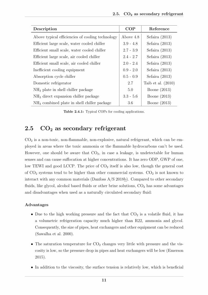
Description COP Reference
Above typical efficiencies of cooling technology Above 4.8 Sefaira (2013)
Efficient large scale, water cooled chiller 3.9 - 4.8 Sefaira (2013)
Efficient small scale, water cooled chiller 2.7 - 3.9 Sefaira (2013)
Efficient large scale, air cooled chiller 2.4 - 2.7 Sefaira (2013)
Efficient small scale, air cooled chiller 2.0 - 2.4 Sefaira (2013)
Inefficient cooling equipment 0.9 - 2.0 Sefaira (2013)
Absorption cycle chiller 0.5 - 0.9 Sefaira (2013)
Domestic refrigerator 2.7 Taib et al. (2010)
NH3 plate in shell chiller package 5.0 Boone (2013)
NH3 direct expansion chiller package 3.3 - 5.6 Boone (2013)
NH3 combined plate in shell chiller package 3.6 Boone (2013)
Table 2.4.1: Typical COPs for cooling applications.
2.5 CO2 as secondary refrigerant
CO2 is a non-toxic, non-flammable, non-explosive, natural refrigerant, which can be em-
ployed in areas where the toxic ammonia or the flammable hydrocarbons can’t be used.
However, one should be aware that CO2, in case a leakage, is undetectable for human
senses and can cause suffocation at higher concentrations. It has zero ODP, GWP of one,
low TEWI and good LCCP. The price of CO2 itself is also low, though the general cost
of CO2 systems tend to be higher than other commercial systems. CO2 is not known to
interact with any common materials (Danfoss A/S 2018b). Compared to other secondary
fluids, like glycol, alcohol based fluids or other brine solutions, CO2 has some advantages
and disadvantages when used as a naturally circulated secondary fluid:
Advantages
• Due to the high working pressure and the fact that CO2 is a volatile fluid, it has
a volumetric refrigeration capacity much higher than R22, ammonia and glycol.
Consequently, the size of pipes, heat exchangers and other equipment can be reduced
(Sawalha et al. 2000).
• The saturation temperature for CO2 changes very little with pressure and the vis-
cosity is low, so the pressure drop in pipes and heat exchangers will be low (Emerson
2015).
• In addition to the viscosity, the surface tension is relatively low, which is beneficial
11

2.5. CO2 as secondary refrigerant
for efficient heat exchangers and flow through pipes. The heat transfer in heat
exchangers is also high due to the high pressure and density, allowing for either
a lower temperature difference in the heat exchanger, or smaller heat exchangers
(Emerson 2015).
• CO2 has a very high volumetric expansion coefficient, which additionally increases
with higher temperature. This is very beneficial for natural circulation loops (Kumar
2017).
• A study by Kumar & Ramgopal (2009), comparing CO2 to other secondary fluids,
found out that for the same geometry and heat input, CO2 required the smallest
temperature difference across heat exchangers.
Disadvantages
• The operating pressures are high, increasing the leakage potential and wall thickness
of pipes and other equipment (Emerson 2015).
• CO2 has a low critical temperature, restricting the temperature to a maximum of
31.06°C to operate conventionally.
12

Chapter 3
Horticulture in India
3.1 Highlights
In this chapter, the production amount, production location and harvest season of the
most important fruits and vegetables are investigated. In addition, the wholesale price
fluctuations through the last four years are presented together with some short info on
the current situation for each crop with regards to export and cold chain management.
At last, storage recommendations are presented.
Fruits
The most important fruits are, in listed order, identified as mangoes, grapes, apples, or-
anges and bananas. India is the fifth largest producer of apples in the world, the largest of
bananas, ninth largest of grapes, the largest of mangoes and sixth largest producer of or-
anges. Southern India is the most productive region. Bananas are the only fruit produced
throughout the entire year, while the remaining fruits are seasonal. As a consequence of
this, the price of bananas stay relatively constant through the year. The remaining fruits,
especially mangoes, experience large fluctuations in price depending on the season. The
only fruit with a noteworthy cold chain are grapes. Grapes are pre-cooled in modern
packhouse facilities and exported. Mangoes are handled and treated in packhouses as
well, but lack cold chain facilities, causing post-harvest losses of up to 34%.
Vegetables
The most important vegetables are, in listed order, identified as potatoes, onions, toma-
toes, cauliflowers, cabbages and okra. India is the world’s second largest producer of
cabbages, cauliflowers, onions, potatoes and tomatoes, while it is the largest producer of
okra. Eastern and central India are the most productive regions. Cabbages, cauliflowers
13

3.2. Background
and onions are seasonal crops, while okra, potatoes and tomatoes are produced through-
out the entire year. Cabbages, cauliflowers, okra and tomatoes experience some price
fluctuations through the year, though inferior to the large variations in price for fruits.
The remaining vegetables have a more or less constant price. Compared to fruits, none
of the vegetables are deemed competitive for storage, either due to short storage life or
unfavourable prices. Modern packhouses for sorting and grading onions are available in
production zones, but cold chain facilities are lacking. Potatoes are the only vegetable
stored in cold storages, where about 75% of cold storages in India are used to store
potatoes.
3.2 Background
India is the largest producer of fruits and second largest producer of vegetables in the
world (NCCD 2015, Paul et al. 2016). 90.2 million tonnes of fruits are produced over 63
thousand square kilometres of land and 169.1 million tonnes of vegetables are produced
over 101 thousand square kilometres of land (APEDA 2018). This employs about 150
million farmers across the country. Due to the warm and diverse climate, a wide variety
of horticultural products are grown. Production statistics are available for about 30
different fruits and 20 different vegetables. The most important crops, with regards to
production and consumption, are listed below (APEDA 2018, NCCD 2015). The selected
fruits and vegetables will be further investigated.
Fruits: Mango, grape, apple, orange, banana.
Vegetables: Potato, onion, tomato, cauliflower, cabbage, okra.
India is composed of 29 states and seven union territories, but in this study they will all be
referred to as states. The states are divided into six six geographical regions, illustrated
in Figure 3.2.1 on page 15.
14

3.3. Fruits
Figure 3.2.1: Regions of India (Wikipedia 2018).
Northern India: Chandigarh, Dehli, Haryana, Himachal Pradesh, Jammu and Kash-
mir, Punjab, Rajasthan.
North-Easthern India: Arunachal Pradesh, Assam, Manipur, Meghalaya, Mizoram,
Nagaland, Sikkim, Tripura.
Central India: Chhattisgarh, Madhya Pradesh, Uttarakhand, Uttar Pradesh.
Eastern India: Bihar, Jharkand, Odisha, West Bengal.
Western India: Dadra and Nagar Haveli, Daman and Diu, Goa, Gujarat, Maharashtra.
Southern India: Andaman and Nicobar Islands, Andhra Pradesh, Karnataka, Kerala,
Lakshadweep, Puducherry, Tamil Nadu, Telangana.
3.3 Fruits
The production location and amount for the selected fruits are shown in Table 3.3.1 on
page 16. Production statistics are from the 2015-2016 season, as statistics for recent years
still are provisional or estimated numbers.
15

3.3. Fruits
Region/State Apple Banana Grapes Mango Orange
Northern 2 449 850 7 260 9 120 347 110 1 424 890
Haryana - - 160 89 970 -
Himachal Pradesh 777 130 420 130 37 630 13 030
Jammu and Kashmir 1 672 720 - 320 23 740 4 210
Punjab - 6 430 8 490 113 500 1 140 310
Rajasthan - 410 20 82 270 267 340
North-Eastern 9 290 1 503 730 23 050 113 130 437 550
Arunachal Pradesh 7 280 31 640 - - -
Assam - 882 710 - 46 150 210 140
Manipur - 93 950 - - 43 340
Meghalaya - 88 710 - - 42 840
Mizoram - 141 030 22 550 4 180 41 340
Nagaland 2 010 108 510 500 3 740 51 690
Sikkim - 3 560 - - 16 800
Tripura - 153 620 - 59 060 31 400
Central 61 940 5 406 680 2 200 5 454 530 1 126 270
Chhattisgarh - 587 420 - 420 610 -
Madhya Pradesh - 1 758 050 2 200 371 480 1 126 270
Uttar Pradesh - 3 061 210 - 4 512 710 -
Uttarakhand 61 940 - - 149 730 -
Eastern - 3 203 630 - 3 330 710 39 210
Bihar - 1 535 300 - 1 464 930 -
Jharkhand - 33 280 - 393 670 -
Odisha - 462 710 - 778 720 -
West Bengal - 1 172 340 - 693 390 39 210
Western - 7 210 670 2 048 110 1 704 760 768 990
Gujarat - 4 185 520 - 1 241 590 -
Maharashtra - 3 025 150 2 048 110 463 170 768 990
Southern 20 11 749 330 507 560 7 665 280 315 820
Andhra Pradesh - 3 570 620 14 640 2 803 660 217 040
Karnataka - 2 370 950 429 780 1 725 670 92 050
Kerala - 1 292 410 15 500 382 520 30
Tamil Nadu 20 4 331 650 34 100 975 110 6 260
Telangana - 183 700 13 540 1 778 320 440
Others - 53 550 - 27 000 60
Total 2 521 100 29 134 850 2 590 040 18 642 520 4 112 790
Table 3.3.1: Production of fruits in India 2015-2016 (Datanet India 2015-2016a). Values in tonnes.
16

3.3. Fruits
Apple
India is the worlds fifth largest producer of apples, with about 2.5% of the world share
(NCCD 2015). Export values are 6.07 million US$, mainly to Nepal and Bangladesh
(APEDA 2018). Northern India is the main producer of apples with about 97% of the
national production, where Jammu and Kashmir and Himachal Pradesh are the produc-
ing states. Uttarakhand in Central India is the third largest producer. North-Eastern
India has some production, though inferior to the mentioned states. The harvest season
for apples varies from June to November, depending on the location, as can be seen in
Table 3.3.2.
Region/State Jan Feb Mar Apr May Jun Jul Aug Sep Oct Nov Dec
Northern
Himachal Pradesh
Jammu and Kashmir
North-Eastern
Arunachal Pradesh
Central
Uttarakhand
Peak season Lean season Throughout year
Table 3.3.2: Harvest season of apples (APEDA 2018, NCCD 2015).
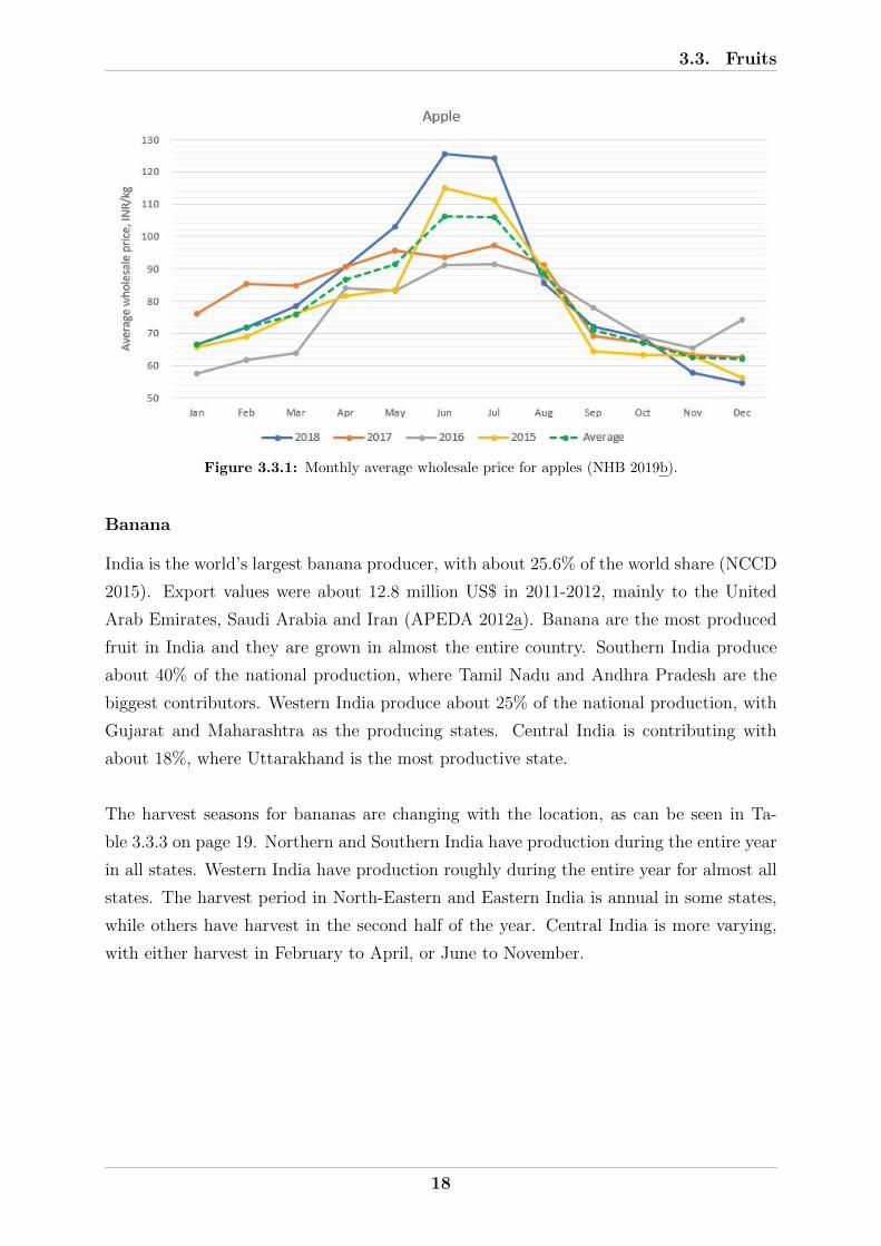
Figure 3.3.1 on page 18 shows the average price each month at wholesale markets in
India for the last four years. During season there is high availability and the price is
consequently low. After the short season, the price increase each month and reaches
almost double the value in June before the season begins again. The short season and
large price variations makes apples an economically ideal product for storage.
17
3.3. Fruits
Figure 3.3.1: Monthly average wholesale price for apples (NHB 2019b).
Banana
India is the world’s largest banana producer, with about 25.6% of the world share (NCCD
2015). Export values were about 12.8 million US$ in 2011-2012, mainly to the United
Arab Emirates, Saudi Arabia and Iran (APEDA 2012a). Banana are the most produced
fruit in India and they are grown in almost the entire country. Southern India produce
about 40% of the national production, where Tamil Nadu and Andhra Pradesh are the
biggest contributors. Western India produce about 25% of the national production, with
Gujarat and Maharashtra as the producing states. Central India is contributing with
about 18%, where Uttarakhand is the most productive state.
The harvest seasons for bananas are changing with the location, as can be seen in Ta-
ble 3.3.3 on page 19. Northern and Southern India have production during the entire year
in all states. Western India have production roughly during the entire year for almost all
states. The harvest period in North-Eastern and Eastern India is annual in some states,
while others have harvest in the second half of the year. Central India is more varying,
with either harvest in February to April, or June to November.
18

3.3. Fruits
Region/State Jan Feb Mar Apr May Jun Jul Aug Sep Oct Nov Dec
Northern
Rajasthan
North-Eastern
Assam
Manipur
Meghalaya
Mizoram
Nagaland
Tripura
Central
Chhattisgarh
Madhya Pradesh
Uttar Pradesh
Uttarakhand
Eastern
Bihar
Jharkhand
Odisha
West Bengal
Western
Gujarat
Maharashtra
Southern
Andhra Pradesh
Karnataka
Tamil Nadu
Peak season Lean season Throughout year
Table 3.3.3: Harvest season of bananas (APEDA 2018, NCCD 2015).
Figure 3.3.2 on page 20 shows the average price each month at wholesale markets in India
for the last four years. Since bananas are available throughout the year, the price stays
more or less constant, only varying with about 3 INR/kg. The high availability and low
price variation makes bananas economically unfavourable for storage.
19

3.3. Fruits
Figure 3.3.2: Monthly average wholesale price for bananas (NHB 2019b).
Grapes
India is the world’s ninth largest producer of grapes, with about 3.6% of the world share
(NCCD 2015). Hot and dry climate is ideal for growing grapes, but temperate and warm
regions in general are productive. Grapes are one of the fruits in India with the most
complete cold chain. Modern packhouse facilities with automatic forced air systems for
pre-cooling are available in all commercial production. Traceability systems are also cur-
rently used for grapes. Due to this, grapes are a high-value export product. Export values
were about 294.6 million US$ in 2017-2018, mainly to Netherland, Russia, UK, Germany
and the United Arab Emirates (APEDA 2018).
Maharashtra in Western India represent about 79% of the national production. Most of
the remaining production takes place in Southern India, in Karnataka, which produce
about 19% of the grapes. The harvest seasons vary throughout the country, as seen
in Table 3.3.4 on page 21. Northern India harvest grapes fram May to July. Western
and Southern India have more or less similar harvest periods, with total season from
December to May and peak season in February and March. Southern India additionally
harvest twice a year, with the second harvest in July. The only exception is Tamil Nadu
which follows the same harvest season as Northern India.
20

3.3. Fruits
Region/State Jan Feb Mar Apr May Jun Jul Aug Sep Oct Nov Dec
Northern
Haryana
Punjab
Western
Maharashtra
Southern
Andhra Pradesh
Karnataka
Tamil Nadu
Peak season Lean season Throughout year
Table 3.3.4: Harvest season of grapes (APEDA 2012b).
Figure 3.3.3 shows the average price each month at wholesale markets in India for the last
four years. During season, the availability is high and the price consequently hits a low
point in March. The price between March and September vary a lot between the different
years, but most years have a minimum point in September. In October to December,
right before the season begins, the price is at its highest. The seasonal price variations
makes grapes an economically ideal product for storage.
Figure 3.3.3: Monthly average wholesale price for grapes (NHB 2019b).
Mango
India is the world’s largest producer of mangoes, with about 40% of the world share
(NCCD 2015). Mangoes are usually grown in tropical and subtropical regions, making
21

3.3. Fruits
India an ideal country. The Indian mangoes comes in many different shapes and sizes,
with different flavour, aroma and taste. However, only a few varieties are cultivated and
they keep a high quality in terms of both taste and nutritional value. Mangoes are treated
relatively good in India to maintain the high quality. Modern packhouses exist in all major
producing zones and they are treated according to international requirements, with irra-
diation facilities, identification systems and traceability systems. However, post-harvest
losses of mangoes can still be as high as 34% due to lack of appropriate cold storage
facilities (Sab et al. 2017). Because of the relatively high quality and high production
of mangoes, India is a prominent exporter to the world. Export values were about 59.3
million US$ in 2017-2018, mainly to the United Arab Emirates, United Kingdom, Saudi
Arabia and Qatar (APEDA 2018).
Mangoes are the second most produced fruit in India, after bananas. It is grown to a
large extent in more or less the entire country, although the production in the Northern
and North Eastern parts of India are inferior to the remaining regions. Southern India
has the highest production with about 41% of the national production. Andhra Pradesh,
Karnataka and Telangana are South Indias most productive states. Central India comes
second with about 29% and Eastern India is third with about 18%. Uttar Pradesh in
Central India is the most productive state and Bihar is the most productive state in
Eastern India. The harvest season in Northern, Eastern and Central India are usually a
little bit later compared to Southern and Western India, as seen in Table 3.3.5. Western
and Southern India have harvest season from January to July, with peak around April
to May. Central and Eastern India has its main season from June to August, with peak
season in June to July.
Region/State Jan Feb Mar Apr May Jun Jul Aug Sep Oct Nov Dec
Central
Uttar Pradesh
Eastern
Bihar
Western
Gujarat
Maharashtra
Southern
Andhra Pradesh
Karnataka
Peak season Lean season Throughout year
Table 3.3.5: Harvest season of mangoes (NCCD 2015).
22

3.3. Fruits
Figure 3.3.4 shows the average price each month at wholesale markets in India for the last
four years. During the season, from March to July, there is high availability of the product
and the price consequently drops to a low point in June. However, after the season ends,
the price increase with over 40 INR/kg to September. The price for the different years vary
and the profile for 2015 is opposite the other years, as it starts high and ends low. The
2018 season also lasted two months longer than the other years. Still, the short season
and large price variation makes mangoes an economically ideal product for storage.
Figure 3.3.4: Monthly average wholesale price for alphonso mangoes (NHB 2019b).
Orange
India is the world’s sixth largest producer of oranges, with only 4% of the world share
(NCCD 2015). Oranges are the most common citrus fruit in India, occupying nearly 40%
of the total area used for citrus cultivation (NHB 2012). Export values for oranges were
about the same as for apples, about 5.4 million US$ in 2017-2018, mainly to Bangladesh
and Nepal (APEDA 2018). Oranges are usually transported to the neighbouring coun-
tries by road, without cooling or other treatment, often leading to large losses (NHB 2012).
Most of the oranges are produced in Northern and Central India, with about 35% and
27%, respectively, of the national production. Punjab accounts for most of the production
in Northern India, while Madhya Pradesh produce the entire amount in Central India.
Maharashtra comes third and accounts for the entire production in Western India. The
harvest seasons are roughly around the new year in most of India, as seen in Table 3.3.6
on page 24. In Northern, North-Eastern and Central India, the season last from October
23

3.3. Fruits
to March, with peak season in November to February for most states. Eastern India
is slightly later, with season from December to March and peak season in January and
February. Western India has production the entire year, except for July and August, with
peak season from March to May. Southern India has two harvest periods, one around
February/March and one around September or November/December.
Region/State Jan Feb Mar Apr May Jun Jul Aug Sep Oct Nov Dec
Northern
Himachal Pradesh
Jammu and Kashmir
Punjab
Rajasthan
North-Eastern
Assam
Manipur
Meghalaya
Mizoram
Sikkim
Tripura
Central
Madhya Pradesh
Eastern
West Bengal
Western
Maharashtra
Southern
Andhra Pradesh
Tamil Nadu
Peak season Lean season Throughout year
Table 3.3.6: Harvest season of oranges (APEDA 2018, NCCD 2015).
Figure 3.3.5 on page 25 shows the average price each month at wholesale markets in
India for the last four years. The price varies considerably between the different years
and oranges were generally very expensive in 2018. During the season, from November to
March, the price is low due to the high availability. When the season ends, around March,
the price increase with an average of 12 INR/kg to May. The seasonal variations and price
variations makes oranges somewhat suited for storage, however, not to the same extent
as mangoes, grapes and apples.
24

3.4. Vegetables
Figure 3.3.5: Monthly average wholesale price for oranges (NHB 2019b).
3.4 Vegetables
Most vegetables in India are grown from temperate to humid tropics. The production
location and amount for the selected vegetables are shown in Table 3.4.1 on page 26.
Production statistics are from the 2015-2016 season, as statistics for recent years still are
provisional or estimated numbers.
25

3.4. Vegetables
Region/State Cabbage Cauliflower Okra Onion Potato Tomato
Northern 655 910 1 080 770 328 520 2 447 850 3 779 390 1 523 480
Haryana 310 550 578 950 193 820 705 800 853 810 675 380
Himachal Pradesh 160 740 119 010 38 770 47 960 183 250 485 540
Jammu and Kashmir 73 230 85 260 42 990 65 270 127 240 88 090
Punjab 104 410 248 450 42 600 193 710 2 385 260 191 180
Rajasthan 6 980 49 100 10 340 1 435 110 229 830 83 290
North-Eastern 1 176 150 572 450 238 930 108 760 1 471 170 602 330
Arunachal Pradesh 9 620 2 670 170 - 5 650 3 320
Assam 754 980 443 950 183 290 80 310 1 037 260 445 020
Manipur 96 980 32 600 1 530 5 170 - 31 610
Meghalaya 41 570 20 470 3 440 4 600 183 820 34 020
Mizoram 48 900 1 080 25 000 8 430 1 440 10 200
Nagaland 135 670 4 950 1 550 7 140 60 940 20 100
Sikkim 5 380 3 350 6 870 1 730 53 550 4 250
Tripura 83 050 63 380 17 080 1 380 128 510 53 810
Central 1 178 380 1 707 110 958 790 3 688 330 18 015 830 4 107 470
Chhattisgarh 374 370 433 300 291 270 375 990 644 830 908 980
Madhya Pradesh 444 420 842 060 342 050 2 848 000 3 161 000 2 285 900
Uttar Pradesh 292 020 393 260 301 210 422 750 13 851 760 819 370
Uttarakhand 67 570 38 490 24 260 41 590 358 240 93 220
Eastern 4 511 500 3 766 110 2 678 590 2 425 100 15 678 280 3 726 620
Bihar 719 810 1 003 900 763 000 1 247 340 6 345 520 1 001 010
Jharkhand 475 990 258 640 452 120 254 630 627 010 230 190
Odisha 1 057 670 614 530 566 170 378 580 278 750 1 290 990
West Bengal 2 258 030 1 889 040 897 300 544 550 8 427 000 1 204 430
Western 787 370 731 710 978 560 7 885 120 3 800 840 2 295 690
Gujarat 608 160 544 710 859 470 1 355 780 3 549 380 1 319 110
Maharashtra 179 210 187 000 119 090 6 529 340 251 460 976 580
Southern 496 080 183 900 643 060 4 358 600 656 090 6 462 200
Andhra Pradesh 40 580 36 010 225 470 885 420 38 860 2 236 560
Karnataka 231 210 83 320 90 820 2 695 990 455 450 2 046 140
Kerala 21 190 6 440 31 860 280 17 920 58 800
Tamil Nadu 143 860 36 220 123 220 380 950 72 230 645 700
Telangana 59 240 21 910 171 690 395 960 71 630 1 475 000
Others 560 47 720 22 120 17 490 15 450 14 200
Total 8 805 950 8 089 770 5 848 570 20 931 250 43 417 050 18 731 990
Table 3.4.1: Production of vegetables in India 2015-2016 (Datanet India 2015-2016b). Values in tonnes.
Cabbage
India is the world’s second largest producer of cabbages, with about 12% of the world
share (NCCD 2015). Export values are relatively low compared to fruits, with about
131.5 thousand US$ in 2017-2018, mainly to Mauritius, Nepal, Qatar and the United
26

3.4. Vegetables
Arab Emirates (APEDA 2018). Over 50% of the cabbages are produced in Eastern In-
dia, with West Bengal and Odisha as the biggest producers in the country. Central and
North-Eastern India are the second and third largest producers, with about 13% of the
national production each.
The harvest season is roughly around new year in most of the country, as seen in Ta-
ble 3.4.2. Central, Eastern and Western India have harvest period from around Novem-
ber to March/April, with peak season in January and February. Most of Northern and
North-Eastern India follows the same harvest season, however, Nagaland has peak season
in July and August. Southern India differs even more, with two harvest seasons through
the year.
Region/State Jan Feb Mar Apr May Jun Jul Aug Sep Oct Nov Dec
Northern
Rajasthan
North-Eastern
Assam
Manipur
Meghalaya
Mizoram
Nagaland
Central
Chhattisgarh
Madhya Pradesh
Uttar Pradesh
Uttarakhand
Eastern
Bihar
Jharkand
Odisha
West Bengal
Western
Gujarat
Maharashtra
Southern
Andhra Pradesh
Karnataka
Tamil Nadu
Peak season Lean season Throughout year
Table 3.4.2: Harvest season of cabbages (APEDA 2018, NCCD 2015).
27

3.4. Vegetables
Figure 3.4.1 shows the average price each month at wholesale markets in India for the
last four years. Compared to the selected fruits, the general price level is considerably
lower. Still, at the end of the season in March, when the average price is at its lowest,
the price more than doubles until July. Then, it stays high until November when the
season starts again. This increase in price makes cabbages somewhat ideal for storage,
but considering that the increase is only about 8 INR/kg over four months, it’s uncertain
whether it is economically feasible or not.
Figure 3.4.1: Monthly average wholesale price for cabbages (NHB 2019b).
Cauliflower
India is the world’s second largest producer of cauliflowers, with 36% of the world share
(NCCD 2015). Export values are about the same as cabbages, 148.2 thousand US$ in
2017-2018, mainly to United Kingdom, Nepal and Japan (APEDA 2018). Eastern India
is the largest producer of cauliflowers with about 47% of the national production. West
Bengal and Bihar in Eastern India are the largest contributors both regional and national.
Central India is the second largest producer with about 21% of the national production,
and Madhya Pradesh is the biggest contributor. Northern India is third, with about 13%
of the national production volume.
The harvest season is generally around the new year in most regions, as can be seen in
Table 3.4.3 on page 29. Northern, Eastern, Western and Southern India have harvest
from October to March for most states, with peak season from December to February.
Central India has its main peak season in December to February, where Uttarakhand has
28

3.4. Vegetables
an additional peak season in August and September. North-Eastern India has a bit earlier
harvest season, where for instance Nagaland has harvest season from June to October with
peak in July and August.
Region/State Jan Feb Mar Apr May Jun Jul Aug Sep Oct Nov Dec
Northern
Haryana
Punjab
Rajasthan
North-Eastern
Assam
Manipur
Meghalaya
Mizoram
Nagaland
Sikkim
Central
Chhattisgarh
Madhya Pradesh
Uttar Pradesh
Uttarakhand
Eastern
Bihar
Jharkand
Odisha
West Bengal
Western
Gujarat
Southern
Karnataka
Peak season Lean season Throughout year
Table 3.4.3: Harvest season of cauliflower (APEDA 2018, NCCD 2015).
Figure 3.4.2 on page 30 shows the average price each month at wholesale markets in India
for the last four years. The seasons for cauliflowers are very similar to that of cabbages,
with low price from about December to March. The average price is lowest in February
before it increases with about 2.5 times until July, making storage economically feasible.
However, cauliflower can not be stored for much more than about a month, making it
difficult to profit from the increased price.
29
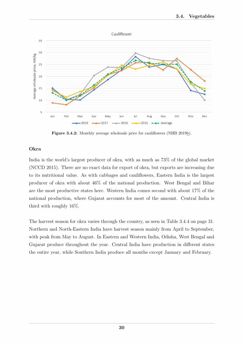
3.4. Vegetables
Figure 3.4.2: Monthly average wholesale price for cauliflowers (NHB 2019b).
Okra
India is the world’s largest producer of okra, with as much as 73% of the global market
(NCCD 2015). There are no exact data for export of okra, but exports are increasing due
to its nutritional value. As with cabbages and cauliflowers, Eastern India is the largest
producer of okra with about 46% of the national production. West Bengal and Bihar
are the most productive states here. Western India comes second with about 17% of the
national production, where Gujarat accounts for most of the amount. Central India is
third with roughly 16%.
The harvest season for okra varies through the country, as seen in Table 3.4.4 on page 31.
Northern and North-Eastern India have harvest season mainly from April to September,
with peak from May to August. In Eastern and Western India, Odisha, West Bengal and
Gujarat produce throughout the year. Central India have production in different states
the entire year, while Southern India produce all months except January and February.
30
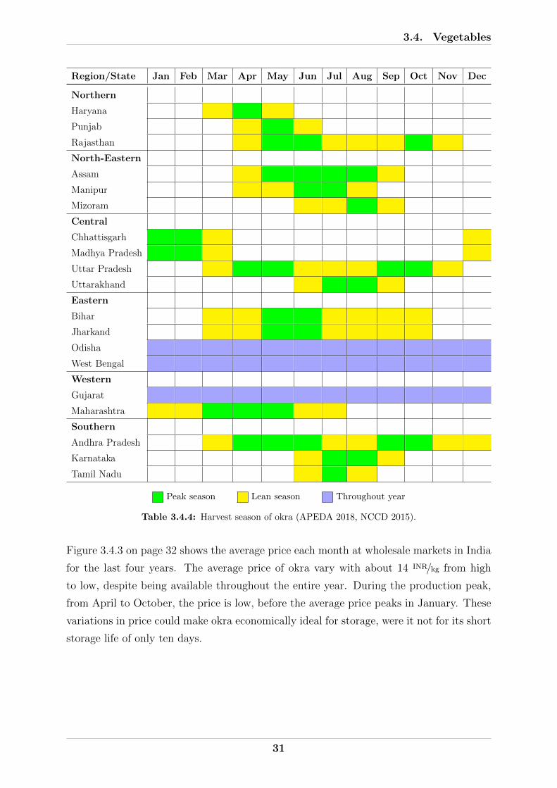
3.4. Vegetables
Region/State Jan Feb Mar Apr May Jun Jul Aug Sep Oct Nov Dec
Northern
Haryana
Punjab
Rajasthan
North-Eastern
Assam
Manipur
Mizoram
Central
Chhattisgarh
Madhya Pradesh
Uttar Pradesh
Uttarakhand
Eastern
Bihar
Jharkand
Odisha
West Bengal
Western
Gujarat
Maharashtra
Southern
Andhra Pradesh
Karnataka
Tamil Nadu
Peak season Lean season Throughout year
Table 3.4.4: Harvest season of okra (APEDA 2018, NCCD 2015).
Figure 3.4.3 on page 32 shows the average price each month at wholesale markets in India
for the last four years. The average price of okra vary with about 14 INR/kg from high
to low, despite being available throughout the entire year. During the production peak,
from April to October, the price is low, before the average price peaks in January. These
variations in price could make okra economically ideal for storage, were it not for its short
storage life of only ten days.
31

3.4. Vegetables
Figure 3.4.3: Monthly average wholesale price for okra (NHB 2019b).
Onion
India is the world’s second largest producer of onions, with 20% of the world share (NCCD
2015). There are many varieties of onions in India, and the statistics include both red and
yellow onions. Indian onions are famous for their pungency and they are an extremely
important crop, not only for national consumption, but also for international export
(APEDA 2012c). Export values for onions are the highest of all fruits and vegetables,
with 479.3 million US$ in 2017-2018. They are mainly exported to Bangladesh, Malaysia,
Sri Lanka, United Arab Emirates and Nepal. Due to the high demand of Indian onions to
the world, modern packhouses for sorting and grading are available at production zones
(APEDA 2018). However, refrigerating facilities are lacking.
Onions are grown to large extents in the entire country, except North-Eastern India.
Western India, primarily because of Maharashtra, produce most onions with about 38%
of the national production. Southern India is second with about 21% of the production
and Central India is third with about 18%. Maharashtra in Western India, Madhya
Pradesh in Central India and Karnataka in Southern India account for the majority of
the production in each region. The harvest pattern for the leading onion growing states
are shown in Table 3.4.5 on page 33. Southern India have production of onions almost
throughout the entire year, except January and February. Otherwise in India, onions
are grown seasonal, with one season around March to May and another in November to
December.
32

3.4. Vegetables
Region/State Jan Feb Mar Apr May Jun Jul Aug Sep Oct Nov Dec
Northern
Haryana
Rajasthan
Central
Madhya Pradesh
Uttar Pradesh
Eastern
Bihar
Western
Gujarat
Maharashtra
Southern
Andhra Pradesh
Karnataka
Peak season Lean season Throughout year
Table 3.4.5: Harvest season of onions (APEDA 2012c, NCCD 2015).
Figure 3.4.4 shows the average price each month at wholesale markets in India for the last
four years. The average price of onions stays relatively constant, only varying with about
10 INR/kg. There are some variations between the different years and especially 2015 differs
from the rest, with its peak price of 45 INR/kg in September. Despite this individual price
peak, onions are not considered economically favourable for storage compared to some of
the other crops.
Figure 3.4.4: Monthly average wholesale price for onions (NHB 2019b).
33

3.4. Vegetables
Potato
India is the world’s second largest producer of potatoes, with 12% of the world share
(NCCD 2015). Potatoes are the most produced vegetable and probably one of the most
important crops in India. Export values were 63.9 million US$ in 2017-2018, primarily
to Nepal, Sri Lanka and Oman (APEDA 2018). Central India is the largest producer of
potatoes, because of Uttar Pradesh, with about 41% of the national production. Eastern
India is second with about 36%, where West Bengal and Bihar are the most productive
states. Western and Northern India produce about 8% each. Potatoes are among the few
crops actually stored in cold storages. About 75% of cold storages in India are used to
store potatoes (RX India 2013).
The harvest season for potatoes vary significantly throughout the country, as can be seen
in Table 3.4.6 on page 35. Northern India has peak season around May and October,
while North-Eastern India has peak season in June and July. Central India has several
peaks and more or less some production throughout the entire year. Eastern and Western
India have both full production the entire year. Southern India has season from March
to December.
34
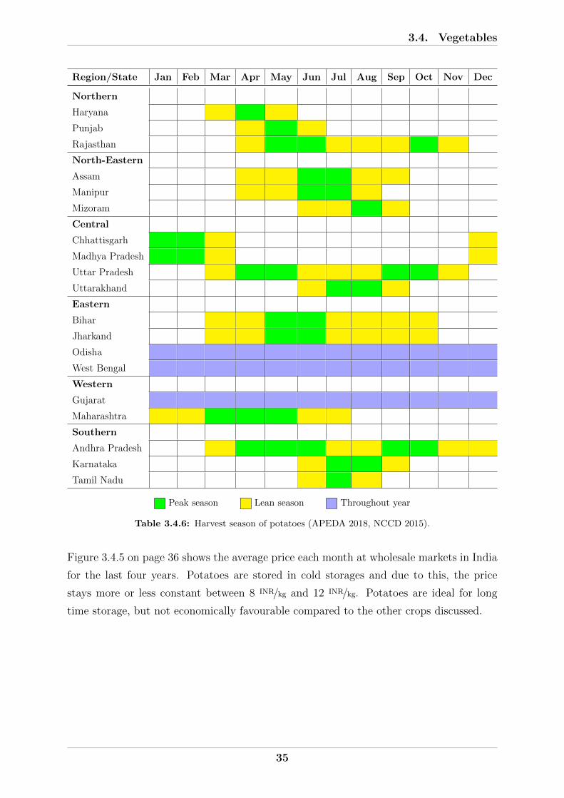
3.4. Vegetables
Region/State Jan Feb Mar Apr May Jun Jul Aug Sep Oct Nov Dec
Northern
Haryana
Punjab
Rajasthan
North-Eastern
Assam
Manipur
Mizoram
Central
Chhattisgarh
Madhya Pradesh
Uttar Pradesh
Uttarakhand
Eastern
Bihar
Jharkand
Odisha
West Bengal
Western
Gujarat
Maharashtra
Southern
Andhra Pradesh
Karnataka
Tamil Nadu
Peak season Lean season Throughout year
Table 3.4.6: Harvest season of potatoes (APEDA 2018, NCCD 2015).
Figure 3.4.5 on page 36 shows the average price each month at wholesale markets in India
for the last four years. Potatoes are stored in cold storages and due to this, the price
stays more or less constant between 8 INR/kg and 12 INR/kg. Potatoes are ideal for long
time storage, but not economically favourable compared to the other crops discussed.
35

3.4. Vegetables
Figure 3.4.5: Monthly average wholesale price for potatoes (NHB 2019b).
Tomato
India is the world’s second largest producer of tomatoes, with 11% of the world share
(NCCD 2015). It is the third most important vegetable in India, after potatoes and
onions. Export values were 17.67 million US$ in 2017-2018, primarily to United Arab
Emirates and Nepal (APEDA 2018). There is increased focus on enhancing the quality
and productivity of tomatoes in India, to bring them to an international level in terms of
packaging, presentation and quality (APEDA 2012d).
Tomatoes are grown somewhat evenly over the entire country, except for the northern
areas. Southern India is the largest producer of tomatoes, with about 34% of the national
production. Central India is second largest with about 22% and Eastern India is third
with about 15%. Madhya Pradesh in Central India and Andhra Pradesh and Karnataka
in Southern India are the most productive states. The harvest season is varying through
the country, as can be seen in Table 3.4.7 on page 37. The main season for Northern,
North-Eastern, Central and Eastern India is around November to February. Central India,
together with Western and Southern India, have production throughout the entire year
in some states.
36
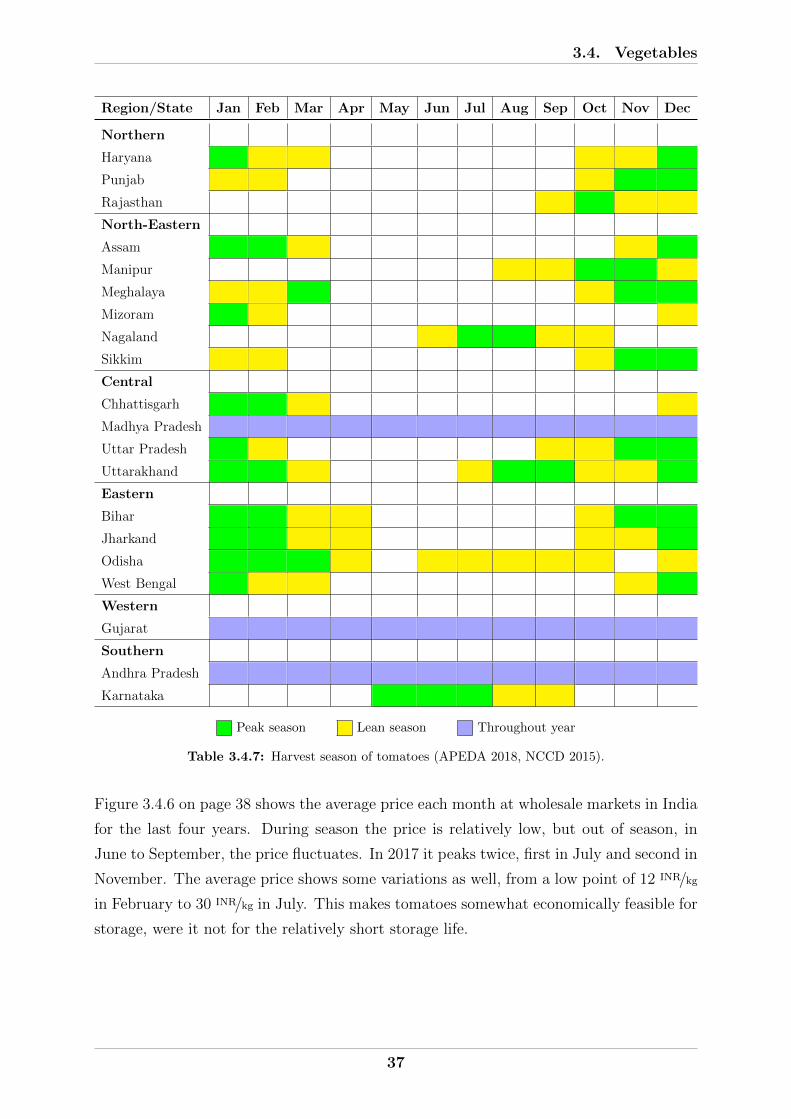
3.4. Vegetables
Region/State Jan Feb Mar Apr May Jun Jul Aug Sep Oct Nov Dec
Northern
Haryana
Punjab
Rajasthan
North-Eastern
Assam
Manipur
Meghalaya
Mizoram
Nagaland
Sikkim
Central
Chhattisgarh
Madhya Pradesh
Uttar Pradesh
Uttarakhand
Eastern
Bihar
Jharkand
Odisha
West Bengal
Western
Gujarat
Southern
Andhra Pradesh
Karnataka
Peak season Lean season Throughout year
Table 3.4.7: Harvest season of tomatoes (APEDA 2018, NCCD 2015).
Figure 3.4.6 on page 38 shows the average price each month at wholesale markets in India
for the last four years. During season the price is relatively low, but out of season, in
June to September, the price fluctuates. In 2017 it peaks twice, first in July and second in
November. The average price shows some variations as well, from a low point of 12 INR/kg
in February to 30 INR/kg in July. This makes tomatoes somewhat economically feasible for
storage, were it not for the relatively short storage life.
37
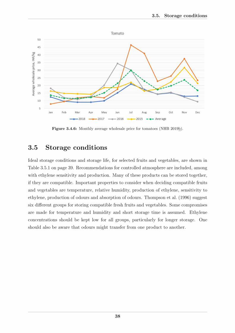
3.5. Storage conditions
Figure 3.4.6: Monthly average wholesale price for tomatoes (NHB 2019b).
3.5 Storage conditions
Ideal storage conditions and storage life, for selected fruits and vegetables, are shown in
Table 3.5.1 on page 39. Recommendations for controlled atmosphere are included, among
with ethylene sensitivity and production. Many of these products can be stored together,
if they are compatible. Important properties to consider when deciding compatible fruits
and vegetables are temperature, relative humidity, production of ethylene, sensitivity to
ethylene, production of odours and absorption of odours. Thompson et al. (1996) suggest
six different groups for storing compatible fresh fruits and vegetables. Some compromises
are made for temperature and humidity and short storage time is assumed. Ethylene
concentrations should be kept low for all groups, particularly for longer storage. One
should also be aware that odours might transfer from one product to another.
38
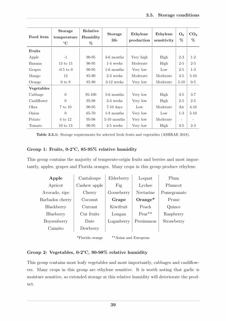
3.5. Storage conditions
Food item
Storage
temperature
°C
Relative
Humidity
%
Storage
life
Ethylene
production
Ethylene
sensitivity
O2
%
CO2
%
Fruits
Apple -1 90-95 3-6 months Very high High 2-3 1-2
Banana 13 to 15 90-95 1-4 weeks Moderate High 2-5 2-5
Grapes -0.5 to 0 90-95 1-6 months Very low Low 2-5 1-3
Mango 13 85-90 2-3 weeks Moderate Moderate 3-5 5-10
Orange 0 to 9 85-90 3-12 weeks Very low Moderate 5-10 0-5
Vegetables
Cabbage 0 95-100 5-6 months Very low High 3-5 3-7
Cauliflower 0 95-98 3-4 weeks Very low High 2-5 2-5
Okra 7 to 10 90-95 7-10 days Low Moderate Air 4-10
Onion 0 65-70 1-8 months Very low Low 1-3 5-10
Potato 4 to 12 95-98 5-10 months Very low Moderate - -
Tomato 10 to 13 90-95 2-5 weeks Very low High 3-5 2-3
Table 3.5.1: Storage requirements for selected fresh fruits and vegetables (ASHRAE 2018).
Group 1: Fruits, 0-2°C, 85-95% relative humidity
This group contains the majority of temperate-origin fruits and berries and most impor-
tantly, apples, grapes and Florida oranges. Many crops in this group produce ethylene.
Apple Cantaloupe Elderberry Loquat Plum
Apricot Cashew apple Fig Lychee Plumcot
Avocado, ripe Cherry Gooseberry Nectarine Pomegranate
Barbados cherry Coconut Grape Orange* Prune
Blackberry Currant Kiwifruit Peach Quince
Blueberry Cut fruits Longan Pear** Raspberry
Boysenberry Date Loganberry Persimmon Strawberry
Caimito Dewberry
*Florida orange **Asian and European
Group 2: Vegetables, 0-2°C, 90-98% relative humidity
This group contains most leafy vegetables and most importantly, cabbages and cauliflow-
ers. Many crops in this group are ethylene sensitive. It is worth noting that garlic is
moisture sensitive, so extended storage at this relative humidity will deteriorate the prod-
uct.
39

3.5. Storage conditions
Alfalfa Sprouts Broccoflower Cut vegetables Kohlrabi Salsify
Amaranth Brussels sprouts Daikon Leek Scorzonera
Anise Cabbage Endive-Chickory Lettuce Shallot
Artichoke Carrot Escarole Mint Snow Pea
Arugula Cauliflower Fennel Mushroom Spinach
Asparagus Celeriac Garlic Mustard greens Sweet Pea
Beans* Celery Green onion Parsley Swiss chard
Bean sprouts Chard Herbs (not basil) Parsnip Turnip
Beet Chinese cabbage Horseradish Radicchio Turnip greens
Belgian endive Chinese turnip Jerusalem artichoke Radish Water chestnut
Bok choy Collard Kailon Rutabaga Watercress
Broccoli Corn** Kale Rhubard
*Fava and Lima **Sweet and baby
Group 3: Fruits, 7-10°C, 85-95% relative humidity
This group contains citrus and subtropical fruits and most importantly California and
Valencia oranges.
Avocado, unripe Durian Kumquat Orange* Tamarillo
Babaco Feijoa Lemon Passion fruit Tamarind
Cactus pear Granadilla Lime Pepino Tangelo
Calamondin Grapefruit Limequat Pineapple Tangerine
Carambola Guava Mandarin Pummelo Ugli fruit
Cranberry Juan canary melon Olive Sugar apple Watermelon
Custard apple
*California and Valencia orange
Group 4: Vegetables, 7-10°C, 85-95% relative humidity
This group contains many fruit-type vegetables and most importantly okra.
Basil Chayote Kiwano Pepper**
Beans* Cowpea Long bean Squash***
Cactus leaves Cucumber Malanga Tomatillo
Calabasa Eggplant Okra Winged bean
*Span, green and wax **Bell and chili ***Summer, soft rind
40

3.5. Storage conditions
Group 5: Fruits 13-18°C, 85-95% relative humidity
This group contains most tropical fruits and melons and most importantly bananas and
mangoes.
Atemoya Casaba Melon Jabolicaba Mangosteen Rambutan
Banana Cherimoya Jackfruit Papaya Sapodilla
Breadfruit Crenshaw melon Mamey sapote Persian melon Sapote
Canistel Honeydew melon Mango Plantain Soursop
Group 6: Vegetables, 13-18°C, 85-95% relative humidity
This group contains common root-type vegetables and most importantly onions, potatoes
and tomatoes. It is worth noting that onions are moisture sensitive and should ideally
be stored at 0°C, so extended storage at these conditions will deteriorate the product. In
tropical climates like India, it is not common to store onions refrigerated. They are rather
stored at 25-30°C with proper ventilation to avoid condensation on the onions when they
are taken out of storage, which would destroy the product. Storage life at 25-30°C with
proper ventilation can still be up to 9 months (MFI group 2018).
Bitter melon Dry onion Potato Sweet potato Tomato**
Boniato Ginger Pumpkin Taro Yam
Cassava Jicama Squash*
*Winter, hard rind **Ripe, partially ripe and mature green
41

Chapter 4
The Indian scenario
4.1 Highlights
In this chapter the export and domestic cold chains are investigated. The cold chain and
commodity flow through the Indian mandis, the fruit and vegetable wholesale markets
throughout the country, are also investigated. Important weak links and challenges in the
chains are identified. The findings are then compared to the results of a field investigation
performed at IIT Kharagpur in India, before a specific problem and solution are discussed.
At last, the technical layout, revenue and assumptions for the discussed solution are
presented.
Cold chains
A typical cold chain for export of fresh horticultural produce is presented in Figure 4.2.1
on page 45. Lack of refrigerated transport and pre-cooling were found to be major weak
links in the export cold chain. Grapes are the only crop pre-cooled and transported in
refrigerated containers. None of the other crops are pre-cooled before export and most
are transported to neighbouring countries by road, without refrigeration. To increase the
revenue from export of fresh horticultural produce, one solution proposed is to use the
experience they have from exporting grapes, to adapt technologies to pre-cool and export
other crops. Mangoes are highlighted as a very potential export product. A typical cold
chain for domestic horticultural produce is presented in Figure 4.3.1 on page 47. The
domestic cold chain is not as well developed as the export cold chain, but, similar to
the export chain, lack of pre-cooling and refrigerated transport are identified as major
inhibitors. Additionally, there is a need for cold storages. Cold storages are present in
India, but 75% are used for potatoes and 16% are out of operation.
42

4.1. Highlights
The Indian mandis
One problem highlighted in both cold chains are the very large number of intermediates.
This was found to especially inhibit the cold chain and commodity flow through the
Indian mandis. A typical cold chain for the product flow through the mandis is presented
in Figure 4.4.1 on page 48. The mandis is associated with low quality, poor remuneration
and very high wastes due to lack of cold chain facilities. Products are displayed at ambient
temperatures, which may reach above 40°C, often forcing the seller to discard the unsold
produce at the end of each day due to deterioration. The mandis is identified as an
important link in both the export and domestic flow chain, as seen in Figure 4.4.2 on
page 49.
Field investigation
The field investigation at IIT Kharagpur confirmed many of the previously discussed con-
ditions. In total, 66 people answered the survey, all from professors to fruit and vegetable
vendors and grocery shop owners. Most people answered that they do refrigerate their
food, except for the fruit and vegetable vendors. None of them used refrigeration. Despite
this, they answered that the product quality is most important to them, but that they
don’t see the need for refrigeration to maintain the quality. In terms of wasting food, there
is little correlation between education and amount of food waste. Most people actually
reported less waste than what is presented in literature.
When asked how important they believe refrigeration is for food quality and shelf life,
those higher educated think it is more important. Controversially, the majority of fruit
and vegetable vendors answered that refrigeration is very important. However, when
asked how important it is for them that their food or product is refrigerated the answers
are different. Even though most people are aware of the importance of refrigeration,
they do not really care if their food is refrigerated or not. Almost all fruit and vegetable
vendors answered that refrigeration is unimportant to them. The majority of people
agreed that there should be more use of refrigeration in Indian homes and that the lack
of domestic refrigeration is due to economical reasons. However, when asked about the
current use of refrigeration between production and consumption, more people find the
current system sufficient. Generally, only those with higher education see the need for a
better cold chain. Poor infrastructure is highlighted as the main reason for the lack here.
Some people elaborated further on their answers and some elaborations can be seen in
section 4.5.
43

4.2. Export cold chain
Cold storage at Indian mandis
It was decided to approach the problem of lacking cold chain facilities at the mandis. Some
approaches and considerations revolving the problem are discussed, like design, configu-
ration, energy sources, refrigeration system and costs. A small, movable cold storage, the
size of a 20ft shipping container, was considered an appropriate solution. The layout can
be seen in Figure 4.6.1 on page 58. Two configurations of the refrigeration system are
compared, a single stage NH3 refrigeration system with and without CO2 in a NCL. The
refrigeration systems are illustrated in Figure 4.6.2 on page 59 and the assumptions taken
when designing the storage are presented in subsection 4.6.3.
To decide which products to store, the wholesale price variations from chapter 3 are
investigated. To operate the storage through the entire year, the products regarded as
most economically feasible for storage are apples, grapes and mangoes. The monthly
average wholesale prices for apples, grapes and mangoes are presented in Figure 4.6.3
on page 60. Apples can be bought in January for 66 INR/kg, stored until June and sold
for 106 INR/kg. Mangoes can be bought for 84 INR/kg in July and stored for as long as
possible to be sold for 125 INR/kg in August. Then, grapes can be bought for 39 INR/kg in
September, stored until December and sold for 83 INR/kg. To ensure that there is available
product when storage starts, the monthly supply of each product for the last four years
are investigated. A summary of the logistics is presented in Table 4.6.2 on page 63.
4.2 Export cold chain
The importance of a proper cold chain was discussed in chapter 1 and 2. For fruits and
vegetables, the cold chain is all about extending the shelf life and maintaining the de-
sired food quality, so that the product is in a consumable state for a longer period of
time. A cold chain for fruits and vegetables, is often very similar to the general cold
chain portrayed in Figure 1.1.1 on page 3, with refrigeration all the way from producers
to consumers. A typical flow diagram for fresh horticultural produce should consist of
pre-cooling, reefer transport, cold storage, refrigerated distribution and retail.
A typical cold chain flow diagram for export of fresh horticulture is illustrated in Fig-
ure 4.2.1 on page 45. This is similar to the cold chain recommended by NHB (2019a) for
export of apples, bananas, citrus, grapes and mango. To maintain the high quality they
emphasise the importance of refrigerated transport during export. However, many fruits
and vegetables are transported without refrigeration in India. Several problems are high-
lighted in section 2.2, and the main inhibitors are economy, poor infrastructure, absence
44

4.2. Export cold chain
of national focus, social norms and lack of knowledge. Another major issue is the presence
of a large number of intermediates. Each of the separate steps in the flow diagram may
often include several different agents. This decreases the reliability and increases the cost
of the exported produce. However, the lack of refrigerated transport and reefer trucks are
possibly the biggest challenge.
Figure 4.2.1: Typical cold chain for export of fresh horticultural produce.
Pre-cooling or cold storage at farm level is another important part of the cold chain often
not performed. The need for pre-cooling is not felt in India, as people are used to buying
or selling their product fresh on a daily basis. This will, however, vary depending on
which crop they export. Grapes are one of the most exported fruits in India and conse-
quently, they have the most complete cold chain. Grapes are pre-cooled, before they are
transported in refrigerated containers to Europe, Asia and Middle East. The transport
by sea to England might take three weeks and grapes are expected to maintain farm fresh
for up to six weeks. Due to this, Indian exporters quickly realised that the only way they
45

4.3. Domestic cold chain
could meet this need is by having a proper cold chain (Aswaney 2007).
Another high value export product are mangoes. The mango flow chain lacks pre-cooling,
cold storages and cold chain facilities, inhibiting the export and increasing the post-harvest
losses. Similar to grapes, mangoes have the potential to be a high value export product,
but they need appropriate cold chain facilities to fulfil this potential. The situation is
similar for oranges and onions too, as they are also transported to the neighbouring coun-
tries by road, without refrigeration.
The obvious weak links in the export cold chain are the lack of pre-cooling and refrigerated
transport (excluding grapes). The potential for exporting other crops is huge, but they
need to increase the quality and shelf life of the other fresh horticultural produces to reach
their full potential. One way of doing this is by using the experience they have gained
from exporting grapes. For several years, India have successfully pre-cooled grapes and
transported them with refrigeration to the international market. The easiest way to
improve the export cold chain would probably be to use this experience and knowledge
to adapt the technology to pre-cool and transport other horticultural crops.
4.3 Domestic cold chain
A typical cold chain flow diagram for perishable crops produced and sold domestically is
illustrated in Figure 4.3.1 on page 47. This is similar to that suggested by NCCD (2015).
The domestic cold chain is not as developed as the export cold chain. There is less money
to be made on domestic sale compared to exports. The reasons are many, but the main
reason is the average economical level. From section 2.2, it is known that the cost of
storing food refrigerated is very high, often making it too expensive for both farmers and
customers. In general, fruits and vegetables are not cooled at all, as it is not considered
necessary (Aswaney 2007).
46

4.3. Domestic cold chain
Figure 4.3.1: Typical cold chain for domestic horticultural produce.
There is a major need for pre-cooling in the domestic cold chain. The few crops actually
cooled, are usually just put directly into the cold storage from ambient temperature. The
need for cold storages is also huge. From section 2.2, it is known that they need double
the current cold storage capacity. Potatoes are more or less the only horticultural produce
stored in cold storages. About 75% of cold storages in India are used to store potatoes
(RX India 2013). Considering that almost 16% of the cold storage capacity is out of
operation, there is only about 10% capacity left for other crops. In addition, India has
negligible reefer transportation of perishable horticultural produce. Almost all crops are
transported by road at ambient conditions (NCCD 2015).
47

4.4. The Indian mandis
4.4 The Indian mandis
One of the problems highlighted in section 2.2 is the large number of intermediates in
the Indian food chain. Each step in Figure 4.3.1 can include several other independent
agents, like the producer, customer, village, itinerary merchant, pre-harvest contractors,
commissioning agents, transport agents etc. (Krishnan 2008). This is a major problem
in the all food chains and it is especially inhibiting the Indian mandis. The agricultural
mandis’ are the fruit and vegetable wholesale markets throughout the country. There
are about 7 500 mandis’ all over India and they are among the most common place to
both buy and sell fruits and vegetables. A more realistic cold chain flow diagram for
horticultural produce sold through the mandis, is illustrated in Figure 4.4.1.
Figure 4.4.1: Typical cold chain for the Indian mandis.
The large number of intermediates are inhibiting the efficiency of the food chain and
economy of all agents, resulting in high wastes, lower quality and poor remuneration to
the growers (Krishnan 2008). The lack of appropriate cold storages is the main reason for
the high waste and post-harvest losses through the mandis. People usually display their
48

4.5. Field investigation at IIT Kharagpur
products in ambient conditions, which may reach above 40°C. Due to this, they often have
to discard the produce they have not sold at the end of the day, as it has deteriorated
in the high ambient temperatures. The Indian mandis is in great need of modernisation.
One of the main objectives in the modernisation is to provide efficient cold storages for
the perishable produce. Providing cold storage facilities to the mandis is probably the
easiest and most important step to improve the cold chains in India. This would allow
sellers to store the unsold crop, instead of having to discard it at the end of each day.
Post-harvest losses would decrease, the quality of the horticultural produce would increase
and, in turn, the profit of the different agents would improve.
In the investigated cold chains, the weakest links are the lack of pre-cooling, reefer trucks
and cold storages. If India aim to increase its profit from export, it needs to improve its
domestic cold chain. In addition to being a crucial link in the domestic food flow chain,
the mandis form an important link in the overall flow chain, including export, which is
illustrated in Figure 4.4.2.
Figure 4.4.2: Commodity flow through a mandis.
4.5 Field investigation at IIT Kharagpur
In relation to writing the Master Thesis, a stay at IIT Kharagpur in India was carried out
from 22.01.2019 to 05.04.2019. The purpose of this stay was to investigate and experience
the conditions, culture and mindset of the country and its people, in addition to under-
standing why they face certain challenges. One of the challenges experienced was India’s
growing population and their mindset. A large amount of the population are uneducated
and unaware of what’s best for the environment and the world around them. Another
challenge is the average economy. Many people do not have the economy to neither buy
or use the appropriate tools, equipment or technologies to, for example, cool, store or
49

4.5. Field investigation at IIT Kharagpur
process food the right way. The majority of the lesser educated people in India did not
know how, or why, to store food the correct way. They live on a day-to-day basis, i.e.
they buy the food they eat each day. By the end of the day, they have consumed whatever
they have bought. However, this is not only due to the mindset, it is also a consequence
of economy and poverty. Domestic refrigerators are making their way into Indian homes,
but many people still don’t see the need for it. This lack of knowledge is one of the many
reasons why the high post-harvest wastes in India. The people producing, transporting
and selling the food are usually uneducated and unaware of how the food should be treated.
To map peoples perspective on food and refrigeration, a survey was conducted, where
students, professors, shop owners, fruit and vegetable vendors, fish vendors and other
people answered. In total, 66 people answered, and their occupations are presented in
Figure 4.5.1. Asking agents at the local market at IIT Kharagpur proved to be more
difficult than expected. Even though the survey was given in both an English version and
a Bengali version, the language spoken in the state of West Bengal, many people could
not answer as they did not know how to read. To overcome this problem, the survey
was conducted orally with an interpreter. However, some people still refused to answer,
as they felt they might give a “wrong” answer, even though it was thoroughly explained
that there are no right or wrong answers. The easiest source of proper answers was other
students at IIT Kharagpur, which is the reason most answers are from students. However,
the main targets of the survey were agents at the market and other people in the same
line of trade.
Figure 4.5.1: Investigation: Occupation.
In Figure 4.5.2 on page 51, the results from the question “Do you refrigerate your food?”
are presented, sorted by occupation. As shown, both fish vendors and grocery shop owners
generally refrigerate their food which is crucial, especially when dealing with fresh fish.
50

4.5. Field investigation at IIT Kharagpur
People with higher education also tend to refrigerate their food. However, none of the
fruit or vegetable vendors answered that they refrigerate their food. Refrigerating fruits
or vegetables is not something considered important among market agents in India, as
they just don’t see the need for cooling. This confirms the conditions for the previously
discussed cold chains. What is very controversial is that most fruit and vegetable vendors
answer that quality is the most important aspect for them when buying food, in Fig-
ure 4.5.3, yet none of them refrigerate their product to maintain the quality. The second
most important aspect is the season and since cold storage of fruits and vegetables can
extend the shelf life with months, depending on the product, is it interesting that none
of them use it. People in general prefer quality when buying food.
Figure 4.5.2: Investigation: Do you refrigerateyour food?
Figure 4.5.3: Investigation: What is most im-portant for you when buying food?
Knowing whether people refrigerate their food or not and what they consider most im-
portant when buying food, the question “Approximately how much of your fruits and
vegetables do you throw away due to deterioration or poor quality?” was asked. The
results are presented, sorted by occupation, in Figure 4.5.4 on page 52. There is no clear
correlation between education and reported waste. In fact, most people answer that they
waste less food than what was investigated in the literature in section 2.2. Surprisingly,
only two fruit/vegetable vendors reported losses of above 31%. Despite this, they are,
together with students, those with the highest wastes.
Most people buy their food at small vendors or the, previously investigated, mandis,
as seen in Figure 4.5.5 on page 52. In addition, many students buy their food at food
stalls, canteens or restaurants. This might be a source of inaccuracy for the question
“Do you refrigerate your food?”, as they are not in the need of refrigerating food if they
eat at canteens, food stalls or restaurants. Both fish, fruit and vegetable vendors buy
their products from local distribution markets instead of directly from the farmer, which
51

4.5. Field investigation at IIT Kharagpur
confirms the high number of intermediates in the food chain discussed in section 4.4. The
local market at IIT Kharagpur is where they sell their product to most of the other people
asked in the survey.
Figure 4.5.4: Investigation: Approximately howmuch of your fruits and vegetables do you throwaway due to deterioration or poor quality?
Figure 4.5.5: Investigation: Where do you buymost of your food?
To further investigate their mindset, they were asked to, on a scale from one (not im-
portant) to ten (very important), say how important they think refrigeration is for food
quality and shelf life. The results are presented in Figure 4.5.6, sorted by occupation and
level of education. Those with higher education tend to understand the importance of
refrigeration, while those with only secondary school or lower are more unaware. Five of
the people asked were uneducated, however, two of them answered that refrigeration is
very important. Out of the nine fruit and vegetable vendors asked, four answered a value
of ten, while three answered an importance of three or lower.
(a) Sorted by occupation. (b) Sorted by education level.
Figure 4.5.6: Investigation: How important do you think refrigeration is for food quality and shelf life?
52

4.5. Field investigation at IIT Kharagpur
On the same scale from one to ten, they were asked “How important is it for you that your
food has been refrigerated before you buy it?”. The results are presented in Figure 4.5.7.
The results clearly state that even though people might be aware of the importance of
refrigeration, it may not be that important for them that it is refrigerated. Almost all
fruit and vegetable vendors, grocery owners and chicken vendors answered that they don’t
care whether the food is refrigerated before they buy it, or not. This might be one of
the reasons why fruit and vegetable vendors don’t refrigerate their products. The chicken
vendors are a source of inaccuracy as they buy live chickens, which are kept alive until
they are sold, so they do not require refrigeration. On the other side, most fish vendors
say that cooling the fish is very important for them, which is good. It is more difficult to
see a relation between level of education and care for refrigeration.
(a) Sorted by occupation (b) Sorted by education level
Figure 4.5.7: Investigation: How important is it for you that your food has been refrigerated beforeyou buy it?
When asked “Do you think there should be more use of refrigeration in Indian homes?”
the results, in Figure 4.5.8 on page 54, are clear. The majority of those asked agree that
there should be more use of refrigeration in Indian homes. As discussed in section 2.2,
domestic refrigerators are coming, but obviously, people see the need for more. This is
a very good sign, as the results state that people are aware of the benefits of domestic
refrigeration. However, it is interesting that most fruit and vegetable vendors think there
should be more use of domestic refrigeration, when the previous results state that they
neither refrigerate the food themselves, or find it important for the food they buy. When
asked “If yes, what do you think is the main reason for lack of refrigeration in Indian
homes?”, the results, in Figure 4.5.9 on page 54, are also evident, economy is the main
reason. This confirms the problems discussed in section 2.2 and the investigated cold
chains. Economical reasons might be the reason why fruit and vegetable vendors don’t
use refrigeration.
53
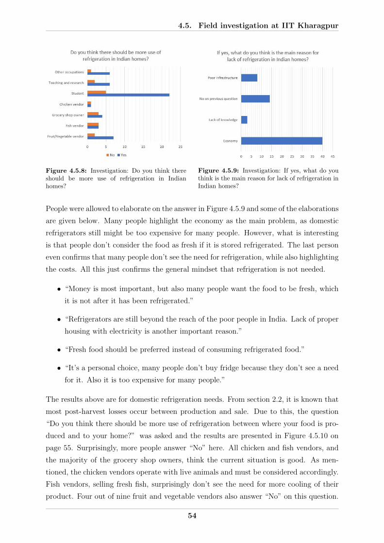
4.5. Field investigation at IIT Kharagpur
Figure 4.5.8: Investigation: Do you think thereshould be more use of refrigeration in Indianhomes?
Figure 4.5.9: Investigation: If yes, what do youthink is the main reason for lack of refrigeration inIndian homes?
People were allowed to elaborate on the answer in Figure 4.5.9 and some of the elaborations
are given below. Many people highlight the economy as the main problem, as domestic
refrigerators still might be too expensive for many people. However, what is interesting
is that people don’t consider the food as fresh if it is stored refrigerated. The last person
even confirms that many people don’t see the need for refrigeration, while also highlighting
the costs. All this just confirms the general mindset that refrigeration is not needed.
• “Money is most important, but also many people want the food to be fresh, which
it is not after it has been refrigerated.”
• “Refrigerators are still beyond the reach of the poor people in India. Lack of proper
housing with electricity is another important reason.”
• “Fresh food should be preferred instead of consuming refrigerated food.”
• “It’s a personal choice, many people don’t buy fridge because they don’t see a need
for it. Also it is too expensive for many people.”
The results above are for domestic refrigeration needs. From section 2.2, it is known that
most post-harvest losses occur between production and sale. Due to this, the question
“Do you think there should be more use of refrigeration between where your food is pro-
duced and to your home?” was asked and the results are presented in Figure 4.5.10 on
page 55. Surprisingly, more people answer “No” here. All chicken and fish vendors, and
the majority of the grocery shop owners, think the current situation is good. As men-
tioned, the chicken vendors operate with live animals and must be considered accordingly.
Fish vendors, selling fresh fish, surprisingly don’t see the need for more cooling of their
product. Four out of nine fruit and vegetable vendors also answer “No” on this question.
54

4.5. Field investigation at IIT Kharagpur
Most students and people working within teaching and research, i.e. those with higher
education, see the need for more refrigeration in the supply chain. When asked “If yes,
what do you think is the main reason for the lack of refrigeration between producers and
homes in India?”, the results, in Figure 4.5.11, deviates from the above. Poor infrastruc-
ture is the main reason for this lack of refrigeration, although both economy and lack of
knowledge score high. In other words, people are aware that the agents in the food chain
just don’t know why they should use refrigeration.
Figure 4.5.10: Investigation: Do you think thereshould be more use of refrigeration between whereyour food is produced and to your home?
Figure 4.5.11: Investigation: If yes, what do youthink is the main reason for lack of refrigerationbetween producers and homes in India?
People were also allowed to elaborate on the answer in Figure 4.5.11 and some of the
elaborations are given below. Many people answered that they find the existing system
and capacity sufficient, which contradicts most literature presented section 2.2. However,
some are aware of the problems and highlight the lack of cold chain facilities and refrig-
erated trucks and minimum support from the government, which confirms the discussed
problems. One person even highlights the ignorance of agents working in the food chains
and the fact that they only care for profit. Many answers also focus on the costs of refrig-
eration and how it is too expensive for some people. The last two answers are both from
fruit and vegetable vendors. Their view on the situation is very different. One of them
state that he only buys the amount of goods he can sell so that he won’t need to store
the product refrigerated. However, the other person explicitly says that he often finds
deteriorated food and that he wants, and would use, a cold storage, if it was available.
• “The demand for cooling is met in the market. Demand and supply is equal.”
• “The existing system is sufficient.”
• “Lack of proper cold chain facilities and availability of electricity.”
55

4.6. Cold storage at Indian mandis
• “Refrigerated trucks are scarce. Economy is a major factor.”
• “In my locality from where I belong, no cold storage facility is available nearby to
store the vegetables. This is due to lack of awareness as well as poor economic condi-
tion of the farmers. Also, there is minimum support from government organisations
in increasing the awareness and developing the infrastructure.”
• “Since the producers and the sellers only care of profits, they don’t care of what
should be done in between.”
• “The cost of using refrigeration adds to the price of vegetables and fruits which
might turn away people from purchasing it.”
• “Many times i find deteriorated food at the place i am buying it. There is no
refrigeration which makes a lot of food go bad. If a cold storage would be made
available to me I would use it, I want it.”
• “I buy the capacity for the day and sell that amount.”
4.6 Cold storage at Indian mandis
Based on the investigation of the different cold chains and the answers in the survey at
IIT Kharagpur, improving the food quality and shelf life by introducing a cold storage at
the mandis, seems like a good solution to a much needed problem. The mandis is in great
need for modernisation and cold chain facilities are among the most needed improvements.
Such a system could be beneficial for smaller markets as well. One problem with cold
storage facilities at mandis’ is the costs. They might be to expensive for the agents at
the mandis or the market. It is therefore important that the cold storage is cost-effective,
easy to maintain and operate and energy efficient.
A cold storage that is movable would be very flexible, as it could come to the seller,
instead of having the seller come to the storage. By designing a cold storage the size of
a container, it could either be moved by a large truck or it could be designed as a trailer
to be attached to a vehicle and moved around. A problem that might arise when it is
movable is the energy source. Should it rely on an external electrical input or should it
produce its own power through a solar panel? The power supply in India is very unstable
and varying, and a renewable power source would be beneficial for both the environment
and the flexibility of the storage. However, the costs would increase and power would
become a problem at nighttime with a solar panel. Therefore, the most cost-effective
alternative would be to make it dependent on an external electrical input and skip the
56

4.6. Cold storage at Indian mandis
solar panels. The storage should not be in operation during transport, it should only be
powered when stationary.
From section 2.3, it is known that India is going through a comprehensive plan to phase
out HCFCs and HFCs, so use of natural refrigerants should be in focus. Ammonia is a
refrigerant used for a long time in India, but there are uncertainties around its safety.
By using ammonia as primary refrigerant in combination with a secondary refrigerant, it
is possible to contain the ammonia to the machine room. Hence, ammonia pipes would
never be in contact with food or the food storage room. It would still require proper
training for service and maintenance personnel to operate the ammonia refrigeration sys-
tem. A potential secondary, natural refrigerant is CO2. CO2 has many advantages when
used as secondary refrigerant, highlighted in section 2.5. It is not toxic, nor flammable, it
is environmental friendly and considered among the safest refrigerants. In addition CO2
can be used in both natural and forced circulation loops.
The refrigeration system should be cost-effective, efficient and easy to control and main-
tain. Using a single stage ammonia refrigeration system is a cost-effective and efficient
solution. The possibility of having CO2 in a NCL should be further investigated, to
avoid distributing ammonia to the storage space. Having a multi-commodity storage will
increase the flexibility and allow storage of multiple groups investigated in section 3.5.
However, it is uncertain whether or not the people at the market would use this correctly.
The different agents using the storage are probably not educated in correct use of the
storage and would store whatever food they have wherever it is available space, without
taking concern to the products storage requirements. The results from the survey at
IIT Kharagpur also indicate that knowledge about proper storage might be scarce. In
addition, having separate storage spaces would decrease the capacity and increase the
complexity of the refrigeration system and consequently increase the costs. Hence, the
storage will be designed with one large storage space.
4.6.1 Layout
The cold storage is designed as a trailer, on wheels, to make it movable. This will eliminate
the need for a crane when placing the storage at the desired location. The size will be
according to the ISO shipping container sizes, respectively the standard 20ft shipping
container. Anything larger will be difficult to transport by road in India. The specific
sizes can be found in Table 4.6.1 on page 58. The given measures are without insulation.
57

4.6. Cold storage at Indian mandis
Length Width Height
Exterior 6.10 m 2.44 m 2.60 m
Interior 5.87 m 2.34 m 2.38 m
Table 4.6.1: ISO 20ft shipping container standards (Container Solutions 2019).
The cold storage layout is illustrated in Figure 4.6.1. Measures are given for the exterior
size. The aisle spans the entire length of the cold storage and is the same width as the
door. This is to ensure access to all commodities. Storage space is alongside each wall,
from floor to roof. The machine room, with required equipment, is assumed to be placed
on top of the storage to maximise the available storage space. This will shield the storage
from some sunlight, though refrigeration load calculations are performed with sun expo-
sure on the entire roof. The door is assumed to be facing north. Loading of the storage is
assumed to happen evenly during the first week. The storage is then assumed to be fully
loaded until the last day of the month the products are sold.
(a) Interior.
(b) Exterior.
Figure 4.6.1: Cold storage layout.
The refrigeration systems investigated in this thesis are a single stage vapour compression
cycle, using ammonia as working fluid, with and without CO2 in a Natural Circulation
Loop (NCL). The two configurations investigated are illustrated in Figure 4.6.2 on page
59.
58

4.6. Cold storage at Indian mandis
(a) Without CO2 in NCL.
(b) With CO2 in NCL.
Figure 4.6.2: Single stage ammonia refrigeration system.
Since the machine room is assumed to be on top of the storage, the NCL should have
sufficient height to function. Heat is transferred from the refrigerated space to the NCL.
The CO2 will then partly or fully evaporate and its density will decrease. The resulting
buoyancy force will drive the CO2 from the evaporator and up to the CO2 receiver in
the machine room, which also acts as the IHX. Here, the CO2 transfer the heat to the
ammonia refrigeration system and condenses. This denser, liquid CO2, flows down to the
evaporator due to gravity. This way, heat can be transferred from the refrigerated space,
to the machine room, without any need for pumping power. It is important that the
evaporator is located below the CO2 receiver/IHX for this to work.
Changing the evaporation temperature of CO2 in the NCL requires changing the pressure
in the loop, which is impossible without adding another compressor. Consequently, the
NCL must be designed to keep a constant pressure and temperature level regardless of the
room temperature. Matching this level to apples and grapes, which have similar storage
conditions, is possible, but problems will arise when storing mangoes at 13°C. When
mangoes are in storage, the evaporator will operate with a temperature difference much
larger than what is necessary and the efficiency of the system will decrease. Using natural
circulation loops can be beneficial for conditions requiring a constant temperature, but in
this case, where the room temperature varies, it is more difficult. Despite the inhibitors,
performance of the system with the NCL will be investigated.
59
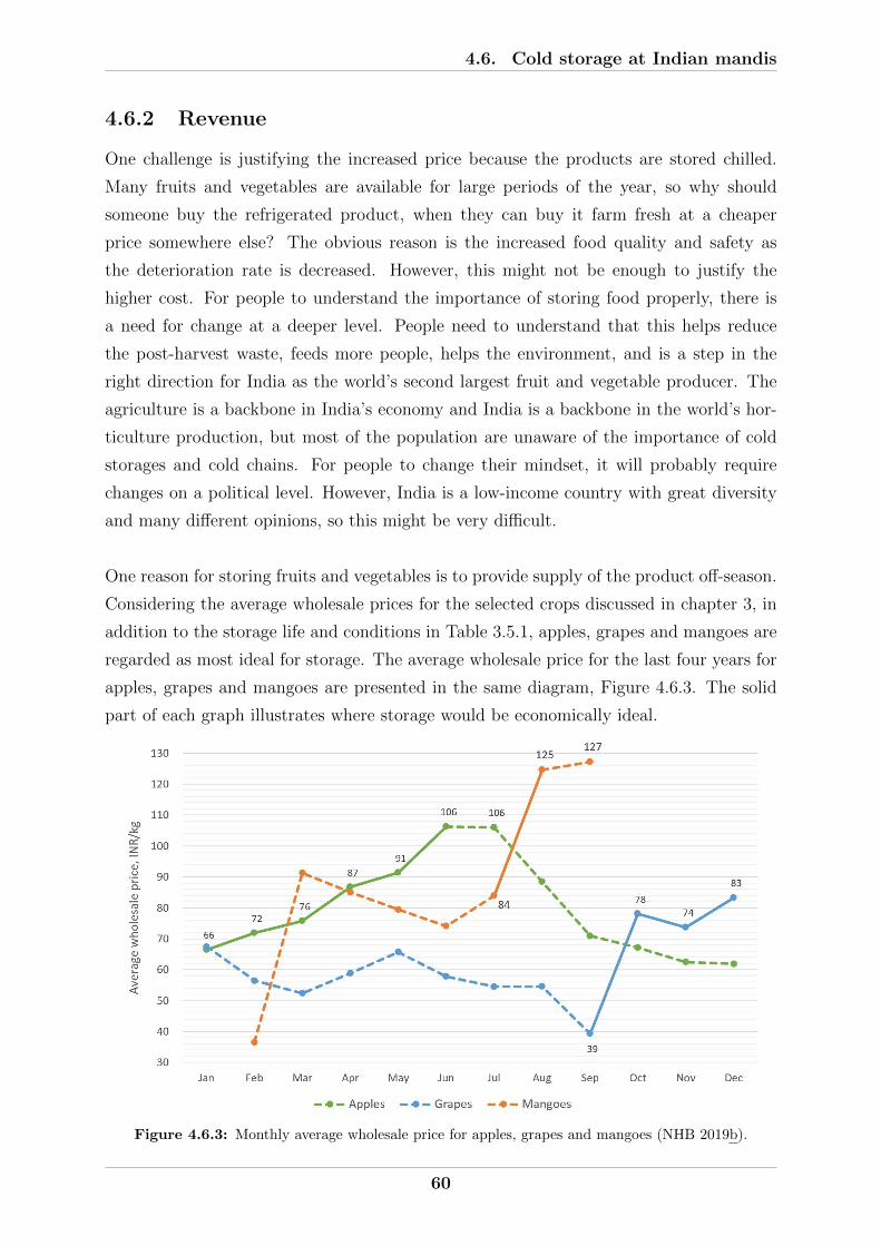
4.6. Cold storage at Indian mandis
4.6.2 Revenue
One challenge is justifying the increased price because the products are stored chilled.
Many fruits and vegetables are available for large periods of the year, so why should
someone buy the refrigerated product, when they can buy it farm fresh at a cheaper
price somewhere else? The obvious reason is the increased food quality and safety as
the deterioration rate is decreased. However, this might not be enough to justify the
higher cost. For people to understand the importance of storing food properly, there is
a need for change at a deeper level. People need to understand that this helps reduce
the post-harvest waste, feeds more people, helps the environment, and is a step in the
right direction for India as the world’s second largest fruit and vegetable producer. The
agriculture is a backbone in India’s economy and India is a backbone in the world’s hor-
ticulture production, but most of the population are unaware of the importance of cold
storages and cold chains. For people to change their mindset, it will probably require
changes on a political level. However, India is a low-income country with great diversity
and many different opinions, so this might be very difficult.
One reason for storing fruits and vegetables is to provide supply of the product off-season.
Considering the average wholesale prices for the selected crops discussed in chapter 3, in
addition to the storage life and conditions in Table 3.5.1, apples, grapes and mangoes are
regarded as most ideal for storage. The average wholesale price for the last four years for
apples, grapes and mangoes are presented in the same diagram, Figure 4.6.3. The solid
part of each graph illustrates where storage would be economically ideal.
Figure 4.6.3: Monthly average wholesale price for apples, grapes and mangoes (NHB 2019b).
60
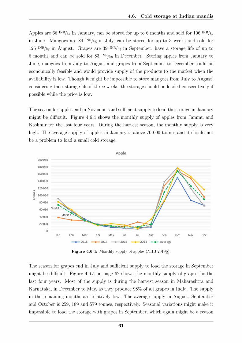
4.6. Cold storage at Indian mandis
Apples are 66 INR/kg in January, can be stored for up to 6 months and sold for 106 INR/kg
in June. Mangoes are 84 INR/kg in July, can be stored for up to 3 weeks and sold for
125 INR/kg in August. Grapes are 39 INR/kg in September, have a storage life of up to
6 months and can be sold for 83 INR/kg in December. Storing apples from January to
June, mangoes from July to August and grapes from September to December could be
economically feasible and would provide supply of the products to the market when the
availability is low. Though it might be impossible to store mangoes from July to August,
considering their storage life of three weeks, the storage should be loaded consecutively if
possible while the price is low.
The season for apples end in November and sufficient supply to load the storage in January
might be difficult. Figure 4.6.4 shows the monthly supply of apples from Jammu and
Kashmir for the last four years. During the harvest season, the monthly supply is very
high. The average supply of apples in January is above 70 000 tonnes and it should not
be a problem to load a small cold storage.
Figure 4.6.4: Monthly supply of apples (NHB 2019b).
The season for grapes end in July and sufficient supply to load the storage in September
might be difficult. Figure 4.6.5 on page 62 shows the monthly supply of grapes for the
last four years. Most of the supply is during the harvest season in Maharashtra and
Karnataka, in December to May, as they produce 98% of all grapes in India. The supply
in the remaining months are relatively low. The average supply in August, September
and October is 259, 189 and 579 tonnes, respectively. Seasonal variations might make it
impossible to load the storage with grapes in September, which again might be a reason
61

4.6. Cold storage at Indian mandis
for the unusually low average price. Still, the average supply in September is 189 tonnes
and loading of the storage this month is assumed possible.
Figure 4.6.5: Monthly supply of grapes (NHB 2019b).
The season for mangoes end in July and sufficient supply to load the storage should be
available. Figure 4.6.6 on page 63 shows the monthly supply of alphonso mangoes for
the last four years. Early in the harvest season, especially in 2016, the monthly supply is
high. There is no supply of mangoes from October to January and supply of mangoes in
August and September only happened in 2018, which explains the increase in price these
months. It seems to be a steady supply of mangoes in July, with an average of above 20
000 tonnes and loading the storage should not be a problem. In addition, the longer the
mango is stored with acceptable quality after July, the higher price it can be sold for.
62

4.6. Cold storage at Indian mandis
Figure 4.6.6: Monthly supply of mangoes (NHB 2019b).
If the average supply of apples, grapes and mangoes stays relatively constant the coming
years, it should be possible to operate a cold storage with these three commodities through
the entire year. Table 4.6.2 shows a summary of the logistics and revenue for storing these
fruits.
Commodity Loading Cost Storage time Selling Income Profit
Apples January 66 INR/kg 6 months June 106 INR/kg 40 INR/kg
Mangoes July 84 INR/kg 2 months August 125 INR/kg 41 INR/kg
Grapes September 39 INR/kg 4 months December 83 INR/kg 44 INR/kg
Table 4.6.2: Cold storage logistics and revenue.
Loading is assumed to happen during the first week of the month or as soon as sufficient
supply of the respective commodity is available. Sale of the product will happen consec-
utively through the respective month or in earlier months if the product degrades sooner.
Mangoes might be impossible to store for two months, so the storage should be refilled
when possible, if the price is low. Calculations are performed for full storage until the
last day of the month for all products. The profit is calculated as the difference between
the wholesale price when loading and when selling. This is a conservative approach con-
sidering that agents at wholesale markets buys the product from distribution markets,
merchants or other agents at a lower price than the wholesale price that given month.
The profit might, in reality, be larger than listed here. The revenue is relatively equal
for the commodities, where grapes have the highest price increase, with 44 INR/kg from
September to December. Investigating the monthly profit reveals that mangoes increase
63

4.6. Cold storage at Indian mandis
with 20.5 INR/kg per month, making it the most valuable product. Apples have about 6.7
INR/kg and grapes 11 INR/kg increase per month.
4.6.3 Assumptions
Ambient temperatures:
Ambient temperatures are used according to the daily temperatures provided in
Figure 4.6.7. Product loading temperatures are equal to the ambient conditions at
the day of loading.
Figure 4.6.7: Daily average temperatures in Kolkata year 2005 (Meteotest Genossenschaft 2005).
Products and temperatures:
• Apples are stored at -0.5°C room temperature.
• Grapes are stored at -0.5°C room temperature.
• Mangoes are stored at 13°C room temperature.
• All products are loaded at the ambient temperature the respective day.
Storage density:
Compact storage with 200 kg/m3 density (IIR 1993).
Loading rate and pull down time:
The storage is loaded with with 1/7 of the total capacity each day, over a period of 7
days, to reduce the pull down load. The storage should reach optimal temperature
within 24 hours after each loading.
64

4.6. Cold storage at Indian mandis
Door:
Size is chosen for pressed steel doors according to manual by CPWD (2006), where
width and height are 0.8 m and 2.045 m, respectively. Insulation is equal to the wall
insulation. The door is opened once a day to check on the stored product. Open-
close time is set to 30 seconds. It is assumed to stand open for 5 minutes when
checking the product, and for 1 hour when loading. Strip curtains are installed to
inhibit air flow through open door, with effectiveness of E=0.9 (ASHRAE 2018).
Ventilation:
The storage should be properly ventilated to remove excess ethylene. The heat gain
from ventilation is, however, negligible in such a small cold storage and ventilation
is not regarded any further.
Equipment:
Equipment loads are set to contribute 10% of the holding load.
Heat exchangers:
• Evaporator: Forced air finned coil evaporator. A fin spacing of 3 mm is used
(Grundfos 2019). Fin thickness is neglected in further calculations. A tube
spacing of 25 mm is used.
• Intermediate Heat Exchanger (IHX): Cascade heat exchanger with the NH3
evaporator inside the CO2 receiver.
• Condenser: Geometry and area are not considered in this thesis. Temperature
difference is set constant to 5°C.
Compressors:
Compressor efficiency will vary with the pressure ratio over the compressor, which
again is dependent on evaporator and condenser temperature. Studying varying
compressor efficiency is not considered as a relevant goal in this thesis and efficiency
is therefore set constant as η = 0.8, according to the isentropic efficiency chart,
Figure A.3.1 in Appendix A.
Insulation:
Expanded polystyrene (R-142b) is used. Thermal conductivity, kins = 0.037 W/mK.
Thickness, δins = 75 mm (ASHRAE 2018).
Walls, roof, floor:
Exterior and interior walls, roof and floor are (corrugated) sheet metal. Thickness
and thermal conductivity are negligible. Exterior walls and roof are painted in a
light colour.
65

4.6. Cold storage at Indian mandis
Sun allowance:
Heat gain due to sun radiation is included according to Table 5.2.1 on page 68 for
light-coloured surfaces.
Safety factor:
A safety factor of 10% is included in refrigeration loads.
66

Chapter 5
Method
5.1 Highlights
In this chapter, methods for the different calculations made when designing the cold stor-
age and refrigeration system are discussed. First the relevant equations and information
to calculate the refrigeration loads are presented. Then the method used to design both
refrigeration systems are discussed, before the method for heat exchanger calculations are
investigated and presented. At last, pressure losses through the NCL are discussed.
5.2 Refrigeration load calculation
5.2.1 Transmission loads
This is the heat loss related heat transmission through the walls, roof and floor of the
refrigerated space. The transmission load is usually the largest load and can be calculated
as:
QT = UA(Tamb − TR) (5.2.1)
where A is the surface area, Tamb is ambient temperature and TR is the cold storage room
temperature. U is the heat transfer coefficient, defined as:
U =kinsδins
(5.2.2)
where kins and δins are the thermal conductivity and thickness of the insulation, re-
spectively. The solar irradiation will influence the transmission through the wall. To
compensate for the solar irradiation, a sun-air temperature difference, ∆Tsun, is added,
depending on the direction the wall is facing and the type of surface. The sun-air tem-
67

5.2. Refrigeration load calculation
perature differences are shown in Table 5.2.1.
Typical surface types East/West wall, K South wall, K Flat roof, K
Dark-coloured surfaces: 5 3 11
Slate or tar roofing,
black paint
Medium-coloured surfaces: 4 3 9
Unpainted wood, brick,
red tile, dark cement,
red, gray, green paint
Light-coloured surfaces: 3 2 5
White stone, light coloured
cement, white paint
Table 5.2.1: Allowance for sun effect (ASHRAE 2018).
Instead of using the ambient temperature in Equation 5.2.1, the wall temperature, Twall,
must be used:
Twall = Tamb + ∆Tsun (5.2.3)
5.2.2 Infiltration loads
Infiltration loads are the heat gains from infiltrating air. When opening the door, there will
be air flow between the refrigerated room and the ambient. Heat load through doorways
from air exchange is as follows (ASHRAE 2018):
QD = QSDtDf (1 − E) (5.2.4)
where QS is the sensible and latent refrigeration load due to air exchange. For fully
established flow, it is:
QS = 0.221AD(hamb − hR)ρR
(1 − ρamb
ρR
)0.5
(gHD)0.5Fm (5.2.5)
where g is the gravitational constant, AD and HD are the doorway area and height, hamb
and ρamb are the ambient air enthalpy and density and hR and ρR are the cold storage
68
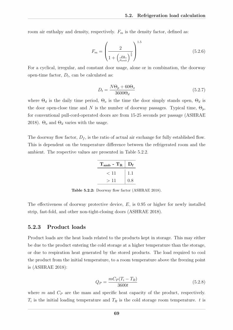
5.2. Refrigeration load calculation
room air enthalpy and density, respectively. Fm is the density factor, defined as:
Fm =
2
1 +(
ρRρamb
) 13
1.5
(5.2.6)
For a cyclical, irregular, and constant door usage, alone or in combination, the doorway
open-time factor, Dt, can be calculated as:
Dt =NΘp + 60Θo
3600Θd
(5.2.7)
where Θd is the daily time period, Θo is the time the door simply stands open, Θd is
the door open-close time and N is the number of doorway passages. Typical time, Θp,
for conventional pull-cord-operated doors are from 15-25 seconds per passage (ASHRAE
2018). Θo and Θd varies with the usage.
The doorway flow factor, Df , is the ratio of actual air exchange for fully established flow.
This is dependent on the temperature difference between the refrigerated room and the
ambient. The respective values are presented in Table 5.2.2.
Tamb - TR Df
< 11 1.1
> 11 0.8
Table 5.2.2: Doorway flow factor (ASHRAE 2018).
The effectiveness of doorway protective device, E, is 0.95 or higher for newly installed
strip, fast-fold, and other non-tight-closing doors (ASHRAE 2018).
5.2.3 Product loads
Product loads are the heat loads related to the products kept in storage. This may either
be due to the product entering the cold storage at a higher temperature than the storage,
or due to respiration heat generated by the stored products. The load required to cool
the product from the initial temperature, to a room temperature above the freezing point
is (ASHRAE 2018):
QP =mCP (Ti − TR)
3600t(5.2.8)
where m and CP are the mass and specific heat capacity of the product, respectively.
Ti is the initial loading temperature and TR is the cold storage room temperature. t is
69

5.2. Refrigeration load calculation
the time, in hours, required for the product to reach the room temperature. The specific
heat capacity for the investigated products are listed in Table 5.2.3. The values apply to
mature products shortly after harvest.
Product CP, kJ/kgK
Apple 3.81
Grape 3.70
Mango 3.74
Table 5.2.3: Specific heat capacity above freezing for selected fresh fruits (ASHRAE 2018).
The heat of respiration for the selected fruits, at selected temperatures, are shown in Ta-
ble 5.2.4. The respiration close to the freezing point is unavailable due to the temperature
being borderline to damaging the food. The listed heat of respiration is not constant and,
as some values indicate, it might vary over a given range for the same temperature. Foods
are living things and properties will vary between each single fruit or vegetable. Young,
actively growing tissues or fast-developing fruits have a high heat of respiration. Slow
developing crops however, have lower heat of respiration. Additionally, the first one or
two days after harvest, the heat of respiration will be high, but within a few days it will
stabilise at a lower equilibrium value. Crops that ripen in storage function the opposite
way, they will increase in respiration rate as they ripen.
Product Temperature, °C Heat of respiration, mW/kg
Apple, Delicious 0 10.2
5 15.0
Grape, Thompson seedless 0 5.8
5 14.1
Mango 15 133.4
20 222.6-449.1
Table 5.2.4: Heat of respiration for selected fresh fruits (ASHRAE 2018).
5.2.4 Equipment loads
There might be other refrigeration equipment contributing to the total refrigeration load,
like:
• Fan motors when forced-air circulation is used.
• Heat from defrosting of evaporators. This can be done by hot-gas defrost, electricity
70

5.3. Refrigeration cycle calculations
defrost or water defrost. Water defrost produces the least amount of load, while
electricity defrost contributes most to the refrigeration load.
At refrigeration temperatures above -1°C, equipment loads usually contribute about 5%
of the total refrigeration load. At lower refrigeration temperatures, like -30°C, this part
can become as high as 15%, or more, of the total refrigeration load (ASHRAE 2018).
5.2.5 Safety factor
When calculating the total refrigeration load, it is very common to add a safety factor to
allow for possible discrepancies between the design and the actual operation. This factor
will vary depending on the quality of the cold storage, but generally, a safety factor of
10% of the total refrigeration load is used (ASHRAE 2018).
5.3 Refrigeration cycle calculations
The refrigeration systems investigated in this thesis are a single stage vapour compression
cycle, using ammonia as working fluid, either combined with CO2 in a NCL or without.
The two configurations, with state points, are illustrated in Figure 5.3.1.
(a) Without CO2 in NCL.
(b) With CO2 in NCL.
Figure 5.3.1: Single stage ammonia refrigeration system.
71

5.3. Refrigeration cycle calculations
Looking at the ammonia system in Figure 5.3.1a, the heat absorbed in the evaporator is
given as:
Qe = me · (h6 − h5) (5.3.1)
where me is the mass flow through the evaporator and h is the enthalpy. Qe is equal to
the total refrigeration load, QL. Adding the NCL in Figure 5.3.1b, the heat absorbed by
the CO2 in the evaporator is given as:
Qe = me · (h8 − h7) (5.3.2)
The heat transferred from the CO2 NCL to the ammonia system in in the IHX is given
as:
QIHX = mNH3 · (h6 − h5) = mCO2 · (h8 − h7) (5.3.3)
where mNH3 and mCO2 are the mass flows of NH3 and CO2 through the IHX, respectively.
The energy balance over the NH3 receiver can be expressed as:
Qin = Qout
m4h4 + m6h6 = m1h1 + m5h5
(5.3.4)
The relations between the real compressor work, W , the isentropic compressor work, Wis,
and the isentropic compressor efficiency, ηis, is given as:
Wis = mc · (h2s − h1) (5.3.5)
W = mc · (h2 − h1) (5.3.6)
ηis =Wis
W=mc · (h2s − h1)
mc · (h2 − h1)=h2s − h1
h2 − h1
(5.3.7)
where mc is the mass flow through the compressor and condenser. The isentropic com-
pressor efficiency can often be found in tables or graphs, if the compressor pressure ratio,
π, is known
π =P2
P1
(5.3.8)
72
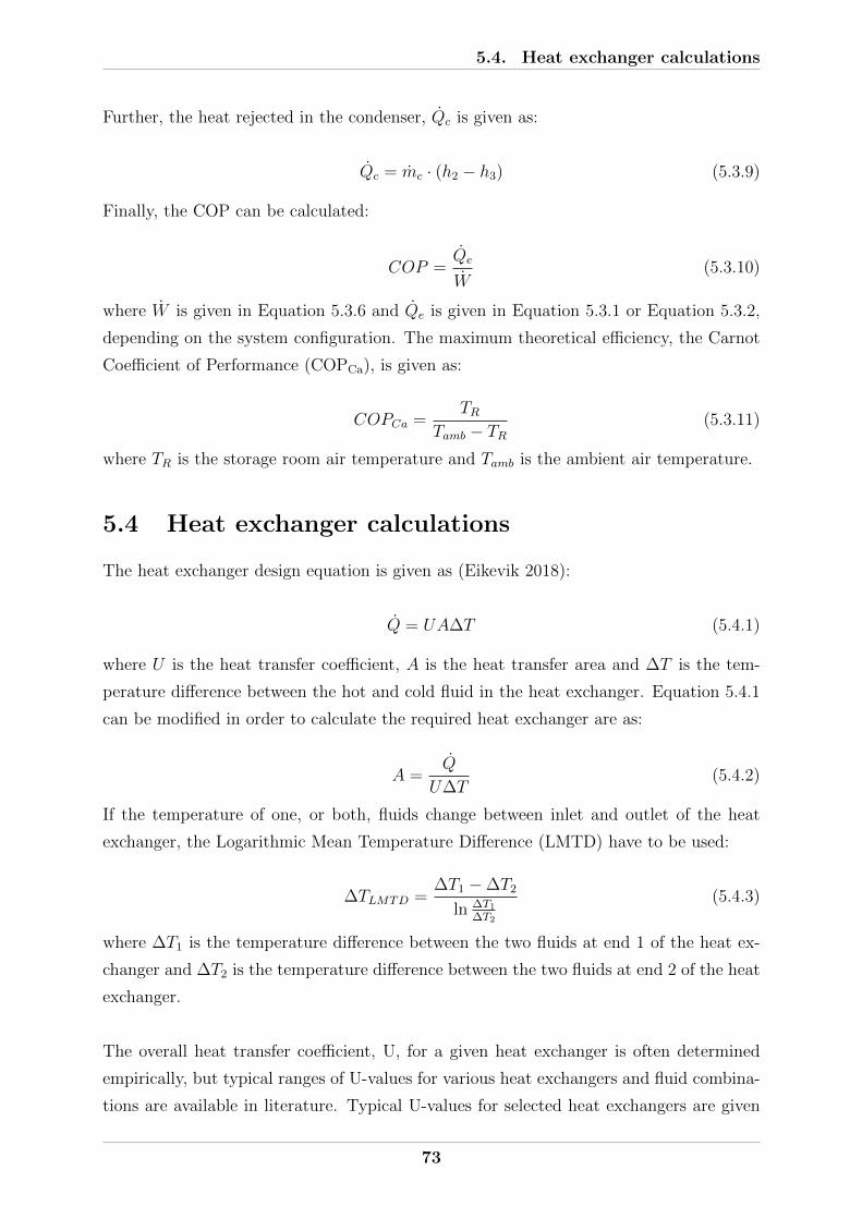
5.4. Heat exchanger calculations
Further, the heat rejected in the condenser, Qc is given as:
Qc = mc · (h2 − h3) (5.3.9)
Finally, the COP can be calculated:
COP =Qe
W(5.3.10)
where W is given in Equation 5.3.6 and Qe is given in Equation 5.3.1 or Equation 5.3.2,
depending on the system configuration. The maximum theoretical efficiency, the Carnot
Coefficient of Performance (COPCa), is given as:
COPCa =TR
Tamb − TR(5.3.11)
where TR is the storage room air temperature and Tamb is the ambient air temperature.
5.4 Heat exchanger calculations
The heat exchanger design equation is given as (Eikevik 2018):
Q = UA∆T (5.4.1)
where U is the heat transfer coefficient, A is the heat transfer area and ∆T is the tem-
perature difference between the hot and cold fluid in the heat exchanger. Equation 5.4.1
can be modified in order to calculate the required heat exchanger are as:
A =Q
U∆T(5.4.2)
If the temperature of one, or both, fluids change between inlet and outlet of the heat
exchanger, the Logarithmic Mean Temperature Difference (LMTD) have to be used:
∆TLMTD =∆T1 − ∆T2
ln ∆T1∆T2
(5.4.3)
where ∆T1 is the temperature difference between the two fluids at end 1 of the heat ex-
changer and ∆T2 is the temperature difference between the two fluids at end 2 of the heat
exchanger.
The overall heat transfer coefficient, U, for a given heat exchanger is often determined
empirically, but typical ranges of U-values for various heat exchangers and fluid combina-
tions are available in literature. Typical U-values for selected heat exchangers are given
73
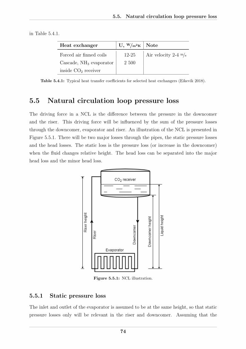
5.5. Natural circulation loop pressure loss
in Table 5.4.1.
Heat exchanger U, W/m2K Note
Forced air finned coils 12-25 Air velocity 2-4 m/s
Cascade, NH3 evaporator 2 500
inside CO2 receiver
Table 5.4.1: Typical heat transfer coefficients for selected heat exchangers (Eikevik 2018).
5.5 Natural circulation loop pressure loss
The driving force in a NCL is the difference between the pressure in the downcomer
and the riser. This driving force will be influenced by the sum of the pressure losses
through the downcomer, evaporator and riser. An illustration of the NCL is presented in
Figure 5.5.1. There will be two major losses through the pipes, the static pressure losses
and the head losses. The static loss is the pressure loss (or increase in the downcomer)
when the fluid changes relative height. The head loss can be separated into the major
head loss and the minor head loss.
Figure 5.5.1: NCL illustration.
5.5.1 Static pressure loss
The inlet and outlet of the evaporator is assumed to be at the same height, so that static
pressure losses only will be relevant in the riser and downcomer. Assuming that the
74

5.5. Natural circulation loop pressure loss
CO2 through the downcomer and riser is incompressible, ideal and moving with constant
velocity, Bernoulli’s equation can be simplified to give the pressure difference caused by
changing relative height through the pipe as (The Engineering ToolBox 2019a):
∆Pstatic = ρg∆H (5.5.1)
where ρ is the fluid density, g is the gravitational constant and ∆H is the change in height.
5.5.2 Head loss
The head losses can be separated into major head losses, the frictional pressure drops
through the pipe, and the minor head losses, the pressure losses through valves, bends
and fittings.
Major head loss
The major head loss will be dependent on whether the fluid is in single-phase or two-phase.
The fluid in the downcomer will be in single, liquid phase, while the fluid in the evaporator
and riser will be two-phased. The frictional pressure drop for a steady flow through a pipe
with constant cross-section area can be expressed through the Darcy-Weisbach equation
as (Singal et al. 2015):
∆Pmajor = fl
d
ρv2
2(5.5.2)
Using that the fluid velocity, v = V/A, and that the volume flow, V = m/ρ, Equation 5.5.2
can be expressed as
∆Pmajor = fl
d
ρ(VA
)2
2= f
l
d
ρ(
(m/ρ)A
)2
2= f
l
d
m2
2ρA2(5.5.3)
The cross-section area, A = πd2/4, is constant, which gives:
∆Pmajor = fl
d
m2
2ρ (πd2/4)2 = f
2
π
l
d3
m2
ρ(5.5.4)
where l is the length of the pipe, d is the diameter of the pipe, ρ is the fluid density
and m is the mass flow. The friction factor, f , is dependent on whether the fluid is in
single-phase or two-phase. For laminar flow, Re <2 000, the single-phase friction factor,
f1ph, is given as:
f1ph =64
Re1ph
(5.5.5)
75

5.5. Natural circulation loop pressure loss
where Re1ph is the single-phase Reynolds number, given as:
Re1ph =ρvd
µ=md
Aµ=
4
π
m
dµ1ph
(5.5.6)
where µ1ph is the single-phase dynamic viscosity. If the flow is turbulent, Re1ph >4 000,
the single-phase friction factor can be implicitly estimated using the Colebrook-White
formula. However, a good explicit approximation of the Colebrook-White formula is the
Swamee and Jain formula, given as (Zeghadnia et al. 2019):
f1ph =
[−2log
(ε/d
3.7+
5.74
Re0.91ph
)]−2
(5.5.7)
where ε is the absolute surface roughness of the pipe. Absolute roughness, ε, for new
copper, lead, brass and aluminium pipes are 0.001-0.002 mm (The Engineering ToolBox
2019b).
The two-phase friction factor, f2ph is defined through the following equation (Shannak
2008):
1√f2ph
= −2log
[269.7963
ε
d− 5.0452
Re2ph
log
(1
2.8257
(1000ε
d
)1.1098
+5.8506
Re0.89812ph
)](5.5.8)
where the Reynolds number for two-phase flow, Re2ph, is expressed as (Shannak 2008):
Re2ph =4000m
πd·x2 + (1 − x)2
(ρgρl
)µgx+ µl(1 − x)
(ρgρl
) (5.5.9)
where µg and µl are the dynamic viscosities of gas and liquid face, respectively, and ρg
and ρl are the densities of the gas and liquid face, respectively. x is the vapour quality,
here assumed to be constant for the given pipe length. The vapour quality through the
evaporator will change, making this model invalid. To deal with the changing vapour
quality, the total length of the evaporator will be divided into several smaller sections
where the vapour quality is assumed to be constant.
Minor head loss
There are several bends in the pipes going from the receiver through the evaporator and
back. These minor head losses can be modelled with the equivalent length in the Darcy-
76

5.5. Natural circulation loop pressure loss
Weisbach equation as (Singal et al. 2015):
∆Pminor = fleqd
ρv2
2= f
2
π
leqd3
m2
ρ(5.5.10)
where f is the friction factor given in Equation 5.5.5 or Equation 5.5.8, depending on
whether the flow is single-phased or two-phased. leq is the equivalent length for the
fitting. Relevant fittings are tabulated in Table 5.5.1.
Outer pipe diameter, mm 6 9 12 18
leq for regular 90° bend, m 0.7 0.9 1.1 1.3
leq for regular 180° bend, m 0.7 0.9 1.1 1.3
Table 5.5.1: Equivalent straight length for relevant pipe fittings (Singal et al. 2015).
77

Chapter 6
Results and discussion
6.1 Highlights
In this chapter, the results of all all cold storage calculations are presented. First, the
refrigeration loads during the entire year and during the loading week of each product
are presented. Then, heat exchangers are investigated, where temperature differences
and surface areas are calculated. When the size of the evaporator is known, the natural
circulation loop is designed. First, the results of changing gas quality are investigated,
before the optimal height and circulation rate are decided, based on the pressure drop
through the system. More specifics around the evaporator and CO2 receiver are given.
When height and circulation rate are chosen, the performance of the NCL at different
loads are investigated. Once all parameters are set, the SCOPs for the investigated
refrigeration systems are presented. Knowing the performance of the entire system, the
required compressor works are used to give an estimate about the operating profits for
the cold storage.
Refrigeration load
The refrigeration load variations, based on the daily average ambient temperatures in
Kolkata in 2005 (Figure 4.6.7 on page 64), are presented in Figure 6.2.1 on page 81.
The peak loads naturally occur during the loading weeks, when the pull down loads are
occurring. The highest refrigeration load, when loading grapes, is 2.43 kW. The lowest
refrigeration load is 0.84 kW, in January. When the load variations are investigated using
the hourly temperatures during the loading week, the resulting loads are smaller. When
storing apples, the load peak the first day with 1.81 kW. Loads when storing mangoes
peak the seventh day with 1.77 kW and grapes the fourth day with 2.30 kW. They are
presented in Figure 6.2.2, 6.2.3 and 6.2.4 on page 82 and 83.
78
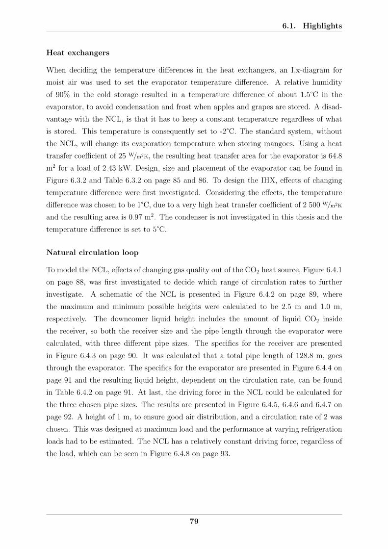
6.1. Highlights
Heat exchangers
When deciding the temperature differences in the heat exchangers, an I,x-diagram for
moist air was used to set the evaporator temperature difference. A relative humidity
of 90% in the cold storage resulted in a temperature difference of about 1.5°C in the
evaporator, to avoid condensation and frost when apples and grapes are stored. A disad-
vantage with the NCL, is that it has to keep a constant temperature regardless of what
is stored. This temperature is consequently set to -2°C. The standard system, without
the NCL, will change its evaporation temperature when storing mangoes. Using a heat
transfer coefficient of 25 W/m2K, the resulting heat transfer area for the evaporator is 64.8
m2 for a load of 2.43 kW. Design, size and placement of the evaporator can be found in
Figure 6.3.2 and Table 6.3.2 on page 85 and 86. To design the IHX, effects of changing
temperature difference were first investigated. Considering the effects, the temperature
difference was chosen to be 1°C, due to a very high heat transfer coefficient of 2 500 W/m2K
and the resulting area is 0.97 m2. The condenser is not investigated in this thesis and the
temperature difference is set to 5°C.
Natural circulation loop
To model the NCL, effects of changing gas quality out of the CO2 heat source, Figure 6.4.1
on page 88, was first investigated to decide which range of circulation rates to further
investigate. A schematic of the NCL is presented in Figure 6.4.2 on page 89, where
the maximum and minimum possible heights were calculated to be 2.5 m and 1.0 m,
respectively. The downcomer liquid height includes the amount of liquid CO2 inside
the receiver, so both the receiver size and the pipe length through the evaporator were
calculated, with three different pipe sizes. The specifics for the receiver are presented
in Figure 6.4.3 on page 90. It was calculated that a total pipe length of 128.8 m, goes
through the evaporator. The specifics for the evaporator are presented in Figure 6.4.4 on
page 91 and the resulting liquid height, dependent on the circulation rate, can be found
in Table 6.4.2 on page 91. At last, the driving force in the NCL could be calculated for
the three chosen pipe sizes. The results are presented in Figure 6.4.5, 6.4.6 and 6.4.7 on
page 92. A height of 1 m, to ensure good air distribution, and a circulation rate of 2 was
chosen. This was designed at maximum load and the performance at varying refrigeration
loads had to be estimated. The NCL has a relatively constant driving force, regardless of
the load, which can be seen in Figure 6.4.8 on page 93.
79

6.2. Refrigeration load
Performance
With all relevant parts of the refrigeration system and cold storage designed, the perfor-
mance was estimated, based on the presented load variations. The SCOP was calculated
to be between about 4.5 and 10, for both systems through the year, as seen in Figure 6.5.1
on page 95. When storing apples and grapes, the COP for the NCL system is just slightly
below the COP for the standard system, but the difference is almost negligible. The stan-
dard system has an average COP through the year of about 6.5, while the NCL system
has about 5.6. This is due to relatively poor performance of the NCL system, compared
to the standard configuration, when storing mangoes. During this period, the standard
system operates with a COP of between 8 and 10, while the NCL system, due to the
unnecessary low evaporation temperature, operates with a COP of around 5. The COPs
during the loading weeks are also presented, in Figure 6.5.2, 6.5.3 and 6.5.4 on page 96 and
97. As expected, when using hourly temperatures, the calculated COPs vary more. They
are both higher and lower, than the COP calculated with the average daily temperature.
Revenue
The final part of the results is the estimated revenue of the system. Using two average
electrical rates in India, Table 6.6.1 on page 98, and the expected profit from changing
market price, Table 4.6.2 on page 63, the operating profits are estimated. When a domestic
consumer rate is used, the estimated operating profit for one year is about 479 000 INR
for the standard system and about 478 000 for the NCL system. If a commercial consumer
rate is used, the estimated operating profit is about 476 000 INR for the standard system
and about 474 000 for the NCL system. The electricity rates in India vary from state to
state, but on average, they are low and almost negligible to the income. The power costs
for one year is calculated to be only between 9 000 INR and 16 000 INR, depending on
the system configuration and electricity rate. Detailed results can be found in Table 6.6.3
to 6.6.6 on page 99 and 100. Investment costs are not considered.
6.2 Refrigeration load
The refrigeration loads are calculated using Engineering Equations Solver (EES) and the
respective codes used can be seen in section B.2, B.3 and B.4 in Appendix B. The refrig-
eration load will change depending on the product stored and the ambient temperature.
Figure 6.2.1 on page 81 shows how the total refrigeration load changes throughout the
year, based on the temperatures in Kolkata in 2005, Figure 4.6.7 on page 64. Generally,
the loads change more or less similar to how the ambient temperature changes. The
80

6.2. Refrigeration load
highest loads naturally occur during the loading week for the three products, where the
absolute peak is 2.43 kW when grapes are loaded. The total loading capacity of the
storage is 3 914 kg, when using the storage density assumed in subsection 4.6.3.
Figure 6.2.1: Annual total refrigeration load.
The refrigeration system should be designed to handle the maximum load. Ideally, the
fruits should be pre-cooled rapidly to the desired storage temperature with a suited pre-
cooling system, to avoid the large pull down loads. The master thesis written by Espedalen
(2019) investigates the possibility of a pre-cooling system, which would be a great addition
to the cold storage investigated in this thesis. However, as discussed in section 3.3 and
chapter 4, pre-cooling is only performed when exporting grapes. It is therefore reason-
able to believe that the product will be loaded at ambient temperatures and pull down
loads have to be regarded. The system will be in need of a compressor covering a range
from about 0.8 kW to 2.5 kW and from about 15°C to about 34°C ambient temperature.
From section 2.4, it is known that Frigopol produce separating hood compressors with an
operating range from -30°C to 50°C, which is sufficient for Indian conditions. In addition,
it can provide a cooling capacity of 1 kW, up to 95 kW, with capacity control down to
20% of the chosen capacity. Using this compressor for a maximum capacity of 2.5 kW is
a good solution. It can be regulated down to 0.5 kW, which covers the entire range of
refrigeration loads.
The total loads in Figure 6.2.1 are calculated with the average daily temperature. Real
temperatures will become higher than this, often close to 40°C for a few hours during the
day. Hourly loads are therefore investigated to determine whether or not the average daily
temperatures provide a decent representation. Since the highest loads occur during the
loading week, the hourly loads during the loading week for each of the products are further
81

6.2. Refrigeration load
investigated. The temperatures each hour during the week, when loading apples, mangoes
and grapes, can be seen in Figure A.4.1, Figure A.5.1 and Figure A.6.1 in Appendix A.
Apples
The different loads during the loading week for apples are presented in Figure 6.2.2. The
dominating load is the transmission load, reaching above 1.1 kW the first day. The pull
down load is the second largest load, also highest during the first day. The remaining
loads are relatively small. The highest total load, occurring at the middle of the first
day, is 1.81 kW. This is equal to the peak load for calculations using the average daily
temperature. Hence, using the average daily temperatures provides a good estimation of
refrigeration loads when storing apples.
Figure 6.2.2: Refrigeration loads during loading week for apples.
Mangoes
The different loads during the loading week for mangoes are presented in Figure 6.2.3 on
page 83. The dominating load is the transmission load, reaching about 0.9 kW the first
three days. From day four and out, the temperatures vary less between day and night,
making the load variations less predictable. The pull down load is the second largest
load, the first four days. The respiration heat for mangoes, however, is much larger than
the respiration heat of apples and grapes. When loading more mangoes each day, the
respiration load eventually exceed the pull down load, reaching a value of above 0.5 kW.
The equipment and infiltration loads are relatively small. The highest total load occur
at the middle of day seven, reaching 1.71 kW. This is actually smaller than the load
calculated with the average daily temperature, 1.89 kW in Figure 6.2.1. Hence, using the
average daily temperature is a conservative approach when storing mangoes.
82

6.2. Refrigeration load
Figure 6.2.3: Refrigeration loads during loading week for mangoes.
Grapes
The different loads during the loading week for grapes are presented in Figure 6.2.4. The
dominating load is the transmission load, reaching above 1.4 kW several days. Grapes
are loaded when ambient temperatures are high and they are stored below 0°C, so the
pull down load is the second largest load, staying relatively constant around 0.75 kW.
The remaining loads are relatively small. The total load reach its peak value on day four,
with 2.3 kW. As with mangoes, this load is smaller than the load calculated with the
average daily temperature, 2.43 kW. Using the average daily temperature will therefore
be a conservative approach when storing grapes.
Figure 6.2.4: Refrigeration loads during loading week for grapes.
83

6.3. Heat exchangers
6.3 Heat exchangers
6.3.1 Evaporator
Temperature difference
The room temperature should be kept at -0.5°C for apples and grapes, and 13°C for
mangoes. The relative humidity, from Table 3.5.1 on page 39, should ideally be kept
at 90-95% for apples and grapes, and 85-90% for mangoes. A relative humidity of 90%
is therefore a decent compromise for all three products. Looking at Figure 6.3.1, for a
storage temperature of -0.5°C and relative humidity of 90%, the temperature difference
between the evaporator and storage air should be no more than 1.5°C to avoid moisture
to condense on the evaporator. Hence, the evaporator, when using the NCL will operate
at a temperature of -2°C. Since the evaporation temperature must be kept constant when
using the NCL, problems will arise when storing mangoes. From the I,x-diagram, we see
that an evaporator temperature of -2°C will be far into the condensing area for moist air
when the room temperature is 13°C with relative humidity of 90%. Water will condense
on equipment below about 11°C. Consequently, condensation and frost will form on the
evaporator when storing mangoes.
This problem will only occur when using the NCL, which must be kept at a constant
temperature. The standard system configuration can change its evaporation tempera-
ture. When storing apples and grapes, the evaporator will still operate at -2°C to avoid
condensation, but when storing mangoes, the evaporator will be kept at 11.5°C to avoid
condensation. In both cases, with or without the NCL, the temperature difference between
the evaporator and storage air should stay low enough to avoid condensation.
Figure 6.3.1: I,x-diagram for moist air.
84

6.3. Heat exchangers
Evaporator surface area
The evaporator area must be designed at the maximum load, which is during the fourth
day of loading grapes. The peak load was calculated to be 2.43 kW and the evaporator
temperature difference has already been set to 1.5°C. From Table 5.4.1 on page 74, the heat
transfer coefficient, U, is set to 25 W/m2K. Using Equation 5.4.2, the required evaporator
surface area can be calculated. The results are presented in Table 6.3.1.
Parameter Value Unit
Q 2 430 W
U 25 W/m2K
∆T 1.5 °C
A 64.8 m2
Table 6.3.1: Required evaporator area.
The required evaporator surface area is calculated to be 64.8 m2. The width of the
evaporator is set equal to the aisle width, 80 cm, so it can be placed on the wall opposite
of the door, see Figure 6.3.2b. Using a fin spacing of 3 mm and neglecting fin thickness,
see subsection 4.6.3, results in a maximum of 266 plates. The depth is set to 20 cm, to
avoid a large pressure loss in the air through the evaporator, resulting in a fin height of
about 61 cm. Size specifics are summarised in Table 6.3.2 on page 86.
(a) Schematic. (b) Placement.
Figure 6.3.2: Evaporator design.
85
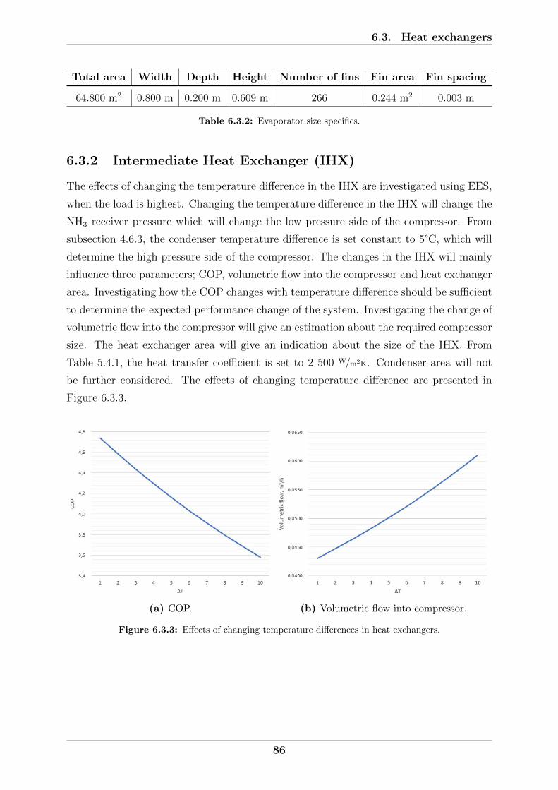
6.3. Heat exchangers
Total area Width Depth Height Number of fins Fin area Fin spacing
64.800 m2 0.800 m 0.200 m 0.609 m 266 0.244 m2 0.003 m
Table 6.3.2: Evaporator size specifics.
6.3.2 Intermediate Heat Exchanger (IHX)
The effects of changing the temperature difference in the IHX are investigated using EES,
when the load is highest. Changing the temperature difference in the IHX will change the
NH3 receiver pressure which will change the low pressure side of the compressor. From
subsection 4.6.3, the condenser temperature difference is set constant to 5°C, which will
determine the high pressure side of the compressor. The changes in the IHX will mainly
influence three parameters; COP, volumetric flow into the compressor and heat exchanger
area. Investigating how the COP changes with temperature difference should be sufficient
to determine the expected performance change of the system. Investigating the change of
volumetric flow into the compressor will give an estimation about the required compressor
size. The heat exchanger area will give an indication about the size of the IHX. From
Table 5.4.1, the heat transfer coefficient is set to 2 500 W/m2K. Condenser area will not
be further considered. The effects of changing temperature difference are presented in
Figure 6.3.3.
(a) COP. (b) Volumetric flow into compressor.
Figure 6.3.3: Effects of changing temperature differences in heat exchangers.
86

6.3. Heat exchangers
(c) IHX area.
Figure 6.3.3: Effects of changing temperature differences in heat exchangers.
In Figure 6.3.3a, increasing the temperature difference in the IHX, will reduce the COP
with about 0.13/°C. However, even with a temperature difference of ∆T=10, the COP
is above 3.5. Looking at the volumetric flow into the compressor in Figure 6.3.3b, an
increase in temperature difference will increase the flow with about 4%/°C. In other words,
keeping a low temperature difference allows for a smaller compressor. In Figure 6.3.3c,
for a temperature difference of ∆T=1, the required heat transfer area is below 1 m2. The
required area change somewhat exponentially, so increasing the temperature difference
to ∆T=4 reduce the required area to about 0,25 m2. For temperature differences above
∆T=4, the decrease in area is relatively small. When calculating the IHX area, the NCL
is assumed to be an ideal loop, meaning no loss in energy, so that there is 2.43 kW heat
flow through the IHX. This heat exchanger is designed as a cascade heat exchanger, which
is very efficient as both fluids go through a phase change. Considering all the effects of
changing the temperature difference in the IHX, a temperature difference of ∆T=1 seems
possible due to the high efficiency, resulting in the best performance of the system. ∆T
is therefore set equal to 1 for the IHX and the specifics are given in Table 6.3.3.
Parameter Value Unit
Q 2 430 W
U 2 500 W/m2K
∆T 1 °C
A 0.97 m2
Table 6.3.3: IHX size specifics.
87

6.4. Natural circulation loop
6.4 Natural circulation loop
The NCL is modelled using EES and the respective pressure losses discussed in section 5.5.
The EES code can be seen in section B.1 in Appendix B.
6.4.1 Gas quality out of CO2 heat source
Effects of changing gas quality out of the CO2 heat source are investigated when the
refrigeration load is highest. Since the NCL in the refrigeration system in Figure 5.3.1b
is designed with the IHX inside the CO2 receiver, changing the gas quality out of the
evaporator will mainly change the required CO2 mass flow through the evaporator to
remove the desired amount of heat. Effects of changing gas quality out of CO2 evaporator
are presented in Figure 6.4.1.
Figure 6.4.1: Effects of changing gas quality out of CO2 evaporator.
If the gas quality decrease from 1, down to 0.5, the mass flow through the evaporator must
double to provide the required cooling capacity. This change is, however, small compared
to the increase in mass flow when the gas quality is below about 0.3 to 0.4. For low gas
qualities, the required mass flow has an exponential increase, reaching values about 10
times the mass flow for gas quality equal to 1. Typical recommended circulation rates
through heat exchangers are between 2 and 4, which corresponds to a gas quality between
0.5 and 0.25, but circulation rates from 1 to 5 will be investigated during modelling of
the NCL.
88

6.4. Natural circulation loop
6.4.2 Optimal height and circulation rate
The system is modelled from the CO2 receiver and down, including downcomer, riser and
evaporator. A schematic of the loop, showing piping and liquid height, is illustrated in
Figure 6.4.2a. Figure 6.4.2b shows the minimum and maximum height possible for the
placement of the evaporator inside the cold storage. Note that neither of the drawings
are to scale, they are only illustrational. The riser is designed with two 90°bends, while
the downcomer only have one. The optimum height of the evaporator will be investigated
between 1.0 m and 2.5 m. Heights above 2.5 m are possible if the receiver are raised above
the roof, but 2.5 m is assumed to be the maximum height in this model.
(a) NCL schematic.
(b) NCL placement.
Figure 6.4.2: Design of NCL.
When calculating the liquid height, a minimum liquid level in the receiver have to be
decided. When the system is in operation, the liquid height will change depending on the
circulation rate and pipe length. The receiver is modelled as a standing cylinder with a
diameter of 30 cm. The minimum liquid height, when the downcomer, evaporator and
riser, are filled with liquid, is set to 10 cm, see Figure 6.4.3 on page 90. The receiver
height is set to 20 cm above the maximum liquid height.
89

6.4. Natural circulation loop
Parameter Value Unit
Diameter, d 0.3 m
Minimum liquid height, HL,min 0.1 m
Receiver height, H Liquid hgt. + 0.2 m
Figure 6.4.3: CO2 receiver.
To estimate the liquid standing in the evaporator during system standstill, the pipe length
through the evaporator have to be calculated. Using Figure 6.3.2a, with the calculated
sizes, the number of pipes can be decided. Three different pipe sizes will be investigated,
3/8”, 1/2” and 5/8”. Specific pipe sizes are provided in Table 6.4.1. The pipe size is
assumed to be equal in all parts of the NCL.
Size Outer diameter Wall thickness Maximum pressure
3/8” 9.53 mm 0.76 mm 48 bars
1/2” 12.70 mm 0.89 mm 48 bars
5/8” 15.88 mm 1.02 mm 48 bars
Table 6.4.1: Selected pipe sizes.
The resulting pipe lengths are presented in Figure 6.4.4 on page 91. The bends on the
sides of the evaporator, connecting each pipe, are neglected in total length.
90

6.4. Natural circulation loop
Parameter Value Unit
Npipes,x 7 pcs
Npipes,z 23 pcs
Npipes,tot 161 pcs
Lpipe,y 0.8 m
Lpipes,tot 128.8 m
Figure 6.4.4: Pipe length through evaporator.
Knowing the total pipe length below the receiver, the change in liquid height when the
system is running can be calculated. The resulting receiver liquid heights are presented
in Table 6.4.2. The length of the downcomer and riser are negligible compared to the
pipe length trough the evaporator. Due to this, the liquid height in the receiver will be
approximately only dependent on the circulation rate. Changes in pipe length in the
downcomer and riser influence the liquid height in the receiver with a maximum of about
5 mm. Hence, liquid height is set constant for all heights, varying only with circulation
rate. The inlet of the riser is set to 10 cm above the highest liquid height.
Circulation rateLiquid height
3/8” pipe
Liquid height
1/2” pipe
Liquid height
5/8” pipe
1 0.18 m 0.26 m 0.35 m
2 0.14 m 0.18 m 0.23 m
3 0.13 m 0.15 m 0.18 m
4 0.12 m 0.14 m 0.16 m
5 0.12 m 0.13 m 0.15 m
Table 6.4.2: Liquid height in the CO2 receiver.
The liquid height will influence the static pressure increase through the downcomer and
the length of the riser. When the pipe size is set, the operation conditions of the NCL will
be dependent on the riser and downcomer height and the circulation rate. Plotting the
circulation rate against the height to visualise the pressure difference in the downcomer
versus the riser, will give an indication about the optimal height and circulation rate.
91

6.4. Natural circulation loop
The driving force for the NCL for the different pipe sizes are presented in Figure 6.4.5 to
Figure 6.4.7.
Figure 6.4.5: NCL driving force for 3/8” pipes.
Figure 6.4.6: NCL driving force for 1/2” pipes.
Figure 6.4.7: NCL driving force for 5/8” pipes.
92
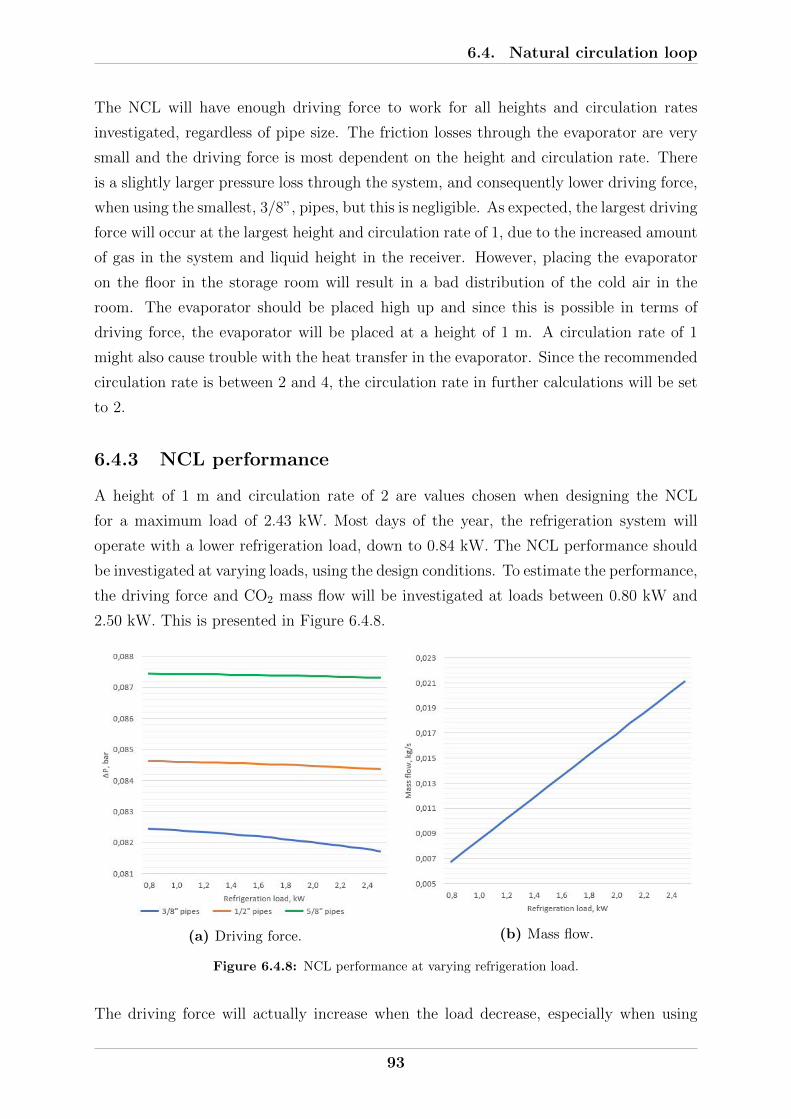
6.4. Natural circulation loop
The NCL will have enough driving force to work for all heights and circulation rates
investigated, regardless of pipe size. The friction losses through the evaporator are very
small and the driving force is most dependent on the height and circulation rate. There
is a slightly larger pressure loss through the system, and consequently lower driving force,
when using the smallest, 3/8”, pipes, but this is negligible. As expected, the largest driving
force will occur at the largest height and circulation rate of 1, due to the increased amount
of gas in the system and liquid height in the receiver. However, placing the evaporator
on the floor in the storage room will result in a bad distribution of the cold air in the
room. The evaporator should be placed high up and since this is possible in terms of
driving force, the evaporator will be placed at a height of 1 m. A circulation rate of 1
might also cause trouble with the heat transfer in the evaporator. Since the recommended
circulation rate is between 2 and 4, the circulation rate in further calculations will be set
to 2.
6.4.3 NCL performance
A height of 1 m and circulation rate of 2 are values chosen when designing the NCL
for a maximum load of 2.43 kW. Most days of the year, the refrigeration system will
operate with a lower refrigeration load, down to 0.84 kW. The NCL performance should
be investigated at varying loads, using the design conditions. To estimate the performance,
the driving force and CO2 mass flow will be investigated at loads between 0.80 kW and
2.50 kW. This is presented in Figure 6.4.8.
(a) Driving force. (b) Mass flow.
Figure 6.4.8: NCL performance at varying refrigeration load.
The driving force will actually increase when the load decrease, especially when using
93

6.5. Refrigeration system performance
3/8” pipes, as seen in Figure 6.4.8a. At high loads, the mass flow will increase and the
smallest pipe might restrict the flow, causing the drop in driving force. However, for the
investigated loads, this change is very small and negligible, so the driving force can be
considered constant for this range. The slightly larger driving force when using larger
pipes can be seen here. The variations in mass flow for varying refrigeration loads are
presented in Figure 6.4.8b. The mass flow will be linearly dependent on the load, and will
consequently be low at low loads. When modelling, the mass flow is decided using the
given refrigeration load and enthalpy difference over the evaporator, causing this relation.
Increasing the circulation rate will increase the mass flow, if it becomes to low, but when
estimating COP, the circulation rate will still be set to 2.
One problem with NCLs not investigated in this thesis are the challenges related to
instability. Here, it is modelled under ideal conditions, without unsuspected variations
in operating conditions. Due to the lack of a pump controlling the flow, it will be very
unpredictable in real applications. This is a difficult problem to address, as most solutions
would include the addition of equipment governing the flow, like a pump, which in turn
makes the flow forced. A constant circulation rate is also decided, which will not be
constant in real applications. Misale (2014) discuss the problem in more detail. They
highlight the nonlinear nature and low driving force as the main source for the instability.
The buoyancy and friction forces are not in phase, so small disturbances can heavily affect
the driving force and cause oscillations when the system should be in steady state. This
instability is a problem not yet considered solved for industrial applications.
6.5 Refrigeration system performance
Based on the previous calculations, designs and loads, the expected performance of the
system can be calculated. SCOP and COP during the loading weeks are investigated
using EES and the codes can be seen in section B.2, B.3 and B.4 in Appendix B. A
comparison of the SCOP for both system configurations are presented in Figure 6.5.1 on
page 95.
94

6.5. Refrigeration system performance
Figure 6.5.1: Refrigeration system SCOP, with and without NCL.
The COP for the standard system is slightly better than the COP when using the NCL.
However, the difference is relatively small and the NCL system is competitive. The aver-
age SCOP for the standard system during the entire year is 6.47, while the NCL system
operates with an average SCOP of 5.57. Compared to the COPCa, which is an average of
11.92, they are inferior. However, comparing the performance with the systems described
in section 2.4, the performance of both systems are considered to be good. Both systems
have a COP in the higher range of COPs discussed in Table 2.4.1.
One of the major weaknesses of the NCL is obvious here, the issue with evaporator tem-
perature. When storing mangoes, from July to September, at a room temperature of
13°C, the standard ammonia system can change its evaporator temperature up to 11.5°Cand the COP is consequently excellent, with values of around 8 to 10. However, when
using the NCL, the evaporation must continue at -2°C, and the COP is around 5. It is
obvious that the addition of a NCL is ineffective when the system operates with a varying
room temperature. On the other hand, if the room temperature is kept constant, using a
NCL can be a good alternative to avoid distributing ammonia into the storage room.
In section 6.2, refrigeration loads every hour during the loading weeks were investigated
to validate the use of average daily temperatures. Based on this, the COPs during loading
weeks for all three products will be presented.
95

6.5. Refrigeration system performance
Apples
The COPs during the loading week of apples are presented in Figure 6.5.2. The COP
vary from about 5 to above 10, with peaks higher than the calculated COP using the
average daily temperature. Hence, the performance can actually be better than what is
estimated in Figure 6.5.1. The COP is highly dependent on the ambient temperature and
the variation is therefore similar to how the ambient temperature change in Figure A.4.1
in Appendix A. The NCL system has a COP of about 0.2 to 0.5 lower than the standard
ammonia system.
Figure 6.5.2: COP during loading week of apples.
Mangoes
The COPs during the loading week of mangoes are presented in Figure 6.5.3 on page 97.
It is obvious that the addition of the NCL makes the performance inferior. The standard
system operates with an excellent COP of about 7 to 11.5, depending on the ambient
temperature. The NCL system only operates at a COP of about 4 to 6. However, the
variations in COP during the day is smaller for the NCL system, compared to the standard
system. Just as for apples, the estimated performance when using hourly temperatures
can be higher than when using the average daily temperature in Figure 6.5.1.
96

6.5. Refrigeration system performance
Figure 6.5.3: COP during loading week of mangoes.
Grapes
The COPs during the loading week of grapes are presented in Figure 6.5.4. The COP
varies from about 4.2 to 5.8. The performance of the NCL system is slightly worse than
the performance of the standard system, with a COP of about 0.2 lower. Despite this,
the NCL system is considered to be competitive for these conditions. The average COP
when using hourly temperatures can be, similar to apples and mangoes, higher than when
using daily average temperatures.
Figure 6.5.4: COP during loading week of grapes.
97
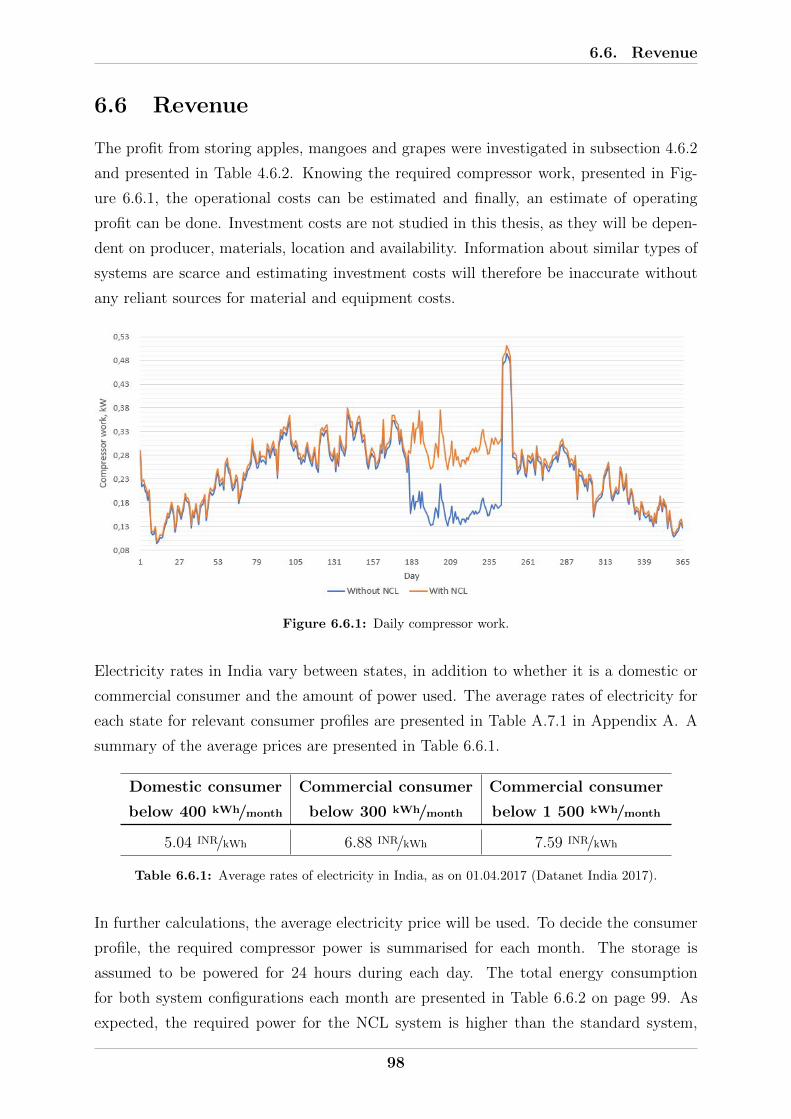
6.6. Revenue
6.6 Revenue
The profit from storing apples, mangoes and grapes were investigated in subsection 4.6.2
and presented in Table 4.6.2. Knowing the required compressor work, presented in Fig-
ure 6.6.1, the operational costs can be estimated and finally, an estimate of operating
profit can be done. Investment costs are not studied in this thesis, as they will be depen-
dent on producer, materials, location and availability. Information about similar types of
systems are scarce and estimating investment costs will therefore be inaccurate without
any reliant sources for material and equipment costs.
Figure 6.6.1: Daily compressor work.
Electricity rates in India vary between states, in addition to whether it is a domestic or
commercial consumer and the amount of power used. The average rates of electricity for
each state for relevant consumer profiles are presented in Table A.7.1 in Appendix A. A
summary of the average prices are presented in Table 6.6.1.
Domestic consumer
below 400 kWh/month
Commercial consumer
below 300 kWh/month
Commercial consumer
below 1 500 kWh/month
5.04 INR/kWh 6.88 INR/kWh 7.59 INR/kWh
Table 6.6.1: Average rates of electricity in India, as on 01.04.2017 (Datanet India 2017).
In further calculations, the average electricity price will be used. To decide the consumer
profile, the required compressor power is summarised for each month. The storage is
assumed to be powered for 24 hours during each day. The total energy consumption
for both system configurations each month are presented in Table 6.6.2 on page 99. As
expected, the required power for the NCL system is higher than the standard system,
98

6.6. Revenue
especially in July and August. The total consumption is below 300 kWh/month and the
commercial consumer profile when using less than 300 kWh/month can be used. Further,
the operating profit for the domestic consumer rate and the chosen commercial consumer
rate will be presented.
Month Standard system, kWh NCL system, kWh
January 114.26 119.55
February 126.62 131.83
March 186.21 193.15
April 207.89 215.27
May 230.08 238.06
June 210.52 217.97
July 122.24 223.38
August 118.78 217.10
September 222.08 230.10
October 188.41 195.37
November 143.81 149.57
December 108.84 113.72
Table 6.6.2: Monthly power consumption.
6.6.1 Domestic consumer rate
If the domestic consumer rate is used, the electricity rate will be, on average, 5.04 INR/kWh.
The storage can hold 3 914 kg of each product. Operating profits for each system con-
figuration are presented in Table 6.6.3 and Table 6.6.4. The difference in income due to
the lower efficiency of the NCL system is negligible, only about 1 300 INR. The total
operating profit for both configurations are just above 477 000 INR, making both solu-
tions economically favourable. The power costs are very low, only about 2% of the total
income. In other words, many of the other crops investigated in chapter 3 can yield a
positive profit even for just a short time period. Due to the increased complexity of the
NCL system, the investment costs using this configuration will be higher.
CommodityStorage
time
Income
INR/kg
Capacity
kg
Income
INR
Power consum-
ption, kWh
Electricity
rate, INR/kWh
Power costs
INR
Profit
INR
Apples Jan-Jun 40 3 914 156 560 1 076 5.04 5 419 151 141
Mangoes Jul-Aug 41 3 914 160 474 241 5.04 1 214 159 260
Grapes Sep-Dec 44 3 914 172 216 663 5.04 3 341 168 875
Total Jan-Dec 125 3 914 489 250 1 980 5.04 9 978 479 275
Table 6.6.3: Operating profits for standard system configuration using domestic consumer rate.
99

6.6. Revenue
CommodityStorage
time
Income
INR/kg
Capacity
kg
Income
INR
Power consum-
ption, kWh
Electricity
rate, INR/kWh
Power costs
INR
Profit
INR
Apples Jan-Jun 40 3 914 156 560 1 116 5.04 5 622 150 938
Mangoes Jul-Aug 41 3 914 160 474 440 5.04 2 219 158 255
Grapes Sep-Dec 44 3 914 172 216 689 5.04 3 470 168 748
Total Jan-Dec 125 3 914 489 250 2 245 5.04 11 311 477 939
Table 6.6.4: Operating profits for NCL system configuration using domestic consumer rate.
6.6.2 Commercial consumer rate
An electricity rate of 6.88 INR/kWh is used when profits are calculated with a commercial
consumer rate. As discussed, the power costs are very low and the profit will naturally
be high even though a higher electricity rate is used. Operating profits for the standard
system are presented in Table 6.6.5 and for the NCL system in Table 6.6.6. Both con-
figurations results in a profit of above 473 000 INR, when investment costs are excluded.
The standard system configuration will yield a profit of about 1 800 INR more, which
is a negligible difference. When increasing the electricity rate from 5.04 INR/kWh to 6.88
INR/kWh, the power costs will be about 3% of the the total income during the year. Even
with a higher power tariff, both system configurations results in good operating profits.
Other crops investigated in chapter 3, even those with lower potential for income, can
yield a positive profit over a short period of time.
CommodityStorage
time
Income
INR/kg
Capacity
kg
Income
INR
Power consum-
ption, kWh
Electricity
rate, INR/kWh
Power costs
INR
Profit
INR
Apples Jan-Jun 40 3 914 156 560 1 076 6.88 7 405 149 155
Mangoes Jul-Aug 41 3 914 160 474 241 6.88 1 659 158 815
Grapes Sep-Dec 44 3 914 172 216 663 6.88 4 565 167 651
Total Jan-Dec 125 3 914 489 250 1 980 6.88 13 629 475 621
Table 6.6.5: Operating profits for standard system configuration using commercial consumer rate.
CommodityStorage
time
Income
INR/kg
Capacity
kg
Income
INR
Power consum-
ption, kWh
Electricity
rate, INR/kWh
Power costs
INR
Profit
INR
Apples Jan-Jun 40 3 914 156 560 1 116 6.88 7 682 148 878
Mangoes Jul-Aug 41 3 914 160 474 440 6.88 3 032 157 442
Grapes Sep-Dec 44 3 914 172 216 689 6.88 4 742 167 794
Total Jan-Dec 125 3 914 489 250 2 245 6.88 15 456 473 794
Table 6.6.6: Operating profits for NCL system configuration using commercial consumer rate.
100
Chapter 7
Conclusion
7.1 Horticulture and cold chains
India is among the world’s most prominent producers of fruits and vegetables, with more
than 90 million tonnes of fruit and more than 169 million tonnes of vegetables. The most
important fruits are considered to be, in the following order, mangoes, grapes, apples,
oranges and bananas. Southern India is the most productive region. Except bananas,
all fruits are seasonal crops and they experience relatively large fluctuations in whole-
sale price through the year. Especially mangoes, grapes and apples are considered ideal
products for storage, both in terms of storage life and wholesale price increase. The only
documented cold chains are for grapes, which are successfully exported. Mangoes are to
some extent handled in packhouses, but lack of cold storage facilities cause post-harvest
losses up to 34%. As revealed in relevant literature, growth in production is increasing,
but post-harvest management and handling are not.
The most important vegetables are considered to be, in the following order, potatoes,
onions, tomatoes, cauliflowers, cabbages and okra. Eastern and Central India are the
most productive regions. Cabbages, cauliflowers and onions are seasonal crops, while
okra, potatoes and tomatoes are annual crops. Cabbages, cauliflowers, okra and toma-
toes experience some fluctuations in wholesale price through the year, but they are not
as ideal for storage as the discussed fruits. The increase in price is small and the storage
life is too short to fully utilise the increased price. However, as revealed when estimating
the revenue of the storage, even a small increase in price can yield a positive profit, as
operating costs are low. Storing vegetables might therefore be economically feasible if
supply of the chosen fruits are unavailable.
When investigating typical cold chains for export and domestic sale of horticultural crops,
101

7.1. Horticulture and cold chains
it is revealed that there are major deficiencies in all investigated chains. The lack of re-
frigerated transport and pre-cooling are highlighted as the major inhibitors in the export
chain. One solution proposed is to use the experience from exporting grapes, to export
other products. The deficiencies are larger for the domestic cold chain, compared to the
export chain, as there is less money to be made on domestic sale. It suffers from the same
challenges as the export chain, but in addition, there is a great need for cold storages.
From the literature study, it is known that India have cold storage capacity for about 30
million tonnes of food, but need capacity to handle above 60 million tonnes. In addition,
75% of the cold storages are already used to store potato, while 16% are out of operation.
80% of them also run on outdated technology. Another issue with the domestic chain is
the high number of intermediates, which is especially inhibiting the product flow through
the Indian mandis.
The Indian mandis’, the fruit and vegetable wholesale markets throughout the country,
are associated with low quality, poor remuneration and high wastes. This was revealed
to be due to the high number of intermediates and lack of cold chain facilities. From
harvest at the farm, to retail at the mandis, there might be several independent agents,
like an itinerary merchant, pre-harvest contractor, commissioning agent and transport
agent. The number of intermediates are difficult to change, but the wastes can be lowered
by supplying appropriate cold chain facilities, as more or less no food flowing through
the mandis are cooled. The mandis also form a crucial link in the export chain, thus,
modernising and improving the cold chain facilities at the mandis is concluded as the
most promising solution.
The field investigation conducted at IIT Kharagpur in India confirms many of the dis-
cussed problems. As expected, the fruit and vegetable vendors answered that they do
not refrigerate their food. They favour selling high quality products and they are aware
that refrigeration is very important. Yet, they do not refrigerate their products or care
if the products they buy are cooled. It seems like they just don’t care for refrigeration
as long as they are able to sell their product. The major inhibitor was concluded to be
economy, but it was also revealed to be linked to their mindset and knowledge. Many
people in India do not consider food fresh if it is refrigerated. They prefer consuming
food without refrigeration and do not see the need for refrigeration. One of the fruit and
vegetable vendors admitted to finding deteriorated food when buying his products from
the distribution market. He was aware that the lack of refrigeration was an issue and
answered that he would use a cold storage if it was available. This confirmed the need for
a cold storage at the mandis or other small markets.
102

7.2. Cold storage and refrigeration system
7.2 Cold storage and refrigeration system
From the investigated cold chains and the field investigation, it was concluded that de-
signing a cold storage intended to be used at the Indian mandis or other small markets is
a good solution. From the literature review on refrigerants in India it was revealed that
the focus is mainly on HFCs, as natural refrigerants not are considered competitive. To
prove otherwise, using natural refrigerants like NH3 and CO2 was decided. The refrig-
eration systems investigated are therefore a single stage NH3 system, with and without
CO2 in a NCL. A movable cold storage the size of a 20ft container was considered a good
option, as the cold storage could be delivered to the agents at the market, instead of them
coming to the storage. Renewable energy sources like a solar panel were discussed, but
not considered feasible due to economical reasons.
The choice of products to store was based on the average wholesale price variations. After
investigating how the price for each fruit or vegetable changes, it was decided that storing
apples from January to June, mangoes from July to August and grapes from September to
December resulted in the highest income. Apples can be bought for 66 INR/kg in January
and sold for 106 INR/kg in June. Mangoes can be bought for 84 INR/kg in July and sold
for 125 INR/kg in August. Grapes can be bought for 39 INR/kg in September and sold for
83 INR/kg in December. Knowing that the electricity rates are low, other products can be
stored with positive profit, if supply of apples, mangoes or grapes are unavailable.
By studying the I,x-diagram for moist air, it was concluded that an evaporation tempera-
ture of -2°C, when storing apples and grapes, was the best option with regards to relative
humidity, condensation and frost. This meant that the NCL system had to operate with
an evaporation temperature of -2°C, even when mangoes are stored at a room tempera-
ture of 13°C. The standard system is be able to change its evaporation temperature to
11.5°C when storing mangoes and operate with a temperature difference of 1.5°C in the
evaporator. This resulted in a surface area of 64.8 m2. By considering the width of the
aisle, the most practical size was considered to be 80 cm wide, about 61 cm high and
20 cm deep. Results of changing temperature temperature difference in the IHX was
investigated and after consideration, the temperature difference was decided to be 1°C,
resulting in a surface area of 0.97 m2.
When the NCL was designed, heights between 1.0 m and 2.5 m and circulation rates
between 1 and 5 was investigated. The resulting driving force was positive for all height
and circulation rates, but highest at low circulation rates and high height. To ensure a
good distribution of cold air in the storage and a good heat transfer in the evaporator,
103

7.2. Cold storage and refrigeration system
it was concluded that a height of 1.0 m and circulation rate of 2 was the best option.
Further investigation showed that the driving force, at this height and circulation rate,
would be sufficient at all loads from 0.8 kW to 2.5 kW. One problem with NCLs discussed
is the issue with instability. This problem is yet not solved for the relevant applications.
When estimating the SCOPs for both system configurations, the results were considered
very good compared to the COPs presented from other cooling applications in literature.
For most parts of the year the COP for the NCL system was just slightly below the stan-
dard system configuration. The only exception was, as expected, when storing mangoes.
The standard system configuration resulted in an average annual SCOP of 6.47, while the
NCL system resulted in an annual average SCOP of 5.57. In conclusion, both systems
have a good performance and the NCL system is definitively competitive if the evapora-
tion temperature can be kept constant.
The revenue of the system is also considered good. Operating profits are high, as elec-
tricity rates are low. With a domestic consumer electricity rate, the standard system
configuration will result in an operating profit about 479 000 INR, while the NCL system
is just below with about 478 000 INR. If a higher, commercial consumer, rate is used,
the operating profit of the standard system is estimated to about 476 000 INR, while
the NCL system is estimated to 474 000 INR. Based on this, it is concluded that both
system configurations are highly feasible in economical terms, as they can yield a positive
operating profit even for low-value products with a short storage life time.
Hopefully, this proves that such a system is feasible and can be profitable when used at
Indian mandis’ or small markets. It will extend the season and availability of the stored
product for the consumer, reduce post-harvest wastes, improve the much needed cold
chain facilities in the Indian food cold chain and increase the profit and revenue of the
salesman. This might show other agents that one can benefit from using cold storages for
more than just potatoes. As discussed in section 2.2 and 2.3, much of the cold storage
industry in India is unorganised and based on environmentally harmful refrigerants. It is
important that a system like the one investigated in this thesis is integrated in a larger
chain of refrigerating and processing facilities. Just placing a storage at one market is
not enough. The cold chain must be maintained from harvest, through the mandis, and
to the consumer. This cold storage address one of the weakest links in both the domestic
and export cold chain and it can be a crucial step in the right direction. The technology is
modern and use of natural refrigerants are emphasised. However, it will require training in
both maintenance and operation of the storage, to keep the equipment in good condition.
104

Chapter 8
Further Work
Investment costs
Investment costs are not considered in this thesis. Information about similar types
of systems are scarce and estimating investment costs will therefore be inaccurate
without any reliant sources for material and equipment costs. With more time,
different suppliers of refrigeration systems in India can be contacted in order to
create an estimation of investment costs. Operating profits are high, but investment
costs will probably exceed them and the payback time might be several years.
NCL instability
One of the mentioned challenges with NCLs are the issues around instability as there
are no equipment governing the flow. The instability of NCLs are not investigated
further in this thesis. Only the driving force for the circulation is investigated and
decided. In reality, even small disturbances might heavily affect the driving force.
For a better modelling of the NCL, this instability should be investigated.
Controlling the NCL
In relation to future studies on the instability of NCLs, different methods for control-
ling the flow through the NCL externally can be investigated. It might be possible
to control the NCL by altering the evaporation fan or the circulation of NH3 through
the IHX.
Condenser
The condenser is not designed in this thesis. Only the evaporator and IHX are
investigated. Future work on this cold storage and refrigeration system should
include design of the condenser as ambient temperatures in India might become
very high and heat rejection can become an issue.
105
Larger scale
The proposed solution in this thesis is a small-scale system. For larger mandis’ or
markets it might be to small. It is proven to be feasible both in terms of products
and revenue. A part of the future work can therefore be to estimate performance,
revenue and usefulness of a larger system, which can handle a much larger portion
of the produced fruits or vegetables.
Cold chain integration
As discussed, such a system should be integrated in a larger cold chain to ensure
that a larger parts of the cold chains are maintained. Future studies around the cold
storage solution, can include additional refrigeration systems and ways to integrate
several system into a larger cold chain. This way, the problem with unorganised
cold chains and numerous intermediates can be addressed.
106

Bibliography
Bibliography
APEDA (2012a), ‘Banana’.
URL: http://agriexchange.apeda.gov.in/Market%20Profile/one/BANANA.aspx
APEDA (2012b), ‘Grapes’.
URL: http://agriexchange.apeda.gov.in/market%20profile/one/grapes.aspx
APEDA (2012c), ‘Onion’.
URL: http://agriexchange.apeda.gov.in/Market%20Profile/one/ONION.aspx
APEDA (2012d), ‘Tomato’.
URL: http://agriexchange.apeda.gov.in/Market%20Profile/one/TOMATO.aspx
APEDA (2018), ‘Fresh fruits & vegetables’.
URL: https://bit.ly/2GAQykD
ASHRAE (2018), 2018 ASHRAE Handbook: Refrigeration, ASHRAE.
Aswaney, M. (2007), ‘Forced-air precooling of fruits & vegetables’, Air Conditioning and
Refrigeration Journal .
Aung, M. M. & Chang, Y. S. (2014), ‘Temperature management for the quality assurance
of a perishable food supply chain’, Food Control 40, 198–207.
Ayub, Z., Siller, D. A., Gage, C., Reindl, D., Mueller, N., DeBullet, J., Pearson, A. &
Ciconkov, R. (2011), ‘Natural refrigerants’, ASHRAE Position Document .
Badia-Melis, R., Mc Carthy, U., Ruiz-Garcia, L., Garcia-Hierro, J. & Villalba, J. R.
(2018), ‘New trends in cold chain monitoring applications-a review’, Food Control
86, 170–182.
Boone, J. (2013), ‘Ammonia chillers in different industrial plants in switzerland’, 5th
conference on ammonia refrigeration technology .
Container Solutions (2019), ‘Specifications’.
URL: http://containersolutions.net/specifications/
107

Bibliography
Coulomb, D., Dupont, J.-L. & Pichard, A. (2015), ‘The role of refrigeration in the global
economy, 29th informatory note on refrigeration technologies’, IIR Document .
CPWD (2006), ‘Manual on door and window details for residential buildings’, 1.
Danfoss A/S (2018a), ‘Ammonia (NH3)’.
URL: https://www.danfoss.com/en/about-danfoss/our-
businesses/cooling/refrigerants-and-energy-efficiency/refrigerants-for-lowering-the-
gwp/ammonia-nh3/
Danfoss A/S (2018b), ‘Carbon dioxide (CO2)’.
URL: https://www.danfoss.com/en/about-danfoss/our-
businesses/cooling/refrigerants-and-energy-efficiency/refrigerants-for-lowering-the-
gwp/carbon-dioxide-co2/
Datanet India (2015-2016a), ‘Fruits and nuts’.
URL: https://www.indiastat.com/agriculture-data/2/horticulture/118/fruits-and-
nuts/17426/stats.aspx
Datanet India (2015-2016b), ‘Vegetables’.
URL: https://www.indiastat.com/agriculture-data/2/horticulture/118/vegetables/174
27/stats.aspx
Datanet India (2017), ‘Utility-wise average rates of electricity supply and electricity
duty/tax’.
URL: https://www.indiastat.com/power-data/26/power-tariff/33671/utility-
wise-average-rates-of-electricity-supply-and-electricity-duty-tax-1998-
2015/728055/stats.aspx
Drawdown (2019), ‘100 solutions to reverse global warming’.
URL: https://www.drawdown.org/
D’Souza, R. M., Becker, N. G., Hall, G. & Moodie, K. B. A. (2004), ‘Does ambient
temperature affect foodborne disease?’, Epidemiology 15(1), 86–92.
Eikevik, T. M. (2018), Heat Pumping Processes and system, NTNU.
Emerson (2015), ‘Co2 as a refrigerant - r744 advantages/disadvantages’.
URL: https://emersonclimateconversations.com/2015/07/30/co2-as-a-refrigerant-r-
744-advantagesdisadvantages/
Espedalen, B. H. (2019), ‘Conceptual study of a portable cooling system based on renew-
able energy for use on fruits and vegetables’.
108

Bibliography
Frigopol (2019), ‘Separating hood compressor’.
URL: http://www.frigopol.com/en/compressors/separating-hood-compressor/
Grundfos (2019), ‘Fin spacing’.
URL: https://www.grundfos.com/service-support/encyclopedia-search/fin-
spacing.html
Guilpart, J. & Clark, E. (2018), ‘Cold chain technology brief: Refrigeration in food pro-
duction and processing’, IIR Book 1(5A).
Gwanpua, S. G., Verboven, P., Leducq, D., Brown, T., Verlinden, B., Bekele, E., Aregawi,
W., Evans, J., Foster, A., Duret, S. et al. (2015), ‘The frisbee tool, a software for
optimising the trade-off between food quality, energy use, and global warming impact
of cold chains’, Journal of Food Engineering 148, 2–12.
Hernandez, J. A. (2009), ‘Foodservice distribution: Maintaining the cold chain’, Food
Safety Magazine .
IIR (1993), Cold Store Guide, 3rd edition, International Institute of Refrigeration.
IIR-Billard, F. & Dupont, J. (2002), ‘Industry as a partner for sustainable development-
refrigeration, ed. by international institute of refrigeration (iir), final report prepared for
unep-united nations environment programme’, International Institute of Refrigeration,
Paris, France .
ISHRAE (2015), ‘ISHRAE Position Document on Refrigerants for Indian Re-
frigeration & Air Conditioning Industries - Challenges & Responsibilities’,
ISHRAE Position Document .
URL: http://ishrae.in/images/ISHRAE-Position-Documents-Refrigerants.pdf
ISHRAE (2018), ‘Cold chain magazine’, Air Conditioning and Refrigeration Journal 9(5).
James, S. & James, C. (2010), ‘The food cold-chain and climate change’, Food Research
International 43(7), 1944 – 1956. Climate Change and Food Science.
URL: http://www.sciencedirect.com/science/article/pii/S0963996910000566
Joshi, R., Banwet, D. & Shankar, R. (2011), ‘A Delphi-AHP-TOPSIS based benchmark-
ing framework for performance improvement of a cold chain’, Expert Systems with
Applications 38(8), 10170–10182.
Kitinoja, L. (2013), ‘Use of cold chains for reducing food losses in developing countries’,
Population 6(1.23), 5–60.
109

Bibliography
Krishnan, R. (2008), ‘The role of refrigeration in modernising india’s mandis’, Air
Conditioning and Refrigeration Journal .
Kumar, K. K. (2017), ‘Co2 as secondary fluid in forced circulation loops’, International
Journal of Engineering Technology Science and Research .
URL: http://ijetsr.com/images/short pdf/1508143132 518-526-ieteh361 ijetsr.pdf
Kumar, K. K. & Ramgopal, M. (2009), ‘Carbon dioxide as a secondary fluid in natu-
ral circulation loops’, Proceedings of the Institution of Mechanical Engineers, Part E:
Journal of Process Mechanical Engineering 223(3), 189–194.
URL: https://journals.sagepub.com/doi/pdf/10.1243/09544089JPME242
Lobnig, S. (2009), ‘Ammonia in small systems: Challenges & compressors’, Ammonia21 .
URL: http://www.ammonia21.com/articles/1690/ammonia in small systems
challenges compressors
Meteotest Genossenschaft (2005), ‘Global meteorological database for engineers, planners
and education’.
URL: https://meteonorm.com/
MFI group (2018), ‘How are onions stored?’.
URL: https://www.onions-potatoes.com/storage/onions.php
Misale, M. (2014), ‘Overview on single-phase natural circulation loops’.
URL: https://www.researchgate.net/publication/263205682 Overview on single-
phase natural circulation loops
NCCD (2015), All India Cold-chain Infrastructure Capacity (Assessment of Status &
Gap), NCCD Dehli.
URL: https://www.nccd.gov.in/
Ndraha, N., Hsiao, H.-I., Vlajic, J., Yang, M.-F. & Lin, H.-T. V. (2018), ‘Time-
temperature abuse in the food cold chain: Review of issues, challenges, and recom-
mendations’, Food Control 89, 12–21.
NHB (2012), ‘Orange (mandarin)’.
URL: http://nhb.gov.in/report files/orange/orange.htm
NHB (2019a), ‘Fruit crop high tech cultivation in open field’.
URL: http://nhb.gov.in/fruit.aspx?enc=3ZOO8K5CzcdC/Yq6HcdIxMOOMG8vWKO
c9k87IRNmkfI=
110

Bibliography
NHB (2019b), ‘Monthwise annual price and arrival report’.
URL: http://www.nhb.gov.in/OnlineClient/MonthwiseAnnualPriceandArrivalReport.
aspx
Paul, V., Ezekiel, R. & Pandey, R. (2016), ‘Cold storage in india: present scenario and
future directions’, Process Food Ind 19.
Reardon, T., Minten, B. et al. (2011), ‘The quiet revolution in india’s food supply chains’,
IFPRI discussion papers 1115.
Rediers, H., Claes, M., Peeters, L. & Willems, K. A. (2009), ‘Evaluation of the cold
chain of fresh-cut endive from farmer to plate’, Postharvest Biology and Technology
51(2), 257–262.
Roy, S. (2019), ‘Cold chain hot opportunities’, Cooling India .
URL: https://www.coolingindia.in/cold-chain-hot-opportunities/
Rule, D., Cole, R., Dettmers, D., Hamilton, D., Kazachki, G., Royal, R.,
Schrivener, G., Anderson, M. K. & Nelson, C. (2017), ‘Ammonia as a refrigerant’,
ASHRAE Position Document .
RX India (2013), ‘Cold chain industry in india’.
URL: http://indiacoldchainshow.com/Cold-Chain-Industry-in-India-A-Report.pdf
Sab, M., Ashok, M. & Sudhakara, S. (2017), ‘Estimation of post-harvest losses of mangoes
at different stages from harvesting to consumption’, Int. J. Curr. Microbiol. App. Sci
6(12), 310–318.
Sawalha, S., Palm, B. & Rolfsman, L. (2000), ‘Co2 as secondary refrigerant in sweden’.
URL: https://www.researchgate.net/publication/237735784 CO2 AS SECONDARY
REFRIGERANT IN SWEDEN
Sefaira (2013), ‘Typical values guide’.
URL: https://sefaira.com/resources/typical-values-guide-3/
Shannak, B. A. (2008), ‘Frictional pressure drop of gas liquid two-phase flow in pipes’,
Nuclear Engineering and Design 238(12), 3277 – 3284.
URL: http://www.sciencedirect.com/science/article/pii/S0029549308004603
Shashi, Cerchione, R., Singh, R., Centobelli, P. & Shabani, A. (2017), ‘Food cold chain
management: From a structured literature review to a conceptual framework and re-
search agenda’, The International Journal of Logistics Management 29(3), 792–821.
URL: https://doi.org/10.1108/IJLM-01-2017-0007
111

Bibliography
Singal, L. C., Sham, R. & Kumar, S. (2015), ‘Single and two phase pressure drop in fluid
flow - a review’, 6.
URL: https://www.ijltet.org/wp-content/uploads/2015/11/5.pdf
Taib, M. Y., Aziz, A. A. & Alias, A. B. S. (2010), ‘Performance analysis of a domestic re-
frigerator’, National Conference in Mechanical Engineering Research and Postgraduate
Students .
URL: http://umpir.ump.edu.my/id/eprint/1593/1/59 NCMER 068.pdf
The Engineering ToolBox (2019a), ‘Bernoulli equation’.
URL: https://www.engineeringtoolbox.com/bernouilli-equation-d 183.html
The Engineering ToolBox (2019b), ‘Ventilation ducts - roughness & surface coefficients’.
URL: https://www.engineeringtoolbox.com/surface-roughness-ventilation-ducts-
d 209.html
The Linde Group (2018), ‘R717 (Ammonia)’.
URL: http://www.linde-gas.com/en/products and supply/refrigerants/natural refriger
ants/r717 ammonia/index.html
Thompson, J., Kader, A. & Sylva, K. (1996), ‘Compatibility chart for fruits and vegetables
in short-term transport or storage. oakland: Univ’, Calif. Div. Ag. and Nat. Res. Publ
21560.
UN DESA (2013), World Economic and Social Survey 2013: Sustainable Development
Challenges, United Nations.
UN DESA (2017), ‘World population prospects: The 2017 revision’.
URL: https://www.un.org/development/desa/publications/world-population-prospects-
the-2017-revision.html
UNEP (2018), ‘HFC Baselines and Phase-down Timetable’,
OzonAction Kigali Fact Sheet 5 .
URL: http://www.unep.fr/ozonaction/information/mmcfiles/7880-e-
Kigali FS05 Baselines & Timetable.pdf
Ucar, A. & Ozfer Ozcelik, A. (2013), ‘Individuals’ knowledge and practices of the cold
chain’, Ecology of Food and Nutrition 52(2), 116–129. PMID: 23445391.
URL: https://doi.org/10.1080/03670244.2012.706009
Wikipedia (2018), ‘Administrative divisions of india’.
URL: https://en.wikipedia.org/wiki/Administrative divisions of India
112

Bibliography
Zeghadnia, L., Robert, J.-L. & Achour, B. (2019), ‘Explicit solutions for turbulent
flow friction factor: A review, assessment and approaches classification’, Ain Shams
Engineering Journal .
113

Appendix A
Additional material
A-1

A.1. Current and alternative refrigerants in India
A.1 Current and alternative refrigerants in India
Figure A.1.1: Current and alternative refrigerants in India (ISHRAE 2015).
A-2

A.2. Effects of various ammonia concentrations
A.2 Effects of various ammonia concentrations
Concentration, ppm Effect
5 Average odour threshold
100-200 Irritating eyes
400 Immediate throat irritation
Below 500 No permanent eye damage to even chronic exposure
1700 Cough
2400 Threat to life after 30 minutes
5000, pure liquid Second degree burns with blisters
7338 Lethal concentration, one hour LC50
Table A.2.1: Effect of various ammonia concentrations (Rule et al. 2017).
A.3 Ammonia compressor efficiency chart
Figure A.3.1: Isentropic efficiency for twin screw ammonia compressors (Eikevik 2018).
A-3
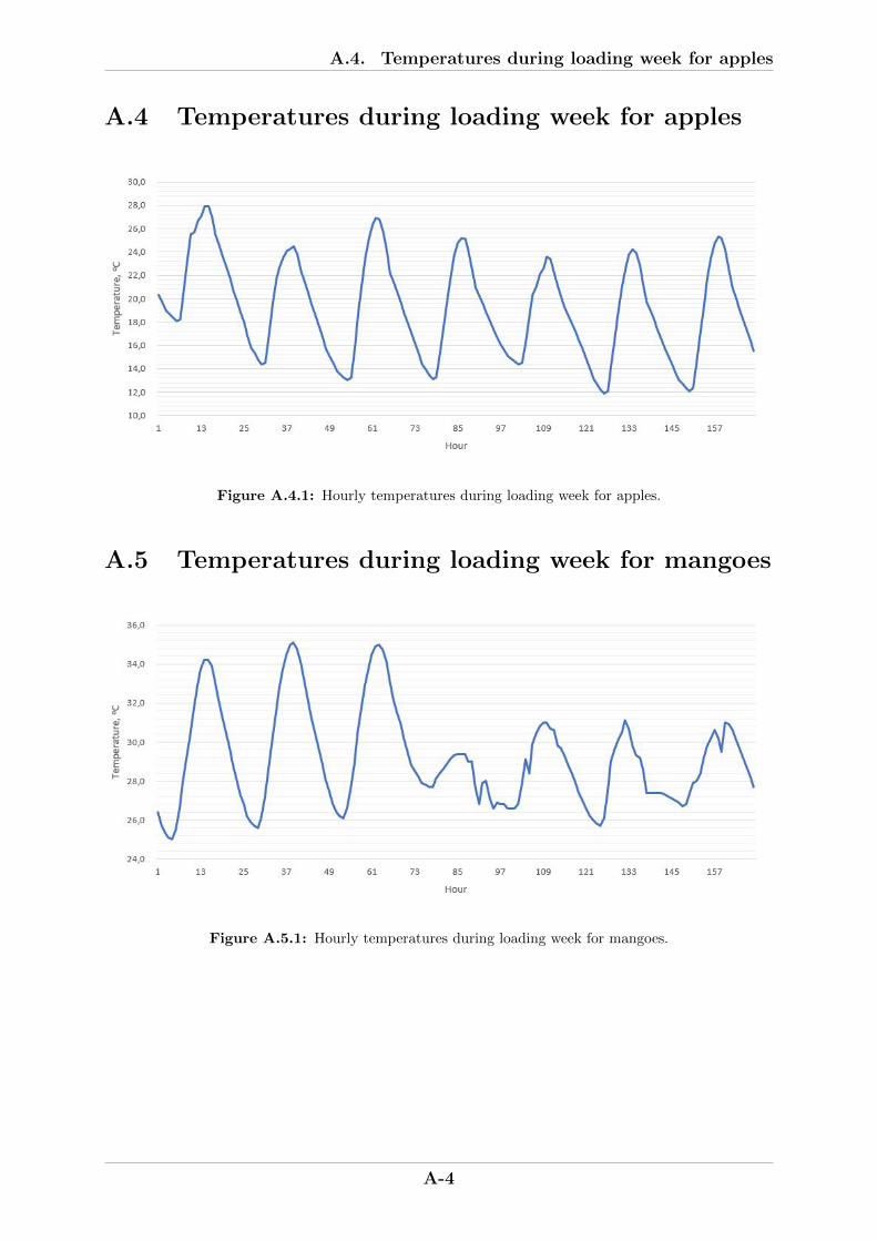
A.4. Temperatures during loading week for apples
A.4 Temperatures during loading week for apples
Figure A.4.1: Hourly temperatures during loading week for apples.
A.5 Temperatures during loading week for mangoes
Figure A.5.1: Hourly temperatures during loading week for mangoes.
A-4

A.6. Temperatures during loading week for grapes
A.6 Temperatures during loading week for grapes
Figure A.6.1: Hourly temperatures during loading week for grapes.
A-5

A.7. State-wise average rates of electricity in India
A.7 State-wise average rates of electricity in India
StateDomestic consumer
below 400 kWh/month
Commercial consumer
below 300 kWh/month
Commercial consumer
below 1 500 kWh/month
Andaman and Nicobar Islands 4.56 6.78 8.40
Andhra Pradesh 4.92 8.57 9.81
Arunachal Pradesh 4.00 5.00 5.00
Assam 6.36 8.14 8.34
Bihar 4.62 6.45 7.89
Chandigarh 4.15 5.88 6.14
Chhattishgarh 5.23 7.02 8.66
Dadra and Nagar Haveli 1.93 3.08 3.30
Daman and Diu 1.93 3.32 3.58
Delhi (BYPL/BRPL/NDPL) 5.49 9.94 9.94
Delhi (NDMC) 4.33 8.51 8.51
Goa 2.43 4.68 5.23
Gujarat 5.18 5.85 5.85
Haryana 5.31 6.15 6.85
Himachal Pradesh 3.04 5.81 5.53
Jammu and Kashmir 2.94 4.02 6.28
Jharkhand 3.23 7.17 7.21
Karnataka 6.67 8.82 8.96
Kerala 6.91 8.54 10.63
Lakshadweep 3.56 6.68 7.50
Madhya Pradesh 8.04 7.39 7.44
Maharashtra 9.66 10.20 12.28
Manipur 4.70 5.57 6.26
Meghalaya 4.78 6.99 7.38
Mizoram 4.50 5.00 5.75
Nagaland 5.66 7.58 8.48
Odisha 4.88 6.27 7.08
Puducherry 2.84 6.01 6.45
Punjab 6.60 7.54 7.61
Rajasthan 7.29 9.53 9.86
Sikkim 3.63 5.34 6.12
Tamil Nadu 4.70 8.37 9.33
Telangana 6.69 8.91 9.75
Tripura 7.55 6.92 7.68
Uttar Pradesh 5.86 8.28 10.05
Uttarakhand 3.86 5.62 5.62
West Bengal 8.44 8.81 10.27
Average 5.04 6.88 7.59
Table A.7.1: State-wise average rates of electricity in India, as on 01.04.2017 (Datanet India 2017).Rates in INR/kWh.
A-6

Appendix B
EES code
B-1

File:D:\OneDrive - NTNU\Tom André\NTNU\Masteroppgave\EES\NCL.EES 26.06.2019 11.21.30 Page 1EES Ver. 10.494: #3812: For use only by students and faculty Dept. of Energy and Process Engineering, NTNU, NORWAY
1: $UnitSystem SI Radian Mass kJ kg C Pa 2: 3: Procedure liquidheight(CO2$;T;d_pipe;d_receiver;CR;H;H_receiver_min;L_evaporator:H_L;H_receiver) 4: 5: x_liquid = 0 [-] 6: x_gas = 1 [-] 7: 8: rho_liquid = density(CO2$; x=x_liquid; T=T) 9: rho_gas = density(CO2$; x=x_gas; T=T) 10: 11: V_downcomer = 1/4*pi*d_pipe^2*H 12: V_riser = 1/4*pi*d_pipe^2*H 13: V_evaporator = 1/4*pi*d_pipe^2*L_evaporator 14: 15: V_receiver_standstill = 1/4*pi*d_receiver^2*H_receiver_min 16: 17: m_tot = rho_liquid*(V_downcomer+V_riser+V_evaporator+V_receiver_standstill) 18: m_downcomer = rho_liquid*V_downcomer 19: m_riser = 1/CR*rho_gas*V_riser + (1-1/CR)*rho_liquid*V_riser 20: m_evaporator = 1/CR*rho_gas*V_evaporator + (1-1/CR)*rho_liquid*V_evaporator 21: 22: m_receiver = m_tot-m_downcomer-m_riser-m_evaporator 23: V_receiver = m_receiver/rho_liquid 24: 25: H_receiver = V_receiver/(1/4*pi*d_receiver^2) 26: H_L = H+H_receiver 27: 28: End procedure 29: 30: 31: 32: Procedure maxliquidheight(CO2$;T;d_pipe;d_receiver;H;H_receiver_min;L_evaporator:H_L_max) 33: 34: CR_max = 1 [-] 35: 36: x_liquid = 0 [-] 37: x_gas = 1 [-] 38: 39: rho_liquid = density(CO2$; x=x_liquid; T=T) 40: rho_gas = density(CO2$; x=x_gas; T=T) 41: 42: V_downcomer = 1/4*pi*d_pipe^2*H 43: V_riser = 1/4*pi*d_pipe^2*H 44: V_evaporator = 1/4*pi*d_pipe^2*L_evaporator 45: 46: V_receiver_standstill = 1/4*pi*d_receiver^2*H_receiver_min 47: 48: m_tot = rho_liquid*(V_downcomer+V_riser+V_evaporator+V_receiver_standstill) 49: m_downcomer = rho_liquid*V_downcomer 50: m_riser = 1/CR_max*rho_gas*V_riser + (1-1/CR_max)*rho_liquid*V_riser 51: m_evaporator = 1/CR_max*rho_gas*V_evaporator + (1-1/CR_max)*rho_liquid*V_evaporator 52: 53: m_receiver = m_tot-m_downcomer-m_riser-m_evaporator 54: V_receiver = m_receiver/rho_liquid 55: 56: H_receiver = V_receiver/(1/4*pi*d_receiver^2) 57: H_L_max = H+H_receiver 58: 59: End procedure 60: 61:
B.1. NCL design
B.1 NCL design
B-2

File:D:\OneDrive - NTNU\Tom André\NTNU\Masteroppgave\EES\NCL.EES 26.06.2019 11.21.30 Page 2EES Ver. 10.494: #3812: For use only by students and faculty Dept. of Energy and Process Engineering, NTNU, NORWAY
62: 63: 64: Procedure downcomer(CO2$;g;x_liquid;m;rho_liquid;T;H;H_L;d_pipe;l_eq;epsilon:dP_downcomer) 65: 66: "Static pressure increase in downcomer" 67: dP_static = rho_liquid*g*H_L 68: 69: "Major head loss in downcomer, liquid flow" 70: mu = viscosity(CO2$; x=x_liquid; T=T) 71: Re = ( 4/pi )*(( m )/( d_pipe*mu )) 72: f = ( -2 * log10 ( (epsilon/d_pipe)/(3,7) + (5,74)/(Re^(0,9)) ) )^(-2) 73: dP_major = f * ( (2)/(pi) ) * ( (H)/(d_pipe^3) ) * ((m^2)/(rho_liquid)) 74: 75: "Minor head loss, one 90 degree bend" 76: dP_minor = f * ((2)/(pi)) * ((l_eq)/(d_pipe^3)) * ((m^2)/(rho_liquid)) 77: 78: "Total downcomer pressure difference" 79: dP_downcomer = dP_static - dP_major - dP_minor 80: 81: End procedure 82: 83: 84: 85: Procedure riser(CO2$;g;x;m;rho;rho_liquid;rho_gas;mu_gas;mu_liquid;T;H_L;H_L_max;d_pipe;l_eq;epsilon:dP_riser) 86: 87: H_riser = H_L_max + 0,2 88: 89: "Static pressure loss" 90: dP_static = rho*g*H_riser 91: 92: "Major loss, two-phase fluid" 93: Re = ( (4000*m)/(pi*d_pipe) ) * ( (x^2 + (1-x)^2 *((rho_gas)/(rho_liquid)) )/( mu_gas*x + mu_liquid*(1-x)*((rho_gas)
/(rho_liquid)) ) ) 94: f_inv = -2* log10( 269,7963 * ((epsilon)/(d_pipe)) - ((5,0452)/(Re)) * log10 ( ((1)/(2,8257)) * ((1000*epsilon)/(d_pipe))^(1,1098
) + ((5,8506)/(Re^(0,8981))) ) ) 95: f = (1/f_inv)^2 96: dP_major = f * ( (2)/(pi) ) * ( (H_riser)/(d_pipe^3) ) * ((m^2)/(rho)) 97: 98: "Minor loss, two 90 degree bends" 99: dP_minor = 2*( f * ((2)/(pi)) * ((l_eq)/(d_pipe^3)) * ((m^2)/(rho)) ) 100: 101: "Total riser pressure difference" 102: dP_riser = dP_static + dP_major + dP_minor 103: 104: End procedure 105: 106: 107: 108: Procedure evaporator(CO2$;g;x;x_liquid;m;rho_liquid;rho_gas;mu_gas;mu_liquid;T;d_pipe;N_pipes
;L_evaporator_single_pipe;l_eq;epsilon:dP_evaporator) 109: $Arrays on 110: 111: "Major loss, two-phase fluid" 112: dP_major = 0 [Pa] 113: 114: Duplicate i=1;N_pipes 115: 116: dx = (x-x_liquid)/N_pipes 117: x_maj[i] = x_liquid + i*dx 118:
B.1. NCL design
B-3

File:D:\OneDrive - NTNU\Tom André\NTNU\Masteroppgave\EES\NCL.EES 26.06.2019 11.21.31 Page 3EES Ver. 10.494: #3812: For use only by students and faculty Dept. of Energy and Process Engineering, NTNU, NORWAY
119: rho_maj[i] = density(CO2$; x=x_maj[i]; T=T) 120: 121: Re_maj[i] = ( ( 4000*m ) / ( pi*d_pipe ) ) * ( ( x_maj[i]^2 + (1-x_maj[i])^2 *((rho_gas)/(rho_liquid)) ) / ( mu_gas*x_maj[i] +
mu_liquid*(1-x_maj[i])*(rho_gas/rho_liquid) ) ) 122: f_inv = -2* log10( 269,7963 * ((epsilon)/(d_pipe)) - ((5,0452)/(Re_maj[i])) * log10 ( ((1)/(2,8257)) * ((1000*epsilon)/(d_pipe))
^(1,1098) + ((5,8506)/(Re_maj[i]^(0,8981))) ) ) 123: f_maj[i] = (1/f_inv)^2 124: dP_major_dx[i] = f_maj[i] * ( (2)/(pi) ) * ( (L_evaporator_single_pipe)/(d_pipe^3) ) * ((m^2)/(rho_maj[i])) 125: dP_major = dP_major + dP_major_dx[i] 126: 127: End duplicate 128: 129: "Minor loss, 180 degree U-bend aT end of each pipe except last pipe" 130: dP_minor = 0 [Pa] 131: N_bends = N_pipes-1 132: 133: Duplicate i=1;N_bends 134: 135: dx = (x-x_liquid)/N_pipes 136: x_min[i] = x_liquid + i*dx 137: 138: rho_min[i] = density(CO2$; x=x_min[i]; T=T) 139: 140: Re_min[i] = ( ( 4000*m ) / ( pi*d_pipe ) ) * ( ( x_min[i]^2 + (1-x_min[i])^2 *((rho_gas)/(rho_liquid)) ) / ( mu_gas*x_min[i] +
mu_liquid*(1-x_min[i])*(rho_gas/rho_liquid) ) ) 141: f_inv = -2* log10( 269,7963 * ((epsilon)/(d_pipe)) - ((5,0452)/(Re_min[i])) * log10 ( ((1)/(2,8257)) * ((1000*epsilon)/(d_pipe))
^(1,1098) + ((5,8506)/(Re_min[i]^(0,8981))) ) ) 142: f_min[i] = (1/f_inv)^2 143: dP_minor_dx[i] = f_min[i] * ((2)/(pi)) * ((l_eq)/(d_pipe^3)) * ((m^2)/(rho_min[i])) 144: dP_minor = dP_minor + dP_minor_dx[i] 145: 146: End duplicate 147: 148: dP_evaporator = dP_major + dP_minor 149: 150: End Procedure 151: 152: 153: 154: Procedure drivingforce(dP_downcomer;dP_riser;dP_evaporator:dP_tot_Pa;dP_tot_bar) 155: 156: dP_tot_Pa = dP_downcomer - dP_riser - dP_evaporator 157: dP_tot_bar = dP_tot_Pa/10^5 158: 159: End procedure 160: 161: 162: CO2$ = 'carbondioxide' 163: g = 9,81 [m/s^2] 164: 165: T = -2 [C] 166: 167: CR = 2 [-] 168: x_gas = 1 [-] 169: x_liquid = 0 [-] 170: x = 1/CR 171: 172: h_downcomer = enthalpy(CO2$; x=x_liquid; T=T) 173: h_riser = enthalpy(CO2$; x=x; T=T) 174:
B.1. NCL design
B-4
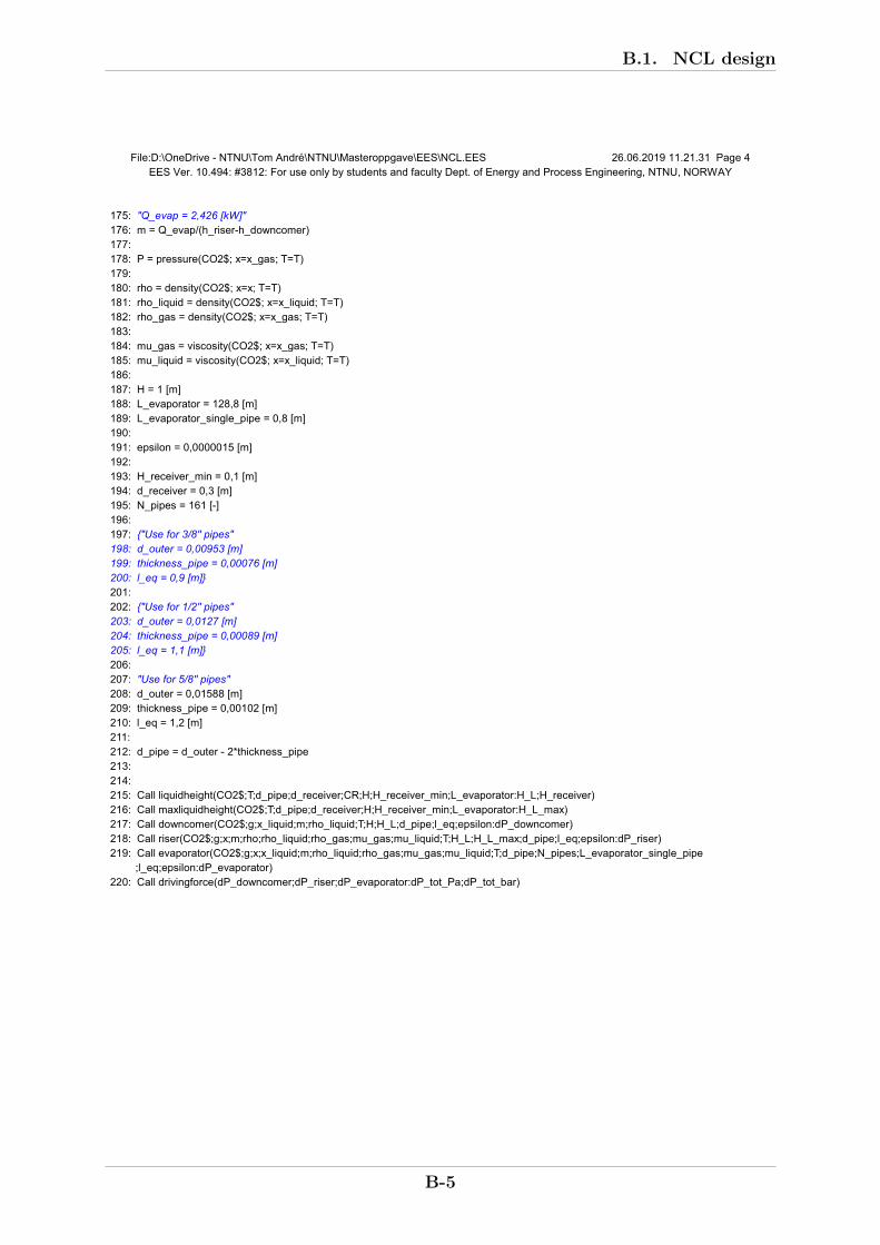
File:D:\OneDrive - NTNU\Tom André\NTNU\Masteroppgave\EES\NCL.EES 26.06.2019 11.21.31 Page 4EES Ver. 10.494: #3812: For use only by students and faculty Dept. of Energy and Process Engineering, NTNU, NORWAY
175: "Q_evap = 2,426 [kW]" 176: m = Q_evap/(h_riser-h_downcomer) 177: 178: P = pressure(CO2$; x=x_gas; T=T) 179: 180: rho = density(CO2$; x=x; T=T) 181: rho_liquid = density(CO2$; x=x_liquid; T=T) 182: rho_gas = density(CO2$; x=x_gas; T=T) 183: 184: mu_gas = viscosity(CO2$; x=x_gas; T=T) 185: mu_liquid = viscosity(CO2$; x=x_liquid; T=T) 186: 187: H = 1 [m] 188: L_evaporator = 128,8 [m] 189: L_evaporator_single_pipe = 0,8 [m] 190: 191: epsilon = 0,0000015 [m] 192: 193: H_receiver_min = 0,1 [m] 194: d_receiver = 0,3 [m] 195: N_pipes = 161 [-] 196: 197: {"Use for 3/8'' pipes" 198: d_outer = 0,00953 [m] 199: thickness_pipe = 0,00076 [m] 200: l_eq = 0,9 [m]} 201: 202: {"Use for 1/2'' pipes" 203: d_outer = 0,0127 [m] 204: thickness_pipe = 0,00089 [m] 205: l_eq = 1,1 [m]} 206: 207: "Use for 5/8'' pipes" 208: d_outer = 0,01588 [m] 209: thickness_pipe = 0,00102 [m] 210: l_eq = 1,2 [m] 211: 212: d_pipe = d_outer - 2*thickness_pipe 213: 214: 215: Call liquidheight(CO2$;T;d_pipe;d_receiver;CR;H;H_receiver_min;L_evaporator:H_L;H_receiver) 216: Call maxliquidheight(CO2$;T;d_pipe;d_receiver;H;H_receiver_min;L_evaporator:H_L_max) 217: Call downcomer(CO2$;g;x_liquid;m;rho_liquid;T;H;H_L;d_pipe;l_eq;epsilon:dP_downcomer) 218: Call riser(CO2$;g;x;m;rho;rho_liquid;rho_gas;mu_gas;mu_liquid;T;H_L;H_L_max;d_pipe;l_eq;epsilon:dP_riser) 219: Call evaporator(CO2$;g;x;x_liquid;m;rho_liquid;rho_gas;mu_gas;mu_liquid;T;d_pipe;N_pipes;L_evaporator_single_pipe
;l_eq;epsilon:dP_evaporator) 220: Call drivingforce(dP_downcomer;dP_riser;dP_evaporator:dP_tot_Pa;dP_tot_bar)
B.1. NCL design
B-5

File:Refrigeration load apples.EES 26.06.2019 11.24.51 Page 1EES Ver. 10.494: #3812: For use only by students and faculty Dept. of Energy and Process Engineering, NTNU, NORWAY
1: $UnitSystem SI Radian Mass kJ kg C bar 2: 3: 4: Procedure transmissionload(T_room;T_amb:Q_Transmission) 5: 6: "Cold storage exterior size" 7: L_ext = 6,1 [m] "Length" 8: W_ext = 2,44 [m] "Width" 9: H_ext = 2,6 [m] "Height" 10: 11: "Surface areas" 12: A_north = W_ext*H_ext "North wall
area" 13: A_south = W_ext*H_ext "South wall
area" 14: A_east = L_ext*H_ext "East wall
area" 15: A_west = L_ext*H_ext "West wall
area" 16: A_roof = W_ext*L_ext "Roof area" 17: A_floor = W_ext*L_ext "Floor area" 18: 19: "Insulation, expanded polysterene" 20: delta_ins = 0,075 [m] "Insulation
thickness" 21: k_ins = 0,037 [W/(m*K)] "Thermal
conductivity of insulation" 22: U_ins = k_ins/delta_ins "Insulation
heat transfer coefficient" 23: 24: "Allowance for sun effect" 25: dT_sun_east = 3 [C] "East wall
allowance" 26: dT_sun_west = 3 [C] "West wall
allowance" 27: dT_sun_south = 2 [C] "South wall
allowance" 28: dT_sun_roof = 5 [C] "Flat roof
allowance" 29: 30: T_wall_east = T_amb+dT_sun_east "East wall" 31: T_wall_west = T_amb+dT_sun_west "West wall" 32: T_wall_south = T_amb+dT_sun_south "South wall" 33: T_wall_north = T_amb "North wall,
with door" 34: T_roof = T_amb+dT_sun_roof "Flat roof" 35: T_floor = T_amb "Floor" 36: 37: 38: "Transmission load" 39: Q_T_south = U_ins*A_south*(T_wall_south-T_room) "South wall,
[W]" 40: Q_T_east = U_ins*A_east*(T_wall_east-T_room) "East wall,
[W]" 41: Q_T_west = U_ins*A_west*(T_wall_west-T_room) "West wall,
[W]" 42: Q_T_north = U_ins*A_north*(T_wall_north-T_room) "North wall,
[W]" 43: Q_T_roof = U_ins*A_roof*(T_roof-T_room) "Flat roof,
[W]" 44: Q_T_floor = U_ins*A_floor*(T_floor-T_room) "Floor, [W]"
B.2. Storing apples
B.2 Storing apples
B-6

File:Refrigeration load apples.EES 26.06.2019 11.24.51 Page 2EES Ver. 10.494: #3812: For use only by students and faculty Dept. of Energy and Process Engineering, NTNU, NORWAY
45: 46: Q_Transmission = (Q_T_south+Q_T_east+Q_T_west+Q_T_north+Q_T_roof+Q_T_floor)/1000 "Total
transmission load, [kW]" 47: 48: End 49: 50: 51: Procedure infiltrationload(T_amb;T_room:Q_Infiltration) 52: 53: air$ = 'air' 54: P_amb = 1,01325 [bar] "Atmospheri
c pressure" 55: g = 9,81 [m/s^2] "Gravity" 56: 57: H_door = 2,045 [m] "Door height" 58: W_door = 0,8 [m] "Door width" 59: A_door = H_door*W_door "Door area" 60: 61: D_f = 0,8 [-] "Doorway
flow factor" 62: E = 0,9 [-] "New strip
curtains" 63: Theta_d = 24 [h] "Time period" 64: Theta_o = 5 [min] "Door
simply stands open" 65: Theta_p = 30 [s] "Door open
-close time" 66: N = 1 [-] "Door is
opened once a day" 67: 68: h_amb = enthalpy(air$; T=T_amb) "Ambient
air enthalpy" 69: rho_amb = density(air$; T=T_amb; P=P_amb) "Density
ambient air" 70: 71: h_room = enthalpy(air$; T=T_room) "Cold
storage air enthalpy" 72: rho_room = density(air$; T=T_room; P=P_amb) "Density
cold storage air" 73: 74: D_t = (N*Theta_p+60*Theta_o)/(3600*Theta_d) "Doorway
open-time factor" 75: F_m = ((2)/(1+(rho_room/rho_amb)^(1/3)))^(1,5) "Density
factor" 76: Q_s = 0,221*A_door*(h_amb-h_room)*rho_room*(1-(rho_amb/rho_room))^(0,5)*(g*H_door)^(0,5)*F_m "Sensible
and latent refrigeration load, [kW]" 77: 78: Q_Infiltration = Q_s*D_t*D_f*(1-E) "Total
infiltration load, [kW]" 79: 80: End 81: 82: 83: Procedure respirationheat(:Q_Respiration) 84: 85: "Cold storage interior size, without insulation" 86: L_int_ex_ins = 5,87 [m] "Length" 87: W_int_ex_ins = 2,34 [m] "Width" 88: H_int_ex_ins = 2,38 [m] "Height" 89:
B.2. Storing apples
B-7

File:Refrigeration load apples.EES 26.06.2019 11.24.52 Page 3EES Ver. 10.494: #3812: For use only by students and faculty Dept. of Energy and Process Engineering, NTNU, NORWAY
90: delta_ins = 0,075 [m] "Insulation thickness"
91: 92: "Interior size, including insulation thickness" 93: L_int = L_int_ex_ins-delta_ins "Length" 94: W_int = W_int_ex_ins-delta_ins "Width" 95: H_int = H_int_ex_ins-delta_ins "Height" 96: A_int = L_int*W_int "Floor area" 97: 98: L_aisle=L_int "Aisle length" 99: W_aisle=0,8 [m] "Aisle width" 100: 101: V_storage = (W_int-W_aisle)*L_int*H_int "Available
storage space" 102: rho_storage = 200 [kg/m^3] "Storage
density" 103: m_apple = (7/7)*rho_storage*V_storage "Mass of
apples stored" 104: 105: q_resp_apple = 0,0102 [W/kg] "Respiration
rate, apple" 106: 107: Q_Respiration = (m_apple*q_resp_apple)/1000 "Respiration
heat, [kW]" 108: 109: End 110: 111: 112: Procedure equipmentload(Q_Transmission;Q_Infiltration;Q_Respiration:Q_Equipment) 113: 114: Q_Equipment = 0,1*(Q_Transmission+Q_Infiltration+Q_Respiration) "10 % of
total load, [kW]" 115: 116: End 117: 118: 119: Procedure holdingload(Q_Transmission;Q_Infiltration;Q_Respiration;Q_Equipment:Q_HoldingLoad) 120: 121: Q_HoldingLoad = 1,1*(Q_Transmission+Q_Infiltration+Q_Respiration+Q_Equipment) "Total
steady state holding refrigeration load, with safety factor of 10%, [kW]" 122: 123: End 124: 125: 126: Procedure pulldownload(T_room;T_amb:Q_Pulldown) 127: 128: T_apple = T_amb "Apple
loading temperature" 129: 130: "Cold storage interior size, without insulation" 131: L_int_ex_ins = 5,87 [m] "Length" 132: W_int_ex_ins = 2,34 [m] "Width" 133: H_int_ex_ins = 2,38 [m] "Height" 134: 135: delta_ins = 0,075 [m] "Insulation
thickness" 136: 137: "Interior size, including insulation thickness" 138: L_int = L_int_ex_ins-delta_ins "Length" 139: W_int = W_int_ex_ins-delta_ins "Width"
B.2. Storing apples
B-8

File:Refrigeration load apples.EES 26.06.2019 11.24.52 Page 4EES Ver. 10.494: #3812: For use only by students and faculty Dept. of Energy and Process Engineering, NTNU, NORWAY
140: H_int = H_int_ex_ins-delta_ins "Height" 141: 142: L_aisle=L_int "Aisle length" 143: W_aisle=0,8 [m] "Aisle width" 144: 145: V_storage = (W_int-W_aisle)*L_int*H_int "Available
storage space" 146: rho_storage = 200 [kg/m^3] "Storage
density" 147: m_apple = (1/7)*rho_storage*V_storage "Mass of
apples loaded each day" 148: 149: C_P_apple = 3,81 [kJ/(kg*K)] 150: 151: q_pulldown_apple = m_apple*C_P_apple*(T_apple-T_room) "Heat
removed for apples, [kJ]" 152: 153: t_Pulldown = 24 "Pull down
time, [h]" 154: 155: Q_Pulldown = 1,1*((q_pulldown_apple)/(3600*t_Pulldown))
"Pulldown load, including safety factor of 10%, [kW]" 156: 157: "Q_Pulldown = 0 [kW]" "Use when
no pull down load" 158: 159: End 160: 161: 162: Procedure refrigerationload(Q_HoldingLoad;Q_Pulldown:Q_TotalLoad) 163: 164: Q_TotalLoad = Q_HoldingLoad+Q_Pulldown "Total
refrigeration load, [kW]" 165: 166: End 167: 168: Procedure ammonia(T_amb;T_room;Q_TotalLoad:COP;V_compressor;m_cond;m_evap;W;Q_cond;dP) 169: $Arrays on 170: 171: NH3$ = 'ammonia' 172: 173: T_evap = -2 [C] "Evaporator
temperature" 174: T_cond = T_amb+5 "Condenser
temperature" 175: 176: eta = 0,8 [-] "Isentropic
efficiency compressor" 177: 178: "Decide load" 179: Q_L = Q_TotalLoad 180: 181: "Point 5: Inlet evaporator" 182: x[5] = 0 [-] 183: T[5] = T_evap 184: P[5] = pressure(NH3$; x=x[5]; T=T[5]) 185: h[5] = enthalpy(NH3$; x=x[5]; T=T[5]) 186: s[5] = entropy(NH3$; x=x[5]; T=T[5]) 187: v[5] = volume(NH3$; x=x[5]; T=T[5]) 188:
B.2. Storing apples
B-9

File:Refrigeration load apples.EES 26.06.2019 11.24.52 Page 5EES Ver. 10.494: #3812: For use only by students and faculty Dept. of Energy and Process Engineering, NTNU, NORWAY
189: "Point 6: Exit evaporator" 190: x[6] = 1 [-] 191: P[6] = P[5] 192: T[6] = temperature(NH3$; x=x[6]; P=P[6]) 193: h[6] = enthalpy(NH3$; x=x[6]; P=P[6]) 194: s[6] = entropy(NH3$; x=x[6]; P=P[6]) 195: v[6] = volume(NH3$; x=x[6]; P=P[6]) 196: 197: "Point 1: Inlet compressor" 198: x[1] = 1 [-] 199: P[1] = P[5] 200: T[1] = temperature(NH3$; x=x[1]; P=P[1]) 201: h[1] = enthalpy(NH3$; x=x[1]; P=P[1]) 202: s[1] = entropy(NH3$; x=x[1]; P=P[1]) 203: v[1] = volume(NH3$; x=x[1]; P=P[1]) 204: 205: "Point 3: Exit condenser" 206: x[3] = 0 [-] 207: T[3] = T_cond 208: P[3] = pressure(NH3$; x=x[3]; T=T[3]) 209: h[3] = enthalpy(NH3$; x=x[3]; T=T[3]) 210: s[3] = entropy(NH3$; x=x[3]; T=T[3]) 211: v[3] = volume(NH3$; x=x[3]; T=T[3]) 212: 213: "Point 4: Two-phase inlet receiver, after expansion" 214: h[4] = h[3] 215: P[4] = P[5] 216: T[4] = temperature(NH3$; h=h[4]; P=P[4]) 217: s[4] = entropy(NH3$; h=h[4]; P=P[4]) 218: x[4] = quality(NH3$; h=h[4]; P=P[4]) 219: v[4] = volume(NH3$; h=h[4]; P=P[4]) 220: 221: "Point 2s: Isentropic exit compressor" 222: ss[2] = s[1] 223: P[2] = P[3] 224: Ts[2] = temperature(NH3$; s=ss[2]; P=P[2]) 225: hs[2] = enthalpy(NH3$; s=ss[2]; P=P[2]) 226: xs[2] = quality(NH3$; s=ss[2]; P=P[2]) 227: vs[2] = volume(NH3$; s=ss[2]; P=P[2]) 228: 229: "Mass flows" 230: m_evap = Q_L/(h[6]-h[5]) "Mass flow
through evaporator" 231: m_cond = m_evap*((h[5]-h[6])/(h[4]-h[1])) "Mass flow
through condenser" 232: 233: "Compressor work" 234: W_is = m_cond*(hs[2]-h[1]) 235: W = W_is/eta 236: 237: "Point 2: Real exit compressor" 238: h[2] = h[1]+W/m_cond 239: T[2] = temperature(NH3$; h=h[2]; P=P[2]) 240: s[2] = entropy(NH3$; h=h[2]; P=P[2]) 241: x[2] = quality(NH3$; h=h[2]; P=P[2]) 242: v[2] = volume(NH3$; h=h[2]; P=P[2]) 243: 244: "Rejected heat condenser" 245: Q_cond = m_cond*(h[2]-h[3]) 246:
B.2. Storing apples
B-10

File:Refrigeration load apples.EES 26.06.2019 11.24.52 Page 6EES Ver. 10.494: #3812: For use only by students and faculty Dept. of Energy and Process Engineering, NTNU, NORWAY
247: "Pressure ratio" 248: dP = P[2]/P[1] 249: 250: "COP" 251: COP = Q_L/W 252: 253: "Volumetric floWs" 254: V_compressor = m_cond*v[1] 255: 256: End 257: 258: 259: Procedure ammoniancl(x_exit_evap;T_amb;T_room;Q_TotalLoad:COP_NCL;V_compressor_NCL;m_cond_NCL
;m_evap_NCL;W_NCL;Q_cond_NCL;dP_NCL) 260: $Arrays on 261: 262: NH3$ = 'ammonia' 263: CO2$ = 'carbondioxide' 264: 265: T_evap = -2 [C] "Evaporator
temperature" 266: T_cond = T_amb+5 "Condenser
temperature" 267: T_HX = T_evap-1 "NH3/CO2
heat exchanger temperature" 268: 269: eta = 0,8 [-] "Isentropic
efficiency compressor" 270: 271: "Decide load" 272: Q_L = Q_TotalLoad 273: 274: "Point 5: NH3 inlet intermediate HX" 275: x[5] = 0 [-] 276: T[5] = T_HX 277: P[5] = pressure(NH3$; x=x[5]; T=T[5]) 278: h[5] = enthalpy(NH3$; x=x[5]; T=T[5]) 279: s[5] = entropy(NH3$; x=x[5]; T=T[5]) 280: v[5] = volume(NH3$; x=x[5]; T=T[5]) 281: 282: "Point 6: NH3 exit intermediate HX" 283: x[6] = 1 [-] 284: P[6] = P[5] 285: T[6] = temperature(NH3$; x=x[6]; P=P[6]) 286: h[6] = enthalpy(NH3$; x=x[6]; P=P[6]) 287: s[6] = entropy(NH3$; x=x[6]; P=P[6]) 288: v[6] = volume(NH3$; x=x[6]; P=P[6]) 289: 290: "Point 1: Inlet compressor" 291: x[1] = 1 [-] 292: P[1] = P[5] 293: T[1] = temperature(NH3$; x=x[1]; P=P[1]) 294: h[1] = enthalpy(NH3$; x=x[1]; P=P[1]) 295: s[1] = entropy(NH3$; x=x[1]; P=P[1]) 296: v[1] = volume(NH3$; x=x[1]; P=P[1]) 297: 298: "Point 3: Exit condenser" 299: x[3] = 0 [-] 300: T[3] = T_cond 301: P[3] = pressure(NH3$; x=x[3]; T=T[3])
B.2. Storing apples
B-11
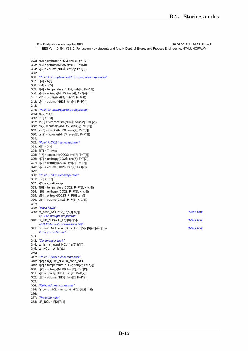
File:Refrigeration load apples.EES 26.06.2019 11.24.52 Page 7EES Ver. 10.494: #3812: For use only by students and faculty Dept. of Energy and Process Engineering, NTNU, NORWAY
302: h[3] = enthalpy(NH3$; x=x[3]; T=T[3]) 303: s[3] = entropy(NH3$; x=x[3]; T=T[3]) 304: v[3] = volume(NH3$; x=x[3]; T=T[3]) 305: 306: "Point 4: Two-phase inlet receiver, after expansion" 307: h[4] = h[3] 308: P[4] = P[5] 309: T[4] = temperature(NH3$; h=h[4]; P=P[4]) 310: s[4] = entropy(NH3$; h=h[4]; P=P[4]) 311: x[4] = quality(NH3$; h=h[4]; P=P[4]) 312: v[4] = volume(NH3$; h=h[4]; P=P[4]) 313: 314: "Point 2s: Isentropic exit compressor" 315: ss[2] = s[1] 316: P[2] = P[3] 317: Ts[2] = temperature(NH3$; s=ss[2]; P=P[2]) 318: hs[2] = enthalpy(NH3$; s=ss[2]; P=P[2]) 319: xs[2] = quality(NH3$; s=ss[2]; P=P[2]) 320: vs[2] = volume(NH3$; s=ss[2]; P=P[2]) 321: 322: "Point 7: CO2 inlet evaporator" 323: x[7] = 0 [-] 324: T[7] = T_evap 325: P[7] = pressure(CO2$; x=x[7]; T=T[7]) 326: h[7] = enthalpy(CO2$; x=x[7]; T=T[7]) 327: s[7] = entropy(CO2$; x=x[7]; T=T[7]) 328: v[7] = volume(CO2$; x=x[7]; T=T[7]) 329: 330: "Point 8: CO2 exit evaporator" 331: P[8] = P[7] 332: x[8] = x_exit_evap 333: T[8] = temperature(CO2$; P=P[8]; x=x[8]) 334: h[8] = enthalpy(CO2$; P=P[8]; x=x[8]) 335: s[8] = entropy(CO2$; P=P[8]; x=x[8]) 336: v[8] = volume(CO2$; P=P[8]; x=x[8]) 337: 338: "Mass flows" 339: m_evap_NCL = Q_L/(h[8]-h[7]) "Mass flow
of CO2 through evaporator" 340: m_HX_NH3 = Q_L/(h[6]-h[5]) "Mass flow
of NH3 through intermediate HX" 341: m_cond_NCL = m_HX_NH3*((h[5]-h[6])/(h[4]-h[1])) "Mass flow
through condenser" 342: 343: "Compressor work" 344: W_is = m_cond_NCL*(hs[2]-h[1]) 345: W_NCL = W_is/eta 346: 347: "Point 2: Real exit compressor" 348: h[2] = h[1]+W_NCL/m_cond_NCL 349: T[2] = temperature(NH3$; h=h[2]; P=P[2]) 350: s[2] = entropy(NH3$; h=h[2]; P=P[2]) 351: x[2] = quality(NH3$; h=h[2]; P=P[2]) 352: v[2] = volume(NH3$; h=h[2]; P=P[2]) 353: 354: "Rejected heat condenser" 355: Q_cond_NCL = m_cond_NCL*(h[2]-h[3]) 356: 357: "Pressure ratio" 358: dP_NCL = P[2]/P[1]
B.2. Storing apples
B-12

File:Refrigeration load apples.EES 26.06.2019 11.24.52 Page 8EES Ver. 10.494: #3812: For use only by students and faculty Dept. of Energy and Process Engineering, NTNU, NORWAY
359: 360: "COP" 361: COP_NCL = Q_L/W_NCL 362: 363: "Volumetric floWs" 364: V_compressor_NCL = m_cond_NCL*v[1] 365: 366: End 367: 368: 369: T_room_K = T_room + 273,15 370: T_amb_K = T_amb + 273,15 371: COP_Ca = (T_room_K)/(T_amb_K - T_room_K) "Carnot
COP" 372: 373: "Room and ambient temperatures" 374: T_room = -0,5 [C] "Cold
storage temperature, -0,5 degrees" 375: T_amb = 33,5 [C] "Ambient
temperature" 376: CR = 2 [-] "Circulation
rate" 377: x_exit_evap = 1/CR "Gas
quality at exit of CO2 evaporator" 378: "Day = x" 379: 380: Call transmissionload(T_room;T_amb:Q_Transmission) 381: Call infiltrationload(T_amb;T_room:Q_Infiltration) 382: Call respirationheat(T_room:Q_Respiration) 383: Call equipmentload(Q_Transmission;Q_Infiltration;Q_Respiration:Q_Equipment) 384: Call holdingload(Q_Transmission;Q_Infiltration;Q_Respiration;Q_Equipment:Q_HoldingLoad) 385: Call pulldownload(T_room;T_amb:Q_Pulldown) 386: Call refrigerationload(Q_HoldingLoad;Q_Pulldown:Q_TotalLoad) 387: Call ammonia(T_amb;T_room;Q_TotalLoad:COP;V_compressor;m_cond;m_evap;W;Q_cond;dP) 388: Call ammoniancl(x_exit_evap;T_amb;T_room;Q_TotalLoad:COP_NCL;V_compressor_NCL;m_cond_NCL;m_evap_NCL
;W_NCL;Q_cond_NCL;dP_NCL)
B.2. Storing apples
B-13

File:Refrigeration load mango.EES 26.06.2019 11.27.37 Page 1EES Ver. 10.494: #3812: For use only by students and faculty Dept. of Energy and Process Engineering, NTNU, NORWAY
1: $UnitSystem SI Radian Mass kJ kg C bar 2: 3: 4: Procedure transmissionload(T_room;T_amb:Q_Transmission) 5: 6: "Cold storage exterior size" 7: L_ext = 6,1 [m] "Length" 8: W_ext = 2,44 [m] "Width" 9: H_ext = 2,6 [m] "Height" 10: 11: "Surface areas" 12: A_north = W_ext*H_ext "North wall
area" 13: A_south = W_ext*H_ext "South wall
area" 14: A_east = L_ext*H_ext "East wall
area" 15: A_west = L_ext*H_ext "West wall
area" 16: A_roof = W_ext*L_ext "Roof area" 17: A_floor = W_ext*L_ext "Floor area" 18: 19: "Insulation, expanded polysterene" 20: delta_ins = 0,075 [m] "Insulation
thickness" 21: k_ins = 0,037 [W/(m*K)] "Thermal
conductivity of insulation" 22: U_ins = k_ins/delta_ins "Insulation
heat transfer coefficient" 23: 24: "Allowance for sun effect" 25: dT_sun_east = 3 [C] "East wall
allowance" 26: dT_sun_west = 3 [C] "West wall
allowance" 27: dT_sun_south = 2 [C] "South wall
allowance" 28: dT_sun_roof = 5 [C] "Flat roof
allowance" 29: 30: T_wall_east = T_amb+dT_sun_east "East wall" 31: T_wall_west = T_amb+dT_sun_west "West wall" 32: T_wall_south = T_amb+dT_sun_south "South wall" 33: T_wall_north = T_amb "North wall,
with door" 34: T_roof = T_amb+dT_sun_roof "Flat roof" 35: T_floor = T_amb "Floor" 36: 37: 38: "Transmission load" 39: Q_T_south = U_ins*A_south*(T_wall_south-T_room) "South wall,
[W]" 40: Q_T_east = U_ins*A_east*(T_wall_east-T_room) "East wall,
[W]" 41: Q_T_west = U_ins*A_west*(T_wall_west-T_room) "West wall,
[W]" 42: Q_T_north = U_ins*A_north*(T_wall_north-T_room) "North wall,
[W]" 43: Q_T_roof = U_ins*A_roof*(T_roof-T_room) "Flat roof,
[W]" 44: Q_T_floor = U_ins*A_floor*(T_floor-T_room) "Floor, [W]"
B.3. Storing mangoes
B.3 Storing mangoes
B-14

File:Refrigeration load mango.EES 26.06.2019 11.27.37 Page 2EES Ver. 10.494: #3812: For use only by students and faculty Dept. of Energy and Process Engineering, NTNU, NORWAY
45: 46: Q_Transmission = (Q_T_south+Q_T_east+Q_T_west+Q_T_north+Q_T_roof+Q_T_floor)/1000 "Total
transmission load, [kW]" 47: 48: End 49: 50: 51: Procedure infiltrationload(T_amb;T_room:Q_Infiltration) 52: 53: air$ = 'air' 54: P_amb = 1,01325 [bar] "Atmospheri
c pressure" 55: g = 9,81 [m/s^2] "Gravity" 56: 57: H_door = 2,045 [m] "Door height" 58: W_door = 0,8 [m] "Door width" 59: A_door = H_door*W_door "Door area" 60: 61: D_f = 0,8 [-] "Doorway
flow factor" 62: E = 0,9 [-] "New strip
curtains" 63: Theta_d = 24 [h] "Time period" 64: Theta_o = 5 [min] "Door
simply stands open" 65: Theta_p = 30 [s] "Door open
-close time" 66: N = 1 [-] "Door is
opened once a day" 67: 68: h_amb = enthalpy(air$; T=T_amb) "Ambient
air enthalpy" 69: rho_amb = density(air$; T=T_amb; P=P_amb) "Density
ambient air" 70: 71: h_room = enthalpy(air$; T=T_room) "Cold
storage air enthalpy" 72: rho_room = density(air$; T=T_room; P=P_amb) "Density
cold storage air" 73: 74: D_t = (N*Theta_p+60*Theta_o)/(3600*Theta_d) "Doorway
open-time factor" 75: F_m = ((2)/(1+(rho_room/rho_amb)^(1/3)))^(1,5) "Density
factor" 76: Q_s = 0,221*A_door*(h_amb-h_room)*rho_room*(1-(rho_amb/rho_room))^(0,5)*(g*H_door)^(0,5)*F_m "Sensible
and latent refrigeration load, [kW]" 77: 78: Q_Infiltration = Q_s*D_t*D_f*(1-E) "Total
infiltration load, [kW], during holding" 79: 80: End 81: 82: 83: Procedure respirationheat(:Q_Respiration) 84: 85: "Cold storage interior size, without insulation" 86: L_int_ex_ins = 5,87 [m] "Length" 87: W_int_ex_ins = 2,34 [m] "Width" 88: H_int_ex_ins = 2,38 [m] "Height" 89:
B.3. Storing mangoes
B-15

File:Refrigeration load mango.EES 26.06.2019 11.27.37 Page 3EES Ver. 10.494: #3812: For use only by students and faculty Dept. of Energy and Process Engineering, NTNU, NORWAY
90: delta_ins = 0,075 [m] "Insulation thickness"
91: 92: "Interior size, including insulation thickness" 93: L_int = L_int_ex_ins-delta_ins "Length" 94: W_int = W_int_ex_ins-delta_ins "Width" 95: H_int = H_int_ex_ins-delta_ins "Height" 96: A_int = L_int*W_int "Floor area" 97: 98: L_aisle=L_int "Aisle length" 99: W_aisle=0,8 [m] "Aisle width" 100: 101: V_storage = (W_int-W_aisle)*L_int*H_int "Available
storage space" 102: rho_storage = 200 [kg/m^3] "Storage
density" 103: m_mango = (7/7)*rho_storage*V_storage "Mass of
mango stored" 104: 105: q_resp_mango = 0,1334 [W/kg] "Respiration
rate, mango" 106: 107: Q_Respiration = (m_mango*q_resp_mango)/1000 "Respiration
heat, [kW]" 108: 109: End 110: 111: 112: Procedure equipmentload(Q_Transmission;Q_Infiltration;Q_Respiration:Q_Equipment) 113: 114: Q_Equipment = 0,1*(Q_Transmission+Q_Infiltration+Q_Respiration) "10 % of
total load, [kW]" 115: 116: End 117: 118: 119: Procedure holdingload(Q_Transmission;Q_Infiltration;Q_Respiration;Q_Equipment:Q_HoldingLoad) 120: 121: Q_HoldingLoad = 1,1*(Q_Transmission+Q_Infiltration+Q_Respiration+Q_Equipment) "Total
steady state holding refrigeration load, with safety factor of 10%, [kW]" 122: 123: End 124: 125: 126: Procedure pulldownload(T_room;T_amb:Q_Pulldown) 127: 128: T_mango = T_amb "Mango
loading temperature" 129: 130: "Cold storage interior size, without insulation" 131: L_int_ex_ins = 5,87 [m] "Length" 132: W_int_ex_ins = 2,34 [m] "Width" 133: H_int_ex_ins = 2,38 [m] "Height" 134: 135: delta_ins = 0,075 [m] "Insulation
thickness" 136: 137: "Interior size, including insulation thickness" 138: L_int = L_int_ex_ins-delta_ins "Length" 139: W_int = W_int_ex_ins-delta_ins "Width"
B.3. Storing mangoes
B-16

File:Refrigeration load mango.EES 26.06.2019 11.27.37 Page 4EES Ver. 10.494: #3812: For use only by students and faculty Dept. of Energy and Process Engineering, NTNU, NORWAY
140: H_int = H_int_ex_ins-delta_ins "Height" 141: 142: L_aisle=L_int "Aisle length" 143: W_aisle=0,8 [m] "Aisle width" 144: 145: V_storage = (W_int-W_aisle)*L_int*H_int "Available
storage space" 146: rho_storage = 200 [kg/m^3] "Storage
density" 147: m_mango = (1/7)*rho_storage*V_storage "Mass of
mango loaded each day" 148: 149: C_P_mango = 3,74 [kJ/(kg*K)] 150: 151: q_pulldown_mango = m_mango*C_P_mango*(T_mango-T_room) "Heat
removed for mango, [kJ]" 152: 153: t_Pulldown = 24 "Pull down
time, [h]" 154: 155: Q_Pulldown = 1,1*((q_pulldown_mango)/(3600*t_Pulldown)) "Pulldown
load, including safety factor of 10%, [kW]" 156: 157: End 158: 159: 160: Procedure refrigerationload(Q_HoldingLoad;Q_Pulldown:Q_TotalLoad) 161: 162: Q_TotalLoad = Q_HoldingLoad+Q_Pulldown "Total
refrigeration load, [kW]" 163: 164: End 165: 166: 167: Procedure ammonia(T_amb;T_room;Q_TotalLoad:COP;V_compressor;m_cond;m_evap;W;Q_cond;dP) 168: $Arrays on 169: 170: NH3$ = 'ammonia' 171: 172: T_evap = 11,5 [C] "Evaporator
temperature" 173: T_cond = T_amb+5 "Condenser
temperature" 174: 175: eta = 0,8 [-] "Isentropic
efficiency compressor" 176: 177: "Decide load" 178: Q_L = Q_TotalLoad 179: 180: "Point 5: Inlet evaporator" 181: x[5] = 0 [-] 182: T[5] = T_evap 183: P[5] = pressure(NH3$; x=x[5]; T=T[5]) 184: h[5] = enthalpy(NH3$; x=x[5]; T=T[5]) 185: s[5] = entropy(NH3$; x=x[5]; T=T[5]) 186: v[5] = volume(NH3$; x=x[5]; T=T[5]) 187: 188: "Point 6: Exit evaporator" 189: x[6] = 1 [-]
B.3. Storing mangoes
B-17
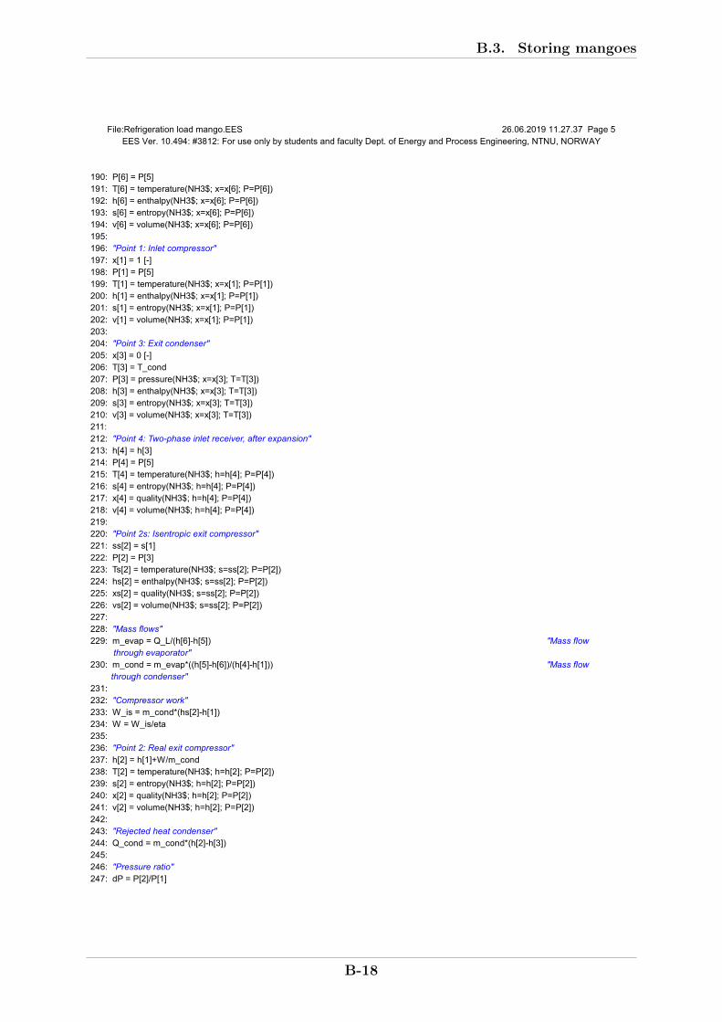
File:Refrigeration load mango.EES 26.06.2019 11.27.37 Page 5EES Ver. 10.494: #3812: For use only by students and faculty Dept. of Energy and Process Engineering, NTNU, NORWAY
190: P[6] = P[5] 191: T[6] = temperature(NH3$; x=x[6]; P=P[6]) 192: h[6] = enthalpy(NH3$; x=x[6]; P=P[6]) 193: s[6] = entropy(NH3$; x=x[6]; P=P[6]) 194: v[6] = volume(NH3$; x=x[6]; P=P[6]) 195: 196: "Point 1: Inlet compressor" 197: x[1] = 1 [-] 198: P[1] = P[5] 199: T[1] = temperature(NH3$; x=x[1]; P=P[1]) 200: h[1] = enthalpy(NH3$; x=x[1]; P=P[1]) 201: s[1] = entropy(NH3$; x=x[1]; P=P[1]) 202: v[1] = volume(NH3$; x=x[1]; P=P[1]) 203: 204: "Point 3: Exit condenser" 205: x[3] = 0 [-] 206: T[3] = T_cond 207: P[3] = pressure(NH3$; x=x[3]; T=T[3]) 208: h[3] = enthalpy(NH3$; x=x[3]; T=T[3]) 209: s[3] = entropy(NH3$; x=x[3]; T=T[3]) 210: v[3] = volume(NH3$; x=x[3]; T=T[3]) 211: 212: "Point 4: Two-phase inlet receiver, after expansion" 213: h[4] = h[3] 214: P[4] = P[5] 215: T[4] = temperature(NH3$; h=h[4]; P=P[4]) 216: s[4] = entropy(NH3$; h=h[4]; P=P[4]) 217: x[4] = quality(NH3$; h=h[4]; P=P[4]) 218: v[4] = volume(NH3$; h=h[4]; P=P[4]) 219: 220: "Point 2s: Isentropic exit compressor" 221: ss[2] = s[1] 222: P[2] = P[3] 223: Ts[2] = temperature(NH3$; s=ss[2]; P=P[2]) 224: hs[2] = enthalpy(NH3$; s=ss[2]; P=P[2]) 225: xs[2] = quality(NH3$; s=ss[2]; P=P[2]) 226: vs[2] = volume(NH3$; s=ss[2]; P=P[2]) 227: 228: "Mass flows" 229: m_evap = Q_L/(h[6]-h[5]) "Mass flow
through evaporator" 230: m_cond = m_evap*((h[5]-h[6])/(h[4]-h[1])) "Mass flow
through condenser" 231: 232: "Compressor work" 233: W_is = m_cond*(hs[2]-h[1]) 234: W = W_is/eta 235: 236: "Point 2: Real exit compressor" 237: h[2] = h[1]+W/m_cond 238: T[2] = temperature(NH3$; h=h[2]; P=P[2]) 239: s[2] = entropy(NH3$; h=h[2]; P=P[2]) 240: x[2] = quality(NH3$; h=h[2]; P=P[2]) 241: v[2] = volume(NH3$; h=h[2]; P=P[2]) 242: 243: "Rejected heat condenser" 244: Q_cond = m_cond*(h[2]-h[3]) 245: 246: "Pressure ratio" 247: dP = P[2]/P[1]
B.3. Storing mangoes
B-18
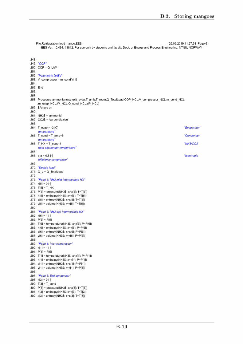
File:Refrigeration load mango.EES 26.06.2019 11.27.38 Page 6EES Ver. 10.494: #3812: For use only by students and faculty Dept. of Energy and Process Engineering, NTNU, NORWAY
248: 249: "COP" 250: COP = Q_L/W 251: 252: "Volumetric floWs" 253: V_compressor = m_cond*v[1] 254: 255: End 256: 257: 258: Procedure ammoniancl(x_exit_evap;T_amb;T_room;Q_TotalLoad:COP_NCL;V_compressor_NCL;m_cond_NCL
;m_evap_NCL;W_NCL;Q_cond_NCL;dP_NCL) 259: $Arrays on 260: 261: NH3$ = 'ammonia' 262: CO2$ = 'carbondioxide' 263: 264: T_evap = -2 [C] "Evaporator
temperature" 265: T_cond = T_amb+5 "Condenser
temperature" 266: T_HX = T_evap-1 "NH3/CO2
heat exchanger temperature" 267: 268: eta = 0,8 [-] "Isentropic
efficiency compressor" 269: 270: "Decide load" 271: Q_L = Q_TotalLoad 272: 273: "Point 5: NH3 inlet intermediate HX" 274: x[5] = 0 [-] 275: T[5] = T_HX 276: P[5] = pressure(NH3$; x=x[5]; T=T[5]) 277: h[5] = enthalpy(NH3$; x=x[5]; T=T[5]) 278: s[5] = entropy(NH3$; x=x[5]; T=T[5]) 279: v[5] = volume(NH3$; x=x[5]; T=T[5]) 280: 281: "Point 6: NH3 exit intermediate HX" 282: x[6] = 1 [-] 283: P[6] = P[5] 284: T[6] = temperature(NH3$; x=x[6]; P=P[6]) 285: h[6] = enthalpy(NH3$; x=x[6]; P=P[6]) 286: s[6] = entropy(NH3$; x=x[6]; P=P[6]) 287: v[6] = volume(NH3$; x=x[6]; P=P[6]) 288: 289: "Point 1: Inlet compressor" 290: x[1] = 1 [-] 291: P[1] = P[5] 292: T[1] = temperature(NH3$; x=x[1]; P=P[1]) 293: h[1] = enthalpy(NH3$; x=x[1]; P=P[1]) 294: s[1] = entropy(NH3$; x=x[1]; P=P[1]) 295: v[1] = volume(NH3$; x=x[1]; P=P[1]) 296: 297: "Point 3: Exit condenser" 298: x[3] = 0 [-] 299: T[3] = T_cond 300: P[3] = pressure(NH3$; x=x[3]; T=T[3]) 301: h[3] = enthalpy(NH3$; x=x[3]; T=T[3]) 302: s[3] = entropy(NH3$; x=x[3]; T=T[3])
B.3. Storing mangoes
B-19

File:Refrigeration load mango.EES 26.06.2019 11.27.38 Page 7EES Ver. 10.494: #3812: For use only by students and faculty Dept. of Energy and Process Engineering, NTNU, NORWAY
303: v[3] = volume(NH3$; x=x[3]; T=T[3]) 304: 305: "Point 4: Two-phase inlet receiver, after expansion" 306: h[4] = h[3] 307: P[4] = P[5] 308: T[4] = temperature(NH3$; h=h[4]; P=P[4]) 309: s[4] = entropy(NH3$; h=h[4]; P=P[4]) 310: x[4] = quality(NH3$; h=h[4]; P=P[4]) 311: v[4] = volume(NH3$; h=h[4]; P=P[4]) 312: 313: "Point 2s: Isentropic exit compressor" 314: ss[2] = s[1] 315: P[2] = P[3] 316: Ts[2] = temperature(NH3$; s=ss[2]; P=P[2]) 317: hs[2] = enthalpy(NH3$; s=ss[2]; P=P[2]) 318: xs[2] = quality(NH3$; s=ss[2]; P=P[2]) 319: vs[2] = volume(NH3$; s=ss[2]; P=P[2]) 320: 321: "Point 7: CO2 inlet evaporator" 322: x[7] = 0 [-] 323: T[7] = T_evap 324: P[7] = pressure(CO2$; x=x[7]; T=T[7]) 325: h[7] = enthalpy(CO2$; x=x[7]; T=T[7]) 326: s[7] = entropy(CO2$; x=x[7]; T=T[7]) 327: v[7] = volume(CO2$; x=x[7]; T=T[7]) 328: 329: "Point 8: CO2 exit evaporator" 330: P[8] = P[7] 331: x[8] = x_exit_evap 332: T[8] = temperature(CO2$; P=P[8]; x=x[8]) 333: h[8] = enthalpy(CO2$; P=P[8]; x=x[8]) 334: s[8] = entropy(CO2$; P=P[8]; x=x[8]) 335: v[8] = volume(CO2$; P=P[8]; x=x[8]) 336: 337: "Mass flows" 338: m_evap_NCL = Q_L/(h[8]-h[7]) "Mass flow
of CO2 through evaporator" 339: m_HX_NH3 = Q_L/(h[6]-h[5]) "Mass flow
of NH3 through intermediate HX" 340: m_cond_NCL = m_HX_NH3*((h[5]-h[6])/(h[4]-h[1])) "Mass flow
through condenser" 341: 342: "Compressor work" 343: W_is = m_cond_NCL*(hs[2]-h[1]) 344: W_NCL = W_is/eta 345: 346: "Point 2: Real exit compressor" 347: h[2] = h[1]+W_NCL/m_cond_NCL 348: T[2] = temperature(NH3$; h=h[2]; P=P[2]) 349: s[2] = entropy(NH3$; h=h[2]; P=P[2]) 350: x[2] = quality(NH3$; h=h[2]; P=P[2]) 351: v[2] = volume(NH3$; h=h[2]; P=P[2]) 352: 353: "Rejected heat condenser" 354: Q_cond_NCL = m_cond_NCL*(h[2]-h[3]) 355: 356: "Pressure ratio" 357: dP_NCL = P[2]/P[1] 358: 359: "COP"
B.3. Storing mangoes
B-20

File:Refrigeration load mango.EES 26.06.2019 11.27.38 Page 8EES Ver. 10.494: #3812: For use only by students and faculty Dept. of Energy and Process Engineering, NTNU, NORWAY
360: COP_NCL = Q_L/W_NCL 361: 362: "Volumetric flows" 363: V_compressor_NCL = m_cond_NCL*v[1] 364: 365: End 366: 367: T_room_K = T_room + 273,15 368: T_amb_K = T_amb + 273,15 369: COP_Ca = (T_room_K)/(T_amb_K - T_room_K) "Carnot
COP" 370: 371: 372: 373: "Room and ambient temperatures" 374: T_room = 13 [C] "Cold
storage temperature, 13 degrees" 375: T_amb = 27,1 [C] "Ambient
temperature" 376: CR = 2 [-] "Circulation
rate" 377: x_exit_evap = 1/CR "Gas
quality at exit of CO2 evaporator" 378: "Day = x" 379: 380: Call transmissionload(T_room;T_amb:Q_Transmission) 381: Call infiltrationload(T_amb;T_room:Q_Infiltration) 382: Call respirationheat(T_room:Q_Respiration) 383: Call equipmentload(Q_Transmission;Q_Infiltration;Q_Respiration:Q_Equipment) 384: Call holdingload(Q_Transmission;Q_Infiltration;Q_Respiration;Q_Equipment:Q_HoldingLoad) 385: Call pulldownload(T_room;T_amb:Q_Pulldown) 386: Call refrigerationload(Q_HoldingLoad;Q_Pulldown:Q_TotalLoad) 387: Call ammonia(T_amb;T_room;Q_TotalLoad:COP;V_compressor;m_cond;m_evap;W;Q_cond;dP) 388: Call ammoniancl(x_exit_evap;T_amb;T_room;Q_TotalLoad:COP_NCL;V_compressor_NCL;m_cond_NCL;m_evap_NCL
;W_NCL;Q_cond_NCL;dP_NCL)
B.3. Storing mangoes
B-21

File:Refrigeration load grapes.EES 26.06.2019 11.26.14 Page 1EES Ver. 10.494: #3812: For use only by students and faculty Dept. of Energy and Process Engineering, NTNU, NORWAY
1: $UnitSystem SI Radian Mass kJ kg C bar 2: 3: 4: Procedure transmissionload(T_room;T_amb:Q_Transmission) 5: 6: "Cold storage exterior size" 7: L_ext = 6,1 [m] "Length" 8: W_ext = 2,44 [m] "Width" 9: H_ext = 2,6 [m] "Height" 10: 11: "Surface areas" 12: A_north = W_ext*H_ext "North wall
area" 13: A_south = W_ext*H_ext "South wall
area" 14: A_east = L_ext*H_ext "East wall
area" 15: A_west = L_ext*H_ext "West wall
area" 16: A_roof = W_ext*L_ext "Roof area" 17: A_floor = W_ext*L_ext "Floor area" 18: 19: "Insulation, expanded polysterene" 20: delta_ins = 0,075 [m] "Insulation
thickness" 21: k_ins = 0,037 [W/(m*K)] "Thermal
conductivity of insulation" 22: U_ins = k_ins/delta_ins "Insulation
heat transfer coefficient" 23: 24: "Allowance for sun effect" 25: dT_sun_east = 3 [C] "East wall
allowance" 26: dT_sun_west = 3 [C] "West wall
allowance" 27: dT_sun_south = 2 [C] "South wall
allowance" 28: dT_sun_roof = 5 [C] "Flat roof
allowance" 29: 30: T_wall_east = T_amb+dT_sun_east "East wall" 31: T_wall_west = T_amb+dT_sun_west "West wall" 32: T_wall_south = T_amb+dT_sun_south "South wall" 33: T_wall_north = T_amb "North wall,
with door" 34: T_roof = T_amb+dT_sun_roof "Flat roof" 35: T_floor = T_amb "Floor" 36: 37: 38: "Transmission load" 39: Q_T_south = U_ins*A_south*(T_wall_south-T_room) "South wall,
[W]" 40: Q_T_east = U_ins*A_east*(T_wall_east-T_room) "East wall,
[W]" 41: Q_T_west = U_ins*A_west*(T_wall_west-T_room) "West wall,
[W]" 42: Q_T_north = U_ins*A_north*(T_wall_north-T_room) "North wall,
[W]" 43: Q_T_roof = U_ins*A_roof*(T_roof-T_room) "Flat roof,
[W]" 44: Q_T_floor = U_ins*A_floor*(T_floor-T_room) "Floor, [W]"
B.4. Storing grapes
B.4 Storing grapes
B-22

File:Refrigeration load grapes.EES 26.06.2019 11.26.14 Page 2EES Ver. 10.494: #3812: For use only by students and faculty Dept. of Energy and Process Engineering, NTNU, NORWAY
45: 46: Q_Transmission = (Q_T_south+Q_T_east+Q_T_west+Q_T_north+Q_T_roof+Q_T_floor)/1000 "Total
transmission load, [kW]" 47: 48: End 49: 50: 51: Procedure infiltrationload(T_amb;T_room:Q_Infiltration) 52: 53: air$ = 'air' 54: P_amb = 1,01325 [bar] "Atmospheri
c pressure" 55: g = 9,81 [m/s^2] "Gravity" 56: 57: H_door = 2,045 [m] "Door height" 58: W_door = 0,8 [m] "Door width" 59: A_door = H_door*W_door "Door area" 60: 61: D_f = 0,8 [-] "Doorway
flow factor" 62: E = 0,9 [-] "New strip
curtains" 63: Theta_d = 24 [h] "Time period" 64: Theta_o = 60 [min] "Door
simply stands open" 65: Theta_p = 30 [s] "Door open
-close time" 66: N = 1 [-] "Door is
opened once a day" 67: 68: h_amb = enthalpy(air$; T=T_amb) "Ambient
air enthalpy" 69: rho_amb = density(air$; T=T_amb; P=P_amb) "Density
ambient air" 70: 71: h_room = enthalpy(air$; T=T_room) "Cold
storage air enthalpy" 72: rho_room = density(air$; T=T_room; P=P_amb) "Density
cold storage air" 73: 74: D_t = (N*Theta_p+60*Theta_o)/(3600*Theta_d) "Doorway
open-time factor" 75: F_m = ((2)/(1+(rho_room/rho_amb)^(1/3)))^(1,5) "Density
factor" 76: Q_s = 0,221*A_door*(h_amb-h_room)*rho_room*(1-(rho_amb/rho_room))^(0,5)*(g*H_door)^(0,5)*F_m "Sensible
and latent refrigeration load, [kW]" 77: 78: Q_Infiltration = Q_s*D_t*D_f*(1-E) "Total
infiltration load, [kW], during holding" 79: 80: End 81: 82: 83: Procedure respirationheat(:Q_Respiration) 84: 85: "Cold storage interior size, without insulation" 86: L_int_ex_ins = 5,87 [m] "Length" 87: W_int_ex_ins = 2,34 [m] "Width" 88: H_int_ex_ins = 2,38 [m] "Height" 89:
B.4. Storing grapes
B-23

File:Refrigeration load grapes.EES 26.06.2019 11.26.14 Page 3EES Ver. 10.494: #3812: For use only by students and faculty Dept. of Energy and Process Engineering, NTNU, NORWAY
90: delta_ins = 0,075 [m] "Insulation thickness"
91: 92: "Interior size, including insulation thickness" 93: L_int = L_int_ex_ins-delta_ins "Length" 94: W_int = W_int_ex_ins-delta_ins "Width" 95: H_int = H_int_ex_ins-delta_ins "Height" 96: A_int = L_int*W_int "Floor area" 97: 98: L_aisle=L_int "Aisle length" 99: W_aisle=0,8 [m] "Aisle width" 100: 101: V_storage = (W_int-W_aisle)*L_int*H_int "Available
storage space" 102: rho_storage = 200 [kg/m^3] "Storage
density" 103: m_grape = (4/7)*rho_storage*V_storage "Mass of
grapes stored" 104: 105: q_resp_grape = 0,0058 [W/kg] "Respiration
rate, grapes" 106: 107: Q_Respiration = (m_grape*q_resp_grape)/1000 "Respiration
heat, [kW]" 108: 109: End 110: 111: 112: Procedure equipmentload(Q_Transmission;Q_Infiltration;Q_Respiration:Q_Equipment) 113: 114: Q_Equipment = 0,1*(Q_Transmission+Q_Infiltration+Q_Respiration) "10 % of
total load, [kW]" 115: 116: End 117: 118: 119: Procedure holdingload(Q_Transmission;Q_Infiltration;Q_Respiration;Q_Equipment:Q_HoldingLoad) 120: 121: Q_HoldingLoad = 1,1*(Q_Transmission+Q_Infiltration+Q_Respiration+Q_Equipment) "Total
steady state holding refrigeration load, with safety factor of 10%, [kW]" 122: 123: End 124: 125: 126: Procedure pulldownload(T_room;T_amb:Q_Pulldown) 127: 128: T_grape = T_amb "Grape
loading temperature" 129: 130: "Cold storage interior size, without insulation" 131: L_int_ex_ins = 5,87 [m] "Length" 132: W_int_ex_ins = 2,34 [m] "Width" 133: H_int_ex_ins = 2,38 [m] "Height" 134: 135: delta_ins = 0,075 [m] "Insulation
thickness" 136: 137: "Interior size, including insulation thickness" 138: L_int = L_int_ex_ins-delta_ins "Length" 139: W_int = W_int_ex_ins-delta_ins "Width"
B.4. Storing grapes
B-24

File:Refrigeration load grapes.EES 26.06.2019 11.26.14 Page 4EES Ver. 10.494: #3812: For use only by students and faculty Dept. of Energy and Process Engineering, NTNU, NORWAY
140: H_int = H_int_ex_ins-delta_ins "Height" 141: 142: L_aisle=L_int "Aisle length" 143: W_aisle=0,8 [m] "Aisle width" 144: 145: V_storage = (W_int-W_aisle)*L_int*H_int "Available
storage space" 146: rho_storage = 200 [kg/m^3] "Storage
density" 147: m_grape = (1/7)*rho_storage*V_storage "Mass of
grapes loaded each day" 148: 149: C_P_grape = 3,70 [kJ/(kg*K)] 150: 151: q_pulldown_grape = m_grape*C_P_grape*(T_grape-T_room) "Heat
removed for grapes, [kJ]" 152: 153: t_Pulldown = 24 "Pull down
time, [h]" 154: 155: Q_Pulldown = 1,1*((q_pulldown_grape)/(3600*t_Pulldown)) "Pulldown
load, including safety factor of 10%, [kW]" 156: 157: "Q_Pulldown = 0 [kW]" "Use when
no pull down" 158: 159: End 160: 161: 162: Procedure refrigerationload(Q_HoldingLoad;Q_Pulldown:Q_TotalLoad) 163: 164: Q_TotalLoad = Q_HoldingLoad+Q_Pulldown "Total
refrigeration load, [kW]" 165: 166: End 167: 168: 169: Procedure ammonia(T_amb;T_room;Q_TotalLoad:COP;V_compressor;m_cond;m_evap;W;Q_cond;dP) 170: $Arrays on 171: 172: NH3$ = 'ammonia' 173: 174: T_evap = -2 [C] "Evaporator
temperature" 175: T_cond = T_amb+5 "Condenser
temperature" 176: 177: eta = 0,8 [-] "Isentropic
efficiency compressor" 178: 179: "Decide load" 180: Q_L = Q_TotalLoad 181: 182: "Point 5: Inlet evaporator" 183: x[5] = 0 [-] 184: T[5] = T_evap 185: P[5] = pressure(NH3$; x=x[5]; T=T[5]) 186: h[5] = enthalpy(NH3$; x=x[5]; T=T[5]) 187: s[5] = entropy(NH3$; x=x[5]; T=T[5]) 188: v[5] = volume(NH3$; x=x[5]; T=T[5])
B.4. Storing grapes
B-25

File:Refrigeration load grapes.EES 26.06.2019 11.26.14 Page 5EES Ver. 10.494: #3812: For use only by students and faculty Dept. of Energy and Process Engineering, NTNU, NORWAY
189: 190: "Point 6: Exit evaporator" 191: x[6] = 1 [-] 192: P[6] = P[5] 193: T[6] = temperature(NH3$; x=x[6]; P=P[6]) 194: h[6] = enthalpy(NH3$; x=x[6]; P=P[6]) 195: s[6] = entropy(NH3$; x=x[6]; P=P[6]) 196: v[6] = volume(NH3$; x=x[6]; P=P[6]) 197: 198: "Point 1: Inlet compressor" 199: x[1] = 1 [-] 200: P[1] = P[5] 201: T[1] = temperature(NH3$; x=x[1]; P=P[1]) 202: h[1] = enthalpy(NH3$; x=x[1]; P=P[1]) 203: s[1] = entropy(NH3$; x=x[1]; P=P[1]) 204: v[1] = volume(NH3$; x=x[1]; P=P[1]) 205: 206: "Point 3: Exit condenser" 207: x[3] = 0 [-] 208: T[3] = T_cond 209: P[3] = pressure(NH3$; x=x[3]; T=T[3]) 210: h[3] = enthalpy(NH3$; x=x[3]; T=T[3]) 211: s[3] = entropy(NH3$; x=x[3]; T=T[3]) 212: v[3] = volume(NH3$; x=x[3]; T=T[3]) 213: 214: "Point 4: Two-phase inlet receiver, after expansion" 215: h[4] = h[3] 216: P[4] = P[5] 217: T[4] = temperature(NH3$; h=h[4]; P=P[4]) 218: s[4] = entropy(NH3$; h=h[4]; P=P[4]) 219: x[4] = quality(NH3$; h=h[4]; P=P[4]) 220: v[4] = volume(NH3$; h=h[4]; P=P[4]) 221: 222: "Point 2s: Isentropic exit compressor" 223: ss[2] = s[1] 224: P[2] = P[3] 225: Ts[2] = temperature(NH3$; s=ss[2]; P=P[2]) 226: hs[2] = enthalpy(NH3$; s=ss[2]; P=P[2]) 227: xs[2] = quality(NH3$; s=ss[2]; P=P[2]) 228: vs[2] = volume(NH3$; s=ss[2]; P=P[2]) 229: 230: "Mass flows" 231: m_evap = Q_L/(h[6]-h[5]) "Mass flow
through evaporator" 232: m_cond = m_evap*((h[5]-h[6])/(h[4]-h[1])) "Mass flow
through condenser" 233: 234: "Compressor work" 235: W_is = m_cond*(hs[2]-h[1]) 236: W = W_is/eta 237: 238: "Point 2: Real exit compressor" 239: h[2] = h[1]+W/m_cond 240: T[2] = temperature(NH3$; h=h[2]; P=P[2]) 241: s[2] = entropy(NH3$; h=h[2]; P=P[2]) 242: x[2] = quality(NH3$; h=h[2]; P=P[2]) 243: v[2] = volume(NH3$; h=h[2]; P=P[2]) 244: 245: "Rejected heat condenser" 246: Q_cond = m_cond*(h[2]-h[3])
B.4. Storing grapes
B-26

File:Refrigeration load grapes.EES 26.06.2019 11.26.14 Page 6EES Ver. 10.494: #3812: For use only by students and faculty Dept. of Energy and Process Engineering, NTNU, NORWAY
247: 248: "Pressure ratio" 249: dP = P[2]/P[1] 250: 251: "COP" 252: COP = Q_L/W 253: 254: "Volumetric floWs" 255: V_compressor = m_cond*v[1] 256: 257: End 258: 259: 260: Procedure ammoniancl(x_exit_evap;T_amb;T_room;Q_TotalLoad:COP_NCL;V_compressor_NCL;m_cond_NCL
;m_evap_NCL;W_NCL;Q_cond_NCL;dP_NCL) 261: $Arrays on 262: 263: NH3$ = 'ammonia' 264: CO2$ = 'carbondioxide' 265: 266: T_evap = -2 [C] "Evaporator
temperature" 267: T_cond = T_amb+5 "Condenser
temperature" 268: T_HX = T_evap-1 "NH3/CO2
heat exchanger temperature" 269: 270: eta = 0,8 [-] "Isentropic
efficiency compressor" 271: 272: "Decide load" 273: Q_L = Q_TotalLoad 274: 275: "Point 5: NH3 inlet intermediate HX" 276: x[5] = 0 [-] 277: T[5] = T_HX 278: P[5] = pressure(NH3$; x=x[5]; T=T[5]) 279: h[5] = enthalpy(NH3$; x=x[5]; T=T[5]) 280: s[5] = entropy(NH3$; x=x[5]; T=T[5]) 281: v[5] = volume(NH3$; x=x[5]; T=T[5]) 282: 283: "Point 6: NH3 exit intermediate HX" 284: x[6] = 1 [-] 285: P[6] = P[5] 286: T[6] = temperature(NH3$; x=x[6]; P=P[6]) 287: h[6] = enthalpy(NH3$; x=x[6]; P=P[6]) 288: s[6] = entropy(NH3$; x=x[6]; P=P[6]) 289: v[6] = volume(NH3$; x=x[6]; P=P[6]) 290: 291: "Point 1: Inlet compressor" 292: x[1] = 1 [-] 293: P[1] = P[5] 294: T[1] = temperature(NH3$; x=x[1]; P=P[1]) 295: h[1] = enthalpy(NH3$; x=x[1]; P=P[1]) 296: s[1] = entropy(NH3$; x=x[1]; P=P[1]) 297: v[1] = volume(NH3$; x=x[1]; P=P[1]) 298: 299: "Point 3: Exit condenser" 300: x[3] = 0 [-] 301: T[3] = T_cond
B.4. Storing grapes
B-27

File:Refrigeration load grapes.EES 26.06.2019 11.26.14 Page 7EES Ver. 10.494: #3812: For use only by students and faculty Dept. of Energy and Process Engineering, NTNU, NORWAY
302: P[3] = pressure(NH3$; x=x[3]; T=T[3]) 303: h[3] = enthalpy(NH3$; x=x[3]; T=T[3]) 304: s[3] = entropy(NH3$; x=x[3]; T=T[3]) 305: v[3] = volume(NH3$; x=x[3]; T=T[3]) 306: 307: "Point 4: Two-phase inlet receiver, after expansion" 308: h[4] = h[3] 309: P[4] = P[5] 310: T[4] = temperature(NH3$; h=h[4]; P=P[4]) 311: s[4] = entropy(NH3$; h=h[4]; P=P[4]) 312: x[4] = quality(NH3$; h=h[4]; P=P[4]) 313: v[4] = volume(NH3$; h=h[4]; P=P[4]) 314: 315: "Point 2s: Isentropic exit compressor" 316: ss[2] = s[1] 317: P[2] = P[3] 318: Ts[2] = temperature(NH3$; s=ss[2]; P=P[2]) 319: hs[2] = enthalpy(NH3$; s=ss[2]; P=P[2]) 320: xs[2] = quality(NH3$; s=ss[2]; P=P[2]) 321: vs[2] = volume(NH3$; s=ss[2]; P=P[2]) 322: 323: "Point 7: CO2 inlet evaporator" 324: x[7] = 0 [-] 325: T[7] = T_evap 326: P[7] = pressure(CO2$; x=x[7]; T=T[7]) 327: h[7] = enthalpy(CO2$; x=x[7]; T=T[7]) 328: s[7] = entropy(CO2$; x=x[7]; T=T[7]) 329: v[7] = volume(CO2$; x=x[7]; T=T[7]) 330: 331: "Point 8: CO2 exit evaporator" 332: P[8] = P[7] 333: x[8] = x_exit_evap 334: T[8] = temperature(CO2$; P=P[8]; x=x[8]) 335: h[8] = enthalpy(CO2$; P=P[8]; x=x[8]) 336: s[8] = entropy(CO2$; P=P[8]; x=x[8]) 337: v[8] = volume(CO2$; P=P[8]; x=x[8]) 338: 339: "Mass flows" 340: m_evap_NCL = Q_L/(h[8]-h[7]) "Mass flow
of CO2 through evaporator" 341: m_HX_NH3 = Q_L/(h[6]-h[5]) "Mass flow
of NH3 through intermediate HX" 342: m_cond_NCL = m_HX_NH3*((h[5]-h[6])/(h[4]-h[1])) "Mass flow
through condenser" 343: 344: "Compressor work" 345: W_is = m_cond_NCL*(hs[2]-h[1]) 346: W_NCL = W_is/eta 347: 348: "Point 2: Real exit compressor" 349: h[2] = h[1]+W_NCL/m_cond_NCL 350: T[2] = temperature(NH3$; h=h[2]; P=P[2]) 351: s[2] = entropy(NH3$; h=h[2]; P=P[2]) 352: x[2] = quality(NH3$; h=h[2]; P=P[2]) 353: v[2] = volume(NH3$; h=h[2]; P=P[2]) 354: 355: "Rejected heat condenser" 356: Q_cond_NCL = m_cond_NCL*(h[2]-h[3]) 357: 358: "Pressure ratio"
B.4. Storing grapes
B-28

File:Refrigeration load grapes.EES 26.06.2019 11.26.14 Page 8EES Ver. 10.494: #3812: For use only by students and faculty Dept. of Energy and Process Engineering, NTNU, NORWAY
359: dP_NCL = P[2]/P[1] 360: 361: "COP" 362: COP_NCL = Q_L/W_NCL 363: 364: "Volumetric floWs" 365: V_compressor_NCL = m_cond_NCL*v[1] 366: 367: End 368: 369: 370: T_room_K = T_room + 273,15 371: T_amb_K = T_amb + 273,15 372: COP_Ca = (T_room_K)/(T_amb_K - T_room_K) "Carnot
COP" 373: 374: 375: "Room and ambient temperatures" 376: T_room = -0,5 [C] "Cold
storage temperature, -0.5 degree" 377: T_amb = 30,9 [C] "Ambient
temperature" 378: CR = 2 [-] "Circulation
rate" 379: x_exit_evap = 1/CR "Gas
quality at exit of CO2 evaporator" 380: "Day = x" 381: 382: Call transmissionload(T_room;T_amb:Q_Transmission) 383: Call infiltrationload(T_amb;T_room:Q_Infiltration) 384: Call respirationheat(T_room:Q_Respiration) 385: Call equipmentload(Q_Transmission;Q_Infiltration;Q_Respiration:Q_Equipment) 386: Call holdingload(Q_Transmission;Q_Infiltration;Q_Respiration;Q_Equipment:Q_HoldingLoad) 387: Call pulldownload(T_room;T_amb:Q_Pulldown) 388: Call refrigerationload(Q_HoldingLoad;Q_Pulldown:Q_TotalLoad) 389: Call ammonia(T_amb;T_room;Q_TotalLoad:COP;V_compressor;m_cond;m_evap;W;Q_cond;dP) 390: Call ammoniancl(x_exit_evap;T_amb;T_room;Q_TotalLoad:COP_NCL;V_compressor_NCL;m_cond_NCL;m_evap_NCL
;W_NCL;Q_cond_NCL;dP_NCL)
B.4. Storing grapes
B-29
Appendix C
Risk assesment
C-1

C-2

C-3

C-4

C-5

Tom A
ndré Bredesen
NTN
UN
orw
egia
n U
nive
rsity
of S
cien
ce a
nd T
echn
olog
yFa
cult
y of
Eng
inee
ring
Dep
artm
ent o
f Ene
rgy
and
Pro
cess
Eng
inee
ring
Mas
ter’
s th
esis
Tom André Bredesen
Design and simulation of a small coldstorage with NH3 refrigeration systemand CO2 as indirect cooling loop forstoring of fresh fruits and vegetables
Master’s thesis in Energy and Environmental EngineeringSupervisor: Trygve Magne Eikevik
July 2019