
Design and development of a composite automotive anti-roll bar
123
University of Windsor University of Windsor Scholarship at UWindsor Scholarship at UWindsor Electronic Theses and Dissertations Theses, Dissertations, and Major Papers Winter 2013 Design and development of a composite automotive anti-roll bar Design and development of a composite automotive anti-roll bar Michael Doody University of Windsor Follow this and additional works at: https://scholar.uwindsor.ca/etd Recommended Citation Recommended Citation Doody, Michael, "Design and development of a composite automotive anti-roll bar" (2013). Electronic Theses and Dissertations. 5040. https://scholar.uwindsor.ca/etd/5040 This online database contains the full-text of PhD dissertations and Masters’ theses of University of Windsor students from 1954 forward. These documents are made available for personal study and research purposes only, in accordance with the Canadian Copyright Act and the Creative Commons license—CC BY-NC-ND (Attribution, Non-Commercial, No Derivative Works). Under this license, works must always be attributed to the copyright holder (original author), cannot be used for any commercial purposes, and may not be altered. Any other use would require the permission of the copyright holder. Students may inquire about withdrawing their dissertation and/or thesis from this database. For additional inquiries, please contact the repository administrator via email ([email protected]) or by telephone at 519-253-3000ext. 3208.
-
Upload
khangminh22 -
Category
Documents
-
view
0 -
download
0
Transcript of Design and development of a composite automotive anti-roll bar

University of Windsor University of Windsor
Scholarship at UWindsor Scholarship at UWindsor
Electronic Theses and Dissertations Theses, Dissertations, and Major Papers
Winter 2013
Design and development of a composite automotive anti-roll bar Design and development of a composite automotive anti-roll bar
Michael Doody University of Windsor
Follow this and additional works at: https://scholar.uwindsor.ca/etd
Recommended Citation Recommended Citation Doody, Michael, "Design and development of a composite automotive anti-roll bar" (2013). Electronic Theses and Dissertations. 5040. https://scholar.uwindsor.ca/etd/5040
This online database contains the full-text of PhD dissertations and Masters’ theses of University of Windsor students from 1954 forward. These documents are made available for personal study and research purposes only, in accordance with the Canadian Copyright Act and the Creative Commons license—CC BY-NC-ND (Attribution, Non-Commercial, No Derivative Works). Under this license, works must always be attributed to the copyright holder (original author), cannot be used for any commercial purposes, and may not be altered. Any other use would require the permission of the copyright holder. Students may inquire about withdrawing their dissertation and/or thesis from this database. For additional inquiries, please contact the repository administrator via email ([email protected]) or by telephone at 519-253-3000ext. 3208.

DESIGN AND DEVELOPMENT OF A COMPOSITE AUTOMOTIVEANTI-ROLL BAR
byMichael Doody
A ThesisSubmitted to the Faculty of Graduate Studies
through Mechanical Engineeringin Partial Fulfilment of the Requirements for
the Degree of Master of Applied Science at theUniversity of Windsor
Windsor, Ontario, Canada
©2013 Michael Doody

978-0-494-95697-7
Your file Votre référence
Library and ArchivesCanada
Bibliothèque etArchives Canada
Published HeritageBranch
395 Wellington StreetOttawa ON K1A 0N4Canada
Direction duPatrimoine de l'édition
395, rue WellingtonOttawa ON K1A 0N4Canada
NOTICE:
ISBN:
Our file Notre référence
978-0-494-95697-7ISBN:
The author has granted a non-exclusive license allowing Library andArchives Canada to reproduce,publish, archive, preserve, conserve,communicate to the public bytelecommunication or on the Internet,loan, distrbute and sell thesesworldwide, for commercial or non-commercial purposes, in microform,paper, electronic and/or any otherformats.
The author retains copyrightownership and moral rights in thisthesis. Neither the thesis norsubstantial extracts from it may beprinted or otherwise reproducedwithout the author's permission.
In compliance with the CanadianPrivacy Act some supporting formsmay have been removed from thisthesis.
While these forms may be included in the document page count, theirremoval does not represent any lossof content from the thesis.
AVIS:L'auteur a accordé une licence non exclusivepermettant à la Bibliothèque et Archives Canada de reproduire, publier, archiver,sauvegarder, conserver, transmettre au public par télécommunication ou par l'Internet, prêter,distribuer et vendre des thèses partout dans lemonde, à des fins commerciales ou autres, sursupport microforme, papier, électronique et/ouautres formats.
L'auteur conserve la propriété du droit d'auteur et des droits moraux qui protege cette thèse. Nila thèse ni des extraits substantiels de celle-ci ne doivent être imprimés ou autrement reproduits sans son autorisation.
Conformément à la loi canadienne sur laprotection de la vie privée, quelques formulaires secondaires ont été enlevés decette thèse.
Bien que ces formulaires aient inclus dansla pagination, il n'y aura aucun contenu manquant.

Design and Development of a Composite Automotive Anti-Roll Bar
by
Michael Doody
APPROVED BY
Dr. A. AlpasMechanical, Automotive, & Materials Engineering
Dr. W. AltenhofMechanical, Automotive, & Materials Engineering
Dr. J. Johrendt, Co-AdvisorMechanical, Automotive, & Materials Engineering
Dr. B. Minaker, Co-AdvisorMechanical, Automotive, & Materials Engineering
October 9, 2013

iii
Author’s Declaration of Originality
I hereby certify that I am the sole author of this thesis and that no part of this thesis has been published
or submitted for publication.
I certify that, to the best of my knowledge, my thesis does not infringe upon anyone’s copyright
nor violate any proprietary rights and that any ideas, techniques, quotations, or any other material
from the work of other people included in my thesis, published or otherwise, are fully acknowledged
in accordance with the standard referencing practices. Furthermore, to the extent that I have included
copyrighted material that surpasses the bounds of fair dealing within the meaning of the Canada Copy-
right Act, I certify that I have obtained a written permission from the copyright owner(s) to include such
material(s) in my thesis and have included copies of such copyright clearances to my appendix.
I declare that this is a true copy of my thesis, including any final revisions, as approved by my thesis
committee and the Graduate Studies office, and that this thesis has not been submitted for a higher
degree to any other University or Institution.

iv
Abstract
An analytical elasticity model is developed for laminated cylindrically anisotropic cylinders subjected to
extension, bending, pressure, torsion, and transverse shearing. The model predicts the elastic response
of thin or thick walled tubes as well as cylinders, and accounts for all elastic coupling present in the
aforementioned loading cases. This model is incorporated into analysis software that predicts the linear-
elastic response of a composite automotive anti-roll bar. The user may input the bar’s two-dimensional
geometry, fibre-layup, diameter, and material properties. A filament-wound composite anti-roll bar is
designed to act as a lightweight drop-in replacement for the high-performance steel anti-roll bar that is
thoroughly benchmarked herein. A mass reduction of 63% is observed when comparing the structural
composite bar design to the existing steel bar.

v
To my parents,
for their support of my often exhausting compulsion to know how things work.

vi
Acknowledgements
This research has been made possible by the generous financial assistance of the Federal Economic Devel-
opment Agency of Southern Ontario; for that, I am grateful. Additionally, I would like to thank Andrew
Glover, David Glover, and Stephen Ouellette of Thunder Composite Technologies Ltd, for providing me
with the opportunity to work closely with them in an industry collaboration on such a promising project.
I would like to thank my supervisors Dr. Bruce Minaker, and Dr. Jennifer Johrendt. The support and
guidance they have provided me with has made this experience a positive one. I owe much of my intel-
lectual and professional enrichment to them.
I owe a debt of gratitude to my committee members Dr. Ahmet Alpas, and Dr. William Altenhof.
A special thank you goes out to my colleagues Sean Maloney and Hart Honickman, they have helped me
maintain some sanity with my journey through graduate school; I look forward to witnessing their sure
success. A special acknowledgement is deserved by Hart, my comrade in anisotropy; the technical ad-
vice, friendly guidance, and deeply theoretical conversations he has shared with me have had a marked
effect on this work; without him, it would not be what it is.
Finally, I must thank my family and my partner, Sabrina, for their patience and understanding during
this endeavour. They have provided me with comfort, solace, and endless love during both challenging
and exciting times.

vii
Contents
Author’s Declaration of Originality iii
Abstract iv
Dedication v
Acknowledgements vi
List of Tables x
List of Figures xi
List of Abbreviations & Definitions xiii
Notation xv
1 Introduction 1
1.1 Motivation . . . . . . . . . . . . . . . . . . . . . . . . . . . . . . . . . . . . . . . . . . . . . . . . . 1
1.2 Research Objectives . . . . . . . . . . . . . . . . . . . . . . . . . . . . . . . . . . . . . . . . . . . . 2
1.3 Thesis Structure . . . . . . . . . . . . . . . . . . . . . . . . . . . . . . . . . . . . . . . . . . . . . . 2
2 Background Theory 4
2.1 The Automotive Anti-Roll Bar . . . . . . . . . . . . . . . . . . . . . . . . . . . . . . . . . . . . . . 4
2.2 Composites . . . . . . . . . . . . . . . . . . . . . . . . . . . . . . . . . . . . . . . . . . . . . . . . . 5
2.2.1 Applications . . . . . . . . . . . . . . . . . . . . . . . . . . . . . . . . . . . . . . . . . . . . 5
2.2.2 Fibres . . . . . . . . . . . . . . . . . . . . . . . . . . . . . . . . . . . . . . . . . . . . . . . . 6
2.2.3 Polymer Matrices . . . . . . . . . . . . . . . . . . . . . . . . . . . . . . . . . . . . . . . . . 7
2.2.4 Production and Manufacture . . . . . . . . . . . . . . . . . . . . . . . . . . . . . . . . . 8
2.2.5 Mechanics of Continuous-Fibre-Reinforced Composites . . . . . . . . . . . . . . . . . 10
2.2.6 Lamination Theory . . . . . . . . . . . . . . . . . . . . . . . . . . . . . . . . . . . . . . . . 18
2.2.7 Elastic Coupling of Composite Laminates . . . . . . . . . . . . . . . . . . . . . . . . . . 22

CONTENTS viii
2.3 Review of Current Literature . . . . . . . . . . . . . . . . . . . . . . . . . . . . . . . . . . . . . . 24
3 Laminated Cylinder Model 27
3.1 Overview . . . . . . . . . . . . . . . . . . . . . . . . . . . . . . . . . . . . . . . . . . . . . . . . . . 27
3.2 Derivation of Stiffness Matrix Terms . . . . . . . . . . . . . . . . . . . . . . . . . . . . . . . . . 30
3.2.1 Axial Force . . . . . . . . . . . . . . . . . . . . . . . . . . . . . . . . . . . . . . . . . . . . . 30
3.2.2 Moment . . . . . . . . . . . . . . . . . . . . . . . . . . . . . . . . . . . . . . . . . . . . . . 32
3.2.3 Internal Moment Equilibrium . . . . . . . . . . . . . . . . . . . . . . . . . . . . . . . . . 32
3.2.4 Pressure . . . . . . . . . . . . . . . . . . . . . . . . . . . . . . . . . . . . . . . . . . . . . . 34
3.2.5 Torsion . . . . . . . . . . . . . . . . . . . . . . . . . . . . . . . . . . . . . . . . . . . . . . . 35
3.2.6 Shear . . . . . . . . . . . . . . . . . . . . . . . . . . . . . . . . . . . . . . . . . . . . . . . . 36
3.3 Result: Relationship Between Loading and Elastic Response . . . . . . . . . . . . . . . . . . . 38
3.4 Discussion . . . . . . . . . . . . . . . . . . . . . . . . . . . . . . . . . . . . . . . . . . . . . . . . . 40
3.4.1 Bending . . . . . . . . . . . . . . . . . . . . . . . . . . . . . . . . . . . . . . . . . . . . . . 40
3.4.2 Transverse Strain Gradients . . . . . . . . . . . . . . . . . . . . . . . . . . . . . . . . . . 40
3.4.3 Pressure . . . . . . . . . . . . . . . . . . . . . . . . . . . . . . . . . . . . . . . . . . . . . . 40
3.4.4 Transverse Shear . . . . . . . . . . . . . . . . . . . . . . . . . . . . . . . . . . . . . . . . . 41
3.4.5 Additional Stress and Strain Distribution Considerations . . . . . . . . . . . . . . . . 43
3.4.6 Through-Thickness Normal Stress . . . . . . . . . . . . . . . . . . . . . . . . . . . . . . 44
4 Validation of The Elasticity Model 45
4.1 Finite Element Analysis . . . . . . . . . . . . . . . . . . . . . . . . . . . . . . . . . . . . . . . . . 45
4.1.1 Elastic Response to Torsion of a Thin-Walled Tube . . . . . . . . . . . . . . . . . . . . 45
4.1.2 The Effect of Tube Wall-Thickness on Axial Response & Coupling . . . . . . . . . . . 47
4.1.3 Final Remarks . . . . . . . . . . . . . . . . . . . . . . . . . . . . . . . . . . . . . . . . . . . 50
4.2 Experimental Program . . . . . . . . . . . . . . . . . . . . . . . . . . . . . . . . . . . . . . . . . . 50
4.2.1 Specimens . . . . . . . . . . . . . . . . . . . . . . . . . . . . . . . . . . . . . . . . . . . . . 50
4.2.2 Apparatus . . . . . . . . . . . . . . . . . . . . . . . . . . . . . . . . . . . . . . . . . . . . . 51
4.2.3 Three-Point-Bending Tests . . . . . . . . . . . . . . . . . . . . . . . . . . . . . . . . . . . 56
4.2.4 Torsion Tests . . . . . . . . . . . . . . . . . . . . . . . . . . . . . . . . . . . . . . . . . . . 58
4.2.5 Discussion . . . . . . . . . . . . . . . . . . . . . . . . . . . . . . . . . . . . . . . . . . . . . 60
5 Anti-Roll Bar Analysis & Design 63
5.1 Benchmarking of the Steel Anti-Roll Bar . . . . . . . . . . . . . . . . . . . . . . . . . . . . . . . 64
5.1.1 Classical Analytical Methods . . . . . . . . . . . . . . . . . . . . . . . . . . . . . . . . . . 64
5.1.2 Finite Element Analysis . . . . . . . . . . . . . . . . . . . . . . . . . . . . . . . . . . . . . 65
5.1.3 Experimental Testing . . . . . . . . . . . . . . . . . . . . . . . . . . . . . . . . . . . . . . 69

CONTENTS ix
5.2 Composite Anti-Roll Bar . . . . . . . . . . . . . . . . . . . . . . . . . . . . . . . . . . . . . . . . . 71
5.2.1 Analysis Software . . . . . . . . . . . . . . . . . . . . . . . . . . . . . . . . . . . . . . . . 71
5.2.2 Design . . . . . . . . . . . . . . . . . . . . . . . . . . . . . . . . . . . . . . . . . . . . . . . 74
5.2.3 Discussion and Recommendations . . . . . . . . . . . . . . . . . . . . . . . . . . . . . . 76
6 Conclusions & Recommendations 78
6.1 Summary . . . . . . . . . . . . . . . . . . . . . . . . . . . . . . . . . . . . . . . . . . . . . . . . . . 78
6.2 Conclusions . . . . . . . . . . . . . . . . . . . . . . . . . . . . . . . . . . . . . . . . . . . . . . . . . 79
6.3 Recommendations for Future Work . . . . . . . . . . . . . . . . . . . . . . . . . . . . . . . . . . 79
6.4 Contributions . . . . . . . . . . . . . . . . . . . . . . . . . . . . . . . . . . . . . . . . . . . . . . . 81
References 82
A Specimen Measurements 85
B Laminated Cylinder Model Input 87
C Laminated Cylinder Model Code 89
D Composite Anti-Roll Bar Analysis Code 94
Vita Auctoris 103

x
List of Tables
2.1 Fibre-direction strain under various loading directions . . . . . . . . . . . . . . . . . . . . . . 15
2.2 Elastic coupling in various classes of laminate architecture . . . . . . . . . . . . . . . . . . . . 24
4.1 In-plane properties of unidirectional carbon-fibre/epoxy laminate used in FE studies . . . 46
4.2 Mesh sensitivity study of torsionally loaded FE model . . . . . . . . . . . . . . . . . . . . . . . 47
4.3 Axially loaded model results: axial force response dl & associated extensional-torsional
coupling φ for a number of tubes with varying wall-thickness . . . . . . . . . . . . . . . . . . 49
4.4 Cylindrical FRP test specimen dimensions . . . . . . . . . . . . . . . . . . . . . . . . . . . . . . 51
4.5 Three point flexure test: experimental results and laminated cylinder model predictions
for each specimen . . . . . . . . . . . . . . . . . . . . . . . . . . . . . . . . . . . . . . . . . . . . . 58
4.6 Torsion test: experimental results and laminated cylinder model predictions . . . . . . . . . 60
4.7 Sensitivity of the model’s elastic response prediction to input variables and properties . . . 62
5.1 Stiffness contributions in steel anti-roll bar . . . . . . . . . . . . . . . . . . . . . . . . . . . . . 65
5.2 Steel ARB finite element mesh-sensitivity study data . . . . . . . . . . . . . . . . . . . . . . . 68
5.3 Steel ARB test (polymer bushings) . . . . . . . . . . . . . . . . . . . . . . . . . . . . . . . . . . . 71
5.4 Steel ARB test (steel bushings) . . . . . . . . . . . . . . . . . . . . . . . . . . . . . . . . . . . . . 71
5.5 In-plane properties of carbon and E-glass unidirectional laminates . . . . . . . . . . . . . . . 74
A.1 Sample 1A measurements . . . . . . . . . . . . . . . . . . . . . . . . . . . . . . . . . . . . . . . . 85
A.2 Sample 1B measurements . . . . . . . . . . . . . . . . . . . . . . . . . . . . . . . . . . . . . . . . 85
A.3 Sample 1C measurements . . . . . . . . . . . . . . . . . . . . . . . . . . . . . . . . . . . . . . . . 86
A.4 Sample 2A measurements . . . . . . . . . . . . . . . . . . . . . . . . . . . . . . . . . . . . . . . . 86
A.5 Sample 2B measurements . . . . . . . . . . . . . . . . . . . . . . . . . . . . . . . . . . . . . . . . 86
A.6 Sample 2C measurements . . . . . . . . . . . . . . . . . . . . . . . . . . . . . . . . . . . . . . . . 86
B.1 Material properties of E-glass fibres and epoxy matrix used in test specimens . . . . . . . . 87
B.2 Specimen fibre volume fraction calculation . . . . . . . . . . . . . . . . . . . . . . . . . . . . . 88
B.3 Local elastic properties of individual laminae in test specimens . . . . . . . . . . . . . . . . . 88

xi
List of Figures
2.1 Effect of an anti-roll bar vehicle body roll . . . . . . . . . . . . . . . . . . . . . . . . . . . . . . 4
2.2 Anti-Roll bar as seen in a vehicle . . . . . . . . . . . . . . . . . . . . . . . . . . . . . . . . . . . . 5
2.3 Notation and dimensions for the discussed laminate . . . . . . . . . . . . . . . . . . . . . . . . 19
2.4 Moments and forces on an element in lamination theory . . . . . . . . . . . . . . . . . . . . . 21
2.5 Undeformed and deformed shape of a unidirectional lamina with off-axis loading . . . . . 23
3.1 Local and global coordinate systems for a layered FRP tube in arbitrary state of deformation 28
3.2 Depiction of area used in axial, moment, torsion, and shear calculations . . . . . . . . . . . 31
3.3 Depiction of area used to equilibrate internal moments . . . . . . . . . . . . . . . . . . . . . . 33
3.4 Depiction of area used in internal pressure calculations . . . . . . . . . . . . . . . . . . . . . . 35
3.5 Distribution of shear stress in circular cross-sections with response to transverse shear
loading (of an isotropic material) . . . . . . . . . . . . . . . . . . . . . . . . . . . . . . . . . . . 42
4.1 FE torsion model: constraints and loading (0.5 mm mesh shown) . . . . . . . . . . . . . . . 46
4.2 FE axial loading model: constraints and loading . . . . . . . . . . . . . . . . . . . . . . . . . . 48
4.3 Percent difference in predictions of FE and laminated cylinder model on axial response
and axial-torsional coupling . . . . . . . . . . . . . . . . . . . . . . . . . . . . . . . . . . . . . . . 49
4.4 MTS® Model 642.25 Bend Fixture . . . . . . . . . . . . . . . . . . . . . . . . . . . . . . . . . . . 52
4.5 Torsion Testing Machine . . . . . . . . . . . . . . . . . . . . . . . . . . . . . . . . . . . . . . . . . 53
4.6 Primary-function components of torsion testing machine . . . . . . . . . . . . . . . . . . . . 55
4.7 Experimental setup: three point flexure test (sample 1C) . . . . . . . . . . . . . . . . . . . . 57
4.8 Experimental setup: torsion test (live-end with specimen 2A mounted) . . . . . . . . . . . 59
4.9 Experimental setup: torsion test (dead-end with specimen 2A mounted) . . . . . . . . . . . 59
5.1 Geometry of existing steel anti-roll bar . . . . . . . . . . . . . . . . . . . . . . . . . . . . . . . . 63
5.2 Simplified anti-roll bar geometry: plan view . . . . . . . . . . . . . . . . . . . . . . . . . . . . . 64
5.3 Solid element mesh (2.5 mm nominal element length) . . . . . . . . . . . . . . . . . . . . . . 66
5.4 Wireframe model showing constraints and applied loading . . . . . . . . . . . . . . . . . . . 67

LIST OF FIGURES xii
5.5 Coarsest and finest mesh used in steel ARB convergence study . . . . . . . . . . . . . . . . . 68
5.6 Steel ARB finite element solution convergence: linear spring-rate vs. element size . . . . . 69
5.7 Physical testing setup: fixed end with polymer bushing . . . . . . . . . . . . . . . . . . . . . . 70
5.8 Physical testing setup: actuated end with steel bushing . . . . . . . . . . . . . . . . . . . . . . 70
5.9 Line geometry input to CARBA software (congruent with classical analysis) . . . . . . . . . 72
5.10 Vertical displacement profile output from CARBA software for the steel bar . . . . . . . . . 73
5.11 Desired line geometry of composite ARB . . . . . . . . . . . . . . . . . . . . . . . . . . . . . . . 74
5.12 Linear anti-roll bar stiffness vs. fibre angle for composite bars . . . . . . . . . . . . . . . . . . 75
5.13 Vertical displacement profile output from CARBA software for the composite bar . . . . . 75

xiii
List of Abbreviations & Definitions
All abbreviations used in this work are described in this section; some esoteric terms used here are also
defined for convenience.
Abbreviations
Abbreviation Meaning
ASTM American Society for Testing and Materials
ARB Anti-Roll Bar
CHEXA An Eight Noded Hexahedral Brick Element
CPU Central Processing Unit
CLPT Classical Laminated Plate Theory
CARBA Composite Anti-Roll Bar Analysis
CQUAD4 A First Order Four Noded Shell Element
FRP Fibre-Reinforced Polymer
FE Finite Element
MATLAB® Matrix Laboratory
PC Personal Computer
RTM Resin Transfer Moulding
RBE2 Rigid Body Element (interpolation type)
RBE3 Rigid Body Element (true rigid type)
SMC Sheet Moulding Compound
SPC Single Point Constraint

xiv
Definitions
Term Definition
Anisotropic Having elastic properties that depend on direction or orientation, and being
fully described by 21 elastic constants
Axial-symmetrical
loading
A loading that tends to induce strains that are symmetrical about an axis,
e.g., torsion, axial tension/compression, and uniform pressure loading
Cylindrically
anisotropic
A material is cylindrically anisotropic when its elastic properties are con-
stant within a cylindrical coordinate system
Isotropic Having elastic properties independent of direction or orientation, and being
fully described by two elastic constants
Orthotropic Having three orthogonal planes of material symmetry, within which elastic
properties are independent of direction, and being fully described by nine
elastic constants
Transversely
isotropic
Having elastic properties that are constant within a plane, but different
along the direction normal to this plane: a special case of orthotropy re-
quiring only five elastic constants to be fully described

xv
Notation
Mathematical notation throughout this work is listed below, separated by the chapter in which it first
appears.
Background Theory
Label Description
A Extensional stiffness matrix
Amn The nth entry in the mth row of the A matrix
B Coupling stiffness matrix
Bmn The nth entry in the mth row of the B matrix
C Laminate stiffness matrix
D Bending stiffness matrix
Dmn The nth entry in the mth row of the D matrix
E11 Effective elastic modulus in the fibre-direction
E22 Effective elastic modulus in the transverse 2-direction
E33 Effective elastic modulus in the transverse 3-direction
Ef Longitudinal elastic modulus of fibre
Em Elastic modulus of matrix
G12 In-plane shear modulus
G13 Out-of-plane fibre-direction shear modulus
G23 Out-of-plane transverse shear modulus
hx Elevation h to the outer edge of lamina x
k Designated layer number
Mx x , and My y Bending moment per unit width of laminate in the x-z and y-z
planes, respectively
Mx y Twisting moment per unit width of laminate
N Total number of Laminae within the laminate

xvi
Nx x , and Ny y Normal force per unit width of laminate in the x and y direction,
respectively
Nx y In plane x-y shear force, per unit width of laminate
Q The orthotropic lamina stiffness matrix
Q̄ The transformed lamina stiffness matrix
Q̄11 The first term of the first row of the transformed lamina stiffness
matrix
Q11 The first entry in the first row of the Q matrix
Q̄x y The y th entry in the x th row of the transformed lamina stiffness
matrix
Qx y The y th entry in the x th row of the Q matrix
S Laminate compliance matrix
S3D Three-dimensional compliance matrix for an orthotropic lamina
Tg Glass transition temperature
u, v, and w Displacement in the x , y , and z directions, respectively
Vf Ratio of fibre to matrix volume (fibre-volume fraction)
zk The distance between the mid-plane of lamina k and the mid-plane
of the laminate, referred to as lamina elevation
ε1 Strain in the fibre direction
ε2 Strain in the transverse 2-direction
ε3 Strain in the transverse 3-direction
εx xk, and εy yk
Normal strain in the x and y directions, respectively, within lamina
k
ε0x x , and ε0
y y Mid-plane normal strain in the x and y directions, respectively, of
the laminate
γ12 Shear strain in the 1-2 plane
γ23 Shear strain in the 2-3 plane
γ31 Shear strain in the 3-1 plane
γx ykIn-plane x-y shear strain (engineering strain) within lamina k
γ0x y Mid-plane in-plane x-y shear strain (engineering strain) in the lam-
inate
κx x , and κy y Bending curvature of the laminate in the x-z and y-z planes, respec-
tively
κx y Twisting curvature of the laminate
ν12 Poissons ratio in the 2-direction due to 1-direction loading (major
Poisson’s ratio)

xvii
ν13 Poissons ratio in the 3-direction due to 1-direction loading
ν21 Poissons ratio in the 1-direction due to 2-direction loading (minor
Poisson’s ratio)
ν23 Poissons ratio in the 3-direction due to 2-direction loading
ν31 Poissons ratio in the 1-direction due to 3-direction loading
ν32 Poissons ratio in the 2-direction due to 3-direction loading
ν f Poisson’s ratio of fibre
νm Poisson’s ratio of matrix
σ1 Normal stress in the fibre direction
σ2 Normal stress in the transverse 2-direction
σ3 Normal stress in the transverse 3-direction
τ12 Shear stress in the 1-2 plane
τ23 Shear stress in the 2-3 plane
τ31 Shear stress in the 3-1 plane
θ The angle of fibres within a lamina, relative to the x axis of the x-y-z
coordinate system
Laminated Cylinder Model
Label Description
a, and b Distance from the tube’s center to the outer and inner edges, respectively,
of a laminate
dFj jn Normal force in the j j direction acting on an infinitesimal element in lam-
ina n
Fx x Applied axial force
Gik Shear modulus in the i-k direction
Mintxtotal internal moment about the x axis
M Laminated cylinder model stiffness matrix
My , and Mz Applied bending moment about the y and z axes, respectively
P Internal Pressure
ri Inner radius of the tube
rn Mid-lamina radius of lamina n
T Torque applied axially to the tube
tn Thickness of lamina n

xviii
Vi j , and Vik Shear loading in the i- j and i-k planes, respectively
Vx y , and Vxz Applied global shear loading in the x-y and x-z planes, respectively
εii Strain in the axial (ii) direction
ε j j Strain in the tangential ( j j) direction
εD Uniform diametric expansion strain
γi jshearShear strain in the i- j plane caused by transverse shear
γi j Shear strain in the i- j plane
γt ransverse Transverse in-plane shear strain that results from an axial load
γx y , and γxz Global transverse shear deformation in the x-y and x-z planes, respectively
κy , and κz Angle of cuvature about the y and z axes, respectively
φ Angle of twist
ψ Variable defined for convenience
σii Normal stress in the axial (ii) direction
σ j j Normal stress in the tangential ( j j) direction
τi j , and τik Shear stress in the i- j and i-k planes, respectively
θ Angle between y axis and point or plane of interest
Validation
Label Description
EI Bending stiffness
Jclassical Polar moment of interia, calculated in the classical and exact manner
Jshel l Polar moment of interia, calculated as modelled with FE shell ele-
ments
JG Torsional Rigidity
L Span length
P Applied load
T Applied torsion
x Deflection

1
Chapter 1
Introduction
The introduction consists of three sections; the first section discusses the motivation behind the research
presented herein. The second section outlines three major research objectives, and the third section
provides the reader with an overview of the thesis structure.
1.1 Motivation
The automotive industry is increasingly being pushed by government fuel economy and emissions man-
dates to make cars more efficient, lighter, and ‘greener’. This movement has facilitated development
of an impressive suite of technology ranging from highly efficient small-displacement forced-induction
internal combustion engines, to hybrid or purely electric powertrains among other technologies. While
these technologies and many others are helping automotive manufacturers lower emissions and ap-
proach mileage targets, they will not suffice without supplement; substantial vehicle lightweighting is
necessary. Generally, this means that traditional material choices are reconsidered. To this end, the use of
aluminium alloys, high strength steel alloys, and fibre reinforced polymers (FRPs) is gaining popularity.
Fibre reinforced composite parts are used extensively in the aerospace and motorsports industries for
structural applications. The automotive industry, however, has not yet seen the same level of composite
material integration into structural elements of high-production-volume vehicles. The author believes
this is a function of primarily two factors: a lack of low-cost high-volume manufacturability, and a
lack of understanding of the behaviour of the composite materials themselves. The work presented
herein has been motivated by an industry collaboration that aims to make improvements to both of the
aforementioned factors, with research focused on the latter.
A proprietary manufacturing methodology for filament-wound FRP structures that allows varying
fibre-angle and cross-section throughout the length of a member has been developed. The conventional
design approach of finite element modelling does not lend itself well to optimization schemes for a

CHAPTER 1. INTRODUCTION 2
structure of this type. This point, compounded by a deficit in literature of a comprehensive analytical
elasticity model for thick-walled composite tubes and beams of circular cross-section, demonstrates the
need for research.
1.2 Research Objectives
The first objective of the research is development an analytical elasticity model for axially symmetric,
cylindrically anisotropic tubes and rods subjected to extension, bending, pressure, torsion, and trans-
verse shearing. The model captures all of the elastic coupling phenomena present in the loading of a
helically wound continuous-fibre composite laminated cylinder.
The second objective is validation of the derived elasticity model. Computational validation was car-
ried out using commercial finite element software; in addition, a limited amount of physical testing was
performed to serve as experimental validation of predicted torsional stiffness and bending compliance.
The third objective is development of a structural design for a filament-wound composite automotive
anti-roll bar that will act as a lightweight replacement to an existing steel bar. Care will be given to ensure
that the design is both cost effective, and lightweight. The model established in the first objective will
be used in a computer design package to tailor the elastic response of the composite anti-roll bar. The
desired response is a function of parameters determined through analytical and physical benchmarking
of the existing steel bar.
1.3 Thesis Structure
The author has made an effort to present the material of this thesis in an order that is both logical and
conducive to a firm understanding of the work documented herein. The first chapter provides the reader
with some insight into what motivated this research, as well as a clear outline of the research objectives.
The second chapter will serve to introduce the novice reader to the background theory that is nec-
essary to understand the material presented in the chapters that follow; for the reader who is versed in
this area of science, it may serve as a reference. An introduction is provided on the automotive anti-roll
bar, followed by a definition of composite materials, with a focus on fibre-reinforced polymers. Com-
mon applications and manufacturing methods of composites are discussed before outlining the theory
associated with their analysis and design. Finally, a review of current and relevant literature is presented.
The third chapter addresses the first research objective, presenting a novel elasticity model for cylin-
drically anisotropic laminated cylinders and tubes, and outlining the model’s derivation. A thorough
discussion is given with regard to the assumptions, limitations, and implications of the model.
The fourth chapter details the computational and experimental model validation that was performed.
The physical test specimens, apparatus, experimental tests, and results are discussed in detail.

CHAPTER 1. INTRODUCTION 3
The fifth chapter describes the benchmarking of the steel anti-roll bar, and presents the procedure
adopted in utilizing the developed model for design of a composite anti-roll bar, as well as the design
that resulted.
Conclusions are drawn and provided in the sixth chapter.

4
Chapter 2
Background Theory
This chapter provides an introduction to the automotive anti-roll bar, followed by some background
theory necessary for a solid understanding of fire-reinforced composite materials and their design. Lastly,
a review is provided of current literature relevant to the work presented herein.
2.1 The Automotive Anti-Roll Bar
An anti-roll bar (ARB), known also as a sway bar, is an automotive suspension component that elastically
couples the suspension on one side of a vehicle to the adjacent side. If the suspension on one side of the
vehicle is compressed, a reactive force will be generated by the ARB tending to compress the suspension
on the adjacent side of the vehicle. This coupling serves to reduce the amount of ‘body roll’ a vehicle
will experience during cornering (see Figure 2.1). Body roll is defined as the angle through which the
vehicle’s body rotates about its longitudinal axis; this motion is not only uncomfortable for passengers,
but detrimental to vehicle traction and handling due to the non-linear response of pneumatic automotive
tires.
UWINDSORUWINDSOR
High Roll StiffnessLow Roll Stiffness
Figure 2.1: Effect of an anti-roll bar vehicle body roll
The most conventional style of ARB is a long C-shaped spring-steel member of circular and constant
cross section; this style is shown in Figure 2.2. The bar is affixed to the frame of the vehicle with rubber

CHAPTER 2. BACKGROUND THEORY 5
bushings allowing rotation of the bar while constraining translation. The ends of the bar are pinned to
the moving suspension components on each side of the vehicle by ‘end links’: short links with a spherical
joint at each end. If the vehicle’s left and right wheels move upward in unison, as would be the case
when driving over a speed bump (perpendicularly), both ends of the bar move together causing only
rotation within the rubber bushings. However, if one wheel moves independently, the mid-span of the
bar is put into a state of torsional deflection as the cantilevered anti-roll bar ends move relative to each
other. Therefore, the stiffness of the anti-roll bar (measured in a manner consistent with the deformation
observed) directly dictates the degree of coupling between the left and right side vehicle suspension.
ARB Induced motion
Road Induced Motion
Bushings
End Link Location
Figure 2.2: Anti-Roll bar as seen in a vehicle (reproduced and adapted fromwww.carbibles.com)
A large amount of research and effort [1][2][3] has been aimed at studying the effects of vehicle
roll stiffness as well as the effect ARBs have on vehicle dynamics. Numerous designs including active
electronically-controlled ARBs are in existence, but not discussed here. The purpose of this section is
to provide a novice reader with a rudimentary understanding of ARB basics; this understanding will be
necessary to comprehend the implications of an anti-roll bar’s structural and elastic behaviour.
2.2 Composites
2.2.1 Applications
Fibre reinforced composites have found their way into numerous industries; the number of applications
seems limitless and is continually growing. Some significant applications are listed in the following
discussion, but by no means is this an exhaustive list.
The aircraft and military industries seem to be at the forefront of FRP development, likely due to their
inherent need for lightweight structural materials, as well as the considerable funding and resources

CHAPTER 2. BACKGROUND THEORY 6
typically available to them. Boron fibre-epoxy composite stabilizer skins were introduced to production
F-14 fighter aircraft in the late 1960s, and the use of FRPs in aerospace has only increased; today
there are many aircraft having airframes composed mostly of FRP. Many modern helicopters exploit the
advantages of FRP rotor blades, allowing reduced weight, greater fatigue and corrosion resistance, and
less vibration sensitive designs. The fibre angle can even be altered along the length of the rotor to tune
the vibration characteristics of the rotor blade reducing the effect of resonance frequencies.
The automotive industry has been slower to adopt heavy use of FRP components and structure to a
production environment, likely because of the cost and production time associated with most manufac-
turing methods. Lower production, higher budget products in the automotive industry make extensive
use of composites; Formula 1 racecars are made primarily of carbon FRPs. A process that will be de-
scribed later in the text uses sheet moulding compound (SMC) to allow fast and cheap production of
hoods, deck lids, doors, and various other automotive panels. Sheet moulding compound panels are typ-
ically composed of chopped strand glass-fiber and polyester resin. General Motors began using filament
wound, compression moulded composite leaf springs for the Corvette in 1981, providing an 80% weight
savings [4]. More recently the Corvette has adopted front and rear composite leaf springs mounted in a
manner conducive to an anti-roll effect. Carbon FRP driveshafts have been implemented and proven in
both racing and heavy industrial applications; the increased damping and decreased mass allow for use
of a longer unsupported drive shaft without the severe resonance encountered in metallic driveshafts.
Other industries include sporting goods (golf clubs, bicycles, skis, etc), marine (boat hulls, masts,
etc), and even civil engineering (glass and carbon fibre have been used to reinforce concrete and elimi-
nate corrosion based degradation).
2.2.2 Fibres
The fibre component of a fibre-reinforced composite has a much larger effect on strength and stiffness
than the matrix. There is more than one reason for this: generally the fibre volume fraction (discussed in
detail in Section 2.2.5) is larger than 50% – meaning the composite contains more fibre than matrix; also,
more importantly, the tensile strength and modulus of the fibre is generally much higher than that of the
matrix. With fibre properties being so dominant, much effort goes into the characterization of different
types of fibres. Important properties are tensile and compressive modulus and strength, density, fatigue
behaviour, cost of manufacture, and electrical and thermal properties. Fibres are typically arranged into
either a cloth with one or more fibre directions, strands (a unidirectional yarn of fibres), or rovings (a
continuous bundle of strands). Fibres may be totally raw, or coated in a sizing that promotes matrix
adhesion or reduces fibre-fibre friction in rovings. Also available are pre-impregnated or ‘prepreg’ forms
of fibres: uncured resin is infused into the roving, strand, or cloth at a specific ratio. The prepreg
material is typically stored in a refrigerated environment to prevent any premature or undesired curing.
Attributes of the more popular fibres are discussed in the descriptions that follow.

CHAPTER 2. BACKGROUND THEORY 7
Glass Fibres
Glass fibres remain the most popular fibre for FRPs. This is likely a result of low-cost manufacturability,
and moderate strength-to-weight ratio. Glass fibres are highly resistant to chemicals, provide very good
insulating properties, and have high tensile strength. Disadvantages include high density, low modu-
lus, and brittle behavior. Two main types of glass are available: E-glass (electrical grade) and S-glass
(structural grade). S-glass provides higher tensile strength at a cost premium. Diameters of glass fibres
typically range from 8–14 microns [5].
Carbon Fibres
Carbon fibres can offer significant performance advantages over glass: high stiffness-to-weight ratio,
low density, and high strength-to-weight ratio at an intermediate cost. The properties of carbon fibres
can vary drastically depending on the method of manufacture, allowing the engineer to make a decision
based on whether strength or stiffness is of more importance – generally there is a trade off. The
tensile modulus of carbon fibres has been reported [6] to range from 207 GPa to 1035 GPa. Tensile
strength ranges from 1.9 GPa to as high as 6.9 GPa in recent developments with diameter ranging from
6–8 microns [5]. Aside from the qualities listed, carbon fibres boast a very low coefficient of thermal
expansion, a high thermal conductivity, and good fatigue strength characteristics. Disadvantages can
include high electrical conductivity, low strain-to-failure, and poor impact resistance.
Aramid Fibres
Known also under the trade name Kevlar 49, aramid fibres exhibit a remarkably low density and high
strength-to-weight ratio, and very good impact resistance (even failing in a ductile manner). Aramid
fibres show moderate chemical resistivity, and great resistance to high temperatures and combustion.
Their tensile strength is approximately 3.6 GPa, tensile modulus: 130 GPa, and fibre diameters are on
the order of 12 microns. Disadvantages of aramid fibres include poor compressive strength and difficulty
in cutting.
Other Less Frequently Used Fibres
Extended chain polyethylene fibres (known also by their trade name Spectra or Dyneema) have an
extremely high strength to weight ratio, good abrasion resistance, but poor matrix adhesion and unde-
sirable properties of creep.
2.2.3 Polymer Matrices
While it has been stated that the properties of the fibre are dominant, the matrix of a fibre-reinforced
composite plays a significant role in the overall performance of the material. The presence of a matrix

CHAPTER 2. BACKGROUND THEORY 8
facilitates fibre-to-fibre stress transfer as well as fibre stability and resistance to buckling under com-
pressive load. Inter-laminar shear strength and elastic shear modulus are governed largely by matrix
choice and matrix-fibre adhesion. The toughness or resistance to brittle fracture of a composite can be
influenced heavily by matrix properties. The matrix also provides the fibres with abrasion resistance,
and isolation from potentially harmful moisture and chemicals.
There are two major categories of polymer matrices: thermosets, and thermoplastics. Thermoset
polymers include epoxies, polyesters, vinyl esters, phenolics, polyimides and cyanate esters. Thermo-
plastic polymers include nylons, polycarbonates, polyethylene terephthalate, and many others.
Thermoset polymers typically begin production as a two part system of low viscosity liquids that are
mixed together, allowing a curing reaction to take place. Once cured, the long chain-like molecules form
cross-links that strengthen and stiffen the material, but also prevent the reforming that is possible with
thermoplastics. Generally, thermosets provide superior resistance to creep and stress relaxation when
compared to thermoplastics. There are disadvantages to thermoset polymers: low strain to failure,
extended curing or polymerization times, and limited pot life – the length of time a mixed liquid batch
of thermoset ingredients can be left at room temperature.
Thermoplastic polymers do not require a chemical curing process to form molecular cross-links and
assume a stable solid shape. Because thermoplastics are not cross-linked, they may be heated or melted
and formed into a desired shape repeatedly. While thermoplastics do not offer good creep and stress
relaxation characteristics, they do exhibit larger values of strain-to-failure and better resistance to crack
propagation.
Both thermosets and thermoplastics exhibit a significant behaviour shift at a certain elevated temper-
ature known as the glass transition temperature Tg . The stiffness of the polymer is significantly reduced
at, and even leading up to Tg , limiting the temperature range within which a particular matrix is useful.
Non-polymer matrices such as metal and ceramic do exist and have been proven as a very useful
technology, but the scope of this document will be limited to polymers – or rather, fibre-reinforced
polymers (FRPs).
2.2.4 Production and Manufacture
The direction of fibres in an FRP component has a profound effect on its performance; because of this,
an understanding of the manufacturing process is important to the analysis of an FRP structure. Certain
manufacturing processes lend themselves well to particular shapes, or to high production-rates and low
manual labour requirements. The automotive industry is largely responsible for the recent advancements
in low-labour high production rate manufacturing processes.

CHAPTER 2. BACKGROUND THEORY 9
Sheet Moulding Compound
Sheet moulding compound (SMC) refers to both a material and the manufacturing process used to make
it. The process involves fibres (typically glass) being strewn atop a sheet of un-cured polyester resin;
once the chopped rovings are settled, another resin sheet is laid on top. The resin-fibre-resin stackup is
then sandwiched between two layers of thin sheeting known as carrier film. These layers of film are later
removed when the sheet is placed into a heated compression mould to be shaped and cured. The process
lends itself very well to a mass production environment, which is likely why it has such popularity in the
automotive industry for the manufacture of hoods, deck lids, door panels, and other suitable parts.
Filament Winding
Another manufacturing method that can be highly automated is filament winding: a process in which
continuous rovings or strands are wound around a mandrel that is later removed. A typical setup has the
mandrel rotating while a fibre is laid down at some angle by a carrier moving laterally to the longitudinal
axis of the part. The rovings may be wetted out prior to winding, or alternatively, prepreg rovings can
be used to eliminate the sometimes messy procedure of wet layup. Examples of parts typically produced
using filament winding are automotive drive shafts, large storage tanks, pipelines, and helicopter rotor
blades. Numerous variations of the filament winding process have been established to meet needs
specific to certain applications; no attempt has been made here to detail each of them.
Tube Rolling
Tube rolling is another process that can produce hollow and axisymmetric1 tubes. Lengths of tape
(usually prepreg) are wrapped onto a mandrel by a specialized set of rollers. Once the fibre layup is
complete, the mandrel and uncured material may be placed in a split mould for cure, or encased in a
heat shrink wrap and placed in a air-circulating oven. Tube rolling offers higher production rates than
filament winding, but does not offer the same flexibility in fibre angle.
Pultrusion
Pultrusion is a continuous process in which unidirectional fibres and possibly woven cloth are pulled
through a heated die, emerging cured in the desired cross sectional shape and cut into lengths. Fibres
pass through a wet-out bath before being arranged into the mould by a preform. Often, woven cloth is
added to the outside of pultruded members such that the outermost layer of fibres is oriented at an angle
to add transverse strength. Additionally, the woven cloth protects the load bearing unidirectional core
from abrasion – both in the mould and in the member’s end use. Much like filament winding, variations
1When tube rolling is performed on tapered mandrels, the result is not always a perfectly axisymmetric fibre layup.

CHAPTER 2. BACKGROUND THEORY 10
on the process are plentiful; a noteworthy example is pull-winding, where fibres are wound or even
braided around a core as they are pulled through a die.
Resin Transfer Moulding
The resin transfer moulding or RTM process involves dry layers of continuous strand mat, chopped
strand mat, or woven cloth set into a two part mould containing channels through which resin may be
injected (at pressures reaching 690 KPa [6]). Precautions are taken such that the air, which the resin is
displacing, has an escape path and does not become entrapped as a void.
Prepreg Layup & Vacuum Bagging
Prepreg layup is a labour-intensive and low production rate manufacturing process most used in motor-
sports, military, and aerospace industries. Sheets of woven cloth or unidirectional ply are removed from
their refrigerated storage and cut by hand or with automated cutting machinery using a laser, water
jet, or an ultrasonic cutter. The plies are warmed slightly to increase pliability and tackiness and then
stacked in a mould by hand, or by an automated machine. Once the desired layup is fitted into the
mould, a series of bleeder, breather, and barrier materials are laid atop, before the vacuum bag is sealed
around the part and mould. After vacuum is applied to a valve on the vacuum bag, removing most
of the air, the whole assemblage is placed in an autoclave, where it can be subjected to a prescribed
temperature-pressure schedule. Part quality and performance is remarkable in this process, justifying its
use if cost and production rate are of secondary concern.
2.2.5 Mechanics of Continuous-Fibre-Reinforced Composites
The primary factor distinguishing the analysis of conventional engineering materials like steel or alu-
minium from that of composite materials is a directionality of material properties. Steel and alu-
minium can typically be treated as isotropic1 (having material properties equal in all directions), while
continuous-fibre-reinforced composites exhibit large variations in strength, moduli, Poisson’s ratio, and
thermal expansion coefficients depending on the angle at which they are measured. In general a mate-
rial of this type is known to be anisotropic; when the material can be shown to have certain symmetries
it is orthotropic. An orthotropic material has principal axes along which tensile or compressive loading
produces no resulting shear stress. Similarly, shear loading in the plane of symmetry induces no normal
stress.
In the case of continuous-fibre-reinforced composites, an orthotropic material model is assumed. The
properties of the fibre and the matrix are used to give a “smeared” set of net material properties which
1Most steel and aluminium alloys do exhibit a directionality of material properties; however, this phenomenon does not be-come pronounced until dealing with the plastic deformation of materials processed in complex manners (multi-stage rolling andstretching).[7]

CHAPTER 2. BACKGROUND THEORY 11
are treated as homogeneous throughout that particular orientation of material.
Before delving fully into macro-mechanics level stress-strain relations, it is necessary to examine the
microstructure of continuous-fibre-reinforced materials – moreover, the interaction between the fibres
and the matrix. While the apparent purpose of studying micro-mechanics is to develop material proper-
ties that are usable in macro-mechanics, the reality is not generally a reliable correlation. In cases where
appropriate test material can be obtained, the majority of reliance will be placed on the results of physi-
cal testing. Micro-mechanics theories prove more useful in providing insight towards failure modes and
allowing the inference (from physical test data) of material properties within a range of volume fraction
[5]. The sections that follow will outline current theory and methodology relating to micro-mechanics,
and to macro-mechanics.
Micro-Mechanics: Fibre-Matrix Interaction
There are three constants required to describe the linear-elastic response of an isotropic material. For an
anisotropic material this number is twenty-one, for an orthotropic material it is nine: E11, E22, E33, G12,
G13, G23, ν12, ν13, and ν23 [8].
If the arrangement of fibres in the matrix is uniform, the material is assumed to be transversely
isotropic (the transverse stiffness properties in a plane perpendicular to the fibre direction are indepen-
dent of orientation). The result is that E22 = E33, G12 = G13, ν12 = ν13. Also, it is known [6] that the
out-of-plane shear modulus G23 is a function of E22, and ν23:
G23 =E22
2�1+ ν23
� (2.1)
Therefore, the number of independent elastic constants required to describe a transversely isotropic
material drops to only five: E11, E22, G12, ν12 and ν23.
A number of models exist with the aim of determining the constituent material properties of a trans-
versely isotropic lamina using the individually known properties of the fibre and matrix. These models
range from a low-fidelity weighted average calculation, to higher fidelity models involving an exact elas-
tic solution, energy theorems, or a numerical solution to an assumed cross section. It should be noted
that all of the micro-mechanics models described here require that all fibres are perfectly bonded to the
matrix, and the lamina is free of voids. Strain is assumed to be uniform throughout the cross section of
the lamina.
Many of the models do not present a method of determining the last of the five aforementioned
elastic constants: the transverse out-of-plane Poisson’s ratio ν23. Christensen[9] presents a method
showing that ν23 can be calculated as a function of the known in-plane Poisson’s Ratios ν12, and ν21
using the following relationship:
ν23 = ν121− ν21
1− ν12(2.2)

CHAPTER 2. BACKGROUND THEORY 12
where:
ν21 =E22
E11ν12 (2.3)
Rule-of-Mixtures Model The rule-of-mixtures model states that under the aforementioned assump-
tions, the effective fibre-direction properties can be calculated using a weighted average. This average
is weighted by a factor known as the fibre volume fraction Vf : the ratio of fibre to matrix volume. In
a cross section perpendicular to the fibre direction, the volume fraction is equal to the cross-sectional
area-ratio of fibre to matrix.
The effective modulus E11 is calculated as shown in Equation 2.4. As expected, the effective modulus
lies between that of the fibre and that of the matrix.
For the case of transverse modulus E22, the fibre and matrix are in series and so the contribution of
their individual moduli becomes additive (as with springs in series); the resulting relationship is shown
in Equation 2.5.
E11 = Ef
�Vf
�+ Em
�1− Vf
�(2.4)
E22 = E33 =Ef Em
Ef − Vf
�Ef − Em
� (2.5)
where:
Vf = fibre volume fraction: ratio of fibre volume to matrix volume (equal to area fraction Af )
E11 = Effective elastic modulus of lamina in the fibre direction
Ef = Longitudinal elastic modulus of the fibre
Em = Elastic modulus of the matrix
A similar derivation applying a shear stress to the fibres and matrix produces the following relation
that describes the lamina shear modulus:
G12 = G21 = G13 = G31 =Gf Gm
Gf − Vf
�Gf − Gm
� (2.6)
Note that because a unidirectional fibre-reinforced composite lamina is treated as transversely isotropic,
the shear modulus G12 = G13.
The major Poisson’s ratio ν12 can be found using the ratio of lateral to axial strain, giving a result
simlar to Equation 2.4. The minor Poissons ratio ν21 is calculated using the conventional relationship
shown in Equation 2.3.

CHAPTER 2. BACKGROUND THEORY 13
ν12 = ν12 fVf + ν12m
�1− Vf
�(2.7)
where:
ν12 = Major Poisson’s ratio
ν f = Poisson’s ratio for fibre
νm = Poisson’s ratio for matrix
The predictions given by the rule-of-mixtures model for E11 and ν12 are generally accepted as accu-
rate; the series calculations, however, are not as highly regarded. These transverse stiffness coefficients
are under-predicted by the rule-of-mixtures model; this is likely caused by the inaccuracy of using a
purely in-series stiffness calculation. It is easy to imagine a fibre geometry with fibres directly in contact
with each other, or perhaps interlocked such that the matrix thickness between fibres is very small. A
simple volume-fraction based series calculation puts more reliance on the moduli of the matrix than is
the reality. In this case it makes sense that as volume fraction increases, predictions lose accuracy.
Concentric-Cylinder Model Hashin and Rosen[10] apply a concentric-cylinder model developed by
Hill[11] that assumes a geometry consisting of parallel cylinders (fibres) of varying size inside concentric
tubes (matrix). The range of radii has no lower bound; infinitesimally small cylinders ensure the cross-
sectional area is fully occupied. Geometrically this model is clearly inaccurate – it is known that fibres
are relatively uniform in size. Despite this, the predictions are said to be of a reasonable accuracy [5].
The model provides an exact elasticity solution for all but one of the five properties needed to model
the stiffness of a transversely isotropic material. A method of modelling the undetermined property –
transverse shear modulus – is presented by Christensen and Lo[12] as a quadratic whose terms are a
function of fibre-volume fraction and material properties of the fibre and matrix.
Halpin-Tsai Relationships A set of curve-fitting relations were developed by Halpin and Tsai pre-
dicting stiffness coefficients based on a number of previously published high-fidelity micro-mechanics
models. The derivation of the now well known ‘Halpin-Tsai’ relations is well outlined in [13], along with
derivations from works which formed their foundation.
The existing rule-of-mixtures results are used for E11, and ν12, while the previously under-predicted
stiffness coefficients in the transverse direction are calculated using a curve fit. The Halpin-Tsai relations
have been shown to model the transverse properties of a fibre-reinforced composite lamina with more
accuracy. The relevant equations are shown as follows:
G12
Gm=
1+ ζηVf
1−ηVf(2.8)

CHAPTER 2. BACKGROUND THEORY 14
where:
η =G12 f/G12m
− 1
G12 f/G12m
+ ζ(2.9)
and similarly, for the transverse modulus:
E22
Em=
1+ ζηVf
1−ηVf(2.10)
where:
η =E12 f/Em − 1
E12 f/Em + ζ
(2.11)
and ζ is a curve fitting factor.
Characterization for a Unidirectional Lamina: Experimental Methods
As mentioned, physical testing is the primary method of establishing reliable material properties for
fibre-reinforced composites. Relatively simple test procedures exist to find fibre-direction modulus E11,
Poisson’s ratio ν12, transverse modulus E22, and shear modulus G12. These procedures are described in
the following paragraphs.
Fibre-Direction Tensile Testing: E11, E22, ν12 A tensile test of a unidirectional coupon with fibres
oriented along the axis of loading can be used to establish the modulus E11, and the Poisson’s ratio
ν12. The coupon is a high aspect-ratio rectangular prism with two compliant and strain-compatible tabs
adhered to each end, sandwiching the test material. These adhered tabs serve to distribute the stress
concentrations caused by wedge-style grippers. Longitudinal and transverse strains are measured using
strain-gauges along and perpendicular to the fibre direction, respectively. The modulus E11 is simply the
ratio of stress to strain measured in the longitudinal direction. The Poisson’s ratio is found as the ratio of
longitudunal strain to transverse strain: ν12 = −ε1/ε2. An ASTM procedure is available (ASTM D-3039)
which outlines exact coupon dimensions and strain rates.
The transverse modulus E22 is found with a similar test having fibre oriented perpendicular to the
tensile loading direction. Although this could be used to obtain ν21 in a manner analogous to how ν12 is
determined, this is not common practice as the strain being measured is generally an order of magnitude
smaller than that associated with ν12. Instead the reciprocity relationship shown in Equation 2.3 can be
exploited.
Transverse Shear Testing: G12 A number of methods exist for determination of the transverse shear
modulus G12 [14].
The Iosipescu shear test was developed by Nicolai Iosipescu[15] for use in determining the shear
properties of isotropic metals. It was later applied to composites materials by Walrath and Adams[16].

CHAPTER 2. BACKGROUND THEORY 15
Table 2.1: Fibre-direction strain under various loading directions
Loading Strain in Direction 1σ1 ε1 = σ1/E11σ2 ε1 = −v21ε2 = −v21[σ2/E22]σ3 ε1 = −v31ε3 = −v31[σ2/E33]
The test uses a specimen with V-notches cut into the top and bottom of the material as viewed from the
side. The specimen is subjected to asymmetrical four point bending such that the transverse plane of
interest is at a location of zero bending moment and experiences pure shear1. Strain gauges are placed
at a 45◦ angle to the longitudinal axis of the specimen (and fibres). Specific information about the
Iosipescu test is found in ASTM D-5379[17].
A method involving a more complicated test specimen is known as the torsion tube test. The test
utilizes a thin-walled tube with fibres wound in the hoop direction. Advantages of the torsion tube test
include the presence of well-defined stress fields and the ease of eliminating end-effects [5]. The method
was found to show stiffness properties equivalent to those found with the Iosipescu test. A comparison
can be found between the torsion tube test and the Iosipescu shear test in a manuscript by Swanson et
al.[18].
Another method of shear modulus determination exists (ASTM 3518), in which a coupon consisting
of ±45◦ laminae is tested in the same manner as the aforementioned tensile coupon testing.
A difficulty exists in all methods of shear stiffness quantification for fibre-reinforced composites: the
shear response is typically quite non-linear [18] [19].
Macro-Mechanics: Stress-Strain Response of a Lamina
The objective of the preceding Section 2.2.5 is the characterization of a single unidirectional lamina by
virtue of predicting five elastic constants. The current section discusses methodology regarding use of
these elastic constants to model the stress-strain response of a unidirectional lamina, with loading at an
angle offset to the fibre direction.
Consider a single ply (lamina) of unidirectional-fibre composite with three orthogonal normal load-
ings applied. Assume that the material is loaded exactly along and transverse to its fibre direction. The
effect of the loading in each direction on the strain in the fibre direction is shown in Table 2.1. Loading
σ1 in the fibre direction causes an elastic response; loadings σ2 and σ3 transverse to the fibre direc-
tion cause strain through Poisson’s ratio effects. It follows that the fibre-direction strain ε1 under these
three loadings can be expressed as the superposition of the effect from each loading. This relationship
is shown in Equation 2.12.
1Stress concentrations exist near the V-notches of the specimen, but analyses have shown pure shear to exist at the center ofthe specimen.

CHAPTER 2. BACKGROUND THEORY 16
ε1 = σ1/E11 − v21[σ2/E22]− v31[σ3/E33] (2.12)
Similar relations hold for strains in the other directions and the complete stress-strain relationship
can be conveniently shown in a matrix equation:
⎡⎢⎢⎢⎢⎢⎢⎢⎢⎢⎢⎢⎢⎣
ε1
ε2
ε3
γ23
γ31
γ12
⎤⎥⎥⎥⎥⎥⎥⎥⎥⎥⎥⎥⎥⎦
=
⎡⎢⎢⎢⎢⎢⎢⎢⎢⎢⎢⎢⎢⎣
1/E11 −v21/E22 −v31/E33 0 0 0
−v12/E11 1/E22 −v32/E33 0 0 0
−v13/E11 −v23/E22 1/E33 0 0 0
0 0 0 1/G23 0 0
0 0 0 0 1/G31 0
0 0 0 0 0 1/G12
⎤⎥⎥⎥⎥⎥⎥⎥⎥⎥⎥⎥⎥⎦
⎧⎪⎪⎪⎪⎪⎪⎪⎪⎪⎨⎪⎪⎪⎪⎪⎪⎪⎪⎪⎩
σ1
σ2
σ3
τ23
τ31
τ12
⎫⎪⎪⎪⎪⎪⎪⎪⎪⎪⎬⎪⎪⎪⎪⎪⎪⎪⎪⎪⎭
(2.13)
or
{ε}= [S3D]{σ} (2.14)
where S3D is the three-dimensional compliance matrix for an orthotropic lamina.
With fibre-reinforced composites it is quite common that the thickness of a laminate is very small in
comparison with length and width. In this case it is generally1 reasonable to assume that the through-
thickness stresses are negligible, or rather that material exhibits a state of plane stress – strain is not
restrained in the through-thickness direction, but assumed negligible. This assumption reduces the
compliance matrix in Equation 2.13 to the three by three matrix shown in Equation 2.15.
⎧⎪⎨⎪⎩ε1
ε2
γ12
⎫⎪⎬⎪⎭ =
⎡⎢⎢⎢⎢⎣
1/E11 −v21/E22 0
−v12/E11 1/E22 0
0 0 1/G12
⎤⎥⎥⎥⎥⎦
⎧⎪⎨⎪⎩σ1
σ2
τ12
⎫⎪⎬⎪⎭ (2.15)
Inverting the compliance matrix in Equation 2.15 produces the lamina stiffness matrix Q such that
⎧⎪⎨⎪⎩σ11
σ22
τ12
⎫⎪⎬⎪⎭ =
⎡⎢⎢⎢⎢⎣
Q11 Q12 0
Q21 Q22 0
0 0 Q66
⎤⎥⎥⎥⎥⎦
⎧⎪⎨⎪⎩ε11
ε22
γ12
⎫⎪⎬⎪⎭ (2.16)
or
{σ}= [Q]{ε} (2.17)
1Even with thin laminates cases exist where through-thickness stress facilitates a failure mode. An example is the “free-edgeeffect” phenomenon in which through-thickness shear develops with the attenuation of in-plane shear at the free edge of a stressedlaminate.

CHAPTER 2. BACKGROUND THEORY 17
where
Q11 =E11
1− ν12ν21(2.18)
Q22 =E22
1− ν12ν21(2.19)
Q12 =Q21 =ν12E22
1− ν12ν21=
ν21E11
1− ν12ν21(2.20)
Q66 = G12 (2.21)
The stress-strain relationship of Equation 2.16 is valid only when the coordinate system of loading
coincides with the material-fibre coordinate system. It is very rare that a laminate does not have at least
some laminae with fibre-directions offset from the loading direction. This is due to the large differential
in transverse versus longitudinal stiffness and strength of continuous-fibre composites.
It becomes necessary to define a matrix which allows the stress-strain relation to be extended to a
lamina with fibres oriented at any angle. This is achieved by applying standard transformation proce-
dures which can be found in any mechanics of materials text. The resulting relation is shown in Equa-
tion 2.22 containing the lamina stiffness matrix Q̄ that allows stress-strain relation for a transversely
isotropic material with its principal material axis arbitrarily oriented in the plane of the lamina.
⎧⎪⎨⎪⎩σx x
σy y
τx y
⎫⎪⎬⎪⎭ =
⎡⎢⎢⎢⎢⎣
Q̄11 Q̄12 Q̄16
Q̄21 Q̄22 Q̄26
Q̄61 Q̄62 Q̄66
⎤⎥⎥⎥⎥⎦
⎧⎪⎨⎪⎩εx x
εy y
γx y
⎫⎪⎬⎪⎭ =
�Q̄�⎧⎪⎨⎪⎩εx x
εy y
γx y
⎫⎪⎬⎪⎭ (2.22)
where:
σx x = normal stress in the x direction
σy y = normal stress in the y direction
τx y = in-plane x-y shear stress
εx x = normal strain in the x direction
εy y = normal strain in the y direction
γx y = in-plane x-y shear strain

CHAPTER 2. BACKGROUND THEORY 18
The elements in the Q̄ matrix are calculated as [6]:
Q̄11 =Q11 cos4 θ + 2�Q12 + 2Q66
�sin2 θ cos2 θ +Q22 sin4 θ
Q̄12 = Q̄21 =Q12
�sin4 θ + cos4 θ
�+�Q11 +Q22 − 4Q66
�sin2 θ cos2 θ
Q̄22 =Q11 sin4 θ + 2�Q12 + 2Q66
�sin2 θ cos2 θ +Q22 cos4 θ
Q̄16 = Q̄61 =�Q11 −Q12 − 2Q66
�sinθ cos3 θ +
�Q12 −Q22 + 2Q66
�sin3 θ cosθ
Q̄26 = Q̄62 =�Q11 −Q12 − 2Q66
�sin3 θ cosθ +
�Q12 −Q22 + 2Q66
�sinθ cos3 θ
Q̄66 =�Q11 +Q22 − 2Q12 − 2Q66
�sin2 θ cos2 θ +Q66
�sin4 θ + cos4 θ
�
(2.23)
where θ is the angle of the fibres within the lamina, relative to the x axis of the x-y-z coordinate system.
In Section 2.2.6 that follows, the usefulness of Equation 2.22 will come into focus as one moves
from analysis of a single lamina to analysis of a laminate with numerous layers of arbitrary fibre angle.
In preparation for a multi-lamina analysis, the Q̄ matrix is rewritten for a given lamina k as Q̄k and
Equation 2.22 is re-written in a manner that is specific to lamina k:
⎧⎪⎨⎪⎩σx xk
σy yk
τx yk
⎫⎪⎬⎪⎭ =
⎡⎢⎢⎢⎢⎣
Q̄11kQ̄12k
Q̄16k
Q̄21kQ̄22k
Q̄26k
Q̄61kQ̄62k
Q̄66k
⎤⎥⎥⎥⎥⎦
⎧⎪⎨⎪⎩εx xk
εy yk
γx yk
⎫⎪⎬⎪⎭ =
�Q̄k
�⎧⎪⎨⎪⎩εx xk
εy yk
γx yk
⎫⎪⎬⎪⎭ (2.24)
where:
σx xk= normal stress in the x direction within lamina k
σy yk= normal stress in the y direction within lamina k
τx yk= in-plane x-y shear stress within lamina k
εx xk= normal strain in the x direction within lamina k
εy yk= normal strain in the y direction within lamina k
γx yk= in-plane x-y shear strain within lamina k
2.2.6 Lamination Theory
Classical Laminated Plate Theory (CLPT) is probably the most widely used theory in the analysis of
fibre-reinforced composites. The theory is useful in the analysis of thin-walled composite structures with
distinct layers in which continuous fibres have a uniform direction; these distinct layers – or laminae
– make up a laminate. Classical laminated plate theory provides a means of calculating stresses and
strains in each lamina of a laminate structure subjected to a set of in-plane loads and bending moments.
A number of assumptions are necessary to maintain the validity of using CLPT for a given structure
[6][5]:

CHAPTER 2. BACKGROUND THEORY 19
• The thickness of the laminate is of a significantly smaller dimension than the width and length.
• All laminae are perfectly bonded to each-other.
• Each lamina is of uniform thickness, is orthotropic and homogeneous in nature, and behaves as a
linear elastic material.
• The through thickness distribution of in-plane strain is linear, and the laminate adheres to the
Kirchoff-Love assumptions: straight lines normal to the mid-surface remain straight and normal
throughout deformation.
hk−1hk
hN−1hN
−h1 −h0
z
Lamina 1
Lamina k
Lamina N
xy
Figure 2.3: Notation and dimensions for the discussed laminate
Consider the flat laminate shown in Figure 2.3 with an x , y coordinate system located in its mid-
plane, containing N laminae. It has been shown [5] that for an arbitrary set of mid-plane strains and
curvatures, the corresponding in-plane strains in each lamina k are as follows:
εx xk=∂ u
∂ x− zk
∂ 2w
∂ x2
εy yk=∂ v
∂ y− zk
∂ 2w
∂ y2 (2.25)
γx yk=∂ u
∂ x+∂ v
∂ y− 2zk
∂ 2w
∂ x∂ y
where:
u, v, and w represent displacements in the x , y , and z directions, respectively.
εx xk= normal strain in the x direction within lamina k
εy yk= normal strain in the y direction within lamina k
γx yk= in-plane x-y shear strain (engineering strain) within lamina k
zk = distance between the mid-plane of lamina k and the mid-plane of the laminate, referred to
as lamina elevation

CHAPTER 2. BACKGROUND THEORY 20
or, in a more compact and useful format:
⎧⎪⎨⎪⎩εx xk
εy yk
γx y k
⎫⎪⎬⎪⎭ =
⎧⎪⎨⎪⎩ε0
x xk
ε0y yk
γ0x yk
⎫⎪⎬⎪⎭+ zk
⎧⎪⎨⎪⎩κx x
κy y
κx y
⎫⎪⎬⎪⎭ (2.26)
where:
ε0x x = mid-plane normal strain in the x direction of the laminate
ε0y y = mid-plane normal strain in the y direction of the laminate
γ0x y = mid-plane in-plane x-y shear strain (engineering strain) in the laminate
κx x = bending curvature of the laminate in the x-z plane
κy y = bending curvature of the laminate in the y-z plane
κx y = twisting curvature of the laminate
A set of stress resultants {N} is defined as the integration of stresses over the thickness of the lam-
inate; these terms manifest themselves as applied force per unit width. Similarly, a set of moment
resultants {M} is applied moment per unit width. The convention and nomenclature relating to these
resultants can be seen in Figure 2.4. The mathematical definitions of {N} and {M} are shown below as
an equilibrium summation with force resultants equated to the integral of stress, and moment resultants
equated to the integral of stress multiplied by distance from the center line:
⎧⎪⎨⎪⎩
Nx x
Ny y
Nx y
⎫⎪⎬⎪⎭ =
h∫−h
⎧⎪⎨⎪⎩σx x
σy y
τx y
⎫⎪⎬⎪⎭ dz (2.27)
⎧⎪⎨⎪⎩
Mx x
My y
Mx y
⎫⎪⎬⎪⎭ =
h∫−h
⎧⎪⎨⎪⎩σx x
σy y
τx y
⎫⎪⎬⎪⎭ zdz (2.28)
where h is half the total thickness of the laminate.
Using the constitutive relationships in 2.22 developed for a single orthotropic lamina at an arbitrary
angle, the stress matrices in Equations 2.27, 2.28 can be replaced by [Q̄]{ε}. A summation across all
laminae is necessary to relate the force and moment resultants to strains in the laminate – for example:
Nx x =N∑
k=1
hk∫hk−1
σx xkdz (See Figure 2.3)
The integral in the example shown is easily integrated over the constant material properties of each

CHAPTER 2. BACKGROUND THEORY 21
lamina. Doing this for each resultant equation yields the following:
Amn =N∑
k=1
�Q̄mnk
�hk − hk−1
��; [A] =
⎡⎢⎢⎢⎢⎣
A11 A12 A16
A21 A22 A26
A61 A62 A66
⎤⎥⎥⎥⎥⎦ (2.29)
Bmn =1
2
N∑k=1
�Q̄mnk
�h2
k − h2k−1
��; [B] =
⎡⎢⎢⎢⎢⎣
B11 B12 B16
B21 B22 B26
B61 B62 B66
⎤⎥⎥⎥⎥⎦ (2.30)
Dmn =1
3
N∑k=1
�Q̄mnk
�h3
k − h3k−1
��; [D] =
⎡⎢⎢⎢⎢⎣
D11 D12 D16
D21 D22 D26
D61 D62 D66
⎤⎥⎥⎥⎥⎦ (2.31)
where:
N = total number of laminae
Q̄mnk= mn term of the Q̄k matrix for the kth lamina
Amn = mn term of the A matrix for the laminate
Bmn = mn term of the B matrix for the laminate
Dmn = mn term of the D matrix for the laminate
hk−1 = distance from the mid-plane of the laminate to the bottom surface of the kth lamina
hk = distance from the mid-plane of the laminate to the top surface of the kth lamina
y
x
z
Nx xNx x
Ny y
Ny y
Nx y
Mx xMx xMy y
My y
Mx y
Mx y
Mx y
Mx y
Figure 2.4: Moments and forces on an element in lamination theory
The A, B, and D matrices are used to form a larger matrix C, known as the laminate stiffness matrix.
Laminate stiffness matrix= [C] =
⎡⎢⎣[A] [B]
[B] [D]
⎤⎥⎦ (2.32)

CHAPTER 2. BACKGROUND THEORY 22
The stiffness matrix relates forces and moments applied to the laminate to mid-plane strains and curva-
tures:
⎧⎪⎪⎪⎪⎪⎪⎪⎪⎪⎨⎪⎪⎪⎪⎪⎪⎪⎪⎪⎩
Nx x
Ny y
Nx y
Mx x
My y
Mx y
⎫⎪⎪⎪⎪⎪⎪⎪⎪⎪⎬⎪⎪⎪⎪⎪⎪⎪⎪⎪⎭
=
⎡⎢⎢⎢⎢⎢⎢⎢⎢⎢⎢⎢⎢⎣
A11 A12 A16 B11 B12 B16
A21 A22 A26 B21 B22 B26
A61 A62 A66 B61 B62 B66
B11 B12 B16 D11 D12 D16
B21 B22 B26 D21 D22 D26
B61 B62 B66 D61 D62 D66
⎤⎥⎥⎥⎥⎥⎥⎥⎥⎥⎥⎥⎥⎦
⎧⎪⎪⎪⎪⎪⎪⎪⎪⎪⎨⎪⎪⎪⎪⎪⎪⎪⎪⎪⎩
ε0x x
ε0y y
γ0x y
kx x
ky y
kx y
⎫⎪⎪⎪⎪⎪⎪⎪⎪⎪⎬⎪⎪⎪⎪⎪⎪⎪⎪⎪⎭
(2.33)
where:
Nx x = normal force in the x direction, per unit width of laminate
Ny y = normal force in the y direction, per unit width of laminate
Nx y = in-plane x-y shear force, per unit width of laminate
Mx x = bending moment in the x-z plane, per unit width of laminate
My y = bending moment in the y-z plane, per unit width of laminate
Mx y = twisting moment per unit width of laminate
Strains and curvatures can be defined as a function of applied resultant forces and moments by
inverting the stiffness matrix C to obtain the compliance matrix S:
Laminate compliance matrix= [S] = [C]−1 =
⎡⎢⎣ [a] [b]
[b]T [d]
⎤⎥⎦ (2.34)
With a compliance matrix defined, Equation 2.33 can be modified to take the form:
⎧⎪⎪⎪⎪⎪⎪⎪⎪⎪⎨⎪⎪⎪⎪⎪⎪⎪⎪⎪⎩
ε0x x
ε0y y
γ0x y
kx x
ky y
kx y
⎫⎪⎪⎪⎪⎪⎪⎪⎪⎪⎬⎪⎪⎪⎪⎪⎪⎪⎪⎪⎭
=
⎡⎢⎢⎢⎢⎢⎢⎢⎢⎢⎢⎢⎢⎣
a11 a12 a16 b11 b12 b16
a21 a22 a26 b21 b22 b26
a61 a62 a66 b61 b62 b66
b11 b21 b61 d11 d12 d16
b12 b22 b62 d21 d22 d26
b16 b26 b66 d61 d62 d66
⎤⎥⎥⎥⎥⎥⎥⎥⎥⎥⎥⎥⎥⎦
⎧⎪⎪⎪⎪⎪⎪⎪⎪⎪⎨⎪⎪⎪⎪⎪⎪⎪⎪⎪⎩
Nx x
Ny y
Nx y
Mx x
My y
Mx y
⎫⎪⎪⎪⎪⎪⎪⎪⎪⎪⎬⎪⎪⎪⎪⎪⎪⎪⎪⎪⎭
(2.35)
2.2.7 Elastic Coupling of Composite Laminates
The anisotropic nature of a unidirectional lamina subjected to loading at an angle to the fibre direction
results in a shear coupling effect. This effect is seen in Equation 2.22 when the Q̄16 term is non-zero, as
it will be for any off-axis unidirectional lamina. The effect is also depicted in Figure 2.5 for clarity. It is

CHAPTER 2. BACKGROUND THEORY 23
worth noting that the coupling is independent of which stress is applied: shear stress will result in axial
stress by virtue of a non-zero Q̄61 term.
F
F
Figure 2.5: Undeformed and deformed shape of a unidirectional lamina with off-axisloading
Typical laminates consist of many layers, each having a potentially different fibre-angle or a different
fibre entirely. The mismatch of degree to which each layer exhibits extensional-shear coupling results in
interesting and sometimes counter-intuitive behaviour of the laminate as a whole. The elastic behaviour
depends very much on the architecture of the laminate; three special classes of laminate architecture are
defined as follows:
Balanced Laminates
A balanced laminate exists when each lamina with fibre-angle θ is balanced by a lamina of equal thick-
ness at fibre-angle −θ . For balanced laminates, the A16 and A26 terms of the A matrix in Equation 2.32
are zero; removing any extensional-shear coupling.
Symmetric Laminates
A symmetric laminate exists when symmetry of fibre angle, and lamina thickness can be found with
respect to a plane halfway through the thickness of the laminate. Each lamina above the mid-plane has
a matching lamina below and at the same distance from the mid-plane. For symmetric laminates, the
entire B matrix of Equation 2.32 goes to zero; this eliminates extensional-bending, extensional-twisting,
shear-bending, and shear-twisting coupling.
Anti-Symmetric Laminates
An anti-symmetric laminate exists when for each fibre angle θ , there is a fibre-angle −θ of equal thick-
ness at an equal distance from the mid-plane.

CHAPTER 2. BACKGROUND THEORY 24
In the interest of clarity, the coupling to be expected is summarized for the aforementioned special
cases of laminate architecture in Table 2.2. Two cases are not shown in the table:
1. A laminate that is both balanced and symmetric. In this case the expected coupling may be resolved
by superposition of the corresponding columns, resulting in only bending-twisting coupling.
2. A laminate that is neither balanced nor symmetric, which has the potential to exhibit all forms of
coupling.
Table 2.2: Elastic coupling in various classes of laminate architecture (reproducedand adapted with permission from [20])
Type of Coupling Laminate Architecture
Balanced SymmetricBalancedAnti-symmetric
Extensional-Shear None May be present NoneExtensional-Bending May be present None NoneBending-Twisting May be present May be present NoneShear-Bending May be present None May be presentShear-Twisting May be present None NoneExtensional-Twisting May be present None May be present
2.3 Review of Current Literature
The first instance found in the open literature of an analytical solution for mechanical loading of a cylin-
drically anisotropic cylinder belongs to Lekhnitskii[21]; he establishes the governing partial differential
equations for analysis of a single cylindrical tube of anisotropic material loaded axisymmetrically. Many
of the manuscripts to be discussed build upon Lekhnitskii’s formalism, expanding the theory to account
for multiple layers in a laminate.
Sherrer[22] presents a theoretical elastic solution for filament-wound cylinders having any number
of layers with any fibre-angle in each layer. The presented solution is claimed valid for axial-symmetric
(axial, torsional, and pressure) loading of thin or thick-walled tubes. Sherrer takes the stress-strain
relations for an orthotropic material used by Cutler[23] and combines them with element equilibrium
equations extracted from Timoshenko’s text[24] to arrive at matrix expressions for strain and stress.
Compatibility is then enforced by equating stresses and displacements at layer interfaces allowing treat-
ment of laminated cylinders.
Important points are made by Pagano, Halpin and Whitney[25] regarding the existence of a uniform
stress field as well as the influence of end constraints in the axial-force mechanical testing of cylindrically
anisotropic tubes. It is noted that a uniform stress field is possible only as thickness approaches zero for
CHAPTER 2. BACKGROUND THEORY 25
specimens subjected to uniaxial tension with one end free to rotate. When both ends are rigidly held
against rotation and axial tension is applied, an approximately uniform stress field is possible; however,
the resulting axial modulus will be significantly different from the unrestrained case. The rigid-constraint
configuration results in shear stress (torque) in the material, and can lead to instability (torsional buck-
ling) in thin-walled cylinders. Pagano and Whitney[26] perform a quantitative investigation on the
stress fields present in highly anisotropic cylinders subjected to simple loadings. A procedure is pre-
sented that serves to quantify the elastic stress gradients present through the thickness as well as along
the length of a tube under axial loading, torsional loading, and pressure loading. Parametric studies are
provided that shed light on the sensitivity of through-thickness stress uniformity to parameters such as
tube thickness ratio and degree of material anisotropy. Normal, shear, and hoop stresses are examined,
corresponding to axial, torsional, and pressure loading, respectively. It is shown that stress gradients
are significantly reduced in symmetrically laminated cylinders. Further study of stress gradients in a
symmetric angle-ply laminate is presented by Pagano[27] as somewhat of an addendum to [26].
Reissner and Tsai[28] present an analysis demonstrating that orthotropic laminated cylindrical shells
exhibit a significant reduction in their bending and stretching stiffness factors when a longitudinal slit
is present. An analogous and well known phenomenon exists with torsion of homogeneous shells, but
no such effect is seen when comparing the axial or bending stiffness of closed versus open cross-section
tubes.
The elastic behaviour of a system of coaxial orthotropic cylinders loaded in tension, torsion, and
bending is analysed by Jolicoeur and Cardou[29] by expanding upon the work of Lekhnitskii. The
treatment of multiple layers is accomplished by stipulation of boundary conditions at the interfaces
between individual cylinders; cases of both no-slip and no-friction are investigated. Numerical results
show a development of cross-section warping during bending; the effect is pronounced in the no-friction
case, but less so in the no-slip case. This result has implications on the validity of using a Euler-Bernoulli
hypothesis to model bending of cylindrically anisotropic cylinders. Extension, torsion, outer and inner
surface tractions, and pressurizing of a cylindrically anisotropic tube are investigated by Ting[30] and
subsequently by Chen et al.[31]. These authors assume that stress distribution is a function of radial
distance. Chouchaoui and Ochoa[32] extend the analysis of Jolicoeur and Cardou[29] to include tensile,
torsion, bending, and pressure loading of laminated cylindrically anisotropic tubes.
A so-called ‘state space approach’ is presented by Tarn and Wang[33] as a solution to the problem of
a cylindrically anisotropic layered tube under extension, torsion, bending, constant surface traction, and
pressurizing. Again, Leknitskii’s[21] differential equations are used as a starting point. The equations
of anisotropic elasticity are formulated in the cylindrical coordinate system and arranged to form a
system matrix that is independent of radius; this allows the state equation to be solved with matrix
algebra. The result shows an axisymmetric state of stress caused by extension, torsion, pressurizing, and
constant surface tractions, and an axially asymmetric state of stress caused by bending. In a subsequent

CHAPTER 2. BACKGROUND THEORY 26
publication, Tarn[34] updates the approach to handle temperature change and body-force.
In summary, a number of theories that aim to describe the elastic response of cylindrically anisotropic
tubes are present in the literature; the majority are based upon Lekhnitskii’s stress functions and are
limited to axisymmetric loadings. A few authors extend the analysis to include the asymmetric effects
of bending, namely Jolicoeur et al.[29], and Chouchaoui et al.[32]. All of the discussed analyses that
are based on the Leknhitskii stress functions involve first finding an elasticity solution for each layer or
lamina, and then stipulating the boundary conditions on each layer to enforce compatibility. Ultimately
this layer-by-layer approach results in large and unwieldy systems of equations that need to be solved
before constants in the stress and displacement equations can be determined. The ‘state space’ solution
presented by Tarn and Wang[33] is probably the most comprehensive model in the literature, accounting
for tensile, torsion, bending, traction (outer and inner surface), and pressure loading. Despite the
misleading use of the term shearing when referring to surface tractions, the authors make no attempt
at handling a transverse shear loading. Moreover, the bending solution that is presented as exact does
not account for bending-shear coupling – a phenomenon present in all cases of cylindrically anisotropic
materials subjected to bending, excluding the special case of cylindrical orthotropy.

27
Chapter 3
Laminated Cylinder Model
In the case of a thin-walled laminated composite tube, it is appropriate to use CLPT to obtain a smeared
set of properties that describe the behaviour of the laminate and use those properties to predict the
elastic response of the tube. However, this method loses validity as the ratio of tube thickness to diameter
increases. At higher thickness-to-diameter ratios, the outermost layers have a more pronounced effect
on the behaviour of the tube than the inner layers; the outer layers are at a larger radius and contribute
more to the overall elastic behaviour of the tube. To account for the area differential as well as the
difference in elastic contribution between outer and inner layers, a through-thickness integration that
accounts for radius is necessary. This chapter presents an analytical model that accounts for these points,
and details its derivation. Discussion about the assumptions and implications is included.
3.1 Overview
Consider a layered FRP tube with a global x-y-z coordinate system having its x axis aligned axially with
the tube. Allow a local i- j-k coordinate system to exist with its k axis aligned radially at the point of
interest. The tube is shown in Figure 3.1 in an arbitrary state of deformation, where the stress state
at any point in layer n can be described with respect to the local i- j-k coordinate system by six values:
σiin , σ j jn , σkkn, τi jn , τikn
, and τ jkn. With the assumption of zero through-thickness stress, the number of
values required to describe the stress state at any point reduces to three: σiin , σ j jn , and τi jn . It should
be mentioned here that it will later become necessary to include τiknin the derivation that follows; the
reason will be evident. It was shown in Equation 2.22 that a set of stresses in a given coordinate system
can be related to strains in that coordinate system by the Q̄ matrix; applying this approach to the current

CHAPTER 3. LAMINATED CYLINDER MODEL 28
consideration gives: ⎧⎪⎨⎪⎩σiin
σ j jn
τi jn
⎫⎪⎬⎪⎭ =
⎡⎢⎢⎢⎢⎣
Q̄11nQ̄12n
Q̄16n
Q̄21nQ̄22n
Q̄26n
Q̄16nQ̄26n
Q̄66n
⎤⎥⎥⎥⎥⎦
⎧⎪⎨⎪⎩εiin
ε j jn
γi jn
⎫⎪⎬⎪⎭ (3.1)
or, for clarity:
σiin = Q̄11nεiin + Q̄12n
ε j jn + Q̄16nγi jn (3.2)
σ j jn = Q̄21nεiin + Q̄22n
ε j jn + Q̄26nγi jn (3.3)
τi jn = Q̄16nεiin + Q̄26n
ε j jn + Q̄66nγi jn (3.4)
where the elements of the Q̄n matrix are as described in Equation 2.23, leaving only the strains εii , ε j j ,
and γi j as unknowns.
θ
r
x
y
z
k
ij
Figure 3.1: Local and global coordinate systems for a layered FRP tube in arbitrarystate of deformation
Expressions are formed for εii , ε j j , and γi j and substituted into Equations 3.2, 3.3, and 3.4 such that
σiin , σ j jn , and τi jn can be expressed as a function of lamina properties (Q̄n matrix terms), state of strain,
and location (θ) in the cross-sectional plane of interest.
Just as in Kirchoff-Love plate analysis, longitudinal strain εii is calculated as the superposition of
midplane strain (or in the current case, axial strain) and strain caused by bending curvature κ. Note
that it is necessary to use the relevant elevation from the axis of curvature, seen in Equation 3.5 as cosθ
and sinθ terms, multiplied by radius. The κz term is negative in accordance with the chosen coordinate
systems – a positive curvature κz results in negative strain εii at positive values of rcosθ .
εii = ε0x x + κy rsinθ − κz rcosθ (3.5)
An expression is required for ε j j that will allow the superposition of uniform diametric expansion

CHAPTER 3. LAMINATED CYLINDER MODEL 29
strain εD and the non-uniform transverse strain caused by bending and Poisson’s ratio effects. A trans-
verse strain gradient is defined with respect to the y and z axes asdε j j
dzand
dε j j
d y, respectively. These
strain gradients do not have direct relevance, but are needed to quantify the relationship between trans-
verse strain and elevation from the axis of curvature. The transverse strain is assumed to vary linearly
with elevation from the neutral axis (this assumption is based upon classical Euler beam theory). The
transverse strains discussed occur as a result of normal strain (Poisson’s ratio effects). Equation 3.6
provides the desired superposition of uniform and non-uniform transverse strains.
ε j j = εD +dε j j
dzrsinθ +
dε j j
d yrcosθ (3.6)
The transverse shear γi j is induced by torsional deformation of the tube, as well as shear deformation.
A rate of twistdφ
d xthat relates torsional deformation and strain in a particular lamina at radius r is
defined. To relate shear deformation of the tube to local shear deformation in a lamina, a conversion
must be made between the global x-y-z coordinate system, and the local i- j-k coordinate system that
follows the lamina. A conventional strain transformation procedure will show that the local shear strain
caused by transverse shear can be expressed as γi jshear= γx y sinθ − γxz cosθ where θ denotes the angle
between the horizontal, or rather the global y axis, and the k axis of the local coordinate system. Again
a superposition is employed and the full local-shear-strain expression is seen in Equation 3.7.
γi j = −rdφ
d x+ γx y sinθ − γxz cosθ (3.7)
Each of the three strain expressions presented contains three terms; consequently, a total of nine
terms are necessary to fully describe the arbitrary state of strain under consideration. In a manner that
draws a parallel to CLPT, a 9x9 stiffness matrix M can be defined such that it embodies the relationship
between loadings and elastic responses. The proposed relationship is shown in Equation 3.8 and the
derivations necessary to establish the terms of the M matrix will follow.
⎧⎪⎪⎪⎪⎪⎪⎪⎪⎪⎪⎪⎪⎪⎪⎪⎪⎪⎨⎪⎪⎪⎪⎪⎪⎪⎪⎪⎪⎪⎪⎪⎪⎪⎪⎪⎩
Fx x
My
Mz
0∗
0∗
Pri
T
Vx y
Vxz
⎫⎪⎪⎪⎪⎪⎪⎪⎪⎪⎪⎪⎪⎪⎪⎪⎪⎪⎬⎪⎪⎪⎪⎪⎪⎪⎪⎪⎪⎪⎪⎪⎪⎪⎪⎪⎭
=�
M�
⎧⎪⎪⎪⎪⎪⎪⎪⎪⎪⎪⎪⎪⎪⎪⎪⎪⎪⎨⎪⎪⎪⎪⎪⎪⎪⎪⎪⎪⎪⎪⎪⎪⎪⎪⎪⎩
ε0x x
κy
κz
dε j j/dz
dε j j/d y
εD
dφ/d x
γx y
γxz
⎫⎪⎪⎪⎪⎪⎪⎪⎪⎪⎪⎪⎪⎪⎪⎪⎪⎪⎬⎪⎪⎪⎪⎪⎪⎪⎪⎪⎪⎪⎪⎪⎪⎪⎪⎪⎭
(3.8)

CHAPTER 3. LAMINATED CYLINDER MODEL 30
where:
Fx x = axial force
My , Mz = bending moments about the y and z axes, respectively
Pri = product of internal pressure and inner radius
T = torsion about the x axis
Vx y , Vxz = shear loading in the x-y and x-z planes, respectively
and:
ε0x x = axial strain
κy , κz = curvature about the y and z axes, respectively
dε j j/dz, dε j j/d y = circumferential strain gradient in the z and y directions, respectively
εD = diametric strain
dφ/d x = rate of twist about the x axis
γx y , γxz = shear strain in the x-y and y-z planes, respectively
*Note that the need for zero terms will be clarified in the sections that follow.
3.2 Derivation of Stiffness Matrix Terms
Each row of the stiffness matrix M contains nine terms (some of which are zero) that emerge from an
equation relating loading to stress and strain. Each of the equations that are derived in the subsections
that follow are based upon the assumption of static equilibrium at a cross section, which is chosen to
match the primary stress resulting from the loading.
3.2.1 Axial Force
Consider a tube under axial loading; let Fx x denote the total normal force acting upon a cross section
that is perpendicular to the center axis of the tube.
An expression can be formed for the force dFx x acting on the wedge-shaped section shown in Fig-
ure 3.2. Beginning with an infinitely thin element within a single lamina, the x direction force can be
found by a simple multiplication of normal stress σii and area rdθdr (arc length times thickness). An
integration through the thickness of the lamina and a summation across laminae extends calculation to
represent dFx x , the normal force on the wedge-shaped section:
dFx x =N∑
n=1
b∫a
σii(rdθdr) (3.9)

CHAPTER 3. LAMINATED CYLINDER MODEL 31
where:
a = rn − tn/2
b = rn + tn/2
θ
a rn b dθ r
dr
x
y
z
k
ij
Figure 3.2: Depiction of area used in axial, moment, torsion, and shear calculations
The next step is to integrate Equation 3.9 from 0 to 2π to find Fx x : the total normal force on the
cross section due to axial loading. A substitution of Equation 3.2 for σiin , as well as 3.5, 3.6, and 3.7 for
strains shows:
Fx x =N∑
n=1
2π∫0
b∫a
�Q̄11n
�ε0
x x + κy rsinθ − κz rcosθ�+ Q̄12n
�r
dε j j
dzsinθ + r
dε j j
d ycosθ + εD
�. . .
+ Q̄16n
�−r
dφ
d x+ γx y sinθ − γxz cosθ
� rdrdθ (3.10)
Performing the integration through θ has all sin or cos terms fall to zero:
Fx x =N∑
n=1
b∫a
�2πQ̄11n
ε0x x + 2πQ̄12n
εD − 2πQ̄16nr
dφ
d x
rdr (3.11)
Performing the through-thickness integration produces:
Fx x =N∑
n=1
2π
�Q̄11nε0
x x
�b2 − a2
2
�+ Q̄12n
εD
�b2 − a2
2
�− Q̄16n
dφ
d x
�b3 − a3
3
� (3.12)

CHAPTER 3. LAMINATED CYLINDER MODEL 32
3.2.2 Moment
Bending moment produces normal forces in the same plane discussed with axial loading. For this reason
the derivation is very similar and uses the same area shown in Figure 3.2. The moment calculation
shown in Equation 3.13 differs from what was seen in axial loading in that a moment arm is needed; in
the case of My this means the distance from the y axis, or rsinθ .
My =N∑
n=1
2π∫0
b∫a
σii(rsinθ )rdrdθ (3.13)
where:
a = rn − tn/2
b = rn + tn/2
Once again Equation 3.2 is substituted for σiin , followed by 3.5, 3.6, and 3.7 for strains:
My =N∑
n=1
2π∫0
b∫a
�Q̄11n
�ε0
x x + κy rsinθ − κz rcosθ�+ Q̄12k
�r
dε j j
dzsinθ + r
dε j j
d ycosθ + εD
�. . .
+ Q̄16n
�−r
dφ
d x+ γx y sinθ − γxz cosθ
� r2sinθdrdθ
The integration through θ eliminates sinθ , cosθ , or sinθ · cosθ terms. Evaluating the through-thickness
integration yields:
My =N∑
n=1
π
�Q̄11nκy
�b4 − a4
4
�+ Q̄12n
dε j j
dz
�b4 − a4
4
�+ Q̄16n
γx y
�b3 − a3
3
� (3.14)
The derivation for Mz is analogous and not shown, but yields the following expression:
Mz =N∑
n=1
π
�Q̄11nκz
�b4 − a4
4
�− Q̄12n
dε j j
d y
�b4 − a4
4
�+ Q̄16n
γxz
�b3 − a3
3
� (3.15)
3.2.3 Internal Moment Equilibrium
Two equations are necessary to describe the relationship between the newly defined transverse strain
gradients and the loadings on the left side of Equation 3.8. An equilibration of internal moments acting
on a longitudinal cross-section (see Figure 3.3) will generate the expressions that yield the necessary M
matrix terms. The internal moments must sum to zero, and hence the loading terms must be zero.

CHAPTER 3. LAMINATED CYLINDER MODEL 33
ab
x
y
z
ji
k
ij
k
d x
Figure 3.3: Depiction of area used to equilibrate internal moments
In a manner much the same as that seen in the preceding derivations, a summation across laminae
of stress multiplied by area – integrated through the thickness – produces an expression for force, which
is then multiplied by an elevation to give moment. In this case the area is drd x , the normal stress is ε j j ,
and the elevation from the x axis is rsinθ . This produces an expression for total internal moment in the
element d x:
dMintx k =N∑
n=1
b∫a
σ j j(drd x)rsinθ (3.16)
where:
a = rn − tn/2
b = rn + tn/2
Note that no shear force is shown in the equilibration; because it has been assumed that the stress state
is independent of x , any shear force acting in the i- j plane that might tend to induce a moment about
the x axis will be cancelled out by and equal and opposite force on the adjacent element face.
The d x term is constant throughout the thickness and can be extracted to the left hand side of the
expression, giving an internal moment per unit length:
dMintx
d x=
N∑n=1
b∫a
σ j j rsinθdr (3.17)
Because the local i- j-k coordinate system follows each lamina, a longitudinal cross-section will pass
through two separate local coordinate systems. Consequently, Equation 3.17 must be evaluated at two
values of θ , 180◦ apart. The values of θ are irrelevant to the result so long as they are in the same plane;

CHAPTER 3. LAMINATED CYLINDER MODEL 34
internal moments must sum to zero in any chosen plane. For convenience, θ is chosen as π/2 and 3π/2
in this derivation. Substituting Equation 3.3 for σ j j and evaluating at the chosen values of θ produces
Equation 3.18.
dMintx
d x=
N∑n=1
b∫a
�rsinθ
�Q̄21nεii + Q̄22n
ε j j + Q̄26nγi j
� !!!!θ=π/2
. . .
+ rsinθ�
Q̄21nεii + Q̄22n
ε j j + Q̄26nγi j
� !!!!θ=3π/2
dr (3.18)
Strain equations 3.5, 3.6, and 3.7 are substituted and each case of θ is evaluated. This substitution is
followed by a number of algebraic steps in which most terms drop out or cancel with one another; the
terms that do not are additive and double. The reduced expression is:
dMintx
d x=
N∑n=1
b∫a
2
�Q̄21nκy r2 + Q̄22n
dε j j
dzr2 + Q̄26n
γx y r
dr (3.19)
Evaluating the through-thickness integral and enforcing the requirement that internal moment sums to
zero brings the result:
0=N∑
n=1
2
�Q̄21nκy
�b3 − a3
3
�+ Q̄22n
dε j j
dz
�b3 − a3
3
�+ Q̄26n
γx y
�b2 − a2
2
� (3.20)
The derivation of dMintxassociated with
dε j j
d yis analogous and not shown, but yields the following
expression:
0=N∑
n=1
2
�−Q̄21n
κz
�b3 − a3
3
�+ Q̄22n
dε j j
d y
�b3 − a3
3
�− Q̄26n
γxz
�b2 − a2
2
� (3.21)
3.2.4 Pressure
Consider again a longitudinal cross-section of the tube (refer to Figure 3.4), this time subjected to a
pressure-induced force on its inner diameter. Normal stress forms at the face shown to hold the tube
together. The stress induced by internal pressure is axisymmetric and as a result it is not necessary to be
concerned with cross-section orientation in this derivation. Define dFj jn as the total normal force acting
on lamina n in the element with area tnd x . Note that a through-thickness derivation is not necessary
since lamina elevation does not factor into the following equation.

CHAPTER 3. LAMINATED CYLINDER MODEL 35
x
y
z
ji
k
ij
k
d x
2ri
tn
Figure 3.4: Depiction of area used in internal pressure calculations (note that onlythe component of pressure that acts in the j direction is shown)
dFj j =N∑
n=1
σ j j tnd x (3.22)
Substituting Equation 3.3 for σ j j and dividing both sides by d x yields an expression of force per unit
length (Equation 3.24). This expression represents only one half (top or bottom laminae in Figure 3.4)
of the total force equilibrating the pressure induced force. To enforce static equilibrium, the summation
of forces acting on the face shown is set to zero, or rather the force per unit length caused by pressure is
equated to twice the force per unit length described in Equation 3.22:
2dFj j
d x= 2ri P (3.23)
where 2ri P represents the force per unit length caused by pressure, i.e., diameter times pressure. From
Equation 3.23 it should be evident howdFj j
d x= Pri .
dFj j
d x=
N∑n=1
�Q̄21nε0
x x + Q̄22nεD − Q̄26n
rdφ
d x
tn = Pri (3.24)
3.2.5 Torsion
In developing an expression for torsion, one may refer back to Figure 3.2, and consider the shear loading
τi j imposed on an infinitesimal element within a lamina. The torque contribution of this element is
expressed as the product of stress, area, and moment arm (radius). Integrating through the thickness

CHAPTER 3. LAMINATED CYLINDER MODEL 36
gives the torque contribution of lamina n:
dTn =
b∫a
−τi j(rdθdr)r (3.25)
A summation across laminae and an integration through θ gives total torque:
T =N∑
n=1
2π∫0
b∫a
−τi j(rdθdr)r (3.26)
Substitution of Equation 3.4 for τi j followed by 3.5, 3.6, and 3.7 for strains gives:
T = −N∑
n=1
2π∫0
b∫a
�Q̄61n
�ε0
x x + κy rsinθ − κz rcosθ�+ Q̄62n
�r
dε j j
dzsinθ + r
dε j j
d ycosθ + εD
�. . .
+ Q̄66n
�−r
dφ
d x+ γx y sinθ − γxz cosθ
� r2drdθ (3.27)
Finally, an evaluation of the integrals presents the expression for torque:
T =N∑
n=1
2π
�− Q̄61n
ε0x x
�b3 − a3
3
�− Q̄62n
εD
�b3 − a3
3
�+ Q̄66n
dφ
d x
�b4 − a4
4
� (3.28)
3.2.6 Shear
Forming an expression for shear force requires a slightly more involved approach than has been seen in
the preceding derivations; a transverse shear loading in the global coordinate system results in a lamina
shear stress which varies direction in the local coordinate system, depending on location θ in the plane
of interest. It is necessary to employ stress and strain transformation theories to quantify the effect of
global shear loading on a particular lamina.
In the local coordinate system, forming an expression for shear force is simple; consider again the
infinitesimal element in Figure 3.2 under shear loading. The shear force acting on the element may be
expressed as the product of stress and area:
dVi jn = τi jn rd rdθ
dVikn= τikn
rd rdθ(3.29)
where dVi jn and dViknare the shear forces acting on an infinitesimal element in lamina n, and τi jn τikn
the
shear stresses. Needless to say, these shears are not in the global coordinate system and, therefore, must
be converted before carrying forward with the development of an expression for global shear loading.
It is possible to arrive at an expression for shear loading in the global coordinate system by treating

CHAPTER 3. LAMINATED CYLINDER MODEL 37
the loadings as vectors and applying some simple trigonometry to convert between coordinate systems:
dVx yn= dVi jn sinθ + dVikn
cosθ
dVxzn= dVikn
sinθ − dVi jn cosθ(3.30)
Substituting Equations 3.29 into 3.30 produces the desired expressions of global shear force as a function
of local shear stress:
dVx yn= τi jn sinθ rdrdθ +τikn
cosθ rdrdθ
dVxzn= τikn
sinθ rdrdθ −τi jn cosθ rdrdθ(3.31)
Just as with the preceding derivations, the next step is to substitute expressions for stresses, in this
case τi j and τik. While Equation 3.4 can be used for τi j , the stress τik has not yet been defined. If
it is assumed that there is no coupling associated with the i-k plane one may simply use the relation
τikn= Gikγik. Substituting Equation 3.4 for τi j and the newly defined expression for τik into Equations
3.31 gives:
dVx yn=��
Q̄61nεiin + Q̄62n
ε j jn + Q̄66nγi jn
�sinθ +
�Giknγikn
�cosθ
�rdrdθ
dVxzn=��
Giknγikn
�sinθ − �Q̄61n
εiin + Q̄62nε j jn + Q̄66n
γi jn
�cosθ
�rdrdθ
(3.32)
The next step is to substitute in equations for the strains; it should be noticed first that expressions
are needed for Gik and γik. An expression for Gik can be derived in a procedure involving vector addition
of strains and a ‘wedge-method’ equilibration of stresses. Alternatively, the expression is found in [35]
as:
Gik = G13cos2( fa) + G23sin2( fa) (3.33)
where fa is the fibre angle, G23 is found from Equation 2.1, and transverse isotropy requires that G13 =
Q66 [9]. The same strain transformation procedure that produced the relation for γi j (Equation 3.7)
caused by shear can be applied to show that γikshear= γx y cosθ + γxzsinθ . Recalling the assumption that
no coupling exists that can induce the shear γik, one may write:
γik = γx y cosθ + γxzsinθ (3.34)
The variables εii , ε j j , γi j , Gik, and γik in the expression for dVx ynof Equations 3.32 are replaced by
inserting equations 3.5, 3.6, 3.7, 3.33, and 3.34, respectively. A double integration and summation takes

CHAPTER 3. LAMINATED CYLINDER MODEL 38
the infinitesimal element force dVx ynto the total shear force in the x-y direction Vx y :
Vx y =N∑
n=1
2π∫0
b∫a
��Q̄61nε0
x x + Q̄61nκy rsinθ − Q̄61n
κz rcosθ + Q̄62nεD + Q̄62n
dε j j
dzrsinθ + Q̄62n
dε j j
d yrcosθ . . .
− Q̄66nr
dφ
d x+ Q̄66n
�γx y sinθ − γxz cosθ
��sinθ + Gik
�γx y cosθ + γxzsinθ
� rdrdθ (3.35)
Carrying out the integrations gives:
Vx y =N∑
n=1
π
��b3 − a3
3
��Q̄61κy + Q̄62
dε j j
dz
�+
�b2 − a2
2
��γx y
��Q̄66 + Gik
� (3.36)
A similar procedure will take the dVxznterm of Equations 3.32 to an expression for the total shear force
in the x-z direction Vxz:
Vxz =N∑
n=1
π
��b3 − a3
3
��Q̄61κz − Q̄62
dε j j
d y
�+
�b2 − a2
2
��γxz��
Q̄66 + Gik
� (3.37)
3.3 Result: Relationship Between Loading and Elastic Response
Each of the preceding expressions corresponds to an entry in the loading matrix and contains three
terms; each term being a multiple of an entry in the elastic response matrix. Arranging all of these
derived expressions into matrix form produces the relationship between loadings and elastic responses:
⎧⎪⎪⎪⎪⎪⎪⎪⎪⎪⎪⎪⎪⎪⎪⎪⎪⎪⎨⎪⎪⎪⎪⎪⎪⎪⎪⎪⎪⎪⎪⎪⎪⎪⎪⎪⎩
Fx x
My
Mz
0
0
Pri
T
Vx y
Vxz
⎫⎪⎪⎪⎪⎪⎪⎪⎪⎪⎪⎪⎪⎪⎪⎪⎪⎪⎬⎪⎪⎪⎪⎪⎪⎪⎪⎪⎪⎪⎪⎪⎪⎪⎪⎪⎭
=
⎡⎢⎢⎢⎢⎢⎢⎢⎢⎢⎢⎢⎢⎢⎢⎢⎢⎢⎢⎢⎢⎢⎣
M11 0 0 0 0 M16 M17 0 0
0 M22 0 M24 0 0 0 M28 0
0 0 M33 0 M35 0 0 0 M39
0 M42 0 M44 0 0 0 M48 0
0 0 M53 0 M55 0 0 0 M59
M61 0 0 0 0 M66 M67 0 0
M71 0 0 0 0 M76 M77 0 0
0 M82 0 M84 0 0 0 M88 0
0 0 M93 0 M95 0 0 0 M99
⎤⎥⎥⎥⎥⎥⎥⎥⎥⎥⎥⎥⎥⎥⎥⎥⎥⎥⎥⎥⎥⎥⎦
⎧⎪⎪⎪⎪⎪⎪⎪⎪⎪⎪⎪⎪⎪⎪⎪⎪⎪⎨⎪⎪⎪⎪⎪⎪⎪⎪⎪⎪⎪⎪⎪⎪⎪⎪⎪⎩
ε0x x
κy
κz
dε j j/dz
dε j j/d y
εD
dφ/d x
γx y
γxz
⎫⎪⎪⎪⎪⎪⎪⎪⎪⎪⎪⎪⎪⎪⎪⎪⎪⎪⎬⎪⎪⎪⎪⎪⎪⎪⎪⎪⎪⎪⎪⎪⎪⎪⎪⎪⎭
(3.38)

CHAPTER 3. LAMINATED CYLINDER MODEL 39
where
M11 =N∑
n=12πQ̄11n
ψ2 ; M16 =N∑
n=12πQ̄12n
ψ2 ; M17 =N∑
n=1−2πQ̄16n
ψ3 ;
M22 = M33 =N∑
n=1πQ̄11n
ψ4 ; M24 = −M35 =N∑
n=1πQ̄12n
ψ4 ; M28 = M39 =N∑
n=1πQ̄16n
ψ3 ;
M42 = −M53 =N∑
n=1−2Q̄21n
ψ3 ; M44 = M55 =N∑
n=12Q̄22n
ψ3 ; M48 = −M59 =N∑
n=1−2Q̄26n
ψ2 ;
M61 =N∑
n=1Q̄21nψ1 ; M66 =
N∑n=1
Q̄22nψ1 ; M67 =
N∑n=1−Q̄26n
ψ2 ;
M71 =N∑
n=1−2πQ̄61n
ψ3 ; M76 =N∑
n=1−2πQ̄62n
ψ3 ; M77 =N∑
n=12πQ̄66n
ψ4 ;
M82 = M93 =N∑
n=1πQ̄61n
ψ3 ; M84 = −M95 =N∑
n=1πQ̄62n
ψ3 ; M88 = M99 =N∑
n=1π�
Q̄66n+ Gikn
�ψ2 ;
and,
ψ1 = (b− a) ; ψ2 =
�b2 − a2
2
�; ψ3 =
�b3 − a3
3
�; ψ4 =
�b4 − a4
4
�
The relationship described by Equation 3.38 is most useful when rearranged to form an expression
for elastic responses as a function of loading:
⎧⎪⎪⎪⎪⎪⎪⎪⎪⎪⎪⎪⎪⎪⎪⎪⎪⎪⎨⎪⎪⎪⎪⎪⎪⎪⎪⎪⎪⎪⎪⎪⎪⎪⎪⎪⎩
ε0x x
κy
κz
dε j j/dz
dε j j/d y
εD
dφ/d x
γx y
γxz
⎫⎪⎪⎪⎪⎪⎪⎪⎪⎪⎪⎪⎪⎪⎪⎪⎪⎪⎬⎪⎪⎪⎪⎪⎪⎪⎪⎪⎪⎪⎪⎪⎪⎪⎪⎪⎭
=�
M−1�
⎧⎪⎪⎪⎪⎪⎪⎪⎪⎪⎪⎪⎪⎪⎪⎪⎪⎪⎨⎪⎪⎪⎪⎪⎪⎪⎪⎪⎪⎪⎪⎪⎪⎪⎪⎪⎩
Fx x
My
Mz
0
0
Pri
T
Vx y
Vxz
⎫⎪⎪⎪⎪⎪⎪⎪⎪⎪⎪⎪⎪⎪⎪⎪⎪⎪⎬⎪⎪⎪⎪⎪⎪⎪⎪⎪⎪⎪⎪⎪⎪⎪⎪⎪⎭
(3.39)
This relationship is not easily solved by hand as it involves the inversion of a nine by nine matrix.
A code has been developed in the MATLAB® computing environment that allows for a fast and efficient
solution (see Appendix C). Computing time is on the order of 0.25 seconds1. The user is required to
generate a spreadsheet that describes the FRP layup, as well as one that describes the cross-section
geometry and loading conditions. The program accesses these spreadsheets and generates a Q̄ matrix
corresponding to each layer, then populates the M matrix. Once the M matrix has been generated, the
elastic response may be obtained through solution of Equation 3.39. It is possible that this system of
equations could be reorganized to form a banded stiffness matrix; however, the increase in calculation
efficiency would not warrant the effort, as computational runtimes are already very low.
1Analyses were performed on a PC running Microsoft® Windows® 7 Professional (64 bit) with an Intel® CoreTM i7-2600k CPU@ 3.40 GHz. The PC was equipped with 16 GB of RAM.

CHAPTER 3. LAMINATED CYLINDER MODEL 40
3.4 Discussion
A number of assumptions were made in the preceding derivations; they are discussed with regard to
their implications and potential effects on model accuracy, as follows:
3.4.1 Bending
The bending model employed here is one of Euler-Bernoulli beam theory; axial-direction normal strains
resulting from bending are assumed to vary linearly with distance from the neutral axis. Euler-Bernoulli
beam theory does not consider the transverse shear strain caused by a bending moment that varies
through the beam’s length. Consequently, the model loses integrity as the beam’s length-to-diameter
ratio decreases, particularly in the case of a beam having a thin outer layer with significantly higher
moduli than the inner layer or layers. These problems are not unexpected; classical Euler-Bernoulli
treatment of beam bending is known to over-predict bending stiffness in low aspect-ratio beams and
especially in sandwich-panel beams having a low aspect-ratio. The use of an expression for bending
moment that is based on Timoshenko beam theory would account for this shortcoming of the current
model, but was not included due to the unwarranted complexity. The typical use case of the expressions
will be long slender members where the error will be small.
3.4.2 Transverse Strain Gradients
A set of ‘strain gradients’ was defined with the purpose of capturing the lamina strain ε j j , which varies
linearly with elevation from the neutral axis. To clarify: a curvature κy results in a strain ε j j that varies
linearly with elevation from the y axis; the rate of variance is characterized bydε j j
dz. Likewise, curvature
κz results in a strain ε j j varying linearly with elevation from the z axis, characterized bydε j j
d y. It was
mentioned that these strain gradients do not have a direct significance, but are necessary to quantify the
non-uniform transverse strain in the tube. It is therefore unlikely that these values will be pertinent to
design, but the terms that emerge from the preceding derivations capture an important characteristic of
transverse strain within the tube.
3.4.3 Pressure
The expression for pressure developed and used in the current model is based upon plane-stress as-
sumptions for thin-walled tubes. A derivation could be produced and included that accounts for the
non-uniform distribution of normal stress σ j j present when a thick-walled tube is subjected to a pressure
loading. However, this has not been done; the primary intent of the current model is accurate prediction
of the elastic response to common structural loadings (i.e., axial force, bending moment, torsion, and
transverse shear). While certain cases of these loadings may cause σ j j stress, the distribution thereof

CHAPTER 3. LAMINATED CYLINDER MODEL 41
is not critical to the overall stiffness characteristics of the tube. The inclusion of a pressure term in the
model serves to allow quantification of uniform diametric strain. This strain is present in the pure axial
and torsional loading of tubes and cylinders as a result of Poisson’s ratio effects; the effect of this strain
(in loadings other than pressure) depends on the M16, and M76 terms of the M matrix, for axial loading
and torsional loading, respectively. Without the pressure expression included in the model, the effect of
these terms would not be included.
All of the terms that appear in the loading matrix on the left hand side of Equation 3.8 are simply
loads, except the pressure term Pri , which includes a geometric parameter (inner radius). An effort to
maintain consistency would see the equation re-arranged to have the pressure load P alone on one side
of the equals sign. However, this model is developed with the potential to analyse the response of not
only tubes, but also solid cylinders where ri = 0. Expressing Equation 3.24 with P alone on one side of
the equation would result in an ri denominator term; moving a potentially null variable into position as
a denominator opens the door for problems with computer coding, which is the ultimate destination of
these derivations. For this reason the term remains as Pri .
3.4.4 Transverse Shear
In the derivation of an expression for shear, it was assumed that no coupling associated with the i-k
plane exists. This assumption allows the through-thickness transverse shear stress τik to be described by
the relation τik = Gikγik. This assumption of no coupling in the i-k plane is backed by two realizations:
1. Recall the study of the stress-strain response of a single lamina, seen in Section 2.2.5 where the
fibre direction is labelled as the one direction, and the in-plane, and through-thickness directions
are labelled two and three, respectively. Rotation of the one-two-three coordinate system such that
the fibre axis does not coincide with a primary axis, but remains within the plane of the lamina,
is then labelled x-y-z. A transformation of the compliance matrix of Equation 2.13 to represent
an x-y-z coordinate system will show that the through-thickness shear strain γxz is a function of
only the out-of-plane shear stress τyz , and the through-thickness shear stress τxz . Inverting this
relationship will show the through-thickness shear stress τxz to be a function of only the out-of-
plane shear strain γyz , and the through-thickness shear strain γxz . Relating this to the current case
with an i- j-k coordinate system reveals that the through-thickness shear stress τik is a function of
only the out-of-plane shear strain γ jk, and the through-thickness shear strain γik. Furthermore,
the coupling term associated with the out-of-plane shear strain γ jk is zero for any lamina where
the two out-of-plane shear moduli are equal (Gjk = Gik); while this is typically not true, their
magnitudes are generally very close, resulting in a negligible coupling term.
2. Regardless of the size of the compliance term associated with the out-of-plane shear strain γ jk, the
cylinder subjected to any loading under the current investigation will not experience a significant

CHAPTER 3. LAMINATED CYLINDER MODEL 42
γ jk shear deformation, and so the effect of any coupling is further diminished.
The current treatment of a transversely applied shear loading harbours another assumption; no
consideration has been given to the attenuation of transverse shear toward the free edges of the cross
section. It is known that a free surface can not bear a through-thickness shear stress; in the case of a tube
with circular cross-section, the free surfaces exist at the inner and outer diameter of the tube. Strictly
speaking, the only free surfaces that truly do not exhibit shear stress with response to the applied shear
loading are those that are perpendicular to the applied shear loading, i.e., infinitesimally small tangent
extremities of the cross-section. Recall the well known shear stress distribution for a thin-walled tube
and a solid rod (both of isotropic material) found in any good mechanics of materials text (reproduced
for convenience in Figure 3.5). For a shear force in the y direction, zero shear stress surfaces exist on the
y axis, at ±ri and ±ro. While the average value of transverse shear stress in the model will match the
reality, the assumed through-thickness distribution of transverse shear is inaccurate – a result of ignoring
the free surfaces’ inability to carry shear stress. In reality, the through-thickness shear stress distribution
will diminish near to the inner and outer diameters in a non-linear manner.
The stress distribution seen in Figure 3.5 is not necessarily representative of a composite tube; it is
likely that anisotropy and coupling effects may augment, slightly, the non-linearity of the shear stress
distribution. However, the distribution shown provides some insight into the potential for erroneous
predictions of maximum shear stress; the shear stress is significantly higher at the location of τmax than
the average used in the current model. This would become gravely important if the current model was
adapted to include failure prediction; shear failure is a common mode in FRP laminates due to the
relatively low shear strength and modulus. For current purpose of the model though, shear stiffness
is the relevant parameter, and while the model’s failure to account for shear stress distribution gives
erroneous peak shear stress values, the average should remain accurate, given that the laminae are
transversely isotropic. Consequently, transverse shear stiffness is modelled with sufficient accuracy.
τaverage τaverage
Thin-Walled Tube Solid Cylindrical Beam
τmax τmax
Figure 3.5: Distribution of shear stress in circular cross-sections with response totransverse shear loading (of an isotropic material)

CHAPTER 3. LAMINATED CYLINDER MODEL 43
3.4.5 Additional Stress and Strain Distribution Considerations
The current model assumes that end-effects are negligible, i.e., the application of loading is far enough
away from the area of interest that end effects become irrelevant. The effects of end constraints, shear
lag, etc., are well beyond the scope of the model presented.
It was shown in [25] that a uniform stress field generally does not result from axial loading, even far
from the area of load application; the mechanics, however, are not well explained. Consider the cross
section of a thick-walled tube of +45◦ FRP subjected to uniform axial tension. Uniform axial strain is
assumed; as a result, the tendency of any point through the thickness of the tube is to strain transversely,
by an equal amount (extensional shear lamina coupling). Because the lamina is tubular and seamless,
the global result is extensional-torsional coupling. The tube’s induced torsional deflection results in a
transverse strain that varies with radius, through the thickness of the tube – each point is forced to strain
by an unequal amount. In comparing the global effect of each point’s tendency to transversely strain,
the inner points would cause more torsional deflection for a given transverse strain than the outer; this
is clear upon examination of the geometric relation γt ransverse = rφ, or clearer yet when the relation is
expressed as φ = γt ransverse/r. What this means is that in reality, where transverse strain distribution is
a function of r, the material on the outside is strained more than its natural tendency, and the material
on the inside is strained less. The differential between imposed shear strain and the natural lamina
shear strain response generates variation in the normal stress distribution through the thickness of the
tube. The current model accounts for this phenomenon precisely as it was described here. It would be
valuable to perform an investigation using the current model, on the the distribution of normal stress
through the thickness of a thick-walled tube, and compare the result to existing predictions of [25]. This
study has not been performed here due to time constraints, but would be easily done using the computer
code developed for the model presented.
It is also worth nothing that an effect somewhat analogous to that described in the preceding para-
graph exists when the tube is subjected to uniform transverse shear loading; transverse shear stress
develops throughout the thickness, but more so in laminae that have their tendency to exhibit shear-
extensional coupling suppressed by surrounding laminae. Consider, for example, a tube comprising
three layers, configured as (from the inside out) a unidirectional 0◦ lamina, a +45◦ lamina, and another
unidirectional 0◦ lamina, loaded in uniform transverse shear. The +45◦ lamina will adopt more shear
stress as a result of having a higher transverse shear modulus, but the effect is augmented by the fact
that the unidirectional laminae are very stiff in extension and are bonded to the middle lamina, restrain-
ing its extension (through inter-laminar shear). This increase in shear stress, however, is local to the
section of laminae that is parallel to the direction of transverse shear loading; as the laminae approach
a perpendicular orientation, the effect is no longer present (this is the cause of global shear-bending
coupling). Consequently, not only can the transverse shear stress distribution vary between laminae, but
also through location θ in a lamina, and as discussed, with proximity to a free surface. While it was

CHAPTER 3. LAMINATED CYLINDER MODEL 44
mentioned that no provisions have been made for attenuation of transverse shear stress near the free
surface, no constraints are imposed by the model on the transverse shear stress distribution – it is al-
lowed to develop the distribution discussed. The author has not encountered any study in the literature
of this distribution, but one could be performed using the presented model.
3.4.6 Through-Thickness Normal Stress
Lastly, it is necessary to discuss through-thickness normal stress. The model presented here makes no
attempt at accounting for through-thickness normal stress. Aside from pressure loading of thick-walled
tubes, none of the applied loadings included in the model directly produce a through-thickness normal
stress. It is possible that a differential, between lamina, of diametric expansion would subject certain
laminae to through-thickness normal stress, but the effect is likely minuscule. Discussion has been
presented already with regard to shortcomings of the model’s treatment of pressure; through thickness
normal stress falls into the same category and could be added to the model if desired.

45
Chapter 4
Validation of The Elasticity Model
Validation of the elasticity model is sought through computational and experimental means. The fol-
lowing sections detail the efforts, results, and shortcomings of both methodologies. The first section
focuses on computational validation and provides a thorough analysis of a select few cases, comparing
between finite element predictions and laminated cylinder model predictions of elastic tube response.
Lastly, some final remarks are provided with regard to missing aspects of validation. The second section
will provide details and information regarding the specimens subjected to physical testing, the appara-
tus used therein, and the experiments themselves: three point flexure tests, as well as torsion tests. A
discussion is provided, outlining the implications of the experiments.
4.1 Finite Element Analysis
Two finite element (FE) studies were performed, with each study containing numerous FE models. The
first study compares the response of a thin-walled tube in torsion as modelled using 1) shell elements in
FE, and 2) the laminated cylinder model. The second study examines the effect tube thickness has on
the FE and laminated cylinder model prediction of axial force response as well as extensional-torsional
coupling. The FE models were meshed and preprocessed using Altair® Hypermesh®, and solved using
the linear static solver of RADIOSS®.
4.1.1 Elastic Response to Torsion of a Thin-Walled Tube
A tube of 20 mm length, 2 mm diameter, and 0.1 mm wall-thickness was modelled using both the FE
method, and the laminated cylinder model; the tube’s torsional deformation (angular deflection φ) in
response to an applied torsional loading of 1 N·mm is predicted. The solutions of the FE method and the
laminated cylinder model are compared and discussed. A mesh sensitivity study is included to ensure
convergence of the FE solution.

CHAPTER 4. VALIDATION OF THE ELASTICITY MODEL 46
Finite Element Model Architecture
An FE model was generated with CQUAD4 quadrilateral shell elements approximating the tube; elements
were meshed with a 0.5 mm nominal-size. A linear-elastic orthotropic material model was used with the
properties shown in Table 4.1 and the fibre-angle was specified as 45◦.
Table 4.1: In-plane properties of unidirectional carbon-fibre/epoxy laminate used inFE studies (Vf = 0.6)
Material E11 (GPa) E22 (GPa) v12 G12 (GPa) Ref.AS4(Carbon)/3501-6(Epoxy) 131.0 11.2 0.28 6.55 [36]
The nodes at one end of the model are all constrained in translational movement in the axial (x)
direction using single-point constraints (SPCs). The tube is restrained from rotation by special treat-
ment of the top-most, bottom-most, left-most, and right-most nodes; the top and bottom nodes, which
coincide with the vertical (z) axis, have their translation in the horizontal (y) direction constrained as
well. The left and right nodes, which coincide with the y axis, are also restricted from translation in z.
This treatment allows the end of the tube to expand, while prohibiting translation or rotation. These
constraints may be seen in Figure 4.1a.
On the nodes at the opposing end of the model, a torsion is imposed through an interpolation (RBE3)
element. The central node of this element has a moment applied and evenly distributes tangential forces
to each node at one end of the model – simulating torsional loading. This configuration may be seen in
Figure 4.1b.
(a) Minimally constrained end – SPCs (b) Torsionally loaded end – RBE3
Figure 4.1: FE torsion model: constraints and loading (0.5 mm mesh shown)

CHAPTER 4. VALIDATION OF THE ELASTICITY MODEL 47
Results
Three FE models were generated using the following mesh sizes: 1.0 mm, 0.5 mm, and 0.25 mm. The
torsional deflection prediction that results from each mesh size is shown in Table 4.2. Beyond a 0.5 mm
mesh, no significant change is seen in the solution.
Table 4.2: Mesh sensitivity study of torsionally loaded FE model
Mesh Size (mm) φFE (degrees)1.0 0.22210.5 0.1958
0.25 0.1958
The laminated cylinder model predicts an angular displacement of 0.1835◦ in the tube. Comparing
the FE method solution to that of the laminated cylinder model produces a 6.7% difference.
Discussion
The solution of the FE model and the laminated cylinder model do not converge to the extent that one
might expect when dealing with a thin-walled tube; the tube diameter to wall-thickness ratio is 20, which
should be sufficiently high to warrant the use of shells in the FE model. Moreover, the tube diameter
to wall-thickness ratio should be high enough to warrant use of CLPT to obtain a shear modulus for
the material and proceed with classical torsional deformation calculations using φ = T L/JG. Doing
this produces an angular displacement prediction of 0.1841◦ for the tube under consideration. This is
within 0.3% of the laminated cylinder model’s prediction. Given the tube diameter to wall-thickness
ratio, and the comparability of the classical and laminated cylinder model prediction, it is likely that the
FE model is not producing a fully accurate solution; further investigation with a non-linear FE solver or
a solid element model could provide a great deal of insight as to why, but is not performed here due to
limitations in time and resources.
4.1.2 The Effect of Tube Wall-Thickness on Axial Response & Coupling
Five tubes of varying wall-thickness with a length of 20 mm and a diameter of 2 mm were modelled
using FE methods and the laminated cylinder model. The tubes were subjected to an axial tensile force
of 100 N and the axial strain response (change in length dl) and torsional coupling response (angular
displacement φ) were predicted using both methods; the results were then compared over the range
of tube wall-thickness. In all cases, the tube was modelled to contain a single lamina of unidirectional
carbon-fibre/epoxy at a 45◦ helix angle. The material properties of the lamina are shown in Table 4.1.

CHAPTER 4. VALIDATION OF THE ELASTICITY MODEL 48
Finite Element Model Architecture
An FE model was generated with quadrilateral shell elements approximating the tube; elements were
meshed with a 0.5 mm nominal-size. A linear-elastic orthotropic material model was used with the
properties shown in Table 4.1 and the fibre-angle was specified at 45◦.The nodes at one end of the model are constrained using SPCs in the same manner that was discussed
in Section 4.1.1. The opposing end of the model has its nodes subjected to a tensile force in the axial
direction. Both the constraints (SPCs) and the loading may be seen in Figure 4.2.
(a) Minimally constrained end – SPCs (b) Axially loaded end – nodal forces
Figure 4.2: FE axial loading model: constraints and loading
Results
The axial response predictions (shown as extension dl) as well as predictions of the resulting torsional
deformation (shown as φ) are shown in Table 4.3 for each tube wall-thickness investigated. The differ-
ence between the two predictions is seen in the aforementioned table, or more clearly (as an absolute
value) plotted in Figure 4.3. Also present on the plot is the percent difference between two values for
polar moment of inertia: one obtained using the classical formula Jclassical =π(r4
o − r4i )
2for tubes, as
well as the moment of inertia that results from a shell calculation Jshel l = 2πt r3, where t is the tube
wall-thickness. The latter of these formulae is likely unfamiliar to the reader, but may be easily derived
from the definition of a cross-section’s polar moment of inertia J =∫
Aρ2dA, where ρ is the distance
from the axis of interest to the centroid of area dA. In the case of a tube modelled as a shell, the distance
ρ is constant, and the total area may be given by 2πr t. The relevance of this line on the plot is clarified
in the section that follows.

CHAPTER 4. VALIDATION OF THE ELASTICITY MODEL 49
Table 4.3: Axially loaded model results: axial force response dl & associatedextensional-torsional coupling φ for a number of tubes with varying wall-thickness
Thickness(mm)
dlmodel(mm)
dlFE(mm)
Difference(%)
φmodel(degrees)
φFE(degrees)
Difference(%)
0.10 0.195 0.196 0.51 7.411 7.490 1.070.25 0.078 0.077 -1.03 2.893 2.889 -0.150.50 0.039 0.037 -4.15 1.335 1.270 -4.890.75 0.026 0.024 -5.88 0.793 0.709 -10.621.00 0.019 0.017 -10.53 0.521 0.437 -16.07
0 0.2 0.4 0.6 0.8 1 1.2
0
10
20
Tube Wall-Thickness (mm)
Dif
fere
nce
(%)
FE Polar Moment of Inertia ErrorRotation φAxial Extension dl
Figure 4.3: Percent difference (absolute value) in predictions of FE and laminatedcylinder model on axial response and axial-torsional coupling. The percent differencebetween the polar moment of inertia calculated using classical methods and that ofshell assumptions is also shown.
Discussion
A distinct divergence of the FE and laminated cylinder model prediction for axial strain response to
tensile loading is evident in Table 4.3. The magnitude of said divergence is depicted by the plot of
the percent difference between dl predictions in Figure 4.3 (solid-line). For a thin-walled tube, the
prediction of the two models is quite similar; however, as tube thickness increases, there is a development
of the non-uniform normal stress discussed in the second paragraph of Section 3.4.5. Ultimately, the
inner portion of the lamina tends to add to the transverse shear strain (in a direction tangential to
the tube) of the outer portion because of the inner portion’s tendency to create greater torsional tube
deformation for a given transverse shear strain. This adds to the net transverse lamina shear strain as
well as the tube’s rotational deformation, which increases axial normal strain. Although the FE shell
model accurately describes the magnitude of cross-sectional area of the tube, all stresses are evaluated
at the plane of the shell and consequently, there is no capture of the through-thickness non-uniformity of
normal stress existent in the tension of cylindrically anisotropic thick-walled tubes. It is for this reason
that the FE model over-predicts tube stiffness when compared to the laminated cylinder model.
Examine now, in Table 4.3, the difference between the two models’ predictions of the tube’s an-

CHAPTER 4. VALIDATION OF THE ELASTICITY MODEL 50
gular deformation that results from axial loading; again the magnitude of this difference is plotted in
Figure 4.3, this time as a tightly-dashed line. The FE model’s apparent under-prediction of extensional-
torsional coupling in thick-walled tubes is likely due to the existence of the same non-uniform stress
field discussed in the preceding paragraph. To further promote this point, examine the loosely-dotted
plot in Figure 4.3 showing the error present in the polar moment of inertia of the FE shell model; the
plot is very close to that of the difference in torsional deformation predictions. At this point, it is worth
noting that the FE model does predict some extensional-torsional coupling of the tube. This may be
attributed to the fact that the FE model performs CLPT on the laminate to arrive upon the behaviour of
the shell, and does still capture the lamina’s extensional-shear coupling that causes some of the tube’s
extensional-torsional coupling. The FE shell model does not, however, capture the additional coupling
that results from the discussed normal stress non-uniformity.
4.1.3 Final Remarks
Only a select few loading cases are considered here to illustrate some key behaviours and observations
that are important to the modelling of anisotropic cylinders and tubes. The FE models here are limited to
ones of shell elements; as such, their viability is greatly limited in the study of thick-walled tubes. Shell
element models subjected to bending, transverse shear, and pressure are not presented; theoretically, the
shell model elastic response solutions to these loadings should coincide with those of classical elasticity
formulae when using a material model obtained via CLPT. This is evident when comparing the solu-
tions obtained using the laminated cylinder model to those obtained with CLPT and classical elasticity
formulae for thin-walled tubes: the solutions converge as the tube’s relative wall-thickness decreases.
While much was gained from the studies presented, the obvious next step would be production of
either a multi-shell FE model or a solid element FE model to provide further insight into the validity
of the laminated cylinder model’s elastic response and elastic coupling predictions for the loading of
thick-walled tubes, as well as cylinders. To that end, an attempt was made at generation of a multi-shell
FE model in which concentric tubular shells of different diameter serve to capture the effects previously
discussed; however, complications in tying the shells together without adding false stiffness to the model
proved prohibitive. A solid element model was not produced due to time and resource constraints.
4.2 Experimental Program
4.2.1 Specimens
A total of six cylindrical beam E-glass/epoxy FRP specimens were manufactured and subsequently tested
in two separate loading cases: bending and torsion. The specimens comprise two sets of three; the
specimens of the first set have a unidirectional core with outer layers of fibres helically wrapped at an

CHAPTER 4. VALIDATION OF THE ELASTICITY MODEL 51
alternating angle of approximately ±45◦, while those of the second set have a fibre-angle that varies
linearly from 0◦ to θ f i bre along the radius. Hereafter, the three samples of the first set will be designated
1A, 1B, and 1C; and those of the second set: 2A, 2B, and 2C. All specimens were manufactured with
a nominal diameter of 25 mm and a nominal length of 914.4 mm. Each specimen had approximately
90 mm of length removed from each end, to ensure that the material tested is not affected by the
temperature gradient toward the edges of the mould in which the specimens were cured. The glass
fibres used in the core of the first set of specimens, and the entirety of the second set are Jushi® E6
312T direct rovings. The first set of specimens used helically-wound outer layers of FiberexTM TR-503-
N-4900T blown fibre roving. The thermoset system used is Cass Polymers’ AdtechTM EP-700 epoxy with
EP-802 hardener. Elastic properties for these materials can be found in Table B.1.
Each specimen was carefully measured and weighed; resulting properties are shown in Table 4.4.
The specimens were weighed using a scale accurate to a tenth of a gram. Two measurements of length
were obtained using a large set of calipers and then averaged, having rotated the specimen 90◦ between
measurements to account for imperfect (non-perpendicular) end-cuts. Six measurements of diameter
were obtained and averaged, having rotated the specimen 90◦ between the first and last three measure-
ments to account for any ovalization that may have occurred during manufacture. Three measurements
of fibre-angle were taken using an angle gauge accurate to the degree and averaged. Specimens having
a core of different fibre-angle had said core measured twice on each end of the cylinder, again rotating
the specimen 90◦ between the first and second measurement to account for any ovalization of the core.
Table 4.4: Cylindrical FRP test specimen dimensions
Sample Mass (g) Length (mm) Diameter (mm)Core Diameter(mm)
Fibre-Angle1
(Degrees)1A 640.8 733.92 25.20 13.85 521B 644.7 734.15 25.10 14.02 -461C 649.2 734.28 25.20 16.08 -47
2A 682.1 734.23 25.03 -15.672B 677.4 733.61 24.96 7.672C 680.5 734.69 25.20 10.67
1Fibre-angle measured at outer diameter of specimen. Note that 1A, 1B, and 1C all contain 11 outer layersat alternating (±) fibre-angle.
4.2.2 Apparatus
A great deal of equipment and material was involved in the experimental testing of the specimens
described in the preceding subsection; namely, a bending testing machine, a torsional testing machine,
and the materials and fixtures designed to mount the specimens for torsion testing. Each of these is
described in the current subsection.
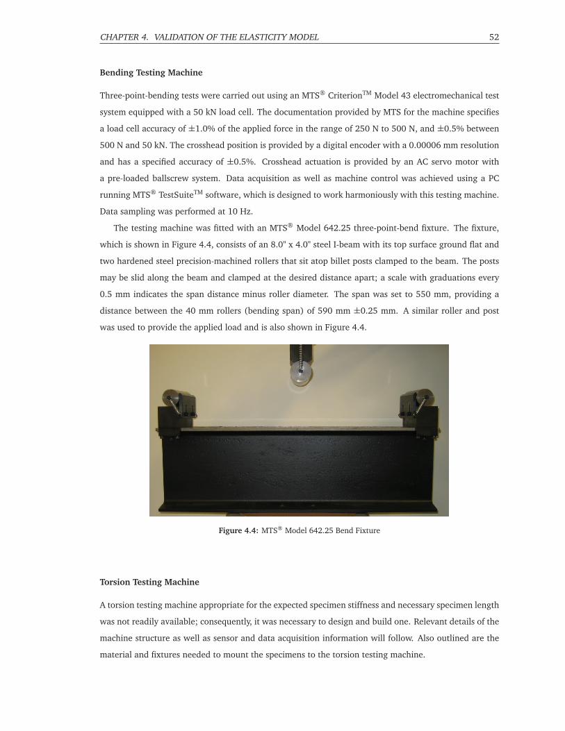
CHAPTER 4. VALIDATION OF THE ELASTICITY MODEL 52
Bending Testing Machine
Three-point-bending tests were carried out using an MTS® CriterionTM Model 43 electromechanical test
system equipped with a 50 kN load cell. The documentation provided by MTS for the machine specifies
a load cell accuracy of ±1.0% of the applied force in the range of 250 N to 500 N, and ±0.5% between
500 N and 50 kN. The crosshead position is provided by a digital encoder with a 0.00006 mm resolution
and has a specified accuracy of ±0.5%. Crosshead actuation is provided by an AC servo motor with
a pre-loaded ballscrew system. Data acquisition as well as machine control was achieved using a PC
running MTS® TestSuiteTM software, which is designed to work harmoniously with this testing machine.
Data sampling was performed at 10 Hz.
The testing machine was fitted with an MTS® Model 642.25 three-point-bend fixture. The fixture,
which is shown in Figure 4.4, consists of an 8.0" x 4.0" steel I-beam with its top surface ground flat and
two hardened steel precision-machined rollers that sit atop billet posts clamped to the beam. The posts
may be slid along the beam and clamped at the desired distance apart; a scale with graduations every
0.5 mm indicates the span distance minus roller diameter. The span was set to 550 mm, providing a
distance between the 40 mm rollers (bending span) of 590 mm ±0.25 mm. A similar roller and post
was used to provide the applied load and is also shown in Figure 4.4.
Figure 4.4: MTS® Model 642.25 Bend Fixture
Torsion Testing Machine
A torsion testing machine appropriate for the expected specimen stiffness and necessary specimen length
was not readily available; consequently, it was necessary to design and build one. Relevant details of the
machine structure as well as sensor and data acquisition information will follow. Also outlined are the
material and fixtures needed to mount the specimens to the torsion testing machine.

CHAPTER 4. VALIDATION OF THE ELASTICITY MODEL 53
Figure 4.5: Torsion Testing Machine
Machine Structure: The machine seen in Figure 4.5 was designed by the author and a colleague[20]
having similar motives; machining and assembly was commissioned to a local manufacturing company,
REKO Manufacturing Group Inc. Much consideration went into producing a machine that is versatile,
adjustable, and robust. A capability was desired to characterize the stiffness of specimens at least one
meter in length, but maintain an adjustable fixture set, such that shorter specimens can be easily ac-
commodated. It was expected that the machine would need to produce values of torque over 1000 Nm,
while still harbouring a capacity to accurately measure torques well under 100 Nm. Ability to produce
at least 45◦ of torsional deformation was needed, with accurate measurement thereof.
The machine is composed fundamentally of three fixtures: a ‘live-end’ fixture that serves to produce
and measure rotation as well as torque at one end of the specimen, a ‘dead-end’ fixture to restrict rotation
at the opposing end of the specimen, and a flat rigid base upon which the fixtures are mounted.
Machine Base: The base of the machine is a welded box section having four legs of hollow struc-
tural steel channel. The top of the box section is a 1600 mm by 450 mm steel plate of 15.875 mm
thickness that has been blanchard ground to provide a flat surface on which to mount the fixtures. The
box section alone was designed to have a stiffness at least 100 times greater than that of the stiffest spec-

CHAPTER 4. VALIDATION OF THE ELASTICITY MODEL 54
imen to be tested. The legs are bolted to a ground-level concrete floor to further stiffen the assembly;
high stiffness is critical to the design, as any torsional flexure of the machine affects the measurement of
torsional deflection in the specimen.
Dead-End Fixture: The dead-end fixture consists of a 19.05 mm thick plate positioned perpen-
dicularly to the base. This plate is welded to a bottom plate that mounts to the base, as well as to two
triangular gussets that support the main dead end fixture plate. A number of holes are bored in a circular
pattern through the dead-end fixture plate to allow the mounting of specimens or specimen flanges. The
entire dead-end fixture bolts to the base by four bolts and is aligned by two precision dowels. The base
features a number of mounting holes and dowel holes arranged with a longitudinal spacing of 130 mm
to allow mounting of the dead end at various positions, corresponding to various specimen lengths.
Live-End Fixture: The live-end fixture, which is mounted to the base and opposes the dead-end, is
also a weldment of 19.05 mm plate bolted in place with dowels for alignment. While the live-end fixture
as a whole may be seen in Figure 4.5, the functional components that are described in this paragraph are
best understood from a simplified line drawing: see Figure 4.6. Two heavy duty ball bearings pressed
into the live-end fixture plates support a 50 mm main shaft that serves to transfer torsional loading
into the second mounting point of the specimen. On the inbound end of the main shaft is the live-end
mounting plate having the same bolt pattern found on the dead-end, with the same purpose of specimen
mounting. A large sprocket is affixed to the center of the main shaft by two keys and held in place
between the bearings with set-screws. A 530 series roller chain, which mates with the sprocket, is pulled
downward toward the base by an Acme-threaded rod to create angular motion of the live-end mounting
plate, imposing a torque on the specimen. Rotation of a wheel and nut pulls the rotationally-fixed
Acme-threaded rod downward through the base. The top end of the threaded rod is connected to the
hanging end of the chain by a load cell with a U-joint at each end. Consequently, the downward pull
on the chain may be monitored and knowledge of the sprocket radius allows determination of applied
torque. A rotary potentiometer is fixed to the stationary part of the live-end fixture, having its actuator
shaft mated with the main shaft. The unloaded side of the chain hangs freely from the sprocket with a
counter-weight attached to balance the weight of the load cell and threaded rod assembly.
Sensors and Data Acquisition: The torsion testing machine utilizes two sensors and a data acquisition
system, described as follows.
Load Cell: While the machine was designed to allow the use of different load cells depending on the
desired range of torque application, only one load cell was used during the torsion tests discussed in the
current manuscript: a 1.33 kN capacity Model 60001 S-beam load cell manufactured by SensortronicsTM
of Vishay® Precision Group. The calibration data supplied with the load cell specifies a sensor output

CHAPTER 4. VALIDATION OF THE ELASTICITY MODEL 55
Dead-End Mounting Plate
Blanchard Ground Base
Wheel & Nut
Acme-Threaded Rod
Counter-Weight
Sprocket
Rotary Potentiometer
Load Cell
Live-End Mounting Plate
Figure 4.6: Primary-function components of torsion testing machine
of 3.582 mV/V. The NTEP® Class III rating gives a combined error of ±0.02% of full scale (±0.267 N,
or ±47.22 N·mm as pertaining to the machine). Non-repeatability is listed as ±0.01% of full scale
(±0.134 N, or ±23.71 N·mm). As recommended by the manufacturer, the load cell was supplied a 10 V
excitation.
Rotary Potentiometer: A CelescoTM Model RT9101-001-131-4110 rotational position transducer
with a 360◦ range was affixed to the machine, having its actuator shaft mated with the machine’s main
shaft. The specifications of the sensor are as follows: sensor output is 2.661 mV/V/degree, specified
calibration accuracy is ±0.179% of the reading, repeatability is ±0.02% of full stroke (±0.072◦), and
resolution of the plastic-hybrid precision potentiometer sensor is essentially infinite. A 10 V input signal
was supplied to the rotary potentiometer.
Data Acquisition System: Data was processed and recorded using a System 8000 StrainSmart®
Data Acquisition System manufactured by Micro-Measurements® of Vishay® Precision Group. The sys-
tem communicates over an ethernet network to a PC running the included StrainSmart® software, which
allows adjustment of parameters pertaining to calibration and sensor excitation voltage, among others.

CHAPTER 4. VALIDATION OF THE ELASTICITY MODEL 56
Sensor excitation as well as sensor signal is transmitted through an eight pin RJ45 connector. Each signal
is read by a channel-specific, 24-bit analogue-to-digital converter and filtered to remove noise. Data is
processed by a 32-bit, floating-point, digital signal processor operating at 300 MHz. Strain-gauge-based,
millivolt-level, sensor (e.g. load cell) readings are measured with a 0.25 μV resolution and amplified
with a DC gain accuracy of ±0.05%. High-level sensor (e.g. potentiometer) readings are measured with
a 100 μV effective resolution. The system’s excitation voltage accuracy is ±10 mV with a resolution of
3 mV.
Mounting Fixtures and Material: A means was required to rigidly affix the torsion test specimens
to the live-end and dead-end mounting plates of the torsion machine. Sets of rectangular aluminium
plates were manufactured and secured to the ends of the specimens with an epoxy joint. The 26 mm
thick plates were water-jet cut with a mounting hole at each corner, and subsequently drilled to have a
stepped hole in their center. The stepped hole served to precisely locate the specimen, while allowing
a 0.75 mm thick layer of epoxy to bond the 25 mm diameter specimens to the inner surface of the
bored hole. The stepped section of the hole amounts to only 3 mm of thickness, leaving a 23 mm
thick by 27 mm diameter bonding area. The bond thickness was kept relatively low to ensure that the
shear deformation of the epoxy itself does not significantly contribute to the measurement of torsional
deflection. Epoxy typically displays a strain-to-failure of approximately 2.0% [5], and so the joint will
likely fail before any significant torsional deformation is present.
The aluminium plates as well as the specimens were prepared with 80-grit sandpaper and cleaned
with isopropyl alcohol before being bonded together with Henkel LePage® Gel Epoxy (Henkel product
number 1165246). Henkel reports the epoxy’s tensile strength as 13.355 ±0.614 MPa when adhered
to sandblasted aluminium and cured for at least 24 hours. In accordance, each specimen/plate set was
allowed 24 hours of cure time before testing began. The specimen/plate assembly was bolted into the
machine immediately after the epoxy was applied and remained in place during cure to ensure perfect
alignment. Once fixed in the testing machine, distance between the aluminium mounting plates was
measured as 682 ±0.5 mm. A line was drawn across the bonded joint from the aluminium plate onto
the specimen to allow easy detection of any slippage in the joint – there was none.
4.2.3 Three-Point-Bending Tests
The six specimens described in Section 4.2.1 were tested in three point flexure using the setup described
in detail in Section 4.2.2 and seen in Figure 4.7. Each specimen was subjected to at least five mm of mid-
point deflection. The force-displacement curve produced by each test was fitted with a linear trend-line
to determine the slope, or spring-rate, in the linear regime of the test.
The slope obtained from the data corresponding to each test was used to determine the flexural
rigidity EI for each specimen. This was accomplished by a rearrangement of the Euler-Bernoulli equation

CHAPTER 4. VALIDATION OF THE ELASTICITY MODEL 57
for deflection of a simply supported beam point-loaded at its midspan (Equation 4.1).
EI =−P L3
48x(4.1)
where x is the midspan beam deflection, P is the applied load, L defines the span length, and EI is the
beam’s flexural rigidity.
The value of EI extracted from each experiment is compared to that which was calculated by the
laminated cylinder model; a prediction of EI may be obtained by taking the inverse of the m22 or m33
terms of the compliance matrix seen in Equation 3.39. However, this prediction does not include the
effects of transverse shear load, while the experimentally obtained flexural rigidity does; to remedy this,
an effective flexural rigidity was calculated using the m99 shear compliance term, and added to the
aforementioned EI prediction using a series spring-rate summation. The input to the laminated cylinder
model is shown and discussed for each specimen in Appendix B.
The experimentally determined flexural rigidity, the predicted flexural rigidity (including transverse
shear1), and the error observed in comparing the predicted value to the experimental is shown for each
specimen in Table 4.5.
Figure 4.7: Experimental setup: three point flexure test (sample 1C)
1Note that in this case ‘transverse shear’ refers to through-thickness transverse shear, not to be confused with the Timoshenkoshear effects that are not included in the current laminated cylinder model.

CHAPTER 4. VALIDATION OF THE ELASTICITY MODEL 58
Table 4.5: Three point flexure test: experimental results and laminated cylindermodel predictions for each specimen
SpecimenEI (Experimental)(N·mm2)
EI (Predicted)(N·mm2) Error (%)
1A 278.0 x 10⁶ 217.9 x 10⁶ -21.61B 312.8 x 10⁶ 245.5 x 10⁶ -21.51C 362.3 x 10⁶ 287.0 x 10⁶ -20.8
2A 672.5 x 10⁶ 691.2 x 10⁶ 2.82B 740.0 x 10⁶ 806.3 x 10⁶ 9.02C 712.3 x 10⁶ 765.9 x 10⁶ 7.5
4.2.4 Torsion Tests
The six specimens described in Section 4.2.1 were tested in torsion using the setup described in detail
in Section 4.2.2 and seen in Figures 4.8 and 4.9. The torsion beam span of the specimens was measured
to be 682 ±0.5 mm. Each specimen was subjected to at least 10◦ of rotation. Trend-lines were fit to
the linear regime (between zero and six degrees in this case) of plots showing applied torque versus
rotational displacement. The slope of each trend-line represents the measured torsional stiffness of the
corresponding specimen in N·mm/degree. In a treatment analogous to that of Equation 4.1, a value of
torsional rigidity JG may be extracted from the experimental data using Equation 4.2: a rearrangement
of the classical formula for torsional deflection of a solid beam of circular cross-section.
JG =T L
φ(4.2)
where φ is the angular deflection, T is the applied torque, and L is the torsion span length.
The laminated cylinder model’s prediction of torsional rigidity may be obtained by calculating the in-
verse of the m77 term in Equation 3.39. This produces a value of JG in N·mm2/radian which may be con-
verted to N·mm2/degree. The experimentally obtained torsional rigidity, the predicted torsional rigidity,
and the error observed in comparing the predicted value to the experimental is shown in Table 4.6. As
was mentioned, the input to the laminated cylinder model is shown and discussed in Appendix B.

CHAPTER 4. VALIDATION OF THE ELASTICITY MODEL 59
Figure 4.8: Experimental setup: torsion test (live-end with specimen 2A mounted)
Figure 4.9: Experimental setup: torsion test (dead-end with specimen 2A mounted)
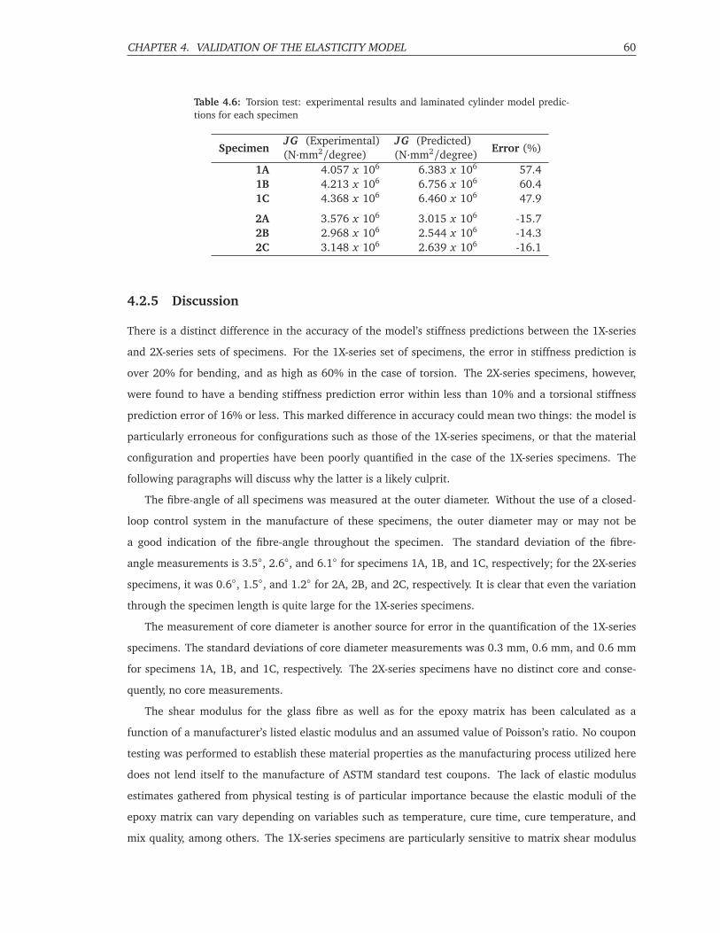
CHAPTER 4. VALIDATION OF THE ELASTICITY MODEL 60
Table 4.6: Torsion test: experimental results and laminated cylinder model predic-tions for each specimen
SpecimenJG (Experimental)(N·mm2/degree)
JG (Predicted)(N·mm2/degree) Error (%)
1A 4.057 x 10⁶ 6.383 x 10⁶ 57.41B 4.213 x 10⁶ 6.756 x 10⁶ 60.41C 4.368 x 10⁶ 6.460 x 10⁶ 47.9
2A 3.576 x 10⁶ 3.015 x 10⁶ -15.72B 2.968 x 10⁶ 2.544 x 10⁶ -14.32C 3.148 x 10⁶ 2.639 x 10⁶ -16.1
4.2.5 Discussion
There is a distinct difference in the accuracy of the model’s stiffness predictions between the 1X-series
and 2X-series sets of specimens. For the 1X-series set of specimens, the error in stiffness prediction is
over 20% for bending, and as high as 60% in the case of torsion. The 2X-series specimens, however,
were found to have a bending stiffness prediction error within less than 10% and a torsional stiffness
prediction error of 16% or less. This marked difference in accuracy could mean two things: the model is
particularly erroneous for configurations such as those of the 1X-series specimens, or that the material
configuration and properties have been poorly quantified in the case of the 1X-series specimens. The
following paragraphs will discuss why the latter is a likely culprit.
The fibre-angle of all specimens was measured at the outer diameter. Without the use of a closed-
loop control system in the manufacture of these specimens, the outer diameter may or may not be
a good indication of the fibre-angle throughout the specimen. The standard deviation of the fibre-
angle measurements is 3.5◦, 2.6◦, and 6.1◦ for specimens 1A, 1B, and 1C, respectively; for the 2X-series
specimens, it was 0.6◦, 1.5◦, and 1.2◦ for 2A, 2B, and 2C, respectively. It is clear that even the variation
through the specimen length is quite large for the 1X-series specimens.
The measurement of core diameter is another source for error in the quantification of the 1X-series
specimens. The standard deviations of core diameter measurements was 0.3 mm, 0.6 mm, and 0.6 mm
for specimens 1A, 1B, and 1C, respectively. The 2X-series specimens have no distinct core and conse-
quently, no core measurements.
The shear modulus for the glass fibre as well as for the epoxy matrix has been calculated as a
function of a manufacturer’s listed elastic modulus and an assumed value of Poisson’s ratio. No coupon
testing was performed to establish these material properties as the manufacturing process utilized here
does not lend itself to the manufacture of ASTM standard test coupons. The lack of elastic modulus
estimates gathered from physical testing is of particular importance because the elastic moduli of the
epoxy matrix can vary depending on variables such as temperature, cure time, cure temperature, and
mix quality, among others. The 1X-series specimens are particularly sensitive to matrix shear modulus

CHAPTER 4. VALIDATION OF THE ELASTICITY MODEL 61
when subjected to bending stress, as the principal stresses in the material are not aligned with the
fibre direction; an erroneous estimate of shear modulus can have a large effect on predicted bending
stiffness accuracy. Strictly speaking, the torsional stiffness of a specimen with a fibre-angle of ±45◦ is not
affected by matrix shear modulus at all, as the principal stresses are oriented along and perpendicular to
the fibre-direction; torsional stiffness of this type of specimen is governed by Young’s modulus in tension
and compression. What this says is that the torsional stiffness predictions of the 1X-series specimens is
influenced heavily by elastic modulus estimates for both the fibre and matrix.
As a result of the vast difference in moduli between fibre and matrix, the fibre-volume fraction has a
substantial effect on the stiffness of a lamina. The 1X-series specimens have a unidirectional 0◦ core of
non-blown fibre roving, i.e., fibres that are tightly bundled together in their roving. The fibres that make
up the outer layer are blown-fibre roving, meaning they have been blasted with compressed air to spread
out the roving and increase resin absorption. Compounding this differential in fibre packing densities,
the fibre-angle of outer layers of the 1X-series specimens are alternating from layer to layer, forming voids
between the overlapping fibres – voids which are filled by resin, reducing the net fibre-volume fraction
of the laminate. The point here is that in the 1X-series specimens, a difference likely exists between the
fibre-volume fraction of the core and that of the outer layers. The assumption inherent to the method
that was used to determine the fibre-volume fraction is that the fraction is uniform and homogeneous
throughout the specimen; as a result the core has likely been given an under-predicted fraction, while the
outer layers are likely over-predicted. This could explain some of the torsional stiffness over-prediction
of the 1X-series specimens, especially when considering that the outermost layers generally contribute
the majority of specimen torsional stiffness. However, if this is the case, the bending stiffness under-
prediction is greater than shown.
A brief sensitivity study reveals that the uncertainty in measurements and properties could quickly
compound on each other and produce relatively large margins or error. In the cases of both bending and
torsion of the 1X-series specimens, 5% changes were made to certain input variables, and the change
in the model’s deformation prediction was recorded. The variables changed were fibre angle, core
diameter, fibre-volume fraction at the outer layers Vf , fibre modulus in the outer layers Ef , and matrix
modulus in the outer layers Em. The results are shown in Table 4.7, where Δφ represents the change
in torsional deformation that results from a 5% change in the variable/property when the cylinder is
subjected to torsion, and Δκ represents the change in curvature that results from a 5% change in the
variable/property when the cylinder is subjected to constant bending moment.

CHAPTER 4. VALIDATION OF THE ELASTICITY MODEL 62
Table 4.7: Sensitivity of the model’s elastic response prediction to input variables andproperties
Variable/Property Δφ (%) Δκ(%)Fibre Angle 3.8 2.6
Core Diameter 1.3 5.3Vf Outer 4.9 3.4Ef Outer 4.1 0.5Em Outer 0.9 2.8

63
Chapter 5
Anti-Roll Bar Analysis & Design
The composite anti-roll bar (ARB) has been designed to match the stiffness and some geometrical at-
tributes of an existing steel anti-roll bar. No information was made available regarding the desired
force-displacement characteristics of the composite anti-roll bar, or the geometric envelope within which
it may exist. Consequently, it was necessary to benchmark the existing steel anti-roll bar with the aim of
replicating its stiffness.
The present chapter is broken into two sections, the first of which describes the benchmarking pro-
cedure used to characterize the steel bar. The second section details the design of the composite bar;
software is developed and used to establish a configuration that meets the defined design criteria.
The geometry of the steel bar is depicted in Figure 5.1. The indicated loading points receive opposing
forces in and out of the page while the bushings are rigidly mounted to the vehicle body. The compliance
of the bar will be defined as the relative vertical displacement of the endpoints per unit force applied in
opposition; the stiffness of the bar is the inverse of this.
800 mm
700 mm
1075 mm
207 mmLoading Point Loading Point
Bushing Bushing
Figure 5.1: Geometry of existing steel anti-roll bar

CHAPTER 5. ANTI-ROLL BAR ANALYSIS & DESIGN 64
5.1 Benchmarking of the Steel Anti-Roll Bar
The steel anti-roll bar is benchmarked using three methods: conventional analytical methods, a finite
element analysis, and experimental testing. Each of these methods is described in detail in the sections
that follow.
5.1.1 Classical Analytical Methods
If the geometry of the steel ARB is simplified to what is shown in Figure 5.2, it can be analysed with
relative ease using the classical formulae for Saint-Venant torsion and Euler-Bernoulli bending of beams
applied to each section of the bar. The bar is broken into three elastic sections: a mid-section 800
mm wide, and two cantilevered sections 270 mm in length oriented at 50◦ to the mid-span. Two short
sections exist at the endpoints but are assumed rigid due to their short length and larger moment of
inertia – these sections are the only portion of the steel bar in which the cross-section varies from
circular to rectangular. The loading points are at a perpendicular distance of 47.5 mm from the mid-axis
of the cantilevered sections, and are separated from each other by 1075 mm of horizontal distance. The
compliance of the bar is assumed to consist of four contributions: torsion of the mid-span, bending of
the midspan, bending of the cantilevered arms, and torsion of the cantilevered arms caused by loading
which is offset to their shear-center. Each section of the bar is analysed with regard to its contribution
to the bar’s overall stiffness.
800 mm
700 mm
1075 mm
50◦270 mm
47.5 mm
Figure 5.2: Simplified anti-roll bar geometry: plan view
The torsional spring-rate of the mid-span is easily calculated asJG
land will have units of N·mm/rad.
This angular spring-rate can be converted into an effective linear spring-rate in our context with the
following unit conversion:
N·mm
rad∗ N
207 N·mm∗ π rad
(207 mm)(π rad)=
N
42849 mm(5.1)
This converted rate represents the linear spring-rate which would exist at a fixed moment arm of 207 mm
(recall that 207 mm is the perpendicular distance from the loading point to the mid-span). Ultimately,

CHAPTER 5. ANTI-ROLL BAR ANALYSIS & DESIGN 65
Table 5.1: Stiffness contributions in steel anti-roll bar
Form of Compliance Linear Spring-Rate (N/mm)Mid-Span Torsion 261.13Mid-Span Bending 1892.25
Cantilevered Section Torsion 86886.51Cantilevered Section Bending 1771.57Overall Linear Spring-Rate: 181.87
this means that the contribution of the mid-span to the overall bar stiffness is equal to:
JG
42849(l)N/mm (5.2)
where J is the polar moment of inertia of the cross-section, G is the shear modulus of the steel, and l is
the length.
Torsion of the cantilevered section due to offset loading can be accounted for in a manner analogous
to the treatment of the mid-span torsion; the only difference being that the moment arm in the current
case is 47.5 mm
Bending of the cantilevered sections and of the midspan can be found by evaluating the linear spring-
rate for a beam in bending as3EI
l3 , where E is Young’s modulus, and I is the area moment of inertia
of the cross-section. Timoshenko shear effects are included in the calculations, but are a negligible
contribution to compliance.
The individual contribution to overall bar stiffness of each type of compliance is shown in Table 5.1.
Each of the shown spring-rates is superimposed by a series spring calculation, to arrive at the overall
anti-roll bar stiffness.
5.1.2 Finite Element Analysis
A CAD model of the steel ARB was established using the geometric specifications provided by its manu-
facturer. The inherently anti-symmetric loading of the symmetric bar allows the use of special constraints
and a half-model. Meshing and preprocessing was performed using Altair® Hypermesh®, and the model
was solved using the linear static solver of RADIOSS®.
Model Architecture:
The majority of the bar is of constant circular cross-section, meaning that it can be meshed using a solid
FE map. To that end, a two-dimensional mesh of quadrilateral elements was swept along the length
of the bar to create a number of eight-noded CHEXA solid elements. The nominal length of the solid
elements (specified during their creation) was chosen to be equal to the average length of elements

CHAPTER 5. ANTI-ROLL BAR ANALYSIS & DESIGN 66
in the two-dimensional mesh and was different for each model in the convergence study to be shown.
Consequently, elements resemble cubes as closely as possible while still capturing the desired geometry.
However, the elements at the inner radius in curved portions of the bar tend to attain high aspect-
ratios, becoming short in length relative to their width and height. This issue was negated by carefully
selecting an edge-density1 that lessens the severity of element aspect-ratios at the cost of increasing
average element length. The maximum aspect ratio in the finest mesh was 4.8, and only 1% of the
elements exceeded an aspect ratio of 2.0.
The end of the bar is forged into a rectangular cross-section with holes drilled at the loading points.
While this section and its transition into the circular section are both mappable, use of solid mapping pro-
duces a heavily distorted mesh between the rectangular and circular cross-sections. Instead, tetrahedral
elements were used to fill the volume of these sections. While it is generally known that first-order tetra-
hedral elements produce erroneously stiff results in bending-dominated problems, it should be noted
that the portion of the bar containing tetrahedral elements is small and at a low bending moment. Fur-
thermore, this section has little contribution in terms of additional bar compliance due to the fact that
its area moment of inertia is much larger than that of the circular cross-section which contains equal
volume. An example of the full mesh can be seen in Figure 5.3
zy x
Figure 5.3: Solid element mesh (2.5 mm nominal element length)
There are two boundary conditions that constrain the bar: the anti-symmetric loading condition, and
the bushing. The anti-symmetric loading condition has been addressed by attaching the independent
nodes of a rigid body (RBE2) element to the symmetry-plane face of the half-bar. The rigid element’s
dependent node is located at the center of this face and is constrained with an SPC in x and z translation,
as well as in rotation about the x axis. No effort has been made to model the compliance associated
with that of the bushings; the rationale should be clear in the subsection that follows. The bushing is
instead assumed rigid; however, axial translation of the bar within the bushing is permitted, as well as
rotation in all directions. The modelling of the bushing constraint is similar to that of the anti-symmetric
loading: a rigid body (RBE2) element has its dependent node located such that it represents the center
1Edge-density defines the number of elements along the length of a particular edge

CHAPTER 5. ANTI-ROLL BAR ANALYSIS & DESIGN 67
of the bushing, while the independent nodes are connected to the surface of the bar – where the bushing
would make contact. The dependent node is then constrained with an SPC to restrict translation in the
y and z directions. Both the bushing and anti-symmetry condition constraints can be seen in Figure 5.4.
It should be noted that rigid body elements, and in particular RBE2 (true rigid) elements, can add
unrealistic stiffness to a model. However, this particular case should not produce great concern as the
areas affected by the rigid elements are small in relation to the bar. The use of an interpolation element
such as an RBE3 may have alleviated some of the induced stiffness, but RBE3 elements do not allow the
use of an SPC at the dependent node. Without an SPC restricting the motion of the bar’s symmetry-plane
face, the model is under-constrained.
A 5 kN force was applied in the z direction at the loading point of the bar. The force was distributed
to the nodes at the inner surface of the hole using an RBE3 element as shown in Figure 5.4.
RBE2 Elements
RBE3 Element
SPCsForce
z
y x
Figure 5.4: Wireframe model showing constraints and applied loading
Mesh Sensitivity Study:
The analysis was performed using a number of progressively finer meshes to ensure the solver had
converged upon a solution.
The solid map used to mesh the constant cross-section length of the bar was generated using a
nominal element size ranging from 5 mm to 1.25 mm. The tetrahedral mesh at the loaded end of the
bar was re-meshed in each case to allow proper transition into the newly mapped hexahedral mesh.
Aside from this, the nominal element size (4 mm) of the tetrahedral mesh was not changed throughout
the study. Some properties of the meshes used can be found in Table 5.2. The 5 mm and 1.25 mm
meshes are shown in Figure 5.5. The trend of the linear spring-rates extracted from the study is shown
in Figure 5.6. Note that only 0.9% difference separates the 2.5 mm and 1.25 mm meshes, an indication
that sufficient convergence has been achieved. The solution of linear stiffness resulting from the classical
analysis is shown on the plot to allow convenient comparison between classical and numerical solutions;
the finest mesh results in a stiffness within 0.04% of the classical analysis result. Careful inspection

CHAPTER 5. ANTI-ROLL BAR ANALYSIS & DESIGN 68
of the plot will reveal that perhaps an even finer mesh would produce slightly stiffer results than the
classical analysis, but it is unlikely that this differential would be at all substantial.
Table 5.2: Steel ARB finite element mesh-sensitivity study data
Nominal Element
Length (mm)
Number of
Elements
Computing
Time1 (s)
Resulting Linear
Spring-Rate (N/mm)
5.00 6536 0 171.53
4.00 16783 4 176.80
2.50 38387 12 180.24
1.25 323049 409 181.80
(a) Coarse Mesh (b) Fine Mesh
Figure 5.5: Coarsest and finest mesh used in steel ARB convergence study
1Analyses were performed on a PC running Microsoft® Windows® 7 Professional (64 bit) with an Intel® CoreTM i7-2600k CPU
@ 3.40 GHz. The PC was equipped with 16 GB of RAM.

CHAPTER 5. ANTI-ROLL BAR ANALYSIS & DESIGN 69
12345170
175
180
185
Nominal Element Length (mm)
Line
arSp
ring
-Rat
e(N/m
m)
Linear Spring-Rate (FEA)Linear Spring-Rate (Classical Analysis)
Figure 5.6: Steel ARB finite element solution convergence: linear spring-rate vs.element size
5.1.3 Experimental Testing
Physical testing was performed on the existing steel bar as part of the benchmarking regimen. The
test setup geometry was as shown in Figure 5.1 with bushings spaced at 700 mm center-to-center. The
bushings were mounted to square-channel structural steel pillars that were bolted to a steel platen
table. The loading point at one end of the bar was pinned to a steel yoke and pillar (see Figure 5.7).
At the opposing loading point, a hydraulic cylinder was used to produce the applied load, which was
transmitted into the bar by a steel yoke and pin. A button-style load cell was positioned between the
yoke and the hydraulic cylinder to measure the applied force; this can be seen in Figure 5.8. A height
gauge indicated the vertical displacement of the yoke. Load cell force measurements were taken at
three incremental values of vertical displacement during the quasi-static tests with the intent of gaining
perspective on the linearity of the bar’s elastic response.
The first set of tests was performed using the polymer bushings that were provided with the bar;
these bushings can be seen in Figure 5.7. Results are averaged from three tests and shown in Table 5.3.
Significant deformation of the bushings produced values of stiffness that are not a good representation of
the bar’s elastic response – much of the measured compliance was a direct result of bushing deformation.
For this reason, further testing was performed using a set of steel bushings, each bushing comprising two
mating halves to encase the bar (see Figure 5.8). The steel bushings were mounted in the same manner
as with the previous tests, after being greased to reduce friction between the bar and the bushings. The
results, again averaged over three tests, can be seen in Table 5.4.

CHAPTER 5. ANTI-ROLL BAR ANALYSIS & DESIGN 70
Figure 5.7: Physical testing setup: fixed end with polymer bushing
Figure 5.8: Physical testing setup: actuated end with steel bushing

CHAPTER 5. ANTI-ROLL BAR ANALYSIS & DESIGN 71
Table 5.3: Steel ARB test (polymer bushings)
Deflection (mm) Load (N) Linear Spring-Rate (N/mm)10 1230.7 123.0720 2584.4 129.2230 4510.2 138.34
Table 5.4: Steel ARB test (steel bushings)
Deflection (mm) Load (N) Linear Spring-Rate (N/mm)10 1786.7 178.6720 3647.5 182.3830 5627.0 187.57
5.2 Composite Anti-Roll Bar
Conventional FRP materials rarely offer an elastic modulus as high as that of steel even at their stiffest
fibre angle; this deficit between moduli only increases as the loading direction deviates from that which
is optimal. Because of this, the composite bar must be of a larger diameter than the steel to provide
comparable stiffness. In lieu of a geometric design envelope, it is assumed that the diameter of the bar
may be increased moderately but that the basic shape may not change.
5.2.1 Analysis Software
It is possible to design a computer program that will establish the state of loading in each section of a
discretized ARB given a known applied force. It was mentioned in Section 3.3 that a computer program
was developed that quickly and efficiently computes a solution to the elastic response of a laminated FRP
tube or cylinder subjected to arbitrary loading. A program has been developed, again in the MATLAB®
environment, that communicates with the aforementioned elasticity model software to determine the
deformed shape of a composite ARB subjected to a known force at its loading point. The code is included
in Appendix D.
The program, henceforth referred to as CARBA (Composite Anti-Roll Bar Analysis), accepts a user-
generated list of coordinates in spreadsheet form to describe the shape of the ARB. A number of assump-
tions are employed to simplify the program:
1. The desired line geometry of the ARB is known and exists within a two-dimensional plane. Fur-
thermore, the cross-section of the bar is circular and is centered about the known line geometry.

CHAPTER 5. ANTI-ROLL BAR ANALYSIS & DESIGN 72
2. The ARB is not a curved beam, but a beam comprising a number of straight sections subjected to
small and linear deformation.
3. The ARB is subjected to a known force at the first and last points listed in the coordinate spread-
sheet. These points are loaded in opposing directions that are perpendicular to the two-dimensional
plane in which the bar exists.
4. Exactly two bushings constrain the ARB at the point on the bar coincident with the bushing. The
bar is constrained by the bushings only in translation, and the bushing locations are specified in
the coordinate spreadsheet by the user.
5. Loading points and bushings are symmetrically located with respect to a vertical line passing
through the center of the bar.
As an example, a simple geometry is shown in Figure 5.9, where the points are indicated by the ‘x’
marks, and bushings are circled. The line about which the loading points and bushings must remain
symmetric is represented by the dashed line.
0 200 400 600 800 1,000 1,2000
100
200
X coordinate (mm)
Yco
ordi
nate
(mm
)
Figure 5.9: Line geometry input to CARBA software (congruent with classical analy-sis)
Software Structure:
The CARBA software imports the user-defined line geometry and calculates the length and orientation of
each section. Under assumptions two and three, the moments and transverse shear force at each point
can be calculated with respect to the global X-Y coordinate system. The global loading state at each
point is resolved into a local coordinate system to describe the loading in the sections adjacent to the
point (e.g., if two sections are perpendicular to each other, the bending moment in the first section will
equate to the torque in the second and vice-versa). The torsion within a section is modelled as constant,
while the bending moment may be a function of position; locations closer to the bushing are generally
subjected to greater bending moments. Each section is further discretized into a number of straight

CHAPTER 5. ANTI-ROLL BAR ANALYSIS & DESIGN 73
beams (subsections) to allow a linear interpolation of bending moment along the length of that section.
The transverse shear force in the bar is ultimately constant in three regions of the bar – separated by the
bushings.
The state of loading now defined for each section and subsection of the bar is input individually
to the laminated cylinder model; an elastic response corresponding to each section and subsection is
returned. Starting at the bushings and working outward toward the end points, the strain and curvature
resultants returned by the laminated cylinder model are used to compute the vertical displacement of
the bar at all points. Prior to this, however, the deformation in the mid-region (between the bushings)
is determined to allow definition of boundary conditions (slope and torsional deflection) required to
quantify deflection of the outer regions of the bar.
The vertical displacement corresponding to each user-input point is displayed in a plot. Figure 5.10
shows the plot generated with a 1 N force applied at the loaded ends of the bar shown in Figure 5.9.
The value of deflection at the loading points can be extracted and resolved into a compliance (mm/N).
Because the applied force is simply 1 N, an inversion of the total relative displacement between the
loaded ends produces a linear stiffness compatible with those found during the benchmarking of the
steel bar in Section 5.1.
0 200 400 600 800 1,000 1,200
−0.001−0.002−0.003
00.0010.0020.003
X coordinate (mm)
Vert
ical
Dis
plac
emen
t(m
m)
Figure 5.10: Vertical displacement profile output from CARBA software for the steelbar
Validation:
An example representing the geometry which is used in the classical analysis of Section 5.1.1 was shown
in Figure 5.9; both this geometry, and the material properties used in the classical analysis were input
to the CARBA software. The resulting vertical deflection profile has already been presented in Fig-
ure 5.10. The result is a deflection at the loading points of 0.002884 mm, or a relative displacement
of 0.005768 mm from a 1 N applied load. Resolving the linear stiffness from this produces a value of
175.07 N/mm; within 3.7% of the classical analysis result. Certainly, some of the additional compliance
seen in the CARBA software output can be explained by slight differences between the classical anal-

CHAPTER 5. ANTI-ROLL BAR ANALYSIS & DESIGN 74
ysis and the software-based analysis. Both analyses compute the mid-span deflection and its effect on
stiffness, but the classical analysis does not include the portion of the mid-span that extends into and
slightly beyond the bushings.
5.2.2 Design
As was mentioned, the center-line geometry of the ARB will remain fixed throughout the design. While
a simple geometry was shown in the preceding subsection for the purpose of validation, it is sensible to
use a coordinate set that more precisely matches the desired geometry during design of the composite
bar; that coordinate set and resulting line geometry is shown in Figure 5.11.
With an unknown geometric envelope in which the composite bar may exist, it was determined
that keeping the diameter relatively small is of importance. Use of a fibre/matrix combination that is
readily available and cost effective increases the viability of high-volume production. For these reasons,
a general purpose structure of Hexcel® AS4 carbon fibre and 3501-6 epoxy was specified for the outer
layers of helically wrapped FRP. The core of the bar, which provides little contribution to stiffness and
strength relative to the outer layers, will comprise a more cost-effective fibre: E-glass. Typical in-plane
stiffness properties are listed in Table 5.5 for AS4 and E-glass laminated in 3501-6 epoxy with a volume
fraction of Vf =0.6.
0 200 400 600 800 1,000 1,2000
100
200
X coordinate (mm)
Yco
ordi
nate
(mm
)
Figure 5.11: Desired line geometry of composite ARB
Table 5.5: In-plane properties of carbon and E-glass unidirectional laminates
Material E11 (GPa) E22 (GPa) v12 G12 (GPa) Density (g/cc) Ref.AS4(Carbon)/3501-6(Epoxy) 131.0 11.2 0.28 6.55 1.55 [36]
E-glass/Epoxy 38.6 8.27 0.26 4.14 1.80 [37]
For reasons pertinent to the intended manufacturing process, the thickness of the helically wound
outer layers has been defined as 0.45 mm and the core diameter as 20 mm. The helically wound

CHAPTER 5. ANTI-ROLL BAR ANALYSIS & DESIGN 75
layers are configured such that each successive layer has a fibre-angle equal in magnitude but opposite
in sign to the last. An investigation was performed using the CARBA software that demonstrates the
variance of expected stiffness with fibre-angle and number of outer layers; the results of this are shown
in Figure 5.12. Recall that the benchmarking performed in Section 5.1 established a desired linear
spring-rate of approximately 180 N/mm. An outer layer count of 27 produces a peak value of stiffness
of 176.13 N/mm at a fibre angle of ±30◦.With a fixed layer size of 0.45 mm, the simplest way to fine-tune the stiffness is by slight adjustment
of the core diameter; a 20.30 mm E-glass fibre reinforced epoxy core wound with 27 layers of 0.45 mm
thick ±30◦ carbon fibre reinforced epoxy produces a stiffness of 180.78 N/mm. The outer diameter of
the composite ARB resulting from the specified configuration is 44.3 mm. The vertical displacement
profile from which the stiffness was extracted can be seen in Figure 5.13.
15 20 25 30 35 40 45
100
150
200
Fibre Angle (degrees)
Line
arSt
iffn
ess
(N/m
m)
28 layers27 layers26 layers22 layers
Figure 5.12: Linear anti-roll bar stiffness vs. fibre angle for composite bars having20 mm E-glass unidirectional cores wound with varying numbers of 0.45 mm helicallywound carbon/epoxy layers
0 200 400 600 800 1,000 1,200
−0.001−0.002−0.003
00.0010.0020.003
X coordinate (mm)
Vert
ical
Dis
plac
emen
t(m
m)
Figure 5.13: Vertical displacement profile output from CARBA software for the com-posite bar
The steel bar’s mass has been calculated as 8.58 kg; the mass of the proposed composite bar design

CHAPTER 5. ANTI-ROLL BAR ANALYSIS & DESIGN 76
can be calculated in the same manner as 3.18 kg. This results in a mass reduction of 63%. However, this
number will likely be reduced slightly when provisions are made for load application connection points
on the FRP anti-roll bar.
While the runtime of the CARBA software is a function of the number of input geometry points, as
well as other input variables, it is worth noting that the current design requires a runtime of 9.2 sec-
onds1. An FE model was not produced for the composite bar, but recall that runtimes on the order of
400 seconds were observed in the numerical analysis of the isotropic steel bar.
5.2.3 Discussion and Recommendations
A number of assumptions were necessary in the design of the composite ARB; some of these assumptions
have deviated the design from what is optimal. Discussion and recommendations are presented in the
following text with regard to areas in which design compromises are present.
With no information available regarding the limits the vehicle’s configuration imposes on bar ge-
ometry, changes to the bar’s overall shape were kept to a minimum to reduce the likelihood of toler-
ance/interference issues upon installation. It may be safe to conclude that the shape of the existing steel
bar is a product of thoughtful consideration of what is optimal, but a filament wound composite bar has
considerably different behaviour; a shape that is optimal for a steel ARB is almost certainly not optimal
for its composite counterpart.
Perhaps the most limiting assumption present in the current design is that of constant fibre-angle,
shape, and bar diameter throughout the length of the ARB. It has been shown that loading varies
throughout the length of the bar; the mid-span section (between the bushings) experiences significantly
more torsion and less bending load than the sections that extend outward from the bushings. More-
over, the bending moment in the end-sections is maximum near the bushings, but diminishes toward the
loading points. The moment varies throughout the mid-span section as well. A design that truly exploits
these observations would have fibre-angle, bar diameter, and cross-sectional geometry varying along the
length of the bar to reduce its total mass. To that end, the CARBA software has been written in a manner
that is conducive to the addition of an optimization scheme producing varying bar diameter and fibre
layup, though time constraints prevented the author from including these capabilities.
The CARBA software is limited to the analysis of strictly two-dimensional geometries. This limitation
alone has no effect on the present bar design; recall that the lack of a defined geometric envelope
restricted the design to a single plane. However, one could easily speculate on the need to design or
analyse an ARB that simply cannot be constrained to two dimensions. Three dimensional capability
could be added to the CARBA software using the same principles that allowed loading and deformation
to be determined in the two-dimensional case. Another possibility is the development of a beam element
1Analyses were performed on a PC running Microsoft® Windows® 7 Professional (64 bit) with an Intel® CoreTM i7-2600k CPU@ 3.40 GHz. The PC was equipped with 16 GB of RAM.

CHAPTER 5. ANTI-ROLL BAR ANALYSIS & DESIGN 77
for a finite element solver; the elasticity model presented herein could be used in parallel with an FE
solver to arrive upon the elastic response of an anti-roll bar having complex three-dimensional geometry.

78
Chapter 6
Conclusions & Recommendations
The first section of this chapter provides a summary of what was accomplished. The second section
draws conclusions with regard to the work herein, and the third section discusses recommendations for
future work.
6.1 Summary
An analytical elasticity model has been developed for laminated cylindrically anisotropic cylinders sub-
jected to extension, bending, pressure, torsion, and transverse shearing; care has been taken to ensure
that the model captures all elastic coupling present in these loading cases. The model may be applied
to thick or thin walled tubes, as well as solid cylinders. While the model’s derivation is somewhat long,
the end result is pragmatic and concise in matrix form. Once coded into a computer software, the model
provides a fast and efficient means of obtaining the elastic response of the tube or cylinder as a function
of user-input loadings; elastic response is returned in the form of nine values that describe strain and
curvature resultants, as well as strain gradients.
Some computational validation has been provided by comparing the predictions of the laminated
cylinder model to those of FE methods for the elastic response of a thin-walled tube subjected to torsional
and axial loading. Some experimental validation has been provided by the physical testing, in torsion
and in three-point flexure, of two sets of glass-fibre/epoxy cylindrical test specimens.
An existing steel anti-roll bar has been rigorously benchmarked using classical analytical methods,
FE methods, and experimental testing. An analysis software has been generated that uses the laminated
cylinder model presented herein to predict the linear-elastic response of an anti-roll bar. The center-
line geometry of the bar must be planar, but may be specified by a user-generated coordinate set. The
analysis software is limited to the linear regime of the bar’s elastic response. This software has been used
to establish a composite anti-roll bar design, which has been presented here, with the aim of replacing

CHAPTER 6. CONCLUSIONS & RECOMMENDATIONS 79
the existing steel bar.
6.2 Conclusions
The presented laminated cylinder model provides a concise method of obtaining a prediction for the
elastic response of thick-walled tubes, thin-walled tubes, and cylinders subjected to axial force, bending
moment, pressure, torsion, and transverse shearing. The following conclusions may be made regarding
this model:
• The predicted response to pressure is not valid for thick-walled tubes. The model does not account
for through-thickness normal stress, Timoshenko shear in bending, shear stress attenuation at free
edges, or material non-linearity. The model neglects the possibility of any buckling and ignores
end-effects associated with loading and shear lag.
• While significant further work is needed for a full validation, the model shows promise to provide
a useful means of establishing accurate predictions of elastic response, and internal stress.
• The model is well suited for integration into optimization schemes directed at materials in the
discussed regime.
The presented composite anti-roll bar analysis software – CARBA – provides a convenient and ef-
ficient means of analysing the linear-elastic stiffness of proposed designs for filament wound, fibre-
reinforced, composite anti-roll bars. The CARBA software relies directly on the accuracy of the lami-
nated cylinder model; consequently, it too has yet to be fully validated and adopts all the assumptions
of the laminated cylinder model as well as the limitations thereof. The software does not account for
the geometric non-linearity of large deformation of the anti-roll bar, and hosts other assumptions and
limitations that have been discussed.
A composite bar having a 10.15 mm radius E-glass/epoxy unidirectional 0◦ core helically wound
with 27 layers of ±30◦ AS4 carbon fibre/epoxy will provide a linear stiffness of 180.78 N·mm. This
configuration results in a 44.3 mm diameter anti-roll bar and is expected to have a mass that is 63% less
than the steel bar it serves to replace.
6.3 Recommendations for Future Work
Some recommendations for future work are provided as follows with regard to both the laminated
cylinder model, and the composite anti-roll bar design.

CHAPTER 6. CONCLUSIONS & RECOMMENDATIONS 80
Laminated Cylinder Model
First and foremost, the presented model requires a thorough validation through both FE methods and
an experimental program. A non-linear solver could be employed to solve solid-element FE models for
a number of tube diameter to wall-thickness ratios, as well as solid cylinders. All loadings handled by
the model should be addressed. A large range of laminate configurations needs to be included in the
study to ensure proper handling of internal stress; with a fine solid mesh, one could compare stress
distributions predicted by the model and the FE method. A number of cases should be validated through
experimental testing as well, to provide further confidence in the FE solutions.
Upon the successful completion of model validation, attention could be given to capturing higher-
fidelity phenomena such as Timoshenko shear effects, through-thickness normal stress, material non-
linearity, and the pressure loading of thick-walled tubes.
The model could easily be adapted to include a failure model such as Tsai-Wu[38], or something
more sophisticated to predict matrix cracking, durability, and fatigue. With internal strains and stresses
already modelled and accessible, focus could be put directly into application of a current and existing
failure model. While some concern should be present regarding material fracture toughness, a protective
coating may be enough to provide protection from impact with road debris. General Motor’s Corvette
uses a GFRP transverse leaf spring that has proved successful for over 30 years (and counting); this
spring is in the same general location and orientation that is necessary for an anti-roll bar – in fact the
spring doubles as an anti-roll bar.
Composite Anti-Roll Bar
The composite anti-roll bar design presented herein is very much a first order prototype proposal; how-
ever, the analysis software has been structured in a manner that is conducive to the addition of design
capabilities and changes that are to be recommended in the paragraphs that follow.
The first recommendation is modification of the analysis software to account for a varying diameter,
fibre-angle, and layer count throughout the length of the anti-roll bar. There are a number of ways this
could be accomplished, but the simplest would likely be to allow user input of a fibre-angle profile as
well as a diameter profile, in much the same way that the anti-roll bar shape is handled. The fibre-
angle and diameter profiles could be discretized with the same resolution as the bar itself; an individual
interpolated value for fibre angle and diameter would be sent to the laminated cylinder model software
for each discretized section.
The second recommendation is that provisions be made to the software such that a fibre-angle and
diameter profile are generated, instead of input. Reasonable assumptions that would greatly simplify the
implementation of this capability include constant layer thickness and constant fibre-angle through the
thickness. It is also reasonable to assume that each layer should be oriented negatively to the last. An
iterative process could seek to minimize maximum stress within the bar (while still achieving a desired

CHAPTER 6. CONCLUSIONS & RECOMMENDATIONS 81
overall stiffness), or to add diameter to sections of the bar whose compliance most greatly reduces
overall bar stiffness, after first optimizing fibre-angle with the same goal.
Lastly, the program could be modified to accommodate three-dimensional bar shape as well as non-
vertical loading, with provisions for the non-linearity of large deformation.
The recommended changes for the laminated cylinder model itself would also add a great deal of
capability to the software.
6.4 Contributions
This section will outline the aspects of the work presented herein that are particularly novel or contrib-
utory.
The largest contribution of this work is an elasticity model for laminated cylindrically anisotropic
cylinders. To the best knowledge of the author, no elasticity model precedes this publication that ac-
counts for axial, bending, pressure, torsion, and shear loadings, while accounting for all elastic coupling.
Moreover, few existing elasticity models provide the simplicity and applicability offered here.
A tailored analysis software has been presented that can provide a foundation for composite anti-roll
bar design, utilizing the aforementioned elasticity model. A composite anti-roll bar design has been
presented with good argument to support deviation from intuitive and erroneous design optimization
decisions.
A robust and versatile torsion testing machine was designed by the author and a colleague. Mate-
rials, manufacture, and funding was provided by external agencies, but the machine is property of the
University of Windsor and remains in service for future use.

82
References
[1] L. Segel, “Theoretical prediction and experimental substantiation of the response of the automobile
to steering control,” Proceedings of the Institution of Mechanical Engineers: Automobile Division,
vol. 10, no. 1, pp. 310–330, 1956.
[2] N. Barter, “Measurement of vehicle handling by tethered testing,” Proceedings of the Institution of
Mechanical Engineers: Automobile Division, vol. 184, no. 1, pp. 219–231, 1969.
[3] H. Pacejka, Tyre and Vehicle Dynamics. Oxford, UK: Elsevier, 2005.
[4] J. Chang, “Method of manufacturing hybrid composite leaf springs,” June 20 1995. US Patent
5,425,829.
[5] S. R. Swanson, Introduction to Design and Analysis With Advanced Composite Materials. Upper
Saddle River, New Jersey, USA: Prentice Hall, 1997.
[6] P. Mallick, Fiber-Reinforced Composites: Materials, Manufacturing, and Design. Boca Raton, Florida,
USA: CRC Press, 3rd ed., 2008.
[7] Makelainen, Pentti, and P. Hassinen, Light-weight Steel and Aluminium Structures. Elsevier Science,
1st ed., 1999.
[8] R. Jones, Mechanics of Composite Materials. New York: Hemisphere Publishing, 1975.
[9] R. Christensen, “The numbers of elastic properties and failure parameters for fiber composites,”
Journal of Engineering Materials and Technology, vol. 120, pp. 110–113, April 1998.
[10] Z. Hashin and B. Rosen, “The elastic moduli of fiber-reinforced materials,” Journal of Applied Me-
chanics, vol. 46, no. 2, pp. 543–550, 1964.
[11] R. Hill, “Theory of mechanical properties of fibre-strengthened materials: 1. elastic behaviour,”
Journal of Mechanics and Physics of Solids, vol. 12, pp. 199–212, 1964.
[12] R. Christensen and H. Lo, “Solutions for effective shear properties in three phase sphere and cylin-
der models,” Journal of Mechanics and Physics of Solids, vol. 27, pp. 315–330, 1979.

REFERENCES 83
[13] J. Halpin and J. Kardos, “The halpin-tsai equations: A review,” Polymer Engineering and Science,
vol. 16, pp. 344–352, May 1976.
[14] Y. Yeow and H. Brinson, “A comparison of simple shear characteriztion methods for composite
laminates,” Composites, vol. 9, pp. 49–55, January 1978.
[15] N. Iosipescu, “New accurate procedure for single shear testing of metals,” Journal of Materials,
vol. 2, no. 3, pp. 537–566, 1967.
[16] D. Walrath and D. Adams, “The losipescu shear test as applied to composite materials,” Experimen-
tal Mechanics, vol. 23, no. 1, pp. 105–110, 1983.
[17] ASTM, “Standard test method for shear properties of composite materials by the v-notched beam
method.”
[18] S. Swanson, M. Messick, and G. Toombes, “Comparison of torsion tube and iosipescu in-plane shear
test results for a carbon fibre-reinforced epoxy composite,” Composites, vol. 16, no. 3, pp. 220–224,
1985.
[19] B. Rosen, “A simple procedure for experimental determination of the longitudinal shear modulus
of unidirectional composites,” Journal of Composite Materials, vol. 6, pp. 552–554, 1972.
[20] H. Honickman, J. Johrendt, D. Northwood, and P. Frise, “Design of a pultruded steel-gfrp hybrid
structural member,” in proceedings of the ASME 2010 International Mechanical Engineering Congress
and Exposition, no. IMECE2010-37378, (Vancouver, British Columbia, Canada), American Society
of Mechanical Engineers (ASME), November 12–18 2010.
[21] S. Lekhnitskii, “Stress distribution in an elastic bar with curvilinear anisotropy under a tensile force
and bending moments,” Prikl. Matem. i Mekh., vol. 13, no. 3, pp. 307–316, 1949.
[22] R. E. Sherrer, “Filament-wound cylinders with axial-symmetric loads,” Journal of Composite Mate-
rials, vol. 1, no. 4, pp. 344–355, 1967.
[23] V. C. Cutler, “Bending analysis of directionally reinforced plastic pipe,” in 16th Annual Technical
And Management Conference Proceedings, The Society of Plastic Industry Inc, 1961.
[24] S. Timoshenko and J. Goodier, Theory of Elasticity. McGraw-Hill Book Company, 1951.
[25] N. Pagano, J. Halpin, and J. Whitney, “Tension buckling of anisotropic cylinders,” Journal of Com-
posite Materials, vol. 2, no. 2, pp. 154–167, 1968.
[26] N. Pagano and J. Whitney, “Geometric design of composite cylindrical characterization specimens,”
Journal of Composite Materials, vol. 4, no. 3, pp. 360–378, 1970.

REFERENCES 84
[27] N. Pagano, “Stress gradients in laminated composite cylinders,” Journal of Composite Materials,
vol. 5, no. 2, pp. 260–265, 1971.
[28] E. Reissner and W. Tsai, “On pure bending and stretching of orthotropic laminated cylindrical
shells,” Journal of Applied Mechanics, vol. 41, p. 168, 1974.
[29] C. Jolicoeur and A. Cardou, “Analytical solution for bending of coaxial orthotropic cylinders,” Jour-
nal of Engineering Mechanics, vol. 120, no. 12, pp. 2556–2574, 1994.
[30] T. Ting, “Pressuring, shearing, torsion and extension of a circular tube or bar of cylindrically
anisotropic material,” Proceedings of the Royal Society of London. Series A: Mathematical, Physical
and Engineering Sciences, vol. 452, no. 1954, pp. 2397–2421, 1996.
[31] T. Chen, C. Chung, and W. Lin, “A revisit of a cylindrically anisotropic tube subjected to pressuring,
shearing, torsion, extension and a uniform temperature change,” International Journal of Solids
and Structures, vol. 37, no. 37, pp. 5143–5159, 2000.
[32] C. Chouchaoui and O. Ochoa, “Similitude study for a laminated cylindrical tube under tensile, tor-
sion, bending, internal and external pressure. part i: Governing equations,” Composite Structures,
vol. 44, no. 4, pp. 221–229, 1999.
[33] J. Tarn and Y. Wang, “Laminated composite tubes under extension, torsion, bending, shearing and
pressuring: a state space approach,” International Journal of Solids and Structures, vol. 38, no. 50,
pp. 9053–9075, 2001.
[34] J. Tarn, “A state space formalism for anisotropic elasticity.: Part ii: Cylindrical anisotropy,” Interna-
tional Journal of Solids and Structures, vol. 39, no. 20, pp. 5157–5172, 2002.
[35] S. Swanson, “Torsion of laminated rectangular rods,” Composite Structures, no. 42, pp. 23–31,
1998.
[36] S. Swanson and A. Christoforou, “Response of quasi-isotropic carbon/epoxy laminates to biaxial
stress,” Journal of Composite Materials, vol. 20, no. 5, pp. 457–471, 1986.
[37] S. W. Tsai and T. N. Massard, Composites Design. Think Composites, 1985.
[38] W. E. Tsai, S.W., “A general theory of strength for anisotropic materials,” Journal of Composite
Materials, vol. 5, no. 1, pp. 58–80, 1971.

85
Appendix A
Specimen Measurements
As was discussed in Section 4.2.1, each specimen was subjected to a number of measurements to estab-
lish average dimensions and properties; each measurement is shown as follows:
Table A.1: Sample 1A measurements
Mass (g) Length (mm) Diameter (mm) Core Diameter (mm) Fibre angle (degrees)640.8 733.98 24.90 14.21 50
733.86 25.08 14.00 5625.10 13.69 5025.15 13.5025.5425.40
Table A.2: Sample 1B measurements
Mass (g) Length (mm) Diameter (mm) Core Diameter (mm) Fibre angle (degrees)644.7 734.18 25.03 14.16 -43
734.11 25.40 13.30 -4725.75 14.70 -4824.10 13.9025.0025.29

APPENDIX A. SPECIMEN MEASUREMENTS 86
Table A.3: Sample 1C measurements
Mass (g) Length (mm) Diameter (mm) Core Diameter (mm) Fibre angle (degrees)649.2 734.26 25.00 16.31 -50
734.30 24.90 15.70 -5125.05 16.80 -4025.48 15.5025.4225.35
Table A.4: Sample 2A measurements
Mass (g) Length (mm) Diameter (mm) Fibre angle (degrees)682.1 734.33 24.88 -16
734.13 25.08 -1624.99 -1524.9825.1825.05
Table A.5: Sample 2B measurements
Mass (g) Length (mm) Diameter (mm) Fibre angle (degrees)677.4 733.63 24.84 9
733.58 25.02 625.01 824.8125.0525.02
Table A.6: Sample 2C measurements
Mass (g) Length (mm) Diameter (mm) Fibre angle (degrees)680.5 734.37 25.14 10
735.01 25.53 1025.19 1225.1125.2324.98

87
Appendix B
Laminated Cylinder Model Input
The material properties of the Jushi® E6 312T E-glass fibres used in the core of samples 1A, 1B, 1C, and
in samples 2A, 2B, 2C are listed in Table B.1 as EF core, Gf core, and ν f . The properties of the FiberexTM
TR-503-N-4900T E-glass fibres used in the outer layer of samples 1A, 1B, and 1C are shown in Table B.1
as as EF outer, Gf outer, and ν f . The density of the fibres is assumed to be 0.002540 g/mm3.
The material properties of the cured AdtechTM EP-700 epoxy with EP-802 hardener are shown in
Table B.1 as Em, Gm, and νm. The density of the cured matrix was assumed to be 0.001107 g/mm3
For both the fibres and the matrix, the longitudinal moduli Ef and Em were extracted from the
manufacturers’ documentation, while Poisson’s ratios ν f and νm were assumed from [6]; Gf and Gm
were calculated using the values just listed.
Table B.1: Material properties of E-glass fibres and epoxy matrix used in test speci-mens
Ef core(MPa)
Ef outer(MPa)
Em(MPa)
Gf core(MPa)
Gf outer(MPa)
Gm(MPa) ν f νm
80454 73000 3200 32705 29675 1185.2 0.23 0.35
The specimen measurements that are seen in Appendix A were averaged and used to calculate a fibre
volume fraction. The volume of the specimens was calculated as length times cross-sectional area; this
volume was used to calculate specimen density. From there, an iterative solver was used to establish
the volume fraction necessary to produce the calculated specimen density, knowing the fibre and matrix
densities. The results of this fibre volume fraction calculation are shown in Table B.2.
The elastic properties of the laminae that constitute sections of the samples were established using
the fibre and matrix material properties seen in Table B.1 and the fibre volume fraction results of Ta-
ble B.2. Longitudinal moduli (E11), and Poisson’s ratios (ν12, ν21) were calculated using the rule of
mixtures model, while transverse properties (E22, G12) were calculated using Halpin-Tsai formulation.
The resulting elastic properties for each specimen are shown in Table B.3.

APPENDIX B. LAMINATED CYLINDER MODEL INPUT 88
Each of the 1X-series specimens contains 11 layers of helically wrapped outer layers of alternating
fibre-angle and a uni-directional core. The thickness of the outer layers was established by subtract-
ing the measured core diameter from the outer diameter. The 11 layers were assumed to be of equal
thickness and opposing angles.
The 2X-series specimens do not contain distinct layers, but a continuum of linearly varying fibre-
angle. Accordingly, they were modelled with 30 layers of equal thickness having a fibre-angle that varies
linearly from 0 to θ , where theta is the average of the measured outer fibre-angles listed in Appendix A.
The use of 30 layers is somewhat arbitrary, but also somewhat irrelevant: beyond a certain number of
layers, little change in elastic response is observed with additional layers.
Table B.2: Specimen fibre volume fraction calculation
Sample Volume (mm3) Net Density calc Density Vf
1A 365904.1 0.0017513 0.0017513 0.449621B 363116.6 0.0017755 0.0017755 0.466501C 366228.9 0.0017727 0.0017727 0.464552A 361183.6 0.0018885 0.0018885 0.545362B 358908.2 0.0018874 0.0018874 0.544592C 366336.5 0.0018576 0.0018576 0.52380
Table B.3: Local elastic properties of individual laminae in test specimens
Sample E11 v12 v21 G12 E221A (core) 37935 0.29605 0.043946 2888.8 9597.91A (outer) 34583 0.29605 0.048051 2867.3 9474.4
1B (core) 39239 0.29402 0.043434 3001.8 10008.61B (outer) 35762 0.29402 0.047494 2978.3 9874.0
1C (core) 39088 0.29425 0.043488 2988.4 9960.01C (outer) 35626 0.29425 0.047553 2965.1 9826.7
2A 45331 0.28456 0.042171 3625.0 12243.7
2B 45272 0.28465 0.042174 3618.0 12219.0
2C 43665 0.28714 0.042337 3436.9 11574.2

89
Appendix C
Laminated Cylinder Model Code
The laminated cylinder model discussed in Chapter 3 has beed coded into MATLAB®. That code is shown
in this appendix.

19/09/13 1:38 PM E:\Documents\MSc Thesis\Thu...\Laminated_cylinder_model_func.m 1 of 4
function [strain_curvs] = Laminated_cylinder_model_func(resultants)
%Import Data from CSV filelayup = importdata('layup.csv', ',', 1);
r_i =0.0; % Inner Radius
%Material Properties by layert_k = layup.data(:,2); % layer thickensstheta_fiber = layup.data(:,3); % fiber angleE11 = layup.data(:,4); % Long. ModulusE22 = layup.data(:,5); % Trans. Modulusv12 = layup.data(:,6); v21 = layup.data(:,7);G12 = layup.data(:,8); % Shear Modulus% F1t = layup.data(:,9); %--------------------------% F2t = layup.data(:,10); %% F1c = layup.data(:,11); % Tsai-Wu failure criteria% F2c = layup.data(:,12); %% F6 = layup.data(:,13); %--------------------------r_k = zeros([length(t_k),1]); %Preallocate matrix for speedr_k(1) = r_i + t_k(1)/2; %Mid-layer radiifor i = 2 : length(t_k) %Mid-layer radii r_k(i) = r_k(i-1) + t_k(i-1)/2 + t_k(i)/2; end
%% Generate Q and Q_bar Matrices
D = (1 - v12.*v21); %denominator for Q matrixQ11 = E11./D; %-------------Q12 = v21.*E11./D; %Q21 = v12.*E22./D; % Q MatrixQ22 = E22./D; % Q66 = G12; %-------------
m = cos(deg2rad(theta_fiber)); %cos term for Q bar eqnn = sin(deg2rad(theta_fiber)); %sin term for Q bar eqn% Q Bar MatrixQbar11 = Q11.*(m.^4) + 2*(Q12 + 2*Q66).*n.^2.*m.^2 + Q22.*n.^4;Qbar12 = (Q11 + Q22 - 4.*Q66).*n.^2.*m.^2 + Q12.*(n.^4 + m.^4);Qbar21 = Qbar12;Qbar22 = Q11.*n.^4 + 2*(Q12 + 2.*Q66).*n.^2.*m.^2 + Q22.*m.^4;Qbar16 = (Q11 - Q12 - 2*Q66).*n.*m.^3 + (Q12 - Q22 + 2*Q66).*n.^3.*m;Qbar61 = Qbar16;Qbar26 = (Q11 - Q12 - 2*Q66).*n.^3.*m + (Q12 - Q22 + 2*Q66).*n.*m.^3;Qbar62 = Qbar26;Qbar66 = (Q11 + Q22 - 2*Q12 - 2*Q66).*n.^2.*m.^2 + Q66.*(n.^4 + m.^4);
APPENDIX C. LAMINATED CYLINDER MODEL CODE 90

19/09/13 1:38 PM E:\Documents\MSc Thesis\Thu...\Laminated_cylinder_model_func.m 2 of 4
%Generate G terms needed for Shear CalculationsG13 = Q66;v23 = v12.*(1-v21)./(1-v12);G23 = E22./(2.*(1+v23));Gik = G13.*(cos(theta_fiber)).^2+G23.*(sin(theta_fiber)).^2;
%% Generate M matrix terms%---------------------------------------------%Axial Force Equationssum = 0;for i = 1 : length(t_k)% sum = sum + t_k(i)*r_k(i)*Qbar11(i); sum = sum + ((r_k(i)+t_k(i)/2)^2-(r_k(i)-t_k(i)/2)^2)/2*Qbar11(i);endM(1,1) = 2*pi()*sum; % M_11 term in M matrix
sum = 0;for i = 1 : length(t_k)% sum = sum + t_k(i)*r_k(i)*Qbar12(i); sum = sum + ((r_k(i)+t_k(i)/2)^2-(r_k(i)-t_k(i)/2)^2)/2*Qbar12(i);endM(1,6) = 2*pi()*sum; % M_16 term in M matrix
sum = 0;for i = 1 : length(t_k)% sum = sum + t_k(i)*r_k(i)^2*Qbar16(i); sum = sum + ((r_k(i)+t_k(i)/2)^3-(r_k(i)-t_k(i)/2)^3)/3*Qbar16(i);endM(1,7) = -2*pi()*sum; % M_17 term in M matrix%---------------------------------------------%Moment Equationssum = 0;for i = 1 : length(t_k) sum = sum + ((r_k(i)+t_k(i)/2)^4-(r_k(i)-t_k(i)/2)^4)/4*Qbar11(i);endM(2,2) = pi()*sum; % M_22 term in M matrixM(3,3) = --M(2,2); % M_33 term in M matrix
sum = 0;for i = 1 : length(t_k) sum = sum + ((r_k(i)+t_k(i)/2)^4-(r_k(i)-t_k(i)/2)^4)/4*Qbar12(i);endM(2,4) = pi()*sum; % M_24 term in M matrixM(3,5) = -M(2,4); % M_35 term in M matrix
sum = 0;for i = 1 : length(t_k) sum = sum + ((r_k(i)+t_k(i)/2)^3-(r_k(i)-t_k(i)/2)^3)/3*Qbar16(i);endM(2,8) = pi()*sum; % M_28 term in M matrixM(3,9) = --M(2,8); % M_39 term in M matrix
APPENDIX C. LAMINATED CYLINDER MODEL CODE 91

19/09/13 1:38 PM E:\Documents\MSc Thesis\Thu...\Laminated_cylinder_model_func.m 3 of 4
%---------------------------------------------%Equilibrium Equationssum = 0;for i = 1 : length(t_k) sum = sum + ((r_k(i)+t_k(i)/2)^3-(r_k(i)-t_k(i)/2)^3)/3*Qbar21(i);endM(4,2) = 2*sum; % M_42 term in M matrixM(5,3) = -M(4,2); % M_53 term in M matrix
sum = 0;for i = 1 : length(t_k) sum = sum + ((r_k(i)+t_k(i)/2)^3-(r_k(i)-t_k(i)/2)^3)/3*Qbar22(i);endM(4,4) = 2*sum; % M_44 term in M matrixM(5,5) = M(4,4); % M_55 term in M matrix
sum = 0;for i = 1 : length(t_k) sum = sum + ((r_k(i)+t_k(i)/2)^2-(r_k(i)-t_k(i)/2)^2)/2*Qbar26(i);endM(4,8) = 2*sum; % M_48 term in M matrixM(5,9) = -M(4,8); % M_59 term in M matrix%---------------------------------------------%Pressure*radius Equationssum = 0;for i = 1 : length(t_k) sum = sum + t_k(i)*Qbar21(i);endM(6,1) = sum; % M_61 term in M matrix
sum = 0;for i = 1 : length(t_k) sum = sum + t_k(i)*Qbar22(i);endM(6,6) = sum; % M_66 term in M matrix
sum = 0;for i = 1 : length(t_k) sum = sum + ((r_k(i)+t_k(i)/2)^2-(r_k(i)-t_k(i)/2)^2)/2*Qbar26(i);endM(6,7) = -sum; % M_67 term in M matrix%---------------------------------------------%Torsion Equationssum = 0;for i = 1 : length(t_k) sum = sum + ((r_k(i)+t_k(i)/2)^3-(r_k(i)-t_k(i)/2)^3)/3*Qbar61(i);endM(7,1) = -2*pi()*sum; % M_71 term in M matrix
sum = 0;for i = 1 : length(t_k)
APPENDIX C. LAMINATED CYLINDER MODEL CODE 92

19/09/13 1:38 PM E:\Documents\MSc Thesis\Thu...\Laminated_cylinder_model_func.m 4 of 4
sum = sum + ((r_k(i)+t_k(i)/2)^3-(r_k(i)-t_k(i)/2)^3)/3*Qbar62(i);endM(7,6) = -2*pi()*sum; % M_76 term in M matrix
sum = 0;for i = 1 : length(t_k) sum = sum + ((r_k(i)+t_k(i)/2)^4-(r_k(i)-t_k(i)/2)^4)/4*Qbar66(i);endM(7,7) = 2*pi()*sum; % M_77 term in M matrix%---------------------------------------------%Shear Force Equationssum = 0;for i = 1 : length(t_k) sum = sum + ((r_k(i)+t_k(i)/2)^3-(r_k(i)-t_k(i)/2)^3)/3*Qbar61(i);endM(8,2) = pi()*sum; % M_82 term in M matrixM(9,3) = pi()*sum; % M_93 term in M matrix
sum = 0;for i = 1 : length(t_k) sum = sum + ((r_k(i)+t_k(i)/2)^3-(r_k(i)-t_k(i)/2)^3)/3*Qbar62(i);endM(8,4) = pi()*sum; % M_84 term in M matrixM(9,5) = -pi()*sum; % M_95 term in M matrix
sum = 0;for i = 1 : length(t_k) sum = sum + ((r_k(i)+t_k(i)/2)^2-(r_k(i)-t_k(i)/2)^2)/2 * (Qbar66(i) + Gik(i));endM(8,8) = pi()*sum; % M_88 term in M matrixM(9,9) = pi()*sum; % M_99 term in M matrix
%% Calculate Strains
m = inv(M);
strain_curvs = m*resultants';
end
APPENDIX C. LAMINATED CYLINDER MODEL CODE 93

94
Appendix D
Composite Anti-Roll Bar Analysis Code
The composite anti-roll bar analysis (CARBA) software discussed in Section 5.2.1 has beed coded into
MATLAB®. That code is shown in this appendix.

19/09/13 1:41 PM E:\Documents\MSc Thesis\Thunder Composi...\SwayBarProgram_11.m 1 of 8
%% Copyright (C) 2013, Michael Doody%% This is free software; you can redistribute it and/or modify it%% under the terms of the GNU General Public License as published by%% the Free Software Foundation.%%%% This software is distributed in the hope that it will be useful, but%% WITHOUT ANY WARRANTY; without even the implied warranty of%% MERCHANTABILITY or FITNESS FOR A PARTICULAR PURPOSE. See the GNU%% General Public License for more details at www.gnu.org/copyleft/gpl.html.%%%%--------------------------------------------------------------------
% ASSUMPTIONS:% - The desired centerline geometry of the ARB is known and exists% within a two-dimensional plane% - The bar is round in cross section throughout its entirety % - Loads are at first and last (X,Y) point.% - Exactly two bushings are defined by the presence of a "1" in the% cell to the right of the corresponding (X,Y) pair.% - Loads and bushings are symetric about a vertical line passing% through the center of the sway bar.% - Sway bar is not a curved beam, but a collection of straight% sections.% - Bushings constrain all translation but no rotation.
clear allclose allclc
%% Import/plot Model Input
%Import Data from CSV file shape = importdata('shape.csv', ',', 1); X = shape.data(:,1); % X values of sway bar shape Y = shape.data(:,2); % Y values of sway bar shape bushings = shape.data(:,3); F = shape.data(1,4); % Force magnitude numPoints = length(X); % Plot csv data plot(X,Y,'-+') axis equal title('Sway Bar Shape') grid on hold on%% Determine & plot Bushing Locationi=0;while i <= numPoints-1 i = i+1; if isfinite(bushings(i)) == 1
APPENDIX D. COMPOSITE ANTI-ROLL BAR ANALYSIS CODE 95

19/09/13 1:41 PM E:\Documents\MSc Thesis\Thunder Composi...\SwayBarProgram_11.m 2 of 8
bushing1 = i; plot(X(i),Y(i),'ro') i = numPoints+100; % force exit loop endend
i = bushing1+1;while i <= numPoints if isfinite(bushings(i)) == 1 bushing2 = i; plot(X(i),Y(i),'ro') end i = i+1;endbushingSpacing = X(bushing2) - X(bushing1); %determine bushing spacingtotalSpan = X(numPoints)-X(1);%% Determine global angle of each sectionfor i = 1:numPoints-1 if (X(i+1)-X(i)) >= 0 % angle is right of the vertical if (Y(i+1)-Y(i)) >= 0 %first quadrant sectOrient(i) = atan( (Y(i+1)-Y(i))/(X(i+1)-X(i)) ); %angle from horizontal of section i else %fourth quadrant sectOrient(i) = 2*pi() + atan( (Y(i+1)-Y(i))/(X(i+1)-X(i)) ); %angle from horizontal of section i endelse % angle is left of the vertical if (Y(i+1)-Y(i)) >= 0 %second quadrant sectOrient(i) = pi() + atan( (Y(i+1)-Y(i))/(X(i+1)-X(i)) ); %angle from horizontal of section i else %third quadrant sectOrient(i) = pi() + atan( (Y(i+1)-Y(i))/(X(i+1)-X(i)) ); %angle from horizontal of section i endendend %% Calculate Moments, torques, shears
% Initialize variablesMyArm = zeros([numPoints-1,2]); % starting (1st column) and final (2nd column) moment arm for each sectionMy = zeros([numPoints-1,2]);TArm = zeros([numPoints-1,1]); % torque in each section (constant across section)T = zeros([numPoints-1,1]);V = zeros([numPoints-1,1]); % shear force in each section (constant across section)l = zeros([numPoints-1,1]); % length of section iMx_global = zeros([numPoints,1]);My_global = zeros([numPoints,1]);
%Loops for all left, middle and right sections %Left Section of bar
APPENDIX D. COMPOSITE ANTI-ROLL BAR ANALYSIS CODE 96

19/09/13 1:41 PM E:\Documents\MSc Thesis\Thunder Composi...\SwayBarProgram_11.m 3 of 8
for i = 1:bushing1 %nodes Mx_global(i) = -F * ( Y(i) - Y(1) ); My_global(i) = F * ( X(i) - X(1) ); end for i = 1:(bushing1-1) %sections My(i,1) = Mx_global(i)*sin(sectOrient(i)) - My_global(i)*sin( pi()/2 - sectOrient(i)) ; My(i,2) = Mx_global(i+1)*sin(sectOrient(i)) - My_global(i+1)*sin( pi()/2 - sectOrient(i)) ; T(i,1) = Mx_global(i)*cos(sectOrient(i)) + My_global(i)*cos( pi()/2 - sectOrient(i)) ; T(i,2) = Mx_global(i+1)*cos(sectOrient(i)) + My_global(i+1)*cos( pi()/2 - sectOrient(i)) ; V(i,1) = -F; l(i) = ((X(i+1)-X(i))^2+(Y(i+1)-Y(i))^2)^0.5; %section length (for later use) end %Right section of bar for i = bushing2:numPoints %nodes Mx_global(i) = -F * ( Y(i) - Y(numPoints) ); My_global(i) = F * ( X(i) - X(numPoints) ); end for i = bushing2:(numPoints-1) %sections My(i,1) = -Mx_global(i)*sin(sectOrient(i)) + My_global(i)*sin( pi()/2 - sectOrient(i)) ; My(i,2) = -Mx_global(i+1)*sin(sectOrient(i)) + My_global(i+1)*sin( pi()/2 - sectOrient(i)) ; T(i,1) = Mx_global(i)*cos(sectOrient(i)) + My_global(i)*cos( pi()/2 - sectOrient(i)) ; T(i,2) = Mx_global(i+1)*cos(sectOrient(i)) + My_global(i+1)*cos( pi()/2 - sectOrient(i)) ; V(i,1) = -F; l(i) = ((X(i+1)-X(i))^2+(Y(i+1)-Y(i))^2)^0.5; %section length (for later use) end %Middle section - between bushings shearMidSect = F*(totalSpan/bushingSpacing - 1); for i = bushing1:bushing2 %nodes Mx_global(i) = Mx_global(bushing1) - (Y(i)-Y(bushing1))*shearMidSect; My_global(i) = My_global(bushing1) - (X(i)-X(bushing1))*shearMidSect; end for i = bushing1:(bushing2-1) %sections My(i,1) = -Mx_global(i)*sin(sectOrient(i)) + My_global(i)*sin( pi()/2 - sectOrient(i)) ; My(i,2) = -Mx_global(i+1)*sin(sectOrient(i)) + My_global(i+1)*sin( pi()/2 -
APPENDIX D. COMPOSITE ANTI-ROLL BAR ANALYSIS CODE 97

19/09/13 1:41 PM E:\Documents\MSc Thesis\Thunder Composi...\SwayBarProgram_11.m 4 of 8
sectOrient(i)) ; T(i,1) = Mx_global(i)*cos(sectOrient(i)) + My_global(i)*cos( pi()/2 - sectOrient(i)) ; T(i,2) = Mx_global(i+1)*cos(sectOrient(i)) + My_global(i+1)*cos( pi()/2 - sectOrient(i)) ; V(i,1) = F*(totalSpan/bushingSpacing-1); l(i) = ((X(i+1)-X(i))^2+(Y(i+1)-Y(i))^2)^0.5; %section length (for later use) end %%%Break each section into parts, query laminated tube function for deflections
numEls = 100;strain_curvs = zeros([9 numEls]); % number of discrete elements in each section
for i = 1:(numPoints-1) % calculate for each section for j = 1:numEls %break each section into discrete beams with constant moment, torque, shear, radius etc. F_xx = 0; M_y(j,i) =(My(i,1)+(My(i,2)-My(i,1))*(j-0.5)/numEls); %moment interpolated at midpoint of discrete beam 'j' in section 'i' M_z = 0; % 0 % 0 Pr_i = 0; T_model(j,i) = T(i,1); V_xy(j,i) = 0; V_xz = V(i,1); resultants = [F_xx,M_y(j,i),M_z,0,0,Pr_i,T_model(j,i),V_xy(j,i),V_xz]; [strain_curvs(:,(i-1)*(numEls)+j)] = Laminated_cylinder_model_func(resultants); %matrix containing a strains/curvatures column for each discrete beam of each section end end
%% Begin calculating deflection/curvature%initialize variablesZ_2 = zeros(1,numPoints-1);slope = zeros(numEls,numPoints-1);phi = zeros(numEls,numPoints-1);deltaZ = zeros(1,numPoints);kappa_y = zeros(1,numPoints); %Curvature of discrete subsectiondPhidx = zeros(1,numPoints); %Angle of twist of discrete subsectiongammaxz = zeros(1,numPoints); %Shear deformation angle of discrete subsection
APPENDIX D. COMPOSITE ANTI-ROLL BAR ANALYSIS CODE 98

19/09/13 1:41 PM E:\Documents\MSc Thesis\Thunder Composi...\SwayBarProgram_11.m 5 of 8
%Middle Section of barslopeBushing1 = 0 ;slopeBushing2 = 0 ;phiBushing1 = 0 ;deltaSlopeMid = 0;p=0;while abs(abs(slopeBushing1)-abs(slope(numEls,bushing2-1))) >= 0.0001*abs(slope(numEls,bushing2-1)) || abs(slopeBushing2)==0for i = bushing1:(bushing2-1) %sections elLength = l(i)/numEls; for j = 1:numEls kappa_y(j) = strain_curvs(2,(i-1)*(numEls)+j); %Curvature of discrete subsection dPhidx(j) = strain_curvs(7,(i-1)*(numEls)+j); %Angle of twist of discrete subsection gammaxz(j) = strain_curvs(9,(i-1)*(numEls)+j); %Shear deformation angle of discrete subsection if j == 1 % transfer slopes and twists into coordinate system of next section if i == bushing1 slope(j,i) = slopeBushing1 + kappa_y(j)*elLength ; phi(j,i) = phiBushing1 + elLength*dPhidx(j); else slope(j,i) = kappa_y(j)*elLength... + slope(numEls, i-1)*cos( sectOrient(i-1) - sectOrient(i) )... + phi(numEls, i-1)*sin( sectOrient(i-1) - sectOrient(i) ) ; phi(j,i) = elLength*dPhidx(j)... - slope(numEls, i-1)*sin( sectOrient(i-1) - sectOrient(i) )... + phi(numEls, i-1)*cos( sectOrient(i-1) - sectOrient(i) ) ; deltaZ(j) = elLength*gammaxz(j)... %shear + (1-cos(elLength*kappa_y(j)))/kappa_y(j)... %curvature + elLength*sin(slope(numEls,i-1)); %tangency end else slope(j,i) = kappa_y(j)*elLength + slope(j-1,i) ; %cumulative slope phi(j,i) = elLength*dPhidx(j) + phi(j-1,i); %cumulative angle of twist deltaZ(j) = elLength*gammaxz(j)... %shear + (1-cos(elLength*kappa_y(j)))/kappa_y(j)... %curvature + elLength*sin(slope(j-1,i)); %tangency end end Z_2(i+1) = sum(deltaZ) + Z_2(i); end
deltaSlopeMid =atan(Z_2(bushing2)/(bushingSpacing));
slopeBushing1 = slopeBushing1 - deltaSlopeMid;slopeBushing2 = slope(numEls,bushing2-1) - deltaSlopeMid;
APPENDIX D. COMPOSITE ANTI-ROLL BAR ANALYSIS CODE 99

19/09/13 1:41 PM E:\Documents\MSc Thesis\Thunder Composi...\SwayBarProgram_11.m 6 of 8
deltaPhiMid = phi(numEls,bushing2-1) - phiBushing1;
phiBushing1 = -deltaPhiMid/2;phiBushing2 = deltaPhiMid/2;
p = p+1;end
%Left Section of bar (up to but not including bushing #1) for i = (bushing1 - 1):-1:1 elLength = l(i)/numEls; for j = numEls:-1:1 %curvatures and strains become negative when moving backwards %along the beam kappa_y(j) = -strain_curvs(2,(i-1)*(numEls)+j); %Curvature of discrete subsection dPhidx(j) = -strain_curvs(7,(i-1)*(numEls)+j); %Angle of twist of discrete subsection gammaxz(j) = -strain_curvs(9,(i-1)*(numEls)+j); %Shear deformation angle of discrete subsection if j == numEls % transfer slopes and twists into coordinate system of next section if i == (bushing1 - 1) % Section connected to bushing slope(j,i) = kappa_y(j)*elLength... slope at end (pointing away from bushing) of constant curvature beam j + -slopeBushing1*cos(sectOrient(i) - sectOrient(i+1))... + phiBushing1*sin(sectOrient(i) - sectOrient(i+1)); phi(j,i) = elLength*dPhidx(j)... - -slopeBushing1*sin( sectOrient(i) - sectOrient(i+1) )... + phiBushing1*cos( sectOrient(i) - sectOrient(i+1) ); deltaZ(j) = elLength*gammaxz(j)... %shear + (1-cos(elLength*kappa_y(j)))/kappa_y(j)... %curvature + -elLength*sin(slopeBushing1); %tangency else %section connected to node slope(j,i) = kappa_y(j)*elLength... slope at end (pointing away from bushing) of constant curvature beam j + slope(1, i+1)*cos(sectOrient(i) - sectOrient(i+1))... + phi(1, i+1)*sin(sectOrient(i) - sectOrient(i+1)); phi(j,i) = elLength*dPhidx(j)... - slope(1, i+1)*sin( sectOrient(i) - sectOrient(i+1) )... + phi(1, i+1)*cos( sectOrient(i) - sectOrient(i+1) ); deltaZ(j) = elLength*gammaxz(j)... %shear + (1-cos(elLength*kappa_y(j)))/kappa_y(j)... %curvature + elLength*sin(slope(1,i+1)); %tangency
APPENDIX D. COMPOSITE ANTI-ROLL BAR ANALYSIS CODE 100

19/09/13 1:41 PM E:\Documents\MSc Thesis\Thunder Composi...\SwayBarProgram_11.m 7 of 8
end else %section connected to element slope(j,i) = kappa_y(j)*elLength + slope(j+1,i) ; %cumulative slope phi(j,i) = elLength*dPhidx(j) + phi(j+1,i); %cumulative angle of twist deltaZ(j) = elLength*gammaxz(j)... %shear + (1-cos(elLength*kappa_y(j)))/kappa_y(j)... %curvature + elLength*sin(slope(j+1,i)); %tangency end end Z_2(i) = sum(deltaZ) + Z_2(i+1); end %Right Section of bar (from but not including bushing #2) for i = bushing2:(numPoints-1) %sections elLength = l(i)/numEls; for j = 1:numEls kappa_y(j) = strain_curvs(2,(i-1)*(numEls)+j); %Curvature of discrete subsection dPhidx(j) = strain_curvs(7,(i-1)*(numEls)+j); %Angle of twist of discrete subsection gammaxz(j) = strain_curvs(9,(i-1)*(numEls)+j); %Shear deformation angle of discrete subsection if j == 1 % transfer slopes and twists into coordinate system of next section slope(j,i) = kappa_y(j)*elLength... + slope(numEls, i-1)*cos( sectOrient(i-1) - sectOrient(i) )... + phi(numEls, i-1)*sin( sectOrient(i-1) - sectOrient(i) ) ; phi(j,i) = elLength*dPhidx(j)... - slope(numEls, i-1)*sin( sectOrient(i-1) - sectOrient(i) )... + phi(numEls, i-1)*cos( sectOrient(i-1) - sectOrient(i) ) ; deltaZ(j) = elLength*gammaxz(j)... %shear + (1-cos(elLength*kappa_y(j)))/kappa_y(j)... %curvature + elLength*sin(slope(numEls,i-1)); %tangency else slope(j,i) = kappa_y(j)*elLength + slope(j-1,i) ; %cumulative slope phi(j,i) = elLength*dPhidx(j) + phi(j-1,i); %cumulative angle of twist deltaZ(j) = elLength*gammaxz(j)... %shear + (1-cos(elLength*kappa_y(j)))/kappa_y(j)... %curvature + elLength*sin(slope(j-1,i)); %tangency end end Z_2(i+1) = sum(deltaZ) + Z_2(i); end
APPENDIX D. COMPOSITE ANTI-ROLL BAR ANALYSIS CODE 101

19/09/13 1:41 PM E:\Documents\MSc Thesis\Thunder Composi...\SwayBarProgram_11.m 8 of 8
figure plot(X, Z_2, '+-') title('Sway Bar Deflected Shape') grid on 1/(Z_2(1)*2)
APPENDIX D. COMPOSITE ANTI-ROLL BAR ANALYSIS CODE 102

103
Vita Auctoris
Michael Doody was born in Saint John, New Brunswick, Canada, in 1989. He graduated from Hampton
High School in Hampton, New Brunswick in 2007, and from University of New Brunswick in 2011 with
a Bachelor’s degree in Mechanical Engineering. This document will mark the final requirements of his
degree at the University of Windsor, a Master of Science in Mechanical Engineering.