symmetryS S

Review

Design and Description of the CMS Magnetic System Model

Vyacheslav Klyukhin 1,2

Citation: Klyukhin, V. Design and

Description of the CMS Magnetic

System Model. Symmetry 2021, 13,

1052. https://doi.org/10.3390/

sym13061052

Academic Editors:

Yanagisawa Takashi and Sergei

D. Odintsov

Received: 29 April 2021

Accepted: 9 June 2021

Published: 10 June 2021

Publisher’s Note: MDPI stays neutral

with regard to jurisdictional claims in

published maps and institutional affil-

iations.

Copyright: © 2021 by the author.

Licensee MDPI, Basel, Switzerland.

This article is an open access article

distributed under the terms and

conditions of the Creative Commons

Attribution (CC BY) license (https://

creativecommons.org/licenses/by/

4.0/).

1 Skobeltsyn Institute of Nuclear Physics, Lomonosov Moscow State University, RU-119992 Moscow, Russia;Vyacheslav.Klyukhin@cern.ch; Tel.: +7-412-2767-6561

2 CERN, CH-1211 Geneva 23, Switzerland

Abstract: This review describes the composition of the Compact Muon Solenoid (CMS) detector andthe methodology for modelling the heterogeneous CMS magnetic system, starting with the formu-lation of the magnetostatics problem for modelling the magnetic flux of the CMS superconductingsolenoid enclosed in a steel flux-return yoke. The review includes a section on the magnetizationcurves of various types of steel used in the CMS magnet yoke. The evolution of the magnetic systemmodel over 20 years is presented in the discussion section and is well illustrated by the CMS modellayouts and the magnetic flux distribution.

Keywords: electromagnetic modeling; magnetic flux density; superconducting magnets; scalarmagnetic potential; boundary conditions

1. Introduction

The discovery of the Higgs boson [1–3] with a mass of 125 GeV/c2 became possibledue to an observation of the signals in two decay channels of this particle produced inproton–proton interactions. The first channel with a probability of 0.2% [4], is the decaychannel of the Higgs boson (H) [5–7] into two gamma rays: H→γγ. This signal is hardlydistinguished from the prevailing background of the numerous electromagnetic decaysof hadrons. The second decay channel, called “gold”, is a 2.7% [4] probability decay ofthe Higgs boson into two Z bosons, one of which is virtual, with their subsequent decaysinto two oppositely charged leptons each: H→ZZ*→4l. In this case, by leptons l we meanelectrons (positrons) e and muons µ. In the Higgs boson invariant mass reconstruction,four-momenta of leptons are used. This requires not only measuring the three-dimensionalmomenta of leptons, but also a reliable identification of these particles.

In modern detectors at circular accelerators, in particular at the Large Hadron Collider(LHC) [8], the precision tracking detectors placed in a magnetic field are used to measuremomenta of the charged secondary particles generated in the interactions of the acceleratedprimary particle beams. The magnetic field gives to the particle trajectories in the trackingdetector a curvature [9], which depends on the magnetic flux density B. A higher magneticflux density provides a larger curvature and, as a result, a more accurate measurementof the momentum of a charged particle. Electrons and muons are identified using othersystems of the experimental setup—an electromagnetic calorimeter and a muon spectrome-ter [10,11]. As a rule, the superconducting solenoids with a central magnetic flux densityof 2–4 T [12–19] are used to create a magnetic field in modern experimental setups at thecircular colliders.

During the preparation of proposals for multi-purpose experiments [20–24] on thesearch for new particle phenomena at the circular colliders with the centre-of-mass energiesof colliding beams of 6–14 TeV, the processes of the Higgs boson production with a massof up to 1 TeV/c2 with its decay into leptons in the final state were studied [25–28]. For agiven mass of the Higgs boson, the statistical significance of the signal from its productionremains constant in the region of transverse lepton momenta of 50–100 GeV/c. Therefore,the measurement of the lepton momentum in this region should occur in a tracking detector

Symmetry 2021, 13, 1052. https://doi.org/10.3390/sym13061052 https://www.mdpi.com/journal/symmetry

Symmetry 2021, 13, 1052 2 of 18

with a high accuracy. It was shown that the experimental resolution across the transversemomentum of a charged particle is not only directly related to the magnetic flux densityin the volume of the tracking detector, but also is determined by the degradation of thedouble integrals of the magnetic field along the particle paths in the extreme regions of thecylindrical volume of the tracking detector [29,30].

Modern magnetic systems of multi-purpose detectors at the circular colliders aremostly heterogeneous [18,19,31,32], i.e., the magnetic flux they create penetrates both non-magnetic and ferromagnetic materials of the experimental setup. The steel yoke of themagnet is used, as a rule, as magnetized layers wrapping muons, which makes it possible toidentify them and measure their momenta in a muon spectrometer. In a solenoidal magnet,the large volume of steel yoke around a coil and the inhomogeneity of the magnetic fluxdensity in the yoke make direct measurements of the magnetic field inside the yoke blocksdifficult. Existing methods for measuring the magnetic field using Hall sensors or nuclearmagnetic resonance (NMR) sensors are successfully applied within the volume of thesolenoidal magnet and provide a high measurement accuracy. To use such sensors inmeasurement of the magnetic flux density B inside the blocks of the magnet steel yoke, thinair gaps cutting the blocks in planes perpendicular to the magnetic field lines are needed.This greatly complicates the yoke as a supporting structure. An alternative option is touse a magnet current ramp down from the operating value to zero and to integrate overtime the electrical signals induced by changes in the magnetic flux in sections of specialflux loops installed around the yoke blocks. In the latter case, as a result of integration,the initial average density of the magnetic flux in the cross section of the flux coil canbe reconstructed.

Both options allow only discrete measurements of the magnetic flux distributionin the magnet steel yoke. These are insufficient to measure muon momenta in a muonspectrometer. A computing modelling of the magnetic system to obtain the distribution ofthe magnetic flux throughout the entire experimental setup achieves this goal.

2. Materials and Methods2.1. The CMS Detector Description

In the Compact Muon Solenoid (CMS) detector [11] at the LHC [8], the magnetic fieldis provided by a wide-aperture superconducting thin solenoid [33] with a diameter of6 m and a length of 12.5 m, where a central magnetic flux density |B0| of 3.8 T is createdby an operational direct current of 18.164 kA [34–36]. The CMS multi-purpose detector,schematically shown in Figure 1, includes a silicon pixel tracking detector [37], a siliconstrip tracking detector [38], a solid crystal electromagnetic calorimeter [39] to register eand γ particles, and a hadron calorimeter of total absorption [40] both located inside thesuperconducting solenoid, as well as a muon spectrometer [41–44] and a forward hadroncalorimeter [45], both located outside of the superconducting coil. One of the main goals ofthe CMS setup was to detect the Higgs boson by its decay mode into four leptons H→4l,where l = e, µ, and the technical design of all the detector systems has led to the success inachieving this purpose.

The heart of the CMS detector–magnetic system comprises a NbTi superconductingsolenoid and a magnetic flux return yoke made of construction steel containing up to 0.17%carbon and up to 1.22% manganese, as well as small amounts of silicon, chromium, andcopper. The solenoid [34], creating a magnetic flux of 130 Wb, is installed in a vacuumcryostat in the central four-layer barrel wheel of the magnet yoke [35]. The magnet yokealso includes two three-layer barrel wheels around the solenoid cryostat on each side ofthe central barrel wheel, two nose disks inside each end of the solenoid cryostat, and fourendcap disks on each side of the cryostat.

Symmetry 2021, 13, 1052 3 of 18

Symmetry 2021, 13, x FOR PEER REVIEW 3 of 17

are 13.99 m, the inscribed outer diameters of the 12-sided endcap disks are 13.91 m, the length of the magnet yoke is 21.61 m, and the weight of the magnetic flux return yoke is more than 10,000 tons. There are two halves of the forward hadron calorimeter, and two radiation shields around the vacuum beam pipe downstream of the endcap disks on each side of the yoke at 10.86 m off the solenoid centre. The total thickness of steel along the radius of the central barrel wheel is 1.705 m, the total thickness of the endcap disks on each side is 1.541 m, and the thickness of each nose disk is 0.924 m.

(a) (b)

Figure 1. Schematic view [46] of the CMS detector in transverse (a) and longitudinal (b) sections. Designations are as follows: S1–S12—the detector azimuthal sectors; TC and L1–L3—layers of the yoke barrel wheels (W); D—the yoke endcap disks; Chimneys—grooves in the barrel wheels W + 1 and W − 1 for pipelines of the cryogenic system and current leads of the solenoid (COIL), respectively.

Only two thirds of the solenoid magnetic flux passes through the cross sections of the magnet yoke. The remaining third of the magnetic flux creates a stray magnetic field around the magnet yoke, the value of which decreases with a radius around the solenoid axis and with a distance along the axis. At a radius of 50 m from the coil axis in the central plane of the detector, the value of the magnetic flux density is 2.1 mT. At a distance of 50 m from the centre of the solenoid along its axis, the value of the magnetic flux density becomes 0.6 mT. The contribution of the barrel wheels, nose, and endcap disks to the cen-tral magnetic field is 7.97%, the contribution of the steel absorber of the forward hadron calorimeter, ferromagnetic elements of the radiation shielding, and the 40 mm thick steel floor of the experimental underground cavern is only 0.03%.

The CMS detector provides registration of charged particles in the pseudorapidity region |η| < 2.5, registration of e and γ in the region |η| < 3, registration of hadronic jets in the region |η| < 5.2, and registration of µ in the region |η| < 2.4 [11]. The pseudorapidity η is determined as η = –ln[tan(θ/2)], where θ is a polar angle in the detector reference frame.

The origin of the CMS coordinate system is located in the centre of the superconduct-ing solenoid, the X axis lies in the LHC plane and is directed to the centre of the LHC machine, the Y axis is directed upward and is perpendicular to the LHC plane, and the Z axis makes up the right triplet with the X and Y axes and is directed along the vector of magnetic induction created on the axis of the superconducting coil.

Until 2013, a pixel tracking detector [37] consisted of 1440 silicon modules; a strip tracking detector [38] consists of 15,148 silicon modules. Both tracking detectors provide a resolution in the impact parameter of charged particles at a level of ≈15 μm and a reso-lution in the transverse momentum 𝑝 of charged particles of about 1.5% at 𝑝 = 100 GeV/c.

Figure 1. Schematic view [46] of the CMS detector in transverse (a) and longitudinal (b) sections. Designations are asfollows: S1–S12—the detector azimuthal sectors; TC and L1–L3—layers of the yoke barrel wheels (W); D—the yoke endcapdisks; Chimneys—grooves in the barrel wheels W + 1 and W − 1 for pipelines of the cryogenic system and current leads ofthe solenoid (COIL), respectively.

The inner diameter of the solenoid cryostat is 5.945 m, the diameter of each nose diskis 5.26 m, the inscribed outer diameters of the 12-sided barrel wheels around the cryostatare 13.99 m, the inscribed outer diameters of the 12-sided endcap disks are 13.91 m, thelength of the magnet yoke is 21.61 m, and the weight of the magnetic flux return yoke ismore than 10,000 tons. There are two halves of the forward hadron calorimeter, and tworadiation shields around the vacuum beam pipe downstream of the endcap disks on eachside of the yoke at 10.86 m off the solenoid centre. The total thickness of steel along theradius of the central barrel wheel is 1.705 m, the total thickness of the endcap disks on eachside is 1.541 m, and the thickness of each nose disk is 0.924 m.

Only two thirds of the solenoid magnetic flux passes through the cross sections ofthe magnet yoke. The remaining third of the magnetic flux creates a stray magnetic fieldaround the magnet yoke, the value of which decreases with a radius around the solenoidaxis and with a distance along the axis. At a radius of 50 m from the coil axis in the centralplane of the detector, the value of the magnetic flux density is 2.1 mT. At a distance of50 m from the centre of the solenoid along its axis, the value of the magnetic flux densitybecomes 0.6 mT. The contribution of the barrel wheels, nose, and endcap disks to thecentral magnetic field is 7.97%, the contribution of the steel absorber of the forward hadroncalorimeter, ferromagnetic elements of the radiation shielding, and the 40 mm thick steelfloor of the experimental underground cavern is only 0.03%.

The CMS detector provides registration of charged particles in the pseudorapidityregion |η| < 2.5, registration of e and γ in the region |η| < 3, registration of hadronic jets inthe region |η| < 5.2, and registration of µ in the region |η| < 2.4 [11]. The pseudorapidity ηis determined as η = −ln[tan(θ/2)], where θ is a polar angle in the detector reference frame.

The origin of the CMS coordinate system is located in the centre of the superconductingsolenoid, the X axis lies in the LHC plane and is directed to the centre of the LHC machine,the Y axis is directed upward and is perpendicular to the LHC plane, and the Z axis makesup the right triplet with the X and Y axes and is directed along the vector of magneticinduction created on the axis of the superconducting coil.

Until 2013, a pixel tracking detector [37] consisted of 1440 silicon modules; a striptracking detector [38] consists of 15,148 silicon modules. Both tracking detectors provide aresolution in the impact parameter of charged particles at a level of≈15 µm and a resolutionin the transverse momentum pT of charged particles of about 1.5% at pT = 100 GeV/c.

Symmetry 2021, 13, 1052 4 of 18

An electromagnetic homogeneous calorimeter ECAL [39] consists of 75,848 leadtungstate crystals and overlaps the pseudorapidity regions |η| < 1.479 in the centralpart (EB) and 1.479 < |η| < 3 in the two endcaps (EE). In EB, the crystals have a length of23 cm and an end surface area of 2.2 × 2.2 cm2, while in EE, the length of the crystals is22 cm, and the end surface area is 2.86 × 2.86 cm2. All crystals are optically isolated fromeach other and are directed by their ends to the point of interaction of the primary particlebeams, which allows the direction of e иγ to be determined and registered in the ECAL. Apreshower strip detector is placed in front of each EE and has a layer of lead between twolayers of sensitive elements equivalent to three radiation lengths. The preshower detectorhas a high spatial resolution that ensures the separation of two spatially close gamma rays.

The ECAL energy resolution for electrons with a transverse energy of about 45 GeV,originating from decays Z→ e+e−, is better than 2% in the central region at |η| < 0.8, andstands between 2% and 5% outside this area.

The hadron heterogeneous calorimeter (HCAL) [40] consists of brass layers of ahadron absorber and thin plates of plastic scintillators between them, which registersignals from the passage of particles through the calorimeter. The register cells of thecalorimeter are grouped along the calorimeter thickness in towers with projective geometryand granularity of ∆η × ∆ϕ = 0.087 × 0.087 in the central region (HB) at |η| < 1.3 and∆η × ∆ϕ = 0.17 × 0.17 in the endcap area (HE) at 1.3 < |η| < 2.9 (here ϕ is an azimuthalangle in the detector reference system). The forward hadron calorimeter [45] increases thehadronic jet detection interval to the pseudorapidity of |η| < 5.2.

Finally, a muon spectrometer covering the pseudorapidity interval |η| < 2.4, consistsof three systems for measuring muon momenta—drift tube chambers [41] in the central partof the muon spectrometer, cathode-strip chambers [42] in the endcap parts, and resistiveplate chambers [43]. The global fit of the muon trajectory in the muon spectrometer tothe parameters of the muon trajectory found and reconstructed in the tracking detectorsprovides a resolution in the particle transverse momentum, averaged over the azimuthalangle and pseudorapidity, at a level from 1.8% for the muon transverse momentum ofpT = 30 GeV/c to 2.3% for pT = 50 GeV/c [44].

2.2. Formulation of the Magnetostatic Problem for Modelling the Magnetic Flux of the CMSSuperconducting Solenoid

A three-dimensional model of the CMS magnetic system reproduces the magneticflux generated by the system in a cylindrical volume of 100 m in diameter and 120 min length [47–53]. The well-proven TOSCA (two scalar potential method) program [54],developed in 1979 [55] in the Rutherford Appleton Laboratory, is chosen as a tool forcreating a model of the magnetic system.

It is well known [56] that the problem of determining the magnetic field of linearcurrents, neglecting the volumes of conductors, can be solved as a problem of potentialtheory. The main idea of the TOSCA program is to use nonlinear partial differential equa-tions with two scalar magnetic potentials for solving magnetostatic problems—total (inthe Laplace equation) and reduced (in the Poisson equation) [57]. For this, two regionsare distinguished in the magnetic system model. In one, Ωj, containing conductors with adirect current, the reduced scalar magnetic potential ϕ is used for the solution, as well asthe Biot–Savard law [56] which takes into account the magnetic field of current-carryingconductors; in the other, Ωk, which does not contain current-carrying conductors, butcontains ferromagnetic isotropic or anisotropic materials, the total scalar magnetic poten-tial ψ is used for the solution, and at the interface between the two regions the normalcomponents of the magnetic flux density Bn and the tangential components of the magneticfield strength Ht satisfy the continuity conditions [56,58] as follows:

Bnk = Bnj, (1)

Htk = Htj. (2)

Symmetry 2021, 13, 1052 5 of 18

Herein, at the remote outer boundaries of the domain Ωk depending on the config-uration of the magnetic system, either the Dirichlet ψ = 0 or Neumann ∂ψ

∂n = 0 boundaryconditions are used, where n is the outer unit normal to the boundary of the domain Ωk.

The basic equations for solving the nonlinear magnetostatic problem are Maxwell’sequations [56]

∇·B = 0, (3)

∇×H = J, (4)

where vector B denotes the magnetic flux density, vector H denotes the magnetic fieldstrength, and J is the vector of a given current density in the current elements of themagnetic system. Herein, the vectors B and H are related to each other by the equation

B = µ(H)(H−Hc), (5)

where µ(H) is the magnetic permeability of the medium in which the magnetic field isdetermined, and Hc is the coercive force in the medium.

For a nonlinear problem µ(H) is a function of the magnetic field strength in themedium and in general case can be a tensor. For isotropic materials such as constructionsteel used in the CMS magnet yoke,

µ(|H|) = µr(|H|)µ0, (6)

where µ0 is the magnetic permeability of free space, and µr(|H|) is the relative magneticpermeability, which in a magnetic medium is a dimensionless nonlinear function of themagnetic field strength and reaches a value of about 2000 units in steel. Equation (5)is the so-called material magnetization curve. At the same time, the coercive force Hcin the most magnetic materials is assumed to be zero, but it plays an essential role inpermanent magnets.

By the Helmholtz expansion theorem, if the divergence and curl of a vector field aredefined at each point of a finite open region in space, then everywhere in this region thevector field can be represented as a sum of irrotational and solenoidal fields. Then, inthe region Ωk, where there are no current elements, the vortex part of the magnetic fieldstrength is absent and the field H is solenoidal and can be represented as the gradient ofthe total scalar potential ψ at any point in this region:

H = −∇ψ. (7)

Thus, considering Equations (5), (6), Equation (3) transforms into the Laplace equationfor the scalar potential ψ:

∇·µr∇ψ = 0. (8)

In the domain Ωj, containing conductors with a direct current, the vector of themagnetic field strength is separated into two parts—the solenoidal field Hm represented asthe gradient of the reduced scalar potential ϕ

Hm = −∇ϕ, (9)

and the vortex field of the current elements Hs, which, at a distance R from the currentsource, is determined according to the Biot–Savard law:

Hs =∫

Ωj

J×R

|R|3dΩj. (10)

Symmetry 2021, 13, 1052 6 of 18

Thus, considering Equations (5), (6), (9) and (10), Equation (3) transforms into thePoisson equation for the reduced scalar magnetic potential ϕ:

∇·µr∇ϕ = ∇·µrHs. (11)

Using the full scalar magnetic potential in the space around conductors significantlyincreases the accuracy of calculations. Both Equations (8) and (11) are solved in theTOSCA program by the numerical finite element method [59] at nodes of a mesh, whichdiscretises the entire region of the magnetic system model into quadrangular and triangularprisms. The introduction of two types of scalar magnetic potentials in the TOSCA programis determined by the fact that the fields Hm and Hs in the ferromagnetic elements of themagnetic system outside the conductors are directed towards each other, and the calculationof the resulting magnetic field strength by the method of the reduced scalar potential leadsto large errors. The use of the total scalar magnetic potential in the space around conductorssignificantly increases the accuracy of calculations.

Thus, to solve the magnetostatic problem in the TOSCA program [54] means tocalculate the scalar magnetic potential, total or reduced, at the nodes of the spatial finiteelement mesh. The components of the magnetic field strength H are then calculated as thegradients of the scalar potentials (Equations (7) and (9)), while in the region of the reducedscalar potential they are supplemented with the components of the magnetic field strengthcreated by current-carrying conductors and determined by the Biot–Savard law (10). Thecomponents of the magnetic flux density B are calculated using Equations (5) and (6) underthe conditions of Equations (1) and (2) of the component continuities.

3. Results3.1. Description of the CMS Superconducting Solenoid Model

In the model of the CMS magnetic system, the region of the reduced scalar potentialΩj is a system of five cylinders with a total length along the Z axis of 12.666 m and withdiameters from 6.94625 to 6.95625 m. The central cylinder has the largest diameter, thediameter of the two adjacent cylinders is 4 mm less, and the diameter of the two outercylinders is another 6 mm less than the diameter of the central cylinder. This configurationof the volume containing the superconducting coil reflects the deformation of the solenoidunder electromagnetic forces at an operating current of 18.164 kA, which leads to anincrease in the coil radius by 5 mm in the central plane of the solenoid [33]. The axial lengthof the volume, equal to 12.666 m, corresponds to the distance between the nose discs of themagnet yoke at the operating current of the solenoid. The rest of the CMS magnet modelvolume is the region Ωk of the total scalar potential ψ which is also distributed insidethe ferromagnetic elements of the system. The entire CMS magnet model is subdividedfor linear finite elements with azimuth lengths corresponding to an angle of 3.75. In theregion of the reduced scalar potential ϕ, the average length of the finite element is 65.5 mmin the radial direction, and 86.8 mm in the axial direction.

The CMS superconducting solenoid winding consists of four layers of a superconduc-tor with a cross section of 64 × 21.6 mm2, stabilized with pure aluminium and wound bythe short side on the inner surfaces of five modules of a mandrel made of 50 mm thickaluminium alloy. The inner diameter of the mandrel is 6.846 m, the axial length of eachmodule is 2.5 m, and the radial thickness of the solenoid, including the mandrel, interturn,and interlayer electrical insulation, is 0.313 m [34]. In the direction of the magnetic fieldinside the solenoid along the Z axis, the modules are labelled as CB − 2, CB − 1, CB0(central module), CB + 1, and CB + 2. Each superconductor layer in one coil module consistsof 109 turns, except for the inner layer of the CB − 2 module, in which only 108 turns arewound. The total number of turns in the solenoid is 2179, the total current strength in thecoil at an operating current of 18.164 kA is 39.58 MA-turns. The loss of one turn duringwinding the CB − 2 module led to a shift in the geometrical position of the magnetic fluxdensity maximum central value with respect to the origin of the CMS coordinate system

Symmetry 2021, 13, 1052 7 of 18

by 16 mm in the positive direction of the Z axis, which was then taken into account in theoperation of tracking detectors.

The superconductor is composed of a superconducting cable with a cross section of20.63 × 2.34 mm2, an aluminium stabilizer around it with a purity of 99,998% and a crosssection of 30 × 21.6 mm2, and two reinforcements of a high-strength aluminium alloy withcross section of 17 × 21.6 mm2 [60] each, welded to the sides of the aluminium stabilizerby electron beam welding. The superconducting cable is composed of 32 superconductingtwisted strands of 1.28 mm in diameter, each of which contains from 500 to 700 filaments ofsuperconducting NbTi alloy extruded in a high purity copper matrix [61]. All dimensionsare given at room temperature of 295 K. In the solenoid computing model, the positionof the superconducting cable corresponds to the temperature contraction of the lineardimensions with a factor of 0.99585 when the solenoid is cooled down with liquid heliumto an operating temperature of 4.2 K.

When describing the solenoid in the CMS magnet model, in correspondence with anassumption that at the achieved superconductivity all the current flows only through thesuperconducting cable, only the cable geometrical dimensions and location at cryogenictemperature are considered. Each coil module, with the exception of CB − 2, is presentedin the form of four concentric cylinders of 2.4532 m long and 20.54 mm thick with averagediameters corresponding to the deformation of the solenoid when the operating currentreaches a value of 18.164 kA [48–50]. So, for example, in the central module CB0, theaverage diameters of the current cylinders are 6.37008, 6.50034, 6.6306, and 6.76086 m. Theaverage diameters of the CB ± 1 current cylinders are each 4 mm less and in modulesCB ± 2 the current cylinder bores are reduced by another 6 mm. The distance betweenthe cylinders of adjacent modules in the model is 41.4 mm. The inner layer of the CB–2module in the model consists of two cylinders with an average diameter of 6.36008 m—asingle turn of 2.33 mm long nearby the CB − 1 module, and a cylinder of 2.4158 m longseparated from this turn by an air gap of 35.07 mm. The current density in the cylinders iscalculated from the number of Ampere-turns in the section of each cylinder. Its value hasthree meanings—one is for each of 19 cylinders with the same cross-sectional area and thetwo others are for cylinders corresponding to a single and 107 turns of a superconductingcable, respectively. In addition to the current cylinders, the model also includes two currentlinear conductors corresponding to the coil electrical leads. These conductors are alsosurrounded in the model by a region of reduced scalar magnetic potential.

An accurate description of the geometry of the coil conductors in the model playsan essential role in the reconstruction of the trajectories of muons penetrating the entirethickness of the coil winding. So, for example, in the middle plane of the CB0 moduleinside the solenoid winding, the magnetic flux density decreases stepwise from 2.94 Tbetween the first and second layers to 0.93 T between the third and fourth layers, whichshould be taken into account when reconstructing the muon trajectory.

3.2. Description of the CMS Magnet Yoke Model

In Figure 2 an isometric view of the CMS magnetic flux return yoke model is shown. Asferromagnetic elements of the magnet yoke, the model includes five multi-layer steel barrelwheels, W0, W ± 1, and W ± 2, around the solenoid cryostat, steel nose disks, four endcapdisks, D ± 1, D ± 2, D ± 3, and D ± 4, at each side of the solenoid cryostat, steel bracketsfor connecting the layers of the barrel wheels, steel feet of the barrel wheels and carts of theendcap disks, steel absorbers and collars of the forward hadron calorimeter, steel elementsof the radiation shielding, and collimators of proton beams, as well as the 40 mm thick steelfloor of the experimental underground cavern with an area of 48 × 9.9 m2 [48–53]. Herein,the signs “+” and “−” denote the barrel wheels and endcap disks at positive and negativevalues of coordinates along the Z axis, respectively.

According to the number of faces, the barrel wheels and endcap disks have 12 az-imuthal sectors, 30 each. The sectors are numbered in the direction of increasing the valuesof the azimuthal angle and the numbering starts from a horizontally located sector S1, the

Symmetry 2021, 13, 1052 8 of 18

middle of which coincides with the X axis. As can be seen from Figure 3a, each barrelwheel sector consists of three layers, connected by steel brackets, one (L1) of 0.285 m thickand two (L2 and L3) of 0.62 m thick each. Thick layers consist of two types of steel—steelG is in 0.085 m thick linings and steel I is in a core with a thickness of 0.45 m.

Symmetry 2021, 13, x FOR PEER REVIEW 8 of 17

the middle of which coincides with the X axis. As can be seen from Figure 3а, each barrel wheel sector consists of three layers, connected by steel brackets, one (L1) of 0.285 m thick and two (L2 and L3) of 0.62 m thick each. Thick layers consist of two types of steel—steel G is in 0.085 m thick linings and steel I is in a core with a thickness of 0.45 m.

Figure 2. Three-dimensional model of the CMS magnet [53], using the TOSCA program for calcu-lating the magnetic flux at a solenoid current of 18.164 kA. The ferromagnetic materials of the mag-net yoke are marked with different color shades, in which three different magnetization curves are used. Shown are five steel barrel wheels, W0, W ± 1, and W ± 2, with their feet; four steel endcap disks, D ± 1, D ± 2, D ± 3, and D ± 4, on each side of the central part with the upper parts of their carts; the most distant ferromagnetic elements of the model, extending to distances of ±21.89 m in both directions from the centre of the solenoid; steel absorbers and collars of the forward hadron calorimeter; ferromagnetic elements of the radiation shielding; and collimators of the proton beams. Two linear conductors of the current leads in a special chimney in the W–1 barrel wheel, a chimney in the W + 1 barrel wheel for pipelines of the cryogenic system, and a 40 mm thick steel floor are seen as well.

(a) (b)

Figure 3. (a) Model of the central barrel wheel W0 with steel feet and a floor in the presence of four layers of supercon-ducting cable and two linear current conductors and (b) finite element mesh in the XY plane.

Figure 2. Three-dimensional model of the CMS magnet [53], using the TOSCA program for cal-culating the magnetic flux at a solenoid current of 18.164 kA. The ferromagnetic materials of themagnet yoke are marked with different color shades, in which three different magnetization curvesare used. Shown are five steel barrel wheels, W0, W ± 1, and W ± 2, with their feet; four steel endcapdisks, D ± 1, D ± 2, D ± 3, and D ± 4, on each side of the central part with the upper parts of theircarts; the most distant ferromagnetic elements of the model, extending to distances of ±21.89 m inboth directions from the centre of the solenoid; steel absorbers and collars of the forward hadroncalorimeter; ferromagnetic elements of the radiation shielding; and collimators of the proton beams.Two linear conductors of the current leads in a special chimney in the W–1 barrel wheel, a chimneyin the W + 1 barrel wheel for pipelines of the cryogenic system, and a 40 mm thick steel floor are seenas well.

Symmetry 2021, 13, x FOR PEER REVIEW 8 of 17

the middle of which coincides with the X axis. As can be seen from Figure 3а, each barrel wheel sector consists of three layers, connected by steel brackets, one (L1) of 0.285 m thick and two (L2 and L3) of 0.62 m thick each. Thick layers consist of two types of steel—steel G is in 0.085 m thick linings and steel I is in a core with a thickness of 0.45 m.

Figure 2. Three-dimensional model of the CMS magnet [53], using the TOSCA program for calcu-lating the magnetic flux at a solenoid current of 18.164 kA. The ferromagnetic materials of the mag-net yoke are marked with different color shades, in which three different magnetization curves are used. Shown are five steel barrel wheels, W0, W ± 1, and W ± 2, with their feet; four steel endcap disks, D ± 1, D ± 2, D ± 3, and D ± 4, on each side of the central part with the upper parts of their carts; the most distant ferromagnetic elements of the model, extending to distances of ±21.89 m in both directions from the centre of the solenoid; steel absorbers and collars of the forward hadron calorimeter; ferromagnetic elements of the radiation shielding; and collimators of the proton beams. Two linear conductors of the current leads in a special chimney in the W–1 barrel wheel, a chimney in the W + 1 barrel wheel for pipelines of the cryogenic system, and a 40 mm thick steel floor are seen as well.

(a) (b)

Figure 3. (a) Model of the central barrel wheel W0 with steel feet and a floor in the presence of four layers of supercon-ducting cable and two linear current conductors and (b) finite element mesh in the XY plane. Figure 3. (a) Model of the central barrel wheel W0 with steel feet and a floor in the presence of four layers of superconductingcable and two linear current conductors and (b) finite element mesh in the XY plane.

Symmetry 2021, 13, 1052 9 of 18

The distance between the thin layer L1 and the middle thick layer L2 is 0.45 m,the same between two thick layers is 0.405 m. The air gaps between the central barrelwheel W0 and the adjacent wheels W ± 1 are 0.155 m each, the gaps between the wheelsW ± 1 and W ± 2 are equal to 0.125 m each [50]. There is an additional fourth TC layerof 0.18 m thick in the central wheel W0 at 3.868 m from the solenoid axis, which absorbshadrons escaping the barrel hadron calorimeter due to its insufficient thickness at lowvalues of pseudorapidity. The blocks of this layer are displaced in the azimuth angle by5 with respect to other blocks in the sector [51]. The distance between the layers TCand L1 is 0.567 m, and their material is steel G. The same type of steel is used in theconnecting brackets and the barrel wheel feet. The material for the floor of the experimentalunderground cavern is steel S.

Steel S is used in the large and small endcap disks that close the flux-return yoke oneach side of the solenoid cryostat, as well as in the connection rings between them andin the plates of the disk carts. The thickness of each of the first two disks is 0.592 m, thethird disk is 0.232 m thick, and the fourth small disk is 0.075 m. The air gaps between theW ± 2 barrel wheels and the D ± 1 disks are 0.649 m each, the gaps between the D ± 1 andD ± 2 disks are 0.663 m each, the gaps between the D ± 2 and D ± 3 disks are 0.668 m eachand, finally, the gaps between the D ± 3 and D ± 4 disks are 0.664 m each [50].

In 2013–2014 the fourth small disk of 5 m in diameter was increased to an inscribeddiameter of 13.91 m, and the thickness of this outer part of the disk is 0.125 m [51]. Theextended part of the fourth disk consists of two steel plates, each 25 mm thick, and aspecialized concrete between them containing oxides of boron and iron, while the ironcontent is 57%. In the model the magnetization curve of steel G is used for the fourth disk’sextended plates, and concrete is described by the same curve with a packing factor of 0.57.

When building a three-dimensional model, a two-dimensional mesh of finite elementsis created initially in the XY plane, as shown in Figure 3b, where all ferromagnetic elementsused in the model are discretised. Then this mesh is extruded layer-by-layer in the directionof the Z axis, while the coordinates of the mesh nodes are transformed to describe complexgeometric volumes, mainly cylindrical and conical, with a minimum number of the planemesh nodes. Layers in the Z direction and the location of elements in the XY planesbetween them are used to describe the materials of the model elements. At present, themodel of the CMS magnetic system contains 140 layers and 8,759,730 nodes of the spatialmesh in a cylindrical volume with a diameter of 100 m and a length of 120 m.

3.3. Magnetization Curves of Steel in the CMS Magnet Model

To describe the properties of the ferromagnetic elements of the CMS magnetic system,the model uses three curves of the isotropic nonlinear dependence of the magnetic fluxdensity B on the magnetic field strength H [49], presented in Figure 4 on a semi-log scale.

Symmetry 2021, 13, 1052 10 of 18Symmetry 2021, 13, x FOR PEER REVIEW 10 of 17

Figure 4. Magnetization curves of the steel used in the CMS magnet. Steel I (dashed line) is used to produce blocks of the barrel wheel thick layers. Steel S (dotted line) is used to produce the yoke nose and endcap disks. The same B–H curve in the model describes the magnetic properties of the disk carts and the floor of the experimental cavern. The magnetization curve of steel G (solid line) is used in the model for all other ferromagnetic elements.

The magnetization curves of steel samples were measured in the range B from 0.003 to 2 T. For the magnetic flux density values exceeding 2.15 T, all curves use the magneti-zation curve of steel I, measured up to a B value of 7.4887 T. In this interval, the depend-ence of B vs. H becomes linear with a slope coefficient greater than the magnetic permea-bility of vacuum by 0.42%.

4. Discussion The development of the CMS magnet model strongly depended from the computer

technology capabilities. The first model, shown in Figure 5, was created in June 1997 in the framework of the TOSCA program version 6.6 and was calculated on a UNIX server IBM RISC System 6000. The scalar magnetic potential was calculated in 1/8 part of a cy-lindrical volume with a radius of 13 m. The length of the part was 14 m. The model in-cluded 20 cylinders of a superconducting cable with dimensions corresponding to a tem-perature of 4.2 K and increased by 5 mm to consider the electromagnetic forces acting on the solenoid. The model comprised a half of the barrel wheels and four endcap disks de-scribed by one B-H curve, since the production of the yoke blocks had not yet begun. The model contained 83,832 spatial mesh nodes and was calculated for 1.9 h of CPU time. Today, this model required only 56 s of processor time to be calculated on a personal com-puter with a dual-core processor having a clock rate of 2.4 GHz.

A limitation on the maximum number of nodes to 400,000 in the TOSCA program version 6.6 did not allow the volume of the next model to be expanded by more than to half a cylinder with a radius of 13 m and a length of 28 m, but this extension was sufficient to calculate the mechanical forces on a superconducting solenoid at its possible displace-ments under the acting electromagnetic forces [62,63], that allowing the scheme of the coil suspension in the cryostat to be selected.

A year later, the first basic CMS magnet model, version 66_980612 [47,64], which in-cluded the steel elements of the forward hadron calorimeter, was created. This model al-lowed the influence of various configurations of the CMS magnet yoke on the field inside the solenoid to be investigated. In particular, from the magnetic field map shown in Figure 6 and from the calculation of axial forces acting on the yoke elements, the necessity to manufacture a support cylinder for the endcap calorimeters from non-magnetic stainless steel was declared. The finite-element mesh was constructed from 107,784 nodes.

Figure 4. Magnetization curves of the steel used in the CMS magnet. Steel I (dashed line) is used toproduce blocks of the barrel wheel thick layers. Steel S (dotted line) is used to produce the yoke noseand endcap disks. The same B–H curve in the model describes the magnetic properties of the diskcarts and the floor of the experimental cavern. The magnetization curve of steel G (solid line) is usedin the model for all other ferromagnetic elements.

Each B-H curve was obtained by averaging the magnetization curves measured forsamples corresponding to different melts of a given type of steel used in the flux-returnyoke elements. For the magnetization curve of steel G, averaging was performed over33 samples, while scattering between the magnetization curves of the samples was, onaverage, (11.5 ± 9.1)%. For the magnetization curve of steel I, averaging was performedover 65 samples, and a spread between the magnetization curves of the samples was, onaverage, (8.7 ± 8.0)%. For the magnetization curve of steel S averaging was performedover 72 samples, while a dispersion between the magnetization curves of the samples was,on average, (8.2 ± 7.8)%.

The magnetization curves of steel samples were measured in the range B from 0.003 to2 T. For the magnetic flux density values exceeding 2.15 T, all curves use the magnetizationcurve of steel I, measured up to a B value of 7.4887 T. In this interval, the dependence ofB vs. H becomes linear with a slope coefficient greater than the magnetic permeability ofvacuum by 0.42%.

4. Discussion

The development of the CMS magnet model strongly depended from the computertechnology capabilities. The first model, shown in Figure 5, was created in June 1997 inthe framework of the TOSCA program version 6.6 and was calculated on a UNIX serverIBM RISC System 6000. The scalar magnetic potential was calculated in 1/8 part of acylindrical volume with a radius of 13 m. The length of the part was 14 m. The modelincluded 20 cylinders of a superconducting cable with dimensions corresponding to atemperature of 4.2 K and increased by 5 mm to consider the electromagnetic forces actingon the solenoid. The model comprised a half of the barrel wheels and four endcap disksdescribed by one B-H curve, since the production of the yoke blocks had not yet begun.The model contained 83,832 spatial mesh nodes and was calculated for 1.9 h of CPU time.Today, this model required only 56 s of processor time to be calculated on a personalcomputer with a dual-core processor having a clock rate of 2.4 GHz.

Symmetry 2021, 13, 1052 11 of 18Symmetry 2021, 13, x FOR PEER REVIEW 11 of 17

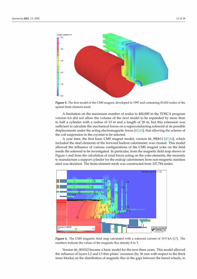
Figure 5. The first model of the CMS magnet, developed in 1997 and containing 83,832 nodes of the spatial finite element mesh.

Figure 6. The CMS magnetic field map calculated with a solenoid current of 19.5 kA [47]. The num-bers indicate the values of the magnetic flux density B in T.

Version 66_001012 became a basic model for the next three years. This model allowed the influence of layers L2 and L3 thin plates’ recession (by 36 mm with respect to the thick inner blocks) on the distribution of magnetic flux in the gaps between the barrel wheels, to be studied. In this model, the scalar magnetic potential was calculated in 1/24 part of a cylindrical volume with a radius of 13 m. The length of the part was 18 m. To obtain the distribution of the magnetic flux in a full cylinder volume of 26 m in diameter and 36 m in length, 12 rotations of the model 30° azimuthal sector around the Z axis, and a reflection of the scalar potential values with a minus sign into the region of negative coordinates of the Z axis with respect to the XY median plane were used. In contrast to the previous version, three B–H curves described the types of steel that were used in the flux-return yoke. The model was calculated on Sun-4u computers with the 64-bit UltraSPARC pro-cessors on a mesh of 219,678 spatial nodes

The next model version, 85_030919, differed from the previous version, 66_001012, only by the number of mesh nodes, which increased in the TOSCA program version 8.5 to 822,492. This model, for the first time, allowed to create a space map of the magnetic flux distribution in the entire volume of the CMS detector. The idea of this map came from

Figure 5. The first model of the CMS magnet, developed in 1997 and containing 83,832 nodes of thespatial finite element mesh.

A limitation on the maximum number of nodes to 400,000 in the TOSCA programversion 6.6 did not allow the volume of the next model to be expanded by more thanto half a cylinder with a radius of 13 m and a length of 28 m, but this extension wassufficient to calculate the mechanical forces on a superconducting solenoid at its possibledisplacements under the acting electromagnetic forces [62,63], that allowing the scheme ofthe coil suspension in the cryostat to be selected.

A year later, the first basic CMS magnet model, version 66_980612 [47,64], whichincluded the steel elements of the forward hadron calorimeter, was created. This modelallowed the influence of various configurations of the CMS magnet yoke on the fieldinside the solenoid to be investigated. In particular, from the magnetic field map shown inFigure 6 and from the calculation of axial forces acting on the yoke elements, the necessityto manufacture a support cylinder for the endcap calorimeters from non-magnetic stainlesssteel was declared. The finite-element mesh was constructed from 107,784 nodes.

Symmetry 2021, 13, x FOR PEER REVIEW 11 of 17

Figure 5. The first model of the CMS magnet, developed in 1997 and containing 83,832 nodes of the spatial finite element mesh.

Figure 6. The CMS magnetic field map calculated with a solenoid current of 19.5 kA [47]. The num-bers indicate the values of the magnetic flux density B in T.

Version 66_001012 became a basic model for the next three years. This model allowed the influence of layers L2 and L3 thin plates’ recession (by 36 mm with respect to the thick inner blocks) on the distribution of magnetic flux in the gaps between the barrel wheels, to be studied. In this model, the scalar magnetic potential was calculated in 1/24 part of a cylindrical volume with a radius of 13 m. The length of the part was 18 m. To obtain the distribution of the magnetic flux in a full cylinder volume of 26 m in diameter and 36 m in length, 12 rotations of the model 30° azimuthal sector around the Z axis, and a reflection of the scalar potential values with a minus sign into the region of negative coordinates of the Z axis with respect to the XY median plane were used. In contrast to the previous version, three B–H curves described the types of steel that were used in the flux-return yoke. The model was calculated on Sun-4u computers with the 64-bit UltraSPARC pro-cessors on a mesh of 219,678 spatial nodes

The next model version, 85_030919, differed from the previous version, 66_001012, only by the number of mesh nodes, which increased in the TOSCA program version 8.5 to 822,492. This model, for the first time, allowed to create a space map of the magnetic flux distribution in the entire volume of the CMS detector. The idea of this map came from

Figure 6. The CMS magnetic field map calculated with a solenoid current of 19.5 kA [47]. Thenumbers indicate the values of the magnetic flux density B in T.

Version 66_001012 became a basic model for the next three years. This model allowedthe influence of layers L2 and L3 thin plates’ recession (by 36 mm with respect to the thickinner blocks) on the distribution of magnetic flux in the gaps between the barrel wheels, to

Symmetry 2021, 13, 1052 12 of 18

be studied. In this model, the scalar magnetic potential was calculated in 1/24 part of acylindrical volume with a radius of 13 m. The length of the part was 18 m. To obtain thedistribution of the magnetic flux in a full cylinder volume of 26 m in diameter and 36 m inlength, 12 rotations of the model 30 azimuthal sector around the Z axis, and a reflection ofthe scalar potential values with a minus sign into the region of negative coordinates of theZ axis with respect to the XY median plane were used. In contrast to the previous version,three B–H curves described the types of steel that were used in the flux-return yoke. Themodel was calculated on Sun-4u computers with the 64-bit UltraSPARC processors on amesh of 219,678 spatial nodes.

The next model version, 85_030919, differed from the previous version, 66_001012,only by the number of mesh nodes, which increased in the TOSCA program version 8.5to 822,492. This model, for the first time, allowed to create a space map of the magneticflux distribution in the entire volume of the CMS detector. The idea of this map came fromearlier works [64,65] and was based on discretizing the entire space of the magnetic systeminto primitive volumes of several types, such as sectors of cylinders and cones, tubes andtruncated tubes, and prisms and parallelepipeds. In the CMS magnet model, all rotationvolumes are centred along the Z axis; the barrel wheel elements are described by prismsand parallelepipeds. This arrangement of the volumes allows each azimuthal sector ofthe magnet model to cut the rotation volumes by YZ planes with a constant step alongthe azimuthal angle, and to cut the prisms and parallelepipeds by planes parallel to theouter faces of the barrel wheels with a constant step between them. Each cutting planecan be evenly divided into cells, and, thus, each primitive volume contains a mesh of thespace nodes.

In these nodes three components of the magnetic flux density are calculated from thescalar potential distribution obtained with TOSCA program, and the field between thenodes is computed by a linear interpolation of the magnetic induction values over the eightnearest nodes [64–66]. The discretization of space into primitive volumes allows a fastsearch for the needed nodes around the coordinates of the points along the trajectories ofcharged particles to be performed.

Along the trajectories of charged particles in the programs for simulation and recon-struction of the primary particle collision events, the special class MagneticField returns thevalues of the magnetic flux density components for the coordinates of each requested spacepoint. To describe the magnetic field map calculated with the model version 85_030919,271 primitive volumes in the only azimuth sector S1 were used. The magnetic field in allother sectors was determined by rotating the coordinates of the desired point to sector S1and then by translating the components of the found magnetic induction to the desiredspace point.

At the beginning of 2007, the TOSCA program version 11.03 appeared and then inMay 2007, it was installed at CERN on the 64-bit x86_64 processor computers under theLinux operating system. In this version, the limit on the mesh node number was increasedto 5 million, which allowed the magnetic flux with model version 1103_071212 in a halfcylinder volume with a radius of 13 m and a length of 40 m to be described. The model,shown in Figures 7 and 8, contained 1,922,958 nodes of the spatial mesh and included thedeformation of the solenoid and a displacement of the nose and endcap disks toward thecoil centre under the electromagnetic forces as well as an absence of one turn in the innerlayer of the CB − 2 coil module.

Symmetry 2021, 13, 1052 13 of 18Symmetry 2021, 13, x FOR PEER REVIEW 13 of 17

Figure 7. The CMS magnet model version 1103_071212. The colour scale corresponds to the interval of the magnetic flux density B from zero to 5 T with an increment of 0.5 T. The distribution of the magnetic field is presented on the inner surfaces of the flux-return yoke.

Figure 8. The CMS magnet model version 1103_071212. The colour scale corresponds to the interval of the magnetic flux density B from zero to 5 T with an increment of 0.5 T. The distribution of the magnetic field is presented on the outer surfaces of the flux-return yoke.

To minimize this effect, a half a cylinder used for calculations was expanded by in-creasing the cylinder radius from 13 to 30 m and the cylinder length from 40 to 70 m. Consequently, the number of spatial mesh nodes in the new model 1103_090322 was in-creased to 1,993,452. The model comprised a 40 mm thick steel floor of the underground experimental cavern. The magnetic field map created with this model was used in the CMS detector during the entire first run of the LHC operation in 2009–2012, and with this description of the magnetic flux distribution in the detector volume the Higgs boson was discovered [2,3].

In the next version, 14_120812, both halves of the CMS magnet yoke were separately included in the model. The model comprised enlarged fourth endcap disks, the endcap disk keels in the azimuthal sector S10, and an outer part of the radiation shielding with cylindrical gaps between the shield and the collar of the forward hadron calorimeter. The volume of each half a cylinder used for calculations was increased in radius from 30 to 50 m and in length from 70 to 120 m. This version was the last one designed for the computers based on the x86_64 processor, and the division of the model into two halves was dictated

Figure 7. The CMS magnet model version 1103_071212. The colour scale corresponds to the intervalof the magnetic flux density B from zero to 5 T with an increment of 0.5 T. The distribution of themagnetic field is presented on the inner surfaces of the flux-return yoke.

Symmetry 2021, 13, x FOR PEER REVIEW 13 of 17

Figure 7. The CMS magnet model version 1103_071212. The colour scale corresponds to the interval of the magnetic flux density B from zero to 5 T with an increment of 0.5 T. The distribution of the magnetic field is presented on the inner surfaces of the flux-return yoke.

Figure 8. The CMS magnet model version 1103_071212. The colour scale corresponds to the interval of the magnetic flux density B from zero to 5 T with an increment of 0.5 T. The distribution of the magnetic field is presented on the outer surfaces of the flux-return yoke.

To minimize this effect, a half a cylinder used for calculations was expanded by in-creasing the cylinder radius from 13 to 30 m and the cylinder length from 40 to 70 m. Consequently, the number of spatial mesh nodes in the new model 1103_090322 was in-creased to 1,993,452. The model comprised a 40 mm thick steel floor of the underground experimental cavern. The magnetic field map created with this model was used in the CMS detector during the entire first run of the LHC operation in 2009–2012, and with this description of the magnetic flux distribution in the detector volume the Higgs boson was discovered [2,3].

In the next version, 14_120812, both halves of the CMS magnet yoke were separately included in the model. The model comprised enlarged fourth endcap disks, the endcap disk keels in the azimuthal sector S10, and an outer part of the radiation shielding with cylindrical gaps between the shield and the collar of the forward hadron calorimeter. The volume of each half a cylinder used for calculations was increased in radius from 30 to 50 m and in length from 70 to 120 m. This version was the last one designed for the computers based on the x86_64 processor, and the division of the model into two halves was dictated

Figure 8. The CMS magnet model version 1103_071212. The colour scale corresponds to the intervalof the magnetic flux density B from zero to 5 T with an increment of 0.5 T. The distribution of themagnetic field is presented on the outer surfaces of the flux-return yoke.

The model comprised the barrel wheel steel feet, the upper plates of the endcap diskcarts, and an inner part of the radiation shielding. The new CMS magnetic field mapused 312 primitive volumes to describe the magnetic flux distribution in the azimuthalsector S1. Distinguishing it from the previous version of the magnetic field map, the newmap included the sectors S3 and S4 with chimneys for cryogenic and electrical leads (seeFigure 1), as well as the sector S11 with the barrel wheel feet. The magnetic induction in theremaining sectors but S9 was determined based on the primitive volumes of the sector S1.

The simulated magnetic field values were compared with the field values obtained in2006 [36] with a field mapping machine [67] measuring the magnetic flux density B insidethe superconducting solenoid. The measurements were performed with an accuracy of0.07%. The model reproduced the measured field with an accuracy of 0.1%. In this model,for the first time, the coil operating current of 18.164 kA was used, which gave a centralmagnetic flux density of 3.81 T.

Symmetry 2021, 13, 1052 14 of 18

At the end of 2008, the CMS detector was assembled in an underground experimentalcavern and commissioned with the cosmic muons. It was noted [46], that the magnitude ofthe magnetic field in the layers of the barrel wheels in the model, especially the extremeones, is overestimated by several percent. This effect of the magnetic field map arosebecause of a compression of the returned magnetic flux of the solenoid in the insufficientfull volume of the model.

To minimize this effect, a half a cylinder used for calculations was expanded byincreasing the cylinder radius from 13 to 30 m and the cylinder length from 40 to 70 m.Consequently, the number of spatial mesh nodes in the new model 1103_090322 wasincreased to 1,993,452. The model comprised a 40 mm thick steel floor of the undergroundexperimental cavern. The magnetic field map created with this model was used in theCMS detector during the entire first run of the LHC operation in 2009–2012, and with thisdescription of the magnetic flux distribution in the detector volume the Higgs boson wasdiscovered [2,3].

In the next version, 14_120812, both halves of the CMS magnet yoke were separatelyincluded in the model. The model comprised enlarged fourth endcap disks, the endcapdisk keels in the azimuthal sector S10, and an outer part of the radiation shielding withcylindrical gaps between the shield and the collar of the forward hadron calorimeter. Thevolume of each half a cylinder used for calculations was increased in radius from 30 to50 m and in length from 70 to 120 m. This version was the last one designed for thecomputers based on the x86_64 processor, and the division of the model into two halveswas dictated by the limitation on the number of mesh nodes. One of the model halvescontained 3,624,593 nodes, the other one used 3,584,357 nodes.

To create the magnetic field map, 720 primitive volumes were used in each azimuthalsector divided into two halves of 15 azimuth angle each. The total number of primitivevolumes in a cylinder with a diameter of 18 m and a length of 40 m, used to describe thedistribution of the magnetic flux in the CMS detector, was 8640.

Both halves of the model 14_120812 were combined into a single volume in thenext model version, 16_130503, shown in Figure 9. Starting with this version, all sub-sequent models were designed for personal computers with an Intel64/x64 processorand with RAM of 8–16 GB under the Windows operating system. The model contained7,111,713 nodes of the spatial mesh and required 10 h of processor time to calculate. Tocreate the magnetic field map, the number of primitive volumes in a cylinder with thesame dimensions of 18 m in diameter and 40 m in length was increased to 9648 due to amore detailed description of the regions outside the barrel wheels, where the last layer ofthe muon drift tube chambers is located.

Symmetry 2021, 13, 1052 15 of 18

Symmetry 2021, 13, x FOR PEER REVIEW 14 of 17

by the limitation on the number of mesh nodes. One of the model halves contained 3,624,593 nodes, the other one used 3,584,357 nodes.

To create the magnetic field map, 720 primitive volumes were used in each azimuthal sector divided into two halves of 15° azimuth angle each. The total number of primitive volumes in a cylinder with a diameter of 18 m and a length of 40 m, used to describe the distribution of the magnetic flux in the CMS detector, was 8640.

Both halves of the model 14_120812 were combined into a single volume in the next model version, 16_130503, shown in Figure 9. Starting with this version, all subsequent models were designed for personal computers with an Intel64/x64 processor and with RAM of 8–16 GB under the Windows operating system. The model contained 7,111,713 nodes of the spatial mesh and required 10 h of processor time to calculate. To create the magnetic field map, the number of primitive volumes in a cylinder with the same dimen-sions of 18 m in diameter and 40 m in length was increased to 9648 due to a more detailed description of the regions outside the barrel wheels, where the last layer of the muon drift tube chambers is located.

Figure 9. The CMS magnet model version 14_130503. The colour scale corresponds to the range of magnetic flux density B from zero to 5 T with an increment of 0.5 T. The distribution of the magnetic field is shown on the outer surface of the flux-return yoke.

Finally, the next two versions, 18_160812 and 18_170812 of the model differ from each other only by a slight refinement of the magnetization curve of steel S, which, like the other curves, did not change after version 66_001012. To complete the geometrical de-scription of the magnetic system, the most distant part of the radiation shielding was added to both model versions propagated to distances of ±21.89 m on both sides from the centre of the solenoid, as shown in Figure 2. Thus, the length of the CMS magnetic field map cylinder was increased to 48 m, and the number of primitive volumes in all 12 azi-muthal sectors was increased to 11,088.

5. Conclusions For more than 10 years of the CMS detector operation, a computing modelling of the

magnetic system has been used to obtain the distribution of the magnetic flux throughout the experimental setup. Applying the magnetic flux simulation to the CMS magnet, results in the creation of a magnetic field map in the entire CMS volume, allowing the precise measurement of the electron (positron) and muon momenta, which has made it possible to reconstruct the invariant mass of the Higgs boson—the last brick of the Standard Model of elementary particles—with a high precision.

Figure 9. The CMS magnet model version 14_130503. The colour scale corresponds to the range ofmagnetic flux density B from zero to 5 T with an increment of 0.5 T. The distribution of the magneticfield is shown on the outer surface of the flux-return yoke.

Finally, the next two versions, 18_160812 and 18_170812 of the model differ from eachother only by a slight refinement of the magnetization curve of steel S, which, like the othercurves, did not change after version 66_001012. To complete the geometrical description ofthe magnetic system, the most distant part of the radiation shielding was added to bothmodel versions propagated to distances of ±21.89 m on both sides from the centre of thesolenoid, as shown in Figure 2. Thus, the length of the CMS magnetic field map cylinderwas increased to 48 m, and the number of primitive volumes in all 12 azimuthal sectorswas increased to 11,088.

5. Conclusions

For more than 10 years of the CMS detector operation, a computing modelling of themagnetic system has been used to obtain the distribution of the magnetic flux throughoutthe experimental setup. Applying the magnetic flux simulation to the CMS magnet, resultsin the creation of a magnetic field map in the entire CMS volume, allowing the precisemeasurement of the electron (positron) and muon momenta, which has made it possible toreconstruct the invariant mass of the Higgs boson—the last brick of the Standard Model ofelementary particles—with a high precision.

Several consecutive versions of the CMS magnet model were developed using differenttypes of geometrical and scalar magnetic potential symmetries. This has allowed themagnetic flux in the entire CMS detector during a long period of time to be described withminimal computer resources, corresponding to the available computer technology capabilities.

Funding: This research received no external funding.

Institutional Review Board Statement: Not applicable.

Informed Consent Statement: Not applicable.

Data Availability Statement: Not applicable.

Acknowledgments: The author is very thankful to Alain Hervé, François Kircher, Richard P. Smith,Austin Ball, Wolfram Zeuner, Eduard Boos, Lyudmila Sarycheva, and Mikhail Panasyuk for adminis-trative and technical support for many years.

Conflicts of Interest: The author declares no conflict of interest.

Symmetry 2021, 13, 1052 16 of 18

References1. Aad, G.; Abajyan, T.; Abbott, B.; Abdallah, J.; Khalek, S.A.; Abdelalim, A.; Abdinov, O.; Aben, R.; Abi, B.; Abolins, M.; et al.

Observation of a new particle in the search for the Standard Model Higgs boson with the ATLAS detector at the LHC. Phys. Lett.B 2012, 716, 1–29. [CrossRef]

2. Chatrchyan, S.; Khachatryan, V.; Sirunyan, A.; Tumasyan, A.; Adam, W.; Aguilo, E.; Bergauer, T.; Dragicevic, M.; Erö, J.;Fabjan, C.; et al. Observation of a new boson at a mass of 125 GeV with the CMS experiment at the LHC. Phys. Lett. B 2012, 716,30–61. [CrossRef]

3. Chatrchyan, S.; The CMS Collaboration; Khachatryan, V.; Sirunyan, A.M.; Tumasyan, A.; Adam, W.; Bergauer, T.; Dragicevic, M.;Erö, J.; Fabjan, C.; et al. Observation of a new boson with mass near 125 GeV in pp collisions at

√s = 7 and 8 TeV. J. High Energy

Phys. 2013, 2013, 81. [CrossRef]4. Dittmaier, S.; Mariotti, C.; Passarino, G.; Tanaka, R. (Eds.) Handbook of LHC Higgs Cross Sections: 1. Inclusive Observables; Report

CERN-2011-002 of the LHC Higgs Cross Section Working Group; CERN: Geneva, Switzerland, 2011; ISBN 978-92-9083-358-1.Available online: http://cds.cern.ch/record/1318996 (accessed on 9 June 2021).

5. Englert, F.; Brout, R. Broken symmetry and the masses of gauge vector mesons. Phys. Rev. Lett. 1964, 13, 321–323. [CrossRef]6. Higgs, P. Broken symmetries, massless particles and gauge fields. Phys. Lett. 1964, 12, 132–133. [CrossRef]7. Higgs, P.W. Broken Symmetries and the Masses of Gauge Bosons. Phys. Rev. Lett. 1964, 13, 508–509. [CrossRef]8. Evans, L.; Bryant, P. LHC Machine. J. Instrum. 2008, 3, S08001. [CrossRef]9. Lorentz, H.A. La théorie électromagnétique de Maxwell et son application aux corps mouvants. Arch. Néerl. 1892, 25, 451.10. ATLAS Collaboration. The ATLAS Experiment at the CERN Large Hadron Collider. J. Instrum. 2008, 3, S08003. [CrossRef]11. CMS Collaboration. The CMS Experiment at the CERN LHC. J. Instrum. 2008, 3, S08004. [CrossRef]12. Vishnyakov, I.A.; Vorob’ev, A.P.; Kechkin, V.F.; Klyukhin, V.I.; Kozlovsky, E.A.; Malyaev, V.K.; Selivanov, G.I. Superconducting

solenoid for a collider detector. Zhurnal Tekhnicheskoi Fiziki 1992, 62, 146–156. (In Russian)13. Vishnyakov, I.A.; Vorob’ev, A.P.; Kechkin, V.F.; Klyukhin, V.I.; Kozlovsky, E.A.; Malyaev, V.K.; Selivanov, G.I. Superconducting

solenoid for a colliding beams device. Sov. Phys. Tech. Phys. 1992, 37, 195–201.14. The DØ Collaboration. E823 (DØ Upgrade): Magnetic Tracking; D0 Note 1933; FNAL: Batavia, IL, USA, 1993. Available online:

https://inspirehep.net/literature/1234049 (accessed on 9 June 2021).15. The DØ Collaboration. DØ Upgrade. FERMILAB-PROPOSAL-0823; FNAL: Batavia, IL, USA, 1993. Available online: https:

//inspirehep.net/literature/362587 (accessed on 9 June 2021).16. The DØ Collaboration. The DØ Upgrade. FERMILAB-Conf-95/177-E; FNAL: Batavia, IL, USA, 1995. Available online: https:

//inspirehep.net/literature/397654 (accessed on 9 June 2021).17. Wayne, M.R. The DØ upgrade. Nucl. Instrum. Methods Phys. Res. Sect. A Accel. Spectrometer Detect. Assoc. Equip. 1998, 408,

103–109. [CrossRef]18. CMS. The Magnet Project; Technical Design Report, CERN/LHCC 97-10, CMS TDR 1; CERN: Geneva, Switzerland, 1997; ISBN

92-9083-101-4. Available online: http://cds.cern.ch/record/331056 (accessed on 9 June 2021).19. ATLAS. Magnet System; Technical Design Report, CERN/LHCC 97-18, ATLAS TDR 6; CERN: Geneva, Switzerland, 1997; ISBN

92-9083-104-9. Available online: http://cds.cern.ch/record/338080 (accessed on 9 June 2021).20. Galic, H.; Wohl, C.; Armstrong, B.; Dodder, D.; Klyukhin, V.; Ryabov, Y.; Illarionova, N.; Lehar, F.; Oyanagi, Y.; Olin, A.; et al.

Current Experiments in Elementary Particle Physics. Technical Report LBL-91-Rev.-6-92; 1992; p. 131. Available online:https://www.osti.gov/biblio/10181103 (accessed on 9 June 2021).

21. Galic, H.; Lehar, F.; Klyukhin, V.; Ryabov, Y.; Bilak, S.; Illarionova, N.; Khachaturov, B.; Strokovsky, E.; Hoffman, C.;Kettle, P.-R.; et al. Current Experiments in Particle Physics. Technical Report LBL-91-Rev.-9-96; 1996; p. 46. Available online:https://www.osti.gov/biblio/469140 (accessed on 9 June 2021).

22. The LHC Study Group. Design Study of the Large Hadron Collider (LHC). A Multiparticle Collider in the LEP Tunnel; CERN-91-03,CERN-AC-DI-FA-90-06-REV; CERN: Geneva, Switzerland, 1991. [CrossRef]

23. CMS. The Compact Muon Solenoid. Letter of Intent by the CMS Collaboration for a General Purpose Detector at the LHC; CERN/LHCC/92-3; LHCC/I 1; CERN: Geneva, Switzerland, 1992; Available online: https://cds.cern.ch/record/290808 (accessed on 9 June 2021).

24. ATLAS. Letter of Intent for a General-Purpose PP Experiment at the Large Hadron Collider at CERN; CERN/LHCC/92-4, LHCC/I 2;CERN: Geneva, Switzerland, 1992; Available online: http://cds.cern.ch/record/291061 (accessed on 9 June 2021).

25. Erdogan, A.; Zmushko, V.V.; Klyukhin, V.I.; Froidevaux, D. Study of the H → WW → lνjj and H → ZZ → lljj decays formH = 1 TeV/c2 at the LHC energies. Yadernaya Fizika 1994, 59, 290–301. (In Russian)

26. Erdogan, A.; Froidevaux, D.; Klyukhin, V.; Zmushko, V. On the Experimental study of the H→WW→ lνjj and H→ ZZ→ lljjDecays for mH = 1 TeV/c2 at LHC energies. Phys. Atom. Nucl. 1994, 57, 274–284.

27. Zmushko, S.; Erdogan, A.; Froidevaux, D.; Klioukhine, S. Study of H→WW→ Lνjj and H→ ZZ→ Lljj Decays for mH = 1 TeV;ATLAS Internal note PHYS-No-008; CERN: Geneva, Switzerland, 1992; Available online: https://cds.cern.ch/record/682128(accessed on 9 June 2021).

28. ATLAS. Technical Proposal for a General-Purpose PP Experiment at the Large Hadron Collider at CERN; CERN/LHCC/94-43, LHCC/P2;CERN: Geneva, Switzerland, 1994; pp. 233–235. ISBN 92-9083-067-0. Available online: http://cds.cern.ch/record/290968(accessed on 9 June 2021).

29. Klyukhin, V.I.; Poppleton, A.; Schmitz, J. Magnetic Field Integrals for the ATLAS Tracking Volume; IHEP: Protvino, Russia, 1993.

Symmetry 2021, 13, 1052 17 of 18

30. Klyukhin, V.I.; Poppleton, A.; Schmitz, J. Field Integrals for the ATLAS Tracking Volume; ATLAS Internal note INDET-NO-023;CERN: Geneva, Switzerland, 1993; Available online: http://cds.cern.ch/record/685858 (accessed on 9 June 2021).

31. ALICE. Technical Proposal for a Large Ion Collider Experiment at the LHC; CERN/LHCC 95-71, LHCC/P3; CERN: Geneva, Switzerland,1995; pp. 99–101. ISBN 92-9083-088-077-8. Available online: http://cds.cern.ch/record/293391 (accessed on 9 June 2021).

32. ALICE. The Forward Muon Spectrometer; Addendum to the ALICE Technical Proposal. CERN/LHCC 96-32, LHCC/P3-Addendum1; CERN: Geneva, Switzerland, 1996; pp. 9–10. ISBN 92-9083-088-3. Available online: http://cds.cern.ch/record/314011 (accessedon 9 June 2021).

33. Herve, A. Constructing a 4-Tesla Large Thin Solenoid at the Limit of What Can Be Safely Operated. Mod. Phys. Lett. A 2010, 25,1647–1666. [CrossRef]

34. Kircher, F.; Bredy, P.; Calvo, A.; Cure, B.; Campi, D.; Desirelli, A.; Fabbricatore, P.; Farinon, S.; Herve, A.; Horvath, I.; et al. Finaldesign of the CMS solenoid cold mass. IEEE Trans. Appl. Supercond. 2000, 10, 407–410. [CrossRef]

35. Herve, A.; Blau, B.; Bredy, P.; Campi, D.; Cannarsa, P.; Cure, B.; Dupont, T.; Fabbricatore, P.; Farinon, S.; Feyzi, F.; et al. Status ofthe Construction of the CMS Magnet. IEEE Trans. Appl. Supercond. 2004, 14, 542–547. [CrossRef]

36. Campi, D.; Cure, B.; Gaddi, A.; Gerwig, H.; Herve, A.; Klyukhin, V.; Maire, G.; Perinic, G.; Bredy, P.; Fazilleau, P.; et al.Commissioning of the CMS Magnet. IEEE Trans. Appl. Supercond. 2007, 17, 1185–1190. [CrossRef]

37. CMS Collaboration. Commissioning and performance of the CMS pixel tracker with cosmic ray muons. J. Instrum. 2010, 5, T03007.[CrossRef]

38. CMS Collaboration. Commissioning and performance of the CMS silicon strip tracker with cosmic ray muons. J. Instrum. 2010,5, T03008. [CrossRef]

39. CMS Collaboration. Performance and operation of the CMS electromagnetic calorimeter. J. Instrum. 2010, 5, T03010. [CrossRef]40. CMS Collaboration. Performance of the CMS hadron calorimeter with cosmic ray muons and LHC beam data. J. Instrum. 2010,

5, T03012. [CrossRef]41. CMS Collaboration. Performance of the CMS drift tube chambers with cosmic rays. J. Instrum. 2010, 5, T03015. [CrossRef]42. CMS Collaboration. Performance of the CMS cathode strip chambers with cosmic rays. J. Instrum. 2010, 5, T03018. [CrossRef]43. CMS Collaboration. Performance study of the CMS barrel resistive plate chambers with cosmic rays. J. Instrum. 2010, 5, T03017.

[CrossRef]44. CMS Collaboration. Performance of CMS muon reconstruction in cosmic-ray events. J. Instrum. 2010, 5, T03022. [CrossRef]45. Abdullin, S.; The CMS-HCAL Collaboration; Abramov, V.; Acharya, B.; Adams, M.; Akchurin, N.; Akgun, U.; Anderson, E.;

Antchev, G.; Arcidy, M.; et al. Design, performance, and calibration of CMS forward calorimeter wedges. Eur. Phys. J. C 2007, 53,139–166. [CrossRef]

46. CMS Collaboration. Precise mapping of the magnetic field in the CMS barrel yoke using cosmic rays. J. Instrum. 2010, 5, T03021.[CrossRef]

47. Klioukhine, V.; Campi, D.; Cure, B.; Desirelli, A.; Farinon, S.; Gerwig, H.; Grillet, J.; Herve, A.; Kircher, F.; Levesy, B.; et al. 3Dmagnetic analysis of the CMS magnet. IEEE Trans. Appl. Supercond. 2000, 10, 428–431. [CrossRef]

48. Klyukhin, V.I.; Ball, A.; Campi, D.; Cure, B.; Dattola, D.; Gaddi, A.; Gerwig, H.; Hervé, A.; Loveless, R.; Reithler, H.; et al.Measuring the Magnetic Field Inside the CMS Steel Yoke Elements. In Proceedings of the 2008 IEEE Nuclear Science SymposiumConference Record, Dresden, Germany, 19–25 October 2008; pp. 2270–2273.

49. Klyukhin, V.I.; Amapane, N.; Andreev, V.; Ball, A.; Cure, B.; Herve, A.; Gaddi, A.; Gerwig, H.; Karimaki, V.; Loveless, R.; et al.The CMS Magnetic Field Map Performance. IEEE Trans. Appl. Supercond. 2010, 20, 152–155. [CrossRef]

50. Klyukhin, V.I.; Amapane, N.; Ball, A.; Cure, B.; Gaddi, A.; Gerwig, H.; Mulders, M.; Herve, A.; Loveless, R. Measuring theMagnetic Flux Density in the CMS Steel Yoke. J. Supercond. Nov. Magn. 2012, 26, 1307–1311. [CrossRef]

51. Klyukhin, V.I.; Amapane, N.; Ball, A.; Cure, B.; Gaddi, A.; Gerwig, H.; Mulders, M.; Calvelli, V.; Herve, A.; Loveless, R. Validationof the CMS Magnetic Field Map. J. Supercond. Nov. Magn. 2014, 28, 701–704. [CrossRef]

52. Klyukhin, V.I.; Amapane, N.; Ball, A.; Curé, B.; Gaddi, A.; Gerwig, H.; Mulders, M.; Hervé, A.; Loveless, R. Flux LoopMeasurements of the Magnetic Flux Density in the CMS Magnet Yoke. J. Supercond. Nov. Magn. 2016, 30, 2977–2980. [CrossRef]

53. Klyukhin, V.I.; Cure, B.; Amapane, N.; Ball, A.; Gaddi, A.; Gerwig, H.; Herve, A.; Loveless, R.; Mulders, M. Using the StandardLinear Ramps of the CMS Superconducting Magnet for Measuring the Magnetic Flux Density in the Steel Flux-Return Yoke. IEEETrans. Magn. 2018, 55, 8300504. [CrossRef]

54. TOSCA/OPERA-3d 18R2 Reference Manual; Cobham CTS Ltd.: Kidlington, UK, 2018; pp. 1–916.55. Simkin, J.; Trowbridge, C. Three-dimensional nonlinear electromagnetic field computations, using scalar potentials. In IEE

Proceedings B Electric Power Applications; Institution of Engineering and Technology (IET): London, UK, 1980; Volume 127,pp. 368–374. [CrossRef]

56. Landau, L.D.; Lifshitz, E.M. Electrodynamics of Continuous Media, 2nd ed.; Nauka: Moscow, Russia, 1982; pp. 154–163. (In Russian)57. Simkin, J.; Trowbridge, C.W. On the use of the total scalar potential on the numerical solution of fields problems in electromagnetics.

Int. J. Numer. Methods Eng. 1979, 14, 423–440. [CrossRef]58. Tamm, I.E. Fundamentals of the Theory of Electricity, 9th ed.; Nauka: Moscow, Russia, 1976; pp. 285–288. (In Russian)59. Zienkiewicz, O.; Lyness, J.; Owen, D. Three-dimensional magnetic field determination using a scalar potential—A finite element

solution. IEEE Trans. Magn. 1977, 13, 1649–1656. [CrossRef]60. Herve, A. The CMS detector magnet. IEEE Trans. Appl. Supercond. 2000, 10, 389–394. [CrossRef]

Symmetry 2021, 13, 1052 18 of 18

61. Horvath, I.; Dardel, B.; Marti, H.-P.; Neuenschwander, J.; Smith, R.; Fabbricatore, P.; Musenich, R.; Calvo, A.; Campi, D.;Cure, B.; et al. The CMS conductor. IEEE Trans. Appl. Supercond. 2000, 10, 395–398. [CrossRef]

62. Klioukhine, V. Calculation of Magnetic Forces on the CMS Coil with TOSCA; DSM/DAPNIA/STCM Technical Report 5C2100T–M 1000 020 97. 1997. Available online: http://klyukhi.web.cern.ch/klyukhi/notes/V_Klioukhine_Saclay_020_1997.pdf(accessed on 9 June 2021).

63. Klioukhine, V. Magnetic Forces in the CMS Magnetic System Calculated with TOSCA; DSM/DAPNIA/STCM Technical Report5C 2100T–M 1000 023 97. 1997. Available online: http://klyukhi.web.cern.ch/klyukhi/notes/V_Klioukhine_Saclay_023_1997.pdf(accessed on 9 June 2021).

64. Klioukhine, V.I. The TOSCA-GEANT Interface Tools; CMS Conference Report CMS CR 1998/016; CERN: Geneva, Switzerland,1998; Available online: https://cds.cern.ch/record/687563 (accessed on 9 June 2021).

65. Klyukhin, V.I. Interface Program for POISSON and GEANT Packages. In Proceedings of the International Conference onComputing in High Energy Physics ’92, Annecy, France, 21–25 September 1992; CERN Report, 92-07. Verkerk, C., Wójcik, W., Eds.;CERN: Geneva, Switzerland, 1992; pp. 844–846, ISBN 92-9083-049-2. Available online: http://cds.cern.ch/record/401030(accessed on 9 June 2021).

66. Amapane, N.; Andreev, V.; Drollinger, V.; Karimaki, V.; Klyukhin, V.; Todorov, T. Volume-Based Representation of the Magnetic Field;CMS Conference Report CMS CR 2005/011; CERN: Geneva, Switzerland, 2005; Available online: https://cds.cern.ch/record/883293 (accessed on 9 June 2021).

67. Klyukhin, V.; Ball, A.; Bergsma, F.; Campi, D.; Cure, B.; Gaddi, A.; Gerwig, H.; Herve, A.; Korienek, J.; Linde, F.; et al. Measurementof the CMS Magnetic Field. IEEE Trans. Appl. Supercond. 2008, 18, 395–398. [CrossRef]