Design and Analysis of Algorithm – SCSA1403
123
1 SCHOOL OF COMPUTING DEPARTMENT OF INFORMATION TECHNOLOGY UNIT - I Design and Analysis of Algorithm – SCSA1403
-
Upload
khangminh22 -
Category
Documents
-
view
1 -
download
0
Transcript of Design and Analysis of Algorithm – SCSA1403
1
SCHOOL OF COMPUTING
DEPARTMENT OF INFORMATION TECHNOLOGY
UNIT - I
Design and Analysis of Algorithm – SCSA1403
2
Introduction 9 Hrs.
Fundamentals of Algorithmic Problem Solving - Time Complexity - Space complexity with
examples - Growth of Functions - Asymptotic Notations: Need, Types - Big Oh, Little Oh,
Omega, Theta - Properties - Complexity Analysis Examples - Performance measurement -
Instance Size, Test Data, Experimental setup.
Fundamentals of Algorithmic Problem Solving
An Algorithm is a finite sequence of instructions or steps (i.e. inputs) to achieve a
particular task. All algorithms must satisfy the following criteria:
1. Input- zero or more quantities are externally supplied.
2. Output- At least one quantity is produced.
3. Definiteness-Each instruction is clear and unambiguous.
4. Finiteness- The algorithm terminates after a finite number of steps.
5. Effectiveness- the degree to which something is successful in producing a desired
result.
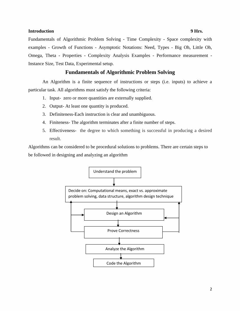
Algorithms can be considered to be procedural solutions to problems. There are certain steps to
be followed in designing and analyzing an algorithm
Understand the problem
Decide on: Computational means, exact vs. approximate
problem solving, data structure, algorithm design technique
Design an Algorithm
Prove Correctness
Analyze the Algorithm
Code the Algorithm
3
1. Understanding the problem:
The problem given should be understood completely. Check if it is similar to
some standard problems and if a Known algorithm exists, otherwise a new algorithm has
to be devised.
2. Ascertain the capabilities of the computational device: Once a problem is understood
we need to know the capabilities of the computing device this can be done by knowing
the type of the architecture, speed and memory availability.
3. Exact /approximate solution: Once algorithm is devised, it is necessary to show that it
computes answer for all the possible legal inputs.
4. Deciding data structures : Data structures play a vital role in designing and analyzing
the algorithms. Some of the algorithm design techniques also depend on the structuring
data specifying a problem’s instance.
Algorithm + Data structure = Programs
5. Algorithm design techniques: Creating an algorithm is an art which may never be fully
automated. By mastering these design strategies, it will become easier for you to devise
new and useful algorithms.
6. Prove correctness:
Correctness has to be proved for every algorithm. For some algorithms, a proof of
correctness is quite easy; for others it can be quite complex. A technique used for proving
correctness by mathematical induction because an algorithm’s iterations provide a
natural sequence of steps needed for such proofs. But we need one instance of its input
for which the algorithm fails. If it is incorrect, redesign the algorithm, with the same
decisions of data structures design technique etc
7. Analyze the algorithm
There are two kinds of algorithm efficiency: time and space efficiency. Time
efficiency indicates how fast the algorithm runs; space efficiency indicates how much
extra memory the algorithm needs.
8. Coding
Programming the algorithm by using some programming language. Formal
verification is done for small programs. Validity is done by testing and debugging. Inputs
4
should fall within a range and hence require no verification. Some compilers allow code
optimization which can speed up a program by a constant factor whereas a better
algorithm can make a difference in their running time. The analysis has to be done in
various sets of inputs.
Complexity
Performance of a program: The performance of a program is measured based on the amount
of computer memory and time needed to run a program.
The two approaches which are used to measure the performance of the program are:
1. Analytical method → called the Performance Analysis.
2. Experimental method → called the Performance Measurement.
Space Complexity
Space complexity: The Space complexity of a program is defined as the amount of memory it needs to
run to completion.
As said above the space complexity is one of the factor which accounts for the performance of the
program. The space complexity can be measured using experimental method, which is done by running
the program and then measuring the actual space occupied by the program during execution. But this is
done very rarely. We estimate the space complexity of the program before running the program.
The reasons for estimating the space complexity before running the program even for the first
time are:
(1) We should know in advance, whether or not, sufficient memory is present in the computer.
If this is not known and the program is executed directly, there is possibility that the program
may consume more memory than the available during the execution of the program. This
leads to insufficient memory error and the system may crash, leading to severe damages if
that was a critical system.
(2) In Multi user systems, we prefer, the programs of lesser size, because multiple copies of the
program are run when multiple users access the system. Hence if the program occupies less
space during execution, then more number of users can be accommodated.
Space complexity is the sum of the following components:
(i) Instruction space:
The program which is written by the user is the source program. When this program is compiled,
a compiled version of the program is generated. For executing the program an executable version of the
program is generated. The space occupied by these three when the program is under execution, will
account for the instruction space.
5
The instruction space depends on the following factors:
Compiler used – Some compiler generate optimized code which occupies less space.
Compiler options – Optimization options may be set in the compiler options.
Target computer – The executable code produced by the compiler is dependent on the
processor used.
(ii) Data space:
The space needed by the constants, simple variables, arrays, structures and other data structures
will account for the data space.
The Data space depends on the following factors:
Structure size – It is the sum of the size of component variables of the structure.
Array size – Total size of the array is the product of the size of the data type and
the number of array locations.
(iii) Environment stack space:
The Environment stack space is used for saving information needed to resume execution
of partially completed functions. That is whenever the control of the program is transferred from
one function to another during a function call, then the values of the local variable of that
function and return address are stored in the environment stack. This information is retrieved
when the control comes back to the same function.
The environment stack space depends on the following factors:
Return address
Values of all local variables and formal parameters.
The Total space occupied by the program during the execution of the program is the sum of the
fixed space and the variable space.
(i) Fixed space - The space occupied by the instruction space, simple variables and
constants.
(ii) Variable space – The dynamically allocated space to the various data structures and
the environment stack space varies according to the input from the user.
Space complexity S(P) = c + Sp
c -- Fixed space or constant space
Sp -- Variable space
6
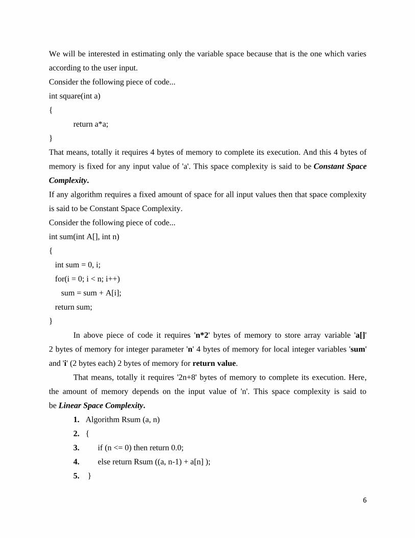
We will be interested in estimating only the variable space because that is the one which varies
according to the user input.
Consider the following piece of code...
int square(int a)
return a*a;
That means, totally it requires 4 bytes of memory to complete its execution. And this 4 bytes of
memory is fixed for any input value of 'a'. This space complexity is said to be Constant Space
Complexity.
If any algorithm requires a fixed amount of space for all input values then that space complexity
is said to be Constant Space Complexity.
Consider the following piece of code...
int sum(int A[], int n)
int sum = 0, i;
for(i = 0; i < n; i++)
sum = sum + A[i];
return sum;
In above piece of code it requires 'n*2' bytes of memory to store array variable 'a[]'
2 bytes of memory for integer parameter 'n' 4 bytes of memory for local integer variables 'sum'
and 'i' (2 bytes each) 2 bytes of memory for return value.
That means, totally it requires '2n+8' bytes of memory to complete its execution. Here,
the amount of memory depends on the input value of 'n'. This space complexity is said to
be Linear Space Complexity.
1. Algorithm Rsum (a, n)
2.
3. if (n <= 0) then return 0.0;
4. else return Rsum ((a, n-1) + a[n] );
5.
7
Recursive function for sum:
In the above algorithm instances are characterized by n. the recursion stack space includes space
for the formal parameters, the local variables, and the return address. Assume that the return
address requires only 2 byte of memory. Each call to Rsum requires at least 3 * 2 = 6 byte
(including space for the value of n, the return address, and a pointer to a[]). Since the depth of
recursion is n+1, the recursion state space needed is >=3*2(n+1) = 6(n+1).
Time Complexity
Time complexity: Time complexity of the program is defined as the amount of computer time it
needs to run to completion.
The time complexity can be measured, by measuring the time taken by the program when
it is executed. This is an experimental method. But this is done very rarely. We always try to
estimate the time consumed by the program even before it is run for the first time.
The reasons for estimating the time complexity of the program even before running the
program for the first time are:
(1) We need real time response for many applications. That is a faster execution of the
program is required for many applications. If the time complexity is estimated
beforehand, then modifications can be done to the program to improve the
performance before running it.
(2) It is used to specify the upper limit for time of execution for some programs. The
purpose of this is to avoid infinite loops.
The time complexity of the program depends on the following factors:
• Compiler used – some compilers produce optimized code which consumes less
time to get executed.
• Compiler options – The optimization options can be set in the options of the
compiler.
• Target computer – The speed of the computer or the number of instructions
executed per second differs from one computer to another.
The total time taken for the execution of the program is the sum of the compilation time and the
execution time.
(i) Compile time – The time taken for the compilation of the program to produce the
intermediate object code or the compiler version of the program. The compilation
8
time is taken only once as it is enough if the program is compiled once. If optimized
code is to be generated, then the compilation time will be higher.
(ii) Run time or Execution time - The time taken for the execution of the program. The
optimized code will take less time to get executed.
Time complexity T(P) = c + Tp
c -- Compile time
Tp -- Run time or execution time
We will be interested in estimating only the execution time as this is the one which varies
according to the user input.
So the time T(p) taken by a program p is the sum of the compile time and the run time. The
compile time does not depend on the instance characteristics. But run time is depending on the
instance characteristics. This run time is denoted by tp(instance characteristics).
The many of the factors tp depends on the number of additions, subtractions, multiplications,
divisions, compares, loads, stores and so on, so tp(n) of the form
Tp(n) = Ca ADD(n) + Cs SUB(n) + Cm MUL(n) + Cd DIV +…..
Where n denotes the instance characteristics, and Ca, Cs, Cm, Cd and so on respectively, denote
the time needed for an addition, subtraction, multiplication, division, and so on and ADD, SUB,
MUL, DIV and so on are functions whose values are the numbers of additions, subtractions,
multiplications, divisions, and so on.
The Tp(n) is obtain a count for the total number of operations. To obtain number of operations,
just count only the number of program steps. A program step is loosely defined as a syntactically
or semantically meaningful segment of a program that has an execution time that is independent
of the instance characteristics.
The number of steps any program statement is assigned depends on the kind of statement. For
example, comments count as zero step, an assignment statement which does not involve any calls
to other algorithms is counted as one step, in an iterative statement such as the for, while and
repeat until statement, we consider the step counts only for the control part of the statement.
The control parts for For and while statements have the following forms.
9
For i = <expr> to <expr1> do
While<expr>do
Each execution of the control part of a while statement is given a step count equal to the number
of step counts assignable to <expr>. The step count for each execution of the control part of a for
statement is one.
We can determine the number of steps needed by a program to solve a particular problem
instance is one of two ways. In the first method, we introduce a new variable, count, into the
program. This is a global variable with initial value 0. each time a statement is executed, count is
incremented by one.
Example:
When the statements to increment count are introduced then the algorithm will be
Algorithm Sum(a, n)
s: = 0.0;
//count = count + 1 - count is global, it is initially zero
for i=1 to n do
//count = count + 1 - For for
s = s + a[i]; //count = count + 1 - for assignment
count = count +1 //for last time of for
count = count +1 // for the return
return s;
for every initial value of count, the above algorithm compute the same finial value for count. It is
easy to see that in the for loop, the value of count will increase by a total of 2n. if count is zero
to start with, then it will be(2n + 3) on termination. So each invocation of sum (the above
algorithm) executes a total of (2n + 3) steps.
Example 2 :
When the statements to increment count are introduced in Recursive function for sum ,we will
get the following algorithm.
Algorithm Rsum (a, n)
// count = count + 1 - for the if conditional
if (n<= 0) then
10
// count = count + 1 -for the return
return 0.0;
else
// count = count +1- for the addition, function invocation and return
return Rsum (a, n-1) + a[n];
let tRsum (n) be the count value when above algorithm is terminates.
We can see that tRsum(0) = 2, if n = 0. when n > 0, count increase by 2 plus whatever increase
result from the invocations of Rsum from within the else clause. From the definition of tRsum, it
follows that this additional increase is tRsum (n-1), so if the value of count is zero initially, its
value at the time of termination is (2 + tRsum (n-1)), n > 0.
When analyzing a recursive program for its step count, we often obtain a recursive formula for
the step count, for example.
tRsum (n) = 2 if n = 0
2 +tRsum (n-1) if n >0
These recursive formulas are referred to as recurrence relations. One way to solve the recurrence
relation is
tRsm (n) = 2 + tRsum (n-1)
= 2 + 2 + tRsum (n-2)
= 2(2) + tRsum (n-2)
.. . = n(2) + tRsum (0)
= 2n + 2 n >= 0
so the step count for Rsum is 2n + 2.
The second method is determined the stop count of an algorithm is to build a table in which we
list the total number of steps contributed by each statement. This figure is often arrived at by first
11
determining the number of steps per execution (s/e) of the statements and the total number of
times (is frequency) each statement is executed.
The (s/e) of a statement is the amount by which the count changes as a result of the execution of
that statement, by combining these two quantities, the total contribution of each statement is
obtained. By adding the contribution of all statements, the step count for the entire algorithm is
obtained.
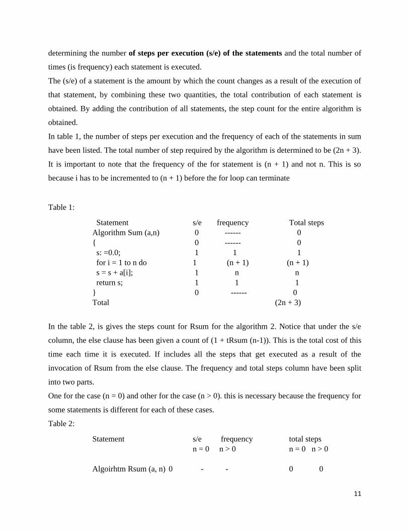
In table 1, the number of steps per execution and the frequency of each of the statements in sum
have been listed. The total number of step required by the algorithm is determined to be (2n + 3).
It is important to note that the frequency of the for statement is (n + 1) and not n. This is so
because i has to be incremented to (n + 1) before the for loop can terminate
Table 1:
Statement s/e frequency Total steps
Algorithm Sum (a,n) 0 ------ 0
0 ------ 0
s: =0.0; 1 1 1
for i = 1 to n do 1 (n + 1) (n + 1)
s = s + a[i]; 1 n n
return s; 1 1 1
0 ------ 0
Total (2n + 3)
In the table 2, is gives the steps count for Rsum for the algorithm 2. Notice that under the s/e
column, the else clause has been given a count of (1 + tRsum (n-1)). This is the total cost of this
time each time it is executed. If includes all the steps that get executed as a result of the
invocation of Rsum from the else clause. The frequency and total steps column have been split
into two parts.
One for the case (n = 0) and other for the case (n > 0). this is necessary because the frequency for
some statements is different for each of these cases.
Table 2:
Statement s/e frequency total steps
n = 0 n > 0 n = 0 n > 0
Algoirhtm Rsum (a, n) 0 - - 0 0
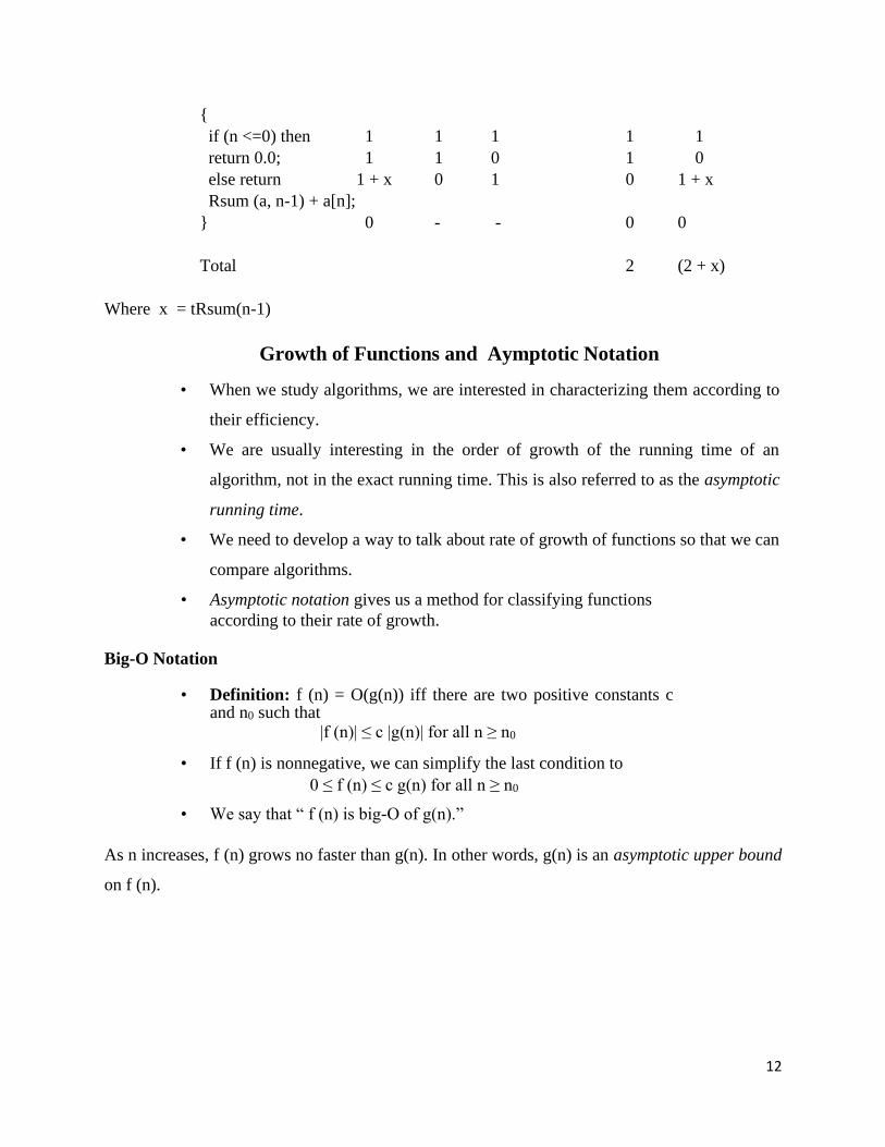
12
if (n <=0) then 1 1 1 1 1
return 0.0; 1 1 0 1 0
else return 1 + x 0 1 0 1 + x
Rsum (a, n-1) + a[n];
0 - - 0 0
Total 2 (2 + x)
Where x = tRsum(n-1)
Growth of Functions and Aymptotic Notation
• When we study algorithms, we are interested in characterizing them according to
their efficiency.
• We are usually interesting in the order of growth of the running time of an
algorithm, not in the exact running time. This is also referred to as the asymptotic
running time.
• We need to develop a way to talk about rate of growth of functions so that we can
compare algorithms.
• Asymptotic notation gives us a method for classifying functions
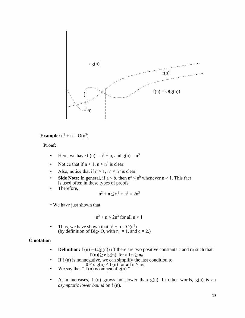
according to their rate of growth. Big-O Notation
• Definition: f (n) = O(g(n)) iff there are two positive constants c and n0 such that
|f (n)| ≤ c |g(n)| for all n ≥ n0
• If f (n) is nonnegative, we can simplify the last condition to 0 ≤ f (n) ≤ c g(n) for all n ≥ n0
• We say that “ f (n) is big-O of g(n).”
As n increases, f (n) grows no faster than g(n). In other words, g(n) is an asymptotic upper bound
on f (n).
13
cg(n)
f(n)
f(n) = O(g(n))
n0
Example: n2 + n = O(n3)
Proof:
• Here, we have f (n) = n2 + n, and g(n) = n3
• Notice that if n ≥ 1, n ≤ n3 is clear.
• Also, notice that if n ≥ 1, n2 ≤ n3 is clear.
• Side Note: In general, if a ≤ b, then na ≤ nb whenever n ≥ 1. This fact is used often in these types of proofs.
• Therefore,
n2 + n ≤ n3 + n3 = 2n3
• We have just shown that
n2 + n ≤ 2n3 for all n ≥ 1
• Thus, we have shown that n2 + n = O(n3) (by definition of Big- O, with n0 = 1, and c = 2.)
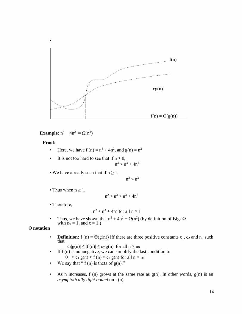
Ω notation
• Definition: f (n) = Ω(g(n)) iff there are two positive constants c and n0 such that |f (n)| ≥ c |g(n)| for all n ≥ n0
• If f (n) is nonnegative, we can simplify the last condition to 0 ≤ c g(n) ≤ f (n) for all n ≥ n0
• We say that “ f (n) is omega of g(n).”
• As n increases, f (n) grows no slower than g(n). In other words, g(n) is an
asymptotic lower bound on f (n).
14
•
f(n)
cg(n)
f(n) = O(g(n))
Example: n3 + 4n2 = Ω(n2)
Proof:
• Here, we have f (n) = n3 + 4n2, and g(n) = n2
• It is not too hard to see that if n ≥ 0, n3 ≤ n3 + 4n2
• We have already seen that if n ≥ 1,
n2 ≤ n3
• Thus when n ≥ 1, n2 ≤ n3 ≤ n3 + 4n2
• Therefore,
1n2 ≤ n3 + 4n2 for all n ≥ 1
• Thus, we have shown that n3 + 4n2 = Ω(n2) (by definition of Big- Ω, with n0 = 1, and c = 1.)
Θ notation
• Definition: f (n) = Θ(g(n)) iff there are three positive constants c1, c2 and n0 such that
c1|g(n)| ≤ |f (n)| ≤ c2|g(n)| for all n ≥ n0 • If f (n) is nonnegative, we can simplify the last condition to
0 ≤ c1 g(n) ≤ f (n) ≤ c2 g(n) for all n ≥ n0 • We say that “ f (n) is theta of g(n).”
• As n increases, f (n) grows at the same rate as g(n). In other words, g(n) is an
asymptotically tight bound on f (n).
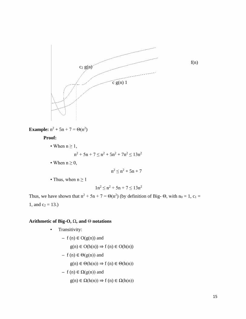
15
f(n) c2 g(n)
c g(n) 1
Example: n2 + 5n + 7 = Θ(n2)
Proof:
• When n ≥ 1,
n2 + 5n + 7 ≤ n2 + 5n2 + 7n2 ≤ 13n2
• When n ≥ 0,
n2 ≤ n2 + 5n + 7
• Thus, when n ≥ 1
1n2 ≤ n2 + 5n + 7 ≤ 13n2
Thus, we have shown that n2 + 5n + 7 = Θ(n2) (by definition of Big- Θ, with n0 = 1, c1 =
1, and c2 = 13.)
Arithmetic of Big-O, Ω, and Θ notations
• Transitivity:
– f (n) ∈ O(g(n)) and
g(n) ∈ O(h(n)) ⇒ f (n) ∈ O(h(n))
– f (n) ∈ Θ(g(n)) and
g(n) ∈ Θ(h(n)) ⇒ f (n) ∈ Θ(h(n))
– f (n) ∈ Ω(g(n)) and
g(n) ∈ Ω(h(n)) ⇒ f (n) ∈ Ω(h(n))
16
• Scaling: if f (n) ∈ O(g(n)) then for any k > 0, f (n) ∈
O(kg(n))
• Sums: if f1(n) ∈ O(g1(n)) and f2(n) ∈
O(g2(n)) then
(f1 + f2)(n) ∈ O(max(g1(n), g2(n)))
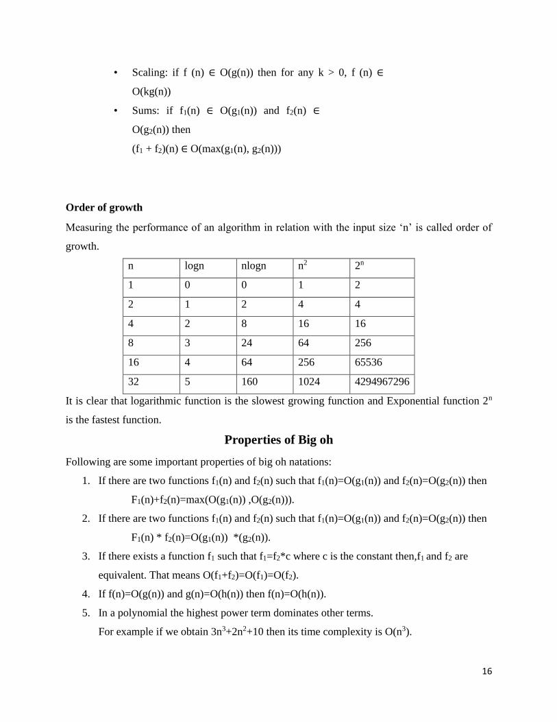
Order of growth
Measuring the performance of an algorithm in relation with the input size ‘n’ is called order of
growth.
n logn nlogn n2 2n
1 0 0 1 2
2 1 2 4 4
4 2 8 16 16
8 3 24 64 256
16 4 64 256 65536
32 5 160 1024 4294967296
It is clear that logarithmic function is the slowest growing function and Exponential function 2n
is the fastest function.
Properties of Big oh
Following are some important properties of big oh natations:
1. If there are two functions f1(n) and f2(n) such that f1(n)=O(g1(n)) and f2(n)=O(g2(n)) then
F1(n)+f2(n)=max(O(g1(n)) ,O(g2(n))).
2. If there are two functions f1(n) and f2(n) such that f1(n)=O(g1(n)) and f2(n)=O(g2(n)) then
F1(n) * f2(n)=O(g1(n)) *(g2(n)).
3. If there exists a function f1 such that f1=f2*c where c is the constant then,f1 and f2 are
equivalent. That means O(f1+f2)=O(f1)=O(f2).
4. If f(n)=O(g(n)) and g(n)=O(h(n)) then f(n)=O(h(n)).
5. In a polynomial the highest power term dominates other terms.
For example if we obtain 3n3+2n2+10 then its time complexity is O(n3).
17
6. Any constant value leads to O(1) time complexity. That is if f(n)=c then it Ɛ O(1) time
complexity.
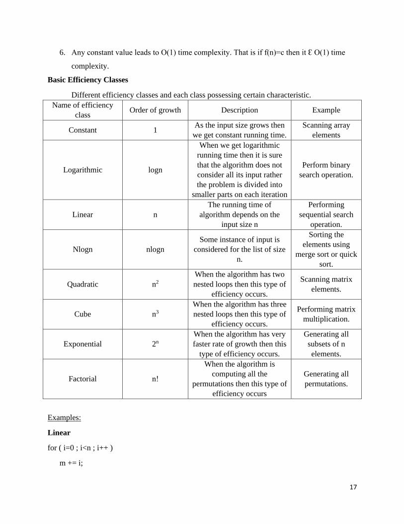
Basic Efficiency Classes
Different efficiency classes and each class possessing certain characteristic.
Name of efficiency
class Order of growth Description Example
Constant 1 As the input size grows then
we get constant running time.
Scanning array
elements
Logarithmic logn
When we get logarithmic
running time then it is sure
that the algorithm does not
consider all its input rather
the problem is divided into
smaller parts on each iteration
Perform binary
search operation.
Linear n
The running time of
algorithm depends on the
input size n
Performing
sequential search
operation.
Nlogn nlogn
Some instance of input is
considered for the list of size
n.
Sorting the
elements using
merge sort or quick
sort.
Quadratic n2
When the algorithm has two
nested loops then this type of
efficiency occurs.
Scanning matrix
elements.
Cube n3
When the algorithm has three
nested loops then this type of
efficiency occurs.
Performing matrix
multiplication.
Exponential 2n
When the algorithm has very
faster rate of growth then this
type of efficiency occurs.
Generating all
subsets of n
elements.
Factorial nǃ
When the algorithm is
computing all the
permutations then this type of
efficiency occurs
Generating all
permutations.
Examples:
Linear
for ( i=0 ; i<n ; i++ )
m += i;
18
Time Complexity O(n)
Quadratic
for ( i=0 ; i<n ; i++ )
for( j=0 ; j<n ; j++ )
sum[i] += entry[i][j];
Time Complexity O(n2)
Cubic
For(i=1;i<=n;i++)
For(j=1;j<=n;j++)
For(k=1;k<=n;k++)
Printf(“AAA”);
Time Complexity is O(n3)
Logarithmic
For(i=1;i<n;i=i*2)
Printf(“AAA”)
Time Complexity O(log n)
Linear Logarithmic (Nlogn)
For(i=1;i<n;i=i*2)
For(j=1;j<=n,j++)
Printf(“AAA”)
Performance Measurement
Performance measurement is concerned with obtaining the space and time requirements of a
particular algorithm. These quantities depend on the compiler and options used as well as on
which the algorithm is run. To obtain the computing or run time of a program, we need a
clocking procedure. Clock() that returns the current time in milliseconds. This function returns
the number of clock ticks since the program started.
19
To determine the worst case time requirements of functions Insertion sort. First we need to
1.Decide on the values of n for which the times to be obtained.
2. Determine, for each of the above values of n, the data that exhibits the worst-case behavior. Choosing Instant size
We decide on which values of n to use according to two factors: the amount of timing we want to
perform and what we expect to do with the times. In insertion sort the worst case complexity is
O(n2). It is Quadratic in n. We can obtain the time for all other values of n from this quadratic
function. We need the times for more than three values of n for the following reasons:
1.Asymptotic analysis tells the behavior only for sufficiently large values for n. For smaller
values of n, the run time may not follow the asymptotic curve. To determine the point beyond
which the asymptotic curve is followed, we need to examine the times for several values of n.
2.Even in the region where the asymptotic behavior is exhibited, the times may not lie exactly on
the predicted curve because of the effects of low-order terms that are discarded in the asymptotic
analysis. For instance, a program with asymptotic complexity O(n2) can have an actual
complexity that is c1n2+c2nlogn+c3n+c4- or any function of n in which the highest order term is
c1n2 for some constant c1, c1>0.
Developing the test Data
For many programs, we can generate manually or by computer the data that exhibits the best and
worst case time complexity. The average complexiy, is usually quite difficult to demonstrate. In
insertion sort, the worst case data for any n is a decreasing sequence such as n, n-1, n-2,….1. The
best case data is sorted sequence such as 0,1,…..n-1.
When we are unable to develop the data that exhibits the complexity we want to measure,
we can pick the least(maximum, average) measured time from some randomly generated data as
an estimate of the best(worst,average) behavior.
Setting up the Experiment
Having selected the instance sizes and developed the test data, then write the program that will
measure the desired run times. For the insertion sort , this program to be written as.
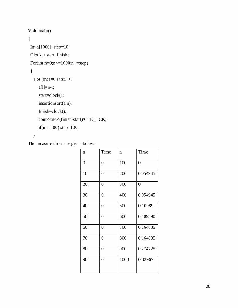
20
Void main()
Int a[1000], step=10;
Clock_t start, finish;
For(int n=0;n<=1000;n+=step)
For (int i=0;i<n;i++)
a[i]=n-i;
start=clock();
insertionsort(a,n);
finish=clock();
cout<<n<<(finish-start)/CLK_TCK;
if(n==100) step=100;
The measure times are given below.
n Time n Time
0 0 100 0
10 0 200 0.054945
20 0 300 0
30 0 400 0.054945
40 0 500 0.10989
50 0 600 0.109890
60 0 700 0.164835
70 0 800 0.164835
80 0 900 0.274725
90 0 1000 0.32967
21
In the above example, no time is needed to sort arrays with 100 or fewer numbers and that there
is no difference in the times to sort 500 through 600 numbers.All measurements are accurate to
with in one clock tick. If CLK-TCK=18.2 on our computer, the actual times may deviate from
the measured times by up to one tick or 1/18.2˜0.055 seconds.
22
SCHOOL OF COMPUTING
DEPARTMENT OF INFORMATION TECHNOLOGY
UNIT - II
Design and Analysis of Algorithm – SCSA1403
23
Mathematical Foundations 9 Hrs.
Solving Recurrence Equations - Substitution Method - Recursion Tree Method - Master Method
- Best Case - Worst Case - Average Case Analysis - Sorting in Linear Time - Lower bounds for
Sorting - Counting Sort - Radix Sort - Bucket Sort.
Recurrence Equations
The recurrence equation is an equation that defines a sequence recursively .It is normally in the
form
T(n) = T(n-1) + n for n>0 (Recurrence relation)
T(0) = 0 (Initial condition)
The general solution to the recursive function specifies some formula.
Solving Recurrence Equations The recurrence relation can be solved by following methods
Substitution method
Master’s method
1.Substitution Method
There are two types of substitution
Forward substitution
Backward substitution
Forward Substitution method This method makes use of an initial condition in the initial term and value for the next
term is generated. This process is continued until some formula is guessed. Thus in this kind of
method, we use recurrence equations to generate few terms.
For Example
Consider a recurrence relation T(n) = T(n-1) + n with initial condition T(0) = 0
Let T(n) = T(n-1) + n
If n = 1 then
T(1) = T(0) + 1 = 0+1 = 1 ------- (1)
If n = 2 then
T(2) = T(1) + 2 = 1+2 = 3 ------- (2)
If n = 3 then
T(3) = T(2) + 3 = 3 + 3 = 6 -------- (3)
By observing above equation , we can says that it is sum of n natural number
T(n) = 𝑛(𝑛+1)
𝑛 = 𝑛2/2 +
𝑛
2
So we can written as
T(n) = O(n2)
24
Backward Substitution Method
In this method backward values are substituted recursively in order to derive some formula.
For Example
Consider , a recurrence relation T(n) = T(n-1) + n with initial condition T(0) = 0 ------ (1)
Solution:
In Eqa(1) , to calculate T(n) , we need to know the value of T(n-1)
T(n-1) = T(n-1-1) + (n-1) = T(n-2)+(n-1)
Now Equ(1) becomes T(n) = T(n-2)+(n-1) + n ------------ (2)
T(n-2) = T(n-2-1) + (n-2) = T(n-3) + (n-2)
Now Eqa(2) becomes T(n) = T(n-3)+(n-2)+(n-1)+n ------ ---(3)
In the kth terms
T(n) = T(n-k)+(n-k+1)+(n-k+2)+-----+n ---------(4)
If k = n in equ(4) then
T(n) = T(0)+1+2+3+ ------ +n
T(n) = 0+1+2+3+-----+n by substituting initial value T(0) = 0
T(n) = 𝑛(𝑛+1)
𝑛 = 𝑛2/2 +
𝑛
2
So T(n) in terms of big oh notation as
T(n) = O(n2)
Example : 2
T(n) = T(n-1) + 1 with initial condition with T(0) = 0 . Find big oh notation.
Solution:
T(n) = T(n-1) + 1 --------- (1)
T(n-1) = T(n-2)+1
Now eqa(1) becomes T(n) = (T(n-2)+1)+1 = T(n-2)+2 -------- (2)
T(n-2) = T(n-3) + 1
Now eqa(2) becomes T(n) = (T(n-3)+1)+2 = T(n-3)+3 ------ (3)
So
T(n) = T(n-k)+k ------------ (4)
25
If k = n then eqa(4) becomes
T(n ) = T(0) + n = 0 + n = n
T(n) = O(n)
Example 3:
T(n) = 2T(n/2) + n. T(1) = 1 as initial condition
Solution:
T(n) = 2T(n/2) + n. ------------- (1)
T(n/2) = 2𝑇(𝑛/4) + 𝑛/2
Now Eqa (1) becomes
T(n) = 2[2𝑇(𝑛/4) + 𝑛/2]+n = 4T(n/4)+n+n = 4T(n/4)+2n ----- (2)
T(n/4) = 2𝑇(𝑛/8) + 𝑛/4
Now eqa(2) becomes
T(n) = 4[2𝑇(𝑛/8) + 𝑛/4]+2n = 8T(n/8)+n+2n = 8T(n/8)+3n ------ (3)
Equ(3) can be written as
T(n) = 23T(n/23)+3n
In general
T(n) = 2kT(n/2k) + kn ---------- (4)
Assume 2k = n
Now Equ(4) can be written as
T(n) = n.T(n/n)+logn.n
=n.T(1) + n.logn
T(n) = n + n.logn
i.e T(n) = O(n.logn)
Example 4:
T(n) = T(n/3) + C and initial condition T(1) = 1
Solution :
T(n) = T(n/3) + C ----------- (1)
T(n/3) = T(n/9)+C
Now Equ(1) becomes

26
T(n) = [T(n/9)+C] + C = T(n/9) + 2C ----- (2)
T(n/9) = T(n/27) + C
Now Equ(2) becomes
T(n) = [T(n/27)+C] + 2C
T(n) = T(n/27) + 3C
In General
T(n) = T(n/3k) + kC
Put 3k = n then
T(n) = T(n/n)+log3n.C
= T(1) + log3n.C
T(n) = C. log3n + 1
Tree Method
In this method, we buit a recurrence tree in which each node represents the cost of a single sub
problemin the form of recursive function invocations.Then we sum up the cost at each levelto
determine the overall cost.Thus the recursion tree helps us to make a good guess of time
complexity. The pattern is typically a arithmetic or geometric series.
For example consider the recurrence relation
T(n) = T(n/4) + T(n/2) + cn2
cn2
/ \
T(n/4) T(n/2)
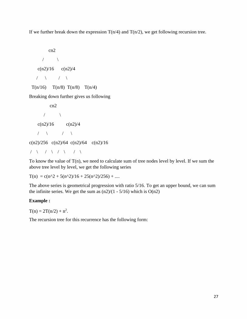
27
If we further break down the expression T(n/4) and T(n/2), we get following recursion tree.
cn2
/ \
c(n2)/16 c(n2)/4
/ \ / \
T(n/16) T(n/8) T(n/8) T(n/4)
Breaking down further gives us following
cn2
/ \
c(n2)/16 c(n2)/4
/ \ / \
c(n2)/256 c(n2)/64 c(n2)/64 c(n2)/16
/ \ / \ / \ / \
To know the value of T(n), we need to calculate sum of tree nodes level by level. If we sum the
above tree level by level, we get the following series
T(n) = c(n^2 + 5(n^2)/16 + 25(n^2)/256) + ....
The above series is geometrical progression with ratio 5/16. To get an upper bound, we can sum
the infinite series. We get the sum as (n2)/(1 - 5/16) which is O(n2)
Example :
T(n) = 2T(n/2) + n2.
The recursion tree for this recurrence has the following form:
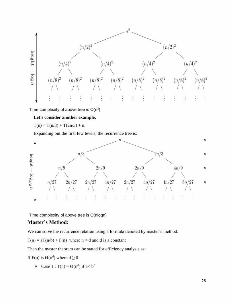
28
Time complexity of above tree is O(n2)
Let's consider another example,
T(n) = T(n/3) + T(2n/3) + n.
Expanding out the first few levels, the recurrence tree is:
Time complexity of above tree is O(nlogn)
Master’s Method:
We can solve the recurrence relation using a formula denoted by master’s method.
T(n) = aT(n/b) + F(n) where n ≥ d and d is a constant
Then the master theorem can be stated for efficiency analysis as:
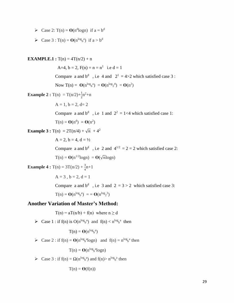
If F(n) is ϴ(nd) where d ≥ 0
Case 1 : T(n) = ϴ(nd) if a< bd
29
Case 2: T(n) = ϴ(ndlogn) if a = bd
Case 3 : T(n) = ϴ(nlogb
a) if a > bd
EXAMPLE.1 : T(n) = 4T(n/2) + n
A=4, b = 2, F(n) = n = n1 i.e d = 1
Compare a and bd , i.e 4 and 21 = 4>2 which satisfied case 3 :
Now T(n) = ϴ(nlogb
a) = ϴ(nlog24) = ϴ(n2)
Example 2 : T(n) = T(n/2)+1
2n2+n
A = 1, b = 2, d= 2
Compare a and bd , i.e 1 and 22 = 1<4 which satisfied case 1:
T(n) = ϴ(nd) = ϴ(n2)
Example 3 : T(n) = 2T(n/4) + √𝑛 + 42
A = 2, b = 4, d = ½
Compare a and bd , i.e 2 and 41/2 = 2 = 2 which satisfied case 2:
T(n) = ϴ(n1/2logn) = ϴ(√𝑛logn)
Example 4 : T(n) = 3T(n/2) + 3
4n+1
A = 3 , b = 2, d = 1
Compare a and bd , i.e 3 and 2 = 3 > 2 which satisfied case 3:
T(n) = ϴ(nlogba) = = ϴ(nlog
23)
Another Variation of Master’s Method:
T(n) = aT(n/b) + f(n) where n ≥ d
Case 1 : if f(n) is O(nlogb
a) and f(n) < nlogba then
T(n) = ϴ(nlogba)
Case 2 : if f(n) = ϴ(nlogb
alogn) and f(n) = nlogb
a then
T(n) = ϴ(nlogbalogn)
Case 3 : if f(n) = Ω(nlogb
a) and f(n)> nlogba then
T(n) = ϴ(f(n))
30
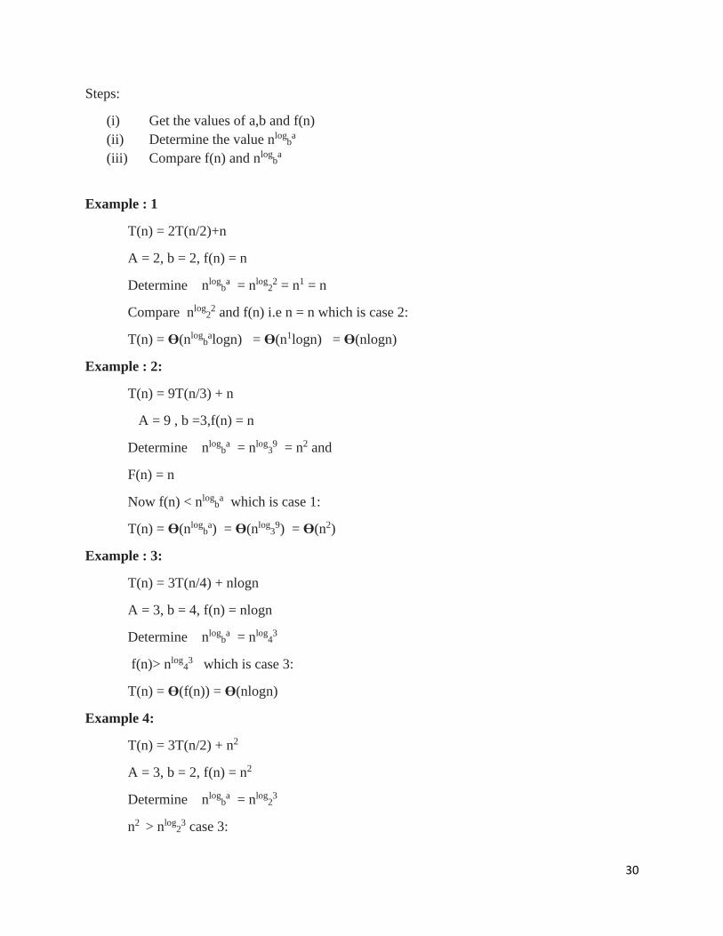
Steps:
(i) Get the values of a,b and f(n)
(ii) Determine the value nlogba
(iii) Compare f(n) and nlogb
a
Example : 1
T(n) = 2T(n/2)+n
A = 2, b = 2, f(n) = n
Determine nlogba = nlog
22 = n1 = n
Compare nlog22 and f(n) i.e n = n which is case 2:
T(n) = ϴ(nlogbalogn) = ϴ(n1logn) = ϴ(nlogn)
Example : 2:
T(n) = 9T(n/3) + n
A = 9 , b =3,f(n) = n
Determine nlogba = nlog
39 = n2 and
F(n) = n
Now f(n) < nlogb
a which is case 1:
T(n) = ϴ(nlogba) = ϴ(nlog
39) = ϴ(n2)
Example : 3:
T(n) = 3T(n/4) + nlogn
A = 3, b = 4, f(n) = nlogn
Determine nlogba = nlog
43
f(n)> nlog43 which is case 3:
T(n) = ϴ(f(n)) = ϴ(nlogn)
Example 4:
T(n) = 3T(n/2) + n2
A = 3, b = 2, f(n) = n2
Determine nlogba = nlog
23
n2 > nlog23 case 3:
31
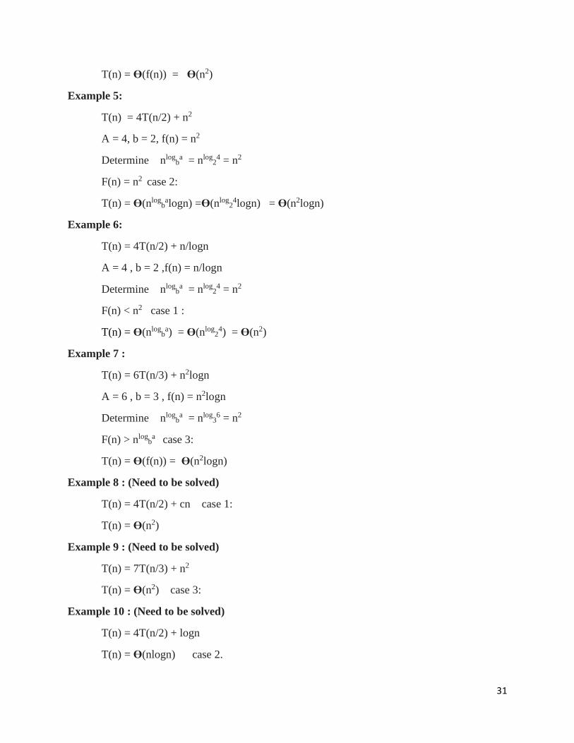
T(n) = ϴ(f(n)) = ϴ(n2)
Example 5:
T(n) = 4T(n/2) + n2
A = 4, b = 2, f(n) = n2
Determine nlogba = nlog
24 = n2
F(n) = n2 case 2:
T(n) = ϴ(nlogbalogn) =ϴ(nlog
24logn) = ϴ(n2logn)
Example 6:
T(n) = 4T(n/2) + n/logn
A = 4 , b = 2 ,f(n) = n/logn
Determine nlogba = nlog
24 = n2
F(n) < n2 case 1 :
T(n) = ϴ(nlogba) = ϴ(nlog
24) = ϴ(n2)
Example 7 :
T(n) = 6T(n/3) + n2logn
A = 6 , b = 3 , f(n) = n2logn
Determine nlogba = nlog
36 = n2
F(n) > nlogb
a case 3:
T(n) = ϴ(f(n)) = ϴ(n2logn)
Example 8 : (Need to be solved)
T(n) = 4T(n/2) + cn case 1:
T(n) = ϴ(n2)
Example 9 : (Need to be solved)
T(n) = 7T(n/3) + n2
T(n) = ϴ(n2) case 3:
Example 10 : (Need to be solved)
T(n) = 4T(n/2) + logn
T(n) = ϴ(nlogn) case 2.
32
Example 11 : (Need to be solved)
T(n) = 16T(n/4) + n
T(n) = ϴ(n2) case 1
Example 12 : (Need to be solved)
T(n) = 2T(n/2) + nlogn
T(n) = ϴ( logn) case 3.
Worst Case - Average Case Analysis - Linear Search
Let us consider the following implementation of Linear Search.
// Linearly search x in arr[]. If x is present then return the index,
// otherwise return -1
int search(int arr[], int n, int x)
int i;
for (i=0; i<n; i++)
if (arr[i] == x)
return i;
return -1;
Worst Case Analysis (Usually Done)
In the worst case analysis, we calculate upper bound on running time of an algorithm. We must
know the case that causes maximum number of operations to be executed. For Linear Search, the
worst case happens when the element to be searched (x in the above code) is not present in the
array or the search element is present at nth location. For these cases, the search() functions
compares it with all the elements of arr[] one by one. Therefore, the worst case time complexity
of linear search would be O(n).
Average Case Analysis (Sometimes done)
Average case complexity gives information about the behaviour of an algorithm on a random
input. Let us understand some terminologies that are required for computing average case time
complexity.
33
Let the algorithm is for linear search and P be a probability of getting successful search.N is the
total number of elements in the list.
The first match of the element will occur at ith location. Hence the probability of occurring first
match is P/n for every ith element.The probability of getting unsuccessful search is (1-P).
Now, we can find average case time complexity Ɵ (n) as-
Ɵ (n) =probability of successful search+ probability of unsuccessful search
Ɵ (n) =[1.P/n+2.P/n+...+i.P/n+...n.P/n] +n. (1-P) //There may be n elements at which
chances of not getting element are possible. Hence n. (1-P)
=P/n [1+2+...+i...n] +n (1-P)
=P/n. (n (n+1))/2+n (1-P)
Ɵ (n) =P (n+1)/2+n (1-P)
Thus we can obtain the general formula for computing average case time complexity.
Suppose if P=0 that means there is no successful search i.e. we have scanned the entire list of n
elements and still we do not found the desired element in the list then in such a situation ,
Ɵ (n) =O (n+1) / 2+n (1-0)
Ɵ (n) = n
Thus the average case running time complexity is n.Suppose if P=1 i.e. we get a successful
search then
Ɵ (n) = 1(n+1)/2 + n (1-1)
Ɵ (n) = (n+1) / 2
That means the algorithm scans about half of the elements from the list. Thus computing average
case time complexity is difficult than computing worst case and best case time complexities.
Best Case Analysis (omega)
In the best case analysis, we calculate lower bound on running time of an algorithm. We must
know the case that causes minimum number of operations to be executed. In the linear search
problem, the best case occurs when x is present at the first location. The number of operations in
the best case is constant (not dependent on n). So time complexity in the best case would be Ω
(1).
34
Time complexity for linear search
Best Case Worst Case Average Case
Ω(1) O(n) Ɵ (n)
Sorting In Linear Time Most of the sorting algorithms can sort n numbers in O(n lg n) time. Merge sort and heapsort
achieve this upper bound in the worst case; quicksort achieves it on average. Moreover, for each
of these algorithms, we can produce a sequence of n input numbers that causes the algorithm to
run in (n lg n) time. All those algorithms possess an interesting property say the sorted order
they determine is based only on comparisons between the input elements. Therefore such sorting
algorithms can be called as comparison sorts.
The following section proves that any comparison sort must make (n lg n) comparisons in the
worst case to sort a sequence of n elements. Thus, merge sort and heapsort are asymptotically
optimal, and no comparison sort exists that is faster by more than a constant factor. Further three
sorting algorithms which includes--counting sort, radix sort, and bucket sort--that run in linear
time. Needless to say, these algorithms use operations other than comparisons to determine the
sorted order. Consequently, the (n lg n) lower bound does not apply to them.
Lower bounds for sorting:
In a comparison sort, comparisons between elements made in order to gain the order information
about an input sequence a1, a2, . . . ,an) That is, given two elements ai and aj, One of the tests
might be performed ai < aj, ai aj, ai = aj, ai aj, or ai > aj to determine their relative order. We
may not inspect the values of the elements or gain order information about them in any other
way. We assume without loss of generality that all of the input elements are distinct. Given this
assumption, comparisons of the form ai = aj are useless, so we can assume that no comparisons
of this form are made. We also note that the comparisons ai aj, ai aj, ai > aj, and ai < aj are
all equivalent in that they yield identical information about the relative order of ai and aj. We
therefore assume that all comparisons have the form ai aj.
35
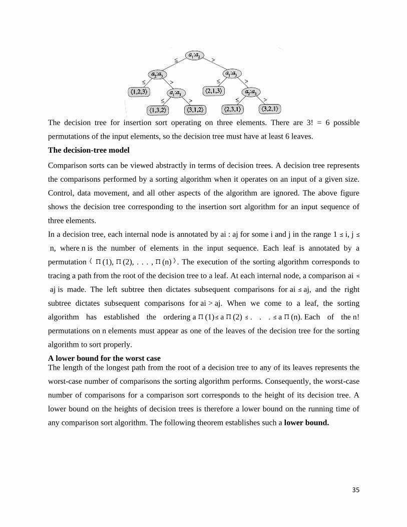
The decision tree for insertion sort operating on three elements. There are 3! = 6 possible
permutations of the input elements, so the decision tree must have at least 6 leaves.
The decision-tree model
Comparison sorts can be viewed abstractly in terms of decision trees. A decision tree represents
the comparisons performed by a sorting algorithm when it operates on an input of a given size.
Control, data movement, and all other aspects of the algorithm are ignored. The above figure
shows the decision tree corresponding to the insertion sort algorithm for an input sequence of
three elements.
In a decision tree, each internal node is annotated by ai : aj for some i and j in the range 1 i, j
n, where n is the number of elements in the input sequence. Each leaf is annotated by a
permutation (1), (2), . . . , (n) . The execution of the sorting algorithm corresponds to
tracing a path from the root of the decision tree to a leaf. At each internal node, a comparison ai
aj is made. The left subtree then dictates subsequent comparisons for ai aj, and the right
subtree dictates subsequent comparisons for ai > aj. When we come to a leaf, the sorting
algorithm has established the ordering a (1) a (2) . . . a (n). Each of the n!
permutations on n elements must appear as one of the leaves of the decision tree for the sorting
algorithm to sort properly.
A lower bound for the worst case
The length of the longest path from the root of a decision tree to any of its leaves represents the
worst-case number of comparisons the sorting algorithm performs. Consequently, the worst-case
number of comparisons for a comparison sort corresponds to the height of its decision tree. A
lower bound on the heights of decision trees is therefore a lower bound on the running time of
any comparison sort algorithm. The following theorem establishes such a lower bound.
36
Theorem
Any decision tree that sorts n elements has height (n lg n).
Proof Consider a decision tree of height h that sorts n elements. Since there are n! permutations
of n elements, each permutation representing a distinct sorted order, the tree must have at least n!
leaves. Since a binary tree of height h has no more than 2h leaves, we have
n! 2h ,
which, by taking logarithms, implies
h lg(n!) ,
since the lg function is monotonically increasing. From Stirling's approximation, we have
Radix Sort
The idea of Radix Sort is to do digit by digit sort starting from least significant digit to most
significant digit. Radix sort uses counting sort as a subroutine to sort. Radix sort iteratively
orders all the strings by their nth character – in the first iteration, the strings are ordered by their
last character. In the second run, the strings are ordered in respect to their penultimate character.
And because the sort is stable, the strings, which have the same penultimate character, are still
sorted in accordance to their last characters. After nth run the strings are sorted in respect to all
character positions.
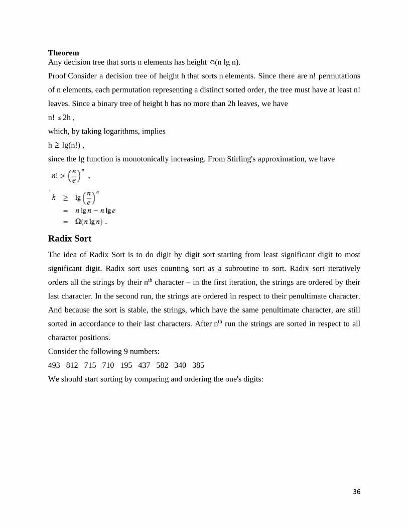
Consider the following 9 numbers:
493 812 715 710 195 437 582 340 385
We should start sorting by comparing and ordering the one's digits:
37
Digit Sublist
0 710,340
1
2 812, 582
3 493
4
5 715, 195, 385
6
7 437
8
9
Notice that the numbers were added onto the list in the order that they were found, which is why
the numbers appear to be unsorted in each of the sub lists above. Now, we gather the sub lists (in
order from the 0 sub list to the 9 sub list) into the main list again:
710, 340 ,812, 582, 493, 715, 195, 385, 437
Note: The order in which we divide and reassemble the list is extremely important, as this is one
of the foundations of this algorithm.
Now, the sub lists are created again, this time based on the ten's digit:
Digit Sub list
0
1 710,812, 715
2
3 437
4 340
5
6
7
8 582,,385
9 493, 195
Now the sub lists are gathered in order from 0 to 9:
710, 812, 715, 437, 340, 582,385, 493,195
38
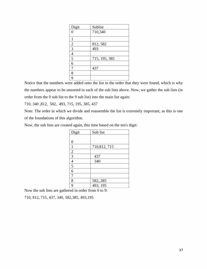
Finally, the sub lists are created according to the hundred's digit:
Digit Sub list
0
1 195
2
3 340, 385
4 437, 493
5 582
6
7 710 ,715
8 812
9
At last, the list is gathered up again:
195, 340, 385,437,493,582,710,715,812
And now we have a fully sorted array! Radix Sort is very simple, and a computer can do it fast.
When it is programmed properly, Radix Sort is in fact one of the fastest sorting algorithms for
numbers or strings of letters.
Radix-Sort(A, d)
// Each key in A[1..n] is a d-digit integer.
(Digits are // numbered 1 to d from right to left.)
for i = 1 to d do
Use a stable sorting algorithm to sort A on digit i.
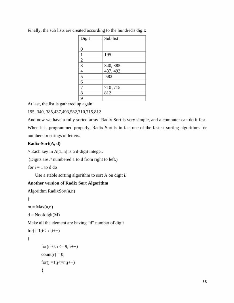
Another version of Radix Sort Algorithm
Algorithm RadixSort(a,n)
m = Max(a,n)
d = Noofdigit(M)
Make all the element are having “d” number of digit
for(i=1;i<=d,i++)
for(r=0; r<= 9; r++)
count[r] = 0;
for(j =1;j<=n;j++)
39
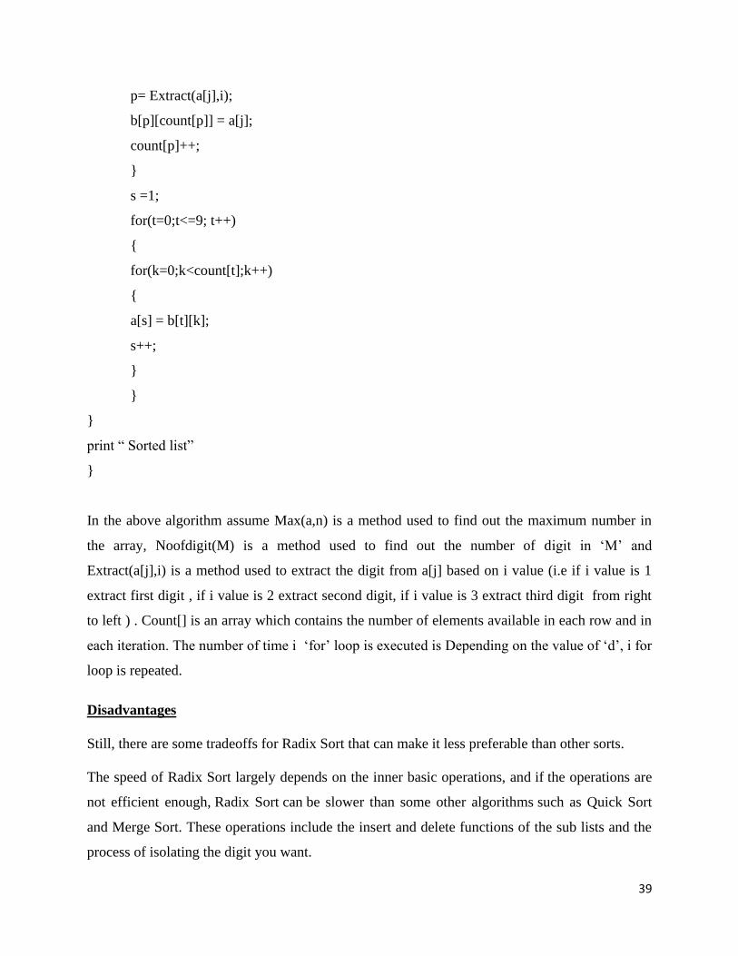
p= Extract(a[j],i);
b[p][count[p]] = a[j];
count[p]++;
s =1;
for(t=0;t<=9; t++)
for(k=0;k<count[t];k++)
a[s] = b[t][k];
s++;
print “ Sorted list”
In the above algorithm assume Max(a,n) is a method used to find out the maximum number in
the array, Noofdigit(M) is a method used to find out the number of digit in ‘M’ and
Extract(a[j],i) is a method used to extract the digit from a[j] based on i value (i.e if i value is 1
extract first digit , if i value is 2 extract second digit, if i value is 3 extract third digit from right
to left ) . Count[] is an array which contains the number of elements available in each row and in
each iteration. The number of time i ‘for’ loop is executed is Depending on the value of ‘d’, i for
loop is repeated.
Disadvantages
Still, there are some tradeoffs for Radix Sort that can make it less preferable than other sorts.
The speed of Radix Sort largely depends on the inner basic operations, and if the operations are
not efficient enough, Radix Sort can be slower than some other algorithms such as Quick Sort
and Merge Sort. These operations include the insert and delete functions of the sub lists and the
process of isolating the digit you want.
40
In the example above, the numbers were all of equal length, but many times, this is not the case.
If the numbers are not of the same length, then a test is needed to check for additional digits that
need sorting. This can be one of the slowest parts of Radix Sort, and it is one of the hardest to
make efficient.
Analysis
Worst case complexity O(d *n)
Average case complexity ϴ( d* n).
Best Case Complexity Ω( d * n )
Let there be d digits in input integers. Radix Sort takes O(d*(n+b)) time where b is the base for
representing numbers, for example, for decimal system, b is 10. What is the value of d? If k is
the maximum possible value, then d would be O(logb(k)). So overall time complexity is O((n+b)
* logb(k)). Which looks more than the time complexity of comparison based sorting algorithms
for a large k. Let us first limit k. Let k <= nc where c is a constant. In that case, the complexity
becomes O(nLogb(n)). But it still doesn’t beat comparison based sorting algorithms.
What if we make value of b larger?. What should be the value of b to make the time complexity
linear? If we set b as n, we get the time complexity as O(n). In other words, we can sort an array
of integers with range from 1 to nc if the numbers are represented in base n (or every digit takes
log2(n) bits).
Bucket Sort
Bucket sort (bin sort) is a stable sorting algorithm based on partitioning the input array into
several parts – so called buckets – and using some other sorting algorithm for the actual sorting
of these sub problems.
At first algorithm divides the input array into buckets. Each bucket contains some range of input
elements (the elements should be uniformly distributed to ensure optimal division among
buckets).In the second phase the bucket sort orders each bucket using some other sorting
algorithm, or by recursively calling itself – with bucket count equal to the range of values, bucket
sort degenerates to counting sort. Finally the algorithm merges all the ordered buckets. Because
every bucket contains different range of element values, bucket sort simply copies the elements
of each bucket into the output array (concatenates the buckets).
41
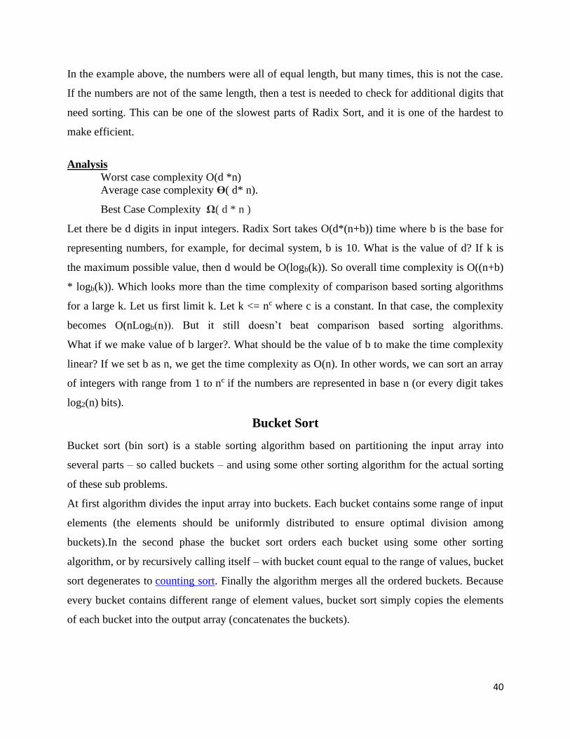
BUCKET SORT (a,n)
n ← length [a]
m = Max(a,n)
nob = 10 // Number of backet
divider = ceil((m+1)/nob);
for i = 1 to n do
j = floor(a[i]/divider)
b[j] = a[i]
for i = 0 to 9 do
sort b[i] with Insertion sort
concatenate the lists B[0], B[1], . . B[9] together in order.
End Bucket Sort
Example :
a = 123,67,45,3,69,245,35,90
n= 8
max = 245
nob = 10 ( No of backet)
divider = ceil((m+1)/nob) = ceil((245+1)/nob)
= ceil(246/10) = ceil(24.6) = 25
j = floor(125/25) = 5 , so b[5] = 125
j = floor(67/25) = floor(2.68) = 2 , so b[2] = 67
j = floor(45/25) = floor(1.8) = 1 , so b[1] = 45
j = floor(3/25) = floor(0.12) = 0 , so b[0] = 3
j = floor(69/25) = floor(2.76) = 2 , so b[2] = 69
j = floor(245/25) = floor(9.8) = 9 , so b[9] = 245
j = floor(35/25) = floor(1.4) = 1 , so b[1] = 35
j = floor(90/25) = floor(3.6) = 3, so b[3] = 90
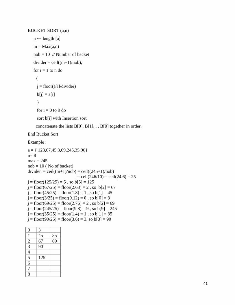
0 3
1 45 35
2 67 69
3 90
4
5 125
6
7
8
42
9 245
In the above array apply insertion sort in each row
0 3
1 35 45
2 67 69
3 90
4
5 125
6
7
8
9 245
Now concatenate all the row elements of b array
So sorted list is a = 3,35,45,67,69,125,245
Complexity
T(n) = [time to insert n elements in array A] + [time to go through auxiliary array B[0 . . n-1] *
(Sort by INSERTION_SORT)
= O(n) + (n-1) * (n)
= O(n) + n2 – n
= O(n2)
Worse case = O(n2)
Best case : Ω( n+k )
Average case : ϴ( n + k).
Therefore, the entire Bucket sort algorithm runs in linear expected time.
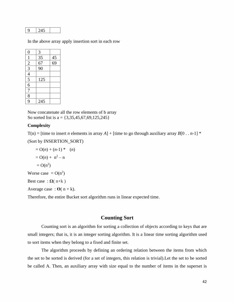
Counting Sort
Counting sort is an algorithm for sorting a collection of objects according to keys that are
small integers; that is, it is an integer sorting algorithm. It is a linear time sorting algorithm used
to sort items when they belong to a fixed and finite set.
The algorithm proceeds by defining an ordering relation between the items from which
the set to be sorted is derived (for a set of integers, this relation is trivial).Let the set to be sorted
be called A. Then, an auxiliary array with size equal to the number of items in the superset is
43
defined, say B. For each element in A, say e, the algorithm stores the number of items in A
smaller than or equal to e in B(e). If the sorted set is to be stored in an array C, then for each e in
A, taken in reverse order, C[B[e]] = e. Counting sort assumes that each of the n input elements is
an integer in the range 0 to k. that is n is the number of elements and k is the highest value
element.
Counting sort determines for each input element x, the number of elements less than x.
And it uses this information to place element x directly into its position in the output array.
Consider the input set : 4, 1, 3, 4, 3. Then n=5 and k=4
The algorithm uses three array:
Input Array: A[1..n] store input data where A[j] ∈ 1, 2, 3, …, k
Output Array: B[1..n] finally store the sorted data
Temporary Array: C[1..k] store data temporarily
Counting Sort Example
Example 1 :
Given List :
A = 2,5,3,0,2,3,0,3
Step:1
A
1 2 3 4 5 6 7 8
2 5 3 0 2 3 0 3
C- Highest Element is 5 in the given array
0 1 2 3 4 5
0 0 0 0 0 0
B-Output Array
Step:2
C[A[J]]=C[A[J]]+1
C[A[1]]=C[2]=C[2]+1 . In the place of C[2] add 1.
0 1 2 3 4 5
0 0 1 0 0 0
44
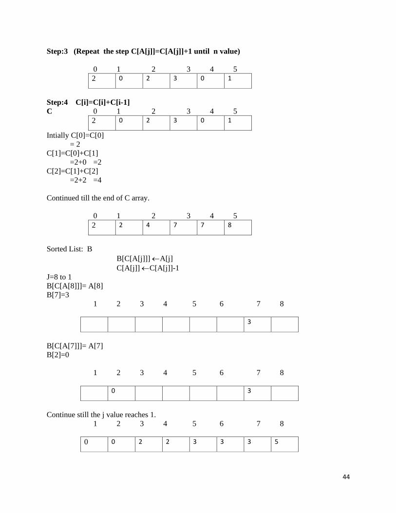
Step:3 (Repeat the step C[A[j]]=C[A[j]]+1 until n value)
0 1 2 3 4 5
2 0 2 3 0 1
Step:4 C[i]=C[i]+C[i-1]
C 0 1 2 3 4 5
2 0 2 3 0 1
Intially C[0]=C[0]
= 2
C[1]=C[0]+C[1]
=2+0 =2
C[2]=C[1]+C[2]
=2+2 =4
Continued till the end of C array.
0 1 2 3 4 5
2 2 4 7 7 8
Sorted List: B
B[C[A[j]]] A[j]
C[A[j]] C[A[j]]-1
J=8 to 1
B[C[A[8]]]= A[8]
B[7]=3
1 2 3 4 5 6 7 8
3
B[C[A[7]]]= A[7]
B[2]=0
1 2 3 4 5 6 7 8
0 3
Continue still the j value reaches 1.
1 2 3 4 5 6 7 8
0 0 2 2 3 3 3 5
45
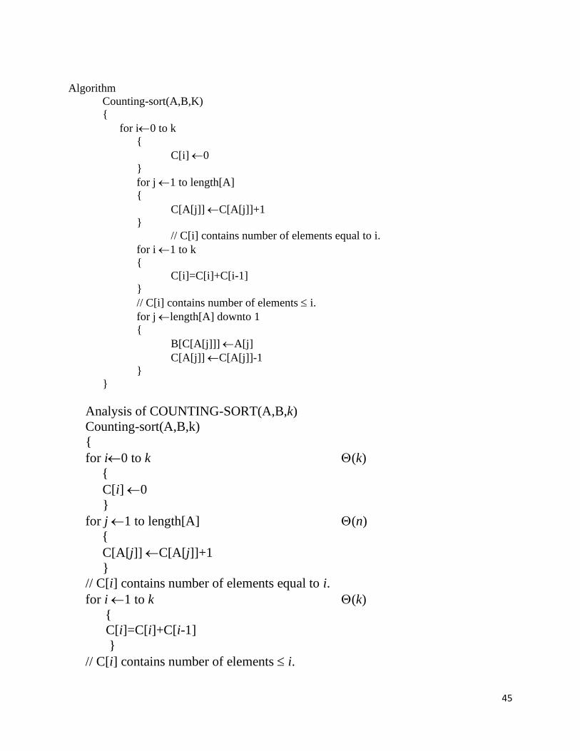
Algorithm
Counting-sort(A,B,K)
for i0 to k
C[i] 0
for j 1 to length[A]
C[A[j]] C[A[j]]+1
// C[i] contains number of elements equal to i.
for i 1 to k
C[i]=C[i]+C[i-1]
// C[i] contains number of elements i.
for j length[A] downto 1
B[C[A[j]]] A[j]
C[A[j]] C[A[j]]-1
Analysis of COUNTING-SORT(A,B,k)
Counting-sort(A,B,k)
for i0 to k (k)
C[i] 0
for j 1 to length[A] (n)
C[A[j]] C[A[j]]+1
// C[i] contains number of elements equal to i.
for i 1 to k (k)
C[i]=C[i]+C[i-1]
// C[i] contains number of elements i.
46
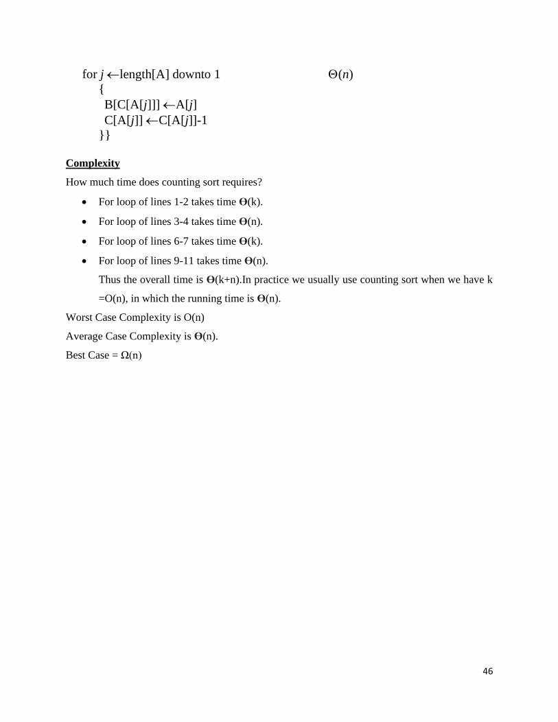
for j length[A] downto 1 (n)
B[C[A[j]]] A[j]
C[A[j]] C[A[j]]-1
Complexity
How much time does counting sort requires?
• For loop of lines 1-2 takes time ϴ(k).
• For loop of lines 3-4 takes time ϴ(n).
• For loop of lines 6-7 takes time ϴ(k).
• For loop of lines 9-11 takes time ϴ(n).
Thus the overall time is ϴ(k+n).In practice we usually use counting sort when we have k
=O(n), in which the running time is ϴ(n).
Worst Case Complexity is O(n)
Average Case Complexity is ϴ(n).
Best Case = Ω(n)
47
SCHOOL OF COMPUTING
DEPARTMENT OF INFORMATION TECHNOLOGY
UNIT - III
Design and Analysis of Algorithm – SCSA1403
48
Brute Force And Divide-And-Conquer 9 Hrs.
Brute Force:- Travelling Salesman Problem - Knapsack Problem - Assignment Problem - Closest
Pair and Convex Hull Problems - Divide and Conquer Approach:- Binary Search - Quick Sort -
Merge Sort - Strassen’s Matrix Multiplication.
Brute Force Algorithms
It is a straight forward approach which depends on problem statement and definition. Following
algorithms belong to this category.“Force” comes from using computer power not intellectual
power
Examples
1. Selection Sort
2. Computing an (a > 0, n a nonnegative integer)
3. Graph Traversal
4. Computing n!
5. Simple Computational Tasks
6. Exhaustive Search
7. Multiplying two matrices
8. Searching for a key of a given value in a list
Strengths
1. Most of the practical problems apply this approach
2. Simple
3. Results in acceptable algorithms for some important problems like matrix
multiplication, sorting, searching and string matching
Weaknesses
1. Algorithms cannot be guaranteed as efficient
2. Some of these algorithms are very slow
3. Useful only for instances of small size
4. Not as constructive as some other design techniques
Example 1:
Computing an (a > 0, n a nonnegative integer) based on the definition of exponentiation
an = a * a * a*.....*a
The brute force algorithm requires n-1 multiplications.
49
The recursive algorithm for the same problem, based on the observation that an =an/2 * an/2
requires Θ(log (n)) operations.
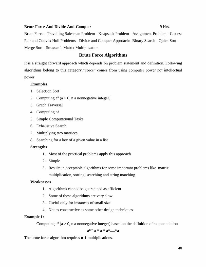
Travelling Salesman Problem
A complete graph KN is a graph with N vertices and an edge between every two vertices.
Using Hamilton circuit we can find a solution. It is a circuit that uses every vertex of a graph
once.
A weighted graph is a graph in which each edge is assigned a weight (representing the
time, distance, or cost of traversing that edge).
The Travelling Salesman Problem (TSP) is the problem of finding a minimum-weight
Hamilton circuit in KN
Example:
Given n cities with known distances between each pair, find the shortest tour that passes
through all the cities exactly once before returning to the starting city.
To solve TSP using Brute-force method we can use the following steps:
Step 1. Calculate the total number of tours
Step 2. Draw and list all the possible tours
Step 3. Calculate the distance of each tour
Step 4. Choose the shortest tour, this is the optimal solution
Solution to TSP byExhaustive approach
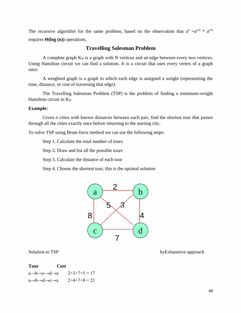
Tour Cost
a→b→c→d→a 2+3+7+5 = 17
a→b→d→c→a 2+4+7+8 = 21
a b
c d
8
2
7
5 34
2
5 3
4
7
8
50
a→c→b→d→a 8+3+4+5 = 20
a→c→d→b→a 8+7+4+2 = 21
a→d→b→c→a 5+4+3+8 = 20
a→d→c→b→a 5+7+3+2 = 17
Efficiency:Θ((n-1)!)
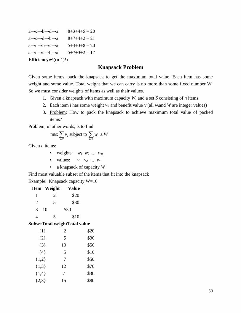
Knapsack Problem
Given some items, pack the knapsack to get the maximum total value. Each item has some
weight and some value. Total weight that we can carry is no more than some fixed number W.
So we must consider weights of items as well as their values.
1. Given a knapsack with maximum capacity W, and a set S consisting of n items
2. Each item i has some weight wi and benefit value vi(all wiand W are integer values)
3. Problem: How to pack the knapsack to achieve maximum total value of packed
items?
Problem, in other words, is to find
Ti
i
Ti
i Wwv subject to max
Given n items:
• weights: w1 w2 … wn
• values: v1 v2 … vn
• a knapsack of capacity W
Find most valuable subset of the items that fit into the knapsack
Example: Knapsack capacity W=16
Item Weight Value
1 2 $20
2 5 $30
3 10 $50
4 5 $10
SubsetTotal weightTotal value
1 2 $20
2 5 $30
3 10 $50
4 5 $10
1,2 7 $50
1,3 12 $70
1,4 7 $30
2,3 15 $80
51
2,4 10 $40
3,4 15 $60
1,2,3 17 not feasible
1,2,4 12 $60
1,3,4 17 not feasible
2,3,4 20 not feasible
1,2,3,4 22 not feasible
Efficiency: Θ(2n)
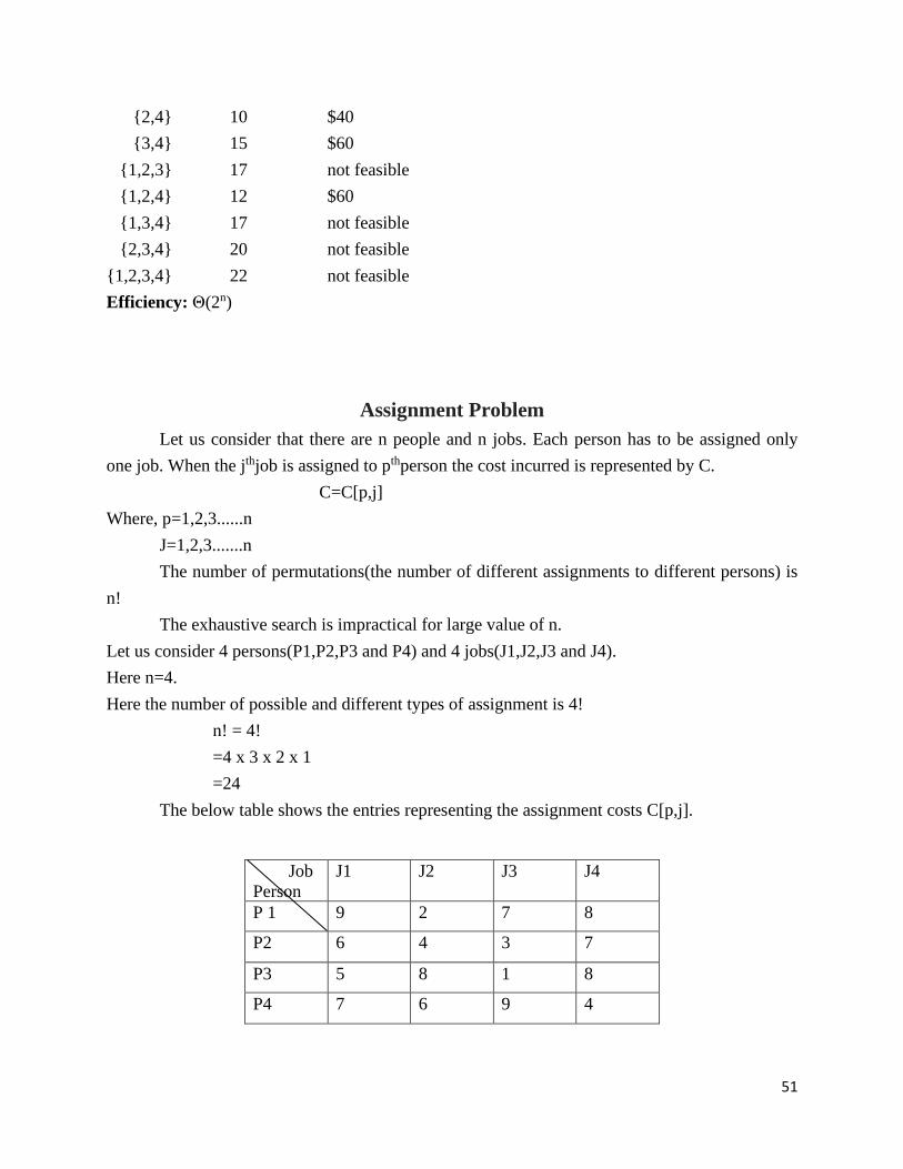
Assignment Problem
Let us consider that there are n people and n jobs. Each person has to be assigned only
one job. When the jthjob is assigned to pthperson the cost incurred is represented by C.
C=C[p,j]
Where, p=1,2,3......n
J=1,2,3.......n
The number of permutations(the number of different assignments to different persons) is
n!
The exhaustive search is impractical for large value of n.
Let us consider 4 persons(P1,P2,P3 and P4) and 4 jobs(J1,J2,J3 and J4).
Here n=4.
Here the number of possible and different types of assignment is 4!
n! = 4!
=4 x 3 x 2 x 1
=24
The below table shows the entries representing the assignment costs C[p,j].
Job
Person
J1 J2 J3 J4
P 1 9 2 7 8
P2 6 4 3 7
P3 5 8 1 8
P4 7 6 9 4
52
Iterations of solving the above assignment problem are given below. Here 4 persons indicated by
P1,P2,P3 and P4; Similarly 4 jobs are indicated by J1,J2,J3 and J4.
Let us consider that the assignments can be grouped into 4 groups.
In the first group J1 is assigned to person P1. The remaining jobs J2, J3 and J4 are
assigned to persons P2, P3 and P4. The number of ways in which these three jobs can be
assigned to three persons is 3!(3!=6).
Group-I
Group-2
In the second group J2 is assigned to person P1. The remaining jobs J3,J4,J1 are
assigned to persons P2,P3 and P4. The number of ways in which these three jobs can be assigned
to three persons is 3!(3!=6).
9+4+8+9 = 30
9+4+1+8 = 18
9+3+8+4= 24
9+3+8+6= 26
9+7+8+9= 33
9+7+1+6= 23
P1 P2 P3 P4
J1 J2 J3 J4
P1 P2 P3 P4
J1 J2 J4 J3
P1 P2 P3 P4
J1 J3 J2 J4
P1 P2 P3 P4
J1 J3 J4 J2
P1 P2 P3 P4
J1 J4 J2 J3
P1 P2 P3 P4
J1 J4 J3 J2
53
Group-3
In the third group J3 is assigned to person P1. The remaining jobs J2,J4,J1 are assigned
to persons P2,P3 and P4. The number of ways in which these three jobs can be assigned to three
persons is 3!(3!=6).
2+3+5+4 = 14
2+3+8+7 = 20
2+7+1+7= 17
2+7+5+9= 23
2+6+1+4= 13
2+6+8+9= 25
P1 P2 P3 P4
J2 J3 J4 J1
P1 P2 P3 P4
J2 J3 J1 J4
P1 P2 P3 P4
J2 J4 J3 J1
P1 P2 P3 P4
J2 J4 J1 J3
P1 P2 P3 P4
J2 J1 J3 J4
P1 P2 P3 P4
J2 J1 J4 J3
54
Group-4
In the Fourth group J4 is assigned to person P1. The remaining jobs J2,J3,J1 are assigned
to persons P2,P3 and P4. The number of ways in which these three jobs can be assigned to three
persons is 3!(3!=6).
7+7+8+7 = 29
7+7+5+6 = 25
7+6+8+6= 27
7+4+8+7= 26
7+6+8+4= 25
7+4+5+4= 20
P1 P2 P3 P4
J3 J4 J1 J2
P1 P2 P3 P4
J3 J4 J2 J1
P1 P2 P3 P4
J3 J1 J4 J2
P1 P2 P3 P4
J3 J2 J4 J1
P1 P2 P3 P4
J3 J1 J2 J4
P1 P2 P3 P4
J3 J2 J1 J4
55
In the above four groups low costs are:
Group 1- 1st iteration is lowest 18
Group-II – 5th iteration is lowest 13
Group-III- 6th iteration is lowest 20
Group-IV- 4th iteration is lowest 20
Efficiency – O(n)!
8+6+8+9 = 31
8+6+1+6 = 21
8+4+5+9= 26
8+4+1+7= 20
8+3+5+6= 22
8+3+8+7= 26
P1 P2 P3 P4
J4 J1 J2 J3
P1 P2 P3 P4
J4 J1 J3 J2
P1 P2 P3 P4
J4 J2 J1 J3
P1 P2 P3 P4
J4 J2 J3 J1
P1 P2 P3 P4
J4 J3 J1 J2
P1 P2 P3 P4
J3 J3 J2 J1
56
Closest Pair Algorithm
Given n points in the plane, find a pair with smallest Euclidean distance between them.
When brute force method is used, it is required to check all pairs of points p and q with (n2)
comparisons.
Euclidean distance d(Pi, Pj) = Sqrt[(xi-xj)2 + (yi-yj)
2]
Find the minimal distance between a pairs in a set of points
Algorithm BruteForceClosestPoints(P)
// P is list of points
dmin ← ∞
fori ← 1 to n-1 do
for j ← i+1 to n do
d ← sqrt((xi-xj)2 + (yi-yj)
2)
if d<dmin then
dmin ← d; index1 ← i; index2 ← j
return index1, index2
Analysis:
Note the algorithm does not have to calculate the square root
Then the basic operation is squaring
C(n) = ∑i=1n-1 ∑j=i+1
n 2
= 2∑j=i+1n (n-i)
= 2n(n-1)/2
Θ(n2)
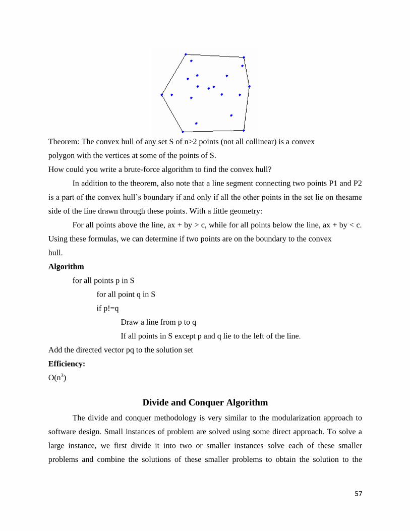
Convex Hull Problems In this problem, we want to compute the convex hull of a set of points?
· Formally: It is the smallest convex set containing the points. A convex set is one in
which if we connect any two points in the set, the line segment connecting these points
must also be in the set.
· Informally: It is a rubber band wrapped around the "outside" points.
57
Theorem: The convex hull of any set S of n>2 points (not all collinear) is a convex
polygon with the vertices at some of the points of S.
How could you write a brute-force algorithm to find the convex hull?
In addition to the theorem, also note that a line segment connecting two points P1 and P2
is a part of the convex hull’s boundary if and only if all the other points in the set lie on thesame
side of the line drawn through these points. With a little geometry:
For all points above the line, ax + by > c, while for all points below the line, ax + by < c.
Using these formulas, we can determine if two points are on the boundary to the convex
hull.
Algorithm
for all points p in S
for all point q in S
if p!=q
Draw a line from p to q
If all points in S except p and q lie to the left of the line.
Add the directed vector pq to the solution set
Efficiency:
O(n3)
Divide and Conquer Algorithm
The divide and conquer methodology is very similar to the modularization approach to
software design. Small instances of problem are solved using some direct approach. To solve a
large instance, we first divide it into two or smaller instances solve each of these smaller
problems and combine the solutions of these smaller problems to obtain the solution to the
58
original instance. The smaller instances are often instances of the original problem and may be
solved using divide and conquer strategy recursively.
In Divide and Conquer approach ,we solve a problem recursively by applying 3 steps
1.DIVIDE-break the problem into several sub problems of smaller size.
2.CONQUER-solve the problem recursively.
3.COMBINE-combine these solutions to create a solution to the original problem.
CONTROL ABSTRACTION FOR DIVIDE AND CONQUER ALGORITHM
Algorithm DivideandConquer (P)
if small(P)
then return S(P)
Else
divide P into smaller instances P1 ,P2 .....Pk
Apply Divide and Conquer to each sub problem
Return combine (D and C(P1)+ D and C(P2)+.......+D and C(Pk))
Efficiency Analysis of Divide and Conquer
Let a recurrence relation is expressed as T(n)= ϴ(1), if n<=C
T(n)=aT(n/b) +f(n)
Assume n=bk,
T(bk)= aT(bk/b)+f(bk)
T(bk)= aT(bk-1)+f(bk) .............(1)
Assume n=bk-1,
T(bk-1)= aT(bk-1/b)+f(bk-1)
T(bk-1)= aT(bk-2)+f(bk-2)
Substitute in (1) equation
T(bk)= a(aT(bk-2)+f(bk-2))+ f(bk)
T(bk)= a2T(bk-2)+af(bk-2)+ f(bk) ............(2)
Assume n=bk-2,
T(bk-2)= aT(bk-2/b)+f(bk-2)
T(bk-2)= aT(bk-3)+f(bk-2)
Substitute in (2) equation
T(bk)= a2(aT(bk-3)+ f(bk-2))+af(bk-2)+ f(bk)
59
T(bk)= a3T(bk-3)+ a2f(bk-2))+af(bk-2)+ f(bk)............(3)
Continuing in this way, we will get
= akT(bk-k)+ ak-1f(bk-(k-1)))+ ak-2f(bk-(k-2))) +.........+ af(bk-1)+ f(bk)
= akT(b0)+ ak-1f(b1))+ ak-2f(b2)) +.........+ af(bk-1)+ f(bk)
= akT(1)+ ak-1f(b1))+ ak-2f(b2)) +.........+ af(bk-1)+ f(bk)
= akT(1)+ ak-1f(b1))+ ak-2f(b2)) +.........+ af(bk-1)+ f(bk)
=akT(1)+𝑎𝑘
𝑎+ 𝑓(𝑏1) +
𝑎𝑘
𝑎2 𝑓(𝑏2) +𝑎𝑘
𝑎3 𝑓(𝑏3) + ⋯ +𝑎𝑘
𝑎𝑘−1 𝑓(𝑏𝑘−1) +𝑎𝑘
𝑎𝑘 𝑓(𝑏𝑘)
=ak[T(1)+𝑓(𝑏)
𝑎+
𝑓(𝑏2)
𝑎2 + ⋯ +𝑓(𝑏𝑘−1)
𝑎𝑘−1 +𝑓(𝑏𝑘)
𝑎𝑘 ]
T(bk) = ak[T(1)+∑𝑓(𝑏𝑗)
𝑎𝑗𝑘𝑗=1 ]
By property of logarithm,
𝑎𝑙𝑜𝑔𝑏𝑥=𝑥𝑙𝑜𝑔𝑏𝑎
ak=𝑎𝑙𝑜𝑔𝑏𝑛
ak=𝑛𝑙𝑜𝑔𝑏𝑎
K=log𝑏 𝑛
Substituting the values of ak and k
T(b) = alogb
a[T(1)+∑𝑓(𝑏𝑗)
𝑎𝑗
log𝑏 𝑛𝑗=1
Binary Search
Binary search method is very fast and efficient. This method requires that the list of
elements be in sorted order. Binary search cannot be applied on an unsorted list.
Principle: The data item to be searched is compared with the approximate middle entry of the
list. If it matches with the middle entry, then the position will be displayed. If the data item to
be searched is lesser than the middle entry, then it is compared with the middle entry of the first
half of the list and procedure is repeated on the first half until the required item is found. If the
data item is greater than the middle entry, then it is compared with the middle entry of the second
half of the list and procedure is repeated on the second half until the required item is found. This
process continues until the desired number is found or the search interval becomes empty.
Algorithm:
ALGORITHM BINARYSEARCH(K, N, X)
// K is the array containing the list of data items
// N is the number of data items in the list
// X is the data item to be searched
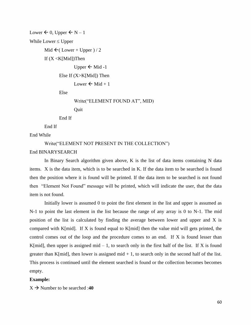
60
Lower 0, Upper N – 1
While Lower Upper
Mid ( Lower + Upper ) / 2
If (X <K[Mid])Then
Upper Mid -1
Else If (X>K[Mid]) Then
Lower Mid + 1
Else
Write(“ELEMENT FOUND AT”, MID)
Quit
End If
End If
End While
Write(“ELEMENT NOT PRESENT IN THE COLLECTION”)
End BINARYSEARCH
In Binary Search algorithm given above, K is the list of data items containing N data
items. X is the data item, which is to be searched in K. If the data item to be searched is found
then the position where it is found will be printed. If the data item to be searched is not found
then “Element Not Found” message will be printed, which will indicate the user, that the data
item is not found.
Initially lower is assumed 0 to point the first element in the list and upper is assumed as
N-1 to point the last element in the list because the range of any array is 0 to N-1. The mid
position of the list is calculated by finding the average between lower and upper and X is
compared with K[mid]. If X is found equal to K[mid] then the value mid will gets printed, the
control comes out of the loop and the procedure comes to an end. If X is found lesser than
K[mid], then upper is assigned mid – 1, to search only in the first half of the list. If X is found
greater than K[mid], then lower is assigned mid + 1, to search only in the second half of the list.
This process is continued until the element searched is found or the collection becomes becomes
empty.
Example:
X → Number to be searched :40
61
U → Upper
L → Lower=N-1
M→ Mid
i = 0 i =1 i = 2 i = 3 i = 4 i = 5 i = 6 i = 7 i = 8 i = 9
1 22 35 40 43 56 75 83 90 98
L = 0 M = (0+9)/2 =4 U = 9
X<K[4] → U = 4 – 1 = 3
1 22 35 40 43 56 75 83 90 98
L = 0 M = (0+3)/2=1 U = 3
X >K[1] → L = 1 + 1 = 2
1 22 35 40 43 56 75 83 90 98
L, M = 2 U = 3
K > A [2] → L = 2 + 1 = 3
1 22 35 40 43 56 75 83 90 98
L, M, U = 3
K = A[3] → P = 3 : Number found at position 3
The binarysearch( ) function gets the element to be searched in the variable X. Initially
lower is assigned 0 and upper is assumed N – 1. The mid position is calculated and if K[mid] is
found equal to X, then mid position will gets displayed. If X is less than K[mid] upper is
assigned mid – 1 to search only in first half of the list else lower is assigned mid + 1 to search
only in the second half of the list. This is process is continued until lower is less than or equal to
upper. If the element is not found even after the loop is completed, then the Not Found Message
will be displayed to the user indicating that the element is not found.
Advantages:
1. Searches several times faster than the linear search.
2. In each iteration, it reduces the number of elements to be searched from n to n/2.
Disadvantages:
1. Binary search can be applied only on a sorted list.
Analysis of Binary Search
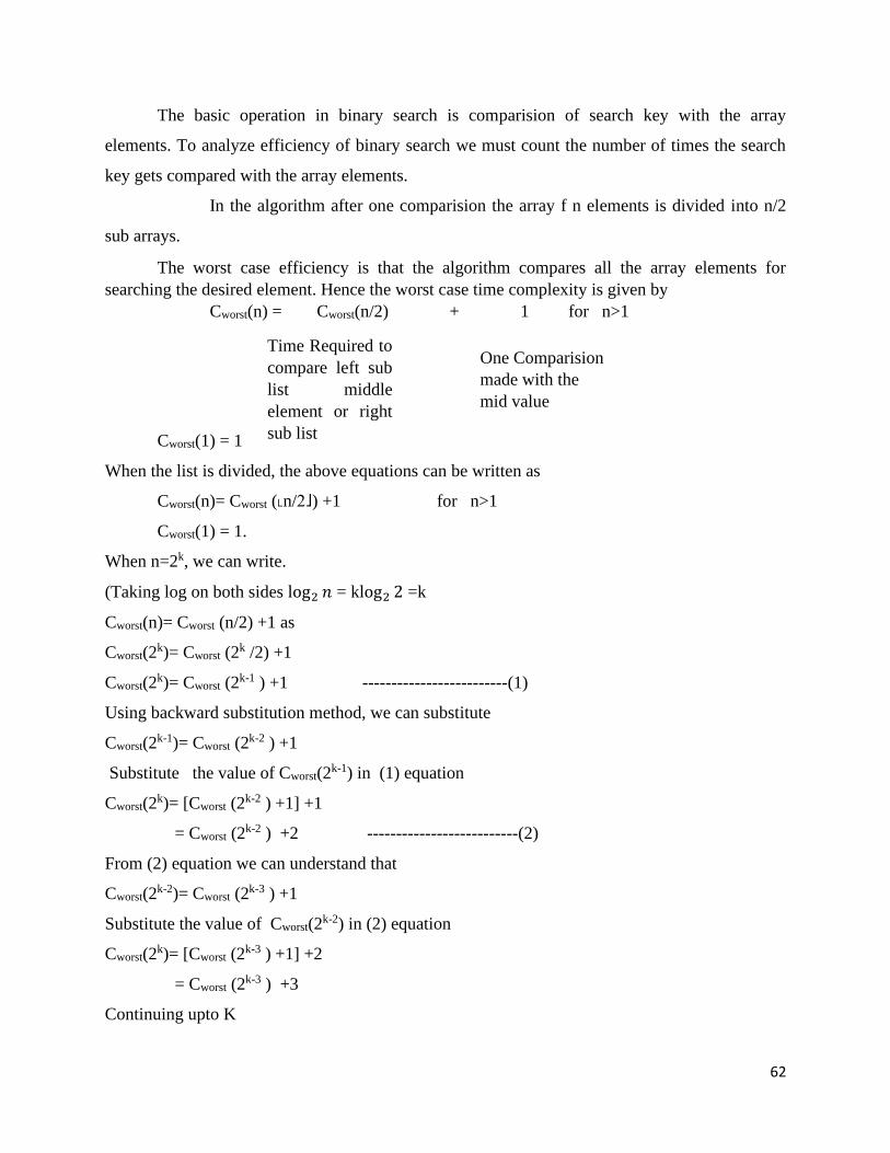
62
The basic operation in binary search is comparision of search key with the array
elements. To analyze efficiency of binary search we must count the number of times the search
key gets compared with the array elements.
In the algorithm after one comparision the array f n elements is divided into n/2
sub arrays.
The worst case efficiency is that the algorithm compares all the array elements for
searching the desired element. Hence the worst case time complexity is given by
Cworst(n) = Cworst(n/2) + 1 for n>1
Cworst(1) = 1
When the list is divided, the above equations can be written as
Cworst(n)= Cworst (˪n/2˩) +1 for n>1
Cworst(1) = 1.
When n=2k, we can write.
(Taking log on both sides log2 𝑛 = klog2 2 =k
Cworst(n)= Cworst (n/2) +1 as
Cworst(2k)= Cworst (2
k /2) +1
Cworst(2k)= Cworst (2
k-1 ) +1 -------------------------(1)
Using backward substitution method, we can substitute
Cworst(2k-1)= Cworst (2
k-2 ) +1
Substitute the value of Cworst(2k-1) in (1) equation
Cworst(2k)= [Cworst (2
k-2 ) +1] +1
= Cworst (2k-2 ) +2 --------------------------(2)
From (2) equation we can understand that
Cworst(2k-2)= Cworst (2
k-3 ) +1
Substitute the value of Cworst(2k-2) in (2) equation
Cworst(2k)= [Cworst (2
k-3 ) +1] +2
= Cworst (2k-3 ) +3
Continuing upto K
Time Required to
compare left sub
list middle
element or right
sub list
One Comparision
made with the
mid value
63
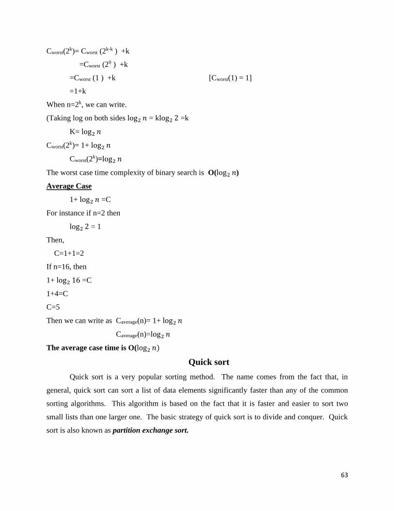
Cworst(2k)= Cworst (2
k-k ) +k
=Cworst (20 ) +k
=Cworst (1 ) +k [Cworst(1) = 1]
=1+k
When n=2k, we can write.
(Taking log on both sides log2 𝑛 = klog2 2 =k
K= log2 𝑛
Cworst(2k)= 1+ log2 𝑛
Cworst(2k)=log2 𝑛
The worst case time complexity of binary search is O(log2 𝑛)
Average Case
1+ log2 𝑛 =C
For instance if n=2 then
log2 2 = 1
Then,
C=1+1=2
If n=16, then
1+ log2 16 =C
1+4=C
C=5
Then we can write as Caverage(n)= 1+ log2 𝑛
Caverage(n)=log2 𝑛
The average case time is O(log2 𝑛)
Quick sort
Quick sort is a very popular sorting method. The name comes from the fact that, in
general, quick sort can sort a list of data elements significantly faster than any of the common
sorting algorithms. This algorithm is based on the fact that it is faster and easier to sort two
small lists than one larger one. The basic strategy of quick sort is to divide and conquer. Quick
sort is also known as partition exchange sort.
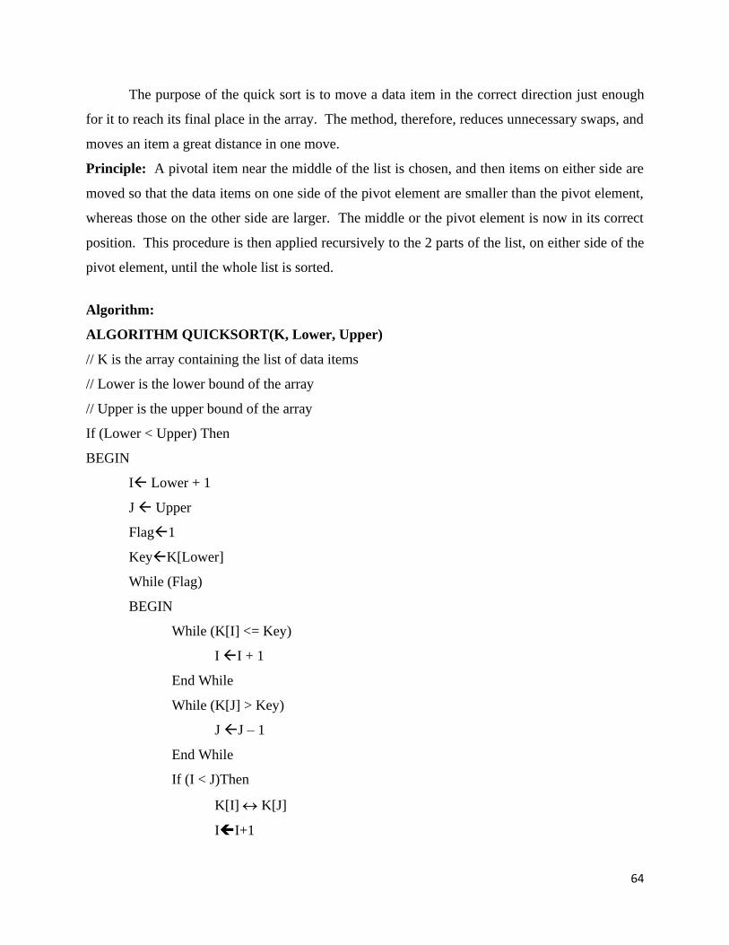
64
The purpose of the quick sort is to move a data item in the correct direction just enough
for it to reach its final place in the array. The method, therefore, reduces unnecessary swaps, and
moves an item a great distance in one move.
Principle: A pivotal item near the middle of the list is chosen, and then items on either side are
moved so that the data items on one side of the pivot element are smaller than the pivot element,
whereas those on the other side are larger. The middle or the pivot element is now in its correct
position. This procedure is then applied recursively to the 2 parts of the list, on either side of the
pivot element, until the whole list is sorted.
Algorithm:
ALGORITHM QUICKSORT(K, Lower, Upper)
// K is the array containing the list of data items
// Lower is the lower bound of the array
// Upper is the upper bound of the array
If (Lower < Upper) Then
BEGIN
I Lower + 1
J Upper
Flag1
KeyK[Lower]
While (Flag)
BEGIN
While (K[I] <= Key)
I I + 1
End While
While (K[J] > Key)
J J – 1
End While
If (I < J)Then
K[I] K[J]
II+1
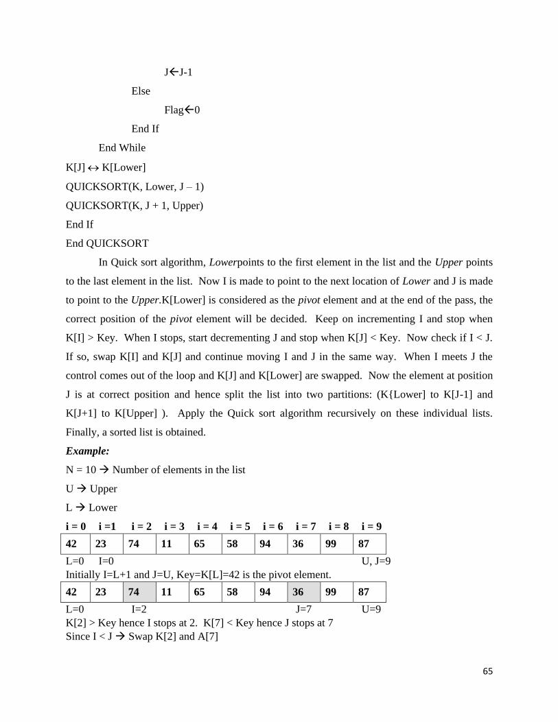
65
JJ-1
Else
Flag0
End If
End While
K[J] K[Lower]
QUICKSORT(K, Lower, J – 1)
QUICKSORT(K, J + 1, Upper)
End If
End QUICKSORT
In Quick sort algorithm, Lowerpoints to the first element in the list and the Upper points
to the last element in the list. Now I is made to point to the next location of Lower and J is made
to point to the Upper.K[Lower] is considered as the pivot element and at the end of the pass, the
correct position of the pivot element will be decided. Keep on incrementing I and stop when
K[I] > Key. When I stops, start decrementing J and stop when K[J] < Key. Now check if I < J.
If so, swap K[I] and K[J] and continue moving I and J in the same way. When I meets J the
control comes out of the loop and K[J] and K[Lower] are swapped. Now the element at position
J is at correct position and hence split the list into two partitions: (KLower] to K[J-1] and
K[J+1] to K[Upper] ). Apply the Quick sort algorithm recursively on these individual lists.
Finally, a sorted list is obtained.
Example:
N = 10 → Number of elements in the list
U → Upper
L → Lower
i = 0 i =1 i = 2 i = 3 i = 4 i = 5 i = 6 i = 7 i = 8 i = 9
42 23 74 11 65 58 94 36 99 87
L=0 I=0 U, J=9
Initially I=L+1 and J=U, Key=K[L]=42 is the pivot element.
42 23 74 11 65 58 94 36 99 87
L=0 I=2 J=7 U=9
K[2] > Key hence I stops at 2. K[7] < Key hence J stops at 7
Since I < J → Swap K[2] and A[7]
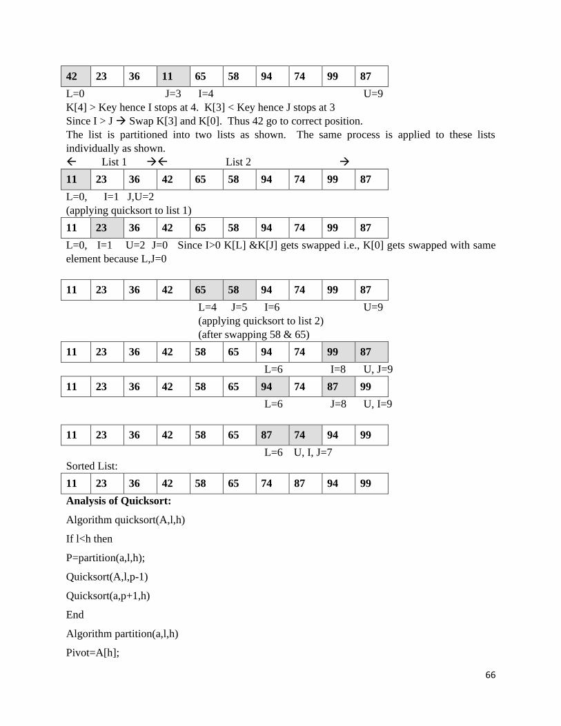
66
42 23 36 11 65 58 94 74 99 87
L=0 J=3 I=4 U=9
K[4] > Key hence I stops at 4. K[3] < Key hence J stops at 3
Since I > J → Swap K[3] and K[0]. Thus 42 go to correct position.
The list is partitioned into two lists as shown. The same process is applied to these lists
individually as shown.
List 1 → List 2 →
11 23 36 42 65 58 94 74 99 87
L=0, I=1 J,U=2
(applying quicksort to list 1)
11 23 36 42 65 58 94 74 99 87
L=0, I=1 U=2 J=0 Since I>0 K[L] &K[J] gets swapped i.e., K[0] gets swapped with same
element because L,J=0
11 23 36 42 65 58 94 74 99 87
L=4 J=5 I=6 U=9
(applying quicksort to list 2)
(after swapping 58 & 65)
11 23 36 42 58 65 94 74 99 87
L=6 I=8 U, J=9
11 23 36 42 58 65 94 74 87 99
L=6 J=8 U, I=9
11 23 36 42 58 65 87 74 94 99
L=6 U, I, J=7
Sorted List:
11 23 36 42 58 65 74 87 94 99
Analysis of Quicksort:
Algorithm quicksort(A,l,h)
If l<h then
P=partition(a,l,h);
Quicksort(A,l,p-1)
Quicksort(a,p+1,h)
End
Algorithm partition(a,l,h)
Pivot=A[h];
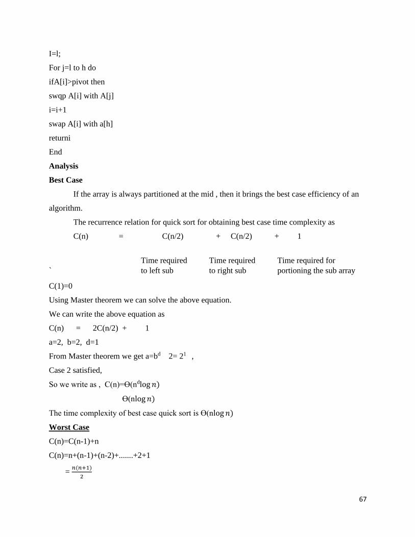
67
I=l;
For j=l to h do
ifA[i]>pivot then
swqp A[i] with A[j]
i=i+1
swap A[i] with a[h]
returni
End
Analysis
Best Case
If the array is always partitioned at the mid , then it brings the best case efficiency of an
algorithm.
The recurrence relation for quick sort for obtaining best case time complexity as
C(n) = C(n/2) + C(n/2) + 1
`
C(1)=0
Using Master theorem we can solve the above equation.
We can write the above equation as
C(n) = 2C(n/2) + 1
a=2, b=2, d=1
From Master theorem we get a=bd 2= 21 ,
Case 2 satisfied,
So we write as , C(n)=Ɵ(ndlog 𝑛)
Ɵ(nlog 𝑛)
The time complexity of best case quick sort is Ɵ(nlog 𝑛)
Worst Case
C(n)=C(n-1)+n
C(n)=n+(n-1)+(n-2)+.......+2+1
= 𝑛(𝑛+1)
2
Time required
to left sub
array
Time required
to right sub
array
Time required for
portioning the sub array
68
C(n)= 1
2𝑛2
C(n)= Ɵ(𝑛2)
The time complexity of worst case quick sort is Ɵ(𝑛2)
Average Case
The recurrence relation for random input array is
C(n)=C(0)+C(n-1)+n
C(n)=C(1)+C(n-2)+n
C(n)=C(2)+C(n-3)+n
..
.
.
C(n)=C(n-1)+C(0)+n
The array value of C(n) is the sum of all the above values divided by n
Cavg(n)=2𝐶(0)+𝐶(1)+𝐶(2)+⋯…..𝐶(𝑛−1)+𝑛.𝑛
𝑛
Cavg(n)=2
𝑛𝐶(0) + 𝐶(1) + 𝐶(2) + ⋯ … . . 𝐶(𝑛 − 1) + 𝑛
Multiplying both sides by n we get,
nCavg(n)= 2𝐶(0) + 𝐶(1) + 𝐶(2) + ⋯ … . . 𝐶(𝑛 − 1) + 𝑛2
Cavg(n)=2n ln n =1.38n log2 𝑛
Cavg(0)=0 and Cavg(1)=0
Time Complexity of average case quick sort is Ɵ(𝑛 log2 𝑛)
Merge Sort Principle: The given list is divided into two roughly equal parts called the left and the
right subfiles. These subfiles are sorted using the algorithm recursively and then the two
subfiles are merged together to obtain the sorted file.
Given a sequence of N elements K[0],K[1] ….K[N-1], the general idea is to
imagine them split into various subtables of size is equal to 1. So each set will have a
individually sorted items with it, then the resulting sorted sequences are merged to
produce a single sorted sequence of N elements. Thus this sorting method follows
Divide and Conquer strategy. The problem gets divided into various subproblems and
by providing the solutions to the subproblems the solution for the original problem will
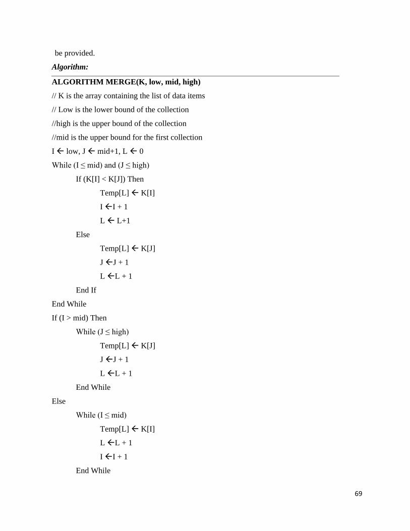
69
be provided.
Algorithm:
ALGORITHM MERGE(K, low, mid, high)
// K is the array containing the list of data items
// Low is the lower bound of the collection
//high is the upper bound of the collection
//mid is the upper bound for the first collection
I low, J mid+1, L 0
While (I ≤ mid) and (J ≤ high)
If (K[I] < K[J]) Then
Temp[L] K[I]
I I + 1
L L+1
Else
Temp[L] K[J]
J J + 1
L L + 1
End If
End While
If (I > mid) Then
While (J ≤ high)
Temp[L] K[J]
J J + 1
L L + 1
End While
Else
While (I ≤ mid)
Temp[L] K[I]
L L + 1
I I + 1
End While
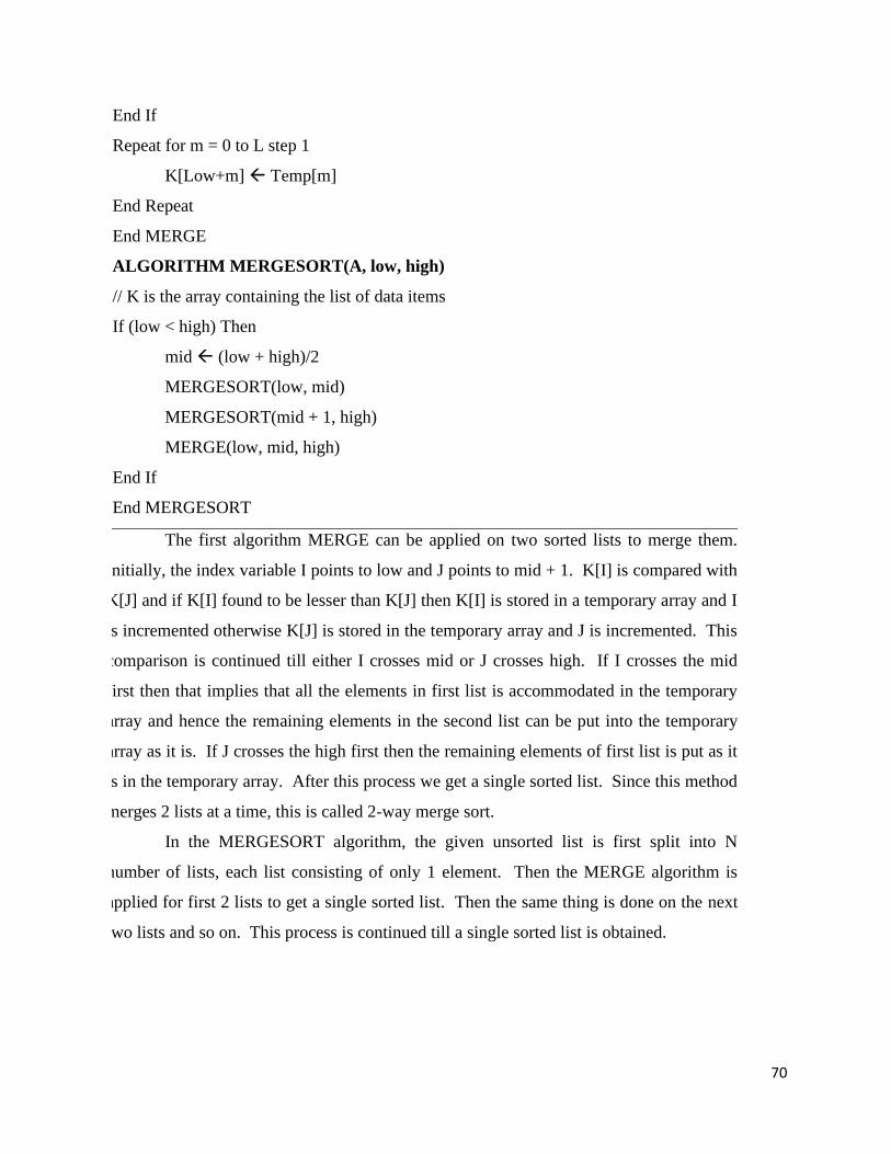
70
End If
Repeat for m = 0 to L step 1
K[Low+m] Temp[m]
End Repeat
End MERGE
ALGORITHM MERGESORT(A, low, high)
// K is the array containing the list of data items
If (low < high) Then
mid (low + high)/2
MERGESORT(low, mid)
MERGESORT(mid + 1, high)
MERGE(low, mid, high)
End If
End MERGESORT
The first algorithm MERGE can be applied on two sorted lists to merge them.
Initially, the index variable I points to low and J points to mid + 1. K[I] is compared with
K[J] and if K[I] found to be lesser than K[J] then K[I] is stored in a temporary array and I
is incremented otherwise K[J] is stored in the temporary array and J is incremented. This
comparison is continued till either I crosses mid or J crosses high. If I crosses the mid
first then that implies that all the elements in first list is accommodated in the temporary
array and hence the remaining elements in the second list can be put into the temporary
array as it is. If J crosses the high first then the remaining elements of first list is put as it
is in the temporary array. After this process we get a single sorted list. Since this method
merges 2 lists at a time, this is called 2-way merge sort.
In the MERGESORT algorithm, the given unsorted list is first split into N
number of lists, each list consisting of only 1 element. Then the MERGE algorithm is
applied for first 2 lists to get a single sorted list. Then the same thing is done on the next
two lists and so on. This process is continued till a single sorted list is obtained.
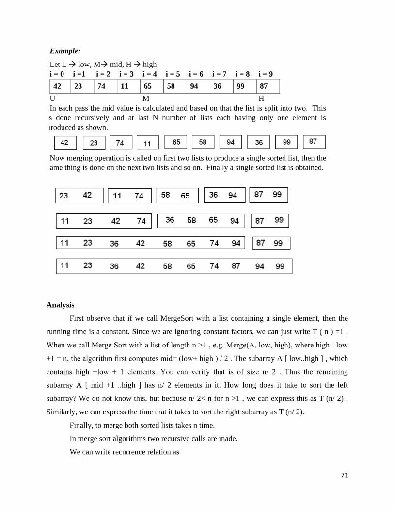
71
Analysis
First observe that if we call MergeSort with a list containing a single element, then the
running time is a constant. Since we are ignoring constant factors, we can just write T ( n ) =1 .
When we call Merge Sort with a list of length n >1 , e.g. Merge(A, low, high), where high −low
+1 = n, the algorithm first computes mid= (low+ high ) / 2 . The subarray A [ low..high ] , which
contains high −low + 1 elements. You can verify that is of size n/ 2 . Thus the remaining
subarray A [ mid +1 ..high ] has n/ 2 elements in it. How long does it take to sort the left
subarray? We do not know this, but because n/ 2< n for n >1 , we can express this as T (n/ 2) .
Similarly, we can express the time that it takes to sort the right subarray as T (n/ 2).
Finally, to merge both sorted lists takes n time.
In merge sort algorithms two recursive calls are made.
We can write recurrence relation as
Example:
Let L → low, M→ mid, H → high
i = 0 i =1 i = 2 i = 3 i = 4 i = 5 i = 6 i = 7 i = 8 i = 9
42 23 74 11 65 58 94 36 99 87
U M H
In each pass the mid value is calculated and based on that the list is split into two. This
is done recursively and at last N number of lists each having only one element is
produced as shown.
Now merging operation is called on first two lists to produce a single sorted list, then the
same thing is done on the next two lists and so on. Finally a single sorted list is obtained.
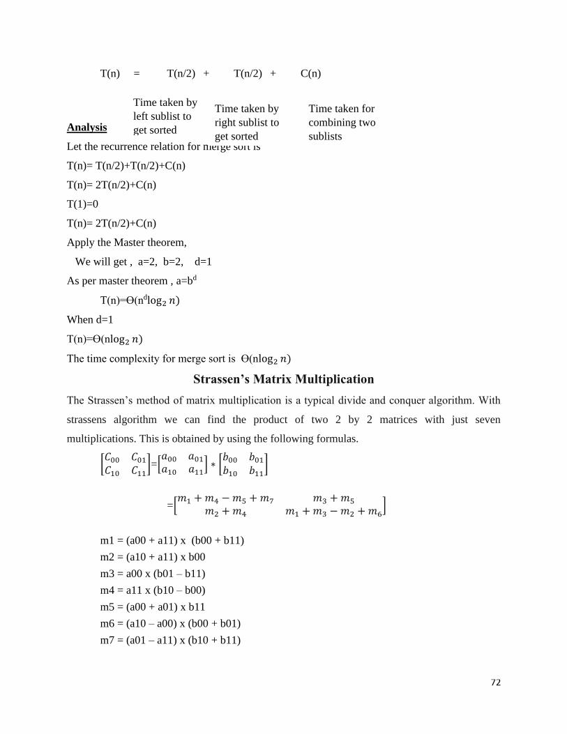
72
T(n) = T(n/2) + T(n/2) + C(n)
Analysis
Let the recurrence relation for merge sort is
T(n)= T(n/2)+T(n/2)+C(n)
T(n)= 2T(n/2)+C(n)
T(1)=0
T(n)= 2T(n/2)+C(n)
Apply the Master theorem,
We will get , a=2, b=2, d=1
As per master theorem , a=bd
T(n)=Ɵ(ndlog2 𝑛)
When d=1
T(n)=Ɵ(nlog2 𝑛)
The time complexity for merge sort is Ɵ(nlog2 𝑛)
Strassen’s Matrix Multiplication
The Strassen’s method of matrix multiplication is a typical divide and conquer algorithm. With
strassens algorithm we can find the product of two 2 by 2 matrices with just seven
multiplications. This is obtained by using the following formulas.
[𝐶00 𝐶01
𝐶10 𝐶11]=[
𝑎00 𝑎01
𝑎10 𝑎11] ∗ [
𝑏00 𝑏01
𝑏10 𝑏11]
=[𝑚1 + 𝑚4 − 𝑚5 + 𝑚7 𝑚3 + 𝑚5
𝑚2 + 𝑚4 𝑚1 + 𝑚3 − 𝑚2 + 𝑚6]
m1 = (a00 + a11) x (b00 + b11)
m2 = (a10 + a11) x b00
m3 = a00 x (b01 – b11)
m4 = a11 x (b10 – b00)
m5 = (a00 + a01) x b11
m6 = (a10 – a00) x (b00 + b01)
m7 = (a01 – a11) x (b10 + b11)
Time taken by
left sublist to
get sorted
Time taken by
right sublist to
get sorted
Time taken for
combining two
sublists
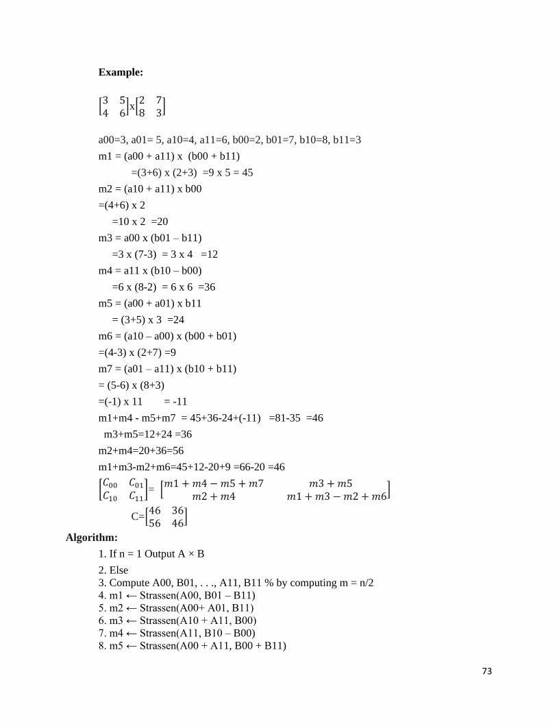
73
Example:
[3 54 6
]x[2 78 3
]
a00=3, a01= 5, a10=4, a11=6, b00=2, b01=7, b10=8, b11=3
m1 = (a00 + a11) x (b00 + b11)
=(3+6) x (2+3) =9 x 5 = 45
m2 = (a10 + a11) x b00
=(4+6) x 2
=10 x 2 =20
m3 = a00 x (b01 – b11)
=3 x (7-3) = 3 x 4 =12
m4 = a11 x (b10 – b00)
=6 x (8-2) = 6 x 6 =36
m5 = (a00 + a01) x b11
= (3+5) x 3 =24
m6 = (a10 – a00) x (b00 + b01)
=(4-3) x (2+7) =9
m7 = (a01 – a11) x (b10 + b11)
= (5-6) x (8+3)
=(-1) x 11 = -11
m1+m4 - m5+m7 = 45+36-24+(-11) =81-35 =46
m3+m5=12+24 =36
m2+m4=20+36=56
m1+m3-m2+m6=45+12-20+9 =66-20 =46
[𝐶00 𝐶01
𝐶10 𝐶11]= [
𝑚1 + 𝑚4 − 𝑚5 + 𝑚7 𝑚3 + 𝑚5𝑚2 + 𝑚4 𝑚1 + 𝑚3 − 𝑚2 + 𝑚6
]
C=[46 3656 46
]
Algorithm:
1. If n = 1 Output A × B
2. Else
3. Compute A00, B01, . . ., A11, B11 % by computing m = n/2
4. m1 ← Strassen(A00, B01 – B11)
5. m2 ← Strassen(A00+ A01, B11)
6. m3 ← Strassen(A10 + A11, B00)
7. m4 ← Strassen(A11, B10 – B00)
8. m5 ← Strassen(A00 + A11, B00 + B11)
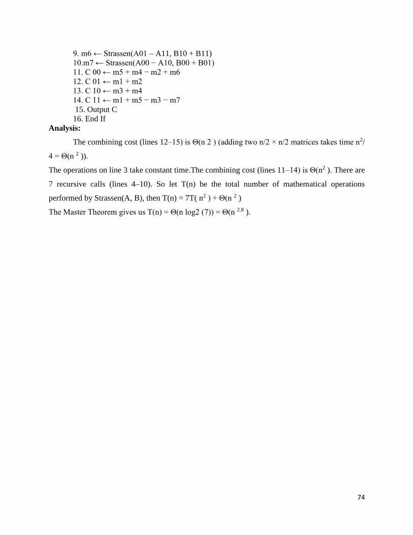
74
9. m6 ← Strassen(A01 – A11, B10 + B11)
10.m7 ← Strassen(A00 − A10, B00 + B01)
11. C 00 ← m5 + m4 − m2 + m6
12. C 01 ← m1 + m2
13. C 10 ← m3 + m4
14. C 11 ← m1 + m5 − m3 − m7
15. Output C
16. End If
Analysis:
The combining cost (lines 12–15) is Θ(n 2 ) (adding two n/2 × n/2 matrices takes time n2/
4 = Θ(n 2 )).
The operations on line 3 take constant time.The combining cost (lines 11–14) is Θ(n2 ). There are
7 recursive calls (lines 4–10). So let T(n) be the total number of mathematical operations
performed by Strassen(A, B), then T(n) = 7T( n2 ) + Θ(n 2 )
The Master Theorem gives us T(n) = Θ(n log2 (7)) = Θ(n 2.8 ).
75
SCHOOL OF COMPUTING
DEPARTMENT OF INFORMATION TECHNOLOGY
UNIT - IV
Design and Analysis of Algorithm – SCSA1403
76
Greedy Approach and Dynamic Programming 9 Hrs.
Greedy Approach:- Optimal Merge Patterns- Huffman Code - Job Sequencing problem- -- Tree
Vertex Splitting Dynamic Programming:– Dice Throw-- Optimal Binary Search Algorithms.
Greedy Approach
Greedy is the most straight forward design technique. Most of the problems have n inputs and
require us to obtain a subset that satisfies some constraints. Any subset that satisfies these
constraints is called a feasible solution. We need to find a feasible solution that either maximizes
or minimizes the objective function. A feasible solution that does this is called an optimal
solution.
The greedy method is a simple strategy of progressively building up a solution, one element at a
time, by choosing the best possible element at each stage. At each stage, a decision is made
regarding whether or not a particular input is in an optimal solution. This is done by considering
the inputs in an order determined by some selection procedure. If the inclusion of the next input,
into the partially constructed optimal solution will result in an infeasible solution then this input
is not added to the partial solution. The selection procedure itself is based on some optimization
measure. Several optimization measures are plausible for a given problem. Most of them,
however, will result in algorithms that generate sub-optimal solutions. This version of greedy
technique is called subset paradigm. Some problems like Knapsack, Job sequencing with
deadlines and minimum cost spanning trees are based on subset paradigm.
For the problems that make decisions by considering the inputs in some order, each decision is
made using an optimization criterion that can be computed using decisions already made. This
version of greedy method is ordering paradigm. Some problems like optimal storage on tapes,
optimal merge patterns and single source shortest path are based on ordering paradigm.
Algorithm Greedy (a, n)
// a(1 : n) contains the ‘n’ inputs
solution := ∞ ; // initialize the solution to empty for
i:=1 to n do
x := select (a); if feasible (solution, x) then
solution := Union (Solution, x); return solution;
77
Procedure Greedy describes the essential way that a greedy based algorithm will look, once a
particular problem is chosen and the functions select, feasible and union are properly
implemented.
The function select selects an input from ‘a’, removes it and assigns its value to ‘x’. Feasible is a
Boolean valued function, which determines if ‘x’ can be included into the solution vector. The
function Union combines ‘x’ with solution and updates the objective function.
Applications of the Greedy Strategy Optimal solutions:
• Change Making For “Normal” Coin Denominations
• Minimum Spanning Tree (Mst)
• Single-Source Shortest Paths
• Simple Scheduling Problems
• Huffman codes
Approximations/heuristics:
• Traveling salesman problem (TSP)
• Knapsack Problem
Optimal Merge Patterns Problem
Given n sorted files, find an optimal way (i.e., requiring the fewest comparisons or record
moves) to pair wise merge them into one sorted file. It fits ordering paradigm.
Example
Three sorted files (x1, x2, x3) with lengths (30, 20, 10)
Solution 1: merging x1 and x2 (50 record moves), merging the result with x3 (60 moves) à
total 110 moves
Solution 2: merging x2 and x3 (30 moves), merging the result with x1 (60 moves) à total 90
moves
The solution 2 is better.
A greedy method (for 2-way merge problem)
At each step, merge the two smallest files. e.g., five files with lengths (20, 30, 10, 5, 30).
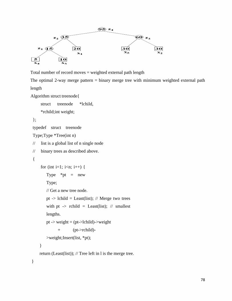
78
Total number of record moves = weighted external path length
The optimal 2-way merge pattern = binary merge tree with minimum weighted external path
length
Algorithm struct treenode
struct treenode *lchild,
*rchild; int weight;
;
typedef struct treenode
Type; Type *Tree(int n)
// list is a global list of n single node
// binary trees as described above.
for (int i=1; i<n; i++)
Type *pt = new
Type;
// Get a new tree node.
pt -> lchild = Least(list); // Merge two trees
with pt -> rchild = Least(list); // smallest
lengths.
pt -> weight = (pt->lchild)->weight
+ (pt->rchild)-
>weight; Insert(list, *pt);
return (Least(list)); // Tree left in l is the merge tree.
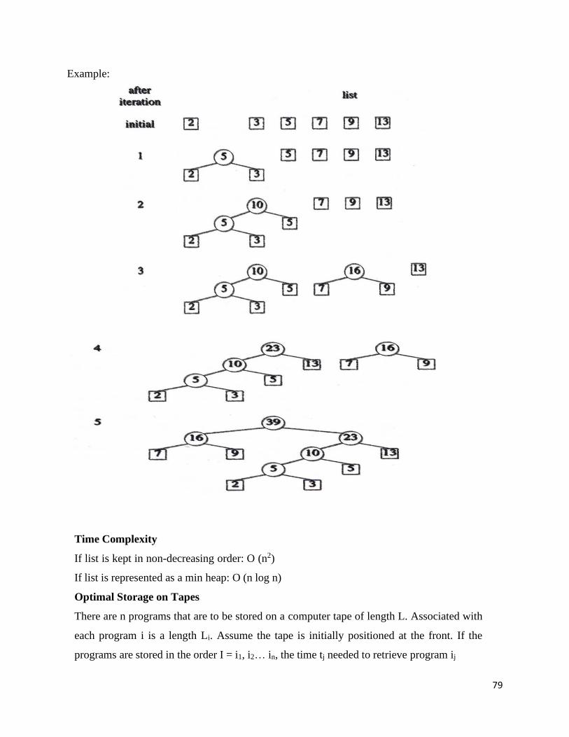
79
Example:
Time Complexity
If list is kept in non-decreasing order: O (n2)
If list is represented as a min heap: O (n log n)
Optimal Storage on Tapes
There are n programs that are to be stored on a computer tape of length L. Associated with
each program i is a length Li. Assume the tape is initially positioned at the front. If the
programs are stored in the order I = i1, i2… in, the time tj needed to retrieve program ij
80
k
If all programs are retrieved equally often, then the mean retrieval time (MRT) =this
problem fits the ordering paradigm. Minimizing the MRT is equivalent to minimizing n j
D (I) = Lik
j 1 k 1
Example
n=3 (l1, l2, l3) = (5, 10, 3) 3! =6 total combinations
L1 l2
l3 = l1+ (l1+l2) + (l1+l2+l3) = 5+15+18 = 38/3=12.6
n 3
L1 l
3
l2 = l1 + (l1+l3) + (l1+l2+l3) = 5+8+18 = 31/3=10.3
n 3
L2 l
1
l3 = l2 + (l2+l1) + ( l2+l1+l3) = 10+15+18 = 43/3=14.3
n 3
L2 l3
l1 = 10+13+18 = 41/3=13.6
3
L3 l1 l2 = 3+8+18 = 29/3=9.6 min
3
L3 l2 l1 = 3+13+18 = 34/3=11.3 min
3 permutations at (3, 1, 2)
Example
n = 4, (p1, p2, p3, p4) = (100, 10, 1 5, 27) (d1, d2, d3, d4) = (2, 1, 2, 1)
Feasible solution Processing sequence value
1
(1,2)
2,1
110
2 (1,3) 1,3 or 3, 1 115
3 (1,4) 4, 1 127
4 (2,3) 2, 3 25
5 (3,4) 4,3 42
81
6 (1) 1 100
7 (2) 2 10
8 (3) 3 15
9 (4) 4 27
Example
Let n = 3, (L1, L2, L3) = (5, 10, 3). 6 possible orderings. The optimal is 3, 1, 2
Ordering I d(I)
1,2,3 5+5+10+5+10+3 = 38
1,3,2 5+5+3+5+3+10 = 31
2,1,3 10+10+5+10+5+3 = 43
2,3,1 10+10+3+10+3+5 = 41
3,1,2 3+3+5+3+5+10 = 29
3,2,1, 3+3+10+3+10+5 = 34
Huffman Trees and Codes
Huffman coding is a lossless data compression algorithm. The idea is to assign variable-
length codes to input characters, lengths of the assigned codes are based on the frequencies of
corresponding characters. The most frequent character gets the smallest code and the least
frequent character gets the largest code.The variable-length codes assigned to input characters
are Prefix Codes, means the codes (bit sequences) are assigned in such a way that the code
assigned to one character is not prefix of code assigned to any other character.
This is how Huffman Coding makes sure that there is no ambiguity when decoding the
generated bit stream. Let us understand prefix codes with a counter example. Let there be four
characters a, b, c and d, and their corresponding variable length codes be 00, 01, 0 and 1. This
coding leads to ambiguity because code assigned to c is prefix of codes assigned to a
and b. If the compressed bit stream is 0001, the de-compressed output may be “cccd” or “ccb” or
“acd” or “ab”.
There are mainly two major parts in Huffman Coding
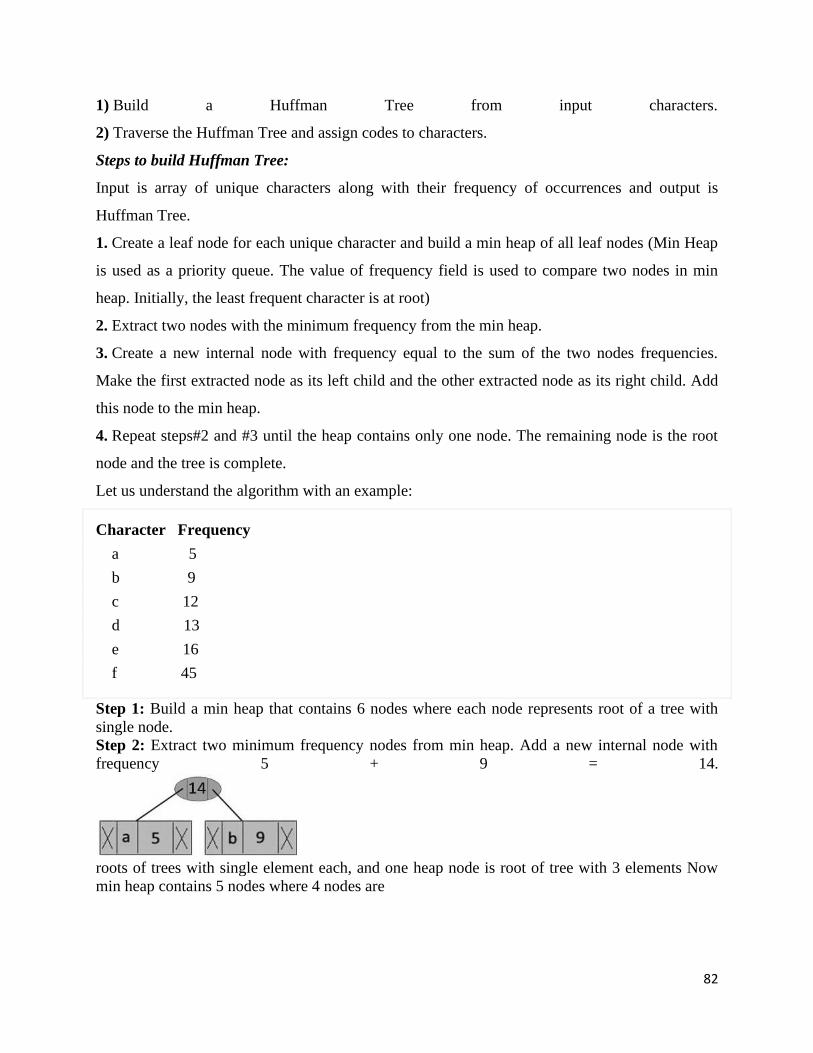
82
1) Build a Huffman Tree from input characters.
2) Traverse the Huffman Tree and assign codes to characters.
Steps to build Huffman Tree:
Input is array of unique characters along with their frequency of occurrences and output is
Huffman Tree.
1. Create a leaf node for each unique character and build a min heap of all leaf nodes (Min Heap
is used as a priority queue. The value of frequency field is used to compare two nodes in min
heap. Initially, the least frequent character is at root)
2. Extract two nodes with the minimum frequency from the min heap.
3. Create a new internal node with frequency equal to the sum of the two nodes frequencies.
Make the first extracted node as its left child and the other extracted node as its right child. Add
this node to the min heap.
4. Repeat steps#2 and #3 until the heap contains only one node. The remaining node is the root
node and the tree is complete.
Let us understand the algorithm with an example:
Character Frequency
a 5
b 9
c 12
d 13
e 16
f 45
Step 1: Build a min heap that contains 6 nodes where each node represents root of a tree with
single node.
Step 2: Extract two minimum frequency nodes from min heap. Add a new internal node with
frequency 5 + 9 = 14.
roots of trees with single element each, and one heap node is root of tree with 3 elements Now
min heap contains 5 nodes where 4 nodes are
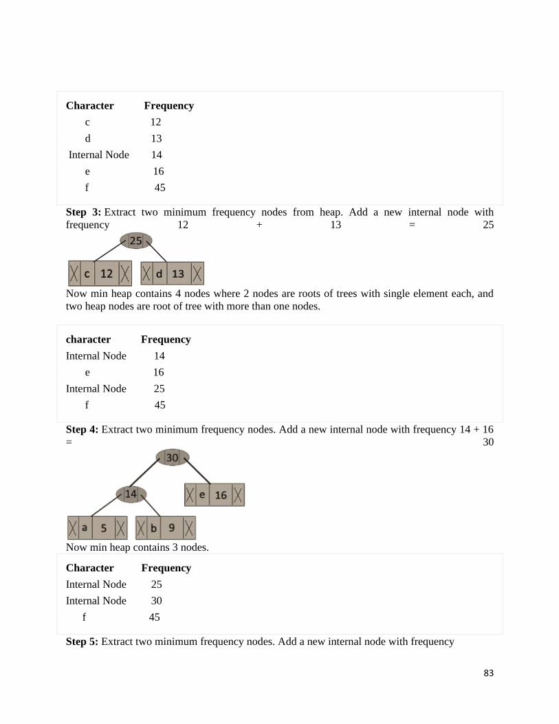
83
Character Frequency
c 12
d 13
Internal Node 14
e 16
f 45
Step 3: Extract two minimum frequency nodes from heap. Add a new internal node with
frequency 12 + 13 = 25
Now min heap contains 4 nodes where 2 nodes are roots of trees with single element each, and
two heap nodes are root of tree with more than one nodes.
character Frequency
Internal Node 14
e 16
Internal Node 25
f 45
Step 4: Extract two minimum frequency nodes. Add a new internal node with frequency 14 + 16
= 30
Now min heap contains 3 nodes.
Character Frequency
Internal Node 25
Internal Node 30
f 45
Step 5: Extract two minimum frequency nodes. Add a new internal node with frequency
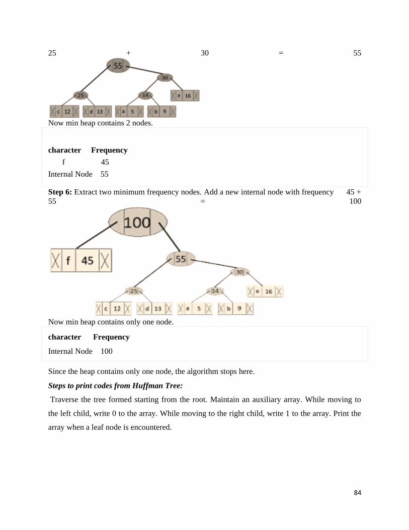
84
25 + 30 = 55
Now min heap contains 2 nodes.
character Frequency
f 45
Internal Node 55
Step 6: Extract two minimum frequency nodes. Add a new internal node with frequency 45 +
55 = 100
Now min heap contains only one node.
character Frequency
Internal Node 100
Since the heap contains only one node, the algorithm stops here.
Steps to print codes from Huffman Tree:
Traverse the tree formed starting from the root. Maintain an auxiliary array. While moving to
the left child, write 0 to the array. While moving to the right child, write 1 to the array. Print the
array when a leaf node is encountered.
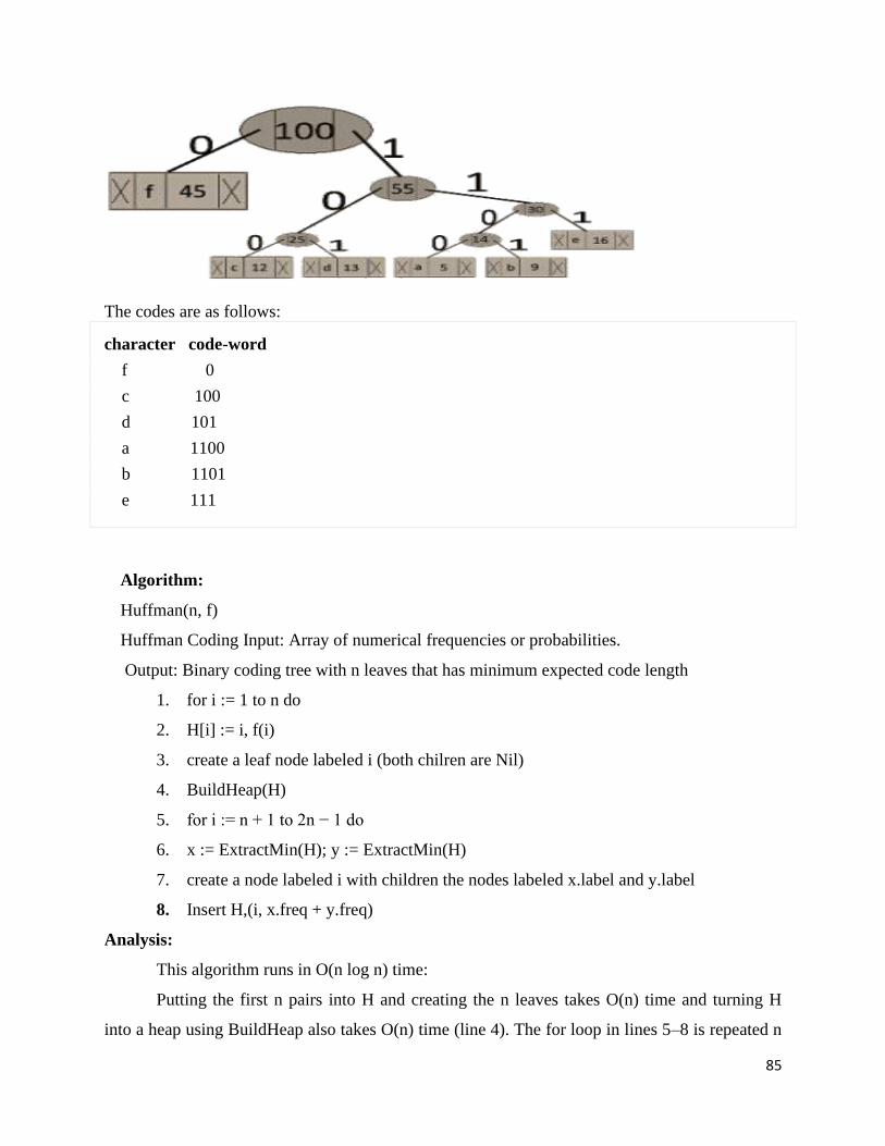
85
The codes are as follows:
character code-word
f 0
c 100
d 101
a 1100
b 1101
e 111
Algorithm:
Huffman(n, f)
Huffman Coding Input: Array of numerical frequencies or probabilities.
Output: Binary coding tree with n leaves that has minimum expected code length
1. for i := 1 to n do
2. H[i] := i, f(i)
3. create a leaf node labeled i (both chilren are Nil)
4. BuildHeap(H)
5. for i := n + 1 to 2n − 1 do
6. x := ExtractMin(H); y := ExtractMin(H)
7. create a node labeled i with children the nodes labeled x.label and y.label
8. Insert H,(i, x.freq + y.freq)
Analysis:
This algorithm runs in O(n log n) time:
Putting the first n pairs into H and creating the n leaves takes O(n) time and turning H
into a heap using BuildHeap also takes O(n) time (line 4). The for loop in lines 5–8 is repeated n
86
− 1 times. In each iteration we perform two ExtractMin operations and one Insert operation, each
of which takes O(log n) time.
So the loop takes O(n log n) time, and the entire algorithm takes O(n) + O(n) + O(n log
n) = O(n log n) time.
The time complexity of the Huffman algorithm is O(nlogn). Using a heap to store the
weight of each tree, each iteration requires O(logn) time to determine the cheapest weight and
insert the new weight. There are O(n) iterations, one for each item.
Job Sequencing Problem
Job sequencing with deadlines the problem is stated as below. There are n jobs to be processed
on a machine. Each job i has a deadline di ≥ 0 and profit pi≥0. Pi is earned iff the job is
completed by its deadline. The job is completed if it is processed on a machine for unit time.
Only one machine is available for processing jobs. Only one job is processed at a time on the
machine.A given Input set of jobs 1,2,3,4 have sub sets 2n so 24 =16 It can be written as
1,2,3,4,Ø,1,2,1,3,1,4,2,3,2,4,3,4,1,2,3,
1,2,4,2,3,4,1,2,3,4,1,3,4 total of 16 subsets
Problem:
n=4 , P=(70,12,18,35) , d=(2,1,2,1)
Feasible
Solution
Processing
Sequence Profit value
0
Time Line
1
2
1 1 70
2 2 12
3 3 18
4 4 35
1,2 2,1 82
1,3 1,3 /3,1 88
1,4 4,1 105
2,3 3,2 /2,3 30
3,4 4,3/3,4 53
We should consider the pair i,j where di <=dj if di>dj we should not consider pair then reverse
the order. We discard pair (2, 4) because both having same dead line(1,1) and cannot process
same. Time and discarded pairs (1,2,3), (2,3,4), (1,2,4)…etc since processes are not completed
87
within their deadlines. A feasible solution is a subset of jobs J such that each job is completed by
its deadline. An optimal solution is a feasible solution with maximum profit value.
Example
Let n = 4, (p1,p2,p3,p4) = (100,10,15,27), (d1,d2,d3,d4) = (2,1,2,1)
Sr.No. Feasible
Solution
Processing
Sequence Profit value
(i) (1, 2) (2, 1) 110
(ii) (1, 3) (1, 3) or (3, 1) 115
(iii) (1, 4) (4, 1) 127 is the optimal one
(iv) (2, 3) (2, 3) 25
(v) (3, 4) (4, 3) 42
(vi) (1) (1) 100
(vii) (2) (2) 10
(viii) (3) (3) 15
(ix) (4) (4) 27
Problem: n jobs, S = 1, 2… n, each job i has a deadline di 0 and a profit pi 0. We need one
unit of time to process each job and we can do at most one job each time. We can earn the
profit pi if job i is completed by its deadline.
The optimal solution = 1, 2, 4.
The total profit = 20 + 15 + 5 = 40.
Algorithm
Step 1: Sort pi into non-increasing order.
After sorting p1 p2 p3 … pi.
Step 2: Add the next job i to the solution set if i can be completed by its deadline. Assign i
to time slot [r-1, r], where r is the largest integer such that 1 r di and [r-1, r] is free.
Step 3: Stop if all jobs are examined. Otherwise, go to step
2. Time complexity: O (n2)
i 1 2 3 4 5
pi 20 15 10 5 1
di 2 2 1 3 3
88
Example
assign to [1, 2] assign to [0, 1] Reject assign to [2, 3] Reject
solution = 1, 2, 4
total profit = 20 + 15 + 5 = 40
Greedy Algorithm to Obtain an Optimal Solution
Consider the jobs in the non increasing order of profits subject to the constraint that the
resulting job sequence J is a feasible solution.
In the example considered before, the non-increasing profit vector
is (100 27 15 10) (2 1 2 1)
p1 p4 p3 p2 d1 d4 d3
d2 J = 1 is a feasible one
J = 1, 4 is a feasible one with processing sequence
J = 1, 3, 4 is not feasible
J = 1, 2, 4 is not feasible
J = 1, 4 is optimal
High level description of job sequencing
algorithm Procedure greedy job (D, J, n)
// J is the set of n jobs to be completed by their deadlines
J:=
1;
for i:=2 to n do
if (all jobs in J Ui can be completed by their
deadlines) then J:= ß J U i;
I pi di
1 20 2
2 15 2
3 10 1
4 5 3
5 1 3
89
Greedy Algorithm for Sequencing unit time jobs
Procedure JS(d,j,n)
d[0]:=J[0]:=0; //initialize and J(0) is a fictious job with d(0) =
0 // J[1]:=1; //include job 1
K:=1; // job one is inserted into J //
for i :=2 to n do // consider jobs in non increasing order of pi //
r:=k;
While ((d[J[r]]>d[i]) and (d[J[r]]#r)) do r:=r-1;
If ((d[J[r] d[i]) and d[i]>r)) then //insert i into
J[] For q:=k to (r+1) step-1 do j[q+1]:=j[q];
J[r+1]:=i; k:=k+1;
return k;
TVSP (Tree Vertex Splitting Problem)
Let T= (V, E, W) be a directed tree. A weighted tree can be used to model a distribution
network in which electrical signals are transmitted. Nodes in the tree correspond to
receiving stations & edges correspond to transmission lines. In the process of transmission
some loss is occurred. Each edge in the tree is labeled with the loss that occurs in
traversing that edge. The network model may not able tolerate losses beyond a certain
level. In places where the loss exceeds the tolerance value boosters have to be placed.
Given a networks and tolerance value, the TVSP problem is to determine an optimal
placement of boosters. The boosters can only placed at the nodes of the tree.
d (u) = Max d(v) + w(Parent(u), u)
d(u) – delay of node v-set of all edges & v belongs to
child(u) δ tolerance value
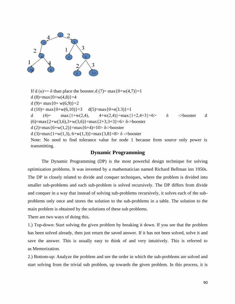
90
If d (u)>= δ than place the booster. d (7)= max0+w(4,7)=1
d (8)=max0+w(4,8)=4
d (9)= max0+ w(6,9)=2
d (10)= max0+w(6,10)=3 d(5)=max0+e(3.3)=1
d (4)= max1+w(2,4), 4+w(2,4)=max1+2,4+3=6> δ ->booster d
(6)=max2+w(3,6),3+w(3,6)=max2+3,3+3=6> δ->booster
d (2)=max6+w(1,2)=max6+4)=10> δ->booster
d (3)=max1+w(1,3), 6+w(1,3)=max3,8=8> δ ->booster
Note: No need to find tolerance value for node 1 because from source only power is
transmitting.
Dynamic Programming
The Dynamic Programming (DP) is the most powerful design technique for solving
optimization problems. It was invented by a mathematician named Richard Bellman inn 1950s.
The DP in closely related to divide and conquer techniques, where the problem is divided into
smaller sub-problems and each sub-problem is solved recursively. The DP differs from divide
and conquer in a way that instead of solving sub-problems recursively, it solves each of the sub-
problems only once and stores the solution to the sub-problems in a table. The solution to the
main problem is obtained by the solutions of these sub problems.
There are two ways of doing this.
1.) Top-down: Start solving the given problem by breaking it down. If you see that the problem
has been solved already, then just return the saved answer. If it has not been solved, solve it and
save the answer. This is usually easy to think of and very intuitively. This is referred to
as Memorization.
2.) Bottom-up: Analyze the problem and see the order in which the sub-problems are solved and
start solving from the trivial sub problem, up towards the given problem. In this process, it is
91
guaranteed that the sub problems are solved before solving the problem. This is referred to
as Dynamic Programming.
Dice Throw
Given n dice each with m faces, numbered from 1 to m, find the number of ways to get sum X. X
is the summation of values on each face when all the dice are thrown.
The Naive approach is to find all the possible combinations of values from n dice and keep on
counting the results that sum to X.
This problem can be efficiently solved using Dynamic Programming (DP).
Let the function to find X from n dice is: Sum(m, n, X)
The function can be represented as:
Sum(m, n, X) = Finding Sum (X - 1) from (n - 1) dice plus 1 from nth dice
+ Finding Sum (X - 2) from (n - 1) dice plus 2 from nth dice
+ Finding Sum (X - 3) from (n - 1) dice plus 3 from nth dice
...................................................
...................................................
...................................................
+ Finding Sum (X - m) from (n - 1) dice plus m from nth dice
So we can recursively write Sum(m, n, x) as following
Sum(m, n, X) = Sum(m, n - 1, X - 1) +
Sum(m, n - 1, X - 2) +
.................... +
Sum(m, n - 1, X - m)
Why DP approach?
The above problem exhibits overlapping subproblems. See the below diagram. Also,
see this recursive implementation. Let there be 3 dice, each with 6 faces and we need to find the
number of ways to get sum 8:
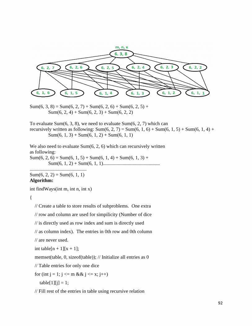
92
Sum(6, 3, 8) = Sum(6, 2, 7) + Sum(6, 2, 6) + Sum(6, 2, 5) +
Sum(6, 2, 4) + Sum(6, 2, 3) + Sum(6, 2, 2)
To evaluate Sum(6, 3, 8), we need to evaluate Sum(6, 2, 7) which can
recursively written as following: Sum(6, 2, 7) = Sum(6, 1, 6) + Sum(6, 1, 5) + Sum(6, 1, 4) +
Sum(6, 1, 3) + Sum(6, 1, 2) + Sum(6, 1, 1)
We also need to evaluate Sum(6, 2, 6) which can recursively written
as following:
Sum(6, 2, 6) = Sum(6, 1, 5) + Sum(6, 1, 4) + Sum(6, 1, 3) +
Sum(6, 1, 2) + Sum(6, 1, 1)..............................................
..............................................
Sum(6, 2, 2) = Sum(6, 1, 1)
Algorithm:
int findWays(int m, int n, int x)
// Create a table to store results of subproblems. One extra
// row and column are used for simpilicity (Number of dice
// is directly used as row index and sum is directly used
// as column index). The entries in 0th row and 0th column
// are never used.
int table[n + 1][x + 1];
memset(table, 0, sizeof(table)); // Initialize all entries as 0
// Table entries for only one dice
for (int j = 1; j <= m && j <= x; j++)
table[1][j] = 1;
// Fill rest of the entries in table using recursive relation
93
// i: number of dice, j: sum
for (int i = 2; i <= n; i++)
for (int j = 1; j <= x; j++)
for (int k = 1; k <= m && k < j; k++)
table[i][j] += table[i-1][j-k];
/* Uncomment these lines to see content of table
for (int i = 0; i <= n; i++)
for (int j = 0; j <= x; j++)
cout << table[i][j] << " ";
cout << endl;
*/
return table[n][x];
Time Complexity: O(m * n * x) where m is number of faces, n is number of dice and x is given
sum.
We can add the following two conditions at the beginning of findWays() to improve performance
of the program for extreme cases (x is too high or x is too low)
// When x is so high that sum can not go beyond x even when we
// get maximum value in every dice throw.
if (m*n <= x)
return (m*n == x);
// When x is too low
if (n >= x)
return (n == x);
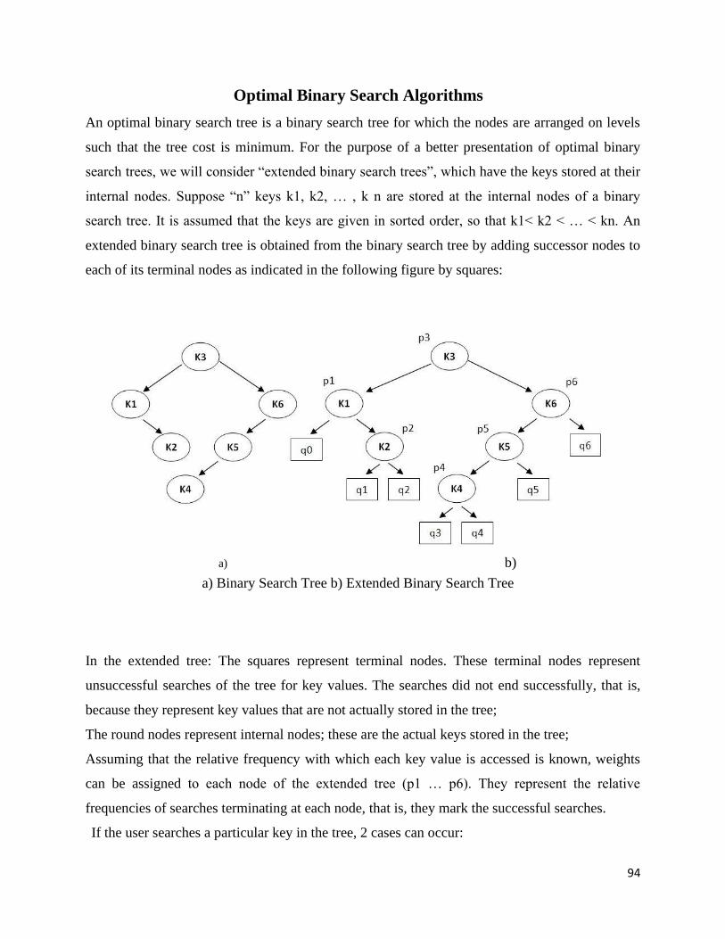
94
Optimal Binary Search Algorithms
An optimal binary search tree is a binary search tree for which the nodes are arranged on levels
such that the tree cost is minimum. For the purpose of a better presentation of optimal binary
search trees, we will consider “extended binary search trees”, which have the keys stored at their
internal nodes. Suppose “n” keys k1, k2, … , k n are stored at the internal nodes of a binary
search tree. It is assumed that the keys are given in sorted order, so that k1< k2 < … < kn. An
extended binary search tree is obtained from the binary search tree by adding successor nodes to
each of its terminal nodes as indicated in the following figure by squares:
a) b)
a) Binary Search Tree b) Extended Binary Search Tree
In the extended tree: The squares represent terminal nodes. These terminal nodes represent
unsuccessful searches of the tree for key values. The searches did not end successfully, that is,
because they represent key values that are not actually stored in the tree;
The round nodes represent internal nodes; these are the actual keys stored in the tree;
Assuming that the relative frequency with which each key value is accessed is known, weights
can be assigned to each node of the extended tree (p1 … p6). They represent the relative
frequencies of searches terminating at each node, that is, they mark the successful searches.
If the user searches a particular key in the tree, 2 cases can occur:
95
Case 1 – the key is found, so the corresponding weight ‘p’ is incremented;
Case 2 – the key is not found, so the corresponding ‘q’ value is incremented.
Where optimal binary search trees may be used
In general, word prediction is the problem of guessing the next word in a sentence as the
sentence is being entered, and updates this prediction as the word is typed. Currently “word
prediction” implies both “word completion and word prediction”. Word completion is defined as
offering the user a list of words after a letter has been typed, while word prediction is defined as
offering the user a list of probable words after a word has been typed or selected, based on
previous words rather than on the basis of the letter. Word completion problem is easier to solve
since the knowledge of some letter(s) provides the predictor a chance to eliminate many of
irrelevant words.
Online dictionaries rely heavily on the facilities provided by optimal search trees. As the
dictionary has more and more users, it is able to assign weights to the corresponding words,
according to the frequency of their search. This way, it will be able to provide a much faster
answer, as search time dramatically decreases when storing words into a binary search tree.
Word prediction applications are becoming increasingly popular. For example, when you start
typing a query in google search, a list of possible entries almost instantly appears.
The terminal node in the extended tree that is the left successor of k1 can be interpreted as
representing all key values that are not stored and are less than k1. Similarly, the terminal node
in the extended tree that is the right successor of kn, represents all key values not stored in the
tree that are greater than kn. The terminal node that is successed between ki and ki-1 in an
inorder traversal represents all key values not stored that lie between ki and ki-1.
In the extended tree in the above figure if the possible key values are 0, 1, 2, 3, …, 100 then the
terminal node labeled q0 represents the missing key values 0, 1 and 2 if k1=3. The terminal node
labeled q3 represents the key values between k3 and k4. If k3=17 and k4=21 then the terminal
node labeled q3 represents the missing key values 18, 19 and 20. If k6 is 90 then the terminal
node q6 represents the missing key values 91 through 100.
An obvious way to find an optimal binary search tree is to generate each possible binary search
tree for the keys, calculate the weighted path length, and keep that tree with the smallest
weighted path length. This search through all possible solutions is not feasible, since the number
of such trees grows exponentially with “n”.
96
An alternative would be a recursive algorithm. Consider the characteristics of any optimal tree.
Of course it has a root and two subtrees. Both subtrees must themselves be optimal binary search
trees with respect to their keys and weights. First, any subtree of any binary search tree must be
a binary search tree. Second, the subtrees must also be optimal.
Since there are “n” possible keys as candidates for the root of the optimal tree, the recursive
solution must try them all. For each candidate key as root, all keys less than that key must appear
in its left subtree while all keys greater than it must appear in its right subtree. Stating the
recursive algorithm based on these observations requires some notations:
OBST(i, j) denotes the optimal binary search tree containing the keys ki, ki+1, …, kj;
Wi, j denotes the weight matrix for OBST(i, j)
Wi, j can be defined using the following formula:
Ci, j, 0 ≤ i ≤ j ≤ n denotes the cost matrix for OBST(i, j)
Ci, j can be defined recursively, in the following manner: Ci, i = Wi, j
Ci, j = Wi, j + mini<k≤j(Ci, k - 1 + Ck, j)
Ri, j, 0 ≤ i ≤ j ≤ n denotes the root matrix for OBST(i, j)
Assigning the notation Ri, j to the value of k for which we obtain a minimum in the above
relations, the optimal binary search tree is OBST(0, n) and each subtree OBST(i, j) has the root
kRij and as subtrees the trees denoted by OBST(i, k-1) and OBST(k, j).
OBST(i, j) will involve the weights qi-1, pi, qi, …, pj, qj.
All possible optimal subtrees are not required. Those that are consist of sequences of keys that
are immediate successors of the smallest key in the subtree, successors in the sorted order for the
keys.
The bottom-up approach generates all the smallest required optimal subtrees first, then all next
smallest, and so on until the final solution involving all the weights is found. Since the algorithm
requires access to each subtree’s weighted path length, these weighted path lengths must also be
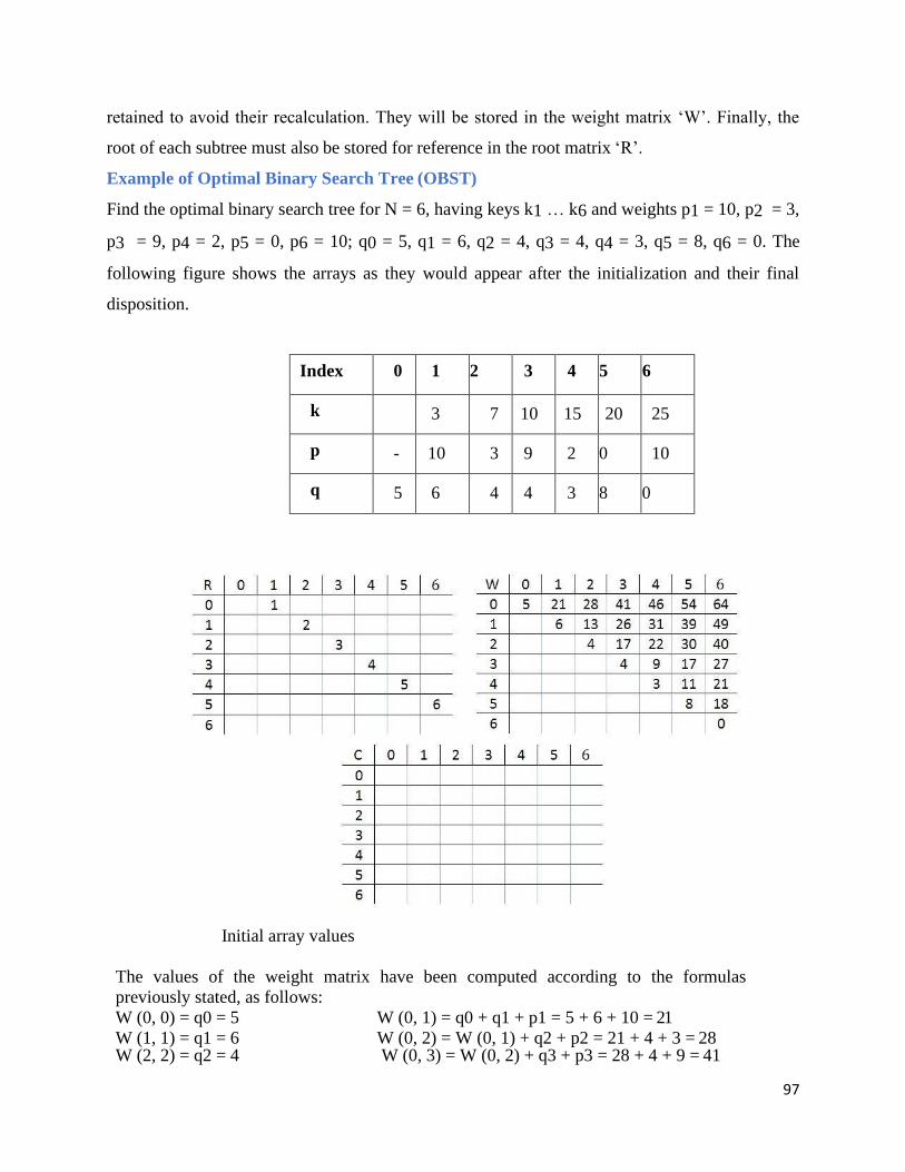
97
retained to avoid their recalculation. They will be stored in the weight matrix ‘W’. Finally, the
root of each subtree must also be stored for reference in the root matrix ‘R’.
Example of Optimal Binary Search Tree (OBST)
Find the optimal binary search tree for N = 6, having keys k1 … k6 and weights p1 = 10, p2 = 3,
p3 = 9, p4 = 2, p5 = 0, p6 = 10; q0 = 5, q1 = 6, q2 = 4, q3 = 4, q4 = 3, q5 = 8, q6 = 0. The
following figure shows the arrays as they would appear after the initialization and their final
disposition.
Index 0 1 2 3 4 5 6
k 3 7 10 15 20 25
p - 10 3 9 2 0 10
q 5 6 4 4 3 8 0
Initial array values
The values of the weight matrix have been computed according to the formulas
previously stated, as follows:
W (0, 0) = q0 = 5 W (0, 1) = q0 + q1 + p1 = 5 + 6 + 10 = 21
W (1, 1) = q1 = 6 W (0, 2) = W (0, 1) + q2 + p2 = 21 + 4 + 3 = 28 W (2, 2) = q2 = 4 W (0, 3) = W (0, 2) + q3 + p3 = 28 + 4 + 9 = 41
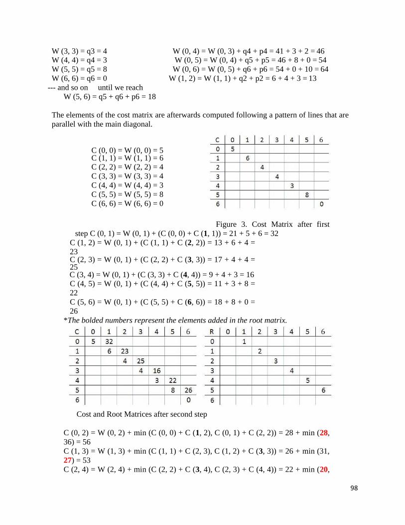
98
W (3, 3) = q3 = 4 W (0, 4) = W (0, 3) + q4 + p4 = 41 + 3 + 2 = 46 W (4, 4) = q4 = 3 W (0, 5) = W (0, 4) + q5 + p5 = 46 + 8 + 0 = 54
W (5, 5) = q5 = 8 W (0, 6) = W (0, 5) + q6 + p6 = 54 + 0 + 10 = 64
W (6, 6) = q6 = 0 W (1, 2) = W (1, 1) + q2 + p2 = 6 + 4 + 3 = 13
--- and so on until we reach
W (5, 6) = q5 + q6 + p6 = 18
The elements of the cost matrix are afterwards computed following a pattern of lines that are
parallel with the main diagonal.
C (0, 0) = W (0, 0) = 5 C (1, 1) = W (1, 1) = 6 C (2, 2) = W (2, 2) = 4
C (3, 3) = W (3, 3) = 4
C (4, 4) = W (4, 4) = 3
C (5, 5) = W (5, 5) = 8
C (6, 6) = W (6, 6) = 0
Figure 3. Cost Matrix after first
step C (0, 1) = W (0, 1) + (C (0, 0) + C (1, 1)) = 21 + 5 + 6 = 32
C (1, 2) = W (0, 1) + (C (1, 1) + C (2, 2)) = 13 + 6 + 4 =
23 C (2, 3) = W (0, 1) + (C (2, 2) + C (3, 3)) = 17 + 4 + 4 = 25
C (3, 4) = W (0, 1) + (C (3, 3) + C (4, 4)) = 9 + 4 + 3 = 16 C (4, 5) = W (0, 1) + (C (4, 4) + C (5, 5)) = 11 + 3 + 8 =
22
C (5, 6) = W (0, 1) + (C (5, 5) + C (6, 6)) = 18 + 8 + 0 =
26
*The bolded numbers represent the elements added in the root matrix.
Cost and Root Matrices after second step
C (0, 2) = W (0, 2) + min (C (0, 0) + C (1, 2), C (0, 1) + C (2, 2)) = 28 + min (28,
36) = 56
C (1, 3) = W (1, 3) + min (C (1, 1) + C (2, 3), C (1, 2) + C (3, 3)) = 26 + min (31,
27) = 53
C (2, 4) = W (2, 4) + min (C (2, 2) + C (3, 4), C (2, 3) + C (4, 4)) = 22 + min (20,
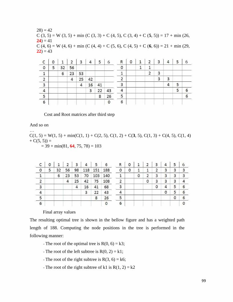
99
28) = 42
C (3, 5) = W (3, 5) + min (C (3, 3) + C (4, 5), C (3, 4) + C (5, 5)) = 17 + min (26,
24) = 41
C (4, 6) = W (4, 6) + min (C (4, 4) + C (5, 6), C (4, 5) + C (6, 6)) = 21 + min (29,
22) = 43
Cost and Root matrices after third step
And so on
…
C(1, 5) = W(1, 5) + min(C(1, 1) + C(2, 5), C(1, 2) + C(3, 5), C(1, 3) + C(4, 5), C(1, 4)
+ C(5, 5)) =
= 39 + min(81, 64, 75, 78) = 103
Final array values
The resulting optimal tree is shown in the bellow figure and has a weighted path
length of 188. Computing the node positions in the tree is performed in the
following manner:
- The root of the optimal tree is R(0, 6) = k3;
- The root of the left subtree is R(0, 2) = k1;
- The root of the right subtree is R(3, 6) = k6;
- The root of the right subtree of k1 is R(1, 2) = k2
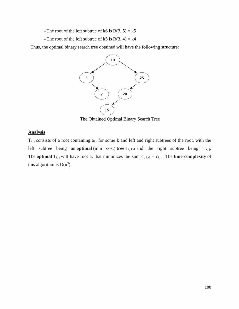
100
- The root of the left subtree of k6 is R(3, 5) = k5
- The root of the left subtree of k5 is R(3, 4) = k4
Thus, the optimal binary search tree obtained will have the following structure:
The Obtained Optimal Binary Search Tree
Analysis
Ti, j consists of a root containing ak, for some k and left and right subtrees of the root, with the
left subtree being an optimal (min cost) tree Ti, k-1 and the right subtree being Tk, j.
The optimal Ti, j will have root ak that minimizes the sum ci, k-1 + ck, j. The time complexity of
this algorithm is O(n3).
101
SCHOOL OF COMPUTING
DEPARTMENT OF INFORMATION TECHNOLOGY
UNIT - V
Design and Analysis of Algorithm – SCSA1403
102
Backtracking and Branch and Bound 9 Hrs.
Backtracking:- 8 Queens - Hamiltonian Circuit Problem - Branch and Bound - Assignment
Problem - Knapsack Problem:- Travelling Salesman Problem - NP Complete Problems - Clique
Problem - Vertex Cover Problem.
Backtracking
Backtracking can be defined as a general algorithmic technique that considers searching every
possible combination in order to solve a computational problem.
There are three types of problems in backtracking –
1. Decision Problem – In this, we search for a feasible solution.
2. Optimization Problem – In this, we search for the best solution.
3. Enumeration Problem – In this, we find all feasible solutions.
8 Queens Problem
You are given an 8x8 chessboard; find a way to place 8 queens such that no queen can attack any
other queen on the chessboard. A queen can only be attacked if it lies on the same row, or same
column, or the same diagonal of any other queen. Print all the possible configurations.
To solve this problem, we will make use of the Backtracking algorithm. The backtracking
algorithm, in general checks all possible configurations and test whether the required result is
obtained or not. For this given problem, we will explore all possible positions the queens can be
relatively placed at. The solution will be correct when the number of placed queens = 8. The time
complexity of this approach is O(N!).
Input - the number 8, which does not need to be read, but we will take an input number for the
sake of generalization of the algorithm to an NxN chessboard.
Output - all matrices that constitute the possible solutions will contain the numbers 0(for empty
cell) and 1(for a cell where queen is placed). Hence, the output is a set of binary matrices.
Visualization from a 4x4 chessboard solution:
In this configuration, we place 2 queens in the first iteration and see that checking by placing
further queens is not required as we will not get a solution in this path. Note that in this
configuration, all places in the third rows can be attacked.
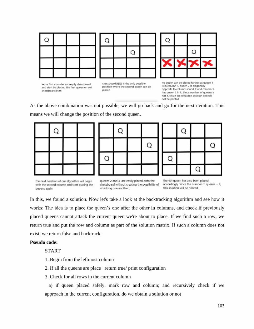
103
As the above combination was not possible, we will go back and go for the next iteration. This
means we will change the position of the second queen.
In this, we found a solution. Now let's take a look at the backtracking algorithm and see how it
works: The idea is to place the queen’s one after the other in columns, and check if previously
placed queens cannot attack the current queen we're about to place. If we find such a row, we
return true and put the row and column as part of the solution matrix. If such a column does not
exist, we return false and backtrack.
Pseudo code:
START
1. Begin from the leftmost column
2. If all the queens are place return true/ print configuration
3. Check for all rows in the current column
a) if queen placed safely, mark row and column; and recursively check if we
approach in the current configuration, do we obtain a solution or not
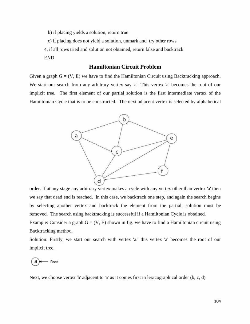
104
b) if placing yields a solution, return true
c) if placing does not yield a solution, unmark and try other rows
4. if all rows tried and solution not obtained, return false and backtrack
END
Hamiltonian Circuit Problem
Given a graph G = (V, E) we have to find the Hamiltonian Circuit using Backtracking approach.
We start our search from any arbitrary vertex say 'a'. This vertex 'a' becomes the root of our
implicit tree. The first element of our partial solution is the first intermediate vertex of the
Hamiltonian Cycle that is to be constructed. The next adjacent vertex is selected by alphabetical
order. If at any stage any arbitrary vertex makes a cycle with any vertex other than vertex 'a' then
we say that dead end is reached. In this case, we backtrack one step, and again the search begins
by selecting another vertex and backtrack the element from the partial; solution must be
removed. The search using backtracking is successful if a Hamiltonian Cycle is obtained.
Example: Consider a graph G = (V, E) shown in fig. we have to find a Hamiltonian circuit using
Backtracking method.
Solution: Firstly, we start our search with vertex 'a.' this vertex 'a' becomes the root of our
implicit tree.
Next, we choose vertex 'b' adjacent to 'a' as it comes first in lexicographical order (b, c, d).
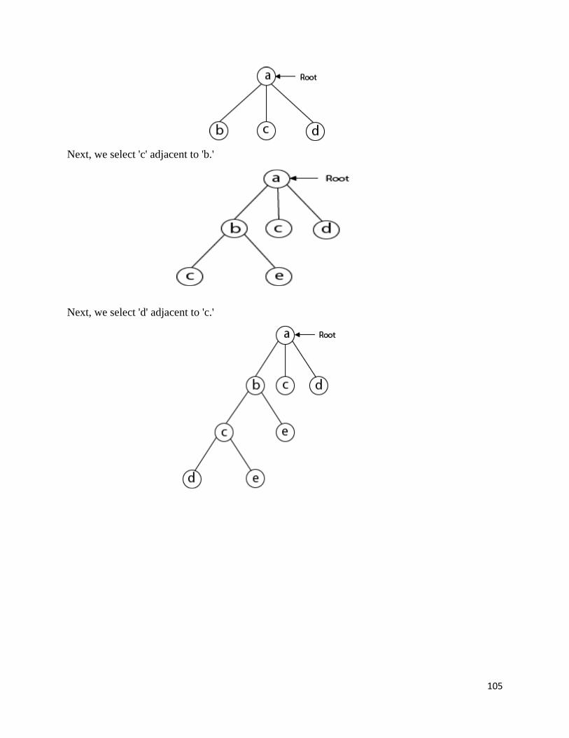
105
Next, we select 'c' adjacent to 'b.'
Next, we select 'd' adjacent to 'c.'
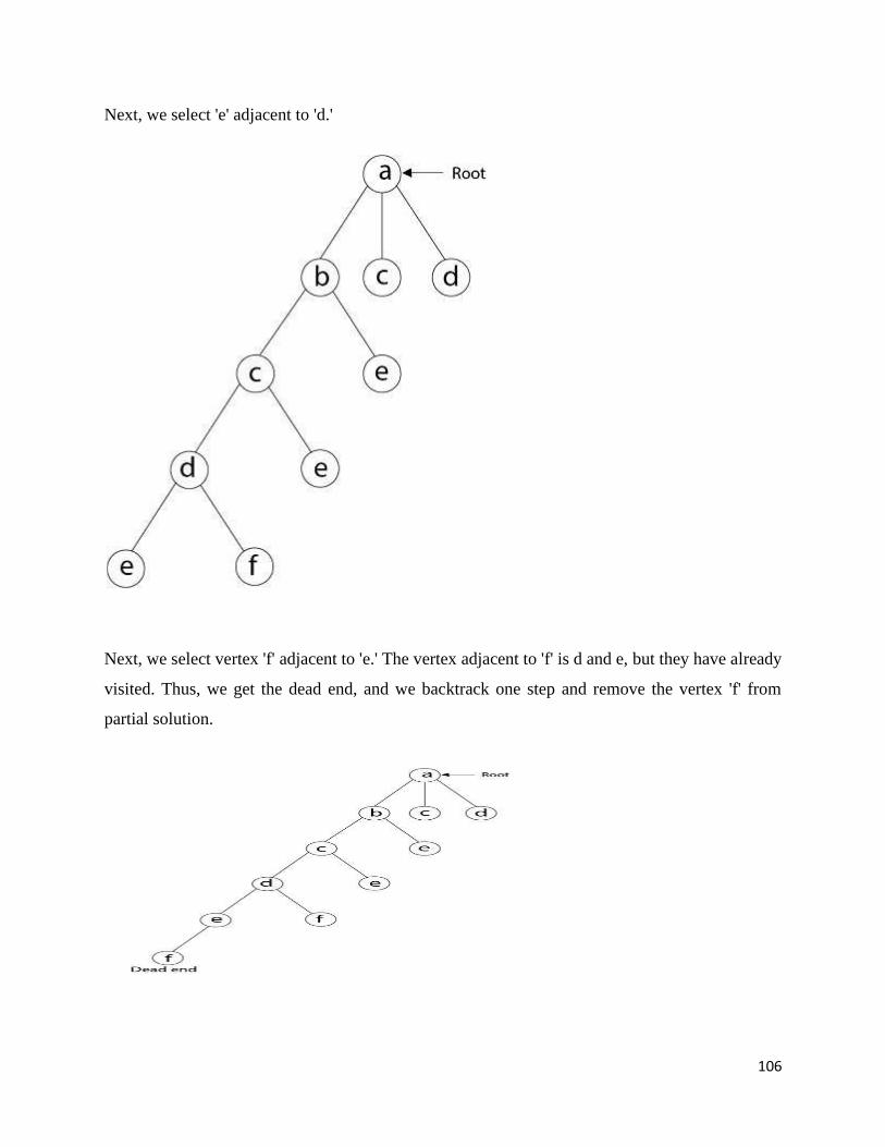
106
Next, we select 'e' adjacent to 'd.'
Next, we select vertex 'f' adjacent to 'e.' The vertex adjacent to 'f' is d and e, but they have already
visited. Thus, we get the dead end, and we backtrack one step and remove the vertex 'f' from
partial solution.

107
From backtracking, the vertex adjacent to 'e' is b, c, d, and f from which vertex 'f' has already
been checked, and b, c, d have already visited. So, again we backtrack one step. Now, the vertex
adjacent to d are e, f from which e has already been checked, and adjacent of 'f' are d and e. If 'e'
vertex, revisited them we get a dead state. So again we backtrack one step.
Now, adjacent to c is 'e' and adjacent to 'e' is 'f' and adjacent to 'f' is 'd' and adjacent to 'd' is 'a.'
Here, we get the Hamiltonian Cycle as all the vertex other than the start vertex 'a' is visited only
once. (a - b - c - e - f -d - a).
Dead end
Backtrack
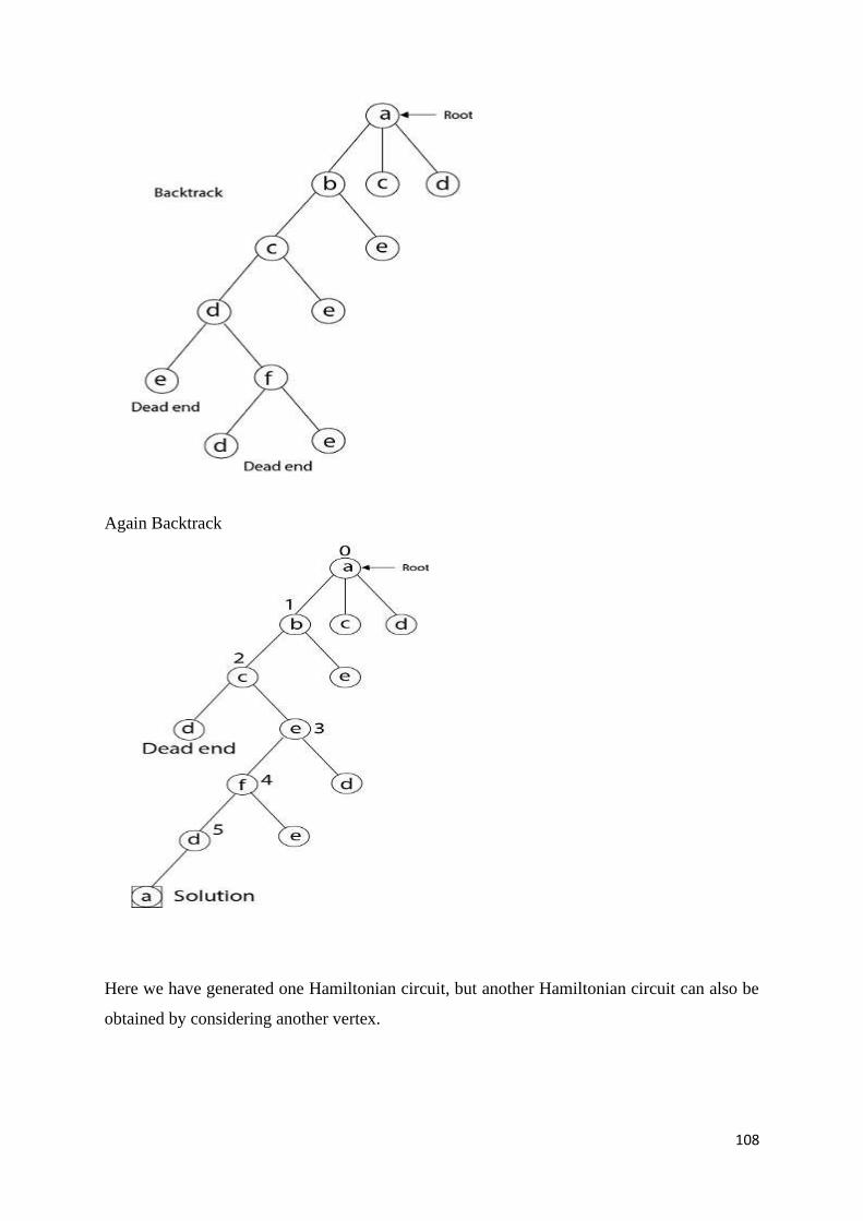
108
Again Backtrack
Here we have generated one Hamiltonian circuit, but another Hamiltonian circuit can also be
obtained by considering another vertex.
109
Branch and bound
Branch and bound is an algorithm design paradigm which is generally used for solving
combinatorial optimization problems. These problems are typically exponential in terms of
time complexity and may require exploring all possible permutations in worst case. The
Branch and Bound Algorithm technique solves these problems relatively quickly.
Job Assignment Problem:
Problem Statement:
Let’s first define a job assignment problem. In a standard version of a job assignment
problem, there can be jobs and workers. To keep it simple, we’re taking jobs and
workers in our example:
We can assign any of the available jobs to any worker with the condition that if a job is
assigned to a worker, the other workers can’t take that particular job. We should also notice
that each job has some cost associated with it, and it differs from one worker to another.
Here the main aim is to complete all the jobs by assigning one job to each worker in such a
way that the sum of the cost of all the jobs should be minimized.
Pseudocode:
110
Here, M[][] is the input cost matrix that contains information like the number of available
jobs, a list of available workers, and the associated cost for each job. The function
MinCost() maintains a list of active nodes. The function LeastCost() calculates the minimum
cost of the active node at each level of the tree. After finding the node with minimum cost,
we remove the node from the list of active nodes and return it. We are using
the Add() function in the pseudocode, which calculates the cost of a particular node and adds
it to the list of active nodes. In the search space tree, each node contains some information,
such as cost, a total number of jobs, as well as a total number of workers.
Initially, we have 3 jobs available. The worker A has the option to take any of the available
jobs. So at level 1, we assigned all the available jobs to the worker A and calculated the cost.
We can see that when we assigned jobs 2 to the worker A, it gives the lowest cost in
level 1 of the search space tree. So we assign the job 2 to worker A and continue the
algorithm. “Yes” indicates that this is currently optimal cost.
After assigning the job 2 to worker A, we still have two open jobs. Let’s consider
worker B now. We are trying to assign either job 1 or 3 to worker B to obtain optimal cost.
Either we can assign the job 1 or 3 to worker B. Again we check the cost and assign job 1 to
worker B as it is the lowest in level 2.
Finally, we assign the job 3 to worker C, and the optimal cost is 12.
111
Knapsack Problem
Given two arrays v[] and w[] that represent values and weights associated with n items
respectively. Find out the maximum value subset (Maximum Profit) of v[] such that sum of
the weights of this subset is smaller than or equal to Knapsack capacity Cap(W).
Branch and bound (BB) is an algorithm design paradigm for discrete and combinatorial
optimization problems, as well as mathematical optimization. Combinatorial optimization
problems are mostly exponential in terms of time complexity. Also it may require to solve all
possible permutations of the problem in worst case. So, by using Branch and Bound it can be
solved quickly.
The backtracking based solution works better than brute force by ignoring infeasible
solutions. To do better (than backtracking) if we know a bound on best possible solution
subtree rooted with every node. If the best in subtree is worse than current best, we can
simply ignore this node and its subtrees. So we compute bound (best solution) for every node
and compare the bound with current best solution before exploring the node.
112
To find bound for every node for Knapsack:
To check if a particular node can give us a better solution or not, we compute the optimal
solution (through the node) using Greedy method. If the solution computed by Greedy
approach is more than the best until now , then we can’t get a better solution through the
node.
Algorithm:
1. Sort all items in decreasing order of V/W so that upper bound can be computed using
Greedy Approach.(The nodes taken in the image are accordingly.)
2. Initialize profit, max = 0
3. Create an empty queue, Q.
4. Create a dummy node of decision tree and enqueue it to Q. Profit and weight of
dummy node are 0.
5. Do while (Q is not empty).
• Extract an item from Q. Let the item be x.
• Compute profit of next level node. If the profit is more than max, then update
max. (Profit from root to this node (include this node)).
• Compute bound of next level node. If bound is more than max, then add next
level node to Q.(Upper Bound of the maximum Profit in subtree of this node)
• Consider the case when next level node is not considered as part of solution
and add a node to queue with level as next, but weight and profit without
considering next level nodes.
Branch and Bound Method
The branch and bound method are similar to the backtracking method except that, this
method searches the nodes of the solution space in the Breadth First Search method. This
branches to various nodes in search of the solution, but if an infeasible solution is
encountered, then we bound back and try the next adjacent branch.
Travelling Salesman Problem
We have already solved this problem using the dynamic programming method. Now
let us see how to solve this problem using branch and bound technique.
Given:
• A graph showing n number of cities connected by edges.
• Cost of each edge is given using the cost matrix.
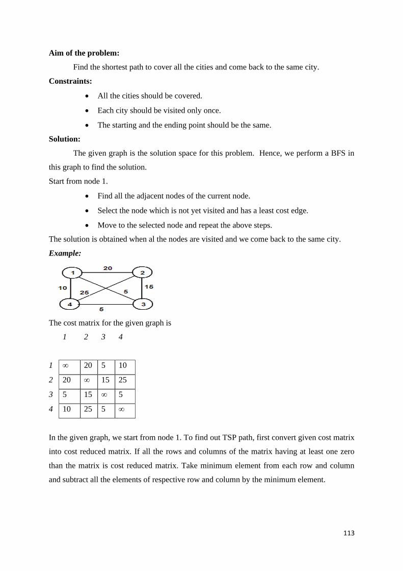
113
Aim of the problem:
Find the shortest path to cover all the cities and come back to the same city.
Constraints:
• All the cities should be covered.
• Each city should be visited only once.
• The starting and the ending point should be the same.
Solution:
The given graph is the solution space for this problem. Hence, we perform a BFS in
this graph to find the solution.
Start from node 1.
• Find all the adjacent nodes of the current node.
• Select the node which is not yet visited and has a least cost edge.
• Move to the selected node and repeat the above steps.
The solution is obtained when al the nodes are visited and we come back to the same city.
Example:
The cost matrix for the given graph is
1 2 3 4
1 ∞ 20 5 10
2 20 ∞ 15 25
3 5 15 ∞ 5
4 10 25 5 ∞
In the given graph, we start from node 1. To find out TSP path, first convert given cost matrix
into cost reduced matrix. If all the rows and columns of the matrix having at least one zero
than the matrix is cost reduced matrix. Take minimum element from each row and column
and subtract all the elements of respective row and column by the minimum element.
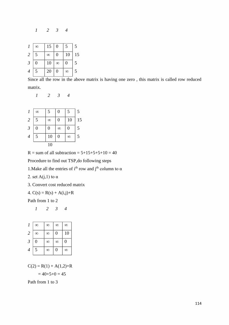
114
1 2 3 4
1 ∞ 15 0 5 5
2 5 ∞ 0 10 15
3 0 10 ∞ 0 5
4 5 20 0 ∞ 5
Since all the row in the above matrix is having one zero , this matrix is called row reduced
matrix.
1 2 3 4
1 ∞ 5 0 5 5
2 5 ∞ 0 10 15
3 0 0 ∞ 0 5
4 5 10 0 ∞ 5
10
R = sum of all subtraction = 5+15+5+5+10 = 40
Procedure to find out TSP,do following steps
1.Make all the entries of ith row and jth column to α
2. set A(j,1) to α
3. Convert cost reduced matrix
4. C(s) = R(s) + A(i,j)+R
Path from 1 to 2
1 2 3 4
1 ∞ ∞ ∞ ∞
2 ∞ ∞ 0 10
3 0 ∞ ∞ 0
4 5 ∞ 0 ∞
C(2) = R(1) + A(1,2)+R
= 40+5+0 = 45
Path from 1 to 3
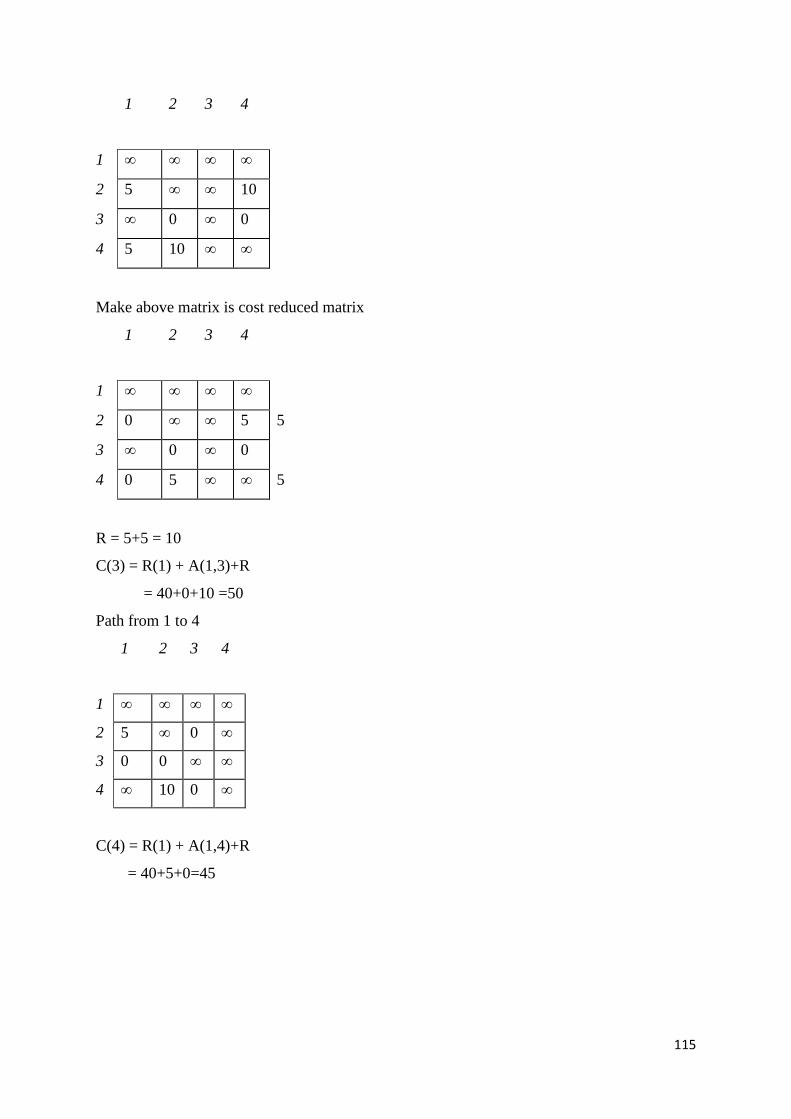
115
1 2 3 4
1 ∞ ∞ ∞ ∞
2 5 ∞ ∞ 10
3 ∞ 0 ∞ 0
4 5 10 ∞ ∞
Make above matrix is cost reduced matrix
1 2 3 4
1 ∞ ∞ ∞ ∞
2 0 ∞ ∞ 5 5
3 ∞ 0 ∞ 0
4 0 5 ∞ ∞ 5
R = 5+5 = 10
C(3) = R(1) + A(1,3)+R
= 40+0+10 =50
Path from 1 to 4
1 2 3 4
1 ∞ ∞ ∞ ∞
2 5 ∞ 0 ∞
3 0 0 ∞ ∞
4 ∞ 10 0 ∞
C(4) = R(1) + A(1,4)+R
= 40+5+0=45
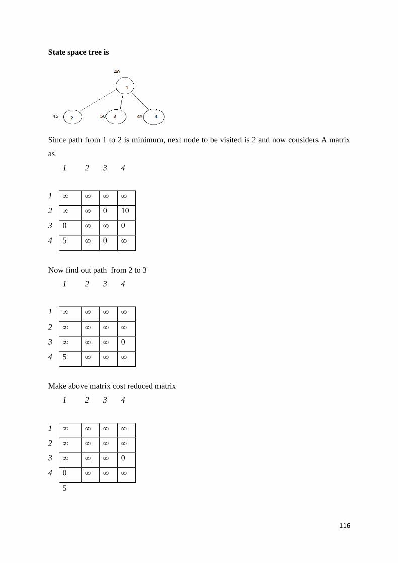
116
State space tree is
Since path from 1 to 2 is minimum, next node to be visited is 2 and now considers A matrix
as
1 2 3 4
1 ∞ ∞ ∞ ∞
2 ∞ ∞ 0 10
3 0 ∞ ∞ 0
4 5 ∞ 0 ∞
Now find out path from 2 to 3
1 2 3 4
1 ∞ ∞ ∞ ∞
2 ∞ ∞ ∞ ∞
3 ∞ ∞ ∞ 0
4 5 ∞ ∞ ∞
Make above matrix cost reduced matrix
1 2 3 4
1 ∞ ∞ ∞ ∞
2 ∞ ∞ ∞ ∞
3 ∞ ∞ ∞ 0
4 0 ∞ ∞ ∞
5
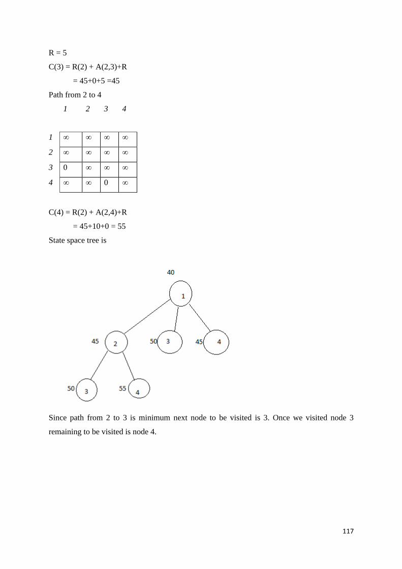
117
R = 5
C(3) = R(2) + A(2,3)+R
= 45+0+5 =45
Path from 2 to 4
1 2 3 4
1 ∞ ∞ ∞ ∞
2 ∞ ∞ ∞ ∞
3 0 ∞ ∞ ∞
4 ∞ ∞ 0 ∞
C(4) = R(2) + A(2,4)+R
= 45+10+0 = 55
State space tree is
Since path from 2 to 3 is minimum next node to be visited is 3. Once we visited node 3
remaining to be visited is node 4.
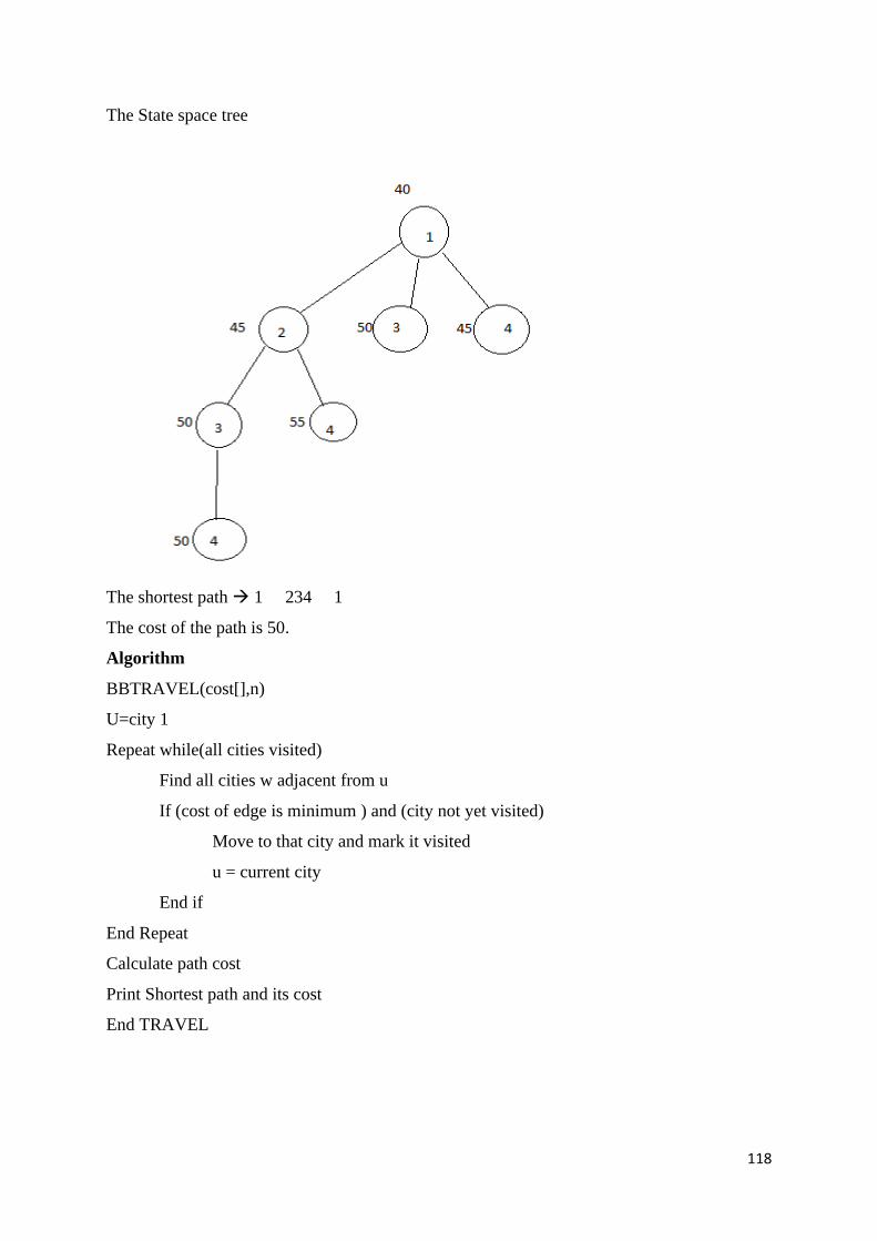
118
The State space tree
The shortest path → 1 234 1
The cost of the path is 50.
Algorithm
BBTRAVEL(cost[],n)
U=city 1
Repeat while(all cities visited)
Find all cities w adjacent from u
If (cost of edge is minimum ) and (city not yet visited)
Move to that city and mark it visited
u = current city
End if
End Repeat
Calculate path cost
Print Shortest path and its cost
End TRAVEL
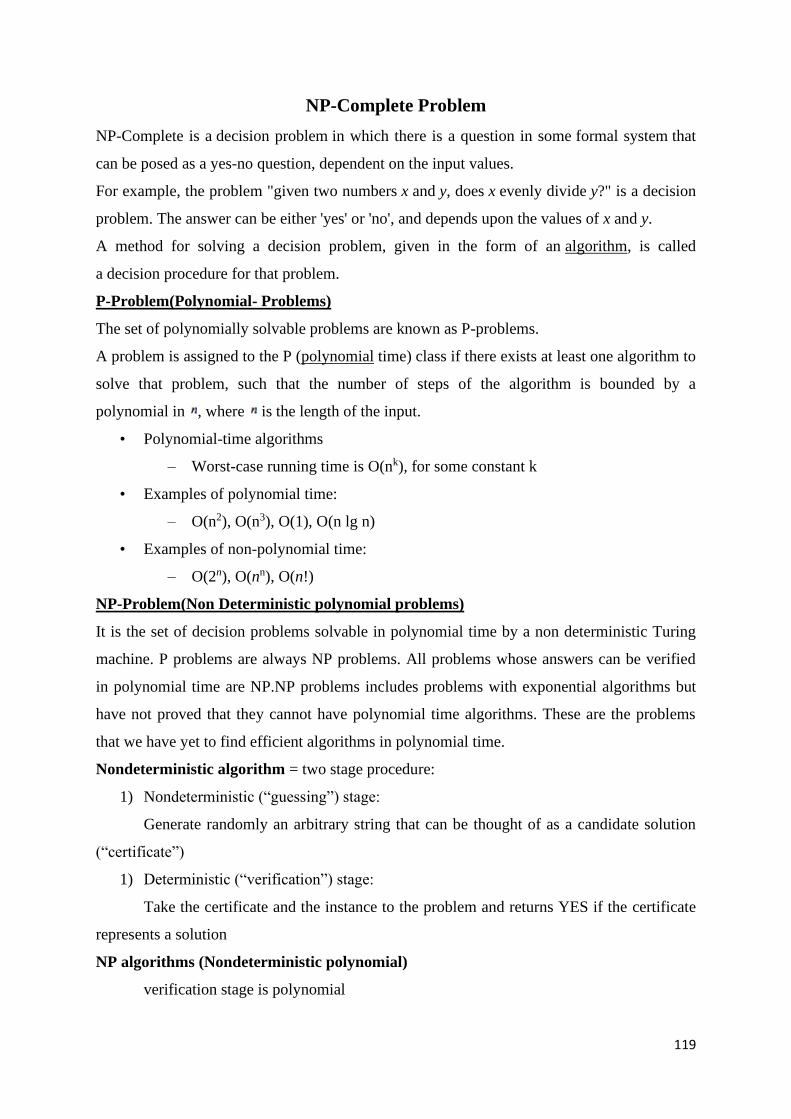
119
NP-Complete Problem
NP-Complete is a decision problem in which there is a question in some formal system that
can be posed as a yes-no question, dependent on the input values.
For example, the problem "given two numbers x and y, does x evenly divide y?" is a decision
problem. The answer can be either 'yes' or 'no', and depends upon the values of x and y.
A method for solving a decision problem, given in the form of an algorithm, is called
a decision procedure for that problem.
P-Problem(Polynomial- Problems)
The set of polynomially solvable problems are known as P-problems.
A problem is assigned to the P (polynomial time) class if there exists at least one algorithm to
solve that problem, such that the number of steps of the algorithm is bounded by a
polynomial in , where is the length of the input.
• Polynomial-time algorithms
– Worst-case running time is O(nk), for some constant k
• Examples of polynomial time:
– O(n2), O(n3), O(1), O(n lg n)
• Examples of non-polynomial time:
– O(2n), O(nn), O(n!)
NP-Problem(Non Deterministic polynomial problems)
It is the set of decision problems solvable in polynomial time by a non deterministic Turing
machine. P problems are always NP problems. All problems whose answers can be verified
in polynomial time are NP.NP problems includes problems with exponential algorithms but
have not proved that they cannot have polynomial time algorithms. These are the problems
that we have yet to find efficient algorithms in polynomial time.
Nondeterministic algorithm = two stage procedure:
1) Nondeterministic (“guessing”) stage:
Generate randomly an arbitrary string that can be thought of as a candidate solution
(“certificate”)
1) Deterministic (“verification”) stage:
Take the certificate and the instance to the problem and returns YES if the certificate
represents a solution
NP algorithms (Nondeterministic polynomial)
verification stage is polynomial
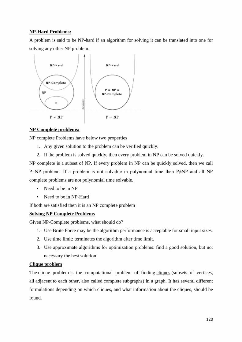
120
NP-Hard Problems:
A problem is said to be NP-hard if an algorithm for solving it can be translated into one for
solving any other NP problem.
NP Complete problems:
NP complete Problems have below two properties
1. Any given solution to the problem can be verified quickly.
2. If the problem is solved quickly, then every problem in NP can be solved quickly.
NP complete is a subset of NP. If every problem in NP can be quickly solved, then we call
P=NP problem. If a problem is not solvable in polynomial time then P≠NP and all NP
complete problems are not polynomial time solvable.
• Need to be in NP
• Need to be in NP-Hard
If both are satisfied then it is an NP complete problem
Solving NP Complete Problems
Given NP-Complete problems, what should do?
1. Use Brute Force may be the algorithm performance is acceptable for small input sizes.
2. Use time limit: terminates the algorithm after time limit.
3. Use approximate algorithms for optimization problems: find a good solution, but not
necessary the best solution.
Clique problem
The clique problem is the computational problem of finding cliques (subsets of vertices,
all adjacent to each other, also called complete subgraphs) in a graph. It has several different
formulations depending on which cliques, and what information about the cliques, should be
found.
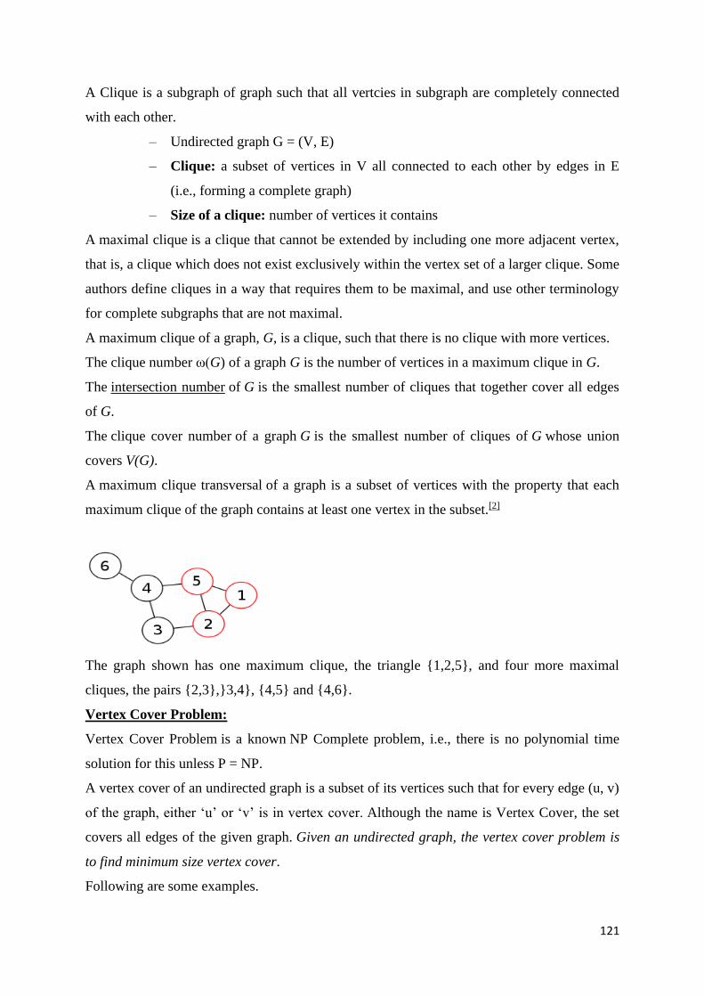
121
A Clique is a subgraph of graph such that all vertcies in subgraph are completely connected
with each other.
– Undirected graph G = (V, E)
– Clique: a subset of vertices in V all connected to each other by edges in E
(i.e., forming a complete graph)
– Size of a clique: number of vertices it contains
A maximal clique is a clique that cannot be extended by including one more adjacent vertex,
that is, a clique which does not exist exclusively within the vertex set of a larger clique. Some
authors define cliques in a way that requires them to be maximal, and use other terminology
for complete subgraphs that are not maximal.
A maximum clique of a graph, G, is a clique, such that there is no clique with more vertices.
The clique number ω(G) of a graph G is the number of vertices in a maximum clique in G.
The intersection number of G is the smallest number of cliques that together cover all edges
of G.
The clique cover number of a graph G is the smallest number of cliques of G whose union
covers V(G).
A maximum clique transversal of a graph is a subset of vertices with the property that each
maximum clique of the graph contains at least one vertex in the subset.[2]
The graph shown has one maximum clique, the triangle 1,2,5, and four more maximal
cliques, the pairs 2,3,3,4, 4,5 and 4,6.
Vertex Cover Problem:
Vertex Cover Problem is a known NP Complete problem, i.e., there is no polynomial time
solution for this unless P = NP.
A vertex cover of an undirected graph is a subset of its vertices such that for every edge (u, v)
of the graph, either ‘u’ or ‘v’ is in vertex cover. Although the name is Vertex Cover, the set
covers all edges of the given graph. Given an undirected graph, the vertex cover problem is
to find minimum size vertex cover.
Following are some examples.
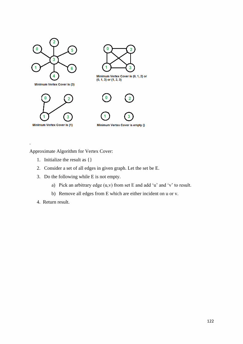
122
.
Approximate Algorithm for Vertex Cover:
1. Initialize the result as
2. Consider a set of all edges in given graph. Let the set be E.
3. Do the following while E is not empty.
a) Pick an arbitrary edge (u,v) from set E and add ‘u’ and ‘v’ to result.
b) Remove all edges from E which are either incident on u or v.
4. Return result.
123