A semantic learning for content-based image retrieval using analytical hierarchy process
Upload
khangminh22Category
view
1download
0
Pilar Hernández Mesa
Pila
r H
erná
ndez
Mes
aD
esig
n a
nd
an
alys
is o
f a
con
ten
t-b
ased
imag
e re
trie
val s
yste
m
Forschungsberichte aus derIndustriellen Informationstechnik
16
Design and analysis of a content-based image retrieval system


Pilar Hernández Mesa
Design and analysis of a content-based image retrieval system

Forschungsberichte aus der Industriellen Informationstechnik Band 16
Institut für Industrielle Informationstechnik Karlsruher Institut für TechnologieHrsg. Prof. Dr.-Ing. Fernando Puente León Prof. Dr.-Ing. habil. Klaus Dostert
Eine Übersicht aller bisher in dieser Schriftenreihe erschienenen Bände finden Sie am Ende des Buchs.

Design and analysis of a content-based image retrieval system
by Pilar Hernández Mesa

Print on Demand 2017 – Gedruckt auf FSC-zertifiziertem Papier
ISSN 2190-6629ISBN 978-3-7315-0692-8 DOI 10.5445/KSP/1000071866
This document – excluding the cover, pictures and graphs – is licensed under a Creative Commons Attribution-Share Alike 4.0 International License (CC BY-SA 4.0): https://creativecommons.org/licenses/by-sa/4.0/deed.en
The cover page is licensed under a Creative CommonsAttribution-No Derivatives 4.0 International License (CC BY-ND 4.0):https://creativecommons.org/licenses/by-nd/4.0/deed.en
Impressum
Karlsruher Institut für Technologie (KIT) KIT Scientific Publishing Straße am Forum 2 D-76131 Karlsruhe
KIT Scientific Publishing is a registered trademark of Karlsruhe Institute of Technology. Reprint using the book cover is not allowed.
www.ksp.kit.edu
Karlsruher Institut für TechnologieInstitut für Industrielle Informationstechnik
Design and analysis of a content-based image retrieval system
Zur Erlangung des akademischen Grades eines Doktor-Ingenieurs von der Fakultät für Elektrotechnik und Informationstechnik des Karlsruher Instituts für Technologie (KIT) genehmigte Dissertation
von Dipl.-Ing. Pilar Hernández Mesa geb. in Firgas, Spanien
Tag der mündlichen Prüfung: 02. Juni 2017Referent: Prof. Dr.-Ing. Fernando Puente León, KITKorreferent: apl. Prof. Dr.-Ing. Ralf Mikut, KIT


Design and analysis of acontent-based image retrieval system
Zur Erlangung des akademischen Grades eines
DOKTOR-INGENIEURS
von der Fakultät für
Elektrotechnik und Informationstechnik
des Karlsruher Instituts für Technologie (KIT)
genehmigte
DISSERTATION
von
Dipl.-Ing. Pilar Hernández Mesa
geb. in Firgas, Spanien
Tag der mündl. Prüfung: 02. Juni 2017Hauptreferent: Prof. Dr.-Ing. Fernando Puente León, KITKorreferent: apl. Prof. Dr.-Ing. Ralf Mikut, KIT


Acknowledgements
This doctoral thesis would not have been possible without the supportof many people.
To begin I would like to thank Prof. Dr.-Ing. Fernando Puente Leónfor supporting the execution of this thesis as supervisor and for lettingme be part of his team over the last years. I am also extremely gratefulto apl. Prof. Dr.-Ing. Ralf Mikut for taking over the duty of secondexaminer. Special thanks go to Prof. Dr. rer. nat. Olaf Dössel, Prof. Dr.rer. nat. Uli Lemmer, and Prof. Dr.-Ing. Eric Sax who kindly accepted tojoin the board of examiners.
This work was performed during my time as a research associateat the Institut für Industrielle Informationstechnik (IIIT) which belongs tothe Karlsruhe Institute of Technology (KIT). I am extremely grateful toProf. Dr.-Ing. Michael Heizmann for his advice, time, and support atthe completion of the doctoral process as well as for encouraging mesince he joined the IIIT. I also want to thank all my colleagues at the IIITfor their contributions. Special thanks go to Mario Lietz and Dr.-Ing.Johannes Pallauf, as well as to Manuela Moritz for her great support.During my time at the IIIT I had the opportunity to work with manystudents and supervise Bachelor, Master, and Diploma theses. I want toexpress to all of them my warmest gratitude.
It is a pleasure for me to thank Prof. Dr.-Ing. Barbara Deml, Dipl.-Psych., and her research associates Dr.-Ing. Marc Schneider and TobiasHeine. Without their support the psychology experiment in my workwould not have been possible.
Last but not least I want to thank my friends and family for theirunconditional support and trust in me. I thank Christoph for his sup-port and encouragement over the last years as well as for his carefullyproofreading of this thesis. I am deeply indebted with my sister María,who has carefully proofread this thesis and moreover supported meover this project and all the other ones in my life. Finally, I want tothank my parents, Toñi and Roque, for supporting and believing in me

ii Acknowledgements
always, as well as for the possibilities, education, and everything thatthey have given me through my whole life. Without them and my sisterMaría none of this would have been possible.
Karlsruhe, June 2017 Pilar Hernández Mesa
Kurzfassung
Sehen ist einer der fünf Sinne des Menschen, der uns ermöglicht, unserevisuelle Umgebung wahrzunehmen. Ein Bild zu zeigen ist oft einfacher,schneller und genauer als eine Beschreibung des Inhalts mit Worten,was nicht immer möglich ist. Die Technologie zur Herstellung von digi-talen Kameras und Speichern hat in den letzten Jahrzehnten enormeFortschritte gemacht. Heutzutage sind digitale Kameras sogar in vielenGeräten, wie Mobiltelefonen und Laptops, integriert. Eine schnelle undeinfache Aufnahme von Bildern ist somit möglich. Tatsache ist, dassan jedem Tag sehr viele digitale Bilder generiert werden. Diese Bilderenthalten Informationen, die leider verloren gehen können, wenn eskeine geeigneten Methoden gibt, um die Bilder inhaltlich miteinanderzu vergleichen. Diese Problematik wird in der inhaltsbasierten Bild-suche behandelt. Ziel dieser Arbeit ist die Untersuchung der Sortierungvon Bildern aufgrund deren Ähnlichkeit mit einem Eingangsbild. Fürdas Ähnlichkeitsmaß wird von der menschlichen Wahrnehmung aus-gegangen, welche spontan und ohne Anstrengung und Überlegungdurchgeführt wird, wie bei Julesz in [73] beschrieben. Ähnlichkeiten auf-grund weiterer Verarbeitungen im Gehirn, wie zum Beispiel aufgrundeiner Objekterkennung, liegen außerhalb des Umfangs dieser Arbeit.
Die unabhängige Extraktion von Farb-, Form- und Texturmerkmalen,die getrennte Sortierung dieser Merkmale nach Ähnlichkeit und dieDetektion von Regionen in Bildern, aufgrund zusammenhängenderFlächen mit ähnlicher Farbe oder aufgrund von Mustern basierendauf abwechselnden Farbkombinationen, werden als Vorgehensweiseausgewählt. Methoden werden für alle diese Aspekte vorgeschla-gen, getestet und evaluiert. Zudem ist, um die menschliche Ähn-lichkeitswahrnehmung anhand von Mustermerkmalen bewerten zu kön-nen, mit Hilfe von Psychologen ein Experiment mit Probanden durchge-führt worden. Ein Wahrnehmungsraum wird aus diesen Daten erstellt.
Anschließend wird die Fusion der unterschiedlichen extrahiertenInformationen untersucht. Zuerst werden die extrahierten Regionen

iv Kurzfassung
durch die Fusion mit den Musterinformationen verbessert. Anschlie-ßend wird aus der Fusion aller extrahierter Informationen ein inhalts-basiertes Suchsystem vorgestellt. Diese ist in der Lage, automatischdie Gewichtung der einzelnen Merkmale beim Ähnlichkeitsvergleich jenach Eigenschaften der verglichenen Bilder anzupassen. Die Ergebnissezeigen, dass diese Methodik immer sehr gute Sortierungsergebnisseerreicht und sogar in vielen Fällen die Sortierungsergebnisse nach deneinzelnen Merkmalen übertrifft.

Contents
Nomenclature . . . . . . . . . . . . . . . . . . . . . . . . . . . . . . ix
1 Introduction . . . . . . . . . . . . . . . . . . . . . . . . . . . . . 11.1 Motivation . . . . . . . . . . . . . . . . . . . . . . . . . . . 11.2 Content-based image retrieval . . . . . . . . . . . . . . . . 21.3 Scope of this work . . . . . . . . . . . . . . . . . . . . . . 41.4 Outline of this work . . . . . . . . . . . . . . . . . . . . . 41.5 Own contribution . . . . . . . . . . . . . . . . . . . . . . . 5
2 Mathematical background . . . . . . . . . . . . . . . . . . . . 92.1 Distance functions and similarity comparisons . . . . . . 92.2 Graph theory . . . . . . . . . . . . . . . . . . . . . . . . . 11
2.2.1 Basic concepts of graph theory . . . . . . . . . . . 112.2.2 Directed graphs . . . . . . . . . . . . . . . . . . . . 132.2.3 Trees . . . . . . . . . . . . . . . . . . . . . . . . . . 14
2.3 Space-frequency representations . . . . . . . . . . . . . . 162.3.1 One-dimensional Fourier transform . . . . . . . . 162.3.2 Two-dimensional Fourier transform . . . . . . . . 182.3.3 One-dimensional wavelet transform . . . . . . . . 182.3.4 Two-dimensional wavelet transform . . . . . . . . 19
3 Color . . . . . . . . . . . . . . . . . . . . . . . . . . . . . . . . . 213.1 Introduction to color . . . . . . . . . . . . . . . . . . . . . 21
3.1.1 Color representation . . . . . . . . . . . . . . . . . 223.1.2 State of the art . . . . . . . . . . . . . . . . . . . . 23
3.2 A compact color signature in CIELAB color space forimages . . . . . . . . . . . . . . . . . . . . . . . . . . . . . 253.2.1 Graph representation of the color information . . 263.2.2 Types of nodes . . . . . . . . . . . . . . . . . . . . 263.2.3 Compact representation of the graph . . . . . . . 273.2.4 Color signature of the image . . . . . . . . . . . . 28

vi Contents
3.3 Humans’ color categories . . . . . . . . . . . . . . . . . . 293.3.1 Processing the recorded database . . . . . . . . . 303.3.2 Extraction of the color categories . . . . . . . . . . 313.3.3 Representation of color using the extracted color
categories . . . . . . . . . . . . . . . . . . . . . . . 32
4 Shape . . . . . . . . . . . . . . . . . . . . . . . . . . . . . . . . 354.1 Introduction to shape . . . . . . . . . . . . . . . . . . . . . 35
4.1.1 Shape representation . . . . . . . . . . . . . . . . . 364.1.2 State of the art . . . . . . . . . . . . . . . . . . . . 37
4.2 Normal angular descriptors . . . . . . . . . . . . . . . . . 404.2.1 Normal angular descriptor . . . . . . . . . . . . . 404.2.2 Similarity comparisons . . . . . . . . . . . . . . . 40
4.3 Fourier descriptors . . . . . . . . . . . . . . . . . . . . . . 444.3.1 Scaling-invariant descriptor . . . . . . . . . . . . . 454.3.2 Descriptor with normalized energy . . . . . . . . 454.3.3 Scaling- and rotation-invariant descriptor . . . . . 45
5 Texture . . . . . . . . . . . . . . . . . . . . . . . . . . . . . . . . 475.1 Introduction to texture . . . . . . . . . . . . . . . . . . . . 47
5.1.1 Texture representation . . . . . . . . . . . . . . . . 475.1.2 State of the art . . . . . . . . . . . . . . . . . . . . 50
5.2 Analysis, detection, and sorting of regular textures . . . 525.2.1 Extraction of the texel and its displacement
vectors . . . . . . . . . . . . . . . . . . . . . . . . . 535.2.2 Detection of regular textures . . . . . . . . . . . . 625.2.3 Sorting of regular textures . . . . . . . . . . . . . . 675.2.4 Perception map of regular textures . . . . . . . . 74
5.3 Detection of near-regular textures and extraction of theirregular texture . . . . . . . . . . . . . . . . . . . . . . . . . 785.3.1 Detection and grouping of characteristic texel
points . . . . . . . . . . . . . . . . . . . . . . . . . 785.3.2 Extraction of the texels . . . . . . . . . . . . . . . . 815.3.3 Post-processing . . . . . . . . . . . . . . . . . . . . 92
6 Detection of regions . . . . . . . . . . . . . . . . . . . . . . . . 956.1 Introduction to the detection of regions . . . . . . . . . . 95
6.1.1 State of the art . . . . . . . . . . . . . . . . . . . . 966.2 Structure of the proposed region detectors . . . . . . . . 98

Contents vii
6.3 Detection of color regions in images . . . . . . . . . . . . 986.3.1 Extraction of non-overlapping stable color
regions . . . . . . . . . . . . . . . . . . . . . . . . . 986.3.2 Extraction of color regions in images using
humans’ color categories . . . . . . . . . . . . . . 1046.4 Detection and extraction of patterns . . . . . . . . . . . . 108
6.4.1 Detection and extraction of patterns based on theCIELAB color space . . . . . . . . . . . . . . . . . 114
6.4.2 Detection and extraction of patterns based on thehumans’ color categories . . . . . . . . . . . . . . 127
7 Fusion of the methods . . . . . . . . . . . . . . . . . . . . . . 1337.1 Significant patterned regions . . . . . . . . . . . . . . . . 1337.2 Image sorting according to their similarity fusing color,
shape, and texture information . . . . . . . . . . . . . . . 1367.2.1 Feature extraction . . . . . . . . . . . . . . . . . . 1377.2.2 Sorting method . . . . . . . . . . . . . . . . . . . . 139
8 Results . . . . . . . . . . . . . . . . . . . . . . . . . . . . . . . . 1418.1 General evaluation concerns . . . . . . . . . . . . . . . . . 141
8.1.1 Self-made databases . . . . . . . . . . . . . . . . . 1418.1.2 Quality measurements for retrieval applications . 143
8.2 Results of the color . . . . . . . . . . . . . . . . . . . . . . 1458.2.1 A compact color signature in CIELAB color space
for images . . . . . . . . . . . . . . . . . . . . . . . 1468.2.2 Humans’ color categories . . . . . . . . . . . . . . 150
8.3 Results of the shape . . . . . . . . . . . . . . . . . . . . . . 1558.4 Results of the texture . . . . . . . . . . . . . . . . . . . . . 158
8.4.1 Regular textures . . . . . . . . . . . . . . . . . . . 1588.4.2 Near-regular textures . . . . . . . . . . . . . . . . 178
8.5 Results of the detection of regions . . . . . . . . . . . . . 1918.5.1 Color regions in images . . . . . . . . . . . . . . . 1928.5.2 Pattern extraction . . . . . . . . . . . . . . . . . . . 196
8.6 Results of the fusion of the methods . . . . . . . . . . . . 2098.6.1 Significant patterned regions . . . . . . . . . . . . 2098.6.2 Image sorting according to their similarity fusing
color, shape, and texture information . . . . . . . 211
9 Conclusions . . . . . . . . . . . . . . . . . . . . . . . . . . . . . 221

viii Contents
Bibliography . . . . . . . . . . . . . . . . . . . . . . . . . . . . . . 223List of publications . . . . . . . . . . . . . . . . . . . . . . . . . 234List of supervised theses . . . . . . . . . . . . . . . . . . . . . . 236
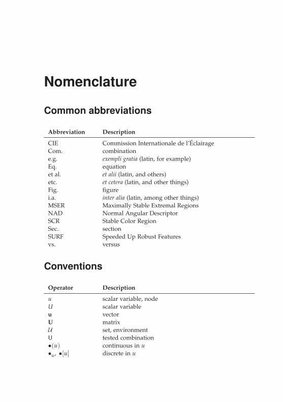
Nomenclature
Common abbreviations
Abbreviation Description
CIE Commission Internationale de l’ÉclairageCom. combinatione.g. exempli gratia (latin, for example)Eq. equationet al. et alii (latin, and others)etc. et cetera (latin, and other things)Fig. figurei.a. inter alia (latin, among other things)MSER Maximally Stable Extremal RegionsNAD Normal Angular DescriptorSCR Stable Color RegionSec. sectionSURF Speeded Up Robust Featuresvs. versus
Conventions
Operator Description
u scalar variable, nodeU scalar variableu vectorU matrixU set, environmentU tested combination•(u) continuous in u•u, •[u] discrete in u

x Nomenclature
Letters
Latin letters
Symbol Description
AAff parameters of the affine transformation that may implyscale, shear, and rotation
a displacement vector of a one-dimensional texture inspace domain
a second vector used to span a parallelogram for theextraction of a texel of a one-dimensional texture
ak displacement vectors of two-dimensional textures inspace domain, k ∈ {1, 2}
B width of the imageB similarity of the componentsb(•) degree of a nodeb+(•) outdegree of a nodeb−(•) indegree of a nodeC1, . . . ,C10 tested combinations to detect and extract color regionscColor
k (•) color represented by the color category kcColor(•) vector representation of the colors represented with
color categoriescPCA principal componentd(•, •) distance functiondBound(•) distance function to detect clusters consisting merely of
contour pointsdCC,1(•) color distance based on the correlation coefficient of the
color categoriesdCC,2(•) color distance based on the �2-norm of the color
categoriesdFourier(•, •) similarity distance between Fourier descriptorsdNAD
1 (•, •) similarity distance between normal angulardescriptors based on the correlation for circular data
dNAD2 (•, •) similarity distance between warped normal angular
descriptors based on the correlation for circular datadNAD
3 (•, •) similarity distance between warped normal angulardescriptors based on the Euclidean distance
dSCRu image of the difference between neighboring pixels
Nomenclature xi
Symbol Description
dSCR,1u image of the difference between neighboring pixels of a
smoothed imagedSCR,2
u image of the difference between neighboring pixels of asmoothed image that preserves edges
dT,1(•, •) similarity distance for the detection of regular texturesin space domain
E(•) set of edgese edgeePCA
u eigentexelFk
u maximum over all color channels and stages of theback projection of the detail signals per orientation,k ∈ {horizontal, vertical, diagonal}
f frequencyf Fourier Fourier descriptorsf norm,hor normalized frequency for the highest stage of the
wavelet transform in horizontal directionf norm,ver normalized frequency for the highest stage of the
wavelet transform in vertical directionf NT,1 relashionship of the length of the displacement vectorsG(•) Fourier transform of g(•)G graphg(u) one-dimensional signalg(u) single-channel imageg(u) reconstructed single-channel imagegbin(u) binary image describing the pixels that belong to a color
regiongMod(u) modified single-channel imagegSynth(u) synthetic single-channel imagegwin(u) one-dimensional windowed signalg(u) three-channel imagegR(u) reconstructed three-channel imageH height of the imageh histogramhArea histogram of the area of the regions in a texelhBright histogram of the brightnessI inputIG relations between the nodes and edges of a graph Gk running index with K as maximum

xii Nomenclature
Symbol Description
L length of a line containing alternating structuresl minimal length of an alternating structurel∗, a∗, b∗ channels of the CIELAB color spacel displacement vector of a one-dimensional texture in
frequency domainl vector orthogonal to the displacement vector of a one-
dimensional texture in frequency domainlk displacement vectors of a two-dimensional texture in
frequency domain, k ∈ {1, 2}m featurem(ϕ) addition of the magnitudes of the Fourier transform
along the radial projection with angle ϕ
mT1 feature for the detection of regular textures in frequencyspace
mT2 feature for the detection of regular textures in frequencyspace
mT3 feature to describe the unlikeliness of a point to belongto the lattice of a near-regular texture
N (•) set of neighbors of a nodeN+(•) set of outneighbors of a nodeN−(•) set of inneighbors of a nodeN1, . . . ,N13 tested combinations to detect and extract near-regular
texturesN natural numbers
nC color namenC,1 number of different color names used by a usernC,2 number of colors named by a usernC,3 number of different subjects that used a color namenC,4 number of times a color name has been usednEdge number of edgesnGM number of good matches in a databasenGM
k number of good matches under k retrievalsnLine number of edge orientations in a texelnRegion number of regions in a texelnT,1 number of spatially closest points to be considerednT,2 number of considered rows, columns, to prove the
repeatability of the texels at the contourn normal vector
Nomenclature xiii
Symbol Description
O outputP1, . . . ,P11 tested combinations to detect and extract patterned
regionsp(• |•) likelihood, probability distributionpcons considered pointpgrid point of a cellpgrid,2 point of a quadrangle where the texels are projectedpk point kpBound
k point k of the compact boundaryplatt point of the latticepposs possible pointqk color category kqP1(•) quality criterion: number of detected color regionsqP2(•) quality criterion: percentage of the image included in a
color regionqP3(•) quality criterion: mean image representation errorqP4(•) quality criterion: common area normalized by the area
of the surfaceqP5(•) quality criterion: common area normalized by the area
of the extracted patternqP6(•) quality criterion: trade-off between qP4(•) and qP5(•)qpre• precision
qpre,ideal• ideal precision
qrec• recall
qretr quality value of the retrieved resultsqS1 unnormalized separability coefficientqsep normalized separability coefficientqT1(•) quality criterion: percentage of the surface covered by
the extracted latticeqT2(•) quality criterion: error between the synthetic image and
the modified input image
q(
vC)
most probably color name of vC
r(•, •) correlation coefficientrCC(•) average correlation coefficient between neighboring
pixelsS structuring elementS1, . . . ,S8 tested combinations to sort shapes by similaritys similarity degree

xiv Nomenclature
Symbol Description
T color term matrixttempk,f template function
tThreshk,u thresholded texel
tu texeltAffu affinely transformed texel
tDetu texel at a determined position
tindu normalized affinely transformed texel
tindu normalized affinely transformed texel approximated via
principal component analysis
tindu average texel over all normalized affinely transformed
texelstModu texels from the modified input image gMod
utrepu representative texel
U1, U2 width and height of the quadrangles where the texelsare projected
U environment in frequency domain dependent on thedisplacement vectors
u position in one-dimensional domainu position in image domainV(•) set of nodesVC set of pixels that belong to a color regionVN set of pixels that belong at least to one of the extracted
texelsv node of a graphvC color valuevlatt node of a graph describing a latticevAff translation of the affine transformationw strengthw(u) one-dimensional window functionw(u) two-dimensional window functionZ Fourier coefficientsZ integer numbers

Nomenclature xv
β absolute difference between the smallest angles of notanti-parallel vectors
Γ(λ, κ) wavelet transformed signalγ angle of the Fourier coefficientsΔ distance valueδ(•) , δ• Dirac delta functionη normal angular descriptorκ shift parameter of the wavelet transformλ scaling parameter of the wavelet transformλPCA eigenvalueμ, μ(•) mean value, average valueρ(•, •) correlation coefficient for circular dataσ, σ(•) standard deviationτ threshold valueτC1 threshold value: maximal allowed length along each
color dimensionτC2 threshold value: minimum number of times a color
name has to be namedτCC threshold value: used for the obtention of color regionsτPCA threshold value: number of strongest eigenvalues to be
consideredτSP1 threshold value: maximal spatial distance to incorporate
a pixel to the mask of a significant patterned regionτT1 threshold value: minimal relationship of the lengths of
the vectorsτT2 threshold value: maximal angle differenceτT3 threshold value: maximal normalized difference to
detect regular texturesτT4 threshold value: overlap of the texels for the
computation of gSynth(u)ϕ orientationϕ( f ) phase of the spectrumψ(•) mother wavelet
Greek letters
Symbol Description
α angle spanned between a displacement vector and theu1-axis

xvi Nomenclature
Mathematical operators
Operator Description
DFT{•} discrete Fourier transformE{•} expected valuemax(•) maximummin(•) minimummed{•} median•rem(•) remainderΣ•• addition| • | magnitude, number of members in a set‖•‖2 �2−norm∅ empty set(•, •) undirected edge[•, •] directed edge�•, �(•) angle∠(•, •) angle between two vectors∀ for all∗ one-dimensional convolution∗∗ two-dimensional convolution(•)T transpose(•)∗ complex conjugate

1 Introduction
Starting with the motivation of the problem that led to the elaboration ofthis work (Sec. 1.1) and an overview of the content-based image retrievalproblem (Sec. 1.2), the scope of this thesis (Sec. 1.3) is presented andits outline is discussed (Sec. 1.4). The most important constributions ofthis work according to the author’s best knowledge are presented atthe end of this chapter (Sec. 1.5).
1.1 Motivation
Sight, one of the five humans’ senses, allows the visual perception ofthe environment. Showing a picture is often easier, faster, more detailed,and more informative than describing its content. What is more, a fulldescription with words of what we perceive with our eyes is not alwayseven possible.
The huge technology progress over the last decades regarding digitalcameras and storage devices enables us to take pictures very fast andeasily. Nowadays, we even find digital cameras integrated in manydevices like cellular phones, notebooks, etc.
Whether digital images make it possible to record the visual per-ception of humans, or due to the progress of the technology, or acombination of both, the fact is that a gigantic amount of digital imagesis created every day. However, this huge amount of data will not be op-timally used and may even become useless if no adequate methods existto compare and sort images automatically by their content according toour similarity perception. This is one of the goals of the content-basedimage retrieval.
Many applications will profit from an adequate content-based imageretrieval like, e.g., search engines and database management systems.Robots are also likely to profit from such a system. Whereas nowadaysthey either recognize objects or categorize them as unknown, more

2 1 Introduction
powerful tasks could be performed if they are able to recognize similarobjects and scenes.
1.2 Content-based image retrieval
The retrieval of images according to the similarity of their content is achallenging task. The initial attempts to solve this problem at the 1970stransfer it to a text-based retrieval. This implies that the images mustbe manually annotated by humans first. This is a tedious job, whichis human dependent and impracticable with a big number of images.To overcome these drawbacks, the content-based image retrieval wasintroduced [87, 123].
“Find similar images to my query” seems to be a clear descriptionof the content-based image retrieval problem, but what does “similarimages” mean? The answer to this question depends, i.a., on the aim ofthe search. Smeulders et al. point in [127] three broad categories: thetarget search, where the user searches either for a specific image or animage of the same object of which he has an image, the category search,where the user searches image representatives of a specific class, andthe association search, where the user is interested in finding interestingthings and does not even have a specific aim of what he is searching for.Chalom et al. give in [31] an overview of some applications to measureimage similarity. They describe a pattern recognition approach, whichimplies training a system, and image stabilization, where correspondingpoints of images are mapped.
Two gaps existing at the content-based image retrieval problem aredescribed by Smeulders et al. in [127]. The sensory gap, which is thegap between the scene in the real world and the image representation(e.g., the occlusions of objects), and the semantic gap, which is the gapbetween the visual information and the interpretation derived fromthe user.
Depending on the aim of the search, different types of queries andsystem specifications are necessary. The query may be a text, a sketch,an image, or a group of images. Training the system with previousknowledge of object classes or even by interacting with the user (rel-evance feedback) is also possible. Overviews of content-based imageretrieval methods are given in [38, 39, 87, 123, 127].

1.2 Content-based image retrieval 3
No matter what the concrete aim of the search is, the proceedingsmentioned at the overview of the content-based image retrieval methodsin [38, 39, 87, 123, 127] always propose the extraction of features fromthe images. These features are compared to measure the similarity ordissimilarity between the images. Global or local features are possiblethat describe, i.a., the color, the shape, or the texture information.Many researchers have focused on features describing only one typeof the information. They consider the retrieval of the images using,e.g., only color, shape, or texture features. Furthermore, when localfeatures are used, an image segmentation may also be necessary or thedetection of regions or salient features [39, 87, 123, 127]. An overviewof region-based image retrieval can be found in [69]. They also followthe procedure of extracting features from the images describing, e.g.,their color, shape, or texture property and compare them next.
SIMPLIcity [139] and the system described in [30], that uses theBlobworld representation presented in [30], are examples of content-based image retrieval systems. In both cases the image is segmentedfirst and the regions are compared based on their color, texture, andeventually shape features next. The overall similarity between twoimages is then calculated from a linear combination of the differentproperties. In [30] these may even be independently weighted fromeach other.
If we move over to image web search systems we find, e.g., TinEye[132] and Google Images [57]. TinEye states that they are the first imagesearch engine in the web that only uses image identification technologywithout keywords, metadata, or watermarks. However, they do notpresent their system as a method to find similar images, but just alteredcopies of the input image, as the system cannot recognize the contentof the images. The search of different images containing the same,or similar, objects is therefore not possible [133]. On the other hand,no detailed official publication of the procedure followed by GoogleImages is known to the author except the broad statement that fromthe most distinctive points, lines, and textures found at the input imagea mathematical model is built [55]. However, in [56] Google states thatthe system works best if the query image is likely to be on the web.

4 1 Introduction
1.3 Scope of this work
As the content-based image retrieval is a challenging task with nodetailed requirements (see Sec. 1.2), the following system specificationsare expected in this thesis.
� The query can only be formulated as a single image. No metadata,watermarks, labels, or several images are allowed as a query.
� Only information extracted directly from the images is used. Nometadata, watermarks, text, etc., can be used from the system tocompare and retrieve the images.
� The system searches images with similar content. This impliesthat similar images are not limited to altered copies of the inputimage, nor to the recognition of the same objects of the inputimage.
� As similarity, the focus is set on pure perception of humans.This implies similarity that is spontaneously applied withouteffort or deliberation as described by Julesz in [73]. Similarityassumptions due to further processing in the brain, e.g., objectcategorization, is beyond the scope of this work. This implies, i.a.,that two objects should not be considered similar because theyhave the same functionality or are biologically classified into thesame group. For example, a car and a motorcycle should not beretrieved as similar because they are both modes of transport.
� No interaction with the user is desired. Relevance feedback istherefore beyond the scope of this work. On the one hand theuser should not be bothered, on the other hand an interactionwith the user is not always possible, e.g., in applications where arobot “sees” something new and unknown.
1.4 Outline of this work
This work is organized in nine chapters. A brief introduction to themost important mathematical background needed is given in the nextchapter (chapter 2). The use of features is considered for the content-based image retrieval problem (see Fig. 1.1). The extraction of the color,

1.5 Own contribution 5
the shape, and the texture information from images are independentlyconsidered from each other. For this purpose, the extraction of these fea-tures, as well as their comparisons, are addressed in chapter 3, chapter 4,and chapter 5, respectively. However, as most images consist of severalmeaningful regions that are independent of each other, the featuresshould not be extracted from the whole image but from the differentregions. The detection and extraction of connected regions in the im-ages due to areas with a similar color or a pattern, which is consideredin this work as a repetition of alternating colors, is therefore necessary.In chapter 6 the detection of such kind of regions is addressed. Bothbetter extracted meaningful regions and better content-based imageretrievals are expected from the fusion of the previously mentionedmethods. Chapter 7 addresses the fusion of the methods and presentsthe proposed content-based image retrieval environment that worksfollowing the sketch of Fig. 1.1. Finally, the results of the presentedmethods are shown in chapter 8 followed by the conclusions of thework and an outlook in chapter 9.
1.5 Own contribution
The decomposition of the content-based image retrieval problem tothe extraction of features describing the properties of the image is acommon procedure that is likely to be combined with a segmentationor detection of salient features. Although several researchers havealready investigated different possible features describing, i.a., color,shape, or texture properties, the author believes in the need for featuresand similarity comparisons strongly based on the human perception.Furthermore, the author also believes in the importance of a good fusionof features describing different properties together with an appropriateselection of significant regions of the image describing its content. Thisallows to create a prototype of a content-based image retrieval system.
The color, shape, and texture properties have been selected to describethe content of images. Particular focus has been set on the descriptionand comparison of color and texture properties based on the humanperception. The color representation with the help of human colorcategories is addressed in Sec. 3.3 and implemented in Secs. 6.3.2 and6.4.2 for the detection and extraction of regions with a similar color and

6 1 Introduction
for the detection and extraction of patterns. The representation of thecolor information by the color categories is inspired by the psychologicalfindings from Berlin and Kay [18], and Kay and Regier [75]. Amongthe texture properties of images, the author believes in the benefitsof a prior identification of the textures into regular or irregular, ashumans can easily perform this classification [20, 41, 107] apart fromthe difficulties that arise when they try to define what a texture is [19,20, 41, 51, 54, 107]. This is presented in Sec. 5.2.2. The focus is thenset on the extraction and comparison of features for regular textures(see Sec. 5.2.3), which consider, i.a., statistical properties up to a secondorder, which correlates with the statement of Julesz [73] that differencesup to a second order can be perceived by humans in a perceptual way.However, as no perception map of regular textures is known to theauthor, an experiment has been performed with subjects to extract ahuman perception map in Sec. 5.2.4 of regular textures. With its helpthe extracted features and similarity comparisons from Sec. 5.2.3 arevalidated.
Furthermore, a compact color signature is proposed in Sec. 3.2 tocompare the color information of images, the normal angular descrip-tors are presented in Sec. 4.2 as shape features, and a region detectorfor regions with a similar color or pattern are presented in Secs. 6.3.1and 6.4.1. As perfectly regular textures are seldom found in digitalimages, the detection of near-regular textures and the extraction of theirregular textures are considered in Sec. 5.3. Some methods indeed existto detect near-regular textures, but the author proposes here, i.a., todetect an almost regular part of the texture first and to consider thecolor information. Although these last methods are not derived frompsychological findings, they belong to blocks that are necessary to beable to fuse all of the methods and obtain the prototype presented inthis thesis for the content-based image retrieval problem.
Finally, the fusion of all of the methods is considered in Sec. 7. On theone hand the detection of significant patterned regions is considered byfusing the extracted regions with the detected near-regular textures. Onthe other hand the content-based image retrieval method is presentedwith the singularity that the total similarity between the images is notmeasured as a linear combination of the similarities achieved by thedifferent extracted features but as an adjustable comparison of thedifferent features that is automatically determined.
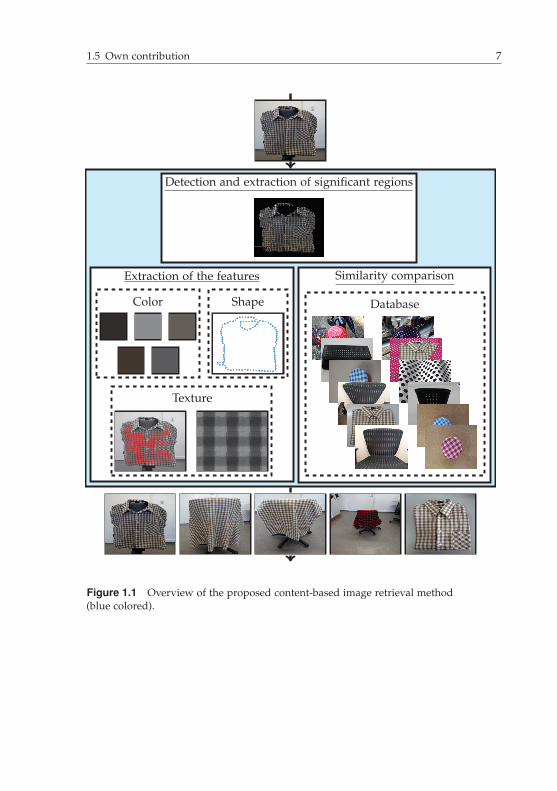
1.5 Own contribution 7
Color Shape
Texture
Extraction of the features
Database
Similarity comparison
Detection and extraction of significant regions
Figure 1.1 Overview of the proposed content-based image retrieval method(blue colored).


2 Mathematical background
Relevant distance functions and similarity comparisons used in thisthesis are presented in Sec. 2.1. As graphs and space-frequency rep-resentations are necessary in several chapters of this thesis, a briefintroduction to the most important topics needed for this work is re-spectively presented in Sec. 2.2 and Sec. 2.3.
2.1 Distance functions andsimilarity comparisons
The distance functions and similarity comparisons that are most relevantfor this thesis are briefly introduced next.
The Euclidean distance, or also named �2-norm, between two vectorsyA, yB is calculated as [7, 45]
∥∥∥yA − yB∥∥∥
2, (2.1)
where
‖x‖2 =
√xTx. (2.2)
In case of a function g(u), the Euclidean distance is defined as [8]
‖g(u)‖2 =
√ˆ|g(u)|2. (2.3)
This distance can be found in this thesis in connection with shape(Sec. 4) and texture (Sec. 5) properties as well as with the detection ofregions (Sec. 6).

10 2 Mathematical background
The quadratic-form distance is a measure to compare two histogramshA, hB taking into consideration the similarity between bins. It is de-fined as [108, 122]
d(
hA, hB)=
√(hA − hB
)TB(
hA − hB)
, (2.4)
where B denotes a similarity matrix whose element bk1k2expresses the
cross-bin dependence between the bins k1 and k2. The quadratic-formdistance is used in this work to compare regular textures (Sec. 5.2.3).
The correlation coefficient between gA(u) and gB(u) is calculatedaccording to [45, 114, 119]
r(
gA(u) , gB(u))=
E{(
gA(u)− E{
gA(u)})(
gB(u)− E{
gB(u)})}
√E{
gA(u)− E{
gA(u)}}
E{
gB(u)− E{
gB(u)}} .
(2.5)
It is a normalized value between −1 and +1. In this thesis the cor-relation coefficient can be found at the detection and extraction ofnear-regular textures (Sec. 5.3) and at the detection of color regions(Sec. 6.3.2).
The correlation for circular data presented by Fisher and Lee in [49]is used to compare circular data ϕA
k , ϕBk , 1 ≤ k ≤ N, via the following
“correlation”:
ρ(
ϕA, ϕB)=
N−2∑k1=0
N−1∑k2=k1+1
sin(
θAk1,k2
)· sin
(θB
k1,k2
)
√√√√(
N−2∑k1=0
N−1∑k2=k1+1
sin2(
θAk1,k2
))(N−2∑k1=0
N−1∑k2=k1+1
sin2(
θBk1,k2
)) ,
(2.6)
where θsk1,k2
= ϕsk1− ϕs
k2, s ∈ {A, B}. In this thesis this correlation for
circular data is used to compare shape features (Sec. 4.2.2).The earth mover’s distance as a metric for image retrieval is inves-
tigated by Rubner et al. in [122]. It represents the difference betweentwo distributions as a transportation problem. The overall dissimilarityis obtained from the total cost, deduced from the conversion of oneof the distributions into the other one. In order to calculate the costs

2.2 Graph theory 11
of the transportation, the distributions must be represented as a setof cluster representatives and their corresponding weights. The dis-similarity between the cluster representatives and the weights of thecluster representatives are taken into consideration to obtain the totaldissimilarity between the two inputs. The earth mover’s distance isused in this work to evaluate the proposed compact color signaturefrom Sec. 3.2 (Sec. 8.2.1).
2.2 Graph theory
Graphs are a powerful mathematical model to analyze many problemsand to describe the relationship between objects. In this thesis graphsare used to obtain a compact color signature for images (Sec. 3.2), todetect near-regular textures (Sec. 5.3), to extract non-overlapping stablecolor regions (Sec. 6.3.1), and to extract patterns in images (Sec. 6.4).Because of their frequent application, a brief introduction to graphtheory is given in the next sections. The focus is set on basics needed tounderstand the proposed methods. This introduction is mostly basedon [12, 121, 141], where more detailed information about graph theorycan be found.
2.2.1 Basic concepts of graph theory
A graph is a triple G =(V(G) , E(G) , IG
)[12, 141]. V(G) is the set
formed by the nodes v, also called vertices. Edges e are the elements ofthe set E(G), whereas
V(G) ∩ E(G) = ∅ (2.7)
must apply [121]. IG describes relations by associating each edge fromE(G) a pair of nodes from V(G), which may be twice the same node incase of a loop:
IG(e) =(
vk1, vk2
), (2.8)
where e ∈ E(G) and vk1, vk2
∈ V(G).For simplification purposes, edges e will be denoted in this work
as (vk1, vk2
). This notation already contains the information of the

12 2 Mathematical background
nodes that are being connected by the corresponding edge. Some graphexamples are shown in Fig. 2.1. If an edge (vk1
, vk2) exists between two
different nodes (k1 �= k2), then the nodes are neighbors and adjacent[12, 141].
v1
(a)
v1
(v1, v1)
(b)
v1
v2
v3
v4
(c)
(v1, v2)
(v1, v3)
(v1, v4)
(v2, v4)
b(v1) = 3
b(v2) = 2
b(v3) = 1
b(v4) = 2
b(v1) = 2b(v1) = 0
Figure 2.1 Degree of nodes. The graph at the left consists of an isolated node. A loopis shown in (b).
v1
v2
v3
v4
(a)
v1
v2
v3
v4
(b)
v1
v2
v3
(c)
Figure 2.2 Some examples of graphs. (a) shows a connected, complete graph. (b)displays a connected graph that is not complete. (c) shows a clique from b).

2.2 Graph theory 13
neighbor set of v. The degree of a node b(v) is its number of incidentedges. Some examples are shown in Fig. 2.1. Loops are counted plustwo when the degree of a node is calculated (see Fig. 2.1(b)). If a nodehas a degree of zero, no edge in E(G) exists that associates the nodewith another one in the graph. Such nodes are called isolated (seeFig. 2.1(a)) [12, 141].
A subgraph of G is any graph Gk with V(Gk) ⊆ V(G) and E(Gk) ⊆E(G). A graph G is called complete if for every pair of nodes in V(G) anedge exists that associates them (see Fig. 2.2(a)). Complete subgraphsof a graph G are known as cliques (see Fig. 2.2(c)) [12, 141].
A walk is an alternating sequence of nodes and edges along thegraph. If the edges that appear in the walk are not repeated, then thewalk is called a trail, and if the nodes are not repeated, a path. As aconsequence, every path is a valid trail, but every trail is not necessarilya valid path [12, 141].
Two nodes are connected if a path exists along them. Moreover, agraph G is called connected if paths exist between every pair of nodes.Every not connected graph can be divided into connected subgraphscalled components of G [12, 141].
2.2.2 Directed graphs
A directed graph, also called digraph, is a triple G =(V(G) , E(G) , IG
),
where V(G) is the set of nodes in the graph and E(G) the set of arcs,which are called edges in this work [12, 141]. Equation 2.7 must alsoapply between V(G) and E(G) at digraphs. IG associates each edge ofthe graph two nodes, however, the edges become a direction at digraphs(see Fig. 2.3(a),(b)). For simplification purposes, edges from digraphs arerepresented in this work as [vk1
, vk2], vk1
, vk2∈ V(G), with vk1
definingthe tail of the edge and vk2
the head of the edge. vk1, vk2
are also knownas the ends of the edge [vk1
, vk2] [12, 121, 141]. Furthermore, the edge
[vk1, vk2
] is incident out of vk1and incident into vk2
(see Fig. 2.3(a)) [12].If two nodes vk1
and vk2are connected by an edge [vk1
, vk2], then vk1
is an inneighbor of vk2, and vk2
is an outneighbor of vk1. N+(vk1
) is the
set of outneighbors of vk1and N−(vk1
) its set of inneighbors [12].
N (v), v ∈ V(G), is the set of all neighbors of v and is called the

14 2 Mathematical background
number of edges that are incident out of vk, and the indegree b−(vk) isthe number of edges that are incident into vk [141]. For digraphs thedegree b(vk) of vk is defined as
b(vk) = b+(vk) + b−(vk) . (2.9)
An isolated node at a directed graph is a node with a degree of zero [12].An underlaying graph is obtained from a directed graph if the ori-
entations are removed from the edges (see Fig. 2.3(b),(c)) [12]. If theunderlaying graph is a connected one, then the directed graph is calledweakly connected. If for every pair of nodes in a directed graph asequence of edges exists connecting them, then the graph is stronglyconnected. The direction of the edges is taken into consideration todetermine if a graph is strongly connected [141].
v1
(a)
v1
v2
v3
v4
(b)
v1
v2
v3
v4
(c)
v2
[v1, v2]
Figure 2.3 Examples of directed graphs. (a) shows a directed edge. (b) is a directedgraph and (c) its corresponding underlaying graph.
2.2.3 Trees
Every graph and digraph that does not contain cycles is called a forest.A forest can be formed from trees, which are connected graphs withoutcycles (the underlaying graph is considered in case of a directed graphto determine the connectedness), and from isolated nodes. Therefore,every pair of vertices of a tree is connected by a unique path (itscorresponding underlaying graph in case of a digraph) [12, 121]. An
As the edges have a direction at digraphs, different kinds of degreescan be obtained per node. The outdegree b+(vk) of vk, vk ∈ V(G), is the

2.2 Graph theory 15
from which all nodes can be reached alternating nodes and edges (v1and v9 in Fig. 2.4). The inneighbor of a node is also called its parentand its outneighbors its children [121, 141]. For example, in Fig. 2.4 theparent of v11 is v9 and its children are v12 and v13. Furthermore, nodesthat do not have children are called the leaves of the tree (e.g., v4 andv5 in Fig. 2.4).
The last concept introduced in this section is the binary tree. A treeis of binary kind if every node has a maximum of two children. Theright tree in Fig. 2.4 represents a binary tree [121, 141].
v1
v2 v3
v4 v6v5 v7
v8 v9
v10 v11
v12 v13
Figure 2.4 Example of a forest.
2.2.3.1 k-d tree
The k-d tree, which is a binary tree to structure k-dimensional data, wasproposed by Bentley [17]. Every node in the tree represents a recordof the data and each level in the tree corresponds to a dimension ofthe data, whereas the dimension changes cyclically along the depth ofthe tree. The nodes in the tree that are not leafs always point into twonodes, whereas according to the depth of the tree one node is alwaysbigger along the considered dimension than the other one.
To obtain an optimal k-d tree, Bentley proposed an algorithm toassure that the number of nodes from the left branch of the tree, startingfrom the root, differ at most by one from the right branch [17]. For thispurpose, the data set is divided along the tree alternating the dimension
example is shown in Fig. 2.4. The forest there is composed of two treesand the isolated node v8. At digraphs the root of a tree is the node,

16 2 Mathematical background
into two sets by their respective median value. Figure 2.5 shows anexample for two-dimensional data.
0 1 2 3 4 50
1
2
3
4
5
x2
x1
3, 3
2, 4 4, 3
x1 < 3 x1 > 3
2, 2 1, 5
x2 < 4 x2 > 4
5, 1 5, 4
x2 < 3 x2 > 3
Figure 2.5 Example of a k-d tree for two-dimensional data.
2.3 Space-frequency representations
Depending on the available characteristics of signals and the processingintended with them, the space, the frequency, or the space-frequencydomain may be favorable. Along this thesis all of the three mentioneddomains are used. The one-dimensional frequency domain is used, e.g.,in Sec. 4.3 to compare shapes, the two-dimensional frequency domainin Sec. 5.2 to detect regular textures and extract features from them,and the space-frequency domain in Sec. 6.4 to detect patterns in images.A brief overview of the corresponding transforms used in this thesis isgiven in the next sections.
2.3.1 One-dimensional Fourier transform
The Fourier transform of a signal g(u) is an integral transformationcalculated as [20, 76, 120]
G( f ) =ˆ ∞
−∞g(u) · exp (− j 2π f u)du, (2.10)

2.3 Space-frequency representations 17
whereas G( f ) is also called the spectrum of g(u) and it can be separatedinto its magnitude |G( f )| and phase ϕ( f ):
G( f ) = |G( f )| · exp (j ϕ( f )). (2.11)
Fine details (fast changes) in the space function g(u) imply higherfrequency components in the spectrum. Rough details imply lowerfrequency components [20].
According to Eq. 2.10 to obtain the spectrum of a space signal, thesignal must be continuous and infinitely long to be integrated over thewhole space domain. However, these two properties are not present inreal environments and are therefore briefly discussed next.
Spectral leakage appears due to the limitation of g(u) along the spacedomain when the Fourier transform is calculated. Mathematically, theFourier transform is calculated from the windowed signal gwin(u):
gwin(u) = wrect(u) · g(u) , (2.12)
where wrect(u) denotes a rectangular window function of length lrectdefined as [63, 112, 113]
wrect(u) =
{1 if − lrect
2 ≤ u ≤ lrect2
0 otherwise.(2.13)
The product of the window function with the analyzing signal impliesa convolution in frequency domain and may therefore distort the spec-trum. An appropriate selection of the window function may smoothspectral leakage [20, 120].
The discretization of the space and frequency domains is necessary tohandle images in computers, as they cannot process continuous signals.The discretization in space domain is mathematically described as theproduct of the continuous signal with an impulse train. This impliesthe convolution of the spectrum of the input image with an impulsetrain in frequency domain and therefore its repetition. A discretizationof the frequency domain is also necessary. It can also be described asthe multiplication of the spectrum with a new impulse train, whoseconsequence is the convolution of the discrete signal in space domainwith the Fourier transform of the impulse train. Consequently, thisimplies its repetition over the space domain [20, 120]. The discretizationin space domain and the discretization in frequency domain distorttherefore the analysis of the signals.

18 2 Mathematical background
2.3.2 Two-dimensional Fourier transform
The Fourier transform of two-dimensional signals g(u), like, e.g., gray-level images g(u), is calculated by the following relation [20]:
G(f) =ˆ ∞
−∞
ˆ ∞
−∞g(u) · exp
(− j 2πfTu
)du. (2.14)
Due to the separability property it can be interpreted as two one-dimensional Fourier transforms of the input signal. The Fourier trans-form along the u2 direction is calculated from the Fourier transformedsignal along the u1 direction [20]:
G(f) =ˆ ∞
−∞
ˆ ∞
−∞g(u) · exp(− j 2π ( f1u1 + f2u2))du1du2 (2.15)
=
ˆ ∞
−∞
(ˆ ∞
−∞g(u)·exp(− j 2π f1u1)du1
)exp(− j 2π f2u2)du2.
(2.16)
As in the one-dimensional case, spectral leakage and discretizationissues must be considered in the Fourier transform of two-dimensionalsignals.
2.3.3 One-dimensional wavelet transform
The wavelet transform of a one-dimensional signal g(u) is obtainedfrom the comparison with a mother wavelet ψ(u) which is scaled andshifted:
Γ(λ, κ) =
∞
−∞
g(u)1√λ
ψ∗(
u − κ
λ
)du. (2.17)
In contrast to the Fourier transform (see Sec. 2.3.1), the wavelet trans-form delivers a space-frequency description of the input signal. Thisallows the localization of signal components in space and frequencydomain up to a certain resolution. Lower frequencies can be localizedvery good in frequency and therefore rougher in space, whereas higherfrequencies can be localized very good in space and therefore rougherin frequency [20, 40, 76, 120].

2.3 Space-frequency representations 19
2.3.3.1 Fast implementation of the wavelet transformfor the discrete case
A discrete and fast wavelet transform is necessary to assure a reasonablesignal processing with computers. Besides the discretization of the inputsignal gu, the mother wavelet and its scaling and shifting parametersmust also be quantized [20, 40, 76].
The fast wavelet transform is the consecutive projection of the inputsignal onto subspaces, whereas subspaces at a same stage are orthogo-nal to each other. The input signal is represented in a coarser mannerwith increasing stages. At every stage the coarse representation of gu isdivided into a detailed and a coarser representation, yielding the coarserapproximation and detail coefficients of gu at the following stage. Thisdecomposition of the signal can be done very fast with the applicationof low-pass and band-pass filters with subsequent downsampling to thecoarser approximation coefficients of the previous stage. Usually thequantized input signal is used as the coarser approximation coefficientsat the initial stage. The projection of the input signal to the differentsubspaces can be calculated from the coarser approximation and detailcoefficients. The original input signal can be reconstructed from thedetail coefficients over all stages and the coarser approximation coeffi-cients at the last stage via projection onto the higher spaces. This canalso be implemented very fast by upsampling and subsequently usinglow-pass and band-pass filters [20, 40, 76].
2.3.4 Two-dimensional wavelet transform
As in the case of the two-dimensional Fourier transform (see Sec. 2.3.2),the two-dimensional wavelet transform is obtained applying the one-dimensional wavelet transform along one of the directions (e.g., u1) andthen along the other direction (e.g., u2). Two dimensions and two filtertypes (low-pass and band-pass) must be considered, so four signalsresult from every stage of the two-dimensional wavelet transform: acoarser approximation of the input image and three detail signals, con-taining information about horizontal, vertical and diagonal structures.Like in the one-dimensional case, the approximation of the input imageis further divided along the stages, and the input image can be totallyreconstructed from the detail signals and the approximation of theimage at the last stage (see Fig. 2.6) [20].

20 2 Mathematical background
Figure 2.6 Sketch of a fast two-dimensional wavelet transform with three stages (up)and example of a fast two-dimensional wavelet transform, represented with pseudo-colors,for an input image with two stages (bottom).

3 Color
Many objects and materials in our environment only exist with certaincolors. The grass is mostly green, the ocean blue, clouds white or gray,etc. The perception of color is therefore a powerful tool for classificationand optical inspection of objects and materials. Due to this fact, theprocessing of the color information and its use as a feature for thecontent-based image retrieval is considered in this chapter.
First, an introduction to color considering what color is, how it can berepresented, and an overview of the state of the art is given in Sec. 3.1. Acompact color signature in CIELAB color space for content-based imageretrieval purposes is then presented in Sec. 3.2. The representation ofthe color information using humans’ color categories is considered inSec. 3.3 together with the procedure followed in this thesis to determinerepresentative humans’ color categories. The result of the presentedmethods are shown in Sec. 8.2.
3.1 Introduction to color
Color is a perceptual property that derives from the spectrum of lightinteracting with the eye [20]. Visible light consists of frequencies in theelectromagnetic spectrum. Depending on the electromagnetic spectrumthat is emitted by or reflected from the surfaces of the objects, a color isperceived by humans. If the incident spectra consists of all frequenciesbelonging to visible light, then surfaces that reflect all of the frequenciesof the electromagnetic spectrum appear white to humans [54]. However,the colors perceived by humans depend on many facts like the surfacesof the objects, the environment, and the human itself. It is therefore nota property of an object or material [20].
Berlin and Kay studied the universality of color naming across differ-ent languages and societies [18]. Although different basic color termsmay exist depending on the language, they found that the evolution

22 3 Color
of the basic color terms is highly correlated between the languages.They concluded with eleven basic color terms in English language:white, black, gray, yellow, brown, green, blue, purple, pink, orange, red. LaterKay and Regier [75] studied the color naming from languages in in-dustrialized and non-industrialized societies. Although the numberof basic color terms and their boundaries may vary between differentlanguages, they found that the eleven basic color terms of the Englishlanguage seem to be anchored across the different languages as pointsin color space.
3.1.1 Color representation
When representing color information digitally, color spaces are used.Different color spaces exist depending on the final task. They canbe roughly classified into device inspired color spaces or perceptionoriented inspired color spaces [20]. The widely spread RGB color spaceis an example of the first group, whereas the CIELAB color space isan example of the second group. An overview of these color spacesis given next, as they are used along this thesis. A more exhaustiveconsideration about color spaces can be found in [20, 54].
The RGB color space is based on the three primary colors red, greenand blue [20, 54]. In this color space a color is represented as a threedimensional vector g ∈ [0, 1]3, whereas every dimension representsone of the three primary colors. A color is then the addition of theirproportion of red, green, and blue colors. The RGB color space is widelyspread, as the three primary colors are often the basic colors of cameras,displays, and projectors. However, not every perceivable color can berepresented in this color space. Furthermore, the RGB color space isdevice dependent, as it depends on the exact red, green, and blue colorsthat are added to create new colors [20].
To overcome the drawbacks of a device dependent color space, thesRGB color space has been defined. For this purpose, the three primarycolors are normalized [20].
The CIELAB color space also represents a color as a three dimen-sional vector g. One dimension represents the brightness of the color,whereas the other two dimensions respectively represent the differencebetween green and red colors, and blue and yellow [20]. This colorspace is a so called uniform color space, where the distance between

3.1 Introduction to color 23
points in color space is a reference of their perceivable color differencefor humans. However, the comparison is rather reasonable for smallercolor differences than for bigger ones [20, 51].
3.1.2 State of the art
Many researchers have focused on the research of content-based im-age retrieval systems using the color information. For this purpose,appropriate features must be extracted from the images.
Swain and Ballard propose the use of color histograms to indeximages in a large database and the histogram intersection as a metricfor image retrieval in [131]. To this end, the intersection between bothhistograms is regarded by a bin-by-bin comparison. Several metricshave been proposed to compare histograms bin-by-bin [122]. Theirmain drawback is that the result depends on the selected bin sizeand that no cross similarity between bins is considered. To overcomethese problems, Niblack et al. also compare cross-bins taking intoconsideration the similarity between bins in [108].
While color histograms yield a global statement of the colors in animage and their amount, the information about the spatial relationshipbetween the different colors gets lost. Pass et al. propose thereforethe color coherence vectors in [117]. The pixels in the input image areclassified into two groups, coherent or incoherent. A pixel is coherentif it forms a sufficiently big connected area with other pixels of thesame color. For this purpose, the color space is quantized and everyquantized unit is considered a color. The feature proposed by Passet al. consists of a vector per input image formed out of pairs. Everypair represents one color of the image and it contains the amount ofcoherent pixels in the image with the considered color and the amountof incoherent pixels [117]. Huang et al. propose color correlograms toovercome the loss of the spatial relationship between the colors in [68].It consists of a table indexed by color pairs that contains the probabilityof finding a pixel of a certain color at a given distance of a pixel withanother considered color. Stehling et al. propose in [128] the cell/colorhistograms to consider the spatial displacement of the appearing colorsand also to reduce the storage place needed, compared to the basic colorhistograms. The image is divided into cells but instead of computingone color histogram per cell, one histogram is computed per appearing
24 3 Color
color in the image. Each histogram contains the number of pixels ofthe considered color per cell. Consequently, only as many histogramsare needed as colors appearing in the image [128]. This method isextended in [138] to enable cross-bins comparisons, which allows toconsider rotations and translations of the images. Konstantinidis et al.propose in [77] a color histogram with only 10 bins to reduce storage.The histograms are obtained after considering the color space as a fuzzyset [145].
Several features have also been proposed without using histograms.Deng et al. propose in [43] to use only the dominant colors in an image.They searched for clusters in the colors of the pixels first and concludedthat three to four colors are typically enough to represent the colorinformation of the image [43]. Yoo et al. propose to sort images inthree steps in [144]. First, the four major colors appearing in the queryimage are extracted. All images in the database that do not contain themajor colors of the query are discarded. In a second step, images in thedatabase whose major colors are not similarly distributed to the queryimage are discarded. Finally, the remaining images in the database aresorted [144]. Other systems use color moments like, e.g., the average ofthe appearing color [139].
Rubner et al. evaluate in [122], i.a., the earth mover’s distance as ametric for content-based image retrieval using only color information.To this end, a color signature per image is extracted by partitioning thecolor space into regions in depedence of the considered image. Two k-dtrees are used (see Sec. 2.2.3.1). First, one k-d tree is performed withall color pixels of the image. The data is divided into nodes until thelength of the color regions along the dimensions is smaller or equalto a given threshold. In a second step a second k-d tree is performedover the centroids of the final color regions of the first k-d tree. In thiscase only the half of the previous threshold is the maximum allowedlength per dimension. The color signature of an image is obtained fromthe centroids of the regions. What is specially interesting about thismetric is that the number of color representatives describing the colordistribution of the image may vary. The similarity is the total costsobtained if the distribution of one of the images is converted into theother one [122].
The eleven basic color terms from the English language have been aninspiration for many researchers dealing with image processing. Van

3.2 A compact color signature in CIELAB color space for images 25
den Broek et al. use the eleven basic color terms to create a user colorselection interface for content-based image retrieval purposes in [24].Furthermore, van den Broek et al. experimentally prove the eleven basiccolor terms in [23]. They also use them in [23] as a feature for thecontent-based image retrieval. The assignment of color values to theeleven basic color terms is a challenging task. In [140] van de Weijeret al. study how to learn the color values of the eleven basic colorterms from real images. Heer and Stone propose in [65] a procedureto construct a probabilistic model for color naming. They obtain 153color names associated to color regions in color subspaces and use thisinformation to create, i.a., a color dictionary and a wand selector inimages.
3.2 A compact color signature in CIELABcolor space for images
Inspired by the work in [122], a color signature for the content-basedimage retrieval is proposed. The usage of k-d trees (see Sec. 2.2.3.1)enables a compact representation of the color information in an image.However, the compression of the color information may also lead toa loss of information. The second k-d tree in [122] may be speciallycritical as it reduces the representation of the color information from analready compressed representation. With these concerns the followingmethod is proposed. Comparison results to the usage of the two k-dtrees are shown in Sec. 8.2.1.
Color regions with a similar color are obtained first in CIELAB colorspace by grouping the data using a k-d tree as in [122]. For this purpose,the pixels are divided into groups along the k-d tree according to theircolor until the length spanned by the color of the pixels in each groupover each color dimension is smaller than a given threshold value τC1.Some final nodes of the k-d tree may be merged without exceedingthe maximum allowed length of the color regions along the differentdimensions, due to the fact that the k-d tree divides the databasealternating the dimensions. To detect and merge such color regions,a graph representation of the color information is used in Sec. 3.2.1.Characteristic nodes are defined in Sec. 3.2.2. The number of nodes

26 3 Color
is reduced in Sec. 3.2.3, and a compact color signature is obtained inSec. 3.2.4.
3.2.1 Graph representation of the color information
Every leaf of the k-d tree is represented by a node vk in the graph andit represents a subspace in CIELAB color space. The subspace of eachnode is characterized by the maximum and minimum value per channelfrom all pixels that have been assigned to it:
vk =
⎧⎪⎨⎪⎩
u
∣∣∣∣∣∣∣
⎛⎜⎝
l∗mink
a∗mink
b∗mink
⎞⎟⎠ ≤ g(u) ≤
⎛⎝
l∗maxk
a∗maxk
b∗maxk
⎞⎠⎫⎪⎬⎪⎭
. (3.1)
Consequently, every node represents a set of points. Nodes spanninga similar color subspace are connected by an edge. The dissimilaritybetween two nodes vk1
, vk2is measured via the following distance
function:
d(
vk1, vk2
)=max
[max
(l∗maxk1
, l∗maxk2
)− min
(l∗mink1
, l∗mink2
),
max(
a∗maxk1
, a∗maxk2
)− min
(a∗min
k1, a∗min
k2
),
max(
b∗maxk1
, b∗maxk2
)− min
(b∗min
k1, b∗min
k2
)].
(3.2)
Nodes with a distance smaller than τC1 could be merged withoutexceeding the maximum allowed length per channel. Such nodes areconsidered similar and therefore connected by an edge in the graph.However, this is not a transitive relation. The node vk2
may be similarto vk1
and vk3, but this does no imply that vk1
and vk3must be similar.
An example is shown in Fig. 3.1(a), where v2 is similar to v1, v3, and v4.However, v1 is only similar to v2.
3.2.2 Types of nodes
Neighboring nodes are classified as identical or relative first, to obtainthe compact color signature next.
Identical nodes are two nodes vk1, vk2
if they are connected by edgesto the same nodes and also between each other:

3.2 A compact color signature in CIELAB color space for images 27
1. d(
vk1, vk2
)≤ τC1
2.{
vk| d(
vk, vk1
)≤ τC1
}∪{
vk1
}={
vk| d(
vk, vk2
)≤ τC1
}∪{
vk2
}.
Such nodes could be merged without exceeding the maximum allowedlength per channel and without changing the similarity, and thereforeedges, between the remaining nodes (see, e.g., v3 and v4 in Fig. 3.1(a)).
Relative nodes in the graph are nodes that are directly connected byan edge and are not of identical type (see, e.g., v1 and v2 in Fig. 3.1(a)).
v1
v2
v3∪4
v5 v6
(b)
1
8
210
v1
v2
v3 v4
v5 v6
(a)v1∪2
v3∪4∪6
v5
(c)
Figure 3.1 Example of the graph representation and merging methods to obtain thecompact color signature. The weights of the edges are the dissimilarity distances betweenthe nodes (see Eq. 3.2). These weights are used when only relative nodes are left in thegraph.
3.2.3 Compact representation of the graph
As long as there are edges in the graph, nodes may be merged withoutviolating the maximum size allowed per color subspace. Because ofthis, the graph is processed until it consists of isolated nodes.
Pairs of identical nodes vk1, vk2
are merged first until no more identi-cal nodes are left in the graph. Per pair of identical nodes merged, a

28 3 Color
new node vk1∪k2is created whose limits in color space are the extrema
of the merged pairs:
l∗mink1∪k2
= min(
l∗mink1
, l∗mink2
)l∗maxk1∪k2
= max(
l∗mink1
, l∗maxk2
)
a∗mink1∪k2
= min(
a∗mink1
, a∗mink2
)a∗max
k1∪k2= max
(a∗min
k1, a∗max
k2
)
b∗mink1∪k2
= min(
b∗mink1
, b∗mink2
)b∗max
k1∪k2= max
(b∗min
k1, b∗max
k2
). (3.3)
This step is exemplified in Fig. 3.1(a)-(b) (the weights of the edges areexplained next).
Once all identical nodes have been merged, the relative nodes areprocessed and merged. An adequate selection of the relative nodesthat are going to be merged is very important, as it will change thesimilarity relations of the spanned color subspaces. For example, inFig. 3.1(b) if v1 is merged with v2, then the new node will not be similarwith v3∪4 anymore. To select adequate merging pairs, the graph isextended to a weighted one (see Fig. 3.1(b)). The weights of the edgesare obtained from the dissimilarity distance between the nodes (seeEq. 3.2). The number of nodes that can be reached directly via an edgeis calculated for every pair of nodes. Iteratively the pair with the highestnumber of common nodes is merged. The boundaries in color spacefrom the new node are calculated as in Eq. 3.3 and the edges in thegraph are updated according to the similarity condition. In the case ofthe existence of many relative pairs with the highest number of relativenodes in common, then the pair with the smallest distance will bemerged (see Fig. 3.1(c)).
3.2.4 Color signature of the image
The color signature of the image obtained via the k-d tree and the graphoperations is formed from a color representative per node and its weightin the image. The color representative of each node is the mean color(calculated over the three color channels in CIELAB color space) from allpixels whose color values are in the spanned color subspace. However,the subspaces in color space spanned by the nodes may overlap. Thisis exemplified in Fig. 3.2 for two-dimensional subspaces. Points in thegray area are in the subspaces spanned by v1 and v2∪3. Such points

3.3 Humans’ color categories 29
have been considered at the mean color calculation of all nodes to whichthey could belong.
v2
v1
v3
v1
v2∪3
Regions from the k-d tree Regions after the merge step
Figure 3.2 After merging two nodes the represented subspaces may overlap. Points inthe gray area belong to v1 and v2∪3.
Finally, the weight of each node is the percentage of pixels whosecolor values are closest to the mean color assigned to the node.
3.3 Humans’ color categories
Due to the fact that the comparison of colors in the CIELAB colorspace is more reasonable for smaller color differences than for biggerones [51], the representation of the color information via humans’ colorcategories is considered in this section inspired by the psychologicalstudies from Berlin and Kay [18], and Kay and Regier [75]. However, asthe eleven basic color terms from the English language are insufficientto distinguish between shades, the extraction of representative humans’color categories is needed.
Here, the same database is processed as by Heer and Stone in [65]to extract the color categories. The database is online available [142]and consists of more than 3.4 million colors that have been named in an
30 3 Color
online survey by more than 145,000 subjects. Although it is not possibleto assume that every monitor used for the survey was calibrated, thedatabase is due to the high number of available answers important.In Sec. 3.3.1 the processing, followed in this thesis, of this database ispresented, which differs from the one in [65]. Next, the method used toextract the representative humans’ color categories from the processeddatabase is explained in Sec. 3.3.2 followed by the presentation of thefeatures used to represent color information via the extracted humans’color categories in Sec. 3.3.3. A preliminary version of this work hasbeen presented in [160]. The extracted humans’ color categories areshown in Sec. 8.2.2 and conclusions from the representation of the colorusing the humans’ color categories can be drawn from the results fromSec. 8.5.
3.3.1 Processing the recorded database
The database [142] consists of more than 3.4 million colors sampledfrom the full RGB cube that were named by more than 145,000 subjectsin an online survey. The subjects were asked to name a color displayedon their screens in a text input field. Any text answer was acceptedand a subject could name as many colors as desired. However, thepermission of all possible text answers also lead to misspellings (seeSec. 3.3.1.1) and spam answers (see Sec. 3.3.1.2) that should be handledfirst.
3.3.1.1 Editing of the color names
Consecutive space characters in the color names are merged into onefirst. Responses containing only special characters, less than threecharacters, or more than three words are removed from the database.Next, misspellings are corrected at some color names like yyellow orgren. The correction of all misspellings is not possible due to the bigamount of responses and the ambiguity of some answers. For example,is graen green or gray?
3.3.1.2 Suppression of spam answers
After editing the color names, spam answers are suppressed. Swear-words, insults, and words with no color information as not or asdf are

3.3 Humans’ color categories 31
removed from the database. Like at the correction of misspellings, alldisturbing answers cannot be removed due to the huge amount of data.However, 37.73 % of the color names in the database are removed bythe editing and the suppression of disturbing words.
The responses from subjects that named almost all colors with thesame color name are considered as spam and removed from the data-base. To detect such subjects, the number of different color namesnC,1 they used is compared to the total number of colors nC,2 that theynamed. If
nC,1 <(
nC,2) 1
3 (3.4)
applies, then all responses from the subject are removed from the data-base as they are considered spam answers. This relationship has beenobtained empirically.
Furthermore, color names in the database that are named by a lownumber of different subjects are also considered as spam answers. Suchcolor names are detected by comparing the number of times a colorname has been used nC,4 to the number of different subjects that usedthe color name nC,3. If
nC,3 <(
nC,4) 1
3 (3.5)
applies, then the analyzed color name is considered as a spam an-swer and removed from the database. This relationship has also beenobtained empirically.
As representative color names from the full RGB cube are searched,color names named less than τC2 times are excluded from the database.
3.3.2 Extraction of the color categories
Humans’ color categories are extracted from the valid remaining an-swers of the database. For this purpose, the color values are transformedinto the CIELAB color space, as it is based on human color perceptionin contrast to the RGB color space (see Sec. 3.1.1). The quantization ofthe l∗- , a∗- and b∗-channels divides the color values into subspaces ofthe CIELAB color space. From the color names nC and the color valuesvC a color term matrix T is obtained as in [65]. The rows of T represent

32 3 Color
the different subspaces in CIELAB color space vC, and the columnsrepresent the remaining color names nC in the database. Each elementin T contains the number of color values in the database that belongto the color subspace vC and that have been named with the colorname nC.
From T the probability distribution p(nC∣∣∣ vC) of a color name nC
given a color value from a zone in color space vC is calculated as
p(
nC∣∣∣ vC)=
t[vCnC
]
∑nC
t[vCnC
] , (3.6)
where t[vCnC
]is the element of T at the row vC and at the column nC.
The most probable color names over the color subspaces considered inT are
q(
vC)= arg max
nCp(
nC∣∣∣ vC)
. (3.7)
The extracted humans’ color categories Q = {q1, . . . , qK} are the uniquecolor names from q(vC) over all color subspaces vC.
3.3.3 Representation of color using theextracted color categories
Every color value of a pixel can be represented by the extracted humans’color categories qk, 1 ≤ k ≤ K. For this purpose, the color categoriesare represented via their mean colors μk and covariance matrices Σk.The values are calculated in CIELAB color space from all color valueswhose assigned names in the database coincide with the respectivecolor category qk. The likelihood of the color of a pixel to belong to acolor category qk is approximated here as
p(gu| qk) =1√
(2π)3 |Σk|
· exp[−1
2(gu − μk)
T Σ−1k (gu − μk)
]. (3.8)

3.3 Humans’ color categories 33
The color value of a pixel in an image gu using humans’ color categoriesis represented by the normalized likelihoods
cColork (gu) =
p(gu| qk)∑k
p(gu| qk)(3.9)
over the color categories. In some applications a vector representationmay be preferable. It is easily obtained by considering each colorcategory as a dimension:
cColor(gu) =(
cColor1 , . . . , cColor
K
)T. (3.10)


4 Shape
Disregarding objects and materials that do not have a defined shape(like liquids and gases), many objects and living beings exist that havea defined shape: books, cars, trees, planes, and the like. The objects ofall of these classes have a roughly basic shape in common. Althoughthe concrete shape in-between a class may vary, they are coarselysimilar. The shape information is therefore an interesting feature forcontent-based image retrieval, which is the reason for considering it inthis chapter.
An overall introduction to shape is given first in Sec. 4.1. For thispurpose, the basic concepts of shape representation needed in thisthesis are presented followed by an impression of the state of the art.Normal angular descriptors and Fourier descriptors are considered nextin Secs. 4.2 and 4.3 for shape retrieval. Retrieval results achieved by thenormal angular descriptors and the Fourier descriptors are presentedin Sec. 8.3.
4.1 Introduction to shape
Although many objects and living beings in our environment have adefined shape, their corresponding shapes in images may vary slightly.There are many reasons for this. On the one hand we find reasonsrelated to the nature of the objects and living beings, like articulatedlimbs, the adaptation to the environment, and the individualism insidethe classes. On the other hand we find reasons related to the acqui-sition of the image. The projection of the three-dimensional world toa two-dimensional one involves, i.a., affine transformations [54, 107].An appropriate representation of the shape information, appropriatefeatures, and an appropriate similarity comparison of the features arenecessary for a successful retrieval of shapes.
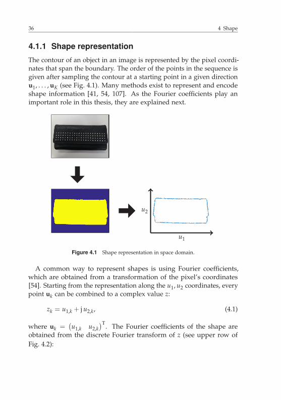
36 4 Shape
4.1.1 Shape representation
The contour of an object in an image is represented by the pixel coordi-nates that span the boundary. The order of the points in the sequence isgiven after sampling the contour at a starting point in a given directionu1, . . . , uK (see Fig. 4.1). Many methods exist to represent and encodeshape information [41, 54, 107]. As the Fourier coefficients play animportant role in this thesis, they are explained next.
u2
u1
Figure 4.1 Shape representation in space domain.
A common way to represent shapes is using Fourier coefficients,which are obtained from a transformation of the pixel’s coordinates[54]. Starting from the representation along the u1, u2 coordinates, everypoint uk can be combined to a complex value z:
zk = u1,k + j u2,k, (4.1)
where uk =(u1,k u2,k
)T. The Fourier coefficients of the shape areobtained from the discrete Fourier transform of z (see upper row ofFig. 4.2):
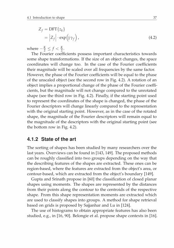
4.1 Introduction to shape 37
Zf = DFT{zk}=∣∣∣Zf
∣∣∣ · exp(
j γ f
), (4.2)
where −K2 ≤ f < K
2 .The Fourier coefficients possess important characteristics towards
some shape transformations. If the size of an object changes, the spacecoordinates will change too. In the case of the Fourier coefficientstheir magnitude will be scaled over all frequencies by the same factor.However, the phase of the Fourier coefficients will be equal to the phaseof the unscaled object (see the second row in Fig. 4.2). A rotation of anobject implies a proportional change of the phase of the Fourier coeffi-cients, but the magnitude will not change compared to the unrotatedshape (see the third row in Fig. 4.2). Finally, if the starting point usedto represent the coordinates of the shape is changed, the phase of theFourier descriptors will change linearly compared to the representationwith the original starting point. However, as in the case of the rotatedshape, the magnitude of the Fourier descriptors will remain equal tothe magnitude of the descriptors with the original starting point (seethe bottom row in Fig. 4.2).
4.1.2 State of the art
The sorting of shapes has been studied by many researchers over thelast years. Overviews can be found in [143, 149]. The proposed methodscan be roughly classified into two groups depending on the way thatthe describing features of the shapes are extracted. These ones can beregion-based, where the features are extracted from the object’s area, orcontour-based, which are extracted from the object’s boundary [149].
Gupta and Srinath propose in [60] the classification of closed planarshapes using moments. The shapes are represented by the distancesfrom their points along the contour to the centroids of the respectiveshape. From this shape representation moments are extracted whichare used to classify shapes into groups. A method for shape retrievalbased on grids is proposed by Sajjanhar and Lu in [124].
The use of histograms to obtain appropriate features has also beenstudied, e.g., in [16, 90]. Belongie et al. propose shape contexts in [16].

38 4 Shape
u2
u1
u2
u1
u2
u1
u2
u1
|Zref|
f
|Z||Zref|
f
|Z||Zref|
f
|Z||Zref|
f
|ϕ|
f
|ϕ||ϕref|
f
|ϕ||ϕref|
f
|ϕ||ϕref|
f
Figure 4.2 Fourier coefficients underlying affine transformations. The reference contourwith its magnitude of its Fourier coefficients and phase are displayed in the first row. Thestarting point is marked in red.

4.1 Introduction to shape 39
The shape context of a point is a histogram of the boundary points in itsneighborhood that depends on their proximity and angle. Mahmoudi etal. propose the edge orientation autocorrelogram, which is a histogramobtained from the most prominent edges in an image, in [90]. Thishistogram contains the number of edges with a similar orientationdepending on their distances.
From a description of the boundary with some of its points, Lateckiand Lakämper use the relative angle between the points and theirdistances as a feature in [81]. Petrakis et al. propose in [118] an approachthat enables the comparison of open and closed shapes. Via dynamicprogramming two shapes are compared, which are divided first intoconcave and convex segments. Angular patterns and binary angularpatterns are proposed by Hu et al. in [67]. For this purpose, the anglesspanned by adjacent points along the boundary are calculated. Higherscales are considered by calculating the angles between adjacent pointsplaced farther away. From the comparison of the magnitudes of theangles, a sort of local binary pattern for angles is built, which is usedfor shape retrieval.
Mokhtarian et al. consider a curvature scale space representation ofshapes [105] to obtain information for shape retrieval in [103, 104]. Thecurvature scale space enables the description of the shape with differentlevels of detail.
Several researchers have studied the potential of the Fourier transformof shapes’ signatures for retrieval purposes. Zhang and Lu considerdifferent signatures for shape representation in [146], from which theycalculate the Fourier transform. With the help of the Euclidean distancefunction the transformed signatures of the shapes are compared andsorted in a second step. In [150] Zhang and Lu give a more exhaustiveevaluation about Fourier description methods. Fourier descriptorsinvariant to scale, rotation, and translation are proposed by Burkhardt in[25]. Affine-invariant Fourier descriptors, which are also shear-invariant,are proposed by Burkhardt et al. in [26]. Bartolini et al. also useFourier descriptors for shape retrieval in [13]. However, in their workthe features are transformed back into space domain for comparisonpurposes. A distance is used which considers that correspondingsegments of different objects may vary on their length. Zhang and Lupropose and use the generic Fourier descriptor in [147, 148], which is aregion-based Fourier descriptor.

40 4 Shape
4.2 Normal angular descriptors
The angles from the normal vectors along the contour of the shapeare considered in this thesis for shape retrieval. For this purpose, thenormal angular descriptor is extracted first from the analyzed shape(Sec. 4.2.1) and compared to the normal angular descriptors of othershapes next (Sec. 4.2.2). To this end, three different comparisons for thenormal angular descriptors are presented. A preliminary version of thiswork has been presented in [157, 158].
4.2.1 Normal angular descriptor
The normal vectors n of a shape are calculated via the following relation:
nk =
(− (u2,k+1 − u2,k)
u1,k+1 − u1,k
). (4.3)
The normal angular descriptor of a shape is obtained from the anglesof the normal vectors along the shape:
ηk = �nk. (4.4)
These descriptors possess interesting characteristics towards some im-age transformations. The descriptors are invariant to a change of theshape’s size (compare the diagrams in the first and second row ofFig. 4.3). Rotations of the object imply an offset over the angles com-pared to the descriptors of the unrotated shape (compare the diagramsin the first and third row of Fig. 4.3). If the starting point is changedwhen the shape is sampled, then the descriptor is circular shifted alongthe k axis in comparison with the descriptor of the originally sampledshape (compare the diagrams in the first and fourth row of Fig. 4.3).
4.2.2 Similarity comparisons
Three different distances, presented in [157] and [158], are explained inthe following Secs. 4.2.2.1 and 4.2.2.2 to measure the similarity betweenshapes using normal angular descriptors. In Sec. 4.2.2.2 the descrip-tors compared are aligned first into each other before their similaritydistance is calculated, and two different distances are presented.

4.2 Normal angular descriptors 41
u2
u1
u2
u1
u2
u1
u2
u1
η
k
η
k
η
k
η
k
Figure 4.3 Normal angular descriptors underlying affine transformations.
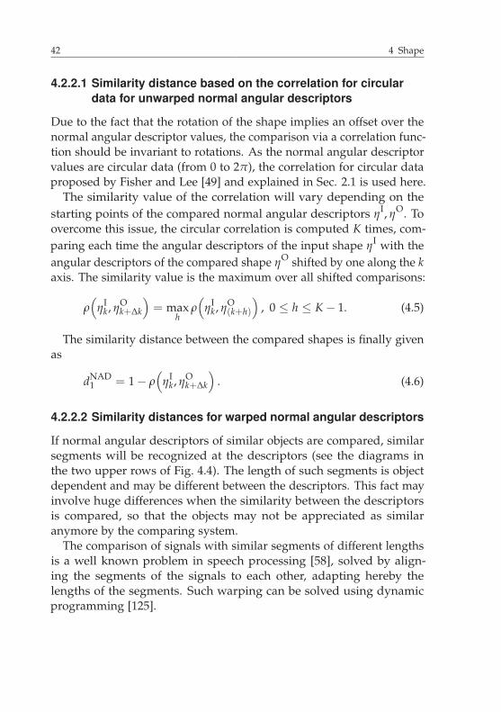
42 4 Shape
4.2.2.1 Similarity distance based on the correlation for circulardata for unwarped normal angular descriptors
Due to the fact that the rotation of the shape implies an offset over thenormal angular descriptor values, the comparison via a correlation func-tion should be invariant to rotations. As the normal angular descriptorvalues are circular data (from 0 to 2π), the correlation for circular dataproposed by Fisher and Lee [49] and explained in Sec. 2.1 is used here.
The similarity value of the correlation will vary depending on thestarting points of the compared normal angular descriptors ηI, ηO. Toovercome this issue, the circular correlation is computed K times, com-paring each time the angular descriptors of the input shape ηI with theangular descriptors of the compared shape ηO shifted by one along the kaxis. The similarity value is the maximum over all shifted comparisons:
ρ(
ηIk, ηO
k+Δk
)= max
hρ(
ηIk, ηO
(k+h)
), 0 ≤ h ≤ K − 1. (4.5)
The similarity distance between the compared shapes is finally givenas
dNAD1 = 1 − ρ
(ηI
k, ηOk+Δk
). (4.6)
4.2.2.2 Similarity distances for warped normal angular descriptors
If normal angular descriptors of similar objects are compared, similarsegments will be recognized at the descriptors (see the diagrams inthe two upper rows of Fig. 4.4). The length of such segments is objectdependent and may be different between the descriptors. This fact mayinvolve huge differences when the similarity between the descriptorsis compared, so that the objects may not be appreciated as similaranymore by the comparing system.
The comparison of signals with similar segments of different lengthsis a well known problem in speech processing [58], solved by align-ing the segments of the signals to each other, adapting hereby thelengths of the segments. Such warping can be solved using dynamicprogramming [125].

4.2 Normal angular descriptors 43
u2
u1
u2
u1
η
k
η
k
η
k
η
k
Figure 4.4 Alignment of normal angular descriptors.
Equivalent to speech processing, the normal angular descriptors aretreated as non-circular features first and the values that can be projectedinto each other are calculated using dynamic programming. However,as a cyclic displacement along the k axis may occur due to a differentstarting point, the circular shift between the angular descriptors of the

44 4 Shape
compared features must be calculated before aligning the features intoeach other (bottom left diagram in Fig. 4.4). For this purpose, the cyclicshift Δk along the k axis between the compared features is calculatedfirst using the correlation for circular data proposed by Fisher and Lee[49] and explained in Sec. 2.1:
ρ(
ηIk, ηO
k+Δk
)= max
hρ(
ηIk, ηO
k+h
). (4.7)
The aligned descriptors ηIk1
and ηOk1
, 1 ≤ k1 ≤ K1, 1 ≤ K1 ≤ K, are finally
calculated from ηIk and ηO
k+Δk and are ready to be compared (bottomright diagram of Fig. 4.4).
The comparison via the correlation for circular data is consideredfirst. The similarity distance between ηI
k1and ηO
k1can be obtained as in
Sec. 4.2.2.1 using the correlation for circular data:
dNAD2 = 1 − ρ
(ηI
k1, ηO
k1
). (4.8)
The comparison based on the Euclidean distance (see Sec. 2.1) isalso considered as a similarity distance. This was presented in [158] tocompare ηI
k1and ηO
k1, and it is inspired by [9]:
dNAD3 =
∑k1
(ηI
k1− ηO
k1+ θ)2
K1, (4.9)
where θ is calculated as
θ =
∑k1
ηOk1− ηI
k1
K1. (4.10)
4.3 Fourier descriptors
The Fourier descriptors presented in the following Sections 4.3.1 – 4.3.3are based on the extracted Fourier coefficients of the contour and wereused in [157] and [158]. They are used to compare the normal angulardescriptors with descriptors extracted from the established Fouriercoefficients (see Sec. 4.1.1).

4.3 Fourier descriptors 45
The similarity distance between the Fourier descriptors f Fourierf of
two objects is calculated using the �2-norm (see Sec. 2.1):
dFourier =∥∥∥ f Fourier,I
f − f Fourier,Of
∥∥∥2
. (4.11)
4.3.1 Scaling-invariant descriptor
If the magnitudes of the Fourier coefficients of the input object aredivided by the magnitude at any determined position p, then a scaling-invariant Fourier descriptor is obtained, as the proportional factorimplied by the scale is suppressed (see Sec. 4.1.1):
f Fourier1, f =
∣∣∣Zf
∣∣∣∣∣∣Zp
∣∣∣· exp
(j γ f
). (4.12)
4.3.2 Descriptor with normalized energy
Fourier descriptors with normalized energy are obtained here from theoriginal Fourier coefficients, by dividing its magnitudes by their energy:
f Fourier2, f =
∣∣∣Zf
∣∣∣∑
f
∣∣∣Zf
∣∣∣· exp
(j γ f
). (4.13)
4.3.3 Scaling- and rotation-invariant descriptor
Scaling- and rotation-invariant descriptors are extracted here as in [25]:
f Fourier3, f =
∣∣∣Zf
∣∣∣∣∣∣Zq
∣∣∣· exp
(j[γ f + αγr − βγq
]), (4.14)
where α, β, and r are defined as
α =q − fr − q
, β =r − fr − q
,
r = q + s, q ∈ N+. (4.15)
s is the desired rotation symmetry of the object. To define the parameterq, three options are tested:

46 4 Shape
1. q = 1,
2. q = p,∣∣∣Zp
∣∣∣ = maxf
∣∣∣Zf
∣∣∣ , p ∈ N+,
3. q = p,∣∣∣Zp
∣∣∣ = maxf
∣∣∣Zf
∣∣∣ , p ∈ Z.
Please note that although q ∈ N+ is expected in [25], q ∈ Z is allowedin the third option.
5 Texture
If we take a look at our environment, we will see that we are surroundedby textures everywhere. We find textures, e.g., at textiles, buildings,tilings, and the surfaces of skins and objects. Because textures are socommon in our lives and they also describe many specific information(e.g., at surfaces), its use as a feature for the content-based imageretrieval is considered in this chapter.
A brief introduction to textures including its types and an overviewof the state of the art is given in Sec. 5.1. The analysis, detection, andsorting of regular textures is then considered in Sec. 5.2 together withthe procedure followed to extract a perception map of regular texturesfrom an experiment executed with subjects. As near-regular texturesare more common in digital images than perfectly regular textures, theextraction of regular textures from near-regular ones is considered inSec. 5.3. The results of the methods presented along this chapter areshown in Sec. 8.4.
5.1 Introduction to texture
Although we can easily recognize textures in a visual way, it is reallyhard to define them using words [19, 20, 41, 51, 54, 107]. In the nextsection 5.1.1 a classification of types of texture is given. Section 5.1.2gives an overview of methods proposed in the literature to describetextures’ information and to classify and sort them.
5.1.1 Texture representation
Textures can easily be classified into two groups: regular and irregularones [20, 41, 107]. However, there is not a clear boundary between bothgroups (see Fig. 5.1) [20, 41].

48 5 Texture
RegularTextures
IrregularTextures
Figure 5.1 Types of textures.
Regular textures are also called structural textures [20]. They havean element called texel, which is placed all over the image at equal dis-tances. The positions where the texels appear form a grid or alsocalled lattice. The lattice is completely described by the displace-ment vectors, as the texels appear at multiple combinations of thedisplacement vectors.
Mathematically, each regular texture is described by a texel t(x)and its displacement vectors a (in case of one-dimensional textures),ak, k = 1, 2 (for two-dimensional textures) [20]:
g(u) =
⎧⎪⎪⎨⎪⎪⎩
t(u) ∗ ∑k∈Z
δ(u − ka) for 1-D textures
t(u) ∗∗ ∑(k1,k2)∈Z
2δ(u − k1a1 − k2a2) for 2-D textures.
(5.1)
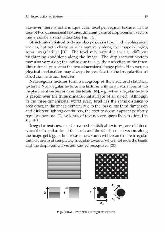
5.1 Introduction to texture 49
may describe a valid lattice (see Fig. 5.2).Structural-statistical textures also possess a texel and displacement
vectors, but both characteristics may vary along the image bringingsome irregularities [20]. The texel may vary due to, e.g., differentbrightening conditions along the image. The displacement vectorsmay also vary along the lattice due to, e.g., the projection of the three-dimensional space onto the two-dimensional image plain. However, nophysical explanation may always be possible for the irregularities atstructural-statistical textures.
Near-regular textures form a subgroup of the structural-statisticaltextures. Near-regular textures are textures with small variations of thedisplacement vectors and/or the texels [86], e.g., when a regular textureis placed over the three dimensional surface of an object. Althoughin the three-dimensional world every texel has the same distance toeach other, in the image domain, due to the loss of the third dimensionand different lighting conditions, the texture doesn’t appear perfectlyregular anymore. These kinds of textures are specially considered inSec. 5.3.
Irregular textures, or also named statistical textures, are obtainedwhen the irregularities of the texels and the displacement vectors alongthe image get bigger. In this case the textures will become more irregularuntil we arrive at completely irregular textures where not even the texelsand the displacement vectors can be recognized [20].
a a a1
a2
a1
a2
Figure 5.2 Properties of regular textures.
However, there is not a unique valid texel per regular texture. In thecase of two dimensional textures, different pairs of displacement vectors

50 5 Texture
5.1.2 State of the art
Many methods have been proposed to sort textures. For this purpose,features are extracted from the image itself, or a modified versionfrom it. Some features are extracted in space domain, while others areextracted in the space-frequency domain. Depending on the domainwhere the features are extracted, the methods can be roughly classifiedinto two groups.
Gabor wavelets are commonly used to extract texture features inspace-frequency domain. Manjunath and Ma propose in [92] a strategyto reduce the redundancy implied by Gabor wavelets. Furthermore,they propose a texture feature based on the information derived fromthe transformation with the Gabor wavelets and applied it to imageretrieval. However, their proposed feature is not rotation invariant. Thisis considered by Zhang et al. in [151]. An overview and comparisonover different texture features extracted from the information deliveredby the Gabor wavelets can be found in [34]. Furthermore, the extractionof texture features based on the transformations achieved by the Gaborwavelets is also combined with the color information of the input imagein [91, 106]. The Radon transform [20] combined with the wavelettransform is considered to analyze textures in [70, 71]. Based on theRadon transform and the wavelet transform, the ridgelet transform[27] has also won interest to analyze images, as it can deal better withedges. Do and Vetterli propose therefore the finite ridgelet transformfor image representation in [44], whereas Gonde et al. use the ridgelettransform to extract features for content-based image retrieval purposesin [53]. Zhang et al. consider in [152] the curvelet transform, which theydescribe as an extension of the ridgelet transform, to extract rotationinvariant features for region-based image retrieval.
On the other hand, many methods have also been proposed to extractfeatures describing the characteristics of textures in space domain.Masotti and Campanini perform first the ranklet transform of theimages to extract their features, which they use to classify texturesin [95]. Afifi and Ashour combine features that represent the colorinformation of the images with texture features extracted from theranklet transform of the gray-level images in [4]. In [5] Afifi and Ashourextract only color features from the images, but as a pre-processing stepthey apply the ranklet transform to each color channel of the analyzed

5.1 Introduction to texture 51
image. Several researchers have considered motifs to extract texturefeatures [10, 72, 83, 129]. For this purpose, the input image is dividedinto 2×2 grids. Different motifs are assigned to the grids depending onthe distribution of the intensity. Liu et al. extract in [85] texture featuresto sort the images according to their texton images. Ojala et al. proposein [110] local binary patterns for texture classification, whereas Ahonenet al. widen in [6] the local binary patterns to Fourier features also toclassify textures.
Lin et al. concentrate in [84] in the retrieval of regular textures. Forthis purpose, two valid displacement vectors of the input texture areextracted with the help of the autocorrelation of the image. Withthe detected displacement vectors a parallelogram is spanned thatdescribes a valid texel of the image. Five features are then extracted fromthe co-occurrence matrices of the detected texel to describe statisticalcomponents of the image. These features are used to sort the regulartextures in the database.
However, perfectly regular textures are seldom found in images.Near-regular textures are more common. The detection of near-regulartextures and the extraction of their appearance model is a challengingtask with many application fields like geo-tagging [126] and texturesythesis [66, 86]. Liu et al. represent near-regular textures as a decompo-sition of geometric deformations, lighting variations, and color changesin [86]. Once the synthesis information of a near-regular texture hasbeen extracted, new ones are created by replacing the texel informationbut maintaining all other extracted characteristics. However, in theirwork the interaction with a user is necessary. The user must give apair of displacement vectors and adapt the lattice created from the twodisplacement vectors to the irregularities of the near-regular texture.Interest point or region detectors are used to automatically extract theregular texture information without the interaction with a user. Hayset al. propose in [64] the use of the MSER detector [96] to detect in-terest points and a cross-correlation method in case that the detectedpoints are not enough to extract the characteristics of the near-regulartextures. Schindler et al. extract SIFT features [88, 89] first and groupthem according to the similarity of their descriptors into N groups in[126]. As the features of the points in a group are similar, each groupshould contain points that span valid texels and are placed along theanalyzed near-regular texture at positions with a similar environment.

52 5 Texture
Interest points extracted via a corner detector are used by Park et al.in [115]. These ones are clustered into groups of similar points usingmean-shift [33, 35, 52], which has the advantage that no number ofclusters must be defined in advance. However, in their work they use awindow of fixed size along the detected interest points to extract theinformation of their environment, without considering changes dueto scale and orientation. Hilsmann et al. combine the SIFT featureswith the mean-shift approach to automatically divide them into groupsin [66]. The lattice of the analyzed near-regular texture is searched intheir work starting from three neighboring characteristic points whosevectors are L-shaped. They are expanded to a lattice next.
5.2 Analysis, detection, and sorting ofregular textures
As we can easily classify textures into regular and irregular ones, inthis thesis the sorting of textures according to their type is considered.Although many features have been proposed in the literature to comparetextures independently of their type, features adapted to the type oftexture are not so common or even missing. Specially for regulartextures many comparisons could be made from the two elementsthat describe it completely: the displacement vectors and the texel.Because of this, the focus is set on the detection of regular texturesfirst (see Sec. 5.2.2), followed by the sorting of these type of textures(see Sec. 5.2.3). For this purpose, adapted features of regular texturesare proposed that enable a direct comparison from properties of thetextures like, e.g., their sizes, rotations, or structures appearing in theirtexels. A preliminary version of this work has been presented in [155].
Although many features can be presented to compare textures andsort them according to their similarity, the evaluation of their potentialis a challenging task. The perception of similarity by humans is non-metric and subject dependent. However, signs of what is perceived byhumans are necessary to be able to evaluate the proposed methods,implement new ones, and improve them. In Sec. 5.2.4 the extraction ofa perception map of regular textures is therefore considered.

5.2 Analysis, detection, and sorting of regular textures 53
5.2.1 Extraction of the texel and itsdisplacement vectors
Regular textures are completely described by a texel and its displace-ment vectors. In an idealized case we can consider the texture ascontinuous and of infinite extent in the space domain. The extraction ofthe texel and its displacement vectors in this idealized case is consideredin Sec. 5.2.1.1. However, real images are discrete and limited in thespace domain, which is why the extraction is considered for the realcase in Sec. 5.2.1.2.
5.2.1.1 Ideal case
The properties of regular textures from the Fourier transform can beused to extract the displacement vectors of a regular texture [20]:
G(f) ∝
⎧⎪⎪⎨⎪⎪⎩
T(f)∑
k∈Z
δ(f − kl1) · 1(l)
for 1-D textures, l1⊥l
T(f)∑
(k1,k2)∈Z2
δ(f − k1l1 − k2l2) for 2-D textures.
(5.2)
The convolution of the texel with the Dirac impulses at multiplesof the displacement vectors in space domain (see Eq. 5.1) becomes amultiplication in frequency domain. The energy of the texture is there-fore expected at multiples of the displacement vectors l (1-dimensionaltexture), lk, k = 1, 2 (2-dimensional texture), in frequency domain (seeFig. 5.3).
The relationship between the displacement vectors in space andfrequency domain for two-dimensional textures is [20]
(a1, a2) =
(lT1lT2
)−1
. (5.3)

54 5 Texture
domain, an inversion of the vector’s length is necessary, due to theproperties of the Fourier transform:
a =1
‖l‖2 · l. (5.4)
The concentration of the energy of the Fourier transform at Diracimpulses, placed at multiple combinations of the displacement vectorsl (for 1-dimensional textures), lk, k = 1, 2 (in case of 2-dimensionaltextures), makes an extraction of the displacement vectors easier thanin space domain. Two bigger maxima are expected in |G(f)| in caseof two-dimensional regular textures, and one maximum is expectedfor a one-dimensional regular texture. The angles of the vectors arecalculated from the radial projection of the magnitude of the Fourierspectrum G(r, ϕ), considering frequencies along the f2 coordinate andonly the positive f1 coordinate, as |G(f)| is centrally symmetric. Dueto the fact that higher energies are expected at lines with the sameorientation as the displacement vectors and their linear combinations,the magnitude of the Fourier transform is integrated over all radii r perangle ϕ for the considered interval:
m(ϕ) =
ˆ|G(r, ϕ)|dr. (5.5)
Local maxima are expected in m(ϕ) at the orientations of the anglesof the displacement vectors and their combinations. In case of a one-dimensional texture only one peak is expected at the angle of thedisplacement vector. On the other hand, in case of two-dimensionalregular textures several local maxima may appear in m(ϕ). The twoangles of the displacement vectors are the ones that are local maximain m(ϕ) and possess the higher magnitude in G(f) along its corre-sponding radial projection. This process is shown in Fig. 5.4 for thetwo-dimensional regular texture of Fig. 5.3.
The length of the displacement vectors is obtained from the maximaalong the lines derived as radial projection of G(f) with the orienta-tions of the displacement vectors. The distance from the origin tothe first considerable maximum is the length of the considered vector.Once the displacement vectors in frequency domain lk have been ex-
To obtain the displacement vector of a one-dimensional texture inspace domain from its corresponding displacement vector in frequency

5.2 Analysis, detection, and sorting of regular textures 55
a is calculated via Eq. 5.4 from the extracted displacement vector l infrequency domain.A valid texel t(u) from the regular texture is finally extracted from
the parallelogram spanned by the displacement vectors in space domain.In case of a one-dimensional regular texture the second vector a usedto span the parallelogram is a vector orthogonal to the displacementvector a.
gu
DFT{gu}f2
f1
2-D texturegu
DFT{gu}f2
f1
1-D texture
Figure 5.3 Properties of regular textures. The magnitudes of the Fourier transforms(lower row) are represented with pseudo-colors whose varying ranges are shown on theright of each plot.
tracted, the displacement vectors in space domain ak are calculated viaEq. 5.3. In case of one-dimensional textures the displacement vector
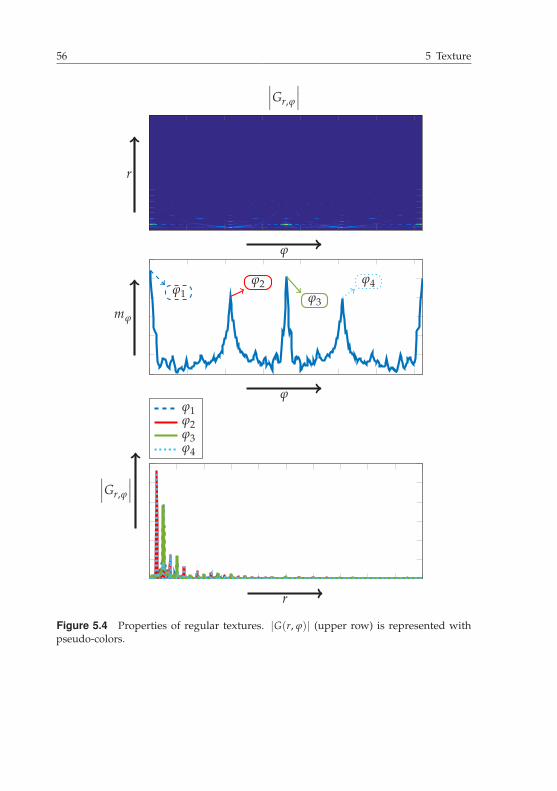
56 5 Texture
∣∣∣Gr,ϕ
∣∣∣
r
ϕ
ϕ1ϕ2
ϕ3
ϕ4
mϕ
ϕϕ1ϕ2ϕ3ϕ4
∣∣∣Gr,ϕ
∣∣∣
r
Figure 5.4 Properties of regular textures. |G(r, ϕ)| (upper row) is represented withpseudo-colors.
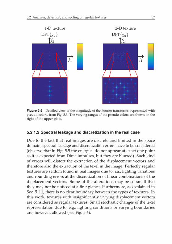
5.2 Analysis, detection, and sorting of regular textures 57
DFT{gu}f2
f1
2-D textureDFT{gu}
f2
f1
1-D texture
Figure 5.5 Detailed view of the magnitude of the Fourier transforms, represented withpseudo-colors, from Fig. 5.3. The varying ranges of the pseudo-colors are shown on theright of the upper plots.
5.2.1.2 Spectral leakage and discretization in the real case
Due to the fact that real images are discrete and limited in the spacedomain, spectral leakage and discretization errors have to be considered(observe that in Fig. 5.5 the energies do not appear at exact one pointas it is expected from Dirac impulses, but they are blurred). Such kindof errors will distort the extraction of the displacement vectors andtherefore also the extraction of the texel in the image. Perfectly regulartextures are seldom found in real images due to, i.a., lighting variationsand rounding errors at the discretization of linear combinations of thedisplacement vectors. Some of the alterations may be so small thatthey may not be noticed at a first glance. Furthermore, as explained inSec. 5.1.1, there is no clear boundary between the types of textures. Inthis work, textures with insignificantly varying displacement vectorsare considered as regular textures. Small stochastic changes of the texelrepresentation due to, e.g., lighting conditions or varying boundariesare, however, allowed (see Fig. 5.6).

58 5 Texture
whole image is not expected at real images, two texels are extracted perinput image. The parallelograms spanned by the displacement vectorsare a valid template of the area of the texels in the image. The firstextracted texel tu is the mean texel from all the extracted ones in theimage if the image is completely covered by repetitions of the templatewithout them overlapping. The second considered texel tDet
u is the oneextracted from only one template placed at one position in the image.
Figure 5.6 Examples of textures considered in this work as regular despite the stochasticchanges of the texels.
To overcome the distortions caused by the impurity of the regulartextures, fourteen window functions and three degrees of zero padding[20, 120] have been considered and are explained next. For this purpose,the input image is windowed first and padded with zeros before themagnitude of the two-dimensional Fourier transform is calculated,from which the displacement vectors are extracted. Furthermore, theextraction of the displacement vectors as in Sec. 5.2.1.1 implies theradial projection of the magnitude of the Fourier transform of theanalyzed image. Two kinds of interpolations are examined to overcomediscretization issues. In total 84 different combinations are studied toimprove the extraction of the displacement vectors as a pre-processingstep of the two-dimensional Fourier transform.
Window functions are widely used in signal processing tasks. Asthe discretization of the Fourier transform of discrete signals implies therepetition of both the analyzed signal and its spectrum (see Sec. 2.3.1),abrupt jumps between the repetitions of the signals should be attenu-ated. Several windows have been proposed for one dimensional signalsin the literature [22, 29, 37, 61, 63, 109, 112, 113, 116]. In this work thefollowing 14 one-dimensional window functions are considered.
As the exact deterministic repetition of one unique texel over the

5.2 Analysis, detection, and sorting of regular textures 59
� Modified Bartlett-Hannwindow [61]
� Blackman window[63, 112, 113]
� Bohman window [22, 63]
� Flat top window [37]
� Hann window[21, 63, 112, 113]
� Blackman-Harriswindow [63]
� Rectangular window [63,112, 113] (see Eq. 2.13)
� Dolph-Chebyshevwindow [63]
� Hamming window [21, 63,112, 113]
� 4-term window specified byNuttal [109]
� Triangular window (simi-lar to the Bartlett window[21, 63, 112, 113] but withno zero values at the endpoints)
� Kaiser window [74, 112, 113]
� De la Vallé-Poussin window[63, 116]
� Taylor window [29]
The input images are windowed by the two-dimensional windowfunctions calculated from the one-dimensional ones as
wu = wu1· wu2
, (5.6)
where u =(u1 u2
)T and w denotes the representation of one of thewindow functions used in the one-dimensional case. The consideredtwo-dimensional window functions are shown in Figs. 5.7 – 5.9.
Zero padding is a method to increase the frequency resolution. Forthis purpose, the interval at which the signal is observed must be in-creased. In the case of two-dimensional signals this is done by paddingthe new unknown values to zero [20, 120]. The quality of the extractionof the displacement vectors has been tested for the input image (whichmay be a windowed one) with no zero padding and increasing its sizeby a factor of two and three.
Interpolation at the radial projection of the magnitude is necessary inreal environments as these positions are discrete. The nearest neighborinterpolation assigns the value of the next existing neighbor to thepredicted point. The bilinear interpolation is a linear interpolation ofthe next four neighboring points of the predicted one [20, 119]. Bothinterpolations are considered in this work.

60 5 Texture
010
20
0
20
0
0.5
1
Mod. Bartlett-Hann
010
20
0
20
0
0.5
1
Blackman-Harris
010
20
0
20
0
0.5
1
Blackman
010
20
0
20
0
1
2
Rectangular
010
20
0
20
0
0.5
1
Bohman
010
20
0
20
0
0.5
1
Dolph-Chebyshev
Figure 5.7 Two-dimensional window functions.

5.2 Analysis, detection, and sorting of regular textures 61
010
20
0
20
0
1
Flat top
010
20
0
20
0
0.5
1
Hamming
010
20
0
20
0
0.5
1
Hann
010
20
0
20
0.9
0.95
1
Kaiser
010
20
0
20
0
0.5
1
4-term window spec. by Nuttal
010
20
0
20
0
0.5
1
De la Vallé-Poussin
Figure 5.8 Two-dimensional window functions.
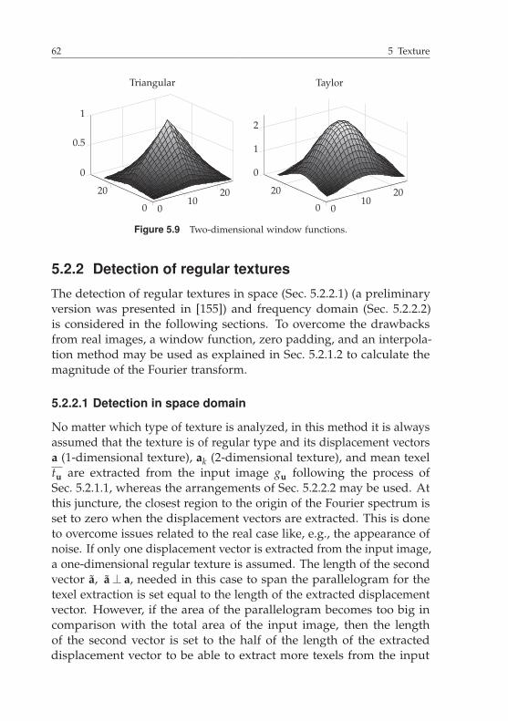
62 5 Texture
010
20
0
20
0
0.5
1
Triangular
010
20
0
20
0
1
2
Taylor
Figure 5.9 Two-dimensional window functions.
5.2.2 Detection of regular textures
The detection of regular textures in space (Sec. 5.2.2.1) (a preliminaryversion was presented in [155]) and frequency domain (Sec. 5.2.2.2)is considered in the following sections. To overcome the drawbacksfrom real images, a window function, zero padding, and an interpola-tion method may be used as explained in Sec. 5.2.1.2 to calculate themagnitude of the Fourier transform.
5.2.2.1 Detection in space domain
No matter which type of texture is analyzed, in this method it is alwaysassumed that the texture is of regular type and its displacement vectorsa (1-dimensional texture), ak (2-dimensional texture), and mean texeltu are extracted from the input image gu following the process ofSec. 5.2.1.1, whereas the arrangements of Sec. 5.2.2.2 may be used. Atthis juncture, the closest region to the origin of the Fourier spectrum isset to zero when the displacement vectors are extracted. This is doneto overcome issues related to the real case like, e.g., the appearance ofnoise. If only one displacement vector is extracted from the input image,a one-dimensional regular texture is assumed. The length of the secondvector a, a⊥ a, needed in this case to span the parallelogram for thetexel extraction is set equal to the length of the extracted displacementvector. However, if the area of the parallelogram becomes too big incomparison with the total area of the input image, then the lengthof the second vector is set to the half of the length of the extracteddisplacement vector to be able to extract more texels from the input

5.2 Analysis, detection, and sorting of regular textures 63
image. Using the extracted displacement vectors and the mean texel,the assumed regular texture gu is reconstructed following Eq. 5.1:
gu =
⎧⎪⎪⎨⎪⎪⎩
tu∗∗∑
(k1,k2)∈Z
δu−k1a−k2a for 1-D textures
tu∗∗∑
(k1,k2)∈Z2
δu−k1a1−k2a2for 2-D textures.
(5.7)
If the input texture gu was from regular type, its reconstructed imagegu will be very similar. From the comparison of both images a detec-tion of the type of texture (regular/irregular) is possible. Due to thequantization and the allowed small stochastic variations of the texels,the reconstructed image gu will not be equal to the input one, evenif the analyzed texture is perfectly regular. dT,1(gu, gu), named in thiswork similarity distance, compares the input texture and the recon-structed one and is calculated by two-dimensional median filtering ofthe absolute difference between gu and gu:
dT,1(gu, gu) =μ(med{|gu − gu|})
2 · σ(gu), (5.8)
where μ(med{|gu − gu|}) is the mean value after median filtering theabsolute differences between both images and σ(gu) the standard devi-ation of the gray values of the input image.
Due to quantization errors and small stochastic differences allowedbetween texels, med{|gu − gu|} will be bigger at texels containing big-ger differences between their gray values. To overcome this prob-lem, dT,1(gu, gu) is calculated normalizing med{|gu − gu|} by 2 · σ(gu),whereas the factor 2 may be replaced by any other constant factor. Aslong as this factor remains equal across different images, the ratios oftheir dT,1(gu, gu) will remain equal. However, the results presented inSec. 8.4.1.3 are calculated setting this factor to 2.
If dT,1(gu, gu) is smaller than a predifined threshold τT3, then thetexture is detected as a regular one.
5.2.2.2 Detection in frequency domain
According to Eq. 5.2 the energy of regular textures is expected in fre-quency domain at linear combinations of the displacement vectors l(1-dimensional textures), lk (2-dimensional textures). If every texture is

64 5 Texture
assumed of regular type and their displacement vectors are extracted,then the energy distributed at the linear combinations of the extracteddisplacement vectors compared to the energy distributed along thewhole frequency domain will be a good feature to detect regular tex-tures, as the energies should be equal. However, we have to deal withthe real case instead of the ideal one as noise may appear and theimages are discrete and limited. Spectral leakage, discretization errors,and random noise must be considered. For this purpose, seven differenttemplates are proposed to extract the energy at the linear combinationsof the displacement vectors. Eight regions in frequency domain, andtwo different features are also considered.
As a first step, every considered texture is assumed of regulartype and their displacement vectors l (1-dimensional texture), lk (2-dimensional texture), are extracted according to Sec. 5.2.1.1, whereasthe arrangements of Sec. 5.2.1.2 may be adopted. If the lengths of thedisplacement vectors in frequency domain are too short, the lengthof their corresponding displacement vectors in space domain will betoo long, without even allowing enough repetitions along the texturedimage. In such cases the analyzed texture will be directly classifiedas irregular, as in Sec. 5.2.2.1 where the detection in space domain isconsidered. Next, the linear combinations of the extracted displacementvectors are detected and their energy is extracted.
Templates ttempk,f , 1 ≤ k ≤ 7, can be used to attenuate the issues related
to real images. Due to spectral leakage and discretization, the energyin frequency domain may not be exactly at the linear combinations ofthe displacement vectors but close to them or even spread over severalfrequencies. Seven different templates are therefore set at the linearcombinations of the displacement vectors to extract the energy, creatinga texture dependent window function wk,f. The templates are shown inFig. 5.10. Template 1 is the only one which considers only one discretefrequency. All of the other templates extract the energy at severaldiscrete frequencies. Templates 2 to 5 normalize the total extractedamount of energy per considered position in contrast to the templates6 and 7. Furthermore, templates 3 and 5 take into consideration thedistance of the discrete frequency from which the energy is extracted tothe expected position of the linear combinations of the displacementvectors, by weighting the energy extracted at the expected positionsstronger than the energy extracted at their neighbors.
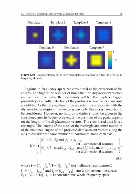
5.2 Analysis, detection, and sorting of regular textures 65
Template 1 Template 2 Template 3 Template 4
Template 5 Template 6
0
0.5
1Template 7
Figure 5.10 Representation of the seven templates considered to extract the energy infrequency domain.
Regions in frequency space are considered at the extraction of theenergy. The higher the number of times that the displacement vectorsare combined, the higher the uncertainty will be. This implies a biggerprobability of a faulty detection of the positions where the local maximashould be. As the propagation of the uncertainty corresponds with thedistance to the origin in frequency space, only this closest area shouldbe considered. However, no hard boundaries should be given to theconsidered area in frequency space, as the positions of the peaks dependon the length of the displacement vectors. The considered area U is arectangle. The lengths of the sides of the rectangle are entire multiplesof the maximal lengths of the projected displacement vectors along theaxis to consider the same number of harmonics along each axis:
U=
⎧⎪⎪⎨⎪⎪⎩
f
∣∣∣∣∣∣∣∣
| f1| < k1 ·|l1| and | f2| < k1 ·|l2|for 1-dimensional textures
| f1| < k1 ·max(∣∣l1,1
∣∣ , ∣∣l2,1∣∣) and | f2| < k1 ·max
(∣∣l1,2∣∣ , ∣∣l2,2
∣∣)for 2-dimensional textures
⎫⎪⎪⎬⎪⎪⎭
,
(5.9)
where f =(
f1 f2)T, l =
(l1 l2
)T (for 1-dimensional textures),
l1 =(l1,1 l1,2
)T and l2 =(l2,1 l2,2
)T (for 2-dimensional textures),k1 ∈ {2, 3, 4, ∞}. k1 = ∞ considers the whole frequency space.

66 5 Texture
Four more combinations of the regions in frequency space are takeninto consideration by suppressing the energies situated immediatelyclose to the origin, as these energies are much bigger than the otherones and can therefore distort the comparison (see Fig. 5.11).
Figure 5.11 The considered regions in frequency space are marked in yellow.
Features are extracted from the magnitudes in frequency domainand used for the detection of regular textures. Two different featuresmT1, mT2 are proposed to detect the type of texture. For both featuresa window function wk,f is obtained first depending on the selectedtemplate to extract the energy:
wk,f =∑
(k1,k2)∈Z2
ttempk,f ∗∗δf−k1l1−k2l2
. (5.10)
The first feature compares in the considered frequency environmentthe magnitude of the windowed spectrum to the not windowed one:
mT1 =
∑f∈U
wk,f · |Gf|∑f∈U
|Gf|. (5.11)
Furthermore, the second feature also considers the relationship betweenthe area allowed by the window function and the considered regionin frequency domain, to punish textures whose projection of the dis-placement vectors in frequency domain along one of the axis is verysmall:

5.2 Analysis, detection, and sorting of regular textures 67
mT2 =
∑f∈U
wk,f·|Gf|∑f∈U
|Gf|∑f∈U
wk,f
|U |
. (5.12)
Such kind of textures are more likely to be of irregular type, but theircorresponding window function will extract energy from a big area ofthe selected environment. This implies that the relationship consideredin feature mT1 will be high, as expected from regular textures.
The higher the values of the features mT1, mT2 are, the higher theexpectation for a texture of regular type will be.
5.2.3 Sorting of regular textures
If an input image has been detected as a regular texture following oneof the approaches in Sec. 5.2.2, it will be compared with the previouslydetected regular textures stored at the database. The input image will becompared with each image in the database to define a similarity values between the compared textures. For this purpose, one-dimensionaltextures will only be compared with one-dimensional textures andtwo-dimensional textures with two-dimensional ones. The images inthe database will then be sorted depending on their similarity to theinput image.
Eight different similarity features sk, 1 ≤ k ≤ 8, are explained herethat were presented in [155]. As similarity perception is human- andtask-dependent, the strength of the similarity features sk can be inde-pendently selected wk. Their combination yields the total similaritybetween the compared textures:
s =∏
k
swkk , wk ∈ [0, 1] , (5.13)
meaning s = 1 a maximum similarity and s = 0 no similarity. The fea-tures sk can be classified into two groups: texel’s properties (Sec. 5.2.3.1)and displacement properties (Sec. 5.2.3.2).

68 5 Texture
5.2.3.1 Texels’ features
Five similarity features s1, . . . , s5 are extracted from the texels of theregular textures. The extracted mean texel of the texture tu and oneextracted texel per image tDet
u will be used. The input image will becharacterized with the index I and the image in the database with theindex O.
Three features s1, s2, s3 compare the intensities that appear in thetexels. s4 and s5 extract information about the similarity of the contentof the texels.
Brightness s1: The mean brightness between the textures are com-pared via the mean gray values μ
(tu)
of the extracted mean texels ofthe textures. The smaller mean value is divided by the bigger one toget a normalized feature:
s1 =μ(
tc1u
)
μ(
tc2u
) , (5.14)
where {c1, c2} ∈ {I, O} , c1 �= c2, and μ(
tc1u
)≤ μ(
tc2u
)must apply.
Homogeneity of the Brightness s2: The range of intensities appear-ing in the texels is compared in s2. For this purpose, the standarddeviations of the mean texels σ
(tu)
of the images are divided yieldinga normalized value:
s2 =σ(
tc1u
)
σ(
tc2u
) , (5.15)
where {c1, c2} ∈ {I, O} , c1 �= c2, and σ(
tc1u
)≤ σ(
tc2u
)must apply.
Distribution of the Brightness s3: The feature s3 is a measure forthe similarity of the distribution of the intensities appearing in thetexels. Histograms of the appearing gray values in the texels hBright arecomputed first and compared using the quadratic-form distance next[108, 122] (see Sec. 2.1):
s3 = 1 −√(
hBright,I − hBright,O)T
B(
hBright,I − hBright,O)
, (5.16)

5.2 Analysis, detection, and sorting of regular textures 69
where
bij = 1 − dij
dmax(5.17)
is an element of the matrix B and dij denotes the distance between thegray values of the center bin i and j. dmax is the length of the maximumrange spanned by the gray values.
Structure s4: The similarity of the structure of the texels is measuredby the feature s4 based on the edges that appear in the texels of theregular textures that are extracted at a certain point from the originalimages tDet
u . The edges are detected here filtering the texels tDetu with
the Canny operator [20, 28]. s4 is obtained from two comparisons: thenumber of edges orientations s4,1 and their relative angles s4,2:
s4 = s4,1 · s4,2. (5.18)
In the Fourier transform of the image filtered with the Canny operatorthe edges will appear as straight lines passing through the origin.Following the approach described in Sec. 5.2.1.1 the straight lines canbe detected. The comparison of the number of detected lines yields
s4,1 =nLine,c1
nLine,c2, (5.19)
where {c1, c2} ∈ {I, O} , c1 �= c2, and nLine,c1 ≤ nLine,c2 must apply.From the slopes of the lines in frequency domain, the orientations of theedges ϕk, 1 ≤ k ≤ nLine, are extracted and sorted from higher to lowervalue. The difference from each edge orientation to the next smaller oneis represented by Δϕk. If Δϕk is bigger than π
2 , then the difference to π2
is calculated and set as Δϕk. s4,2 is the quotient of the mean differencesof the orientation angles per image:
s4,2 =μ(
Δϕc1k
)
μ(
Δϕc2k
) , (5.20)
where {c1, c2} ∈ {I, O} , c1 �= c2, and μ(
Δϕc1k
)≤ μ(
Δϕc2k
)must apply.
If many edge orientations are detected in a texture, then almost circularstructures can be assumed. This implies that the mean difference μ(Δϕk)

70 5 Texture
will become very small. Consequently, s4,2 and s4 will become close tozero and with them the total similarity s independently of the othersimilarity features. To avoid this, in such cases μ(Δϕk) is set to π
18 .Regions s5: This feature compares the regions that possess an
almost constant intensity. For this purpose, the regions in the texelmust be determined first. Such regions are detected using a watershedfilling method [54] in a similar way to the MSER detector [96]. The texelextracted at a determined position in the texture is compared with anincreasing threshold τ =
(τ1, τ2, . . . , τK
)T that varies from the minimalpossible intensity to the maximum one, to obtain thresholded texelstThreshk,u , 1 ≤ k ≤ K. Each pixel in the texel is marked at the compared
threshold intensity if its value is smaller than the threshold value:
tThreshk,u =
{1 if tDet
u < τk
0 otherwise.(5.21)
The thresholded images are then compared with the ones at the nextthreshold value:
ΔtThreshk,u = tThresh
k,u − tThreshk+1,u . (5.22)
Closed regions with an almost constant intensity are considered those,whose area does not vary considerably over a minimum number ofconsecutive thresholds. Due to the fact that regions detected at higherthreshold values will overlap with smaller regions detected at smallerthresholds, the regions from the smaller thresholds will be removedfrom the bigger ones, as non-overlapping regions are searched. Thetexels of regular textures are displaced all over the plane, so detectedregions at the contours of the texel tDet
u may have been extracted sepa-rately. However, as the texel will be repeated all over the image plain,such regions are not separated in the real image. In a final step thoseregions are grouped together.
Once the gray-level regions in the texel have been extracted, twocomparisons are taken between the images to compare their content:the number of detected regions s5,1 and the size of the regions s5,2:
s5 = s5,1 · s5,2. (5.23)
5.2 Analysis, detection, and sorting of regular textures 71
The number of regions between the images is compared via thenormalized quotient of the number of detected regions nRegion perimage:
s5,1 =nRegion,c1
nRegion,c2, (5.24)
where {c1, c2} ∈ {I, O} , c1 �= c2, and nRegion,c1 ≤ nRegion,c2 must apply.Per image, a histogram of the area of the regions normalized overthe whole area of the texel hArea is calculated first. The histogramsare compared next using the quadratic-form distance [108, 122] (seeSec. 2.1):
s5,2 = 1 −√(
hArea,I − hArea,O)T
B(
hArea,I − hArea,O)
, (5.25)
where
bij = 1 − dij (5.26)
is an element of the matrix B and dij denotes the distance of the repre-sented relative areas at the center bins i and j.
5.2.3.2 Displacement features
The bases for the features comparing the similarity between the latticesof regular textures are their displacement vectors. From now on aI (forone-dimensional textures), aI
k, k ∈ {1, 2} (for two-dimensional textures),are the displacement vectors of the input texture and aO (for one-dimensional textures), aO
k , k ∈ {1, 2} (for two-dimensional textures),the vectors of the compared image in the database. Three features,s6, s7, and s8, are presented to compare the lattices of two-dimensionaltextures. Two features, s6 and s7, are used in case of one-dimensionaltextures.
Scale s6: Variations of the scale at regular textures imply variationsof the lengths of the displacement vectors. In case of one-dimensionaltextures the quotient of the vector lengths is used as similarity feature

72 5 Texture
between the scales. To obtain a normalized feature, the length of thesmaller vector is divided by the length of the bigger one:
s6 =
∥∥ac1∥∥
2∥∥ac2∥∥
2, (5.27)
where {c1, c2} ∈ {I, O} , c1 �= c2, and∥∥ac1
∥∥2 ≤ ∥∥ac2
∥∥2 must apply. When
dealing with two-dimensional textures, the displacement of the texelalong the image is represented via two displacement vectors. The scalesimilarity is also obtained by comparing the lengths of the displacementvectors. In this case the length of the smallest displacement vector fromthe input texture (e.g., aI
2) is compared to the smallest displacementvector of the texture in the database (e.g., aO
1 ). Respectively, the lengthsof the remaining bigger vectors are also compared. Following the
example, let’s assume that∥∥∥aO
1
∥∥∥2≥∥∥∥aI
2
∥∥∥2
and∥∥∥aI
1
∥∥∥2≥∥∥∥aO
2
∥∥∥2, then
s6 =
√√√√√∥∥∥aI
2
∥∥∥2∥∥∥aO
1
∥∥∥2
·∥∥∥aO
2
∥∥∥2∥∥∥aI
1
∥∥∥2
. (5.28)
Rotation s7: The similarity of the rotation between two features isextracted depending on the dimension of the compared textures.
If the textures are one-dimensional, then the angles α spanned viatheir displacement vectors and the horizontal axis are calculated pertexture. For this purpose, the angles must point into the positive u1-axis,using their projection over the origin if this is not the case. The rotationsimilarity between the two one-dimensional textures is calculated as
s7 =
⎧⎪⎪⎪⎪⎨⎪⎪⎪⎪⎩
1 −∣∣∣αI−αO
∣∣∣π2
if∣∣∣αI − αO
∣∣∣ ≤ π2
1 − π−∣∣∣αI−αO
∣∣∣π2
otherwise.
(5.29)
If the textures are two-dimensional, then the angles α spanned bytheir displacement vectors and the u1-axis are also calculated first,as in the one-dimensional case. From the two obtained angles α perimage, only the smaller one will be further considered (e.g., αI
2, αO2 ).
These angles are used to calculate the absolute rotation γ per image as

5.2 Analysis, detection, and sorting of regular textures 73
the remainder of its division by the angles ∠(a1, a2) spanned by theircorresponding displacement vectors ak:
γc = αc2rem
(∠(ac
1, ac2))
, (5.30)
where c ∈ {I, O} and ∠(a1, a2) is the smallest angle spanned by thedisplacement vectors, whereas its difference to π
2 is considered in casethat the angle is bigger than π
2 . The similarity parameter is obtained bycomparing the absolute rotation of the textures taking into considerationthe relative angles between the displacement vectors of the input image:
s7 =
⎧⎪⎪⎪⎪⎪⎪⎪⎪⎨⎪⎪⎪⎪⎪⎪⎪⎪⎩
1 −∣∣∣γI−γO
∣∣∣∠(
aI1,aI
2
)
2
if∣∣∣γI − γO
∣∣∣≤ ∠(
aI1,aI
2
)2
1 −∠(
aI1,aI
2
)
2 −(∣∣∣γI−γO
∣∣∣rem
(∠(
aI1,aI
2
)
2
))
∠(
aI1,aI
2
)
2
otherwise.
(5.31)
As the similarity parameter s7 for two-dimensional textures dependson the relative angle of the displacement vectors of the input image, itis not a symmetric feature.
Orientation s8: The orientation feature s8 is only extracted fromtwo-dimensional textures by comparing the relative angles between thedisplacement vectors:
s8 =∠(
ac11 , ac1
2
)
∠(
ac21 , ac2
2
) , (5.32)
where {c1, c2} ∈ {I, O} , c1 �= c2, and ∠(
ac11 , ac1
2
)≤ ∠
(ac2
1 , ac22
)must
apply. For this purpose, the smaller angles spanned by the respectivedisplacement vectors are used. If the angles are bigger than π
2 , thentheir differences to π
2 are defined as the relative angles.

74 5 Texture
Collection of anonymouscharacteristics of the subjects
Explanation of the experiment
Simulacrum of the evaluations
Evaluation of the similarityof the pairs of textures
Statements of the sim-ilarity criteria used
Figure 5.12 Sequence of the experiment performed with humans.
5.2.4 Perception map of regular textures
Appropriate methods are necessary to sort images according to theirsimilarity. The knowledge of human perception is important to beable to compare, evaluate, and improve these methods. However, thisis a challenging task as human perception is subjective. Since in this

5.2 Analysis, detection, and sorting of regular textures 75
thesis the sorting of textures is considered depending on their typeand that the sorting of regular textures has been especially focused,the creation of a perception map [82] of regular textures is interestingto evaluate the sorting results of the method proposed in Secs. 5.2.2and 5.2.3. Furthermore, such a perception map will also enable us toevaluate if the proposed sorting method is reasonable or useless.
With the help of psychologists an experiment has been drafted. Itsprocedure is presented in Sec. 5.2.4.1. The analysis of the data obtainedfrom the experiment to extract the perception map of regular texturesis explained in Sec. 5.2.4.2.
5.2.4.1 Experimental procedure
With the help of an experiment, statements of subjects about the rela-tionship between different regular textures are collected. The evaluationof the similarity of pairs of regular textures turned out to be an appro-priate approach for a good trade-off between the collection of manystatements to different regular textures and a fast and simple ques-tion for the subjects to answer. For this purpose, pairs of textures areconsecutively shown to the subjects and the similarities between thepairs are evaluated by a numerical rating scale. Every texture mustbe compared with every other considered one to be able to analyzethe data (see Sec. 5.2.4.2), which means k·(k+1)
2 pair comparisons for ktextures. As the number of pairs of textures that must be comparedincreases enormously with the number of considered textures and theexperiment must be done in a reasonable time to avoid fatigued sub-jects, a representative selection is necessary to build the pairs of textures.Furthermore, the experiment should be repeated to several subjects tobecome generalized perception maps.
Twenty subjects participated in the experiment, which took placefor all of them always at the same computer in the same room. Theexperiment’s sequence is shown in Fig. 5.12. In a first step the subjectsmust answer some questions that may alter the results, e.g., if theypossess any defective sight. Next, the rating of the similarity of pairsof textures is explained with the help of text. This is the scope ofthe experiment. Five pairs of textures are consecutively shown toenable the subjects to become familiar with the type of textures that arecompared. Subsequently, a simulacrum of the experiment is done. For

76 5 Texture
this purpose, five pairs of textures are consecutively shown, and thesubjects must evaluate after the display of the corresponding pair oftextures in a six-point scale how similar the compared textures are. Theonly information told to the subjects about the scale is that one indicatesvery dissimilar and six very similar. The evaluation of the similarity ofevery pair of textures is continued with the question to the subjects ofhow confident they are, rated on a four-point scale. The information ofone as very unsure and four as very sure was the only one transmittedto the subjects about this rating scale. The subjects themselves were theones who set the velocity of the experiment, as they could decide perclick on the computer’s mouse when to answer and continue with thenext pair of textures. Every subject evaluated the same pairs of textures,but their order at the evaluation was randomly chosen to overcomefatigue over the subjects or possible dependencies across consecutivepairs of textures. At the end of the experiment the subjects were askedto explain their criteria used for the similarity evaluation. Ten of theevaluated pairs of textures (the same for all subjects) were shown to thesubjects on the monitor and also on a paper to help them remember thekind of pairs of textures they analyzed. These ones could also be usedas support when the subjects explained their evaluation criteria.
5.2.4.2 Data analysis
The data can be analyzed once it has been collected in form of similaritystatements between pairs of textures. The goal is to obtain a perceptionmap of regular textures, in which the analyzed textures are representedas points in a multidimensional space [82]. The distance betweenthe points in space should correlate with the similarity between theirrespective represented textures. Exactly this kind of problems areaddressed by multidimensional scaling [11, 48], which is commonlyapplied in psychology and market research problems [11, 48]. Thenon-metric multidimensional scaling [48, 78, 79] is considered, whichcan be applied to the collected data directly. For this purpose, theEuclidean distance is selected as distance function and the dimensionsof the space, in which the textures are represented, are limited to two.
Over all subjects one similarity statement is calculated per pair of tex-tures. These ones are obtained from the median value over all similaritystatements of all subjects of the corresponding pair of textures.

5.2 Analysis, detection, and sorting of regular textures 77
Detection and grouping ofcharacteristic texel points
Extraction of the texels
Post-processing
Figure 5.13 Overview of the procedure to extract regular textures from near-regular ones.

78 5 Texture
5.3 Detection of near-regular textures andextraction of their regular texture
Regular textures are seldom found in digital images due to lightingvariations and the projection of the three-dimensional world onto thetwo-dimensional image plain. Near-regular textures (see Sec. 5.1.1) aretherefore more common in digital images. In the following sections thedetection and extraction of regular textures from near-regular ones isconsidered. An overview of the procedure is shown in Fig. 5.13. Thismodus operandi is inspired by [66]. However, different options areproposed for the resolution of the goal of each block that may evenbe fused. First, regions or points of interest are detected in the imageand grouped according to their similarity (Sec. 5.3.1). Per cluster alattice over the input image is spanned to extract the average texelof the texture (Sec. 5.3.2). Finally, the suppression of faulty extractedtexels, as well as the fusion of repeated extracted texels, is considered inSec. 5.3.3. Note that no previuos segmentation of the image is neededto detect near-regular textures in images with the presented methods.A preliminary version of this work has been presented in [159].
5.3.1 Detection and grouping of characteristictexel points
The detection of characteristic points or regions of interest in an inputimage is considered in Sec. 5.3.1.1 and their grouping into clusters withsimilar characteristics in Sec. 5.3.1.2. In Sec. 5.3.1.3 the obtained clustersare further processed to assure spatially compact points and discardclusters that do not describe a valid near-regular texture.
5.3.1.1 Detection of points of interest
As a near-regular texture is composed of a repetition of a texel, regionsor points of interest detected at texels will be repeated all over thetexture. Due to the fact that variations of the displacement vectors andthe texel appear at near-regular textures, the detectors should be robustto lighting variations and affine transformations. The SURF detector[14, 15] and the MSER detector [96] are considered here to respectivelydetect points and regions of interest.
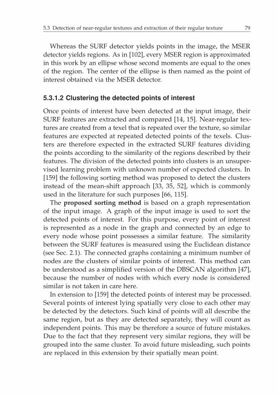
5.3 Detection of near-regular textures and extraction of their regular texture 79
Whereas the SURF detector yields points in the image, the MSERdetector yields regions. As in [102], every MSER region is approximatedin this work by an ellipse whose second moments are equal to the onesof the region. The center of the ellipse is then named as the point ofinterest obtained via the MSER detector.
5.3.1.2 Clustering the detected points of interest
Once points of interest have been detected at the input image, theirSURF features are extracted and compared [14, 15]. Near-regular tex-tures are created from a texel that is repeated over the texture, so similarfeatures are expected at repeated detected points of the texels. Clus-ters are therefore expected in the extracted SURF features dividingthe points according to the similarity of the regions described by theirfeatures. The division of the detected points into clusters is an unsuper-vised learning problem with unknown number of expected clusters. In[159] the following sorting method was proposed to detect the clustersinstead of the mean-shift approach [33, 35, 52], which is commonlyused in the literature for such purposes [66, 115].
The proposed sorting method is based on a graph representationof the input image. A graph of the input image is used to sort thedetected points of interest. For this purpose, every point of interestis represented as a node in the graph and connected by an edge toevery node whose point possesses a similar feature. The similaritybetween the SURF features is measured using the Euclidean distance(see Sec. 2.1). The connected graphs containing a minimum number ofnodes are the clusters of similar points of interest. This method canbe understood as a simplified version of the DBSCAN algorithm [47],because the number of nodes with which every node is consideredsimilar is not taken in care here.
In extension to [159] the detected points of interest may be processed.Several points of interest lying spatially very close to each other maybe detected by the detectors. Such kind of points will all describe thesame region, but as they are detected separately, they will count asindependent points. This may be therefore a source of future mistakes.Due to the fact that they represent very similar regions, they will begrouped into the same cluster. To avoid future misleading, such pointsare replaced in this extension by their spatially mean point.

80 5 Texture
5.3.1.3 Post-processing of the clustered points of interest
An immediate post-processing of the extracted clusters is profitable tocorrect clusters and remove those that do not contain adequate pointsto describe a valid lattice of a near-regular texture.
Spatially compact point clouds are required from the clusteredpoints to improve the detection of the near-regular texures. An im-age may contain several objects with a similar texture. The detectedpoints of similar textures will be grouped into the same clusters, asno spatial localization is considered when the points are grouped. Toextract the correct lattices of all textures in the image, the spatiallyseparated points should therefore be located at different clusters. Forthis purpose, every point in a cluster is represented as a node of agraph. Every node is connected by an edge to its nT1 spatially closestpoints that belong to its cluster. If a cluster consists of several pointsthat belong to spatially separated similar textures, several connectedgraphs (see Sec. 2.2.1) are expected at its graph representation. Eachconnected graph is therefore considered as an extra cluster to assurethat the points are spatially agglomerated at one place.
The suppression of clusters of points situated merely along edgesis considered next. A valid lattice of a near-regular texture may beextracted from every cluster containing enough points of interest. How-ever, some clusters may only consist of points displaced along thecontours or edges from regions in the image. The sooner such clus-ters are discarded, the better, most of all due to time consumption,it is. From the points in a cluster pk, 1 ≤ k ≤ K, pk =
(u1,k u2,k
)T,the ones that spatially envelop all points and compactly describe thespatial boundary pBound
k1, 1 ≤ k1 ≤ K1, K1 < K, are searched first. Their
spatial distance to the center of the cluster pk is calculated next, and theminimum distance is compared via a division by the mean distance ofthe points in the boundary to the center of the cluster:
dBound(pk) =min
k(‖pk − pk‖2)
μ(∥∥∥pBound
k1− pk
∥∥∥2
) . (5.33)
If dBound(pk) is higher than a predefined threshold, then the cluster isdiscarded as it merely contains points situated at an edge.
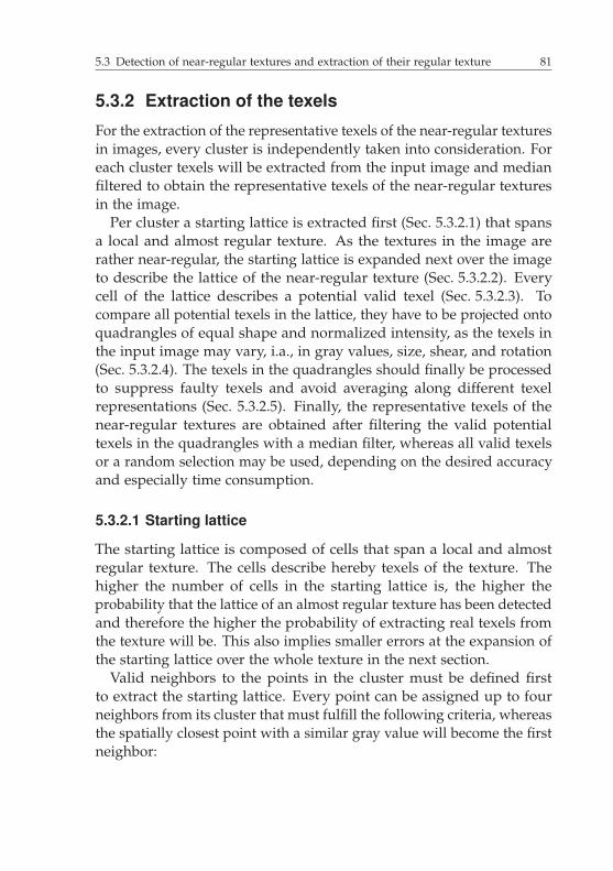
5.3 Detection of near-regular textures and extraction of their regular texture 81
5.3.2 Extraction of the texels
For the extraction of the representative texels of the near-regular texturesin images, every cluster is independently taken into consideration. Foreach cluster texels will be extracted from the input image and medianfiltered to obtain the representative texels of the near-regular texturesin the image.
Per cluster a starting lattice is extracted first (Sec. 5.3.2.1) that spansa local and almost regular texture. As the textures in the image arerather near-regular, the starting lattice is expanded next over the imageto describe the lattice of the near-regular texture (Sec. 5.3.2.2). Everycell of the lattice describes a potential valid texel (Sec. 5.3.2.3). Tocompare all potential texels in the lattice, they have to be projected ontoquadrangles of equal shape and normalized intensity, as the texels inthe input image may vary, i.a., in gray values, size, shear, and rotation(Sec. 5.3.2.4). The texels in the quadrangles should finally be processedto suppress faulty texels and avoid averaging along different texelrepresentations (Sec. 5.3.2.5). Finally, the representative texels of thenear-regular textures are obtained after filtering the valid potentialtexels in the quadrangles with a median filter, whereas all valid texelsor a random selection may be used, depending on the desired accuracyand especially time consumption.
5.3.2.1 Starting lattice
The starting lattice is composed of cells that span a local and almostregular texture. The cells describe hereby texels of the texture. Thehigher the number of cells in the starting lattice is, the higher theprobability that the lattice of an almost regular texture has been detectedand therefore the higher the probability of extracting real texels fromthe texture will be. This also implies smaller errors at the expansion ofthe starting lattice over the whole texture in the next section.
Valid neighbors to the points in the cluster must be defined firstto extract the starting lattice. Every point can be assigned up to fourneighbors from its cluster that must fulfill the following criteria, whereasthe spatially closest point with a similar gray value will become the firstneighbor:
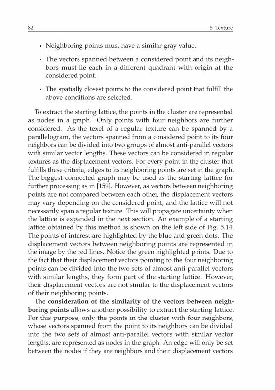
82 5 Texture
� Neighboring points must have a similar gray value.
� The vectors spanned between a considered point and its neigh-bors must lie each in a different quadrant with origin at theconsidered point.
� The spatially closest points to the considered point that fulfill theabove conditions are selected.
To extract the starting lattice, the points in the cluster are representedas nodes in a graph. Only points with four neighbors are furtherconsidered. As the texel of a regular texture can be spanned by aparallelogram, the vectors spanned from a considered point to its fourneighbors can be divided into two groups of almost anti-parallel vectorswith similar vector lengths. These vectors can be considered in regulartextures as the displacement vectors. For every point in the cluster thatfulfills these criteria, edges to its neighboring points are set in the graph.The biggest connected graph may be used as the starting lattice forfurther processing as in [159]. However, as vectors between neighboringpoints are not compared between each other, the displacement vectorsmay vary depending on the considered point, and the lattice will notnecessarily span a regular texture. This will propagate uncertainty whenthe lattice is expanded in the next section. An example of a startinglattice obtained by this method is shown on the left side of Fig. 5.14.The points of interest are highlighted by the blue and green dots. Thedisplacement vectors between neighboring points are represented inthe image by the red lines. Notice the green highlighted points. Due tothe fact that their displacement vectors pointing to the four neighboringpoints can be divided into the two sets of almost anti-parallel vectorswith similar lengths, they form part of the starting lattice. However,their displacement vectors are not similar to the displacement vectorsof their neighboring points.
The consideration of the similarity of the vectors between neigh-boring points allows another possibility to extract the starting lattice.For this purpose, only the points in the cluster with four neighbors,whose vectors spanned from the point to its neighbors can be dividedinto the two sets of almost anti-parallel vectors with similar vectorlengths, are represented as nodes in the graph. An edge will only be setbetween the nodes if they are neighbors and their displacement vectors

5.3 Detection of near-regular textures and extraction of their regular texture 83
are similar. By these means two features are assigned per node. Thefirst feature f NT,1 is the relationship of the lengths of the displacementvectors. The average length of the anti-parallel vectors are thereforecalculated and the smallest one is divided by the bigger one to obtainf NT,1. The second feature β is the absolute difference between thesmallest angles between not anti-parallel vectors. The displacementvectors between neighboring points are considered similar (an edge istherefore set in the graph between their nodes) if the relationships oftheir displacement vectors’ lengths and angles are similar:
� f NT,1 > τT1
� β < τT2.
The biggest component graph is the starting lattice. However, due tothe further consideration of the similarity of the vectors from the pointsto their neighbors, the probability of extracting local regular textures ishigher (see Fig. 5.14 right).
5.3.2.2 Expansion of the starting lattice
Once the starting lattice has been detected at a local regular texture, it isexpanded along the texture. Bigger variations between the displacementvectors are now allowed along the lattice. In [159] a method wasproposed to expand the starting lattice and it is explained next. Thegoal in [159] was the extraction of the regular texture from the near-regular one, which is possible after extracting the correct texel of thetexture. A perfect extraction of the lattice of the texture is, however,not indispensable. A second method is further presented here to alsoimprove the correctness of the extracted lattice.
The basis for both methods is a graph whose nodes are all pointsof interest in the considered cluster. The nodes that form part of thestarting lattice are connected by a directed edge if they are neighbors.From now on vlatt
k (1 ≤ k ≤ K) are the nodes that form part of thelattice, [vlatt
k1, vlatt
k2], (k1, k2) ∈ K2, is a directed edge from node vlatt
k1to
vlattk2
, meaning that vlattk2
is considered in the lattice as a neighbor of vlattk1
,
and N+(vlattk ) is the set of all outneighbors of vlatt
k (see Sec. 2.2.2).As the lattice will be expanded now over a near-regular texture, vari-
ations in the lighting conditions are expected, so new added neighbors

84 5 Texture
to the lattice do not need to have a similar gray value in contrast to theconditions imposed for neighbors at the starting lattice (see Sec. 5.3.2.1).
Figure 5.14 The starting lattices for an input image, without taking into considerationthe similarity of the displacement vectors of neighboring points (left) and considering it(right). The dots are the points of interest in the starting lattice and the red lines connectneighboring points.
Based on [159] the starting lattice is expanded as explained next. Ev-ery node in the graph with less than four outneighbors (|N+(vlatt
k )| < 4)is further considered to expand the starting lattice. For this purpose,new outneighbors are searched in the points that belong to the cluster.The potential outneighbors must lie only in an environment of theposition where the point will be if the texture were regular. In case thatseveral points in the cluster fulfill these criteria, then the closest pointof interest to the expected position will become the outneighbor of thesearched node and a directed edge will be therefore set (e.g., in Fig. 5.15

5.3 Detection of near-regular textures and extraction of their regular texture 85
upper row left, the point pposs1 will become part of the lattice instead of
pposs2 ). The expected position is calculated from the vectors spanned by
the inneighbors of the considered node to their respective outneighbors.As a node can have several inneighbors and the texture is not regular,different vectors will be used to obtain the proposed new outneighbors.Because of this, a node may have more than four outneighbors.
pposs1
pposs2
pposs1
pposs2
platt
pcons
pposs
Figure 5.15 Illustration of the selection of new points for the lattice. The method basedon [159] will select pposs
1 in the upper configuration as new point, whereas the otherproposed approach will select pposs
2 .
Considering the maximum number of outneighbors per node, thestarting lattice is expanded as follows. Every node in the graph withless than four outneighbors (|N+(vlatt
k )| < 4) is also considered inthis approach to expand the starting lattice. However, the number ofallowed outneighbors per node is restricted in this version of the ex-pansion of the starting lattice to four. Similar to the previous approach,outneighbors will be searched from points in the cluster that lie in anenvironment where the point is expected if the texture were regular.

86 5 Texture
The expected position will also be calculated from the vectors spannedfrom the inneighbors to the considered node, but, in contrast to theprevious approach, they will not be considered independently. Averagevectors will be calculated from the parallel vectors and used for thesearch. Furthermore, if several points of interest pposs
k1, 1 < k1 ≤ K1,
in the cluster lie in the allowed environment, the closest point to theexpected one will not be necessarily selected anymore. In this version,the vectors spanned from the point of the considered node pcons to thepoints pposs
k1representing the new possible outneighbors are compared.
The candidate point in the cluster whose vector becomes more similarto the expected one will be selected (e.g., in Fig. 5.15 upper row right,the point pposs
2 will become part of the lattice instead of pposs1 ). The
similarity is measured by taking into consideration the angles of thevectors and their lengths. For this purpose, the following cost functionis minimized:
mT3k1
=
∥∥∥ppossk1
− pcons∥∥∥
2
μ(∥∥∥pposs
k1− pcons
∥∥∥2
) ·∣∣∣�(
ppossk1
)−�(pcons)∣∣∣ , (5.34)
where �(p) denotes the angle spanned by the vector p and the u1-axis.In case that the spanned vectors of several candidate points have asimilar angle to the angle of the expected vector, then the point withthe smallest spatial distance to the considered point will be selected(e.g., in Fig. 5.15 down, the right green point will be selected instead ofthe left one) to avoid springing interest points along the direction.
Finally, vectors whose outneighbors have already been searchedbut still have less than four outneighbors will be considered againif they become inneighbors of a new considered node. Note that inthis approach the number of outneighbors per node is restricted toa maximum of four, but the number of inneighbors that a node maypossess is not restricted.
5.3.2.3 Detection of potential texels
Once the lattice of the near-regular texture has been detected, potentialtexels are searched. They are found at every closed cell in the expandedlattice (see Fig. 5.16 upper row left). As a consequence, every node in thelattice with outneighbors is considered (see Fig. 5.16 upper row right).
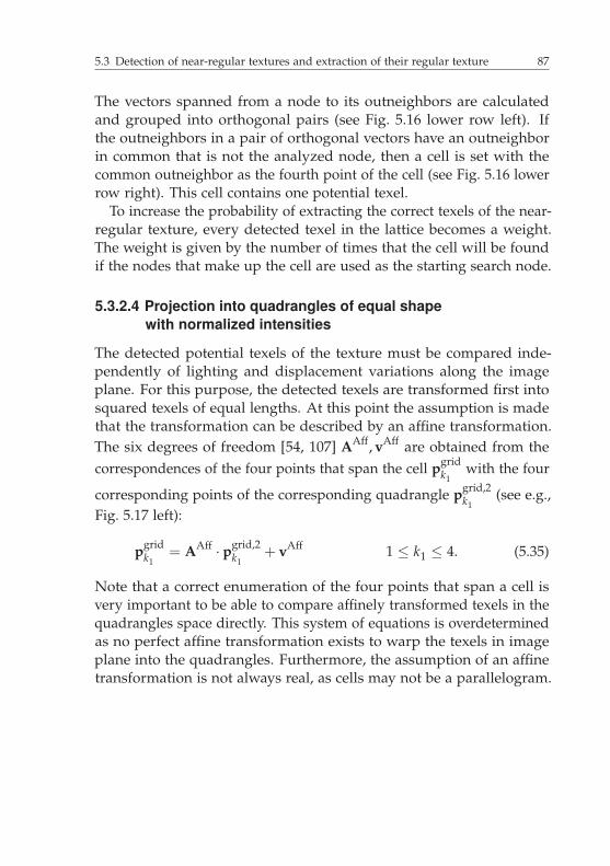
5.3 Detection of near-regular textures and extraction of their regular texture 87
The vectors spanned from a node to its outneighbors are calculatedand grouped into orthogonal pairs (see Fig. 5.16 lower row left). Ifthe outneighbors in a pair of orthogonal vectors have an outneighborin common that is not the analyzed node, then a cell is set with thecommon outneighbor as the fourth point of the cell (see Fig. 5.16 lowerrow right). This cell contains one potential texel.
To increase the probability of extracting the correct texels of the near-regular texture, every detected texel in the lattice becomes a weight.The weight is given by the number of times that the cell will be foundif the nodes that make up the cell are used as the starting search node.
5.3.2.4 Projection into quadrangles of equal shapewith normalized intensities
The detected potential texels of the texture must be compared inde-pendently of lighting and displacement variations along the imageplane. For this purpose, the detected texels are transformed first intosquared texels of equal lengths. At this point the assumption is madethat the transformation can be described by an affine transformation.The six degrees of freedom [54, 107] AAff, vAff are obtained from thecorrespondences of the four points that span the cell pgrid
k1with the four
corresponding points of the corresponding quadrangle pgrid,2k1
(see e.g.,Fig. 5.17 left):
pgridk1
= AAff · pgrid,2k1
+ vAff 1 ≤ k1 ≤ 4. (5.35)
Note that a correct enumeration of the four points that span a cell isvery important to be able to compare affinely transformed texels in thequadrangles space directly. This system of equations is overdeterminedas no perfect affine transformation exists to warp the texels in imageplane into the quadrangles. Furthermore, the assumption of an affinetransformation is not always real, as cells may not be a parallelogram.

88 5 Texture
the least-squares method [59]:
⎛⎜⎜⎜⎜⎝
pgrid1
pgrid2
pgrid3
pgrid4
⎞⎟⎟⎟⎟⎠
=
⎛⎜⎜⎜⎜⎜⎜⎜⎜⎜⎜⎜⎜⎜⎜⎜⎝
pgrid,21,1 pgrid,2
1,2 0 0 1 0
0 0 pgrid,21,1 pgrid,2
1,2 0 1
pgrid,22,1 pgrid,2
2,2 0 0 1 0
0 0 pgrid,22,1 pgrid,2
2,2 0 1
pgrid,23,1 pgrid,2
3,2 0 0 1 0
0 0 pgrid,23,1 pgrid,2
3,2 0 1
pgrid,24,1 pgrid,2
4,2 0 0 1 0
0 0 pgrid,24,1 pgrid,2
4,2 0 1
⎞⎟⎟⎟⎟⎟⎟⎟⎟⎟⎟⎟⎟⎟⎟⎟⎠
︸ ︷︷ ︸Φ
·
⎛⎜⎜⎜⎜⎜⎜⎜⎜⎝
aAff11
aAff12
aAff21
aAff22
vAff1
vAff2
⎞⎟⎟⎟⎟⎟⎟⎟⎟⎠
(5.36)
→
⎛⎜⎜⎜⎜⎜⎜⎜⎜⎝
aAff11
aAff12
aAff21
aAff22
vAff1
vAff2
⎞⎟⎟⎟⎟⎟⎟⎟⎟⎠
=(
ΦT · Φ)−1 · ΦT ·
⎛⎜⎜⎜⎜⎝
pgrid1
pgrid2
pgrid3
pgrid4
⎞⎟⎟⎟⎟⎠
, (5.37)
where pck1
=(
pck11 pc
k12
)T, 1 ≤ k1 ≤ 4, c ∈ {grid, grid, 2}, aij is a
component of the matrix AAff, i, j ∈ {1, 2}, and vAff =(
vAff1 vAff
2
)T.
With these equations the corresponding positions of the points of thetexel in the quadrangle can be calculated in the image plane to adopttheir image values and therefore transform the detected texels to thequadrangles tAff
u that are robust to affine transformations.Finally, the affinely transformed texels must also become lighting in-
dependent. For this purpose, the transformed texels are all normalizedby the following equation in contrast to [159]:
tindu =
tAffu − min
u
(tAffu
)
maxu
(tAffu
)− min
u
(tAffu
) . (5.38)
The parameters of the affine transformation are therefore estimated by

5.3 Detection of near-regular textures and extraction of their regular texture 89
Figure 5.16 Illustration of the extraction of potential texels. An extracted lattice over atexture is shown (upper row left), whereas the interesting points are the blue dots and theirrelationship to their neighbors is given by the red arrows. The outneighbors (green dots)of a considered point (violet dot) are selected first (upper row right). Two outneighborswith orthogonal vectors are selected next (green) and their common outneighbor (yellowdot) is searched (lower row left). The cell spanned by the four selected points is a potentialtexel (lower row right).
5.3.2.5 Extraction of the representative texel
The representative texel trepu of the detected near-regular texture is the
median texel from the extracted ones projected onto the quadranglestindk1,u, 1 ≤ k1 ≤ K1. However, as shown in [159], processing the texels in

90 5 Texture
the quadrangles before the filtering step will improve the quality of therepresentative texel. On the one hand, the suppression of inappropriatetexels minimizes errors when the median value is calculated. For thispurpose, outliers in the set of extracted texels, as well as texels withno repetitions at the contours, are considered here. On the other hand,different texels may have been extracted at one cluster, e.g., if the imageconsists of two textures, one occluded by the other one, with similardetected points of interest. In such cases the texels of both textures maybe correctly extracted, but the median filtering over them will reveala wrong texel of the textures. However, the detection of the differenttexel groups will allow to separate them and extract different averagetexels, one per texture. All of these methods may be performed or onlya selection of them. For simplification purposes, the methods will beexplained with tind
k1,u, 1 ≤ k1 ≤ K1.
pgrid3
pgrid,23
pgrid1
pgrid,21
pgrid4
pgrid,24
pgrid2
pgrid,22
Figure 5.17 Projection of the texels into a quadrangle.
The occlusion of outliers is considered via the principal componentanalysis [45]. The eigentexels ePCA
u and eigenvalues λPCA are extractedfrom all texels tind
k1,u, 1 ≤ k1 ≤ K1. These are approximated in a secondstep using only the eigentexels with the τPCA strongest eigenvalues:
5.3 Detection of near-regular textures and extraction of their regular texture 91
tindk1,u =
τPCA∑k
cPCAk · ePCA
u,k + tindu , (5.39)
where cPCAk denotes the k-th strongest principal component and tind
u theaverage texel over all texels in the quadrangles tind
k1,u. All of the texels
tindk1,u that vary significantly from their reconstructed ones tind
k1,u via theprincipal component analysis method are discarded, as they can beassumed as outliers.
The repeatability of the texels at the contours is considered next.As the texel of the texture is repeated over the texture, the texel shouldhave similar boundaries. This condition has already been used in [66]and in [159] to discard faulty texels. Here the condition is implementedas in [159], where the correlation coefficient (see Sec. 2.1) of the left andright contour, respectively top and lower contour
� r(
tind[(
1k
)], tind
[(1
U2 − k
)])
� r(
tind[(
k1
)], tind
[(U1 − k
1
)])
has to be high, where 1 ≤ k ≤ nT,2, U1 is the number of columns in thetexel and U2 the number of rows. However, if the compared contoursare of an almost homogeneous gray value, then the texels would not beclassified as faulty.
The grouping of texels according to their similarity is consideredto improve the extraction of the representative texels. Different texelsmay be extracted at one cluster if the characteristic points of differenttextures are not separated. Faulty texels may be extracted, i.a., due tothe simplification of the assumption of an affine transformation of thetexels to project them onto the quadrangles. Therefore clusters andisolated texels may be obtained at the extracted texels from the image ifthe similarity of their content is compared. To detect such cases, all ofthe extracted texels are represented by a node in a graph and pairwisecompared using the correlation coefficient r(tind
k1,u, tindk2,u) (see Sec. 2.1).

92 5 Texture
Similar texels will have a correlation coefficient close to one and theircorresponding nodes will be therefore connected by an edge. Clusters ofsimilar texels are every connected graph. Isolated vertices or connectedgraphs with a small number of nodes are extracted texels that areprobably not a real texel of the image, as they appear seldom. Due tothis fact, only the connected graphs containing a minimum number ofnodes will further be considered. Representative texels will be extractedfrom every cluster group via median filtering and will represent thetextures in the image.
If more than one representative texel trepu is extracted per cluster,
then the expanded lattice may also be divided, so that every latticeis composed from cells that are similar to only one of the obtainedrepresentative texels. However, in this case the texels of every cell in theoriginal expanded lattice must be transformed to the quadrangles robustto affine transformations and lighting variations, and finally compared,e.g., using the correlation coefficient, to the extracted representativetexels.
5.3.3 Post-processing
The extracted representative texels trepu of the image represent the near-
regular textures detected at the input image. Due to the fact that thereis not a unique texel per texture (see Sec. 5.1.1), some of the extractedrepresentative texels trep
u may represent the same texture. In Sec. 5.3.3.1the detection of texels that represent the same texture is considered.
Furthermore, some of the extracted representative texels trepu may not
belong to a valid texture in the image at all. The average texels may re-sult from more than one texel. A method to detect such overdeterminedtexels is explained in Sec. 5.3.3.2.
Finally, the repeatibility at the contours of the texels may also be testedfor the extracted representative texels trep
u as explained in Sec. 5.3.2.5.
5.3.3.1 Fusion of similar texels
Points of interest with different corresponding features may be extractedfrom one texture. This will lead after the clustering of the points ofinterest according to their features to different clusters and therefore todifferent extracted texels of the same texture. Redundant information is
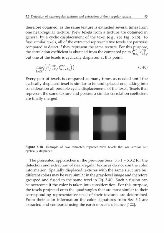
5.3 Detection of near-regular textures and extraction of their regular texture 93
therefore obtained, as the same texture is extracted several times fromone near-regular texture. New texels from a texture are obtained ingeneral by a cyclic displacement of the texel (e.g., see Fig. 5.18). Tofuse similar texels, all of the extracted representative texels are pairwisecompared to detect if they represent the same texture. For this purpose,the correlation coefficient is obtained from the compared pairs trep
u,k1, trep
u,k2,
but one of the texels is cyclically displaced at this point:
maxk∈Z
2
(r(
trepu,k1
, trepu+k,k2
)). (5.40)
Every pair of texels is compared as many times as needed until thecyclically displaced texel is similar to its undisplaced one, taking intoconsideration all possible cyclic displacements of the texel. Texels thatrepresent the same texture and possess a similar correlation coefficientare finally merged.
Figure 5.18 Example of two extracted representative texels that are similar butcyclically displaced.
The presented approaches in the previous Secs. 5.3.1 – 5.3.2 for thedetection and extraction of near-regular textures do not use the colorinformation. Spatially displaced textures with the same structure butdifferent colors may be very similar in the gray-level image and thereforegrouped and fused to the same texel in Eq. 5.40. Such a fusion canbe overcome if the color is taken into consideration. For this purpose,the texels projected onto the quadrangles that are most similar to theircorresponding representative texel of their textures are determined.From their color information the color signatures from Sec. 3.2 areextracted and compared using the earth mover’s distance [122].

94 5 Texture
Figure 5.19 Example of an overdetermined texel.
5.3.3.2 Detection of overdetermined texels
Extracted representative texels resulting from several valid texels (over-determined) distort the result. To detect and discard them, a regulartexture is created for every extracted representative texel trep
u followingEq. 5.1 as
gu =
(K1,K2)∑(k1,k2)=(1,1)
trepu ∗∗δ
[u − k1 · U1
(10
)− k2 · U2
(01
)], (5.41)
where U2 is the height and U1 the width of the quadrangles on whichthe detected texels in the image plane are projected. The Fouriertransform of this image is according to Eq. 5.2
Gu ∝ Trepf
(K1,K2)∑(k1,k2)
δf−k1l1−k2l2, (5.42)
where(
lT1lT2
)=
(U1 00 U2
)−1
. (5.43)
If the first considerable peaks of |Gu| do not appear at the expectedpositions, then the extracted average texel is discarded.
6 Detection of regionsThe recognition of connected regions due to stable colors or a repeatingpattern is a very important task in image processing. Otherwise, theextraction of the color, shape, and texture features presented in theprevious chapters can be distorted if different regions contribute to them.The detection of such regions should be robust to affine transformations,as the regions should be detected independently of their scale, rotation,shear, or position in the image. This step is considered in this chapter.
This chapter is organized as follows. An introduction to the detectionof regions and to the state of the art is given in Sec. 6.1. The structure ofthe proposed region detectors is presented in Sec. 6.2. It can be dividedinto two steps, the detection of color regions in images (Sec. 6.3) andthe detection and extraction of patterns (Sec. 6.4). The results achievedby the proposed region detectors are shown in Sec. 8.5.
6.1 Introduction to the detection of regions
The division of an image into meaningful areas is called segmentation[20, 54]. For this purpose, every pixel in the image is assigned to aregion, whereas the regions must be spatially connected and must notoverlap between each other. Two types of methods exist to segmentimages: edge-oriented methods, where edges between the regions aresearched, and region-oriented methods, where neighboring pixels withsimilar characteristics are grouped into regions [20, 54].
The detection of regions robust to affine transformations and lightingconditions (up to a certain variation) in images and the representationof their neighborhood is another way of describing the informationin images. However, in this case not all of the pixels in an image areused. Only interesting points or regions are searched first. Typically,the neighborhood of the detected points and even the detected regionsare approximated by an ellipse [102], from which the characteristics areextracted.
96 6 Detection of regions
Due to noise and distortions in the images, e.g., compression artifacts,the need to assign every pixel to a region may alternate the propertiesof the meaningful areas in the image. Every pixel in the image maynot be necessary for the image processing or not even improve it. Onthe other hand, the description of the image information with theneighborhood of interesting points may contain information of differentobjects appearing in the image. Because of this, the detection andextraction of meaningful regions is considered. Regions in the inputimages are searched, whose pixels possess either a similar color or forma pattern of alternating colors. However, the assignment of every pixelto a region is not forced in this thesis.
6.1.1 State of the art
Many segmentation methods have been proposed in the literature. Abrief overview of some of the segmentation methods that consider colorand texture information and do not need interaction with humans ispresented first. Wang et al. segment in [139] the image block-wiseinstead of pixel-wise. For this purpose, they partition the image into4×4 pixel blocks. A feature vector is then assigned to each blockthat contains information about the average color in the block and theaverage coefficients of their wavelet transform. With the help of thek-means algorithm [45] the image is segmented. The JSEG method isproposed by Deng and Manjunath in [42]. This segmentation methodworks in two steps. First, the colors appearing in the images arequantized. In the second step homogenous areas are searched. Thehomogeneity is measured at different scales taking into considerationthe spatial distribution of the quantized values of the pixels. Carsonet al. present Blobworld in [30], where the image is segmented intoregions using the color and texture properties of the pixels plus theirspatial location. To extract the texture properties, an appropriate scaleis selected per pixel.
Furthermore, several detectors have been proposed for the detec-tion of points and regions of interest in images. An overview andcomparison between some of them can be found in [101, 102]. Theycan be roughly classified into their search aim, “points of interest” or“regions of interest.” In case of detectors searching for points, promi-nent points are desired. Tuytelaars and Van Gool use in [134] local

6.1 Introduction to the detection of regions 97
invariants to describe the neighborhood of points of interest. For thispurpose, they represent affinely invariant regions as a parallelogramobtained at corner points using their adjacent edges. In [135] Tuyte-laars and Van Gool search for affinely invariant regions from maximaintensities instead of using corner points. Furthermore, the affinelyinvariant regions are represented with the help of ellipses instead ofparallelograms. Mikolajczyk and Schmid consider the detection of scaleand affinely invariant interest points in [98–100]. The Harris detector[62] is therefore combined with automatic scale selection. Lowe alsoconsiders an automatic scale selection to detect points of interest in[88, 89]. For this purpose, the Hessian matrix is used instead of theHarris detector. A descriptor for the local image regions at the detectedinteresting points is also proposed. The descriptor is the histogram ofthe orientation of the gradients around the interest point. The SpeededUp Robust Features (SURF) detector and descriptor are presented by Bayet al. in [14, 15]. The detection of points of interest is also based ona scale-space analysis. An approximation of the second order of theGaussian derivatives is used together with integral images [36, 136]to improve the performance when the points are being detected. Thedescriptor also considers the gradients around the interest point, but inthis case the wavelet transform is used. The area around the interestpoint (its size is dependent on the scale at which the interest pointwas detected) is subdivided into regions, from which the descriptoris extracted.
The second type of detectors tries to detect regions of interest inimages, like the Maximally Stable Extremal Regions (MSER) detector[96]. This one analyzes gray-level images by comparing the intensityvalues of all pixels with an increasing threshold value. Along theiterations the pixels with an intensity smaller than the threshold valueare marked and grouped into connected regions. If two regions areconnected in a new iteration, then the smaller one is added to thebigger one. Stable regions are those whose area remain similar duringdifferent threshold values. The Maximally Stable Colour Regions (MSCR)detector extends the idea of the MSER detector to color images [50].The color differences between neighboring pixels are calculated first. In[50] the use of the Chi-squared distance is preferred to the Euclideandistance. Like the MSER detector, the color differences between thepixels are iteratively compared with an increasing threshold value,
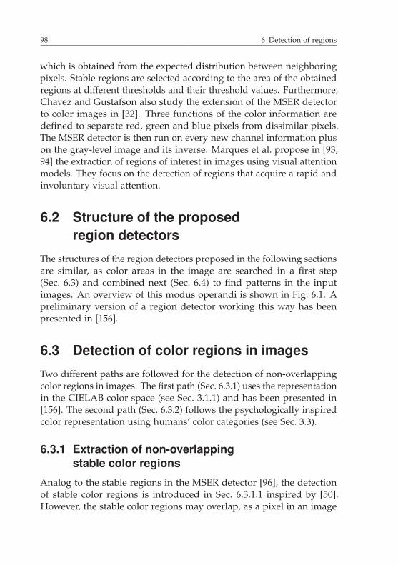
98 6 Detection of regions
which is obtained from the expected distribution between neighboringpixels. Stable regions are selected according to the area of the obtainedregions at different thresholds and their threshold values. Furthermore,Chavez and Gustafson also study the extension of the MSER detectorto color images in [32]. Three functions of the color information aredefined to separate red, green and blue pixels from dissimilar pixels.The MSER detector is then run on every new channel information pluson the gray-level image and its inverse. Marques et al. propose in [93,94] the extraction of regions of interest in images using visual attentionmodels. They focus on the detection of regions that acquire a rapid andinvoluntary visual attention.
6.2 Structure of the proposedregion detectors
The structures of the region detectors proposed in the following sectionsare similar, as color areas in the image are searched in a first step(Sec. 6.3) and combined next (Sec. 6.4) to find patterns in the inputimages. An overview of this modus operandi is shown in Fig. 6.1. Apreliminary version of a region detector working this way has beenpresented in [156].
6.3 Detection of color regions in images
Two different paths are followed for the detection of non-overlappingcolor regions in images. The first path (Sec. 6.3.1) uses the representationin the CIELAB color space (see Sec. 3.1.1) and has been presented in[156]. The second path (Sec. 6.3.2) follows the psychologically inspiredcolor representation using humans’ color categories (see Sec. 3.3).
6.3.1 Extraction of non-overlappingstable color regions
Analog to the stable regions in the MSER detector [96], the detectionof stable color regions is introduced in Sec. 6.3.1.1 inspired by [50].However, the stable color regions may overlap, as a pixel in an image
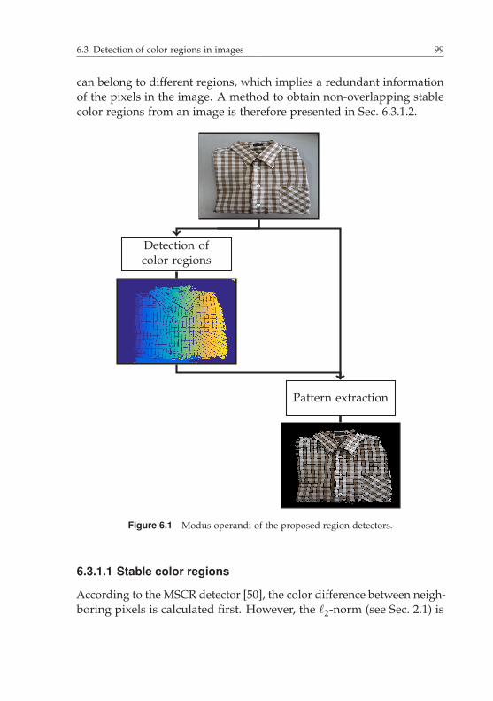
6.3 Detection of color regions in images 99
can belong to different regions, which implies a redundant informationof the pixels in the image. A method to obtain non-overlapping stablecolor regions from an image is therefore presented in Sec. 6.3.1.2.
Detection ofcolor regions
Pattern extraction
Figure 6.1 Modus operandi of the proposed region detectors.
6.3.1.1 Stable color regions
According to the MSCR detector [50], the color difference between neigh-boring pixels is calculated first. However, the �2-norm (see Sec. 2.1) is

100 6 Detection of regions
used for this purpose instead of the chi-squared distance recommendedin [50]:
dSCRu =
∥∥∥∥gu − g[
u +
(10
)]∥∥∥∥2+
∥∥∥∥gu − g[
u +
(01
)]∥∥∥∥2
. (6.1)
The difference image dSCRu is iteratively compared with the increasing
values of a threshold vector. The values of the vector were obtainedempirically from the inversed cumulative distribution function of thedifference image dSCR
u of some test images [156]. The maximally stablecolor regions are then further determined as in [50].
In order to reduce noise, two difference images dSCR,1u , dSCR,2
u areobtained per input image. From both difference images the maximallystable color regions are extracted. dSCR,1
u and dSCR,2u are obtained after
filtering the input image with a Gaussian filter. However, in dSCR,2u
the color values of the real input image are kept at edges that aredetected by the Canny operator [20, 28]. Pixels that already belong toa maximally stable color region extracted with the difference imagedSCR,2
u are suppressed from the maximally stable color regions obtainedfrom dSCR,1
u to reduce the number of stable color regions that a pixelmay belong to.
Stable color regions of an input image are all maximally stable colorregions from dSCR,1
u and dSCR,2u with a minimum size.
6.3.1.2 Non-overlapping stable color regions
The stable color regions extracted in Sec. 6.3.1.1 can have pixels incommon and therefore overlap (see Fig. 6.2 top, the boundaries ofthe extracted stable color regions are displayed in black). However,non-overlapping color regions are essential for the algorithm to detectpatterns in Sec. 6.4 and to avoid redundant information. To obtainnon-overlapping stable color regions, a graph representation is used.The extracted stable color regions are represented as nodes vk from thegraph. Edges are set between the nodes if they overlap and no otherstable color region exists being part of the bigger stable color regionand containing the smaller one (e.g., (v5, v4) and (v5, v1)) in Fig. 6.2).Although in Fig. 6.2 the stable color region v2 is part of v5, it is notdirectly connected with it by an edge because v4 contains v2 and is part

6.3 Detection of color regions in images 101
of v5. Another exemplary graph representation is shown in the left ofFig. 6.3. The methods used to obtain non-overlapping color regionsexplained next will be exemplified with this graph.
v2
v3
v1 v1
v4v5
Stable color regionsInput image
Graph representation
v5
v4 v1
v2 v3
Figure 6.2 Graph representation of the extracted color regions. Five stable color regionsare extracted from the input image (top left) and their boundaries are displayed in blackin the illustrations (top). v5 is a stable color region that contains the whole circle and allthe other extracted color regions. However, v5 is not directly connected with v2 and v3 inthe graph representation (bottom), as v4 contains v2 and v3 and is itself contained in v5.
For every input image, the graph of the stable color regions willcontain isolated vertices for the stable color regions that do not overlap(e.g., v1, v8 in Fig. 6.3 left) and trees with the color regions that overlap(e.g., v2, . . . , v7 in Fig. 6.3 left). Therefore, to obtain non-overlappingstable color regions, the trees in the graph must be processed until thegraph consists only of isolated vertices.
From now on vertices connected by an edge to a smaller color regionwill be denoted as a parent and the smaller color region as a child. Bythese means, a child may also be a parent of another stable color regionand vice versa. For every parent in the graph, the set of pixels that

102 6 Detection of regions
belong to the parent but not to its children is determined first. Fromthese pixels connected areas with a minimum size are determined. Eachconnected area that is big enough will be added as new node in thegraph (νk), as a child of the considered parent node vk (see Fig. 6.3 rightν5, ν7). The remaining pixels that do not form a big connected area inthe image are considered at its corresponding node vk as ωk (ω3, ω5, ω7in Fig. 6.3 right). The trees in the graph representation are furtherprocessed until isolated vertices are left. For this purpose, every parentnode will be iteratively considered starting with the corresponding oneto the smallest color region. Depending on the number of children thata parent node has, different approches are used. These are exemplifiedin Fig. 6.4 for the red squared color regions in Fig. 6.3 right.
v7
v5 v6
v3 v4
v2
v1 v8
(a) Graph representation
v7
v5 v6
v3 v4
v2
ν7
ν5
ω7
ω3
ω5
v1 v8
(b) Extended graph
Figure 6.3 Exemplary graph representation of the extracted color regions.
If the considered node has only one child (e.g v3 in Fig. 6.4 top left),then the child will be discarded and the original color region of theparent kept, including its pixels in ωk. For example, v3 is kept in ourexample graph and v2 discarded (see Fig. 6.4 top right). However, ifa parent has more than one child, then the relationship between thechildren must be considered to process the tree. To this end, an auxiliarygraph is used, whose nodes are the children (see Fig. 6.4 bottom left).The children in the auxiliary graph will be connected by an edge if their
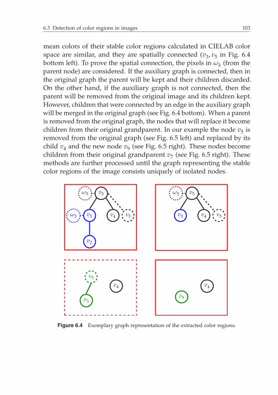
6.3 Detection of color regions in images 103
mean colors of their stable color regions calculated in CIELAB colorspace are similar, and they are spatially connected (v3, ν5 in Fig. 6.4bottom left). To prove the spatial connection, the pixels in ωk (from theparent node) are considered. If the auxiliary graph is connected, then inthe original graph the parent will be kept and their children discarded.On the other hand, if the auxiliary graph is not connected, then theparent will be removed from the original image and its children kept.However, children that were connected by an edge in the auxiliary graphwill be merged in the original graph (see Fig. 6.4 bottom). When a parentis removed from the original graph, the nodes that will replace it becomechildren from their original grandparent. In our example the node v5 isremoved from the original graph (see Fig. 6.5 left) and replaced by itschild v4 and the new node v9 (see Fig. 6.5 right). These nodes becomechildren from their original grandparent v7 (see Fig. 6.5 right). Thesemethods are further processed until the graph representing the stablecolor regions of the image consists uniquely of isolated nodes.
v5
v3 v4
v2
ω3
ω5
ν5
v5
v3 v4
ω5
ν5
v3
v4
ν5
v4
v9
Figure 6.4 Exemplary graph representation of the extracted color regions.
104 6 Detection of regions
v7
v5 v6
v3 v4
v2
ν7
ν5
ω7
ω3
ω5
v1 v8
(b) Extended graph
v7
v9 v6v4
v1 v8ω7
ν7
(c) Processing steps
Figure 6.5 Exemplary graph representation of the extracted color regions.
6.3.2 Extraction of color regions in images usinghumans’ color categories
The extraction of color regions in images using the extracted humans’color categories from Sec. 3.3 is considered in the following sections. Apreliminary version has been published in [160].
Neighboring pixels with a similar color are expected to have a similardistribution over the extracted color categories cColor
k (gu) , cColor(gu).Because of this, the comparison of the color representation of neighbor-ing pixels can be used to detect regions of colors in images. However, ifthe pixels are compared with their direct neighbors, errors may occurdue to blur. To reduce such kind of errors, the colors of the pixels arecompared with their direct neighbors in Δ distance along the u1 and u2direction and the analyzed image may be a filtered version of the inputimage. Two different distance comparisons are considered (Sec. 6.3.2.1).Once the distances to the neighboring pixels in Δ distance have beencalculated for all pixels in the image, color regions are extracted as inSec. 6.3.2.2. Though the comparison of every pixel with its neighborsin Δ distance reduces artifacts due to blur, some color regions may beextracted from the input image containing different colors that are notclearly separated between each other via an edge. Methods to over-

6.3 Detection of color regions in images 105
come such problems, to increase the areas of the detected color regions,and to reduce the number of detected color regions are described inSec. 6.3.2.3.
6.3.2.1 Color relationship between pixels
Two distances are proposed to measure the color relationship betweenneighboring pixels in Δ distance, whereas their color information is rep-resented with the extracted humans’ color categories. The first distancedCC,1
u is based on the correlation coefficient (see Sec. 2.1) and thereforethe colors of the pixels are represented over the color categories via theprobability distribution cColor
k (gu) (see Eq. 3.9). The second distance tomeasure the color similarity is based on the �2-norm (see Sec. 2.1) anduses the vector representation cColor(gu) (see Eq. 3.10).
Color relationship based on the correlation coefficient: The prob-ability distribution cColor
k (gu) of the color of a pixel at the position uover the color categories is interpreted for the first distance measuredCC,1
u as a random variable with the color categories k as the elementaryevents. Therefore the colors between neighboring pixels in Δ distancecan be compared using the correlation coefficient. Two comparisons aredone per pixel to consider its direct neighbors in Δ distances along theu1- and u2-axis:
rCCu =
rCC1,u + rCC
2,u
2, (6.2)
where
rCC1,u = r
(cColor
k (gu) , cColork
(g[
u +
(Δ0
)]))(6.3)
rCC2,u = r
(cColor
k (gu) , cColork
(g[
u +
(0Δ
)])). (6.4)
The color distances between the neighboring pixels, and therefore acomplementary measure of the probability of the pixels of being at asame color region, is given by
dCC,1u = 1 − rCC
u . (6.5)

106 6 Detection of regions
Color relationship based on the �2-norm: If the vector represen-tation of the color of the pixels cColor(gu) is used (see Sec. 3.3), thenthe distance of the colors of neighboring color pixels can be calculatedusing the �2-norm:
dCC,2u =
dCC,21,u + dCC,2
2,u
2, (6.6)
where
dCC,21,u =
∥∥∥∥cColor(gu)− cColor(
g[
u +
(Δ0
)])∥∥∥∥2
(6.7)
dCC,22,u =
∥∥∥∥cColor(gu)− cColor(
g[
u +
(0Δ
)])∥∥∥∥2
. (6.8)
6.3.2.2 Extraction of the color regions
Let dCCu ∈ {dCC,1
u , dCC,2u } be one of the distances used to compare the
colors between neighboring pixels in Δ distance. Over all positions inthe image, the calculated color distances are compared with a thresholdvalue τCC. A new binary image gbin
u is created as
gbinu =
{1 if dCC
u < τCC,0 otherwise.
(6.9)
The connected components in the binary image are the extracted colorregions of the input image gu.
6.3.2.3 Post-processing of the extracted color regions
The more homogenous the color, the bigger the area, and the lowerthe number of extracted color regions are, the more accurate and fasterfuture processing will be. To improve the three conditions, three differ-ent approaches are explained next to increase the areas, increment thehomogeneity of the color within the color regions, and reduce the totalnumber of extracted color regions.
The expansion of color regions is considered first. The detectionof color regions following the procedure proposed in the previoussections is based on the color distance of pixels with their neighbors

6.3 Detection of color regions in images 107
in Δ distances. The color distance dCCu ∈ {dCC,1
u , dCC,2u } between the
pixel at the position u and its neighbors in Δ distance is calculated andassigned to the pixel at the position u. However, when the color regionsare extracted, the connected areas in dCC
u are searched with a smallassigned color distance. The pixel at the position u may belong to a
color region but its neighboring pixel, e.g., at the position u +
[0Δ
], not
if its color distance to its respective neighbors in Δ distance is too high.The extracted color regions will be therefore smaller than the real onesin the input image. The morphological dilation [20] of the extractedcolor regions will increment their size. This is done via the followingstructuring element with cardinality (Δ + 1)2:
S =
{(u1u2
)∣∣∣∣ |u1| ≤Δ + 1
2and |u2| ≤
Δ + 12
}. (6.10)
Pixels that already belonged to a color region before the dilation stepwill also belong to the same color region after the dilation. The colorregions will only be expanded by the pixels that did not belong to acolor region before the dilation but formed part of the area of a dilatedcolor region.
The incrementation of the color homogeneity within a color regionis considered next. Although the color distances are compared betweenpixels at Δ distance when the color regions are extracted, some colorregions may contain different colors due to blur or no clear boundariesbetween the colors. To detect such color regions and divide them intoseveral new color regions, which increments the color homogeneitywithin the color regions, a reconstructed image gR
u is created first. Thecolor regions in gR
u are represented by the average color of their pixels inthe analyzed image (calculated in the CIELAB color space). Unassignedpixels to color regions are represented with a black color, but they willnot influence the process. The colors of the pixels in the reconstructedimage are compared, using the correlation function, with the colors
of the input image r(
cColork (gu) , cColor
k
(gR
u
)). To this end, the colors of
the pixels are represented over the color categories via the probabilitydistribution function cColor
k (gu). Connected pixels whose colors inthe reconstructed image vary significantly from the input image are
108 6 Detection of regions
detected and if they span big connected areas, they are separated fromtheir assigned color regions to create new color regions.
For the reduction of the total number of extracted color regions, thereconstructed image gR
u that assigns every pixel the mean color of itscolor region is also used. Neighboring color regions in the reconstructedimage with a similar assigned mean color are detected and groupedtogether to form a bigger color region. Color regions are neighborsif they possess neighboring pixels. 4-neighbors and 8-neighbors ofa pixel (see [54]) are therefore considered. The comparison of thecolor similarity between the color regions is done by representing theassigned color of the regions via the normalized probabilities over theextracted humans’ color categories and calculating their distances viathe correlation coefficient.
6.4 Detection and extraction of patterns
As in Sec. 6.3, two different paths are followed to extract the patternsfrom images depending on the way that the color is processed. Alongthe first path discussed in Sec. 6.4.1 the color information of the detectedcolor regions is directly processed and compared in the CIELAB colorspace (see Sec. 3.1.1), whereas in the second path presented in Sec. 6.4.2color categories (see Sec. 3.3) are used for color representation andprocessing. Although the methods in Sec. 6.4.1 compare the colordirectly in the CIELAB color space, the extracted color regions fromSec. 6.3.2 using the color categories can also be used as extracted colorareas. Furthermore, the color regions from Sec. 6.3.1 can also be usedas input information for the pattern recognition using the methodsof Sec. 6.4.2.
No matter which kind of the mentioned color representation andprocessing method is selected, both approaches to extract patternsfollow a similar modus operandi which can be visualized in Fig. 6.6and has been already used in [156]. The goal of each block is brieflyexplained next. However, the methods to resolve the goals of each blockvary depending on the selected color representation method, with theexception of the extracted information based on the space-frequencyanalysis, which is therefore explained in detail next.

6.4 Detection and extraction of patterns 109
Space-frequency analysis
Preparation ofthe color regions
One-dimensional patterndetection and extraction
Expansion of the one-dimensional pattern toa two-dimensional one
Post-processing
Figure 6.6 Modus operandi to detect and extract patterns.
Space-frequency analysis is a powerful tool to roughly detect theplace of repetitions in signals. In this work, the two-dimensional wavelettransform (see Sec. 2.3.4) is used to analyze the input images, as higherenergies at certain frequencies are expected at the image where repeti-tions of alterations of color regions are located. The goal of this block isthe detection of candidate color regions involved in patterns.

110 6 Detection of regions
To consider the color information, the wavelet transform is calcu-lated. Per color channel three matrices with the detail signals forthe different structure types (horizontal, vertical, and diagonal) areobtained at each stage. The detail signals at every stage and orienta-tion are independently projected back onto the original space domain.Per orientation (horizontal, vertical, and diagonal) and stage a two-dimensional signal of equal size to the analyzed input signal is ob-tained. For each pixel the maximum per orientation over all stages andcolor channels is stored at its corresponding location and orientationin Fk
u, k ∈ {horizontal, vertical, diagonal}. After filtering these signalswith a Gaussian filter [20], a measure is obtained which describes theprobability of a pixel to belong to a pattern. Every color region fromSec. 6.3 containing a pixel with a high measure of probability to belongto a pattern that is not situated at its contour is further considered asa candidate color region of a pattern. The limit from which pixels areconsidered to have a high degree of probability to belong to a patternis automatically set depending on the considered input image to allowa dynamic adjustment of the algorithm.
As different images may possess different sizes, an automatic selec-tion of the number of stages is necessary to assure equal conditions.Furthermore, as the height and width of the images can be different,different stages are reasonable depending on the kind of structures(horizontal, vertical, diagonal) that are analyzed. Let l be the minimallength that alternating structures along a line of length L have thatmust be detected and H the height and B the width of the input image(see Fig. 6.7). The normalized frequencies that the highest stage of thewavelet transform in horizontal and vertical direction must pass alongthe band-pass filter is given by
f norm,ver =Ll· 1
Hand f norm,hor =
Ll· 1
B. (6.11)
The number of stages along the horizontal and vertical analysis isrespectively given from the first stage at which these normalized fre-quencies are passed through the corresponding band-pass filter. Thenumber of considered stages for the analysis of diagonal structures isset equal to the minimum of the number of stages needed for horizontaland vertical structures.

6.4 Detection and extraction of patterns 111
. . .
l l
L
Figure 6.7 Automatic selection of the number of stages of the wavelet transform.
The preparation of the color regions obtained by the methods pre-sented in Sec. 6.3 for the pattern detection and extraction is the goalof this block. The assignment of neighbors to the color regions is anecessary feature for the pattern detection and extraction independentlyof the path followed to process the color. The following three conditionsare considered for this purpose.
1. For every pixel at the contour of an analyzed color region itsspatially closest color region becomes a neighbor.
2. Spatially close color regions become neighbors.
3. If a color region is a neighbor of another color region, then thissecond color region is also a neighbor of the first color region.
At this point the smallest spatial distance between color regions is givenby the smallest distance between two boundary pixels of the consideredcolor regions. The third condition is necessary to assure a symmetricrelation. An additional preparation of the color regions is requireddepending on the path selected for the processing of color informationand is therefore explained in detail in Sec. 6.4.1.1 and Sec. 6.4.2.1.
The one-dimensional pattern detection and extraction is the basisfor the pattern recognition along the image. Every color region classifiedas candidate of a pattern due to the space-frequency analysis is thereforeconsidered, starting with the one containing the pixel with the highestmeasure of probability to belong to a pattern. The goal of this blockis to detect if the color regions form part of a one-dimensional patternand its extraction if this is the case. For this purpose, parallel linesare set along the considered color region. The orientation of the linesalong which the one-dimensional pattern is searched depends on theexpected orientation (horizontal, vertical, or diagonal) of the patternaccording to the space-frequency analysis (see Fig. 6.8 top). Along the
112 6 Detection of regions
lines the next similar color region to the analyzed one is searched. Thecriterion used to measure the similarity depends at this juncture onthe followed path explained in the next sections. The use of severallines reduces wrong detections, as the color regions are actually twodimensional and may therefore have different sizes. A single line couldnot even contain a valid part of the searched pattern. If several similarregions are found along the lines, the line containing less number ofcolor regions in-between the similar color regions is selected for thefurther extraction of the pattern along the line (the one-dimensionalpattern extraction). Note that the number of colors in the detectedpattern is equal to the number of regions in-between the similar onesplus one (see Fig. 6.8 top).
A basic unit of the pattern formed from one color region per colorappearing in the pattern can be detected from the estimated numberof colors in the pattern together with the color region that is beinganalyzed due to the space-frequency analysis (see Fig. 6.8 middle). Inorder to avoid overhead, new patterns will not be searched in futureiterations from the color regions that become part of a basic unit of apattern. The reason is that possible patterns from these color regionsare already considered in the current iteration. Once the basic unit hasbeen detected (which depends on the path followed for color processing,see Sec. 6.4.1 and Sec. 6.4.2), the pattern can be extracted along theselected line considering the similarity of the color regions along theline to the ones that form the detected basic unit of the pattern andconsidering also the sequence in which the colors appear. For thispurpose, the use of graph representations is useful. As many graphsare necessary as number of colors expected in the pattern (see Fig. 6.8down). Nodes of the graphs are the color regions along the line placedat whole multiples of the expected number of colors in the pattern. Inevery graph the nodes are connected by an edge if they are similarand exactly placed at the expected number of colors in the patternfrom each other. However, edges are removed from the graphs if thecolor regions that they represent are not connected by a path in theircorresponding graphs to one of the nodes of the color regions that formthe basic unit of the pattern. The one-dimensional pattern along theline is extracted from the graph representations as the color regionswhose corresponding nodes are connected by a valid path to one of the

6.4 Detection and extraction of patterns 113
Fig. 6.8 down).
0
3
0
(a) Number of colors in the pattern
Basic unit of the pattern
(b) Basic unit of the pattern
One-dimensional pattern
(c) One-dimensional pattern
Figure 6.8 Overview of the detection and extraction of the patterns alongone dimension.
nodes of the color regions that form the basic unit of the pattern (see

114 6 Detection of regions
Once more, the similarity between color regions depends on theselected path for the processing of the color information and is thereforeexplained in detail in the next sections (Sec. 6.4.1.2 and Sec. 6.4.2.2).
The expansion of the one-dimensional pattern to a two-dimensional one is the goal of this block. For this purpose, the expan-sion of the one-dimensional pattern along the whole image is consid-ered. Only one-dimensional patterns that have at least one color regionper color in the pattern and at least two colors in the pattern formedfrom two color regions are expanded to a two-dimensional pattern.Similar neighboring color regions to the ones that already form thedetected pattern are included to the pattern. For this purpose, the colorsappearing in the pattern are consecutively considered. Per consideredcolor of the pattern, its neighboring color regions that do not belongto the pattern are detected. If they are similar to the color regions inthe pattern of the next expected color, then they are included in thepattern. This process is iteratively repeated until no new regions areadded to the pattern. The definition of similarity between the regions isstrongly dependent on the followed path to compare and process thecolor information and is therefore explained in the following sections(Sec. 6.4.1.3 and Sec. 6.4.2.3).
The post-processing of the extracted patterns may improve the re-sults. The fusion of similar extracted patterns, the merger of concate-nated patterns, and the suppression of some color regions (e.g., merelyframes) from the pattern can improve the extracted patterns and re-duce duplicates. These optional methods are explained in detail in thefollowing sections (Sec. 6.4.1.4 and Sec. 6.4.2.4) as they depend on theselected color representation and processing.
6.4.1 Detection and extraction of patterns based onthe CIELAB color space
The CIELAB color space (see Sec. 3.1.1) is used for color representationand processing in this version of the region detector. Color dissimi-larities are measured using the �2-norm (see Sec. 2.1) of the CIELABvalues along all of the steps of the detector. A preliminary version ofthis region detector has been presented in [156].

6.4 Detection and extraction of patterns 115
6.4.1.1 Preparation of the color regions
Although any of the extracted color regions from the image followingthe methods in Sec. 6.3 may be used, this version of the algorithmfocuses on the direct representation and processing of color in theCIELAB color space. The results in Sec. 8.5.1 show that the color regionsextracted by the method presented in Sec. 6.3.1 using the CIELAB valuesdirectly do not cover on average almost all of the image. Small colorregions that appear stable at a first sight might not be found as colorregions due to, e.g., compression artifacts. As part of the preparationof the color regions for the pattern detection, such kind of missingintermediate regions are searched. For this purpose, the color of a colorregion is obtained from the mean color over all pixels that belong toit, calculated in CIELAB color space. Missing intermediate regions aretypically found between two color regions that are neighbors, have asimilar color, and several pixels with a high measure of probability tobelong to a pattern due to the space-frequency analysis. If such regionsdo not have a common neighbor or the minimal spatial distance formost of the pixels on the boundaries is between each other, then anintermediate region is probably missing. To detect the missing region,all of the pixels between the two color regions that have not beenassigned to a color region yet are taken into consideration. Pixels witha similar color to one of the two neighbor regions are discarded, as theydo not produce an alternation between the colors. Out of the possibleremaining pixels the biggest spatially connected area is added as a newcolor region if it reaches a minimium size and a minimum measureof the probability to belong to a pattern. As the new potential colorregion was not detected in Sec. 6.3, the color between the pixels willbe different, but their measure of probability to belong to a pattern isstill high. Because of this, the measure of probability for such potentialcolor regions to belong to a pattern is calculated per orientation fromthe average value of the maxima measure of probability to belong to apattern over all its pixels.
Due to the fact that new color regions are added, the neighborsbetween the color regions may change. These ones must be thereforeassigned again (as defined in Sec. 6.4) after the inclusion of the newregions. However, the accuracy of the assigned neighborhoods mustfurther be considered because two regions may become neighbors even

116 6 Detection of regions
if they are spatially far away from each other. This is possible becausethe first condition to assign neighbors in Sec. 6.4 does not consider theamount of spatial distance between the color regions, together withthe fact that the results show (see Sec. 8.5.1) that not almost all of theimage is covered by the stable color regions extracted using the CIELABvalues for the processing of the color as shown in Sec. 6.3.1. To avoiddefining as neighbors color regions that are far from each other butalso take into consideration the proportion of the distance between theregions to their sizes, an average extent is defined per color region. Ifthe minimal spatial distance between two pixels on the boundaries ofthe neighboring regions is bigger than the mean average extents of thecorresponding regions, then the regions will only still be considered asneighbors if the color of the pixels in-between (that were not assigned toa color region) are similar to one of the colors of the considered regionsor their CIELAB color value lay between the CIELAB color values ofthe colors of the regions. Spatially separated regions by a color gradientof themselves that were not assigned to a color region will be thereforemaintained as neighbors.
Color clusters formed from neighboring color regions with a similarcolor, as well as background regions, are identified at this step in orderto consider them in the following steps when the pattern is detectedand extracted. A background region may be any color region or colorcluster placed mainly in a defined frame of the image. For this purpose,the rows and columns of the regions are taken into considerationindependently of each other.
6.4.1.2 One-dimensional pattern detection and extraction
The specific details to detect and extract the one-dimensional patternfollowing the trend from Sec. 6.4 considered in this version of thealgorithm are explained next.
An initial manipulation of the selected line containing the minimalnumber of colors for a pattern is necessary for the detection of thebasic unit of the pattern (see Sec. 6.4 and Fig. 6.8) and, furthermore,for the extraction of the one-dimensional pattern. As the main focusof this version of the algorithm relies on the direct process of color inthe CIELAB color space and the results show that the extracted colorregions based on the color representation in CIELAB color space do not

6.4 Detection and extraction of patterns 117
cover almost all of the input image (see Sec. 8.5.1), color regions may bespatially separated by a big number of pixels that were not assignedto a color region. To avoid the inclusion of such kind of regions in thebasic unit of the pattern and in the one-dimensional extracted pattern,the selected line must be processed. To this end, all color regions alongthe line that are separated by a long chain of unassigned pixels from thecolor region that is being analyzed are suppressed from the line. Next,every pixel along the line that was not assigned to a color region isremoved from the line, as patterns are searched between color regionsand undefined pixels will always be between their contours.
Due to the fact that the size of the color regions is not consideredwhen the similarity between them is compared and that in many im-ages background regions are much bigger than the regions belongingto patterns (e.g., sky or floor), background regions should be removedfrom the line as in [156]. However, a valid pattern may be placedor expanded over the frames of an image and therefore over the de-fined background regions. To fulfill both considerations, in contrastto [156], the background regions appearing at the start and end of theline are detected. Color regions between the start of the line and thefirst detected background region, as well as between the last detectedbackground region of the line and the end of it, are suppressed fromthe line together with the two detected background regions.
The detection of the basic unit of the pattern is considered next.Once the number of colors in the pattern has been detected and theline manipulated, the basic unit is detected. This one consists of somany neighboring color regions along the line as colors expected in thepattern, whereas the color region that initialized the search of the one-dimensional pattern is always part of it. Its color distance (measuredusing the �2-norm in CIELAB color space) to its next neighbors isrespectively calculated and added (as many as missing in the basic unit)along the left hand side of the line and the right hand side. The sidewith the biggest cumulative difference contains the color regions thatcomplete the basic unit of the pattern.
The similarity criteria for the one-dimensional pattern extractionis obtained from the color dissimilarity calculated using the �2-normof the color values in CIELAB color space. Every pair of color regionswhose �2-norm of their colors is smaller than a predefined thresholdis considered similar. Furthermore, if the distance is bigger than the
118 6 Detection of regions
threshold but still small enough, then the colors of the regions will beconsidered similar if their values along the channels considering thedifference between green and red colors and blue and yellow vary onlyslightly. This is done to overcome brightness differences, as these onesare described by the other channel. Finally, two color regions will notbe considered similar independently of the similarity of their color ifboth of them have a color region between them in the line with a similarcolor to them.
6.4.1.3 Expansion of the one-dimensional pattern to atwo-dimensional one
For the expansion of the one-dimensional pattern to a two-dimensionalone, the colors appearing in the pattern are compared to the potentialnew color regions of the pattern. For this purpose, a color of the patternis defined as the mean color values calculated in CIELAB color spacefrom all color regions in the pattern that belong to the considered color.As the pattern is iteratively expanded, the colors of the pattern are alsoupdated with each new added color region.
The similarity between the color regions and the color of a patternis calculated as in the one-dimensional case (see Sec. 6.4.1.2). For thispurpose, the potential new color region of the pattern is compared tothe considered color of the pattern. Additionally, the new potential colorregion of the pattern is compared to every color region that alreadybelongs to the pattern for the considered color, to avoid imprecisenessdue to the arithmetic mean. If a high similarity is found at any of theabove mentioned comparisons, then the new potential color region willbe added to the pattern.
However, for the incorporation of background regions to the pattern astricter condition must apply to avoid incorporating big frame regions tothe pattern. To be incorporated to the pattern, background regions mustfulfill the above mentioned similarity criterion, but also its size mustbe adequate to the size of the pattern. If the considered backgroundregions form part of a color cluster, then the adequate size is proved forthe whole color cluster.
Finally, if a color region that belongs to a color cluster is part of theextracted pattern, then all color regions belonging to the color clusterare also added to the pattern and assigned to the same color of the
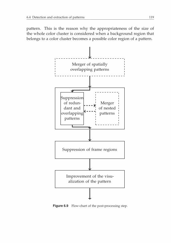
6.4 Detection and extraction of patterns 119
pattern. This is the reason why the appropriateness of the size ofthe whole color cluster is considered when a background region thatbelongs to a color cluster becomes a possible color region of a pattern.
Merger of spatiallyoverlapping patterns
Suppressionof redun-dant and
overlappingpatterns
Mergerof nestedpatterns
Suppression of frame regions
Improvement of the visu-alization of the pattern
Figure 6.9 Flow-chart of the post-processing step.
120 6 Detection of regions
6.4.1.4 Post-processing
Many patterns and pattern combinations are possible. The extractedpatterns from Sec. 6.4.1.3 must be therefore processed and selected in afinal step. The merger of spatially overlapping patterns, the suppressionof redundant and overlapping patterns, the merger of nested patterns,the suppression of merely frame regions, and the improvement of thepattern representation is therefore considered. All of these approachescan be considered independently or combined. A flow-chart is shownin Fig. 6.9, in which dotted squares represent optional processing steps.
The merger of spatially overlapping patterns improves their extrac-tion and also reduces their total number. The pattern detection andextraction with the methods proposed so far are based on the number ofcolors expected in the pattern, which is given from the minimal numberof color regions along the selected line until a similar color region tothe one that initiated the search of the pattern is found. However, theapproximation of the two-dimensional pattern to a one-dimensionalone along a single line may not describe the real pattern completely,so that the number of colors in the original pattern is not completelydetected. This will result in the extraction of several patterns with alower number of colors than the real one. An example for such kind ofpatterns is shown in Fig. 6.10. The goal of this approach is the detectionof such patterns as well as the detection of patterns whose number ofcolors has been correctly detected and that spatially overlap, and mergethe patterns to improve the pattern extraction and reduce the numberof extracted and redundant patterns.
For this purpose, all of the extracted patterns are compared betweeneach other and represented as nodes in a graph. Edges are set betweenthe corresponding nodes of patterns whose area spanned by theirrespective convex hulls highly overlap. The common area of bothconvex hulls is normalized by their biggest area to perform a normalizedcomparison. Furthermore, to avoid the merger of patterns whose convexhulls highly overlap but do not represent the pattern spatially goodenough (e.g., when the convex hull includes big areas that are notin the pattern), only patterns whose areas compared to the areas oftheir convex hulls are high enough are considered for the comparison.Once the graph that contains the relationships about the spatial overlapbetween the patterns exists, all patterns whose nodes can be reached by

6.4 Detection and extraction of patterns 121
a valid path are merged. If the patterns that are merged have similarcolors, which are calculated as explained in Sec. 6.4.1.2 and comparedusing the �2-norm, then the color regions of the patterns that belong tothe corresponding colors are merged together to form one color of thenew merged pattern; otherwise, the number of colors of the mergedpatterns increases.
2
2
Figure 6.10 Demonstrative representation of the need of a spatial merger. In the patternof the left the lines will only recognize two colors along the one-dimensional patterninstead of the three present in the two-dimensional pattern. In this regard, the twopatterns of the right side can be detected but not the whole one.
The suppression of redundant and overlapping patterns is a veryimportant step of the post-processing. As color regions in patternsare likely to have a high probability to belong to the pattern, severalstart color regions will be found for each pattern. This will lead to aredundant extraction of patterns. Nonetheless, the repeatedly extractedpatterns may vary in the color regions that they possess due to colorvariations of the color regions. Furthermore, a color region shouldbelong to maximal one extracted pattern, as a pattern is associated with

122 6 Detection of regions
an object. The processing of the extracted patterns so far is necessary toassure non-overlapping patterns.
First of all, patterns included in bigger ones are deleted, as they donot contain additional information of the extracted pattern of the image.This is the case if all of the color regions of the smaller pattern areincluded in a bigger one, and the number of colors in the pattern isequal for both patterns. If the number of colors is not equal, then thesmaller pattern will not be discarded, as it describes another patternthan the bigger one.
To merge similar extracted patterns that refer to the same pattern inthe image, the neighboring color regions of every pattern are needed.These are color regions that do not belong to the pattern but are neigh-bors of the color regions in the pattern. If two patterns have a colorregion in common or if a neighboring color region of a pattern is partof the color regions of the other pattern, then the patterns are mergedif they have the same number of colors and the colors are similar. Thesimilarity is obtained as in Sec. 6.4.1.2 from the distances of the colorsof the pattern. At this juncture, the pattern detected first (the order isgiven by the probability of the pixels to belong to a pattern) is amplifiedwith the other one.
Patterns detected later (lower probability to find a pattern) are morelikely to repeat already extracted patterns. Because of this, every patterncontaining per color at least one color region that already belongs to adifferent pattern is suppressed. In contrast to [156], here the conditionis proved that the color regions that are already part of another patternalso belong to different colors in the other patterns. As these colorregions may appear in various patterns in different colors, the colorgroup of the pattern with which these color regions appeared first arethe ones considered for this purpose. Furthermore, color regions thatappear in different patterns are always considered as if they belong todifferent colors in the patterns.
Non-overlapping patterns are obtained from the assignment of thecolor regions that are part of different extracted patterns to only onepattern. For this purpose, the extracted patterns that were detected first(and possess therefore a higher probability to describe a real patternin the image) will maintain these color regions. As color regions arenow suppressed from some patterns, other color regions may remain inthe pattern that are not spatially connected with the described pattern

6.4 Detection and extraction of patterns 123
anymore. Such kind of regions are detected easily, as their neighboringcolor regions are not included in the pattern. These color regions aresuppressed from the pattern. The suppression of color regions may re-duce the number of colors in a pattern or produce patterns that are notspatially connected. For the first case, the number of colors in the pat-tern is updated together with the assigned color values in CIELAB colorspace. In case of patterns that are spatially separated, these ones willbe separated into new independent and spatially connected patterns.At this juncture the number of patterns increases. They are thereforesorted according to the highest assigned measure of probability of theircolor regions to belong to a pattern.
The manipulation of the different patterns to reduce redundant infor-mation and assure non-overlapping patterns can deliver some non-validpatterns, like, e.g., patterns containing less number of color regionsas colors expected in the pattern or less than two colors. Such invalidpatterns are suppressed.
The appropriateness of color clusters in the remaining patterns isproved next. At the two-dimensional extraction of the patterns (seeSec. 6.4.1.3) color regions belonging to a color cluster were automaticallyadded to a pattern if at least one of its color regions belonged to thepattern. If the number of color regions assigned to the color of a patternthat do not belong to the considered color cluster is higher than thenumber of color regions in the color cluster, then their suitability isproved. If the mean color, calculated in CIELAB color space, of the colorregions that belong to the color cluster differs considerably from themean color formed from the other color regions, then the color clusteris suppressed from the pattern.
For every pattern which is morphologically dilated [20] and notspatially connected, only one of its spatially connected regions is con-sidered as the pattern for further processing. For this purpose, thespatially connected region with the biggest area that possesses a validpattern (contains at least two different colors) is kept.
The merger of nested patterns is an optional approach to permit thedetection and extraction of nested patterns. Nested patterns are differ-ent overlapping patterns with some common colors and one patternspatially including the other one (an example is shown in Fig. 6.11).Such kind of patterns cannot be detected by the one-dimensional detec-tion and extraction, nor by the two-dimensional expansion and must
124 6 Detection of regions
be therefore considered. This optional approach to detect and mergethem is a supplement to the above presented method to suppress re-dundant and overlapping regions and is executed after the suppressionof patterns whose colors contain at least one color region that alreadybelongs to other patterns and before the explicit assignment of everycolor region to exact one pattern to assure non-overlapping patterns.
Nested patterns are detected between extracted pairs of patternswhen the following conditions apply:
1. The color of every pattern is formed from at least two colorregions, which may be the same.
2. One of the patterns is included in the closed filled area of theother pattern.
3. The area of both patterns overlap.
If several patterns are extracted from the input image, then the searchfor nested patterns is done between every extracted pair of patterns.Every pattern is then represented as a node in a graph and connectedby an edge to the respective node of another pattern if they are nested.All of the patterns whose corresponding nodes can be reached via avalid path in the graph are then merged. For this purpose, the colors ofthe patterns that are going to be merged are compared and merged incase of similarity.
As the patterns have changed the number of colors, a new extractionof the pattern along the two-dimensions, like at the expansion of thepattern from the one-dimensional case to the two-dimensional one, isreasonable. However, to avoid redundant information, the new mergedpatterns that describe the same pattern are merged first as explainedabove. Furthermore, the color regions are assigned to only one patternto reduce redundant processing. After the expansion of the patterns,patterns describing similar patterns are merged. In this case, the patternfound later (lower measure of probability for a pattern) is included tothe pattern found earlier. For this purpose, extracted patterns describesimilar patterns in the input image if they have the same numberof colors, a high percentage of overlapping color regions, and all ofthe non-overlapping color regions of the later detected pattern have asimilar color with one of the colors of the pattern.

6.4 Detection and extraction of patterns 125
Figure 6.11 Example of a nested pattern (left), which is composed from twopatterns (right).
The suppression of frame regions is an approach to improve thequality of the extracted patterns. Up to now the color and neighborhoodbetween color regions are the only conditions used by the algorithmto detect, extract, and post-process the patterns. The relationship oftheir sizes has only been considered if one of the color regions was alsoclassified as a background region. As a consequence, real patterns inthe input image surrounded by a color region whose color is similar toone of the colors of the pattern will be extracted together as one pattern.Such kind of color regions that are incorporated in the extracted patternbut do not belong to the real pattern are called from now on frameregions, as they are a frame of the real pattern.
To detect frame regions, a similar procedure is used as for the detec-tion of the background regions (see Sec. 6.4.1.1). Horizontal and verticallines are set along the pattern. Starting from the outside boundaryof the pattern every line along the pattern running through only onecolor region is selected, until the first line appears running throughmore than two color regions. Along the selected lines, the length ofthe pattern is compared to the mean length of the pattern along allhorizontal or vertical lines, depending on the considered orientation.From the selected lines, those whose corresponding pattern length is

126 6 Detection of regions
almost as big as the mean length of the pattern along the consideredorientation are further processed for the detection of frame regions.The remaining lines to be considered run each through only one colorregion. These color regions represent potential frame regions of thepattern. Per line, if the maximal length or height (depending on theconsidered orientation) of its corresponding color region is big enoughcompared to the maximal length, respectively height, of the pattern,then it is kept as a potential frame region. In a final step these potentialcolor regions are compared to all other color regions in the pattern thatare associated with the same color of the pattern. If the maximal lengthor height (depending on the considered orientation) of the potentialcolor region is much bigger than respectively the maximal length orheight over all other color regions, then a frame region exists and it issuppressed from the extracted pattern.
If a pattern is formed from one color containing other ones, then thecolor region of the outer color may be detected as a frame region andsuppressed, involving a false extraction of the pattern. To avoid thiscase, if the first color region found at the boundary of the analyzedpattern contains many color regions in its holes that belong to thepattern, then no frame regions will be searched.
To improve the visualization of the pattern, the pixels that havenot been assigned to a color region and are situated in the closedarea spanned by the pattern are considered. Unassigned pixels to acolor region typically appear at the transition between color regions.However, their incorporation to the pattern will improve the qualityimpression of the extracted pattern. Because of this, all unassignedpixels having a similar color to the pixels that belong to the patternare incorporated for visualization purposes to the pattern if they arespatially connected to the pattern, either directly or via a chain ofunassigned pixels. Furthermore, every color region that is completely inthe closed area of the extracted pattern and describes a color transitionbetween color regions of the pattern is also incorporated to improve thequality of its visualization.
6.4 Detection and extraction of patterns 127
6.4.2 Detection and extraction of patterns based onthe humans’ color categories
This path of the pattern detection and extraction focuses on the process-ing of color with the use of color categories (see Sec. 3.3).
6.4.2.1 Preparation of the color regions
Due to the fact that the color regions obtained based on the humans’color categories cover almost all of the image (see Sec. 8.5.1), the neigh-bors assigned with the criteria of Sec. 6.4 are considered valid andno further processing is necessary in contrast to the path followed inSec. 6.4.1, as we can assume that no color regions that are spatially faraway from each other will become neighbors.
For the pattern detection and extraction a color must be assignedto each color region. As color regions contain pixels with a similarcolor, the color is calculated from the average values in CIELAB colorspace over all pixels. However, when the color between color regionsis compared, the representation over color categories is used. For thispurpose, the color of the regions must be presented via the normalizedlikelihoods over the color categories (see Sec. 3.3.3).
Furthermore, the size, in pixels, must also be assigned to eachcolor region to be able to detect and extract the pattern with thepresented method.
In contrast to the preparation of the color regions for the version ofthe algorithm processing the color directly in CIELAB color space (seeSec. 6.4.1), the detection of background regions is not necessary here,as the size and color similarity is considered when the one-dimensionalpattern is detected and extracted.
6.4.2.2 One-dimensional pattern detection and extraction
The specific details for the one-dimensional pattern detection and ex-traction using color categories are presented in this section.
The initial manipulation of the selected line for this version of thealgorithm is done by the suppression of unassigned pixels to colorregions. As the results of the obtained color regions processing thecolor information via the color categories show that almost all of theimage is covered by the extracted color regions (see Sec. 8.5.1), no long

128 6 Detection of regions
sequences of unassigned pixels are expected along the line in contrastto the processing of color directly in CIELAB color space (see Sec. 6.4.1).
The similarity criteria for the one-dimensional pattern detectionand extraction between two color regions considers their color and size.Any of the color distance functions presented in Sec. 6.3.2.1 can beused to compare the colors. The size of color regions is compared bytheir quotient. To obtain a normalized value, meaning a score close toone a high similarity, the smaller size will be always divided by thebigger one.
The basic unit of the pattern consists of one representative colorregion per expected color in the pattern, whereas the color region thatinitiated the search of the one-dimensional pattern is always part ofit. Along the line the similarity of this region is compared to its nextneighbors on the left and right hand side of the line separated exactlyby the number of expected colors in the pattern minus one. If similarityonly applies for one of the sides of the line, then the color regionsin-between are the missing representatives of the colors of the patternin its basic unit. Otherwise, the color distances per side of the line arecalculated between the regions in-between and the color region alreadybelonging to the basic unit of the pattern. The regions in-between thathave a bigger cumulative color distance are the ones that complete thebasic unit of the pattern in this case.
6.4.2.3 Expansion of the one-dimensional pattern to atwo-dimensional one
When the appropriateness of new candidate color regions to the patternis evaluated, four different similarity comparisons considering theircolor information, their size, or both characteristics are presented. Thisallows four versions of the algorithm. From now on the similaritycomparison of new possible color regions of the pattern with the colorregions of the pattern that represent one of its colors is considered.
An approximation of the colors in the pattern is considered in thiscase. To this end, every color in the pattern is defined as the mean colorvalue in CIELAB color space over the color of all its corresponding colorregions. The color distance between the new candidate color regionand the considered color of the pattern can be calculated with anyof the functions presented in Sec. 6.3.2.1. For this purpose, the color
6.4 Detection and extraction of patterns 129
assigned to the pattern is represented with the normalized likelihoodsover the color categories (see Sec. 3.3.3). As the number of color regionsbelonging to a color of the pattern increases iteratively, the color of thepattern must be updated.
An approximation of the colors and sizes of the color regions be-longing to the pattern is considered in this version. New color regionswill only be added to the detected pattern if they have a similar colorand size to the color regions forming the considered color of the pattern.The color similarity is calculated as in the above explained version,where the approximation of the colors of the pattern is considered.For the size similarity, the mean size over the color regions formingthe color of the pattern is calculated first and compared to the size ofthe candidate color regions via their quotient. To obtain a normalizedmeasure, the smaller value will be divided by the bigger one. Similaritydue to the size is only present in case of a high quotient.
An exact color comparison between the color regions that form acolor of a pattern and its new possible color regions is considerednow. Potential color regions will be added to the pattern if they have asimilar color to at least one of the color regions that form the consideredcolor of the pattern. For this purpose, the color distance betweenthe color regions can be measured using any of the color distancespresented in Sec. 6.3.2.1. The comparison of the similarity of the colorhere avoids inaccuracies due to the calculation of the average value.Furthermore, it also fulfills the condition that the CIELAB color spaceis rather reasonable for smaller color differences than for bigger ones.
An exact color and size comparison between the color regions thatform a color of a pattern and its new possible color regions is consideredfor the similarity measure in this version. New possible color regionswill only be added to the pattern if they have a similar color and sizeto the color regions that form the considered color of the pattern. Thecolor similarity is measured as explained in the above version of theexact color comparison. For the size similarity, the size of the newpossible color region is compared to the size of every color regionthat belongs to the considered color of the pattern, by building theirquotient, whereas the smaller value is divided by the bigger one toobtain a normalized value. The new possible color region is consideredsimilar in size if its size is similar to at least the size of one of the colorregions in the pattern.

130 6 Detection of regions
Finally, an optional processing approach is presented to detect pat-terns that actually represent the same pattern in the image and tomerge them. For this purpose, the area spanned by the convex hull ofthe actually expanded pattern along the two dimensions is comparedwith the convex hulls spanned by every pattern that has already beenexpanded over the two-dimensions. Patterns with highly overlappingareas spanned by their convex hulls are merged as in Sec. 6.4.1.4 (mergerof spatially overlapping patterns). However, to detect if the patternsthat are merged have similar colors, the colors of the pattern and alsothe sizes of the color regions that form each color are considered. Thecolor information is processed in this version using the color categoriesrepresentation from Sec. 3.3. The colors of the pattern are representedvia the normalized likelihoods over the color categories of the meancolors, calculated in CIELAB color space, of the color regions that formeach color. The color similarity is obtained according to Sec. 6.4.2.2. Onthe other hand, per color appearing in the pattern the mean size over itscolor regions is calculated. Between different patterns, the sizes of theircolors are considered similar if the quotient of the smallest mean sizedivided by the biggest mean size is large enough. The color regionsforming colors of patterns detected as similar are merged to form onlyone color of the pattern.
6.4.2.4 Post-processing
After the detection and extraction of the pattern along one dimensionand its expansion over two dimensions, many pattern combinationsdescribing the same pattern in the input image may be possible. Becauseof this, post-processing becomes necessary to avoid redundant patternsand also to improve the quality of the extracted ones.
In a first step invalid patterns are detected and suppressed. These arepatterns not containing an enough number of color regions comparedto the number of colors that are expected in the pattern.
Two approaches are considered to detect extracted patterns describingthe same pattern in the input image. On the one hand, overlappingpatterns with a high percentage of area in common are detected. Forthis purpose, the extracted patterns are pairwise compared. The totalnumber of pixels belonging to both compared patterns is respectivelydivided by the total number of pixels in the one pattern and the other

6.4 Detection and extraction of patterns 131
one. If any of the calculated quotients is high, then the areas of thepatterns highly overlap and the patterns are merged into one. On theother hand, patterns with highly overlapping areas spanned by theirconvex hulls are detected and merged. At this juncture, the relationsfor the detection of patterns describing the same one in the input imageare transitive. This means that if, e.g., the first and second extractedpatterns highly overlap and the second and third patterns too, then allof the three patterns are merged into one.


7 Fusion of the methods
In the previous chapters several properties have been considered relatedto the sorting of images according to the similarity of their content. Thedetection and extraction of regions with a similar color together withthe detection and extraction of patterned regions in images (Sec. 6),the detection of near-regular textures together with the extraction oftheir regular textures (Sec. 5.3), and the extraction and comparisonof color (Sec. 3), shape (Sec. 4), and texture (Sec. 5) properties havebeen considered. The fusion of these methods is considered in thischapter to enable a content-based image retrieval environment. Thedetection and extraction of significant patterned regions is consideredin Sec. 7.1, which results from the fusion of the detected and extractedcolor regions, patterned regions, and near-regular textures. The methodto sort images considering color, shape, and texture information is thenpresented in Sec. 7.2. The results yielded by the methods proposed inthis chapter are shown in Sec. 8.6.
7.1 Significant patterned regions
A pattern is a generalized concept of a near-regular texture. Whereas anear-regular texture is always a valid pattern, a pattern is not alwaysa near-regular texture. The detection and extraction of near-regulartextures and patterned surfaces has been considered in Secs. 5.3 and 6.4.The following conclusions can be drawn from the results (Secs. 8.4.2and 8.5.2) of the presented methods:
1. A high percentage of the near-regular textures from the testeddatabase (up to 98.08 %) is detected.
2. The extraction of the areas spanned by the near-regular texturesare limited to the areas spanned by a whole number of the de-tected texels. The area of the objects containing the near-regulartextures cannot be approximated perfectly.

134 7 Fusion of the methods
3. All of the near-regular textures in the database (100 %) are part ofat least one of the extracted patterns. However, several patternsare extracted that contain parts of near-regular textures that arealready part of another pattern.
4. Many patterns that do not contain a near-regular texture aredetected.
In this section the fusion of the results achieved by the methods to detectand extract near-regular textures and patterns is considered to selectsignificant patterned regions in the images that will be used in Sec. 7.2.2in a content-based image retrieval environment. The procedure used tofuse the methods is shown in Fig. 7.1 and explained next.
From the detected near-regular textures a mask per surface is esti-mated. For this purpose, all of the points of interest extracted fromthe input image that belong to the same cluster from which the near-regular texture was detected are considered. From this point cloud,their alpha-shape [46] is calculated. This one is obtained from thestraight lines that connect alpha-neighbors. Two points of the pointcloud are alpha-neighbors if they lie on the boundary of a disc (or itscomplement depending on the sign of alpha) that contains all of thepoints. The radius of the disc depends on the selected alpha. In thiswork, alpha is adapted for every point cloud to the value that producesthe tightest fitting alpha shape that encloses all of the interest points.The area spanned by this boundary together with the boundary itselfis the mask of the near-regular texture. If more than one near-regulartexture is detected per image and one of them covers the borders of theimage, its corresponding mask will be spread over almost the wholeimage. To avoid such cases, its corresponding mask will be spreadover almost the whole image apart from the regions, where masks fromother detected near-regular textures are already placed.
The fusion of the masks of the near-regular textures with the ex-tracted color regions from Sec. 6.3 is considered next. For this purposeevery detected color region whose area lies mostly at the mask of thenear-regular texture is added to a new broadened mask. The mask isbroadened with the color information of the image. Areas in the maskthat are not covered by a color region lying mostly at the mask are notincorporated to the broadened mask.

7.1 Significant patterned regions 135
Mask of the near-regular texture
Color regions atthe mask of the
near-regular texture
Relation of the near-regular textures and
patterned regions
Extraction ofsignificant patterns
Figure 7.1 Extraction of significant patterned regions.
136 7 Fusion of the methods
The masks of the near-regular textures are also fused with the ex-tracted patterns. For this purpose, extracted patterns that lie at themask of a near-regular texture are fused, as well as masks of near-regular textures that lie at an extracted pattern. The information ex-tracted from the near-regular texture is also incorporated to the commonextracted patterns.
In a final step, significant patterns are extracted by fusing everyavailable information. Significant patterns can come from two differentpaths. On the one hand, every extracted pattern that lies mostly at themask of a near-regular texture is the basis of a future significant pattern.However, the areas spanned by the broadened mask and the extractedpattern are usually not equal. A fusion of both possibilities is thereforenecessary. For this purpose, their appropriateness is valued first. Ifthe considered pattern and broadened mask of the near-regular texturehave only a small percentage of the color regions in common, then theextracted pattern is directly considered as a significant pattern. The rea-son is that the extracted near-regular textures cannot be approximatedperfectly. However, if the percentage of color regions in common ishigh, then the sizes of the color regions in common are compared to thesizes of the color regions that only form part of the extracted pattern.Color regions that only form part of the extracted pattern and whosesizes vary considerably from the sizes of the color regions in commonare suppressed. The improved version of the extracted patterns areconsidered as significant patterns.
On the other hand, every extracted pattern that contains a big numberof color regions is directly considered as a significant pattern.
7.2 Image sorting according to theirsimilarity fusing color, shape, andtexture information
Once the significant patterned regions have been detected and extracted,the images can be sorted. The problem of sorting the content of theimages according to their similarity is transferred to the problem ofsorting the detected significant patterns according to their similarity.
7.2 Image sorting according to their similarity fusing color, shape, ... 137
Therefore, the assumption is made that the most important content ofthe image is given by the significant patterns.
The adjustment of the color (Sec. 3), shape (Sec. 4), and texture (Sec. 5)methods proposed in the previous sections to the detected and extractedsignificant patterns (Sec. 7.1) is considered next. For this purpose, theextraction of the features is considered in Sec. 7.2.1 and the sorting ofthe images considering all three properties in Sec. 7.2.2.
7.2.1 Feature extraction
Adequate features describing the significant patterned regions are nec-essary for their comparison. The color, shape, and texture informationis separately considered per significant region. Their extraction isbriefly explained next and results as a fusion with the methods alreadypresented in Secs. 3, 4, and 5.
As color feature the compact color signature proposed in Sec. 3.2 isused. However, this one is not directly extracted from the color valuesof the pixels in the input image that belong to the patterned regionsbut from the mean colors of their corresponding detected color regions.Nevertheless, the sizes of every detected color region in the consid-ered significant pattern is still considered in its respective compactcolor signature.
The shape feature of a significant pattern is the normal angulardescriptor from Sec. 4.2.1 of its boundary. The determination of theboundary of a significant patterned region is a challenging task, asthe patterned regions must not be a connected component. At thecontours of color regions pixels are expected that do not belong to acolor region and will not be part of the considered significant patternedregion. To overcome this problem, a mask of the surface spannedby the considered significant patterned region is created. Every pixelwith a spatial distance smaller than a given threshold τSP1 is added tothe mask, including of course all pixels that belong to the significantpatterned region. As this process increases the area, a morphologicalerosion [20] is subsequently performed. The boundary of the mask isthen determined. In case that the mask still consists of more than oneconnected component, then the boundary is extracted from the onewith the biggest area.

138 7 Fusion of the methods
The texture information is only used for the detected significantpatterned regions that contain at least one of the detected near-regulartextures. The sorting of regular textures has been exhaustively con-sidered in Sec. 5.2.3. This method has to be adjusted now for regulartextures that have been extracted from near-regular ones. As the colorinformation is separated from the texture information, the gray-levelnear-regular texture is considered to extract the features.
All of the eight similarity features proposed in Sec. 5.2.3 are alsoused to compare near-regular textures. The mean texel of the regulartexture, one extracted texel, and its displacement vectors are the threecharacteristics needed in Sec. 5.2.3 to compare regular textures. Thesecharacteristics must be defined now for near-regular textures. Therepresentative texel of the near-regular texture is used to obtain thecorresponding features extracted from the mean texel in case of regulartextures. Among all extracted texels from the near-regular texture, themost similar one to the extracted representative texel is used to calculatethe similarity feature s4, which compares the structure between the tex-els. Furthermore, the similarity parameter s5 that compares the regionswith an almost constant intensity between texels is calculated from asharpened version of the extracted texel that is most similar to the rep-resentative one. The sharpening is performed by the unsharp maskingmethod [54]. This is necessary to improve the detection of the regions,which is based on a watershed filling method, as the transformation ofthe extracted texel to the quadrangles robust to affine transformationsand lighting variations often implicates the loss of sharpness.
The vectors spanned by the sides of the extracted texels are used toobtain the displacement vectors that are assigned to the near-regulartexture for comparison purposes. The vectors are divided into twogroups, where each group contains the vectors corresponding to theparallel sides of the texels. At this point it is important to consideronly parallel vectors per group. The median value per dimension andgroup yields the displacement vectors which are used for the extractionof the similarity features comparing the displacement between near-regular textures.

7.2 Image sorting according to their similarity fusing color, shape, ... 139
Shapesimilarity
Colorsimilarity
Texturesimilarity
Images inthe database
Similarityfusion
Input image
Figure 7.2 Sketch of the proposed sorting method fusing the detection of regions inimages, the color, the shape, and the texture information.
7.2.2 Sorting method
An overview of the sorting method is shown in Fig. 7.2. The extractedsignificant patterned regions are actually the ones that are being sorted,as the sorting of the images according to the similarity of their contentis transferred in this thesis to the sorting of these regions. If the inputimage consists of several significant patterned regions, then as manysorting results of the images will be given as number of extractedsignificant patterned regions, namely one per region. The sorting ofthe images is resolved in two stages.
First, the images in the database are sorted three times, one accordingto their color similarity with the input image, one according to theirshape similarity, and one according to their texture similarity. Thesorting of the images according to the different characteristics can betherefore done in parallel, which enables a higher performance. Incase that an image in the database contains more than one significantpatterned region, then the image will appear as many times in thesorting results as extracted significant patterned regions.
In the second step the information of the similarity sorting accordingto the color, shape, and texture is fused. All of these comparisonsrespectively yield per image in the database a value that expresses the

140 7 Fusion of the methods
dissimilarity distance (in case of the color and shape comparisons) orsimilarity (in case of the texture comparison) with the input image.However, these values cannot be compared between each other directly.On the one hand they have different magnitudes, on the other hand thetotal similarity does not always depend with the same strength on thedifferent characteristics. To overcome the challenging task of finding amodel that combines the three values directly, the direct considerationof the rank position achieved by each extracted significant patternedregion is proposed. The median value of the three rank positions (color,shape, and texture similarity) is calculated per extracted significantpatterned region. This permits an automatic adjustment of the strengthof the color, shape, and texture similarity depending on the comparedsignificant patterned regions. According to the median values of therank positions of the extracted significant patterned regions, the imagesare sorted. Images in the database that contain more than one extractedpatterned region are then retrieved only at their first achieved position.

8 Results
Several methods have been proposed in the previous chapters inspiredby the content-based image retrieval problem. The detection of regionsin images (Sec. 6), the analysis of the color (Sec. 3), shape (Sec. 4), andtexture (Sec. 5) properties, and the fusion of all of these methods (Sec. 7)have been considered. The results of all of these methods are presentedand discussed in this chapter. For this purpose, the methods have beenimplemented using Matlab [97] as software.
General evaluation concerns are addressed in Sec. 8.1 followed bythe results considering color (Sec. 8.2), shape (Sec. 8.3), and textureproperties (Sec. 8.4). The results yielded by the region detectors are pre-sented in Sec. 8.5. The results achieved by the fusion of the previouslyindependently considered characteristics are shown in Sec. 8.6, wherethe fusion of the different methods for a content-based image retrievalis considered.
8.1 General evaluation concerns
Adequate images and quality parameters are necessary to be ableto evaluate new presented methods. Two self-made databases arepresented in Sec. 8.1.1 that are used to test the presented methods.Furthermore, in Sec. 8.1.2 common criteria used to measure the qualityof retrieval applications are discussed. A strategy to measure thequality of content-based image retrieval applications is also presentedin Sec. 8.1.2.
8.1.1 Self-made databases
Adequate images are necessary to evaluate the proposed methodsoptimally. Several databases were created during this work that arepresented next.

142 8 Results
Figure 8.1 A selection of the images in the IIIT texture database.
The IIIT texture database consists of 1079 gray-level textured imagesand was developed to analyze and compare the different types oftextures (see Sec. 5.1.1). All of the images in the database were digitallycomputed with a ray-tracing program [3]. Images containing regular,structural-statistical, and irregular textures form the database. Asno clear boundary exists between the types of textures, a previousclassification of the images is difficult. However, this is a necessary step

8.1 General evaluation concerns 143
to be able to evaluate the methods presented in Sec. 5.2. 698 images areclassified in this database as regular textures, which may succumb smallstochastic variations along the texels due to, e.g., lighting conditions orvariations at their edges representation. 193 images form the structural-statistical textures of the database and allow a bigger deviation of thedisplacement vectors and the texel representation, not being able insome cases to group the displacement vectors. Finally, 188 images areclassified as irregular textures in the database. These images consist ofcompletely irregular textures, where not even a texel can be identified.One-dimensional and two-dimensional textures form part of the regularand the structural-statistical textures. An overview of some images ofthe database is shown in Fig. 8.1. This database was preliminarily usedin [155].
The IIIT patterned image database consists of 50 colored images thatcontain both patterned objects and patterned backgrounds, whereas thepatterns are textures of structural-statistical type. Some of the imageseven consist of a patterned object in front of a patterned background.This database was developed to test the different proposed methodswith the challenges of ordinary images, where no high resolution canalways be expected. Almost all of the images were taken with a mobilephone under different lighting conditions and perspectives of patternedobjects and patterned backgrounds. Objects with similar patterns butdifferent colors, as well as similar patterns over different objects, canbe found in the database. Textiles, floor tiles, and lacquered metallicsurfaces form the patterned regions. An example of some of the imagesis shown in Fig. 8.2.
8.1.2 Quality measurements for retrieval applications
Precision and recall are established methods in the literature to evaluatethe quality of retrieval applications [4, 5, 10, 13, 43, 53, 77, 83, 85, 90,91, 106, 118, 124, 128, 129, 138, 144, 146–148, 150, 152]. Precision qpre
kdepends on the number of considered retrievals and is calculated as thequotient of the number of good matches that are retrieved nGM
k dividedby the number of retrievals k [80]:
qprek =
nGMkk
. (8.1)

144 8 Results
The higher the precision values are, the better the results will be. How-ever, no information about the completeness of the results can bededuced from the precision values as the total number of good matchesis not considered. Recall qrec
k completes in this sense the analysis ofthe quality of retrieval applications, as it compares the good matchesthat are retrieved to the total number of good matches in the databasenGM [80]:
qreck =
nGMk
nGM . (8.2)
8.1.2.1 Quality criterion used in this thesis
The evaluation of retrieval systems on a database consisting of differentclasses with different total number of good retrievals becomes complexand confusing when precision and recall are used. On the one handtwo different functions have to be considered, and on the other handprecision and recall cannot be compared between classes containingdifferent numbers of good matches, as no normalization exists. In thiswork the sole use of one quality value is aimed to overcome these issues.Because the fast retrieval of good matches is more important for theapplications that motivate this thesis (see Sec. 1) than the completenessof the results, the quality value is extracted from the k-dependentprecision. The higher the summation of the k-dependent precisionover all retrievals is, the better and more complete the results will be.However, no conclusions can be obtained from the comparison of thesevalues between classes containing different number of good matches.To overcome this issue, the summation of the k-dependent precisionover all retrievals is compared to the summation of the precision thatwould be reached in the ideal case qpre,ideal
k , where all good matches areretrieved first. The value reached by the tested method is expressed aspercentage of the ideal one:
qretr =
∑k
qprek
∑k
qpre,idealk
· 100 %. (8.3)

8.2 Results of the color 145
Figure 8.2 A selection of the images in the IIIT patterned image database.
8.2 Results of the color
The results of the color processing methods presented in Sec. 3 areshown in this section. The use of the compact color signature in CIELABcolor space is considered in Sec. 8.2.1 and the representation of colorinformation via humans’ color categories in Sec. 8.2.2.

146 8 Results
8.2.1 A compact color signature in CIELAB colorspace for images
In this section the compact color signature presented in Sec. 3.2 iscompared to the signature obtained from two k-d trees [122] whichinspired it. For this purpose, every pixel of the image is assigned toone of the final color regions obtained via the two k-d trees. The meanvalue along each color dimension releases the centroid of the regions.The weight of each color region is then the percentage of pixels in theimage belonging to the appendant region. In both cases the CIELABcolor space (see Sec. 3.1.1) is used and the maximal length along eachdimension is set to 25 as in [122]. The signatures are evaluated at adatabase which consists of 700 images of natural scenes that is availablein the Internet [2, 137].
The criteria used for the evaluation is presented in Sec. 8.2.1.1 andthe results are shown in Sec. 8.2.1.2.
8.2.1.1 Evaluation criteria
Three criteria are considered to evaluate the results of the color signa-tures: the number of color representatives, the comparison of the colordistributions, and the sorting of images according to the similarity tothe input image.
The extraction of the color representatives and their weights is nec-essary in many applications for further processing. The smaller thenumber of clusters representing the color information of the image is,the faster and more efficient further processing may become.
However, a compact representation of the color distribution of theimage may lead to bigger deviations compared to the color distributionof the input image due to the compression. The color distribution ofthe input image is therefore compared to the color distribution afterthe compression. For this purpose, a synthetic image is calculatedfrom the assignment of every pixel in the input image to its next colorrepresentative of the color signature. The distance is calculated usingthe �2-norm (see Sec. 2.1). The mean image representation error derivedfrom the color signatures is the mean color difference (calculated usingthe �2-norm) from the synthetic image to the input image over all pixelsand color dimensions.

8.2 Results of the color 147
Table 8.1 Average numbers of color representatives and their standard deviations.
Mean number Standard deviationof color of the number
Method representatives of color representatives
One k-d tree 61.57 48.85Two k-d trees 28.49 22.10
Proposed method 23.69 14.87
Finally, the impact of the signatures for the content-based imageretrieval is considered. Every image in the database is therefore pairwisecompared using the earth mover’s distance (see Sec. 2.1) with all ofthe images in the database. These ones are sorted according to theirsimilarity with the input image, from more to less similar. As no groundtruth is available about the similarity between the images according tohumans’ concerns, the ranking of the images depending on the numberof retrievals is compared between the two considered color signatures.Per input image the percentage of retrievals matching in both signaturesis obtained depending on the number of retrieved images.
8.2.1.2 Evaluation results
The results according to the evaluation criteria presented in Sec. 8.2.1.1are presented next.
The number of cluster representatives needed on average by theconsidered methods to extract the color signatures and the standard de-viations of the number of cluster representatives are shown in Table 8.1.The use of two k-d trees to obtain the color signature compared tothe sole use of one k-d tree reduces on average the number of colorrepresentatives by 53.73 %. The standard deviation of the number ofcolor representatives is also considerably reduced when two k-d treesare used to obtain the color signature instead of one. This implies lesssensitivity to the input image. However, the lowest number of colorrepresentatives and the lowest standard deviation towards the numberof color representatives are reached by the method presented in Sec. 3.2.23.69 color representatives are needed on average by this method incontrast to the 28.49 of the two k-d trees and the 61.57 of the one k-d tree.

148 8 Results
The standard deviation is about two thirds of the one obtained fromthe two k-d trees and almost a third part of the one obtained from theone k-d tree. By these means, the total number of color representativesobtained via the method presented in Sec. 3.2 is less sensitive towardsthe input image than the ones extracted via k-d trees.
Despite the lower number of color representatives needed on averageby the method proposed in Sec. 3.2 compared to the two k-d trees,the actual number of representatives is compared per image over bothmethods. For each image in the database the number of color represen-tatives extracted via the method presented in Sec. 3.2 is subtracted fromthe number of color representatives obtained from the use of two k-dtrees. The histogram over all differences is shown in Fig. 8.3.
−60 −40 −20 0 20 40 600
20
40
60
80
Figure 8.3 Histogram of the number of color representatives of the two k-d trees methodminus the proposed method.
For most of the images in the database the number of color rep-resentatives is smaller if the method from Sec. 3.2 is used to extractthem, with up to 52 numbers of color representatives less. Althoughthe two k-d tree method provides in some cases less number of colorrepresentatives (31.57 %), the method from Sec. 3.2 only needs a fewrepresentatives more.

8.2 Results of the color 149
Table 8.2 Averages of the mean image representation errors and their standard devia-tions.
Average of the Standard deviationmean image of the mean image
Method representation errors representation errors
Two k-d trees 11.17 · 10−3 1.26 · 10−3
Proposed method 9.80 · 10−3 1.11 · 10−3
At this point the conclusion can be drawn that the smallest numberof color clusters together with less sensitivity to the input image isachieved by the method proposed in Sec. 3.2.
The averages and standard deviations over all images in the data-base from the mean image representation error created by the colorsignatures extracted from the two k-d trees and the method proposedin Sec. 3.2 are shown in Table 8.2. On average, the method presentedin Sec. 3.2 not only possesses a smaller error of the color representa-tion, its standard deviation is also smaller, which implies a more stablemethod towards the analyzed image. Figure 8.4 shows the histogramof the differences of the mean image representation errors by the colorsignatures, where per image in the database the error obtained from themethod proposed in Sec. 3.2 is subtracted from the one obtained fromthe two k-d trees. For most of the images in the database (96.86 %) theerror of the distribution of the color due to the compression is smallerif the method presented in Sec. 3.2 is used.
The percentage of retrievals matching in both signatures per inputimage is shown in Fig. 8.5 in case that all of the images in the databaseare considered as retrievals (top) and for the first 150 retrievals (bottom).Small deviations can be noticed by little number of retrievals, but a highcompliance of retrievals exists between both signatures as the numberof retrievals increases. As it can be recognized in Fig. 8.6, over 90 % ofthe retrieved images match on average between the two color signaturesby 21 retrievals. On average 100 % of the retrievals match when oneimage is retrieved because the input image is always retrieved first forboth color signatures.
Overall, the following conclusions can be drawn. The method pro-posed in Sec. 3.2 reduces for most of the images in the database the

150 8 Results
number of color representatives or needs a comparable number to theones extracted by the two k-d trees. The error due to the color compres-sion is for 96.86 % of the images in the database smaller if the methodpresented in Sec. 3.2 is used, although the number of color represen-tatives decreases on average. The retrievals of images sorted by colorsimilarity with an input image are comparable for both signatures.
−0.006 −0.004 −0.002 0 0.002 0.004 0.0060
5
10
15
20
25
30
Figure 8.4 Histogram of the differences of the mean image representation errorsachieved by the two k-d trees method minus the proposed one.
8.2.2 Humans’ color categories
In this section the humans’ color categories extracted according toSec. 3.3 are presented. After the editing of the color names (Sec. 3.3.1.1)and the suppression of spam answers (Sec. 3.3.1.2), with τC2 set to 10,only 8.73 % of the color names of the raw database remain and aretherefore not considered as misspellings or spam answers.

8.2 Results of the color 151
100 200 300 400 500 600 700
100
200
300
400
500
600
700
Input image
Num
berof
retrieva
ls
0 %
20%
40%
60%
80%
100%
Figure 8.5 Percentage of retrievals matching for both signatures.
From the remaining valid answers the color categories were extractedas explained in Sec. 3.3.2. For this purpose, the CIELAB color space

152 8 Results
must be quantized. 25 bins are used for the channel that representsthe brightness of the color and 64 bins for the other two channels. Theextracted humans’ color categories are then 145 color names that areshown in Table 8.3 together with their mean color value calculated inCIELAB color space.
0 100 200 300 400 500 600 70080 %
85 %
90 %
95 %
100 %
Number of retrievals
Ret
riev
als
mat
chin
gin
both
sign
atur
es
Figure 8.6 Average of the percentage of retrievals matching in both signatures pernumber of retrievals.
Table 8.3 Extracted humans’ color categories.
1. anthracite 74. ligh green2. aqua 75. light blue3. aqua marine 76. light brown4. aquamarine 77. light green5. army green 78. light grey6. azul 79. light lavender7. azure 80. light light purple8. baby blue 81. light orange9. baby puke 82. light pink10. baby shit brown 83. light purple11. baby yellow 84. light tan

8.2 Results of the color 153
12. beige 85. light yellow13. black 86. lilac14. blackish 87. lime15. blood 88. lime green16. blue 89. magenta17. blue green 90. maroon18. blue grey 91. mauve19. bluegreen 92. midnight blue20. bordeaux 93. mud21. brick 94. mulberry22. brick red 95. mustard23. bright fuchsia 96. mustard yellow24. bright green 97. navy25. bright purple 98. navy blue26. brown 99. nude27. brown orange 100. ocher28. burgundy 101. off white29. burnt orange 102. olive30. burnt umber 103. olive green31. butter yellow 104. orange32. chartreuse 105. orange tan33. claret 106. pale blue34. coral 107. pale green35. coral red 108. pale lavender36. cream 109. pale orange37. custard 110. pale pink38. cyan 111. pale rose39. dark blue 112. pale yellow40. dark blue green 113. peach41. dark brown 114. pee yellow42. dark er pink 115. periwinkle43. dark green 116. pink44. dark grey 117. puce45. dark magenta 118. puke green46. dark maroon 119. purple47. dark olive 120. purple pink48. dark pink 121. red49. dark purple 122. red orange

154 8 Results
50. dark red 123. red purple51. dark salmon 124. robin egg blue52. dark teal 125. rose53. deep purple 126. royal blue54. dove grey 127. salmon55. eggplant 128. sea foam green56. eggshell 129. shit brown57. emerald green 130. sky blue58. flesh 131. tan59. forest green 132. teal60. fuchsia 133. turquoise61. gold 134. vermillion62. grapefruit 135. very dark green63. grass green 136. very light blue64. green 137. very light green65. green grey 138. violet66. green yellow 139. viridian67. grey 140. vivid blue68. grey blue 141. white69. grey green 142. wine red70. hot pink 143. yellow71. indigo 144. yellow green72. khaki 145. yellowish brown73. lavender
Notice that some of the names of the color categories suggest mis-spellings (like, e.g., aquamarine and aqua marine or ligh green and lightgreen). The fusion of color categories has been considered by the au-thor, but it is outside the scope of this work. The 145 color categoriesrepresent 0.08 % of all color names used by the users.
Figure 8.7 shows the histogram of the color values named with theextracted color categories. The bins are represented by the mean colorof each category. Notice that the number of colors assigned to eachcolor category is different, from the 36 colors that form ligh green tothe 315,933 colors that span green. This implies that different forms ofsubspaces in the CIELAB color space are spanned by the color categories.These ones may overlap or even contain each other.
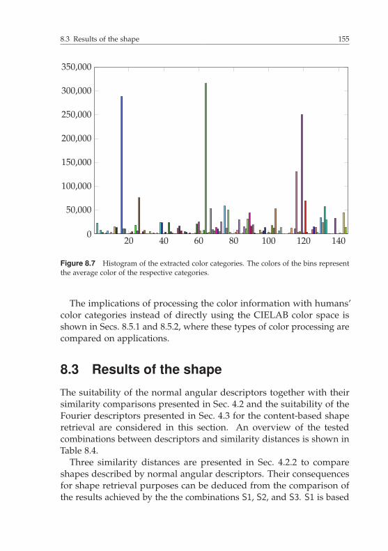
8.3 Results of the shape 155
20 40 60 80 100 120 1400
50,000
100,000
150,000
200,000
250,000
300,000
350,000
Figure 8.7 Histogram of the extracted color categories. The colors of the bins representthe average color of the respective categories.
The implications of processing the color information with humans’color categories instead of directly using the CIELAB color space isshown in Secs. 8.5.1 and 8.5.2, where these types of color processing arecompared on applications.
8.3 Results of the shape
The suitability of the normal angular descriptors together with theirsimilarity comparisons presented in Sec. 4.2 and the suitability of theFourier descriptors presented in Sec. 4.3 for the content-based shaperetrieval are considered in this section. An overview of the testedcombinations between descriptors and similarity distances is shown inTable 8.4.
Three similarity distances are presented in Sec. 4.2.2 to compareshapes described by normal angular descriptors. Their consequencesfor shape retrieval purposes can be deduced from the comparison ofthe results achieved by the the combinations S1, S2, and S3. S1 is based

156 8 Results
on unwarped normal angular descriptors, whereas S2 and S3 considerwarped normal angular descriptors (see Sec. 4.2.2.2). Furthermore, S1and S2 use the correlation for circular data (see Sec. 2.1) while S3 usesthe comparison method based on the Euclidean distance.
Table 8.4 Tested combinations for shape retrieval.
Descriptors Similaritydistances
Com. ηk f Fourier1, f f Fourier
2, f f Fourier3, f dNAD
1 dNAD2 dNAD
3 dFourierf
S1 • •S2 • •S3 • •S4 • •S5 • •S6 • •S7 • •S8 • •
The combinations S4 to S8 are based on the Fourier descriptors,whose similarities between two objects are always calculated by theEuclidean distance (see Sec. 2.1). S4 uses scaling-invariant descriptors,S5 Fourier descriptors with normalized energy, and S6 to S8 the scaling-and rotation-invariant descriptors (with the desired rotation symmetryof the object s set to 1). S6 to S8 correspond with the three testedcombinations of the parameter q presented in Sec. 4.3.3.
The methods are evaluated at the MPEG-7 CE-Shape database [1],which is commonly used to test such cases [13, 16, 67, 81, 146, 150].This database consists of 1400 images of white objects on a black back-ground. There are 70 object classes, each of them containing 20 images.For the evaluation of the proposed methods, the boundaries of theobjects are extracted and described with 101 points as in [157] and[158]. The extracted boundaries consisting of more than 101 points arereduced to 101 using the Fourier descriptors by eliminating the higherfrequency components.
The parameter qretr is used to evaluate the retrieval quality of thecombinations presented in Table 8.4. For this purpose, the images inthe database are sorted 1400 times. Every image in the database is

8.3 Results of the shape 157
used as query and according to the sorted results qretrk is calculated per
query object, where 1 ≤ k ≤ 1400 represents the query object. Objectsfrom the same object class as the query object are defined as its goodmatches. Notice that some objects belonging to other classes may beconsidered similar to the shape of the query object as similarity is ahuman dependent task. However, as established in literature, onlyobjects that belong to the same class are defined as good matches.
Two parameters are used to compare the quality of the retrievalresults between the different tested combinations. Per object classthe mean value of qretr
k from all objects that belong to the class iscalculated qretr
k1, 1 ≤ k1 ≤ 70. The mean value μ(qretr
k1) and standard
deviation σ(qretrk1
) from this parameter over all object classes yield thetwo evaluation parameters.
8.3.1 Evaluation results
The evaluation results of the tested combinations are shown in Table 8.5.The methods based on the Fourier descriptors yield lower μ(qretr
k1) val-
ues than those based on the normal angular descriptors. Among themethods based on the Fourier descriptors the highest μ(qretr
k1) is reached
by the Fourier descriptors with the normalized energies (S5). This com-bination also possesses under the Fourier descriptors based methodsthe lowest standard deviation σ(qretr
k1), which implies a higher robust-
ness against the query object. Mixed quality results are reached bythe scaling- and rotation-invariant descriptors (S6 to S8). On the onehand it yields the second highest μ(qretr
k1) value under the Fourier de-
scriptors based methods, but on the other hand it also yields the lowestone. Under these combinations, the highest values are reached by thethird combination presented in Sec. 4.3.3 which allows q ∈ Z althoughq ∈ N+ is expected in [25]. However, this combination also reaches thehighest standard deviation of all tested combinations.
The best μ(qretrk1
) values are achieved by the combinations based onthe normal angular descriptors. Whereas the use of the correlationfor circular data (S1 and S2) yields higher μ(qretr
k1) values than in case
of the similarity distance based on the Euclidean distance (S3), thecomparisons of warped angular descriptors (S2 and S3) possess thelowest standard deviations σ(qretr
k1) of all tested combinations. The use
of warped angular descriptors with the correlation for circular data as
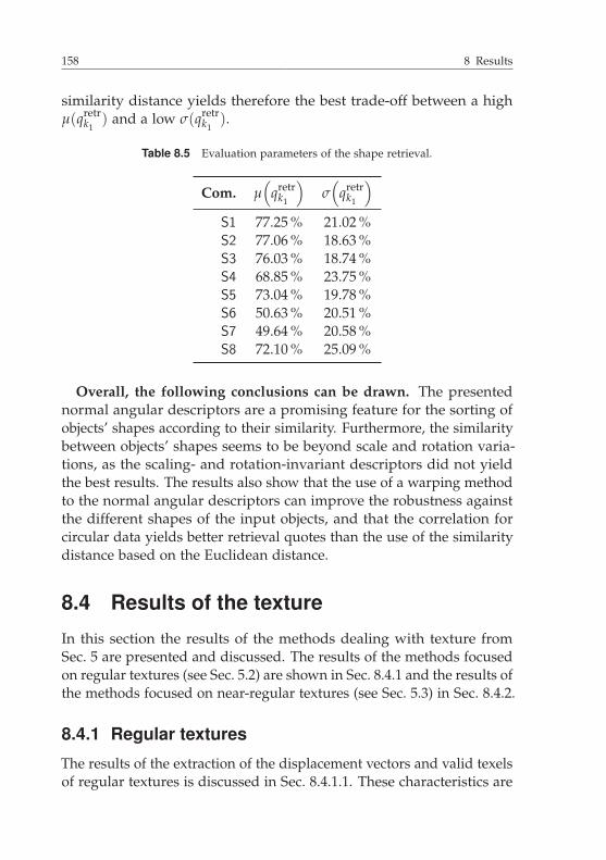
158 8 Results
similarity distance yields therefore the best trade-off between a highμ(qretr
k1) and a low σ(qretr
k1).
Table 8.5 Evaluation parameters of the shape retrieval.
Com. μ(
qretrk1
)σ(
qretrk1
)
S1 77.25 % 21.02 %S2 77.06 % 18.63 %S3 76.03 % 18.74 %S4 68.85 % 23.75 %S5 73.04 % 19.78 %S6 50.63 % 20.51 %S7 49.64 % 20.58 %S8 72.10 % 25.09 %
Overall, the following conclusions can be drawn. The presentednormal angular descriptors are a promising feature for the sorting ofobjects’ shapes according to their similarity. Furthermore, the similaritybetween objects’ shapes seems to be beyond scale and rotation varia-tions, as the scaling- and rotation-invariant descriptors did not yieldthe best results. The results also show that the use of a warping methodto the normal angular descriptors can improve the robustness againstthe different shapes of the input objects, and that the correlation forcircular data yields better retrieval quotes than the use of the similaritydistance based on the Euclidean distance.
8.4 Results of the texture
In this section the results of the methods dealing with texture fromSec. 5 are presented and discussed. The results of the methods focusedon regular textures (see Sec. 5.2) are shown in Sec. 8.4.1 and the results ofthe methods focused on near-regular textures (see Sec. 5.3) in Sec. 8.4.2.
8.4.1 Regular textures
The results of the extraction of the displacement vectors and valid texelsof regular textures is discussed in Sec. 8.4.1.1. These characteristics are

8.4 Results of the texture 159
necessary to be able to detect and sort regular textures as proposedin Sec. 5.2. The detection of regular textures is considered next. Forthis purpose, the detections in space and in frequency domain wereconsidered in Sec. 5.2.2. The criteria used to evaluate the quality ofthe detection methods are presented in Sec. 8.4.1.2 followed by theevaluation results of the detection in space (Sec. 8.4.1.3) and in frequencydomain (Sec. 8.4.1.4). Once the regular textures have been detected,their sorting according to their similarity was considered in Sec. 5.2.3.The sorting results achieved by this method are presented in Sec. 8.4.1.5.Finally, in Sec. 8.4.1.6 the perception map of regular textures derivedfrom the results of the experiment presented in Sec. 5.2.4 is shown,discussed, and compared with the sorting results achieved by theproposed method.
8.4.1.1 Extraction of the texel and its displacementvectors in the real case
The extraction of the displacement vectors and texels of regular texturesfor an ideal case was presented in Sec. 5.2.1.1. However, as mentioned inSec. 5.2.1.2, due to the discretization of the images in space domain andthe lack of a clear boundary between regular and structural-statisticaltextures, the real case must be considered. 14 window functions, twotypes of interpolations, and the use of zero padding were proposedin Sec. 5.2.1.2 to overcome the issues related to the real case. Theirappropriateness for the extraction of the characteristics are comparedin this section. For this purpose, the textures classified as regular in theIIIT texture database (see Sec. 8.1.1) are considered.
The evaluation of the different methods for the extraction of thecharacteristics of regular textures is not trivial. On the one hand, manydisplacement vectors combined with different texels may describe theconsidered regular texture correctly (see Sec. 5.1.1), so no unique so-lution exists. On the other hand, the displacement vectors must notbe of discrete nature in contrast to the input image, which makes theirexact extraction from a given image difficult. Furthermore, an exactextraction of the displacement vectors is not even possible if the regulartexture underlies small stochastic variations. The storage of all validdisplacement vectors and texels that may describe the input images asground truth data is not possible and alternative evaluation methods are

160 8 Results
necessary. The better the extraction of the displacement vectors is, thebetter the extraction of the texel in the image will be and therefore thebetter the original image may be represented. By these means, the abso-lute difference between an input image and its respective reconstructedimage dT,1(gu, gu) (as presented in Sec. 5.2.2.1) is a good indicator ofthe quality of the extracted displacement vectors and texel. The smallerdT,1(gu, gu) is, the better the estimation of the texture characteristicswill be. Furthemore, as images containing big areas spanned by theirdisplacement vectors are directly classified as irregular and thereforenot reconstructed, the number of regular textures in the database thatare directly classified as irregular is also an important parameter toevalute the goodness of the analyzed combinations, as all of the texturesconsidered in this section are regular.
Figure 8.8 shows the average of dT,1(gu, gu) over all the regular tex-tures in the database that were reconstructed depending on the windowfunction, the kind of interpolation, and the type of zero padding usedfor the extraction. From now on the use of no zero padding and its useby increasing the size of the input image by a factor of two and three isalso referred as a zero padding of zero, one, and two degree, respec-tively. The results show that the use of a bilinear interpolation (dashedand/or dotted curves) instead of the nearest neighbor interpolation(solid curves) reduces the average error μ(dT,1(gu, gu)) over all imagesin the database. This error also becomes smaller, the higher the degreeof zero padding (coded by the color) is. Among the window functionsthe conclusions can be drawn that the quality of the extracted charac-teristics of the regular textures by the flat top window is on averageworse than when the other window functions are used. Particularly atthe rectangular and Kaiser windows, the improvements of the bilinearinterpolation and the use of zero padding can be noticed. Whereas thesewindows deliver together with the flat top window the highest averageerrors over all images in the database μ(dT,1(gu, gu)) when the nearestneighbor interpolation and no zero padding is used, they reach onaverage the smallest errors μ(dT,1(gu, gu)) when zero padding and thebilinear interpolation is used. The modified Bartlett-Hann, Hamming,Taylor, and triangular windows together with a bilinear interpolationand zero padding yield similar good results to those achieved by theKaiser and rectangular windows.
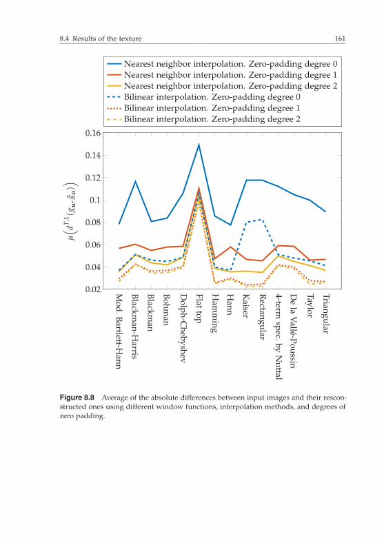
8.4 Results of the texture 161
Mod.Bartlett-H
ann
Blackman-H
arris
Blackman
Bohman
Dolph-C
hebyshev
Flattop
Ham
ming
Hann
Kaiser
Rectangular
4-termspec.by
Nuttal
De
laV
allé-Poussin
Taylor
Triangular
0.02
0.04
0.06
0.08
0.1
0.12
0.14
0.16
μ( dT
,1(g
u,g
u))
Nearest neighbor interpolation. Zero-padding degree 0Nearest neighbor interpolation. Zero-padding degree 1Nearest neighbor interpolation. Zero-padding degree 2Bilinear interpolation. Zero-padding degree 0Bilinear interpolation. Zero-padding degree 1Bilinear interpolation. Zero-padding degree 2
Figure 8.8 Average of the absolute differences between input images and their rescon-structed ones using different window functions, interpolation methods, and degrees ofzero padding.

162 8 Results
Table 8.6 Number of images whose displacement vectors have been estimated too long.
Nearest neighbor Bilinearinterpolation interpolation
Window Degree Degreefunction of zero padding of zero padding
0 1 2 0 1 2
Mod. Bartlett-Hann 3 2 3 2 2 2Blackman-Harris 4 3 3 3 3 3
Blackman 2 3 3 3 3 2Bohman 3 3 3 3 2 2
Dolph-Chebyshev 5 3 3 3 3 3Flat top 7 7 8 6 6 6
Hamming 3 1 1 2 0 0Hann 3 2 3 2 2 2
Kaiser 4 2 1 0 2 2Rectangular 4 2 1 0 1 2
4-term spec. by Nuttal 4 3 3 3 2 2De la Vallé-Poussin 5 3 3 3 2 3
Taylor 0 1 0 0 0 0Triangular 1 1 0 1 0 0
Table 8.6 shows over all analyzed combinations the number of imagesthat were directly classified as irregular, because the area spanned bytheir extracted displacement vectors was too big. Ideally, none of theanalyzed images should be classified as irregular, as only the regulartextures were analyzed from the database. The results show that overall combinations only a small number of textures are directly consid-ered of irregular type (up to 1.15 % for the flat top window). TheHamming, Kaiser, rectangular, Taylor, and triangular windows are theonly windows that manage not to classify input textures directly asirregular. In case of the Kaiser and rectangular windows this onlyhappens with a bilinear interpolation and no zero padding. However,these two combinations yielded a high average error μ(dT,1(gu, gu)).The Hamming window achieves it in combination with the bilinearinterpolation and zero padding, and the triangular window togetherwith bilinear interpolation and zero padding and also in case of the

8.4 Results of the texture 163
nearest neighbor interpolation if a zero padding degree of two is ap-plied. The stablest window towards the interpolation methods and theusage of zero padding to avoid an assignment of the analyzed imagesas irregular is the Taylor window. When it is applied together withthe nearest neighbor interpolation and a zero padding degree of one,only one image is directly classified as irregular, otherwise the char-acteristics of regular textures were extracted for all considered imagesin the database.
Overall, the following conclusions can be drawn. The higher thedegree of zero padding together with a bilinear interpolaton, the betterthe extraction of the characteristics of regular textures is. Furthermore,for these combinations the Hamming, Taylor, and triangular windowsextract for all considered images in the database their displacementvectors and texel. The best trade-off between a small average errorμ(dT,1(gu, gu)) and a good extraction of the characteristics of regulartextures over all considered images in the database is reached by theTaylor window together with the bilinear interpolation and a zeropadding degree of two.
8.4.1.2 Evaluation criteria for the detection of regular textures
In Sec. 5.2.2 the detection of regular textures in space and frequencydomain is respectively considered. The modus operandi in both casesis to assume first that the analyzed input texture is of regular type andto extract therefore its displacement vectors. If the area spanned byits displacement vectors in space domain is too big, then the analyzedtexture is directly classified as not regular. If the area is small, then theanalyzed texture is further processed until a final value is extracted,according to which the input texture is classified as regular or not. Forthe detection in space domain (see Sec. 5.2.2.1) this value is the result ofthe similarity distance function defined in Eq. 5.8, for the detection infrequency domain (see Sec. 5.2.2.2) two different features are proposedin Eq. 5.11 and Eq. 5.12. In order to evaluate the appropriateness of thedifferent methods, the suitability of the extracted values is consideredtogether with the classification results of the analyzed images, whichare the textured images from the IIIT texture database (see Sec. 8.1.1).Since the Taylor window together with the bilinear interpolation and adegree of two for the zero padding yielded the best results in Sec. 8.4.1.1,this combination is also used in the following Secs. 8.4.1.3 and 8.4.1.4.

164 8 Results
The suitability of the extracted parameters for the detection of reg-ular textures is measured considering their similarity within texturesof the same type together with the similarity between the two clas-sified groups. This way of proceeding is the basis of the Fisher lin-ear discriminant analysis [45] to reduce the dimension of data takinginto consideration a good separability between the different groups.The higher
qS1 =(μ1 − μ2)
2
σ21 + σ2
2, (8.4)
where
μk =1
|Mk|∑
m∈Mk
m, (8.5)
σ2k =
∑m∈Mk
(m − μk)2 , (8.6)
k ∈ {1, 2} for the two groups, and Mk is the set of all features m belong-ing to the cluster k, the better the separability between the two groups.
The goal of the approaches presented in Sec. 5.2.2 is the detectionof regular textures and thus the classification into regular or not regu-lar. The appropriateness of the approaches can be compared by theirachieved quotient qS1. Furthermore, it is also interesting to analyze thelimits of the extracted classification features if a further classificationinto the three types of textures (regular, structural-statistical, and ir-regular) is considered. However, as the number of representatives pertexture type in the IIIT texture database is different, this may distort qS1.To overcome this issue, the within class variations σ2
k are normalized bytheir number of representatives in the database:
qsep =(μ1 − μ2)
2
σ21 + σ2
2, (8.7)
where
σ2k =
∑m∈Mk
(m − μk)2
|Mk|, (8.8)
k ∈ {1, 2}. qsep is named from now on as separability quotient.

8.4 Results of the texture 165
The confusion matrix [130] of the classification of the images in thedatabase into regular and not regular is the second evaluation criterion.18.90 % of the textures in the database that are not of regular type (72images) are directly classified as not regular, because the area spannedby their extracted displacement vectors in space domain is too big.10.03 % (31 images) are randomly chosen from the remaining irregularand structural-statistical textures in the database that have not beendirectly classified as not regular. Together with 31 randomly chosenregular textures from the database they form the training data [80, 130],which is used to obtain the threshold value according to which theinput images are classified. The confusion matrix is evaluated for theremaining images in the database that were not part of the trainingprocedure to avoid overfitting [45].
8.4.1.3 Evaluation results for the detection in space domain
The quality of the similarity distance dT,1(gu, gu) for the detectionand classification according to the type of textures is presented anddiscussed next.
The similarity distances between an input image and its recon-structed one dT,1(gu, gu) for all images in the database whose areaspanned by their displacement vectors is small enough to not be directlyclassified as an irregular texture are presented in form of a histogramin Fig. 8.9. We can recognize that the distance values are much smallerfor textures of regular type. There is even a gap between the distancevalues obtained from the regular textures and the other ones. Further-more, within the textures that are not regular, the structural-statisticaltextures tend to have smaller distance values than the irregular textures,which corresponds to the fact that no clear boundary exists betweenthe different types of textures. The gap between the regular texturesand the structural-statistical ones should be therefore reduced if moretextures are considered with a finer transition from their regularityto structural-statistical ones. According to these results the similaritydistance between an input image and its reconstructed one is a validfeature for a successful detection of regular textures. Moreover, thisfeature can also be used as an orientation for the type of irregularity.
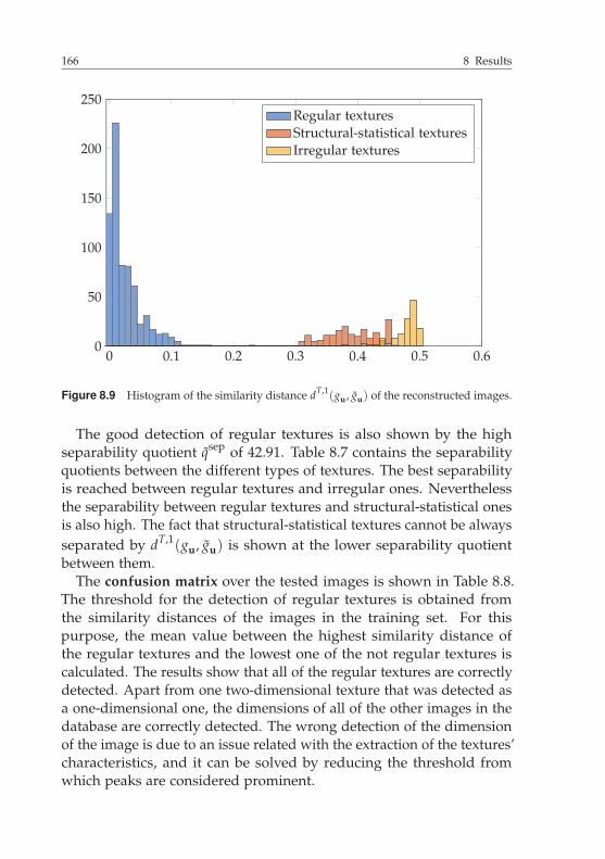
166 8 Results
0 0.1 0.2 0.3 0.4 0.5 0.60
50
100
150
200
250Regular texturesStructural-statistical texturesIrregular textures
Figure 8.9 Histogram of the similarity distance dT,1(gu, gu) of the reconstructed images.
The good detection of regular textures is also shown by the highseparability quotient qsep of 42.91. Table 8.7 contains the separabilityquotients between the different types of textures. The best separabilityis reached between regular textures and irregular ones. Neverthelessthe separability between regular textures and structural-statistical onesis also high. The fact that structural-statistical textures cannot be alwaysseparated by dT,1(gu, gu) is shown at the lower separability quotientbetween them.
The confusion matrix over the tested images is shown in Table 8.8.The threshold for the detection of regular textures is obtained fromthe similarity distances of the images in the training set. For thispurpose, the mean value between the highest similarity distance ofthe regular textures and the lowest one of the not regular textures iscalculated. The results show that all of the regular textures are correctlydetected. Apart from one two-dimensional texture that was detected asa one-dimensional one, the dimensions of all of the other images in thedatabase are correctly detected. The wrong detection of the dimensionof the image is due to an issue related with the extraction of the textures’characteristics, and it can be solved by reducing the threshold fromwhich peaks are considered prominent.
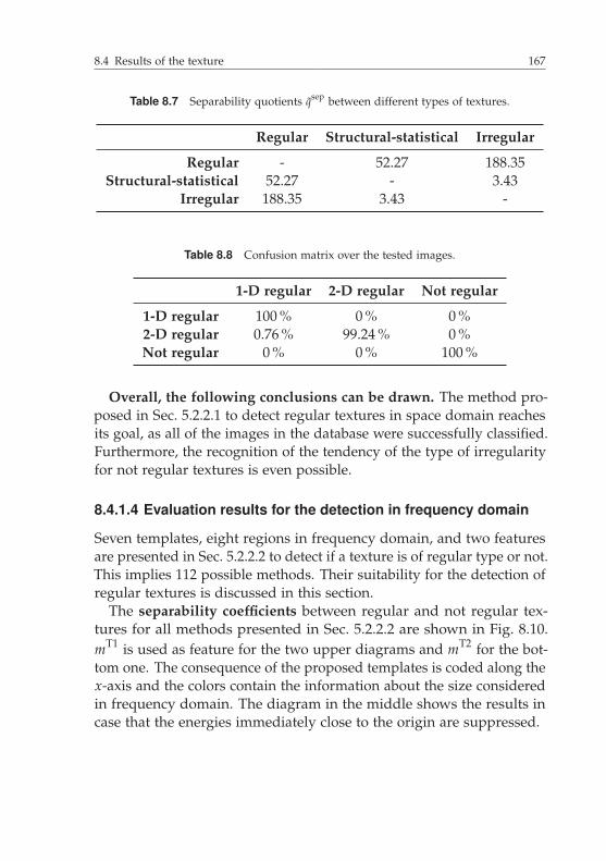
8.4 Results of the texture 167
Table 8.7 Separability quotients qsep between different types of textures.
Regular Structural-statistical Irregular
Regular - 52.27 188.35Structural-statistical 52.27 - 3.43
Irregular 188.35 3.43 -
Table 8.8 Confusion matrix over the tested images.
1-D regular 2-D regular Not regular
1-D regular 100 % 0 % 0 %2-D regular 0.76 % 99.24 % 0 %Not regular 0 % 0 % 100 %
Overall, the following conclusions can be drawn. The method pro-posed in Sec. 5.2.2.1 to detect regular textures in space domain reachesits goal, as all of the images in the database were successfully classified.Furthermore, the recognition of the tendency of the type of irregularityfor not regular textures is even possible.
8.4.1.4 Evaluation results for the detection in frequency domain
Seven templates, eight regions in frequency domain, and two featuresare presented in Sec. 5.2.2.2 to detect if a texture is of regular type or not.This implies 112 possible methods. Their suitability for the detection ofregular textures is discussed in this section.
The separability coefficients between regular and not regular tex-tures for all methods presented in Sec. 5.2.2.2 are shown in Fig. 8.10.mT1 is used as feature for the two upper diagrams and mT2 for the bot-tom one. The consequence of the proposed templates is coded along thex-axis and the colors contain the information about the size consideredin frequency domain. The diagram in the middle shows the results incase that the energies immediately close to the origin are suppressed.

168 8 Results
1 2 3 4 5 6 70
2
4
6mT1
k = 2k = 3k = 4k = ∞
⎫⎪⎪⎬⎪⎪⎭
Considered regions in frequency space
1 2 3 4 5 6 70
2
4
6mT1
1 2 3 4 5 6 70
0.1
0.2
0.3mT2
Figure 8.10 Separability coefficients achieved by the tested methods.
The separability values (y-axis) are much smaller than in case of thedetection in space domain (42.91, see Sec. 8.4.1.3). Within the detectorsin frequency domain, the extraction of the features via mT1 yields abetter separability than in case of mT2. Furthermore, a tendency between
8.4 Results of the texture 169
the sizes of the considered regions in frequency domain can be observed.For mT1, the smaller the size of the regions in frequency domain, thebetter the detection of regular textures is. On the other hand, the biggerthe size of the regions in frequency domain, the better the detection ofregular textures if mT2 is used as feature. The type of template usedfor the detection plays a less important role in comparison to the otherdegrees of freedom.
The feature values mT1 (top) and mT2 (middle and bottom) are shownin Fig. 8.11 as histograms of their respective combinations that reachedthe best separability coefficient. No matter if mT1 or mT2 is used, theregular textures tend to have higher features than the not regular ones.However, in contrast to the detection in space domain, the featuresin the histogram are not clearly grouped depending on their type oftexture, which explains the lower separability coefficients.
Table 8.9 Confusion matrices over the tested images.
mT1 1-D regular 2-D regular Not regular
1-D regular 75.37 % 0 % 24.63 %2-D regular 0.76 % 97.71 % 1.53 %Not regular 0 % 1.44 % 98.56 %
mT2 1-D regular 2-D regular Not regular
1-D regular 5.97 % 0 % 94.03 %2-D regular 0 % 0 % 100 %Not regular 0.89 % 0 % 99.11 %
The confusion matrices over all tested images per best combinationsof mT1 and mT2 are shown in Table 8.9. The thresholds for the detectionof regular textures were calculated per considered feature mT1 andmT2 from the feature values of the textures that form the trainingset. For this purpose, the mean values between the lowest value ofthe regular textures and the highest one of the not regular ones wererespectively calculated. The majority of the regular textures and theirdimensions are correctly detected by the method using mT1 as feature.Almost all two-dimensional regular textures are correctly detected inthis case (97.71 %). Like in the case of the detection in space domain,

170 8 Results
one of the two-dimensional textures is detected as a one-dimensionalone. The percentage of one-dimensional textures that are detected isalso high (75.37 %) but not as high as in the case of two-dimensionaltextures. Furthermore, almost all not regular textures are also correctlyidentified, apart from 1.44 % which are detected as two-dimensionalregular textures.
0 5 10 15 20 25 30 35 400
20406080
100
0 500 1,000 1,500 2,000 2,5000
50
100
150Regular texturesStructural-statistical texturesIrregular textures
0 0.01 0.02 0.03 0.040
20406080
100Regular texturesStructural-statistical texturesIrregular textures
Figure 8.11 Histogram of the best separability results reached by the features mT1 (top)and mT2 (middle and bottom).
The detections rates are different if mT2 is used as feature. In thiscase almost all textures are detected as not regular ones independentlyof their real types.

8.4 Results of the texture 171
8.4.1.5 Sorting of regular textures
The suitability of the sorting method for regular textures presented inSec. 5.2.3 is discussed in this section. For this purpose, the textures ofthe IIIT texture database detected as regular in space domain using aTaylor window, bilinear interpolation, and a zero padding degree oftwo are considered. Eight different similarity features whose strengthcan be independently selected were presented in Sec. 5.2.3 to comparepairs of regular textures. This implies many possible ways to combinethe similarity features, which makes possible to focus on differentcharacteristics of the textures like their size or rotation. However, as thesimilarity perception is a human dependent task and no ground truthdata is established in the literature or known to the author so far, theevaluation of the results and especially the optimization of the selectionof the strengths of the different similarity parameters is a challengingtask. Following the procedure established in literature to evaluate imageretrieval systems, the regular textures of the IIIT texture database aregrouped for the evaluation into classes, so that quality measurementslike the precision and recall functions can be calculated (see Sec. 8.1.2).In Sec. 8.4.1.6 the results achieved by this sorting method are comparedto the perception map extracted according to Sec. 5.2.4.
Chess
Hexagons
Dots
Tiling1
Tiling2
Lines
Transientlines
0
50
0
500
Chess
Hexagons
Dots
Tiling1
Tiling2
Lines1
Lines2
Transientlines
0
50
0
200
Two-dimensional texturesOne-dimensional textures
Figure 8.12 Histogram of the images in the database belonging to the bigger classes.A total of 10 classes is permitted if a higher stochastic variation is permitted (left) or 11classes for a small stochastic variation (right).

172 8 Results
For the evaluation of the results, in this section, a class consists of im-ages containing the same pattern which may be rotated, scaled, containdifferent gray values, or small stochastic variations of the texels. Twodifferent allocations of the regular textures into classes are considereddepending on the permitted amount of stochastic variation. 10 and 11bigger classes respectively appear in the database (see Fig. 8.12, whichshows the amount of images per class, where two-dimensional texturesare represented in black and one-dimensional ones in gray), whereasmore smaller classes exist. Whilst the number of images in the classesslightly decreases for most of the types of patterns, the Lines class is splitinto two classes (Lines 1, Lines 2) when a smaller stochastic variation ofthe texels is permitted. Together with the two considered allocationsof the images into classes two different strength configurations of thesimilarity distances are considered for the evaluation results. In thefirst case all of the similarity distances are considered equally strong;in the second case all of the similarity distances contribute to the totalsimilarity between pairs of textures except the one considering theorientation (w7 = 0).
The value qretr, presented in Sec. 8.1.2.1 to evaluate the quality ofretrieval applications, is shown for every image that belongs to one ofthe bigger classes in Fig. 8.13 for a bigger permitted stochastic variationand in Fig. 8.14 in case of a smaller permitted variation. The bluecolor represents the results when all similarity distances are consideredequally strong and the red color when the orientation information isnot considered, whereas the dashed lines represent the average resultsat the considered class. The results show that for both allocations of theimages into classes and for both strength configurations, the retrievalof the images are very close to the ideal one. Only at the Transient Linesclass some of the input images did not achieve as good retrievals as theother input images. This happened mainly at horizontal and verticaloriented transient lines, where the displacement features predominatedover the texels’ features. Nevertheless, very good retrieval results areobtained on average for each class (see Table 8.10) and over all classes(see Table 8.11). This happens although the strengths for the differentsimilarity distances were not adjusted to detect textures of same classes.

8.4 Results of the texture 173
20%
40%
60%
80%
100
%
Inpu
tim
age
Che
ss
20%
40%
60%
80%
100
%
Inpu
tim
age
Hex
agon
s
20%
40%
60%
80%
100
%
Inpu
tim
age
Dot
s
20%
40%
60%
80%
100
%
Inpu
tim
age
Tili
ng1
20%
40%
60%
80%
100
%
Inpu
tim
age
Tili
ng2
20%
40%
60%
80%
100
%
Inpu
tim
age
Line
s
20%
40%
60%
80%
100
%
Inpu
tim
age
Tran
sien
tli
nes
Figure 8.13 qretr per texture class and features’ strength in case of bigger acceptedstochastic variations.

174 8 Results
20%
40%
60%
80%
100%
Inpu
tim
age
Che
ss
20%
40%
60%
80%
100%
Inpu
tim
age
Hex
agon
s
20%
40%
60%
80%
100%
Inpu
tim
age
Dot
s
20%
40%
60%
80%
100%
Inpu
tim
age
Tili
ng1
20%
40%
60%
80%
100%
Inpu
tim
age
Tili
ng2
20%
40%
60%
80%
100%
Inpu
tim
age
Line
s1
20%
40%
60%
80%
100%
Inpu
tim
age
Line
s2
20%
40%
60%
80%
100%
Inpu
tim
age
Tran
sien
tli
nes
Figure 8.14 qretr per texture class and features’ strength in case of smaller acceptedstochastic variations.

8.4 Results of the texture 175
Table 8.10 Average qretr per texture class and features’ strength.
Bigger stochastic Smaller stochasticvariations variations
Pattern wk = 1, ∀k w7 = 0 wk = 1, ∀k w7 = 0class wk = 1, ∀
k �=7k wk = 1, ∀
k �=7k
Chess 99.52 % 99.90 % 99.52 % 99.90 %Hexagons 96.42 % 100 % 96.42 % 100 %
Dots 98.45 % 97.82 % 98.92 % 99.69 %Tiling 1 95.55 % 98.17 % 95.59 % 97.49 %Tiling 2 96.53 % 97.35 % 97.83 % 98.54 %
Lines 99.41 % 100 % - -Lines 1 - - 72.13 % 75.61 %Lines 2 - - 70.94 % 74.59 %
Transientlines 89.46 % 90.87 % 89.46 % 90.87 %
Table 8.11 Average qretr per features’ strength over all textures.
wk = 1, ∀k w7 = 0wk = 1, ∀
k �=7k
Bigger stochastic variations 96.48 % 97.73 %Smaller stochastic variations 90.10 % 92.09 %
8.4.1.6 Perception map of regular textures
In this section the details of the experimental procedure to extract aperception map according to Sec. 5.2.4 are presented first, followedby the analysis of the experimental data. A comparison between theconclusions drawn from the perception map and the sorting of regu-lar textures according to their similarity as presented in Sec. 5.2.3 isavailable at the end of this section.

176 8 Results
Figure 8.15 Selected images for the experiment.
For the experimental procedure the IIIT texture database is selected.As the number of pairs of textures increases enormously with thenumber of considered textures and a variety of texture characteristicsand repetitions is necessary to be able to draw relationships betweenthe textures, in this experiment the focus is set on regular textures.From the 698 regular textures in the database 34 are selected, 9 one-dimensional textures and 25 two-dimensional ones (see Fig. 8.15). Thisimplies 595 pairs of textures, whose similarity must be evaluated by thesubjects. The one-dimensional textures are variations (rotation, scale,

8.4 Results of the texture 177
small stochastic variations) from two texture types (the classes Lines andTransient Lines or Lines 1, Lines 2, and Transient Lines from Sec. 8.4.1.5).The two-dimensional textures are made up from 22 textures belongingto the five bigger classes that appear in the database (the classes Chess,Hexagons, Dots, Tiling 1 and Tiling 2 from Sec. 8.4.1.5). The remainingthree textures used in the experiment contain each a new pattern. Thesoftware OpenSesame [111] was used to create and run the experiment.
The analysis of the experiment is presented next. According to thejudgments of the subjects, the similarity criterion shape is the mostmentioned one, followed by color, orientation, color gradient, and size.
Dimension 1
Dim
ensi
on2
Figure 8.16 Two-dimensional perception map obtained via non-metric multidimen-sional scaling.
The two-dimensional perception map obtained via non-metric mul-tidimensional scaling is shown in Fig. 8.16. It is noticeable that all ofthe considered textures are grouped according to their type of patternindependently of rotation, scaling, or small stochastic variations of the
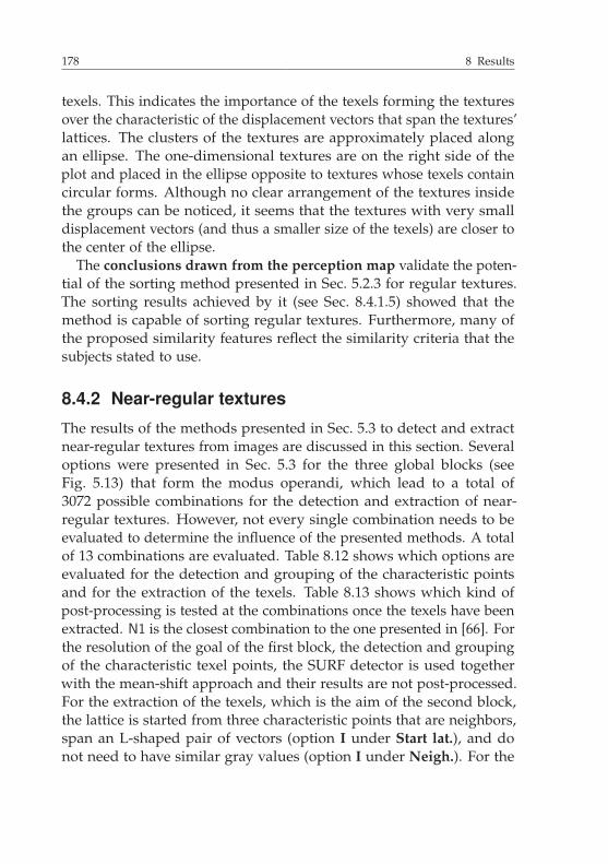
178 8 Results
texels. This indicates the importance of the texels forming the texturesover the characteristic of the displacement vectors that span the textures’lattices. The clusters of the textures are approximately placed alongan ellipse. The one-dimensional textures are on the right side of theplot and placed in the ellipse opposite to textures whose texels containcircular forms. Although no clear arrangement of the textures insidethe groups can be noticed, it seems that the textures with very smalldisplacement vectors (and thus a smaller size of the texels) are closer tothe center of the ellipse.
The conclusions drawn from the perception map validate the poten-tial of the sorting method presented in Sec. 5.2.3 for regular textures.The sorting results achieved by it (see Sec. 8.4.1.5) showed that themethod is capable of sorting regular textures. Furthermore, many ofthe proposed similarity features reflect the similarity criteria that thesubjects stated to use.
8.4.2 Near-regular textures
The results of the methods presented in Sec. 5.3 to detect and extractnear-regular textures from images are discussed in this section. Severaloptions were presented in Sec. 5.3 for the three global blocks (seeFig. 5.13) that form the modus operandi, which lead to a total of3072 possible combinations for the detection and extraction of near-regular textures. However, not every single combination needs to beevaluated to determine the influence of the presented methods. A totalof 13 combinations are evaluated. Table 8.12 shows which options areevaluated for the detection and grouping of the characteristic pointsand for the extraction of the texels. Table 8.13 shows which kind ofpost-processing is tested at the combinations once the texels have beenextracted. N1 is the closest combination to the one presented in [66]. Forthe resolution of the goal of the first block, the detection and groupingof the characteristic texel points, the SURF detector is used togetherwith the mean-shift approach and their results are not post-processed.For the extraction of the texels, which is the aim of the second block,the lattice is started from three characteristic points that are neighbors,span an L-shaped pair of vectors (option I under Start lat.), and donot need to have similar gray values (option I under Neigh.). For the
8.4 Results of the texture 179
expansion of the lattice from the starting lattice the maximum numberof outneighbors per node is not considered (option I under Exp.).
Table 8.12 Tested combinations for the detection and grouping of the characteristictexel points (up) and for the extraction of the texels (down).
Detec. PoI Clustering Post-
Com. SURF MSER Mean-shift Graph processing
N1 • •N2 • •N3 • •N4 • •N5 • •N6 • •N7 • •N8 • • •N9 • • •
N10 • • •N11 • • •N12 • • •N13 • • •
Neigh. Start lat. Exp. Weig. Lim. Extr.
Com. I II I II III I II I II
N1 • • • •N2 • • • •N3 • • • •N4 • • • •N5 • • • •N6 • • • •N7 • • • •N8 • • • •N9 • • • •N10 • • • • •N11 • • • • •N12 • • • •N13 • • • •

180 8 Results
The suitability of all projected texels is considered by suppressing alltransformed texels with no repeatability at the contours before themedian one is calculated (option I under Extr.). No limitation of thenumber of transformed texels (option Lim.) is imposed together withno weights to the transformed texels (option Weig.). Furthermore, noadditional post-processing of the extracted texels is considered (seeTable 8.13). Differences to the detection and extraction of near-regulartextures due to the clustering method can be determined by comparingthe results of the methods N1 and N2 as the only difference betweenthem is the clustering method used to group the detected characteristictexel points. While N1 uses the mean-shift approach, N2 uses thegraph based method presented in Sec. 5.3.1.2. The consequences ofstarting from a local regular texture (option II under Start lat.) insteadof starting from three neighboring points can be deduced from thecomparison of the results achieved by N2 and N3. N4, in contrast toN3, requires neighboring points of the local regular starting latticeto have a similar gray value. The consequences of considering thesimilarity of the vectors between neighboring points when the startinglattice is created (option III under Start lat.) can be deduced from thecomparison of the results of N4 and N5. N6, in contrast to N5, considersthe maximum number of outneighbors per node when the startinglattice is expanded (option II under Exp.). From the comparison ofthe results of N5 and N7 deductions can be made about the influenceof the occlusion of outliers and the grouping of the texels accordingto their similarity. For this purpose, in N7 the repeatability of thecontours of the texels is proved from the median filtered extractedtexels (option II under Extr.). Furthermore, the comparison of theresults from N7 and N8 yields an information about the post-processingof the extracted and grouped characteristic points before the extractionof the texels. N9 fuses all of the proposed methods for the detectionand extraction of regular textures. It extends N8 with the methodsproposed to reach the goal of the third block, the post-processing. N10to N13 are very similar to N9. N10 incorporates the option to weight thetexels that are transformed to the quadrangles that are robust to affinetransformations and lighting variations (option Weig.), N11 limitatesthe number of texels that are transformed to the quadrangles (optionLim.), N12 uses the MSER detector to detect the characteristic pointsinstead of the SURF detector, and N13 uses the color information of

8.4 Results of the texture 181
the input image when the extracted texels are post-processed (optionColor).
Table 8.13 Tested options for the post-processing of already extracted texels.
Com. Gray-levels Color
N1N2N3N4N5N6N7N8N9 •N10 •N11 •N12 •N13 •
The criteria used to evaluate the quality of the different combina-tions are explained in Sec. 8.4.2.1, whereas the results are presented inSec. 8.4.2.2.
8.4.2.1 Evaluation criteria
The precision of the detection of near-regular textures and the qualityof the extraction of the detected near-regular textures are considered atthe evaluation of the results. Different evaluation criteria are presentednext to evaluate the results of the combinations presented in Tables 8.12and 8.13. The combinations are all tested at the IIIT patterned imagedatabase.

182 8 Results
Figure 8.17 Two black and white images are shown on the top containing each twotextured surfaces. As the texels of the textures of each object per image are very similar,only one kind of texture type is expected per image. If the color of the images isconsidered, then two kind of texture types are expected per image (lower images).
The quality of the detection is measured using three values peranalyzed image. The first one is the number of near-regular texturesthat are correctly detected in an input image (without repetitions). If

8.4 Results of the texture 183
the color of the image is considered during the detection and extraction,then a distinction is made between the number of near-regular texturesthat should be detected. For example, in Fig. 8.17 one texture type isexpected per gray-level image but two texture types per color image.The second value contains the number of times that a near-regulartexture is repeated in the detections, and the third value is the numberof wrong detections. In order to become an overview of the potential ofthe tested combinations, these three quality values are added over allimages in the database. The higher the number of correctly detectedtextures and the smaller the number of both wrong detections andcorrectly detected but repeated textures are, the better the consideredmethod will be.
To measure the quality of the extraction, a synthetic image gSynthu
is created per extracted near-regular texture. For this purpose, theextracted median texel of the texture is projected back onto the imageplane (see Fig. 8.18). The affine transformation used for the transfor-mation into the quadrangles is inverted. The texels in the quadrangleswere also normalized towards their gray values to overcome lightingvariations along the image. Because of this, the input image must alsobe modified before it can be compared with the synthetic one (seeFig. 8.18). For this purpose, the gray values of the detected texels in theinput image are respectively normalized as
tModu =
tu − minu
(tu)
maxu
(tu)− minu
(tu), (8.9)
and all other pixels that do not belong to the detected texels are sup-pressed. The addition of the respective gray-level offset min
u(tu) to tMod
u
across the whole modified input image gModu yields an impression of
the variation of the brightness.Two characteristics are defined to measure the quality of the extrac-
tion of the textures. The bigger the area of the expanded lattice over thenear-regular textures is, the better the detections of the surfaces will be.This implies a better extraction. The percentage of the area covered bythe expanded lattice over the patterned surface in the image qT1(gu) istherefore the first quality characteristic, where gu denotes the analyzedimage. For this purpose ground truth data was generated from the IIITpatterned image database. The patterned surfaces in the image were

184 8 Results
manually labeled. The achievement of a 100 % overlap between the areaspanned by any expanded lattice and a patterned surface in an imageis almost impossible. On the one hand the surfaces can have any shapeat the contour, whereas the lattice is limited by the parallelograms ofthe cells (see Fig. 8.18 middle), on the other hand the labeled surfacesmay contain areas where no characteristic points may be detected orpossess similar characteristics due to strong scale variations, limitationsof the resolution, or reflections on the surfaces (see Fig. 8.19).
If detected texels overlap more than τT4 (normalized to the area ofthe texels and set here to 0.20), then only the one with the smallestdifference between its projection onto the synthetic image and thenormalized input image is further considered. Small overlaps betweentexels (e.g., at edges) become their average gray value in the syntheticimage, as well as in the modified input image gMod
u .The second characteristic used to measure the quality of the extracted
textures considers the error between the synthetic image and the modi-fied input image:
qT2(gu) =
√ ∑u∈VN
(gMod
u − gSynthu
)2
∣∣∣VN∣∣∣
· 100 %. (8.10)
For this purpose, only the pixels that belong to at least one of theextracted texels VN are considered.
Similar to the criteria used to evaluate the quality of the detec-tion, both evaluation characteristics for the quality of the extractedtextures are obtained from all images in the database. The mean valuesμ(qT1(gu)), μ(qT2(gu)) and standard deviations σ(qT1(gu)), σ(qT2(gu)are considered in this case. The higher mean value of the coveredpercentage and the lower the mean value of the error representationsare, the better the results will be. Furthermore, the smaller the standarddeviations are, the more stable the methods towards the input imagewill be. Notice that even if the color information of the input image isused to detect and extract the near-regular textures, the quality of theextraction is always evaluated at the gray-level images, as the detectionand extraction take place at the gray-level images and the color infor-mation is only used to decide if detected and extracted texels should bemerged.

8.4 Results of the texture 185
Detection of thenear-regular texture
Modified inputimage gMod
u
Brightnessinformation
Syntheticimage gSynth
u
Figure 8.18 Once the lattice has been expanded over the near-regular texture and thetexels detected, a synthetic image is created from the median texel and the input image ismodified to separate the information given by the brightness.
Figure 8.19 Example images from the database displayed with gray values. The areamanually marked as ground truth data is highlighted in red.

186 8 Results
Table 8.14 Evaluation of the quality of the detected near-regular textures. The percent-age of the correctly detected textures is shown together with the percentage of correctlyextracted but repeated textures from the total number of correctly detected textures.
Com. To detect True Repeat False
N1 52 36 69.23 % 19 52.78 % 14N2 52 36 69.23 % 16 44.44 % 5N3 52 44 84.62 % 24 54.55 % 7N4 52 48 92.31 % 25 52.08 % 5N5 52 48 92.31 % 25 52.08 % 2N6 52 45 86.54 % 26 57.78 % 10N7 52 49 94.23 % 25 51.02 % 2N8 52 50 96.15 % 36 72.00 % 1N9 52 50 96.15 % 2 4.00 % 0N10 52 51 98.08 % 6 11.76 % 2N11 52 50 96.15 % 2 4.00 % 0N12 52 47 90.38 % 1 2.13 % 1N13 57 55 96.49 % 2 3.64 % 0
8.4.2.2 Evaluation results
The evaluation results of the quality of the near-regular texture detectionare presented next followed by the evaluation results of the quality ofthe extraction.
The parameters used to measure the quality of the detection forthe different evaluated combinations are shown in Table 8.14, whereasTrue is the number of detected textures (without repetitions), Repeatthe number of correctly extracted but repeated textures, and Falsethe number of wrong detections. A total of 52 textures should bedetected (To detect) at the gray-level images, 57 if the color informationis considered. The closest combination to the one presented in [66](N1) yields the highest number of wrong detections (14) together withthe lowest number of correctly detected textures (69.23 %). The numberof correctly extracted but repeated textures is also quite high (52.78 %of the correctly detected textures).
The use of the sorting method proposed in Sec. 5.3.1.2 instead ofthe mean-shift approach (N2 vs. N1) did not increment the numberof correctly detected textures (69.23 %), but it reduced the number

8.4 Results of the texture 187
of wrong detections by 64.29 % and also the number of correctly ex-tracted but repeated textures by 15.79 %. The use of the presentedsorting method from Sec. 5.3.1.2 instead of the mean-shift approach istherefore promising.
Starting from a local regular texture instead of a single cell (N3 vs. N2)clearly increments the number of correctly detected textures (84.62 % vs.69.23 %), but it also implies a higher number of both correctly extractedbut repeated textures and wrong detections. Nevertheless, due to thehigher number of correctly detected textures, the start with a localregular texture is worth the mild increment of correctly extracted butrepeated textures and wrong detections.
Furthermore, if similar gray values are required between valid neigh-bors in the local regular texture (N4 vs. N3), then the number of correctlydetected textures is incremented (92.31 % vs. 84.62 %) and the numberof wrong detections decreases. The total number of correctly extractedbut repeated textures is incremented by one when similar gray valuesare required, but compared to the total number of correctly detectedtextures it implies a decrease of 2.45 %.
A further reduction of the number of wrong detections (2 vs. 5) withno worsen of both the detection rate (92.31 %) and the percentage ofcorrectly extracted but repeated textures (52.08 %) is achieved if thesimilarity between the vectors of neighboring characteristic points isconsidered when the starting lattice is created (N5 vs. N4).
The comparison of the results yielded by N6 and N5 shows that theconsideration of the maximum number of outneighbors per node at theexpansion of the local regular texture does not improve the results. Thenumber of detected and extracted regular textures is decreased in N6compared to N5 (86.54 % vs. 92.31 %). The number of wrong detectionsand the number of correctly extracted but repeated textures achievedby N6 is also worsen than those achieved by N5.
As N5 has reached the best trade-off so far between many gooddetected textures and little number of wrong detections, it is widened toocclude outliers and group similar extracted texels in the combinationN7. This permits the correct detection and extraction of one moretexture (94.23 %) with no additional costs of more correctly extractedbut repeated textures or wrong detections. Furthermore, the percentageof correctly extracted but repeated textures is decreased (51.02 %) dueto the higher number of correctly detected textures.

188 8 Results
The expansion of N7 to N8 considers the post-processing of the clus-tered points of interest. The number of correctly extracted textures isincremented by one (96.15 %), and the number of wrong detections isalso decreased by one. The number of correctly extracted but repeatedtextures increases in a remarkable way. This can be explained because inthe post-processing step the spatial localization of the clustered points istaken into consideration. If an image consists of more than one surfacewith a similar near-regular texture, then only one texture should bedetected. However, when the spatial information is considered, thesespatially separated surfaces will be independently extracted.
The post-processing step from Sec. 5.3.3 is proposed to reduce thenumber of correctly extracted but repeated textures and the numberof wrong detections. N9 adds to N8 the post-processing step withoutconsidering the color information of the input image. The best detectionresults so far are achieved by N9. 96.15 % of the textures are correctlydetected and there are no wrong detections. Furthermore, only 4.00 %of the correctly detected textures are repeatedly extracted.
The weighting of the extracted texels (N10) reaches a correct detectionof the textures of 98.08 %, but it also increments the percentage ofcorrectly extracted but repeated textures (11.76 %) and the number ofwrong detections.
From the comparison of N9 and N11 no consequences towards thequality of the detection can be noticed for the case that the number oftexels projected onto the quadrangles are limited.
The use of the MSER detector instead of the SURF detector (N12vs. N9) reduces the number of correctly detected textures (90.38 %),and it increments the number of wrong detections by one. However,the percentage of correctly extracted but repeated textures dependingon the number of correctly detected textures is the lowest one of allcombinations (2.13 %).
Finally, the color information is considered in the combination N13.All other methods are selected as in N9, as it has yielded the bestresults so far. 57 textures should be detected if the color information isconsidered. N13 yields a detection rate of 96.49 % by a repetition rate of3.64 % and no wrong detections.
The parameters used to measure the quality of the extraction areshown in Table 8.15 for the different tested combinations. N1, which isthe closest version to [66], yields the highest mean error between the

8.4 Results of the texture 189
synthetic image and the normalized input image (11.78) and the higheststandard deviation (8.16) across the mean errors of all extracted patterns.Furthermore, the covered percentage of the near-regular textures is quitelow (20.00 %) in comparison with the other tested combinations.
Table 8.15 Evaluation of the near-regular texture extraction quality.
qT1(gu) qT2(gu)
Com. μ σ μ σ
N1 20.00 % 14.04 % 11.78 8.16N2 20.36 % 12.57 % 9.51 7.63N3 23.37 % 18.26 % 9.26 5.18N4 22.88 % 16.72 % 9.48 5.74N5 21.98 % 16.00 % 9.08 5.14N6 25.08 % 17.65 % 10.68 7.90N7 18.07 % 14.38 % 7.18 2.83N8 17.09 % 14.60 % 6.99 2.45N9 24.12 % 16.03 % 7.07 2.41N10 23.18 % 17.15 % 6.90 2.84N11 21.23 % 11.05 % 7.07 2.39N12 38.40 % 18.24 % 7.57 2.74N13 24.18 % 16.30 % 7.03 2.40
The use of the proposed sorting method from Sec. 5.3.1.2 insteadof the mean-shift approach (N2 vs. N1) improves the results towardsthe quality of the extraction, as the mean error is reduced (9.51) andthe covered percentage of the surfaces is, on average (20.36 %), slightlyincremented.
The quality of the extractions achieved by N2 is further improvedif the lattice is expanded from a local regular texture (N3) instead ofa single cell. This option reduces the mean error more (9.26), and itincrements the covered percentage of the near-regular textures in theinput image (23.37 %).
Whereas the imposition of similar gray values between neighboringcharacteristic points at the starting lattice (N4) slightly reduces thecovered percentage of the near-regular textures and slightly incrementsthe mean error, its combination with the consideration of similar vectors

190 8 Results
of neighboring characteristic points (N5) reduces the mean error over allextracted patterns (9.08). However, N5 does not increment the commonarea of the extracted textures and the textured surfaces in the realimages (21.98 %).
Although the covered percentage is higher if the maximum numberof outneighbors is considered when the starting lattice is expanded(N6 vs. N5, 25.08 % vs. 21.98 %), the mean error reaches in this case thesecond highest value of all combinations (10.68).
The mean error parameter is clearly reduced if outliers are occludedand similar extracted texels grouped before the median texel is cal-culated (N7 vs. N5, 7.18 vs. 9.08). The standard deviation is almostreduced to its half (2.83 vs. 5.14), which implies a higher robustnesstowards the kind of input image. However, the covered percentageof the near-regular textures is reduced (18.07 % vs. 21.98 %), which isexplained by the occlusion of outliers.N8 further reduces the mean extraction error (6.99) of N7 by adding
the post-processing step to the clustered points of interest. Because ofthis, the mean covered percentage of the images is also slightly reduced,which is explained by the creation of more spatially separated detectedtextures that become smaller.
The addition of the post-processing step without considering the colorinformation to the combination N8 (N9) slightly increments the meanerror (7.07), but it reduces its standard deviation implying a higherrobustness towards the input image and it also increments considerablyon average the covered percentage of the textured surfaces (24.12 %).
Similar good results to N9 are reached if the projected texels intothe quadrangles are weighted (N10) or limited (N11). Notice that thelimitation of the number of projected texels must imply a smallerpercentage of the covered area of the near-regular textures in the inputimage, which is reflected in the results.
The best trade-off between a high covered percentage of the near-regular textures (38.40 %) and a small mean extraction error (7.57) isreached by N12, which uses the MSER detector instead of the SURFdetector.
If the color information of the input image is considered (N13), similargood results are achieved to the case when the color information issuppressed (N9).

8.5 Results of the detection of regions 191
Whereas the mean extraction error is reduced by the different detec-tion and extraction methods proposed in Sec. 5.3, its standard deviationis also reduced, which has also the advantage of more robust methodstowards the analyzed input image.
Overall, the following conclusions can be drawn. The methodcloser to [66] possesses the worse detection and extraction quality,as it delivers both the lowest number of correctly detected textures andthe highest mean extraction error. On the other hand, the methodsproposed in Sec. 5.3 improve the results. A good trade-off between agood detection quality and a good extraction quality is reached by thecombination N9, which searches for a local regular texture first that isexpanded along the near-regular part of the surface and post-processesthe detected and clustered characteristic points and the extracted me-dian texels. N9 also occludes outliers and groups similar texels beforethe median texel is calculated. The limitation of the number of projectedtexels into the quadrangles (N11) is a good alternative to N9 if a fasterdetection and extraction is desired, as the quality of the detection andthe extraction error are comparable, at the cost of lower covered areasbetween the extracted textures and the surfaces of the near-regulartextures in the input image.
Both detectors, MSER and SURF, are valid for this task. While forthis tested database the SURF detector achieved better detection results,the MSER detector yielded better extraction results. The selection of thekind of detector depends on the images that are analyzed, as the SURFdetector searches for characteristic points, whereas the MSER detectorsearches for areas with an almost stable gray value.
Furthermore, if the color is taken into consideration, N13 yields com-parable results to those from N9, where only the gray-level informationof the input image is considered.
8.5 Results of the detection of regions
Two region detectors with similar modus operandi were presented inSec. 6. Their results are shown and discussed in this section. The resultsof the detection of color regions in images are shown and discussed inSec. 8.5.1, whereas the results of the pattern extraction are presented inSec. 8.5.2.
192 8 Results
8.5.1 Color regions in images
In this section the results of the methods proposed in Sec. 6.3 to detectcolor regions in images are analyzed. One method was presented inSec. 6.3.1 if the color is directly processed in CIELAB color space. Thismethod is represented from now on as C0. On the other hand, if theprocessing of the color is inspired by the humans’ color categories,then two forms of measuring the color relationship between pixelsand three optional post-processing methods were proposed whichimply 24 variations of the detector (see Sec. 6.3.2). However, not everycombination must be processed to determine which variations are morepromising. Table 8.16 shows the combinations of the tested detectors.The comparison of the results of the combinations C2 and C3 showsthe consequences of the different distance functions (dCC,1
u ,dCC,2u ) to
obtain the color relationship between pixels. Furthermore, C5 and C6compared to C2 and C3 incorporate the post-processing step to expandthe areas of the color regions (option Exp. in Table 8.16). For the sakeof completeness C1 and C4 follow the same combinations as C2 andC5 with the exception that the color is directly processed in CIELABcolor space and not with the humans’ color categories. The detectors ofthe combinations C7 and C8 incorporate the post-processing methodto reduce the number of color regions via a 8- and 4-neighborhood,respectively (option Red. in Table 8.16). C9 incorporates the division ofcolor regions containing a color gradient (option Div. in Table 8.16) toC6. Finally, C10 possesses all of the post-processing methods.
The criteria used to evaluate the quality of the different combinationsis explained in Sec. 8.5.1.1 and the results are presented in Sec. 8.5.1.2.
8.5.1.1 Evaluation criteria
Three criteria are considered to evaluate the quality of the detectionand extraction of color regions.
The smaller the number of detected color regions is, the faster futurepost-processing may become. The first evaluation criterion considerstherefore the number of detected color regions per input image qP1(gu).Over all images in the tested database the mean value μ(qP1(gu)) andstandard deviation σ(qP1(gu)) of the extracted number of color regionsis calculated. The higher the standard deviation is, the bigger the

8.5 Results of the detection of regions 193
difference according to the number of color regions between the inputimages will be.
Table 8.16 Tested combinations for the detection and extraction of color regions inimages.
Color Color Post-representation relationship processing
Com. CIELAB Catego. dCC,2u dCC,1
u Exp. Div. Red.
C1 • •C2 • •C3 • •C4 • • •C5 • • •C6 • • •C7 • • • •C8 • • • •C9 • • • •
C10 • • • • •
However, not enough color regions may lead to a faulty or even anincomplete representation of the content of the image. The goal of thecolor region detectors presented in Sec. 6.3 is to group neighboringpixels with similar colors into color regions. Neighboring pixels withdifferent colors, like, e.g., at edges or overlaid with noise, may notbelong to a color region. Because of this, the detected color regionswill not contain all of the pixels in the image. The higher the per-centage of the image that is included in a color region qP2(gu), themore information of the image can be processed in the future. For thispurpose, the mean value over the covered percentage of the images inthe tested database μ(qP2(gu)) together with the standard deviationof the covered percentage of the images σ(qP2(gu)) is used as secondevaluation criterion.
The third evaluation criterion considers how good the analyzedimage can be represented by the detected color regions. Let gR
u bethe reconstructed image in CIELAB color space of the analyzed image,whereas the detected color regions are represented by the mean color

194 8 Results
of their respective pixels. Pixels that were not assigned to a color regionare represented in gR
u by black pixels for representation purposes. Themean image representation error per image is calculated as
qP3(gu) =
∑u∈VC
∥∥∥gu − gRu
∥∥∥2
∣∣∣VC∣∣∣
, (8.11)
where |VC| is the set of all pixels that belong to a color region and guthe analyzed image in CIELAB color space. The mean value over allmean image representation errors of the images in the tested databaseμ(qP3(gu)) and the standard deviation of the mean image representa-tion errors of the images σ(qP3(gu)) are the parameters used for theevaluation.
Table 8.17 Evaluation of the detected and extracted color regions.
Com.qP1(gu) qP2(gu) qP3(gu)
μ σ μ σ μ σ
C0 401.7 366.29 73.99 % 25.89 % 7.55 5.36C1 2795.3 3179.4 74.87 % 14.61 % 6.26 4.79C2 1378.5 1305.1 76.96 % 13.14 % 6.09 2.63C3 1404.8 1317.9 76.45 % 13.18 % 5.97 2.59C4 2795.3 3179.4 93.01 % 6.43 % 7.02 4.50C5 1378.5 1305.1 92.07 % 5.97 % 6.91 2.38C6 1404.8 1317.9 91.68 % 6.01 % 6.79 2.35C7 694.7 570.6 91.68 % 6.01 % 7.06 2.32C8 761.1 653.2 91.68 % 6.01 % 7.04 2.32C9 1519.7 1362.6 91.68 % 6.01 % 6.19 1.78C10 927.9 814.7 91.68 % 6.01 % 6.33 1.78
8.5.1.2 Evaluation results
The evaluation results for the images of the IIIT patterned image data-base are shown in Table 8.17. Δ was set to two for the detectors C1to C10 and their analyzed image was the input image filtered with amedian filter. The method presented in Sec. 6.3.1, which processes the

8.5 Results of the detection of regions 195
color information directly in CIELAB color space (C0), yields on averagethe smallest number of detected color regions, but their covered portionof the image, as well as the mean image representation error, are onaverage worse than when the other detectors are used. The standarddeviations concerning the covered percentage of the image and themean image representation errors are also higher than in case of theother detectors, which implies that the color region detector is moresensitive to the type of analyzed image.
When the color is directly processed in CIELAB color space but thecolor regions are detected following the modus operandi presented inSec. 6.3.2, then the number of detected color regions is higher than incase of processing the color with the humans’ color categories (2795.3from C1 vs. 1378.5 from C2 and 2795.3 from C4 vs. 1378.5 from C5).A higher sensitiveness to the input image can also be appreciated forthe number of color regions (3179.4 vs. 1305.1) but also towards thecovered portion of the image (14.61 % vs. 13.14 % and 6.43 % vs. 5.97 %)and the mean image representation error (4.79 vs. 2.63 and 4.50 vs.2.38). The higher average mean image representation error also showsworse results than when the color is processed over the humans’ colorcategories (6.26 vs. 6.09 and 7.02 vs. 6.91). Overall, the conclusion canbe drawn that the processing of color with humans’ color categories,instead of directly using the CIELAB color space, improves the detectionof color regions.
Among the two distance functions proposed in Sec. 6.3.2.1 to extractthe color relationship between pixels (C2 vs. C3 and C5 vs. C6), the onebased on the �2-norm reduces indeed on average the number of colorregions (1378.5 vs. 1404.8), but its mean image representation error is onaverage also higher than in case of the distance function based on thecorrelation coefficient (6.09 vs. 5.97 and 6.91 vs. 6.79). As a distortion ofthe input image will also distort further post-processing steps, the colorrelationship based on the correlation function should be preferred toobtain the color relationship between pixels.
The expansion of the color regions (C6 vs. C3) slightly increases onaverage the mean image representation error (6.79 vs. 5.97), as expected.However, this approach also implies a significant increment of thecovered portion of the image (91.68 % vs. 76.45 %), which justifies thesmall increment of the mean image representation error. Furthermore,the mean image representation error and the covered percentage of the

196 8 Results
image are on average more stable when the color regions are expanded.This can be deduced from the respective smaller standard deviations(2.35 vs. 2.59 and 6.01 vs. 13.18).
The average number of detected color regions is decreased by themethod proposed in Sec. 6.3.2.3 for the reduction of the total numberof extracted color regions to 49.45 % if a 4-neighborhood is used (761.1from C8 vs. 1404.8 from C6) and to 54.18 % in case of a 8-neighborhood(694.7 from C7 vs. 1404.8 from C6). The mean image representation errorslightly increases by the reduction of the number of color regions (7.04and 7.06 vs. 6.79), but it also becomes more robust towards the inputimage, as indicated by the lower standard deviations (2.32 and 2.32 vs.2.35). On the other hand, the division of color regions containing a colorgradient increments on average the number of color regions by 8.18 %(1519.7 from C9 vs. 1404.8 from C6), but it reduces the mean imagerepresentation error over the input images in the database (6.19 vs. 6.79)and its dependence on the type of analyzed image (1.78 vs. 2.35).
Finally, the color region detector based on processing color using thehumans’ color categories, the determination of the color relationshipbetween pixels via the correlation function, and all of the proposedpost-processing methods (C10) yields the best trade-off between a lownumber of color regions (927.9), a high coverage of the analyzed images(91.68 %), and a small image representation error over the input images(6.33), plus a smaller dependence on the analyzed image.
Overall, the following conclusions can be drawn. The processingof the color information via the humans’ color categories yields betterdetections and extractions of the color regions in the images. The useof the correlation function to determine the color relationship betweenneighboring pixels and the incorporation of all of the proposed post-processing methods yield the best quality towards the detection andextraction of the color regions.
8.5.2 Pattern extraction
One global modus operandi (see Fig. 6.6) is presented in Sec. 6.4 todetect and extract patterns. However, several methods are proposed forthe resolution of each block. In this section the results achieved by themethods of Sec. 6.4 are presented and discussed. An overview of thetested combinations is shown in Table 8.18 and is clarified next.
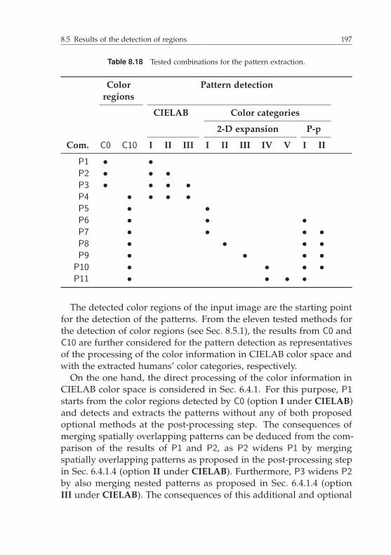
8.5 Results of the detection of regions 197
Table 8.18 Tested combinations for the pattern extraction.
Color Pattern detectionregions
CIELAB Color categories
2-D expansion P-p
Com. C0 C10 I II III I II III IV V I II
P1 • •P2 • • •P3 • • • •P4 • • • •P5 • •P6 • • •P7 • • • •P8 • • • •P9 • • • •
P10 • • • •P11 • • • •
The detected color regions of the input image are the starting pointfor the detection of the patterns. From the eleven tested methods forthe detection of color regions (see Sec. 8.5.1), the results from C0 andC10 are further considered for the pattern detection as representativesof the processing of the color information in CIELAB color space andwith the extracted humans’ color categories, respectively.
On the one hand, the direct processing of the color information inCIELAB color space is considered in Sec. 6.4.1. For this purpose, P1starts from the color regions detected by C0 (option I under CIELAB)and detects and extracts the patterns without any of both proposedoptional methods at the post-processing step. The consequences ofmerging spatially overlapping patterns can be deduced from the com-parison of the results of P1 and P2, as P2 widens P1 by mergingspatially overlapping patterns as proposed in the post-processing stepin Sec. 6.4.1.4 (option II under CIELAB). Furthermore, P3 widens P2by also merging nested patterns as proposed in Sec. 6.4.1.4 (optionIII under CIELAB). The consequences of this additional and optional
198 8 Results
approach can therefore be concluded from the comparison of their re-spective results. The last tested combination considering the processingof color directly in the CIELAB color space for the pattern detection isP4, which also includes both optional post-processing methods. How-ever, in contrast to P3, the color regions used for the pattern detectionare the ones detected by the color categories via the combination C10(see Table 8.16) instead of C0.
On the other hand, humans’ color categories are considered for colorrepresentation and processing for the pattern detection and extrac-tion in Sec. 6.4.2. A total of seven different combinations are testedto prove their suitability for pattern extraction. The color regions ex-tracted via C10 are used as starting point for the pattern extraction,as this combination reached the best trade-off. Due to this fact, thecolor information is presented from now on via the normalized likeli-hood functions and compared via the distance function based on thecorrelation function. Four different similarity comparisons are pro-posed in Sec. 6.4.2.3 to expand the one-dimensional detected patternto a two-dimensional one. P5 uses the approximation of the colorsin the pattern as similarity criterion (option I under 2-D expansion)with no post-processing after the expansion of the one-dimensionalpattern to a two-dimensional one. P6 widens P5 by including the post-processing approach of merging patterns with a high percentage of areain common once the one-dimensional pattern has been expanded to atwo-dimensional one as presented in Sec. 6.4.2.4 (option I under P-p).The inclusion of all proposed approaches at the post-processing step(see Sec. 6.4.2.4), the merger of patterns with a high percentage of areain common and also with highly overlapping areas spanned by theirconvex hulls (option II under P-p) are done at the combination P7 asan expansion of P5 and P6.
The three remaining similarity comparisons used to expand the one-dimensional pattern to a two-dimensional one (presented in Sec. 6.4.2.3)are tested in P8, which considers the approximation of the colors andsizes of the color regions belonging to the pattern (option II under 2-Dexpansion), P9, which uses an exact color comparison (option III under2-D expansion), and P10, which considers an exact comparison of thecolor and size of the color regions (option IV under 2-D expansion). Forthese combinations both optional approaches from the post-processingstep are also implemented. The consequences of the different similarity

8.5 Results of the detection of regions 199
comparisons can be therefore deduced from the comparisons betweeneach other and with P7.
Finally, P10 is widened to P11 by incorporating the optional process-ing approach proposed at the expansion of the one-dimensional patternto the two-dimensional one in Sec. 6.4.2.3, where patterns with convexhulls that highly overlap are merged directly, without waiting to thepost-processing step (option V under 2-D expansion).
Across the results of the eleven presented combinations the conse-quences of the different methods presented in Sec. 6.4 can be deducedwithout the need of implementing the 396 possible combinations, 36 ifonly the pattern extraction is considered.
The evaluation criteria used to compare the results of the differentmethods to detect and extract patterns are presented in Sec. 8.5.2.1 andthe evaluation results are then shown and discussed in Sec. 8.5.2.2.
8.5.2.1 Evaluation criteria
The goodness of the detection of the patterns and the quality of the ex-tracted patterns are considered for the evaluation of the results. For thispurpose, the tested combinations presented in Table 8.18 are evaluatedat the IIIT patterned image database.
The goodness of the detection is measured using three parameters.The first one is the total number of patterns that has been detectedand extracted. Many valid patterns may be detected at the real images.However, if further knowledge is incorporated, patterns that form sur-faces of objects or textiles will be more significant than patterns thatappear between the color regions of different objects. As the IIIT pat-terned image database consists of 57 patterned objects and backgroundsof near-regular texture types, the number of near-regular textures atdetected and extracted patterns is used as second evaluation parameter.The higher this parameter is, the better the detection of patterns will be.The third parameter is the number of repeatedly extracted patterns con-taining one of the already detected near-regular textures. The smaller itis, the less overhead indicating better detection results.
The quality of the extracted patterns is measured at the extractedpatterns that contain some part of one of the near-regular textures. Asin Sec. 8.4.2.1 ground truth data has been manually generated firstfrom the images in the database, highlighting the surfaces of objects

200 8 Results
or backgrounds that contain a valid near-regular texture. While theground truth data from Sec. 8.4.2.1 is orientated towards near-regularlytextured surfaces, the whole surface of the object is considered here (seeFig. 8.20). Two characteristics are obtained from the comparison of theareas spanned by the extracted patterns and the surfaces of the objectsand backgrounds stored as ground truth data.
Figure 8.20 Examples of manually labeled ground truth data, highlighted in red, forthe input images shown on the left. Whereas in Sec. 8.4.2.1 the ground truth is orientatedtowards near-regular textures (middle), the whole surface of the object is considered here(right).
On the one hand, the higher the overlap of the areas stored as groundtruth data with the areas of the extracted patterns, the better the near-regular textures are detected and extracted as a single pattern (seeFig. 8.21). The first characteristic qP4(gu) is therefore the common areanormalized by the real area of the surface. The mean value μ(qP4(gu))
and standard deviation σ(qP4(gu)) of qP4(gu) over all detected patternsare the first quality parameters.

8.5 Results of the detection of regions 201
Pattern extraction
Quality of thedetected patterns
Common area Disjunctive area
Figure 8.21 Overview of the characteristics used to measure the quality of the extracion.The ground truth data is highlighted in the input image in red, whereas the common areaof the ground truth and the extracted pattern in blue, and their respective disjunctivearea in green over the extracted pattern.
On the other hand, the bigger the amount of area of the extractedpatterns that overlap with the areas stored as ground truth data, thebetter the quality of the extraction will be. The second characteristic

202 8 Results
is therefore the common area normalized by the total area of the ex-tracted pattern qP5(gu). This characteristic considers the disjunctivearea between the extracted pattern and the ground truth area of thepatterned surface (see Fig. 8.21). The bigger qP5(gu) is, the better thequality of the pattern extraction will be, as less color regions are addedto the extracted pattern that do not belong to the textured surface ofthe object or background. The mean value μ(qP5(gu)) and standarddeviation σ(qP5(gu)) of qP5(gu) over all considered patterns are alsoused as quality criteria of the pattern extraction.
The higher qP4(gu) and qP5(gu) are, the better the quality of theextraction will be. However, a smaller qP4(gu) combined with a higherqP5(gu) is better than the other way around as it means an incompleteextraction of the whole surface but no wrongly incorporated regionsto the pattern. This information about the relation between qP4(gu)
and qP5(gu) gets lost when the mean values and standard deviationsare calculated over all extracted patterns. To overcome this, qP6(gu) isdefined as
qP6(gu) =100 % − qP5(gu)
qP4(gu)(8.12)
per extracted pattern. The smaller qP6(gu) is, the better the patternextraction will be. The mean value of μ(qP6(gu)) over all consideredextracted patterns is the last parameter used to measure the quality ofthe pattern extraction.
Finally, qP4(gu) is plotted over qP5(gu) for every extracted pattern pertested combination. The higher the density of the points on the righthand side of the plot is, the better the quality of the extraction will be, asless color regions have been added to the pattern that do not belong toany near-regular texture. In the ideal case all of the plotted points willlie on the upper right corner of the plot. This implies a high coverageof the near-regular textures by the extracted patterns with no inclusionof foreign color regions to the surfaces of the extracted patterns.
8.5.2.2 Evaluation results
The extracted parameters to measure the goodness of the pattern detec-tion and extraction are shown in Table 8.19. All is the total number of

8.5 Results of the detection of regions 203
extracted patterns, Tex the total number of near-regular textures thatare part of an extracted pattern, and Rep the total number of repeatedlyextracted patterns that contain a near-regular texture that is alreadypart of another extracted pattern. The total number of near-regulartextures that should be represented in the extracted patterns is 57.
The parameters used to measure the goodness of the detection canbe divided into two groups, which correspond with the two paths to pro-cess the color information during the pattern detection and extraction.The direct processing of the color information in CIELAB color space(P1 to P4) yields in total a lower number of extracted patterns togetherwith a lower number of extracted patterns containing a near-regulartexture and repetitions from it.
72 patterns are extracted from the whole database when the colorinformation is directly processed in the CIELAB color space and noneof the optional methods at the post-processing step are used (P1). Fromthe 57 near-regular textures 89.47 % can be recognized in at least one ofthe extracted patterns and 4 of the extracted patterns repeat an alreadyrecognized near-regular texture.
The merger of spatially overlapping patterns as an additional post-processing step (P2 vs. P1) does not increment the total number ofextracted patterns, but it increments the near-regular textures that arepart of an extracted pattern to 91.23 % and the number of extractedpatterns that contain a near-regular texture that is already part ofanother extracted pattern to 6.
If nested patterns are also merged as a further additional post-pro-cessing step (P3), then the percentage of near-regular textures being partof an extracted pattern remains by 91.23 %, but the number of extractedpatterns repeating a near-regular texture placed already at anotherextracted pattern is reduced to 2, which may imply less overhead.Also the number of total extracted patterns is decreased in this caseto 66. The conclusion can therefore be drawn that the inclusion ofboth additional post-processing steps proposed in Sec. 6.4.1.4 to mergespatially overlapping and nested patterns improves the goodness ofthe pattern detection as more of the near-regular textures are part ofthe extracted patterns at a decrease of extracted patterns repeatingnear-regular textures.

204 8 Results
Table8.19
Eval
uati
onof
the
patt
ern
dete
ctio
nan
dex
trac
tion
qual
ity.
Goo
dnes
sof
the
Qua
lity
ofth
eex
trac
ted
patt
erns
dete
ctio
ns
All
Tex
Rep
qP4(g
u)
qP5(g
u)
qP6(g
u)
Com
.μ
σμ
σμ
P1
7251
481
.34
%26
.14
%90
.41
%20
.62
%0.
10P2
7252
674
.84
%29
.34
%91
.01
%20
.00
%0.
10P3
6652
285
.04
%22
.50
%89
.47
%21
.09
%0.
11P4
6249
291
.35
%19
.07
%72
.77
%26
.76
%0.
54P5
1143
5710
0252
.68
%30
.72
%88
.81
%21
.21
%0.
41P6
165
5769
39.1
7%
36.5
2%
96.0
6%
10.9
6%
0.21
P7
165
5760
39.8
4%
38.2
3%
95.7
8%
1.33
%0.
22P8
327
5625
513
.63
%25
.21
%99
.40
%4.
27%
0.17
P9
9456
970
.41
%29
.18
%91
.34
%17
.02
%0.
13P10
101
5716
62.6
7%
30.9
0%
98.2
4%
4.69
%0.
02P11
122
5721
58.6
3%
33.8
2%
97.3
5%
8.06
%0.
06
The combination of extracted color regions with color categories andpattern extraction processing the color information directly in CIELABcolor space (P4) reduces the quality of the detected patterns. In contrastto a full processing of the color in CIELAB color space, only 85.96 % ofthe near-regular textures are part of an extracted pattern vs. the 91.23 %achieved by the tested combination P3.
On the other hand, the processing of the color information with thecolor categories (P5 to P11) increments the number of patterns contain-ing a near-regular texture and the total number of extracted patterns.

8.5 Results of the detection of regions 205
A 100 % inclusion of the types of near-regular textures in the ex-tracted patterns is already achieved by the combination P5, which usesthe approximation of the colors in the pattern as similarity criterionto expand the one-dimensional pattern to a two-dimensional one andno post-processing. However, this combination also yields the high-est number of extracted patterns with near-regular textures alreadyincluded in other extracted patterns, which implies a high overhead.
The expansion of P5 by the merger of patterns with a high percentageof area in common once the one-dimensional pattern has been expandedto the two-dimensional one (P6) also reaches the 100 % inclusion of thetypes of near-regular textures in the extracted patterns. Furthermore,P6 reduces in comparison with P5 the number of extracted patterns thatrepeat an already detected near-regular texture by 93.11 %. The totalnumber of extracted patterns is also reduced, in this case by 85.56 %.These big reductions imply an improvement of the goodness of thedetection towards the combination P5, as less overhead is created.
If extracted patterns whose convex hulls highly overlap are alsomerged (P7), then the total number of extracted patterns repeating analready extracted near-regular texture is further reduced by 13.04 %,with no deterioration of the 100 % recognition of the near-regular tex-tures in the extracted patterns and no increment of the total number ofextracted patterns. By these means, the incorporation of both optionalmethods presented in Sec. 6.4.2.4 for the post-processing step is highlyencouraged as it improves all of the parameters used to measure thegoodness of the detection.
The similarity comparisons used to expand the one-dimensional pat-tern to a two-dimensional one influence the goodness of the detection.Whereas the similarity comparisons based on the approximation ofthe colors and sizes of the color regions belonging to the pattern (P8),as well as the exact color comparison (P9), do not contain over theextracted patterns any part of one of the near-regular textures (retrievalquote of 98.25 %), the similarity comparison based on the exact com-parison of the color and size of the color regions (P10) achieves a 100 %retrieval quote. What is more, the combination P10 achieves under allcombinations with a 100 % retrieval quote of the near-regular texturesthe lowest number of extracted patterns that contain a near-regulartexture that is already part of another extracted pattern and the lowestnumber of extracted patterns. It possesses therefore the best trade-

206 8 Results
off between extracting as many patterns with near-regular textures aspossible and as less number of repeated extracted patterns as possible.
Comparable good detection results are yielded by the combinationP11, which merges patterns whose convex hulls highly overlap directlyat the expansion of the one-dimensional patterns to the two-dimensionalones, without waiting to the post-processing step. While this combi-nation produces some overhead of the results compared to P10, itaccelerates the time needed for the pattern extraction.
The quality of the pattern extraction is discussed next. The methodsbased on the direct processing of the color in the CIELAB color space(P1 to P4) yield a better coverage of the area of the near-regular texturesqP4(gu) than the methods that process the color information with thecolor categories. The highest coverage is reached on average (91.35 %)by P4, which uses the extracted color regions via the color categoriesfor the pattern extraction. However, this combination also possessesthe lowest μ(qP5(gu)). Together with the high μ(qP6(gu)), it indicatesthat many color regions were added by P4 to the extracted patternsthat do not belong to the surfaces of the near-regularly textured objectsand backgrounds. Among the other three tested combinations process-ing the color information directly in the CIELAB color space for thepattern extraction, comparable quality parameters are achieved. Whilethe incorporation of all proposed optional post-processing steps (P3)yields the second highest μ(qP4(gu)), it also yields the second lowestσ(qP4(gu)). The highest μ(qP5(gu)) is reached by the combination thatmerges spatially overlapping patterns (P2), which achieves otherwisethe lowest μ(qP4(gu)). If μ(qP6(gu)) is considered, then the combina-tions P1 and P2 are slightly better than P3. These impressions of thequality of the extractions are confirmed at the plots of qP4(gu) overqP5(gu) (see Fig. 8.22 upper row and second row left). P1 to P3 yieldcomparable results. Many of their points possess an qP4(gu) value closeto 100 %, but some points also have a low qP5(gu) value. The worseresults are yielded by the combination P4. The incorporation of manycolor regions that do not belong to the near-regular textures to theextracted patterns explains the high number of extracted regions with alower qP5(gu) combined with a high qP4(gu).

8.5 Results of the detection of regions 207
0% 50% 100%0%
50%
100%
qP5(gu)
qP4(g
u)
P1
0% 50% 100%0%
50%
100%
qP5(gu)
qP4(g
u)
P2
0% 50% 100%0%
50%
100%
qP5(gu)
qP4(g
u)
P3
0% 50% 100%0%
50%
100%
qP5(gu)
qP4(g
u)
P4
0% 50% 100%0%
50%
100%
qP5(gu)
qP4(g
u)
P5
0% 50% 100%0%
50%
100%
qP5(gu)
qP4(g
u)
P6
0% 50% 100%0%
50%
100%
qP5(gu)
qP4(g
u)
P7
0% 50% 100%0%
50%
100%
qP5(gu)
qP4(g
u)
P8
0% 50% 100%0%
50%
100%
qP5(gu)
qP4(g
u)
P9
0% 50% 100%0%
50%
100%
qP5(gu)
qP4(g
u)
P10
0% 50% 100%0%
50%
100%
qP5(gu)
qP4(g
u)
P11
Figure 8.22 qP4(gu) over qP5(gu) for all tested combinations.
On the other hand, the combinations based on the processing of thecolor information by the color categories (P5 to P11) achieve on averagethe highest qP5 rates. This implies that less color regions are added tothe extracted patterns that do not form part of the near-regular textures.

208 8 Results
Along the μ(qP6(gu)) values the consequences of the different pro-posed methods for the pattern extraction considering the color infor-mation by color categories can be recognized. The merger of patternswith a high percentage of area in common (P6), as well as the themerger of patterns whose convex hulls highly overlap once the one-dimensional pattern has been extracted to a two-dimensional one (P7),reduces μ(qP6(gu)) in comparison with no implementation of the post-processing steps (P5) almost by a half. This implies a clear improvementof the quality of the pattern extraction.
Furthermore, the use of different similarity comparisons to expandthe one-dimensional patterns to two-dimensional ones also has impli-cations on μ(qP6(gu)). The consideration of the approximation of thecolors and sizes of the color regions appearing in the pattern (P8) aswell as an exact color comparison (P9) reduces μ(qP6(gu)) in contrastto the consideration of the similarity comparison by an approximationof the colors (P7). However, the best μ(qP6(gu)) among all of the testedcombinations for the pattern extraction is reached by the combinationP10, which considers an exact comparison of the color and size ofthe color regions belonging to the patterns when the one-dimensionalpatterns are expanded to two-dimensional ones plus the merger ofpatterns with a high percentage of area in common. The μ(qP4(gu))
over μ(qP5(gu)) plots from P5 to P10 ratify this knowledge. The use ofthe post-processing steps (P6 and P7 vs. P5) increments the density ofthe points on the right hand side of the plots. This is also achieved bythe incorporation of the size information of the color regions belongingto the patterns when the one-dimensional patterns are expanded totwo-dimensional ones (P8). These points are further concentrated onthe right hand side of the plot if exact similarity comparisons (P9 andP10) are used instead of approximated ones (P7 and P8).
The direct merger of patterns whose convex hulls highly overlap atthe expansion of the one-dimensional patterns to two-dimensional ones(P11) reaches the second best μ(qP6(gu)) value.
Overall, the following conclusions can be drawn. The pattern ex-traction processing the color information with color categories yieldsbetter results than the direct processing of the color in the CIELAB colorspace. The combination P10 reaches the best results as it incorporatesparts from all of the near-regular textures in extracted patterns and

8.6 Results of the fusion of the methods 209
it possesses the highest quality of the extracted patterns. The highμ(qP5(gu)) values confirm that P10 did not add extra color regions tothe patterns that describe parts of the near-regular textures. Althoughμ(qP4(gu)) values are not concentrated around 100 %, 71.23 % of theextracted patterns that contain a part of a near-regular texture coverthese ones by more than 50 % (see Fig. 8.23).
10 20 30 40 50 60 700 %
20 %40 %60 %80 %
100 %
Figure 8.23 qP4(gu) over all extracted patterns using the combination P10 that containpart of a near-regular texture.
8.6 Results of the fusion of the methods
In this section the results achieved by the fusion of the proposed meth-ods according to Sec. 7 are presented. The extracted significant pat-terned regions are presented and evaluated in Sec. 8.6.1, whereas the re-sults of the sorting of the images fusing their color, shape, and texture in-formation are shown in Sec. 8.6.2 together with their evaluation method.
8.6.1 Significant patterned regions
The consequences of the fusion of the near-regular textures from Sec.5.3 and the extracted patterned regions from Sec. 6 to extract significantpatterned regions as presented in Sec. 7.1 are considered in this sec-tion. For this purpose, the detected and extracted near-regular texturesfrom combination N13 (see Tables 8.12 and 8.13) are combined withthe extracted patterned regions from the combination P10 (see Table8.18), as they reached the best trade-off between a high detection andextraction quality.

210 8 Results
Like in Sec. 8.5.2, the quality of the detected significant patternsand their extraction quality are important. Because of this, the qualitycriteria presented in Sec. 8.5.2.1 to evaluate the results are also used inthis section to evaluate the significant patterned regions. The resultsare presented in Sec. 8.6.1.1.
8.6.1.1 Evaluation results
The evaluation results are shown in Table 8.20. P10 are the resultsachieved by the region detector before its fusion with the informationfrom the near-regular textures. SP1 are the results yielded beforethe significant patterned regions are extracted, at the stage where thedetected and extracted patterns are fused with the help of the mask ofthe near-regular textures. SP2 are the results achieved by the extractedsignificant patterned regions.
Table 8.20 Evaluation of the pattern detection and extraction quality.
Goodness of Quality of the extracted patternsthe detections
All Tex Rep qP4(gu) qP5(gu) qP6(gu)
Com. μ σ μ σ μ
P10 101 57 16 62.67 % 30.90 % 98.24 % 4.69 % 0.02SP1 84 57 2 77.73 % 17.46 % 97.83 % 5.27 % 0.03SP2 61 57 2 75.61 % 19.84 % 98.03 % 5.02 % 0.03
The fusion of the extracted patterned regions with the mask of thenear-regular textures reduces the extracted patterns to 16.83 % and thepatterned regions that contain a near-regular texture that is already partof another pattern by 87.50 %. As all of the near-regular textures are stilldetected, the quality of the detected patterns is improved compared tothe results achieved by the region detector. Furthermore, the goodnessof the detections is also better than the one achieved by the method todetect the near-regular textures, which detects 55 from the 57 surfaces.
With respect to the quality of the extracted patterns, the percentage ofground truth area covered by the patterns μ(qP4(gu)) of the combinationSP1 (77.73 %) is higher than the one reached by P10 (62.67 %). Further-
8.6 Results of the fusion of the methods 211
more, the standard deviation σ(qP4(gu)) reached by SP1 is almost thehalf of the one reached by P10, which implies a higher robustnessof the combination SP1 towards the analyzed image. μ(qP5(gu)) andμ(qP6(gu)) achieved by SP1 are slightly worse than those achieved byP10, but due to the considerable increment of μ(qP4(gu)) and decreaseof σ(qP4(gu)) the quality of the patterns extracted via the combinationSP1 is higher than the one extracted via P10.
The quality results of the detected significant patterns (SP2) showan improvement compared to the patterned regions detected by P10.The reduction of the detected regions by a 39.60 % implies that re-dundant extracted patterned regions are suppressed, without havingworsened the number of patterns that contain part of a near-regulartexture (100 % detection rate). Furthermore, the number of extractedpatterned regions that contain a near-regular texture that is already partof another extracted region is clearly reduced by SP2 in comparisonwith P10 (87.50 %).
The quality of the extracted patterns achieved by SP2 is comparable tothe results achieved by SP1 and therefore better than the ones achievedby P10. In this case SP2 yields a slightly better qP5(gu) than SP1 but aslightly worsen qP4(gu). However, both combinations reach a similargood qP6(gu).
Overall, the following conclusions can be drawn. The fusion ofthe extracted patterns from Sec. 8.5.2 with the extracted near-regulartextures from Sec. 8.4.2 to extract significant regions as presented inSec. 7.1 improves the results. On the one hand, the goodness of thedetections is higher, as no representative patterns are suppressed andredundant ones are clearly reduced. On the other hand, the quality ofthe extracted patterns is also improved. Although the percentage ofthe patterns that lie on a ground-truth pattern is slightly worsen, thecovered area of the ground truth data is clearly higher and more robusttowards the input image.
8.6.2 Image sorting according to their similarity fusingcolor, shape, and texture information
In this section the results of the fusion of the extracted patterned regionswith their color, shape, and texture information in a content-based im-

212 8 Results
age retrieval environment are presented. As introduced in Sec. 7.2.2, theimages in the database are sorted in a first step three times accordingto their color, shape, and texture information, respectively. The featuresdescribing these properties are extracted as described in Sec. 7.2.1. Theearth mover’s distance is then used to compare the extracted compactcolor signatures between the images as in Sec. 8.2.1, whereas the normalangular descriptors are warped first and compared next using the corre-lation for circular data dNAD
2 , which yielded the best results in Sec. 8.3.Furthermore, at the sorting of regular textures according to Sec. 5.2.3,the strength of the different properties that are compared can be differ-ently selected. In Sec. 8.4.1.5 results were presented for regular texturesfor two strength combinations of the parameters: considering all simi-larity comparisons as equally important wk = 1, k ∈ {1, 2, 3, 4, 5, 6, 7},and considering all similarity comparisons except for the one consid-ering the orientation wk = 1, k ∈ {1, 2, 3, 4, 5, 6} , w7 = 0. At thispoint, the use of all similarity comparisons apart from those com-paring the orientation of the textures and the regions in their texelswk = 1, k ∈ {1, 2, 3, 4, 6} , w5 = 0, w7 = 0, is also considered. Thisis motivated from the suspicion that due to the projection of the tex-els from the image plane to the quadrangles of equal shape usingthe affine transformation and the nearest neighbor interpolation, clearboundaries between the regions may be difficult to find, hindering thedetection of the regions in the image via the watershed filling method(see Sec. 5.2.3).
Furthermore, to evaluate the consequences of the fusion of the color,shape, and texture information for the sorting of the images, the perfor-mance will be compared to those achieved if only the color, the shape,or the texture information is used. The evaluation criteria are explainedin Sec. 8.6.2.1 followed by the results in Sec. 8.6.2.2.
8.6.2.1 Evaluation criteria
The retrieval quality according to the content of the images is evaluatedvia the IIIT patterned image database and the parameter qretrpresentedin Sec. 8.1.2.1. For this purpose, good matches of the images have tobe defined. Within the content of the images in the database, eightcharacteristic classes can be found that are repeated over the images inthe database, showing color, shape, or texture variations. Two images

8.6 Results of the fusion of the methods 213
per class are shown in Fig. 8.24. The images are considered similarbecause they possess at least one region with high similarity in color,shape, or texture, but at least two of the characteristics (e.g., color andshape, or shape and texture) must be similar. For evaluation purposesevery extracted significant patterned region is assigned to one of theseeight classes, or a ninth class Other in case that the considered regionis not similar to the regions that belong to the eight first classes. Thenumber of representatives per class is shown in Fig. 8.25. Notice thatthe classes do not have the same sizes.
Per image in the database that contains a significant patterned regionbelonging to one of the eight classes, the quality of their retrievals iscalculated via qretr. Every significant patterned region that belongsto its class is considered as a good match. Per class the mean valueμ(qretr) and standard deviation σ(qretr) are calculated over the qretr
values achieved by the sorting results of every significant patternedregion belonging to the class.
Finally, the mean value is also calculated from the qretr values achievedby all extracted significant patterned regions that belong to one of theeight characteristic classes and also over the mean qretr achieved perclass, to weight all classes as equally important. This avoids that a classconsisting of more objects than others distorts the results if it yieldsvery good or very bad results.
8.6.2.2 Evaluation results
The evaluation results according to the criteria presented in Sec. 8.6.2.1are shown next.
The sorting of the images using only the texture information isconsidered first. The retrieval results for the three tested strength com-binations of the similarity distances are shown in Table 8.21. The resultsshow that depending on the characteristic class different strength com-binations of the similarity distances yield better results. However, if theaverage over all images and the average over all classes are considered,then the combination that does not consider the comparisons of the ori-entations and regions in the texels yields the best results. Furthermore,apart from the characteristic class Bell, this combination never yieldsover the other characteristic classes the worst average of qretr. All in all,this combination yields therefore the best trade-off over all retrievals.
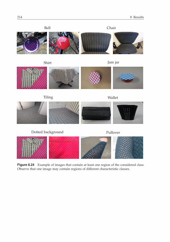
214 8 Results
Bell Chair
Shirt Jam jar
Tiling Wallet
Dotted background Pullover
Figure 8.24 Example of images that contain at least one region of the considered class.Observe that one image may contain regions of different characteristic classes.

8.6 Results of the fusion of the methods 215
Bell
Chair
Shirt
Jamjar
Tiling
Wallet
Dotted
background
Pullover
Other
0
5
10
15
Figure 8.25 Histogram of the characteristic classes.
The performance of the method considering the color, texture, andshape information is considered next. The evaluated parametersare shown in Table 8.22 for the cases when only the color informa-tion (Color), the shape information (Shape), the texture information(Texture), and the fusion of all of the methods (Fusion) is used. Theevaluated parameters considering only the texture information are theones from the combination that consider all similarity distances exceptthose considering the rotation of the textures and the regions in theirtexels wk = 1, k ∈ {1, 2, 3, 4, 6} , w5 = 0, w7 = 0, as this yielded thebest trade-off over all considered images and classes from the threetested combinations.
Let us concentrate first on the results achieved when only one char-acteristic is used to sort the images. Depending on the consideredcharacteristic class the color, the shape, or the texture informationyields better results. This strengths the statement from Sec. 7.2.2: thetotal similarity does not always depend with the same strength on the differentcharacteristics. This is reasonable as significant patterned regions thatbelong to a characteristic class have similar color, shape, or textureproperties in common but always at least two of the properties. How-ever, the sorting of the images according to the shape similarities oftheir extracted significant patterned regions yields on average over allimages in the database and over the classes the worst results, whereasthe texture information yields the second best results and the colorinformation achieves the best ones.
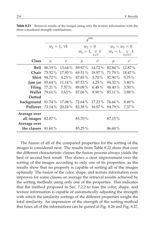
216 8 Results
Table 8.21 Retrieval results of the images using only the texture information with thethree considered strength combinations.
qretr
wk = 1, ∀k w7 = 0 w5 = w7 = 0wk = 1, ∀
k �=7k wk = 1, ∀
k �=5,7k
Class μ σ μ σ μ σ
Bell 86.19 % 13.64 % 89.97 % 14.72 % 82.84 % 12.87 %Chair 75.52 % 17.95 % 69.51 % 18.97 % 71.79 % 18.47 %Shirt 94.72 % 4.23 % 87.85 % 5.70 % 92.90 % 5.75 %
Jam jar 85.64 % 11.14 % 87.53 % 4.25 % 94.32 % 3.40 %Tiling 77.21 % 7.57 % 89.09 % 6.48 % 94.40 % 3.50 %Wallet 79.61 % 3.63 % 87.06 % 8.90 % 85.11 % 3.88 %Dotted
background 81.74 % 17.08 % 72.64 % 17.23 % 76.66 % 8.49 %Pullover 72.14 % 20.24 % 82.38 % 16.07 % 94.79 % 7.37 %
Average overall images 82.87 % 83.70 % 87.15 %
Average overthe classes 81.60 % 83.25 % 86.60 %
The fusion of all of the compared properties for the sorting of theimages is considered next. The results from Table 8.22 show that overthe different characteristic classes the fusion process always yields thebest or second best result. This shows a clear improvement over thesorting of the images according to only one of its properties, as theresults show that no property is capable of sorting all of the imagesoptimally. The fusion of the color, shape, and texture information evenimproves for some classes on average the retrieval results achieved bythe sorting methods using only one of the properties. This indicatesthat the method proposed in Sec. 7.2.2 to fuse the color, shape, andtexture information is capable of automatically adjusting the strengthwith which the similarity sortings of the different properties weight thetotal similarity. An impression of the strength of the sorting methodthat fuses all of the informations can be gained at Fig. 8.26 and Fig. 8.27,

8.6 Results of the fusion of the methods 217
where the first eight retrievals are shown for images from the character-istic classes Jam jar, Wallet, Chair, and Tiling.
Overall, the following conclusions can be drawn. The fusion of theextracted significant patterned regions with their sorting according totheir color, shape, and texture information shows promising results fora retrieval of images according to the similarity of their content. Theresults show that a method capable of adjusting the strength of the color,shape, and texture similarity depending on the images compared forthe estimation of the total similarity between images is advantageous.
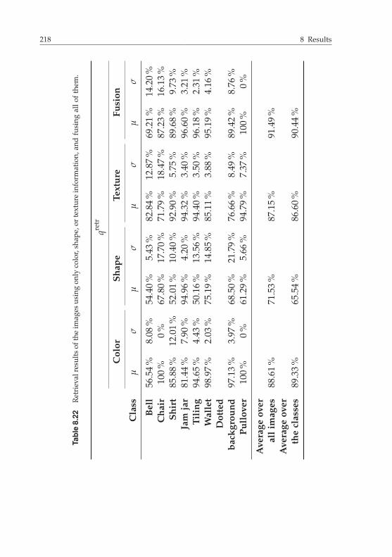
218 8 Results
Table8.22
Ret
riev
alre
sults
ofth
eim
ages
usin
gon
lyco
lor,
shap
e,or
text
ure
info
rmat
ion,
and
fusi
ngal
lof
them
.
qretr
Col
orSh
ape
Text
ure
Fusi
on
Cla
ssμ
σμ
σμ
σμ
σ
Bel
l56
.54
%8.
08%
54.4
0%
5.43
%82
.84
%12
.87
%69
.21
%14
.20
%C
hair
100
%0
%67
.80
%17
.70
%71
.79
%18
.47
%87
.23
%16
.13
%Sh
irt
85.8
8%
12.0
1%
52.0
1%
10.4
0%
92.9
0%
5.75
%89
.68
%9.
73%
Jam
jar
81.4
4%
7.90
%94
.96
%4.
20%
94.3
2%
3.40
%96
.60
%3.
21%
Tili
ng94
.65
%4.
43%
50.1
6%
13.5
6%
94.4
0%
3.50
%96
.18
%2.
31%
Wal
let
98.9
7%
2.03
%75
.19
%14
.85
%85
.11
%3.
88%
95.1
9%
4.16
%D
otte
dba
ckgr
ound
97.1
3%
3.97
%68
.50
%21
.79
%76
.66
%8.
49%
89.4
2%
8.76
%Pu
llov
er10
0%
0%
61.2
9%
5.66
%94
.79
%7.
37%
100
%0
%
Ave
rage
over
all
imag
es88
.61
%71
.53
%87
.15
%91
.49
%A
vera
geov
erth
ecl
asse
s89
.33
%65
.54
%86
.60
%90
.44
%

8.6 Results of the fusion of the methods 219
Input 1. 2. 3.
4. 5. 6. 7.
Input 1. 2. 3.
4. 5. 6. 7.
Figure 8.26 First seven retrieved images for an image of the class jam jar (top) and animage of the class Wallet (bottom). The number indicates the retrieval position.
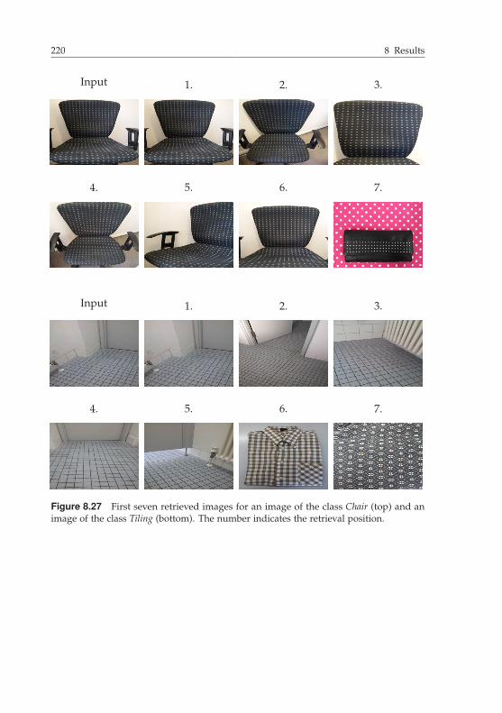
220 8 Results
Input 1. 2. 3.
4. 5. 6. 7.
Input 1. 2. 3.
4. 5. 6. 7.
Figure 8.27 First seven retrieved images for an image of the class Chair (top) and animage of the class Tiling (bottom). The number indicates the retrieval position.
9 Conclusions
In this work the content-based image retrieval problem is consid-ered. The extraction of color, shape, and texture features togetherwith the detection of significant regions in the image are selected asmodus operandi.
Every block forming part of the image retrieval approach is inves-tigated. Solutions are proposed for all of them and conscientiouslytested: a compact color signature (see Sec. 3.2), the color representationwith the help of the humans’ color categories (see Sec. 3.3), the normalangular descriptors (see Sec. 4.2), the detection of regular textures (seeSec. 5.2.2), features and similarity distances to compare textures ofregular type (see Sec. 5.2.3), the detection of near-regular textures andthe extraction of their regular textures (see Sec. 5.3), and the detectionand extraction of meaningful regions in images (see Sec. 6).
With the help of psychologists, an experiment with subjects hasalso been performed. Its data is used to extract a perception map ofregular textures (see Secs. 5.2.4). This one (see Sec. 8.4.1.6) indicates thesimilarity distances proposed in Sec. 5.2.3 for regular textures and theirextracted features.
Furthermore, the fusion of the detected and extracted regions withthe detected near-regular textures (see Sec. 7.1) improves the extractionof the near-regularly textured surfaces in the images, which results ina better extraction of their properties as they are less adulterated bythe neighboring regions. The sorting of the images according to theautomatic adjustment of their color, shape, and texture features (seeSec. 7.2) show promising results. This combination always yields thebest or second best retrieval result. It even outperforms in many casesthe best sorting result of images according to only one feature.
The decomposition of the problem to the detection of significantpatterned regions and the independent extraction and comparison ofthe features of the images with a final fusion via an automaticallyadjustable weight of the features is thus a powerful approach. Whereas
222 9 Conclusions
the comparison of the color, the shape, or the texture properties of theimage can be independently analyzed and enhanced in the proposedapproach, all of the properties are important and necessary to improvethe quality of the retrievals.
The proposed approach for the content-based image retrieval can befurther widened in the future. As the color representation with thehelp of the extracted humans’ color categories improves the results incomparison with the direct representation of the color in the CIELABcolor space, the analysis of the relationship between the extracted colorcategories is worthy. The spatial relation between significant patternedregions appearing in the same image is not considered for retrievalpurposes. However, this reveals information about the spatial distribu-tion of the content of the image and it could be therefore incorporatedin the future to compare the similarity between images. Finally, theverification of the ideas and concepts proposed in this thesis shall betested with more images.

Bibliography
[1] http://www.cis.temple.edu/~latecki/. Visited on 07.10.2014.
[2] https://www.mpi-inf.mpg.de/departments/computer-vision-and-multimodal-computing/software-and-datasets/. Visited on 14.03.2013.
[3] http://www.povray.org/. Visited on 22.01.2014.
[4] Afifi, A. J. and Ashour, W. M. Content-Based Image Retrieval Using Invari-ant Color and Texture Features. In: 2012 International Conference on DigitalImage Computing Techniques and Applications (DICTA). IEEE, 2012.
[5] Afifi, A. J. and Ashour, W. M. Image Retrieval Based on Content UsingColor Feature. In: ISRN Computer Graphics 2012 (2012).
[6] Ahonen, T., Matas, J., He, C., and Pietikäinen, M. Rotation InvariantImage Description with Local Binary Pattern Histogram Fourier Features. In:Image Analysis: 16th Scandinavian Conference, SCIA 2009, Oslo, Norway,June 2009. Proceedings. Ed. by Salberg, A.-B., Hardeberg, J. Y., andJenssen, R. Berlin, Heidelberg: Springer, 2009, pp. 61–70.
[7] Alabiso, C. and Weiss, I. A Primer on Hilbert Space Theory: Linear Spaces,Topological Spaces, Metric Spaces, Normed Spaces, and Topological Groups.UNITEXT for Physics. Cham i.a.: Springer, 2015.
[8] Alessio, S. M. Digital Signal Processing and Spectral Analysis for Scien-tists: Concepts and Applications. Signals and Communication Technology.Cham, i.a.: Springer, 2016.
[9] Arkin, E. M., Chew, L. P., Huttenlocher, D. P., Kedem, K., and Mitchell,J. S. B. An Efficiently Computable Metric for Comparing Polygonal Shapes.In: IEEE Transactions on Pattern Analysis and Machine Intelligence 13.3(1991), pp. 209–216.
[10] Babu Rao, M., Prabhakara Rao, B., and Govardhan, A. CTDCIRS:Content Based Image Retrieval System Based on Dominant Color and TextureFeatures. In: International Journal of Computer Applications (0975-8887)Volume 18-No.6 (2011).
[11] Backhaus, K., Erichson, B., and Weiber, R. Fortgeschrittene multivariateAnalysemethoden: Eine anwendungsorientierte Einführung. 2. ed. Springer-Lehrbuch. Berlin Heidelberg: Springer Gabler, 2013.

224 Bibliography
[12] Balakrishnan, R. and Ranganathan, K. A Textbook of Graph Theory. 2.ed. Universitext. New York, NY: Springer, 2012.
[13] Bartolini, I., Ciaccia, P., and Patella, M. Warp: Accurate Retrieval ofShapes Using Phase of Fourier Descriptors and Time Warping Distance. In:IEEE Transactions on Pattern Analysis and Machine Intelligence 27.1 (2005),pp. 142–147.
[14] Bay, H., Tuytelaars, T., and Van Gool, L. SURF: Speeded Up RobustFeatures. In: Computer Vision–ECCV 2006: 9th European Conference onComputer Vision, Graz, Austria, May 2006. Proceedings, Part I. Berlin Hei-delberg: Springer, 2006, pp. 404–417.
[15] Bay, H., Ess, A., Tuytelaars, T., and Van Gool, L. Speeded-Up RobustFeatures (SURF). In: Computer Vision and Image Understanding 110.3 (2008),pp. 346–359.
[16] Belongie, S., Malik, J., and Puzicha, J. Shape Matching and Object Recog-nition Using Shape Contexts. In: IEEE Transactions on Pattern Analysis andMachine Intelligence 24.4 (2002), pp. 509–522.
[17] Bentley, J. L. Multidimensional Binary Search Trees Used for AssociativeSearching. In: Communications of the ACM 18.9 (1975), pp. 509–517.
[18] Berlin, B. and Kay, P. Basic Color Terms: Their Universality and Evolution.Berkeley: Univ. of California Press, 1969.
[19] Beyerer, J., Puente León, F., and Frese, C. Automatische Sichtprüfung:Grundlagen, Methoden und Praxis der Bildgewinnung und Bildauswertung. 2ed. Berlin Heidelberg: Springer Vieweg, 2016.
[20] Beyerer, J., Puente León, F., and Frese, C. Machine Vision – AutomatedVisual Inspection: Theory, Practice and Applications. Berlin Heidelberg:Springer, 2016.
[21] Blackman, R. B. and Tukey, J. W. The Measurement of Power Spectra:From the Point of View of Communications Engineering. New York: DoverPublications Inc., 1958.
[22] Bohman, H. Approximate Fourier Analysis of Distribution Functions. In:Arkiv för Matematik 4.2 (1961), pp. 99–157.
[23] Broek, E. L. van den, Kisters, P. M. F., and Vuurpijl, L. G. The Utiliza-tion of Human Color Categorization for Content-Based Image Retrieval. In:Human Vision and Electronic Imaging IX. Vol. 5292. Proc. SPIE. SPIE, 2004,pp. 351–362.

Bibliography 225
[24] Broek, E. L. van den, Vuurpijl, L. G., Kisters, P. M. F., and Schmid,J. C. M. von. Content-Based Image Retrieval: Color-selection exploited. In:Proceedings of the Third Dutch-Belgian Information Retrieval Workshop (DIR-2002). Ed. by Moens, M.-F., Brusser, R. de, Hiemstra, D., and Kraaij,W. Leuven, Belgium, 2002.
[25] Burkhardt, H. Transformationen zur lageinvarianten Merkmalgewinnung.Düsseldorf: VDI-Verlag, 1979.
[26] Burkhardt, H., Fenske, A., and Schulz-Mirbach, H. Invariants for theRecognition of Planar Contour and Gray-Scale Images. In: tm - TechnischesMessen 59.10 (1992), pp. 398–407.
[27] Candès, E. J. and Donoho, D. L. Ridgelets: A Key to Higher-DimensionalIntermittency? In: Philosophical Transactions of the Royal Society of London A:Mathematical, Physical and Engineering Sciences 357.1760 (1999), pp. 2495–2509.
[28] Canny, J. A Computational Approach to Edge Detection. In: IEEE Transac-tions on Pattern Analysis and Machine Intelligence PAMI-8.6 (1986), pp. 679–698.
[29] Carrara, W. G., Goodman, R. S., and Majewski, R. M. Spotlight Syn-thetic Aperture Radar: Signal Processing Algorithms. The Artech HouseRemote Sensing Library. Boston London: Artech House, 1995.
[30] Carson, C., Belongie, S., Greenspan, H., and Malik, J. Blobworld: Im-age Segmentation Using Expectation-Maximization and Its Application toImage Querying. In: IEEE Transactions on Pattern Analysis and MachineIntelligence 24.8 (2002), pp. 1026–1038.
[31] Chalom, E., Asa, E., and Biton, E. Measuring Image Similarity: AnOverview of Some Useful Applications. In: IEEE Instrumentation & Measure-ment Magazine 16.1 (2013), pp. 24–28.
[32] Chavez, A. and Gustafson, D. Color-Based Extensions to MSERs. In:Advances in Visual Computing: 7th International Symposium, ISVC 2011, LasVegas, NV, USA, September 2011. Proceedings, Part II. Berlin Heidelberg:Springer, 2011, pp. 358–366.
[33] Cheng, Y. Mean Shift, Mode Seeking, and Clustering. In: IEEE Transactionson Pattern Analysis and Machine Intelligence 17.8 (1995), pp. 790–799.
[34] Clausi, D. A. and Jernigan, M. E. Designing Gabor Filters for OptimalTexture Separability. In: Pattern Recognition 33.11 (2000), pp. 1835–1849.
[35] Comaniciu, D. and Meer, P. Mean Shift: A Robust Approach Toward Fea-ture Space Analysis. In: IEEE Transactions on Pattern Analysis and MachineIntelligence 24.5 (2002), pp. 603–619.

226 Bibliography
[36] Crow, F. C. Summed-Area Tables for Texture Mapping. In: ACM SIGGRAPHComputer Graphics 18.3 (1984), pp. 207–212.
[37] D’Antona, G. and Ferrero, A. Digital Signal Processing for MeasurementSystems: Theory and Applications. Information Technology: Transmission,Processing, and Storage. New York, NY: Springer, 2006.
[38] Datta, R., Li, J., and Wang, J. Z. Content-Based Image Retrieval – Ap-proaches and Trends of the New Age. In: Proceedings of the 7th ACM SIGMMInternational Workshop on Multimedia Information Retrieval. MIR ’05. ACM,2005, pp. 253–262.
[39] Datta, R., Joshi, D., Li, J., and Wang, J. Z. Image Retrieval: Ideas, Influ-ences, and Trends of the New Age. In: ACM Computing Surveys 40.2 (2008),5:1–5:60.
[40] Daubechies, I. Ten Lectures on Wavelets. Philadelphia, Pa.: Society forIndustrial and Applied Mathematics, 1992.
[41] Davies, E. R. Machine Vision: Theory, Algorithms, Practicalities. 3. ed.Amsterdam [i.a.]: Morgan Kaufmann, 2005.
[42] Deng, Y. and Manjunath, B. S. Unsupervised Segmentation of Color-Texture Regions in Images and Video. In: IEEE Transactions on PatternAnalysis and Machine Intelligence 23.8 (2001), pp. 800–810.
[43] Deng, Y., Manjunath, B. S., Kenney, C., Moore, M. S., and Shin, H.An Efficient Color Representation for Image Retrieval. In: IEEE Transactionson Image Processing 10.1 (2001), pp. 140–147.
[44] Do, M. N. and Vetterli, M. The Finite Ridgelet Transform for Image Repre-sentation. In: IEEE Transactions on Image Processing 12.1 (2003), pp. 16–28.
[45] Duda, R. O., Hart, P. E., and Stork, D. G. Pattern Classification. 2. ed.New York [i.a.]: Wiley, 2001.
[46] Edelsbrunner, H., Kirkpatrick, D. G., and Seidel, R. On the Shape of aSet of Points in the Plane. In: IEEE Transactions on Information Theory 29.4(1983), pp. 551–559.
[47] Ester, M., Kriegel, H.-P., Sander, J., and Xu, X. A Density-Based Algo-rithm for Discovering Clusters in Large Spatial Databases with Noise. In:Proceedings of the Second International Conference on Knowledge Discoveryand Data Mining (KDD-96). 1996, pp. 226–231.
[48] Everitt, B. and Hothorn, T. An Introduction to Applied Multivariate Anal-ysis with R. Use R! New York, NY: Springer, 2011.
[49] Fisher, N. I. and Lee, A. J. A Correlation Coefficient for Circular Data. In:Biometrika 70.2 (1983), pp. 327–332.

Bibliography 227
[50] Forssén, P.-E. Maximally Stable Colour Regions for Recognition and Match-ing. In: IEEE Conference on Computer Vision and Pattern Recognition. 2007.
[51] Forsyth, D. A. and Ponce, J. Computer Vision: A Modern Approach. Pren-tice Hall Series in Artificial Intelligence. Upper Saddle River, NJ: PearsonEducation, 2003.
[52] Fukunaga, K. and Hostetler, L. D. The Estimation of the Gradient ofa Density Function, with Applications in Pattern Recognition. In: IEEETransactions on Information Theory 21.1 (1975), pp. 32–40.
[53] Gonde, A. B., Maheshwari, R. P., and Balasubramanian, R. MultiscaleRidgelet Transform for Content Based Image Retrieval. In: Advance ComputingConference (IACC), 2010 IEEE 2nd International. IEEE. 2010, pp. 139–144.
[54] Gonzalez, R. C. and Woods, R. E. Digital Image Processing. 3. ed. UpperSaddle River, NJ: Pearson Education, 2008.
[55] Google. https://search.googleblog.com/2011/06/search-by-text-voice-or-image.html. Visited on 25.08.2016.
[56] Google. https://support.google.com/websearch/answer/1325808?p=searchbyimagepage&hl=en. Visited on 25.08.2016.
[57] Google Images. https://images.google.com/. Visited on 25.08.2016.
[58] Gopi, E. S. Digital Speech Processing Using Matlab. Signals and Commu-nication Technology. New Delhi, i.a.: Springer, 2014.
[59] Grewal, M. S. and Andrews, A. P. Kalman Filtering: Theory and PracticeUsing MATLAB. 2. ed. New York [i.a.]: Wiley, 2001.
[60] Gupta, L. and Srinath, M. D. Contour Sequence Moments for the Classifica-tion of Closed Planar Shapes. In: Pattern Recognition 20.3 (1987), pp. 267–272.
[61] Ha, Y. H. and Pearce, J. A. A New Window and Comparison to StandardWindows. In: IEEE Transactions on Acoustics, Speech, and Signal Processing37.2 (1989), pp. 298–301.
[62] Harris, C. and Stephens, M. A Combined Corner and Edge Detector. In:In Proc. of Fourth Alvey Vision Conference. 1988, pp. 147–151.
[63] Harris, F. J. On the Use of Windows for Harmonic Analysis with the DiscreteFourier Transform. In: Proceedings of the IEEE 66.1 (1978), pp. 51–83.
[64] Hays, J., Leordeanu, M., Efros, A. A., and Liu, Y. Discovering TextureRegularity as a Higher-Order Correspondence Problem. In: Computer Vision–ECCV 2006: 9th European Conference on Computer Vision, Graz, Austria,May 2006. Proceedings, Part II. Berlin Heidelberg: Springer, 2006, pp. 522–535.
228 Bibliography
[65] Heer, J. and Stone, M. Color Naming Models for Color Selection, ImageEditing and Palette Design. In: Proceedings of the SIGCHI Conference onHuman Factors in Computing Systems. ACM. 2012, pp. 1007–1016.
[66] Hilsmann, A., Schneider, D. C., and Eisert, P. Warp-Based Near-RegularTexture Analysis for Image-Based Texture Overlay. In: Proc. InternationalWorkshop on Vision, Modeling and Visualization (VMV). Ed. by Eisert, P.,Polthier, K., and Hornegger, J. Eurographics Association, 2011, pp. 73–80.
[67] Hu, R.-X., Jia, W., Ling, H., Zhao, Y., and Gui, J. Angular Pattern andBinary Angular Pattern for Shape Retrieval. In: IEEE Transactions on ImageProcessing 23.3 (2014), pp. 1118–1127.
[68] Huang, J., Kumar, S. R., Mitra, M., Zhu, W.-J., and Zabih, R. ImageIndexing Using Color Correlograms. In: Proceedings., 1997 IEEE ComputerSociety Conference on Computer Vision and Pattern Recognition. IEEE. 1997,pp. 762–768.
[69] Huang, W., Gao, Y., and Chan, K. L. A Review of Region-Based ImageRetrieval. In: Journal of Signal Processing Systems 59.2 (2010), pp. 143–161.
[70] Jafari-Khouzani, K. and Soltanian-Zadeh, H. Radon Transform Orienta-tion Estimation for Rotation Invariant Texture Analysis. In: IEEE Transactionson Pattern Analysis and Machine Intelligence 27.6 (2005), pp. 1004–1008.
[71] Jafari-Khouzani, K. and Soltanian-Zadeh, H. Rotation-Invariant Mul-tiresolution Texture Analysis Using Radon and Wavelet Transforms. In: IEEETransactions on Image Processing 14.6 (2005), pp. 783–795.
[72] Jhanwar, N., Chaudhuri, S., Seetharaman, G., and Zavidovique, B.Content Based Image Retrieval Using Motif Cooccurrence Matrix. In: Imageand Vision Computing 22.14 (2004), pp. 1211–1220.
[73] Julesz, B. Experiments in the Visual Perception of Texture. In: ScientificAmerican 232.4 (1975), pp. 34–43.
[74] Kaiser, J. F. Nonrecursive Digital Filter Design Using the I0-sinh WindowFunction. In: Proceedings 1974 IEEE International Symposium on Circuitsand Systems. 1974.
[75] Kay, P. and Regier, T. Resolving the Question of Color Naming Universals.In: Proceedings of the National Academy of Sciences of the United States ofAmerica 100.15 (2003), pp. 9085–9089.
[76] Kiencke, U., Schwarz, M., and Weickert, T. Signalverarbeitung: Zeit-Frequenz-Analyse und Schätzverfahren. München: Oldenbourg, 2008.

Bibliography 229
[77] Konstantinidis, K., Gasteratos, A., and Andreadis, I. Image RetrievalBased on Fuzzy Color Histogram Processing. In: Optics Communications248.4-6 (2005), pp. 375–386.
[78] Kruskal, J. B. Multidimensional Scaling by Optimizing Goodness of Fit to aNonmetric Hypothesis. In: Psychometrika 29.1 (1964), pp. 1–27.
[79] Kruskal, J. B. Nonmetric Multidimensional Scaling: A Numerical Method.In: Psychometrika 29.2 (1964), pp. 115–129.
[80] Kubat, M. An Introduction to Machine Learning. Cham i.a.: Springer, 2015.
[81] Latecki, L. J. and Lakämper, R. Shape Similarity Measure Based on Cor-respondence of Visual Parts. In: IEEE Transactions on Pattern Analysis andMachine Intelligence 22.10 (2000), pp. 1185–1190.
[82] Lilien, G. L., Rangaswamy, A., and De Bruyn, A. Principles of MarketingEngineering. 2. ed. State College, Pa.: DecisionPro, 2013.
[83] Lin, C.-H., Chen, R.-T., and Chan, Y.-K. A Smart Content-Based ImageRetrieval System Based on Color and Texture Feature. In: Image and VisionComputing 27.6 (2009), pp. 658–665.
[84] Lin, H.-C., Wang, L.-L., and Yang, S.-N. Regular-Texture Image RetrievalBased on Texture-Primitive Extraction. In: Image and Vision Computing 17.1(1999), pp. 51–63.
[85] Liu, G.-H., Zhang, L., Hou, Y.-K., Li, Z.-Y., and Yang, J.-Y. Image Re-trieval Based on Multi-Texton Histogram. In: Pattern Recognition 43.7 (2010),pp. 2380–2389.
[86] Liu, Y., Lin, W.-C., and Hays, J. Near-Regular Texture Analysis and Ma-nipulation. In: ACM Transactions on Graphics (TOG) – Proceedings of ACMSIGGRAPH 2004 23.3 (2004), pp. 368–376.
[87] Liu, Y., Zhang, D., Lu, G., and Ma, W.-Y. A Survey of Content-Based ImageRetrieval with High-Level Semantics. In: Pattern Recognition 40.1 (2007),pp. 262–282.
[88] Lowe, D. G. Object Recognition from Local Scale-Invariant Features. In: TheProceedings of the Seventh IEEE International Conference on Computer Vision.IEEE. 1999.
[89] Lowe, D. G. Distinctive Image Features from Scale-Invariant Keypoints. In:International Journal of Computer Vision 60.2 (2004), pp. 91–110.
[90] Mahmoudi, F., Shanbehzadeh, J., Eftekhari-Moghadam, A.-M., andSoltanian-Zadeh, H. Image Retrieval Based on Shape Similarity by EdgeOrientation Autocorrelogram. In: Pattern Recognition 36.8 (2003), pp. 1725–1736.

230 Bibliography
[91] Mangijao Singh, S. and Hemachandran, K. Content-Based Image Re-trieval Using Color Moment and Gabor Texture Feature. In: InternationalJournal of Computer Science Issues 9.5 (2012), pp. 299–309.
[92] Manjunath, B. S. and Ma, W. Y. Texture Features for Browsing and Retrievalof Image Data. In: IEEE Transactions on Pattern Analysis and MachineIntelligence 18.8 (1996), pp. 837–842.
[93] Marques, O., Mayron, L. M., Borba, G. B., and Gamba, H. R. Using Vi-sual Attention to Extract Regions of Interest in the Context of Image Retrieval.In: Proceedings of the 44th Annual Southeast Regional Conference. ACM.2006, pp. 638–643.
[94] Marques, O., Mayron, L. M., Borba, G. B., and Gamba, H. R. AnAttention-Driven Model for Grouping Similar Images with Image RetrievalApplications. In: EURASIP Journal on Advances in Signal Processing 2007(2007), pp. 1–17.
[95] Masotti, M. and Campanini, R. Texture Classification Using InvariantRanklet Features. In: Pattern Recognition Letters 29.14 (2008), pp. 1980–1986.
[96] Matas, J., Chum, O., Urban, M., and Pajdla, T. Robust Wide-BaselineStereo from Maximally Stable Extremal Regions. In: Image and Vision Com-puting 22.10 (2004), pp. 761–767.
[97] Matlab. https://www.mathworks.com/. Last visit on 19.02.2017.
[98] Mikolajczyk, K. and Schmid, C. Indexing Based on Scale Invariant InterestPoints. In: Proceedings. Eighth IEEE International Conference on ComputerVision. IEEE. 2001, pp. 525–531.
[99] Mikolajczyk, K. and Schmid, C. An Affine Invariant Interest Point Detec-tor. In: Computer Vision - ECCV 2002: 7th European Conference on ComputerVision, Copenhagen, Denmark, May 2002. Proceedings, Part I. Springer.Berlin Heidelberg, 2002, pp. 128–142.
[100] Mikolajczyk, K. and Schmid, C. Scale & Affine Invariant Interest PointDetectors. In: International Journal of Computer Vision 60.1 (2004), pp. 63–86.
[101] Mikolajczyk, K. and Schmid, C. A Performance Evaluation of Local De-scriptors. In: IEEE Transactions on Pattern Analysis and Machine Intelligence27.10 (2005), pp. 1615–1630.
[102] Mikolajczyk, K., Tuytelaars, T., Schmid, C., Zisserman, A., Matas, J.,Schaffalitzky, F., Kadir, T., and Van Gool, L. A Comparison of AffineRegion Detectors. In: International Journal of Computer Vision 65.1 (2005),pp. 43–72.

Bibliography 231
[103] Mokhtarian, F., Abbasi, S., and Kittler, J. Robust and Efficient ShapeIndexing through Curvature Scale Space. In: Proceedings of British MachineVision Conference. 1996, pp. 53–62.
[104] Mokhtarian, F., Abbasi, S., and Kittler, J. Efficient and Robust Retrievalby Shape Content through Curvature Scale Space. In: Image Databases AndMulti-Media Search. Vol. 8. World Scientific, 1997, pp. 51–58.
[105] Mokhtarian, F. and Mackworth, A. K. A Theory of Multiscale, Curvature-Based Shape Representation for Planar Curves. In: IEEE Transactions onPattern Analysis and Machine Intelligence 14.8 (1992), pp. 789–805.
[106] Murala, S., Gonde, A. B., and Maheshwari, R. P. Color and Texture Fea-tures for Image Indexing and Retrieval. In: 2009 IEEE International AdvanceComputing Conference . IACC 2009. IEEE. 2009, pp. 1411–1416.
[107] Nadler, M. and Smith, E. P. Pattern Recognition Engineering. A Wiley-Interscience Publication. New York [i.a.]: Wiley, 1993.
[108] Niblack, W., Barber, R., Equitz, W., Flickner, M., Glasman, E.,Petkovic, D., Yanker, P., Faloutsos, C., and Taubin, G. The QBICProject: Querying Images By Content Using Color, Texture, and Shape. In:Proc. SPIE 1908, Storage and Retrieval for Image and Video Databases. 1993,pp. 173–187.
[109] Nuttall, A. H. Some Windows with Very Good Sidelobe Behavior. In: IEEETransactions on Acoustics, Speech, and Signal Processing ASSP-29.1 (1981),pp. 84–91.
[110] Ojala, T., Pietikäinen, M., and Mäenpää, T. Multiresolution Gray-Scaleand Rotation Invariant Texture Classification with Local Binary Patterns. In:IEEE Transactions on Pattern Analysis and Machine Intelligence 24.7 (2002),pp. 971–987.
[111] OpenSesame. http://osdoc.cogsci.nl/. Visited on 17.06.2015.
[112] Oppenheim, A. V. and Schafer, R. W. Discrete Time Signal Processing.Prentice Hall Signal Processing Series. Englewoods Cliffs, NJ: Prentice-Hall International, 1989.
[113] Oppenheim, A. V., Schafer, R. W., and Buck, J. R. Zeitdiskrete Sig-nalverarbeitung. 2. ed. München [i.a.]: Pearson Studium, 2004.
[114] Papoulis, A. and Unnikrishna Pillai, S. Probability, Random Variablesand Stochastic Processes. 4. ed. Boston, i.a.: McGraw-Hill, 2002.
[115] Park, M., Brocklehurst, K., Collins, R. T., and Liu, Y. Deformed LatticeDetection in Real-World Images Using Mean-Shift Belief Propagation. In:IEEE Transactions on Pattern Analysis and Machine Intelligence 31.10 (2009),pp. 1804–1816.

232 Bibliography
[116] Parzen, E. Mathematical Considerations in the Estimation of Spectra. In:Technometrics 3.2 (1961), pp. 167–190.
[117] Pass, G., Zabih, R., and Miller, J. Comparing Images Using Color Coher-ence Vectors. In: Proceedings of the Fourth ACM International Conferenceon Multimedia. MULTIMEDIA ’96. New York, NY, USA: ACM, 1996,pp. 65–73.
[118] Petrakis, E. G. M., Diplaros, A., and Milios, E. Matching and Retrievalof Distorted and Occluded Shapes Using Dynamic Programming. In: IEEETransactions on Pattern Analysis and Machine Intelligence 24.11 (2002),pp. 1501–1516.
[119] Puente León, F. Messtechnik: Systemtheorie für Ingenieure und Informatiker.10 ed. Berlin Heidelberg: Springer Vieweg, 2015.
[120] Puente León, F. and Jäkel, H. Signale und Systeme. 6. ed. Berlin/Boston:De Gruyter Oldenbourg, 2015.
[121] Puente León, F. and Kiencke, U. Ereignisdiskrete Systeme: Modellierungund Steuerung verteilter Systeme. 3. ed. München: Oldenbourg, 2013.
[122] Rubner, Y., Tomasi, C., and Guibas, L. J. The Earth Mover’s Distanceas a Metric for Image Retrieval. In: International Journal of Computer Vision40.2 (2000), pp. 99–121.
[123] Rui, Y., Huang, T. S., and Chang, S.-F. Image Retrieval: Current Tech-niques, Promising Directions, and Open Issues. In: Journal of Visual Commu-nication and Image Representation 10.1 (1999), pp. 39–62.
[124] Sajjanhar, A. and Lu, G. A Grid-Based Shape Indexing and RetrievalMethod. In: Australian Computer Journal 29.4 (1997), pp. 131–140.
[125] Sakoe, H. and Chiba, S. Dynamic Programming Algorithm Optimizationfor Spoken Word Recognition. In: IEEE Transactions on Acoustics, Speech,and Signal Processing ASSP-26.1 (1978), pp. 43–49.
[126] Schindler, G., Krishnamurthy, P., Lublinerman, R., Liu, Y., and Del-laert, F. Detecting and Matching Repeated Patterns for Automatic Geo-tagging in Urban Environments. In: IEEE Conference on Computer Visionand Pattern Recognition. 2008, pp. 1–7.
[127] Smeulders, A. W. M., Worring, M., Santini, S., Gupta, A., and Jain,R. Content-Based Image Retrieval at the End of the Early Years. In: IEEETransactions on Pattern Analysis and Machine Intelligence 22.12 (2000),pp. 1349–1380.
[128] Stehling, R. O., Nascimento, M. A., and Falcão, A. X. Cell HistogramsVersus Color Histograms for Image Representation and Retrieval. In: Knowl-edge and Information Systems 5.3 (2003), pp. 315–336.

Bibliography 233
[129] Subrahmanyam, M., Wu, Q.M. J., Maheshwari, R.P., and Balasubra-manian, R. Modified Color Motif Co-Occurrence Matrix for Image Indexingand Retrieval. In: Computers and Electrical Engineering 39.3 (2013), pp. 762–774.
[130] Suthaharan, S. Machine Learning Models and Algorithms for Big Data Clas-sification: Thinking with Examples for Effective Learning. Vol. 36. IntegratedSeries in Information Systems. New York, i.a.: Springer, 2016.
[131] Swain, M. J. and Ballard, D. H. Color Indexing. In: International Journalof Computer Vision 7.1 (1991), pp. 11–32.
[132] TinEye. https://www.tineye.com/. Visited on 25.08.2016.
[133] TinEye. https://www.tineye.com/faq#how. Visited on 25.08.2016.
[134] Tuytelaars, T. and Van Gool, L. Content-Based Image Retrieval Based onLocal Affinely Invariant Regions. In: Visual Information and InformationSystems: Third International Conference, VISUAL’99 Amsterdam, The Nether-lands. Ed. by Huijsmans, D. P. and Smeulders, A. W. M. Springer. 1999,pp. 493–500.
[135] Tuytelaars, T. and Van Gool, L. Wide Baseline Stereo Matching Basedon Local, Affinely Invariant Regions. In: Proceedings of the British MachineVision Conference. 2000.
[136] Viola, P. and Jones, M. Rapid Object Detection Using a Boosted Cascadeof Simple Features. In: Proceedings of the 2001 IEEE Computer Society Con-ference on Computer Vision and Pattern Recognition. IEEE. 2001, pp. I-511–I-518.
[137] Vogel, J. and Schiele, B. Semantic Modeling of Natural Scenes for Content-Based Image Retrieval. In: International Journal of Computer Vision 72.2(2007), pp. 133–157.
[138] Vu, V. H., Huu, Q. N., and Thu, H. N. T. Content Based Image Retrievalwith Bin of Color Histogram. In: 2012 International Conference on Audio,Language and Image Processing (ICALIP). IEEE. 2012, pp. 20–25.
[139] Wang, J. Z., Li, J., and Wiederhold, G. SIMPLIcity: Semantics-SensitiveIntegrated Matching for Picture LIbraries. In: IEEE Transactions on PatternAnalysis and Machine Intelligence 23.9 (2001), pp. 947–963.
[140] Weijer, J. van de, Schmid, C., and Verbeek, J. Learning Color Namesfrom Real-World Images. In: IEEE Conference on Computer Vision and PatternRecognition. 2007.
[141] West, D. B. Introduction to Graph Theory. 2. ed. Upper Saddle River, NJ:Prentice Hall, 2001.
234
[142] XKCD Dataset. blog.xkcd.com/2010/05/03/color-survey-results/. Lastvisit on 25.10.2016.
[143] Yang, M., Kpalma, K., and Ronsin, J. A Survey of Shape Feature Extrac-tion Techniques. In: Pattern Recognition, IN-TECH (2008. <hal-00446037>),pp. 43–90.
[144] Yoo, H.-W., Park, H.-S., and Jang, D.-S. Expert System for Color ImageRetrieval. In: Expert Systems with Applications 28.2 (2005), pp. 347–357.
[145] Zadeh, L. A. Fuzzy Sets. In: Information and Control 8.3 (1965), pp. 338–353.
[146] Zhang, D. and Lu, G. A Comparative Study of Fourier Descriptors for ShapeRepresentation and Retrieval. In: The 5th Asian Conference on ComputerVision. 2002.
[147] Zhang, D. and Lu, G. Generic Fourier Descriptor for Shape-Based ImageRetrieval. In: Proceedings. 2002 IEEE International Conference on Multimediaand Expo. IEEE. 2002, pp. 425–428.
[148] Zhang, D. and Lu, G. Shape-Based Image Retrieval Using Generic FourierDescriptor. In: Signal Processing: Image Communication 17.10 (2002),pp. 825–848.
[149] Zhang, D. and Lu, G. Review of Shape Representation and DescriptionTechniques. In: Pattern Recognition 37.1 (2004), pp. 1–19.
[150] Zhang, D. and Lu, G. Study and Evaluation of Different Fourier Methodsfor Image Retrieval. In: Image and Vision Computing 23.1 (2005), pp. 33–49.
[151] Zhang, D., Wong, A., Indrawan, M., and Lu, G. Content-Based ImageRetrieval Using Gabor Texture Features. In: The First IEEE Pacific-RimConference on Multimedia (2000 International Symposium on MultimediaInformation Processing). 2000.
[152] Zhang, D., Monirul Islam, M., Lu, G., and Jahan Sumana, I. RotationInvariant Curvelet Features for Region Based Image Retrieval. In: InternationalJournal of Computer Vision 98.2 (2012), pp. 187–201.
List of publications[153] Back, K., Hernández Mesa, P., and Puente León, F. Modellbasiertes
dreidimensionales Posentracking mittels evolutionärem Algorithmus. In: Fo-rum Bildverarbeitung 2012. Ed. by Puente León, F. and Heizmann, M.Karlsruhe: KIT Scientific Publishing, 2012, pp. 267–278.
List of publications
List of publications 235
[154] Back, K., Hernández Mesa, P., Diebold, M., and Puente León, F. Drei-dimensionales Körper-Tracking mit Hilfe eines evolutionären Algorithmus. In:tm - Technisches Messen 80.10 (2013), pp. 335–342.
[155] Hernández Mesa, P., Anastasiadis, J., and Puente León, F. Identifi-cation and Sorting of Regular Textures According to Their Similarity. In:Automated Visual Inspection and Machine Vision. Ed. by Beyerer, J. andPuente León, F. Vol. 9530. Proceedings of SPIE. Bellingham, WA: SPIE,2015.
[156] Hernández Mesa, P., Heiman, R., and Puente León, F. Verdeckungs-und affin-invarianter Regionendetektor basierend auf Farb- und Frequenzin-formation. In: Forum Bildverarbeitung 2014. Ed. by Puente León, F. andHeizmann, M. Karlsruhe: KIT Scientific Publishing, 2014, pp. 61–72.
[157] Hernández Mesa, P. and Puente León, F. Normalenrichtung der Konturals Formmerkmal zur Sortierung von Objekten für die inhaltsbasierte Bildsuche.In: XXIX. Messtechnisches Symposium 2015. Ed. by Fröhlich, T. andManske, E. Berlin: De Gruyter Oldenbourg, 2015, pp. 131–138.
[158] Hernández Mesa, P. and Puente León, F. Comparison of Fourier andNormal Angle Descriptors for the Content-Based Image Retrieval. In: tm -Technisches Messen 83.4 (2016), pp. 225–233.
[159] Hernández Mesa, P. and Puente León, F. Extraction of Regular Texturesfrom Real Images. In: Forum Bildverarbeitung 2016. Ed. by Heizmann, M.,Längle, T., and Puente León, F. Karlsruhe: KIT Scientific Publishing,2016, pp. 87–98.
[160] Hernández Mesa, P. and Puente León, F. Repräsentation der Farbe digi-taler Bilder mit Hilfe von wahrnehmungsinspirierten Farbklassen. In: XXX.Messtechnisches Symposium 2016. Ed. by Zimmermann, S. Berlin: DeGruyter, 2016.
[161] Hernández Mesa, P. and Puente León, F. Detektion zusammenhängenderFarbregionen in Bildern mit Hilfe wahrnehmungsrelevanter Farbklassen. In:tm - Technisches Messen 84.9 (2017).
[162] McCune, D. J., Badarinarayan, H., Hernández Mesa, P., and Saikalis,G. Fuel Delivery System. United States Patent 8,789,513. 2014.
[163] McCune, D. J., Badarinarayan, H., Hernández Mesa, P., and Saikalis,G. Fuel Delivery System. United States Patent 9,593,655. 2017.

236
List of supervised theses[164] Anastasiadis, J. Indentifikation und Sortierung struktureller Texturen nach
Ähnlichkeit mit Hilfe der Fourier-Transformation. Bachelorarbeit. KIT, 2014.
[165] Dicke, E. Untersuchung der Ähnlichkeit geschlossener Konturen im Orts-und Frequenzbereich. Bachelorarbeit. KIT, 2014.
[166] Dipika, D. Unsupervised Color Image Segmentation Based on K-Means Clus-tering and the JSEG Method. Bachelor thesis. KIT, 2013.
[167] Hauer, D. Untersuchung der menschlichen Ähnlichkeitswahrnehmung beistrukturellen grauwertigen Texturbildern. Bachelorarbeit. KIT, 2016.
[168] Heiman, R. Erkennung zusammengehörender Bildbereiche unter Ausnutzungvon Farb- und Frequenzinformationen. Masterarbeit. KIT, 2014.
[169] Hetz, A.-M. Sortierung nach Ähnlichkeit von strukturell-statistischen Textur-typen extrahiert aus Bildern. Masterarbeit. KIT, 2016.
[170] Kohlberger, C. Untersuchung der Textur-Ähnlichkeit von Grauwertbildernim Ortsraum anhand von Motiven. Bachelorarbeit. KIT, 2014.
[171] Matthäus, R. Analyse und Klassifikation von Farbe basierend auf der men-schlichen Wahrnehmung. Masterarbeit. KIT, 2015.
[172] Mitschke, N. Gewinnung eines Darstellungsmodells von strukturell-statistischen Texturtypen. Bachelorarbeit. KIT, 2015.
[173] Moser, L. Untersuchung histogrammbasierter Verfahren zur formbasiertenMerkmalsextraktion für die Bildsortierung nach Ähnlichkeit. Bachelorarbeit.KIT, 2015.
[174] Nagel, C. Gewinnung des Darstellungsmodells von strukturell-statistischenTexturen durch Schätzung der 3D-Koordinaten. Bachelorarbeit. KIT, 2016.
[175] Rommel, C. Untersuchung von Farbklassen zur Bilddarstellung ausgehendvon der menschlichen Wahrnehmung. Masterarbeit. KIT, 2016.
[176] Sauer, M. Methoden der paarweisen Angleichung von Konturen und winkel-basierten Merkmalsextraktion für die formbasierte Bildsortierung nach Ähn-lichkeit. Bachelorarbeit. KIT, 2016.
[177] Weber, T. Methoden zur Erzeugung künstlicher Bilder aus deren Form- undTexturcharakteristik. Diplomarbeit. KIT, 2014.
[178] Weiler, J. Identifikation statistischer Texturen durch AR-Modelle undSortierung nach Ähnlichkeit auf Basis der lokalen Vorzugsrichtungen. Bache-lorarbeit. KIT, 2014.
[179] Wiegand, G. CRF-basiertes semantisches Labeling urbaner Szenarien. Mas-terarbeit. KIT, 2015.
List of supervised theses

List of supervised theses 237
[180] Zimmermann, C. Vergleich unterschiedlicher Verfahren zur Extraktion derFarbinformation eines Bildes. Bachelorarbeit. KIT, 2013.


Band 1 Pérez Grassi, Ana Variable illumination and invariant features for detecting and classifying varnish defects. (2010) ISBN 978-3-86644-537-6
Band 2 Christ, Konrad Kalibrierung von Magnet-Injektoren für Benzin- Direkteinspritzsysteme mittels Körperschall. (2011) ISBN 978-3-86644-718-9
Band 3 Sandmair, Andreas Konzepte zur Trennung von Sprachsignalen in unterbestimmten Szenarien. (2011) ISBN 978-3-86644-744-8
Band 4 Bauer, Michael Vergleich von Mehrträger-Übertragungsverfahren und Entwurfskriterien für neuartige Powerline-Kommunikations- systeme zur Realisierung von Smart Grids. (2012) ISBN 978-3-86644-779-0
Band 5 Kruse, Marco Mehrobjekt-Zustandsschätzung mit verteilten Sensorträgern
am Beispiel der Umfeldwahrnehmung im Straßenverkehr. (2013) ISBN 978-3-86644-982-4
Band 6 Dudeck, Sven Kamerabasierte In-situ-Überwachung gepulster
Laserschweißprozesse. (2013) ISBN 978-3-7315-0019-3
Band 7 Liu, Wenqing Emulation of Narrowband Powerline Data Transmission
Channels and Evaluation of PLC Systems. (2013) ISBN 978-3-7315-0071-1
Forschungsberichteaus der Industriellen Informationstechnik(ISSN 2190-6629)
Institut für Industrielle InformationstechnikKarlsruher Institut für Technologie (KIT)
Hrsg.: Prof. Dr.-Ing. Fernando Puente León, Prof. Dr.-Ing. habil. Klaus Dostert
Die Bände sind unter www.ksp.kit.edu als PDF frei verfügbar oder als Druckausgabe bestellbar.
Band 8 Otto, Carola Fusion of Data from Heterogeneous Sensors with Distributed Fields of View and Situation Evaluation for Advanced Driver Assistance Systems. (2013) ISBN 978-3-7315-0073-5
Band 9 Wang, Limeng Image Analysis and Evaluation of Cylinder Bore Surfaces in Micrographs. (2014) ISBN 978-3-7315-0239-5
Band 10 Michelsburg, Matthias Materialklassifikation in optischen Inspektionssystemen mithilfe hyperspektraler Daten. (2014) ISBN 978-3-7315-0273-9
Band 11 Pallauf, Johannes Objektsensitive Verfolgung und Klassifikation von Fußgängern mit verteilten Multi-Sensor-Trägern. (2016) ISBN 978-3-7315-0529-7
Band 12 Sigle, Martin Robuste Schmalband-Powerline-Kommunikation
für Niederspannungsverteilernetze. (2016) ISBN 978-3-7315-0539-6
Band 13 Opalko, Oliver Powerline-Kommunikation für Batteriemanagement-Systeme
in Elektro- und Hybridfahrzeugen. (2017) ISBN 978-3-7315-0647-8
Band 14 Han, Bin Characterization and Emulation of Low-Voltage Power Line
Channels for Narrowband and Broadband Communication. (2017) ISBN 978-3-7315-0654-6
Band 15 Alonso, Damián Ezequiel Wireless Data Transmission for the Battery Management System of Electric and Hybrid Vehicles. (2017) ISBN 978-3-7315-0670-6
Die Bände sind unter www.ksp.kit.edu als PDF frei verfügbar oder als Druckausgabe bestellbar.

Band 16 Hernández Mesa, Pilar Design and analysis of a content-based image
retrieval system. (2017) ISBN 978-3-7315-0692-8
Die Bände sind unter www.ksp.kit.edu als PDF frei verfügbar oder als Druckausgabe bestellbar.

Pila
r H
erná
ndez
Mes
aD
esig
n a
nd
an
alys
is o
f a
con
ten
t-b
ased
imag
e re
trie
val s
yste
m
ISSN 2190-6629 ISBN 978-3-7315-0692-8 Gedruckt auf FSC-zertifi ziertem Papier
9 783731 506928
ISBN 978-3-7315-0692-8
Copyright © 2022 FDOKUMEN