J. Ital. Statist. Soc. (1995) 2, pp. 235-249

D E S CRIPTIO N OF A S U B F A M I L Y OF THE DISCRETE P E A R S O N SYSTEM AS

G E N E R A L I Z E D - B I N O M I A L D I S T R I B U T I O N S

Jorge Ollero University of Granada, Spain

Hrctor M. Ramos University of C~diz, Spain

Summary

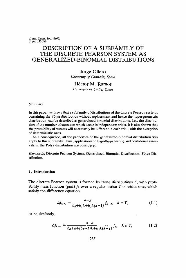
In this paper we prove that a subfamily of distributions of the discrete Pearson system, containing the P61ya distribution without replacement and hence the hypergeometric distribution, can be described as generalized-binomial distributions, i.e., the distribu- tion of the number of successes which occur in independent trials. It is also shown that the probability of success will necessarily be different in each trial, with the exception of deterministic ones.

As a consequence, all the properties of the generalized-binomial distribution will apply to this subfamily. Thus, applications to hypothesis testing and confidence inter- vals in the P61ya distribution are considered.

Keywords: Discrete Pearson System; Generalized-Binomial Distribution; P61ya Dis- tribution.

I. Introduction

The discrete Pearson system is formed by those distributions F, with prob- ability mass function (pmf) fk over a regular lattice T of width one, which satisfy the difference equation

a - k Ark-1 = fk-l , k ~ T, (1.1)

bo+blk+bek(k-1)

or equivalently,

A r k - 1 "~" a - k

bo+a+ (bl-1)k+b2k(k-1) fk, k ~ r , (1.2)

235

J. O L L E R O " H . M. RAMOS

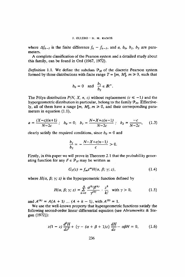
where Zlfk_ 1 is the finite difference fk - f k - 1 , and a, bo, b~, b 2 a r e para- meters.

A complete classification of the Pearson system and a detailed study about this family, can be found in Ord (1967, 1972).

Definition 1.1. We define the subclass @H of the discrete Pearson system formed by those distributions with finite range T = [m, M], m I> 0, such that

b o = O and _bte/R +. b2

The P61ya distribution P(N, X, n, c) without replacement (c <~ - 1 ) and the hypergeometric distribution in particular, belong to the family ~H. Effective- ly, all of them have a range [m, M], m I> 0, and their corresponding para- meters in equation (1.1),

( X - c ) ( n + l ) " bo=O; bl N - X + c ( n - 1 ) . b2 - - c (1.3) a - N - 2 c " = N - 2 c ' N - 2-"" '~ '

clearly satisfy the required conditions, since bo = 0 and

bt N - X + c ( n - 1 )

be c > 0 .

Firstly, in this paper we will prove in Theorem 2.1 that the probability gener- ating function for any F ~ ~t-t may be written as

GF(Z ) = fmzmH(ct, fl, y, z ) , (1.4)

where H(a, r; y; z) is the hypergeometric function defined by

H(a, ~; ~,; z) ~ a(k)ffk) Zk = �9 - - with y > 0, (1.5) k=O ~k) k.t

and A ~k) = A ( A + 1) ... (A + k - 1), with A ~~ = 1. We use the well-known property that hypergeometric functions satisfy the

following second-order linear differential equation (see Abramowitz & Ste- gun (1972)):

d2H dH z ( 1 - z) ~ + { ~ , - (a + fl + 1)z} -~z - a f ln = o, (1.6)

236

DISCRETE P E A R S O N SYSTEM

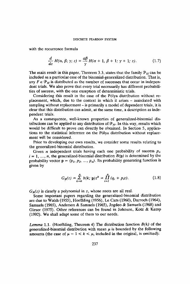
with the recurrence formula

d H(a, ~; ~; z) = aft H(a + 1, ~ + 1; y + 1; z). (1.7) dz 7

The main result in this paper, Theorem 3.3, states that the family ~ n can be included as a particular case of the binomial-generalized distribution. That is, any F e ~ n is distributed as the number of successes that occur in indepen- dent trials. We also prove that every trial necessarily has different probabili- ties of success, with the one exception of deterministic trials.

Considering this result in the case of the Pr lya distribution without re- placement, which, due to the context in which it arises - associated with sampling without replacement - is primarily a model of dependent trials, it is clear that this distribution can admit, at the same time, a description as inde- pendent trials.

As a consequence, well-known properties of generalized-binomial dis- tributions can be applied to any distribution of ~H. In this way, results which would be difficult to prove can directly be obtained. In Section 5, applica- tions to the statistical inference on the Prlya distribution without replace- ment will be considered.

Prior to developing our own results, w e consider some results relating to the generalized-binomial distribution.

Given n independent trials having each one probability of success Pi, i = 1 . . . . . n, the generalized-binomial distribution B(p) is determined by the probability vector p = (Pl, P2 . . . . . p,). Its probability generating function is given by

GB(z) = ~ b(k; p)z k = h (qi + piz). k=O i = l

(1.8)

Gs(z) is clearly a polynomial in z, whose roots are all real. Some important papers regarding the generalized-binomial distribution

are due to Walsh (1955), Hoeffding (1956), Le Cam (1960), Darroch (1964), Samuels (1965), Anderson & Samuels (1965), Jogdeo & Samuels (1968) and Gleser (1975). Other references can be found in Johnson, Kotz & Kemp (1992). We shall adapt some of them to our needs.

Lemma 1.1. (Hoeffding, Theorem 4) The distribution function B(k) of the generalized-binomial distribution with mean/~ is bounded by the following amounts (the case of/~ - 1 < k < #, included in the original, is omitted):

237

J . O L L E R O �9 H. M. R A M O S

(I) O<~B(k)<~B(k;n , - - -~) 0 ~ < k ~ < # - I

B(k; n, p) being the distribution function of the Bernoulli binomial B(n, p).

Lemma 1.2. (Samuels, p. 1273) The successive finite backward differences of the pmf of the generalized-binomial distribution, defined by recurrence as

Do (k) = b(k);

Dr(k) = Dr-l(k) - Dr - l ( k - 1), for k = 1, 2, ...,

satisfy the following inequalities:

D,(k) 12 > Or(k-l_______~) D,(k+ 1)

~ k ~ J (n+r l (n+r l \ k - l / \ k + l ]

f o r r = 0 , 1 . . . . a n d k = 1 . . . . . n + r - 1.

Lemma 1.3. (Jogdeo & Samuels, Theorem 3.3) If k ~</~ < k + 1, the median of the generalized-binomial distribution with mean # is

(I) k, if/~ ~ ~,t

(II) k + l , if/~ > ~.2,

~,t and ~,2 being the respective solutions of

1 _ rain B n - r , , ~ = max B k - s ; n - s , 2 ,=o . . . . . n-k-I n--r 2 s=O ..... k n - s /

2. Probability generating function for the subfamily ~ n

Theorem 2.1. Given a distribution F ~ ~H, with a range [m, M], m >~ O, its probability generating function can be expressed as

238

DISCRETE PEARSON SYSTEM

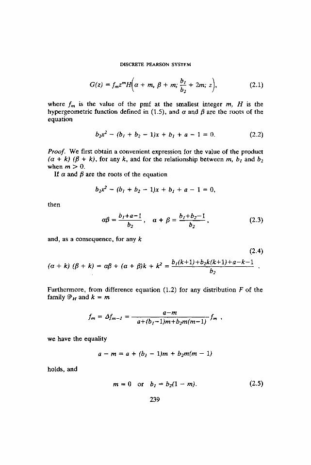
G(z ) = fmzmH(ot + m, fl + m; b, + 2m; z ) b2

(2.1)

where f,,, is the value of the pmf at the smallest integer m, H is the hypergeometric function defined in (1.5), and a and fl are the roots of the equation

b2 x2 - (bl + b2 - 1)x + bl + a - 1 = O. (2.2)

Proof . We first obtain a convenient expression for the value of the product (a + k) (fl + k) , for any k, and for the relationship between m, bl and b2 when m > 0.

If a and fl are the roots of the equation

b2x 2 - (bl + b2 - 1)x + bt + a - 1 = 0 ,

then

b l + a - 1 b ~ + b 2 - 1 (2.3) a f t - b2 , a + f l - b2 '

and, as a consequence, for any k

(2.4)

(a + k) (fl + k) = ctfl + (a + fl)k + k 2 = b ~ ( k + l ) + b 2 k ( k + l ) + a - k - 1 b2

Furthermore , from difference equation (1.2) for any distribution F of the family ~ H and k = m

a- -m fm = Afro-1 = fm ,

a + (b 1 - 1) m + b e m ( m - 1)

we have the equality

a - m = a + (bl - 1 )m + b2m(m - 1)

holds, and

m = 0 or bl = b2(1 - m) . (2.5)

239

J . O L L E R O " H . M . R A M O S

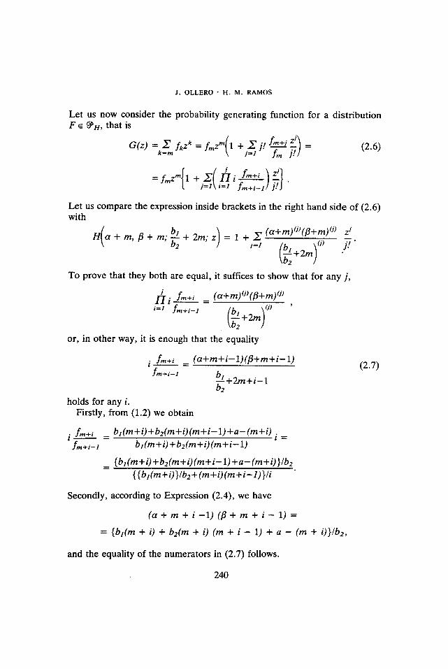
Let us now consider the probability generating function for a distribution F e ~ n , that is

G(z) = ~' fkzk = fmzm(a ~ j! f"+Y.~_m i f ) = zy (2.6)

= f, nz,,~{1 +j_Z1 ( i~_li fra+i I Z] fm+i-I ] ? } "

Let us compare the expression inside brackets in the right hand side of (2.6) with

( b' ) H a + m, fl + m;-~2 + 2m; z = 1 + z (a+m)(J)(fl+m)(J) zj j=~ /i. \0) j! "

[ ~ + 2 m / \b2 I

To prove that they both are equal, it suffices to show that for any j,

h i f,,+i _ (a+m)~ (j) i=l fro+i--1 /l-. \(J) '

I-~ +2m) 2

or, in other way, it is enough that the equality

i f,n+i = (a+m+i-1) ( f l+m+i-1) fro+,-1

holds for any i. Firstly, from (1.2) we obtain

�9 f ~ + i l - - fm+i-I

b l + 2 m + i - 1 b2

_ bz(m+i)+b2(m+i)(m+i-1)+a-(m+i) . l =

b,(m+i) +be(re+i) (m+i - 1)

{ bl(m+i)+b2(m+i)(m+i-1)+a-(m+i) }/b2 { { bl(m+i) }/b2+ (m+i)(m+i-1) }/i

(2.7)

Secondly, according to Expression (2.4), we have

(a + m + i - l ) (fl + m + i - 1) =

= { b l ( m + i) + b a ( m + i) ( m + i - 1) + a - ( m + i ) } ]b2 ,

and the equality of the numerators in (2.7) follows.

240

DISCRETE PEARSON SYSTEM

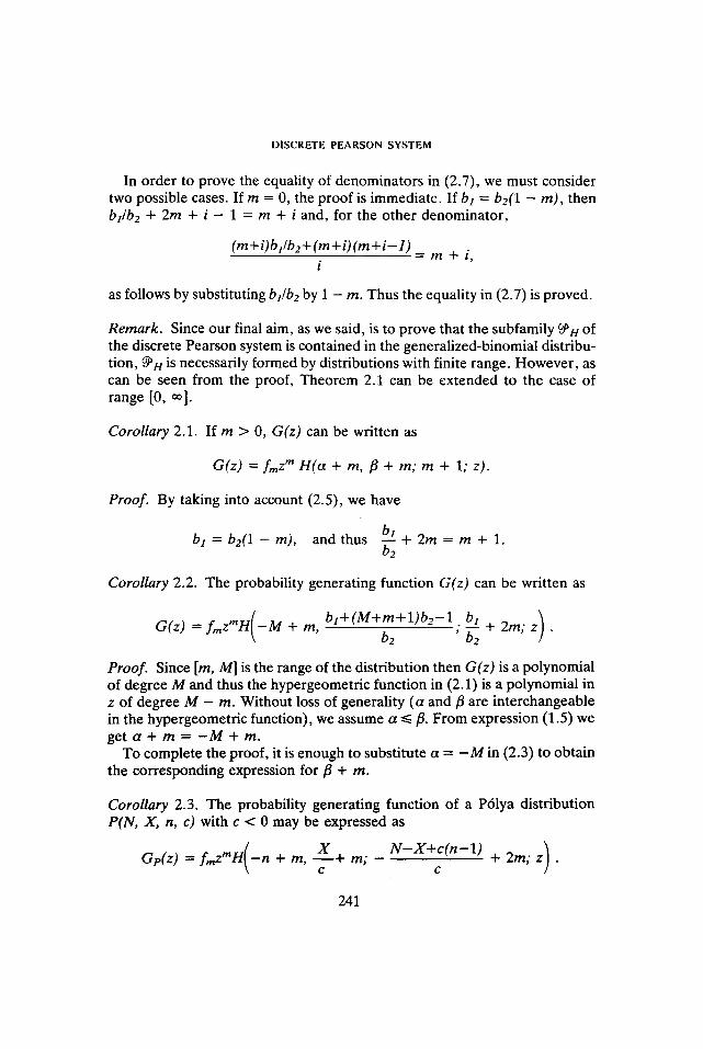
In order to prove the equality of denominators in (2.7), we must consider two possible cases. If m = 0, the proof is immediate. If bl = b2(1 - m) , then bl/b2 + 2m + i - 1 = m + i and, for the other denominator ,

(m+i)bl/b2+ (m+i) ( m + i - 1 ) = m + i ,

as follows by substituting bl/b2 by I - m. Thus the equality in (2.7) is proved.

Remark. Since our final aim, as we said, is to prove that the subfamily @H of the discrete Pearson system is contained in the generalized-binomial distribu- tion, ~H is necessarily formed by distributions with finite range. However , as can be seen from the proof, Theorem 2.1 can be extended to the case of range [0, ~] .

Corollary 2.1. If m > 0, G(z) can be written as

G(z) = fmz" H(a + m, fl + m; m + 1; z).

Proof. By taking into account (2.5), we have

b l b l = b 2 ( 1 - m), and thus ~2 + 2m = m + 1.

Corollary 2.2. The probability generating function G(z) can be written as

G(z) = f m z ' H ( - M + m, b l + ( M + m + l ) b2-1 b__zl \

+ 2m; z l , b2 ' b2 /

Proof. Since [m, M] is the range of the distribution then G(z) is a polynomial of degree M and thus the hypergeometric function in (2.1) is a polynomial in z of degree M - m. Without loss of generality (a and fl are interchangeable in the hypergeometric function), we assume a ~< ft. From expression (1.5) we g e t a + m = - M + m .

To complete the proof, it is enough to substitute a = - M in (2.3) to obtain the corresponding expression for fl + m.

Corollary 2.3. The probability generating function of a P61ya distribution P(N, X, n, c) with c < 0 may be expressed as

h~ X N - X + c ( n - 1 ) ) Gp(z) = fmz m - n + m, + m; - + 2m; z . c c

241

J . O L L E R O " H . M . R A M O S

Proof. The corresponding values of the first two arguments of the hypergeometric function given in (2.1), obtained by solving equat ion (2.2) when a, bl and b2 take the values (1.3), are a = - n and fl = X/c. Furth- ermore, the expression of the third argument is immediate from bl and bz values.

3. ~ n as a subfamily of B(p)

Firstly, let us consider some properties of the particular hypergeometric func- tions involved in the probability generating function of the distributions in ~H.

Lemma 3.1. If the hypergeometric function H ( - a , - f l ; y; z), with a e N, a ~< fl and ), ~/R +, attains a maximum or a minimum in z = ~, then H(~) ~ 0 or H(~) <~ O, respectively.

Proof. By hypothesis, H ( - a , -fl; ~,; z) is a polynomial in z of degree a and all its coefficients are positive. Consequently, it is an increasing function for all z i> 0.

Thus, any possible critical value r must be negative and therefore

and d.--H-H[ = 0 . ~ ( 1 - r < 0 az l z=l;

By substituting in (1.6), the equation is reduced to

den[ = afln(~). - r

Thus, it follows that H(~) >I 0 in the case of a maximum, and H(r <<. 0 in the case of a minimum.

Remark. Obviously, the lemma is also true when fl ~ N and fl ~< a.

Theorem 3.1. The hypergeometric function H ( - a , -f l; ~,; z) with a e N, a ~< fl and y e JR +, has a different negative real roots.

Proof. We proceed by induction. For a = 1,

H ( - a , -fl; y; z) = 1 + ~ z. Y

242

DISCRETE PEARSON SYSTEM

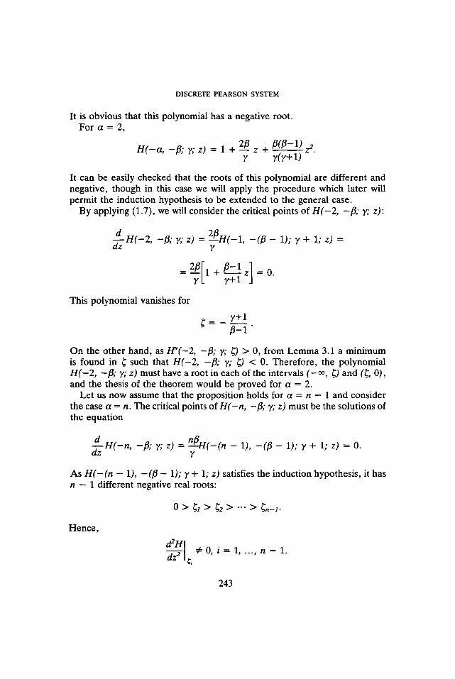
It is obvious that this polynomial has a negative root. For a = 2,

H ( - a , - f i ; ]q z) 1 + 2fl = - - z + ~ ( 1 3 - 1 ) z 2. y y(y+ I)

It can be easily checked that the roots of this polynomial are different and negative, though in this case we will apply the procedure which later will permit the induction hypothesis to be extended to the general case.

By applying (1.7), we will consider the critical points of H(-2, -~; y; z):

J • H ( - 2 , - f l ; y; z) = - ' H ( - 1 , - ( f l - 1); y + 1; z) = 9/]

Y

f l - 1 0

This polynomial vanishes for

~.= _ y + l

fl-l"

On the other hand, as H " ( - 2 , - ~ ; y; r > 0, f rom L e m m a 3.1 a min imum is found in r such that H ( - 2 , - ~ ; y; ~) < 0. Therefore , the polynomial H ( - 2 , - ~ ; y; z) must have a root in each of the intervals ( - % r and (r 0), and the thesis of the theorem would be proved for a = 2.

Let us now assume that the proposit ion holds for a = n - 1 and consider the case a = n. The critical points of H ( - n , - ,6; y; z) must be the solutions of the equat ion

J • H ( - n , - ,6; y; z) = " ' ' H ( - ( n - 1), - ( f l - 1); $ + 1; z) = n tq

O. Y

As H ( - ( n - 1), - ( f l - 1); y + 1; z) satisfies the induction hypothesis, it has n - 1 different negative real roots:

o > ~ > ~2 > -.. > ~,,_~.

Hence ,

d2H II :/:0, i = 1 . . . . . n - 1 . dz 2 I r

243

J . O L L E R O �9 H. M. R A M O S

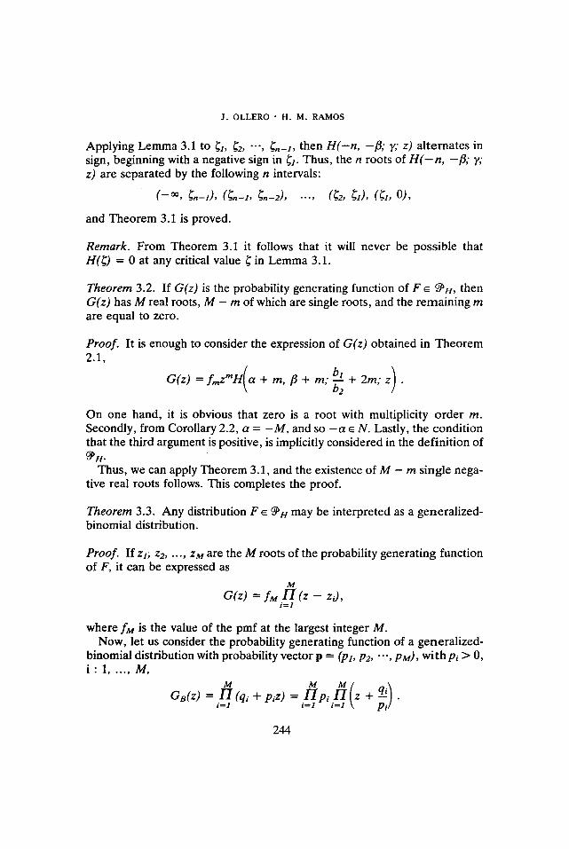
Applying Lemma 3.1 to r ~2, "", ~,,-z, then H ( - n , - f l ; y; z) al ternates in sign, beginning with a negative sign in ~z. Thus, the n roots of H(--n , - f l ; 7; z) are separated by the following n intervals:

( -~, ~n-z), (~n-l, ~ - 2 ) , .-., (~2, ~z), (~z, 0),

and Theorem 3.1 is proved.

Remark. From Theorem 3.1 it follows that it will never be possible that H(r = 0 at any critical value r in Lemma 3.1.

Theorem 3.2. If G(z) is the probability generating function of F e @H, then G(z) has M real roots, M - m of which are single roots, and the remaining m are equal to zero.

Proof. It is enough to consider the expression of G(z) obtained in T h e o r e m 2.1,

G(z) = fmzmH ct + m, fl + m; -~2 + 2m; z .

On one hand, it is obvious that zero is a root with multiplicity o rde r m. Secondly, from Corollary 2.2, a = - M , and so - a ~ N. Lastly, the condit ion that the third argument is positive, is implicitly considered in the definit ion of

~H. Thus, we can apply Theorem 3.1, and the existence of M - m single nega-

tive real roots follows. This completes the proof.

Theorem 3.3. Any distribution F ~ ~ n may be interpreted as a general ized- binomial distribution.

Proof. If zz; z2 . . . . , zM are the M roots of the probability generat ing function of F, it can be expressed as

M

G(z) = fM H (z - zi), i=l

where fM is the value of the pmf at the largest integer M. Now, let us consider the probability generating function of a general ized-

binomial distribution with probability vector p = (Pz, P2, "", pM), with Pi > 0, i : l . . . . . M,

Ga(z) = i=lH (qi + p i Z) = i__~l Pi z -4- .

244

DISCRETE PEARSON SYSTEM

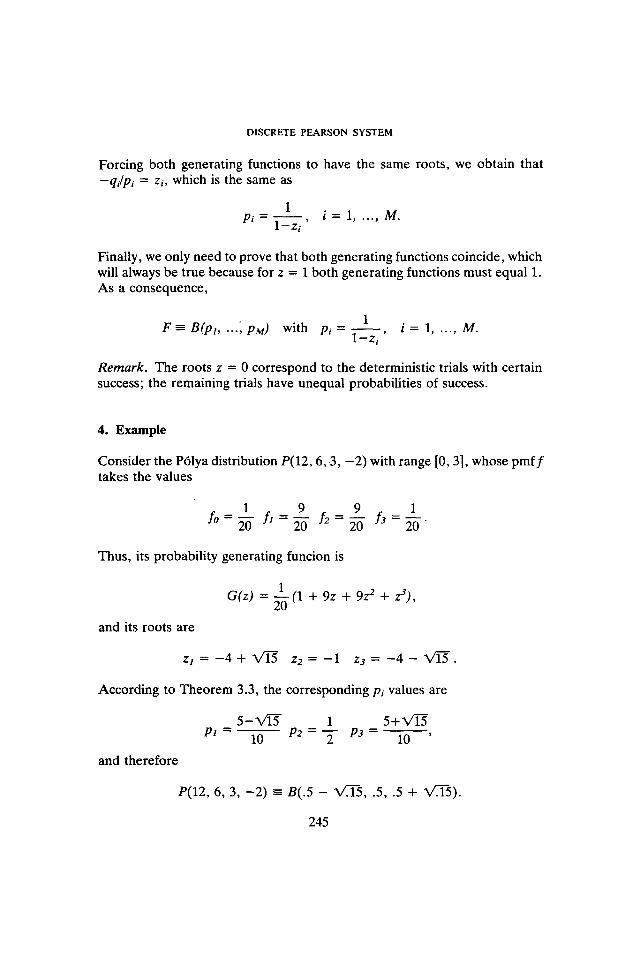
Forcing both generating functions to have the same roots, we obtain that - q i / P i = zi , which is the same as

1 - ~ P i - 1--Zi i 1, M.

Finally, we only need to prove that both generating functions coincide, which will always be true because for z = 1 both generating functions must equal 1. As a consequence,

1 F - B ( p l . . . . ~ p ~ ) with Pi -- i = 1, . . . , M .

1--Zi '

R e m a r k . T h e roots z = 0 correspond to the deterministic trials with certain success; the remaining trials have unequal probabilities of success.

4. Example

Consider the P61ya distribution P ( 1 2 , 6, 3, - 2 ) with range [0, 3], whose p m f f takes the values

1 9 9 1 f o = ' ~ f, = - ~ f 2 = ~ f3": 2-- ~.

Thus, its probability generating funcion is

G ( z ) = 1 - ~ ( 1 + 9z + 9z 2 + z 3 ) ,

and its roots are

z l = - 4 + ~ z2 = - 1 z3 = - 4 - V ' ~ .

According to Theorem 3.3, the corresponding Pi values are

and therefore

5-vT5" 1 5+ V' i5 P l - 1"---'~- Pe = "-~ P3 - 1-----~-'

P(12, 6, 3, - 2 ) -- B(.5 - V7i--5, .5, .5 + X/~'5).

245

J . O L L E R O �9 H. M. R A M O S

5. Applications

In this section we apply some known properties of the generalized-binomial distribution to the P61ya distribution without replacement. In this way , we do some developments which have not yet been studied for this family of dis- tributions. All of them, with the exception of those relating to statistical in- ference, are applicable to any distribution of @H. Let ~(N, X, n, c) be a P61ya distribution with c < 0, range [m, M] and expected value/~ = nX/N; let P(k) be its distribution function and let p(k) be its probability mass function.

5.1. Bounds on the distribution function

In order to get bounds for P(k), using Lemma 1.1 adapted to the case of a P61ya distribution, we have the binomial B(n, ~n) as an approximating dis- tribution. By taking into account the particular range of P(N, X, n, c) and its interpretation as Poisson trials, i.e., there must be m deterministic trials hav- ing certain success and n - M trials having certain failure. Thus two addition- al approximating distributions are obtained with the same expected value #: the binomial distribution B(M, ~ M ) a n d the shifted binomial distribution m + B(M - m, (~ - m)/(M - rn)).

According to Theorem 2.2 in Anderson & Samuels (1965), we prove that the best bound is obtained by using the latter binomial distributions and then the following bounds are obtained:

(i) P(k) = 0 , i f 0 ~ < k ~ < m - 1 (ii) 0 < P ( k ) < B ( k - m ) , i f m ~ < k ~ < # - 1 (iii) B(k - m) < P(k) < 1, if # ~< k < M (iv) P(k) = 1, i f M ~ < k ~ < n ,

(5.1)

B(k) being the distribution function of the Bernoulli binomial distribution B(M - m, (p - m)/(M - m)).

5.2. Confidence intervals and hypothesis testing

As a result of combining cases (i) and (iii) in (5.1), the usual tes t for the binomial parameter p, with one or two tails, can directly be appl ied to test the corresponding hypotheses for the proportion parameter p = X / N in a P61ya distribution with c < 0.

246

DISCRETE PEARSON SYSTEM

Let us assume the significance level of this test to be the maximum prob- ability of the type I error in any possible condition. Then, its actual value is at most the same as that nominal value of the binomial test used. Walsh (1955) considered which approximate corrections would be required to obtain the true probabilities under the null hypothesis.

Similarly, it can be proved that the power of such a test, when we have an alternative value which is not very close to the null hypothesis, is at least equal to the power of the corresponding binomial test.

Further, the binomial confidence intervals can be used to estimate the proport ion parameter of the P61ya distribution without replacement. When the confidence level is sufficiently high, the actual confidence level is greater than the nominal level.

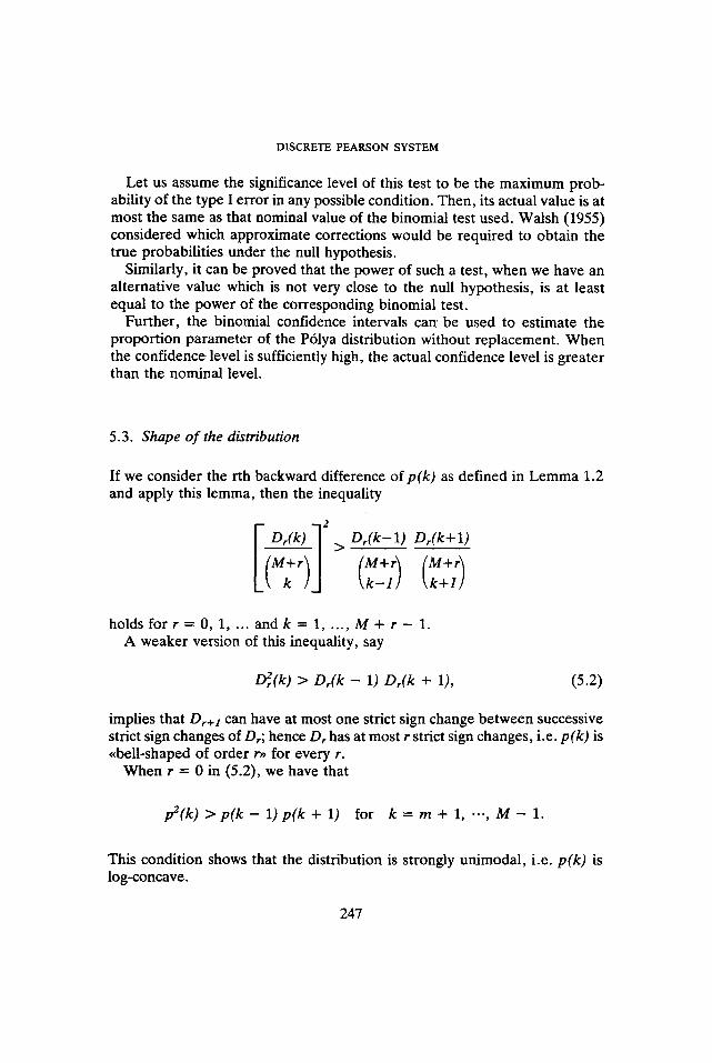
5.3. Shape of the distribution

If we consider the rth backward difference ofp(k) as defined in Lemma 1.2 and apply this lemma, then the inequality

I Or(k) 12 > Dr(k-1._........~) Dr(k+l)

- ' ~ i J (M+r~ (M+r I \ k - l / \ k+l /

holds for r = 0, 1, ... and k = 1, ..., M + r - 1. A weaker version of this inequality, say

D~,(k) > Dr(k - 1) Dr(k + 1), (5.2)

implies that Dr+~ can have at most one strict sign change between successive strict sign changes of Dr; hence Dr has at most r strict sign changes, i.e. p(k) is ~bell-shaped of order r~ for every r.

When r = 0 in (5.2), we have that

p2(k) > p(k - 1 ) p(k + l) for k = m + l, ..., M - 1 .

This condition shows that the distribution is strongly unimodal, i.e. p(k) is log-concave.

247

J . O L L E R O �9 H . M. R A M O S

5.4. Location o f the median and mode

The general results on the localization of the median and m o d e in the generalized-binomial distribution shows that the median and m o d e of the P61ya distribution without replacement may be localized only at the adjacent integers to the mean. If the mean were an integer, then they b o t h would coincide with it. The application of Lemma 1.3 provides the sets of mean values which lead to a unique median. Darroch (1964) provides a similar result for the mode.

Acknowledgment

The authors wish to thank to Professor E. Moreno and J. M. Angulo for their help and useful suggestions during the revision of this paper.

R E F E R E N C E S

[1] ABRAMOWrrz, M. and STEt3Ur~, I. A. (1972). Handbook of Mathematical func- tions. New York: Dover.

[2] ANDERSON, T. W. and SAMUELS, S. M. (1965). Some Inequalities among Bino- mial and Poisson Probabilities. Proc. of the 5 th Berkeley Simp. on Math. and Prob, 1, 1-12.

[3] DARROCH, J. N. (1964). On the Distribution of the Number of Successes in Inde- pendent Trials. Ann. Math. Statist, 35, 1317-1321.

[4] GLESV.R, L. (1975). On the Distribution of the Number of Successes in Indepen- dent Trials. Ann. Probability, 3, 182-188.

[5] HOEFFDIr~G, W. (1956). On the Distribution of the Number of Successes in Inde- pendent Trials. Ann. Math. Statist., 27, 713-721.

[6] JOaDEO, J. and SAMUELS, S. M. (1968). Monotone Convergence of Binomial Probabilities and a Generalization of Ramanujan's Equation. Ann. Math. Stat- /st., 39, 1191-1195.

[7] JOrINSON, N. L., Korz, S. and KEMP, A. W. (1992). Univariate Discrete Distribu- t/ons (Second Edition). New York: Wiley.

[8] LE CAM, L. (1960). An approximation Theorem for the Poisson Binomial Dis- tribution. Pacific J. Math., 10, 1181-1197.

[9] ORD, J. K. (1967). On a System of Discrete Distributions. Biometrika, 54, 649- 656.

[10] ORD, J. K. (1972). Families of Frequency Distributions. London: Griffin.

248

DISCRETE PEARSON SYSTEM

[11] SAMUELS, S. M. (1965). On the Number of Successes in independent Trials. Ann. Math. Statist., 36, 1272-1278.

[12] WALSH, J. (1955). Approximate Probability Values for Observed Number of successes from Statistically Independent Binomial Events with Unequal Probabi- lities. Sankhya, 15, 281-290.

249