Description and demonstration of the EXPOLIS simulation model: Two examples of modeling population...

Description and demonstration of the EXPOLIS simulation model:

Two examples of modeling population exposure to particulate matter

HANNEKE KRUIZE,a OTTO HANNINEN,b OSCAR BREUGELMANS,a ERIK LEBRETa

AND MATTI JANTUNENb

aNational Institute of Public Health and the Environment (RIVM), Bilthoven, The NetherlandsbKTL, Department of Environmental Health, Kuopio, Finland

As a part of the EXPOLIS study, a stochastic exposure-modeling framework was developed. The framework is useful to compare exposure distributions

of different (sub-) populations or different scenarios, and to gain insight into population exposure distributions and exposure determinants. It was

implemented in an MS-Excel workbook using @Risk add-on software. Basic concept of the framework is that time-weighted average exposure is a sum

of partial exposures in the visited microenvironments. Partial exposure is determined by the concentration and the time spent in the microenvironment. In

the absence of data, indoor concentrations are derived as a function of ambient concentrations, effective penetration rates and contribution of indoor

sources. Framework input parameters are described by probability distributions. A lognormal distribution is assumed for the microenvironment

concentrations and for the contribution of indoor sources, and a beta distribution for the time spent in a microenvironment and for the penetration factor.

Mean and standard deviation values parameterize the distributions. In this paper, Latin Hypercube sampling is used for the input distributions. The

outcome of the framework is an estimate of the population exposure distribution for the selected air pollutant. The framework is best suited for averaging

times from 24h upwards. Sensitivity analyses can be performed to determine the most influential factors of exposure. The application of the framework is

illustrated in two examples. The EXPOLIS PM2.5 example uses microenvironment measurement and time–activity data from the EXPOLIS study to

model PM2.5 population exposure distributions in four European cities. The results are compared to the observed personal exposure distributions from

the same study. The Dutch PM10 example uses input data from several (Dutch) databases and from literature, and shows a more complex application of

the framework for comparison of scenarios and subpopulations.

Journal of Exposure Analysis and Environmental Epidemiology (2003) 13, 87–99. doi:10.1038/sj.jea.7500258

Keywords: population exposure distributions, microenvironment approach, exposure model, air pollution, PM2.5, PM10.

Introduction

Epidemiological research of the past 20 years has revealed

significant mortality and morbidity effects in association to

present European and North American levels of urban air

pollution, especially fine particulate matter (PM). These

studies are based on air pollution levels that have been

measured at centrally located ambient air monitoring stations

(Vedal, 1997; Spix et al., 1998; Dab et al., 2001; Pope et al.,

2002). Health effects of air pollutants, however, are caused

by the exposures people experience during their daily

activities. People in Europe and North America spend most

of their time indoors (Szalai, 1972; Schwab et al., 1990;

Klepeis et al., 2001) where, in addition to pollution from

outdoor sources, also indoor sources of air pollutants are

present (Lioy, 1990). Indoor and personal pollution levels

often correlate poorly with outdoor air levels (Dockery and

Spengler, 1981; Letz et al., 1984; Sexton et al., 1984; Ott,

1985; Spengler et al., 1985; Ryan et al., 1986; Lioy, 1990,

1995; Law et al., 1997; Pellizzari et al., 1999; Kousa et al.,

2002). Better understanding of the relationships between the

personal exposures to various air pollutants and ambient air

levels, and their relationships to other significant exposure

determinants (such as indoor sources, sinks, and personal

activities) are therefore needed before the epidemiological

findings can be interpreted into efficient risk reduction

policies (Ott, 1984; NRC, 1998).

Exposure can be defined as the contact of a target and a

chemical, physical, or biological agent in an environmental

carrier medium (Duan, 1982; Ott, 1985; Zartarian et al.,

1997). It can be measured or modeled (Ryan, 1991), either

directly (personal measurements) or indirectly (microenviron-

ment approach) (Duan, 1982, 1991; Ott, 1984, 1985; Ott

et al., 1988; Lioy, 1990; Ryan, 1991; Duan and Mage,

1997). Personal exposure measurements are expensive

(Ott, 1984; Ryan, 1991), labor intensive and invasive (Letz

et al., 1984; Sexton et al., 1984). Modeling requires a validated

1. Address all correspondence to: Hanneke Kruize, National Institute of

Public Health and the Environment, PO Box 1, 3720 BA Bilthoven, The

Netherlands. Tel.: +31-30-2743599 or +31-30-2533398. Fax: +31 30-

2744451. E-mail: [email protected]

Received 28 May 2002

Journal of Exposure Analysis and Environmental Epidemiology (2003) 13, 87–99

r 2003 Nature Publishing Group All rights reserved 1053-4245/03/$25.00

www.nature.com/jea

model, and sufficient, representative, good-quality input

data. Once these requirements are met, a model can be

repeated for a large number of individuals or populations.

Models can be used to assess past exposures, exposures of not

sampled or undersampled groups in the population or to

compare alternative future exposure scenarios (Letz et al., 1984;

Lioy, 1990, 1995; Ryan, 1991). Only little demands have to be

made on the study population in comparison with personal

measurements (for which the study population, e.g., has to

carry sampling equipment). These are all significant benefits

when compared to measurements (Letz et al., 1984; Ryan et al.,

1986).

Ryan (1991) describes three classes of human exposure

models for air pollutants: statistical, physical, and physical–

stochastic models. Statistical models can be used for

descriptive analyses and testing of hypotheses on collected

data. In the physical approach, the model is based on

physical (and sometimes chemical) laws. The a priori defined

physical model is transformed into a mathematical model

(Ryan, 1991). An example of this deterministic type of

models is the National Ambient Air Quality Standards

(NAAQS) Exposure Model (NEM) (Johnson, 1995;

McCurdy, 1995). Physical–stochastic type of models are

based on physical equations like the pure physical models,

but instead of relying on deterministic input data to fully

describe the variability F or ignoring the variability F in

input parameters, physical–stochastic models apply prob-

abilistic techniques to propagate the variability through the

model. These models describe parameters with frequency or

probability distributions instead of single values (Ryan,

1991). Examples of this type of models are the Simulation of

Human Air Pollution Exposures model (SHAPE) (Ott,

1984; Ott et al., 1988; Duan, 1991; Ryan, 1991), pNEM, the

probabilistic version of the NEM model (McCurdy, 1995;

Law et al., 1997), and the Air Pollution Exposure model

(AirPEX) (Freijer et al., 1998). These models can be used to

predict population exposures for both existing and past or

scenario situations, and for subpopulations for whom no

measurement data are available (Ryan, 1991), by simulating

from the distributions of input parameters.

Full description of personal exposure to an air pollutant

requires knowledge of the magnitude of pollutant concentra-

tion in the exposure environment, duration of exposure, and

the time pattern of the exposure (Ryan, 1991). The

microenvironment approach has been commonly used to

model exposures (Fugas, 1975; Dockery and Spengler, 1981;

Ott, 1984; Letz et al., 1984; Ryan et al., 1986; Freijer et al.,

1998). In the microenvironment approach the exposure E is

calculated as the sum of the partial exposures across the

visited microenvironments Eq. (1) (e.g., Duan, 1982; Ryan

et al., 1986):

E ¼XN

i

fiCi

where Ci is the concentration in microenvironment i, fi the

fractional time spent in microenvironment i, and N the

number of microenvironments.

In literature, the exposure E is often defined as ‘‘total

exposure’’, (e.g., Ryan, 1991). However, we prefer to use the

term ‘‘time-weighted average exposure’’, because in our

opinion it better expresses the fact that the exposure is the

sum of weighted concentrations to which people are exposed

in the microenvironments they visit. This equation can be

used for any averaging time and any number of microenvir-

onments, for any air pollutant. In case no measured data are

available for indoor environments, the concentration can be

derived as a function of outdoor concentration, the effective

penetration factor, and the contribution of indoor sources

(e.g., Dockery and Spengler, 1981; Ryan et al., 1986): (Eq (2))

Ci ¼ Capi þ Si

where Ca is the ambient concentration, pi the effective

penetration factor of the air pollutant in microenvironment i,

and Si the contribution of indoor sources in microenviron-

ment i.

The effective penetration factor includes both first-order

infiltration and first-order loss mechanisms (sinks) (Ryan

et al., 1986). According to Ryan et al. (1986), pi and Si are

dependent on many parameters, such as ventilation rates and

family activity patterns. In Figure 1, this nested model is

outlined for two types of outdoor environments (in this

example, the urban and rural environment), with different

indoor microenvironments nested within them.

As a part of the EXPOLIS study, a European multicenter

study for measurement of air pollution exposures and

microenvironment concentrations of working age urban

populations (Jantunen et al., 1998, 1999), a population

exposure simulation framework was developed to assess and

predict exposure distributions of air pollutants of European

urban populations. This simulation framework should be

applicable in scenario studies, to assess the public health gain

of environmental policy options in terms of population

exposure. Another condition was that the framework should

fit on information resulting from the EXPOLIS study.

Furthermore, it had to be developed in such a way that all

participating centers of the EXPOLIS study could use it

without extensive developer’s support. Also, the framework

should be applicable to perform calculations for various

(sub-) populations and air pollutants, and should produce

population exposure distributions (Jantunen et al., 1998).

Based on these conditions, the Dutch National Institute of

Public Health and the Environment (RIVM) developed the

modeling framework in collaboration with KTL (Finnish

National Public Health Institute).

This paper describes the development and structure of the

framework. Two examples demonstrate the application of the

framework to simulate population exposure to particulate

matter. The first one, the EXPOLIS PM2.5 example, applies

EXPOLIS simulation modelKruize et al.

88 Journal of Exposure Analysis and Environmental Epidemiology (2003) 13(2)

the framework to four EXPOLIS cities to model the adult

urban 48-h population exposure distributions to fine

particulate matter (PM2.5). The results are compared to the

observed 48-h personal exposure distributions from the same

study. The second one, the Dutch PM10 example, shows a

more complex application, using the framework to model

24-h respirable particulate matter (PM10) exposures of the

whole Dutch population. In this example, the target population

is divided into eight subpopulations based on age, work status

and living in either a rural or an urban area. In the Dutch

example, the results are calculated separately for the current

scenario, including exposures to Environmental Tobacco

Smoke (ETS), and for a hypothetical non-ETS scenario.

Methods

General Features of the FrameworkThe developed framework is based on Eqs. (1) and (2). It

was implemented as a Microsoft Excel workbook. An Excel

add-on software package @Risk (version 3.5, Palisade

Corporation, 1994) is needed to supply the probabilistic

functions for the stochastic functionality. The spreadsheet-

based approach allows easy use of the framework by

researchers who are not modelers or programmers by

training. @Risk offers the user possibilities to choose their

own simulation features, for example, selecting either

sampling by the Latin Hypercube method or the Monte

Carlo method. When Latin Hypercube sampling is used to

create random realizations from the input distributions, the

input probability distribution is stratified into equal intervals.

Samples are taken randomly from each interval of the input

distribution. Therefore, compared to the regular Monte

Carlo sampling, fewer samples are needed to create the whole

distribution. Owing to this way of sampling, also situations

occurring with a lower probability are represented in the

simulation output, for example, high concentrations sampled

from the tail of a microenvironmental concentration

distribution. Moreover, @Risk allows correlation among

input variables, according to the researcher’s specification.

@Risk offers several options to present or analyze model

outputs.

Required Input DataEquations (1) and (2) show that three types of input data

are required. First of all, relevant microenvironments need to

be defined. The specification of microenvironments depends

on the goal for which the framework is applied, data

availability, and correlation between the microenvironments.

The pollutant being studied is important for the selection of

microenvironments, because the microenvironments, in

which the source of the pollutant is present, vary between

pollutants (Ott, 1985). Furthermore, a more detailed

distinction with more microenvironments can produce a

more accurate estimate, but it also requires more input data.

Secondly, concentration distributions need to be described

for each microenvironment. In literature, concentration

distributions and other distributions, which have a minimum

Micro environment: 2Micro environment: 1

µE: 3, Home indoors µE: 4, Other indoors µE: 5,Home indoors

C2

f2

C1

f1

C5

f5C3

f3C4 f4

Exposures in urban sub population

(health effects)

p5

Si

p4

Si

µE: 6, Other indoors

C6

f6

p5

Si

URBAN ENVIRONMENT RURAL ENVIRONMENT

Exposures in rural sub population

Population distribution of time-weighted 24-hour average exposures

Si

Figure 1. Outline of the nested structure of a microenvironmental exposure model. Concentration distributions for microenvironments 1 and 2 andfor the microenvironment 3 are known. Concentrations for microenvironments 4–6 are modeled using penetrations and local sources.

EXPOLIS simulation model Kruize et al.

Journal of Exposure Analysis and Environmental Epidemiology (2003) 13(2) 89

level of zero and no upper limit, are often approached as a

lognormal distribution (Ryan et al., 1986). Therefore, we

assume all concentration distributions to be lognormal. For

the microenvironments for which input data are available,

Eq. (1) is used. In case the concentration distribution for an

indoor microenvironment is not available, it is derived from

the ambient concentrations, the effective penetration factors,

and the contributions of indoor sources (Eq. (2)). For the

distribution of the effective penetration factor, a beta

distribution is assumed, limited between zero and one. This

type of distribution allows many different shapes (Ryan et al.,

1986). For the contribution of indoor sources a lognormal

distribution is assumed. Furthermore, the percentage of

indoor microenvironments with specified sources needs to be

given.

Finally, data on time–activity patterns are needed,

specified as the fraction of time spent in each microenviron-

ment. People spend their time differently, depending on

employment status, age (Letz et al., 1984), season, and day

of week (Johnson, 1995), among other factors (Chapin,

1974). Therefore, it is important to define groups of people

with similar time–activity patterns. For such subpopulations

exposure distributions need to be simulated separately, and

eventually merged together to get an exposure distribution

for the whole population. We describe time fractions with a

beta distribution, limited between zero and one, for the same

reason as mentioned for the penetration factor. The

simulation framework samples the time fractions from

independent beta distributions. To scale the total fraction of

time for each simulated individual to unity, each time fraction

is divided by the sum of the fractions before calculating the

partial exposures in microenvironments.

All distributions are entered as mean and standard

deviation (SD) into the worksheet of the framework. The

@Risk lognormal function is described by its mean and SD

(note: not geometric mean and GSD) values. For the @Risk

beta function, the mean and SD are transformed with Excel

formulas to the needed function called parameters a1 and a2.Since input variables might be correlated (for example, a

person spending much time indoors will spend less time

outdoors), a correlation matrix was implemented, in which

the user can enter rank correlation coefficients. After having

sampled from all relevant distributions using the Latin

Hypercube sampling technique, the sampled values are

combined, resulting in a partial exposure in one microenvir-

onment for one individual. Summing all partial exposures

and repeating this procedure according to the selected

number of iterations generates the distribution of time-

weighted average exposure levels for the target (sub-)

population. From this population exposure distribution

several exposure measures can be derived, such as the

average exposure level, or exposure levels at different

percentiles of the population exposure distribution. Also,

sensitivity analyses can be performed to give an overview of

the relative influence of the input parameters on the simulated

population exposure distribution.

The following examples demonstrate the application of the

framework.

The EXPOLIS PM2.5 ExampleThe EXPOLIS PM2.5 example demonstrates the use of the

simulation framework in its simplest form. No subpopula-

tions are defined, and no correlation structures between the

model parameters are taken into account. ETS or any other

indoor sources are not modeled separately, but are included

in the observed total indoor microenvironment concentra-

tions. One simulation was run for each city to estimate adult

(age 25–55 years) urban population exposure distributions in

Athens, Basel, Helsinki, and Prague. The modeled and

measured 48-h population exposure distributions were

compared to give a general impression of the validity of the

framework. Table 1 summarizes the input data, which were

Table 1. Input values for the EXPOLIS PM2.5 example: lognormal concentration distributions (arithmetic mean, SD) and beta distributions (arithmetic

mean, SD) for time–activity for each of the three microenvironments of this model.

Microenvironment Helsinki

mean (SD)

Basel

mean (SD)

Prague

mean (SD)

Athens

mean (SD)

PM2.5 concentrations (mg/m�3)

No of subjects 201 50 50 50

Home indoors 12.1 (15.1) 24.4 (24.7) 35.9 (30.0) 32.4 (20.9)

Work indoors 15.9 (34.8) 27.8 (38.5) 43.8 (44.6) 91.9 (81.3)

Outdoorsa 9.3 (6.9) 21.4 (13.9) 26.9 (10.5) 36.6 (26.7)

Time activity (fractions)

No of diaries 434 322 83 100

Home indoors 0.58 (0.13) 0.56(0.14) 0.59(0.15) 0.64(0.18)

Work indoors 0.25 (0.18) 0.23(0.14) 0.23(0.14) 0.17(0.14)

Other placesb 0.18 (0.10) 0.21(0.11) 0.18(0.12) 0.19(0.11)

a In Helsinki: fixed station 1 h, in other cities: EXPOLIS home outdoor 2-night concentration.b ‘‘Outdoors’’ concentration is used for ‘‘Other places’’ in the simulation.



extracted from the EXPOLIS database Hanninen (et al.,

2002). Three microenvironments were defined: ‘‘Home

indoors’’, ‘‘Work indoors’’, and ‘‘Other places’’ (an aggre-

gate microenvironment covering all other places visited). In

the EXPOLIS study, data were collected from the fall of

1996 to the winter of 1997–1998. Measurements were carried

out during two consecutive weekdays. Concentration dis-

tributions for PM2.5 were available for the ‘‘Home indoors’’

(measurement period was 2� 16¼ 32 h) and ‘‘Work

indoors’’ microenvironments (measurement period was

2� 8¼ 16 h). The measured indoor concentrations include

both ambient PM2.5 particles penetrated indoors, as well as

particles from any indoor source. In Helsinki, 1-hour

ambient concentrations measured at a traffic-oriented fixed

monitoring station were randomly sampled for the ‘‘Other

places’’ microenvironment, because the visits to the ‘‘Other

places’’ microenvironments are typically short, and often

occur in traffic. In Athens, Basel, and Prague, the

approximately 32-h average concentrations measured out-

doors at home were used, because no hourly fixed site PM2.5

data were available for these cities. This treatment is likely to

narrow the distribution of concentrations experienced in the

‘‘Other places’’ from their real, but unknown, values. No

correction was applied to the standard deviations in spite of

the different averaging times. Data on the fractions of time

spent in the defined microenvironments were also available

from the EXPOLIS database. The participants kept a 15min

resolution time–microenvironment–activity diary for 48 con-

secutive hours. Time–activity data were collected during

weekdays, but not in weekends or holidays. Time spent in

the microenvironment ‘‘Other places’’ was calculated by

subtracting the time spent in the other microenvironments

‘‘Home indoors’’ and ‘‘Work indoors’’ from total time that the

diary was kept. In all, 2000 iterations and a random number

seed were selected for each of the four simulation runs.

The Dutch PM10 ExampleWe present the second example to show the use of the

EXPOLIS framework for purposes other than the EXPOLIS

study itself, in a larger and more complex set up, for

comparisons of subpopulations and scenarios based on

different policy options. This example is derived from work

performed for the Dutch Health Inspectorate, in which

rough estimates were made for the exposure of the Dutch

population to fine particles. We estimated the population

exposure distribution on the basis of directly available

information from existing (Dutch) databases and from

literature, gathered within a short time period. In this

example, ‘‘fine particles’’ were defined to be PM10, because

Dutch air-quality guidelines are defined at PM10. Conse-

quently, more Dutch data were available for PM10 compared

to PM2.5, at least for the outdoor microenvironment. The

input data are summarized in Tables 2–5. The subpopula-

tions were formed on the basis of expected general similarity

of time–activity patterns within groups and data availability.

This resulted in the following subpopulations: children

(0–12 years), the working/studying population (13–64 years),

the nonworking and nonstudying population (13–64 years),

and the elderly (Z65 years). In the following, we will refer to

these groups as ‘‘Children’’, ‘‘Adults W’’, ‘‘Adults N’’, and

‘‘Elderly’’. The subpopulations, with their percentages of

occurrence in the general Dutch population, are shown in

Table 2. Two scenarios were simulated: the current Dutch

situation including the presence of ETS in indoor environ-

ments (current scenario), in which we tried to give a rough

estimate of the current exposure of the Dutch population to

PM10, and the hypothetical situation with no indoor smoking

(non-ETS scenario). For the definition of microenviron-

ments, we selected those for which we expected Dutch input

data to be available, and for which the distinction would be

meaningful in relation to PM. This resulted in four

microenvironments ‘‘Outdoors’’, ‘‘Home indoors’’, ‘‘Other

indoors’’, and ‘‘In transport’’.

Since measurements from fixed monitoring stations

indicated that the ambient PM10 concentrations were higher

in urban areas compared to rural areas (mean 39.7 mg/m3,

SD 17.4 mg/m3 and mean 35.1mg/m3, SD 18.3 mg/m3

respectively), we made a distinction between the urban and

the rural part of the Netherlands (Kruize et al., 2000).

Ambient concentrations were available from the National

Air Quality Monitoring Network of the RIVM (Elzakker

and Buijsman, 1999). We considered data on indoor PM10

Table 2. Subpopulations, their percentages of occurrence in the Dutch population, and the number of iterations used in the Dutch PM10 example.

Subpopulation Age (years) Urban Rural Total

(%) Iterations (%) Iterations (%) Iterations

Children 0–12 5.4 2170 10 4011 15.5 6181

Adults Wa 13–64 18.2 7283 25.7 10,288 43.9 17,571

Adults Nb 13–64 11.3 4516 15.9 6378 27.2 10,894

Elderly 65+ 5.9 2342 7.5 3012 13.4 5354

Total F 40.8 16,311 59.2 23,689 100 40,000

aWorking or studying adults.bAdults not working or studying.



concentrations, available from Dutch studies (for example,

Janssen, 1998; Fischer et al., 2000), not to be representative

for Dutch homes in general, because measurements were

performed in a limited number of Dutch homes, at a limited

number of locations in The Netherlands. Therefore, the

indoor concentration distribution for PM10 was derived from

ambient concentrations using a penetration factor (Eq. (2)).

In the absence of Dutch data on penetration factors,

parameters of the probability distribution for the penetration

factor were derived from calculations using a mass balance

model, in which the input consisted of ambient concentra-

tions, a fixed ventilation rate (0.64 h�1), and the half-life for

PM10 (1.41 h) (Freijer and Bloemen, 2000). The resulting

distribution for the effective penetration rate was parameter-

ized with a mean of 0.6 and an SD of 0.04. These values are

comparable with values presented in literature (Colome et al.,

1992; Li, 1994). Owing to a lack of specific data for different

types of indoor microenvironments, the distribution para-

meters of the microenvironment ‘‘Home indoors’’ were also

used for the microenvironments ‘‘Other indoors’’ and ‘‘In

transport’’.

The additional indoor concentrations caused by ETS were

simulated in a separate simplified stochastical model. In this

model (a modified version of the one described in Kruize

et al., 2000), data on the additional indoor concentration of

fine particles from one cigarette, the number of smoked

cigarettes per person, and the number of smokers in a

household, were combined to derive the input parameters of

the lognormal distribution for the contribution of ETS. The

additional indoor concentration per cigarette (2.2 mg/m3) was

derived from the average emission per cigarette (12mg;

Koutrakis et al., 1992), the average volume of a Dutch house

(assumed to be 250m3), a deposition rate of 12 per day, and

a ventilation rate of 15.3 per day (Freijer and Bloemen,

2000). The number of smoked cigarettes per person was

derived from a Dutch survey on smoking (Stivoro, 1999).

For the adult and elderly subpopulations it was assumed that

smoking would be present only in the ‘‘Home indoors’’ and

‘‘Other indoors’’ microenvironments. For the ‘‘Other in-

doors’’ microenvironment the same input parameters for the

Table 4. Input values for time–activity for the Dutch PM10 example: fractions of time spent daily in the microenvironments (arithmetic mean, SD), by

subpopulation.

Children 0–12 years Adults Wa 13–64 years Adults Nb 13–64 years Elderly 65+ years

n=1101 n=2805 n=874 n=276

Mean (SD) Mean (SD) Mean (SD) Mean (SD)

Outdoors 0.13 (0.13) 0.13 (0.14) 0.14 (0.13) 0.15 (0.13)

Home indoors 0.72 (0.13) 0.62 (0.18) 0.76 (0.17) 0.78 (0.14)

Other indoors 0.11 (0.13) 0.19 (0.17) 0.06 (0.1) 0.04 (0.07)

In transport 0.04 (0.04) 0.05 (0.05) 0.04 (0.06) 0.03 (0.05)

Columns do not add up 1.00 due to rounding.aworking or studying adults.bAdults not working or studying.

Table 5. Spearman rank correlation input values for time–activity fractions used in the Dutch PM10 example.

Home indoors Other indoors Outdoors

Children Adults Wa Adults Nb Elderly Children Adults W Adults N Elderly Children Adults W Adults N Elderly

Home indoors 1 1 1 1 F F F F F F F FOther indoors �0.49 �0.56 �0.29 �0.11 1 1 1 1 F F F FOutdoors �0.56 �0.24 �0.68 �0.72 �0.20 �0.49 �0.15 �0.22 1 1 1 1

In transport �0.3 �0.42 �0.3 �0.29 0.33 0.28 0.43 0.5 �0.09 �0.05 �0.07 0.06


Table 3. ETS concentration input values Dutch PM10 example: percen-

tage of Dutch households with ETS, and the concentration distribution of

additional PM10 in indoor environments caused by ETS (arithmetic mean,

SD), by subpopulation.

Subpopulation Age (years) Percentage of

households (%)

ETS-caused PM10

level (mg/m3)

Mean (SD)

Children 0–12 47.9 57.1 (51.7)

Adults Wa 13–64 53.2 59.1 (55.0)

Adults Nb 13–64 53.2 55.7 (50.6)

Elderly 65+ 28.7 46.8 (41.2)




contribution of ETS were applied as used for the ‘‘Home

indoors’’ microenvironment, because no representative spe-

cific data could be found for different types of indoor

microenvironments. For children, it was assumed that ETS

exposure would only occur in ‘‘Home indoors’’, because we

assumed no smokers to be present with children in ‘‘Other

indoors’’ (for example, Dutch day nurseries) and ‘‘In

transport’’ (Kruize et al., 2000). The number of indoors or

household and the percentages of households with smoking

were derived from a time–activity survey performed by the

Dutch research institute ‘‘Intomart’’ in a sample of the Dutch

population (n¼ 5056) (Freijer et al., 1998). The input data

used to simulate the contribution of ETS in indoor

microenvironments are summarized in Table 3.

The earlier mentioned Dutch time–activity survey per-

formed by Intomart aimed at gathering data of different

subpopulations in The Netherlands in such a way that they

could be used to estimate exposures to air pollutants for these

subpopulations. Therefore, we could use these data for the

Dutch PM10 example. Data were collected for both week and

weekend days, during three time periods: the summer period

(July–September 1994), the winter period (November 1994–

February 1995), and in episodes with predicted maximum

temperatures above 251C (July and September 1994).

Intomart weighed time–activity data for age and gender in

order to get representative time–activity data for The

Netherlands. During 24 h people selected every 15min, the

location they visited at that moment, the activity they

performed at that moment, and how strenuous the activity

was, from a preformatted list. From these data statistics were

calculated for the selected subpopulations and microenviron-

ments as presented in this example. The time–activity input

parameters are summarized in Table 4. Spearman rank

correlation between distributions of time spent in the different

microenvironments was calculated using data from the Dutch

time–activity survey (Table 5).

For each scenario, separate simulations were performed

for urban and rural inhabitants, and for the mentioned

subpopulations. A weighted number of iterations were

selected according to the occurrence of each subpopulation

in the Dutch population, as derived from Dutch Census data

(Table 2). For each subpopulation, we selected at least 2000

iterations, and we used a random seed. In total, 40,000

iterations were used for each scenario. Sensitivity analyses

were performed using regression analyses, in order to

determine the influence of the input parameters on the

outcome (Kruize et al., 2000).

Results

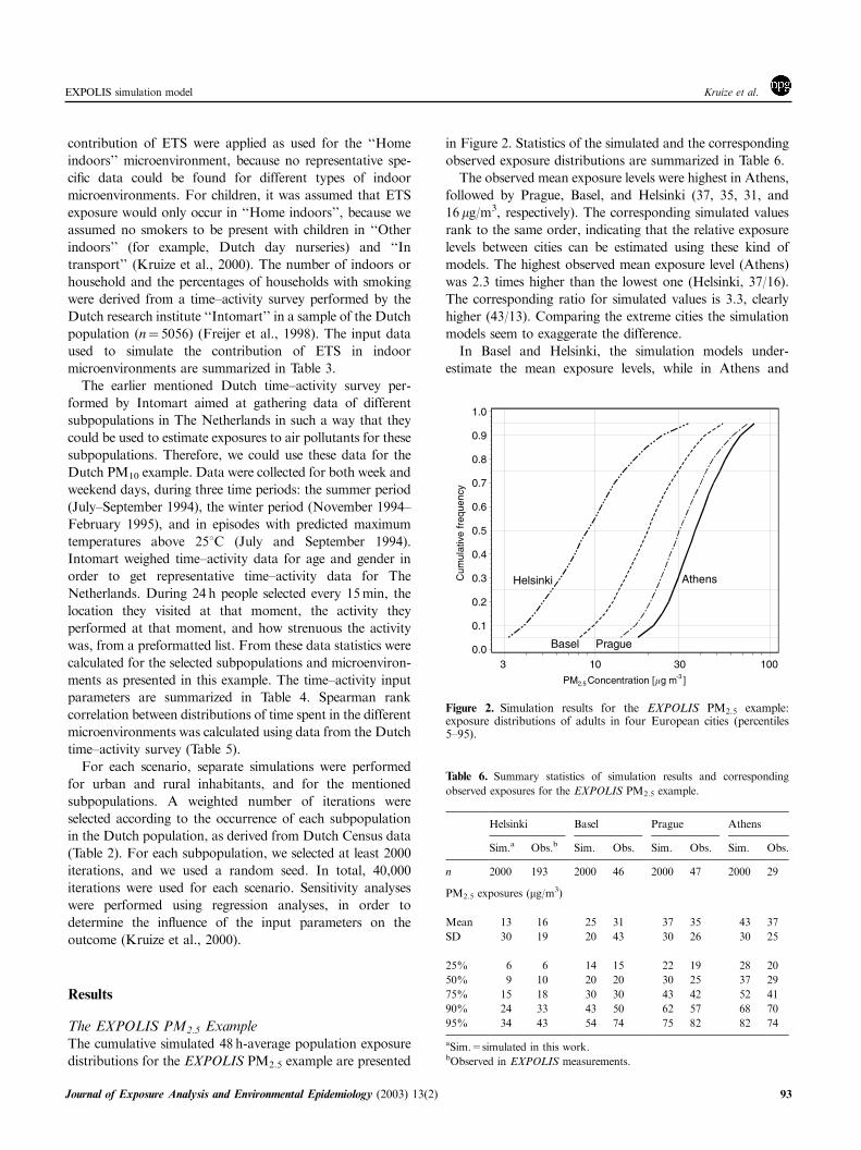
The EXPOLIS PM2.5 ExampleThe cumulative simulated 48 h-average population exposure

distributions for the EXPOLIS PM2.5 example are presented

in Figure 2. Statistics of the simulated and the corresponding

observed exposure distributions are summarized in Table 6.

The observed mean exposure levels were highest in Athens,

followed by Prague, Basel, and Helsinki (37, 35, 31, and

16 mg/m3, respectively). The corresponding simulated values

rank to the same order, indicating that the relative exposure

levels between cities can be estimated using these kind of

models. The highest observed mean exposure level (Athens)

was 2.3 times higher than the lowest one (Helsinki, 37/16).

The corresponding ratio for simulated values is 3.3, clearly

higher (43/13). Comparing the extreme cities the simulation

models seem to exaggerate the difference.

In Basel and Helsinki, the simulation models under-

estimate the mean exposure levels, while in Athens and

Athens

Basel

Helsinki

Prague0.0

0.1

0.2

0.3

0.4

0.5

0.6

0.7

0.8

0.9

1.0

PM Concentration [�g m ]2.5-3

3 10 10030

Cum

ulat

ive

freq

uenc

y

Figure 2. Simulation results for the EXPOLIS PM2.5 example:exposure distributions of adults in four European cities (percentiles5–95).

Table 6. Summary statistics of simulation results and corresponding

observed exposures for the EXPOLIS PM2.5 example.

Helsinki Basel Prague Athens

Sim.a Obs.b Sim. Obs. Sim. Obs. Sim. Obs.

n 2000 193 2000 46 2000 47 2000 29

PM2.5 exposures (mg/m3)

Mean 13 16 25 31 37 35 43 37

SD 30 19 20 43 30 26 30 25

25% 6 6 14 15 22 19 28 20

50% 9 10 20 20 30 25 37 29

75% 15 18 30 30 43 42 52 41

90% 24 33 43 50 62 57 68 70

95% 34 43 54 74 75 82 82 74

aSim.=simulated in this work.bObserved in EXPOLIS measurements.



Prague the simulated levels are higher than the observed

ones. Differences between the observed and the simulated

means range from +2 mg/m3 in Prague to 76mg/m3 in

Athens and Basel. Relatively speaking, these maximum

differences are +16 and �19%, respectively.

The simulated standard deviations do not rank to the same

order as the corresponding observed values. Especially in

Helsinki, the simulated standard deviation is too high and in

Basel too low (+58 and �54%, respectively). Basel is the

only city for which the standard deviation was under-

estimated.

The simulated main percentiles shown in Table 6 compare

to the observed values similarly to the mean values in most

cases. If the mean was underestimated, most of the

percentiles are underestimated too; in fact, for Basel and

Helsinki none of the percentiles was overestimated. For

Athens and Prague most of the percentiles (except the 90th

and 95th, respectively) were overestimated.

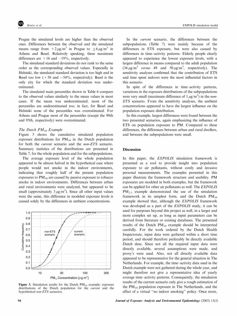
The Dutch PM10 ExampleFigure 3 shows the cumulative simulated population

exposure distributions for PM10 in the Dutch population

for both the current scenario and the non-ETS scenario.

Summary statistics of the distributions are presented in

Table 7, for the whole population and for the subpopulations.

The average exposure level of the whole population

appeared to be almost halved in the hypothetical case where

people would not smoke in the indoor environments,

indicating that roughly half of the present population

exposures to PM10 are caused by passive exposure to tobacco

smoke in indoor environments. Differences between urban

and rural environments were analyzed, but appeared to be

small (approximately 3mg/m3). Since all other input values

were the same, this difference in modeled exposure levels is

caused solely by the differences in ambient concentrations.

In the current scenario, the differences between the

subpopulations (Table 7) were mainly because of the

differences in ETS exposure, but were also caused by

differences in time–activity patterns. Elderly people clearly

appeared to experience the lowest exposure levels, with a

largest difference in means compared to the adult population

(36mg/m3 versus 49 and 50mg/m3, respectively). The

sensitivity analyses confirmed that the contribution of ETS

and time spent indoors were the most influential factors in

this scenario.

In spite of the differences in time–activity patterns,

variations in the exposure distributions of the subpopulations

were very small (maximum difference of 1 mg/m3) in the non-

ETS scenario. From the sensitivity analyses, the ambient

concentrations appeared to have the largest influence on the

population exposure distribution.

In this example, largest differences were found between the

two presented scenarios, again emphasizing the influence of

ETS on population exposure to PM. Compared to these

differences, the differences between urban and rural dwellers,

and between the subpopulations were small.

Discussion

In this paper, the EXPOLIS simulation framework is

presented as a tool to provide insight into population

exposure to air pollutants, without costly and invasive

personal measurements. The examples presented in this

paper illustrate the framework structure and usability. PM

exposures are modeled in both examples, but the framework

can be applied for other air pollutants as well. The EXPOLIS

PM2.5 example demonstrated the use of the simulation

framework in its simplest form, and the Dutch PM10

example showed that, although the EXPOLIS framework

was developed as a part of the EXPOLIS study, it can be

used for purposes beyond this project as well, in a larger and

more complex set up, as long as input parameters can be

derived from literature or existing databases. The presented

results of the Dutch PM10 example should be interpreted

carefully. For the work ordered by the Dutch Health

Inspectorate, input data were gathered within a short time

period, and should therefore preferably be directly available

Dutch data. Since not all the required input data were

directly available, several assumptions were made, and

proxy’s were used. Also, not all directly available data

appeared to be representative for the general situation in The

Netherlands. For example, the time–activity data used in the

Dutch example were not gathered during the whole year, and

might therefore not give a representative idea of yearly

average time–activity patterns. Consequently, the simulation

results of the current scenario only give a rough estimation of

the PM10 population exposure in The Netherlands, and the

effect of a virtual ‘‘no indoor smoking’’ policy. Once more,

non-ETS scenario

current scenario

0.0

0.1

0.2

0.3

0.4

0.5

0.6

0.7

0.8

0.9

1.0

10 100 300

PM Concentration [ g m ]10-3

30

Cum

ulat

ive

freq

uenc

y

�

Figure 3. Simulation results for the Dutch PM10 example: exposuredistributions of the Dutch population for the current and thehypothetical non-ETS scenarios.



we would like to emphasize that this example presented

mainly to show the usability of the EXPOLIS framework for

comparisons of subpopulations and scenarios, more than

showing the most accurate results.

Usability of the FrameworkThe presented examples show that the framework can

be used well for comparison between several existing or

nonexisting situations or populations. First, we presented a

comparison of population exposures to PM2.5 in four

European cities (Athens, Basel, Helsinki, and Prague),

included in the EXPOLIS study, which demonstrates how

models can be built to estimate population exposures in

different cities. From the study of Rotko et al. (2000b) it

appears that response rates were below US standards.

However, because both the input for the simulations and

the personal measurement data were derived from the same

EXPOLIS database, and the low response rates do not stand

in the way the comparison between simulation and measured

data as presented here. Furthermore, the fact that the

nonresponse was high, emphasizes the need of modeling next

to measuring. The simulated means compared rather well to

observed ones; absolute maximum differences were +6 mg/m3 in Athens and �6mg/m3 in Basel, and both of these

values are within 720% of the observed levels. The main

reason for these differences is that the ETS exposures are not

fully captured by the microenvironment measurements used

as inputs for the EXPOLIS framework, as some ETS

exposure occurs also in other places (and rooms) than where

the microenvironmental measurements were taken. Further-

more, the simulated variances of three out of four cities were

overestimated probably because of the fact that the

lognormal concentration distributions used in this work were

not truncated. One or two extreme concentration values

generated by the Latin Hypercube sampling increase the

simulated standard deviation significantly. In the case of

Helsinki, the simulated maximum exposure was higher

(1128mg/m3) than in any of the other cities and more than

an order of magnitude higher than any of the hundreds of

measured concentrations, even though all microenvironment

concentration means were the lowest in Helsinki. This

artefact caused by the sampling technique does not affect

any of the percentiles below 99th and, owing to the large

number of samples, affects the mean only slightly. The

artefact, however, does affect the standard deviation, and

thus the truncation of lognormal distributions should be

considered, as suggested by Hanninen et al. (2003) and

Hanninen and Jantunen, 2003), when the standard devia-

tions (or other measures of variance) are reported.

Secondly, we performed a scenario analysis for The

Netherlands, considering the current population exposure

to PM10 (including ETS) with a non-ETS scenario, serving as

an example of determining the effect of a potential policy

option, in this case a ‘‘no indoor smoking’’ policy. The

average exposure level of the whole population appeared to

be almost halved in case people would not smoke in the

indoor environments. Also, the sensitivity analyses showed

ETS to be an important determinant of exposure, together

with time spent indoors (where ETS exposure took place).

Other exposure studies also indicate that tobacco smoking

is the most or one of the most important contributors of

personal exposure to PM (Dockery and Spengler, 1981; Letz

et al., 1984; Sexton et al., 1984; Spengler et al., 1985;

Koutrakis et al., 1992; Rotko et al., 2000a; Koistinen et al.,

2001). It is important to keep in mind that both the measured

and modeled exposures in relation to tobacco smoke, both

for smokers and nonsmokers, only include the impact of

passive smoking and inhalation of environmental tobacco

smoke (ETS). We realize that the exposure of a smoker from

active smoking is much greater, but it was not assessed in this

study.

The same ETS occurrences and concentration parameters

modeled for a standard Dutch home as explained in the

methods were used for the ‘‘Home indoors’’ and ‘‘Other

Table 7. Simulation result statistics for the subpopulations and the whole population in the Dutch PM10 example.

Children Adults Wa Adults Nb Elderly All

Current

(mg/m3)

Non-ETS

(mg/m3)

Current

(mg/m3)

Non-ETS

(mg/m3)

Current

(mg/m3)

Non-ETS

(mg/m3)

Current

(mg/m3)

Non-ETS

(mg/m3)

Current

(mg/m3)

Non�ETS(mg/m3)

n=6181 n=17,571 n=10,894 n=5354 n=40,000

Mean 44 24 50 24 49 24 36 24 47 24

SD 36 12 39 12 39 12 28 12 38 12

25% 20 15 25 16 23 16 19 16 23 16

50% 34 21 40 22 38 22 28 22 37 22

75% 55 30 62 30 61 30 43 30 58 30

90% 84 39 93 40 92 40 67 40 88 40

95% 110 46 119 48 116 47 87 47 114 47




indoors’’ microenvironments for adults and elderly people,

which can be considered an important approximation done in

the PM10 model. For example, Hanninen and Jantunen

(2002) report PM2.5 ETS concentrations analyzed from

EXPOLIS Helsinki data that are almost double in work-

places compared to homes. It is likely that also in the

Netherlands the ETS concentrations in workplaces and, for

example, restaurants are different from those in homes. This

question cannot be answered without representative measure-

ments. The current ETS model used in the Dutch PM10

example can be considered to be the best possible estimate,

using directly available data.

A third comparison made in this paper was on subpopula-

tions of the Dutch population. Elderly people appeared to

experience lower exposures compared to the other subpopu-

lations according to the current scenario. In the presented

example, these differences between the subpopulations are

caused for a greater part by the differences in the estimated

exposures to ETS; a small fraction of the differences between

the subpopulations is attributable to the differences in the

ratio of times spent indoors and outdoors. In general, this

type of comparison between subpopulations can be used to

determine, for example, what part of the population is at risk,

or to model exposure for specific sensitive groups, such as the

elderly or children.

Another subdivision presented in the Dutch example was

based on a (spatial) distinction between urban and rural

dwellers. The differences in exposures between the Dutch

urban and rural dwellers in the example are caused solely by

the difference in ambient levels, being approximately 0.6� (40–

35) mgm3¼ 3mg/m3, because all other input parameters were

assumed to be equal between these two subpopulations.

With the simulated population exposure it is possible to

estimate the health effects of the exposure as well, if reliable

and comparable exposure–response relationships are avail-

able for PM from different sources and in different

microenvironments. The elemental composition of indoor

and outdoor PM can be rather different (Letz et al., 1984;

Spengler et al., 1985; Koutrakis et al., 1992), and data are

only emerging on the differences in the risk levels of PM from

different sources (Laden et al., 2000; Pope et al., 2002). The

only indoor source, for which broad-based risk assessments

are available, is ETS (Hackshaw et al., 1997; Law et al.,

1997), which is also the most important indoor source for

PM. In order to be able to calculate the risks from multiple

indoor and outdoor sources, the outcome measure of the

modeling result should be the same as the exposure measure

used in the exposure–response relationship.

The outcomes of the EXPOLIS framework can be

tested against air-quality standards considering both indoor

and outdoor environments. Again, for the PM-oriented

examples presented in this paper it was not possible,

because the standard for PM is based on only ambient

concentrations.

Another aspect on the usability of the EXPOLIS frame-

work concerns the averaging time for which the model can be

used. As the time–activity is modeled as fractions of time, the

framework can be applied to calculation of exposures with

wide range of averaging times, but is best suitable for

averaging times from 24 h upwards.

A last remark should be made on the way total fraction of

time is calculated in the presented version of the model. Since

fractions of time spent in the defined microenvironments are

sampled from independent distributions for each defined

microenvironment, the total sampled time might end up

below or above one. In the presented version of the

EXPOLIS framework, total time spent in the visited

microenvironments is scaled to unity, by dividing each time

fraction by the sum of all of the fractions of time of the

visited microenvironments, before calculating the partial

exposures in microenvironments, as applied in the Dutch

PM10 example. In the EXPOLIS PM2.5 example scaling was

not necessary, because time spent in the microenvironment

‘‘Other places’’ was calculated by subtracting the time spent

in the other microenvironments ‘‘Home indoors’’ and ‘‘Work

indoors’’ from total time that the diary was kept a day,

automatically resulting in a total sampled time of one, being

another possibility to deal with this problem. We are aware

that there are probably more (accurate) solutions (e.g.,

binary trees of probability distributions for occurrence of

time fractions). Further research is needed to find out what is

the effect of the way this problem is treated, and what

solution would be best.

Data AvailabilityUsers of the EXPOLIS framework have many opportunities

to adapt the framework to their own needs within the

limitations of data availability. These limitations of data

availability became also apparent in the examples presented

in this paper.

For example, in both examples presented in this paper,

some data referred to only a short period of time for each

study participant. In the EXPOLIS study, the participants

kept a diary during two weekdays. The Dutch participants

filled out the diary during only one day. This short period

that the diary was kept does not necessarily represent the

normal (average) time–activity pattern of a person. There-

fore, the presented population exposure distributions do not

allow analyses on an individual level (Klepeis, 1999).

However, if time–activity data and concentration data would

be available on a longer consecutive period of time, it would

be possible to derive distributions of personal exposure levels

of specific individuals.

Apart from this, data availability was not a big problem in

the EXPOLIS PM2.5 example, because the framework was

built around the design of the EXPOLIS study. However,

the Dutch PM10 example illustrates that data availability

may become a problem when using the framework for other



purposes. Although the current EXPOLIS framework has

simple input requirements, representative PM10 concentra-

tion data for indoor environments and indoor sources (even

on ETS) were not directly available for the Netherlands.

Therefore, we had to decide whether to use available foreign

data or Dutch data based on a limited number of

measurement locations, assuming that these data are

representative for the Netherlands, or to estimate input data

making assumptions and using proxies. In this case, we chose

the latter solution. For example, to be able to calculate the

effect of passive smoking, we estimated the contribution of

ETS to indoor concentrations with a separate stochastical

model. It is well possible that another researcher would

decide to use the available foreign or Dutch data of Janssen

(1998) or Fischer et al. (2000) instead. This example makes it

clear that the researcher’s decision can influence the modeling

results. In the absence of validation, however, it is

questionable what solution would approach the real exposure

situation most accurately.

As this problem must be recognizable for many researchers

in the field of exposure modeling, it would be very helpful if

more databases on (indoor) concentration data and

exposure-relevant time–activity data were published and

made available (Klepeis, 1999). In the USA, several useful

initiatives have been taken already so far (Sexton et al., 1994;

Johnson, 1995). For example, the CHAD is a large database

in which several time–activity databases from the US and

Canada are included, such as the NHAPS database (Klepeis,

1999; Klepeis et al., 2001; McCurdy et al., 2000). However,

it is questionable as to what extent data from these studies

can be used for other (European) countries, because time–

activity patterns might be rather different in different

countries, caused by the cultural differences in how people

spend their time for example. Therefore, more large,

international, multicenter exposure studies would offer a rich

source of (comparable) data, often for more countries at the

same time. The EXPOLIS study is an example of such a

study, from which the database (including outdoor, indoor,

and personal concentration data and time–activity data

among others) will become accessible for the international

research community. When more data on (indoor) concen-

trations of air pollutants, indoor sources, and time–activity

patterns would become available in the future, one still needs

to be careful in using them as input for the model, and one

should evaluate the representativeness of the input data case

by case.

Conclusions

The EXPOLIS simulation framework, described in this

paper, is a helpful tool for researchers to support policy

makers and policy evaluating processes by evaluating air

pollution exposures in different scenarios, population groups,

and locations. It is also useful for helping researchers to

understand the factors affecting exposure levels.

The EXPOLIS example showed that the model predicted

mean population exposure levels in four European cities with

better than 20% accuracy. The presented version of the

simulation framework, not applying truncation to lognormal

concentration distributions, however, overestimated var-

iances in three out of four cases.

The Dutch population PM10 exposure example demon-

strated the use of the framework in modeling exposure levels

of a large complex population in alternative scenarios, for

different subpopulations. The results support the findings

from field surveys that exposure to tobacco smoke approxi-

mately doubles the population exposures to particulate

matter. Limited data availability asked for creative ways to

derive input parameters for the EXPOLIS framework, and

emphasizes the need for general accessibility of databases on

(indoor) concentration data and exposure-relevant time–

activity patterns to support researchers in the field of

exposure modeling.

Acknowledgments

EXPOLIS has been supported by European Union 4th

Framework Research, Technology and Development (RTD)

program, contracts ENV4-CT96-0202 (DG12-DTEE) and

ERB IC20-CT96-0061 (Prague); Academy of Finland

contract No. 36586 (Helsinki); Swiss Ministry for Education

and Science Contract BBW No. 95.0894 (Basel); French

National Environment Agency (ADEME), Union Routiere

de France Communaute de Communes (Grenoble); and

other national research funds, and intramural funding from

the participating institutes. The Dutch PM10 example was

derived from calculations performed as a part of a work

commissioned by the Dutch Health Inspectorate.

We thank Dr. J.I. Freijer for his helpful comments on the

draft versions of this manuscript.

References

Chapin Jr FS. Human Activity Patterns in the City F Things People Do

in Time and Space. John Wiley & Sons, Inc., New York, USA,

1974.

Colome SD., Kado NY., Jacques P., and Kleinman M. Indoor–outdoor

air pollution relations: particulate matter less than 10 mm in

aerodynamic diameter (PM10) in homes of asthmatics. Atmos

Environ 1992: 6A ( 6 ): 2173–2178.

Dab W., Segala C., Dor F., Festy B., Lamelose P., Moullec le Y., Tertre

le A., Medina S., Quenel P., Wallaert B., and Zmirou D. Air

pollution and health: correlation or causality? The case of the

relationship between exposure to particles and cardiopulmonary

mortality. J Air Waste Manage Assoc 2001: 51: 220–235.

Dockery DW., and Spengler JD. Indoor–outdoor relationships of

respirable sulfates and particles. Atmos Environ 1981: 15: 335–343.



Duan N. Models for human exposure to air pollution. Environ Int 1982:

8: 305–309.

Duan N. Stochastic microenvironmental models for air pollution

exposure. J Expos Anal Environ Epidemiol 1991: 1 ( 2 ): 235–257.

Duan N., and Mage DT. Combination of direct and indirect approaches

for exposure assessment. J Expos Anal Environ Epidemiol 1997: 7

( 4 ): 439–470.

Elzakker BG., and Buijsman E. Measurement activities in 1999 by the

National Air Quality Monitoring Network (in Dutch) (Report No.

723101 032). National Institute of Public Health and the Environ-

ment, Bilthoven, The Netherlands, 1999.

Fischer PH., Hoek G., Reeuwijk van H., Briggs DJ., Lebret E., Wijnen

van JH., Kingham S., and Elliott PE. Traffic related differences in

outdoor and indoor concentrations of particles and volatile organic

compounds in Amsterdam. Atmos Environ 2000: 34: 3713–3722.

Freijer JI., Bloemen HJTh., Loos de S., Marra M., Rombout PJA.,

Steentjes GM., and Veen van MP. Modelling exposure of the Dutch

population to air pollution. J Hazard Mater. 1998: 61: 107–114.

Freijer JI., and Bloemen HJT. Modelling relationships between indoor

and outdoor air quality. J Air and Waste Manage Assoc 2000: 50:

292–300.

Fugas M. Assessment of total exposure to an air pollutant. Proceedings

of the International Conference on Environmental Sensing and

Assessment. Paper No. 38-5, Vol. 2, IEEE #75-CH 1004-1, ICESA,

1975, Las Vegas.

Hanninen OO., and Jantunen MJ. Simulating personal PM2.5 Exposure

Distributions in Helsinki using ambient measurements as inputs

(submitted).

Hanninen OO., and Kaarakainen E., and Alm S. EXPOLIS Databases.

Project document manuscript. 2002. KTL, Kuopio, Finland.

Hanninen OO., Kruize H., Lebret E., and Jantunen, and MJ.

EXPOLIS simulation model: PM2.5 application and comparison to

measurements in Helsinki. J Expos Anal Environ Epidemiol 2003:

13: 74–85.

Hackshaw AK., Law MR., and Wald NJ. The accumulated evidence on

lung cancer and environmental tobacco smoke. BMJ 1997: 315:

980–988.

Jantunen MJ., Katsouyanni K., Knoppel H., Kunzli N., Lebret E.,

Maroni M., Saarela K., Sram R., and Zmirou D., et al. Air pollution

exposure in European cities: the EXPOLIS study. Final EU

Report Contract nos. ENV4-CT96-0202 and ERB IC20-CT96-

0061, 1998.

Jantunen MJ., Hanninen O., Katsouyanni K., Knoppel H., Kunzli N.,

Lebret E., Maroni M., Saarela K., Sram R., and Zmirou D. Air

pollution exposure in European cities: the ‘‘EXPOLIS’’ study.

J Expos Anal Environ Epidemiol 1999: 8: 495–518.

Janssen NAH. Personal exposure to airborne particles F validity of

outdoor concentrations as a measure of exposure in time series

studies. PhD dissertation, Agricultural University of Wageningen,

Wageningen, 1998.

Johnson TR. Recent advances in the estimation of population exposure

to mobile source pollutants. J Expos Anal Environ Epidemiol 1995: 5

( 4 ): 551–571.

Klepeis NE. An introduction to the indirect exposure assessment

approach: modeling human exposure using microenvironmental

measurements and the recent National Human Activity Pattern

Survey. Environ Health Perspect 1999: 107 ( 2 ): 365–374.

Klepeis NE., Nelson WC., Ott WR., Robinson JP., Tsang AM., Switzer

P., Behar JV., Hern SC., and Engelmann WH. The National

Human Activity Pattern Survey (NHAPS): a resource for assessing

exposure to environmental pollutants. J Expos Anal Environ

Epidemiol 2001: 11 ( 3 ): 231–252.

Koistinen KJ., Hanninen O., Rotko T., Edwards RD., Moschandreas

D., and Jantunen MJ. Behavioral and environmental determinants of

personal exposures to PM2.5 in EXPOLIS-Helsinki, Finland. Atmos

Environ 2001: 35 ( 14 ): 2473–2481.

Kousa A., Oglesby L., Koistinen K., Kunzli N., and Jantunen M.

Exposure chain of urban air PM2.5 – association between ambient

fixed site, residential outdoor, indoor, workplace and personal

exposures in four European cities in the EXPOLIS-study. Atmos

Environ 2002: 36: 3031–3039.

Koutrakis P., Briggs SLK., and Leaderer BP. Source apportionment of

indoor aerosols in Suffolk and Onondaga Counties, NewYork.

Environ Sci Technol 1992: 26 ( 3 ): 521–527.

Kruize H., Freijer JI., Franssen EAM., Fischer PH., Lebret E., and

Bloemen HJTh. Verdeling van de blootstelling aan fijn stof in de

Nederlandse bevolking (in Dutch) (Report no. 263610 005). RIVM,

Bilthoven, The Netherlands, 2000.

Laden F., Neas LM., Dockery DW., and Schwartz J. Association of fine

particulate matter from different sources with daily mortality in six

U.S. cities. Environ Health Perspect 2000: 108 ( 10 ): 941–947.

Law MR., Morris JK., and Wald NJ. Environmental tobacco smoke

exposure and ischaemic heart disease: an evaluation of the evidence.

BMJ 1997a: 315: 973–980.

Law PL., Lioy PJ., Zelenka MP., Huber AH., and McCurdy TR.

Evaluation of a probabilistic exposure model applied to carbon

monoxide (pNEM/CO) using Denver personal exposure monitoring

data. J Air Waste Manage Assoc 1997b: 47: 491–500.

Letz R., Ryan PB., and Spengler JD. Estimating personal exposures to

respirable particles. Environ Monit Assess 1984: 4: 351–359.

Li C-S. Relationships of indoor/outdoor inhalable and respirable

particles in domestic environments. Sci Total Environ 1994: 151:

205–211.

Lioy PJ. Assessing total human exposure to contaminants Fa multidisciplinary approach. Environ Sci Technol 1990: 7: 938–945.

Lioy PJ. Measurement methods for human exposure analysis. Environ

Health Perspect 1995: 103 ( 3 ): 35–44.

McCurdy T. Estimating human exposure to selected motor vehicle

pollutants using the NEM series of models: lessons to be learned.

J Expos Anal Environ Epidemiol 1995: 5 ( 4 ): 533–550.

McCurdy T., Glen G., Smith L., and Lakkadi Y. The National

Exposure Research Laboratory’s Consolidated Human Activity

Database. J Expos Anal Environ Epidemiol 2000: 10 ( 6 ): 566–578.

NRC (National Research Council) Research Priorities for Airborne

Particulate Matter. I: Immediate Priorities and Long Term Research

Portfolio. National Academy Press, Washington, DC, 1998, 127pp.

Ott WR. Exposure estimates based on computer generated activity

patterns. J Toxicol-clin Toxicol 1984: 21 (1 and 2): 97–128.

Ott WR. Total human exposure F an emerging science focuses on

humans as receptors of environmental pollution. Environ Sci Technol

1985: 19 ( 10 ): 880–886.

Ott W., Thomas J., Mage D., and Wallace L. Validation of the

simulation of human activity and pollutant exposure (SHAPE)

model using paired days from the Denver, Colorado carbon

monoxide field study. Atmos Environ 1988: 22: 2101–2113.

Palisade Corporation. @Risk F Risk Analysis and Simulation Add-in

for Microsoft Excel or Lotus 1-2-3. Palisade Corporation, Newfield,

USA, 1994.

Pellizzari ED., Clayton CA., Rodes CE., Mason RE., Piper LL., Fort

B., Pfeifer G., and Lynam D. Particulate matter and manganese

exposures in Toronto, Canada. Atmos Environ 1999: 33 ( 5 ):

721–734.

Pope CA., Burnett RT., Thun MJ., Calle EE., Krewski D., Ito K., and

Thurston GD. Lung cancer, cardiopulmonary mortality, and long-

term exposure to fine particulate air pollution. J Am Med Assoc

2002: 287: 1132–1141.

Rotko T., Oglesby L., Kunzli N., and Jantunen MJ. Population

sampling in European air pollution exposure study, EXPOLIS:



comparisons between the cities and representativeness of the samples.

J Expos Anal Environ Epidemiol 2000a: 10 ( 4 ): 355–364.

Rotko T., Koistinen K., Hanninen O., and Jantunen M. Socio-

demographic descriptors of personal exposure to fine particles

(PM2.5) in EXPOLIS-Helsinki. J Expos Anal Environ Epidemiol

2000b: 10 ( 4 ): 385–393.

Ryan PB., Spengler JD., and Letz R. Estimating personal exposures to

NO2. Environ Int 1986: 12: 395–400.

Ryan PB. An overview of human exposure modeling. J Expos Anal

Environ Epidemiol 1991: 1 ( 4 ): 453–474.

Schwab M., Colome SD., Spengler JD., Ryan PB., and Billick IH.

Activity Patterns applied to pollutant exposure assessment: data from

a personal monitoring study in Los Angeles. Toxicol Ind Health

1990: 6 ( 6 ): 517–532.

Sexton K., Spengler JD., and Treitman RD. Personal exposure to

respirable particles: a case study in Waterbury, Vermont. Atmos

Environ 1984: 18 ( 4 ): 1385–1398.

Sexton K., Wagener DK., Selevan SG., Miller TO., and Lybager JA.

An inventory of human exposure-related data bases. J Expos Anal

Environ Epidemiol 1994: 4 ( 1 ): 95–109.

Spengler JD., Treitman RD., Tosteson TD., Mage DT., and Soczek

ML. Personal exposures to respirable particulates and implications

for air pollution epidemiology. Environ Sci Technol 1985: 19:

700–707.

Spix C., Anderson HR., Schwartz J., Vigotti MA., LeTertre A., Vonk

JM., Touloumi G., Balducci F., Piekarski T., Bacharova L., Tobias

A., Ponka A., and Katsouyanni K. Short-term effects of air

pollution on hospital admissions of respiratory diseases in Europe: a

quantitative summary of APHEA study results. Arch Environ Health

1998: 53 ( 1 ): 54–64.

Stivoro (Stichting Volksgezondheid en Roken). Jaarverslag 1998 (in

Dutch). The Hague, The Netherlands, 1999.

Szalai A. (Ed.). The Use of Time: Daily Activities of Urban and Suburban

Populations in Twelve Countries. Mouton, The Hague, Netherlands,

1972.

Vedal S. Ambient particles and health: lines that divide. J Air Waste

Manage Assoc 1997: 47:551–581.

Zartarian VG., Ott WR., and Duan N. A quantitative definition of

exposure and related concepts. J Expos Anal Environ Epidemiol 1997:

7 ( 4 ): 411–437.



Description and demonstration of the EXPOLIS simulation model: Two examples of modeling population...

Documents

Transcript of Description and demonstration of the EXPOLIS simulation model: Two examples of modeling population...