Depth variation of seismic source scaling relations: implications for earthquake hazard in...

www.elsevier.com/locate/tecto

Tectonophysics 390

Depth variation of seismic source scaling relations: implications

for earthquake hazard in southeastern Australia

Trevor I. Allena,*, Gary Gibsona,b, Amy Brownb,1, James P. Culla

aSchool of Geosciences, Monash University, P.O. Box 28E, VIC 3800, AustraliabES&S Seismology Research Centre, 8 River St., Richmond, VIC 3121, Australia

Received 12 February 2002; received in revised form 25 September 2002; accepted 9 March 2004

Available online 5 October 2004

Abstract

Advances in earthquake data acquisition and processing techniques have allowed for improved quantification of source

parameters for local Australian earthquakes. Until recently, only hypocentral locations and local magnitudes (ML) had been

determined routinely, with little attention given to the inversion of additional source parameters. The present study uses these

new source data (e.g. seismic moment, stress drop, source dimensions) to further extend our understanding of seismicity and the

continental stress regime of the Australian landmass and its peripheral regions.

Earthquake activity within Australia is typically low, and the proportion of small to large events (i.e. the b value) is also low.

It is observed that average stress drops for southeastern Australian earthquakes appear to increase with seismic moment to

relatively high levels, up to approximately 10 MPa for ML 5.0 earthquakes. This is thought to be indicative of high compressive

crustal stress, coupled with strong rocks and fault asperities. Furthermore, the data indicates that shallow focus earthquakes

(shallower than 6 km) appear to produce lower than average stress drops than deeper earthquakes (between 6 and 20 km) with

similar moment.

Recurrence estimates were obtained for a discrete seismogenic zone in southeastern Australia. Decreasing b values with

increasing focal depth for this zone indicate that larger earthquakes (with high stress drops) tend to occur deeper in the crust.

This may offer an explanation for the apparent increase of stress drop with hypocentral depth. Consequently, earthquake hazard

estimates that assume a uniform Gutenburg–Richter distribution with depth (i.e. constant b value) may be too conservative and

therefore slightly overestimate seismic hazard for surface sites in southeastern Australia.

D 2004 Published by Elsevier B.V.

Keywords: Depth variation; Seismic source scaling; Earthquake hazard

0040-1951/$ - see front matter D 2004 Published by Elsevier B.V.

doi:10.1016/j.tecto.2004.03.018

* Corresponding author. Present address: Geoscience Australia,

GPO Box 378, Canberra, ACT 2601, Australia. Tel.: +61 2 6249

9864; fax: +61 2 6249 9986.

E-mail address: [email protected] (T.I. Allen).1 Present address: FM Global, Level 37, 140 William Street,

Melbourne, VIC 3000, Australia.

1. Introduction

It has long been recognised that the stress field of

continental Australia is of high horizontal compres-

(2004) 5–24

T.I. Allen et al. / Tectonophysics 390 (2004) 5–246

sion (Worotnicki and Denham, 1976; Denham et al.,

1979; and others). At the inception of the of the World

Stress Map compilation (Zoback et al., 1989; Zoback,

1992), knowledge of the stress regime of the continent

was still poorly constrained. However, recent initia-

tives to compile stress orientation data from analysis

of in situ measurements coupled with earthquake focal

mechanisms now provide a more detailed account of

the continental stress field in Australia and its

peripheral regions (Hillis and Reynolds, 2000; and

others). Unlike most stable continental regions,

Australia does not exhibit uniform horizontal com-

pressive stress parallel to the direction of absolute

plate motion (Zoback et al., 1989; Richardson, 1992;

Hillis and Reynolds, 2000; Reynolds et al., 002).

Observational measurements of in situ stress demon-

strate high horizontal stress at shallow depths (Den-

ham et al., 1979).

Historically, knowledge of Australian seismicity

has been limited by the relatively short recording

period and the sparse seismograph network, especially

prior to the 1960s (Gibson et al., 1981). As a result,

many smaller earthquakes were not recorded, heavily

biasing the Australian earthquake catalogue with a

greater proportion of larger events relative to small

events. If the catalogue deficiencies are not considered

in earthquake hazard estimates, apparent b values

become too low (i.e. having a comparatively low

proportion of small to large events), giving erroneously

high hazard when ground shaking is extrapolated to

moderate-to-long return periods. With the expansion of

seismic networks in the mid 1970s, the seismograph

coverage in eastern Australia has become quite good

by world standards. An increased number of low

magnitude events can now be detected and located,

giving more accurate estimates for the recurrence of

small to moderate earthquakes in these areas. Seismo-

graph coverage in the remote western and central

regions of the continent is still relatively poor.

Most of the earthquakes recorded in Australia tend

to be shallow and are restricted to a seismogenic zone

within the upper 20 km of the crust (Denham, 1988).

Given that the earthquakes are shallow, it is not

uncommon for the larger events to be associated with

surface rupture, as was observed with the 1968 MS 6.8

Meckering earthquake (Denham, 1988) and the MS

6.3, 6.4 and 6.7 earthquakes of the 1988 Tennant

Creek sequence (Jones et al., 1991). There have been

some documented earthquakes within continental

Australia that are reported to have focal depths in

excess of 30 km (e.g. McCue and Michael-Leiba,

1993; Michael-Leiba et al., 1994). However, these

occurrences have been rare and are not representative

of the continent-wide trend.

In contrast to most stable continental regions,

where the largest earthquakes are concentrated in

failed rifts or passive margins, Australia’s largest

onshore earthquakes have occurred in the unrifted

ancient Proterozoic and Archean terranes of western

and central Australia (Johnston and Kanter, 1990).

More complex earthquake distributions are observed

in the younger terranes of the Phanerozoic eastern

margins (Fig. 1).

The purpose of the current study is to firstly

examine any possible variation of source scaling

relations of southeastern Australian earthquakes with

respect to focal depth. Secondly, we investigate the

Gutenburg–Richter distribution for well-located events

in terms of hypocentral depth and local stress, and

consider any implications for earthquake source scal-

ing and discuss any consequences for hazard estimates.

2. Earthquake source parameters

2.1. Theory of earthquake source scaling

Resolving earthquake source parameters from the

measurement of elastic wave energy propagating

through complex geological terrains remains the

fundamental challenge facing seismologists. Conse-

quently, appropriate care must be taken when evaluat-

ing earthquake source parameters; e.g. seismic

moment, rupture size, stress drop and magnitude.

2.2. Seismic moment

The seismic moment M0 is one of the most robust

measures of an earthquake’s size and is defined

following (Aki and Richards, 1980)

M0 ¼ luA; ð1Þ

where l is the shear modulus at the source, u is the

average displacement across the rupture, and A is the

fault area. M0 can occasionally be calculated using

Fig. 1. Distribution of documented Australian earthquakes of magnitude ML 4.0 and greater, 1801–2002, overlying the major orogenic domains

and covers. Note the relative number of Australian earthquakes compared to the Indonesian subduction zone events to the north. (Adapted after

Foster and Gray, 2000; Betts et al., 2002).

T.I. Allen et al. / Tectonophysics 390 (2004) 5–24 7

relation (1) whenever the average displacement across

the fault can be quantified by surface rupture. In

practice, seismic moment is evaluated from the

asymptote of low-frequency earthquake motion, esti-

mated from the low-frequency spectral level X0 of the

far-field displacement spectrum A( f ). The displace-

ment spectrum can be modelled following

A fð Þ ¼ X0

1þ f =fcð Þc ; ð2Þ

where fc is the corner frequency and c is the

asymptotic high-frequency spectral decay exponent.

c is a value typically bound to at least 1.5 (required to

obey conservation of energy laws) and 3; given

M0~fc�3 (assuming constant source scaling; Hough,

1996). Observationally, c is usually found to be about

2. The Brune (1970) model relates the spectral

amplitude of P- or S-wave coda to the seismic

moment by

M0 ¼4pq0c

30G rð ÞX0

U/h; ð3Þ

where q0 is the density of the source medium, c0 is

either the P- or S-wave velocity at the source, U/h is


the mean radiation pattern (0.52 and 0.63 for P- and

S-waves, respectively; Boore and Boatwright, 1984)

and the geometric spreading coefficient G(r) is given

by the relations (Herrmann and Kijko, 1983)

G rð Þ ¼ r r V r0r0rð Þ1=2 r N r0

;

�ð4Þ

where r0 is typically taken to be 80 km; the

approximate distance where geometrical spreading

becomes less severe owing to surface-wave arrivals

(Castro et al., 1997).

2.2.1. Source dimensions

Unlike the seismic moment calculation from Eq.

(3), estimates of earthquake source dimensions are

highly model dependent and can be susceptible to

systematic errors (Beresnev, 2001), particularly in the

underestimation of the corner frequency from far-field

displacement spectra owing to the attenuation of high-

frequency perturbations. The Brune (1970) model

represents a circular dislocation with instantaneous

stress release. The radius R0 of a circular fault is

inversely related to the corner frequency following

R0 ¼Kcb0

2pfc; ð5Þ

where b0 is the shear-wave velocity in the source area

and Kc is a constant depending on the source model,

where Kc=2.34 (Brune, 1971).

2.2.2. Stress drop

Stress drop Dr is defined as the difference between

the initial and final stress levels averaged over the

fault plane and is given by (Brune, 1970, 1971)

Dr ¼ 7

16

M0

R30

: ð6Þ

The relationship represents a uniform decrease in

shear stress acting to produce seismic slip over a

circular fault.

It is generally accepted that the seismic stress

drops are relatively uniform over a wide magnitude

range and have observationally been found to be

independent of earthquake size; therefore following

the scaling law M0~fc�3 (e.g. Aki, 1967; McGarr

et al., 1981; Somerville et al., 1987; Urbancic et

al., 1992; Abercrombie and Leary, 1993; Aber-

crombie, 1995; and others). These findings suggest

that earthquakes of all magnitudes exhibit self-

similarity and are scaled at constant stress drop.

However, the debate as to the validity of earth-

quake scaling at constant stress drop over all

magnitudes is a controversial issue in observational

seismology. Many authors have observed a break-

down in earthquake self-similarity for small magni-

tude earthquakes (e.g. Molnar and Wyss, 1972;

Garcıa-Garcıa et al., 1996; Shi et al., 1998; and

others). Gibowicz et al. (1991) calculated source

parameters for very small events of magnitude MW

�3.6 to �1.9 from active seismicity at the Under-

ground Research Laboratory, Canada. They also

observed stress drop to increase with increasing

seismic moment, although they and others have

suggested that the apparent breakdown at low

magnitudes does not agree with predicted models

(Aki, 1967), and is simply an artefact of severe

attenuation of the high-frequency energy obscuring

the corner frequency in the upper few kilometres of

the crust (e.g. Abercrombie and Leary, 1993;

Abercrombie, 1995; Prejean and Ellsworth, 2001)

and limitations in sampling bandwidth (Hough,

1996; Ide and Beroza, 2001; Hiramatsu et al.,

2002). Abercrombie and Leary (1993), and Aber-

crombie (1995) have compared seismograms

recorded at a 2.5-km depth to those recorded at

the surface for the same events and have demon-

strated this near-surface attenuation.

The attenuation of high-frequency energy is a

particular concern when evaluating stress drop for

crustal earthquakes. Shi et al. (1998) demonstrated

that they can simulate corner frequencies by spectral

fitting, typically higher than those obtained via

conventional asymptote methods that are consistent

with hypocentral distance. These estimates are based

largely on the evaluation of seismic moment

obtained employing local attenuation relations.

Accounting for discrepancies in conventional and

simulated corner frequencies, Shi et al. still observed

an apparent breakdown of constant source scaling for

small magnitude earthquakes in eastern North

America.


Nuttli (1983a) has previously suggested that earth-

quakes within stable continental regions are suscep-

tible to systematic increases of average stress drop

with seismic moment (e.g. Nuttli, 1983b; Bungum et

al., 1992). In contrast, he adds, earthquakes near plate

margins have nearly constant stress drop, consistent

with constant earthquake source scaling.

Several studies have shown intraplate earth-

quakes to have higher stress drops than interplate

earthquakes with similar moment (e.g. Molnar and

Wyss, 1972; Kanamori and Anderson, 1975; Scholz

et al., 1986; Houston, 2001). It is suspected that

near plate margins where high levels of earthquake

activity are common, fault rheology is typically

uniformly weak, consequently Dj appears to be

low. In contrast, the effect of fault healing over

time is more apparent in intraplate regions of low

seismicity. Consequently, we observe higher levels

of stress release resulting from the initiation of

rupture on new growth surfaces or healed fault

asperities (e.g. Molnar and Wyss, 1972). Johnston

(1992), however, argued that there was insufficient

evidence to confirm any significant disparity

between the magnitude of stress drop of intraplate

and interplate earthquakes. Recent evaluations of

source parameters from the 2001 MW 7.6 Bhuj,

India earthquake, however, indicate that this was a

high stress drop event (Antolik and Dreger, 2003).

The earthquake, which occurred in stable continen-

tal crust, possessed relatively high-frequency ground

motion and a short rupture duration which suggests

a relatively small rupture size. Tightly clustered

hypocentral locations from the aftershock sequence

reinforce the assumed small rupture size of the

main shock (Johnston, personal communication,

2002).

Average stress drops for intraplate earthquakes

have been reported to range from 0.1 to about 100

MPa (Johnston, 1992; Abercrombie and Leary, 1993)

although most do not exceed 10 MPa.

2.2.3. Earthquake magnitude

There are several different definitions of earth-

quake magnitude, each evaluated taking advantage of

different characteristics of recorded ground motion.

Some magnitude scales perform better for different

sized earthquakes at different distances, however, all

are scaled to some degree to give approximately

equivalent solutions for any specific earthquake. The

local magnitude scale, ML (Richter, 1935), provided

the first convenient measure of earthquake size from

instrumental recordings and may be calculated

following

ML ¼ logA� logA0 rð Þ þ Sj; ð7Þ

where Sj is the site correction factor, A is the recorded

trace amplitude at hypocentral distance r and the

�log A0(r) term is scaled such that for an event of

ML 3.0, A=1 mm recorded at an epicentral distance of

100 km on a standard horizontal-component Wood–

Anderson seismograph (Richter, 1935, 1958). The

local magnitude scale has since been redefined for

southeastern Australia by Michael-Leiba and Mala-

fant (1992), and subsequently extended by Wilkie et

al. (1994).

Moment magnitude MW can be derived from

seismic moment M0 employing the following empiri-

cal definition proposed by Hanks and Kanamori

(1979)

MW ¼ 2

3logM0 � 6:07; ð8Þ

where M0 is in N-m.

2.3. Data selection

Given the relatively low levels of seismicity and a

wide distribution of epicentres, coupled with a sparse

seismograph network, constraining depths for many

Australian earthquakes can be difficult. Earthquakes

chosen for the present study were all selected from

southeastern Australia where, due to the development

of much of the nation’s infrastructure and higher than

average earthquake activity, the seismograph network

is well developed. Data for this project were recorded

and located by the ES&S Seismology Research

Centre, Melbourne. Most of the earthquakes selected

were well-located, having well-constrained focal

depths with uncertainties of about F4 km or less.

Of the many thousands of events in the catalogue, 93

events which met these criteria were chosen. These

events occurred from 1993 to 2001 and magnitudes

ranged from ML 1.6 to ML 5.0.


Some exceptions to these criteria were made. To

maximise the earthquake magnitude range for the

study given the small number of moderate-large

events recorded at close range (necessary to obtain

good depth control), several larger earthquakes with

slightly less well-defined focal depths were included.

In addition, several deeper events with slightly higher

depth uncertainties were also added to the study

catalogue to give improved constraints for any

possible depth dependence of earthquake source

scaling parameters. Fig. 2 shows a schematic map of

the selected earthquakes together with the local

seismograph network.

2.4. Methodology

All seismograms used in the analysis were digitally

recorded on three-component seismographs at a sample

Fig. 2. Schematic map of selected earthquakes with respect to the lo

rate of 100 Hz, with an anti-alias filter at 25 Hz. Fourier

spectra of the S-wave coda for each event were

calculated and corrected for instrumental response

and attenuation from anelastic and scattering processes.

Attenuation was corrected using the apparent

quality factor Qa( f,r) recently derived for south-

eastern Australia (Allen, 2004). Owing to complex

heterogeneities in the structure of the Earth’s litho-

sphere and upper mantle (e.g. Kennett, 1989), it is

often insufficient to use a discrete Q( f ) function to

evaluate earthquake source parameters for local earth-

quakes. The apparent quality factor Qa( f,r) proposed

by Allen (2004) therefore extends on conventional

Q( f ) functions by allowing for additional complexity

in the variation of crustal structure with depth, and

considers factors such as variable velocity gradients

and anomalous large-amplitude reflections from the

Moho. Following the form Qa( f,r)=Qr(r)g(r), the

cation of the Australian seismograph network (open triangles).

Fig. 3. Attenuation model of the form Qa( f,r)=Qr(r)fg(r) used to

evaluate earthquake source parameters.

Table 1

Site corrections Sj and standard errors (in ML) for the vertica

component of the 56 seismographs for which more than one record

was used in the present study

Site Correction nk Site Correction nk

ABEM �0.04F0.08 36 KOWA �0.10F0.25 3

APN +0.15F0.08 16 KTLM �0.31F0.10 25

AVD �0.05F0.13 8 LBXM +0.26F0.08 19

AVO �0.04F0.08 25 LGT +0.21F0.12 20

BANM �0.13F0.04 3 MACM +0.35F0.10 11

BJEM �0.04F0.08 33 MCV +0.24F0.14 26

BUDM +0.02F0.04 26 MDRM �0.13F0.27 3

CCRM �0.02F0.25 8 MITM �0.20F0.15 26

CDNM +0.05F0.15 22 MLWM �0.26F0.25 6

COP +0.07F0.39 2 MTL �0.01F0.10 17

CPXM +0.01F0.07 34 NARM �0.11F0.10 22

CTBM +0.13F0.07 16 NATM �0.14F0.07 38

DDC �0.24F0.73 3 PAT �0.16F0.10 34

DON +0.04F0.12 15 ROYM �0.19F0.08 42

DRAM �0.05F0.07 48 RUSM �0.09F0.18 14

DTMM �0.17F0.08 37 SGTH +0.32F0.71 2

DVBX �0.00F0.12 21 SMBT +0.17F0.41 2

EUGM +0.12F0.24 13 STN �0.38F0.09 2

FSHM +0.26F0.12 25 TALM +0.09F0.08 37

FTZM +0.15F0.06 22 TAT +0.06F0.25 4

GOGM �0.35F0.19 7 TOMM �0.05F0.11 25

GRVM �0.12F0.10 17 TYR +0.23F0.10 37

GVL +0.06F0.12 22 WAH �0.23F0.20 2

HOPM �0.09F0.27 5 WER �0.23F0.10 28

IVSM +0.01F0.10 29 WGBM �0.11F0.08 27

JBD +0.03F0.20 7 WILL +0.50F0.28 3

JBRM �0.06F0.09 19 WRNM +0.12F0.29 4

KANM +0.08F0.09 42 YERM +0.14F0.08 35

All corrections are additive and nk is the number of records at site

used to calculate Sj. Standard errors are given to a 95% confidence

interval.


attenuation model used in the present study is defined

as (Allen, 2004) (Fig. 3);

Qa f ; rð ÞrV150 ¼ ð1:85r þ 10e�r10Þf 0:96�0:0039rð Þ

Qa f ; rð ÞrN150 ¼ 0:42r þ 212:11ð Þf 0:50�0:0003rð Þ ð9Þ

The term Qr increases systematically with hypo-

central distance and gives an apparent quality factor

which must be used to estimate seismic wave

amplitude at distance r from the source. Because

Australian earthquakes are shallow, at present, it is

assumed that Qa( f,r) does not vary with focal depth.

This new attenuation model further extends prior

estimates of Q( f ) by Wilkie and Gibson (1994) and

more recent studies presented by Allen et al. (2002).

Following Brune’s (1970, 1971) model, earthquake

source parameters [i.e. seismic moment M0, rupture

radius r0, and stress drop Dr; Eqs. (3, 5 and 6),

respectively] were subsequently calculated from ver-

tical component seismograms employing an S-wave

velocity of 3.58 km s�1 and density of 2.67 g cm�3.

In addition, local magnitudes ML were estimated

from synthesized Wood–Anderson seismograms. Ini-

tially setting the site correction factor Sj=0 [Eq. (7)],

we calculate an average magnitude Mi for the ith

event following the relations of Wilkie et al. (1994).

Using vertical component seismograms, site correc-

tions were subsequently derived following

Sj ¼

Xnkk¼1

ðMi �MijÞ

nk; ð10Þ

where Mij is the magnitude at the jth site and nk is the

number of records recorded at j. Evaluation of site

corrections for 56 of the sites used in this study (with

at least two records) coupled with their standard errors

is shown in Table 1.

2.5. Analysis of data

Typically, far-field displacement spectra obeyed

Brune’s (1970) source model of decreasing amplitude

as x�2 for frequencies above fc, where x=2pf and f is

the frequency of the ground perturbation (Fig. 4).

Resulting earthquake source parameters are presented

in Table 2.

Average Brune stress drop for southeastern Austral-

ian earthquakes appear to increase with seismic

l

j

Fig. 4. Typical S-wave far-field displacement spectra for four southeastern Australian earthquakes calculated from vertical component

seismograms. Spectra are corrected for the effects of anelastic attenuation and scattering following the relations of Allen (2004).


Table 2

Source parameters from southeastern Australian earthquakes

Place Date HHMM Longitude

(8E)Latitude

(8N)Depth

(km)

M0

(Nm)

MW ML R0

(km)

Dr(MPa)

fc(Hz)

ni

Katoomba 1993-03-22 0806 150.346 �33.826 17 5.06e+12 2.41 2.53 0.16 0.50 8.12 12

Mt St Gwear 1993-05-03 1523 146.327 �37.782 7 8.31e+11 1.88 1.68 0.16 0.20 10.28 5

Churchill 1993-07-24 1333 146.485 �38.353 15 2.01e+13 2.82 3.00 0.28 0.41 4.79 5

Taralgon South 1993-09-25 0240 146.530 �38.311 10 2.32e+13 2.83 3.03 0.21 1.02 6.45 5

Mullengrove 1993-10-10 1606 149.174 �34.505 19 3.82e+12 2.33 2.48 0.12 0.89 10.80 6

Moe 1993-10-31 1004 146.268 �38.150 12 1.45e+12 2.07 1.80 0.17 0.14 8.03 3

Boolarra South 1994-02-01 0553 146.350 �38.536 17 1.20e+14 3.31 4.00 0.32 1.70 4.13 14

Mullengrove 1994-04-19 1823 149.241 �34.592 3 4.66e+12 2.40 2.43 0.11 1.41 11.79 6

Mullengrove 1994-04-29 0749 149.225 �34.579 5 9.63e+12 2.59 2.86 0.20 0.52 6.63 7

Ettamogah 1994-05-21 0859 146.962 �36.034 3 1.52e+13 2.73 3.10 0.21 0.68 6.22 8

Lapstone 1994-06-06 0802 150.527 �33.784 20 2.94e+12 2.25 2.21 0.14 0.49 9.68 10

Fish Creek 1994-06-27 0152 145.962 �38.722 12 1.56e+13 2.74 2.98 0.19 0.96 6.95 5

Ellalong 1994-08-06 1104 151.292 �32.917 1 7.01e+15 4.53 5.58 0.75 7.82 1.79 12

Walhalla 1994-12-26 0344 146.548 �38.008 17 2.17e+12 2.17 2.05 0.15 0.28 8.93 6

Bowral 1995-01-03 1351 150.484 �34.534 7 1.11e+13 2.65 2.81 0.19 0.76 7.18 12

Warragul 1995-01-11 0711 145.992 �38.165 9 2.44e+13 2.86 3.27 0.17 2.23 7.91 7

Boolarra South 1995-02-01 1021 146.259 �38.462 10 2.45e+13 2.87 3.23 0.28 0.51 4.81 6

Dora Dora 1995-03-26 0653 147.233 �35.958 4 2.41e+13 2.86 3.18 0.27 0.57 5.03 10

Newnes 1995-05-03 0424 150.249 �33.186 11 3.54e+13 2.96 3.38 0.20 2.01 6.75 21

Boolarra South 1995-05-03 1748 146.283 �38.472 15 3.54e+13 2.95 3.20 0.25 1.05 5.43 6

Jenolan Caves 1995-05-20 1129 150.083 �33.868 14 8.70e+13 3.22 3.71 0.25 2.59 5.41 17

Glendon Brook 1995-05-28 2313 151.549 �32.543 14 1.14e+14 3.31 4.05 0.32 1.47 4.12 17

Adaminaby 1995-07-21 1426 148.859 �36.031 5 4.46e+13 3.04 3.65 0.26 1.09 5.10 14

Frogmore 1995-07-29 1343 148.735 �34.283 3 1.59e+13 2.74 3.06 0.25 0.45 5.35 12

Benambra 1995-07-30 0441 147.658 �36.761 11 8.79e+13 3.23 3.71 0.33 1.05 4.02 12

Boorawa 1995-08-17 0141 148.739 �34.313 4 1.85e+13 2.78 3.25 0.25 0.53 5.39 19

Boorawa 1995-08-19 0901 148.741 �34.312 1 2.39e+13 2.85 3.39 0.20 1.36 6.76 22

Boorawa 1995-09-12 1024 148.720 �34.310 1 3.04e+13 2.93 3.43 0.22 1.31 6.16 22

Frogmore 1995-10-14 0411 148.761 �34.317 3 3.56e+13 2.98 3.50 0.24 1.18 5.64 24

Katoomba 1995-11-05 1053 150.355 �33.830 17 1.39e+12 2.01 1.87 0.12 0.40 11.55 7

Tooborac 1995-11-18 0932 144.764 �37.114 13 6.77e+13 3.15 3.89 0.25 1.95 5.38 19

Mt Martha 1996-01-16 1030 145.070 �38.284 11 9.17e+12 2.56 2.74 0.22 0.40 6.16 8

Eucumbene 1996-02-18 1934 148.666 �36.152 13 7.29e+13 3.18 3.74 0.28 1.53 4.85 6

Toorongo 1996-05-10 0548 146.145 �37.733 11 8.96e+12 2.58 2.78 0.23 0.37 5.70 12

Yerranderie 1996-05-21 1008 150.323 �34.174 17 1.59e+12 2.07 1.95 0.17 0.13 7.67 11

Lake Burragorang 1996-06-06 0254 150.288 �34.128 20 4.86e+12 2.41 2.47 0.15 0.64 8.91 15

Dalton 1996-08-13 1233 149.214 �34.749 1 1.80e+13 2.78 3.17 0.27 0.43 5.04 22

Thomson Reservoir 1996-09-25 0453 146.425 �37.859 11 6.04e+13 3.13 3.44 0.36 0.55 3.67 16






Katoomba 1996-10-01 2142 150.393 �33.830 9 2.64e+13 2.88 3.09 0.21 1.33 6.48 21

Yinnar 1996-10-30 1222 146.366 �38.308 19 7.18e+12 2.51 2.43 0.19 0.46 7.02 7

Thirlmere 1996-12-10 1254 150.501 �34.153 12 1.75e+13 2.76 3.02 0.17 1.52 7.79 19

Thirlmere 1996-12-10 1258 150.504 �34.152 12 8.33e+12 2.57 2.78 0.16 0.90 8.35 19


Cape Paterson 1996-12-24 2228 145.534 �38.696 17 4.14e+13 3.01 3.37 0.22 1.62 5.96 11

Red Hill 1997-01-20 1103 145.031 �38.379 19 5.64e+13 3.10 3.56 0.24 1.85 5.62 8


(continued on next page)


Place Date HHMM Longitude

(8E)Latitude

(8N)Depth

(km)

M0

(Nm)

MW ML R0

(km)

Dr(MPa)

fc(Hz)

ni

Pakenham 1997-04-03 1632 145.470 �38.102 9 3.33e+12 2.29 2.26 0.16 0.38 8.55 7

Warragul 1997-05-04 2233 145.959 �38.135 14 3.18e+13 2.94 3.18 0.25 0.89 5.33 12

Murrindindi 1997-05-23 0040 145.442 �37.318 12 4.35e+12 2.36 2.50 0.13 0.78 9.92 8

Tatong 1997-06-27 0320 146.094 �36.781 9 3.82e+14 3.67 4.27 0.41 2.40 3.24 20

Cootamundra 1997-08-23 0012 148.197 �34.627 4 2.98e+13 2.91 3.57 0.24 0.93 5.53 19

Brindabella 1998-02-14 1823 148.702 �35.375 9 2.96e+14 3.59 4.47 0.31 4.22 4.26 23

Merriwa 1998-03-09 1241 150.055 �32.171 4 4.67e+13 3.05 3.79 0.32 0.63 4.18 11

Fish Creek 1998-04-04 0955 146.124 �38.709 16 5.71e+13 3.12 3.60 0.27 1.27 4.94 11

Corryong 1998-07-17 0122 148.005 �36.441 12 5.77e+14 3.79 4.65 0.31 8.14 4.24 10



Barmedman 1998-09-27 0147 147.437 �34.218 4 1.11e+13 2.62 3.12 0.19 0.74 7.12 6

Portsea 1998-09-27 2232 144.741 �38.290 21 9.83e+13 3.27 3.77 0.22 4.24 6.16 8

Junee 1998-10-16 1346 147.457 �34.751 16 1.35e+14 3.37 4.12 0.22 5.36 6.00 6

Wee Jasper 1998-11-07 2242 148.893 �35.144 7 2.17e+13 2.83 3.27 0.24 0.67 5.51 17

Michelago 1998-12-31 0611 149.154 �35.783 4 3.47e+13 2.98 3.46 0.27 0.81 5.03 16

Yallourn North 1999-01-13 0940 146.317 �38.097 12 1.31e+14 3.35 3.89 0.32 1.82 4.22 17

West Wyalong 1999-03-14 0013 147.070 �34.009 12 6.65e+14 3.83 4.44 0.34 7.20 3.88 11

Appin 1999-03-17 0158 150.748 �34.253 5 1.20e+15 3.99 4.54 0.47 4.38 2.83 12

Lake Mountain 1999-04-16 1051 145.984 �37.413 4 2.63e+13 2.88 3.13 0.24 0.86 5.61 14

Lake Mountain 1999-04-16 1108 145.973 �37.415 4 1.14e+13 2.66 2.81 0.20 0.59 6.56 13

Frogmore 1999-07-13 0142 148.976 �34.286 4 3.17e+13 2.94 3.37 0.20 1.80 6.75 19

Whouroly South 1999-08-03 0347 146.562 �36.554 3 4.85e+12 2.40 2.54 0.15 0.66 9.05 7

Lake Mountain 1999-08-15 1320 146.026 �37.495 12 2.32e+12 2.17 2.17 0.13 0.44 10.07 6

Epping 1999-08-19 1710 144.993 �37.495 4 8.14e+12 2.54 2.73 0.18 0.64 7.54 10

Dalton 1999-09-27 0929 149.163 �34.753 4 8.94e+12 2.57 2.73 0.23 0.34 5.88 12

Bowral 1999-09-29 0042 150.492 �34.523 7 6.43e+12 2.48 2.56 0.21 0.33 6.49 18

Warrawaralong 1999-10-11 2024 150.459 �33.521 12 3.45e+12 2.31 2.36 0.14 0.54 9.44 16

Lake Burragorang 1999-10-18 0307 150.352 �34.162 16 9.60e+11 1.91 1.78 0.16 0.11 8.52 12

Young 2000-02-27 1749 148.392 �34.472 4 1.77e+13 2.77 3.30 0.18 1.40 7.54 7

Rochester 2000-03-11 1501 144.713 �36.308 23 6.55e+12 2.47 2.73 0.16 0.71 8.36 6

Gaffneys Creek 2000-03-16 1326 146.103 �37.496 8 9.16e+13 3.25 3.78 0.22 3.64 5.99 13

Lapstone 2000-05-15 1011 150.567 �33.798 13 7.89e+11 1.88 1.58 0.18 0.06 7.44 4

Boolarra South 2000-06-11 1840 146.302 �38.425 17 7.48e+12 2.54 2.69 0.21 0.34 6.26 9

Graytown 2000-06-22 1813 144.864 �36.815 6 3.80e+13 2.98 3.35 0.30 0.60 4.41 13

Dandenong 2000-07-24 0747 145.272 �37.958 20 1.97e+13 2.79 3.04 0.22 0.79 6.02 11

Fish Creek 2000-08-03 1128 145.987 �38.752 16 3.46e+13 2.97 3.25 0.36 0.32 3.67 12

Boolarra South 2000-08-29 1020 146.236 �38.391 15 1.62e+13 2.75 2.76 0.28 0.34 4.85 12

Boolarra South 2000-08-29 1205 146.245 �38.402 15 6.92e+14 3.82 4.78 0.37 6.33 3.60 21

Mt. Worth 2001-01-05 1604 146.012 �38.256 8 8.81e+12 2.58 2.70 0.22 0.35 6.00 10

ni is the number of records used to obtain average source parameters for the ith event.

Table 2 (continued)


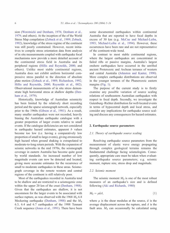
moment to the highest magnitudes in the data set (i.e. to

at least ML 5.0; Fig. 5) to relatively high levels (up to

approximately 10 MPa). These observations are con-

trary to the belief that stress drop is independent of

earthquake size. The non-uniformity of average stress

drop with magnitude is further demonstrated by

plotting stress drop against corner frequency, super-

imposed with lines of constant stress drop (Fig. 6). For

moderate to large events (with characteristically lower

fc), Dr appears to plateau near 10 MPa (i.e. for fcb3

Hz). If we consider that disparities observed in earth-

quake scaling are an artefact of high-frequency

attenuation, then compensation for losses of high-

frequency ground motion would force corner frequen-

cies higher, particularly for low magnitude earth-

quakes. This would, to some extent, improve the

uniformity of scaling parameters for earthquakes in

southeastern Australia. Unfortunately the argument

Fig. 5. Relationship between Dr and M0 for the selected data, showing a systematic increase in average Brune stress drop with seismic moment

for the 0bhV6 km, 6bhV14 km and hN14 km depth ranges respectively (a–c). The combined data indicates a subtle increase in Dr with

increasing depth (d).


over scaling at constant Dr versus increasing Dr with

seismic moment is presently limited by the absence of

high quality records from largeMLN5.0 earthquakes in

southeastern Australia. Stress drops that plateau for

fcb3 Hz may indicate a breakdown in self-similarity for

smaller earthquakes with higher corner frequencies.

The present are classified into three depth win-

dows, 0bhV6 km, 6bhV14 km and hN14 km

representing shallow, moderate and the deeper focus

events respectively. These categories were selected to

preserve approximately equal depth increments down

to the base of the seismogenic zone (about 20 km).

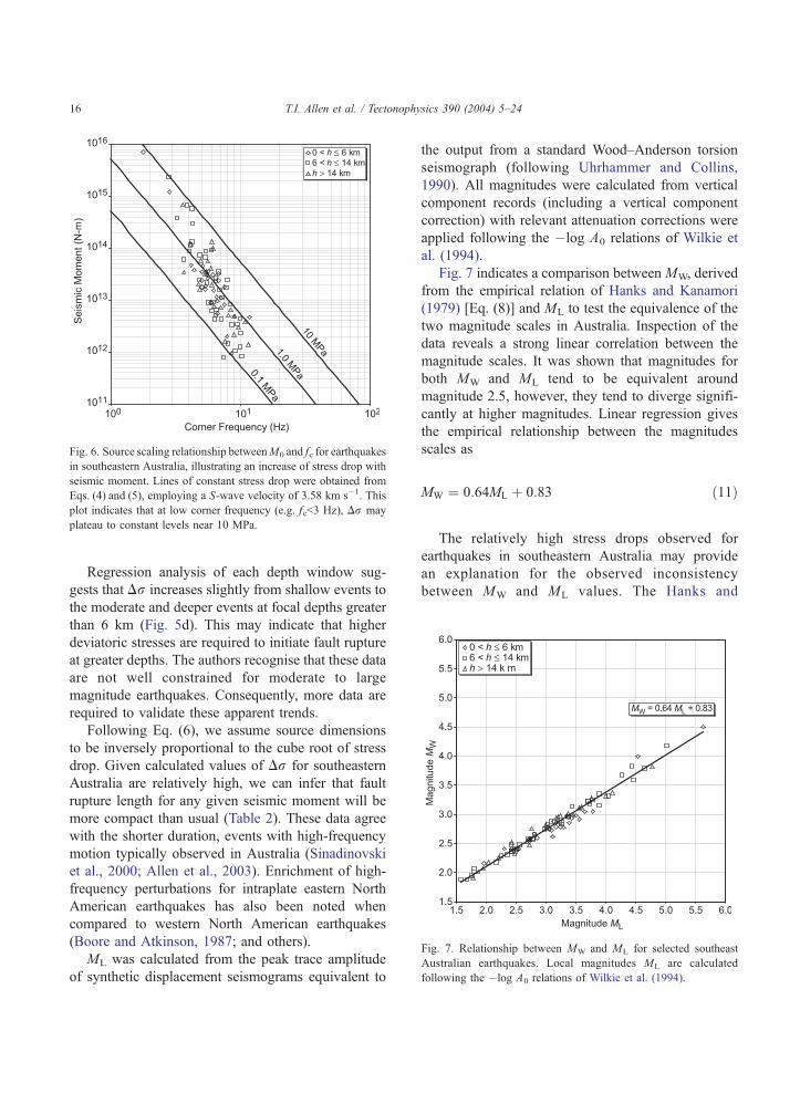
Fig. 6. Source scaling relationship betweenM0 and fc for earthquakes

in southeastern Australia, illustrating an increase of stress drop with

seismic moment. Lines of constant stress drop were obtained from

Eqs. (4) and (5), employing a S-wave velocity of 3.58 km s�1. This

plot indicates that at low corner frequency (e.g. fcb3 Hz), Dr may

plateau to constant levels near 10 MPa.

Fig. 7. Relationship between MW and ML for selected southeas

Australian earthquakes. Local magnitudes ML are calculated

following the �log A0 relations of Wilkie et al. (1994).


Regression analysis of each depth window sug-

gests that Dr increases slightly from shallow events to

the moderate and deeper events at focal depths greater

than 6 km (Fig. 5d). This may indicate that higher

deviatoric stresses are required to initiate fault rupture

at greater depths. The authors recognise that these data

are not well constrained for moderate to large

magnitude earthquakes. Consequently, more data are

required to validate these apparent trends.

Following Eq. (6), we assume source dimensions

to be inversely proportional to the cube root of stress

drop. Given calculated values of Dr for southeastern

Australia are relatively high, we can infer that fault

rupture length for any given seismic moment will be

more compact than usual (Table 2). These data agree

with the shorter duration, events with high-frequency

motion typically observed in Australia (Sinadinovski

et al., 2000; Allen et al., 2003). Enrichment of high-

frequency perturbations for intraplate eastern North

American earthquakes has also been noted when

compared to western North American earthquakes

(Boore and Atkinson, 1987; and others).

ML was calculated from the peak trace amplitude

of synthetic displacement seismograms equivalent to

the output from a standard Wood–Anderson torsion

seismograph (following Uhrhammer and Collins,

1990). All magnitudes were calculated from vertical

component records (including a vertical component

correction) with relevant attenuation corrections were

applied following the �log A0 relations of Wilkie et

al. (1994).

Fig. 7 indicates a comparison between MW, derived

from the empirical relation of Hanks and Kanamori

(1979) [Eq. (8)] and ML to test the equivalence of the

two magnitude scales in Australia. Inspection of the

data reveals a strong linear correlation between the

magnitude scales. It was shown that magnitudes for

both MW and ML tend to be equivalent around

magnitude 2.5, however, they tend to diverge signifi-

cantly at higher magnitudes. Linear regression gives

the empirical relationship between the magnitudes

scales as

MW ¼ 0:64ML þ 0:83 ð11Þ

The relatively high stress drops observed for

earthquakes in southeastern Australia may provide

an explanation for the observed inconsistency

between MW and ML values. The Hanks and

t


Kanamori (1979) relation was originally defined using

mostly large to great interplate earthquakes assuming

a constant stress drop of about 5 MPa (Singh and

Havskov, 1980), significantly lower than stress drops

observed for moderate-to-large intraplate Australian

earthquakes.

3. Earthquake recurrence parameters

3.1. Theory

Earthquake size distribution can usually be

described by the Gutenburg–Richter magnitude–fre-

quency law (Gutenburg and Richter, 1944) for a

discrete seismogenic zone

logN ¼ a� bm; ð12Þ

where N is the number of earthquakes having a

magnitude zm, and a and b are constants. a is the rate

of occurrence of earthquakes, or the level of seis-

micity, while the bb valueQ is a convenient means of

describing the relative proportion of small to large

earthquakes. These parameters are an essential input

for probabilistic earthquake hazard analysis. Follow-

ing Eq. (12), a b value of 1.0 would correspond to ten

times as many earthquakes exceeding magnitude m as

would exceed magnitude m+1. A large b value (e.g.

bN1.0) implies a higher proportion of small events

with respect to large events, whereas a lower

proportion of small events will give rise to a low b.

Most earthquake catalogues are complete for larger

earthquakes, but incomplete for smaller events, so

considerable care must be taken to avoid systematic

error when estimating b. The earthquake magnitude

above which a catalogue is complete normally varies

with both time and place.

Frohlich and Davis (1993) suggested that for

teleseismic earthquakes at least, b has a value of

1.0, in the sense that it is usually between 0.7 and 1.4.

The b value is a statistical measure and given it is

resolved from the gradient of a log–log distribution,

these bounds represent a dramatic variation in the

nature of seismicity. Some authors have shown that

the b value may be susceptible to significant regional

lateral and vertical variation (Karnık and Klıma, 1993;

Wiemer and Benoit, 1996; Mori and Abercrombie,

1997; Wiemer and Wyss, 1997; Gerstenburger et al.,

2001) and that its value may vary with time (Urbancic

et al., 1992).

It has been shown, both experimentally (Scholz,

1968) and observationally in underground excavations

(Urbancic et al., 1992), that b demonstrates an inverse

relationship to stress. Urbancic et al. (1992) also noted

that spatial and temporal variations in decreasing b

values were well correlated with increasing stress

estimates for time intervals prior to rockbursts in

mines. Furthermore, Urbancic et al. found that at the

completion of an aftershock sequence (which facili-

tates stress redistribution subsequent to a rockburst

and leads to a temporary increase of b), the b values

were again observed to decrease. Moreover, Wiemer

and Wyss (1997) observed that b values on fault

asperities are significantly lower than for the rest of

the fault zone. This observation is consistent with the

findings of Urbancic et al. (1992). Consequently, it is

reasonable to suggest that investigations into the

temporal and spatial variability of b can provide

limited information for earthquake prediction. Con-

sistently low b values can simply mean that both the

rocks and fault asperities are strong.

Evaluation of b is highly dependent on the accurate

measurement of magnitudes. Frohlich and Davis

(1993) remarked that despite being a logarithmic

scale, magnitudes for individual events can still vary

by up to 0.5 over a network of seismograph sites. This

is to be expected given that many attenuation

relationships used to calculate magnitudes do not

consider many effects on ground motion by factors

such as radiation pattern, soft surface sediments,

topography, etc. It was shown earlier that different

magnitude scales are not necessarily equivalent over

all magnitude ranges (Fig. 7) and this may result in

increased uncertainties when converting between

scales. Consequently, the robustness of b is dependent

on which magnitude definition is chosen, and on any

combinations of magnitude scales used. Some seis-

mologists argue that the b value is essentially constant

and any studies to the contrary suffer from statistical

or observational inadequacies (Frohlich and Davis,

1993; Kagan, 1999). Nevertheless, we believe that the

b value can exhibit spatial variation and must be

considered to give reasonable estimates of earthquake

recurrence.


3.2. Data selection

Given that the determination of b value can be

sensitive to relatively minor idiosyncrasies in earth-

quake catalogues, it was necessary to be more

inclusive and thus less rigorous in our selection criteria

than for the source parameter data, especially given

Australia’s relatively low levels of seismicity. For this

component of the study, a seismogenic region in

southeastern Australia, with good seismograph cover-

Fig. 8. Schematic map of the study area showing the location of seismic rec

0bhV6 km, 6bhV14 km and hN14 km depth ranges, respectively (b–d). I

Basins (BB) with respect to the underlying Lachlan Fold Belt (LFB) sys

proportion of small events from the shallow to the deep focus earthquake

age, was selected. The region, delineated in Fig. 8, has

an area of approximately 43,400 km2 and partially

encompasses the Gippsland Basin to the south and the

Southern Highlands of the Lachlan Fold Belt (Fig. 8a).

The data were extracted from the ES&S Seismol-

ogy Research Centre’s earthquake catalogue, which

has had a level of completeness down to below ML

2.0 in this region since 1976 (see Fig. 9a). All events

with calculated hypocentral depths encompassed

within the selected zone were included and the list

orders (a) with respect to the epicentral locations of the events for the

ndicated in the map are the Gippsland (GB), Otway (OB) and Bass

tem. Note the differences in spatial distribution and the decreasing

s.

Fig. 9. Earthquake recurrence from Gutenburg–Richter magnitude–frequency relations determined using the maximum likelihood fitting method

for all events in the study area (a) and the 0bhV6 km, 6bhV14 km and hN14 km depth ranges, respectively (b–d). The segments that are defined

by 10 or fewer events are shown as heavy dashed lines in black. The fine dashed lines model the a and b values which best fit the sample data.


declustered by the removal of foreshocks and after-

shocks. The b values were subsequently calculated

from these data. The same depth increments were

applied as for the source parameter investigation

above. Although many earthquake depths were well-

constrained, a large number have depth uncertainties


in the order of 5 to 10 km, consequently introducing

unavoidable uncertainties in the following analysis.

3.3. Methodology and results

Fig. 8b–d gives earthquake locations for the 0bhV6km, 6bhV14 km and hN14 km depth ranges within the

region, respectively. From visual inspection, it appears

that the earthquakes in the upper depth range (Fig. 8b)

tend to be scattered relatively uniformly over the

region. For the moderately deep focus events, the

majority of seismicity seems to be more concentrated

in the southeast (Fig. 8c), and delineation of active

seismogenic zones, typically trending NE–SW,

becomes more obvious. For the deeper focus events

(Fig. 8d), we again see further concentration of

earthquakes in the southeast. In addition, the shallow

focus earthquakes in Fig. 8b appear to have a higher

proportion of small events relative to large events

when compared to the moderate and deeper focus

earthquakes (Fig. 8c–d).

Individual b values were calculated employing the

maximum likelihood method as described by Aki

(1965), who gave a relation equivalent to

1

b¼ ln 10ð Þ m� m0Þð ð13Þ

where m is the sample’s mean magnitude, and m0 is

the lowest magnitude for which the event catalogue is

complete.

An overall b value was firstly calculated for the

combined data (Fig. 9a). The b values for the three

depth ranges were subsequently calculated. Fig. 9

illustrates the average recurrence relationships deter-

mined using the maximum likelihood method

described above assuming a maximum magnitude

Mmax of 7.5. The b values evaluated in Table 3 were

Table 3

Local magnitude b values for the combined and 0bhV6 km, 6bhV14km and hN14 km and depth ranges, respectively

Depth range Number of events m0 b Value

All depths 2340 1.4 0.88F0.02

0Vhb6 km 1036 1.8 1.06F0.13

6Vhb14 km 842 1.8 1.00F0.06

hN14 km 462 1.5 0.77F0.06

The table includes the number of events and the lowest magnitude

for which the catalogue is complete for each depth range.

resolved from local magnitudes ML only. These plots

indicate a systematic decrease in b value with depth.

This implies that larger earthquakes tend to occur at

greater hypocentral depths. If moment magnitudes

were used for comparison, then computed b values

would be higher given that MW appears to be lower

than ML for moderate-to-high magnitude events (see

Fig. 7).

It should be noted that the b value calculation for

the 0- to 6-km depth range was influenced by the

largest earthquake in this region and depth range only

having a magnitude of ML 3.1. This observation in

itself reinforces our suggestion that larger earthquakes

tend to be deeper.

4. Discussion

4.1. Earthquake source parameters in southeastern

Australia

Source parameters evaluated for southeastern

Australian earthquakes associated with well-con-

strained hypocentres indicate that stress drop appears

to increase systematically to relatively high levels for

the largest events used in the study. There may be

some evidence to suggest that stress drops plateau

for larger events and the apparent magnitude depend-

ence of stress drop is a result of a breakdown in

constant source scaling at lower magnitudes. How-

ever, this argument is difficult to quantify in south-

eastern Australia given the deficiency of quality

ground motion records from large nearby MLN5.0

earthquakes.

Unlike western and central Australia, relatively

high levels of crustal attenuation characterise south-

eastern Australia (Allen et al., 2002; Allen, 2004).

Attenuation of high-frequency elastic energy, critical

for the measurement of fc, may therefore provide an

explanation for the apparent increase of Dr with

seismic moment. The high stress drops observed for

southeastern Australia imply higher frequency ground

motion and that earthquake source dimensions are

more compact than usual. Response spectra calculated

for some Australian earthquakes indicate enrichment

of high-frequency ground motion, consistent with the

relatively high stress drops evaluated in the present

study (Sinadinovski et al., 2000; Allen et al., 2003).


Depth characteristics of the stress drops described

above were investigated using the same data set (Fig.

5). Linear least squares regression for each depth

profile was performed and indicated that the stress

drop appears to increase slightly with depth for

southeastern Australian earthquakes of similar seis-

mic moment. It may be expected that higher

deviatoric stresses at greater depths have an influence

on stress drops of intraplate earthquakes. Indeed,

Hanks and Johnston (1992) reported the occurrence

of two deep crustal eastern North American earth-

quakes with well-constrained hypocentral depths

greater than 20 km having higher than average stress

drop (the MW 5.4 southern Illinois earthquake, 9

November 1968; and the MW 5.9 Saguenay, Quebec

earthquake, 25 November 1988). It is subjective to

draw conclusions on the basis of two earthquakes,

however, these occurrences in particular further

suggest that deeper focus earthquakes may possess

higher stress drops than earthquakes of similar

seismic moment at shallower depths. It is also

possible that the observed increase in average stress

drop with hypocentral depth is merely an artefact of

the larger events (assumed to have higher stress drop)

being more likely to occur at greater depths,

subsequently introducing a systematic bias into the

data set.

A comparison between ML and MW as calculated

using the Hanks and Kanamori (1979) function

reveals a strong linear correlation, as would be

expected. Regression analysis of the two parameters

demonstrated that the magnitude scales are roughly

equivalent at a magnitude of 2.5, however, ML

calculated employing the �log A0 relations of Wilkie

et al. (1994) increases more rapidly than MW. The

relationship between the two magnitude scales for

southeastern Australian earthquakes was empirically

evaluated as MW=0.64 ML+0.83 [Eq. (11)] for events

less than ML 5.0. The discrepancy between the

magnitude scales may result from the assumption of

a constant stress drop which is lower than that

observed in southeastern Australia, inherent within

the Hanks and Kanamori (1979) relation [Eq. (8)]

(e.g. Singh and Havskov, 1980). Allen (2004) inves-

tigates an alternative methodology for the evaluation

of ML employing the anelastic attenuation parameters

described in Eq. (9). Local magnitudes evaluated

using the method of Allen (2004) have significantly

lower uncertainties than ML’s evaluated using the

�log A0 relations of Wilkie et al. (1994) and

addresses the relatively poor comparison between

MW and ML observed in the present study. Employing

the attenuations of Wilkie et al., local magnitudes

calculated for individual events are observed to

increase systematically with r. In contrast, ML

residuals calculated using the methodologies of Allen

(2004) and averaged at uniform distance separation

define a linear relationship with a near zero gradient,

for rb~750 km. Allen (2004) suggests that local

magnitudes calculated using the attenuation relations

of Wilkie et al. may overestimate the size of an

earthquake by as much as 0.3 of a magnitudes unit,

particularly for moderate-to-large events recorded at

large hypocentral distances.

4.2. Earthquake recurrence parameters in southeast-

ern Australia

Despite errors which may have been introduced

due to uncertainties in hypocentral depth for many of

the less well-located earthquakes used in the recur-

rence calculations, a decrease in b value with

hypocentral depth was detected (Table 3). The differ-

ence between the shallow and moderate depth ranges

is small and could possibly be an artefact of catalogue

incompleteness or limitations in reliable earthquake

depth control. Although many well-located earth-

quakes occur within 6 km of the surface, no event

larger than ML 3.1, well-located or otherwise, had a

depth of less than 6 km in the study region. The

observed decrease of b for the deeper focus events is

well-defined, implying that a larger proportion of

moderate-large earthquakes occur at depth. As we are

limited by relatively low earthquake activity in

Australia, it is difficult to map lateral and/or vertical

variability of b, however, our data do agree with

previous studies of Mori and Abercrombie (1997),

Gerstenburger et al. (2001) and others, who also

demonstrate a systematic decrease of b value with

depth within the seismogenic zone.

Previous b value estimates for this region have

been obtained by Gaull et al. (1990). Although their

source zones differed from that of the current study,

for a similar region, they obtained an overall b value

of 0.77, compared to our 0.88 for the combined data.

This discrepancy may be due to the sensitivity of the


b value to either difference of source zones, or

catalogue incompleteness for lower magnitude earth-

quakes. In addition, Koo et al. (2000) estimated a b

value of 0.81 for the Melbourne Metropolitan Area,

adjacent to our study area. Note that these b values are

all based on local magnitudes. If earthquake recur-

rence were based on the moment magnitudes as

calculated in this study, the b values would be a little

higher, subsequently increasing the recurrence inter-

val for large damaging earthquakes and lowering the

associated hazard.

Both Scholz (1968) and Urbancic et al. (1992)

showed that b demonstrates an inverse relationship to

stress. From these findings, it may be implied that

stress drops for earthquakes in regions of low b

should be higher than those of earthquakes of similar

seismic moment in regions of high b. Alternatively,

this similarity may simply imply that the larger

earthquakes that appear to have high stress drop

occur at greater depths.

5. Conclusions

The Qa( f,r) model employed in the our estimates

of the earthquake source parameters provides a simple

model for the variation of seismic attenuation at

varying source–receiver distances and allows for more

consistent estimates of source parameters in south-

eastern Australia compared to earlier Q models (e.g.

Wilkie and Gibson, 1994).

A systematic increase in Brune stress drop with

increasing magnitude to at least ML 5.0 was

observed. It remains to be seen whether stress drops

will continue to increase for earthquakes of MLN5.0.

The relatively high stress drops evaluated suggest

compact source dimensions and high-frequency

ground motion. In addition, stress drops were

observed to increase slightly with increasing hypo-

central depth.

For a discrete study area in southeastern Australia,

b values were observed to decrease with depth,

implying that both rock strength and thus yield stress

increase with depth. Decreasing b values with source

depth suggest that larger earthquakes (with high stress

drops) tend to occur deeper. Moreover, this observa-

tion may explain why stress drop appears to increase

with hypocentral depth. Consequently, current models

may slightly overestimate earthquake hazard for

surface sites in southeastern Australia.

The relationship between ML and MW has a

significant effect on current estimates of ground

motion recurrence, and consequently on earthquake

hazard estimates. If moment magnitude (as calcu-

lated in this study) were used in ground motion

recurrence estimates, it would have the effect of

increasing the b value, consequently lowering hazard

associated with southeastern Australian earthquakes.

Therefore, the quantification of earthquake magni-

tude for hazard studies remains a major source of

uncertainty and is a problem that must be addressed

in the future to achieve reliable probabilistic hazard

estimates.

Acknowledgments

The authors would like to thank the staff at the

Seismology Research Centre for access to resources

and their generous cooperation. Special thanks go to

Greg McPherson and Bradley White for their kind

assistance in the software development phase of this

research. We also acknowledge Heidi Houston for her

critical review and thoughtful suggestions on the

original manuscript. Dan Clark is thanked for provid-

ing the digital elevation model in Fig. 2. This research

was supported by a Monash University postgraduate

scholarship.

References

Abercrombie, R.E., 1995. Earthquake source scaling relationships

from �1 to 5 ML using seismograms recorded at 2.5 km depth.

J. Geophys. Res. 100, 24,015–24,036.

Abercrombie, R., Leary, P., 1993. Source parameters of small

earthquakes recorded at 2.5 km depth, Cajon Pass, Southern

California: implications for earthquake scaling. Geophys. Res.

Lett. 20, 1511–1514.

Aki, K., 1965. Maximum likelihood estimate of b in the formula log

N=a�bM and its confidence limits. Bull. Earthq. Res. Inst.

Univ. Tokyo 43, 237–239.

Aki, K., 1967. Scaling law of seismic spectrum. J. Geophys. Res.

72, 1217–1231.

Aki, K., Richards, P.G., 1980. Quantitative Seismology; Theory and

Methods. W.H. Freeman, New York, pp. 932.

Allen, T.I., 2004. Spectral attenuation and earthquake source

parameters from recorded ground motion; implications for


earthquake hazard and the crustal stress field of southeastern

Australia. PhD thesis, Monash University, Melbourne.

Allen, T., Gibson, G., Love, D., Cull, J., 2002. New estimates for a

frequency dependent seismic quality factor Q( f ) for south-

eastern Australia. In: Griffith, M.C., Love, D., McBean, P.,

McDougall, A., Butler, B. (Eds.), Total Risk Management in the

Privatised Era Proc. Aust. Earthquake Eng. Soc. 2002 Conf.,

Australian Earthquake Engineering Society, Adelaide.

Allen, T., Gibson, G., Cull, J., 2003. Comparative study of average

response spectra from Australian and New Zealand earth-

quakes. Earthquake Risk Mitigation Proc. Aust. Earthquake

Eng. Soc. 2003 Conf., Australian Earthquake Engineering

Society, Melbourne.

Antolik, M., Dreger, D.S., 2003. Rupture process of the 26 January

2001 MW 7.6 Bhuj, India, earthquake from teleseismic broad-

band data. Bull. Seismol. Soc. Am. 93, 1235–1248.

Beresnev, I.A., 2001. What we can and cannot learn about

earthquake sources from the spectra of seismic waves. Bull.

Seismol. Soc. Am. 91, 397–400.

Betts, P.G., Giles, D., Lister, G.S., Frick, L.R., 2002. Evolution of

the Australian lithosphere. Aust. J. Earth Sci. 49, 661–695.

Boore, D.M., Atkinson, G.M., 1987. Stochastic prediction of

ground motion and spectral response parameters at hard-rock

sites in eastern North America. Bull. Seismol. Soc. Am. 77,

440–467.

Boore, D.M., Boatwright, J., 1984. Average body-wave radiation

coefficients. Bull. Seismol. Soc. Am. 74, 1615–1621.

Brune, J.N., 1970. Tectonic stress and the spectra of seismic shear

waves from earthquakes. J. Geophys. Res. 75, 4997–5009.

Brune, J.N., 1971. Corrections to: tectonic stress and the spectra of

seismic shear waves from earthquakes. J. Geophys. Res. 76,

5002.

Bungum, H., Dahle, A., Toro, G., McGuire, R., Gudmestad, O.T.,

1992. Ground motions from intraplate earthquakes. Proc. 10th

World Conf. Earthquake Eng., vol. 2. International Association

of Earthquake Engineers, Madrid, pp. 611–616.

Castro, R.R., Reboller, C.J., Inzunza, L., Orozco, L., Sanchez, J.,

Galvez, O., Farfan, F.J., Mendez, I., 1997. Direct body-wave Q

estimated in northern Baja California, Mexico. Phys. Earth

Planet. Inter. 103, 33–38.

Denham, D., 1988. Australian seismicity—the puzzle of the not-so-

stable continent. Seismol. Res. Lett. 59, 235–240.

Denham, D., Alexander, L.G., Worotnicki, G., 1979. Stresses in the

Australian crust: evidence from earthquakes and in situ stress

measurements. BMR J. Aust. Geol. Geophys. 4, 289–295.

Foster, D.A., Gray, D.R., 2000. Evolution and structure of the

Lachlan Fold Belt (Orogen) of eastern Australia. Annu. Rev.

Earth Planet. Sci. 28, 47–80.

Frohlich, C., Davis, S.D., 1993. Teleseismic b values; or, much ado

about 1.0. J. Geophys. Res. 98, 631–644.

Garcıa-Garcıa, J.M., Vidal, F., Romacho, M.D., Martın-Marfil, J.M.,

Posadas, A., Luzon, F., 1996. Seismic source parameters for

microearthquakes of the Granada basin (southern Spain).

Tectonophysics 261, 51–66.

Gaull, B.A., Michael-Leiba, M.O., Rynn, J.M.W., 1990. Probabil-

istic earthquake risk maps of Australia. Aust. J. Earth Sci. 37,

169–187.

Gerstenburger, M., Wiemer, S., Giardini, D., 2001. A systematic test

of the hypothesis that b value varies with depth in California.

Geophys. Res. Lett. 28, 57–60.

Gibowicz, S.J., Young, R.P., Talebi, S., Rawlence, D.J., 1991.

Source parameters of seismic events at the Underground

Research Laboratory in Manitoba, Canada: scaling relations

for events with moment magnitude smaller than �2. Bull.

Seismol. Soc. Am. 81, 1157–1182.

Gibson, G., Wesson, V., Cuthbertson, R., 1981. Seismicity of

Victoria to 1980. J. Geol. Soc. Aust. 28, 341–356.

Gutenburg, B., Richter, C.F., 1944. Frequency of earthquakes in

California. Bull. Seismol. Soc. Am. 34, 185–188.

Hanks, T.C., Johnston, A.C., 1992. Common features of the

excitation and propagation of strong ground motion for North

American earthquakes. Bull. Seismol. Soc. Am. 82, 1–23.

Hanks, T.C., Kanamori, H., 1979. A moment–magnitude scale.

J. Geophys. Res. 84, 2348–2350.

Herrmann, R.B., Kijko, A., 1983. Modeling some empirical

vertical component Lg relations. Bull. Seismol. Soc. Am. 73,

157–171.

Hillis, R.R., Reynolds, S.D., 2000. The Australian stress map.

J. Geol. Soc. (Lond.) 157, 915–921.

Hiramatsu, Y., Yamanaka, H., Tadokoro, K., Nishigami, K.,

Ohmi, S., 2002. Scaling law between corner frequency and

seismic moment of microearthquakes: is the breakdown of the

cube law a nature of earthquakes?. Geophys. Res. Lett. 29

(doi:10.1029/2001GL013894).

Hough, S.E., 1996. Observational constraints on earthquake source

scaling: understanding the limits in resolution. Tectonophysics

261, 83–95.

Houston, H., 2001. Influence of depth, focal mechanism, and

tectonic setting on the shape and duration of earthquake source

time functions. J. Geophys. Res. 106, 11,137–11,150.

Ide, S., Beroza, G.C., 2001. Does apparent stress vary with

earthquake size? Geophys. Res. Lett. 28, 3349–3352.

Johnston, A.C., 1992. Brune stress drops of stable continental

earthquakes: are they higher than bnormalQ and do they increase

with seismic moment? Seismol. Res. Lett. (Abstr.) 63, 609.

Johnston, A.C., Kanter, L.R., 1990. Earthquakes in stable con-

tinental crust. Sci. Am. 262, 42–49.

Jones, T.D., Gibson, G., McCue, K.F., Denham, D., Gregson, P.J.,

Bowman, J.R., 1991. Three large intraplate earthquakes near

Tennant Creek, Northern Territory, on 22 January 1988. BMR J.

Aust. Geol. Geophys. 12, 339–343.

Kagan, Y.Y., 1999. Universality of the seismic moment–frequency

relation. Pure Appl. Geophys. 155, 537–573.

Kanamori, H., Anderson, D.L., 1975. Theoretical basis for some

empirical relations in seismology. Bull. Seismol. Soc. Am. 65,

1073–1095.

Karnık, V., Klıma, K., 1993. Magnitude–frequency distribution in

the European–Mediterranean earthquake regions. Tectonophy-

sics 220, 309–323.

Kennett, B.L.N., 1989. Lg-wave propagation in heterogeneous

media. Bull. Seismol. Soc. Am. 79, 157–171.

Koo, R., Brown, A., Lam, N., Wilson, J., Gibson, G., 1989. A

full range response spectrum model for rock sites in the

Melbourne Metropolitan Area. In: Jensen, V.H., Butler, B.

http://dx.doi.org/doi:10.1029/2001GL013894


(Eds.), Dams, Fault Scarps and Earthquakes Proc. Aust.

Earthquake. Eng. Soc. Conf., Australian Earthquake Engineer-

ing Society, Hobart.

McCue, K., Michael-Leiba, M., 1993. Australia’s deepest known

earthquake. Seismol. Res. Lett. 64, 201–206.

McGarr, A., Green, R.W.E., Spottiswoode, S.M., 1981. Strong

ground motion of mine tremors: some implications for near-

source ground motion parameters. Bull. Seismol. Soc. Am. 71,

295–319.

Michael-Leiba, M., Malafant, K., 1992. A new local magnitude

scale for southeastern Australia. BMR J. Aust. Geol. Geophys.

13, 201–205.

Michael-Leiba, M., Love, D., McCue, K., Gibson, G., 1994. The

Uluru (Ayers Rock), Australia, earthquake of 28 May 1989.

Bull. Seismol. Soc. Am. 84, 209–214.

Molnar, P., Wyss, M., 1972. Moments, source dimensions and stress

drops of shallow-focus earthquakes in the Tonga-Kermadec Arc.

Phys. Earth Planet. Inter. 6, 263–278.

Mori, J., Abercrombie, R.E., 1997. Depth dependence of earthquake

frequency–magnitude distributions in California: implications

for rupture initiation. J. Geophys. Res. 102, 15,081–15,090.

Nuttli, O.W., 1983a. Empirical magnitude and spectral scaling

relations for mid-plate and plate-margin earthquakes. Tectono-

physics 93, 207–223.

Nuttli, O.W., 1983b. Average seismic source–parameter relations for

mid-plate earthquakes. Bull. Seismol. Soc. Am. 73, 519–535.

Prejean, S.G., Ellsworth, W.L., 2001. Observations of earthquake

source parameters at 2 km depth in the Long Valley Caldera,

eastern California. Bull. Seismol. Soc. Am. 91, 165–177.

Reynolds, S.D., Coblentz, D.D., Hillis, R.R., 2002. Tectonic forces

controlling the regional intraplate stress field in continental

Australia: results from new finite element modeling. J. Geophys.

107 (doi:10.1029/2001JB000408).

Richardson, R.M., 1992. Ridge forces, absolute plate motions, and

the intraplate stress field. J. Geophys. Res. 97, 11,739–11,748.

Richter, C.F., 1935. An instrumental earthquake magnitude scale.


Richter, C.F., 1958. Elementary Seismology. W.H. Freeman, San

Francisco, pp. 768.

Scholz, C.H., 1968. The frequency–magnitude relation of micro-

fractureing in rock and its relation to earthquakes. Bull. Seismol.

Soc. Am. 58, 399–415.

Scholz, C.H., Aviles, C.A., Wesnousky, S.G., 1986. Scaling

differences between large interplate and intraplate earthquakes.


Shi, J., Kim, W.-Y., Richards, P.G., 1998. The corner frequencies

and stress drops of intraplate earthquakes in the northeastern

United States. Bull. Seismol. Soc. Am. 88, 531–542.

Sinadinovski, C., McCue, K.F., Somerville, M., 2000. Character-

istics of strong ground motion for typical Australian intra-plate

earthquakes and their relationship with the recommended

response spectra. Soil Dyn. Earthqu. Eng. 20, 101–110.

Singh, S.K., Havskov, J., 1980. On moment–magnitude scale. Bull.


Somerville, P.G., McLaren, J.P., LeFevre, L.V., Burger, R.W.,

Helmberer, D.V., 1987. Comparison of source scaling relations

of eastern and western North American earthquakes. Bull.


Uhrhammer, R.A., Collins, E.R., 1990. Synthesis of Wood–

Anderson seismograms from broadband digital records. Bull.


Urbancic, T.I., Trifu, C.-I., Long, J.M., Young, P.G., 1992. Space–

time correlations of b values with stress release. Pure Appl.

Geophys. 139, 449–462.

Wiemer, S., Benoit, J.P., 1996. Mapping the b value anomaly at 100

km depth in the Alaska and New Zealand subduction zones.

Geophys. Res. Lett. 23, 1557–1560.

Wiemer, S., Wyss, M., 1997. Mapping the frequency–magnitude

distribution in asperities: an improved technique to calculate

recurrence times? J. Geophys. Res. 102, 15,115–15,128.

Wilkie, J., Gibson, G., 1994. Estimation of seismic quality factor

Q for Victoria, Australia. AGSO J. Aust. Geol. Geophys. 15,

511–517.

Wilkie, J., Gibson, G., Wesson, V., 1994. Richter magnitudes and

site corrections using vertical component seismograms. Aust. J.

Earth Sci. 41, 221–228.

Worotnicki, G., Denham, D., 1976. The state of stress in the upper

part of the Earth’s crust in Australia according to measurements

in mines and tunnels and from seismic observations. Proc.

ISRM Symp., Investigation of Stress in Rock, Advances in

Stress Measurement. Australian Geomechanics Society, Sydney,

pp. 71–82.

Zoback, M.L., 1992. First- and second-order patterns of stress in the

lithosphere: the world stress map project. J. Geophys. Res. 97,

11,703–11,728.

Zoback, M.L., Zoback, M.D., Adams, J., Assumpcao, M., Bell, S.,

Bergman, E.A., Blqmling, P., Brereton, N.R., Denham, D., Ding,

J., Fuchs, K., Gay, N., Gregersen, S., Gupta, H.K., Gvishiani, A.,

Jacob, K., Klein, R., Knoll, P., Magee, M., Mercier, J.L., Mqller,B.C., Paquin, C., Rajendran, K., Stephansson, O., Suarez, G.,

Suter, M., Udias, A., Xu, Z.H., Zhizhin, M., 1989. Global

patterns of tectonic stress. Nature 341, 291–298.

http://dx.doi.org/doi:10.1029/2001JB000408

Depth variation of seismic source scaling relations: implications for earthquake hazard in...

Documents

Transcript of Depth variation of seismic source scaling relations: implications for earthquake hazard in...