Department Wasser-Atmosphäre-Umwelt (WAU)

Institut für Meteorologie (BOKU-Met)

Vorstand: O. Univ.-Prof. Dr. Helga Kromp-Kolb

Betreuer: Ao. Univ.-Prof. Mag. Dr. Philipp Weihs

FERNERKUNDLICHE UNTERSUCHUNG VON TROCKENSTRESS UND SCHÄTZUNG VON VEGETATIONSPARAMETERN FÜR LAND- UND FORSTWIRTSCHAFTLICHE ANWENDUNGSGEBIETE

Dissertation zur Erlangung des Doktorgrades an der Universität für Bodenkultur Wien

Eingereicht von Mag. Katja Richter

Wien, Juni 2009

Danksagung

Die vorliegende Dissertation entstand teilweise im Rahmen des Projekts “Crop Drought Stress Monitoring by Remote Sensing” (DROSMON) an der Universität für Bodenkultur, Wien, Österreich, das vom österreichischen Fonds zur Förderung der wissenschaftlichen Forschung (FWF, Projekt Nr. P17647-N04) finanziert wurde. Im Weiteren wurde sie durch das „Participatory multi-Level EO-assisted tools for Irrigation water management and Agricultural Decision-Support“ (PLEIADeS) Projekt der Universität Federico II di Napoli, Italien, finanziert.

Mein besonderer Dank gilt Prof. Dr. Philipp Weihs für die gute durchgehende Betreuung der Arbeit. Im Weiteren gilt mein Dank Rita Linke, Pablo Rischbeck, Prof. Werner Schneider, Josef Eitzinger, Franz Suppan und allen anderen Kollegen des DROSMON Projekts für ihre große Unterstützung. Insbesondere bedanke ich mich bei Prof. Guido D’Urso, der mir Rahmen und Ideen für die Weiterführung der Dissertation gegeben hat. Großer Dank gilt auch Clement Atzberger und Wim Timmermans für die gute Zusammenarbeit und ihre motivierende Mitarbeit an den gemeinsamen Publikationen.

Außerdem danke ich Frédéric Baret und den Kollegen des INRA, Avignon, für die Bereitstellung der verwendeten Reflexionsmodelle und den wissenschaftlichen Austausch.

Vielen Dank aber im Besonderen an meine Familie, die guten Freunde und Francesco.

2

Abstract

The availability of high spatial and temporal resolution optical remote sensing data allows the estimation of biophysical parameters for a wide territorial coverage. This is of essential importance for ecological, hydrological, climatic and other applications, giving the basis for a sustainable management of agricultural and forestry resources.

The present studies analysed the use of physically based approaches for the quantification of the Leaf Area Index (LAI) and other important vegetation characteristics. Comparisons with traditional empirical models, using vegetation indices, are performed.

Furthermore, the relevance of canopy reflectance models for precision farming applications, such as the detection of drought stress zones, monitoring of vegetation growth and dynamic and energy balance modelling, is highlighted. The models were validated and moreover, the physiological reaction of plants to drought stress and recovery was analysed by means of optical leaf reflectance field and laboratory measurements. Additionally, the configuration of the forthcoming ESA Sentinel-2 mission was tested in an operative perspective.

The remotely sensed and ground based data used in the studies were acquired, amongst others, in the framework of the “Crop Drought Stress Monitoring by Remote Sensing“ (DROSMON) project of the University of Natural Resources and Applied Life Sciences, Vienna.

Summarizing the results of all studies, it could be shown that optical remote sensing is a valuable tool rather for estimating structural changes of the canopy (such as LAI) than for an early drought stress detection. The physically based estimation of surface parameters could be performed for a wide range of conditions, i. e. for different geographical locations, sensors and vegetation types, and in a satisfyingly accurate way using turbid medium modelling schemes.

The method is therefore recommended for an operational quantification of biophysical products or for the determination of medium or longer term drought stress in agricultural and forestry applications.

Keywords: vegetation parameters, LAI, model inversion, drought stress, optical remote sensing

3

Kurzfassung

Der Einsatz fernerkundlicher Methoden ermöglicht die flächenhafte Bestimmung biophysikalischer Vegetationsparameter in hoher räumlicher und zeitlicher Auflösung. Diese stellen bedeutende Informationen u. a. für die Bereiche der Ökologie, Hydrologie und Klimatologie dar und schaffen somit die Basis für ein nachhaltiges Management in Land- und Forstwirtschaft.

Die vorliegenden Studien analysierten die Verwendung physikalisch basierter Modelle für die Quantifizierung von Blattflächenindex (LAI) und anderer Vegetationsparameter im Vergleich zu empirischen Ansätzen. Insbesondere wurde die Bedeutung von Bestandesreflexionsmodellen für wichtige Precision Farming-Anwendungen wie Trockenstresszonierung, Beobachtung des Wachstums und der Dynamik der Vegetation und Energiebilanzmodellierung aufgezeigt. Im Weiteren wurde die Konfiguration zukünftiger Satelliten (Sentinel-2) hinsichtlich ihrer Eignung für operative Anwendungen getestet. Die Modelle wurden evaluiert und außerdem die physiologische Reaktion der Pflanzen auf Trockenstress und Erholung anhand spektraler Signale auf Blattebene untersucht.

Die in den Studien verwendeten hyper- und multispektralen Sensordaten und Bodenmessungen wurden im Rahmen des „Crop Drought Stress Monitoring by Remote Sensing“ (DROSMON) Projekts der Universität für Bodenkultur, Wien und verschiedener anderer Feldkampagnen erhoben.

Zusammenfassend konnte gezeigt werden, dass die Fernerkundung vom sichtbaren bis zum mittleren Infrarotbereich eine Eignung eher für die Erkennung struktureller Veränderungen des Bestands, z. B. LAI, als für die Trockenstressfrüherkennung aufweist. Die physikalisch basierte Schätzung von Vegetationsparametern kann mit zufriedenstellender Genauigkeit und auch unter diversen Bedingungen, d. h. in unterschiedlicher geographischer Lage, für eine Reihe von Sensortypen und verschiedene Vegetationsarten, durch Inversion von homogenen Turbid Medium-Modellen durchgeführt werden.

Die verwendeten Methoden werden daher für eine operative Quantifizierung von biophysikalischen Vegetationsparametern bzw. für die Bestimmung von mittel- und langfristigem sowie potentiellem Trockenstress in Land- und Forstwirtschaft sehr empfohlen.

Schlüsselwörter: Vegetationsparameter, Blattflächenindex, Modellinversion, Trockenstress, optische Fernerkundung

4

Inhaltsverzeichnis

1 Einleitung ______________________________________________________ 6 1.1 Bedeutung der Fernerkundung für Land- und Forstwirtschaft _________________ 6 1.2 Schätzung von Vegetationsparametern__________________________________ 7 1.3 Fernerkundliche Bestimmung von Trockenstress __________________________ 9

2 Überblick über die Publikationen__________________________________ 10 2.1 Thematischer Zusammenhang zwischen den Publikationen_________________ 11 2.2 Schlussfolgerung und Ausblick _______________________________________ 15

3 Literaturverzeichnis ____________________________________________ 17

4 Publikationen__________________________________________________ 20 4.1 Publikation I ______________________________________________________ 20 4.2 Publikation II _____________________________________________________ 39 4.3 Publikation III _____________________________________________________ 52 4.4 Publikation IV_____________________________________________________ 71 4.5 Publikation V _____________________________________________________ 94

5 Anhang (Bestätigung der Publikation I) ___________________________ 106

6 Lebenslauf/CV ________________________________________________ 107

5

1 Einleitung

Zur Einführung wird ein Überblick zum großen Themenfeld der fernerkundlichen Untersuchungen in Land- und Forstwirtschaft gegeben, in das die vorliegende Dissertation einzuordnen ist. Die in den Studien bearbeitete Thematik analysiert die Fernerkundung als Mittel für Untersuchungen von Trockenstress und insbesondere zur Schätzung von Vegetationsparametern für land- und forstwirtschaftliche Anwendungsbereiche.

1.1 Bedeutung der Fernerkundung für Land- und Forstwirtschaft

Vegetation hat die Eigenschaft, elektromagnetische Strahlung in bestimmten Wellenlängenbereichen zu reflektieren, zu absorbieren, zu transmittieren und auch zu emittieren. Dies wird von der Fernerkundung, die als berührungsfreie Erfassung und Messung von Objekten der Erdoberfläche definiert ist (Barrett and Curtis, 1976), ausgenutzt. Für fernerkundliche Beobachtungen werden einerseits passive Sensoren eingesetzt, die entweder die von der Erdoberfläche oder Atmosphäre reflektierte Solarstrahlung (z. B. anhand Multispektralscanner) messen oder die Wärmestrahlung von Objekten (z. B. anhand Thermalkameras) untersuchen. Die zweite Möglichkeit sind aktive Aufnahmesysteme, wobei die Rückstreuung von Objekten, z. B. anhand Radar- oder Lasersystemen, gemessen wird.

Fernerkundliche Aufnahmen von flugzeug- oder satellitenbasierten Plattformen eröffnen den besonderen Vorteil der wiederholten großflächigen Erfassung von Gebieten. Dies bringt eine hohe Kosteneffizienz gegenüber arbeits- und zeitintensiven bodengebundenen Messungen.

Die hier vorliegende Arbeit konzentriert sich auf die multi- und hyperspektrale optische Fernerkundung, wobei die Wellenlängenbereiche des sichtbaren Lichts, des nahen Infrarots (IR) und teilweise des mittleren IR genutzt werden, um die räumliche und die zeitliche Dynamik der terrestrischen Biosphäre zu erfassen.

In land- und forstwirtschaftlichen Forschungs- und Anwendungsbereichen wird die Fernerkundung eingesetzt, um anhand des spektralen Reflektionsverhaltens verschiedene Pflanzenspezies zu unterscheiden und biophysikalische Vegetationsparameter zu bestimmen. In der praktischen Anwendung kann die fernerkundliche Bestimmung von biophysikalischen Parametern ein nachhaltiges landwirtschaftliches Management unterstützen und somit das Ertragspotential von Anbauflächen deutlich erhöhen. Eine große Bedeutung hat in dieser Hinsicht bereits das sogenannte „Precision Farming“ (Präzisionslandwirtschaft) erlangt, wobei z. B. Dünge- und Pflanzenschutzmittel nicht mehr einheitlich, sondern räumlich differenziert, je nach Bedarf auf einer Anbaufläche eingesetzt werden (SCHUELLER 1992). Ein weiteres Anwendungsbeispiel sind Programme zur Bewässerungsberatung (DE MICHELE et al. 2009), für die Informationen über die kleinräumliche Verteilung und die zeitliche Veränderung bestimmter Vegetationsparameter Voraussetzung sind.

Auch im Forstbereich wird anhand fernerkundlicher Kartierung von Baumarten und Waldstruktur, Baumvitalität bzw. Baumschäden zu einer nachhaltigeren Bewirtschaftung beigetragen (FRANKLIN 2001, ATZBERGER 2003).

In den letzten Jahrzehnten wurde eine große Anzahl neuer Satelliten gestartet (ESA 2008). Dennoch war es bis heute trotz großer technischer Fortschritte nicht möglich, hohe räumliche mit hoher zeitlicher Auflösung zu verbinden. Somit sind Daten von räumlich hochauflösenden Sensoren (d. h. 10-30 m, z. B. Landsat TM, SPOT) nur in mäßiger zeitlicher Auflösung verfügbar (d. h. 15-30 Tage), während Daten mit niedriger räumlicher Auflösung (250-1000 m, z. B. Aqua/Terra MODIS, SPOT/VGT) viel häufiger zugänglich sind (ein bis drei

6

Tage) (BSAIBES et al. 2009). Eine Lösung ist die Kombination verschiedener Sensoren, was aber oft zu Schwierigkeiten in der Vergleichbarkeit der abgeleiteten Produkte durch sensorspezifische Charakteristiken (z. B. räumliche und spektrale Auflösung, spektrale Responsfunktionen, u. a.) führt (SOUDANI et al. 2006). Eine weitere Möglichkeit bietet die Datenfusion von Sensoren verschiedener räumlicher und zeitlicher Auflösung, z. B. von MERIS und Landsat. Hierbei werden anhand Spectral Unmixing Techniken die häufig verfügbaren Daten von MERIS auf die höhere geometrische Genauigkeit von Landsat gerechnet (ZURITA-MILLA et al. 2007).

Um diese Schwierigkeiten zu erleichtern und insbesondere um den ständig steigenden Anforderungen der Nutzer entgegenzukommen, wurden bereits neue Missionen gestartet oder sind für die nahe Zukunft geplant. Eine wichtige Rolle spielen dabei die Sentinel-Satelliten des Global Monitoring for Environment and Security (GMES) Programms der European Space Agency (ESA). Für die operative Beobachtung der Landbedeckung und Landnutzung ist der multispektrale Sentinel-2 Sensor vorgesehen, der ab dem Jahr 2012 Daten in mittlerer räumlicher Auflösung (10–60 m) in 13 Spektralkanälen (im Wellenlängenbereich des sichtbaren Lichts bis zum mittleren IR) liefern soll (MARTIMORT 2007).

Mit der durch die neuen Satelliten erwarteten Verbesserung der Datenlage eröffnen sich vielfältige Möglichkeiten im Bereich der Landkartierung, im Umweltmonitoring sowie für die ökologische Prozessskalierung von lokaler zu globaler Ebene (SOUDANI et al. 2006). Einerseits können bereits existierende Modelle für die Quantifizierung von biophysikalischen Vegetationsparametern evaluiert und andererseits neue Algorithmen entwickelt werden.

1.2 Schätzung von Vegetationsparametern

Charakteristika und raumzeitliche Verteilungsmuster von biophysikalischen Vegetationsparametern helfen wichtige Prozesse und Wechselwirkungen des Systems Boden – Pflanze - Atmosphäre zu beschreiben und sind daher bedeutende Eingangsgrößen für ökologische, hydrologische, klimatische und andere Modellansätze (RUNNING et al. 1989, ATZBERGER 2000).

Der wohl am intensivsten in ökologischen Feld- und Modellierungsstudien untersuchte biophysikalische Vegetationsparameter ist der Blattflächenindex („leaf area index“, LAI), der als die (einseitige) Oberfläche sämtlicher grüner Blätter bzw. Nadeln über einer bestimmten Bodenfläche definiert ist (BSAIBES et al. 2009). Der Blattflächenindex kann in verschiedenen räumlichen Skalen gemessen, analysiert und modelliert werden. Eine besondere Schlüsselrolle spielt der LAI für die Beschreibung des Vegetationszustands. Er ist somit ein wichtiger Indikator für Prozesse des Bodenwasserhaushalts, z. B. der Verdunstungsleistung des Bestands, der Interzeption oder der aerodynamischen Verhältnisse (ASNER et al. 2003). Der Parameter wird in einer Vielzahl von physiologischen, klimatologischen und biochemischen Studien benötigt. Zum Beispiel ermöglicht die Bestimmung von LAI mittels fernerkundlichen Methoden die Einführung der räumlichen Dimension in die Wachstumsmodellierung (GUERIF and DUKE 1998). Des Weiteren ist LAI einer der wichtigsten Eingangsparameter für Energiebilanzmodelle (KUSTAS and NORMAN 1996).

7

Die Bestimmung des LAI oder anderer Parameter, wie z. B. Blattchlorophyllgehalt (Cab), mittlerer Blattwinkel (ALA), Bedeckungsgrad (fCover) oder ein Bodenfaktor (αsoil) aus spektralen Signaturen ist jedoch kein einfaches Verfahren, da ebenso eine Vielzahl von anderen Parametern (V) sowie einige Randbedingungen (θ) das Spektrum der Vegetation (ρλ) beeinflussen (ATZBERGER 2003):

ρλ = f (V1,…, Vn, θ)

Prinzipiell gibt es zwei Gruppen von Optionen für die Bestimmung der Vegetationsparameter aus spektralen Signalen (ATZBERGER 2003):

1 Empirisch-statistische Verfahren.

2 Inversion physikalisch basierter Modelle.

Zu (1) gehören Korrelationen zwischen Bandkombinationen verschiedener Spektralanteile (Vegetationsindizes, VIs) und den zu schätzenden Parametern (BARET and GUYOT 1991; JI and PETERS 2007), die anhand Feldkampagnen kalibriert werden müssen (DORIGO et al. 2007).

Die Anwendung von physikalisch basierten Reflexionsmodellen (2) eröffnet neue potentielle Möglichkeiten, da die Genauigkeit der Parameterschätzung durch das Einbeziehen von a-priori-Wissen sowie der gesamten spektralen Information erhöht werden kann. Es kommt einerseits zu keinem Informationsverlust durch Verhältnisbildung (wie bei VIs), und andererseits werden Randbedingungen (θ), wie z. B. Beleuchtungs- und Sichtgeometrie, berücksichtigt. Die Modelle können, basierend auf physikalischen Prinzipien, die spektrale bidirektionale Reflexion von Vegetationsbeständen berechnen. Die Modellierungsstrategien reichen von Turbid Medium-Ansätzen, über geometrisch–optische, hybride bis zu Monte Carlo Ray-Tracing, das auf der dreidimensionalen (3-D) Beschreibung des Bestands basiert (ATZBERGER 2003). Ein Überblick zu diesem Thema findet sich in der Arbeit von GOEL (1988) oder in PINTY et al. (2004). Generell gilt, je komplexer die Modellierungsstrategie, desto genauer kann die spektrale Reflexion auch modelliert werden und z. B. auch die ungleichmäßige Verteilung der Blätter / des Pflanzenbestands („clumping“) berücksichtigen. Allerdings erfordert ein sehr genaues Modell auch eine große Menge an Eingangsparametern sowie eine hohe Rechenzeit.

Für die anwendungsorientierte Forschung stellen Turbid Medium-Ansätze einen guten Kompromiss zwischen Parametrisierungsaufwand und Simulationsgenauigkeit dar. Ein Beispiel ist das bereits vielfach getestete Blatt- und Bestandesreflexionsmodell PROSPECT+SAILH (PROSAILH) (JACQUEMOUD and BARET 1990, VERHOEF 1984, VERHOEF 1985) für die Landwirtschaft oder das Zwei-Schichten Modell ACRM (KUUSK 2001) für Simulationen im Forstbereich. Das PROSAILH Modell wird bereits operativ für die Schätzung von Vegetationsprodukten eingesetzt (BARET et al. 2007).

8

Um aus den fernerkundlich erfassten spektralen Signalen die jeweiligen Parameter zu schätzen, ist die Inversion der Modelle notwendig. Es gibt verschiedene Arten von Inversionsstrategien, u. a.:

– „Look-up table“ (LUT) Verfahren (z. B. DARVISHZADEH et al. 2008, KOETZ et al. 2005, WEISS et al. 2000).

– Iterative numerische Minimierungen (z. B. JACQUEMOUD et al. 1995, MERONI et al. 2004).

– Künstliche Neuronale Netze (NN) (z. B. ATZBERGER 2004, SCHLERF and ATZBERGER 2006).

– Support-Vektor-Maschinen (z. B. CAMPS-VALLS et al. 2009, DURBHA et al. 2007).

– Bayes’sche Verfahren (z. B. YAO et al. 2008).

Die Methoden sollen hier nicht im Detail erklärt und diskutiert werden. Es ist aber anzumerken, dass die LUT-Strategie die wohl einfachste aber auch robusteste und gemeinsam mit den NN die effektivste Methode für operative Anwendungen darstellt (BARET and BUIS 2008). Für eine ausführliche Diskussion der wichtigsten Inversionsstrategien wird auf KIMES et al. (2000) oder BARET and BUIS (2008) verwiesen.

Eine grundlegende Schwierigkeit bei der Inversion von Reflexionsmodellen besteht darin, dass sehr unterschiedliche Parameterkombinationen zu (fast) identischen spektralen Signaturen führen können. Für das sogenannte „ill-posed“ Problem (COMBAL et al. 2002) werden in der Literatur verschiedene Lösungsansätze aufgezeigt, z.B. der Einsatz von a priori Informationen (COMBAL et al. 2002) oder die Verwendung sogenannter Objektsignaturen (ATZBERGER 2004).

1.3 Fernerkundliche Bestimmung von Trockenstress

Wassermangel, durch Klima- oder Bodeneigenschaften hervorgerufen, führt zu pflanzlichem Trockenstress und ist eines der Hauptprobleme für die weltweite landwirtschaftliche Produktion. Pflanzen reagieren entsprechend der Dauer der Trockenphase mit reversiblen (bei kurzfristigem Stress) oder irreversiblen (bei längerfristigem Stress) Veränderungen. Eine der ersten Reaktionen auf Wassermangel ist das Absinken des Turgordrucks in den Blattzellen und die Schließung der Spaltöffnungen, was zu einer Erhöhung der Blattoberflächentemperatur führt (CASA 2003). Solche Variationen der Bestandstemperatur können sehr gut mit Sensoren, die im thermalen infraroten (TIR) Bereich des elektromagnetischen Spektrums empfindlich sind, erfasst werden (z. B. GONZALEZ-DUGO et al. 2005). Mithilfe von Energiebilanzmodellen kann dann die Partitionierung der eingestrahlten Sonnenenergie in Energieflüsse fühlbarer und latenter sowie in Boden- bzw. Bestandswärmeströme simuliert werden (z. B. KUSTAS and NORMAN 1996).

Eine Schwierigkeit für die Trockenstressfrüherkennung auf operationeller Basis bzw. im Kontext von Precision Farming ist die unzureichende Verfügbarkeit von TIR Daten in hoher räumlicher Auflösung (d. h. mindestens 10–20 m). Insbesondere für sehr heterogene landwirtschaftliche Gebiete bzw. für Analysen der Inner-Feldvariabilität ist eine solche Mindestauflösung aber erforderlich.

Mittel- oder längerfristiger Trockenstress dagegen führt zu strukturellen Veränderungen der Bestandsarchitektur, z. B. Verringerung des LAI, die mithilfe Methoden der optischen Fernerkundung erfasst werden können (CASA 2003). Optische Sensoren – empfindlich im Spektralbereich des sichtbaren Lichts bis zum mittleren IR - haben gegenüber den thermalen außerdem den Vorteil der häufigen Verfügbarkeit in hoher räumlicher Auflösung.

9

2 Überblick über die Publikationen

Folgende fünf Publikationen wurden in der vorliegenden Dissertation zusammengefasst:

Publikation I:

Katja Richter, Clement Atzberger, Francesco Vuolo, Guido D’Urso, and Philipp Weihs (2009): Experimental assessment of the Sentinel-2 band setting for RTM-based LAI retrieval of sugar beet and maize. Canadian Journal of Remote Sensing, accepted for publication.

Publikation II:

Katja Richter and Wim Timmermans (2009): Physically based retrieval of crop characteristics for improved water use estimates. Hydrology and Earth System Sciences 13: 663-674.

Publikation III:

Katja Richter, Pablo Rischbeck, Josef Eitzinger, Werner Schneider, Franz Suppan, and Philipp Weihs (2008): Plant growth monitoring and potential drought risk assessment by means of Earth Observation data. International Journal of Remote Sensing 29 (17-18): 4943–4960.

Publikation IV:

Philipp Weihs, Franz Suppan, Katja Richter, Richard Petritsch, Hubert Hasenauer, and Werner Schneider (2008): Validation of forward and inverse modes of a homogeneous canopy reflectance model. International Journal of Remote Sensing 29 (5): 1317–1338.

Publikation V:

Rita Linke, Katja Richter, Judith Haumann, Werner Schneider, and Philipp Weihs (2008): Occurrence of repeated drought events: can repetitive stress situations and recovery from drought be traced with leaf reflectance? Periodicum Biologorum 110 (3): 219-229.

Kategorien und Bewertung der Zeitschriften:

Publikation I wurde in der offiziellen Zeitschrift der Canadian Remote Sensing Society, dem „Canadian Journal of Remote Sensing“ publiziert.

– Kategorie: Remote Sensing (12/14)

– Journal Impact Factor: 0.658

Publikation II wurde im “Interactive Open Access Journal of the European Geosciences Union”, dem “Hydrology and Earth System Sciences” publiziert.

– Kategorie: Geosciences, multidisciplinary (26/127), Water Resources (2/59)

– Journal Impact Factor: 2.27

Publikationen III und IV wurden in der offiziellen Zeitschrift der “Remote Sensing and Photogrammetry Society“, dem „International Journal of Remote Sensing“ publiziert.

– Kategorie: Remote Sensing (9/14), Imaging Science & Photographic Technology (5/11)

– Journal Impact Factor: 0.987

Publikation V wurde im der Zeitschrift der „Croatian Society of Natural Sciences“, im „Periodicum Biologorum“ publiziert.

– Kategorie: Biology (66/71)

– Journal Impact Factor: 0.262

10

2.1 Thematischer Zusammenhang zwischen den Publikationen

Im Folgenden werden die Ziele, Methoden und Ergebnisse der fünf Studien jeweils kurz vorgestellt und danach in ihrem Zusammenhang erläutert.

Publikation I

In Publikation I wurde das Potential des zukünftigen ESA Satelliten Sentinel-2 für die Schätzung des LAI von Zuckerrüben und Mais getestet. Dabei wurde untersucht, ob die Bestimmung von LAI anhand einer LUT-basierten Inversion des PROSAILH Models mit einer Genauigkeit von < 10 % (definiert vom GMES-Komitee) durchführbar ist. Die Studie basiert (u. a.) auf Daten der ESA AgriSAR 2006 Kampagne in Mecklenburg-Vorpommern (Deutschland), wobei hyperspektrale CASI Daten aufgenommen und entsprechend der spektralen Responsefunktion von Sentinel-2 aufbereitet wurden. Zu Validierungszwecken wurden bodengebundene LAI Messungen anhand des LAI-2000 Plant Canopy Analyzer Instruments durchgeführt. Der LUT-Ansatz wurde mit zwei weiteren Inversionsmethoden (iterative Minimierung und NN) verglichen und außerdem in einer alternativen Bandkonfiguration angewendet.

Für Zuckerrüben konnte die erforderliche Schätzungsgenauigkeit getroffen werden (8-9 %), während sie für Mais verfehlt wurde (16-22 %). Auch die alternativen Inversionsstrategien konnten keine Verbesserung der Ergebnisse erzielen. Der LUT-Ansatz erwies sich als die stabilste und robusteste Inversionsmethode. Des Weiteren wurde die günstige Position der Spektralkanäle des Sentinel-2 Sensors bestätigt.

In der Schlussfolgerung wird die verwendete Schätzungsmethode für eine operative Auswertung der Sentinel-2 Daten dennoch empfohlen, da sie einen guten Kompromiss zwischen Genauigkeit und Modellkomplexität bietet. Um den Genauigkeitsansprüchen der potentiellen Nutzer zu genügen, sollte allerdings für Feldfrüchte mit der Neigung zum „clumping“ - wie Mais im frühen Wachstumsstadium - ein komplexerer Modellansatz gewählt werden.

Publikation II

In Publikation II wird die gleiche LUT–basierte Schätzungsmethode wie in Publikation I für LAI und fCover angewendet. Zusätzlich werden die Parameter mit einem empirischen Modell, d. h. mit der Beziehung zwischen den Parametern und dem skalierten „Normalized Difference Vegetation Index“ (NDVI), bestimmt. Beide Arten von Schätzungen wurden in Kartenform als Eingangsgrößen für ein Energiebilanzmodell (TSEB) verwendet, und die simulierten Energieflüsse wurden auf Basis von Landnutzungsklassen analysiert. Die Studie stützte sich auf Daten der Messkampagne SPARC 2004 in Barrax, Spanien, wobei thermale und optische hyperspektrale Daten erhoben sowie Bodenmessungen der Parameter und Energieflüsse durchgeführt wurden.

Im direkten Vergleich mit den Bodenmessungen übertraf die physikalische die empirische Schätzungsmethode in der Genauigkeit. Für den LAI erzielte die physikalische Schätzung einen mittleren quadratischen Fehler (RMSE) von 0.79, und für fCover einen RMSE von 0.12, während das empirische Modell für LAI nur einen RMSE von 1.44 und für fCover von 0.15 erreichte. Des Weiteren konnten insbesondere für die Landnutzungsklassen mit einer hohen Vegetationsbedeckung fühlbare und latente Energieflüsse sowie der

11

Bodenwärmestrom realistischer mit den Eingangsparametern des physikalischen Modells simuliert werden.

Als Schlussfolgerung wird für die Energiebilanzmodellierung von Vegetationsflächen die Inversion eines physikalischen Modells für die Quantifizierung von LAI und fCover gegenüber einem empirischen Modell empfohlen. Die höhere Genauigkeit des physikalischen Modells erhöht ebenso die Präzision der Simulation von Energieflüssen und erfordert außerdem keine Kalibrierung in Abhängigkeit der Vegetationstypen.

Publikation III

In Publikation III wurde ebenso die LUT-basierte Inversionsmethode am PROSAILH Modell durchgeführt, um die räumliche Variation von Vegetations- und Bodenparametern innerhalb eines Weizenfeldes (Triticum Durum) aus hyperspektralen Hymap Daten zu schätzen. Die Studie wurde im Marchfeld, Österreich, im Rahmen des „Crop Drought Stress Monitoring by Remote Sensing“ (DROSMON) Projekts der Universität für Bodenkultur, Wien, durchgeführt. Im Marchfeld herrscht die Besonderheit von Sandsträngen ehemaliger Donaumäander, die die Felder durchziehen und dadurch die Wasserverfügbarkeit für die Feldfrüchte verringern.

Bodenbedingter Trockenstress innerhalb des Feldes wurde anhand von Bodenprofilmessungen nachgewiesen. Außerdem wurde die spektrale Abhängigkeit bzw. die Veränderung des Bodenspektrums bei verschiedenen Wassergehalten in einem Laborversuch untersucht. Die geschätzten biophysikalischen Parameter (LAI, ALA und Cab) sowie ein Bodenfaktor (αsoil) wurden mittels einer Clusteranalyse gruppiert und das Weizenfeld wurde in vier verschiedene Zonen mit unterschiedlichem Trockenstressniveau unterteilt.

Im Vergleich mit der empirischen NDVI-Methode konnten keine signifikanten Unterschiede in der Zonierung erzielt werden. Dennoch brachte die physikalische Modellierung den Vorteil, dass insbesondere unter Verwendung hyperspektraler Daten bestimmte Pflanzenparameter und Bodeneigenschaften geschätzt werden konnten, die wiederum einen höheren Erklärungswert als ein einfacher Index haben. In der Schlussfolgerung wird empfohlen, mithilfe der getesteten Methodik gefährdete Trockenstresszonen innerhalb von Feldern zu orten und mithilfe eines entsprechenden Managements zu bearbeiten (bewässern). Auf diese Weise können mögliche Ernteverluste vermieden werden.

Publikation IV

Publikation IV untersuchte, ob hyperspektrale Signaturen (Hymap Sensor) von Buchenwald mit einem Bestandesreflexionsmodell für Wald (ACRM) simuliert werden können. Im Weiteren wurde mit einer iterativen Inversionsmethode der LAI bestimmt. Die Studie basiert auf Daten des Lehrforsts „Rosalia“ der Universität für Bodenkultur und wurde ebenfalls im Rahmen des DROSMON-Projekts durchgeführt. Die Blattreflexion konnte mit einem spezifischen Eingangsdatensatz sehr gut anhand des Blattreflexionsmodells PROSPECT im Vergleich zu spektralen Blattmessungen modelliert werden. Die anhand des ACRM Modells simulierten Spektren des Bestands zeigten allerdings eine erhöhte Reflexion im Vergleich zu den Hymap-Signaturen (Offset 4-77 %, entsprechend dem spektralen Bereich). Dies könnte auf fehlende Informationen über die räumliche Variation der Eingangsdaten (z. B. Blattchlorophyll- oder Blattwassergehalt) zurückzuführen sein. Der Vergleich von LAI-Felddaten und durch Modellinversion geschätzte Werte erzielte dennoch sehr gute Ergebnisse mit RMSE von 0.3 bis 0.5. Die Ergebnisse der physikalischen Schätzungsmethode wurde mit einer Auswahl empirischer Indizes verglichen, die jedoch keine höhere Genauigkeit in der Bestimmung des LAI erzielten.

12

Als Schlussfolgerung wird darauf hingewiesen, dass für die Modellierung der spektralen Signatur von Waldbeständen mit dem ACRM Modell ein Offset notwendig ist. Wie schon in Publikation II wird die verwendete physikalisch basierte Schätzungsmethode gegenüber empirischen Modellen für die Bestimmung von LAI sehr empfohlen.

Publikation V

In der in Publikation V vorgestellten Studie, die ebenfalls im Rahmen des DROSMON–Projekts erarbeitet worden ist, wurden zwei verschiedene Weizensorten (Triticum Aestivum und Triticum Durum) in der Klimakammer in Blüte und Reifephase unter Trockenstress gesetzt. Des Weiteren wurden Erholungsphasen (d. h. ausreichende Bewässerung) nach dem Trockenstress in der Blüte eingebaut. Physiologische Messungen (z. B. Photosyntheseraten, Blattleitfähigkeit, relativer und absoluter Blattwassergehalt) und optische Blattreflexionsmessungen wurden regelmäßig an den Testpflanzen durchgeführt, um mögliche Signale von Trockenstress bzw. der erfolgten Erholung nachzuweisen. Trockenstress führte zu einer signifikanten Reduktion der physiologischen Parameter, unabhängig von der Wachstumsphase seines Einsetzens. Ausreichende Bewässerung nach der Trockenheit in der Blüte führte wieder zu einer Normalisierung der Werte. Das war nicht für die spektrale Blattreflexion der Fall. Diese erhöhte sich nach dem Trockenstress irreversibel und signifikant über das gesamte Spektrum (400–2500 nm), allerdings mit Unterschieden zwischen den Weizensorten.

Die Anwendung spektraler Indizes führte zwar zu ausreichenden Relationen mit den physiologischen Parametern. Dennoch weisen die Indizes keine Eignung für die Trockenstressfrüherkennung bzw. den Nachweis von Trockenstress nach Erholungsphasen auf.

Im thematischen Zusammenhang beschäftigen sich die Publikationen I bis III mit der Schätzung von biophysikalischen Vegetationsparametern aus optischen multi– bzw. hyperspektralen Fernerkundungsdaten für (hauptsächlich) landwirtschaftliche Anwendungen.

Dabei steht in Publikation I die Eignung der Inversionsmethode für die LAI-Schätzung an sich bzw. auf Basis des zukünftigen Sensors Sentinel-2 im Vordergrund.

Publikationen II und III konzentrieren sich dagegen eher auf die Verwendung der geschätzten Parameter (LAI, fCover, ALA, Cab und αsoil) als Eingangsgrößen für spezielle Anwendungsbereiche, d. h. Energiebilanzmodellierung bzw. Zonierung von Trockenstressgefährdung.

Publikation IV beschäftigt sich ebenso mit der physikalisch basierten Schätzung von LAI anhand eines Reflexionsmodells aber hierbei für Waldbestände. Im Rahmen der Studie wird zusätzlich ein weiterer essentieller Aspekt in der Arbeit mit Reflexionsmodellen untersucht: die Evaluierung des Modells, d. h. der Vergleich von simulierten mit denen eines Sensors gemessenen spektralen Signaturen. Diese Untersuchung stellt im Grunde die Voraussetzung für weitere Arbeitsschritte, wie der Modellinversion, dar. Fehler in der Parameterschätzung können bereits durch Fehler des Modells entstehen und müssen nicht erst aufgrund der Inversionsalgorithmen zustande kommen. Ein weiterer kritischer Punkt und unverzichtbare Voraussetzung für die Arbeit mit Fernerkundungsdaten wird ebenso diskutiert: die Korrektur der gemessenen Spektren auf atmosphärische Effekte.

Publikation V unterscheidet sich auf den ersten Blick thematisch etwas von den Publikationen I bis IV und wurde daher an das Ende gereiht. Dennoch liefert die Studie

13

wichtige grundsätzliche Erkenntnisse für die anderen Arbeiten, da darin der direkte Zusammenhang zwischen den ersten physiologischen Reaktionen der Pflanzen auf Trockenstress und den spektralen Signaturen im optischen Wellenlängenbereich auf der Blattebene untersucht wird. Es wird auf die Schwierigkeit in der Erfassung von (vergangenem) Trockenstress in diesem Spektralbereich (400-2500 nm) hingewiesen, da selbst innerhalb von Pflanzenarten Unterschiede in der Reaktion auf Wassermangel auftreten können.

14

2.2 Schlussfolgerung und Ausblick

Die Schätzung biophysikalischer Vegetationsparameter ist von grundlegender Bedeutung für die Erkennung von Trockenstress sowie für zahlreiche ähnliche Anwendungen, um eine nachhaltige Land- und Forstwirtschaft zu garantieren. Die Fernerkundung ist dabei das wichtigste Mittel, denn ohne Datenverfügbarkeit in guter räumlicher, spektraler und zeitlicher Auflösung wäre ein flächenhaftes Monitoring der Vegetation viel zu kosten- , zeit- und arbeitsintensiv.

Die vorliegenden Studien konzentrierten sich vor allem auf die Quantifizierung der Parameter anhand physikalisch–basierten Schätzungsmethoden. Der Informationswert spektraler Signaturen wurde dabei auf fünf verschiedenen räumlichen Skalen untersucht, von hoher zu niedriger räumlicher Auflösung:

– auf Blattebene (Publikation V).

– auf Bestandsebene (Publikation IV).

– auf Feld-Skala (Publikation III).

– für wenige Felder mit zwei verschiedenen Feldkulturen (Publikation I).

– für größere landwirtschaftliche Gebiete mit vielen verschiedenen Feldkulturen (Publikation II).

Im Vergleich zu empirischen Beziehungen (d. h. VIs) erzielte die Schätzung der biophysikalischen Parameter mittels Inversion von Bestandesreflexionsmodellen in allen Studien (I-IV) bessere bzw. zumindest gleichwertige Ergebnisse.

Die Hauptgrund für diese höhere Genauigkeit der physikalisch-basierten Algorithmen liegt in ihrer Fähigkeit Ursache–Wirkungsbeziehungen realistischer zu beschreiben. Das bedeutet, dass bei der Berechnung der spektralen Signale die Beobachtungs- und Beleuchtungsgeometrie, der Bodeneinfluss (v. a. Bodenfeuchte) und Bestandseigenschaften zum Beobachtungszeitpunkt berücksichtigt werden (DORIGO et al. 2007). Das macht diese Art von Modellen robuster als empirische Ansätze, die bei Veränderungen dieser Faktoren oftmals erneut kalibriert werden müssen (DORIGO et al. 2007).

Dennoch ist eine weitere Verbesserung der physikalischen Algorithmen notwendig, z. B. um die „ill–posed“ Problematik der Modellinversion zu lösen, auch wenn keine Zusatzinformationen durch Feldmessungen vorhanden sind. Weitere Probleme bestehen in der ungenügenden Beschreibung komplexerer Bestandsarchitekturen anhand des Turbid Medium-Konzepts bzw. in der naturgegebenen Variabilität der Vegetationsparameter, die oft zu Unsicherheiten in der Modellparametrisierung führt (BARET and BUIS 2008). Allerdings würde die Verwendung komplexerer dreidimensionaler Modelle wiederum Aufwand und Rechenzeit stark erhöhen. Diese erscheinen daher oftmals für operative Anwendungen nicht geeignet.

Häufig werden die Schätzungsfehler allein in der Modellierung gesucht, während die Genauigkeit der Feldmessungen als selbstverständlich betrachtet wird. Es gibt aber eine Vielzahl von Faktoren, die die Genauigkeit solcher bodengebundenen Messungen bestimmen. Dazu gehören Unterschiede in den Instrumenten und in Mess- und Auswertemethodiken sowie subjektive Einflüsse durch die Beobachter. Deshalb sollten Messwerte immer mit großer Sorgfalt betrachtet, hinterfragt und analysiert werden.

Für die zukünftige Arbeit wird daher die Durchführung korrekt geplanter Messkampagnen für die Evaluierung und mögliche Verbesserung der Schätzungsalgorithmen sehr empfohlen.

15

Zusammenfassend konnte im Rahmen der vorliegenden Studien gezeigt werden, dass eine physikalisch basierte Schätzung von wichtigen biophysikalischen Vegetationsparametern anhand von homogenen Turbid Medium-Modellen sehr gut und auch unter diversen Bedingungen, d. h. in unterschiedlicher geographischer Lage, für eine Reihe von Sensortypen und verschiedene Vegetationsarten, möglich ist.

Auf dieser Grundlage wurden in den vorliegenden Studien folgende neue Erkenntnisse gewonnen:

Insbesondere wurde die Eignung des zukünftigen ESA Satelliten Sentinel-2 für die LAI–Bestimmung verschiedener Feldfrüchte hinsichtlich der Anforderungen des GMES Komitees teilweise erfolgreich getestet. Es wurden Unsicherheiten in der Modellierung im Vergleich zu gemessenen hyperspektralen Fernerkundungsdaten aufgezeigt. Im Weiteren wurde der Einsatz von physikalisch geschätzten Vegetations- und Bodenparametern für die Bestimmung von längerfristigem bzw. potentiellem Trockenstress anhand einer Zonierung der Felder analysiert. Es wurde nachgewiesen, dass kurzfristiger oder vergangener Trockenstress nur eingeschränkt anhand der optischen Fernerkundung, d. h. Blattreflexion, nachweisbar ist. Im Weiteren eigneten sich physikalisch basierte Schätzungen von LAI und fCover besser für die Bestimmung von Energieflüssen im Rahmen der Energiebilanzmodellierung als die herkömmlichen empirischen Methoden.

Die in den Studien bearbeiteten Techniken bieten einerseits die Basis für weitere wissenschaftliche Untersuchungen und können andererseits integrierte Lösungen für ein effektives und operatives Management und somit eine nachhaltige Entwicklung in Land- und Forstwirtschaft unterstützen.

16

3 Literaturverzeichnis

ASNER, P.G.; SCURLOCK, J.M.O.; HICKE, J.A. (2003): Global synthesis of leaf area index observations: implications for ecological and remote sensing studies. Global Ecol. Biogeogr. 12: 191-205.

ATZBERGER, C. (2000): INFORM: Ein invertierbares Forstreflexionsmodell zur fernerkundlichen Bestimmung biophysikalischer Größen. In Albertz (Hrsg.): Photogrammetrie und Fernerkundung. Neue Sensoren – Neue Anwendungen. Publikationen der Deutschen Gesellschaft für Photogrammetrie und Fernerkundung 8: 163-173.

ATZBERGER, C. (2003): Möglichkeiten und Grenzen der fernerkundlichen Bestimmung biophysikalischer Vegetationsparameter mittels physikalisch basierter Reflexionsmodelle. Photogrammetrie, Fernerkundung, Geoinformation 1: 51– 61.

ATZBERGER, C. (2004): Object-based retrieval of biophysical canopy variables using artificial neural nets and radiative transfer models. Remote Sens. Environ. 93: 53-67.

BARET, F. and GUYOT (1991): Potentials and limits of vegetation indices for LAI and PAR assessment. Remote Sens. Environ. 35: 161−173.

BARET, F.; HAGOLLE, O.; GEIGER, B. et al. (2007): LAI, fAPAR and fCover CYCLOPES global products derived from VEGETATION. Part 1: Principles of the algorithm. Remote Sens. Environ. 110(3): 275- 286.

BARET, F. and BUIS, S. (2008): Estimating canopy characteristics from remote sensing observations. Review of methods and associated problems. In S. Liang (ed.): Advances in Land Remote Sensing: System, Modeling, Inversion and Application. Springer Netherlands, 172-301.

BARRET, E.C. and CURTIS, L.F. (1976): Introduction to environmental remote sensing. London: Chapman and Hall.

BSAIBES, A.; COURAULT, D.; BARET, F. et al. (2009): Albedo and LAI estimates from FORMOSAT-2 data for crop monitoring. Remote Sens. Environ. 113: 716-729.

CAMPS-VALLS, G.; MUÑOZ-MARI, J.; GOMEZ-CHOVA, L. et al. (2009): Biophysical Parameter Estimation With a Semisupervised Support Vector Machine. Geosci. Rem. Sens. Lett. IEEE 6 (2): 248-252.

CASA, R. (2003): Multiangular remote sensing of crop canopy structure for plant stress monitoring. Dundee, Scotland: PhD Thesis, University of Dundee.

COMBAL, B.; BARET, F.; WEISS, M. et al. (2002): Retrieval of canopy biophysical variables from bidirectional reflectance using prior information to solve the ill-posed inverse problem. Remote Sens. Environ. 84: 1– 15.

DARVISHZADEH, R.; SKIDMORE, A.; SCHLERF, M. et al. (2008): Inversion of a radiative transfer model for estimating vegetation LAI and chlorophyll in a heterogeneous grassland. Remote Sens. Environ. 112: 2592-2604.

DE MICHELE, C.; VUOLO, F.; D´URSO, G. et al. (2009): The Irrigation Advisory Program of Campania Region: from research to operational support for the Water Directive in Agriculture. In: proceedings of 33rd International Symposium on Remote Sensing of Environment, Stresa, Italy, 4-8 May 2009 (in print).

17

DORIGO, W.; ZURITA-MILLA, R.; DE WIT, A. J. W. et al. (2007): A review on reflective remote sensing and data assimilation techniques for enhanced agroecosystem modeling. Int. J. Appl. Earth Obs. Geoinf. 9: 165–193.

DURBHA, S. S.; KING, R. L.; YOUNAN, N. H. (2007): Support vector machines regression for retrieval of leaf area index from multi-angle imaging spectroradiometer. Remote Sens. Environ. 107: 348−361.

EUROPEAN SPACE AGENCY, ESA (2008): The Earth Observation Handbook, Climate Change Special Edition 2008. www.eohandbook.com/eohb2008/earthobservation.htm (Letzter Zugriff 04.06.2009)

FRANKLIN, S.E. (2001): Remote sensing for sustainable forest management. Boca Raton, Lewis Publishers.

GOEL, N.S. (1988): Models of vegetation canopy reflectance, their use in estimation of bio physical parameters from reflectance data. Rem. Sens. Rev. 4: 1-212.

GONZALEZ-DUGO, M.; MORAN, M.S.; MATEOS, L. et al. (2006): Canopy temperature variability as an indicator of crop water stress severity. J. Irrig. Sci. 24: 233-240.

GUERIF, M. and DUKE, C. L. (1998): Calibration of the SUCROS emergence and early growth module for sugar beet using optical remote sensing data assimilation. Eur. J. Agron. 9: 127-136.

KIMES, D.; KNJAZIKHIN, Y.; PRIVETTE, J.L. et al. (2000): Inversion methods for physically-based models. Remote Sens. Rev. 18: 381-440.

KOETZ, B.; BARET, F.; POILVE, H. et al. (2005): Use of coupled canopy structure dynamic and radiative transfer models to estimate biophysical canopy characteristics. Remote Sens. Environ. 95: 115– 124.

KUSTAS, W. P. and NORMAN, J. M. (1996): Use of remote sensing for evapotranspiration monitoring over land surfaces. Hydrolog. Sci. J. 41: 495−516.

JACQUEMOUD, S. and BARET, F. (1990): PROSPECT: A model of leaf optical properties spectra. Remote Sens. Environ. 34: 75-91.

JACQUEMOUD, S.; BARET, F.; ANDRIEU, B. et al. (1995): Extraction of Vegetation Biophysical Parameters by Inversion of the PROSPECT + SAIL Models on Sugar Beet Canopy Reflectance Data. Application to TM and AVIRIS Sensors. Remote Sens. Environ. 52: 163-172.

KUUSK, A. (2001): A two-layer canopy reflectance model. J. Quant. Spectrosc. Ra. 71: 1–9.

JI, L. and PETERS, A. J. (2007): Performance evaluation of spectral vegetation indices using a statistical sensitivity function. Remote Sens. Environ. 106(1): 59-65.

MARTIMORT, P. (2007): Sentinel-2 — The optical high-resolution mission for GMES operational services. ESA Bulletin 131: 18−23.

MERONI, M.; COLOMBO, R. and PANIGADA, C. (2004): Inversion of a Radiative transfer model with hyperspectral observations for LAI mapping in poplar plantations. Remote Sens. Environ. 92(2): 195−206.

PINTY, B.; WIDLOWSKI, J.L.; TABERNER, M. et al. (2004): Radiation Transfer Model Intercomparison (RAMI) exercise - results from the second phase. J. Geophys. Res. 109: D06210, doi:10.1029/2003JD004252.

18

RUNNING, S.W.; NEMANI, R.R.; PETERSON, D.L. et al. (1989): Mapping regional forest evapotranspiration and photosynthesis by coupling satellite data with ecosystem simulation. Ecology 70(4): 1090-1101.

SCHLERF, M. and ATZBERGER, C. (2006): Inversion of a forest reflectance model to estimate structural canopy variables from hyperspectral remote sensing. Remote Sens. Environ. 100: 281-294.

SCHUELLER, J.K. (1992): A review and integrating analysis of spatially-variable control of crop production. Fert. Res. 33: 1-34.

SOUDANI, K.; FRANCOIS, C.; LE MAIRE, G. et al. (2006): Comparative analysis of IKONOS, SPOT, and ETM+ data for leaf area index estimation in temperate coniferous and deciduous forest stands. Remote Sens. Environ. 102 (1): 161-175.

VERHOEF, W. (1984): Light scattering by leaf layers with application to canopy reflectance modeling: the SAIL Model. Remote Sens. Environ 16: 125-141.

VERHOEF, W. (1985): Earth observation modeling based on layer scattering matrices. Remote Sens. Environ. 17: 165−178.

WEISS, M.; BARET, F.; MYNENI, R.B. et al. (2000): Investigation of a model inversion technique to estimate canopy biophysical variables from spectral and directional reflectance data. Agronomie 20: 3-22.

YAO, Y.; LIU, Q.; LIU, Q. et al. (2008): LAI retrieval and uncertainty evaluations for typical row-planted crops at different growth stages. Remote Sens. Environ. 112(1): 94-106.

ZURITA-MILLA, R.; KAISER, G.; CLEVERS, J.P.G.W. et al. (2007): Spatial unmixing of MERIS data for monitoring vegetation dynamics. In: H. Lacoste & L. Ouwehand (Eds.), Proceedings of the Envisat Symposium 2007, Montreux 23.-27 April 2007, copyright 2007 European Space Agency, The Netherlands.

19

4 Publikationen

4.1 Publikation I

Experimental assessment of the Sentinel-2 band setting for RTM-based LAI retrieval of sugar beet

and maize

Katja Richter, Clement Atzberger, Francesco Vuolo, Guido D’Urso, and Philipp Weihs

Canadian Journal of Remote Sensing. 2009 (In print).

20

Can. J. Remote Sensing, Vol. x, No. x, pp. xx–xx, 2009

Experimental assessment of the Sentinel-2 band setting for RTM-based LAI retrieval

of sugar beet and maize

Katja Richter, Clement Atzberger, Francesco Vuolo, Philipp Weihs, Guido D’Urso

Abstract. The present work aimed at testing the potential of the upcoming E.O. satellite Sentinel-2 (European GMES/Kopernikus programme) for the operational estimation of the Leaf Area Index (LAI) of two contrasting agricultural crops (sugar beet and maize). Mapping of LAI was achieved by using a Look-up table (LUT) based inversion of a physically based radiative transfer model (SAILH+PROSPECT). Besides the Sentinel-2 spectral sampling, another band set described as ‘ideal’ for vegetation studies, has been evaluated in a comparative way. Analyses were mainly carried out using hyperspectral data acquired by the optical airborne instrument CASI during the ESA AgriSAR 2006 campaign. Additionally, data from two other experiments were tested to extend the validation database. Alternative inversion methods, i.e. an iterative optimization technique (SQP) and a neural network (NN) have been evaluated for comparison purposes. The GMES/Kopernikus defined precision of 10 % for LAI estimation, evaluated with in situ LAI measurements, was met for sugar beet (8-9 %), but not for maize (16-22%). The inversion approach and band setting had only a minor influence on the retrieval accuracy, with the only exception of the iterative optimization technique which failed to give reliable results. The results demonstrate the importance of using an appropriate radiative transfer model for each crop. For row crops with strong leaf clumping and not covering completely the soil surface, such as maize at early stage, the standard SAILH+PROSPECT does not appear suitable.

Résumé. Dans le cadre de la présente étude nous examinons le potentiel du futur satellite Sentinel-2 (programme européen GMES/Kopernikus) pour l'estimation opérationnelle de l’indice de surface foliaire (LAI) de deux cultures différentes (maïs et betterave à sucre). L’inversion du LAI a été effectuée en utilisant des tables pré-calculées par un modèle de transfer radiatif (SAILH + PROSPECT). Les mesures hyper spectrales de l'instrument aéroporté CASI faites dans le cadre de la campagne ESA AgriSAR 2006 ont été utilisées pour cette analyse. Deux configurations de bandes spectrales ont été utilisées l'une

correspondante à l'instrument Sentinel-2 et une autre correspondante à une configuration idéale pour l'étude des couverts végétaux. Plusieurs techniques d'inversion ont également été considérées, une technique d'optimisation itérative (SQP) et une autre utilisant les réseaux de neurones. En utilisant des mesures in situ du LAI ainsi que celle de deux expériences supplémentaires nous montrons que il est possible d’obtenir une précision de 10 %, similaire aux objectifs définis par le programme GMES/Kopernikus, pour la betterave rouge (8-9 %). Pour le maïs la précision est dégradée notablement (16-22%). La technique d´inversion ainsi que le choix des bandes spectrales n´ont qu'une influence moindre sur la précision dans la plupart des cas à l´exception des inversions utilisant la technique d´optimisation itérative. Ces résultats démontrent clairement la nécessité d’utiliser un modèle de transfer radiatif approprié pour chaque culture. Pour des cultures en rangées avec couverture incomplète du sol comme le maïs au premier stade du développement, l´utilisation du modèle SAILH+PROSPECT n’est pas appropriée.

* Received 15 December 2008. Accepted 03 May 2009

K. Richter1 and G. D’Urso. Agricultrue Faculty, University of Naples “Federico II”, via Università 100, 80055 Portici (Na), Italy. C. Atzberger. Joint Research Centre of the European Commission, JRC, Via Enrico Fermi 2749, 21027 Ispra (VA), Italy. F. Vuolo. ARIESPACE srl, via Roma 47, 80056 Ercolano (NA), Italy. P. Weihs. Institute for Meteorology Department of Water, Atmosphere, Environment, University of Natural Resources and Applied Life Sciences, Peter Jordan Str. 82, A-1190 Vienna, Austria. 1Corresponding author (e-mail: katja.rich@gmail.com).

21

Introduction In the last years a new generation of sensors was launched for various environmental applications (ESA, 2008). The additional sensors increase significantly the availability of high spectral, spatial and temporal resolution data. This new Earth Observation (E.O.) database offers on the one hand the opportunity to exploit the potential of remote sensing in an operational context, and on the other hand it provides the possibility to test the performance of existing and new methodologies for land surface characterization. This is of particular interest in the context of precision farming, where information of crop and soil characteristics must be obtained on a large scale, in a rapid and cost-effective way, with a stable and high accuracy.

Sentinel-2: future operational E.O. satellite In the framework of Kopernikus (former GMES: Global Monitoring for Environment and Security), the European Space Agency (ESA) initiated the Sentinel-2 multi-spectral mission, aiming at replacing and improving the current generation of satellite sensors. GMES/Kopernikus is a joint initiative of the European Commission (EC) and ESA, designed to establish a European capacity for the provision and use of operational monitoring information for environment and security applications (ESA, 2007). Thus, GMES/ Kopernikus Sentinel-2 mission intends to provide continuity to services relying on multi-spectral high-resolution optical observations over global terrestrial surfaces, such as the adequate quantification of geo-biophysical variables. Additionally, the mission aims at enhancing the quality of the current service, as required by the growing user demand. This implies advancements in E.O. products, such as improved land cover/change classification, atmospheric correction, cloud/snow separation and the quantitative assessment of the structural and biochemical vegetation status. Spectral sampling of Sentinel-2 satellite is based on sensors used for vegetation monitoring in the last decades, such as SPOT and Landsat, but also includes channels originating from MODIS, MERIS, ALI and LDCM, to fulfill the new requirements. The future satellite Sentinel-2 is scheduled to be launched in the year 2012. With a spatial resolution of 10-60 m, Sentinel-2 is designed to address medium resolution applications. As outcome the mission will provide service data, comprising Level 1a, 1b, 1c, 2a and a catalogue of Level 2b/3 products. More information about the mission, services and the technical details of the sensor can be found in the GMES mission requirement document (ESA, 2007) or in the indicated web-pages (see reference section).

The Level 2b/3 product Leaf Area Index (LAI) will be included in the final catalogue together with a number of other products, such as land cover maps, fractional vegetation cover, fraction of absorbed photosynthetically active radiation, leaf water and leaf chlorophyll content. To ensure that the final product can meet the user requirements, the committee defined a goal accuracy of 10 % for the “maps with the green leaf area per unit soil area”, i.e. LAI (ESA, 2007). Until now, only few studies addressed this precision requirement over contrasting crops. Leaf Area Index – a key variable in land biophysical

processes

The biophysical surface parameter attracting most interest in studies dealing with E.O. data is the Leaf Area Index. LAI is defined as the total one-sided area of photosynthetic tissue per unit of ground area (Breda, 2003). Due to the role of green leaves in a wide range of biological and physical processes, LAI represents a key parameter, characterizing the structure and functioning of vegetation cover (Scurlock et al., 2001): LAI describes the surface for mass and energy exchanges between the Earth's surface and the atmosphere; it influences the within- as well as the below-canopy microclimate, determines and controls canopy water interception, radiation extinction, water and carbon gas exchange. Moreover, any change in LAI, for instance caused by weather extremes (such as drought, frost and storms) or management practices, may modify the productivity of the crops (Breda, 2003). Due to its role as interface between ecosystem and atmosphere and involvement in many processes, information about LAI is requested in various fields of application and research, such as hydrology, ecophysiology, farm and forest management, ecology and meteorology (Breda, 2003; Gower et al., 1999; Liang, 2004a; Myneni et al., 2002).

LAI estimation from E.O. data: empirical and

physical based approaches

Since ground based LAI measurements are time-consuming, cost-intensive and spatially as well as temporally constricted, E.O. data have been recognized as an important resource for LAI retrieval. Several studies have been carried out on estimating surface parameters by using newly developed hyperspectral vegetation indices (VI) (Darvishzadeh et al., 2008b; Haboudane et al., 2004; Schlerf et al., 2005), the analysis of the red edge (Cho et al., 2008; Filella and Penuelas, 1994; Liu et al., 2004), or spectral unmixing approaches (e.g., Haboudane et al., 2004; Hu et al., 2004) as an alternative to the traditional empirical approaches (Myneni et al., 1995; Thenkabail et al.,

22

2002). However, despite the intense work, there is still a need for collecting in situ calibration data sets, implying high costs and a labor intensive measurement program to cover a wide range of species, canopy conditions and view/sun constellations.

For these reasons, many studies focused on the more complex approach of physically based parameter estimation by means of radiative transfer model inversion (e.g. Jacquemoud et al., 2000; Koetz et al., 2005; Schlerf and Atzberger, 2006; Weiss et al., 2000; Baret and Buis, 2008). These radiative transfer models (RTM) permit to use the full spectrum acquired by hyperspectral sensors (400-2500 nm), as contrasted to VIs that generally use only two / three spectral bands. In addition, RTMs can also consider the directional signature of multi-angle sensors. Nevertheless, some shortcomings of these models, such as the need of an extensive parameterization, as well as the high computational demand, have to be considered. Moreover, some RTMs may be too simplistic to cope with complex canopies such as row crops, which are often affected by foliage clumping (Dorigo et al., 2008; Yao et al., 2008). Furthermore, the ill-posed problem has to be taken into account when performing model inversion: different parameter combinations may produce almost identical spectra, resulting in significant uncertainties in the estimated vegetation characteristics (Atzberger, 2004; Combal et al., 2002).

Model inversion methods: advantages and

constraints

To retrieve canopy biophysical variables from radiative transfer models three inversion methods are commonly used (Atzberger, 2004; Kimes et al., 2000): iterative optimization techniques (Atzberger, 1997; Goel, 1988; Jacquemoud et al., 1995), look-up tables (LUT) (Combal et al., 2002, 2003; Darvishzadeh et al., 2008a; Pragnère et al., 1999; Weiss et al., 2000) and neural networks (NN) (Atkinson and Tatnall, 1997; Bacour et al., 2006; Schlerf and Atzberger, 2006, Walthall et al., 2004). Recently, the new approach of Support Vector Machines regression (SVR) has been applied to estimate biophysical variables from E.O. imagery (e.g. Camps-Valls et al., 2006; Durbha et al., 2007). Iterative optimization techniques and LUT based RTM inversions are based on the minimization of a distance between simulated and measured reflectance. The NN and SVR, on the contrary, directly map the reflectance into parameter space (Baret & Buis, 2008).

As proved and outlined by several studies, LUT and NN were performing best in the inversion of the RTMs in terms of accuracy and speed (e.g. Baret and Buis, 2008; Pragnère et al., 1999; Weiss et al., 2000). The constraints of the iterative optimization algorithms are a relatively high computational load, the requirement of

an initial guess and the risk of converging to a local minimum, which may not be necessarily close to the actual solution (Kimes et al., 2000; Liang, 2004b; Qiu et al., 1998). As for the LUTs, neural nets rely on a large database of pre-calculated (synthetic) canopy reflectance spectra first simulated using the RTM in direct mode. Alternatively, actual data (ground or remotely sensed) or a mix of actual and synthetic data can be used to feed the NN learning database or the LUT. The NN are then trained to learn the relation between canopy reflectance spectra (inputs) and canopy biophysical variables (outputs). To represent the relation between input and output variables, NN use connected layers composed of neurons. Weights and biases have to be learned (using the outputs of the forward RTM simulations) to transform spectral signatures into biophysical variables. Provided that there are enough neurons in the hidden layer, NN can represent any non-linear relationship between in- and outputs (Demuth and Beale, 2003). The major advantage of NN is their speed during application. Also, storage requirements are very low. Major drawbacks relate to the often time-consuming training phase and the unpredictable behavior of NNs when measured and/or RTM signatures are biased. As the NNs are extremely powerful in learning even complex relationships, care must also be taken to prevent overfitting and overspecialization. The conceptually simple LUT procedure may partly overcome the limitations of the iterative optimization algorithms and the neural nets. Since the full parameter space is searched for the optimum solution, problems related to the initial guesses of iterative approaches are avoided. Further, by optimizing (minimizing) the number of cases, calculation time can be diminished. Moreover, in case that the spectral characteristics of the targets are not well represented by the modeled spectra, the LUT method shows less unexpected behavior than the NN (Darvishzadeh et al., 2008a; Schlerf and Atzberger, 2006). With LUT it is also relatively easy to associate different weights to the various spectral channels and to include prior knowledge about the retrieved canopy characteristics in the inversion process (Baret and Buis, 2008). Care has to be taken in the sampling of parameter spaces and the decision of the LUT size to avoid sub-optimal solutions. Concerning the LUT dimension, Weiss et al. (2000) investigated the effect of the size of the LUT for the accuracy of canopy variable estimation. The realization of a RTM inversion with tables ranging from 25 000 to 280 000 cases resulted in an ‘optimal’ size of 100 000 cases, regarded by the authors as a good compromise between computer resources requirements and the accuracy of the estimates. Only few studies addressed the issue of inversion approach over several crop types at the same time.

23

Objective of the study The main objective of the present work is the experimental assessment of the future Sentinel-2 band setting for RTM-based LAI retrieval for early/mid season sugar beet and maize with a maximum value of LAI up to 4 - 5 for maize and up to 5 - 6 for sugar beet. We evaluated if the retrieval accuracy of 10 %, specified by the GMES user committee, can be reached for these two particular crops, using the widely used SAILH+PROSPECT canopy reflectance model, originally developed for homogeneous canopies, and employing LUT for RTM inversion. To verify that the retrieval errors are neither due to inappropriately selected spectral inputs nor to the chosen inversion approach, the RTM was alternatively inverted with a different spectral sampling and two other inversion algorithms: neural networks and iterative optimization. This allows refining the application range of the RTM used in this study.

Material and methods

Campaign and study area

The present research was mainly done in the context of the ESA AgriSAR 2006 campaign (Hajnsek et al., 2007), designed and performed on the consolidated long-term test site DEMMIN (Durable Environmental Multidisciplinary Monitoring Information Network: http://www.caf.dlr.de/caf/anwendungen/umwelt/dauertestfeld_demmin). The DEMMIN test site is an agricultural flat area, located approx. 150 km north of Berlin in Mecklenburg-Western Pomerania, Germany (Figure 1). The DEMMIN site comprises four large-area farms with a size of 25 000 ha, managed by a farming association (“IG-Demmin”). The main crops of the region are winter wheat, sugar beet, winter barley, winter rape and maize, grown on very large parcels (in average 80 ha). The AgriSAR study was focused on the Goermin farm, situated in the north-eastern part of the test site, with the main geographical coordinates N ~ 54°00’ and E ~ 13°16’.

The principal work, carried out by the AgriSAR teams, included intense airborne and ground data acquisitions on various crop types in the period between April 18th and August 2nd in 2006. A considerable amount of imagery was generated from different radar frequencies and polarizations (X-, C- and L-Band), as well as from thermal and hyperspectral optical sensors. Together with the simultaneously collected ground data, this database provides a valuable resource for the examination and validation of bio-/geo-physical parameter retrievals (Hajnsek et al., 2007).

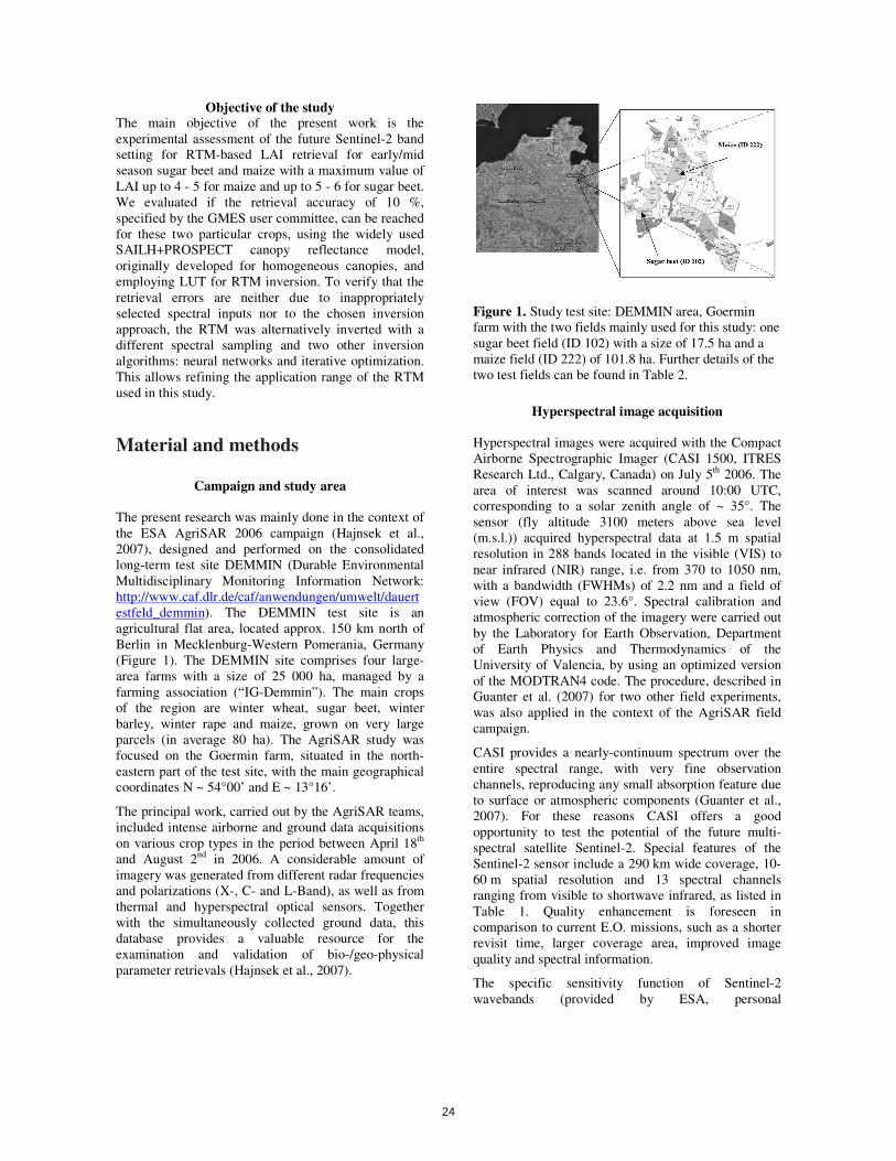
Figure 1. Study test site: DEMMIN area, Goermin farm with the two fields mainly used for this study: one sugar beet field (ID 102) with a size of 17.5 ha and a maize field (ID 222) of 101.8 ha. Further details of the two test fields can be found in Table 2.

Hyperspectral image acquisition Hyperspectral images were acquired with the Compact Airborne Spectrographic Imager (CASI 1500, ITRES Research Ltd., Calgary, Canada) on July 5th 2006. The area of interest was scanned around 10:00 UTC, corresponding to a solar zenith angle of ~ 35°. The sensor (fly altitude 3100 meters above sea level (m.s.l.)) acquired hyperspectral data at 1.5 m spatial resolution in 288 bands located in the visible (VIS) to near infrared (NIR) range, i.e. from 370 to 1050 nm, with a bandwidth (FWHMs) of 2.2 nm and a field of view (FOV) equal to 23.6°. Spectral calibration and atmospheric correction of the imagery were carried out by the Laboratory for Earth Observation, Department of Earth Physics and Thermodynamics of the University of Valencia, by using an optimized version of the MODTRAN4 code. The procedure, described in Guanter et al. (2007) for two other field experiments, was also applied in the context of the AgriSAR field campaign.

CASI provides a nearly-continuum spectrum over the entire spectral range, with very fine observation channels, reproducing any small absorption feature due to surface or atmospheric components (Guanter et al., 2007). For these reasons CASI offers a good opportunity to test the potential of the future multi-spectral satellite Sentinel-2. Special features of the Sentinel-2 sensor include a 290 km wide coverage, 10-60 m spatial resolution and 13 spectral channels ranging from visible to shortwave infrared, as listed in Table 1. Quality enhancement is foreseen in comparison to current E.O. missions, such as a shorter revisit time, larger coverage area, improved image quality and spectral information.

The specific sensitivity function of Sentinel-2 wavebands (provided by ESA, personal

24

communication) was applied to configure the CASI measurements according to the future Sentinel-2 satellite. To mimic the planned spatial resolution of Sentinel-2 (4 channels with 10 m and 4 with 20 m, see Table 1), the high spatial resolution CASI data (1.5 m) were degraded to a coarser resolution of 20 m for the whole imagery. Table 1. Spectral sampling of the proposed Sentinel-2 sensor: central wavebands, spectral widths, spatial resolution and purpose (from ESA GMES mission document, 2007). In grey the 8 bands used for the simulations.

Central waveb.

λ (nm)

Spectral width

∆λ (nm)

Spatial res. (m)

Purpose

443 20 60 Atmospheric correction (aerosol scattering)

490 65 10 Sensitive to vegetation senescing, carotenoid, browning and soil background; atmospheric correction (aerosol scattering)

560 35 10 Green peak, sensitive to total chlorophyll in vegetation.

665 30 10 Max. chlorophyll absorption.

705 15 20 Position of red edge; consolidation of atmospheric corrections / fluorescence baseline.

740 15 20 Position of red edge, atmospheric correction, retrieval of aerosol load.

775 20 20 LAI, edge of the NIR plateau

842 115 10 LAI

865 20 20 NIR plateau, sensitive to total Chlorophyll, biomass, LAI and protein; water vapor absorption reference; retrieval of aerosol load and type.

940 20 60 Water vapor absorption, atmospheric correction.

1375 20 60 Detection of thin cirrus for atmospheric correction.

1610 90 20 Sensitive to lignin, starch and forest above ground biomass. Snow/ice/cloud separation.

2190 180 20 Assessment of Mediterranean vegetation conditions. Distinction of clay soils for the monitoring of soil erosion. Distinction between live biomass, dead biomass and soil, e.g. for burn scars mapping.

In situ LAI measurements

Leaf area index measurements were carried out on two fields: one sugar beet field (ID 102: 8 samples) and one maize field (ID 222: 16 samples) (Figure 1). In situ LAI measurements were taken at the day of the sensor overpass or the evening of the preceding day. The measurements were performed with the Plant Canopy Analyzer LAI-2000 instrument (LICOR Inc., Lincoln, NE, USA).

Information about the monitored crop fields, phenological stages and some biophysical characteristics of the plants monitored during AgriSAR campaign are summarized in Table 2 together with two additional data sets used for validation purposes. Detailed information about these supplementary data can be found in Richter et al. (2008a) and Richter and Timmermans (2009).

The measurement principle of the LAI-2000 instrument is based on non-destructive indirect gap fraction measurements. The gap fractions are assessed by measuring the light transmission through the canopy. This is done by comparing differential light measurements above and below the canopy at five zenith angles (with central angles of 7, 23, 38, 53 and 68°) (Jonckheere et al, 2004). A detailed description of the instrument can be found in Cutini et al. (1998) or in the instruments manual (LI-COR, 1992). One shortcoming of the widely used instrument is that it does not distinguish photosynthetically active leaf tissue from other plant elements such as stems, branches, flowers or senescent leaves. The measurement should therefore be considered as “Plant Area Index” (PAI) (Jonckheere et al., 2004). Moreover, the possible non-random positioning of canopy elements is neglected. Hence, without carrying out a correction of the clumping, the term “effective LAI“ (Le) is more adequate (Chen and Black, 1992). In fact, the instrument tends to underestimate LAI, especially in case of discontinuous and heterogeneous canopies with clumped foliage (Jonckeere et al., 2004). On the contrary, vertical elements in canopies (such as stems) increase/overestimate LAI. Hence, the measurement accuracy does not only depend on phenological stage, but also on crop type and structure.

Since no corrections were applied to account for these two aspects, the term ‘LAI’ should, in the context of this study, be understood as ‘effective plant area index’ (PAIeff) (Chen et al., 1997, Darvishzadeh et al., 2008a; Soudani et al., 2006). On the other hand, the LAI measured by LAI-2000 (or other optical methods) is quite close to the leaf surface visible by a remote

25

Crop AgriSAR

Sugar beet

AgriSAR

Maize

PLEIADeS

Maize

SPARC

Sugar beet

SPARC

Maize

ID 102 222 - - -

Field size (ha) 17.5 101.8 - - -

Cultivar Ricarda(a) Salagor(a) no information no information no information

Sowing date end of March 2006(b)

beginning of May 2006(b)

end of May 2007 end of March 2004 beginning of June

2004

Developmental stage

(Eucarpia Scale, EC) EC stage 33(a) EC stage 39(a) no information no information no information

Plant height (m) ~0.25(b) ~ 1(b) 0.35 – 3.2 (d) 0.45-0.6 (d) 1.6 – 2.5 (d)

Plants per m² 10 (b) 15 (b) no information no information no information

Crop coverage (%) 50 (b) 40 (b) 10-95 (d) 60-80 (d) 40-80 (d)

Mean LAI (mean, SD)

1.5 (0.5) (b) 1.7 (0.5) (b) 2.0 (1.2) (d) 4.9 (0.4) (d) 2.4 (0.6) (d)

Chlorophyll (mean, SD) (µg/cm²)

40 (10) (b,c) 45 (10) (b,c) not measured 49 (1) (d) 52 (1) (d)

Table 2. Description of the test fields of the AgriSAR campaign (corresponding to time of sensor overpass), mainly analyzed in the study, and from the other two campaigns, when data were available.

a Personal communication (Agrisar Team); b Gerighausen et al., 2007 (3 measurement points); c Minolta SPAD measurements, d campaigns measurements, more information in: Richter et al., 2008a; Richter and Timmermans, 2009.

sensor which is not necessarily the case for the real leaf area index (Stenberg et al., 2004). According to Soudani et al. (2006), a correction for the clumping effect is therefore not absolutely necessary.

Each of the 24 AgriSAR in situ measurements (8 in ID 102 and 16 in ID 222) was based on three consecutive series of 8 readings below the canopy (plus one reference reading above the canopy) covering an Elementary Surface Unit (ESU) of approximately 20 x 20 m geolocated by means of a GPS (accuracy roughly 5 m). The average value of LAI, resulting from the set of 24 readings (576 measurements in total), has been considered as representative for the respective ESU. The standard deviation around the mean has been kept as a measure of uncertainty. Field measured LAI values ranged between 1.0 and 2.0 for the sugar beet field (ID 102) and 0.9 and 2.3 for the maize field (ID 222). Measurements were always taken under uniform clear diffuse skies at low solar elevation (i.e., ~ 1 h before sunset). Samples of below and above -canopy radiation were performed by experienced operators in the opposite direction to the sun to prevent direct sunlight on the sensor. A view restrictor of 180° was mounted on the sensor and care was taken that the instrument remained horizontal.

To avoid biases in the measurements due to particular crop architectures (such as sugar beet or maize in early

growth stages), the measurements were carried out in a systematic and standardized way; that is the sensor was placed alternately in the middle of the row and between two rows. Moreover, below canopy readings have been taken close to the soil with appropriate distances to the leaves.

To consider a wider range of LAI values than available from the AgriSAR campaign, data from two other experiments were consulted (see also Table 2): the LAI data set of 21 measurements of maize from the PLEIADeS 2007 field campaign, Sardinia, Italy (Richter et al., 2008a) and the LAI data set of 8 measurements of maize and 6 of sugar beet from the SPARC 2004 campaign, Barrax, Spain (Richter and Timmermans, 2009). In both experiments, measurements of LAI were performed by using the same protocol as described above for the AgriSAR campaign. During PLEIADeS, hyperspectral field measurements with the ASD FieldSpec UV-VNIR field spectrometer (operating in the spectral range from 350 to 1050 nm) were acquired in correspondence of LAI measurements and the spectral signatures configured according to the Sentinel-2 spectral bands. During SPARC experiment, imagery of CHRIS/Proba satellite was acquired and as well configured using the specific sensitivity function of Sentinel-2 wavebands (using near zenith view angle). The experiments are described in detail in the mentioned references.

26

Model and inversion techniques

Radiative transfer model: PROSAILH

A physical based method of canopy reflectance modelling was selected for the study: the widespread SAILH model (Scattering from Arbitrarily Inclined Leaves, Verhoef, 1984, 1985). It has been later extended by Kuusk (1991) to take into account the hot spot effect. The SAILH model is based on the turbid medium assumption, and describes the canopy structure in a fairly simple way. Despite its simplicity, it produces realistic results of bidirectional reflectance spectra as reported by several studies for different crops including maize and sugar beet (e.g. Andrieu et al., 1997; Goel and Thompson, 1984; Jacquemoud et al., 1995, 2000; Koetz et al., 2005; Major et al., 1992). For the purpose of our study, the SAILH model has been combined with the PROSPECT leaf optical properties model (Jacquemoud and Baret, 1990) to ‘PROSAILH’ (e.g., Atzberger, 1997; Baret et al., 2007; Verhoef and Bach, 2003; Weiss et al., 2000) to account for variations in leaf structure and composition.

The SAILH model simulates canopy bi-directional reflectance as a function of three structural parameters (i.e., LAI, average leaf inclination angle (ALA) and hot spot parameter (HotS) - roughly defined as the ratio of the leaf size to canopy height; Verhoef and Bach, 2003), soil spectral reflectance, leaf reflectance and transmittance, fraction of diffuse irradiance (skyl) and the view and illumination geometry. Leaf reflectance and transmittance were simulated by the PROSPECT model as a function of four structural and biochemical leaf parameters: leaf chlorophyll content (Cab), dry matter content (Cm), leaf water thickness (Cw) and a leaf mesophyll structural parameter (N).

The PROSAILH model has been preferred to other radiative transfer models, describing the canopy in a more complex way (for a review on these models see Dorigo et al., 2007), such as 3D hybrid radiative transfer models (e.g. Goel and Grier, 1988), Monte Carlo ray tracing models (Goel and Thompson, 2000) and others (Peddle et al., 2003, 2004). This decision is justified with the focus of potential usage of the method for operational applications. For operational applications, the execution speed of complex models is a limiting factor, especially when large quantities of data have to be processed on a regular (daily) basis. Moreover, the higher the complexity of the model the larger the requirement of knowledge concerning parameterization, construction of the merit function or use of prior information (Dorigo et al., 2007). On the other hand, the generality and robustness of the physical model approach favored the choice over VIs, which may also achieve accurate results and are easy to apply with low computer requirements.

Look-up table approach (LUT)

In the standard setting, the PROSAILH radiative transfer model was inverted by using a look-up table (LUT). Three principal steps have to be performed to realize this approach: (1) Generation of an appropriate number of canopy parameter combinations: A LUT size of 100 000 (‘LUT1’) cases of canopy parameter combinations was chosen according to the results of Weiss et al. (2000). Canopy parameter realizations, i.e. bounds and distributions, are depicted in Table 3. Parameter bounds were taken from measurement campaigns and/or other studies working with the same crops. They were chosen in order to describe the characteristics of both crop types used in the study, maize and sugar beet. Gaussian distributions have been generated for LAI and Cab in order to put more emphasis on the parameter values being present in the actual growth stages of the crops (Gerighausen et al., 2007). On the contrary, HotS, αsoil, Cm, and N were sampled from a uniform distribution (Koetz et al., 2005) since no information from the campaign measurements was available. The range of Cab was set to 10 – 70 µm, as in D’Urso et al. (2004) for a range of crops including sugar beet and maize. Similar ranges were used in other studies, e.g. in Weiss et al. (2000) and Koetz et al. (2005) for maize. LAI was allowed to vary between 0 and 6 with a mean of 2 close to the observed average LAI value of the two fields. The range of ALA was set quite large: 40°-70°, allowing the simulation of planophile (40°) to erectophile (70°) canopies. Similar large ranges have been used by Bacour et al. (2002), Combal et al. (2003) and Weiss et al. (2000), whereas other studies used either very small ranges (Koetz et al., 2005) or even fixed ALA to a single value (Espana et al., 1999). The bounds of the HotS parameter have been set to a large range (0.05-1). This range has also been used by Combal et al. (2003) for maize and Combal et al. (2002) for sugar beet. As the absorption of leaf water is not influencing the spectral range used in this study (< 1000 nm), Cw was fixed to an arbitrary value (Cw= 0.02 cm). Dry matter content Cm has been measured during a field campaign for maize (Huber et al., 2006). The parameter limits were set accordingly (Cm = 0.004-0.007 mg/cm²). The N-parameter was set to a range corresponding to values often used in the literature for maize and sugar beet (N = 1.3 - 1.7). Similar values have been found by PROSPECT inversion (González-Sanpedro et al., 2007; Haboudane et al., 2004; Jacquemoud et al., 1995). The soil reflectance spectrum for running the PROSAILH model was extracted from the CASI

27

imagery (mean of several bare soil pixel). A simple multiplicative soil brightness factor (αsoil) was introduced, representing the overall soil brightness, which was assumed to vary with soil water content and surface roughness (Atzberger et al., 2003). The range (0.7 - 1.3) was defined according to Koetz et al. (2005) and other studies. Within the distributions defined in Table 3, a random sampling scheme was applied to all parameters. For PLEIADeS and SPARC data, the canopy parameter realizations were set in the same way (Richter et al., 2008a; Richter and Timmermans, 2009). (2) Simulation of Sentinel-2 spectral sampling The model was applied in direct mode to simulate reflectance signatures corresponding to the proposed spectral sampling for the Sentinel-2 sensor. Table 1 gives some specifications of the sensor, with central wavebands, spectral width, spatial resolution and field of application for each channel. All wavebands interesting for LAI or vegetation studies were included in the simulation. Hence, the calculations comprised the VIS (490, 560, 665 nm), the red edge (705 and 740 nm) and the NIR (775, 842 and 865 nm) parts of the spectrum. The channels located at 443, 940 and 1375 nm, sensitive to aerosol scattering and water vapor absorption, were not considered, since their scope is to support the atmospheric correction of the imagery. The two wavebands located in the short wave infrared (1610 and 2190 nm) were as well out of interest for the study, because they will be used for cloud/ice separation and burn scars mapping, respectively. The measurement configuration used for the model simulations presented the actual condition during the sensor overpass with a solar zenith angle of 35° and a view zenith angle of 0° according to the almost-nadir position of the acquisitions. The fraction of diffuse irradiance, skyl, was fixed to 0.1 across all wavebands, according to many similar studies (Bacour et al., 2002; Schlerf and Atzberger, 2006; Weiss et al., 2002). Hence, we neglected both the wavelength dependence of skyl, as well as the fact that the amount of diffuse sky light depends on atmospheric conditions and solar zenith angle. This simplification seems justified by the fact that skyl has only a very small influence on canopy reflectance (Clevers and Verhoef, 1993). To take into account sensor and model uncertainties, a Gaussian (white) noise was added to the simulated canopy reflectance spectra before going to step (3). The noise was assumed to be proportional to the reflectance (mean of zero and standard deviation of 0.04) (Bacour et al., 2006, Baret et al., 2007). The simulated reflectance spectra were resampled according to the Sentinel-2 sensitivity.

(3) Sorting of the LUT along with a simple cost function: The cost function used in this study calculates the root mean square error (RMSE) between measured and simulated spectra found in the LUT. The solution is the average of the parameter combinations found within less than 10 % of the lowest RMSE value.

(1)

where λn is the number of wavelengths used in the

calculation, s

i

meaR the measured image reflectance, and i

LUTR the simulated reflectance of the spectrum in the

LUT at wavelength i. Usually, only little information is available about the crop status in an agricultural area. Thus, from an operational point of view, algorithms used for parameter (LAI) estimation from E.O. data have to fulfill the requirement to be universally valid. Consequently, a simple cost function, instead of a modified one, including a-priori information (e.g., Combal et al., 2003; Huber et al., 2006; Weiss et al., 2000) was applied to the algorithm. Note however, that in the construction of the LUT we applied a denser sampling around the most probable Cab and LAI values (see Table 3), which can also be seen as a kind of prior information.

Alternative retrieval algorithms To test the potential of the LUT approach and the suitability of the Sentinel-2 band configuration, two other retrieval algorithms (iterative optimization and neural nets) have been applied to the AgriSAR data set. In this way we verified that the findings of the standard approach (as described in 2.4.2) are not biased by the selected inversion approach. Furthermore, an alternative band composition has been tested (B2), regarded as ‘ideal’ for vegetation studies (Thenkabail et al., 2004). By comparing the Sentinel-2 band setting (B1) with B2 we confirm/reject the band setting of the future sensor. To make the different approaches as comparable as possible, the same Gaussian (white) noise was used for all algorithms.

Neural Networking (NN)

To invert PROSAILH using a neural network (NN), the synthetic database (LUT) of simulated canopy spectra and corresponding parameter sets was used (section 2.4.2.). The simulated database allows training the non-linear relationship between the spectral variables (as “measured” inputs) and the desired canopy biophysical

( )∑=

−=λ

λ

n

i

i

LUTs

i

mea RRn

RMSE1

21

28

Table 3. Range of input variables (lower (LB) and upper (UB) bounds) for PROSAILH model inversion using SQP algorithm, as well as number of classes and distribution of input variables used to establish the synthetic canopy reflectance data base for use in the LUT and for the training of the NN.

Similar variable ranges/values were used by the following studies : 1 González-Sanpedro et al., 2007 ; 2 Haboudane et al., 2004 ; 3 D’Urso et al, 2004 ; 4 Huber et al., 2006; 5Geringhausen et al., 2007; 6 Atzberger 2004; 7,8 Combal et al., 2002, 2003; 9 Koetz et al., 2005 variables (as “estimated” outputs). Once trained, the NN is applied to the CASI/Sentinel-2 spectra to map the canopy biophysical variables. To prevent network overfitting and overspecialization (and hence lack of generalization) several measures were taken. First of all, a simple three layer feed-forward backpropagation network with a tan-sigmoidal transfer function in the hidden layer and a linear transfer function in the output layer was selected. After several trial and errors, the following (compact) network structure was chosen: 5 neurons in the hidden layer, 7 input neurons (8 for the B2 band setting) and 3 output neurons (to predict simultaneously LAI, the leaf chlorophyll content, Cab, and the soil brightness factor, αsoil) were used. Both, the low number of hidden neurons and the simultaneous estimation of several biophysical variables prevent overfitting and overspecialization (Atzberger, 2004; Udelhoven et al., 2000). To further improve network generalization, the early stopping technique (Demuth and Beale, 2003) was applied. For this purpose, the patterns generated with PROSAILH were divided into three subsets (60, 20 and 20 %). The first subset (60 % of the pattern) was used

for updating the weight and biases of the network (training data set). The error on the test data set (20 % of the pattern) was monitored during the training process. The training was stopped automatically when the error in the test data set started to rise while the error on the training data set continued decreasing; such a situation is an indication of network overfitting. The third subset (remaining 20 % of the synthetic spectra) was used after completion of the training to assess the accuracy of the RTM inversion on synthetic spectra. To avoid sub-optimal network results, 51 networks were trained with randomly initialized weights/biases and with different synthetic training, test and validation data sets. As the networks gave very similar results on the synthetic validation data sets, it was decided to keep them all and to invert the image spectra with all networks. The final output was then simply the average of the 51 results. The standard deviation around the estimated average was kept as a measure of uncertainty.

Model Variables Units Min (LB) Max (UB) Distribution of variables

Leaf parameters:

(PROSPECT)

N(1,2,10) Leaf structure index unitless 1.3 1.7 Uniform

Cab (3) Leaf chlorophyll content [µg/cm²] 10 70 Gaussian (mean 40, SD

10) Cm

(4) Leaf dry matter content [g/cm²] 0.004 0.007 Uniform

Canopy variables:

(SAILH)

LAI(5) Leaf area index [m²/ m2] 0 6.0 Gaussian (Mean 2, SD 1)

ALA (6) Average leaf angle [°] 40 70 Uniform

HotS (7,8) Hot spot parameter [m /m] 0.05 1 Uniform

αso il (9) Soil brightness factor unitless 0.7 1.3 Uniform

θs sun zenith angle [degree] 35 /

θv view zenith angle [degree] 0 /

ø azimuth anlge between sun and sensor

[degree] 0 /

29

Iterative optimization approach (SQN)

Traditionally, radiative transfer models have often been inverted using iterative optimization techniques. Thus, we included this inversion strategy as another benchmark for comparison with the results achieved by means of the standard LUT approach. For the iterative optimization, the Sequential Quadratic Programming (SQP) has been implemented by using the MATLAB function fmincon. This function solves a quadratic programming (QP) sub-problem iteratively. The method allows to mimic closely Newton's method for constrained optimization. An approximation is performed for each major iteration of the Hessian Lagrangian function using a quasi-Newton updating method. An overview of SQP can be found in the Matlab documentation (MathWorks, Inc., 1984-2007). The SQP requires an initial set of parameters to start off the optimization process. However, these initial parameter values may affect strongly the solution achieved by the algorithm (Jacquemoud et al., 1995). In order to mitigate this effect, five different initial sets for the parameters were randomly selected in the ranges shown in Table 3.

Table 4. Spectral sampling (named B2) used as alternative band set to the Sentinel-2 band configuration. Wavebands and their sensitivity to plant components are extracted from the work of Thenkabail et al. (2004). Note: Thenkabail et al. (2004) proposed 22 bands, but here only those matching the CASI spectral configuration (≤ 885 nm) could be used.

Central waveband Λ (nm)

Sensitivity to plant components

495 Sensitive to senescing, carotenoid, browning, and soil background

555 Green peak, sensitive to total chlorophyll

655 Absorption pre-maxima, sensitive to biomass and soil background

675 Absorption maxima, greatest soil –crop contrast in 350–2500 nm

705 Start of rapid change of slope, sensitive to vegetation stress and dynamics

735 End of rapid change of slope, sensitive to vegetation stress and dynamics

885 NIR pre-peak; sensitive to biomass, LAI, and protein

In contrast to the LUT and NN based inversion, no prior information concerning the parameter distribution (such as LAI and Cab) was implemented in the algorithm. The optimization algorithm was only forced to remain within the parameter bounds. This hinders a detailed comparison of the three approaches which was nevertheless out of the scope of this study.

Larger Look-up Table and alternative ‘ideal’ spectral

sampling

To verify that the standard LUT size of 100 000 parameters is appropriate, a LUT with a size of 200 000 cases of canopy parameter combinations (‘LUT2’) was constructed for comparison. Parameter bounds, distribution and sampling scheme applied were the same as for the LUT described in section 2.4.2.

Furthermore, another band set (‘B2’) was chosen according to the results of a work from Thenkabail et al. (2004). These wavebands were found to characterize and classify best vegetation and crops due to their sensitivity to chlorophyll, biomass, LAI, plant moisture and vegetation stress. The seven bands (out of 22 proposed by Thenkabail et al., 2004) located in the CASI spectra were averaged in a bandwidth of 10 nm. Table 4 gives an overview of the B2 band set and the sensitivities of the various bands in vegetation related studies.

Results In this chapter we first present the quality of LAI estimation from all campaigns using the standard LUT approach (3.1.). RTM simulation accuracy is then presented in the following sub-section (3.2.). Next, the standard LUT results are compared to other model inversion approaches and to results obtained by the B2 band combination (3.3.) using the data set of the AgriSAR campaign. A general discussion on the applied method(s), their problems and applicability in an operational context of Sentinel-2 is given in the discussion (4.).

Performance of the LUT with the Sentinel –2 spectral sampling

Scatterplots between measured and estimated LAI values are shown in Figure 2a-e, including error bars of ±1 standard deviation of measurements and retrievals. The performance of the LUT approach using the spectral bands of the future Sentinel-2 sensor can be regarded as satisfying in the case of sugar beet (Figure 2a: AgriSAR; Figure 2d: SPARC) but indicates some problems for maize (Figure 2b: AgriSAR; Figure 2c: PLEIADeS; Figure 2e: SPARC). For sugar beet, a root mean square error (RMSE) of 0.18 was achieved for AgriSAR and a RMSE of 0.6 for SPARC. (rel. RMSE: 8 % and 9.2 % respectively). However, for maize the estimation performance was significantly lower with RMSE of 0.43 for AgriSAR and RMSE of 0.4 for PLEIADeS and SPARC (rel. RMSE: 22 %, 16.7 and 16.3 %, respectively). Thus, the estimation quality for

30

Figure 2. Measured and estimated LAI values for all campaigns (2a: AgiSAR sugar beet field (ID 102); 2b: AgriSAR maize field (ID 222); 2c: PLEIADeS maize; 2d: SPARC sugar beet; 2e: SPARC maize). The LAI estimates were obtained from LUT inversion approach and using the Sentinel-2 band configuration (B1). The standard deviations of measurements and simulations are indicated by error bars.

sugar beet is well within the 10 % requirements of the GMES mission. On the contrary, in the case of maize, the inversion falls short of expectations. Especially for the AgriSAR fields, a trend toward underestimation could be observed. The underestimation of LAI is small for sugar beet but pronounced for the maize field.

Spatial LAI of the two AgriSAR fields, obtained with the LUT inversion method, are illustrated in Figure 3ab. One easily recognizes distinct spatial structures, revealing the knowledge of the fields: The maps confirm a mean value of LAI around 1.5-2 for both crops, as monitored by the AgriSAR teams during this period (Gerighausen et al., 2007). Maize exhibited a slightly higher range (LAI: 0.5 - 3.0) than the sugar beet (LAI: 0.5 - 2.5). This within field growth variability reflects a typical pattern for crops in rainfed agriculture, being more sensitive to soil heterogeneity than irrigated crops (Richter et al., 2008b).

Match between measured spectra and RTM

simulations

When inverting radiative transfer models an important aspect is to control its ability to recreate the measured spectra using the retrieved model parameters. After the LUT inversion process, the estimated parameters were used as input to run the model in the forward way. Then the RMSE between measured and re-simulated reflectance for all 8 wavebands was calculated pixelwise for the whole fields. The resulting maps of RMSE are depicted in Figure 3c for sugar beet and 3d for maize of the AgriSAR campaign. The results suggest a good overall performance of the model for sugar beet with generally acceptable matches between measured and simulated spectra (0.008-0.017). The higher RMSE values of maize (0.007-0.088) correspond to the lower LAI retrieval performance for this crop. It indicates a general mismatch between input spectra and PROSAILH simulated reflectances. Probably, the pronounced row structure (clumping) and the early growth stage of maize (with low coverage) requires a specific canopy reflectance model that takes this effects into account (e.g., Yao et al., 2008). As both fields were geographically close to each other and

31

Table 5. Root mean square error (RMSE), relative percentage error (%) and coefficient of determination (R2) between measured and simulated LAI for two agricultural fields of the AgriSAR campaign: ID 102 (sugar beet) and ID 222 (maize). The results obtained with the standard LUT are shown in bold. Four alternative solutions are also presented: a larger LUT with 200 000 entries, SQP and NN with the Sentinel-2 band configuration and a LUT run with an alternative band setting B2 (Thenkabail et al., 2004).

LUT1

100 000

Sentinel-2

LUT2

200 000

Sentinel-2

SQP

Sentinel-2

NN

Sentinel-2

LUT1

100 000

B2

RMSE 0.18 0.19 0.58 0.16 0.29

% error 8.0 9.8 26.8 7.9 18.5

ID102

sugar beet

R2 0.92 0.90 0.19 0.88 0.70

RMSE 0.43 0.40 0.62 0.94 0.34

% error 22.8 21.4 30.5 52.8 18.7

ID222

maize

R2 0.35 0.36 0.13 0.35 0.36

sampled within the same image, artifacts related to the atmospheric and radiometric pre-processing can be excluded.

Comparison with alternative methods

The standard LUT approach (size 100 000) has been compared with two alternative inversion approaches and a different band setting for the AgriSAR data set. Results are summarized in Table 5 giving RMSE, R² and % error for all inversion methods and the alternative (B2) band set. From Table 5 it can be seen that an increased LUT size (200 000) did not change the estimation accuracies compared to the standard approach. This confirms the findings of Weiss et al. (2000) who pointed out that 100 000 LUT entries are appropriate. Larger differences were observed if SQP or NN were used for RTM inversion. SQP gave significantly lower accuracies for both fields with increased RMSE and lower R2. The neural nets performed well for sugar beet but resulted in strongly biased LAI values in the case of maize. Compared to the standard LUT approach, the R2 remained more or less unchanged indicating that the spatial structure of the estimates was preserved. In summary, the results clearly show that the observed errors of the standard LUT are not the results of an inappropriately chosen inversion approach. Likewise, the alternative band setting (B2) had also only insignificant effects when compared to the standard LUT approach; for one field (sugar beet) the accuracies

decreased slightly, whereas for the other field (maize) somewhat better results have been obtained. From this finding it can be concluded that the Sentinel-2 band setting is well suited for vegetation related studies. Retrieval accuracy of the neural net

The neural nets learned easily the relation between spectral inputs and the (three) output variables. For the synthetic validation data set, the RMSE for the three outputs and the 51 duplicate nets were 0.4 m2/m2 (LAI), 5.5 µg/cm2 (Cab) and 0.12 (αsoil) with a slope close to one and intercept of zero (not shown). As the validation data set did not enter in the network calibration, the low RMSE indicate very good network learning. Generally, the error of the synthetic training, test and validation data sets decreased very fast. The error curve was steep during the first 20 iterations before reaching a more or less horizontal level (not shown). On average, the early stopping criteria automatically stopped training after less than 50 iterations. For the two AgriSAR fields, the NN explained between 35 % (maize) and 89 % (sugar beet) of the total variance in the field measured LAI. However, a strong offset in the retrieved LAI of maize (ID 222) can be noted, resulting in high RMSE for this field compared to the standard LUT approach. We suppose that the offset results from a combination of RTM shortcomings (i.e., the row structure of the maize is not taken into account) and biased in situ measurements (i.e., the stems reduce the measured gap fractions).

32

Figure 3. Sentinel-2 derived LAI maps (a-b) from the AgriSAR campaign and maps of the RMSE between measured and simulated spectra (c-d). The results were obtained using the standard LUT approach (100 000 cases of parameter combinations) with the proposed band configuration of the upcoming Senintel-2 satellite. The RMSE (c-d) have been calculated across the 8 Sentinel bands with canopy parameters found by the LUT approach.

Retrieval accuracy using the iterative optimization

approach

Despite the use of the same radiative transfer model, an identical cost function and range of input variables, the differences in accuracy between the SQP inversion, compared to the LUT and NN approaches, are pronounced (Table 5). The failure of the SQP inversion may be explained by the drawback of iterative optimization methods to converge into local minima (Qiu et al., 1998). To partially overcome this problem, five different initial parameter sets were considered to start off the optimization. According to the criterion applied for the LUT, 10% was added to the smallest RMSE (between simulated and measured reflectance) in order to average all solutions being in this range. However, the difference between the smallest RMSE and the other four cases resulted mostly in errors greater than 10 %, indicating the importance of the initial parameter set. Thus, only the result with the smallest RMSE was selected as single solution. No attempts were made to run further initializations as the iterative optimization is computationally intensive in particular if large data sets have to be inverted.

Discussion

The estimation accuracies achieved with the LUT algorithm can be seen as fair. For sugar beet, the GMES/ Kopernikus requirements were barely met (precision: 8 - 9 %). On the other hand, with only 16 - 22 % accuracy, the LAI estimated for maize was beyond the GMES/ Kopernikus goal. The results confirm the findings of several studies for similar crops, using the same and also other retrieval methods, for example: (1) Sugar beet: Combal et al. (2002): RMSE = 0.5-1.4; D’Urso et al. (2004): RMSE = 0.49; Jacquemoud et al. (1995): RMSE = 0.79; (2) Maize: Haboudane et al. (2004): RMSE = 0.46-1.21; Koetz et al. (2005): RMSE = 0.69-0.79; Koetz et al. (2007): RMSE = 0.73; Vuolo et al. (2006): RMSE = 0.41 – 0.76; Walthall et al. (2004): RMSE = 0.41-1.27; Wu et al. (2007): RMSE = 0.63. In particular for small LAI values of maize, our results reveal a significant underestimation of the estimated LAI. The canopy characteristics of both crops deviate strongly from the turbid medium assumption of the PROSAILH model (Andrieu et al., 1997): maize and

33

sugar beet are typically row-planted and affected by leaf clumping (i.e. leaves are grouped together rather than distributed uniformly). The chosen PROSAILH model, however, does not account for the leaf clumping induced by the row structure of maize. Lopez-Lozano et al. (2007) compared canopy gap fractions of heterogeneous maize canopies with turbid, homogeneous canopies using simulations from a 3-dimensional RTM. The results showed that gap fractions of a heterogeneous canopy observed from nadir were generally higher than those of a homogeneous canopy. Consequently, inversion of the nadir measured remote sensing signal of row planted maize canopies leads to an underestimation of LAI values using turbid medium RTM. Similar findings were also described by Koetz et al. (2007). For maize it has also to be considered that the in situ measurements using the LAI-2000 instrument are probably too high as vertical elements like stems significantly reduce the measured gap fractions of the LAI-2000 instrument, albeit without influencing to the same extent the measured canopy reflectance.

A possible explanation of the better results achieved for sugar beet may also be related to the different crop growth stages during the image acquisition. In the AgriSAR campaign, the maize plants reached only a height of ca. 1 m (maximum usually up to 4 m) and a coverage of ~ 40 %; whereas the sugar beet showed in this later growth stage already a more homogeneous coverage (~ 50 %). During the SPARC campaign, sugar beet plants covered almost completely the ground (i.e. ~ 80 %). Consequently, the influence of the soil background (which is further enhanced by the row structure of these crops) is probably stronger for maize fields compared to the sugar beet. The RTM falsely interprets the strong soil signal as a low(er) coverage leading to a too low LAI. Also for PLEIADeS maize, the lower LAI values (LAI < 4) were slightly underestimated. This cannot be confirmed for SPARC data, but here all LAI values were higher than 2.

In a future study it has to be tested if a simple mixture model, such as the one proposed by Baret et al. (2007) at landscape level or GEOSAIL proposed by Huemmrich (2001), is capable of reducing this effect. These considerations are also supported by Yao et al. (2008), who proposed the use of a row structure model for the early growth stage (before elongation) of maize canopies, and a homogeneous one for later growth stages (after elongation).

In the present study we used a unique parameter set for both crop types as the objective was to select for every parameter the most realistic bounds and distributions without introducing too detailed prior information that usually is not available without a simultaneous field campaign. However, the differences in the resulting retrieval accuracy suggest that the use of a well adapted

parameter input set for every single crop species may be necessary to increase the estimation quality. That means, a priori information, such as from on-site measurements, knowledge of the type of canopy architecture and of the distribution of canopy biophysical variables (Combal et al., 2003) should be specified according to the crop type monitored. However, the establishment of crop and phenology specific LUTs can be a time-consuming task, which is sub-optimum in view of an operational monitoring process, where fast and universally valid (and accurate) algorithms are required. Our results also highlight the limitations of too simplistic RTMs which fail if the basic assumptions are not met by the crop under investigation. In an operational context, this also implies that a detailed crop map is available in order to choose the most appropriate RTM.

By comparing the standard LUT approach with two contrasting inversion approaches it was possible to verify that the sometimes inaccurate estimations are not due to an inappropriate inversion algorithm. The chosen LUT approach resulted more accurate and more robust than the iterative optimization approach and the neural net. The latter was accurate for the sugar beet field but gave strongly biased results in the case of maize. The insufficient accuracy of the NN to estimate the LAI of maize correctly highlights one of the major disadvantages of neural nets. In fact, NN often show relatively unpredictable behavior when fed with input spectra that are (too) different from what has been presented during the learning stage (e.g., Baret & Buis, 2008; Kimes et al., 1998; Schlerf and Atzberger, 2006). If the targets are not well represented by the modeled spectra, LUTs are indeed more robust compared to NN. Walthall et al. (2004) pointed out that the performance of the NN process may be improved if model input parameters were estimated from direct field measurements. This, however, would run counter to the stated objective of this analysis, which was to retrieve regional LAI estimates from satellite data without relying heavily on site-specific, ground calibration measurements. Another way to increase the robustness of the nets is to train them with higher noise levels as the one used in this research (e.g., Udelhoven et al., 2000). In the present study, however, such possible improvements have not been evaluated. Unreliable results have been obtained for both crops with the SQP inversion. This finding, however, probably only holds for this study, as the SQP inversion was seriously penalized with respect to the LUT approach (and to some extent also the NN inversion) as it did not take advantage of the available prior information regarding LAI and Cab (Table 3). This prior information has been taken into account for the LUT construction. The same LUT has also been used to train the NN. It would have been possible to include the prior information also in the SQP inversion (using a

34

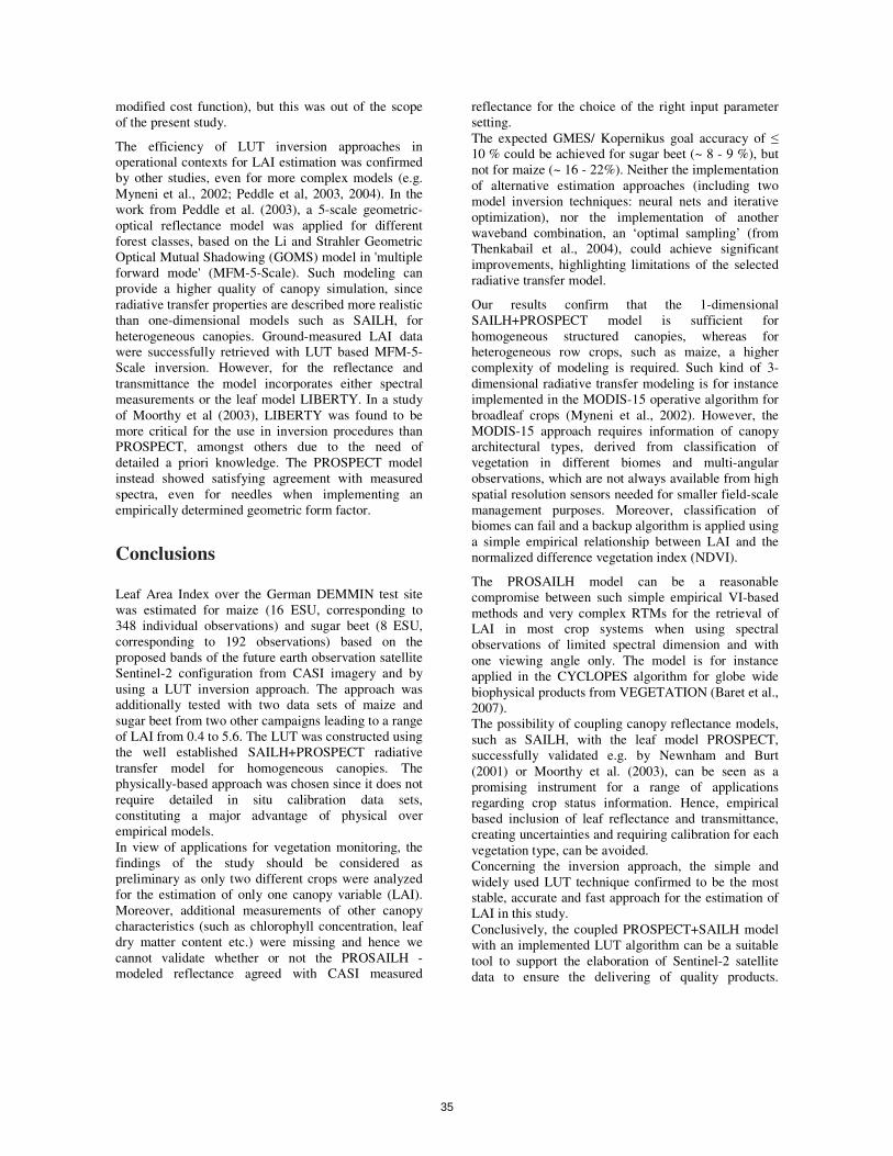
modified cost function), but this was out of the scope of the present study.

The efficiency of LUT inversion approaches in operational contexts for LAI estimation was confirmed by other studies, even for more complex models (e.g. Myneni et al., 2002; Peddle et al, 2003, 2004). In the work from Peddle et al. (2003), a 5-scale geometric-optical reflectance model was applied for different forest classes, based on the Li and Strahler Geometric Optical Mutual Shadowing (GOMS) model in 'multiple forward mode' (MFM-5-Scale). Such modeling can provide a higher quality of canopy simulation, since radiative transfer properties are described more realistic than one-dimensional models such as SAILH, for heterogeneous canopies. Ground-measured LAI data were successfully retrieved with LUT based MFM-5-Scale inversion. However, for the reflectance and transmittance the model incorporates either spectral measurements or the leaf model LIBERTY. In a study of Moorthy et al (2003), LIBERTY was found to be more critical for the use in inversion procedures than PROSPECT, amongst others due to the need of detailed a priori knowledge. The PROSPECT model instead showed satisfying agreement with measured spectra, even for needles when implementing an empirically determined geometric form factor.

Conclusions Leaf Area Index over the German DEMMIN test site was estimated for maize (16 ESU, corresponding to 348 individual observations) and sugar beet (8 ESU, corresponding to 192 observations) based on the proposed bands of the future earth observation satellite Sentinel-2 configuration from CASI imagery and by using a LUT inversion approach. The approach was additionally tested with two data sets of maize and sugar beet from two other campaigns leading to a range of LAI from 0.4 to 5.6. The LUT was constructed using the well established SAILH+PROSPECT radiative transfer model for homogeneous canopies. The physically-based approach was chosen since it does not require detailed in situ calibration data sets, constituting a major advantage of physical over empirical models. In view of applications for vegetation monitoring, the findings of the study should be considered as preliminary as only two different crops were analyzed for the estimation of only one canopy variable (LAI). Moreover, additional measurements of other canopy characteristics (such as chlorophyll concentration, leaf dry matter content etc.) were missing and hence we cannot validate whether or not the PROSAILH - modeled reflectance agreed with CASI measured

reflectance for the choice of the right input parameter setting. The expected GMES/ Kopernikus goal accuracy of ≤ 10 % could be achieved for sugar beet (~ 8 - 9 %), but not for maize (~ 16 - 22%). Neither the implementation of alternative estimation approaches (including two model inversion techniques: neural nets and iterative optimization), nor the implementation of another waveband combination, an ‘optimal sampling’ (from Thenkabail et al., 2004), could achieve significant improvements, highlighting limitations of the selected radiative transfer model.

Our results confirm that the 1-dimensional SAILH+PROSPECT model is sufficient for homogeneous structured canopies, whereas for heterogeneous row crops, such as maize, a higher complexity of modeling is required. Such kind of 3-dimensional radiative transfer modeling is for instance implemented in the MODIS-15 operative algorithm for broadleaf crops (Myneni et al., 2002). However, the MODIS-15 approach requires information of canopy architectural types, derived from classification of vegetation in different biomes and multi-angular observations, which are not always available from high spatial resolution sensors needed for smaller field-scale management purposes. Moreover, classification of biomes can fail and a backup algorithm is applied using a simple empirical relationship between LAI and the normalized difference vegetation index (NDVI).

The PROSAILH model can be a reasonable compromise between such simple empirical VI-based methods and very complex RTMs for the retrieval of LAI in most crop systems when using spectral observations of limited spectral dimension and with one viewing angle only. The model is for instance applied in the CYCLOPES algorithm for globe wide biophysical products from VEGETATION (Baret et al., 2007). The possibility of coupling canopy reflectance models, such as SAILH, with the leaf model PROSPECT, successfully validated e.g. by Newnham and Burt (2001) or Moorthy et al. (2003), can be seen as a promising instrument for a range of applications regarding crop status information. Hence, empirical based inclusion of leaf reflectance and transmittance, creating uncertainties and requiring calibration for each vegetation type, can be avoided. Concerning the inversion approach, the simple and widely used LUT technique confirmed to be the most stable, accurate and fast approach for the estimation of LAI in this study. Conclusively, the coupled PROSPECT+SAILH model with an implemented LUT algorithm can be a suitable tool to support the elaboration of Sentinel-2 satellite data to ensure the delivering of quality products.

35

However, when accuracies of 10 % are required even for row crops, more complex RTMs should be applied.

Acknowledgement The authors thank L. Guanter and colleagues from the Laboratory for Earth Observation, Department of Earth Physics and Thermodynamics, University of Valencia, for radiometric and spectral calibrations and atmospheric correction of CASI imagery.

This work is carried out in the framework of PLEIADeS project (Participatory multi-Level EO-assisted tools for Irrigation water management and Agricultural Decision-Support; Contract 037095 financed by U.E.- VI F.P.).

References Andrieu, B., Baret, F., Jacquemoud, S., Malthus, T. and Steven, M. 1997. Evaluation of an improved version of SAIL model for simulating bidirectional reflectance of sugar beet canopies. Remote Sensing of Environment, Vol. 60, No. 3, pp. 247-257. Atkinson, P. M. and Tatnall, A. R. L. 1997. Neural networks in remote sensing. International Journal of Remote Sensing, Vol. 18, No. 4, pp. 699– 709. Atzberger, C. 1997. Estimates of winter wheat production through remote sensing and crop growth modeling. VWF Verlag fuer

Wissenschaft und Forschung, Berlin. 261 pp. Atzberger, C. 2004. Object-based retrieval of biophysical canopy variables using artificial neural nets and radiative transfer models. Remote Sensing of Environment Vol. 93, pp. 53-67. Atzberger, C., Jarmer, T., Schlerf, M., Koetz, B., Werner, W. 2003. Retrieval of wheat bio-physical attributes from hyperspectral data and SAILH+PROSPECT radiative transfer model. Proceedings of 3rd EARSeL Workshop on Imaging

Spectroscopy, 13-16 May 2003, Herrsching, Germany. Bacour, C., Jacquemoud, S., Tourbier, Y., Dechambre, M. and Frangi, J.-P. 2002. Design and analysis of numerical experiments to compare four canopy reflectance models. Remote

Sensing of Environment, Vol. 79, pp. 72–83. Bacour, C., Baret, F., Béal, D., Weiss, M., Pavageau, K. 2006. Neural network estimation of LAI, fAPAR, fCover and LAI×Cab, from top of canopy MERIS reflectance data: Principles and validation. Remote Sensing of Environment, Vol. 105, No. 4, pp. 313-325. Baret, F. and Buis, S. 2008. Estimating canopy characteristics from remote sensing observations. Review of methods and associated problems. In S. Liang (ed.), Advances in Land Remote

Sensing: System, Modeling, Inversion and Application.

Springer Netherlands, DOI: 10.1007/978-1-4020-6450-0_7, pp. 172-301. Baret, F., Hagolle, O., Geiger, B., Bicheron, P., Miras, B., Huc, M., Berthelot, B., Nino, F., Weiss, M, Samain, O., Roujean, J.L., Leroy, M. 2007. LAI, fAPAR and fCover CYCLOPES global products derived from VEGETATION. Part 1: Principles of the algorithm. Remote Sensing of Environment, Vol. 110, No. 3, pp.275- 286. Breda, N.J.J. 2003. Ground-based measurements of leaf area index: a review of methods, instruments and current controversies. Journal of Experimental Botany, Vol. 54, No. 392, pp. 2403- 2417. Camps-Valls, G., Bruzzone, L., Rojo-Álvarez, J.L., Melgani, F. 2006. Robust Support Vector Regression for Biophysical Variable Estimation From Remotely Sensed Images. IEEE

Geoscience and Remote Sensing Letters, Vol. 3, No. 3, pp. 339-343. Chen, J.M., Black, T.A. 1992. Defining leaf area index for non-flat leaves. Plant, Cell and Environment, Vol. 15, pp. 421–429. Chen, J. M., Rich, P. M., Gower, S. T., Norman, J. M. and Plummer, S. 1997. Leaf area index of boreal forests: Theory, techniques and measurements. Journal of Geophysical Research, Vol. 102, No. D24, pp. 29429– 29444. Cho, M., Skidmore, A., Atzberger, C. 2008. Towards red-edge positions less sensitive to canopy biophysical parameters for leaf chlorophyll estimations using properties optique spectrales des feuilles (PROSPECT) and scattering by arbitrarily inclined leaves (SAILH) simulated data. International Journal of Remote

Sensing Vol. 29, No. 7-8, pp. 2241-2255. Clevers, J.G.P.W. and Verhoef, W. 1993. LAI estimation by means of the WDVI: a sensitivity analysis with a combined PROSPECT-SAIL model. Remote Sensing Reviews, Vol. 7, No. 1, pp. 43-64. Combal, B., Baret, F. and Weiss, M. 2002. Improving canopy variables estimation from remote sensing data by exploiting ancillary information. Case study on sugar beet canopies. Agronomie, Vol. 22, No. 2, pp. 205–215. Combal, B., Baret, F., Weiss, M., Trubuil, A., Macé, D., Pragnére, A. 2003. Retrieval of canopy biophysical variables from bidirectional reflectance using prior information to solve the ill- posed inverse problem. Remote Sensing of Environment, Vol. 84, pp. 1– 15. Cutini, A., Matteucci, G. and Mugnozza, G. S. 1998. Estimation of leaf area index with the Li-Cor LAI 2000 in deciduous forests. Forest Ecology and Management, Vol. 105, pp. 55–65. Darvishzadeh, R., Skidmore, A., Schlerf, M., Atzberger, C. 2008a. Inversion of a radiative transfer model for estimating vegetation LAI and chlorophyll in a heterogeneous grassland. Remote Sensing of Environment, Vol. 112, pp. 2592-2604. Darvishzadeh, R., Atzberger, C., van Wieren, S. and Skidmore, A. 2008b. Estimation of vegetation LAI from hyperspectral reflectance data: effects of soil type and plant architecture. International Journal of Applied Earth Observation and

Geoinformation, Vol. 10, No. 3, pp. 358-373. Demuth, H. and Beale, M. 2003. Manual of Neural Network Tool Box - For Use with MATLAB, MATLAB User's Guide, Version 4, the Math Works Inc. Dorigo, W.A., Zurita-Milla, R., de Wit, A.J.W., Brazile, J., Singh, R. and Schaepman, M.E. 2007. A review on reflective remote sensing and data assimilation techniques for enhanced agroecosystem modelling. International Journal of Applied

Earth Observation and Geoinformation, Vol. 9, No. 2, pp. 165- 193. Durbha, S. S., King, R. L., and Younan, N. H. 2007. Support vector machines regression for retrieval of leaf area index from multi- angle imaging spectroradiometer. Remote Sensing of

Environment, Vol. 107, No. 1–2, pp. 348−361. D’Urso G., Dini L., Vuolo F., Guanter L. 2004. Retrieval of vegetation biophysical parameters by inverting hyperspectral, multiangular CHRIS/PROBA Data from SPARC 2003. Proceedings of the 2nd CHRIS/Proba Workshop, ESA/ESRIN, 28-30 April 2004, Frascati, Italy. España, M., Baret, L., Aries, F., Chelle, F., Andrieu, B. and Prévot, L. 1999. Modeling maize canopy 3D architecture application to reflectance simulation. Ecological Modelling, Vol. 122, pp. 25−43. EUCARPIA, the European Association for Research on Plant Breeding. URL. http://www.eucarpia.org/index.html (Accessed March 4, 2009) European Space Agency (ESA) 2007. GMES Sentinel-2 Mission Requirements Document, issue 2 revision 0- 30/01/2007, EOP-SM/1163/MR-dr, 31 p., European Space Agency (ESA), 2007. URLs: http://www.esa.int/esaLP/ASERBVNW9SC_index_0.html http://www.esa.int/esaLP/SEMZHM0DU8E_LPgmes_2.html http://www.esa.int/esaEO/SEMH574XQEF_environment_0.html

36

(Accessed March 4, 2009) European Space Agency (ESA) 2008. The Earth Observation Handbook, Climate Change Special Edition 2008. URL: http://www.eohandbook.com/eohb2008/earthobservation.htm (Accessed March 4, 2009) Filella, I. and Penuelas, J. 1994. The red edge position and shape as indicators of plant chlorophyll content, biomass and hydric status. International Journal of Remote Sensing, Vol. 15, No. 7, pp.1459-1470. Gerighausen, H., Borg, E., Wloczyk, C., Fichtelmann, B., Günther,A., Vajen,H.H., Rosenberg, M., Schulz,M., Engler, H- G. 2007. DEMMIN – a test site for the validation of Remote Sensing data products. General description and application during AgriSAR 2006. Proceedings of the AGRISAR and

EAGLE campaigns final workshop, 15-16 October, 2007. ESA/ESTEC, Noordwijk, The Netherlands. 9 p. Goel, N. S. 1988. Models of vegetation canopy reflectance, their use in estimation of biophysical parameters from reflectance data. Remote Sensing Reviews, Vol. 4, pp. 1 – 212. Goel, N.S. and Grier, T. 1988. Estimation of canopy parameters for inhomogeneous vegetation canopies from reflectance data: III. Trim: A model for radiative transfer in heterogeneous three- dimensional canopies. Remote Sensing of Environment, Vol. 25, No. 3, pp. 255–293. Goel, N. S. and Thompson, R. L. 1984. Inversion of vegetation canopy reflectance models for estimating agronomic variables: 4. Total inversion of the sail model. Remote Sensing of

Environment, Vol. 15, No. 3, pp. 237– 253. Goel, N.S. and Thompson, R.L. 2000. A snapshot of canopy reflectance models and a universal model for the radiation regime. Remote Sensing Reviews, Vol. 18 , pp. 197–225. González-Sanpedro, M. C., Le Toan, T., Moreno, J., Kergoat, L., Rubio, E. 2007. Seasonal variations of leaf area index of agricultural fields retrieved from Landsat data. Remote Sensing

of Environment, Vol. 112, No. 3, pp. 810- 824. Gower, S.T., Kucharik, C.J., Norman, J.M. 1999. Direct and indirect estimation of leaf area index, fAPAR, and net primary production of terrestrial ecosystems. Remote Sensing of Environment, Vol. 70, No.1, pp. 29-51. Guanter, L., Estellés, V., Moreno, J. 2007. Spectral calibration and atmospheric correction of ultra-fine spectral and spatial resolution remote sensing data. Application to CASI-1500 data. Remote Sensing of Environment, Vol. 109, pp. 54–65. Haboudane, D., Miller, J.R., Pattey, E., Zarco-Tejada, P.J., Strachan, I.B. 2004. Hyperspectral vegetation indices and novel algorithms for predicting green LAI of crop canopies: Modeling and validation in the context of precision agriculture. Remote

Sensing of Environment, Vol. 90, pp. 337-352. Hajnsek, I., Bianchi, R., Davidson, M., D'Urso, G., Gomez-Sanches, A., Hausold, A., Horn, R., Howse, J., Low, A.J., Lopez- Sanchez, J.J., Ludwig, R., et al. 2007. AgriSAR 2006: airborne SAR and optics campaigns for an improved monitoring of agricultural processes and practices. Proceedings of the

AGRISAR and EAGLE campaigns final workshop, 15-16 October, 2007. ESA/ESTEC, Noordwijk, The Netherlands. 8 p. Hu, B., Miller, J.R., Chen, J.M. and Hollinger, A.B. 2004. Retrieval of the canopy leaf area index in the BOREAS flux tower sites using linear spectral mixture analysis. Remote Sensing of

Environment, Vol. 89, pp. 176–188. Huber K., Dorigo W. A., Bauer T., Eitzinger J., Haumann J., Kaiser G., Linke R., Postl W., Rischbeck P., Schneider W., Suppan F., Weihs P. 2006. Changes In Spectral Reflectance Of Crop Canopies Due To Drought Stress. Proceedings of Earth

observation for vegetation monitoring and water management, American American Institute of Physics. 10-11 November 2005, Napoli. G. D'Urso, M.A. Osann Jochum, J. Moreno. (Eds), pp. 258-265. Huemmrich, K. F. 2001. The GeoSail model: a simple addition to the SAIL model to describe discontinuous canopy reflectance. Remote Sensing of Environment, Vol. 75, No. 3, pp. 423-431.

Itres Research Ltd, 2006. URL. http://www.itres.com/CASI_1500 (Accessed March 4, 2009). Jacquemoud, S. and Baret, F. 1990. PROSPECT: A model of leaf optical properties spectra. Remote Sensing of Environment, Vol. 34, pp. 75-91. Jacquemoud, S., Baret, F., Andrieu, B., Danson, F. M. and Jaggard, K. 1995. Extraction of Vegetation Biophysical Parameters by Inversion of the PROSPECT + SAIL Models on Sugar Beet Canopy Reflectance Data. Application to TM and AVIRIS Sensors. Remote Sensing of Environment, Vol. 52, pp. 163-172. Jacquemoud, S., Bacour, C., Poilve, H. and Frangi, J.P. 2000. Comparison of four radiative transfer models to simulate plant canopies reflectance: Direct and inverse mode. Remote Sensing

of Environment, Vol. 74, pp. 417–481. Jonckheere, I., Fleck, S., Nackaerts, K., Muys, B., Coppin, P., Weiss, M. and Baret, F. 2004. Review of methods for in- situ leaf area index determination. Part I. Theories, sensors and hemispherical photography. Agricultural and Forest

Meteorology, Vol. 121, pp. 19–35. Kimes, D.S., Nelson, R.F., Manry, M.T. and Fung, A.K. 1998. Attributes of neural networks for extracting continuous vegetation variables from optical and radar measurements. International Journal of Remote Sensing, Vol. 19, No. 14, pp. 2639-2662. Kimes, D., Knjazikhin, Y., Privette, J. L., Abuelgasim, A. and Gao, F. 2000. Inversion methods for physically-based models. Remote

Sensing Reviews, Vol. 18, pp. 381-440. Koetz, B., Baret, F., Poilvè, H., Hill, J. 2005. Use of coupled canopy structure dynamic and radiative transfer models to estimate biophysical canopy characteristics. Remote Sensing of

Environment, Vol. 95, pp. 115– 124. Koetz, B., Kneubühler, M., Huber, S., Schopfer, J. and Baret, F. 2007. LAI Estimation Based on Multi-Temporal CHRIS/PROBA Data and Radiative Transfer Modelling. Proceedings of ENVISAT Symposium, Montreux (CH), 23- 27 April 2007, ESA Publications Division, Noordwijk (NL), SP- 636, CD-ROM. Kuusk, A., 1991. The hot-spot effect in plant canopy reflectance. Photon – vegetation interactions. Applications in Optical

Remote Sensing and Plant Ecology. R.B. Myneni and J. Ross (Ed.), Springer-Verlag, New York, pp. 139– 159. LI-COR 1992. LAI-2000 Plant Canopy Analyzer Instruction Manual Lincoln, NE, USA: LICOR Inc. Liang, N.S. 2004a. Quantitative remote sensing of land surfaces. John Wiley and Sons, New York. Liang, N.S., 2004b. Estimation of Land Surface Biophysical Variables. Qualitative Remote Sensing of Land Surfaces. Kong, G.A. (Ed.), New York: Wiley Series in Remote Sensing. John Wiley and Sons, pp. 246–309. Lopez-Lozano, R., Baret, F., Chelle, M., Rochdi, N., and Espana, M. 2007. Sensitivity of gap fraction to maize architectural characteristics based on 4D model simulations. Agricultural and

Forest Meteorology, Vol. 143, No. 3-4, pp. 217-229. Liu, J., Miller, J.R., Haboudane, D., Pattey, E. 2004. Exploring the relationship between red edge parameters and crop variables for precision agriculture. In IGARSS’04, Proceedings of the

International Geoscience and Remote Sensing Symposium, 20- 24 September 2004, Anchorage, Alaska, Vol. 2, pp. 1276-1279. Major, D. J., Schaalje, G. B., Wiegand, C. and Blad, B. L. 1992. Accuracy and sensitivity analyses of sail model- predicted reflectance of maize. Remote Sensing of Environment, Vol. 41, No. 1, pp. 61– 70. Moorthy,I., Miller, J.R., Zarco-Tejada, P.J., Noland, T.L. 2003. Needle chlorophyll content estimation: a comparative study of PROSPECT and LIBERTY. In IGARSS’03, Proceedings of

the IEEE International Geoscience and Remote Sensing

Symposium, 21 – 25 July 2003, Toulouse, France, Vol. 3, pp. 1676- 1678. Myneni, R.B., Maggion, S., Iaquinto, J., Privette, J.L., Gobron, N., Pinty, B. 1995. Optical remote-sensing of vegetation — modeling, caveats and algorithms. Remote Sensing of

Environment, Vol. 51, pp. 169– 188.

37

Myneni, R.B., Hoffman, S., Knyazikhin, Y., Privette, J.L., Glassy, J., Tian, Y., Wang, Y., Song, X., Zhang, Y., Smith, G. R., Lotsch, A. , Friedl, M., Morisette, J. T. , Votava, P., Nemani, R. R. and Running, S. W. 2002. Global products of vegetation leaf area and fraction absorbed PAR from year one of MODIS data. Remote Sensing of Environment, Vol. 83, No. 1-2, pp. 214-231. Newnham, G.J. and Burt, T. 2001. Validation of a leaf reflectance and transmittance model for three agricultural crop species. In IGARSS’01, Proceeding of the International Geoscience and

Remote Sensing Symposium, 9 – 13 July 2001, Sydney, Australia, Vol. 7, pp. 2976-2978. Peddle, D.R., Johnson, R.L. , Cihlar, J. , Leblanc, S.G., Chen, J.M. and Hall, F.G. 2003. Physically-Based Inversion Modeling for Unsupervised Cluster Labeling, Independent Forest Classification and LAI Estimation using MFM-5-Scale. Canadian Journal of Remote Sensing, Vol. 33, No. 3, pp. 214- 225. Peddle, D.R., Johnson, R.L., Cihlar, J., Latifovic, R. 2004. Large area forest classification and biophysical parameter estimation using the 5-Scale canopy reflectance model in Multiple-Forward- Mode. Remote Sensing of Environment, Vol. 89, No. 2, pp.252- 263, Pragnère, A., Baret, F., Weiss, M., Myneni, R., Knyazikhin, Y., Wang, L.B. 1999. Comparison of three radiative transfer model inversion techniques to estimate canopy biophysical variables from remote sensing data. In IGARSS’99, Proceeding

of the International Geoscience and Remote Sensing Symposium,

28 June – 2 July 1999, Hamburg, Germany, Vol. 2, pp. 1093- 1095. Qiu, J., Gao, W., Lesht, B.M. 1998. Inverting optical reflectance to estimate surface properties of vegetation canopies. International Journal of Remote Sensing, Vol. 19, No. 4, pp. 641–656. Richter, K. and Timmermans, W., 2009. Physically based retrieval of crop characteristics for improved water use estimates. Hydrology and Earth System Sciences, Vol. 13, pp. 663-674. Richter, K., Vuolo, F., D’Urso, G. 2008a. Leaf area index and surface albedo estimation: comparative analysis from vegetation indexes to radiative transfer models. In IGARSS’08, Proceeding of the International Geoscience and Remote Sensing

Symposium, 6-11 July 2008, Boston (MA), Vol. 3, pp. 736-739. Richter, K., Rischbeck, M.P., Eitzinger, J., Schneider, W., Suppan, F., Weihs, P. 2008b. Plant growth monitoring and potential drought risk assessment by means of Earth Observation data. International Journal of Remote Sensing, Vol. 29, No. 17-18, pp. 4943-4960. Schlerf, M. and Atzberger, C. 2006. Inversion of a forest reflectance model to estimate structural canopy variables from hyperspectral remote sensing. Remote Sensing of Environment, Vol. 100, No. 3, pp. 281-294. Schlerf, M., Atzberger, C. and Hill, J. 2005. Remote sensing of forest biophysical variables using HyMap imaging spectrometer data. Remote Sensing of Environment, Vol. 95, No. 2, pp. 177- 194. Scurlock, J. M. 0., Asner, G. P. and Gower, S. T. 2001. Worldwide Historical Estimates of Leaf Area Index, 1932- 2000. Oak

Ridge National Laboratory, 0RNL/TM-2001/268. Soudani, K., Francois, C., le Maire, G., Le Dantec, V., Dufrene, E. 2006. Comparative analysis of IKONOS, SPOT, and ETM+ data for leaf area index estimation in temperate coniferous and deciduous forest stands. Remote Sensing of Environment, Vol. 102, No. 1, pp. 161-175. Stenberg, P., Rautiainen, M., Manninen, T., Voipio, P. and Smolander, H. 2004. Reduced simple ratio better than NDVI for estimating LAI in Finnish pine and spruce stands. Silva Fennica, Vol. 38, No. 1, pp. 3–14. Thenkabail, P.S., Smith, R.B., De-Pauw, E. 2002. Hyperspectral vegetation indices and their relationships with agricultural crop characteristics. Remote Sensing of Environment, Vol. 71, pp. 158–182.

Thenkabail, P.S., Enclona, E.A., Ashton, M.S., Van Der Meer, B. 2004. Accuracy assessments of hyperspectral waveband performance for vegetation analysis applications. Remote

Sensing of Environment, Vol. 91, pp. 354- 376. Udelhoven, T., Atzberger, C. and Hill, J. 2000. Retrieving Structural and Biochemical Forest Characteristics Using Artificial Neural Networks and Physically Based Reflectance Models. Proceedings of the 20th EARSeL Symposium, Dresden, 14-16 June, Dresden, Buchroithner (ed.), pp. 205-211. Verhoef, W. 1984. Light scattering by leaf layers with application to canopy reflectance modeling: the SAIL Model. Remote

Sensing of Environment, Vol. 16, pp. 125-141. Verhoef, W. 1985. Earth observation modeling based on layer scattering matrices. Remote Sensing of Environment, Vol. 17, pp. 165−178. Verhoef, W., Bach, H. 2003. Simulation of hyperspectral and directional radiance images using coupled biophysical and atmospheric radiative transfer models. Remote Sensing of

Environment, Vol. 87, pp. 23–41. Vuolo, F., D’Urso, L. Dini, G. 2006. Cost-effectiveness of vegetation biophysical parameters retrieval from remote sensing data. In:

SPIE’s conference proceedings: Remote Sensing for Agriculture,

Ecosystems, and Hydrology VIII. M. Owe, G. D'Urso, C. M. Neale, Ben T. Gouweleeuw (Eds), Stockholm, Sweden, September 2006, Vol. 6359, pp. 63590N. Walthall, C., Dulaney, W., Anderson, M., Norman, J., Fang, H. and Liang, S. 2004. A comparison of empirical and neural network approaches for estimating corn and soybean leaf area index from Landsat ETM+ imagery. Remote Sensing of Environment, Vol. 92, No. 4, pp. 465-474. Weiss, M., Baret, F., Myneni, R.B., Pragnère, A. and Knyazikhin, Y. 2000. Investigation of a model inversion technique to estimate canopy biophysical variables from spectral and directional reflectance data. Agronomie, Vol. 20, pp. 3-22. Weiss, M., Baret, F., Leroy, M., Hautecœur, O., Bacour, C., Prévot, L., Bruguier, N. 2002. Validation of neural net techniques to estimate canopy biophysical variables from remote sensing data. Agronomie, Vol. 22, No. 6, pp. 547-553. Wu, J., Wang, D., Bauer, M.E. 2007. Assessing broadband vegetation indices and QuickBird data in estimating leaf area index of corn and potato canopies. Field Crops Research, Vol. 102, No. 1, pp. 33-42. Yao, Y., Liu, Q., Liu, Q., Li, X. 2008. LAI retrieval and uncertainty evaluations for typical row-planted crops at different growth stages. Remote Sensing of Environment, Vol. 112, No. 1, pp. 94- 106.

38

4.2 Publikation II

Physically based retrieval of crop characteristics for improved water use estimates.

Katja Richter and Wim Timmermans

Hydrology and Earth System Sciences 13: 663-674, 2009.

39

Hydrol. Earth Syst. Sci., 13, 663–674, 2009www.hydrol-earth-syst-sci.net/13/663/2009/© Author(s) 2009. This work is distributed underthe Creative Commons Attribution 3.0 License.

Hydrology andEarth System

Sciences

Physically based retrieval of crop characteristics for improved wateruse estimates

K. Richter 1 and W. J. Timmermans2

1Department of Agricultural Engineering, University of Naples “Federico II”, via Universita 100, 80055 Portici (Na), Italy2International Institute for Geo-information Sciences and Earth Observation, Dept. of Water Resources, P. O. Box 6,7500 AA Enschede, The Netherlands

Received: 28 January 2009 – Published in Hydrol. Earth Syst. Sci. Discuss.: 6 March 2009Revised: 20 May 2009 – Accepted: 21 May 2009 – Published: 27 May 2009

Abstract. The increasing scarcity of water from local toglobal scales requires the efficient monitoring of this valu-able resource, especially in the context of a sustainable man-agement in irrigated agriculture. In this study, a two-sourceenergy balance model (TSEB) was applied to the Barraxtest site. The inputs of leaf area index (LAI) and fractionalvegetation cover (fCover) were estimated from CHRIS im-agery by using the traditional scaled NDVI and a look-uptable (LUT) inversion approach. The LUT was constructedby using the well established SAILH + PROSPECT radiativetransfer model. Simulated fluxes were compared with towermeasurements and vegetation characteristics were evaluatedwith in situ LAI and fCover measurements of a range of cropsfrom the SPARC campaign 2004. Results showed a betterretrieval performance for the LUT approach for canopy pa-rameters, affecting flux predictions that were related to landuse.

1 Introduction

Given the increasing scarcity of water at local, regional andglobal scales, an efficient monitoring of this valuable re-source becomes more and more essential, especially in thecontext of a sustainable management in irrigated agricul-ture and other water-related disciplines, such as hydrologicalmodelling, numerical weather forecasting or climate changeprediction (Anderson et al., 2007). Partitioning of avail-able energy between sensible and latent heat is hereby ofprime interest and various models have been developed in the

Correspondence to:K. Richter(katja.rich@gmail.com)

last years that describe this interaction between land surfaceand atmosphere. Those models, known as soil-vegetation-atmosphere transfer schemes (SVAT), vary widely in theircomplexity and dimensionality (Timmermans et al., 2007).

The conjunction of currently optical, thermal and mi-crowave Earth Observation (E. O.) data with SVAT schemesallows the spatial estimation of surface flux partitioning fromland-surface temperature and dynamic vegetation variables(Anderson et al., 2007; Bindlish et al., 2001; Schmugge etal., 1998). For homogeneous canopies and land surfaces, asingle-source modelling approach can be sufficient. How-ever, vegetated surfaces are usually under heterogeneousconditions, which are better described by two-source models,treating the land surface as a composite of soil and vegeta-tion components with separate fluxes and temperatures (An-derson et al., 2007; Timmermans et al., 2007). The Two-Source Energy Balance model (TSEB) for instance, first de-scribed in Norman et al. (1995) and updated by Kustas andNorman (1999) and Kustas et al. (2004), uses directional ra-diometric surface temperature for estimating component heatfluxes from soil and vegetation, i.e. instantaneous fluxes ofnet radiation (RN ), soil (G), sensible (H) and latent heat(LE). Several studies validated TSEB successfully againstflux tower measurements or other modelling schemes (e.g.Anderson et al., 2007; Schmugge et al., 1998; Timmermanset al., 2007) and research is ongoing to improve model per-formance (Kustas and Norman, 1999; Li et al., 2005). Innu-merable publications focused on improving accuracy of tem-perature and roughness characteristics, but despite the impor-tance of vegetation characteristics, still either rather simpleempirical models are used, or vegetation parameters are de-rived from visual observations, some samples or indirectlyfrom measurements of biomass or plant species type (Zhanet al., 1996). However, analyses by Zhan et al. (1996) and

Published by Copernicus Publications on behalf of the European Geosciences Union.

664 K. Richter and W. J. Timmermans: Physically based retrieval of crop characteristics

more recently by Timmermans et al. (2007) revealed thatTSEB, as well as other existing models, shows a considerablesensitivity to small variations of fractional vegetation cover(fCover) and/or leaf area index (LAI) on soil and canopy tem-perature estimation, in particular for high cover conditions.These findings emphasize the importance of accurate valuesof these parameters, usually determined from optical E. O.data. Although not model specific, the common approachapplied within the TSEB model to estimate LAI and fCoveris by means of rather simple empirical formulations utilizingeither the Normalized Difference Vegetation Index (NDVI)(Schmugge et al., 1998) or a scaled NDVI (Choudhury etal., 1994; French et al., 2003; Kustas and Norman, 1999).Such empirical approaches are based on relationships be-tween the parameter (e.g. LAI) and Vegetation Indices (VIs).Many studies showed that the application of VIs can giveappropriate results, especially when using newly developedhyperspectral VIs (e.g. Haboudane et al., 2004). However,a spectral signature is the integration of several factors andcan not be explained by just one parameter. Moreover, theseempirical models are often crop-, site- and sensor-specific(Atzberger, 2004; Vuolo et al., 2008). Therefore, many ef-forts have been undertaken in the last decades to developand improve canopy reflectance models based on radiativetransfer equations. In these radiative transfer models (RTM),the complexity of the spectral signal is taken into accountby a function of canopy geometry (e.g. LAI, leaf angle dis-tribution), optical leaf and soil properties, illumination andviewing geometry. Inversion of such models then offers thepossibility of extracting these biophysical parameters.

The objective of the present study is to test whether a phys-ically based retrieval of LAI and fCover can support moreaccurate estimations of fluxes in two-source energy balancemodelling.

2 Material and methods

In this section first a description of the models used for theestimation of vegetation characteristics and energy fluxes isgiven. Then the campaign with ground and E. O. data acqui-sitions is described.

2.1 Estimation of vegetation characteristics

2.1.1 Empirical model

Traditionally, the estimation of surface parameters for en-ergy balance modelling is based on empirical methods. Sev-eral empirical models have been developed to estimate thebiophysical parameters. Though not characteristic for theTSEB model, recent versions (French et al., 2003; Li et al.,2005) employ the approach as proposed by Choudhury etal. (1994). This so-called scaled NDVI – approach deter-

mines fCover for nadir viewing angles (fCover (θo), θo=0)as follows:

fCover(0)= 1 −

(NDVImax − NDVI

NDVImax − NDVImin

)p

(1)

Hereby, the end-member NDVI values, NDVImax andNDVImin, characterize a surface fully covered and com-pletely uncovered by vegetation, respectively. The parameterp is defined asp=3/κ, describing the ratio of a leaf angledistribution term,3 (set to 0.5 for randomly oriented leaves,Campbell and Norman, 1998), to canopy extinction,κ (set to0.55, approximating typical extinction for many canopies ata solar zenith angle of 25 degrees, following Campbell andNorman, 1998), leading to ap value of 0.9.

The NDVI end-members were obtained by combiningan NDVI histogram analysis (Timmermans et al., 2007)with local field observations resulting in NDVImax=0.85 andNDVImin=0.10.

Leaf area index (LAI), is then calculated from fCover(Choudhury, 1987):

LAI =ln (1 − fCover(0))

3(2)

2.1.2 Radiative transfer model

As an alternative to the empirical approach, a physicallybased model of canopy reflectance was applied: the com-bined SAILH (Kuusk, 1991; Verhoef, 1984, 1985) andPROSPECT (Jacquemoud and Baret, 1990) models (called“PROSAILH”), widely used for canopy reflectance mod-elling and applications, amongst others by Atzberger (2004),Baret et al. (2007), Darvishzadeh et al. (2008), Richter etal. (2009) or Weiss et al. (2000).

SAILH is a one-dimensional turbid medium radiativetransfer model, later modified to take into account the hotspot effect (Kuusk, 1991). It simulates the bidirectional top-of-canopy (TOC) reflectance as a function of three structureparameters, defined by LAI (m2/m2); average leaf inclina-tion angle, ALA (deg), assuming an ellipsoidal distribution,and hot spot size parameter,Hot (m/m). Further it requiresthe soil spectral reflectance, fraction of diffuse incoming so-lar radiation (skyl), and the view and illumination geome-try (i.e. sun zenith angle,θ s (deg); sensor viewing angle,θo

(deg) and azimuth angle between sun and sensor,φ (deg)).Leaf hemispherical reflectance and transmittance are simu-lated by the PROSPECT model as a function of four struc-tural and biochemical parameters: leaf chlorophyll a+b con-centration,Cab (µg/cm2); dry matter content,Cm (mg/cm2);leaf water thickness,Cw (cm) and a leaf mesophyll structuralparameter,N (unitless). To account for the changes in soilreflectance (induced by soil water content and roughness), awavelength independent scaling factor “αsoil” is introduced,i.e. multiplied with the soil spectrum.

Hydrol. Earth Syst. Sci., 13, 663–674, 2009 www.hydrol-earth-syst-sci.net/13/663/2009/41

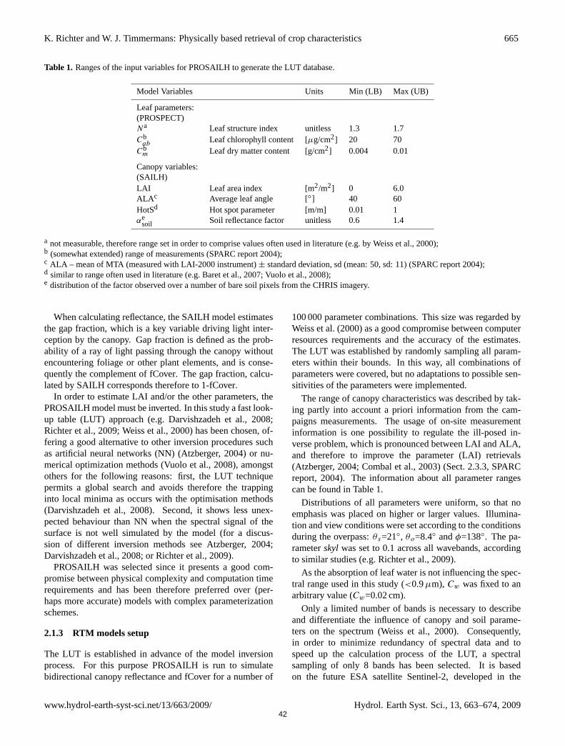
K. Richter and W. J. Timmermans: Physically based retrieval of crop characteristics 665

Table 1. Ranges of the input variables for PROSAILH to generate the LUT database.

Model Variables Units Min (LB) Max (UB)

Leaf parameters:(PROSPECT)Na Leaf structure index unitless 1.3 1.7Cb

abLeaf chlorophyll content [µg/cm2] 20 70

Cbm Leaf dry matter content [g/cm2] 0.004 0.01

Canopy variables:(SAILH)LAI Leaf area index [m2/m2] 0 6.0ALA c Average leaf angle [◦] 40 60HotSd Hot spot parameter [m/m] 0.01 1αe

soil Soil reflectance factor unitless 0.6 1.4

a not measurable, therefore range set in order to comprise values often used in literature (e.g. by Weiss et al., 2000);b (somewhat extended) range of measurements (SPARC report 2004);c ALA – mean of MTA (measured with LAI-2000 instrument)± standard deviation, sd (mean: 50, sd: 11) (SPARC report 2004);d similar to range often used in literature (e.g. Baret et al., 2007; Vuolo et al., 2008);e distribution of the factor observed over a number of bare soil pixels from the CHRIS imagery.

When calculating reflectance, the SAILH model estimatesthe gap fraction, which is a key variable driving light inter-ception by the canopy. Gap fraction is defined as the prob-ability of a ray of light passing through the canopy withoutencountering foliage or other plant elements, and is conse-quently the complement of fCover. The gap fraction, calcu-lated by SAILH corresponds therefore to 1-fCover.

In order to estimate LAI and/or the other parameters, thePROSAILH model must be inverted. In this study a fast look-up table (LUT) approach (e.g. Darvishzadeh et al., 2008;Richter et al., 2009; Weiss et al., 2000) has been chosen, of-fering a good alternative to other inversion procedures suchas artificial neural networks (NN) (Atzberger, 2004) or nu-merical optimization methods (Vuolo et al., 2008), amongstothers for the following reasons: first, the LUT techniquepermits a global search and avoids therefore the trappinginto local minima as occurs with the optimisation methods(Darvishzadeh et al., 2008). Second, it shows less unex-pected behaviour than NN when the spectral signal of thesurface is not well simulated by the model (for a discus-sion of different inversion methods see Atzberger, 2004;Darvishzadeh et al., 2008; or Richter et al., 2009).

PROSAILH was selected since it presents a good com-promise between physical complexity and computation timerequirements and has been therefore preferred over (per-haps more accurate) models with complex parameterizationschemes.

2.1.3 RTM models setup

The LUT is established in advance of the model inversionprocess. For this purpose PROSAILH is run to simulatebidirectional canopy reflectance and fCover for a number of

100 000 parameter combinations. This size was regarded byWeiss et al. (2000) as a good compromise between computerresources requirements and the accuracy of the estimates.The LUT was established by randomly sampling all param-eters within their bounds. In this way, all combinations ofparameters were covered, but no adaptations to possible sen-sitivities of the parameters were implemented.

The range of canopy characteristics was described by tak-ing partly into account a priori information from the cam-paigns measurements. The usage of on-site measurementinformation is one possibility to regulate the ill-posed in-verse problem, which is pronounced between LAI and ALA,and therefore to improve the parameter (LAI) retrievals(Atzberger, 2004; Combal et al., 2003) (Sect. 2.3.3, SPARCreport, 2004). The information about all parameter rangescan be found in Table 1.

Distributions of all parameters were uniform, so that noemphasis was placed on higher or larger values. Illumina-tion and view conditions were set according to the conditionsduring the overpass:θ s=21◦, θo=8.4◦ andφ=138◦. The pa-rameterskyl was set to 0.1 across all wavebands, accordingto similar studies (e.g. Richter et al., 2009).

As the absorption of leaf water is not influencing the spec-tral range used in this study (<0.9µm), Cw was fixed to anarbitrary value (Cw=0.02 cm).

Only a limited number of bands is necessary to describeand differentiate the influence of canopy and soil parame-ters on the spectrum (Weiss et al., 2000). Consequently,in order to minimize redundancy of spectral data and tospeed up the calculation process of the LUT, a spectralsampling of only 8 bands has been selected. It is basedon the future ESA satellite Sentinel-2, developed in the

www.hydrol-earth-syst-sci.net/13/663/2009/ Hydrol. Earth Syst. Sci., 13, 663–674, 200942

666 K. Richter and W. J. Timmermans: Physically based retrieval of crop characteristics

framework of Global Monitoring for Environment and Se-curity (GMES/Kopernikus, ESA, 2007) to replace and im-prove the old generation of satellite sensors. Sentinel-2 isscheduled to be launched in the year 2012 and as outcomethe mission will provide service data, comprising productssuch as LAI and fCover. The multi spectral data, used forthe simulations in the study, involve the following CHRISwavebands: 492, 563, 664, 706, 738, 773, 844 and 862 nm(corresponding to Sentinel-2: 490, 560, 665, 705, 740, 775,842 and 865 nm, ESA 2007). In this way all spectral bandsof Sentinel-2 with the purpose to retrieve LAI and other veg-etation characteristics (i.e. 8 out of 13 bands) are included.This spectral sampling has been tested for its suitability forLAI estimation by Richter et al. (2009).

In the final step the solution within the LUT is selectedby applying a simple cost function calculating the root meansquare error (RMSE) between simulated and measured spec-tra (e.g. Darvishzadeh et al., 2008), as follows:

RMSE=

√∑ni=1 Rmeas(λ)− Rlut(λ))2

n(3)

where Rmeas corresponds to the measured reflectance atwavelengthλ, andRlut stands for the simulated reflectancecalculated with the PROSAILH model. The number of bandsis indicated withn.

The resulting parameter combination was built as the av-erage of all parameter combinations found within less than20% of the lowest RMSE value (e.g. Richter et al., 2009).

2.2 TSEB model

The land surface model used here to derive latent and sensi-ble heat fluxes is originally designed to use input data primar-ily from remote sensing platforms. Its main characteristic isthat it discriminates between a soil and vegetation compo-nent, aiming at a more physical description of heterogeneoussurfaces when dealing with radiative and aerodynamic prop-erties. Required remote sensing input consists of spatial in-formation on surface temperature as well as vegetation den-sity, being fCover and LAI. The version implemented herebasically follows what is described as the “series resistancenetwork” in Appendix A of Norman et al. (1995). In the cur-rent version a physically based algorithm is implemented forestimating the net radiation, which is described in detail inKustas and Norman (1999). As such, the model implementedis described in detail in Norman et al. (1995) and Kustas andNorman (1999); reason to only sketch its main characteris-tics and highlight those parts that are affected by fCover andLAI.

First of all, fCover is used to estimate canopy and soil tem-peratures (TC andTS , respectively) from observed radiomet-ric surface temperature,TR, with a simple non-linear mixingmodel, described by:

T nR = fCoverT n

C+ (1 − fCover)Tn

S . (4)

where n is the power in the Stefan-Boltzmann equationthat reasonably approximates the appropriate integral of thePlanck blackbody emission function for the wavelength ofthe sensor.

A first estimate of the latent heat flux from the canopy,LEC , is obtained by applying the Priestley and Taylor ap-proach on the canopy component of the net radiation,RN,C ,which works reasonably well under unstressed vegetationconditions. The canopy sensible heat flux,HC , is then de-termined by evaluating the canopy energy budget. By usinga linearized form of Eq. (4), following the procedure out-lined in the Appendix A of Norman et al. (1995), the within-canopy air temperature,TAC , is derived, which also yieldsthe canopy temperature,TC . Substitution in Eq. (4) yieldsTS , providing the possibility of obtaining the soil sensibleheat flux,HS . The soil heat flux,G, is determined as a time-dependant ratio of the soil net radiation,RN,S , after whichthe soil latent heat flux,LES , is determined by evaluating thesoil energy budget. In caseLES is negative, then the soil islikely to be dry andLES is set to zero. Under these circum-stances,HS is derived from the soil energy budget, and anadjustedTS is obtained. Equation (4) provides a new esti-mate forTC which is then used to calculate an updatedHC .

The algorithm used for estimating the net radiation diver-gence requires incident solar radiation observations and for-mulations for the transmission of direct and diffuse short-wave radiation and for the transmission of longwave radia-tion through the canopy (Campbell and Norman, 1998). Thecanopy component of net radiation,RN,C , is given by:

RN,C = (1 − τLW ) × (RLW,sky + RLW,S − 2RLW,C) (5)

+(1 − τSW ) × (1 − ρC) × RSW

and the soil net radiation component,RN,S , by:

RN,S = τLW × RLW,sky + (1 − τLW ) × RLW,C (6)

−RLW,S + τSW × (1 − ρS) × RSW

where τ represents transmissivity through the canopy andsubscriptsSWandLW stand for shortwave and longwave, re-spectively. Subscripts sky,S andC represent the sky, soil andcanopy components, whereasρ is the reflectance, or short-wave albedo. Since the reflection and absorption of radiationin the visible and near-infrared wavelengths are rather dif-ferent for vegetation and soils, the visible and near-infraredalbedos of the soil and canopy were evaluated differently be-fore combining to give an overall shortwave albedo. Theequations for estimating the transmission and reflection ofdirect and diffuse shortwave radiation are provided in Camp-bell and Norman (1998). We suffice here with the observa-tion that their spatial variation is solely determined by LAI.The longwave transmissivity finally is approximated by a sin-gle exponential function depending on an extinction coeffi-cient and LAI.

Hydrol. Earth Syst. Sci., 13, 663–674, 2009 www.hydrol-earth-syst-sci.net/13/663/2009/43

K. Richter and W. J. Timmermans: Physically based retrieval of crop characteristics 667

The parameterization of the resistances used in the seriesresistance network was taken from Norman et al. (1995).Aerodynamic properties such as canopy height, displacementheight, aerodynamic roughness, leaf width, as well as lim-ited micrometeorological observations are required as inputparameters and are assigned a priori. They are described inthe following section.

2.3 Experimental setup and observations

2.3.1 Site description

The analyses are based on data of the interdisciplinary ESASPARC 2004 Campaign. (Moreno et al., 2004; SPARC re-port 2004). The objective of the campaign was to advance theunderstanding of land – atmosphere exchanges of water andenergy in space and time over heterogeneous land surfaces.

In this context, satellite and ground data were collected inBarrax (30◦3′ N, 2◦6′ W), an agricultural test area situated inthe Castilla-La Mancha region in southern Spain. Figure 1shows an overview of the location and the area of interest.

The Barrax site, a flat area at 700 m above sea level, ischaracterized by a large variety of uniform land use units ofdifferent crops and dry bare soils, leading to a wide range ofLAI from 0 up to 6.5.

The Castilla-La Mancha region receives an annual precip-itation of only 400 mm and is therefore one of the driest re-gions in Europe. One third of the land is irrigated (35%),comprising amongst others alfalfa, maize, potatoes, sun-flower, onion, garlic, sugar beet and vineyard. The other twothirds (65%) are rainfed cultivations, such as winter/springcereals and bare soils/fallow land.

2.3.2 E. O. data acquisition

Optical data

Hyperspectral and multiangular E. O. data from CompactHigh Resolution Imaging Spectrometer (CHRIS) instrument,located on the Project for On-Board Autonomy (PROBA)platform, were acquired on 16 July 2004 around 11:25 UTC.Since the system PROBA/CHRIS has multiangular capabili-ties, five consecutive images from five different view angleshave been obtained during the overpass, with a minimumsatellite zenith angle of 8.4◦. Since it was not the scope ofthe current study to analyze the contribution of directionalinformation to the parameter estimates (Vuolo et al., 2008),only the imagery with the viewing angle closest to nadir hasbeen considered.

The sensor covers the visible/near-infrared region (from400 nm to 1050 nm) with a spectral sampling interval rang-ing between 1.25 nm (at 400 nm) and 11 nm (at 1000 nm).CHRIS data were acquired in Mode-1, having a spatial reso-lution of 34 m and 62 spectral bands.

Fig. 1. Location of the study area: Barrax Site, La-Mancha, Spain.

Radiometric calibration and atmospheric and geometriccorrection of CHRIS imagery were carried out by the De-partment of Thermodynamics of the University of Valencia.

Thermal imagery

The thermal remote sensing data from SPARC 2004 used inthis study consisted of ASTER imagery, acquired on 18 July2004 to obtain surface temperature. ASTER has 5 thermalinfrared bands with a 90 m spatial resolution.

After atmospheric correction, the land surface tempera-ture was extracted using a split-window technique (Jimenez-Munoz and Sobrino, 2007) on channels 13 and 14 of theASTER data. This method was preferred over the standardTES algorithm due to insufficient accuracy in land surfacetemperature retrieval that was noted over certain land covertypes (Sobrino et al., 2007).

Despite ASTER’s excellent capabilities for surface energyflux mapping here CHRIS/PROBA data were used due totheir more advantageous spectral characteristics for mappingthe vegetation characteristics, assuming these do not changesignificantly within 2 days time.

2.3.3 Ground observations

The ground-based data used here consisted of vegetationcharacteristics, meteorological observations as well as radia-tion and turbulent flux exchanges (Su et al., 2008), collectedduring the time of the satellite acquisitions.

Observations of vegetation surface parameters, such asvegetation height, LAI, mean tilt angle (MTA), fCover, leafchlorophyll, water and dry matter content, were conducted

www.hydrol-earth-syst-sci.net/13/663/2009/ Hydrol. Earth Syst. Sci., 13, 663–674, 200944

668 K. Richter and W. J. Timmermans: Physically based retrieval of crop characteristics

(Fernandez et al., 2005) at several locations for calibrationand validation of remote sensing derived vegetation input tothe flux model.

Non-destructive field measurements of LAI were per-formed with the Plant Canopy Analyzer LAI-2000 instru-ment (LICOR Inc., Lincoln, NE, USA), measuring simul-taneously the MTA that corresponds to the ALA parameterin the PROSAILH model (Sect. 2.1.2).

To reduce the effect of multiple scattering on LAI-2000measurements, the instrument was operated maximal twohours after sunrise or before sunset, under diffuse radiationconditions. In order to prevent interference caused by the op-erator’s presence and the illumination condition, the sensorfield of view was limited with a 180◦ view-cap. Measure-ments were azimuthally oriented opposite to the sun azimuthangle. Each single LAI value was the result of an averageof 24 measurements taken randomly within an ElementarySampling Unit (ESU) of approximately 15×15 m2.

Since no corrections were applied to account for clump-ing or the influence of non-photosynthetic plant components(such as stems), the term “LAI” should here be understoodas “effective plant area index” (PAIeff) (Chen et al., 1997;Darvishzadeh et al., 2008). However, LAI measured by LAI-2000 (or other optical methods) is quite close to the leaf sur-face visible by a remote sensor which is not necessarily thecase for the real LAI. Therefore, a correction for the clump-ing effect is not absolutely necessary (Stenberg et al., 2004).

A data set of 48 LAI measurements, located in/near thearea of interest (maize: 8, garlic: 13, potatoes: 15, sugarbeet: 6, sunflower: 6) have been selected for the validation.

Measurements of fCover, being of essential interest forthis study, have been performed using hemispherical pho-tography. According to the crop structure, different sam-pling strategies were applied. The photographs were pro-cessed using a specialized software package (CAN-EYE),developed at INRA-CSE Avignon. The procedure of thesoftware is based on gap fraction estimation using classifi-cation techniques (detailed information about the measure-ments and data elaboration can be found in the SPARC 2004report). The final fCover estimate for each ESU (20×20 m)was calculated as the average of twelve measurements. Forthe present study, a total number of 21 measurements havebeen used for validation (garlic: 4, potatoes: 4, sunflower: 4,onion: 4, sugar beet: 3, maize: 2).

Meteorological and radiation observations (incomingshortwave radiation, air temperature, relative humidity, airpressure and wind speed) that were needed as input to theTSEB model, were taken from a tower in the centre of thearea.

Validation data concerning turbulent fluxes exchanges andradiation for the time of the ASTER overpass were madeat several locations that were chosen such that typical landcover units were covered (described in detail in Su et al.,2008). They comprised a forest nursery, a wheat stubblefield, vineyard (2 sites), a sunflower field and a corn field. At

all sites measurements of sensible heat flux,H , were madeeither by 1-D or 3-D sonic anemometers or by scintillometer(vineyard) and in one position also latent heat flux,LE, wasmeasured (vineyard). However, due to the pivot irrigationsystem at the corn field, the sensor had to be located at theedge of the corn field adjacent to the vineyard, meaning thatthe measurement either represented the vineyard or the corn,depending on wind direction. Net radiation and soil heat fluxwere measured only at four sites; the vineyard, forest nurs-ery, corn and a wheat stubble field. For a location map one isreferred to Fig. 1 in Van der Kwast et al. (2009) where alsoa land cover map is provided, showing the main land coverunits.

Aerodynamic properties were assigned to the differentland cover units using averaged field observations of canopyheight,hc (Fernandez et al., 2005) in combination with theclassical relations (Brutsaert, 1982) where surface rough-ness length for momentum transport,z0M, is taken equal to1/8*hC and the displacement height,d0, equal to 2/3*hC .An exception was made for the roughness length of the cornfields, which were extremely dense, resulting in a muchsmoother surface. Therefore a roughness length value equalto that of the sunflower was assigned, which closely resem-bled estimates from turbulence measurements done over themaize (Timmermans et al., 2009). Moreover, the displace-ment heights of the wheat stubble and forest nursery landcover were chosen equal to zero, since these units were char-acterized by a very open and heterogeneous character.

3 Results and discussion

In this section we first present the quality and the differencesin LAI and fCover estimations using the LUT inversion andthe scaled NDVI approaches. Validation of the energy bal-ance model output is then performed by means of the fluxtowers measurements. Differences in the flux componentssimulated with both canopy parameter retrieval methods areanalyzed additionally in a spatial context. A general discus-sion on the applied method(s), their problems and applicabil-ity (in an operational context) concludes this section.

3.1 Vegetation characteristics versus observations

Retrieval performances of the LUT inversion and NDVI ap-proaches were evaluated using LAI and fCover data fromcampaigns measurements (see Sect. 2.3.3). Crops not cov-ered by the flux stations, such as sugar beet, garlic, potatoesand onion, were included in the analyses as well to test thegeneral applicability of the models.

The comparison with the ground measured fCover datawith both approaches (LUT inversion: “fCoverlut”; NDVIapproach: “fCoverndvi”) resulted in a slightly higher ac-curacy of fCoverlut, with Root Mean Squared Differences(RMSD) for fCoverlut of 0.12 and for fCoverndvi of 0.15. The

Hydrol. Earth Syst. Sci., 13, 663–674, 2009 www.hydrol-earth-syst-sci.net/13/663/2009/45

K. Richter and W. J. Timmermans: Physically based retrieval of crop characteristics 669

plots in Fig. 2a, b give a graphical impression of the estima-tion quality, indicating a tendency of overestimation of theNDVI approach, especially at the higher values. Since TSEBhas a greater sensitivity to fCover, in determining the tur-bulent fluxes, especially at high vegetation cover conditions(Timmermans et al., 2007) this is considered an importantdrawback of the NDVI approach.

In case of LAI (LUT inversion: “LAIlut”; NDVI approach:“LAI ndvi”) the LUT inversion approach provided clearly ahigher retrieval accuracy in comparison with the ground data(Fig. 2c, d), with RMSD of 0.79 (LAIlut) versus RMSD of1.44 (LAIndvi). Also here the empirical model has a trendto overestimate the parameter. Clearly noticeable is alsothe well-known problem of saturation at higher LAI values(“plateau-effect”), illustrated by the scatter plot in Fig. 2c.

The overestimation of fCover using the scaled NDVI ap-proach can be caused by an inaccurate NDVImin value, i.e.the value for bare soil reflectance, which in reality variesand is probably different (higher) when calculating the meanover all bare soil pixels in the scene (Montandon and Small,2008). Soils have a variable NDVI due to the fact that the rel-ative variation of the spectral signal in the visible red wave-band region is larger than in the near infrared. Increasing soilwater leads consequently to an augmentation of NDVI, gen-erating for example a difference of NDVI of 10% between awet and a dry soil background for a LAI of 1 (Bach and Ver-hoef, 2003). Differences of land cover and irrigation practisewhich influence the soil background will therefore also havean effect on fCover estimation accuracy.

The PROSAILH model overcomes this problem by takinginto account the soil reflectance variation by means of theαsoil-factor.

However, the model tends to slightly underestimate highLAI values for crops with strong leaf clumping, as it wasthe case for potatoes in the present growth stage. This be-haviour results from the nonlinearity of the LAI-reflectancerelationship, leading to saturation effects (Baret et al., 2007).On the other hand, even the measurements could cause anoverestimation of LAI, since the LAI-2000 can not separatebetween photosynthetic and non-photosynthetic plant com-ponents. This may occur whenever the built-in assumption ofrandomly distributed plant elements holds true. Thus, non-green elements (such as stems or senescent leaves) reducethe measured gap fractions.

A detailed interpretation of the retrieval performances forthe specific crop types is not given, since the objective isto evaluate the overall applicability of the RTM model forcanopy parameter estimations. Considering that the PRO-SAILH model simplifies the canopy as a turbid medium, ofwhich none of the crops really corresponds to, the retrievalperformance can be regarded as satisfying. The implemen-tation of some a priori information from the field measure-ments can support accurate retrievals.

Fig. 2. Estimated versus measured fCover(a, b) and LAI values(c, d) using the scaled NDVI approach (a, c) and a LUT inversionapproach based on PROSAILH model (b, d), for different cropsmonitored during the SPARC 2004 campaign.

3.2 Water and heat fluxes

Validation of the TSEB model output was performed in com-parison with tower-based flux observations for the day ofASTER overpass. Model flux components were extractedfrom the image pixels in the vicinity of the flux towers, fol-lowing a simple analytical footprint model, which is a re-formulated version of Gash (1986). Details of the footprintmodel can be found in Timmermans et al. (2009).

The models are run on an area of almost 6×6 km compris-ing 64×64 pixels around the Barrax vineyard which was thecentre point of attention during the SPARC 2004 campaign(see also Fig. 1).

For all components, both TSEB runs (RTM inversion:“TSEBlut” and scaled NDVI: “TSEBndvi”) yielded compara-ble results versus observations and RMSD were in all caseslower than 50 W/m2, which is considered acceptable. Netradiation yielded a RMSD of 46 W/m2 versus observationsfor both approaches and gave almost identical results in all4 sites (Fig. 3a). Also for the soil heat flux (Fig. 3b) andthe sensible heat flux (Fig. 3c) output negligible differencesbetween the NDVI and LUT approaches were seen. RMSDwith observations forG were 36 and 38 W/m2 for the NDVIand LUT approaches, whereas forH these were 43 and42 W/m2, respectively.

Although RMSD forG andH were almost equal for bothTSEBndvi and TSEBlut, TSEBlut appears to perform betterat the lower values ofG andH . With the exception of theG observation at the cut wheat site, all other sites showedsimilar performances for bothG andH . TSEBlut perform-ing better at low values ofG andH may indicate that themodel performs better at sites that are characterized by highfCover, such as it is the case for the sunflower and maizefields. Therefore the model performance is discussed in aspatial context in the next section.

www.hydrol-earth-syst-sci.net/13/663/2009/ Hydrol. Earth Syst. Sci., 13, 663–674, 200946

670 K. Richter and W. J. Timmermans: Physically based retrieval of crop characteristics

Fig. 3. Modelled versus observed fluxes ofRN (a),G (b) andH (c),using the two approaches of canopy parameter estimations. Crosssymbols represent the output from the scaled NDVI approach andthe circles from LUT inversion.

3.3 Spatial differences of flux modelling

Differences between the two modelling approaches areshown in Fig. 4. Spatially distributed output forRN , G, H

andLE from TSEBndvi are subtracted from output of TSEBlut(TSEBlut – TSEBndvi).

The maps reflect what was noticed from observations atthe flux tower sites;RN differences are negligible whereasG

estimates for TSEBlut are higher than for TSEBndvi at highfCover, while H (and to a lesser extentLE) shows lowerfluxes for TSEBlut in these areas, especially in the maizefields. The net radiation estimation seems rather insensitiveto variations in LAI and fCover. This is understandable sinceLAI and fCover are only indirect inputs to the net radiationestimation, which is mainly driven by incoming solar radi-ation, and their effects basically act on the soil and canopycomponents. For example an increase in LAI will decreasethe shortwave transmission which will increase the canopynet radiation but at the same time decrease the soil net radi-ation, see also Eqs. (4) and (5). As a result the net effect onthe total net radiation is negligible. In order to consider thevariations in the other energy balance components, that seemto originate from crop characteristics, the flux estimates willbe analyzed in terms of land cover classes.

On the basis of a land cover map (Van der Kwast et al.,2009), simulated fluxes were extracted for all land uses.However, here we will focus on the five different land useclasses covered by the stations (forest nursery, vineyard, sun-flower, corn and wheat stubble), which enables us to assessthe model accuracy to a certain extent. SinceRN estimatesare rather similar for both approaches we will focus on theremaining flux components from now on.

Figure 5 shows the spatial differences between TSEBlutand TSEBndvi calculated flux components, for every of thefive land use classes and Fig. 6 the estimated fCover and LAIvalues for the respective classes.

Even though the estimation ofH andG was almost identi-cal for both model versions at the flux site at the forest nurs-ery, the physical approach shows a trend of higherH andlower G fluxes when examining the entire class. HigherH

values theoretically might indicate more realistic results from

Fig. 4. Differences between TSEB outputRN , G, H and LE(W/m2), subtracting empirical approach of surface parameter es-timations from the physical (TSEBlut – TSEBndvi), Barrax test site,18 July 2004.

TSEBlut, although uncertain as to how high, since this landuse class is characterized by rather small green vegetationcover, low LAI values, but at the same time has rather largeamounts of senescent grass cover. This would imply rela-tively highH and relatively lowG. To a certain extent this isalso reflected in the higher estimates of fCover by the LUTapproach. However, unfortunately there are no observationsof fCover and LAI made over the forest nursery.

The vineyard case shows almost no differences betweenthe two approaches, but the small number of pixels (n=5)does not allow to draw significant conclusions.

Due to their planophile leaf orientation, sunflowers inearly growth stages exhibit – with still relatively low LAIvalues (≤2.7) – already high fCover (here up to 0.76). Forthis crop class the physical approach yielded also more re-alistic estimates of fCover (RMSD=0.07 for fCoverlut andRMSD=0.11 for fCoverndvi). Since TSEB is sensitive tofCover with respect toH , the fluxes were probably modelledmore accurate by TSEBlut (as is shown forH). No measure-ments ofG andRN were available from this station, but thetrend of higherG from TSEBlut confirms the conclusion oflower fCover and LAI (visible in Fig. 6) being more realistic.

The land use class maize must be regarded as a specialcase. During the time of ASTER overpass, the dominatingwind direction was west, causing the flux observation in thissite to reflect the vineyard instead of the maize. This is con-firmed by a high value forH , equal to 233 W/m2, which ap-pears far too high for an irrigated maize field with an fCover

Hydrol. Earth Syst. Sci., 13, 663–674, 2009 www.hydrol-earth-syst-sci.net/13/663/2009/47

K. Richter and W. J. Timmermans: Physically based retrieval of crop characteristics 671

Fig. 5. Simulated fluxes ofRN , G, H andLE and by TSEBndvi versus TSEBlut for different land use classes.

Fig. 6. Estimated values of fCover and LAI from scaled NDVI versus estimated by LUT inversion for the land use classes.

of 0.9 and LAI up to 6. The estimation of LAI for maizewas performed more accurate by the physical model (RMSDof 0.4 from LAIlut against RMSD of 2.1 from LAIndvi), aswell as for fCover, even though only two measurements wereavailable (RMSD=0.24 for fCoverlut and RMSD=0.34 forfCoverndvi).

The overestimation of LAI, and to a lesser extent fCover,by the TSEBndvi approach results in an underestimation ofG for this land use, also illustrated by the observation at thissite, Fig. 3b. This effect is clearly visible for all maize-fieldsin Fig. 4b.

TSEBlut estimates ofH for this land cover generally werelower than those from TSEBndvi, where differences overthe maize field next to the vineyard reached values up to50 W/m2, with TSEBlut values around 75 W/m2. These val-ues resemble observations made over the maize during dayspreceding the ASTER overpass, when wind direction wascoming from the maize (Timmermans et al., 2009). There-fore we feel that theH fluxes are simulated more realisti-cally by using the RTM based values of LAI and fCover asinput. Differences forLE estimates were variable within thisland cover class, with a tendency of TSEBlut yielding lower

www.hydrol-earth-syst-sci.net/13/663/2009/ Hydrol. Earth Syst. Sci., 13, 663–674, 200948

672 K. Richter and W. J. Timmermans: Physically based retrieval of crop characteristics

estimates. The differences seem to vary from field to field,which may originate from the irrigation scheme. The differ-ent estimation results of the two approaches may be causedby variations in soil reflectance due to (superficial) soil mois-ture differences, which are taken into account only by thephysical model. This may also be an explanation for the factthat regarding the comparison of fluxes between TSEBlut andTSEBndvi, maize exhibits the most pronounced differences ofall land use classes, since some fields were fully irrigated andsome neglected. The tendency of overestimating fCover withthe NDVI approach seems to influence especially theLE fora certain group of pixels, mainly over irrigated maize, result-ing in differences ranging from 30 to 35 W/m2.

In the last land use class, a wheat field shortly harvested,TSEBlut resulted in a slightly better estimate ofH , whereasG was better estimated by TSEBndvi at the flux observationsite. When looking at the entire land cover class however, nodistinct differences are seen for either one of the fluxes. BothGandH exhibit some scatter around the 1:1 line, which isalso seen in theLE flux but at a lesser extent. Although nomeasurements of LAI and fCover were made over this landuse, it is characterized by rather low fCover (<0.1) and LAI(≤2). When looking at the scatter plots of Fig. 6 it is noticedthat in the lower regions of LAI and fCover no clear dis-tinction can be made between the NDVI and LUT approach,which is reflected in the scatter of the fluxes around the 1:1line in Fig. 5 for this class.

Summarizing,RN shows for all land use classes the small-est variations between the two approaches.G andH , and toa somewhat lesser extentLE, exhibit more pronounced dif-ferences, mainly over areas with high vegetation cover andhigh LAI. The LAI mainly influences the estimation ofG,since an increase in LAI invokes a decrease in radiation re-ceived at the soil, whereas fCover mainly influences the tur-bulent fluxes through its effect on the component tempera-tures. This is of importance since the TSEB model is sen-sitive to fCover, when estimating turbulent fluxes, in partic-ular at the high end as stated by Timmermans et al. (2007).This could be of interest for a wider range of crops or veg-etation, because even for other crops with high fCover – notincluded in the measurements of flux towers – the physicalapproach yielded a slightly higher retrieval accuracy (see alsoFig. 2) with sugar beet: RMSD (fCoverlut)=0.14 vs. RMSD(fCoverndvi)=0.16 and potatoes: RMSD (fCoverlut)=0.10 vs.RMSD (fCoverndvi)=0.11. Even though flux observationswere only available for a limited number of land covers, it isargued that the improved estimation of both LAI and fCoverin general leads to slightly better flux estimates. However,further research is needed to demonstrate this effect also un-der a wider range of canopy characteristics.

Spatial differences between the TSEBlut and the TSEBndvimodel results were clearly related to land cover, with notice-able differences up to 50 W/m2 for H and 35 W/m2 for LEover irrigated crops and up to 20 W/m2 for both the turbu-lent fluxes over dry areas. Although this may seem rather

small, an instantaneous error of 35 W/m2 could translate into1.2 mm error in water use, which has considerable conse-quences for irrigation management.

4 Conclusions

In this study, the TSEB model was applied to the Barraxtest site and evaluated with ground measurements from theSPARC campaign 2004. The inputs of leaf area index andfractional vegetation cover were estimated from CHRIS im-agery by using the traditional scaled NDVI and a LUT inver-sion approach, based on the proposed bands of future ESASentinel-2 satellite. The LUT was constructed using the wellestablished SAILH + PROSPECT radiative transfer model.The validation by means of a range of crops over the SPARCBarrax test site resulted in a better retrieval performance forthe LUT approach. Differences in flux predictions in com-parison with a limited number of station measurements wererather small. However, a differentiation between land useclasses indicated a higher estimation quality of the physicalapproach, especially over areas that were characterized byhigher LAI and higher fCover.

In view of operational applications, a physically based ap-proach has several advantages over empirical methods. Dif-ferences in soil background due to soil moisture variationsare taken into account by the RTM model and thus canopyparameters, such as LAI and fCover can be estimated moreaccurately. Moreover, the RTM based inversion does not(necessarily) require detailed in situ calibration data sets.This constitutes a major general advantage of physical overempirical models, rendering them more robust and generallyapplicable. The application of physically based models forestimating vegetation parameter as input for energy balancemodels is therefore recommended.

Acknowledgements.This work has been partly fundedthrough ESA 18307/04/NL/FF. We would like to thank Juan-Carlos Jimenez-Munoz from the Global Change Unit of theUniversity of Valencia for radiometric and atmospheric correctionof the thermal ASTER data and Luis Guanter from Geo-ForschungsZentrum (GFZ) Potsdam, and his former Department ofThermodynamics of the University of Valencia, for preprocessingof CHRIS/Proba data.

Edited by: J. Wen

References

Anderson, M. C., Norman, J. M., Mecikalski, J. R., Otkin, J. A.,and Kustas, W. P.: A climatological study of evapotranspirationand moisture stress across the continental U.S. based on ther-mal remote sensing. I. Model formulation, J. Geophys. Res,. 112,D11112, doi:10.1029/2006JD007506, 2007.

Atzberger, C.: Object-based retrieval of biophysical canopy vari-ables using artificial neural nets and radiative transfer models,Remote Sens. Environ., 93, 53–67, 2004.

Hydrol. Earth Syst. Sci., 13, 663–674, 2009 www.hydrol-earth-syst-sci.net/13/663/2009/49

K. Richter and W. J. Timmermans: Physically based retrieval of crop characteristics 673

Bach, H. and Verhoef, W.: Sensitivity studies on the effect of sur-face soil moisture on canopy reflectance using the radiative trans-fer model GeoSAIL, in proceedings of IGARSS 2003, 1679–1681, 2003.

Baret, F., Hagolle, O., Geiger, B., Bicheron, P., Miras, B., Huc,M., Berthelot, B., Nino, F., Weiss, M., Samain, O., Roujean, J.L., and Leroy, M.: LAI, fAPAR and fCover CYCLOPES globalproducts derived from VEGETATION. Part 1: Principles of thealgorithm, Remote Sens. Environ., 110, 275–286, 2007.

Bindlish, R., Kustas, W. P., French, A. N., Diak, G. R., andMecikalski, J. R.: Influence of near-surface soil moisture on re-gional scale heat fluxes: model results using microwave remotesensing data from SGP97, IEEE T. Geosci. Remote, 39, 1719–1728, 2001.

Brutsaert W.: Evaporation into the atmosphere. Reidel, Dordrecht,The Netherlands, 299 pp., 1982.

Campbell, G. S. and Norman, J. M.: An introduction to Environ-mental Biophysics, Springer, New York ISBN 0-387-94937-2,286 pp., 1998.

Chen, J. M., Rich, P. M., Gower, S. T., Norman, J. M., and Plummer,S.: Leaf area index of boreal forests: Theory, techniques andmeasurements, J. Geophys. Res.-Atmos., 102, 429–443, 1997.

Choudhury, B. J., Ahmed, N. U., Idso, S. B., Reginato, R. J., andDaughtry, C. S. T.: Relations between evaporation coefficientsand vegetation indices studied by model simulations, RemoteSens. Environ., 50, 1–17, 1994.

Choudhury, B. J.: Relationships between vegetation indices, radia-tion absorption, and net photosynthesis evaluated by a sensitivityanalysis, Remote Sens. Environ., 22, 209–233, 1987.

Combal, B., Baret, F., Weiss, M., Trubuil, A., Mace, D., Pragnere,A., Myneni, R., Y. Knyazikhin, Y., and Wang, L.: Retrieval ofcanopy biophysical variables from bidirectional reflectance usingprior information to solve the ill-posed inverse problem, RemoteSens. Environ., 84, 1–15, 2003.

Darvishzadeh, R., Skidmore, A., Schlerf, M., and Atzberger, C.:Inversion of a radiative transfer model for estimating vegetationLAI and chlorophyll in a heterogeneous grassland, Remote Sens.Environ., 112, 2592–2604, 2008.

European Space Agency (ESA): GMES Sentinel-2 Mission Re-quirements Document, issue 2 revision 0-30/01/2007, EOP-SM/1163/MR-dr, p. 31, 2007.

Fernandez, G., Moreno, J., Gandia, S., Martinez, B., Vuolo, F., andMorales, F.: Statistical variability of field measurements of bio-physical parameters in SPARC-2003 and SPARC-2004 data cam-paigns, in: Proceedings of the SPARC Final Workshop WPP-250, Enschede, The Netherlands, 4–5 July 2005, 2005.

French, A. N., Schmugge, T. J., Kustas, W. P., Brubaker, K. L.,and Prueger, J.: Surface energy fluxes over El Reno, Oklahoma,using high-resolution remotely sensed data, Water Resour. Res.,39 (6), 1164, 2003.

Gash, J. H. C.: A note on estimating the effect of a limited fetchon micrometeorological evaporation measurements, Bound.-Lay.Meteorol., 35, 409–413, 1986.

Haboudane, D., Miller, J. R., Pattey, E., Zarco-Tejada, P. J., andStrachan, I. B.: Hyperspectral vegetation indices and novel algo-rithms for predicting green LAI of crop canopies: Modeling andvalidation in the context of precision agriculture, Remote Sens.Environ., 90, 337–352, 2004.

Jacquemoud, S. and Baret, F.: PROSPECT: A model of leaf optical

properties spectra, Remote Sens. Environ., 34, 75–91, 1990.Jimenez-Munoz, J. C. and Sobrino, J. A.: Feasibility of retriev-

ing land-surface temperature from ASTER TIR bands using two-channel algorithms: a case study of agricultural areas, IEEE T.Geosci. Remote, 4, 60–64, 2007.

Kustas, W. P. and Norman, J. M.: Evaluation of soil and vegeta-tion heat flux predictions using a simple two-source model withradiometric temperatures for partial canopy cover, Agr. ForestMeteorol., 94, 13–29, 1999.

Kustas, W. P., Norman, J. M., Schmugge, T. J., and Anderson, M.C.: Mapping surface energy fluxes with radiometric temperature,in: Thermal remote sensing in land surface processes, edited by:Quattrochi. D. A. and Luvall, J. C., Boca Raton, Florida, CRCPress, 205–253, 2004.

Kuusk, A.: The hot-spot effect in plant canopy reflectance, in:R.B. Myneni and J. Ross (Ed.), Photon –vegetation interactions,Springer-Verlag, New York, 139– 159, 1991.

Li, F., Kustas, W. P., Prueger, J. H., Neale, C. M. U., and Jackson,T. J.: Utility of remote sensing based two-source energy balancemodel under low and high vegetation cover conditions, J. Hy-drometeorol., 6, 878–891, 2005.

Montandon, L. M. and Small, E. E.: The impact of soil reflectanceon the quantification of the green vegetation fraction from NDVI,Remote Sens. Environ., 112(4), 1835–1845, 2008.

Moreno, J. and participants of the SPARC campaigns: The SPEC-TRA Barrax Campaign (SPARC): Overview and first resultsfrom CHRIS data, in: Proceeding of the 2nd CHRIS/ProbaWorkshop Frascati, Italy, ESA/ESRIN, 28–30 April, 2004.

Norman, J. M., Kustas, W. P., and Humes, K. S.: A two-sourceapproach for estimating soil and vegetation energy fluxes in ob-servations of directional radiometric surface temperature, Agr.Forest Meteorol., 77, 263–293, 1995.

Richter, K., Atzberger, C., Vuolo, F., Weihs, P., and D’Urso, G.: Ex-perimental assessment of the Sentinel-2 band setting for RTM-based LAI retrieval of sugar beet and maize, Can. J. RemoteSens., in press, 2009.

Schmugge, T. J., Kustas, W. P., and Humes, K. S.: Monitoring landsurface fluxes using ASTER observations, IEEE T. Geosci. Re-mote, 36, 1421–1430, 1998.

Sobrino, J. A., Jimenez-Munoz, J. C., Balick L., Gillespie, A. R.,Sabol, D. A., and Gustafson W. T.: Accuracy of ASTER level-2 thermal-infrared standard products of an agricultural area inSpain, Remote Sens. Environ., 106, 146–153, 2007.

SPARC data acquisition report, Contract no: 18307/04/NL/FF, Uni-versity Valencia, 2004.

Stenberg, P., Rautiainen, M., Manninen, T., Voipio, P., and Smolan-der, H.: Reduced simple ratio better than NDVI for estimatingLAI in Finnish pine and spruce stands, Silva Fenn., 38(1), 3–14,2004.

Su, Z., Timmermans, W. J., Gieske, A. S. M., Jia, L., Elbers, J. A.,Olioso, A., Timmermans, J., Van der Velde, R., Jin, X., Van derKwast, H., Sabol, D., Sobrino, J. A., Moreno, J., and Bianchi,R.: Quantification of land-atmosphere exchanges of water, en-ergy and carbon dioxide in space and time over the heteroge-neous Barrax site, Int. J. Remote Sens., 29, 5215–5235, 2008.

Timmermans, W. J., Kustas, W. P., Anderson, M. C., and French,A. N.: An intercomparison of the Surface Energy Balance Al-gorithm for Land (SEBAL) and the Two-Source Energy Balance(TSEB) modeling schemes, Remote Sens. Environ., 108, 369–

www.hydrol-earth-syst-sci.net/13/663/2009/ Hydrol. Earth Syst. Sci., 13, 663–674, 200950

674 K. Richter and W. J. Timmermans: Physically based retrieval of crop characteristics

384, 2007.Timmermans, W. J., Su, Z., and Olioso, A.: Footprint issues in scin-

tillometry over heterogeneous landscapes, Hydrol. Earth Syst.Sci. Discuss., 6, 2099–2127, 2009,http://www.hydrol-earth-syst-sci-discuss.net/6/2099/2009/.

van der Kwast, J., Timmermans, W., Gieske, A., Su, Z., Olioso,A., Jia, L., Elbers, J., Karssenberg, D., and de Jong, S.: Eval-uation of the Surface Energy Balance System (SEBS) appliedto ASTER imagery with flux-measurements at the SPARC 2004site (Barrax, Spain), Hydrol. Earth Syst. Sci. Discuss., 6, 1165–1196, 2009,http://www.hydrol-earth-syst-sci-discuss.net/6/1165/2009/.

Verhoef, W.: Light scattering by leaf layers with application tocanopy reflectance modeling: the SAIL Model, Remote Sens.Environ., 16, 125–141, 1984.

Verhoef, W.: Earth observation modeling based on layer scatteringmatrices, Remote Sens. Environ., 17, 165–178, 1985.

Vuolo, F., Dini, L., and D’Urso, G.: Retrieval of Leaf Area In-dex from CHRIS/PROBA data: an analysis of the directionaland spectral information content, Int. J. Remote Sens., 29(17),5063–5072, 2008.

Weiss, M., Baret, F., Myneni, R. B., Pragnere, A., and Knyazikhin,Y.: Investigation of a model inversion technique to estimatecanopy biophysical variables from spectral and directional re-flectance data, Agronomie, 20, 3–22, 2000.

Zhan, X., Kustas, W. P., and Humes, K. S.: An intercomparisonstudy on models of sensible heat flux over partial canopy sur-faces with remotely sensed surface temperature, Remote Sens.Environ., 58, 242–256, 1996.

Hydrol. Earth Syst. Sci., 13, 663–674, 2009 www.hydrol-earth-syst-sci.net/13/663/2009/51

4.3 Publikation III

Plant growth monitoring and potential drought risk assessment by means of Earth Observation data

Katja Richter, Pablo Rischbeck, Josef Eitzinger, Werner Schneider, Franz Suppan, and Philipp Weihs

International Journal of Remote Sensing 29 (17-18): 4943 – 4960, 2008.

52

Plant growth monitoring and potential drought risk assessment bymeans of Earth observation data

K. RICHTER*{{, P. RISCHBECK{{, J. EITZINGER{, W. SCHNEIDER{,

F. SUPPAN{ and P. WEIHS{{Institute of Meteorology, University of Natural Resources and Applied Life Sciences,

Vienna, Austria

{Institute of Surveying, Remote Sensing and Land Information, University of Natural

Resources and Applied Life Sciences, Vienna, Austria

(Received 15 November 2006; in final form 5 December 2007 )

The potential of hyperspectral imagery for the determination of drought risk

zones, responsible for heterogeneous plant growth due to different soil

compositions, was assessed at the field scale. The research was carried out in

the Marchfeld region, an agricultural, flat area east of Vienna, Austria, during

June 2005 by means of an airborne imaging spectrometer (HyMap). The

inversion of a radiative transfer model by using a look-up-table (LUT) approach

was performed to retrieve canopy parameters, indicators of plant growth, such as

leaf area index (LAI), chlorophyll content and a soil reflectance factor (ALFA).

To quantify ALFA with respect to its relationship to soil surface water content,

the soil reflectance was measured at different levels of known soil water

conditions. Finally, a cluster analysis was performed using the parameters

estimated from the model inversion to explain plant growth variability,

quantified by means of measured yield. The results were compared with a

simple Normalized Differenced Vegetation Index (NDVI) approach to evaluate

the contribution of hyperspectral data to vegetation monitoring. Areas

characterizing different levels of drought risk could be determined by both

methods with a similar performance.

1. Introduction

The early detection of potential drought stress areas within crop fields is a vital issue

because of the substantial importance of an efficient crop production and thus

prevention of food shortages. Drought stress, which occurs when plant water

demand exceeds the water supply, can be traced back to two main factors: (1) lowavailability of soil water, limiting the water supply to the roots, and (2) specific dry

weather conditions, such as high temperature, high irradiance, low precipitation and

low relative air humidity. This can take place on a seasonal or diurnal time-scale,

depending on the geographical situation of the agricultural area and its specific

climate and soil characteristics.

Water deficiency leads to changes in plant energy balance. As one of the first

reactions, plants reduce stomatal conductance, which causes a decrease in

assimilation rate. The reduction of transpiration through stomatal closure results

in higher leaf temperatures. Furthermore, depending on the type of vegetation,

*Corresponding author. Email: katja.huber@boku.ac.at

International Journal of Remote Sensing

Vol. 29, Nos. 17–18, September 2008, 4943–4960

International Journal of Remote SensingISSN 0143-1161 print/ISSN 1366-5901 online # 2008 Taylor & Francis

http://www.tandf.co.uk/journalsDOI: 10.1080/01431160802036268

Downloaded By: [ETH Zuerich] At: 15:44 14 November 2008

changes in leaf form and inclination might occur. Most of these short-term reactions

are reversible when the stress is alleviated, whereas longer-lasting water deficiencies

lead to a change in the canopy structure (Casa 2003). The consequence is a reduction

in leaf area development, expressed by the leaf area index (LAI), when plants are

still in the vegetative phase. The LAI was first defined as the total one-sided area of

photosynthetic tissue per unit of ground area (Watson 1947). Thus, the LAI is one

of the quantities characterizing the status of crops and may be seen as one of the

most important parameters indicating drought stress on a medium-term time-scale

(Casa 2003, Casa and Jones 2005).

Several studies have reported an effect of drought stress on plant pigments

(Ashraf et al. 1994, Ashraf and Iram 2005). In most crop species water deficiency

leads to a reduction of chlorophyll content. Sarker et al. (1999), for instance, studied

the effect of water stress on the biochemical constituents of wheat crops and found a

higher chlorophyll a and b content and a higher a : b ratio of the fourth and flag

leaves of irrigated compared with non-irrigated plants.

These biophysical parameters can be determined from in situ measurements (Ross

1981, Weiss et al. 2004) for many localized studies (i.e. at the scale of 1–10 ha).

However, when repetitive measurements are needed over larger heterogeneous

areas, in most cases field campaigns do not provide a feasible solution because

ground-based measurements of the vegetative surface are time-consuming and cost-

intensive as well as spatially and temporally constricted.

Remote sensing from space has shown its potentiality in the retrieval of

biophysical parameters of vegetation, in particular LAI, because of its relevance in

many land surface processes.

Besides the LAI, chlorophyll and the other canopy parameters, the soil system

must be regarded as an important factor in the context of crop growth. Soil moisture

availability plays an essential role in the process of mass and energy exchange

between surface and atmosphere (Weidong et al. 2002), resulting in a need for data

availability in application systems. Thus, as for vegetation parameters, the benefits

of Earth observation (EO) data have also been exploited to study the soil system.

Different wavelength regions have been investigated in terms of soil moisture

sensitivity, particularly by using remote sensing in the microwave region of the

spectrum. The potential of active microwave sensors (ERS/SAR) has been studied,

for instance, by Quesney et al. (2000). The authors indicated the difficulty in

retrieving soil moisture by means of active sensors because of the effects of spatial

and temporal fluctuations of soil roughness and the presence of dense vegetation

cover, leading to attenuation and scattering.

However, passive remote sensing in the microwave region reveals a high potential

to retrieve soil moisture information with high temporal sampling and on a

regional scale (Wigneron et al. 2002). Observations at frequencies between 1 and

3 GHz (L-band) are useful for the detection of soil moisture because the energy

emitted from deeper soil layers is less affected by absorption and reflection from

vegetation. In this context SMOSREX (Surface Monitoring Of the Soil Reservoir

EXperiment), the first long-term field experiment for the L-band, and also

multispectral remote sensing of the surface, was initiated in January 2001

(Rosnay et al. 2006).

Finally, even the solar domain (400–2500 nm) has been exploited regarding its

potential for soil moisture assessment (e.g. Dalal 1986, Leone and Sommer 2000, for

review see Weidong et al. 2002). Several studies have analysed the change in spectral

4944 K. Richter et al.

Downloaded By: [ETH Zuerich] At: 15:44 14 November 2008

54

reflectance in this wavelength region with varying soil surface moisture content (e.g.

Bowers and Hanks 1965, Stoner and Baumgardner 1980, Neema et al. 1987,

Weidong et al. 2002). All of these studies confirmed an overall decrease in

reflectance with increasing soil moisture. However, when carrying out the

experiment up to very high soil moisture content, the authors noted a reversal of

this trend: the reflectance increased again. This phenomenon was called ‘cut-off

thickness’, defined by the thickness of sand that transmits only 5% of incident light.

However, under typical agriculture conditions the soil moisture is normally too low

to reach this critical point.

Soil reflectance is mainly controlled by three components that determine

brightness and colour:

(1) the absorption and scattering properties of its constituents (water, air,

minerals and organic matter);

(2) physical structure (aggregation, surface roughness, soil texture); and

(3) observation configuration (zenith and azimuth angles of the sun and the

observer).

For a given location, such as a field, soil mineral components and organic matter as

well as soil structure should reveal only small modifications within the course of a

vegetation period. However, surface water content can change depending on the

weather conditions and soil water storage capacity.

Weidong et al. (2002) proposed that a simple linear relationship could be used for

a rough estimation of soil moisture from bare soil reflectance. The complexity of soil

moisture estimation from spectral signals increases in the presence of vegetation

cover. Depending on canopy type and site conditions, there is a development from a

high soil influence on the spectra at the beginning of the season until the soil ceases

to affect the signal when it is completely overshadowed by the vegetation (see

Weidong et al. 2002). For a low LAI (up to 2–3) the soil still influences the

reflectance spectra acquired by a sensor. In particular, the red and near-infrared

wavelength regions exhibit a pronounced difference between vegetation and soil

components (Atzberger et al. 2003). The challenge is to distinguish between these

components and extract the respective information needed. Consequently the

monitoring of vegetation by airborne or satellite remote sensing provides the only

way to retrieve the LAI, chlorophyll, soil characteristics and other canopy properties

on a large scale and in a rapid, accurate and cost-effective way. In particular, the

recent availability of hyperspectral data, ranging from the visible to the mid-

infrared, provides a promising source for applications in agriculture, for example in

precision farming. Compared to broadband data, the higher spectral information

content of these data may allow more accurate analyses of the canopy spectral

response within a high spatial resolution.

The estimation of canopy structure (such as the LAI or leaf angle distribution)

and biochemical parameters (such as chlorophyll or leaf water content) from remote

sensing data is generally performed by two different approaches:

(1) The classical and most simple methods are based on statistical–empirical

relationships between the parameter and ‘vegetation indices’ (VIs) (Myneni

et al. 1995, Thenkabail et al. 2002, Casa and Jones 2005). These regression

models consist of different mathematical forms with empirical coefficients

that vary depending on canopy structure (leaf angle distribution, leaf spatial

distribution, raw orientation and spacing), leaf and soil optical properties

Recent Advances in Quantitative Remote Sensing II 4945

Downloaded By: [ETH Zuerich] At: 15:44 14 November 2008

55

and sun–target–sensor geometry (Huete 1987, Bacour et al. 2002). VIs may

provide a satisfactory level of accuracy in the estimation of important

vegetation biophysical parameters such as LAI. A limiting factor of this

method is the need for reference measurements to calibrate the models

for specific vegetation type, site and sensor characteristics (Curran and

Williamson 1986).

(2) The alternative to VIs is the estimation of biophysical parameters by means

of physically based models of canopy reflectance. This may allow more

accurate parameter retrieval than with VI for the following reasons. The

physical approach allows a higher validity as there is no restriction by

empirical relationships. The particular advantage of the physical approach is

its ability to exploit the full spectrum obtained by hyperspectral sensors.

However, there are also restrictions, such as the need for an extensive

parameterization, which causes high computational demand. Furthermore,

the ill-posed inverse problem has to be taken into account, as it may lead to

significant uncertainties in parameter estimation because different parameter

combinations may produce almost identical spectra (Baret and Guyot 1991,

Myneni et al. 1995, Casa and Jones 2005).

Different methodologies have been proposed to alleviate the inverse problem, for

example by constraining some of the parameters to fixed values or by the use of a

priori knowledge, taking into account the temporal evolution of the crop cycle.

Another possibility is the object-based retrieval of canopy parameters, considering

the radiometric information of neighbouring pixels during model inversion (reviews

in Kimes et al. 2000, Combal et al. 2002, Atzberger 2004).

The present work is part of a study in the framework of the project ‘crop drought

stress monitoring by remote sensing’ (DROSMON) (Schneider et al. 2005).

DROSMON aims to adapt and develop existing and new EO techniques for the

detection of drought stress of crops. The objective of this study was to exploit the

potential of hyperspectral imagery for analysing the degree of within-field variability

of plant growth due to heterogeneous soil conditions. This should provide valuable

information for mapping potential risks of crop drought stress. Physical methods of

canopy reflectance modelling were used to estimate biophysical parameters (i.e.

LAI, average leaf angle, leaf chlorophyll content and soil brightness). The

estimation of these parameters, all sensitive to drought stress, was then used to

classify a single field in terms of potential drought risk. A statistical cluster analysis

was applied to group estimated parameters into similar zones. These clusters can

provide a starting point for examining the reasons for yield variability (Reyniers

2003, Vrindts et al. 2005) due to soil conditions causing drought stress.

2. Experiment and methods

2.1 Study area and experimental data sampling

2.1.1 Experimental field area. In the Marchfeld, an agricultural area situated in

the east of Vienna, Austria, wheat is grown as one of the principal crops. Under the

regional climate conditions, which are considered as semi-arid, cereals are generally

not irrigated. The dominant soil types of this area are chernozem and fluvisol, the

latter being present at the test site of this study. The general soil conditions are

characterized by a humus-rich A horizon and a sandy C horizon, followed by fluvial

gravel from the former river bed of the Danube. The groundwater table is situated in

4946 K. Richter et al.

Downloaded By: [ETH Zuerich] At: 15:44 14 November 2008

56

this gravel body at a depth of more than 6 m. Gravel inhibits capillary rise and

thus no groundwater impact is present in the rooting zone of the crops. A particular

attribute of these soils is the local presence of sand streams caused by former river

meanders. Sand, characterized by lower water storage capacity, interferes with the

plant growth. In dry periods, as was the case in the weeks before the data

acquisition, this negative effect can be increased. For this study a Triticum durum

wheat field was selected (location shown in figure 1), representing this situation.

2.1.2 Field data acquisition. At the beginning of the campaign 20 soil profiles were

dug, spread equally over the field. They revealed the presence of sandy streams at

different depths within the field. A spatial map of sand depth distribution was

attained by means of the Kriging interpolation technique, demonstrated in figure 2.

The minimal depth of sand appearance under the surface is 30 cm due to the even

ploughing of the field at a depth of about 30 cm before seeding. Therefore, sandy

bands were not visible on the surface.

Agriculture practices, such as fertilization treatments and seedbed preparation,

were carried out uniformly within the field. Weather and environmental conditions

can be considered as unchanged within the extension of the field (,13 ha).

Consequently, for this case study, the soil can be regarded as the only factor that

could significantly lead to differences in plant growth.

The yield (in dt ha21) was measured destructively at the end of the growing season

(end of July 2005) accompanied by differential Global Positioning System (GPS)

techniques to locate harvest samplings in a 2-m resolution. For one HyMap pixel

four measured yield points were averaged and thus made directly comparable to

the results of image processing. Due to missing simultaneous and area-wide

in situ measurements of biophysical parameters, these data were used for indirect

validation.

Figure 1. Location of the study area, Marchfeld, Austria.

Recent Advances in Quantitative Remote Sensing II 4947

Downloaded By: [ETH Zuerich] At: 15:44 14 November 2008

57

2.1.3 Hyperspectral airborne and ground data. The test site was monitored on 21

June 2005 by means of the airborne imaging spectrometer HyMap. HyMap data

have a high spatial and spectral resolution (3.9 m, 126 bands, ranging from ,400 to

2500 nm). The availability of ground-based spectra, carried out with an Analytical

Spectral Devices (ASD) field spectroradiometer, enabled atmospheric correction of

the HyMap image to be performed by means of the empirical line (EL) approach

(see Roberts et al. 1985, Conel et al. 1987). This method is based on a linear

correlation between the radiance measured by the sensor and the reflectance

simultaneously measured in the field (Smith and Milton 1999). Nine targets of the

scene were linearly correlated against the corresponding field spectra. In the visible

(434–722 nm) and mid-infrared (1313–2485 nm) parts of the spectrum, radiance

from the HyMap sensor and reflectance from FieldSpec were well correlated

(R250.96 and 0.98, respectively). However, in the near-infrared part of the spectrum

(737–1299 nm), the correlation performed less well (R250.5).

2.2 Data processing

In this study the turbid medium SAILH (Scattering by Arbitrarily Inclined Leaves,

with Hotspot effect) model (Verhoef 1984, Kuusk 1985) was used in combination

with the leaf model PROSPECT (Jacquemoud and Baret 1990, Baret and Fourty

1997). This is a widely used approach and many authors (e.g. Jacquemoud et al.

2000) have reported its reliable performance for a variety of crops, in particular for

wheat.

2.2.1 Parameter estimation by model inversion. The SAILH model simulates

canopy reflectance as a function of structure parameters (defined by the LAI, the

average leaf inclination angle (ALA) and a hotspot parameter (HOT)), soil spectral

Figure 2. Sand depth distribution within the field, Kriging interpolation of soil profiles.

4948 K. Richter et al.

Downloaded By: [ETH Zuerich] At: 15:44 14 November 2008

58

reflectance, leaf reflectance and transmittance, fraction of diffuse irradiance and the

view and illumination geometry. Leaf reflectance and transmittance were simulated

by the PROSPECT model as a function of four structural and biochemical

parameters: leaf chlorophyll content (Cab), dry matter content (Cm), leaf water

thickness (Cw) and a leaf mesophyll structural parameter (N).

Parameter estimation was based on a look-up-table (LUT) inversion approach,

which is considered as one of the simplest methods to invert a model (Weiss et al.

2000). The working process is split into three parts:

(1) Generation of an appropriate number of canopy parameter combinations and

space. The LUT size could be reduced to a number of 12 960 combinations realized

in the following structure: parameters followed Gaussian distribution for LAI (ten

classes, ranging from 0.1 to 6.0), ALA (four classes, ranging from 40u to 70u) and

Cab (six classes, ranging from 35 to 70 mg/m2). Because of the availability of a priori

knowledge of the field properties and the presence of only one wheat cultivar,

Gaussian distribution laws were chosen for these parameters. For the leaf

parameters Cm and Cw, uniform distribution and only three classes were assumed

(Cm: 0.004–0.007 g/cm2 and Cw: 0.01–0.02 cm). The leaf structure parameter N was

fixed to an average value of 1.55, as has been applied to many crops (see Haboudane

et al. 2004). The HOT parameter is roughly defined as the ratio of the leaf size to

canopy height (Verhoef and Bach 2003). In this study HOT was set to 0.2 according

to the average of several measurements of canopy height (90 cm) and leaf size

(18 cm) during the field campaign.

The soil reflectance spectrum was measured in situ with a field spectroradiometer

and implemented in the model. A simple multiplicative soil brightness factor

‘ALFA’ was introduced (Atzberger et al. 2003), representing the overall brightness

of the soil, which was assumed to vary according to the surface water content.

Figure 3 demonstrates the measured soil spectrum with the ALFA factor ranging

from 0.7 to 1.3, representing the range from wettest to driest soil conditions.

A first approach to quantify this relationship by means of a field experiment is

described in section 2.2.2.

Figure 3. Average soil reflectance (21 selected bands) used as input for inversion of thePROSPECT + SAILH model, and its variance according to the ALFA soil factor.

Recent Advances in Quantitative Remote Sensing II 4949

Downloaded By: [ETH Zuerich] At: 15:44 14 November 2008

59

(2) Running the radiative transfer model to simulate the corresponding reflectance

table. For the simulation in direct mode, 21 out of the 126 HyMap bands were

chosen according to the results of Thenkabail et al. (2004). A selection of ‘optimal’

spectral bands was considered because the number of spectral bands is not simply

equal to the dimensionality of the information content because of band correlation

and data redundancy (Vuolo et al. 2005).

The chosen wavebands were found to best characterize and classify vegetation

and crops due to their sensitivity to chlorophyll, soil background, biomass, LAI,

plant moisture and vegetation stress (Thenkabail et al. 2004). They cover the ultra-

violet (492.7 nm), the visible (554.3, 646.2 and 676.5 nm), the red edge (707.3, 722.4

and 737.5 nm), the near-infrared (874, 888.5, 911.1, 990.2, 1082.9, 1127.7, 1214.5,

1243.1 and 1285.4 nm), the early mid-infrared (1675.7 and 1725.4 nm) and the far

mid-infrared (2225.7, 2293.7 and 2343.1 nm) parts of the spectrum. The measure-

ment configuration used for the model simulations presented the actual conditions

during the sensor overpass with a solar zenith angle of 25u and a view zenith angle of

2u according to the almost-nadir position of the plane with respect to the field.

(3) Sorting of the LUT along with a simple cost function. This function calculates

the root mean square error (RMSE) between modelled spectra found in the LUT

and measured reflectance. The solution is the average of the parameters corre-

sponding to the 10% lowest RMSE values between measured and simulated spectra.

The procedure was applied to all 8599 pixels situated in the wheat field.

2.2.2 Quantification of the ALFA soil factor. The inhomogeneous plant growth in

the test field can be traced back mainly to sand streams causing dryer soil conditions

(see section 2.1.1 for more details). As stated in section 2.2.1., the ALFA factor,

introduced into the SAILH model, represents the overall brightness of the soil,

which is assumed to vary according to the surface water content.

The following approach was carried out to quantify the relationship between the

ALFA factor and the soil surface water content (h) by means of a spectral

measurement experiment. A soil sample with a size of approximately 14.5 dm3

(5463069 cm) was taken from the wheat field, keeping the original bulk density and

texture. The soil was dried in a laboratory until the water content was equal to zero.

Five spectral reflectance measurements were achieved in the course of one day with

the ASD Pro FR portable field spectroradiometer. The instrument acquires spectral

reflectance in the range of 350–2500 nm with a spectral resolution of 1.4 nm in the

shorter and 2.0 in the longer wavelength region. The sensor (with a 25u field of view)

was set up nadir looking to the soil probe at a distance of ,20 cm. This configuration

was chosen to minimize the influence of surface roughness leading to shadowing.

After each measurement a known quantity of water was added. Before

performing the next measurement a period of 2–3 h was required to ensure even

distribution of the water in the soil probe. Additionally, the soil was covered during

this time to avoid evaporation. Simultaneously with every spectral measurement,

the current soil water content was again determined by weighing the soil. The

experiment was carried out under clear sky conditions and the soil sample was

always adjusted perpendicularly to the sun.

2.3 Cluster analysis

As simultaneous and area-wide reference measurements of LAI, chlorophyll, leaf

angle and soil water content were missing, direct validation of the inversion results

4950 K. Richter et al.

Downloaded By: [ETH Zuerich] At: 15:44 14 November 2008

60

was not possible. Thus, the yield measurements, suggesting also the occurrence of

drought stress of the crops during the growing period, provided the only alternativeto validate the retrieved data set.

Cluster analysis is used in statistical studies to arrange a set of parameters into

relatively homogeneous subgroups or clusters (see Leilah and Al-Khateeb 2005). Itseeks to identify a set of groups that minimize within-group variation and maximize

between-group variation. The procedure starts with each case of a variable in a

separate cluster and then combines the clusters sequentially, reducing the number of

clusters at each step until a defined number remains.

In this context the technique was applied to determine whether it was possible to

sort the estimated parameters (LAI, ALA, ALFA and Cab) into a number of groups in

which the members had a strong degree of association to each other, but a weak

association to another group. The following assumption was established: high ALA,

LAI, Cab and low ALFA values should characterize higher yield zones, whereas lower

ALA, LAI, Cab, but higher ALFA, values should correspond to lower yield areas.

Hierarchical cluster analysis was carried out using Ward’s method and the squared

Euclidian distance as the interval measure. Several numbers of clusters (ranging from

two to seven) were built and analysed in terms of the above-mentioned assumption.

All statistical analyses were performed using the SPSS software package (SPSS

Inc., 2001).

3. Results

3.1 Parameter estimation from model inversion

Figure 4 depicts the resulting distribution of the estimated canopy parameters and

figure 5 shows the corresponding spatial maps of the wheat field.

Figure 4. Distribution of wheat canopy parameters (LAI, ALA, ALFA and Cab), estimatedby model inversion from HyMap acquisition data (Marchfeld, 21 June 2005).

Recent Advances in Quantitative Remote Sensing II 4951

Downloaded By: [ETH Zuerich] At: 15:44 14 November 2008

61

As simultaneous and area-wide reference measurements of LAI, chlorophyll

content and average leaf angle were missing, direct validation of the inversion results

was not possible. Instead, the coefficient of determination (R2) between the

measured yield and LAI was calculated and the performance compared with the

well-known Normalized Differenced Vegetation Index (NDVI) calculated from

the wheat reflectance by using the relationship between red and near-infrared

wavebands: NDVI5(NIR2RED)/(NIR + RED). Figure 6 shows the results. Both

coefficients reveal similar significant but moderate results (LAI and yield: R250.355;

Figure 5. Maps of canopy parameters (LAI, ALA, ALFA and Cab) of wheat, estimated bymodel inversion from HyMap acquisition data (Marchfeld, 21 June 2005).

Figure 6. Correlation between measured yield and estimated LAI and NDVI.

4952 K. Richter et al.

Downloaded By: [ETH Zuerich] At: 15:44 14 November 2008

62

NDVI and yield: R250.373), whereas the coefficient of correlation between LAI and

NDVI reaches a high significant level (R250.916).

Concerning the performance of ALFA parameter estimation, only an approx-

imate comparison with the interpolated soil depth map (figure 2) could be used for

the validation. The comparison partly revealed a concordance between high ALFA

values and lower depth of sand streams, especially in the lower middle part of the

field, whereas lower ALFA values correspond to deeper sand occurrence in the

northern and western parts of the field. Nevertheless, spatial soil moisture

measurements and accurate texture analysis are necessary for a reliable validation

of this parameter.

3.2 Soil experiment

Figure 7 shows the resulting reflectance curves (using the 21 bands mentioned in

section 2.2.1) with the corresponding percentage volumetric water content. The

maximal amount of water content measurements did not reach the cut-off thickness

(see section 1.2).

Various empirical relationships were tested to estimate the soil surface water

content from the reflectance values. For low water content levels (up to about

h52.5) a linear relationship can be used to estimate the soil water content. However,

for higher water content levels the relationship shows a nonlinear behaviour.

Regarding soil reflectance for single wavebands plotted against soil water content,

the curve is comparable to an exponential function.

Thus, the reflectance data were transformed and the best fit was achieved by using

an exponential function of the form:

f xð Þ~a1 exp b1x{1� �

ð1Þ

where x is the wavelength specific reflectance value.

Figure 7. Results of the soil experiment, reflectance curves (21 selected bands) withcorresponding soil water content.

Recent Advances in Quantitative Remote Sensing II 4953

Downloaded By: [ETH Zuerich] At: 15:44 14 November 2008

63

Five wavelength regions, representing the visible 646.2 nm (‘B3’), red edge

722.4 nm (‘B6’), near-infrared 990.2 nm (‘B11’), early mid-infrared 1725.4 nm (‘B18’)

and far mid-infrared 2293.7 nm (‘B20’) were selected and coefficients calculated (see

table 1). Figure 8 shows an example of the fitted functions for wavebands B6 and

B18. By means of this function, the soil surface water content could be calculated for

the measured soil spectra (figure 3), introduced in the model inversion procedure.

Calculating the mean of the five resulting water content values (presented in table 1),

resulted in 9.41 vol% (standard deviation 2.01).

3.3 Cluster analysis

Applying different numbers of clusters (two up to seven) to the parameters Cab,

LAI, ALA and ALFA should ideally resulted in the establishment of four clusters

(see figure 9(a)). This decision was taken by analysing the statistics of the parameters

and the yield in every cluster. Table 2 shows results for the ‘optimal’ cluster

composition. From cluster 1 to cluster 4 there is an increase of the mean value of Cab

(from 48.9 to 64.7 mg m22), LAI (from 0.6 to 4.1) and ALA (from 45.4u to 69.1u) but

a decrease of mean ALFA from 1.26 to 0.98. The application of the function for the

retrieval of soil water content from reflectance would result in h510.33 (SD52.17)

for ALFA 0.98 and h53.74 (SD51.17) for ALFA 1.26. Yield means are increasing

from cluster 1 (42.5 dt ha21) to cluster 4 (68.4 dt ha21), confirming the assumptions.

The establishment of four clusters leads to the greatest possible distinction of the

grouped parameters. By increasing the number of clusters (up to seven), this

tendency could no longer be observed, probably because of the increasing relative

errors from parameter estimation when aggregating the data into smaller clusters.

Table 1. Wavelength-specific coefficients for the exponential function (equation (1)) todetermine volumetric soil water content (h) from reflectance, and results for measured soil

spectrum.

a b R2 RMSE h (soil reflectance)

B3 0.03949 0.6051 0.99 0.4417 7.83B6 0.04314 0.7173 0.99 0.3214 6.87B11 0.07081 0.9662 0.99 0.3054 11.79B18 0.1737 0.8973 0.99 0.5466 10.25B20 0.3463 0.5704 0.99 0.9298 10.31

Figure 8. Exponential fit between measured reflectance data and volumetric water contentfor two wavelengths: 722.4 nm (B6) and 1725.4 nm (B18).

4954 K. Richter et al.

Downloaded By: [ETH Zuerich] At: 15:44 14 November 2008

64

In addition, when comparing the resulting maps of estimated LAI, ALA, ALFA

and Cab (see figure 5), yield and cluster (see figure 9(c)), the general structure of the

field is clearly visible in all: first, the large stream of high ALFA, low LAI, ALA, Cab

and yield that is stretching from the southwest to the east of the field, and second,

the notable spot in the middle of the field. In these parts the humus-rich A horizon

of the soil reached a depth of only 30–40 cm and therefore the area is mostly

grouped to cluster 1, corresponding to the driest conditions. The underlying sand

band was identified by four of the 20 soil profiles (figure 2). Instead, a section ofhigh yield with high ALA, Cab and LAI, but lower ALFA, was found in the

northwest part of this sand band and in the north of the field. In this region the A

horizon reached a thickness up to 80 or 90 cm and was grouped to higher clusters

(3 to 4).

Table 2. Statistics of parameters and yield in the four clusters: number of cases (N), meanvalues (Mean) and standard deviation (SD). Clusters were generated by means of a cluster

analysis, using estimated LAI, ALA, ALFA and Cab parameters from model inversion.

Parameter Cluster N Mean SD

Chlorophyll a + b (Cab) (mg cm22) 1 167 48.93 5.232 1135 58.49 2.253 4177 60.12 1.434 3120 64.69 1.42

Leaf area index (LAI) 1 167 0.64 0.232 1135 1.60 0.583 4177 3.65 0.984 3120 4.12 0.87

Average leaf angle (ALA) (u) 1 167 45.43 4.182 1135 60.69 4.303 4177 68.39 1.234 3120 69.15 0.53

Soil factor ALFA 1 167 1.26 0.022 1135 1.20 0.053 4177 1.00 0.134 3120 0.98 0.12

Measured yield (dt ha21) 1 167 42.54 9.692 1135 53.54 8.743 4177 65.33 9.834 3120 68.38 9.49

Figure 9. Resulting four clusters for the wheat field (a), established by means of clusteranalysis, four classes of NDVI map (b) and ground measured yield (dt h21) (c) by GPS inJuly 2005.

Recent Advances in Quantitative Remote Sensing II 4955

Downloaded By: [ETH Zuerich] At: 15:44 14 November 2008

65

In the last step, the results were compared with the NDVI map to evaluate the

contribution of hyperspectral data for vegetation monitoring, in particular with

regard to the aim of the present study, the drought risk zones assessment within a

field. The classification of the NDVI into four parts (quartiles) revealed a similar

result to the cluster establishment. Table 3 presents the resulting statistics (means

and standard deviation) of yield and NDVI, indicating comparable behaviour of the

yield distribution as in the clusters: from the first to the fourth class, there is an

increasing trend of the values from both parameters (NDVI from 0.64 to 0.92 and

yield from 54.9 to 71.6 dt ha21). In addition, the structure of the NDVI map

(figure 9(b)) depicts a similar pattern to the cluster map.

4. Conclusions

Due to the typical soil conditions in the Marchfeld region (sandy streams from

former river meanders), the soil can be seen as one of the most important factors

inducing potential drought risk, with a decrease in plant growth and loss in crop

yield (especially for non-irrigated conditions). An understanding of the current

spatial distribution of the sandy streams can be useful for establishing differential

field management strategies (Taylor et al. 2003, Vrindts et al. 2005), enabling

farmers to effectively control each zone and adjust the application rate of irrigation

and fertilization input, and consequently improve crop production efficiency.

In this study the monitoring of plant growth at the field scale has been used as an

indicator of the sandy stream location. Thus, the heterogeneous plant growth due to

different soil compositions has been characterized by means of a physical-based

approach for canopy parameter estimation from EO data.

The experiment was carried out within a wheat crop field by using airborne data

acquired from the hyperspectral and high spatial resolution HyMap sensor. At the

time of airplane overpass, most of the soil was covered with plants (wheat crop in

the anthesis stage). The data acquisition within the vegetation period may

complicate the image analysis because of interference of soil and plant information

on the spectral signal. Nevertheless, in this time period the presence of the sandy soil

streams is assumed to be more visible than in winter, when crops are absent from the

fields, for the following reason: every year, before seeding, the fields are ploughed

evenly to a depth of approximately 30 cm, so that the influence of the sandy soil

vanishes, at least on the surface.

As an indication of plant state variability, the canopy parameters LAI, ALA,

ALFA and Cab were estimated by model inversion and analysed by means of

multiple cluster analysis. The study demonstrated that the estimated canopy

parameters correlated moderately with yield measurements. They can be used to

group the yields into zones ranging from lower to higher values within a field. Thus,

it was possible to cluster the parameters in zones with different ‘potential drought

Table 3. Statistics of NDVI and yield in four classes, based on NDVI quartiles: number ofcases (N), mean values (mean) and standard deviation (SD).

Class N Mean NDVI (SD) Mean yield (SD)

1 2195 0.64 (0.08) 54.92 (9.76)2 2226 0.78 (0.03) 63.66 (9.27)3 2229 0.86 (0.02) 68.34 (8.88)4 1949 0.92 (0.02) 71.6 (8.56)

4956 K. Richter et al.

Downloaded By: [ETH Zuerich] At: 15:44 14 November 2008

66

levels’. The method could be applied to the prediction of potential drought risk

areas within fields on a medium-term time-scale. Considering the amount of error

and sources of uncertainty covering the measurements, radiometric calibration,

modelling, inversion technique and limitations of the statistic method, the results

can be considered as an acceptable compromise.

Nevertheless, this work also aimed at demonstrating processing and modelling

techniques, to assess the strengths and limitations of vegetation parameter

estimation from EO data, in particular from high spectral resolution sensors, such

as HyMap. However, nowadays only data from multispectral broadband and high

spatial resolution imagery from space (such as IKONOS, Quickbird or SPOT) are

available for studies on a small scale. They represent the only cost-effective way to

operatively gather information on the Earth’s surface status even within the small

scale of single fields. Therefore, the use of a simple empirical method, that is one

based on a vegetation index and on a few spectral bands, has been considered here

as an alternative approach to model inversion in an operational context for drought

risk zone assessment. To this end, the NDVI was calculated and grouped into the

same number of clusters. The results revealed no significant difference in the

performance of the two approaches.

However, high spectral resolution imagery, like that from a HyMap sensor, may

provide the potential to estimate biophysical parameters, such as chlorophyll or soil

water content, in a more accurate way as broadband imagery, either by means of

model inversion or by using the new generation of narrow band vegetation indices.

In conclusion, it should be emphasized that this study was based on only one

wheat field that served as calibration and validation data set. Although there were

other factors influencing yield performance, such as local weather conditions

(especially after the image acquisition), they could not be taken into consideration.

Thus, in further studies the method should be validated and tested with other fields

(e.g. in the Marchfeld region), taking into account all aspects influencing plant

growth. There might also be variability in yield patterns within several years, as it is

even higher in non-irrigated areas. Therefore, to classify the field into zones

reflecting stable behaviour, the method should be tested using image acquisition and

yield in consecutive years. Furthermore, direct validation data sets are required to

test the applied methods comprising in situ chlorophyll and LAI measurements as

well as a repetition of the soil experiment by collecting different soil probes.

Acknowledgements

This research study received financial support from the Fonds zur Forderung der

wissenschaftlichen Forschung (FWF, Austria; grant no. P17647-N04). We thank the

DROSMON team for acquiring field data and performing the geometric correction

of the HyMap data.

ReferencesASHRAF, M.Y., AZMI, A.R., KHAN, A.H. and ALA, S.A., 1994, Effect of water stress on total

phenols, peroxidase activity and chlorophyll content in wheat (Triticum aestivum L.).

Acta Physiologiae Plantarum, 16, pp. 185–191.

ASHRAF, M. and IRAM, A., 2005, Drought stress induced changes in some organic substances

in nodules and other plant parts of two potential legumes differing in salt tolerance.

Flora – Morphology, Distribution, Functional Ecology of Plants, 200, pp. 535–546.

ATZBERGER, C., 2004, Object-based retrieval of biophysical canopy variables using neural

nets and radiative transfer models. Remote Sensing of Environment, 93, pp. 53–67.

Recent Advances in Quantitative Remote Sensing II 4957

Downloaded By: [ETH Zuerich] At: 15:44 14 November 2008

67

ATZBERGER, C., JARMER, T., SCHLERF, M., KOTZ, B. and WERNER, W., 2003, Retrieval of

wheat bio-physical attributes from hyperspectral data and SAILH + PROSPECT

radiative transfer model. In The Third EARSeL Workshop on Imaging Spectroscopy,

13–16 May 2003, Herrsching, Germany, M. Habermeyer, A. Muller and S. Holzwarth

(Eds), pp. 473–482.

BACOUR, C., JACQUEMOUD, S., LEROY, M., HAUTECOEUR, O., WEISS, M., PREVOT, L.,

BRUGUEIR, N. and CHAUKI, H., 2002, Reliability of the estimation of vegetation

characteristics by inversion of three canopy reflectance models on airborne POLDER

data. Agronomie, 22, pp. 555–565.

BARET, F. and FOURTY, T., 1997, Estimation of leaf water content and specific leaf weight

from reflectance and transmittance measurements. Agronomie, 17, pp. 455–464.

BARET, F. and GUYOT, G., 1991, Potentials and limits of vegetation indices for LAI and

APAR assessment. Remote Sensing of Environment, 35, pp. 161–173.

BOWERS, S.A. and HANKS, R.J., 1965, Reflection of radiant energy from soils. Soil Science,

100, pp. 130–138.

CASA, R., 2003, Multiangular remote sensing of crop canopy structure for plant stress

monitoring. PhD thesis, University of Dundee.

CASA, R. and JONES, G.H., 2005, LAI retrieval from multiangular image classification and

inversion of a ray tracing model. Remote Sensing of Environment, 98, pp. 414–428.

COMBAL, B., BARET, F., WEISS, M., TRUBUIL, A., MACE, D., PRAGNERE, A., MYNENIC, R.,

KNYAZIKHINC, Y. and WANG, L., 2002, Retrieval of canopy biophysical variables

from bidirectional reflectance using prior information to solve the ill-posed inverse

problem. Remote Sensing of Environment, 84, pp. 1–15.

CONEL, J.E., GREEN, R.O., VANE, G., BRUEGGE, C.J., ALLEY, R.E. and CURTISS, B.J., 1987,

Airborne imaging spectrometer-2: radiometric spectral characteristics and com-

parison of ways to compensate for the atmosphere. Proceedings of SPIE, 834,

pp. 140–157.

CURRAN, P.J. and WILLIAMSON, H.D., 1986, Sample size for ground and remotely sensed

data. Remote Sensing of Environment, 20, pp. 31–41.

DALAL, H., 1986, Simultaneous determination of moisture, organic carbon, and total

nitrogen by infrared reflectance spectrometry. Soil Science Society of America, 50,

pp. 120–123.

HABOUDANE, D., MILLER, J.R., PATTEY, E., ZARCO-TEJADA, P.J. and STRACHAN, I.B., 2004,

Hyperspectral vegetation indices and novel algorithms for predicting green LAI of

crop canopies: modeling and validation in the context of precision agriculture. Remote

Sensing of Environment, 90, pp. 337–352.

HUETE, A.R., 1987, Soil and sun angle interactions on partial canopy spectra. International

Journal of Remote Sensing, 8, pp. 1307–1317.

JACQUEMOUD, S., BACOUR, C., POILVE, H. and FRANGI, J.P., 2000, Comparison of four

radiative transfer models to simulate plant canopies reflectance: direct and inverse

mode. Remote Sensing of Environment, 74, pp. 417–481.

JACQUEMOUD, S. and BARET, F., 1990, A model of leaf optical properties spectra. Remote

Sensing of Environment, 34, pp. 75–91.

KIMES, D.S., KNYAZIKHIN, Y., PRIVETTE, J.L., ABUELGASIM, A.A. and GAO, F., 2000,

Inversion methods for physically-based models. Remote Sensing of Environment, 18,

pp. 381–439.

KUUSK, A., 1985, The hot spot effect on a uniform vegetative cover. Soviet Journal of Remote

Sensing, 3, pp. 645–658.

LEILAH, A.A. and AL-KHATEEB, S.A., 2005, Statistical analysis of wheat yield under drought

conditions. Journal of Arid Environments, 61, pp. 483–496.

LEONE, A.P. and SOMMER, S., 2000, Multivariate analysis of laboratory spectra for the

assessment of soil development and soil degradation in the Southern Apennines.

Remote Sensing of Environment, 72, pp. 346–359.

4958 K. Richter et al.

Downloaded By: [ETH Zuerich] At: 15:44 14 November 2008

68

MYNENI, R.B., MAGGION, S., IAQUINTO, J., PRIVETTE, J.L., GOBRON, N. and PINTY, B., 1995,

Optical remote-sensing of vegetation – modeling, caveats and algorithms. Remote

Sensing of Environment, 51, pp. 169–188.

NEEMA, D.L., SHAH, A. and PATEL, A.N., 1987, A statistical optical model for light

reflection and penetration through sand. International Journal of Remote Sensing, 8,

pp. 1209–1217.

QUESNEY, A., LE HEGARAT-MASCLE, S., TACONET, O., VIDAL-MADJAR, D., WIGNERON, J.P.,

LOUMAGNE, C. and NORMAND, M., 2000, Estimation of watershed soil moisture index

from ERS/SAR data. Remote Sensing of Environment, 72, pp. 290–303.

REYNIERS, M., 2003, Precision farming techniques to support grain crop production. PhD

thesis, Faculty of Applied BioSciences, Katholieke Universiteit Leuven, Belgium.

ROBERTS, D.A., YAMAGUCHI, Y. and LYON, R.J.P., 1985, Calibration of airborne imaging

spectrometer data to percent reflectance using field spectral measurements. In

Proceedings of the 19th International Symposium on Remote Sensing of Environment,

21–25 October 1985, Ann Arbor, MI, USA, pp. 295–298.

ROSNAY, P., CALVET, J., KERR, Y., WIGNERON, J., LEMAITRE, F., ESCORIHUELA, M.,

SABATER, J., SALEH, K., BARRIE, J., BOUHOURS, G., CORET, L., CHEREL, G.,

DEDIEU, G., DURBE, R., FRITZ, N.E.-D., FROISSARD, F., HOEDJES, J.,

KRUSZEWSKI, A., LAVENU, F., SUQUIA, D. and WALDTEUFEL, P., 2006,

SMOSREX: a long term field campaign experiment for soil moisture and land

surface processes remote sensing. Remote Sensing of Environment, 102, pp. 377–389.

ROSS, J., 1981, The Radiation Regime and Architecture of Plant Stands (The Hague: W. Junk).

SARKER, A.M., RAHMAN, M.S. and PAUL, N.K., 1999, Effect of soil moisture on relative leaf

water content, chlorophyll, proline and sugar accumulation in wheat. Journal of

Agronomy and Crop Science, 183, pp. 225–229.

SCHNEIDER, W., EITZINGER, J., HAUMANN, J., HUBER, K., KAISER, G., LINKE, R., POSTL, W.

and WEIHS, P., 2005, Crop drought stress monitoring by remote sensing. Geophysical

Research Abstracts, 7, pp. 04665. Available online at: http://www.cosis.net/abstracts/

EGUOS/04665/EGUOS-J-04665.pdf (accessed 21 April 2008).

SMITH, G. and MILTON, E., 1999, The use of the empirical line method to calibrate remotely

sensed data to reflectance. International Journal of Remote Sensing, 20, pp. 2653–2662.

STONER, E.R. and BAUMGARDNER, M.F., 1980, Physiochemical, Site and Bidirectional

Reflectance Factor Characteristics of Uniformly Moist Soils, Technical Report 111679

(West Lafayette, IN: LARS/Purdue University).

TAYLOR, J.C., WOOD, G.A., EARL, R. and GODWIN, R.J., 2003, Soil factors and their

influence on within-field crop variability. Part II: Spatial analysis and determination

of management zones. Biosystems Engineering, 84, pp. 441–453.

THENKABAIL, P.S., ENCLONA, E.A., ASHTON, M.S. and VAN DER MEER, B., 2004, Accuracy

assessments of hyperspectral waveband performance for vegetation analysis applica-

tions. Remote Sensing of Environment, 91, pp. 354–376.

THENKABAIL, P.S., SMITH, R.B. and DE PAUW, E., 2002, Hyperspectral vegetation indices

and their relationships with agricultural crop characteristics. Remote Sensing of

Environment, 71, pp. 158–182.

VERHOEF, W., 1984, Light scattering by leaf layers with application to canopy reflectance

modeling: the SAIL model. Remote Sensing of Environment, 16, pp. 125–141.

VERHOEF, W. and BACH, H., 2003, Simulation of hyperspectral and directional radiance

images using coupled biophysical and atmospheric radiative transfer models. Remote

Sensing of Environment, 87, pp. 23–41.

VRINDTS, E., MOUAZEN, A.M., REYNIERS, M., MAERTENS, K., MALEKI, M.R., RAMON, H.

and DE BAERDEMAEKER, J., 2005, Management zones based on correlation between

soil compaction, yield and crop data. Biosystems Engineering, 92, pp. 419–428.

VUOLO, F., DINI, L. and D’URSO, G., 2005, Assessment of LAI retrieval accuracy by inverting

a RT model and a simple empirical model with multiangular and hyperspectral

CHRIS/Proba data from SPARC. In Proceedings of the Third ESA CHIRS/Proba

Recent Advances in Quantitative Remote Sensing II 4959

Downloaded By: [ETH Zuerich] At: 15:44 14 November 2008

69

Workshop, 21–23 March, M. Barnsley (Ed.) (Frascati, Italy: ESRIN), pp. 21–23.

Available online at: http://earth.esa.int/workshops/chros_proba_OS/papers/16_

vuolo.pdf (accessed 21 April 2008)

WATSON, D.J., 1947, Comparative physiological studies in the growth of field crops. I.

Variation in net assimilation rate and leaf area between species and varieties, and

within and between years. Annals of Botany, 11, pp. 41–76.

WEIDONG, L., BARET, F., XINGFA, G., QINGXI, T., LANFEN, T. and BING, Z., 2002, Relating

soil surface moisture to reflectance. Remote Sensing of Environment, 81, pp. 238–246.

WEISS, M., BARET, F., MYNENI, R.B., PRAGNERE, A. and KNYAZIKHIN, Y., 2000,

Investigation of a model inversion technique to estimate canopy biophysical variables

from spectral and directional reflectance data. Agronomie, 20, pp. 3–22.

WEISS, M., BARET, F., SMITH, G.J., JONCKHEERE, I. and COPPIN, P., 2004, Review of methods

for in situ leaf area index (LAI) determination. Part II. Estimation of LAI, errors and

sampling. Agricultural and Forest Meteorology, 121, pp. 37–53.

WIGNERON, J.P., CHANZY, A., CALVET, J.C., OLIOSO, A. and KERR, Y., 2002, Modeling

approaches to assimilating L band passive microwave observations over land

surfaces. Journal of Geophysical Research, 107, pp. 4219.

4960 Recent Advances in Quantitative Remote Sensing II

Downloaded By: [ETH Zuerich] At: 15:44 14 November 2008

70

4.4 Publikation IV

Validation of forward and inverse modes of a homogeneous canopy reflectance model

Philipp Weihs, Franz Suppan, Katja Richter, Richard Petritsch, Hubert Hasenauer, and Werner Schneider

International Journal of Remote Sensing 29 (5): 1317 – 1338, 2008.

71

Validation of forward and inverse modes of a homogeneous canopyreflectance model

P. WEIHS*{, F. SUPPAN{, K. RICHTER{, R. PETRITSCH§, H. HASENAUER§

and W. SCHNEIDER{{Institute for Meteorology, Department of Water, Atmosphere and Environment,

University of Applied Life Sciences and Natural Resources (BOKU), Peter Jordan

Strasse 82, Vienna A-1190, Austria

{Institute of Surveying, Remote Sensing and Land Information, Department of

Landscape, Spatial and Infrastructure Sciences, University of Applied Life Sciences and

Natural Resources (BOKU), Peter Jordan Strasse 82, Vienna A-1190, Austria

§Institute for Forest Growth Research, Department of Forest and Soil Sciences,

University of Applied Life Sciences and Natural Resources (BOKU), Peter Jordan

Strasse 82, Vienna A-1190, Austria

The homogeneous canopy reflectance model ACRM was used to simulate forest

reflectance and was compared with hyperspectral data of the topographically

complex experimental forest Rosalia of the University of Applied Life Sciences and

Natural Resources (BOKU) in Austria. Forward and inverse modes of the ACRM

model were validated. Ground truth data were taken (1) from experiments

performed at 17 pure beech plots and (2) from model simulations performed for 21

pure beech plots using an ecosystem model. The validations were performed

separately for these two types of reference data. The ground reflectance obtained

from the HyMap data was compared with simulations performed with ACRM. In

addition to the correction of the data to remove the atmospheric effects,

corrections had to be applied to remove the effects of the complex topography

of the area of Rosalia. The simulated reflectance showed an offset to the HyMap

retrieved reflectance between + 4% and + 6% in the visible (extending from 400 nm

to 700 nm), + 28% to + 30% in the near infrared (NIR) (extending from 700 nm to

1400 nm) + 53% to + 77% in the middle-infrared (MIR) (extending from 1400 nm

to 3000 nm) using the modelled and the experimental ground truth, respectively.

The correlation coefficient varied between 0.35 and 0.45 in the visible, 0.6 and 0.76

in the NIR and between 0.37 and 0.64 in the MIR. This correlation may be

improved, if within canopy fluctuations of chlorophyll and water content were

available. The leaf area index (LAI) was retrieved using the ACRM model. The

estimated LAI was in good agreement with the LAI ground measurements and

systematically higher by 0.1 compared to the simulated LAI. The correlation was

0.49 and 0.82, respectively. Altogether, the ACRM model showed a large offset to

the HyMap retrieved reflectance in the NIR and MIR wavelength ranges. A

precision around 33% to 74% may be expected after correction of the offset. The

LAI may be determined with a precision between 0.32 and 0.5. The ACRM model

is a useful tool to predict LAI. Care should be taken for the forward modelling of

forest canopy reflectance.

*Corresponding author. Email: weihs@mail.boku.ac.at

International Journal of Remote Sensing

Vol. 29, No. 5, 10 March 2008, 1317–1338

International Journal of Remote SensingISSN 0143-1161 print/ISSN 1366-5901 online # 2008 Taylor & Francis

http://www.tandf.co.uk/journalsDOI: 10.1080/01431160701736463

Downloaded By: [University of Southampton] At: 18:37 15 May 2009

1. Introduction

Interpretation of satellite remote sensing data requires appropriate reflectance models

to interpret observed features in terms of ground reflectance. Forest reflectance

models (FRMs) have been developed to improve the interpretation of airborne and

satellite measurements of wooded areas. The inversion of these models is used to

obtain—with reasonable accuracy—leaf area index (LAI) (e.g. Weiss and Baret 1999,

Chen et al. 2002, Myneni et al. 2002, Eklundh et al. 2003, Meroni et al. 2004,

Rautiainen 2005b, Soudani et al. 2006) and other structural canopy variables (Peddle

et al. 2004, Rautiainen et al. 2004, Schlerf and Atzberger 2006), soil reflectance (Kimes

et al. 2002) and other biochemical parameters (Demarez and Gastellu-Etchegorry

2000, Zarco Tejada et al. 2004). A good overview of investigations performed is given

by Schlerf et al. (2005). Most of the inversions were performed using vegetation

indices and bivariate regression analyses. The correlation coefficient between ground

truth and retrieved LAI lies between 0.3 and 0.94.

Forest reflectance models are usually subdivided into 3-dimensional Monte Carlo

ray tracing models (e.g. Govaerts and Verstraete 1998) and hybrid models (e.g. Li

et al. 1995) or in 1-dimensional (for most of the canopies applicable) turbid medium

reflectance models (Verhoef 1984) and radiosity reflectance models ( e.g. Qin and

Gerstl 2000). These models were intercompared within the radiation transfer model

intercomparison exercise (RAMI) intercomparison exercise (Pinty et al. 2001, 2004).

The model intercomparisons confirmed a good agreement between the models for

simple radiation transfer problems, but showed significant discrepancies for more

complex problems.

With regard to validation using ground truth data, more investigations have been

performed on the validation of inversion procedures than on the validation of

forward model calculations. The validation of forward calculations was addressed

by Kuusk and Nilson (2001) who not only found a systematic overestimation of the

NIR and MIR reflectance by the model in conifer stands but also a considerable

overestimation of the MIR reflectance for deciduous trees.

The new techniques of hyperspectral instruments have opened new possibilities,

such as the validation of forest reflectance models over the whole spectrum with

high spectral resolution. Investigations into the potential of hyperspectral data have

been performed (e.g. Schlerf et al. 2005, Schlerf and Atzberger 2006). Schlerf and

Atzberger (2006) used hyperspectral data to estimate LAI, crown coverage and stem

density of Norway spruce by model inversion and vegetation indices. The obtained

accuracy of the LAI map amounted to a root mean square error (rmse) of 0.59 with

an R2 equal to 0.73 using a forest reflectance model. A slightly better accuracy (rmse

equal to 0.52–0.54 and R2 equal to 0.77–0.79) was obtained using some vegetation

indices also for Norway spruce. In addition, model input parameters influence the

accuracy of calculations (Eriksson et al. 2006) and also of the inversion

performance. Eriksson et al. (2006) showed the importance of understory vegetation

on canopy reflectance. Variations in understory vegetation could lead to changes in

retrieved LAI of up to 1.6 units.

According to the statements made above, there is still a need for validation and

improvement of reflectance models using hyperspectral data, and still a need for

validation of forward and inverse modes of forest reflectance models.

The purpose of the study is to evaluate how well a homogeneous canopy

reflectance can model the reflectance of a forest area. This will be tested, first in

forward mode and secondly in inverse mode, by using hyperspectral data (HyMap).

1318 P. Weihs et al.

Downloaded By: [University of Southampton] At: 18:37 15 May 2009

73

Three-dimensional models are physically more accurate, but they usually lack

information concerning the exact 3-dimensional structures within the forest canopy.

Homogeneous 1-dimensional models have an advantage, compared to 3-dimensional

models, in user friendliness and in ease of determination of the model input

parameters. Because of the shortage of ground truth data we chose the second type of

models and used the directional multispectral homogeneous (turbid medium) model

ACRM (Kuusk 2001).

2. Study area

The experimental forest of BOKU is situated 70 km south of Vienna in the Rosalia

Mountains. The forest covers 1000 ha and is situated at elevations between 400 m

and 900 m. The forest consists mainly of Norway spruce (Picea abies), common

beech (Fagus silvatica), but also includes silver fir (Abies alba) and some Scots pine

(Pinus silvestris). Forest inventory is routinely performed, based on systematic

sampling with permanent plots. In addition, more extensive measurements are

performed at several research plots. Since it is well known that modelling of

coniferous tree reflectance has not been solved in a satisfying way until now

(Rautiainen 2005a, Kuusk and Nilson 2001), we only concentrate on pure beech

stands, which are the most common deciduous tree type at the experimental forest

Rosalia. Figure 1 shows an example of the large difference between beech and spruce

reflectances derived from HyMap measurements. This difference is still not

explained by model simulations at the moment.

The limitation of our study to one tree type restricts the number of factors that

may influence the canopy reflectance and therefore simplifies our analysis. Two

types of ‘ground truth’ data were used within the scope of this investigation: (1) At

17 locations, LAI was determined by analysing hemispherical photographs. (2) At

21 other locations, LAI was obtained from an ecosystem model (see §3.2 and §3.3).

Figure 1. Comparison of HyMap measurements of pure beech stands and of pure sprucestands with an ACRM reflectance simulation for spruce.

3D Remote Sensing in Forestry 1319

Downloaded By: [University of Southampton] At: 18:37 15 May 2009

74

The slope and aspect of the different plots were determined from a digital elevation

model. Within one stand, inclination and orientation may vary respectively up to

17u and 56u due to the very complex topography. The average slope of the different

plots ranges between 12u and 28u. More detailed information about the study site

and the overflight is given in table 1.

3. Methodology

Following our aim, the validation of the ACRM model consisted of two steps: in a

first step the forward mode of this model was compared to hyperspectral (HyMap)

reflectance data taken during an overflight of Rosalia experimental forest. In a

second step we tested the inversion procedure on LAI.

Before this comparison, HyMap data were first calibrated and then corrected for

the atmospheric influence (see §3.3.2). For the determination of model input

parameters, the observations in the field were used and some additional

measurements were performed (see §3.4.).

3.1 Description of reflectance model ACRM

The model ACRM is a directional multispectral homogeneous (turbid medium) two

layer canopy reflectance model. The input parameters include leaf area index (LAI),

leaf angle inclination, leaf size, biochemical parameters of the leaves, and soil

reflectance. The model performs the calculations in the wavelength range 400–

2400 nm with a 1 nm resolution. The view angle and directional reflectance effects

are taken into account. It works for any view and sun direction in forward and

inverse modes. The values retrieved in inverse mode are obtained using a merit

function, having its minimum value when the difference between measured and

simulated data is minimized. The minimum value of the merit function is obtained in

an optimization procedure (Kuusk 1991).

The canopy is divided into two horizontal layers. For each layer, the above

mentioned parameters (LAI, leaf inclination, leaf size, biochemical parameters of

the leaves) have to be defined. The lower layer is mainly used to define the

understory vegetation parameters. The model consists of several sub-models, which

can also be run independently. One sub-model includes parameters concerning the

chemical properties of the leaves. It provides input parameters to the sub model

PROSPECT (Jacquemoud and Baret 1990), which uses this information to simulate

the reflectance of a single leaf.

Table 1. Overview of the study site.

Elevation of Rosalia Mountains 400–900 m above sea levelFlight altitude 1910 m above groundStart latitude and longitude of flight 47.675uN; 16.3uEEnd latitude and longitude of flight 47.833uN; 16.23uEFOV HyMap 61.3uRange of view angles for the studied plots 0.36–0.59u (363 pixels to 565 pixels)Size of a pixel Approx. 464 mForest stand types Pure beechCrown closure 50–100%Tree density 150–2000 trees ha21

Tree height 3–30 mStand age 10–155 years

1320 P. Weihs et al.

Downloaded By: [University of Southampton] At: 18:37 15 May 2009

75

The spectral reflectance of the soil is described using the four soil parameters of

the Price function (Walthall et al. 1985, Price 1990). The Price function was,

however, only used for the validation of the inverse mode. For the forward

calculations (§4.1) the measured soil reflectance was used instead.

3.2 Description of the ecosystem model

The ecosystem model (EM) is based on the Biome-BGC 4.1.1 model (Thornton et al.

2002), which was originally developed by the Numerical Terradynamic Simulation

Group (NTSG) at the University of Montana. New developments at BOKU include

the consideration of ground water (Pietsch et al. 2003), the species-specific

parametrization of current tree types of Austria (Pietsch et al. 2005) as well as an

improvement in the self initialization of the model (Pietsch and Hasenauer 2006).

The EM uses a daily time step and performs a simulation of fluxes and storage of

energy, water, carbon and nitrogen for the vegetation and soil components of

terrestrial ecosystems. The primary model purpose is to study global and regional

interactions between climate, disturbance, and biogeochemical cycles. Input

parameters include latitude, elevation and albedo of the location, uptake of

nitrogen by the soil, soil structure, as well as daily climate data such as maximum

and minimum temperature, precipitation, solar irradiance and humidity. The

estimated carbon assimilation is distributed into the various compartments of the

ecosystem. The mass of leaves is converted into LAI by means of the specific leaf

area. LAI is then used for the determination of the photosynthesis, which in turn can

be used to determine the carbon uptake. For the present investigation, only the LAI

output from the ecosystem model was used.

3.3 Field measurements

3.3.1 Instrumentation. Fieldspec spectrometer. Spectro-radiometric measurements

in the field were carried out with the FieldSpec Pro FR spectro-radiometer

(Analytical Spectral Devices 2002, Boulder CO 80301, USA). This instrument

performs measurements from 350 to 2500 nm at wavelength intervals varying

between 1,4 nm (visible and near infrared) and 2 nm (mid infrared). The spectral

resolution (full width at half maximum) is 3 nm in the visible and near infrared and

up to 12 nm in the mid infrared. Reflectance measurements are performed at

constant irradiation by first measuring the radiance from a spectralon panel with

known reflectance (near 100%) and afterwards from the target. The reflectance

factor of the target is then obtained as the ratio of the two measurements at the

target and at the spectralon, multiplied by the spectralon reflectance (the reflectance

factor will be called ‘reflectance’ throughout the whole present manuscript). The

measurements were performed with a so-called contact probe device, which includes

an irradiating lamp. The contact probe is directly placed on the target (e.g. leaf,

bark, soil) and allows for reflectance measurements at low levels of natural

irradiation and without disturbances from changes in natural irradiation.

Hemispherical photographs. Several studies (Ross 1981, Jonckheere et al. 2004,

Weiss et al. 2004, Leblanc and Fournier 2005) were carried out comparing different

LAI measurement techniques. The most accurate method of LAI determination

would be the direct measurement on harvested plants. To overcome the limitations

of this technique (labour requirement, destructive character, etc.) numerous indirect

LAI measurement methods have been developed, based on the estimation of the

3D Remote Sensing in Forestry 1321

Downloaded By: [University of Southampton] At: 18:37 15 May 2009

76

contact frequency or the gap fraction (Ross 1981, Weiss et al. 2004). LAI

determination by hemispherical photographs (e.g. the CAN EYE method

(Jonckheere et al. 2004, Weiss et al. 2004)) seems to perform with a good

accuracy and may belong to the most precise methods (Weiss et al. 2004). According

to Baret and Weiss (http://www.avignon.inra.fr/can_eye/CAN_EYE4.pps),

discrepancies between the different LAI determination techniques of up to 1 may

occur. The method CAN EYE was used within the scope of the present

investigation.

3.3.2 Airborne data. On 21 June 2005, 10:53 UTC, HyMap hyperspectral data of

the Rosalia area were acquired. The HyMap sensor was operated aboard a Do 228

aircraft of DLR within the HyMap Europe 2005 campaign. The HyMap sensor

collects radiation in 128 spectral bands that cover the wavelength range from 400 nm

to 2500 nm. The bandwidth is approximately 15 nm. The mean flight altitude of the

aircraft was 1910 m above ground level, which results in a mean pixel size of 4 m.

The flight direction was 343u (almost northern direction). The azimuth angle of the

sun was 178u, the zenith angle of the sun was 24u. No hot spot effects may occur in

this configuration.

3.3.3 Measurements of spectral reflectance for calibration. Calibration of HyMap

data. Reflectance measurements at 7 reference points in the HyMap scene were

taken with the Fieldspec spectroradiometer and the contact probe device. The

reference points were selected observing two criteria: a wide range of reflectance

values, and isotropic reflectance characteristics. The software 6S (Vermote et al.

1997) was used to perform the atmospheric correction. Aerosol optical thickness and

water vapour concentration situated in the layer between the airborne platform and

the ground was obtained in an iterative way until the best fit between HyMap-

retrieved ground reflectance and measured ground reflectance was obtained at the

seven reference points. The values that were obtained for water vapour concentration

was 1.55 g cm22 and the value for the aerosol optical depth at 550 nm was 0.01. For

ozone, column ozone measurements of the next ground station Sonnblick (47.05uN,

12.95uE) were used. The measured ozone concentration was 300 Dobson units on this

day. For the remaining atmospheric parameters (vertical temperature and pressure

profile) the 6S software automatically selects the values from the US standard

atmosphere 1962. The reflectance obtained from the HyMap measurements and

shown in the following sections is the reflected radiance after atmospheric correction

multiplied by PI and divided by the global irradiance calculated by the 6S software.

Beside the determination of atmospheric turbidity and water vapour concentra-

tion, a recalibration function was applied to the data following the procedure of

Guanter et al. (2004) in order to remove spectral artefacts.

The calibration was cross-checked using the same seven reference points and a

second independent calibration method: the empirical line method (Roberts et al.

1985, Conel et al. 1987). An agreement within 5% of the resulting reflectance

obtained by both methods was achieved.

When comparing the atmospherically corrected Hymap data to the modelled

reflectance data, slope and aspect of the plots have to be taken into account. We

therefore either referred both to horizontal plots or to inclined plots. In order to

take into account the inclination of the plots and the fact that the trees are in upright

position, the Sun-canopy-sensor (SCS)-correction, suggested by Gu and Gillespie

(1998) was applied to the data:

1322 P. Weihs et al.

Downloaded By: [University of Southampton] At: 18:37 15 May 2009

77

Ln~L0 cos að Þ cos usð Þð Þ=cos ið Þ ð1Þ

L0 is the radiance arriving at the sensor from pixels on the sloped terrain; Ln is the

radiance arriving at the sensor corrected so that it is comparable to radiance

reflected from horizontal pixels. a is the slope of the terrain surface, us is the sun

zenith angle, i is the sun incidence angle measured from the surface normal.

Some more sophisticated correction procedures based on the SCS method are

available (Koukal et al. 2005, Soenen and Peddle 2005), which take into account the

diffuse irradiance component. Since the slope of the plots is below 30u and the

wavelengths of interest are higher than 500 nm, we expect (according to our

simulations) the difference between the correction factors of the different procedures

to be lower than 1%.

3.4 Determination of model input parameters

Tables 2 and 3 show an overview of the measurements and of the assumptions

regarding the model input parameters for the 38 plots.

3.4.1 Determination of leaf model input parameters. The reflectance from 350 nmto 2500 nm of the reflectance of several types of understory vegetation was measured

using the ASD FieldSpec spectrometer contact probe (figure 2(a) and (b)). Five

samples of each type of plant were measured. The reflectance of grass is with 60% in

the near infrared (NIR), around 20% higher than the reflectance of fern, moss,

clover and various other types of vegetation. These reflectance spectra were used in

the following simulations to determine an average ground reflectance. The

reflectance of beech leaves was measured on 11 samples with the spectrometer

contact probe. We then compared the measured reflectance values with PROSPECT

Table 2. Overview of parameters for which best fit with PROSPECTis obtained. These parameters were also used for all the model

calculations.

SLW (specific leaf weight) 100 g m22

N effective number of cell layers 1.68Water concentration 59 g m22

Chlorophyll 94 mg cm2^2Dry matter 20 g m22

Brown pigment 0.2 g m22

Table 3. Model input parameters describing the canopy used for theforward calculations. Average values of leaf inclination, relative leafsize and Markov parameter were assumed according to the observa-tions on-site. LAI was determined using hemispherical photography

(CAN-EYE method) and using ecological modelling (EM).

Thm Leaf inclination 0uSl, relative leaf size 0.02Markov parameter 1LAI determined for each stand separately

with CAN-EYE method 1.5–3.4with EM 1.58–2.34

3D Remote Sensing in Forestry 1323

Downloaded By: [University of Southampton] At: 18:37 15 May 2009

78

Figure 2. Measured reflectance of different types of understory vegetation (moss, clover,grass (a) and fern and various other types (b)) measured in the field with the contact probe(artificial irradiation).

1324 P. Weihs et al.

Downloaded By: [University of Southampton] At: 18:37 15 May 2009

79

model simulations (figure 3). The driving parameter, which mostly influences the

leaf reflectance, is the parameter N which is an indicator of the compactness of the

leaf. The best fit was obtained for N equal to 1.68. The values of all input parameters

for which the best fits were obtained are shown in table 2. For the simulations shown

in the next sections we used the measured leaf reflectance and we calculated the

transmittance using the parameter values resulting in the best fit. The same leaf

biochemical parameter values were used for all sites.

3.4.2 Determination of canopy model input parameters. The LAI was estimated

using two methods: with hemispherical photographs analysed by the CAN EYE

method, and with the ecosystem model (EM). In the following sections comparisons

between the two types of ground truth data will be made separately. No corrections

were made for clumping or stem influence for the deciduous stands, since these two

components show compensatory effects in forest stands (Eriksson et al. 2006). The

Markov parameter, which is an indicator for clumpiness, was therefore set to 1 for

all the stands.

According to the size of the leaves (5–10 cm) and the height of the trees (5–30 m)

we used for the relative leaf size the minimum value mentioned in the ACRM

program of 0.02. An overview of all the model input parameters is given in table 3.

3.4.3 Ground characteristics. At each stand, detailed photographs of the ground

and canopy conditions were taken. Based on the photographs and observations, the

average percentage of different ground type was determined for each plot. In most

stands, the ground was covered with senescent leaves or with ground vegetation.

Figure 4 shows different types of ground reflectance measured with the Fieldspec

spectrometer. Ground covered with senescent leaves has a NIR reflectance between

Figure 3. Typical modelled (thin line) and measured (bold line) reflectance of a beech leaf.Error bars show the standard deviation of the measured leaf reflectance. Model simulationswere performed with the model PROSPECT.

3D Remote Sensing in Forestry 1325

Downloaded By: [University of Southampton] At: 18:37 15 May 2009

80

60% and 65%, which is twice as high as the reflectance of living ground vegetation,with NIR reflectance of 45% to 50%. The ground reflectance used for modelling the

reflectance of each stand was determined by weighted summation of the measured

reflectance values. Weighting was performed according to the proportion of the

different types of components on the ground. For the forward calculations, the

ACRM model was changed so that model input parameters were directly taken

from the measured and weighted spectral ground reflectance. No specification of the

model ground reflectance using the method by Price (1990) was required.

4. Results and discussion

4.1 Comparison of HyMap data with modelling

For the direct mode, model simulations were performed for the 126 HyMap

wavelengths.

For the simulation in inverse mode, 21 ‘optimum’ bands of the 126 HyMap were

chosen, following findings of Thenkabail et al. (2004) who identified 22 ‘optimum’

hyperspectral narrow wavebands (in the 400–2500 nm range) by means of statisticalmethods. One of these wavebands did not correspond to any of the HyMap

wavelengths. Therefore, in the present study only 21 bands were used for the

simulation in inverse mode. Due to their sensitivity to chlorophyll, soil background,

biomass, LAI, plant moisture and vegetation stress, these wavebands characterize

and classify best vegetation and crops.

The selected bands corresponding to HyMap are located in the visible part

(492.7 nm, 554.3 nm, 646.2 nm and 676.5 nm), the red edge region (707.3 nm,

722.4 nm and 737.5 nm), the near infrared (874 nm, 888.5 nm, 911.1 nm, 990.2 nm,1082.9 nm, 1127.7 nm, 1214.5 nm, 1243.1 nm and 1285.4 nm), the early mid-infrared

(1675.7 nm and 1725.4 nm) and the far mid-infrared (2225.7 nm, 2293.7 nm and

Figure 4. Reflectance of bare ground and ground covered with senescent leaves measured inthe field with the contact probe compared to the average reflectance of ground vegetation(average of results shown in figure 2).

1326 P. Weihs et al.

Downloaded By: [University of Southampton] At: 18:37 15 May 2009

81

2343.1 nm) part of the spectrum. The measurement configuration used for the model

represented the actual condition during the sensor overpass with a solar zenith angle

of 24u and a view zenith angle to the different stands between 0 and 29u.Figure 5 shows a comparison, over the whole spectrum, of the average of all 38

plots of HyMap-derived reflectance and modelled reflectance. This comparison is

representative for all the plots (see also figures 6, 7 and 8). The standard deviation

between the different plots of the HyMap-derived retrieved reflectance is also

shown. The uncertainty of the model calculations is shown at the wavelengths

554 nm, 888.5 nm, 1675 nm and 2207 nm. For the estimation of the model

uncertainty we took into account an uncertainty in LAI determination of ¡0.03,

a change in relative leaf size from 0.15 to 0.02 and a Markov parameter of 0.6

instead of 1. The error bars show the maximum and minimum values obtained for

one combination of the three above mentioned parameters. Besides the dependence

on LAI the ACRM model shows a high sensitivity to changes in the Markov

parameter. Decreasing the Markov parameter to 0.6 would lead to an increase in the

calculated reflectance by approximately 20% and in turn to an increase in the

discrepancy between model calculations and measurements. A change in LAI of 0.06

and an increase in relative leaf size of 0.13 (which is completely unrealistic) would

result in a change in the reflectance of approximately 0.025% or 6%.

There is agreement between modelled reflectance and HyMap-derived retrieved

reflectance only in the visible wavelength range. In the remaining wavelength ranges,

the model always overestimates the retrieved reflectance. Even if the model and the

measurement uncertainties are taken into account, the discrepancy between both

remains. This fact is also confirmed when the reflectance values for the individual

plots are compared (figures 6, 7, and 8). For each analysed spectral band we

calculated the following parameters shown in the figures: the correlation coefficient

Figure 5. Typical modelled reflectance (thin line) compared with the average reflectancederived from HyMap (bold line) for the 38 beech plots. The error bars show the fluctuations(maximum and minimum values) of the model calculations. The dotted lines indicate thestandard deviation of the derived HyMap reflectance of the 38 plots.

3D Remote Sensing in Forestry 1327

Downloaded By: [University of Southampton] At: 18:37 15 May 2009

82

R, the root mean square error (rmse) and the mean relative difference (mrd),

indicating the magnitude of the offset between model retrieved and HyMap

retrieved data:

mrd~1

n

Xn

i~1

yi{xi

xizyið Þ=2

� �100 %ð Þ ð2Þ

Figure 6. Modelled reflectance for each stand compared with HyMap derived reflectance at554 nm. For the model simulations the measured leaf area index (LAI) (a) and the LAI fromecosystem modelling (EM) (b) are used.

1328 P. Weihs et al.

Downloaded By: [University of Southampton] At: 18:37 15 May 2009

83

where xi is the reflectance determined from HyMap and yi is the modelledreflectance. The mrd indicates the magnitude of the offset between model and

HyMap retrieved data.

In order to determine the significance of the correlation between modelled

reflectance and HyMap-derived reflectance, a t-test was applied at the 95%

confidence level to the data.

In the visible wavelength range (554 nm), figures 6(a) and (b) show a mrd of 4% to

7%, which indicates a good agreement between model and retrieved reflectance. The

rmse is around 0.001, which represents in both cases a relative rmse around 13% to

14%. Altogether with an R-value between 0.35 and 0.45 and n equal to 17 and 21,respectively, the t-test showed no significance at the 95% level between modelled and

HyMap retrieved reflectance.

Figure 7. Comparison of modelled reflectance and HyMap derived reflectance at 888.5 nmfor various conditions: (a) leaf area index (LAI) input from measured data, Gu and Gillespiecorrection applied to HyMap derived reflectance; (b) LAI input from ecological modelling,Gu and Gillespie correction applied to HyMap derived reflectance; (c) LAI input frommeasured data, HyMap data without topographic normalization, reflectance modelling forinclined terrain surface (cosine correction), (d) LAI input from measured data, HyMap datawithout topographic normalization. Reflectance modelling performed for horizontal surfacesimilar to cases (a) and (b).

3D Remote Sensing in Forestry 1329

Downloaded By: [University of Southampton] At: 18:37 15 May 2009

84

Figure 8. Modelled reflectance for each stand compared with HyMap-derived reflectance at1675 nm. For the model simulations the measured (a) and the modelled (b) leaf area index(LAI) are used.

1330 P. Weihs et al.

Downloaded By: [University of Southampton] At: 18:37 15 May 2009

85

The strong dependence of reflectance on chlorophyll in this wavelength range may

explain the lack of correlation. The fluctuations in the measured reflectance may

probably mainly be caused by inhomogeneities in stand structure (varying stem

density and volume, varying crown cover). Besides that, it may also be attributable

to varying chlorophyll content between the stands. Our leaf reflectance measure-

ments were not performed at all the sites. We therefore assumed the same

biochemical properties of the leaves at all the locations. A small uncertainty may

also be added by the relatively low signal-to-noise ratio in this wavelength range and

the strong influence of the atmosphere (more scattering and extinction) that may

add some noise and scattering to HyMap retrieved reflectance.

In the NIR (888.5 nm) (figure 7(a) and (b)), the correlation R between model

calculations and HyMap measurements ranges from 0.6 to 0.76. The t-test shows a

statistically significant correlation in both cases. The systematic overestimation of

the reflectance by the model is between 28% and 30%. The absolute deviation of the

reflectance is approximately 0.14 to 0.18. The rmse is between 37% and 38%.

In figure 7(a) and (b), the HyMap-derived reflectance is topographically corrected

with the SCS method, and the modelled reflectance applies to horizontal terrain. In

contrast to this, figure 7(c) and (d) show the topographically uncorrected HyMap-

derived reflectance. The modelled reflectance applies to inclined terrain (corre-

sponding to the actual plot inclination) in figure 7(c) and to horizontal terrain in

figure 7(d). The comparison of these figures illustrates the influence of topography.

The variation in the reflectance between the plots can be seen to be much larger in

the case of inclined plots, resulting in higher R values. An uncertainty in the

topographic correction results from the fact that orientation and inclination may

vary within a plot as mentioned in §2.

In the MIR (1675 nm) (figure 8(a) and (b)), the systematic deviation between

modelled and measured reflectance is even larger. The model overestimates the

reflectance by 74% (with measured LAI input) and 52% (with LAI input from

ecosystem modelling). The average absolute deviation is 0.20 and 0.18, respectively.

The correlation between model and measurement is, with R50.37 and R50.64,

slightly better than in the visible wavelength range. It is significant only for LAI

input from ecosystem modelling. A general explanation for the low correlation may

be the fact that certain parameters influencing the reflectance, such as LAI and

water concentration in the leaves, were kept constant in the model simulations. The

explanation for the correlation being lower in the MIR compared to the NIR may

lie in the larger dependence of the reflectance on LAI in the NIR as compared to the

MIR.

4.2 Estimation of the LAI

4.2.1 Estimation of the LAI using ACRM model. LAI was determined from the

HyMap reflectance values using the inversion mode of the ACRM model. Three

parameters were left free in this inversion: the LAI and the weighting factors s1 and s2

of the Price function. The Markov parameter was set to 1. The leaf parameters were

chosen as determined according to §3.4.1. The inversions were performed with

measurements at 21 wavelengths corresponding to the wavelength indicated by

Thenkabail et al. (2004), leaving out the one band not available in HyMap. The results

are shown in figure 9(a) and (b). The retrieved LAI shows considerable variation

around the values measured using hemispherical photographs. The correlation

coefficient is 0.49 for the comparison of the retrieved LAI with the measured LAI and

3D Remote Sensing in Forestry 1331

Downloaded By: [University of Southampton] At: 18:37 15 May 2009

86

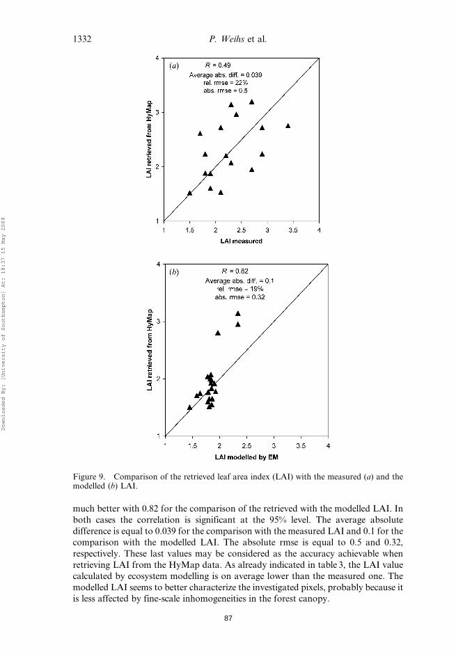
much better with 0.82 for the comparison of the retrieved with the modelled LAI. In

both cases the correlation is significant at the 95% level. The average absolute

difference is equal to 0.039 for the comparison with the measured LAI and 0.1 for the

comparison with the modelled LAI. The absolute rmse is equal to 0.5 and 0.32,

respectively. These last values may be considered as the accuracy achievable when

retrieving LAI from the HyMap data. As already indicated in table 3, the LAI value

calculated by ecosystem modelling is on average lower than the measured one. The

modelled LAI seems to better characterize the investigated pixels, probably because it

is less affected by fine-scale inhomogeneities in the forest canopy.

Figure 9. Comparison of the retrieved leaf area index (LAI) with the measured (a) and themodelled (b) LAI.

1332 P. Weihs et al.

Downloaded By: [University of Southampton] At: 18:37 15 May 2009

87

A prerequisite for accurate LAI retrieval is the appropriate choice of the leaf

biochemical parameters—dry matter, chlorophyll content, water content and leaf

structure N. Our simulations showed that the accuracy of the LAI retrieval may be

strongly affected by the wrong choice of these leaf parameters.

4.2.2 Estimation of the LAI using vegetation indices. In order to test the

performance of the ACRM model for LAI retrieval, the obtained correlations were

compared to the correlations with well known vegetation indices. The vegetation

indices that were used are shown in table 4. Indices identified by Schlerf et al. (2005)

as those showing the highest correlations with the LAI, such as the hyperspectral

perpendicular vegetation index (PVI_hyp), the perpendicular vegetation index

(PVI), the transformed soil-adjusted vegetation index (TSAVI), the hyperspectral

ratio vegetation index (RVI_hyp), or widely used indices such as the simple ratio

vegetation index (SR) and the normalized difference vegetation index (NDVI), were

chosen for the present study. The TSAVI and PVI indices require a parameter a,

which corresponds to the soil line slope, and a parameter b corresponding to the

point of intercept (Baret et al. 1989). Since, in the present study, the very non-

homogeneous soil conditions (senescent leaves, ground vegetation, bare ground,

etc.) did not allow the determination of a soil line slope, the soil line parameters were

fixed to arbitrary values (a51.17, b53.37 according to Leblon (http://www.r-s-c-

c.org/rscc/Volume4/Leblon/leblon.htm)). For the TM3 and TM4 channels the

average reflectance over the wavelength range of the channels was used for the index

calculations.

The correlation coefficients R of these indices with the measured and with the

modelled LAI values are shown in table 5. The lowest correlations were obtained

with SR, with RVI_hyp and with NDVI. The highest correlations were obtained

with PVI_hyp, with PVI and with TSAVI. However, all these correlation coefficients

range below the correlation coefficients obtained with the canopy reflectance model

(CRM). No significant correlations were obtained between measured LAI and the

Table 4. Overview of the indices used in this study.

Name Abbreviation Equation Reference

Hyperspectralperpendicularvegetation index

PVI_hyp ref 1148{a � ref 807{bffiffiffiffiffiffiffiffiffiffiffiffi1za2p Schlerf et al. 2005

Perpendicularvegetation index

PVI refTM4{a � refTM3{bffiffiffiffiffiffiffiffiffiffiffiffi1za2p Richardson and

Wiegand 1977

a51.17, b53.37Transformed

soil-adjustedvegetation index

TSAVI a refTM4{a � refTM3{bð Þa � refTM4za � refTM3{ab

Baret et al. 1989

a51.17, b53.37Hyperspectral ratio

vegetation indexRVI_hyp ref 1088

ref 1148

Schlerf et al. 2005

Simple ratio SR refTM4

refTM3

Pearson andMiller 1972

Normalized differencevegetation index

NDVI refTM4{refTM3

refTM4zrefTM3

Rouse et al. 1974

ref, reflectance; TM 3, Thematic Mapper channel 3 (630–690 nm); TM 4, Thematic Mapperchannel 4 (760–900 nm); ref1088, reflectance at 1088 nm; ref1148, reflectance at 1148 nm;ref807, reflectance at 807 nm.

3D Remote Sensing in Forestry 1333

Downloaded By: [University of Southampton] At: 18:37 15 May 2009

88

indices. Correlations between modelled LAI and the indices were significant for

TSAVI, PVI and PVI_hyp.

5. Conclusions

The PROSPECT leaf reflectance model accurately calculates the reflectance of a leaf

in the whole wavelength range, when the model input parameters are carefully

chosen. The ACRM did not perform well in the forward mode in the NIR and MIR

wavelength ranges, but seems to be a useful tool for LAI retrieval in the inversion

mode.

The ACRM strongly overestimates the reflectance in the NIR by approximately

28–30% and in the MIR by 50–74%. The correlation coefficients of 0.60 and 0.76 in

the NIR (888.5 nm) show that the model may, with reservations, be used in the

forward mode if the systematic offset is taken into account. If the offset is taken into

account, an absolute accuracy not better than 0.14 to 0.18 may be expected in the

NIR.

The lack of data on fluctuations in chlorophyll and water content between

individual trees did not allow the exact sensitivity of the ACRM model to

chlorophyll and to water content to be tested. This fact may explain the rather low

correlation coefficient in the visible (554 nm) and MIR (1675 nm) wavelength

ranges. A low mean relative deviation was, however, obtained between modelled

and HyMap retrieved reflectance in the visible wavelength range with an absolute

error of 0.006.

The largest mean relative difference as well as the largest relative rmse occur in the

MIR (1675 nm). The model strongly overestimates the HyMap-retrieved reflectance

by 50–74%.

Since a very good agreement between retrieved and experimentally determined

LAI was obtained, we can assume that the effect of LAI on canopy reflectance is

properly taken into account by the model. The most probable reason for the

overestimation of the canopy reflectance by the ACRM model may lie in an

overestimation of multiple scattering and multiple reflectance phenomena within the

canopy. ACRM takes into account leaves that have a high reflectance and

transmittance only. Stems and branches, which usually show a low reflectance and

which do not transmit any radiation are ignored in the ACRM code. Another

possible reason for the strong overestimation by the model may also lie in an

overestimation of the influence of the ground reflectance by the code. Kuusk and

Nilson (2001) compared Boreal Ecosystem Atmosphere Study (BOREAS) data with

simulations performed with the semi-homogeneous model MCRM, which includes

Table 5. Correlation coefficients R with measured and modelled leaf area index (LAI) ofvarious vegetation indices.

CRM PVI_hyp PVI TSAVI RVI_hyp SR NDVI

LAI measured 0.49 0.3827 0.4028 0.4625 0.3209 0.2238 0.2509LAI modelled 0.82 0.7337 0.7329 0.555 0.0377 0.18 0.1758

CRM, canopy reflectance model (ACRM model); PVI_hyp, hyperspectral perpendicularvegetation index; PVI, perpendicular vegetation index; TSAVI, transformed soil-adjustedvegetation index; RVI_hyp, the hyperspectral ratio vegetation index; SR, simple ratiovegetation index;NDVI, normalized difference vegetation index.

1334 P. Weihs et al.

Downloaded By: [University of Southampton] At: 18:37 15 May 2009

89

geometrical and structural parameters such as the crown radius and the tree height.

They also found an overestimation of the modelled signal in the MIR wavelength

range. They explained this discrepancy with an overestimation of multiple

reflectance phenomena within the canopy by the canopy reflectance model.

Referring to the inverse mode, we compared the retrieval accuracy for LAI

obtained with the ACRM to the retrieval accuracy possible with the well-known

indices TSAVI, SR, NDVI, PVI, PVI_hyp and RVI_hyp. The correlation

coefficients between ACRM-retrieved LAI and LAI measured or determined by

ecosystem modelling was higher than the correlation coefficients between any of the

indices and the measured or modelled LAI. The ACRM may therefore be used for

the determination of LAI with an expected accuracy of 0.32 to 0.5. A prerequisite is

the appropriate choice of the leaf biochemical parameters—dry matter, chlorophyll

content, water content and leaf structure N. The accuracy of the LAI retrieval may

strongly be affected by the wrong choice of these leaf parameters, which may be

determined as the set of parameters giving the best fit of measured leaf reflectance

and leaf reflectance modelled by PROSPECT.

We can summarize that for the forward modelling of forest canopy reflectance a

correction of the offset should be performed. In reverse mode, the ACRM model is

well suited for the retrieval of LAI even for complex terrain.

Acknowledgments

These investigations were performed within the scope of the project ‘Crop Drought

Stress Monitoring by Remote Sensing (DROSMON)’, supported by the Austrian

Science foundation (FWF), grant number P17647-N04. We thank the reviewers for

their most valuable suggestions.

ReferencesBARET, F., GUYOT, G. and MAJOR, D.J., 1989, Crop biomass evaluation using radiometric

measurements. Photogrammetria (PRS), 43, pp. 241–256.

CHEN, J.M., PAVLIC, G., BROWN, L., CIHLAR, J., LEBLANC, S.G. and WHITE, H.P., et al. 2002,

Derivation and validation of Canada-wide coarse-resolution leaf area index maps

using high resolution satellite imagery and ground measurements. Remote Sensing of

Environment, 80, pp. 165–184.

CONEL, J.E., GREEN, R.O., VANE, G., BRUEGGE, C.J., ALLEY, R.E. and CURTISS, B.J., 1987,

Airborne imaging spectrometer-2: radiometric spectral characteristics and compar-

ison of ways to compensate for the atmosphere. Proceedings of SPIE, 834, pp.

140–157.

DEMAREZ, V. and GASTELLU-ETCHEGORRY, J.P., 2000, A modeling approach for studying

forest chlorophyll content. Remote Sensing of Environment, 71, pp. 226–238.

EKLUNDH, L., HALL, K., ERIKSSON, H., ARDO, J. and PILESJO, P., 2003, Investigating the use

of Landsat Thematic Mapper data for estimation of forest leaf area index in southern

Sweden. Canadian Journal of Remote Sensing, 29, pp. 349–362.

ERIKSSON, H.M., EKLUNDH, L., KUUSK, A. and NILSON, J., 2006, Impact of understory

vegetation on forest canopy reflectance and remotely sensed LAI estimates. Remote

Sensing of Environment, 103, pp. 408–418.

GOVAERTS, Y. and VERSTRAETE, M.M., 1998, Raytran: a Monte Carlo ray tracing model to

compute light scattering in three-dimensional heterogeneous media. IEEE

Transactions on Geoscience and Remote Sensing, 36, pp. 493–505.

GU, D. and GILLESPIE, A., 1998, Topographic normalization of Landsat TM images of forest

based on subpixel sun-canopy-sensor geometry. Remote Sensing of Environment, 64,

pp. 166–175.

3D Remote Sensing in Forestry 1335

Downloaded By: [University of Southampton] At: 18:37 15 May 2009

90

GUANTER, L., ALONSO, L. and MORENO, J., 2004, Atmospheric correction of CHRIS/Proba

data acquired in the SPARC campaign. In Proceedings of the 2nd CHRIS/Proba

Workshop, ESA/ESRIN, Frascati, Italy, 2004, ESA-SP-578 (Paris: European Space

Agency).

JACQUEMOUD, S. and BARET, F., 1990, a model of leaf optical properties spectra. Remote

Sensing of Environment, 34, pp. 75–91.

JONCKHEERE, I., FLECK, S., NACKAERTS, K., MUYS, B., COPPIN, P., WEISS, M. and BARET, F.,

2004, Review of methods for in situ leaf area index determination, Part I. Theories,

sensors and hemispherical photography. Agricultural and Forest Meteorology, 121,

pp. 19–35.

KIMES, D., GASTELLU-ETCHEGORRY, J. and ESTEVE, P., 2002, Recovery of forest canopy

characteristics through inversion of a complex 3D model. Remote Sensing of

Environment, 79, pp. 320–328.

KOUKAL, T., SCHNEIDER, W. and SUPPAN, F., 2005, Radiometric-topographic normalization

in mountainous terrain for Landsat-TM-based forest parameter assessment by the

kNN method. In M. Oluic (Ed.), New Strategies for European Remote Sensing,

Proceedings of the 24th Symposium of the European Association of Remote Sensing

Laboratories (EARSeL), Dubrovnik, Croatia, 25–27 May 2004 (Rotterdam:

Millpress).

KUUSK, A., 1991, Determination of vegetation canopy parameters from optical measure-

ments. Remote Sensing of Environment, 37, pp. 207–218.

KUUSK, A., 2001, A two-layer canopy reflectance model. Journal of Quantitative Spectroscopy

and Radiative Transfer, 71, pp. 1–9.

KUUSK, A. and NILSON, T., 2001, Testing directional properties of a forest reflectance model.

Journal of Geophysical Research, 106, pp. 12011–12021.

LEBLANC, S.G. and FOURNIER, R.A., 2005, Towards a better understanding of in-situ canopy

measurements used in the derivation and validation of remote sensing leaf area index

products. In 31st International Symposium on Remote Sensing of Environment, Saint

Petersburg, Russia (Saint Petersburg: Russian Federation of Remote Sensing), 20–24

June 2005.

LI, X., STRAHLER, A.H. and WOODCOCK, C.E., 1995, A hybrid geometric optical

radiative transfer approach for modeling albedo and directional reflectance of

discontinuous canopies. IEEE Transactions on Geoscience and Remote Sensing, 33, pp.

466–480.

MERONI, M., COLOMBO, R. and PANIGADA, C., 2004, Inversion of a radiative transfer model

with hyperspectral observations for LAI in poplar plantations. Remote Sensing of

Environment, 92, pp. 195–206.

MYNENI, R., HOFFMAN, S., KNYAZIKHIN, Y., PRIVETTE, J., GLASSY, J. and TIAN, Y., et al.

2002, Global products of vegetation leaf area and fraction absorbed PAR from one

year of MODIS data. Remote Sensing of Environment, 83, pp. 214–221.

PEARSON, R.L. and MILLER, L.D., 1972, Remote mapping of standing crop biomass for

estimation of the productivity of the short-grass prairie, Pawnee National Grasslands,

Colorado. In Proceedings of the 8th International Symposium on Remote Sensing of

Environment (Ann Arbor, MI: ERIM International), pp. 1357–1381.

PEDDLE, D.R., JOHNSON, R.L., CIHLAR, J. and LATIFOVIC, R., 2004, Large area forest

classification and biophysical parameter estimation using the 5-scale canopy

reflectance model in multiple-forward-mode. Remote Sensing of Environment, 89,

pp. 252–263.

PIETSCH, S.A. and HASENAUER, H., 2006, Evaluating the self-initialisation procedure of large

scale ecosystem models. Global Change Biology, 12, pp. 1658–1669.

PIETSCH, S.A., HASENAUER, H., KUCERA, J. and CERMAK, J., 2003, Modeling effects of

hydrological changes on the carbon and nitrogen balance of oak in floodplains. Tree

Physiology, 23, pp. 735–746.

1336 P. Weihs et al.

Downloaded By: [University of Southampton] At: 18:37 15 May 2009

91

PIETSCH, S.A., HASENAUER, H. and THORNTON, P.E., 2005, BGC-model parameters for tree

species growing in central European forests. Forest Ecology and Management, 211, pp.

264–295.

PINTY, B., et al. 2001, The Radiation Transfer Model Intercomparison (RAMI) exercise.

Journal of Geophysical Research, 106, pp. 11937–11956.

PINTY, B., et al. 2004, Radiation Transfer Model Intercomparison (RAMI) exercise: results

from the second phase. Journal of Geophysical Research, 109, pp. D06210,

doi:10.1029/2003JD004252.

PRICE, J.C., 1990, On the information content of soil reflectance spectra. Remote Sensing of

Environment, 33, pp. 113–121.

QIN, W. and GERSTL, S.A.W., 2000, 3-D scene modeling of semi-desert vegetation cover and

its radiation regime. Remote Sensing of Environment, 74, pp. 145–162.

RAUTIAINEN, M., 2005a, The spectral signature of coniferous forests: the role of stand

structure and leaf area index. Academic Dissertation, Department of Forest Ecology

Faculty of Agriculture and Forestry, University of Helsinki, Finland.

RAUTIAINEN, M., 2005b, Retrieval of leaf area index for a coniferous forest by inverting a

forest reflectance model. Remote Sensing of Environment, 99, pp. 295–303.

RAUTIAINEN, M., STENBERG, P., NILSON, T. and KUUSK, A., 2004, The effect of crown shape

on the reflectance of coniferous stands. Remote Sensing of Environment, 89, pp. 41–52.

RICHARDSON, A.J. and WIEGAND, C.L., 1977, Distinguishing vegetation from soil back-

ground information. Photogrammetric Engineering and Remote Sensing, 43, pp.

1541–1552.

ROBERTS, D.A., YAMAGUCHI, Y. and LYON, R.J.P., 1985, Calibration of airborne imaging

spectrometer data to percent reflectance using field spectral measurements. In

Proceedings of the 19th International Symposium on Remote Sensing of Environment,

pp. 295–298.

ROSS, J., 1981, The Radiation Regime and Architecture of Plant Stands, The Hague: Dr. W.

Junk Publishing, 391 pp.

ROUSE, J.W., HAAS, R.H. and SCHELL, J.A., 1974, Monitoring the vernal advancement of

retrogradiation of natural vegetation. In NASA/GSFC, Type III, Final Report (pp.

1–371), Greenbelt, MD.

SCHLERF, M. and ATZBERGER, C., 2006, Inversion of a forest reflectance model to estimate

structural canopy variables from hyperspectral remote sensing data. Remote Sensing

of Environment, 100, pp. 281–294.

SCHLERF, M., ATZBERGER, C. and HILL, J., 2005, Remote sensing of forest biophysical

variables using HyMap imaging spectrometer data. Remote Sensing of Environment,

95, pp. 177–194.

SOENEN, S.A. and PEDDLE, D.R., 2005, SCS + C: A modified sun-canopy-sensor topographic

correction in forested terrain. IEEE Transactions on Geoscience and Remote Sensing,

43, pp. 2148–2154.

SOUDANI, K., FRANCOIS, C., LE MAIRE, G., LE DANTEC, V. and DUFRENE, E., 2006,

Comparative analysis of IKONOS, SPOT, and ETM + data for leaf area index

estimation in temperate coniferous and deciduous forest stands. Remote Sensing of

Environment, 102, pp. 161–175.

THENKABAIL, P.S., ENCLONA, M.S., ASHTON, B. and VAN DER MEER, 2004, Accuracy

assessments of hyperspectral waveband performance for vegetation analysis applica-

tions. Remote Sensing of Environment, 91, pp. 354–376.

THORNTON, P.E., LAW, B.E., GHOLZ, H.L., CLARK, K.L., FALGE, E., ELLSWORTH, D.S.,

GOLDSTEIN, A.H., MONSON, R.K., HOLLINGER, D., FALK, M., CHEN, J. and

SPARKS, J.P., 2002, Modeling and measuring the effects of disturbance history and

climate on carbon and water budgets in evergreen needleleaf forests. Agricultural and

Forest Meteorology, 113, pp. 185–222.

VERHOEF, W., 1984, Light scattering by leaf layers with application to canopy reflectance

modelling: the SAIL model. Remote Sensing of Environment, 16, pp. 125–141.

3D Remote Sensing in Forestry 1337

Downloaded By: [University of Southampton] At: 18:37 15 May 2009

92

VERMOTE, E.F., TANRE, D., DEUZE, J.L., HERMAN, M. and MORCRETTE, J.J., 1997, Second

simulation of the satellite signal in the solar spectrum, 6S—an overview. IEEE

Transactions on Geoscience and Remote Sensing, 35, pp. 675–686.

WALTHALL, C.L., NORMAN, J.M., WELLES, J.M., CAMPBELL, G. and BLAD, B.L., 1985,

Simple equation to approximate the bidirectional reflectance from vegetative canopies

and bare soil surfaces. Applied Optics, 24, pp. 383–387.

WEISS, M. and BARET, F., 1999, Evaluation of canopy biophysical variable retrieval

performances from the accumulation of large swath satellite data. Remote Sensing of

Environment, 70, pp. 293–306.

WEISS, M., BARET, F., SMITH, G.J., JONCKHEERE, I. and COPPIN, P., 2004, Review of methods

for in situ leaf area index (LAI) determination Part II. Estimation of LAI, errors and

sampling. Agricultural and Forest Meteorology, 121, pp. 37–53.

ZARCO-TEJADA, P.J., MILLER, J.R., HARRON, J., BAOXIN, H., NOLAND, T.L., GOEL, N.,

MOHAMMED, G.H. and SAMPSON, P., 2004, Needle chlorophyll content estimation

through model inversion using hyperspectral data from boreal conifer forest canopies.

Remote Sensing of Environment, 89, pp. 189–199.

1338 3D Remote Sensing in Forestry

Downloaded By: [University of Southampton] At: 18:37 15 May 2009

93

4.5 Publikation V

Occurrence of repeated drought events: can repetitive stress situations and recovery from

drought be traced with leaf reflectance?

Rita Linke, Katja Richter, Judith Haumann, Werner Schneider, and Philipp Weihs

Periodicum Biologorum 110 (3): 219-229, 2008.

94

Occurrence of repeated drought events: can repetitive

stress situations and recovery from drought be traced

with leaf reflectance?

Abstract

Within the last years a lot of effort has been made to improve irrigationefficiency and early drought stress detection by using various remote sensingtechniques. In the present study two different species of wheat (Triticumaestivum and Triticum durum), cultivated in a growth chamber, wereused to investigate the effects of drought occurring at different phenologicalstages. Plant physiological traits and spectral leaf reflectance were used toassess the potential of remote sensing techniques. Drought stress was appliedeither at flowering and/or at grain filling. Subsequently, a treatment fol-lowing recovery after drought stress at flowering was set up. The effects ofdrought were traced by following the changes in plant physiological traits(i.e. photosynthetic rate, leaf conductance, relative and actual leaf watercontent) as well as in leaf reflectance. Drought resulted in a significant re-duction of plant physiological traits and water relations, independently ofthe time of its occurrence. Rewatering plants after the stress period at flow-ering resulted in a recovery of plant physiological traits. Single leaf re-flectance of plants subjected to drought increased over the entire range of thespectrum. However, five spectral regions with relatively high differenceswere observed: 520–530 nm, 570–590 nm, 690–710 nm, 1410–1470 nmand 1880–1940 nm. Additionally, three spectral indices were tested towardstheir applicability for tracing drought stress and subsequent recovery, yield-ing a reasonable relationship with measured leaf water content, photosyn-thetic rate and leaf nitrogen content.

INTRODUCTION

Water scarcity is increasingly important in many parts of the world.Within the next centuries global climate change is expected to re-

sult in a long-term trend towards higher temperatures, greater evapo-transpiration, and an increased incidence of drought in specific regions(1, 2). Moreover, not only changes in the spatial but also in the temporaldistribution patterns of precipitation and radiation are to be expected(3); e.g.: in Europe higher precipitation levels are predicted for the win-ter half-year and drier periods for the summer half-year (2).

Under conditions of drought stress, absorption of radiation by theleaf tends to decrease due to lower leaf water content. Although waterabsorbs most strongly in the wavelengths of the infrared region of the

RITA LINKE1

KATJA RICHTER2,3

JUDITH HAUMANN1

WERNER SCHNEIDER2

PHILIPP WEIHS3

1 Department of Ecophysiologyand Functional Anatomy of Plants,Faculty of Life Sciences, University of Vienna,Althanstraße 14, 1090 Vienna

2 Institute of Surveying, Remote Sensing andLand Information, Department of Landscape,Spatial and Infrastructure Sciences,University of Natural Resources and AppliedLife Sciences (BOKU), Peter Jordan Straße82, 1190 Vienna

3 Institute of Meteorology, Departmentof Water, Atmosphere and Environment,University of Natural Resources and AppliedLife Sciences (BOKU), Peter Jordanstraße82, 1190 Vienna

Correspondence:Rita LinkeDepartment of Ecophysiology andFunctional Anatomy of Plants, Faculty of LifeSciences, University of Vienna, Althanstraße14, 1090 ViennaE-mail: r.linke@gmx.at

Key words: wheat, drought stress, recovery,leaf reflectance, relative water content,photosynthesis, chlorophyll

Received October 18, 2008.

PERIODICUM BIOLOGORUM UDC 57:61VOL. 110, No 3, 219–229, 2008 CODEN PDBIAD

ISSN 0031-5362

Original scientific paper

95

spectrum from approximately 1300 nm to 2500 nm (4),some absorption also occurs at lower wavelengths. Aswater is lost from a leaf, reflectance increases and absorp-tion decreases, primarily as a result of water’s radiativeproperties (5, 6). Even after accounting for the radiativecharacteristics of water, secondary effects occur. Theseinclude the influence of water content on absorption byother substances in the leaves, such as pigments. Also in-cluded as secondary are the effects of water content onwavelength-independent processes, particularly multi-ple reflections inside the leaf (7).

Moreover, drought stress not only causes leaf watercontent to decline but also affects physiological processes(e.g. leaf conductance, photosynthetic rates, etc.). Fur-thermore, changes in pigment and nitrogen concentra-tion of plant tissue will occur. For example, chlorophylland RubisCO contents decline as the leaf remobilizes re-sources under stress conditions (8). Chlorophyll and ac-cessory pigments absorb strongly in the visible range (9,10). Carter and Knapp (11) described a consistent stressinduced alteration of leaf reflectance at visible wave-lengths (~400–720nm) since chlorophyll is the major ab-sorber in the leaf and the metabolic disturbance broughtabout by stress alters leaf chlorophyll concentrations (9).Leaf reflectance in the visible range of plants experienc-ing nutrient deficiency was also found to increase sincenitrogen (and magnesium) is essential in the formationof chlorophyll. As leaves become more chlorotic, reflec-tance increases and the reflectance peak, normally cen-tred at about 550 nm, broadens towards the red as ab-sorption of incident light by chlorophyll decreases (12).Plant responses to water deficit therefore include bothbiochemical and morphological changes that primarilylead to acclimation and later to functional damage andthe loss of plant parts (13).

A lot of effort has been made towards the use of spec-tral reflectance of leaves and canopies for stress detectionin agricultural environments. While leaf reflectance isdriven by the chemical composition of the leaves, thereflectance of a canopy is influenced by its geometry – theleaf area index, inclination and clumping of the leaves –as well as the reflectance of single leaves. In this study weonly concentrate on the reflectance of leaves and not ofthe whole canopy.

The aim of the present study was, on the one hand, toevaluate the impact of drought stress on plant physiolog-ical traits and leaf reflectance of wheat (Triticum aestivumand Triticum durum) occurring at different phenological

stages (at flowering and/or grain filling). On the otherhand, the incidence of two consecutive drought eventsand recovery of plants after drought was investigated.The analysis of the effect of consecutive stress periodsand recovery on changes in leaf reflectance has rarelybeen performed until now but might gain in importanceconsidering the predicted increased frequency of droughtevents whereby plants could be exposed to drought re-peatedly (2, 14, 15, 16).

MATERIAL AND METHODS

1. Experimental Setup

Plants (Triticum aestivum L. cv. Xenos and Triticumdurum L. cv. Floradur) were grown in 8 litre plastic pots(7). Simulation of seasons in the growth chamber wasbased upon long-time observation of temperature andrelative humidity (past 10 years; meteorological station:16°29' eastern longitude and 48°15' northern latitude). Il-lumination of the growth chamber was accomplished by54 lamp units consisting of a lamp (Powerstar HQI TS250/NDL UVS, 250W, Osram, Germany) and an appro-priate reflector (Osram, Germany) yielding a PPFD of~1200 mmol m–2 s–1 in 1.5m above the ground. Detailedclimatic conditions are summarized in Table 1.

For germination, 25 seeds of T. aestivum / T. durumwere placed in each pot (7 replicates) and seedlings werethinned to 20 plants per pot. Nitrogen fertilization (2.11gN per pot; equivalent to 150kg N/ha) with Nitramoncal(27% N) was evenly split in three bits (before sowing, atstem elongation and at heading). P and K were suppliedwith Hortipray (NPK 0:52:34; 2.05g/pot, equivalent to180kg K/ha). Prior to sowing the agricultural soil was ad-ditionally fertilized with »Flory Basisdünger 10®« (EuflorGmbH, Germany; trace elements). As cultural substrate,a 2:1 mixture of air-dried and sieved (<4mm) agricul-tural top soil (6.33kg; A-Horizon; chernozem) and quartzsand (3.17kg; 0.2-2.0 mm) was used.

Four different treatments were set up per species –one control treatment and three treatments exposed todrought at different times during ontogeny:

AC/DC: control plants of T. aestivum / T. durum;AF/DF: T. aestivum / T. durum exposed to drought stressat flowering; recovery after anthesis; AG/DG: T. aesti-vum / T. durum exposed to drought stress at grain filling;AFG/DFG: T. aestivum / T. durum exposed to droughtstress at flowering and grain filling.

220 Period biol, Vol 110, No 3, 2008.

Rita Linke et al. Can stress and recovery be traced by changes leaf reflectance?

TABLE 1

Summary of climatic conditions in the growth chamber.

Spring Summer

Temperature 07–14°C day / 06–12°C night 17–26°C day / 14–20°C night

Relative humidity 60–80% day / 75–90% night 50–70% day / 60–90% night

Light (1m above ground) ~ 700 mmol m–2 s–1 ~ 700 mmol m–2 s–1

Day length 13.5 h 15.5 h

96

Soil humidity of control plants was consistently heldat 20–23 vol% (AC/DC). Drought stress at flowering wasimposed by halving water supply 10 days before the be-ginning of pollen shedding resulting in a soil humidity of~10 vol% (TDR Trime, Imko Micromodultechnik GmbH,Germany) at flowering (AF/DF). After flowering, plantsreceiving a second stress at grain filling were allowed torecover for 8 days (water supply similar to control plants)before the second stress was imposed by halving watersupply again (soil humidity during measuring period~10 vol%; AFG/DFG). Plants receiving drought stressonly at grain filling (AG/DG) were treated similar tocontrol plants until after flowering. Drought stress wasimposed at the same time as in plants of the treatmentstressed twice.

2. Measurements

2.1. Physiological Measurements

Physiological and spectral measurements were madein the mid region of the youngest fully expanded leaves atthree developmental stages: vegetative growth, floweringand grain filling.

Gas exchange measurements (A/Ci curves) were madeusing a CIRAS-I system (PP-Systems, U.K.) with an ex-ternal air conditioning system. Leaves were placed in acuvette of 2.5 cm², which was illuminated with a PPFDof 1000 mmol m–2 s–1. Temperature of the leaf chamberwas maintained at 20 °C, air flow was set to 300 ml min–1

and relative humidity of the incoming air was held at45–55%. Light saturated photosynthetic rates (Asat) referto measurements at growth conditions under saturatinglight intensities (CO2: 350–370 mmol mol–1; light: 1000mmol m–2 s–1).

Actual leaf conductance (gL) was measured with asteady state porometer (PMR-4, PP-Systems; U.K.). Datawere collected separately for both upper (adaxial) andlower (abaxial) leaf surface.

Chlorophyll content (Chltot) of leaves was determinedwith a SPAD-502 hand held chlorophyll meter (Minolta,Japan; (18)). For the measurement of absolute chloro-phyll content per unit leaf area [mg cm–2] small leaf discsof known area were cut and transferred to 5 ml of N,N-Dimethylformamide. Samples were stored at –18°C untilspectrophotometer readings of the eluate were taken(DU-7400, Beckman, USA; (19)). A calibration curve ofSPAD readings versus absolute chlorophyll content wasused to convert the SPAD readings into area based chlo-rophyll contents.

For calculation of the relative water content (RWC),leaf material was collected and fresh weight was immedi-ately determined. Saturated weight was measured afterplacing the leaf discs in Petri dishes between wet filter pa-per for 24 hours (4 °C, dark). Dry weight was determinedafter drying leaf material to constant weight at 70 °C.Relative water content (20) was then calculated as:

RWC = ((fresh weight – dry weight) /(saturated weight – dry weight)) * 100 [%]

and actual leaf water content was calculated as

AWC = ((fresh weight – dry weight) /(fresh weight)) * 100 [%].

Plant material for measuring leaf nitrogen content([N], expressed as percentage of dry matter) was dried toconstant weight (70°C) and milled (Cyclotec® SampleMill; Planetary Ball Mill, PM 4000, Retsch). An aliquotof 1–2 mg of each sample (pooled samples) was weighedinto tin capsules and analysed by isotope ratio mass spec-trometry (IRMS). A continuous-flow IRMS system, con-sisting of an elemental analyser (EA 1110, CE Instru-ments, Milan, Italy) which was interfaced to the IRMS(DeltaPLUS, Finnigan MAT, Germany) was used.

2.2. Spectral measurements

Leaf spectral reflectance was measured with a Field-Spec Pro FR in connection with a plant reflectance probefrom Analytical Spectral Devices Inc., Boulder, CO. Theradiometer operates in the spectral range from 350 to 2500nm. In the 350 to 1000 nm range, the sampling interval isapproximately 1.4 nm and the spectral resolution (fullwidth at half maximum) is 3 nm. In the 1000 to 2500 nmrange, the sampling interval is 2 nm and the spectral reso-lution is 10 to 12 nm. The reflectance probe is equippedwith an internal light source and works with a bi-conicalmeasurement geometry. The device was adapted for asample area of 19 mm by 7 mm to be able to measure thereflectance of individual wheat leaves. The detector fieldof view subtends an angle of up to 25°, and its axis is in-clined by an angle of 25° to the sample normal. Radiancemeasurements were performed on single leaves (youngestfully expanded) and on a Spectralon panel serving as awhite reference. Reflectance values were obtained as ratiosof leaf radiances and Spectralon radiances.

Relative difference of reflectance spectra betweenstress and control treatments (DR/R) was calculated as[((Rstress–Rcontrol)/Rcontrol)*100; (%)].

In addition, three spectral indices were calculated:photochemical reflectance index (PRI), an index for theestimation of relative water content (RWCi) and an indexfor the estimation of the actual water content (AWCi).The PRI is widely used for the estimation of photo-synthetic radiation use efficiency. It was proposed ac-cording to the finding that the interconversion of xantho-phyll cycle pigments in intact leaves can be detected assubtle changes in absorbance at 505–510 nm (21) or thereflectance at 531 nm (22). The photochemical reflectanceindex (PRI), incorporating reflectance at 531 nm (xantho-phyll cycle signal), was then defined as [(R570-R531) /(R570+R531)] in the attempt to establish a reflectance-based photosynthetic index (23). Concerning the attemptto trace leaf water content (RWC and AWC) with spec-tral indices, a lot of effort has been made and a number ofdifferent indices have been developed for numerous cropspecies: among them the water index (WI; R900 / R970;

Period biol, Vol 110, No 3, 2008. 221

Can stress and recovery be traced by changes leaf reflectance? Rita Linke et al.

97

(24)), the water band index (WBI; R905 / R980; (25)) andsome other indices described by Yu et al. (26). In the presentstudy, for estimating RWC the ratio RWCi = R1483 / R1650

and for estimating AWC the ratio AWCi = R1121 / R1430

(26) were used.

2.3. Statistical Analysis

To test the level of significance between control plantsand those of the stress treatments, data were subjected toa one-way analysis of variance (ANOVA; Systat 8, SPSSInc.). For spectral measurements the mean of the five re-gions showing greatest differences between treatmentswas calculated (520–530nm, 570–590 nm, 690–710 nm,

1410-1470nm and 1880-1940nm) and used for statistics(ANOVA). All tests were made separately for the differ-ent species and phenological stages. Correlation analysis,testing the relationship between physiological parametersand spectral indices, was performed with StatgraphicsPlus 5.0 software package (Statistical Graphics Inc.).

RESULTS

Physiological Measurements

Drought stress at flowering substantially reduced lightsaturated photosynthetic rates (Asat) of both species (AF:–36%, DF: –37%; Table 2). Rewatering caused Asat to re-

222 Period biol, Vol 110, No 3, 2008.

Rita Linke et al. Can stress and recovery be traced by changes leaf reflectance?

TABLE 2

Summary of physiological traits of T. aestivum and T. durum. Significance levels refer to the differences between control and

stress treatments. n=5-30; n.s.: not significant, *: p £ 0.05; **: p £ 0.01; ***: p £ 0.001.

Triticum aestivum L. Triticum durum L.

AC AF AG AFG DC DF DG DFG

Asat vegetative 21.2 17.5

flowering 16.9 10.7*** 15.6 9.9***

grain filling 13.8 12.2 n.s. 4.4*** 6.9*** 11.5 14.5** 3.9*** 6.1***

gL US vegetative 185.0 224.3

flowering 453.9 81.2*** 342.9 113.3***

grain filling 508.2 387.2*** 56.9*** 93.0*** 382.5 370.7 n.s. 86.8*** 125.0***

gL LS vegetative 84.0 87.4

flowering 164.1 18.4*** 129.3 25.7***

grain filling 171.8 116.3** 15.3*** 20.3*** 142.5 101.1* 26.4*** 48.1***

RWC vegetative 86.7 91.3

flowering 83.8 74.0** 86.5 82.9 n.s.

grain filling 76.3 81.9* 57.1*** 64.0*** 81.8 82.0 n.s. 67.4*** 74.2*

AWC vegetative 81.2 83.1

flowering 72.2 68.8** 77.4 76.0 n.s.

grain filling 74.1 74.8 n.s. 68.3 n.s. 71.1** 77.8 78.0 n.s. 75.5** 76.0 n.s.

Chltot vegetative 46.8 53.5

flowering 55.0 59.2*** 55.7 53.4*

grain filling 48.3 50.3** 61.7*** 55.6*** 49.2 54.0*** 52.1** 53.4***

Leaf [N] vegetative 4.3 4.6

flowering 4.4 4.2** 4.2 3.8***

grain filling 2.4 2.3 n.s. 1.9** 2.0** 2.4 2.5 n.s. 2.1* 2.2 n.s.

Abbreviations: A: T. aestivum; D: T. durum; C: control; F: drought at flowering, plants were recovered at grain filling; G: droughtstress at grain filling; FG: drought stress at flowering and grain filling. Asat: [mmol m–2 s–1

], gL: [mmol m–2 s–1], RWC: [%], AWC [%],

Chltot: [mg cm–2]; Leaf [N]: leaf nitrogen content in % dry matter; US: upper leaf surface, LS: lower leaf surface

98

Period biol, Vol 110, No 3, 2008. 223

Can stress and recovery be traced by changes leaf reflectance? Rita Linke et al.

Figure 1. Leaf reflectance of T. aestivum. Row 1a-d shows leaf reflectance of control plants (AC; ) and drought stressed (AF; – – –) plants atflowering. Row 2a-d represents leaf spectra of control plants (AC; ) and plants rewatered for 15 days (AF; – – –; recovery) at grain filling. Row3a-d shows leaf reflectance of control plants (AC; ) and plants stressed at grain filling either the first time (AG; . . . .) or the second time (AFG;– ... –). 1-3a shows the original leaf spectrum and 1-3/b-d show the regions of greatest differences between stress and control treatments in detail.Curves represent the mean of 20-30 leaf spectra ± standard error.

Figure 2. Leaf reflectance of T. durum. Row 1a-d shows leaf reflectance of control plants (DC; ) and drought stressed (DF; – – –) plants at flow-ering. Row 2a-d represents leaf spectra of control plants (DC; ) and plants rewatered for 15 days (DF; – – –; recovery) at grain filling. Row 3a-dshows leaf reflectance of control plants (DC; ) and plants stressed at grain filling either the first time (DG; . . . .) or the second time (DFG; – ... –).1-3a shows the original leaf spectrum and 1-3/b-d show the regions of greatest differences between stress and control treatments in detail. Curves rep-resent the mean of 20-30 leaf spectra ± standard error.

99

cover to nearly control values until grain filling in T.aestivum (–11%). In T. durum, values at grain filling evenexceeded those of control plants (+25%). At grain fillinghowever, in both species, reductions were more pro-nounced in plants receiving drought stress only at grainfilling (AG: –68%, DG: –66%) than in those alreadystressed at flowering (AFG: –50%, DFG: –47%).

Regarding leaf conductance (gL), T. aestivum was moresusceptible to drought than T. durum independently ofphenology (Table 2). Rewatering plants after droughtstress at flowering restored gL on the upper surface in T.durum. In T. aestivum, however, values remained some-what below values of control plants. Drought at grainfilling more strongly affected gL in AG/DG compared toAFG/DFG.

Relative water content (RWC) of plants stressed atflowering was reduced (AF: –12%, DF: –4%; Table 2). Atgrain filling, RWC of formerly stressed plants was equalto or even exceeded values of control plants (AF: +7%,DF: +0.3%). Drought at grain filling resulted in an even

stronger reduction of RWC than at flowering (average:A: –21%, D: –14%). In both species, RWC of plantsstressed only at grain filling was lower than that of plantsalready stressed at flowering.

Actual leaf water content (AWC) was also reducedsignificantly under drought (Table 2). In contrast to RWCthe changes of AWC in the course of phenology weremore pronounced which is due to the fact that the AWConly represents the water content as percentage of freshweight whereas the RWC represents the actual watercontent given with respect to a standard measure (leavesunder conditions of water saturation).

Drought at flowering caused an increase of total chlo-rophyll content (Chltot; mg cm–2) in AF (+11%) and a de-crease in DF (–4%; Table 2). Rewatering resulted inhigher Chltot contents at grain filling (AF: +4%, DF:+10%). Those plants subjected to drought at grain filling,either the first or the second time, also showed higherChltot values compared to control plants (AG: +28%, DG:+6% and AFG: +15%, DFG: +8%, respectively).

Leaf nitrogen content (leaf [N], in % of dry matter)was reduced in plants subjected to drought at flowering(AF: –6%, DF: –11%; Table 2). At grain filling, leaf [N]from formerly stressed plants was still lower in T. aesti-vum (–5%) but higher in T. durum (+8%) when com-pared to control plants of either species. Plants subjectedto drought stress during grain filling showed a reductionin leaf [N]. However, the reductions were more pro-nounced in plants stressed only at grain filling (AG:–20%, DG: –11%; AFG: –16%, DFG: –7%).

Spectral Measurements

Subjecting plants to drought stress, either at floweringor at grain filling, resulted in a general increase of singleleaf reflectance (R; Figure 1–3). In both species, fivespectral regions with relatively high differences were ob-served: 520–530 nm, 570–590 nm, 690–710 nm, 1410–1470 nm and 1880–1940 nm (Figure 3). Drought at flow-ering increased R in these spectral regions by up to +12%,+12%, +10%, +5% and +9% in T. aestivum and by upto +11%, +12%, +9%, +5% and +15% in T. durum(Table 3). Although rewatering plants after the stress pe-riod at flowering resulted in a recovery of plant physio-logical traits and water relations (see above) the effectsobserved on leaf R were different. Changes in leaf re-flectance (DR/R, %) between control plants and formerlystressed plants of T. aestivum in the range of 520–530 nm,570–590 nm and 690-710 nm were even greater after re-covery than during the stress period (520–530 nm:+15%, 570–590 nm: +17%, 690–710 nm: +15%; Table3). However, the differences at 1410–1470 nm and1880-1940 nm decreased during recovery. In contrast,DR/R of T. durum decreased during recovery within theentire range of the spectrum. The greatest decrease inDR/R was observed in the 1880-1940 nm range.

At grain filling, T. aestivum stressed solely at grain fill-ing (AG) showed the smallest increase of R in compari-son to control plants which was surprising since the

224 Period biol, Vol 110, No 3, 2008.

Rita Linke et al. Can stress and recovery be traced by changes leaf reflectance?

Figure 3. Relative difference (DR/R) between reflectance of stressedand control plants of a) T. aestivum and b) T. durum. Differences

were calculated as [(Rstress – Rcontrol)/ Rcontrol]*100 (%). Legend: AF.DF: differences between control and plants stressed at flowering.measured at flowering; AF. DF (recov.): differences between controland plants stressed at flowering. measured at grain filling after beingrewatered for 15 days; AG. DG: differences between control andplants stressed at grain filling. measured at grain filling; AFG. DFG:differences between control and plants stressed at flowering andgrain filling. measured at grain filling; n=20-30.

100

changes in physiological traits were greatest (Table 2). InT. durum, however, DR/R between stressed plants andcontrol was greater than that observed in plants stressedat flowering. (The only exception gave the wavelengthrange of 1880–1940 nm where the differences were smal-ler at grain filling compared to flowering.)

Drought not only caused leaf R in the near infrared re-gion (NIR) to increase but also in the visible range of thespectrum. Here, the changes were even greater than inthe NIR independently of the occurrence of drought inphenology. Of all stress treatments and stress periods inphenology, the greatest DR/R in the visible range was ob-served at grain filling in the treatment stressed twice (sec-ond stress period; Table 3).

Spectral indices for estimating leaf RWC (RWCi) andAWC (AWCi) as well as photochemical reflectance index(PRI) were calculated to follow RWC and AWC as wellas Asat and leaf [N] in the course of phenology (Figure 4,5; Table 4). In both species, RWCi was less correlatedwith the measured values (T. aestivum: r²=0.079, T. du-

rum: r²=0.467) than AWCi was (T. aestivum: r²=0.715,T. durum: r²=0.953). Tracing the measured values ofRWC using RWCi was neither possible in T. aestivum norin T. durum (Figure 4). Using AWCi it appeared possibleto follow the trend of measured AWC in both T. aestivum

and T. durum, during phenology but only for controlplants. At grain filling, the difference in the AWC esti-mated from leaf R in T. aestivum between recovered and

Period biol, Vol 110, No 3, 2008. 225

Can stress and recovery be traced by changes leaf reflectance? Rita Linke et al.

TABLE 3

Summary of relative difference (%) for physiological parameters and spectral regions of greatest difference. All data refer to

the differences between plants subjected to drought stress either at flowering and/or grain filling and control plants. Bold val-

ues highlight the differences between control plants and recovered plants (measured at grain filling). Relative difference (%)

was calculated as [(stress – control)/ (control)*100]. Significance levels refer to the differences between stress treatments or

recovered plants and control. n=5-30; n.s.: not significant, *: p £ 0.05; **: p £ 0.01; ***: p £ 0.001.

Triticum aestivum L. Triticum durum L.

AF/AC AG/AC AFG/AC DF/DC DG/DC DFG/DC

RWC flowering –12%** –4% n.s.

grain filling +7%* –25%*** –16%*** +0,3% n.s. –18%*** –16%*

AWC flowering –5%** –2% n.s.

grain filling +1% n.s. –8% n.s. –4%** +0,3% n.s. –3%** –2% n.s.

Chltot flowering +11%*** –4%*

grain filling +4%** +28%*** +15%*** +10%*** +6%** +15%***

Leaf [N] flowering –6%** –11%***

grain filling –5% n.s. –20%** –16%** +8% n.s. –11%* –16% n.s.

R520-530 flowering +12%*** +11%***

grain filling +15%*** +0,2% n.s. +13%*** +4% n.s. +17%*** +22%***

R560-590 flowering +12%*** +12%***

grain filling +17%*** +3% n.s. +14%*** +5% n.s. +18%*** +24%***

R690-710 flowering +10%*** +9%***

grain filling +15%*** +2% n.s. +14%*** +5% n.s. +4%*** +19%***

R1410-1470 flowering +5%*** +5%*

grain filling +4%*** +4%** +3%* +4%*** +9%*** +6%***

R1880-1940 flowering +9%*** +15%***

grain filling +7%*** +1% n.s. +4%* +3%* +12%*** +7%***

Abbreviations: see Table 2, R: leaf reflectance.

101

control plants give the impression of an even greater re-duction than during the stress period at flowering itself,although the measurements of AWC reveal full recovery.In T. durum the differences decreased during recovery.However, values of AWCi remained below control plantsdespite the complete recovery becoming obvious frommeasured values (Figure 4; see also DR/R, Figure 3).

PRI correlated quite well with Asat but even betterwith leaf [N] in both species (Table 4). Tracing pheno-logical changes in Asat and leaf [N] using PRI did not givegood results for plants subjected to drought stress at anytime in ontogeny. Better results for this correlation wereonly obtained for control plants. Therefore, neither re-covery of plants after drought at flowering nor the extentof change in Asat and leaf [N] due to drought could be es-timated appropriately.

4. DISCUSSION

Drought stress significantly influenced plant physio-logical traits independently of the time of its applicationin phenology. The lowering of the actual leaf conduc-tance (gL), as observed during all stress periods in thepresent study, is one of the first processes occurring underdecreased soil water availability providing a higher wateruse efficiency to the plant (27, 28, 29). Moreover, as re-viewed by Cornic (30), stomatal closure is mainly re-sponsible for the decline in net photosynthetic rate of C3

leaves subjected to moderate drought stress. However, ata certain stage of stress, internal CO2 concentration (Ci)

226 Period biol, Vol 110, No 3, 2008.

Rita Linke et al. Can stress and recovery be traced by changes leaf reflectance?

Figure 4. Comparison of the phenological course of measured and es-timated RWC and AWC. a-d) T. aestivum and e-h) T. durum. Leg-end: A: T. aestivum; D: T. durum; C: control. F: drought at flower-ing. recovered at grain filling. G: drought at grain filling. FG:drought at flowering and grain filling. n=6 for measured RWC andAWC. n=20-30 for estimated RWC (RWCi) and AWC (AWCi).Errors represent standard error.

Figure 5. Comparison of the phenological course of light saturated

photosynthetic rates (Asat). leaf nitrogen content (leaf [N]) and pho-tochemical reflectance index (PRI). a-c) T. aestivum and d-f) T.durum. Legend: A: T. aestivum; D: T. durum; C: control. F:drought at flowering. recovered at grain filling. G: drought at grainfilling. FG: drought at flowering and grain filling. n=3-12 for Asat

and leaf [N]. n=20-30 for PRI. Errors represent standard error.

TABLE 4

Correlation statistics for the relationship between physio-

logical parameters (RWC, AWC, Asat and leaf [N]) and

spectral indices (RWCi, AWCi and PRI). In addition to the

correlation coefficient (r²) and the significance level (p),

the slope and intercept of the linear equation are given.

r² p slope intercept

Triticum aestivum L.

RWC 0.079 0.542 -4.526 0.526

AWC 0.715 0.017 0.037 0.564

Asat 0.679 0.023 1.096 0.024

leaf [N] 0.774 0.009 5.774 0.019

Triticum durum L.

RWC 0.467 0.091 -1.611 0.613

AWC 0.953 0.000 0.094 -3.848

Asat 0.514 0.070 1.293 0.020

leaf [N] 0.986 0.000 8.499 8.551

102

frequently increases, indicating the predominance ofnon-stomatal limitations to photosynthesis (31, 32, 33).Reductions of light saturated photosynthetic rates (Asat)in the present experiment were mainly due to stomatalimitation since a significantly lower Ci was found (datanot shown).

In the present study, drought stress resulted in higherleaf reflectance (R) over the entire spectrum both in T.aestivum and in T. durum, a response also found else-where (c.f. 34, 35, 26). However, five regions with rela-tively high differences were observed: 520–530 nm, 570–590 nm, 690–710 nm, 1410–1470 nm and 1880–1940 nm(Figure 1–3).

Rewatering plants after the stress period at floweringallowed them to restore their physiological traits untilgrain filling (15 days rewatered). RWC of recovered plantseven exceeded that of control in T. aestivum (+7%) andwas restored to control level in T. durum (+0.3%). There-with, Asat also recovered. Only gL of plants from both spe-cies remained somewhat lower than that of control plants.However, the results from leaf R did not follow this trend.In T. aestivum, DR/R within the range of 1410–1470 nmand 1880–1940 nm remained nearly as high as during thestress period at flowering despite the 7% higher RWC ofrecovered plants. Though in T. durum a reduction of DR/Rwas found, leaf R still remained above that of controlplants. Within the visible range of leaf spectra DR/R in T.aestivum even increased during recovery compared to theactual stress period. In T. durum DR/R within the visiblerange decreased during recovery but R still remainedabove that of control plants as already observed for thenear infrared region. The results of the present studytherefore indicate that quantifying the extent of change foreither leaf water content or Chltot and leaf [N] fromchanges in leaf R is problematic. Especially recovery fromdrought could not be traced using leaf R since the differ-ences between formerly stressed plants and control plantsremained high as observed in T. aestivum or decreasedonly slightly as in T. durum but in neither of the species in-vestigated leaf R returned to control level despite the com-plete recovery of physiological traits.

The reason for the enduring differences in leaf R be-tween fully recovered plants and control plants remainsrather unclear and information on leaf R during recoveryof plants after a stress period is rare in literature. How-ever, it is assumed that secondary effects followingdrought stress might be involved. Drought can affect thecell structure and biochemistry (e.g.: 36, 37, 38, 39) and isfurther known to influence the morphology of the leafsurface by means of changes in the content and/or com-position of epicuticular waxes (40, 41, 42, 43) or the oc-currence of hairs (42). Moreover, drought has the poten-tial to accelerate ontogenetic development (44, 45). Suchalterations of leaf morphology and/or biochemical com-position could not only have influenced leaf R after re-covery but also have attributed to (or might be the reasonfor) the unexpectedly great differences in leaf R observedin plants subjected to a second stress period at grain fill-ing. This result contrasts again with the observations of

physiological traits since those were more affected bydrought in AG and DG compared to AFG and DFG atgrain filling. The less pronounced reaction of physiologi-cal traits to a second drought period is attributed to somepreconditioning of plants already exposed to drought atflowering and/or the higher amount of green biomass(transpiring surface) of plants from the treatment stres-sed solely at grain filling. Plants of the treatment stressedtwice (AFG and DFG) were watered optimally for eightdays after drought at flowering before water supply washalved again. Leaf osmotic potential remained below(more negative) that of control plants during these daysproviding a better initial situation concerning osmoticadjustment (data not shown) for plants already experi-encing a first drought period at flowering.

The differences observed in DR/R during recovery be-tween T. aestivum and T. durum show that no generalprediction can be made concerning the potential to tracerecovery from a stress situation with leaf reflectance. Ap-parently, different species and even cultivars respond in-consistently to drought stress with respect to their spec-tral signature. Especially the cultivar of T. aestivum usedin this study (cv. Xenos) appears not promising for trac-ing recovery with leaf reflectance. In T. durum (cv.Floradur) DR/R decreased during recovery within theentire range of the spectrum but the greatest decrease inDR/R occurred in the 1880–1940 nm range. Since thisspectral range falls into the main atmospheric water bandsit is unsuitable for remote sensing by satellite or airplane.However, to test an eventual potential for short distanceremote sensing/ precision farming, we performed simu-lations of the transmittance in these wavelength rangesusing the code LOWTRAN 7 (46) assuming the worstcase scenario (99% air humidity). Results showed that atdistances below 100 m the transmittance was largerthan 50% in the wavelength range 1410–1470 nm. At1880–1940 nm transmittance became larger than 50%only at distances below 15 m. This shows a potential for ashort distance (below 100 m) remote sensing mainly inthe wavelength range 1410–1470 nm. This remote sens-ing application would however at least require an accu-rate determination of the distance between sensor andcanopy, an artificial radiation source (since the solar radi-ation is already totally absorbed) and an accurate deter-mination of air humidity (to apply a correction to themeasured transmittance). Other aspects like sensor sen-sitivity, characteristics of the radiation source, require-ments regarding the accuracy of the sensor to determineplant optical path etc… would be needed to be investi-gated within the scope of a future study.

In contrast to changes in leaf R within the range of1410–1470 nm and 1880–1940 nm, which can be attrib-uted mainly to differences in leaf water content, thechanges within the visible range are not well definedwith respect to a certain stressor. As already described byCarter (47) an increased reflectance at visible wavelengths(400–700 nm) is the most consistent response to stresswithin the 400–2500 nm range. The often made assump-tion that the chlorophyll content of leaves was propor-

Period biol, Vol 110, No 3, 2008. 227

Can stress and recovery be traced by changes leaf reflectance? Rita Linke et al.

103

tional to moisture content (e.g. 48) may be correct forsome species but cannot be generalized to all ecosystems.Variations in chlorophyll content can be caused by waterstress but also by phenological status of the plant, atmo-spheric pollution, nutrient deficiency, toxicity, plant dis-ease, and radiation stress (39, 49). These findings aresupported by the results from the present study wheredifferent trends for RWC, Chltot and leaf [N] were found.Due to these adverse effects of leaf [N] (decrease) andChltot (increase) an interpretation of the increased leaf Ris difficult. At least the specific cause of these differencesremains uncertain. However, the increased Chltot con-tent found might result from leaf shrinkage leading to aseemingly higher chlorophyll content per unit leaf area(mg cm–2).

Finally, three spectral indices (RWCi, AWCi and PRI)were tested towards their ability in estimating biophysi-cal parameters (RWC, AWC, Asat and leaf [N]; Table 4).Concerning the estimation of leaf water content a bettercorrelation was found for AWC. Unfortunately, the AWCis the less meaningful parameter since it only gives thewater content as percentage of fresh weight which mightvary greatly between species, phenology and environ-mental conditions (39). The RWC, however, representsthe actual leaf water content with respect to a standardmeasure (leaves under conditions of water saturation;(39) and is therefore the more appropriate indicator ofplant water status. Moreover, following changes in bio-physical parameters using these indices was not possibledue to the different extent of changes in leaf R comparedto physiological traits under drought stress at differentphenological stages. From these results it is concludedthat a good relationship between spectral indices andbiophysical parameters does not necessarily lead to anappropriate estimation of biophysical parameters at agiven phenological state and/or physiological status.

5. CONCLUSION

Drought stress occurring at different phenologicalstages increased leaf R throughout the whole spectrum.Unfortunately, the degree to which plant physiologicaltraits and water relations changed could not be quanti-fied by the extent of change in leaf R, at least whendrought occurred at different phenological stages. Themain concern of the present study, however, was to testthe ability of leaf reflectance to follow recovery of physio-logical traits after a stress period which may be of essentialimportance when considering the occurrence of repeateddrought events. Distinguishing between a currently oc-curring stress situation and an already passed one couldbecome crucial in context with the application of spectralmeasurements in the field to trace stress situations and tomake recommendations on fertilization or irrigation.Unfortunately, recovery from drought stress could not betraced by leaf R since the differences between formerlystressed plants and control plants remained either highas observed in T. aestivum or decreased only slightly as inT. durum. In neither species leaf R returned to controllevel despite the complete recovery of physiological traits.

These results, however, also indicate that rather big dif-ferences between different species might occur andfurther investigations using different species with differ-ent leaf morphology and anatomy would be needed.

Estimating leaf water content (RWC and AWC) aswell as Chltot and leaf [N] from reflectance measure-ments gave good correlations. For tracing changes inphysiological parameters during phenology and stressperiods, however, the use of these indices was not prom-ising due to false estimation of stress situations and re-covery (Figure 4, 5). An appropriate estimation appear-ed, if at all, only possible in unstressed control plants. Agood correlation between spectral indices and physiolog-ical parameters alone is therefore not necessarily suffi-cient for estimating physiological parameters from leafspectra appropriately.

Acknowledgement: This research was financially sup-ported by the Fonds zur Förderung der wissenschaftlichenForschung (FWF, Austria; grant number P17647-N04). FranzSuppan is thanked for performing spectral measurements.

REFERENCES

1. HILLEL D, ROSENZWEIG C 2002 Desertification in relation toclimate variability and change. Advances in Agronomy 77: 1–38

2. IPCC 2007 CLIMATE CHANGE 2007: The physical science basis,summary for Policymakers, Contribution of Working Group I to theFourth Assessment Report of the Intergovernmental Panel on ClimateChange, International Panel on Climate Change. WMO UNEP re-port.; www.ipcc.ch

3. LAWLOR D W, MITCHELL R A C 1991 The effects of increasingCO2 on crop photosynthesis and productivity: a review of field stud-ies. Plant, Cell & Environment 14: 807-818

4. CURCIO J A, PETTY C C 1951 The near infrared absorption spec-trum of liquid water. Journal of the Optical Society of America 41:302–304

5. BOWMAN W D 1989 The relationship between leaf water status,gas exchange, and spectral reflectance in cotton leaves. RemoteSensing of Environment 30: 249–255

6. HUNT E R, ROCK B N 1989 Detection of changes in leaf watercontent using near- and middle-infrared reflectance. Remote Sensingof Environment 30: 43–54

7. CARTER G A 1991 Primary and secondary effects of water contenton the spectral reflectance of leaves. American Journal of Botany 78:916–924

8. PARRY M A J, ANDRALOJC P J, KHAN S, KEYS A J 2002 Rubiscoactivity: effects of drought stress. Annals of Botany 89: 833-839

9. KNIPLING E B 1970 Physical and physiological basics for thereflectance of visible and near-infrared radiation from vegetation.Remote Sensing of Environment 1: 155-159

10. CARTER G A, MITCHELL R J, CHAPPELKA A H, BREWER CH 1992 Response of leaf spectral reflectance in loblolly pine to in-creased atmospheric ozone and precipitation acidity. Journal of Ex-perimental Botany 43: 577–584

11. CARTER G A, KNAPP A K 2001 Leaf optical properties in higherplants: Linking spectral characteristics to stress and chlorophyll con-centration. American Journal of Botany 88(4): 677-684

12. AYALA-SILVA T, BEYL C A 2005 Changes in spectral reflectance ofwheat leaves in response to specific macronutrient deficiency. Ad-vances in Space Research 35: 305-317

13. CHAVES M M, PEREIRA J S, MAROCO J, RODRIGUES M L,RICARDO C P P, OSÓRIO M L, CARVALHO I, FARIA T,PINHEIRO C 2002 How plants cope with water stress in the field.Photosynthesis and growth. Annals of Botany 89: 907-916

14. SCHÄR C, VIDALE P L, LÜTHI D, FREI C, HÄBERLI C,LINIGER M A, APPENZELLER C 2004 The role of increasingtemperature variability in European summer heatwaves. Nature 427:332-336

228 Period biol, Vol 110, No 3, 2008.

Rita Linke et al. Can stress and recovery be traced by changes leaf reflectance?

104

15. VIDALE P L, LÜTHI D, WEGMANN R, SCHÄR C 2007 Euro-pean climate variability in a heterogeneous multi-model ensemble.Climatic Change 81: 209-232

16. SENEVIRATNE S I, LÜTHI D, LITSCHI M, SCHÄR C 2006Land–atmosphere coupling and climate change in Europe. Nature443: 205-209

17. KICK H, GROSSE-BRAUCKMANN E 1961 Über dieKonstruktion eines Vegetationsgefäßes aus Kunststoff. Zeitschrift fürPflanzenernährung, Düngung und Bodenkunde 95(140): 52-55

18. MARKWELL J, OSTERMANN J C, MITCHELL J L (1995). Cal-ibration of the Minolta SPAD-502 leaf chlorophyll meter. Photosyn-thesis Research 46: 467-472

19. INSKEEP W P, BLOOM P R 1985 Extinction coefficients of Chlo-rophyll a and b in N,N-Dimethylformamide and 80% Acetone.Plant Physiology 77: 483-485

20. LÖSCH R 2003 Wasserhaushalt der Pflanzen. Vlg. Quelle & Meyer,p 39

21. BILGER W, BJÖRKMANN O, THAYA S 1989 Light-induced spec-tral absorbance changes in relation to photosynthesis and theepoxidation state of xanthophylls cycle components in cotton leaves.Plant Physiology 91: 542-551

22. GAMON J A, FIELD C B, BILGER W, BJÖRKMANN O,FREDEEN A L, PENUELAS J 1990 Remote sensing of the xantho-phylls cycle and chlorophyll fluorescence in sunflower leaves andcanopies. Oecologia 85: 1-7

23. GAMON J A, SERRANO L, SURFUS J S 1997 The photochemicalreflectance index: an optical indicator of photosynthetic radiationuse efficiency across species, functional types, and nutrient levels.Oecologia 112: 492-501

24. PENUELAS J, FILELLA I 1998 Visible and near infraredreflectance techniques for diagnosing plant physiological status.Trends in Plant Science 3(4): 151-156

25. DAVENPORT J R, LANG N S, PERRY F M 2000 Leaf spectralreflectance for early detection of misorders in model annual and pe-rennial crops. ASA-CSSA-SSSA, 677 Segoe Road, Madison, WI53711, USA. Proceedings of the Fifth International Conference on Pre-cision Agriculture.

26. YU G-R, MIWA T, NAKAYAMA K, MATSUOKA N, KON H 2000A proposal for universal formulas for estimating leaf water status ofherbaceous and woody plants based on spectral reflectance proper-ties. Plant and Soil 227: 47-58

27. CORNIC G, MASSACCI A 1996 Leaf photosynthesis underdrought stress. In: Photosynthesis and the Environment (ed. N.R.Baker), Kluwer Academic Press, p 347-366

28. LAWLOR D W, CORNIC G 2002 Photosynthetic carbon assimila-tion and associated metabolism in relation to water deficit in higherplants. Plant, Cell & Environment 25: 275-294

29. FLEXAS J, MEDRANO H 2002 Drought inhibition of photosyn-thesis in C3 plants: stomatal versus non-stomatal limitations revis-ited. Annals of Botany 89: 183-189

30. CORNIC G 1994 Drought stress and high light effects on leaf pho-tosynthesis. In: Photoinhibition of Photosynthesis (eds N.R. Bakerand J.R. Bowyer), BIOS, Scientific Publishers, p 297-313

31. LAWLOR D W 1995 The effects of water deficits on photosynthesis.In: Environment and plant metabolism (ed. Smirnoff). BIOS Scien-tific Publishers, Oxford, p 129-160

32. BRODRIBB 1996 Dynamics of changing intercellular CO2 concen-tration (Ci) during drought and determination of minimal function-ing Ci. Plant Physiology 111: 179-185

33. MEDRANO H, ESCALONA J M, BOTA J, GULÍAS J, FLEXAS J2002 Regulation of photosynthesis of C3 plants in response to pro-gressive drought: stomatal conductance as a reference parameter.Annals of Botany 89: 895-905

34. WOOLLEY 1971 Reflectance and Transmittance of Light byLeaves. Plant Physiology 47: 656-662

35. PENUELAS J, INOUE Y 1999 Reflectance indices indicative ofchanges in water and pigment contents of peanut and wheat leaves.Photosynthetica 36(3): 355-360

36. YORDANOV I, VELIKOVA V, TSONEV T 2000 Plant responses todrought stress, and stress tolerance. Photosynthetica 38(2): 171-186

37. READ J, STOKES A 2006 Plant biomechanics in an ecological con-text. American Journal of Botany 93(10): 1546-1565

38. LAMBERS H, CHAPIN III FS, PONS T L 1998 »Plant PhysiologicalEcology«. Springer.

39. LARCHER W 2003 »Physiological Plant Ecology – Ecophysiologyand Stress Physiology of Functional Groups«. Springer (4th edition).

40. JORDAN W R, MONK R L, MILLER F R, ROSENOW D T,CLARK L E, SHOUSE P J 1983 Environmental physiology of sor-ghum. I. Environmental and genetic control of epicuticular waxload. Crop Science 23: 552–558

41. JOHNSON D A, RICHARDS R A, TURNER N C 1983 Yield, wa-ter relations, gas exchange and surface reflectances of near-isogenicwheat lines differing in glaucousness. Crop Science 23: 318–325 72.

42. DENG X-P, SHAN L, INANAGA S, INOUE M 2005 Water-savingapproaches for improving wheat production. Journal of the Science ofFood and Agriculture 85: 1379-1388

43. SEHPERD T, GRIFFITHS D W 2006 The effect of stress on plantcuticular waxes. New Phytologist 171: 469-499

44. FOYER C H, DESCOURVIÈRES P, KUNERT K J 1994 Protec-tion against oxygen radicals: an important defence mechanism stud-ied in transgenic plants. Plant, Cell & Environment 17: 507– 523

45. KIMBALL B A 1995 Productivity and water use of wheat under freeair CO2 enrichment. Global Change Biology 1: 429-442

46. KNEIZYS F X, SHETTLE E P, ABREU L W, CHETWYND J H,ANDERSON G P, GALLERY W O, SELBY J E A, CLOUGH S A1988 Users guide to Lowtran 7. AFGL-TR-88-0177, Air Force Geo-physics Laboratory.

47. CARTER G A 1994 Ratios of leaf reflectances in narrow wavebandsas indicators of plant stress. International. Journal of Remote Sensing15(3): 697-703

48. TUCKER C J 1977 Assymptotic nature of grass canopy spectralreflectance. Applied Optics 16(5): 1151-1156

49. CECCATO P, FLASSE S, TARANTOLA S, JACQUEMOUD S,GRÉGOIRE J-M 2001 Detecting vegetation leaf water content us-ing reflectance in the optical domain. Remote Sensing of Environment77: 22-33

Period biol, Vol 110, No 3, 2008. 229

Can stress and recovery be traced by changes leaf reflectance? Rita Linke et al.

105

5 Anhang (Bestätigung der Publikation I)

03-May-2009

Dear Ms. Richter:

I am pleased to inform you that your manuscript entitled: "Experimental assessment of the Sentinel-2 band setting for RTM-based LAI retrieval of sugar beet and maize" has been accepted as a Research Article for publication in the Canadian Journal of Remote Sensing.

Your manuscript will be forwarded to the National Research Council Research Press for publication and in you should expect to hear from them directly concerning your galley proofs.

If you have not already done so, would you please read the attached Copyright and Publication Charge files, fill out the appropriate parts of these forms and return them to me by mail or by fax as indicated on the forms.

Thank you for your interest in publishing in the Canadian Journal of Remote Sensing.

The AE has prepared a new version of the abstract of the paper in FRENCH. It is attached for your interest and I assume you will be happy with it. If not, please let me know. Else I will pass this new one to NRC Press.

Congratulations

Sincerely,

Prof. Nicholas Coops

Editor in Chief, Canadian Journal of Remote Sensing

editor.cjrs@ubc.ca

106

6 Lebenslauf/CV

Persönliche Daten

Name

Geburtstag

Geburtsort

Land

Staatsbürgerschaft

Katja Richter

06.09.1978

Dresden

Deutschland

Deutschland

Ausbildung

1985-1997

1997-2003

Ab 2004

J. Haydn-Gymnasium Dresden-Striesen (Abschluss Abitur, 15.07. 1997), Dtl.

Studium Geographie, TU Dresden, Dtl., und Universität Wien, Ö. Spezialisierung: Klimatologie und Geoinformatik

Studium Doktorat, Universität für Bodenkultur Wien (BOKU), Fachrichtung Landwirtschaft/ Fernerkundung

Beruflicher Werdegang

2001-2008

2004-2005

2005-2007

seit 2007

Tutorin, Studienassistentin und Lektorin für zahlreiche Lehrveranstaltungen im Bereich Geographie/Klimatologie/GIS/Fernerkundung an der Universität Wien, BOKU und Universität Federico II di Napoli, Italien.

Mitarbeiterin im Laboratorium für Umweltanalytik GesmbH, Wien, Ö.

Wissenschaftliche Mitarbeiterin am Institut für Vermessung, Fernerkundung und Landinformation (IVFL) der Universität für Bodenkultur, Wien, im Rahmen des Projekts: Crop Drought Stress Monitoring by Remote Sensing (DROSMON).

Wissenschaftliche Mitarbeiterin an der Universität Federico II di Napoli, Italien, im Rahmen des EU Projekts: Participatory multi-Level EO-assisted tools for Irrigation water management and Agricultural Decision-Support (PLEIADeS).

Internationale Aktivitäten

seit 2004

seit 2008

Teilnahme an zahlreichen internationalen Kongressen und Workshops (EGU, SPIE, RAQRS, IGARSS, ISRSE u. a.).

Session Co-Chair, SPIE Europe Remote Sensing.

Wien Juni 2009

107