
Degree-days: theory and application - U-Cursos
106
© CIBSE Degree-days: theory and application TM41: 2006 The Chartered Institution of Building Services Engineers 222 Balham High Road, London SW12 9BS
-
Upload
khangminh22 -
Category
Documents
-
view
4 -
download
0
Transcript of Degree-days: theory and application - U-Cursos

© CIBSE
Degree-days: theory and application
TM41: 2006
The Chartered Institution of Building Services Engineers
222 Balham High Road, London SW12 9BS
© CIBSE
i
The rights of publication or translation are reserved.
No part of this publication may be reproduced, stored in a retrieval system or transmitted in any form or by any means without prior permission.
© September 2006 The Chartered Institution of Building Services Engineers,
London SW12 9BS
Registered Charity Number 278104
ISBN-10: 1-903287-76-6
ISBN-13: 978-1-903287-76-7
This document is based on the best knowledge available at the time of publication. However no responsibility of any kind for any injury, death, loss, damage or delay however caused resulting from the use of these recommendations can be accepted by the Chartered Institution of Building Services Engineers, the authors or others involved in its publication.
In adopting these recommendations for use each adopter by doing so agrees to accept full responsibility for any personal injury, death, loss, damage or delay arising out of or in connection with their use by or on behalf of such adopter irrespective of the cause or reason therefore and agrees to defend, indemnify and hold harmless the above named bodies, the authors and others involved in their publication from any and all liability arising out of or in connection with such use as aforesaid and irrespective of any negligence on the part of those indemnified.
Typeset by CIBSE Publications
Note from the publisher
This publication is primarily intended to provide guidance to those responsible for the design, installation, commissioning, operation and maintenance of building services. It is not intended to be exhaustive or definitive and it will be necessary for users of the guidance given to exercise their own professional judgement when deciding whether to abide by or depart from it.

© CIBSE
ii
Foreword Degree-days are a tool that can be used in the assessment and analysis of weather related energy consumption in buildings. They have their origins in agricultural research where knowledge of variation in outdoor air temperature is important, and the concept is readily transferable to building energy. Essentially degree-days are a summation of the differences between the outdoor temperature and some reference (or base) temperature over a specified time period. A key issue in the application of degree-days is the definition of the base temperature, which, in buildings, relates to the energy balance of the building and system. This can apply to both heating and cooling systems, which leads to the dual concepts of heating and cooling degree-days.
This TM replaces previous guidance given in section 18 of the 1986 edition of CIBSE Guide B [CIBSE 1986] and Fuel Efficiency Booklet 7 [Energy Efficiency Office 1993]. It provides a detailed explanation of the concepts described above, and sets out the fundamental theory upon which building related degree-days are based. It demonstrates the ways in which degree-days can be applied, and provides some of the historical backdrop to these uses. This TM can be read alongside Good Practice Guide 310: Degree days for energy management – a practical introduction [Carbon Trust 2006], which serves as an introduction to their use. The material in this document provides deeper insights into the degree-day concept, but can be used in conjunction with GPG 310 for advanced building energy analysis.
Principal author
Prof. Tony Day (London South Bank University)
Steering Group
Bryan Franklin (Chairman)
Prof. Martin Fry (Carbon Trust)
Prof. Michael Holmes (Arup)
Tony Johnston (BRE)
Jim Mansfield (formerly West Norfolk District Council)
David Wood
Dr Hywel Davies (CIBSE Research Manager)
Editor
Ken Butcher
CIBSE Research Manager
Hywel Davies
CIBSE Publishing Manager
Jacqueline Balian

© CIBSE
iii
How to use this publication
This publication is designed to provide both the theory of degree-days and guidance on their use. It is of interest to two types of user: designers wishing to check the likely energy consumption of a particular design, and energy managers wishing to assess energy performance of existing buildings. Each use requires a different level of knowledge: detailed understanding of degree-day theory is not needed to use them in practice. For example, energy managers need not understand the mathematics of the energy prediction techniques to obtain useful results; designers may never need to construct a performance line or energy signature.
This publication is therefore set out in discrete chapters that may be of interest to specific audiences. However, it is ordered in such a way as to present a logical picture of how the theory of degree-days underpins, and is consistent with, the various applications. The reader who wishes to grasp the degree-day concept as a whole is advised to read the whole document in order to appreciate the consistency of the theory, and also to assess its shortcomings. It must be stressed that the theoretical models presented here (for example for intermittent heating) are not the only possible approach: building dynamics are extremely complex, and the issue of thermal capacity in particular has never been satisfactorily dealt with in simplified energy estimation models. However, what is presented here is designed to inform the user of the main issues that need to be accounted for in energy analysis.
Chapter 1 gives an overview of the degree-day concept and describes the applications in fairly non-mathematical terms. It describes how they are calculated and why they are applicable to building energy analysis. It presents the strengths and weaknesses of the various techniques and defines where these can be sensibly used. Those new to degree-days should start here.
Chapter 2 presents the mathematics of calculating degree-days, which is entirely distinct from the way they are applied. Degree-days are also commonly applied to the analysis of plant growth as well as building energy, but the way they are calculated is a common issue to all applications. Thus the chapter shows how different calculation methods have differing degrees of accuracy, and suggests the conditions for which each method may be best employed. Often this is a question of what weather data the user has access to.
Chapter 3 presents detailed mathematical applications of degree-days to building energy estimation, showing how estimates can be conducted for heating and cooling systems, including the effects of intermittent plant operation. These techniques are necessarily simplifications and cannot replace full thermal simulations, but can be used to rapidly calculate typical magnitudes of consumption. They can also be used for rapid sensitivity analysis of key influencing factors; for example how energy consumption varies with changes in glazing area. The techniques in the chapter are best applied in a spreadsheet to remove the need for manual calculations. Earlier published procedures employed correction factors to simplify the procedure; the philosophy adopted in this publication is that such procedures were opaque and inaccurate, and computer technology allows easy access to more powerful techniques. In addition the methodologies are considered to be instructive about energy flows in buildings.
Chapter 4 presents worked examples of the procedures in chapter 3.
Chapter 5 examines how energy managers can use degree-days to assess an existing building’s energy performance. It examines the use of energy signatures and performance lines, and the relationship between degree-days used in this way and the theory presented in chapter 3. It gives guidance on how performance lines can be interpreted. It extends the theory to present some deeper analysis techniques, developed on the premise that buildings perform (at least roughly) according to theory; this chapter does not attempt to provide guidance on generic interpretations for non-standard performance lines — it is assumed that where these occur the energy manager would examine the building more closely for causes of anomalies.

© CIBSE
iv
Contents Preface vi
1 An introduction to degree-days and their uses 1
1.1 An introduction to calculating degree-days 2 1.1.1 Published degree-days 4
1.2 Degree-days for energy estimation 6 1.2.1 Heating 6 1.2.2 Energy consumption and building mass 9 1.2.3 Cooling 10 1.2.4 Heat recovery and other systems 11
1.3 Degree-days for energy management 12
2 Calculating degree-days 15
2.1 Mean degree-hours 16
2.2 The Meteorological Office equations 17
2.3 Mean daily temperature 18
2.4 Hitchin’s formula 18
2.5 Other methods 19
2.6 Errors associated with calculation methods 19
2.7 Base temperature correction 21
2.8 Summary 23
3 Energy estimation techniques 24
3.1 Heating applications 25
3.2 Intermittent heating 27
3.3 Accuracy and uncertainty 32
3.4 Carbon dioxide emissions 35
3.5 Determination of gains 36 3.5.1 Utilisation factors 38
3.6 Cooling applications 42 3.6.1 All air systems 42 3.6.2 Fan coil systems 49 3.6.3 Chilled beams and ceilings 50 3.6.4 Other issues for cooling energy analysis 51
3.7 Summary 51
4 Worked examples 53
4.1 Heating 53
4.2 All-air cooling 55
5 Using degree-days in energy management 60
5.1 Normalisation of energy performance indicators for weather 60 5.1.1 Normalisation and base temperature 61
5.2 Energy signatures 62
5.3 Performance lines and degree-days 63
5.4 Further diagnostics using performance lines 73 5.4.1 Heating and cooling 75 5.4.2 Identifying gains 76 5.4.3 The heating case 77
© CIBSE
v
5.4.4 Cooling performance line interpretation 79 5.4.5 Base temperature and controls 80
5.5 Regression analysis: caveats and interpretations 80
5.6 Summary 82
Nomenclature 84
References 86
Appendix A1: Degree-day errors 89
Appendix A2: Ratios and corrections 91
Appendix A3: Base temperature conversion using Hitchin’s formula 93
Appendix A4: Derivation of mean internal temperature for intermittent heating 95
Appendix A5: Areas of on-going work 97

© CIBSE
vi
Preface This technical memorandum presents the theory of the Degree Day for use by practising engineers, based on a rigorous review of the material which is available in the public domain. Its primary objective is to provide engineers with an explanation of the current state of degree day theory and practice to enable its application where appropriate in engineering decisions.
The scientific theory, however, is still evolving and the final appendix identifies issues which would benefit from further work. Whilst this text has received warm approval from the large majority of commentators, one researcher has made clear his commitment to an alternative view of the science. As well as providing guidance to engineers, a second objective of this technical memorandum is to further the concept of degree day theory by stimulating a considered debate on these issues through the normal process of publication and peer review.

© CIBSE
vii
Degree-days: theory and application
© CIBSE
1
1 An introduction to degree-days and their uses
This chapter presents a non-mathematical description of degree-days and their uses. It gives an introduction to the subsequent chapters that deal with the detailed theory. The two main uses for degree-days in buildings are:
to estimate energy consumption and carbon dioxide emissions due to space heating and cooling for new build and major refurbishments
for on-going energy monitoring and analysis of existing buildings based on historical data.
The former can be used in order to set energy budgets, negotiate energy tariffs and provide a check of the building’s expected performance against typical benchmarks. The latter can be used to evaluate performance in-use and identify changes in consumption patterns, provide some building and system characterisation, and to set future energy consumption targets.
Degree-days are essentially the summation of temperature differences over time, and hence they capture both extremity and duration of outdoor temperatures. The temperature difference is between a reference temperature and the outdoor air temperature. The reference temperature is known as the base temperature which, for buildings, is a balance point temperature, i.e. the outdoor temperature at which the heating (or cooling) systems do not need to run in order to maintain comfort conditions.
When the outdoor temperature is below the base temperature (see box on page 3), the heating system needs to provide heat. Since heat loss from a building is directly proportional to the indoor-to-outdoor temperature difference, it follows that the energy consumption of a heated building over a period of time should be related to the sum of these temperature differences over this period. The usual time period is 24 hours, hence the term degree-days, but it is possible to work with degree-hours. (Degree-days are in fact mean degree-hours, or degree-hours divided by 24). In order to appreciate the use of degree-days for building energy applications it is important to address some of the key concepts of this seemingly simple idea.
Degree-days originated (and are still extensively used) in assessment of crop growing conditions. Lt-Gen. Sir Richard Strachey introduced them as a means of identifying the length of the growing season. Much of the terminology used and the basis upon which degree-days are calculated to this day originate from his work [Strachey 1878].
They are therefore not a concept unique to building energy analysis. In this respect it must be recognised that there are two clearly distinct (and essentially unrelated) issues surrounding degree-days and their uses. The first is the way degree-days are calculated, and the second is the way they are applied to building energy. It is important that these two issues are not confused, as they are completely independent of each other. For example degree-days calculated by any technique can be applied either to crop growth or to buildings. What makes the two uses different is the choice of base temperature (and how it is selected), which is discussed in the box, and what one then does with the resulting degree-day total.
It must be stressed that, particularly for estimation purposes, degree-day techniques can only provide approximate results since there are a number of simplifying assumptions that need to be made. These assumptions particularly relate to the use of average conditions (internal temperatures, casual gains, air infiltration rates etc), and that these can be used in conjunction with each other to provide a good approximation of building response. The advantage to their use, therefore, lies in their relative ease and speed of use, and all of the information required to conduct estimation analysis is available from the building design
Degree-days: theory and application
© CIBSE
2
criteria. Unlike full thermal simulation models degree-day calculations can be carried out manually or within computer spreadsheets; they have a transparency and repeatability that full simulations may not provide.
Degree-days provide a significant advantage over other simplified methods that use mean outdoor temperatures to calculate energy demand (for example BS EN ISO 13790 [2004]). Because degree-days account for fluctuations in the outdoor temperature, and eliminate those periods when heating (or cooling) systems do not need to operate, they can capture extreme conditions in a way that mean temperature methods cannot. This makes them more reliable in estimating energy consumption, particularly in the milder months, but also in those periods with extreme cold snaps where they capture both magnitude and duration of an event.
1.1 An introduction to calculating degree-days
This section provides an overview of degree-day calculation methods and sources of degree-day data. Chapter 3 defines the procedures mathematically, and the diagrams and equations in that chapter should be referred to for a complete understanding of the subject.
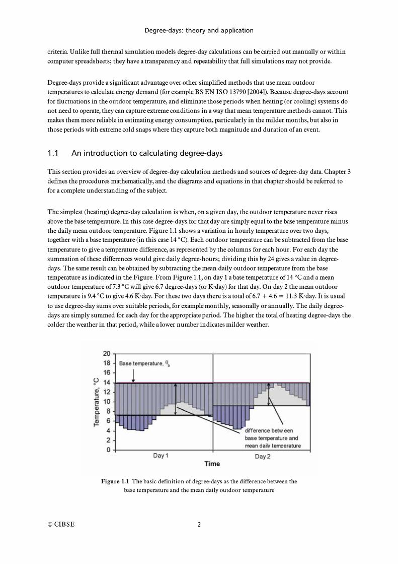
The simplest (heating) degree-day calculation is when, on a given day, the outdoor temperature never rises above the base temperature. In this case degree-days for that day are simply equal to the base temperature minus the daily mean outdoor temperature. Figure 1.1 shows a variation in hourly temperature over two days, together with a base temperature (in this case 14 °C). Each outdoor temperature can be subtracted from the base temperature to give a temperature difference, as represented by the columns for each hour. For each day the summation of these differences would give daily degree-hours; dividing this by 24 gives a value in degree-days. The same result can be obtained by subtracting the mean daily outdoor temperature from the base temperature as indicated in the Figure. From Figure 1.1, on day 1 a base temperature of 14 °C and a mean outdoor temperature of 7.3 °C will give 6.7 degree-days (or K·day) for that day. On day 2 the mean outdoor temperature is 9.4 °C to give 4.6 K·day. For these two days there is a total of 6.7 + 4.6 = 11.3 K·day. It is usual to use degree-day sums over suitable periods, for example monthly, seasonally or annually. The daily degree-days are simply summed for each day for the appropriate period. The higher the total of heating degree-days the colder the weather in that period, while a lower number indicates milder weather.
Figure 1.1 The basic definition of degree-days as the difference between the
base temperature and the mean daily outdoor temperature

Degree-days: theory and application
© CIBSE
3
However, in practice it is more complex as the outdoor temperature may fluctuate around the base temperature. In building heating applications this happens in the warmer months or when the base temperature is particularly low. In this case calculation methods are required that capture the fact that degree-days are positive when the temperature falls below the base for part of the day, but ignore the times when it rises above the base (there can be no negative degree-day values). Ideally this can be calculated from continuous (i.e. hourly or even shorter interval) temperature data if it is available. Positive temperature differences are taken and negative ones set to zero; these are summed over the day and divided by the number of readings (24 in the case of hourly data). This is described mathematically in section 2.1, and is, strictly speaking, the most precise way to calculate degree-days.
Base temperature
The base temperature is central to the successful understanding and use of degree-days. It is formally defined in section 3.1, but this brief description introduces the concept.
In a heated building during cold weather heat is lost to the external environment. Some of this heat is replaced by casual heat gains to the space — from people, lights, machines and solar gains — while the rest is supplied by the heating system. Since the casual gains provide a contribution to the heating within the building, there will be some outdoor temperature, below the occupied set point temperature, at which the heating system will not need to run. At this point the casual gains equal the heat loss. This temperature will be the base temperature for the building (sometimes called the balance point temperature [ASHRAE 2001]).
When the outdoor temperature is below the base temperature heating is required from the heating system. Heating degree-days are a measure of the amount of time when the outside temperature falls below the base temperature. They are the sum of the differences between outside and base temperature whenever the outside temperature falls below the base temperature.
For an actively cooled building the base temperature is the outdoor temperature at which the cooling plant need not run, and is again related to the casual heat gains to the space (which now add to the cooling load). In this case cooling degree-days are related to temperature differences above this base.
The difficulty that arises is that casual gains vary throughout the day, from day to day, and throughout the season. In addition the base temperature depends on the building’s thermal characteristics such as its heat loss coefficient, thermal capacity, and heat loss mechanisms such as the infiltration rate that may vary with time. This means that to define the base temperature it is necessary to take average values of these variables over a suitable time period (for example a month). The uncertainty in the accuracy of the results therefore increases with decreasing time scale, i.e. daily energy estimates are likely to be less accurate than monthly ones [Day 1999].
In the years before computers it was necessary to find a calculation method based on fewer data, and fewer calculations. The use of maximum and minimum daily temperatures was developed initially by Strachey and then the Meteorological Office [1928]. This requires a set of equations that attempt to determine degree-days for all conditions, depending on the relationship between the base temperature and the maximum and minimum temperatures. These equations are presented in section 2.2, and they are an attempt to approximate the true integral (i.e. summation) of the daily temperature differences. It should be stressed that as outdoor temperature variations do not follow a fixed pattern (i.e. there is no definite function that defines outdoor temperature changes), these equations can only ever be approximations. Section 2.6 attempts to show the differences that can be expected from true degree-days. This method produces small errors, but it is important to recognise that

Degree-days: theory and application
© CIBSE
4
they exist. The Meteorological equations continue to be the standard calculation method for published degree-days in the UK.
The standard definition of degree-days varies around the world. For example, in the United States degree-days are calculated from mean daily temperatures only, as discussed in section 2.3 and shown in the examples at the beginning of this section. This will give slightly different results from the degree-hour method in warmer months, but as degree-day totals are small in these months the actual magnitude of these differences is small (even if the percentage difference appears high). Analysis in section 2.6 and Appendix A1 for one location (Stansted) shows this method and the use of the Meteorological Office equations to give similar results. The choice of degree-day calculation method is less important than how they are applied. What is important is consistency, so that comparisons of results using degree-day analysis should be based on the same method of degree-day generation.
It is often the case that the user does not have access to hourly or daily data, or may have monthly degree-days to a specific base temperature. Methods have been developed that can calculate degree-days from very limited data, specifically mean monthly temperature and standard deviation of the temperature throughout the month. In the UK one such method was developed by Hitchin, described in section 2.4, in which it is not essential to know even the standard deviation (some typical constants for the UK are provided). This method shows less accuracy in months where the mean monthly temperature is close to the base temperature, but again the actual magnitude of error is small, although percentage error is high. This equation has another advantage as it provides a way of converting a degree-day total from one base temperature to another.
Base temperature conversion is not as simple as it might first appear as degree-days do not vary linearly with base temperature. The relationship between degree-days and base temperature is in fact dependent upon the actual outdoor temperature patterns, which vary from place to place and from time to time. It is not possible to convert monthly degree-days calculated to 15.5 °C to (say) a base of 13 °C by multiplying by a single factor for all months and for all regions. This issue of base temperature correction is discussed in section 2.7.
1.1.1 Published degree-days
In the UK, degree-days are published monthly for 18 regions to a traditional base temperature of 15.5 °C1. There are also electronic sources of data available for different base temperatures and for different locations. The 18 regions are shown in Figure 1.2. It is convenient to use such degree-days, and the accuracy of the measurements is assured, thus providing some reliability in the data. However, local temperature patterns can vary significantly, and it can be argued that locally generated degree-days may be more appropriate for a particular building. However, the quality of locally sourced temperature data may not be assured (due to sensor location and calibration etc).
1Degree day data is provided for DEFRA and made freely available by Degree Days Direct Ltd. See
http://www.vesma.com/ddd/index.htm.

Degree-days: theory and application
© CIBSE
5
Figure 1.2 Degree-day regions in the United Kingdom
Published degree-days are given both for the current month and the 20-year rolling average for each month. This 20-year average is useful if the user wishes to compare current use against long term average conditions, or wishes to set energy budgets against such conditions. Typical 20-year average monthly and annual degree-day (and cooling degree-hour) values are given in section 2.5 of CIBSE Guide A [CIBSE 2006], and section 4.3 of CIBSE Guide J [CIBSE 2002]. Degree-days are also published in journals such as Energy and Environmental Management (available free of charge from DEFRA) and Energy World (available free of charge to members of the Energy Institute), as well as various web sources.
Effect of climate change
Note that the rise of atmospheric temperatures due to climate change may mean that historic 20-year averages will not be appropriate. The rate of temperature rise in the near future will dictate how reliable these values will be for setting energy budgets. In the period 1976–1995, annual heating degree-days in London and Edinburgh fell by around 10% [CIBSE TM36 2005]. It is predicted that heating degree-days could fall by 30–40% in the UK by the 2080s, with a similar reduction in heating energy consumption. The setting of longer-term energy budgets should therefore take account of these general trends in climate by not relying solely on the past 20-year average degree-days. The problem is that there are no accurate predictions about the rate of change of climate, and it may be appropriate to set long-term budgets using different scenario assumptions.
Regions 1 Thames valley 2 South East 3 South 4 South West 5 Severn Valley 6 Midland 7 West Pennines 8 North West 9 Borders 10 North East 11 East Pennines 12 East Anglia 13 Wales 14 W Scotland 15 E Scotland 16 NE Scotland 17 Northern Ireland 18 NW Scotland
Degree-days: theory and application
© CIBSE
6
1.2 Degree-days for energy estimation
The preferred method for estimating the expected energy consumption of a particular building design is by full thermal simulation. Buildings are complex entities, and energy consumption is determined by a large number of influencing factors. This makes simulation a detailed and time-consuming process that requires a high degree of skill. Simulation may not accurately predict energy use, due to the way the building is used or to systems not working as intended, but can provide a detailed way to investigate the impacts of a wide range of design parameters.
Degree-days, on the other hand, can provide a simplified method for energy estimation (for heating and cooling) that requires less data input, and can be used to assess rapidly how energy consumption may be influenced by major design decisions (e.g. levels of insulation, assumptions about infiltration, building thermal capacity etc). The accuracy of such techniques is inevitably more questionable, although it is probably more helpful to talk in terms of uncertainty in, rather than accuracy of, the results. The calculation procedures set out in section 3.2 of this document attempt to define this uncertainty for heating energy demand. One advantage degree-day methods do have is that the reduced number of inputs can reduce user input error — something that is difficult to check with extensive simulation packages. This helps to provide some confidence in the results of sensitivity tests.
Understanding the theory of how degree-days can be used in estimation is also helpful in understanding their more common usage in monitoring existing buildings. Chapter 3 sets this theory out in detail, with recommended procedures for conducting analyses on different types of operation including continuous and intermittent heating, and different types of cooling systems. To explain these procedures fully it is necessary to present the mathematical development as given in that chapter. What follows below is a brief and largely non-mathematical synopsis of the degree-day energy model, which is heavily based on the notion of determining the correct base temperature.
1.2.1 Heating
There are a number of ways of interpreting the degree-day concept with respect to simplified heating analysis, for example as discussed by Hitchin and Hyde [1979]. However, these are all predicated on the notion that heating energy demand is directly proportional to the indoor-to-outdoor temperature difference, such that:
Heat loss (kW) = overall heat loss coefficient (kW·K–1) temperature difference (K)
The overall heat loss coefficient is made up of two components: the fabric coefficient, and the air infiltration rate. (It is also legitimate to combine ventilation air with the infiltration rate to give an overall loss coefficient for these components. See Appendix A5 for further discussion on this matter.) The fabric coefficient is the sum of the U A values (U-value times area, A) for all the building components. This overall coefficient is the first of the simplifying assumptions as it is necessary to make a reasonable estimate of infiltration rate, which is increasingly becoming a major component of the total heat loss. Infiltration will also vary over time (for example between night and day), in which case average values need to be taken. Estimation of infiltration is an area of difficulty for all simplified estimation methods.
The expression above gives an instantaneous rate of heat loss in kW and assumes steady conditions which, if the conditions prevail for a period of time, say an hour, will give units of energy, i.e. kW·h. As the outdoor air temperature changes, the driving temperature difference changes and there is a proportional change in demand. It is this summation of temperature differences for different periods of time (each day in the case of
Degree-days: theory and application
© CIBSE
7
degree-days) that provides both the varying driving force for the heat loss, and the change from rates of heat flow to an energy total. Therefore:
Heating energy demand (kW·h) = overall heat loss coefficient (kW·K–1)
degree-days (K·day) 24 (h·day–1)
(The 24 is included to convert from days to hours.)
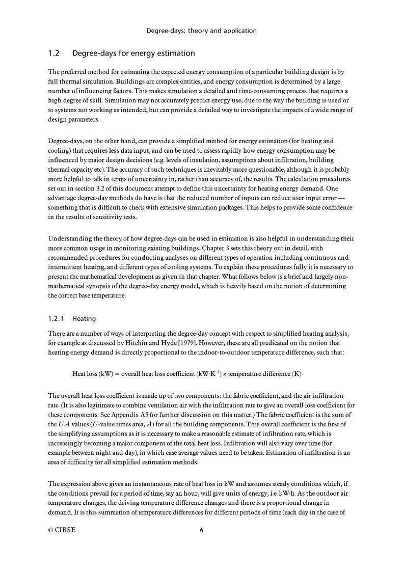
It remains to define properly the indoor-to-outdoor temperature difference. While the total heat loss from a building is related to the actual indoor temperature, it does not follow that all of this heat loss is replaced by the heating system — some is met from incidental heat gains arising from solar insolation, people, lights and equipment. There is an energy balance whereby the sum of the heat inputs to the building equals the overall loss (see Figure 1.3), and the degree-day approach assumes that all of the incidental gains can be averaged out over time to give some representative indoor temperature which relates to the heating system contribution.
Figure 1.3 Energy balance on a heated building
The base temperature is then entered into the degree-day calculation procedures described in chapter 3.
However, neither the gains nor the internal temperature are constant over the course of a day (particularly for an intermittently occupied building). Gains can be averaged over the day, applying some appropriate gain utilisation factor to account for which gains are useful. Solar gains are something of a problem as average daily useful solar gains are not normally given in guidance literature. Some values are given, for example, in CIBSE Building Energy Code 1 [CIBSE 1999]. CIBSE Guide J [CIBSE 2002] gives measured monthly mean daily irradiation (in W·h·m–2) for 3 sites in the UK for different orientations and different slope angles (including vertical). These values can be divided by 24 to give monthly mean daily irradiance (in W·m–2), although further adjustment is necessary to convert this into a gain to the space. Section 3.5 describes the method by which to do this, together with example solar irradiance values.
QS Solar gains
QC Heat flow into and out of structure
QL Heat losses
QE Output from heating system
QI Internal gains (lights, people machines)
Degree-days: theory and application
© CIBSE
8
Internal temperature variation can be dealt with in a number of ways. Such variation is most marked in intermittently occupied buildings where the plant is switched off overnight and at weekends. The change in internal temperature will vary from building to building according to levels of insulation and effective thermal capacity, and will also be affected by plant size and the length of the unoccupied period. In the past it has been usual to apply correction factors to account for this, but such factors have been shown to be highly unreliable [Day 1999]. The method presented in this publication is to calculate a 24-hour mean internal temperature which takes all the relevant factors into account. So for an intermittently occupied building:
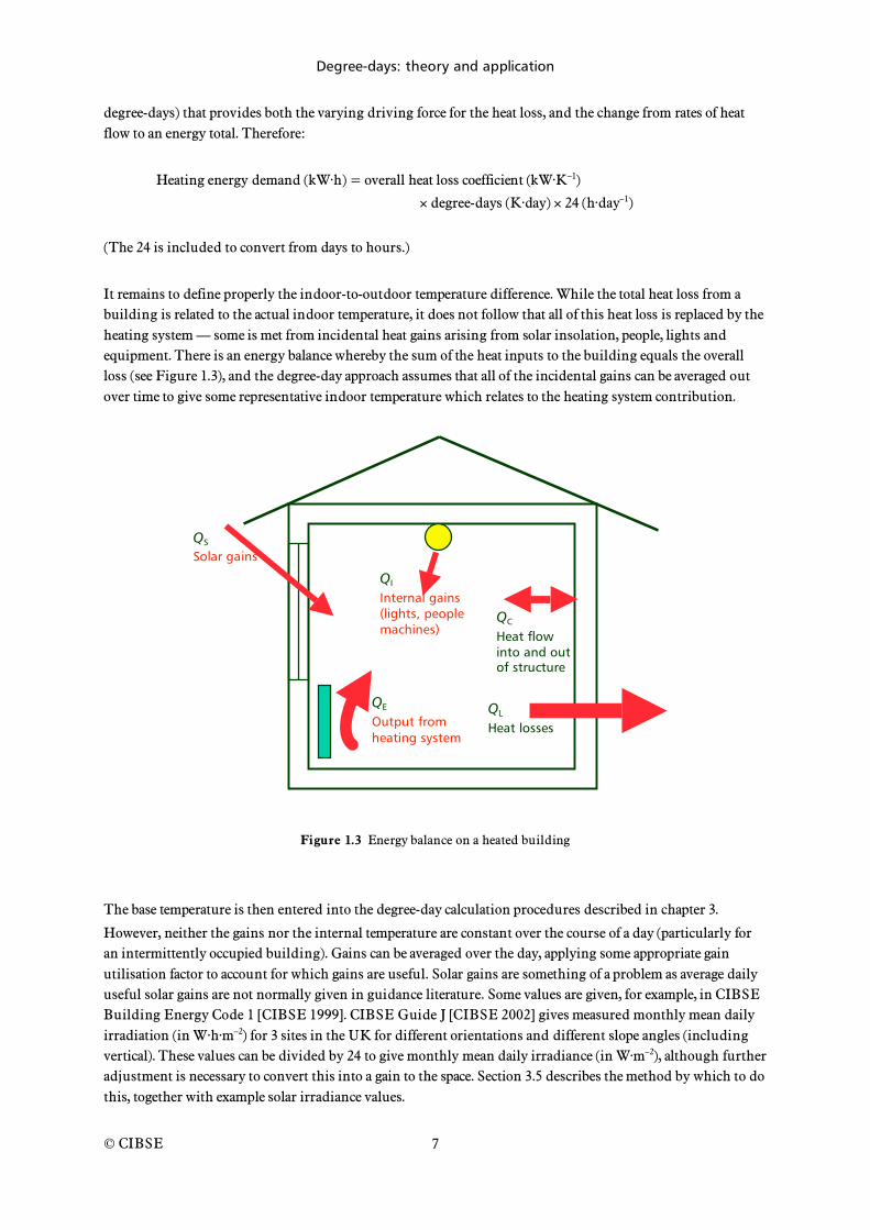
Base temperature = 24-hour mean internal temperature – (mean daily gains ÷ heat loss coefficient)
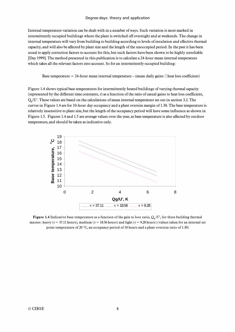
Figure 1.4 shows typical base temperatures for intermittently heated buildings of varying thermal capacity (represented by the different time constants, ) as a function of the ratio of casual gains to heat loss coefficient, Qg/U'. These values are based on the calculations of mean internal temperature set out in section 3.2. The curves in Figure 1.4 are for 10-hour day occupancy and a plant oversize margin of 1.30. The base temperature is relatively insensitive to plant size, but the length of the occupancy period will have some influence as shown in Figure 1.5. Figures 1.4 and 1.5 are average values over the year, as base temperature is also affected by outdoor temperature, and should be taken as indicative only.
10
11
12
13
14
15
16
17
18
19
0 2 4 6 8
Qg/U', K
Ba
se
te
mp
era
ture
, oC
= 37.11 = 18.56 = 9.28
Figure 1.4 Indicative base temperature as a function of the gain to loss ratio, Qg /U , for three building thermal
masses: heavy ( = 37.11 hours), medium ( = 18.56 hours) and light ( = 9.28 hours) (values taken for an internal set point temperature of 20 °C, an occupancy period of 10 hours and a plant oversize ratio of 1.30)
Degree-days: theory and application
© CIBSE
9
10
11
12
13
14
15
16
17
18
19
0 1 2 3 4 5 6 7
Qg/U', K
Ba
se
te
mp
era
ture
, oC
12 hour day 10 hour day 8 hour day
Figure 1.5 Indicative base temperature as a function of the gain to loss ratio, Qg/U', for a medium weight building
( = 18.65 hours) for different length of occupancy periods.
If the mean internal temperature is calculated for a notional average day in the month, this provides a basis to calculate monthly degree-days and produce monthly energy estimates. There are a number of ways in which this mean internal temperature can be calculated, for example using the CIBSE admittance method or calculations that use the thermal capacitance of the structure. It is the latter that is presented in this publication. The admittance method is a viable alternative, and is understood by many engineers, but is much better suited to cooling rather than heating situations.
The method presented in section 3.2 is based on a first order Newtonian response, assuming a single time constant for the building. The method may appear cumbersome, but can be easily incorporated into a spreadsheet for rapid use. The amount of information required is no more than for an admittance calculation, the main difference being that it employs the actual thermal capacitance of the structural elements. The main issue of uncertainty is how much of the structure to use — there is no definitive guidance on this, but some indications are given in section 3.2. The method allows a ready ability to change the effective depth of mass to see how sensitive the energy estimate is to assumed thermal capacity. The equations assume optimum start time of the plant and calculate a notional pre-heat time. The result is, for a given building and set of conditions, a representative mean internal temperature. Such a procedure is imperfect, but has the advantage of flexibility and transparency (i.e. all of the assumptions are known by the user). Chapter 3 also includes an attempt to show the level of accuracy (or uncertainty) that can be expected from such a calculation.
Finally the heating demand should be converted to fuel consumption, cost and carbon dioxide emissions. The consumption is calculated by dividing the energy demand by the system efficiency. The efficiency is another variable , which is likely to decrease in warmer weather (part load boiler efficiency, for conventional boilers, is less than full load efficiency), in which case some average efficiency should be used. Once the fuel consumption has been determined this can be multiplied by the price of the fuel and its carbon dioxide emission factor.
1.2.2 Energy consumption and building mass
The method described above accounts for the thermal capacity of a building according to the mass of its elements. However, some care is needed when interpreting the results of such simplified calculation methods. The procedure set out in chapter 3 will tend to show that heavyweight buildings consume more heating energy when operated intermittently than equivalent lightweight buildings with identical heat loss coefficients (and

Degree-days: theory and application
© CIBSE
10
when all other aspects of the buildings are the same). This is because the thermal mass keeps the overall structure temperature higher (it cools more slowly overnight), leading to greater average indoor to outdoor temperature differences, and therefore greater overall heat loss [Uglow 1980] . The pre-heat time will therefore be longer in such a building, which accounts for greater energy consumption.
However, some studies have shown that greater thermal mass can lead to lower energy consumption than in lightweight structures [Noren et al., 1999]. In fact there is no contradiction here when the detail is considered. Noren et al. considered a domestic dwelling that is continually heated throughout the season, and dynamically simulated the building for different structural masses. The reduced energy consumption can be explained by the increased use of casual gains (solar, people, lights etc); the structure absorbs more heat, which is gradually released when needed, offsetting the fuel consumption. In terms of a degree-day model, the increased gain utilisation leads to a lower base temperature, which in turn would yield a reduced degree-day total and energy demand. What is required is a method for determining gain utilisation as a function of thermal mass; BS EN ISO 13790 [2004] presents gain utilisation factors as a function of both gain magnitude (relative to the heat loss coefficient) and a building time constant for continuous heating, which can be used for this purpose.
Intermittently occupied buildings present a further problem. In this case the absorbed gains are only re-emitted to the space once the air temperature falls below the temperature of the structure, i.e. when the heating system is switched off and people leave the building. In this case the stored gains actually have no use in terms of maintaining thermal comfort; and as there are no gains into the building overnight, all the pre-heating for the next day must be supplied by the heating system. However, even under these considerations a heavyweight building may still have higher gain utilisation than a lightweight building, in which case the heavyweight building can have a lower base temperature.
BS EN ISO 13790 includes gain utilisation factors for intermittent operation that, for the reasons outlined above, are less than those for continuously heated buildings. There are other possible ways of approaching this (e.g. Hitchin [1990]), although these are currently less well defined than the use of the more traditional base temperature. The issue of gain utilisation (as set out in BS EN ISO 13790) is discussed in detail in section 3.5.
1.2.3 Cooling
Cooling energy demand contains the added complications of latent loads and the variety of system configurations that exist. The approach adopted in this publication is to conduct an energy balance on the cooling element (whether central or dispersed cooling coils, chilled beams etc). The calculations focus on chiller energy consumption, but consumption due to heat rejection, fans and pumps can be incorporated via the system coefficient of performance (CoP).
Cooling degree-days are calculated from temperatures above a base temperature; the equations to calculate them simply subtract the base from the outdoor temperature using similar principles as for the heating case. The key once again is how the base temperature is defined, which varies according to the type of system. Section 3.6 sets out ways this can be done for three types of system: all-air system with central coil, fan coil units, and chilled beams/ceilings.
For all-air systems without heat recovery the energy extracted by the cooling coil is related to the mass flow rate of air, and the temperature difference across the coil. Where there is no latent load (i.e. the coil runs dry) there is only sensible heat removal at a rate given by:

Degree-days: theory and application
© CIBSE
11
Heat removal (kW) = mass flow rate (kg·s–1) specific heat of air (kJ·kg–1·K–1)
(outdoor air temperature – off-coil temperature) (K)
The off-coil temperature is generally determined by the gains to the space; where these are constant then the off-coil temperature is constant. It follows that the off-coil temperature is in fact the cooling base temperature, and the energy removed from the air by the coil over time is given by:
Cooling coil energy removal (kW·h) = mass flow rate of air (kg·s–1)
specific heat of air (kJ·kg–1·K–1)
cooling degree-days (K·day) 24 (hour day–1)
The question arises how to deal with the latent load on the coil, i.e. the latent heat removed from the air that results in a reduction in moisture content across the coil. As degree-days are calculated only in terms of dry bulb temperatures this appears a difficult problem. Note it is possible to work in enthalpy (and use the concept of enthalpy days), but this changes the concept of using a dry-bulb parameter. One way around this is to treat the latent load as if it were an equivalent sensible load, and to calculate a sensible temperature difference that would give the same load on the coil. Taking typical values of latent heat of vaporisation and specific heat of air it can be shown that this ‘notional temperature difference’ can be related to the moisture difference across the coil as follows:
Notional temperature difference (K) = 2400 (K·kg(dry air)·kg–1(water vapour)) (on-coil moisture content (kg(water vapour)·kg–1 (dry air)) – off-coil moisture content (kg(water vapour)·kg–1(dry air)))
The base temperature can now be defined as the off-coil dry bulb temperature minus the notional latent temperature difference. For example, for an average off-coil temperature of 16 °C and an average moisture content difference of 0.001 kg·kg–1 the base temperature will be 16 – (2400 0.001) = 13.6 °C. The moisture content values can be determined from psychrometric calculations, for example, if dry and wet bulb temperatures are known. The off-coil moisture content can be calculated by assuming a suitable percentage saturation of the off-coil air (in the region of 90 to 95%) at the off-coil temperature. It is recommended that, as for heating, only average monthly values are used to find one base temperature per month.
Since the actual off-coil temperature is a function of the gains into the conditioned space (and system gains such as fan and duct gains) section 3.6 breaks down the individual loads that contribute to this. This results in what appears to be a complex base temperature calculation, but it only contains existing parts of the air-conditioning design process.
1.2.4 Heat recovery and other systems
All good air-conditioning systems should employ heat recovery to ensure fresh air loads are minimised. This can be dealt with by modifying the on-coil air according to some heat recovery rate. This does add a complication, but it can be dealt with as shown in section 3.6.
The principles outlined above can be extended to work out energy balances for other system types. In this publication examples are given for fan coils and chilled ceilings. The latter is very similar to the heating case. This document cannot present the equations for all types of system, but using the general principles that are presented it is possible to work out the energy balance and base temperature equations for all types of system.

Degree-days: theory and application
© CIBSE
12
These methods should not be used in place of full thermal simulation, and their accuracy is limited, but they will give representative solutions for typical systems.
1.3 Degree-days for energy management
The energy estimation models described above can be used to assess the magnitude of fuel consumption that might be expected for a building, and might even serve the energy manager as a rough benchmark when assessing a building’s energy performance. However, probably the most common use of degree-days is in the monitoring of existing building energy consumption. The theory described in the previous section shows that the space conditioning energy consumption of a building (whether heating or sensible cooling) should vary linearly with changes in dry bulb temperature. It follows that a graph of heating energy against heating degree-days should produce a straight line (see for example Figure 5.3 in section 5.3). This ‘performance line’ would then show how the energy consumption varies according to the monthly variation in temperature, which can be used to compare current energy demand against previous performance.
Such graphs form the basis of a very important energy management tool as these plots of energy use against degree-days can be used to characterise a building’s performance. If the building persistently and systematically departs from historical trends this indicates that something has changed in the energy consumption pattern. The performance line can be used to quantify such changes and to monitor whether a building meets expectations. For example, when an energy manager implements some energy saving measure, there needs to be a mechanism by which resulting savings can be quantified. As outdoor conditions vary from month to month and from year to year it is necessary to account for this in order to compare, for example, the energy consumption in January of the current year with that of the previous January.
If the historical performance shows a reasonably linear relationship between energy and degree-days then, if nothing has changed in the building, one would expect the monthly metered energy consumption (when plotted on the graph against monthly degree-days) to also lie on or close to the line. If the point lies below the line the building is using less energy than expected, and if above it is using more. If the differences between metered data and the performance line show a regular or systematic pattern (for example if they are always below the line) then it can be inferred that the building is consuming energy differently.
In the case that they are always below the line, this suggests energy savings against previous performance. This can be linked to particular energy saving measures and the savings quantified. Similarly where more energy is being consumed than expected (points lie above the line), this can alert the energy manager to failures or changes in the system operation.
This use of performance lines is the subject of another publication — Good Practice Guide 310 [Carbon Trust 2006] — which gives step-by-step guidance on conducting these procedures. The reader is referred to that document. Chapter 5 of this TM examines how performance lines are constructed, and discusses issues of how they may be interpreted. Their applicability is related to the concept of building energy signatures, where daily energy consumption is plotted against mean daily temperature. The data to plot such energy signatures are not always available to the energy manager, but where they exist these can be very instructive as to how buildings behave from day to day. Chapter 5 shows that in theory it is possible to estimate the building base temperature from these signatures (i.e. the temperature at which space conditioning energy is not required). However, it is also possible to use monthly performance lines to establish the same thing. This has important implications for the physical interpretation of performance lines — these are examined in detail in chapter 5.

Degree-days: theory and application
© CIBSE
13
It must be emphasised that this is not a precise science, but a statistical process and any inferences drawn must be treated with some circumspection. What performance lines can do is draw attention to trends and anomalies, which serve as a starting point for physical investigations that can explain them; there is no real substitute for a detailed knowledge of a building and its systems in energy management. However, the analysis presented in chapter 5 does suggest that, in theory, some deeper aspects of building energy performance can be explored. As more buildings are comprehensively monitored, it is important that this information is effectively used in order to maximise building energy efficiency. The use of performance lines is an important step in this process.
The history of degree days
The concept of degree-days originates from the work of Lt-Gen. Sir Richard Strachey [Strachey 1878]. Terms such as ‘day-degree’, ‘hour-degree’ and ‘base temperature’ appear to originate here. Strachey’s work was concerned with crop growth, and he devised formulae for determining ‘accumulated temperature’ above a base temperature of 42 °F (5.6 °C), the temperature above which plant growth is sustained. He extended his work to include accumulated
temperature (or degree-days in modern terminology) below a given base temperature. In 1928 the Meteorological Office published formulae based on Strachey’s work in the form that is currently used to calculate degree-days (see section 3.2). It was the London and Counties Coke Association that appears to have adopted this approach for the first time (around 1939) in the calculation of building energy related degree-days.
The first recorded application of degree-days to buildings originates in the United States with the American Gas Association in the 1920s [ASHVE 1933]. It had shown (statistically) that fuel consumption in dwellings varied in proportion to degree-days to a base temperature of 65 °F (18.3 °C); with the internal set point assumed to be 70 °F. This led to the notion that internal gains contributed a 5 °F rise in internal temperature. This was translated in the UK in 1934 by Dufton [Dufton 1934], who suggested that internal temperatures were more like 65 °F in the UK and that if the gains were similar this would lead to a sensible choice of base temperature as 60 °F — or 15.5 °C. This is
the base temperature that is still taken to be the standard in the UK, even though building standards and occupant activities have changed significantly since then. Although the literature is full of calls to adopt building specific base temperatures [Grierson, Fischer, Knight and Cornell, Billington 1966], the use of 15.5 °C continues.
The foundations of modern usage were laid in the 1940s by a number of papers in the Journal of the Institution of Heating and Ventilating Engineers (the forerunner of CIBSE) [Grierson, McVicker, Pallot, Fischer]. The most important of these was by McVicker in 1946, who tackled the issues of calculating degree-days and their use both as predictive and monitoring tools. Refinements were explored by Knight and Cornell [Knight and Cornell 1958], who suggested that intermittently occupied buildings should use ‘split day’ degree-days with different base temperatures for day and night. This idea was taken up again much later by Holmes [1980] who introduced thermal capacity and variable gain effects.
It was Billington [1964, 1966] who developed the estimation methodology that was accepted as the CIBSE standard approach. His approach included the use of building specific base temperatures and the concept of ‘equivalent full load running hours’. The method adopted correction factors for intermittently heated buildings, which were based on sets of finite difference calculations for a variety of structures. Tabulated correction factors undoubtedly simplified the procedure greatly, but are rather inflexible and the likely error is impossible to quantify. Such approaches were always seen as (and were only intended to be) indicative.
Other degree-day estimation models have been proposed, with modifications including, for example, gain utilisation [e.g. Hitchin and Hyde 1979; Claridge et al. 1987a]. Holmes [1980] proposed a model that calculates mean internal temperature of an intermittently occupied building, and the base temperature is determined from this (an approach also supported by others [e.g. Fisk, Bloomfield and Fisk]). Holmes used the admittance method [Milbank and Harrington-Lynn; CIBSE 1999], which is relatively easy to use, but suffers from a need to estimate pre-heat times for buildings. Using mean internal temperature is a reasonable compromise on more complex models as it incorporates

Degree-days: theory and application
© CIBSE
14
thermal capacity effects of the building but retains a level of simplicity. It also has the advantage of removing the need for tabulated correction factors.
This admittance-based model was later examined in more detail, together with an alternative method for calculating the mean internal temperature of intermittent buildings [Day 1999; Day and Karayiannis 1999b], which forms the basis of the model set out in chapter 3. A more detailed discussion of the merits of these approaches can be found in that section.
With respect to the monitoring of energy use there is little in the literature to demonstrate the underpinning theory. McVicker [1946] demonstrated the principle of plotting monthly fuel consumption against monthly degree-days. Variations have been suggested on this (for example by Knight and Cornell [1959]). Although some of their arguments are not mathematically robust, the basic techniques are still used today. Harris [1989] is largely responsible for bringing regression and cumulative sum difference (CUSUM) techniques to the attention of building energy managers, and these techniques have gained wide acceptance. Good Practice Guide GPG310 [2006] sets out the standard practice for CUSUM analysis.
The use of regression analysis in building energy performance monitoring has largely been confined to using standard degree-days to base 15.5 °C. Theory suggests that building specific base temperatures may yield more useful
results, and there is evidence to show this may be of practical benefit [Day et al 2003]. Chapter 5 of this publication presents the theory of these revised regression techniques, and their application to building energy analysis.
The discussions above have focussed exclusively on heating applications. Cooling degree-days have received much less attention (and prior to 2000 almost exclusively in the United States). Standard theory has never previously been set out in any UK guidance. In those places where definitions do occur (e.g. ASHRAE Fundamentals) these employ base temperature definitions identical to the heating case. This TM presents a more rigorous treatment of cooling degree-day base temperatures based on work published in 2000 [Day et al 2000].
Degree-days: theory and application
© CIBSE
15
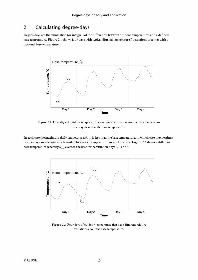
2 Calculating degree-days Degree-days are the summation (or integral) of the differences between outdoor temperatures and a defined base temperature. Figure 2.1 shows four days with typical diurnal temperature fluctuations together with a notional base temperature.
Time
Te
mp
era
ture
, oC
Day 1 Day 2 Day 3
Base temperature, b
max
min
Day 4
Figure 2.1 Four days of outdoor temperature variation where the maximum daily temperature
is always less than the base temperature.
In each case the maximum daily temperature, max, is less than the base temperature, in which case the (heating) degree-days are the total area bounded by the two temperature curves. However, Figure 2.2 shows a different base temperature whereby max exceeds the base temperature on days 2, 3 and 4.
Time
Te
mp
era
ture
, oC
Day 1 Day 2 Day 3
Base temperature, b
max
min
Day 4
Figure 2.2 Four days of outdoor temperature that have different relative
variations about the base temperature.

Degree-days: theory and application
© CIBSE
16
The calculation of degree-days needs to be able to cope with these situations (for both heating and cooling). There are a number of ways in which this can be done:
mean degree-hours; calculated from the hourly temperature record
using daily maximum and minimum temperatures; e.g. the Meteorological Office equations
from mean daily temperatures
direct calculation of monthly degree-days from mean monthly temperature and the monthly standard deviation; e.g. Hitchin’s formula.
There are variants on each of the above, of which some mention will be made, but only the accepted methods will be discussed in detail here.
Note that calculated daily degree-days are summed over a month to get monthly values. Monthly values can in turn be summed to give annual or seasonal values. Seasonal heating degree-days, for example, take only those months when the heating system is switched on (normally October to April in the UK).
2.1 Mean degree-hours
The most rigorous (and most mathematically precise) method of calculating degree-days is to sum hourly temperature differences and divide by 24. (Smaller time increments may be used if the data exists, but there is little to be gained in terms of accuracy.) It is important that only positive differences are summed; in the case of heating degree-hours when the outdoor temperature exceeds the base temperature the value is set to zero for that hour. Equation 1 shows the general formula for this process for heating degree-days:
Dd =
b o, j( )j=1
24
b o, j( ) > 0( )24
(2.1)
Where Dd is the daily degree-days for one day, b is the base temperature and o,j is the outdoor temperature in hour j. The subscript denotes that only positive values are taken. For cooling degree-days this simply becomes:
Dd =
o, j b( )j=1
24
o, j b( ) > 0( )24
(2.2)
Daily degree-days are then summed over the appropriate period — usually over a month, a season or a year. However, this method of calculation requires a great deal more data handling and storage capability than other methods, although this is not a significant problem for electronic data systems.
Using hourly temperatures to calculate degree-days does not imply that hourly energy estimates can be produced accurately — it is the summation of degree-days over a suitably long period of time that is of any real value in building energy analysis. While there have been calls for the increased use of degree-hours [e.g. Waide and Norton 1995], the greater (mathematical) accuracy from using hourly values may be of little practical value in building energy analysis. Some quantification of the differences between this and other methods of calculating degree-days are presented later in this chapter.
Degree-days: theory and application
© CIBSE
17
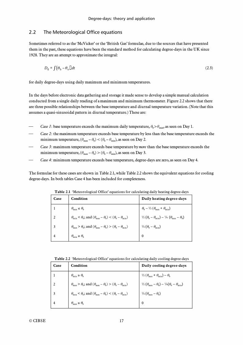
2.2 The Meteorological Office equations
Sometimes referred to as the ‘McVicker’ or the ‘British Gas’ formulae, due to the sources that have presented them in the past, these equations have been the standard method for calculating degree-days in the UK since 1928. They are an attempt to approximate the integral:
Dd = b o( ) dt (2.3)
for daily degree-days using daily maximum and minimum temperatures.
In the days before electronic data gathering and storage it made sense to develop a simple manual calculation conducted from a single daily reading of a maximum and minimum thermometer. Figure 2.2 shows that there are three possible relationships between the base temperature and diurnal temperature variation. (Note that this assumes a quasi-sinusoidal pattern in diurnal temperature.) These are:
Case 1: base temperature exceeds the maximum daily temperature, b> max, as seen on Day 1.
Case 2: the maximum temperature exceeds base temperature by less than the base temperature exceeds the minimum temperature, ( max – b) < ( b – min), as seen on Day 2.
Case 3: maximum temperature exceeds base temperature by more than the base temperature exceeds the minimum temperature, ( max – b) > ( b – min), as seen on Day 3.
Case 4: minimum temperature exceeds base temperature, degree-days are zero, as seen on Day 4.
The formulae for these cases are shown in Table 2.1, while Table 2.2 shows the equivalent equations for cooling degree-days. In both tables Case 4 has been included for completeness.
Table 2.1 ‘Meteorological Office’ equations for calculating daily heating degree-days
Case Condition Daily heating degree-days
1 max b b – ½ ( max + min)
2 min < b; and ( max – b) < ( b – min) ½ ( b – min) – ( max – b)
3 max > b; and ( max – b) > ( b – min) ¼ ( b – min)
4 min b 0
Table 2.2 ‘Meteorological Office’ equations for calculating daily cooling degree-days
Case Condition Daily cooling degree-days
1 min b ½ ( max + min) – b
2 max > b; and ( max – b) > ( b – min) ½ ( max – b) – ( b – min)
3 min < b; and ( max – b) < ( b – min) ¼ ( max – b)
4 max b 0

Degree-days: theory and application
© CIBSE
18
The coefficients of 0.5 and 0.25 in the equations of Tables 2.1 and 2.2 were originally determined by trial and error. A detailed parametric study of the factors that govern the accuracy of these equations was conducted [Day 1999, Day and Karayiannis 1998]. The results concluded that the equation for Case 2 has a tendency to underestimate degree-days, and Case 3 to overestimate them for ideal temperature curves (based on partial sine curves). The analysis of the accuracy of the Meteorological Office equations for real temperature data presented in section 2.6 confirms these tendencies, but the patterns of variations depend on geographical location. These results suggest that the coefficient 0.25 should in fact be reduced, but that any changes in coefficient must be location dependent. However, any adjustment to the coefficients cannot eliminate the errors entirely. The Meteorological equations are based on the assumptions that diurnal patterns are sinusoidal in nature or, at least, made up of partial sine curves. In reality temperature variations depart from such ideal situations and there is no mathematical treatment that can provide a single set of coefficients to deal with all eventualities.
2.3 Mean daily temperature
This is the method generally used in other countries, for example the USA [AHSRAE 2001] and Germany [German Standard VDI 2067], where degree-days are calculated from the mean daily temperature (Case 1 in Tables 2.1 and 2.2). This makes the definition and calculation of degree-days simpler, and makes the (reasonable) assumption that heating systems do not operate on days where average outdoor temperatures exceed the base. In effect this treats days such as Case 2 as Case 1, and ignores days with patterns as Case 3. While there are differences between degree-days calculated by this method and using hourly temperatures (see section 2.6), these are small. It forms the standard definition of degree-days in the USA as defined by ASHRAE [ASHRAE 2001].
2.4 Hitchin’s formula
There have been a number of attempts to calculate degree-days from reduced weather data, for example Thom [1952, 1954, 1966] and Erbs [1983] in the USA, based on the statistical analysis of truncated temperature distributions. These are usually based on mean monthly temperature and the standard deviation throughout the month, and thus are location-sensitive. Hitchin [1983] proposed a relatively simple formula for heating degree-days that showed a better correlation with the UK climate than Thom’s method. Hitchin’s formula states:
Dm = Nm ( b – o,m )
1 – –k ( b – o, m)e (2.4)
where Dm is the monthly degree-day value, Nm is the number of days in the month, o,m is the mean monthly temperature, and k is a location specific constant given by:
k =2.5
(2.5)
where is the standard deviation of the variation in temperature throughout the month. Unfortunately is rarely known by the typical user, and Hitchin suggested the best values of k for different sites as shown in Table 2.3.

Degree-days: theory and application
© CIBSE
19
Table 2.3 Values of k for use in Hitchin’s formula [Hitchin 1983]
Site Constant, k
Heathrow 0.66
Manchester 0.70
Birmingham 0.66
Glasgow 0.74
Cardiff 0.78
Mean 0.71
Hitchin further suggested that using the mean value of 0.71 for inland areas made little significant difference to the results. The benefit of Hitchin’s formula is that it is quick to use and requires only limited information (which is freely available on the internet from the Met Office website (http://www.metoffice.gov.uk) or from http://www.wunderground.com); it can also be used for base temperature correction (see section 2.7). However, it does suffer from a loss of accuracy at small values of ( b – o,m) , i.e. in warmer months or where the base
temperature is very low.
2.5 Other methods
There are other methods in use. ASHRAE recommends the method by Erbs [1983], similar to Hitchin, for estimating monthly degree-days. There are also reports of individual energy managers adopting their own techniques based on the kind of weather data that is available to them. However, it should be noted that equations 2.1 and 2.2 should always be the preferred option if suitable hourly data and adequate data processing tools are available.
2.6 Errors associated with calculation methods
The error associated with a calculation method can be expressed in terms of a percentage difference from mean degree-hours (given by equations 2.1 and 2.2), which for the benefit of clarity will be termed Dactual. Thus if the Dapprox is given by some calculation method the error, or difference, , is given by:
=Dactual Dapprox
Dactual
100%. (2.6)
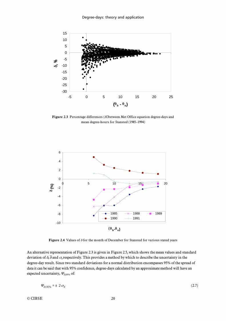
Values of for monthly degree-days to different base temperatures have been calculated for all three approximate methods described above for ten years of weather data and for a number of locations [Day and Karayiannis 1997]. An example of the results for Stansted using the Meterological Office equations is shown in Figure 2.3.
This clearly shows that the error, while small for large ( b – o,m) increases significantly as the base
temperature approaches the mean monthly temperature. Although the percentages appear high, it must be remembered that these apply to small numerical degree-day values, in which case they may not be overly significant. Any attempt to improve the coefficients is complicated by the fact that the nature of the error (whether an over- or underestimate) will vary for a particular location from month to month and from year to year. This is demonstrated in Figure 2.4, which shows values of for Stansted for the month of December for selected years.
Degree-days: theory and application
© CIBSE
20
-30
-25
-20
-15
-10
-5
0
5
10
15
-5 0 5 10 15 20 25
( b - o)
, %
Figure 2.3 Percentage differences ( ) between Met Office equation degree-days and
mean degree-hours for Stansted (1985–1994)
-10
-8
-6
-4
-2
0
2
4
6
0 5 10 15 20
(b- o)
(%
)
1985 1988 1989
1990 1991
Figure 2.4 Values of for the month of December for Stansted for various stated years
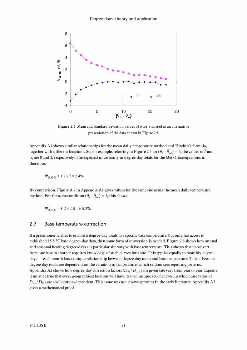
An alternative representation of Figure 2.3 is given in Figure 2.5, which shows the mean values and standard deviation of , and respectively. This provides a method by which to describe the uncertainty in the degree-day result. Since two standard deviations for a normal distribution encompasses 95% of the spread of data it can be said that with 95% confidence, degree-days calculated by an approximate method will have an expected uncertainty, D,95% of:
D,95% = ± 2 (2.7)
Degree-days: theory and application
© CIBSE
21
-4
-2
0
2
4
6
8
0 5 10 15 20
( b - o)
an
d
, %
Figure 2.5 Mean and standard deviation values of for Stansted as an alternative
presentation of the data shown in Figure 2.3.
Appendix A1 shows similar relationships for the mean daily temperature method and Hitchin’s formula, together with different locations. So, for example, referring to Figure 2.5 for ( b – o,m) = 5, the values of and
are 0 and 2, respectively. The expected uncertainty in degree-day totals for the Met Office equations is therefore:
D,95% = ± 2 2 = ± 4%
By comparison, Figure A.2 in Appendix A1 gives values for the same site using the mean daily temperature method. For the same condition ( b – o,m) = 5, this shows:
D,95% = ± 2 2.6 = ± 5.2%
2.7 Base temperature correction
If a practitioner wishes to establish degree-day totals to a specific base temperature, but only has access to published 15.5 °C base degree-day data, then some form of conversion is needed. Figure 2.6 shows how annual and seasonal heating degree-days at a particular site vary with base temperature. This shows that to convert from one base to another requires knowledge of such curves for a site. This applies equally to monthly degree-days — each month has a unique relationship between degree-day totals and base temperature. This is because degree-day totals are dependent on the variation in temperature, which seldom sees repeating patterns. Appendix A2 shows how degree-day correction factors (D b / D15.5) at a given site vary from year to year. Equally it must be true that every geographical location will have its own unique set of curves, in which case ratios of D b / D15.5 are also location-dependent. This issue was not always apparent in the early literature. Appendix A2 gives a mathematical proof.

Degree-days: theory and application
© CIBSE
22
0
500
1000
1500
2000
2500
3000
3500
4000
0 5 10 15 20 25
Base temperature, oC
Deg
ree-d
ays
Annual
Heating months only
Figure 2.6 The relationship between degree-days and base temperature for both annual and heating month degree-
days. (Data for Stansted 1994).
An improved method of base temperature correction was put forward by Hitchin [1981] whereby annual degree-day conversions were achieved by linear regression factors such that:
D b = a D15.5 + b (2.8)
where a and b are location dependent parameters.
Hitchin produced a set of regression graphs for three separate locations — inland, East coastal, and South and West Coastal. These conversion graphs were later adopted within BREDEM 12, the BRE’s Domestic Energy Model that forms the basis of the UK Standard Assessment Procedure (SAP) for dwellings.
An alternative method is to use Hitchin’s formula for base temperature correction. Published monthly degree-days to base 15.5 °C can be converted by inserting these into equation 2.4 and solving for the mean monthly temperature, o,m. The new base temperature can then be used to calculate the monthly degree-days.
Such an approach has two drawbacks: it inevitably introduces errors, especially at low base temperatures, and it requires a numerical iterative solution to find o,m. The first drawback must be seen as inevitable, although for small degree-day numbers, the errors are numerically small. However, it is always better to have access to local temperature records rather than rely on conversions. With respect to the second drawback such numerical solutions can easily be adopted within a spreadsheet. A standard practical method is the Newton-Raphson iteration. A full worked example is included in Appendix A3 to show how this can be conducted, together with a typical VBA coded routine that can be written into a spreadsheet macro.
Degree-days: theory and application
© CIBSE
23
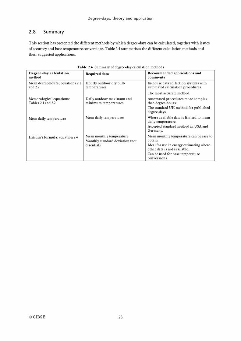
2.8 Summary
This section has presented the different methods by which degree-days can be calculated, together with issues of accuracy and base temperature conversions. Table 2.4 summarises the different calculation methods and their suggested applications.
Table 2.4 Summary of degree-day calculation methods
Degree-day calculation method
Required data Recommended applications and comments
Mean degree-hours; equations 2.1 and 2.2
Hourly outdoor dry bulb temperatures
In-house data collection systems with automated calculation procedures.
The most accurate method.
Meteorological equations: Tables 2.1 and 2.2
Daily outdoor maximum and minimum temperatures
Automated procedures more complex than degree-hours. The standard UK method for published degree-days.
Mean daily temperature Mean daily temperatures Where available data is limited to mean daily temperature. Accepted standard method in USA and Germany.
Hitchin’s formula: equation 2.4 Mean monthly temperature Monthly standard deviation (not essential)
Mean monthly temperature can be easy to obtain. Ideal for use in energy estimating where other data is not available. Can be used for base temperature conversions.

Degree-days: theory and application
© CIBSE
24
3 Energy estimation techniques Weather related energy consumption in buildings is one of the largest single contributions to UK carbon dioxide emissions, and for some buildings may be the largest component of energy bills. Space heating uses around 30% of the UK energy budget [DTI 2002], and it is therefore necessary to have methods that can provide reliable information about individual building consumption.
Buildings are complex thermal environments, with a large number of variables that may influence energy demand. Figure 3.1 attempts to illustrate this, and provides a basis for developing energy analysis models.
Figure 3.1 The parameters and their interrelationships that influence space heating
energy consumption in buildings
Degree-days: theory and application
© CIBSE
25
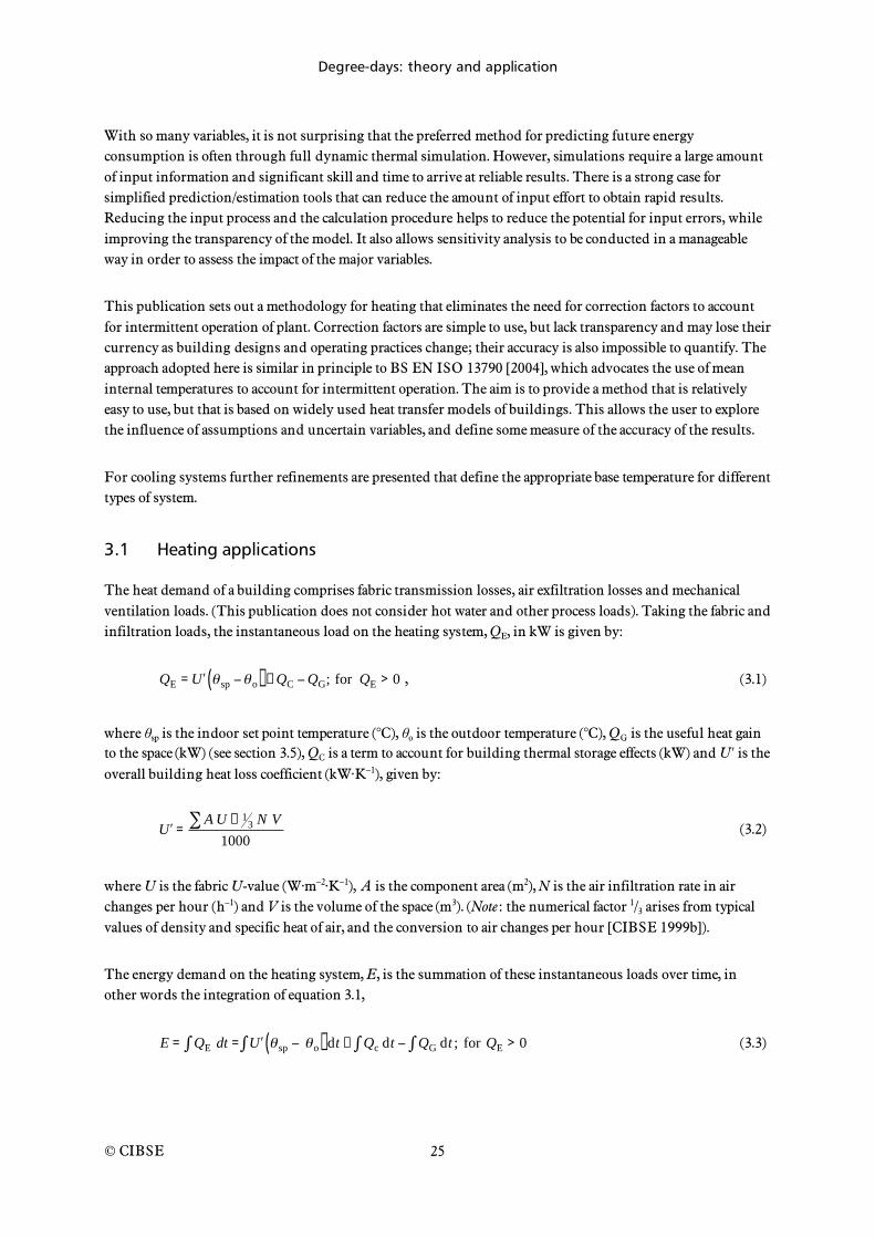
With so many variables, it is not surprising that the preferred method for predicting future energy consumption is often through full dynamic thermal simulation. However, simulations require a large amount of input information and significant skill and time to arrive at reliable results. There is a strong case for simplified prediction/estimation tools that can reduce the amount of input effort to obtain rapid results. Reducing the input process and the calculation procedure helps to reduce the potential for input errors, while improving the transparency of the model. It also allows sensitivity analysis to be conducted in a manageable way in order to assess the impact of the major variables.
This publication sets out a methodology for heating that eliminates the need for correction factors to account for intermittent operation of plant. Correction factors are simple to use, but lack transparency and may lose their currency as building designs and operating practices change; their accuracy is also impossible to quantify. The approach adopted here is similar in principle to BS EN ISO 13790 [2004], which advocates the use of mean internal temperatures to account for intermittent operation. The aim is to provide a method that is relatively easy to use, but that is based on widely used heat transfer models of buildings. This allows the user to explore the influence of assumptions and uncertain variables, and define some measure of the accuracy of the results.
For cooling systems further refinements are presented that define the appropriate base temperature for different types of system.
3.1 Heating applications
The heat demand of a building comprises fabric transmission losses, air exfiltration losses and mechanical ventilation loads. (This publication does not consider hot water and other process loads). Taking the fabric and infiltration loads, the instantaneous load on the heating system, QE, in kW is given by:
QE = U sp o( ) + QC QG; for QE > 0 , (3.1)
where sp is the indoor set point temperature (°C), o is the outdoor temperature (°C), QG is the useful heat gain to the space (kW) (see section 3.5), QC is a term to account for building thermal storage effects (kW) and U is the overall building heat loss coefficient (kW·K–1), given by:
U =A U + 1
3 N V
1000 (3.2)
where U is the fabric U-value (W·m–2·K–1), A is the component area (m2), N is the air infiltration rate in air changes per hour (h–1) and V is the volume of the space (m3). (Note: the numerical factor 1/3 arises from typical values of density and specific heat of air, and the conversion to air changes per hour [CIBSE 1999b]).
The energy demand on the heating system, E, is the summation of these instantaneous loads over time, in other words the integration of equation 3.1,
E = QE dt = U sp o( ) dt + Qc dt QG dt ; for QE > 0 (3.3)
Degree-days: theory and application
© CIBSE
26
In the case of a continuously heated building, the QC term is equal to zero in which case the terms can be rearranged to bring the gains into the temperature integral:
E = U sp oQG
U
dt (3.4)
The term QG /U has the units of temperature difference (K) and can be considered the internal temperature rise due to gains. Subtracting this gain-related temperature rise from the internal temperature gives rise to the concept of a base temperature, thus:
b = spQG
U (3.5)
giving the energy demand on the heating system as:
E = U b o( ) dt (3.6)
where the temperature integral is the degree-day total as previously defined in equation 2.3, i.e:
Dd = b o( ) dt
which is calculated from the methods set out in chapter 2 over the appropriately defined timescale, typically taken as a heating season or a month. The estimated fuel consumption, F (kW·h) is then found from:
F =24 U Dd (3.7)
where is overall seasonal heating system efficiency, and 24 is the conversion factor from days to hours.
From the above it can be seen that the use of a ‘standard’ base temperature of 15.5 °C is not appropriate for all buildings. Over the years changes to Building Regulations have had the effect of reducing the value of U significantly, while internal gains have greatly increased. It is not uncommon to have buildings with base temperatures of 10 °C or less. The need to determine the correct base temperature has further implications for intermittent heating.
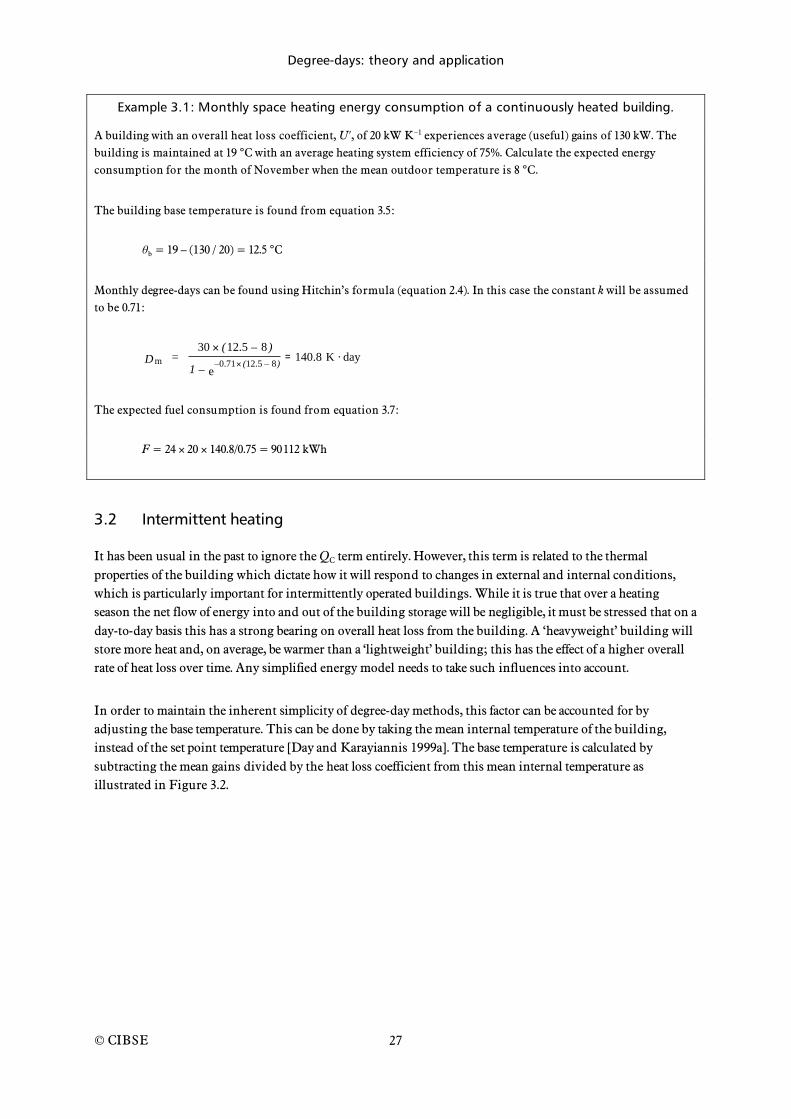
Degree-days: theory and application
© CIBSE
27
Example 3.1: Monthly space heating energy consumption of a continuously heated building.
A building with an overall heat loss coefficient, U , of 20 kW K–1 experiences average (useful) gains of 130 kW. The building is maintained at 19 °C with an average heating system efficiency of 75%. Calculate the expected energy consumption for the month of November when the mean outdoor temperature is 8 °C.
The building base temperature is found from equation 3.5:
b = 19 – (130 / 20) = 12.5 °C
Monthly degree-days can be found using Hitchin’s formula (equation 2.4). In this case the constant k will be assumed to be 0.71:
mD = 30 (12.5 – 8 )
1 – –0.71 (12.5 – 8)e
= 140.8 K day
The expected fuel consumption is found from equation 3.7:
F = 24 20 140.8/0.75 = 90 112 kWh
3.2 Intermittent heating
It has been usual in the past to ignore the QC term entirely. However, this term is related to the thermal properties of the building which dictate how it will respond to changes in external and internal conditions, which is particularly important for intermittently operated buildings. While it is true that over a heating season the net flow of energy into and out of the building storage will be negligible, it must be stressed that on a day-to-day basis this has a strong bearing on overall heat loss from the building. A ‘heavyweight’ building will store more heat and, on average, be warmer than a ‘lightweight’ building; this has the effect of a higher overall rate of heat loss over time. Any simplified energy model needs to take such influences into account.
In order to maintain the inherent simplicity of degree-day methods, this factor can be accounted for by adjusting the base temperature. This can be done by taking the mean internal temperature of the building, instead of the set point temperature [Day and Karayiannis 1999a]. The base temperature is calculated by subtracting the mean gains divided by the heat loss coefficient from this mean internal temperature as illustrated in Figure 3.2.

Degree-days: theory and application
© CIBSE
28
0
5
10
15
20
25
0 24 48 72 96
Hours
Te
mp
era
ture
, oC
outdoor temperature
indoor temperature mean indoor temperature
base temperatureTemperature rise
due to gains
subtracted from
the mean indoor
temperature to
give the base
temperature
Figure 3.2 For intermittent heating the base temperature is related to the mean
internal temperature of the building, not the set point temperature.
It has been shown that taking the mean monthly internal temperature is a good compromise with respect to accuracy and reducing the number of calculations [Day and Karayiannis 1999a]. This can be found by considering a notional average day within a month and determining the mean internal temperature for that day. Figure 3.3 shows an idealised indoor temperature profile over a 24-hour period (starting from when the occupants leave and the plant shuts down). This also shows the 24-hour mean internal temperature, and a representative base temperature relative to the actual internal temperature. The calculation of the mean temperature depends on the thermal properties of the building (heat loss coefficient and thermal capacity), the plant output capacity, the length of the unoccupied period and the set point and outdoor temperatures.
10
12
14
16
18
20
22
TIme
Inte
rna
l te
mp
era
ture
, o
C
Occupied periodUnoccupied period
preheat
mean internal temperature
base temperature
t1 t2 t3
Figure 3.3 Internal temperature variations in an intermittently heated building; the mean internal temperature is
determined by summing the hourly temperatures over the day and dividing by 24
Degree-days: theory and application
© CIBSE
29
These key variables can be incorporated into a simplified first order thermal response model of the building. (Similar approaches have been used by others to show the behaviour of buildings under intermittent heating [Levermore, 1992].) Two classical equations for the cooling and heating of a structure are:
for cooling:
Cd i
dt= U ( i o) (3.8)
and for heating:
Cd i
dt= Qp U ( i o) (3.9)
where Qp is the heating system output (at full load), d /dt is the rate of change of the building temperature. C is the effective thermal capacitance of the building given by:
C = cp Vfn
(3.10)
where Vf is the volume of the structural element that is thermally responsive (m3), is the density of the element (kg·m–3) and cp is the specific heat of the element (kJ·kg–1·K–1) for n active elements.
The main difficulty is in assessing the effective depth of mass that should be chosen. BS EN ISO 13790 [2004] recommends that for each internal element the depth should be taken up to the first insulating layer, up to a maximum depth of 30 mm. Thus for a concrete slab 30 mm depth should be used to calculate the volume of the element, but for a wall dry lined with plasterboard only the thickness of the plasterboard should be taken.
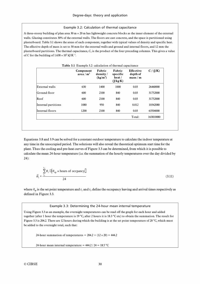
Degree-days: theory and application
© CIBSE
30
Example 3.2: Calculation of thermal capacitance
A three-storey building of plan area 30 m 20 m has lightweight concrete blocks as the inner element of the external
walls. Glazing constitutes 30% of the external walls. The floors are cast concrete, and the space is partitioned using plasterboard. Table 3.1 shows the areas of each component, together with typical values of density and specific heat. The effective depth of mass is set to 30 mm for the external walls and ground and internal floors, and 12 mm the plasterboard partitions. The thermal capacitance, C, is the product of the four preceding columns. This gives a value of C for the building of 1.638 105 kJ·K–1.
Table 3.1 Example 3.2: calculation of thermal capacitance
Component area / m2
Fabric density / (kg/m3)
Fabric specific
heat / (J/kg·K)
Effective depth of mass / m
C / (J/K)
External walls 630 1400 1000 0.03 26460000
Ground floor 600 2100 840 0.03 31752000
Roof 600 2100 840 0.03 31752000
Internal partitions 1080 950 840 0.012 10342080
Internal floors 1200 2100 840 0.03 63504000
Total: 163810080
Equations 3.8 and 3.9 can be solved for a constant outdoor temperature to calculate the indoor temperature at any time in the unoccupied period. The solutions will also reveal the theoretical optimum start time for the plant. Thus the cooling and pre-heat curves of Figure 3.3 can be determined, from which it is possible to calculate the mean 24-hour temperature (i.e. the summation of the hourly temperatures over the day divided by 24):
i =
i +t1
t3
sp hours of occpancy( )
24 (3.11)
where sp is the set point temperature and t1 and t3 define the occupancy leaving and arrival times respectively as defined in Figure 3.3.
Example 3.3: Determining the 24-hour mean internal temperature
Using Figure 3.3 as an example, the overnight temperatures can be read off the graph for each hour and added together (after 1 hour the temperature is 19 °C, after 2 hours it is 18.3 °C etc) to obtain the summation. The result for Figure 3.3 is 204.2. There are 12 hours during which the building is at the set point temperature of 20 °C, which must
be added to the overnight total, such that:
24-hour summation of temperatures = 204.2 + (12 20) = 444.2
24-hour mean internal temperature = 444.2 / 24 = 18.5 °C
Degree-days: theory and application
© CIBSE
31
However, the summation of overnight hourly temperatures can be found analytically using equation 3.12 below, which has been developed from the solutions of equations 3.8 and 3.9 (see Appendix A4 for derivation).
Thus:
it1
t3
= o t3 t1( ) + sp o( ) e
t3 t2
e
t2 t1
+
Qp
U 1+
t3 t2
e
t3 t2
(3.12)
where is the building time constant (h), obtained from:
=C
3600 U (3.13)
and t2 is the optimum switch-on time, obtained from:
t3 – t2 = –C
3600 U ln
Qp – U ( sp – o)
Qp – U ( so – o)
(3.14)
with the plant switch-on temperature, so (°C), obtained from:
so = o +Qp sp o( ) e
–t3 – t1
Qp + U sp o( ) e
t3 t1
U sp o( )
(3.15)
A full derivation of these expressions can be found in Appendix A4, with further discussions about their applicability in Appendix A5. In theory, the value of o used in equations 3.12, 3.14 and 3.15 should be the mean overnight temperature. This can range between 0.2 ºC to 1.5 ºC below the mean monthly temperature depending on location and time of year. In practice, using the overall mean monthly temperature makes very little difference (generally less than 1%) to the final energy calculations. This has the advantage of needing to know only one outdoor temperature.
(Note: equation 3.14 probably overestimates the length of pre-heat times for most medium to heavyweight buildings, and too much credence should not be given to the absolute value obtained. More important, however, is the overall mean internal temperature determined from the procedure, which can be seen as the mean 24-hour internal temperature that drives the average rate of heat loss. This has been shown to be reasonably consistent with temperatures obtained from simulations of buildings [Day 1999] for all but the most heavyweight buildings. However, the errors in forecasting mean temperatures are of secondary importance, as the degree-day energy forecasts have been shown to correspond well with simulations.)
The base temperature can be found as for the continually heated case (equation 3.5) with the set point temperature replaced by the mean internal temperature, i.e:
b = iQG
U (3.16)

Degree-days: theory and application
© CIBSE
32
Calculation of degree-days and fuel consumption follow the same procedure as for the continuously heated case with this revised base temperature. While appearing to contain a good deal of complex calculation the method has the advantage of removing the need for correction factors, and allows for all of the input assumptions to be tested for their impact on the results. It is recommended that the equations be entered into a spreadsheet, which allows rapid and repeatable calculations to be made. An example calculation procedure is shown in section 4.1.
The method set out above determines the monthly fuel consumption of the building. This can be repeated for all months of the heating system and the total seasonal fuel demand determined by summing these values. The length of the heating season is chosen by the user by selecting those months that the heating system is switched on. There is no need to try to fix the precise start and finish times of the heating season, as these are effectively accounted for by the degree-day approach.
The method presented here is also only possible using a time-based approach such as degree-days; alternative methods, such as frequency of occurrence (or bin) methods [ASHRAE 2001], cannot readily take thermal capacity effects into account.
3.3 Accuracy and uncertainty
Studies have shown that energy estimates based on mean monthly internal temperature as presented in section 3.2 are much more reliable than previously published methods [Day 1999, Day and Karayiannis 1999a]. The errors associated with earlier methods were shown to be both very large and unsystematic (i.e. no correction factors could remove these errors). Comparisons of the mean monthly temperature approach against full thermal simulations allowed the expected uncertainty in degree-day energy estimates to be determined.
Figures 3.4 and 3.5 show the expected uncertainty in monthly and seasonal energy estimates against respective degree-day totals. The monthly uncertainty curve in Figure 3.4 has the equation:
E(95%) = 130 Dm–1.3 100 (3.17)
Similarly, the seasonal uncertainty equation from Figure 3.5 is:
E(95%) = 1600 Dm( )–1.35
100 (3.18)
where E,95% is the uncertainty in the energy estimate for 95% of all calculations, and Dm is the sum of monthly degree-days over the heating season.
These equations are based on accurate and well-defined input values; for their derivation see Day and Karayiannis [1999a]. Estimates using the procedure set out in section 3.2 also fall within these uncertainty limits, and thus equations 3.17 and 3.18 provide a reasonable estimate of the expected accuracy of the method.
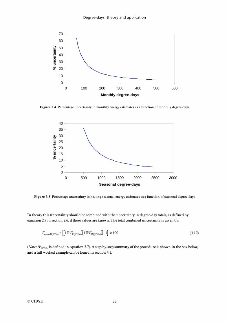
Degree-days: theory and application
© CIBSE
33
0
10
20
30
40
50
60
70
0 100 200 300 400 500 600
Monthly degree-days
% u
ncert
ain
ty
Figure 3.4 Percentage uncertainty in monthly energy estimates as a function of monthly degree-days
0
5
10
15
20
25
30
35
40
0 500 1000 1500 2000 2500 3000
Seasonal degree-days
% u
ncert
ain
ty
Figure 3.5 Percentage uncertainty in heating seasonal energy estimates as a function of seasonal degree-days
In theory this uncertainty should be combined with the uncertainty in degree-day totals, as defined by equation 2.7 in section 2.6, if these values are known. The total combined uncertainty is given by:
overall(95%) = 1+ E(95%)( ) 1+ D((95%)( ) 1[ ] 100 (3.19)
(Note: D(95%) is defined in equation 2.7). A step-by-step summary of the procedure is shown in the box below, and a full worked example can be found in section 4.1.
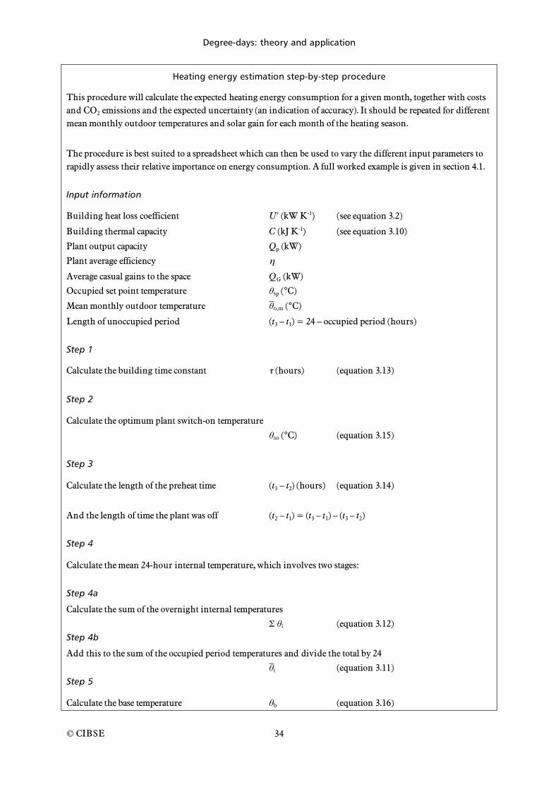
Degree-days: theory and application
© CIBSE
34
Heating energy estimation step-by-step procedure
This procedure will calculate the expected heating energy consumption for a given month, together with costs and CO2 emissions and the expected uncertainty (an indication of accuracy). It should be repeated for different mean monthly outdoor temperatures and solar gain for each month of the heating season.
The procedure is best suited to a spreadsheet which can then be used to vary the different input parameters to rapidly assess their relative importance on energy consumption. A full worked example is given in section 4.1.
Input information
Building heat loss coefficient U (kW K-1) (see equation 3.2)
Building thermal capacity C (kJ K-1) (see equation 3.10)
Plant output capacity Qp (kW)
Plant average efficiency
Average casual gains to the space QG (kW)
Occupied set point temperature sp (°C)
Mean monthly outdoor temperature o,m (°C)
Length of unoccupied period (t3 – t1) = 24 – occupied period (hours)
Step 1
Calculate the building time constant (hours) (equation 3.13)
Step 2
Calculate the optimum plant switch-on temperature
so (°C) (equation 3.15)
Step 3
Calculate the length of the preheat time (t3 – t2) (hours) (equation 3.14)
And the length of time the plant was off (t2 – t1) = (t3 – t1) – (t3 – t2)
Step 4
Calculate the mean 24-hour internal temperature, which involves two stages:
Step 4a
Calculate the sum of the overnight internal temperatures
i (equation 3.12) Step 4b
Add this to the sum of the occupied period temperatures and divide the total by 24
i (equation 3.11) Step 5
Calculate the base temperature b (equation 3.16)
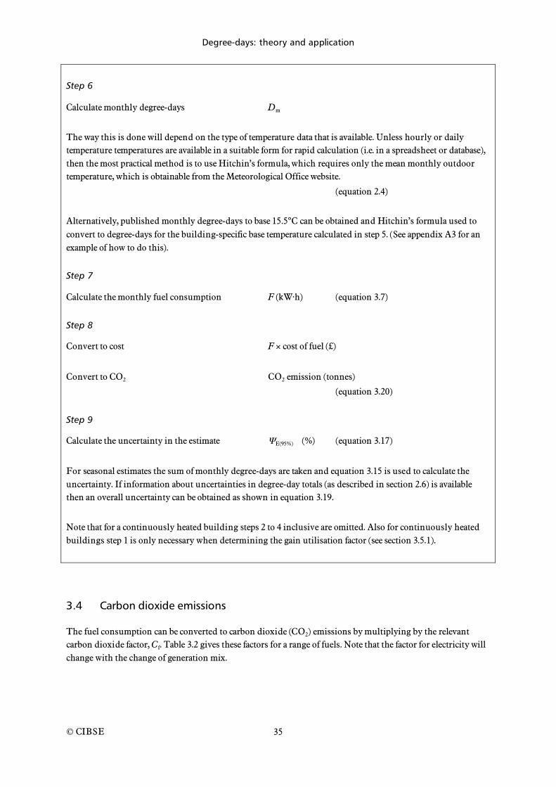
Degree-days: theory and application
© CIBSE
35
Step 6
Calculate monthly degree-days Dm
The way this is done will depend on the type of temperature data that is available. Unless hourly or daily temperature temperatures are available in a suitable form for rapid calculation (i.e. in a spreadsheet or database), then the most practical method is to use Hitchin’s formula, which requires only the mean monthly outdoor temperature, which is obtainable from the Meteorological Office website.
(equation 2.4)
Alternatively, published monthly degree-days to base 15.5°C can be obtained and Hitchin’s formula used to convert to degree-days for the building-specific base temperature calculated in step 5. (See appendix A3 for an example of how to do this).
Step 7
Calculate the monthly fuel consumption F (kW·h) (equation 3.7)
Step 8
Convert to cost F cost of fuel (£)
Convert to CO2 CO2 emission (tonnes)
(equation 3.20)
Step 9
Calculate the uncertainty in the estimate E(95%) (%) (equation 3.17)
For seasonal estimates the sum of monthly degree-days are taken and equation 3.15 is used to calculate the uncertainty. If information about uncertainties in degree-day totals (as described in section 2.6) is available then an overall uncertainty can be obtained as shown in equation 3.19.
Note that for a continuously heated building steps 2 to 4 inclusive are omitted. Also for continuously heated buildings step 1 is only necessary when determining the gain utilisation factor (see section 3.5.1).
3.4 Carbon dioxide emissions
The fuel consumption can be converted to carbon dioxide (CO2) emissions by multiplying by the relevant carbon dioxide factor, Cf. Table 3.2 gives these factors for a range of fuels. Note that the factor for electricity will change with the change of generation mix.
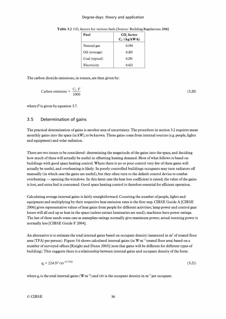
Degree-days: theory and application
© CIBSE
36
Table 3.2 CO2 factors for various fuels [Source: Building Regulations 2006]
Fuel CO2 factor Cf / (kg/kW·h)
Natural gas 0.194
Oil (average) 0.265
Coal (typical) 0.291
Electricity 0.422
The carbon dioxide emissions, in tonnes, are then given by:
Carbon emission =Cf F
1000 (3.20)
where F is given by equation 3.7.
3.5 Determination of gains
The practical determination of gains is another area of uncertainty. The procedure in section 3.2 requires mean monthly gains into the space (in kW), to be known. These gains come from internal sources (e.g. people, lights and equipment) and solar radiation.
There are two issues to be considered: determining the magnitude of the gains into the space, and deciding how much of these will actually be useful in offsetting heating demand. Most of what follows is based on buildings with good space heating control. Where there is no or poor control very few of these gains will actually be useful, and overheating is likely. In poorly controlled buildings occupants may turn radiators off manually (in which case the gains are useful), but they often turn to the default control device to combat overheating — opening the windows. In this latter case the heat loss coefficient is raised, the value of the gains is lost, and extra fuel is consumed. Good space heating control is therefore essential for efficient operation.
Calculating average internal gains is fairly straightforward. Counting the number of people, lights and equipment and multiplying by their respective heat emission rates is the first step. CIBSE Guide A [CIBSE 2006] gives representative values of heat gains from people for different activities; lamp power and control gear losses will all end up as heat in the space (unless extract luminaries are used); machines have power ratings. The last of these needs some care as nameplate ratings normally give maximum power; actual running power is normally less [CIBSE Guide F 2004].
An alternative is to estimate the total internal gains based on occupant density (measured in m2 of treated floor area (TFA) per person). Figure 3.6 shows calculated internal gains (in W·m–2 treated floor area) based on a number of surveyed offices [Knight and Dunn 2003] (note that gains will be different for different types of building). This suggests there is a relationship between internal gains and occupant density of the form:
qI = 224.97 OD0.7334 (3.21)
where qI is the total internal gains (W·m–2) and OD is the occupant density in m–2 per occupant.
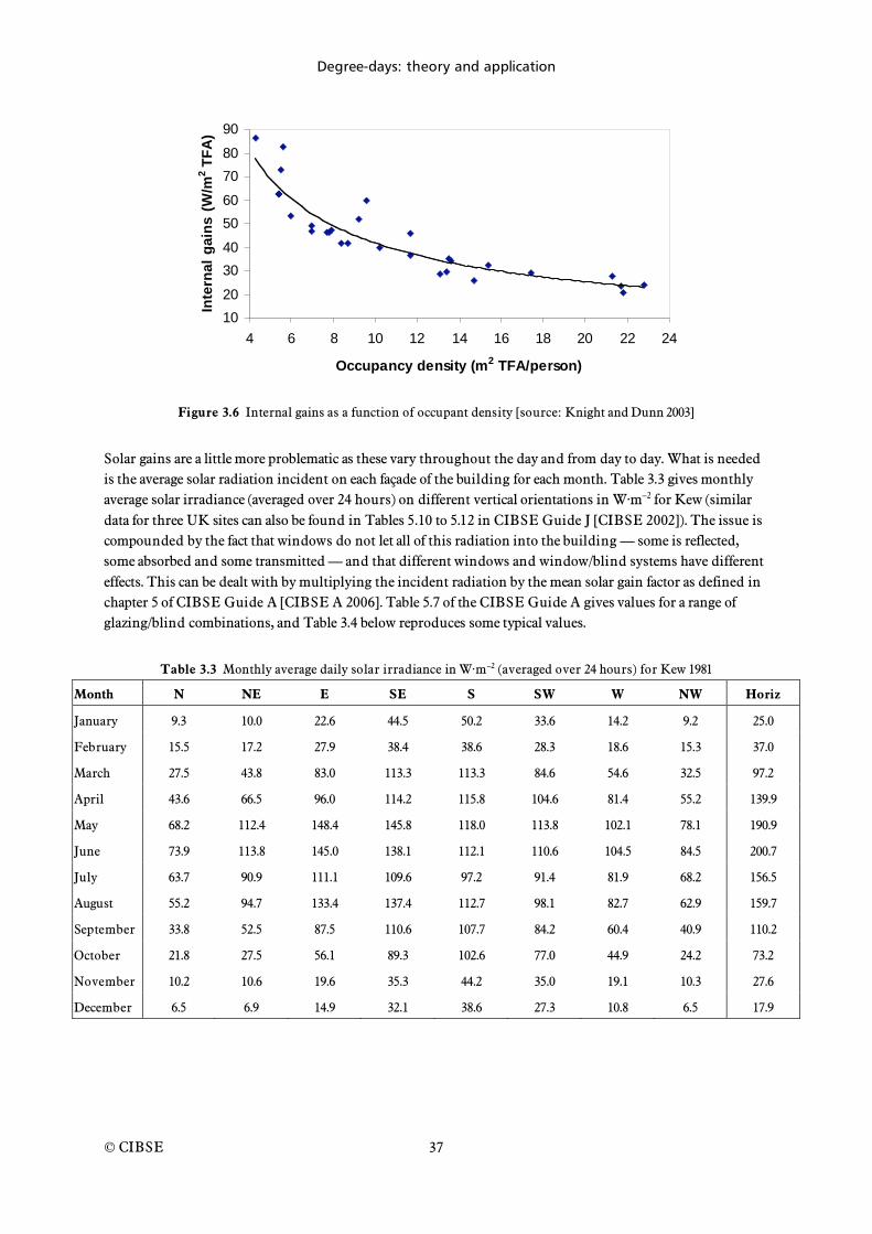
Degree-days: theory and application
© CIBSE
37
10
20
30
40
50
60
70
80
90
4 6 8 10 12 14 16 18 20 22 24
Occupancy density (m2 TFA/person)
Inte
rna
l g
ain
s (
W/m
2 T
FA
)
Figure 3.6 Internal gains as a function of occupant density [source: Knight and Dunn 2003]
Solar gains are a little more problematic as these vary throughout the day and from day to day. What is needed is the average solar radiation incident on each façade of the building for each month. Table 3.3 gives monthly average solar irradiance (averaged over 24 hours) on different vertical orientations in W·m–2 for Kew (similar data for three UK sites can also be found in Tables 5.10 to 5.12 in CIBSE Guide J [CIBSE 2002]). The issue is compounded by the fact that windows do not let all of this radiation into the building — some is reflected, some absorbed and some transmitted — and that different windows and window/blind systems have different effects. This can be dealt with by multiplying the incident radiation by the mean solar gain factor as defined in chapter 5 of CIBSE Guide A [CIBSE A 2006]. Table 5.7 of the CIBSE Guide A gives values for a range of glazing/blind combinations, and Table 3.4 below reproduces some typical values.
Table 3.3 Monthly average daily solar irradiance in W·m–2 (averaged over 24 hours) for Kew 1981
Month N NE E SE S SW W NW Horiz
January 9.3 10.0 22.6 44.5 50.2 33.6 14.2 9.2 25.0
February 15.5 17.2 27.9 38.4 38.6 28.3 18.6 15.3 37.0
March 27.5 43.8 83.0 113.3 113.3 84.6 54.6 32.5 97.2
April 43.6 66.5 96.0 114.2 115.8 104.6 81.4 55.2 139.9
May 68.2 112.4 148.4 145.8 118.0 113.8 102.1 78.1 190.9
June 73.9 113.8 145.0 138.1 112.1 110.6 104.5 84.5 200.7
July 63.7 90.9 111.1 109.6 97.2 91.4 81.9 68.2 156.5
August 55.2 94.7 133.4 137.4 112.7 98.1 82.7 62.9 159.7
September 33.8 52.5 87.5 110.6 107.7 84.2 60.4 40.9 110.2
October 21.8 27.5 56.1 89.3 102.6 77.0 44.9 24.2 73.2
November 10.2 10.6 19.6 35.3 44.2 35.0 19.1 10.3 27.6
December 6.5 6.9 14.9 32.1 38.6 27.3 10.8 6.5 17.9

Degree-days: theory and application
© CIBSE
38
Table 3.4 Example average solar gain factors (taken from CIBSE Guide A Table 5.7).
Glazing type Solar gain factor, S e
Single clear glass 0.76
Single clear glass with blind 0.34
Double glazed, clear glass 0.62
Double glazed with low-e inner pane 0.62
Double glazed with blind 0.29
Triple glazed, clear glass 0.52
Triple glazed with low-e mid pane 0.53
Example 3.4: Determining the average solar gain
A rectangular building in west London has 360 m2 of glazing on each of the north and south facades, and 180 m2 on each of the east and west facades. The windows are double glazed with clear glass and no blinds. Calculate the average solar gain into the space for January.
Taking the 24-hour averaged solar irradiance from Table 3.3 for the different facades, and multiplying each by the relevant area gives:
360 9.3 + 360 50.2 + 180 22.6 + 180 14.2 = 28 044 W = 28 kW
Applying the solar gain factor of 0.62 from Table 3.4 gives:
28 0.62 = 17.36 kW
Internal and solar gains should be averaged over a 24-hour period for use in the procedure (for solar this has already been done in Table 3.3). The use of averaged 24-hour gains is important even though degree-days actually take account of temperature variations within the day. Attempts to account for gain variation throughout the day have largely been unsuccessful [Holmes 1980]; for example the use of hourly gains in an hourly heat balance will not account for the absorption of gains into the structure for later use. Using average gains with suitable utilisation factors is therefore a pragmatic way to deal with this issue.
3.5.1 Utilisation factors
BS EN ISO 13790 [2004] sets out a methodology for determining gain utilisation factors. These are defined in terms of the gain to loss ratio, , as follows:
= Q G
Ql
(3.22)
where QG is the average uncorrected gain to the space and Ql is the average rate of heat loss from the space for the period given by:
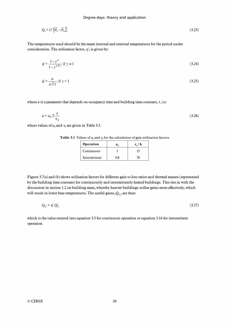
Degree-days: theory and application
© CIBSE
39
Ql = U i o( ) (3.23)
The temperatures used should be the mean internal and external temperatures for the period under consideration. The utilisation factor, , is given by:
=1 a
1 a +1; if 1 (3.24)
=a
a +1; if = 1 (3.25)
where a is a parameter that depends on occupancy time and building time constant, , i.e:
a = a0 +0
(3.26)
where values of a0 and 0 are given in Table 3.5.
Table 3.5 Values of a0 and 0 for the calculation of gain utilisation factors
Operation ao o / h
Continuous 1 15
Intermittent 0.8 70
Figure 3.7(a) and (b) shows utilisation factors for different gain to loss ratios and thermal masses (represented by the building time constant) for continuously and intermittently heated buildings. This ties in with the discussion in section 1.2 on building mass, whereby heavier buildings utilise gains more effectively, which will result in lower base temperatures. The useful gains, QG , are then:
QG = Q G (3.27)
which is the value entered into equation 3.5 for continuous operation or equation 3.16 for intermittent operation.

Degree-days: theory and application
© CIBSE
40
0
0.2
0.4
0.6
0.8
1
1.2
0 0.5 1 1.5 2 2.5 3
Gain to loss ratio
Ga
in u
tili
sa
tio
n fa
cto
r
8 hours 1 day 2 days 1 week
,
(a)
0
0.2
0.4
0.6
0.8
1
1.2
0 0.5 1 1.5 2 2.5 3
Gain to loss ratio
Ga
in u
tili
sa
tio
n fa
cto
r
8 hours 1 day 2 days 1 week
,
(b)
Figure 3.7 Gain utilisation factors for a range of building time constants: (a) continuously heated buildings,
(b) intermittently heated buildings [methodology taken from BS EN ISO 13790]

Degree-days: theory and application
© CIBSE
41
Example 3.5: Determination of gains
An 8000 m2 building occupied for 8 hours per day has a heat loss coefficient, U , of 8 kW K–1 and a calculated time constant, , of 21.24 hours. The mean internal temperature of the building is 18.2°C for a mean outdoor temperature of 8°C. For an occupant density of 15 m2 person–1 and solar gains (averaged over 24 hours) of 16.6 kW calculate the
gain utilisation factor and useful casual gains into the building.
The total internal gains during occupied hours can be estimated from equation 3.21:
qI = 224.97 15–0.7334 = 30.9 W m–2
This gives a peak internal gain of:
30.9 8000/1000 = 247.2 kW
This needs to be averaged over 24 hours and added to the solar gains:
247.2 8/24 + 16.6 = 99 kW
The average rate of heat loss is found from equation 3.23:
Ql = 8 (18.2 – 8) = 81.6 kW
The gives a gain to loss ratio, , of:
= 99/81.6 = 1.21
The gain utilisation factor can be read from Figure 3.7(b) or calculated using equation 3.24. In order to calculate ,
the parameter a is found from equation 3.26 and Table 3.5:
a = 0.8 + 21.24/70 = 1.1
Hence the gain utilisation factor, , is:
=1 1.211.1
1 1.211.1+1= 0.47
In which case the useful gains to the space are
QG = 0.47 99 47 kW

Degree-days: theory and application
© CIBSE
42
3.6 Cooling applications
The application of degree-days to cooling applications poses a number of additional complications, which have tended to be overlooked in the interests of maintaining simplicity. To become credible a cooling degree-day model must attempt to account for these factors. In their most general form these are:
the presence of latent loads
the possibility of high fresh air loads
the use of heat recovery, whether sensible only or sensible plus latent
variable air flows
the wide variety of cooling systems in use
the temperature dependence of chiller coefficient of performance (CoP).
The issue of latent loads has tended to suggest the use of enthalpy rather than simply dry bulb temperature in the energy analysis of systems. Such methods have been proposed [Sherman 1986]. More commonly enthalpy has been used in so-called ‘bin’ (or frequency of occurrence) calculations to estimate energy in air conditioning systems [ASHRAE 2001]. Bin methods can also handle heat recovery, system variety, and variation of CoP. However, bin methods suffer from an inability to distinguish when particular loads occur. Degree-days, on the other hand, offer the possibility of month-by-month assessments. In addition, they use the same parameter (dry bulb temperature) as used for the heating case, providing some continuity and consistency between the two applications. In developing a consistent and rational cooling degree-day approach, the way is set to understand how cooling degree-days can further be used in energy management for analysing existing buildings. The analyses described in chapter 5 therefore follow from the theory set out in the sections below.
As with heating applications the key to a credible cooling degree-day energy assessment lies in the definition of base temperature. The problem for cooling is that this needs to be defined specifically for each different type of cooling system. It is not possible to provide definitions for all system configurations, but three types of system will be presented here. The same principle can be adopted to determine the base temperature for other system types.
3.6.1 All air systems
ASHRAE [2001] defines cooling degree-day base temperature in the same way as for heating, i.e. using equation 3.5. However, with an air conditioned building the outdoor temperature will exceed the internal temperature for much of the time the system is operating (although not necessarily all of the time depending on the magnitude of the gains). Under these high outdoor temperature conditions the term QG / U has little physical significance in terms of the building energy balance; in any case this term has no relationship to the fresh air or latent components of the cooling demand. It follows that equation 3.5 cannot be used as a reliable definition of base temperature for all-air cooling systems. (It is more credible for other types of system as discussed in section 3.6.3.)
An alternative approach is to define the base temperature with reference to the cooling coil, which can be achieved by considering the coil energy balance [Day et al 2000]. Consider the 100% fresh air system in Figure 3.8.

Degree-days: theory and application
© CIBSE
43
Figure 3.8 Basic schematic of a full fresh air air-conditioning system
The energy extracted from the air is given by:
QE = ˙ m cp ao c( ) + ˙ m hfg go gs( ) (3.28)
where QE is the rate of heat removal from the air (kW), m& is the mass flow rate of the air (kg·s–1), cp is the specific heat of air (kJ·kg–1·K–1), hfg is the enthalpy of vaporisation of water (kJ·kg–1), ao is the outside air temperature (K),
c is the off-coil air temperature (K), and go and gs are the outside and off-coil moisture contents respectively (kg(water vapour)·kg–1(dry air).
This load can be broken down further into its components:
QE = Qfabric + Qsolar + QI + Qfan + Qfa(S) + Qfa(L) + QL (3.29)
where Qfabric is the fabric gain (kW), Qsolar is the solar gain (kW), QI is the internal sensible gain (kW), Qfan is the heat imparted to the air by the fan (kW), Qfa(S) is the net sensible heat extracted from the fresh air (kW), Qfa(L) is the fresh air latent load (kW) and QL is the room latent load (kW).
The fabric gain is given by:
Qfabric = U eo ai( ) (3.30)
The fabric gain (which may be a loss in certain circumstances) is likely to be reasonably small, especially in the UK where ambient temperatures will be close to the indoor set point temperature for much of the time. In such cases the treatment of this gain does not have to be too rigorous (and the treatment set out below is perfectly adequate). However, in some buildings fabric gain may be significant (for example single storey factory units with large roof areas), in which case more attention may have to be paid to this component. A simplified approach to fabric gains follows. In equation 3.30, eo is the sol-air temperature. This can be simplified by assuming the opaque fabric gains are small compared to the glazing conduction, in which case eo can be replaced by the air temperature, ao. If this is taken as the mean air temperature during the occupied hours, denoted ao(day) , this will capture at least some of these gains to the space. (Using the mean 24-hour air temperature would cancel these gains, and suggest no cooling load at all from this component.)
c o s
r
Cooling coil Fan ai
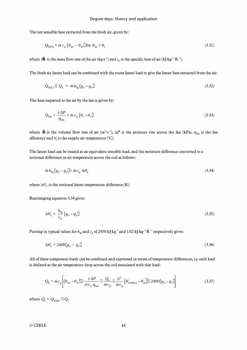
Degree-days: theory and application
© CIBSE
44
The net sensible heat extracted from the fresh air, given by:
Qfa(S) = ˙ m cp ao ai( ) for ao > c (3.31)
where m& is the mass flow rate of the air (kg·s–1) and cp is the specific heat of air (kJ·kg–1·K–1).
The fresh air latent load can be combined with the room latent load to give the latent heat extracted from the air:
Qfa(L) + QL = ˙ m hfg go gs( ) (3.32)
The heat imparted to the air by the fan is given by:
Qfan =˙ v P
fan
= ˙ m cp s c( ) (3.33)
where v& is the volume flow rate of air (m3·s–1), P is the pressure rise across the fan (kPa), fan is the fan efficiency and s is the supply air temperature (°C).
The latent load can be treated as an equivalent sensible load, and the moisture difference converted to a notional difference in air temperature across the coil as follows:
˙ m hfg go gs( ) = ˙ m cp L (3.34)
where L is the notional latent temperature difference (K).
Rearranging equation 3.34 gives:
L =hfg
cp
go gs( ) (3.35)
Putting in typical values for hfg and cp of 2450 kJ·kg–1 and 1.02 kJ·kg–1·K–1 respectively gives:
L = 2400 go gs( ) (3.36)
All of these component loads can be combined and expressed in terms of temperature differences, i.e. each load is defined as the air temperature drop across the coil associated with that load:
QE = ˙ m cp ao ai( ) +˙ v P
˙ m cp fan
+Qs
˙ m cp
+ U
˙ m cp
ao(day) ai( ) + 2400 go gs( )
(3.37)
where Qs = Qsolar + QI

Degree-days: theory and application
© CIBSE
45
In terms of energy extracted over time this can be re-expressed as an integral:
QE dt = ˙ m cp ao ai˙ v P
˙ m cp fan
Qs
˙ m cp
U ˙ m cp
ao(day) ai( ) 2400 go gs( )
dt (3.38)
The integral on the right hand side of equation 3.38 (i.e. in the curly brackets) is the cooling degree-day total, with the term inside the square brackets being the base temperature. More simply stated, the cooling base temperature is the off-coil dry bulb air temperature (required to deal with the sensible loads) minus the notional latent temperature difference.
In order to find the monthly cooling degree-days average monthly values of the variables in the square brackets can be used. In the case of moisture, the average difference can be found from a form of Hitchin’s formula:
(go – gs) =g o gs
1 e k g o gs( ) (3.39)
where g o is the mean monthly outdoor moisture content (kg·kg–1), and k is found from:
k =2.5
go
(3.40)
where go is the standard deviation of outdoor monthly moisture content.
For London, k lies in the region 1220 to 2300 [Day et al 2000] with a mean value of 1700. Note that L is relatively insensitive to changes in k.
It is possible to extend the concept to account for intermittent operation (with thermal capacity effects) and the use of heat recovery, shown in 3.6.1.1 and 3.6.1.2.
3.6.1.1 Thermal capacity effects
The issue of thermal capacity and intermittent operation is highly complex, but it is possible to provide a simplified model to attempt to take some account of this. Gains to the space will be absorbed by internal surfaces before becoming an apparent cooling load. Depending on the thermal capacity of the exposed mass the load on the cooling system can be mitigated if these gains can be stored and effectively released outside of occupancy hours. This is the principle of night-time cooling in which the building fabric cools overnight such that it can absorb heat the next day when the occupants arrive. The building fabric then warms up slowly during the day (staying below the room temperature) — heat is only released from the structure (becoming a gain to the space) when the ambient air temperature falls below the fabric temperature. These effects can be accounted for by using a form of the solution for equation 3.8:
i = i(3) sp( ) = et3 t1
1
sp ao(night)( ) (3.41)
where i is the change in the temperature of the building fabric (K) and (t3 – t1) is the unoccupied period (h).

Degree-days: theory and application
© CIBSE
46
In this case ao(night) should be the average overnight outdoor air temperature (°C). This change in fabric temperature can be multiplied by the thermal capacity of the structure, and divided by 24 3600 to give the average rate of gain that will be absorbed by the structure, QC , during the whole day:
QC =C i
24 3600 (3.42)
QC will have the opposite sign to the gains (i.e. it is a negative number) as it is mitigating the load on the plant. It can be incorporated into the base temperature expression (the square brackets of equation 3.38) as follows:
b = ai˙ v P
˙ m cp fan
Qs
˙ m cp
U ˙ m cp
ao(day) ai( ) 2400 go gs( )QC
˙ m cp
(3.43)
3.6.1.2 Heat recovery
Heat recovery in air conditioning systems can be either sensible only or sensible plus latent recovery. ‘Sensible only’ heat recovery devices include plate heat exchangers, run around coils and heat pipes; ‘sensible plus latent’ systems employ air recirculation or hygroscopic thermal wheels. Figure 3.9 shows a plate heat exchanger, giving sensible heat recovery.
Figure 3.9 Basic schematic of a full fresh air air-conditioning system employing sensible heat recovery
The effectiveness, , of a counter flow heat exchanger is constant and is given by:
=ao m( )
ao r( ) (3.44)
Where r is the return air temperature (normally the room air temperature plus a temperature rise for fan and duct gains) and the on-coil air temperature, m , is therefore:
m = ao ao r( ) (3.45)
where only positive values of ( ao – r) are valid.
c m
ao
s
r
Cooling coil Fan
Heat recovery
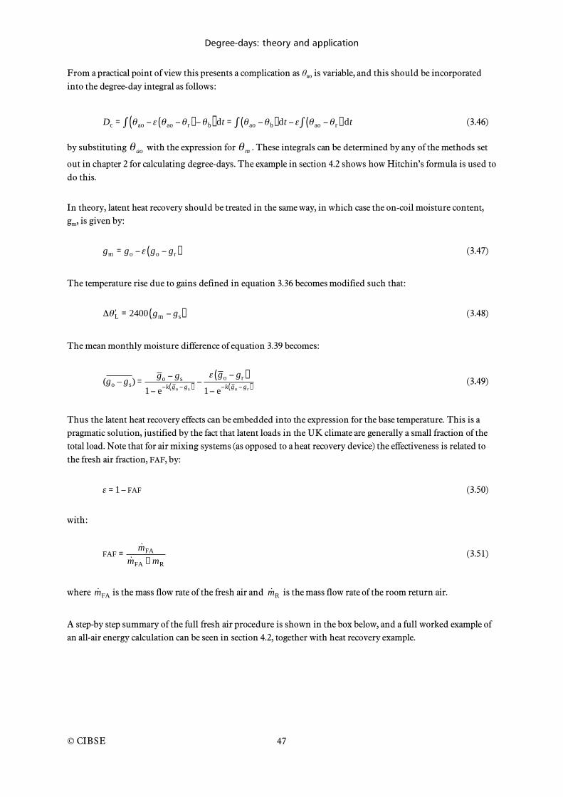
Degree-days: theory and application
© CIBSE
47
From a practical point of view this presents a complication as ao is variable, and this should be incorporated into the degree-day integral as follows:
Dc = ao ao r( ) b( ) dt = ao b( ) dt ao r( ) dt (3.46)
by substituting ao
with the expression for m
. These integrals can be determined by any of the methods set
out in chapter 2 for calculating degree-days. The example in section 4.2 shows how Hitchin’s formula is used to do this.
In theory, latent heat recovery should be treated in the same way, in which case the on-coil moisture content, gm, is given by:
gm = go go gr( ) (3.47)
The temperature rise due to gains defined in equation 3.36 becomes modified such that:
L = 2400 gm gs( ) (3.48)
The mean monthly moisture difference of equation 3.39 becomes:
(go – gs) =g o gs
1 e k g o gs( )
g o gr( )
1 e k g o g r( ) (3.49)
Thus the latent heat recovery effects can be embedded into the expression for the base temperature. This is a pragmatic solution, justified by the fact that latent loads in the UK climate are generally a small fraction of the total load. Note that for air mixing systems (as opposed to a heat recovery device) the effectiveness is related to the fresh air fraction, FAF, by:
= 1 FAF (3.50)
with:
FAF =˙ m FA
˙ m FA + mR
(3.51)
where ˙ m FA is the mass flow rate of the fresh air and ˙ m R is the mass flow rate of the room return air.
A step-by step summary of the full fresh air procedure is shown in the box below, and a full worked example of an all-air energy calculation can be seen in section 4.2, together with heat recovery example.

Degree-days: theory and application
© CIBSE
48
Cooling energy estimation step-by-step procedure (full fresh-air system)
This procedure will calculate the expected cooling energy consumption for a given month, together with costs and CO2 emissions. There is no expression available for defining the uncertainty in the procedure
A full worked example of this procedure can be found in section 4.2.
Input information
Building heat loss coefficient U (kW·K–1) (see equation 3.2)
Building thermal capacity C (kJ·K–1) (see equation 3.10)
Plant average Coefficient of Performance CoP
Average casual gains to the space QG (kW)
Occupied internal air temperature ai (°C)
Room moisture content gr (kg·kgdry air–1)
Mean monthly outdoor temperature o,m (°C)
Mean monthly daytime outdoor temperature ao, day (°C)
Mean monthly overnight outdoor temperature ao, night (°C)
Supply air moisture content gs (kg·kgdry air–1)
Monthly mean outdoor moisture content go (kg·kgdry air–1)
Fan pressure p (Pa)
Fan efficiency fan
Length of unoccupied period (t3 – t1) = 24 – occupied period (hours)
Step 1
Calculate heat carrying capacity of air, ˙ m cp , and the building time constant, .
Step 2
Calculate the various sensible loads on the coil in terms of their contribution to the supply air temperature. These are the fan gain, room casual gains (internal and solar), and the fabric gain.
2a – temperature rise due to fan gain =˙ v P
˙ m cp fan
2b – temperature rise due to casual gains =QS
˙ m cp
2c – temperature rise due to fabric gain =U'˙ m cp
ao,day ai( )
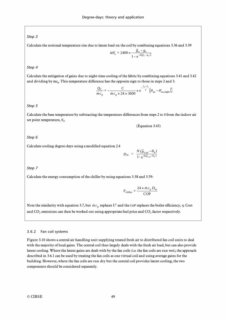
Degree-days: theory and application
© CIBSE
49
Step 3
Calculate the notional temperature rise due to latent load on the coil by combining equations 3.36 and 3.39
L = 2400g o gs
1 e k g o gs( )
Step 4
Calculate the mitigation of gains due to night-time cooling of the fabric by combining equations 3.41 and 3.42 and dividing by mcp. This temperature difference has the opposite sign to those in steps 2 and 3.
QC
˙ m cp
=C
˙ m cp 24 3600e
t3 t1
sp ao,night( )
Step 5
Calculate the base temperature by subtracting the temperature differences from steps 2 to 4 from the indoor air set point temperature, ai
(Equation 3.43)
Step 6
Calculate cooling degree-days using a modified equation 2.4
mD = N ( o,m b )
1 - -k( o,m b )e
Step 7
Calculate the energy consumption of the chiller by using equations 3.38 and 3.59:
Fchiller =24 ˙ m cp Dm
COP
Note the similarity with equation 3.7, but ˙ m cp replaces U and the CoP replaces the boiler efficiency, . Cost
and CO2 emissions can then be worked out using appropriate fuel price and CO2 factor respectively.
3.6.2 Fan coil systems
Figure 3.10 shows a central air handling unit supplying treated fresh air to distributed fan coil units to deal with the majority of local gains. The central coil thus largely deals with the fresh air load, but can also provide latent cooling. Where the latent gains are dealt with by the fan coils (i.e. the fan coils are run wet), the approach described in 3.6.1 can be used by treating the fan coils as one virtual coil and using average gains for the building. However, where the fan coils are run dry but the central coil provides latent cooling, the two components should be considered separately.
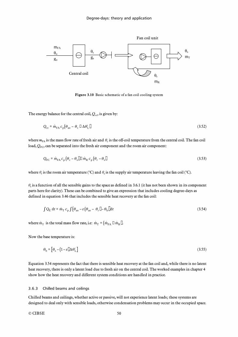
Degree-days: theory and application
© CIBSE
50
Figure 3.10 Basic schematic of a fan coil cooling system
The energy balance for the central coil, Qcc, is given by:
Qcc = ˙ m FA cp ao c + L( ) (3.52)
where mFA is the mass flow rate of fresh air and c is the off-coil temperature from the central coil. The fan coil load, QFC, can be separated into the fresh air component and the room air component:
QFC = ˙ m FA cp c s( ) + ˙ m R cp r s( ) (3.53)
where r is the room air temperature (°C) and s is the supply air temperature leaving the fan coil (°C).
s is a function of all the sensible gains to the space as defined in 3.6.1 (it has not been shown in its component parts here for clarity). These can be combined to give an expression that includes cooling degree-days as defined in equation 3.46 that includes the sensible heat recovery at the fan coil:
QE dt = ˙ m T cp ao ao r( ) b( ) dt (3.54)
where ˙ m T is the total mass flow rate, i.e: ˙ m T = ˙ m FA + ˙ m R( ) .
Now the base temperature is:
b = s 1( ) L[ ] (3.55)
Equation 3.54 represents the fact that there is sensible heat recovery at the fan coil and, while there is no latent heat recovery, there is only a latent load due to fresh air on the central coil. The worked examples in chapter 4 show how the heat recovery and different system conditions are handled in practice.
3.6.3 Chilled beams and ceilings
Chilled beams and ceilings, whether active or passive, will not experience latent loads; these systems are designed to deal only with sensible loads, otherwise condensation problems may occur in the occupied space.
r
mR
mFA
o
go
c
gs
s
mT
Central coil
Fan coil unit
Degree-days: theory and application
© CIBSE
51
These systems can be dealt with in the same way as the heating system. The energy balance on the cooling element will be equal to the sensible gains minus the losses from the space:
QC = QG U i o( ) (3.56)
At zero load the gains equal the losses, and this occurs when the outdoor temperature equals the base temperature (i.e. o = b):
i b( ) =QG
U (3.57)
This leads to precisely the same definition of base temperature as in the case of heating degree-days, but the temperatures within the degree-day integral are reversed. Thus the energy demand will be:
QE dt = U ao b( ) dt (3.58)
From this simple energy balance it is possible to draw inferences that may help in building energy diagnostics. For example when o = i (i.e. there are no losses) then the load will be equal to the gains, or QE = QG. Chapter 5 considers the implications of this and other issues arising from these energy balances for building energy analysis techniques.
3.6.4 Other issues for cooling energy analysis
The above analysis has only been concerned with the energy demand on the cooling element and not the energy consumption of the refrigeration plant. This will again be related to the plant efficiency, which for chillers will be the coefficient of performance, or CoP. Thus:
Fchiller =QE dt
COP (3.59)
However, CoP is strongly linked to outdoor temperature, as this has a bearing on the condensing pressure, and hence the work done by the compressor (or generator in the case of absorption chillers). A detailed discussion of this is beyond the scope of this publication, and average seasonal or monthly CoP s will be assumed.
The above theoretical system treatments do not include variable air volume systems. In such cases it may be more viable to adopt a frequency of occurrence (‘bin’) approach.
3.7 Summary
Degree-days measure the variation in outdoor temperature over time relative to a building base temperature. Since energy demand for space conditioning (heating or cooling) has a linear relationship with temperature difference it follows that there should be a linear relationship between energy consumed and degree-days. This section has set out a theoretical approach by which monthly energy estimates can be calculated for heating and cooling. These require a number of necessary simplifying assumptions:

Degree-days: theory and application
© CIBSE
52
It is legitimate to use average values of heat loss coefficient, temperature and gains coincidentally to obtain reasonable results.
The buildings and systems are well controlled.
A first-order response is reasonable for such simplified calculations.
The methods are not overly sensitive to assumptions about building thermal capacity.
Given the complexity of buildings, the above assumptions may be seen as difficulties in providing reliable results. However, the theory as set out is consistent and serves to demonstrate, in principle, how buildings behave. It is from this basis that other aspects of degree-day use can be explained, for example the use of performance lines as set out in chapter 5.
The above comments notwithstanding there is still merit in conducting degree-day based energy estimates, given the speed with which they can be carried out and the reduced potential for input error (when compared, say, to simulation). The methods presented for cooling systems are not fully comprehensive — there is not enough space available to construct energy balances for every conceivable cooling system — but the principle can be adopted and extended for all types of system.
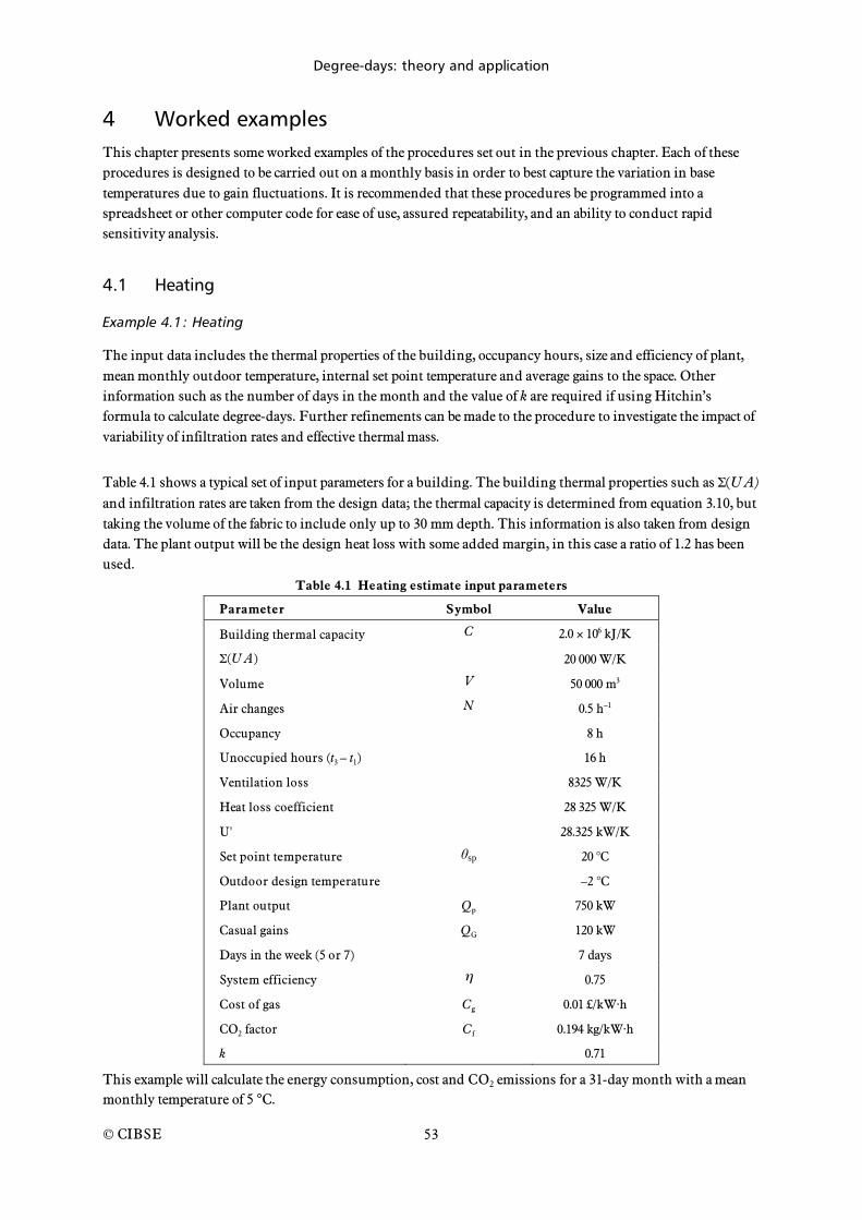
Degree-days: theory and application
© CIBSE
53
4 Worked examples This chapter presents some worked examples of the procedures set out in the previous chapter. Each of these procedures is designed to be carried out on a monthly basis in order to best capture the variation in base temperatures due to gain fluctuations. It is recommended that these procedures be programmed into a spreadsheet or other computer code for ease of use, assured repeatability, and an ability to conduct rapid sensitivity analysis.
4.1 Heating
Example 4.1: Heating
The input data includes the thermal properties of the building, occupancy hours, size and efficiency of plant, mean monthly outdoor temperature, internal set point temperature and average gains to the space. Other information such as the number of days in the month and the value of k are required if using Hitchin’s formula to calculate degree-days. Further refinements can be made to the procedure to investigate the impact of variability of infiltration rates and effective thermal mass.
Table 4.1 shows a typical set of input parameters for a building. The building thermal properties such as (U A) and infiltration rates are taken from the design data; the thermal capacity is determined from equation 3.10, but taking the volume of the fabric to include only up to 30 mm depth. This information is also taken from design data. The plant output will be the design heat loss with some added margin, in this case a ratio of 1.2 has been used.
Table 4.1 Heating estimate input parameters
Parameter Symbol Value
Building thermal capacity C 2.0 106 kJ/K
(U A) 20 000 W/K
Volume V 50 000 m3
Air changes N 0.5 h–1
Occupancy 8 h
Unoccupied hours (t3 – t1) 16 h
Ventilation loss 8325 W/K
Heat loss coefficient 28 325 W/K
U' 28.325 kW/K
Set point temperature sp 20 °C
Outdoor design temperature –2 °C
Plant output Qp 750 kW
Casual gains QG 120 kW
Days in the week (5 or 7) 7 days
System efficiency 0.75
Cost of gas Cg 0.01 £/kW·h
CO2 factor Cf 0.194 kg/kW·h
k 0.71
This example will calculate the energy consumption, cost and CO2 emissions for a 31-day month with a mean monthly temperature of 5 °C.

Degree-days: theory and application
© CIBSE
54
From the thermal properties the building time constant is calculated using equation 3.13:
= 2 106 / (3600 28.325) = 19.61 hours
The optimum plant switch-on temperature is then determined using equation 3.15:
so = 5 +750 20 5( ) e
16
19.61
750 + 28.325 20 5( ) e
16
19.61
28.325 20 5( )
= 14.7 °C
The pre-heat time (t3 – t2) is found from equation 3.14:
t3 – t2 = –19.61 ln750 – 28.325 (20 – 5)
750 – 28.325 (14.7 – 5)
= 7.45 h
and:
t2 – t1 = 16 – 7.45 = 8.55 h
(Note that this may appear an overly long pre-heat time. In reality we may expect shorter pre-heat times, i.e. buildings get up to acceptable temperatures more quickly. These equations only account for structure temperature, whereas in reality the air temperature (which is what an optimum start controller responds to) rises much faster. Therefore this model provides an average structure temperature that models the average heat loss driving force reasonably well.)
The mean internal temperature is now found from equations 3.12 and 3.11:
it1
t3
= (5 16) +19.61 20 5( ) e
7.45
19.61
e
8.55
19.61
+
19.61 750
28.3251+
7.45
19.61
e
7.45
19.61
= 277.12
i =277.12 + (20 8)
24= 18.21°C
The base temperature is now found from equation 3.16:
b = 18.21120
28.325= 13.97°C
which is used to calculate degree-days from Hitchin’s formula, equation 2.4:
Dm = 31 (13.97 – 5)
1 – –0.71 (13.97 – 5)e= 279 K day

Degree-days: theory and application
© CIBSE
55
Equation 3.7 is used to determine the fuel consumption:
F =24 28.325 279
0.75= 252886 kW h
It remains to calculate the expected accuracy of the result, the cost and associated CO2 emissions. The uncertainty of monthly energy estimates is found from equation 3.17:
E(95%) = 130 279 1.3 100 = 8.6%
Hence, the cost is:
252886 0.01 = £2528.86
and the CO2 emissions are:
(252886 0.194) / 1000 = 49 tonnes
For a 5-day per week occupancy, an additional step of calculating the weekend mean internal temperature needs to be conducted, and the overall mean internal temperature calculated according to a weighting of 3/7:
4/7 for the weekend (with Monday pre-heat) and normal weekday values respectively. This is done by using weekend unoccupied hours in place of the overnight hours to calculate the optimum switch on time, with the rest of the calculation proceeding as above.
4.2 All-air cooling
For a centralised all-air air conditioning system, monthly energy estimates can be carried out according to the method set out in 3.6.1. This section presents examples for both full fresh air and heat recovery using air recirculation. The recirculation method can also be used for heat recovery systems employing sensible and latent recovery (for example hygroscopic thermal wheels), and can be adapted for sensible-only recovery by ignoring the latent recovery component. Using degree-day methods for heat recovery systems suffers from an inability to explicitly vary the amount of heat recovery according to prevailing conditions; bin methods are able to account for the control of (for example) damper positions dependent upon outdoor temperature or enthalpy. However, the methodology set out here does implicitly account for this heat recovery control and any errors due to lack of explicit rigour are likely to be small.
Unlike the heating example, uncertainty analysis has not been conducted on the cooling methodology, and caution is urged when interpreting the results.
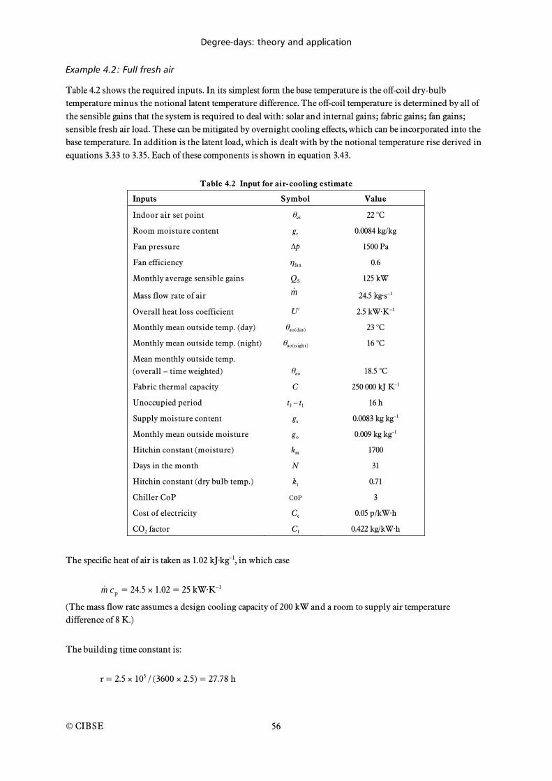
Degree-days: theory and application
© CIBSE
56
Example 4.2: Full fresh air
Table 4.2 shows the required inputs. In its simplest form the base temperature is the off-coil dry-bulb temperature minus the notional latent temperature difference. The off-coil temperature is determined by all of the sensible gains that the system is required to deal with: solar and internal gains; fabric gains; fan gains; sensible fresh air load. These can be mitigated by overnight cooling effects, which can be incorporated into the base temperature. In addition is the latent load, which is dealt with by the notional temperature rise derived in equations 3.33 to 3.35. Each of these components is shown in equation 3.43.
Table 4.2 Input for air-cooling estimate
Inputs Symbol Value
Indoor air set point ai 22 °C
Room moisture content gr 0.0084 kg/kg
Fan pressure p 1500 Pa
Fan efficiency fan 0.6
Monthly average sensible gains QS 125 kW
Mass flow rate of air ˙ m 24.5 kg·s–1
Overall heat loss coefficient U 2.5 kW·K–1
Monthly mean outside temp. (day) ao(day) 23 °C
Monthly mean outside temp. (night) ao(night) 16 °C
Mean monthly outside temp. (overall – time weighted) ao 18.5 °C
Fabric thermal capacity C 250 000 kJ K–1
Unoccupied period t3 – t1 16 h
Supply moisture content gs 0.0083 kg kg–1
Monthly mean outside moisture go 0.009 kg kg–1
Hitchin constant (moisture) km 1700
Days in the month N 31
Hitchin constant (dry bulb temp.) kt 0.71
Chiller CoP CoP 3
Cost of electricity Ce 0.05 p/kW·h
CO2 factor Cf 0.422 kg/kW·h
The specific heat of air is taken as 1.02 kJ·kg–1, in which case
˙ m cp = 24.5 1.02 = 25 kW·K–1
(The mass flow rate assumes a design cooling capacity of 200 kW and a room to supply air temperature difference of 8 K.)
The building time constant is:
= 2.5 105 / (3600 2.5) = 27.78 h
Degree-days: theory and application
© CIBSE
57
Taking the components of equation 3.43 in turn:
Fan temperature rise, from equation 3.33:
s c( ) =20.4 1.5
25 0.6= 2 K
Sensible gains to the space (solar, people, lights and machines):
Qs
˙ m cp
=125
25= 5 K
Daytime fabric gain from equation3.30, and dividing by ˙ m cp :
U
˙ m cp
ao ai( ) =2.5
2523 22( ) = 0.1 K
Notional latent component, combining equations 3.36 and 3.39:
L = 24000.009 0.0083
1 e 1700 0.009 0.0083( )= 2.41 K
Mitigation due to overnight cooling, combining equations 3.41 and 3.42 and dividing by ˙ m cp :
QC
˙ m cp
=250 103
24 3600
e16
27.78 1
22 16( )
25= 0.30 K
Putting all of these together (equation 3.43) now gives the base temperature
b = 22 – 2 – 5 – 0.1 – 2.41 +0.30 = 12.79 °C
Degree-days can now be calculated from a modified form of Hitchin’s formula, equation 2.4, that simply exchanges the positions of the temperatures (i.e. now using o – b):
Dm = 31 (18.5 – 12.79)
1 – –0.71 (18.5 –12.79)e= 180.1 K day
Since these degree-days are the effective summation of temperature difference across the coil, these are multiplied by the mass flow and specific heat of the air, ˙ m cp , and then by 24 to give kW·h. This is divided by
the CoP of the chiller to obtain the fuel consumption:
F =24 25 180.1
3.0= 36 020 kW h
Degree-days: theory and application
© CIBSE
58
The cost is:
36020 0.05 = £1801
and related CO2 emissions are:
(36020 0.422) / 1000 = 15.2 tonnes
Example 4.3: Sensible and latent heat recovery
This is an extension to Example 4.2. If we consider a recirculation system, sensible and latent heat will be recovered in proportion to the amount of room air mixing with the fresh air. This is normally expressed in terms of the fresh air fraction, FAF, or effectiveness, (which is actually (1 – FAF)). Thus for a FAF of 0.25, the effectiveness is 0.75. This can be incorporated into equations 3.46 and 3.49 to deal with the influence of heat recovery. Equation 3.49 will reduce the latent load on the coil according to how often go exceeds gr; the form of Hitchin’s formula accounts for the distribution of go that enables this. Thus the reduced notional latent temperature rise is now:
L = 24000.009 0.0083
1 e 1700 0.009 0.0083( )
0.75 0.009 0.0084( )
1 e 1700 0.009 0.0084( )
= 0.73K
This gives a revised base temperature of:
b = 22 – 2 – 5 – 0.1 – 0.73 + 0.3 = 14.5 °C
When using Hitchin’s formula equation 3.46 is dealt with in the same way as the latent component above. If working with daily or hourly outdoor temperatures the individual differences ( o – b) and ( o – r) would be determined separately and summed. Using Hitchin’s formula the solution is found as follows:
Dm = 3118.5 14.5
1 e 0.71 18.5 14.5( )
0.75 18.5 22( )
1 e 0.71 18.5 22( )
= 124 K day
Giving the energy consumption:
F =24 25 124
3.0= 24 800 kW h
Comparing this with the solution in Example 4.2 shows the savings due to heat recovery.
Example 4.4: Sensible only recovery
It is possible to conduct the analysis for sensible-only recovery by ignoring the adjustment for latent load in Example 4.3. This is done by entering the base temperature from Example 4.2 into the degree-day calculation of Example 4.3:

Degree-days: theory and application
© CIBSE
59
Dm = 3118.5 12.79
1 e 0.71 18.5 12.79( )
0.75 18.5 22( )
1 e 0.71 18.5 22( )
= 172.7 K day
Giving the energy consumption:
F =24 25 172.7
3.0= 34 540 kW h
Example 4.5: Fan coils
Using the same values as Example 4.2, the supply air temperature will be the room set point minus the temperature rise due to sensible gains (including overnight gain mitigation). In this case:
s = 22 – 2 – 5 – 0.1 +0.30 = 15.2 °C
The base temperature is found from equation 3.55. The notional latent temperature rise (at the central coil) is still 2.41 K as in Example 4.2. For a fresh air fraction of 0.25, equation 3.55 gives:
b = 15.2 0.25 2.41[ ] = 14.59 °C
Incorporating sensible heat recovery at the fan coil gives a degree-day total of :
Dm = 3118.5 14.59
1 e 0.71 18.5 14.59( )
0.75 18.5 22( )
1 e 0.71 18.5 22( )
= 121.9 K day
And an energy consumption of:
F =24 25 121.9
3.0= 24 380 kW h

Degree-days: theory and application
© CIBSE
60
5 Using degree-days in energy management The most common application of degree-days is in the analysis of energy consumption in existing buildings. Comparing the energy consumption of a building from one year to the other can be misleading without accounting for variations in weather, and since external temperature is the most important energy related variable (for space conditioning) it follows that degree-days can provide a mechanism to allow comparisons to take place.
There are different levels of analysis that can be conducted, from annual normalisation for rough benchmarks to detailed analysis with daily or hourly data. This chapter describes some of the techniques that can be used to draw inferences about the energy performance of a building. Section 5.1 discusses simple normalisation of annual space heating energy consumption often used for comparing buildings to standard benchmarks. Section 5.2 introduces the concept of energy signatures, which is used further in section 5.3 in the discussion on energy performance lines. Performance lines are a standard energy management tool, but their use can be extended for deeper analysis. This idea is taken further in section 5.4. Section 5.5 discusses some of the caveats that must be applied when considering the statistical techniques used in constructing performance lines. Section 5.6 summarises the chapter.
5.1 Normalisation of energy performance indicators for weather
Normalisation is a process of correcting for weather variations so that buildings in different regions can report standardised annual energy consumptions. The process requires the separation of weather and non-weather related loads. This can be done by assuming the summer heating consumption is due to non-weather demands (e.g. the hot water service), and that this is consistent throughout the year. It is also possible to use the regression analysis described later in this section to identify the base load.
Weather related loads are then divided by local annual degree-days to give energy consumed per degree-day, which is then multiplied by the UK 20-year average degree-day value — usually taken as 2462 K·day (using 15.5 °C base temperature). This provides a weather normalised space heating consumption, which is then added back to the base load and divided by the floor area to give a value in kW·h/m2.
Example 5.1: Normalised energy consumption
An open plan naturally ventilated office building with 20 000 m2 of treated floor area has a total measured gas consumption of 3.0 106 kW·h, 20% of which has been determined to be base load (non-weather related). Local average degree-days to base temperature 15.5 °C for that year were 2141 K·day. Calculate the normalised energy consumption for standard UK degree-days of 2462 (to base 15.5 °C):
Space heating consumption = 3.0 106 (1 – 0.2) = 2.4 106 kW·h
Weather correction = 2.4 106 (2462 / 2141) = 2 759 832 kW·h
Total corrected consumption = 2 759 832 + (3.0 106 0.2) = 3 359 832 kW·h
Normalised consumption = 3 359 832 / 20 000 = 168 kW·h/m2
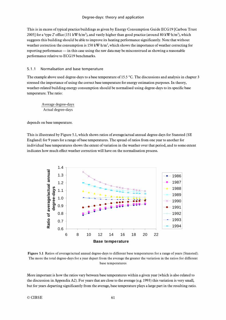
Degree-days: theory and application
© CIBSE
61
This is in excess of typical practice buildings as given by Energy Consumption Guide ECG19 [Carbon Trust 2005] for a ‘type 2’ office (151 kW·h/m2), and vastly higher than good practice (around 80 kW·h/m2), which suggests this building should be able to improve its heating performance significantly. Note that without weather correction the consumption is 150 kW·h/m2, which shows the importance of weather correcting for reporting performance — in this case using the raw data may be misconstrued as showing a reasonable performance relative to ECG19 benchmarks.
5.1.1 Normalisation and base temperature
The example above used degree-days to a base temperature of 15.5 °C. The discussions and analysis in chapter 3 stressed the importance of using the correct base temperature for energy estimation purposes. In theory, weather-related building energy consumption should be normalised using degree-days to its specific base temperature. The ratio:
Average degree days
Actual degree days
depends on base temperature.
This is illustrated by Figure 5.1, which shows ratios of average/actual annual degree-days for Stansted (SE England) for 9 years for a range of base temperatures. The spread of ratios from one year to another for individual base temperatures shows the extent of variation in the weather over that period, and to some extent indicates how much effect weather correction will have on the normalisation process.
0.6
0.7
0.8
0.9
1.0
1.1
1.2
1.3
1.4
6 8 10 12 14 16 18 20 22
Base temperature
Ra
tio
of
av
era
ge
/ac
tua
l a
nn
ua
l
de
gre
e-d
ay
s
1986
1987
1988
1989
1990
1991
1992
1993
1994
Figure 5.1 Ratios of average/actual annual degree-days to different base temperatures for a range of years (Stansted). The more the total degree-days for a year depart from the average the greater the variation in the ratios for different
base temperatures
More important is how the ratios vary between base temperatures within a given year (which is also related to the discussion in Appendix A2). For years that are close to the average (e.g. 1993) this variation is very small, but for years departing significantly from the average, base temperature plays a large part in the resulting ratio.
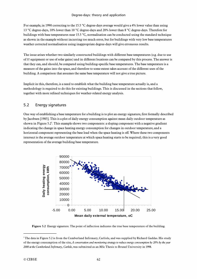
Degree-days: theory and application
© CIBSE
62
For example, in 1990 correcting to the 15.5 °C degree-days average would give a 4% lower value than using 13 °C degree-days, 10% lower than 10 °C degree-days and 20% lower than 8 °C degree-days. Therefore for buildings with base temperatures near 15.5 °C, normalisation can be conducted using the standard technique as shown in the example without incurring too much error, but for buildings with very low base temperatures weather corrected normalisation using inappropriate degree-days will give erroneous results.
The issue arises whether two similarly constructed buildings with different base temperatures (e.g. due to use of IT equipment or use of solar gains) and in different locations can be compared by this process. The answer is that they can, and should, be compared using building-specific base temperatures. The base temperature is a measure of the gains into the space, and therefore to some extent takes account of the different uses of the building. A comparison that assumes the same base temperature will not give a true picture.
Implicit in this, therefore, is a need to establish what the building base temperature actually is, and a methodology is required to do this for existing buildings. This is discussed in the sections that follow, together with more refined techniques for weather-related energy analysis.
5.2 Energy signatures
One way of establishing a base temperature for a building is to plot an energy signature, first formally described by Jacobsen [1985]. This is a plot of daily energy consumption against mean daily outdoor temperature as shown in Figure 5.21. This example shows two components: a sloping component with a negative gradient indicating the change in space heating energy consumption for changes in outdoor temperature, and a horizontal component representing the base load when the space heating is off. Where these two components intersect is the average outdoor temperature at which space heating starts to be required; this is a very good representation of the average building base temperature.
0
10000
20000
30000
40000
50000
60000
70000
80000
90000
-5.00 0.00 5.00 10.00 15.00 20.00 25.00
Mean daily external temperature, oC
Da
ily
he
ati
ng
en
erg
y
co
ns
um
pti
on
, k
Wh
Figure 5.2 Energy signature. The point of inflection indicates the true base temperature of the building.
1 The data in Figure 5.2 is from the Cumberland Infirmary, Carlisle, and was supplied by Richard Gaddas. His study of the energy consumption of the site, A conservation and monitoring strategy to reduce energy consumption by 20% by the year 2000 at the Cumberland Infirmary, Carlisle, was submitted as an MSc Thesis to Brunel University in 1998.

Degree-days: theory and application
© CIBSE
63
In theory this intersection can be found rigorously by separating the data into two parts, sorted by temperature, and applying regression analysis (a line of best fit) to the lower temperature set and putting a horizontal line through the upper data set (see Figure 5.2). The difficulty is choosing where the set should be split; a good first guess can be made by studying the plot and seeing where the change appears to occur. Some trial and error can be conducted in varying the point of split to maximise the coefficient of determination (R2 value). (For more explanation of regression analysis see section 5.5.) In this way it may be possible to find the most appropriate average base temperature. In practice it can be reasonably accurate to draw the lines manually by eye, and it should be emphasised that this is not a precise science.
Energy signatures can also be constructed for cooling energy analysis, i.e. a plot of electricity consumption against outdoor air temperature. This can give reliable results particularly where cooling plant energy consumption is sub-metered.
5.3 Performance lines and degree-days
Since energy signatures require large data sets that may not be available to a typical building operator, the more usual analysis tool is the performance line, which is a plot of monthly energy consumption against monthly degree-days. Performance lines have been in use for many years, and are well documented as an energy management tool (for example McVicker [1946], Harris [1989], Levermore [1989]). Performance lines exhibit much less scatter than a daily energy signature, as many of the thermal capacity effects, gain fluctuations, and occupancy (e.g. weekend) fluctuations are subsumed within single monthly energy and degree-day values. The performance line is the tool typically used to show how energy consumption varies with weather; it gives reliable indications of a building’s response with manageable amounts of data.
The theory set out in section 3.1 shows that if all other factors are reasonably constant, space heating energy consumption is proportional to changes in outdoor temperature (a similar assertion can be made for cooling energy). It follows that such energy consumption is proportional to degree-days, as explicitly stated by equation 3.7, i.e:
F =24 U Dd
Therefore, in theory, a graph that plots building energy consumption against degree-days should yield a straight line of the form:
F = Dd + (5.1)
where is the y-axis intercept, which under specific conditions will represent the base load energy consumption (i.e. that energy consumption not related to space heating) and is the slope of the line, which according to equation 3.7 is related to the building heat loss coefficient thus:
=F
Dd
=24 U
(5.2)
However, for equation 5.2 to be true (and therefore for to equal the true base load), the degree-days must be calculated to the building-specific base temperature. This will be illustrated in the examples that follow.
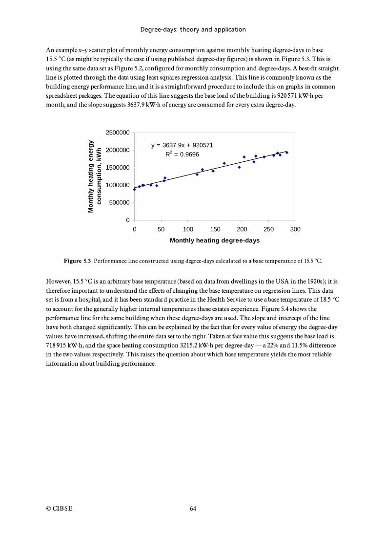
Degree-days: theory and application
© CIBSE
64
An example x–y scatter plot of monthly energy consumption against monthly heating degree-days to base 15.5 °C (as might be typically the case if using published degree-day figures) is shown in Figure 5.3. This is using the same data set as Figure 5.2, configured for monthly consumption and degree-days. A best-fit straight line is plotted through the data using least squares regression analysis. This line is commonly known as the building energy performance line, and it is a straightforward procedure to include this on graphs in common spreadsheet packages. The equation of this line suggests the base load of the building is 920 571 kW·h per month, and the slope suggests 3637.9 kW·h of energy are consumed for every extra degree-day.
y = 3637.9x + 920571
R2 = 0.9696
0
500000
1000000
1500000
2000000
2500000
0 50 100 150 200 250 300
Monthly heating degree-days
Mo
nth
ly h
ea
tin
g e
ne
rgy
co
ns
um
pti
on
, k
Wh
Figure 5.3 Performance line constructed using degree-days calculated to a base temperature of 15.5 °C.
However, 15.5 °C is an arbitrary base temperature (based on data from dwellings in the USA in the 1920s); it is therefore important to understand the effects of changing the base temperature on regression lines. This data set is from a hospital, and it has been standard practice in the Health Service to use a base temperature of 18.5 °C to account for the generally higher internal temperatures these estates experience. Figure 5.4 shows the performance line for the same building when these degree-days are used. The slope and intercept of the line have both changed significantly. This can be explained by the fact that for every value of energy the degree-day values have increased, shifting the entire data set to the right. Taken at face value this suggests the base load is 718 915 kW·h, and the space heating consumption 3215.2 kW·h per degree-day — a 22% and 11.5% difference in the two values respectively. This raises the question about which base temperature yields the most reliable information about building performance.

Degree-days: theory and application
© CIBSE
65
y = 3215.2x + 718915
R2 = 0.9639
0
500000
1000000
1500000
2000000
2500000
0 100 200 300 400
Monthly heating degree-days
Mo
nth
ly h
ea
tin
g e
ne
rgy
co
ns
um
pti
on
, k
Wh
Figure 5.4 Performance line constructed using degree-days calculated to a base temperature of 18.5 °C
Standard practice for constructing performance lines, for example in CUSUM analysis (see, for example GPG310 [Carbon Trust 2006]), suggests it is perfectly reasonable to use published values to base 15.5 °C. (An example CUSUM analysis is presented in the box below to illustrate this standard energy management technique.) This provides consistency in the normalisation process, and the degree-day values will come from a reliable source. Where this practice exists it is sensible to continue with it. However, it may be more beneficial to try to establish the true base temperature of the building. Figure 5.2 showed this is possible with daily energy data, but it is also possible using just monthly energy data.
Figure 5.5 shows the same plot as Figure 5.4 (i.e. base temperature 18.5 ° C) but with a polynomial line of best fit of the form:
y = x 2+ x + (5.3)
y = 2.3128x2 + 2243x + 791973
R2 = 0.9676
0
500000
1000000
1500000
2000000
2500000
0 100 200 300 400
Monthly heating degree-days
Mo
nth
ly h
ea
tin
g e
ne
rgy
co
ns
um
pti
on
, k
Wh
Figure 5.5 Polynomial line of best fit (degree-days to base 18.5 °C)
This is also a standard function of most spreadsheet packages. In this case is positive and there is an observed curvature of the line. Figure 5.6 shows a polynomial fit using degree-days to base 14.5 °C (this has
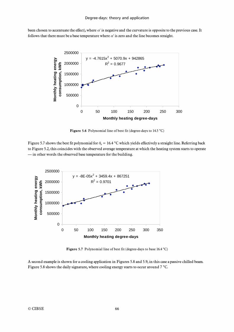
Degree-days: theory and application
© CIBSE
66
been chosen to accentuate the effect), where is negative and the curvature is opposite to the previous case. It follows that there must be a base temperature where is zero and the line becomes straight.
y = -4.7615x2 + 5070.9x + 942865
R2 = 0.9677
0
500000
1000000
1500000
2000000
2500000
0 50 100 150 200 250 300
Monthly heating degree-days
Mo
nth
ly h
ea
tin
g e
ne
rgy
co
ns
um
pti
on
, k
Wh
Figure 5.6 Polynomial line of best fit (degree-days to 14.5 °C)
Figure 5.7 shows the best fit polynomial for b = 16.4 °C which yields effectively a straight line. Referring back to Figure 5.2, this coincides with the observed average temperature at which the heating system starts to operate — in other words the observed base temperature for the building.
y = -8E-05x2 + 3459.4x + 867251
R2 = 0.9701
0
500000
1000000
1500000
2000000
2500000
0 50 100 150 200 250 300 350
Monthly heating degree-days
Mo
nth
ly h
ea
tin
g e
ne
rgy
co
ns
um
pti
on
, k
Wh
Figure 5.7 Polynomial line of best fit (degree-days to base 16.4 °C)
A second example is shown for a cooling application in Figures 5.8 and 5.9, in this case a passive chilled beam. Figure 5.8 shows the daily signature, where cooling energy starts to occur around 7 °C.
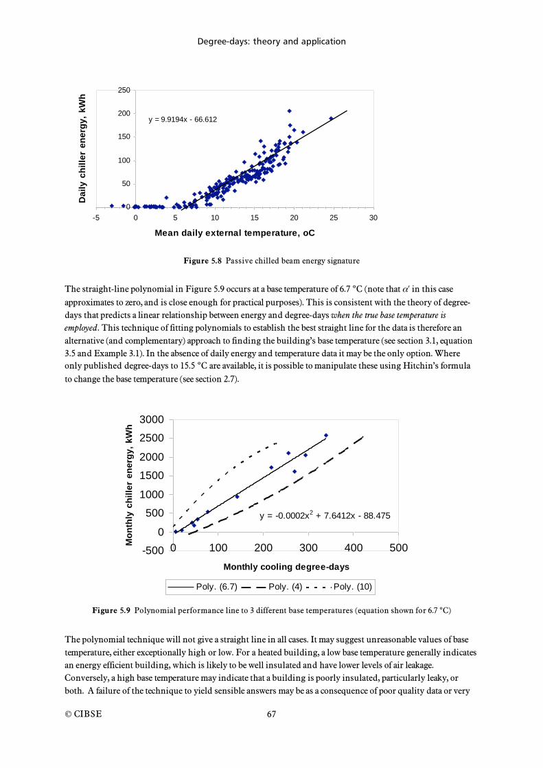
Degree-days: theory and application
© CIBSE
67
0
50
100
150
200
250
-5 0 5 10 15 20 25 30
Mean daily external temperature, oC
Da
ily
ch
ille
r e
ne
rgy
, k
Wh
y = 9.9194x - 66.612
Figure 5.8 Passive chilled beam energy signature
The straight-line polynomial in Figure 5.9 occurs at a base temperature of 6.7 °C (note that in this case approximates to zero, and is close enough for practical purposes). This is consistent with the theory of degree-days that predicts a linear relationship between energy and degree-days when the true base temperature is employed. This technique of fitting polynomials to establish the best straight line for the data is therefore an alternative (and complementary) approach to finding the building’s base temperature (see section 3.1, equation 3.5 and Example 3.1). In the absence of daily energy and temperature data it may be the only option. Where only published degree-days to 15.5 °C are available, it is possible to manipulate these using Hitchin’s formula to change the base temperature (see section 2.7).
y = -0.0002x2 + 7.6412x - 88.475
-500
0
500
1000
1500
2000
2500
3000
0 100 200 300 400 500
Monthly cooling degree-days
Mo
nth
ly c
hil
ler
en
erg
y,
kW
h
Poly. (6.7) Poly. (4) Poly. (10)
Figure 5.9 Polynomial performance line to 3 different base temperatures (equation shown for 6.7 °C)
The polynomial technique will not give a straight line in all cases. It may suggest unreasonable values of base temperature, either exceptionally high or low. For a heated building, a low base temperature generally indicates an energy efficient building, which is likely to be well insulated and have lower levels of air leakage. Conversely, a high base temperature may indicate that a building is poorly insulated, particularly leaky, or both. A failure of the technique to yield sensible answers may be as a consequence of poor quality data or very
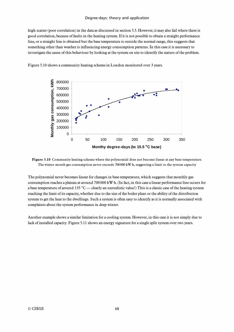
Degree-days: theory and application
© CIBSE
68
high scatter (poor correlation) in the data as discussed in section 5.5. However, it may also fail where there is good correlation, because of faults in the heating system. If it is not possible to obtain a straight performance line, or a straight line is obtained but the base temperature is outside the normal range, this suggests that something other than weather is influencing energy consumption patterns. In this case it is necessary to investigate the cause of this behaviour by looking at the system on site to identify the nature of the problem.
Figure 5.10 shows a community heating scheme in London monitored over 3 years.
0
100000
200000
300000
400000
500000
600000
700000
800000
0 50 100 150 200 250 300 350
Monthy degree-days (to 15.5 oC base)
Mo
nth
ly g
as
co
ns
um
pti
on
, k
Wh
Figure 5.10 Community heating scheme where the polynomial does not become linear at any base temperature.
The winter month gas consumption never exceeds 700 000 kW·h, suggesting a limit to the system capacity
The polynomial never becomes linear for changes in base temperature, which suggests that monthly gas consumption reaches a plateau at around 700 000 kW·h. (In fact, in this case a linear performance line occurs for a base temperature of around 135 °C — clearly an unrealistic value!) This is a classic case of the heating system reaching the limit of its capacity, whether due to the size of the boiler plant or the ability of the distribution system to get the heat to the dwellings. Such a system is often easy to identify as it is normally associated with complaints about the system performance in deep winter.
Another example shows a similar limitation for a cooling system. However, in this case it is not simply due to lack of installed capacity. Figure 5.11 shows an energy signature for a single split system over two years.
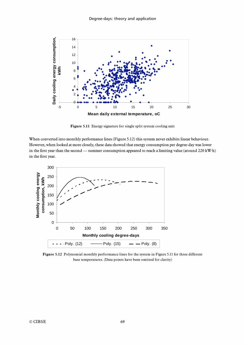
Degree-days: theory and application
© CIBSE
69
0
2
4
6
8
10
12
14
16
-5 0 5 10 15 20 25 30
Mean daily external temperature, oC
Da
ily
co
oli
ng
en
erg
y c
on
su
mp
tio
n,
kW
h
Figure 5.11 Energy signature for single split system cooling unit
When converted into monthly performance lines (Figure 5.12) this system never exhibits linear behaviour. However, when looked at more closely, these data showed that energy consumption per degree-day was lower in the first year than the second — summer consumption appeared to reach a limiting value (around 220 kW·h) in the first year.
0
50
100
150
200
250
300
0 50 100 150 200 250 300 350
Monthly cooling degree-days
Mo
nth
ly c
oo
lin
g e
ne
rgy
co
ns
um
pti
on
, k
Wh
Poly. (12) Poly. (15) Poly. (8)
Figure 5.12 Polynomial monthly performance lines for the system in Figure 5.11 for three different
base temperatures. (Data points have been omitted for clarity)
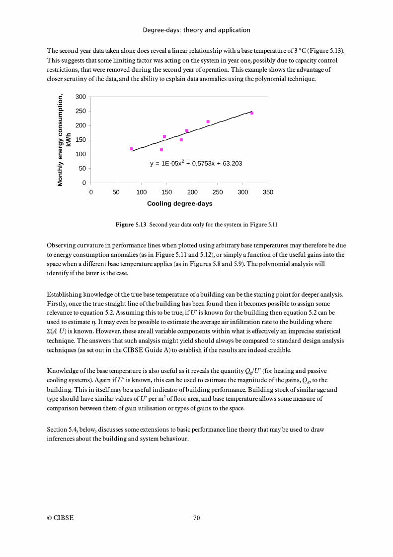
Degree-days: theory and application
© CIBSE
70
The second year data taken alone does reveal a linear relationship with a base temperature of 3 °C (Figure 5.13). This suggests that some limiting factor was acting on the system in year one, possibly due to capacity control restrictions, that were removed during the second year of operation. This example shows the advantage of closer scrutiny of the data, and the ability to explain data anomalies using the polynomial technique.
y = 1E-05x2 + 0.5753x + 63.203
0
50
100
150
200
250
300
0 50 100 150 200 250 300 350
Cooling degree-days
Mo
nth
ly e
ne
rgy
co
ns
um
pti
on
,
kW
h
Figure 5.13 Second year data only for the system in Figure 5.11
Observing curvature in performance lines when plotted using arbitrary base temperatures may therefore be due to energy consumption anomalies (as in Figure 5.11 and 5.12), or simply a function of the useful gains into the space when a different base temperature applies (as in Figures 5.8 and 5.9). The polynomial analysis will identify if the latter is the case.
Establishing knowledge of the true base temperature of a building can be the starting point for deeper analysis. Firstly, once the true straight line of the building has been found then it becomes possible to assign some relevance to equation 5.2. Assuming this to be true, if U is known for the building then equation 5.2 can be used to estimate . It may even be possible to estimate the average air infiltration rate to the building where
(A U) is known. However, these are all variable components within what is effectively an imprecise statistical technique. The answers that such analysis might yield should always be compared to standard design analysis techniques (as set out in the CIBSE Guide A) to establish if the results are indeed credible.
Knowledge of the base temperature is also useful as it reveals the quantity Qg/U (for heating and passive cooling systems). Again if U is known, this can be used to estimate the magnitude of the gains, Qg, to the building. This in itself may be a useful indicator of building performance. Building stock of similar age and type should have similar values of U per m2 of floor area, and base temperature allows some measure of comparison between them of gain utilisation or types of gains to the space.
Section 5.4, below, discusses some extensions to basic performance line theory that may be used to draw inferences about the building and system behaviour.

Degree-days: theory and application
© CIBSE
71
Example 5.1: CUSUM
The table below shows the energy consumption and heating degree-days for a variable refrigerant flow (VRF) reverse cycle heat pump system monitored over a 16-month period. Note that all values have been rounded for clarity.
Date Degree-days Actual energy consumption
/ kW·h
Predicted energy
consumption / kW·h
Difference / kW·h
CUSUM
/ kW·h
Savings (at 5 p / kW·h)
/ £
Dec-00 119 15503 13285 2218 2218
Jan-01 168 14106 14645 –540 1678
Feb-01 118 12645 13241 –596 1083
Mar-01 101 12147 12790 –643 439
Apr-01 42 10583 11155 –572 –132
May-01 25 10125 10684 –559 –691
Jun-01 0 9544 9983 –439 –1130
Jul-01 0 11113 9983 1130 0
Aug-01 0 8785 9983 –1198 –1198 60
Sep-01 0 5380 9983 –4603 –5801 290
Oct-01 0 5274 9992 –4718 –10519 526
Nov-01 59 8787 11629 –2842 –13361 668
Dec-01 157 12232 14322 –2089 –15450 773
Jan-02 72 9943 11967 –2024 –17474 874
Feb-02 71 8191 11949 –3758 –21232 1062
Mar-02 43 9608 11176 –1568 –22800 1140
In August 2001 a time clock was installed to prevent the system operating at weekends when the building was unoccupied. Hitherto the system had run all weekend. A performance line was constructed using the data for December 2000 to July 2001 inclusive to show the performance of the system prior to the time clock activation (see below).
y = 27.672x + 9983.1
0
2000
4000
6000
8000
10000
12000
14000
16000
18000
0.0 50.0 100.0 150.0 200.0
Monthly heating degree-days
Mo
nth
ly e
ne
rgy
, k
Wh
Example 5.1 Performance line
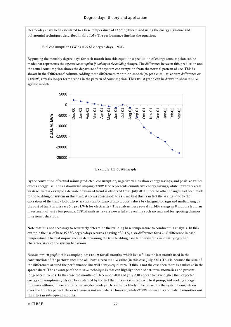
Degree-days: theory and application
© CIBSE
72
Degree-days have been calculated to a base temperature of 13.6 °C (determined using the energy signature and
polynomial techniques described in this TM). The performance line has the equation:
Fuel consumption (kW·h) = 27.67 degree-days + 9983.1
By putting the monthly degree-days for each month into this equation a prediction of energy consumption can be made that represents the expected consumption if nothing in the building changes. The difference between this prediction and the actual consumption shows the departure of the system consumption from the normal pattern of use. This is shown in the ‘Difference’ column. Adding these differences month-on-month (to get a cumulative sum difference or ‘CUSUM’) reveals longer term trends in the pattern of consumption. The CUSUM graph can be drawn to show CUSUM against month.
-25000
-20000
-15000
-10000
-5000
0
5000
Dec-0
0
Jan-0
1
Feb-0
1
Mar-
01
Apr-
01
May-0
1
Jun-0
1
Jul-01
Aug-0
1
Sep-0
1
Oct-
01
Nov-
01
Dec-0
1
Jan-0
2
Feb-0
2
Mar-
02
CU
SU
M,
kW
h
Example 5.1 CUSUM graph
By the convention of ‘actual minus predicted’ consumption, negative values show energy savings, and positive values excess energy use. Thus a downward sloping CUSUM line represents cumulative energy savings, while upward reveals wastage. In this example a definite downward trend is observed from July 2001. Since no other changes had been made to the building or system in this time, it seems reasonable to assume that this is in fact the savings due to the operation of the time clock. These savings can be turned into money values by changing the sign and multiplying by the cost of fuel (in this case 5 p per kW·h for electricity). The analysis here reveals £1140 savings in 8 months from an investment of just a few pounds. CUSUM analysis is very powerful at revealing such savings and for spotting changes in system behaviour.
Note that it is not necessary to accurately determine the building base temperature to conduct this analysis. In this example the use of base 15.5 °C degree-days returns a saving of £1177, a 3% difference for a 2 °C difference in base
temperature. The real importance in determining the true building base temperature is in identifying other characteristics of the system behaviour.
Note on CUSUM graphs: this example plots CUSUM for all months, which is useful as the last month used in the construction of the performance line will have a zero CUSUM value (in this case July 2001). This is because the sum of the differences around the performance line will always equal zero. If this is not the case then there is a mistake in the spreadsheet! The advantage of the CUSUM technique is that can highlight both short-term anomalies and present longer-term trends. In this case the months of December 2000 and July 2001 appear to have higher than expected energy consumptions. July can be explained by the fact that this is a reverse cycle heat pump, and cooling energy increases although there are zero heating degree-days. December is likely to be caused by the system being left on over the holiday period (the exact cause is not recorded). However, while CUSUM shows this anomaly it smoothes out the effect in subsequent months.
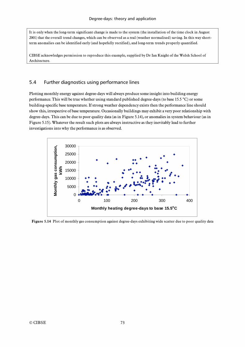
Degree-days: theory and application
© CIBSE
73
It is only when the long-term significant change is made to the system (the installation of the time clock in August 2001) that the overall trend changes, which can be observed as a real (weather normalised) saving. In this way short-term anomalies can be identified early (and hopefully rectified), and long-term trends properly quantified.
CIBSE acknowledges permission to reproduce this example, supplied by Dr Ian Knight of the Welsh School of Architecture.
5.4 Further diagnostics using performance lines
Plotting monthly energy against degree-days will always produce some insight into building energy performance. This will be true whether using standard published degree-days (to base 15.5 °C) or some building-specific base temperature. If strong weather dependency exists then the performance line should show this, irrespective of base temperature. Occasionally buildings may exhibit a very poor relationship with degree-days. This can be due to poor quality data (as in Figure 5.14), or anomalies in system behaviour (as in Figure 5.15). Whatever the result such plots are always instructive as they inevitably lead to further investigations into why the performance is as observed.
0
5000
10000
15000
20000
25000
30000
0 100 200 300 400
Monthly heating degree-days to base 15.5oC
Mo
nth
ly g
as
co
ns
um
pti
on
,
kW
h
Figure 5.14 Plot of monthly gas consumption against degree-days exhibiting wide scatter due to poor quality data

Degree-days: theory and application
© CIBSE
74
0
500
1000
1500
2000
2500
3000
3500
0 100 200 300 400 500
Monthly Cooling degree-days
Mo
nth
ly c
hil
ler
en
erg
y c
on
su
mp
tio
n,
kW
h
Figure 5.15 Plot of monthly chiller electricity consumption against cooling degree-days (base temperature 5 °C)
exhibiting wide scatter due to system anomalies
In the case of poor relationships it may be possible to extract better quality data, or ascertain the causes of anomalies (for example control failure or occupant behaviour). Figure 5.16 shows the latter 6.5 years of data from Figure 5.14, with suitable adjustments for timings of meter readings. Inspection of these data showed the early years to be unreliable with missing data and some evidently fabricated data. It also showed December data to be routinely low and January routinely high. This indicated manual meter readings taken to account for the Christmas holiday period. Simple pro-rata adjustments can be made to reduce (although not eliminate) the scatter due to these reading anomalies. Exceptional anomalies that still exist can be identified and investigated further (for example the December month circled in Figure 5.16). This data can now be used for more reliable analysis of the building energy use.
0
2000
4000
6000
8000
10000
12000
14000
0 50 100 150 200 250 300 350
Monthly heating degree-days to base 15.5oC
Mo
nth
ly G
as
Co
ns
um
pti
on
,
kW
h
Figure 5.16 Latter 6.5 years of the data from Figure 5.14 with adjustments for early December meter readings
Cases such as Figure 5.15, where data quality is assured, will require closer investigation of the system operation. This case (employing split air conditioning units) is not easy to explain, although very high energy consumptions in the first summer (ringed in Figure 5.15) led to control adjustments. While this certainly led to reduced energy use it did not lead to an improved performance line that could be used in, say, a CUSUM

Degree-days: theory and application
© CIBSE
75
analysis. Such a situation should always prompt more detailed investigations into the system and building to further determine the causes for this performance.
In many cases such investigations will yield improvements that will tend to linearise subsequent performance lines, in which case the more detailed investigation into performance can be conducted using the techniques described in section 5.3 above. Where linearity is never exhibited this is likely to be the result of specific system or plant behaviour that needs to be explained on a case-by-case basis. Where linearity does exist some possible further uses of performance lines are given in the sections that follow.
5.4.1 Heating and cooling
Where a building is equipped with heating and cooling it is possible to identify possible conflicts in the control system, such that there may be simultaneous heating and cooling or overlap in the system operation. Figure 5.17 shows the daily energy signature for an active chilled beam system employing a reverse cycle heat pump. From this data it is evident that a changeover occurs from heating to cooling at around 10°C, but it is not possible to separate heating and cooling energy in this region. In theory there should be a dead band between heating and cooling demand, but there is no clear evidence of this. This apparent overlap may be explained by variation in gains from day to day, and as these are independent of outdoor temperature they introduce scatter into the data.
0
200
400
600
800
1000
1200
1400
-5 0 5 10 15 20 25 30
Outdoor temperature, oC
Da
ily
en
erg
y c
on
su
mp
tio
n,
kW
h
Figure 5.17 Daily energy signature — active chilled beams with reverse-cycle heat pump
By separating the data into cooling and heating months and calculating cooling and heating degree-days, it is possible to establish polynomial best fit lines as described above. These are shown for heating and cooling in Figures 5.18 and 5.19 respectively. These suggest that the cooling base temperature is 9.3°C and the heating base temperature is 7.2°C, which would appear to confirm that there is some dead band between the two modes. Had the heating base temperature exceeded that for cooling, it would have indicated a conflict in the control strategy which may require attention.
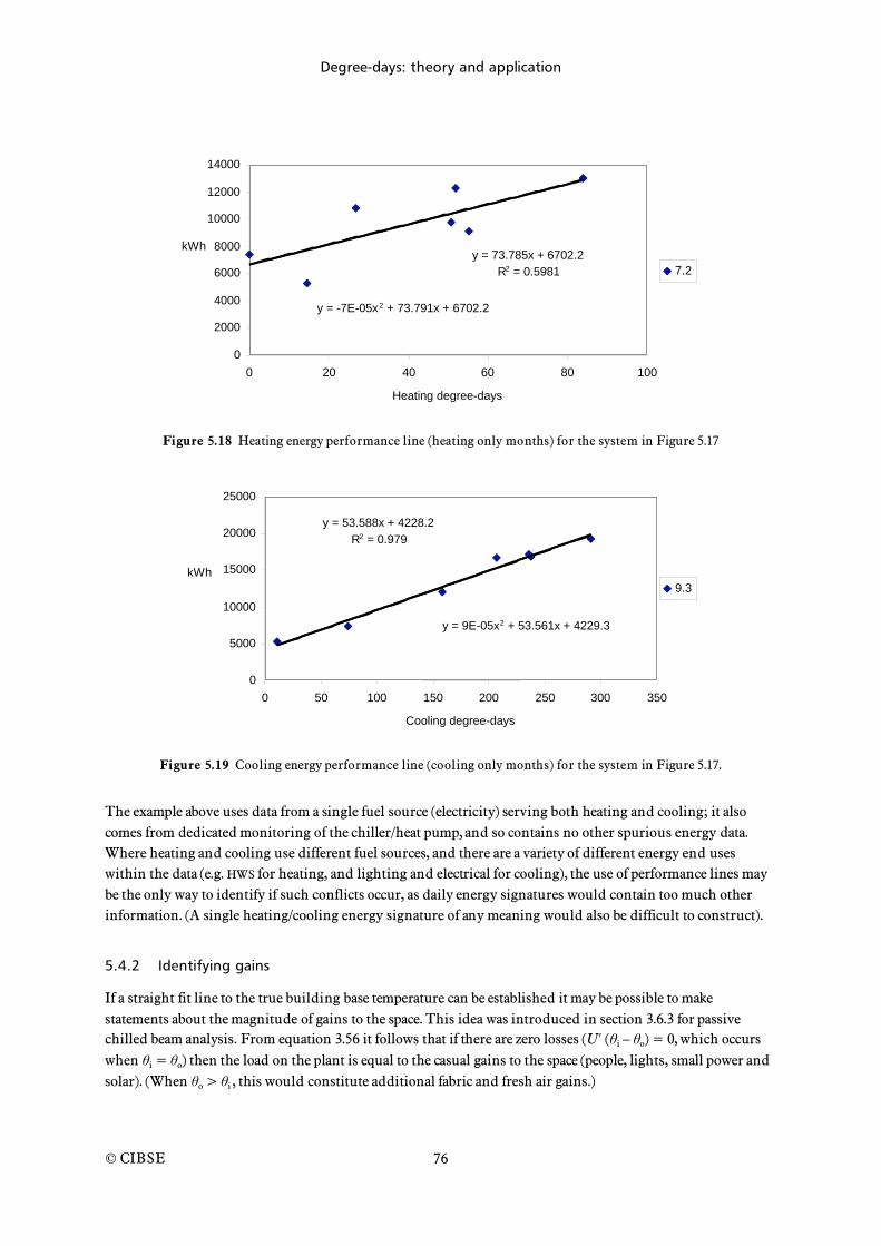
Degree-days: theory and application
© CIBSE
76
y = -7E-05x 2 + 73.791x + 6702.2
y = 73.785x + 6702.2
R 2 = 0.5981
0
2000
4000
6000
8000
10000
12000
14000
0 20 40 60 80 100
Heating degree-days
kWh
7.2
Figure 5.18 Heating energy performance line (heating only months) for the system in Figure 5.17
y = 53.588x + 4228.2
R 2 = 0.979
y = 9E-05x 2 + 53.561x + 4229.3
0
5000
10000
15000
20000
25000
0 50 100 150 200 250 300 350
Cooling degree-days
kWh
9.3
Figure 5.19 Cooling energy performance line (cooling only months) for the system in Figure 5.17.
The example above uses data from a single fuel source (electricity) serving both heating and cooling; it also comes from dedicated monitoring of the chiller/heat pump, and so contains no other spurious energy data. Where heating and cooling use different fuel sources, and there are a variety of different energy end uses within the data (e.g. HWS for heating, and lighting and electrical for cooling), the use of performance lines may be the only way to identify if such conflicts occur, as daily energy signatures would contain too much other information. (A single heating/cooling energy signature of any meaning would also be difficult to construct).
5.4.2 Identifying gains
If a straight fit line to the true building base temperature can be established it may be possible to make statements about the magnitude of gains to the space. This idea was introduced in section 3.6.3 for passive chilled beam analysis. From equation 3.56 it follows that if there are zero losses (U ( i – o) = 0, which occurs when i = o) then the load on the plant is equal to the casual gains to the space (people, lights, small power and solar). (When o > i , this would constitute additional fabric and fresh air gains.)
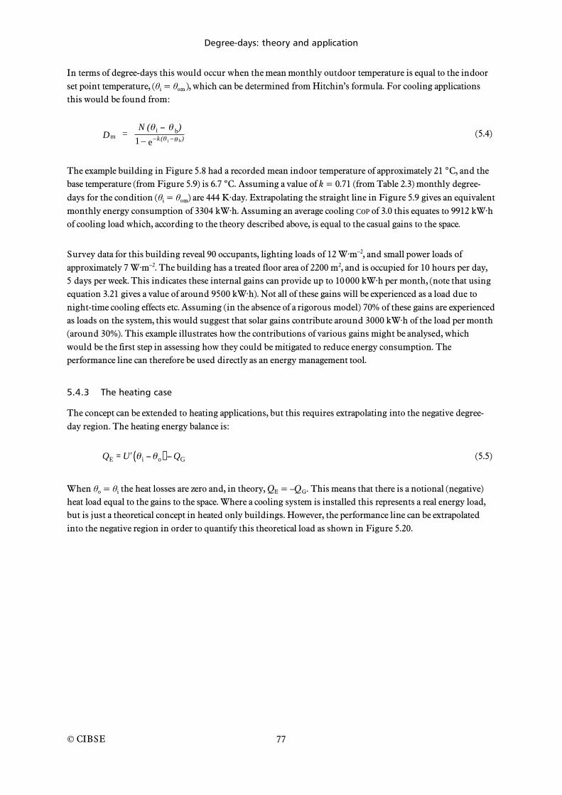
Degree-days: theory and application
© CIBSE
77
In terms of degree-days this would occur when the mean monthly outdoor temperature is equal to the indoor set point temperature, ( i = om ), which can be determined from Hitchin’s formula. For cooling applications this would be found from:
mD = N ( i b)
1 – –k ( i b )e (5.4)
The example building in Figure 5.8 had a recorded mean indoor temperature of approximately 21 °C, and the base temperature (from Figure 5.9) is 6.7 °C. Assuming a value of k = 0.71 (from Table 2.3) monthly degree-days for the condition ( i = om) are 444 K·day. Extrapolating the straight line in Figure 5.9 gives an equivalent monthly energy consumption of 3304 kW·h. Assuming an average cooling CoP of 3.0 this equates to 9912 kW·h of cooling load which, according to the theory described above, is equal to the casual gains to the space.
Survey data for this building reveal 90 occupants, lighting loads of 12 W·m–2, and small power loads of approximately 7 W·m–2. The building has a treated floor area of 2200 m2, and is occupied for 10 hours per day, 5 days per week. This indicates these internal gains can provide up to 10 000 kW·h per month, (note that using equation 3.21 gives a value of around 9500 kW·h). Not all of these gains will be experienced as a load due to night-time cooling effects etc. Assuming (in the absence of a rigorous model) 70% of these gains are experienced as loads on the system, this would suggest that solar gains contribute around 3000 kW·h of the load per month (around 30%). This example illustrates how the contributions of various gains might be analysed, which would be the first step in assessing how they could be mitigated to reduce energy consumption. The performance line can therefore be used directly as an energy management tool.
5.4.3 The heating case
The concept can be extended to heating applications, but this requires extrapolating into the negative degree-day region. The heating energy balance is:
QE = U i o( ) QG (5.5)
When o = i the heat losses are zero and, in theory, QE = –QG. This means that there is a notional (negative) heat load equal to the gains to the space. Where a cooling system is installed this represents a real energy load, but is just a theoretical concept in heated only buildings. However, the performance line can be extrapolated into the negative region in order to quantify this theoretical load as shown in Figure 5.20.
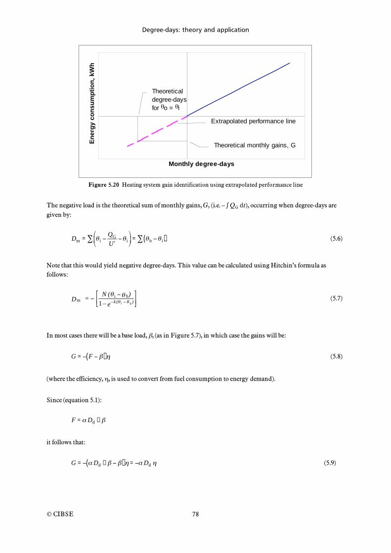
Degree-days: theory and application
© CIBSE
78
Monthly degree-days
En
erg
y c
on
su
mp
tio
n,
kW
hTheoretical
degree-days
for o = i
Theoretical monthly gains, G
Extrapolated performance line
Figure 5.20 Heating system gain identification using extrapolated performance line
The negative load is the theoretical sum of monthly gains, G, (i.e. – QG d t), occurring when degree-days are given by:
Dm = iQG
U i
= b i( ) (5.6)
Note that this would yield negative degree-days. This value can be calculated using Hitchin’s formula as follows:
mD = N ( i b)
1 – –k ( i b )e
(5.7)
In most cases there will be a base load, , (as in Figure 5.7), in which case the gains will be:
G = F( ) (5.8)
(where the efficiency, , is used to convert from fuel consumption to energy demand).
Since (equation 5.1):
F = Dd +
it follows that:
G = Dd +( ) = Dd (5.9)

Degree-days: theory and application
© CIBSE
79
Note that this can only be true if the performance line is constructed using the true building base temperature, and the caveats that the polynomial technique is seen to work reliably, and that a straight line can be obtained, must apply before giving credibility to equation 5.9 in any particular instance.
Using Figure 5.7 as an example, if we assume a mean internal temperature of 22 °C, and the base temperature to be 16.4 °C, the notional degree-days using equation 5.7 are –177 K·day (for a 31-day month). If the plant efficiency is assumed to be 0.75, equation 5.9 suggests that monthly gains amount to:
–(3459.3 –177 0.75) = 459 222 kW·h
These are the gains that constitute a useful contribution to the site. Further analysis (from site surveys etc) can be used to identify individual sources of gains. This may even form a basis upon which to capitalise on this knowledge — i.e. improve controls to capture more gains, or reduce wastage and over-heating. Such deeper analysis is beyond the scope of this publication.
5.4.4 Cooling performance line interpretation
The theory presented in section 3.6.1 has further ramifications for the construction and interpretation of performance lines. For all-air cooling systems with latent cooling the analysis effectively states:
Fchiller =˙ m cp Dd
COP (5.10)
where the degree-days are found from:
Dd = ao b( ) (5.11)
for values of ao greater than b.
The base temperature is more fully defined by equation 3.43, but reduces to:
b = c L (5.12)
Equation 5.10 suggests the slope of the performance line is equal to ˙ m cp
COP, i.e. the slope contains information
about the mass flow rate of air in the system and the system CoP. However, for cooling systems the base temperature can be highly variable (more so, perhaps, than heating systems). This is because the gains (particularly solar gains) vary greatly from month to month, thus varying c significantly; in addition the latent load, captured by L , varies. The base temperature is therefore likely to fluctuate throughout the year.
Therefore a performance line of Fchiller against Dd can only have a slope of ˙ m cp
COP if the individual monthly base
temperatures (including the notional latent component) are used to calculate monthly degree-days. This is possible in real systems where off-coil conditions are being measured, and on-coil moisture content (or humidity) is also measured.
Degree-days: theory and application
© CIBSE
80
Theoretical and empirical studies have shown that this is a reasonable approach to take, and that it may be possible to draw inferences about system CoPs where air flow rates are known [Day 2005]. However, for monitoring and targeting purposes, for example when using CUSUM techniques, it is necessary to use a common base temperature for all months. Theory predicts that in an ideal case, if the average off-coil dry bulb temperature is used for the base temperature (for all months), a straight line fit will emerge but with a slope and intercept different from using monthly variable base temperatures. The variation in slope comes from using a fixed reference base temperature that will reduce warmest month degree-days (variable bases that include latent effects will produce higher mid-summer cooling degree-days); such a constraint will increase the slope of the line. However, theory also suggests that the intercept produced by this line will be equal to the average latent load on the coil.
This last point must be treated with caution, but empirical evidence suggests there may be some validity in this. The value of such information can once again be in what it says about the loads on the system, and may therefore provide indicators about where improvements may be made.
5.4.5 Base temperature and controls
Many buildings employ compensator controls to vary the heating system output with variations in outdoor temperature (see for example Day et al [2003] and Levermore [1992]). In cases where there is no additional internal sensing (for example using thermostatic radiator valves) this type of control will not allow for internal gains and the space may overheat.
Compensators reduce the system flow temperatures linearly with a rise in outdoor temperature, and these schedules tend to be based on design flow temperatures and external and internal design conditions. However, they could be constructed to take account of internal gains by suppressing flow temperatures further. To do this effectively, such that adequate heating is maintained for all outdoor conditions, the minimum flow temperature could be set against the base temperature rather than the room design temperature. This would suggest that knowledge of the building base temperature would be useful in setting up such a controller.
The base temperature analysis using polynomials and energy signatures can be used to identify the base, and then to monitor that the adjusted controls are working effectively. In theory one should observe reduced scatter in performance lines and energy signatures if the controls were set to building specific requirements.
5.5 Regression analysis: caveats and interpretations
Discussions about performance lines rely heavily on the validity of regression analysis to provide sound statistical models of system behaviour. It is beyond the scope of this publication to describe the full theory of regression analysis, and there are many books on mathematics and statistics that cover this subject (e.g. Draper and Smith [1998]). However, a few words are necessary in order to point out some of the pitfalls of relying on the results of regression analysis.
Regression analysis is based on the method of least squares. This fits a line through the centre of the data points such that the sum of the differences between the actual y-values and the line for each x-value comes to zero. For this to be mathematically useful it is necessary to square these y-value differences; the line that yields zero sum of differences will also yield the minimum sum of the differences squared. If y is the actual data value and y is the predicted value on the line, these above statements are, mathematically:

Degree-days: theory and application
© CIBSE
81
yi ˆ y i( )i=1
n
= 0 (5.13)
when:
yi ˆ y i( )2
i=1
n
= S = minimum (5.14)
where n is the number of data points.
Since:
ˆ y i = xi + (5.15)
then:
S = yi xi( )2
i=1
n
(5.16)
By partial differentiation of S with respect to and , and setting the solutions to zero (i.e. at the minima) gives:
S
= 2 xi yi xi( )i=1
n
= 0 = xi (yi xi )i=1
n
(5.17)
and:
S
= 2 yi xi( )i=1
n
= 0 = y xi( )i=1
n
(5.18)
These two expressions give rise to the following:
yii=1
n
= xii=1
n
+ n (5.19)
and:
xiyii=1
n
= xii=1
n
+ xi2
i=1
n
(5.20)
These are called the normal equations, which can be solved simultaneously to find and . Spreadsheets can routinely carry out this task, but it is important to recognise that regression analysis is only a statistical technique that shows whether or not a correlation is likely to exist between the variables. Such a correlation may or may not imply a causal relationship. Thus, any physical meaning assigned to and is done solely at the discretion of the investigator, and with a good understanding of the physical system.
Another important issue is the degree of scatter shown by the data. A good measure of this is the quantity known as the coefficient of determination, written mathematically as R2. This is formally defined as:
R2 =ˆ y i y ( )
2
yi y ( )2
(5.21)

Degree-days: theory and application
© CIBSE
82
and is the proportion of the total variation about the mean explained by the regression [Draper and Smith 1998]. The square root of this value, R, is also called the correlation coefficient, but this will not be discussed further here.
R2 is a number between 0 and 1. The higher the number, the more the regression model can be relied on. Figures 5.18 and 5.19 (above) show two different regressions (one for heating and one cooling for the same building) including their straight line R2 values. Figure 5.18 shows this to be almost 0.6 (or 60%), while Figure 5.19 has a value of around 0.98 (or 98%). This would suggest there is a better relationship for cooling energy consumption and degree-days than heating. All of the analysis described in this section must be tempered by a realisation of what any scatter in the data might indicate.
Scatter may be due to a number of factors which include poor control, poor meter readings, high variability in the base load, holiday shut downs. Where low R2 values are observed it is generally a sign that further investigation is required into the quality of the data, or the operation of the system and building to explain why this has occurred.
One further issue on least squares regression is worth noting: the normal equations are derived on the basis that all the scatter is due to the y-component — the energy data — and that the x-component contains no errors. As has been discussed degree-day values are strongly influenced by the choice of the base temperature, and that to represent a true energy balance the correct base must be used. In real buildings the gains vary from time to time, particularly solar gains, which leads to the concept of variable monthly base temperatures (this was demonstrated most clearly in the section on cooling degree-days). This implies there is indeed inherent error in the degree-day data, which will influence the value of .
The theory behind this is complex, and in real situations may be impossible to determine, since by definition the true base temperature for each month cannot be determined using the techniques outlined here. Only the average overall base temperature can be determined using the polynomial technique. Certain other errors in degree-days, such as those described in section 3.6, can be analysed, but such analysis is generally beyond the needs of the general user. A fuller discussion can be found in Day and Karayiannis [1997].
5.6 Summary
Plotting monthly energy consumption against degree-days, ‘the performance line’ is a highly practical tool in energy management. In theory this should yield a straight line if energy consumption is directly related to variations in the weather; this follows directly from the theory set out in section 3. However, the expectation of a straight line relationship pre-supposes that degree-days encapsulate aspects of the energy balance of the building, i.e. the base temperature to which the degree-days are calculated is the true balance temperature of the building.
The implications for using an incorrect or arbitrary base temperature are that normalisation may be inaccurate, and that the parameters (the slope and intercept) of the performance line cannot be assigned rigid physical interpretations. However, there are techniques available, such as using polynomial regression analysis or daily energy signatures, which can assist in finding the building base temperature. This information can then be used to conduct further analysis such as determining the gains into a building.
It should be remembered that these are statistically based techniques, subject to their areas of applicability. But the interpretations of the results are based on the fundamental theory of heat transfer in buildings, and if used

Degree-days: theory and application
© CIBSE
83
correctly can provide the energy manager with a means of quantifying energy savings and provide insights into building energy performance.

Degree-days: theory and application
© CIBSE
84
Nomenclature
A Area (m2)ƒ
C Thermal capacity of fabric (= cpf Vf ) (kJ·K–1)
Cf Carbon dioxide factor (kg·kW–1·h–1)
cp Specific heat capacity (kJ·kg–1·K–1)
CoP Coefficient of performance
Dc Cooling degree-days (K·day)
Dd Daily degree-days (K·day)
Dm Monthly degree-days (K·day)
E Building energy demand (kW·h)
F Fuel consumption (kW·h)
FAF Fresh air fraction
G Summation of monthly useful gains (kW·h)
gs Moisture content of supply air (kg·kg–1 of dry air)
go Moisture content of outside air (kg·kg–1 of dry air)
hfg Enthalpy of vaporisation of water (kJ·kg–1)
k Constant
˙ m Mass flow rate of air (kg·s–1) ˙ m fa Mass flow rate of fresh air (kg·s–1)
˙ m r Mass flow rate of return air (kg·s–1)
˙ m t Total mass flow rate of air (kg·s–1)
N Number of air changes per hour (h–1) or
Nm Number of days in the month
P Pressure rise across fan (kPa)
QC Heat flow into thermal storage (kW)
Qfabric Heat gain through the building fabric (kW)
Qfa(S) Sensible fresh air load (kW)
Qfan Heat gain across the supply air fan (kW)
Qfa(L) Latent fresh air load(kW)
QG Useful gains (kW)
QG Total uncorrected gains to the space (kW)
QI Internal sensible heat gains to the building (kW)
qI Internal sensible gains per m2 of floor area (W·m–2)
QL Latent heat gains into the building (kW)
QL Total effective latent gain (kW)
Qp Installed plant output capacity (kW)
QS Sensible heat gains to building (= Qsolar + QI) (kW)
Qsolar Solar heat gains into the building (kW)
Q1 Average rate of heat loss from the building (kW)
t Time (h)
U Building fabric U-value (W·m–2·K–1)
U Building overall heat loss coefficient (= [ (U A) + 1/3 N V] / 1000) (kW·K–1)

Degree-days: theory and application
© CIBSE
85
V Volume of space (m3)
Vf Volume of fabric (m3)
v& Volume flow rate of air (m3·s–1)
Parameter
Parameter
Parameter
Degree-day difference (equation 2.6)
Heat exchanger effectiveness
i Change in internal temperature (K)
L' Notional temperature rise from latent gains (K)
Gain to loss ratio
System efficiency
Gain utilisation factor
fan Fan efficiency
i Internal temperature (°C)
o Outside temperature (°C)
ao(day) Mean outside temperature during occupied hours (°C)
ao(night) Mean outside temperature during unoccupied hours (°C)
b Base temperature (°C)
c Off coil temperature (°C)
eo Sol-air temperature (°C)
m Mixed or recovered air temperature (°C)
max Maximum daily temperature (°C)
min Minimum daily temperature (°C)
r Return air temperature (°C)
s Supply air temperature (°C)
so Plant switch-on temperature (°C)
sp Control set point temperature (°C)
Density of building fabric (kg·m–3)
go Standard deviation of outside moisture content (kg·kg–1 of dry air)
Standard deviation of outdoor temperature
Standard deviation of degree-day errors
Building time constant (= C / 3600 U') (h)
Uncertainty (%)

Degree-days: theory and application
© CIBSE
86
References
ASHRAE (2001) ‘Energy estimating and modelling methods’ Ch. 31 in ASHRAE Handbook: Fundamentals (Atlanta, GA: American Society of Heating, Refrigerating and Air-Conditioning Engineers)
ASHVE (1933) ASHVE Guide (New York, NY: American Society of Heating and Ventilating Engineers)
Billington N S (1966) ‘Estimation of annual fuel consumption’ J. Inst. Heating Ventilating Eng. 34 253–256
Billington N S, Colthorpe K J and Shorter D N (1964) Intermittent heating BSRIA Laboratory Report No. 26 (Bracknell: Building Services Research and Information Association)
Bloomfield D P and Fisk D J (1977) ‘Optimisation of intermittent heating’ Building and Environment 12 43–55
BS EN ISO 13790 (2004) Thermal performance of buildings. Calculation of building energy demand for heating (London: British Standards Institution)
Building Regulations 2000 (2006) Conservation of fuel and power in new buildings other than dwellings Approved Document L2A (London: NBS/RIBA Enterprises)
CIBSE (2005) Climate change and the internal environment CIBSE TM36 (London: Chartered Institution of Building Services Engineers)
CIBSE (2006) ‘Accumulated temperature difference’ Sec. 2.5 in Environmental design CIBSE Guide A (London: Chartered Institution of Building Services Engineers)
CIBSE (2006) ‘Thermal response and plant sizing’ Ch. 5 in Environmental design CIBSE Guide A (London: Chartered Institution of Building Services Engineers)
CIBSE (1986) ‘Owning and operating costs’ Sec. 18 in Installation and equipment data CIBSE Guide B (London: Chartered Institution of Building Services Engineers)
CIBSE (2004) Energy efficiency in buildings CIBSE Guide F (London: Chartered Institution of Building Services Engineers)
CIBSE (2002) Weather, solar and illuminance data CIBSE Guide J (London: Chartered Institution of Building Services Engineers)
Claridge D E, Bida M, Krarti M, Jeon H S, Hamzawi E, Zwack W and Weiss I (1987a) ‘A validation study of variable-base degree day heating calculations’ ASHRAE Trans. 2 (93)
Claridge D E, Krarti M and Bida M (1987b) ‘A validation study of variable-base degree day cooling calculations’ ASHRAE Trans. 2 (93) 90–104
Day A R (1999) An investigation into the estimation and weather normalisation of energy consumption in buildings using degree-days PhD Thesis (London: South Bank University)
Day A R (2005) ‘The improved use of cooling degree-days for analysing chiller energy consumption in buildings’ Build. Serv. Eng. Res. Technol. 26(2) 1–13
Day A R, Knight I, Dunn G, Gaddas R (2003) ‘Improved methods for evaluating base temperature for use in building energy performance lines’ Build. Serv. Eng. Res. Technol. 24(4)
Day A R and Karayiannis T G (1999a) ‘Identification of the uncertainties in degree-day based energy estimates’ Build. Serv. Eng. Res. Technol. 20(4) 165–172
Day A R and Karayiannis T G (1999b) ‘A new degree-day model for estimating energy demand in buildings’, Build. Serv. Eng. Res. Technol. 20(4) 173–178
Day A R and Karayiannis T G (1998) ‘Degree-days: comparison of calculation methods’ Build. Serv. Eng. Res. Technol. 19(1) 7–13
Degree-days: theory and application
© CIBSE
87
Day A R, Maidment G G, Ratcliffe M S (2000) ‘Cooling degree-days and their applicability to building energy estimation’ Proc. Conf. 20:20 Vision: CIBSE/ASHRAE Conf., Dublin, September 2000
Day A R, Ratcliffe M S, Shepherd K J (2003) Heating systems plant and control (Oxford: Blackwell Science)
Draper N and Smith H (1998) Applied regression analysis 3rd edn. (Chichester: Wiley)
DTI (2002) Energy consumption in the UK (London: Department of Trade and Industry) (updated July 2004)
Dufton A F (1934) ‘Degree-days’ J. Inst. Heating Ventilating Eng. 2 83–85
Knight I and Dunn G (2003) ‘Evaluation of heat gains in UK office environments’ Proc. CIBSE ASHRAE Conf., Edinburgh, September 2003
Action Energy (2000) Energy use in offices Energy Consumption Guide ECG19 (Carbon Trust) (available from http://www.carbontrust.co.uk)
Erbs D G, Klein S A and Beckman W A (1983) ‘Estimation of degree-days and ambient temperature bin data from monthly average temperatures’ ASHRAE J. 25(6) 60–65
Fischer L J (1943) ‘Degree-time’ J. Inst. Heating Ventilating Eng. 10 217–232
Fisk D J (1981) Thermal control of buildings (Oxford: Applied Science Publishers/Elsevier)
EEO (1993) Degree-days Fuel Efficiency Booklet No. 7 (London: Energy Efficiency Office)
Gaddas R (1998) A conservation and monitoring strategy to reduce energy consumption by 20% by the year 2000 at the Cumberland Infirmary, Carlisle MSc Thesis (Uxbridge: Brunel University)
Good Practice Guide 310 (2006) Degree days for energy management – a practical introduction (The Carbon Trust) (available from http://www.carbontrust.co.uk)
Grierson R (1941) ‘Degree-days’ J. Inst. Heating Ventilating Engineers 8 381–424
Harrington Lynn J (1974) ‘The admittance procedure: intermittent plant operation’ Build. Serv. Engineer 42 219–221
Harris P (1989) Energy monitoring and target setting using CUSUM (Cheriton Technology Publications)
Hitchin E R (1981) ‘Degree-days in Britain’ Build. Serv. Eng. Res. Technol. 2(1)
Hitchin E R (1983) ‘Estimating monthly degree-days’ Build. Serv. Eng. Res. Technol. 4(4) 159
Hitchin E R (1990) ‘Developments in degree-day methods for estimating energy use’ Building and Environment 25(1) 1–6
Hitchin E R and Hyde A J (1979) ‘The estimation of heating energy use in buildings’ Proc. Symp. Environment Inside Buildings, Institute of Mathematics and its Applications, Southend-on-Sea, May 1979
Holmes M J and Hitchin E R (1978) ‘An example year for the calculation of energy demand in buildings’ Build. Serv. Engineer 45 186–9
Holmes M J (1980) ‘Degree day methods’ Proc. CIBS/Industrial Energy Thrift Scheme Seminar, January 1980
Jacobson F R (1985) ‘Energy signatures and energy management in building energy management systems’ Proc. CLIMA 2000, Copenhagen, 1985
Knight I and Dunn G (2003) ‘Evaluation of heat gains in UK office environments’ Proc. CIBSE/ASHRAE Conf., Edinburgh, 24–26 September 2003
Knight J C and Cornell A A (1958) ‘Degree-days and fuel consumption for office buildings’ J. Inst. Heating Ventilating Engineers 26 309–328
Levermore G J (1992) Building energy management systems (London: E & F N Spon)

Degree-days: theory and application
© CIBSE
88
Levermore G J (1989) ‘Performance lines and energy signatures: review and analysis’ Build. Serv. Eng. Res. Technol. 10(3)
McVicker I F G (1946) ‘The calculation and use of degree-days’ J. Inst. Heating Ventilating Engineers 14 252–299
Milbank N O and Harrington Lynn J (1974) ‘Thermal response and the admittance procedure’ Build. Serv. Engineer 42 38–54
Norén A, Akander J, Isfält E, Söderström O (1999) ‘The effect of thermal inertia on energy requirement in Swedish building; results obtained with three calculation models’ Intl. J. Low Energy and Sustainable Buildings 1
Pallot A C (1940) ‘The effect of weather conditions upon the fuel requirements of buildings’ J. Inst. Heating Ventilating Engineers 8 249–277
Sherman M H (1986) ‘Infiltration degree-days: a statistic for infiltration-related climate’ ASHRAE Trans. January 1986.
Strachey Lt-Gen. Sir Richard (1878) ‘Paper on the computation and quantity of heat in excess of a fixed base temperature received at any place during the course of the year to supply a standard comparison with the progress of vegetation’ Quarterly Weather Report Appendix II
The Meteorological Office (1928) The Weekly Weather Report 26th Feb, 1928 (London: His Majesty’s Stationery Office)
Thom H C S (1952) ‘Seasonal degree-day statistics for the United States’ Monthly Weather Review 80(9) 143–149
Thom H C S (1954) ‘The rational relationship between heating degree-days and weather’ Monthly Weather Review 82(1) 1–6
Thom H C S (1954) ‘Normal degree-days below any base’ Monthly Weather Review 82(5) 111–115
Thom H C S (1966) ‘Normal degree-days above any base by the universal truncation coefficient’ Monthly Weather Review 94(7) 461–466
Uglow C E (1980) ‘A study of the effects of thermal capacity on domestic heating energy requirements’ Build. Serv. Eng. Res. Technol. 1(3) 119
VDI 2067 Economic efficiency of building installations (Düsseldorf: Verein Deutscher Ingenieure)
Waide P A and B Norton (1995) ‘Degree-hour steady-state temperature index’ Build. Serv. Eng. Res. Technol. 16(2) 107–113
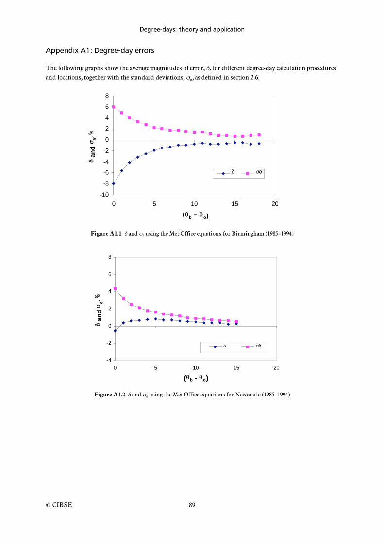
Degree-days: theory and application
© CIBSE
89
Appendix A1: Degree-day errors
The following graphs show the average magnitudes of error, , for different degree-day calculation procedures and locations, together with the standard deviations, , as defined in section 2.6.
-10
-8
-6
-4
-2
0
2
4
6
8
0 5 10 15 20
(b
o)
an
d
, %
Figure A1.1 and using the Met Office equations for Birmingham (1985–1994)
-4
-2
0
2
4
6
8
0 5 10 15 20
( b - o)
an
d
, %
Figure A1.2 and using the Met Office equations for Newcastle (1985–1994)
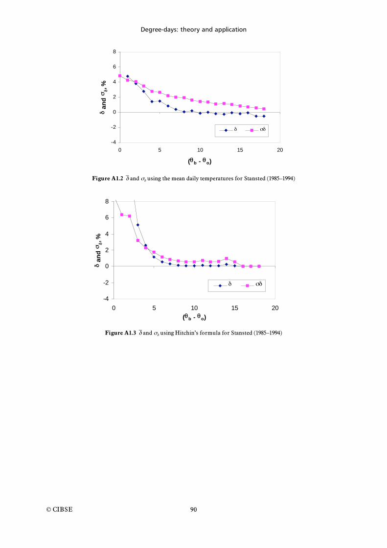
Degree-days: theory and application
© CIBSE
90
-4
-2
0
2
4
6
8
0 5 10 15 20
( b - o)
an
d
, %
Figure A1.2 and using the mean daily temperatures for Stansted (1985–1994)
-4
-2
0
2
4
6
8
0 5 10 15 20
( b - o)
an
d
, %
Figure A1.3 and using Hitchin’s formula for Stansted (1985–1994)
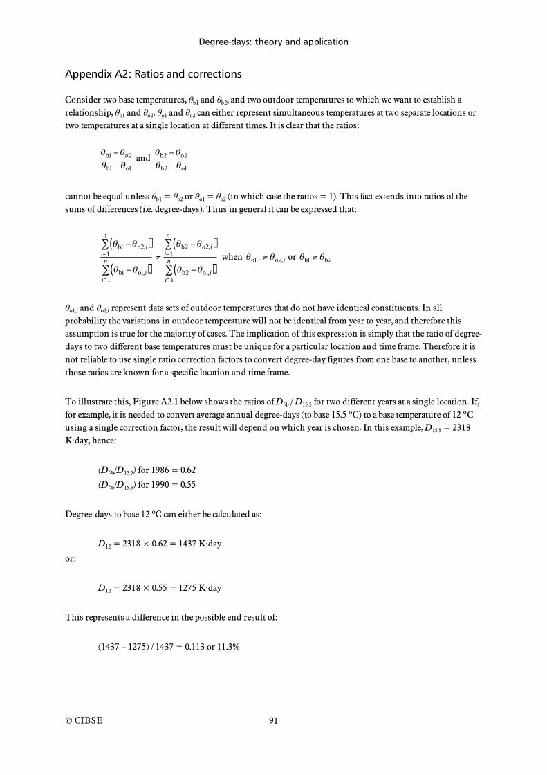
Degree-days: theory and application
© CIBSE
91
Appendix A2: Ratios and corrections
Consider two base temperatures, b1 and b2, and two outdoor temperatures to which we want to establish a relationship, o1 and o2. o1 and o2 can either represent simultaneous temperatures at two separate locations or two temperatures at a single location at different times. It is clear that the ratios:
b1 o2
b1 o1
and b2 o2
b2 o1
cannot be equal unless b1 = b2 or o1 = o2 (in which case the ratios = 1). This fact extends into ratios of the sums of differences (i.e. degree-days). Thus in general it can be expressed that:
b1 o2,i( )
i=1
n
b1 o1,i( )i=1
n
b2 o2,i( )i=1
n
b2 o1,i( )i=1
n when o1,i o2,i or b1 b2
o1,i and o2,i represent data sets of outdoor temperatures that do not have identical constituents. In all probability the variations in outdoor temperature will not be identical from year to year, and therefore this assumption is true for the majority of cases. The implication of this expression is simply that the ratio of degree-days to two different base temperatures must be unique for a particular location and time frame. Therefore it is not reliable to use single ratio correction factors to convert degree-day figures from one base to another, unless those ratios are known for a specific location and time frame.
To illustrate this, Figure A2.1 below shows the ratios of D b / D15.5 for two different years at a single location. If, for example, it is needed to convert average annual degree-days (to base 15.5 ºC) to a base temperature of 12 ºC using a single correction factor, the result will depend on which year is chosen. In this example, D15.5 = 2318 K·day, hence:
(D b/D15.5) for 1986 = 0.62
(D b/D15.5) for 1990 = 0.55
Degree-days to base 12 ºC can either be calculated as:
D12 = 2318 × 0.62 = 1437 K·day
or:
D12 = 2318 × 0.55 = 1275 K·day
This represents a difference in the possible end result of:
(1437 – 1275) / 1437 = 0.113 or 11.3%
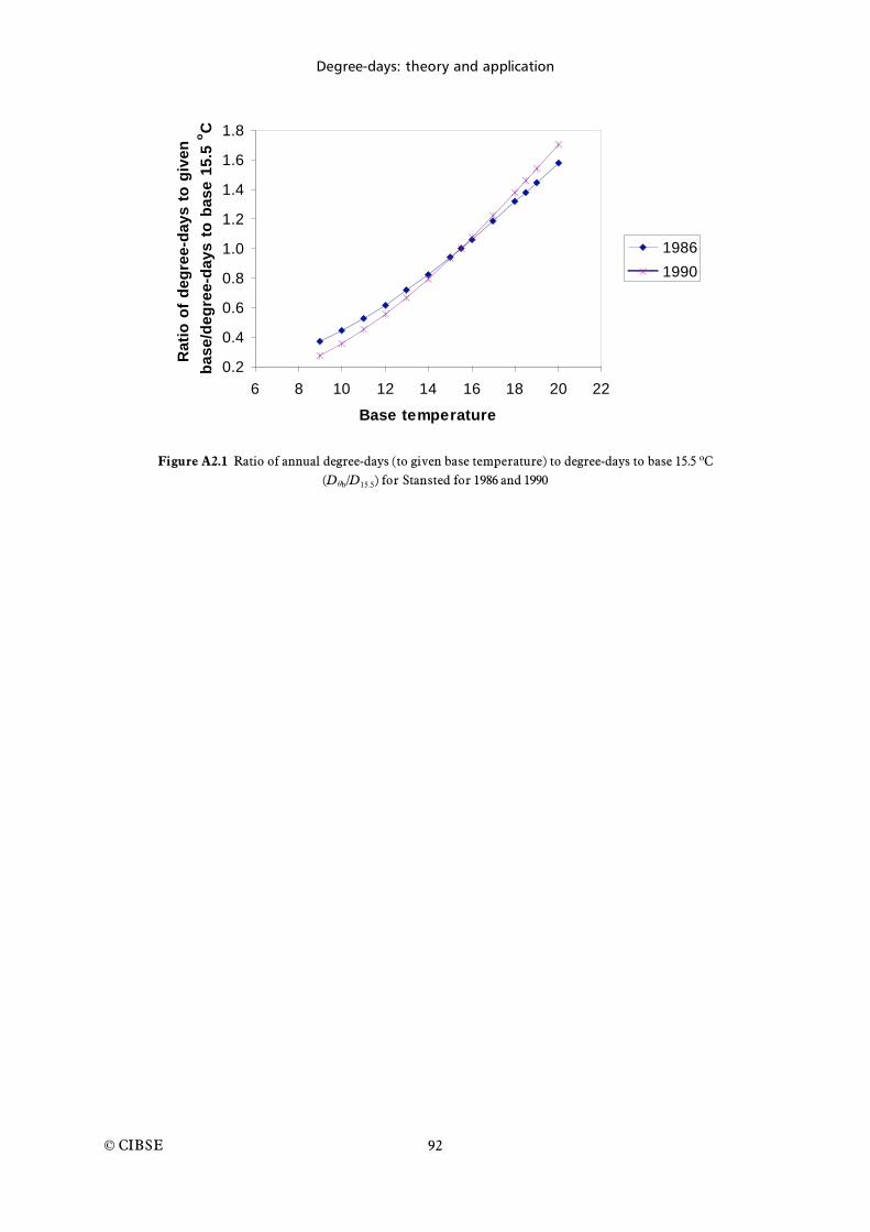
Degree-days: theory and application
© CIBSE
92
0.2
0.4
0.6
0.8
1.0
1.2
1.4
1.6
1.8
6 8 10 12 14 16 18 20 22
Base temperature
Ra
tio
of
de
gre
e-d
ay
s t
o g
ive
n
ba
se
/de
gre
e-d
ay
s t
o b
as
e 1
5.5
oC
1986
1990
Figure A2.1 Ratio of annual degree-days (to given base temperature) to degree-days to base 15.5 ºC
(D b/D15.5) for Stansted for 1986 and 1990

Degree-days: theory and application
© CIBSE
93
Appendix A3: Base temperature conversion using Hitchin’s formula
Base temperature correction of known monthly degree-days to a defined base can be carried out by using Hitchin’s formula (equation 2.4) to find the mean monthly temperature, and then enter the new required base temperature to calculate corrected monthly degree-days. It is necessary to do this through an iterative technique such as the Newton-Raphson method. The function of the target variable (in this case o,m) must be set to zero and differentiated in order to carry out the following iteration:
o,m (n +1) = o,m (n )
f o,m(n )( ) f o,m(n )( )
(A3.1)
where o,m (n ) is the nth estimate of o,m , which is a root of f o,m(n )( ) .
Rearranging Hitchin’s formula for o,m gives:
o,m = bDm
Nm
+Dm
Nm
ek b o,m( ) (A3.2)
where Nm is the number of days in the month.
Setting this to zero by subtracting o,m from both sides gives the required function f o,m( ) :
f o,m( ) = b o,mDm
Nm
+Dm
Nm
ek b o,m( ) (A3.3)
Differentiating this gives:
f o,m( ) = 1+Dm
Nm
k ek b o,m( ) (A3.4)
An initial guess of o,m is required to feed into the iteration; b, Dm and k are all known.
For example to convert monthly degree-days of 115 at 15.5 °C base to a base of 13 °C, assuming k = 0.71 would be found in the following steps. Best first guess:
Dd = Dm / Nm = b – o,m
Dd = 115 / 31 = 3.71
o,m (1) = 15.5 – 3.71 = 11.8 °C
Use this value to start the process; the first iteration is:

Degree-days: theory and application
© CIBSE
94
o,m (2) = 11.815.5 11.8 3.71+ 3.71 e 0.71 15.5 11.8( )
1+ 3.71 0.71 e 0.71 15.5 11.8( )= 12.02
After successive iterations this gives the final result:
o,m = 12.1 °C
New degree-days:
Dm = 31 (13–12.1) / [1 – exp (–0.71(13 – 12.1))] = 59 K·day
The iteration to determine the mean monthly temperature can be written into a spreadsheet macro. A Visual Basic for Applications routine to form a function called ‘meantemp’ that can conduct this task is shown below.
Function meantemp(Degree_days, k, base_temp, days_in_month)
D = Degree_days / days_in_month
For n = 1 To 3
If n = 1 Then x = base_temp - D Else x = b
y = (-x + base_temp - D + (D * Exp(-k * (base_temp - x))))
z = -1 - D * k * Exp(-k * (base_temp - x))
b = x - y / z
Next n
meantemp = b
End Function

Degree-days: theory and application
© CIBSE
95
Appendix A4: Derivation of mean internal temperature for intermittent heating
The terms and symbols used in this appendix are the same as in chapter 3. The cooling of a structure to a constant temperature heat sink is given by:
Cd
dt= U ( i o) (A4.1)
See Appendix A5 for a description of the assumptions and caveats which apply to this equation.
Assuming that the structure is in a heat sink which is at a constant temperature, rearranging gives:
dtt1
t2=
d i
i o( )i1
i 2
, for ( i > o) (A4.2)
where:
=C
U (A4.3)
The solution to this integration is:
t2 – t1 = – ln( i,2 – o)
( i,1 – o)
(A4.4)
For a heated building i,1 is the set point temperature, sp, at time t1.
Equation A4.4 can be rearranged to give the temperature of the building at any time:
i,2 = o + et2 t1
sp o( ) (A4.5)
Similarly, during the heating up period the change in temperature is found from:
Cd i
dt= Qp U ( i o) (A4.6)
which, for Qp > U ( i – o), has the solution:
t3 – t2 = – lnQp – U ( i,3 – o)
Qp – U ( i,2 – o)
(A4.7)
Rearranging equation A4.7 gives:

Degree-days: theory and application
© CIBSE
96
i,2 = o +Qp e
–t3 t2
Qp U i,3 o( )( )
U e
t3 t2
(A4.8)
Note that the plant switch on temperature, so = i,2 , (the optimum start temperature) is found from the
simultaneous solution of equations A4.4 and A4.7 to give:
so = o +Qp sp o( ) e
t3 t1
Qp + U sp o( ) e
t3 t1
U sp o( )
(A4.9)
From which can be found the switch-on time, t2, by inserting the value of so
(for i,2 ) into equation A4.7.
The mean internal temperature of the building over 24 hours is the sum of the hourly temperatures divided by 24. The sum of the overnight temperatures can be found by integrating equations A4.5 and A4.8:
it1
t2
dt = o + et t1
i,1 o( )
dt
t1
t2
(A4.10)
and:
it2
t3
dt = o +Qp e
t t2
Qp U i,1 o( )( )
U e
t t2
dtt2
t3
(A4.11)
Summing the solutions to equations A4-10 and A4-11 gives:
it1
t3
= o t3 t1( ) + i,1 o( ) e
t3 t2
e
t2 t1
+
Qp
U 1+
t3 t2
e
t3 t2
(A4.12)
This is added to the sum of the temperatures during the occupied period and the total value divided by 24 to give the 24 hour mean internal temperature:
i =
i + spt1
t3
24 + t1 t3( )
24 (A4.13)
Clearly, the initial assumption of a constant external temperature is unrealistic. However, using this approach to derive the mean internal temperature of an intermittently heated building is a reasonable approximation in practice, and has been confirmed by sensitivity analysis.

Degree-days: theory and application
© CIBSE
97
Appendix A5: Areas of on-going work
Simplified energy analysis techniques for buildings by their very nature require a set of simplifying assumptions, short cuts and approximations. Because no two buildings are exactly alike, either in built form or occupancy usage patterns, it is almost impossible to verify any energy predictive technique absolutely, as fully controlled experimental verification on real buildings is either prohibitively expensive or subject to the vagaries of occupants’ behaviour and long-term reliability of data collection techniques.
The techniques described in this publication are two-fold:
energy estimation of heating and cooling systems in buildings not yet built
energy analysis of existing buildings.
For reasons described above any verification of the techniques for energy estimation has been carried out against thermal simulation models. This is the only way of ensuring all of the variables are properly defined and controlled in order to assess the effects of outdoor temperature variation in such a simplified form as degree-days. There are a number of issues surrounding simplified energy estimation techniques that are not fully defined nor fully understood at this time. Some of these are discussed below.
Simplified methods assume that average values of gains, infiltration and building temperature can be used in conjunction with each other to assess building energy balances. In reality the magnitudes of each of these vary independently of each other over time. This raises questions about the appropriateness of using average values, but this is the only real way of reducing the amount of input data to manageable levels.
Building thermal capacity and its effect on response of systems and their controls is highly complex. The models here assume the thermal mass can be lumped together as a single entity. Understanding of thermal capacity effects (including location of mass, and effective depth) on energy use is currently incomplete, and further research is necessary to refine the guidance in this area. However, assumptions about thermal mass have less impact on the results than, say, heat loss coefficients.
The thermal capacity equations used are strictly for a homogenous structure. Buildings are far from homogenous and internal air temperatures vary more rapidly than the fabric temperature. The method for heat energy estimation avoids this difficulty by assuming an overall effective structure temperature. Only detailed simulations can properly account for the differing temperatures of spaces and elements throughout a building as they change over time.
In the heating model it is suggested that mechanical ventilation can be included with infiltration in the heat loss coefficient. This is only true for properly balanced ventilation systems. Where supply and extract volumes differ a more complicated relationship arises between the mechanical ventilation and infiltration/exfiltration.
If mechanical ventilation is included within the heat loss coefficient then any heat recovery must also be accounted for via the effectiveness of the heat recovery system. For example if 70% of the heat from exhaust air is recovered by the supply air, 30% of the supply air flow rate can be combined with the infiltration rate. Given the uncertainty in real infiltration rates it is probably not necessary to be overly precise about heat recovery effectiveness. However, this is an issue that requires more detailed research and analysis.
Fabric gains are generally a small fraction of heat gains in cooled buildings. However, in some buildings such gains may become significant. In this case a more detailed consideration may have to be given to these in the

Degree-days: theory and application
© CIBSE
98
model. However, it would probably defeat the purpose of simple models if a rigorous methodology were developed. There is scope for future work in the area to define the influence of various gain components on building energy use.
Where degree-days are applied to energy management in existing buildings there are a number of issues to be resolved. Some of these are discussed below.
Buildings rarely perform according to theory. There are a large number of factors that influence energy consumption beyond fluctuations in weather conditions. These include occupants’ behaviour, changes in casual gains (e.g. solar), non-weather loads (catering, hot water, other processes), system controls, plant faults or maintenance. In addition there may be variability in the timings of meter readings (particularly where this is done manually). Between them these factors all contribute to observed scatter in energy signatures and performance lines, and it is the job of the energy manager to decipher the information contained in such data. This publication has presented ways in which a building can be assessed in accordance with expected theory. Buildings often do present linear energy/degree-day relationships, which suggests that there is an underlying weather-related consumption according to theory, and the techniques presented here attempt to exploit this to the full. However, where buildings do not exhibit readily identifiable behaviour there is a need to examine the data and building further to assess the causes. Performance lines are a very good starting point from which to understand building energy performance, but due to the variety of potential faults and operational failures further methodical and scientifically rigorous research is needed to build a better understanding of our existing building stock.
In all degree-day applications considered in this publication, it is recommended that building-specific base temperatures be used where possible. This includes estimation, normalisation and performance line construction. Various methods for generating degree-days to different base temperatures have been described, but it does highlight the point that published monthly degree-days should be presented for a range of base temperatures. There are services that can do this for a fee, but there is a pressing need to provide building operators with improved weather data in order to fully exploit the techniques described in this publication. (Note: CIBSE Guide A section 2.5 and CIBSE Guide J section 4.3 contain some historical values for different base temperatures, but these are not adequate for on-going monitoring regimes.)
In buildings equipped with building energy management systems that have full energy and environmental monitoring it is possible to collect large quantities of energy and temperature data. If using these data to generate local degree-days it is important to ensure the correct calibration of sensors, and that data collection and storage is uninterrupted and accurate.
The use of cooling degree-days has been limited in the UK for monitoring and targeting. Their use should be encouraged, especially where disaggregated cooling energy data are available (e.g. from sub-metering), as this can start to build a better picture of electricity use in buildings.