Defining Geographical Boundaries with Social and Technical ...

An Anticipatory-Lifecycle Approach Towards Increasing the Environmental Gains from

Photovoltaic Systems Through Improved Manufacturing and Recycling

by

Dwarakanath Triplican Ravikumar

A Dissertation Presented in Partial Fulfillment of the Requirements for the Degree

Doctor of Philosophy

Approved November 2016 by the Graduate Supervisory Committee:

Thomas Seager, Co-Chair

Matthew P. Fraser, Co-Chair Mikhail Chester Parikhit Sinha

Meng Tao

ARIZONA STATE UNIVERSITY

December 2016

i

ABSTRACT

Photovoltaics (PV) is an environmentally promising technology to meet climate goals

and transition away from greenhouse-gas (GHG) intensive sources of electricity. The

dominant approach to improve the environmental gains from PV is increasing the module

efficiency and, thereby, the renewable electricity generated during use. While increasing the

use-phase environmental benefits, this approach doesn’t address environmentally intensive

PV manufacturing and recycling processes.

Lifecycle assessment (LCA), the preferred framework to identify and address

environmental hotspots in PV manufacturing and recycling, doesn’t account for time-

sensitive climate impact of PV manufacturing GHG emissions and underestimates the

climate benefit of manufacturing improvements. Furthermore, LCA is inherently

retrospective by relying on inventory data collected from commercial-scale processes that

have matured over time and this approach cannot evaluate environmentally promising pilot-

scale alternatives based on lab-scale data. Also, prospective-LCAs that rely on hotspot

analysis to guide future environmental improvements, (1) don’t account for stake-holder

inputs to guide environmental choices in a specific decision context, and (2) may fail in a

comparative context where the mutual differences in the environmental impacts of the

alternatives and not the environmental hotspots of a particular alternative determine the

environmentally preferable alternative

This thesis addresses the aforementioned problematic aspects by (1)using the time-

sensitive radiative-forcing metric to identify PV manufacturing improvements with the

highest climate benefit, (2)identifying the environmental hotspots in the incumbent CdTe-

PV recycling process, and (3)applying the anticipatory-LCA framework to identify the most

ii

environmentally favorable alternative to address the recycling hotspot and significant

stakeholder inputs that can impact the choice of the preferred recycling alternative.

The results show that using low-carbon electricity is the most significant PV

manufacturing improvement and is equivalent to increasing the mono-Si and multi-Si

module efficiency from a baseline of 17% to 21.7% and 16% to 18.7%, respectively. The

elimination of the ethylene-vinyl acetate encapsulant through mechanical and chemical

processes is the most significant environmental hotspot for CdTe PV recycling. Thermal

delamination is the most promising environmental alternative to address this hotspot. The

most significant stake-holder input to influence the choice of the environmentally preferable

recycling alternative is the weight assigned to the different environmental impact categories.

iii

DEDICATION

To Thara, Miyuki and my family without whose love, support, and sacrifice this

effort would not have been possible.

iv

ACKNOWLEDGMENTS

The guidance and advise from my committee members has contributed immensely

towards the research presented in this dissertation and my intellectual and professional

growth over the last four years. I am grateful to Dr. Thomas Seager who has spent a

significant amount of his time emphasizing the importance of systems thinking while

analyzing large-scale environmental challenges, the significance of thermodynamics as a tool

to understand the lifecycle impacts of renewable energy technologies, and improving my

scientific presentation skills. I thank Dr. Matthew Fraser for the guidance on the

environmental chemistry aspects of this research, laboratory facilities for the photovoltaic

delamination experiments and the support for photovoltaic (PV) environmental research as a

part of the Quantum Energy and Sustainable Solar Technologies (QESST) engineering

research center at Arzona State University. Dr. Parikhit Sinha has been very generous with

his time while providing an industry perspective on PV recycling research and was

instrumental in me getting introduced to the recycling team and gaining access to the

recycling plant at First Solar. This ensured that the findings in this dissertation can guide the

PV industry towards environmentally improved pathways or recycling. I thank Dr. Mikhail

Chester for the difficult, but immensely valuable, questions on Lifecycle Assessment (LCA)

of emerging technologies which has significantly influenced the methodological basis of this

dissertation. I thank Dr. Meng Tao for helping me gain a deeper understanding of PV device

fundamentals and how this can inform recycling processes. I am lucky to have been part of

many informative discussions with Ben Wender and Valentina Prado on how LCA can guide

environmental improvements in emerging technologies. These discussions have influenced

my approach towards prospectively assessing the environmental impacts of novel PV

recycling technologies.

v

I am thankful for the organizational support received from First Solar’s recycling

team over a two-year period and the findings in this dissertation would not have been

possible without their data on recycling operations and the constructive feedback received

from their leadership team.

This dissertation is primarily supported by the National Science Foundation (NSF)

and the Department of Energy (DOE) under NSF CA No.EEC-1041895 and 1140190. Any

opinions, findings and conclusions or recommendations expressed in this material are those

of the author and do not necessarily reflect those of NSF or DOE.

vi

TABLE OF CONTENTS

Page

LIST OF TABLES………………………………………………………………………..xi

LIST OF FIGURES ……………………………………………………………...…….. xii

CHAPTER

1.INTRODUCTION .......................................................................................................................... 1

Environmental Benefits of Improved PV Manufacturing ...................................................... 2

Environmentally Improved Pathways for CdTe PV Recycling .............................................. 4

Chapter-wise Summary ................................................................................................................. 6

References .................................................................................................................................... 15

2.INTERTEMPORAL CUMULATIVE RADIATIVE FORCING EFFECTS OF

PHOTOVOLTAIC DEPLOYMENTS ........................................................................................ 17

Introduction ................................................................................................................................. 17

Time Sensitive Warming Impacts of GHG Emissions .................................................. 18

Methods ........................................................................................................................................ 20

Factors Impacting Magnitude of GHG Emitted and Avoided over PV Lifecycle..... 20

CRF Calculations for GHGs .............................................................................................. 21

GHGs Considered for CRF Calculations ......................................................................... 22

Timing of GHGs Emitted and Avoided over PV Lifecycle .......................................... 23

Timing of GHG Emissions for FLS .................................................................................. 24

Timing of GHG Emissions for BLS.................................................................................. 26

Optimization Framework for PV Deployment ............................................................... 27

vii

CHAPTER Page

Scenario and Sensitivity Analysis ........................................................................................ 29

Results and Discussion ............................................................................................................... 30

Optimal PV Deployment Strategy and Scenario Analysis for GHG and CRF Impacts

................................................................................................................................................. 30

Sensitivity Analysis ............................................................................................................... 34

Model Limitations and Uncertainties ................................................................................ 36

Acknowledgements ..................................................................................................................... 37

References .................................................................................................................................... 37

3.A COMPELLING CLIMATE RATIONALE FOR CARBON EFFICIENCY IN

PHOTOVOLTAICS MANUFACTURE ...................................................................................... 41

Introduction ................................................................................................................................. 41

Methods ........................................................................................................................................ 44

Data Collection, Harmonization and Generation of PV Manufacturing Experience

Curve ...................................................................................................................................... 44

Cumulative Radiative Forcing (CRF) of PV Installations .............................................. 45

Difference Between the GHG and CRF Metric .............................................................. 48

Short-Term Equivalence Between Module Efficiency Increase and Manufacturing

Improvements ....................................................................................................................... 49

Climate Hotspots in PV Manufacturing ........................................................................... 50

Climate Benefits of Addressing PV Manufacturing Hotspots ....................................... 51

Long-Term Equivalence Between Module Efficiency Increase and Manufacturing

Improvements ....................................................................................................................... 54

viii

CHAPTER Page

Results and Discussion ............................................................................................................... 54

PV Manufacturing Environmental Experience Curve .................................................... 54

Underestimation of the Climate Benefit of PV Manufacturing Improvements as

Measured by GHG Metrics................................................................................................. 56

Short-Term Climate Benefit of Improved PV Manufacturing ...................................... 59

Climate Hotspots in Current PV Manufacturing Processes........................................... 60

Equivalence Between Manufacturing and Module Efficiency Improvements ............ 62

Acknowledgements ..................................................................................................................... 67

References .................................................................................................................................... 67

4.AN ANTICIPATORY APPROACH TO QUANTIFY ENERGETICS OF

RECYCLING CDTE PHOTOVOLTAIC SYSTEMS .............................................................. 79

Introduction ................................................................................................................................. 79

Methods ........................................................................................................................................ 83

Energy and Material Flows for HVR of CdTe PV Systems........................................... 83

Calculating and Allocating the Net Energy Impacts of Recycling ................................ 85

Scenario Analysis .................................................................................................................. 88

Sensitivity Analysis for Process Parameters and Allocation Method, Centralized

Versus Decentralized Recycling, and Uncertainty Analysis ........................................... 89

Results ........................................................................................................................................... 93

Acknowledgements ................................................................................................................... 104

References .................................................................................................................................. 105

ix

CHAPTER Page

5.AN ANTICIPATORY LIFECYCLE ASSESSMENT OF NOVEL AND EXISTING

CDTE PV MODULE RECYCLING PROCESSES ................................................................ 110

Introduction ............................................................................................................................... 110

Methods ...................................................................................................................................... 114

Energy and Material Flows for the Incumbent and Emerging Recycling Processes 114

Incumbent CdTe PV Recycling Process ......................................................................... 115

Thermal Delamination of EVA........................................................................................ 116

Delaminating EVA by Heating in an Organic Solvent ................................................. 116

Delaminating EVA by Sonicating in an Organic Solvent ............................................ 117

Extracting Cadmium Through Ion Exchange ............................................................... 117

Solvent Extraction of Cadmium ...................................................................................... 118

Anticipatory LCA Framework to Evaluate and Improve the Environmental Impact

of CdTe PV Recycling ....................................................................................................... 120

Scenario Analysis: Centralized and Decentralized Recycling ....................................... 122

Global Sensitivity Analysis ................................................................................................ 124

Results and Discussion ............................................................................................................. 125

6.CONCLUSION ............................................................................................................................ 135

REFERENCES ................................................................................................................................ 139

APPENDIX ..................................................................................................................................... 144

A. PREVIOUSLY PUBLISHED MATERIAL AND CO-AUTHOR PERMISSION 144

x

APPENDIX Page

B. SUPPORTING INFORMATION FOR CHAPTER 2 ................................................ 146

C. SUPPORTING INFORMATION FOR CHAPTER 3 ................................................ 173

D. SUPPORTING INFORMATION FOR CHAPTER 4 ............................................... 260

E. SUPPORTING INFORMATION FOR CHAPTER 5 ................................................ 284

xi

LIST OF TABLES Table Page

1. Chapter 2 Summary .................................................................................................................. 6

2. Chapter 3 Summary .................................................................................................................. 8

3. Chapter 4 Summary ................................................................................................................ 10

4. Chapter 5 Summary ................................................................................................................ 12

5. Material Recovery from CdTe PV System Recycling. ....................................................... 94

6. Definitions for all the Acronyms .......................................................................................... 95

7. Summary of the Seven CdTe Recycling Alternatives. ..................................................... 119

xii

LIST OF FIGURES

Figure ............................................................................................................................... Page

1. PV GHG and CRF Payback Times. ...................................................................................... 7

2. Equivalence Between Manufacturing and Module Efficiency Imporvements. ............... 9

3. Sensitivty Analysis of CdTe PV Recycling Energetics....................................................... 11

4. Environmental Rankings of CdTe PV Recycling Alternatives. ........................................ 14

5. Factors Impacting Net GHG Emissions over PV Lifecycle ............................................ 20

6. GHG Flows for Front-loading of PV Systems. ................................................................. 24

7. GHG Flows for Back-loading of PV Systems. ................................................................... 26

8. GHG Payback-time of PV Systems. .................................................................................... 31

9. CRF Payback-time of PV Systems. ...................................................................................... 32

10. Sensitivity Analysis of PV CRF Impacts ........................................................................... 34

11. PV Manufacturing Energy Trends ..................................................................................... 55

12. Difference Between GHG and CRF Impacts .................................................................. 56

13. Short-term Climate Benefit of PV Manufacturing Imporvements................................ 59

14. CRF Hotspots Multi-silicon PV modules ......................................................................... 60

15. The Equivalence Between Manufacturing and Module Efficiency Imporvements .... 62

16. Energy and Material Flows for CdTe PV Recycling. ....................................................... 83

17. Recycling Scenarios for CdTe PV Systems. ...................................................................... 89

18. Net Energy Impact of CdTe PV System Recycling. ........................................................ 93

19. Allocation Method and Recycling Net Energy Benefit Calculations ........................... 99

20. Energy Impacts of Centralized and Decentralized Recycling. ..................................... 100

21. Sensitivity Analysis of CdTe PV Recycling Energetics. ................................................ 101

xiii

Figure ............................................................................................................................... Page

22. Material and Energy Flows for CdTe Recycling Alternatives. ..................................... 114

23. Anticipatory LCA Framework for CdTe PV Recycling. ............................................... 120

24. Process Time for EVA Elimination. ................................................................................ 125

25. Environmental Ranking for the CdTe PV Recycling Alternatives. ............................. 127

26. Environmental Rankings for Centralized and Decentralized Recycling. .................... 128

27. Global Sensitivity Analysis Results (With Weights). ..................................................... 130

28. Global Sensitivity Analysis Results (Without Weights). ............................................... 131

1

CHAPTER 1

INTRODUCTION

Global cumulative PV installations have increased from 1.4 GW in 2000 to 177 GW

in 2014 [1][2] to meet climate goals and transition away from fossil fuels for electricity

generation [3][4]. The environmental benefit of a PV system accrues during the use phase,

when PV electricity displaces carbon-intense electricity, and is predicated upon

environmental investments in the manufacturing and recycling phases. To date, the

dominant approach to increase the environmental benefits of PV systems is to improve the

module efficiency as this increases the renewable electricity generated over the lifespan of a

PV system [5]. While achieving significant environmental and economic improvements, this

approach fails to address the environmental burdens in the manufacturing and recycling

processes. For example, manufacturing processes like silicon purification and wafer sawing

continue to be energetically burdensome and have significant material losses[6][7]. Further,

end-of-life modules are projected to reach 78 million tonnes by 2050 [8].The gradual shift in

and PV manufacturing activities to GHG-intensive regions like China [9] and possible

resource constraints [10][11] [12][13] further underscore the need to identify novel,

environmentally improved pathways for PV manufacturing and recycling.

The typical approach to realize such environmental improvements is identifying

existing hotspots, addressing them through alternate, less environmentally burdensome

processes and analyzing the corresponding environmental trade-offs through a lifecycle

assessment (LCA). LCA is a retrospective framework as it depends on material and energy

inventory datasets that are available only after a process has technologically matured and

commercialized over time [14]. Such inventory data is lacking for the emerging lab scale

2

processes (e.g. novel PV recycling methods) and investigators, during the research and

development stage, focus primarily on the feasibility of the process and not on reporting

energy and material requirements. The lack of technological maturity in the early stage of

research of development, unavailability of inventory data and the retrospective mode of

analysis limits the application of a traditional LCA approach in evaluating the environmental

performance of emerging PV recycling and manufacturing methods.

Anticipatory LCA [15], a recent methodological innovation, addresses these

problematic aspects by stochastically comparing the environmental impacts of the

incumbent and the novel methods, identifying the environmental hotspots through a

sensitivity analysis and prioritizing the future research to address the hotspots and maximize

the environmental benefits of commercializing novel alternatives. The material and energy

inventory data required for the environmental impact assessment for the novel recycling

methods are determined from laboratory experiments and secondary literature sources.

This thesis applies the aLCA framework and presents the environmental rationale for

extending beyond the dominant approach of improving the use-phase PV module efficiency

to increase the lifecycle environmental gains from a PV system through improved

manufacturing and recycling practices. Environmental hotspots in the existing PV

manufacturing and recycling phases are identified and the aLCA framework is applied to

quantify the environmental benefit of addressing the PV recycling hotspots through seven

alternate recycling processes.

Environmental benefits of improved PV manufacturing

Improving the environmental performance of PV manufacturing processes requires

an understanding of trends that drove past improvements and using this to prospectively

3

analyze the potential for further improvements. For example, reduction in the silicon wafer

thickness which drove past manufacturing improvements, may not be a viable strategy in the

future as breakage and cracking rates in wafer manufacturing operations increase below a

threshold thickness [16]. To establish historical environmental gains from manufacturing

improvements, this thesis presents an experience curve depicting manufacturing energy

improvements over the past two decades for the four main PV technologies –amorphous

silicon, CdTe, multi and mono crystalline silicon. This manufacturing experience curve will

be based on a data harmonization of previously published PV manufacturing environmental

lifecycle studies. Significant reductions in manufacturing energy for the four PV technologies

in the experience curve are identified and the corresponding manufacturing process

improvements that resulted in these reductions are investigated.

Manufacturing improvements, identified in the experience curve, reduce electricity

requirements and the corresponding emissions which depend on the GHG intensity of

electricity at the PV manufacturing site. Further, the GHGs avoided in the manufacturing

phase temporally precede emissions avoided in the use phase when PV electricity displaces

GHG intensive electricity. Previous research has demonstrated that the global warming

impacts of GHG emissions are dependent on the timing of the emission and is directly

proportional to the residence time in the atmosphere [17]. Therefore, a mass of GHG

emission avoided in the manufacturing phase has a greater environmental benefit than that

in the use phase. This thesis uses the time sensitive radiative forcing metric [18] [19]to

account for geographical and temporal sensitivities of the environmental impacts of GHGs

emitted and avoided over the PV lifecycle and determine if future PV manufacturing

improvements offer significant environmental gains. To demonstrate the significance of the

climate benefits through manufacturing improvements the equivalent increase in module

4

efficiency required to achieve the same climate benefit is calculated. An increase in module

efficiency increases the renewable electricity generation at the deployment site and therefore

increases the climate benefit by avoiding electricity generated from fossil fuels.

Environmentally improved pathways for CdTe PV recycling

With rapid global deployments, the volume of end of life PV systems will increase

after a typical lifetime of 25 years. An environmentally efficient strategy to manage this PV

waste requires an assessment of the environmental performance and hotspots in existing

processes that recycle the entire PV system (module, balance of system and electrical

systems). To date, there is no comprehensive study that evaluates the environmental impact

of transporting and recycling an entire PV system and identifies recycling process hotspots.

This thesis addresses this knowledge gap through an energetic analysis of CdTe PV recycling

operations at First Solar, which is the world’s largest recycler. The outcomes of this section

includes quantifying the energetic impacts of PV recycling, calculating benefits of recovering

secondary materials and identifying process hotspots that can be addressed in the future.

Furthermore, the aLCA framework is applied to identify environmentally favorable

pathways for addressing recycling hotspots by replacing the incumbent process with novel

alternatives. The novel methods are selected based on a detailed literature review of PV

recycling studies and the inventory requirements are determined from laboratory

experiments and from published studies. The environmental performance of the incumbent

and novel methods is compared using the aLCA framework. Furthermore, to prioritize

future research effort, the parameters that significantly improve the environmental

performance of the novel recycling methods at a commercial scale are identified through a

global sensitivity analysis.

5

To manage PV waste from deployments across disperse geographies, PV recyclers

can either transport end of life modules to centralized plants operating the incumbent

method or recycle modules at the deployment site through decentralized mobile plants

operating the novel methods. The environmental trade-off between the increased

transportation burden to centralized recycling sites and the environmental gains from mature

processes and economies of scale at centralized plants are calculated to determine the

optimal strategy for locating recycling infrastructure. The optimal strategy for locating the

recycling plant is determined by applying aLCA framework to two scenarios (1) centralized

recycling in Kuala Lumpur, Malaysia and decentralized recycling in Biejing, China, and (2)

centralized recycling in Perrysburg, Ohio and decentralized recycling at the Topaz Solar

plant, California. China and California are selected for decentralized recycling as PV

deployments in these geographies are increasing rapidly and corresponding end- of-life waste

is expected to increase in the next 25 years. Kuala Lumpur and Perryburg are chosen as sited

for centralized plants as First Solar, the world’s largest PV recycler, is currently operating

commercial scale CdTe PV recycling plants at these locations to manage PV waste from

multiple locations.

6

Chapter-wise Summary

Table 1 Chapter 2 summary

Chapter 2: Intertemporal Cumulative Radiative Forcing Effects of Photovoltaic Deployments

Research

questions

Do current PV LCAs underestimate the climate impacts of PV

manufacturing emissions that occur earlier than the emissions avoided

gradually over the use-phase of the PV module? How can the time-

sensitive climate impact of PV manufacturing emissions be quantified?

What are the existing hotspots in the crystalline silicon PV

manufacturing process that drive this climate impact?

Approach Analyze the climate-trade-off between the emissions emitted and

avoided during the manufacturing and use-phase, respectively, using

the time-sensitive cumulative radiative forcing (CRF) metric. Using a

sensitivity analysis determine the operational parameters in the PV

manufacturing process that can minimize this climate impact.

Deliverable Journal article in Environmental Science and Technology (ES&T)

Intellectual

Merit

This study demonstrates that existing PV environmental studies

underestimate manufacturing improvements by failing to account for

the time sensitive radiative forcing impacts of manufacturing

emissions. The CRF payback-time is greater than the GHG payback-

time. The most significant climate hotspots in the PV manufacturing is

the GHG intensity of mono and poly Si manufacturing processes.

Key figure

7

Figure 1 PV GHG and CRF payback times. GHG (upper plot) and CRF (lower plot) payback times for PV systems manufactured in China and deployed in California and Wyoming. If the curve is below the X axis then GHG/CRF cost exceeds GHG/CRF benefit. If the curve is above the X axis GHG/CRF benefit exceeds the GHG/CRF cost. GHG/CRF payback occurs when the curve crosses the X axis. The CRF payback time in the (lower plot) exceeds the GHG payback time (upper plot) for all the scenarios.

8


Chapter 3: A Compelling Climate Rationale for Carbon Efficiency in Photovoltaics

Manufacture

Research

questions

What are the manufacturing experience curves for the four main PV

technologies –amorphous silicon, CdTe, multi and mono crystalline

silicon? Are there any distinct trends in the four curves and can they

inform future PV manufacturing? Is there a climate rational for extending

beyond the dominant approach of improving module efficiency and

improving the lifecycle environmental performance of a PV module

through manufacturing improvements?

Approach Review previous PV manufacturing studies and harmonize manufacturing

energy trends for 1 m2 of a PV module. Identify and explain key

transitions in the manufacturing energy trends and identify scenarios for

future manufacturing improvements. Compare the climate benefit of

manufacturing and module efficiency improvements using the CRF

metric.

Deliverable Conference proceeding in IEEE Photovoltaic Specialists Conference

(PVSC). Journal article in Applied Energy.

Intellectual

Merit

This study demonstrates that crystalline mono-silicon panels show a

higher (74%) reduction in manufacturing energy from 1998 to 2008 than

thin film technologies. This resulted from silicon PV industry reducing the

silicon feedstock requirements for module manufacturing. The climate

benefit of increased carbon-efficiency in mono-silicon manufacturing

9

operations is equivalent to increasing the module efficiency from 17 to

21.7%.

Key figure

Figure 2 Equivalence between manufacturing and module efficiency imporvements. The equivalence in the CRF benefits between addressing hotspots in PV manufacturing and an increase in module efficiency for mono-Si modules manufactured in China and deployed in California. The manufacturing improvement that addresses the hotspot is accounted for by lowering the manufacturing GHG intensity (y-axis). The equivalent increase in module efficiency is determined by projecting the difference between the CRF benefit equivalence lines of the baseline and the improved manufacturing scenario to the x-axis.

10


Chapter 4: An Anticipatory Approach to Quantify Energetics of Recycling CdTe Photovoltaic

Systems

Research

questions

What is the net energetic impact of recycling a CdTe PV system and

what are the hotspots in the recycling process? What is the energetic

trade-off between centralizing and decentralizing the three steps of

PV recycling – system disassembly, unrefined semiconductor material

(USM) separation, USM refining?

Approach Calculate the net energy benefit of recycling as the difference between

the energetic gains of recovering secondary materials and the

energetic cost of the recycling process. Identify hotspots in the

recycling process that significantly impact the net energy benefit of

CdTe PV recycling. Determine the threshold distance at which

transportation energy impacts to centralized locations exceed the

energetic benefits of economies of scale at a centralized recycling

plant.

Deliverable Journal article in Progress in Photovoltaics : Research and

Applications

Intellectual

Merit

Recovery of bulk secondary materials (e.g. steel, aluminum, glass)

reduces the lifecycle energy footprint by approximately 24% of the

energy required to manufacture the CdTe PV system. Eliminating

EVA in the semiconductor recovery step is an energetic hotspot.

Centralized recycling is favorable for USM refining and decentralized

11

recycling is favorable for system disassembly and unrefined

semiconductor material (USM) separation.

Key Figure

Figure 3 Sensitivty analysis of CdTe PV recycling energetics. Sensitivity of recycling energy benefits to parameters under the control of a recycler. The parameter is incremented and decremented by 20% and the horizontal bars depict the corresponding percentage change in recycling energy benefit from the base value (0% line).

12


Chapter 5: Anticipatory Lifecycle Assessment of CdTe Photovoltaic Recycling

Research

questions

What are the novel CdTe PV recycling methods proposed in

literature? Which among these novel CdTe PV recycling methods is

the most environmentally preferred to address the hotspot of EVA

elimination in the incumbent recycling process (identified in chapter

3)? Will recycling the CdTe PV module through a novel method in

decentralized plants be environmentally preferable to recycling in a

centralized plant? What are the research priorities to further reduce

the environmental impact when commercializing the most favorable

novel method?

Approach The environmental impact of the incumbent and six emerging PV

recycling processes are stochastically aggregated and compared using

the aLCA and stochastic multi-attribute analysis (SMAA) framework.

The environmental impacts of operating the most environmentally

promising novel method in a decentralized plant at the deployment

site is compared with the impacts of transporting and recycling the

module in a centralized plant. Using a global sensitivity analysis, the

most significant parameters that influence the environmental

performance of the novel method is determined.

Deliverable Journal article in Energy and Environmental Science

Intellectual

Merit

Thermally delaminating the EVA and recovering the cadmium and

tellurium through leaching and precipitation is the most favored novel

13

Chapter 5: Anticipatory Lifecycle Assessment of CdTe Photovoltaic Recycling

recycling process and environmentally outperforms the incumbent

recycling process. Also, this novel method, operating in decentral

plants, environmentally outperforms the centralized recycling when

the dominant mode of transportation to centralized plants is road.

When the dominant mode of transport is shipping, centralized

recycling is environmentally preferable. The environmental

performance of the novel method is most sensitive to weights

assigned by the stakeholders to the environmental impact categories.

If the weights are not included in the global sensitivity analysis, the

environmental impact of the novel recycling method can be improved

by decreasing the electricity consumption or using less GHG-intense

sources of electricity.

14

Figure 4 Environmental rankings of CdTe PV recycling alternatives. Percentage number of times the incumbent and six novel CdTe PV recycling methods obtain a particular environmental rank (based on an aggregated environmental score) in 1000 stochastic runs of the aLCA and SMAA framework. Rank one is environmentally the most favored. The aggregated environmental score for the novel method, which eliminates the EVA thermally and subsequently recovers cadmium and tellurium through leaching and precipitation (thermal+leach+prcp), is ranked one 78% of times and is, therefore, environmentally the most favored.

15

References

[1] European Photovoltaic Industry Association, “Global market outlook for photovoltaics until 2016,” p. 12, 2012.

[2] International Energy Agency, “2014 Snapshot of global PV markets,” p. 6, 2014.

[3] European Comission, “Renewable energy directive,” 2009. [Online]. Available: https://ec.europa.eu/energy/en/topics/renewable-energy/renewable-energy-directive.

[4] Environmental Protection Agency, “Clean Power Plan,” 2015. [Online]. Available: http://www2.epa.gov/cleanpowerplan/clean-power-plan-existing-power-plants.

[5] Office of Energy Efficiency and Renewable Energy, “Photovoltaics Research and Development,” 2015. [Online]. Available: http://energy.gov/eere/sunshot/photovoltaics-research-and-development.

[6] E. Alsema and M. de Wild-Scholten, “Reduction of Environmental Impacts in Crystalline Silicon Photovoltaic Technology: An Analysis of Driving Forces and Opportunities,” MRS Proc., vol. 1041, Feb. 2011.

[7] A. Goodrich, P. Hacke, Q. Wang, B. Sopori, R. Margolis, T. L. James, and M. Woodhouse, “A wafer-based monocrystalline silicon photovoltaics road map: Utilizing known technology improvement opportunities for further reductions in manufacturing costs,” Sol. Energy Mater. Sol. Cells, vol. 114, pp. 110–135, Jul. 2013.

[8] International Renewable Energy Agency, “End of Life Management: Solar Photovoltaic Panels,” 2016.

[9] Fraunhofer Institute for Solar Energy Systems ISE, “Photovoltaics Report,” no. August, p. 4, 2015.

[10] K. Burrows and V. Fthenakis, “Glass needs for a growing photovoltaics industry,” Sol. Energy Mater. Sol. Cells, vol. 132, pp. 455–459, 2015.

[11] C. Candelise, M. Winskel, and R. Gross, “Implications for CdTe and CIGS technologies production costs of indium and tellurium scarcity,” Prog. Photovoltaics Res. Appl., vol. 20, no. 6, pp. 816–831, 2012.

16

[12] D. Ravikumar and D. Malghan, “Material constraints for indigenous production of CdTe PV: Evidence from a Monte Carlo experiment using India’s National Solar Mission Benchmarks,” Renew. Sustain. Energy Rev., vol. 25, pp. 393–403, Sep. 2013.

[13] M. Redlinger, R. Eggert, and M. Woodhouse, “Evaluating the availability of gallium, indium, and tellurium from recycled photovoltaic modules,” Sol. Energy Mater. Sol. Cells, vol. 138, pp. 58–71, 2015.

[14] B. a. Wender, R. W. Foley, T. a. Hottle, J. Sadowski, V. Prado-Lopez, D. a. Eisenberg, L. Laurin, and T. P. Seager, “Anticipatory life-cycle assessment for responsible research and innovation,” J. Responsible Innov., vol. 1, no. 2, pp. 200–207, 2014.

[15] B. a Wender, R. W. Foley, V. Prado-Lopez, D. Ravikumar, D. a Eisenberg, T. a Hottle, J. Sadowski, W. P. Flanagan, A. Fisher, L. Laurin, M. E. Bates, I. Linkov, T. P. Seager, M. P. Fraser, and D. H. Guston, “Illustrating anticipatory life cycle assessment for emerging photovoltaic technologies.,” Environ. Sci. Technol., vol. 48, no. 18, pp. 10531–8, Sep. 2014.

[16] S. Pingel, Y. Zemen, O. Frank, T. Geipel, and J. Berghold, “Mechanical stability of solar cells within solar panels,” in Proc. of 24th EUPVSEC, 2009, pp. 3459–3464.

[17] A. Kendall, “Time-adjusted global warming potentials for LCA and carbon footprints,” Int. J. Life Cycle Assess., vol. 17, no. 8, pp. 1042–1049, May 2012.

[18] R. Pachauri and A. Reisinger, “IPCC Fourth Assessment Report: Climate Change 2007 (section 2.2),” 2012. [Online]. Available: http://www.ipcc.ch/publications_and_data/ar4/wg1/en/faq-2-1.html.

[19] T. F. Stocker, Q. Dahe, and G. K. Plattner, “IPCC Fifth Assessment Report - Climate Change 2013: The Physical Science Basis (Chapter 8 Supplementary Information Section 8.SM.11.3.1),” 2013.

17

CHAPTER 2

INTERTEMPORAL CUMULATIVE RADIATIVE FORCING EFFECTS OF

PHOTOVOLTAIC DEPLOYMENTS

This chapter has been published in Environmental Science & Technology and appears as

published. The citation for the article is: Ravikumar, D., Seager, T. P., Chester, M. V., &

Fraser, M. P. (2014). Intertemporal cumulative radiative forcing effects of photovoltaic

deployments. Environmental Science & Technology, 48(17),10010-10018.

Introduction

Global photovoltaic (PV) electricity generating capacity has increased from 0.3 GW

in 2000 to 32.2 GW in 2012 and is projected to grow further 1, 2, 3, increasing to about 11%

of total electricity generated worldwide by 2050 4. In the United States (US), the Department

of Energy’s (DoE) Sun Shot initiative seeks to deploy 632 GW by 2050, representing over

200 times the 2010 US capacity of 2.5GW 3, 5. The primary motive for increasing PV is to

reduce dependence on fossil fuels for electricity generation and prevent the global warming

impacts of the associated greenhouse gas (GHG) emissions 4, 6. However, production of new

PV is itself energy intensive, and consequently creates GHG emissions during raw material

extraction and purification, panel manufacturing and module installation that are gradually

offset by the GHG avoided when PV electricity displaces grid electricity generated from

fossil fuels. Consequently, rapid expansion of PV capacity can temporarily increase global

warming impacts 7.

Life Cycle Assessment (LCA) is the preferred analytic framework for evaluating the

systemic environmental consequences of competing energy technologies 8. LCA quantifies

18

the environmental impacts of the material and energy flows at each stage of the product

supply chain, to ensure that mitigation efforts do not simply shift impacts from one life cycle

stage to another 9. PV LCAs typically rely on ‘grams/kWh’ to compare the CO2 footprint of

PV electricity with other traditional electricity sources10, 11, 12, 13. This metric is determined by

aggregating the PV lifecycle net CO2 emissions over the total electricity generated during the

use phase of the PV modules, without regard to the timing of these emissions 14. By

ignoring the CO2 footprint of the electricity displaced at the deployment location, existing

PV studies 11, 13, 15, 16 do not measure temporal trade-off of CO2 over the PV lifecycle and

cannot measure the corresponding short-term global warming impacts.

With regard to energy analysis, the primary temporal assessment metric for PV

systems is Energy Payback Time (EPBT), expressed as a ratio between the total energy

invested in manufacture and the annual energy produced during use 17 18. However, EPBT

does not quantify the inter-temporal GHG tradeoffs or differences between the GHG

intensity of energy supplies at panel manufacturing and deployment locations. These

shortcomings limit the utility of EPBT to assess the global warming impacts of PV

deployments.

Time sensitive warming impacts of GHG emissions

The Cumulative Radiative Forcing (CRF) metric provides a time sensitive

quantitative measure of the atmospheric warming induced by GHG emissions. The CRF

impact is determined by (i) radiative forcing (in Wm-2) which is a measure of the change in

the balance of incoming solar and outgoing infrared radiation in the atmosphere due to the

emission of a specific GHG 19 and (ii) time period (in years) over which the annual radiative

forcing impacts are cumulatively summed. For a fixed time period, earlier emissions have

19

relatively longer atmospheric residence time and therefore, cause higher CRF impacts than

emissions occurring later in time. The quantitative framework to measure the time sensitive

CRF impacts of GHG emissions is explained in the methods section.

Recent LCA studies highlight the necessity of understanding time-sensitive impact

assessment methods in LCA of energy and infrastructure investments and the difference in

the magnitude of CO2 and CRF benefits and the time frames over which benefits accrue.

The CRF metric has been used to quantify the difference in climate impacts for different

diffusion rates and timing of carbon capture and storage (CCS) deployments and efficiency

improvements for coal-fired power plants 20. LCAs of bio-fuels and transportation systems

have used CRF to develop correction factors that account for the timing of the GHG

emission during the product lifecycle 21, 22, 23 and calculate the difference between the CO2e

and CRF payback times 24. Another analysis shows that the CRF benefits of PV system

deployments outweigh the CRF impacts of reduced albedo due to large scale deployments of

dark surfaced PV systems 25.

This paper presents the results of a novel CRF-based model specifically for PV

systems and calculates GHG and CRF-based payback times. The model also incorporates

the prevailing geographical heterogeneities in the global PV supply chain to assess the impact

of PV module manufacturing in coal-intensive geographies and deployment in comparatively

less carbon-intensive electricity grids, under different conditions of solar insolation. We

present an optimization framework that minimizes the CRF impacts of deploying PV

modules to meet California Solar Initiative (CSI) policy targets and conduct a scenario

analysis to demonstrate variations in GHG emissions and CRF with geographic locations,

deployment strategies and technology mixes. Through a sensitivity analysis, we identify the

20

most important technology and supply chain parameters that, when improved, can

significantly decrease CRF impacts of future PV deployments.

Methods

Factors impacting magnitude of GHG emitted and avoided over PV lifecycle

The parameters that influence the global warming impacts of new PV installations

are depicted in Figure 5.

Figure 5 Factors impacting net GHG emissions over PV lifecycle PV supply chain and technology parameters that impact the magnitude of GHGs emitted and avoided over the PV lifecycle

The annual PV target (Yr Trgt) is modeled as being fulfilled by a technology mix

(PV mix) of monocrystalline silicon (mSi), polycrystalline silicon (pSi) and thin film CdTe

(CdTe) modules as these technologies constitute around 95% of the world PV market 26.

The GHGs emitted over the manufacturing phase of the PV lifecycle (GHG Manf) is

dependent on the primary energy mix at the manufacturing location (PE Mix ML) and the

21

manufacturing energy requirements of the PV technology. The manufacturing GHG

footprint includes raw material extraction and purification, cell and module manufacturing

(including frames) and the balance of systems (inverters, mounting, cables and connectors

The GHGs emitted during manufacture of mSi (MCI china mono si) and CdTe (MCI

Malaysia CdTe) modules are the highest and lowest, respectively (Table S6 in Appendix B).

Crystalline silicon PV modules are primarily manufactured in China where coal contributes

to around 70% of the primary energy mix 27. By contrast, CdTe cells are produced

predominantly by First Solar, Inc., which locates 70% of its manufacturing capacity in

Malaysia 28. This results in a lower GHG footprint for CdTe due to both the less intensive

processes associated with materials purification and a less GHG-intensive primary energy

mix at the manufacturing location.

The environmental benefit of PV deployments is determined by the GHG emissions

avoided annually (GHG avd) as PV electricity offsets grid electricity generated from fossil

fuels. GHG avd is dependent on the electricity grid mix (Elec Mix DL), solar irradiation at

the deployment location (Irr) and the rated PV capacity deployed in that year (PV Mix).

The GHGs emitted while maintaining, decommissioning and recycling PV modules (GHG

Oper, GHG EoL) are assumed to be 10% of the overall GHG emitted to manufacture PV

modules 29. The magnitude and timing of GHG Manf ,GHG avd, GHG Oper and GHG

EoL determine the net CRF impact (PV CRF) over the policy time frame.

CRF calculations for GHGs

CRF (in W m-2 yr) for a GHG pulse over a time period of TH years is given by

TH

ghg

0

CRF= a ×c(t) dt (1)

22

where c(t) is the fraction of the initial GHG emission (in kg) that remains in the

atmosphere after ‘t’ years have elapsed. The radiative efficiency (aghg) of the GHG, in

W m-2 kg-1, is the radiative forcing per unit mass of the GHG in the atmosphere 30 31.

Radiative efficiency values are tabulated in Section 1 in Appendix B. The calculated CRF for

methane is incremented by 40% to account for the indirect impacts of methane emissions

on ozone and stratospheric water vapor concentrations 32.

The lifetime of atmospheric CO2 described by c(t) is defined by the Bern carbon

cycle model 33 and is given by

t /172.9 t /18.51 t /1.186c(t) 0.217 (0.259 e ) (0.338 e ) (0.186*e ) (2)

For GHGs apart from CO2, c(t) is given by 34

( / )c(t)= e dtt

(3)

where τ is the time required (years) for the GHG emission to decay to 1/e times the initial

emission (perturbation time).

GHGs considered for CRF calculations

Typical GHG emissions for PV manufacturing processes and electricity production

are reported as an aggregate CO2e value calculated over a hundred year time frame (GWP100).

This masks the CRF impacts of GHGs which are potent over shorter time frames (e.g. CH4).

To disaggregate CO2e emissions, the SimaPro software package was used to develop a GHG

inventory for mSi and pSi manufacturing in China, CdTe manufacturing in Malaysia and grid

emissions in California and Wyoming (Section 7, 8 in Appendix B).

For PV manufacturing CRF calculations, this study considers CO2, CH4, SF6 and

HFC-152a for mSi and pSi modules and CO2 and CH4 for CdTe modules. These gases

contribute 97.74%, 98% and 99% of the total 10 year CRF impact for mSi, pSi and CdTe

23

manufacturing, respectively (Tables S14, S15, and S16 in Appendix B). For CRF calculations

of grid emissions avoided at Wyoming and California, we consider only CO2 and CH4 as they

contribute 99% of the total 10 year CRF impact (Tables S17, S18 in Appendix B). The CRF

calculations also include the negative forcing impacts of SO2 and NOx emissions as they

have significant short-term cooling impacts when there is a change in the fuel mix used to

generate electricity 35, 36. CRF values are determined by calculating the product of net SO2

and NOx emitted each year by the radiative efficiencies of SO2 and NOx, respectively. The

CRF in a particular year is equal to the annual instantaneous RF in that year as the

atmospheric residence times of SO2 and NOx are less than two weeks 37, 38.

The net SO2 and NOx emission in any year is the difference between the PV SO2 and

NOx emitted and avoided at the manufacturing and deployment location, respectively

(Figure S4 and S5 in Appendix B). The radiative efficiencies of SO2 and NOx is determined

by calculating the ratio of the annual global average radiative forcing attributed to SO2 and

NOx and the annual global emissions 39 (Table S10 in Appendix B).

Timing of GHGs emitted and avoided over PV lifecycle

The decision to increase PV deployments earlier during the policy time frame (front

loading) to displace more fossil fuel electricity versus the decision to postpone deployments

to a later date (back loading) must weigh potential technology improvements in the PV

system which may produce greater electricity with lower manufacturing impacts. Technology

improvements over time are modeled by a decrease in PV manufacturing GHG emissions

(grams/kWp) due to increasing manufacturing and module efficiencies (Section 3 in

Appendix B).

Consider the following strategies for deploying 1 GW of PV capacity:

24

Front loading strategy (FLS): 1 GW in year 1

Back loading strategy (BLS): 1 GW in year 3

The GHG trade-off, which influences the CRF impacts, for FLS and BLS are shown in

Figure 6 and Figure 7, respectively.

Timing of GHG emissions for FLS

Figure 6 GHG flows for front loading of PV systems. GHG flows for FLS. The positive Y axis represents GHG benefits and the negative Y axis the GHG costs of deploying PV systems. The PV system is deployed in year 1 and the corresponding PV manufacturing GHG emission is represented by the solid red bar. The pink bar represents the portion of the emitted GHG which is removed from the atmosphere annually (determined by equation (2) and(3)). The solid green bars from year 2 onwards (e.g., b1, b2, b3) represent the GHG emissions avoided as PV electricity displaces grid electricity and this is cumulatively deducted from the red bar (represented by the solid brown bars). The dashed brown line represents the removal of the avoided GHG had it been emitted. The dashed red arrows represent the gradual removal of PV manufacturing GHG emissions from the atmosphere.

The magnitude of the PV manufacturing emissions is a product of the PV capacity

deployed and the GHG intensity of the manufactured PV modules.

25

t t _ i t _ i

i monoSi,PolySi,CdTe

mGHG W MCI

(4)

Where:

mGHGt = PV manufacturing GHG emissions in year ‘t’ (grams),

i = PV technology deployed. Three types of PV technology are considered: mSi, pSi,

CdTe,

W t_i = capacity of a particular PV technology ‘i’ deployed in the year ‘t’ (kWp),

MCI t_i = GHG intensity of the manufactured PV modules in the year‘t’ for

technology ‘i’ (grams/kWp).

The GHGs avoided every year (solid green bars) is mathematically defined as

t

t k _ i t

i monoSi, k 1PolySi,CdTe

aGHG W pr irr (1 op) (1 tl) DGI apd

(5)

Where:

aGHGt is the GHG emission avoided in year ‘t’ (grams),

W k_i is the cumulative rated PV capacity addition till the year t (kWp),

pr is the performance ratio, the ratio between the AC power generated to the rated

DC power,

irr is the annual average solar irradiation at the deployment location (kWh/m2/year),

op is the ratio of energy spent on the operations and maintenance of the PV module

to the total energy generated by the PV module,

tl is the transmissions losses during electricity distribution (%),

26

DGI t_i is the GHG intensity of the grid (grams/kWh), at the deployment location

in the year ‘t’,

apd is the annual performance degradation (in %) for the PV module.

In the FLS strategy (Figure 2), the GHG benefits of a PV module accrue slowly over

time; only in the 8th year is there a net GHG benefit.

Timing of GHG emissions for BLS

Figure 7 GHG flows for back loading of PV systems. GHG flows for BLS. The PV capacity is deployed in year 3 and the grey bars in year 1 and 2 represent the GHG emissions due to continued reliance on grid electricity. The other depictions are similar to Figure 6.

One benefit of BLS is that PV modules deployed in the future will have higher

efficiencies and lower manufacturing energy requirements than present day PV modules and

this increases environmental benefits. However, the environmental cost of BLS is that users

continue to rely on fossil fuels in the interim. In Figure 3, year 1 and 2 GHG emissions are

27

due to the continued reliance on fossil fuels for electricity. These emissions are equal to

those that are displaced by the PV electricity from year 3 on (equation(5)). GHG emissions

due to back loading can be mathematically defined as

t

t k _ i t

i monoSi, k 1PolySi,CdTe

bGHG C W pr irr (1 op) (1 tl) DGI apd

(6)

where, C is the total policy target (in kWp). The remaining terms in equation (6) are the same

as in equation (5)

Optimization framework for PV deployment

The model presented herein arrives at the optimal PV deployment strategy (FLS or

BLS) for minimal CRF impacts over the ten year time frame defined in the CSI 40

incorporating the PV supply chain and technology factors depicted in Figure 1.

The optimal deployment strategy is obtained by maximizing the objective function Z which

quantifies the difference between PV CRF benefits and costs.

n

mnf (t ) bl(t )av(t )

t 1

Z CRF CRF CRF

(7)

CRFav(t) is the CRF benefit due to the avoided GHGs (equation (5)) and is

mathematically defined as

2 4,

2, x

n

av t t t

CO ,CH t 1SO NO

CRF (aGHG k )

(8)

kt is the time sensitive CRF impact per unit mass of CO2, CH4, N2O, and SF6 emitted. kt is

calculated for a ten year horizon (2007 to 2017) and is dependent on the year in which the

GHG is emitted. The values are tabulated in tables S2, S3, S4, S5 in the Appendix B.

28

CRFmnf(t) is the CRF cost due to manufacturing GHGs emissions (equation (4))

and is mathematically defined as

2 4

6

2 x

n

mnf t t t

CO ,CH , t 1SF ,HFC152aSO ,NO

CRF mGHG k

(9)

CRFbl(t) is the CRF cost due to back loading (equation (6)) and is mathematically

defined as

2 4,

2, X

n

bl t t t

CO ,CH t 1SO NO

CRF bGHG k

(10)

The decision variable is the annual PV deployment (Wt), which determines aGHG,

bGHG, mGHG (equations(4), (5), and(6)) and therefore determines CRFav(t), CRFmnf(t)

and CRFbl(t). By either deploying Wt during the initial years (FLS) or delaying it for the final

years (BLS), Z can be optimized for maximum CRF benefits. The only constraint on Wt is

that it should be less than the total PV target

1

n

tW C (11)

The CSI goal is to add 1940 MW of PV capacity between 2007 and 2016 40. Based on

the data published by the California Energy Commission, 81 MW and 169 MW were

deployed in 2007 and 2008 and therefore these values are modeled as fixed 41. The

deployment of the remaining 1690 MW (‘C’) will be optimized between 2009 and 2016 with

no annual constraints being imposed other than equation(11). The optimal strategy is a

29

choice between deploying all the capacity in 2009 (FLS) or in 2016 (BLS). FLS is optimal if

CRF gains are maximized by displacing fossil fuel electricity with PV electricity (maximizing

CRFav(t) in Equation (7)). This results in all the capacity being deployed in 2009. BLS is

optimal if CRF gains are maximized when the PV manufacturing emissions resulting from

PV technology improvements over time and the GHG footprint of the displaced grid

electricity are minimal (CRFmnf(t) and CRFbl(t) in Equation (7)). This results in all the capacity

being deployed in 2016. Any intermediate deployment strategy, apart from these two feasible

policy extremes, is environmentally suboptimal as it staggers deployments across

intermediate years which decrease maximum possible FLS or BLS CRF gains. The data

assumptions for the optimization framework are explained in Section 2 in Appendix B.

Scenario and Sensitivity Analysis

We calculate the variations in GHG and CRF impacts for eleven scenarios with

different PV technology mixes, type of loads displaced and deployment strategies in

California and Wyoming. The different PV technology mixes consist of 100% for a

particular technology as well as a 35% mSi, 55% pSi and 10% CdTe mix, based on a

worldwide market share of 30 to 40% for mSi, 50 to 60% for pSi and 6 to 10% for CdTe

from 2004 to 2010 26. We consider two scenarios in California where PV displaces base and

peak loads each having different grid GHG intensities and we also include two scenarios for

FLS and sub-optimal deployment strategies. For FLS in CA and WY, 81MW and 169 MW

are deployed in 2007 and 2008 and the remaining capacity of 1689 MW is deployed in 2009.

For sub-optimal deployment, 81MW and 169 MW are deployed in 2007 and 2008 and the

remaining capacity of 1689 MW is equally deployed between 2009 and 2016. California and

Wyoming were chosen to demonstrate the difference in GHG and CRF benefits for

30

different grid GHG intensities and solar insolation at the deployment location (DGI and Irr

values in Table S6 in Appendix B).

We perform a sensitivity analysis (Figure 10) to quantify the change in the CRF value

calculated when PV supply chain and technology parameters (depicted in Figure 5) are

varied. The CRF is calculated for a base scenario in which capacities of 81, 169 and 1690

MW were deployed in California in 2007, 2008 and 2009, respectively, with a technology mix

of 35% mSi, 55% pSi and 10% CdTe. Calculations assume Si technologies are manufactured

in China, CdTe technologies are manufactured in Malaysia, and the CRF is measured over a

10 year period. After calculating the base scenario CRF, 12 runs were conducted by

increasing and decreasing each parameter by 10% of its base condition value while keeping

the other 11 parameters constant. CRF values for each of the 12 runs were recorded and

plotted as a percentage change from the base condition CRF. A similar approach is used to

quantify the variations in CRF impacts when the radiative efficiencies of GHGs are varied

within the uncertainty range identified by IPCC (Section 9 in Appendix B).

Results and Discussion

Optimal PV deployment strategy and Scenario Analysis for GHG and CRF impacts

FLS is optimal for California and Wyoming for any technology mix that is chosen

when the CRF impacts are considered from 2007 to 2017 (Section 4 in Appendix B). Figure

8 and Figure 9 depict scenarios that bracket the trends for GHG flows and the CRF impacts

which are applicable to all the scenarios (Section 5 in Appendix B).

31

Figure 8 GHG payback time of PV systems. Aggregated GHG benefits of PV deployments in California and Wyoming plotted from 2007 to 2017. Emissions due to PV manufacturing and the continued reliance on fossil fuels (for sub-optimal deployment) are the GHG costs of PV deployments. GHGs avoided when PV electricity offsets grid electricity represents the GHG benefit. If the curve is below the X axis then GHG costs exceed GHG benefits. If the curve is above the X axis GHG benefits exceed the GHG costs. GHG payback occurs when the curve crosses the X axis. At the chosen Y axis scale, curves for CA,35% mSi, 55% pSi, 10% CdTe, Opt – Base and Peak overlap as the difference in the grid GHG intensities is 8% 42.

32

Figure 9 CRFpayback time of PV systems. CRF benefits of PV deployments in California and Wyoming plotted from 2007 to 2017. CRF impacts of manufacturing emissions and emissions due to the continued reliance on fossil fuels (for sub-optimal deployment) represent PV CRF costs. The CRF impacts avoided when PV electricity offsets grid electricity represent the CRF benefits. If the curve is below the X axis then CRF costs exceed CRF benefits of deploying the PV module and if the curve is above the X axis then CRF benefits exceed CRF costs. CRF payback occurs when the curve goes from below to above the X axis.

The CRF benefit is positive from 2007 to 2010 due to the cooling impacts of short-

lived SO2 and NOx emissions during PV manufacturing. As the short term negative forcing

impact decrease and the positive forcing impacts of longer lived manufacturing GHG

emissions (CO2, CH4, SF6, HFC-152a) dominate, the calculated net CRF benefit becomes

negative. The net CRF benefit is positive only when the CRF benefits of the GHGs

displaced at the deployment location exceed the CRF costs incurred during PV

manufacturing.

In all cases, CRF payback times are greater than GHG payback times. GHG payback

occurs when the mass of GHG avoided is equal to the GHG emitted and is insensitive to

33

the timing and atmospheric residence time of emissions. CRF payback is sensitive to the

magnitude and timing of emission and the residence time of GHG in the atmosphere. Early

manufacturing emissions have a higher CRF impact than emissions avoided after

deployment and this increases the payback time required to offset the CRF impacts of

manufacturing GHG emissions

The GHG displaced and CRF impacts are dependent on the optimal rate of PV

capacity deployment. For the sub-optimal strategy (e.g., WY, 35% mSi 55% pSi 100% CdTe,

Sub), the grid continues to rely on electricity that is generated from fossil fuels and the CRF

impacts of the resulting GHG emissions are greater than benefits of reduced GHG

emissions resulting from manufacturing process improvements overtime. The optimal FLS

(e.g., WY, 35% mSi 55% pSi 100% CdTe, Opt) yields greater CRF benefits as it displaces

fossil fuel based grid electricity emissions early during the policy time frame. Thus, in

California and Wyoming, aggressive upfront PV deployments at the current state of

technology will yield greater benefits than a strategy of delayed deployments.

The difference between the CRF benefits when PV displaces either base and peak

electrical loads is depicted by the CA, 35% mSi 55% pSi 100% CdTe, Opt base and peak

scenarios. The CRF benefits are higher for the peak scenario as the grid GHG intensities for

California’s peak load is greater than base load by 8% 42.

GHG and CRF benefits depend on the GHG intensity of the grid electricity being

offset at the deployment location. PV electricity will displace more emissions for locations

with higher grid GHG intensities and this will decrease the GHG and CRF payback time.

Thus, Wyoming’s GHG and CRF payback times are less than that calculated for California’s

(WY and CA scenarios in Figure 8 and Figure 9). An earlier GHG and CRF payback implies

34

that the GHG and CRF benefits for all the Wyoming strategies are higher than the

corresponding strategies in California for a 10 year time frame.

The choice of PV technology influences the GHG and CRF impacts. For example,

among the three technology mixes in California – (i) CA, 100% mSi, Opt, (ii) CA, 100% pSi,

Opt, and (iii) CA, 100% CdTe, Opt - the 100% CdTe mix has the highest GHG and CRF

benefits and the earliest GHG and CRF break even time because CdTe has the lowest

manufacturing GHG emissions among the three technologies (MCI malayisa cdte, MCI

china poly Si, MCI china mono Si in Table S6 in Appendix B). Thus, with the current state

of technology, a deployment mix relying more on CdTe and pSi will have lower

environmental impacts than mSi.

Sensitivity Analysis

Figure 10 depicts the sensitivity analysis results and identifies parameters that

significantly influence CRF impacts of PV deployments from 2007 to 2017. CRF impacts are

most and least sensitive to the parameters at the top and bottom of the graph, respectively.

Figure 10 Sensitivity analysis of PV CRF impacts Sensitivity analysis results identifying parameters that significantly influence CRF impacts of PV deployments. Variations in the most significant parameters result in the greatest percentage change in CRF from the base condition. The base scenario’s CRF value is represented by the vertical line passing through zero.

35

CRF impacts are most sensitive to the GHG emitted while manufacturing mSi and

pSi modules. This is due to the 90% share of pSi and mSi technology in the PV market and

most of the world’s Si PV modules being manufactured in China 2 with GHG intense

electricity. Less energy intensive PV manufacturing processes and increased energy and

material efficiencies in manufacturing Si modules will substantially reduce CRF impacts. The

energy required to manufacture a unit area of mSi module has decreased by only 6% from

2006 to 2011 43,44. A decrease in the energy requirements of upstream metallurgical refining

processes that contribute around 63% and 79% of the total energy footprint for pSi and mSi

modules 44, respectively, will reduce CRF impacts and manufacturing costs. Recent studies

identify reducing kerf loss through improved wafering techniques, decreasing cell thickness,

lowering energy required for ingot growth and recycling kerf as potential pathways to

reduce the environmental impacts and economic costs of manufacturing crystalline Si PV

modules 45, 46. Also, significant CRF gains can be achieved by reducing the GHG intensity of

energy supply in China through the use of renewable energy sources at manufacturing

locations16.

PV system deployments will temporarily increase CRF impacts if the electricity

displaced at the deployment location has a significant SO2 footprint. However, as the time

frame of analysis increases, the long term warming impacts of long-lived GHGs become

more significant than temporary cooling impacts of displaced SO2 emissions35. Further, the

significance of this parameter will decrease as environmental regulations continue to reduce

power plant SO2 emissions to mitigate aerosol formation47.

A PV deployment mix with a higher share of pSi and CdTe will offer greater CRF

benefits as the GHG intensity of manufacturing mSi is 80% and 475% greater than pSi and

36

CdTe, respectively (MCIchina mono Si , MCIchina poly Si , MCImalayisa CdTe in Table S6

in Appendix B).

Grid GHG intensity and solar insolation at the deployment location have significant

influence on CRF impacts. PV deployments will have the maximum CRF benefits when PV

panels are deployed in locations with a higher grid GHG footprint and solar insolation

which increases the displacement of grid electricity. All scenarios (for different technology

mixes, deployment and manufacturing locations) show greater CRF benefits over 10 or 25

year time frames for early deployments when compared to delayed deployments.

Model limitations and uncertainties

Using a SimaPro model to disaggregate the GHG inventory introduces uncertainties

in the actual emissions and corresponding CRF calculations. With the availability of a

disaggregated PV lifecycle GHG inventory, CRF impacts can be determined as explained in

Section 7 of the Appendix B. The model does not incorporate regional climate impacts of

SO2 and NOx emitted and avoided over the PV lifecycle. We assume constant radiative

efficiency values for emissions over ten years and do not include the impact of changing

background atmospheric concentrations31. We analyzed the change in the CRF value

calculated (Figures S6, S7 in Appendix B) when the radiative efficiencies of GHGs is varied

within the uncertainty range defined by IPCC. This uncertainty is significant for certain

GHGs (e.g. + 116/- 124% for NOx in Table S19 in Appendix B). The CRF impact in 2017,

calculated using IPCC’s upper (and lower) radiative efficiency estimate, is greater (and lesser)

than the CRF calculated using the base radiative efficiency estimate by 22% (Figure S6 in

Appendix B). Also, the CRF payback time decreases and increases by one year and one and a

half years for IPCC’s upper and lower radiative efficiency estimates, respectively. The net

37

CRF impacts of PV deployments are most sensitive to uncertainty in radiative efficiency

estimates of SO2 over 10 years and CO2 over 25 years (Figure S7 and S8 in Appendix B).

Over longer time frames, the uncertainties in the radiative efficiency estimates of long lived

CO2 emissions dominate the CRF impacts.

Acknowledgements

This study is primarily supported by the National Science Foundation (NSF) and the

Department of Energy (DOE) under NSF CA No.EEC-1041895 and 1140190. Any


of the author and do not necessarily reflect those of NSF or DOE. The authors are thankful

for the feedback received from colleagues at the Quantum Energy and Sustainable Solar

Technologies (QESST) center, Dr. Susan Spierre Clark, members of the Sustainable Energy

& Environmental Decision Science (SEEDS) studio at ASU and the anonymous reviewers.

References

1.Masson, G.; Latour, M.; Biancardi, D., Global market outlook for photovoltaics until 2016. European Photovoltaic Industry Association 2012. 2.Green Tech Media,GTM Research: Yingli Gains Crown as Top Producer in a 36 GW Global PV Market. http://www.greentechmedia.com/articles/read/Yingli-Gains-Crown-As-Top-Producer-in-a-36-GW-Global-PV-Market. 3.US Department of Energy, Sunshot Vision Study. 2012. 4.IEA,Technology Roadmap: Solar photovoltaic energy; 2010. 5.US Department of Energy,2010 Solar Technologies Market Report; 2011. 6.Drury, E.; Denholm, P.; Margolis, R. M., The solar photovoltaics wedge: pathways for growth and potential carbon mitigation in the US. Environmental Research Letters 2009, 4 (3), 034010. 7.Ravikumar, D.; Chester, M.; Seager, T. P.; Fraser, M. P. In Photovoltaic Capacity Additions: The Optimal Rate of Deployment with Sensitivity to Time-Based GHG Emissions, International Symposium on Sustainable Systems and Technologies, 2013.

http://www.greentechmedia.com/articles/read/Yingli-Gains-Crown-As-Top-Producer-in-a-36-GW-Global-PV-Market


38

8.Fthenakis, V.; Kim, H. C., Photovoltaics: Life-cycle analyses. Solar Energy 2011, 85 (8), 1609-1628. 9.ISO, 14040 Environmental management-life cycle assessment-principles and framework. London: British Standards Institution 2006. 10.Hsu, D. D.; O’Donoughue, P.; Fthenakis, V.; Heath, G. A.; Kim, H. C.; Sawyer, P.; Choi, J. K.; Turney, D. E., Life cycle greenhouse gas emissions of crystalline silicon photovoltaic electricity generation. Journal of Industrial Ecology 2012, 16 (s1), S122-S135. 11.Kim, H. C.; Fthenakis, V.; Choi, J. K.; Turney, D. E., Life Cycle Greenhouse Gas

Emissions of Thin‐film Photovoltaic Electricity Generation. Journal of Industrial Ecology 2012, 16 (s1), S110-S121. 12.Peng, J.; Lu, L.; Yang, H., Review on life cycle assessment of energy payback and greenhouse gas emission of solar photovoltaic systems. Renewable and Sustainable Energy Reviews 2013, 19, 255-274. 13.Kato, K.; Hibino, T.; Komoto, K.; Ihara, S.; Yamamoto, S.; Fujihara, H., A life-cycle analysis on thin-film CdS/CdTe PV modules. Solar Energy Materials and Solar Cells 2001, 67 (1), 279-287.

14.Alsema, E., Energy pay‐back time and CO2 emissions of PV systems. Progress in photovoltaics: research and applications 2000, 8 (1), 17-25. 15.Held, M.; Ilg, R., Update of environmental indicators and energy payback time of CdTe PV systems in Europe. Progress in photovoltaics: research and applications 2011, 19 (5), 614-626. 16.Fthenakis, V. M.; Kim, H. C.; Alsema, E., Emissions from photovoltaic life cycles. Environmental science & technology 2008, 42 (6), 2168-2174. 17.Gutowski, T. G.; Gershwin, S. B.; Bounassisi, T. In Energy payback for energy systems ensembles during growth, Sustainable Systems and Technology (ISSST), 2010 IEEE International Symposium on, IEEE: 2010; pp 1-5. 18.Fthenakis, V.; Alsema, E., Photovoltaics energy payback times, greenhouse gas emissions and external costs: 2004–early 2005 status. Progress in photovoltaics: research and applications 2006, 14 (3), 275-280. 19.Pachauri, R.; Reisinger, A. IPCC fourth assessment report (Section 2.2). http://www.ipcc.ch/publications_and_data/ar4/wg1/en/faq-2-1.html. 20.Sathre, R.; Masanet, E., Long-term energy and climate implications of carbon capture and storage deployment strategies in the US coal-fired electricity fleet. Environmental science & technology 2012, 46 (17), 9768-9776.

http://www.ipcc.ch/publications_and_data/ar4/wg1/en/faq-2-1.html

39

21.Kendall, A.; Price, L., Incorporating time-corrected life cycle greenhouse gas emissions in vehicle regulations. Environmental science & technology 2012, 46 (5), 2557-2563. 22.Kendall, A.; Chang, B.; Sharpe, B., Accounting for time-dependent effects in biofuel life cycle greenhouse gas emissions calculations. Environmental science & technology 2009, 43 (18), 7142-7147. 23.Kendall, A., Time-adjusted global warming potentials for LCA and carbon footprints. The International Journal of Life Cycle Assessment 2012, 17 (8), 1042-1049. 24.Chang, B.; Kendall, A., Life cycle greenhouse gas assessment of infrastructure construction for California’s high-speed rail system. Transportation Research Part D: Transport and Environment 2011, 16 (6), 429-434. 25.Nemet, G. F., Net radiative forcing from widespread deployment of photovoltaics. Environmental science & technology 2009, 43 (6), 2173-2178. 26.FRAUNHOFER Photovoltaics Report - Fraunhofer institute for solar energy systems; 2012. 27.Administration, U. E. I. China Energy Analysis. http://www.eia.gov/countries/cab.cfm?fips=CH. 28.Personal Communication with First Solar. 2013. 29.FirstSolar Life Cycle Carbon Impacts of Utility Scale Photovoltaic Projects; 2011. 30.Joos, F.; Roth, R.; Fuglestvedt, J.; Peters, G.; Enting, I.; Bloh, W. v.; Brovkin, V.; Burke, E.; Eby, M.; Edwards, N., Carbon dioxide and climate impulse response functions for the computation of greenhouse gas metrics: a multi-model analysis. Atmospheric Chemistry and Physics Discussions 2012, 12 (8), 19799-19869. 31.Stocker, T. F., Dahe, Q., & Plattner, G. K IPCC Fifth Assessment Report - Climate Change 2013: The Physical Science Basis (Chapter 8 Supplementary Information Section 8.SM.11.3.1); 2013. 32.Stocker, T. F., Dahe, Q., & Plattner, G. K, IPCC Fifth Assessment Report - Climate Change 2013: The Physical Science Basis (Chapter 8 Supplementary Information Section 8.SM.11.3.2). 2013. 33.Pachauri, R.; Reisinger, A. IPCC fourth assessment report (Table 2.14 notes). http://www.ipcc.ch/publications_and_data/ar4/wg1/en/ch2s2-10-2.html. 34.Stocker, T. F., Dahe, Q., & Plattner, G. K, IPCC Fifth Assessment Report - Climate Change 2013: The Physical Science Basis (Chapter 8 Supplementary Information Section 8.SM.11.1). 2013. 35.Hayhoe, K.; Kheshgi, H. S.; Jain, A. K.; Wuebbles, D. J., Substitution of natural gas for coal: climatic effects of utility sector emissions. Climatic Change 2002, 54 (1-2), 107-139.

http://www.ipcc.ch/publications_and_data/ar4/wg1/en/ch2s2-10-2.html

40

36.Shindell, D.; Faluvegi, G., The net climate impact of coal-fired power plant emissions. Atmospheric Chemistry and Physics 2010, 10 (7), 3247-3260. 37.Hobbs, P. V., Introduction to atmospheric chemistry (Section 8.3). Cambridge University Press: 2000. 38.Ehhalt, D.; Prather, M.; Dentener, F.; Derwent, R.; Dlugokencky, E. J.; Holland, E.; Isaksen, I.; Katima, J.; Kirchhoff, V.; Matson, P. Atmospheric chemistry and greenhouse gases (Section 4.2.3.3); Pacific Northwest National Laboratory (PNNL), Richland, WA (US): 2001. 39.Shine, K. P.; Fuglestvedt, J. S.; Hailemariam, K.; Stuber, N., Alternatives to the global warming potential for comparing climate impacts of emissions of greenhouse gases (page297). Climatic Change 2005, 68 (3), 281-302. 40.California Public Utilities Commission,California Solar Initiative. http://www.cpuc.ca.gov/puc/energy/solar/aboutsolar.htm. 41.California Energy Commission,California Solar Photovoltaic Statistics & Data. http://energyalmanac.ca.gov/renewables/solar/pv.html. 42.US Environmental Protection Agency,State Level Emissions data. http://cfpub.epa.gov/egridweb/view_st.cfm. 43.Fthenakis, V.; Kim, H.; Held, M.; Raugei, M.; Krones, J. In Update of PV energy payback times and life-cycle greenhouse gas emissions, 24th European Photovoltaic Solar Energy Conference and Exhibition, 2009; pp 21-25. 44.Wild-Scholten, M. J. M. d., Energy payback time and carbon footprint of commercial photovoltaic systems. Solar Energy Materials and Solar Cells 2013, 119, 296-305. 45.Alsema, E.; WildScholten, M. In Reduction of environmental impacts in crystalline silicon photovoltaic technology: an analysis of driving forces and opportunities, Materials Research Society Fall 2007 Symposium, Boston, Cambridge Univ Press: 2007; p 10. 46.Goodrich, A.; Hacke, P.; Wang, Q.; Sopori, B.; Margolis, R.; James, T. L.; Woodhouse, M., A wafer-based monocrystalline silicon photovoltaics road map: Utilizing known technology improvement opportunities for further reductions in manufacturing costs. Solar Energy Materials and Solar Cells 2013, 114, 110-135. 47.United States Environmental Protection Agency,National Trends in Sulfur Dioxide Levels. http://www.epa.gov/airtrends/sulfur.html.

http://www.cpuc.ca.gov/puc/energy/solar/aboutsolar.htm

http://energyalmanac.ca.gov/renewables/solar/pv.html

http://cfpub.epa.gov/egridweb/view_st.cfm

http://www.epa.gov/airtrends/sulfur.html

41

CHAPTER 3

A COMPELLING CLIMATE RATIONALE FOR CARBON EFFICIENCY IN

PHOTOVOLTAICS MANUFACTURE

Introduction

Global photovoltaic (PV) installations are projected to exceed 1 terawatt as policy-

makers strive to reduce global warming impacts of electricity production. For example, the

SunShot Initiative launched by the United States Department of Energy proposes more than

630 GW of installed PV capacity by 2050 [1] and China is targeting 150 GW of installed

capacity by 2020 [2]. The climate benefits of PV are determined by the displacement of non-

renewable electricity sources during the use phase of the PV life-cycle, compared to the

GHG emissions required to manufacture PV modules. Thus, improvements in the life-cycle

GHG emissions of PV can take two forms (1) increasing module efficiencies to generate

more electricity during use, and, (2) reducing GHG emissions associated with PV

manufacturing processes.

To date, the dominant PV research and development (R&D) strategy is to improve

life-cycle environmental and economic performance by increasing PV module efficiency

[3][4]. In response to R&D, use phase efficiencies for commercial and emerging PV

technologies have increased significantly over the last 3 decades [5], albeit at irregular rates

[6]. Nonetheless, the upstream silicon feedstock purification processes necessary to produce

high-efficiency modules continue to be energetically expensive, accounting for 40% of the

energy consumed in manufacturing crystalline silicon modules [7]. Furthermore, as PV

manufacturing increasingly migrates to locations sourced by GHG-intensive electric mixes,

the GHG emissions of global PV manufacture may also increase. For example, China’s

42

contribution in the worldwide module production market has increased from 5% in 2005 to

69% in 2014 [8]. Therefore, current PV R&D efforts focusing on module efficiency

improvements may forgo opportunities to enhance the climate and environmental

performance of PV systems through manufacturing improvements, as well as derive

concomitant benefits like reduced toxicity, better human health and safety [9] and decreased

reliance on materials with limited availability [10][11][12].

Reducing the climate impact of upstream processes associated with PV technologies

requires understanding the technology specific trends that drove historical improvements

and using this to prospectively analyze the potential for further incremental improvements as

intrinsic material and manufacturing limits are approached. For example, reduction in the

silicon wafer thickness which drove past manufacturing improvements, may not be a viable

strategy in the future as breakage and cracking rates in wafer manufacturing operations

increase below a threshold thickness [13]. Additionally, it is necessary to compare the

potential of hypothetical improvements in current PV manufacturing processes to those that

may be available by increases to module efficiency that could achieve the same climate

benefit. Because manufacturing occurs prior to use, such a comparison must account for

temporal dimensions of radiative imbalances in the atmosphere [14][15][16][17][18]. Thus,

for an equal mass of GHG emitted and offset, the climate impact of manufacturing

emissions is greater than the global warming burdens avoided by the GHGs offset later in

the use phase.

Existing PV environmental studies quantify PV manufacturing improvements using

the GHG and energy payback time metrics [7][19][20][21] and do not account for this time-

sensitive climate impact of GHG emissions [16]. In this way, current practices may

underestimate the global warming impacts of manufacturing emissions and cannot inform

43

the PV R&D policy on the actual magnitude of the climate gains to be achieved by reducing

the manufacturing energy and GHG footprint. Although there have been recent reviews and

harmonization studies on the GHG intensity of PV electricity[16][17] and research on

optimally locating manufacturing and deployment sites for reducing the GHG and energy

impacts during rapid growth phases of global PV installations [24][25], these stopped short

of analyzing the potential for future gains in time-sensitive climate benefits of improving PV

manufacturing. One study presented manufacturing trends over a shorter time frame of 5

years [26], but does not quantify the climate benefit of GHG and energy reduction in PV

manufacturing processes using a time sensitive metric.

To address the above knowledge gaps and identify strategies to increase the climate

benefit of future PV installations, this research presents an environmental experience curve

that plots manufacturing energy trends over the past three decades for the dominant PV

technologies (Figure 11). Through analysis of the historical factors that resulted in significant

manufacturing improvements, this research quantifies the climate benefit of PV

manufacturing improvements using the time sensitive cumulative radiative forcing (CRF)

metric [27]. The CRF metric is a time integrated measure of the radiative forcing (in Wm-2)

due to an imbalance in the incoming and outgoing infrared radiation in the atmosphere

induced by a GHG emission and depends on the mass and timing of the GHG emission

[28]. By calculating the net CRF benefit over the PV lifecycle as the difference between the

CRF impacts of PV manufacturing emissions and the CRF benefit through the GHGs

subsequently offset by PV electricity generation, this research determines the time-sensitive

climate benefit of GHG emission reductions through PV manufacturing improvements.

Further, this approach demonstrates that the use of conventional GHG metrics

underestimate the climate benefits of PV manufacturing improvements (Figure 12). To

44

accelerate the development of less climate-intensive PV manufacturing pathways for the

future, this work identifies CRF hotspots in existing PV manufacturing processes (Figure

14). Finally, the short and long-term climate benefits of addressing manufacturing hotspots

are compared to equivalent increases in module efficiency (Figure 13 and Figure 15).

Methods

Data collection, harmonization and generation of PV manufacturing experience

curve

To analyze temporal trends in the manufacturing energy embodied in a PV module,

data from published PV studies must be harmonized for the primary energy required to

produce one peak watt of a PV module (MJ/Wp) [7], [19]–[21], [26], [29]–[101]. Four

commercially dominant PV technologies – mono-crystalline silicon (mono-si), multi-

crystalline silicon (multi-si), cadmium telluride (CdTe) and amorphous silicon – account for

around 99% of the world PV market. A broad review results in 214 data points, covering

energy requirements for raw material extraction, purification, fabrication of PV cells, and PV

module assembly. However, data from studies with ambiguous system boundary definitions

or assumptions for the material and energy used in PV production must be eliminated. For

example, [73] does not mention if frames are included in the energy required to manufacture

the module and, therefore, this data point is excluded from our analysis. To avoid

duplications, data points which were repeated across multiple studies are considered only

once as a part of the final analysis. For example, [101] cited values for CdTe originally

reported in [54] and only the original value is included to avoid duplication.

After this initial data screening, the system boundaries and assumptions for the

remaining data points are examined to facilitate consistent comparisons across data from

45

across different studies. For crystalline silicon modules, the following processes are included

as a part of the system boundary: quartz processing and purification of metallurgical grade

silicon, production of solar-grade silicon from metallurgical grade silicon, cell and module

manufacturing, and capital equipment. For amorphous silicon and CdTe the system

boundary includes cell production, module manufacturing, and capital equipment. If the

reported energy values did not include energy requirements for all the steps in the system

boundary, we assume values based on contemporary studies published on the same PV

technology. For example,[50] published in 1991, does not include the energy requirements

for up-stream silicon purification and, therefore, we include the value reported from [69]

which was published two years earlier. The data harmonization exercise resulted in the

inclusion and rejection of 51 and 163 data points, respectively.

Based on the 51 data points collected and harmonized between 1988 and 2013, we

generate a manufacturing experience curve by plotting the primary energy requirements for

manufacturing 1 peak watt of the module for each PV technology as a function of time

(Figure 11). The complete list of the literature surveyed, PV manufacturing energy data

points, justification for the inclusion or rejection of data points, ambiguous boundary

conditions and duplications is listed in section S1 of Appendix C.

Cumulative Radiative Forcing (CRF) of PV installations

The CRF impact of one kg of a GHG emission for a time period t is given by

ghg ghg ghg

0

CRF = [RE × f(t) ] dt

t

12

In equation 12 RE, the radiative efficiency of the GHG (Wm-2kg-1), is the radiative

forcing induced per unit mass of the gas in the atmosphere and f(t) represents the fraction of

46

the initial GHG emission remaining in the atmosphere after a time t. f(t) for CO2 (equation

13) and CH4 (equation 14) is given by [27]

2-t/172.9 -t/18.51 -t/1.186

COf(t) = 0.217+0.259e +0.338e +0.186e 13

4-t/12

CHf(t) = e d(t) 14

RECO2 and RECH4 have the values of 1.75x10-15 and 1.30x10-13 Wm-2kg-1, respectively [16].

The CRF impact of CH4 is increased by 40% to include the indirect impacts of CH4

emissions on stratospheric water vapor and ozone concentrations [102]. The CRF analysis in

this paper considers only carbon dioxide and methane as a previous study shows that these

two GHGs are responsible for 97% of the CRF impacts over the PV lifecycle [16].

The net global warming benefit (CRFbenf_t) in year t of the PV use-phase is given by

the difference between the global warming impact avoided (CRFavd_t) when PV electricity

displaces fossil-fuel derived electricity, and the global warming impact of PV manufacturing

GHG emissions (CRFmnf).

benf_t avd_t mnfCRF = CRF - CRF 15

The avoided global warming impact, CRFavd_t is given by

avd_t ghg_x ghg ghg

1 0

CRF = avd [RE × f(t) ] dt]

xt

x

16

where, avdghg_t is the mass of GHG emissions avoided in year t per m2 of the PV module and

is given by

2 tghgavd = deply_gGHG_kWh×kWp_m ×irrd×perf_rat×(1-perf_deg) 17

where, deply_gGHG_kWh is the GHG intensity of the grid electricity displaced by the PV

system at the deployment location (g/kWh), kWp_m2 is the peak wattage per m2 of the PV

module (kW), irrd is the annual solar irradiation (kWh m-2 yr-1) at the deployment location,

47

perf_rat (performance ratio) is the ratio of the AC to DC power generated by the PV system

and perf_deg is the annual performance degradation of the PV module (%).

The global warming impact of PV manufacturing GHG emissions, CRFmnf, is given

by

mnf ghg ghg ghg

0

CRF =mnf [RE × f(t) ]dt

t

18

where mnfghg ,the PV manufacturing emission, is given by

ghgmnf =(fdstk_kWh+non_fdstk_kWh)×mnf_gGHG_kWh 19

where fdstk_kWh is the electricity required per m2 of the module for feedstock purification

processes (kWh/ m2), non_fdstk_kWh is the electricity required for non-feedstock processes

per m2 of the module (kWh/ m2), and mnf_gGHG_kWh is the GHG intensity of the

electricity at the PV manufacturing location (g/kWh).

The electricity required for feedstock purification, fdstk_kWh, is given by

2fdstk_kWh = kWh_Si×Si_Wp Wp_m 20

where kWh_Si is the electricity required to produce one gram of solar grade silicon (kWh/g)

and Si_Wp is the number of grams of silicon required to manufacture 1 peak watt of the PV

module (g/Wp).

As 69% of the world’s mono and multi-crystalline PV modules are manufactured in

China [8], we assume the Chinese grid mix for CO2 and CH4 intensity of the electricity used

at the PV manufacturing location.

The list of abbreviations, the assumptions for the module efficiency and the module

manufacturing energy requirements for mono-Si and multi-Si and the parameters used to

48

calculate the avoided CRF, PV manufacturing CRF and the CRF pay back time (PBT,

equations 12 to 21) are tabulated in section S2 in the Appendix C.

The CRF PBT is calculated as the year in which CRF burdens of PV manufacturing

is equal to the CRF benefits of avoided GHG emissions from PV deployments and is given

by

avd_t mnfCRF = CRF 21

The CRF PBT is a short-term temporal metric as it quantifies the minimum time for

the PV system to realize CRF benefits and the long-term CRF benefits are expected to

accrue beyond the CRF PBT period over the 25-year lifetime of the PV system (equation

15). This study reports short-term CRF PBT in addition to long-term impacts, as rapid

cumulative PV capacity additions can have short-term negative GHG and CRF burdens

[16][17].

Difference between the GHG and CRF metric

To demonstrate the difference between the climate impacts as measured by the

GHG and CRF metric, we plot the net GHG and CRF benefit equivalence lines for a

baseline scenario representing the current state of commercial PV technology and improved

PV manufacturing scenarios (Figure 12). The equivalence lines represent combinations of

the GHG-intensity of PV manufacturing and the module efficiency that result in the same

net GHG and CRF benefit, respectively. The net GHG benefit is the difference between the

total GHG avoided over 25-year lifespan of the PV installation (avdghg in equation 17) and

the GHG emission from PV manufacturing (mnfghg in equation 19). The net CRF benefit is

determined from equation 15. Manufacturing improvements are simulated by decreasing the

49

GHG intensity of PV manufacturing from the current value to a lower value representing

less-GHG intensive PV manufacturing practice.

A difference in the climate benefits as measured by the GHG and the time-sensitive

CRF metric is demonstrated by a difference in the (1) sensitivity of the CRF and GHG

equivalence lines to the GHG intensity of PV manufacturing and (2) magnitude of benefits

between the two GHG and CRF benefit equivalence lines corresponding to the baseline and

improved manufacturing scenario.

Short-term equivalence between module efficiency increase and manufacturing

improvements

To demonstrate the comparability of short-term climate benefits between a

reduction in energy and material intensity of PV manufacturing processes and an increase in

the module efficiency improvements, we generate an equivalence plot between the two

strategies using the CRF payback time (CRF PBT) metric (Figure 13). The plot contains a

series of CRF PBT lines which represent combinations of module efficiency and

manufacturing material and energy intensity values that result in a particular CRF PBT

(calculated using equations 15 to 21). Moving vertically downwards on the plot, from a

higher to lower CRF PBT line, represents a decrease in CRF PBT through a reduction in

manufacturing material and energy intensity. Moving horizontally towards the right, between

the same pair of CRF PBT lines, represents an equivalent decrease in CRF PBT through an

increase in module efficiency. This downward or rightward movement between the same

pair of lines represents an equivalence in reducing CRF PBT by decreasing the

manufacturing energy and material intensity or increasing the module efficiency, respectively.

50

The CRF benefits of PV are dependent on the GHG intensity of the electricity

avoided at the deployment location (deply_gCO2_kWh in equation 17 and CRFavd in

equation 15). For example, PV that displaces hydropower will result in lesser comparative

climate benefits than PV that displaces coal combustion. To account for this geographical

sensitivity, we will generate the CRF PBT equivalence plot based on grid emissions in

Wyoming and California which are assumed to represent upper and lower extremes for grid

GHG intensity, respectively (deply_gCO2_kWh_CA and deply_gCO2_kWh_WY in Table 1

in Appendix C). The difference in the grid GHG intensity is a result of Wyoming’s reliance

on coal when compared to California’s reliance on renewable sources and natural gas for

electricity generation.

Climate hotspots in PV manufacturing

To maximize the long-term CRF benefits of future PV deployments, we identify the

PV manufacturing hotspots by modeling the energy and flows for manufacturing 1 m2 of a

multi-silicon module. The parameters in the hotspot analysis include energy for purifying

metallurgical grade silicon from quartz, energy and feedstock requirements for solar grade

polysilicon production, manufacturing cells, wafers and panel and the GHG intensity of

electricity at the manufacturing location. Multi-silicon technology is selected as it is the most

widely installed PV technology with a 56% PV market share [8]. To investigate sensitivity,

each parameter is increased and decreased by 10% from the baseline value (section S4 in

Appendix C) while keeping other parameters fixed. The net change in the CRF benefit is

calculated from equation 15. The most significant hotspots result in the highest variation in

the CRF benefit resulting from the sensitivity investigation.

51

Climate benefits of addressing PV manufacturing hotspots

Based on the hotspots identified, this paper explores five scenarios that simulate

improvements in PV manufacturing parameters that are assumed to be within the

operational control of the PV manufacturer and quantify the corresponding CRF benefits.

The scenarios simulate both: 1) incremental energy and material efficiency improvements in

incumbent PV manufacturing processes, and 2) replacement of incumbent processes with

novel methods that are expected to gradually gain a market share in the future.

Reducing the energy intensity of the Siemens’ process (“Siemen's energy

reduction”): The Siemen’s chemical vapor deposition process produces between 80 to 90%

of the world’s solar grade silicon [103][104]. Design improvements that can potentially

reduce the manufacturing energy requirements of the Siemen’s process include : reducing the

radiative losses in the reactor by using thermal shields, capture and recycling of waste heat,

increasing the reactor capacity, and optimizing deposition conditions and growth rate

[104][105][106][107][108]. In this scenario, the energy requirements for the Siemen’s process

is reduced by 48 kWh/kg (from baseline conditions) by increasing the number of reactor

rods, improving the properties of the reactor wall and introducing thermal shields [106].

Alternatives to the Siemen’s process (“FBR” and “UMG”): Two scenarios

simulate the gradual market adoption of alternate solar-grade silicon production processes

through either: (1) the fluidized bed reactor route which has a 6% share of the polysilicon

market [103] and is currently the main, commercially significant, alternative to the Siemen’s

process [104], or (2) the upgraded metallurgical grade (UMG) route which is an emerging

process that requires less energy but has no appreciable market share.

52

The energy estimates for FBR energy requirements range between 30 to75 kWh per

kg of polysilicon [104][109][110] and a middle value of 50 kWh/kg is assumed for this

scenario (FBR). The energy requirements for UMG range between 18 to 55 kWh per kg of

purified polysilicon [104][111][112] and this scenario (UMG) assumes a middle value of 35

kWh/kg.

Reducing kerf losses (“sawing 100µmwire 2µmabrasive” and “sawing

diamond coated wire”): Around 50% of the purified and energetically intensive polysilicon

is wasted as kerf loss during the wafer sawing process in the PV manufacturing industry

[113]. The kerf loss in the incumbent multi-wire slurry sawing (MWSS) process is linearly

related to the steel wire thickness and the diameter of the abrasive silicon carbide particles in

the slurry [114]. Currently, the standard values for steel wire and abrasive particle diameters

for MWSS in the industry are 120-140 µm and 9.3 µm diameter, respectively [113][114].

Strategies to reduce kerf loss include: reducing the abrasive particle and steel wire diameter,

replacing MWSS with diamond coated wire sawing, recycling the solar grade silicon kerf

from the slurry and novel kerfless sawing processes [115][116][117][118][113]. This paper

models improvements in future wafer sawing process through two scenarios:

(1) “ sawing 100µmwire 2µmabrasive” where the kerf loss in MWSS is decreased by reducing

the steel wire diameter and silicon carbide particle size to 100 µm and 2 µm, respectively,

and this decreases kerf loss by 50% [119], and

(2)“sawing diamond coated wire” where diamond coated wire sawing replaces MWSS which

reduces kerf loss by 25% [120]. Diamond coated wire sawing has been considered to replace

MWSS as it is expected to be increasingly adopted in the PV manufacturing industry, is

compatible with the incumbent upstream Siemen’s process, does not decrease the cell

53

efficiency or wafer quality for downstream processes relative to the MWSS process and

doesn’t require slurry based sawing [121][118][122]. For these reasons, this approach avoids

silicon losses in the slurry and the calculation for the reduced silicon feedstock requirement

in these two scenarios is explained in section S8 of Appendix C.

Reducing silicon wafer thickness (“SiLayer 100µm”): A reduction in the silicon

wafer thickness will reduce energy and material contributions from upstream silicon

purification processes that represent around 40% of the silicon PV module’s energetic

footprint [7]. At present, the silicon wafer is 180 µm thick and this incremental scenario

assumes that the thickness can be reduced to 100 µm without a significant loss in efficiency

or wafer breakage[123].

Sourcing manufacturing energy from low-carbon sources (“PV elect mnf”,

“Natural gas elec mnf”): Apart from decreasing the material and energy intensity of

processes, the environmental performance of PV manufacturing can be improved by

utilizing electricity from less GHG intensive sources. With domestic PV deployments

increasing rapidly in China [2] and natural gas expected to meet 10% of China’s total energy

needs in 2020 [124], this scenario assumes that the electricity requirements for PV

manufacturing in China will be sourced from PV installations and combined cycle natural

gas systems. The CRF benefits will be calculated based on a GHG intensity of 51 and 450

gCO2/kWh for electricity sourced from PV installations and combined cycle natural gas

systems (section S3 in Appendix C).

54

Long-term equivalence between module efficiency increase and manufacturing

improvements

Addressing the PV manufacturing hotspots results in GHG improvements that

could also be achieved by increasing the PV module efficiency, as both the approaches

increase the CRF benefits over the PV systems life-span. We demonstrate this equivalence

(Figure 15) by calculating the increase in the CRF benefit (using equation 15) for the

strategies that address the PV manufacturing hotspots when compared to the baseline

scenario. The manufacturing parameters are then fixed at the baseline value (Table 2 in

Appendix C) and the increase in baseline value of module efficiency required to achieve the

same increase in CRF benefit over the 25-year lifetime of a PV module is determined.


PV manufacturing environmental experience curve

The results of the data harmonization of the PV manufacturing energy values

reported in the literature from 1987 to 2013 is depicted in Figure 11.

55

Figure 11 PV manufacturing energy trends PV manufacturing energy trends for mono-silicon, multi-silicon, CdTe and amorphous silicon. The lines depict a linear fit for the data points.

Data indicates that mono-Si, multi-Si and CdTe have shown a reduction of

approximately 40, 32 and 18 MJ/Wp (Figure 11) between 1988 and 2012, 1988 and 2012,

and 1993 and 2010, respectively. These historical energetic improvements in manufacturing

crystalline PV technologies were driven by the shift in feedstock from electronic grade

silicon to solar grade and the reduction in the mass of silicon feedstock per m2 of the

module. The shift in the feedstock to solar grade silicon was driven by a worldwide shortage

in the supply of electronic grade silicon [83][104]. The energy intensity of manufacturing

solar grade silicon (100-150 kWh/kg [83]), produced via the modified Siemen’s process, is

lower by 50-100 kWh/kg than electronic grade silicon (200-250 kWh/kg [83][69][50]) due to

the lower purity requirement of solar grade silicon. A reduction in wafer thickness in

crystalline PV modules from 350 µm in 1999 to 270-300 µm in 2005 resulted in a 25%

reduction in embodied energy [26]. For the period from 2004 to 2008, Fthenakis et al have

56

reported a 40% reduction in manufacturing energy requirements for mono-Si cells from a

reduction in cell thickness [101]. For the CdTe PV industry manufacturing energy

improvements can be attributed to incremental process improvements, improved production

yields and a reduction in CdTe layer thickness [125].

Underestimation of the climate benefit of PV manufacturing improvements as

measured by GHG metrics

Figure 12 Difference between GHG and CRF impacts Difference in the climate benefit of improved PV manufacturing as measured by the net GHG and net CRF benefits for multi-Si modules manufactured in China and deployed in California. The green and orange lines represent combinations of PV manufacturing GHG intensity and module efficiency that result in the same net GHG and net CRF benefit over the 25-year lifespan of a module, respectively. A reduction in the GHG intensity of PV manufacturing from 314 to 17 kg CO2e/m2 increases the net GHG benefit by only 10% (2900 to 3200 kg CO2e) when compared to 20% increase in the net CRF benefit (4.2x10-11 to 5.0x10-11 Wm-2yr), as CRF is more sensitive to timing of the PV manufacturing GHG emissions.

To demonstrate the difference between the climate impacts as measured by the

GHG and CRF metric, we use the current state of technology for commercial multi-silicon

57

PV modules with a baseline efficiency of 16% and a manufacturing GHG intensity of 314 kg

CO2e/m2 (point X in Figure 12). This corresponds to a net GHG and CRF benefit of 2900

kg CO2e and 4.2x10-11 Wm-2yr, respectively, over the 25-year lifespan of the PV module. The

upper GHG (green) and CRF (orange) equivalence lines represent combinations of module

efficiency and PV manufacturing GHG intensity resulting in the same net GHG and CRF

benefit, respectively, as the baseline scenario. Each of the lower green and orange line

represents a 10% increase in the net GHG and CRF benefit (versus the upper line),

respectively, due to lowered GHG intensity of PV manufacturing. For example, reducing the

GHG intensity of PV manufacturing to 17 kg CO2e/m2 (X->X’ by using low GHG

electricity for PV manufacturing) increases the net GHG and CRF benefit to 3200 kg CO2e

and 5.0x10-11 Wm-2yr, respectively. The optimal pathway of achieving the same increase in

GHG benefit is to move from X->G along the shortest distance between the two GHG

equivalence lines. However, the optimal pathway when accounting for the climate forcing

benefit of reducing the GHG intensity of PV manufacturing is X->C.

The difference in the trajectories of X->C and X->G calls attention to the fact that

the CRF metric is more sensitive to the GHG intensity of PV manufacturing than the net

GHG benefit metric. Improved PV manufacturing (X->X’) increases the net GHG benefit

by only 10% (2900 to 3200 kg CO2e) when compared to a 20% increase (4.2x10-11 to 5.0x10-

11 Wm-2yr) in the net CRF benefit. Similar results are observed for multi-Si and mono- Si

modules manufactured in China and deployed in California and Wyoming (section S9 in

Appendix C). Manufacturing emissions avoided earlier in the PV lifecycle, by lowering the

GHG intensity of PV manufacturing, have an immediate climate benefit (as measured by the

CRF metric) than emissions avoided later in the use phase which are dependent on the

module efficiency. Therefore, conventional time-insensitive GHG based metrics

58

underestimate the climate benefit of PV manufacturing improvements. Policies based on

GHG gas targets[126] might emphasize investments on module efficiency at the expense of

manufacturing improvements. By comparison, policies based on a CRF metric will

correspond better with eventual climate impacts [16].

Due to the significant difference in magnitude of impacts measured by the time-

insensitive GHG metric and the CRF metric (Figure 12), this paper uses the CRF metric to

quantify the short-term and long-term benefits of PV manufacturing improvements in

subsequent results.

59

Short-term climate benefit of improved PV manufacturing

Figure 13 Short-term climate benefit of PV manufacturing imporvements CRF payback time (PBT) equivalence between module efficiency improvements and reduction in feedstock energy intensity (left plot) and feedstock material intensity (right plot) for multi-Si modules. Moving vertically downwards or moving horizontally towards the right decreases the CRF PBT by reducing feedstock energy intensity (or feedstock material intensity in the right plot) or increasing the module efficiency, respectively.

Figure 13 depicts the equivalence between increasing the module efficiency and

decreasing the energy and material intensity of PV manufacturing in reducing the CRF PBT

for multi-Si PV modules manufactured in China and deployed in California. The slanted

lines represent combinations of solar grade silicon energy intensity (kWh/kg) and module

efficiencies that result in a particular CRF payback time (PBT). For example, points Q’ (130

kWh/kg, 16%) and Q (150kWh/kg, 17%) represent combinations of feedstock energy

intensity and module efficiency for a CRF PBT of 3.7 years. A reduction in feedstock energy

intensity and an equivalent increase in module efficiency is represented by moving down

vertically and moving right horizontally, respectively, between two CRF PBT lines. As an

example, reducing the feedstock energy by 20kWh/kg (P to Q’) is equivalent to increasing

the module efficiency from 16 to 17%(P to Q) as both these approaches reduce the CRF

PBT from 4 to 3.7 years. Similar CRF PBT equivalence plots for multi-silicon PV

deployments in Wyoming and mono-Si modules manufactured in China and deployed in

60

California and Wyoming are shown in section S5 in Appendix C. The results show that, for

mono-Si and multi-Si modules, decreasing the feedstock energy intensity by 15-17 kWh/kg

or feedstock material intensity by 0.065-0.120 kg/m2 is equivalent to increasing the module

efficiency by 1% when considering the resulting decrease in CRF PBT (Table 3 and Table 4,

section S5 in Appendix C).

Climate hotspots in current PV manufacturing processes

Figure 14 CRF hotspots multi-silicon PV modules CRF hotspots multi-silicon PV modules manufactured in China and deployed in California. The width of the bars indicate the percentage change in the CRF benefit of the baseline scenario when a parameter in the manufacturing process is incremented and decremented by 10%. The widest bars correspond to the PV manufacturing process parameters with the highest CRF impacts.

The results in Figure 14 demonstrate the percentage change in the baseline CRF

benefits (equation 15) when a particular PV manufacturing parameter is increased or

decreased by 10% while keeping the other parameters constant at the baseline value (section

S4 in Appendix C). The CRF benefit in the baseline scenario is represented by the vertical

61

0% line. Figure 14 suggests that sourcing electricity from less GHG intensive sources has the

most potential to reduce the CRF footprint of a multi-Silicon PV module. The

corresponding CRF benefit is evaluated in the “Natural gas elec mnf” and “PV elec mnf”

scenario in Figure 15. Furthermore, for material and energy parameters that are within the

control of a manufacturer, reducing the polysilicon feedstock per m2 of the module and

energy required to purify this polysilicon are two other significant CRF hotspots in the

current crystalline PV manufacturing processes. Similar results are observed for multi-Si and

mono- Si modules manufactured in China and deployed in California and Wyoming (section

S10 in Appendix C).

62

Equivalence between manufacturing and module efficiency improvements

Figure 15 The equivalence between manufacturing and module efficiency imporvements The equivalence in the CRF benefits between addressing hotspots in PV manufacturing (Figure 14) and an increase in module efficiency for mono-Si (upper plot) and multi-Si (lower plot) modules manufactured in China and deployed in California. The manufacturing improvement that addresses the hotspot is accounted for by lowering the manufacturing GHG intensity (y-axis). The equivalent increase in module efficiency is determined by projecting the difference between the CRF

63

benefit equivalence lines of the baseline and the improved manufacturing scenario to the x-axis.

In Figure 15, the CRF benefit equivalence line of each scenario represents a

combination of PV manufacturing GHG intensity and module efficiency resulting in the

same net CRF benefit over the 25-year life span of a PV module. The PV manufacturing

improvement in a particular scenario is quantified by starting the net CRF benefit

equivalence line from a point that is lower than the baseline scenario on the y-axis. For

example, the manufacturing improvement between the baseline and the “PV elec mnf”

scenario for mono-Si modules (upper plot) is a reduction in the PV manufacturing GHG

intensity from 563 to 30 CO2e kg/m2 and the corresponding CRF benefit increases from

3.80x10-11 to 5.31x10-11 Wm-2yr (black and pink lines).

As the GHG intensity of electricity used in the PV manufacturing process is the

most significant CRF hotspot (Figure 14), using electricity from less GHG-intensive sources

like PV at the manufacturing location (PV elec mnf) offers the greatest CRF benefit. While

reducing manufacturing emissions receives relatively little PV R&D focus compared to

increasing use-phase efficiency, the analysis shows it is equivalent to increasing the mono-Si

and multi-Si module efficiency from the baseline value of 17% to 21.7% and 16% to 18.6%,

respectively. Alternate solar grade silicon refining processes like UMG and FBR also offer a

significant CRF benefit equivalent to increasing the baseline efficiency to a value between

18.4 and 18.7% for mono-Si modules and 16.7 and 16.85% for multi-Si modules.

The incremental strategies of improving existing manufacturing processes by

reducing the silicon layer thickness to 100µm, decreasing the energy footprint of the

Siemen’s process, reducing the wire thickness and abrasive particle diameters in the MWSS

process and using the diamond coated wire sawing process yield lower CRF benefits that

provide an equivalent module efficiency gain between 17.3% to 17.9% for mono-Si modules

64

and, 16.2% and 16.5% for multi-Si modules. The equivalent increase in module efficiency

from short and long-term CRF benefits of PV manufacturing improvements (as calculated in

Figure 13 and Figure 15) is significant as commercial multi-silicon PV modules have shown

an average year on year efficiency increase of only 0.25% from 2004 to 2016 (section S7 in

Appendix C). It is important to note that the equivalent improvement in module efficiency is

independent for each scenario and implementing multiple manufacturing process

improvements would yield an additive CRF benefit and a corresponding module efficiency

gain. Further, the Siemen’s energy reduction, UMG and the FBR scenarios are mutually

exclusive as they represent alternate solar-grade silicon refining processes.

For modules manufactured in China and deployed in Wyoming, the CRF benefit of

using PV electricity for manufacturing (PV elec mnf) is equivalent to increasing the module

efficiency from 17 to 20% for mono-Si and 16 to 17.7% for multi-Si modules, respectively

(section S6 in Appendix C). Wyoming has a higher GHG intensity of grid electricity than

California and, therefore, the net CRF benefit (CRFbnf in equation 15) is more sensitive to

the CRF impact of GHGs avoided per unit of PV electricity generated (CRFavd) than CRF

impacts of lowered PV manufacturing emissions (CRFmnf in equation 15). Thus, the

equivalent increase in module efficiency is lower in Wyoming than California. The results

demonstrate that shifting to low-carbon electricity sources for PV manufacturing in GHG

intensive geographies like China results in the greatest increase in the climate benefit of PV

systems.

Recent reports show that commercial PV electricity in China will reach grid parity in

the next five years [127][128][129] and, therefore, this transition to low-carbon electricity at

manufacturing sites is economically favorable and may not impact module prices. Natural

gas electricity, with a cost comparable to coal electricity in China [127], is a potential

65

intermediate source that can enable a transition to a less carbon intensive electricity sources

(like PV) in the future for PV manufacturing. The climate benefit from this transition is also

significant as this is equivalent to increasing the efficiency of multi-Si and mono-Si modules

from 16 to 17.5% and 17 to 19.6%, respectively. Further, sourcing electricity from these low-

carbon sources will not impact PV manufacturing costs significantly as energy contributes to

less than 2% of the wafer, cell and module costs in China [130].

While the adoption of UMG and FBR for silicon purification also result in

significant CRF benefits, a large scale transition to these processes in the near future will be

limited by the advantages of the incumbent Siemen’s process including market dominance,

the economic gains realized from scale and the cumulative technical experience of

manufacturers over the last 60 years [103][131]. To increase the economic and

environmental attractiveness of FBR refining methods, PV manufacturing research should

address loss of silicon yields in trichlorosilane (TCS) based FBR reactors due to reverse

reactions [132] and the formation of fine particles and consequent contamination of silicon

in silane based FBR reactors [133]. Market adoption of UMG silicon can be accelerated

through focused research on reducing light induced degradation due to boron-oxygen

clusters [134], improving defect gettering in UMG silicon feedstock [135], increasing

efficiencies through novel cell fabrication processes [136], and reducing carbon, boron and

phosphorus impurity levels [137][138] to avoid cell performance issues in downstream PV

processing activities. In addition to the novel silicon refining processes, pursuing incremental

manufacturing improvements, as highlighted by the last four scenarios in Figure 15, will

offer significant climate benefits. Further research is required to enable a transition to

thinner wafers by analyzing the physical limits and potential issues that downstream PV

manufacturing processes will face with incremental improvements like reducing the

66

thickness of the silicon absorber layer. Past studies have indicated that at values below 100

µm, current manufacturing processes will require changes to avoid an increase in breakage in

the robotic handling and transfer steps, manage increased flexibility, lower temperature

soldering, kerf-free wafer processes, advanced light trapping methods and improved surface

passivation methods to reduce surface recombination [139][140][13][141].

Conclusion

The current practice of using GHG metrics underestimates the climate benefit of

addressing PV manufacturing hotspots (Figure 12) that can be realized through PV R&D

focusing on upstream PV manufacturing processes. The PV manufacturing experience curve

generated by harmonizing PV manufacturing data from the last three decades (Figure 11)

shows that reducing the thickness of the silicon wafer and replacing electronic grade silicon

with less energetically intensive solar grade silicon historically drove PV manufacturing

energy improvements. Further improvements are suggested by a hotspot analysis for the

current crystalline silicon module manufacturing processes (Figure 14), which identifies the

GHG intensity of the electricity used for manufacturing processes and the material and

energy intensity of solar-grade silicon feedstock as the most significant opportunities to

improve the climate benefit from PV manufacturing and deployment. Based on the short-

term CRF payback time analysis (Figure 13), reducing solar-grade silicon’s energy intensity

by 15-17 kWh/kg or the solar-grade silicon material intensity by 0.065-0.120 kg/m2 is

equivalent to a 1% increase in the baseline efficiency for mono-Si or multi-Si modules.

Furthermore, by using low-carbon electricity sources like PV for manufacturing, the climate

benefit realized over the 25-year lifetime of a PV module is equivalent to increasing the

efficiency of multi-Si and mono-Si modules from 16% to 18.7% and 17% to 21.7%,

67

respectively (Figure 15). These potential efficiency gains that can be realized by pursuing PV

manufacturing improvements are significant as the commercial crystalline silicon module

efficiencies have increased annually by only 0.25% over the last 12 years. Thus, prospective

CRF benefits of possible manufacturing improvements demonstrate the climate case for

complementing the dominant PV R&D strategy of increasing the module efficiency with

manufacturing improvements to increase the climate benefit of a terawatt scale of PV

installations.

Acknowledgements




of the author and do not necessarily reflect those of NSF or DOE.

References

[1] US DOE, “SunShot Vision Study,” 2012. [Online]. Available: http://energy.gov/sites/prod/files/2014/01/f7/47927_executive_summary.pdf. [Accessed: 01-Jan-2016].

[2] PV Magazine, “China aims for 150 GW of solar PV by 2020,” 2015. [Online].

Available: http://www.pv-magazine.com/news/details/beitrag/china-aims-for-150-gw-of-solar-pv-by-2020_100021548/#ixzz418vtDQAo. [Accessed: 01-Jan-2016].

[3] European Commission, “Solar Photovoltaics: An overview of European research and

policy,” p. 14, 2014. [4] Office of Energy Efficiency and Renewable Energy, “Photovoltaics,” 2015. [Online].

Available: http://energy.gov/eere/renewables/solar. [5] NREL, “Best Research-Cell Efficiencies,” 2016. [Online]. Available:

http://www.nrel.gov/ncpv/images/efficiency_chart.jpg. [Accessed: 01-Jan-2016]. [6] B. a Wender, R. W. Foley, V. Prado-Lopez, D. Ravikumar, D. a Eisenberg, T. a

Hottle, J. Sadowski, W. P. Flanagan, A. Fisher, L. Laurin, M. E. Bates, I. Linkov, T. P. Seager, M. P. Fraser, and D. H. Guston, “Illustrating anticipatory life cycle assessment

68

for emerging photovoltaic technologies.,” Environ. Sci. Technol., vol. 48, no. 18, pp. 10531–8, Sep. 2014.

[7] M. J. De Wild-Scholten, “Energy payback time and carbon footprint of commercial

photovoltaic systems,” Sol. Energy Mater. Sol. Cells, vol. 119, pp. 296–305, 2013. [8] Fraunhofer Institute For Solar Energy Systems, “Photovoltaics Report,” 2015.

[Online]. Available: https://www.ise.fraunhofer.de/de/downloads/pdf-files/aktuelles/photovoltaics-report-in-englischer-sprache.pdf. [Accessed: 01-Jan-2016].

[9] V. M. Fthenakis and P. D. Moskowitz, “Photovoltaics: Environmental, Health and

Safety Issues and Perspectives,” Prog. Photovoltaics Res. Appl., vol. 8, no. 1, pp. 27–38, 2000.

[10] V. Fthenakis, “Sustainability metrics for extending thin-film photovoltaics to terawatt

levels,” MRS Bull., vol. 37, no. 04, pp. 425–430, 2012. [11] C. S. Tao, J. Jiang, and M. Tao, “Natural resource limitations to terawatt-scale solar

cells,” Sol. Energy Mater. Sol. Cells, vol. 95, no. 12, pp. 3176–3180, 2011. [12] D. Ravikumar and D. Malghan, “Material constraints for indigenous production of

CdTe PV: Evidence from a Monte Carlo experiment using India’s National Solar Mission Benchmarks,” Renew. Sustain. Energy Rev., vol. 25, pp. 393–403, Sep. 2013.

[13] S. Pingel, Y. Zemen, O. Frank, T. Geipel, and J. Berghold, “Mechanical stability of

solar cells within solar panels,” in Proc. of 24th EUPVSEC, 2009, pp. 3459–3464. [14] A. Kendall, “Time-adjusted global warming potentials for LCA and carbon

footprints,” Int. J. Life Cycle Assess., vol. 17, no. 8, pp. 1042–1049, May 2012. [15] A. Kendall and L. Price, “Incorporating time-corrected life cycle greenhouse gas

emissions in vehicle regulations.,” Environ. Sci. Technol., vol. 46, no. 5, pp. 2557–63, Mar. 2012.

[16] D. Ravikumar, T. P. Seager, M. V Chester, and M. P. Fraser, “Intertemporal

Cumulative Radiative Forcing Effects of Photovoltaic Deployments,” Environ. Sci. Technol., vol. 48, no. 17, pp. 10010–10018, 2014.

[17] D. Ravikumar, “Photovoltaic Capacity Additions: The optimal rate of deployment

with sensitivity to time-based GHG emissions,” Masters Thesis, Arizona State University, 2013.

[18] D. Ravikumar, M. Chester, T. P. Seager, and M. P. Fraser, “Photovoltaic Capacity

Additions: The optimal rate of deployment with sensitivity to time-based GHG emissions,” in International Symposium of Sustainable Systems and Technologies (ISSST), 2013.

69

[19] V. M. Fthenakis, R. Betita, M. Shields, R. Vinje, J. Blunden, M. Shields, R. Betita, and R. Vinje, “Life cycle analysis of high-performance monocrystalline silicon photovoltaic systems: Energy payback times and net energy production value,” 27th Eur. Photovolt. Sol. Energy Conf. Exhib., pp. 4667–4672, 2012.

[20] V. M. Fthenakis and H. C. Kim, “Photovoltaics: Life-cycle analyses,” Sol. Energy, vol.

85, no. 8, pp. 1609–1628, Aug. 2011. [21] E. A. Alsema, “Energy pay-back time and CO2 emissions of PV systems,” Prog.

Photovoltaics Res. Appl., vol. 8, no. 1, pp. 17–25, Jan. 2000. [22] H. C. Kim, V. Fthenakis, J. K. Choi, and D. E. Turney, “Life Cycle Greenhouse Gas

Emissions of Thin-film Photovoltaic Electricity Generation: Systematic Review and Harmonization,” J. Ind. Ecol., vol. 16, no. S1, pp. S110–S121, 2012.

[23] D. D. Hsu, P. O’Donoughue, V. Fthenakis, G. A. Heath, H. C. Kim, P. Sawyer, J. K.

Choi, and D. E. Turney, “Life Cycle Greenhouse Gas Emissions of Crystalline Silicon Photovoltaic Electricity Generation: Systematic Review and Harmonization,” J. Ind. Ecol., vol. 16, no. S1, pp. S122–S135, 2012.

[24] K. Kawajiri, T. G. Gutowski, and S. B. Gershwin, “Net CO 2 emissions from global

photovoltaic development,” RSC Adv., vol. 4, no. 102, pp. 58652–58659, 2014. [25] K. Kawajiri and Y. Genchi, “The right place for the right job in the photovoltaic life

cycle.,” Environ. Sci. Technol., vol. 46, no. 13, pp. 7415–21, Jul. 2012. [26] E. A. Alsema, “The real environmental impacts of crystalline silicon PV modules: an

analysis based on up-to-date manufacturers data,” 20th Eur. Photovolt. Sol. Energy Conf., vol. 6, p. 10, 2005.

[27] G. K. Stocker, T.F., Dahe, Q., & Plattner, “IPCC Fifth Assessment Report - Climate

Change 2013: The Physical Science Basis (Chapter 8 Supplementary Information Section 8.SM.11.1),” 2013.

[28] P. Forster, V. Ramaswamy, P. Artaxo, T. Berntsen, R. Betts, D. W. Fahey, J.

Haywood, J. Lean, D. C. Lowe, G. Myhre, J. Nganga, R. Prinn, G. Raga, M. Schulz, and R. Van Dorland, “Changes in Atmospheric Constituents and in Radiative Forcing.,” Clim. Chang. 2007 Phys. Sci. Basis. Contrib. Work. Gr. I to Fourth Assess. Rep. Intergov. Panel Clim. Chang., 2007.

[29] D. Ravikumar, P. Sinha, T. Seager, and M. P. Fraser, “An anticipatory approach to

quantify energetics of recycling CdTe photovoltaic systems,” Prog. Photovoltaics Res. Appl., 2015.

[30] F. Filippidou, P. N. Botsaris, K. Angelakoglou, and G. Gaidajis, “A comparative

analysis of a cdte and a poly-Si photovoltaic module installed in North Eastern Greece,” Appl. Sol. Energy, vol. 46, no. 3, pp. 182–191, 2010.

70

[31] M. Ito, K. Kato, K. Komoto, T. Kichimi, and K. Kurokawa, “A comparative study on

cost and life‐cycle analysis for 100 MW very large‐scale PV (VLS‐PV) systems in

deserts using m‐Si, a‐Si, CdTe, and CIS modules,” Prog. Photovoltaics Res. Appl., vol. 16, no. 1, pp. 17–30, 2008.

[32] M. Ito, M. Kudo, M. Nagura, and K. Kurokawa, “A comparative study on life cycle

analysis of 20 different PV modules installed at the Hokuto mega‐solar plant,” Prog. Photovoltaics Res. Appl., vol. 19, no. 7, pp. 878–886, 2011.

[33] F. Kreith, P. Norton, and D. Brown, “A comparison of CO2 emissions from fossil

and solar power plants in the United States,” Energy, vol. 15, no. 12, pp. 1181–1198, 1990.

[34] G. Bizzarri and G. L. Morini, “A Life Cycle Analysis of roof integrated photovoltaic

systems,” Int. J. Environ. Technol. Manag., vol. 7, no. 1/2, pp. 134–146, 2007. [35] K. Kato, T. Hibino, and K. Komoto, “A life-cycle analysis on thin-film CdS/CdTe

PV modules,” Sol. Energy Mater. …, vol. 67, pp. 279–287, 2001. [36] D. H. W. Li, S. K. H. Chow, and E. W. M. Lee, “An analysis of a medium size grid-

connected building integrated photovoltaic (BIPV) system using measured data,” Energy Build., vol. 60, pp. 383–387, 2013.

[37] M. Ito, K. Kato, K. Komoto, T. Kichimi, H. Sugihara, and K. Kurokawa, “An

analysis of variation of very large-scale PV(VLS-PV) systems in the world deserts,” Photovolt. Energy Conversion, 2003. Proc. 3rd World Conf., vol. 3, pp. 2809–2814, 2003.

[38] K. M. Hynes, a. E. Baumann, and R. Hill, “An assessment of the environmental

impacts of thin film cadmium telluride modules based on life cycle analysis,” Proc. 1994 IEEE 1st World Conf. Photovolt. Energy Convers. - WCPEC (A Jt. Conf. PVSC, PVSEC PSEC), vol. 1, pp. 958–961, 1994.

[39] K. Knapp and T. Jester, “An Empirical Perspective on the Energy Payback Time for

Photovoltaic Modules,” Proc. Sol. Conf., pp. 641–648, 2000. [40] G. a Keoleian and G. M. Lewis, “Application of life-cycle energy analysis to

photovoltaic module design,” Prog. Photovoltaics, vol. 5, no. February, pp. 287–300, 1997.

[41] D. Gürzenich and H. J. Wagner, “Cumulative energy demand and cumulative

emissions of photovoltaics production in Europe,” Energy, vol. 29, no. 12–15 SPEC. ISS., pp. 2297–2303, 2004.

[42] P. Zhai and E. D. Williams, “Dynamic hybrid life cycle assessment of energy and

carbon of multicrystalline silicon photovoltaic systems.,” Environ. Sci. Technol., vol. 44, no. 20, pp. 7950–7955, 2010.

71

[43] J. L. Bernal-Agustín and R. Dufo-López, “Economical and environmental analysis of

grid connected photovoltaic systems in Spain,” Renew. Energy, vol. 31, no. 8, pp. 1107–1128, 2006.

[44] I. Nawaz and G. N. Tiwari, “Embodied energy analysis of photovoltaic (PV) system

based on macro- and micro-level,” Energy Policy, vol. 34, no. 17, pp. 3144–3152, 2006. [45] R. Prakash and N. K. Bansal, “Energy analysis of solar photovoltaic module

production in India,” Energy Sources, vol. 17, no. 6, pp. 605–613, 1995. [46] K. E. Knapp, T. L. Jester, and G. B. Mihaiik, “Energy balances for photovoltaic

modules: status and prospects,” Photovolt. Spec. Conf. 2000, pp. 1450–1455, 2000. [47] A. Tiwari, P. Barnwal, G. S. Sandhu, and M. S. Sodha, “Energy metrics analysis of

hybrid - photovoltaic (PV) modules,” Appl. Energy, vol. 86, no. 12, pp. 2615–2625, 2009.

[48] K. Kato, A. Murata, and K. Sakuta, “Energy pay•back time and life•cycle CO2

emission of residential PV power system with silicon PV module,” Prog. Photovoltaics …, vol. 115, no. December 1997, pp. 105–115, 1998.

[49] O. Perpiñan, E. Lorenzo, M. A. Castro, and R. Eyras, “Energy payback time of grid

connected PV systems: comparison between tracking and fixed systems,” Prog. Photovoltaics Res. Appl., vol. 17, no. 2, pp. 137–147, 2009.

[50] W. Palz and H. Zibetta, “Energy Pay-Back Time of Photovoltaic Modules,” Int. J. Sol.

Energy, vol. 10, no. 3–4, pp. 211–216, 1991. [51] M. de Wild-Scholten, “Energy payback times of PV modules and systems,” Work.

Photovoltaik-Modultechnik, 2009. [52] E. A. Alsema, “Energy Requirements and CO2 Mitigation Potential of PV Systems,”

Present. BNL/NREL Work. “PV Environ. 1998,” 1998. [53] E. Alsema, “Energy requirements of thin-film solar cell modules—a review,” Renew.

Sustain. Energy Rev., 1998. [54] V. Fthenakis and H. C. Kim, “Energy Use and Greenhouse Gas Emissions in the Life

Cycle of CdTe Photovoltaics,” MRS Proc., vol. 895, pp. 83–88, 2005. [55] E. A. Alsema and E. Nieuwlaar, “Energy viability of photovoltaic systems,” Energy

Policy, vol. 28, no. 14, pp. 999–1010, Nov. 2000. [56] Y. Tripanagnostopoulos, M. Souliotis, R. Battisti, and a. Corrado, “Energy, cost and

LCA results of PV and hybrid PV/T solar systems,” Prog. Photovoltaics Res. Appl., vol. 13, no. 3, pp. 235–250, 2005.

72

[57] E. . Alsema, “Environmental Aspects of Solar Cell Modules Summary Report,”

Netherlands Agency Energy Environ., 1996. [58] E. Alsema and Mar, “Environmental impacts of crystalline silicon photovoltaic

module production,” MRS Proc., vol. 895, pp. 0895–G03, 2005. [59] E. A. Alsema and M. J. De Wild-scholten, “Environmental impacts of crystalline

silicon photovoltaic module production,” 13th CIRP Int. Conf. Life Cycle Eng., 2006. [60] E. A. Alsema, M. J. de Wild-Scholten, and V. M. Fthenakis, “Environmental impacts

of PV electricity generation-a critical comparison of energy supply options,” 21st Eur. Photovolt. Sol. Energy Conf., vol. 3201, 2006.

[61] G. Phylipsen and E. Alsema, “Environmental life-cycle assessment of multicrystalline

silicon solar cell modules (NOVEM Report 95057),” Netherlands Agency Energy Environ. Hague, 1995.

[62] L. Lu and H. X. Yang, “Environmental payback time analysis of a roof-mounted

building-integrated photovoltaic (BIPV) system in Hong Kong,” Appl. Energy, vol. 87, no. 12, pp. 3625–3631, 2010.

[63] F. Cucchiella and I. D’Adamo, “Estimation of the energetic and environmental

impacts of a roof-mounted building-integrated photovoltaic systems,” Renew. Sustain. Energy Rev., vol. 16, no. 7, pp. 5245–5259, 2012.

[64] P. N. Botsaris and F. Filippidou, “Estimation of the Energy Payback Time (EPR) for

a PV Module Installed in North Eastern Greece,” Appl. Sol. Energy, vol. 45, no. 3, pp. 166–175, 2009.

[65] R. Battisti and A. Corrado, “Evaluation of technical improvements of photovoltaic

systems through life cycle assessment methodology,” Energy, vol. 30, no. 7, pp. 952–967, Jun. 2005.

[66] S. A. Pacca, “Global Warming Effect Applied to Electricity Generation

Technologies,” 2003. [67] V. M. Fthenakis and H. C. Kim, “Greenhouse-gas emissions from solar electric- and

nuclear power: A life-cycle study,” Energy Policy, vol. 35, no. 4, pp. 2549–2557, 2007. [68] H. Schaefer and G. Hagedorn, “Hidden energy and correlated environmental

characteristics of P.V. power generation,” Renew. Energy, vol. 2, no. 2, pp. 159–166, 1992.

[69] G. Hagedorn, “Hidden energy in solar cells and photovoltaic power stations,” 9th

Eur. Photovolt. Sol. Energy Conf., pp. 542–545, 1989. [70] K. E. Knapp and T. L. Jester, “Initial empirical results for the energy payback time of

73

photovoltaic modules.,” Proc. 16th Eur. PVSEC, pp. 2053–2056, 2000. [71] B. Azzopardi and J. Mutale, “Life cycle analysis for future photovoltaic systems using

hybrid solar cells,” Renew. Sustain. Energy Rev., vol. 14, no. 3, pp. 1130–1134, Apr. 2010.

[72] A. Müller, K. Wambach, and E. Alsema, “Life Cycle Analysis of Solar Module

Recycling Process,” Mater. Res. Soc. Symp. Proc., vol. 895, 2005. [73] R. Laleman, J. Albrecht, and J. Dewulf, “Life cycle analysis to estimate the

environmental impact of residential photovoltaic systems in regions with a low solar irradiation,” Renew. Sustain. Energy Rev., vol. 15, no. 1, pp. 267–271, 2011.

[74] M. Held and R. Ilg, “Life Cycle Assessment (LCA) of CdTe thin film modules and

Material Flow Analysis of cadmium within EU27,” 23rd Eur. Photovolt. Sol. Energy Conf. (EU PVSEC), vol. 10, pp. 2551–2557, 2010.

[75] M. Raugei, S. Bargigli, and S. Ulgiati, “Life cycle assessment and energy pay-back time

of advanced photovoltaic modules: CdTe and CIS compared to poly-Si,” Energy, vol. 32, no. 8, pp. 1310–1318, Aug. 2007.

[76] N. Jungbluth, C. Bauer, R. Dones, and R. Frischknecht, “Life cycle assessment for

emerging technologies: Case studies for photovoltaic and wind power,” Int. J. Life Cycle Assess., vol. 10, no. 1, pp. 24–34, 2005.

[77] S. A. F. Sherwani, J. A. Usmani, Varun, “Life cycle assessment of 50 kWp grid

connected solar photovoltaic (SPV) system in India,” Intern. J. Energy Environ., vol. 2, no. 1, pp. 49–56, 2011.

[78] T. Muneer, S. Younes, N. Lambert, and J. Kubie, “Life cycle assessment of a

medium-sized photovoltaic facility at a high latitude location,” Proc. Inst. Mech. Eng. Part A J. Power Energy, vol. 220, no. 6, pp. 517–524, 2006.

[79] H. Kim, K. Cha, V. M. Fthenakis, P. Sinha, and T. Hur, “Life cycle assessment of

cadmium telluride photovoltaic (CdTe PV) systems,” Sol. Energy, vol. 103, pp. 78–88, 2014.

[80] N. Jungbluth, “Life cycle assessment of crystalline photovoltaics in the Swiss

ecoinvent database,” Prog. Photovoltaics Res. Appl., vol. 13, no. 5, pp. 429–446, Aug. 2005.

[81] A. Stoppato, “Life cycle assessment of photovoltaic electricity generation,” Energy,

vol. 33, no. 2, pp. 224–232, 2008. [82] R. Dones and R. Frischknecht, “Life Cycle assessment of photovoltaic systems:

results of Swiss studies on energy chains,” Prog. Photovoltaics Res. Appl., vol. 6, no. 2, pp. 117–125, 1998.

74

[83] N. Jungbluth, M. Tuchschmid, and M. de Wild-Scholten, “Life Cycle Assessment of

Photovoltaics: Update of ecoinvent data v2. 0,” ESU-services Ltd., 2008. [84] S. Pacca, D. Sivaraman, and G. a Keoleian, “Life Cycle Assessment of the 33 kW

Photovoltaic System on the Dana Building at the University of Michigan : Thin Film Laminates, Multi-crystalline Modules, and Balance of System Components (Report No. CSS05-09),” Univ. Michigan, 2006.

[85] R. García-Valverde, C. Miguel, R. Martínez-Béjar, and A. Urbina, “Life cycle

assessment study of a 4.2kWp stand-alone photovoltaic system,” Sol. Energy, vol. 83, no. 9, pp. 1434–1445, 2009.

[86] R. Kannan, K. C. Leong, R. Osman, H. K. Ho, and C. P. Tso, “Life cycle assessment

study of solar PV systems: An example of a 2.7kWp distributed solar PV system in Singapore,” Sol. Energy, vol. 80, no. 5, pp. 555–563, 2006.

[87] R. Dones, C. Bauer, R. Bolliger, B. Burger, M. Faist Emmenegger, R. Frischknecht, T.

Heck, N. Jungbluth, A. Röder, and M. Tuchschmid, “Life Cycle Inventories of Energy Systems: Results for Current Systems in Switzerland and other UCTE Countries,” Ecoinvent Rep. No 5, 2007.

[88] M. Pehnt, A. Bubenzer, and A. Räuber, “Life Life Cycle Assessment of Photovoltaic

Systems –Trying To Fight Deep-Seated Prejudices,” in Photovoltaics guidebook for

decision-makers : technological status and potential role in energy economy, Springer, 2003, pp. 179–213.

[89] M. Ito, K. Komoto, and K. Kurokawa, “Life-cycle analyses of very-large scale PV

systems using six types of PV modules,” Curr. Appl. Phys., vol. 10, no. 2 SUPPL., pp. S271–S273, 2010.

[90] A. Sumper, M. Robledo-García, R. Villafáfila-Robles, J. Bergas-Jané, and J. Andrés-

Peiró, “Life-cycle assessment of a photovoltaic system in Catalonia (Spain),” Renew. Sustain. Energy Rev., vol. 15, no. 8, pp. 3888–3896, 2011.

[91] P. J. Meier, “Life-Cycle Assessment of Electricity Generation Systems and

Applications for Climate Change Policy Analysis,” PhD Thesis, 2002. [92] A. Meijer, M. a. J. Huijbregts, J. J. Schermer, and L. Reijnders, “Life-cycle assessment

of photovoltaic modules: Comparison of mc-Si, InGaP and InGaP/mc-Si solar modules,” Prog. Photovoltaics Res. Appl., vol. 11, no. 4, pp. 275–287, Jun. 2003.

[93] P. J. Meier and G. L. Kulcinski, “Life-Cycle Energy Costs and Greenhouse Gas

Emissions for Building-Integrated Photovoltaics,” Energy Cent. Wisconsin, 2002. [94] J. K. Kaldellis, D. Zafirakis, and E. Kondili, “Optimum autonomous stand-alone

75

photovoltaic system design on the basis of energy pay-back analysis,” Energy, vol. 34, no. 9, pp. 1187–1198, 2009.

[95] S. Pacca, D. Sivaraman, and G. a. Keoleian, “Parameters affecting the life cycle

performance of PV technologies and systems,” Energy Policy, vol. 35, no. 6, pp. 3316–3326, 2007.

[96] Alsema and M. J. E. De Wild-Scholten, “Reduction of the environmental impacts in

crystalline silicon module manufacturing,” 22nd Eur. Photovolt. Sol. Energy Conf., pp. 829–836, 2007.

[97] P. Frankl, A. Masini, M. Gamberale, and D. Toccaceli, “Simplified life-cycle analysis

of PV systems in buildings: Present situation and future trends,” Prog. Photovoltaics, vol. 6, no. 2, pp. 137–146, 1998.

[98] T. Williams, J. Guice, and J. Coyle, “Strengthening the Environmental Case for

Photovoltaics: A Life-Cycle Analysis,” 2006 IEEE 4th World Conf. Photovolt. Energy Conf., pp. 2509–2512, 2006.

[99] R. Wilson and A. Young, “The embodied energy payback period of photovoltaic

installations applied to buildings in the U.K.,” Build. Environ., vol. 31, no. 4, pp. 299–305, 1996.

[100] M. Held and R. Ilg, “Update of environmental indicators and energy payback time of

CdTe PV systems in Europe,” Prog. Photovoltaics Res. Appl., vol. 19, no. January, pp. 614–626, 2011.

[101] V. M. Fthenakis, H. C. Kim, M. Held, M. Raugei, and J. Krones, “Update of PV

energy payback times and life-cycle greenhouse emissions,” 24th Eur. Photovolt. Sol. Energy Conf., no. September, p. 4412, 2009.

[102] T. F. Stocker, Q. Dahe, and G. K. Plattner, “IPCC Fifth Assessment Report - Climate

Change 2013: The Physical Science Basis (Chapter 8, Supplementary Information Section 8.SM.11.3.2),” 2013.

[103] R. Fu, T. L. James, and M. Woodhouse, “Economic measurements of polysilicon for

the photovoltaic industry: Market competition and manufacturing competitiveness,” IEEE J. Photovoltaics, vol. 5, no. 2, pp. 515–524, 2015.

[104] G. Bye and B. Ceccaroli, “Solar grade silicon: Technology status and industrial

trends,” Sol. Energy Mater. Sol. Cells, vol. 130, pp. 634–646, 2014. [105] G. Del Coso, C. Del Canizo, and A. Luque, “Disclosing the polysilicon deposition

proess,” in Proc. 25th European Photovoltaic Solar Energy Conf. and Exhibition, 5th World Conf. on PV Energy Conversion, 2010, pp. 1216–1219.

[106] G. Del Coso, C. Del Canizo, and A. Luque, “Radiative energy loss in a polysilicon

76

CVD reactor,” Sol. Energy Mater. Sol. Cells, vol. 95, no. 4, pp. 1042–1049, 2011. [107] A. Ramos, J. Valdehita, J. C. Zamorano, and C. del Cañizo, “Thermal Shields for Heat

Loss Reduction in Siemens-Type CVD Reactors,” ECS J. Solid State Sci. Technol., vol. 5, no. 3, pp. P172–P178, 2016.

[108] J. R. Hamilton and A. C. Rami, “Best in Class Polysilicon Technology,” in ECS

Transactions, 2010, vol. 27, no. 1, pp. 1007–1013. [109] N. Jungbluth, M. Stucki, F. Karin, R. Frischknecht, and S. Büsser, “Life Cycle

Inventories of Photovoltaics,” 2012. [110] M. Tao, Terawatt Solar Photovoltaics: Roadblocks and Challenges. 2014. [111] J. Odden and G. Halvorsen, “Comparison of the energy consumption in different

production processes for solar grade silicon,” Silicon Chem. …, pp. 1–16, 2008. [112] M. J. de Wild-Scholten, R. Gløkner, J.-O. Odden, G. Halvorsen, and R. Tronstad,

“LCA Comparison of the ELKEM Solar Metallurgical Route and Conventional Gas Routes to Solar Silicon,” 23rd Eur. Photovolt. Sol. Energy Conf. Exhib., no. September, pp. 1225–1229, 2008.

[113] M. Schumann, T. Orellana Peres, and S. Riepe, “The solar cell wafering process,”

Photovoltaics Int., vol. 5, p. 53, 2009. [114] A. Masolin, “Fabrication and Characterization of Ultra-Thin Silicon Crystalline

Wafers for Photovoltaic Applications using a Stress-Induced Lift-Off Method,” 2012. [115] T. Y. Wang, Y. C. Lin, C. Y. Tai, R. Sivakumar, D. K. Rai, and C. W. Lan, “A novel

approach for recycling of kerf loss silicon from cutting slurry waste for solar cell applications,” J. Cryst. Growth, vol. 310, no. 15, pp. 3403–3406, 2008.

[116] F. Henley, S. Kang, Z. Liu, L. Tian, J. Wang, and Y. L. Chow, “Kerf-free 20-150 μm

c-Si wafering for thin PV manufacturing,” 24th Eur. Photovolt. Sol. Energy Conf., no. September, pp. 886–890, 2009.

[117] F. J. Henley, “Kerf-free wafering: Technology overview and challenges for thin PV

manufacturing,” in 35th IEEE Photovoltaic Specialists Conference, 2010, pp. 001184–001192.

[118] J. I. Bye, S. A. Jensen, F. Aalen, C. Rohr, Ø. Nielsen, B. Gäumann, J. Hodsden, and

K. Lindemann, “Silicon Slicing with Diamond Wire for Commercial Production of PV Wafers,” in 24th European photovoltaic solar energy conference, 2015, pp. 1269–1272.

[119] M. Schumann, M. Singh, T. O. Pérez, and S. Riepe, “Reaching a kerf loss below 100

µm by optimizing the relation between wire thickness and abrasive size for multi-wire sawing,” in Proceedings of the 24th European Photovoltaic Solar Energy Conference, 2009, pp.

77

1222–1227. [120] D. Kray, M. Schumann, A. Eyer, G. P. Willeke, R. Kubler, J. Beinert, and G. Kleer,

“Solar wafer slicing with loose and fixed grains,” Conf. Rec. 2006 IEEE 4th World Conf. Photovolt. Energy Conversion, WCPEC-4, vol. 1, pp. 948–951, 2007.

[121] A. Bidiville, K. Wasmer, R. Kraft, and C. Ballif, “Diamond Wire-Sawn Silicon Wafers

– from the Lab to the Cell Production,” in Proceedings of the 24th EU PV-SEC (No. PV-LAB-CONF-2010-026), 2009, no. September, pp. 1400–1405.

[122] J. I. Bye, L. Norheim, B. Holme, O. Nielsen, S. Steinsvik, S. A. Jensen, G.

Fragiacomo, and I. Lombardi, “Industrialised Diamond Wire Wafer Slicing for High Efficiency Solar Cells,” in Proceedings of the 26th European photovoltaic solar energy conference, 2011, pp. 956–960.

[123] M. J. Kerr, P. Campbell, and A. Cuevas, “Lifetime and efficiency limits of crystalline

silicon solar cells,” in 29th IEEE Photovoltaic Specialists Conference, 2002, pp. 438–441. [124] US Energy Information Administration (EIA), “Natural gas serves a small, but

growing, portion of China’s total energy demand,” 2014. [Online]. Available: http://www.eia.gov/todayinenergy/detail.cfm?id=17591.

[125] M. Green, “Learning experience for thin‐film solar modules: First Solar, Inc. case study,” Prog. Photovoltaics Res. …, no. November 2010, pp. 498–500, 2011.

[126] EPA, “FACT SHEET: Clean Power Plan By The Numbers,” 2015. [Online].

Available: https://www.epa.gov/cleanpowerplan/fact-sheet-clean-power-plan-numbers.

[127] NREL, “Renewable Electricity: Insights for the Coming Decade (No. NREL/TP-

6A50-63604),” 2015. [128] RenewEconomy, “Solar at grid parity in most of world by 2017,” 2015. [Online].

Available: http://solarindustrymag.com/photovoltaic-grid-parity-expected-by-2017-in-us-china.

[129] Solar Industry, “Photovoltaic Grid Parity Expected By 2017 In U.S., China,” 2012.

[Online]. Available: http://solarindustrymag.com/photovoltaic-grid-parity-expected-by-2017-in-us-china.

[130] A. C. Goodrich, D. M. Powell, T. L. James, M. Woodhouse, and T. Buonassisi,

“Assessing the drivers of regional trends in solar photovoltaic manufacturing,” Energy {&} Environ. Sci., vol. 6, p. 2811, 2013.

[131] L. Fabry and K. Hesse, “Crystalline Silicon Feedstock Preparation and Analysis,” in

Advances in Photovoltaics:Part 1, 2012, pp. 226–229.

78

[132] W. O. Filtvedt, A. Holt, P. A. Ramachandran, and M. C. Melaaen, “Chemical vapor deposition of silicon from silane: Review of growth mechanisms and modeling/scaleup of fluidized bed reactors,” Sol. Energy Mater. Sol. Cells, vol. 107, pp. 188–200, 2012.

[133] J. Li, G. Chen, P. Zhang, W. Wang, and J. Duan, “Technical challenges and progress

in fluidized bed chemical vapor deposition of polysilicon,” Chinese J. Chem. Eng., vol. 19, no. 5, pp. 747–753, 2011.

[134] K. Petter, Y. Ludwig, R. Bakowskie, M. Hlusiak, S. Diez, and L. Ritz, “Latest results

on production of solar cells using umg-Si feedstock,” in 25th European Photovoltaic Solar Energy Conference and Exhibition, 2010, pp. 1624–1627.

[135] K. Peter, R. Kopecek, A. Soiland, and E. Enebakk, “Future potential for SoG-Si

feedstock from the metallurgical process route,” Proc. 23rd Eur. Photovolt. Sol. Energy Conf., pp. 14–17, 2008.

[136] P. Preis, F. Buchholz, P. Diaz-Perez, J. Glatz-Reichenbach, C. Peter, S. Schmitt, J.

Theobald, K. Peter, and A. K. S??iland, “Towards 20 % solar cell efficiency using silicon from metallurgical process route,” Energy Procedia, vol. 55, pp. 589–595, 2014.

[137] D. Sarti and R. Einhaus, “Silicon feedstock for the multi-crystalline photovoltaic

industry,” Sol. Energy Mater. Sol. Cells, vol. 72, no. 1–4, pp. 27–40, 2002. [138] S. Pizzini, “Towards solar grade silicon: Challenges and benefits for low cost

photovoltaics,” Sol. Energy Mater. Sol. Cells, vol. 94, no. 9, pp. 1528–1533, 2010. [139] E. Van Kerschaver, K. Baert, and J. Poortmans, “Challenges in producing

photovoltaic modules on thin wafers,” Photovoltaics Int. Technol. Resour. PV Prof., no. 4, pp. 64–67, 2009.

[140] X. Brun, “Analysis of Handling Stresses and Breakage of Thin Crystalline Silicon

Wafers,” 2008. [141] C. a. Wolden, J. Kurtin, J. B. Baxter, I. Repins, S. E. Shaheen, J. T. Torvik, A. a.

Rockett, V. M. Fthenakis, and E. S. Aydil, “Photovoltaic manufacturing: Present status, future prospects, and research needs,” J. Vac. Sci. Technol. A, vol. 29, p. 030801, 2011.

79

CHAPTER 4

AN ANTICIPATORY APPROACH TO QUANTIFY ENERGETICS OF RECYCLING

CDTE PHOTOVOLTAIC SYSTEMS

This chapter has been accepted for publication in the peer-reviewed Progress in Photovoltaics:

Research and Applications and appears as accepted. The citation for the article is: Ravikumar,

D., Sinha, P., Seager, T. P., & Fraser, M. P. (2016). An anticipatory approach to quantify

energetics of recycling CdTe photovoltaic systems. Progress in Photovoltaics: Research and

Applications, 24(5),735-746

Introduction

PV is an important technology for transitioning to a low carbon economy as solar

energy offers the highest global technical potential for electricity generation among

renewable energy sources [1]. To meet growing electricity demands and increase the

environmental gains from PV systems, deployment needs to increase from gigawatt (GW) to

terawatt (TW) scale. With the PV systems expected to reach EOL after typical operational

lifetime of 30 years [2], TW scale deployments necessitate a corresponding increase in the

scale of environmentally efficient PV recycling operations to meet existing and potential

regulatory requirements [3][4], achieve manufacturer sustainability goals [5][6][7], minimize

environmental and human health impacts of managing PV waste [8][9], and address potential

material constraints [10][11][12]. The design of environmentally efficient PV recycling

processes requires (i) quantifying the net environmental impacts of existing processes that

recycle bulk and semiconductor materials in PV module, ES and BOS, (ii) identifying

environmental hotspots in the existing recycling process for future improvements, and (iii)

80

optimally locating PV recycling facilities to minimize the transportation impacts of material

flows.

Existing PV recycling operations manage EOL waste through two alternatives - low

value recycling (LVR) and high value recycling (HVR) [13]. In LVR, the shredding, sorting

and crushing processes are designed to recycle only the bulk materials including glass,

aluminum and copper but not the semiconductor layer [13]. LVR will likely require less

initial outlay of capital than HVR as recycling infrastructure for the bulk materials captured

in LVR are likely already established whereas HVR may require novel processing of the

specialized materials such as the semiconductor layer. In the absence of PV-specific

treatment standards, LVR is therefore more likely to be adopted if it meets the regulatory

requirements of the region in which the PV systems have to be recycled. HVR is preferred

by First Solar, a leading PV recycler [14], as it separates the semiconductor material from the

glass, prevents the contamination of the glass with semiconductor, ensures recovery of a

greater percentage of the total system’s mass, reduces abiotic resource depletion [15][16], and

removes and contains potentially harmful substances (e.g. compounds of Pb, Cd, Se) that are

common in commercial PV technologies.

The net environmental impact of HVR operations is the difference between the

environmental burden and benefit of recycling materials from the module, ES and BOS. To

the best knowledge of the authors there is no study that provides a comprehensive

environmental analysis of recycling the entire PV system. Existing literature (i) assess the

environmental performance of recovering materials from either only the module [17][18]

[19] (ii) analyze the lifecycle environmental impacts of only the BOS and EOS [20][21], (iii)

propose novel process improvements [22][23][24][25][26][27][28][29][30], (iv) present a

81

break-up of the module recycling energy requirements [31], and (v) analyze optimal plant

locations for module recycling to minimize environmental and economic impacts [32][33].

By not including the BOS and ES and analyzing the environmental impacts of

recycling only the module, these studies fail to assess the energy and transportation impacts

of around 50% of the mass of the PV system (mass of BOS and ES). Moreover, existing PV

recycling environmental impact assessments [17][18] are limited to a retrospective analysis

of mature recycling processes. Given the temporal lag between manufacturing and

installation of PV systems and the processing at EOL, a prospective analysis is necessary to

identify environmental improvements for future recycling processes. Further, with large scale

commercial recyclers identifying in-situ recycling as a promising strategy to reduce

transportation impacts [14], there is a need to evaluate the environmental trade-offs between

de-centralized in-situ recycling [34][35] and the existing strategy of transporting and recycling

modules at centralized locations.

To address the above knowledge gaps, this paper presents an energy and material

flow model (Figure 16) to analyze the energy burden and benefit of collecting, disassembling

and recycling an entire CdTe PV system based on First Solar’s recycling processes. The

analysis is based on CdTe technology as it is the primary technology recycled by First Solar

which operates the PV industry’s largest commercial recycling plants with a capacity of

around 25,000 metric tons (~200MWp) [14] of end of life and prompt scrap modules per

year. The model disaggregates energy flows for recycling CdTe PV systems under multiple

EOL scenarios and demonstrates the energy benefits of recycling bulk materials from the ES

and BOS. Using an energetic hotspot analysis, this paper identifies significant recycling

process parameters (Figure 21), which upon improvement; will reduce the energetic

performance of future PV recycling processes. Further, through a frontier diagram (Figure

82

20), we depict the optimal recycling strategy that minimizes recycling energy by choosing

between recycling PV systems partially or completely in a de-centralized facility and

transporting and recycling the PV system in a centralized facility.

This paper focusses on the energy metric as it enables material flows to be compared

with recycling energy based on the energy difference between producing materials from the

primary and secondary sources. Energy impacts can be combined with data on the

greenhouse gas (GHG) intensity for different primary energy mixes to calculate other

environmental impacts like GHG emissions and global warming impact. Further, data is

currently unavailable for other environmental metrics for all the CdTe PV recycling

steps[18][17] and the model presented in this paper can be extended to quantify other

environmental impact categories when this data, normalized to unit mass of the recycled

material, is made available.

83

Methods

Energy and material flows for HVR of CdTe PV systems

Figure 16 Energy and material flows for CdTe PV recycling. Energy flows and material flows (thick arrows) for the three steps in HVR of CdTe PV systems. Energy used and saved is depicted by thin arrows directed towards and away from the recycling steps, respectively. Landfill energy is bidirectional as energy is used and recovered from landfill operations and incineration, respectively. Mass, energy and distance are represented by ‘M, ‘E’ and ‘D’, respectively. Refer equation 1 to 7 for calculations of the energy flow depicted.

The material and energy flows for CdTe PV system recycling (Figure 16) are

normalized to 1 m2 of the module for utility scale deployment conditions and the scope of

this analysis includes materials recovered from (i) PV modules (ii) mounting, cabling,

84

conduits and fittings, and concrete footing and pads for the BOS and (iii) inverters and

transformers in the ES. The inventory data for BOS and ES is from [20] and [21] and

literature sources for the material and energy flows described below are presented in

section 1 in Appendix D.

The PV system (Msys kg) is transported over a distance Dsys km from the deployment

site to the disassembly site where the module is separated from the BOS and electrical

systems in the system disassembly step (step 1). The materials recovered and recycled

(Mrecy_sys) consists of steel, aluminum and copper from the transformers and inverters and

PVC, synthetic rubber (EPDM), HDPE and concrete from the remaining BOS. Based on a

previous LCA of transformers [36], we assume that 90% of the mass of the transformer,

inverter and BOS per m2 of the PV module is recovered and the remaining is landfilled

(Mlnd_fl_sys). The disassembled modules (Mmod) are transported over a distance Dmod km and

subjected to mechanical and chemical processes in semiconductor separation step (step 2) to

recover CdTe as unrefined semiconductor material (USM). The processes in step 2 are

described in detail in [17]. Glass cullet (Mrecy_mod) is recovered as a byproduct and is re-used in

industrial and commercial applications and the remaining inert glass is landfilled (Mlnd_fl_mod)

[18]. The recovery rates for the glass and semiconductor in the module is 90% and 95%,

respectively [18]. The USM (Msc) is transported over a distance Dsc km to be further refined

in step 3. Solar grade cadmium and tellurium [18] is recovered in step 3 (Mrecy_sc) and the

residue from this recovery process is landfilled (Mlnd_fl_sc). Step 3 processes are described in

[18] .

Eemis_cont is the energy used to control and treat emissions from the three recycling

steps to meet regulatory requirements. Landfill energy requirements (Elnd_fl) accounts for the

energy required to separate metals and glass at the sorting site and the energy recovered from

85

incinerating the remaining materials. We assume transportation by a 20 metric ton truck with

ultra-low sulfur diesel as fuel and the transportation energy (Etrans) is determined from the

mass transported and the distance of transport. The materials recovered (Mrecy_sys, Mrecy_mod,

Mrecy_sc) from the 3 recycling steps save energy by avoiding landfill operations (Eavd_lnd_fl). The

energy benefits of recycled materials (Erecy_mat) accounts for recovered materials displacing

virgin material production and is the product of the mass of the material recovered and the

difference between the energy intensity of producing the material through virgin and

recycled routes. Erecov is the energy recovered from each of the recycling steps.

Calculating and allocating the net energy impacts of recycling

The total energy used for recycling end-of-life CdTe PV systems (Eused ) is given by

the sum of the energy required for recycling processes (E), controlling emissions (Eemis_cont),

landfill processes (Elnd_fl), and transportation (Etrans) of recovered PV system materials to

facilities for the three recycling steps,

X X

X

used emis_cont_ lnd_fl trans

= sys,mod,sc

E = (E + E ) E E[ ] 22

Ex and Eemis_cont for the three steps are based on literature reported values (section 1

in Appendix D). Elnd_fl is given by

X

X

lnd_fl lnd_fl_ trk lnd_fl lnd_fl_op lnd_fl_inc

= sysmod,sc

E = M [(E D ) + E - E ] 23

where, Mlnd_fl is the material landfilled. The energy intensity of transporting freight by truck

(Etrk) over a distance (Dlnd_fl) to the landfill, energy used for landfill operations (Elnd_fl_op) and

energy recovered from incineration of materials at the landfill (Elnd_fl_inc) are constant across

the three recycling steps.

86

Etrans is determined by the product of the mass of materials (M), material recovery

rate in each step (rr), distance over which the materials are transported (D) and Etrk

X x X

X

trans trk

= sys,mod,sc

E = M rr D E 24

The total energy saved (Esaved) by recycling is given by

X

X

saved recy_mat avd_lnd_fl recov_

=sys,mod,sc

E = E E E 25

where, Erecy_mat is the energy benefits of recycling materials, Eavd_lnd_fl is the energy saved when

landfilling is avoided by recycling, and Erecov is the energy recovered from each recycling step.

Y sys Y mod Y sc

Y Y

recy_mat recy_sys_ sec_prod_bnf_ recy_mod_glass sec_prod_bnf_glass recy_sc_ se

=trn_st,inv_st,inv_al, =te,cdbos_st,bos_al,bos_cu,bos_pvc,bos_hdpe,bos_epdm,bos_conc

E = (M *rr *E ) + M *rr *E + M *rr *E[ ] [ ] [ Yc_prod_bnf_ ]

26

where, Mrecy is the mass of a particular material recycled (from the PV system, module and

semiconductor) and Esec_prod_bnf is the energy difference between producing a material from

virgin and secondary (recycled) sources (refer section 2 in Appendix D).

Eavd_lnd_fl is given by

Y Y

Y Y

avd_lnd_fl recy_sys_ sys recy_mod_glass mod recy_sc_ sc trk* lnd_fl lnd_fl_op

=trn_st,inv_st,inv_al, =te,cdbos_st,bos_al,bos_cu,bos_pvc,bos_hdpe,bos_epdm,bos_conc

E = (M *rr ) + (M *rr ) + M *rr * (E D )+E[ [] ]

27

87

The net energy impact (Enet_imp) of CdTe PV recycling is the difference between the

energy used for recycling operations (equation 22) and energy saved through recycling

(equation 25).

net_imp used saved E =E E 28

Existing literature propose two main approaches to allocate the benefits of recycling

(Enet_imp) i) end of life recycling (EOLR) allocation, and ii) recycled content (RC) or cut-off

allocation [37][38][39][40]. In EOLR allocation, the benefit of EOL recycling is realized from

recycled material displacing primary production. The environmental burdens and benefits of

recycling are allocated to the product producing the EOL waste and the product’s

manufacturing burden is calculated assuming production from 100% primary material with

no secondary content. In RC allocation, the benefit of recycled content is realized during

manufacturing by calculating the manufacturing burdens for only the primary material used

in the product. Also, burdens of recycling are not allocated to the product producing the

EOL waste. We select the EOLR approach as it is recommended for recycled metals

[40][41] which represent the largest share (by mass) of recovered materials and contribute

the most to recycling energy benefits (steel, aluminum, copper and bulk material like glass in

Figure 21). Further, by accounting for recycling benefits as the energetic difference between

the primary and secondary production routes (Figure 1 in Appendix D), our results will not

depend on any subsequent material purification required for secondary application. This

subsequent purification is assumed to represent a common energy cost that is incurred

irrespective of whether the metal is produced through the primary or secondary route.

88

Scenario Analysis

After reaching EOL due to breakage, premature failure or completion of 30 years of

deployment, the PV system can be managed by (i) landfilling (ii) a combination of landfilling

and recycling and (iii) recycling. The mass of the material recycled and landfilled in each of

these methods determines the energy used and saved in recycling operations and energy

impacts of transportation. For example, if the BOS components are landfilled and not

recycled then energy required for landfill operations (equation 23) increases and the energy

benefits of recycled materials and avoided landfill benefits decrease (equations 26 and 27).

We create 3 groups with a total of 10 scenarios (Figure 17) with increasing magnitude of PV

system mass being recycled and quantify the corresponding recycling and transportation

energy impacts. For no recycling (NR) scenarios, only landfilling strategy is adopted and no

mass is recycled. The medium recycling (MR) and high recycling (HR) scenarios use varying

degrees of landfilling and recycling and 10 to 30 kg/m2 and 30 to 40 kg/m2 of the PV system

mass is recycled, respectively. For example, HR3 belongs to “High recycling” group as 32

kg/m2 of the module, BOS, inverter and transformer are recycled at the end of life and this

is indicated by the green color for all the PV system components.

89

Figure 17 Recycling scenarios for CdTe PV systems. Recycling scenarios and the corresponding end of life method for handling waste from the module, BOS, inverter and transformer. Recycling and material recovery is not applicable (NA) in NR1 and MR1 as the BOS components continue to be used at the deployment site when there is a premature end of life of modules. Inv-inverter, Trnsf-transformer.

NR1 and MR1 simulate a premature end of life when only the failed or damaged

module at the deployment site or manufacturing location is landfilled or recycled,

respectively. NR2 and HR3 represent no recycling and maximum recycling when all the PV

system components are landfilled and recycled, respectively. NR3 is similar to NR2 and only

the landfilling distance is changed from the default 160 km to 500 km identical to calculate

the change Enet_imp when the transportation energy for landfilling increases. In MR3 we

calculate the energy impact of recycling when the BOS life is extended from 30 to 60 years

as recommended by the LCA guidelines for PV systems [2].In scenarios MR4, HR1 and

HR2 we calculate the change in the net energy benefits when only the module, transformer

and inverter are landfilled, respectively. Based on the mass of recycled materials, we calculate

the energy impacts for each of the scenarios using equation 28.

Sensitivity analysis for process parameters and allocation method, centralized versus

decentralized recycling, and uncertainty analysis

The sensitivity analysis identifies process parameters under the direct control of a

recycler that, when improved, will increase the net recycling energy benefit the most for a

given scenario. We select HR3 as the base scenario as it includes material flows and the

corresponding recycling operations for all the three recycling steps. We increase and decrease

each of the recycling process parameters (Figure 21) by 20% and calculate the corresponding

variation in the net energy benefit for HR 3 from equation28. 20% is assumed to be a

reasonable upper and lower bound as the recycling processes are mature and have been

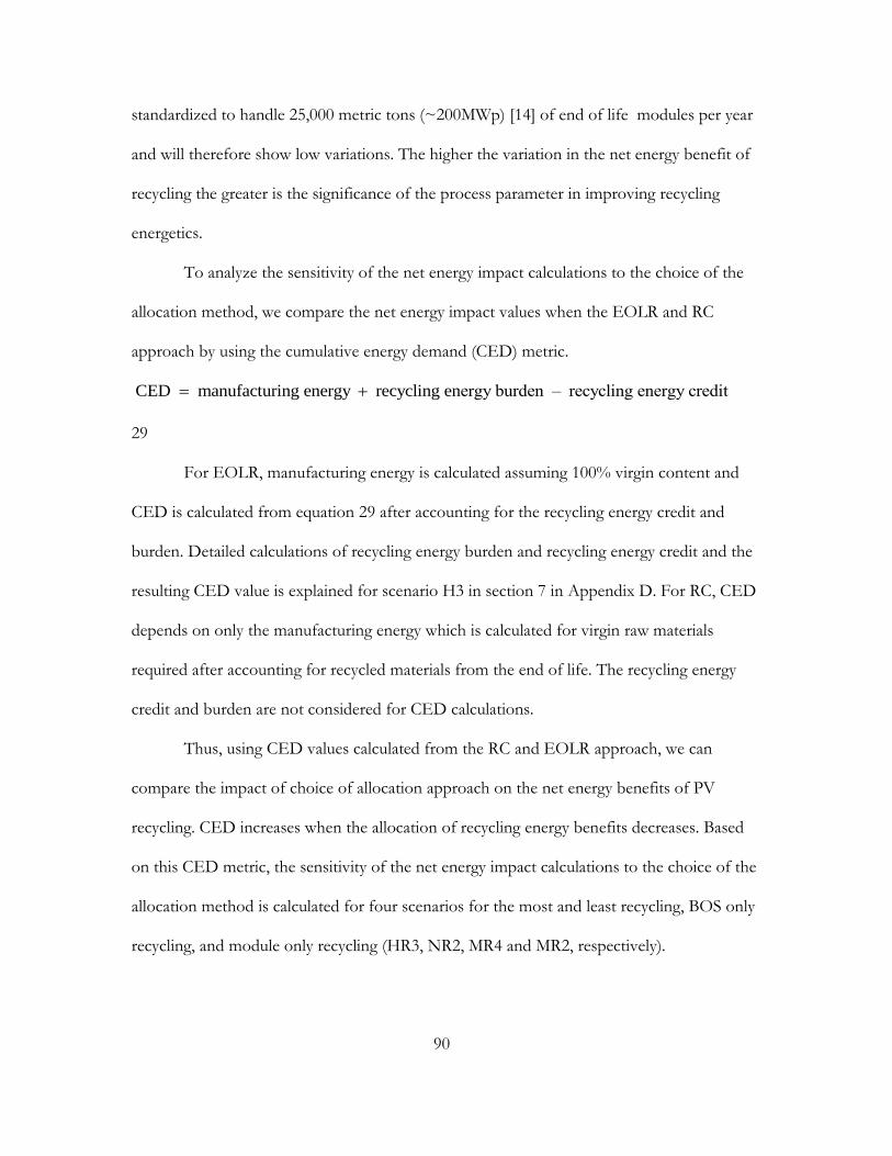
90

standardized to handle 25,000 metric tons (~200MWp) [14] of end of life modules per year

and will therefore show low variations. The higher the variation in the net energy benefit of

recycling the greater is the significance of the process parameter in improving recycling

energetics.

To analyze the sensitivity of the net energy impact calculations to the choice of the

allocation method, we compare the net energy impact values when the EOLR and RC

approach by using the cumulative energy demand (CED) metric.

CED manufacturing energy recycling energy burden – recycling energy credit

29

For EOLR, manufacturing energy is calculated assuming 100% virgin content and

CED is calculated from equation 29 after accounting for the recycling energy credit and

burden. Detailed calculations of recycling energy burden and recycling energy credit and the

resulting CED value is explained for scenario H3 in section 7 in Appendix D. For RC, CED

depends on only the manufacturing energy which is calculated for virgin raw materials

required after accounting for recycled materials from the end of life. The recycling energy

credit and burden are not considered for CED calculations.

Thus, using CED values calculated from the RC and EOLR approach, we can

compare the impact of choice of allocation approach on the net energy benefits of PV

recycling. CED increases when the allocation of recycling energy benefits decreases. Based

on this CED metric, the sensitivity of the net energy impact calculations to the choice of the

allocation method is calculated for four scenarios for the most and least recycling, BOS only

recycling, and module only recycling (HR3, NR2, MR4 and MR2, respectively).

91

At end of life, some or all of the system material can be recovered in decentralized

mobile units at the PV installation site or the system material can be transported to

centralized sites where disaggregation and recycling can be accomplished at permanent

facilities capturing economies of scale. For example, consider two options for separating and

refining the semiconductor from the module. In the first option, the semiconductor material

is separated from module glass at a mobile plant and then transported to a centralized facility

where it is refined. In the second option, the semiconductor is separated from glass and

refined at the mobile plant. The choice between recycling at a centralized or a decentralized

location is an energetic trade-off between (i) transporting the EOL PV system components

(with mass Mx, x = sys, mod, sc) over a distance (D km) and recycling it in the centralized

refining facility and, (ii) recycling the PV system components in the decentralized plants.

This energetic trade-off can be expressed as an energy penalty (Epenalty) that is incurred for

recycling PV systems decentrally.

penalty decentral_x trk x xE E - [(D E M )+E ] 30

where x = sys, mod, sc and Ex and Edecentral_x are the recycling energy requirements in the

centralized and decentralized facilities, respectively. Refer Table 1 in Appendix D for values

of Mx, Ex and Etrk. D is varied between 0 and 2500 km as transportation distances can vary

significantly based on the site of deployment and location at which the recycling

infrastructure exists. Decentralized recycling is energetically favorable if penaltyE < 0 as the

energy required to transport and recycle a PV system in a centralized location exceeds that of

decentralized recycling. Similarly, centralized recycling is favored when penaltyE > 0 . Since the

values of Mx, Ex and Etrk are known, Epenalty depends only on the values of Edecentral_x and D.

92

Therefore, we can determine combinations of Edecentral_x and D for which decentralized

recycling is favorable ( penaltyE < 0 ) and centralized recycling is favorable ( penaltyE > 0 ).

Literature values for the difference in energy between producing materials from the

primary and secondary routes vary between an upper and lower bound (Esec_prod_bnf values in

section 2 in Appendix D). The analysis assumes a point value for Esec_prod_bnf (equation 26) for

each material based on the average of the upper and lower bounds to calculate net energy

impact of recycling (equation28). The uncertainty analysis determines the sensitivity of the

net energy impact calculations to the point value of Esec_prod_bnf for four dominant materials

(by mass) – steel, aluminum, copper and glass (section 8 in Appendix D). The upper and

lower bounds of Esec_prod_bnf for a particular material is incremented and decremented by 20%

while keeping the Esec_prod_bnf for the other three materials fixed at the base point value. 10000

uniformly distributed random values of Esec_prod_bnf are generated between the newly

incremented and decremented bounds for the particular material and the corresponding

Enet_imp for each of these 10000 iterations is calculated using equation 28. The whisker plot

of the 10000 Enet_imp values generated for each of the four materials is compared with a

corresponding whisker plot for a base scenario (HR3).

93

Results

Figure 18 Net energy impact of CdTe PV system recycling. Net energy impact of CdTe PV system recycling for ten scenarios in Table 2. Negative values in green indicate a net energy benefit (energy saved > energy used) and positive values in brown indicate that energy used exceeds energy saved. The parenthesis contain the net energy impact as a percentage of the current energy intensity of manufacturing CdTe PV systems which is 1190 MJ/m2 (section 11 in Appendix D).

In Figure 18, the break-up of the energy used in recycling and the energy saved by

recovering materials through recycling and avoiding landfill operations are represented above

and below the x-axis, respectively. The results demonstrate that the energy benefits of

recycling increases with the mass of the PV system recycled. For example in HR3, where the

maximum mass is recycled (Table 5), the net energy benefit of recycling is 289 MJ per m2 of

the recycled CdTe system and this is 24% of the current energy intensity of manufacturing 1

m2 of a CdTe PV system.

94

Table 5 Material recovery from CdTe PV system recycling. Results for quantities (in kg per m2) of PV system materials recovered by scenario. Recycling and material recovery is not applicable (NA) in NR1 and MR1 as the BOS components continue to be used at the deployment site when there is a premature end of life of modules.

NR

1

NR

2

NR

3

MR

1

MR 2 MR

3

MR

4

HR

1

HR

2

HR 3

Glass 0 0 0 13.2 13.2 6.6 0 13.2 13.

2 13.2

Te 0 0 0 0.008 0.008 0.004 0 0.008 0.0

08 0.008

Cd 0 0 0 0.007 0.007 0.004 0 0.007 0.0

07 0.007

Steel NA 0 0 NA 0 5.4 10.8 10.8 10.

8 10.8

Aluminum NA 0 0 NA 0 0.3 0.3 0.3 0.3 0.3

Copper NA 0 0 NA 0 0.4 0.8 0.8 0.8 0.8

PVC NA 0 0 NA 0 0.02 0.04 0.04 0.0

4 0.04

HDPE NA 0 0 NA 0 0.1 0.3 0.3 0.3 0.3

EPDM NA 0 0 NA 0 0.03 0.06 0.06 0.0

6 0.06

Concrete NA 0 0 NA 0 1.7 3.4 3.4 3.4 3.4

Total 0 0 0 13.2 13.2 14.5 15.6 28.8 28.

8 28.8

95

Table 6 Definitions for all the acronyms

Abbreviation Definition Unit

sys PV system components (Transformer, Inverter -

mod PV module -

sc Semiconductor material in the PV module(CdTe) -

Eused Total energy used for recycling end-of-life CdTe PV

systems

MJ/ m2

E Energy required for recycling processes MJ/ m2

Eemis_cont Energy for controlling emissions from recycling

operations

MJ/ m2

Elnd_fl Total energy for landfill processes MJ/ m2

Etrans Energy for transportation MJ/ m2

Mlnd_fl Material landfilled kg/ m2

Dlnd_fl Distance to the landfill km

Etrk Energy intensity of transporting freight by truck MJ/ m2

Elnd_fl_op Energy used for landfill operations MJ/ m2

Elnd_fl_inc Energy recovered from incineration of materials at the

landfill

MJ/ m2

M Mass of material (in the PV system, module and

semiconductor)

kg/m2

rr Material recovery rate in each recycling step %

D Distance over which the materials are transported km

Esaved Total energy saved from recycling MJ/ m2

96

Abbreviation Definition Unit

Erecy_mat Energy benefits of recycling materials MJ/ m2

Eavd_lnd_fl Energy saved when landfilling is avoided by recycling MJ/ m2

Erecov Energy recovered from each recycling step MJ/ m2

Mrecy Mass of material recycled (from the PV system, module

and semiconductor)

kg/ m2

Esec_prod_bnf Energy difference between producing a material from

virgin and secondary (recycled) sources

MJ

Enet_imp Net energy impact of recycling MJ/ m2

Epenalty Energy penalty that is incurred for recycling PV systems

decentrally

MJ/ m2

Edecentral_x Recycling energy requirements in decentralized facilities MJ/ m2

To provide some perspective on the magnitude of the net energy benefit for HR3, it

would result in a reduction in the energy payback time (EPBT) of the PV system comparable

to increasing CdTe PV module conversion efficiency from its current average value of 14%

to over 18.42% (for calculations refer section 4 in Appendix D) , which is the current

medium-term (2016-2017) target for this technology [42]. Therefore, PV system recycling

has the potential to improve the energy payback time of PV systems [43] as much as

improved module conversion efficiency. MR4, HR1, HR2, and HR3 have the highest energy

gains and the magnitude of the green bars is largely due to recycling of glass in PV modules

and metals in the BOS, inverter and transformer (for a break-up of the energy gains of

recycling materials refer section 6 in Appendix D). The advantages of PV system recycling is

97

further demonstrated in MR2 and NR2 where recycling energy benefits are reduced as the

BOS and electrical systems are landfilled and therefore, energy gains from recycling materials

is zero.

It should be noted that the magnitude of the net energy impact of scenarios MR2

and NR2 is small (<=5%) relative to the energy intensity of manufacturing CdTe PV

systems. In the context of the uncertainty in this analysis (Figure 5 in Appendix D), the net

energy impact of these scenarios is approximately neutral. However, these scenarios reflect

differing approaches to waste management, with MR2 including PV module recycling and

NR2 including PV module landfilling. The finding that these differing scenarios yield similar

(approximately neutral) net energy impacts indicates an important limitation of this study,

which focuses on the energy demand of PV system recycling. The motivation for PV

recycling extends beyond energy demand to management of environmentally sensitive

materials and recovery of critical materials. For example, Bergesen et al. [9] indicated that

PV system recycling can achieve on the order of 50% reductions in life cycle carcinogenic

emissions and metal depletion, and Held [17] indicated that PV module recycling can achieve

on the order of 6-8% reductions in acidification, euthrophication, and photochemical ozone

creation potential. Therefore, although MR2 and NR2 have similar net energy impacts, the

broader life cycle impacts with regards to health and resource depletion should be

considered when evaluating PV module recycling (MR2) versus landfilling (NR2). As shown

in Table 5, MR2 includes recoverable quantities of 13.2 kg of glass, 0.008 kg of Te, and

0.007 kg of Cd per m2 of system, whereas NR2 has no material recovery.

In NR3, as distances to landfills increase, the transportation energy of bulk materials

in BOS, inverters and transformers to the landfill increases, though it is still relatively small

98

compared with the energy required to manufacture 1 m2 of a CdTe PV system. Scenario

MR3 demonstrates that recycling benefits decrease by 52% (MR3 versus HR3) when the

BOS life is extended to 60 years as energy benefits are alocated equally over two installations

of PV modules having a life of 30 years each. MR3 shows the net positive energy impact of

recycling all materials in a PV system even after halving energy benefits of recovering BOS

materials. For scenarios MR1 and NR1 that simulate premature end-of-life due to

unanticipated breakage or failures at the manufacturing or deployment location, net energy

impacts are similar and approximately neutral. As discussed above in the comparison of

MR2 and NR2, the finding of similar net energy impacts for MR1 and NR1 again indicates a

limitation of this study. In addition to considering energy impacts, the broader life cycle

impacts with regards to health and resource depletion should be considered when evaluating

PV module recycling (MR1) versus landfilling (NR1).

The results depicting sensitivity of net energy benefit calculations to the choice of

allocation approach (Figure 19) shows that the CED in the EOLR approach is higher by 0.4

to 10.2% than the RC approach. The EOLR approach decreases the recycling benefits

allocated to the PV system. Therefore, the results in Figure 18, calculated using the EOLR

approach, represent the lower bound of the net recycling energy benefits allocated to the

CdTe PV system.

99

Figure 19. Allocation method and recycling net energy benefit calculations Cumulative energy demands across all four scenarios are comparable, regardless of whether the Recylced Content (RC) or End Of Life Recycling (EOLR) approaches are adopted.

The uncertainty analysis results (section 8 in Appendix D) demonstrate that net

energy benefit calculation is most sensitive to Esec_prod_bnf values for steel. Even when lowest

literature reported value for the recycling energy benefit of steel (Esec_prod_bnf_steel) is used,

recycling offers a net benefit of around 10% (122 MJ/m2 in Figure 5 in Appendix D) of the

manufacturing energy requirements of 1190 MJ/m2. The ES and BOS requirement per m2 of

the PV system are modeled based on utility scale deployments (3.5 MW and 550 MWAC

plants in [20] and [21]). This requirement may vary for non-utility scale deployments and this

will change the magnitude of recycled material and the corresponding recycling energy

benefits. The scenario and uncertainty analysis demonstrate that recycling of PV systems

(module+ BOS+ES) and the credits earned through recycling these materials can reduce the

cumulative energy demand of the PV system by 10 to 24% (137 MJ/m2 in Figure 5 in

100

Appendix D and 289 MJ/m2 for HR3 in Figure 18 in main paper, respectively) on a lifecycle

basis.

Figure 20 Energy impacts of centralized and decentralized recycling. Frontier diagram depicting two regions where centralized and decentralized facilities are favorable for module semiconductor separation (step 2). Decentralized recycling is favorable in the blue region where the combination of the distance to the centralized facility and the energy required at the decentralized facility result in a negative energy penalty (Epenalty < 0 from equation 30). Similarly, centralized recycling is favored in the orange region when energy penalty of decentralization is positive.

Figure 20 in the main paper and Figure 6 in the Appendix D demonstrate that with

increasing distances to the centralized location, in-situ mobile based operations that

disassemble the system and separate the glass from the module is favored. This is due to the

increase in energy impacts when bulk metals and glass in the PV system and module (33.98

and 16.66 kg/m2) are transported over larger distances. Centralized operations are

comparatively favorable for the semiconductor refining step (step 3 in Figure 16) even with

increasing distances (figure 7 in Appendix D) because the transportation impact increase

101

insignificantly as the mass of unrefined USM transported for step 3 is only 0.06 kg/m2.

Decentralized refining of semiconductor will only be favorable if the energy requirements

are lower than the current energy footprint in centralized facilities (Esc = 26 MJ/m2, refer

Table 1 in Appendix D).

Figure 21 Sensitivity analysis of CdTe PV recycling energetics. Sensitivity of recycling energy benefits to parameters under the control of a recycler. The parameter is incremented and decremented by 20% and the horizontal bars depict the corresponding percentage change in recycling energy benefit from the base value in HR3.

In Figure 21, the net energy benefits of recycling is most sensitive to parameters with

the widest bars and a recycler can identify strategies to improve these parameters to

maximize the energy benefits of CdTe system recycling. Benefits can be maximized by

increasing steel and glass recovery from module, BoS and the electrical components and

reducing energy requirements for separation of unrefined semiconductor material (Emod in

step 2 in Figure 16).

Conclusion

102

The net energy impact analysis shows that 24% of the manufacturing energy of a

CdTe PV system is recovered under conditions of maximum recycling (scenario HR3 in

Figure 18). Further, these recycling energy benefits are conservative estimates as they are

calculated using the EOLR allocation approach which lowers benefits by 0.5 to 10.2% when

compared to the RC allocation approach (Figure 19). The uncertainty analysis (Figure 5 in

Appendix D) shows that the calculation of the net energy impact is most sensitive to the

difference between the energy intensity of primary and secondary pathways of steel

production (Esec_prod_bnf). Even when the conservative lower bound of literature reported

values for Esec_prod_bnf is used, 10% of the manufacturing energy of CdTe PV systems is

recovered through recycling (122 MJ/m2 in Figure 5 in Appendix D).

An energy trade-off analysis between decentralized and centralized PV recycling

operations (Figure 20 in main paper and Figure 6 in Appendix D) shows that, with

increasing distances, decentralized operations are favorable as they minimize the

transportation energy impacts of bulk materials processed during system disassembly and

module semiconductor separation (steps 1 and 2 in Figure 16). Decentralization can include

(i) leveraging the existing network of metal and glass recyclers and industries where recycled

materials can be used as raw materials for subsequent processes [44][45], (ii) locating mobile

recycling units for step 2 in the vicinity of disassembly centers or deployment sites.

Centralized operations are favorable for semiconductor refining (Figure 6 in Appendix D) as

transportation energy requirements for 0.06 kg/m2 of the USM is negligible. The results on

centralization and decentralization for the different PV recycling steps are relevant to current

recycling operations where manufacturers are managing EOL PV systems based on recycling

warranties at the time of purchase. In the future, these findings can inform policy on

incentivizing optimal locations for recycling infrastructure to minimize environmental

103

impacts when small scale and third party recyclers are expected to play a larger role in PV

recycling.

The sensitivity analysis results (Figure 21) reveals that a recycler can significantly

increase the recycling energy benefits by reducing the energy footprint of the USM recovery

process (Emod). Approximately half of the USM separation energy is spent on removing or

delaminating the ethylene vinyl acetate (EVA) encapsulant through mechanical processes

[46] and reducing the energy for this process is a potential area for technical improvement

[47]. Preliminary lab scale research has identified thermal processing [48], organic

solvents[49], ultrasonic radiation [50], micro-emulsions [23] and cryogenic treatment[23]- as

alternate methods for EVA removal. With current PV recycling studies using retrospective

data based on commercially mature processes, methodological advances in impact

assessments are required to analyze the energy and environmental impacts of adopting these

alternate lab scale methods at an industrial scale. Recent studies on the anticipatory lifecycle

assessment (a-LCA) framework [51][52] contain methodological advances to extrapolate lab

scale data to a commercial scale and explore a prospective range of energy and

environmental impacts for simulated scenarios. These a-LCA methods can be applied to lab

scale data for alternate EVA removal methods and inform recyclers on favorable pathways

to minimize the energy impacts and improve the environmental performance of future PV

recycling.

Application of a similar approach can identify environmentally improved pathways

for recycling c-Si PV systems which account for 90% of the global PV deployments [53] and

will be the largest source of PV waste after an operational life span of 30 years. The first two

steps of CdTe PV recycling (Figure 16) are applicable to c-Si systems as the components and

bulk material contained in the BOS and ES of c-Si and CdTe PV systems are similar

104

[20][21]. Therefore, decentralization of recycling facilities, as demonstrated for CdTe PV

recycling, will reduce transportation impacts of system disassembly and semiconductor

module separation for c-Si PV recycling. The proposed a-LCA approach to evaluate

environmental impacts of novel encapsulant removal methods for CdTe PV recycling is

equally applicable to c-Si systems as EVA is the most common encapsulant in the PV

industry [54]. Currently, 90% of the glass is recovered from CdTe PV modules [18] in step 2

and a similar recovery rate for bulk material from end of life c-Si PV systems will result in

significant energy benefits. The energetics for the third step of recycling will be significantly

different for c-Si systems as the mass of unrefined solar grade silicon (1.4 kg/m2, refer

section 10 in Appendix D) that will be transported for semiconductor recovery is higher

than USM in CdTe PV recycling (0.06 kg/m2, Msc in Table 5 in Appendix D). Further,

energy benefits derived from refining silicon in step 3 is higher compared to CdTe refining

as the displaced primary process that produces solar grade silicon is energetically the most

expensive for c-Si modules [55] and incurs high production losses of 40 -50 % during wafer

slicing [56]. The corresponding values for energetic share in the module manufacturing

process [31] and semiconductor manufacturing losses [57] are significantly lower for thin

film CdTe PV systems.

Acknowledgements




of the author and do not necessarily reflect those of NSF or DOE. We are thankful for the

timely feedback and continued support from First Solar. The authors acknowledge the

105

support from B.A.Wender, Valentina Prado Lopez and other colleagues at the Quantum

Energy and Sustainable Solar Technologies (QESST) center and members of the AWƩ

studio at ASU. We thank the anonymous reviewers for their feedback which has helped

improve this paper.

References

[1] O. Edenhofer, R. Pichs-Madruga, Y. Sokona, K. Seyboth, P. Matschoss, S. Kadner, T. Zwickel, P. Eickemeier, G. Hansen, S. Schlömer, and C. von Stechow, IPCC, 2011: Summary for Policymakers. In: IPCC Special Report on Renewable Energy Sources and Climate Change Mitigation. 2011.

[2] E. Alsema, D. Fraile, R. Frischknecht, V. Fthenakis, M. Held, H. . Kim, W. Pölz, M. Raugei, and M. de Wild Scholten, “Methodology guidelines on life cycle assessment of photovoltaic electricity,” IEA PVPS Rep., 2011.

[3] European Union, “Article 2(1)(a) in Directive 2012/19/EU of the European Parliament and of the Council on waste electrical and electronic equipment (WEEE),” 2012. [Online]. Available: http://eur-lex.europa.eu/LexUriServ/LexUriServ.do?uri=OJ:L:2012:197:FULL:EN:PDF.

[4] “Article 11.6, SB 1020 (California Photovoltaic Panel Collection and Recycling Act of 2014),” 2014. [Online]. Available: http://www.leginfo.ca.gov/pub/13-14/bill/sen/sb_1001-1050/sb_1020_bill_20140214_introduced.html.

[5] First Solar, “Sustainability Metrics,” 2014. [Online]. Available: http://www.firstsolar.com/en/about-us/corporate-responsibility/sustainability-metrics.

[6] Trina Solar, “Sustainability,” 2014. [Online]. Available: http://www.trinasolar.com/us/about-us/Sustainability.html.

[7] Yingli Solar, “Corporate Sustainability Report,” 2013. [Online]. Available: http://www.yinglisolar.com/us/about/sustainability/.

[8] M. Raugei, M. Isasa, and P. F. Palmer, “Potential Cd emissions from end-of-life CdTe PV,” Int. J. Life Cycle Assess., vol. 17, no. 2, pp. 192–198, 2012.

[9] J. D. Bergesen, G. A. Heath, T. Gibon, and S. Suh, “Thin-film photovoltaic power generation offers decreasing greenhouse gas emissions and increasing environmental co-benefits in the long term.,” Environ. Sci. Technol., vol. 48, no. 16, pp. 9834–43, Aug. 2014.

106

[10] M. Marwede and A. Reller, “Future recycling flows of tellurium from cadmium telluride photovoltaic waste,” Resour. Conserv. Recycl., 2012.

[11] M. Redlinger, R. Eggert, and M. Woodhouse, “Evaluating the availability of gallium, indium, and tellurium from recycled photovoltaic modules,” Sol. Energy Mater. Sol. Cells, vol. 138, pp. 58–71, 2015.

[12] V. Fthenakis, “Sustainability of photovoltaics: The case for thin-film solar cells,” Renew. Sustain. Energy Rev., vol. 13, no. 9, pp. 2746–2750, Dec. 2009.

[13] Bifa environmental Institute, “Eco-efficiency Analysis of Photovoltaic Modules,” 2013.

[14] First Solar, “PV Recycling Policies and Technology,” IEA PVPS, 2014.

[15] P. Sinha, M. J. de Wild-Scholten, Y. Matsuno, K. Brutsaert, and I. Soga, “Environmental benefits of a megasolar CdTe PV project in Japan,” in 6th World Conference on Photovoltaic Energy Conversion, 2014.

[16] P. Sinha, M. J. de Wild-Scholten, and L. Luckhurst, “Environmental Benefits of Solar Photovoltaics in South Africa,” in 1st Africa Photovoltaic Solar Energy Conference Proceedings, 2014.

[17] M. Held, “Life cycle assessment of CdTe module recycling,” in 24th EU PVSEC Conference, 2009, pp. 2370 – 2375.

[18] P. Sinha, M. Cossette, and J.-F. Menard, “End-of-life CdTe recycling with semiconductor refining,” in 27th EU PVSEC, 2012, pp. 24–28.

[19] A. Müller, K. Wambach, and E. Alsema, “Life Cycle Analysis of Solar Module Recycling Process,” Mater. Res. Soc. Symp. Proc., vol. 895, pp. 1–6, 2006.

[20] J. E. Mason, V. M. Fthenakis, T. Hansen, and H. C. Kim, “Energy payback and life-

cycle CO2 emissions of the BOS in an optimized 3·5 MW PV installation,” Prog. Photovoltaics Res. Appl., vol. 14, no. 2, pp. 179–190, Mar. 2006.

[21] P. Sinha and M. de Wild-Scholten, “Life Cycle Assessment of Utility-Scale CdTe PV Balance of Systems,” in 27th European Photovoltaic Solar Energy Conference, 2012, pp. 4657 – 4660.

[22] W. Berger, F.-G. Simon, K. Weimann, and E. A. Alsema, “A novel approach for the recycling of thin film photovoltaic modules,” Resour. Conserv. Recycl., vol. 54, no. 10, pp. 711–718, Aug. 2010.

107

[23] M. Marwede, W. Berger, M. Schlummer, A. Mäurer, and A. Reller, “Recycling paths for thin-film chalcogenide photovoltaic waste – Current feasible processes,” Renew. Energy, vol. 55, pp. 220–229, Jul. 2013.

[24] G. Granata, F. Pagnanelli, E. Moscardini, T. Havlik, and L. Toro, “Recycling of photovoltaic panels by physical operations,” Sol. Energy Mater. Sol. Cells, vol. 123, pp. 239–248, Apr. 2014.

[25] G. Giacchetta, M. Leporini, and B. Marchetti, “Evaluation of the environmental benefits of new high value process for the management of the end of life of thin film photovoltaic modules,” J. Clean. Prod., vol. 51, pp. 214–224, Jul. 2013.

[26] J. B. Manuel Diequez Campo, Dieter Bonnet, Rainer Gegenwart, “Process for recycling CdTe/Cds thin film solar cell modules,” US 6572782 B22003.

[27] P. Taylor and M. DeFilippo, “Process to recycle end of life CDTE modules and manufacturing scrap,” US 8821711 B22014.

[28] V. Fthenakis and W. Wang, “extraction; leaching; cation exchange resins; for recycling photovoltaic devices,” US 7731920 B22010.

[29] S. Kang, S. Yoo, J. Lee, B. Boo, and H. Ryu, “Experimental investigations for recycling of silicon and glass from waste photovoltaic modules,” Renew. Energy, vol. 47, pp. 152–159, Nov. 2012.

[30] E. Klugmann-Radziemska and P. Ostrowski, “Chemical treatment of crystalline silicon solar cells as a method of recovering pure silicon from photovoltaic modules,” Renew. Energy, vol. 35, no. 8, pp. 1751–1759, Aug. 2010.

[31] M. Held and R. Ilg, “Update of environmental indicators and energy payback time of CdTe PV systems in Europe,” Prog. Photovoltaics Res. Appl., vol. 19, no. January, pp. 614–626, 2011.

[32] J. K. Choi and V. Fthenakis, “Design and optimization of photovoltaics recycling infrastructure.,” Environ. Sci. Technol., vol. 44, no. 22, pp. 8678–83, Nov. 2010.

[33] J. K. Choi and V. Fthenakis, “Crystalline silicon photovoltaic recycling planning: Macro and micro perspectives,” J. Clean. Prod., vol. 66, pp. 443–449, 2014.

[34] V. Fthenakis, “End-of-life management and recycling of PV modules,” Energy Policy, vol. 28, no. 2000, pp. 1051–1058, 2000.

108

[35] European Commission, “Photovoltaic panels Mobile Recycling Device (PV-MOREDE),” 2014. [Online]. Available: http://ec.europa.eu/environment/eco-innovation/projects/en/projects/pv-morede.

[36] R. S. Jorge, T. R. Hawkins, and E. G. Hertwich, “Life cycle assessment of electricity transmission and distribution—part 2: transformers and substation equipment,” Int. J. Life Cycle Assess., vol. 17, no. 2, pp. 184–191, Sep. 2011.

[37] R. Frischknecht, “LCI modelling approaches applied on recycling of materials in view of environmental sustainability, risk perception and eco-efficiency,” Int. J. Life Cycle Assess., vol. 15, no. 7, pp. 666–671, Jun. 2010.

[38] J. X. Johnson, C. A. McMillan, and G. A. Keoleian, “Evaluation of Life Cycle Assessment Recycling Allocation Methods,” J. Ind. Ecol., vol. 17, no. 5, pp. 700–711, Sep. 2013.

[39] A. Dubreuil, S. B. Young, J. Atherton, and T. P. Gloria, “Metals recycling maps and allocation procedures in life cycle assessment,” Int. J. Life Cycle Assess., vol. 15, no. 6, pp. 621–634, 2010.

[40] J. Atherton, “Declaration by the Metals Industry on Recycling Principles,” Int. J. Life Cycle Assess., vol. 12, no. 1, pp. 59–60, 2007.

[41] G. Bergsma and M. Sevenster, “End-of-life best approach for allocating recycling benefits in LCAs of metal packaging,” 2013.

[42] R. Garabedian, “Technology Update,” First Sol. Anal. Meet., 2014.

[43] M. Goe and G. Gaustad, “Strengthening the case for recycling photovoltaics: An energy payback analysis,” Appl. Energy, vol. 120, pp. 41–48, May 2014.

[44] K. Burrows and V. Fthenakis, “Glass needs for a growing photovoltaics industry,” Sol. Energy Mater. Sol. Cells, vol. 132, pp. 455–459, 2015.

[45] J. M. Pearce, “Industrial symbiosis of very large-scale photovoltaic manufacturing,” Renew. Energy, vol. 33, no. 5, pp. 1101–1108, 2008.

[46] First Solar, “Personal Communication,” 2014.

[47] First Solar, “PV Recycling Policies and Technology,” IEA PVPS, 2014.

[48] T. Wang, J. Hsiao, and C. Du, “Recycling of materials from silicon base solar cell module,” 38th IEEE Photovolt. Spec. Conf., pp. 2355–2358, 2012.

109

[49] T. Doi, I. Tsuda, H. Unagida, A. Murata, K. Sakuta, and K. Kurokawa, “Experimental study on PV module recycling with organic solvent method,” Sol. Energy Mater. Sol. Cells, vol. 67, no. 1–4, pp. 397–403, Mar. 2001.

[50] Y. Kim and J. Lee, “Dissolution of ethylene vinyl acetate in crystalline silicon PV modules using ultrasonic irradiation and organic solvent,” Sol. Energy Mater. Sol. Cells, vol. 98, no. x, pp. 317–322, Mar. 2012.

[51] T. R. Dwarakanath, B. A. Wender, T. Seager, and M. P. Fraser, “Towards anticipatory life cycle assessment of photovoltaics,” in 2013 IEEE 39th Photovoltaic Specialists Conference (PVSC), 2013, pp. 2392–2393.

[52] B. A. Wender, R. W. Foley, V. Prado-Lopez, D. Ravikumar, D. A. Eisenberg, T. A. Hottle, J. Sadowski, W. P. Flanagan, A. Fisher, L. Laurin, M. E. Bates, I. Linkov, T. P. Seager, M. P. Fraser, and D. H. Guston, “Illustrating Anticipatory Life Cycle Assessment for Emerging Photovoltaic Technologies.,” Environ. Sci. Technol., Sep. 2014.

[53] “Photovoltaics Report - Fraunhofer institute for solar energy systems.” [Online]. Available: http://www.ise.fraunhofer.de/en/downloads-englisch/pdf-files-englisch/photovoltaics-report.pdf. [Accessed: 11-May-2014].

[54] NREL, “Module Encapsulation Materials, Processing and Testing,” 2008. [Online]. Available: http://www.nrel.gov/docs/fy09osti/44666.pdf.

[55] N. Jungbluth, M. Tuchschmid, and M. de Wild-Scholten, “Life Cycle Assessment of Photovoltaics: Update of ecoinvent data v2. 0,” ESU-services Ltd., 2008, pp. 1–22, 2008.

[56] T. Y. Wang, Y. C. Lin, C. Y. Tai, R. Sivakumar, D. K. Rai, and C. W. Lan, “A novel approach for recycling of kerf loss silicon from cutting slurry waste for solar cell applications,” J. Cryst. Growth, vol. 310, no. 15, pp. 3403–3406, 2008.

[57] M. Woodhouse, A. Goodrich, R. Margolis, T. James, R. Dhere, T. Gessert, T. Barnes, R. Eggert, and D. Albin, “Perspectives on the pathways for cadmium telluride photovoltaic module manufacturers to address expected increases in the price for tellurium,” Sol. Energy Mater. Sol. Cells, pp. 1–14, Apr. 2012.

110

Chapter 5

AN ANTICIPATORY LIFECYCLE ASSESSMENT OF NOVEL AND EXISTING

CDTE PV MODULE RECYCLING PROCESSES

Introduction

Worldwide PV system deployments are increasing to reduce the reliance on

electricity generated from greenhouse gas (GHG) intensive sources and meet climate goals.

With these deployments expected to reach end of life (EOL) in 25 years, environmentally

improved processes are required to recycle 78 million tons of projected PV waste in 2050

[1]. First Solar, the world’s largest recycler, transports EOL PV systems from multiple

deployment sites to centrally located recycling plants and recycles them through a

combination of mechanical and chemical processes. Proposing and evaluating possible

environmental improvements to existing recycling methods require a (1) quantification of

energy and material flows and identifying environmental hotspots in existing operations that

recycle the PV system (2) identifying novel recycling methods that can address the hotspots

(3) evaluating the environmental trade-offs of replacing the incumbent recycling process

with alternatives at a commercial scale. Recent research on the energetics of CdTe PV

recycling shows that the mechanical shredding and hammering processes, required to

weaken the ethylene vinyl acetate (EVA) encapsulant before recycling the module materials,

accounts for around 50% of the energy footprint [2]. Replacing the mechanical processes

with chemical or high temperature alternatives may offer potential environmental

improvements. Also, adopting these alternatives in decentralized plants at the deployment

site may be environmentally preferable to the current approach of transporting and recycling

modules at centralized facilities.

111

Lifecycle assessment (LCA), the preferred framework for analyzing the

environmental trade-offs between alternate choices, relies on inventory data gathered from

commercial scale processes that have matured over a period of time and, therefore, is

methodologically retrospective [3]. In contrast, the novel processes are studied at a lab or

pilot scale and literature on these processes focus primarily on the feasibility of recovering

materials from the EOL module and do not always report the material and energy inventory

requirements. Recent studies on the elimination of the ethylene vinyl acetate (EVA)

encapsulant using organic solvents and ultrasonic radiation [4], dissolution in organic

solvents [5], pyrolysis [6][7] and a combination of thermal and physical processes[8] do not

report the raw material requirements and energy used. Furthermore, studies reporting energy

or material values for novel PV recycling methods contain significant uncertainty. For

example, energy requirements for the thermal delamination of EVA per wafer vary

significantly between 0.1 kWh [9] and 0.65 kWh [10]. Another study, exploring a

combination of thermal and chemical processes for delamination, reported a value of 81.7

kWh/m2 without disaggregating the energy between the thermal and chemical processes [11].

Also, prospective LCAs that evaluate an emerging technology and identify

environmental hotspots for future improvements [12][13][14][15] may fail in a comparative

context where the mutual differences in the environmental impacts of the alternatives and

not the environmental hotspots of a particular alternative determine the environmental

preferable alternative. For example, a recent study comparing five PV technologies[16]

showed that the choice of CdTe as an environmentally preferable option over crystalline

silicon technologies is driven by the mutual difference in the water depletion impact

category. A prospective LCA, in this case, would have identified freshwater eutrophication as

the environmental hotspot for future improvement. Also, by evaluating the environmental

112

hotspots without accounting for the relevant stakeholder inputs, prospective LCAs cannot

guide an emerging technology towards an environmentally favorable trajectory in a specific

decision context.

The lack of a comprehensive study that compares the environmental impacts of

multiple CdTe PV recycling alternatives, unavailable or uncertain material and energy data

for emerging PV recycling processes and the inherent methodological limitations in

traditional and prospective LCA methods prevents PV recyclers from addressing three

questions that can environmentally improve future CdTe PV recycling operations– (1) Do

the alternative recycling methods at the lab scale environmentally outperform the incumbent

process at the commercial scale? (2) What are the future research priorities to further reduce

the environmental impact of the most environmentally promising PV recycling alternative?

(3) Are the alternative methods operating in small-scale decentral plants environmentally

preferable to transporting and recycling modules in centralized plants?

This study uses the Anticipatory LCA framework[17], a recent methodological

innovation, to address these problematic aspects by stochastically comparing the

environmental impacts of the incumbent and the alternatives for recycling CdTe PV

modules, identifying the most environmentally promising pilot-scale recycling alternative for

future commercialization, determining the uncertainties and stakeholder inputs that can

impact the choice of this preferable alternative, identifying the environmental hotspots and

prioritizing future research to address the hotspots and maximize the environmental benefit

of commercializing the preferred alternative.

This study evaluates the environmental impact of four pilot-scale alternatives –

thermal delamination of EVA [18], EVA dissolution by heating in an organic solvent [5], and

EVA dissolution through probe [4] or bath sonication - to the incumbent mechanical

113

shredding and hammering process that eliminates the EVA encapsulant [19]. As an

alternative to the incumbent leaching and precipitation process for the recovery of cadmium

and tellurium [19], the environmental impacts of solvent extraction [20][21][22] and ion-

exchange [23][24] are investigated. Energy and material inventory data for EVA elimination

through - pyrolysis, dissolution by heating in an organic solvent and dissolution though

sonication (probe and bath) - is gathered from laboratory experiments. Energy and material

inventory data for EVA elimination in the incumbent commercial process [25] and recovery

of cadmium and tellurium through - precipitation [25], solvent extraction (section 3

Appendix E), ion-exchange (section 1 Appendix E) - are determined from published

literature. Based on different combinations of methods for EVA delamination and cadmium

and tellurium recovery, seven CdTe PV recycling alternatives (Table 7) are compared for

environmental impacts (Figure 22). The LCA software - SimaPro® [26] - is used to calculate

the lognormal mean and standard deviation of the 18 environmental impact categories in

ReCiPe impact assessment method [27] from the material and energy inventories for the

seven recycling alternatives.

Using Stochastic Multi-attribute Assessment (SMAA) framework [28], this research

stochastically generates values for the 18 environmental impact categories from the

lognormally distributed mean and standard deviation, compares and outranks the values, and

calculates an aggregated environmental score for each of the recycling alternatives. The

aggregated environmental scores range between -1 (environmentally least favorable) and +1

(environmentally most favorable). To analyze the environmental trade-offs between

decentralized and centralized recycling, the aggregated environmental scores of the most

environmentally promising novel alternative operating in a decentralized and the centralized

recycling plant are compared. To prioritize future research effort, the parameters that

114

significantly improve the environmental performance of the novel recycling methods at a

commercial scale are identified through a global sensitivity analysis (GSA) [29].

Methods

Energy and material flows for the incumbent and emerging recycling processes

Figure 22 Material and energy flows for CdTe recycling alternatives. Material and energy flows for the incumbent (black) and alternate (green) recycling processes considered in this research.

Figure 22 represents the material and energy flows for the incumbent CdTe PV

recycling process consisting of EVA delamination (shredding and hammering) and the

recovery of cadmium and tellurium (leaching & agitation, solid-liquid separation,

precipitation) [25]. This study evaluates the environmental impacts of replacing the

incumbent EVA delamination process with alternate methods (organic solvent dissolution/

115

ultrasonication/ thermal delamination), and cadmium and tellurium recovery methods

(cadmium solvent extraction + cadmium stripping &precipitation + tellurium precipitation/

cadmium ion exchange + cadmium stripping & precipitation + tellurium precipitation). The

functional unit for the comparative environmental impact assessment is 1 m2 of an end-of-

life CdTe PV module and the common outputs are cord plate, copper wiring, glass, and

cadmium and tellurium precipitate. The feasibility and the energy and material requirements

for the alternate EVA delamination methods are determined experimentally as there are no

studies evaluating these processes for CdTe modules. The energy and material requirements

for the incumbent process and alternative cadmium and tellurium recovery methods are

calculated from published literature.

Incumbent CdTe PV recycling process

In the incumbent recycling process (black in Figure 22), the EOL module is

preprocessed to remove the cord plate and copper wiring. The module is shred to large

pieces and then hammered to 4-5 mm size pieces. The smaller size reduces the binding

strength of the EVA encapsulant and exposes the CdTe layer to the leaching reactions

(section 2 SI). Under acidic and oxidative conditions in the rotating leach drum, the CdTe

layer is solubilized to Te4+ and Cd2+ after reacting with sulfuric acid and hydrogen peroxide

[30][31]. The leachate is subsequently separated from the remaining glass particles in the

solid-liquid separation step. After separation the leachate’s pH is increased by adding sodium

hydroxide to precipitate and recover the cadmium and tellurium in the form of a

semiconductor cake. For the energy and material requirements of the incumbent CdTe PV

recycling process refer section 4 of Appendix E.

116

Thermal delamination of EVA

This study experimentally determines the minimum time and energy requirements to

completely delaminate glass samples by heating them to 500⁰C in air. Previous studies report

deacetylation and the formation of terminal alkenes at 360⁰C and 480⁰C, respectively

[9][11][10][18][32]. 8x8 inch glass samples [33] were laminated with EVA [34] in a PV

module laminator [35] and heated to 500⁰C in a Vulcan 3-1750 box furnace [36] for Trun

minutes. The furnace is then switched off and the sample is allowed to cool inside the closed

furnace for Tclose minutes as the residue from EVA heating combusts if the furnace is

immediately opened after Trun minutes. The furnace is then opened and the delaminated

sample is allowed to cool for Topen minutes as the glass cracks if the sample is removed

immediately after opening the furnace. Complete delamination is confirmed through a mass-

balance by weighing the sample before and after the thermal delamination. The energy

required to run the furnace for Trun minutes is measured with an energy meter. The

experimental runs, values for Trun, Tclose, Topen , and the energy requirements are reported in

section 6 of Appendix E.

Delaminating EVA by heating in an organic solvent

This study experimentally measures the energy, solvent volume and time required for

delaminating 2x2 inch glass samples [33] laminated with EVA [34] in a PV module laminator

[35] by heating in (1) o-dichlorobenzene(99.8% anhydrous, [37]) at 165⁰C, (2) toluene(99.8%

anhydrous, [38]) at 95⁰C, and (3) trichloroethylene(>= 99%, [39]) at 70⁰C. The temperatures

chosen is 15⁰C lower than the respective boiling points to prevent evaporation of the

solvents. The samples are immersed in 300 ml of the solvent in a closed beaker and heated

on a hot-plate until delamination. The energy required for heating is measured with an

117

energy meter. The experimental runs, delamination time, and energy requirements are

reported in section 7 of Appendix E.

Delaminating EVA by sonicating in an organic solvent

This study experimentally measures the energy and time required for delaminating

glass samples immersed in (1) o-dichlorobenzene (99.8% anhydrous, [37]), (2) toluene(99.8%

anhydrous, [38]), and (3) trichloroethylene(>= 99%, [39]), and ultrasonicated with bath and

probe sonicators. For the bath sonication, 2x2 inch glass samples [33] laminated with EVA

[34] in a PV module laminator [35] are immersed in the solvent and the beaker was placed in

a bath sonicator [40] containing water. The temperature during the bath sonication was set

to the maximum allowed value of 60⁰C.

For the probe sonication, 2x2 inch glass samples [33] laminated with EVA [34] in a

PV module laminator [35] are immersed in the solvent and ultrasonicated with a probe tip.

The probe sonicator is set to an alternate 3 minute on and off cycles to prevent over-heating

of the probe tip. The solvent is not heated before sonication as heat is generated by the

probe tip during sonication.

Extracting cadmium through ion exchange

Wang and Fthenakis experimentally investigated the feasibility of removing cadmium

dissolved in an acidic solution (simulating the leachate from the solid-liquid separation in

Figure 22) using Amberlyst 15 and DOWEX 50X8 [23], [24], [41]. The energy and material

requirements for ion-exchange extraction of cadmium (section 1 Appendix E) is calculated

from values reported in [23] which simulates the operational conditions similar to that of

CdTe module recycling in the incumbent process.

118

Solvent extraction of cadmium

The cadmium from the leachate obtained from the solid-liquid separation in Figure

22 can be extracted into an organic phase using the extractant molecule di(2-ethylhexyl)

Phosphoric Acid (D2EHPA) dissolved in kerosene. This study calculates the energy and

material requirements of the solvent extraction of cadmium using D2EHPA as it is

commonly used for extracting cadmium [20][21][22] and was evaluated in a pilot scale

process for recycling CdTe module recycling [42]. The energy and material requirements for

solvent extraction of cadmium is determined from literature and is detailed in section 3 of

Appendix E.

119

Table 7 Summary of the seven CdTe recycling alternatives. Summary of the seven CdTe recycling alternatives which are based on different combinations of methods for EVA delamination, and cadmium and tellurium recovery.

Sl No Recycling alternative

name

Recycling process for EVA

delamination (refer Figure

22)

Recycling process for cadmium and

tellurium recovery (refer Figure 22)

1 mech+leach+prcp

(incumbent)

Shredding and hammering Leaching and agitation+Solid liquid

separation+Precipitation

2 thermal+leach+ion

exch+prcp

Thermal delamination Leaching and agitation+Solid liquid

separation+Cd ion exchange+Te

Precipitation+Cd stripping precipitation

3 thermal+leach+prcp Thermal delamination Leaching and agitation+Solid liquid


4 thermal+leach+solv

ext+prcp

Thermal delamination Leaching and agitation+Solid liquid

separation+Cd solvent extraction+Te

Precipitation+Cd stripping&precipitation

5 org solv+leach+ion

exch+prcp

Organic solvent dissolution Leaching and agitation+Solid liquid

separation+Cd ion exchange+Te


6 org solv+leach+prcp Organic solvent dissolution Leaching and agitation+Solid liquid


7 org solv+leach+solv

ext+prcp

Organic solvent dissolution Leaching and agitation+Solid liquid

separation+Cd solvent extraction+Te


120

Anticipatory LCA framework to evaluate and improve the environmental impact of

CdTe PV recycling

Figure 23 Anticipatory LCA framework for CdTe PV recycling. Anticipatory LCA framework for comparing the environmental impacts of the seven CdTe PV recycling processes (Table 7). The incumbent method and the alternatives (Table 7) are depicted in black and green, respectively. The inventory requirements are collected from the laboratory experiments and secondary literature. SimaPro® is used to calculate the lognormally distributed mean and standard distribution for 18 environmental impact categories from the material and energy inventory (blue text). The pedigree matrix values accounts for the uncertainty in the inventory data. The SMAA method (implemented in MATLAB®) ranks the seven recycling alternatives by - using the preference function to outrank the stochastically generated values from the environmental impact distributions and aggregating the outranking scores using the weights for the environmental impact categories (orange text).

The anticipatory (aLCA) framework (Figure 23) compares the environmental

performance of the incumbent CdTe PV recycling method with six novel alternatives (Table

7). Apart from the basic data uncertainty in the inventory values obtained from the

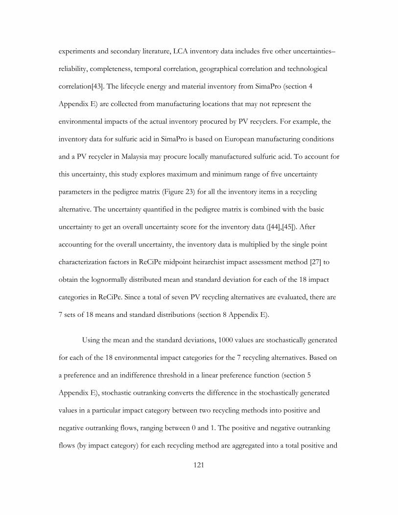
121

experiments and secondary literature, LCA inventory data includes five other uncertainties–

reliability, completeness, temporal correlation, geographical correlation and technological

correlation[43]. The lifecycle energy and material inventory from SimaPro (section 4

Appendix E) are collected from manufacturing locations that may not represent the

environmental impacts of the actual inventory procured by PV recyclers. For example, the

inventory data for sulfuric acid in SimaPro is based on European manufacturing conditions

and a PV recycler in Malaysia may procure locally manufactured sulfuric acid. To account for

this uncertainty, this study explores maximum and minimum range of five uncertainty

parameters in the pedigree matrix (Figure 23) for all the inventory items in a recycling

alternative. The uncertainty quantified in the pedigree matrix is combined with the basic

uncertainty to get an overall uncertainty score for the inventory data ([44],[45]). After

accounting for the overall uncertainty, the inventory data is multiplied by the single point

characterization factors in ReCiPe midpoint heirarchist impact assessment method [27] to

obtain the lognormally distributed mean and standard deviation for each of the 18 impact

categories in ReCiPe. Since a total of seven PV recycling alternatives are evaluated, there are

7 sets of 18 means and standard distributions (section 8 Appendix E).

Using the mean and the standard deviations, 1000 values are stochastically generated

for each of the 18 environmental impact categories for the 7 recycling alternatives. Based on

a preference and an indifference threshold in a linear preference function (section 5

Appendix E), stochastic outranking converts the difference in the stochastically generated

values in a particular impact category between two recycling methods into positive and

negative outranking flows, ranging between 0 and 1. The positive and negative outranking

flows (by impact category) for each recycling method are aggregated into a total positive and

122

negative flow using a weighting function (section 5 Appendix E). The weighting function

assigns a weight to each environmental impact category based on the relative importance (as

elicited from PV recycling stakeholders) or through a stochastic process. This study assigns

weights stochastically to each of the 18 impact categories to explore the entire range of

possibilities. The weights for the 18 impact categories will be a beta-distribution between 0

and 1 and the sum of all the weights is constrained to one.

The aggregated probabilistic environmental score for a recycling method is calculated

by subtracting the total negative outranking flow from the total positive outranking flow

(section 5 Appendix E). The net probabilistic environmental score ranges between -1

(environmentally least preferable) and 1 (environmentally most preferable). Based on the

1000 stochastic runs, each of the recycling alternatives will have 1000 aggregated

environmental scores ranging between +1 and -1. The seven recycling alternatives are ranked

between 1 (most environmentally favored) and 7 (least environmentally favored) in each of

the 1000 runs and the percentage value for the number of times (out of a 1000) a recycling

alternative obtains a particular rank is calculated.

To explore the full range of uncertainty in the material and energy inventory, the

environmental rankings are calculated for both maximum and minimum uncertainty in the

pedigree matrix.

Scenario analysis: centralized and decentralized recycling

The scenario analysis determines the environmentally favorable option between

operating the most preferable recycling alternative in a decentralized and a centralized

facility. In the centralized mode, the end-of-life PV modules are transported from the

deployment site to an industrial-scale centralized recycling facility. The environmental trade-

123

off is between the burden of transporting end-of-life CdTe PV modules and the gains from

operational efficiencies due to the economies of scale at the centralized recycling facility. In

the decentralized mode, the end-of-life PV modules are recycled in a small-scale temporary

facility located at the deployment site. The environmental trade-off is between the burden of

lower operational efficiencies due to small-scale operations and the advantage of avoiding

the transportation of end-of-life CdTe PV modules to the centralized facility.

To guide PV recyclers on the environmental trade-offs between pursuing R&D to

further decrease the material and energy requirements in a centralized plant or investing in

small-scale decentralized plants to avoid transportation burdens, this study environmentally

compares and ranks centralized and decentralized recycling scenarios. To account for the

higher operational efficiency with increasing the scale of operations from the baseline

conidition, the material and energy inventory requirements in centralized recycling plants are

assumed to be 15 and 30% lower than the baseline value. Similarly, for decentralized, small-

scale recycling plants the inventory requirements are assumed to be 15 and 30% higher than

the baseline coniditon to account for lower operational efficiencies. Additionally, a scenario

with the centralized plant operating with 30% lower inventory requirements and electricity

generated from PV systems is included in the scenario analysis. This scenario is assumed to

represent the environmental best case with an inventory reduction through increased scale of

operations and R&D, and an improvement in operations by shifting to PV electricity.

Beijing and California are chosen as PV deployment sites as they account for a

significant share of the world-wide and US deployments, respectively [50][51]. Kuala

Lumpur, Malaysia and Perrysburg, Ohio are chosen as the sites for centralized recycling as

First Solar operates facilities at these locations. The assumptions for the shipping and the

road transportation distances for centralized recycling are presented in section 9 of the

124

Appendix E. The environmental favorability is determined by ranking the aggregate

probabilistic environmental scores (Figure 23) of the aforementioned centralized and

decentralized recycling scenarios.

Global Sensitivity Analysis

The aggregate environmental score of a recycling alternative depends on (1)

stochastically generated characterized inventory values in the 18 environmental impact

categories for the particular alternative, (2) stochastically generated characterized inventory

values in the 18 environmental impact categories for the 6 other recycling alternatives, and

(3) the beta-normally distributed weights assigned to the 18 impact categories. Thus, the

aggregate environmental score is dependent on a total of 144 input parameters.

To inform PV recyclers on the most significant parameters that can be addressed to

further reduce the environmental impact of a particular recycling alternative, a global

sensitivity analysis (GSA) [29] is performed. GSA is preferred as it accounts for the first and

higher order interactions between the various input parameters when determining the

sensitivity of the aggregated environmental score to a specific input parameter and is

applicable to models with non-monotonic and non-linear relationships between the input

and output parameters [46]. In the variance based GSA method that is implemented, a

change in the most sensitive input parameter results in the greatest change in the variance of

the aggregate environmental score. For a detailed quantitative discussion of variance based

GSA refer [29], [47], [48]. The MATLAB® implementation of the variance based GSA is

based on the approach presented in [49].

125


Figure 24 Process time for EVA elimination. Process time for elimination of EVA by the thermal process (left) and heating in an organic solvent (right).

For the thermal delamination process, a minimum of 7 minutes (Trun) is required to

delaminate the 8x8 inch samples and eliminate 100% of the EVA (section 6 Appendix E).

Further, the sample is required to remain in the closed and switched-off furnace for a

minimum of 11 minutes (Tclose) to prevent the combustion of the residue from the melting of

EVA. The sample is subsequently cooled for 9 minutes (Topen) by opening the furnace so that

the temperature of the glass decreases from 500 to 220-280⁰C to prevent the cracking

(section 6 Appendix E). The total process time is 27 minutes and 0.48 kWh of electricity is

consumed in the first 7 minutes to thermally delaminate 1 m2 of the sample (section 6

Appendix E).

When the 2x2 glass samples laminated with EVA are heated in the organic solvents,

delamination time for o-dcb, TCE and toluene are 4 to 23, 32 to 48, and 36 to 53 hours,

respectively (section 7 Appendix E). The boiling point of o-dcb (180.5⁰C) is greater than

TCE (87.2⁰C) or toluene (110.6⁰C) and, therefore, a higher heating temperature with o-dcb

results in a shorter delamination time. With PV recyclers preferring short process times for

126

recycling, only o-dcb is considered for the recycling alternatives that delaminate EVA by

heating in an organic solvent (“org solv+leach+ion exch+prcp”, “org solv+leach+prcp”,

and “org solv+leach+solv ext+prcp”). 6.8L of o-DCB and 5.4 to 36.7 kWh of electricity is

required to delaminate 1 m2 of the sample (section 7 Appendix E).

While a previous study reported the delamination of silicon PV modules with a

Tedlar back-surface in 70 minutes[4], probe sonication failed to delaminate the 2x2 inch

glass samples after 3 hours in o-dcb, TCE or toluene. The failure of probe sonicator to

delaminate may be attributed to both the front and back surface of the sample being glass (as

in commercially manufactured CdTe PV modules). Bath sonication failed to delaminate the

2x2 inch glass samples in 48 hours in o-DCB, TCE or toluene. Therefore, bath and probe

sonication are not considered as possible alternatives to the incumbent shredding and

hammering delamination process (Figure 22) and are not included in the environmental

comparison with other recycling alternatives (Table 7).

127

Figure 25 Environmental ranking for the CdTe PV recycling alternatives. Environmental rankings for the 7 recycling alternatives with rank 1 being most environmentally preferable. The rankings are calculated based on maximum uncertainty in the energy and material values in the pedigree matrix. The x-axis shows the ranks and the y-axis depicts the percentage value out of a 1000 runs that a particular recycling alternative obtains a rank.

The environmental rankings (Figure 25) demonstrate that the novel alternative

“thermal+leach+prcp” is the most environmentally favored as it ranks first in 78% of the

1000 stochastic runs and the incumbent recycling method (“mech+leach+prcp”) ranks

second. Furthermore, when the minimum uncertainty for material and energy inventory

values are selected in the pedigree matrix and the rankings are recalculated, the novel

alternative “thermal+leach+prcp” is the most environmentally favored as it ranks first in

95% of the 1000 stochastic runs and the incumbent recycling method (“mech+leach+prcp”)

ranks second (section 12 Appendix E). The “thermal+leach+prcp” alternative is

environmentally favored due to the lower energy requirements for thermal delamination

128

(0.48 kWh/m2) when compared to mechanical shredding and hammering (2.2 kWh/m2) to

delaminate EVA in the incumbent process (section 4 Appendix E).

Figure 26 Environmental rankings for centralized and decentralized recycling. Environmental rankings when the “thermal+leach+prcp” recycling alternative is adopted in centralized and decentralized plants (rank 1 being the most environmentally favorable). The + and - percentage values represent the increased and decreased inventory requirements (compared to the baseline scenario) due to lower and higher operational efficiencies in decentralized and centralized plants, respectively. Decentralized recycling in California is environmentally preferable to centralized recycling in Ohio (top). Decentralized recycling in China environmentally outperforms the baseline scenario of centralized recycling in Malaysia only when the inventory requirementis less than 1.15 times the baseline value (bottom).

129

The results (Figure 26) show that decentral recycling of CdTe PV modules at the

deployment site in California, with the most environmentally promising novel alternative

“thermal+leach+prcp” (refer Figure 25), is environmentally preferable to recycling in

centralized locations in Ohio and Malaysia, respectively. This due to the environmental

burden of transporting spent CdTe PV modules by road from California to Ohio (100% of

the total transportation share, section 9 Appendix E) outweighing the environmental benefit

of increased operational efficiencies at the centralized plant at Ohio (due to economies of

scale). For example, even with 30% lower inventory requirements than the baseline value

and using PV electricity for centralized recycling operations, recycling decentrally in

California with 90% increased inventory requirements is environmentally preferable (ranking

of “Ohio PV elec -30% inventory” versus “California: grid elec +30% inventory”).

Decentralized recycling in China is environmentally preferable to the baseline

scenario of centralized recycling in Malaysia only when the inventory requirement is less than

1.15 times the baseline value (“China grid elec +15% inventory” outranks “Malaysia natural

gas elec baseline”). If the inventory requirements in decentralized plants in China is greater

than 1.15 times the baseline value, the difference in ranking with the baseline scenario is

statistically insignificant (“ China grid elec +30% inventory” versus “Malaysia natural gas elec

baseline”). Furthermore, if the inventory requirements is 30% lower than baseline

requirement and PV electricity is used for recycling operations, centralized recycling in

Malysia outperforms decentralized recycling in China (“Malaysia PV elec -30% inventory”

obtains rank one 40% of the times).

Comparing the results in the top and the bottom, we observe that environmentral

rankings for decentralized recycling in China is less favorable than decentralized recycling in

130

California. This is because shipping, which accounts for 97% of the total transportation

between China and Malaysia (in ton-km, section 9 Appendix E), has a lower environmental

burden than road transportation which accounts for 100% of the total transportation

between California and Ohio (section 13 Appendix E).

A possible approach to improve the environmental performance of decentral

recycling in China is to replace carbon-intensive grid electricity with PV electricity for the

decentral recycling processes. In this scenario, decentralized recycling in China is the

environmentally preferred alternative only if the inventory requirements are within 1.3 times

the baseline inventory requirements (in a centralized plant) (section 14 Appendix E). The

results suggest that recyclers can improve the environmental performance of PV recycling by

(1) locating centralized recycling plants in the vicinity of shipping ports to decrease the share

of transportation by road (2) adopting decentralized recycling if transporting end-of-life

modules to the nearest centralized plant involves a significant distance by road, and (3)

utilizing carbon-efficient sources of electricity (e.g. photovoltaics) for centralized and

decentralized recycling plant operations.

Figure 27 Global sensitivity analysis results (with weights). Global sensitivity analysis results showing the values of the sensitivity indices for the three most significant input parameters (out of a total of 144 input parameters). The environmental ranking of the incumbent “mech+leach+prcp” (left) and the novel “thermal+leach+prcp” (right) recycling alternatives are most sensitive to the weights assigned to the three environmental impact categories.

131

The results from the GSA (Figure 27, left) demonstrate that beta-distributed random

weights assigned to the water depletion, marine eutrophication, and particulate matter

formation impact categories are the three most significant parameters (out of 144 input

parameters) influencing the environmental ranking of the incumbent “mech+leach+prcp”

alternative. Similarly, for the novel “thermal+leach+prcp” alternative (Figure 27, right), the

weights assigned to the particulate matter formation, photochemical oxidant formation, and

urban land occupation impact categories are the three most significant parameters.

Furthermore, the ten most significant input parameters to influence the environmental

rankings are all weights assigned to the environmental impact categories (section 11

Appendix E).

Figure 28 Global sensitivity analysis results (without weights). Global sensitivity analysis results showing the values of the sensitivity indices for the three most significant environmental impact categories (out of a total of 126 impact cateogories) that influence the environmental ranking of the incumbent “mech+leach+prcp” (left) and the novel “thermal+leach+prcp” (right) alternatives. The weights are not included in the sensitivity analysis.

While demonstrating that dominance of the weights in determining the

environmental rankings, the results in Figure 27 fail to identify uncertainties or hotspots in

the recycling processes that PV recycling stakeholders can address in the future through

research and development (R&D), and operational improvements. Therefore, this study

repeats the GSA by including only the environmental impact categories and excluding the

132

weights. When the weights are excluded from the GSA, the results show that climate change,

natural land transformation, and fossil depletion are the most significant environmental

impact categories in the incumbent recycling process (Figure 28,left). Similarly, reducing the

natural land transformation, ozone depletion potential and fossil depletion will further

improve the environmental performance of the novel “thermal+leach+prcp” (Figure

28,right). These impact categories can be reduced if process improvements reduce the

electricity used in the recycling operations (section 10 Appendix E). Furthermore, shifting to

more carbon-efficient electricity sources (e.g. photovoltaics) can reduce the climate impacts

of large scale PV recycling. It should be noted that the results in Figure 28 are specific to

beta-randomly distributed weights for the impact categories and will change if the weighting

method is modified.

The results from the a-LCA demonstrate the significance of eliciting inputs from

various stakeholders (e.g. environmental engineers, regulatory authorities, recycling plant

managers) on the most significant environmental impact categories (Figure 27) in a specific

decision context and prioritize the R&D efforts towards addressing these environmental

impacts. For example, stakeholders will assign a higher value to the weight for human

toxicity than other impact categories in PV recycling markets with regulations sensitive to

human toxicity. The a-LCA is then repeated to identify the recycling alternative with the least

human toxicity impact and this can prioritize R&D efforts towards the addressing the

significant environmental hotspots in the most preferable process. Furthermore, the results

from the aLCA identify uncertainties in the lifecycle data of inventory items that significantly

influence the environmental ranking (Figure 28). To improve decision making and identify

the environmental preferable recycling alternative, research efforts should focus on

133

collecting and improving the upstream lifecycle data quality for these specific inventory

items.

The environmental rankings (Figure 25) are based on the material and energy inputs

and do not include the environmental burdens of emissions and emission control

requirements for the recycling alternatives. Emission data at a commercial scale is only

available for the incumbent process [25] and not the other recycling alternatives which

operate only at the pilot-scale. For consistency in calculating the environmental rankings, the

emissions are excluded for both the incumbent and novel alternatives. Furthermore, the

“thermal+leach+prcp” alternative can emit volatile organic compounds ( 1-butene, ethylene,

methane), carbon dioxide, carbon monoxide and methane [52]. The volatile organic emission

control requirements which are implemented for the incumbent “mech+leach+prcp”

process at a commercial scale are not included while calculating the environmental impacts.

Therefore, assuming the same process is used to manage volatile organic emissions for the

“thermal+leach+prcp” alternative and excluding them from the environmental impact

calculations will not impact the relative environmental ranking of the two methods. Existing

research also confirms the thermal stability of CdTe at the range of temperatures used in the

thermal delamination process [53][54]. Therefore, the environmental burdens of cadmium

and tellurium emissions from thermal delamination of EVA in CdTe PV modules are not

included in this analysis.

The results presented in this research consider only the environmental impacts when

ranking the recycling alternatives. The choice of a particular recycling alternative or a facility

location strategy (decentralized versus centralized) is also influenced by economic and

regulatory considerations. For example, when regulations do no permit end-of-life products

containing cadmium to be transported to centralized recycling facilities across international

134

borders, recyclers have to manage the PV waste decentrally irrespective of the environmental

and economic impacts. Further analysis on the economic, operational and regulatory aspects

of PV recycling will complement this work on informing PV recycling stakeholders on the

preferred recycling alternative and the location strategy.

135

CONCLUSION

The dominant approach to improve the environmental performance of PV systems

is increasing the module efficiency and, therefore, the renewable electricity generated in the

use phase. However, this approach fails to identify and address the potential environmental

hotspots in PV manufacturing and recycling. This dissertation provides a compelling

environmental rationale for an alternative strategy of improving the environmental

performance of PV systems through improved manufacturing and recycling.

Chapter 2 identifies a methodological limitation in current PV LCAs which do not

account for the time-sensitive climate impacts of manufacturing emissions that occur earlier

than the emissions avoided in the use-phase. A framework with the CRF metric is presented

to address this methodological limitation and account for the time-sensitive climate impacts

of PV manufacturing emissions. The result show that the GHG payback time, the preferred

environmental metric in PV LCAs, is always lower than the CRF payback-time of a PV

system. GHG payback occurs when the mass of GHG avoided is equal to the GHG emitted

and is insensitive to the timing and atmospheric residence time of emissions. CRF payback is

sensitive to the magnitude and timing of emission and the residence time of GHG in the

atmosphere. Therefore, early manufacturing emissions have a higher CRF impact than

emissions avoided after deployment and this increases the CRF payback time. By not

accounting for this time-sensitive climate impact of PV manufacturing emissions, current PV

LCAs underestimate the environmental benefits from PV manufacturing emissions.

Chapter 3 further develops the findings in Chapter 2 which identifies CRF as the

appropriate metric to quantify the time-sensitive climate impact of PV manufacturing

emissions and prospectively evaluates strategies to decrease the climate impact of future PV

manufacturing. The results show that GHG- intensity of the electricity used for PV

136

manufacturing has the most significant climate impact. This is the result of PV modules

being predominantly manufactured in China with GHG-intense sources of electricity. The

climate benefit of shifting to GHG-efficient electricity sources (e.g PV) for PV

manufacturing is equivalent to increasing the module efficiency from the current commercial

value of 17% to 21.7% and 16% to 18.7% for mono-Si and multi-Si modules, respectively.

This equivalent module efficiency gain is significant as the module efficiency for crystalline

silicon-PV technologies has increased annually by only 0.25% in the last twelve years.

To identify the environmental hotspots in PV recycling, Chapter 4 presents the first

detailed energetic assessment of commercial-scale CdTe PV system recycling operations.

The findings show that recovering and recycling the bulk materials (steel, aluminum, copper

and glass) from end-of-life CdTe systems can reduce the lifecycle energy footprint of the

CdTe PV system by approximately 24% of the energy required to manufacture the PV

system. Furthermore, the process to eliminate the EVA polymer that encapsulates the

module to recover the unrefined the semiconductor material is the most significant

environmental hotspot.

To environmentally improve future PV recycling operations, Chapter 5 evaluates the

environmental trade-off of replacing the hotspot identified in chapter 4 with novel pilot-

scale recycling alternatives. Lifecycle assessment (LCA), the preferred framework to evaluate

the environmental trade-offs between multiple alternatives, is methodologically retrospective

by relying on inventory data gathered from commercial scale processes that have matured

over time. In contrast, the existing research on the feasibility of novel pilot-scale processes

do not always report the material and energy inventory requirements which is required for an

LCA. Additionally, a limited number of studies adopt a prospective mode of LCA to

evaluating an emerging technology by identifying environmental hotspots for future

137

improvements. This approach may fail in a comparative context where the environmental

preferable choice is determined by the mutual differences in the environmental impacts of

the alternatives and not the environmental hotspots of an alternative. Chapter 5 addresses

these methodological shortcomings by using the anticipatory lifecycle assessment framework

to evaluate the incumbent CdTe PV recycling process and 6 pilot-scale alternatives. The

results show that thermally eliminating the EVA is environmentally the most favorable

alternative to the incumbent mechanical process. Furthermore, when road is the dominant

mode for transporting end-life modules to centralized recycling locations from the

deployment site, recycling end-of-life modules decentrally in mobile plants near the

deployment site is environmentally favorable. Centralized recycling is environmentally

favorable if shipping is the dominant mode of transport. Additionally, the results show that

the choice of the environmentally preferred alternative is most sensitive to the stakeholder

inputs on the relative importance of the multiple environmental impact categories used to

evaluate the alternatives. If the weights assigned to the environmental impact categories are

excluded from the sensitivity analysis, the results show that the environmental performance

of the incumbent recycling process and the thermal delamination alternative is most sensitive

to the GHG intensity of the electricity for recycling operations. Therefore, apart from

adopting the novel thermal delamination alternative, recyclers can further reduce the

environmental impact of future recycling operations by using GHG-efficient sources of

electricity.

This dissertation’s findings on increasing the environmental benefits from PV

systems through improved manufacturing and recycling are significant to stakeholders in the

PV industry as PV manufacturing facilities that are expected to meet the terawatt-scale of

global demand are increasingly shifting to GHG intensive manufacturing locations like

138

China. Furthermore, with a typical lifespan of twenty-five years, the rapid acceleration of PV

installations post-2005 will contribute to a significant increase in end-of-life volumes over

the next ten to 20 years. Identifying and implementing environmentally promising

alternatives in present-day recycling plants at a smaller scale is operationally and

economically preferable to modifying the recycling technology at a much larger scale in the

future when end-of-life volumes are expected to increase.

139

REFERENCES

[1] International Renewable Energy Agency, “End of Life Management: Solar Photovoltaic Panels,” 2016.

[2] D. Ravikumar, P. Sinha, T. Seager, and M. P. Fraser, “An anticipatory approach to

quantify energetics of recycling CdTe photovoltaic systems,” Prog. Photovoltaics Res. Appl., 2015.

[3] B. a. Wender, R. W. Foley, T. a. Hottle, J. Sadowski, V. Prado-Lopez, D. a. Eisenberg,

L. Laurin, and T. P. Seager, “Anticipatory life-cycle assessment for responsible research and innovation,” J. Responsible Innov., vol. 1, no. 2, pp. 200–207, 2014.

[4] Y. Kim and J. Lee, “Dissolution of ethylene vinyl acetate in crystalline silicon PV

modules using ultrasonic irradiation and organic solvent,” Sol. Energy Mater. Sol. Cells, vol. 98, no. x, pp. 317–322, Mar. 2012.

[5] T. Doi, I. Tsuda, H. Unagida, A. Murata, K. Sakuta, and K. Kurokawa, “Experimental

study on PV module recycling with organic solvent method,” Sol. Energy Mater. Sol. Cells, vol. 67, no. 1–4, pp. 397–403, Mar. 2001.

[6] P. Dias, S. Javimczik, M. Benevit, and H. Veit, “Recycling WEEE: Polymer

characterization and pyrolysis study for waste of crystalline silicon photovoltaic modules,” Waste Manag., 2016.

[7] Z. De-wen, M. Born, and K. Wambachz, “Pyrolysis of EVA and its application in

recycling of photovoltaic modules,” J. Environ. Sci., 2004. [8] G. Granata, F. Pagnanelli, E. Moscardini, T. Havlik, and L. Toro, “Recycling of

photovoltaic panels by physical operations,” Sol. Energy Mater. Sol. Cells, vol. 123, pp. 239–248, Apr. 2014.

[9] L. Frisson, H. Hofkens, K. de Clercq, J. Nijs, and A. Geeroms, “Cost effective

recycling of PV modules and the impact on environment, life cycle, energy payback time and cost,” in 2nd World Conference on Photovoltaic Solar Technology, 1998, pp. 2210–2213.

[10] L. Frisson, K. Lieten, T. Bruton, K. Declercq, J. Szlufcik, H. De Moor, M. Goris, A.

Benali, and O. Aceves, “Recent improvements in industrial PV module recycling,” in 16th European Photovoltaic Solar Energy Conference, 2000.

[11] A. Müller, K. Wambach, and E. Alsema, “Life Cycle Analysis of Solar Module

Recycling Process,” MRS Proc., vol. 895, no. August 2015, pp. 18–21, 2005. [12] N. Jungbluth, “Life cycle assessment of crystalline photovoltaics in the Swiss

ecoinvent database,” Prog. Photovoltaics Res. Appl., vol. 13, no. 5, pp. 429–446, Aug. 2005.

140

[13] N. Jungbluth, C. Bauer, R. Dones, and R. Frischknecht, “Life cycle assessment for

emerging technologies: Case studies for photovoltaic and wind power,” Int. J. Life Cycle Assess., vol. 10, no. 1, pp. 24–34, 2005.

[14] A. Meijer, M. a. J. Huijbregts, J. J. Schermer, and L. Reijnders, “Life-cycle assessment

of photovoltaic modules: Comparison of mc-Si, InGaP and InGaP/mc-Si solar modules,” Prog. Photovoltaics Res. Appl., vol. 11, no. 4, pp. 275–287, Jun. 2003.

[15] D. Ravikumar, T. P. Seager, M. V. Chester, and M. P. Fraser, “Intertemporal

cumulative radiative forcing effects of photovoltaic deployments,” Environ. Sci. Technol., vol. 48, no. 17, pp. 10010–10018, 2014.

[16] V. Prado-lopez, B. A. Wender, T. P. Seager, L. Laurin, M. Chester, and E. Arslan,

“Tradeoff Evaluation Improves comparative life cycle assessment A Photovoltaic Case Study,” J. Ind. Ecol., vol. 0, no. 0, pp. 1–9, 2015.

[17] B. a Wender, R. W. Foley, V. Prado-Lopez, D. Ravikumar, D. a Eisenberg, T. a

Hottle, J. Sadowski, W. P. Flanagan, A. Fisher, L. Laurin, M. E. Bates, I. Linkov, T. P. Seager, M. P. Fraser, and D. H. Guston, “Illustrating anticipatory life cycle assessment for emerging photovoltaic technologies.,” Environ. Sci. Technol., vol. 48, no. 18, pp. 10531–8, Sep. 2014.

[18] M. L. Marín, a. Jiménez, J. López, and J. Vilaplana, “Thermal degradation of ethylene

(vinyl acetate),” J. Therm. Anal., vol. 47, no. 1, pp. 247–258, 1996. [19] M. Held, “Life cycle assessment of CdTe module recycling,” in 24th EU PVSEC

Conference, 2009, pp. 2370–2375. [20] A. Babakhani, F. Rashchi, A. Zakeri, and E. Vahidi, “Selective separation of nickel

and cadmium from sulfate solutions of spent nickel-cadmium batteries using mixtures of D2EHPA and Cyanex 302,” J. Power Sources, vol. 247, pp. 127–133, 2014.

[21] Ehsan Vahidi et Al., “Modeling of synergistic effect of Cyanex 302 and D2EHPA on

separation of nickel and cadmium from sulfate leach liquors of spent Ni–Cd batteries,” Eng. Technol., vol. 6, no. 12, p. 53, 2012.

[22] V. Kumar, M. Kumar, M. K. Jha, J. Jeong, and J. C. Lee, “Solvent extraction of

cadmium from sulfate solution with di-(2-ethylhexyl) phosphoric acid diluted in kerosene,” Hydrometallurgy, vol. 96, no. 3, pp. 230–234, 2009.

[23] W. Wang and V. Fthenakis, “Kinetics study on separation of cadmium from tellurium

in acidic solution media using ion-exchange resins,” J. Hazard. Mater., vol. 125, no. 1–3, pp. 80–88, 2005.

[24] V. Fthenakis and W. Wang, “System and method for separating tellurium from

cadmium waste,” US7731920 B2, 2010.

141

[25] P. Sinha, M. Cossette, and J.-F. Ménard, “End-of-Life CdTe PV Recycling with

Semiconductor Refining,” in PVSEC 2012, pp. 8–11. [26] PRe Consultants, “Simapro version 8.0.3.14,” 2015. [Online]. Available:

http://www.pre-sustainability.com/simapro. [27] M. Goedkoop, R. Heijungs, M. Huijbregts, A. De Schryver, J. Struijs, and R. van

Zelm, “ReCiPe 2008 - A life cycle impact assessment method which comprises harmonised category indicators at the midpoint and the endpoint level,” 2013.

[28] V. Prado-Lopez, T. P. Seager, M. Chester, L. Laurin, M. Bernardo, and S. Tylock,

“Stochastic multi-attribute analysis (SMAA) as an interpretation method for comparative life-cycle assessment (LCA),” Int. J. Life Cycle Assess., vol. 19, no. 2, pp. 405–416, 2014.

[29] A. Saltelli, M. Ratto, T. Andres, J. C. Francesca Campolongo, D. Gatelli, M. Saisana,

and S. Tarantola, “Global Sensitivity Analysis: The Primer,” 2008, pp. 159–167. [30] C. Zeng, A. Ramos-Ruiz, J. a. Field, and R. Sierra-Alvarez, “Cadmium telluride

(CdTe) and cadmium selenide (CdSe) leaching behavior and surface chemistry in response to pH and O2,” J. Environ. Manage., vol. 154, pp. 78–85, 2015.

[31] M. Pourbaix, Atlas of electrochemical equilibria in aqueous solutions. 1974. [32] B. J. McGrattan, “Examining the Decomposition of Ethylene-Vinyl Acetate

Copolymers Using TG/GC/IR,” Appl. Spectrosc., vol. 48, no. 12, pp. 1472–1476, 1994. [33] AGC Solar, “SOLITETM - Extra Clear Patterned Glass For Solar Applications,” 2016.

[Online]. Available: http://www.agc-solar.com/agc-solar-products/patterned-glass/solite.html.

[34] Specialized Technology Resources, “EVA - STR Photocap15420P/UF,” 2016.

[Online]. Available: http://www.strsolar.com/UploadedFiles/Files/15420P_2015-01.pdf.

[35] NPC Incorporated, “Photovoltaic Module Laminator LM-110X 160-S.” [36] Vulcan, “Vulcan Box Furnace - Owner & Operator’s Manual.” [Online]. Available:

http://www.coleparmer.com/Assets/manual_pdfs/33855-10.pdf. [37] Sigma Aldrich, “1,2-Dichlorobenzene (99%, anhydrous),” 2016. [Online]. Available:

http://www.sigmaaldrich.com/catalog/product/sial/240664?lang=en&region=US. [38] Sigma Aldrich, “Toluene (99.8%, anhydrous),” 2016. [Online]. Available:

http://www.sigmaaldrich.com/catalog/product/sial/244511?lang=en&region=US.

142

[39] Sigma Aldrich, “Trichloroethylene (>=99%),” 2016. [Online]. Available: http://www.sigmaaldrich.com/catalog/product/aldrich/133124?lang=en&region=US.

[40] Fisher Scientific, “FS60 Ultrasonic Cleaner.” [Online]. Available:

https://fscimage.fishersci.com/cmsassets/downloads/segment/Scientific/pdf/fisher_ultrasonic_cleaner_data.pdf?&storeId=10652.

[41] V. M. Fthenakis and W. Wang, “Extraction and separation of Cd and Te from

cadmium telluride photovoltaic manufacturing scrap,” Prog. Photovoltaics Res. Appl., vol. 14, no. 4, pp. 363–371, 2006.

[42] A. Mezei, M. Ashbury, M. Canizares, R. Molnar, H. Given, A. Meader, K. Squires, F.

Ojebuoboh, T. Jones, and W. Wang, “Hydrometallurgical recycling of the semiconductor material from photovoltaic materials—part II: metal recovery,” in Hydrometallurgy, 2008, pp. 224–237.

[43] B. P. Weidema and M. S. Wesnæs, “Data quality management for life cycle

inventories—an example of using data quality indicators,” J. Clean. Prod., vol. 4, no. 3–4, pp. 167–174, 1996.

[44] B. P. Weidema, C. Bauer, R. Hischier, T. Nemecek, J. Reinhard, C. O. Vadenbo, and

G. Wernet, “Overview and methodology. Data quality guideline for the ecoinvent database version 3,” Ecoinvent Rep. 1(v3). St. Gall. ecoinvent Cent., pp. 70–78, 2013.

[45] S. Muller, P. Lesage, A. Ciroth, C. Mutel, B. P. Weidema, and R. Samson, “The

application of the pedigree approach to the distributions foreseen in ecoinvent v3,” Int. J. Life Cycle Assess., 2014.

[46] X. Zhang, M. N. Trame, L. J. Lesko, and S. Schmidt, “Sobol Sensitivity Analysis : A Tool to Guide the Development and Evaluation of Systems Pharmacology Models,” CPT pharmacometrics Syst. Pharmacol., vol. 4, no. October 2014, pp. 1–4, 2015.

[47] A. Saltelli, “Global Sensitivity Analysis : An Introduction,” in 4th International Conference on Sensitivity Analysis of Model Output (SAMO’04), 2004, pp. 27–43.

[48] A. Saltelli, P. Annoni, I. Azzini, F. Campolongo, M. Ratto, and S. Tarantola,

“Variance based sensitivity analysis of model output. Design and estimator for the total sensitivity index,” Comput. Phys. Commun., vol. 181, no. 2, pp. 259–270, 2010.

[49] A. Saltelli, M. Ratto, T. Andres, J. C. Francesca Campolongo, D. Gatelli, M. Saisana,

and S. Tarantola, “Global Sensitivity Analysis: The Primer,” 2008, pp. 164–167. [50] Fraunhofer Institute for Solar Energy Systems ISE, “Photovoltaics Report,” no.

August, p. 4, 2015. [51] Solar Energy Industries Association (SEIA), “Solar Market Insight Report 2016 Q2,”

143

2016. [Online]. Available: http://www.seia.org/research-resources/solar-market-insight-report-2016-q2.

[52] M. B. Maurin, L. W. Dittert, and A. A. Hussain, “Thermogravimetric Analysis of

Ethylene- vinyl Acetate Copolymers with Fourier Transform Infrared Analysis of the Pyrolysis Products,” Thermochim. Acta, vol. 186, no. 1, pp. 97–102, 1991.

[53] V. M. Fthenakis, M. Fuhrmann, J. Heiser, a. Lanzirotti, J. Fitts, and W. Wang,

“Emissions and encapsulation of cadmium in CdTe PV modules during fires,” Prog. Photovoltaics Res. Appl., vol. 13, no. 8, pp. 713–723, Dec. 2005.

[54] European Chemicals Agency (ECHA), “Cadmium telluride,” 2010. [Online].

Available: https://www.echa.europa.eu/en/web/guest/registration-dossier/-/registered-dossier/12227/4/3.

144

APPENDIX A

A. PREVIOUSLY PUBLISHED MATERIAL AND CO-AUTHOR PERMISSION

145

Chapter 2 was published in Environmental Science & Technology and appears as

published. The citation for the article is: Ravikumar, D., Seager, T. P., Chester, M. V., &

Fraser, M. P. (2014). Intertemporal cumulative radiative forcing effects of photovoltaic

deployments. Environmental Science & Technology, 48(17),10010-10018.

Chapter 4 has been published in Progress in Photovoltaics: Research and Applications and

appears as published. The citation for the article is: Ravikumar, D., Sinha, P., Seager, T. P., &

Fraser, M. P. (2016). An anticipatory approach to quantify energetics of recycling CdTe

photovoltaic systems. Progress in Photovoltaics: Research and Applications, 24(5),735-746.

All co-authors have granted their permission for the use of this material in this

dissertation.

146

APPENDIX B

B. SUPPORTING INFORMATION FOR CHAPTER 2

147

1. Calculation of Radiative Efficiencies and CRF impacts

The radiative forcing calculations in the model are performed for emissions measured in

kilograms. Therefore, to convert radiative efficiency values from W m-2 ppb-1 to W m-2 kg-1

they are multiplied by (Ma/Mi)*(109/Tm)1 where,

Ma is the mean molecular weight of air (28.97 kg kmol−1)

Mi is the molecular weight of the GHG species (kg)

Tm is the total mass of the atmosphere(5.1352 × 1018kg) 1

A B C D

GHG Molecular mass Mi (kg kmol-1)

Radiative efficiency aghg (W m-2 ppb-1) 1,2

Radiative efficiency

aghg (W m-2

kg-1)

CO2 44.01 1.37E-05 1.75E-15

CH4 16.04 3.7E-04 1.30E-13

HFC-152a 66.05 9E-02 7.68E-12

SF6 146.06 5.2E-01 2.00E-11

Table S8 Radiative Efficiencies for CO2, CH4, HFC-152a, SF6.

The time sensitive CRF impact of CO2 emissions for a ten year horizon is tabulated

in Table S9.

148

A B C D E

Atmospheric residence

time (years)

CO2 remaining in the

atmosphere (kg)

Radiative Forcing (W m-

2)

CRF impact ‘kt’(W m-2 yr)

kt allocated to CO2 emitted in

year

1 8.75E-01 1.50E-15 1.50E-15 10

2 8.11E-01 1.39E-15 2.89E-15 9

3 7.74E-01 1.32E-15 4.21E-15 8

4 7.49E-01 1.28E-15 5.50E-15 7

5 7.29E-01 1.25E-15 6.75E-15 6

6 7.13E-01 1.22E-15 7.97E-15 5

7 6.98E-01 1.19E-15 9.17E-15 4

8 6.84E-01 1.17E-15 1.03E-14 3

9 6.71E-01 1.15E-15 1.14E-14 2

10 6.58E-01 1.12E-15 1.26E-14 1

Table S9 Calculation of CRF impacts for 1 kg of CO2 emitted for each year between year 1 and 10. The CRF impacts are measured over a 10 year period.

Column B values are calculated by substituting ‘t’ (in equation 2 in main paper) with

the corresponding Column A values. Column C values are calculated by multiplying the

corresponding column B values by aco2, the radiative efficiency of CO2 (column D in Table

S8). Column D values are the cumulative sum of column C values until that year. The CRF

impact of ‘m’ kg of CO2 emitted in year ‘n’ (column E) is calculated by multiplying ‘m’ by

the corresponding value in column D. For example if 5 kg of CO2 is emitted in year 4 the

CRF impact is 5*9.17E-15 (row 7 in column D).

The CRF impacts for CH4, HFC-152a, SF6 emissions are similarly calculated in Table

S10, Table S11 and Table S12, respectively. Column B values in the following 3 tables are

calculated using equation 3 from the main paper and perturbation time (τ) values of 12, 1.4

and 3200 years for CH4, HFC-152a and SF6 , respectively 2.

149

A B C D E


time (years)

CH4 remaining in the atmosphere (kg)


2)


kt allocated to CH4

emitted in year

1 9.20E-01 1.68E-13 1.68E-13 10

2 8.46E-01 1.55E-13 3.23E-13 9

3 7.79E-01 1.42E-13 4.65E-13 8

4 7.17E-01 1.31E-13 5.96E-13 7

5 6.59E-01 1.20E-13 7.17E-13 6

6 6.07E-01 1.11E-13 8.27E-13 5

7 5.58E-01 1.02E-13 9.29E-13 4

8 5.13E-01 9.38E-14 1.02E-12 3

9 4.72E-01 8.63E-14 1.11E-12 2

10 4.35E-01 7.94E-14 1.19E-12 1

Table S10 Calculation of CRF impacts for 1 kg of CH4 emitted for each year between year 1 and 10. The CRF impacts are measured over a 10 year period. Column C values are multiplied by a factor of 1.4 (only in this table) to account for the indirect impacts

of methane emissions on ozone and stratospheric water vapor concentrations 3

A B C D E


time (years)

HFC-152a remaining in the atmosphere

(kg)


2)


kt allocated to HFC-

152a emitted in

year

1 4.90E-01 3.76E-12 3.76E-12 10

2 2.40E-01 1.84E-12 5.60E-12 9

3 1.17E-01 9.01E-13 6.50E-12 8

4 5.74E-02 4.41E-13 6.94E-12 7

5 2.81E-02 2.16E-13 7.16E-12 6

6 1.38E-02 1.06E-13 7.26E-12 5

7 6.74E-03 5.17E-14 7.32E-12 4

8 3.30E-03 2.53E-14 7.34E-12 3

9 1.61E-03 1.24E-14 7.35E-12 2

10 7.90E-04 6.07E-15 7.36E-12 1

Table S11 Calculation of CRF impacts for 1 kg of HFC-152a emitted for each year between year 1 and 10. The CRF impacts are measured over a 10 year period.

150

A B C D E


time (years)

SF6 remaining in the atmosphere (kg)


2)


kt allocated

to SF6

emitted in year

1 9.99E-01 2.01E-11 2.01E-11 10

2 9.99E-01 2.01E-11 4.02E-11 9

3 9.99E-01 2.01E-11 6.03E-11 8

4 9.98E-01 2.01E-11 8.03E-11 7

5 9.98E-01 2.01E-11 1E-10 6

6 9.98E-01 2.01E-11 1.2E-10 5

7 9.98E-01 2.01E-11 1.41E-10 4

8 9.97E-01 2.00E-11 1.61E-10 3

9 9.97E-01 2.00E-11 1.81E-10 2

10 9.97E-01 2.00E-11 2.01E-10 1

Table S12 Calculation of CRF impacts for 1 kg of SF6 emitted for each year between year 1 and 10. The CRF impacts are measured over a 10 year period.

2. Data Assumptions for the Optimization Framework

China is assumed to be the manufacturing location for monocrystalline Silicon (mSi) and

polycrystalline Si (pSi) modules as around 60% of the world’s Si PV modules are

manufactured in China and 11 among the top 15 PV module manufacturers are in China 4.

First Solar is the only thin film PV manufacturer in the top 10 PV manufacturers worldwide

5. Malaysia is assumed to be the manufacturing location for CdTe modules as 70% of First

Solar’s modules are produced in Malaysia 6. The degradation in the module performance

over time is assumed to be 0.7%/year 7. The following values are used in the optimization

framework

151

Parameter Value Equation in the main paper using this parameter

Source

MCIchina mono Si in 2011

2,870,000 (grams CO2e /kWp)

4 7.

MCIchina poly Si in 2011

1,590,000 (grams CO2e /kWp)

4 7

MCImalayisa CdTe in 2011

498,000 (grams CO2e /kWp)

4 7 has reported a value of 630,000 g/ kWp based on manufacturing conditions in China. This value is multiplied by a ratio of the current grid mixes in Malaysia (909 g/kWh from 8) and China (1,148 g/kWh from 8) as CdTe is assumed to be manufactured in Malaysia.

DGI California 2007

481 (CO2e g/kWh)

5,6 8

DGI Wyoming 2007

1,105 (CO2e g/kWh)

5,6 8

pr 0.75 5,6 9

Irr California 2,000 (kwh/m2 /year)

5,6 10

Irr Wyoming 1,700 (kwh/m2 /year)

5,6 10

op .1 5,6 11

tl .07 5,6 12

Table S13 Values of parameters used for optimizing PV deployment strategy for minimal CRF impacts

152

The CO2e emissions per kWh of electricity produced in California and

Wyoming have not shown a consistent trend from 2001 to 2009 13. An annual

decrease of 2% is assumed for the period from 2007 to 2016. This annual decrease is

comparable to the 17% GHG emission reductions mandated by the American

Climate and Energy Security Act for the period between 2005 and 2020 14.

3. PV technology improvements

As PV technology improves, manufacturing GHG emissions (MCI) decrease

over time. The base value for MCI is assumed to be in the year 2011 (Table S13).

MCI value in year ‘t’ (MCIt) is (i) directly proportional to the manufacturing energy

(MEt) used to manufacture the PV module (MJ/m2) and, (ii) inversely proportional

to the module efficiency (efft) as increasing module efficiencies reduce material and

manufacturing energy requirement which decreases manufacturing GHG emissions.

Thus, the MCIt value for any year ‘t’ between 2007 and 2017 is modelled by the

equation,

t 2011 t 2011 2011 tMCI = MCI (ME /ME ) (eff /eff ) (SI 1)

ME values for mSi, pSi and CdTe were 6200 ( including 500 MJ for the module

frame in 2000 15), 3700 (in 2005 16) and 1200 MJ/ m2 (in 2005 16),respectively. These

values decreased to 4697 (in 2011 7), 2624 (in 2011 7) and 940 MJ/ m2 (in 2011 7),

respectively. Based on this, ME is assumed to decrease annually by 2.5%, 5.5% and

4% for mSi, pSi and CdTe, respectively.

Module efficiency values for mSi and pSi in 2007 were 13.7% and 13.1% and

increased to 15.1% and 14.7% in 2012, respectively 7. Therefore, module efficiency is

153

assumed to increase annually by 2% and 1.5% for mSi and pSi, respectively. CdTe module

efficiencies between 2007 and 2017 were based on data from de Wild-Scholten 7.

Based on these assumptions and equation (SI 1) the MCI values for mSi, pSi and

CdTe are shown in Table S14, Table S15 and Table S16, respectively.

Year Module efficiency (%)

Manufacturing energy ME (MJ/ m2)

Manufacturing emissions MCI (CO2e g/kWp)

2007 13.7 5198 3,430,873

2008 13.9 5068 3,296,970

2009 13.9 4941 3,214,546

2010 14.4 4817 3,025,356

2011 (base year) 14.8 4697 2,870,000

2012 15.1 4580 2,742,656

2013 15.4 4465 2,621,656

2014 15.7 4353 2,505,995

2015 16.0 4245 2,395,436

2016 16.3 4139 2,289,755

2017 16.7 4035 2,188,737

Table S14 Technology improvements (decreasing MCI) for mSi modules




2007 13.1 3290 2,145,941

2008 13.3 3109 1,997,419

2009 13.5 2938 1,859,597

2010 13.7 2777 1,731,665

2011 (base year) 14.1 2624 1,590,000

2012 14.7 2480 1,441,221

2013 14.9 2343 1,341,827

2014 15.1 2214 1,249,287

2015 15.4 2093 1,163,129

2016 15.6 1978 1,082,914

2017 15.8 1869 1,008,230

Table S15 Technology improvements (decreasing MCI) for pSi modules

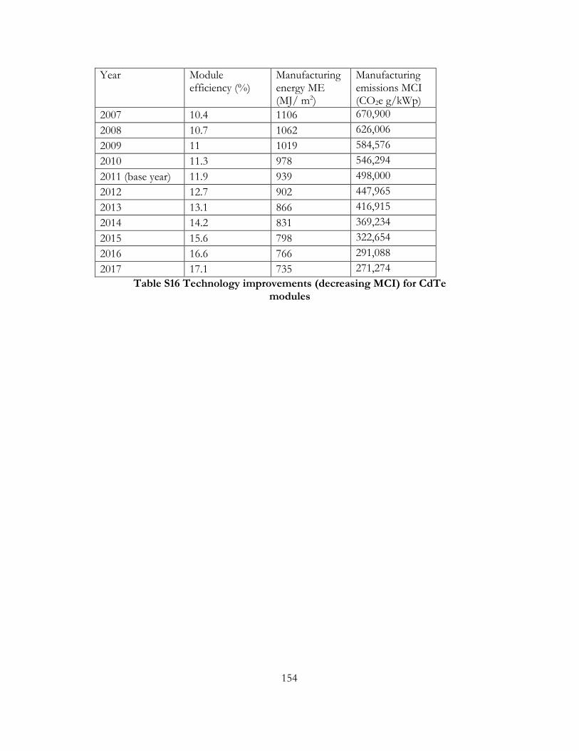
154




2007 10.4 1106 670,900

2008 10.7 1062 626,006

2009 11 1019 584,576

2010 11.3 978 546,294

2011 (base year) 11.9 939 498,000

2012 12.7 902 447,965

2013 13.1 866 416,915

2014 14.2 831 369,234

2015 15.6 798 322,654

2016 16.6 766 291,088

2017 17.1 735 271,274

Table S16 Technology improvements (decreasing MCI) for CdTe modules

155

4. Optimal Deployment Strategy for California and Wyoming

Optimization was carried out in Matlab using the Global Optimization Toolbox.

Figure S29 Optimal PV deployment strategy for minimized CRF impact. The Y-axis represents the CO2e intensity (g/kWp) of manufacturing PV modules and X-axis represents the grid CO2e intensity (g/kWh) at the deployment location. Frontier lines separate the plot into two optimal deployment strategy zones. The optimal deployment strategy is decided by plotting the CO2e intensity of manufacturing energy (Y value) and the grid CO2e intensity at the deployment location (X value) on the graph. If the plotted point is above the frontier line then back loading is the optimal strategy else front loading is the optimal strategy. The three blue lines depict the CO2e intensity of manufacturing mSi, pSi (in China) and CdTe (in Malaysia). For example, consider a scenario where PV targets in California are met by importing only mSi modules from China. The intersection is at the point ‘P1’. The frontier line for this scenario is the solid green line. This corresponds to a front loading strategy as this point lies below the solid green frontier line. Front loading is the optimal strategy for modules manufactured in China (mSi and pSi) or Malaysia (CdTe) are deployed in California or Wyoming. These are depicted by the six points.

Since mSi and CdTe represent the most and least GHG intensive PV systems

to manufacture, respectively, the CO2 intensity of manufacturing a PV deployment

mix that relies on all the three technologies will be represented by a horizontal line

lying between the blue lines for mSi and CdTe. Front loading will be the preferred

strategy across the two states for any technology mix since the PV manufacturing

GHG intensity line for the technology mix will lie below the blue line for mSi. The

156

frontier line for California is above that of Wyoming as the solar irradiation in

California is higher (Table S13) and this increases the PV electricity generation and

the grid electricity CO2 that is displaced. Therefore, for the same PV capacity that is

deployed, the probability of Front Loading being the favorable strategy in California

is higher when compared to Wyoming. This is reflected in the increased area covered

by the front loading region for California when compared to Wyoming.

5. GHG and CRF payback times in California and Wyoming for all scenarios

Figure S30 GHG payback times for all scenarios in CA (green) and

WY(brown). In optimal deployment, 81MW and 169 MW are deployed in 2007 and 2008 and the remaining capacity of 1689 MW is deployed in 2009. For sub-optimal deployment, 81MW and 169 MW are deployed in 2007 and 2008 and the remaining capacity of 1689 MW is equally deployed between 2009 and 2016.

157

Figure S31 CRF payback times for all scenarios in CA and WY. Optimal deployment and sub-optimal deployments are the same as in Figure S30. CRF impacts of manufacturing emissions and emissions due to the continued reliance on fossil fuels (for sub-optimal deployment) represent PV CRF costs. The CRF impacts avoided when PV electricity offsets grid electricity represent the CRF benefits. If the curve is below the X axis then CRF costs exceed CRF benefits of deploying the PV module and if the curve is above the X axis then CRF benefits exceed CRF costs.

6. CRF impacts of SO2 and NOx emissions

Figure S32 Net SO2 emitted during PV manufacturing in China/Malaysia and avoided during deployments in California/Wyoming. Annual capacity additions for Optimal (Opt) and sub-optimal (Sub) scenarios are explained in Figure S30.

158

The SO2 emitted during PV manufacturing and avoided at the deployment

location are determined by multiplying the CO2 emissions (per kWh electricity used

and avoided) by the ratio of SO2 and CO2 emitted per kWh for grid electricity in

China, Wyoming, California. This ratio is 0.0082 (for China), 0.0069 (for Wyoming)

and 0.0086 (for California). ((i) Electricity mix/CN U, (ii) eGrid, RMPA, 2008/RNA

U, and (iii) eGrid, CAMX, 2008/RNA U in Simapro).

Figure S33 Net NOx emissions over the PV manufacturing and use-phase. Net emission calculations are the same as in Figure S32.

The method for calculating NOx emitted during PV manufacturing and

avoided at the deployment location is identical to net SO2 emission calculations. The

NOx / CO2 ratio per kWh of grid electricity is 0.0037 in China, 0.0027 in Wyoming

and 0.001 in California ((i) Electricity mix/CN U , (ii) eGrid, RMPA, 2008/RNA U,

and (iii) eGrid, CAMX, 2008/RNA U in Simapro).

159

Emission Global mean annual radiative forcing (W m-2)

Global mean annual emissions

Radiative Efficiency (W m-

2 kg-1)

NOx -0.15 17 48.8 Tg 18 -3.07E-12

SO2 -0.4 17 100 Tg SO2 19 -4E-12

Table S17 Radiative efficiency for NOx and SO2. The negative sign indicates a net cooling impact.

7. SimaPro model to disaggregate emissions reported in CO2e into a GHG inventory for mSi, pSi and CdTe manufacturing

The steps to model mSi and pSi manufacturing in China using SimaPro are shown in

Table S18 and Table S19. SimaPro defaults to a European grid mix for each step and this

was replaced with a Chinese grid mix (Electricity mix/CN U in the SimaPro database) to

simulate PV manufacturing in China. The GHG inventory for CdTe manufacturing

(modeled in Table S20) was calculated using the Chinese grid mix which was then multiplied

by a ratio of the current grid mixes in Malaysia (909 g/kWh 8) and China (1148 g/kWh 8).

160

SimaPro Process

Description Inventory Amount per kWp

Assumptions based on the SimaPro database

MG-silicon, at plant/NO U

Gate to gate inventory for production of MG-silicon from silica sand including materials, energy use, wastes and air emissions.

5.73 kg 1 kg of solar grade Silicon requires 1.13 kg of MG-Silicon. Therefore, 5.07 kg requires 5.73 kg of MG-Silicon.

Silicon, solar grade, modified Siemens process, at plant/RER U

Gate to gate inventory for the production of high purity polycrystalline silicon from MG-silicon in actual processes.

5.07 kg 1 kg of CZ single crystalline silicon requires 1.07 kg of solar grade Silicon. Therefore, 4.74 kg requires 5.07 kg of solar grade Silicon.

CZ single crystalline silicon, photovoltaics, at plant/RER U

Gate to gate inventory for an improved Czochralski process.

4.74 kg 1 m2 of mSi wafer requires 1.0748 kg of CZ single crystalline silicon. Therefore, 4.41 m2 requires 4.74 kg of CZ single crystalline silicon.

Single-Si wafer, photovoltaics, at plant/RER U

Sawing and cleaning of wafers.

4.41 m2 1 m2 of mSi PV cell requires 1.06 m2 of mSi wafer. Therefore, 4.16 m2 requires 4.41 m2 of mSi wafer.

Photovoltaic cell, single-Si, at plant/RER U

Cleaning, damage etching, texture etching, covering of backside, phosphor dotation, phosphor glass etching, printing of contacts, cleaning and quality testing.

4.16 m2 1 m2 of mSi wafer PV panel requires 0.93241 m2 of mSi PV cells. Therefore, 4.46 m2 requires 4.16 m2 of mSi PV cells.

Photovoltaic panel, single-Si wafer

Production of the cell matrix, cutting of foils and washing of glass, production of laminate, isolation. Aluminum frame of the panel. Disposal after end of life.

4.46 m2 1 m2 of a mSi PV panel has a rated capacity of 224 Wp. Therefore, 1 kWp requires 4.46 m2 of mSi panel.

Table S18 SimaPro model to disaggregate CO2e into a GHG inventory

when a 1 kWp mSi module is manufactured in China

161

SimaPro Process

Description Inventory Amount per kWp


MG-silicon, at plant/NO U

Gate to gate inventory for production of MG-silicon from silica sand including materials, energy use, wastes and air emissions.

6.91 kg 1 kg of solar grade Silicon requires 1.13 kg of MG-Silicon. Therefore, 6.12 kg requires 6.91 kg of MG-Silicon.

Silicon, solar grade, modified Siemens process, at plant/RER U

Gate to gate inventory for the production of high purity polycrystalline silicon from MG-silicon in actual processes.

6.12 kg 1 kg of a multi-Si cast requires 1.14 kg of solar grade Silicon. Therefore, 5.37 kg requires 6.12 kg of solar grade Silicon.

Silicon, multi-Si, casted, at plant/RER U

Purified silicon is melted in cast in a graphite box. Than edges are sliced and blocks are sawn.

5.37 kg 1 m2 of a multi-Si wafer requires 1.14 kg of multi-Si cast. Therefore, 4.71 m2 requires 5.37 kg of multi-Si cast.

Multi-Si wafer, at plant/RER U

Sawing and cleaning of wafers. The process data includes electricity use, water and working material consumption.

4.71 m2 1 m2 of a pSi PV cell requires 1.06 m2of multi-Si wafer. Therefore, 4.44 m2 requires 4.71 m2 of multi-Si wafer.

Photovoltaic cell, multi-Si, at plant/RER U

Cleaning, damage etching, texture etching, covering of backside, phosphor dotation, phosphor glass etching, printing of contacts, cleaning and quality testing.

4.44 m2 1 m2 of a pSi panel requires 0.93241 m2 of pSi PV cell. Therefore, 4.76 m2 requires 4.44 m2 of pSi PV cells.

Photovoltaic panel, multi-Si, at plant/RER/I U

Production of the cell matrix, cutting of foils and washing of glass, production of laminate, isolation. Aluminium frame of the panel. Disposal after end of life.

4.76 m2 1 m2 of a pSi panel has a rated capacity of 210 Wp. Therefore, 1 kWp requires 4.76 m2 of pSi panel.

Table S19 SimaPro model used to disaggregate CO2e into a GHG

inventory when a 1 kWp pSi module is manufactured in China

162

SimaPro Process Description Inventory

Amount per kWp


Cadmium telluride, semiconductor-grade, at plant/US U

0.66 kg Each module

requires 0.043 kg of CdTe semiconductor; therefore, 15.38 modules require 0.66 kg.

Photovoltaic laminate, CdTe, at plant/DE/I

Electricity including overhead operations and office use, materials, transport of materials, infrastructure. Module processing includes film deposition, etching, cleaning and module assembly. Disposal after end of life.

15.38 modules Each module has a rated capacity of 65Wp. Therefore, 1 kWp requires 15.38 modules.

Table S20 SimaPro model to disaggregate CO2e into GHG inventory when a 1 kWp CdTe module is manufactured in Malaysia

The disaggregated GWP100 inventory for manufacturing 1 kWp of mSi modules

based on the SimaPro model (Table S18) is shown in column B in Table S21. Column D is

calculated by

china mono Si gwp% gwp100(MCI ×GHG )/GHG (SI 2)

where, GHGgwp% = Column B value, GHGgwp100 = Column C value. Based on the

emission mass in column D the 10 year CRF value is calculated as explained in the

introduction section in the main paper. Similar calculations are performed for pSi (Table

S22) and CdTe (Table S23) modules.

163

A B C D E

GHG % of total GWP100

GWP100 Emission mass (grams)

% of 10 Year CRF

Carbon dioxide, fossil 8.39E+01 1 2.41E+08 6.25E+01

Methane, fossil 1.25E+01 25 1.43E+06 3.48E+01

Sulfur hexafluoride 1.63E+00 22800 2.05E+02 8.06E-01

Ethane, 1,1-difluoro-, HFC-152a 1.24E-01 124 2.88E+03 6.09E-01

Methane, chlorodifluoro-, HCFC-22 1.32E-01 1810 2.10E+02 3.65E-01

Methane, tetrafluoro-, CFC-14 6.87E-01 7390 2.67E+02 3.36E-01

Dinitrogen monoxide 4.28E-01 298 4.13E+03 3.01E-01

Ethane, hexafluoro-, HFC-116 3.83E-01 12200 9.02E+01 1.88E-01

Methane, trifluoro-, HFC-23 6.85E-02 14800 1.33E+01 3.93E-02

Ethane, 1,1,1,2-tetrafluoro-, HFC-134a 9.07E-03 1430 1.82E+01 2.26E-02

Methane, dichlorodifluoro-, CFC-12 1.93E-02 10900 5.09E+00 1.42E-02

Methane, tetrachloro-, CFC-10 4.00E-03 1400 8.20E+00 6.38E-03

Chloroform 6.61E-04 31 6.12E+01 3.19E-03

Methane, bromochlorodifluoro-, Halon 1211 2.71E-04 1890 4.11E-01 6.15E-04

Methane, bromotrifluoro-, Halon 1301 5.39E-04 7140 2.17E-01 4.78E-04

Ethane, 1,2-dichloro-1,1,2,2-tetrafluoro-, CFC-114 5.66E-04 10000 1.62E-01 3.21E-04

Methane, trichlorofluoro-, CFC-11 1.12E-04 4750 6.78E-02 1.23E-04

Methane, monochloro-, R-40 9.56E-06 13 2.11E+00 4.63E-05

Methane, dichloro-, HCC-30 5.61E-06 8.7 1.85E+00 2.75E-05

Methane, dichlorofluoro-, HCFC-21 2.20E-06 151 4.18E-02 1.07E-05

Ethane, 1,1,1-trichloro-, HCFC-140 8.86E-08 146 1.74E-03 3.76E-07

Ethane, 1,1,2-trichloro-1,2,2-trifluoro-, CFC-113 3.89E-09 6130 1.82E-06 3.05E-10

Methane, bromo-, Halon 1001 4.25E-14 5 2.44E-08 1.99E-13

Table S21 Disaggregating CO2e values into a GHG inventory for manufacturing a 1 kWp mSi module.

164

A B C D E

GHG % contribution

to total GWP100

GWP100 Emission mass (grams)

% contributio

n to 10 Year CRF

Carbon dioxide, fossil 8.37E+01 1 1.33E+06 6.17E+01

Methane, fossil 1.23E+01 25 7.82E+03 3.40E+01

Sulfur hexafluoride 1.89E+00 22800 1.32E+00 1.30E+00

Ethane, 1,1-difluoro-, HFC-152a 1.49E-01 124 1.91E+01 1.01E+00

Methane, chlorodifluoro-, HCFC-22 1.59E-01 1810 1.39E+00 6.06E-01

Methane, tetrafluoro-, CFC-14 8.25E-01 7390 1.77E+00 5.59E-01

Dinitrogen monoxide 3.88E-01 298 2.06E+01 3.78E-01

Ethane, hexafluoro-, HFC-116 4.60E-01 12200 5.99E-01 3.13E-01

Methane, trifluoro-, HFC-23 8.23E-02 14800 8.83E-02 6.53E-02

Ethane, 1,1,1,2-tetrafluoro-, HFC-134a 1.09E-02 1430 1.20E-01 3.75E-02

Methane, dichlorodifluoro-, CFC-12 2.32E-02 10900 3.38E-02 2.36E-02

Methane, tetrachloro-, CFC-10 4.91E-03 1400 5.56E-02 1.08E-02

Chloroform 7.93E-04 31 4.06E-01 5.30E-03

Methane, bromochlorodifluoro-, Halon 1211 2.60E-04 1890 2.18E-03 8.17E-04

Methane, bromotrifluoro-, Halon 1301 5.94E-04 7140 1.32E-03 7.30E-04

Ethane, 1,2-dichloro-1,1,2,2-tetrafluoro-, CFC-114 6.10E-04 10000 9.68E-04 4.79E-04

Methane, trichlorofluoro-, CFC-11 1.35E-04 4750 4.50E-04 2.04E-04

Methane, monochloro-, R-40 1.15E-05 13 1.40E-02 7.71E-05

Methane, dichloro-, HCC-30 6.74E-06 8.7 1.23E-02 4.58E-05

Methane, dichlorofluoro-, HCFC-21 2.64E-06 151 2.77E-04 1.78E-05

Ethane, 1,1,1-trichloro-, HCFC-140 1.06E-07 146 1.15E-05 6.23E-07

Ethane, 1,1,2-trichloro-1,2,2-trifluoro-, CFC-113 4.75E-09 6130 1.23E-08 5.16E-10

Methane, bromo-, Halon 1001 5.10E-14 5 1.62E-10 3.32E-13

Table S22 Disaggregating CO2e values into a GHG inventory for manufacturing a 1 kWp pSi module.

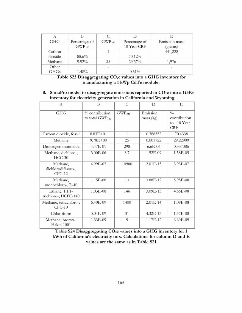
165

A B C D E

GHG Percentage of GWP100

GWP100 Percentage of 10 Year CRF

Emission mass (grams)

Carbon dioxide 88.6%

1 70.12%

441,228

Methane 9.92% 25 29.37% 1,976

Other GHGs 1.48%

- 0.51%

-

Table S23 Disaggregating CO2e values into a GHG inventory for manufacturing a 1 kWp CdTe module.

8. SimaPro model to disaggregate emissions reported in CO2e into a GHG inventory for electricity generation in California and Wyoming

A B C D E

GHG % contribution to total GWP100

GWP100 Emission mass (kg)

% contribution to 10 Year CRF

Carbon dioxide, fossil 8.83E+01 1 0.388552 70.4338

Methane 9.78E+00 25 0.001722 29.22909

Dinitrogen monoxide 4.47E-01 298 6.6E-06 0.337086

Methane, dichloro-, HCC-30

3.00E-06 8.7 1.52E-09 1.58E-05

Methane, dichlorodifluoro-,

CFC-12

4.99E-07 10900 2.01E-13 3.93E-07

Methane, monochloro-, R-40

1.15E-08 13 3.88E-12 5.95E-08

Ethane, 1,1,1-trichloro-, HCFC-140

1.03E-08 146 3.09E-13 4.66E-08

Methane, tetrachloro-, CFC-10

6.40E-09 1400 2.01E-14 1.09E-08

Chloroform 3.04E-09 31 4.32E-13 1.57E-08

Methane, bromo-, Halon 1001

1.33E-09 5 1.17E-12 6.69E-09

Table S24 Disaggregating CO2e values into a GHG inventory for 1 kWh of California’s electricity mix. Calculations for column D and E

values are the same as in Table S21

166

This study considers only two GHGs - CO2, CH4 – for CRF calculations for

electricity displaced in California as they contribute 98% and 99.6% of the GWP100 inventory

and the 10 year CRF impact, respectively (Table S24).

A B C D E

GHG % contribution to total GWP100

GWP100 Emission mass (kg)

% contribution to 10 Year CRF

Carbon dioxide, fossil 9.47E+01 1 0.88142 8.34E+01

Methane 5.00E+00 25 0.001862 1.65E+01

Dinitrogen monoxide 2.35E-01 298 2.22E-06 5.91E-02

Methane, dichloro-, HCC-30 7.10E-02

8.7 5.05E-08 2.74E-04

Methane, dichlorodifluoro-, CFC-12 4.72E-05

10900 7.69E-13 7.83E-07

Methane, monochloro-, R-40 9.01E-07

13 3.82E-11 3.06E-07

Ethane, 1,1,1-trichloro-, HCFC-140 5.33E-08

146 2.06E-12 1.62E-07

Chloroform 3.24E-08 31 3.47E-12 6.60E-08

Methane, tetrachloro-, CFC-10 1.42E-08

1400 9.41E-14 2.67E-08

Methane, bromo-, Halon 1001 1.16E-08

5 1.15E-11 3.44E-08

Table S25 Disaggregating CO2e values into a GHG inventory for 1 kWh of Wyoming’s electricity mix. Calculations for column D and E

values are the same as in Table S21

This study considers only two GHGs - CO2, CH4 – for the CRF calculations for the

electricity displaced in Wyoming as they contribute 99% of the GWP100 inventory and the 10

year CRF impact (Table S25).

167

9. Sensitivity of CRF calculations to IPCC’s uncertainty range for radiative efficiencies of GHGs

Gas (IPCC

radiative efficiency uncertainty range)

Radiative Efficiency – Base

value (W m-2 kg-1)

Radiative Efficiency - Upper limit value

(W m-2 kg-1)

Radiative Efficiency - Lower

limit value (W m-2 kg-1)

CO2 (+/- 10%) 1.75E-15 1.92E-15 1.57E-15

CH4 (+/- 17%) 1.30E-13 1.52E-13 1.07E-13

HFC 152a (+/- 10%)

7.68E-12 8.44 E-12 6.91 E-12

SF6 (+/- 10%) 2.00E-11 2.20E-11 1.80E-11

SO2 (+/- 50%) -4E-12 -2E-12 -6E-12

NOx (+ 116/- 124%)

-3.07E-12 4.91E-13 -6.88E-12

Table S26 Upper and lower limits for radiative efficiencies of GHGs based on IPCC estimates 20

Figure S34 Change in CRF and CRF payback times when the radiative efficiency of GHGs are varied between IPCC’s upper and lower limits. CRF impacts of manufacturing emissions and emissions due to the continued reliance on fossil fuels (for sub-optimal deployment) represent PV CRF costs. The CRF impacts avoided when PV electricity offsets grid electricity represent the CRF benefits. If the curve is below the X axis then CRF costs exceed CRF benefits of deploying the PV module and if the curve is above the X axis then CRF benefits exceed CRF costs. All the CRF calculations are performed for scenario CA: S4 (refer Figure S31). The CRF impacts in 2017 and 2031 are greater and lesser than the base scenario by 22% when using the upper and lower radiative efficiency estimates, respectively.

168

Figure S35 The graph depicts percentage change in CRF (measured in 2017) from the base condition when radiative efficiencies of emissions are varied by a range established by IPCC20 (shown in brackets). The base scenario’s CRF value is represented by the vertical line passing through zero and is identical to the base scenario in Figure 6 in the main paper.

Figure S36 Calculations in Figure S35 are repeated for a 25 year time period.

Among the gases considered, CRF impacts are the most sensitive to radiative

efficiency of SO2 over a 10 year period (Figure S35) and CO2 over a 25 year period (Figure

S36).

169

10. Acronym List

Acronym Expansion Units

aGHG t

GHG emissions avoided in year ‘t’ at the deployment location

grams

aghg Radiative efficiency of a GHG watts m-2 kg−1

apd annual performance degradation for the PV module

%/year

bGHG t GHG emissions due to BLS in year ‘t’ at the deployment location

grams

BLS Back loading strategy

C Total policy target kWp

CA California

CdTe cadmium telluride

CO2e CO2 equivalent

CRF Cumulative Radiative Forcing W m-2 yr

CRFav CRF benefit due to avoided GHG emissions

W m-2 yr

CRFbl CRF due to back loading W m-2 yr

CRFmnf CRF due to PV manufacturing GHG emissions

W m-2 yr

DGI t CO2e intensity of the grid (base load), at the deployment location in the year ‘t’

CO2e g/kWh

CSI California Solar Initiative

eff t PV module efficiency in the year 't' %

EPBT Energy payback time years

FLS Front loading strategy

GHG Greenhouse gas

IPCC Intergovernmental Panel on Climate Change

Irr Annual average solar irradiation at the deployment location

kWh/m2/year

kt CRF impact of one kg of a GHG depending on the year of emission over a ten year period

W m-2 yr

kW Kilowatts

LCA Life Cycle Assessment

Ma Mean molecular mass of air kg kmol−1

MCI t_i CO2e intensity of the manufactured PV technology 'i' in the year ‘t’

CO2e g/kWp

MCIchina mono Si CO2e intensity of the mono Si PV manufactured in China

CO2e g/kWp

MCIchina poly Si CO2e intensity of the poly Si PV manufactured in China

CO2e g/kWp

170

Acronym Expansion Units

MCImalayisa CdTe CO2e intensity of the CdTe PV manufactured in Malaysia

CO2e g/kWp

mGHGt PV manufacturing GHG emissions in year ‘t’

grams

ME Manufacturing energy embedded in the PV module

MJ/m2

Mi molecular weight of the GHG species

kg kmol-1

mSi mono-Silicon

MW Megawatts

op Ratio of energy spent on the operations and maintenance of the PV module to the total energy generated by the PV module

opt Optimal PV deployment strategy

pr Performance ratio, the ratio between the AC power generated to the rated DC power

pSi poly Silicon

PV Photovoltaics

S1 PV deployment Scenario 1. PV targets met using a 100% mSi mix.

S2 PV deployment Scenario 2. PV targets met using a 100% pSi mix.

S3 PV deployment Scenario 3. PV targets met using a 100% CdTe mix.

S4 PV deployment Scenario 4. PV targets met using a 35% mSi, 55% pSi and 10% CdTe mix. Optimal deployment

S5 PV deployment Scenario 5. PV targets met using a 35% mSi, 55% pSi and 10% CdTe mix. Sub-optimal deployment

SI Supplementary information

Sub Sub-optimal PV deployment strategy

tl transmissions losses during electricity distribution

%

Tm Total mass of the atmosphere kg

TH Time period for CRF calculation years

W t_i Capacity of a particular PV technology 'i' deployed in the year ‘t’

kWp

WY Wyoming

τ Perturbation time years

Table 27 Acronym list

171

REFERENCES

1.Stocker, T. F., Dahe, Q., & Plattner, G. K IPCC Fifth Assessment Report - Climate Change 2013: The Physical Science Basis (Chapter 8 Supplementary Information Section 8.SM.11.3); 2013. 2.Pachauri, R. R., A. IPCC fourth assessment report (Table 2.14). http://www.ipcc.ch/publications_and_data/ar4/wg1/en/ch2s2-10-2.html. 3.Stocker, T. F., Dahe, Q., & Plattner, G. K, IPCC Fifth Assessment Report - Climate Change 2013: The Physical Science Basis (Chapter 8 Supplementary Information Section 8.SM.11.3.2). 2013. 4.Green Tech Media,GTM Research: Yingli Gains Crown as Top Producer in a 36 GW Global PV Market. http://www.greentechmedia.com/articles/read/Yingli-Gains-Crown-As-Top-Producer-in-a-36-GW-Global-PV-Market. 5.PVTECH Top 10 PV module suppliers in 2012. http://www.pv-tech.org/guest_blog/top_10_pv_module_suppliers_in_2012. 6.Personal Communication with First Solar. 2013. 7.Wild-Scholten, M. J. M. d., Energy payback time and carbon footprint of commercial photovoltaic systems. Solar Energy Materials and Solar Cells 2013, 119, 296-305. 8.Simparo, Grid CO2 intensity as reported by Simparo. 2013. 9.Fthenakis, V.; Frischknecht, R.; Raugei, M.; Kim, H.; Alsema, E.; Held, M.; de Wild-Scholten, M., Methodology guidelines on life cycle assessment of photovoltaic electricity. IEA PVPS Task 2011, 12. 10.NREL National Solar Radiation Data Base - Class I locations. http://rredc.nrel.gov/solar/old_data/nsrdb/1991-2010/hourly/list_by_state.html#C. 11.FirstSolar Life Cycle Carbon Impacts of Utility Scale Photovoltaic Projects; 2011. 12.EIA Transmission and Distribution losses in the United States. http://www.eia.gov/tools/faqs/how-much-electricity-lost-transmission-and-distribution-united-states. 13.DOE, U. State Electrcity Profiles. http://www.eia.gov/electricity/state/. 14.EPA EPA Analysis of the American Clean Energy and Security Act of 2009; 2009.

15.Alsema, E., Energy pay‐back time and CO2 emissions of PV systems. Progress in photovoltaics: research and applications 2000, 8 (1), 17-25.

http://www.ipcc.ch/publications_and_data/ar4/wg1/en/ch2s2-10-2.html



http://www.pv-tech.org/guest_blog/top_10_pv_module_suppliers_in_2012

http://www.pv-tech.org/guest_blog/top_10_pv_module_suppliers_in_2012

http://rredc.nrel.gov/solar/old_data/nsrdb/1991-2010/hourly/list_by_state.html#C

http://www.eia.gov/tools/faqs/how-much-electricity-lost-transmission-and-distribution-united-states

http://www.eia.gov/tools/faqs/how-much-electricity-lost-transmission-and-distribution-united-states

http://www.eia.gov/electricity/state/

172

16.Fthenakis, V.; Kim, H.; Held, M.; Raugei, M.; Krones, J. In Update of PV energy payback times and life-cycle greenhouse gas emissions, 24th European Photovoltaic Solar Energy Conference and Exhibition, 2009; pp 21-25. 17.Stocker, T. F.; Dahe, Q.; Plattner, G.-K., Climate Change 2013: The Physical Science Basis (Chapter 8 Supplementary Information, Table 8.SM.6) Working Group I Contribution to the Fifth Assessment Report of the Intergovernmental Panel on Climate Change. Summary for Policymakers (IPCC, 2013) 2013. 18.Stocker, T. F.; Dahe, Q.; Plattner, G.-K., Climate Change 2013: The Physical Science Basis (Chapter 6, Table 6.9). Working Group I Contribution to the Fifth Assessment Report of the Intergovernmental Panel on Climate Change. Summary for Policymakers (IPCC, 2013) 2013. 19.Klimont, Z.; Smith, S. J.; Cofala, J., The last decade of global anthropogenic sulfur dioxide: 2000–2011 emissions (Supplementary Information Table S-1). Environmental Research Letters 2013, 8 (1), 014003. 20.Myhre, G., D. Shindell, F.-M. Bréon, W. Collins, J. Fuglestvedt, J. Huang, D. Koch, J.-F. Lamarque, D. Lee, B. Mendoza, T. Nakajima, A. Robock, G. Stephens, T. Takemura and H. Zhang, Anthropogenic and Natural Radiative Forcing Supplementary Material. In: Climate Change 2013: The Physical Science Basis. Contribution of Working Group I to the Fifth Assessment Report of the Intergovernmental Panel on Climate Change (Table 8.SM.7). 2013.

173

APPENDIX C

C. SUPPORTING INFORMATION FOR CHAPTER 3

174

S1 Data for PV manufacturing experience curve

Table 28 List of abbreviations and modeling parameters with assumed values and references

Sl

No

Year Tech

nolog

y

Energ

y

Unit Comments Considere

d for

analysis?

Reason for

not

considering

Source Section

referred

to in

source

1 1998 Multi

Si

4200 MJ/m2 Energy value includes silicon winning

and purification, silicon wafer

production, cell/module processing,

module encapsulation materials,

overhead operations and equipment

manufacturing.

Yes E.A Alsema, E

Nieuwlaar, Energy

viability of

photovoltaic systems,

Energy Policy,

Volume 28, Issue 14,

November 2000,

Pages 999-1010

Table 1

2 1998 amor

phous

Si

1100 MJ/m2 Energy value includes cell material,

cell/module processing, module

encapsulation materials, overhead

operations and equipment

manufacturing.

Yes E.A Alsema, E

Nieuwlaar, Energy

viability of


Energy Policy,


November 2000,

Pages 999-1010

Table 2

3 2000 Other

non

a-si

TF

PV

MJ/m2 No Only Mono

Si, Multi Si,

CdTe,

amorphous Si

is considered

in this analysis

E.A Alsema, E

Nieuwlaar, Energy

viability of


Energy Policy,


November 2000,

Pages 999-1010,

4 1992 amor

phous

Si


encapsulation material, direct processes,

ancillary processing. For consistency

with other literature reported values, we

have not included 396 MJ/m2 for

capital equipment.

Yes Erik Alsema, Energy

requirements of thin-

film solar cell

modules—a review,

Renewable and

Sustainable Energy

Reviews, Volume 2,

Issue 4, 1 December

1998, Pages 387-415

Table 2

5 1993 amor

phous

Si


encapsulation material, processing

direct, ancillary processing. For

consistency with other literature

No Duplicate

value. This

study refers to

value

Erik Alsema, Energy


film solar cell

modules—a review,

Renewable and

Table 2

175

Sl

No

Year Tech

nolog

y

Energ

y


d for

analysis?

Reason for

not

considering

Source Section

referred

to in

source

reported values, we have not included

443 MJ/m2 for capital equipment.

published in

Sl No 206.

Sustainable Energy

Reviews, Volume 2,

Issue 4, 1 December

1998, Pages 387-415

6 1991 amor

phous

Si

708 MJ/m2 Quoted in paper based on older study. No Duplicate

value. This

study refers to

value

published in

Sl No 107.

Erik Alsema, Energy


film solar cell

modules—a review,

Renewable and

Sustainable Energy

Reviews, Volume 2,

Issue 4, 1 December

1998, Pages 387-415

Table 2

7 1992 amor

phous

Si



direct, ancillary processing.



film solar cell

modules—a review,

Renewable and

Sustainable Energy

Reviews, Volume 2,

Issue 4, 1 December

1998, Pages 387-415

Table 2

8 1995 amor

phous

Si



direct, ancillary processing. For



9 MJ/m2 for capital equipment.



film solar cell

modules—a review,

Renewable and

Sustainable Energy

Reviews, Volume 2,

Issue 4, 1 December

1998, Pages 387-415

Table 2

9 1996/

1997

amor

phous

Si

881-

1130

MJ/m2 Energy value includes input materials

and manufacturing.

No Duplicate

value. This

study refers to

value

published in

Sl No 131.

Erik Alsema, Energy


film solar cell

modules—a review,

Renewable and

Sustainable Energy

Reviews, Volume 2,

Issue 4, 1 December

1998, Pages 387-415

Table 2

10 1994 CdTe 938 MJ/m2 Energy value includes material and

manufacturing. For consistency with

No Duplicate

value. This

Erik Alsema, Energy


Table 2

176

Sl

No

Year Tech

nolog

y

Energ

y


d for

analysis?

Reason for

not

considering

Source Section

referred

to in

source

other literature reported values, we


capital equipment.

study refers to

value

published in

Sl No 156.

film solar cell

modules—a review,

Renewable and

Sustainable Energy

Reviews, Volume 2,

Issue 4, 1 December

1998, Pages 387-415

11 1995 CdTe 642 MJ/m2 This is for worst case. Energy value

includes direct and indirect process

requirements and input materials. For



446 MJ/m2 for capital

No Duplicate

value. This

study refers to

value

published in

Sl No 209.

Erik Alsema, Energy


film solar cell

modules—a review,

Renewable and

Sustainable Energy

Reviews, Volume 2,

Issue 4, 1 December

1998, Pages 387-415

Table 2

12 1993 CdTe 1415 MJ/m2 Energy value includes cell material,

encapsulation material, direct processes,

ancillary processing.



film solar cell

modules—a review,

Renewable and

Sustainable Energy

Reviews, Volume 2,

Issue 4, 1 December

1998, Pages 387-415

Table 2

13 1998 CdTe 520-

880

MJ/m2 Energy value includes cell material,

substrate+encapsulation material,

processing direct, processing ancillary.

For consistency with other literature


capital equipment of 100-200 MJ/m2.

No Author

estimates

based on

previously

reported

literature

values and not

actual industry

data.

Erik Alsema, Energy


film solar cell

modules—a review,

Renewable and

Sustainable Energy

Reviews, Volume 2,

Issue 4, 1 December

1998, Pages 387-415

Table 4

14 1998 CdTe 690-

1070







No Author

estimates

based on

previousy

reported

literature

values and not

Erik Alsema, Energy


film solar cell

modules—a review,

Renewable and

Sustainable Energy

Reviews, Volume 2,

Table 4

177

Sl

No

Year Tech

nolog

y

Energ

y


d for

analysis?

Reason for

not

considering

Source Section

referred

to in

source

actual industry

data.

Issue 4, 1 December

1998, Pages 387-415

15 1998 amor

phous

Si

670-

1090







No Author

estimates

based on

previously

reported

literature

values and not

actual industry

data.

Erik Alsema, Energy


film solar cell

modules—a review,

Renewable and

Sustainable Energy

Reviews, Volume 2,

Issue 4, 1 December

1998, Pages 387-415

Table 4

16 1998 amor

phous

Si

840-

1280







No Author

estimates

based on

previously

reported

literature

values and not

actual industry

data.

Erik Alsema, Energy


film solar cell

modules—a review,

Renewable and

Sustainable Energy

Reviews, Volume 2,

Issue 4, 1 December

1998, Pages 387-415

Table 4

17 2000 Mono

Si

5700 MJ/m2 Energy value includes Si Production,

purification,crystallization, wafering,

cell Processing, module assembly

No Author

estimates

based on

previously

reported

literature

values and not

actual industry

data.

Energy pay-back time

and CO2 emissions

of PV systems E. A.

Alsema* - Progress in

Photovoltaics:

Research and

Applications Volume

8, Issue 1, pages 17–

25, January/February

2000

Table 1

18 2000 Multi

Si




No Author

estimates

based on

previously

reported

literature

values and not

actual industry

data.


and CO2 emissions

of PV systems E. A.


Photovoltaics:

Research and

Applications Volume



2000

Table 1

178

Sl

No

Year Tech

nolog

y

Energ

y


d for

analysis?

Reason for

not

considering

Source Section

referred

to in

source

19 2000 amor

phous

Si


substrate and encapsulation,

cell/module processing and overhead

operations. For consistency with other

literature reported values, we have not

included capital equipment of 150

MJ/m2.

No Author

estimates

based on

previously

reported

literature

values and not

actual industry

data.


and CO2 emissions

of PV systems E. A.


Photovoltaics:

Research and

Applications Volume



2000

Table 3

20 2006 CdTe 1200 MJ/m2 Energy value includes materials and

manufacturing

No Duplicate

value. This

study refers to

value

published in

Sl No 150.

UPDATE OF PV

ENERGY

PAYBACK TIMES

AND LIFE-CYCLE

GREENHOUSE

GAS EMISSIONS

- 24th European

Photovoltaic Solar

Energy Conference,

21-25 September

2009, Hamburg,

Germany

V. Fthenakis, H.C.

Kim, M. Held, M.

Raugei and J. Krones

Table 1


manufacturing

Yes UPDATE OF PV

ENERGY

PAYBACK TIMES

AND LIFE-CYCLE

GREENHOUSE

GAS EMISSIONS

- 24th European

Photovoltaic Solar

Energy Conference,

21-25 September

2009, Hamburg,

Germany

V. Fthenakis, H.C.

Kim, M. Held, M.


Table 1

179

Sl

No

Year Tech

nolog

y

Energ

y


d for

analysis?

Reason for

not

considering

Source Section

referred

to in

source


manufacturing. Based on actual

industrial data.

Yes UPDATE OF PV

ENERGY

PAYBACK TIMES

AND LIFE-CYCLE

GREENHOUSE

GAS EMISSIONS

- 24th European

Photovoltaic Solar

Energy Conference,

21-25 September

2009, Hamburg,

Germany

V. Fthenakis, H.C.

Kim, M. Held, M.


Table 1


manufacturing

No Duplicate

value. This

study refers to

value

published in

Sl No 155.

UPDATE OF PV

ENERGY

PAYBACK TIMES

AND LIFE-CYCLE

GREENHOUSE

GAS EMISSIONS

- 24th European

Photovoltaic Solar

Energy Conference,

21-25 September

2009, Hamburg,

Germany

V. Fthenakis, H.C.

Kim, M. Held, M.


Table 1

24 2006 Mono

Si

5000 MJ/m2 Energy value includes materials and


industrial data.

Yes UPDATE OF PV

ENERGY

PAYBACK TIMES

AND LIFE-CYCLE

GREENHOUSE

GAS EMISSIONS

- 24th European

Photovoltaic Solar

Energy Conference,

21-25 September

2009, Hamburg,

Germany

Table 2

180

Sl

No

Year Tech

nolog

y

Energ

y


d for

analysis?

Reason for

not

considering

Source Section

referred

to in

source

V. Fthenakis, H.C.

Kim, M. Held, M.


25 2008 Mono

Si



industrial data.

No Duplicate

value. This

study refers to

value

published in

Sl No 49.

UPDATE OF PV

ENERGY

PAYBACK TIMES

AND LIFE-CYCLE

GREENHOUSE

GAS EMISSIONS

- 24th European

Photovoltaic Solar

Energy Conference,

21-25 September

2009, Hamburg,

Germany

V. Fthenakis, H.C.

Kim, M. Held, M.


Table 2

26 2005 Multi

Si



industrial data.

Yes UPDATE OF PV

ENERGY

PAYBACK TIMES

AND LIFE-CYCLE

GREENHOUSE

GAS EMISSIONS

- 24th European

Photovoltaic Solar

Energy Conference,

21-25 September

2009, Hamburg,

Germany

V. Fthenakis, H.C.

Kim, M. Held, M.


Table 2

27 2007 Multi

Si



industrial data.

No Duplicate

value. This

study refers to

value

published in

Sl No 50.

UPDATE OF PV

ENERGY

PAYBACK TIMES

AND LIFE-CYCLE

GREENHOUSE

GAS EMISSIONS

- 24th European

Photovoltaic Solar

Energy Conference,

Table 2

181

Sl

No

Year Tech

nolog

y

Energ

y


d for

analysis?

Reason for

not

considering

Source Section

referred

to in

source

21-25 September

2009, Hamburg,

Germany

V. Fthenakis, H.C.

Kim, M. Held, M.


28 2005 Ribbo

n Si



industrial data.

No This study

only considers

mono Si,

multi Si,

CdTe, a Si

UPDATE OF PV

ENERGY

PAYBACK TIMES

AND LIFE-CYCLE

GREENHOUSE

GAS EMISSIONS

- 24th European

Photovoltaic Solar

Energy Conference,

21-25 September

2009, Hamburg,

Germany

V. Fthenakis, H.C.

Kim, M. Held, M.


Table 2

29 2009 Ribbo

n Si



industrial data.

No This study

only considers

mono Si,

multi Si,

CdTe, a Si

UPDATE OF PV

ENERGY

PAYBACK TIMES

AND LIFE-CYCLE

GREENHOUSE

GAS EMISSIONS

- 24th European

Photovoltaic Solar

Energy Conference,

21-25 September

2009, Hamburg,

Germany

V. Fthenakis, H.C.

Kim, M. Held, M.


Table 2



industrial data.

Yes Update of

environmental

indicators and energy

payback time of

CdTe PV systems in

Europe - Michael

Figure 3

182

Sl

No

Year Tech

nolog

y

Energ

y


d for

analysis?

Reason for

not

considering

Source Section

referred

to in

source

Held*, Robert Ilg -

Progress in

Photovoltaics:

Research and

Applications

Volume 19, Issue 5,

pages 614–626,

August 2011



industrial data.

No Duplicate

value. This

study refers to

value

published in

Sl No 150.

V.M. Fthenakis, H.C.

Kim, Photovoltaics:

Life-cycle analyses,

Solar Energy, Volume

85, Issue 8, August

2011, Pages 1609-

1628

Table 1

32 2006 Mono

Si



industrial data.

No Duplicate

value. The

author

updates the

original value

published in

Sl No 65 to

reflect

improvements

in 2006.


Kim, Photovoltaics:



85, Issue 8, August

2011, Pages 1609-

1628

Table 1

33 2006 Multi

Si



industrial data.

No Duplicate

value. The

author

updates the

original value

published in

Sl No 174 to

reflect

improvements

in 2006.


Kim, Photovoltaics:



85, Issue 8, August

2011, Pages 1609-

1628

Table 1

34 1999 Multi

Si

4200 MJ/m2 Energy value includes frame, module

assembly, cell production, ingot+wafer,

Si feedstock

No Duplicate

value. This

study refers to

the estimates

published in

Sl No 18.

Alsema, EA and de

Wild-Scholten,

MJ,The real

environmental

impacts of crystalline

silicon PV modules:

an analysis based on

Figure 5

183

Sl

No

Year Tech

nolog

y

Energ

y


d for

analysis?

Reason for

not

considering

Source Section

referred

to in

source

up-to-date

manufacturers data,

2005

35 1999 Mono

Si



Si feedstock

No Duplicate

value. This

study refers to

the estimates

published in

Sl No 17.

Alsema, EA and de

Wild-Scholten,

MJ,The real

environmental


silicon PV modules:


up-to-date

manufacturers data,

2005

Figure 5

36 2004 Multi

Si



Si feedstock. Based on actual

manufacturing data.

Yes Alsema, EA and de

Wild-Scholten,

MJ,The real

environmental


silicon PV modules:


up-to-date

manufacturers data,

2005

Figure 5

37 2004 Mono

Si




manufacturing data.

Yes Alsema, EA and de

Wild-Scholten,

MJ,The real

environmental


silicon PV modules:


up-to-date

manufacturers data,

2005

Figure 5

38 1998 Multi

Si

3254 MJ/m2 Energy value includes Si production

process, casting and cutting, cell

production, module assembly and

others at a production scale of 10MW

per year. The original data reported in

the paper (3534 mj/m2) includes the

frame for 280 mj/m2 (see "A life-cycle

analysis on thin-film CdS/CdTe PV

No The material

inventory and

energy values

are author

estimates and

not based on

actual

manufacturing

data.

Kato, K. and Murata,

A. and Sakuta, K.,


and life-cycle CO2

emission of

residential PV power

system with silicon

PV module,1998

Table 2

184

Sl

No

Year Tech

nolog

y

Energ

y


d for

analysis?

Reason for

not

considering

Source Section

referred

to in

source

modules" from the same authors). This

frame energy value is deducted.

39 1998 Multi

Si





per year.The original data reported in






No The material

inventory and

energy values

are author

estimates and

not based on

actual

manufacturing

data.


A. and Sakuta, K.,


and life-cycle CO2

emission of


system with silicon

PV module,1998

Table 2

40 1998 Multi

Si





per year.The original data reported in






No The material

inventory and

energy values

are author

estimates and

not based on

actual

manufacturing

data.


A. and Sakuta, K.,


and life-cycle CO2

emission of


system with silicon

PV module,1998

Table 2

41 1998 amor

phous

Si

1363 MJ/m2 Energy value includes cell production,

module assembly and others at a

production scale of 10MW per year.The

original data reported in the paper

(1643 mj/m2) includes the frame for

280 mj/m2 (see "A life-cycle analysis

on thin-film CdS/CdTe PV modules"

from the same authors). This frame

energy value is deducted.

No The material

inventory and

energy values

are author

estimates and

not based on

actual

manufacturing

data.


A. and Sakuta, K.,


and life-cycle CO2

emission of


system with silicon

PV module,1998

Table 3

42 1998 amor

phous

Si



production scale of 30MW per year.

The original data reported in the paper






No The material

inventory and

energy values

are author

estimates and

not based on

actual

manufacturing

data.


A. and Sakuta, K.,


and life-cycle CO2

emission of


system with silicon

PV module,1998

Table 3

185

Sl

No

Year Tech

nolog

y

Energ

y


d for

analysis?

Reason for

not

considering

Source Section

referred

to in

source

43 1998 amor

phous

Si










No The material

inventory and

energy values

are author

estimates and

not based on

actual

manufacturing

data.


A. and Sakuta, K.,


and life-cycle CO2

emission of


system with silicon

PV module,1998

Table 3

44 2001 CdTe 1523 MJ/m2 Energy value includes cell production,


production scale of 10MW per year.The



280 mj/m2. This frame energy value is

deducted.

No The material

inventory and

energy values

are author

estimates and

not based on

actual

manufacturing

data.

Kato, K. and Hibino,

T. and Komoto, K.

and Ihara, S. and

Yamamoto, S. and

Fujihara, H., A life-

cycle analysis on thin-

film CdS/CdTe PV

modules,2001

Table 2







deducted.

No The material

inventory and

energy values

are author

estimates and

not based on

actual

manufacturing

data.


T. and Komoto, K.

and Ihara, S. and

Yamamoto, S. and



film CdS/CdTe PV

modules,2001

Table 2







deducted.

No The material

inventory and

energy values

are author

estimates and

not based on

actual

manufacturing

data.


T. and Komoto, K.

and Ihara, S. and

Yamamoto, S. and



film CdS/CdTe PV

modules,2001

Table 2

47 2005 Multi

Si

3727 MJ/m2 Energy value includes Si

feedstock,ingot and wafer, cell

production, module assembly

No Duplicate

value. This

study refers to

the estimates

published in

Sl No 174.

Alsema, E., & de

Wild, M. J. (2005,

January).

Environmental

impact of crystalline

silicon photovoltaic

Figure 3

186

Sl

No

Year Tech

nolog

y

Energ

y


d for

analysis?

Reason for

not

considering

Source Section

referred

to in

source

module production.

In MRS

Proceedings (Vol. 895,

pp. 0895-G03).

Cambridge University

Press.

48 1999 Mono

Si


processes for Ingot, wafer, cells and

module. The reported values is 5598

kWh/kWp including the frame.

Without the energy values for frame

(324 kWh/kWp) we get 5274

kWh/kWp. This value corresponds to

the SP75 module and 1 m2 of a

module contains 118 Wp (

http://www.abcsolar.com/pdf/sp75.p

df ). Converting the energy value to a

m2 basis we get 622 kWh per m2 and

this corresponds to 7000 MJ/m2 (using

a grid factor of 0.32 and conversion

factor of 3.6 between MJ and kWh).

This study reports actual manufacturing

data.

No Duplicate

value. This

study refers to

the estimates

published in

Sl No 104.

Knapp, Karl, and

Theresa Jester. "An

empirical perspective

on the energy

payback time for

photovoltaic

modules." PROCEE

DINGS OF THE

SOLAR

CONFERENCE.

AMERICAN

SOLAR ENERGY

SOCIETY;

AMERICAN

INSTITUTE OF

ARCHITECTS,

2000.

Slide 9

49 2008 Mono

Si



industrial data.

Yes Mariska de Wild-

Scholten,Energy

payback time of

photovoltaic modules

and systems,2009

Slide 9

50 2007 Multi

Si



industrial data.


Scholten,Energy

payback time of


and systems,2009

Slide 9

51 2008 amor

phous

Si



industrial data.


Scholten,Energy

payback time of


and systems,2009

Slide 9

52 2008 amor

phous

Si



industrial data.


Scholten,Energy

payback time of

Slide 9

187

Sl

No

Year Tech

nolog

y

Energ

y


d for

analysis?

Reason for

not

considering

Source Section

referred

to in

source


and systems,2009



industrial data.


Scholten,Energy

payback time of


and systems,2009

Slide 9

54 1998 Mono

Si

6000 MJ/m2 This is for the "low scenario".Energy

value includes Si production,

purification and crystallization,

wafering, cell processing and module

assembly.

No The reported

values are

assumptions

based on

values

reported in

previous

studies and

not actual

production

data.

Alsema, E. A., Frankl,

P., & Kato, K. (1998,

July). Energy pay-

back time of

photovoltaic energy

systems: present

status and prospects.

In 2nd World

Conference on

photovoltaic solar

energy conversion,

Vienna (pp. 6-10).

Table 1

54 1998 Mono

Si

13900 MJ/m2 This is for the "high scenario".Energy

value includes Si production,



assembly.

No The reported

values are

assumptions

based on

values

reported in

previous

studies and

not actual

production

data.


P., & Kato, K. (1998,

July). Energy pay-

back time of

photovoltaic energy

systems: present


In 2nd World

Conference on

photovoltaic solar

energy conversion,

Vienna (pp. 6-10).

Table 1

55 1998 amor

phous

Si

1050 MJ/m2 Energy value include cell material,


cell/module processing, overhead




MJ/m2.

No The reported

values are

assumptions

based on

values

reported in

previous

studies and

not actual

production

data.


P., & Kato, K. (1998,

July). Energy pay-

back time of

photovoltaic energy

systems: present


In 2nd World

Conference on

photovoltaic solar

Table 3

188

Sl

No

Year Tech

nolog

y

Energ

y


d for

analysis?

Reason for

not

considering

Source Section

referred

to in

source

energy conversion,

Vienna (pp. 6-10).

56 1995 Multi

Si

2916 MJ/m2 This is for worst case. Energy value





576 MJ/m2 for investments.

No The reported

values are

assumptions

based on

values

reported in

previous

studies and

not actual

production

data.

Phylipsen, G. J. M., &

Alsema, E. A. (1995).

Environmental life-

cycle assessment of

multicrystalline

silicon solar cell

modules (NOVEM

Report 95057).

Netherlands Agency

for Energy and the

Environment: The

Hague, The

Netherlands.

Table 4.3

57 1995 Multi

Si

1296 MJ/m2 This is for base case. Energy value






No The reported

values are

assumptions

based on

values

reported in

previous

studies and

not actual

production

data.


Alsema, E. A. (1995).

Environmental life-

cycle assessment of

multicrystalline

silicon solar cell

modules (NOVEM

Report 95057).

Netherlands Agency

for Energy and the

Environment: The

Hague, The

Netherlands.

Table 4.3

58 1995 Multi

Si

576 MJ/m2 This is for best case. Energy value






No The reported

values are

assumptions

based on

values

reported in

previous

studies and

not actual

production

data.


Alsema, E. A. (1995).

Environmental life-

cycle assessment of

multicrystalline

silicon solar cell

modules (NOVEM

Report 95057).

Netherlands Agency

for Energy and the

Environment: The

Hague, The

Netherlands.

Table 4.3

189

Sl

No

Year Tech

nolog

y

Energ

y


d for

analysis?

Reason for

not

considering

Source Section

referred

to in

source

59 1998 Mono

Si

15524 MJ/m2 Energy value includes metal grade Si

production, poly Si production,

Czochralski Si and wafer production,

cell production and module assembly

No The reported

values are

assumptions

based on

values

reported in

previous

studies and

not actual

production

data.

Kato, K., Murata, A.,

& Sakuta, K. (1998).

Energy pay‐ back

time and life‐ cycle

CO2 emission of


system with silicon

PV module. Progress

in Photovoltaics:

Research and

Applications, 6(2),

105-115.

Table 5

60 1998 Mono

Si





No The reported

values are

assumptions

based on

values

reported in

previous

studies and

not actual

production

data.


& Sakuta, K. (1998).

Energy pay‐ back


CO2 emission of


system with silicon

PV module. Progress

in Photovoltaics:

Research and

Applications, 6(2),

105-115.

Table 5

61 1998 Mono

Si





No The reported

values are

assumptions

based on

values

reported in

previous

studies and

not actual

production

data.


& Sakuta, K. (1998).

Energy pay‐ back


CO2 emission of


system with silicon

PV module. Progress

in Photovoltaics:

Research and

Applications, 6(2),

105-115.

Table 5

62 1999 amor

phous

Si


module assembly, overhead at a 10MW

per year production scale.The original

data reported in the paper (1731

mj/m2) includes the frame for 275

No The material

inventory and

energy values

are author

estimates and

not based on

Kato, K., Hibino, T.,

Komoto, K., Ihara,

S., Yamamoto, S., &

Fujihara, H. (2001). A

life-cycle analysis on

thin-film CdS/CdTe

Figure 4

190

Sl

No

Year Tech

nolog

y

Energ

y


d for

analysis?

Reason for

not

considering

Source Section

referred

to in

source

mj/m2. This frame energy value is

deducted.

actual

manufacturing

data.

PV modules. Solar

Energy Materials and

Solar Cells, 67(1),

279-287.

63 1999 amor

phous

Si


module assembly, overhead at a 30MW

per year production scale.The original

data reported in the paper (1681

mj/m2) includes the frame for 275

mj/m2. This frame energy value is

deducted.

No The material

inventory and

energy values

are author

estimates and

not based on

actual

manufacturing

data.


Komoto, K., Ihara,

S., Yamamoto, S., &



thin-film CdS/CdTe

PV modules. Solar


Solar Cells, 67(1),

279-287.

Figure 4

64 1999 amor

phous

Si


module assembly, overhead at a

100MW per year production scale.The




deducted.

No The material

inventory and

energy values

are author

estimates and

not based on

actual

manufacturing

data.


Komoto, K., Ihara,

S., Yamamoto, S., &



thin-film CdS/CdTe

PV modules. Solar


Solar Cells, 67(1),

279-287.

Figure 4

65 2005 Mono

Si



industrial data.

Yes Alsema, E., & de

Wild, M. J. (2005,

January).

Environmental



module production.

In MRS


pp. 0895-G03).


Press.

Figure 3

66 1998 Multi

Si


value includes Si production, Si


wafering, cell processing, module

assembly.

No The reported

values are

assumptions

based on

values

reported in

Alsema, E. "Energy

requirements and

CO2 mitigation

potential of PV

systems." Photovoltai

cs and the

Table 1

191

Sl

No

Year Tech

nolog

y

Energ

y


d for

analysis?

Reason for

not

considering

Source Section

referred

to in

source

previous

studies and

not actual

production

data.

Environment 1999

(1998).

67 1998 Mono

Si





assembly.

No The reported

values are

assumptions

based on

values

reported in

previous

studies and

not actual

production

data.

Alsema, E. "Energy

requirements and

CO2 mitigation

potential of PV


cs and the

Environment 1999

(1998).

Table 1

68 1998 amor

phous

Si







MJ/m2.

No The reported

values are

assumptions

based on

values

reported in

previous

studies and

not actual

production

data.

Alsema, E. "Energy

requirements and

CO2 mitigation

potential of PV


cs and the

Environment 1999

(1998).

Table 3

69 2006 Multi

Si

3245 MJ/m2 Energy value includes Si feedstock,

ingot, wafer, cell production and

module assembly. Data based on actual

production data.

Yes Alsema, E. A., de

Wild-Scholten, M. J.,

& Fthenakis, V. M.

(2006, September).

Environmental

impacts of PV

electricity generation-

a critical comparison

of energy supply

options. In 21st

European photovoltaic

solar energy conference,

Dresden, Germany (Vol.

3201).

Figure 2

192

Sl

No

Year Tech

nolog

y

Energ

y


d for

analysis?

Reason for

not

considering

Source Section

referred

to in

source

70 2006 Multi

Si




production data.

Yes Alsema, E. A., & de

Wild-Schoten, M. J.

(2007, September).

Reduction of the

environmental

impacts in crystalline

silicon module

manufacturing. In

22nd European

Photovoltaic Solar

Energy Conference

(pp. 829-836). WIP-

Renewable Energies.

Figure 2

71 2006 Mono

Si




production data.

Yes Alsema, E. A., & de

Wild-Schoten, M. J.

(2007, September).

Reduction of the

environmental

impacts in crystalline

silicon module

manufacturing. In

22nd European

Photovoltaic Solar

Energy Conference

(pp. 829-836). WIP-

Renewable Energies.

Figure 2


processes for laminate production.

Efficiency used in the study is 9% and

this multiplied by 7600 MJ/kWp value

reported. Based on actual production

data.

Yes Raugei, Marco;

Bargigli, Silvia;

Ulgiati, Sergio Life

cycle assessment and

energy pay-back time

of advanced

photovoltaic

modules: CdTe and

CIS compared to

poly-Si

Figure 5

73 2006 Multi

Si

9716 MJ/m2 This data assumes that electronic grade

silicon is used to manufacture the multi

Si module and the entire energetic

burden of electronic grade silicon is

allocated to the PV module.

No This value

does not

include actual

industrial data

for upstream

Raugei, Marco;

Bargigli, Silvia;




of advanced

Figure 5

193

Sl

No

Year Tech

nolog

y

Energ

y


d for

analysis?

Reason for

not

considering

Source Section

referred

to in

source

silicon

purification.

photovoltaic

modules: CdTe and

CIS compared to

poly-Si

74 2006 Multi

Si

3542 MJ/m2 This data assumes that electronic grade

silicon is used to manufacture the multi

Si module and 30% of the energetic

burden of electronic grade silicon is

allocated to the PV module.

No This value

does not

include actual

industrial data

for upstream

silicon

purification.

Raugei, Marco;

Bargigli, Silvia;




of advanced

photovoltaic

modules: CdTe and

CIS compared to

poly-Si

Figure 5

75 2006 Multi

Si




manufacturing data.

No Duplicate

value. This

study refers to

the estimates

published in

Sl No 36.

Raugei, Marco;

Bargigli, Silvia;




of advanced

photovoltaic

modules: CdTe and

CIS compared to

poly-Si

Figure 5


processes for laminate production.

Efficiency used in the study is 9% and

this multiplied by 7600 MJ/kWp value

reported. Based on actual production

data.

No Duplicate

value. This

study refers to

the estimates

published in

Sl No 72.

Azzopardi, B; Mutale,

J Life cycle analysis

for future

photovoltaic systems

using hybrid solar

cells

Figure 1

77 2001 Multi

Si



module assembly. Based on actual

production data and secondary

literature reported values.

No This value

does not

include actual

industrial data

for upstream

silicon

purification.

Riccardo Battisti,

Annalisa Corrado,

Evaluation of

technical

improvements of


through life cycle

assessment

methodology

Figure 4

78 2008 Multi

Si

1442 MJ/m2 Energy value of 177 kWh for 1.38 m2

and this includes materials and

manufacturing. Converting kWh to MJ

No Energy values

are not based

on actual

Botsaris, P N;

Filippidou, F,

Estimation of the

Table 6

194

Sl

No

Year Tech

nolog

y

Energ

y


d for

analysis?

Reason for

not

considering

Source Section

referred

to in

source

and normalizing to an area of 1 m2 we

get 1442

production

data but

calculated

using the CES

EduPack

2008, Granta

software.

Energy Payback Time

(EPR) of a PV

Module Installed in

North–Eastern

Greece

79 1998 Multi

Si






manufacturing.

No Duplicate

value. This

study refers to

the estimates

published in

Sl No 1

Jose L. Bernal-

Agustın*, Rodolfo

Dufo-Lopez,

Economical and

environmental

analysis of grid

connected


in Spain.

Table 1

80 1998 amor

phous

Si

1050 MJ/m2 Energy value include cell material,



operations.

No Duplicate

value. This

study refers to

the estimates

published in

Sl No 55.

Jose L. Bernal-

Agustın*, Rodolfo

Dufo-Lopez,

Economical and

environmental

analysis of grid

connected


in Spain.

Table 1

81 1998 Mono

Si

9950 MJ/m2 Energy value includes Si production,



assembly.

No Author has

taken the

average of the

values

reported in Sl

no 54 -

Alsema, E. A.,

Frankl, P., &

Kato, K.

(1998, July).

Energy pay-

back time of

photovoltaic

energy

systems:

present status

and prospects.

Bizzarri, G., and G.

L. Morini. "A Life

Cycle Analysis of

roof integrated

photovoltaic

systems." International

journal of environmental

technology and

management 7.1-2

(2007): 134-146.

Table 5

195

Sl

No

Year Tech

nolog

y

Energ

y


d for

analysis?

Reason for

not

considering

Source Section

referred

to in

source

In 2nd World

Conference

on

photovoltaic

solar energy

conversion,

Vienna (pp. 6-

10).

82 1998 Multi

Si

7898 MJ/m2 This scenario is the same as sl no

89,90. Data was averaged over the

range reported in Sl no 89,90

No Author has

taken the

average of the

values

reported in Sl

no 54 -

Alsema, E. A.,

Frankl, P., &

Kato, K.

(1998, July).

Energy pay-

back time of

photovoltaic

energy

systems:

present status

and prospects.

In 2nd World

Conference

on

photovoltaic

solar energy

conversion,

Vienna (pp. 6-

10).

Bizzarri, G., and G.

L. Morini. "A Life

Cycle Analysis of

roof integrated

photovoltaic

systems." International

journal of environmental

technology and

management 7.1-2

(2007): 134-146.

Table 5

83 1988 Mono

Si

8285 MJ/m2 Energy value includes Si purification, Si

wafer and cell production and module

production with frame. Based on actual

production data and we deduct 700

mj/m2 for the frame. Since this study

was published in 1988 we assume an

extra 200 mj/m2 for the frame when

compared to 500 mj/m2 assumed in a

later study ,"Energy pay-back time and

Yes Hagedorn, G. (1989).

Hidden energy in

solar cells and

photovoltaic power

stations. In 9th

European

Photovoltaic Solar

Energy Conference

(p. 542).

Section

7.1.1

196

Sl

No

Year Tech

nolog

y

Energ

y


d for

analysis?

Reason for

not

considering

Source Section

referred

to in

source

CO2 emissions of PV systems",

published in year 2000.

84 1988 Multi

Si












Yes Hagedorn, G. (1989).

Hidden energy in

solar cells and

photovoltaic power

stations. In 9th

European

Photovoltaic Solar

Energy Conference

(p. 542).

Section

7.1.2

85 1988 amor

phous

Si

1785 MJ/m2 Energy value includes module

production

No Not based on

actual

production

data

Hagedorn, G. (1989).

Hidden energy in

solar cells and

photovoltaic power

stations. In 9th

European

Photovoltaic Solar

Energy Conference

(p. 542).

Section

7.2

86 1988 Mono

Si



production without frame.

No Not based on

actual

production

data and

represents

improved

manufacturing

in the future.


Hidden energy in

solar cells and

photovoltaic power

stations. In 9th

European

Photovoltaic Solar

Energy Conference

(p. 542).

Section

7.1.1

87 1988 Multi

Si




No Not based on

actual

production

data and

represents

improved

manufacturing

in the future.


Hidden energy in

solar cells and

photovoltaic power

stations. In 9th

European

Photovoltaic Solar

Energy Conference

(p. 542).

Section

7.1.2

197

Sl

No

Year Tech

nolog

y

Energ

y


d for

analysis?

Reason for

not

considering

Source Section

referred

to in

source

88 1988 amor

phous

Si


production

No Not based on

actual

production

data


Hidden energy in

solar cells and

photovoltaic power

stations. In 9th

European

Photovoltaic Solar

Energy Conference

(p. 542).

Section

7.2

89 1998 Multi

Si





assembly.

No The reported

values are

assumptions

based on

values

reported in

previous

studies and

not actual

production

data.

Alsema, EA and

Frankl, P. and Kato,

K.,Energy pay-back

time of photovoltaic

energy systems:

present status and

prospects,1998

Table 1

90 1998 Multi

Si

11600 MJ/m2 This is for the "high scenario".Energy




assembly.

No The reported

values are

assumptions

based on

values

reported in

previous

studies and

not actual

production

data.

Alsema, EA and

Frankl, P. and Kato,

K.,Energy pay-back

time of photovoltaic

energy systems:

present status and

prospects,1998

Table 1

91 2000 Mono

Si




No Duplicate

value. This

study refers to

the estimates

published in

Sl No 17.

García-Valverde, R.,

Miguel, C., Martínez-

Béjar, R., & Urbina,

A. (2009). Life cycle

assessment study of a

4.2 kW p stand-alone

photovoltaic system.

Solar Energy, 83(9),

1434-1445.

Section

3.2.1.1

92 1998 Multi

Si



No Duplicate

value. This

Ito, M., Kato, K.,

Komoto, K.,

Table 4

198

Sl

No

Year Tech

nolog

y

Energ

y


d for

analysis?

Reason for

not

considering

Source Section

referred

to in

source



per year

study refers to

the estimates

published in

Sl No 40.

Kichimi, T., &

Kurokawa, K. (2008).

A comparative study

on cost and life‐

cycle analysis for 100

MW very large‐ scale

PV (VLS‐ PV)

systems in deserts

using m‐ Si, a‐ Si,

CdTe, and CIS

modules. Progress in

Photovoltaics:

research and

applications, 16(1),

17-30.

93 2000 amor

phous

Si




No Not based on

actual

production

data. The

authors

mention that

this value

represents an

update of the

value reported

in sl no 43

Ito, M., Kato, K.,

Komoto, K.,

Kichimi, T., &


A comparative study

on cost and life‐



PV (VLS‐ PV)

systems in deserts


CdTe, and CIS


Photovoltaics:

research and


17-30.

Table 4




No Not based on

actual

production

data. The

authors

mention that

this value

represents an

update of the

Ito, M., Kato, K.,

Komoto, K.,

Kichimi, T., &


A comparative study

on cost and life‐



PV (VLS‐ PV)

systems in deserts

Table 4

199

Sl

No

Year Tech

nolog

y

Energ

y


d for

analysis?

Reason for

not

considering

Source Section

referred

to in

source

value reported

in sl no 46


CdTe, and CIS


Photovoltaics:

research and


17-30.

95 2006 Multi

Si

2300 MJ/m2 1494 Mj per panel of area 0.65 m2.

Energy value includes Si Production,



No Not based on

actual

production

data. The

authors

estimate the

value from

commonly

used industrial

processes.

Stoppato, A. (2008).

Life cycle assessment

of photovoltaic

electricity generation.

Energy, 33(2), 224-

232.

Section 4

96 2009 Mono

Si




No Author

estimates not

based on

actual

production

data.

Ito, Masakazu, et al.

"A comparative study

on life cycle analysis

of 20 different PV

modules installed at

the Hokuto mega‐

solar plant." Progress

in Photovoltaics:

Research and

Applications 19.7

(2011): 878-886.

Table 3

97 2009 Multi

Si




No Author

estimates not

based on

actual

production

data.




of 20 different PV


the Hokuto mega‐


in Photovoltaics:

Research and

Applications 19.7

(2011): 878-886.

Table 3

98 2001 amor

phous

Si




No Author

estimates not

based on




Table 3

200

Sl

No

Year Tech

nolog

y

Energ

y


d for

analysis?

Reason for

not

considering

Source Section

referred

to in

source

actual

production

data.

Duplicate

value. This

study refers to

the estimates

published in

Sl No 93.

of 20 different PV


the Hokuto mega‐


in Photovoltaics:

Research and

Applications 19.7

(2011): 878-886.

99 2009 Multi

Si

19712 GJ/M

W

Energy value includes mining,

manufacturing, transport, construction,

transmission, operation.

No Data given in

GJ/MW

without

module

efficiency

values.

Therefore, we

cannot

convert this to

a MJ/m2

value. Further

the LCA data

referred to by

the authors is

the same as

the study in Sl

No 95 to 98

Ito, Masakazu,

Keiichi Komoto, and

Kosuke Kurokawa.

"Life-cycle analyses

of very-large scale PV

systems using six

types of PV

modules." Current

Applied Physics 10.2

(2010): S271-S273.

Figure 2

100 2009 Mono

Si

28119 GJ/M

W




No Data given in

GJ/MW

without

module

efficiency

values.

Therefore, we

cannot

convert this to

a MJ/m2

value. Further

the LCA data

referred to by

the authors is

the same as

Ito, Masakazu,

Keiichi Komoto, and

Kosuke Kurokawa.



systems using six

types of PV

modules." Current


(2010): S271-S273.

Figure 2

201

Sl

No

Year Tech

nolog

y

Energ

y


d for

analysis?

Reason for

not

considering

Source Section

referred

to in

source

the study in Sl

No 95 to 98

101 2009 amor

phous

Si

14181 GJ/M

W




No Data given in

GJ/MW

without

module

efficiency

values.

Therefore, we

cannot

convert this to

a MJ/m2

value. Further

the LCA data

referred to by

the authors is

the same as

the study in Sl

No 95 to 98

Ito, Masakazu,

Keiichi Komoto, and

Kosuke Kurokawa.



systems using six

types of PV

modules." Current


(2010): S271-S273.

Figure 2

102 2009 CdTe 14181 GJ/M

W




No Data given in

GJ/MW

without

module

efficiency

values.

Therefore, we

cannot

convert this to

a MJ/m2

value.

Ito, Masakazu,

Keiichi Komoto, and

Kosuke Kurokawa.



systems using six

types of PV

modules." Current


(2010): S271-S273.

Figure 2

103 1999 Mono

Si













No Duplicate

value. This

study refers to

the estimates

published in

Sl No 104.

Knapp, Karl E., and

Theresa L. Jester.

"Initial empirical

results for the energy

payback time of

photovoltaic

modules."

Proceedings of 16th

European PVSEC,

Glasgow, Scotland

(2000): 2053-2056.

Table 1

202

Sl

No

Year Tech

nolog

y

Energ

y


d for

analysis?

Reason for

not

considering

Source Section

referred

to in

source




104 1999 Mono

Si
















This study reports actual manufacturing

data.

Yes Knapp, K., & Jester,

T. (2001). Empirical

investigation of the

energy payback time

for photovoltaic

modules. Solar

Energy, 71(3), 165-

172.

Table 1

105 1999 Mono

Si
















No Duplicate

value. This

study refers to

the estimates

published in

Sl No 103.

Kannan, R., Leong,

K. C., Osman, R.,

Ho, H. K., & Tso, C.

P. (2006). Life cycle

assessment study of

solar PV systems: an

example of a 2.7 kW

p distributed solar PV

system in Singapore.

Solar energy, 80(5),

555-563.

Section

4.2

106 1991 Multi

Si

5456 MJ/m2 The value reported is 235 kWh/m2.

However, this does not include the

purification of metal grade silicon to

poly silicon as the author assumes poly

silicon is got from electronic industry

off specs. 1.16 kg/m2 of purified

silicon is required. To account for this

Yes Palz, W., & Zibetta,

H. (1991). Energy

pay-back time of

photovoltaic

modules.

International Journal

Table 1

203

Sl

No

Year Tech

nolog

y

Energ

y


d for

analysis?

Reason for

not

considering

Source Section

referred

to in

source

we include 250 kWh/kg refining energy

that is reported in "EG-Silicon" section

in "Hagedorn, G. (1989). Hidden

energy in solar cells and photovoltaic

power stations. In 9th European

Photovoltaic Solar Energy Conference

(p. 542).". We select this study as it is

the closest in time with the Palz and

Zibetta study.

Energy value includes Silicon

purification, cutting, wafering, cell

preparation, encapsulation materials

and process and indirect processes.

of Solar Energy, 10(3-

4), 211-216.

107 1991 amor

phous

Si

774 MJ/m2 Energy value includes glass substrate,

SnO2 layer, laser cutting, a-Si

deposition, Al deposition,

encapsulation, raw materials, indirect

processes.

Yes Palz, W., & Zibetta,

H. (1991). Energy

pay-back time of

photovoltaic

modules.


of Solar Energy, 10(3-

4), 211-216.

Table 3

108 2005 Mono

Si

3444 MJ/m2 The study reports 24.6 GJ/kWp and

this is converted to 3444 MJ/m2 based

on the efficiency of 14% (140 Wp per

m2). This study reports actual

manufacturing data.

Energy value includes materials and

processes for Si Ingot, wafer, cells and

module production.

Yes Jungbluth, N.,

Tuchschmid, M., &

de Wild-Scholten, M.

(2008). Life Cycle

Assessment of

Photovoltaics: update

of ecoinvent data V2.

0. ESU-services Ltd.

Figure 5

109 2005 Multi

Si

2640 MJ/m2 The study reports 20 GJ/kWp and this

is converted to 2640 MJ/m2 based on

the efficiency of 13.2% (132 Wp per


manufacturing data.

Energy value includes materials and

processes for Si Ingot, wafer, cells and

module production.

Yes Jungbluth, N.,

Tuchschmid, M., &


(2008). Life Cycle

Assessment of




Figure 5

110 2005 CdTe 1036 MJ/m2 The study reports 14.6 GJ/kWp and


on the efficiency of 7.1% (71 Wp per


manufacturing data.

Yes Jungbluth, N.,

Tuchschmid, M., &


(2008). Life Cycle

Assessment of

Figure 5

204

Sl

No

Year Tech

nolog

y

Energ

y


d for

analysis?

Reason for

not

considering

Source Section

referred

to in

source




111 2005 amor

phous

Si

1150 MJ/m2 The study reports 17.7 GJ/kWp and


on the efficiency of 6.5% (65 Wp per

m2).

No This study

refers to the

estimates

published in

Sl No 179 and

180

Jungbluth, N.,

Tuchschmid, M., &


(2008). Life Cycle

Assessment of




Figure 5

112 2011 Mono

Si


ingot and cell production, module

production. Based on actual

manufacturing data. Assumes electricity

used for manufacturing is based on

UCTE (continental Europe) grid mix.

Yes de Wild-Scholten, M.

M. (2013). Energy

payback time and

carbon footprint of

commercial

photovoltaic systems.

Solar Energy

Materials and Solar

Cells, 119, 296-305.

Table 1

(page 298)

113 2011 Mono

Si





used for manufacturing is based on the

grid mix in China.


M. (2013). Energy

payback time and

carbon footprint of

commercial


Solar Energy

Materials and Solar

Cells, 119, 296-305.

Table 1

(page 298)

114 2011 Multi

Si








M. (2013). Energy

payback time and

carbon footprint of

commercial


Solar Energy

Materials and Solar

Cells, 119, 296-305.

Table 1

(page 298)

115 2011 Multi

Si






M. (2013). Energy

payback time and

carbon footprint of

Table 1

(page 298)

205

Sl

No

Year Tech

nolog

y

Energ

y


d for

analysis?

Reason for

not

considering

Source Section

referred

to in

source

used for manufacturing is based on the

grid mix in China.

commercial


Solar Energy

Materials and Solar

Cells, 119, 296-305.

116 2008 amor

phous

Si







M. (2013). Energy

payback time and

carbon footprint of

commercial


Solar Energy

Materials and Solar

Cells, 119, 296-305.

Table 1

(page 298)

117 2008 amor

phous

Si







M. (2013). Energy

payback time and

carbon footprint of

commercial


Solar Energy

Materials and Solar

Cells, 119, 296-305.

Table 1

(page 301)

118 2010 CdTe 752 MJ/m2 Energy value includes module






M. (2013). Energy

payback time and

carbon footprint of

commercial


Solar Energy

Materials and Solar

Cells, 119, 296-305.

Table 1

(page 301)







M. (2013). Energy

payback time and

carbon footprint of

commercial


Solar Energy

Materials and Solar

Cells, 119, 296-305.

Table 1

(page 301)

206

Sl

No

Year Tech

nolog

y

Energ

y


d for

analysis?

Reason for

not

considering

Source Section

referred

to in

source

120 1998 Mono

Si



production. See "calculations" tab on

how the energy valued is determined.

Based on actual manufacturing data.

Yes Dones, R., &

Frischknecht, R.

(1998). Life-cycle

assessment of

photovoltaic systems:

results of Swiss

studies on energy

chains. Progress in

Photovoltaics

Research and

Applications, 6(2),

117-125.

Table 1

and Figure

1

121 1998 Multi

Si





Based on actual manufacturing data.

Yes Dones, R., &

Frischknecht, R.

(1998). Life-cycle

assessment of

photovoltaic systems:

results of Swiss

studies on energy

chains. Progress in

Photovoltaics

Research and

Applications, 6(2),

117-125.

Table 1

and Figure

1

122 2000 Mono

Si





No This study

updates Sl No

120 for

technological

imprvements

and is not

based on

actual

manufacturing

data.

Jungbluth, N. (2005).


of crystalline

photovoltaics in the

Swiss ecoinvent

database. Progress in

Photovoltaics: Research

and Applications, 13(5),

429-446.

Table 4

123 2000 Multi

Si





No This study

updates Sl No

121 for

technological

imprvements

and is not

based on

actual

Jungbluth, N. (2005).


of crystalline

photovoltaics in the

Swiss ecoinvent

database. Progress in

Photovoltaics: Research

Table 4

207

Sl

No

Year Tech

nolog

y

Energ

y


d for

analysis?

Reason for

not

considering

Source Section

referred

to in

source

manufacturing

data.

and Applications, 13(5),

429-446.

124 1989 Mono

Si












No Duplicate

value. This

study refers to

the estimates

published in

Sl No 83.

Schaefer, H., &


Hidden energy and

correlated

environmental

characteristics of PV

power generation.

Renewable Energy,

2(2), 159-166.

Table 1

125 1989 Multi

Si












No Duplicate

value. This

study refers to

the estimates

published in

Sl No 84.

Schaefer, H., &


Hidden energy and

correlated

environmental


power generation.

Renewable Energy,

2(2), 159-166.

Table 1

126 1989 amor

phous

Si


production

No Duplicate

value. This

study refers to

the estimates

published in

Sl No 85.

Schaefer, H., &


Hidden energy and

correlated

environmental


power generation.

Renewable Energy,

2(2), 159-166.

Table 1

127 1989 Mono

Si




No Duplicate

value. This

study refers to

the estimates

published in

Sl No 86.

Schaefer, H., &


Hidden energy and

correlated

environmental


power generation.

Renewable Energy,

2(2), 159-166.

Table 1

208

Sl

No

Year Tech

nolog

y

Energ

y


d for

analysis?

Reason for

not

considering

Source Section

referred

to in

source

128 1989 Multi

Si




No Duplicate

value. This

study refers to

the estimates

published in

Sl No 87.

Schaefer, H., &


Hidden energy and

correlated

environmental


power generation.

Renewable Energy,

2(2), 159-166.

Table 1

129 1989 amor

phous

Si


production

No Duplicate

value. This

study refers to

the estimates

published in

Sl No 88.

Schaefer, H., &


Hidden energy and

correlated

environmental


power generation.

Renewable Energy,

2(2), 159-166.

Table 1

130 1999 Mono

Si
















No Duplicate

value. This

study refers to

the estimates

published in

Sl No 104.

Knapp, K. E., Jester,

T. L., & Mihaiik, G.

B. (2000). Energy

balances for

photovoltaic

modules: status and

prospects. In

Photovoltaic

Specialists

Conference, 2000.

Conference Record

of the Twenty-Eighth

IEEE (pp. 1450-

1455). IEEE.

Figure 2

131 1997 amor

phous

Si

895 MJ/m2 Module dimension is 0.1194 m * 0.34

m and the corresponding energy

requirement is 366.7 MJ. Energy value

includes input materials and

manufacturing.

Yes Keoleian, G. A. and

Lewis, G. McD.

(1997), Application of

life-cycle energy

analysis to

photovoltaic module

design. Prog.

Photovolt: Res.

Appl., 5: 287–300.

"Energy

Analysis"

subsection

under

"Results

and

Discussio

n"

209

Sl

No

Year Tech

nolog

y

Energ

y


d for

analysis?

Reason for

not

considering

Source Section

referred

to in

source

132 2011 Mono

Si

5572 MJ/m2 Boundary is unclear as the authors

don’t mention if they include the frame,

BOS or not

No This study

refers to the

ecoinvent

report for PV

manufacturing

inventory and

is not based

on actual

manufacturing

data

Laleman, R.,

Albrecht, J., &

Dewulf, J. (2011).

Life cycle analysis to

estimate the

environmental impact

of residential


in regions with a low

solar irradiation.

Renewable and

Sustainable Energy

Reviews, 15(1), 267-

281.

Figure 1

133 2011 Multi

Si



BOS or not

No This study

refers to the

ecoinvent

report for PV

manufacturing

inventory and

is not based

on actual

manufacturing

data

Laleman, R.,

Albrecht, J., &

Dewulf, J. (2011).


estimate the


of residential



solar irradiation.

Renewable and

Sustainable Energy

Reviews, 15(1), 267-

281.

Figure 1

134 2011 amor

phous

Si



BOS or not

No This study

refers to the

ecoinvent

report for PV

manufacturing

inventory and

is not based

on actual

manufacturing

data

Laleman, R.,

Albrecht, J., &

Dewulf, J. (2011).


estimate the


of residential



solar irradiation.

Renewable and

Sustainable Energy

Reviews, 15(1), 267-

281.

Figure 1

210

Sl

No

Year Tech

nolog

y

Energ

y


d for

analysis?

Reason for

not

considering

Source Section

referred

to in

source

135 2011 CdTe 2233 MJ/m2 Boundary is unclear as the authors


BOS or not

No This study

refers to the

ecoinvent

report for PV

manufacturing

inventory and

is not based

on actual

manufacturing

data

Laleman, R.,

Albrecht, J., &

Dewulf, J. (2011).


estimate the


of residential



solar irradiation.

Renewable and

Sustainable Energy

Reviews, 15(1), 267-

281.

Figure 1

136 2004 Mono

Si

7174 MJ/m2 Author does not mention explicitly

whether frame is included in this energy

value that accounts for the

manufacturing processes and materials

required to produce the PV module.

We assume the embodied energy

includes a frame and therefore deduct a

value of 150 MJ/m2 for frame based

on a similar study (Sl no 71) published

during the same time.

No Energy values

are

determined by

reviewing

existing

literature and

not based on

actual

manufacturing

data.

Gürzenich, D., &

Wagner, H. J. (2004).

Cumulative energy

demand and

cumulative emissions

of photovoltaics

production in

Europe. Energy,

29(12), 2297-2303.

Table 3

137 2004 Multi

Si

2588 MJ/m2 Author does not mention explicitly

whether frame is included in this energy

value that accounts for the

manufacturing processes and materials

required to produce the PV module.

We assume the embodied energy

includes a frame and therefore deduct a

value of 150 MJ/m2 for frame based

on a similar study (Sl no 71) published

during the same time.

No Energy values

are

determined by

reviewing

existing

literature and

not based on

actual

manufacturing

data.

Gürzenich, D., &

Wagner, H. J. (2004).

Cumulative energy

demand and


of photovoltaics

production in

Europe. Energy,

29(12), 2297-2303.

Table 3

138 2004 amor

phous

Si

1576 MJ/m2 Energy value includes manufacturing

processes and materials required to

produce the PV module

No Energy values

are

determined by

reviewing

existing

literature and

not based on

actual

Gürzenich, D., &

Wagner, H. J. (2004).

Cumulative energy

demand and


of photovoltaics

production in

Table 3

211

Sl

No

Year Tech

nolog

y

Energ

y


d for

analysis?

Reason for

not

considering

Source Section

referred

to in

source

manufacturing

data.

Europe. Energy,

29(12), 2297-2303.

139 2008 Mono

Si

3528 MJ/m2 Energy value includes Silicon

purification and processing, silicon

ingot slicing and module fabrication.

No Energy values

are

determined by

reviewing

existing

literature and

not based on

actual

manufacturing

data.

Estimation of the

energetic Cucchiella,

F., & D'Adamo, I.

(2012). Estimation of

the energetic and

environmental

impacts of a roof-

mounted building-

integrated


Renewable and

Sustainable Energy

Reviews, 16(7), 5245-

5259.and

environmental

impacts of a roof-

mounted building-

integrated


Table 8

140 2004 Mono

Si




No Energy values

are

determined by

reviewing

existing

literature and

not based on

actual

manufacturing

data.

Estimation of the


F., & D'Adamo, I.


the energetic and

environmental

impacts of a roof-

mounted building-

integrated


Renewable and

Sustainable Energy

Reviews, 16(7), 5245-

5259.and

environmental

impacts of a roof-

mounted building-

integrated


Table 8

212

Sl

No

Year Tech

nolog

y

Energ

y


d for

analysis?

Reason for

not

considering

Source Section

referred

to in

source

141 2011 Mono

Si




No Energy values

are

determined by

reviewing

existing

literature and

not based on

actual

manufacturing

data.

Estimation of the


F., & D'Adamo, I.


the energetic and

environmental

impacts of a roof-

mounted building-

integrated


Renewable and

Sustainable Energy

Reviews, 16(7), 5245-

5259.and

environmental

impacts of a roof-

mounted building-

integrated


Table 8

142 2012 Mono

Si




No Energy values

are

determined by

reviewing

existing

literature and

not based on

actual

manufacturing

data.

Estimation of the


F., & D'Adamo, I.


the energetic and

environmental

impacts of a roof-

mounted building-

integrated


Renewable and

Sustainable Energy

Reviews, 16(7), 5245-

5259.and

environmental

impacts of a roof-

mounted building-

integrated


Table 9

143 2012 Multi

Si




No Energy values

are

determined by

reviewing

Estimation of the


F., & D'Adamo, I.


Table 9

213

Sl

No

Year Tech

nolog

y

Energ

y


d for

analysis?

Reason for

not

considering

Source Section

referred

to in

source

existing

literature and

not based on

actual

manufacturing

data.

the energetic and

environmental

impacts of a roof-

mounted building-

integrated


Renewable and

Sustainable Energy

Reviews, 16(7), 5245-

5259.and

environmental

impacts of a roof-

mounted building-

integrated



manufacturing.

No Energy values

are

determined by

reviewing

existing

literature and

not based on

actual

manufacturing

data.

Estimation of the


F., & D'Adamo, I.


the energetic and

environmental

impacts of a roof-

mounted building-

integrated


Renewable and

Sustainable Energy

Reviews, 16(7), 5245-

5259.and

environmental

impacts of a roof-

mounted building-

integrated


Table 9

145 2000 Mono

Si





No Duplicate

value. This

study refers to

the estimates

published in

Sl No 122.

Dones, R., Bauer, C.,

Bolliger, R., Burger,

B., Faist

Emmenegger, M.,

Frischknecht, R., ... &

Tuchschmid, M.

(2007). Life cycle

inventories of energy

Table 12.2

214

Sl

No

Year Tech

nolog

y

Energ

y


d for

analysis?

Reason for

not

considering

Source Section

referred

to in

source

systems: results for

current systems in

Switzerland and other

UCTE countries.

Ecoinvent report,

5(5).

146 2008 Multi

Si

1912 MJ/m2 Energy value includes material and

manufacture and excludes

transportation and use.

No Not based on

actual

manufacturing

data and is

based on

source in Sl

No 78.

Filippidou, F.,

Botsaris, P. N.,

Angelakoglou, K., &

Gaidajis, G. (2010). A

comparative analysis

of a cdte and a poly-

Si photovoltaic

module installed in

North Eastern

Greece1. Applied


182-191.

Table 6


manufacturing and excludes

transportation and use.

No Duplicate

value. This

study refers to

the estimates

published in

Sl No 10.

Filippidou, F.,

Botsaris, P. N.,

Angelakoglou, K., &

Gaidajis, G. (2010). A

comparative analysis

of a cdte and a poly-

Si photovoltaic

module installed in

North Eastern

Greece1. Applied


182-191.

Table 5

148 1995 Mono

Si


manufacturing.

No The author

refers to a

source which

is in Italian.

Further the

boundary

conditions

and the

processes

included in

this energy

calculation

Frankl, P., Masini, A.,

Gamberale, M. and

Toccaceli, D. (1998),

Simplified life-cycle

analysis of PV

systems in buildings:

present situation and

future trends. Prog.

Photovolt: Res.

Appl., 6: 137–146

Table 3

215

Sl

No

Year Tech

nolog

y

Energ

y


d for

analysis?

Reason for

not

considering

Source Section

referred

to in

source

cannot be

verified from

this paper and

the mass

based

allocation of

the energy

impacts of

producing

electronic

grade silicon

between the

PV and the

electronic

industries has

not be

explained in

detail.

149 1995 Multi

Si


manufacturing.

No The author

refers to a

source which

is in Italian.

Further the

boundary

conditions

and the

processes

included in

this energy

calculation

cannot be

verified from

this paper and

the mass

based

allocation of

the energy

impacts of

producing

electronic

grade silicon

between the

Frankl, P., Masini, A.,

Gamberale, M. and

Toccaceli, D. (1998),

Simplified life-cycle

analysis of PV

systems in buildings:

present situation and

future trends. Prog.

Photovolt: Res.

Appl., 6: 137–146

Table 3

216

Sl

No

Year Tech

nolog

y

Energ

y


d for

analysis?

Reason for

not

considering

Source Section

referred

to in

source

PV and the

electronic

industries has

not be

explained in

detail.


manufacturing.

Yes Fthenakis, V., & Kim,

H. C. (2005, January).

Energy use and

greenhouse gas

emissions in the life

cycle of CdTe

photovoltaics. In

MRS Proceedings

(Vol. 895, pp. 0895-

G03). Cambridge

University Press.

Table 2

151 2005 Multi

Si



production, module assembly.

No Duplicate

value. This

study refers to

the estimates

published in

Sl No 47. Sl

47 has the

embodied

energy of

frame

deducted

where as this

paper reports

values with

the frame

Fthenakis, V. M., &

Kim, H. C. (2007).

Greenhouse-gas

emissions from solar

electric-and nuclear

power: A life-cycle

study. Energy Policy,

35(4), 2549-2557.

Section 3


manufacturing for module production.

Yes Authors refer

"Fthenakis,

V.M., Kim,

H.C., 2006.

Life cycle

energy use

and

greenhouse

gas emissions

embedded in

Fthenakis, V. M., &

Kim, H. C. (2007).

Greenhouse-gas

emissions from solar

electric-and nuclear

power: A life-cycle

study. Energy Policy,

35(4), 2549-2557.

Section 3

217

Sl

No

Year Tech

nolog

y

Energ

y


d for

analysis?

Reason for

not

considering

Source Section

referred

to in

source

electricity

generated by

thin film

CdTe

photovoltaics.

Material

Research

Society

Symposium

Proceedings'

which we

were not able

to locate.

Therefore, we

use this data

point

153 2011 Multi

Si



production, module assembly. Based on

actual manufacturing data.

Yes Fthenakis, V., Betita,

R., Shields, M., Vinje,

R., & Blunden, J.

(2012). Life cycle

analysis of high-

performance

monocrystalline


systems: energy

payback times and

net energy

production value. In

27th European

Photovoltaic Solar

Energy Conference

and Exhibition.

Table 4

154 2000 Mono

Si




No Duplicate

value. This

study uses the

same data as

used in Sl No

17.

García-Valverde, R.,

Miguel, C., Martínez-

Béjar, R., & Urbina,

A. (2009). Life cycle

assessment study of a

4.2 kW p stand-alone

photovoltaic system.


1434-1445.

Section

3.2.1.1

218

Sl

No

Year Tech

nolog

y

Energ

y


d for

analysis?

Reason for

not

considering

Source Section

referred

to in

source


manufacturing and is based on actual

industrial production.

Yes Held, M., & Ilg, R.

(2008). Life Cycle

Assessment (LCA) of

CdTe thin film

modules and Material

Flow Analysis of

cadmium within

EU27'. In 23rd

European

Photovoltaic Solar

Energy Conference

(EU PVSEC) (Vol.

10).

Figure 2





capital equipment.

No Not based on

actual

manufacturing

data

Hynes, K. M.,

Baumann, A. E., &

Hill, R. (1994). An

assessment of the

environmental

impacts on thin film

cadmium telluride

modules based on life

cycle analysis. In 1994

IEEE first world

conference on

photovoltaic energy

conversion:

Conference record of

the twenty fourth

IEEE photovoltaic

specialists

conference--1994.

Volume 1.

Table 2





capital equipment.

No Not based on

actual

manufacturing

data

Hynes, K. M.,

Baumann, A. E., &

Hill, R. (1994). An

assessment of the

environmental

impacts on thin film

cadmium telluride

modules based on life

cycle analysis. In 1994

IEEE first world

Table 2

219

Sl

No

Year Tech

nolog

y

Energ

y


d for

analysis?

Reason for

not

considering

Source Section

referred

to in

source

conference on

photovoltaic energy

conversion:

Conference record of

the twenty fourth

IEEE photovoltaic

specialists

conference--1994.

Volume 1.

158 1998 Multi

Si





per year

No Duplicate

value. This

study uses the

same data as

used in Sl No

92.

Ito, M., Kato, K.,

Komoto, K.,

Kichimi, T., Sugihara,

H., & Kurokawa, K.

(2003, May). An

analysis of variation

of very large-scale PV

(VLS-PV) systems in

the world deserts. In

Photovoltaic Energy

Conversion, 2003.

Proceedings of 3rd

World Conference on

(Vol. 3, pp. 2809-

2814). IEEE.

Table 6

159 2000 Mono

Si



production.

No Duplicate

value. This

study uses the

same data as

used in Sl No

122.

Jungbluth, N., Bauer,

C., Dones, R., &

Frischknecht, R.

(2005). Life cycle

assessment for

emerging

technologies: case

studies for

photovoltaic and

wind power (11 pp).

The International

Journal of Life Cycle

Assessment, 10(1),

24-34.

Table 4

160 2000 Multi

Si



production.

No Duplicate

value. This

study uses the

same data as

Jungbluth, N., Bauer,

C., Dones, R., &

Frischknecht, R.

(2005). Life cycle

Table 4

220

Sl

No

Year Tech

nolog

y

Energ

y


d for

analysis?

Reason for

not

considering

Source Section

referred

to in

source

used in Sl No

123.

assessment for

emerging

technologies: case

studies for

photovoltaic and

wind power (11 pp).

The International

Journal of Life Cycle

Assessment, 10(1),

24-34.

161 2006 Mono

Si

3513 MJ/m2 Energy value includes Si purification

and processing, cell fabrication and

module assembly

No Based on

previously

published

literature

values

Nawaz, I., & Tiwari,

G. N. (2006).

Embodied energy

analysis of

photovoltaic (PV)

system based on

macro-and micro-

level. Energy Policy,

34(17), 3144-3152.

Table 3

162 2009 Mono

Si

4284 MJ/m2 Based on review of previous literature.

Do not use this.

No Based on

previously

published

literature

values

Kaldellis, J. K.,

Zafirakis, D., &

Kondili, E. (2009).

Optimum

autonomous stand-

alone photovoltaic

system design on the

basis of energy pay-

back analysis. Energy,

34(9), 1187-1198.

Table 1

163 2009 Multi

Si


Do not use this.

No Based on

previously

published

literature

values

Kaldellis, J. K.,

Zafirakis, D., &

Kondili, E. (2009).

Optimum

autonomous stand-

alone photovoltaic




34(9), 1187-1198.

Table 1

164 2009 CdTe 1360 MJ/m2 Based on review of previous literature.

Do not use this.

No Based on

previously

published

Kaldellis, J. K.,

Zafirakis, D., &

Kondili, E. (2009).

Table 1

221

Sl

No

Year Tech

nolog

y

Energ

y


d for

analysis?

Reason for

not

considering

Source Section

referred

to in

source

literature

values

Optimum

autonomous stand-

alone photovoltaic




34(9), 1187-1198.

165 2009 amor

phous

Si


Do not use this.

No Based on

previously

published

literature

values

Kaldellis, J. K.,

Zafirakis, D., &

Kondili, E. (2009).

Optimum

autonomous stand-

alone photovoltaic




34(9), 1187-1198.

Table 1

166 2013 CdTe 495 MJ/m2 Based on actual production data.

Energy value includes module

manufacturing.

Yes Kim, H., Cha, K.,

Fthenakis, V. M.,

Sinha, P., & Hur, T.

(2014). Life cycle

assessment of

cadmium telluride

photovoltaic (CdTe

PV) systems. Solar

Energy, 103, 78-88.

Section

4.3

167 1990 Mono

Si

9618 MJ/m2 Boundary assumptions is not

mentioned.

No Author has

not

metnioned the

boundary

assumptions

and not

provided the

source for the

embodied

energy values.

Kreith, F., Norton,

P., & Brown, D.

(1990). A comparison

of CO 2 emissions

from fossil and solar

power plants in the

United States.

Energy, 15(12), 1181-

1198.

Table 6

168 2006 Mono

Si



module assembly

No Duplicate

value. This

study uses the

same data as

used in Sl No

161.

Li, D. H. W., Chow,

S. K. H., & Lee, E.

W. M. (2013). An

analysis of a medium

size grid-connected

building integrated

Section 4

222

Sl

No

Year Tech

nolog

y

Energ

y


d for

analysis?

Reason for

not

considering

Source Section

referred

to in

source

photovoltaic (BIPV)

system using

measured data.

Energy and Buildings,

60, 383-387.

169 2006 Mono

Si



module assembly

No Duplicate

value. This

study uses the

same data as

used in Sl No

161.

Lu, L., & Yang, H. X.

(2010).

Environmental

payback time analysis

of a roof-mounted

building-integrated

photovoltaic (BIPV)

system in Hong

Kong. Applied

Energy, 87(12), 3625-

3631.

Section

3.1

170 1997 amor

phous

Si

782 MJ/m2 Energy value includes input materials

and manufacturing.

No Not based on

actual

manufacturing

data and is

based on

source in Sl

No 131.

Meier, P. J. (2002).

Life-cycle assessment

of electricity

generation systems

and applications for

climate change policy

analysis. University of

Wisconsin--Madison.

Chicago

Table B3

171 1997 amor

phous

Si


and manufacturing.

No Not based on

actual

manufacturing

data and is

based on

source in Sl

No 131.

Meier PJ, Kulcinski.

Life-Cycle Energy

Costs and

Greenhouse Gas

Emissions for

Building-Integrated

Photovoltaics. 2002.

Table in

page A2

172 1998 Mono

Si


and manufacturing.

No Not based on

actual

manufacturing

data and

calculated

from

published

literature

values

Meijer, A.,

Huijbregts, M. A. J.,

Schermer, J. J., &

Reijnders, L. (2003).

Life‐ cycle

assessment of

photovoltaic

modules: Comparison

of mc‐ Si, InGaP and

InGaP/mc‐ Si solar

Table 2

(page 282)

223

Sl

No

Year Tech

nolog

y

Energ

y


d for

analysis?

Reason for

not

considering

Source Section

referred

to in

source


Photovoltaics:

Research and

Applications, 11(4),

275-287.

173 2004 Multi

Si



module assembly

No Not based on

actual

manufacturing

data and is

based on

source in Sl

No 174.

Müller, A., Wambach,

K., & Alsema, E.

(2005, January). Life

Cycle Analysis of

solar module

recycling process. In

MRS Proceedings

(Vol. 895, pp. 0895-

G03). Cambridge

University Press.

Table 1

174 2004 Multi

Si



industrial data.

Yes Alsema, E., & de

Wild, M. J. (2005,

January).

Environmental



module production.

In MRS


pp. 0895-G03).


Press.

Figure 3

175 2005 Mono

Si

4050 MJ/m2 Energy value includes processes and

materials for the PV module. 180 kWh

thermal for 160 m2.

No Not based on

actual

manufacturing

data and

calculated

from

published

literature

values

Muneer, T., Younes,

S., Lambert, N., &

Kubie, J. (2006). Life

cycle assessment of a

medium-sized

photovoltaic facility

at a high latitude

location. Proceedings

of the Institution of

Mechanical

Engineers, Part A:

Journal of Power and

Energy, 220(6), 517-

524.

Table 2

224

Sl

No

Year Tech

nolog

y

Energ

y


d for

analysis?

Reason for

not

considering

Source Section

referred

to in

source

176 1998 Multi

Si






manufacturing.

No Duplicate

value. This

study refers to

the estimates

published in

Sl No 1

Pacca, S. A. (2003).

Global warming

effect applied to

electricity generation

technologies

(Doctoral

dissertation,

University of

California, Berkeley).

Table 10

177 1998 amor

phous

Si


cell/module processing, module

encapsulation materials, overhead

operations and equipment

manufacturing.

No Duplicate

value. This

study refers to

the estimates

published in

Sl No 2

Pacca, S. A. (2003).

Global warming

effect applied to

electricity generation

technologies

(Doctoral

dissertation,

University of

California, Berkeley).

Table 10

178 1998 Multi

Si

4435 MJ/m2 Energy value includes direct and

indirect process requirements and input

materials.

No Duplicate

value. This

study refers to

the estimates

published in

Sl No 1 and

56-58.

Pacca, S., Sivaraman,

D., & Keoleian, G. A.

(2006). Life cycle

assessment of the 33

kW photovoltaic

system on the Dana

building at the

University of

Michigan: thin film

laminates, multi-

crystalline modules,

and balance of system

components.

University of

Michigan.

Table 12

179 2006 amor

phous

Si

861 MJ/m2 Energy value includes the production

of the module. Based on actual

production data.

Yes Pacca, S., Sivaraman,


(2006). Life cycle


kW photovoltaic

system on the Dana

building at the

University of

Michigan: thin film

Table 12.

Energy

and

material

inventory

aspects are

explained

on page

27.

225

Sl

No

Year Tech

nolog

y

Energ

y


d for

analysis?

Reason for

not

considering

Source Section

referred

to in

source

laminates, multi-



components.

University of

Michigan.

180 2006 amor

phous

Si


of the module. Based on actual

production data.

Yes Pacca, S., Sivaraman,


(2006). Life cycle


kW photovoltaic

system on the Dana

building at the

University of

Michigan: thin film

laminates, multi-



components.

University of

Michigan.

Table 12.

Energy

and

material

inventory

aspects are

explained

on page

27.

181 1998 Multi

Si

4435 MJ/m2 Energy value includes direct and

indirect process requirements and input

materials.

No Duplicate

value. This

study refers to

the estimates

published in

Sl No 178



(2007). Parameters

affecting the life cycle

performance of PV

technologies and

systems. Energy

Policy, 35(6), 3316-

3326.

Section

3.3

182 2006 amor

phous

Si


of the module.

No Duplicate

value. This

study refers to

the estimates

published in

Sl No 179



(2007). Parameters

affecting the life cycle

performance of PV

technologies and

systems. Energy

Policy, 35(6), 3316-

3326.

Section

3.3

183 2000 Multi

Si

3560 MJ/m2 Energy value includes Si purification,

cell processing and module assembly

No Not based on

actual

manufacturing

Pehnt, M., Bubenzer,

A., & Räuber, A.

(2003). Life cycle

Table 4.2

226

Sl

No

Year Tech

nolog

y

Energ

y


d for

analysis?

Reason for

not

considering

Source Section

referred

to in

source

data. Author

calculates the

value by

averaging

previously

published

literature

values.

assessment of

photovoltaic

systems—trying to

fight deep-seated

prejudices. In

Photovoltaics

Guidebook for

Decision-Makers (pp.

179-213). Springer

Berlin Heidelberg.

184 2005 Mono

Si


manufacturing.

No Duplicate

value. This

study refers to

the estimates

published in

Sl No 65

Perpiñan, O.,

Lorenzo, E., Castro,

M. A., & Eyras, R.

(2009). Energy

payback time of grid

connected PV

systems: comparison

between tracking and

fixed systems.

Progress in

Photovoltaics:

Research and

Applications, 17(2),

137-147.

Table 2

185 1993 Mono

Si



module assembly. Based on actual

production data

Yes Prakash, R., &

Bansal, N. K. (1995).

Energy analysis of

solar photovoltaic

module production in

India. Energy

Sources, 17(6), 605-

613.

Refer

"Module

Productio

n" section

186 1993 Mono

Si



module assembly.

No Not using this

value as it is

based on a 3

month

industrial shift

where as Sl

No 185 (in the

same study) is

for a longer

observation

Prakash, R., &

Bansal, N. K. (1995).

Energy analysis of

solar photovoltaic

module production in

India. Energy

Sources, 17(6), 605-

613.

Refer

"Module

Productio

n" section

227

Sl

No

Year Tech

nolog

y

Energ

y


d for

analysis?

Reason for

not

considering

Source Section

referred

to in

source

period of 9

months.

187 2000 amor

phous

Si



cell/module processing and overhead

operations.

No Not based on

actual

manufacturing

data but

derived from

literature

value in Sl No

19

Sherwani, A. F., &

Usmani, J. A. (2011).


of 50 kW p grid

connected solar

photovoltaic (SPV)

system in India.


of Energy &

Environment, 2(1).

Table 4

188 2011 Multi

Si


processing of PV module.

No Not based on

actual

manufacturing

data and is

based on

published

literature

values

Sumper, A., Robledo-

García, M., Villafáfila-

Robles, R., Bergas-

Jané, J., & Andrés-

Peiró, J. (2011). Life-

cycle assessment of a

photovoltaic system

in Catalonia (Spain).

Renewable and

Sustainable Energy

Reviews, 15(8), 3888-

3896.

Table 3

189 2006 Mono

Si



module assembly

No Duplicate

value. This

study refers to

the estimates

published in

Sl No 161

Tiwari, A., Barnwal,

P., Sandhu, G. S., &

Sodha, M. S. (2009).

Energy metrics

analysis of hybrid–

photovoltaic (PV)

modules. Applied

Energy, 86(12), 2615-

2625.

Table 8

190 2005 Multi

Si



No Not based on

actual

manufacturing

data and is

based on data

from the

Simapro

software

Tripanagnostopoulos,

Y., Souliotis, M.,

Battisti, R., &

Corrado, A. (2005).

Energy, cost and

LCA results of PV

and hybrid PV/T

solar systems.

Progress in

Table 4

228

Sl

No

Year Tech

nolog

y

Energ

y


d for

analysis?

Reason for

not

considering

Source Section

referred

to in

source

Photovoltaics:

Research and


235-250.

191 2005 Multi

Si



No Not based on

actual

manufacturing

data and is

based on data

from the

Simapro

software

Tripanagnostopoulos,

Y., Souliotis, M.,

Battisti, R., &

Corrado, A. (2006).

Performance, cost

and life‐ cycle

assessment study of

hybrid PVT/AIR

solar systems.

Progress in

Photovoltaics:

Research and


65-76.

Table 3

192 2006 Mono

Si


and processing, sawing, wafering, cell

fabrication and module assembly.

kWh/m2 value is converted to MJ/m2

using a grid factor of 0.32 and

conversion factor of 3.6 between MJ

and kWh.

No Not based on

actual

manufacturing

data and is

based on

published

literature

values

Williams, T., Guice,

J., & Coyle, J. (2006,

May). Strengthening

the Environmental

Case for

Photovoltaics: A Life-

Cycle Analysis. In

Photovoltaic Energy

Conversion,

Conference Record

of the 2006 IEEE 4th

World Conference on

(Vol. 2, pp. 2509-

2512). IEEE.

Chicago

Figure 1

193 2006 Mono

Si







and kWh.

No Not based on

actual

manufacturing

data and is

based on

published

literature

values


J., & Coyle, J. (2006,

May). Strengthening

the Environmental

Case for


Cycle Analysis. In

Photovoltaic Energy

Conversion,

Figure 1

229

Sl

No

Year Tech

nolog

y

Energ

y


d for

analysis?

Reason for

not

considering

Source Section

referred

to in

source

Conference Record


World Conference on

(Vol. 2, pp. 2509-

2512). IEEE.

Chicago

194 2006 Multi

Si







and kWh.

No Not based on

actual

manufacturing

data and is

based on

published

literature

values


J., & Coyle, J. (2006,

May). Strengthening

the Environmental

Case for


Cycle Analysis. In

Photovoltaic Energy

Conversion,

Conference Record


World Conference on

(Vol. 2, pp. 2509-

2512). IEEE.

Chicago

Figure 1

195 2006 Multi

Si







and kWh.

No Not based on

actual

manufacturing

data and is

based on

published

literature

values


J., & Coyle, J. (2006,

May). Strengthening

the Environmental

Case for


Cycle Analysis. In

Photovoltaic Energy

Conversion,

Conference Record


World Conference on

(Vol. 2, pp. 2509-

2512). IEEE.

Chicago

Figure 1

196 2006 Multi

Si






No Not based on

actual

manufacturing

data and is

based on

published


J., & Coyle, J. (2006,

May). Strengthening

the Environmental

Case for


Figure 1

230

Sl

No

Year Tech

nolog

y

Energ

y


d for

analysis?

Reason for

not

considering

Source Section

referred

to in

source


and kWh.

literature

values

Cycle Analysis. In

Photovoltaic Energy

Conversion,

Conference Record


World Conference on

(Vol. 2, pp. 2509-

2512). IEEE.

Chicago

197 2006 Multi

Si







and kWh.

No Not based on

actual

manufacturing

data and is

based on

published

literature

values


J., & Coyle, J. (2006,

May). Strengthening

the Environmental

Case for


Cycle Analysis. In

Photovoltaic Energy

Conversion,

Conference Record


World Conference on

(Vol. 2, pp. 2509-

2512). IEEE.

Chicago

Figure 1

198 1988 Mono

Si



production with frame.

No Duplicate

value. This

study refers to

value

published in

Sl No 83.

Wilson, R., & Young,

A. (1996). The

embodied energy

payback period of

photovoltaic

installations applied

to buildings in the

UK. Building and

environment, 31(4),

299-305.

Table 1

199 2005 Mono

Si



industrial data.

No Duplicate

value. This

study refers to

value

published in

Sl No 65.

Alsema, E., de Wild-

Scholten, M. J.

Environmental



module production.

13th CIRP

International

Figure 3

231

Sl

No

Year Tech

nolog

y

Energ

y


d for

analysis?

Reason for

not

considering

Source Section

referred

to in

source

Conference on Life

Cycle Engineering ;

Leuven, Belgium, 31

May-2 June, 2006

200 2004 Multi

Si



industrial data.

No Duplicate

value. This

study refers to

value

published in

Sl No 174

Alsema, E., de Wild-

Scholten, M. J.

Environmental



module production.

13th CIRP

International

Conference on Life

Cycle Engineering ;

Leuven, Belgium, 31

May-2 June, 2006

Figure 3

201 2006 Multi

Si


ingot+wafer, cell production and

module assembly.

No Authors have

modified

previously

published

literature

values to

account for

technological

improvements

in the PV

manufacturing

process.

Alsema, E. A., de

Wild-Scholten, M. J.,

& Fthenakis, V. M.

(2006, September).

Environmental

impacts of PV

electricity generation-

a critical comparison

of energy supply

options. In 21st

European

photovoltaic solar

energy conference,

Dresden, Germany

(Vol. 3201).

Figure 2

202 2007 Multi

Si


ingot+wafer, cell production and

module assembly.

No Authors have

modified

previously

data published

in Sl 201 to

account for

technological

improvements

in the PV

manufacturing

process.

Zhai, P., & Williams,

E. D. (2010).

Dynamic hybrid life

cycle assessment of

energy and carbon of

multicrystalline


systems.Environmental

science &

technology, 44(20),

7950-7955.

Table 2

232

Sl

No

Year Tech

nolog

y

Energ

y


d for

analysis?

Reason for

not

considering

Source Section

referred

to in

source

203 1995 Multi

Si







No Values are the

same as in Sl

No 56

Alsema, Erik A.

Environmental

aspects of solar cell

modules. Summary

report.

Rijksuniversiteit

Utrecht

(Netherlands). Dept.

of Science,

Technology and

Society, 1996.

Table 4.1

204 1995 Multi

Si







No Values are the

same as in Sl

No 57

Alsema, Erik A.

Environmental


modules. Summary

report.

Rijksuniversiteit

Utrecht


of Science,

Technology and

Society, 1996.

Table 4.1

205 1995 Multi

Si







No Values are the

same as in Sl

No 58

Alsema, Erik A.

Environmental


modules. Summary

report.

Rijksuniversiteit

Utrecht


of Science,

Technology and

Society, 1996.

Table 4.1

206 1995 amor

phous

Si







No The reported

values are

assumptions

based on

values

reported in

previous

studies and

not actual

Alsema, Erik A.

Environmental


modules. Summary

report.

Rijksuniversiteit

Utrecht


of Science,

Table 4.2

233

Sl

No

Year Tech

nolog

y

Energ

y


d for

analysis?

Reason for

not

considering

Source Section

referred

to in

source

production

data.

Technology and

Society, 1996.

207 1995 amor

phous

Si







No The reported

values are

assumptions

based on

values

reported in

previous

studies and

not actual

production

data.

Alsema, Erik A.

Environmental


modules. Summary

report.

Rijksuniversiteit

Utrecht


of Science,

Technology and

Society, 1996.

Table 4.2

208 1995 amor

phous

Si







No The reported

values are

assumptions

based on

values

reported in

previous

studies and

not actual

production

data.

Alsema, Erik A.

Environmental


modules. Summary

report.

Rijksuniversiteit

Utrecht


of Science,

Technology and

Society, 1996.

Table 4.2

209 1995 CdTe 637 MJ/m2 This is for worst case. Energy value






No The reported

values are

assumptions

based on

values

reported in

previous

studies and

not actual

production

data.

Alsema, Erik A.

Environmental


modules. Summary

report.

Rijksuniversiteit

Utrecht


of Science,

Technology and

Society, 1996.

Table 4.3

210 1995 CdTe 504 MJ/m2 This is for base case. Energy value






No The reported

values are

assumptions

based on

values

reported in

previous

Alsema, Erik A.

Environmental


modules. Summary

report.

Rijksuniversiteit

Utrecht

Table 4.3

234

Sl

No

Year Tech

nolog

y

Energ

y


d for

analysis?

Reason for

not

considering

Source Section

referred

to in

source

studies and

not actual

production

data.


of Science,

Technology and

Society, 1996.

211 1995 CdTe 407 MJ/m2 This is for best case. Energy value






No The reported

values are

assumptions

based on

values

reported in

previous

studies and

not actual

production

data.

Alsema, Erik A.

Environmental


modules. Summary

report.

Rijksuniversiteit

Utrecht


of Science,

Technology and

Society, 1996.

Table 4.3

212 1998 Multi

Si

11600 MJ/m2 This is for the "high scenario". Energy




assembly.

No The reported

values are

assumptions

based on

values

reported in

previous

studies and

not actual

production

data.

Alsema, E. "Energy

requirements and

CO2 mitigation

potential of PV


cs and the

Environment 1999

(1998).

Table 1

213 1998 Mono

Si

13900 MJ/m2 This is for the "high scenario". Energy




assembly.

No The reported

values are

assumptions

based on

values

reported in

previous

studies and

not actual

production

data.

Alsema, E. "Energy

requirements and

CO2 mitigation

potential of PV


cs and the

Environment 1999

(1998).

Table 1



industrial data.

No This study

reports 1190

MJ/m2 for

the entire

CdTe PV

Ravikumar, D., Sinha,

P., Seager, T. P., &

Fraser, M. P. (2015).

An anticipatory

approach to quantify

Figure 3

235

Sl

No

Year Tech

nolog

y

Energ

y


d for

analysis?

Reason for

not

considering

Source Section

referred

to in

source

system and

includes the

750 Mj/m2 of

the CdTe

module

reported in Sl

no 30.

energetics of

recycling CdTe


Progress in

Photovoltaics:

Research and

Applications.

236

S2 Abbreviation list and parameter values

Table 29 List of abbreviations and modeling parameters with assumed values and references

Term Unit Value Explanation Comment/So

urce

RECO2 Wm-2kg-1 1.75e-

15

Radiative

efficiency of

CO2

(1)

RECH4 Wm-2kg-1 1.30e-

13

Radiative

efficiency of

CH4

(1)

CRFbnf Wm-2yr CRF benefit

after PV

installation

Used in

Equation 4

main paper

CRFavd Wm-2yr CRF impact of

GHGs avoided

after PV

installation

Used in

Equation 4

main paper

CRFmnf Wm-2yr CRF impact of

PV

manufacturing

GHGs

Used in

Equation 4

main paper

237


urce

avdghg g GHGs avoided

after PV

installation

Used in

Equation 5

main paper

deply_gGHG_kWh g/kWh GHG intensity

of the grid

electricity

displaced by the

PV system at the

deployment

location

Used in

Equation 6

main paper

deply_gCO2_kWh_CA g/kWh 389 CO2 intensity of

the grid

electricity

displaced by the

PV system at

California

(2)

deply_gCH4_kWh_CA g/kWh 1.96 CH4 intensity of

the grid

electricity

displaced by the

(2)

238


urce

PV system at

California

deply_gCO2_kWh_WY g/kWh 881 CO2 intensity of

the grid

electricity

displaced by the

PV system at

Wyoming

(2)

deply_gCH4_kWh_WY g/kWh 1.86 CH4 intensity of

the grid

electricity

displaced by the

PV system at

Wyoming

(2)

kWp_m2 kW/m2 peak watts per

m2 of the PV

module

Used in

Equation 6

main paper

kWp_m2_mono_si kW/m2 0.17 peak watts per

m2 of the mono-

Si PV module

Based on 17%

efficiency

value reported

by commercial

239


urce

manufacturer

(3)

kWp_m2_multi_si kW/m2 0.16 peak watts per

m2 of the multi-

Si PV module

Based on 16%

efficiency

value reported

by commercial

manufacturers

in (4)(5)

irrd kWh m-2

yr-1

Annual solar

irradiation

Used in

Equation 6

main paper

Irrd_CA kWh m-2

yr-1

2000 Annual solar

irradiation in

California

(6)

Irrd_WY kWh m-2

yr-1

1700 Annual solar

irradiation in

Wyoming

(6)

perf_rat No unit 0.75 Ratio of the AC

to DC power

generated by the

PV system

Used in

Equation 6

main paper.

Value from (7)

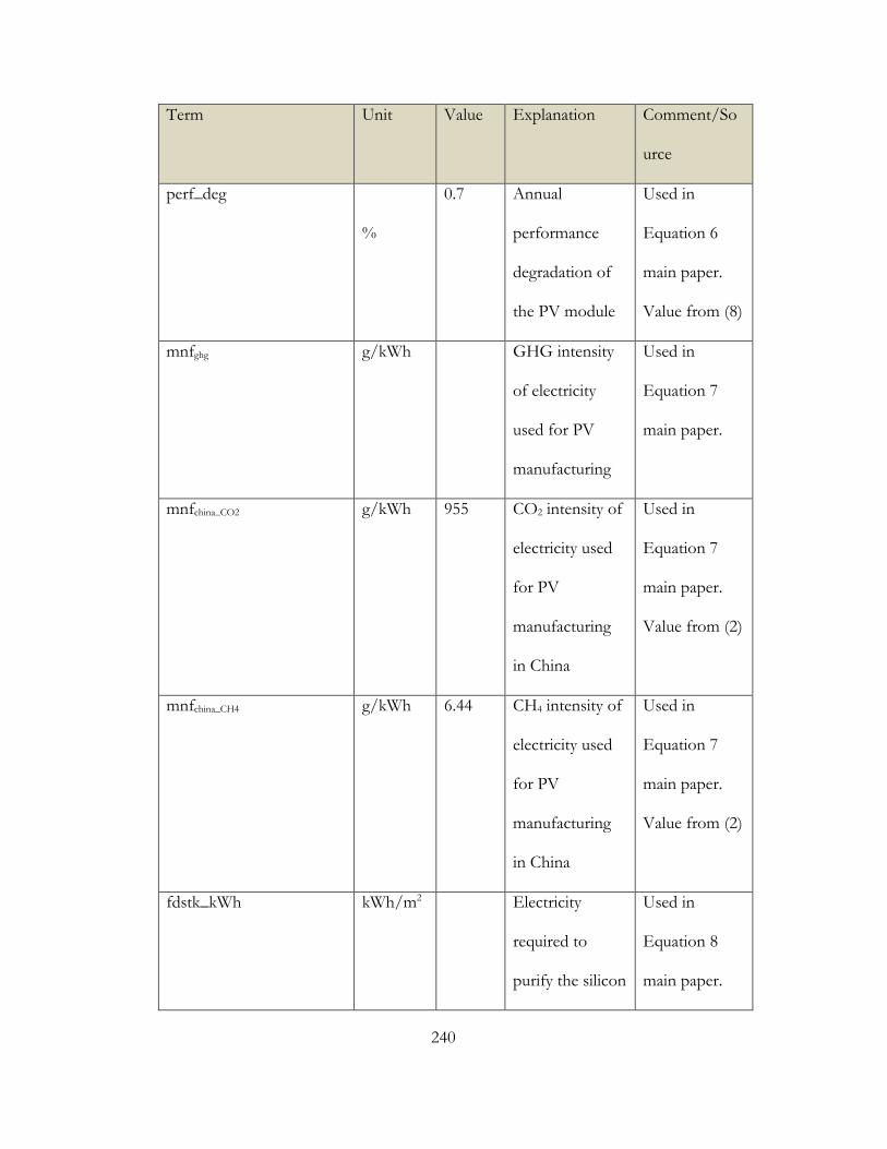
240


urce

perf_deg

%

0.7 Annual

performance

degradation of

the PV module

Used in

Equation 6

main paper.

Value from (8)

mnfghg g/kWh GHG intensity

of electricity

used for PV

manufacturing

Used in

Equation 7

main paper.

mnfchina_CO2 g/kWh 955 CO2 intensity of

electricity used

for PV

manufacturing

in China

Used in

Equation 7

main paper.

Value from (2)

mnfchina_CH4 g/kWh 6.44 CH4 intensity of

electricity used

for PV

manufacturing

in China

Used in

Equation 7

main paper.

Value from (2)

fdstk_kWh kWh/m2 Electricity

required to

purify the silicon

Used in

Equation 8

main paper.

241


urce

feedstock per m2

of the module.

non_fdstk_kWh kWh/m2 Electricity

required for

non-feedstock

processes per m2

of the module

Used in

Equation 8

main paper.

fdstk_kWh_multiSi kWh/m2 92.1 Electricity

required to

purify silicon

feedstock for 1

m2 of the multi-

silicon PV

module

Used in

Equation 9

main paper.

Value from (8)

fdstk_kWh_monoSi kWh/m2 175.37 Electricity

required to

purify silicon

feedstock for 1

m2 of the mono-

silicon PV

module

Used in

Equation 9

main paper.

Value from (8)

242


urce

non_fdstk_kWh_multiSi kWh/m2 115.78 Electricity

required for

non-feedstock

processes per m2

of the multi-Si

module

Used in

Equation 8

main paper.

Value from (8)

non_fdstk_kWh_monoSi kWh/m2 211 Electricity

required for

non-feedstock

processes per m2

of the mono-Si

module

Used in

Equation 8

main paper.

Value from (8)

Ingot_wafer_kWh_multiSi kWh/m2 55.87 Electricity

required for

ingot and wafer

processing (non-

feedstock

process) per m2

of the multi-Si

module

Used in Figure

3 main paper.

Value from (8)

243


urce

lamination_kWh_multiSi kWh/m2 39.47 Electricity

required for

lamination (non-

feedstock

process) per m2

of the multi-Si

module

Used in Figure

3 main paper.

Value from (8)

cell_kWh_multiSi kWh/m2 20.4 Electricity

required for cell

processing (non-

feedstock

process) per m2

of the multi-Si

module

Used in Figure

3 main paper.

Value from (8)

244

S3 CO2 intensity of PV electricity

The electricity produced by 1 m2 of a PV system over a 25-year lifetime is given by

252 t

1

pv_elec = kWp_m ×irrd×perf_rat×(1-perf_deg)t

S2

where kWp_m2 is the peak wattage in (kW) per m2 of the PV module, irrd is the annual solar

irradiation (kWh m-2 yr-1) at the deployment location, perf_rat (performance ratio) is the ratio

of the AC to DC power generated by the PV system and perf_deg is the annual performance

degradation of the PV module (%).

The values for kWp_m2, perf_rat and perf_deg are given in Table 29. Based on the

daily average solar irradiation value of 4.03 kWh/m2 (9), we assume an annual average value

of 1500 kWh/m2 for irrd in China.

The manufacturing GHG emissions for 1m2 of a PV module is given by

china_CO22 fdstk_kWh_multiSi + non_fdstk_kWh_multiSi) mnpv_mnf_CO ( f= S3

The values for the terms in equation S3 are given in Table 29.

For a PV system manufactured and installed in china, the CO2 intensity of PV

electricity is a ratio of PV_mnf_CO2 and PV_elec (equations S3 and S2) and is equal to 51

g/kWh.

245

S4 CRF hotspot analysis: parameters and baseline values

Table 30 Baseline value of parameters used in the scenario analysis in the main paper

Term Unit Value Explanation Comment/Refere

nce

mnfchina_CO2 g/kWh 955 CO2 intensity of

electricity used for PV

manufacturing in

China

Value from (2)

mnfchina_CH4 g/kWh 6.44 CH4 intensity of

electricity used for PV

manufacturing in

China

Value from (2)

Ingot_wafer_k

Wh_multiSi

kWh/m2 55.87 Electricity required for

ingot and wafer

processing (non-

feedstock process) per

m2 of the multi-Si

module

Value from (8)

lamination_kWh

_multiSi


lamination (non-


m2 of the multi-Si

module

Value from (8)

246

cell_kWh_multi

Si


cell processing (non-


m2 of the multi-Si

module

Value from (8)

fdstk_kWh_mult

iSi

kWh/kg 147.37 Electricity required to

purify 1 kg of solar-

grade silicon feedstock

for the multi-silicon

PV module

Ratio of feedstock

energy intensity

value of 92.1

kWh/m2 and

feedstock material

intensity value of

0.625 kg/m2.

Values from (8)

fdstk_kWh_mult

iSi

Kg/m2 0.625 Solar-grade silicon

feedstock material

intensity for 1m2 of

the multi-silicon PV

module

Value from (8)

247

S5 Equivalence between a decrease in solar-grade silicon energy/feedstock intensity and an increase in module efficiency

Figure 37 CRF payback time (PBT) equivalence between module efficiency improvements and reduction in solar-grade energy intensity for poly-silicon modules manufactured in China and installed in California.

In Figure 37, the dotted horizontal line and the y-axis intersect the CRF PBT

equivalence lines at multiples module efficiency and feedstock energy intensity values. As

explained in the main paper, the CRF PBT can be reduced from 4 to 3.7 years by decreasing

the feedstock energy intensity from 147 to 127 kWh kg-1 or increasing the module efficiency

from 16 to 16.89%. This corresponds to an equivalence ratio of 22.47 kWh kg-1 per unit

percentage increase in module efficiency (20 kWh kg-1/0.89%). Similar equivalence ratios

between the feedstock energy intensity and the module efficiency values are calculated by

moving horizontally and vertically between pairs of CRF PBT lines. The mean of all the

calculated equivalence ratios is 16.93 kWh kg-1 per unit increase in module efficiency

percentage. Similar equivalence values for mono-Si and multi-Si modules manufactured in

China and deployed in Wyoming and California are tabulated in Table 4 and Table 5.

248

Table 31 Equivalence between solar-grade silicon energy intensity (kWh/kg) and unit increase in module efficiency (%) for mono and poly-Si modules manufactured in China and installed in California and Wyoming

Scenario Equivalence between energy

intensity (kWh/kg) and unit

increase in module efficiency

(%)

Reference Figure

multi-Si manufactured in

China, Installed in California

16.93 Figure 37

multi-Si manufactured in

China, Installed in Wyoming

16.02 Figure 3

mono-Si manufactured in

China, Installed in California

17.19 Figure 5

mono-Si manufactured in

China, Installed in Wyoming

15.59 Figure 7

Table 32 Equivalence between solar-grade silicon feedstock intensity (kg/m2) and a unit increase in module efficiency (%) for mono and poly-Si modules manufactured in China and installed in California and Wyoming

Scenario Equivalence between feedstock intensity (kg m-2) and unit increase in module efficiency (%)

Reference figure

multi-Si manufactured in China, Installed in California

0.065 Figure 2

multi-Si manufactured in China, Installed in Wyoming

0.069 Figure 4

mono-Si manufactured in China, Installed in California

0.128 Figure 6

mono-Si manufactured in China, Installed in Wyoming

0.119 Figure 8

249

Figure 38 CRF payback time (PBT) equivalence between an increase in module efficiency and reduction in solar-grade feedstock intensity for poly-silicon modules manufactured in China and installed in California.

Figure 39 CRF payback time (PBT) equivalence between an increase in module efficiency and reduction in solar-grade energy intensity for poly-silicon modules manufactured in China and installed in Wyoming.

250

Figure 40 CRF payback time (PBT) equivalence between an increase in module efficiency and reduction in solar-grade feedstock intensity for poly-silicon modules manufactured in China and installed in Wyoming.

Figure 41 CRF payback time (PBT) equivalence between an increase in module efficiency and reduction in solar-grade energy intensity for mono-silicon modules manufactured in China and installed in California.

251

Figure 42 CRF payback time (PBT) equivalence between an increase in module efficiency and reduction in solar-grade feedstock intensity for mono-silicon modules manufactured in China and installed in California.

Figure 43 CRF payback time (PBT) equivalence between an increase in module efficiency and reduction in solar-grade energy intensity for mono-silicon modules manufactured in China and installed in Wyoming.

252

Figure 44 CRF payback time (PBT) equivalence between an increase in module efficiency and reduction in solar-grade feedstock intensity for mono-silicon modules manufactured in China and installed in Wyoming.

253

S6 Equivalent increase in module efficiency by addressing CRF hotspots in manufacturing processes

Figure 45 The equivalence in the CRF benefits between addressing PV

manufacturing hotspots (Figure 14) and an increase in module efficiency for mono-Si

(upper plot) and multi-Si (lower plot) modules manufactured in China and deployed

in Wyoming. The manufacturing improvement that addresses the hotspot is

accounted for by lowering the manufacturing GHG intensity (y-axis). The equivalent

increase in module efficiency is determined by projecting the difference between the

CRF benefit equivalence lines of the improved manufacturing and baseline scenario

on to the x-axis.

254

S7 Growth in commercial multi-silicon module efficiency

The commercial module efficiency in 2004 was 13.2% (10) and has increased to 16.7% in

2016 (4)(5). This corresponds to an annual increment of 0.25% per year from 2004 to 2016.

S8 Kerf loss and silicon feedstock requirement

The solar-grade silicon feedstock in 1m2 of a multi-silicon PV wafer is 0.625 kg (8). The

typical thickness of the silicon wafer is 180 µm and the volume is 180x10-6 m3 (8). Based on

the density of silicon (2330 kg/m3), the mass of solar-grade silicon contained in 180 x10-6 m3

of the multi-silicon wafer is 0.41 kg and, therefore, the kerf-loss is 0.2 kg/m2 (0.625-0.41) or

33%.

If the kerf loss is decreased by 50% (“mwss_wire_abrasive_reduced_diameter” scenario

in the main paper) or by 25% (“diamond_coated_wire_saw” scenario in the main paper), the

new feedstock requirement will be 0.52 kg or 0.57 kg per m2 respectively.

255

S9 Difference between GHG and CRF metrics

Figure 46 Difference in the climate benefit of improved PV manufacturing as measured by the net GHG and net CRF benefits for multi-Si modules manufactured in China and deployed in Wyoming. The green and orange lines represent combinations of PV manufacturing GHG intensity and module efficiency that result in the same net GHG and net CRF benefit over the 25-year lifespan of a module, respectively. A reduction in the GHG intensity of PV manufacturing from 314 to 17 kg CO2e/m2 increases the net GHG benefit by only 6% (4700 to 5000 kg CO2e) when compared to 11% increase in the net CRF benefit (7.2x10-11 to 8.0x10-11 Wm-2yr)

Figure 47 Difference in the climate benefit of improved PV manufacturing as measured by the net GHG and net CRF benefits for mono-Si modules manufactured in China and deployed in California. The green and orange lines represent combinations of PV manufacturing GHG intensity and module efficiency that result in the same net GHG and net CRF benefit over the 25-year lifespan of a module, respectively. A reduction in the GHG intensity of PV manufacturing from 563 (current state of manufacturing) to 30 kg CO2e/m2 (using PV electricity for PV

256

manufacturing) increases the net GHG benefit by only 18% (2800 to 3300 kg CO2e) when compared to 39% increase in the net CRF benefit (3.8x10-11 to 5.3x10-11 Wm-2yr)

Figure 48 Difference in the climate benefit of improved PV manufacturing as measured by the net GHG and net CRF benefits for mono-Si modules manufactured in China and deployed in Wyoming. The green and orange lines represent combinations of PV manufacturing GHG intensity and module efficiency that result in the same net GHG and net CRF benefit over the 25-year lifespan of a module, respectively. A reduction in the GHG intensity of PV manufacturing from 563 (current state of manufacturing) to 30 kg CO2e/m2 (using PV electricity for PV manufacturing) increases the net GHG benefit by only 13% (4700 to 5300 kg CO2e) when compared to 21% increase in the net CRF benefit (7.0x10-11 to 8.5x10-11 Wm-2yr)

257

S10 CRF Hotspot analysis

Figure 49 CRF hotspots multi-silicon PV modules manufactured in China and deployed in Wyoming. The width of the bars indicate the percentage change in the CRF benefit of the baseline scenario when a parameter in the manufacturing process is incremented and decremented by 10%. The widest bars correspond to the PV manufacturing process parameters with the highest CRF impacts.

Figure 50 CRF hotspots mono-silicon PV modules manufactured in China and deployed in California. The width of the bars indicate the percentage change in the CRF benefit of the baseline scenario when a parameter in the manufacturing process is incremented and decremented by 10%. The widest bars correspond to the PV manufacturing process parameters with the highest CRF impacts.

258

Figure 51 CRF hotspots mono-silicon PV modules manufactured in China and deployed in Wyoming. The width of the bars indicate the percentage change in the CRF benefit of the baseline scenario when a parameter in the manufacturing process is incremented and decremented by 10%. The widest bars correspond to the PV manufacturing process parameters with the highest CRF impacts.

259

References

1. Ravikumar D, Seager TP, Chester M V, Fraser MP. Intertemporal Cumulative Radiative Forcing Effects of Photovoltaic Deployments. Environ Sci Technol. 2014;48(17):10010–8.

2. SimaPro version 8.03. Grid GHG intensity as reported by SimaPro. 2014; 3. Yingli Solar. Monocrystalline Solar Panels [Internet]. 2015 [cited 2016 Jan 1].

Available from: http://www.yinglisolar.com/us/products/monocrystalline/ 4. Trina Solar. DUOMAX Series Dual Glass Module [Internet]. 2016 [cited 2016 Jan 1].

Available from: http://www.trinasolar.com/us/product/PDG5.html 5. Yingli Solar. Multicrystalline Solar Panels [Internet]. 2016 [cited 2016 Jan 1]. Available

from: http://www.yinglisolar.com/us/products/multicrystalline/ 6. NREL. National Solar Radiation Data Base - Class I locations [Internet]. [cited 2016

Jan 1]. Available from: http://rredc.nrel.gov/solar/old_data/nsrdb/1991-2010/hourly/list_by_state.html#C

7. Alsema E, Fraile D, Frischknecht R, Fthenakis V, Held M, Kim HC, et al.

Methodology guidelines on life cycle assessment of photovoltaic electricity. IEA PVPS Rep [Internet]. 2011 [cited 2014 Dec 25]; Available from: http://www.seas.columbia.edu/clca/IEA_Task12_LCA_Guidelines_12_1_11_Latest.pdf

8. De Wild-Scholten MJ. Energy payback time and carbon footprint of commercial

photovoltaic systems. Sol Energy Mater Sol Cells [Internet]. Elsevier; 2013;119:296–305. Available from: http://dx.doi.org/10.1016/j.solmat.2013.08.037

9. Department of Energy. Solar: monthly and annual average direct normal (DNI) GIS

data at 40km resolution for China from NREL [Internet]. 2015. Available from: http://catalog.data.gov/dataset/solar-monthly-and-annual-average-direct-normal-dni-gis-data-at-40km-resolution-for-china-f-e67c1

10. Alsema E, Mar. Environmental impacts of crystalline silicon photovoltaic module

production. MRS Proc. 2005;895:0895–G03.

260

APPENDIX D

D. SUPPORTING INFORMATION FOR CHAPTER 4

261

1. Values for energy inputs and material and energy recovered

Table 33 Values for energy inputs and material and energy recovered

Step1 - System disassembly

Label Description Value Source

Esys Primary energy for

disassembling PV system

(step 1)

8.52 MJ/m2 Refer section 2 in

SI

Msys Material transported from

deployment site to step 1

location

33.98 kg/ m2 Sum of electrical

systems and BOS

(RM1 to RM10)

and the module

which weighs

16.66 kg/ m2

Dsys Distance between

deployment site and step 1

location

50 km Assumption

rrsys Material recovery rate from BOS, inverter and transformer

0.9 [1]

Mrecy_sys_trn_st Steel content in

transformer

0.82 kg/m2 [2]

Mrecy_sys_inv_st Steel content in inverter 0.37 kg/m2 [2]

Mrecy_sys_inv_al Aluminum content in

inverter

0.11 kg/m2 [2]

Mrecy_sys_bos_st Steel content in BOS 10.83 kg/m2 [3]

Mrecy_sys_ bos_al Aluminum content in BOS 0.17 kg/m2 [3]

Mrecy_sys_bos_cu Copper content in BOS 0.88 kg/m2 [3]

Mrecy_sys_bos_pvc PVC content in BOS 0.04 kg/m2 [3]

Mrecy_sys_bos_hdpe HDPE content in BOS 0.28 kg/m2 [3]

Mrecy_sys_bos_epdm EPDM content in BOS 0.06 kg/m2 [3]

Mrecy_sys_bos_conc Concrete content in BOS 3.74 kg/m2 [3]

Mlnd_fl_sys Land filled material 1.73 kg/m2 Refer section 2 in

SI

Eemis_cont_sys Primary energy used for

controlling emissions

0/m2 Assumed that

there is no

emission in step 1

while dismantling

the PV system.

Erecov_sys Energy recovered from

waste incineration

0 MJ/m2 Assumed that

there is no energy

recovered from

the PV system

disassembly step

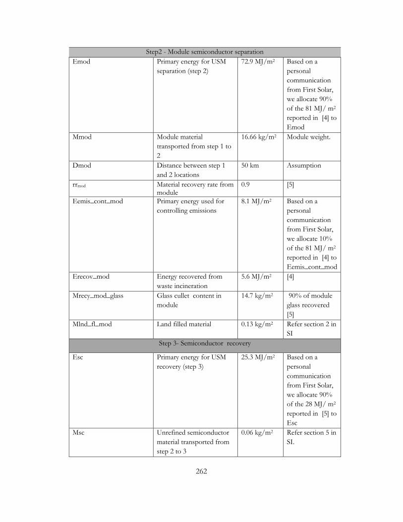
262

Step2 - Module semiconductor separation

Emod Primary energy for USM

separation (step 2)

72.9 MJ/m2 Based on a

personal

communication

from First Solar,

we allocate 90%

of the 81 MJ/ m2

reported in [4] to

Emod

Mmod Module material

transported from step 1 to

2

16.66 kg/m2 Module weight.

Dmod Distance between step 1

and 2 locations

50 km Assumption

rrmod Material recovery rate from module

0.9 [5]

Eemis_cont_mod Primary energy used for



personal

communication

from First Solar,

we allocate 10%

of the 81 MJ/ m2

reported in [4] to

Eemis_cont_mod

Erecov_mod Energy recovered from

waste incineration

5.6 MJ/m2 [4]

Mrecy_mod_glass Glass cullet content in

module

14.7 kg/m2 90% of module

glass recovered

[5]

Mlnd_fl_mod Land filled material 0.13 kg/m2 Refer section 2 in

SI

Step 3- Semiconductor recovery

Esc Primary energy for USM

recovery (step 3)


personal

communication

from First Solar,

we allocate 90%

of the 28 MJ/ m2

reported in [5] to

Esc

Msc Unrefined semiconductor

material transported from

step 2 to 3

0.06 kg/m2 Refer section 5 in

SI.

263

Dsc Distance between step 2

and 3 locations

50 km Assumption

Eemis_cont_sc Primary energy used for



personal

communication

from First Solar,

we allocate 10%

of the 28 MJ/ m2

reported in [5] to

Eemis_cont_sc

rrsc Material recovery rate CdTe

0.95 [5]

Mrecy_sc_te Te content in

semiconductor material


CdTe recovered

[4]

Mrecy_sc_cd Cd content in

semiconductor material


CdTe recovered

[4]

Mlnd_fl_sc Land filled material 0.043 kg/m2 Refer section 5 in

SI

Common parameters across the three steps

Esec_prod_bnf_inv_st,

Esec_prod_bnf_trn_st,

Esec_prod_bnf_bos_st

Energy benefit of recycling

secondary steel recovered

from the inverter,

transformer and BOS

22.06 MJ/kg Refer section 2 in

SI

Esec_prod_bnf_inv_al Energy benefit of recycling

aluminum recovered from

the inverter

151 MJ/kg Refer section 2 in

SI

Esec_prod_bnf_bos_cu Energy benefit of recycling

copper recovered from

the BOS


SI

Esec_prod_bnf_glass Energy benefit of

producing glass cullet from

secondary sources


SI

Esec_prod_bnf_te Energy benefit of

producing tellurium from

secondary sources


SI

Esec_prod_bnf_cd Energy benefit of

producing cadmium from

secondary sources


SI

Esec_prod_bnf_bos_hdpe Energy benefit of recycling

high-density polyethylene

(HDPE) recovered from

the BOS

55.7MJ/kg Refer section 2 in

SI

264

Esec_prod_bnf_bos_pvc Energy benefit of recycling

PVC recovered from the

BOS


SI

Esec_prod_bnf_bos_epdm Energy recovered from

synthetic rubber (EPDM)

content of BOS


SI

Esec_prod_bnf_bos_conc Energy benefit of recycling

concrete recovered from

the BOS

-0.22 MJ/kg Refer section 2 in

SI

Etrk Energy intensity of

transportation by truck

0.003 MJ per

kg km

Refer section 2 in

SI

Elnd_fl_op Energy required for landfill

operations


SI

Elnd_fl_inc Electricity recovered from

landfill incineration


SI

Dlnd_fl Distance to landfill 160 km Assumption

based on the

landfill distance

used in an LCA

of PV BOS [2]

265

2. Methodology and data sources for calculating the energy benefits of material

recycling

Figure 52 Conceptual representation of the calculation of energy benefits of material recycling (Esec_prod_bnf) which is the difference between energy intensity of manufacturing the material from virgin and secondary sources.

The estimated difference between the primary and secondary manufacturing pathways

for steel is 22.06 MJ/kg which is the mean of:

53 MJ/kg (difference between scenario ‘b’ and ‘c’ in [6])

7.6 MJ/kg (mean of the values – 3.2, 9.7, 10 - in Table 6 [7])

14.7 MJ/kg (difference between 18.99 million and 5.01 MBtu/ton mentioned in page

3-53 in [8])

13 MJ/kg (slide 7 in [9]).

For copper we calculate the difference between the energy footprints of the primary and

secondary pathways from the second figure in page 12 in [10]. The energy requirement for

the primary pathways range between 33 MJ/kg (3% Cu ore) to 57.3 MJ/kg (3% Cu ore) and

the secondary pathway has a value of 6.3 MJ/kg. Thus, the net energy benefits of recycling

copper ranges between 26.7 and 51 MJ/kg and we use a mean value of 38.85 MJ/kg.

266

Corresponding values for aluminum are 148 [11], 144 [12], 162 MJ/kg [13], and we

use a mean of 151 MJ/kg.

1 kg of glass cullet, when used in glass production, displaces 1.2 kg of virgin raw

material which would have required 2.7 MJ/kg [14] of production energy. Also, each kg of

glass cullet reduces the manufacturing energy of glass by 1.6 MJ (mean of 1.3 to 1.9 MJ/kg

glass cullet reported in [15]) as process temperatures in the production furnace are lowered.

Thus, by displacing virgin raw materials and reducing glass manufacturing energy

requirements, every kg of glass cullet recovered from a PV module results in a total energetic

benefit of 4.3 MJ.

The recycling energy benefits for tellurium and cadmium are calculated by assuming

they displace the energy required for virgin production. The energy for producing virgin

tellurium is 10.9 kWh/kg [16] and this accounts for tellurium purification from anode slimes

that is collected during copper extraction. The equivalent primary energy value is 127 MJ/kg

(using an electricity grid factor of 0.31). The corresponding value for cadmium is 60 MJ/kg

[16].

The energy required to manufacture virgin HDPE is 35.8 million Btu per 1000

pounds (last section in Table 3-2 in [17]).The corresponding values for recycled HDPE

range between 3.72 and 19.9 million Btu per 1000 pounds and we assume a mean of 11.81

Btu per 1000 pounds. Thus, the mean of the difference between virgin and recycled energy

requirements is 55.7 MJ/kg (after converting from Btu per 1000 pounds to MJ/kg).

267

For PVC, the energy difference between virgin and recycled manufacturing routes is

33.6 MJ/kg based on the difference between the “All Energy Resources” value for the

“PVC conventional route” and “Vinyloop” columns in annex 7 in [18].

As there was no LCA study or data available for the energy benefits of recycling

synthetic rubber (EPDM) we assume that energy is recovered through the combustion of

the EPDM present in the BOS. We approximate this by considering a similar process of

combustion of spent rubber tires. The energy recovered from the combustion of spent

rubber tires is 31.8 MJ/kg which is the mean of

32.6 MJ/kg reported for “Rubber, 5 cm w/o metal ” in Table in [19]

31.4 “Scrap tires” in Table 1 in [20]

31.5 MJ/kg (mean of the range of 28 to 35 MJ/kg in page 16-7 [21])

We assume the concrete in the BOS will be recycled as aggregate and literature shows

that recycled aggregate is energetically more expensive than conventional aggregate [22][23].

1 m3 of natural aggregate concrete (NAC) and recycled aggregate concrete (RAC) weigh

2194 kgs (315 kg cement + 1879 kg of natural aggregate) and 2046 kgs (330 kg cement +

1716 kg of natural aggregate), respectively ( Table 5 in [23]). The corresponding energy

requirements are 1570.42 and 1922.62 MJ/ m3 ( Table 10 in [23]) therefore the energy

intensity is 0.71 and 0.93 MJ/kg.

The energy intensity of truck freight ranges from 2.5 (USA specific values in Figure 7

in [24]) to 3.5 MJ per ton-km (North America specific values in Figure 6.4 in [25]) and we

assume a mean of 3 MJ per ton-km.

268

For energy spent on landfill operations (LFO) we assume a value of 0.32 MJ/kg

(“Energy production and use” bar for the “RDF production and combustion” scenario in

figure 5 in [26]).

7.14 MJ of electricity is recovered per kg of landfill incineration (LFI) and this is a mean of

5.38 MJ/kg (“Energy production and use” bar for the “RDF production and

combustion” scenario in figure 5 in [26]).

8.9 MJ/kg, the primary energy equivalent of 0.767 kWh/kg ( gross electricity output

for scenario 2 in Table 1 in [27]). We use a grid factor of 0.31.

3. Energy required for disassembling a PV system

As there is no data available on the energy required to disassemble a PV system, we

assume that the PV system disassembly energy is equal to the energy required to install the

PV system. 0.2 kg of diesel is required to install 1 m2 of a CdTe PV system [28] and we

convert this to a primary energy value of 8.52 MJ/ m2 using the lower heating value (129488

Btu/gallon) and fuel density value (3.206 kg/gallon) of low sulphur diesel provided in [29].

269

4. Reduction in cumulative energy demand (CED) through recycling and PV

module efficiency improvements

Energy payback time (EPBT) is the ratio of the energy required to manufacture the

CdTe PV system and the annual energy produced by the CdTe PV system [30]. EPBT can

be reduced by either decreasing the manufacturing energy or increasing the annual energy

produced by the CdTe PV system through module efficiency improvements. Decreasing

CED by 289 MJ through recycling (Table 34) or increasing the efficiency of CdTe PV

module from 14 to 18.9% (Table 35) reduces the EPBT to 0.41 years.

Table 34 Reduction in EPBT through recycling

Energy input

Parameter description Parameter label

Calculation Parameter value

Source

CdTe PV system CED(MJ/ m2)

A 1190 [31]

% reduction in CED through recycling

B 24% 289 MJ of energy saved in scenario HR3 in Figure 3 in main paper

Net CdTe PV system CED (MJ/ m2)

C a*(1-b) 904

Efficiency module (%) D 14 [32]

Peak watts per m2 (Wp/ m2)

E d*10. Assuming 14% module efficiency is based on standard test conditions of 1000 w/m2

140

CdTe PV system CED (MJ/kWp)

F c/(e/1000) 6460

Energy output

Irradiation (kWh/ m2/yr) G 1800 Average southern European irradiation conditions [31]

270

AC to DC conversion or Performance ratio

H 0.8 Ground mount values in [30]

Generated electricity (kWh/kWp/yr)

I g*h 1440

Primary energy equivalent of electricity generated (MJ/kWh)

J 1 kWh = 3.6 MJ and we use a grid efficiency factor of 0.31

11.41

Avoided energy (MJ/kWp/yr)

K i*j 16425

Energy payback time (EPBT)

EPBT (yr) f/k 0.39

Table 35 Reduction in EPBT through module efficiency improvements

Energy input

Parameter description Parameter label

Calculation Parameter value

Source

CdTe PV system CED (MJ/ m2)

A 1190 [31]

Efficiency module (%) B 18.42

Peak watts per m2 (Wp/ m2 )

C b*10. Assuming 18.9% module efficiency is based on standard test conditions of 1000 w/m2

184.2

CdTe PV system CED (MJ/kWp)

D a/(c/1000) 6460

Energy output

Irradiation (kWh/ m2/yr)

G 1800 Average southern European irradiation conditions [31]

AC to DC conversion or performance ratio

H 0.8 Ground mount values in [30]

Generated electricity (kWh/kWp/yr)

I g*h 1440

Primary energy equivalent of electricity generated (MJ/kWh)

J 1 kWh = 3.6 MJ and we use a grid efficiency factor of 0.31

11.41

271

Avoided energy (MJ/kWp/yr)

K i*j 16425

Energy payback time (EPBT)

EPBT (yr) f/k 0.39

5. Residue content in a CdTe module after USM refining

The density of CdTe is 5860 kg/ m3 and a 1 m2 module with a 3μm thick CdTe layer

contains 0.018 kg of CdTe. 16.5 m2 of a module is processed to recover 1 kg of USM [5] so

processing 1 m2 of a module results in 0.06 kg of USM. Therefore, 1 m2 of a module will

have a residue content of 0.043 kg after 95% of the CdTe is recovered and refined

(0.06-(0.95*0.018)).

272

6. Split of the energy benefits of recycled materials for HR 3 scenario

Figure 53 Split of the energy benefits of recycled materials for HR 3 scenario. The total energy benefit of recycled materials, represented by the entire pie chart, corresponds to the green bar for HR 3 in Figure 3 in the main paper

273

7. Sensitivity of recycling energy benefits to allocation method

Figure 54 EOLR approach to allocate benefits of PV system recycling and calculating the CED.

The manufacturing energy (brown) is calculated assuming 100% virgin content and

this value is 1190 MJ/m2 (section 11 in SI). The recycling energy burden (blue) includes the

transportation, recycling processes, emission control and landfilling (equation 1 in main

paper). The recycling credit (green), 382 MJ/m2, is the sum of the values calculated in the

column on the right in Table 36. The CED using EOLR allocation is 920 MJ/m2 (from

Equation 8 in main paper).

274

Table 36 Calculations for recycling credit

Material 90% recovery of quantities reported in kg/m2 in Table 1 (assuming 90% recovery rate for BOS materials and module glass and 95% for CdTe)

Energy saved through recycling in MJ/kg from Table 1

Energy benefit of recycling material in MJ/m2 (product of values in the previous two columns)

Steel 10.82 (sum of steel from inverter, transformer and BOS)

22.06 238.7

Aluminum 0.25 151 37.9

Cu 0.79 38.85 30.8

Glass cullet

13.23 4.3 56.9

CdTe 0.017 127 for Te and 60 for Cd

1.4 (after splitting the mass of CdTe using the stoichiometric mass ratio of Cd and Te)

HDPE 0.26 55.7 14.4

PVC 0.04 33.6 1.3

EPDM 0.06 31.8 1.8

Concrete 3.37 -0.22 -0.7

275

Figure 55 Recycled content (RC) approach to allocate the benefits of PV recycling and calculating CED.

The manufacturing energy (brown) is calculated assuming 100% recycled content

and the recycling energy burden (blue) and credits are not considered as part of calculations

in the RC approach. We get 809 MJ/m2 after the energy benefits of 90% recycling (sum of

the last column in Table 36) is subtracted from 1190 MJ/m2 (section 11 in SI) which is the

manufacturing energy assuming 100% virgin contents.

Using the same approach we calculate CED using RC and EOLR for scenarios NR2,

MR2 and MR4.

276

8. Flowchart and results for uncertainty analysis

Figure 56 Flowchart for calculating and plotting the sensitivity of net energy impact of recycling (Enet_imp) to values assumed for energy benefits of recycling materials (Esec_prod_bnf). The literature values for lower and upper bounds of Esec_prod_bnf is reported in section 2 in SI. This flowchart is run for the four bulk materials (steel, aluminum, copper, and glass) and results are compared with the base scenario HR3 in Figure 6 in SI.

277

Figure 57 Uncertainty in net recycling energy benefit calculations (Enet_imp in equation 7 in main paper) to Esec_prod_bnf values for the four dominant materials (by mass) in a CdTe PV system. The simulations were run 10,000 times and the box and whisker plots depict the minimum, median and maximum values for the calculated net energy benefit.

Figure 57 demonstrates that net energy benefit calculation is most sensitive to Esec_prod_bnf

values for steel as the maximum value and the median of steel vary the most when compared

to the base scenario. The distribution of net energy benefits shows the maximum variation

between -899 and -122 MJ/m2 when the Esec_prod_bnf values of steel are varied between the

modified upper and lower bounds. Corresponding values for the base HR 3 scenario and

other materials show a smaller variation between -760 and -137 MJ/m2.

278

9. Optimal recycling plant location for system disassembly (step 1) and

semiconductor refining (step 3)

Figure 58 Frontier diagram depicting two regions where centralized and decentralized facilities are favorable for system disassembly (step 1 in figure 1 in main paper). Decentralized recycling is favorable in the blue region where the combination of the distance to the centralized facility and the energy required at the decentralized facility result in a negative energy penalty (Epenalty < 0 from equation 9 in main paper). Similarly, centralized recycling is favored in the orange region when energy penalty of decentralization is positive.

279

Figure 59 Frontier diagram depicting two regions where centralized and decentralized facilities are favorable for semiconductor recovery (step 3 in figure 1 in main paper). Decentralized recycling is favorable in the blue region where the combination of the distance to the centralized facility and the energy required at the decentralized facility result in a negative energy penalty (Epenalty < 0 from equation 9 in main paper). Similarly, centralized recycling is favored in the orange region when energy penalty of decentralization is positive.

280

10. Mass of unrefined solar grade silicon per m2 of a crystalline silicon module

Table 4 in [33] reports a purified silicon use of 9.8 g/Wp and a panel area of 20.8

m2/3kWp in 2007. Based on these values, the mass of unrefined solar grade silicon is 1.4

kg/m2. This is a conservative estimate as it accounts for only the purified content and not

impurities that will be part of the recovered solar grade silicon (from step 2) and transported

to the location of step 3.

11. Manufacturing energy for 1 m2 of a CdTe PV system

The total lifecycle energy of 1270 MJ/m2 is reported for a CdTe PV system in Table III

in [31] and this includes the 81 MJ/m2 of energy for EOL processing. After excluding the

EOL energy component which is accounted for in the energy flow model (Figure 1 in main

paper), the manufacturing energy for 1 m2 of a CdTe PV system is 1190 MJ/m2.

281

References

[1] R. S. Jorge, T. R. Hawkins, and E. G. Hertwich, “Life cycle assessment of electricity transmission and distribution—part 2: transformers and substation equipment,” Int. J. Life Cycle Assess., vol. 17, no. 2, pp. 184–191, Sep. 2011.

[2] J. E. Mason, V. M. Fthenakis, T. Hansen, and H. C. Kim, “Energy payback and life-

cycle CO2 emissions of the BOS in an optimized 3·5 MW PV installation,” Prog. Photovoltaics Res. Appl., vol. 14, no. 2, pp. 179–190, Mar. 2006.

[3] P. Sinha and M. de Wild-Scholten, “Life Cycle Assessment of Utility-Scale CdTe PV Balance of Systems,” in 27th European Photovoltaic Solar Energy Conference, 2012, pp. 4657 – 4660.

[4] M. Held, “Life cycle assessment of CdTe module recycling,” in 24th EU PVSEC Conference, 2009, pp. 2370 – 2375.

[5] P. Sinha, M. Cossette, and J.-F. Menard, “End-of-life CdTe recycling with semiconductor refining,” in 27th EU PVSEC, 2012, pp. 24–28.

[6] J. Johnson, B. K. Reck, T. Wang, and T. E. Graedel, “The energy benefit of stainless steel recycling,” Energy Policy, vol. 36, no. 1, pp. 181–192, Jan. 2008.

[7] World Steel Association, Life cycle inventory study for steel products.

[8] EPA, “Energy Trends in Selected Manufacturing Sectors: Opportunities and Challenges for Environmentally Preferable Energy Outcomes,” no. March, 2007.

[9] Clare Broadbent, “End-of-life recycling and disposal: essential to any LCA study,” in LCA XI, 2011.

[10] Bureau of International Recycling, “Report on the Environmental Benefits of Recycling,” 2008.

[11] PE Americas, “Life cycle impact assessment of aluminum beverage cans,” Prep. Alum. Assoc., 2010.

[12] Aluminum Association, “Aluminum: The element of sustainability,” 2011.

[13] Global Aluminium Recycling Committee, “Global aluminium recycling: a cornerstone of sustainable development,” 2006.

[14] R. F. Cook, “The collection and recycling of waste glass (cullet) in glass container manufacture,” Conserv. Recycl., vol. 2, no. March, pp. 59–69, 1978.

282

[15] A. W. Larsen, H. Merrild, and T. H. Christensen, “Recycling of glass: accounting of greenhouse gases and global warming contributions.,” Waste Manag. Res., vol. 27, no. 8, pp. 754–62, Nov. 2009.

[16] M. Classen et al, “Life Cycle Inventories of Metals. Final report ecoinvent data v2.1, No 10.,” Eco Inven., 2009.

[17] Franklin Associates, A divsion of ERG, “Lifecycle inventory of 100% postconsumer HDPE and PET recycled resin from post consumer containers and packaging,” 2010.

[18] Solvay Group and VinylLoop Ferrara SpA, “The VinyLoop Eco-Footprint - Benchmarking the environmental impact of PVC compound recycled in the VinylLoop process with PVC compound produced in the coventional route,” no. February, 2012.

[19] T. Amari, N. J. Themelis, and I. K. Wernick, “Resource recovery from used rubber tires,” Resour. Policy, vol. 25, no. 3, pp. 179–188, Sep. 1999.

[20] E. Laboy-Nieves, “Energy Recovery from Scrap Tires: A Sustainable Option for Small Islands like Puerto Rico,” Sustainability, vol. 6, no. 5, pp. 3105–3121, May 2014.

[21] US DoT Federal Highway Administration, “User Guidelines for Waste and Byproduct Materials in Pavement Construction,” Publication Number: FHWA-RD-97-148, 2012. [Online]. Available: http://www.fhwa.dot.gov/publications/research/infrastructure/structures/97148/st1.cfm.

[22] M. Weil, “Closed-loop recycling of construction and demolition waste in Germany in view of stricter environmental threshold values,” Waste Manag. Res., vol. 24, no. 3, pp. 197–206, Jun. 2006.

[23] S. Marinković, V. Radonjanin, M. Malešev, and I. Ignjatović, “Comparative environmental assessment of natural and recycled aggregate concrete.,” Waste Manag., vol. 30, no. 11, pp. 2255–64, Nov. 2010.

[24] J. Eom, L. Schipper, and L. Thompson, “We keep on truckin’: Trends in freight energy use and carbon emissions in 11 IEA countries,” Energy Policy, vol. 45, pp. 327–341, Jun. 2012.

[25] International Energy Agency, “Transport Energy and CO2: Moving Towards Sustainability,” OECD Publishing, 2009.

[26] U. Arena, M. . Mastellone, and F. Perugini, “The environmental performance of alternative solid waste management options: a life cycle assessment study,” Chem. Eng. J., vol. 96, no. 1–3, pp. 207–222, Dec. 2003.

283

[27] F. Cherubini, S. Bargigli, and S. Ulgiati, “Life cycle assessment (LCA) of waste management strategies: Landfilling, sorting plant and incineration,” Energy, vol. 34, no. 12, pp. 2116–2123, Dec. 2009.

[28] First Solar, “Personal Communication,” 2014.

[29] Argonne National Laboratory, “The Greenhouse Gases, Regulated Emissions, and Energy Use in Transportation (GREET) Model: Version 2.,” 2014.

[30] E. Alsema, D. Fraile, R. Frischknecht, V. Fthenakis, M. Held, H. . Kim, W. Pölz, M. Raugei, and M. de Wild Scholten, “Methodology guidelines on life cycle assessment of photovoltaic electricity,” IEA PVPS Rep., 2011.

[31] M. Held and R. Ilg, “Update of environmental indicators and energy payback time of CdTe PV systems in Europe,” Prog. Photovoltaics Res. Appl., vol. 19, no. January, pp. 614–626, 2011.

[32] First Solar, “Key Quarterly Financial Data, Feb 2015,” 2015.

[33] N. Jungbluth, M. Tuchschmid, and M. de Wild-Scholten, “Life Cycle Assessment of Photovoltaics: Update of ecoinvent data v2. 0,” ESU-services Ltd., 2008, pp. 1–22, 2008.

284

APPENDIX E

E. SUPPORTING INFORMATION FOR CHAPTER 5

285

1. Cadmium ion-exchange material usage efficiency

The theoretical dry capacity for Amberlyst 15 is 4.7 meq/g [1][2] which corresponds to

263 mg of cadmium per mg of Amberlyst 15. Therefore, to extract 7.74 gram of cadmium

contained in 1 m2 of a CdTe module (see section 2 SI), 0.029 gram of the resin is required.

Wang and Fthenakis experimentally investigated the feasibility of removing cadmium

dissolved in acidic solution (0.5M H2SO4 similar to acidic leachate during recycling

operations) using Amberlyst 15 and DOWEX 50X8 ([2]–[4]). The ion-exchange resin

requirements is determined from [3] as it simulates the separation of cadmium from a

leachate operational conditions encountered in actual CdTe module recycling. An extraction

of 33 mg of cadmium per gram of Amberlyst-15 was reported [3] and, therefore, 234g of

Amberlyst 15 is required to extract 7.74g of cadmium in 1 m2 of the module (section 2 SI).

As there is no study reporting the energy requirement for ion exchange extraction of

cadmium, we estimate a value based on ion exchange systems used in water treatment plants.

The energy requirement ranges between 1.2 and 5.5 x 10-5 kWh per liter of water treated

[5][6] and a mid-point value of 3.35 x 10-5 kWh per liter is assumed. Fthenakis and Wang’s

study on CdTe PV recycling successfully recovered cadmium from a leachate with a

cadmium concentration of 942 ppm (0.942 g/l) [3]. Therefore, to recover 7.7g of cadmium

from 1 m2 of a CdTe module, 8.2 liters of leachate needs to be treated with an ion exchange

resin and this requires 27.5 x 10-5 kWh.

After the ion exchange treatment of the leachate, the cadmium in the saturated resin is

eluted into a solution by washing with 1 to 5 bed volumes of 5M sulfuric acid [2] and we

assume mid-point value of 2.5 bed volumes. This corresponds to 20.5 liters of 5M sulfuric

286

acid or 10052 g of sulfuric acid per m2 of the PV module as a total bed volume of 8.2 liters

of leachate per m2 of the PV module is treated with ion exchange resins.

The eluted cadmium is precipitated using 33 grams of NaOH. This value of 33g is

obtained by splitting a total of 100 grams of NaOH used to precipitate both cadmium and

tellurium in equations 3 and in section 2 of the SI in the corresponding stoichiometric ratio

of 2:4. Similarly, the tellurium remaining in the leachate (after cadmium is separated through

ion exchange) is recovered by precipitating with 67g of NaOH.

2. Cadmium and tellurium in 1 m2 of a CdTe PV module and leaching and

precipitation reactions

Table 37 CdTe and CdS content in 1 m2 of a CdTe module

Compound Layer thickness (t) Density (d) Mass (1 m2 x t x d) Moles

CdTe 3 x 10-6 m 5.86 x 106 g/ m3 18 g 7.5 x 10-2

moles

CdS 6 x 10-8 m [7] 4.82 x 106 g/ m3 0.29 g 2 x 10-3

moles

Based on the atomic masses, the 18 grams of CdTe in 1 m2 of the module consists of

10.26 grams (0.08 moles) and 7.74 grams (0.069 moles) of tellurium and cadmium,

respectively.

The oxidative leaching of CdTe, as explained in the main paper, is represented by the

following reactions

2 2 2 4 4(aq) 2 4 2 (aq)CdTe + 3H O + 3H SO CdSO + 6H O + Te(SO ) 4

287

2 2 2 4 4(aq) 2 (s)CdS + H O + H SO CdSO + 2H O + S 5

The precipitation of Cd and Te from the leachate, as explained in the main paper, is given by

4(aq) 2(s) 2 4 (aq)CdSO + 2NaOH Cd(OH) + Na SO 6

4 2(aq) 2(s) 2 4 (aq) 2Te(SO ) + 4NaOH TeO + 2Na SO + 2H O 7

3. Material requirements for solvent extraction of cadmium

At a pilot scale, four contacting stages of leaching is required to extract 99.995%

cadmium from an acidic leachate which is chemically similar to the leachate processed in

commercial operations [8]. In each stage, 10% D2EHPA (by volume) in four liters of an

organic diluent (kerosene) is mixed with 1 liter of aqueous leachate containing 10 grams of

cadmium. Based on a 0.965 g/mL density value for D2EHPA [9], the 1600 mL of

D2EHPA required for the four stages corresponds to a mass of 1544 grams. Normalizing

this to the 7.74 g of cadmium contained in 1 m2 of the PV module (section 2 in SI), the

pilot scale D2EHPA requirement is 1195 grams/m2. This study assumes kerosene as the

organic diluent in which D2EHPA is dissolved as it was previously used in the solvent

extraction of cadmium [10][11][12]. In each of the four extraction stages for 10 grams of

cadmium, kerosene constitutes 90% by volume of the 4 liters of organic diluent and this

corresponds to a total volume of 14400 mL. Normalizing this to the 7.74 g of cadmium

contained in 1 m2 of the PV module (section 2), the pilot scale kerosene requirements (per

m2) is 11145 mL or 11.8 kg (using a density value of 0.82 kg/cm3 for kerosene).

A previous study reported the use of sulfuric acid (180 g/l) to strip cadmium from the

loaded organic phase consisting of kerosene and D2EHPA with a 1:1 volumetric ratio of

sulfuric acid and the organic phase [11]. Therefore, 16 liters of 180 g/l sulfuric acid is

288

required for 16 liters of the organic phase used for solvent extraction of cadmium from 1

m2 of a CdTe PV module (4 stages each with 4 liters of kerosene containing D2EHPA).

This corresponds to 2880 g of sulfuric acid.

The cadmium stripped through sulfuric acid is precipitated using NaOH. By splitting

the total of 100g of NaOH (Alternative 1 in Table 38 in SI) required to precipitate both

cadmium and tellurium in the stoichiometric ratio of 2:4 (equations 6 and in section 2 of

SI), the NaOH required to precipitate only cadmium is calculated as 33g. Similarly, the

tellurium, remaining in the leachate after cadmium is separated through solvent extraction,

is recovered by precipitating with 67g of NaOH.

As there is no study reporting the energy requirement for solvent extraction of

cadmium, we use a value of 0.5 kWh per liter of the aqueous phase (leachate containing the

cadmium) based on a previous study on the solvent extraction of rare earth elements [13].

With four liters of the aqueous phase, 2 kWh of electricity is required.

289

4. Material and energy requirements for the seven CdTe PV recycling

alternatives

Table 38 Material and energy requirements for the seven CdTe PV recycling alternatives and the corresponding SimaPro dataset used to determine the ReCiPe environmental impact categories.

Recycling Method Inventory item Requirement per m2

[source]

SimaPro dataset

Alternative 1

(Incumbent):

mech+leach+prcp

(incumbent)

electricity for

mechanical

stripping and

crushing of CdTe

PV module

2.2 kWh. We assume 50% of

the energy reported in Table 1

in [14] is required for the

mechanical stripping and

crushing. The remaining 50%

is required for the leaching

process. Based on First Solar’s

current recycling operations in

Malaysia, electricity is sourced

from captive natural gas plants.

Electricity, high voltage

{MY}| electricity

production, natural gas,

at conventional power

plant | Alloc Def, U

electricity for

leaching process




leaching process. The

remaining 50% is required for

the mechanical stripping and

crushing. Based on First

Solar’s current recycling

operations in Malaysia,

electricity is sourced from

captive natural gas plants.


{MY}| electricity




290


[source]

SimaPro dataset

sulfuric acid for the

leaching process

83 g [14] Sulfuric acid {RER}|

production | Alloc

Def, U

hydrogen peroxide

for the leaching

process

570 g [14] Hydrogen peroxide,

without water, in 50%

solution state {RER}|

hydrogen peroxide

production, product in

50% solution state |

Alloc Def, U

sodium hydroxide

for the

precipitation

process

100 g [14] Sodium hydroxide,



chlor-alkali electrolysis,

diaphragm cell | Alloc

Def, U

Alternative 2:

thermal+leach+ion

exch+prcp

Electricity for

furnace operation.

0.48 kWh. Refer section 6 in

SI. Based on First Solar’s





{MY}| electricity




electricity for

leaching process




leaching process. Based on

First Solar’s current recycling


{MY}| electricity




291


[source]

SimaPro dataset





leaching process


production | Alloc

Def, U

hydrogen peroxide

for the leaching

process




hydrogen peroxide



Alloc Def, U

Amberlyst 15

(cation resin) for

ion exchange

process

234 g. Refer section Error!

Reference source not found.

in SI.

Cationic resin {CH}|

production | Alloc

Def, U

Electricity for ion

exchange process

2.75x10-4 kWh. Refer section

Error! Reference source not

found. in SI.


{MY}| electricity




Sulfuric acid to

strip the cadmium



in SI.

Sulfuric acid {RER}|

production | Alloc

Def, U

292


[source]

SimaPro dataset

during the ion

exchange process

Sodium hydroxide

to precipitate the

cadmium during

the ion exchange

process



in SI.

Sodium hydroxide,





Def, U

Sodium hydroxide

to precipitate the

tellurium that

remains in the

leachate.



in SI.

Sodium hydroxide,





Def, U

Alternative 3:

thermal+leach+prcp

Electricity for

furnace operation.







{MY}| electricity




electricity for

leaching process








{MY}| electricity




293


[source]

SimaPro dataset




leaching process


production | Alloc

Def, U

hydrogen peroxide

for the leaching

process




hydrogen peroxide



Alloc Def, U

sodium hydroxide

for the

precipitation

process






Def, U

Alternative 4:

thermal+leach+solv

ext+prcp

Electricity for

furnace operation.







{MY}| electricity




electricity for

leaching process





{MY}| electricity


294


[source]

SimaPro dataset









leaching process


production | Alloc

Def, U

hydrogen peroxide

for the leaching

process




hydrogen peroxide



Alloc Def, U

D2EHPA for

solvent extraction

of cadmium

1195 g. Refer section 3 in SI. Organophosphorus-

compound, unspecified

{RER}| production |

Alloc Def, U

Kerosene for

solvent extraction

of cadmium

11800 g. Refer section 3 in SI. Kerosene {Europe

without Switzerland}|

petroleum refinery

operation | Alloc Def,

U

295


[source]

SimaPro dataset

Sulfuric acid for

solvent extraction

of cadmium

2880 g. Refer section 3 in SI. Sulfuric acid {RER}|

production | Alloc

Def, U

Sodium hydroxide

for solvent

extraction of

cadmium

33 g. Refer section 3 in SI. Sodium hydroxide,





Def, U

Electricity for

solvent extraction

of cadmium

2 kWh. Refer section 3 in SI.

Based on First Solar’s current

recycling operations in




{MY}| electricity




Sodium hydroxide

to precipitate the

tellurium that

remains in the

leachate.






Def, U

Alternative 5:

org solv+leach+ion

exch+prcp

o-dichlorobenzene

for dissolving the

EVA

8840 g. Refer section 7 in SI. O-dichlorobenzene

{RER}| benzene

chlorination | Alloc

Def, U

Electricity for

delaminating EVA

Uniform distribution ranging

between 6.5 to 37.4 kWh.


{MY}| electricity

296


[source]

SimaPro dataset

by heating in o-

DCB

Refer section 7 in SI. Based on








electricity for

leaching process










{MY}| electricity





leaching process


production | Alloc

Def, U

hydrogen peroxide

for the leaching

process




hydrogen peroxide



Alloc Def, U

Amberlyst 15

(cation resin) for



in SI.

Cationic resin {CH}|

production | Alloc

Def, U

297


[source]

SimaPro dataset

ion exchange

process

Electricity for ion

exchange process

2.75x10-4 kWh. Refer section

Error! Reference source not

found. in SI.


{MY}| electricity




Sulfuric acid to

strip the cadmium

during the ion

exchange process



in SI.

Sulfuric acid {RER}|

production | Alloc

Def, U

Sodium hydroxide

to precipitate the

cadmium during

the ion exchange

process



in SI.

Sodium hydroxide,





Def, U

Sodium hydroxide

to precipitate the

tellurium that

remains in the

leachate.



in SI.

Sodium hydroxide,





Def, U

298


[source]

SimaPro dataset

Alternative 6:

org

solv+leach+prcp

o-dichlorobenzene

for dissolving the

EVA


{RER}| benzene


Def, U

Electricity for

delaminating EVA

by heating in o-

DCB









{MY}| electricity




electricity for

leaching process










{MY}| electricity





leaching process


production | Alloc

Def, U

hydrogen peroxide

for the leaching

process




hydrogen peroxide

299


[source]

SimaPro dataset



Alloc Def, U

sodium hydroxide

for the

precipitation

process






Def, U

Alternative 7:

org solv+leach+solv

ext+prcp

o-dichlorobenzene

for dissolving the

EVA


{RER}| benzene


Def, U

Electricity for

delaminating EVA

by heating in o-

DCB









{MY}| electricity




electricity for

leaching process








{MY}| electricity




300


[source]

SimaPro dataset




leaching process


production | Alloc

Def, U

hydrogen peroxide

for the leaching

process




hydrogen peroxide



Alloc Def, U

D2EHPA for

solvent extraction

of cadmium

1195 g. Refer section 3 in SI. Organophosphorus-

compound, unspecified

{RER}| production |

Alloc Def, U

Kerosene for

solvent extraction

of cadmium

11800 g. Refer section 3 in SI. Kerosene {Europe

without Switzerland}|

petroleum refinery

operation | Alloc Def,

U

Sulfuric acid for

solvent extraction

of cadmium

2880 g. Refer section 3 in SI. Sulfuric acid {RER}|

production | Alloc

Def, U

Sodium hydroxide

for solvent



301


[source]

SimaPro dataset

extraction of

cadmium




Def, U

Electricity for

solvent extraction

of cadmium

2 kWh. Refer section 3 in SI.

Based on First Solar’s current

recycling operations in




{MY}| electricity




Sodium hydroxide

to precipitate the

tellurium that

remains in the

leachate.






Def, U

Transportation Road Refer Section 9 in SI for the

values.

Transport, freight,

lorry 16-32 metric ton,

EURO5 {RoW}|

transport, freight, lorry

16-32 metric ton,

EURO5 | Alloc Def,

U

Ship Refer Section 9 in SI for the

values.

Transport, freight, sea,

transoceanic ship

{GLO}| processing |

Alloc Def, U

302

5. Calculating aggregated environmental stochastic score

For illustrative purposes and simplicity, this section demonstrates the aggregation of

outranking scores into an aggregated probabilistic environmental score for 3 recycling

methods across 3 impact categories. The same principles can be extended to the 7 recycling

alternatives and the 18 ReCiPe impact categories discussed in the main paper. This method

was proposed by Prado et al [15] and is based on PROMETHEE II complete ranking [16].

Table 39 Log normal distributions with standard deviations and means for environmental impacts of 3 recycling methods for 3 ReCiPe impact categories. For example, method X has a lognormal distribution Xcc for climate change impacts and

the mean and standard distribution are µCC-X and CC-X, respectively.

Recycling method X Recycling method Y Recycling method

Z

Climate Change

(CC)

Xcc [µCC-X , CC-X] YCC [µCC-Y , CC-Y] ZCC [µCC-Z , CC-Z]

Ozone Depletion

(OD)

XOD [µOD-X , OD-X] YOD [µOD-Y , OD-Y] ZCC [µOD-Z , OD-Z]

Human Toxicity

(HT)

XHT [µHT-X , HT-X] YHT [µHT-Y , HT-Y] ZCC [µHT-Z , HT-Z]

Figure 60 Linear preference function to calculate positive flows. M and N are data points from the stochastically generated values (from mean and standard deviations in Table 39) for a particular environmental impact category for two recycling alternatives, respectively. To calculate negative flows, M is subtracted from N and the difference is similarly converted into an outranking score.

303

In Figure 60, the preference threshold (p) is the smallest difference in the

stochastically generated values in a particular environmental impact category for one

recycling alternative to be preferred over another [17]. Similarly, indifference threshold (q) is

the largest difference yielding no preference between two recycling alternatives in a particular

environmental impact category.

The preference and indifference thresholds can be elicited from experts [18] or

quantified from the uncertainty in the underlying characterization data [15]. This research

uses the latter approach based on a previous study [15] that calculates the p and q as

cdc_1 cdc_2p=( + ) 2

q=p 2

where, cdc_x is the standard deviation for recycling alternative ‘x’ in a particular

environmental impact category ( values are reported in section 8 of Appendix E).

In Figure 60, M and N are the stochastically generated data points for a particular

impact category (from Table 39) for the two recycling alternatives being compared. If the

difference between M and N is less than –p then the alternative with value M is preferred

over alternative with value N and M is assigned a value 1. Similarly, if the difference is

greater than –q then alternative with value M is outperformed by alternative with value N

and M is set to 0. When the difference lies between –p and –q there is a partial preference of

M over N and M is assigned a value between 0 and 1.

The positive outranking flow of X with respect to Y in the CC impact category, αXY-

CC, will range between 0 and 1 and is calculated from

304

XY-CC cc ccα = PF X - Y

PF is the preference function (Figure 60) which is applied to the difference between

the stochastically generated values for the CC impact category of X and Y. The positive

outranking flow is a measure of X being preferred over Y.

Correspondingly, the negative outranking flow, αYX-CC, is a measure of other

alternatives ( e.g. Y) being preferred over X and is calculated from

YX-CC cc ccα = PF Y - X

Similarly, the remaining positive and negative outranking flows are calculated for all

the impact categories for the 6 combinations – XY, XZ, YX, YZ, ZX and ZY.

The total positive outranking flow of X with respect to Y, weighted by stochastically

generated weights (W) for each impact category, is given by

XY-CC CC XY-OD OD XY-HT HTXY

π = ( ×W ) + ( ×W ) ( ×W )α α α

where Wcc, WOD and WHT are beta-randomly distributed random variables (1000 samples

each) such that

CC OD HT W + W + W = 1

Similarly, the remaining positive and negative outranking flows - πXZ, πXZ, πYX, πYZ,

πZX and πZY - are calculated.

The aggregated net probabilistic environmental score () for each of the 3 recycling

methods is calculated from the sum of the net flows (positive minus negative flows) and is

given by

305

XY YX

X XZ ZXΦ = ( - ) ( - )π π π π

YX XY

Y YZ ZYΦ = ( - ) ( - )π π π π

ZY YZ

Z ZX XZΦ = ( - ) ( - )π π π π

x, x and z are distributed between -1 (environmentally least favorable) and +1

(environmentally most favorable).

306

6. Thermal delamination EVA in furnace

Table 40 Experimental observations for thermal delamination of EVA in a furnace

Tria

l

Nu

mb

er

Tempe

rature

of

furnace

(Celsiu

s)

Time

heated

in

furnace

(Trun,mi

n)

Time in

closed

furnace

after

furnace is

switched

off (Tclose,

min)

Time in

open

furnace

after

furnace is

switched

off (Topen,

min)

EVA

Remaining

after

Trun+Tclose

+Topen

minutes

(%)

Delaminat

ed after

Trun+Tclose

+Topen

minutes?

Flames

observe

d after

Trun+Tcl

ose

+Topen

minutes

?

Glass

cracked

after

Trun+Tclo

se +Topen

minutes?

1 500 2 0 0 - No - -

2 500 3 0 0 - No - -

3 500 4 0 0 - No - -

4 500 5 0 0 - No - -

5 500 6 0 0 - No - -

6 500 7 0 0 0 Yes Yes Yes

7 500 7 7 0 0 Yes Yes Yes

8 500 7 9 0 0 Yes Yes Yes

9 500 7 10 0 0 Yes Yes Yes

10 500 7 11 0 0 Yes No Yes

11 500 7 11 6 0 Yes No Yes

12 500 7 11 8 0 Yes No Yes

13 500 7 11 9 0 Yes No No

Two 8x8 inch glass samples were laminated with EVA and heated in a Vulcan 3-1750

box furnace [19] at 500 C for Trun minutes. The furnace is then switched off and the sample

307

is allowed to cool inside the closed furnace for Tclose minutes. The furnace is then opened

and the sample is allowed to cool for Topen minutes as the sample cracks if it is removed

immediately after opening furnace. The EVA remaining in the sample is determined by a

mass balance by weighing the sample before and after the thermal delamination.

Trials 1 to 6 show that 7 minutes is the minimum value for Trun to completely

delaminate the sample (refer “Time heated in furnace (Trun,min)” and “Delaminated

after Trun+Tclose +Topen minutes?” columns)

Trials 5 to 10 show that 11 minutes is the minimum value for Tclose to prevent flames

(refer “Time in closed furnace after furnace is switched off (Tclose, min)” and

“Flames observed after Trun+Tclose +Topen minutes?” columns)

Trials 11 to 13 show that 9 minutes is the minimum value for Topen to prevent

cracking of glass (refer “Time in open furnace after furnace is switched off (Topen,

min)” and “Glass cracked after Trun+Tclose +Topen minutes?” columns)

Therefore, the total process time is 27 minutes with the furnace requiring electricity for

the first 7 minutes.

Trials 6, 10 and 13 were repeated twice to confirm the values for Trun, Tclose, and Topen.

Furthermore, trial 13 was repeated with 4 samples of 8x8 inch glass samples (total area of

0.16 m2) and 100% delamination was observed without flames or cracking.

Based on an energy meter reading, the electricity required for operating the furnace for

12 hours is 8.46 kWh. Therefore, for the 7-minutes the furnace requires 0.08 kWh electricity

to delaminate 0.16 m2 of the module and this corresponds to 0.48 kWh/m2 of the module.

308

7. Material and energy required to delaminate EVA by heating in an organic

solvent

Table 41 Experimental observations for delamination of EVA by heating in an organic solvent

Sl No Solvent Temperature

(Celsius)

Delamination

time (hours)

Energy

required

(kWh/m2)

1 TCE 70 32 -

2 TCE 70 48 -

3 TCE 70 27 -

4 Toluene 85 36 -

5 Toluene 85 53

6 Toluene 85 49

7 o-DCB 165 23 37.4

8 o-DCB 165 17 27.6

9 o-DCB 165 10.5 17.07

10 o-DCB 165 7.5 12.2

11 o-DCB 165 4 6.5

The 2x2 inch glass samples (laminated with EVA) are immersed in an organic solvent in

a closed beaker (to prevent evaporation) and heated on a hotplate. The results in Table 41

show that heating in o-DCB requires the shortest time for delamination (Sl No 9). This is

309

due to the higher heating temperature as ortho-dichlorobenzene has a higher boiling point

(180.5 C) than trichloroethylene (87.2 C) and Toluene (110.6 C).

The volume of a 1 m2 First Solar module with a 0.0068 m thickness is 0.0068 m3.

Therefore, a minimum volume of 0.0068m3 of o-DCB is required to immerse the module

completely in solvent. This volume corresponds to 8.84 kg of o-DCB (density of o-DCB is

1300 kg/m3). No evaporation of o-DCB is observed during the experimental trials with a

closed beaker and this research assumes 10% more (0.0068 x 1.1 = 0.0075m3 or 7.5L or

9.7kg) than the minimum value to account for possible process inefficiencies at a

commercial scale (e.g. when the 1 m2 is removed from the solvent tank after delamination).

Based on an energy meter reading, 2.87 kWh is required to heat and maintain 0.5L of o-

DCB at 165⁰C for 24 hours. The energy values for o-DCB in the table are calculated by

normalizing 2.87 kWh/0.5 L (over 24 hours) to 6.8 L of o-DCB required for 1 m2 of the

module over the delamination time.

310

8. Summary of the mean and standard deviation of the 18 impact categories in

ReCiPe for the seven recycling alternatives

Table 42 Mean and standard distribution for the 18 impact categories in ReCiPe for the seven recycling alternatives as generated by SimaPro [20]

Impact category Unit Mean SD Mean SD Mean SD Mean SD Mean SD Mean SD Mean SD

Agricultural land

occupation

m2a 2.72E-02 1.76E-02 1.13E-01 1.10E-01 2.72E-02 1.72E-02 3.57E-01 2.20E-01 7.11E-01 4.42E-01 6.02E-01 3.73E-01 9.68E-01 5.30E-01

Climate change kg CO2 eq 3.62E+00 1.45E+00 3.35E+00 1.03E+00 2.49E+00 8.89E-01 1.99E+01 6.20E+00 4.39E+01 1.40E+01 4.21E+01 1.36E+01 5.99E+01 1.63E+01

Fossil depletion kg oil eq 1.36E+00 5.71E-01 1.21E+00 3.76E-01 9.22E-01 3.56E-01 1.91E+01 8.59E+00 1.95E+01 6.65E+00 1.88E+01 6.42E+00 3.75E+01 1.06E+01

Freshwater

ecotoxicity

kg 1,4-DB eq 3.05E-02 2.15E-01 5.07E-02 4.19E-01 2.13E-02 2.08E-01 9.42E-02 6.48E+00 1.18E+00 4.43E+00 7.95E-01 4.19E+00 1.31E+00 9.49E+00

Freshwater

eutrophication

kg P eq 3.72E-04 2.47E-04 1.26E-03 3.80E-03 3.66E-04 2.44E-04 1.95E-02 1.05E-02 1.37E-02 9.63E-03 1.22E-02 9.03E-03 3.17E-02 1.47E-02

Human toxicity kg 1,4-DB eq 1.81E+00 5.79E+01 -1.61E+00 1.13E+02 8.89E-02 5.62E+01 -1.62E+01 1.75E+03 3.20E+01 1.25E+03 -5.88E+01 1.13E+03 3.66E+01 2.56E+03

Ionising radiation kBq U235 eq 2.09E-01 2.13E-01 3.76E-01 4.55E-01 2.06E-01 2.41E-01 4.54E+00 3.33E+00 3.68E+00 4.46E+00 3.35E+00 4.14E+00 8.25E+00 8.48E+00

Marine

ecotoxicity

kg 1,4-DB eq 2.46E-02 1.74E-01 4.90E-02 3.40E-01 1.81E-02 1.69E-01 1.22E-01 5.25E+00 4.88E-01 3.57E+00 1.90E-01 3.39E+00 6.40E-01 7.68E+00

Marine

eutrophication

kg N eq 3.65E-04 1.49E-04 8.01E-04 3.48E-04 3.28E-04 1.35E-04 1.58E-02 8.15E-03 7.11E-03 2.86E-03 6.41E-03 2.69E-03 2.18E-02 8.61E-03

Metal depletion kg Fe eq 8.81E-02 5.60E-02 4.62E-01 4.46E-01 7.95E-02 4.59E-02 9.93E-01 5.75E-01 1.96E+00 1.21E+00 1.56E+00 9.88E-01 2.54E+00 1.42E+00

Natural land

transformation

m2 9.34E-04 6.42E-04 7.73E-04 5.24E-04 6.40E-04 4.08E-04 1.48E-02 8.62E-03 7.02E-03 3.91E-03 6.75E-03 3.75E-03 2.19E-02 1.06E-02

Ozone depletion kg CFC-11 eq 1.67E-07 6.50E-08 2.12E-07 8.78E-08 1.57E-07 6.71E-08 4.50E-06 2.78E-06 8.02E-06 3.99E-06 7.68E-06 3.67E-06 1.22E-05 4.86E-06

Particulate matter

formation

kg PM10 eq 2.79E-03 1.08E-03 1.70E-02 8.26E-03 2.15E-03 7.66E-04 5.09E-02 1.83E-02 8.74E-02 3.18E-02 7.01E-02 2.99E-02 1.20E-01 3.86E-02

Photochemical

oxidant

formation

kg NMVOC 5.98E-03 2.27E-03 1.74E-02 6.79E-03 4.55E-03 1.68E-03 9.84E-02 3.70E-02 2.21E-01 9.63E-02 1.98E-01 8.92E-02 2.98E-01 1.08E-01

Terrestrial

acidification

kg SO2 eq 1.01E-02 4.38E-03 7.46E-02 3.78E-02 7.55E-03 2.91E-03 1.79E-01 6.50E-02 2.46E-01 8.07E-02 1.73E-01 6.83E-02 3.47E-01 1.00E-01

Terrestrial

ecotoxicity

kg 1,4-DB eq 2.10E-04 1.49E-03 1.90E-04 2.91E-03 1.29E-04 1.44E-03 2.86E-03 5.25E-02 5.04E-03 3.04E-02 2.86E-03 2.90E-02 8.10E-03 6.98E-02

Urban land

occupation

m2a 7.30E-03 3.23E-03 2.38E-02 1.64E-02 6.25E-03 2.74E-03 1.80E-01 7.90E-02 2.99E-01 1.48E-01 2.72E-01 1.42E-01 4.51E-01 1.80E-01

Water depletion m3 2.72E+00 1.00E+00 6.17E+00 3.16E+00 2.65E+00 1.02E+00 3.92E+01 1.61E+01 7.27E+01 3.18E+01 6.64E+01 2.97E+01 1.05E+02 3.79E+01

thermal+leach+ion

exch+prcp

thermal+leach+solv

ext+prcp

org solv+leach+solv

ext+prcp

mech+leach+prcp

(incumbent)

thermal+leach+prcp org solv+leach+prcporg solv+leach+ion

exch+prcp

311

9. Shipping and road transportation distances for centralized recycling

Table 43 Road transportation distances from the deployment site in California to the centralized recycling facility in Ohio. Transportation by road accounts for 100% of the transportation (in ton-km).

Source Destination Transportation Mode Distance

(km)

Ton-

km

(t-km)

Topaz Solar

Plant, California

Perrysburg, Ohio Road - Lorry (16-32 metric

ton)

3750 62

Table 44 Road and shipping transportation distances from the deployment site in China to the centralized recycling facility in Malaysia. Transportation by ship and road accounts for 97% and 3% of the transportation (in ton-km), respectively.

Source Destination Transportation Mode Distance

(km)

Ton-

km

(t-km)

Beijing, China Tianjin Port, China Road - Lorry (16-32 metric

ton)

182 3

Tianjin Port,

China

Penang Port, Malaysia Ship - Transoceanic freight

ship

5815 97

Penang Port,

Malaysia

First Solar, 8, Jalan Hi

Tech 3 / 3 & Phase 3,

Kulim Hi-tech Park,

09000 Kulim, Kedah,

Malaysia

Road - Lorry (16-32 metric

ton)

24 0.4

312

The ton-km value is calculated by multiplying the distance (km) by 16.66x10-3 ton which

is the weight of 1m2 of a CdTe module [21]. The distances were calculated using Google

maps.

313

10. Contributions of the energy and material inventory items towards the 18

impact categories in ReCiPe (calculated in SimaPro)

Figure 61 Contributions of the energy and material inventory requirements of the incumbent “mech+leach+prcp” method towards the 18 environmental impact categories in ReCiPe.

Electricity use in the “mech+leach+prcp” recycling method contributes the most to

climate change (80%), natural land transformation (85%), and fossil depletion (82%) impact

categories (Figure 61).

314

Figure 62 Contributions of the energy and material inventory requirements of the “thermal+leach+prcp” alternative towards the 18 environmental impact categories in ReCiPe.

Electricity use in the “thermal+leach+prcp” recycling alternative contributes the most to

natural land transformation (78%), and fossil depletion (75%) impact categories. Similarly,

sodium hydroxide use contributes the most to ozone depletion (50%) impact category

(Figure 62).

315

11. Global sensitivity analysis identifying the ten most significant input

parameters

Figure 63 Global sensitivity analysis results showing the values of the sensitivity indices for the ten most significant input parameters (out of a total of 144 input parameters). The environmental ranking of the incumbent “mech+leach+prcp” (left) and the novel “thermal+leach+prcp” (right) recycling alternatives are most sensitive to the weights assigned to the environmental impact categories in ReCiPe impact assessment method.

316

12. Environmental ranking of the seven recycling alternatives with minimum

uncertainty in the pedigree matrix for the material and energy inventory

Figure 64 Environmental rankings for the 7 recycling alternatives with rank 1 being most environmentally preferable. The rankings are calculated based on minimum uncertainty in the energy and material inventory values in the pedigree matrix. The x-axis shows the ranks and the y-axis depicts the percentage value out of a 1000 runs that a particular recycling alternative obtains a rank.

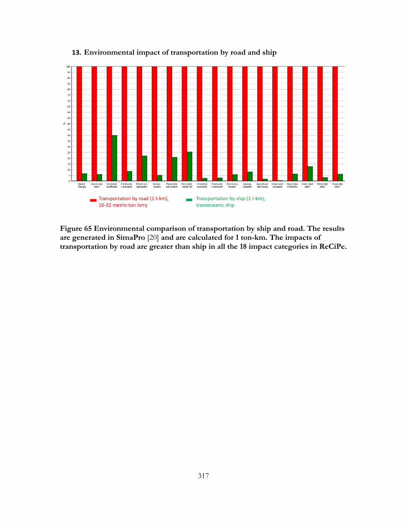
317

13. Environmental impact of transportation by road and ship

Figure 65 Environmental comparison of transportation by ship and road. The results are generated in SimaPro [20] and are calculated for 1 ton-km. The impacts of transportation by road are greater than ship in all the 18 impact categories in ReCiPe.

318

14. Environmental ranking for decentral recycling in China and centralized in

Malaysia when recycling operations in China utilize electricity generated from

PV systems.

Figure 66 Environmental ranking for decentral recycling in China with electricity generated from PV systems and centralized recycling in Malaysia.

Environmental rankings when the “thermal+leach+prcp” recycling alternative is

adopted in both the centralized and decentralized plants in Malaysia and China, respectively

(rank 1 being the most environmentally favorable). The + and - percentage values represent

the increased and decreased inventory requirements (compared to the baseline scenario) due

to lower and higher process efficiencies in decentralized and centralized plants, respectively.

The results depict that decentralized recycling in China with PV electricity is environmentally

preferable to centralized recycling in Malaysia.

319

References

[1] Sigma-Aldrich, “Amberlyst 15 Specifications.” [Online]. Available: http://www.sigmaaldrich.com/catalog/product/sial/06423?lang=en&region=US. [Accessed: 01-Jan-2015]. [2] V. Fthenakis and W. Wang, “System and method for separating tellurium from cadmium waste,” US7731920 B2, 2010. [3] W. Wang and V. Fthenakis, “Kinetics study on separation of cadmium from tellurium in acidic solution media using ion-exchange resins,” J. Hazard. Mater., vol. 125, no. 1–3, pp. 80–88, 2005. [4] V. M. Fthenakis and W. Wang, “Extraction and separation of Cd and Te from cadmium telluride photovoltaic manufacturing scrap,” Prog. Photovoltaics Res. Appl., vol. 14, no. 4, pp. 363–371, 2006. [5] J. K. Choe, M. H. Mehnert, J. S. Guest, T. J. Strathmann, and C. J. Werth, “Comparative assessment of the environmental sustainability of existing and emerging perchlorate treatment technologies for drinking water,” Environ. Sci. Technol., vol. 47, no. 9, pp. 4644–4652, 2013. [6] A. Amini, Y. Kim, J. Zhang, T. Boyer, and Q. Zhang, “Environmental and economic sustainability of ion exchange drinking water treatment for organics removal,” J. Clean. Prod., vol. 104, pp. 413–421, 2015. [7] NREL, “Polycrystalline Thin-Film Materials and Devices R&D.” [Online]. Available: http://www.nrel.gov/pv/thinfilm.html. [Accessed: 01-Jan-2015]. [8] A. Mezei, M. Ashbury, M. Canizares, R. Molnar, H. Given, A. Meader, K. Squires, F. Ojebuoboh, T. Jones, and W. Wang, “Hydrometallurgical recycling of the semiconductor material from photovoltaic materials—part II: metal recovery,” in Hydrometallurgy, 2008, pp. 224–237. [9] Sigma Aldrich, “Bis(2-ethylhexyl) phosphate specification,” 2015. [Online]. Available: http://www.sigmaaldrich.com/catalog/product/aldrich/237825?lang=en&region=US. [10] Ehsan Vahidi et Al., “Modeling of synergistic effect of Cyanex 302 and D2EHPA on separation of nickel and cadmium from sulfate leach liquors of spent Ni–Cd batteries,” Eng. Technol., vol. 6, no. 12, p. 53, 2012. [11] V. Kumar, M. Kumar, M. K. Jha, J. Jeong, and J. C. Lee, “Solvent extraction of cadmium from sulfate solution with di-(2-ethylhexyl) phosphoric acid diluted in kerosene,” Hydrometallurgy, vol. 96, no. 3, pp. 230–234, 2009. [12] A. Babakhani, F. Rashchi, A. Zakeri, and E. Vahidi, “Selective separation of nickel and cadmium from sulfate solutions of spent nickel-cadmium batteries using mixtures of

320

D2EHPA and Cyanex 302,” J. Power Sources, vol. 247, pp. 127–133, 2014. [13] E. Vahidi and F. Zhao, “Life Cycle Analysis for Solvent Extraction of Rare Earth Elements from Aqueous Solutions,” Rewas 2016 Towar. Mater. Resour. Sustain., pp. 113–120, 2016. [14] P. Sinha, M. Cossette, and J.-F. Ménard, “End-of-Life CdTe PV Recycling with Semiconductor Refining,” in PVSEC 2012, pp. 8–11. [15] V. Prado-Lopez, T. P. Seager, M. Chester, L. Laurin, M. Bernardo, and S. Tylock, “Stochastic multi-attribute analysis (SMAA) as an interpretation method for comparative life-cycle assessment (LCA),” Int. J. Life Cycle Assess., vol. 19, no. 2, pp. 405–416, 2014. [16] J.-P. Brans and B. Mareschal, “Promethee Methods,” Mult. Criteria Decis. Anal. State Art Surv., pp. 163–196, 2005. [17] V. Prado, K. Rogers, and T. P. Seager, “Integration of MCDA Tools in Valuation of Comparative Life Cycle Assessment,” Life Cycle Assess. Handb. A Guid. Environ. Sustain. Prod., pp. 413–431, 2012. [18] I. Linkov, F. K. Satterstrom, B. Yatsalo, A. Tkachuk, G. A. Kiker, J. Kim, and K. Gardner, “Comparative assessment of several multi-criteria decision analysis tools for management of contaminated sediments,” Environ. Secur. Harb. Coast. areas, pp. 195–215, 2007. [19] Vulcan, “Vulcan Box Furnace - Owner & Operator’s Manual.” [Online]. Available: http://www.coleparmer.com/Assets/manual_pdfs/33855-10.pdf. [20] PRe Consultants, “Simapro version 8.0.3.14,” 2015. [Online]. Available: http://www.pre-sustainability.com/simapro. [21] First Solar, “First Solar Series 4TM PV Module,” 2015. [Online]. Available: http://www.firstsolar.com/en/Technologies-and-Capabilities/PV-Modules/First-Solar-Series-4-Modules/Documents/Series-4-V2-Datasheet?dl=1.

Defining Geographical Boundaries with Social and Technical ...

Documents

Transcript of Defining Geographical Boundaries with Social and Technical ...