Deep conditional portfolio sorts: The relation between past andfuture stock returns∗

Benjamin Moritz† Tom Zimmermann‡

JOB MARKET PAPER

November 25, 2014

Please find the latest version of the paper HERE.

Abstract

Which variables provide independent information about the cross-section of future returns? Stan-dard techniques like portfolio sorts and Fama-MacBeth regressions cannot easily answer this ques-tion when the number of candidate variables is large and when cross-terms might be important aswell. We introduce a new method, deep conditional portfolio sorts, that can be used in this context.To estimate the model, we import ideas from the machine learning literature and tailor them to oursetting. We apply the method to past-return based predictions, and we recover short-term returns(i.e. the past six most recent one-month returns) as the most important predictors. A tradingstrategy based on these findings has Sharpe and information ratios that are about twice as highas in a Fama-MacBeth framework that accounts for two-way interactions. Transaction costs donot explain these results. Implications for the analysis of cross-sectional predictor variables goingforward are discussed in the conclusion.

∗We thank John Campbell, Robin Greenwood, Owen Lamont, Danial Lashkari, Stefan Mittnik, Sendhil Mullainathan,Lasse Pedersen, Daniel Pollmann, Frank Schilbach, Neil Shephard, Andrei Shleifer and Jeremy Stein for advice, extensivecomments and/or valuable conversations about the project. We also thank seminar audiences at Harvard, Munich, Sal.Oppenheim and Zurich for helpful comments and discussions.

†Ludwig Maximilian University Munich, benjamin.moritz@campus.lmu.de‡Harvard University, tzimmerm@fas.harvard.edu.

1

1 Introduction

Consider the challenge of a portfolio manager who wants to utilize past information to estimate ex-

pected returns at the firm level. He has at his disposal an overwhelming set of potentially correlated

predictor variables as documented by a number of recent survey papers. Subrahmanyam (2010) sur-

veys 50 earnings-based return predictive signals, McLean and Pontiff (2012) document 82, Harvey et al.

(2013) and Green et al. (2013) both extend the list to around 330. These variables range from classic

accounting-based variables like book-to-market to return-based variables like the stock return over the

previous year to more exotic ones like the creativity of a stock’s ticker. Figure 1 shows two graphs from

Harvey et al. (2013) and Green et al. (2013) that illustrate the rate of discovery of predictor variables

over time.1 Both panels show a strong upward trend in the number of published (Harvey et al.) or

publicly available (Green et al.) articles that report new predictor variables of returns, particularly in

the last decade. Many of these variables might interact in non-trivial ways, which increases the set

even more. In addition, the literature suggests a number of stand-ins for many variables (e.g. value or

quality); which one should the manager pick? On top of these questions lurks the risk of overfitting the

data with any estimation method that the manager might use, rendering the analysis worthless for new

observations. How should one then go about estimating expected returns while taking all of these issues

into account?

(a) Harvey et al. (2013) (b) Green et al. (2013)

Figure 1: Time trends in the discovery and publication of return predictive signals

The literature in empirical asset pricing provides a few methods to assist the manager in his decision-

making. As we will show, however, two prominent methods, portfolios sorts and Fama-MacBeth regres-

sions, can only deal with a subset of the questions posed above. We suggest an alternative approach

that is motivated by the method of conditional portfolio sorts but that extends easily to large sets of

1Note that these papers use a different terminology: Predictor variables are factors in Harvey et al. (2013) and return-predictive signals in Green et al. (2013).

2

predictor variables and flexibly deals with their interactions. In contrast to how conditional portfolio

sorts are usually applied, we estimate both the optimal conditioning variables and associated optimal

thresholds from the data.

Our contribution to the literature is threefold: First, we provide a framework that can be used

to organize different methods of estimating expected returns. The framework illustrates that these

methods can be thought of as different approximations of a conditional expectation and it can be used

to evaluate the relative merits of different techniques on simple metrics. We argue that, within this

framework, portfolio sorts and Fama-MacBeth regressions, are not suited to evaluate the independent

information in the entirety of many cross-sectional predictor variables and their potential interactions.

Second, we import ideas from the machine learning literature and tailor them to a financial appli-

cation in order to produce a model that works in this context. While our method is data-driven in

nature, we are careful to develop valid out-of-sample validations of the model. As the machine learning

literature is often criticized for producing black-box predictions, we put particular emphasis on new

measures to extract interpretable information about the structure of the estimated prediction function.

Third, we apply our methodology to past-return based prediction of future returns, and we recover

short-term returns (i.e. the past six most recent one-month return) as the most important predictors.

Implementable trading strategies based on our findings have a risk-adjusted monthly return of around

2 percent per month, with an information ratio that is about three times as high as the information

ratio that can be achieved in a linear framework that does not account for non-linearities and variable

interactions and twice as high as in a Fama-MacBeth framework that accounts for two-way interactions.

Transaction costs cannot account for our results.

While this paper focuses on a particular application, the methodology can be applied more generally

and it has interesting implications for the analysis of cross-sectional predictor variables going forward

that we discuss in the conclusion.

We start by documenting some results that are based on standard methodologies in finance. We

show that, if the investor above had used those methodologies to estimate future returns from past

returns, he could have made reasonable returns of around 1 percent per month (after controlling for

risk factors) with information ratios of about 1. We also show that, had the investor taken potential

two-way interactions between past returns into account, he could have earned similar monthly returns

at an information ratio of 1.3, that is, at much reduced risk. Similarly, when we repeat Fama and

French (2008)’s exercise and extend it to a number of other variables, we show that there are important

interactions between past returns and firm fundamentals.

These results pose a challenge for existing methodologies when the goal is to evaluate many variables

in a joint framework. The portfolio sort methodology, a dominant method in analyzing cross-sectional

predictor variables,2 each month (or year) sorts stocks into three to ten portfolios based on the value

2See the survey of Green et al. (2013).

3

of a particular variable. In the next step, subsequent returns for each portfolio are calculated and it is

checked whether there is a monotone relation between the sorting variable and these subsequent portfolio

returns. In addition, researchers often compute the equal- or value-weighted hedge return of going long

(short) the highest quantile portfolio and going short (long) the lowest quantile portfolio. The relevance

of the sorting variable is then assessed by comparing the hedge return to some equilibrium model of asset

prices (e.g. the capital asset pricing model) and/or by assessing the monotonicity of the returns over

deciles. With regard to the former, a sorting variable is considered relevant if the hedge return strategy

makes abnormal returns that are statistically different from zero. With regard to the latter, Patton and

Timmermann (2010) provide a test for monotonicity in one- or two-variable sorts. The portfolio sort

methodology is a powerful, non-parametric, tool that works best in low dimensional cases. Problems

arise if returns are to be sorted on more than two or three predictor variables as there will be typically

be few stocks in each portfolio. But this makes it challenging to control for information contained in

other variables or, as Fama and French (2008) put it, ”sorts are awkward for drawing inference about

which anomaly variables have unique information about average returns.”

Multivariate Fama-MacBeth regressions are able to address this concern by showing the marginal

effect of each predictor variable once all others are controlled for. The methodology is based on estimating

a cross-sectional regression in each period and averaging the coefficient estimates over time. This works

well with a larger number of predictor variables. But when we include interactions between predictor

variables, this methodology reaches its limit, too: Even if only fifty variables are considered jointly,

the total number of regression coefficients that include all two-way interactions (and no higher-order

interactions) is 1275, higher than the number of companies in early months of the sample, and higher

than the number of companies throughout the entire sample if the sample is split by firm size first as

in Fama and French (2008). Second, as Fama and French note, results can be vulnerable to influential

observations of extreme returns. With this in mind, Green et al. (2014) ”view it as infeasible to examine

non-linearities in RPS-returns relations in the manner undertaken in Fama and French (2008).”

We suggest a method that is based on the well-known idea of conditional portfolio sorts that is

designed to address the aforementioned challenges and that can account for arbitrary interaction terms.3

Conditional portfolio sorts arrange firms into groups based on the value of some variable (e.g. book-to-

market). Within each group, stocks are then sorted again based on the value of some other variable.

Sorting variables and sorting values are typically chosen based on a-priori reasoning. We start from the

assumption that neither the sorting variable nor the sorting value are known and need to be estimated.

Furthermore, conditional sorts are typically conducted for no more than two levels (that is, stocks are

sorted twice) and the same sorting variable is used in all branches on the second level. We estimate sorts

at deeper levels (motivating the method’s name in the title) and allow for flexible variable selection at

3The finance literature is somewhat imprecise about the distinction between interaction terms and non-linearities, andoften uses both terms interchangeably. We reserve ”interactions” for cross-products between two variables, and we thinkof ”non-linearities” as higher-order polynomial terms with respect to a single variable.

4

each branch.

The optimization problem is computationally challenging but can be solved with insights from the

machine learning literature. The solution follows a simple algorithm that, for each portfolio of firms

and starting from the portfolio of all firms (the entire data set), splits the firms in the portfolio into two

new groups. The algorithm finds the sorting variable and associated sorting value that minimize a loss

function over the data in the two resulting groups. The optimization is repeated at every non-terminal

node using the remaining observations as long as that number is not too small and there is still a split

of the data that significantly improves upon the value of the loss function.

There are two well-known and related problems with this approach. First, since the optimization

proceeds stepwise, the variables and sorting values that are selected at each point need not be globally

optimal. But since the sorting rule is discrete, any error in the estimation of the sorting variable and

sorting value could have a large impact on the model’s predictions. Second, the approach is data-driven

and easily overfits the data. We, therefore, need to take great care to make sure that the estimates are

valid out-of-sample.

The solution that we employ is based on model-averaging. We estimate deep conditional portfolio

sorts many times, with different subsets of regressors and on different subsets of the data, and combine

the estimates from all models into a final prediction. The rationale is that by averaging estimates that

come from models that are de-correlated in this manner, one can obtain different but related signals

about the true underlying process, even if the simple underlying models are not entirely correct. At the

same time, model-averaging helps with the overfitting problem because only subsets of the data and

predictor variables are used in each model. The idea is grounded in the computer science literature and

has been successfully applied in many contexts. We find that deep conditional portfolio sorts combined

with model-averaging produces very accurate predictions of expected returns.

The main drawback of averaging over many models is that results are not as easy to interpret as a

single deep conditional sort. In order to shed light on the mechanism, we suggest a number of evaluation

measures. We compute a measure of predictor variable importance that can be interpreted similarly to

t-statistics in regressions. In addition, we develop a way to compute partial derivatives for each predictor

variable so that we are able to talk about directional effects of specific variables. We also run diagnostic

checks to see whether the predictions from the model can be explained by a simple linear regression on

our predictor variables (which would speak against the importance of interaction effects).

The method takes into account that a predictor variable’s influence might vary over time.4 We set up

the out-of-sample tests in such a way that they lend themselves naturally to investigate time-variation

of the importance of particular variables. In each year, we estimate the model with data over the past

years. For the next twelve months, one-month expected returns are then projected by fixing the model

estimates and making predictions based on the new data that were reported only after the estimation

4As Harvey et al. (2013) note ”it is possible that a particular factor is very important in certain economic environmentsand not important in other environments. The unconditional test might conclude the factor is marginal.”

5

period. Not only are our trading results below strong in this exercise, but the approach also enables us

to look at which variables come out as important in the search procedure in which period.

We apply our method to contribute to the debate about whether past returns contain information

about future returns and, if so, which past returns matter the most. This debate has recently regained

interest after Novy-Marx (2012) found that medium-term momentum, that is a stock’s return over the

twelve to seven months prior to portfolio formation, can be a better indicator of future return than

momentum calculated over the entire previous year (excluding the most recent month). Goyal and

Wahal (2013) cannot find this effect in 37 other markets outside the US. Other recent articles have

looked at a moving average strategy derived from past prices (Han et al. (2011)) or construct a trend

factor from daily to annual returns that outperforms the standard momentum factor (Han and Zhou

(2013)). We, therefore, regard the relation between past and future returns as a natural laboratory for

our method.

As predictor variables, we construct a set of decile rankings for the non-overlapping one-month

returns over the two years before portfolio formation. This yields a set of twenty-five predictors and it

is ex-ante unclear how to combine them optimally to forecast next period’s returns.

We use standard methods to derive forecasts and benchmark them against forecasts from deep

conditional portfolio sorts. A strategy based on deep conditional portfolio sorts yields abnormal returns

(relative to the four-factor model) of 2-2.3 percent per month, depending on the exact specification,

with information ratios of around 2.8. Our preferred specification has an abnormal monthly return

at the lower end of that range. Although the strategy has high turnover, transaction costs do not

dwarf the abnormal return. This compares to results from a Fama-MacBeth regression framework with

abnormal returns of 1-1.4 percent per month with an information ratio of 1-1.5, depending on whether

two-way interactions between past returns are included. We conclude that deep conditional portfolio

sorts perform better via producing a moderate increase in average abnormal returns at much reduced

variance.

What is the structure of the prediction function that we estimate? While it cannot be summarized

as a simple linear equation, we can use our suggested evaluation measures to shed light on the black

box: Intriguingly, the most important predictor variables are short-term return functions and returns

appear to become less important when they are in the more distant past. In particular, we show that

the most recent six months of past returns capture almost all the information that is contained in more

distant past returns.

We then show how past returns are related to future returns in the deep conditional portfolio sorts.

While we recover some standard results like short-term reversal over the most recent past month or

momentum over the previous twelve months of returns, we also find evidence for the relevance of non-

linear effects (e.g. both high and low returns over the month before the most recent one predict lower

returns) and interactions (e.g. the one-month return over the second-to-last month is negatively related

6

to returns for stocks with low returns last month, but is positively related to returns with high returns

last month).

The results hold in a variety of alternative settings. We construct another set of predictor variables

that includes many possible past returns with different horizons and gaps to the portfolio formation

date to see how our methodology performs when many of the predictor variables (a total of 126) are

highly correlated. In this setting, abnormal returns are again high and a similar return structure, with

similar partial derivatives for specific predictor variables, is estimated. Our results are also unaffected

by including eighty-six additional firm characteristics from the literature. Here, results for abnormal

returns are actually a bit stronger because of the additional information in accounting variables and

other characteristics, and the return structure results still hold. We then make sure that our results

are not entirely driven by illiquid stocks by re-doing all computations for large, small and micro firms

(in the terminology of Fama and French (2008)) separately. While we find that results are stronger in

small stocks and strongest in micro stocks, our main conclusions hold throughout all size categories. We

conclude that more recent past returns are more relevant than intermediate past returns for prediction

of future returns and, more generally, past returns are related to future returns in a more complex way

than can be captured by any single one past return.

Before we continue, we provide a short overview of the related literature. In his presidential address,

Cochrane (2011) describes the ”factor zoo” of stock market anomalies and how it has developed over

the years. Subrahmanyam (2010), Goyal (2011), Green et al. (2013) and Harvey et al. (2013) review as

many as 330 anomalies that have been found by academic research and call for a synthesis of the existing

literature. While early attempts in this direction where undertaken by Haugen and Baker (1996), Daniel

and Titman (1997) and Brennan et al. (1998) who focus on smaller sets of characteristics, Cochrane

(2011) argues that different methods might be required to find the independent information for average

returns in the entirety of documented predictor variables. Our paper can be read as an attempt to

provide just such a new method.

Green et al. (2014) investigate the mutual information in 100 signals, and find that up to 24 of

them have predictive power for returns when used jointly. They suggest an alternative to the standard

three factor model by Fama and French (1992) that is based on 10 different characteristics. The paper

notes the potential relevance of interactions but does not investigate them in detail.5 Lewellen (2013)

investigates the power of 15 different firm characteristics to predict variation in the cross section. He

finds that expected stock returns derived from the model are strongly predictive of actual stock returns

for as much as 12 months.

Fama and French (2013) follow an alternative approach that attempts to capture variation in returns

by a (small) factor model. They extend the three factor model by proxies for profitability and invest-

5They write, ”fundamental valuation type measures and market trading type measures appear to matter across firmsize. In large-cap firms the important RPS can be broadly classified as fundamental valuation measures or trading typemeasures. For mid-cap and small-cap firms the themes appear slightly different.”

7

ment which appears to capture contemporaneous variation in cross-sectional returns well, except for

small stocks. The paper uses a quadruple sorting strategy to address interactions between size, value,

profitability and investment opportunities. Kogan and Tian (2012) construct all combinations of three

and four factor models from a set of 27 firm characteristics. They find that the best performing models

are unstable across time periods.

The literature on momentum and reversal is too large to review it here but we note a view key

articles. If stock prices systematically over- or underreact, future stock returns should be predictable

from past returns data alone. de Bondt and Thaler test overreaction by sorting stocks based on the

return in the previous three years (the portfolio formation period). They find that losers (the bottom

decile of returns in the formation period) outperforms winners by about 25% over three years. They

hint at the fact that there is some interaction with the January effect. A similar ”reversal effect” has

been found by Jegadeesh (1990) and Lehmann (1990) for portfolios that are formed based on short-term

(one week to one month) prior returns. Jegadeesh and Titman (1993), on the other hand, find evidence

for a ”momentum effect” when portfolios are sorted on medium-term (3 to 12 months) prior return.

”Momentum” means that past winners continue to outperform past losers for up to 12 months (with

an apparent reversal effect after 12 months). The momentum finding survives the analysis in Fama and

French (1996) who use the three-factor model as a model of equilibrium returns. Long-term reversal

disappears as an anomaly once normal returns are approximated by the three factor model. For much

more on momentum, we refer to Asness et al. (2014) who use simple analysis and survey published

studies to show that momentum returns are (among other things) not too volatile, not only a small firm

phenomenon and not dwarfed by tax considerations or transaction costs.

This essay is organized as follows. Section 2 discusses the data, sets up a motivating framework

and investigates two standard methods, portfolio sorts and simple Fama-MacBeth regressions, that a

portfolio manager could employ to predict future returns. Section 3 explains deep conditional portfolio

sorts in detail. Section 4 applies the method to past return predictor variables and section 5 has further

results on transaction costs and a risk factor vs characteristics interpretation. Section E in the appendix

illustrates robustness of our results along several dimensions. Section 6 concludes.

2 Data, motivating framework and standard methods

Before we introduce deep conditional portfolio sorts, we analyze a few standard approaches that an

investor might try. These are: Single variable selection, i.e. investing based on the single best-performing

variable in historical data over a certain time window; standard Fama-MacBeth regressions, i.e. a

multivariate prediction that combines historically important signals; and Fama-MacBeth regressions

that include variable interactions.

8

2.1 Data

Since we will use the relation between past returns and future returns as a running example throughout

the article, we start by describing the data and the variable construction first.

The basis for our analysis is the universe of monthly US stock returns from the Center for Research in

Security Prices (CRSP) from 1963 to 2012. Since we use firm characteristics from Compustat and IBES

in some robustness checks, we match stock price data to those data sets first, and focus our analysis

on those firms that can be linked in all datasets. Firm characteristics include traditional variables like

size, book-to-market, dividend yield, gross profitability and eighty-two others that are described in more

detail in appendix E.1. The number of firms in our sample varies over time between 1182 and 6626. Size,

value, momentum factors and the risk-free interest rate are taken from Kenneth French’s data library.6

Figure 2 illustrates how return-based predictor variables are constructed. Suppose that the investor

wants to form a portfolios at the formation time tf . Return-based predictor variables can be defined

by two parameters; the gap between the time of portfolio formation and the most recent month that is

included in the return calculation, and the length of the return computation horizon. We denote the

former by g, the latter by l and a return function by Ri,tf (g, l) maps returns into cross-sectional decile

ranks. For example, Ri,tf (1, 11) = 10 implies that firm i is in the highest decile of returns at time tf for

the return that is computed over the previous twelve months and leaves out the most recent one.

Our benchmark set of predictors contains all one-month returns over the two years before portfolio

formation, that is, Ri,t(g, 1), g = 0, . . . , 24. Much of the related literature is based on sorting firms

into one of ten deciles depending on the values of a sorting variable. When we consider return-based

strategies below, we refer to buying the upper decile and selling the lower decile based on Ri,t(g, l). As in

Novy-Marx (2012), we will use the notation Ri,t(g, l) to denote both the return for portfolio formation,

and the strategy return based on that simple sorting strategy.7

The problem of predicting future returns based on past returns has the ingredients that make it

difficult for an investor to find the relevant signals: Should momentum be measured over the most

recent six or twelve months? What if the signals go in opposite directions? Should one leave out the

most recent month? Or the most recent six (Novy-Marx (2012))? Degrees-of-freedom in choosing the

gap and length parameters above contribute to the fact that these questions do not have a definitive

answer yet.

6http://mba.tuck.dartmouth.edu/pages/faculty/ken.french/data_library.html7We have checked that results are robust when future returns are computed over the next future month, but skip a

day to make sure that the return would actually be implementable.

9

2.2 Motivating framework

In each time period, an investor has access to information Θit about firm i to model the conditional

expectation of next period’s return as in equation (1), a general version of the model8 that is typically

estimated in the literature.

Et[ri,t+1|Θit] = ft(Θit), (1)

Here, the expectation of ri,t+1 is formed at time t (we take a period to be one month in what follows),

and the function ft() that maps the information set into expected returns can be time-varying. The

information set Θit can contain data on the firm’s past earnings, balance sheet information, past stock

return movements and many other variables. Since we will focus on the relation between past and future

returns in this paper, and in line with the sorting-based literature, we assume that the information set

consists of decile rankings of companies over the past two years, that is, Θit = {Ri,t(0, 1), . . . , Ri,t(24, 1)}.In other words, we consider decile rankings for each of the most recent twenty-five one-month returns.

With that information set, adding an additive error term and choosing the common specification of

a linear form (see e.g. Haugen and Baker (1996), Daniel and Titman (1997) or Brennan et al. (1998))

for the function ft(), equation (1) can be written as

ri,t+1 = a+24∑g=0

βtgRi,t(g, 1) + ϵi,t, (2)

which is usually estimated via a Fama-MacBeth procedure or by a cross-sectional regression. In general,

the model can be viewed as a joint test of the relevance of characteristics and of the linearity assumption.

We first illustrate how an investor could go about predicting returns using standard methods.

2.3 Existing methods

In our running example, the investor faces the problem of predicting returns based on one-month returns

over the previous two years. We consider two possible solutions to that problem that are employed in

the existing literature.

8At a greater level of generality, one could write the model as

Et[ri,t+1|Θit] = ft(zi,t, zi,t−1, . . . , λt, λt−1, . . .),

which would also include risk factors, and zit and λt and their histories are subsumed in the information set Θit ={zi,t, . . . , λt, . . .} at time t. We disregard this aspect for now but note that our framework easily extends to the case whereall returns are interpreted as excess returns over risk factors.

10

2.3.1 Portfolio sort

The potentially simplest strategy is to evaluate one variable at a time, and then base forecasts on the

single variable that has performed best in the past. More specifically, we suggest the following simple

strategy: In each month, compute the m month trailing average return for each sorting variable, pick

the one with the best performance (in terms of the Sharpe ratio), and base the subsequent long and

short orders on values of that variable.

Table 1 shows that the return to such a strategy is .71 percent per month with an information ratio

(relative to the four factor model) of .89, when the trailing performance is computed over the sixty

months that precede the portfolio formation date. While this is already a good result, each month’s

returns are based on the values of a single sorting variable. The question remains whether the investor

can do even better by combining information from different variables. While a few more variables can

be incorporated (e.g. double sorts), the number of observations in each portfolio decreases quickly such

that estimates become unreliable.

2.3.2 Fama-MacBeth regressions

With that question, the investor turns to a multivariate regression setup that we describe in some detail.

We suggest two approaches: A ”kitchen-sink” Fama-MacBeth estimation that throws in all past return

variables and that uses them for prediction regardless of their individual significance. On the other

hand, it could be more appropriate to base predictions solely on the relevant variables where we define

”relevant” as variables that are selected in a LASSO regression.9 While we report results for the LASSO

regression, we have tried other model selection methods (general-to-specific, specific-to-general) and

obtained similar results.

Our general implementation for the Fama-MacBeth-framework works as follows. In each cross-

section, the investor fits the regression

ri,t+1 = βtcons +

24∑g=0

βtgRit(g, 1) + ϵit (3)

and he keeps either all coefficients (kitchen sink) or uses LASSO to select the relevant variables.

His period t+ 1 forecast is computed based on the rolling average of the coefficient estimates up to

period t− 1 and then applying the linear model to Rit(g, 1), that is,

9Least absolute shrinkage and selection operator (LASSO), originally introduced by Tibshirani (1996), is a methodthat regularizes regressions by putting a penalty on the size of regression coefficients. Due to the nature of the penaltyterm (the sum of the absolute values of individual coefficients), the optimum will typically set many coefficients to exactzeros, which is why the method can be viewed as a variable selection device.

11

ri,t+1 = βt−1

cons +24∑g=0

βt−1

g Rit(g, 1), (4)

where βt−1

g = 1m

∑t−1j=t−1−m β

tg. We initially use a rolling window of 120 months but, as Lewellen

(2013), have found that results are robust to varying that parameter.

Lewellen (2013) uses a set of 15 predictor variables that are well-established in the literature. In

contrast, we consider an investor who faces substantial uncertainty about which variables he should

include and, therefore, has to cast a wide net. Consistent with our running example, the investor

considers all one-month returns over the two years before portfolio formation. Each period, he computes

return predictions based on past model estimates, and sorts predictions into ten deciles. He constructs

an equal-weighted hedge portfolio that goes long the highest decile of predicted returns and that goes

short the lowest decile of predicted returns, analogous to the strategies above.

Starting with the kitchen sink model, the first four columns of table 2 show the strategy’s factor

loadings from time-series regressions on the market, size, value and momentum factors. The strategy

has a positive and significant average return of 1.51 percent per month, and loads mostly on the market

and the momentum factor. The alpha relative to the four-factor model is about 1 percent per month,

with an information ratio of about 1.

When we use the LASSO in the Fama-MacBeth framework as described above, results remain almost

unchanged. The last four columns of table 2 show that the average strategy return is again around 1.5

percent per month, and the four-factor alpha is 1 percent per month. The information ratio is close to 1,

as in the kitchen sink regression. The reason that these results are very similar is that many irrelevant

regressors have coefficients close to zero in the kitchen sink case.

Note that the approaches so far have not included variable interactions. The Fama-MacBeth regres-

sion framework lends itself to a simple implementation of additionally including interactions of predictor

variables. Equation (5) shows the regression equation that adds all two-way interactions between past

return rankings.

ri,t+1 = a+24∑g=0

βtgRi,t(g, 1) +

24∑g=0

∑j>g

γtgjRi,t(g, 1)Ri,t(j, 1) + ϵi,t. (5)

Table 3 shows strategy returns that are based on predictions from equation (5).10 At 1.13 percent

per month, the average excess return relative to the four factor model is slightly higher than in the

levels-only version above. The information ratio, however, experiences a much stronger increase to 1.3.-

10Since the model with two-way interactions has 325 regressors, we focus on results based on variable selection.

12

1.4. Hence, the main benefit to including two-way interactions appears to be a reduction in variance

rather than an improved mean return.

Of course, this begs the question whether we have now captured all information in past returns

for future returns or whether we should estimate the prediction equation more flexibly. For instance,

if we are interested in exploring all systematic variation, why would we stop at two-way interactions?

Appealing as the Fama-MacBeth method might seem, it quickly becomes infeasible when we want to

analyze the entirety of potential interactions. Considering only two-way interactions, the number of

terms to include when p candidate predictors are included is p(p+1)2

which starts to become greater than

a thousand at a mere forty-five predictor variables. This prevents the use of Fama-MacBeth regressions

in the early years of the sample (although LASSO would still be a feasible alternative) if all firms are

considered, and over the entire sample if the sample is divided by, say size, first. With higher-order

interactions, estimation becomes difficult for even fewer candidate predictors. In the next section, we

import a method from the machine learning literature that is sufficiently flexible in this setting and

tailor it to a finance application.

3 Estimation strategy

Returning to the general model for expected returns in equation (1), we briefly discuss the difficulties that

arise when the set of firm characteristics gets large. More specifically, even when the set of characteristics

appears manageable, the number of regressors can grow quickly if characteristics interact or are non-

linearly related to returns.

Interactions between different anomalies can arise quite naturally from simple economic models.

Chen et al. (2002) test the theory of gradual information diffusion to explain momentum. They argue

that the rate of information diffusion could be different for firms which would result in different strength

of momentum profits. They find that momentum interacts with firm size and with analyst coverage, and

that the effect of analyst coverage on momentum profits is largest in small firms (a triple interaction).

Vassalou and Xing (2004) illustrate a complex interaction between size and value and default risk. They

show that small stocks earn higher returns than big stocks only if they have higher default risk and the

same holds for the return of value over growth stocks. Complementary, high default risk firms earn higher

returns than low default risk firms if they are small or value stocks. Expected return-relevant two-way

interactions have been demonstrated between size and value (Fama and French (1992)), between size

and seasonal effects (Daniel and Titman (1997)), or between stock exchange and volume (Brennan et al.

(1998)). Some authors have also considered interactions between past-returns and firm fundamentals

(see e.g. Asness (1997) for the interaction between value and momentum, or (Lee and Swaminathan

(2000)) for the interaction between volume and momentum). Interactions between different past-return

variables are rare in the literature, with Grinblatt and Moskowitz (2004) who consider the consistency

13

of return patterns and Han and Zhou (2013) who construct a trend-factor from past returns of different

frequencies being two exceptions.

The literature that investigates interactions has typically used portfolio sorts. This approach sorts

stocks into portfolios based on the characteristics in question, and the returns for each portfolio are

evaluated. It is, however, only feasible for a small set of, typically two, characteristics. Three-way or four-

way sorts are rarely executed at all because the individual portfolios contain few firms.11 Correlations

between firm fundamentals make it difficult to isolate their individual marginal contribution to expected

return prediction.12

One might think that a fully interacted version of equation (2) can overcome this challenge, but in

fact becomes infeasible quickly, too. Consider a model that allows for arbitrary three-way interactions

ri,t+1 = a+G∑

g=0

βtgRi,t(g, 1) +

G∑g=0

∑j>g

γtgjRi,t(g, 1)Ri,t(j, 1)

+G∑

g=0

∑j>g

∑k>j

δtgjkRi,t(g, 1)Ri,t(j, 1)Ri,t(k, 1) + ϵi,t. (6)

Even if we consider a small set of G = 20 firm characteristics, 190 two-way interactions and 1140

three-way interactions would need to be considered. In the application of Green et al. (2014) with

G = 100, these numbers amount to 4950 and 161700 which is prohibitively large for statistical analysis.13

Given the difficulties that stem from comprehensively investigating the interactions between charac-

teristics using these standard methodologies, the existing evidence is restricted to the low-dimensional

cases that have been and can be considered, while we may not learn the full extent to which interactions

are relevant. Our approach below provides one way to address this question.

3.1 Conditional Portfolio Sorts

Our goal is to estimate the conditional expectation in equation (1) more flexibly than can be achieved by

a globally linear model like Fama-MacBeth regressions or, by portfolio sorts that allow for non-linearities

but that, in their usual form, are restricted to one- or two-dimensional cases.

Our estimation is based on the well-known concept of conditional portfolio sorts which are illustrated

schematically in figure 3. Consider sorting stocks into two portfolios based on sorting variable R(g(1), 1)

and threshold τ (1), such that all stocks with R(g(1), 1) ≤ τ (1) are pooled together into one portfolio,

and stocks with R(g(1), 1) > τ (1) are pooled together into another portfolio. For instance, if τ (1) = 5

11For examples, see Daniel and Titman (1997), Fama and French (2008) or Fama and French (2013).12An early contribution that criticizes portfolio sorts for their inability to deal with correlated signals can be found in

Jacobs and Levy (1989).13In general, all k-way interactions are given by

(Gk

).

14

and g(1) = 0, we would sort all stocks with returns below the cross-sectional median in the previous

month into one portfolio and all stocks with returns above cross-sectional median in the previous month

into another portfolio.14 The expected stock returns in each portfolio are now E[ri,t+1|R(g(1), 1) ≤ τ (1)]

and E[ri,t+1|R(g(1), 1) > τ (1)], respectively, and, if the expected return is modeled as a constant within

each portfolio, the prediction is just the average of realizations of next months’ returns within each

group. Sorting stocks within each portfolio again by another (or the same) characteristic with associated

thresholds τ (2a) and τ (2b) results in four different portfolios S1 to S4, e.g. the stocks in portfolio S1 in

the figure have expected return E[ri,t+1|R(g(1), 1) ≤ τ (1), R(g(2a), 1) ≤ τ (2a)].

A simple way to test whether R(g(2a), 1) provides additional information over R(g(1), 1) would com-

pare the sorts on R(g(2a), 1) within each portfolio sorted on R(g(1), 1).15 On the other hand, one could

test whether R(g(2a), 1) creates a return spread only in the portfolio of, e.g. low R(g(1), 1) firms, therefore,

testing for a potential interaction between characteristics R(g(2a), 1) and R(g(1), 1).

In appendix C, we illustrate a basic conditional portfolio sort with a few standard firm characteristics.

Our results complement Fama and French (2008) who sort stocks into three size portfolios first and

then sort each portfolio subsequently on a further firm characteristic. In our illustration, we consider

conditional portfolio sorts that are each based on two of the following variables: short-term reversal,

momentum, intermediate momentum, size, gross profitability, and book-to-market.

We refer the interested reader to the appendix for detailed results but highlight a few notable results

here. The overall picture that emerges is that of return sorts being relatively stable while accounting-

based sorts are less robust to initial sorts on some other return- or accounting-based variable. For

instance, size sorts do not work uniformly when stocks are sorted on short-term reversal or momen-

tum first. Interestingly, momentum sorts continue to work well when firms are sorted on intermediate

momentum first but the reverse is not true.

Of course, there is the question of how to choose the sorting variables and the sorting thresholds in

the first place. The literature typically chooses the sorting variables based on a specific hypothesis and

uses thresholds that evenly sort stocks into three, five or ten portfolios. The same sorting variable is

used in all branches after the first sort. But, if viewed as a way to approximate a conditional expectation

of returns, this restriction might not deliver the best approximation. We relax these constraints in the

next section.

3.2 Deep Conditional Portfolio Sorts

We suggest to extend the method of conditional portfolio sorts along the following dimensions. First,

unlike in our example above that had thresholds and sorting variables chosen ex-ante, we will choose

14The literature usually considers one-variable sorts of stocks into ten different portfolios. However, our sort into twoportfolios is not restrictive because a one-variable sort into multiple portfolios can always be achieved by a repeated sortinto two portfolios.

15This kind of test is, for example, applied in Bandarchuk and Hilscher (2012).

15

thresholds and sorting variables optimally (where ”optimally” will be defined below) within each portfolio

in a data-driven way. Second, we apply the procedure to levels deeper than the two levels that are usually

considered which gives rise to, what we call, a deep conditional portfolio sort. Third, since conditional

sorts involve hard thresholds that are sensitive to small changes in the data, their predictions do not

work very well out-of-sample. Following Kleinberg (1990, 1996), Ho (1998) and Breiman (2001), we

average over many deep conditional portfolio sorts to smooth out the decision boundary which improves

predictions significantly, as explained below in more detail.

Our approach draws on parallel concepts from the machine learning literature. The techniques that

we use to estimate deep conditional portfolio sorts mirror those that are used to estimate a so-called

decision tree in computer science.16 Model averaging or ensemble methods are also developed in that

literature and they are successfully applied to areas as diverse as biology (DNA sequencing), psychology

or motion sensing. Applications in economics are rare17 and our paper can also be read as an attempt

to investigate whether these techniques have something to add to academic research in finance and

economics. This is the first paper that interprets conditional portfolio sorts from a machine learning

perspective, tailors the methodology to similar approaches well-known in finance, and applies it to a

comprehensive financial dataset.

3.2.1 Estimation

We start by describing how variables are selected and how thresholds are estimated. The goal is still to

estimate the expectation of the return of firm i in period t+1 conditional on information in period t as

in equation (1).

To illustrate estimation start out with the conditional portfolio sort in figure 3. Consider the portfolio

S1 in that figure which is defined by variable R(g(1), 1) being less than threshold τ (1) and variable

R(g(2a), 1) being smaller than threshold τ (2a). Other portfolios can be defined similarly by their relations

between sorting variables and associated thresholds. Within each portfolio Sl, the predicted expected

return is modeled as the average return, µl, of all firms in the portfolio, that is,

µl = Mean(ri,t+1|Firm i ∈ Sl in period t) (7)

In other words, analogous to linear regression, we are interested in approximating the conditional mean of

the outcome variable at a value of the regressor by the average of the outcome variable over observations

with close values of the regressors. The conditional portfolio sort therefore generates subsets of firm

16For further reading on decision-trees, see Hastie et al. (2009), Zhang and Ma (2012), Murphy (2012) or Criminisi andShotten (2013).

17A few examples in a macroeconomic context use decision trees to analyze currency crises (Kaminsky (2006)), sovereigndebt crises (Manasse and Roubini (2009)), banking crises (Duttagupta and Cashin (2011)) or to develop early warningindicators for e.g. excessive credit growth (Alessi and Detken (2014)).

16

observations that are more homogenous. Suppose for a moment that we have found such a homogenous

allocation of firms into portfolios. The prediction function could then be written as

ri,t+1 =L∑l=1

µl1(Firm i ∈ Sl in period t), (8)

giving a portfolio-specific expected return prediction for each observation. What we have described so

far is nothing more than a formal definition of the common conditional sorting methodology that we

carried out in the previous section.

Of course, the conditional sort does not need to end after two levels but can be computed at greater

depth. We consider the case in which the depth of the conditional sort, the sorting variables and

associated thresholds are not pre-selected but need to be identified from the data. To start with a

negative result, it can be shown that finding the optimal solution to this problem requires solving an

optimization problem for which a computationally fast solution does not exist (see (Hyafil and Rivest

(1976))).

Instead, we adopt a greedy algorithm from the machine learning literature that proceeds in a step-

wise fashion. We describe the details in appendix D and give a high-level summary here. The algorithm

starts out with all observations and splits them into two subsets. From a given set of variables, it

finds the variable and the associated threshold value that minimize the mean squared error over all

observations if predictions are computed as in equation (7). The algorithm is called greedy because it

solves the minimization problem in a brute-force fashion by trying every combination of variable and

threshold value. The same procedure is then repeated in each subset until the number of observations

in a subset becomes small or if no further split can meaningfully improve upon the mean squared error.

The result is a deep conditional portfolio sort, that is, a conditional portfolio sort with many levels.

Figure 4 illustrates the results of this procedure using the data and variables described in section

2.1 below. Rather than showing the entire iterative sort, the figure only shows the first few nodes. The

first selected split variable is R(0,1), the return over the previous month. The associated threshold is

6, that is, all firms with a return over the previous month in the lowest six deciles are sorted into one

portfolio, and the remaining ones are sorted into the other. Conditional on this split, R(0,1) is selected

again in the left branch at the next level and R(2,1), the one-month return two months ago, is selected

in the right branch. The actual iterative sort goes deeper but, for illustration, we have computed the

one-month ahead returns in each of the four subsets. Differences are already pretty stark: The subset

S1 which is the set of companies that were in the lower of the two R(0,1) groups, display the highest

return, indicating short-term reversal. The right branch illustrates a momentum effect: Stocks with

higher values of R(2,1) have a higher subsequent return on average.

Before we move on, we want to point out a few links to other estimation methods in the literature.

17

The greedy algorithm introduced in this section bears some resemblance to forward-selection methods

in regression models. Forward-selection starts out with the smallest possible linear model, estimates

bivariate regressions of the outcome variable on each candidate regressor separately, and keeps the

one with the highest t-statistic (or some other selected performance criterion). The procedure is then

repeated for all of the remaining variables with the best-performing variable joining the regression each

round until no further variables are significant. As deep conditional sorts, forward-selection works when

there are more regressors than observations. On the other hand, forward selection is global in nature in

the sense that one regression function is fitted for the entire sample and variable selection is based on

performance over the entire sample. In addition, interaction terms would need to be added one-by-one

as well leading to a large set of candidate variables whereas the set of candidate variables is always less

than the number of main signals in iterative conditional portfolio sorts.

Kernel regression is based on approximating an outcome variable by a (kernel-) weighted average of

the outcome at each value of the regressor. Deep conditional portfolio sorts approximate the outcome

by the average value of the outcome for a regressor region defined by split points and threshold values.

Kernel regressions are very flexible but do not extend easily beyond the bivariate case. A small practical

issue is the difficulty to display results in higher dimensions. More importantly, since kernel regression

is based on using local averages, there are few observations in each subspace over which an average is

taken as the number of regressors becomes large. This is known as the curse of dimensionality and one

can show that the convergence rate for kernel regressions deteriorates sharply with the dimensionality

of the regressors. Local linear regressions run into analogous problems in high dimensions.

3.2.2 Model averaging

Constructing deep conditional portfolio sorts in the way described above results in a few challenges.

First, as described above, because of the complexity of the optimization, we have to use a greedy

algorithm to estimate the model. This algorithm, however, does not guarantee that thresholds and split

variables are selected optimally at each node. Second, the threshold rule is discrete, and any error in

the estimation of the threshold could greatly distort the correct path for any expected return that is

supposed to be predicted from the estimated model. Third, our initial results showed that a single

estimated deep conditional portfolio sort summarizes the estimation data well, but the model does not

extend well to new observations. In other words, the deep conditional portfolio sort can often overfit the

estimation sample. The related machine learning literature acknowledges these issues under the label

of weak learners, characterized by the fact that their predictions for new observations are often only

weakly (albeit positively) correlated with the actual values.

We adopt a solution based on averaging over many deep conditional portfolio sorts that combines ele-

ments of Kleinberg (1990, 1996), Breiman (1996), Ho (1998) and Breiman (2001). Kleinberg introduces

the idea of ”stochastic discrimination” to solve estimation problems without overfitting too much in

18

sample. The idea is to estimate a model a number of times using only random subsets of regressors each

time. The resulting models are less prone to overfitting since they are arguably less complex. Kleinberg

shows that by combining predictions from such models the accuracy of out-of-sample estimates can be

improved upon.18 Breiman (1996) suggests a related approach, ”bootstrap aggregating” (or bagging),

that leaves the set of regressors intact but estimates a model several times on different random parts

of the estimation data. The final prediction is then again constructed as an average over the different

models’ predictions. Breiman (2001) combines both elements, stochastic discrimination and bagging, in

the context of decision trees (which are, what we call, deep conditional portfolio sorts). He finds that

this approach that he labels ”random forests”greatly improves upon out-of-sample accuracy.19

The idea of combining many predictions to construct a more accurate one can be illustrated in

a simple voting setup in which people use majority voting to make a decision or to determine the

(objective) value of an object. If everyone has the same information set, then nothing can be learned

from aggregating individual votes, instead every single vote is a sufficient statistic for the outcome.

Only if voters differ in their information, aggregation can lead to a more precise estimate. Stochastic

discrimination and bagging induce just such different information sets.

We apply these concepts to deep conditional portfolio sorts. New predicted expected returns are

generated by first computing an estimated expected return from each deep conditional sort and then

averaging over the individual predictions. More formally, let B be the number of deep conditional sorts

that are computed, and let fb(Θit) be the predicted expected return for stock i at time t that is based

on model b. The final expected return estimate is given by

ri,t+1 =1

B

B∑b=1

fb(Θi,t). (9)

In all results that follow, we construct two hundred deep conditional portfolio sorts (that is, B = 200)

18Kleinberg (1990) provides the following intuition: ”If one were presented again and again with the same poor solutionto a problem, he would have little chance of ever creating anything better than that poor solution - on the other hand, ifhe were presented again and again with equally poor but different solutions to the problem, he would at least be gettingdiverse information; and in this case, stochastic discrimination will enable him to create from this diverse information anessentially perfect solution.”

19While applications of these methods are plentiful in computer science, their theoretical properties are not all well-understood. Breiman (2001) shows that bagging decision-trees implies an upper bound on the out-of-sample mean squarederror that depends on the strength of the individual models and on the correlation between them. In that sense, baggingshields against overfitting if one can sufficiently de-correlate the individual greedy conditional portfolio sorts. Buchlmannand Yu (2002) analyze the bias-variance trade-off of bagging and they show that bagging reduces mean squared errorby substantially reducing variance with only a small effect on bias. They argue that bagging works well for the caseof unstable models that are characterized by hard decision rules like splits based on thresholds. Bagging softens thesehard decision rules because thresholds vary across models with positive probability. The argument carries over to deepconditional portfolio sorts such that one would expect an ensemble of DCPS to make fewer mistakes than each individualone. Biau et al. (2008) provide consistency results of using stochastic discrimination jointly with bagging for decision-treesfor the case in which the outcome variable is ordinal (a classification problem). To our knowledge, analog results are notavailable yet for the case in which the outcome variable is continuous.

19

and we use eight out of twenty-five regressors (that is, roughly 30% of the number of regressors) in each

of them. We have tried other values for the share of sampled regressors (between 20% and 40%) and also

larger values for the number of estimated deep conditional portfolio sorts but have found that results do

not vary much with these choices. We settled on the share of 30% of regressors because it is a standard

recommendation in the random forest literature, and we chose B = 200 because higher values did not

have any apparent benefit for the estimation but are more costly in terms of computation.

3.2.3 Discussion and strategies for evaluating the estimations

Our ultimate goal is to provide a new method that is capable of tracing out which firm characteristics

predict the cross-section of stock returns well. (Deep) conditional portfolio sorts are potentially interest-

ing because they can account for both the correlation and the interactions of candidate characteristics.

Model averaging as described above protects against the risk of in-sample overfitting, and deals with

the hard thresholds that sorting induces.

Our suggested approach differs from previous work in a number of ways. First, we do not need to

handpick variables in advance; instead, our methodology works well with large sets of many potentially

irrelevant variables. Many firm or return characteristics are highly correlated which makes it difficult

to judge their contribution when they are considered in isolation. We aim to include many variables

and let our algorithm control for the correlation structure between all of them. Second, we can allow

for arbitrary interactions between the variables that we include. This is important because, as we

have shown in section 3.1, these interactions tend to be important. However, the universe of potential

interactions is large and can generally not be considered with standard methods.

The flexibility of our approach does not come without costs: Model averaging loses the simple

interpretation from a single deep conditional portfolio sort. Moreover, we cannot summarize our model

as a simple linear equation in the space of firm characteristics and factors. One reason for the popularity

of linear regression methods certainly lies in their apparent transparency. Our approach draws on

methods from computer science that are sometimes criticized for producing black box predictions that

cannot easily be interpreted. One contribution of this paper is to introduce measures with which the

relation between model predictions and regressors can nevertheless be evaluated transparently.

Variable importance Since the relevance of a variable is determined by both its level and its po-

tential interactions with other variables, summarizing statistical significance via a simple t-test is not

appropriate. Instead, we rely on a relative variable importance measure that was suggested in Breiman

(2001) and that can be interpreted similarly to t-statistics in simple regressions.

For each predictor variable and each deep conditional portfolio sort, we compute the mean squared

error (MSE) of the prediction when the values of that variable are randomly permuted, and we express

its MSE relative to the model’s MSE when all variables are at their original values. This fraction is then

20

averaged over all iterative conditional sorts and predictor variables are ranked by this measure, where

higher values imply that random permutations of a predictor variable cause higher increases in mean

squared error, and the predictor variable is therefore considered more relevant.

Results are typically displayed relative to the predictor variable that causes the highest increase in

mean squared error when it is permuted, a convention that we follow. For example, a value of .8 for

a predictor variable means that this variable is associated with an MSE increase equal to 80% of the

variable with the highest MSE increase.

Interactions and partial derivatives Another question that one might ask is whether interactions

are important in the resulting trees or whether a linear model in the predictor variables would have

yielded a similar return forecast. We address this by projecting return forecasts on the space of predictor

variables, that is, we estimate

ri,t+1 = ψcons +24∑g=0

ψgRi,t(g, 1) + ϵit, i = 1, . . . , N ; t = 1, . . . , T, (10)

and we compute the R2 from this regression. This gives us an answer to the question how much of the

variation in forecasts is explained by a simple linear combination of the predictors. In our application

below, we find that R2 is generally low throughout all specifications, illustrating the importance of

interaction effects. Then we run the same specification including all two-way interactions of variables to

measure the increase in (the adjusted) R2 which gives us a sense of how important variable interactions

and non-linearities are for the return predictions.

To assess directional effects of particular predictor variables on the prediction, we define a measure

of partial derivatives that can be applied to deep conditional portfolio sorts. Define Rit(g−, 1) as the

vector of past return variables that does not include past return g. We approximate a partial derivative

of the prediction with respect to past return ranking Rit(g, 1) as follows. Recall that we construct past

return rankings as the cross-sectional decile ranks, that is, Rit(g, 1) ∈ {1, . . . , 10}. For each of the ten

values, counterfactually set Rit(g, 1) = d, ∀d = 1, . . . , 10 for all observations and compute the average

prediction over firms, time and bootstrap samples,

rg,di,t+1 =1

N

1

T

1

B

∑i,t,b

fb(Rit(g, 1);Rit(g−, 1)).

Repeat this for all values of d, and graph the results for each past return g and each value of d. Our

method can easily be extended to varying two (or more) variables at the same time. Below, we also

report partial derivatives for two-way interactions of return variables.

21

Return predictions Finally, we address the question of whether deep conditional portfolio sorts really

work in the sense that they make superior return predictions. Based on our model estimates, we predict

stock returns for each firm in each month and we sort stocks into deciles each month based on those

predictions. We then compute the mean return spread that is generated across deciles. In addition, we

employ a simple trading strategy: Each month, we go long the highest decile of predicted returns and

we go short the lowest decile of predicted returns, therefore earning an equal-weighted hedge return.

It is, of course, essential to test the model out-of-sample. While an actual out-of-sample test is

difficult to implement, we suggest a standard pseudo-out-of-sample procedure that works as summarized

in figure 5 and that we also used in section 2.3. Deep conditional portfolio sorts are re-estimated each

year with data over the past five years. Predicted returns are then calculated for the next twelve months.

In each of these months, we trade on our predicted returns as described in the previous paragraph. This

approach takes into account the potential time-varying importance of different regressors, and answers

whether averaged deep conditional portfolio sorts could, in principle, be used for trading purposes.20

4 Empirics

We apply our method to the prediction of future returns based on past returns. We will provide evidence

for the following results. First, deep conditional portfolio sort works well in this setting in the sense

that expected return predictions are ordinally accurate. Strategy returns and information ratios based

on the model’s predictions are much higher than those from alternative models. Second, among return-

functions the most important ones refer to the more recent past. Third, superior predictive ability can

be traced to flexibly dealing with non-linear relations between past and future returns, and interaction

effects between past return functions. The relation between past and future returns is more complex

(and more predictable) than can be captured by any one summary return.

4.1 Strategy returns

We first show that a strategy that buys high predicted expected returns and that sells low predicted

expected returns makes robust and strong risk-adjusted excess returns.We proceed as described in section

3.2.3, that is, we estimate the model with five years of data up to period t, and use the estimated model

to predict returns for t+1, . . . , t+12. This procedure is repeated for every year between 1968 and 2012.

In both cases, we sort returns into ten deciles from the lowest to the highest predictions each month.

20An alternative strategy for pseudo-out-of-sample testing is often employed when the data can be assumed to beindependently and identically distributed. The model would be estimated once over the entire period with 70% of thedata. Predictions would then be computed for the remaining 30% of the data. Even if data were stratified by month, thisprocedure would not provide proper out-of-sample evidence because returns are cross-sectionally correlated within eachperiod due to common factors.

22

Figure 6 shows that the annual strategy return was positive for each of the past forty-five years.

Returns tend to be somewhat lower after the year 2000 which is consistent with the observation that

momentum strategies have not performed well recently (see Lewellen (2013)). Figure 7 shows the return

to investing $1 in the long portfolio and the short portfolio and illustrates that the deep conditional

portfolio sort works well in both portfolios.

More generally, figure 8 illustrates that the deep conditional portfolio sort manages to spread returns

more accurately across the entire distribution of firm-months than common past return sorting strategies.

It plots the average decile performance for predictions based on the rolling model estimation. The deep

sort does consistently better than a simple sorting on a single past return. Although this is not surprising,

it is not self-evident that a larger set of explanatory variables will do better in these dimensions. Recall

that we evaluate all performances out-of-sample for twelve months by fixing the prediction function

based on past estimates. Deep conditional portfolio sorts appear to excel by producing a much more

pronounced return spread than simple strategies.

Table 4 regresses the return to the long-short strategy on the CAPM, the three-factor model and

the four-factor model. The raw average monthly return in column (1) is 2.3 percent. The strategy

is significantly positively correlated with the market return with a very low factor loading; however,

projecting the strategy return on the market return does not have a strong effect on the average abnormal

return. The strategy does not load highly on the size or value factors.

Overall, results for the CAPM and the three-factor model are very similar, with almost no increase

in R2. As is not surprising, time-variation in the strategy return can partially be explained by the

momentum factor, but the intercept is still strongly significant and large with a value of 2 percent per

month. The R2 goes up to .13 which still leaves a large part of the strategy variation unexplained by

the equilibrium model. We observe very high information ratios at a value of around 2.9 throughout

all specifications. While averaged deep conditional portfolio sorts produce mean excess returns that are

somewhat, if not greatly, above those of the standard methods in section 2.3, the method seems to do

so with a large reduction in variance.

Table 5 sheds more light on the decile portfolios that are formed based on the models’ predictions.

They show the factor loadings of each decile portfolio return for one of four risk models. The returns of

all decile portfolios appear to correlate one-to-one with the market return, with the extreme portfolios

experiencing a slightly higher covariance. Second, there is no apparent spread in factor loadings for the

size and the value factor. The extreme portfolios load slightly higher on the size factor (an issue that

we come back to in appendix E), and slightly lower on the value factor. Third, there is a monotone

relationship of decile returns with respect to loadings on the momentum factor. Quantitatively, however,

these differences are small. Fourth, even though none of these portfolios differ much in their loadings on

risk factors, there is a strong monotone relation between the portfolios and their (risk-adjusted) average

returns. This stands in stark contrast to the seemingly very similar portfolios in terms of risk loadings.

23

What is more, this relation is not only driven by the extreme portfolios (although it is particularly strong

in those portfolios), but it exists across all ten portfolios. In unreported21 monotonicity tests based on

Patton and Timmermann (2010), we confirm that raw and risk-adjusted returns are monotonically

increasing in deciles at all levels of significance.

Deep conditional portfolio sorts appear to work well in our application in the sense that they produce

high and stable excess returns out of sample that are not explained by standard factor models. This

begs the question what the method finds that researchers have not paid attention to. We discuss the

discovered structure of predictor variables next.

4.2 Exploring the mechanism

4.2.1 Predictor variable importance

Recall that we re-estimate the model each year for a total of 45 different estimated models over time.

When we can compute our measure of predictor variable importance for each year, this gives us a

ranking of the importance of each variable in each year. As a first summary, we rank past returns by

their median rank in these 45 models. Table 6 shows the median rank as well as the upper and lower

quartile of ranks for each of the top ten past returns.

The top four return functions are related to the most recent six months of returns; all return functions

over the most recent six months enter the top ten. In addition, some returns that show up provide

information about the intermediate return between six and twelve months before the formation date.

In particular, it is interesting and reassuring to see past return functions considered in the preceding

literature to rank highly in the list. R(0,1), the return over the most previous month is the return

function of Jegadeesh (1990) and many other papers, while R(11,1), the one-month return exactly

twelve months ago, is the seasonal effect documented by Heston and Sadka (2008).

There is also considerable time variation in the exact ranks as illustrated by the interquartile range

of ranks for each past return. All of them were in the top half for more than fifty percent of the time,

and seven out of the ten return functions are in the top ten for at least half of the years. On the other

hand, each variable also had periods during which it appears less relevant to the prediction as expressed

in the last column of the table. Overall (unreported) we find that the rank correlation (Spearman)

of past returns’ importance between subsequent years is around .7, which points to the fact that the

structure is relatively stable.

The fact that the pattern of more recent returns being more relevant than more distant past returns

comes out of an agnostic search procedure is intriguing. We find that it is quite a robust fact in the

data throughout various specifications. For instance, we find very similar results for past-return based

variables when we include other firm characteristics in the estimation (appendix E.1). In appendix E.2

21available on request

24

we consider an expanded set of predictor variables that uses 126 past return functions of different gaps

and different lengths such that standard past return functions like R(0,6) (the return over the most

recent six months) are also part of the set of regressors. In that exercise, all ten predictor variables are

related to the most recent six months of returns and, what is more, the top six return functions are

returns of length one that, taken together, summarize the most recent six month return. The fact that

a standard return like R(0,6) is not chosen but its components are, illustrates that using the return over

the previous year alone (and not the one-month returns that it is based on) leads to a loss of relevant

information. One-month returns contain important information that is neglected when summary returns

such as R(0,6) or R(1,11) are considered. For both sets of past-return functions we repeat the estimations

by firm size in appendix E.3 and again find similar results.

Our first intermediate result is, thus, that deep conditional portfolio sorts work because they ef-

fectively exploit variation in relatively recent one-month returns. The next sections look at how these

variables are combined.

4.2.2 Average partial derivatives

Next, we consider our suggested measure of an approximated partial derivative that we introduced in

section 3.2. For each one-month return ranking over the previous half year, for all observations, we vary

its value from the lowest one (1) to the highest one (10), and compute the counterfactual predictions.

This allows us to trace out whether a variable is monotonically related to returns and to evaluate the

sign of the average derivative going from the lowest to the highest value of the predictor variable. We

focus on the most recent half year before portfolio formation because our results so far suggest that

these returns are most important for return prediction.

Figure 9 shows results. Focus on the first row for now (we will get to the second row in section E.1)

which correspond to the deep conditional portfolio sort that we have considered so far. Each column

shows results for one of the most recent past one-month returns. Each panel varies the respective

predictor from low to high and averages the prediction for each of ten values. We observe that short-

term reversal, the most recent one month return, is negatively related to the return predictions, that is,

higher values of the most recent one-month return predict lower returns. For the next return function,

R(1,1), the one-month return over the second-to-last month, both high and low values are associated

with lower returns. The next return functions are monotonically related to predictions, but in a non-

linear way: Low realizations have a large negative effect on the prediction, but high realizations do not

have as much of a positive effect. These returns, thus, help to identify stocks with low expected returns

but they do not necessarily help much to identify stocks with high expected returns. It is only when we

consider one-month returns that are in the more distant past (more than four months out) that we find

a standard momentum effect, that is, a monotonically positive and close to linear relation between past

and predicted returns.

25

The literature has not paid much attention to non-linear relations between past and future returns.

Given that a. predictions from our deep conditional portfolio sorts make high risk-adjusted excess

returns, b. short-term return functions have high values in our predictor variable importance calculations

and c. the partial effects of these variables cannot all be linearly related to returns, it appears, however,

that non-linearities should be investigated further in future research.

Figure 10 shows contour plots for all two-way interactions of the most recent one-month return

functions. In each panel, darker areas represent lower return predictions and brighter areas represent

higher return predictions. A couple of interesting results stand out: First, many return variables interact

in non-linear ways. For example, the upper left panel shows the interaction of R(0,1), the most recent

one-month return, and R(1,1), the return over the preceding month. Return predictions generally

decrease in the value of R(0,1), reflecting short-term reversal. However, within high values of R(0,1),

return predictions increase in R(1,1), while they decrease in R(1,1) within low values of R(0,1). This

type of non-linearity holds, with some varying extent, in many panels involving R(0,1). Second, for

some return variables, we find monotonically increasing predictions within both return variables, mostly

for those that involve returns from four or more months ago. Third, some return predictions neither

decrease nor increase monotonically in the predictor variable range, but are non-linearly related to

return predictions, once one variable is fixed. For instance, from figure 9 we know that R(1,1) is non-

linearly related to returns. In figure 10, we see that this non-linearity is more pronounced when R(1,1)

is interacted with intermediate returns like R(3,1) or R(4,1).

Finally, we find evidence that the estimate average partial derivates are time-varying. Figure 11

and 12 illustrate this for two different variables. Figure 11 shows average partial derivatives in eight

different years, evenly spaced over the sample period, for R(0,1), the return over the previous month.

Short-term reversal is detectable across all years, but its strength varies over time. While our model

estimates indicate relatively monotone (or regular) short-term reversal across all ten deciles for the first

half of the sample, short-term reversal is more apparent in the extreme deciles in the second half of

the sample. Similar conclusions can be drawn from figure 12 which shows the same calculations for

R(5,1), the one-month return six months before portfolio formation. In the first half of the sample,

momentum is apparent and robust across all deciles. In the second half, however, differences in average

partial derivatives are more pronounced between extreme deciles than between intermediate deciles.

Interestingly, recently (in 2012, the lower right panel), the average partial derivative of R(5,1) has

reversed such that lower values of R(5,1) are associated with higher returns in the model estimates.

Recall that the estimation period for this panel is 2006-2011 which coincides with an episode of a

momentum crash as documented by Daniel and Moskowitz (2014). As we have shown in the previous

section, a trading strategy based on our model estimates has not suffered the strong crash that a standard

momentum strategy has experienced in this period. The average partial derivative at that time indicates

that the model has picked up the weakness of standard momentum and that the estimated relationship

26

was adjusted (in that case: reversed) accordingly.

An extensive discussion of the time-variation of all predictor variables is beyond the scope of the

paper.22 The examples above, however, serve to illustrate its importance. The question of whether

time-variation in past-return signals can be related to, e.g., the macroeconomic or financial cycle is left

for future research.

4.2.3 Do interactions drive the predictions?

We answer this question with the simple exercise outlined in equation (10) in section 3.2.3. We regress

the deep conditional portfolio sort’s predicted expected returns on a linear combination of the regressors

that enter the model. The first row of table 7 shows that this regression has an R2 of 1%, that is,

only a small portion of the variation in predictions can be explained by a model that is linear in the

regressors. The second row adds all two-way interactions between regressors, resulting in a striking

ten-fold increase in R2 (and the adjusted R2). Regressor interactions can therefore explain a much

larger portion of the deep conditional sort’s variation in predicted expected returns. While two-way

interactions help to explain the predictions, there is still a large part of the variations in predictions

that remains unexplained and that should be attributed to higher-order terms.

5 Further results

In this section, we investigate a couple of related questions. Section 5.1 re-estimates the model when

we use only recent past returns and compares the results to a model that uses only intermediate past

returns (seven to twelve months in the past) and therefore contributes to the debate about the relative

merits of standard momentum and intermediate momentum for cross-sectional return variation started

by Novy-Marx (2012). In section 5.2, we compare our results to those of a Fama-MacBeth regression that

uses recent past returns and two-way interactions. Section 5.3 makes sure that the strategy’s estimated

excess return does not disappear after taking transaction costs into account. Section 5.4 addresses the

issue of whether the discovered structure should be given a characteristics or risk factor interpretation.

5.1 Medium-term momentum

Our results suggest that the most important predictor variables are related to the most recent six months

before portfolio formation. One could therefore suspect that short-horizon returns are generally better

predictors of future returns than intermediate horizon returns.

We address this question by defining two more sets of return-based functions that split the regressors

into those that provide information about the most recent six months and into those that provide

22Results will be available in an online appendix, though.

27

information about returns seven to twelve months before portfolio formation. Formally, our split is

based on the sum of the gap and length parameters. One set includes all return-based functions for

which the sum of gap and length is smaller than 7 months (we call this the short-term set), and our

second set includes all return-based functions for which the sum of gap and length is between 7 and

12 months (the intermediate-term set). The latter set of functions includes the function suggested by

Novy-Marx (2012) and other functions that are correlated with it.

Table 8 provides the factor loadings of the equal-weighted hedge return strategy that goes long

the highest predicted decile and that goes short the lowest predicted decile based on the predictions

derived from each set of predictor variables. The first five columns report loadings for the strategy

based on the short-term set and the remaining columns report loadings for the strategy based on the

intermediate-term set. There are a couple of intriguing results. First, we see that both strategies make

high and robust excess returns relative to the CAPM, and the three- and four-factor models. Second, as

is immediately apparent, alpha is lower for the medium-term strategy than for the short-term strategy

throughout all specifications. In columns (5), we add the strategy return of the intermediate-term set to

the factors. As indicated by the t-statistic on the coefficient and the increase in R2, the two strategies

are correlated, and the excess return of the short-term strategy decreases to 1 percent per month.

In column (10), we do the same, and add the short-term strategy return to the factor regression for

the intermediate-strategy return. Interestingly, alpha disappears almost entirely once the short-term

strategy return is accounted for.

We interpret this as evidence that the most important variation for return prediction purposes

stems from short-term variation in returns rather than intermediate-term variation once interactions

and confounding returns are included in the estimation. This reconciles the result in Novy-Marx (2012)

with Goyal and Wahal (2013) who cannot find the intermediate-term momentum effect in 37 out of 38

markets.

5.2 Fama-MacBeth with recent returns only

In this section, we briefly contrast the results from the deep conditional portfolio sorts to the Fama-

MacBeth results in section 2.3.2. Deep conditional portfolio sorts can be viewed as either a kitchen-sink

regression or as a variable selection method (since a variable is selected for each split). An initial

interesting comparison can thus be conducted between the performance of the deep conditional sort in

table 5 and the Fama-MacBeth regressions in table 2. The raw and factor adjusted returns are about .5

percentage points higher than in the Fama-MacBeth regressions and, more interestingly, the information

ratios are generally roughly three times as high. Even if we include all two-way interactions in a Fama-

MacBeth regression as in table 3, average excess returns and information ratios are generally much lower

than in our results for the deep conditional sort.

These results let deep conditional sorts shine in two dimensions. If regarded as a kitchen sink

28

method, the greedy conditional sort leads to better performance than the Fama-MacBeth analogue,

although both perform well. If regarded as a variable selection device, the Fama-MacBeth method

mostly recovers momentum as an important determinant of expected returns whereas the structure

discovered by the greedy conditional sort is more stable and cannot be explained by (simple) factor

models.

In table 9, we contrast this to the case in which only variables that are considered important based on

our deep conditional sorts are included in the Fama-MacBeth estimations. In particular, as a consistent

set, we focus on the six most recent months of past returns, since our results above indicate that the most

recent returns are most important for estimating expected returns. We abstract from variable selection

and therefore act as if variable selection had already been conducted based on the deep conditional sort’s

results.

The first four columns of table 9 use only the return functions themselves and no interactions. The

long-short strategy has an average return of 1.27 percent per month, and a four-factor alpha of .81

percent per month, with an information ratio of .78. Results based on using all past return functions

are slightly higher, indicating that there is some information to be gained by including more distant

past returns as well.

The next four columns of table 9 additionally include the most relevant two-way interactions between

the six most recent return functions based on our previous results. The average strategy return is 1.61

percent per month and the four-factor alpha is 1.38 percent per month, both higher than in the kitchen

sink regression above and also than in the estimations without interactions. Most remarkably, we observe

an about 50% increase in the information ratio relative to the kitchen sink regression, from 1 to 1.49,

indicating that the strategy return is earned at a much better risk-return trade-off.

The last four columns of the table use all (and not only relevant) two-way interactions between the

six most recent return functions. Results are almost identical to including the relevant interactions only.

Table 10 shows that this can be attributed to the fact that the non-relevant interactions have small and

insignificant coefficients and therefore do not have a big impact on the predictions.

Note that the returns in table 9 are still lower than the strategy returns in the original deep con-

ditional portfolio sort. The Fama-MacBeth regressions only include two-way interactions, and recall

from section 4.2.3 that two-way interactions explain only around 10% of the variance of the estimated

expected returns of the deep conditional sort. While the Fama-MacBeth regression with two-way inter-

actions goes some way to achieve similar-sized returns, the remaining differences can be attributed to

the actual return structure being more involved than can be captured by including levels and two-way

interactions of past returns alone.

Table 10 shows the Fama-MacBeth coefficient estimates averaged over the entire sample and corre-

sponding t-statistics for the three regression models in table 9.23 The second column shows coefficients

23Note that for the prediction exercise we based predictions on rolling estimates of past coefficients as described above,

29

in the levels-only regression. We observe the short-term reversal effect while all other past return vari-

ables enter with a positive sign. This is in line with the standard reversal and momentum effects in the

literature.

Column three illustrates how these results completely flip when interaction terms are introduced

in the regression. All level effects are on average negatively associated with expected returns while

interaction terms are positive. This result is robust to including further (less relevant) interaction terms

in column four. A possible interpretation of this finding is that momentum is more likely to exist when

returns are more consistent. For instance, we find that the effect of high returns in either the last

month or in the second-to-last month indicate low returns. When both returns are high, however, the

interaction effect of this consistently high return works against the reversal effect of the two individual

returns. Return consistency effects in momentum have been documented before by, among others,

Watkins (2003) and Grinblatt and Moskowitz (2004).

How do the estimated Fama-MacBeth interactions compare to the average double partial derivatives

in figure 10?24 We find both similarities and differences. When we calculate the same average derivatives

for the Fama-MacBeth model, we find that interactions of returns display the aforementioned consistency

effect, that is, consistently high past returns predict high returns. These patterns coincide with the ones

in figure 10. We also see that in two-way interactions that involve R(0,1), returns are less sensitive to the

more distant returns, as in the top row of figure 10. On the other hand, in the Fama-MacBeth results,

the interactions sometimes overturn the reversal effect, unlike in the deep conditional portfolio sort.

Owing to their simplicity, the Fama-MacBeth regressions do not capture the more involved interaction

patterns between R(1,1) and more distant returns that are apparent in the second row figure 10.

To summarize, we have emphasized the flexibility to control for variable interactions as one of the

strengths of deep conditional portfolio sorts before. Now we see that the (two-way) interactions could

have been discovered in a Fama-MacBeth regression framework, too. The deep conditional portfolio

sort, however, is an efficient way to screen out the irrelevant interactions when the set of candidates is

potentially large. At the same time, it also allows to control for more involved interactions.

5.3 Transaction costs

While the strategy returns in our deep conditional portfolio sort appear high, they could still disappear

after taking transaction costs into account. Strategies that are based on past returns generally have been

found to have relatively high turnover (see de Groot et al. (2012) or Frazzini et al. (2013)), especially

so, when they are based on recent past returns. As the deep conditional portfolio sort mainly exploits

variation in the most recent past returns, we expect turnover to be high as well.

while table 10 gives an average over the entire sample period.24Note that since we do not include higher-order polynomials of the past decile ranks, the average partial derivatives

with respect to each variable will be linear and therefore cannot capture non-linear effects.

30

The first row of table 11 shows that this expectation is correct: An equal-weighted hedge strategy

that goes long $1 and short $1 in the extreme portfolios has an average monthly turnover of 318%.

Turnover is also high using the less extreme hedge returns that go long the ninth or eight decile and

that go short the second or third decile, respectively.25

Recent research has noted the large heterogeneity of trading costs across different types of investors.

Keim and Madhavan (1997) suggest a simple model to estimate transaction costs for a sample of institu-

tional traders. However, as de Groot et al. (2012) note, this model can give rise to negative transaction

costs in recent years. We, therefore, went with a rough calculation that extrapolates transaction costs

from the turnover estimates in Frazzini et al. (2013). Even though the numbers might not apply to our

sample exactly, they should be of similar magnitude, given the similarities of the data sample.

Using this approximation, we find that trading costs are around 7-8 percent per year (second row

of table 11), close to the trading costs of the standard short-term reversal strategy investigated in the

aforementioned papers. The last row of the table subtracts the approximate trading costs from the gross

annual returns that we reported in table 4. After adjusting for trading costs, the hedge strategy that

trades the extreme portfolios has an excess return of 24% per year. Trading the ninth minus the second

decile (recall that these companies are larger and therefore probably more suited to the extrapolation

from Frazzini et al. (2013)) yields an excess return of 5% per year. The excess return of trading the eight

versus the third decile is insignificant and slightly negative. In other words, the iterative conditional

portfolio sort manages to profitably spread 40% of the companies, even after adjusting for transaction

costs.

While our strategy implementation is standard in the stock market anomalies literature, more sophis-

ticated variants could be designed for trading purposes when transaction costs are taken into account.

de Groot et al. (2012) suggest to reduce turnover of the short-term reversal strategy by holding on to

the position in stocks even when they are not ranked in the extreme portfolios. We do not pursue their

implementation here, but, given the return spread in the less extreme portfolios, it is plausible that

such an implementation could be constructed here as well in order to reduce turnover and trading costs

further.26

5.4 Risk factors or return characteristics?

Our results in section 4.1 indicate that portfolios that are based on forecasted returns from the estimated

model have similar loadings on the Fama-French factors and the momentum factor, and yet consistently

have different expected returns. While, at the surface, this seems to be a challenge to the four-factor

25These numbers are similar to those reported in de Groot et al. (2012) or Frazzini et al. (2013) for strategies based onshort-term returns.

26For instance, Novy-Marx and Velikov (2014) finds that many anomalies can be exploited by following an (s,S)-typestrategy that, e.g. buys stocks when they are in the highest decile but only sells them if they drop out of the highestquintile.

31

model, we investigate the issue further in this section.

Table 12 shows the bivariate correlation between the strategy return, formed from the extreme

portfolios, and the four standard risk factors. The strategy return displays low correlation with the

market return and the value factor. It is somewhat higher correlated with the size factor and, as one

would expect from a past return-based strategy, correlated with the momentum factor. In general,

however, these correlations are low relative to the correlations between the other factors, which makes

the strategy return a potentially suitable candidate factor.

This motivates table 13, which mirrors the analysis in Haugen and Baker (1996). It shows the average

values of various firm characteristics in each decile of expected returns. The first panel of the table shows

measures of risk across the ten deciles with no clear (monotone) pattern. Average market beta is higher

in the extreme deciles. The same holds for the profitability measures in the second panel. Interestingly,

gross profitability is very similar in each decile, but expected returns are very different. This illustrates

that our sorting is not driven by Novy-Marx (2013)’ measure of gross profitability. Panel three shows

that book-to-market is balanced across deciles, as one would expect from the balanced factor loadings

in table 5. The last panel shows that the firms in the extreme deciles are on average smaller.

More intriguingly, since the strategy is based on the extreme deciles, it is worthwhile to compare

the average values within these two deciles. Note that the values of most firm characteristics are very

similar in these two deciles. The strategy appears to be based on, on average, riskier, less profitable and

smaller companies. Yet, within the set of these firms, there are stark differences in returns that can be

systematically predicted.

Recall that alternative strategies that are based on buying the second (third) highest decile and selling

the second (third) lowest decile rather than the extreme portfolios also make robust excess returns.

Comparing deciles two and nine, or deciles three and eight, illustrates that the two corresponding

portfolios are again very balanced throughout characteristics. As a sole characteristic, return-on-equity

is lower in decile nine (eight) than in decile two (three), but other measures of profitability indicate that

the portfolios are comparable along this dimension. While the non-extreme decile portfolios display

similar characteristics, their excess returns vary and (see table 5) can be predicted from past returns.

Since the portfolios based on the deep conditional portfolio sort appear not to be discernible based on

many characteristics, we would not expect the strategy return that is based on it to help explain other

anomalies.

As the strategy return itself appears to be unpriced by equilibrium models and unrelated to stan-

dard characteristics, the return could, in principle, be added as an additional risk factor to standard

equilibrium models. However, in unreported results, we found that the strategy return, as expected,

only weakly helps to explain other asset pricing anomalies, which is why we prefer the interpretation

from a characteristics’ rather than a risk factor perspective.

32

6 Conclusion

Some fifty years after the Capital Asset Pricing Model of Sharpe (1964), Lintner (1965) and Mossin

(1966), and some twenty years after the three-factor model of Fama and French (1992), there is still

a remarkable lack of consensus about which variables can be related to expected stock returns. To

date, the literature has found more than 300 variables that spread returns in a way that is unaccounted

for by the standard equilibrium models. This has led Green et al. (2013) to conclude that ”either

US stock markets are pervasively inefficient, or there exist a much larger number of rationally priced

sources of risk in equity returns than previously thought.” Surely, many of these variables contain

correlated information, and some will not hold up out-of-sample, but, so far, the literature has not

rigorously identified which ones are fundamentally important. Furthermore, we have illustrated that

some variables interact in non-trivial ways, making it more challenging to single-out the important ones

with standard methodologies.

We provide a framework, deep conditional portfolio sorts, that is designed to deal with a large number

of variables and their potential non-linearities and interactions. It also puts emphasis on systematic out-

of-sample testing of all results. It connects model evaluation in finance to the machine-learning literature

in computer science and can serve to bridge the two fields.

We apply our framework to find information in past returns that can be related to future returns. A

simple, linear Fama-MacBeth framework finds moderate excess returns relative to the four-factor model.

Using the same variables in the deep conditional portfolio sort framework, on the other hand, yields high

and stable excess returns, indicating that the linear framework does not exploit all relevant information

in the data.

Finance has criticized machine learning for producing black box predictions without any possibility to

”get insights into the underlying structure of the data” (Breiman, 2002). We show that, even though the

structure does not come in the form of simple equations, one can still extract interpretable information

from the resulting deep conditional sorts. First, we find that, among the prior two years of one-month

return functions before portfolio formation, the more recent ones are the most important for accurate

return predictions. Second, some of these return-functions are non-linearly related to future returns,

mostly returns between two and four months before portfolio formation. For instance, both high and

low values of the return over the second-to-last month forecast lower returns. Third, many of the return

functions display non-trivial interactions. For instance, the one-month return over the second-to-last

month, is positively related to returns for stocks with low returns last month, but is positively related to

returns with high returns last month. At a minimum, our results indicate that the relation between past

and future returns is more complex than can be captured by any one summary return, like momentum

or intermediate momentum.

Our results are robust to including a larger set of correlated return functions, and to the inclusion of

other firm characteristics. Similar structures are also discovered within different size-sorted portfolios.

33

The finance literature that tries to understand the drivers of cross-sectional variation in expected

returns, and the literature in machine learning that tries to predict stock returns have largely developed

unnoticed of each other. The machine learning literature has focused on predicting stock returns from

a few return-based and accounting-based variables jointly, but then has largely ignored the structure of

the prediction equation, and has analyzed the quality of the prediction itself instead.2728 This article

can also be viewed as an attempt to connect the two and to provide a synthesized framework that can

be used in either field.

Lastly, deep conditional portfolio sorts can accommodate the inclusion of new predictor variables

quite easily. Starting from the observation that if a predictor variable is relevant, it should show up

among the most important variables that the method finds, one could just add the variable in question

to the existing set of variables. Running the estimation on this extended set effectively controls for

correlations with other variables and takes potential interactions and non-linearities into account. Our

hope is that a framework around deep conditional portfolio sorts can significantly speed up the process

of scientific discovery in this literature.

27See, e.g. Tsai et al. (2011) or Huerta et al. (2013).28The variables that this literature uses for prediction are typically not motivated by results from the finance literature,

but they appear to be chosen based on their availability in different datasets (convenience samples). In analyzing thepredictions itself, the joint hypothesis problem (Fama (1965, 1970)) is usually ignored and the evaluation is conducted forraw return estimates.

34

References

Alessi, L. and C. Detken (2014). Identifying excessive credit growth and leverage. ECB Working Paper.

Asness, C., A. Frazzini, R. Israel, and T. Moskowitz (2014). Fact, fiction and momentum investing.

Journal of Portfolio Management .

Asness, C. S. (1997). The interaction of value and momentum strategies. Financial Analysts Jour-

nal 53 (2), 29–36.

Bandarchuk, P. and J. Hilscher (2012). Sources of Momentum Profits: Evidence on the Irrelevance of

Characteristics. Review of Finance 17 (2), 809–845.

Biau, G., L. Devroye, and G. Lugosi (2008). Consistency of random forests and other averaging classifiers.

The Journal of Machine Learning Research 9, 2015–2033.

Breiman, L. (1996). Bagging predictors. Machine learning 24 (2), 123–140.

Breiman, L. (2001). Random forests. Machine Learning 45 (1), 5–32.

Breiman, L. (2002). Looking inside the black box. downloaded from

www.stat.berkeley.edu/users/breiman/wald2002-2.pdf.

Brennan, M., T. Chordia, and A. Subrahmanyam (1998). Alternative factor specifications, security

characteristics, and the cross-section of expected stock returns. Journal of Financial Economics 49 (3),

345 – 373.

Buchlmann, P. and B. Yu (2002). Analyzing bagging. Annals of Statistics 34 (4), 927–961.

Chen, J., H. Hong, and J. C. Stein (2002). Breadth of ownership and stock returns. Journal of financial

Economics 66 (2), 171–205.

Cochrane, J. H. (2011). Presidential address: Discount rates. The Journal of Finance 66 (4), 1047–1108.

Criminisi, A. and J. Shotten (2013). Decision Forests for Computer Vision and Medical Image Analysis.

Springer.

Daniel, K. and T. J. Moskowitz (2014). Momentum crashes. Working Paper 20439, National Bureau of

Economic Research.

Daniel, K. and S. Titman (1997). Evidence on the characteristics of cross sectional variation in stock

returns. The Journal of Finance 52 (1), 1–33.

35

de Bondt, W. and R. Thaler (1985). Does the stock market overreact? The Journal of Finance 40 (3),

793–805.

de Groot, W., J. Huij, and W. Zhou (2012). Another look at trading costs and short-term reversal

profits. Journal of Banking & Finance 36 (2), 371–382.

Duttagupta, R. and P. Cashin (2011). Anatomy of banking crises in developing and emerging market

countries. Journal of International Money and Finance 30 (2), 354–376.

Fama, E. and K. French (1992). The cross-section of expected stock returns. The Journal of Fi-

nance XLVII (2), 427–467.

Fama, E. and K. French (1996). Multifactor explanations of asset pricing anomalies. The Journal of

Finance 51 (1), 55–84.

Fama, E. and K. French (2008). Dissecting anomalies. The Journal of Finance 63 (4), 1653–1678.

Fama, E. and K. French (2013). A five-factor asset pricing model. Unpublished manuscript.

Fama, E. F. (1965). Random walks in stock-market prices. Financial Analysts Journal 21, 55–59.

Fama, E. F. (1970). Efficient Capital Markets: A Review of Theory and Empirical Work. Journal of

Finance 25 (2), 383–417.

Frazzini, A., R. Israel, and T. J. Moskowitz (2013). Trading costs of asset pricing anomalies. Unpublished

manuscript.

Goyal, A. (2011). Empirical cross-sectional asset pricing: a survey. Financial Markets and Portfolio

Management 26 (1), 3–38.

Goyal, A. and S. Wahal (2013). Is momentum an echo? Unpublished manuscript.

Green, J., J. Hand, and F. Zhang (2013). The supraview of return predictive signals. Review of

Accounting Studies 18 (3), 692–730.

Green, J., J. R. M. Hand, and F. Zhang (2014). The remarkable multidimensionality in the cross section

of expected u.s. stock returns. Unpublished manuscript.

Grinblatt, M. and T. J. Moskowitz (2004). Predicting stock price movements from past returns: The

role of consistency and tax-loss selling. Journal of Financial Economics 71 (3), 541–579.

Han, Y., K. Yang, and G. Zhou (2011). A new anomaly: The cross-sectional profitability of technical

analysis. Unpublished manuscript.

36

Han, Y. and G. Zhou (2013). Trend factor: A new determinant of cross-section stock returns. Unpub-

lished manuscript.

Harvey, C. R., Y. Liu, and H. Zhu (2013). and the cross-section of expected returns. Unpublished

manuscript.

Hastie, T., R. Tibshirani, and J. Friedman (2009). The Elements of Statistical Learning. Springer New

York Inc.

Haugen, R. A. and N. L. Baker (1996, July). Commonality in the determinants of expected stock

returns. Journal of Financial Economics 41 (3), 401–439.

Heston, S. L. and R. Sadka (2008). Seasonality in the cross-section of stock returns. Journal of Financial

Economics 87 (2), 418–445.

Ho, T. K. (1998). The random subspace method for constructing decision forests. Pattern Analysis and

Machine Intelligence, IEEE 20 (8), 832–844.

Huerta, R., F. Corbacho, and C. Elkan (2013). Nonlinear support vector machines can systematically

identify stocks with high and low future returns. Algorithmic Finance 2, 45–58.

Hyafil, L. and R. L. Rivest (1976). Constructing optimal binary decision trees is np-complete. Informa-

tion Processing Letters 5 (1), 15 – 17.

Jacobs, B. I. and K. N. Levy (1989). The complexity of the stock market. The Journal of Portfolio

Management 16 (1), 19–27.

Jegadeesh, N. (1990). Evidence of predictable behavior of security returns. The Journal of Finance 45 (3),

881–898.

Jegadeesh, N. and S. Titman (1993). Returns to buying winners and selling losers: Implications for

stock market efficiency. The Journal of Finance 48 (1), 65–91.

Kaminsky, G. L. (2006). Currency crises: Are they all the same? Journal of International Money and

Finance 25 (3), 503–527.

Keim, D. B. and A. Madhavan (1997). Transactions costs and investment style: an inter-exchange

analysis of institutional equity trades. Journal of Financial Economics 46 (3), 265 – 292.

Kleinberg, E. (1990). Stochastic discrimination. Annals of Mathematics and Artificial intelligence 1 (1),

207–239.

37

Kleinberg, E. (1996). An overtraining-resistant stochastic modeling method for pattern recognition. The

annals of statistics 24 (6), 2319–2349.

Kogan, L. and M. Tian (2012). Firm characteristics and empirical factor models: a data-mining exper-

iment. International Finance Discussion Papers.

Lee, C. M. and B. Swaminathan (2000). Price momentum and trading volume. The Journal of Fi-

nance 55 (5), 2017–2069.

Lehmann, B. (1990). Fads, martingales, and market efficiency. The Quarterly Journal of Eco-

nomics 105 (1), 1–28.

Lewellen, J. (2013). The cross section of expected returns. Unpublished manuscript.

Lintner, J. (1965). The Valuation of Risk Assets and the Selection of Risky Investments in Stock

Portfolios and Capital Budgets. The Review of Economics and Statistics 47 (1), 13–37.

Manasse, P. and N. Roubini (2009). rules of thumb for sovereign debt crises. Journal of International

Economics 78 (2), 192–205.

McLean, R. D. and J. E. Pontiff (2012). Does Academic Research Destroy Stock Return Predictability?

Unpublished working paper.

Mossin, J. (1966). Equilibrium in a capital asset market. Econometrica 34, 768–783.

Murphy, K. P. (2012). Machine learning: a probabilistic perspective. MIT Press.

Novy-Marx, R. (2012). Is momentum really momentum? Journal of Financial Economics 103 (3),

429–453.

Novy-Marx, R. (2013). The other side of value: The gross profitability premium. Journal of Financial

Economics 108 (1), 1–28.

Novy-Marx, R. and M. Velikov (2014). Anomalies and their trading costs. Unpublished working paper.

Patton, A. J. and A. Timmermann (2010). Monotonicity in asset returns: New tests with applications to

the term structure, the CAPM, and portfolio sorts. Journal of Financial Economics 98 (3), 605–625.

Sharpe, W. F. (1964). Capital Asset Prices: A Theory Of Market Equilibrium Under Conditions Of

Risk. Journal of Finance 19 (3), 425–442.

Subrahmanyam, A. (2010). The Cross-Section of Expected Stock Returns: What Have We Learnt from

the Past Twenty-Five Years of Research? European Financial Management 16 (1), 27–42.

38

Tibshirani, R. (1996). Regression shrinkage and selection via the lasso. Journal of the Royal Statistical

Society. Series B (Methodological) 58 (1), 267–288.

Tsai, C.-f., Y.-c. Lin, D. C. Yen, and Y.-m. Chen (2011). Predicting stock returns by classifier ensembles.

Applied Soft Computing Journal 11 (2), 2452–2459.

Watkins, B. (2003). Riding the wave of sentiment: An analysis of return consistency as a predictor of

future returns. The Journal of Behavioral Finance 4 (4), 37–41.

Zhang, C. and Y. Ma (2012). Ensemble Machine Learning: Methods and Applications. Springer.

39

A Tables

Table 1: Strategy factor loadings: Portfolio Sort

(1) (2) (3) (4)

Intercept 0.71 0.74 0.71 0.72(6.45) (6.77) (6.60) (6.67)

MKT -0.03 -0.03 -0.03(-1.51) (-1.28) (-1.28)

SMB 0.03 0.03(0.73) (0.73)

HML 0.04 0.04(1.17) (1.16)

UMD -0.00(-0.11)

R2 0.00 0.01 0.01IR 0.92 0.89 0.89SR 0.88N 540 540 540 540

This table shows time-series regressions of strategy returns on factors. Returns are specified

in percent per month. The strategy is to go long (short) the highest (lowest) decile of

firms based on a single past return variable from the set of the most recent twenty-five past

one-month returns. In each month, the past return that would have produced the highest

strategy Sharpe ratio over the sixty preceding months is selected as the sorting variable.

MKT is the market return, SMB and HML are the Fama-French factors for size and value,

and UMD is the momentum factor. SR is the Sharpe ratio and IR is the information ratio.

The sample period covers 1968 to 2012. T-statistics are in parentheses, and standard errors

are clustered using Newey-West’s adjustment for serial correlation.

40

Table 2: Strategy factor loadings: Fama-MacBeth predictions using all vari-ables

Kitchen sink regression LASSO regression(1) (2) (3) (4) (5) (6) (7) (8)

Intercept 1.51 1.33 1.30 1.00 1.50 1.31 1.28 1.00(8.93) (7.87) (8.06) (6.23) (8.63) (7.60) (7.79) (6.16)

MKT 0.20 0.20 0.26 0.21 0.21 0.26(3.07) (3.08) (4.34) (3.29) (3.34) (4.51)

SMB 0.05 0.06 0.05 0.05(0.58) (0.51) (0.53) (0.47)

HML 0.05 0.14 0.05 0.14(0.40) (1.35) (0.44) (1.31)

UMD 0.30 0.27(4.25) (3.76)

R2 0.06 0.06 0.18 0.06 0.07 0.16IR 1.23 1.20 0.98 1.20 1.17 0.97SR 1.36 1.33N 540 540 540 540 540 540 540 540

This table shows time-series regressions of strategy returns on factors. Returns are

specified in percent per month. Strategies are based on the predictions of a Fama-

MacBeth regressions of future returns on past decile sorts of returns. Past return sorts

include decile rankings R(g,l) with length l equal to 1 and gap g between 0 and 24

months (i.e. all one-month returns over the two years before portfolio formation), that

is, predictions are based on the equation

ri,t+1 = βtcons +

24∑g=0

βtgRit(g, 1) + ϵit.

The kitchen sink Fama-MacBeth model uses all variables in each period regardless of

their significance, and the LASSO model selects a set of relevant variables each period

based on a penalty function approach. Both procedures are described in section 2.3.2.

Strategies go long the highest predicted return decile and go short the lowest predicted

return decile. The sample period covers 1968 to 2012, and all results are based on rolling

out-of-sample estimates of the models. MKT is the market return, SMB and HML are

the Fama-French factors for size and value, and UMD is the momentum factor. SR is

the Sharpe ratio and IR is the information ratio. T-statistics are in parentheses, and

standard errors were clustered using Newey-West’s adjustment for serial correlation.

41

Table 3: Strategy factor loadings: Fama-MacBeth predictions using all variablesand two-way interactions

(1) (2) (3) (4)

Intercept 1.46 1.27 1.28 1.13(9.62) (8.29) (8.35) (7.55)

MKT 0.21 0.18 0.21(4.38) (3.82) (4.40)

SMB 0.12 0.12(1.63) (1.48)

HML -0.03 0.02(-0.33) (0.20)

UMD 0.15(2.91)

R2 0.09 0.11 0.15IR 1.43 1.46 1.32SR 1.57N 540 540 540 540

This table shows time-series regressions of strategy returns on factors. Returns are spec-

ified in percent per month. Strategies are based on the predictions of a Fama-MacBeth

regressions of future returns on past decile sorts of returns. Past return sorts include

decile rankings R(g,l) with length l equal to 1 and gap g between 0 and 24 months (i.e.

all one-month returns over the two years before portfolio formation) and their two-way

interactions, that is, predictions are based on the equation

ri,t+1 = βtcons +

24∑g=0

βtgRi,t(g, 1) +

24∑g=0

∑j>g

γtgjRi,t(g, 1)Ri,t(j, 1) + ϵi,t.

LASSO estimation is applied to select relevant variables each period, described in more

detail in section 2.3.2. Strategies go long the highest predicted return decile and go short

the lowest predicted return decile. The sample period covers 1968 to 2012, and all results

are based on rolling out-of-sample estimates of the models. MKT is the market return,

SMB and HML are the Fama-French factors for size and value, and UMD is the momen-

tum factor. SR is the Sharpe ratio and IR is the information ratio. T-statistics are in

parentheses, and standard errors were clustered using Newey-West’s adjustment for serial

correlation.

42

Table 4: Strategy factor loadings: Deep conditional portfolio sort

(1) (2) (3) (4)

Intercept 2.30 2.23 2.25 2.05(16.75) (16.04) (16.51) (14.54)

MKT 0.07 0.05 0.09(2.14) (1.53) (2.78)

SMB 0.08 0.09(1.40) (1.69)

HML -0.03 0.04(-0.39) (0.61)

UMD 0.20(5.57)

R2 0.02 0.03 0.13IR 2.90 2.93 2.82SR 2.96N 540 540 540 540

This table shows time-series regressions of strategy returns on factors. Returns are specified

in percent per month. Strategies are based on the predictions of a deep conditional portfolio

sort that relates future returns to past decile sorts of returns. Past return sorts include decile

rankings R(g,l) with length l equal to 1 and gap g between 0 and 24 months (i.e. all one-month

returns over the two years before portfolio formation). Predictions are based on the model

in section 3.2. Strategies go long the highest predicted return decile and go short the lowest

predicted return decile. The sample period covers 1968 to 2012, and all results are based on

rolling out-of-sample estimates of the models. MKT is the market return, SMB and HML are

the Fama-French factors for size and value, and UMD is the momentum factor. SR is the Sharpe

ratio and IR is the information ratio. T-statistics are in parentheses, and standard errors were

clustered using Newey-West’s adjustment for serial correlation.

43

Table 5: Factor loadings of decile portfolios: Deep conditional portfolio sort

Low 2 3 4 5 6 7 8 9 High High-Low

Average return -0.53 0.21 0.44 0.58 0.68 0.80 0.94 1.01 1.22 1.76 2.30(-1.74) (0.77) (1.66) (2.29) (2.61) (3.10) (3.52) (3.78) (4.27) (5.54) (16.75)

CAPMIntercept -1.52 -0.73 -0.48 -0.32 -0.23 -0.13 0.01 0.06 0.23 0.72 2.23

(-8.59) (-4.97) (-3.60) (-2.47) (-1.81) (-1.03) (0.08) (0.42) (1.55) (3.97) (16.04)MKT 1.12 1.08 1.06 1.04 1.04 1.06 1.06 1.09 1.14 1.20 0.07

(27.40) (30.01) (31.94) (32.94) (30.65) (31.83) (30.62) (28.90) (29.10) (25.30) (2.14)

Three-factor modelIntercept -1.64 -0.87 -0.63 -0.48 -0.38 -0.28 -0.13 -0.07 0.10 0.61 2.25

(-13.12) (-7.71) (-6.80) (-5.58) (-4.66) (-3.45) (-1.42) (-0.71) (0.98) (4.51) (16.51)MKT 0.99 0.97 0.97 0.96 0.97 0.98 0.98 0.99 1.02 1.04 0.05

(27.70) (29.22) (34.92) (36.04) (38.43) (38.76) (32.98) (29.14) (32.43) (27.55) (1.53)SMB 0.87 0.74 0.69 0.67 0.65 0.66 0.69 0.71 0.80 0.95 0.08

(8.64) (8.49) (8.76) (8.51) (8.80) (8.69) (8.51) (8.84) (10.21) (12.08) (1.40)HML 0.23 0.25 0.27 0.30 0.29 0.28 0.27 0.25 0.25 0.21 -0.03

(2.84) (3.58) (4.44) (4.73) (4.64) (4.44) (4.24) (3.50) (3.68) (2.52) (-0.39)

Four-factor modelIntercept -1.37 -0.67 -0.48 -0.36 -0.29 -0.21 -0.07 -0.02 0.13 0.69 2.05

(-12.77) (-7.10) (-6.32) (-4.96) (-4.11) (-3.10) (-0.90) (-0.25) (1.40) (5.13) (14.54)MKT 0.94 0.94 0.94 0.93 0.95 0.97 0.96 0.98 1.02 1.03 0.09

(30.12) (31.11) (37.89) (39.00) (41.63) (44.66) (36.30) (31.58) (35.46) (27.00) (2.78)SMB 0.86 0.73 0.69 0.67 0.65 0.65 0.69 0.71 0.80 0.95 0.09

(11.69) (11.04) (10.88) (10.14) (10.15) (9.58) (9.15) (9.38) (10.52) (13.16) (1.69)HML 0.15 0.19 0.23 0.26 0.25 0.26 0.25 0.23 0.24 0.18 0.04

(2.47) (3.39) (4.40) (4.91) (4.96) (4.65) (4.53) (3.62) (3.86) (2.34) (0.61)UMD -0.27 -0.20 -0.15 -0.12 -0.10 -0.07 -0.06 -0.05 -0.03 -0.08 0.20

(-7.71) (-6.29) (-4.87) (-3.82) (-2.90) (-2.26) (-1.86) (-1.49) (-0.93) (-2.34) (5.57)

This table shows time-series regressions of decile portfolio returns on factors. Returns are specified in percent per month. Each decile is

formed on the predicted returns of a deep conditional portfolio sort that relates future returns to past decile sorts of returns. Past return sorts

include decile rankings R(g,l) with length l equal to 1 and gap g between 0 and 24 months. Predictions are based on the model in section

3.2. Low denotes the lowest decile of predicted returns and High denotes the highest decile of predicted returns. The first panel reports

the average return, the second panel reports CAPM estimates, the third reports the three-factor model estimates and the fourth panel adds

momentum. MKT is the market return, SMB and HML are the Fama-French factors for size and value, and UMD is the momentum factor.

The sample period covers 1968 to 2012. T-statistics are in parentheses, and standard errors were clustered using Newey-West’s adjustment

for serial correlation.

44

Table 6: Most important past return variables: Rankstatistics

Median 75th percentile 25th percentile

R(0,1) 1 1 1R(1,1) 4 2 15R(2,1) 4 3 8R(3,1) 6 4 12R(11,1) 7 3 9R(4,1) 8 6 11R(5,1) 8 5 14R(8,1) 11 7 18R(10,1) 11 7 16R(9,1) 12 8 15

This table shows the ten most important past returns (by

median rank) in the deep conditional portfolio sort that re-

lates future returns to past decile sorts of returns. Past re-

turn sorts include decile rankings R(g,l) with length l equal

to 1 and gap g between 0 and 24 months (i.e. all one-month

returns over the two years before portfolio formation). The

model is estimated each year between 1968 and 2012 for a

total of 45 different rankings. The table reports the median,

and the upper and the lower quartile for the top ten past

returns (by median rank) over the 45 estimations.

45

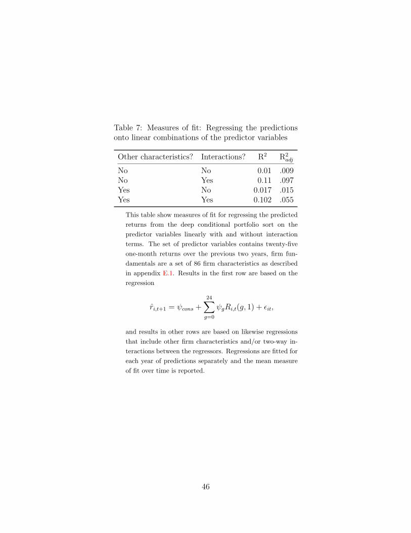
Table 7: Measures of fit: Regressing the predictionsonto linear combinations of the predictor variables

Other characteristics? Interactions? R2 R2adj

No No 0.01 .009No Yes 0.11 .097Yes No 0.017 .015Yes Yes 0.102 .055

This table show measures of fit for regressing the predicted

returns from the deep conditional portfolio sort on the

predictor variables linearly with and without interaction

terms. The set of predictor variables contains twenty-five

one-month returns over the previous two years, firm fun-

damentals are a set of 86 firm characteristics as described

in appendix E.1. Results in the first row are based on the

regression

ri,t+1 = ψcons +24∑g=0

ψgRi,t(g, 1) + ϵit,

and results in other rows are based on likewise regressions

that include other firm characteristics and/or two-way in-

teractions between the regressors. Regressions are fitted for

each year of predictions separately and the mean measure

of fit over time is reported.

46

Table 8: Strategy factor loadings: Short-term and intermediate-term return functions

Dependent variableReturn of short-term strategy Return of intermediate-term strategy

(1) (2) (3) (4) (5) (6) (7) (8) (9) (10)

Intercept 2.15 2.12 2.17 2.04 1.05 1.78 1.74 1.78 1.44 0.16(19.09) (18.47) (19.35) (17.37) (9.11) (15.01) (14.90) (15.52) (13.33) (1.65)

MKT 0.03 0.01 0.03 -0.04 0.05 0.04 0.10 0.08(1.38) (0.46) (1.64) (-2.37) (1.40) (1.32) (4.25) (4.39)

SMB 0.04 0.04 0.06 -0.05 -0.04 -0.06(0.65) (0.85) (1.95) (-0.74) (-0.93) (-2.27)

HML -0.08 -0.04 -0.06 -0.08 0.03 0.05(-1.52) (-0.85) (-1.95) (-1.15) (0.78) (1.85)

UMD 0.13 -0.11 0.35 0.27(3.80) (-4.28) (11.11) (10.71)

MT/ST strategy 0.69 0.63(15.63) (15.24)

R2 0.00 0.02 0.08 0.48 0.01 0.02 0.37 0.64IR 3.38 3.46 3.37 2.29 2.40 2.47 2.49 0.37SR 3.42 2.45N 540 540 540 540 540 540 540 540 540 540

This table shows time-series regressions of strategy returns on factors. Returns are specified in percent per month. Strategies are

based on the predictions of a deep conditional portfolio sort that relates future returns to past decile sorts of returns. Strategies

go long the highest predicted return decile and go short the lowest predicted return decile. The short-term strategy is based on

predictions from a deep conditional portfolio sort that only uses the most recent six months of past return rankings, while the

intermediate-term strategy is based on predictions that use past return rankings from seven to twelve months before portfolio

formation. Predictions are based on the model in section 3.2. The row ”MT/ST strategy” adds the intermediate-term strategy

return to the factor regressions for the short-term strategy, and adds the short-term strategy return when the intermediate-term

strategy is the dependent variable. The sample period covers 1968 to 2012, and all results are based on rolling out-of-sample

estimates of the models. MKT is the market return, SMB and HML are the Fama-French factors for size and value, and UMD

is the momentum factor. SR is the Sharpe ratio and IR is the information ratio. T-statistics are in parentheses, and standard

errors were clustered using Newey-West’s adjustment for serial correlation.

47

Table 9: Strategy factor loadings: Fama-MacBeth predictions using the six most recent one-month returns

Levels only plus relevant two-way interactions plus all two-way interactions(1) (2) (3) (4) (5) (6) (7) (8) (9) (10) (11) (12)

Intercept 1.27 1.19 1.23 0.81 1.61 1.47 1.60 1.38 1.58 1.45 1.57 1.35(6.57) (6.04) (7.21) (4.22) (9.39) (8.73) (9.67) (7.28) (9.29) (8.60) (9.44) (7.08)

MKT 0.09 0.09 0.17 0.16 0.09 0.13 0.14 0.08 0.13(1.36) (1.30) (3.10) (3.23) (1.91) (3.14) (3.11) (1.92) (3.18)

SMB -0.03 -0.03 0.10 0.10 0.09 0.09(-0.35) (-0.38) (1.10) (1.38) (1.01) (1.27)

HML -0.07 0.06 -0.23 -0.16 -0.21 -0.14(-0.48) (0.61) (-2.33) (-2.12) (-2.21) (-1.91)

UMD 0.41 0.22 0.22(4.13) (2.49) (2.59)

R2 0.01 0.01 0.22 0.04 0.09 0.17 0.04 0.08 0.16IR 1.02 1.06 0.78 1.48 1.65 1.49 1.49 1.65 1.48SR 1.09 1.59 1.60N 540 540 540 540 540 540 540 540 540 540 540 540

This table shows time-series regressions of strategy returns on factors. Returns are specified in percent per month. Strategies are

based on the predictions of a Fama-MacBeth regressions of future returns on past decile sorts of returns. Past return sorts include

decile rankings R(g,l) with length equal to 1 and gaps between 0 and 6 months, that is, predictions are based on the equation

ri,t+1 = βtcons +

6∑g=0

βtgRit(g, 1) + ϵit,

or, when two-way interactions are included,

ri,t+1 = βtcons +

24∑g=0

βtgRi,t(g, 1) +

24∑g=0

∑j>g

γtgjRi,t(g, 1)Ri,t(j, 1) + ϵi,t.

The first four columns include only the levels of past returns, the next four columns include relevant two-way interactions as identified

from the deep conditional portfolio sort and the last four columns include all two-way interactions between those returns. Strategies

go long the highest predicted return decile and go short the lowest predicted return decile. The sample period covers 1968 to 2012, and

all results are based on rolling out-of-sample estimates of the models. MKT is the market return, SMB and HML are the Fama-French

factors for size and value, and UMD is the momentum factor. SR is the Sharpe ratio and IR is the information ratio. T-statistics are

in parentheses, and standard errors were clustered using Newey-West’s adjustment for serial correlation.

48

Table 10: Fama-MacBeth regression coefficients and t-statistics: Using the six most recentone-month returns

Coefficients t-statsLevels only Relevant Int All Int Levels only Relevant Int All Int

R(0, 1) -1.63 -6.29 -6.32 -9.20 -16.30 -16.52R(1, 1) 0.06 -2.87 -2.82 0.43 -8.83 -8.69R(2, 1) 0.64 -0.93 -1.48 4.76 -4.65 -4.80R(3, 1) 0.42 -0.87 -1.06 3.44 -4.25 -3.67R(4, 1) 0.43 -0.42 -0.47 3.26 -1.99 -1.66R(5, 1) 0.62 -0.11 -0.20 5.19 -0.60 -0.72R(6, 1) 0.39 -0.33 -0.70 3.51 -1.80 -2.50R(0, 1) X R(1, 1) 2.33 2.33 12.45 12.42R(0, 1) X R(2, 1) 2.19 2.16 11.84 11.81R(0, 1) X R(3, 1) 1.55 1.54 8.83 8.88R(0, 1) X R(4, 1) 0.88 0.87 5.10 5.11R(0, 1) X R(5, 1) 0.82 0.86 5.20 5.48R(0, 1) X R(6, 1) 0.77 0.79 4.85 5.00R(1, 1) X R(2, 1) 0.60 0.53 3.64 3.21R(1, 1) X R(3, 1) 0.73 0.69 4.40 4.18R(1, 1) X R(4, 1) 0.61 0.60 3.73 3.66R(1, 1) X R(5, 1) 0.48 0.49 2.95 3.04R(1, 1) X R(6, 1) 0.54 0.55 3.25 3.27R(2, 1) X R(3, 1) 0.27 1.59R(2, 1) X R(4, 1) 0.29 1.82R(2, 1) X R(5, 1) 0.36 2.24R(2, 1) X R(6, 1) 0.20 1.20R(3, 1) X R(4, 1) -0.01 -0.08R(3, 1) X R(5, 1) -0.10 -0.66R(3, 1) X R(6, 1) 0.22 1.41R(4, 1) X R(5, 1) -0.26 -1.61R(4, 1) X R(6, 1) 0.10 0.65R(5, 1) X R(6, 1) 0.08 0.49

This table shows coefficient estimates and t-statistics for the three regression models in table 9. Past returns

include return-based functions R(g,l) with length equal to 1 and gaps between 0 and 6 months. The sample

period covers 1968 to 2012. ”Levels only” only includes the levels of past return functions and is based on

the equation

ri,t+1 = βtcons +

6∑g=0

βtgRit(g, 1) + ϵit.

”Relevant Int” includes relevant two-way interaction terms and ”All Int” includes all two-way interaction

terms between the six most recent past returns. The first three columns show the coefficient estimates times

100, and the last three columns show t-statistics.

49

Table 11: Turnover and trading costs

Low 2 3 4 5 6 7 8 9 High High-Low 9-2 8-3

Turnover (monthly) 1.56 1.74 1.76 1.78 1.78 1.8 1.78 1.76 1.76 1.62 3.18 3.5 3.52Trading cost (annual) 3.71 4.09 4.13 4.17 4.17 4.21 4.17 4.13 4.13 3.83 7.13 7.81 7.85Gross return (annual) -6.18 2.55 5.41 7.19 8.47 10.03 11.88 12.82 15.66 23.29 31.37 12.82 7.06Net return (annual) -9.88 -1.54 1.28 3.02 4.30 5.82 7.71 8.69 11.53 19.46 24.24 5.01 -.79

This table shows turnover and trading costs for the decile portfolios formed on predictions of the deep conditional portfolio sort in section

4.1. In all rows, the unit of the estimates is percent per month. The first row (turnover) shows monthly turnover for the ten decile

portfolios and for the equal-weighted hedge strategies. Turnover is computed for a strategy that goes $1 long and $1 short. Trading costs

are extrapolated using the results in Frazzini et al. (2013). The gross return is taken from table 5 and the last row computes net return as

the difference between gross return and the estimated trading costs.

50

Table 12: Strategy return correlations with fourfactors

MKT SMB HML UMD DCPS

MKT 1.000 0.306 -0.320 -0.140 0.125SMB 1.000 -0.241 -0.032 0.129HML 1.000 -0.146 -0.081UMD 1.000 0.291DCPS 1.000

Bivariate correlations between the market return

(MKT), the size (SMB) and value (HML) factors,

the momentum factor (UMD) and the strategy re-

turn from an estimated deep conditional portfolio sort

(DCPS).

51

Table 13: Firm characteristics: Portfolios based on deep conditional portfolio sort

Dec. 1 Dec. 2 Dec. 3 Dec. 4 Dec. 5 Dec. 6 Dec. 7 Dec. 8 Dec. 9 Dec. 10

RiskDebt to Equity 2.61 2.33 2.75 2.47 3.29 2.52 2.70 3.62 2.60 3.55Long-term debt to Equity 1.43 0.78 1.15 0.81 1.61 0.74 0.92 1.98 0.90 2.09Debt Ratio 0.51 0.52 0.53 0.53 0.54 0.54 0.54 0.54 0.54 0.54Beta 1.18 1.09 1.07 1.05 1.05 1.05 1.06 1.08 1.12 1.19

ProfitabilityGross Profitability 0.34 0.34 0.34 0.34 0.34 0.34 0.34 0.34 0.34 0.34Return on Assets -0.02 0.01 0.02 0.02 0.02 0.03 0.02 0.02 0.01 -0.02Return on Equity -0.15 0.03 -0.07 0.05 -0.15 0.04 0.04 -0.25 -0.18 -0.33Profit Margin -2.79 -1.31 -1.20 -1.04 -1.11 -1.60 -1.11 -0.75 -1.20 -2.41Gross Margin -1.31 -0.63 -0.26 -0.31 -0.19 -0.22 -0.27 -0.16 -0.37 -1.04Earnings per Share 0.87 1.31 1.45 1.58 1.63 1.64 1.59 1.55 1.34 0.93Basic Earnings Power Ratio 0.04 0.06 0.07 0.07 0.08 0.08 0.08 0.07 0.07 0.03

Price levelPrice Earnings Ratio 4.40 5.18 4.68 6.68 6.15 5.46 3.87 7.04 3.99 4.52Book to Market 0.79 0.81 0.83 0.83 0.83 0.83 0.83 0.83 0.83 0.87Price Sales Ratio 2.00 1.35 0.91 0.88 0.84 0.88 0.88 0.71 0.93 1.42Dividend Yield 0.04 0.03 0.03 0.04 0.04 0.03 0.04 0.03 0.03 0.03

ActivityCurrent Ratio 3.17 2.94 2.83 2.78 2.78 2.74 2.78 2.77 2.82 2.93Quick Ratio 2.05 1.88 1.81 1.77 1.76 1.74 1.76 1.77 1.79 1.86Net Working capital Ratio 0.30 0.29 0.28 0.27 0.27 0.27 0.27 0.28 0.28 0.29Cash Ratio 1.49 1.23 1.13 1.07 1.07 1.04 1.07 1.06 1.11 1.22Assets - Turnover Ratio 1.17 1.17 1.16 1.15 1.15 1.15 1.15 1.16 1.18 1.21Inventory-Turnover Ratio 20.60 19.24 20.12 23.77 22.12 23.97 23.85 21.34 22.33 20.25RandD 0.09 0.08 0.07 0.07 0.07 0.07 0.07 0.07 0.07 0.09

OthersSize 681.95 976.24 1113.54 1177.19 1180.10 1177.22 1156.71 1085.86 967.02 633.43

Each month, all stocks are ranked by their estimated expected return based on a deep conditional portfolio sort that is based on all one-month

return functions over the two years before portfolio formation. The table reports the average value of each firm characteristic in each decile over

time.

52

B Figures

Figure 2: Construction of past return-based characteristics: The investor forms a portfolio at timetf . Return-based predictor variables can be defined by two parameters; the gap between the time ofportfolio formation and the most recent month that is included in the return calculation, and the lengthof the return computation horizon. We denote the former by g, the latter by l and a return function byRi,tf (g, l) maps returns into cross-sectional decile ranks.

53

三岫�岫層岻, 層岻 > �岫層岻三岫�岫層岻, 層岻 ≤ �岫層岻

三岫�岫匝産岻, 層岻 > �岫匝産岻三岫�岫匝産岻, 層岻 ≤ �岫匝産岻三岫�岫匝珊岻, 層岻 > �岫匝珊岻三岫�岫匝珊岻, 層岻 ≤ �岫匝珊岻傘想傘匝 傘惣傘層

Figure 3: Schematic representation of a conditional portfolio sort: First, observations are sorted intotwo portfolios based on past return R(g(1), 1) and threshold τ (1). The resulting portfolios are then sortedagain on variables R(g(2a), 1) and R(g(2b), 1) with thresholds τ (2a) and τ (2b) for a total of four portfoliosS1, S2, S3 and S4.

54

𝜇𝑆1 = .073 𝜇𝑆2 = .010 𝜇𝑆3 = −.093 𝜇𝑆4 = −.024

R(0,1) ≤ 1 R 0,1 > 1 R(2,1) ≤ 2 R 2,1 > 2

R(0,1) ≤ 6 R 0,1 > 6

Figure 4: Deep conditional portfolio sort using the entire data set: First nodes

55

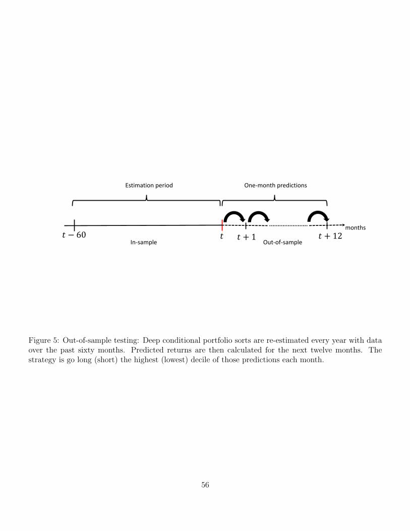
�� − 6ど � + なにEstimation period One-month predictions

� + な months

In-sample Out-of-sample

Figure 5: Out-of-sample testing: Deep conditional portfolio sorts are re-estimated every year with dataover the past sixty months. Predicted returns are then calculated for the next twelve months. Thestrategy is go long (short) the highest (lowest) decile of those predictions each month.

56

Figure 6: Annual strategy return: The strategy is based on the predictions of deep conditional portfoliosorts that relate future returns to past decile sorts of returns. Past return sorts include decile rankingsR(g,l) with length l equal to 1 and gap g between 0 and 24 months (i.e. all one-month returns overthe two years before portfolio formation). The strategy goes long the highest decile of predictions andgoes short the lowest decile of predictions each month. The figure shows the annual return for each offorty-five out-of-sample predictions.

57

Figure 7: Earned profit from investing $1 in the strategy in 1968: The strategy is based on the predictionsof a deep conditional portfolio sort that relates future returns to past decile sorts of returns. Past returnsorts include decile rankings R(g,l) with length l equal to 1 and gap g between 0 and 24 months (i.e. allone-month returns over the two years before portfolio formation). The strategy goes long the highestdecile of predictions and goes short the lowest decile of predictions each month. The figure shows theearned profit from investing $1 in the long and the short portfolio, respectively. For reference, the figurealso includes the returns to investing $1 at the riskfree rate and for investing at the rate of the marketreturn over the same horizon.

58

Figure 8: Average monthly decile return for strategy return and simple return strategies: The strategyis based on the predictions of a deep conditional portfolio sort that relates future returns to past decilesorts of returns. Past return sorts include decile rankings R(g,l) with length equal to 1 and gaps between0 and 24 months. The strategy goes long the highest decile of predictions and goes short the lowestdecile of predictions each month. Simple return strategies are plotted for comparison. R(1,5) is thestrategy that goes long (short) the highest (lowest) decile of returns over the past six months, leavingout the most recent one. R(6,6) is Novy-Marx (2012)’s intermediate return strategy that goes long(short) the highest (lowest) decile of returns that are computed over the six months that skip the mostrecent six months.

59

Figure 9: Average partial derivatives for return characteristics: The figure shows the average prediction when a characteristicis counterfactually varied from low to high values. Details are in section 3.2.3. The first row shows results when we use onlytwenty-five past one-month returns as predictors. The second row shows results for the same one-month return functions whenother firm characteristics (defined in appendix E.1) are included in the estimations as additional variables. Each column showsone return characteristic and predictions are averaged over the sample period.

60

Figure 10: Average double partial derivatives. The figure shows the average prediction when two characteristics are counterfac-tually varied from low to high values. Results are based on rolling optimization of the model and predictions are averaged overthe sample period. Details are in section 3.2.3.

61

Figure 11: Average partial derivatives in different years. The figure shows the average prediction when R(0,1), the return overthe previous month, is counterfactually varied from low to high values, and results are displayed for different years to illustratetime-variation. Results are based on rolling optimization of the model, details can be found in section 3.2.3.

62

Figure 12: Average partial derivatives in different years. The figure shows the average prediction when R(5,1), the one-monthreturn six months before portfolio formation, is counterfactually varied from low to high values, and results are displayed fordifferent years to illustrate time-variation. Results are based on rolling optimization of the model, details can be found in section3.2.3.

63

C Illustration of a conditional portfolio sort

In our illustration, we consider conditional portfolio sorts that are each based on two of the following

variables: short-term reversal, momentum, intermediate momentum, size, gross profitability, and book-

to-market. Our results complement Fama and French (2008) who sort stocks into three size portfolios

first and then sort each portfolio subsequently on a further firm characteristic. We follow the same

approach with a few modifications:

Each month, we sort stocks into one of three portfolios based on the value of a sorting variable from

the following list: short-term reversal, momentum, intermediate momentum, size, gross profitability,

and book-to-market. Short-term reversal is defined as the return over the most recent prior month,

momentum is the return over the past twelve months (excluding the most recent month) and intermediate

momentum is the return over the past twelve months excluding the most recent six months. Accounting-

based variables are constructed in a standard fashion (see appendix E.1).

Each portfolio is then further divided into ten portfolios based on a second sorting variable from

the same list and we compute the equal weighted hedge return based on the second sorting within each

of the three portfolios. Table 14 reports the equal weighted hedge returns, their associated t-statistics,

and the test of Patton and Timmermann (2010) for the monotonicity of returns over the decile sort.29

Columns labeled ”Low” contain estimates based on firms in the lowest tercile of the first sorting variable,

”Middle” and ”High” denote the next two terciles, and ”All” uses all observations without a sort on the

first sorting variable for comparison.30

First, note that all of the sorting variables achieve significant returns in the equal-weighted hedge

portfolios and pass the monotonicity test of Patton and Timmermann. To delve into the details of the

results: When firms are sorted on short-term reversal first, momentum, intermediate momentum and

value still manage to pass the t-test and the monotonicity test within each short-term reversal tercile

portfolio. Size does not work in the top tercile, and gross profitability passes the t-test, but fails to

provide monotone returns throughout all terciles. A similar picture emerges when returns are sorted

on momentum first. Value and short-term reversal work throughout all terciles, while intermediate

momentum yields (weakly) significant t-statistics in each tercile but does not pass the monotonicity

test for the low and middle groups of momentum-sorted returns. Size passes all t-tests, but fails to

provide monotone returns in the lowest two terciles. Interestingly, momentum sorts continue to work

well when firms are sorted on intermediate momentum first but the reverse is not true: Intermediate

momentum sorts do not consistently give a significant hedge return (only in low momentum stocks) or

monotone returns (only in the middle tercile of momentum stocks). Initial sorts on value or size leave the

29Since the Patton and Timmermann test for monotonicity is not (yet) standard, here is a brief summary: It computesthe pairwise difference between the average returns of adjacent decile portfolios, and then tests whether the minimum ofthese differences is greater than zero (if the research hypothesis is that returns are increasing over deciles). If the testrejects, this provides support for the research hypothesis.

30In other words, the column ”All” gives the results for an unconditional sort on the row variable.

64

monotonicity of return sorts intact, but interfere with the monotonicity and t-tests of gross profitability.

When firms are sorted on gross profitability first, equal-weighted hedge returns are significant for all

variables in all terciles, but the returns to medium gross profitability firms is not monotone when sorted

by value.

The overall picture that emerges is that of return sorts being relatively stable while accounting-

based sorts are less robust to initial sorts on some other return- or accounting-based variable. The

results illustrate the potential relevance of correlated return- and accounting-based characteristics, and

the necessity to consider conditional returns when the objective is to evaluate the importance of a

new candidate predictor variable. Variable interactions can also be relevant as is evident from the fact

conditional sorts often work only in some of the tercile portfolios.31

31It is also possible to condition on more than one variable in this setting by first doubly sorting all stocks on twovariables into, say, three categories each for a total of nine portfolios. Within each portfolio, one could then compute thesame statistics as above, and discuss the effects of conditioning on levels and interactions of variables. While, in principle,feasible for a few variables, the approach does not lend itself to an easy interpretation in higher dimensions.

65

Table 14: Conditional portfolio sorts: Average returns, t-statistics and p-values of monotonicity tests

First sort on: R(0,1)

Average return t-statistics p-value PT test

Sorting on Low Mid High All Low Mid High All Low Mid High All

R1 11 0.59 1.51 2.78 1.56 2.88 7.46 12.95 8.54 0.13 0.00 0.00 0.00

R6 6 0.71 1.13 1.74 1.19 3.98 6.32 9.48 7.69 0.00 0.00 0.00 0.00

size -1.50 -0.73 -0.21 -1.28 -5.84 -2.87 -0.86 -5.37 0.00 0.02 0.57 0.00

gross profitability 0.60 0.32 0.77 0.48 4.24 2.32 5.52 3.99 0.39 0.59 0.94 0.09

booktomarket 1.27 1.09 1.00 1.09 7.00 6.02 4.96 6.36 0.00 0.01 0.00 0.00

First sort on: R(1,11)

R0 1 -3.29 -1.02 -0.85 -1.79 -15.17 -6.01 -4.79 -10.60 0.00 0.04 0.00 0.00

R6 6 0.37 0.27 0.25 1.19 2.65 1.90 1.52 7.69 0.97 0.07 0.43 0.00

size -0.75 -1.04 -0.95 -1.28 -3.07 -4.41 -4.04 -5.37 0.62 0.67 0.00 0.00

gross profitability 0.66 0.36 0.57 0.48 4.03 2.82 4.32 3.99 0.05 0.06 0.13 0.09

booktomarket 1.39 1.23 0.67 1.09 7.50 7.25 3.52 6.36 0.00 0.00 0.00 0.00

First sort on: R(6,6)

R0 1 -2.58 -1.46 -1.38 -1.79 -12.62 -8.58 -7.15 -10.60 0.00 0.00 0.00 0.00

R1 11 1.35 1.03 1.24 1.56 7.15 6.43 6.88 8.54 0.09 0.02 0.01 0.00

size -0.92 -1.03 -0.78 -1.28 -3.72 -4.34 -3.38 -5.37 0.08 0.05 0.00 0.00

gross profitability 0.68 0.38 0.50 0.48 4.32 3.22 3.75 3.99 0.00 0.04 0.68 0.09

booktomarket 1.44 1.14 0.83 1.09 7.65 6.12 4.97 6.36 0.00 0.00 0.14 0.00

First sort on: Book to Market

R0 1 -1.74 -1.84 -2.10 -1.79 -9.09 -10.19 -10.33 -10.60 0.12 0.00 0.00 0.00

R1 11 1.98 1.35 1.10 1.56 9.39 6.54 6.11 8.54 0.00 0.00 0.00 0.00

R6 6 1.60 1.00 0.88 1.19 9.17 5.75 5.37 7.69 0.03 0.00 0.08 0.00

size -1.03 -0.73 -1.33 -1.28 -3.49 -3.21 -5.14 -5.37 0.22 0.08 0.07 0.00

66

Average return t-statistics p-value PT test

Sorting on Low Mid High All Low Mid High All Low Mid High All

gross profitability 0.79 0.66 0.37 0.48 4.69 4.53 2.85 3.99 0.32 0.00 0.19 0.09

First sort on: Gross Profitability

R0 1 -1.69 -1.95 -1.93 -1.79 -9.81 -9.74 -10.67 -10.60 0.00 0.00 0.02 0.00

R1 11 1.75 1.40 1.47 1.56 8.37 6.72 8.00 8.54 0.00 0.00 0.00 0.00

R6 6 1.48 0.99 1.02 1.19 8.28 5.45 6.49 7.69 0.00 0.00 0.01 0.00

size -1.30 -1.35 -1.18 -1.28 -4.64 -5.55 -4.40 -5.37 0.08 0.06 0.04 0.00

booktomarket 1.49 1.11 1.00 1.09 7.03 6.36 5.44 6.36 0.00 0.27 0.00 0.00

First sort on: Size

R0 1 -3.09 -1.74 -1.02 -1.79 -11.92 -9.13 -6.58 -10.60 0.00 0.00 0.09 0.00

R1 11 1.44 1.85 1.08 1.56 8.58 8.87 4.82 8.54 0.00 0.00 0.30 0.00

R6 6 0.96 1.27 1.04 1.19 5.71 7.20 5.42 7.69 0.06 0.00 0.00 0.00

gross profitability 0.14 0.68 0.40 0.48 0.87 4.43 2.95 3.99 0.06 0.23 0.23 0.09

booktomarket 0.63 1.05 0.53 1.09 3.74 5.44 2.81 6.36 1.00 0.02 0.00 0.00

67

D Greedy algorithm

To illustrate estimation of a deep conditional portfolio sort start with the conditional portfolio sort in

figure 3. Consider the portfolio S1 in that figure which is defined by variable R(g(1), 1) being less than

threshold τ (1) and variable R(g(2a), 1) being smaller than threshold τ (2a). Other portfolios can be defined

similarly by their relations between sorting variables and associated thresholds. Within each portfolio

Sl, the predicted expected return is just the average return, µl, of all firms in the portfolio, that is,

µl = Mean(ri,t+1|Firm i ∈ Sl in period t) (11)

In other words, analogous to linear regression, we are interested in approximating the conditional mean of

the outcome variable at a value of the regressor by the average of the outcome variable over observations

with close values of the regressors. The conditional portfolio sort therefore generates subsets of firm

observations that are more homogenous. Suppose for a moment that we have found such a homogenous

allocation of firms into portfolios. The prediction function could then be written as

ri,t+1 =L∑l=1

µl1(Firm i ∈ Sl in period t), (12)

giving a portfolio-specific expected return prediction for each observation. What we have described so

far is nothing more than a formal definition of the common conditional sorting methodology that we

carried out in the previous section.

Of course, the conditional sort does not need to end after two levels but can be computed at greater

depth. We consider the case in which the depth of the conditional sort, the sorting variables and

associated thresholds are not pre-selected but need to be identified from the data. Finding the optimal

solution to this problem requires solving an optimization problem that is NP complete (see (Hyafil and

Rivest (1976))), that is, there does not exist a computationally fast solution to optimizing over both

portfolios and predictions.

Instead, we adopt a greedy algorithm from the machine learning literature that proceeds in a step-

wise fashion. Let S1(g, τ) and S2(g, τ) be two portfolios that are defined by a firm’s past return decile

ranking R(g, 1) and a threshold value τ such that, as before, all observations for which R(g, 1) ≤ τ

are in portfolio S1, and all observations for which R(g, 1) > τ are in portfolio S2. At each node, all

observations that are members of that node are split into two such portfolios. The greedy algorithm

finds the past return characteristic R(g, 1) and the threshold value τ such that

(g∗, τ ∗) = argming,τ

SC(g, τ), (13)

68

where SC(g, τ) is a split criterion function which we adopt from the related machine learning literature.

The split criterion function selects the predictor variable and the associated threhold that minimize the

sum of mean squared errors in the resulting portfolios with respect to the expected returns, that is,

SC(g, τ) = minµ1

∑Rit(g,1)∈S1(g,τ)

(ri,t+1 − µ1)2

+minµ2

∑Rit(g,1)∈S2(g,τ)

(ri,t+1 − µ2)2

(14)

and the inner minimizations are solved by equation (7).This algorithm reduces a complex non-linear

estimation problem into subsets of simpler linear ones. The problem is solved in a brute-force fashion

where the value of the split criterion function is computed for each firm characteristic and each threshold

value. The optimization is repeated in each of the resulting portfolios until a. the number of observations

in a node gets too small for further splits, or b. no variable provides a sufficient improvement of the

mean squared error in equation (14). The result is a conditional portfolio sort with many levels.32

E Robustness

We start by adding a set of eighty-six additional firm characteristics to the estimation and show that,

again, the most recent returns are discovered as the most important ones. The same holds true when

we consider a much larger set of correlated past return variables; results are presented in section E.2.

In all cases, we find that the derivatives and interactions are similar to our main results.

We then turn to the question of how our return term structure result varies across firm size categories.

We repeat the analysis for three groups of stocks that are sorted by firm size first in section E.3.

E.1 Including firm characteristics

We investigate whether our results on the structural relation between future and past returns are robust

to including other firm characteristics. For this paper, we focus on the changing nature of the return

term structure result although the effect of firm characteristics (and the question of which of them can

be found by our agnostic procedure) is an interesting one in itself.33

Going back to our original set of one-month return functions, we add eighty-six common firm charac-

teristics, including size, book-to-market, gross profitability, earnings surprises, leverage and many more.

32The question of when to stop adding new levels to the conditional sort relates to a standard bias-variance trade-off.Using many levels potentially results in overfitting which would worsen the predictive power of equation (8) out of sample.Estimating only a few levels might miss important aspects of the data leading to bias. Within this sphere the number oflevels can be chosen. We stop when the number of firms in a portfolio is smaller than 100 and make sure to validate allour estimates out of samples as described in section 3.2.3.

33In ongoing work, a companion paper focuses exclusively on a large set of (mostly accounting- and earnings-based)firm characteristics.

69

The full set is described in detail in the appendix to Green et al. (2014); we generate the same set of

variables from annual and quarterly data on firm fundamentals from Compustat, daily and monthly

stock price data from CRSP, and earnings expectations and firm recommendations data from IBES.

Table 15 mirrors table 4 and shows that the strategy returns are slightly higher when accounting

variables are included in the deep conditional sorts. The out-of-sample performance is not better on

all dimensions though: The information ratio decreases in this setting. The characteristics-augmented

strategy appears to load higher on the size factor than the returns-only strategy in table 4 but loads

similarly on other factors.

Table 15: Strategy factor loadings: Including firm characteristics

(1) (2) (3) (4)

Intercept 2.56 2.46 2.46 2.28(15.65) (14.25) (14.27) (11.99)

MKT 0.12 0.06 0.10(2.75) (1.61) (2.44)

SMB 0.27 0.28(3.80) (4.53)

HML 0.01 0.07(0.11) (0.96)

UMD 0.18(3.44)

R2 0.03 0.09 0.15IR 2.66 2.75 2.63

This table shows time-series regressions of strategy returns on factors. Returns are specified in

percent per month. Strategies are based on the predictions of a deep conditional portfolio sort

that relates future returns to past decile sorts of returns and 86 firm fundamentals. Past return

sorts include decile rankings R(g,l) with length l equal to 1 and gap g between 0 and 24 months

(i.e. all one-month returns over the two years before portfolio formation). Strategies go long

the highest predicted return decile and go short the lowest predicted return decile. The sample

period covers 1968 to 2012, and all results are based on rolling out-of-sample estimates of the

models. MKT is the market return, SMB and HML are the Fama-French factors for size and

value, and UMD is the momentum factor. SR is the Sharpe ratio and IR is the information

ratio. T-statistics are in parentheses, and standard errors were clustered using Newey-West’s

adjustment for serial correlation.

Both panels show strong predictive effects of the estimated prediction algorithm, and including firm

fundamentals generally leads to somewhat better predictions in both deciles. Comparing across panels,

the top and bottom portfolios of each prediction seem to move in lockstep which is confirmed by their

correlations being above .95.

In contrast, the strategy that is additionally based on past fundamentals is significantly positively

correlated with size. This hints at the fact that the performance might vary with firm sizes, an issue

70

that we take up in section E.3.

Here, we observe an apparent difference when we look at the strategy that is additionally based on

firm fundamentals: The top portfolio formed based on these predictions loads more on size than the

other portfolios.

71

Table 16: Factor loadings of decile portfolios: Past return-based characteristics plus firm characteristics

Low 2 3 4 5 6 7 8 9 High High-Low

Average return -0.65 0.06 0.41 0.53 0.68 0.79 0.97 1.10 1.30 1.92 2.56(-2.20) (0.23) (1.55) (1.99) (2.64) (2.98) (3.65) (4.04) (4.45) (5.83) (15.65)

CAPMIntercept -1.59 -0.86 -0.51 -0.40 -0.24 -0.14 0.03 0.13 0.30 0.87 2.46

(-9.35) (-5.88) (-3.71) (-2.89) (-1.81) (-1.02) (0.22) (0.94) (1.96) (4.40) (14.25)MKT 1.08 1.05 1.05 1.06 1.05 1.06 1.08 1.11 1.15 1.20 0.12

(26.49) (28.79) (29.00) (30.96) (30.80) (29.34) (32.31) (30.99) (27.21) (24.38) (2.75)

Three-factor modelIntercept -1.69 -0.98 -0.65 -0.55 -0.40 -0.30 -0.12 -0.02 0.16 0.77 2.46

(-13.39) (-8.42) (-6.53) (-5.65) (-4.13) (-3.32) (-1.30) (-0.23) (1.51) (5.52) (14.27)MKT 0.96 0.96 0.96 0.98 0.99 0.98 0.99 1.02 1.03 1.02 0.06

(26.93) (26.67) (33.60) (32.80) (33.68) (33.06) (36.06) (32.03) (31.20) (28.87) (1.61)SMB 0.81 0.70 0.67 0.65 0.63 0.66 0.69 0.72 0.83 1.08 0.27

(8.86) (7.48) (8.72) (7.62) (7.35) (7.44) (8.49) (8.45) (10.46) (17.17) (3.80)HML 0.19 0.24 0.27 0.28 0.30 0.30 0.28 0.28 0.26 0.20 0.01

(2.52) (3.16) (3.91) (4.30) (4.31) (4.22) (4.53) (4.32) (3.85) (2.56) (0.11)

Four-factor modelIntercept -1.45 -0.79 -0.50 -0.43 -0.29 -0.21 -0.05 0.03 0.19 0.83 2.28

(-12.30) (-8.13) (-5.89) (-5.35) (-3.50) (-2.83) (-0.58) (0.45) (1.87) (5.72) (11.99)MKT 0.91 0.92 0.93 0.96 0.96 0.97 0.98 1.01 1.02 1.01 0.10

(28.35) (27.92) (34.15) (35.73) (36.40) (37.43) (41.35) (35.77) (32.56) (27.22) (2.44)SMB 0.80 0.69 0.67 0.65 0.62 0.65 0.68 0.72 0.83 1.08 0.28

(12.01) (9.63) (10.91) (8.79) (8.46) (8.20) (9.29) (8.98) (10.70) (18.40) (4.53)HML 0.11 0.17 0.22 0.25 0.26 0.27 0.25 0.26 0.25 0.18 0.07

(2.01) (2.85) (3.71) (4.36) (4.36) (4.34) (4.80) (4.68) (4.01) (2.29) (0.96)UMD -0.25 -0.20 -0.15 -0.12 -0.11 -0.09 -0.07 -0.06 -0.03 -0.07 0.18

(-5.94) (-5.13) (-4.62) (-3.23) (-3.22) (-2.37) (-2.31) (-1.71) (-0.80) (-1.83) (3.44)

This table shows time-series regressions of decile portfolio returns on factors. Returns are specified in percent per month. Each decile is

formed on the predicted returns of a deep conditional portfolio sort that relates future returns to past decile sorts of returns and 86 firm

fundamentals. Past return sorts include decile rankings R(g,l) with length l equal to 1 and gap g between 0 and 24 months. Predictions are

based on the model in section 3.2. Low denotes the lowest decile of predicted returns and High denotes the highest decile of predicted returns.

The first panel reports the average return, the second panel reports CAPM estimates, the third reports the three-factor model estimates and

the fourth panel adds momentum. MKT is the market return, SMB and HML are the Fama-French factors for size and value, and UMD

is the momentum factor. The sample period covers 1968 to 2012. T-statistics are in parentheses, and standard errors were clustered using

Newey-West’s adjustment for serial correlation.

72

Table 17 reports the top ten return-based predictor variables. The top ten return functions for

rolling and entire period optimization, again, evolve around the most recent returns, and, apart from

some changes in the exact order of predictor variables, are largely unaffected by the inclusion of other

firm characteristics.

When comparing the top ten variables to the top ten in table 6, we see that nine out of ten show

up in either list, with the exact ordering sometimes slightly altered. Recent returns are again the most

important predictors.

Table 17: Most important predictor variables: In-cluding firm characteristics

Rolling optimization Entire period optimization

R(0,1) 1 R(0,1) 1R(1,1) 0.5 R(1,1) 0.53R(2,1) 0.45 R(2,1) 0.47R(5,1) 0.44 R(3,1) 0.44R(8,1) 0.41 R(11,1) 0.38R(4,1) 0.4 R(5,1) 0.36R(3,1) 0.39 R(6,1) 0.35R(11,1) 0.39 R(7,1) 0.34R(6,1) 0.38 R(8,1) 0.34R(7,1) 0.37 R(4,1) 0.33

This table shows the most important return functions for

the deep conditional portfolio sorts that use all one-month

returns over the two years before portfolio formation and

86 additional firm characteristics. Results are shown for

both the rolling model estimation and for optimization

over the entire horizon. For rolling estimates, return func-

tions are sorted by their median importance over forty-

five years. Variable importance is measured as described

in section 3.2.3.

The second row of average partial derivatives for the most recent one-month return functions in

figure 9 mirror the patterns from the first row that did not include firm characteristics. In particular, we

observe stable linear relationships between past performance and prediction for returns that are further

than four months in the past and for the most recent past return, but we also observe non-monotone or

non-linear relationships for recent past returns in between.

Figure 13 shows double partial derivatives for return characteristics when firm characteristics are

included and corresponds to figure 10. In both cases, we observe patterns that are qualitatively very

similar and only differ in details, e.g. the interaction between R(1,1) and R(3,1) is somewhat more

pronounced.

73

Overall, we conclude that the discovered structure among return characteristics is largely unaffected

by the inclusion of additional firm characteristics.

74

Figure 13: Average double partial derivatives: Firm characteristics included. The figure shows the average prediction whentwo characteristics are counterfactually varied from low to high values. The figure shows results for return functions when 86additional firm characteristics are included in the deep conditional portfolio sort. Results are based on rolling optimization ofthe model and predictions are averaged over the sample period. Details are in section 3.2.3.

75

E.2 Expanded set of return functions

In this section, we directly give the algorithm access to standard notions of momentum, R(1,11) in our

notation, and other past return functions. More precisely, we define an expanded set of past return

functions that includes return-based characteristics {R(g, l)}, g = 0, . . . , 6; l = 1, . . . , 18, that is, the

set includes a total of 126 return-based predictor variables that are often highly correlated. Our main

findings show that the algorithm derives its predictive power from optimally using the variation in

relatively short-term returns. Is the algorithm just trying to re-create standard momentum? Or is there

more information in the individual returns than in a summary return like R(1,11)?

We repeat all of the calculations above for an algorithm that has access to this expanded set of

return functions. The first four columns of table 18 show excess returns and factor loadings for the

implementable trading strategy based on rolling estimation of deep conditional portfolio sorts. Excess

returns are about as high as in table 4 where we used the smaller set of past return functions. The

strategy’s loadings on the value and size factors are similar to the loadings in table 4 while the loading on

the momentum factor is somewhat higher. The four-factor model explains around 20% of the variation

in the strategy return. The information ratio is again much higher than what is usually reported in the

literature that employs methods that do not comprehensively deal with characteristics’ interactions and

non-linearities.

For comparison, the last four columns of table 18 show (non-implementable) strategy returns on the

hold-out sample for optimization over the entire horizon. Factor loadings are generally similar (with

the exception of the value loading in the four factor model), and excess returns are higher which, again,

should not be surprising given that optimization over the entire period uses contemporary information

on cross-sectionally correlated stocks.

We have also looked at the factor loadings of the individual decile portfolios. Since the results

are very similar to our previous results, we describe them here, and refer the interested reader to an

online appendix for the respective tables. Throughout all specifications, predicted return portfolios are

positively correlated with market beta, with no apparent relation between decile portfolio and beta value.

In the four-factor model, the loading on the market factor is around one for all deciles. Loadings on size

seem to be non-monotonic but stronger in the extreme portfolios. Interestingly, only the portfolios based

on entire sample predictions display a significant monotone relation with the value factor. We also find

again the by now familiar result that return deciles are monotonically related to the momentum factor,

which holds for all decile portfolios except for the highest one. In general, loadings on the momentum

factor are low (around -.1) but significant.

Turning to predictor variable importance in table 19, the deep conditional portfolio sorts recover

recent past returns as the most important ones. The rolling optimization in column 1 yields that the ten

most important return functions are all related to the most recent six months of returns and, what is

more, the top seven return functions are returns of length one that, taken together, summarize the most

76

Table 18: Strategy factor loadings: Expanded set of return functions

Rolling optimization Entire Period optimization(1) (2) (3) (4) (5) (6) (7) (8)

Intercept 2.37 2.31 2.36 2.10 3.13 3.04 3.05 2.84(17.65) (17.22) (18.51) (17.08) (22.48) (21.05) (21.12) (19.28)

MKT 0.07 0.04 0.09 0.10 0.08 0.12(2.22) (1.26) (3.35) (2.69) (2.28) (3.34)

SMB 0.06 0.07 0.07 0.07(0.91) (1.36) (1.20) (1.19)

HML -0.09 -0.01 -0.02 0.05(-1.36) (-0.12) (-0.33) (0.90)

UMD 0.27 0.21(8.06) (4.99)

R2 0.02 0.03 0.23 0.02 0.03 0.11IR 3.09 3.18 3.16 3.55 3.56 3.47

This table shows time-series regressions of strategy returns on factors. Returns are specified

in percent per month. Strategies are based on the predictions of a deep conditional portfolio

sort that relates future returns to past decile sorts of returns. Past returns include return-based

functions R(g,l) with length g = 1, . . . , 18 and gaps g = 0, . . . , 6. The sample period covers 1968 to

2012. Results in columns 1-4 are based on rolling out-of-sample estimates of the model, results in

column 5-8 are based on optimizing over the entire horizon. The strategy return used in columns

5-8 is computed on a hold-out sample of 30% of the data. MKT is the market return, SMB and

HML are the Fama-French factors for size and value, and UMD is the momentum factor. IR

is the information ratio. T-statistics are in parentheses, and standard errors are clustered using

Newey-West’s adjustment for serial correlation.

77

recent six month return. Notice that all one-month return-based functions in the expanded set actually

show up as the most important functions. The same result holds for optimization over the entire period

in the second column. The momentum term structure result appears to hold on average over the entire

period.

Recall that the return R(0,6), that is, the total return over the most recent six months, could have

been chosen by the algorithm in the expanded set. The fact that this return is not chosen but its

components are, illustrates that using the return over the previous year alone (and not the one-month

returns that it is based on) leads to a loss of relevant information.

Table 19: Most important predictor variables: Ex-panded set of return functions

Rolling optimization Entire period optimization

R(0,1) 1 R(1,1) 1R(1,1) 0.88 R(2,1) 0.8R(2,1) 0.69 R(3,1) 0.76R(6,1) 0.69 R(4,1) 0.74R(3,1) 0.66 R(6,1) 0.72R(4,1) 0.66 R(0,1) 0.62R(5,1) 0.61 R(5,1) 0.62R(0,2) 0.52 R(6,13) 0.43R(1,2) 0.45 R(5,10) 0.42R(1,3) 0.43 R(6,12) 0.42

This table shows the most important return functions

for a deep conditional portfolio sort that uses past re-

turns functions R(g,l) with length g = 1, . . . , 18 and gaps

g = 0, . . . , 6. Results are shown for both the rolling model

estimation and for optimization over the entire horizon.

For rolling estimates, return functions are sorted by their

median importance over forty-five years. Variable impor-

tance is measured as described in section 3.2.

E.3 Estimation by size categories

We re-estimate the model for three separate size categories of firms. Following Fama and French (2008),

we divide the sample of firms into three size categories based on NYSE breakpoints. Micro stocks

are defined as the smallest 20% of companies by market value, small companies are the next 30% of

companies, and the upper 50% make up the category of large firms. We repeat our analysis within each

size category, and compute the most relevant predictor variables for both our standard set of one-month

return variables and for the expanded set of return functions from appendix E.2. Table 20 shows that

78

the most important predictor variables are remarkably consistent across size categories, apart from some

variations in exact rank of each predictor variable. Furthermore, most predictor variables in both sets

relate to relatively recent returns.

Table 20: Most important predictor variables: Within size category

One-month returns Expanded setMicro Small Big Micro Small Big

R(0,1) 1 R(0,1) 1 R(0,1) 0.99 R(0,1) 1 R(0,1) 1 R(1,1) 1R(2,1) 0.54 R(2,1) 0.75 R(3,1) 0.72 R(1,1) 0.72 R(1,1) 0.65 R(2,1) 0.7R(5,1) 0.51 R(4,1) 0.6 R(4,1) 0.6 R(3,1) 0.63 R(0,2) 0.65 R(3,1) 0.66R(1,1) 0.5 R(1,1) 0.59 R(8,1) 0.6 R(5,1) 0.62 R(2,1) 0.63 R(5,1) 0.66R(3,1) 0.5 R(3,1) 0.59 R(1,1) 0.51 R(2,1) 0.61 R(5,1) 0.56 R(6,1) 0.66R(6,1) 0.49 R(5,1) 0.58 R(2,1) 0.5 R(6,1) 0.59 R(6,1) 0.56 R(4,1) 0.6R(4,1) 0.42 R(6,1) 0.55 R(5,1) 0.5 R(0,2) 0.56 R(3,1) 0.52 R(0,1) 0.57R(11,1) 0.4 R(7,1) 0.52 R(9,1) 0.5 R(4,1) 0.51 R(4,1) 0.5 R(0,2) 0.42R(7,1) 0.39 R(8,1) 0.47 R(11,1) 0.5 R(1,2) 0.42 R(2,2) 0.43 R(6,4) 0.34R(8,1) 0.38 R(23,1) 0.43 R(18,1) 0.5 R(0,3) 0.38 R(3,2) 0.43 R(6,6) 0.34

This table shows predictor variable importance in portfolios that are first sorted on size. Micro stocks are

defined as the smallest 20% of companies by market value, small companies are the next 30% of companies,

and the upper 50% make up the category of large firms. One-month returns include all one-month returns

over the two years before portfolio formation. The expanded set consists of 126 return-based characteristics

R(g,l) over the two years before portfolio formation with length g = 1, . . . , 18 and gaps g = 0, . . . , 6. Results

are shown for both the rolling model estimation and for optimization over the entire horizon. For rolling

estimates, return functions are sorted by their median importance over forty-five years. Variable importance

is measured as described in section 3.2.

F Additional tables and figures

For comparison, the last four columns of table 21 repeat the same exercise for the (non-implementable)

long-short strategy based on estimation over the entire sample period. Here, the returns refer to the

hold-out sample that was not used for model fitting. Factor loadings are, for the most part, similar to

those of the rolling model. However, only a small part of the time series variation can be explained by

the factor models. Even for the four factor model the R2 barely exceeds .1. The average excess returns

in these estimations vary around 3 percent per month and are actually somewhat higher than in the

rolling estimations. This should not be surprising because we optimize over the entire sample period

and returns in the training and test data sets are cross-sectionally correlated.34

34We do emphasize again that while these results can be useful to describe the structure that drove stock returns overthe past fifty years on average, they cannot be used for trading because of the forward-looking nature of the estimationwhen one optimizes over the entire period. For the same reason, they can also not be used for anomaly discovery in realtime.

79

Table 21: Strategy factor loadings

Rolling optimization Entire period optimization(1) (2) (3) (4) (5) (6) (7) (8)

Intercept 2.30 2.23 2.25 2.05 3.07 3.02 2.96 2.83(16.75) (16.04) (16.51) (14.54) (20.91) (20.40) (20.09) (17.72)

MKT 0.07 0.05 0.09 0.06 0.05 0.07(2.14) (1.53) (2.78) (1.47) (1.21) (1.85)

SMB 0.08 0.09 0.13 0.13(1.40) (1.69) (2.03) (2.11)

HML -0.03 0.04 0.09 0.13(-0.39) (0.61) (1.49) (2.16)

UMD 0.20 0.13(5.57) (2.38)

R2 0.02 0.03 0.13 0.01 0.03 0.06IR 2.90 2.93 2.82 3.37 3.34 3.24

This table shows time-series regressions of strategy returns on factors. Returns are specified in

percent per month. Strategies go long the highest predicted return decile and go short the lowest

predicted return quantile. Past returns include all one-month returns over the two years before

portfolio formation. The sample period covers 1968 to 2012. Results in columns 1-4 are based on

rolling out-of-sample estimates of the model, results in column 5-8 are based on optimizing over

the entire horizon. The strategy return used in columns 5-8 is computed on a hold-out sample

of 30% of the data. MKT is the market return, SMB and HML are the Fama-French factors

for size and value, and UMD is the momentum factor. IR is the information ratio. T-statistics

are in parentheses, and standard errors are clustered using Newey-West’s adjustment for serial

correlation.

80

The portfolios based on the hold-out sample for the entire period optimization in table 22 vary one-

to-one with the market. They are overall balanced in terms of loadings on the value and the size factor,

although the extreme portfolios display a slightly higher loading on the size factor and a slightly lower

loading on the value factor. All decile portfolios covary negatively with the standard momentum factor,

and they do so in a monotonically increasing fashion, with the lowest decile displaying the highest

covariance. But even though all decile portfolios look very similar in terms of their factor loadings,

their alphas are very different and they line up monotonically with the predictions of the estimated

model. While the spread between the extreme portfolios is largest (as is typical with sorts that include

return functions), we also observe a reasonable monotone spread across all deciles that is significant in

(unreported) Patton and Timmermann (2010) tests.

81

Table 22: Factor loadings of decile portfolios: Optimizing over the entire period

Low 2 3 4 5 6 7 8 9 High High-Low

Average return -0.87 0.03 0.47 0.54 0.75 0.87 1.13 1.25 1.56 2.20 3.07(-2.80) (0.11) (1.86) (2.28) (3.21) (3.74) (4.61) (4.81) (5.98) (7.24) (20.91)

CAPMIntercept -1.90 -0.93 -0.48 -0.37 -0.16 -0.04 0.19 0.27 0.55 1.12 3.02

(-10.16) (-6.37) (-3.67) (-3.15) (-1.24) (-0.34) (1.44) (1.91) (3.79) (5.79) (20.40)MKT 1.17 1.09 1.08 1.03 1.03 1.04 1.07 1.11 1.15 1.23 0.06

(26.57) (28.57) (31.14) (32.51) (32.34) (31.23) (29.66) (31.61) (28.25) (24.88) (1.47)

Three-factor modelIntercept -2.07 -1.10 -0.67 -0.56 -0.35 -0.23 -0.01 0.09 0.38 0.89 2.96

(-15.24) (-10.40) (-7.30) (-6.73) (-3.48) (-2.62) (-0.10) (0.94) (3.59) (6.66) (20.09)MKT 1.01 0.96 0.99 0.96 0.95 0.95 0.98 1.01 1.02 1.05 0.05

(24.12) (31.71) (41.00) (37.33) (30.27) (34.30) (31.63) (31.99) (27.15) (26.66) (1.21)SMB 0.95 0.79 0.68 0.58 0.62 0.64 0.68 0.73 0.79 1.08 0.13

(8.46) (9.72) (9.50) (9.92) (8.02) (9.45) (8.81) (8.81) (9.24) (11.20) (2.03)HML 0.21 0.22 0.28 0.28 0.29 0.28 0.28 0.24 0.23 0.30 0.09

(2.38) (3.05) (4.49) (4.88) (4.06) (4.56) (4.35) (3.41) (2.94) (3.58) (1.49)

Four-factor modelIntercept -1.79 -0.93 -0.54 -0.48 -0.29 -0.19 0.07 0.15 0.40 1.04 2.83

(-14.86) (-10.12) (-7.09) (-6.39) (-3.05) (-2.24) (0.80) (1.59) (3.93) (7.30) (17.72)MKT 0.96 0.93 0.96 0.95 0.94 0.95 0.97 1.00 1.02 1.03 0.07

(25.95) (32.74) (44.63) (39.82) (31.54) (36.26) (33.73) (34.28) (28.61) (26.64) (1.85)SMB 0.95 0.79 0.68 0.58 0.62 0.64 0.68 0.73 0.79 1.08 0.13

(10.91) (12.11) (11.59) (11.41) (8.72) (10.11) (9.82) (9.42) (9.50) (12.81) (2.11)HML 0.12 0.17 0.24 0.25 0.27 0.26 0.26 0.23 0.22 0.25 0.13

(1.82) (2.89) (4.66) (4.89) (4.27) (4.67) (4.65) (3.56) (3.08) (3.39) (2.16)UMD -0.28 -0.17 -0.14 -0.08 -0.07 -0.05 -0.08 -0.06 -0.03 -0.15 0.13

(-6.52) (-4.66) (-3.65) (-2.51) (-1.86) (-1.69) (-2.39) (-1.57) (-0.70) (-3.29) (2.38)

This table shows time-series regressions of decile portfolio returns on factors. Returns are specified in percent per month. Each decile is formed

on the predicted returns based on model estimates from optimizing over the entire horizon. Returns are computed on a hold-out sample of 30%

of the data. Low denotes the lowest decile of predicted returns and High denotes the highest decile of predicted returns. The first panel reports

the average return, the second panel reports CAPM estimates, the third reports the three-factor model estimates and the fourth panel adds

momentum. MKT is the market return, SMB and HML are the Fama-French factors for size and value, and UMD is the momentum factor.

The sample period covers 1968 to 2012. T-statistics are in parentheses, and standard errors are clustered using Newey-West’s adjustment for

serial correlation.

82