![3 Karakteristik Sensor [Compatibility Mode]](https://static.fdokumen.com/doc/165x107/6323c3a44d8439cb620d1070/3-karakteristik-sensor-compatibility-mode.jpg)
Database Compatibility for Oracle Developer's Guide - EDB ...
438
Database Compatibility for Oracle® Developer’s Guide EDB Postgres™ Advanced Server 12 July 29, 2019
-
Upload
khangminh22 -
Category
Documents
-
view
1 -
download
0
Transcript of Database Compatibility for Oracle Developer's Guide - EDB ...

Database Compatibility for Oracle®
Developer’s Guide
EDB Postgres™ Advanced Server 12
July 29, 2019

Database Compatibility for Oracle® Developer’s Guide
by EnterpriseDB® Corporation Copyright © 2007 - 2019 EnterpriseDB Corporation. All rights reserved.
EnterpriseDB Corporation, 34 Crosby Drive, Suite 201, Bedford, MA 01730, USA
T +1 781 357 3390 F +1 978 467 1307 E [email protected] www.enterprisedb.com
Database Compatibility for Oracle® Developers Guide
Copy right © 2007 - 2019 EnterpriseDB Corporation. All rights reserv ed.
3
Table of Contents
1 Introduction ........................................................................................................................... 9 1.1 What’s New .................................................................................................................. 10 1.2 Typographical Conventions Used in this Guide .................................................................. 10 1.3 Configuration Parameters Compatible with Oracl e Databases .............................................. 11
1.3.1 edb_redwood_date .................................................................................................. 13 1.3.2 edb_redwood_raw_names ........................................................................................ 13 1.3.3 edb_redwood_strings .............................................................................................. 14 1.3.4 edb_stmt_level_tx ................................................................................................... 16 1.3.5 oracle_home .......................................................................................................... 17
1.4 About the Examples Used in this Guide ............................................................................ 18 2 SQL Tutorial ........................................................................................................................ 19
2.1 Getting Started .............................................................................................................. 19 2.1.1 Sample Database .................................................................................................... 20
2.1.1.1 Sample Database Inst allation ................................................................................ 20 2.1.1.2 Sample Database Description ............................................................................... 20
2.1.2 Creating a New Table.............................................................................................. 31 2.1.3 Populating a Table With Rows.................................................................................. 32 2.1.4 Querying a Table .................................................................................................... 33 2.1.5 Joins Between Tables .............................................................................................. 35 2.1.6 Aggregate Functions ............................................................................................... 39 2.1.7 Updates ................................................................................................................. 41 2.1.8 Deletions ............................................................................................................... 42 2.1.9 The SQL Language ................................................................................................. 43
2.2 Advanced Concepts ....................................................................................................... 44 2.2.1 Views ................................................................................................................... 44 2.2.2 Foreign Keys .......................................................................................................... 46 2.2.3 The ROWNUM Pseudo-Column............................................................................... 47 2.2.4 Synonyms .............................................................................................................. 49 2.2.5 Hierarchical Queries ................................................................................................ 53
2.2.5.1 Defining the Parent/Child Relationship .................................................................. 54 2.2.5.2 Selecting the Root Nodes ..................................................................................... 54 2.2.5.3 Organization Tree in the Sample Appli cation .......................................................... 54 2.2.5.4 Node Level ........................................................................................................ 56 2.2.5.5 Ordering the Siblings .......................................................................................... 57 2.2.5.6 Retrieving the Root Node with CONNECT_BY_ROOT ........................................... 58 2.2.5.7 Retrieving a Path with SYS_C ONNECT_BY_P ATH .............................................. 62
2.2.6 Multidimensional Analysis ....................................................................................... 64 2.2.6.1 ROLLUP Extension ............................................................................................ 66 2.2.6.2 CUBE Extension ................................................................................................ 69 2.2.6.3 GROUP ING SETS Extension ............................................................................... 73 2.2.6.4 GROUP ING Function ......................................................................................... 79 2.2.6.5 GROUP ING_ID Function .................................................................................... 82
2.3 Profile Management ....................................................................................................... 85 2.3.1 Creating a New Profile ............................................................................................ 86
2.3.1.1 Creating a Password Function ............................................................................... 89 2.3.2 Altering a Profil e .................................................................................................... 93 2.3.3 Dropping a Profile .................................................................................................. 94 2.3.4 Associating a Profile with an Existing Role ................................................................ 95 2.3.5 Unlocking a Locked Account ................................................................................... 97 2.3.6 Creating a New Role Associat ed with a Profile ........................................................... 99 2.3.7 Backing up Profil e Management Functions ................................................................101
2.4 Optimizer Hints ............................................................................................................102

Database Compatibility for Oracle® Developers Guide
Copy right © 2007 - 2019 EnterpriseDB Corporation. All rights reserv ed.
4
2.4.1 Default Optimization Modes ...................................................................................104 2.4.2 Access Method Hints .............................................................................................106 2.4.3 Speci fying a Join Order ..........................................................................................110 2.4.4 Joining Relations Hints ...........................................................................................111 2.4.5 Global Hints..........................................................................................................114 2.4.6 Using the APPEND Optimizer Hint ..........................................................................117 2.4.7 Parall elism Hints ...................................................................................................118 2.4.8 Conflicting Hints ...................................................................................................123
3 Stored Procedure Language...................................................................................................124 3.1 Basic SPL Elements ......................................................................................................124
3.1.1 Charact er Set .........................................................................................................124 3.1.2 Case Sensitivity .....................................................................................................125 3.1.3 Identi fiers .............................................................................................................125 3.1.4 Quali fi ers .............................................................................................................125 3.1.5 Constants ..............................................................................................................126 3.1.6 User-Defined PL/SQL Subtypes ..............................................................................127
3.2 SPL Programs ..............................................................................................................130 3.2.1 SPL Block Structure...............................................................................................131 3.2.2 Anonymous Blocks ................................................................................................133 3.2.3 Procedures Overview .............................................................................................134
3.2.3.1 Creating a Procedure ..........................................................................................134 3.2.3.2 Calling a Procedure............................................................................................139 3.2.3.3 Deleting a Procedure ..........................................................................................139
3.2.4 Functions Overview ...............................................................................................141 3.2.4.1 Creating a Function ............................................................................................141 3.2.4.2 Calling a Function ..............................................................................................146 3.2.4.3 Deleting a Function ............................................................................................147
3.2.5 Procedure and Function Parameters ..........................................................................148 3.2.5.1 Positional vs. Named Parameter Notation ..............................................................149 3.2.5.2 Parameter Modes ...............................................................................................151 3.2.5.3 Using Default Values in Parameters .....................................................................153
3.2.6 Subprograms – Subprocedures and Subfunctions ........................................................154 3.2.6.1 Creating a Subprocedure .....................................................................................155 3.2.6.2 Creating a Subfunction .......................................................................................157 3.2.6.3 Block Relationships ...........................................................................................159 3.2.6.4 Invoking Subprograms .......................................................................................161 3.2.6.5 Using Forward Declarations ................................................................................168 3.2.6.6 Overloading Subprograms ...................................................................................169 3.2.6.7 Accessing Subprogram Vari ables .........................................................................173
3.2.7 Compilation Errors in Procedures and Functions ........................................................180 3.2.8 Program Security ...................................................................................................182
3.2.8.1 EXEC UTE Privilege ..........................................................................................182 3.2.8.2 Database Object Name Resolution .......................................................................183 3.2.8.3 Database Object Privileges ..................................................................................184 3.2.8.4 Definer’s vs. Invokers Rights ..............................................................................184 3.2.8.5 Security Example...............................................................................................185
3.3 Variable Declarations ....................................................................................................192 3.3.1 Declaring a Vari abl e ..............................................................................................192 3.3.2 Using %TYPE in Vari able Declarations ....................................................................194 3.3.3 Using %R OWTYPE in Record Declarations ..............................................................197 3.3.4 User-Defined Record Types and Record Variables .....................................................198
3.4 Basic Stat ements ...........................................................................................................201 3.4.1 NULL ..................................................................................................................201 3.4.2 Assignment ...........................................................................................................201 3.4.3 SELECT INTO .....................................................................................................202 3.4.4 INSERT ...............................................................................................................204

Database Compatibility for Oracle® Developers Guide
Copy right © 2007 - 2019 EnterpriseDB Corporation. All rights reserv ed.
5
3.4.5 UPDATE..............................................................................................................206 3.4.6 DELETE ..............................................................................................................206 3.4.7 Using the RETURNING INTO Clause......................................................................207 3.4.8 Obtaining the Result Status .....................................................................................210
3.5 Control Structures .........................................................................................................211 3.5.1 IF Statement..........................................................................................................211
3.5.1.1 IF-THEN ..........................................................................................................211 3.5.1.2 IF-THEN-ELSE ................................................................................................212 3.5.1.3 IF-THEN-ELSE IF ............................................................................................213 3.5.1.4 IF-THEN-ELSIF-ELSE ......................................................................................214
3.5.2 RETURN Statement ...............................................................................................216 3.5.3 GOTO Statement ...................................................................................................217 3.5.4 CASE Expression ..................................................................................................219
3.5.4.1 Selector CASE Expression ..................................................................................219 3.5.4.2 Searched CASE Expression .................................................................................220
3.5.5 CASE Statement ....................................................................................................222 3.5.5.1 Selector CASE Stat ement ...................................................................................222 3.5.5.2 Searched CASE st atement ...................................................................................223
3.5.6 Loops ...................................................................................................................226 3.5.6.1 LOOP ..............................................................................................................226 3.5.6.2 EXIT ...............................................................................................................226 3.5.6.3 CONTINUE......................................................................................................227 3.5.6.4 WHILE ............................................................................................................227 3.5.6.5 FOR (integer vari ant) .........................................................................................228
3.5.7 Exception Handling ...............................................................................................230 3.5.8 User-defined Exceptions .........................................................................................232 3.5.9 PRAGMA EXCEPTION_INIT................................................................................234 3.5.10 RAISE_APPLIC ATION_ERROR ............................................................................236
3.6 Transaction Control ......................................................................................................238 3.6.1 COMMIT .............................................................................................................239 3.6.2 ROLLB ACK.........................................................................................................240 3.6.3 PRAGMA AUTONOMOUS_TRANSACTION.........................................................243
3.7 Dynamic SQL ..............................................................................................................251 3.8 Static Cursors ...............................................................................................................254
3.8.1 Declaring a Cursor .................................................................................................254 3.8.2 Opening a Cursor...................................................................................................254 3.8.3 Fetching Rows From a Cursor .................................................................................255 3.8.4 Closing a Cursor....................................................................................................256 3.8.5 Using %R OWTYPE With Cursors ...........................................................................258 3.8.6 Cursor Att ributes ...................................................................................................259
3.8.6.1 %ISOP EN ........................................................................................................259 3.8.6.2 %FOUND ........................................................................................................259 3.8.6.3 %NOTFOUND .................................................................................................260 3.8.6.4 %ROWCOUNT ................................................................................................262 3.8.6.5 Summary of C ursor States and Attributes ..............................................................263
3.8.7 Cursor FOR Loop ..................................................................................................263 3.8.8 Parameteri zed Cursors ............................................................................................264
3.9 REF CURSORs and Cursor Vari ables ..............................................................................266 3.9.1 REF CURSOR Overview........................................................................................266 3.9.2 Declaring a Cursor Vari abl e ....................................................................................266
3.9.2.1 Declaring a SYS_REFC URSOR Cursor Vari able ...................................................266 3.9.2.2 Declaring a User Defined REF CURSOR Type Variable .........................................267
3.9.3 Opening a Cursor Vari able ......................................................................................267 3.9.4 Fetching Rows From a Cursor Vari abl e ....................................................................268 3.9.5 Closing a Cursor Variabl e .......................................................................................268 3.9.6 Usage Rest rictions .................................................................................................269

Database Compatibility for Oracle® Developers Guide
Copy right © 2007 - 2019 EnterpriseDB Corporation. All rights reserv ed.
6
3.9.7 Examples ..............................................................................................................270 3.9.7.1 Returning a REF CURSOR From a Function .........................................................270 3.9.7.2 Modularizing Cursor Operations ..........................................................................271
3.9.8 Dynamic Queries With REF CURSORs ....................................................................273 3.10 Collections ...................................................................................................................276
3.10.1 Associative Arrays .................................................................................................276 3.10.2 Nested Tables ........................................................................................................280 3.10.3 Varrays ................................................................................................................284
3.11 Collection Methods .......................................................................................................287 3.11.1 COUNT ...............................................................................................................287 3.11.2 DELETE ..............................................................................................................287 3.11.3 EXISTS................................................................................................................289 3.11.4 EXTEND .............................................................................................................289 3.11.5 FIRST ..................................................................................................................292 3.11.6 LAST...................................................................................................................292 3.11.7 LIMIT..................................................................................................................293 3.11.8 NEXT ..................................................................................................................293 3.11.9 PRIOR .................................................................................................................294 3.11.10 TRIM...............................................................................................................294
3.12 Working with Collections ..............................................................................................296 3.12.1 TABLE() ..............................................................................................................296 3.12.2 Using the MULTISET UNION Operator ...................................................................296 3.12.3 Using the FOR ALL Stat ement .................................................................................298 3.12.4 Using the BULK COLLECT Clause.........................................................................300
3.12.4.1 SELECT BULK COLLECT ...........................................................................301 3.12.4.2 FETCH BULK COLLECT .............................................................................302 3.12.4.3 EXEC UTE IMMEDIATE BULK COLLECT ....................................................304 3.12.4.4 RETURNING BULK COLLECT ....................................................................304
3.13 Errors and Messages .....................................................................................................307 4 Triggers ..............................................................................................................................308
4.1 Overview.....................................................................................................................308 4.2 Types of Triggers .........................................................................................................309 4.3 Creating Triggers ..........................................................................................................310 4.4 Trigger Vari abl es ..........................................................................................................315 4.5 Transactions and Exceptions ..........................................................................................317 4.6 Compound Triggers ......................................................................................................318 4.7 Trigger Examples .........................................................................................................320
4.7.1 Before Stat ement-Level Trigger...............................................................................320 4.7.2 After Statement -Level Trigger .................................................................................320 4.7.3 Before Row-Level Trigger ......................................................................................321 4.7.4 After Row-Level Trigger ........................................................................................322 4.7.5 INSTEAD OF Trigger ............................................................................................324 4.7.6 Compound Triggers ...............................................................................................325
5 Packages ............................................................................................................................328 6 Object Types and Objects .....................................................................................................329
6.1 Basic Object Concepts ...................................................................................................329 6.1.1 Attributes .............................................................................................................330 6.1.2 Methods ...............................................................................................................330 6.1.3 Overloading Methods .............................................................................................330
6.2 Object Type Components ...............................................................................................331 6.2.1 Object Type Speci fication Syntax ............................................................................331 6.2.2 Object Type Body Syntax .......................................................................................335
6.3 Creating Object Types ...................................................................................................338 6.3.1 Member Methods ...................................................................................................338 6.3.2 Static Methods ......................................................................................................339 6.3.3 Constructor Methods ..............................................................................................340
Database Compatibility for Oracle® Developers Guide
Copy right © 2007 - 2019 EnterpriseDB Corporation. All rights reserv ed.
7
6.4 Creating Object Instances ..............................................................................................343 6.5 Referencing an Object ...................................................................................................344 6.6 Dropping an Object Type...............................................................................................346
7 Open Client Library .............................................................................................................347 8 Oracle Catalog Views ...........................................................................................................348 9 Tools and Utilities................................................................................................................349 10 Table Partitioning .............................................................................................................350
10.1 Selecting a Partition Type ..............................................................................................351 10.2 Using Partition Pruning .................................................................................................352
10.2.1 Example - Partition Pruning ....................................................................................356 10.3 Partitioning Commands Compatible with Oracl e Databases ................................................359
10.3.1 CREATE TABLE…PARTITION BY ......................................................................359 10.3.1.1 Example - PARTITION BY LIST....................................................................363 10.3.1.2 Example - PARTITION BY RANGE ...............................................................364 10.3.1.3 Example - PARTITION BY HAS H .................................................................365 10.3.1.4 Example - PARTITION BY RANGE, SUBPARTITION BY LIST ......................366
10.3.2 ALTER TABLE...ADD PARTITION.......................................................................369 10.3.2.1 Example - Adding a Partition to a LIST Partitioned Table ...................................371 10.3.2.2 Example - Adding a Partition to a RANGE Partitioned Table ..............................372
10.3.3 ALTER TABLE… ADD SUBPARTITION ..............................................................374 10.3.3.1 Example - Adding a Subpartition to a LIST -RANGE Partitioned Table.................376 10.3.3.2 Example - Adding a Subpartition to a RANGE-LIST Partitioned Table.................377
10.3.4 ALTER TABLE...SPLIT PARTITION .....................................................................379 10.3.4.1 Example - Splitting a LIST Partition ................................................................381 10.3.4.2 Example - Splitting a RANGE Partition ............................................................383
10.3.5 ALTER TABLE...SPLIT SUBPARTITION ..............................................................386 10.3.5.1 Example - Splitting a LIST Subpartition ...........................................................388 10.3.5.2 Example - Splitting a RANGE Subpartition .......................................................390
10.3.6 ALTER TABLE… EXCHANGE PARTITION ..........................................................394 10.3.6.1 Example - Exchanging a Table for a Partition ....................................................395
10.3.7 ALTER TABLE… MOVE PARTITION ..................................................................399 10.3.7.1 Example - Moving a Partition to a Di fferent Tablespace ......................................400
10.3.8 ALTER TABLE… RENAME PARTITION ..............................................................402 10.3.8.1 Example - Renaming a Partition ......................................................................403
10.3.9 DROP TABLE ......................................................................................................404 10.3.10 ALTER TABLE… DR OP PARTITION ...............................................................405
10.3.10.1 Example - Deleting a Partition .........................................................................405 10.3.11 ALTER TABLE… DR OP SUBPARTITION .........................................................407
10.3.11.1 Example - Deleting a Subpartition ...................................................................407 10.3.12 TRUNCATE TABLE.........................................................................................409
10.3.12.1 Example - Emptying a Table ...........................................................................409 10.3.13 ALTER TABLE… TRUNCATE PARTITION ......................................................412
10.3.13.1 Example - Emptying a Partition .......................................................................412 10.3.14 ALTER TABLE… TRUNCATE SUBPARTITION ...............................................415
10.3.14.1 Example - Emptying a Subpartition ..................................................................415 10.4 Handling Stray Values in a LIST or RANGE Partitioned Table ...........................................418 10.5 Speci fying Multipl e Partitioning Keys in a RANGE Partitioned Table ..................................424 10.6 Retrieving Information about a Partitioned Table ..............................................................425
10.6.1 Table Partitioning Views - Reference .......................................................................426 10.6.1.1 ALL_P ART_TABLES ...................................................................................426 10.6.1.2 ALL_TAB_P ARTITIONS ..............................................................................427 10.6.1.3 ALL_TAB_S UBPARTITIONS .......................................................................428 10.6.1.4 ALL_P ART_KEY_COLUMNS ......................................................................429 10.6.1.5 ALL_S UBPART_KEY_C OLUMNS ...............................................................429
11 ECPGPlus .......................................................................................................................430 12 dblink_ora .......................................................................................................................431

Database Compatibility for Oracle® Developers Guide
Copy right © 2007 - 2019 EnterpriseDB Corporation. All rights reserv ed.
8
12.1 dblink_ora Functions and Procedures ...............................................................................432 12.1.1 dblink_ora_connect() .............................................................................................432 12.1.2 dblink_ora_st atus() ................................................................................................433 12.1.3 dblink_ora_disconnect() .........................................................................................433 12.1.4 dblink_ora_record() ...............................................................................................434 12.1.5 dblink_ora_call() ...................................................................................................434 12.1.6 dblink_ora_exec() ..................................................................................................434 12.1.7 dblink_ora_copy()..................................................................................................435
12.2 Calling dblink_ora Functions ..........................................................................................436 13 System Catalog Tables ......................................................................................................437 14 Acknowledgements ..........................................................................................................438

Database Compatibility for Oracle® Developers Guide
Copy right © 2007 - 2019 EnterpriseDB Corporation. All rights reserv ed.
9
1 Introduction
Database Compatibility for Oracle means that an application runs in an Oracle environment as well as in the EDB Postgres Advanced Server (Advanced Server)
environment with minimal or no changes to the application code. Developing an application that is compatible with Oracle databases in the Advanced Server requires special attention to which features are used in the construction of the application. For example, developing a compatible application means choosing compatible:
System and built-in functions for use in SQL statements and procedural logic.
Stored Procedure Language (SPL) when creating database server-side application logic for stored procedures, functions, triggers, and packages.
Data types that are compatible with Oracle databases
SQL statements that are compatible with Oracle SQL
System catalog views that are compatible with Oracle’s data dictionary
For detailed information about the compatible SQL syntax, data types, and views, please see the Database Compatibility for Oracle Developers Reference Guide.
The compatibility offered by the procedures and functions that are part of the Built -in
packages is documented in the Database Compatibility for Oracle Developers Built-in Packages Guide.
For information about using the compatible tools and utilities (EDB*Plus, EDB*Loader, DRITA, and EDB*Wrap) that are included with an Advanced Server installation, please see the Database Compatibility for Oracle Developers Tools and Utilities Guide.
For applications written using the Oracle Call Interface (OCI), EnterpriseDB’s Open Client Library (OCL) provides interoperability with these applications. For detailed
information about using the Open Client Library, please see the EDB Postgres Advanced Server OCI Connector Guide.
Advanced Server contains a rich set of features that enables development of database applications for either PostgreSQL or Oracle. For more information about all of the
features of Advanced Server, please consult the user documentation available at the EnterpriseDB website.
Advanced Server documentation is available at:
https://www.enterprisedb.com/resources/product-documentation

Database Compatibility for Oracle® Developers Guide
Copy right © 2007 - 2019 EnterpriseDB Corporation. All rights reserv ed.
10
1.1 What’s New
The following database compatibility for Oracle features have been added to Advanced Server 11 to create Advanced Server 12:
Advanced Server introduces COMPOUND TRIGGERS, which are stored as a PL block that executes in response to a specified triggering event. For information, see the Database Compatibility for Oracle Developer’s Guide.
Advanced Server now supports new VIEWS that provide information that is compatible with the Oracle data dictionary views. For information, see the Database Compatibility for Oracle Developer's Reference Guide.
Advanced Server has added the LISTAGG function to support string aggregation that concatenates data from multiple rows into a single row in an ordered manner.
For information, see the Database Compatibility for Oracle Developer's Reference Guide.
Advanced Server now supports CAST(MULTISET)function, allowing subquery
output to be CAST to a nested table type. For information, see the Database Compatibility for Oracle Developer's Reference Guide.
Advanced Server has added the MEDIAN function to calculate a median value from the set of provided values. For information, see the Database Compatibility for Oracle Developer's Reference Guide.
Advanced Server has added the SYS_GUID function to generate and return a
globally unique identifier in the form of 16-bytes of RAW data. For information, see the Database Compatibility for Oracle Developer's Reference Guide.
Advanced Server now supports an Oracle-compatible SELECT UNIQUE clause in
addition to an existing SELECT DISTINCT clause. For information, see the Database Compatibility for Oracle Developer's Reference Guide.
1.2 Typographical Conventions Used in this Guide
Certain typographical conventions are used in this manual to clarify the meaning and
usage of various commands, statements, programs, examples, etc. This section provides a summary of these conventions.
In the following descriptions a term refers to any word or group of words which may be language keywords, user-supplied values, literals, etc. A term’s exact meaning depends upon the context in which it is used.
Database Compatibility for Oracle® Developers Guide
Copy right © 2007 - 2019 EnterpriseDB Corporation. All rights reserv ed.
11
Italic font introduces a new term, typically, in the sentence that defines it for the first time.
Fixed-width (mono-spaced) font is used for terms that must be given literally such as SQL commands, specific table and column names used in the
examples, programming language keywords, etc. For example, SELECT * FROM emp;
Italic fixed-width font is used for terms for which the user must
substitute values in actual usage. For example, DELETE FROM table_name;
A vertical pipe | denotes a choice between the terms on either side of the pipe. A
vertical pipe is used to separate two or more alternative terms within square brackets (optional choices) or braces (one mandatory choice).
Square brackets [ ] denote that one or none of the enclosed term(s) may be
substituted. For example, [ a | b ], means choose one of “a” or “b” or neither of the two.
Braces {} denote that exactly one of the enclosed alternatives must be specified.
For example, { a | b }, means exactly one of “a” or “b” must be specified.
Ellipses ... denote that the proceeding term may be repeated. For example, [ a |
b ] ... means that you may have the sequence, “b a a b a”.
1.3 Configuration Parameters Compatible with Oracle Databases
EDB Postgres Advanced Server supports the development and execution of applications
compatible with PostgreSQL and Oracle. Some system behaviors can be altered to act in a more PostgreSQL or in a more Oracle compliant manner; these behaviors are controlled
by configuration parameters. Modifying the parameters in the postgresql.conf file
changes the behavior for all databases in the cluster, while a user or group can SET the parameter value on the command line, effecting only their session. These parameters are:
edb_redwood_date – Controls whether or not a time component is stored in
DATE columns. For behavior compatible with Oracle databases, set
edb_redwood_date to TRUE. See Section 1.3.1.
edb_redwood_raw_names – Controls whether database object names appear in uppercase or lowercase letters when viewed from Oracle system catalogs. For
behavior compatible with Oracle databases, edb_redwood_raw_names is set to
its default value of FALSE. To view database object names as they are actually
stored in the PostgreSQL system catalogs, set edb_redwood_raw_names to
TRUE. See Section 1.3.2.
edb_redwood_strings – Equates NULL to an empty string for purposes of string concatenation operations. For behavior compatible with Oracle databases,
set edb_redwood_strings to TRUE. See Section 1.3.3.

Database Compatibility for Oracle® Developers Guide
Copy right © 2007 - 2019 EnterpriseDB Corporation. All rights reserv ed.
12
edb_stmt_level_tx – Isolates automatic rollback of an aborted SQL command to statement level rollback only – the entire, current transaction is not automatically rolled back as is the case for default PostgreSQL behavior. For
behavior compatible with Oracle databases, set edb_stmt_level_tx to TRUE; however, use only when absolutely necessary. See Section 1.3.4.
oracle_home – Point Advanced Server to the correct Oracle installation directory. See Section 1.3.5.

Database Compatibility for Oracle® Developers Guide
Copy right © 2007 - 2019 EnterpriseDB Corporation. All rights reserv ed.
13
1.3.1 edb_redwood_date
When DATE appears as the data type of a column in the commands, it is translated to
TIMESTAMP at the time the table definition is stored in the data base if the configuration
parameter edb_redwood_date is set to TRUE. Thus, a time component will also be stored in the column along with the date. This is consistent with Oracle’s DATE data type.
If edb_redwood_date is set to FALSE the column’s data type in a CREATE TABLE or
ALTER TABLE command remains as a native PostgreSQL DATE data type and is stored as
such in the database. The PostgreSQL DATE data type stores only the date without a time component in the column.
Regardless of the setting of edb_redwood_date, when DATE appears as a data type in any other context such as the data type of a variable in an SPL declaration section, or the data type of a formal parameter in an SPL procedure or SPL function, or the return type
of an SPL function, it is always internally translated to a TIMESTAMP and thus, can handle a time component if present.
See the Database Compatibility for Oracle Developers Reference Guide for more information about date/time data types.
1.3.2 edb_redwood_raw_names
When edb_redwood_raw_names is set to its default value of FALSE, database object names such as table names, column names, trigger names, program names, user names, etc. appear in uppercase letters when viewed from Oracle catalogs (for a complete list of
supported catalog views, see the Database Compatibility for Oracle Developers Reference Guide). In addition, quotation marks enclose names that were created with enclosing quotation marks.
When edb_redwood_raw_names is set to TRUE, the database object names are displayed exactly as they are stored in the PostgreSQL system catalogs when viewed from the Oracle catalogs. Thus, names created without enclosing quotation marks appear in lowercase as expected in PostgreSQL. Names created with enclosing quotation marks appear exactly as they were created, but without the quotation marks.
For example, the following user name is created, and then a session is started with that user.
CREATE USER reduser IDENTIFIED BY password;
edb=# \c - reduser
Password for user reduser:
You are now connected to database "edb" as user "reduser".

Database Compatibility for Oracle® Developers Guide
Copy right © 2007 - 2019 EnterpriseDB Corporation. All rights reserv ed.
14
When connected to the database as reduser, the following tables are created.
CREATE TABLE all_lower (col INTEGER);
CREATE TABLE ALL_UPPER (COL INTEGER);
CREATE TABLE "Mixed_Case" ("Col" INTEGER);
When viewed from the Oracle catalog, USER_TABLES, with edb_redwood_raw_names
set to the default value FALSE, the names appear in uppercase except for the Mixed_Case name, which appears as created and also with enclosing quotation marks.
edb=> SELECT * FROM USER_TABLES;
schema_name | table_name | tablespace_name | status | temporary
-------------+--------------+-----------------+--------+-----------
REDUSER | ALL_LOWER | | VALID | N
REDUSER | ALL_UPPER | | VALID | N
REDUSER | "Mixed_Case" | | VALID | N
(3 rows)
When viewed with edb_redwood_raw_names set to TRUE, the names appear in
lowercase except for the Mixed_Case name, which appears as created, but now without the enclosing quotation marks.
edb=> SET edb_redwood_raw_names TO true;
SET
edb=> SELECT * FROM USER_TABLES;
schema_name | table_name | tablespace_name | status | temporary
-------------+------------+-----------------+--------+-----------
reduser | all_lower | | VALID | N
reduser | all_upper | | VALID | N
reduser | Mixed_Case | | VALID | N
(3 rows)
These names now match the case when viewed from the PostgreSQL pg_tables catalog.
edb=> SELECT schemaname, tablename, tableowner FROM pg_tables WHERE
tableowner = 'reduser';
schemaname | tablename | tableowner
------------+------------+------------
reduser | all_lower | reduser
reduser | all_upper | reduser
reduser | Mixed_Case | reduser
(3 rows)
1.3.3 edb_redwood_strings
In Oracle, when a string is concatenated with a null variable or null column, the result is the original string; however, in PostgreSQL concatenation of a string with a null variable
or null column gives a null result. If the edb_redwood_strings parameter is set to
TRUE, the aforementioned concatenation operation results in the original string as done
by Oracle. If edb_redwood_strings is set to FALSE, the native PostgreSQL behavior is maintained.
Database Compatibility for Oracle® Developers Guide
Copy right © 2007 - 2019 EnterpriseDB Corporation. All rights reserv ed.
15
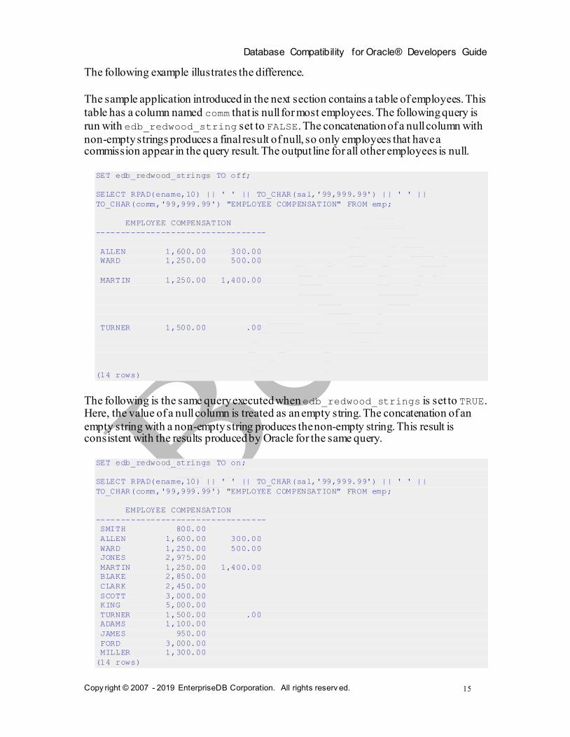
The following example illustrates the difference.
The sample application introduced in the next section contains a table of employees. This
table has a column named comm that is null for most employees. The following query is
run with edb_redwood_string set to FALSE. The concatenation of a null column with
non-empty strings produces a final result of null, so only employees that have a commission appear in the query result. The output line for all other employees is null.
SET edb_redwood_strings TO off;
SELECT RPAD(ename,10) || ' ' || TO_CHAR(sal,'99,999.99') || ' ' ||
TO_CHAR(comm,'99,999.99') "EMPLOYEE COMPENSATION" FROM emp;
EMPLOYEE COMPENSATION
----------------------------------
ALLEN 1,600.00 300.00
WARD 1,250.00 500.00
MARTIN 1,250.00 1,400.00
TURNER 1,500.00 .00
(14 rows)
The following is the same query executed when edb_redwood_strings is set to TRUE. Here, the value of a null column is treated as an empty string. The concatenation of an
empty string with a non-empty string produces the non-empty string. This result is consistent with the results produced by Oracle for the same query.
SET edb_redwood_strings TO on;
SELECT RPAD(ename,10) || ' ' || TO_CHAR(sal,'99,999.99') || ' ' ||
TO_CHAR(comm,'99,999.99') "EMPLOYEE COMPENSATION" FROM emp;
EMPLOYEE COMPENSATION
----------------------------------
SMITH 800.00
ALLEN 1,600.00 300.00
WARD 1,250.00 500.00
JONES 2,975.00
MARTIN 1,250.00 1,400.00
BLAKE 2,850.00
CLARK 2,450.00
SCOTT 3,000.00
KING 5,000.00
TURNER 1,500.00 .00
ADAMS 1,100.00
JAMES 950.00
FORD 3,000.00
MILLER 1,300.00
(14 rows)
Database Compatibility for Oracle® Developers Guide
Copy right © 2007 - 2019 EnterpriseDB Corporation. All rights reserv ed.
16
1.3.4 edb_stmt_level_tx
In Oracle, when a runtime error occurs in a SQL command, all the updates on the
database caused by that single command are rolled back. This is called statement level
transaction isolation. For example, if a single UPDATE command successfully updates five rows, but an attempt to update a sixth row results in an exception, the updates to all
six rows made by this UPDATE command are rolled back. The effects of prior SQL
commands that have not yet been committed or rolled back are pending until a COMMIT
or ROLLBACK command is executed.
In PostgreSQL, if an exception occurs while executing a SQL command, all the updates
on the database since the start of the transaction are rolled back. In addition, the
transaction is left in an aborted state and either a COMMIT or ROLLBACK command must be issued before another transaction can be started.
If edb_stmt_level_tx is set to TRUE, then an exception will not automatically roll back prior uncommitted database updates, emulating the Oracle behavior. If
edb_stmt_level_tx is set to FALSE, then an exception will roll back uncommitted database updates.
Note: Use edb_stmt_level_tx set to TRUE only when absolutely necessary, as this may cause a negative performance impact.
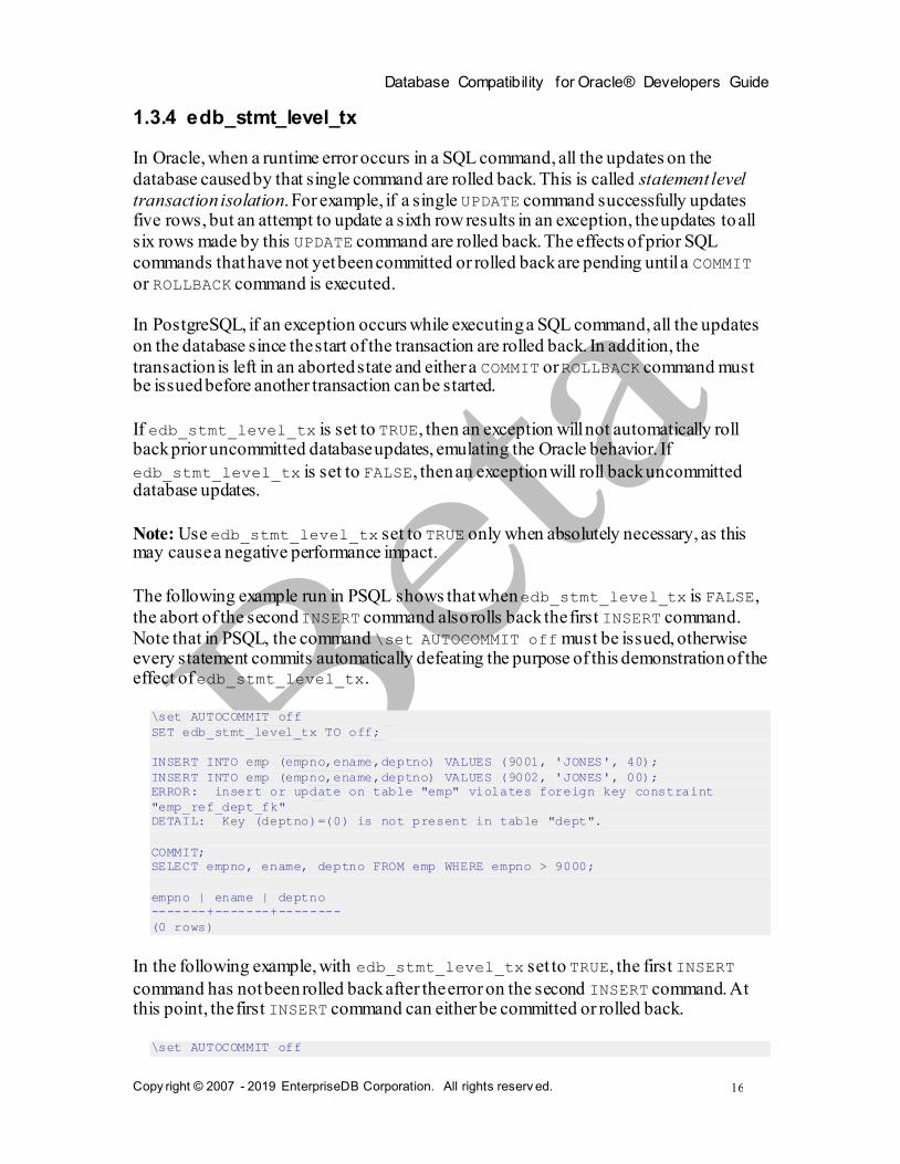
The following example run in PSQL shows that when edb_stmt_level_tx is FALSE,
the abort of the second INSERT command also rolls back the first INSERT command.
Note that in PSQL, the command \set AUTOCOMMIT off must be issued, otherwise every statement commits automatically defeating the purpose of this demonstration of the effect of edb_stmt_level_tx.
\set AUTOCOMMIT off
SET edb_stmt_level_tx TO off;
INSERT INTO emp (empno,ename,deptno) VALUES (9001, 'JONES', 40);
INSERT INTO emp (empno,ename,deptno) VALUES (9002, 'JONES', 00);
ERROR: insert or update on table "emp" violates foreign key constraint
"emp_ref_dept_fk"
DETAIL: Key (deptno)=(0) is not present in table "dept".
COMMIT;
SELECT empno, ename, deptno FROM emp WHERE empno > 9000;
empno | ename | deptno
-------+-------+--------
(0 rows)
In the following example, with edb_stmt_level_tx set to TRUE, the first INSERT
command has not been rolled back after the error on the second INSERT command. At this point, the first INSERT command can either be committed or rolled back.
\set AUTOCOMMIT off

Database Compatibility for Oracle® Developers Guide
Copy right © 2007 - 2019 EnterpriseDB Corporation. All rights reserv ed.
17
SET edb_stmt_level_tx TO on;
INSERT INTO emp (empno,ename,deptno) VALUES (9001, 'JONES', 40);
INSERT INTO emp (empno,ename,deptno) VALUES (9002, 'JONES', 00);
ERROR: insert or update on table "emp" violates foreign key constraint
"emp_ref_dept_fk"
DETAIL: Key (deptno)=(0) is not present in table "dept".
SELECT empno, ename, deptno FROM emp WHERE empno > 9000;
empno | ename | deptno
-------+-------+--------
9001 | JONES | 40
(1 row)
COMMIT;
A ROLLBACK command could have been issued instead of the COMMIT command in
which case the insert of employee number 9001 would have been rolled back as well.
1.3.5 oracle_home
Before creating a link to an Oracle server, you must direct Advanced Server to the correct
Oracle home directory. Set the LD_LIBRARY_PATH environment variable on Linux (or PATH on Windows) to the lib directory of the Oracle client installation directory.
For Windows only, you can instead set the value of the oracle_home configuration
parameter in the postgresql.conf file. The value specified in the oracle_home configuration parameter will override the Windows PATH environment variable.
The LD_LIBRARY_PATH environment variable on Linux (PATH environment variable or
oracle_home configuration parameter on Windows) must be set properly each time you start Advanced Server.
When using a Linux service script to start Advanced Server, be sure LD_LIBRARY_PATH
has been set within the service script so it is in effect when the script invokes the pg_ctl utility to start Advanced Server.
For Windows only: To set the oracle_home configuration parameter in the postgresql.conf file, edit the file, adding the following line:
oracle_home = 'lib_directory '
Substitute the name of the Windows directory that contains oci.dll for lib_directory.
After setting the oracle_home configuration parameter, you must restart the server for the changes to take effect. Restart the server from the Windows Services console.
Database Compatibility for Oracle® Developers Guide
Copy right © 2007 - 2019 EnterpriseDB Corporation. All rights reserv ed.
18
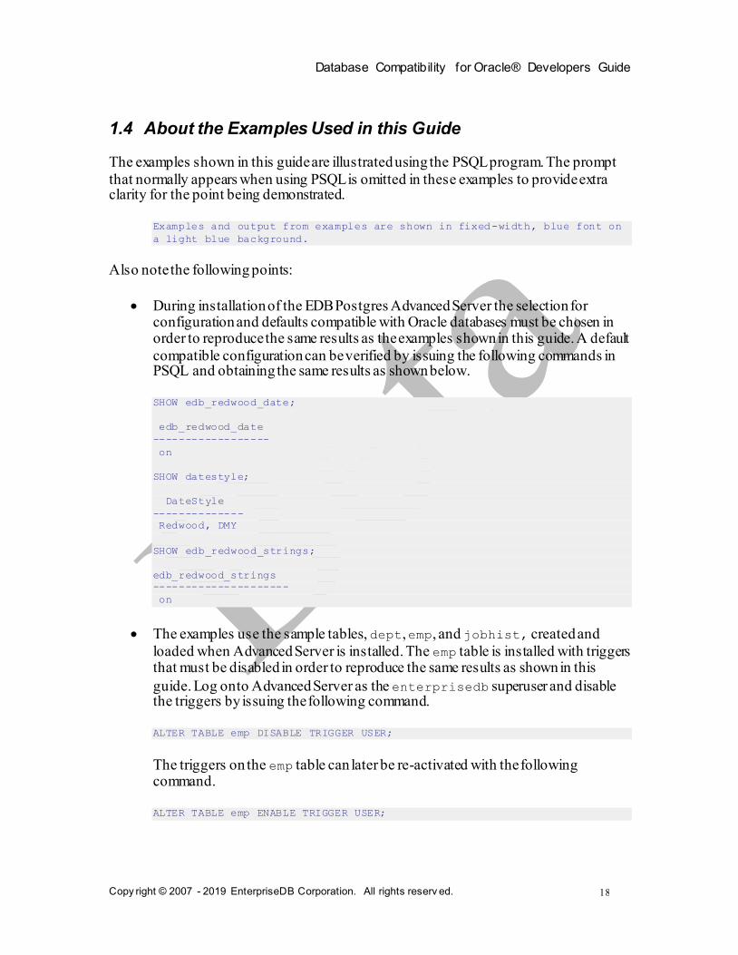
1.4 About the Examples Used in this Guide
The examples shown in this guide are illustrated using the PSQL program. The prompt
that normally appears when using PSQL is omitted in these examples to provide extra clarity for the point being demonstrated.
Examples and output from examples are shown in fixed-width, blue font on
a light blue background.
Also note the following points:
During installation of the EDB Postgres Advanced Server the selection for configuration and defaults compatible with Oracle databases must be chosen in order to reproduce the same results as the examples shown in this guide. A default
compatible configuration can be verified by issuing the following commands in PSQL and obtaining the same results as shown below.
SHOW edb_redwood_date;
edb_redwood_date
------------------
on
SHOW datestyle;
DateStyle
--------------
Redwood, DMY
SHOW edb_redwood_strings;
edb_redwood_strings
---------------------
on
The examples use the sample tables, dept, emp, and jobhist, created and
loaded when Advanced Server is installed. The emp table is installed with triggers that must be disabled in order to reproduce the same results as shown in this
guide. Log onto Advanced Server as the enterprisedb superuser and disable the triggers by issuing the following command.
ALTER TABLE emp DISABLE TRIGGER USER;
The triggers on the emp table can later be re-activated with the following command.
ALTER TABLE emp ENABLE TRIGGER USER;

Database Compatibility for Oracle® Developers Guide
Copy right © 2007 - 2019 EnterpriseDB Corporation. All rights reserv ed.
19
2 SQL Tutorial
This section is an introduction to the SQL language for those new to relational database management systems. Basic operations such as creating, populating, querying, and updating tables are discussed along with examples.
More advanced concepts such as view, foreign keys, and transactions are discussed as well.
2.1 Getting Started
Advanced Server is a relational database management system (RDBMS). That means it
is a system for managing data stored in relations. A relation is essentially a mathematical term for a table. The notion of storing data in tables is so commonplace today that it might seem inherently obvious, but there are a number of other ways of organizing
databases. Files and directories on Unix-like operating systems form an example of a hierarchical database. A more modern development is the object-oriented database.
Each table is a named collection of rows. Each row of a given table has the same set of
named columns, and each column is of a specific data type. Whereas columns have a fixed order in each row, it is important to remember that SQL does not guarantee the order of the rows within the table in any way (although they can be explicitly sorted for display).
Tables are grouped into databases, and a collection of databases managed by a single Advanced Server instance constitutes a database cluster.
Database Compatibility for Oracle® Developers Guide
Copy right © 2007 - 2019 EnterpriseDB Corporation. All rights reserv ed.
20
2.1.1 Sample Database
Throughout this documentation we will be working with a sample database to help explain some basic to advanced level database concepts.
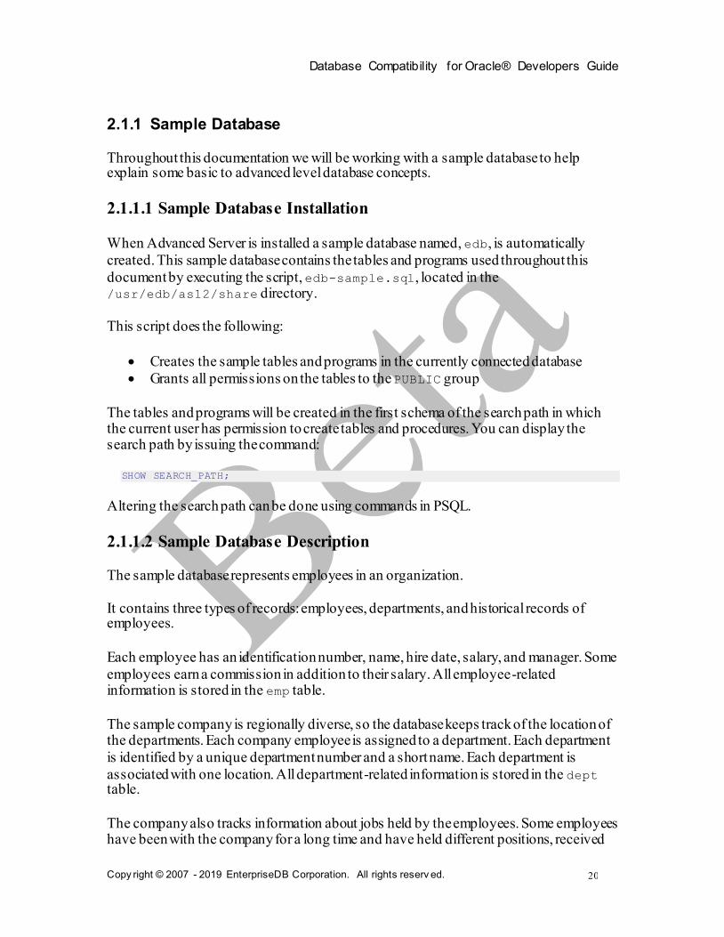
2.1.1.1 Sample Database Installation
When Advanced Server is installed a sample database named, edb, is automatically
created. This sample database contains the tables and programs used throughout this
document by executing the script, edb-sample.sql, located in the /usr/edb/as12/share directory.
This script does the following:
Creates the sample tables and programs in the currently connected database
Grants all permissions on the tables to the PUBLIC group
The tables and programs will be created in the first schema of the search path in which the current user has permission to create tables and procedures. You can display the search path by issuing the command:
SHOW SEARCH_PATH;
Altering the search path can be done using commands in PSQL.
2.1.1.2 Sample Database Description
The sample database represents employees in an organization.
It contains three types of records: employees, departments, and historical records of employees.
Each employee has an identification number, name, hire date, salary, and manager. Some
employees earn a commission in addition to their salary. All employee-related information is stored in the emp table.
The sample company is regionally diverse, so the database keeps track of the location of the departments. Each company employee is assigned to a department. Each department
is identified by a unique department number and a short name. Each department is
associated with one location. All department-related information is stored in the dept table.
The company also tracks information about jobs held by the employees. Some employees have been with the company for a long time and have held different positions, received

Database Compatibility for Oracle® Developers Guide
Copy right © 2007 - 2019 EnterpriseDB Corporation. All rights reserv ed.
21
raises, switched departments, etc. When a change in employee status occurs, the company records the end date of the former position. A new job record is added with the start date
and the new job title, department, salary, and the reason for the status change. All employee history is maintained in the jobhist table.
The following is an entity relationship diagram of the sample database tables.
deptno
dname
loc
empno
ename
job
mgr
hiredate
sal
comm
deptno
empno
s tartdate
enddate
job
sal
comm
deptno
chgdesc
emp
dept
jobhist
Figure 1 Sample Database Tables

Database Compatibility for Oracle® Developers Guide
Copy right © 2007 - 2019 EnterpriseDB Corporation. All rights reserv ed.
22
The following is the edb-sample.sql script.
--
-- Script that creates the 'sample' tables, views, procedures,
-- functions, triggers, etc.
--
-- Start new transaction - commit all or nothing
--
BEGIN;
/
--
-- Create and load tables used in the documentation examples.
--
-- Create the 'dept' table
--
CREATE TABLE dept (
deptno NUMBER(2) NOT NULL CONSTRAINT dept_pk PRIMARY KEY,
dname VARCHAR2(14) CONSTRAINT dept_dname_uq UNIQUE,
loc VARCHAR2(13)
);
--
-- Create the 'emp' table
--
CREATE TABLE emp (
empno NUMBER(4) NOT NULL CONSTRAINT emp_pk PRIMARY KEY,
ename VARCHAR2(10),
job VARCHAR2(9),
mgr NUMBER(4),
hiredate DATE,
sal NUMBER(7,2) CONSTRAINT emp_sal_ck CHECK (sal > 0),
comm NUMBER(7,2),
deptno NUMBER(2) CONSTRAINT emp_ref_dept_fk
REFERENCES dept(deptno)
);
--
-- Create the 'jobhist' table
--
CREATE TABLE jobhist (
empno NUMBER(4) NOT NULL,
startdate DATE NOT NULL,
enddate DATE,
job VARCHAR2(9),
sal NUMBER(7,2),
comm NUMBER(7,2),
deptno NUMBER(2),
chgdesc VARCHAR2(80),
CONSTRAINT jobhist_pk PRIMARY KEY (empno, startdate),
CONSTRAINT jobhist_ref_emp_fk FOREIGN KEY (empno)
REFERENCES emp(empno) ON DELETE CASCADE,
CONSTRAINT jobhist_ref_dept_fk FOREIGN KEY (deptno)
REFERENCES dept (deptno) ON DELETE SET NULL,
CONSTRAINT jobhist_date_chk CHECK (startdate <= enddate)
);
--
-- Create the 'salesemp' view
--
CREATE OR REPLACE VIEW salesemp AS
SELECT empno, ename, hiredate, sal, comm FROM emp WHERE job = 'SALESMAN';
--
-- Sequence to generate values for function 'new_empno'.

Database Compatibility for Oracle® Developers Guide
Copy right © 2007 - 2019 EnterpriseDB Corporation. All rights reserv ed.
23
--
CREATE SEQUENCE next_empno START WITH 8000 INCREMENT BY 1;
--
-- Issue PUBLIC grants
--
GRANT ALL ON emp TO PUBLIC;
GRANT ALL ON dept TO PUBLIC;
GRANT ALL ON jobhist TO PUBLIC;
GRANT ALL ON salesemp TO PUBLIC;
GRANT ALL ON next_empno TO PUBLIC;
--
-- Load the 'dept' table
--
INSERT INTO dept VALUES (10,'ACCOUNTING','NEW YORK');
INSERT INTO dept VALUES (20,'RESEARCH','DALLAS');
INSERT INTO dept VALUES (30,'SALES','CHICAGO');
INSERT INTO dept VALUES (40,'OPERATIONS','BOSTON');
--
-- Load the 'emp' table
--
INSERT INTO emp VALUES (7369,'SMITH','CLERK',7902,'17-DEC-80',800,NULL,20);
INSERT INTO emp VALUES (7499,'ALLEN','SALESMAN',7698,'20-FEB-
81',1600,300,30);
INSERT INTO emp VALUES (7521,'WARD','SALESMAN',7698,'22-FEB-81',1250,500,30);
INSERT INTO emp VALUES (7566,'JONES','MANAGER',7839,'02-APR-
81',2975,NULL,20);
INSERT INTO emp VALUES (7654,'MARTIN','SALESMAN',7698,'28-SEP-
81',1250,1400,30);
INSERT INTO emp VALUES (7698,'BLAKE','MANAGER',7839,'01-MAY-
81',2850,NULL,30);
INSERT INTO emp VALUES (7782,'CLARK','MANAGER',7839,'09-JUN-
81',2450,NULL,10);
INSERT INTO emp VALUES (7788,'SCOTT','ANALYST',7566,'19-APR-
87',3000,NULL,20);
INSERT INTO emp VALUES (7839,'KING','PRESIDENT',NULL,'17-NOV-
81',5000,NULL,10);
INSERT INTO emp VALUES (7844,'TURNER','SALESMAN',7698,'08-SEP-81',1500,0,30);
INSERT INTO emp VALUES (7876,'ADAMS','CLERK',7788,'23-MAY-87',1100,NULL,20);
INSERT INTO emp VALUES (7900,'JAMES','CLERK',7698,'03-DEC-81',950,NULL,30);
INSERT INTO emp VALUES (7902,'FORD','ANALYST',7566,'03-DEC-81',3000,NULL,20);
INSERT INTO emp VALUES (7934,'MILLER','CLERK',7782,'23-JAN-82',1300,NULL,10);
--
-- Load the 'jobhist' table
--
INSERT INTO jobhist VALUES (7369,'17-DEC-80',NULL,'CLERK',800,NULL,20,'New
Hire');
INSERT INTO jobhist VALUES (7499,'20-FEB-81',NULL,'SALESMAN',1600,300,30,'New
Hire');
INSERT INTO jobhist VALUES (7521,'22-FEB-81',NULL,'SALESMAN',1250,500,30,'New
Hire');
INSERT INTO jobhist VALUES (7566,'02-APR-81',NULL,'MANAGER',2975,NULL,20,'New
Hire');
INSERT INTO jobhist VALUES (7654,'28-SEP-
81',NULL,'SALESMAN',1250,1400,30,'New Hire');
INSERT INTO jobhist VALUES (7698,'01-MAY-81',NULL,'MANAGER',2850,NULL,30,'New
Hire');
INSERT INTO jobhist VALUES (7782,'09-JUN-81',NULL,'MANAGER',2450,NULL,10,'New
Hire');
INSERT INTO jobhist VALUES (7788,'19-APR-87','12-APR-
88','CLERK',1000,NULL,20,'New Hire');
INSERT INTO jobhist VALUES (7788,'13-APR-88','04-MAY-
89','CLERK',1040,NULL,20,'Raise');

Database Compatibility for Oracle® Developers Guide
Copy right © 2007 - 2019 EnterpriseDB Corporation. All rights reserv ed.
24
INSERT INTO jobhist VALUES (7788,'05-MAY-
90',NULL,'ANALYST',3000,NULL,20,'Promoted to Analyst');
INSERT INTO jobhist VALUES (7839,'17-NOV-
81',NULL,'PRESIDENT',5000,NULL,10,'New Hire');
INSERT INTO jobhist VALUES (7844,'08-SEP-81',NULL,'SALESMAN',1500,0,30,'New
Hire');
INSERT INTO jobhist VALUES (7876,'23-MAY-87',NULL,'CLERK',1100,NULL,20,'New
Hire');
INSERT INTO jobhist VALUES (7900,'03-DEC-81','14-JAN-
83','CLERK',950,NULL,10,'New Hire');
INSERT INTO jobhist VALUES (7900,'15-JAN-
83',NULL,'CLERK',950,NULL,30,'Changed to Dept 30');
INSERT INTO jobhist VALUES (7902,'03-DEC-81',NULL,'ANALYST',3000,NULL,20,'New
Hire');
INSERT INTO jobhist VALUES (7934,'23-JAN-82',NULL,'CLERK',1300,NULL,10,'New
Hire');
--
-- Populate statistics table and view (pg_statistic/pg_stats)
--
ANALYZE dept;
ANALYZE emp;
ANALYZE jobhist;
--
-- Procedure that lists all employees' numbers and names
-- from the 'emp' table using a cursor.
--
CREATE OR REPLACE PROCEDURE list_emp
IS
v_empno NUMBER(4);
v_ename VARCHAR2(10);
CURSOR emp_cur IS
SELECT empno, ename FROM emp ORDER BY empno;
BEGIN
OPEN emp_cur;
DBMS_OUTPUT.PUT_LINE('EMPNO ENAME');
DBMS_OUTPUT.PUT_LINE('----- -------');
LOOP
FETCH emp_cur INTO v_empno, v_ename;
EXIT WHEN emp_cur%NOTFOUND;
DBMS_OUTPUT.PUT_LINE(v_empno || ' ' || v_ename);
END LOOP;
CLOSE emp_cur;
END;
/
--
-- Procedure that selects an employee row given the employee
-- number and displays certain columns.
--
CREATE OR REPLACE PROCEDURE select_emp (
p_empno IN NUMBER
)
IS
v_ename emp.ename%TYPE;
v_hiredate emp.hiredate%TYPE;
v_sal emp.sal%TYPE;
v_comm emp.comm%TYPE;
v_dname dept.dname%TYPE;
v_disp_date VARCHAR2(10);
BEGIN
SELECT ename, hiredate, sal, NVL(comm, 0), dname
INTO v_ename, v_hiredate, v_sal, v_comm, v_dname
FROM emp e, dept d
WHERE empno = p_empno

Database Compatibility for Oracle® Developers Guide
Copy right © 2007 - 2019 EnterpriseDB Corporation. All rights reserv ed.
25
AND e.deptno = d.deptno;
v_disp_date := TO_CHAR(v_hiredate, 'MM/DD/YYYY');
DBMS_OUTPUT.PUT_LINE('Number : ' || p_empno);
DBMS_OUTPUT.PUT_LINE('Name : ' || v_ename);
DBMS_OUTPUT.PUT_LINE('Hire Date : ' || v_disp_date);
DBMS_OUTPUT.PUT_LINE('Salary : ' || v_sal);
DBMS_OUTPUT.PUT_LINE('Commission: ' || v_comm);
DBMS_OUTPUT.PUT_LINE('Department: ' || v_dname);
EXCEPTION
WHEN NO_DATA_FOUND THEN
DBMS_OUTPUT.PUT_LINE('Employee ' || p_empno || ' not found');
WHEN OTHERS THEN
DBMS_OUTPUT.PUT_LINE('The following is SQLERRM:');
DBMS_OUTPUT.PUT_LINE(SQLERRM);
DBMS_OUTPUT.PUT_LINE('The following is SQLCODE:');
DBMS_OUTPUT.PUT_LINE(SQLCODE);
END;
/
--
-- Procedure that queries the 'emp' table based on
-- department number and employee number or name. Returns
-- employee number and name as IN OUT parameters and job,
-- hire date, and salary as OUT parameters.
--
CREATE OR REPLACE PROCEDURE emp_query (
p_deptno IN NUMBER,
p_empno IN OUT NUMBER,
p_ename IN OUT VARCHAR2,
p_job OUT VARCHAR2,
p_hiredate OUT DATE,
p_sal OUT NUMBER
)
IS
BEGIN
SELECT empno, ename, job, hiredate, sal
INTO p_empno, p_ename, p_job, p_hiredate, p_sal
FROM emp
WHERE deptno = p_deptno
AND (empno = p_empno
OR ename = UPPER(p_ename));
END;
/
--
-- Procedure to call 'emp_query_caller' with IN and IN OUT
-- parameters. Displays the results received from IN OUT and
-- OUT parameters.
--
CREATE OR REPLACE PROCEDURE emp_query_caller
IS
v_deptno NUMBER(2);
v_empno NUMBER(4);
v_ename VARCHAR2(10);
v_job VARCHAR2(9);
v_hiredate DATE;
v_sal NUMBER;
BEGIN
v_deptno := 30;
v_empno := 0;
v_ename := 'Martin';
emp_query(v_deptno, v_empno, v_ename, v_job, v_hiredate, v_sal);
DBMS_OUTPUT.PUT_LINE('Department : ' || v_deptno);
DBMS_OUTPUT.PUT_LINE('Employee No: ' || v_empno);
DBMS_OUTPUT.PUT_LINE('Name : ' || v_ename);
Database Compatibility for Oracle® Developers Guide
Copy right © 2007 - 2019 EnterpriseDB Corporation. All rights reserv ed.
26
DBMS_OUTPUT.PUT_LINE('Job : ' || v_job);
DBMS_OUTPUT.PUT_LINE('Hire Date : ' || v_hiredate);
DBMS_OUTPUT.PUT_LINE('Salary : ' || v_sal);
EXCEPTION
WHEN TOO_MANY_ROWS THEN
DBMS_OUTPUT.PUT_LINE('More than one employee was selected');
WHEN NO_DATA_FOUND THEN
DBMS_OUTPUT.PUT_LINE('No employees were selected');
END;
/
--
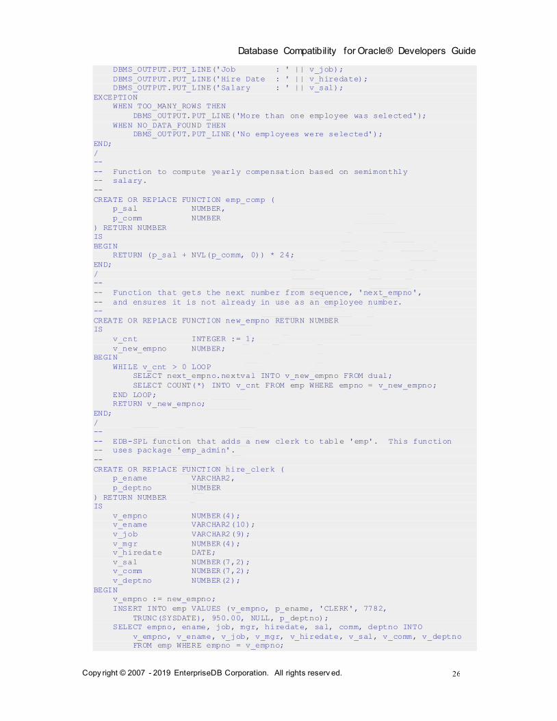
-- Function to compute yearly compensation based on semimonthly
-- salary.
--
CREATE OR REPLACE FUNCTION emp_comp (
p_sal NUMBER,
p_comm NUMBER
) RETURN NUMBER
IS
BEGIN
RETURN (p_sal + NVL(p_comm, 0)) * 24;
END;
/
--
-- Function that gets the next number from sequence, 'next_empno',
-- and ensures it is not already in use as an employee number.
--
CREATE OR REPLACE FUNCTION new_empno RETURN NUMBER
IS
v_cnt INTEGER := 1;
v_new_empno NUMBER;
BEGIN
WHILE v_cnt > 0 LOOP
SELECT next_empno.nextval INTO v_new_empno FROM dual;
SELECT COUNT(*) INTO v_cnt FROM emp WHERE empno = v_new_empno;
END LOOP;
RETURN v_new_empno;
END;
/
--
-- EDB-SPL function that adds a new clerk to table 'emp'. This function
-- uses package 'emp_admin'.
--
CREATE OR REPLACE FUNCTION hire_clerk (
p_ename VARCHAR2,
p_deptno NUMBER
) RETURN NUMBER
IS
v_empno NUMBER(4);
v_ename VARCHAR2(10);
v_job VARCHAR2(9);
v_mgr NUMBER(4);
v_hiredate DATE;
v_sal NUMBER(7,2);
v_comm NUMBER(7,2);
v_deptno NUMBER(2);
BEGIN
v_empno := new_empno;
INSERT INTO emp VALUES (v_empno, p_ename, 'CLERK', 7782,
TRUNC(SYSDATE), 950.00, NULL, p_deptno);
SELECT empno, ename, job, mgr, hiredate, sal, comm, deptno INTO
v_empno, v_ename, v_job, v_mgr, v_hiredate, v_sal, v_comm, v_deptno
FROM emp WHERE empno = v_empno;

Database Compatibility for Oracle® Developers Guide
Copy right © 2007 - 2019 EnterpriseDB Corporation. All rights reserv ed.
27
DBMS_OUTPUT.PUT_LINE('Department : ' || v_deptno);
DBMS_OUTPUT.PUT_LINE('Employee No: ' || v_empno);
DBMS_OUTPUT.PUT_LINE('Name : ' || v_ename);
DBMS_OUTPUT.PUT_LINE('Job : ' || v_job);
DBMS_OUTPUT.PUT_LINE('Manager : ' || v_mgr);
DBMS_OUTPUT.PUT_LINE('Hire Date : ' || v_hiredate);
DBMS_OUTPUT.PUT_LINE('Salary : ' || v_sal);
DBMS_OUTPUT.PUT_LINE('Commission : ' || v_comm);
RETURN v_empno;
EXCEPTION
WHEN OTHERS THEN
DBMS_OUTPUT.PUT_LINE('The following is SQLERRM:');
DBMS_OUTPUT.PUT_LINE(SQLERRM);
DBMS_OUTPUT.PUT_LINE('The following is SQLCODE:');
DBMS_OUTPUT.PUT_LINE(SQLCODE);
RETURN -1;
END;
/
--
-- PostgreSQL PL/pgSQL function that adds a new salesman
-- to table 'emp'.
--
CREATE OR REPLACE FUNCTION hire_salesman (
p_ename VARCHAR,
p_sal NUMERIC,
p_comm NUMERIC
) RETURNS NUMERIC
AS $$
DECLARE
v_empno NUMERIC(4);
v_ename VARCHAR(10);
v_job VARCHAR(9);
v_mgr NUMERIC(4);
v_hiredate DATE;
v_sal NUMERIC(7,2);
v_comm NUMERIC(7,2);
v_deptno NUMERIC(2);
BEGIN
v_empno := new_empno();
INSERT INTO emp VALUES (v_empno, p_ename, 'SALESMAN', 7698,
CURRENT_DATE, p_sal, p_comm, 30);
SELECT INTO
v_empno, v_ename, v_job, v_mgr, v_hiredate, v_sal, v_comm, v_deptno
empno, ename, job, mgr, hiredate, sal, comm, deptno
FROM emp WHERE empno = v_empno;
RAISE INFO 'Department : %', v_deptno;
RAISE INFO 'Employee No: %', v_empno;
RAISE INFO 'Name : %', v_ename;
RAISE INFO 'Job : %', v_job;
RAISE INFO 'Manager : %', v_mgr;
RAISE INFO 'Hire Date : %', v_hiredate;
RAISE INFO 'Salary : %', v_sal;
RAISE INFO 'Commission : %', v_comm;
RETURN v_empno;
EXCEPTION
WHEN OTHERS THEN
RAISE INFO 'The following is SQLERRM:';
RAISE INFO '%', SQLERRM;
RAISE INFO 'The following is SQLSTATE:';
RAISE INFO '%', SQLSTATE;
RETURN -1;
END;
$$ LANGUAGE 'plpgsql';
Database Compatibility for Oracle® Developers Guide
Copy right © 2007 - 2019 EnterpriseDB Corporation. All rights reserv ed.
28
/
--
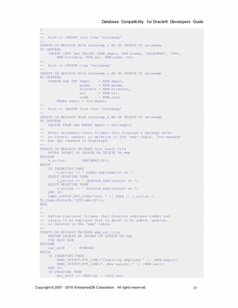
-- Rule to INSERT into view 'salesemp'
--
CREATE OR REPLACE RULE salesemp_i AS ON INSERT TO salesemp
DO INSTEAD
INSERT INTO emp VALUES (NEW.empno, NEW.ename, 'SALESMAN', 7698,
NEW.hiredate, NEW.sal, NEW.comm, 30);
--
-- Rule to UPDATE view 'salesemp'
--
CREATE OR REPLACE RULE salesemp_u AS ON UPDATE TO salesemp
DO INSTEAD
UPDATE emp SET empno = NEW.empno,
ename = NEW.ename,
hiredate = NEW.hiredate,
sal = NEW.sal,
comm = NEW.comm
WHERE empno = OLD.empno;
--
-- Rule to DELETE from view 'salesemp'
--
CREATE OR REPLACE RULE salesemp_d AS ON DELETE TO salesemp
DO INSTEAD
DELETE FROM emp WHERE empno = OLD.empno;
--
-- After statement-level trigger that displays a message after
-- an insert, update, or deletion to the 'emp' table. One message
-- per SQL command is displayed.
--
CREATE OR REPLACE TRIGGER user_audit_trig
AFTER INSERT OR UPDATE OR DELETE ON emp
DECLARE
v_action VARCHAR2(24);
BEGIN
IF INSERTING THEN
v_action := ' added employee(s) on ';
ELSIF UPDATING THEN
v_action := ' updated employee(s) on ';
ELSIF DELETING THEN
v_action := ' deleted employee(s) on ';
END IF;
DBMS_OUTPUT.PUT_LINE('User ' || USER || v_action ||
TO_CHAR(SYSDATE,'YYYY-MM-DD'));
END;
/
--
-- Before row-level trigger that displays employee number and
-- salary of an employee that is about to be added, updated,
-- or deleted in the 'emp' table.
--
CREATE OR REPLACE TRIGGER emp_sal_trig
BEFORE DELETE OR INSERT OR UPDATE ON emp
FOR EACH ROW
DECLARE
sal_diff NUMBER;
BEGIN
IF INSERTING THEN
DBMS_OUTPUT.PUT_LINE('Inserting employee ' || :NEW.empno);
DBMS_OUTPUT.PUT_LINE('..New salary: ' || :NEW.sal);
END IF;
IF UPDATING THEN
sal_diff := :NEW.sal - :OLD.sal;

Database Compatibility for Oracle® Developers Guide
Copy right © 2007 - 2019 EnterpriseDB Corporation. All rights reserv ed.
29
DBMS_OUTPUT.PUT_LINE('Updating employee ' || :OLD.empno);
DBMS_OUTPUT.PUT_LINE('..Old salary: ' || :OLD.sal);
DBMS_OUTPUT.PUT_LINE('..New salary: ' || :NEW.sal);
DBMS_OUTPUT.PUT_LINE('..Raise : ' || sal_diff);
END IF;
IF DELETING THEN
DBMS_OUTPUT.PUT_LINE('Deleting employee ' || :OLD.empno);
DBMS_OUTPUT.PUT_LINE('..Old salary: ' || :OLD.sal);
END IF;
END;
/
--
-- Package specification for the 'emp_admin' package.
--
CREATE OR REPLACE PACKAGE emp_admin
IS
FUNCTION get_dept_name (
p_deptno NUMBER
) RETURN VARCHAR2;
FUNCTION update_emp_sal (
p_empno NUMBER,
p_raise NUMBER
) RETURN NUMBER;
PROCEDURE hire_emp (
p_empno NUMBER,
p_ename VARCHAR2,
p_job VARCHAR2,
p_sal NUMBER,
p_hiredate DATE,
p_comm NUMBER,
p_mgr NUMBER,
p_deptno NUMBER
);
PROCEDURE fire_emp (
p_empno NUMBER
);
END emp_admin;
/
--
-- Package body for the 'emp_admin' package.
--
CREATE OR REPLACE PACKAGE BODY emp_admin
IS
--
-- Function that queries the 'dept' table based on the department
-- number and returns the corresponding department name.
--
FUNCTION get_dept_name (
p_deptno IN NUMBER
) RETURN VARCHAR2
IS
v_dname VARCHAR2(14);
BEGIN
SELECT dname INTO v_dname FROM dept WHERE deptno = p_deptno;
RETURN v_dname;
EXCEPTION
WHEN NO_DATA_FOUND THEN
DBMS_OUTPUT.PUT_LINE('Invalid department number ' || p_deptno);
RETURN '';
END;
--
-- Function that updates an employee's salary based on the
-- employee number and salary increment/decrement passed

Database Compatibility for Oracle® Developers Guide
Copy right © 2007 - 2019 EnterpriseDB Corporation. All rights reserv ed.
30
-- as IN parameters. Upon successful completion the function
-- returns the new updated salary.
--
FUNCTION update_emp_sal (
p_empno IN NUMBER,
p_raise IN NUMBER
) RETURN NUMBER
IS
v_sal NUMBER := 0;
BEGIN
SELECT sal INTO v_sal FROM emp WHERE empno = p_empno;
v_sal := v_sal + p_raise;
UPDATE emp SET sal = v_sal WHERE empno = p_empno;
RETURN v_sal;
EXCEPTION
WHEN NO_DATA_FOUND THEN
DBMS_OUTPUT.PUT_LINE('Employee ' || p_empno || ' not found');
RETURN -1;
WHEN OTHERS THEN
DBMS_OUTPUT.PUT_LINE('The following is SQLERRM:');
DBMS_OUTPUT.PUT_LINE(SQLERRM);
DBMS_OUTPUT.PUT_LINE('The following is SQLCODE:');
DBMS_OUTPUT.PUT_LINE(SQLCODE);
RETURN -1;
END;
--
-- Procedure that inserts a new employee record into the 'emp' table.
--
PROCEDURE hire_emp (
p_empno NUMBER,
p_ename VARCHAR2,
p_job VARCHAR2,
p_sal NUMBER,
p_hiredate DATE,
p_comm NUMBER,
p_mgr NUMBER,
p_deptno NUMBER
)
AS
BEGIN
INSERT INTO emp(empno, ename, job, sal, hiredate, comm, mgr, deptno)
VALUES(p_empno, p_ename, p_job, p_sal,
p_hiredate, p_comm, p_mgr, p_deptno);
END;
--
-- Procedure that deletes an employee record from the 'emp' table based
-- on the employee number.
--
PROCEDURE fire_emp (
p_empno NUMBER
)
AS
BEGIN
DELETE FROM emp WHERE empno = p_empno;
END;
END;
/
COMMIT;
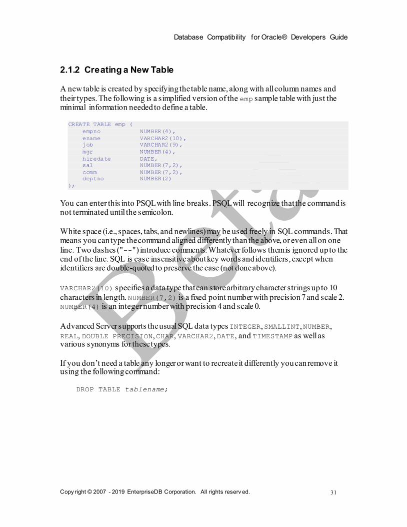
Database Compatibility for Oracle® Developers Guide
Copy right © 2007 - 2019 EnterpriseDB Corporation. All rights reserv ed.
31
2.1.2 Creating a New Table
A new table is created by specifying the table name, along with all column names and
their types. The following is a simplified version of the emp sample table with just the minimal information needed to define a table.
CREATE TABLE emp (
empno NUMBER(4),
ename VARCHAR2(10),
job VARCHAR2(9),
mgr NUMBER(4),
hiredate DATE,
sal NUMBER(7,2),
comm NUMBER(7,2),
deptno NUMBER(2)
);
You can enter this into PSQL with line breaks. PSQL will recognize that the command is not terminated until the semicolon.
White space (i.e., spaces, tabs, and newlines) may be used freely in SQL commands. That means you can type the command aligned differently than the above, or even all on one
line. Two dashes ("--") introduce comments. Whatever follows them is ignored up to the end of the line. SQL is case insensitive about key words and identifiers, except when identifiers are double-quoted to preserve the case (not done above).
VARCHAR2(10) specifies a data type that can store arbitrary character strings up to 10
characters in length. NUMBER(7,2) is a fixed point number with precision 7 and scale 2. NUMBER(4) is an integer number with precision 4 and scale 0.
Advanced Server supports the usual SQL data types INTEGER, SMALLINT, NUMBER,
REAL, DOUBLE PRECISION, CHAR, VARCHAR2, DATE, and TIMESTAMP as well as various synonyms for these types.
If you don’t need a table any longer or want to recreate it differently you can remove it using the following command:
DROP TABLE tablename;

Database Compatibility for Oracle® Developers Guide
Copy right © 2007 - 2019 EnterpriseDB Corporation. All rights reserv ed.
32
2.1.3 Populating a Table With Rows
The INSERT statement is used to populate a table with rows:
INSERT INTO emp VALUES (7369,'SMITH','CLERK',7902,'17-DEC-80',800,NULL,20);
Note that all data types use rather obvious input formats. Constants that are not simple
numeric values usually must be surrounded by single quotes ('), as in the example. The
DATE type is actually quite flexible in what it accepts, but for this tutorial we will stick to the unambiguous format shown here.
The syntax used so far requires you to remember the order of the columns. An alternative syntax allows you to list the columns explicitly:
INSERT INTO emp(empno,ename,job,mgr,hiredate,sal,comm,deptno)
VALUES (7499,'ALLEN','SALESMAN',7698,'20-FEB-81',1600,300,30);
You can list the columns in a different order if you wish or even omit some columns, e.g., if the commission is unknown:
INSERT INTO emp(empno,ename,job,mgr,hiredate,sal,deptno)
VALUES (7369,'SMITH','CLERK',7902,'17-DEC-80',800,20);
Many developers consider explicitly listing the columns better style than relying on the order implicitly.
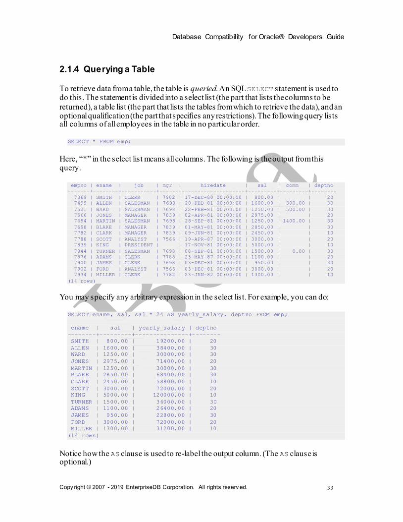
Database Compatibility for Oracle® Developers Guide
Copy right © 2007 - 2019 EnterpriseDB Corporation. All rights reserv ed.
33
2.1.4 Querying a Table
To retrieve data from a table, the table is queried. An SQL SELECT statement is used to do this. The statement is divided into a select list (the part that lists the columns to be
returned), a table list (the part that lists the tables from which to retrieve the data), and an optional qualification (the part that specifies any restrictions). The following query lists all columns of all employees in the table in no particular order.
SELECT * FROM emp;
Here, “*” in the select list means all columns. The following is the output from this query.
empno | ename | job | mgr | hiredate | sal | comm | deptno
-------+--------+-----------+------+--------------------+---------+---------+--------
7369 | SMITH | CLERK | 7902 | 17-DEC-80 00:00:00 | 800.00 | | 20
7499 | ALLEN | SALESMAN | 7698 | 20-FEB-81 00:00:00 | 1600.00 | 300.00 | 30
7521 | WARD | SALESMAN | 7698 | 22-FEB-81 00:00:00 | 1250.00 | 500.00 | 30
7566 | JONES | MANAGER | 7839 | 02-APR-81 00:00:00 | 2975.00 | | 20
7654 | MARTIN | SALESMAN | 7698 | 28-SEP-81 00:00:00 | 1250.00 | 1400.00 | 30
7698 | BLAKE | MANAGER | 7839 | 01-MAY-81 00:00:00 | 2850.00 | | 30
7782 | CLARK | MANAGER | 7839 | 09-JUN-81 00:00:00 | 2450.00 | | 10
7788 | SCOTT | ANALYST | 7566 | 19-APR-87 00:00:00 | 3000.00 | | 20
7839 | KING | PRESIDENT | | 17-NOV-81 00:00:00 | 5000.00 | | 10
7844 | TURNER | SALESMAN | 7698 | 08-SEP-81 00:00:00 | 1500.00 | 0.00 | 30
7876 | ADAMS | CLERK | 7788 | 23-MAY-87 00:00:00 | 1100.00 | | 20
7900 | JAMES | CLERK | 7698 | 03-DEC-81 00:00:00 | 950.00 | | 30
7902 | FORD | ANALYST | 7566 | 03-DEC-81 00:00:00 | 3000.00 | | 20
7934 | MILLER | CLERK | 7782 | 23-JAN-82 00:00:00 | 1300.00 | | 10
(14 rows)
You may specify any arbitrary expression in the select list. For example, you can do:
SELECT ename, sal, sal * 24 AS yearly_salary, deptno FROM emp;
ename | sal | yearly_salary | deptno
--------+---------+---------------+--------
SMITH | 800.00 | 19200.00 | 20
ALLEN | 1600.00 | 38400.00 | 30
WARD | 1250.00 | 30000.00 | 30
JONES | 2975.00 | 71400.00 | 20
MARTIN | 1250.00 | 30000.00 | 30
BLAKE | 2850.00 | 68400.00 | 30
CLARK | 2450.00 | 58800.00 | 10
SCOTT | 3000.00 | 72000.00 | 20
KING | 5000.00 | 120000.00 | 10
TURNER | 1500.00 | 36000.00 | 30
ADAMS | 1100.00 | 26400.00 | 20
JAMES | 950.00 | 22800.00 | 30
FORD | 3000.00 | 72000.00 | 20
MILLER | 1300.00 | 31200.00 | 10
(14 rows)
Notice how the AS clause is used to re-label the output column. (The AS clause is optional.)

Database Compatibility for Oracle® Developers Guide
Copy right © 2007 - 2019 EnterpriseDB Corporation. All rights reserv ed.
34
A query can be qualified by adding a WHERE clause that specifies which rows are wanted.
The WHERE clause contains a Boolean (truth value) expression, and only rows for which
the Boolean expression is true are returned. The usual Boolean operators (AND, OR, and
NOT) are allowed in the qualification. For example, the following retrieves the employees in department 20 with salaries over $1000.00:
SELECT ename, sal, deptno FROM emp WHERE deptno = 20 AND sal > 1000;
ename | sal | deptno
-------+---------+--------
JONES | 2975.00 | 20
SCOTT | 3000.00 | 20
ADAMS | 1100.00 | 20
FORD | 3000.00 | 20
(4 rows)
You can request that the results of a query be returned in sorted order:
SELECT ename, sal, deptno FROM emp ORDER BY ename;
ename | sal | deptno
--------+---------+--------
ADAMS | 1100.00 | 20
ALLEN | 1600.00 | 30
BLAKE | 2850.00 | 30
CLARK | 2450.00 | 10
FORD | 3000.00 | 20
JAMES | 950.00 | 30
JONES | 2975.00 | 20
KING | 5000.00 | 10
MARTIN | 1250.00 | 30
MILLER | 1300.00 | 10
SCOTT | 3000.00 | 20
SMITH | 800.00 | 20
TURNER | 1500.00 | 30
WARD | 1250.00 | 30
(14 rows)
You can request that duplicate rows be removed from the result of a query:
SELECT DISTINCT job FROM emp;
job
-----------
ANALYST
CLERK
MANAGER
PRESIDENT
SALESMAN
(5 rows)
The following section shows how to obtain rows from more than one table in a single query.

Database Compatibility for Oracle® Developers Guide
Copy right © 2007 - 2019 EnterpriseDB Corporation. All rights reserv ed.
35
2.1.5 Joins Between Tables
Thus far, our queries have only accessed one table at a time. Queries can access multiple tables at once, or access the same table in such a way that multiple rows of the table are
being processed at the same time. A query that accesses multiple rows of the same or different tables at one time is called a join query. For example, say you wish to list all the
employee records together with the name and location of the associated department. To
do that, we need to compare the deptno column of each row of the emp table with the
deptno column of all rows in the dept table, and select the pairs of rows where these values match. This would be accomplished by the following query:
SELECT emp.ename, emp.sal, dept.deptno, dept.dname, dept.loc FROM emp, dept
WHERE emp.deptno = dept.deptno;
ename | sal | deptno | dname | loc
--------+---------+--------+------------+----------
MILLER | 1300.00 | 10 | ACCOUNTING | NEW YORK
CLARK | 2450.00 | 10 | ACCOUNTING | NEW YORK
KING | 5000.00 | 10 | ACCOUNTING | NEW YORK
SCOTT | 3000.00 | 20 | RESEARCH | DALLAS
JONES | 2975.00 | 20 | RESEARCH | DALLAS
SMITH | 800.00 | 20 | RESEARCH | DALLAS
ADAMS | 1100.00 | 20 | RESEARCH | DALLAS
FORD | 3000.00 | 20 | RESEARCH | DALLAS
WARD | 1250.00 | 30 | SALES | CHICAGO
TURNER | 1500.00 | 30 | SALES | CHICAGO
ALLEN | 1600.00 | 30 | SALES | CHICAGO
BLAKE | 2850.00 | 30 | SALES | CHICAGO
MARTIN | 1250.00 | 30 | SALES | CHICAGO
JAMES | 950.00 | 30 | SALES | CHICAGO
(14 rows)
Observe two things about the result set:
There is no result row for department 40. This is because there is no matching
entry in the emp table for department 40, so the join ignores the unmatched rows
in the dept table. Shortly we will see how this can be fixed. It is more desirable to list the output columns qualified by table name rather than
using * or leaving out the qualification as follows:
SELECT ename, sal, dept.deptno, dname, loc FROM emp, dept WHERE emp.deptno =
dept.deptno;
Since all the columns had different names (except for deptno which therefore must be
qualified), the parser automatically found out which table they belong to , but it is good style to fully qualify column names in join queries:
Join queries of the kind seen thus far can also be written in this alternative form:

Database Compatibility for Oracle® Developers Guide
Copy right © 2007 - 2019 EnterpriseDB Corporation. All rights reserv ed.
36
SELECT emp.ename, emp.sal, dept.deptno, dept.dname, dept.loc FROM emp INNER
JOIN dept ON emp.deptno = dept.deptno;
This syntax is not as commonly used as the one above, but we show it here to help you understand the following topics.
You will notice that in all the above results for joins no employees were returned that
belonged to department 40 and as a consequence, the record for department 40 never appears. Now we will figure out how we can get the department 40 record in the results despite the fact that there are no matching employees. What we want the query to do is to
scan the dept table and for each row to find the matching emp row. If no matching row
is found we want some “empty” values to be substituted for the emp table’s columns. This kind of query is called an outer join. (The joins we have seen so far are inner joins.) The command looks like this:
SELECT emp.ename, emp.sal, dept.deptno, dept.dname, dept.loc FROM dept LEFT
OUTER JOIN emp ON emp.deptno = dept.deptno;
ename | sal | deptno | dname | loc
--------+---------+--------+------------+----------
MILLER | 1300.00 | 10 | ACCOUNTING | NEW YORK
CLARK | 2450.00 | 10 | ACCOUNTING | NEW YORK
KING | 5000.00 | 10 | ACCOUNTING | NEW YORK
SCOTT | 3000.00 | 20 | RESEARCH | DALLAS
JONES | 2975.00 | 20 | RESEARCH | DALLAS
SMITH | 800.00 | 20 | RESEARCH | DALLAS
ADAMS | 1100.00 | 20 | RESEARCH | DALLAS
FORD | 3000.00 | 20 | RESEARCH | DALLAS
WARD | 1250.00 | 30 | SALES | CHICAGO
TURNER | 1500.00 | 30 | SALES | CHICAGO
ALLEN | 1600.00 | 30 | SALES | CHICAGO
BLAKE | 2850.00 | 30 | SALES | CHICAGO
MARTIN | 1250.00 | 30 | SALES | CHICAGO
JAMES | 950.00 | 30 | SALES | CHICAGO
| | 40 | OPERATIONS | BOSTON
(15 rows)
This query is called a left outer join because the table mentioned on the left of the join
operator will have each of its rows in the output at least once, whereas the table on the
right will only have those rows output that match some row of the left table. When a left -
table row is selected for which there is no right-table match, empty (NULL) values are substituted for the right-table columns.
An alternative syntax for an outer join is to use the outer join operator, “(+)”, in the join
condition within the WHERE clause. The outer join operator is placed after the column name of the table for which null values should be substituted for unmatched rows. So for
all the rows in the dept table that have no matching rows in the emp table, Advanced
Server returns null for any select list expressions containing columns of emp. Hence the above example could be rewritten as:
SELECT emp.ename, emp.sal, dept.deptno, dept.dname, dept.loc FROM dept, emp
WHERE emp.deptno(+) = dept.deptno;

Database Compatibility for Oracle® Developers Guide
Copy right © 2007 - 2019 EnterpriseDB Corporation. All rights reserv ed.
37
ename | sal | deptno | dname | loc
--------+---------+--------+------------+----------
MILLER | 1300.00 | 10 | ACCOUNTING | NEW YORK
CLARK | 2450.00 | 10 | ACCOUNTING | NEW YORK
KING | 5000.00 | 10 | ACCOUNTING | NEW YORK
SCOTT | 3000.00 | 20 | RESEARCH | DALLAS
JONES | 2975.00 | 20 | RESEARCH | DALLAS
SMITH | 800.00 | 20 | RESEARCH | DALLAS
ADAMS | 1100.00 | 20 | RESEARCH | DALLAS
FORD | 3000.00 | 20 | RESEARCH | DALLAS
WARD | 1250.00 | 30 | SALES | CHICAGO
TURNER | 1500.00 | 30 | SALES | CHICAGO
ALLEN | 1600.00 | 30 | SALES | CHICAGO
BLAKE | 2850.00 | 30 | SALES | CHICAGO
MARTIN | 1250.00 | 30 | SALES | CHICAGO
JAMES | 950.00 | 30 | SALES | CHICAGO
| | 40 | OPERATIONS | BOSTON
(15 rows)
We can also join a table against itself. This is called a self join. As an example, suppose
we wish to find the name of each employee along with the name of that employee’s
manager. So we need to compare the mgr column of each emp row to the empno column
of all other emp rows.
SELECT e1.ename || ' works for ' || e2.ename AS "Employees and their
Managers" FROM emp e1, emp e2 WHERE e1.mgr = e2.empno;
Employees and their Managers
------------------------------
FORD works for JONES
SCOTT works for JONES
WARD works for BLAKE
TURNER works for BLAKE
MARTIN works for BLAKE
JAMES works for BLAKE
ALLEN works for BLAKE
MILLER works for CLARK
ADAMS works for SCOTT
CLARK works for KING
BLAKE works for KING
JONES works for KING
SMITH works for FORD
(13 rows)
Here, the emp table has been re-labeled as e1 to represent the employee row in the select
list and in the join condition, and also as e2 to represent the matching employee row acting as manager in the select list and in the join condition. These kinds of aliases can be used in other queries to save some typing, for example:
SELECT e.ename, e.mgr, d.deptno, d.dname, d.loc FROM emp e, dept d WHERE
e.deptno = d.deptno;
ename | mgr | deptno | dname | loc
--------+------+--------+------------+----------
MILLER | 7782 | 10 | ACCOUNTING | NEW YORK
CLARK | 7839 | 10 | ACCOUNTING | NEW YORK
KING | | 10 | ACCOUNTING | NEW YORK
SCOTT | 7566 | 20 | RESEARCH | DALLAS

Database Compatibility for Oracle® Developers Guide
Copy right © 2007 - 2019 EnterpriseDB Corporation. All rights reserv ed.
38
JONES | 7839 | 20 | RESEARCH | DALLAS
SMITH | 7902 | 20 | RESEARCH | DALLAS
ADAMS | 7788 | 20 | RESEARCH | DALLAS
FORD | 7566 | 20 | RESEARCH | DALLAS
WARD | 7698 | 30 | SALES | CHICAGO
TURNER | 7698 | 30 | SALES | CHICAGO
ALLEN | 7698 | 30 | SALES | CHICAGO
BLAKE | 7839 | 30 | SALES | CHICAGO
MARTIN | 7698 | 30 | SALES | CHICAGO
JAMES | 7698 | 30 | SALES | CHICAGO
(14 rows)
This style of abbreviating will be encountered quite frequently.

Database Compatibility for Oracle® Developers Guide
Copy right © 2007 - 2019 EnterpriseDB Corporation. All rights reserv ed.
39
2.1.6 Aggregate Functions
Like most other relational database products, Advanced Server supports aggregate functions. An aggregate function computes a single result from multiple input rows. For
example, there are aggregates to compute the COUNT, SUM, AVG (average), MAX (maximum), and MIN (minimum) over a set of rows.
As an example, the highest and lowest salaries can be found with the following query:
SELECT MAX(sal) highest_salary, MIN(sal) lowest_salary FROM emp;
highest_salary | lowest_salary
----------------+---------------
5000.00 | 800.00
(1 row)
If we wanted to find the employee with the largest salary, we may be tempted to try:
SELECT ename FROM emp WHERE sal = MAX(sal);
ERROR: aggregates not allowed in WHERE clause
This does not work because the aggregate function, MAX, cannot be used in the WHERE
clause. This restriction exists because the WHERE clause determines the rows that will go into the aggregation stage so it has to be evaluated before aggregate functions are
computed. However, the query can be restated to accomplish the intended result by using a subquery:
SELECT ename FROM emp WHERE sal = (SELECT MAX(sal) FROM emp);
ename
-------
KING
(1 row)
The subquery is an independent computation that obtains its own result separately from the outer query.
Aggregates are also very useful in combination with the GROUP BY clause. For example, the following query gets the highest salary in each department.
SELECT deptno, MAX(sal) FROM emp GROUP BY deptno;
deptno | max
--------+---------
10 | 5000.00
20 | 3000.00
30 | 2850.00
(3 rows)

Database Compatibility for Oracle® Developers Guide
Copy right © 2007 - 2019 EnterpriseDB Corporation. All rights reserv ed.
40
This query produces one output row per department. Each aggregate result is computed
over the rows matching that department. These grouped rows can be filtered using the
HAVING clause.
SELECT deptno, MAX(sal) FROM emp GROUP BY deptno HAVING AVG(sal) > 2000;
deptno | max
--------+---------
10 | 5000.00
20 | 3000.00
(2 rows)
This query gives the same results for only those departments that have an average salary greater than 2000.
Finally, the following query takes into account only the highest paid employees who are analysts in each department.
SELECT deptno, MAX(sal) FROM emp WHERE job = 'ANALYST' GROUP BY deptno HAVING
AVG(sal) > 2000;
deptno | max
--------+---------
20 | 3000.00
(1 row)
There is a subtle distinction between the WHERE and HAVING clauses. The WHERE clause
filters out rows before grouping occurs and aggregate functions are applied. The HAVING clause applies filters on the results after rows have been grouped and aggregate functions have been computed for each group.
So in the previous example, only employees who are analysts are considered. From this subset, the employees are grouped by department and only those groups where the average salary of analysts in the group is greater than 2000 are in the final result. This is
true of only the group for department 20 and the maximum analyst salary in department 20 is 3000.00.

Database Compatibility for Oracle® Developers Guide
Copy right © 2007 - 2019 EnterpriseDB Corporation. All rights reserv ed.
41
2.1.7 Updates
The column values of existing rows can be changed using the UPDATE command. For example, the following sequence of commands shows the before and after results of giving everyone who is a manager a 10% raise:
SELECT ename, sal FROM emp WHERE job = 'MANAGER';
ename | sal
-------+---------
JONES | 2975.00
BLAKE | 2850.00
CLARK | 2450.00
(3 rows)
UPDATE emp SET sal = sal * 1.1 WHERE job = 'MANAGER';
SELECT ename, sal FROM emp WHERE job = 'MANAGER';
ename | sal
-------+---------
JONES | 3272.50
BLAKE | 3135.00
CLARK | 2695.00
(3 rows)

Database Compatibility for Oracle® Developers Guide
Copy right © 2007 - 2019 EnterpriseDB Corporation. All rights reserv ed.
42
2.1.8 Deletions
Rows can be removed from a table using the DELETE command. For example, the following sequence of commands shows the before and after results of deleting all
employees in department 20.
SELECT ename, deptno FROM emp;
ename | deptno
--------+--------
SMITH | 20
ALLEN | 30
WARD | 30
JONES | 20
MARTIN | 30
BLAKE | 30
CLARK | 10
SCOTT | 20
KING | 10
TURNER | 30
ADAMS | 20
JAMES | 30
FORD | 20
MILLER | 10
(14 rows)
DELETE FROM emp WHERE deptno = 20;
SELECT ename, deptno FROM emp;
ename | deptno
--------+--------
ALLEN | 30
WARD | 30
MARTIN | 30
BLAKE | 30
CLARK | 10
KING | 10
TURNER | 30
JAMES | 30
MILLER | 10
(9 rows)
Be extremely careful of giving a DELETE command without a WHERE clause such as the following:
DELETE FROM tablename;
This statement will remove all rows from the given table, leaving it completely empty. The system will not request confirmation before doing this.

Database Compatibility for Oracle® Developers Guide
Copy right © 2007 - 2019 EnterpriseDB Corporation. All rights reserv ed.
43
2.1.9 The SQL Language
Advanced Server supports SQL language that is compatible with Oracle syntax as well as
syntax and commands for extended functionality (functionality that does not provide database compatibility for Oracle or support Oracle-styled applications).
The Reference Guide that supports the Database Compatibility for Oracle Developer's Guide provides detailed information about:
Compatible SQL syntax and language elements
Data types
Supported SQL command syntax
To review a copy of the Reference Guide, visit the Advanced Server website at:
https://www.enterprisedb.com/resources/product-documentation

Database Compatibility for Oracle® Developers Guide
Copy right © 2007 - 2019 EnterpriseDB Corporation. All rights reserv ed.
44
2.2 Advanced Concepts
The previous section discussed the basics of using SQL to store and access your data in
Advanced Server. This section discusses more advanced SQL features that may simplify management and prevent loss or corruption of your data.
2.2.1 Views
Consider the following SELECT command.
SELECT ename, sal, sal * 24 AS yearly_salary, deptno FROM emp;
ename | sal | yearly_salary | deptno
--------+---------+---------------+--------
SMITH | 800.00 | 19200.00 | 20
ALLEN | 1600.00 | 38400.00 | 30
WARD | 1250.00 | 30000.00 | 30
JONES | 2975.00 | 71400.00 | 20
MARTIN | 1250.00 | 30000.00 | 30
BLAKE | 2850.00 | 68400.00 | 30
CLARK | 2450.00 | 58800.00 | 10
SCOTT | 3000.00 | 72000.00 | 20
KING | 5000.00 | 120000.00 | 10
TURNER | 1500.00 | 36000.00 | 30
ADAMS | 1100.00 | 26400.00 | 20
JAMES | 950.00 | 22800.00 | 30
FORD | 3000.00 | 72000.00 | 20
MILLER | 1300.00 | 31200.00 | 10
(14 rows)
If this is a query that is used repeatedly, a shorthand method of reusing this query without
re-typing the entire SELECT command each time is to create a view as shown below.
CREATE VIEW employee_pay AS SELECT ename, sal, sal * 24 AS yearly_salary,
deptno FROM emp;
The view name, employee_pay, can now be used like an ordinary table name to perform the query.
SELECT * FROM employee_pay;
ename | sal | yearly_salary | deptno
--------+---------+---------------+--------
SMITH | 800.00 | 19200.00 | 20
ALLEN | 1600.00 | 38400.00 | 30
WARD | 1250.00 | 30000.00 | 30
JONES | 2975.00 | 71400.00 | 20
MARTIN | 1250.00 | 30000.00 | 30
BLAKE | 2850.00 | 68400.00 | 30
CLARK | 2450.00 | 58800.00 | 10
SCOTT | 3000.00 | 72000.00 | 20
KING | 5000.00 | 120000.00 | 10
TURNER | 1500.00 | 36000.00 | 30
ADAMS | 1100.00 | 26400.00 | 20
JAMES | 950.00 | 22800.00 | 30
FORD | 3000.00 | 72000.00 | 20

Database Compatibility for Oracle® Developers Guide
Copy right © 2007 - 2019 EnterpriseDB Corporation. All rights reserv ed.
45
MILLER | 1300.00 | 31200.00 | 10
(14 rows)
Making liberal use of views is a key aspect of good SQL database design. Views provide
a consistent interface that encapsulate details of the structure of your tables which may change as your application evolves.
Views can be used in almost any place a real table can be used. Building views upon other views is not uncommon.
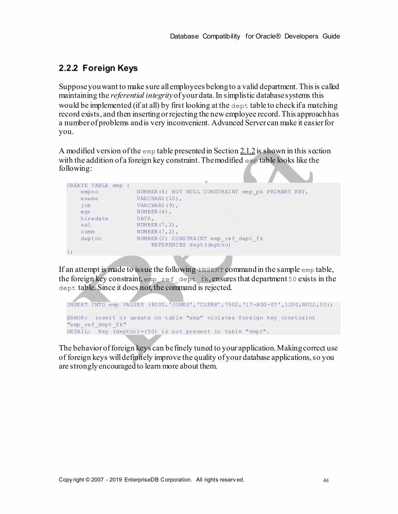
Database Compatibility for Oracle® Developers Guide
Copy right © 2007 - 2019 EnterpriseDB Corporation. All rights reserv ed.
46
2.2.2 Foreign Keys
Suppose you want to make sure all employees belong to a valid department. This is called maintaining the referential integrity of your data. In simplistic database systems this
would be implemented (if at all) by first looking at the dept table to check if a matching record exists, and then inserting or rejecting the new employee record. This approach has a number of problems and is very inconvenient. Advanced Server can make it easier for you.
A modified version of the emp table presented in Section 2.1.2 is shown in this section
with the addition of a foreign key constraint. The modified emp table looks like the following:
CREATE TABLE emp (
empno NUMBER(4) NOT NULL CONSTRAINT emp_pk PRIMARY KEY,
ename VARCHAR2(10),
job VARCHAR2(9),
mgr NUMBER(4),
hiredate DATE,
sal NUMBER(7,2),
comm NUMBER(7,2),
deptno NUMBER(2) CONSTRAINT emp_ref_dept_fk
REFERENCES dept(deptno)
);
If an attempt is made to issue the following INSERT command in the sample emp table,
the foreign key constraint, emp_ref_dept_fk, ensures that department 50 exists in the dept table. Since it does not, the command is rejected.
INSERT INTO emp VALUES (8000,'JONES','CLERK',7902,'17-AUG-07',1200,NULL,50);
ERROR: insert or update on table "emp" violates foreign key constraint
"emp_ref_dept_fk"
DETAIL: Key (deptno)=(50) is not present in table "dept".
The behavior of foreign keys can be finely tuned to your application. Making correct use
of foreign keys will definitely improve the quality of your database applications, so you are strongly encouraged to learn more about them.

Database Compatibility for Oracle® Developers Guide
Copy right © 2007 - 2019 EnterpriseDB Corporation. All rights reserv ed.
47
2.2.3 The ROWNUM Pseudo-Column
ROWNUM is a pseudo-column that is assigned an incremental, unique integer value for each row based on the order the rows were retrieved from a query. Therefore, the first
row retrieved will have ROWNUM of 1; the second row will have ROWNUM of 2 and so on.
This feature can be used to limit the number of rows retrieved by a query. This is demonstrated in the following example:
SELECT empno, ename, job FROM emp WHERE ROWNUM < 5;
empno | ename | job
-------+-------+----------
7369 | SMITH | CLERK
7499 | ALLEN | SALESMAN
7521 | WARD | SALESMAN
7566 | JONES | MANAGER
(4 rows)
The ROWNUM value is assigned to each row before any sorting of the result set takes place.
Thus, the result set is returned in the order given by the ORDER BY clause, but the
ROWNUM values may not necessarily be in ascending order as shown in the following example:
SELECT ROWNUM, empno, ename, job FROM emp WHERE ROWNUM < 5 ORDER BY ename;
rownum | empno | ename | job
--------+-------+-------+----------
2 | 7499 | ALLEN | SALESMAN
4 | 7566 | JONES | MANAGER
1 | 7369 | SMITH | CLERK
3 | 7521 | WARD | SALESMAN
(4 rows)
The following example shows how a sequence number can be added to every row in the
jobhist table. First a new column named, seqno, is added to the table and then seqno is set to ROWNUM in the UPDATE command.
ALTER TABLE jobhist ADD seqno NUMBER(3);
UPDATE jobhist SET seqno = ROWNUM;
The following SELECT command shows the new seqno values.
SELECT seqno, empno, TO_CHAR(startdate,'DD-MON-YY') AS start, job FROM
jobhist;
seqno | empno | start | job
-------+-------+-----------+-----------
1 | 7369 | 17-DEC-80 | CLERK
2 | 7499 | 20-FEB-81 | SALESMAN
3 | 7521 | 22-FEB-81 | SALESMAN
4 | 7566 | 02-APR-81 | MANAGER
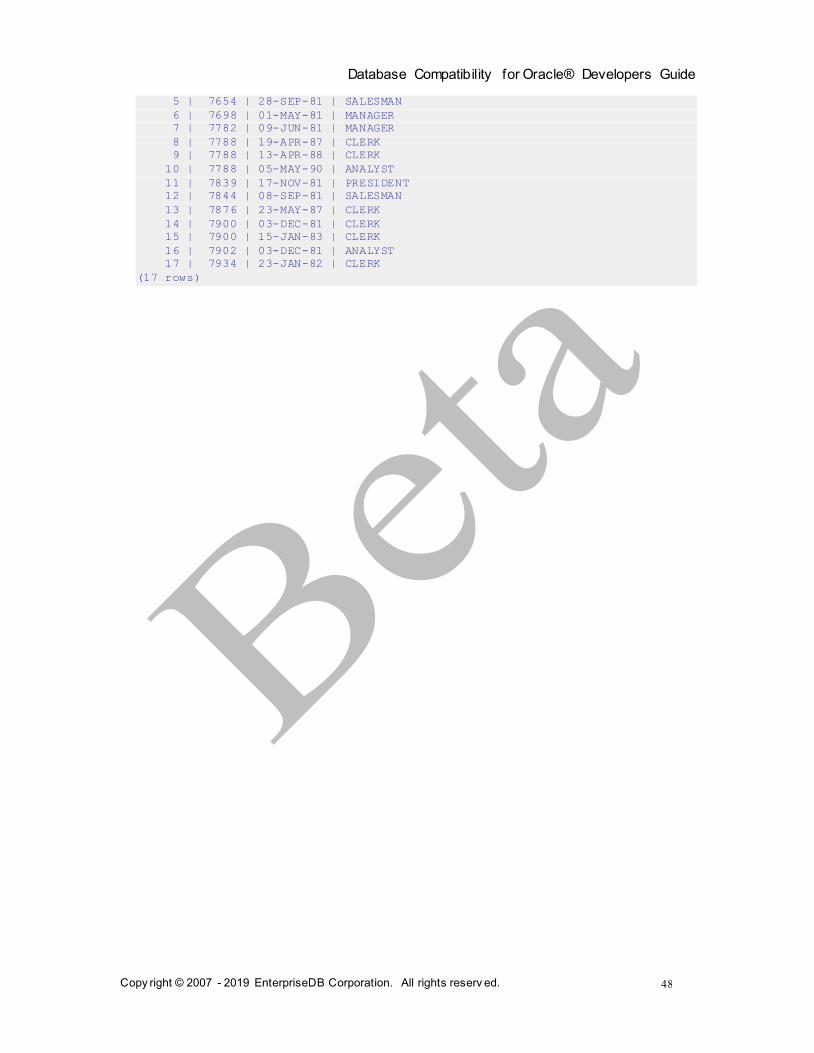
Database Compatibility for Oracle® Developers Guide
Copy right © 2007 - 2019 EnterpriseDB Corporation. All rights reserv ed.
48
5 | 7654 | 28-SEP-81 | SALESMAN
6 | 7698 | 01-MAY-81 | MANAGER
7 | 7782 | 09-JUN-81 | MANAGER
8 | 7788 | 19-APR-87 | CLERK
9 | 7788 | 13-APR-88 | CLERK
10 | 7788 | 05-MAY-90 | ANALYST
11 | 7839 | 17-NOV-81 | PRESIDENT
12 | 7844 | 08-SEP-81 | SALESMAN
13 | 7876 | 23-MAY-87 | CLERK
14 | 7900 | 03-DEC-81 | CLERK
15 | 7900 | 15-JAN-83 | CLERK
16 | 7902 | 03-DEC-81 | ANALYST
17 | 7934 | 23-JAN-82 | CLERK
(17 rows)

Database Compatibility for Oracle® Developers Guide
Copy right © 2007 - 2019 EnterpriseDB Corporation. All rights reserv ed.
49
2.2.4 Synonyms
A synonym is an identifier that can be used to reference another database object in a SQL statement. A synonym is useful in cases where a database object would normally require
full qualification by schema name to be properly referenced in a SQL statement. A synonym defined for that object simplifies the reference to a single, unqualified name.
Advanced Server supports synonyms for:
tables
views
materialized views
sequences
procedures
functions
types
objects that are accessible through a database link
other synonyms
Neither the referenced schema or referenced object must exist at the time that you create the synonym; a synonym may refer to a non-existent object or schema. A synonym will
become invalid if you drop the referenced object or schema. You must explicitly drop a synonym to remove it.
As with any other schema object, Advanced Server uses the search path to resolve
unqualified synonym names. If you have two synonyms with the same name, an unqualified reference to a synonym will resolve to the first synonym with the given name
in the search path. If public is in your search path, you can refer to a synonym in that schema without qualifying that name.
When Advanced Server executes an SQL command, the privileges of the current user are
checked against the synonym’s underlying database object; if the user does not have the proper permissions for that object, the SQL command will fail.
Creating a Synonym
Use the CREATE SYNONYM command to create a synonym. The syntax is:
CREATE [OR REPLACE] [PUBLIC] SYNONYM [schema.]syn_name
FOR object_schema.object_name[@dblink_name];

Database Compatibility for Oracle® Developers Guide
Copy right © 2007 - 2019 EnterpriseDB Corporation. All rights reserv ed.
50
Parameters:
syn_name
syn_name is the name of the synonym. A synonym name must be unique within a schema.
schema
schema specifies the name of the schema that the synonym resides in. If you do
not specify a schema name, the synonym is created in the first existing schema in your search path.
object_name
object_name specifies the name of the object.
object_schema
object_schema specifies the name of the schema that the object resides in.
dblink_name
dblink_name specifies the name of the database link through which a target object may be accessed.
Include the REPLACE clause to replace an existing synonym definition with a new synonym definition.
Include the PUBLIC clause to create the synonym in the public schema. Compatible
with Oracle databases, the CREATE PUBLIC SYNONYM command creates a synonym that resides in the public schema:
CREATE [OR REPLACE] PUBLIC SYNONYM syn_name FOR
object_schema.object_name;
This just a shorthand way to write:
CREATE [OR REPLACE] SYNONYM public.syn_name FOR
object_schema.object_name;
The following example creates a synonym named personnel that refers to the enterprisedb.emp table.
CREATE SYNONYM personnel FOR enterprisedb.emp;

Database Compatibility for Oracle® Developers Guide
Copy right © 2007 - 2019 EnterpriseDB Corporation. All rights reserv ed.
51
Unless the synonym is schema qualified in the CREATE SYNONYM command, it will be
created in the first existing schema in your search path. You can view your search path by executing the following command:
SHOW SEARCH_PATH;
search_path
-----------------------
development,accounting
(1 row)
In our example, if a schema named development does not exist, the synonym will be created in the schema named accounting.
Now, the emp table in the enterprisedb schema can be referenced in any SQL statement (DDL or DML), by using the synonym, personnel:
INSERT INTO personnel VALUES (8142,'ANDERSON','CLERK',7902,'17-DEC-06',1300,NULL,20);
SELECT * FROM personnel;
empno | ename | job | mgr | hiredate | sal | comm | deptno
-------+----------+-----------+------+--------------------+---------+---------+--------
7369 | SMITH | CLERK | 7902 | 17-DEC-80 00:00:00 | 800.00 | | 20
7499 | ALLEN | SALESMAN | 7698 | 20-FEB-81 00:00:00 | 1600.00 | 300.00 | 30
7521 | WARD | SALESMAN | 7698 | 22-FEB-81 00:00:00 | 1250.00 | 500.00 | 30
7566 | JONES | MANAGER | 7839 | 02-APR-81 00:00:00 | 2975.00 | | 20
7654 | MARTIN | SALESMAN | 7698 | 28-SEP-81 00:00:00 | 1250.00 | 1400.00 | 30
7698 | BLAKE | MANAGER | 7839 | 01-MAY-81 00:00:00 | 2850.00 | | 30
7782 | CLARK | MANAGER | 7839 | 09-JUN-81 00:00:00 | 2450.00 | | 10
7788 | SCOTT | ANALYST | 7566 | 19-APR-87 00:00:00 | 3000.00 | | 20
7839 | KING | PRESIDENT | | 17-NOV-81 00:00:00 | 5000.00 | | 10
7844 | TURNER | SALESMAN | 7698 | 08-SEP-81 00:00:00 | 1500.00 | 0.00 | 30
7876 | ADAMS | CLERK | 7788 | 23-MAY-87 00:00:00 | 1100.00 | | 20
7900 | JAMES | CLERK | 7698 | 03-DEC-81 00:00:00 | 950.00 | | 30
7902 | FORD | ANALYST | 7566 | 03-DEC-81 00:00:00 | 3000.00 | | 20
7934 | MILLER | CLERK | 7782 | 23-JAN-82 00:00:00 | 1300.00 | | 10
8142 | ANDERSON | CLERK | 7902 | 17-DEC-06 00:00:00 | 1300.00 | | 20
(15 rows)
Deleting a Synonym
To delete a synonym, use the command, DROP SYNONYM. The syntax is:
DROP [PUBLIC] SYNONYM [schema.] syn_name
Parameters:
syn_name
syn_name is the name of the synonym. A synonym name must be unique within a schema.

Database Compatibility for Oracle® Developers Guide
Copy right © 2007 - 2019 EnterpriseDB Corporation. All rights reserv ed.
52
schema
schema specifies the name of the schema in which the synonym resides.
Like any other object that can be schema-qualified, you may have two synonyms with the
same name in your search path. To disambiguate the name of the synonym that you are
dropping, include a schema name. Unless a synonym is schema qualified in the DROP
SYNONYM command, Advanced Server deletes the first instance of the synonym it finds in your search path.
You can optionally include the PUBLIC clause to drop a synonym that resides in the
public schema. Compatible with Oracle databases, the DROP PUBLIC SYNONYM command drops a synonym that resides in the public schema:
DROP PUBLIC SYNONYM syn_name;
The following example drops the synonym, personnel:
DROP SYNONYM personnel;

Database Compatibility for Oracle® Developers Guide
Copy right © 2007 - 2019 EnterpriseDB Corporation. All rights reserv ed.
53
2.2.5 Hierarchical Queries
A hierarchical query is a type of query that returns the rows of the result set in a hierarchical order based upon data forming a parent-child relationship. A hierarchy is
typically represented by an inverted tree structure. The tree is comprised of interconnected nodes. Each node may be connected to none, one, or multiple child nodes.
Each node is connected to one parent node except for the top node which has no parent. This node is the root node. Each tree has exactly one root node. Nodes that don’t have any children are called leaf nodes. A tree always has at least one leaf node - e.g., the
trivial case where the tree is comprised of a single node. In this case it is both the root and the leaf.
In a hierarchical query the rows of the result set represent the nodes of one or more trees.
Note: It is possible that a single, given row may appear in more than one tree and thus appear more than once in the result set.
The hierarchical relationship in a query is described by the CONNECT BY clause which forms the basis of the order in which rows are returned in the result set. The context of
where the CONNECT BY clause and its associated optional clauses appear in the SELECT command is shown below.
SELECT select_list FROM table_expression [ WHERE ...]
[ START WITH start_expression ]
CONNECT BY { PRIOR parent_expr = child_expr |
child_expr = PRIOR parent_expr }
[ ORDER SIBLINGS BY column1 [ ASC | DESC ]
[, column2 [ ASC | DESC ] ] ...
[ GROUP BY ...]
[ HAVING ...]
[ other ...]
select_list is one or more expressions that comprise the fields of the result set.
table_expression is one or more tables or views from which the rows of the result set
originate. other is any additional legal SELECT command clauses. The clauses pertinent
to hierarchical queries, START WITH, CONNECT BY, and ORDER SIBLINGS BY are described in the following sections.
Note: At this time, Advanced Server does not support the use of AND (or other operators) in the CONNECT BY clause.
Database Compatibility for Oracle® Developers Guide
Copy right © 2007 - 2019 EnterpriseDB Corporation. All rights reserv ed.
54
2.2.5.1 Defining the Parent/Child Relationship
For any given row, its parent and its children are determined by the CONNECT BY clause.
The CONNECT BY clause must consist of two expressions compared with the equals (=)
operator. In addition, one of these two expressions must be preceded by the keyword, PRIOR.
For any given row, to determine its children:
1. Evaluate parent_expr on the given row
2. Evaluate child_expr on any other row resulting from the evaluation of table_expression
3. If parent_expr = child_expr, then this row is a child node of the given
parent row 4. Repeat the process for all remaining rows in table_expression. All rows that
satisfy the equation in step 3 are the children nodes of the given parent row.
Note: The evaluation process to determine if a row is a child node occurs on every row
returned by table_expression before the WHERE clause is applied to table_expression.
By iteratively repeating this process treating each child node found in the prior steps as a parent, an inverted tree of nodes is constructed. The process is complete when the final set of child nodes has no children of their own - these are the leaf nodes.
A SELECT command that includes a CONNECT BY clause typically includes the START
WITH clause. The START WITH clause determines the rows that are to be the root nodes - i.e., the rows that are the initial parent nodes upon which the algorithm described previously is to be applied. This is further explained in the following section.
2.2.5.2 Selecting the Root Nodes
The START WITH clause is used to determine the row(s) selected by table_expression that are to be used as the root nodes. All rows selected by
table_expression where start_expression evaluates to true become a root node
of a tree. Thus, the number of potential trees in the result set is equal to the number of
root nodes. As a consequence, if the START WITH clause is omitted, then every row returned by table_expression is a root of its own tree.
2.2.5.3 Organization Tree in the Sample Application
Consider the emp table of the sample application. The rows of the emp table form a
hierarchy based upon the mgr column which contains the employee number of the
employee’s manager. Each employee has at most, one manager. KING is the president of
the company so he has no manager, therefore KING’s mgr column is null. Also, it is

Database Compatibility for Oracle® Developers Guide
Copy right © 2007 - 2019 EnterpriseDB Corporation. All rights reserv ed.
55
possible for an employee to act as a manager for more than one employee. This relationship forms a typical, tree-structured, hierarchical organization chart as illustrated below.
Figure 2 Employee Organization Hierarchy
To form a hierarchical query based upon this relationship, the SELECT command includes
the clause, CONNECT BY PRIOR empno = mgr. For example, given the company
president, KING, with employee number 7839, any employee whose mgr column is 7839
reports directly to KING which is true for JONES, BLAKE, and CLARK (these are the child
nodes of KING). Similarly, for employee, JONES, any other employee with mgr column equal to 7566 is a child node of JONES - these are SCOTT and FORD in this example.
The top of the organization chart is KING so there is one root node in this tree. The
START WITH mgr IS NULL clause selects only KING as the initial root node.
The complete SELECT command is shown below.
SELECT ename, empno, mgr
FROM emp
START WITH mgr IS NULL
CONNECT BY PRIOR empno = mgr;
The rows in the query output traverse each branch from the root to leaf moving in a top -to-bottom, left-to-right order. Below is the output from this query.
ename | empno | mgr
--------+-------+------
KING | 7839 |
JONES | 7566 | 7839
SCOTT | 7788 | 7566

Database Compatibility for Oracle® Developers Guide
Copy right © 2007 - 2019 EnterpriseDB Corporation. All rights reserv ed.
56
ADAMS | 7876 | 7788
FORD | 7902 | 7566
SMITH | 7369 | 7902
BLAKE | 7698 | 7839
ALLEN | 7499 | 7698
WARD | 7521 | 7698
MARTIN | 7654 | 7698
TURNER | 7844 | 7698
JAMES | 7900 | 7698
CLARK | 7782 | 7839
MILLER | 7934 | 7782
(14 rows)
2.2.5.4 Node Level
LEVEL is a pseudo-column that can be used wherever a column can appear in the SELECT
command. For each row in the result set, LEVEL returns a non-zero integer value
designating the depth in the hierarchy of the node represented by this row. The LEVEL for root nodes is 1. The LEVEL for direct children of root nodes is 2, and so on.
The following query is a modification of the previous query with the addition of the
LEVEL pseudo-column. In addition, using the LEVEL value, the employee names are indented to further emphasize the depth in the hierarchy of each row.
SELECT LEVEL, LPAD (' ', 2 * (LEVEL - 1)) || ename "employee", empno, mgr
FROM emp START WITH mgr IS NULL
CONNECT BY PRIOR empno = mgr;
The output from this query follows.
level | employee | empno | mgr
-------+-------------+-------+------
1 | KING | 7839 |
2 | JONES | 7566 | 7839
3 | SCOTT | 7788 | 7566
4 | ADAMS | 7876 | 7788
3 | FORD | 7902 | 7566
4 | SMITH | 7369 | 7902
2 | BLAKE | 7698 | 7839
3 | ALLEN | 7499 | 7698
3 | WARD | 7521 | 7698
3 | MARTIN | 7654 | 7698
3 | TURNER | 7844 | 7698
3 | JAMES | 7900 | 7698
2 | CLARK | 7782 | 7839
3 | MILLER | 7934 | 7782
(14 rows)
Nodes that share a common parent and are at the same level are called siblings. For
example in the above output, employees ALLEN, WARD, MARTIN, TURNER, and JAMES are
siblings since they are all at level three with parent, BLAKE. JONES, BLAKE, and CLARK are siblings since they are at level two and KING is their common parent.

Database Compatibility for Oracle® Developers Guide
Copy right © 2007 - 2019 EnterpriseDB Corporation. All rights reserv ed.
57
2.2.5.5 Ordering the Siblings
The result set can be ordered so the siblings appear in ascending or descending order by
selected column value(s) using the ORDER SIBLINGS BY clause. This is a special case of the ORDER BY clause that can be used only with hierarchical queries.
The previous query is further modified with the addition of ORDER SIBLINGS BY ename ASC.
SELECT LEVEL, LPAD (' ', 2 * (LEVEL - 1)) || ename "employee", empno, mgr
FROM emp START WITH mgr IS NULL
CONNECT BY PRIOR empno = mgr
ORDER SIBLINGS BY ename ASC;
The output from the prior query is now modified so the siblings appear in ascending
order by name. Siblings BLAKE, CLARK, and JONES are now alphabetically arranged
under KING. Siblings ALLEN, JAMES, MARTIN, TURNER, and WARD are alphabetically arranged under BLAKE, and so on.
level | employee | empno | mgr
-------+-------------+-------+------
1 | KING | 7839 |
2 | BLAKE | 7698 | 7839
3 | ALLEN | 7499 | 7698
3 | JAMES | 7900 | 7698
3 | MARTIN | 7654 | 7698
3 | TURNER | 7844 | 7698
3 | WARD | 7521 | 7698
2 | CLARK | 7782 | 7839
3 | MILLER | 7934 | 7782
2 | JONES | 7566 | 7839
3 | FORD | 7902 | 7566
4 | SMITH | 7369 | 7902
3 | SCOTT | 7788 | 7566
4 | ADAMS | 7876 | 7788
(14 rows)
This final example adds the WHERE clause and starts with three root nodes. After the node
tree is constructed, the WHERE clause filters out rows in the tree to form the result set.
SELECT LEVEL, LPAD (' ', 2 * (LEVEL - 1)) || ename "employee", empno, mgr
FROM emp WHERE mgr IN (7839, 7782, 7902, 7788)
START WITH ename IN ('BLAKE','CLARK','JONES')
CONNECT BY PRIOR empno = mgr
ORDER SIBLINGS BY ename ASC;
The output from the query shows three root nodes (level one) - BLAKE, CLARK, and
JONES. In addition, rows that do not satisfy the WHERE clause have been eliminated from the output.
level | employee | empno | mgr
-------+-----------+-------+------
1 | BLAKE | 7698 | 7839

Database Compatibility for Oracle® Developers Guide
Copy right © 2007 - 2019 EnterpriseDB Corporation. All rights reserv ed.
58
1 | CLARK | 7782 | 7839
2 | MILLER | 7934 | 7782
1 | JONES | 7566 | 7839
3 | SMITH | 7369 | 7902
3 | ADAMS | 7876 | 7788
(6 rows)
2.2.5.6 Retrieving the Root Node with CONNECT_BY_ROOT
CONNECT_BY_ROOT is a unary operator that can be used to qualify a column in order to
return the column’s value of the row considered to be the root node in relation to the current row.
Note: A unary operator operates on a single operand, which in the case of CONNECT_BY_ROOT, is the column name following the CONNECT_BY_ROOT keyword.
In the context of the SELECT list, the CONNECT_BY_ROOT operator is shown by the following.
SELECT [... ,] CONNECT_BY_ROOT column [, ...]
FROM table_expression ...
The following are some points to note about the CONNECT_BY_ROOT operator.
The CONNECT_BY_ROOT operator can be used in the SELECT list, the WHERE
clause, the GROUP BY clause, the HAVING clause, the ORDER BY clause, and the
ORDER SIBLINGS BY clause as long as the SELECT command is for a hierarchical query.
The CONNECT_BY_ROOT operator cannot be used in the CONNECT BY clause or
the START WITH clause of the hierarchical query.
It is possible to apply CONNECT_BY_ROOT to an expression involving a column, but to do so, the expression must be enclosed within parentheses.
The following query shows the use of the CONNECT_BY_ROOT operator to return the employee number and employee name of the root node for each employee listed in the
result set based on trees starting with employees BLAKE, CLARK, and JONES.
SELECT LEVEL, LPAD (' ', 2 * (LEVEL - 1)) || ename "employee", empno, mgr,
CONNECT_BY_ROOT empno "mgr empno",
CONNECT_BY_ROOT ename "mgr ename"
FROM emp
START WITH ename IN ('BLAKE','CLARK','JONES')
CONNECT BY PRIOR empno = mgr
ORDER SIBLINGS BY ename ASC;

Database Compatibility for Oracle® Developers Guide
Copy right © 2007 - 2019 EnterpriseDB Corporation. All rights reserv ed.
59
Note that the output from the query shows that all of the root nodes in columns mgr
empno and mgr ename are one of the employees, BLAKE, CLARK, or JONES, listed in the START WITH clause.
level | employee | empno | mgr | mgr empno | mgr ename
-------+-----------+-------+------+-----------+-----------
1 | BLAKE | 7698 | 7839 | 7698 | BLAKE
2 | ALLEN | 7499 | 7698 | 7698 | BLAKE
2 | JAMES | 7900 | 7698 | 7698 | BLAKE
2 | MARTIN | 7654 | 7698 | 7698 | BLAKE
2 | TURNER | 7844 | 7698 | 7698 | BLAKE
2 | WARD | 7521 | 7698 | 7698 | BLAKE
1 | CLARK | 7782 | 7839 | 7782 | CLARK
2 | MILLER | 7934 | 7782 | 7782 | CLARK
1 | JONES | 7566 | 7839 | 7566 | JONES
2 | FORD | 7902 | 7566 | 7566 | JONES
3 | SMITH | 7369 | 7902 | 7566 | JONES
2 | SCOTT | 7788 | 7566 | 7566 | JONES
3 | ADAMS | 7876 | 7788 | 7566 | JONES
(13 rows)
The following is a similar query, but producing only one tree starting with the single, top-
level, employee where the mgr column is null.
SELECT LEVEL, LPAD (' ', 2 * (LEVEL - 1)) || ename "employee", empno, mgr,
CONNECT_BY_ROOT empno "mgr empno",
CONNECT_BY_ROOT ename "mgr ename"
FROM emp START WITH mgr IS NULL
CONNECT BY PRIOR empno = mgr
ORDER SIBLINGS BY ename ASC;
In the following output, all of the root nodes in columns mgr empno and mgr ename
indicate KING as the root for this particular query.
level | employee | empno | mgr | mgr empno | mgr ename
-------+-------------+-------+------+-----------+-----------
1 | KING | 7839 | | 7839 | KING
2 | BLAKE | 7698 | 7839 | 7839 | KING
3 | ALLEN | 7499 | 7698 | 7839 | KING
3 | JAMES | 7900 | 7698 | 7839 | KING
3 | MARTIN | 7654 | 7698 | 7839 | KING
3 | TURNER | 7844 | 7698 | 7839 | KING
3 | WARD | 7521 | 7698 | 7839 | KING
2 | CLARK | 7782 | 7839 | 7839 | KING
3 | MILLER | 7934 | 7782 | 7839 | KING
2 | JONES | 7566 | 7839 | 7839 | KING
3 | FORD | 7902 | 7566 | 7839 | KING
4 | SMITH | 7369 | 7902 | 7839 | KING
3 | SCOTT | 7788 | 7566 | 7839 | KING
4 | ADAMS | 7876 | 7788 | 7839 | KING
(14 rows)
By contrast, the following example omits the START WITH clause thereby resulting in fourteen trees.
SELECT LEVEL, LPAD (' ', 2 * (LEVEL - 1)) || ename "employee", empno, mgr,
CONNECT_BY_ROOT empno "mgr empno",

Database Compatibility for Oracle® Developers Guide
Copy right © 2007 - 2019 EnterpriseDB Corporation. All rights reserv ed.
60
CONNECT_BY_ROOT ename "mgr ename"
FROM emp
CONNECT BY PRIOR empno = mgr
ORDER SIBLINGS BY ename ASC;
The following is the output from the query. Each node appears at least once as a root
node under the mgr empno and mgr ename columns since even the leaf nodes form the top of their own trees.
level | employee | empno | mgr | mgr empno | mgr ename
-------+-------------+-------+------+-----------+-----------
1 | ADAMS | 7876 | 7788 | 7876 | ADAMS
1 | ALLEN | 7499 | 7698 | 7499 | ALLEN
1 | BLAKE | 7698 | 7839 | 7698 | BLAKE
2 | ALLEN | 7499 | 7698 | 7698 | BLAKE
2 | JAMES | 7900 | 7698 | 7698 | BLAKE
2 | MARTIN | 7654 | 7698 | 7698 | BLAKE
2 | TURNER | 7844 | 7698 | 7698 | BLAKE
2 | WARD | 7521 | 7698 | 7698 | BLAKE
1 | CLARK | 7782 | 7839 | 7782 | CLARK
2 | MILLER | 7934 | 7782 | 7782 | CLARK
1 | FORD | 7902 | 7566 | 7902 | FORD
2 | SMITH | 7369 | 7902 | 7902 | FORD
1 | JAMES | 7900 | 7698 | 7900 | JAMES
1 | JONES | 7566 | 7839 | 7566 | JONES
2 | FORD | 7902 | 7566 | 7566 | JONES
3 | SMITH | 7369 | 7902 | 7566 | JONES
2 | SCOTT | 7788 | 7566 | 7566 | JONES
3 | ADAMS | 7876 | 7788 | 7566 | JONES
1 | KING | 7839 | | 7839 | KING
2 | BLAKE | 7698 | 7839 | 7839 | KING
3 | ALLEN | 7499 | 7698 | 7839 | KING
3 | JAMES | 7900 | 7698 | 7839 | KING
3 | MARTIN | 7654 | 7698 | 7839 | KING
3 | TURNER | 7844 | 7698 | 7839 | KING
3 | WARD | 7521 | 7698 | 7839 | KING
2 | CLARK | 7782 | 7839 | 7839 | KING
3 | MILLER | 7934 | 7782 | 7839 | KING
2 | JONES | 7566 | 7839 | 7839 | KING
3 | FORD | 7902 | 7566 | 7839 | KING
4 | SMITH | 7369 | 7902 | 7839 | KING
3 | SCOTT | 7788 | 7566 | 7839 | KING
4 | ADAMS | 7876 | 7788 | 7839 | KING
1 | MARTIN | 7654 | 7698 | 7654 | MARTIN
1 | MILLER | 7934 | 7782 | 7934 | MILLER
1 | SCOTT | 7788 | 7566 | 7788 | SCOTT
2 | ADAMS | 7876 | 7788 | 7788 | SCOTT
1 | SMITH | 7369 | 7902 | 7369 | SMITH
1 | TURNER | 7844 | 7698 | 7844 | TURNER
1 | WARD | 7521 | 7698 | 7521 | WARD
(39 rows)
The following illustrates the unary operator effect of CONNECT_BY_ROOT. As shown in this example, when applied to an expression that is not enclosed in parentheses, the
CONNECT_BY_ROOT operator affects only the term, ename, immediately following it.
The subsequent concatenation of || ' manages ' || ename is not part of the
CONNECT_BY_ROOT operation, hence the second occurrence of ename results in the

Database Compatibility for Oracle® Developers Guide
Copy right © 2007 - 2019 EnterpriseDB Corporation. All rights reserv ed.
61
value of the currently processed row while the first occurrence of ename results in the value from the root node.
SELECT LEVEL, LPAD (' ', 2 * (LEVEL - 1)) || ename "employee", empno, mgr,
CONNECT_BY_ROOT ename || ' manages ' || ename "top mgr/employee"
FROM emp
START WITH ename IN ('BLAKE','CLARK','JONES')
CONNECT BY PRIOR empno = mgr
ORDER SIBLINGS BY ename ASC;
The following is the output from the query. Note the values produced under the top mgr/employee column.
level | employee | empno | mgr | top mgr/employee
-------+-----------+-------+------+----------------------
1 | BLAKE | 7698 | 7839 | BLAKE manages BLAKE
2 | ALLEN | 7499 | 7698 | BLAKE manages ALLEN
2 | JAMES | 7900 | 7698 | BLAKE manages JAMES
2 | MARTIN | 7654 | 7698 | BLAKE manages MARTIN
2 | TURNER | 7844 | 7698 | BLAKE manages TURNER
2 | WARD | 7521 | 7698 | BLAKE manages WARD
1 | CLARK | 7782 | 7839 | CLARK manages CLARK
2 | MILLER | 7934 | 7782 | CLARK manages MILLER
1 | JONES | 7566 | 7839 | JONES manages JONES
2 | FORD | 7902 | 7566 | JONES manages FORD
3 | SMITH | 7369 | 7902 | JONES manages SMITH
2 | SCOTT | 7788 | 7566 | JONES manages SCOTT
3 | ADAMS | 7876 | 7788 | JONES manages ADAMS
(13 rows)
The following example uses the CONNECT_BY_ROOT operator on an expression enclosed in parentheses.
SELECT LEVEL, LPAD (' ', 2 * (LEVEL - 1)) || ename "employee", empno, mgr,
CONNECT_BY_ROOT ('Manager ' || ename || ' is emp # ' || empno)
"top mgr/empno"
FROM emp
START WITH ename IN ('BLAKE','CLARK','JONES')
CONNECT BY PRIOR empno = mgr
ORDER SIBLINGS BY ename ASC;
The following is the output of the query. Note that the values of both ename and empno
are affected by the CONNECT_BY_ROOT operator and as a result, return the values from the root node as shown under the top mgr/empno column.
level | employee | empno | mgr | top mgr/empno
-------+-----------+-------+------+-----------------------------
1 | BLAKE | 7698 | 7839 | Manager BLAKE is emp # 7698
2 | ALLEN | 7499 | 7698 | Manager BLAKE is emp # 7698
2 | JAMES | 7900 | 7698 | Manager BLAKE is emp # 7698
2 | MARTIN | 7654 | 7698 | Manager BLAKE is emp # 7698
2 | TURNER | 7844 | 7698 | Manager BLAKE is emp # 7698
2 | WARD | 7521 | 7698 | Manager BLAKE is emp # 7698
1 | CLARK | 7782 | 7839 | Manager CLARK is emp # 7782
2 | MILLER | 7934 | 7782 | Manager CLARK is emp # 7782
1 | JONES | 7566 | 7839 | Manager JONES is emp # 7566
2 | FORD | 7902 | 7566 | Manager JONES is emp # 7566

Database Compatibility for Oracle® Developers Guide
Copy right © 2007 - 2019 EnterpriseDB Corporation. All rights reserv ed.
62
3 | SMITH | 7369 | 7902 | Manager JONES is emp # 7566
2 | SCOTT | 7788 | 7566 | Manager JONES is emp # 7566
3 | ADAMS | 7876 | 7788 | Manager JONES is emp # 7566
(13 rows)
2.2.5.7 Retrieving a Path with SYS_CONNECT_BY_PATH
SYS_CONNECT_BY_PATH is a function that works within a hierarchical query to retrieve the column values of a specified column that occur between the current node and the root node. The signature of the function is:
SYS_CONNECT_BY_PATH (column, delimiter)
The function takes two arguments:
column is the name of a column that resides within a table specified in the hierarchical query that is calling the function.
delimiter is the varchar value that separates each entry in the specified
column.
The following example returns a list of employee names, and their managers; if the manager has a manager, that name is appended to the result:
edb=# SELECT level, ename , SYS_CONNECT_BY_PATH(ename, '/') managers
FROM emp
CONNECT BY PRIOR empno = mgr
START WITH mgr IS NULL
ORDER BY level, ename, managers;
level | ename | managers
-------+--------+-------------------------
1 | KING | /KING
2 | BLAKE | /KING/BLAKE
2 | CLARK | /KING/CLARK
2 | JONES | /KING/JONES
3 | ALLEN | /KING/BLAKE/ALLEN
3 | FORD | /KING/JONES/FORD
3 | JAMES | /KING/BLAKE/JAMES
3 | MARTIN | /KING/BLAKE/MARTIN
3 | MILLER | /KING/CLARK/MILLER
3 | SCOTT | /KING/JONES/SCOTT
3 | TURNER | /KING/BLAKE/TURNER
3 | WARD | /KING/BLAKE/WARD
4 | ADAMS | /KING/JONES/SCOTT/ADAMS
4 | SMITH | /KING/JONES/FORD/SMITH
(14 rows)

Database Compatibility for Oracle® Developers Guide
Copy right © 2007 - 2019 EnterpriseDB Corporation. All rights reserv ed.
63
Within the result set:
The level column displays the number of levels that the query returned.
The ename column displays the employee name.
The managers column contains the hierarchical list of managers.
The Advanced Server implementation of SYS_CONNECT_BY_PATH does not support use of:
SYS_CONNECT_BY_PATH inside CONNECT_BY_PATH
SYS_CONNECT_BY_PATH inside SYS_CONNECT_BY_PATH

Database Compatibility for Oracle® Developers Guide
Copy right © 2007 - 2019 EnterpriseDB Corporation. All rights reserv ed.
64
2.2.6 Multidimensional Analysis
Multidimensional analysis refers to the process commonly used in data warehousing
applications of examining data using various combinations of dimensions. Dimensions are categories used to classify data such as time, geography, a company’s departments, product lines, and so forth. The results associated with a particular set of dimensions are
called facts. Facts are typically figures associated with product sales, profits, volumes, counts, etc.
In order to obtain these facts according to a set of dimensions in a relational database system, SQL aggregation is typically used. SQL aggregation basically means data is
grouped according to certain criteria (dimensions) and the result set consists of aggregates of facts such as counts, sums, and averages of the data in each group.
The GROUP BY clause of the SQL SELECT command supports the following extensions that simplify the process of producing aggregate results.
ROLLUP extension
CUBE extension
GROUPING SETS extension
In addition, the GROUPING function and the GROUPING_ID function can be used in the
SELECT list or the HAVING clause to aid with the interpretation of the results when these extensions are used.
Note: The sample dept and emp tables are used extensively in this discussion to provide usage examples. The following changes were applied to these tables to provide more informative results.
UPDATE dept SET loc = 'BOSTON' WHERE deptno = 20;
INSERT INTO emp (empno,ename,job,deptno) VALUES (9001,'SMITH','CLERK',40);
INSERT INTO emp (empno,ename,job,deptno) VALUES (9002,'JONES','ANALYST',40);
INSERT INTO emp (empno,ename,job,deptno) VALUES (9003,'ROGERS','MANAGER',40);
The following rows from a join of the emp and dept tables are used:
SELECT loc, dname, job, empno FROM emp e, dept d
WHERE e.deptno = d.deptno
ORDER BY 1, 2, 3, 4;
loc | dname | job | empno
----------+------------+-----------+-------
BOSTON | OPERATIONS | ANALYST | 9002
BOSTON | OPERATIONS | CLERK | 9001
BOSTON | OPERATIONS | MANAGER | 9003
BOSTON | RESEARCH | ANALYST | 7788
BOSTON | RESEARCH | ANALYST | 7902
BOSTON | RESEARCH | CLERK | 7369

Database Compatibility for Oracle® Developers Guide
Copy right © 2007 - 2019 EnterpriseDB Corporation. All rights reserv ed.
65
BOSTON | RESEARCH | CLERK | 7876
BOSTON | RESEARCH | MANAGER | 7566
CHICAGO | SALES | CLERK | 7900
CHICAGO | SALES | MANAGER | 7698
CHICAGO | SALES | SALESMAN | 7499
CHICAGO | SALES | SALESMAN | 7521
CHICAGO | SALES | SALESMAN | 7654
CHICAGO | SALES | SALESMAN | 7844
NEW YORK | ACCOUNTING | CLERK | 7934
NEW YORK | ACCOUNTING | MANAGER | 7782
NEW YORK | ACCOUNTING | PRESIDENT | 7839
(17 rows)
The loc, dname, and job columns are used for the dimensions of the SQL aggregations
used in the examples. The resulting facts of the aggregations are the number of
employees obtained by using the COUNT(*) function.
A basic query grouping the loc, dname, and job columns is given by the following.
SELECT loc, dname, job, COUNT(*) AS "employees" FROM emp e, dept d
WHERE e.deptno = d.deptno
GROUP BY loc, dname, job
ORDER BY 1, 2, 3;
The rows of this result set using the basic GROUP BY clause without extensions are referred to as the base aggregate rows.
loc | dname | job | employees
----------+------------+-----------+-----------
BOSTON | OPERATIONS | ANALYST | 1
BOSTON | OPERATIONS | CLERK | 1
BOSTON | OPERATIONS | MANAGER | 1
BOSTON | RESEARCH | ANALYST | 2
BOSTON | RESEARCH | CLERK | 2
BOSTON | RESEARCH | MANAGER | 1
CHICAGO | SALES | CLERK | 1
CHICAGO | SALES | MANAGER | 1
CHICAGO | SALES | SALESMAN | 4
NEW YORK | ACCOUNTING | CLERK | 1
NEW YORK | ACCOUNTING | MANAGER | 1
NEW YORK | ACCOUNTING | PRESIDENT | 1
(12 rows)
The ROLLUP and CUBE extensions add to the base aggregate rows by providing additional levels of subtotals to the result set.
The GROUPING SETS extension provides the ability to combine different types of groupings into a single result set.
The GROUPING and GROUPING_ID functions aid in the interpretation of the result set.
The additions provided by these extensions are discussed in more detail in the subsequent sections.

Database Compatibility for Oracle® Developers Guide
Copy right © 2007 - 2019 EnterpriseDB Corporation. All rights reserv ed.
66
2.2.6.1 ROLLUP Extension
The ROLLUP extension produces a hierarchical set of groups with subtotals for each hierarchical group as well as a grand total. The order of the hierarchy is determined by
the order of the expressions given in the ROLLUP expression list. The top of the hierarchy is the leftmost item in the list. Each successive item proceeding to the right moves down the hierarchy with the rightmost item being the lowest level.
The syntax for a single ROLLUP is as follows:
ROLLUP ( { expr_1 | ( expr_1a [, expr_1b ] ...) }
[, expr_2 | ( expr_2a [, expr_2b ] ...) ] ...)
Each expr is an expression that determines the grouping of the result set. If enclosed
within parenthesis as ( expr_1a, expr_1b, ...) then the combination of values returned by expr_1a and expr_1b defines a single grouping level of the hierarchy.
The base level of aggregates returned in the result set is for each unique combination of values returned by the expression list.
In addition, a subtotal is returned for the first item in the list (expr_1 or the combination
of ( expr_1a, expr_1b, ...), whichever is specified) for each unique value. A
subtotal is returned for the second item in the list (expr_2 or the combination of (
expr_2a, expr_2b, ...), whichever is specified) for each unique value, within each
grouping of the first item and so on. Finally a grand total is returned for the entire result set.
For the subtotal rows, null is returned for the items across which the subtotal is taken.
The ROLLUP extension specified within the context of the GROUP BY clause is shown by the following:
SELECT select_list FROM ...
GROUP BY [... ,] ROLLUP ( expression_list ) [, ...]
The items specified in select_list must also appear in the ROLLUP
expression_list; or they must be aggregate functions such as COUNT, SUM, AVG, MIN,
or MAX; or they must be constants or functions whose return values are independent of the individual rows in the group (for example, the SYSDATE function).
The GROUP BY clause may specify multiple ROLLUP extensions as well as multiple occurrences of other GROUP BY extensions and individual expressions.

Database Compatibility for Oracle® Developers Guide
Copy right © 2007 - 2019 EnterpriseDB Corporation. All rights reserv ed.
67
The ORDER BY clause should be used if you want the output to display in a hierarchical or other meaningful structure. There is no guarantee on the order of the result set if no ORDER BY clause is specified.
The number of grouping levels or totals is n + 1 where n represents the number of items
in the ROLLUP expression list. A parenthesized list counts as one item.
The following query produces a rollup based on a hierarchy of columns loc, dname, then job.
SELECT loc, dname, job, COUNT(*) AS "employees" FROM emp e, dept d
WHERE e.deptno = d.deptno
GROUP BY ROLLUP (loc, dname, job)
ORDER BY 1, 2, 3;
The following is the result of the query. There is a count of the number of employees for
each unique combination of loc, dname, and job, as well as subtotals for each unique
combination of loc and dname, for each unique value of loc, and a grand total displayed on the last line.
loc | dname | job | employees
----------+------------+-----------+-----------
BOSTON | OPERATIONS | ANALYST | 1
BOSTON | OPERATIONS | CLERK | 1
BOSTON | OPERATIONS | MANAGER | 1
BOSTON | OPERATIONS | | 3
BOSTON | RESEARCH | ANALYST | 2
BOSTON | RESEARCH | CLERK | 2
BOSTON | RESEARCH | MANAGER | 1
BOSTON | RESEARCH | | 5
BOSTON | | | 8
CHICAGO | SALES | CLERK | 1
CHICAGO | SALES | MANAGER | 1
CHICAGO | SALES | SALESMAN | 4
CHICAGO | SALES | | 6
CHICAGO | | | 6
NEW YORK | ACCOUNTING | CLERK | 1
NEW YORK | ACCOUNTING | MANAGER | 1
NEW YORK | ACCOUNTING | PRESIDENT | 1
NEW YORK | ACCOUNTING | | 3
NEW YORK | | | 3
| | | 17
(20 rows)
The following query shows the effect of combining items in the ROLLUP list within parenthesis.
SELECT loc, dname, job, COUNT(*) AS "employees" FROM emp e, dept d
WHERE e.deptno = d.deptno
GROUP BY ROLLUP (loc, (dname, job))
ORDER BY 1, 2, 3;
In the output, note that there are no subtotals for loc and dname combinations as in the prior example.
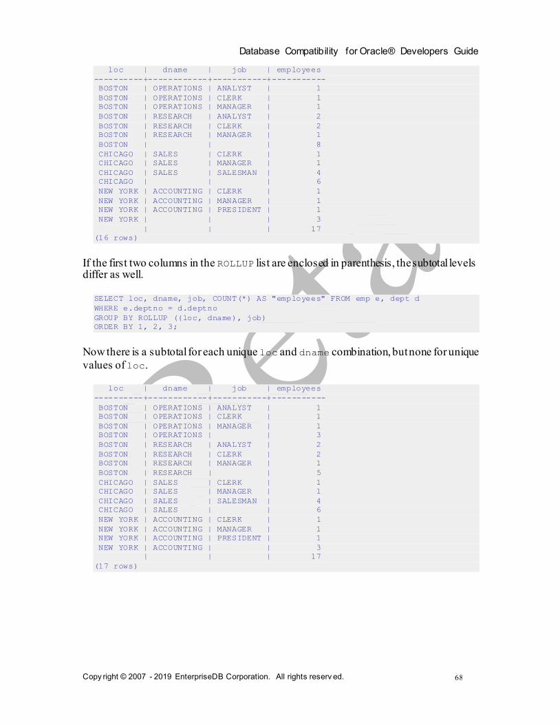
Database Compatibility for Oracle® Developers Guide
Copy right © 2007 - 2019 EnterpriseDB Corporation. All rights reserv ed.
68
loc | dname | job | employees
----------+------------+-----------+-----------
BOSTON | OPERATIONS | ANALYST | 1
BOSTON | OPERATIONS | CLERK | 1
BOSTON | OPERATIONS | MANAGER | 1
BOSTON | RESEARCH | ANALYST | 2
BOSTON | RESEARCH | CLERK | 2
BOSTON | RESEARCH | MANAGER | 1
BOSTON | | | 8
CHICAGO | SALES | CLERK | 1
CHICAGO | SALES | MANAGER | 1
CHICAGO | SALES | SALESMAN | 4
CHICAGO | | | 6
NEW YORK | ACCOUNTING | CLERK | 1
NEW YORK | ACCOUNTING | MANAGER | 1
NEW YORK | ACCOUNTING | PRESIDENT | 1
NEW YORK | | | 3
| | | 17
(16 rows)
If the first two columns in the ROLLUP list are enclosed in parenthesis, the subtotal levels differ as well.
SELECT loc, dname, job, COUNT(*) AS "employees" FROM emp e, dept d
WHERE e.deptno = d.deptno
GROUP BY ROLLUP ((loc, dname), job)
ORDER BY 1, 2, 3;
Now there is a subtotal for each unique loc and dname combination, but none for unique
values of loc.
loc | dname | job | employees
----------+------------+-----------+-----------
BOSTON | OPERATIONS | ANALYST | 1
BOSTON | OPERATIONS | CLERK | 1
BOSTON | OPERATIONS | MANAGER | 1
BOSTON | OPERATIONS | | 3
BOSTON | RESEARCH | ANALYST | 2
BOSTON | RESEARCH | CLERK | 2
BOSTON | RESEARCH | MANAGER | 1
BOSTON | RESEARCH | | 5
CHICAGO | SALES | CLERK | 1
CHICAGO | SALES | MANAGER | 1
CHICAGO | SALES | SALESMAN | 4
CHICAGO | SALES | | 6
NEW YORK | ACCOUNTING | CLERK | 1
NEW YORK | ACCOUNTING | MANAGER | 1
NEW YORK | ACCOUNTING | PRESIDENT | 1
NEW YORK | ACCOUNTING | | 3
| | | 17
(17 rows)

Database Compatibility for Oracle® Developers Guide
Copy right © 2007 - 2019 EnterpriseDB Corporation. All rights reserv ed.
69
2.2.6.2 CUBE Extension
The CUBE extension is similar to the ROLLUP extension. However, unlike ROLLUP, which produces groupings and results in a hierarchy based on a left to right listing of items in
the ROLLUP expression list, a CUBE produces groupings and subtotals based on every
permutation of all items in the CUBE expression list. Thus, the result set contains more rows than a ROLLUP performed on the same expression list.
The syntax for a single CUBE is as follows:
CUBE ( { expr_1 | ( expr_1a [, expr_1b ] ...) }
[, expr_2 | ( expr_2a [, expr_2b ] ...) ] ...)
Each expr is an expression that determines the grouping of the result set. If enclosed
within parenthesis as ( expr_1a, expr_1b, ...) then the combination of values returned by expr_1a and expr_1b defines a single group.
The base level of aggregates returned in the result set is for each unique combination of values returned by the expression list.
In addition, a subtotal is returned for the first item in the list (expr_1 or the combination
of ( expr_1a, expr_1b, ...), whichever is specified) for each unique value. A
subtotal is returned for the second item in the list (expr_2 or the combination of (
expr_2a, expr_2b, ...), whichever is specified) for each unique value. A subtotal
is also returned for each unique combination of the first item and the second item. Similarly, if there is a third item, a subtotal is returned for each unique value of the third item, each unique value of the third item and first item combination, each unique value of
the third item and second item combination, and each unique value of the third item, second item, and first item combination. Finally a grand total is returned for the entire result set.
For the subtotal rows, null is returned for the items across which the subtotal is taken.
The CUBE extension specified within the context of the GROUP BY clause is shown by the following:
SELECT select_list FROM ...
GROUP BY [... ,] CUBE ( expression_list ) [, ...]
The items specified in select_list must also appear in the CUBE expression_list;
or they must be aggregate functions such as COUNT, SUM, AVG, MIN, or MAX; or they must be constants or functions whose return values are independent of the individual rows in
the group (for example, the SYSDATE function).
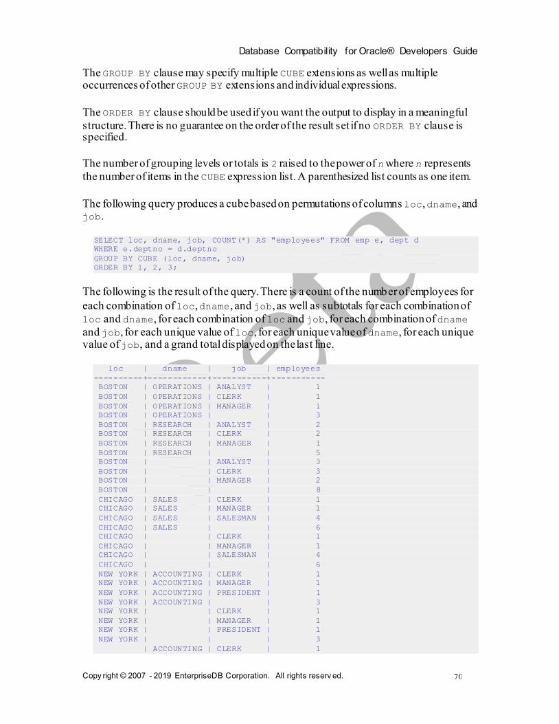
Database Compatibility for Oracle® Developers Guide
Copy right © 2007 - 2019 EnterpriseDB Corporation. All rights reserv ed.
70
The GROUP BY clause may specify multiple CUBE extensions as well as multiple occurrences of other GROUP BY extensions and individual expressions.
The ORDER BY clause should be used if you want the output to display in a meaningful
structure. There is no guarantee on the order of the result set if no ORDER BY clause is specified.
The number of grouping levels or totals is 2 raised to the power of n where n represents
the number of items in the CUBE expression list. A parenthesized list counts as one item.
The following query produces a cube based on permutations of columns loc, dname, and job.
SELECT loc, dname, job, COUNT(*) AS "employees" FROM emp e, dept d
WHERE e.deptno = d.deptno
GROUP BY CUBE (loc, dname, job)
ORDER BY 1, 2, 3;
The following is the result of the query. There is a count of the number of employees for
each combination of loc, dname, and job, as well as subtotals for each combination of
loc and dname, for each combination of loc and job, for each combination of dname
and job, for each unique value of loc, for each unique value of dname, for each unique value of job, and a grand total displayed on the last line.
loc | dname | job | employees
----------+------------+-----------+-----------
BOSTON | OPERATIONS | ANALYST | 1
BOSTON | OPERATIONS | CLERK | 1
BOSTON | OPERATIONS | MANAGER | 1
BOSTON | OPERATIONS | | 3
BOSTON | RESEARCH | ANALYST | 2
BOSTON | RESEARCH | CLERK | 2
BOSTON | RESEARCH | MANAGER | 1
BOSTON | RESEARCH | | 5
BOSTON | | ANALYST | 3
BOSTON | | CLERK | 3
BOSTON | | MANAGER | 2
BOSTON | | | 8
CHICAGO | SALES | CLERK | 1
CHICAGO | SALES | MANAGER | 1
CHICAGO | SALES | SALESMAN | 4
CHICAGO | SALES | | 6
CHICAGO | | CLERK | 1
CHICAGO | | MANAGER | 1
CHICAGO | | SALESMAN | 4
CHICAGO | | | 6
NEW YORK | ACCOUNTING | CLERK | 1
NEW YORK | ACCOUNTING | MANAGER | 1
NEW YORK | ACCOUNTING | PRESIDENT | 1
NEW YORK | ACCOUNTING | | 3
NEW YORK | | CLERK | 1
NEW YORK | | MANAGER | 1
NEW YORK | | PRESIDENT | 1
NEW YORK | | | 3
| ACCOUNTING | CLERK | 1
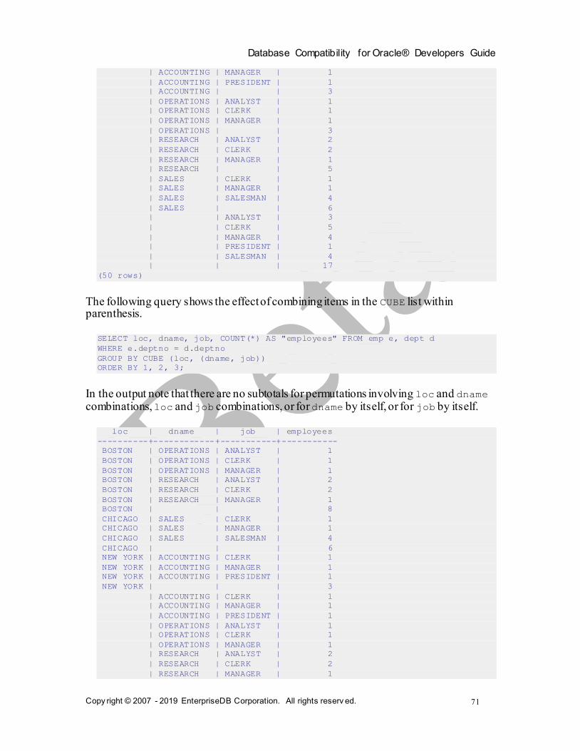
Database Compatibility for Oracle® Developers Guide
Copy right © 2007 - 2019 EnterpriseDB Corporation. All rights reserv ed.
71
| ACCOUNTING | MANAGER | 1
| ACCOUNTING | PRESIDENT | 1
| ACCOUNTING | | 3
| OPERATIONS | ANALYST | 1
| OPERATIONS | CLERK | 1
| OPERATIONS | MANAGER | 1
| OPERATIONS | | 3
| RESEARCH | ANALYST | 2
| RESEARCH | CLERK | 2
| RESEARCH | MANAGER | 1
| RESEARCH | | 5
| SALES | CLERK | 1
| SALES | MANAGER | 1
| SALES | SALESMAN | 4
| SALES | | 6
| | ANALYST | 3
| | CLERK | 5
| | MANAGER | 4
| | PRESIDENT | 1
| | SALESMAN | 4
| | | 17
(50 rows)
The following query shows the effect of combining items in the CUBE list within parenthesis.
SELECT loc, dname, job, COUNT(*) AS "employees" FROM emp e, dept d
WHERE e.deptno = d.deptno
GROUP BY CUBE (loc, (dname, job))
ORDER BY 1, 2, 3;
In the output note that there are no subtotals for permutations involving loc and dname combinations, loc and job combinations, or for dname by itself, or for job by itself.
loc | dname | job | employees
----------+------------+-----------+-----------
BOSTON | OPERATIONS | ANALYST | 1
BOSTON | OPERATIONS | CLERK | 1
BOSTON | OPERATIONS | MANAGER | 1
BOSTON | RESEARCH | ANALYST | 2
BOSTON | RESEARCH | CLERK | 2
BOSTON | RESEARCH | MANAGER | 1
BOSTON | | | 8
CHICAGO | SALES | CLERK | 1
CHICAGO | SALES | MANAGER | 1
CHICAGO | SALES | SALESMAN | 4
CHICAGO | | | 6
NEW YORK | ACCOUNTING | CLERK | 1
NEW YORK | ACCOUNTING | MANAGER | 1
NEW YORK | ACCOUNTING | PRESIDENT | 1
NEW YORK | | | 3
| ACCOUNTING | CLERK | 1
| ACCOUNTING | MANAGER | 1
| ACCOUNTING | PRESIDENT | 1
| OPERATIONS | ANALYST | 1
| OPERATIONS | CLERK | 1
| OPERATIONS | MANAGER | 1
| RESEARCH | ANALYST | 2
| RESEARCH | CLERK | 2
| RESEARCH | MANAGER | 1
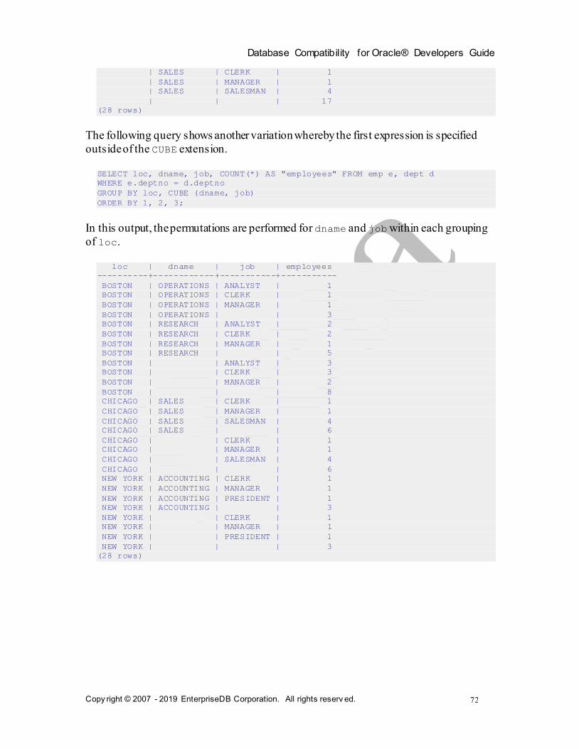
Database Compatibility for Oracle® Developers Guide
Copy right © 2007 - 2019 EnterpriseDB Corporation. All rights reserv ed.
72
| SALES | CLERK | 1
| SALES | MANAGER | 1
| SALES | SALESMAN | 4
| | | 17
(28 rows)
The following query shows another variation whereby the first expression is specified
outside of the CUBE extension.
SELECT loc, dname, job, COUNT(*) AS "employees" FROM emp e, dept d
WHERE e.deptno = d.deptno
GROUP BY loc, CUBE (dname, job)
ORDER BY 1, 2, 3;
In this output, the permutations are performed for dname and job within each grouping
of loc.
loc | dname | job | employees
----------+------------+-----------+-----------
BOSTON | OPERATIONS | ANALYST | 1
BOSTON | OPERATIONS | CLERK | 1
BOSTON | OPERATIONS | MANAGER | 1
BOSTON | OPERATIONS | | 3
BOSTON | RESEARCH | ANALYST | 2
BOSTON | RESEARCH | CLERK | 2
BOSTON | RESEARCH | MANAGER | 1
BOSTON | RESEARCH | | 5
BOSTON | | ANALYST | 3
BOSTON | | CLERK | 3
BOSTON | | MANAGER | 2
BOSTON | | | 8
CHICAGO | SALES | CLERK | 1
CHICAGO | SALES | MANAGER | 1
CHICAGO | SALES | SALESMAN | 4
CHICAGO | SALES | | 6
CHICAGO | | CLERK | 1
CHICAGO | | MANAGER | 1
CHICAGO | | SALESMAN | 4
CHICAGO | | | 6
NEW YORK | ACCOUNTING | CLERK | 1
NEW YORK | ACCOUNTING | MANAGER | 1
NEW YORK | ACCOUNTING | PRESIDENT | 1
NEW YORK | ACCOUNTING | | 3
NEW YORK | | CLERK | 1
NEW YORK | | MANAGER | 1
NEW YORK | | PRESIDENT | 1
NEW YORK | | | 3
(28 rows)

Database Compatibility for Oracle® Developers Guide
Copy right © 2007 - 2019 EnterpriseDB Corporation. All rights reserv ed.
73
2.2.6.3 GROUPING SETS Extension
The use of the GROUPING SETS extension within the GROUP BY clause provides a means to produce one result set that is actually the concatenation of multiple results sets
based upon different groupings. In other words, a UNION ALL operation is performed combining the result sets of multiple groupings into one result set.
Note that a UNION ALL operation, and therefore the GROUPING SETS extension, do not eliminate duplicate rows from the result sets that are being combined together.
The syntax for a single GROUPING SETS extension is as follows:
GROUPING SETS (
{ expr_1 | ( expr_1a [, expr_1b ] ...) |
ROLLUP ( expr_list ) | CUBE ( expr_list )
} [, ...] )
A GROUPING SETS extension can contain any combination of one or more comma-
separated expressions, lists of expressions enclosed within parenthesis, ROLLUP extensions, and CUBE extensions.
The GROUPING SETS extension is specified within the context of the GROUP BY clause as shown by the following:
SELECT select_list FROM ...
GROUP BY [... ,] GROUPING SETS ( expression_list ) [, ...]
The items specified in select_list must also appear in the GROUPING SETS
expression_list; or they must be aggregate functions such as COUNT, SUM, AVG, MIN,
or MAX; or they must be constants or functions whose return values are independent of the individual rows in the group (for example, the SYSDATE function).
The GROUP BY clause may specify multiple GROUPING SETS extensions as well as multiple occurrences of other GROUP BY extensions and individual expressions.
The ORDER BY clause should be used if you want the output to display in a meaningful
structure. There is no guarantee on the order of the result set if no ORDER BY clause is specified.
The following query produces a union of groups given by columns loc, dname, and job.
SELECT loc, dname, job, COUNT(*) AS "employees" FROM emp e, dept d
WHERE e.deptno = d.deptno
GROUP BY GROUPING SETS (loc, dname, job)
ORDER BY 1, 2, 3;

Database Compatibility for Oracle® Developers Guide
Copy right © 2007 - 2019 EnterpriseDB Corporation. All rights reserv ed.
74
The result is as follows:
loc | dname | job | employees
----------+------------+-----------+-----------
BOSTON | | | 8
CHICAGO | | | 6
NEW YORK | | | 3
| ACCOUNTING | | 3
| OPERATIONS | | 3
| RESEARCH | | 5
| SALES | | 6
| | ANALYST | 3
| | CLERK | 5
| | MANAGER | 4
| | PRESIDENT | 1
| | SALESMAN | 4
(12 rows)
This is equivalent to the following query, which employs the use of the UNION ALL operator.
SELECT loc AS "loc", NULL AS "dname", NULL AS "job", COUNT(*) AS "employees"
FROM emp e, dept d
WHERE e.deptno = d.deptno
GROUP BY loc
UNION ALL
SELECT NULL, dname, NULL, COUNT(*) AS "employees" FROM emp e, dept d
WHERE e.deptno = d.deptno
GROUP BY dname
UNION ALL
SELECT NULL, NULL, job, COUNT(*) AS "employees" FROM emp e, dept d
WHERE e.deptno = d.deptno
GROUP BY job
ORDER BY 1, 2, 3;
The output from the UNION ALL query is the same as the GROUPING SETS output.
loc | dname | job | employees
----------+------------+-----------+-----------
BOSTON | | | 8
CHICAGO | | | 6
NEW YORK | | | 3
| ACCOUNTING | | 3
| OPERATIONS | | 3
| RESEARCH | | 5
| SALES | | 6
| | ANALYST | 3
| | CLERK | 5
| | MANAGER | 4
| | PRESIDENT | 1
| | SALESMAN | 4
(12 rows)
The following example shows how various types of GROUP BY extensions can be used together within a GROUPING SETS expression list.
SELECT loc, dname, job, COUNT(*) AS "employees" FROM emp e, dept d
WHERE e.deptno = d.deptno

Database Compatibility for Oracle® Developers Guide
Copy right © 2007 - 2019 EnterpriseDB Corporation. All rights reserv ed.
75
GROUP BY GROUPING SETS (loc, ROLLUP (dname, job), CUBE (job, loc))
ORDER BY 1, 2, 3;
The following is the output from this query.
loc | dname | job | employees
----------+------------+-----------+-----------
BOSTON | | ANALYST | 3
BOSTON | | CLERK | 3
BOSTON | | MANAGER | 2
BOSTON | | | 8
BOSTON | | | 8
CHICAGO | | CLERK | 1
CHICAGO | | MANAGER | 1
CHICAGO | | SALESMAN | 4
CHICAGO | | | 6
CHICAGO | | | 6
NEW YORK | | CLERK | 1
NEW YORK | | MANAGER | 1
NEW YORK | | PRESIDENT | 1
NEW YORK | | | 3
NEW YORK | | | 3
| ACCOUNTING | CLERK | 1
| ACCOUNTING | MANAGER | 1
| ACCOUNTING | PRESIDENT | 1
| ACCOUNTING | | 3
| OPERATIONS | ANALYST | 1
| OPERATIONS | CLERK | 1
| OPERATIONS | MANAGER | 1
| OPERATIONS | | 3
| RESEARCH | ANALYST | 2
| RESEARCH | CLERK | 2
| RESEARCH | MANAGER | 1
| RESEARCH | | 5
| SALES | CLERK | 1
| SALES | MANAGER | 1
| SALES | SALESMAN | 4
| SALES | | 6
| | ANALYST | 3
| | CLERK | 5
| | MANAGER | 4
| | PRESIDENT | 1
| | SALESMAN | 4
| | | 17
| | | 17
(38 rows)
The output is basically a concatenation of the result sets that would be produced
individually from GROUP BY loc, GROUP BY ROLLUP (dname, job), and GROUP BY CUBE (job, loc). These individual queries are shown by the following.
SELECT loc, NULL AS "dname", NULL AS "job", COUNT(*) AS "employees"
FROM emp e, dept d
WHERE e.deptno = d.deptno
GROUP BY loc
ORDER BY 1;

Database Compatibility for Oracle® Developers Guide
Copy right © 2007 - 2019 EnterpriseDB Corporation. All rights reserv ed.
76
The following is the result set from the GROUP BY loc clause.
loc | dname | job | employees
----------+-------+-----+-----------
BOSTON | | | 8
CHICAGO | | | 6
NEW YORK | | | 3
(3 rows)
The following query uses the GROUP BY ROLLUP (dname, job) clause.
SELECT NULL AS "loc", dname, job, COUNT(*) AS "employees" FROM emp e, dept d
WHERE e.deptno = d.deptno
GROUP BY ROLLUP (dname, job)
ORDER BY 2, 3;
The following is the result set from the GROUP BY ROLLUP (dname, job) clause.
loc | dname | job | employees
-----+------------+-----------+-----------
| ACCOUNTING | CLERK | 1
| ACCOUNTING | MANAGER | 1
| ACCOUNTING | PRESIDENT | 1
| ACCOUNTING | | 3
| OPERATIONS | ANALYST | 1
| OPERATIONS | CLERK | 1
| OPERATIONS | MANAGER | 1
| OPERATIONS | | 3
| RESEARCH | ANALYST | 2
| RESEARCH | CLERK | 2
| RESEARCH | MANAGER | 1
| RESEARCH | | 5
| SALES | CLERK | 1
| SALES | MANAGER | 1
| SALES | SALESMAN | 4
| SALES | | 6
| | | 17
(17 rows)
The following query uses the GROUP BY CUBE (job, loc) clause.
SELECT loc, NULL AS "dname", job, COUNT(*) AS "employees" FROM emp e, dept d
WHERE e.deptno = d.deptno
GROUP BY CUBE (job, loc)
ORDER BY 1, 3;
The following is the result set from the GROUP BY CUBE (job, loc) clause.
loc | dname | job | employees
----------+-------+-----------+-----------
BOSTON | | ANALYST | 3
BOSTON | | CLERK | 3
BOSTON | | MANAGER | 2
BOSTON | | | 8
CHICAGO | | CLERK | 1
CHICAGO | | MANAGER | 1
CHICAGO | | SALESMAN | 4
CHICAGO | | | 6

Database Compatibility for Oracle® Developers Guide
Copy right © 2007 - 2019 EnterpriseDB Corporation. All rights reserv ed.
77
NEW YORK | | CLERK | 1
NEW YORK | | MANAGER | 1
NEW YORK | | PRESIDENT | 1
NEW YORK | | | 3
| | ANALYST | 3
| | CLERK | 5
| | MANAGER | 4
| | PRESIDENT | 1
| | SALESMAN | 4
| | | 17
(18 rows)
If the previous three queries are combined with the UNION ALL operator, a concatenation of the three results sets is produced.
SELECT loc AS "loc", NULL AS "dname", NULL AS "job", COUNT(*) AS "employees"
FROM emp e, dept d
WHERE e.deptno = d.deptno
GROUP BY loc
UNION ALL
SELECT NULL, dname, job, count(*) AS "employees" FROM emp e, dept d
WHERE e.deptno = d.deptno
GROUP BY ROLLUP (dname, job)
UNION ALL
SELECT loc, NULL, job, count(*) AS "employees" FROM emp e, dept d
WHERE e.deptno = d.deptno
GROUP BY CUBE (job, loc)
ORDER BY 1, 2, 3;
The following is the output, which is the same as when the GROUP BY GROUPING SETS (loc, ROLLUP (dname, job), CUBE (job, loc)) clause is used.
loc | dname | job | employees
----------+------------+-----------+-----------
BOSTON | | ANALYST | 3
BOSTON | | CLERK | 3
BOSTON | | MANAGER | 2
BOSTON | | | 8
BOSTON | | | 8
CHICAGO | | CLERK | 1
CHICAGO | | MANAGER | 1
CHICAGO | | SALESMAN | 4
CHICAGO | | | 6
CHICAGO | | | 6
NEW YORK | | CLERK | 1
NEW YORK | | MANAGER | 1
NEW YORK | | PRESIDENT | 1
NEW YORK | | | 3
NEW YORK | | | 3
| ACCOUNTING | CLERK | 1
| ACCOUNTING | MANAGER | 1
| ACCOUNTING | PRESIDENT | 1
| ACCOUNTING | | 3
| OPERATIONS | ANALYST | 1
| OPERATIONS | CLERK | 1
| OPERATIONS | MANAGER | 1
| OPERATIONS | | 3
| RESEARCH | ANALYST | 2
| RESEARCH | CLERK | 2
| RESEARCH | MANAGER | 1

Database Compatibility for Oracle® Developers Guide
Copy right © 2007 - 2019 EnterpriseDB Corporation. All rights reserv ed.
78
| RESEARCH | | 5
| SALES | CLERK | 1
| SALES | MANAGER | 1
| SALES | SALESMAN | 4
| SALES | | 6
| | ANALYST | 3
| | CLERK | 5
| | MANAGER | 4
| | PRESIDENT | 1
| | SALESMAN | 4
| | | 17
| | | 17
(38 rows)

Database Compatibility for Oracle® Developers Guide
Copy right © 2007 - 2019 EnterpriseDB Corporation. All rights reserv ed.
79
2.2.6.4 GROUPING Function
When using the ROLLUP, CUBE, or GROUPING SETS extensions to the GROUP BY clause, it may sometimes be difficult to differentiate between the various levels of subtotals
generated by the extensions as well as the base aggregate rows in the result set. The GROUPING function provides a means of making this distinction.
The general syntax for use of the GROUPING function is shown by the following.
SELECT [ expr ...,] GROUPING( col_expr ) [, expr ] ...
FROM ...
GROUP BY [...,]
{ ROLLUP | CUBE | GROUPING SETS }( [...,] col_expr
[, ...] ) [, ...]
The GROUPING function takes a single parameter that must be an expression of a
dimension column specified in the expression list of a ROLLUP, CUBE, or GROUPING SETS extension of the GROUP BY clause.
The return value of the GROUPING function is either a 0 or 1. In the result set of a query,
if the column expression specified in the GROUPING function is null because the row
represents a subtotal over multiple values of that column then the GROUPING function returns a value of 1. If the row returns results based on a particular value of the column
specified in the GROUPING function, then the GROUPING function returns a value of 0. In the latter case, the column can be null as well as non-null, but in any case, it is for a particular value of that column, not a subtotal across multiple values.
The following query shows how the return values of the GROUPING function correspond to the subtotal lines.
SELECT loc, dname, job, COUNT(*) AS "employees",
GROUPING(loc) AS "gf_loc",
GROUPING(dname) AS "gf_dname",
GROUPING(job) AS "gf_job"
FROM emp e, dept d
WHERE e.deptno = d.deptno
GROUP BY ROLLUP (loc, dname, job)
ORDER BY 1, 2, 3;
In the three right-most columns displaying the output of the GROUPING functions, a value
of 1 appears on a subtotal line wherever a subtotal is taken across values of the corresponding columns.
loc | dname | job | employees | gf_loc | gf_dname | gf_job
----------+------------+-----------+-----------+--------+----------+--------
BOSTON | OPERATIONS | ANALYST | 1 | 0 | 0 | 0
BOSTON | OPERATIONS | CLERK | 1 | 0 | 0 | 0
BOSTON | OPERATIONS | MANAGER | 1 | 0 | 0 | 0

Database Compatibility for Oracle® Developers Guide
Copy right © 2007 - 2019 EnterpriseDB Corporation. All rights reserv ed.
80
BOSTON | OPERATIONS | | 3 | 0 | 0 | 1
BOSTON | RESEARCH | ANALYST | 2 | 0 | 0 | 0
BOSTON | RESEARCH | CLERK | 2 | 0 | 0 | 0
BOSTON | RESEARCH | MANAGER | 1 | 0 | 0 | 0
BOSTON | RESEARCH | | 5 | 0 | 0 | 1
BOSTON | | | 8 | 0 | 1 | 1
CHICAGO | SALES | CLERK | 1 | 0 | 0 | 0
CHICAGO | SALES | MANAGER | 1 | 0 | 0 | 0
CHICAGO | SALES | SALESMAN | 4 | 0 | 0 | 0
CHICAGO | SALES | | 6 | 0 | 0 | 1
CHICAGO | | | 6 | 0 | 1 | 1
NEW YORK | ACCOUNTING | CLERK | 1 | 0 | 0 | 0
NEW YORK | ACCOUNTING | MANAGER | 1 | 0 | 0 | 0
NEW YORK | ACCOUNTING | PRESIDENT | 1 | 0 | 0 | 0
NEW YORK | ACCOUNTING | | 3 | 0 | 0 | 1
NEW YORK | | | 3 | 0 | 1 | 1
| | | 17 | 1 | 1 | 1
(20 rows)
These indicators can be used as screening criteria for particular subtotals. For example,
using the previous query, you can display only those subtotals for loc and dname combinations by using the GROUPING function in a HAVING clause.
SELECT loc, dname, job, COUNT(*) AS "employees",
GROUPING(loc) AS "gf_loc",
GROUPING(dname) AS "gf_dname",
GROUPING(job) AS "gf_job"
FROM emp e, dept d
WHERE e.deptno = d.deptno
GROUP BY ROLLUP (loc, dname, job)
HAVING GROUPING(loc) = 0
AND GROUPING(dname) = 0
AND GROUPING(job) = 1
ORDER BY 1, 2;
This query produces the following result:
loc | dname | job | employees | gf_loc | gf_dname | gf_job
----------+------------+-----+-----------+--------+----------+--------
BOSTON | OPERATIONS | | 3 | 0 | 0 | 1
BOSTON | RESEARCH | | 5 | 0 | 0 | 1
CHICAGO | SALES | | 6 | 0 | 0 | 1
NEW YORK | ACCOUNTING | | 3 | 0 | 0 | 1
(4 rows)
The GROUPING function can be used to distinguish a subtotal row from a base aggregate row or from certain subtotal rows where one of the items in the expression list returns
null as a result of the column on which the expression is based being null for one or more rows in the table, as opposed to representing a subtotal over the column.
To illustrate this point, the following row is added to the emp table. This provides a row with a null value for the job column.
INSERT INTO emp (empno,ename,deptno) VALUES (9004,'PETERS',40);

Database Compatibility for Oracle® Developers Guide
Copy right © 2007 - 2019 EnterpriseDB Corporation. All rights reserv ed.
81
The following query is issued using a reduced number of rows for clarity.
SELECT loc, job, COUNT(*) AS "employees",
GROUPING(loc) AS "gf_loc",
GROUPING(job) AS "gf_job"
FROM emp e, dept d
WHERE e.deptno = d.deptno AND loc = 'BOSTON'
GROUP BY CUBE (loc, job)
ORDER BY 1, 2;
Note that the output contains two rows containing BOSTON in the loc column and spaces
in the job column (fourth and fifth entries in the table).
loc | job | employees | gf_loc | gf_job
--------+---------+-----------+--------+--------
BOSTON | ANALYST | 3 | 0 | 0
BOSTON | CLERK | 3 | 0 | 0
BOSTON | MANAGER | 2 | 0 | 0
BOSTON | | 1 | 0 | 0
BOSTON | | 9 | 0 | 1
| ANALYST | 3 | 1 | 0
| CLERK | 3 | 1 | 0
| MANAGER | 2 | 1 | 0
| | 1 | 1 | 0
| | 9 | 1 | 1
(10 rows)
The fifth row where the GROUPING function on the job column (gf_job) returns 1 indicates this is a subtotal over all jobs. Note that the row contains a subtotal value of 9 in
the employees column.
The fourth row where the GROUPING function on the job column as well as on the loc
column returns 0 indicates this is a base aggregate of all rows where loc is BOSTON and
job is null, which is the row inserted for this example. The employees column contains 1, which is the count of the single such row inserted.
Also note that in the ninth row (next to last) the GROUPING function on the job column
returns 0 while the GROUPING function on the loc column returns 1 indicating this is a
subtotal over all locations where the job column is null, which again, is a count of the single row inserted for this example.

Database Compatibility for Oracle® Developers Guide
Copy right © 2007 - 2019 EnterpriseDB Corporation. All rights reserv ed.
82
2.2.6.5 GROUPING_ID Function
The GROUPING_ID function provides a simplification of the GROUPING function in order
to determine the subtotal level of a row in the result set from a ROLLBACK, CUBE, or GROUPING SETS extension.
The GROUPING function takes only one column expression and returns an indication of whether or not a row is a subtotal over all values of the given column. Thus, multiple
GROUPING functions may be required to interpret the level of subtotals for queries with multiple grouping columns.
The GROUPING_ID function accepts one or more column expressions that have been used
in the ROLLBACK, CUBE, or GROUPING SETS extensions and returns a single integer that can be used to determine over which of these columns a subtotal has been aggregated.
The general syntax for use of the GROUPING_ID function is shown by the following.
SELECT [ expr ...,]
GROUPING_ID( col_expr_1 [, col_expr_2 ] ... )
[, expr ] ...
FROM ...
GROUP BY [...,]
{ ROLLUP | CUBE | GROUPING SETS }( [...,] col_expr_1
[, col_expr_2 ] [, ...] ) [, ...]
The GROUPING_ID function takes one or more parameters that must be expressions of
dimension columns specified in the expression list of a ROLLUP, CUBE, or GROUPING SETS extension of the GROUP BY clause.
The GROUPING_ID function returns an integer value. This value corresponds to the base-10 interpretation of a bit vector consisting of the concatenated 1’s and 0’s that would be
returned by a series of GROUPING functions specified in the same left-to-right order as
the ordering of the parameters specified in the GROUPING_ID function.
The following query shows how the returned values of the GROUPING_ID function
represented in column gid correspond to the values returned by two GROUPING functions on columns loc and dname.
SELECT loc, dname, COUNT(*) AS "employees",
GROUPING(loc) AS "gf_loc", GROUPING(dname) AS "gf_dname",
GROUPING_ID(loc, dname) AS "gid"
FROM emp e, dept d
WHERE e.deptno = d.deptno
GROUP BY CUBE (loc, dname)
ORDER BY 6, 1, 2;

Database Compatibility for Oracle® Developers Guide
Copy right © 2007 - 2019 EnterpriseDB Corporation. All rights reserv ed.
83
In the following output, note the relationship between a bit vector consisting of the
gf_loc value and gf_dname value compared to the integer given in gid.
loc | dname | employees | gf_loc | gf_dname | gid
----------+------------+-----------+--------+----------+-----
BOSTON | OPERATIONS | 3 | 0 | 0 | 0
BOSTON | RESEARCH | 5 | 0 | 0 | 0
CHICAGO | SALES | 6 | 0 | 0 | 0
NEW YORK | ACCOUNTING | 3 | 0 | 0 | 0
BOSTON | | 8 | 0 | 1 | 1
CHICAGO | | 6 | 0 | 1 | 1
NEW YORK | | 3 | 0 | 1 | 1
| ACCOUNTING | 3 | 1 | 0 | 2
| OPERATIONS | 3 | 1 | 0 | 2
| RESEARCH | 5 | 1 | 0 | 2
| SALES | 6 | 1 | 0 | 2
| | 17 | 1 | 1 | 3
(12 rows)
The following table provides specific examples of the GROUPING_ID function
calculations based on the GROUPING function return values for four rows of the output.
loc dname Bit Vector
gf_loc gf_dname
GROUPING_ID
gid
BOSTON OPERATIONS 0 * 21 + 0 * 2
0 0
BOSTON null 0 * 21 + 1 * 2
0 1
null ACCOUNTING 1 * 21 + 0 * 2
0 2
null null 1 * 21 + 1 * 2
0 3
The following table summarizes how the GROUPING_ID function return values correspond to the grouping columns over which aggregation occurs.
Aggregation by Column Bit Vector
gf_loc gf_dname
GROUPING_ID
gid
loc, dname 0 0 0
loc 0 1 1
dname 1 0 2
Grand Total 1 1 3
So to display only those subtotals by dname, the following simplified query can be used
with a HAVING clause based on the GROUPING_ID function.
SELECT loc, dname, COUNT(*) AS "employees",
GROUPING(loc) AS "gf_loc", GROUPING(dname) AS "gf_dname",
GROUPING_ID(loc, dname) AS "gid"
FROM emp e, dept d
WHERE e.deptno = d.deptno
GROUP BY CUBE (loc, dname)
HAVING GROUPING_ID(loc, dname) = 2
ORDER BY 6, 1, 2;

Database Compatibility for Oracle® Developers Guide
Copy right © 2007 - 2019 EnterpriseDB Corporation. All rights reserv ed.
84
The following is the result of the query.
loc | dname | employees | gf_loc | gf_dname | gid
-----+------------+-----------+--------+----------+-----
| ACCOUNTING | 3 | 1 | 0 | 2
| OPERATIONS | 3 | 1 | 0 | 2
| RESEARCH | 5 | 1 | 0 | 2
| SALES | 6 | 1 | 0 | 2
(4 rows)

Database Compatibility for Oracle® Developers Guide
Copy right © 2007 - 2019 EnterpriseDB Corporation. All rights reserv ed.
85
2.3 Profile Management
Advanced Server allows a database superuser to create named profiles. Each profile
defines rules for password management that augment password and md5 authentication. The rules in a profile can:
count failed login attempts
lock an account due to excessive failed login attempts
mark a password for expiration
define a grace period after a password expiration
define rules for password complexity
define rules that limit password re-use
A profile is a named set of password attributes that allow you to easily manage a group of
roles that share comparable authentication requirements. If the password requirements
change, you can modify the profile to have the new requirements applied to each user that is associated with that profile.
After creating the profile, you can associate the profile with one or more users. When a user connects to the server, the server enforces the profile that is associated with their
login role. Profiles are shared by all databases within a cluster, but each cluster may have multiple profiles. A single user with access to multiple databases will use the same profile when connecting to each database within the cluster.
Advanced Server creates a profile named default that is associated with a new role when the role is created unless an alternate profile is specified. If you upgrade to Advanced Server from a previous server version, existing roles will automatically be assigned to the default profile. You cannot delete the default profile.
The default profile specifies the following attributes:
FAILED_LOGIN_ATTEMPTS UNLIMITED PASSWORD_LOCK_TIME UNLIMITED PASSWORD_LIFE_TIME UNLIMITED PASSWORD_GRACE_TIME UNLIMITED
PASSWORD_REUSE_TIME UNLIMITED
PASSWORD_REUSE_MAX UNLIMITED
PASSWORD_VERIFY_FUNCTION NULL
PASSWORD_ALLOW_HASHED TRUE
A database superuser can use the ALTER PROFILE command to modify the values
specified by the default profile. For more information about modifying a profile, see Section 2.3.2.

Database Compatibility for Oracle® Developers Guide
Copy right © 2007 - 2019 EnterpriseDB Corporation. All rights reserv ed.
86
2.3.1 Creating a New Profile
Use the CREATE PROFILE command to create a new profile. The syntax is:
CREATE PROFILE profile_name
[LIMIT {parameter value} ... ];
Include the LIMIT clause and one or more space-delimited parameter/value pairs to specify the rules enforced by Advanced Server.
Parameters:
profile_name specifies the name of the profile.
parameter specifies the attribute limited by the profile.
value specifies the parameter limit.
Advanced Server supports the value shown below for each parameter:
FAILED_LOGIN_ATTEMPTS specifies the number of failed login attempts that a user may make before the server locks the user out of their account for the length of time
specified by PASSWORD_LOCK_TIME. Supported values are:
An INTEGER value greater than 0.
DEFAULT - the value of FAILED_LOGIN_ATTEMPTS specified in the
DEFAULT profile.
UNLIMITED – the connecting user may make an unlimited number of failed login attempts.
PASSWORD_LOCK_TIME specifies the length of time that must pass before the server
unlocks an account that has been locked because of FAILED_LOGIN_ATTEMPTS. Supported values are:
A NUMERIC value greater than or equal to 0. To specify a fractional portion
of a day, specify a decimal value. For example, use the value 4.5 to specify 4
days, 12 hours.
DEFAULT - the value of PASSWORD_LOCK_TIME specified in the DEFAULT profile.
UNLIMITED – the account is locked until it is manually unlocked by a database superuser.

Database Compatibility for Oracle® Developers Guide
Copy right © 2007 - 2019 EnterpriseDB Corporation. All rights reserv ed.
87
PASSWORD_LIFE_TIME specifies the number of days that the current password may
be used before the user is prompted to provide a new password. Include the
PASSWORD_GRACE_TIME clause when using the PASSWORD_LIFE_TIME clause to
specify the number of days that will pass after the password expires before
connections by the role are rejected. If PASSWORD_GRACE_TIME is not specified, the password will expire on the day specified by the default value of
PASSWORD_GRACE_TIME, and the user will not be allowed to execute any command until a new password is provided. Supported values are:
A NUMERIC value greater than or equal to 0. To specify a fractional portion
of a day, specify a decimal value. For example, use the value 4.5 to specify 4
days, 12 hours.
DEFAULT - the value of PASSWORD_LIFE_TIME specified in the DEFAULT profile.
UNLIMITED – The password does not have an expiration date.
PASSWORD_GRACE_TIME specifies the length of the grace period after a password
expires until the user is forced to change their password. When the grace period expires, a user will be allowed to connect, but will not be allowed to execute any command until they update their expired password. Supported values are:
A NUMERIC value greater than or equal to 0. To specify a fractional portion
of a day, specify a decimal value. For example, use the value 4.5 to specify 4
days, 12 hours.
DEFAULT - the value of PASSWORD_GRACE_TIME specified in the DEFAULT profile.
UNLIMITED – The grace period is infinite.
PASSWORD_REUSE_TIME specifies the number of days a user must wait before re-
using a password. The PASSWORD_REUSE_TIME and PASSWORD_REUSE_MAX parameters are intended to be used together. If you specify a finite value for one of
these parameters while the other is UNLIMITED, old passwords can never be reused.
If both parameters are set to UNLIMITED there are no restrictions on password reuse. Supported values are:
A NUMERIC value greater than or equal to 0. To specify a fractional portion
of a day, specify a decimal value. For example, use the value 4.5 to specify 4
days, 12 hours.
DEFAULT - the value of PASSWORD_REUSE_TIME specified in the DEFAULT profile.
UNLIMITED – The password can be re-used without restrictions.
PASSWORD_REUSE_MAX specifies the number of password changes that must occur
before a password can be reused. The PASSWORD_REUSE_TIME and

Database Compatibility for Oracle® Developers Guide
Copy right © 2007 - 2019 EnterpriseDB Corporation. All rights reserv ed.
88
PASSWORD_REUSE_MAX parameters are intended to be used together. If you specify a
finite value for one of these parameters while the other is UNLIMITED, old passwords
can never be reused. If both parameters are set to UNLIMITED there are no restrictions on password reuse. Supported values are:
An INTEGER value greater than or equal to 0.
DEFAULT - the value of PASSWORD_REUSE_MAX specified in the DEFAULT profile.
UNLIMITED – The password can be re-used without restrictions.
PASSWORD_VERIFY_FUNCTION specifies password complexity. Supported values are:
The name of a PL/SQL function.
DEFAULT - the value of PASSWORD_VERIFY_FUNCTION specified in the
DEFAULT profile.
NULL
PASSWORD_ALLOW_HASHED specifies whether an encrypted password to be allowed
for use or not. If you specify the value as TRUE, the system allows a user to change
the password by specifying a hash computed encrypted password on the client side.
However, if you specify the value as FALSE, then a password must be specified in a plain-text form in order to be validated effectively, else an error will be thrown if a server receives an encrypted password. Supported values are:
A BOOLEAN value TRUE/ON/YES/1 or FALSE/OFF/NO/0.
DEFAULT - the value of PASSWORD_ALLOW_HASHED specified in the
DEFAULT profile.
Note: The PASSWORD_ALLOW_HASHED is not an Oracle-compatible parameter.
Notes
Use DROP PROFILE command to remove the profile.
Examples
The following command creates a profile named acctg. The profile specifies that if a user has not authenticated with the correct password in five attempts, the account will be locked for one day:
CREATE PROFILE acctg LIMIT
FAILED_LOGIN_ATTEMPTS 5
PASSWORD_LOCK_TIME 1;

Database Compatibility for Oracle® Developers Guide
Copy right © 2007 - 2019 EnterpriseDB Corporation. All rights reserv ed.
89
The following command creates a profile named sales. The profile specifies that a user must change their password every 90 days:
CREATE PROFILE sales LIMIT
PASSWORD_LIFE_TIME 90
PASSWORD_GRACE_TIME 3;
If the user has not changed their password before the 90 days specified in the profile has
passed, they will be issued a warning at login. After a grace period of 3 days, their account will not be allowed to invoke any commands until they change their password.
The following command creates a profile named accts. The profile specifies that a user cannot re-use a password within 180 days of the last use of the password, and must change their password at least 5 times before re-using the password:
CREATE PROFILE accts LIMIT
PASSWORD_REUSE_TIME 180
PASSWORD_REUSE_MAX 5;
The following command creates a profile named resources; the profile calls a user-
defined function named password_rules that will verify that the password provided meets their standards for complexity:
CREATE PROFILE resources LIMIT
PASSWORD_VERIFY_FUNCTION password_rules;
2.3.1.1 Creating a Password Function
When specifying PASSWORD_VERIFY_FUNCTION, you can provide a customized
function that specifies the security rules that will be applied when your users change their password. For example, you can specify rules that stipulate that the new password must be at least n characters long, and may not contain a specific value.
The password function has the following signature:
function_name (user_name VARCHAR2,
new_password VARCHAR2,
old_password VARCHAR2) RETURN boolean
Where:
user_name is the name of the user.
new_password is the new password.
old_password is the user's previous password. If you reference this parameter within your function:

Database Compatibility for Oracle® Developers Guide
Copy right © 2007 - 2019 EnterpriseDB Corporation. All rights reserv ed.
90
When a database superuser changes their password, the third parameter will always be NULL.
When a user with the CREATEROLE attribute changes their password, the parameter will pass the previous password if the statement includes the
REPLACE clause. Note that the REPLACE clause is optional syntax for a user with the CREATEROLE privilege.
When a user that is not a database superuser and does not have the
CREATEROLE attribute changes their password, the third parameter will contain the previous password for the role.
The function returns a Boolean value. If the function returns true and does not raise an exception, the password is accepted; if the function returns false or raises an exception,
the password is rejected. If the function raises an exception, the specified error message is displayed to the user. If the function does not raise an exception, but returns false, the following error message is displayed:
ERROR: password verification for the specified password failed
The function must be owned by a database superuser, and reside in the sys schema.
Example:
The following example creates a profile and a custom function; then, the function is
associated with the profile. The following CREATE PROFILE command creates a profile named acctg_pwd_profile:
CREATE PROFILE acctg_pwd_profile;
The following commands create a (schema-qualified) function named
verify_password:
CREATE OR REPLACE FUNCTION sys.verify_password(user_name varchar2,
new_password varchar2, old_password varchar2)
RETURN boolean IMMUTABLE
IS
BEGIN
IF (length(new_password) < 5)
THEN
raise_application_error(-20001, 'too short');
END IF;
IF substring(new_password FROM old_password) IS NOT NULL
THEN
raise_application_error(-20002, 'includes old password');
END IF;
RETURN true;
END;

Database Compatibility for Oracle® Developers Guide
Copy right © 2007 - 2019 EnterpriseDB Corporation. All rights reserv ed.
91
The function first ensures that the password is at least 5 characters long, and then
compares the new password to the old password. If the new password contains fewer than 5 characters, or contains the old password, the function raises an error.
The following statement sets the ownership of the verify_password function to the enterprisedb database superuser:
ALTER FUNCTION verify_password(varchar2, varchar2, varchar2) OWNER TO
enterprisedb;
Then, the verify_password function is associated with the profile:
ALTER PROFILE acctg_pwd_profile LIMIT PASSWORD_VERIFY_FUNCTION
verify_password;
The following statements confirm that the function is working by first creating a test user
(alice), and then attempting to associate invalid and valid passwords with her role:
CREATE ROLE alice WITH LOGIN PASSWORD 'temp_password' PROFILE
acctg_pwd_profile;
Then, when alice connects to the database and attempts to change her password, she
must adhere to the rules established by the profile function. A non-superuser without CREATEROLE must include the REPLACE clause when changing a password:
edb=> ALTER ROLE alice PASSWORD 'hey';
ERROR: missing REPLACE clause
The new password must be at least 5 characters long:
edb=> ALTER USER alice PASSWORD 'hey' REPLACE 'temp_password';
ERROR: EDB-20001: too short
CONTEXT: edb-spl function verify_password(character varying,character
varying,character varying) line 5 at procedure/function invocation statement
If the new password is acceptable, the command completes without error:
edb=> ALTER USER alice PASSWORD 'hello' REPLACE 'temp_password';
ALTER ROLE
If alice decides to change her password, the new password must not contain the old password:
edb=> ALTER USER alice PASSWORD 'helloworld' REPLACE 'hello';
ERROR: EDB-20002: includes old password
CONTEXT: edb-spl function verify_password(character varying,character
varying,character varying) line 10 at procedure/function invocation statement
To remove the verify function, set password_verify_function to NULL:
ALTER PROFILE acctg_pwd_profile LIMIT password_verify_function NULL;

Database Compatibility for Oracle® Developers Guide
Copy right © 2007 - 2019 EnterpriseDB Corporation. All rights reserv ed.
92
Then, all password constraints will be lifted:
edb=# ALTER ROLE alice PASSWORD 'hey';
ALTER ROLE

Database Compatibility for Oracle® Developers Guide
Copy right © 2007 - 2019 EnterpriseDB Corporation. All rights reserv ed.
93
2.3.2 Altering a Profile
Use the ALTER PROFILE command to modify a user-defined profile; Advanced Server supports two forms of the command:
ALTER PROFILE profile_name RENAME TO new_name;
ALTER PROFILE profile_name
LIMIT {parameter value}[...];
Include the LIMIT clause and one or more space-delimited parameter/value pairs to
specify the rules enforced by Advanced Server, or use ALTER PROFILE…RENAME TO to change the name of a profile.
Parameters:
profile_name specifies the name of the profile.
new_name specifies the new name of the profile.
parameter specifies the attribute limited by the profile.
value specifies the parameter limit.
See the table in Section 2.3.1 for a complete list of accepted parameter/value pairs.
Examples
The following example modifies a profile named acctg_profile:
ALTER PROFILE acctg_profile
LIMIT FAILED_LOGIN_ATTEMPTS 3 PASSWORD_LOCK_TIME 1;
acctg_profile will count failed connection attempts when a login role attempts to
connect to the server. The profile specifies that if a user has not authenticated with the correct password in three attempts, the account will be locked for one day.
The following example changes the name of acctg_profile to payables_profile:
ALTER PROFILE acctg_profile RENAME TO payables_profile;

Database Compatibility for Oracle® Developers Guide
Copy right © 2007 - 2019 EnterpriseDB Corporation. All rights reserv ed.
94
2.3.3 Dropping a Profile
Use the DROP PROFILE command to drop a profile. The syntax is:
DROP PROFILE [IF EXISTS] profile_name [CASCADE|RESTRICT];
Include the IF EXISTS clause to instruct the server to not throw an error if the specified profile does not exist. The server will issue a notice if the profile does not exist.
Include the optional CASCADE clause to reassign any users that are currently associated
with the profile to the default profile, and then drop the profile. Include the optional
RESTRICT clause to instruct the server to not drop any profile that is associated with a role. This is the default behavior.
Parameters
profile_name
The name of the profile being dropped.
Examples
The following example drops a profile named acctg_profile:
DROP PROFILE acctg_profile CASCADE;
The command first re-associates any roles associated with the acctg_profile profile
with the default profile, and then drops the acctg_profile profile.
The following example drops a profile named acctg_profile:
DROP PROFILE acctg_profile RESTRICT;
The RESTRICT clause in the command instructs the server to not drop acctg_profile if there are any roles associated with the profile.

Database Compatibility for Oracle® Developers Guide
Copy right © 2007 - 2019 EnterpriseDB Corporation. All rights reserv ed.
95
2.3.4 Associating a Profile with an Existing Role
After creating a profile, you can use the ALTER USER… PROFILE or ALTER ROLE…
PROFILE command to associate the profile with a role. The command syntax related to profile management functionality is:
ALTER USER|ROLE name [[WITH] option[…]
where option can be the following compatible clauses:
PROFILE profile_name
| ACCOUNT {LOCK|UNLOCK}
| PASSWORD EXPIRE [AT 'timestamp']
or option can be the following non-compatible clauses:
| PASSWORD SET AT 'timestamp'
| LOCK TIME 'timestamp'
| STORE PRIOR PASSWORD {'password' 'timestamp} [, ...]
For information about the administrative clauses of the ALTER USER or ALTER ROLE command that are supported by Advanced Server, please see the PostgreSQL core documentation available at:
https://www.postgresql.org/docs/11/static/sql-commands.html
Only a database superuser can use the ALTER USER|ROLE clauses that enforce profile management. The clauses enforce the following behaviors:
Include the PROFILE clause and a profile_name to associate a pre-defined
profile with a role, or to change which pre-defined profile is associated with a user.
Include the ACCOUNT clause and the LOCK or UNLOCK keyword to specify that the user account should be placed in a locked or unlocked state.
Include the LOCK TIME 'timestamp' clause and a date/time value to lock the
role at the specified time, and unlock the role at the time indicated by the
PASSWORD_LOCK_TIME parameter of the profile assigned to this role. If LOCK
TIME is used with the ACCOUNT LOCK clause, the role can only be unlocked by a database superuser with the ACCOUNT UNLOCK clause.

Database Compatibility for Oracle® Developers Guide
Copy right © 2007 - 2019 EnterpriseDB Corporation. All rights reserv ed.
96
Include the PASSWORD EXPIRE clause with the AT 'timestamp' keywords to
specify a date/time when the password associated with the role will expire. If you omit the AT 'timestamp' keywords, the password will expire immediately.
Include the PASSWORD SET AT 'timestamp' keywords to set the password modification date to the time specified.
Include the STORE PRIOR PASSWORD {'password' 'timestamp} [, ...]
clause to modify the password history, adding the new password and the time the password was set.
Each login role may only have one profile. To discover the profile that is currently associated with a login role, query the profile column of the DBA_USERS view.
Parameters
name
The name of the role with which the specified profile will be associated.
password
The password associated with the role.
profile_name
The name of the profile that will be associated with the role.
timestamp
The date and time at which the clause will be enforced. When specifying a value for timestamp, enclose the value in single-quotes.
Examples
The following command uses the ALTER USER… PROFILE command to associate a profile named acctg with a user named john:
ALTER USER john PROFILE acctg_profile;
The following command uses the ALTER ROLE… PROFILE command to associate a
profile named acctg with a user named john:
ALTER ROLE john PROFILE acctg_profile;

Database Compatibility for Oracle® Developers Guide
Copy right © 2007 - 2019 EnterpriseDB Corporation. All rights reserv ed.
97
2.3.5 Unlocking a Locked Account
A database superuser can use clauses of the ALTER USER|ROLE… command to lock or unlock a role. The syntax is:
ALTER USER|ROLE name ACCOUNT {LOCK|UNLOCK} LOCK TIME 'timestamp'
Include the ACCOUNT LOCK clause to lock a role immediately; when locked, a role’s
LOGIN functionality is disabled. When you specify the ACCOUNT LOCK clause without
the LOCK TIME clause, the state of the role will not change until a superuser uses the ACCOUNT UNLOCK clause to unlock the role.
Use the ACCOUNT UNLOCK clause to unlock a role.
Use the LOCK TIME 'timestamp' clause to instruct the server to lock the account at the
time specified by the given timestamp for the length of time specified by the
PASSWORD_LOCK_TIME parameter of the profile associated with this role.
Combine the LOCK TIME 'timestamp' clause and the ACCOUNT LOCK clause to lock
an account at a specified time until the account is unlocked by a superuser invoking the ACCOUNT UNLOCK clause.
Parameters
name
The name of the role that is being locked or unlocked.
timestamp
The date and time at which the role will be locked. When specifying a value for timestamp, enclose the value in single-quotes.
Note
This command (available only in Advanced Server) is implemented to support Oracle-styled profile management.

Database Compatibility for Oracle® Developers Guide
Copy right © 2007 - 2019 EnterpriseDB Corporation. All rights reserv ed.
98
Examples
The following example uses the ACCOUNT LOCK clause to lock the role named john.
The account will remain locked until the account is unlocked with the ACCOUNT UNLOCK clause:
ALTER ROLE john ACCOUNT LOCK;
The following example uses the ACCOUNT UNLOCK clause to unlock the role named john:
ALTER USER john ACCOUNT UNLOCK;
The following example uses the LOCK TIME 'timestamp' clause to lock the role
named john on September 4, 2015:
ALTER ROLE john LOCK TIME „September 4 12:00:00 2015‟;
The role will remain locked for the length of time specified by the
PASSWORD_LOCK_TIME parameter.
The following example combines the LOCK TIME 'timestamp' clause and the
ACCOUNT LOCK clause to lock the role named john on September 4, 2015:
ALTER ROLE john LOCK TIME „September 4 12:00:00 2015‟ ACCOUNT LOCK;
The role will remain locked until a database superuser uses the ACCOUNT UNLOCK command to unlock the role.

Database Compatibility for Oracle® Developers Guide
Copy right © 2007 - 2019 EnterpriseDB Corporation. All rights reserv ed.
99
2.3.6 Creating a New Role Associated with a Profile
A database superuser can use clauses of the CREATE USER|ROLE command to assign a named profile to a role when creating the role, or to specify profile management details for a role. The command syntax related to profile management functionality is :
CREATE USER|ROLE name [[WITH] option […]]
where option can be the following compatible clauses:
PROFILE profile_name
| ACCOUNT {LOCK|UNLOCK}
| PASSWORD EXPIRE [AT 'timestamp']
or option can be the following non-compatible clauses:
| LOCK TIME 'timestamp'
For information about the administrative clauses of the CREATE USER or CREATE ROLE
command that are supported by Advanced Server, please see the PostgreSQL core documentation available at:
https://www.postgresql.org/docs/11/static/sql-commands.html
CREATE ROLE|USER… PROFILE adds a new role with an associated profile to an Advanced Server database cluster.
Roles created with the CREATE USER command are (by default) login roles. Roles
created with the CREATE ROLE command are (by default) not login roles. To create a login account with the CREATE ROLE command, you must include the LOGIN keyword.
Only a database superuser can use the CREATE USER|ROLE clauses that enforce profile management; these clauses enforce the following behaviors:
Include the PROFILE clause and a profile_name to associate a pre-defined
profile with a role, or to change which pre-defined profile is associated with a user.
Include the ACCOUNT clause and the LOCK or UNLOCK keyword to specify that the user account should be placed in a locked or unlocked state.
Include the LOCK TIME 'timestamp' clause and a date/time value to lock the
role at the specified time, and unlock the role at the time indicated by the
PASSWORD_LOCK_TIME parameter of the profile assigned to this role. If LOCK

Database Compatibility for Oracle® Developers Guide
Copy right © 2007 - 2019 EnterpriseDB Corporation. All rights reserv ed.
100
TIME is used with the ACCOUNT LOCK clause, the role can only be unlocked by a database superuser with the ACCOUNT UNLOCK clause.
Include the PASSWORD EXPIRE clause with the optional AT 'timestamp'
keywords to specify a date/time when the password associated with the role will expire. If you omit the AT 'timestamp' keywords, the password will expire immediately.
Each login role may only have one profile. To discover the profile that is currently
associated with a login role, query the profile column of the DBA_USERS view.
Parameters
name
The name of the role.
profile_name
The name of the profile associated with the role.
timestamp
The date and time at which the clause will be enforced. When specifying a value for timestamp, enclose the value in single-quotes.
Examples
The following example uses CREATE USER to create a login role named john who is associated with the acctg_profile profile:
CREATE USER john PROFILE acctg_profile IDENTIFIED BY “1safepwd”;
john can log in to the server, using the password 1safepwd.
The following example uses CREATE ROLE to create a login role named john who is associated with the acctg_profile profile:
CREATE ROLE john PROFILE acctg_profile LOGIN PASSWORD “1safepwd”;
john can log in to the server, using the password 1safepwd.

Database Compatibility for Oracle® Developers Guide
Copy right © 2007 - 2019 EnterpriseDB Corporation. All rights reserv ed.
101
2.3.7 Backing up Profile Management Functions
A profile may include a PASSWORD_VERIFY_FUNCTION clause that refers to a user-defined function that specifies the behavior enforced by Advanced Server. Profiles are
global objects; they are shared by all of the databases within a cluster. While profiles are global objects, user-defined functions are database objects.
Invoking pg_dumpall with the –g or –r option will create a script that recreates the definition of any existing profiles, but that does not recreate the user-defined functions
that are referred to by the PASSWORD_VERIFY_FUNCTION clause. You should use the
pg_dump utility to explicitly dump (and later restore) the database in which those functions reside.
The script created by pg_dump will contain a command that includes the clause and function name:
ALTER PROFILE… LIMIT PASSWORD_VERIFY_FUNCTION function_name
to associate the restored function with the profile with which it was previously associated.
If the PASSWORD_VERIFY_FUNCTION clause is set to DEFAULT or NULL, the behavior
will be replicated by the script generated by the pg_dumpall –g or pg_dumpall –r command.
Database Compatibility for Oracle® Developers Guide
Copy right © 2007 - 2019 EnterpriseDB Corporation. All rights reserv ed.
102
2.4 Optimizer Hints
When you invoke a DELETE, INSERT, SELECT or UPDATE command, the server generates a set of execution plans; after analyzing those execution plans, the server
selects a plan that will (generally) return the result set in the least amount of time. The server's choice of plan is dependent upon several factors:
The estimated execution cost of data handling operations.
Parameter values assigned to parameters in the Query Tuning section of the
postgresql.conf file.
Column statistics that have been gathered by the ANALYZE command.
As a rule, the query planner will select the least expensive plan. You can use an optimizer hint to influence the server as it selects a query plan. An optimizer hint is a
directive (or multiple directives) embedded in a comment-like syntax that immediately
follows a DELETE, INSERT, SELECT or UPDATE command. Keywords in the comment instruct the server to employ or avoid a specific plan when producing the result set.
Synopsis
{ DELETE | INSERT | SELECT | UPDATE } /*+ { hint [ comment ] }
[...] */
statement_body
{ DELETE | INSERT | SELECT | UPDATE } --+ { hint [ comment ] }
[...]
statement_body
Optimizer hints may be included in either of the forms shown above. Note that in both
forms, a plus sign (+) must immediately follow the /* or -- opening comment symbols, with no intervening space, or the server will not interpret the following tokens as hints.
If you are using the first form, the hint and optional comment may span multiple lines. The second form requires all hints and comments to occupy a single line; the remainder of the statement must start on a new line.
Description
Please Note:
The database server will always try to use the specified hints if at all possible.
If a planner method parameter is set so as to disable a certain plan type, then this plan will not be used even if it is specified in a hint, unless there are no other
possible options for the planner. Examples of planner method parameters are

Database Compatibility for Oracle® Developers Guide
Copy right © 2007 - 2019 EnterpriseDB Corporation. All rights reserv ed.
103
enable_indexscan, enable_seqscan, enable_hashjoin,
enable_mergejoin, and enable_nestloop. These are all Boolean parameters.
Remember that the hint is embedded within a comment. As a consequence, if the hint is misspelled or if any parameter to a hint such as view, table, or column name is misspelled, or non-existent in the SQL command, there will be no
indication that any sort of error has occurred. No syntax error will be given and the entire hint is simply ignored.
If an alias is used for a table or view name in the SQL command, then the alias
name, not the original object name, must be used in the hint. For example, in the
command, SELECT /*+ FULL(acct) */ * FROM accounts acct ...,
acct, the alias for accounts, must be specified in the FULL hint, not the table
name, accounts.
Use the EXPLAIN command to ensure that the hint is correctly formed and the planner is
using the hint. See the Advanced Server documentation set for information on the EXPLAIN command.
In general, optimizer hints should not be used in production applications (where table data changes throughout the life of the application). By ensuring that dynamic columns
are ANALYZEd frequently, the column statistics will be updated to reflect value changes, and the planner will use such information to produce the least cost plan for any given command execution. Use of optimizer hints defeats the purpose of this process and will result in the same plan regardless of how the table data changes.
Parameters
hint
An optimizer hint directive.
comment
A string with additional information. Note that there are restrictions as to what characters may be included in the comment. Generally, comment may only
consist of alphabetic, numeric, the underscore, dollar sign, number sign and space
characters. These must also conform to the syntax of an identifier. Any subsequent hint will be ignored if the comment is not in this form.
statement_body
The remainder of the DELETE, INSERT, SELECT, or UPDATE command.
The following sections describe the optimizer hint directives in more detail.

Database Compatibility for Oracle® Developers Guide
Copy right © 2007 - 2019 EnterpriseDB Corporation. All rights reserv ed.
104
2.4.1 Default Optimization Modes
There are a number of optimization modes that can be chosen as the default setting for an Advanced Server database cluster. This setting can also be changed on a per session basis
by using the ALTER SESSION command as well as in individual DELETE, SELECT, and
UPDATE commands within an optimizer hint. The configuration parameter that controls
these default modes is named OPTIMIZER_MODE. The following table shows the possible values.
Table 2-1 Default Optimization Modes
Hint Description
ALL_ROWS Optimizes for retrieval of all rows of the result set.
CHOOSE Does no default optimization based on assumed number of rows to be retrieved
from the result set. This is the default.
FIRST_ROWS Optimizes for retrieval of only the first row of the result set.
FIRST_ROWS_10 Optimizes for retrieval of the first 10 rows of the results set.
FIRST_ROWS_100 Optimizes for retrieval of the first 100 rows of the result set.
FIRST_ROWS_1000 Optimizes for retrieval of the first 1000 rows of the result set.
FIRST_ROWS(n)
Optimizes for retrieval of the first n rows of the result set. This form may not be
used as the object of the ALTER SESSION SET OPTIMIZER_MODE command.
It may only be used in the form of a hint in a SQL command.
These optimization modes are based upon the assumption that the client submitting the
SQL command is interested in viewing only the first “n” rows of the result set and will then abandon the remainder of the result set. Resources allocated to the query are adjusted as such.
Examples
Alter the current session to optimize for retrieval of the first 10 rows of the result set.
ALTER SESSION SET OPTIMIZER_MODE = FIRST_ROWS_10;
The current value of the OPTIMIZER_MODE parameter can be shown by using the SHOW
command. Note that this command is a utility dependent command. In PSQL, the SHOW command is used as follows:
SHOW OPTIMIZER_MODE;
optimizer_mode
---------------- first_rows_10
(1 row)

Database Compatibility for Oracle® Developers Guide
Copy right © 2007 - 2019 EnterpriseDB Corporation. All rights reserv ed.
105
The SHOW command, compatible with Oracle databases, has the following syntax:
SHOW PARAMETER OPTIMIZER_MODE;
NAME
--------------------------------------------------
VALUE
--------------------------------------------------
optimizer_mode
first_rows_10
The following example shows an optimization mode used in a SELECT command as a hint:
SELECT /*+ FIRST_ROWS(7) */ * FROM emp;
empno | ename | job | mgr | hiredate | sal | comm | deptno
-------+--------+-----------+------+--------------------+---------+---------+--------
7369 | SMITH | CLERK | 7902 | 17-DEC-80 00:00:00 | 800.00 | | 20
7499 | ALLEN | SALESMAN | 7698 | 20-FEB-81 00:00:00 | 1600.00 | 300.00 | 30
7521 | WARD | SALESMAN | 7698 | 22-FEB-81 00:00:00 | 1250.00 | 500.00 | 30
7566 | JONES | MANAGER | 7839 | 02-APR-81 00:00:00 | 2975.00 | | 20
7654 | MARTIN | SALESMAN | 7698 | 28-SEP-81 00:00:00 | 1250.00 | 1400.00 | 30
7698 | BLAKE | MANAGER | 7839 | 01-MAY-81 00:00:00 | 2850.00 | | 30
7782 | CLARK | MANAGER | 7839 | 09-JUN-81 00:00:00 | 2450.00 | | 10
7788 | SCOTT | ANALYST | 7566 | 19-APR-87 00:00:00 | 3000.00 | | 20
7839 | KING | PRESIDENT | | 17-NOV-81 00:00:00 | 5000.00 | | 10
7844 | TURNER | SALESMAN | 7698 | 08-SEP-81 00:00:00 | 1500.00 | 0.00 | 30
7876 | ADAMS | CLERK | 7788 | 23-MAY-87 00:00:00 | 1100.00 | | 20
7900 | JAMES | CLERK | 7698 | 03-DEC-81 00:00:00 | 950.00 | | 30
7902 | FORD | ANALYST | 7566 | 03-DEC-81 00:00:00 | 3000.00 | | 20
7934 | MILLER | CLERK | 7782 | 23-JAN-82 00:00:00 | 1300.00 | | 10
(14 rows)
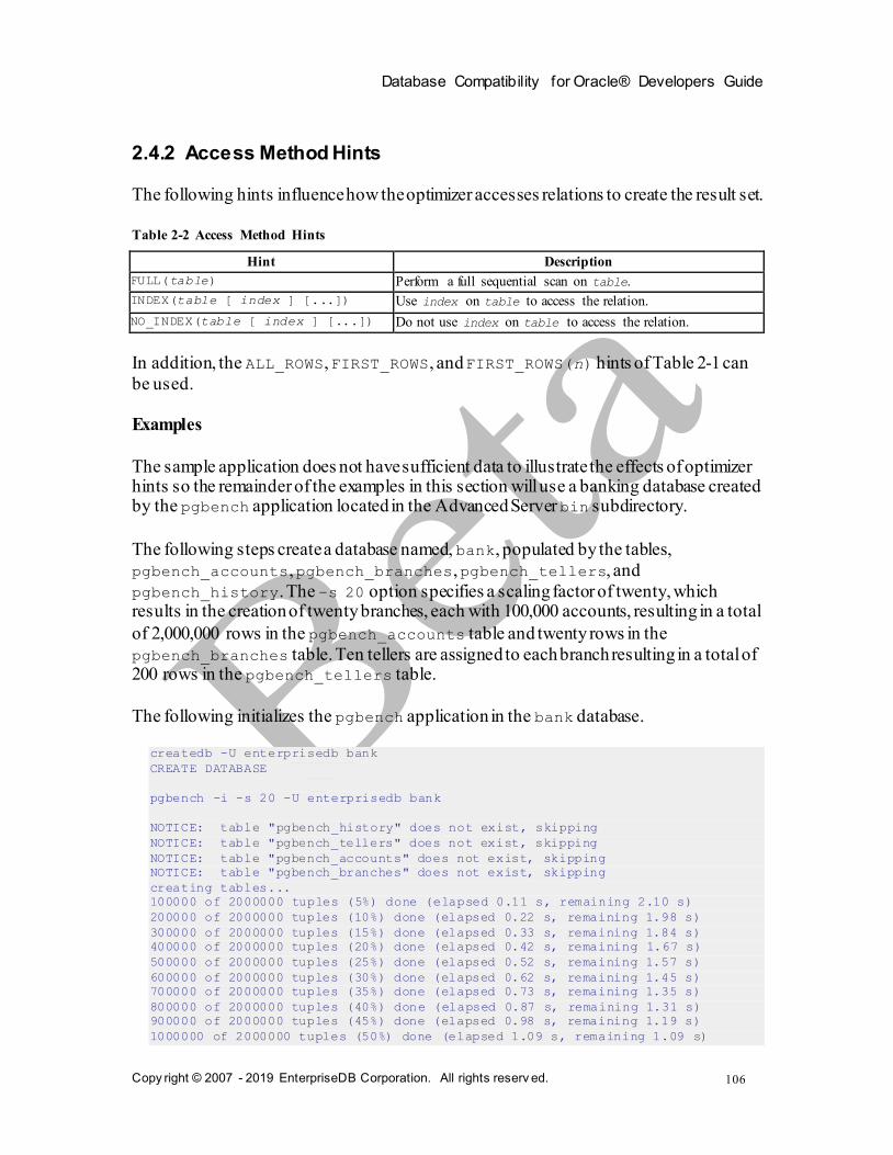
Database Compatibility for Oracle® Developers Guide
Copy right © 2007 - 2019 EnterpriseDB Corporation. All rights reserv ed.
106
2.4.2 Access Method Hints
The following hints influence how the optimizer accesses relations to create the result set.
Table 2-2 Access Method Hints
Hint Description
FULL(table) Perform a full sequential scan on table.
INDEX(table [ index ] [...]) Use index on table to access the relation.
NO_INDEX(table [ index ] [...]) Do not use index on table to access the relation.
In addition, the ALL_ROWS, FIRST_ROWS, and FIRST_ROWS(n) hints of Table 2-1 can
be used.
Examples
The sample application does not have sufficient data to illustrate the effects of optimizer hints so the remainder of the examples in this section will use a banking database created by the pgbench application located in the Advanced Server bin subdirectory.
The following steps create a database named, bank, populated by the tables,
pgbench_accounts, pgbench_branches, pgbench_tellers, and
pgbench_history. The –s 20 option specifies a scaling factor of twenty, which results in the creation of twenty branches, each with 100,000 accounts, resulting in a total
of 2,000,000 rows in the pgbench_accounts table and twenty rows in the
pgbench_branches table. Ten tellers are assigned to each branch resulting in a total of 200 rows in the pgbench_tellers table.
The following initializes the pgbench application in the bank database.
createdb -U enterprisedb bank
CREATE DATABASE
pgbench -i -s 20 -U enterprisedb bank
NOTICE: table "pgbench_history" does not exist, skipping
NOTICE: table "pgbench_tellers" does not exist, skipping
NOTICE: table "pgbench_accounts" does not exist, skipping
NOTICE: table "pgbench_branches" does not exist, skipping
creating tables...
100000 of 2000000 tuples (5%) done (elapsed 0.11 s, remaining 2.10 s)
200000 of 2000000 tuples (10%) done (elapsed 0.22 s, remaining 1.98 s)
300000 of 2000000 tuples (15%) done (elapsed 0.33 s, remaining 1.84 s)
400000 of 2000000 tuples (20%) done (elapsed 0.42 s, remaining 1.67 s)
500000 of 2000000 tuples (25%) done (elapsed 0.52 s, remaining 1.57 s)
600000 of 2000000 tuples (30%) done (elapsed 0.62 s, remaining 1.45 s)
700000 of 2000000 tuples (35%) done (elapsed 0.73 s, remaining 1.35 s)
800000 of 2000000 tuples (40%) done (elapsed 0.87 s, remaining 1.31 s)
900000 of 2000000 tuples (45%) done (elapsed 0.98 s, remaining 1.19 s)
1000000 of 2000000 tuples (50%) done (elapsed 1.09 s, remaining 1.09 s)

Database Compatibility for Oracle® Developers Guide
Copy right © 2007 - 2019 EnterpriseDB Corporation. All rights reserv ed.
107
1100000 of 2000000 tuples (55%) done (elapsed 1.22 s, remaining 1.00 s)
1200000 of 2000000 tuples (60%) done (elapsed 1.36 s, remaining 0.91 s)
1300000 of 2000000 tuples (65%) done (elapsed 1.51 s, remaining 0.82 s)
1400000 of 2000000 tuples (70%) done (elapsed 1.65 s, remaining 0.71 s)
1500000 of 2000000 tuples (75%) done (elapsed 1.78 s, remaining 0.59 s)
1600000 of 2000000 tuples (80%) done (elapsed 1.93 s, remaining 0.48 s)
1700000 of 2000000 tuples (85%) done (elapsed 2.10 s, remaining 0.37 s)
1800000 of 2000000 tuples (90%) done (elapsed 2.23 s, remaining 0.25 s)
1900000 of 2000000 tuples (95%) done (elapsed 2.37 s, remaining 0.12 s)
2000000 of 2000000 tuples (100%) done (elapsed 2.48 s, remaining 0.00 s)
vacuum...
set primary keys...
done.
A total of 500,00 transactions are then processed. This will populate the
pgbench_history table with 500,000 rows.
pgbench -U enterprisedb -t 500000 bank
starting vacuum...end.
transaction type: <builtin: TPC-B (sort of)>
scaling factor: 20
query mode: simple
number of clients: 1
number of threads: 1
number of transactions per client: 500000
number of transactions actually processed: 500000/500000
latency average: 0.000 ms
tps = 1464.338375 (including connections establishing)
tps = 1464.350357 (excluding connections establishing)
The table definitions are shown below:
\d pgbench_accounts
Table "public.pgbench_accounts"
Column | Type | Modifiers
----------+---------------+-----------
aid | integer | not null
bid | integer |
abalance | integer |
filler | character(84) |
Indexes:
"pgbench_accounts_pkey" PRIMARY KEY, btree (aid)
\d pgbench_branches
Table "public.pgbench_branches"
Column | Type | Modifiers
----------+---------------+-----------
bid | integer | not null
bbalance | integer |
filler | character(88) |
Indexes:
"pgbench_branches_pkey" PRIMARY KEY, btree (bid)
\d pgbench_tellers
Table "public.pgbench_tellers"
Column | Type | Modifiers

Database Compatibility for Oracle® Developers Guide
Copy right © 2007 - 2019 EnterpriseDB Corporation. All rights reserv ed.
108
----------+---------------+-----------
tid | integer | not null
bid | integer |
tbalance | integer |
filler | character(84) |
Indexes:
"pgbench_tellers_pkey" PRIMARY KEY, btree (tid)
\d pgbench_history
Table "public.pgbench_history"
Column | Type | Modifiers
--------+-----------------------------+-----------
tid | integer |
bid | integer |
aid | integer |
delta | integer |
mtime | timestamp without time zone |
filler | character(22) |
The EXPLAIN command shows the plan selected by the query planner. In the following
example, aid is the primary key column, so an indexed search is used on index,
pgbench_accounts_pkey.
EXPLAIN SELECT * FROM pgbench_accounts WHERE aid = 100;
QUERY PLAN
-----------------------------------------------------------------------------
------------------
Index Scan using pgbench_accounts_pkey on pgbench_accounts (cost=0.43..8.45
rows=1 width=97)
Index Cond: (aid = 100)
(2 rows)
The FULL hint is used to force a full sequential scan instead of using the index as shown below:
EXPLAIN SELECT /*+ FULL(pgbench_accounts) */ * FROM pgbench_accounts WHERE
aid = 100;
QUERY PLAN
---------------------------------------------------------------------
Seq Scan on pgbench_accounts (cost=0.00..58781.69 rows=1 width=97)
Filter: (aid = 100)
(2 rows)
The NO_INDEX hint forces a parallel sequential scan instead of use of the index as shown below:
EXPLAIN SELECT /*+ NO_INDEX(pgbench_accounts pgbench_accounts_pkey) */ * FROM
pgbench_accounts WHERE aid = 100;
QUERY PLAN
-----------------------------------------------------------------------------
-------
Gather (cost=1000.00..45094.80 rows=1 width=97)
Workers Planned: 2

Database Compatibility for Oracle® Developers Guide
Copy right © 2007 - 2019 EnterpriseDB Corporation. All rights reserv ed.
109
-> Parallel Seq Scan on pgbench_accounts (cost=0.00..44094.70 rows=1
width=97)
Filter: (aid = 100)
(4 rows)
In addition to using the EXPLAIN command as shown in the prior examples, more
detailed information regarding whether or not a hint was used by the planner can be
obtained by setting the trace_hints configuration parameter as follows:
SET trace_hints TO on;
The SELECT command with the NO_INDEX hint is repeated below to illustrate the
additional information produced when the trace_hints configuration parameters is set.
EXPLAIN SELECT /*+ NO_INDEX(pgbench_accounts pgbench_accounts_pkey) */ * FROM
pgbench_accounts WHERE aid = 100;
INFO: [HINTS] Index Scan of [pgbench_accounts].[pgbench_accounts_pkey]
rejected due to NO_INDEX hint.
QUERY PLAN
-----------------------------------------------------------------------------
-------
Gather (cost=1000.00..45094.80 rows=1 width=97)
Workers Planned: 2
-> Parallel Seq Scan on pgbench_accounts (cost=0.00..44094.70 rows=1
width=97)
Filter: (aid = 100)
(4 rows)
Note that if a hint is ignored, the INFO: [HINTS] line will not appear. This may be an
indication that there was a syntax error or some other misspelling in the hint as shown in the following example where the index name is misspelled.
EXPLAIN SELECT /*+ NO_INDEX(pgbench_accounts pgbench_accounts_xxx) */ * FROM
pgbench_accounts WHERE aid = 100;
QUERY PLAN
-----------------------------------------------------------------------------
------------------
Index Scan using pgbench_accounts_pkey on pgbench_accounts (cost=0.43..8.45
rows=1 width=97)
Index Cond: (aid = 100)
(2 rows)

Database Compatibility for Oracle® Developers Guide
Copy right © 2007 - 2019 EnterpriseDB Corporation. All rights reserv ed.
110
2.4.3 Specifying a Join Order
Include the ORDERED directive to instruct the query optimizer to join tables in the order in
which they are listed in the FROM clause. If you do not include the ORDERED keyword, the query optimizer will choose the order in which to join the tables.
For example, the following command allows the optimizer to choose the order in which
to join the tables listed in the FROM clause:
SELECT e.ename, d.dname, h.startdate
FROM emp e, dept d, jobhist h
WHERE d.deptno = e.deptno
AND h.empno = e.empno;
The following command instructs the optimizer to join the tables in the ordered specified:
SELECT /*+ ORDERED */ e.ename, d.dname, h.startdate
FROM emp e, dept d, jobhist h
WHERE d.deptno = e.deptno
AND h.empno = e.empno;
In the ORDERED version of the command, Advanced Server will first join emp e with
dept d before joining the results with jobhist h. Without the ORDERED directive, the join order is selected by the query optimizer.
Please note: the ORDERED directive does not work for Oracle-style outer joins (those joins that contain a '+' sign).

Database Compatibility for Oracle® Developers Guide
Copy right © 2007 - 2019 EnterpriseDB Corporation. All rights reserv ed.
111
2.4.4 Joining Relations Hints
When two tables are to be joined, there are three possible plans that may be used to perform the join.
Nested Loop Join – A table is scanned once for every row in the other joined
table.
Merge Sort Join – Each table is sorted on the join attributes before the join starts. The two tables are then scanned in parallel and the matching rows are combined
to form the join rows.
Hash Join – A table is scanned and its join attributes are loaded into a hash table using its join attributes as hash keys. The other joined table is then scanned and its
join attributes are used as hash keys to locate the matching rows from the first table.
The following table lists the optimizer hints that can be used to influence the planner to use one type of join plan over another.
Table 2-3 Join Hints
Hint Description
USE_HASH(table [...]) Use a hash join for table.
NO_USE_HASH(table [...]) Do not use a hash join for table.
USE_MERGE(table [...]) Use a merge sort join for table.
NO_USE_MERGE(table [...]) Do not use a merge sort join for table.
USE_NL(table [...]) Use a nested loop join for table.
NO_USE_NL(table [...]) Do not use a nested loop join for table.
Examples
In the following example, the USE_HASH hint is used for a join on the
pgbench_branches and pgbench_accounts tables. The query plan shows that a hash
join is used by creating a hash table from the join attribute of the pgbench_branches table.
EXPLAIN SELECT /*+ USE_HASH(b) */ b.bid, a.aid, abalance FROM
pgbench_branches b, pgbench_accounts a WHERE b.bid = a.bid;
QUERY PLAN
-----------------------------------------------------------------------------
------
Hash Join (cost=21.45..81463.06 rows=2014215 width=12)
Hash Cond: (a.bid = b.bid)
-> Seq Scan on pgbench_accounts a (cost=0.00..53746.15 rows=2014215
width=12)
-> Hash (cost=21.20..21.20 rows=20 width=4)
-> Seq Scan on pgbench_branches b (cost=0.00..21.20 rows=20
width=4)

Database Compatibility for Oracle® Developers Guide
Copy right © 2007 - 2019 EnterpriseDB Corporation. All rights reserv ed.
112
(5 rows)
Next, the NO_USE_HASH(a b) hint forces the planner to use an approach other than hash tables. The result is a merge join.
EXPLAIN SELECT /*+ NO_USE_HASH(a b) */ b.bid, a.aid, abalance FROM
pgbench_branches b, pgbench_accounts a WHERE b.bid = a.bid;
QUERY PLAN
-----------------------------------------------------------------------------
------------------
Merge Join (cost=333526.08..368774.94 rows=2014215 width=12)
Merge Cond: (b.bid = a.bid)
-> Sort (cost=21.63..21.68 rows=20 width=4)
Sort Key: b.bid
-> Seq Scan on pgbench_branches b (cost=0.00..21.20 rows=20
width=4)
-> Materialize (cost=333504.45..343575.53 rows=2014215 width=12)
-> Sort (cost=333504.45..338539.99 rows=2014215 width=12)
Sort Key: a.bid
-> Seq Scan on pgbench_accounts a (cost=0.00..53746.15
rows=2014215 width=12)
(9 rows)
Finally, the USE_MERGE hint forces the planner to use a merge join.
EXPLAIN SELECT /*+ USE_MERGE(a) */ b.bid, a.aid, abalance FROM
pgbench_branches b, pgbench_accounts a WHERE b.bid = a.bid;
QUERY PLAN
-----------------------------------------------------------------------------
------------------
Merge Join (cost=333526.08..368774.94 rows=2014215 width=12)
Merge Cond: (b.bid = a.bid)
-> Sort (cost=21.63..21.68 rows=20 width=4)
Sort Key: b.bid
-> Seq Scan on pgbench_branches b (cost=0.00..21.20 rows=20
width=4)
-> Materialize (cost=333504.45..343575.53 rows=2014215 width=12)
-> Sort (cost=333504.45..338539.99 rows=2014215 width=12)
Sort Key: a.bid
-> Seq Scan on pgbench_accounts a (cost=0.00..53746.15
rows=2014215 width=12)
(9 rows)
In this three-table join example, the planner first performs a hash join on the
pgbench_branches and pgbench_history tables, then finally performs a hash join of the result with the pgbench_accounts table.
EXPLAIN SELECT h.mtime, h.delta, b.bid, a.aid FROM pgbench_history h, pgbench_branches
b, pgbench_accounts a WHERE h.bid = b.bid AND h.aid = a.aid;
QUERY PLAN
---------------------------------------------------------------------------------------
-
Hash Join (cost=86814.29..123103.29 rows=500000 width=20)
Hash Cond: (h.aid = a.aid)
-> Hash Join (cost=21.45..15081.45 rows=500000 width=20)
Hash Cond: (h.bid = b.bid)
-> Seq Scan on pgbench_history h (cost=0.00..8185.00 rows=500000 width=20)
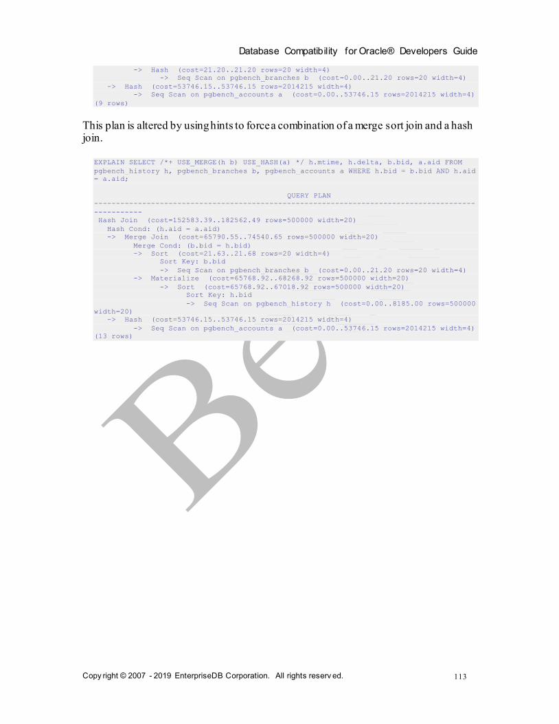
Database Compatibility for Oracle® Developers Guide
Copy right © 2007 - 2019 EnterpriseDB Corporation. All rights reserv ed.
113
-> Hash (cost=21.20..21.20 rows=20 width=4)
-> Seq Scan on pgbench_branches b (cost=0.00..21.20 rows=20 width=4)
-> Hash (cost=53746.15..53746.15 rows=2014215 width=4)
-> Seq Scan on pgbench_accounts a (cost=0.00..53746.15 rows=2014215 width=4)
(9 rows)
This plan is altered by using hints to force a combination of a merge sort join and a hash join.
EXPLAIN SELECT /*+ USE_MERGE(h b) USE_HASH(a) */ h.mtime, h.delta, b.bid, a.aid FROM
pgbench_history h, pgbench_branches b, pgbench_accounts a WHERE h.bid = b.bid AND h.aid
= a.aid;
QUERY PLAN
---------------------------------------------------------------------------------------
-----------
Hash Join (cost=152583.39..182562.49 rows=500000 width=20)
Hash Cond: (h.aid = a.aid)
-> Merge Join (cost=65790.55..74540.65 rows=500000 width=20)
Merge Cond: (b.bid = h.bid)
-> Sort (cost=21.63..21.68 rows=20 width=4)
Sort Key: b.bid
-> Seq Scan on pgbench_branches b (cost=0.00..21.20 rows=20 width=4)
-> Materialize (cost=65768.92..68268.92 rows=500000 width=20)
-> Sort (cost=65768.92..67018.92 rows=500000 width=20)
Sort Key: h.bid
-> Seq Scan on pgbench_history h (cost=0.00..8185.00 rows=500000
width=20)
-> Hash (cost=53746.15..53746.15 rows=2014215 width=4)
-> Seq Scan on pgbench_accounts a (cost=0.00..53746.15 rows=2014215 width=4)
(13 rows)

Database Compatibility for Oracle® Developers Guide
Copy right © 2007 - 2019 EnterpriseDB Corporation. All rights reserv ed.
114
2.4.5 Global Hints
Thus far, hints have been applied directly to tables that are referenced in the SQL command. It is also possible to apply hints to tables that appear in a view when the view
is referenced in the SQL command. The hint does not appear in the view, itself, but rather in the SQL command that references the view.
When specifying a hint that is to apply to a table within a view, the view and table names are given in dot notation within the hint argument list.
Synopsis
hint(view.table)
Parameters
hint
Any of the hints in Table 2-2 or Table 2-3.
view
The name of the view containing table.
table
The table on which the hint is to be applied.
Examples
A view named, tx, is created from the three-table join of pgbench_history,
pgbench_branches, and pgbench_accounts shown in the final example of Section 2.4.4.
CREATE VIEW tx AS SELECT h.mtime, h.delta, b.bid, a.aid FROM pgbench_history
h, pgbench_branches b, pgbench_accounts a WHERE h.bid = b.bid AND h.aid =
a.aid;
The query plan produced by selecting from this view is show below:
EXPLAIN SELECT * FROM tx;
QUERY PLAN
---------------------------------------------------------------------------------------
-
Hash Join (cost=86814.29..123103.29 rows=500000 width=20)
Hash Cond: (h.aid = a.aid)
-> Hash Join (cost=21.45..15081.45 rows=500000 width=20)

Database Compatibility for Oracle® Developers Guide
Copy right © 2007 - 2019 EnterpriseDB Corporation. All rights reserv ed.
115
Hash Cond: (h.bid = b.bid)
-> Seq Scan on pgbench_history h (cost=0.00..8185.00 rows=500000 width=20)
-> Hash (cost=21.20..21.20 rows=20 width=4)
-> Seq Scan on pgbench_branches b (cost=0.00..21.20 rows=20 width=4)
-> Hash (cost=53746.15..53746.15 rows=2014215 width=4)
-> Seq Scan on pgbench_accounts a (cost=0.00..53746.15 rows=2014215 width=4)
(9 rows)
The same hints that were applied to this join at the end of Section 2.4.4 can be applied to the view as follows:
EXPLAIN SELECT /*+ USE_MERGE(tx.h tx.b) USE_HASH(tx.a) */ * FROM tx;
QUERY PLAN
---------------------------------------------------------------------------------------
-----------
Hash Join (cost=152583.39..182562.49 rows=500000 width=20)
Hash Cond: (h.aid = a.aid)
-> Merge Join (cost=65790.55..74540.65 rows=500000 width=20)
Merge Cond: (b.bid = h.bid)
-> Sort (cost=21.63..21.68 rows=20 width=4)
Sort Key: b.bid
-> Seq Scan on pgbench_branches b (cost=0.00..21.20 rows=20 width=4)
-> Materialize (cost=65768.92..68268.92 rows=500000 width=20)
-> Sort (cost=65768.92..67018.92 rows=500000 width=20)
Sort Key: h.bid
-> Seq Scan on pgbench_history h (cost=0.00..8185.00 rows=500000
width=20)
-> Hash (cost=53746.15..53746.15 rows=2014215 width=4)
-> Seq Scan on pgbench_accounts a (cost=0.00..53746.15 rows=2014215 width=4)
(13 rows)
In addition to applying hints to tables within stored views, hints can be applied to tables
within subqueries as illustrated by the following example. In this query on the sample
application emp table, employees and their managers are listed by joining the emp table with a subquery of the emp table identified by the alias, b.
SELECT a.empno, a.ename, b.empno "mgr empno", b.ename "mgr ename" FROM emp a,
(SELECT * FROM emp) b WHERE a.mgr = b.empno;
empno | ename | mgr empno | mgr ename
-------+--------+-----------+-----------
7369 | SMITH | 7902 | FORD
7499 | ALLEN | 7698 | BLAKE
7521 | WARD | 7698 | BLAKE
7566 | JONES | 7839 | KING
7654 | MARTIN | 7698 | BLAKE
7698 | BLAKE | 7839 | KING
7782 | CLARK | 7839 | KING
7788 | SCOTT | 7566 | JONES
7844 | TURNER | 7698 | BLAKE
7876 | ADAMS | 7788 | SCOTT
7900 | JAMES | 7698 | BLAKE
7902 | FORD | 7566 | JONES
7934 | MILLER | 7782 | CLARK
(13 rows)
The plan chosen by the query planner is shown below:
EXPLAIN SELECT a.empno, a.ename, b.empno "mgr empno", b.ename "mgr ename"
FROM emp a, (SELECT * FROM emp) b WHERE a.mgr = b.empno;

Database Compatibility for Oracle® Developers Guide
Copy right © 2007 - 2019 EnterpriseDB Corporation. All rights reserv ed.
116
QUERY PLAN
-----------------------------------------------------------------
Hash Join (cost=1.32..2.64 rows=13 width=22)
Hash Cond: (a.mgr = emp.empno)
-> Seq Scan on emp a (cost=0.00..1.14 rows=14 width=16)
-> Hash (cost=1.14..1.14 rows=14 width=11)
-> Seq Scan on emp (cost=0.00..1.14 rows=14 width=11)
(5 rows)
A hint can be applied to the emp table within the subquery to perform an index scan on index, emp_pk, instead of a table scan. Note the difference in the query plans.
EXPLAIN SELECT /*+ INDEX(b.emp emp_pk) */ a.empno, a.ename, b.empno "mgr
empno", b.ename "mgr ename" FROM emp a, (SELECT * FROM emp) b WHERE a.mgr =
b.empno;
QUERY PLAN
---------------------------------------------------------------------------
Merge Join (cost=4.17..13.11 rows=13 width=22)
Merge Cond: (a.mgr = emp.empno)
-> Sort (cost=1.41..1.44 rows=14 width=16)
Sort Key: a.mgr
-> Seq Scan on emp a (cost=0.00..1.14 rows=14 width=16)
-> Index Scan using emp_pk on emp (cost=0.14..12.35 rows=14 width=11)
(6 rows)

Database Compatibility for Oracle® Developers Guide
Copy right © 2007 - 2019 EnterpriseDB Corporation. All rights reserv ed.
117
2.4.6 Using the APPEND Optimizer Hint
By default, Advanced Server will add new data into the first available free-space in a
table (vacated by vacuumed records). Include the APPEND directive after an INSERT or
SELECT command to instruct the server to bypass mid-table free space, and affix new rows to the end of the table. This optimizer hint can be particularly useful when bulk loading data.
The syntax is:
/*+APPEND*/
For example, the following command, compatible with Oracle databases, instructs the
server to append the data in the INSERT statement to the end of the sales table:
INSERT /*+APPEND*/ INTO sales VALUES
(10, 10, '01-Mar-2011', 10, 'OR');
Note that Advanced Server supports the APPEND hint when adding multiple rows in a single INSERT statement:
INSERT /*+APPEND*/ INTO sales VALUES
(20, 20, '01-Aug-2011', 20, 'NY'),
(30, 30, '01-Feb-2011', 30, 'FL'),
(40, 40, '01-Nov-2011', 40, 'TX');
The APPEND hint can also be included in the SELECT clause of an INSERT INTO statement:
INSERT INTO sales_history SELECT /*+APPEND*/ FROM sales;

Database Compatibility for Oracle® Developers Guide
Copy right © 2007 - 2019 EnterpriseDB Corporation. All rights reserv ed.
118
2.4.7 Parallelism Hints
The PARALLEL optimizer hint is used to force parallel scanning.
The NO_PARALLEL optimizer hint prevents usage of a parallel scan.
Synopsis
PARALLEL (table [ parallel_degree | DEFAULT ])
NO_PARALLEL (table)
Description
Parallel scanning is the usage of multiple background workers to simultaneously perform a scan of a table (that is, in parallel) for a given query. This process provides performance improvement over other methods such as the sequential scan.
Parameters
table
The table to which the parallel hint is to be applied.
parallel_degree | DEFAULT
parallel_degree is a positive integer that specifies the desired number of
workers to use for a parallel scan. If specified, the lesser of parallel_degree
and configuration parameter max_parallel_workers_per_gather is used as the planned number of workers. For information on the
max_parallel_workers_per_gather parameter, please see Section 19.4.6
Asynchronous Behavior located in Section 19.4 Resource Consumption in the PostgreSQL core documentation available at:
https://www.postgresql.org/docs/11/static/runtime-config-resource.html
If DEFAULT is specified, then the maximum possible parallel degree is used.
If both parallel_degree and DEFAULT are omitted, then the query optimizer
determines the parallel degree. In this case, if table has been set with the
parallel_workers storage parameter, then this value is used as the parallel degree, otherwise the optimizer uses the maximum poss ible parallel degree as if
DEFAULT was specified. For information on the parallel_workers storage
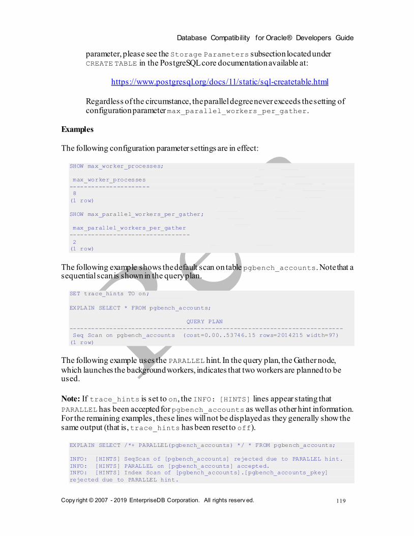
Database Compatibility for Oracle® Developers Guide
Copy right © 2007 - 2019 EnterpriseDB Corporation. All rights reserv ed.
119
parameter, please see the Storage Parameters subsection located under CREATE TABLE in the PostgreSQL core documentation available at:
https://www.postgresql.org/docs/11/static/sql-createtable.html
Regardless of the circumstance, the parallel degree never exceeds the setting of configuration parameter max_parallel_workers_per_gather.
Examples
The following configuration parameter settings are in effect:
SHOW max_worker_processes;
max_worker_processes
----------------------
8
(1 row)
SHOW max_parallel_workers_per_gather;
max_parallel_workers_per_gather
---------------------------------
2
(1 row)
The following example shows the default scan on table pgbench_accounts. Note that a sequential scan is shown in the query plan.
SET trace_hints TO on;
EXPLAIN SELECT * FROM pgbench_accounts;
QUERY PLAN
---------------------------------------------------------------------------
Seq Scan on pgbench_accounts (cost=0.00..53746.15 rows=2014215 width=97)
(1 row)
The following example uses the PARALLEL hint. In the query plan, the Gather node,
which launches the background workers, indicates that two workers are planned to be used.
Note: If trace_hints is set to on, the INFO: [HINTS] lines appear stating that
PARALLEL has been accepted for pgbench_accounts as well as other hint information. For the remaining examples, these lines will not be displayed as they generally show the same output (that is, trace_hints has been reset to off).
EXPLAIN SELECT /*+ PARALLEL(pgbench_accounts) */ * FROM pgbench_accounts;
INFO: [HINTS] SeqScan of [pgbench_accounts] rejected due to PARALLEL hint.
INFO: [HINTS] PARALLEL on [pgbench_accounts] accepted.
INFO: [HINTS] Index Scan of [pgbench_accounts].[pgbench_accounts_pkey]
rejected due to PARALLEL hint.

Database Compatibility for Oracle® Developers Guide
Copy right © 2007 - 2019 EnterpriseDB Corporation. All rights reserv ed.
120
QUERY PLAN
-----------------------------------------------------------------------------
------------
Gather (cost=1000.00..244418.06 rows=2014215 width=97)
Workers Planned: 2
-> Parallel Seq Scan on pgbench_accounts (cost=0.00..41996.56
rows=839256 width=97)
(3 rows)
Now, the max_parallel_workers_per_gather setting is increased:
SET max_parallel_workers_per_gather TO 6;
SHOW max_parallel_workers_per_gather;
max_parallel_workers_per_gather
---------------------------------
6
(1 row)
The same query on pgbench_accounts is issued again with no parallel degree
specification in the PARALLEL hint. Note that the number of planned workers has increased to 4 as determined by the optimizer.
EXPLAIN SELECT /*+ PARALLEL(pgbench_accounts) */ * FROM pgbench_accounts;
QUERY PLAN
-----------------------------------------------------------------------------
------------
Gather (cost=1000.00..241061.04 rows=2014215 width=97)
Workers Planned: 4
-> Parallel Seq Scan on pgbench_accounts (cost=0.00..38639.54
rows=503554 width=97)
(3 rows)
Now, a value of 6 is specified for the parallel degree parameter of the PARALLEL hint. The planned number of workers is now returned as this specified value:
EXPLAIN SELECT /*+ PARALLEL(pgbench_accounts 6) */ * FROM pgbench_accounts;
QUERY PLAN
-----------------------------------------------------------------------------
------------
Gather (cost=1000.00..239382.52 rows=2014215 width=97)
Workers Planned: 6
-> Parallel Seq Scan on pgbench_accounts (cost=0.00..36961.03
rows=335702 width=97)
(3 rows)
The same query is now issued with the DEFAULT setting for the parallel degree. The results indicate that the maximum allowable number of workers is planned.
EXPLAIN SELECT /*+ PARALLEL(pgbench_accounts DEFAULT) */ * FROM
pgbench_accounts;
QUERY PLAN

Database Compatibility for Oracle® Developers Guide
Copy right © 2007 - 2019 EnterpriseDB Corporation. All rights reserv ed.
121
-----------------------------------------------------------------------------
------------
Gather (cost=1000.00..239382.52 rows=2014215 width=97)
Workers Planned: 6
-> Parallel Seq Scan on pgbench_accounts (cost=0.00..36961.03
rows=335702 width=97)
(3 rows)
Table pgbench_accounts is now altered so that the parallel_workers storage parameter is set to 3.
Note: This format of the ALTER TABLE command to set the parallel_workers parameter is not compatible with Oracle databases.
The parallel_workers setting is shown by the PSQL \d+ command.
ALTER TABLE pgbench_accounts SET (parallel_workers=3);
\d+ pgbench_accounts
Table "public.pgbench_accounts"
Column | Type | Modifiers | Storage | Stats target | Description
----------+---------------+-----------+----------+--------------+------------
-
aid | integer | not null | plain | |
bid | integer | | plain | |
abalance | integer | | plain | |
filler | character(84) | | extended | |
Indexes:
"pgbench_accounts_pkey" PRIMARY KEY, btree (aid)
Options: fillfactor=100, parallel_workers=3
Now, when the PARALLEL hint is given with no parallel degree, the resulting number of
planned workers is the value from the parallel_workers parameter:
EXPLAIN SELECT /*+ PARALLEL(pgbench_accounts) */ * FROM pgbench_accounts;
QUERY PLAN
-----------------------------------------------------------------------------
------------
Gather (cost=1000.00..242522.97 rows=2014215 width=97)
Workers Planned: 3
-> Parallel Seq Scan on pgbench_accounts (cost=0.00..40101.47
rows=649747 width=97)
(3 rows)
Specifying a parallel degree value or DEFAULT in the PARALLEL hint overrides the
parallel_workers setting.
The following example shows the NO_PARALLEL hint. Note that with trace_hints set
to on, the INFO: [HINTS] message states that the parallel scan was rejected due to the NO_PARALLEL hint.
EXPLAIN SELECT /*+ NO_PARALLEL(pgbench_accounts) */ * FROM pgbench_accounts;
INFO: [HINTS] Parallel SeqScan of [pgbench_accounts] rejected due to
NO_PARALLEL hint.
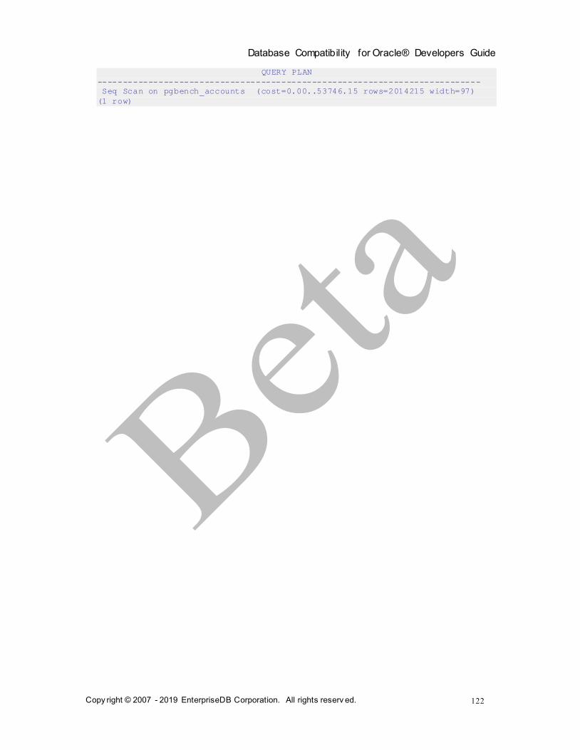
Database Compatibility for Oracle® Developers Guide
Copy right © 2007 - 2019 EnterpriseDB Corporation. All rights reserv ed.
122
QUERY PLAN
---------------------------------------------------------------------------
Seq Scan on pgbench_accounts (cost=0.00..53746.15 rows=2014215 width=97)
(1 row)

Database Compatibility for Oracle® Developers Guide
Copy right © 2007 - 2019 EnterpriseDB Corporation. All rights reserv ed.
123
2.4.8 Conflicting Hints
If a command includes two or more conflicting hints, the server will ignore the contradictory hints. The following table lists hints that are contradictory to each other.
Table 2-4 Conflicting Hints
Hint Conflicting Hint
ALL_ROWS FIRST_ROWS - all formats
FULL(table) INDEX(table [ index ])
PARALLEL(table [ degree ])
INDEX(table)
FULL(table)
NO_INDEX(table)
PARALLEL(table [ degree ])
INDEX(table index)
FULL(table)
NO_INDEX(table index)
PARALLEL(table [ degree ])
PARALLEL(table [ degree ])
FULL(table)
INDEX(table)
NO_PARALLEL(table)
USE_HASH(table) NO_USE_HASH(table)
USE_MERGE(table) NO_USE_MERGE(table)
USE_NL(table) NO_USE_NL(table)

Database Compatibility for Oracle® Developers Guide
Copy right © 2007 - 2019 EnterpriseDB Corporation. All rights reserv ed.
124
3 Stored Procedure Language
This chapter describes the Stored Procedure Language (SPL). SPL is a highly
productive, procedural programming language for writing custom procedures, functions, triggers, and packages for Advanced Server that provides:
full procedural programming functionality to complement the SQL language
a single, common language to create stored procedures, functions, triggers, and
packages for the Advanced Server database
a seamless development and testing environment
the use of reusable code ease of use
This chapter describes the basic elements of an SPL program, before providing an
overview of the organization of an SPL program and how it is used to create a procedure or a function. Triggers, while still utilizing SPL, are sufficiently different to warrant a separate discussion (see Section 4 for information about triggers). Packages are discussed
in the Database Compatibility for Oracle Developers Built-in Package Guide available at:
https://www.enterprisedb.com/resources/product-documentation
The remaining sections of this chapter delve into the details of the SPL language and provide examples of its application.
3.1 Basic SPL Elements
This section discusses the basic programming elements of an SPL program.
3.1.1 Character Set
SPL programs are written using the following set of characters:
Uppercase letters A thru Z and lowercase letters a thru z
Digits 0 thru 9
Symbols ( ) + - * / < > = ! ~ ^ ; : . ' @ % , " # $ & _ | { } ? [ ] White space characters tabs, spaces, and carriage returns
Identifiers, expressions, statements, control structures, etc. that comprise the SPL language are written using these characters.

Database Compatibility for Oracle® Developers Guide
Copy right © 2007 - 2019 EnterpriseDB Corporation. All rights reserv ed.
125
Note: The data that can be manipulated by an SPL program is determined by the character set supported by the database encoding.
3.1.2 Case Sensitivity
Keywords and user-defined identifiers that are used in an SPL program are case
insensitive. So for example, the statement DBMS_OUTPUT.PUT_LINE('Hello
World'); is interpreted to mean the same thing as dbms_output.put_line('Hello
World'); or Dbms_Output.Put_Line('Hello World'); or DBMS_output.Put_line('Hello World');.
Character and string constants, however, are case sensitive as well as any data retrieved from the Advanced Server database or data obtained from other external sources. The
statement DBMS_OUTPUT.PUT_LINE('Hello World!'); produces the following output:
Hello World!
However the statement DBMS_OUTPUT.PUT_LINE('HELLO WORLD!'); produces the output:
HELLO WORLD!
3.1.3 Identifiers
Identifiers are user-defined names that are used to identify various elements of an SPL
program including variables, cursors, labels, programs, and parameters. The syntax rules for valid identifiers are the same as for identifiers in the SQL language.
An identifier must not be the same as an SPL keyword or a keyword of the SQL language. The following are some examples of valid identifiers:
x
last___name
a_$_Sign
Many$$$$$$$$signs_____
THIS_IS_AN_EXTREMELY_LONG_NAME
A1
3.1.4 Qualifiers
A qualifier is a name that specifies the owner or context of an entity that is the object of
the qualification. A qualified object is specified as the qualifier name followed by a dot with no intervening white space, followed by the name of the object being qualified with no intervening white space. This syntax is called dot notation.
The following is the syntax of a qualified object.

Database Compatibility for Oracle® Developers Guide
Copy right © 2007 - 2019 EnterpriseDB Corporation. All rights reserv ed.
126
qualifier. [ qualifier. ]... object
qualifier is the name of the owner of the object. object is the name of the entity
belonging to qualifier. It is possible to have a chain of qualifications where the preceding qualifier owns the entity identified by the subsequent qualifier(s) and object.
Almost any identifier can be qualified. What an identifier is qualified by depends upon what the identifier represents and the context of its usage.
Some examples of qualification follow:
Procedure and function names qualified by the schema to which they belong - e.g., schema_name.procedure_name(...)
Trigger names qualified by the schema to which they belong - e.g., schema_name.trigger_name
Column names qualified by the table to which they belong - e.g., emp.empno
Table names qualified by the schema to which they belong - e.g., public.emp
Column names qualified by table and schema - e.g., public.emp.empno
As a general rule, wherever a name appears in the syntax of an SPL statement, its
qualified name can be used as well. Typically a qualified name would only be used if there is some ambiguity associated with the name. For example, if two procedures with the same name belonging to two different schemas are invoked from within a program or if the same name is used for a table column and SPL variable within the same program.
You should avoid using qualified names if at all possible. In this chapter, the following conventions are adopted to avoid naming conflicts:
All variables declared in the declaration section of an SPL program are prefixed
by v_. E.g., v_empno
All formal parameters declared in a procedure or function definition are prefixed
by p_. E.g., p_empno Column names and table names do not have any special prefix conventions. E.g.,
column empno in table emp
3.1.5 Constants
Constants or literals are fixed values that can be used in SPL programs to represent
values of various types - e.g., numbers, strings, dates, etc. Constants come in the following types:
Numeric (Integer and Real)
Character and String
Date/time

Database Compatibility for Oracle® Developers Guide
Copy right © 2007 - 2019 EnterpriseDB Corporation. All rights reserv ed.
127
3.1.6 User-Defined PL/SQL Subtypes
Advanced Server supports user-defined PL/SQL subtypes and (subtype) aliases. A subtype is a data type with an optional set of constraints that restrict the values that can
be stored in a column of that type. The rules that apply to the type on which the subtype is based are still enforced, but you can use additional constraints to place limits on the precision or scale of values stored in the type.
You can define a subtype in the declaration of a PL function, procedure, anonymous block or package. The syntax is:
SUBTYPE subtype_name IS type_name[(constraint)] [NOT NULL]
Where constraint is:
{precision [, scale]} | length
Where:
subtype_name
subtype_name specifies the name of the subtype.
type_name
type_name specifies the name of the original type on which the subtype is based.
type_name may be:
The name of any of the type supported by Advanced Server.
The name of any composite type.
A column anchored by a %TYPE operator.
The name of another subtype.
Include the constraint clause to define restrictions for types that support precision or
scale.
precision
precision specifies the total number of digits permitted in a value of the subtype.
Database Compatibility for Oracle® Developers Guide
Copy right © 2007 - 2019 EnterpriseDB Corporation. All rights reserv ed.
128
scale
scale specifies the number of fractional digits permitted in a value of the subtype.
length
length specifies the total length permitted in a value of CHARACTER, VARCHAR,
or TEXT base types
Include the NOT NULL clause to specify that NULL values may not be stored in a column of the specified subtype.
Note that a subtype that is based on a column will inherit the column size constraints, but the subtype will not inherit NOT NULL or CHECK constraints.
Unconstrained Subtypes
To create an unconstrained subtype, use the SUBTYPE command to specify the new subtype name and the name of the type on which the subtype is based. For example, the
following command creates a subtype named address that has all of the attributes of the type, CHAR:
SUBTYPE address IS CHAR;
You can also create a subtype (constrained or unconstrained) that is a subtype of another subtype:
SUBTYPE cust_address IS address NOT NULL;
This command creates a subtype named cust_address that shares all of the attributes
of the address subtype. Include the NOT NULL clause to specify that a value of the cust_address may not be NULL.
Constrained Subtypes
Include a length value when creating a subtype that is based on a character type to define the maximum length of the subtype. For example:
SUBTYPE acct_name IS VARCHAR (15);
This example creates a subtype named acct_name that is based on a VARCHAR data type, but is limited to 15 characters in length.
Database Compatibility for Oracle® Developers Guide
Copy right © 2007 - 2019 EnterpriseDB Corporation. All rights reserv ed.
129
Include values for precision (to specify the maximum number of digits in a value of
the subtype) and optionally, scale (to specify the number of digits to the right of the decimal point) when constraining a numeric base type. For example:
SUBTYPE acct_balance IS NUMBER (5, 2);
This example creates a subtype named acct_balance that shares all of the attributes of
a NUMBER type, but that may not exceed 3 digits to the left of the decimal point and 2 digits to the right of the decimal.
An argument declaration (in a function or procedure header) is a formal argument. The value passed to a function or procedure is an actual argument. When invoking a function
or procedure, the caller provides (0 or more) actual arguments. Each actual argument is assigned to a formal argument that holds the value within the body of the function or procedure.
If a formal argument is declared as a constrained subtype:
Advanced Server does not enforce subtype constraints when assigning an actual argument to a formal argument when invoking a function.
Advanced Server enforces subtype constraints when assigning an actual argument to a formal argument when invoking a procedure.
Using the % TYPE Operator
You can use %TYPE notation to declare a subtype anchored to a column. For example:
SUBTYPE emp_type IS emp.empno%TYPE
This command creates a subtype named emp_type whose base type matches the type of
the empno column in the emp table. A subtype that is based on a column will share the column size constraints; NOT NULL and CHECK constraints are not inherited.
Subtype Conversion
Unconstrained subtypes are aliases for the type on which they are based. Any variable of type subtype (unconstrained) is interchangeable with a variable of the base type without conversion, and vice versa.
A variable of a constrained subtype may be interchanged with a variable of the base type without conversion, but a variable of the base type may only be interchanged with a constrained subtype if it complies with the constraints of the subtype. A variable of a
constrained subtype may be implicitly converted to another subtype if it is based on the same subtype, and the constraint values are within the values of the subtype to which it is being converted.

Database Compatibility for Oracle® Developers Guide
Copy right © 2007 - 2019 EnterpriseDB Corporation. All rights reserv ed.
130
3.2 SPL Programs
SPL is a procedural, block-structured language. There are four different types of
programs that can be created using SPL, namely procedures, functions, triggers, and packages.
In addition, SPL is used to create subprograms. A subprogram refers to a subprocedure or a subfunction, which are nearly identical in appearance to procedures and functions,
but differ in that procedures and functions are standalone programs, which are individually stored in the database and can be invoked by other SPL programs or from
PSQL. Subprograms can only be invoked from within the standalone program within which they have been created.
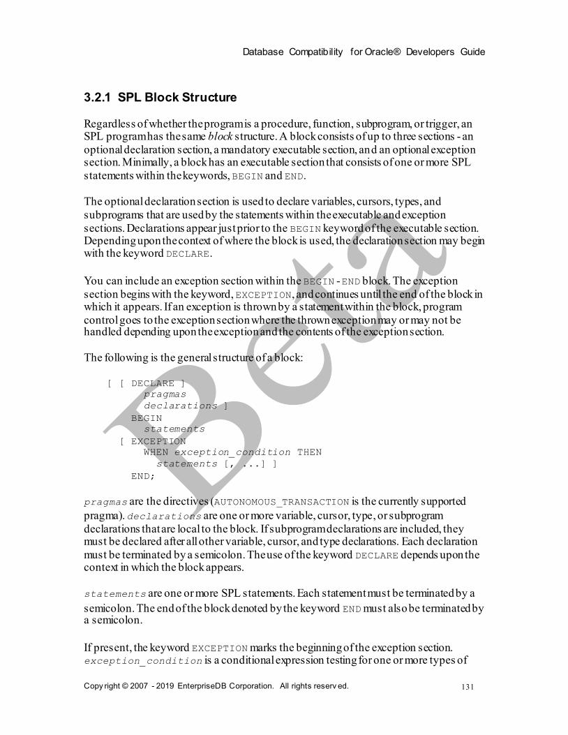
Database Compatibility for Oracle® Developers Guide
Copy right © 2007 - 2019 EnterpriseDB Corporation. All rights reserv ed.
131
3.2.1 SPL Block Structure
Regardless of whether the program is a procedure, function, subprogram, or trigger, an SPL program has the same block structure. A block consists of up to three sections - an
optional declaration section, a mandatory executable section, and an optional exception section. Minimally, a block has an executable section that consists of one or more SPL
statements within the keywords, BEGIN and END.
The optional declaration section is used to declare variables, cursors, types, and
subprograms that are used by the statements within the executable and exception
sections. Declarations appear just prior to the BEGIN keyword of the executable section. Depending upon the context of where the block is used, the declaration section may begin with the keyword DECLARE.
You can include an exception section within the BEGIN - END block. The exception
section begins with the keyword, EXCEPTION, and continues until the end of the block in which it appears. If an exception is thrown by a statement within the block, program
control goes to the exception section where the thrown exception may or may not be handled depending upon the exception and the contents of the exception section.
The following is the general structure of a block:
[ [ DECLARE ]
pragmas
declarations ]
BEGIN
statements
[ EXCEPTION
WHEN exception_condition THEN
statements [, ...] ]
END;
pragmas are the directives (AUTONOMOUS_TRANSACTION is the currently supported
pragma). declarations are one or more variable, cursor, type, or subprogram
declarations that are local to the block. If subprogram declarations are included, they must be declared after all other variable, cursor, and type declarations. Each declaration
must be terminated by a semicolon. The use of the keyword DECLARE depends upon the context in which the block appears.
statements are one or more SPL statements. Each statement must be terminated by a
semicolon. The end of the block denoted by the keyword END must also be terminated by a semicolon.
If present, the keyword EXCEPTION marks the beginning of the exception section. exception_condition is a conditional expression testing for one or more types of

Database Compatibility for Oracle® Developers Guide
Copy right © 2007 - 2019 EnterpriseDB Corporation. All rights reserv ed.
132
exceptions. If an exception matches one of the exceptions in exception_condition,
the statements following the WHEN exception_condition clause are executed.
There may be one or more WHEN exception_condition clauses, each followed by
statements. Note: A BEGIN/END block in itself, is considered a statement; thus, blocks may be nested. The exception section may also contain nested blocks.
The following is the simplest possible block consisting of the NULL statement within the
executable section. The NULL statement is an executable statement that does nothing.
BEGIN
NULL;
END;
The following block contains a declaration section as well as the executable section.
DECLARE
v_numerator NUMBER(2);
v_denominator NUMBER(2);
v_result NUMBER(5,2);
BEGIN
v_numerator := 75;
v_denominator := 14;
v_result := v_numerator / v_denominator;
DBMS_OUTPUT.PUT_LINE(v_numerator || ' divided by ' || v_denominator ||
' is ' || v_result);
END;
In this example, three numeric variables are declared of data type NUMBER. Values are
assigned to two of the variables, and one number is divided by the other, storing the results in a third variable which is then displayed. If executed, the output would be:
75 divided by 14 is 5.36
The following block consists of a declaration, an executable, and an exception:
DECLARE
v_numerator NUMBER(2);
v_denominator NUMBER(2);
v_result NUMBER(5,2);
BEGIN
v_numerator := 75;
v_denominator := 0;
v_result := v_numerator / v_denominator;
DBMS_OUTPUT.PUT_LINE(v_numerator || ' divided by ' || v_denominator ||
' is ' || v_result);
EXCEPTION
WHEN OTHERS THEN
DBMS_OUTPUT.PUT_LINE('An exception occurred');
END;
The following output shows that the statement within the exception section is executed as a result of the division by zero.
An exception occurred

Database Compatibility for Oracle® Developers Guide
Copy right © 2007 - 2019 EnterpriseDB Corporation. All rights reserv ed.
133
3.2.2 Anonymous Blocks
Blocks are typically written as part of a procedure, function, subprogram, or trigger.
Procedure, function, and trigger programs are named and stored in the database for re-use. For quick (one-time) execution (such as testing), you can simply enter the block without providing a name or storing it in the database.
A block of this type is called an anonymous block. An anonymous block is unnamed and
is not stored in the database. Once the block has been executed and erased from the application buffer, it cannot be re-executed unless the block code is re-entered into the application.
Typically, the same block of code will be re-executed many times. In order to run a block
of code repeatedly without the necessity of re-entering the code each time, with some simple modifications, an anonymous block can be turned into a procedure or function.
The following sections discuss how to create a procedure or function that can be stored in the database and invoked repeatedly by another procedure, function, or application program.
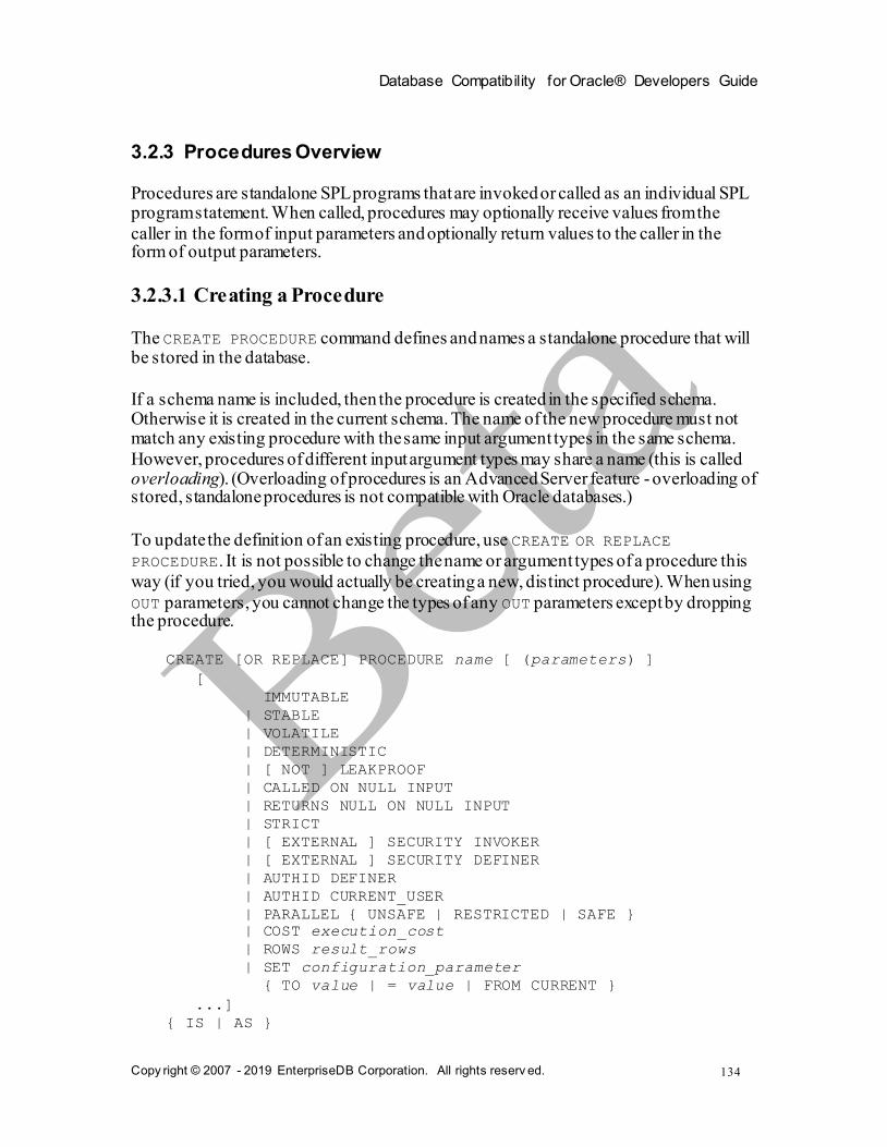
Database Compatibility for Oracle® Developers Guide
Copy right © 2007 - 2019 EnterpriseDB Corporation. All rights reserv ed.
134
3.2.3 Procedures Overview
Procedures are standalone SPL programs that are invoked or called as an individual SPL program statement. When called, procedures may optionally receive values from the
caller in the form of input parameters and optionally return values to the caller in the form of output parameters.
3.2.3.1 Creating a Procedure
The CREATE PROCEDURE command defines and names a standalone procedure that will be stored in the database.
If a schema name is included, then the procedure is created in the specified schema. Otherwise it is created in the current schema. The name of the new procedure must not match any existing procedure with the same input argument types in the same schema.
However, procedures of different input argument types may share a name (this is called overloading). (Overloading of procedures is an Advanced Server feature - overloading of stored, standalone procedures is not compatible with Oracle databases.)
To update the definition of an existing procedure, use CREATE OR REPLACE
PROCEDURE. It is not possible to change the name or argument types of a procedure this
way (if you tried, you would actually be creating a new, distinct procedure). When using
OUT parameters, you cannot change the types of any OUT parameters except by dropping the procedure.
CREATE [OR REPLACE] PROCEDURE name [ (parameters) ]
[
IMMUTABLE
| STABLE
| VOLATILE
| DETERMINISTIC
| [ NOT ] LEAKPROOF
| CALLED ON NULL INPUT
| RETURNS NULL ON NULL INPUT
| STRICT
| [ EXTERNAL ] SECURITY INVOKER
| [ EXTERNAL ] SECURITY DEFINER
| AUTHID DEFINER
| AUTHID CURRENT_USER
| PARALLEL { UNSAFE | RESTRICTED | SAFE }
| COST execution_cost
| ROWS result_rows
| SET configuration_parameter
{ TO value | = value | FROM CURRENT }
...]
{ IS | AS }
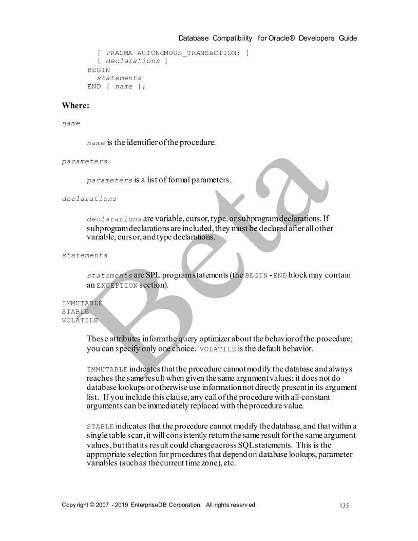
Database Compatibility for Oracle® Developers Guide
Copy right © 2007 - 2019 EnterpriseDB Corporation. All rights reserv ed.
135
[ PRAGMA AUTONOMOUS_TRANSACTION; ]
[ declarations ]
BEGIN
statements
END [ name ];
Where:
name
name is the identifier of the procedure.
parameters
parameters is a list of formal parameters.
declarations
declarations are variable, cursor, type, or subprogram declarations. If
subprogram declarations are included, they must be declared after all other variable, cursor, and type declarations.
statements
statements are SPL program statements (the BEGIN - END block may contain
an EXCEPTION section).
IMMUTABLE
STABLE
VOLATILE
These attributes inform the query optimizer about the behavior of the procedure;
you can specify only one choice. VOLATILE is the default behavior.
IMMUTABLE indicates that the procedure cannot modify the database and always reaches the same result when given the same argument values; it does not do database lookups or otherwise use information not directly present in its argument
list. If you include this clause, any call of the procedure with all-constant arguments can be immediately replaced with the procedure value.
STABLE indicates that the procedure cannot modify the database, and that within a single table scan, it will consistently return the same result for the same argument
values, but that its result could change across SQL statements. This is the appropriate selection for procedures that depend on database lookups, parameter variables (such as the current time zone), etc.
Database Compatibility for Oracle® Developers Guide
Copy right © 2007 - 2019 EnterpriseDB Corporation. All rights reserv ed.
136
VOLATILE indicates that the procedure value can change even within a single table scan, so no optimizations can be made. Please note that any function that has side-effects must be classified volatile, even if its result is quite predictable, to prevent calls from being optimized away.
DETERMINISTIC
DETERMINISTIC is a synonym for IMMUTABLE. A DETERMINISTIC procedure cannot modify the database and always reaches the same result when
given the same argument values; it does not do database lookups or otherwise use information not directly present in its argument list. If you include this clause,
any call of the procedure with all-constant arguments can be immediately replaced with the procedure value.
[ NOT ] LEAKPROOF
A LEAKPROOF procedure has no side effects, and reveals no information about the values used to call the procedure.
CALLED ON NULL INPUT
RETURNS NULL ON NULL INPUT
STRICT
CALLED ON NULL INPUT (the default) indicates that the procedure will be called
normally when some of its arguments are NULL. It is the author's responsibility to check for NULL values if necessary and respond appropriately.
RETURNS NULL ON NULL INPUT or STRICT indicates that the procedure always
returns NULL whenever any of its arguments are NULL. If these clauses are
specified, the procedure is not executed when there are NULL arguments; instead a NULL result is assumed automatically.
[ EXTERNAL ] SECURITY DEFINER
SECURITY DEFINER specifies that the procedure will execute with the privileges
of the user that created it; this is the default. The key word EXTERNAL is allowed for SQL conformance, but is optional.
[ EXTERNAL ] SECURITY INVOKER
The SECURITY INVOKER clause indicates that the procedure will execute with the
privileges of the user that calls it. The key word EXTERNAL is allowed for SQL conformance, but is optional.
AUTHID DEFINER
AUTHID CURRENT_USER

Database Compatibility for Oracle® Developers Guide
Copy right © 2007 - 2019 EnterpriseDB Corporation. All rights reserv ed.
137
The AUTHID DEFINER clause is a synonym for [EXTERNAL] SECURITY
DEFINER. If the AUTHID clause is omitted or if AUTHID DEFINER is specified, the rights of the procedure owner are used to determine access privileges to database objects.
The AUTHID CURRENT_USER clause is a synonym for [EXTERNAL] SECURITY
INVOKER. If AUTHID CURRENT_USER is specified, the rights of the current user executing the procedure are used to determine access privileges.
PARALLEL { UNSAFE | RESTRICTED | SAFE }
The PARALLEL clause enables the use of parallel sequential scans (parallel mode). A parallel sequential scan uses multiple workers to scan a relation in parallel during a query in contrast to a serial sequential scan.
When set to UNSAFE, the procedure cannot be executed in parallel mode. The presence of such a procedure forces a serial execution plan. This is the default setting if the PARALLEL clause is omitted.
When set to RESTRICTED, the procedure can be executed in parallel mode, but the execution is restricted to the parallel group leader. If the qualification for any particular relation has anything that is parallel restricted, that relation won't be chosen for parallelism.
When set to SAFE, the procedure can be executed in parallel mode with no restriction.
COST execution_cost
execution_cost is a positive number giving the estimated execution cost for
the procedure, in units of cpu_operator_cost. If the procedure returns a set,
this is the cost per returned row. Larger values cause the planner to try to avoid evaluating the function more often than necessary.
ROWS result_rows
result_rows is a positive number giving the estimated number of rows that the
planner should expect the procedure to return. This is only allowed when the procedure is declared to return a set. The default assumption is 1000 rows.
SET configuration_parameter { TO value | = value | FROM CURRENT }
The SET clause causes the specified configuration parameter to be set to the
specified value when the procedure is entered, and then restored to its prior value
when the procedure exits. SET FROM CURRENT saves the session's current value of the parameter as the value to be applied when the procedure is entered.

Database Compatibility for Oracle® Developers Guide
Copy right © 2007 - 2019 EnterpriseDB Corporation. All rights reserv ed.
138
If a SET clause is attached to a procedure, then the effects of a SET LOCAL command executed inside the procedure for the same variable are restricted to the procedure; the configuration parameter's prior value is restored at procedure exit.
An ordinary SET command (without LOCAL) overrides the SET clause, much as it
would do for a previous SET LOCAL command, with the effects of such a command persisting after procedure exit, unless the current transaction is rolled back.
PRAGMA AUTONOMOUS_TRANSACTION
PRAGMA AUTONOMOUS_TRANSACTION is the directive that sets the procedure as an autonomous transaction.
Note: The STRICT, LEAKPROOF, PARALLEL, COST, ROWS and SET keywords provide extended functionality for Advanced Server and are not supported by Oracle.
Note: By default, stored procedures are created as SECURITY DEFINERS, but when written in plpgsql, the stored procedures are created as SECURITY INVOKERS.
Example
The following is an example of a simple procedure that takes no parameters.
CREATE OR REPLACE PROCEDURE simple_procedure
IS
BEGIN
DBMS_OUTPUT.PUT_LINE('That''s all folks!');
END simple_procedure;
The procedure is stored in the database by entering the procedure code in Advanced Server.
The following example demonstrates using the AUTHID DEFINER and SET clauses in a
procedure declaration. The update_salary procedure conveys the privileges of the role that defined the procedure to the role that is calling the procedure (while the procedure executes):
CREATE OR REPLACE PROCEDURE update_salary(id INT, new_salary NUMBER)
SET SEARCH_PATH = 'public' SET WORK_MEM = '1MB'
AUTHID DEFINER IS
BEGIN
UPDATE emp SET salary = new_salary WHERE emp_id = id;
END;
Include the SET clause to set the procedure's search path to public and the work
memory to 1MB. Other procedures, functions and objects will not be affected by these settings.

Database Compatibility for Oracle® Developers Guide
Copy right © 2007 - 2019 EnterpriseDB Corporation. All rights reserv ed.
139
In this example, the AUTHID DEFINER clause temporarily grants privileges to a role that might otherwise not be allowed to execute the statements within the procedure. To instruct the server to use the privileges associated with the role invoking the procedure,
replace the AUTHID DEFINER clause with the AUTHID CURRENT_USER clause.
3.2.3.2 Calling a Procedure
A procedure can be invoked from another SPL program by simply specifying the procedure name followed by its parameters, if any, followed by a semicolon.
name [ ([ parameters ]) ];
Where:
name is the identifier of the procedure.
parameters is a list of actual parameters.
Note: If there are no actual parameters to be passed, the procedure may be called with an empty parameter list, or the opening and closing parenthesis may be omitted entirely.
Note: The syntax for calling a procedure is the same as in the preceding syntax diagram
when executing it with the EXEC command in PSQL or EDB*Plus. See the Database Compatibility for Oracle Developers Tools and Utilities Guide for information about the EXEC command.
The following is an example of calling the procedure from an anonymous block:
BEGIN
simple_procedure;
END;
That's all folks!
Note: Each application has its own unique way to call a procedure. For example, in a Java application, the application programming interface, JDBC, is used.
3.2.3.3 Deleting a Procedure
A procedure can be deleted from the database using the DROP PROCEDURE command.
DROP PROCEDURE [ IF EXISTS ] name [ (parameters) ]
[ CASCADE | RESTRICT ];
Where name is the name of the procedure to be dropped.

Database Compatibility for Oracle® Developers Guide
Copy right © 2007 - 2019 EnterpriseDB Corporation. All rights reserv ed.
140
Note: The specification of the parameter list is required in Advanced Server under certain circumstances such as if this is an overloaded procedure. Oracle requires that the parameter list always be omitted.
Note: Usage of IF EXISTS, CASCADE, or RESTRICT is not compatible with Oracle
databases. See the DROP PROCEDURE command in the Database Compatibility for Oracle Developers Reference Guide for information on these options.
The previously created procedure is dropped in this example:
DROP PROCEDURE simple_procedure;

Database Compatibility for Oracle® Developers Guide
Copy right © 2007 - 2019 EnterpriseDB Corporation. All rights reserv ed.
141
3.2.4 Functions Overview
Functions are standalone SPL programs that are invoked as expressions. When evaluated,
a function returns a value that is substituted in the expression in which the function is embedded. Functions may optionally take values from the calling program in the form of input parameters. In addition to the fact that the function, itself, returns a value, a
function may optionally return additional values to the caller in the form of output parameters. The use of output parameters in functions, however, is not an encouraged programming practice.
3.2.4.1 Creating a Function
The CREATE FUNCTION command defines and names a standalone function that will be stored in the database.
If a schema name is included, then the function is created in the specified schema. Otherwise it is created in the current schema. The name of the new function must not
match any existing function with the same input argument types in the same schema. However, functions of different input argument types may share a name (this is called overloading). (Overloading of functions is an Advanced Server feature - overloading of stored, standalone functions is not compatible with Oracle databases.)
To update the definition of an existing function, use CREATE OR REPLACE FUNCTION. It is not possible to change the name or argument types of a function this way (if you
tried, you would actually be creating a new, distinct function). Also, CREATE OR
REPLACE FUNCTION will not let you change the return type of an existing function. To
do that, you must drop and recreate the function. Also when using OUT parameters, you
cannot change the types of any OUT parameters except by dropping the function.
CREATE [ OR REPLACE ] FUNCTION name [ (parameters) ]
RETURN data_type
[
IMMUTABLE
| STABLE
| VOLATILE
| DETERMINISTIC
| [ NOT ] LEAKPROOF
| CALLED ON NULL INPUT
| RETURNS NULL ON NULL INPUT
| STRICT
| [ EXTERNAL ] SECURITY INVOKER
| [ EXTERNAL ] SECURITY DEFINER
| AUTHID DEFINER
| AUTHID CURRENT_USER
| PARALLEL { UNSAFE | RESTRICTED | SAFE }

Database Compatibility for Oracle® Developers Guide
Copy right © 2007 - 2019 EnterpriseDB Corporation. All rights reserv ed.
142
| COST execution_cost
| ROWS result_rows
| SET configuration_parameter
{ TO value | = value | FROM CURRENT }
...]
{ IS | AS }
[ PRAGMA AUTONOMOUS_TRANSACTION; ]
[ declarations ]
BEGIN
statements
END [ name ];
Where:
name
name is the identifier of the function.
parameters
parameters is a list of formal parameters.
data_type
data_type is the data type of the value returned by the function’s RETURN
statement.
declarations
declarations are variable, cursor, type, or subprogram declarations. If
subprogram declarations are included, they must be declared after all other variable, cursor, and type declarations.
statements
statements are SPL program statements (the BEGIN - END block may contain
an EXCEPTION section).
IMMUTABLE
STABLE
VOLATILE
These attributes inform the query optimizer about the behavior of the function;
you can specify only one choice. VOLATILE is the default behavior.
IMMUTABLE indicates that the function cannot modify the database and always
reaches the same result when given the same argument values; it does not do database lookups or otherwise use information not directly present in its argument

Database Compatibility for Oracle® Developers Guide
Copy right © 2007 - 2019 EnterpriseDB Corporation. All rights reserv ed.
143
list. If you include this clause, any call of the function with all-constant arguments can be immediately replaced with the function value.
STABLE indicates that the function cannot modify the database, and that within a single table scan, it will consistently return the same result for the same argument
values, but that its result could change across SQL statements. This is the appropriate selection for function that depend on database lookups, parameter variables (such as the current time zone), etc.
VOLATILE indicates that the function value can change even within a single table scan, so no optimizations can be made. Please note that any function that has side-effects must be classified volatile, even if its result is quite predictable, to prevent calls from being optimized away.
DETERMINISTIC
DETERMINISTIC is a synonym for IMMUTABLE. A DETERMINISTIC function cannot modify the database and always reaches the same result when given the same argument values; it does not do database lookups or otherwise use
information not directly present in its argument list. If you include this clause, any call of the function with all-constant arguments can be immediately replaced with the function value.
[ NOT ] LEAKPROOF
A LEAKPROOF function has no side effects, and reveals no information about the values used to call the function.
CALLED ON NULL INPUT
RETURNS NULL ON NULL INPUT
STRICT
CALLED ON NULL INPUT (the default) indicates that the procedure will be called
normally when some of its arguments are NULL. It is the author's responsibility to check for NULL values if necessary and respond appropriately.
RETURNS NULL ON NULL INPUT or STRICT indicates that the procedure always
returns NULL whenever any of its arguments are NULL. If these clauses are
specified, the procedure is not executed when there are NULL arguments; instead a NULL result is assumed automatically.
[ EXTERNAL ] SECURITY DEFINER
SECURITY DEFINER specifies that the function will execute with the privileges of
the user that created it; this is the default. The key word EXTERNAL is allowed for SQL conformance, but is optional.

Database Compatibility for Oracle® Developers Guide
Copy right © 2007 - 2019 EnterpriseDB Corporation. All rights reserv ed.
144
[ EXTERNAL ] SECURITY INVOKER
The SECURITY INVOKER clause indicates that the function will execute with the
privileges of the user that calls it. The key word EXTERNAL is allowed for SQL conformance, but is optional.
AUTHID DEFINER
AUTHID CURRENT_USER
The AUTHID DEFINER clause is a synonym for [EXTERNAL] SECURITY
DEFINER. If the AUTHID clause is omitted or if AUTHID DEFINER is specified,
the rights of the function owner are used to determine access privileges to database objects.
The AUTHID CURRENT_USER clause is a synonym for [EXTERNAL] SECURITY
INVOKER. If AUTHID CURRENT_USER is specified, the rights of the current user executing the function are used to determine access privileges.
PARALLEL { UNSAFE | RESTRICTED | SAFE }
The PARALLEL clause enables the use of parallel sequential scans (parallel mode). A parallel sequential scan uses multiple workers to scan a relation in parallel during a query in contrast to a serial sequential scan.
When set to UNSAFE, the function cannot be executed in parallel mode. The presence of such a function in a SQL statement forces a serial execution plan.
This is the default setting if the PARALLEL clause is omitted.
When set to RESTRICTED, the function can be executed in parallel mode, but the execution is restricted to the parallel group leader. If the qualification for any
particular relation has anything that is parallel restricted, that relation won't be chosen for parallelism.
When set to SAFE, the function can be executed in parallel mode with no restriction.
COST execution_cost
execution_cost is a positive number giving the estimated execution cost for
the function, in units of cpu_operator_cost. If the function returns a set, this is the cost per returned row. Larger values cause the planner to try to avoid evaluating the function more often than necessary.
ROWS result_rows

Database Compatibility for Oracle® Developers Guide
Copy right © 2007 - 2019 EnterpriseDB Corporation. All rights reserv ed.
145
result_rows is a positive number giving the estimated number of rows that the
planner should expect the function to return. This is only allowed when the function is declared to return a set. The default assumption is 1000 rows.
SET configuration_parameter { TO value | = value | FROM CURRENT }
The SET clause causes the specified configuration parameter to be set to the specified value when the function is entered, and then restored to its prior value
when the function exits. SET FROM CURRENT saves the session's current value of the parameter as the value to be applied when the function is entered.
If a SET clause is attached to a function, then the effects of a SET LOCAL command executed inside the function for the same variable are restricted to the function; the configuration parameter's prior value is restored at function exit. An
ordinary SET command (without LOCAL) overrides the SET clause, much as it
would do for a previous SET LOCAL command, with the effects of such a command persisting after procedure exit, unless the current transaction is rolled back.
PRAGMA AUTONOMOUS_TRANSACTION
PRAGMA AUTONOMOUS_TRANSACTION is the directive that sets the function as an autonomous transaction.
Please Note: The STRICT, LEAKPROOF, PARALLEL, COST, ROWS and SET keywords provide extended functionality for Advanced Server and are not supported by Oracle.
Examples
The following is an example of a simple function that takes no parameters.
CREATE OR REPLACE FUNCTION simple_function
RETURN VARCHAR2
IS
BEGIN
RETURN 'That''s All Folks!';
END simple_function;
The following function takes two input parameters. Parameters are discussed in more detail in subsequent sections.
CREATE OR REPLACE FUNCTION emp_comp (
p_sal NUMBER,
p_comm NUMBER
) RETURN NUMBER
IS
BEGIN
RETURN (p_sal + NVL(p_comm, 0)) * 24;
END emp_comp;

Database Compatibility for Oracle® Developers Guide
Copy right © 2007 - 2019 EnterpriseDB Corporation. All rights reserv ed.
146
The following example demonstrates using the AUTHID CURRENT_USER clause and
STRICT keyword in a function declaration:
CREATE OR REPLACE FUNCTION dept_salaries(dept_id int) RETURN NUMBER
STRICT
AUTHID CURRENT_USER
BEGIN
RETURN QUERY (SELECT sum(salary) FROM emp WHERE deptno = id);
END;
Include the STRICT keyword to instruct the server to return NULL if any input parameter passed is NULL; if a NULL value is passed, the function will not execute.
The dept_salaries function executes with the privileges of the role that is calling the
function. If the current user does not have sufficient privileges to perform the SELECT
statement querying the emp table (to display employee salaries), the function will report an error. To instruct the server to use the privileges associated with the role that defined
the function, replace the AUTHID CURRENT_USER clause with the AUTHID DEFINER clause.
3.2.4.2 Calling a Function
A function can be used anywhere an expression can appear within an SPL statement. A function is invoked by simply specifying its name followed by its parameters enclosed in parenthesis, if any.
name [ ([ parameters ]) ]
name is the name of the function. parameters is a list of actual parameters.
Note: If there are no actual parameters to be passed, the function may be called with an empty parameter list, or the opening and closing parenthesis may be omitted entirely.
The following shows how the function can be called from another SPL program.
BEGIN
DBMS_OUTPUT.PUT_LINE(simple_function);
END;
That's All Folks!
A function is typically used within a SQL statement as shown in the following.
SELECT empno "EMPNO", ename "ENAME", sal "SAL", comm "COMM",
emp_comp(sal, comm) "YEARLY COMPENSATION" FROM emp;
EMPNO | ENAME | SAL | COMM | YEARLY COMPENSATION
-------+--------+---------+---------+---------------------
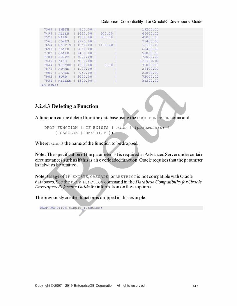
Database Compatibility for Oracle® Developers Guide
Copy right © 2007 - 2019 EnterpriseDB Corporation. All rights reserv ed.
147
7369 | SMITH | 800.00 | | 19200.00
7499 | ALLEN | 1600.00 | 300.00 | 45600.00
7521 | WARD | 1250.00 | 500.00 | 42000.00
7566 | JONES | 2975.00 | | 71400.00
7654 | MARTIN | 1250.00 | 1400.00 | 63600.00
7698 | BLAKE | 2850.00 | | 68400.00
7782 | CLARK | 2450.00 | | 58800.00
7788 | SCOTT | 3000.00 | | 72000.00
7839 | KING | 5000.00 | | 120000.00
7844 | TURNER | 1500.00 | 0.00 | 36000.00
7876 | ADAMS | 1100.00 | | 26400.00
7900 | JAMES | 950.00 | | 22800.00
7902 | FORD | 3000.00 | | 72000.00
7934 | MILLER | 1300.00 | | 31200.00
(14 rows)
3.2.4.3 Deleting a Function
A function can be deleted from the database using the DROP FUNCTION command.
DROP FUNCTION [ IF EXISTS ] name [ (parameters) ]
[ CASCADE | RESTRICT ];
Where name is the name of the function to be dropped.
Note: The specification of the parameter list is required in Advanced Server under certain
circumstances such as if this is an overloaded function. Oracle requires that the parameter list always be omitted.
Note: Usage of IF EXISTS, CASCADE, or RESTRICT is not compatible with Oracle
databases. See the DROP FUNCTION command in the Database Compatibility for Oracle Developers Reference Guide for information on these options.
The previously created function is dropped in this example:
DROP FUNCTION simple_function;

Database Compatibility for Oracle® Developers Guide
Copy right © 2007 - 2019 EnterpriseDB Corporation. All rights reserv ed.
148
3.2.5 Procedure and Function Parameters
An important aspect of using procedures and functions is the capability to pass data from the calling program to the procedure or function and to receive data back from the procedure or function. This is accomplished by using parameters.
Parameters are declared in the procedure or function definition, enclosed within parenthesis following the procedure or function name. Parameters declared in the procedure or function definition are known as formal parameters. When the procedure or
function is invoked, the calling program supplies the actual data that is to be used in the called program’s processing as well as the variables that are to receive the results of the
called program’s processing. The data and variables supplied by the calling program when the procedure or function is called are referred to as the actual parameters.
The following is the general format of a formal parameter declaration.
(name [ IN | OUT | IN OUT ] data_type [ DEFAULT value ])
name is an identifier assigned to the formal parameter. If specified, IN defines the
parameter for receiving input data into the procedure or function. An IN parameter can
also be initialized to a default value. If specified, OUT defines the parameter for returning
data from the procedure or function. If specified, IN OUT allows the parameter to be used
for both input and output. If all of IN, OUT, and IN OUT are omitted, then the parameter
acts as if it were defined as IN by default. Whether a parameter is IN, OUT, or IN OUT is referred to as the parameter’s mode. data_type defines the data type of the parameter.
value is a default value assigned to an IN parameter in the called program if an actual parameter is not specified in the call.
The following is an example of a procedure that takes parameters:
CREATE OR REPLACE PROCEDURE emp_query (
p_deptno IN NUMBER,
p_empno IN OUT NUMBER,
p_ename IN OUT VARCHAR2,
p_job OUT VARCHAR2,
p_hiredate OUT DATE,
p_sal OUT NUMBER
)
IS
BEGIN
SELECT empno, ename, job, hiredate, sal
INTO p_empno, p_ename, p_job, p_hiredate, p_sal
FROM emp
WHERE deptno = p_deptno
AND (empno = p_empno
OR ename = UPPER(p_ename));
END;

Database Compatibility for Oracle® Developers Guide
Copy right © 2007 - 2019 EnterpriseDB Corporation. All rights reserv ed.
149
In this example, p_deptno is an IN formal parameter, p_empno and p_ename are IN
OUT formal parameters, and p_job, p_hiredate, and p_sal are OUT formal parameters.
Note: In the previous example, no maximum length was specified on the VARCHAR2
parameters and no precision and scale were specified on the NUMBER parameters. It is illegal to specify a length, precision, scale or other constraints on parameter declarations.
These constraints are automatically inherited from the actual parameters that are used when the procedure or function is called.
The emp_query procedure can be called by another program, passing it the actual parameters. The following is an example of another SPL program that calls emp_query.
DECLARE
v_deptno NUMBER(2);
v_empno NUMBER(4);
v_ename VARCHAR2(10);
v_job VARCHAR2(9);
v_hiredate DATE;
v_sal NUMBER;
BEGIN
v_deptno := 30;
v_empno := 7900;
v_ename := '';
emp_query(v_deptno, v_empno, v_ename, v_job, v_hiredate, v_sal);
DBMS_OUTPUT.PUT_LINE('Department : ' || v_deptno);
DBMS_OUTPUT.PUT_LINE('Employee No: ' || v_empno);
DBMS_OUTPUT.PUT_LINE('Name : ' || v_ename);
DBMS_OUTPUT.PUT_LINE('Job : ' || v_job);
DBMS_OUTPUT.PUT_LINE('Hire Date : ' || v_hiredate);
DBMS_OUTPUT.PUT_LINE('Salary : ' || v_sal);
END;
In this example, v_deptno, v_empno, v_ename, v_job, v_hiredate, and v_sal are the actual parameters.
The output from the preceding example is shown as follows:
Department : 30
Employee No: 7900
Name : JAMES
Job : CLERK
Hire Date : 03-DEC-81
Salary : 950
3.2.5.1 Positional vs. Named Parameter Notation
You can use either positional or named parameter notation when passing parameters to a
function or procedure. If you specify parameters using positional notation, you must list
the parameters in the order that they are declared; if you specify parameters with named notation, the order of the parameters is not significant.
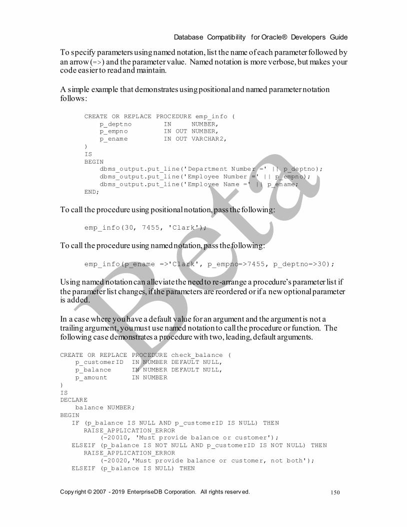
Database Compatibility for Oracle® Developers Guide
Copy right © 2007 - 2019 EnterpriseDB Corporation. All rights reserv ed.
150
To specify parameters using named notation, list the name of each parameter followed by
an arrow (=>) and the parameter value. Named notation is more verbose, but makes your code easier to read and maintain.
A simple example that demonstrates using positional and named parameter notation follows:
CREATE OR REPLACE PROCEDURE emp_info (
p_deptno IN NUMBER,
p_empno IN OUT NUMBER,
p_ename IN OUT VARCHAR2,
)
IS
BEGIN
dbms_output.put_line('Department Number =' || p_deptno);
dbms_output.put_line('Employee Number =' || p_empno);
dbms_output.put_line('Employee Name =' || p_ename;
END;
To call the procedure using positional notation, pass the following:
emp_info(30, 7455, 'Clark');
To call the procedure using named notation, pass the following:
emp_info(p_ename =>'Clark', p_empno=>7455, p_deptno=>30);
Using named notation can alleviate the need to re-arrange a procedure’s parameter list if
the parameter list changes, if the parameters are reordered or if a new optional parameter is added.
In a case where you have a default value for an argument and the argument is not a trailing argument, you must use named notation to call the procedure or function. The following case demonstrates a procedure with two, leading, default arguments.
CREATE OR REPLACE PROCEDURE check_balance (
p_customerID IN NUMBER DEFAULT NULL,
p_balance IN NUMBER DEFAULT NULL,
p_amount IN NUMBER
)
IS
DECLARE
balance NUMBER;
BEGIN
IF (p_balance IS NULL AND p_customerID IS NULL) THEN
RAISE_APPLICATION_ERROR
(-20010, 'Must provide balance or customer');
ELSEIF (p_balance IS NOT NULL AND p_customerID IS NOT NULL) THEN
RAISE_APPLICATION_ERROR
(-20020,'Must provide balance or customer, not both');
ELSEIF (p_balance IS NULL) THEN

Database Compatibility for Oracle® Developers Guide
Copy right © 2007 - 2019 EnterpriseDB Corporation. All rights reserv ed.
151
balance := getCustomerBalance(p_customerID);
ELSE
balance := p_balance;
END IF;
IF (amount > balance) THEN
RAISE_APPLICATION_ERROR
(-20030, 'Balance insufficient');
END IF;
END;
You can only omit non-trailing argument values (when you call this procedure) by using
named notation; when using positional notation, only trailing arguments are allowed to default. You can call this procedure with the following arguments:
check_balance(p_customerID => 10, p_amount = 500.00)
check_balance(p_balance => 1000.00, p_amount = 500.00)
You can use a combination of positional and named notation (mixed notation) to specify
parameters. A simple example that demonstrates using mixed parameter notation follows:
CREATE OR REPLACE PROCEDURE emp_info (
p_deptno IN NUMBER,
p_empno IN OUT NUMBER,
p_ename IN OUT VARCHAR2,
)
IS
BEGIN
dbms_output.put_line('Department Number =' || p_deptno);
dbms_output.put_line('Employee Number =' || p_empno);
dbms_output.put_line('Employee Name =' || p_ename;
END;
You can call the procedure using mixed notation:
emp_info(30, p_ename =>'Clark', p_empno=>7455);
If you do use mixed notation, remember that named arguments cannot precede positional arguments.
3.2.5.2 Parameter Modes
As previously discussed, a parameter has one of three possible modes - IN, OUT, or IN
OUT. The following characteristics of a formal parameter are dependent upon its mode:
Its initial value when the procedure or function is called.
Whether or not the called procedure or function can modify the formal parameter.

Database Compatibility for Oracle® Developers Guide
Copy right © 2007 - 2019 EnterpriseDB Corporation. All rights reserv ed.
152
How the actual parameter value is passed from the calling program to the called program.
What happens to the formal parameter value when an unhandled exception occurs in the called program.
The following table summarizes the behavior of parameters according to their mode.
Table 3-1 Parameter Modes
Mode Property IN IN OUT OUT
Formal parameter initialized to: Actual parameter value Actual parameter value Actual parameter value
Formal parameter modifiable by the
called program? No Yes Yes
Actual parameter contains: (after
normal called program termination)
Original actual
parameter value prior
to the call
Last value of the
formal parameter
Last value of the
formal parameter
Actual parameter contains: (after a
handled exception in the called
program)
Original actual
parameter value prior
to the call
Last value of the
formal parameter
Last value of the
formal parameter
Actual parameter contains: (after an
unhandled exception in the called
program)
Original actual
parameter value prior
to the call
Original actual
parameter value prior
to the call
Original actual
parameter value prior
to the call
As shown by the table, an IN formal parameter is initialized to the actual parameter with
which it is called unless it was explicitly initialized with a default value. The IN parameter may be referenced within the called program, however, the called program
may not assign a new value to the IN parameter. After control returns to the calling program, the actual parameter always contains the same value as it was set to prior to the call.
The OUT formal parameter is initialized to the actual parameter with which it is called. The called program may reference and assign new values to the formal parameter. If the
called program terminates without an exception, the actual parameter takes on the value last set in the formal parameter. If a handled exception occurs, the value of the actual parameter takes on the last value assigned to the formal parameter. If an unhandled exception occurs, the value of the actual parameter remains as it was prior to the call.
Like an IN parameter, an IN OUT formal parameter is initialized to the actual parameter
with which it is called. Like an OUT parameter, an IN OUT formal parameter is modifiable by the called program and the last value in the formal parameter is passed to the calling program’s actual parameter if the called program terminates without an
exception. If a handled exception occurs, the value of the actual parameter takes on the last value assigned to the formal parameter. If an unhandled exception occurs, the value of the actual parameter remains as it was prior to the call.
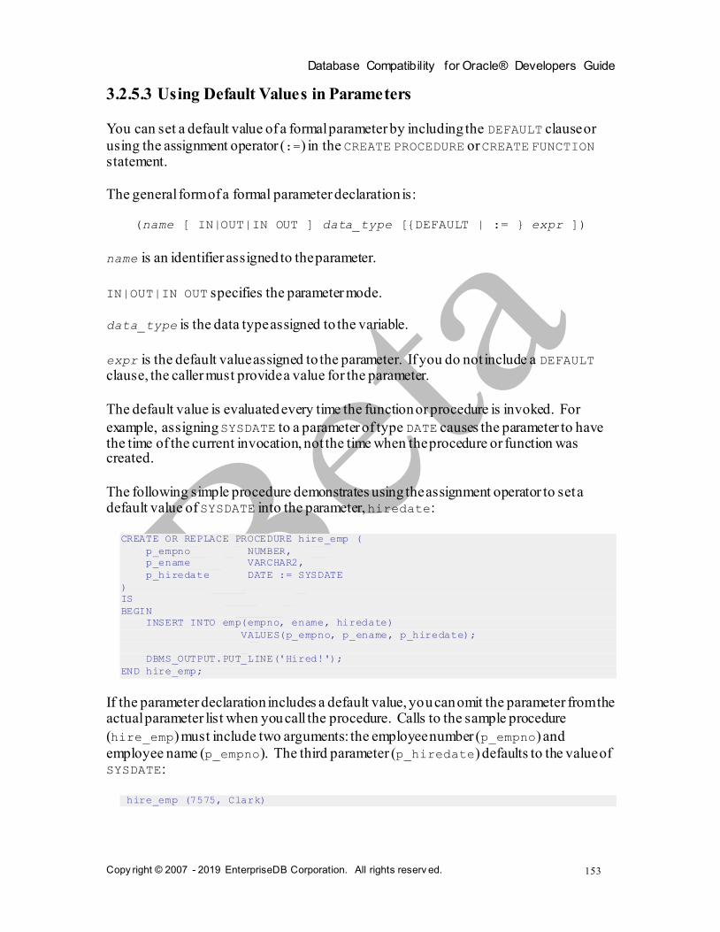
Database Compatibility for Oracle® Developers Guide
Copy right © 2007 - 2019 EnterpriseDB Corporation. All rights reserv ed.
153
3.2.5.3 Using Default Values in Parameters
You can set a default value of a formal parameter by including the DEFAULT clause or
using the assignment operator (:=) in the CREATE PROCEDURE or CREATE FUNCTION statement.
The general form of a formal parameter declaration is:
(name [ IN|OUT|IN OUT ] data_type [{DEFAULT | := } expr ])
name is an identifier assigned to the parameter.
IN|OUT|IN OUT specifies the parameter mode.
data_type is the data type assigned to the variable.
expr is the default value assigned to the parameter. If you do not include a DEFAULT clause, the caller must provide a value for the parameter.
The default value is evaluated every time the function or procedure is invoked. For
example, assigning SYSDATE to a parameter of type DATE causes the parameter to have the time of the current invocation, not the time when the procedure or function was created.
The following simple procedure demonstrates using the assignment operator to set a default value of SYSDATE into the parameter, hiredate:
CREATE OR REPLACE PROCEDURE hire_emp (
p_empno NUMBER,
p_ename VARCHAR2,
p_hiredate DATE := SYSDATE
)
IS
BEGIN
INSERT INTO emp(empno, ename, hiredate)
VALUES(p_empno, p_ename, p_hiredate);
DBMS_OUTPUT.PUT_LINE('Hired!');
END hire_emp;
If the parameter declaration includes a default value, you can omit the parameter from the actual parameter list when you call the procedure. Calls to the sample procedure
(hire_emp) must include two arguments: the employee number (p_empno) and
employee name (p_empno). The third parameter (p_hiredate) defaults to the value of SYSDATE:
hire_emp (7575, Clark)

Database Compatibility for Oracle® Developers Guide
Copy right © 2007 - 2019 EnterpriseDB Corporation. All rights reserv ed.
154
If you do include a value for the actual parameter when you call the procedure, that value takes precedence over the default value:
hire_emp (7575, Clark, 15-FEB-2010)
Adds a new employee with a hiredate of February 15, 2010, regardless of the current
value of SYSDATE.
You can write the same procedure by substituting the DEFAULT keyword for the assignment operator:
CREATE OR REPLACE PROCEDURE hire_emp (
p_empno NUMBER,
p_ename VARCHAR2,
p_hiredate DATE DEFAULT SYSDATE
)
IS
BEGIN
INSERT INTO emp(empno, ename, hiredate)
VALUES(p_empno, p_ename, p_hiredate);
DBMS_OUTPUT.PUT_LINE('Hired!');
END hire_emp;
3.2.6 Subprograms – Subprocedures and Subfunctions
The capability and functionality of SPL procedure and function programs can be used in
an advantageous manner to build well-structured and maintainable programs by organizing the SPL code into subprocedures and subfunctions.
The same SPL code can be invoked multiple times from different locations within a
relatively large SPL program by declaring subprocedures and subfunctions within the SPL program.
Subprocedures and subfunctions have the following characteristics:
The syntax, structure, and functionality of subprocedures and subfunctions are practically identical to standalone procedures and functions. The major difference
is the use of the keyword PROCEDURE or FUNCTION instead of CREATE
PROCEDURE or CREATE FUNCTION to declare the subprogram.
Subprocedures and subfunctions provide isolation for the identifiers (that is, variables, cursors, types, and other subprograms) declared within itself. That is, these identifiers cannot be accessed nor altered from the upper, parent level SPL
programs or subprograms outside of the subprocedure or subfunction. This ensures that the subprocedure and subfunction results are reliable and predictable.
The declaration section of subprocedures and subfunctions can include its own subprocedures and subfunctions. Thus, a multi-level hierarchy of subprograms

Database Compatibility for Oracle® Developers Guide
Copy right © 2007 - 2019 EnterpriseDB Corporation. All rights reserv ed.
155
can exist in the standalone program. Within the hierarchy, a subprogram can access the identifiers of upper level parent subprograms and also invoke upper
level parent subprograms. However, the same access to identifiers and invocation cannot be done for lower level child subprograms in the hierarchy.
Subprocedures and subfunctions can be declared and invoked from within any of the following types of SPL programs:
Standalone procedures and functions
Anonymous blocks
Triggers
Packages
Procedure and function methods of an object type body
Subprocedures and subfunctions declared within any of the preceding programs
The rules regarding subprocedure and subfunction structure and access are discussed in more detail in the next sections.
3.2.6.1 Creating a Subprocedure
The PROCEDURE clause specified in the declaration section defines and names a subprocedure local to that block.
The term block refers to the SPL block structure consisting of an optional declaration
section, a mandatory executable section, and an optional exception section. Blocks are the structures for standalone procedures and functions, anonymous blocks, subprograms, triggers, packages, and object type methods.
The phrase the identifier is local to the block means that the identifier (that is, a variable,
cursor, type, or subprogram) is declared within the declaration section of that block and is therefore accessible by the SPL code within the executable section and optional exception section of that block.
Subprocedures can only be declared after all other variable, cursor, and type declarations included in the declaration section. (That is, subprograms must be the last set of declarations.)
PROCEDURE name [ (parameters) ]
{ IS | AS }
[ PRAGMA AUTONOMOUS_TRANSACTION; ]
[ declarations ]
BEGIN
statements
END [ name ];
Where:

Database Compatibility for Oracle® Developers Guide
Copy right © 2007 - 2019 EnterpriseDB Corporation. All rights reserv ed.
156
name
name is the identifier of the subprocedure.
parameters
parameters is a list of formal parameters.
PRAGMA AUTONOMOUS_TRANSACTION
PRAGMA AUTONOMOUS_TRANSACTION is the directive that sets the subprocedure as an autonomous transaction.
declarations
declarations are variable, cursor, type, or subprogram declarations. If
subprogram declarations are included, they must be declared after all other variable, cursor, and type declarations.
statements
statements are SPL program statements (the BEGIN - END block may contain
an EXCEPTION section).
Examples
The following example is a subprocedure within an anonymous block.
DECLARE
PROCEDURE list_emp
IS
v_empno NUMBER(4);
v_ename VARCHAR2(10);
CURSOR emp_cur IS
SELECT empno, ename FROM emp ORDER BY empno;
BEGIN
OPEN emp_cur;
DBMS_OUTPUT.PUT_LINE('Subprocedure list_emp:');
DBMS_OUTPUT.PUT_LINE('EMPNO ENAME');
DBMS_OUTPUT.PUT_LINE('----- -------');
LOOP
FETCH emp_cur INTO v_empno, v_ename;
EXIT WHEN emp_cur%NOTFOUND;
DBMS_OUTPUT.PUT_LINE(v_empno || ' ' || v_ename);
END LOOP;
CLOSE emp_cur;
END;
BEGIN
list_emp;
END;
Invoking this anonymous block produces the following output:

Database Compatibility for Oracle® Developers Guide
Copy right © 2007 - 2019 EnterpriseDB Corporation. All rights reserv ed.
157
Subprocedure list_emp:
EMPNO ENAME
----- -------
7369 SMITH
7499 ALLEN
7521 WARD
7566 JONES
7654 MARTIN
7698 BLAKE
7782 CLARK
7788 SCOTT
7839 KING
7844 TURNER
7876 ADAMS
7900 JAMES
7902 FORD
7934 MILLER
The following example is a subprocedure within a trigger.
CREATE OR REPLACE TRIGGER dept_audit_trig
AFTER INSERT OR UPDATE OR DELETE ON dept
DECLARE
v_action VARCHAR2(24);
PROCEDURE display_action (
p_action IN VARCHAR2
)
IS
BEGIN
DBMS_OUTPUT.PUT_LINE('User ' || USER || ' ' || p_action ||
' dept on ' || TO_CHAR(SYSDATE,'YYYY-MM-DD'));
END display_action;
BEGIN
IF INSERTING THEN
v_action := 'added';
ELSIF UPDATING THEN
v_action := 'updated';
ELSIF DELETING THEN
v_action := 'deleted';
END IF;
display_action(v_action);
END;
Invoking this trigger produces the following output:
INSERT INTO dept VALUES (50,'HR','DENVER');
User enterprisedb added dept on 2016-07-26
3.2.6.2 Creating a Subfunction
The FUNCTION clause specified in the declaration section defines and names a subfunction local to that block.

Database Compatibility for Oracle® Developers Guide
Copy right © 2007 - 2019 EnterpriseDB Corporation. All rights reserv ed.
158
The term block refers to the SPL block structure consisting of an optional declaration section, a mandatory executable section, and an optional exception section. Blocks are
the structures for standalone procedures and functions, anonymous blocks, subprograms, triggers, packages, and object type methods.
The phrase the identifier is local to the block means that the identifier (that is, a variable, cursor, type, or subprogram) is declared within the declaration section of that block and is
therefore accessible by the SPL code within the executable section and optional exception section of that block.
FUNCTION name [ (parameters) ]
RETURN data_type
{ IS | AS }
[ PRAGMA AUTONOMOUS_TRANSACTION; ]
[ declarations ]
BEGIN
statements
END [ name ];
Where:
name
name is the identifier of the subfunction.
parameters
parameters is a list of formal parameters.
data_type
data_type is the data type of the value returned by the function’s RETURN statement.
PRAGMA AUTONOMOUS_TRANSACTION
PRAGMA AUTONOMOUS_TRANSACTION is the directive that sets the subfunction as an autonomous transaction.
declarations
declarations are variable, cursor, type, or subprogram declarations. If
subprogram declarations are included, they must be declared after all other variable, cursor, and type declarations.
statements

Database Compatibility for Oracle® Developers Guide
Copy right © 2007 - 2019 EnterpriseDB Corporation. All rights reserv ed.
159
statements are SPL program statements (the BEGIN - END block may contain
an EXCEPTION section).
Examples
The following example shows the use of a recursive subfunction:
DECLARE
FUNCTION factorial (
n BINARY_INTEGER
) RETURN BINARY_INTEGER
IS
BEGIN
IF n = 1 THEN
RETURN n;
ELSE
RETURN n * factorial(n-1);
END IF;
END factorial;
BEGIN
FOR i IN 1..5 LOOP
DBMS_OUTPUT.PUT_LINE(i || '! = ' || factorial(i));
END LOOP;
END;
The output from the example is the following:
1! = 1
2! = 2
3! = 6
4! = 24
5! = 120
3.2.6.3 Block Relationships
This section describes the terminology of the relationship between blocks that can be
declared in an SPL program. The ability to invoke subprograms and access identifiers declared within a block depends upon this relationship.
The following are the basic terms:
A block is the basic SPL structure consisting of an optional declaration section, a
mandatory executable section, and an optional exception section. Blocks implement standalone procedure and function programs, anonymous blocks, triggers, packages, and subprocedures and subfunctions.
An identifier (variable, cursor, type, or subprogram) local to a block means that it is declared within the declaration section of the given block. Such local identifiers are accessible from the executable section and optional exception section of the
block.
The parent block contains the declaration of another block (the child block).
Descendent blocks are the set of blocks forming the child relationship starting
from a given parent block.
Database Compatibility for Oracle® Developers Guide
Copy right © 2007 - 2019 EnterpriseDB Corporation. All rights reserv ed.
160
Ancestor blocks are the set of blocks forming the parental relationship starting from a given child block.
The set of descendent (or ancestor) blocks form a hierarchy.
The level is an ordinal number of a given block from the highest, ancestor block. For example, given a standalone procedure, the subprograms declared within the
declaration section of this procedure are all at the same level, for example call it level 1. Additional subprograms within the declaration section of the subprograms declared in the standalone procedure are at the next level, which is
level 2.
The sibling blocks are the set of blocks that have the same parent block (that is, they are all locally declared in the same block). Sibling blocks are also always at
the same level relative to each other.
The following schematic of a set of procedure declaration sections provides an example of a set of blocks and their relationships to their surrounding blocks.
The two vertical lines on the left-hand side of the blocks indicate there are two pairs of
sibling blocks. block_1a and block_1b is one pair, and block_2a and block_2b is the second pair.
The relationship of each block with its ancestors is shown on the right-hand side of the
blocks. There are three hierarchical paths formed when progressing up the hierarchy from
the lowest level child blocks. The first consists of block_0, block_1a, block_2a, and
block_3. The second is block_0, block_1a, and block_2b. The third is block_0, block_1b, and block_2b.

Database Compatibility for Oracle® Developers Guide
Copy right © 2007 - 2019 EnterpriseDB Corporation. All rights reserv ed.
161
CREATE PROCEDURE block_0
IS
.
+---- PROCEDURE block_1a ------- Local to block_0
| IS
| . |
| . |
| . |
| +-- PROCEDURE block_2a ---- Local to block_1a and descendant
| | IS of block_0
| | . |
| | . |
| | . |
| | PROCEDURE block_3 -- Local to block_2a and descendant
| | IS of block_1a, and block_0
| Siblings . |
| | . |
| | . |
| | END block_3; |
| | END block_2a; |
| +-- PROCEDURE block_2b ---- Local to block_1a and descendant
| | IS of block_0
Siblings | , |
| | . |
| | . |
| +-- END block_2b; |
| |
| END block_1a; ---------+
+---- PROCEDURE block_1b; ------- Local to block_0
| IS
| . |
| . |
| . |
| PROCEDURE block_2b ---- Local to block_1b and descendant
| IS of block_0
| . |
| . |
| . |
| END block_2b; |
| |
+---- END block_1b; ---------+
BEGIN
.
.
.
END block_0;
The rules for invoking subprograms based upon block location is described starting with
Section 3.2.6.4. The rules for accessing variables based upon block location is described in Section 3.2.6.7.
3.2.6.4 Invoking Subprograms
A subprogram is invoked in the same manner as a standalone procedure or function by specifying its name and any actual parameters.
The subprogram may be invoked with none, one, or more qualifiers, which are the names
of the parent subprograms or labeled anonymous blocks forming the ancestor hierarchy from where the subprogram has been declared.

Database Compatibility for Oracle® Developers Guide
Copy right © 2007 - 2019 EnterpriseDB Corporation. All rights reserv ed.
162
The invocation is specified as a dot-separated list of qualifiers ending with the subprogram name and any of its arguments as shown by the following:
[[qualifier_1.][...]qualifier_n.]subprog [(arguments)]
If specified, qualifier_n is the subprogram in which subprog has been declared in its
declaration section. The preceding list of qualifiers must reside in a continuous path up the hierarchy from qualifier_n to qualifier_1. qualifier_1 may be any ancestor subprogram in the path as well as any of the following:
Standalone procedure name containing the subprogram
Standalone function name containing subprogram
Package name containing the subprogram
Object type name containing the subprogram within an object type method
An anonymous block label included prior to the DECLARE keyword if a
declaration section exists, or prior to the BEGIN keyword if there is no declaration section.
Note: qualifier_1 may not be a schema name, otherwise an error is thrown upon
invocation of the subprogram. This Advanced Server restriction is not compatible with Oracle databases, which allow use of the schema name as a qualifier.
arguments is the list of actual parameters to be passed to the subprocedure or subfunction.
Upon invocation, the search for the subprogram occurs as follows:
The invoked subprogram name of its type (that is, subprocedure or subfunction) along with any qualifiers in the specified order, (referred to as the invocation list)
is used to find a matching set of blocks residing in the same hierarchical order. The search begins in the block hierarchy where the lowest level is the block from where the subprogram is invoked. The declaration of the subprogram must be in
the SPL code prior to the code line where it is invoked when the code is observed from top to bottom. (An exception to this requirement can be accomplished using
a forward declaration. See Section 3.2.6.5 for information on forward declarations.)
If the invocation list does not match the hierarchy of blocks starting from the
block where the subprogram is invoked, a comparison is made by matching the invocation list starting with the parent of the previous starting block. In other words, the comparison progresses up the hierarchy.
If there are sibling blocks of the ancestors, the invocation list comparison also includes the hierarchy of the sibling blocks, but always comparing in an upward level, never comparing the descendants of the sibling blocks.
This comparison process continues up the hierarchies until the first complete match is found in which case the located subprogram is invoked. Note that the formal parameter list of the matched subprogram must comply with the actual
Database Compatibility for Oracle® Developers Guide
Copy right © 2007 - 2019 EnterpriseDB Corporation. All rights reserv ed.
163
parameter list specified for the invoked subprogram, otherwise an error occurs upon invocation of the subprogram.
If no match is found after searching up to the standalone program, then an error is thrown upon invocation of the subprogram.
Note: The Advanced Server search algorithm for subprogram invocation is not quite
compatible with Oracle databases. For Oracle, the search looks for the first match of the
first qualifier (that is qualifier_1). When such a match is found, all remaining
qualifiers, the subprogram name, subprogram type, and arguments of the invocation must match the hierarchy content where the matching first qualifier is found, otherwise an
error is thrown. For Advanced Server, a match is not found unless all qualifiers , the subprogram name, and the subprogram type of the invocation match the hierarchy content. If such an exact match is not initially found, Advanced Server continues the search progressing up the hierarchy.
The location of subprograms relative to the block from where the invocation is made can be accessed as follows:
Subprograms declared in the local block can be invoked from the executable section or the exception section of the same block.
Subprograms declared in the parent or other ancestor blocks can be invoked from the child block of the parent or other ancestors.
Subprograms declared in sibling blocks can be called from a sibling block or from
any descendent block of the sibling.
However, the following location of subprograms cannot be accessed relative to the block from where the invocation is made:
Subprograms declared in blocks that are descendants of the block from where the invocation is attempted.
Subprograms declared in blocks that are descendants of a sibling block from
where the invocation is attempted.
The following examples illustrate the various conditions previously described.
Invoking Locally Declared Subprograms
The following example contains a single hierarchy of blocks contained within standalone
procedure level_0. Within the executable section of procedure level_1a, the means of invoking the local procedure level_2a are shown, both with and without qualifiers.
Also note that access to the descendant of local procedure level_2a, which is procedure
level_3a, is not permitted, with or without qualifiers. These calls are commented out in the example.
CREATE OR REPLACE PROCEDURE level_0

Database Compatibility for Oracle® Developers Guide
Copy right © 2007 - 2019 EnterpriseDB Corporation. All rights reserv ed.
164
IS
PROCEDURE level_1a
IS
PROCEDURE level_2a
IS
PROCEDURE level_3a
IS
BEGIN
DBMS_OUTPUT.PUT_LINE('........ BLOCK level_3a');
DBMS_OUTPUT.PUT_LINE('........ END BLOCK level_3a');
END level_3a;
BEGIN
DBMS_OUTPUT.PUT_LINE('...... BLOCK level_2a');
DBMS_OUTPUT.PUT_LINE('...... END BLOCK level_2a');
END level_2a;
BEGIN
DBMS_OUTPUT.PUT_LINE('.. BLOCK level_1a');
level_2a; -- Local block called
level_1a.level_2a; -- Qualified local block called
level_0.level_1a.level_2a; -- Double qualified local block called
-- level_3a; -- Error - Descendant of local block
-- level_2a.level_3a; -- Error - Descendant of local block
DBMS_OUTPUT.PUT_LINE('.. END BLOCK level_1a');
END level_1a;
BEGIN
DBMS_OUTPUT.PUT_LINE('BLOCK level_0');
level_1a;
DBMS_OUTPUT.PUT_LINE('END BLOCK level_0');
END level_0;
When the standalone procedure is invoked, the output is the following, which indicates
that procedure level_2a is successfully invoked from the calls in the executable section of procedure level_1a.
BEGIN
level_0;
END;
BLOCK level_0
.. BLOCK level_1a
...... BLOCK level_2a
...... END BLOCK level_2a
...... BLOCK level_2a
...... END BLOCK level_2a
...... BLOCK level_2a
...... END BLOCK level_2a
.. END BLOCK level_1a
END BLOCK level_0
If you were to attempt to run procedure level_0 with any of the calls to the descendent block uncommented, then an error occurs.
Invoking Subprograms Declared in Ancestor Blocks
The following example shows how subprograms can be invoked that are declared in parent and other ancestor blocks relative to the block where the invocation is made.
In this example, the executable section of procedure level_3a invokes procedure level_2a, which is its parent block. (Note that v_cnt is used to avoid an infinite loop.)
CREATE OR REPLACE PROCEDURE level_0
IS

Database Compatibility for Oracle® Developers Guide
Copy right © 2007 - 2019 EnterpriseDB Corporation. All rights reserv ed.
165
v_cnt NUMBER(2) := 0;
PROCEDURE level_1a
IS
PROCEDURE level_2a
IS
PROCEDURE level_3a
IS
BEGIN
DBMS_OUTPUT.PUT_LINE('........ BLOCK level_3a');
v_cnt := v_cnt + 1;
IF v_cnt < 2 THEN
level_2a; -- Parent block called
END IF;
DBMS_OUTPUT.PUT_LINE('........ END BLOCK level_3a');
END level_3a;
BEGIN
DBMS_OUTPUT.PUT_LINE('...... BLOCK level_2a');
level_3a; -- Local block called
DBMS_OUTPUT.PUT_LINE('...... END BLOCK level_2a');
END level_2a;
BEGIN
DBMS_OUTPUT.PUT_LINE('.. BLOCK level_1a');
level_2a; -- Local block called
DBMS_OUTPUT.PUT_LINE('.. END BLOCK level_1a');
END level_1a;
BEGIN
DBMS_OUTPUT.PUT_LINE('BLOCK level_0');
level_1a;
DBMS_OUTPUT.PUT_LINE('END BLOCK level_0');
END level_0;
The following is the resulting output:
BEGIN
level_0;
END;
BLOCK level_0
.. BLOCK level_1a
...... BLOCK level_2a
........ BLOCK level_3a
...... BLOCK level_2a
........ BLOCK level_3a
........ END BLOCK level_3a
...... END BLOCK level_2a
........ END BLOCK level_3a
...... END BLOCK level_2a
.. END BLOCK level_1a
END BLOCK level_0
In a similar example, the executable section of procedure level_3a invokes procedure
level_1a, which is further up the ancestor hierarchy. (Note that v_cnt is used to avoid an infinite loop.)
CREATE OR REPLACE PROCEDURE level_0
IS
v_cnt NUMBER(2) := 0;
PROCEDURE level_1a
IS
PROCEDURE level_2a
IS
PROCEDURE level_3a
IS
BEGIN
DBMS_OUTPUT.PUT_LINE('........ BLOCK level_3a');
v_cnt := v_cnt + 1;
IF v_cnt < 2 THEN

Database Compatibility for Oracle® Developers Guide
Copy right © 2007 - 2019 EnterpriseDB Corporation. All rights reserv ed.
166
level_1a; -- Ancestor block called
END IF;
DBMS_OUTPUT.PUT_LINE('........ END BLOCK level_3a');
END level_3a;
BEGIN
DBMS_OUTPUT.PUT_LINE('...... BLOCK level_2a');
level_3a; -- Local block called
DBMS_OUTPUT.PUT_LINE('...... END BLOCK level_2a');
END level_2a;
BEGIN
DBMS_OUTPUT.PUT_LINE('.. BLOCK level_1a');
level_2a; -- Local block called
DBMS_OUTPUT.PUT_LINE('.. END BLOCK level_1a');
END level_1a;
BEGIN
DBMS_OUTPUT.PUT_LINE('BLOCK level_0');
level_1a;
DBMS_OUTPUT.PUT_LINE('END BLOCK level_0');
END level_0;
The following is the resulting output:
BEGIN
level_0;
END;
BLOCK level_0
.. BLOCK level_1a
...... BLOCK level_2a
........ BLOCK level_3a
.. BLOCK level_1a
...... BLOCK level_2a
........ BLOCK level_3a
........ END BLOCK level_3a
...... END BLOCK level_2a
.. END BLOCK level_1a
........ END BLOCK level_3a
...... END BLOCK level_2a
.. END BLOCK level_1a
END BLOCK level_0
Invoking Subprograms Declared in Sibling Blocks
The following examples show how subprograms can be invoked that are declared in a
sibling block relative to the local, parent, or other ancestor blocks from where the invocation of the subprogram is made.
In this example, the executable section of procedure level_1b invokes procedure level_1a, which is its sibling block. Both are local to standalone procedure level_0.
Note that invocation of level_2a or equivalently, level_1a.level_2a from within
procedure level_1b is commented out as this call would result in an error. Invoking a descendent subprogram (level_2a) of sibling block (level_1a) is not permitted.
CREATE OR REPLACE PROCEDURE level_0
IS
v_cnt NUMBER(2) := 0;
PROCEDURE level_1a
IS
PROCEDURE level_2a
IS
BEGIN

Database Compatibility for Oracle® Developers Guide
Copy right © 2007 - 2019 EnterpriseDB Corporation. All rights reserv ed.
167
DBMS_OUTPUT.PUT_LINE('...... BLOCK level_2a');
DBMS_OUTPUT.PUT_LINE('...... END BLOCK level_2a');
END level_2a;
BEGIN
DBMS_OUTPUT.PUT_LINE('.. BLOCK level_1a');
DBMS_OUTPUT.PUT_LINE('.. END BLOCK level_1a');
END level_1a;
PROCEDURE level_1b
IS
BEGIN
DBMS_OUTPUT.PUT_LINE('.. BLOCK level_1b');
level_1a; -- Sibling block called
-- level_2a; -- Error – Descendant of sibling block
-- level_1a.level_2a; -- Error - Descendant of sibling block
DBMS_OUTPUT.PUT_LINE('.. END BLOCK level_1b');
END level_1b;
BEGIN
DBMS_OUTPUT.PUT_LINE('BLOCK level_0');
level_1b;
DBMS_OUTPUT.PUT_LINE('END BLOCK level_0');
END level_0;
The following is the resulting output:
BEGIN
level_0;
END;
BLOCK level_0
.. BLOCK level_1b
.. BLOCK level_1a
.. END BLOCK level_1a
.. END BLOCK level_1b
END BLOCK level_0
In the following example, procedure level_1a, which is the sibling of procedure
level_1b, which is an ancestor of procedure level_3b is successfully invoked.
CREATE OR REPLACE PROCEDURE level_0
IS
PROCEDURE level_1a
IS
BEGIN
DBMS_OUTPUT.PUT_LINE('.. BLOCK level_1a');
DBMS_OUTPUT.PUT_LINE('.. END BLOCK level_1a');
END level_1a;
PROCEDURE level_1b
IS
PROCEDURE level_2b
IS
PROCEDURE level_3b
IS
BEGIN
DBMS_OUTPUT.PUT_LINE('........ BLOCK level_3b');
level_1a; -- Ancestor's sibling block called
level_0.level_1a; -- Qualified ancestor's sibling block
DBMS_OUTPUT.PUT_LINE('........ END BLOCK level_3b');
END level_3b;
BEGIN
DBMS_OUTPUT.PUT_LINE('...... BLOCK level_2b');
level_3b; -- Local block called
DBMS_OUTPUT.PUT_LINE('...... END BLOCK level_2b');
END level_2b;
BEGIN
DBMS_OUTPUT.PUT_LINE('.. BLOCK level_1b');
level_2b; -- Local block called
DBMS_OUTPUT.PUT_LINE('.. END BLOCK level_1b');

Database Compatibility for Oracle® Developers Guide
Copy right © 2007 - 2019 EnterpriseDB Corporation. All rights reserv ed.
168
END level_1b;
BEGIN
DBMS_OUTPUT.PUT_LINE('BLOCK level_0');
level_1b;
DBMS_OUTPUT.PUT_LINE('END BLOCK level_0');
END level_0;
The following is the resulting output:
BEGIN
level_0;
END;
BLOCK level_0
.. BLOCK level_1b
...... BLOCK level_2b
........ BLOCK level_3b
.. BLOCK level_1a
.. END BLOCK level_1a
.. BLOCK level_1a
.. END BLOCK level_1a
........ END BLOCK level_3b
...... END BLOCK level_2b
.. END BLOCK level_1b
END BLOCK level_0
3.2.6.5 Using Forward Declarations
As discussed so far, when a subprogram is to be invoked, it must have been declared somewhere in the hierarchy of blocks within the standalone program, but prior to where it
is invoked. In other words, when scanning the SPL code from beginning to end, the subprogram declaration must be found before its invocation.
However, there is a method of constructing the SPL code so that the full declaration of
the subprogram (that is, its optional declaration section, its mandatory executable section, and optional exception section) appears in the SPL code after the point in the code where it is invoked.
This is accomplished by inserting a forward declaration in the SPL code prior to its
invocation. The forward declaration is the specification of a subprocedure or subfunction name, formal parameters, and return type if it is a subfunction.
The full subprogram specification consisting of the optional declaration section, the executable section, and the optional exception section must be specified in the same
declaration section as the forward declaration, but may appear following other subprogram declarations that invoke this subprogram with the forward declaration.
Typical usage of a forward declaration is when two subprograms invoke each other as shown by the following:
DECLARE
FUNCTION add_one (
p_add IN NUMBER
) RETURN NUMBER;
FUNCTION test_max (

Database Compatibility for Oracle® Developers Guide
Copy right © 2007 - 2019 EnterpriseDB Corporation. All rights reserv ed.
169
p_test IN NUMBER)
RETURN NUMBER
IS
BEGIN
IF p_test < 5 THEN
RETURN add_one(p_test);
END IF;
DBMS_OUTPUT.PUT('Final value is ');
RETURN p_test;
END;
FUNCTION add_one (
p_add IN NUMBER)
RETURN NUMBER
IS
BEGIN
DBMS_OUTPUT.PUT_LINE('Increase by 1');
RETURN test_max(p_add + 1);
END;
BEGIN
DBMS_OUTPUT.PUT_LINE(test_max(3));
END;
Subfunction test_max invokes subfunction add_one, which also invokes subfunction
test_max, so a forward declaration is required for one of the subprograms, which is implemented for add_one at the beginning of the anonymous block declaration section.
The resulting output from the anonymous block is as follows:
Increase by 1
Increase by 1
Final value is 5
3.2.6.6 Overloading Subprograms
Generally, subprograms of the same type (subprocedure or subfunction) with the same
name, and same formal parameter specification can appear multiple times within the same standalone program as long as they are not sibling blocks (that is, the subprograms are not declared in the same local block).
Each subprogram can be individually invoked depending upon the use of qualifiers and
the location where the subprogram invocation is made as discussed in the previous sections.
It is however possible to declare subprograms, even as siblings, that are of the same subprogram type and name as long as certain aspects of the formal parameters differ.
These characteristics (subprogram type, name, and formal parameter specification) is generally known as a program’s signature.
The declaration of multiple subprograms where the signatures are identical except for certain aspects of the formal parameter specification is referred to as subprogram overloading.

Database Compatibility for Oracle® Developers Guide
Copy right © 2007 - 2019 EnterpriseDB Corporation. All rights reserv ed.
170
Thus, the determination of which particular overloaded subprogram is to be invoked is determined by a match of the actual parameters specified by the subprogram invocation and the formal parameter lists of the overloaded subprograms.
Any of the following differences permit overloaded subprograms:
The number of formal parameters are different.
At least one pair of data types of the corresponding formal parameters (that is, compared according to the same order of appearance in the formal parameter list)
are different, but are not aliases. Data type aliases are discussed later in this section.
Note that the following differences alone do not permit overloaded subprograms :
Different formal parameter names
Different parameter modes (IN, IN OUT, OUT) for the corresponding formal parameters
For subfunctions, different data types in the RETURN clause
As previously indicated, one of the differences allowing overloaded subprograms are different data types.
However, certain data types have alternative names referred to as aliases, which can be used for the table definition.
For example, there are fixed length character data types that can be specified as CHAR or
CHARACTER. There are variable length character data types that can be specified as CHAR
VARYING, CHARACTER VARYING, VARCHAR, or VARCHAR2. For integers, there are
BINARY_INTEGER, PLS_INTEGER, and INTEGER data types. For numbers, there are NUMBER, NUMERIC, DEC, and DECIMAL data types.
For detailed information about the data types supported by Advanced Server, please see the Database Compatibility for Oracle Developers Reference Guide, available from EnterpriseDB at:
https://www.enterprisedb.com/resources/product-documentation
Thus, when attempting to create overloaded subprograms, the formal parameter data types are not considered different if the specified data types are aliases of each other.
It can be determined if certain data types are aliases of other types by displaying the table definition containing the data types in question.
For example, the following table definition contains some data types and their aliases.
CREATE TABLE data_type_aliases (

Database Compatibility for Oracle® Developers Guide
Copy right © 2007 - 2019 EnterpriseDB Corporation. All rights reserv ed.
171
dt_BLOB BLOB,
dt_LONG_RAW LONG RAW,
dt_RAW RAW(4),
dt_BYTEA BYTEA,
dt_INTEGER INTEGER,
dt_BINARY_INTEGER BINARY_INTEGER,
dt_PLS_INTEGER PLS_INTEGER,
dt_REAL REAL,
dt_DOUBLE_PRECISION DOUBLE PRECISION,
dt_FLOAT FLOAT,
dt_NUMBER NUMBER,
dt_DECIMAL DECIMAL,
dt_NUMERIC NUMERIC,
dt_CHAR CHAR,
dt_CHARACTER CHARACTER,
dt_VARCHAR2 VARCHAR2(4),
dt_CHAR_VARYING CHAR VARYING(4),
dt_VARCHAR VARCHAR(4)
);
Using the PSQL \d command to display the table definition, the Type column displays the data type internally assigned to each column based upon its data type in the table definition:
\d data_type_aliases
Column | Type | Modifiers
---------------------+----------------------+-----------
dt_blob | bytea |
dt_long_raw | bytea |
dt_raw | bytea(4) |
dt_bytea | bytea |
dt_integer | integer |
dt_binary_integer | integer |
dt_pls_integer | integer |
dt_real | real |
dt_double_precision | double precision |
dt_float | double precision |
dt_number | numeric |
dt_decimal | numeric |
dt_numeric | numeric |
dt_char | character(1) |
dt_character | character(1) |
dt_varchar2 | character varying(4) |
dt_char_varying | character varying(4) |
dt_varchar | character varying(4) |
In the example, the base set of data types are bytea, integer, real, double
precision, numeric, character, and character varying.
When attempting to declare overloaded subprograms, a pair of formal parameter data
types that are aliases would not be sufficient to allow subprogram overloading. Thus,
parameters with data types INTEGER and PLS_INTEGER cannot overload a pair of
subprograms, but data types INTEGER and REAL, or INTEGER and FLOAT, or INTEGER and NUMBER can overload the subprograms.
Note: The overloading rules based upon formal parameter data types are not compatible with Oracle databases. Generally, the Advanced Server rules are more flexible, and

Database Compatibility for Oracle® Developers Guide
Copy right © 2007 - 2019 EnterpriseDB Corporation. All rights reserv ed.
172
certain combinations are allowed in Advanced Server that would result in an error when attempting to create the procedure or function in Oracle databases.
For certain pairs of data types used for overloading, casting of the arguments specified by
the subprogram invocation may be required to avoid an error encountered during runtime of the subprogram. Invocation of a subprogram must include the actual parameter list that can specifically identify the data types. Certain pairs of overloaded data types may
require the CAST function to explicitly identify data types. For example, pairs of
overloaded data types that may require casting during the invocation are CHAR and VARCHAR2, or NUMBER and REAL.
The following example shows a group of overloaded subfunctions invoked from within an anonymous block. The executable section of the anonymous block contains the use of the CAST function to invoke overloaded functions with certain data types.
DECLARE
FUNCTION add_it (
p_add_1 IN BINARY_INTEGER,
p_add_2 IN BINARY_INTEGER
) RETURN VARCHAR2
IS
BEGIN
RETURN 'add_it BINARY_INTEGER: ' || TO_CHAR(p_add_1 + p_add_2,9999.9999);
END add_it;
FUNCTION add_it (
p_add_1 IN NUMBER,
p_add_2 IN NUMBER
) RETURN VARCHAR2
IS
BEGIN
RETURN 'add_it NUMBER: ' || TO_CHAR(p_add_1 + p_add_2,999.9999);
END add_it;
FUNCTION add_it (
p_add_1 IN REAL,
p_add_2 IN REAL
) RETURN VARCHAR2
IS
BEGIN
RETURN 'add_it REAL: ' || TO_CHAR(p_add_1 + p_add_2,9999.9999);
END add_it;
FUNCTION add_it (
p_add_1 IN DOUBLE PRECISION,
p_add_2 IN DOUBLE PRECISION
) RETURN VARCHAR2
IS
BEGIN
RETURN 'add_it DOUBLE PRECISION: ' || TO_CHAR(p_add_1 + p_add_2,9999.9999);
END add_it;
BEGIN
DBMS_OUTPUT.PUT_LINE(add_it (25, 50));
DBMS_OUTPUT.PUT_LINE(add_it (25.3333, 50.3333));
DBMS_OUTPUT.PUT_LINE(add_it (TO_NUMBER(25.3333), TO_NUMBER(50.3333)));
DBMS_OUTPUT.PUT_LINE(add_it (CAST('25.3333' AS REAL), CAST('50.3333' AS REAL)));
DBMS_OUTPUT.PUT_LINE(add_it (CAST('25.3333' AS DOUBLE PRECISION),
CAST('50.3333' AS DOUBLE PRECISION)));
END;
The following is the output displayed from the anonymous block:
add_it BINARY_INTEGER: 75.0000
add_it NUMBER: 75.6666

Database Compatibility for Oracle® Developers Guide
Copy right © 2007 - 2019 EnterpriseDB Corporation. All rights reserv ed.
173
add_it NUMBER: 75.6666
add_it REAL: 75.6666
add_it DOUBLE PRECISION: 75.6666
3.2.6.7 Accessing Subprogram Variables
Variable declared in blocks such as subprograms or anonymous blocks can be accessed
from the executable section or the exception section of other blocks depending upon their relative location.
Accessing a variable means being able to reference it within a SQL statement or an SPL statement as is done with any local variable.
Note: If the subprogram signature contains formal parameters, these may be accessed in
the same manner as local variables of the subprogram. In this section, all discussion related to variables of a subprogram also applies to formal parameters of the subprogram.
Access of variables not only includes those defined as a data type, but also includes others such as record types, collection types, and cursors.
The variable may be accessed by at most one qualifier, which is the name of the subprogram or labeled anonymous block in which the variable has been locally declared.
The syntax to reference a variable is shown by the following:
[qualifier.]variable
If specified, qualifier is the subprogram or labeled anonymous block in which variable has been declared in its declaration section (that is, it is a local variable).
Note: In Advanced Server, there is only one circumstance where two qualifiers are permitted. This scenario is for accessing public variables of packages where the reference can be specified in the following format:
schema_name.package_name.public_variable_name
For more information about supported package syntax, please see the Database Compatibility for Oracle Developers Built-In Packages Guide.
The following summarizes how variables can be accessed:
Variables can be accessed as long as the block in which the variable has been
locally declared is within the ancestor hierarchical path starting from the block containing the reference to the variable. Such variables declared in ancestor blocks are referred to as global variables.
If a reference to an unqualified variable is made, the first attempt is to locate a local variable of that name. If such a local variable does not exist , then the search

Database Compatibility for Oracle® Developers Guide
Copy right © 2007 - 2019 EnterpriseDB Corporation. All rights reserv ed.
174
for the variable is made in the parent of the current block, and so forth, proceeding up the ancestor hierarchy. If such a variable is not found, then an error
occurs upon invocation of the subprogram.
If a reference to a qualified variable is made, the same search process is performed as described in the previous bullet point, but searching for the first
match of the subprogram or labeled anonymous block that contains the local variable. The search proceeds up the ancestor hierarchy until a match is found. If
such a match is not found, then an error occurs upon invocation of the subprogram.
The following location of variables cannot be accessed relative to the block from where the reference to the variable is made:
Variables declared in a descendent block cannot be accessed,
Variables declared in a sibling block, a sibling block of an ancestor block, or any
descendants within the sibling block cannot be accessed.
Note: The Advanced Server process for accessing variables is not compatible with Oracle
databases. For Oracle, any number of qualifiers can be specified and the search is based upon the first match of the first qualifier in a similar manner to the Oracle matching algorithm for invoking subprograms.
The following example displays how variables in various blocks are accessed, with and without qualifiers. The lines that are commented out illustrate attempts to access variables that would result in an error.
CREATE OR REPLACE PROCEDURE level_0
IS
v_level_0 VARCHAR2(20) := 'Value from level_0';
PROCEDURE level_1a
IS
v_level_1a VARCHAR2(20) := 'Value from level_1a';
PROCEDURE level_2a
IS
v_level_2a VARCHAR2(20) := 'Value from level_2a';
BEGIN
DBMS_OUTPUT.PUT_LINE('...... BLOCK level_2a');
DBMS_OUTPUT.PUT_LINE('........ v_level_2a: ' || v_level_2a);
DBMS_OUTPUT.PUT_LINE('........ v_level_1a: ' || v_level_1a);
DBMS_OUTPUT.PUT_LINE('........ level_1a.v_level_1a: ' ||
level_1a.v_level_1a);
DBMS_OUTPUT.PUT_LINE('........ v_level_0: ' || v_level_0);
DBMS_OUTPUT.PUT_LINE('........ level_0.v_level_0: ' || level_0.v_level_0);
DBMS_OUTPUT.PUT_LINE('...... END BLOCK level_2a');
END level_2a;
BEGIN
DBMS_OUTPUT.PUT_LINE('.. BLOCK level_1a');
level_2a;
-- DBMS_OUTPUT.PUT_LINE('.... v_level_2a: ' || v_level_2a);
-- Error - Descendent block ----^
-- DBMS_OUTPUT.PUT_LINE('.... level_2a.v_level_2a: ' || level_2a.v_level_2a);
-- Error - Descendent block ---------------^
DBMS_OUTPUT.PUT_LINE('.. END BLOCK level_1a');
END level_1a;
PROCEDURE level_1b
IS
v_level_1b VARCHAR2(20) := 'Value from level_1b';

Database Compatibility for Oracle® Developers Guide
Copy right © 2007 - 2019 EnterpriseDB Corporation. All rights reserv ed.
175
BEGIN
DBMS_OUTPUT.PUT_LINE('.. BLOCK level_1b');
DBMS_OUTPUT.PUT_LINE('.... v_level_1b: ' || v_level_1b);
DBMS_OUTPUT.PUT_LINE('.... v_level_0 : ' || v_level_0);
-- DBMS_OUTPUT.PUT_LINE('.... level_1a.v_level_1a: ' || level_1a.v_level_1a);
-- Error - Sibling block -----------------^
-- DBMS_OUTPUT.PUT_LINE('.... level_2a.v_level_2a: ' || level_2a.v_level_2a);
-- Error - Sibling block descendant ------^
DBMS_OUTPUT.PUT_LINE('.. END BLOCK level_1b');
END level_1b;
BEGIN
DBMS_OUTPUT.PUT_LINE('BLOCK level_0');
DBMS_OUTPUT.PUT_LINE('.. v_level_0: ' || v_level_0);
level_1a;
level_1b;
DBMS_OUTPUT.PUT_LINE('END BLOCK level_0');
END level_0;
The following is the output showing the content of each variable when the procedure is invoked:
BEGIN
level_0;
END;
BLOCK level_0
.. v_level_0: Value from level_0
.. BLOCK level_1a
...... BLOCK level_2a
........ v_level_2a: Value from level_2a
........ v_level_1a: Value from level_1a
........ level_1a.v_level_1a: Value from level_1a
........ v_level_0: Value from level_0
........ level_0.v_level_0: Value from level_0
...... END BLOCK level_2a
.. END BLOCK level_1a
.. BLOCK level_1b
.... v_level_1b: Value from level_1b
.... v_level_0 : Value from level_0
.. END BLOCK level_1b
END BLOCK level_0
The following example shows similar access attempts when all variables in all blocks have the same name:
CREATE OR REPLACE PROCEDURE level_0
IS
v_common VARCHAR2(20) := 'Value from level_0';
PROCEDURE level_1a
IS
v_common VARCHAR2(20) := 'Value from level_1a';
PROCEDURE level_2a
IS
v_common VARCHAR2(20) := 'Value from level_2a';
BEGIN
DBMS_OUTPUT.PUT_LINE('...... BLOCK level_2a');
DBMS_OUTPUT.PUT_LINE('........ v_common: ' || v_common);
DBMS_OUTPUT.PUT_LINE('........ level_2a.v_common: ' || level_2a.v_common);
DBMS_OUTPUT.PUT_LINE('........ level_1a.v_common: ' || level_1a.v_common);
DBMS_OUTPUT.PUT_LINE('........ level_0.v_common: ' || level_0.v_common);
DBMS_OUTPUT.PUT_LINE('...... END BLOCK level_2a');
END level_2a;
BEGIN
DBMS_OUTPUT.PUT_LINE('.. BLOCK level_1a');
DBMS_OUTPUT.PUT_LINE('.... v_common: ' || v_common);
DBMS_OUTPUT.PUT_LINE('.... level_0.v_common: ' || level_0.v_common);
level_2a;
Database Compatibility for Oracle® Developers Guide
Copy right © 2007 - 2019 EnterpriseDB Corporation. All rights reserv ed.
176
DBMS_OUTPUT.PUT_LINE('.. END BLOCK level_1a');
END level_1a;
PROCEDURE level_1b
IS
v_common VARCHAR2(20) := 'Value from level_1b';
BEGIN
DBMS_OUTPUT.PUT_LINE('.. BLOCK level_1b');
DBMS_OUTPUT.PUT_LINE('.... v_common: ' || v_common);
DBMS_OUTPUT.PUT_LINE('.... level_0.v_common : ' || level_0.v_common);
DBMS_OUTPUT.PUT_LINE('.. END BLOCK level_1b');
END level_1b;
BEGIN
DBMS_OUTPUT.PUT_LINE('BLOCK level_0');
DBMS_OUTPUT.PUT_LINE('.. v_common: ' || v_common);
level_1a;
level_1b;
DBMS_OUTPUT.PUT_LINE('END BLOCK level_0');
END level_0;
The following is the output showing the content of each variable when the procedure is invoked:
BEGIN
level_0;
END;
BLOCK level_0
.. v_common: Value from level_0
.. BLOCK level_1a
.... v_common: Value from level_1a
.... level_0.v_common: Value from level_0
...... BLOCK level_2a
........ v_common: Value from level_2a
........ level_2a.v_common: Value from level_2a
........ level_1a.v_common: Value from level_1a
........ level_0.v_common: Value from level_0
...... END BLOCK level_2a
.. END BLOCK level_1a
.. BLOCK level_1b
.... v_common: Value from level_1b
.... level_0.v_common : Value from level_0
.. END BLOCK level_1b
END BLOCK level_0
As previously discussed, the labels on anonymous blocks can also be used to qualify
access to variables. The following example shows variable access within a set of nested anonymous blocks:
DECLARE
v_common VARCHAR2(20) := 'Value from level_0';
BEGIN
DBMS_OUTPUT.PUT_LINE('BLOCK level_0');
DBMS_OUTPUT.PUT_LINE('.. v_common: ' || v_common);
<<level_1a>>
DECLARE
v_common VARCHAR2(20) := 'Value from level_1a';
BEGIN
DBMS_OUTPUT.PUT_LINE('.. BLOCK level_1a');
DBMS_OUTPUT.PUT_LINE('.... v_common: ' || v_common);
<<level_2a>>
DECLARE
v_common VARCHAR2(20) := 'Value from level_2a';
BEGIN
DBMS_OUTPUT.PUT_LINE('...... BLOCK level_2a');
DBMS_OUTPUT.PUT_LINE('........ v_common: ' || v_common);
DBMS_OUTPUT.PUT_LINE('........ level_1a.v_common: ' || level_1a.v_common);

Database Compatibility for Oracle® Developers Guide
Copy right © 2007 - 2019 EnterpriseDB Corporation. All rights reserv ed.
177
DBMS_OUTPUT.PUT_LINE('...... END BLOCK level_2a');
END;
DBMS_OUTPUT.PUT_LINE('.. END BLOCK level_1a');
END;
<<level_1b>>
DECLARE
v_common VARCHAR2(20) := 'Value from level_1b';
BEGIN
DBMS_OUTPUT.PUT_LINE('.. BLOCK level_1b');
DBMS_OUTPUT.PUT_LINE('.... v_common: ' || v_common);
DBMS_OUTPUT.PUT_LINE('.... level_1b.v_common: ' || level_1b.v_common);
DBMS_OUTPUT.PUT_LINE('.. END BLOCK level_1b');
END;
DBMS_OUTPUT.PUT_LINE('END BLOCK level_0');
END;
The following is the output showing the content of each variable when the anonymous block is invoked:
BLOCK level_0
.. v_common: Value from level_0
.. BLOCK level_1a
.... v_common: Value from level_1a
...... BLOCK level_2a
........ v_common: Value from level_2a
........ level_1a.v_common: Value from level_1a
...... END BLOCK level_2a
.. END BLOCK level_1a
.. BLOCK level_1b
.... v_common: Value from level_1b
.... level_1b.v_common: Value from level_1b
.. END BLOCK level_1b
END BLOCK level_0
The following example is an object type whose object type method, display_emp,
contains record type emp_typ and subprocedure emp_sal_query. Record variable
r_emp declared locally to emp_sal_query is able to access the record type emp_typ
declared in the parent block display_emp.
CREATE OR REPLACE TYPE emp_pay_obj_typ AS OBJECT
(
empno NUMBER(4),
MEMBER PROCEDURE display_emp(SELF IN OUT emp_pay_obj_typ)
);
CREATE OR REPLACE TYPE BODY emp_pay_obj_typ AS
MEMBER PROCEDURE display_emp (SELF IN OUT emp_pay_obj_typ)
IS
TYPE emp_typ IS RECORD (
ename emp.ename%TYPE,
job emp.job%TYPE,
hiredate emp.hiredate%TYPE,
sal emp.sal%TYPE,
deptno emp.deptno%TYPE
);
PROCEDURE emp_sal_query (
p_empno IN emp.empno%TYPE
)
IS
r_emp emp_typ;
v_avgsal emp.sal%TYPE;
BEGIN
SELECT ename, job, hiredate, sal, deptno
INTO r_emp.ename, r_emp.job, r_emp.hiredate, r_emp.sal, r_emp.deptno
FROM emp WHERE empno = p_empno;

Database Compatibility for Oracle® Developers Guide
Copy right © 2007 - 2019 EnterpriseDB Corporation. All rights reserv ed.
178
DBMS_OUTPUT.PUT_LINE('Employee # : ' || p_empno);
DBMS_OUTPUT.PUT_LINE('Name : ' || r_emp.ename);
DBMS_OUTPUT.PUT_LINE('Job : ' || r_emp.job);
DBMS_OUTPUT.PUT_LINE('Hire Date : ' || r_emp.hiredate);
DBMS_OUTPUT.PUT_LINE('Salary : ' || r_emp.sal);
DBMS_OUTPUT.PUT_LINE('Dept # : ' || r_emp.deptno);
SELECT AVG(sal) INTO v_avgsal
FROM emp WHERE deptno = r_emp.deptno;
IF r_emp.sal > v_avgsal THEN
DBMS_OUTPUT.PUT_LINE('Employee''s salary is more than the '
|| 'department average of ' || v_avgsal);
ELSE
DBMS_OUTPUT.PUT_LINE('Employee''s salary does not exceed the '
|| 'department average of ' || v_avgsal);
END IF;
END;
BEGIN
emp_sal_query(SELF.empno);
END;
END;
The following is the output displayed when an instance of the object type is created and
procedure display_emp is invoked:
DECLARE
v_emp EMP_PAY_OBJ_TYP;
BEGIN
v_emp := emp_pay_obj_typ(7900);
v_emp.display_emp;
END;
Employee # : 7900
Name : JAMES
Job : CLERK
Hire Date : 03-DEC-81 00:00:00
Salary : 950.00
Dept # : 30
Employee's salary does not exceed the department average of 1566.67
The following example is a package with three levels of subprocedures. A record type,
collection type, and cursor type declared in the upper level procedure can be accessed by the descendent subprocedure.
CREATE OR REPLACE PACKAGE emp_dept_pkg
IS
PROCEDURE display_emp (
p_deptno NUMBER
);
END;
CREATE OR REPLACE PACKAGE BODY emp_dept_pkg
IS
PROCEDURE display_emp (
p_deptno NUMBER
)
IS
TYPE emp_rec_typ IS RECORD (
empno emp.empno%TYPE,
ename emp.ename%TYPE
);
TYPE emp_arr_typ IS TABLE OF emp_rec_typ INDEX BY BINARY_INTEGER;
TYPE emp_cur_type IS REF CURSOR RETURN emp_rec_typ;
PROCEDURE emp_by_dept (
p_deptno emp.deptno%TYPE
)

Database Compatibility for Oracle® Developers Guide
Copy right © 2007 - 2019 EnterpriseDB Corporation. All rights reserv ed.
179
IS
emp_arr emp_arr_typ;
emp_refcur emp_cur_type;
i BINARY_INTEGER := 0;
PROCEDURE display_emp_arr
IS
BEGIN
DBMS_OUTPUT.PUT_LINE('EMPNO ENAME');
DBMS_OUTPUT.PUT_LINE('----- -------');
FOR j IN emp_arr.FIRST .. emp_arr.LAST LOOP
DBMS_OUTPUT.PUT_LINE(emp_arr(j).empno || ' ' ||
emp_arr(j).ename);
END LOOP;
END display_emp_arr;
BEGIN
OPEN emp_refcur FOR SELECT empno, ename FROM emp WHERE deptno = p_deptno;
LOOP
i := i + 1;
FETCH emp_refcur INTO emp_arr(i).empno, emp_arr(i).ename;
EXIT WHEN emp_refcur%NOTFOUND;
END LOOP;
CLOSE emp_refcur;
display_emp_arr;
END emp_by_dept;
BEGIN
emp_by_dept(p_deptno);
END;
END;
The following is the output displayed when the top level package procedure is invoked:
BEGIN
emp_dept_pkg.display_emp(20);
END;
EMPNO ENAME
----- -------
7369 SMITH
7566 JONES
7788 SCOTT
7876 ADAMS
7902 FORD
Database Compatibility for Oracle® Developers Guide
Copy right © 2007 - 2019 EnterpriseDB Corporation. All rights reserv ed.
180
3.2.7 Compilation Errors in Procedures and Functions
When the Advanced Server parsers compile a procedure or function, they confirm that
both the CREATE statement and the program body (that portion of the program that
follows the AS keyword) conforms to the grammar rules for SPL and SQL constructs. By default, the server will terminate the compilation process if a parser detects an error. Note that the parsers detect syntax errors in expressions, but not semantic errors (i.e. an expression referencing a non-existent column, table, or function, or a value of incorrect type).
spl.max_error_count instructs the server to stop parsing if it encounters the specified number of errors in SPL code, or when it encounters an error in SQL code. The default
value of spl.max_error_count is 10; the maximum value is 1000. Setting
spl.max_error_count to a value of 1 instructs the server to stop parsing when it encounters the first error in either SPL or SQL code.
You can use the SET command to specify a value for spl.max_error_count for your current session. The syntax is:
SET spl.max_error_count = number_of_errors
Where number_of_errors specifies the number of SPL errors that may occur before the server halts the compilation process. For example:
SET spl.max_error_count = 6
The example instructs the server to continue past the first five SPL errors it encounters. When the server encounters the sixth error it will stop validating, and print six detailed error messages, and one error summary.
To save time when developing new code, or when importing existing code from another
source, you may want to set the spl.max_error_count configuration parameter to a relatively high number of errors.
Please note that if you instruct the server to continue parsing in spite of errors in the SPL code in a program body, and the parser encounters an error in a segment of SQL code,
there may still be errors in any SPL or SQL code that follows the erroneous SQL code. For example, the following function results in two errors:
CREATE FUNCTION computeBonus(baseSalary number) RETURN
number AS
BEGIN
bonus := baseSalary * 1.10;
total := bonus + 100;

Database Compatibility for Oracle® Developers Guide
Copy right © 2007 - 2019 EnterpriseDB Corporation. All rights reserv ed.
181
RETURN bonus;
END;
ERROR: "bonus" is not a known variable
LINE 4: bonus := baseSalary * 1.10;
^
ERROR: "total" is not a known variable
LINE 5: total := bonus + 100;
^
ERROR: compilation of SPL function/procedure
"computebonus" failed due to 2 errors
The following example adds a SELECT statement to the previous example. The error in the SELECT statement masks the other errors that follow:
CREATE FUNCTION computeBonus(employeeName number) RETURN
number AS
BEGIN
SELECT salary INTO baseSalary FROM emp
WHERE ename = employeeName;
bonus := baseSalary * 1.10;
total := bonus + 100;
RETURN bonus;
END;
ERROR: "basesalary" is not a known variable
LINE 3: SELECT salary INTO baseSalary FROM emp WHERE
ename = emp...
Database Compatibility for Oracle® Developers Guide
Copy right © 2007 - 2019 EnterpriseDB Corporation. All rights reserv ed.
182
3.2.8 Program Security
Security over what user may execute an SPL program and what database objects an SPL program may access for any given user executing the program is controlled by the following:
Privilege to execute a program.
Privileges granted on the database objects (including other SPL programs) which a program attempts to access.
Whether the program is defined with definer’s rights or invoker’s rights.
These aspects are discussed in the following sections.
3.2.8.1 EXECUTE Privilege
An SPL program (function, procedure, or package) can begin execution only if any of the following are true:
The current user is a superuser, or
The current user has been granted EXECUTE privilege on the SPL program, or
The current user inherits EXECUTE privilege on the SPL program by virtue of being a member of a group which does have such privilege, or
EXECUTE privilege has been granted to the PUBLIC group.
Whenever an SPL program is created in Advanced Server, EXECUTE privilege is
automatically granted to the PUBLIC group by default, therefore, any user can immediately execute the program.
This default privilege can be removed by using the REVOKE EXECUTE command. The following is an example:
REVOKE EXECUTE ON PROCEDURE list_emp FROM PUBLIC;
Explicit EXECUTE privilege on the program can then be granted to individual users or groups.
GRANT EXECUTE ON PROCEDURE list_emp TO john;
Now, user, john, can execute the list_emp program; other users who do not meet any of the conditions listed at the beginning of this section cannot.
Once a program begins execution, the next aspect of security is what privilege checks occur if the program attempts to perform an action on any database object including:

Database Compatibility for Oracle® Developers Guide
Copy right © 2007 - 2019 EnterpriseDB Corporation. All rights reserv ed.
183
Reading or modifying table or view data.
Creating, modifying, or deleting a database object such as a table, view, index, or
sequence.
Obtaining the current or next value from a sequence. Calling another program (function, procedure, or package).
Each such action can be protected by privileges on the database object either allowed or disallowed for the user.
Note that it is possible for a database to have more than one object of the same type with
the same name, but each such object belonging to a different schema in the database. If this is the case, which object is being referenced by an SPL program? This is the topic of the next section.
3.2.8.2 Database Object Name Resolution
A database object inside an SPL program may either be referenced by its qualified name
or by an unqualified name. A qualified name is in the form of schema.name where
schema is the name of the schema under which the database object with identifier, name,
exists. An unqualified name does not have the “schema.” portion. When a reference is
made to a qualified name, there is absolutely no ambiguity as to exactly which database object is intended – it either does or does not exist in the specified schema.
Locating an object with an unqualified name, however, requires the use of the current user’s search path. When a user becomes the current user of a session, a default search
path is always associated with that user. The search path consists of a list of schemas which are searched in left-to-right order for locating an unqualified database object reference. The object is considered non-existent if it can’t be found in any of the schemas
in the search path. The default search path can be displayed in PSQL using the SHOW search_path command.
edb=# SHOW search_path;
search_path
-----------------
"$user", public
(1 row)
$user in the above search path is a generic placeholder that refers to the current user so
if the current user of the above session is enterprisedb, an unqualified database object
would be searched for in the following schemas in this order – first, enterprisedb, then public.
Once an unqualified name has been resolved in the search path, it can be determined if
the current user has the appropriate privilege to perform the desired action on that specific object.
Database Compatibility for Oracle® Developers Guide
Copy right © 2007 - 2019 EnterpriseDB Corporation. All rights reserv ed.
184
Note: The concept of the search path is not compatible with Oracle databases. For an unqualified reference, Oracle simply looks in the schema of the current user for the
named database object. It also important to note that in Oracle, a user and his or her schema is the same entity while in Advanced Server, a user and a schema are two distinct objects.
3.2.8.3 Database Object Privileges
Once an SPL program begins execution, any attempt to access a database object from
within the program results in a check to ensure the current user has the authorization to
perform the intended action against the referenced object. Privileges on database objects
are bestowed and removed using the GRANT and REVOKE commands, respectively. If the current user attempts unauthorized access on a database object, then the program will throw an exception. See Section 3.5.7 for information about exception handling.
The final topic discusses exactly who is the current user.
3.2.8.4 Definer’s vs. Invokers Rights
When an SPL program is about to begin execution, a determination is made as to what
user is to be associated with this process. This user is referred to as the current user. The current user’s database object privileges are used to determine whether or not access to
database objects referenced in the program will be permitted. The current, prevailing search path in effect when the program is invoked will be used to resolve any unqualified object references.
The selection of the current user is influenced by whether the SPL program was created
with definer’s right or invoker’s rights. The AUTHID clause determines that selection.
Appearance of the clause AUTHID DEFINER gives the program definer’s rights. This is
also the default if the AUTHID clause is omitted. Use of the clause AUTHID
CURRENT_USER gives the program invoker’s rights. The difference between the two is summarized as follows:
If a program has definer’s rights, then the owner of the program becomes the
current user when program execution begins. The program owner’s database object privileges are used to determine if access to a referenced object is permitted. In a definer’s rights program, it is irrelevant as to which user actually
invoked the program.
If a program has invoker’s rights, then the current user at the time the program is called remains the current user while the program is executing (but not necessarily
within called subprograms – see the following bullet points). When an invoker’s rights program is invoked, the current user is typically the user that started the session (i.e., made the database connection) although it is possible to change the
current user after the session has started using the SET ROLE command. In an invoker’s rights program, it is irrelevant as to which user actually owns the
program.

Database Compatibility for Oracle® Developers Guide
Copy right © 2007 - 2019 EnterpriseDB Corporation. All rights reserv ed.
185
From the previous definitions, the following observations can be made:
If a definer’s rights program calls a definer’s rights program, the current user changes from the owner of the calling program to the owner of the called program
during execution of the called program.
If a definer’s rights program calls an invoker’s rights program, the owner of the calling program remains the current user during execution of both the calling and
called programs.
If an invoker’s rights program calls an invoker’s rights program, the current user of the calling program remains the current user during execution of the called
program.
If an invokers’ rights program calls a definer’s rights program, the current user switches to the owner of the definer’s rights program during execution of the called program.
The same principles apply if the called program in turn calls another program in the cases cited above.
This section on security concludes with an example using the sample application.
3.2.8.5 Security Example
In the following example, a new database will be created along with two users – hr_mgr
who will own a copy of the entire sample application in schema, hr_mgr; and
sales_mgr who will own a schema named, sales_mgr, that will have a copy of only
the emp table containing only the employees who work in sales.
The procedure list_emp, function hire_clerk, and package emp_admin will be used in this example. All of the default privileges that are granted upon installation of the
sample application will be removed and then be explicitly re-granted so as to present a more secure environment in this example.
Programs list_emp and hire_clerk will be changed from the default of definer’s
rights to invoker’s rights. It will be then illustrated that when sales_mgr runs these
programs, they act upon the emp table in sales_mgr’s schema since sales_mgr’s search path and privileges will be used for name resolution and authorization checking.
Programs get_dept_name and hire_emp in the emp_admin package will then be
executed by sales_mgr. In this case, the dept table and emp table in hr_mgr’s schema
will be accessed as hr_mgr is the owner of the emp_admin package which is using
definer’s rights. Since the default search path is in effect with the $user placeholder, the schema matching the user (in this case, hr_mgr) is used to find the tables.
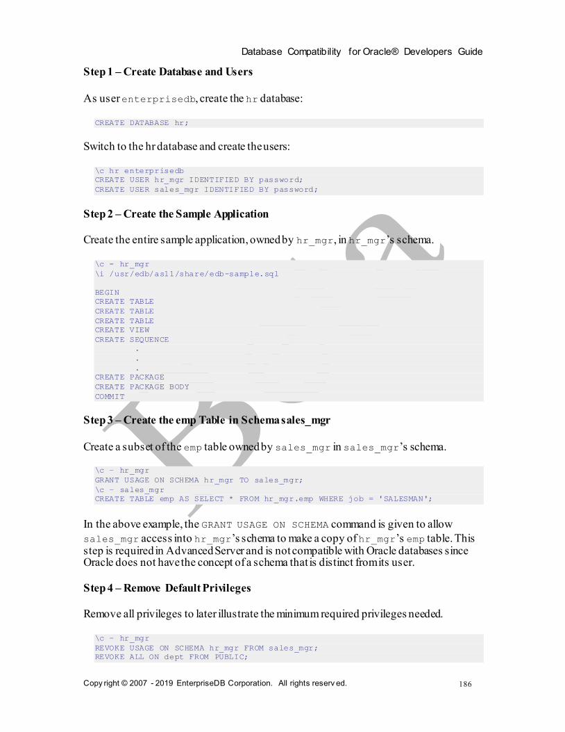
Database Compatibility for Oracle® Developers Guide
Copy right © 2007 - 2019 EnterpriseDB Corporation. All rights reserv ed.
186
Step 1 – Create Database and Users
As user enterprisedb, create the hr database:
CREATE DATABASE hr;
Switch to the hr database and create the users:
\c hr enterprisedb
CREATE USER hr_mgr IDENTIFIED BY password;
CREATE USER sales_mgr IDENTIFIED BY password;
Step 2 – Create the Sample Application
Create the entire sample application, owned by hr_mgr, in hr_mgr’s schema.
\c - hr_mgr
\i /usr/edb/as11/share/edb-sample.sql
BEGIN
CREATE TABLE
CREATE TABLE
CREATE TABLE
CREATE VIEW
CREATE SEQUENCE
.
.
.
CREATE PACKAGE
CREATE PACKAGE BODY
COMMIT
Step 3 – Create the emp Table in Schema sales_mgr
Create a subset of the emp table owned by sales_mgr in sales_mgr’s schema.
\c – hr_mgr
GRANT USAGE ON SCHEMA hr_mgr TO sales_mgr;
\c – sales_mgr
CREATE TABLE emp AS SELECT * FROM hr_mgr.emp WHERE job = 'SALESMAN';
In the above example, the GRANT USAGE ON SCHEMA command is given to allow
sales_mgr access into hr_mgr’s schema to make a copy of hr_mgr’s emp table. This step is required in Advanced Server and is not compatible with Oracle databases since Oracle does not have the concept of a schema that is distinct from its user.
Step 4 – Remove Default Privileges
Remove all privileges to later illustrate the minimum required privileges needed.
\c – hr_mgr
REVOKE USAGE ON SCHEMA hr_mgr FROM sales_mgr;
REVOKE ALL ON dept FROM PUBLIC;
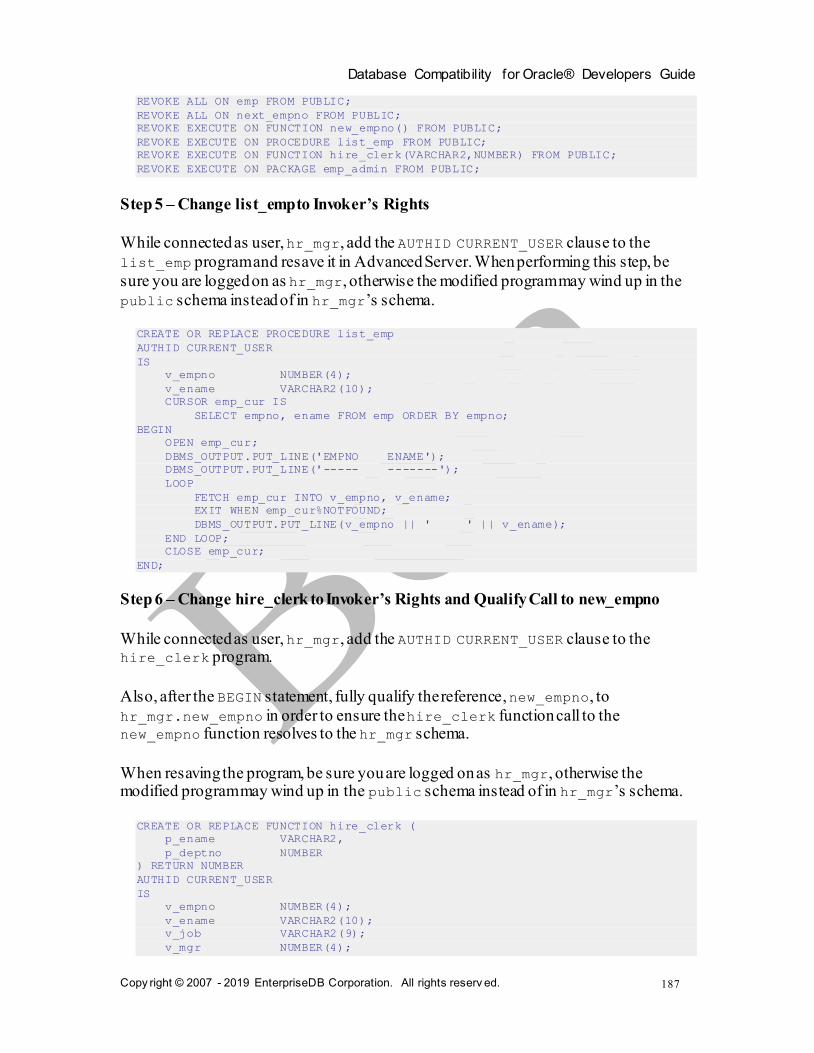
Database Compatibility for Oracle® Developers Guide
Copy right © 2007 - 2019 EnterpriseDB Corporation. All rights reserv ed.
187
REVOKE ALL ON emp FROM PUBLIC;
REVOKE ALL ON next_empno FROM PUBLIC;
REVOKE EXECUTE ON FUNCTION new_empno() FROM PUBLIC;
REVOKE EXECUTE ON PROCEDURE list_emp FROM PUBLIC;
REVOKE EXECUTE ON FUNCTION hire_clerk(VARCHAR2,NUMBER) FROM PUBLIC;
REVOKE EXECUTE ON PACKAGE emp_admin FROM PUBLIC;
Step 5 – Change list_emp to Invoker’s Rights
While connected as user, hr_mgr, add the AUTHID CURRENT_USER clause to the
list_emp program and resave it in Advanced Server. When performing this step, be
sure you are logged on as hr_mgr, otherwise the modified program may wind up in the
public schema instead of in hr_mgr’s schema.
CREATE OR REPLACE PROCEDURE list_emp
AUTHID CURRENT_USER
IS
v_empno NUMBER(4);
v_ename VARCHAR2(10);
CURSOR emp_cur IS
SELECT empno, ename FROM emp ORDER BY empno;
BEGIN
OPEN emp_cur;
DBMS_OUTPUT.PUT_LINE('EMPNO ENAME');
DBMS_OUTPUT.PUT_LINE('----- -------');
LOOP
FETCH emp_cur INTO v_empno, v_ename;
EXIT WHEN emp_cur%NOTFOUND;
DBMS_OUTPUT.PUT_LINE(v_empno || ' ' || v_ename);
END LOOP;
CLOSE emp_cur;
END;
Step 6 – Change hire_clerk to Invoker’s Rights and Qualify Call to new_empno
While connected as user, hr_mgr, add the AUTHID CURRENT_USER clause to the hire_clerk program.
Also, after the BEGIN statement, fully qualify the reference, new_empno, to
hr_mgr.new_empno in order to ensure the hire_clerk function call to the new_empno function resolves to the hr_mgr schema.
When resaving the program, be sure you are logged on as hr_mgr, otherwise the modified program may wind up in the public schema instead of in hr_mgr’s schema.
CREATE OR REPLACE FUNCTION hire_clerk (
p_ename VARCHAR2,
p_deptno NUMBER
) RETURN NUMBER
AUTHID CURRENT_USER
IS
v_empno NUMBER(4);
v_ename VARCHAR2(10);
v_job VARCHAR2(9);
v_mgr NUMBER(4);
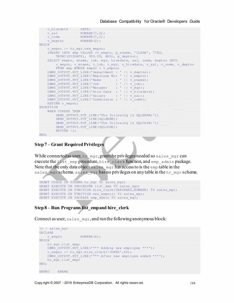
Database Compatibility for Oracle® Developers Guide
Copy right © 2007 - 2019 EnterpriseDB Corporation. All rights reserv ed.
188
v_hiredate DATE;
v_sal NUMBER(7,2);
v_comm NUMBER(7,2);
v_deptno NUMBER(2);
BEGIN
v_empno := hr_mgr.new_empno;
INSERT INTO emp VALUES (v_empno, p_ename, 'CLERK', 7782,
TRUNC(SYSDATE), 950.00, NULL, p_deptno);
SELECT empno, ename, job, mgr, hiredate, sal, comm, deptno INTO
v_empno, v_ename, v_job, v_mgr, v_hiredate, v_sal, v_comm, v_deptno
FROM emp WHERE empno = v_empno;
DBMS_OUTPUT.PUT_LINE('Department : ' || v_deptno);
DBMS_OUTPUT.PUT_LINE('Employee No: ' || v_empno);
DBMS_OUTPUT.PUT_LINE('Name : ' || v_ename);
DBMS_OUTPUT.PUT_LINE('Job : ' || v_job);
DBMS_OUTPUT.PUT_LINE('Manager : ' || v_mgr);
DBMS_OUTPUT.PUT_LINE('Hire Date : ' || v_hiredate);
DBMS_OUTPUT.PUT_LINE('Salary : ' || v_sal);
DBMS_OUTPUT.PUT_LINE('Commission : ' || v_comm);
RETURN v_empno;
EXCEPTION
WHEN OTHERS THEN
DBMS_OUTPUT.PUT_LINE('The following is SQLERRM:');
DBMS_OUTPUT.PUT_LINE(SQLERRM);
DBMS_OUTPUT.PUT_LINE('The following is SQLCODE:');
DBMS_OUTPUT.PUT_LINE(SQLCODE);
RETURN -1;
END;
Step 7 – Grant Required Privileges
While connected as user, hr_mgr, grant the privileges needed so sales_mgr can
execute the list_emp procedure, hire_clerk function, and emp_admin package.
Note that the only data object sales_mgr has access to is the emp table in the sales_mgr schema. sales_mgr has no privileges on any table in the hr_mgr schema.
GRANT USAGE ON SCHEMA hr_mgr TO sales_mgr;
GRANT EXECUTE ON PROCEDURE list_emp TO sales_mgr;
GRANT EXECUTE ON FUNCTION hire_clerk(VARCHAR2,NUMBER) TO sales_mgr;
GRANT EXECUTE ON FUNCTION new_empno() TO sales_mgr;
GRANT EXECUTE ON PACKAGE emp_admin TO sales_mgr;
Step 8 – Run Programs list_emp and hire_clerk
Connect as user, sales_mgr, and run the following anonymous block:
\c – sales_mgr
DECLARE
v_empno NUMBER(4);
BEGIN
hr_mgr.list_emp;
DBMS_OUTPUT.PUT_LINE('*** Adding new employee ***');
v_empno := hr_mgr.hire_clerk('JONES',40);
DBMS_OUTPUT.PUT_LINE('*** After new employee added ***');
hr_mgr.list_emp;
END;
EMPNO ENAME

Database Compatibility for Oracle® Developers Guide
Copy right © 2007 - 2019 EnterpriseDB Corporation. All rights reserv ed.
189
----- -------
7499 ALLEN
7521 WARD
7654 MARTIN
7844 TURNER
*** Adding new employee ***
Department : 40
Employee No: 8000
Name : JONES
Job : CLERK
Manager : 7782
Hire Date : 08-NOV-07 00:00:00
Salary : 950.00
*** After new employee added ***
EMPNO ENAME
----- -------
7499 ALLEN
7521 WARD
7654 MARTIN
7844 TURNER
8000 JONES
The table and sequence accessed by the programs of the anonymous block are illustrated
in the following diagram. The gray ovals represent the schemas of sales_mgr and
hr_mgr. The current user during each program execution is shown within parenthesis in bold red font.
Figure 3 - Invoker's Rights Programs
Selecting from sales_mgr’s emp table shows that the update was made in this table.
SELECT empno, ename, hiredate, sal, deptno,
hr_mgr.emp_admin.get_dept_name(deptno) FROM sales_mgr.emp;
empno | ename | hiredate | sal | deptno | get_dept_name
sales_mgr hr_mgr
emp dept
lis t_emp (sales_mgr)
hire_c lerk (sales_mgr)
new_empno (hr_mgr)
next_
empn
o
emp
(sales_mgr)
BEGIN
hr_mgr.list_emp;
hr_mgr.hire_clerk
... END;

Database Compatibility for Oracle® Developers Guide
Copy right © 2007 - 2019 EnterpriseDB Corporation. All rights reserv ed.
190
-------+--------+--------------------+---------+--------+---------------
7499 | ALLEN | 20-FEB-81 00:00:00 | 1600.00 | 30 | SALES
7521 | WARD | 22-FEB-81 00:00:00 | 1250.00 | 30 | SALES
7654 | MARTIN | 28-SEP-81 00:00:00 | 1250.00 | 30 | SALES
7844 | TURNER | 08-SEP-81 00:00:00 | 1500.00 | 30 | SALES
8000 | JONES | 08-NOV-07 00:00:00 | 950.00 | 40 | OPERATIONS
(5 rows)
The following diagram shows that the SELECT command references the emp table in the
sales_mgr schema, but the dept table referenced by the get_dept_name function in
the emp_admin package is from the hr_mgr schema since the emp_admin package has
definer’s rights and is owned by hr_mgr. The default search path setting with the $user placeholder resolves the access by user hr_mgr to the dept table in the hr_mgr schema.
Figure 4 Definer's Rights Package
Step 9 – Run Program hire_emp in the emp_admin Package
While connected as user, sales_mgr, run the hire_emp procedure in the emp_admin package.
EXEC hr_mgr.emp_admin.hire_emp(9001,
'ALICE','SALESMAN',8000,TRUNC(SYSDATE),1000,7369,40);
This diagram illustrates that the hire_emp procedure in the emp_admin definer’s rights
package updates the emp table belonging to hr_mgr since the object privileges of
hr_mgr are used, and the default search path setting with the $user placeholder resolves to the schema of hr_mgr.
sales_mgr hr_mgr
emp dept next_
empn
o
emp
emp_admin (hr_mgr)
hire_emp
get_dept_name
(sales_mgr)
SELECT empno, ename...
hr_mgr.emp_admin.get_dept_name... FROM sales_mgr.emp

Database Compatibility for Oracle® Developers Guide
Copy right © 2007 - 2019 EnterpriseDB Corporation. All rights reserv ed.
191
Figure 5 Definer's Rights Package
Now connect as user, hr_mgr. The following SELECT command verifies that the new
employee was added to hr_mgr’s emp table since the emp_admin package has definer’s rights and hr_mgr is emp_admin’s owner.
\c – hr_mgr
SELECT empno, ename, hiredate, sal, deptno,
hr_mgr.emp_admin.get_dept_name(deptno) FROM hr_mgr.emp;
empno | ename | hiredate | sal | deptno | get_dept_name
-------+--------+--------------------+---------+--------+---------------
7369 | SMITH | 17-DEC-80 00:00:00 | 800.00 | 20 | RESEARCH
7499 | ALLEN | 20-FEB-81 00:00:00 | 1600.00 | 30 | SALES
7521 | WARD | 22-FEB-81 00:00:00 | 1250.00 | 30 | SALES
7566 | JONES | 02-APR-81 00:00:00 | 2975.00 | 20 | RESEARCH
7654 | MARTIN | 28-SEP-81 00:00:00 | 1250.00 | 30 | SALES
7698 | BLAKE | 01-MAY-81 00:00:00 | 2850.00 | 30 | SALES
7782 | CLARK | 09-JUN-81 00:00:00 | 2450.00 | 10 | ACCOUNTING
7788 | SCOTT | 19-APR-87 00:00:00 | 3000.00 | 20 | RESEARCH
7839 | KING | 17-NOV-81 00:00:00 | 5000.00 | 10 | ACCOUNTING
7844 | TURNER | 08-SEP-81 00:00:00 | 1500.00 | 30 | SALES
7876 | ADAMS | 23-MAY-87 00:00:00 | 1100.00 | 20 | RESEARCH
7900 | JAMES | 03-DEC-81 00:00:00 | 950.00 | 30 | SALES
7902 | FORD | 03-DEC-81 00:00:00 | 3000.00 | 20 | RESEARCH
7934 | MILLER | 23-JAN-82 00:00:00 | 1300.00 | 10 | ACCOUNTING
9001 | ALICE | 08-NOV-07 00:00:00 | 8000.00 | 40 | OPERATIONS
(15 rows)
sales_mgr hr_mgr
emp dept next_
empn
o
emp
emp_admin (hr_mgr)
hire_emp
get_dept_name
(sales_mgr) EXEC hr_mgr.emp_admin.hire_emp...
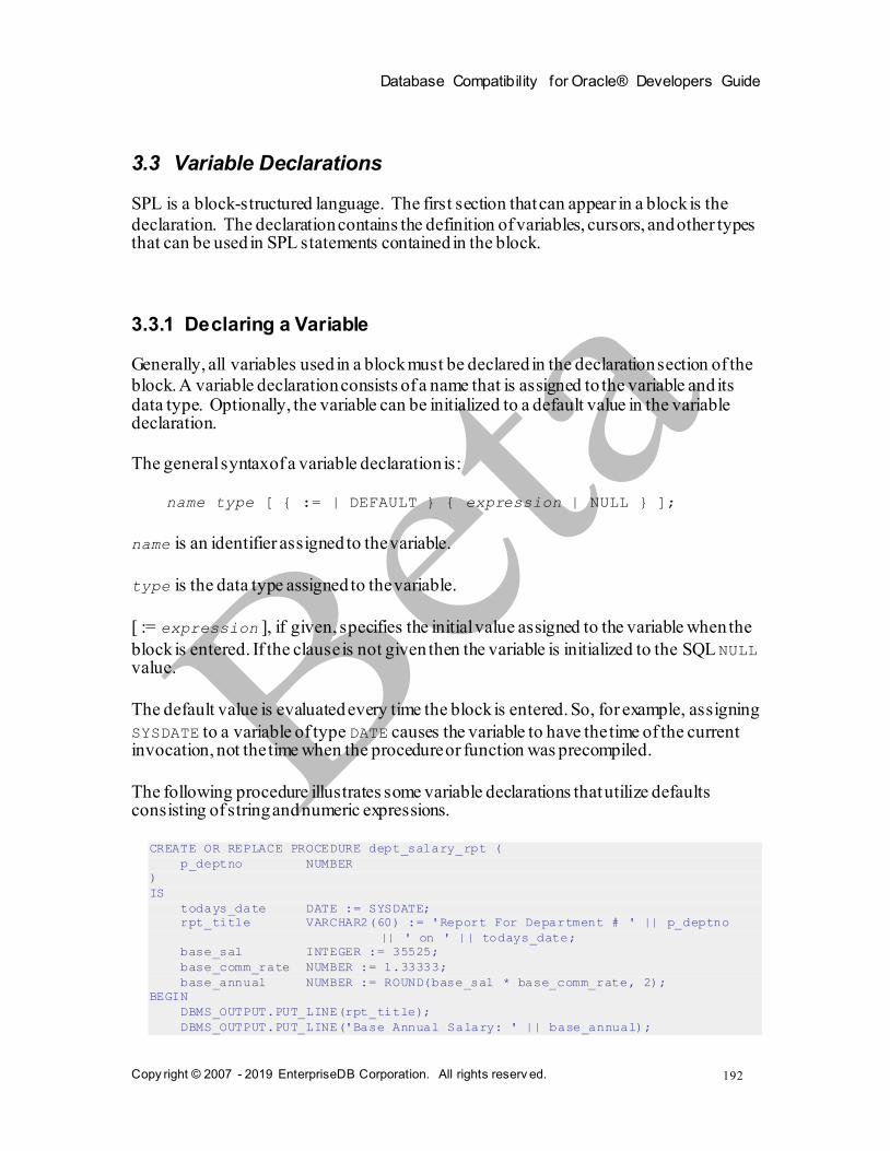
Database Compatibility for Oracle® Developers Guide
Copy right © 2007 - 2019 EnterpriseDB Corporation. All rights reserv ed.
192
3.3 Variable Declarations
SPL is a block-structured language. The first section that can appear in a block is the
declaration. The declaration contains the definition of variables, cursors, and other types that can be used in SPL statements contained in the block.
3.3.1 Declaring a Variable
Generally, all variables used in a block must be declared in the declaration section of the
block. A variable declaration consists of a name that is assigned to the variable and its data type. Optionally, the variable can be initialized to a default value in the variable declaration.
The general syntax of a variable declaration is:
name type [ { := | DEFAULT } { expression | NULL } ];
name is an identifier assigned to the variable.
type is the data type assigned to the variable.
[ := expression ], if given, specifies the initial value assigned to the variable when the
block is entered. If the clause is not given then the variable is initialized to the SQL NULL value.
The default value is evaluated every time the block is entered. So, for example, assigning
SYSDATE to a variable of type DATE causes the variable to have the time of the current invocation, not the time when the procedure or function was precompiled.
The following procedure illustrates some variable declarations that utilize defaults consisting of string and numeric expressions.
CREATE OR REPLACE PROCEDURE dept_salary_rpt (
p_deptno NUMBER
)
IS
todays_date DATE := SYSDATE;
rpt_title VARCHAR2(60) := 'Report For Department # ' || p_deptno
|| ' on ' || todays_date;
base_sal INTEGER := 35525;
base_comm_rate NUMBER := 1.33333;
base_annual NUMBER := ROUND(base_sal * base_comm_rate, 2);
BEGIN
DBMS_OUTPUT.PUT_LINE(rpt_title);
DBMS_OUTPUT.PUT_LINE('Base Annual Salary: ' || base_annual);

Database Compatibility for Oracle® Developers Guide
Copy right © 2007 - 2019 EnterpriseDB Corporation. All rights reserv ed.
193
END;
The following output of the above procedure shows that default values in the variable declarations are indeed assigned to the variables.
EXEC dept_salary_rpt(20);
Report For Department # 20 on 10-JUL-07 16:44:45
Base Annual Salary: 47366.55

Database Compatibility for Oracle® Developers Guide
Copy right © 2007 - 2019 EnterpriseDB Corporation. All rights reserv ed.
194
3.3.2 Using %TYPE in Variable Declarations
Often, variables will be declared in SPL programs that will be used to hold values from
tables in the database. In order to ensure compatibility between the table columns and the SPL variables, the data types of the two should be the same.
However, as quite often happens, a change might be made to the table definition. If the data type of the column is changed, the corresponding change may be required to the variable in the SPL program.
Instead of coding the specific column data type into the variable declaration the column
attribute, %TYPE, can be used instead. A qualified column name in dot notation or the
name of a previously declared variable must be specified as a prefix to %TYPE. The data
type of the column or variable prefixed to %TYPE is assigned to the variable being declared. If the data type of the given column or variable changes, the new data type will be associated with the variable without the need to modify the declaration code.
Note: The %TYPE attribute can be used with formal parameter declarations as well.
name { { table | view }.column | variable }%TYPE;
name is the identifier assigned to the variable or formal parameter that is being declared.
column is the name of a column in table or view. variable is the name of a variable that was declared prior to the variable identified by name.
Note: The variable does not inherit any of the column’s other attributes such as might be specified on the column with the NOT NULL clause or the DEFAULT clause.
In the following example a procedure queries the emp table using an employee number, displays the employee’s data, finds the average salary of all employees in the department to which the employee belongs, and then compares the chosen employee’s salary with the department average.
CREATE OR REPLACE PROCEDURE emp_sal_query (
p_empno IN NUMBER
)
IS
v_ename VARCHAR2(10);
v_job VARCHAR2(9);
v_hiredate DATE;
v_sal NUMBER(7,2);
v_deptno NUMBER(2);
v_avgsal NUMBER(7,2);
BEGIN
SELECT ename, job, hiredate, sal, deptno
INTO v_ename, v_job, v_hiredate, v_sal, v_deptno
FROM emp WHERE empno = p_empno;

Database Compatibility for Oracle® Developers Guide
Copy right © 2007 - 2019 EnterpriseDB Corporation. All rights reserv ed.
195
DBMS_OUTPUT.PUT_LINE('Employee # : ' || p_empno);
DBMS_OUTPUT.PUT_LINE('Name : ' || v_ename);
DBMS_OUTPUT.PUT_LINE('Job : ' || v_job);
DBMS_OUTPUT.PUT_LINE('Hire Date : ' || v_hiredate);
DBMS_OUTPUT.PUT_LINE('Salary : ' || v_sal);
DBMS_OUTPUT.PUT_LINE('Dept # : ' || v_deptno);
SELECT AVG(sal) INTO v_avgsal
FROM emp WHERE deptno = v_deptno;
IF v_sal > v_avgsal THEN
DBMS_OUTPUT.PUT_LINE('Employee''s salary is more than the '
|| 'department average of ' || v_avgsal);
ELSE
DBMS_OUTPUT.PUT_LINE('Employee''s salary does not exceed the '
|| 'department average of ' || v_avgsal);
END IF;
END;
Instead of the above, the procedure could be written as follows without explicitly coding the emp table data types into the declaration section of the procedure.
CREATE OR REPLACE PROCEDURE emp_sal_query (
p_empno IN emp.empno%TYPE
)
IS
v_ename emp.ename%TYPE;
v_job emp.job%TYPE;
v_hiredate emp.hiredate%TYPE;
v_sal emp.sal%TYPE;
v_deptno emp.deptno%TYPE;
v_avgsal v_sal%TYPE;
BEGIN
SELECT ename, job, hiredate, sal, deptno
INTO v_ename, v_job, v_hiredate, v_sal, v_deptno
FROM emp WHERE empno = p_empno;
DBMS_OUTPUT.PUT_LINE('Employee # : ' || p_empno);
DBMS_OUTPUT.PUT_LINE('Name : ' || v_ename);
DBMS_OUTPUT.PUT_LINE('Job : ' || v_job);
DBMS_OUTPUT.PUT_LINE('Hire Date : ' || v_hiredate);
DBMS_OUTPUT.PUT_LINE('Salary : ' || v_sal);
DBMS_OUTPUT.PUT_LINE('Dept # : ' || v_deptno);
SELECT AVG(sal) INTO v_avgsal
FROM emp WHERE deptno = v_deptno;
IF v_sal > v_avgsal THEN
DBMS_OUTPUT.PUT_LINE('Employee''s salary is more than the '
|| 'department average of ' || v_avgsal);
ELSE
DBMS_OUTPUT.PUT_LINE('Employee''s salary does not exceed the '
|| 'department average of ' || v_avgsal);
END IF;
END;
Note: p_empno shows an example of a formal parameter defined using %TYPE.
v_avgsal illustrates the usage of %TYPE referring to another variable instead of a table column.

Database Compatibility for Oracle® Developers Guide
Copy right © 2007 - 2019 EnterpriseDB Corporation. All rights reserv ed.
196
The following is sample output from executing this procedure.
EXEC emp_sal_query(7698);
Employee # : 7698
Name : BLAKE
Job : MANAGER
Hire Date : 01-MAY-81 00:00:00
Salary : 2850.00
Dept # : 30
Employee's salary is more than the department average of 1566.67

Database Compatibility for Oracle® Developers Guide
Copy right © 2007 - 2019 EnterpriseDB Corporation. All rights reserv ed.
197
3.3.3 Using %ROWTYPE in Record Declarations
The %TYPE attribute provides an easy way to create a variable dependent upon a
column’s data type. Using the %ROWTYPE attribute, you can define a record that contains fields that correspond to all columns of a given table. Each field takes on the data type of
its corresponding column. The fields in the record do not inherit any of the column s’
other attributes such as might be specified with the NOT NULL clause or the DEFAULT clause.
A record is a named, ordered collection of fields. A field is similar to a variable; it has an identifier and data type, but has the additional property of belonging to a record, and must be referenced using dot notation with the record name as its qualifier.
You can use the %ROWTYPE attribute to declare a record. The %ROWTYPE attribute is prefixed by a table name. Each column in the named table defines an identically named field in the record with the same data type as the column.
record table%ROWTYPE;
record is an identifier assigned to the record. table is the name of a table (or view)
whose columns are to define the fields in the record. The following example shows how
the emp_sal_query procedure from the prior section can be modified to use
emp%ROWTYPE to create a record named r_emp instead of declaring individual variables for the columns in emp.
CREATE OR REPLACE PROCEDURE emp_sal_query (
p_empno IN emp.empno%TYPE
)
IS
r_emp emp%ROWTYPE;
v_avgsal emp.sal%TYPE;
BEGIN
SELECT ename, job, hiredate, sal, deptno
INTO r_emp.ename, r_emp.job, r_emp.hiredate, r_emp.sal, r_emp.deptno
FROM emp WHERE empno = p_empno;
DBMS_OUTPUT.PUT_LINE('Employee # : ' || p_empno);
DBMS_OUTPUT.PUT_LINE('Name : ' || r_emp.ename);
DBMS_OUTPUT.PUT_LINE('Job : ' || r_emp.job);
DBMS_OUTPUT.PUT_LINE('Hire Date : ' || r_emp.hiredate);
DBMS_OUTPUT.PUT_LINE('Salary : ' || r_emp.sal);
DBMS_OUTPUT.PUT_LINE('Dept # : ' || r_emp.deptno);
SELECT AVG(sal) INTO v_avgsal
FROM emp WHERE deptno = r_emp.deptno;
IF r_emp.sal > v_avgsal THEN
DBMS_OUTPUT.PUT_LINE('Employee''s salary is more than the '
|| 'department average of ' || v_avgsal);
ELSE
DBMS_OUTPUT.PUT_LINE('Employee''s salary does not exceed the '
|| 'department average of ' || v_avgsal);
END IF;
END;

Database Compatibility for Oracle® Developers Guide
Copy right © 2007 - 2019 EnterpriseDB Corporation. All rights reserv ed.
198
3.3.4 User-Defined Record Types and Record Variables
Records can be declared based upon a table definition using the %ROWTYPE attribute as shown in Section 3.3.3. This section describes how a new record structure can be defined that is not tied to any particular table definition.
The TYPE IS RECORD statement is used to create the definition of a record type. A record type is a definition of a record comprised of one or more identifiers and their corresponding data types. A record type cannot, by itself, be used to manipulate data.
The syntax for a TYPE IS RECORD statement is:
TYPE rec_type IS RECORD ( fields )
Where fields is a comma-separated list of one or more field definitions of the
following form:
field_name data_type [NOT NULL][{:= | DEFAULT} default_value]
Where:
rec_type
rec_type is an identifier assigned to the record type.
field_name
field_name is the identifier assigned to the field of the record type.
data_type
data_type specifies the data type of field_name.
DEFAULT default_value
The DEFAULT clause assigns a default data value for the corresponding field. The data type of the default expression must match the data type of the column. If no
default is specified, then the default is NULL.
A record variable or simply put, a record, is an instance of a record type. A record is declared from a record type. The properties of the record such as its field names and types are inherited from the record type.

Database Compatibility for Oracle® Developers Guide
Copy right © 2007 - 2019 EnterpriseDB Corporation. All rights reserv ed.
199
The following is the syntax for a record declaration.
record rectype
record is an identifier assigned to the record variable. rectype is the identifier of a
previously defined record type. Once declared, a record can then be used to hold data.
Dot notation is used to make reference to the fields in the record.
record.field
record is a previously declared record variable and field is the identifier of a field belonging to the record type from which record is defined.
The emp_sal_query is again modified – this time using a user-defined record type and record variable.
CREATE OR REPLACE PROCEDURE emp_sal_query (
p_empno IN emp.empno%TYPE
)
IS
TYPE emp_typ IS RECORD (
ename emp.ename%TYPE,
job emp.job%TYPE,
hiredate emp.hiredate%TYPE,
sal emp.sal%TYPE,
deptno emp.deptno%TYPE
);
r_emp emp_typ;
v_avgsal emp.sal%TYPE;
BEGIN
SELECT ename, job, hiredate, sal, deptno
INTO r_emp.ename, r_emp.job, r_emp.hiredate, r_emp.sal, r_emp.deptno
FROM emp WHERE empno = p_empno;
DBMS_OUTPUT.PUT_LINE('Employee # : ' || p_empno);
DBMS_OUTPUT.PUT_LINE('Name : ' || r_emp.ename);
DBMS_OUTPUT.PUT_LINE('Job : ' || r_emp.job);
DBMS_OUTPUT.PUT_LINE('Hire Date : ' || r_emp.hiredate);
DBMS_OUTPUT.PUT_LINE('Salary : ' || r_emp.sal);
DBMS_OUTPUT.PUT_LINE('Dept # : ' || r_emp.deptno);
SELECT AVG(sal) INTO v_avgsal
FROM emp WHERE deptno = r_emp.deptno;
IF r_emp.sal > v_avgsal THEN
DBMS_OUTPUT.PUT_LINE('Employee''s salary is more than the '
|| 'department average of ' || v_avgsal);
ELSE
DBMS_OUTPUT.PUT_LINE('Employee''s salary does not exceed the '
|| 'department average of ' || v_avgsal);
END IF;
END;
Note that instead of specifying data type names, the %TYPE attribute can be used for the field data types in the record type definition.
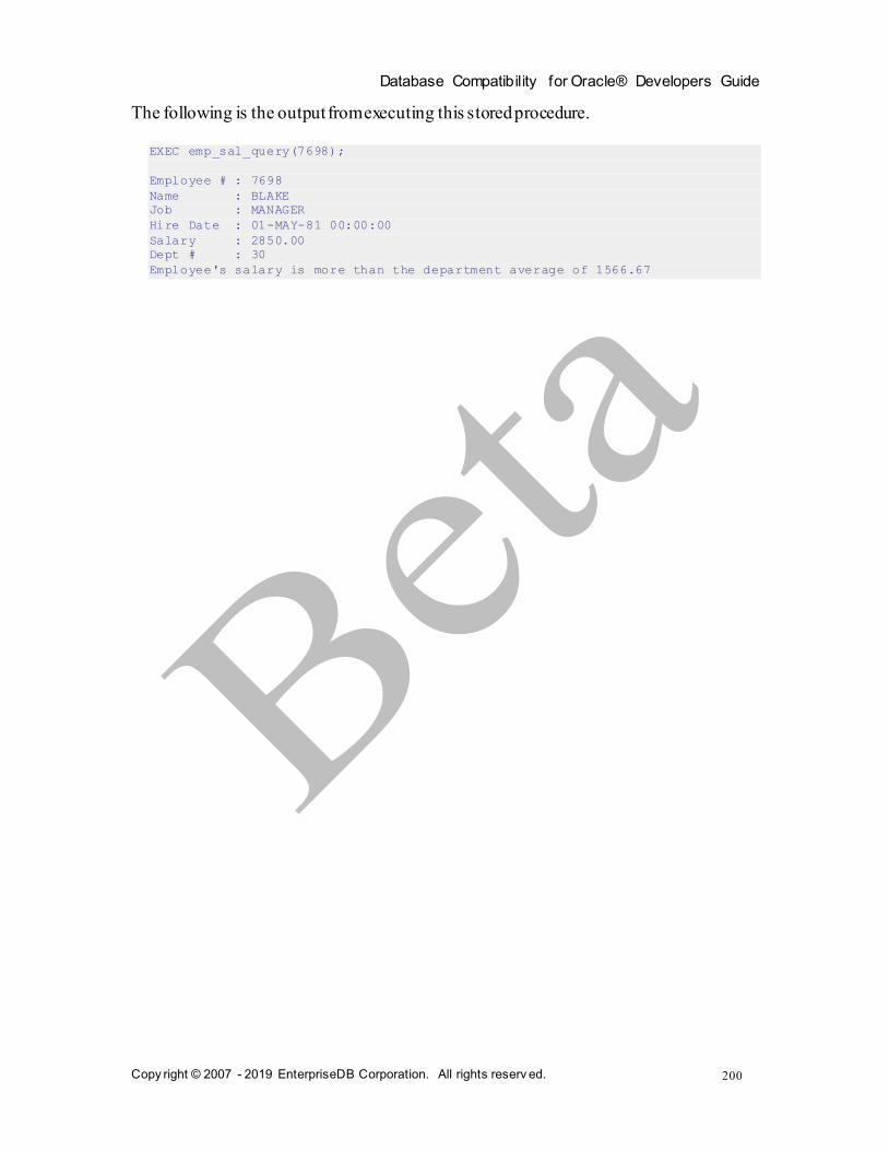
Database Compatibility for Oracle® Developers Guide
Copy right © 2007 - 2019 EnterpriseDB Corporation. All rights reserv ed.
200
The following is the output from executing this stored procedure.
EXEC emp_sal_query(7698);
Employee # : 7698
Name : BLAKE
Job : MANAGER
Hire Date : 01-MAY-81 00:00:00
Salary : 2850.00
Dept # : 30
Employee's salary is more than the department average of 1566.67

Database Compatibility for Oracle® Developers Guide
Copy right © 2007 - 2019 EnterpriseDB Corporation. All rights reserv ed.
201
3.4 Basic Statements
This section begins the discussion of the programming statements that can be used in an SPL program.
3.4.1 NULL
The simplest statement is the NULL statement. This statement is an executable statement that does nothing.
NULL;
The following is the simplest, possible valid SPL program.
BEGIN
NULL;
END;
The NULL statement can act as a placeholder where an executable statement is required
such as in a branch of an IF-THEN-ELSE statement.
For example:
CREATE OR REPLACE PROCEDURE divide_it (
p_numerator IN NUMBER,
p_denominator IN NUMBER,
p_result OUT NUMBER
)
IS
BEGIN
IF p_denominator = 0 THEN
NULL;
ELSE
p_result := p_numerator / p_denominator;
END IF;
END;
3.4.2 Assignment
The assignment statement sets a variable or a formal parameter of mode OUT or IN OUT
specified on the left side of the assignment, :=, to the evaluated expression specified on the right side of the assignment.
variable := expression;
variable is an identifier for a previously declared variable, OUT formal parameter, or
IN OUT formal parameter.

Database Compatibility for Oracle® Developers Guide
Copy right © 2007 - 2019 EnterpriseDB Corporation. All rights reserv ed.
202
expression is an expression that produces a single value. The value produced by the expression must have a compatible data type with that of variable.
The following example shows the typical use of assignment statements in the executable section of the procedure.
CREATE OR REPLACE PROCEDURE dept_salary_rpt (
p_deptno NUMBER
)
IS
todays_date DATE;
rpt_title VARCHAR2(60);
base_sal INTEGER;
base_comm_rate NUMBER;
base_annual NUMBER;
BEGIN
todays_date := SYSDATE;
rpt_title := 'Report For Department # ' || p_deptno || ' on '
|| todays_date;
base_sal := 35525;
base_comm_rate := 1.33333;
base_annual := ROUND(base_sal * base_comm_rate, 2);
DBMS_OUTPUT.PUT_LINE(rpt_title);
DBMS_OUTPUT.PUT_LINE('Base Annual Salary: ' || base_annual);
END;
3.4.3 SELECT INTO
The SELECT INTO statement is an SPL variation of the SQL SELECT command, the differences being:
That SELECT INTO is designed to assign the results to variables or records where they can then be used in SPL program statements.
The accessible result set of SELECT INTO is at most one row.
Other than the above, all of the clauses of the SELECT command such as WHERE, ORDER
BY, GROUP BY, HAVING, etc. are valid for SELECT INTO. The following are the two variations of SELECT INTO.
SELECT select_expressions INTO target FROM ...;
target is a comma-separated list of simple variables. select_expressions and the
remainder of the statement are the same as for the SELECT command. The selected values must exactly match in data type, number, and order the structure of the target or a runtime error occurs.
SELECT * INTO record FROM table ...;

Database Compatibility for Oracle® Developers Guide
Copy right © 2007 - 2019 EnterpriseDB Corporation. All rights reserv ed.
203
record is a record variable that has previously been declared.
If the query returns zero rows, null values are assigned to the target(s). If the query returns multiple rows, the first row is assigned to the target(s) and the rest are discarded. (Note that "the first row" is not well-defined unless you’ve used ORDER BY.)
Note: In either cases, where no row is returned or more than one row is returned, SPL throws an exception.
Note: There is a variation of SELECT INTO using the BULK COLLECT clause that allows
a result set of more than one row that is returned into a collection. See Section 3.12.4.1
for more information on using the BULK COLLECT clause with the SELECT INTO statement.
You can use the WHEN NO_DATA_FOUND clause in an EXCEPTION block to determine whether the assignment was successful (that is, at least one row was returned by the query).
This version of the emp_sal_query procedure uses the variation of SELECT INTO that
returns the result set into a record. Also note the addition of the EXCEPTION block containing the WHEN NO_DATA_FOUND conditional expression.
CREATE OR REPLACE PROCEDURE emp_sal_query (
p_empno IN emp.empno%TYPE
)
IS
r_emp emp%ROWTYPE;
v_avgsal emp.sal%TYPE;
BEGIN
SELECT * INTO r_emp
FROM emp WHERE empno = p_empno;
DBMS_OUTPUT.PUT_LINE('Employee # : ' || p_empno);
DBMS_OUTPUT.PUT_LINE('Name : ' || r_emp.ename);
DBMS_OUTPUT.PUT_LINE('Job : ' || r_emp.job);
DBMS_OUTPUT.PUT_LINE('Hire Date : ' || r_emp.hiredate);
DBMS_OUTPUT.PUT_LINE('Salary : ' || r_emp.sal);
DBMS_OUTPUT.PUT_LINE('Dept # : ' || r_emp.deptno);
SELECT AVG(sal) INTO v_avgsal
FROM emp WHERE deptno = r_emp.deptno;
IF r_emp.sal > v_avgsal THEN
DBMS_OUTPUT.PUT_LINE('Employee''s salary is more than the '
|| 'department average of ' || v_avgsal);
ELSE
DBMS_OUTPUT.PUT_LINE('Employee''s salary does not exceed the '
|| 'department average of ' || v_avgsal);
END IF;
EXCEPTION
WHEN NO_DATA_FOUND THEN
DBMS_OUTPUT.PUT_LINE('Employee # ' || p_empno || ' not found');
END;
If the query is executed with a non-existent employee number the results appear as follows.
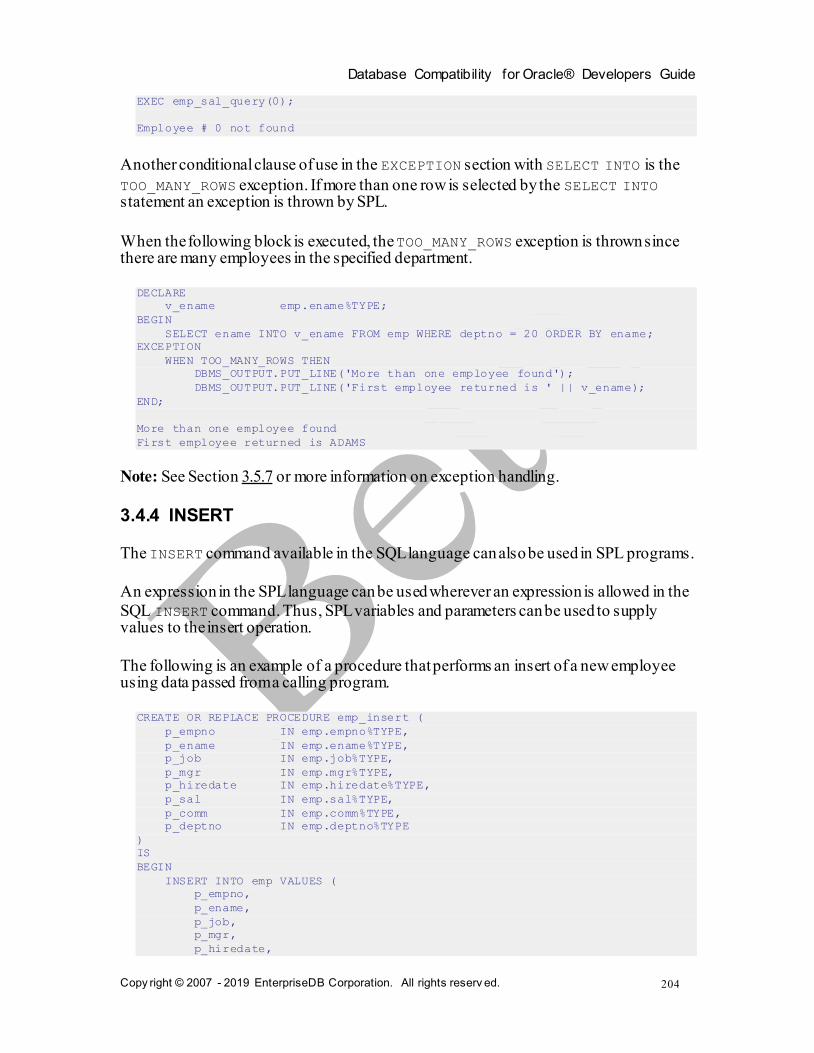
Database Compatibility for Oracle® Developers Guide
Copy right © 2007 - 2019 EnterpriseDB Corporation. All rights reserv ed.
204
EXEC emp_sal_query(0);
Employee # 0 not found
Another conditional clause of use in the EXCEPTION section with SELECT INTO is the
TOO_MANY_ROWS exception. If more than one row is selected by the SELECT INTO statement an exception is thrown by SPL.
When the following block is executed, the TOO_MANY_ROWS exception is thrown since there are many employees in the specified department.
DECLARE
v_ename emp.ename%TYPE;
BEGIN
SELECT ename INTO v_ename FROM emp WHERE deptno = 20 ORDER BY ename;
EXCEPTION
WHEN TOO_MANY_ROWS THEN
DBMS_OUTPUT.PUT_LINE('More than one employee found');
DBMS_OUTPUT.PUT_LINE('First employee returned is ' || v_ename);
END;
More than one employee found
First employee returned is ADAMS
Note: See Section 3.5.7 or more information on exception handling.
3.4.4 INSERT
The INSERT command available in the SQL language can also be used in SPL programs.
An expression in the SPL language can be used wherever an expression is allowed in the
SQL INSERT command. Thus, SPL variables and parameters can be used to supply values to the insert operation.
The following is an example of a procedure that performs an insert of a new employee using data passed from a calling program.
CREATE OR REPLACE PROCEDURE emp_insert (
p_empno IN emp.empno%TYPE,
p_ename IN emp.ename%TYPE,
p_job IN emp.job%TYPE,
p_mgr IN emp.mgr%TYPE,
p_hiredate IN emp.hiredate%TYPE,
p_sal IN emp.sal%TYPE,
p_comm IN emp.comm%TYPE,
p_deptno IN emp.deptno%TYPE
)
IS
BEGIN
INSERT INTO emp VALUES (
p_empno,
p_ename,
p_job,
p_mgr,
p_hiredate,

Database Compatibility for Oracle® Developers Guide
Copy right © 2007 - 2019 EnterpriseDB Corporation. All rights reserv ed.
205
p_sal,
p_comm,
p_deptno);
DBMS_OUTPUT.PUT_LINE('Added employee...');
DBMS_OUTPUT.PUT_LINE('Employee # : ' || p_empno);
DBMS_OUTPUT.PUT_LINE('Name : ' || p_ename);
DBMS_OUTPUT.PUT_LINE('Job : ' || p_job);
DBMS_OUTPUT.PUT_LINE('Manager : ' || p_mgr);
DBMS_OUTPUT.PUT_LINE('Hire Date : ' || p_hiredate);
DBMS_OUTPUT.PUT_LINE('Salary : ' || p_sal);
DBMS_OUTPUT.PUT_LINE('Commission : ' || p_comm);
DBMS_OUTPUT.PUT_LINE('Dept # : ' || p_deptno);
DBMS_OUTPUT.PUT_LINE('----------------------');
EXCEPTION
WHEN OTHERS THEN
DBMS_OUTPUT.PUT_LINE('OTHERS exception on INSERT of employee # '
|| p_empno);
DBMS_OUTPUT.PUT_LINE('SQLCODE : ' || SQLCODE);
DBMS_OUTPUT.PUT_LINE('SQLERRM : ' || SQLERRM);
END;
If an exception occurs all database changes made in the procedure are automatically
rolled back. In this example the EXCEPTION section with the WHEN OTHERS clause
catches all exceptions. Two variables are displayed. SQLCODE is a number that identifies
the specific exception that occurred. SQLERRM is a text message explaining the error. See Section 3.5.7 for more information on exception handling.
The following shows the output when this procedure is executed.
EXEC emp_insert(9503,'PETERSON','ANALYST',7902,'31-MAR-05',5000,NULL,40);
Added employee...
Employee # : 9503
Name : PETERSON
Job : ANALYST
Manager : 7902
Hire Date : 31-MAR-05 00:00:00
Salary : 5000
Dept # : 40
----------------------
SELECT * FROM emp WHERE empno = 9503;
empno | ename | job | mgr | hiredate | sal | comm | deptno
-------+----------+---------+------+--------------------+---------+------+--------
9503 | PETERSON | ANALYST | 7902 | 31-MAR-05 00:00:00 | 5000.00 | | 40
(1 row)
Note: The INSERT command can be included in a FORALL statement. A FORALL
statement allows a single INSERT command to insert multiple rows from values supplied in one or more collections. See 3.12.3 for more information on the FORALL statement.

Database Compatibility for Oracle® Developers Guide
Copy right © 2007 - 2019 EnterpriseDB Corporation. All rights reserv ed.
206
3.4.5 UPDATE
The UPDATE command available in the SQL language can also be used in SPL programs.
An expression in the SPL language can be used wherever an expression is allowed in the
SQL UPDATE command. Thus, SPL variables and parameters can be used to supply values to the update operation.
CREATE OR REPLACE PROCEDURE emp_comp_update (
p_empno IN emp.empno%TYPE,
p_sal IN emp.sal%TYPE,
p_comm IN emp.comm%TYPE
)
IS
BEGIN
UPDATE emp SET sal = p_sal, comm = p_comm WHERE empno = p_empno;
IF SQL%FOUND THEN
DBMS_OUTPUT.PUT_LINE('Updated Employee # : ' || p_empno);
DBMS_OUTPUT.PUT_LINE('New Salary : ' || p_sal);
DBMS_OUTPUT.PUT_LINE('New Commission : ' || p_comm);
ELSE
DBMS_OUTPUT.PUT_LINE('Employee # ' || p_empno || ' not found');
END IF;
END;
The SQL%FOUND conditional expression returns TRUE if a row is updated, FALSE
otherwise. See Section 3.4.8 for a discussion of SQL%FOUND and other similar expressions.
The following shows the update on the employee using this procedure.
EXEC emp_comp_update(9503, 6540, 1200);
Updated Employee # : 9503
New Salary : 6540
New Commission : 1200
SELECT * FROM emp WHERE empno = 9503;
empno | ename | job | mgr | hiredate | sal | comm | deptno
-------+----------+---------+------+--------------------+---------+---------+--------
9503 | PETERSON | ANALYST | 7902 | 31-MAR-05 00:00:00 | 6540.00 | 1200.00 | 40
(1 row)
Note: The UPDATE command can be included in a FORALL statement. A FORALL
statement allows a single UPDATE command to update multiple rows from values supplied in one or more collections. See Section 3.12.3 for more information on the FORALL statement.
3.4.6 DELETE
The DELETE command (available in the SQL language) can also be used in SPL programs.

Database Compatibility for Oracle® Developers Guide
Copy right © 2007 - 2019 EnterpriseDB Corporation. All rights reserv ed.
207
An expression in the SPL language can be used wherever an expression is allowed in the
SQL DELETE command. Thus, SPL variables and parameters can be used to supply values to the delete operation.
CREATE OR REPLACE PROCEDURE emp_delete (
p_empno IN emp.empno%TYPE
)
IS
BEGIN
DELETE FROM emp WHERE empno = p_empno;
IF SQL%FOUND THEN
DBMS_OUTPUT.PUT_LINE('Deleted Employee # : ' || p_empno);
ELSE
DBMS_OUTPUT.PUT_LINE('Employee # ' || p_empno || ' not found');
END IF;
END;
The SQL%FOUND conditional expression returns TRUE if a row is deleted, FALSE
otherwise. See Section 3.4.8 for a discussion of SQL%FOUND and other similar expressions.
The following shows the deletion of an employee using this procedure.
EXEC emp_delete(9503);
Deleted Employee # : 9503
SELECT * FROM emp WHERE empno = 9503;
empno | ename | job | mgr | hiredate | sal | comm | deptno
-------+-------+-----+-----+----------+-----+------+--------
(0 rows)
Note: The DELETE command can be included in a FORALL statement. A FORALL
statement allows a single DELETE command to delete multiple rows from values supplied
in one or more collections. See Section 3.12.3 for more information on the FORALL statement.
3.4.7 Using the RETURNING INTO Clause
The INSERT, UPDATE, and DELETE commands may be appended by the optional
RETURNING INTO clause. This clause allows the SPL program to capture the newly
added, modified, or deleted values from the results of an INSERT, UPDATE, or DELETE command, respectively.
The following is the syntax.
{ insert | update | delete }
RETURNING { * | expr_1 [, expr_2 ] ...}
INTO { record | field_1 [, field_2 ] ...};

Database Compatibility for Oracle® Developers Guide
Copy right © 2007 - 2019 EnterpriseDB Corporation. All rights reserv ed.
208
insert is a valid INSERT command. update is a valid UPDATE command. delete is a
valid DELETE command. If * is specified, then the values from the row affected by the
INSERT, UPDATE, or DELETE command are made available for assignment to the
record or fields to the right of the INTO keyword. (Note that the use of * is an Advanced Server extension and is not compatible with Oracle databases.) expr_1, expr_2... are
expressions evaluated upon the row affected by the INSERT, UPDATE, or DELETE command. The evaluated results are assigned to the record or fields to the right of the INTO keyword. record is the identifier of a record that must contain fields that match in
number and order, and are data type compatible with the values in the RETURNING clause. field_1, field_2,... are variables that must match in number and order, and are
data type compatible with the set of values in the RETURNING clause.
If the INSERT, UPDATE, or DELETE command returns a result set with more than one
row, then an exception is thrown with SQLCODE 01422, query returned more than
one row. If no rows are in the result set, then the variables following the INTO keyword are set to null.
Note: There is a variation of RETURNING INTO using the BULK COLLECT clause that allows a result set of more than one row that is returned into a collection. See Section
3.12.4 for more information on the BULK COLLECT clause.
The following example is a modification of the emp_comp_update procedure introduced in Section 3.4.5, with the addition of the RETURNING INTO clause.
CREATE OR REPLACE PROCEDURE emp_comp_update (
p_empno IN emp.empno%TYPE,
p_sal IN emp.sal%TYPE,
p_comm IN emp.comm%TYPE
)
IS
v_empno emp.empno%TYPE;
v_ename emp.ename%TYPE;
v_job emp.job%TYPE;
v_sal emp.sal%TYPE;
v_comm emp.comm%TYPE;
v_deptno emp.deptno%TYPE;
BEGIN
UPDATE emp SET sal = p_sal, comm = p_comm WHERE empno = p_empno
RETURNING
empno,
ename,
job,
sal,
comm,
deptno
INTO
v_empno,
v_ename,
v_job,
v_sal,
v_comm,
v_deptno;

Database Compatibility for Oracle® Developers Guide
Copy right © 2007 - 2019 EnterpriseDB Corporation. All rights reserv ed.
209
IF SQL%FOUND THEN
DBMS_OUTPUT.PUT_LINE('Updated Employee # : ' || v_empno);
DBMS_OUTPUT.PUT_LINE('Name : ' || v_ename);
DBMS_OUTPUT.PUT_LINE('Job : ' || v_job);
DBMS_OUTPUT.PUT_LINE('Department : ' || v_deptno);
DBMS_OUTPUT.PUT_LINE('New Salary : ' || v_sal);
DBMS_OUTPUT.PUT_LINE('New Commission : ' || v_comm);
ELSE
DBMS_OUTPUT.PUT_LINE('Employee # ' || p_empno || ' not found');
END IF;
END;
The following is the output from this procedure (assuming employee 9503 created by the
emp_insert procedure still exists within the table).
EXEC emp_comp_update(9503, 6540, 1200);
Updated Employee # : 9503
Name : PETERSON
Job : ANALYST
Department : 40
New Salary : 6540.00
New Commission : 1200.00
The following example is a modification of the emp_delete procedure, with the
addition of the RETURNING INTO clause using record types.
CREATE OR REPLACE PROCEDURE emp_delete (
p_empno IN emp.empno%TYPE
)
IS
r_emp emp%ROWTYPE;
BEGIN
DELETE FROM emp WHERE empno = p_empno
RETURNING
*
INTO
r_emp;
IF SQL%FOUND THEN
DBMS_OUTPUT.PUT_LINE('Deleted Employee # : ' || r_emp.empno);
DBMS_OUTPUT.PUT_LINE('Name : ' || r_emp.ename);
DBMS_OUTPUT.PUT_LINE('Job : ' || r_emp.job);
DBMS_OUTPUT.PUT_LINE('Manager : ' || r_emp.mgr);
DBMS_OUTPUT.PUT_LINE('Hire Date : ' || r_emp.hiredate);
DBMS_OUTPUT.PUT_LINE('Salary : ' || r_emp.sal);
DBMS_OUTPUT.PUT_LINE('Commission : ' || r_emp.comm);
DBMS_OUTPUT.PUT_LINE('Department : ' || r_emp.deptno);
ELSE
DBMS_OUTPUT.PUT_LINE('Employee # ' || p_empno || ' not found');
END IF;
END;
The following is the output from this procedure.
EXEC emp_delete(9503);
Deleted Employee # : 9503
Name : PETERSON

Database Compatibility for Oracle® Developers Guide
Copy right © 2007 - 2019 EnterpriseDB Corporation. All rights reserv ed.
210
Job : ANALYST
Manager : 7902
Hire Date : 31-MAR-05 00:00:00
Salary : 6540.00
Commission : 1200.00
Department : 40
3.4.8 Obtaining the Result Status
There are several attributes that can be used to determine the effect of a command.
SQL%FOUND is a Boolean that returns TRUE if at least one row was affected by an
INSERT, UPDATE or DELETE command or a SELECT INTO command retrieved one or more rows.
The following anonymous block inserts a row and then displays the fact that the row has been inserted.
BEGIN
INSERT INTO emp (empno,ename,job,sal,deptno) VALUES (
9001, 'JONES', 'CLERK', 850.00, 40);
IF SQL%FOUND THEN
DBMS_OUTPUT.PUT_LINE('Row has been inserted');
END IF;
END;
Row has been inserted
SQL%ROWCOUNT provides the number of rows affected by an INSERT, UPDATE, DELETE,
or SELECT INTO command. The SQL%ROWCOUNT value is returned as a BIGINT data type. The following example updates the row that was just inserted and displays SQL%ROWCOUNT.
BEGIN
UPDATE emp SET hiredate = '03-JUN-07' WHERE empno = 9001;
DBMS_OUTPUT.PUT_LINE('# rows updated: ' || SQL%ROWCOUNT);
END;
# rows updated: 1
SQL%NOTFOUND is the opposite of SQL%FOUND. SQL%NOTFOUND returns TRUE if no rows
were affected by an INSERT, UPDATE or DELETE command or a SELECT INTO command retrieved no rows.
BEGIN
UPDATE emp SET hiredate = '03-JUN-07' WHERE empno = 9000;
IF SQL%NOTFOUND THEN
DBMS_OUTPUT.PUT_LINE('No rows were updated');
END IF;
END;
No rows were updated

Database Compatibility for Oracle® Developers Guide
Copy right © 2007 - 2019 EnterpriseDB Corporation. All rights reserv ed.
211
3.5 Control Structures
The programming statements in SPL that make it a full procedural complement to SQL are described in this section.
3.5.1 IF Statement
IF statements let you execute commands based on certain conditions. SPL has four forms
of IF:
IF ... THEN
IF ... THEN ... ELSE
IF ... THEN ... ELSE IF
IF ... THEN ... ELSIF ... THEN ... ELSE
3.5.1.1 IF-THEN IF boolean-expression THEN
statements
END IF;
IF-THEN statements are the simplest form of IF. The statements between THEN and END IF will be executed if the condition is TRUE. Otherwise, they are skipped.
In the following example an IF-THEN statement is used to test and display employees who have a commission.
DECLARE
v_empno emp.empno%TYPE;
v_comm emp.comm%TYPE;
CURSOR emp_cursor IS SELECT empno, comm FROM emp;
BEGIN
OPEN emp_cursor;
DBMS_OUTPUT.PUT_LINE('EMPNO COMM');
DBMS_OUTPUT.PUT_LINE('----- -------');
LOOP
FETCH emp_cursor INTO v_empno, v_comm;
EXIT WHEN emp_cursor%NOTFOUND;
--
-- Test whether or not the employee gets a commission
--
IF v_comm IS NOT NULL AND v_comm > 0 THEN
DBMS_OUTPUT.PUT_LINE(v_empno || ' ' ||
TO_CHAR(v_comm,'$99999.99'));
END IF;
END LOOP;
CLOSE emp_cursor;
END;
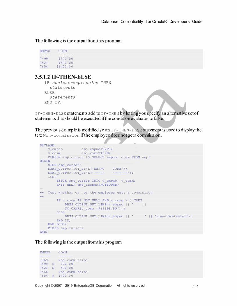
Database Compatibility for Oracle® Developers Guide
Copy right © 2007 - 2019 EnterpriseDB Corporation. All rights reserv ed.
212
The following is the output from this program.
EMPNO COMM
----- -------
7499 $300.00
7521 $500.00
7654 $1400.00
3.5.1.2 IF-THEN-ELSE IF boolean-expression THEN
statements
ELSE
statements
END IF;
IF-THEN-ELSE statements add to IF-THEN by letting you specify an alternative set of statements that should be executed if the condition evaluates to false.
The previous example is modified so an IF-THEN-ELSE statement is used to display the text Non-commission if the employee does not get a commission.
DECLARE
v_empno emp.empno%TYPE;
v_comm emp.comm%TYPE;
CURSOR emp_cursor IS SELECT empno, comm FROM emp;
BEGIN
OPEN emp_cursor;
DBMS_OUTPUT.PUT_LINE('EMPNO COMM');
DBMS_OUTPUT.PUT_LINE('----- -------');
LOOP
FETCH emp_cursor INTO v_empno, v_comm;
EXIT WHEN emp_cursor%NOTFOUND;
--
-- Test whether or not the employee gets a commission
--
IF v_comm IS NOT NULL AND v_comm > 0 THEN
DBMS_OUTPUT.PUT_LINE(v_empno || ' ' ||
TO_CHAR(v_comm,'$99999.99'));
ELSE
DBMS_OUTPUT.PUT_LINE(v_empno || ' ' || 'Non-commission');
END IF;
END LOOP;
CLOSE emp_cursor;
END;
The following is the output from this program.
EMPNO COMM
----- -------
7369 Non-commission
7499 $ 300.00
7521 $ 500.00
7566 Non-commission
7654 $ 1400.00

Database Compatibility for Oracle® Developers Guide
Copy right © 2007 - 2019 EnterpriseDB Corporation. All rights reserv ed.
213
7698 Non-commission
7782 Non-commission
7788 Non-commission
7839 Non-commission
7844 Non-commission
7876 Non-commission
7900 Non-commission
7902 Non-commission
7934 Non-commission
3.5.1.3 IF-THEN-ELSE IF
IF statements can be nested so that alternative IF statements can be invoked once it is
determined whether or not the conditional of an outer IF statement is TRUE or FALSE.
In the following example the outer IF-THEN-ELSE statement tests whether or not an
employee has a commission. The inner IF-THEN-ELSE statements then test whether the employee’s total compensation exceeds or is less than the company average.
DECLARE
v_empno emp.empno%TYPE;
v_sal emp.sal%TYPE;
v_comm emp.comm%TYPE;
v_avg NUMBER(7,2);
CURSOR emp_cursor IS SELECT empno, sal, comm FROM emp;
BEGIN
--
-- Calculate the average yearly compensation in the company
--
SELECT AVG((sal + NVL(comm,0)) * 24) INTO v_avg FROM emp;
DBMS_OUTPUT.PUT_LINE('Average Yearly Compensation: ' ||
TO_CHAR(v_avg,'$999,999.99'));
OPEN emp_cursor;
DBMS_OUTPUT.PUT_LINE('EMPNO YEARLY COMP');
DBMS_OUTPUT.PUT_LINE('----- -----------');
LOOP
FETCH emp_cursor INTO v_empno, v_sal, v_comm;
EXIT WHEN emp_cursor%NOTFOUND;
--
-- Test whether or not the employee gets a commission
--
IF v_comm IS NOT NULL AND v_comm > 0 THEN
--
-- Test if the employee's compensation with commission exceeds the average
--
IF (v_sal + v_comm) * 24 > v_avg THEN
DBMS_OUTPUT.PUT_LINE(v_empno || ' ' ||
TO_CHAR((v_sal + v_comm) * 24,'$999,999.99') ||
' Exceeds Average');
ELSE
DBMS_OUTPUT.PUT_LINE(v_empno || ' ' ||
TO_CHAR((v_sal + v_comm) * 24,'$999,999.99') ||
' Below Average');
END IF;
ELSE
--
-- Test if the employee's compensation without commission exceeds the
average
--

Database Compatibility for Oracle® Developers Guide
Copy right © 2007 - 2019 EnterpriseDB Corporation. All rights reserv ed.
214
IF v_sal * 24 > v_avg THEN
DBMS_OUTPUT.PUT_LINE(v_empno || ' ' ||
TO_CHAR(v_sal * 24,'$999,999.99') || ' Exceeds Average');
ELSE
DBMS_OUTPUT.PUT_LINE(v_empno || ' ' ||
TO_CHAR(v_sal * 24,'$999,999.99') || ' Below Average');
END IF;
END IF;
END LOOP;
CLOSE emp_cursor;
END;
Note: The logic in this program can be simplified considerably by calculating the
employee’s yearly compensation using the NVL function within the SELECT command of
the cursor declaration, however, the purpose of this example is to demonstrate how IF statements can be used.
The following is the output from this program.
Average Yearly Compensation: $ 53,528.57
EMPNO YEARLY COMP
----- -----------
7369 $ 19,200.00 Below Average
7499 $ 45,600.00 Below Average
7521 $ 42,000.00 Below Average
7566 $ 71,400.00 Exceeds Average
7654 $ 63,600.00 Exceeds Average
7698 $ 68,400.00 Exceeds Average
7782 $ 58,800.00 Exceeds Average
7788 $ 72,000.00 Exceeds Average
7839 $ 120,000.00 Exceeds Average
7844 $ 36,000.00 Below Average
7876 $ 26,400.00 Below Average
7900 $ 22,800.00 Below Average
7902 $ 72,000.00 Exceeds Average
7934 $ 31,200.00 Below Average
When you use this form, you are actually nesting an IF statement inside the ELSE part of
an outer IF statement. Thus you need one END IF statement for each nested IF and one for the parent IF-ELSE.
3.5.1.4 IF-THEN-ELSIF-ELSE IF boolean-expression THEN
statements
[ ELSIF boolean-expression THEN
statements
[ ELSIF boolean-expression THEN
statements ] ...]
[ ELSE
statements ]
END IF;

Database Compatibility for Oracle® Developers Guide
Copy right © 2007 - 2019 EnterpriseDB Corporation. All rights reserv ed.
215
IF-THEN-ELSIF-ELSE provides a method of checking many alternatives in one
statement. Formally it is equivalent to nested IF-THEN-ELSE-IF-THEN commands, but only one END IF is needed.
The following example uses an IF-THEN-ELSIF-ELSE statement to count the number of employees by compensation ranges of $25,000.
DECLARE
v_empno emp.empno%TYPE;
v_comp NUMBER(8,2);
v_lt_25K SMALLINT := 0;
v_25K_50K SMALLINT := 0;
v_50K_75K SMALLINT := 0;
v_75K_100K SMALLINT := 0;
v_ge_100K SMALLINT := 0;
CURSOR emp_cursor IS SELECT empno, (sal + NVL(comm,0)) * 24 FROM emp;
BEGIN
OPEN emp_cursor;
LOOP
FETCH emp_cursor INTO v_empno, v_comp;
EXIT WHEN emp_cursor%NOTFOUND;
IF v_comp < 25000 THEN
v_lt_25K := v_lt_25K + 1;
ELSIF v_comp < 50000 THEN
v_25K_50K := v_25K_50K + 1;
ELSIF v_comp < 75000 THEN
v_50K_75K := v_50K_75K + 1;
ELSIF v_comp < 100000 THEN
v_75K_100K := v_75K_100K + 1;
ELSE
v_ge_100K := v_ge_100K + 1;
END IF;
END LOOP;
CLOSE emp_cursor;
DBMS_OUTPUT.PUT_LINE('Number of employees by yearly compensation');
DBMS_OUTPUT.PUT_LINE('Less than 25,000 : ' || v_lt_25K);
DBMS_OUTPUT.PUT_LINE('25,000 - 49,9999 : ' || v_25K_50K);
DBMS_OUTPUT.PUT_LINE('50,000 - 74,9999 : ' || v_50K_75K);
DBMS_OUTPUT.PUT_LINE('75,000 - 99,9999 : ' || v_75K_100K);
DBMS_OUTPUT.PUT_LINE('100,000 and over : ' || v_ge_100K);
END;
The following is the output from this program.
Number of employees by yearly compensation
Less than 25,000 : 2
25,000 - 49,9999 : 5
50,000 - 74,9999 : 6
75,000 - 99,9999 : 0
100,000 and over : 1

Database Compatibility for Oracle® Developers Guide
Copy right © 2007 - 2019 EnterpriseDB Corporation. All rights reserv ed.
216
3.5.2 RETURN Statement
The RETURN statement terminates the current function, procedure or anonymous block and returns control to the caller.
There are two forms of the RETURN Statement. The first form of the RETURN statement is
used to terminate a procedure or function that returns void. The syntax of the first form is:
RETURN;
The second form of RETURN returns a value to the caller. The syntax of the second form of the RETURN statement is:
RETURN expression;
expression must evaluate to the same data type as the return type of the function.
The following example uses the RETURN statement returns a value to the caller:
CREATE OR REPLACE FUNCTION emp_comp (
p_sal NUMBER,
p_comm NUMBER
) RETURN NUMBER
IS
BEGIN
RETURN (p_sal + NVL(p_comm, 0)) * 24;
END emp_comp;

Database Compatibility for Oracle® Developers Guide
Copy right © 2007 - 2019 EnterpriseDB Corporation. All rights reserv ed.
217
3.5.3 GOTO Statement
The GOTO statement causes the point of execution to jump to the statement with the specified label. The syntax of a GOTO statement is:
GOTO label
label is a name assigned to an executable statement. label must be unique within the scope of the function, procedure or anonymous block.
To label a statement, use the syntax:
<<label>> statement
statement is the point of execution that the program jumps to.
You can label assignment statements, any SQL statement (like INSERT, UPDATE,
CREATE, etc.) and selected procedural language statements. The procedural language statements that can be labeled are:
IF
EXIT
RETURN
RAISE
EXECUTE
PERFORM
GET DIAGNOSTICS
OPEN
FETCH
MOVE
CLOSE
NULL
COMMIT
ROLLBACK
GOTO
CASE
LOOP
WHILE
FOR
Please note that exit is considered a keyword, and cannot be used as the name of a label.
GOTO statements cannot transfer control into a conditional block or sub-block, but can transfer control from a conditional block or sub-block.

Database Compatibility for Oracle® Developers Guide
Copy right © 2007 - 2019 EnterpriseDB Corporation. All rights reserv ed.
218
The following example verifies that an employee record contains a name, job description,
and employee hire date; if any piece of information is missing, a GOTO statement transfers the point of execution to a statement that prints a message that the employee is not valid.
CREATE OR REPLACE PROCEDURE verify_emp (
p_empno NUMBER
)
IS
v_ename emp.ename%TYPE;
v_job emp.job%TYPE;
v_hiredate emp.hiredate%TYPE;
BEGIN
SELECT ename, job, hiredate
INTO v_ename, v_job, v_hiredate FROM emp
WHERE empno = p_empno;
IF v_ename IS NULL THEN
GOTO invalid_emp;
END IF;
IF v_job IS NULL THEN
GOTO invalid_emp;
END IF;
IF v_hiredate IS NULL THEN
GOTO invalid_emp;
END IF;
DBMS_OUTPUT.PUT_LINE('Employee ' || p_empno ||
' validated without errors.');
RETURN;
<<invalid_emp>> DBMS_OUTPUT.PUT_LINE('Employee ' || p_empno ||
' is not a valid employee.');
END;
GOTO statements have the following restrictions:
A GOTO statement cannot jump to a declaration.
A GOTO statement cannot transfer control to another function or procedure.
A label should not be placed at the end of a block, function or procedure.

Database Compatibility for Oracle® Developers Guide
Copy right © 2007 - 2019 EnterpriseDB Corporation. All rights reserv ed.
219
3.5.4 CASE Expression
The CASE expression returns a value that is substituted where the CASE expression is located within an expression.
There are two formats of the CASE expression - one that is called a searched CASE and the other that uses a selector.
3.5.4.1 Selector CASE Expression
The selector CASE expression attempts to match an expression called the selector to the
expression specified in one or more WHEN clauses. result is an expression that is type-
compatible in the context where the CASE expression is used. If a match is found, the
value given in the corresponding THEN clause is returned by the CASE expression. If there
are no matches, the value following ELSE is returned. If ELSE is omitted, the CASE expression returns null.
CASE selector-expression
WHEN match-expression THEN
result
[ WHEN match-expression THEN
result
[ WHEN match-expression THEN
result ] ...]
[ ELSE
result ]
END;
match-expression is evaluated in the order in which it appears within the CASE
expression. result is an expression that is type-compatible in the context where the
CASE expression is used. When the first match-expression is encountered that equals
selector-expression, result in the corresponding THEN clause is returned as the
value of the CASE expression. If none of match-expression equals selector-
expression then result following ELSE is returned. If no ELSE is specified, the CASE expression returns null.
The following example uses a selector CASE expression to assign the department name to a variable based upon the department number.
DECLARE
v_empno emp.empno%TYPE;
v_ename emp.ename%TYPE;
v_deptno emp.deptno%TYPE;
v_dname dept.dname%TYPE;
CURSOR emp_cursor IS SELECT empno, ename, deptno FROM emp;
BEGIN
OPEN emp_cursor;

Database Compatibility for Oracle® Developers Guide
Copy right © 2007 - 2019 EnterpriseDB Corporation. All rights reserv ed.
220
DBMS_OUTPUT.PUT_LINE('EMPNO ENAME DEPTNO DNAME');
DBMS_OUTPUT.PUT_LINE('----- ------- ------ ----------');
LOOP
FETCH emp_cursor INTO v_empno, v_ename, v_deptno;
EXIT WHEN emp_cursor%NOTFOUND;
v_dname :=
CASE v_deptno
WHEN 10 THEN 'Accounting'
WHEN 20 THEN 'Research'
WHEN 30 THEN 'Sales'
WHEN 40 THEN 'Operations'
ELSE 'unknown'
END;
DBMS_OUTPUT.PUT_LINE(v_empno || ' ' || RPAD(v_ename, 10) ||
' ' || v_deptno || ' ' || v_dname);
END LOOP;
CLOSE emp_cursor;
END;
The following is the output from this program.
EMPNO ENAME DEPTNO DNAME
----- ------- ------ ----------
7369 SMITH 20 Research
7499 ALLEN 30 Sales
7521 WARD 30 Sales
7566 JONES 20 Research
7654 MARTIN 30 Sales
7698 BLAKE 30 Sales
7782 CLARK 10 Accounting
7788 SCOTT 20 Research
7839 KING 10 Accounting
7844 TURNER 30 Sales
7876 ADAMS 20 Research
7900 JAMES 30 Sales
7902 FORD 20 Research
7934 MILLER 10 Accounting
3.5.4.2 Searched CASE Expression
A searched CASE expression uses one or more Boolean expressions to determine the resulting value to return.
CASE WHEN boolean-expression THEN
result
[ WHEN boolean-expression THEN
result
[ WHEN boolean-expression THEN
result ] ...]
[ ELSE
result ]
END;
boolean-expression is evaluated in the order in which it appears within the CASE
expression. result is an expression that is type-compatible in the context where the
CASE expression is used. When the first boolean-expression is encountered that

Database Compatibility for Oracle® Developers Guide
Copy right © 2007 - 2019 EnterpriseDB Corporation. All rights reserv ed.
221
evaluates to TRUE, result in the corresponding THEN clause is returned as the value of
the CASE expression. If none of boolean-expression evaluates to true then result
following ELSE is returned. If no ELSE is specified, the CASE expression returns null.
The following example uses a searched CASE expression to assign the department name to a variable based upon the department number.
DECLARE
v_empno emp.empno%TYPE;
v_ename emp.ename%TYPE;
v_deptno emp.deptno%TYPE;
v_dname dept.dname%TYPE;
CURSOR emp_cursor IS SELECT empno, ename, deptno FROM emp;
BEGIN
OPEN emp_cursor;
DBMS_OUTPUT.PUT_LINE('EMPNO ENAME DEPTNO DNAME');
DBMS_OUTPUT.PUT_LINE('----- ------- ------ ----------');
LOOP
FETCH emp_cursor INTO v_empno, v_ename, v_deptno;
EXIT WHEN emp_cursor%NOTFOUND;
v_dname :=
CASE
WHEN v_deptno = 10 THEN 'Accounting'
WHEN v_deptno = 20 THEN 'Research'
WHEN v_deptno = 30 THEN 'Sales'
WHEN v_deptno = 40 THEN 'Operations'
ELSE 'unknown'
END;
DBMS_OUTPUT.PUT_LINE(v_empno || ' ' || RPAD(v_ename, 10) ||
' ' || v_deptno || ' ' || v_dname);
END LOOP;
CLOSE emp_cursor;
END;
The following is the output from this program.
EMPNO ENAME DEPTNO DNAME
----- ------- ------ ----------
7369 SMITH 20 Research
7499 ALLEN 30 Sales
7521 WARD 30 Sales
7566 JONES 20 Research
7654 MARTIN 30 Sales
7698 BLAKE 30 Sales
7782 CLARK 10 Accounting
7788 SCOTT 20 Research
7839 KING 10 Accounting
7844 TURNER 30 Sales
7876 ADAMS 20 Research
7900 JAMES 30 Sales
7902 FORD 20 Research
7934 MILLER 10 Accounting

Database Compatibility for Oracle® Developers Guide
Copy right © 2007 - 2019 EnterpriseDB Corporation. All rights reserv ed.
222
3.5.5 CASE Statement
The CASE statement executes a set of one or more statements when a specified search
condition is TRUE. The CASE statement is a stand-alone statement in itself while the
previously discussed CASE expression must appear as part of an expression.
There are two formats of the CASE statement - one that is called a searched CASE and the other that uses a selector.
3.5.5.1 Selector CASE Statement
The selector CASE statement attempts to match an expression called the selector to the
expression specified in one or more WHEN clauses. When a match is found one or more corresponding statements are executed.
CASE selector-expression
WHEN match-expression THEN
statements
[ WHEN match-expression THEN
statements
[ WHEN match-expression THEN
statements ] ...]
[ ELSE
statements ]
END CASE;
selector-expression returns a value type-compatible with each match-
expression. match-expression is evaluated in the order in which it appears within
the CASE statement. statements are one or more SPL statements, each terminated by a
semi-colon. When the value of selector-expression equals the first match-
expression, the statement(s) in the corresponding THEN clause are executed and
control continues following the END CASE keywords. If there are no matches, the
statement(s) following ELSE are executed. If there are no matches and there is no ELSE clause, an exception is thrown.
The following example uses a selector CASE statement to assign a department name and location to a variable based upon the department number.
DECLARE
v_empno emp.empno%TYPE;
v_ename emp.ename%TYPE;
v_deptno emp.deptno%TYPE;
v_dname dept.dname%TYPE;
v_loc dept.loc%TYPE;
CURSOR emp_cursor IS SELECT empno, ename, deptno FROM emp;
BEGIN

Database Compatibility for Oracle® Developers Guide
Copy right © 2007 - 2019 EnterpriseDB Corporation. All rights reserv ed.
223
OPEN emp_cursor;
DBMS_OUTPUT.PUT_LINE('EMPNO ENAME DEPTNO DNAME '
|| ' LOC');
DBMS_OUTPUT.PUT_LINE('----- ------- ------ ----------'
|| ' ---------');
LOOP
FETCH emp_cursor INTO v_empno, v_ename, v_deptno;
EXIT WHEN emp_cursor%NOTFOUND;
CASE v_deptno
WHEN 10 THEN v_dname := 'Accounting';
v_loc := 'New York';
WHEN 20 THEN v_dname := 'Research';
v_loc := 'Dallas';
WHEN 30 THEN v_dname := 'Sales';
v_loc := 'Chicago';
WHEN 40 THEN v_dname := 'Operations';
v_loc := 'Boston';
ELSE v_dname := 'unknown';
v_loc := '';
END CASE;
DBMS_OUTPUT.PUT_LINE(v_empno || ' ' || RPAD(v_ename, 10) ||
' ' || v_deptno || ' ' || RPAD(v_dname, 14) || ' ' ||
v_loc);
END LOOP;
CLOSE emp_cursor;
END;
The following is the output from this program.
EMPNO ENAME DEPTNO DNAME LOC
----- ------- ------ ---------- ---------
7369 SMITH 20 Research Dallas
7499 ALLEN 30 Sales Chicago
7521 WARD 30 Sales Chicago
7566 JONES 20 Research Dallas
7654 MARTIN 30 Sales Chicago
7698 BLAKE 30 Sales Chicago
7782 CLARK 10 Accounting New York
7788 SCOTT 20 Research Dallas
7839 KING 10 Accounting New York
7844 TURNER 30 Sales Chicago
7876 ADAMS 20 Research Dallas
7900 JAMES 30 Sales Chicago
7902 FORD 20 Research Dallas
7934 MILLER 10 Accounting New York
3.5.5.2 Searched CASE statement
A searched CASE statement uses one or more Boolean expressions to determine the resulting set of statements to execute.
CASE WHEN boolean-expression THEN
statements
[ WHEN boolean-expression THEN
statements
[ WHEN boolean-expression THEN
statements ] ...]
[ ELSE

Database Compatibility for Oracle® Developers Guide
Copy right © 2007 - 2019 EnterpriseDB Corporation. All rights reserv ed.
224
statements ]
END CASE;
boolean-expression is evaluated in the order in which it appears within the CASE
statement. When the first boolean-expression is encountered that evaluates to TRUE,
the statement(s) in the corresponding THEN clause are executed and control continues following the END CASE keywords. If none of boolean-expression evaluates to
TRUE, the statement(s) following ELSE are executed. If none of boolean-expression
evaluates to TRUE and there is no ELSE clause, an exception is thrown.
The following example uses a searched CASE statement to assign a department name and location to a variable based upon the department number.
DECLARE
v_empno emp.empno%TYPE;
v_ename emp.ename%TYPE;
v_deptno emp.deptno%TYPE;
v_dname dept.dname%TYPE;
v_loc dept.loc%TYPE;
CURSOR emp_cursor IS SELECT empno, ename, deptno FROM emp;
BEGIN
OPEN emp_cursor;
DBMS_OUTPUT.PUT_LINE('EMPNO ENAME DEPTNO DNAME '
|| ' LOC');
DBMS_OUTPUT.PUT_LINE('----- ------- ------ ----------'
|| ' ---------');
LOOP
FETCH emp_cursor INTO v_empno, v_ename, v_deptno;
EXIT WHEN emp_cursor%NOTFOUND;
CASE
WHEN v_deptno = 10 THEN v_dname := 'Accounting';
v_loc := 'New York';
WHEN v_deptno = 20 THEN v_dname := 'Research';
v_loc := 'Dallas';
WHEN v_deptno = 30 THEN v_dname := 'Sales';
v_loc := 'Chicago';
WHEN v_deptno = 40 THEN v_dname := 'Operations';
v_loc := 'Boston';
ELSE v_dname := 'unknown';
v_loc := '';
END CASE;
DBMS_OUTPUT.PUT_LINE(v_empno || ' ' || RPAD(v_ename, 10) ||
' ' || v_deptno || ' ' || RPAD(v_dname, 14) || ' ' ||
v_loc);
END LOOP;
CLOSE emp_cursor;
END;
The following is the output from this program.
EMPNO ENAME DEPTNO DNAME LOC
----- ------- ------ ---------- ---------
7369 SMITH 20 Research Dallas
7499 ALLEN 30 Sales Chicago
7521 WARD 30 Sales Chicago
7566 JONES 20 Research Dallas
7654 MARTIN 30 Sales Chicago

Database Compatibility for Oracle® Developers Guide
Copy right © 2007 - 2019 EnterpriseDB Corporation. All rights reserv ed.
225
7698 BLAKE 30 Sales Chicago
7782 CLARK 10 Accounting New York
7788 SCOTT 20 Research Dallas
7839 KING 10 Accounting New York
7844 TURNER 30 Sales Chicago
7876 ADAMS 20 Research Dallas
7900 JAMES 30 Sales Chicago
7902 FORD 20 Research Dallas
7934 MILLER 10 Accounting New York

Database Compatibility for Oracle® Developers Guide
Copy right © 2007 - 2019 EnterpriseDB Corporation. All rights reserv ed.
226
3.5.6 Loops
With the LOOP, EXIT, CONTINUE, WHILE, and FOR statements, you can arrange for your SPL program to repeat a series of commands.
3.5.6.1 LOOP LOOP
statements
END LOOP;
LOOP defines an unconditional loop that is repeated indefinitely until terminated by an
EXIT or RETURN statement.
3.5.6.2 EXIT EXIT [ WHEN expression ];
The innermost loop is terminated and the statement following END LOOP is executed next.
If WHEN is present, loop exit occurs only if the specified condition is TRUE, otherwise control passes to the statement after EXIT.
EXIT can be used to cause early exit from all types of loops; it is not limited to use with unconditional loops.
The following is a simple example of a loop that iterates ten times and then uses the EXIT statement to terminate.
DECLARE
v_counter NUMBER(2);
BEGIN
v_counter := 1;
LOOP
EXIT WHEN v_counter > 10;
DBMS_OUTPUT.PUT_LINE('Iteration # ' || v_counter);
v_counter := v_counter + 1;
END LOOP;
END;
The following is the output from this program.
Iteration # 1
Iteration # 2
Iteration # 3
Iteration # 4
Iteration # 5
Iteration # 6
Iteration # 7

Database Compatibility for Oracle® Developers Guide
Copy right © 2007 - 2019 EnterpriseDB Corporation. All rights reserv ed.
227
Iteration # 8
Iteration # 9
Iteration # 10
3.5.6.3 CONTINUE
The CONTINUE statement provides a way to proceed with the next iteration of a loop while skipping intervening statements.
When the CONTINUE statement is encountered, the next iteration of the innermost loop is
begun, skipping all statements following the CONTINUE statement until the end of the loop. That is, control is passed back to the loop control expression, if any, and the body of the loop is re-evaluated.
If the WHEN clause is used, then the next iteration of the loop is begun only if the specified
expression in the WHEN clause evaluates to TRUE. Otherwise, control is passed to the next
statement following the CONTINUE statement.
The CONTINUE statement may not be used outside of a loop.
The following is a variation of the previous example that uses the CONTINUE statement to skip the display of the odd numbers.
DECLARE
v_counter NUMBER(2);
BEGIN
v_counter := 0;
LOOP
v_counter := v_counter + 1;
EXIT WHEN v_counter > 10;
CONTINUE WHEN MOD(v_counter,2) = 1;
DBMS_OUTPUT.PUT_LINE('Iteration # ' || v_counter);
END LOOP;
END;
The following is the output from above program.
Iteration # 2
Iteration # 4
Iteration # 6
Iteration # 8
Iteration # 10
3.5.6.4 WHILE WHILE expression LOOP
statements
END LOOP;
The WHILE statement repeats a sequence of statements so long as the condition
expression evaluates to TRUE. The condition is checked just before each entry to the loop body.

Database Compatibility for Oracle® Developers Guide
Copy right © 2007 - 2019 EnterpriseDB Corporation. All rights reserv ed.
228
The following example contains the same logic as in the previous example except the
WHILE statement is used to take the place of the EXIT statement to determine when to exit the loop.
Note: The conditional expression used to determine when to exit the loop must be
altered. The EXIT statement terminates the loop when its conditional expression is true.
The WHILE statement terminates (or never begins the loop) when its conditional expression is false.
DECLARE
v_counter NUMBER(2);
BEGIN
v_counter := 1;
WHILE v_counter <= 10 LOOP
DBMS_OUTPUT.PUT_LINE('Iteration # ' || v_counter);
v_counter := v_counter + 1;
END LOOP;
END;
The same result is generated by this example as in the prior example.
Iteration # 1
Iteration # 2
Iteration # 3
Iteration # 4
Iteration # 5
Iteration # 6
Iteration # 7
Iteration # 8
Iteration # 9
Iteration # 10
3.5.6.5 FOR (integer variant) FOR name IN [REVERSE] expression .. expression LOOP
statements
END LOOP;
This form of FOR creates a loop that iterates over a range of integer values. The variable name is automatically defined as type INTEGER and exists only inside the loop. The two
expressions giving the loop range are evaluated once when entering the loop. The
iteration step is +1 and name begins with the value of expression to the left of .. and
terminates once name exceeds the value of expression to the right of ... Thus the two expressions take on the following roles: start-value .. end-value.
The optional REVERSE clause specifies that the loop should iterate in reverse order. The first time through the loop, name is set to the value of the right-most expression; the loop terminates when the name is less than the left-most expression.
The following example simplifies the WHILE loop example even further by using a FOR loop that iterates from 1 to 10.

Database Compatibility for Oracle® Developers Guide
Copy right © 2007 - 2019 EnterpriseDB Corporation. All rights reserv ed.
229
BEGIN
FOR i IN 1 .. 10 LOOP
DBMS_OUTPUT.PUT_LINE('Iteration # ' || i);
END LOOP;
END;
Here is the output using the FOR statement.
Iteration # 1
Iteration # 2
Iteration # 3
Iteration # 4
Iteration # 5
Iteration # 6
Iteration # 7
Iteration # 8
Iteration # 9
Iteration # 10
If the start value is greater than the end value the loop body is not executed at all. No error is raised as shown by the following example.
BEGIN
FOR i IN 10 .. 1 LOOP
DBMS_OUTPUT.PUT_LINE('Iteration # ' || i);
END LOOP;
END;
There is no output from this example as the loop body is never executed.
Note: SPL also supports CURSOR FOR loops (see Section 3.8.7).

Database Compatibility for Oracle® Developers Guide
Copy right © 2007 - 2019 EnterpriseDB Corporation. All rights reserv ed.
230
3.5.7 Exception Handling
By default, any error occurring in an SPL program aborts execution of the program. You
can trap errors and recover from them by using a BEGIN block with an EXCEPTION
section. The syntax is an extension of the normal syntax for a BEGIN block:
[ DECLARE declarations ]
BEGIN
statements
EXCEPTION
WHEN condition [ OR condition ]... THEN
handler_statements
[ WHEN condition [ OR condition ]... THEN
handler_statements ]...
END;
If no error occurs, this form of block simply executes all the statements, and then
control passes to the next statement after END. If an error occurs within the statements, further processing of the statements is abandoned, and control passes to
the EXCEPTION list. The list is searched for the first condition matching the error that
occurred. If a match is found, the corresponding handler_statements are executed,
and then control passes to the next statement after END. If no match is found, the error
propagates out as though the EXCEPTION clause were not there at all. The error can be
caught by an enclosing block with EXCEPTION; if there is no enclosing block, it aborts processing of the subprogram.
The special condition name OTHERS matches every error type. Condition names are not case-sensitive.
If a new error occurs within the selected handler_statements, it cannot be caught by
this EXCEPTION clause, but is propagated out. A surrounding EXCEPTION clause could catch it.
The following table lists the condition names that may be used:
Table 3-2 Exception Condition Names
Condition Name Description
CASE_NOT_FOUND
The application has encountered a situation where none of the
cases in a CASE statement evaluates to TRUE and there is no ELSE
condition.
COLLECTION_IS_NULL The application has attempted to invoke a collection method on a
null collection such as an uninitialized nested table.
CURSOR_ALREADY_OPEN The application has attempted to open a cursor that is already
open.

Database Compatibility for Oracle® Developers Guide
Copy right © 2007 - 2019 EnterpriseDB Corporation. All rights reserv ed.
231
Condition Name Description
DUP_VAL_ON_INDEX The application has attempted to store a duplicate value that
currently exists within a constrained column.
INVALID_CURSOR The application has attempted to access an unopened cursor.
INVALID_NUMBER
The application has encountered a data exception (equivalent to
SQLSTATE class code 22). INVALID_NUMBER is an alias for
VALUE_ERROR.
NO_DATA_FOUND No rows satisfy the selection criteria.
OTHERS The application has encountered an exception that hasn’t been
caught by a prior condition in the exception section.
SUBSCRIPT_BEYOND_COUNT The application has attempted to reference a subscript of a nested
table or varray beyond its initialized or extended size.
SUBSCRIPT_OUTSIDE_LIMIT The application has attempted to reference a subscript or extend a
varray beyond its maximum size limit.
TOO_MANY_ROWS
The application has encountered more than one row that satisfies
the selection criteria (where only one row is allowed to be
returned).
VALUE_ERROR
The application has encountered a data exception (equivalent to
SQLSTATE class code 22). VALUE_ERROR is an alias for
INVALID_NUMBER.
ZERO_DIVIDE The application has tried to divide by zero.
User-defined Exception See Section 3.5.8
Note: Condition names INVALID_NUMBER and VALUE_ERROR are not compatible with
Oracle databases for which these condition names are for exceptions resulting only from
a failed conversion of a string to a numeric literal. In addition, for Oracle databases, an
INVALID_NUMBER exception is applicable only to SQL statements while a VALUE_ERROR exception is applicable only to procedural statements.

Database Compatibility for Oracle® Developers Guide
Copy right © 2007 - 2019 EnterpriseDB Corporation. All rights reserv ed.
232
3.5.8 User-defined Exceptions
Any number of errors (referred to in PL/SQL as exceptions) can occur during program execution. When an exception is thrown, normal execution of the program stops, and
control of the program transfers to the error-handling portion of the program. An exception may be a pre-defined error that is generated by the server, or may be a logical error that raises a user-defined exception.
User-defined exceptions are never raised by the server; they are raised explicitly by a
RAISE statement. A user-defined exception is raised when a developer-defined logical rule is broken; a common example of a logical rule being broken occurs when a check is presented against an account with insufficient funds. An attempt to cash a check against an account with insufficient funds will provoke a user-defined exception.
You can define exceptions in functions, procedures, packages or anonymous blocks. While you cannot declare the same exception twice in the same block, you can declare the same exception in two different blocks.
Before implementing a user-defined exception, you must declare the exception in the
declaration section of a function, procedure, package or anonymous block. You can then raise the exception using the RAISE statement:
DECLARE
exception_name EXCEPTION;
BEGIN
...
RAISE exception_name;
...
END;
exception_name is the name of the exception.
Unhandled exceptions propagate back through the call stack. If the exception remains unhandled, the exception is eventually reported to the client application.
User-defined exceptions declared in a block are considered to be local to that block, and
global to any nested blocks within the block. To reference an exception that resides in an outer block, you must assign a label to the outer block; then, preface the name of the exception with the block name:
block_name.exception_name
Conversely, outer blocks cannot reference exceptions declared in nested blocks.

Database Compatibility for Oracle® Developers Guide
Copy right © 2007 - 2019 EnterpriseDB Corporation. All rights reserv ed.
233
The scope of a declaration is limited to the block in which it is declared unless it is created in a package, and when referenced, qualified by the package name. For example,
to raise an exception named out_of_stock that resides in a package named inventory_control a program must raise an error named:
inventory_control.out_of_stock
The following example demonstrates declaring a user-defined exception in a package. The user-defined exception does not require a package-qualifier when it is raised in
check_balance, since it resides in the same package as the exception:
CREATE OR REPLACE PACKAGE ar AS
overdrawn EXCEPTION;
PROCEDURE check_balance(p_balance NUMBER, p_amount NUMBER);
END;
CREATE OR REPLACE PACKAGE BODY ar AS
PROCEDURE check_balance(p_balance NUMBER, p_amount NUMBER)
IS
BEGIN
IF (p_amount > p_balance) THEN
RAISE overdrawn;
END IF;
END;
The following procedure (purchase) calls the check_balance procedure. If
p_amount is greater than p_balance, check_balance raises an exception; purchase
catches the ar.overdrawn exception. purchase must refer to the exception with a
package-qualified name (ar.overdrawn) because purchase is not defined within the ar package.
CREATE PROCEDURE purchase(customerID INT, amount NUMERIC)
AS
BEGIN
ar.check_ balance(getcustomerbalance(customerid), amount);
record_purchase(customerid, amount);
EXCEPTION
WHEN ar.overdrawn THEN
raise_credit_limit(customerid, amount*1.5);
END;
When ar.check_balance raises an exception, execution jumps to the exception handler defined in purchase:
EXCEPTION
WHEN ar.overdrawn THEN
raise_credit_limit(customerid, amount*1.5);
The exception handler raises the customer’s credit limit and ends. When the exception
handler ends, execution resumes with the statement that follows ar.check_balance.
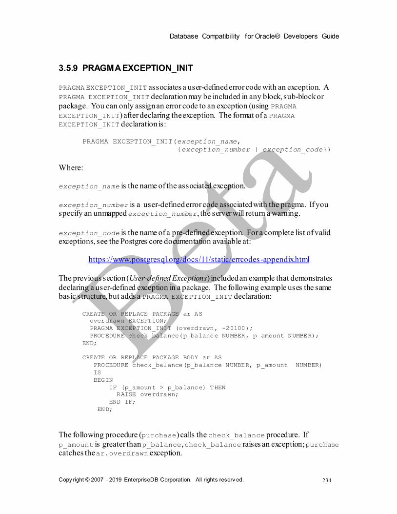
Database Compatibility for Oracle® Developers Guide
Copy right © 2007 - 2019 EnterpriseDB Corporation. All rights reserv ed.
234
3.5.9 PRAGMA EXCEPTION_INIT
PRAGMA EXCEPTION_INIT associates a user-defined error code with an exception. A
PRAGMA EXCEPTION_INIT declaration may be included in any block, sub-block or
package. You can only assign an error code to an exception (using PRAGMA
EXCEPTION_INIT) after declaring the exception. The format of a PRAGMA EXCEPTION_INIT declaration is:
PRAGMA EXCEPTION_INIT(exception_name,
{exception_number | exception_code})
Where:
exception_name is the name of the associated exception.
exception_number is a user-defined error code associated with the pragma. If you specify an unmapped exception_number, the server will return a warning.
exception_code is the name of a pre-defined exception. For a complete list of valid exceptions, see the Postgres core documentation available at:
https://www.postgresql.org/docs/11/static/errcodes -appendix.html
The previous section (User-defined Exceptions) included an example that demonstrates
declaring a user-defined exception in a package. The following example uses the same basic structure, but adds a PRAGMA EXCEPTION_INIT declaration:
CREATE OR REPLACE PACKAGE ar AS
overdrawn EXCEPTION;
PRAGMA EXCEPTION_INIT (overdrawn, -20100);
PROCEDURE check_balance(p_balance NUMBER, p_amount NUMBER);
END;
CREATE OR REPLACE PACKAGE BODY ar AS
PROCEDURE check_balance(p_balance NUMBER, p_amount NUMBER)
IS
BEGIN
IF (p_amount > p_balance) THEN
RAISE overdrawn;
END IF;
END;
The following procedure (purchase) calls the check_balance procedure. If
p_amount is greater than p_balance, check_balance raises an exception; purchase catches the ar.overdrawn exception.

Database Compatibility for Oracle® Developers Guide
Copy right © 2007 - 2019 EnterpriseDB Corporation. All rights reserv ed.
235
CREATE PROCEDURE purchase(customerID int, amount NUMERIC)
AS
BEGIN
ar.check_ balance(getcustomerbalance(customerid), amount);
record_purchase(customerid, amount);
EXCEPTION
WHEN ar.overdrawn THEN
DBMS_OUTPUT.PUT_LINE ('This account is overdrawn.');
DBMS_OUTPUT.PUT_LINE ('SQLCode :'||SQLCODE||' '||SQLERRM );
END;
When ar.check_balance raises an exception, execution jumps to the exception
handler defined in purchase.
EXCEPTION
WHEN ar.overdrawn THEN
DBMS_OUTPUT.PUT_LINE ('This account is overdrawn.');
DBMS_OUTPUT.PUT_LINE ('SQLCode :'||SQLCODE||' '||SQLERRM );
The exception handler returns an error message, followed by SQLCODE information:
This account is overdrawn.
SQLCODE: -20100 User-Defined Exception
The following example demonstrates using a pre-defined exception. The code creates a
more meaningful name for the no_data_found exception; if the given customer
does not exist, the code catches the exception, calls DBMS_OUTPUT.PUT_LINE to report the error, and then re-raises the original exception:
CREATE OR REPLACE PACKAGE ar AS
overdrawn EXCEPTION;
PRAGMA EXCEPTION_INIT (unknown_customer, no_data_found);
PROCEDURE check_balance(p_customer_id NUMBER);
END;
CREATE OR REPLACE PACKAGE BODY ar AS
PROCEDURE check_balance(p_customer_id NUMBER)
IS
DECLARE
v_balance NUMBER;
BEGIN
SELECT balance INTO v_balance FROM customer
WHERE cust_id = p_customer_id;
EXCEPTION WHEN unknown_customer THEN
DBMS_OUTPUT.PUT_LINE('invalid customer id');
RAISE;
END;

Database Compatibility for Oracle® Developers Guide
Copy right © 2007 - 2019 EnterpriseDB Corporation. All rights reserv ed.
236
3.5.10 RAISE_APPLICATION_ERROR
The procedure, RAISE_APPLICATION_ERROR, allows a developer to intentionally abort processing within an SPL program from which it is called by causing an exception. The
exception is handled in the same manner as described in Section 3.5.7. In addition, the
RAISE_APPLICATION_ERROR procedure makes a user-defined code and error message available to the program which can then be used to identify the exception.
RAISE_APPLICATION_ERROR(error_number, message);
Where:
error_number is an integer value or expression that is returned in a variable named
SQLCODE when the procedure is executed. error_number must be a value between
-20000 and -20999.
message is a string literal or expression that is returned in a variable named SQLERRM.
For additional information on the SQLCODE and SQLERRM variables, see Section 3.13, Errors and Messages.
The following example uses the RAISE_APPLICATION_ERROR procedure to display a different code and message depending upon the information missing from an employee.
CREATE OR REPLACE PROCEDURE verify_emp (
p_empno NUMBER
)
IS
v_ename emp.ename%TYPE;
v_job emp.job%TYPE;
v_mgr emp.mgr%TYPE;
v_hiredate emp.hiredate%TYPE;
BEGIN
SELECT ename, job, mgr, hiredate
INTO v_ename, v_job, v_mgr, v_hiredate FROM emp
WHERE empno = p_empno;
IF v_ename IS NULL THEN
RAISE_APPLICATION_ERROR(-20010, 'No name for ' || p_empno);
END IF;
IF v_job IS NULL THEN
RAISE_APPLICATION_ERROR(-20020, 'No job for' || p_empno);
END IF;
IF v_mgr IS NULL THEN
RAISE_APPLICATION_ERROR(-20030, 'No manager for ' || p_empno);
END IF;
IF v_hiredate IS NULL THEN
RAISE_APPLICATION_ERROR(-20040, 'No hire date for ' || p_empno);
END IF;
DBMS_OUTPUT.PUT_LINE('Employee ' || p_empno ||
' validated without errors');
EXCEPTION

Database Compatibility for Oracle® Developers Guide
Copy right © 2007 - 2019 EnterpriseDB Corporation. All rights reserv ed.
237
WHEN OTHERS THEN
DBMS_OUTPUT.PUT_LINE('SQLCODE: ' || SQLCODE);
DBMS_OUTPUT.PUT_LINE('SQLERRM: ' || SQLERRM);
END;
The following shows the output in a case where the manager number is missing from an employee record.
EXEC verify_emp(7839);
SQLCODE: -20030
SQLERRM: EDB-20030: No manager for 7839

Database Compatibility for Oracle® Developers Guide
Copy right © 2007 - 2019 EnterpriseDB Corporation. All rights reserv ed.
238
3.6 Transaction Control
There may be circumstances where it is desired that all updates to a database are to occur
successfully, or none are to occur at all if any error occurs. A set of database updates that are to all occur successfully as a single unit, or are not to occur at all, is said to be a transaction.
A common example in banking is a funds transfer between two accounts. The two parts
of the transaction are the withdrawal of funds from one account, and the deposit of the funds in another account. Both parts of this transaction must occur otherwise the bank’s books will be out of balance. The deposit and withdrawal are one transaction.
An SPL application can be created that uses a style of transaction control compatible with Oracle databases if the following conditions are met:
The edb_stmt_level_tx parameter must be set to TRUE. This prevents the
action of unconditionally rolling back all database updates within the BEGIN/END block if any exception occurs. See Section 1.3.4 for more information on the
edb_stmt_level_tx parameter.
The application must not be running in autocommit mode. If autocommit mode is
on, each successful database update is immediately committed and cannot be undone. The manner in which autocommit mode is turned on or off is application dependent.
A transaction begins when the first SQL command is encountered in the SPL program.
All subsequent SQL commands are included as part of that transaction. The transaction ends when one of the following occurs:
An unhandled exception occurs in which case the effects of all database updates made during the transaction are rolled back and the transaction is aborted.
A COMMIT command is encountered in which case the effect of all database updates made during the transaction become permanent.
A ROLLBACK command is encountered in which case the effects of all database updates made during the transaction are rolled back and the transaction is aborted.
If a new SQL command is encountered, a new transaction begins.
Control returns to the calling application (such as Java, PSQL, etc.) in which case the action of the application determines whether the transaction is committed or
rolled back unless the transaction is within a block in which PRAGMA
AUTONOMOUS_TRANSACTION has been declared in which case the commitment or rollback of the transaction occurs independently of the calling program.
Note: Unlike Oracle, DDL commands such as CREATE TABLE do not implicitly occur within their own transaction. Therefore, DDL commands do not automatically cause an immediate database commit as in Oracle, and DDL commands may be rolled back just like DML commands.

Database Compatibility for Oracle® Developers Guide
Copy right © 2007 - 2019 EnterpriseDB Corporation. All rights reserv ed.
239
A transaction may span one or more BEGIN/END blocks, or a single BEGIN/END block may contain one or more transactions.
The following sections discuss the COMMIT and ROLLBACK commands in more detail.
3.6.1 COMMIT
The COMMIT command makes all database updates made during the current transaction permanent, and ends the current transaction.
COMMIT [ WORK ];
The COMMIT command may be used within anonymous blocks, stored procedures, or
functions. Within an SPL program, it may appear in the executable section and/or the exception section.
In the following example, the third INSERT command in the anonymous block results in
an error. The effect of the first two INSERT commands are retained as shown by the first
SELECT command. Even after issuing a ROLLBACK command, the two rows remain in the
table as shown by the second SELECT command verifying that they were indeed committed.
Note: The edb_stmt_level_tx configuration parameter shown in the example below
can be set for the entire database using the ALTER DATABASE command, or it can be set
for the entire database server by changing it in the postgresql.conf file.
\set AUTOCOMMIT off
SET edb_stmt_level_tx TO on;
BEGIN
INSERT INTO dept VALUES (50, 'FINANCE', 'DALLAS');
INSERT INTO dept VALUES (60, 'MARKETING', 'CHICAGO');
COMMIT;
INSERT INTO dept VALUES (70, 'HUMAN RESOURCES', 'CHICAGO');
EXCEPTION
WHEN OTHERS THEN
DBMS_OUTPUT.PUT_LINE('SQLERRM: ' || SQLERRM);
DBMS_OUTPUT.PUT_LINE('SQLCODE: ' || SQLCODE);
END;
SQLERRM: value too long for type character varying(14)
SQLCODE: 22001
SELECT * FROM dept;
deptno | dname | loc
--------+------------+----------
10 | ACCOUNTING | NEW YORK
20 | RESEARCH | DALLAS
30 | SALES | CHICAGO
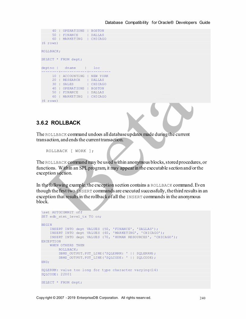
Database Compatibility for Oracle® Developers Guide
Copy right © 2007 - 2019 EnterpriseDB Corporation. All rights reserv ed.
240
40 | OPERATIONS | BOSTON
50 | FINANCE | DALLAS
60 | MARKETING | CHICAGO
(6 rows)
ROLLBACK;
SELECT * FROM dept;
deptno | dname | loc
--------+------------+----------
10 | ACCOUNTING | NEW YORK
20 | RESEARCH | DALLAS
30 | SALES | CHICAGO
40 | OPERATIONS | BOSTON
50 | FINANCE | DALLAS
60 | MARKETING | CHICAGO
(6 rows)
3.6.2 ROLLBACK
The ROLLBACK command undoes all database updates made during the current transaction, and ends the current transaction.
ROLLBACK [ WORK ];
The ROLLBACK command may be used within anonymous blocks, stored procedures, or
functions. Within an SPL program, it may appear in the executable section and/or the exception section.
In the following example, the exception section contains a ROLLBACK command. Even
though the first two INSERT commands are executed successfully, the third results in an
exception that results in the rollback of all the INSERT commands in the anonymous block.
\set AUTOCOMMIT off
SET edb_stmt_level_tx TO on;
BEGIN
INSERT INTO dept VALUES (50, 'FINANCE', 'DALLAS');
INSERT INTO dept VALUES (60, 'MARKETING', 'CHICAGO');
INSERT INTO dept VALUES (70, 'HUMAN RESOURCES', 'CHICAGO');
EXCEPTION
WHEN OTHERS THEN
ROLLBACK;
DBMS_OUTPUT.PUT_LINE('SQLERRM: ' || SQLERRM);
DBMS_OUTPUT.PUT_LINE('SQLCODE: ' || SQLCODE);
END;
SQLERRM: value too long for type character varying(14)
SQLCODE: 22001
SELECT * FROM dept;

Database Compatibility for Oracle® Developers Guide
Copy right © 2007 - 2019 EnterpriseDB Corporation. All rights reserv ed.
241
deptno | dname | loc
--------+------------+----------
10 | ACCOUNTING | NEW YORK
20 | RESEARCH | DALLAS
30 | SALES | CHICAGO
40 | OPERATIONS | BOSTON
(4 rows)
The following is a more complex example using both COMMIT and ROLLBACK. First, the following stored procedure is created which inserts a new employee.
\set AUTOCOMMIT off
SET edb_stmt_level_tx TO on;
CREATE OR REPLACE PROCEDURE emp_insert (
p_empno IN emp.empno%TYPE,
p_ename IN emp.ename%TYPE,
p_job IN emp.job%TYPE,
p_mgr IN emp.mgr%TYPE,
p_hiredate IN emp.hiredate%TYPE,
p_sal IN emp.sal%TYPE,
p_comm IN emp.comm%TYPE,
p_deptno IN emp.deptno%TYPE
)
IS
BEGIN
INSERT INTO emp VALUES (
p_empno,
p_ename,
p_job,
p_mgr,
p_hiredate,
p_sal,
p_comm,
p_deptno);
DBMS_OUTPUT.PUT_LINE('Added employee...');
DBMS_OUTPUT.PUT_LINE('Employee # : ' || p_empno);
DBMS_OUTPUT.PUT_LINE('Name : ' || p_ename);
DBMS_OUTPUT.PUT_LINE('Job : ' || p_job);
DBMS_OUTPUT.PUT_LINE('Manager : ' || p_mgr);
DBMS_OUTPUT.PUT_LINE('Hire Date : ' || p_hiredate);
DBMS_OUTPUT.PUT_LINE('Salary : ' || p_sal);
DBMS_OUTPUT.PUT_LINE('Commission : ' || p_comm);
DBMS_OUTPUT.PUT_LINE('Dept # : ' || p_deptno);
DBMS_OUTPUT.PUT_LINE('----------------------');
END;
Note that this procedure has no exception section so any error that may occur is propagated up to the calling program.
The following anonymous block is run. Note the use of the COMMIT command after all
calls to the emp_insert procedure and the ROLLBACK command in the exception section.
BEGIN
emp_insert(9601,'FARRELL','ANALYST',7902,'03-MAR-08',5000,NULL,40);
emp_insert(9602,'TYLER','ANALYST',7900,'25-JAN-08',4800,NULL,40);
COMMIT;

Database Compatibility for Oracle® Developers Guide
Copy right © 2007 - 2019 EnterpriseDB Corporation. All rights reserv ed.
242
EXCEPTION
WHEN OTHERS THEN
DBMS_OUTPUT.PUT_LINE('SQLERRM: ' || SQLERRM);
DBMS_OUTPUT.PUT_LINE('An error occurred - roll back inserts');
ROLLBACK;
END;
Added employee...
Employee # : 9601
Name : FARRELL
Job : ANALYST
Manager : 7902
Hire Date : 03-MAR-08 00:00:00
Salary : 5000
Commission :
Dept # : 40
----------------------
Added employee...
Employee # : 9602
Name : TYLER
Job : ANALYST
Manager : 7900
Hire Date : 25-JAN-08 00:00:00
Salary : 4800
Commission :
Dept # : 40
----------------------
The following SELECT command shows that employees Farrell and Tyler were successfully added.
SELECT * FROM emp WHERE empno > 9600;
empno | ename | job | mgr | hiredate | sal | comm | deptno
-------+---------+---------+------+--------------------+---------+------+--------
9601 | FARRELL | ANALYST | 7902 | 03-MAR-08 00:00:00 | 5000.00 | | 40
9602 | TYLER | ANALYST | 7900 | 25-JAN-08 00:00:00 | 4800.00 | | 40
(2 rows)
Now, execute the following anonymous block:
BEGIN
emp_insert(9603,'HARRISON','SALESMAN',7902,'13-DEC-07',5000,3000,20);
emp_insert(9604,'JARVIS','SALESMAN',7902,'05-MAY-08',4800,4100,11);
COMMIT;
EXCEPTION
WHEN OTHERS THEN
DBMS_OUTPUT.PUT_LINE('SQLERRM: ' || SQLERRM);
DBMS_OUTPUT.PUT_LINE('An error occurred - roll back inserts');
ROLLBACK;
END;
Added employee...
Employee # : 9603
Name : HARRISON
Job : SALESMAN
Manager : 7902
Hire Date : 13-DEC-07 00:00:00
Salary : 5000
Commission : 3000
Dept # : 20

Database Compatibility for Oracle® Developers Guide
Copy right © 2007 - 2019 EnterpriseDB Corporation. All rights reserv ed.
243
----------------------
SQLERRM: insert or update on table "emp" violates foreign key constraint
"emp_ref_dept_fk"
An error occurred - roll back inserts
A SELECT command run against the table yields the following:
SELECT * FROM emp WHERE empno > 9600;
empno | ename | job | mgr | hiredate | sal | comm | deptno
-------+---------+---------+------+--------------------+---------+------+--------
9601 | FARRELL | ANALYST | 7902 | 03-MAR-08 00:00:00 | 5000.00 | | 40
9602 | TYLER | ANALYST | 7900 | 25-JAN-08 00:00:00 | 4800.00 | | 40
(2 rows)
The ROLLBACK command in the exception section successfully undoes the insert of
employee Harrison. Also note that employees Farrell and Tyler are still in the table as
their inserts were made permanent by the COMMIT command in the first anonymous block.
Note: Executing a COMMIT or ROLLBACK in a plpgsql procedure will throw an error if there is an Oracle-style SPL procedure on the runtime stack.
3.6.3 PRAGMA AUTONOMOUS_TRANSACTION
An SPL program can be declared as an autonomous transaction by specifying the following directive in the declaration section of the SPL block:
PRAGMA AUTONOMOUS_TRANSACTION;
An autonomous transaction is an independent transaction started by a calling program. A commit or rollback of SQL commands within the autonomous transaction has no effect
on the commit or rollback in any transaction of the calling program. A commit or rollback in the calling program has no effect on the commit or rollback of SQL commands in the autonomous transaction.
The following SPL programs can include PRAGMA AUTONOMOUS_TRANSACTION:
Standalone procedures and functions
Anonymous blocks
Procedures and functions declared as subprograms within packages and other calling procedures, functions, and anonymous blocks
Triggers
Object type methods
The following are issues and restrictions related to autonomous transactions:

Database Compatibility for Oracle® Developers Guide
Copy right © 2007 - 2019 EnterpriseDB Corporation. All rights reserv ed.
244
Each autonomous transaction consumes a connection slot for as long as it is in
progress. In some cases, this may mean that the max_connections parameter in
the postgresql.conf file should be raised.
In most respects, an autonomous transaction behaves exactly as if it was a
completely separate session, but GUCs (that is, settings established with SET) are a deliberate exception. Autonomous transactions absorb the surrounding values and can propagate values they commit to the outer transaction.
Autonomous transactions can be nested, but there is a limit of 16 levels of autonomous transactions within a single session.
Parallel query is not supported within autonomous transactions.
The Advanced Server implementation of autonomous transactions is not entirely compatible with Oracle databases in that the Advanced Server autonomous transaction does not produce an ERROR if there is an uncommitted transaction at
the end of an SPL block.
The following set of examples illustrates the usage of autonomous transactions. This first set of scenarios show the default behavior when there are no autonomous transactions.
Before each scenario, the dept table is reset to the following initial values:
SELECT * FROM dept;
deptno | dname | loc
--------+------------+----------
10 | ACCOUNTING | NEW YORK
20 | RESEARCH | DALLAS
30 | SALES | CHICAGO
40 | OPERATIONS | BOSTON
(4 rows)
Scenario 1a – No autonomous transactions with only a final COMMIT
This first set of scenarios show the insertion of three rows starting just after the initial
BEGIN command of the transaction, then from within an anonymous block within the starting transaction, and finally from a stored procedure executed from within the anonymous block.
The stored procedure is the following:
CREATE OR REPLACE PROCEDURE insert_dept_70 IS
BEGIN
INSERT INTO dept VALUES (70,'MARKETING','LOS ANGELES');
END;
The PSQL session is the following:
BEGIN;
INSERT INTO dept VALUES (50,'HR','DENVER');
BEGIN
INSERT INTO dept VALUES (60,'FINANCE','CHICAGO');
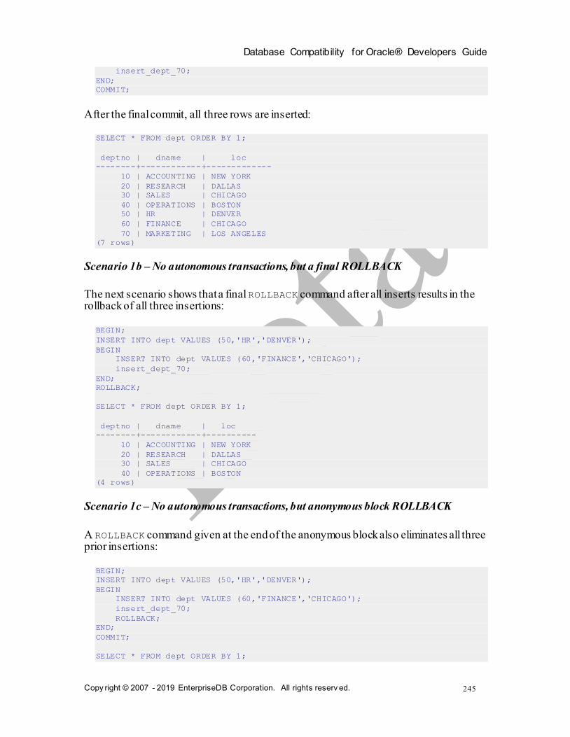
Database Compatibility for Oracle® Developers Guide
Copy right © 2007 - 2019 EnterpriseDB Corporation. All rights reserv ed.
245
insert_dept_70;
END;
COMMIT;
After the final commit, all three rows are inserted:
SELECT * FROM dept ORDER BY 1;
deptno | dname | loc
--------+------------+-------------
10 | ACCOUNTING | NEW YORK
20 | RESEARCH | DALLAS
30 | SALES | CHICAGO
40 | OPERATIONS | BOSTON
50 | HR | DENVER
60 | FINANCE | CHICAGO
70 | MARKETING | LOS ANGELES
(7 rows)
Scenario 1b – No autonomous transactions, but a final ROLLBACK
The next scenario shows that a final ROLLBACK command after all inserts results in the rollback of all three insertions:
BEGIN;
INSERT INTO dept VALUES (50,'HR','DENVER');
BEGIN
INSERT INTO dept VALUES (60,'FINANCE','CHICAGO');
insert_dept_70;
END;
ROLLBACK;
SELECT * FROM dept ORDER BY 1;
deptno | dname | loc
--------+------------+----------
10 | ACCOUNTING | NEW YORK
20 | RESEARCH | DALLAS
30 | SALES | CHICAGO
40 | OPERATIONS | BOSTON
(4 rows)
Scenario 1c – No autonomous transactions, but anonymous block ROLLBACK
A ROLLBACK command given at the end of the anonymous block also eliminates all three prior insertions:
BEGIN;
INSERT INTO dept VALUES (50,'HR','DENVER');
BEGIN
INSERT INTO dept VALUES (60,'FINANCE','CHICAGO');
insert_dept_70;
ROLLBACK;
END;
COMMIT;
SELECT * FROM dept ORDER BY 1;

Database Compatibility for Oracle® Developers Guide
Copy right © 2007 - 2019 EnterpriseDB Corporation. All rights reserv ed.
246
deptno | dname | loc
--------+------------+----------
10 | ACCOUNTING | NEW YORK
20 | RESEARCH | DALLAS
30 | SALES | CHICAGO
40 | OPERATIONS | BOSTON
(4 rows)
This next set of scenarios shows the effect of using autonomous transactions with
PRAGMA AUTONOMOUS_TRANSACTION in various locations.
Scenario 2a – Autonomous transaction of anonymous block with COMMIT
The procedure remains as initially created:
CREATE OR REPLACE PROCEDURE insert_dept_70 IS
BEGIN
INSERT INTO dept VALUES (70,'MARKETING','LOS ANGELES');
END;
Now, the PRAGMA AUTONOMOUS_TRANSACTION is given with the anonymous block
along with the COMMIT command at the end of the anonymous block.
BEGIN;
INSERT INTO dept VALUES (50,'HR','DENVER');
DECLARE
PRAGMA AUTONOMOUS_TRANSACTION;
BEGIN
INSERT INTO dept VALUES (60,'FINANCE','CHICAGO');
insert_dept_70;
COMMIT;
END;
ROLLBACK;
After the ROLLBACK at the end of the transaction, only the first row insertion at the very beginning of the transaction is discarded. The other two row insertions within the
anonymous block with PRAGMA AUTONOMOUS_TRANSACTION have been independently committed.
SELECT * FROM dept ORDER BY 1;
deptno | dname | loc
--------+------------+-------------
10 | ACCOUNTING | NEW YORK
20 | RESEARCH | DALLAS
30 | SALES | CHICAGO
40 | OPERATIONS | BOSTON
60 | FINANCE | CHICAGO
70 | MARKETING | LOS ANGELES
(6 rows)
Scenario 2b – Autonomous transaction anonymous block with COMMIT including procedure with ROLLBACK, but not an autonomous transaction procedure

Database Compatibility for Oracle® Developers Guide
Copy right © 2007 - 2019 EnterpriseDB Corporation. All rights reserv ed.
247
Now, the procedure has the ROLLBACK command at the end. Note, however, that the PRAGMA ANONYMOUS_TRANSACTION is not included in this procedure.
CREATE OR REPLACE PROCEDURE insert_dept_70 IS
BEGIN
INSERT INTO dept VALUES (70,'MARKETING','LOS ANGELES');
ROLLBACK;
END;
Now, the rollback within the procedure removes the two rows inserted within the
anonymous block (deptno 60 and 70) before the final COMMIT command within the anonymous block.
BEGIN;
INSERT INTO dept VALUES (50,'HR','DENVER');
DECLARE
PRAGMA AUTONOMOUS_TRANSACTION;
BEGIN
INSERT INTO dept VALUES (60,'FINANCE','CHICAGO');
insert_dept_70;
COMMIT;
END;
COMMIT;
After the final commit at the end of the transaction, the only row inserted is the first one
from the beginning of the transaction. Since the anonymous block is an autonomous transaction, the rollback within the enclosed procedure has no effect on the insertion that occurs before the anonymous block is executed.
SELECT * FROM dept ORDER by 1;
deptno | dname | loc
--------+------------+----------
10 | ACCOUNTING | NEW YORK
20 | RESEARCH | DALLAS
30 | SALES | CHICAGO
40 | OPERATIONS | BOSTON
50 | HR | DENVER
(5 rows)
Scenario 2c – Autonomous transaction anonymous block with COMMIT including procedure with ROLLBACK that is also an autonomous transaction procedure
Now, the procedure with the ROLLBACK command at the end also has PRAGMA
ANONYMOUS_TRANSACTION included. This isolates the effect of the ROLLBACK command within the procedure.
CREATE OR REPLACE PROCEDURE insert_dept_70 IS
PRAGMA AUTONOMOUS_TRANSACTION;
BEGIN
INSERT INTO dept VALUES (70,'MARKETING','LOS ANGELES');
ROLLBACK;
END;

Database Compatibility for Oracle® Developers Guide
Copy right © 2007 - 2019 EnterpriseDB Corporation. All rights reserv ed.
248
Now, the rollback within the procedure removes the row inserted by the procedure, but not the other row inserted within the anonymous block.
BEGIN;
INSERT INTO dept VALUES (50,'HR','DENVER');
DECLARE
PRAGMA AUTONOMOUS_TRANSACTION;
BEGIN
INSERT INTO dept VALUES (60,'FINANCE','CHICAGO');
insert_dept_70;
COMMIT;
END;
COMMIT;
After the final commit at the end of the transaction, the row inserted is the first one from the beginning of the transaction as well as the row inserted at the beginning of the anonymous block. The only insertion rolled back is the one within the procedure.
SELECT * FROM dept ORDER by 1;
deptno | dname | loc
--------+------------+----------
10 | ACCOUNTING | NEW YORK
20 | RESEARCH | DALLAS
30 | SALES | CHICAGO
40 | OPERATIONS | BOSTON
50 | HR | DENVER
60 | FINANCE | CHICAGO
(6 rows)
The following sections now show examples of PRAGMA AUTONOMOUS_TRANSACTION in a couple of other SPL program types.
Autonomous Transaction Trigger
The following example shows the effect of declaring a trigger with PRAGMA AUTONOMOUS_TRANSACTION.
The following table is created to log changes to the emp table:
CREATE TABLE empauditlog (
audit_date DATE,
audit_user VARCHAR2(20),
audit_desc VARCHAR2(20)
);
The trigger attached to the emp table that inserts these changes into the empauditlog
table is the following. Note the inclusion of PRAGMA AUTONOMOUS_TRANSACTION in the declaration section.
CREATE OR REPLACE TRIGGER emp_audit_trig
AFTER INSERT OR UPDATE OR DELETE ON emp
DECLARE
PRAGMA AUTONOMOUS_TRANSACTION;
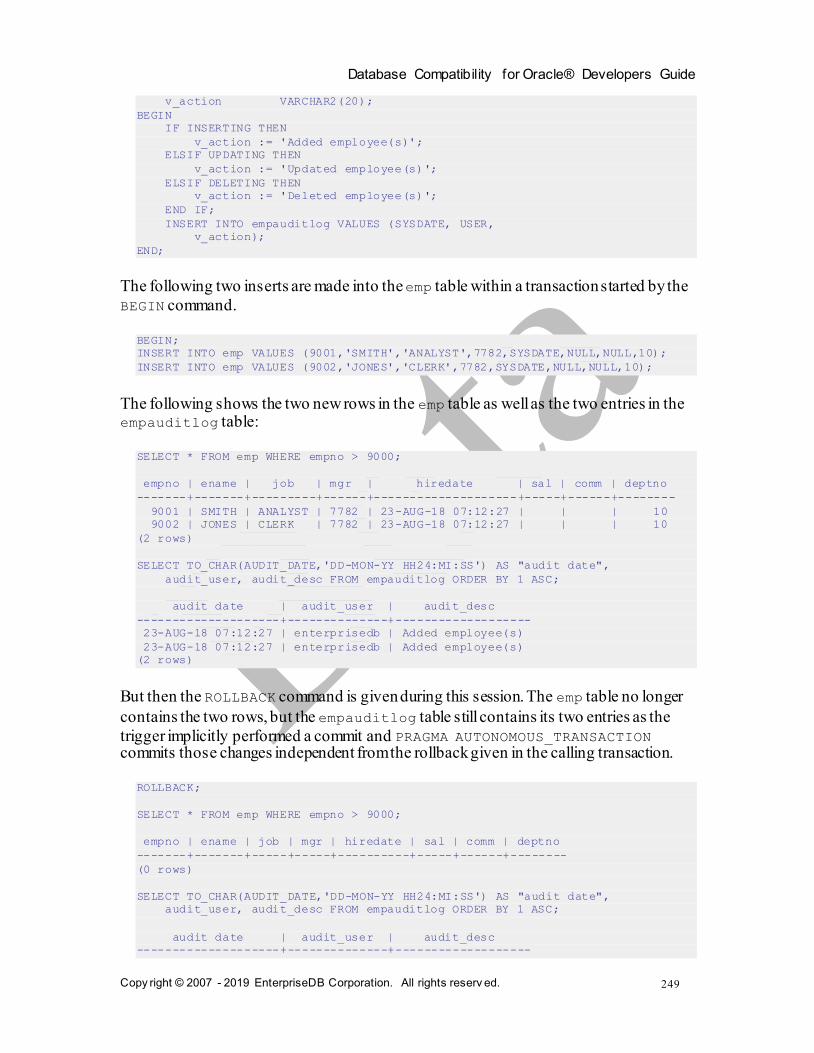
Database Compatibility for Oracle® Developers Guide
Copy right © 2007 - 2019 EnterpriseDB Corporation. All rights reserv ed.
249
v_action VARCHAR2(20);
BEGIN
IF INSERTING THEN
v_action := 'Added employee(s)';
ELSIF UPDATING THEN
v_action := 'Updated employee(s)';
ELSIF DELETING THEN
v_action := 'Deleted employee(s)';
END IF;
INSERT INTO empauditlog VALUES (SYSDATE, USER,
v_action);
END;
The following two inserts are made into the emp table within a transaction started by the
BEGIN command.
BEGIN;
INSERT INTO emp VALUES (9001,'SMITH','ANALYST',7782,SYSDATE,NULL,NULL,10);
INSERT INTO emp VALUES (9002,'JONES','CLERK',7782,SYSDATE,NULL,NULL,10);
The following shows the two new rows in the emp table as well as the two entries in the empauditlog table:
SELECT * FROM emp WHERE empno > 9000;
empno | ename | job | mgr | hiredate | sal | comm | deptno
-------+-------+---------+------+--------------------+-----+------+--------
9001 | SMITH | ANALYST | 7782 | 23-AUG-18 07:12:27 | | | 10
9002 | JONES | CLERK | 7782 | 23-AUG-18 07:12:27 | | | 10
(2 rows)
SELECT TO_CHAR(AUDIT_DATE,'DD-MON-YY HH24:MI:SS') AS "audit date",
audit_user, audit_desc FROM empauditlog ORDER BY 1 ASC;
audit date | audit_user | audit_desc
--------------------+--------------+-------------------
23-AUG-18 07:12:27 | enterprisedb | Added employee(s)
23-AUG-18 07:12:27 | enterprisedb | Added employee(s)
(2 rows)
But then the ROLLBACK command is given during this session. The emp table no longer
contains the two rows, but the empauditlog table still contains its two entries as the
trigger implicitly performed a commit and PRAGMA AUTONOMOUS_TRANSACTION commits those changes independent from the rollback given in the calling transaction.
ROLLBACK;
SELECT * FROM emp WHERE empno > 9000;
empno | ename | job | mgr | hiredate | sal | comm | deptno
-------+-------+-----+-----+----------+-----+------+--------
(0 rows)
SELECT TO_CHAR(AUDIT_DATE,'DD-MON-YY HH24:MI:SS') AS "audit date",
audit_user, audit_desc FROM empauditlog ORDER BY 1 ASC;
audit date | audit_user | audit_desc
--------------------+--------------+-------------------

Database Compatibility for Oracle® Developers Guide
Copy right © 2007 - 2019 EnterpriseDB Corporation. All rights reserv ed.
250
23-AUG-18 07:12:27 | enterprisedb | Added employee(s)
23-AUG-18 07:12:27 | enterprisedb | Added employee(s)
(2 rows)
Autonomous Transaction Object Type Method
The following example shows the effect of declaring an object method with PRAGMA
AUTONOMOUS_TRANSACTION.
The following object type and object type body are created. The member procedure
within the object type body contains the PRAGMA AUTONOMOUS_TRANSACTION in the declaration section along with COMMIT at the end of the procedure.
CREATE OR REPLACE TYPE insert_dept_typ AS OBJECT (
deptno NUMBER(2),
dname VARCHAR2(14),
loc VARCHAR2(13),
MEMBER PROCEDURE insert_dept
);
CREATE OR REPLACE TYPE BODY insert_dept_typ AS
MEMBER PROCEDURE insert_dept
IS
PRAGMA AUTONOMOUS_TRANSACTION;
BEGIN
INSERT INTO dept VALUES (SELF.deptno,SELF.dname,SELF.loc);
COMMIT;
END;
END;
In the following anonymous block, an insert is performed into the dept table, followed
by invocation of the insert_dept method of the object, ending with a ROLLBACK command in the anonymous block.
BEGIN;
DECLARE
v_dept INSERT_DEPT_TYP :=
insert_dept_typ(60,'FINANCE','CHICAGO');
BEGIN
INSERT INTO dept VALUES (50,'HR','DENVER');
v_dept.insert_dept;
ROLLBACK;
END;
Since insert_dept has been declared as an autonomous transaction, its insert of department number 60 remains in the table, but the rollback removes the insertion of department 50.
SELECT * FROM dept ORDER BY 1;
deptno | dname | loc
--------+------------+----------
10 | ACCOUNTING | NEW YORK
20 | RESEARCH | DALLAS
30 | SALES | CHICAGO

Database Compatibility for Oracle® Developers Guide
Copy right © 2007 - 2019 EnterpriseDB Corporation. All rights reserv ed.
251
40 | OPERATIONS | BOSTON
60 | FINANCE | CHICAGO
(5 rows)
3.7 Dynamic SQL
Dynamic SQL is a technique that provides the ability to execute SQL commands that are
not known until the commands are about to be executed. Up to this point, the SQL
commands that have been illustrated in SPL programs have been static SQL - the full command (with the exception of variables) must be known and coded into the program before the program, itself, can begin to execute. Thus using dynamic SQL, the executed SQL can change during program runtime.
In addition, dynamic SQL is the only method by which data definition commands, such as CREATE TABLE, can be executed from within an SPL program.
Note, however, that the runtime performance of dynamic SQL will be slower than static SQL.
The EXECUTE IMMEDIATE command is used to run SQL commands dynamically.
EXECUTE IMMEDIATE 'sql_expression;'
[ INTO { variable [, ...] | record } ]
[ USING expression [, ...] ]
sql_expression is a string expression containing the SQL command to be
dynamically executed. variable receives the output of the result set, typically from a
SELECT command, created as a result of executing the SQL command in
sql_expression. The number, order, and type of variables must match the number,
order, and be type-compatible with the fields of the result set. Alternatively, a record can be specified as long as the record’s fields match the number, order, and are type-
compatible with the result set. When using the INTO clause, exactly one row must be
returned in the result set, otherwise an exception occurs. When using the USING clause
the value of expression is passed to a placeholder. Placeholders appear embedded
within the SQL command in sql_expression where variables may be used.
Placeholders are denoted by an identifier with a colon (:) prefix - :name. The number,
order, and resultant data types of the evaluated expressions must match the number, order and be type-compatible with the placeholders in sql_expression. Note that
placeholders are not declared anywhere in the SPL program – they only appear in sql_expression.
The following example shows basic dynamic SQL commands as string literals.
DECLARE
v_sql VARCHAR2(50);

Database Compatibility for Oracle® Developers Guide
Copy right © 2007 - 2019 EnterpriseDB Corporation. All rights reserv ed.
252
BEGIN
EXECUTE IMMEDIATE 'CREATE TABLE job (jobno NUMBER(3),' ||
' jname VARCHAR2(9))';
v_sql := 'INSERT INTO job VALUES (100, ''ANALYST'')';
EXECUTE IMMEDIATE v_sql;
v_sql := 'INSERT INTO job VALUES (200, ''CLERK'')';
EXECUTE IMMEDIATE v_sql;
END;
The following example illustrates the USING clause to pass values to placeholders in the SQL string.
DECLARE
v_sql VARCHAR2(50) := 'INSERT INTO job VALUES ' ||
'(:p_jobno, :p_jname)';
v_jobno job.jobno%TYPE;
v_jname job.jname%TYPE;
BEGIN
v_jobno := 300;
v_jname := 'MANAGER';
EXECUTE IMMEDIATE v_sql USING v_jobno, v_jname;
v_jobno := 400;
v_jname := 'SALESMAN';
EXECUTE IMMEDIATE v_sql USING v_jobno, v_jname;
v_jobno := 500;
v_jname := 'PRESIDENT';
EXECUTE IMMEDIATE v_sql USING v_jobno, v_jname;
END;
The following example shows both the INTO and USING clauses. Note the last execution of the SELECT command returns the results into a record instead of individual variables.
DECLARE
v_sql VARCHAR2(60);
v_jobno job.jobno%TYPE;
v_jname job.jname%TYPE;
r_job job%ROWTYPE;
BEGIN
DBMS_OUTPUT.PUT_LINE('JOBNO JNAME');
DBMS_OUTPUT.PUT_LINE('----- -------');
v_sql := 'SELECT jobno, jname FROM job WHERE jobno = :p_jobno';
EXECUTE IMMEDIATE v_sql INTO v_jobno, v_jname USING 100;
DBMS_OUTPUT.PUT_LINE(v_jobno || ' ' || v_jname);
EXECUTE IMMEDIATE v_sql INTO v_jobno, v_jname USING 200;
DBMS_OUTPUT.PUT_LINE(v_jobno || ' ' || v_jname);
EXECUTE IMMEDIATE v_sql INTO v_jobno, v_jname USING 300;
DBMS_OUTPUT.PUT_LINE(v_jobno || ' ' || v_jname);
EXECUTE IMMEDIATE v_sql INTO v_jobno, v_jname USING 400;
DBMS_OUTPUT.PUT_LINE(v_jobno || ' ' || v_jname);
EXECUTE IMMEDIATE v_sql INTO r_job USING 500;
DBMS_OUTPUT.PUT_LINE(r_job.jobno || ' ' || r_job.jname);
END;
The following is the output from the previous anonymous block:
JOBNO JNAME
----- -------
100 ANALYST
200 CLERK

Database Compatibility for Oracle® Developers Guide
Copy right © 2007 - 2019 EnterpriseDB Corporation. All rights reserv ed.
253
300 MANAGER
400 SALESMAN
500 PRESIDENT
You can use the BULK COLLECT clause to assemble the result set from an EXECUTE
IMMEDIATE statement into a named collection. See Section 3.12.4, EXECUTE IMMEDIATE BULK COLLECT for information about using the BULK COLLECT clause.
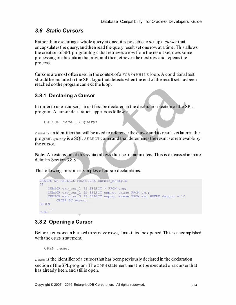
Database Compatibility for Oracle® Developers Guide
Copy right © 2007 - 2019 EnterpriseDB Corporation. All rights reserv ed.
254
3.8 Static Cursors
Rather than executing a whole query at once, it is possible to set up a cursor that
encapsulates the query, and then read the query result set one row at a time. This allows the creation of SPL program logic that retrieves a row from the result set, does some processing on the data in that row, and then retrieves the next row and repeats the process.
Cursors are most often used in the context of a FOR or WHILE loop. A conditional test should be included in the SPL logic that detects when the end of the result set has been reached so the program can exit the loop.
3.8.1 Declaring a Cursor
In order to use a cursor, it must first be declared in the declaration section of the SPL program. A cursor declaration appears as follows:
CURSOR name IS query;
name is an identifier that will be used to reference the cursor and its result set later in the
program. query is a SQL SELECT command that determines the result set retrievable by
the cursor.
Note: An extension of this syntax allows the use of parameters. This is discussed in more detail in Section 3.8.8.
The following are some examples of cursor declarations:
CREATE OR REPLACE PROCEDURE cursor_example
IS
CURSOR emp_cur_1 IS SELECT * FROM emp;
CURSOR emp_cur_2 IS SELECT empno, ename FROM emp;
CURSOR emp_cur_3 IS SELECT empno, ename FROM emp WHERE deptno = 10
ORDER BY empno;
BEGIN
...
END;
3.8.2 Opening a Cursor
Before a cursor can be used to retrieve rows, it must first be opened. This is accomplished with the OPEN statement.
OPEN name;
name is the identifier of a cursor that has been previously declared in the declaration
section of the SPL program. The OPEN statement must not be executed on a cursor that has already been, and still is open.

Database Compatibility for Oracle® Developers Guide
Copy right © 2007 - 2019 EnterpriseDB Corporation. All rights reserv ed.
255
The following shows an OPEN statement with its corresponding cursor declaration.
CREATE OR REPLACE PROCEDURE cursor_example
IS
CURSOR emp_cur_3 IS SELECT empno, ename FROM emp WHERE deptno = 10
ORDER BY empno;
BEGIN
OPEN emp_cur_3;
...
END;
3.8.3 Fetching Rows From a Cursor
Once a cursor has been opened, rows can be retrieved from the cursor’s result set by
using the FETCH statement.
FETCH name INTO { record | variable [, variable_2 ]... };
name is the identifier of a previously opened cursor. record is the identifier of a
previously defined record (for example, using table%ROWTYPE). variable,
variable_2... are SPL variables that will receive the field data from the fetched row.
The fields in record or variable, variable_2... must match in number and order,
the fields returned in the SELECT list of the query given in the cursor declaration. The
data types of the fields in the SELECT list must match, or be implicitly convertible to the data types of the fields in record or the data types of variable, variable_2...
Note: There is a variation of FETCH INTO using the BULK COLLECT clause that can return multiple rows at a time into a collection. See Section 3.12.4 for more information
on using the BULK COLLECT clause with the FETCH INTO statement.
The following shows the FETCH statement.
CREATE OR REPLACE PROCEDURE cursor_example
IS
v_empno NUMBER(4);
v_ename VARCHAR2(10);
CURSOR emp_cur_3 IS SELECT empno, ename FROM emp WHERE deptno = 10
ORDER BY empno;
BEGIN
OPEN emp_cur_3;
FETCH emp_cur_3 INTO v_empno, v_ename;
...
END;
Instead of explicitly declaring the data type of a target variable, %TYPE can be used
instead. In this way, if the data type of the database column is changed, the target variable
declaration in the SPL program does not have to be changed. %TYPE will automatically pick up the new data type of the specified column.
CREATE OR REPLACE PROCEDURE cursor_example
IS
v_empno emp.empno%TYPE;

Database Compatibility for Oracle® Developers Guide
Copy right © 2007 - 2019 EnterpriseDB Corporation. All rights reserv ed.
256
v_ename emp.ename%TYPE;
CURSOR emp_cur_3 IS SELECT empno, ename FROM emp WHERE deptno = 10
ORDER BY empno;
BEGIN
OPEN emp_cur_3;
FETCH emp_cur_3 INTO v_empno, v_ename;
...
END;
If all the columns in a table are retrieved in the order defined in the table, %ROWTYPE can
be used to define a record into which the FETCH statement will place the retrieved data. Each field within the record can then be accessed using dot notation.
CREATE OR REPLACE PROCEDURE cursor_example
IS
v_emp_rec emp%ROWTYPE;
CURSOR emp_cur_1 IS SELECT * FROM emp;
BEGIN
OPEN emp_cur_1;
FETCH emp_cur_1 INTO v_emp_rec;
DBMS_OUTPUT.PUT_LINE('Employee Number: ' || v_emp_rec.empno);
DBMS_OUTPUT.PUT_LINE('Employee Name : ' || v_emp_rec.ename);
...
END;
3.8.4 Closing a Cursor
Once all the desired rows have been retrieved from the cursor result set, the cursor must
be closed. Once closed, the result set is no longer accessible. The CLOSE statement appears as follows:
CLOSE name;
name is the identifier of a cursor that is currently open. Once a cursor is closed, it must
not be closed again. However, once the cursor is closed, the OPEN statement can be issued again on the closed cursor and the query result set will be rebuilt after which the FETCH statement can then be used to retrieve the rows of the new result set.
The following example illustrates the use of the CLOSE statement:
CREATE OR REPLACE PROCEDURE cursor_example
IS
v_emp_rec emp%ROWTYPE;
CURSOR emp_cur_1 IS SELECT * FROM emp;
BEGIN
OPEN emp_cur_1;
FETCH emp_cur_1 INTO v_emp_rec;
DBMS_OUTPUT.PUT_LINE('Employee Number: ' || v_emp_rec.empno);
DBMS_OUTPUT.PUT_LINE('Employee Name : ' || v_emp_rec.ename);
CLOSE emp_cur_1;
END;

Database Compatibility for Oracle® Developers Guide
Copy right © 2007 - 2019 EnterpriseDB Corporation. All rights reserv ed.
257
This procedure produces the following output when invoked. Employee number 7369,
SMITH is the first row of the result set.
EXEC cursor_example;
Employee Number: 7369
Employee Name : SMITH

Database Compatibility for Oracle® Developers Guide
Copy right © 2007 - 2019 EnterpriseDB Corporation. All rights reserv ed.
258
3.8.5 Using %ROWTYPE With Cursors
Using the %ROWTYPE attribute, a record can be defined that contains fields corresponding to all columns fetched from a cursor or cursor variable. Each field takes on the data type
of its corresponding column. The %ROWTYPE attribute is prefixed by a cursor name or cursor variable name.
record cursor%ROWTYPE;
record is an identifier assigned to the record. cursor is an explicitly declared cursor
within the current scope.
The following example shows how you can use a cursor with %ROWTYPE to get information about which employee works in which department.
CREATE OR REPLACE PROCEDURE emp_info
IS
CURSOR empcur IS SELECT ename, deptno FROM emp;
myvar empcur%ROWTYPE;
BEGIN
OPEN empcur;
LOOP
FETCH empcur INTO myvar;
EXIT WHEN empcur%NOTFOUND;
DBMS_OUTPUT.PUT_LINE( myvar.ename || ' works in department '
|| myvar.deptno );
END LOOP;
CLOSE empcur;
END;
The following is the output from this procedure.
EXEC emp_info;
SMITH works in department 20
ALLEN works in department 30
WARD works in department 30
JONES works in department 20
MARTIN works in department 30
BLAKE works in department 30
CLARK works in department 10
SCOTT works in department 20
KING works in department 10
TURNER works in department 30
ADAMS works in department 20
JAMES works in department 30
FORD works in department 20
MILLER works in department 10

Database Compatibility for Oracle® Developers Guide
Copy right © 2007 - 2019 EnterpriseDB Corporation. All rights reserv ed.
259
3.8.6 Cursor Attributes
Each cursor has a set of attributes associated with it that allows the program to test the
state of the cursor. These attributes are %ISOPEN, %FOUND, %NOTFOUND, and %ROWCOUNT. These attributes are described in the following sections.
3.8.6.1 %ISOPEN
The %ISOPEN attribute is used to test whether or not a cursor is open.
cursor_name%ISOPEN
cursor_name is the name of the cursor for which a BOOLEAN data type of TRUE will be
returned if the cursor is open, FALSE otherwise.
The following is an example of using %ISOPEN.
CREATE OR REPLACE PROCEDURE cursor_example
IS
...
CURSOR emp_cur_1 IS SELECT * FROM emp;
...
BEGIN
...
IF emp_cur_1%ISOPEN THEN
NULL;
ELSE
OPEN emp_cur_1;
END IF;
FETCH emp_cur_1 INTO ...
...
END;
3.8.6.2 %FOUND
The %FOUND attribute is used to test whether or not a row is retrieved from the result set
of the specified cursor after a FETCH on the cursor.
cursor_name%FOUND
cursor_name is the name of the cursor for which a BOOLEAN data type of TRUE will be
returned if a row is retrieved from the result set of the cursor after a FETCH.
After the last row of the result set has been FETCHed the next FETCH results in %FOUND
returning FALSE. FALSE is also returned after the first FETCH if there are no rows in the result set to begin with.

Database Compatibility for Oracle® Developers Guide
Copy right © 2007 - 2019 EnterpriseDB Corporation. All rights reserv ed.
260
Referencing %FOUND on a cursor before it is opened or after it is closed results in an INVALID_CURSOR exception being thrown.
%FOUND returns null if it is referenced when the cursor is open, but before the first FETCH.
The following example uses %FOUND.
CREATE OR REPLACE PROCEDURE cursor_example
IS
v_emp_rec emp%ROWTYPE;
CURSOR emp_cur_1 IS SELECT * FROM emp;
BEGIN
OPEN emp_cur_1;
DBMS_OUTPUT.PUT_LINE('EMPNO ENAME');
DBMS_OUTPUT.PUT_LINE('----- -------');
FETCH emp_cur_1 INTO v_emp_rec;
WHILE emp_cur_1%FOUND LOOP
DBMS_OUTPUT.PUT_LINE(v_emp_rec.empno || ' ' || v_emp_rec.ename);
FETCH emp_cur_1 INTO v_emp_rec;
END LOOP;
CLOSE emp_cur_1;
END;
When the previous procedure is invoked, the output appears as follows:
EXEC cursor_example;
EMPNO ENAME
----- ------
7369 SMITH
7499 ALLEN
7521 WARD
7566 JONES
7654 MARTIN
7698 BLAKE
7782 CLARK
7788 SCOTT
7839 KING
7844 TURNER
7876 ADAMS
7900 JAMES
7902 FORD
7934 MILLER
3.8.6.3 %NOTFOUND
The %NOTFOUND attribute is the logical opposite of %FOUND.
cursor_name%NOTFOUND
cursor_name is the name of the cursor for which a BOOLEAN data type of FALSE will
be returned if a row is retrieved from the result set of the cursor after a FETCH.

Database Compatibility for Oracle® Developers Guide
Copy right © 2007 - 2019 EnterpriseDB Corporation. All rights reserv ed.
261
After the last row of the result set has been FETCHed the next FETCH results in
%NOTFOUND returning TRUE. TRUE is also returned after the first FETCH if there are no rows in the result set to begin with.
Referencing %NOTFOUND on a cursor before it is opened or after it is closed, results in an INVALID_CURSOR exception being thrown.
%NOTFOUND returns null if it is referenced when the cursor is open, but before the first FETCH.
The following example uses %NOTFOUND.
CREATE OR REPLACE PROCEDURE cursor_example
IS
v_emp_rec emp%ROWTYPE;
CURSOR emp_cur_1 IS SELECT * FROM emp;
BEGIN
OPEN emp_cur_1;
DBMS_OUTPUT.PUT_LINE('EMPNO ENAME');
DBMS_OUTPUT.PUT_LINE('----- -------');
LOOP
FETCH emp_cur_1 INTO v_emp_rec;
EXIT WHEN emp_cur_1%NOTFOUND;
DBMS_OUTPUT.PUT_LINE(v_emp_rec.empno || ' ' || v_emp_rec.ename);
END LOOP;
CLOSE emp_cur_1;
END;
Similar to the prior example, this procedure produces the same output when invoked.
EXEC cursor_example;
EMPNO ENAME
----- ------
7369 SMITH
7499 ALLEN
7521 WARD
7566 JONES
7654 MARTIN
7698 BLAKE
7782 CLARK
7788 SCOTT
7839 KING
7844 TURNER
7876 ADAMS
7900 JAMES
7902 FORD
7934 MILLER

Database Compatibility for Oracle® Developers Guide
Copy right © 2007 - 2019 EnterpriseDB Corporation. All rights reserv ed.
262
3.8.6.4 %ROWCOUNT
The %ROWCOUNT attribute returns an integer showing the number of rows FETCHed so far from the specified cursor.
cursor_name%ROWCOUNT
cursor_name is the name of the cursor for which %ROWCOUNT returns the number of
rows retrieved thus far. After the last row has been retrieved, %ROWCOUNT remains set to
the total number of rows returned until the cursor is closed at which point %ROWCOUNT will throw an INVALID_CURSOR exception if referenced.
Referencing %ROWCOUNT on a cursor before it is opened or after it is closed, results in an INVALID_CURSOR exception being thrown.
%ROWCOUNT returns 0 if it is referenced when the cursor is open, but before the first
FETCH. %ROWCOUNT also returns 0 after the first FETCH when there are no rows in the result set to begin with.
The following example uses %ROWCOUNT.
CREATE OR REPLACE PROCEDURE cursor_example
IS
v_emp_rec emp%ROWTYPE;
CURSOR emp_cur_1 IS SELECT * FROM emp;
BEGIN
OPEN emp_cur_1;
DBMS_OUTPUT.PUT_LINE('EMPNO ENAME');
DBMS_OUTPUT.PUT_LINE('----- -------');
LOOP
FETCH emp_cur_1 INTO v_emp_rec;
EXIT WHEN emp_cur_1%NOTFOUND;
DBMS_OUTPUT.PUT_LINE(v_emp_rec.empno || ' ' || v_emp_rec.ename);
END LOOP;
DBMS_OUTPUT.PUT_LINE('**********************');
DBMS_OUTPUT.PUT_LINE(emp_cur_1%ROWCOUNT || ' rows were retrieved');
CLOSE emp_cur_1;
END;
This procedure prints the total number of rows retrieved at the end of the employee list as follows:
EXEC cursor_example;
EMPNO ENAME
----- -------
7369 SMITH
7499 ALLEN
7521 WARD
7566 JONES
7654 MARTIN
7698 BLAKE
7782 CLARK

Database Compatibility for Oracle® Developers Guide
Copy right © 2007 - 2019 EnterpriseDB Corporation. All rights reserv ed.
263
7788 SCOTT
7839 KING
7844 TURNER
7876 ADAMS
7900 JAMES
7902 FORD
7934 MILLER
**********************
14 rows were retrieved
3.8.6.5 Summary of Cursor States and Attributes
The following table summarizes the possible cursor states and the values returned by the cursor attributes.
Table 3-3 Cursor Attributes
Cursor State %ISOPEN %FOUND %NOTFOUND %ROWCOUNT
Before OPEN False INVALID_CURSOR
Exception
INVALID_CURSOR
Exception
INVALID_CURSOR
Exception
After OPEN & Before
1st FETCH True Null Null 0
After 1st Successful FETCH
True True False 1
After nth Successful
FETCH (last row) True True False n
After n+1st FETCH
(after last row) True False True n
After CLOSE False INVALID_CURSOR
Exception
INVALID_CURSOR
Exception
INVALID_CURSOR
Exception
3.8.7 Cursor FOR Loop
In the cursor examples presented so far, the programming logic required to process the
result set of a cursor included a statement to open the cursor, a loop construct to retrieve each row of the result set, a test for the end of the result set, and finally a statement to
close the cursor. The cursor FOR loop is a loop construct that eliminates the need to individually code the statements just listed.
The cursor FOR loop opens a previously declared cursor, fetches all rows in the cursor result set, and then closes the cursor.
The syntax for creating a cursor FOR loop is as follows.
FOR record IN cursor
LOOP
statements
END LOOP;

Database Compatibility for Oracle® Developers Guide
Copy right © 2007 - 2019 EnterpriseDB Corporation. All rights reserv ed.
264
record is an identifier assigned to an implicitly declared record with definition,
cursor%ROWTYPE. cursor is the name of a previously declared cursor. statements are one or more SPL statements. There must be at least one statement.
The following example shows the example from Section 3.8.6.3, modified to use a cursor
FOR loop.
CREATE OR REPLACE PROCEDURE cursor_example
IS
CURSOR emp_cur_1 IS SELECT * FROM emp;
BEGIN
DBMS_OUTPUT.PUT_LINE('EMPNO ENAME');
DBMS_OUTPUT.PUT_LINE('----- -------');
FOR v_emp_rec IN emp_cur_1 LOOP
DBMS_OUTPUT.PUT_LINE(v_emp_rec.empno || ' ' || v_emp_rec.ename);
END LOOP;
END;
The same results are achieved as shown in the output below.
EXEC cursor_example;
EMPNO ENAME
----- -------
7369 SMITH
7499 ALLEN
7521 WARD
7566 JONES
7654 MARTIN
7698 BLAKE
7782 CLARK
7788 SCOTT
7839 KING
7844 TURNER
7876 ADAMS
7900 JAMES
7902 FORD
7934 MILLER
3.8.8 Parameterized Cursors
A user can also declare a static cursor that accepts parameters, and can pass values for
those parameters when opening that cursor. In the following example we have created a parameterized cursor which will display the name and salary of all employees from the emp table that have a salary less than a specified value which is passed as a parameter.
DECLARE
my_record emp%ROWTYPE;
CURSOR c1 (max_wage NUMBER) IS
SELECT * FROM emp WHERE sal < max_wage;
BEGIN
OPEN c1(2000);
LOOP
FETCH c1 INTO my_record;
EXIT WHEN c1%NOTFOUND;

Database Compatibility for Oracle® Developers Guide
Copy right © 2007 - 2019 EnterpriseDB Corporation. All rights reserv ed.
265
DBMS_OUTPUT.PUT_LINE('Name = ' || my_record.ename || ', salary = '
|| my_record.sal);
END LOOP;
CLOSE c1;
END;
So for example if we pass the value 2000 as max_wage, then we will only be shown the name and salary of all employees that have a salary less than 2000. The result of the above query is the following:
Name = SMITH, salary = 800.00
Name = ALLEN, salary = 1600.00
Name = WARD, salary = 1250.00
Name = MARTIN, salary = 1250.00
Name = TURNER, salary = 1500.00
Name = ADAMS, salary = 1100.00
Name = JAMES, salary = 950.00
Name = MILLER, salary = 1300.00

Database Compatibility for Oracle® Developers Guide
Copy right © 2007 - 2019 EnterpriseDB Corporation. All rights reserv ed.
266
3.9 REF CURSORs and Cursor Variables
This section discusses another type of cursor that provides far greater flexibility than the previously discussed static cursors.
3.9.1 REF CURSOR Overview
A cursor variable is a cursor that actually contains a pointer to a query result set. The
result set is determined by the execution of the OPEN FOR statement using the cursor variable.
A cursor variable is not tied to a single particular query like a static cursor. The same
cursor variable may be opened a number of times with OPEN FOR statements containing different queries. Each time, a new result set is created from that query and made available via the cursor variable.
REF CURSOR types may be passed as parameters to or from stored procedures and
functions. The return type of a function may also be a REF CURSOR type. This provides the capability to modularize the operations on a cursor into separate programs by passing a cursor variable between programs.
3.9.2 Declaring a Cursor Variable
SPL supports the declaration of a cursor variable using both the SYS_REFCURSOR built-
in data type as well as creating a type of REF CURSOR and then declaring a variable of
that type. SYS_REFCURSOR is a REF CURSOR type that allows any result set to be associated with it. This is known as a weakly-typed REF CURSOR.
Only the declaration of SYS_REFCURSOR and user-defined REF CURSOR variables are different. The remaining usage like opening the cursor, selecting into the cursor and closing the cursor is the same across both the cursor types. For the rest of this chapter our
examples will primarily be making use of the SYS_REFCURSOR cursors. All you need to
change in the examples to make them work for user defined REF CURSORs is the declaration section.
Note: Strongly-typed REF CURSORs require the result set to conform to a declared number and order of fields with compatible data types and can also optionally return a result set.
3.9.2.1 Declaring a SYS_REFCURSOR Cursor Variable
The following is the syntax for declaring a SYS_REFCURSOR cursor variable:
name SYS_REFCURSOR;

Database Compatibility for Oracle® Developers Guide
Copy right © 2007 - 2019 EnterpriseDB Corporation. All rights reserv ed.
267
name is an identifier assigned to the cursor variable.
The following is an example of a SYS_REFCURSOR variable declaration.
DECLARE
emp_refcur SYS_REFCURSOR;
...
3.9.2.2 Declaring a User Defined REF CURSOR Type Variable
You must perform two distinct declaration steps in order to use a user defined REF
CURSOR variable:
Create a referenced cursor TYPE Declare the actual cursor variable based on that TYPE
The syntax for creating a user defined REF CURSOR type is as follows:
TYPE cursor_type_name IS REF CURSOR [RETURN return_type];
The following is an example of a cursor variable declaration.
DECLARE
TYPE emp_cur_type IS REF CURSOR RETURN emp%ROWTYPE;
my_rec emp_cur_type;
...
3.9.3 Opening a Cursor Variable
Once a cursor variable is declared, it must be opened with an associated SELECT
command. The OPEN FOR statement specifies the SELECT command to be used to create the result set.
OPEN name FOR query;
name is the identifier of a previously declared cursor variable. query is a SELECT
command that determines the result set when the statement is executed. The value of the cursor variable after the OPEN FOR statement is executed identifies the result set.
In the following example, the result set is a list of employee numbers and names from a
selected department. Note that a variable or parameter can be used in the SELECT command anywhere an expression can normally appear. In this case a parameter is used in the equality test for department number.
CREATE OR REPLACE PROCEDURE emp_by_dept (
p_deptno emp.deptno%TYPE

Database Compatibility for Oracle® Developers Guide
Copy right © 2007 - 2019 EnterpriseDB Corporation. All rights reserv ed.
268
)
IS
emp_refcur SYS_REFCURSOR;
BEGIN
OPEN emp_refcur FOR SELECT empno, ename FROM emp WHERE deptno = p_deptno;
...
3.9.4 Fetching Rows From a Cursor Variable
After a cursor variable is opened, rows may be retrieved from the result set using the
FETCH statement. See Section 3.8.3 for details on using the FETCH statement to retrieve rows from a result set.
In the example below, a FETCH statement has been added to the previous example so now the result set is returned into two variables and then displayed. Note that the cursor
attributes used to determine cursor state of static cursors can also be used with cursor variables. See Section 3.8.6 for details on cursor attributes.
CREATE OR REPLACE PROCEDURE emp_by_dept (
p_deptno emp.deptno%TYPE
)
IS
emp_refcur SYS_REFCURSOR;
v_empno emp.empno%TYPE;
v_ename emp.ename%TYPE;
BEGIN
OPEN emp_refcur FOR SELECT empno, ename FROM emp WHERE deptno = p_deptno;
DBMS_OUTPUT.PUT_LINE('EMPNO ENAME');
DBMS_OUTPUT.PUT_LINE('----- -------');
LOOP
FETCH emp_refcur INTO v_empno, v_ename;
EXIT WHEN emp_refcur%NOTFOUND;
DBMS_OUTPUT.PUT_LINE(v_empno || ' ' || v_ename);
END LOOP;
...
3.9.5 Closing a Cursor Variable
Use the CLOSE statement described in Section 3.8.4 to release the result set.
Note: Unlike static cursors, a cursor variable does not have to be closed before it can be re-opened again. The result set from the previous open will be lost.
The example is completed with the addition of the CLOSE statement.
CREATE OR REPLACE PROCEDURE emp_by_dept (
p_deptno emp.deptno%TYPE
)
IS
emp_refcur SYS_REFCURSOR;
v_empno emp.empno%TYPE;
v_ename emp.ename%TYPE;

Database Compatibility for Oracle® Developers Guide
Copy right © 2007 - 2019 EnterpriseDB Corporation. All rights reserv ed.
269
BEGIN
OPEN emp_refcur FOR SELECT empno, ename FROM emp WHERE deptno = p_deptno;
DBMS_OUTPUT.PUT_LINE('EMPNO ENAME');
DBMS_OUTPUT.PUT_LINE('----- -------');
LOOP
FETCH emp_refcur INTO v_empno, v_ename;
EXIT WHEN emp_refcur%NOTFOUND;
DBMS_OUTPUT.PUT_LINE(v_empno || ' ' || v_ename);
END LOOP;
CLOSE emp_refcur;
END;
The following is the output when this procedure is executed.
EXEC emp_by_dept(20)
EMPNO ENAME
----- -------
7369 SMITH
7566 JONES
7788 SCOTT
7876 ADAMS
7902 FORD
3.9.6 Usage Restrictions
The following are restrictions on cursor variable usage.
Comparison operators cannot be used to test cursor variables for equality, inequality, null, or not null
Null cannot be assigned to a cursor variable
The value of a cursor variable cannot be stored in a database column
Static cursors and cursor variables are not interchangeable. For example, a static cursor cannot be used in an OPEN FOR statement.
In addition the following table shows the permitted parameter modes for a cursor variable used as a procedure or function parameter depending upon the operations on the cursor variable within the procedure or function.
Table 3-4 Permitted Cursor Variable Parameter Modes
Operation IN IN OUT OUT
OPEN No Yes No
FETCH Yes Yes No
CLOSE Yes Yes No
So for example, if a procedure performs all three operations, OPEN FOR, FETCH, and
CLOSE on a cursor variable declared as the procedure’s formal parameter, then that parameter must be declared with IN OUT mode.

Database Compatibility for Oracle® Developers Guide
Copy right © 2007 - 2019 EnterpriseDB Corporation. All rights reserv ed.
270
3.9.7 Examples
The following examples demonstrate cursor variable usage.
3.9.7.1 Returning a REF CURSOR From a Function
In the following example the cursor variable is opened with a query that selects
employees with a given job. Note that the cursor variable is specified in this function’s RETURN statement so the result set is made available to the caller of the function.
CREATE OR REPLACE FUNCTION emp_by_job (p_job VARCHAR2)
RETURN SYS_REFCURSOR
IS
emp_refcur SYS_REFCURSOR;
BEGIN
OPEN emp_refcur FOR SELECT empno, ename FROM emp WHERE job = p_job;
RETURN emp_refcur;
END;
This function is invoked in the following anonymous block by assigning the function’s
return value to a cursor variable declared in the anonymous block’s declaration section. The result set is fetched using this cursor variable and then it is closed.
DECLARE
v_empno emp.empno%TYPE;
v_ename emp.ename%TYPE;
v_job emp.job%TYPE := 'SALESMAN';
v_emp_refcur SYS_REFCURSOR;
BEGIN
DBMS_OUTPUT.PUT_LINE('EMPLOYEES WITH JOB ' || v_job);
DBMS_OUTPUT.PUT_LINE('EMPNO ENAME');
DBMS_OUTPUT.PUT_LINE('----- -------');
v_emp_refcur := emp_by_job(v_job);
LOOP
FETCH v_emp_refcur INTO v_empno, v_ename;
EXIT WHEN v_emp_refcur%NOTFOUND;
DBMS_OUTPUT.PUT_LINE(v_empno || ' ' || v_ename);
END LOOP;
CLOSE v_emp_refcur;
END;
The following is the output when the anonymous block is executed.
EMPLOYEES WITH JOB SALESMAN
EMPNO ENAME
----- -------
7499 ALLEN
7521 WARD
7654 MARTIN
7844 TURNER

Database Compatibility for Oracle® Developers Guide
Copy right © 2007 - 2019 EnterpriseDB Corporation. All rights reserv ed.
271
3.9.7.2 Modularizing Cursor Operations
The following example illustrates how the various operations on cursor variables can be modularized into separate programs.
The following procedure opens the given cursor variable with a SELECT command that retrieves all rows.
CREATE OR REPLACE PROCEDURE open_all_emp (
p_emp_refcur IN OUT SYS_REFCURSOR
)
IS
BEGIN
OPEN p_emp_refcur FOR SELECT empno, ename FROM emp;
END;
This variation opens the given cursor variable with a SELECT command that retrieves all rows, but of a given department.
CREATE OR REPLACE PROCEDURE open_emp_by_dept (
p_emp_refcur IN OUT SYS_REFCURSOR,
p_deptno emp.deptno%TYPE
)
IS
BEGIN
OPEN p_emp_refcur FOR SELECT empno, ename FROM emp
WHERE deptno = p_deptno;
END;
This third variation opens the given cursor variable with a SELECT command that
retrieves all rows, but from a different table. Also note that the function’s return value is the opened cursor variable.
CREATE OR REPLACE FUNCTION open_dept (
p_dept_refcur IN OUT SYS_REFCURSOR
) RETURN SYS_REFCURSOR
IS
v_dept_refcur SYS_REFCURSOR;
BEGIN
v_dept_refcur := p_dept_refcur;
OPEN v_dept_refcur FOR SELECT deptno, dname FROM dept;
RETURN v_dept_refcur;
END;
This procedure fetches and displays a cursor variable result set consisting of employee number and name.
CREATE OR REPLACE PROCEDURE fetch_emp (
p_emp_refcur IN OUT SYS_REFCURSOR
)
IS
v_empno emp.empno%TYPE;
v_ename emp.ename%TYPE;
BEGIN
DBMS_OUTPUT.PUT_LINE('EMPNO ENAME');

Database Compatibility for Oracle® Developers Guide
Copy right © 2007 - 2019 EnterpriseDB Corporation. All rights reserv ed.
272
DBMS_OUTPUT.PUT_LINE('----- -------');
LOOP
FETCH p_emp_refcur INTO v_empno, v_ename;
EXIT WHEN p_emp_refcur%NOTFOUND;
DBMS_OUTPUT.PUT_LINE(v_empno || ' ' || v_ename);
END LOOP;
END;
This procedure fetches and displays a cursor variable result set consisting of department number and name.
CREATE OR REPLACE PROCEDURE fetch_dept (
p_dept_refcur IN SYS_REFCURSOR
)
IS
v_deptno dept.deptno%TYPE;
v_dname dept.dname%TYPE;
BEGIN
DBMS_OUTPUT.PUT_LINE('DEPT DNAME');
DBMS_OUTPUT.PUT_LINE('---- ---------');
LOOP
FETCH p_dept_refcur INTO v_deptno, v_dname;
EXIT WHEN p_dept_refcur%NOTFOUND;
DBMS_OUTPUT.PUT_LINE(v_deptno || ' ' || v_dname);
END LOOP;
END;
This procedure closes the given cursor variable.
CREATE OR REPLACE PROCEDURE close_refcur (
p_refcur IN OUT SYS_REFCURSOR
)
IS
BEGIN
CLOSE p_refcur;
END;
The following anonymous block executes all the previously described programs.
DECLARE
gen_refcur SYS_REFCURSOR;
BEGIN
DBMS_OUTPUT.PUT_LINE('ALL EMPLOYEES');
open_all_emp(gen_refcur);
fetch_emp(gen_refcur);
DBMS_OUTPUT.PUT_LINE('****************');
DBMS_OUTPUT.PUT_LINE('EMPLOYEES IN DEPT #10');
open_emp_by_dept(gen_refcur, 10);
fetch_emp(gen_refcur);
DBMS_OUTPUT.PUT_LINE('****************');
DBMS_OUTPUT.PUT_LINE('DEPARTMENTS');
fetch_dept(open_dept(gen_refcur));
DBMS_OUTPUT.PUT_LINE('*****************');
close_refcur(gen_refcur);
END;

Database Compatibility for Oracle® Developers Guide
Copy right © 2007 - 2019 EnterpriseDB Corporation. All rights reserv ed.
273
The following is the output from the anonymous block.
ALL EMPLOYEES
EMPNO ENAME
----- -------
7369 SMITH
7499 ALLEN
7521 WARD
7566 JONES
7654 MARTIN
7698 BLAKE
7782 CLARK
7788 SCOTT
7839 KING
7844 TURNER
7876 ADAMS
7900 JAMES
7902 FORD
7934 MILLER
****************
EMPLOYEES IN DEPT #10
EMPNO ENAME
----- -------
7782 CLARK
7839 KING
7934 MILLER
****************
DEPARTMENTS
DEPT DNAME
---- ---------
10 ACCOUNTING
20 RESEARCH
30 SALES
40 OPERATIONS
*****************
3.9.8 Dynamic Queries With REF CURSORs
Advanced Server also supports dynamic queries via the OPEN FOR USING statement. A
string literal or string variable is supplied in the OPEN FOR USING statement to the SELECT command.
OPEN name FOR dynamic_string
[ USING bind_arg [, bind_arg_2 ] ...];
name is the identifier of a previously declared cursor variable. dynamic_string is a
string literal or string variable containing a SELECT command (without the terminating semi-colon). bind_arg, bind_arg_2... are bind arguments that are used to pass
variables to corresponding placeholders in the SELECT command when the cursor variable is opened. The placeholders are identifiers prefixed by a colon character.

Database Compatibility for Oracle® Developers Guide
Copy right © 2007 - 2019 EnterpriseDB Corporation. All rights reserv ed.
274
The following is an example of a dynamic query using a string literal.
CREATE OR REPLACE PROCEDURE dept_query
IS
emp_refcur SYS_REFCURSOR;
v_empno emp.empno%TYPE;
v_ename emp.ename%TYPE;
BEGIN
OPEN emp_refcur FOR 'SELECT empno, ename FROM emp WHERE deptno = 30' ||
' AND sal >= 1500';
DBMS_OUTPUT.PUT_LINE('EMPNO ENAME');
DBMS_OUTPUT.PUT_LINE('----- -------');
LOOP
FETCH emp_refcur INTO v_empno, v_ename;
EXIT WHEN emp_refcur%NOTFOUND;
DBMS_OUTPUT.PUT_LINE(v_empno || ' ' || v_ename);
END LOOP;
CLOSE emp_refcur;
END;
The following is the output when the procedure is executed.
EXEC dept_query;
EMPNO ENAME
----- -------
7499 ALLEN
7698 BLAKE
7844 TURNER
In the next example, the previous query is modified to use bind arguments to pass the query parameters.
CREATE OR REPLACE PROCEDURE dept_query (
p_deptno emp.deptno%TYPE,
p_sal emp.sal%TYPE
)
IS
emp_refcur SYS_REFCURSOR;
v_empno emp.empno%TYPE;
v_ename emp.ename%TYPE;
BEGIN
OPEN emp_refcur FOR 'SELECT empno, ename FROM emp WHERE deptno = :dept'
|| ' AND sal >= :sal' USING p_deptno, p_sal;
DBMS_OUTPUT.PUT_LINE('EMPNO ENAME');
DBMS_OUTPUT.PUT_LINE('----- -------');
LOOP
FETCH emp_refcur INTO v_empno, v_ename;
EXIT WHEN emp_refcur%NOTFOUND;
DBMS_OUTPUT.PUT_LINE(v_empno || ' ' || v_ename);
END LOOP;
CLOSE emp_refcur;
END;

Database Compatibility for Oracle® Developers Guide
Copy right © 2007 - 2019 EnterpriseDB Corporation. All rights reserv ed.
275
The following is the resulting output.
EXEC dept_query(30, 1500);
EMPNO ENAME
----- -------
7499 ALLEN
7698 BLAKE
7844 TURNER
Finally, a string variable is used to pass the SELECT providing the most flexibility.
CREATE OR REPLACE PROCEDURE dept_query (
p_deptno emp.deptno%TYPE,
p_sal emp.sal%TYPE
)
IS
emp_refcur SYS_REFCURSOR;
v_empno emp.empno%TYPE;
v_ename emp.ename%TYPE;
p_query_string VARCHAR2(100);
BEGIN
p_query_string := 'SELECT empno, ename FROM emp WHERE ' ||
'deptno = :dept AND sal >= :sal';
OPEN emp_refcur FOR p_query_string USING p_deptno, p_sal;
DBMS_OUTPUT.PUT_LINE('EMPNO ENAME');
DBMS_OUTPUT.PUT_LINE('----- -------');
LOOP
FETCH emp_refcur INTO v_empno, v_ename;
EXIT WHEN emp_refcur%NOTFOUND;
DBMS_OUTPUT.PUT_LINE(v_empno || ' ' || v_ename);
END LOOP;
CLOSE emp_refcur;
END;
EXEC dept_query(20, 1500);
EMPNO ENAME
----- -------
7566 JONES
7788 SCOTT
7902 FORD

Database Compatibility for Oracle® Developers Guide
Copy right © 2007 - 2019 EnterpriseDB Corporation. All rights reserv ed.
276
3.10 Collections
A collection is a set of ordered data items with the same data type. Generally, the data
item is a scalar field, but may also be a user-defined type such as a record type or an object type as long as the structure and the data types that comprise each field of the user-defined type are the same for each element in the set. Each particular data item in the set is referenced by using subscript notation within a pair of parentheses.
Note: Multilevel collections (that is, where the data item of a collection is another collection) are not supported.
The most commonly known type of collection is an array. In Advanced Server, the
supported collection types are associative arrays (formerly called index-by-tables in Oracle), nested tables, and varrays.
The general steps for using a collection are the following:
A collection of the desired type must be defined. This can be done in the declaration section of an SPL program, which results in a local type that is accessible only within that program. For nested table and varray types this can
also be done using the CREATE TYPE command, which creates a persistent, standalone type that can be referenced by any SPL program in the database.
Variables of the collection type are declared. The collection associated with the
declared variable is said to be uninitialized at this point if there is no value assignment made as part of the variable declaration.
Uninitialized collections of nested tables and varrays are null. A null collection
does not yet exist. Generally, a COLLECTION_IS_NULL exception is thrown if a collection method is invoked on a null collection.
Uninitialized collections of associative arrays exist, but have no elements. An existing collection with no elements is called an empty collection.
To initialize a null collection, you must either make it an empty collection or assign a non-null value to it. Generally, a null collection is initialized by using its constructor.
To add elements to an empty associative array, you can simply assign values to its keys. For nested tables and varrays, generally its constructor is used to assign initial values to the nested table or varray. For nested tables and varrays, the
EXTEND method is then used to grow the collection beyond its initial size established by the constructor.
The specific process for each collection type is described in the following sections.
3.10.1 Associative Arrays
An associative array is a type of collection that associates a unique key with a value. The key does not have to be numeric, but can be character data as well.

Database Compatibility for Oracle® Developers Guide
Copy right © 2007 - 2019 EnterpriseDB Corporation. All rights reserv ed.
277
An associative array has the following characteristics:
An associative array type must be defined after which array variables can be declared of that array type. Data manipulation occurs using the array variable.
When an array variable is declared, the associative array is created, but it is empty - just start assigning values to key values.
The key can be any negative integer, positive integer, or zero if INDEX BY
BINARY_INTEGER or PLS_INTEGER is specified.
The key can be character data if INDEX BY VARCHAR2 is specified.
There is no pre-defined limit on the number of elements in the array - it grows
dynamically as elements are added.
The array can be sparse - there may be gaps in the assignment of values to keys.
An attempt to reference an array element that has not been assigned a value will result in an exception.
The TYPE IS TABLE OF ... INDEX BY statement is used to define an associative array type.
TYPE assoctype IS TABLE OF { datatype | rectype | objtype } INDEX BY { BINARY_INTEGER | PLS_INTEGER | VARCHAR2(n) };
assoctype is an identifier assigned to the array type. datatype is a scalar data type
such as VARCHAR2 or NUMBER. rectype is a previously defined record type. objtype is a previously defined object type. n is the maximum length of a character key.
In order to make use of the array, a variable must be declared with that array type. The following is the syntax for declaring an array variable.
array assoctype
array is an identifier assigned to the associative array. assoctype is the identifier of a
previously defined array type.
An element of the array is referenced using the following syntax.
array(n)[.field ]
array is the identifier of a previously declared array. n is the key value, type-compatible
with the data type given in the INDEX BY clause. If the array type of array is defined
from a record type or object type, then [.field ] must reference an individual field
within the record type or attribute within the object type from which the array type is defined. Alternatively, the entire record can be referenced by omitting [.field ].
The following example reads the first ten employee names from the emp table, stores them in an array, then displays the results from the array.

Database Compatibility for Oracle® Developers Guide
Copy right © 2007 - 2019 EnterpriseDB Corporation. All rights reserv ed.
278
DECLARE
TYPE emp_arr_typ IS TABLE OF VARCHAR2(10) INDEX BY BINARY_INTEGER;
emp_arr emp_arr_typ;
CURSOR emp_cur IS SELECT ename FROM emp WHERE ROWNUM <= 10;
i INTEGER := 0;
BEGIN
FOR r_emp IN emp_cur LOOP
i := i + 1;
emp_arr(i) := r_emp.ename;
END LOOP;
FOR j IN 1..10 LOOP
DBMS_OUTPUT.PUT_LINE(emp_arr(j));
END LOOP;
END;
The above example produces the following output:
SMITH
ALLEN
WARD
JONES
MARTIN
BLAKE
CLARK
SCOTT
KING
TURNER
The previous example is now modified to use a record type in the array definition.
DECLARE
TYPE emp_rec_typ IS RECORD (
empno NUMBER(4),
ename VARCHAR2(10)
);
TYPE emp_arr_typ IS TABLE OF emp_rec_typ INDEX BY BINARY_INTEGER;
emp_arr emp_arr_typ;
CURSOR emp_cur IS SELECT empno, ename FROM emp WHERE ROWNUM <= 10;
i INTEGER := 0;
BEGIN
DBMS_OUTPUT.PUT_LINE('EMPNO ENAME');
DBMS_OUTPUT.PUT_LINE('----- -------');
FOR r_emp IN emp_cur LOOP
i := i + 1;
emp_arr(i).empno := r_emp.empno;
emp_arr(i).ename := r_emp.ename;
END LOOP;
FOR j IN 1..10 LOOP
DBMS_OUTPUT.PUT_LINE(emp_arr(j).empno || ' ' ||
emp_arr(j).ename);
END LOOP;
END;
The following is the output from this anonymous block.
EMPNO ENAME
----- -------
7369 SMITH
7499 ALLEN
7521 WARD

Database Compatibility for Oracle® Developers Guide
Copy right © 2007 - 2019 EnterpriseDB Corporation. All rights reserv ed.
279
7566 JONES
7654 MARTIN
7698 BLAKE
7782 CLARK
7788 SCOTT
7839 KING
7844 TURNER
The emp%ROWTYPE attribute could be used to define emp_arr_typ instead of using the
emp_rec_typ record type as shown in the following.
DECLARE
TYPE emp_arr_typ IS TABLE OF emp%ROWTYPE INDEX BY BINARY_INTEGER;
emp_arr emp_arr_typ;
CURSOR emp_cur IS SELECT empno, ename FROM emp WHERE ROWNUM <= 10;
i INTEGER := 0;
BEGIN
DBMS_OUTPUT.PUT_LINE('EMPNO ENAME');
DBMS_OUTPUT.PUT_LINE('----- -------');
FOR r_emp IN emp_cur LOOP
i := i + 1;
emp_arr(i).empno := r_emp.empno;
emp_arr(i).ename := r_emp.ename;
END LOOP;
FOR j IN 1..10 LOOP
DBMS_OUTPUT.PUT_LINE(emp_arr(j).empno || ' ' ||
emp_arr(j).ename);
END LOOP;
END;
The results are the same as in the prior example.
Instead of assigning each field of the record individually, a record level assignment can
be made from r_emp to emp_arr.
DECLARE
TYPE emp_rec_typ IS RECORD (
empno NUMBER(4),
ename VARCHAR2(10)
);
TYPE emp_arr_typ IS TABLE OF emp_rec_typ INDEX BY BINARY_INTEGER;
emp_arr emp_arr_typ;
CURSOR emp_cur IS SELECT empno, ename FROM emp WHERE ROWNUM <= 10;
i INTEGER := 0;
BEGIN
DBMS_OUTPUT.PUT_LINE('EMPNO ENAME');
DBMS_OUTPUT.PUT_LINE('----- -------');
FOR r_emp IN emp_cur LOOP
i := i + 1;
emp_arr(i) := r_emp;
END LOOP;
FOR j IN 1..10 LOOP
DBMS_OUTPUT.PUT_LINE(emp_arr(j).empno || ' ' ||
emp_arr(j).ename);
END LOOP;
END;

Database Compatibility for Oracle® Developers Guide
Copy right © 2007 - 2019 EnterpriseDB Corporation. All rights reserv ed.
280
The key of an associative array can be character data as shown in the following example.
DECLARE
TYPE job_arr_typ IS TABLE OF NUMBER INDEX BY VARCHAR2(9);
job_arr job_arr_typ;
BEGIN
job_arr('ANALYST') := 100;
job_arr('CLERK') := 200;
job_arr('MANAGER') := 300;
job_arr('SALESMAN') := 400;
job_arr('PRESIDENT') := 500;
DBMS_OUTPUT.PUT_LINE('ANALYST : ' || job_arr('ANALYST'));
DBMS_OUTPUT.PUT_LINE('CLERK : ' || job_arr('CLERK'));
DBMS_OUTPUT.PUT_LINE('MANAGER : ' || job_arr('MANAGER'));
DBMS_OUTPUT.PUT_LINE('SALESMAN : ' || job_arr('SALESMAN'));
DBMS_OUTPUT.PUT_LINE('PRESIDENT: ' || job_arr('PRESIDENT'));
END;
ANALYST : 100
CLERK : 200
MANAGER : 300
SALESMAN : 400
PRESIDENT: 500
3.10.2 Nested Tables
A nested table is a type of collection that associates a positive integer with a value. A nested table has the following characteristics:
A nested table type must be defined after which nested table variables can be declared of that nested table type. Data manipulation occurs using the nested table
variable, or simply, “table” for short.
When a nested table variable is declared, the nested table initially does not exist (it is a null collection). The null table must be initialized with a constructor. You
can also initialize the table by using an assignment statement where the right-hand side of the assignment is an initialized table of the same type. Note: Initialization of a nested table is mandatory in Oracle, but optional in SPL.
The key is a positive integer.
The constructor establishes the number of elements in the table. The EXTEND method adds additional elements to the table. See Section 3.11 for information on collection methods. Note: Usage of the constructor to establish the number of
elements in the table and usage of the EXTEND method to add additional elements to the table are mandatory in Oracle, but optional in SPL.
The table can be sparse - there may be gaps in the assignment of values to keys.
An attempt to reference a table element beyond its initialized or extended size will result in a SUBSCRIPT_BEYOND_COUNT exception.
The TYPE IS TABLE statement is used to define a nested table type within the declaration section of an SPL program.

Database Compatibility for Oracle® Developers Guide
Copy right © 2007 - 2019 EnterpriseDB Corporation. All rights reserv ed.
281
TYPE tbltype IS TABLE OF { datatype | rectype | objtype };
tbltype is an identifier assigned to the nested table type. datatype is a scalar data
type such as VARCHAR2 or NUMBER. rectype is a previously defined record type. objtype is a previously defined object type.
Note: You can use the CREATE TYPE command to define a nested table type that is
available to all SPL programs in the database. See the Database Compatibility for Oracle Developers Reference Guide for more information about the CREATE TYPE command.
In order to make use of the table, a variable must be declared of that nested table type. The following is the syntax for declaring a table variable.
table tbltype
table is an identifier assigned to the nested table. tbltype is the identifier of a
previously defined nested table type.
A nested table is initialized using the nested table type’s constructor.
tbltype ([ { expr1 | NULL } [, { expr2 | NULL } ] [, ...] ])
tbltype is the identifier of the nested table type’s constructor, which has the same name
as the nested table type. expr1, expr2, … are expressions that are type-compatible with
the element type of the table. If NULL is specified, the corresponding element is set to null. If the parameter list is empty, then an empty nested table is returned, which means
there are no elements in the table. If the table is defined from an object type, then exprn
must return an object of that object type. The object can be the return value of a function or the object type’s constructor, or the object can be an element of another nested table of the same type.
If a collection method other than EXISTS is applied to an uninitialized nested table, a
COLLECTION_IS_NULL exception is thrown. See Section 3.11 for information on collection methods.
The following is an example of a constructor for a nested table:
DECLARE
TYPE nested_typ IS TABLE OF CHAR(1);
v_nested nested_typ := nested_typ('A','B');
An element of the table is referenced using the following syntax.
table(n)[.element ]
table is the identifier of a previously declared table. n is a positive integer. If the table
type of table is defined from a record type or object type, then [.element ] must

Database Compatibility for Oracle® Developers Guide
Copy right © 2007 - 2019 EnterpriseDB Corporation. All rights reserv ed.
282
reference an individual field within the record type or attribute within the object type from which the nested table type is defined. Alternatively, the entire record or object can be referenced by omitting [.element ].
The following is an example of a nested table where it is known that there will be four elements.
DECLARE
TYPE dname_tbl_typ IS TABLE OF VARCHAR2(14);
dname_tbl dname_tbl_typ;
CURSOR dept_cur IS SELECT dname FROM dept ORDER BY dname;
i INTEGER := 0;
BEGIN
dname_tbl := dname_tbl_typ(NULL, NULL, NULL, NULL);
FOR r_dept IN dept_cur LOOP
i := i + 1;
dname_tbl(i) := r_dept.dname;
END LOOP;
DBMS_OUTPUT.PUT_LINE('DNAME');
DBMS_OUTPUT.PUT_LINE('----------');
FOR j IN 1..i LOOP
DBMS_OUTPUT.PUT_LINE(dname_tbl(j));
END LOOP;
END;
The above example produces the following output:
DNAME
----------
ACCOUNTING
OPERATIONS
RESEARCH
SALES
The following example reads the first ten employee names from the emp table, stores them in a nested table, then displays the results from the table. The SPL code is written to assume that the number of employees to be returned is not known beforehand.
DECLARE
TYPE emp_rec_typ IS RECORD (
empno NUMBER(4),
ename VARCHAR2(10)
);
TYPE emp_tbl_typ IS TABLE OF emp_rec_typ;
emp_tbl emp_tbl_typ;
CURSOR emp_cur IS SELECT empno, ename FROM emp WHERE ROWNUM <= 10;
i INTEGER := 0;
BEGIN
emp_tbl := emp_tbl_typ();
DBMS_OUTPUT.PUT_LINE('EMPNO ENAME');
DBMS_OUTPUT.PUT_LINE('----- -------');
FOR r_emp IN emp_cur LOOP
i := i + 1;
emp_tbl.EXTEND;
emp_tbl(i) := r_emp;
END LOOP;
FOR j IN 1..10 LOOP

Database Compatibility for Oracle® Developers Guide
Copy right © 2007 - 2019 EnterpriseDB Corporation. All rights reserv ed.
283
DBMS_OUTPUT.PUT_LINE(emp_tbl(j).empno || ' ' ||
emp_tbl(j).ename);
END LOOP;
END;
Note the creation of an empty table with the constructor emp_tbl_typ() as the first
statement in the executable section of the anonymous block. The EXTEND collection method is then used to add an element to the table for each employee returned from the
result set. See Section 3.11.4 for information on EXTEND.
The following is the output.
EMPNO ENAME
----- -------
7369 SMITH
7499 ALLEN
7521 WARD
7566 JONES
7654 MARTIN
7698 BLAKE
7782 CLARK
7788 SCOTT
7839 KING
7844 TURNER
The following example shows how a nested table of an object type can be used. First, an object type is created with attributes for the department name and location.
CREATE TYPE dept_obj_typ AS OBJECT (
dname VARCHAR2(14),
loc VARCHAR2(13)
);
The following anonymous block defines a nested table type whose element consists of
the dept_obj_typ object type. A nested table variable is declared, initialized, and then populated from the dept table. Finally, the elements from the nested table are displayed.
DECLARE
TYPE dept_tbl_typ IS TABLE OF dept_obj_typ;
dept_tbl dept_tbl_typ;
CURSOR dept_cur IS SELECT dname, loc FROM dept ORDER BY dname;
i INTEGER := 0;
BEGIN
dept_tbl := dept_tbl_typ(
dept_obj_typ(NULL,NULL),
dept_obj_typ(NULL,NULL),
dept_obj_typ(NULL,NULL),
dept_obj_typ(NULL,NULL)
);
FOR r_dept IN dept_cur LOOP
i := i + 1;
dept_tbl(i).dname := r_dept.dname;
dept_tbl(i).loc := r_dept.loc;
END LOOP;
DBMS_OUTPUT.PUT_LINE('DNAME LOC');
DBMS_OUTPUT.PUT_LINE('---------- ----------');
FOR j IN 1..i LOOP
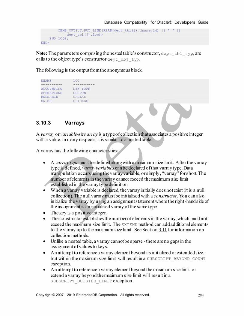
Database Compatibility for Oracle® Developers Guide
Copy right © 2007 - 2019 EnterpriseDB Corporation. All rights reserv ed.
284
DBMS_OUTPUT.PUT_LINE(RPAD(dept_tbl(j).dname,14) || ' ' ||
dept_tbl(j).loc);
END LOOP;
END;
Note: The parameters comprising the nested table’s constructor, dept_tbl_typ, are
calls to the object type’s constructor dept_obj_typ.
The following is the output from the anonymous block.
DNAME LOC
---------- ----------
ACCOUNTING NEW YORK
OPERATIONS BOSTON
RESEARCH DALLAS
SALES CHICAGO
3.10.3 Varrays
A varray or variable-size array is a type of collection that associates a positive integer with a value. In many respects, it is similar to a nested table.
A varray has the following characteristics:
A varray type must be defined along with a maximum size limit. After the varray type is defined, varray variables can be declared of that varray type. Data manipulation occurs using the varray variable, or simply , “varray” for short. The
number of elements in the varray cannot exceed the maximum size limit established in the varray type definition.
When a varray variable is declared, the varray initially does not exist (it is a null
collection). The null varray must be initialized with a constructor. You can also initialize the varray by using an assignment statement where the right-hand side of the assignment is an initialized varray of the same type.
The key is a positive integer.
The constructor establishes the number of elements in the varray, which must not
exceed the maximum size limit. The EXTEND method can add additional elements to the varray up to the maximum size limit. See Section 3.11 for information on
collection methods.
Unlike a nested table, a varray cannot be sparse - there are no gaps in the assignment of values to keys.
An attempt to reference a varray element beyond its initialized or extended size,
but within the maximum size limit will result in a SUBSCRIPT_BEYOND_COUNT exception.
An attempt to reference a varray element beyond the maximum size limit or
extend a varray beyond the maximum size limit will result in a SUBSCRIPT_OUTSIDE_LIMIT exception.

Database Compatibility for Oracle® Developers Guide
Copy right © 2007 - 2019 EnterpriseDB Corporation. All rights reserv ed.
285
The TYPE IS VARRAY statement is used to define a varray type within the declaration section of an SPL program.
TYPE varraytype IS { VARRAY | VARYING ARRAY }(maxsize)
OF { datatype | objtype };
varraytype is an identifier assigned to the varray type. datatype is a scalar data type
such as VARCHAR2 or NUMBER. maxsize is the maximum number of elements permitted in varrays of that type. objtype is a previously defined object type.
Note: The CREATE TYPE command can be used to define a varray type that is available to all SPL programs in the database. In order to make use of the varray, a variable must be declared of that varray type. The following is the syntax for declaring a varray variable.
varray varraytype
varray is an identifier assigned to the varray. varraytype is the identifier of a
previously defined varray type.
A varray is initialized using the varray type’s constructor.
varraytype ([ { expr1 | NULL } [, { expr2 | NULL } ]
[, ...] ])
varraytype is the identifier of the varray type’s constructor, which has the same name
as the varray type. expr1, expr2, … are expressions that are type-compatible with the
element type of the varray. If NULL is specified, the corresponding element is set to null. If the parameter list is empty, then an empty varray is returned, which means there are no elements in the varray. If the varray is defined from an object type, then exprn must
return an object of that object type. The object can be the return value of a function or the
return value of the object type’s constructor. The object can also be an element of another varray of the same varray type.
If a collection method other than EXISTS is applied to an uninitialized varray, a
COLLECTION_IS_NULL exception is thrown. See Section 3.11 for information on collection methods.
The following is an example of a constructor for a varray:
DECLARE
TYPE varray_typ IS VARRAY(2) OF CHAR(1);
v_varray varray_typ := varray_typ('A','B');
An element of the varray is referenced using the following syntax.
varray(n)[.element ]

Database Compatibility for Oracle® Developers Guide
Copy right © 2007 - 2019 EnterpriseDB Corporation. All rights reserv ed.
286
varray is the identifier of a previously declared varray. n is a positive integer. If the
varray type of varray is defined from an object type, then [.element ] must
reference an attribute within the object type from which the varray type is defined. Alternatively, the entire object can be referenced by omitting [.element ].
The following is an example of a varray where it is known that there will be four elements.
DECLARE
TYPE dname_varray_typ IS VARRAY(4) OF VARCHAR2(14);
dname_varray dname_varray_typ;
CURSOR dept_cur IS SELECT dname FROM dept ORDER BY dname;
i INTEGER := 0;
BEGIN
dname_varray := dname_varray_typ(NULL, NULL, NULL, NULL);
FOR r_dept IN dept_cur LOOP
i := i + 1;
dname_varray(i) := r_dept.dname;
END LOOP;
DBMS_OUTPUT.PUT_LINE('DNAME');
DBMS_OUTPUT.PUT_LINE('----------');
FOR j IN 1..i LOOP
DBMS_OUTPUT.PUT_LINE(dname_varray(j));
END LOOP;
END;
The above example produces the following output:
DNAME
----------
ACCOUNTING
OPERATIONS
RESEARCH
SALES

Database Compatibility for Oracle® Developers Guide
Copy right © 2007 - 2019 EnterpriseDB Corporation. All rights reserv ed.
287
3.11 Collection Methods
Collection methods are functions and procedures that provide useful information about a
collection that can aid in the processing of data in the collection. The following sections discuss the collection methods supported by Advanced Server.
3.11.1 COUNT
COUNT is a method that returns the number of elements in a collection. The syntax for using COUNT is as follows:
collection.COUNT
collection is the name of a collection.
For a varray, COUNT always equals LAST.
The following example shows that an associative array can be sparsely populated (i.e.,
there are “gaps” in the sequence of assigned elements). COUNT includes only the elements that have been assigned a value.
DECLARE
TYPE sparse_arr_typ IS TABLE OF NUMBER INDEX BY BINARY_INTEGER;
sparse_arr sparse_arr_typ;
BEGIN
sparse_arr(-100) := -100;
sparse_arr(-10) := -10;
sparse_arr(0) := 0;
sparse_arr(10) := 10;
sparse_arr(100) := 100;
DBMS_OUTPUT.PUT_LINE('COUNT: ' || sparse_arr.COUNT);
END;
The following output shows that there are five populated elements included in COUNT.
COUNT: 5
3.11.2 DELETE
The DELETE method deletes entries from a collection. You can call the DELETE method in three different ways.
Use the first form of the DELETE method to remove all entries from a collection:
collection.DELETE

Database Compatibility for Oracle® Developers Guide
Copy right © 2007 - 2019 EnterpriseDB Corporation. All rights reserv ed.
288
Use the second form of the DELETE method to remove the specified entry from a collection:
collection.DELETE(subscript)
Use the third form of the DELETE method to remove the entries that are within the range specified by first_subscript and last_subscript (including the entries for the first_subscript and the last_subscript) from a collection.
collection.DELETE(first_subscript, last_subscript)
If first_subscript and last_subscript refer to non-existent elements, elements
that are in the range between the specified subscripts are deleted. If first_subscript
is greater than last_subscript, or if you specify a value of NULL for one of the arguments, DELETE has no effect.
Note that when you delete an entry, the subscript remains in the collection; you can re-
use the subscript with an alternate entry. If you specify a subscript that does not exist in the call to the DELETE method, DELETE does not raise an exception.
The following example demonstrates using the DELETE method to remove the element with subscript 0 from the collection:
DECLARE
TYPE sparse_arr_typ IS TABLE OF NUMBER INDEX BY BINARY_INTEGER;
sparse_arr sparse_arr_typ;
v_results VARCHAR2(50);
v_sub NUMBER;
BEGIN
sparse_arr(-100) := -100;
sparse_arr(-10) := -10;
sparse_arr(0) := 0;
sparse_arr(10) := 10;
sparse_arr(100) := 100;
DBMS_OUTPUT.PUT_LINE('COUNT: ' || sparse_arr.COUNT);
sparse_arr.DELETE(0);
DBMS_OUTPUT.PUT_LINE('COUNT: ' || sparse_arr.COUNT);
v_sub := sparse_arr.FIRST;
WHILE v_sub IS NOT NULL LOOP
IF sparse_arr(v_sub) IS NULL THEN
v_results := v_results || 'NULL ';
ELSE
v_results := v_results || sparse_arr(v_sub) || ' ';
END IF;
v_sub := sparse_arr.NEXT(v_sub);
END LOOP;
DBMS_OUTPUT.PUT_LINE('Results: ' || v_results);
END;
COUNT: 5
COUNT: 4
Results: -100 -10 10 100

Database Compatibility for Oracle® Developers Guide
Copy right © 2007 - 2019 EnterpriseDB Corporation. All rights reserv ed.
289
COUNT indicates that before the DELETE method, there were 5 elements in the collection;
after the DELETE method was invoked, the collection contains 4 elements.
3.11.3 EXISTS
The EXISTS method verifies that a subscript exists within a collection. EXISTS returns
TRUE if the subscript exists; if the subscript does not exist, EXISTS returns FALSE. The method takes a single argument; the subscript that you are testing for. The syntax is:
collection.EXISTS(subscript)
collection is the name of the collection.
subscript is the value that you are testing for. If you specify a value of NULL, EXISTS
returns false.
The following example verifies that subscript number 10 exists within the associative array:
DECLARE
TYPE sparse_arr_typ IS TABLE OF NUMBER INDEX BY BINARY_INTEGER;
sparse_arr sparse_arr_typ;
BEGIN
sparse_arr(-100) := -100;
sparse_arr(-10) := -10;
sparse_arr(0) := 0;
sparse_arr(10) := 10;
sparse_arr(100) := 100;
DBMS_OUTPUT.PUT_LINE('The index exists: ' ||
CASE WHEN sparse_arr.exists(10) = TRUE THEN 'true' ELSE 'false' END);
END;
The index exists: true
Some collection methods raise an exception if you call them with a subscript that does
not exist within the specified collection. Rather than raising an error, the EXISTS method returns a value of FALSE.
3.11.4 EXTEND
The EXTEND method increases the size of a collection. There are three variations of the
EXTEND method. The first variation appends a single NULL element to a collection; the syntax for the first variation is:
collection.EXTEND
collection is the name of a collection.
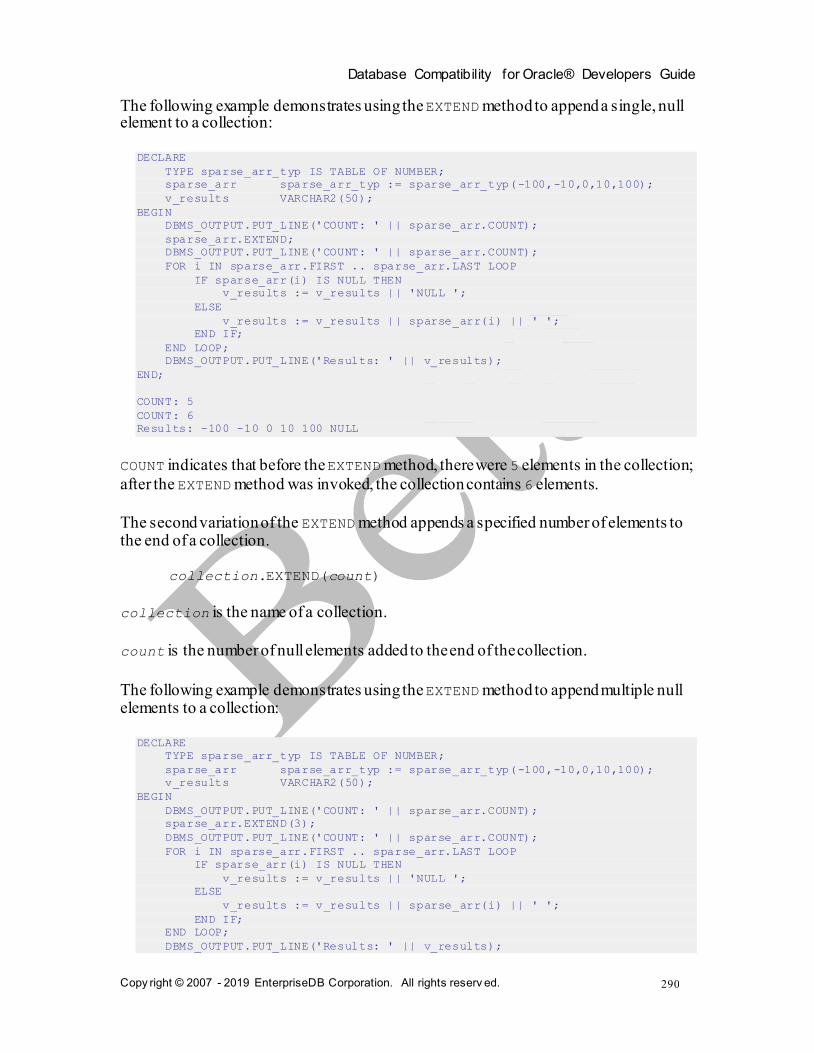
Database Compatibility for Oracle® Developers Guide
Copy right © 2007 - 2019 EnterpriseDB Corporation. All rights reserv ed.
290
The following example demonstrates using the EXTEND method to append a single, null element to a collection:
DECLARE
TYPE sparse_arr_typ IS TABLE OF NUMBER;
sparse_arr sparse_arr_typ := sparse_arr_typ(-100,-10,0,10,100);
v_results VARCHAR2(50);
BEGIN
DBMS_OUTPUT.PUT_LINE('COUNT: ' || sparse_arr.COUNT);
sparse_arr.EXTEND;
DBMS_OUTPUT.PUT_LINE('COUNT: ' || sparse_arr.COUNT);
FOR i IN sparse_arr.FIRST .. sparse_arr.LAST LOOP
IF sparse_arr(i) IS NULL THEN
v_results := v_results || 'NULL ';
ELSE
v_results := v_results || sparse_arr(i) || ' ';
END IF;
END LOOP;
DBMS_OUTPUT.PUT_LINE('Results: ' || v_results);
END;
COUNT: 5
COUNT: 6
Results: -100 -10 0 10 100 NULL
COUNT indicates that before the EXTEND method, there were 5 elements in the collection;
after the EXTEND method was invoked, the collection contains 6 elements.
The second variation of the EXTEND method appends a specified number of elements to the end of a collection.
collection.EXTEND(count)
collection is the name of a collection.
count is the number of null elements added to the end of the collection.
The following example demonstrates using the EXTEND method to append multiple null elements to a collection:
DECLARE
TYPE sparse_arr_typ IS TABLE OF NUMBER;
sparse_arr sparse_arr_typ := sparse_arr_typ(-100,-10,0,10,100);
v_results VARCHAR2(50);
BEGIN
DBMS_OUTPUT.PUT_LINE('COUNT: ' || sparse_arr.COUNT);
sparse_arr.EXTEND(3);
DBMS_OUTPUT.PUT_LINE('COUNT: ' || sparse_arr.COUNT);
FOR i IN sparse_arr.FIRST .. sparse_arr.LAST LOOP
IF sparse_arr(i) IS NULL THEN
v_results := v_results || 'NULL ';
ELSE
v_results := v_results || sparse_arr(i) || ' ';
END IF;
END LOOP;
DBMS_OUTPUT.PUT_LINE('Results: ' || v_results);

Database Compatibility for Oracle® Developers Guide
Copy right © 2007 - 2019 EnterpriseDB Corporation. All rights reserv ed.
291
END;
COUNT: 5
COUNT: 8
Results: -100 -10 0 10 100 NULL NULL NULL
COUNT indicates that before the EXTEND method, there were 5 elements in the collection;
after the EXTEND method was invoked, the collection contains 8 elements.
The third variation of the EXTEND method appends a specified number of copies of a particular element to the end of a collection.
collection.EXTEND(count, index_number)
collection is the name of a collection.
count is the number of elements added to the end of the collection.
index_number is the subscript of the element that is being copied to the collection.
The following example demonstrates using the EXTEND method to append multiple copies of the second element to the collection:
DECLARE
TYPE sparse_arr_typ IS TABLE OF NUMBER;
sparse_arr sparse_arr_typ := sparse_arr_typ(-100,-10,0,10,100);
v_results VARCHAR2(50);
BEGIN
DBMS_OUTPUT.PUT_LINE('COUNT: ' || sparse_arr.COUNT);
sparse_arr.EXTEND(3, 2);
DBMS_OUTPUT.PUT_LINE('COUNT: ' || sparse_arr.COUNT);
FOR i IN sparse_arr.FIRST .. sparse_arr.LAST LOOP
IF sparse_arr(i) IS NULL THEN
v_results := v_results || 'NULL ';
ELSE
v_results := v_results || sparse_arr(i) || ' ';
END IF;
END LOOP;
DBMS_OUTPUT.PUT_LINE('Results: ' || v_results);
END;
COUNT: 5
COUNT: 8
Results: -100 -10 0 10 100 -10 -10 -10
COUNT indicates that before the EXTEND method, there were 5 elements in the collection;
after the EXTEND method was invoked, the collection contains 8 elements.
Note: The EXTEND method cannot be used on a null or empty collection.

Database Compatibility for Oracle® Developers Guide
Copy right © 2007 - 2019 EnterpriseDB Corporation. All rights reserv ed.
292
3.11.5 FIRST
FIRST is a method that returns the subscript of the first element in a collection. The syntax for using FIRST is as follows:
collection.FIRST
collection is the name of a collection.
The following example displays the first element of the associative array.
DECLARE
TYPE sparse_arr_typ IS TABLE OF NUMBER INDEX BY BINARY_INTEGER;
sparse_arr sparse_arr_typ;
BEGIN
sparse_arr(-100) := -100;
sparse_arr(-10) := -10;
sparse_arr(0) := 0;
sparse_arr(10) := 10;
sparse_arr(100) := 100;
DBMS_OUTPUT.PUT_LINE('FIRST element: ' || sparse_arr(sparse_arr.FIRST));
END;
FIRST element: -100
3.11.6 LAST
LAST is a method that returns the subscript of the last element in a collection. The syntax for using LAST is as follows:
collection.LAST
collection is the name of a collection.
The following example displays the last element of the associative array.
DECLARE
TYPE sparse_arr_typ IS TABLE OF NUMBER INDEX BY BINARY_INTEGER;
sparse_arr sparse_arr_typ;
BEGIN
sparse_arr(-100) := -100;
sparse_arr(-10) := -10;
sparse_arr(0) := 0;
sparse_arr(10) := 10;
sparse_arr(100) := 100;
DBMS_OUTPUT.PUT_LINE('LAST element: ' || sparse_arr(sparse_arr.LAST));
END;
LAST element: 100
Database Compatibility for Oracle® Developers Guide
Copy right © 2007 - 2019 EnterpriseDB Corporation. All rights reserv ed.
293
3.11.7 LIMIT
LIMIT is a method that returns the maximum number of elements permitted in a collection. LIMIT is applicable only to varrays. The syntax for using LIMIT is as follows:
collection.LIMIT
collection is the name of a collection.
For an initialized varray, LIMIT returns the maximum size limit determined by the varray type definition. If the varray is uninitialized (that is, it is a null varray), an exception is thrown.
For an associative array or an initialized nested table, LIMIT returns NULL. If the nested table is uninitialized (that is, it is a null nested table), an exception is thrown.
3.11.8 NEXT
NEXT is a method that returns the subscript that follows a specified subscript. The
method takes a single argument; the subscript that you are testing for.
collection.NEXT(subscript)
collection is the name of the collection.
If the specified subscript is less than the first subscript in the collection, the function
returns the first subscript. If the subscript does not have a successor, NEXT returns NULL. If you specify a NULL subscript, PRIOR does not return a value.
The following example demonstrates using NEXT to return the subscript that follows subscript 10 in the associative array, sparse_arr:
DECLARE
TYPE sparse_arr_typ IS TABLE OF NUMBER INDEX BY BINARY_INTEGER;
sparse_arr sparse_arr_typ;
BEGIN
sparse_arr(-100) := -100;
sparse_arr(-10) := -10;
sparse_arr(0) := 0;
sparse_arr(10) := 10;
sparse_arr(100) := 100;
DBMS_OUTPUT.PUT_LINE('NEXT element: ' || sparse_arr.next(10));
END;
NEXT element: 100

Database Compatibility for Oracle® Developers Guide
Copy right © 2007 - 2019 EnterpriseDB Corporation. All rights reserv ed.
294
3.11.9 PRIOR
The PRIOR method returns the subscript that precedes a specified subscript in a
collection. The method takes a single argument; the subscript that you are testing for. The syntax is:
collection.PRIOR(subscript)
collection is the name of the collection.
If the subscript specified does not have a predecessor, PRIOR returns NULL. If the specified subscript is greater than the last subscript in the collection, the method returns the last subscript. If you specify a NULL subscript, PRIOR does not return a value.
The following example returns the subscript that precedes subscript 100 in the associative array, sparse_arr:
DECLARE
TYPE sparse_arr_typ IS TABLE OF NUMBER INDEX BY BINARY_INTEGER;
sparse_arr sparse_arr_typ;
BEGIN
sparse_arr(-100) := -100;
sparse_arr(-10) := -10;
sparse_arr(0) := 0;
sparse_arr(10) := 10;
sparse_arr(100) := 100;
DBMS_OUTPUT.PUT_LINE('PRIOR element: ' || sparse_arr.prior(100));
END;
PRIOR element: 10
3.11.10 TRIM
The TRIM method removes an element or elements from the end of a collection. The syntax for the TRIM method is:
collection.TRIM[(count)]
collection is the name of a collection.
count is the number of elements removed from the end of the collection. Advanced
Server will return an error if count is less than 0 or greater than the number of elements in the collection.
The following example demonstrates using the TRIM method to remove an element from the end of a collection:

Database Compatibility for Oracle® Developers Guide
Copy right © 2007 - 2019 EnterpriseDB Corporation. All rights reserv ed.
295
DECLARE
TYPE sparse_arr_typ IS TABLE OF NUMBER;
sparse_arr sparse_arr_typ := sparse_arr_typ(-100,-10,0,10,100);
BEGIN
DBMS_OUTPUT.PUT_LINE('COUNT: ' || sparse_arr.COUNT);
sparse_arr.TRIM;
DBMS_OUTPUT.PUT_LINE('COUNT: ' || sparse_arr.COUNT);
END;
COUNT: 5
COUNT: 4
COUNT indicates that before the TRIM method, there were 5 elements in the collection;
after the TRIM method was invoked, the collection contains 4 elements.
You can also specify the number of elements to remove from the end of the collection
with the TRIM method:
DECLARE
TYPE sparse_arr_typ IS TABLE OF NUMBER;
sparse_arr sparse_arr_typ := sparse_arr_typ(-100,-10,0,10,100);
v_results VARCHAR2(50);
BEGIN
DBMS_OUTPUT.PUT_LINE('COUNT: ' || sparse_arr.COUNT);
sparse_arr.TRIM(2);
DBMS_OUTPUT.PUT_LINE('COUNT: ' || sparse_arr.COUNT);
FOR i IN sparse_arr.FIRST .. sparse_arr.LAST LOOP
IF sparse_arr(i) IS NULL THEN
v_results := v_results || 'NULL ';
ELSE
v_results := v_results || sparse_arr(i) || ' ';
END IF;
END LOOP;
DBMS_OUTPUT.PUT_LINE('Results: ' || v_results);
END;
COUNT: 5
COUNT: 3
Results: -100 -10 0
COUNT indicates that before the TRIM method, there were 5 elements in the collection;
after the TRIM method was invoked, the collection contains 3 elements.

Database Compatibility for Oracle® Developers Guide
Copy right © 2007 - 2019 EnterpriseDB Corporation. All rights reserv ed.
296
3.12 Working with Collections
Collection operators allow you to transform, query and manipulate the contents of a collection.
3.12.1 TABLE()
Use the TABLE() function to transform the members of an array into a set of rows. The signature is:
TABLE(collection_value)
Where:
collection_value
collection_value is an expression that evaluates to a value of collection type.
The TABLE() function expands the nested contents of a collection into a table format. You can use the TABLE() function anywhere you use a regular table expression.
The TABLE() function returns a SETOF ANYELEMENT (a set of values of any type). For
example, if the argument passed to this function is an array of dates, TABLE() will
return a SETOF dates. If the argument passed to this function is an array of paths, TABLE() will return a SETOF paths.
You can use the TABLE() function to expand the contents of a collection into table form:
postgres=# SELECT * FROM TABLE(monthly_balance(445.00, 980.20, 552.00));
monthly_balance
----------------
445.00
980.20
552.00
(3 rows)
3.12.2 Using the MULTISET UNION Operator
The MULTISET UNION operator combines two collections to form a third collection. The signature is:
coll_1 MULTISET UNION [ ALL | DISTINCT | UNIQUE ] coll_2

Database Compatibility for Oracle® Developers Guide
Copy right © 2007 - 2019 EnterpriseDB Corporation. All rights reserv ed.
297
Where coll_1 and coll_2 specify the names of the collections to combine.
Include the ALL keyword to specify that duplicate elements (elements that are present in both coll_1 and coll_2) should be represented in the result, once for each time they
are present in the original collections. This is the default behavior of MULTISET UNION.
Include the DISTINCT or UNIQUE keyword to specify that duplicate elements should be included in the result only once. The DISTINCT and UNIQUE keywords are synonymous.
The following example demonstrates using the MULTISET UNION operator to combine
two collections (collection_1 and collection_2) into a third collection (collection_3):
DECLARE
TYPE int_arr_typ IS TABLE OF NUMBER(2);
collection_1 int_arr_typ;
collection_2 int_arr_typ;
collection_3 int_arr_typ;
v_results VARCHAR2(50);
BEGIN
collection_1 := int_arr_typ(10,20,30);
collection_2 := int_arr_typ(30,40);
collection_3 := collection_1 MULTISET UNION ALL collection_2;
DBMS_OUTPUT.PUT_LINE('COUNT: ' || collection_3.COUNT);
FOR i IN collection_3.FIRST .. collection_3.LAST LOOP
IF collection_3(i) IS NULL THEN
v_results := v_results || 'NULL ';
ELSE
v_results := v_results || collection_3(i) || ' ';
END IF;
END LOOP;
DBMS_OUTPUT.PUT_LINE('Results: ' || v_results);
END;
COUNT: 5
Results: 10 20 30 30 40
The resulting collection includes one entry for each element in collection_1 and collection_2. If the DISTINCT keyword is used, the results are as follows:
DECLARE
TYPE int_arr_typ IS TABLE OF NUMBER(2);
collection_1 int_arr_typ;
collection_2 int_arr_typ;
collection_3 int_arr_typ;
v_results VARCHAR2(50);
BEGIN
collection_1 := int_arr_typ(10,20,30);
collection_2 := int_arr_typ(30,40);
collection_3 := collection_1 MULTISET UNION DISTINCT collection_2;
DBMS_OUTPUT.PUT_LINE('COUNT: ' || collection_3.COUNT);
FOR i IN collection_3.FIRST .. collection_3.LAST LOOP
IF collection_3(i) IS NULL THEN
v_results := v_results || 'NULL ';
ELSE
v_results := v_results || collection_3(i) || ' ';

Database Compatibility for Oracle® Developers Guide
Copy right © 2007 - 2019 EnterpriseDB Corporation. All rights reserv ed.
298
END IF;
END LOOP;
DBMS_OUTPUT.PUT_LINE('Results: ' || v_results);
END;
COUNT: 4
Results: 10 20 30 40
The resulting collection includes only those members with distinct values. Note in the
following example that the MULTISET UNION DISTINCT operator also removes duplicate entries that are stored within the same collection:
DECLARE
TYPE int_arr_typ IS TABLE OF NUMBER(2);
collection_1 int_arr_typ;
collection_2 int_arr_typ;
collection_3 int_arr_typ;
v_results VARCHAR2(50);
BEGIN
collection_1 := int_arr_typ(10,20,30,30);
collection_2 := int_arr_typ(40,50);
collection_3 := collection_1 MULTISET UNION DISTINCT collection_2;
DBMS_OUTPUT.PUT_LINE('COUNT: ' || collection_3.COUNT);
FOR i IN collection_3.FIRST .. collection_3.LAST LOOP
IF collection_3(i) IS NULL THEN
v_results := v_results || 'NULL ';
ELSE
v_results := v_results || collection_3(i) || ' ';
END IF;
END LOOP;
DBMS_OUTPUT.PUT_LINE('Results: ' || v_results);
END;
COUNT: 5
Results: 10 20 30 40 50
3.12.3 Using the FORALL Statement
Collections can be used to more efficiently process DML commands by passing all the
values to be used for repetitive execution of a DELETE, INSERT, or UPDATE command in
one pass to the database server rather than re-iteratively invoking the DML command with new values. The DML command to be processed in such a manner is specified with
the FORALL statement. In addition, one or more collections are given in the DML command where different values are to be substituted each time the command is executed.
FORALL index IN lower_bound .. upper_bound
{ insert_stmt | update_stmt | delete_stmt };
index is the position in the collection given in the insert_stmt, update_stmt, or
delete_stmt DML command that iterates from the integer value given as lower_bound up to and including upper_bound.

Database Compatibility for Oracle® Developers Guide
Copy right © 2007 - 2019 EnterpriseDB Corporation. All rights reserv ed.
299
Note: If an exception occurs during any iteration of the FORALL statement, all updates
that occurred since the start of the execution of the FORALL statement are automatically rolled back. This behavior is not compatible with Oracle databases. Oracle allows explicit
use of the COMMIT or ROLLBACK commands to control whether or not to commit or roll back updates that occurred prior to the exception.
The FORALL statement creates a loop – each iteration of the loop increments the index variable (you typically use the index within the loop to select a member of a collection). The number of iterations is controlled by the lower_bound .. upper_bound clause.
The loop is executes once for each integer between the lower_bound and
upper_bound (inclusive) and the index is incremented by one for each iteration. For example:
FORALL i IN 2 .. 5
Creates a loop that executes four times – in the first iteration, the index (i) is set to the
value 2; in the second iteration, the index is set to the value 3, and so on. The loop executes for the value 5 and then terminates.
The following example creates a table (emp_copy) that is an empty copy of the emp
table. The example declares a type (emp_tbl) that is an array where each element in the array is of composite type, composed of the column definitions used to create the table,
emp. The example also creates an index on the emp_tbl type.
t_emp is an associative array, of type emp_tbl. The SELECT statement uses the BULK
COLLECT INTO command to populate the t_emp array. After the t_emp array is
populated, the FORALL statement iterates through the values (i) in the t_emp array index
and inserts a row for each record into emp_copy.
CREATE TABLE emp_copy(LIKE emp);
DECLARE
TYPE emp_tbl IS TABLE OF emp%ROWTYPE INDEX BY BINARY_INTEGER;
t_emp emp_tbl;
BEGIN
SELECT * FROM emp BULK COLLECT INTO t_emp;
FORALL i IN t_emp.FIRST .. t_emp.LAST
INSERT INTO emp_copy VALUES t_emp(i);
END;
The following example uses a FORALL statement to update the salary of three employees:
DECLARE
TYPE empno_tbl IS TABLE OF emp.empno%TYPE INDEX BY BINARY_INTEGER;
TYPE sal_tbl IS TABLE OF emp.ename%TYPE INDEX BY BINARY_INTEGER;

Database Compatibility for Oracle® Developers Guide
Copy right © 2007 - 2019 EnterpriseDB Corporation. All rights reserv ed.
300
t_empno EMPNO_TBL;
t_sal SAL_TBL;
BEGIN
t_empno(1) := 9001;
t_sal(1) := 3350.00;
t_empno(2) := 9002;
t_sal(2) := 2000.00;
t_empno(3) := 9003;
t_sal(3) := 4100.00;
FORALL i IN t_empno.FIRST..t_empno.LAST
UPDATE emp SET sal = t_sal(i) WHERE empno = t_empno(i);
END;
SELECT * FROM emp WHERE empno > 9000;
empno | ename | job | mgr | hiredate | sal | comm | deptno
-------+--------+---------+-----+----------+---------+------+--------
9001 | JONES | ANALYST | | | 3350.00 | | 40
9002 | LARSEN | CLERK | | | 2000.00 | | 40
9003 | WILSON | MANAGER | | | 4100.00 | | 40
(3 rows)
The following example deletes three employees in a FORALL statement:
DECLARE
TYPE empno_tbl IS TABLE OF emp.empno%TYPE INDEX BY BINARY_INTEGER;
t_empno EMPNO_TBL;
BEGIN
t_empno(1) := 9001;
t_empno(2) := 9002;
t_empno(3) := 9003;
FORALL i IN t_empno.FIRST..t_empno.LAST
DELETE FROM emp WHERE empno = t_empno(i);
END;
SELECT * FROM emp WHERE empno > 9000;
empno | ename | job | mgr | hiredate | sal | comm | deptno
-------+-------+-----+-----+----------+-----+------+--------
(0 rows)
3.12.4 Using the BULK COLLECT Clause
SQL commands that return a result set consisting of a large number of rows may not be
operating as efficiently as possible due to the constant context switching that must occur between the database server and the client in order to transfer the entire result set. This inefficiency can be mitigated by using a collection to gather the entire result set in
memory which the client can then access. The BULK COLLECT clause is used to specify the aggregation of the result set into a collection.
The BULK COLLECT clause can be used with the SELECT INTO, FETCH INTO and
EXECUTE IMMEDIATE commands, and with the RETURNING INTO clause of the
DELETE, INSERT, and UPDATE commands. Each of these is illustrated in the following sections.

Database Compatibility for Oracle® Developers Guide
Copy right © 2007 - 2019 EnterpriseDB Corporation. All rights reserv ed.
301
3.12.4.1 SELECT BULK COLLECT
The BULK COLLECT clause can be used with the SELECT INTO statement as follows. (Refer to Section 3.4.3 for additional information on the SELECT INTO statement.)
SELECT select_expressions BULK COLLECT INTO collection
[, ...] FROM ...;
If a single collection is specified, then collection may be a collection of a single field,
or it may be a collection of a record type. If more than one collection is specified, then each collection must consist of a single field. select_expressions must match in number, order, and type-compatibility all fields in the target collections.
The following example shows the use of the BULK COLLECT clause where the target collections are associative arrays consisting of a single field.
DECLARE
TYPE empno_tbl IS TABLE OF emp.empno%TYPE INDEX BY BINARY_INTEGER;
TYPE ename_tbl IS TABLE OF emp.ename%TYPE INDEX BY BINARY_INTEGER;
TYPE job_tbl IS TABLE OF emp.job%TYPE INDEX BY BINARY_INTEGER;
TYPE hiredate_tbl IS TABLE OF emp.hiredate%TYPE INDEX BY BINARY_INTEGER;
TYPE sal_tbl IS TABLE OF emp.sal%TYPE INDEX BY BINARY_INTEGER;
TYPE comm_tbl IS TABLE OF emp.comm%TYPE INDEX BY BINARY_INTEGER;
TYPE deptno_tbl IS TABLE OF emp.deptno%TYPE INDEX BY BINARY_INTEGER;
t_empno EMPNO_TBL;
t_ename ENAME_TBL;
t_job JOB_TBL;
t_hiredate HIREDATE_TBL;
t_sal SAL_TBL;
t_comm COMM_TBL;
t_deptno DEPTNO_TBL;
BEGIN
SELECT empno, ename, job, hiredate, sal, comm, deptno BULK COLLECT
INTO t_empno, t_ename, t_job, t_hiredate, t_sal, t_comm, t_deptno
FROM emp;
DBMS_OUTPUT.PUT_LINE('EMPNO ENAME JOB HIREDATE ' ||
'SAL ' || 'COMM DEPTNO');
DBMS_OUTPUT.PUT_LINE('----- ------- --------- --------- ' ||
'-------- ' || '-------- ------');
FOR i IN 1..t_empno.COUNT LOOP
DBMS_OUTPUT.PUT_LINE(t_empno(i) || ' ' ||
RPAD(t_ename(i),8) || ' ' ||
RPAD(t_job(i),10) || ' ' ||
TO_CHAR(t_hiredate(i),'DD-MON-YY') || ' ' ||
TO_CHAR(t_sal(i),'99,999.99') || ' ' ||
TO_CHAR(NVL(t_comm(i),0),'99,999.99') || ' ' ||
t_deptno(i));
END LOOP;
END;
EMPNO ENAME JOB HIREDATE SAL COMM DEPTNO
----- ------- --------- --------- -------- -------- ------
7369 SMITH CLERK 17-DEC-80 800.00 .00 20
7499 ALLEN SALESMAN 20-FEB-81 1,600.00 300.00 30
7521 WARD SALESMAN 22-FEB-81 1,250.00 500.00 30
7566 JONES MANAGER 02-APR-81 2,975.00 .00 20
7654 MARTIN SALESMAN 28-SEP-81 1,250.00 1,400.00 30

Database Compatibility for Oracle® Developers Guide
Copy right © 2007 - 2019 EnterpriseDB Corporation. All rights reserv ed.
302
7698 BLAKE MANAGER 01-MAY-81 2,850.00 .00 30
7782 CLARK MANAGER 09-JUN-81 2,450.00 .00 10
7788 SCOTT ANALYST 19-APR-87 3,000.00 .00 20
7839 KING PRESIDENT 17-NOV-81 5,000.00 .00 10
7844 TURNER SALESMAN 08-SEP-81 1,500.00 .00 30
7876 ADAMS CLERK 23-MAY-87 1,100.00 .00 20
7900 JAMES CLERK 03-DEC-81 950.00 .00 30
7902 FORD ANALYST 03-DEC-81 3,000.00 .00 20
7934 MILLER CLERK 23-JAN-82 1,300.00 .00 10
The following example produces the same result, but uses an associative array on a
record type defined with the %ROWTYPE attribute.
DECLARE
TYPE emp_tbl IS TABLE OF emp%ROWTYPE INDEX BY BINARY_INTEGER;
t_emp EMP_TBL;
BEGIN
SELECT * BULK COLLECT INTO t_emp FROM emp;
DBMS_OUTPUT.PUT_LINE('EMPNO ENAME JOB HIREDATE ' ||
'SAL ' || 'COMM DEPTNO');
DBMS_OUTPUT.PUT_LINE('----- ------- --------- --------- ' ||
'-------- ' || '-------- ------');
FOR i IN 1..t_emp.COUNT LOOP
DBMS_OUTPUT.PUT_LINE(t_emp(i).empno || ' ' ||
RPAD(t_emp(i).ename,8) || ' ' ||
RPAD(t_emp(i).job,10) || ' ' ||
TO_CHAR(t_emp(i).hiredate,'DD-MON-YY') || ' ' ||
TO_CHAR(t_emp(i).sal,'99,999.99') || ' ' ||
TO_CHAR(NVL(t_emp(i).comm,0),'99,999.99') || ' ' ||
t_emp(i).deptno);
END LOOP;
END;
EMPNO ENAME JOB HIREDATE SAL COMM DEPTNO
----- ------- --------- --------- -------- -------- ------
7369 SMITH CLERK 17-DEC-80 800.00 .00 20
7499 ALLEN SALESMAN 20-FEB-81 1,600.00 300.00 30
7521 WARD SALESMAN 22-FEB-81 1,250.00 500.00 30
7566 JONES MANAGER 02-APR-81 2,975.00 .00 20
7654 MARTIN SALESMAN 28-SEP-81 1,250.00 1,400.00 30
7698 BLAKE MANAGER 01-MAY-81 2,850.00 .00 30
7782 CLARK MANAGER 09-JUN-81 2,450.00 .00 10
7788 SCOTT ANALYST 19-APR-87 3,000.00 .00 20
7839 KING PRESIDENT 17-NOV-81 5,000.00 .00 10
7844 TURNER SALESMAN 08-SEP-81 1,500.00 .00 30
7876 ADAMS CLERK 23-MAY-87 1,100.00 .00 20
7900 JAMES CLERK 03-DEC-81 950.00 .00 30
7902 FORD ANALYST 03-DEC-81 3,000.00 .00 20
7934 MILLER CLERK 23-JAN-82 1,300.00 .00 10
3.12.4.2 FETCH BULK COLLECT
The BULK COLLECT clause can be used with a FETCH statement. (See Section 3.8.3 for
information on the FETCH statement.) Instead of returning a single row at a time from the
result set, the FETCH BULK COLLECT will return all rows at once from the result set into the specified collection unless restricted by the LIMIT clause.

Database Compatibility for Oracle® Developers Guide
Copy right © 2007 - 2019 EnterpriseDB Corporation. All rights reserv ed.
303
FETCH name BULK COLLECT INTO collection [, ...] [ LIMIT n ];
If a single collection is specified, then collection may be a collection of a single field,
or it may be a collection of a record type. If more than one collection is specified, then each collection must consist of a single field. The expressions in the SELECT list of
the cursor identified by name must match in number, order, and type-compatibility all
fields in the target collections. If LIMIT n is specified, the number of rows returned into the collection on each FETCH will not exceed n.
The following example uses the FETCH BULK COLLECT statement to retrieve rows into an associative array.
DECLARE
TYPE emp_tbl IS TABLE OF emp%ROWTYPE INDEX BY BINARY_INTEGER;
t_emp EMP_TBL;
CURSOR emp_cur IS SELECT * FROM emp;
BEGIN
OPEN emp_cur;
FETCH emp_cur BULK COLLECT INTO t_emp;
CLOSE emp_cur;
DBMS_OUTPUT.PUT_LINE('EMPNO ENAME JOB HIREDATE ' ||
'SAL ' || 'COMM DEPTNO');
DBMS_OUTPUT.PUT_LINE('----- ------- --------- --------- ' ||
'-------- ' || '-------- ------');
FOR i IN 1..t_emp.COUNT LOOP
DBMS_OUTPUT.PUT_LINE(t_emp(i).empno || ' ' ||
RPAD(t_emp(i).ename,8) || ' ' ||
RPAD(t_emp(i).job,10) || ' ' ||
TO_CHAR(t_emp(i).hiredate,'DD-MON-YY') || ' ' ||
TO_CHAR(t_emp(i).sal,'99,999.99') || ' ' ||
TO_CHAR(NVL(t_emp(i).comm,0),'99,999.99') || ' ' ||
t_emp(i).deptno);
END LOOP;
END;
EMPNO ENAME JOB HIREDATE SAL COMM DEPTNO
----- ------- --------- --------- -------- -------- ------
7369 SMITH CLERK 17-DEC-80 800.00 .00 20
7499 ALLEN SALESMAN 20-FEB-81 1,600.00 300.00 30
7521 WARD SALESMAN 22-FEB-81 1,250.00 500.00 30
7566 JONES MANAGER 02-APR-81 2,975.00 .00 20
7654 MARTIN SALESMAN 28-SEP-81 1,250.00 1,400.00 30
7698 BLAKE MANAGER 01-MAY-81 2,850.00 .00 30
7782 CLARK MANAGER 09-JUN-81 2,450.00 .00 10
7788 SCOTT ANALYST 19-APR-87 3,000.00 .00 20
7839 KING PRESIDENT 17-NOV-81 5,000.00 .00 10
7844 TURNER SALESMAN 08-SEP-81 1,500.00 .00 30
7876 ADAMS CLERK 23-MAY-87 1,100.00 .00 20
7900 JAMES CLERK 03-DEC-81 950.00 .00 30
7902 FORD ANALYST 03-DEC-81 3,000.00 .00 20
7934 MILLER CLERK 23-JAN-82 1,300.00 .00 10

Database Compatibility for Oracle® Developers Guide
Copy right © 2007 - 2019 EnterpriseDB Corporation. All rights reserv ed.
304
3.12.4.3 EXECUTE IMMEDIATE BULK COLLECT
The BULK COLLECT clause can be used with a EXECUTE IMMEDIATE statement to specify a collection to receive the returned rows.
EXECUTE IMMEDIATE 'sql_expression;'
BULK COLLECT INTO collection [,...]
[USING {[bind_type] bind_argument} [, ...]}];
collection specifies the name of a collection.
bind_type specifies the parameter mode of the bind_argument.
A bind_type of IN specifies that the bind_argument contains a value that is passed to the sql_expression.
A bind_type of OUT specifies that the bind_argument receives a value from the sql_expression.
A bind_type of IN OUT specifies that the bind_argument is passed to sql_expression, and then stores the value returned by sql_expression.
bind_argument specifies a parameter that contains a value that is either passed to the
sql_expression (specified with a bind_type of IN), or that receives a value from the
sql_expression (specified with a bind_type of OUT), or both (specified with a bind_type of IN OUT).
If a single collection is specified, then collection may be a collection of a single field,
or a collection of a record type; if more than one collection is specified, each collection must consist of a single field.
3.12.4.4 RETURNING BULK COLLECT
The BULK COLLECT clause can be added to the RETURNING INTO clause of a DELETE,
INSERT, or UPDATE command. (See Section 3.4.7 for information on the RETURNING INTO clause.)
{ insert | update | delete }
RETURNING { * | expr_1 [, expr_2 ] ...}
BULK COLLECT INTO collection [, ...];
insert, update, and delete are the INSERT, UPDATE, and DELETE commands as
described in Sections 3.4.4, 3.4.5, and 3.4.6, respectively. If a single collection is specified, then collection may be a collection of a single field, or it may be a
collection of a record type. If more than one collection is specified , then each

Database Compatibility for Oracle® Developers Guide
Copy right © 2007 - 2019 EnterpriseDB Corporation. All rights reserv ed.
305
collection must consist of a single field. The expressions following the RETURNING
keyword must match in number, order, and type-compatibility all fields in the target
collections. If * is specified, then all columns in the affected table are returned. (Note that
the use of * is an Advanced Server extension and is not compatible with Oracle databases.)
The clerkemp table created by copying the emp table is used in the remaining examples in this section as shown below.
CREATE TABLE clerkemp AS SELECT * FROM emp WHERE job = 'CLERK';
SELECT * FROM clerkemp;
empno | ename | job | mgr | hiredate | sal | comm | deptno
-------+--------+-------+------+--------------------+---------+------+-------
-
7369 | SMITH | CLERK | 7902 | 17-DEC-80 00:00:00 | 800.00 | | 20
7876 | ADAMS | CLERK | 7788 | 23-MAY-87 00:00:00 | 1100.00 | | 20
7900 | JAMES | CLERK | 7698 | 03-DEC-81 00:00:00 | 950.00 | | 30
7934 | MILLER | CLERK | 7782 | 23-JAN-82 00:00:00 | 1300.00 | | 10
(4 rows)
The following example increases everyone’s salary by 1.5, stores the employees’
numbers, names, and new salaries in three associative arrays, and finally, displays the contents of these arrays.
DECLARE
TYPE empno_tbl IS TABLE OF emp.empno%TYPE INDEX BY BINARY_INTEGER;
TYPE ename_tbl IS TABLE OF emp.ename%TYPE INDEX BY BINARY_INTEGER;
TYPE sal_tbl IS TABLE OF emp.sal%TYPE INDEX BY BINARY_INTEGER;
t_empno EMPNO_TBL;
t_ename ENAME_TBL;
t_sal SAL_TBL;
BEGIN
UPDATE clerkemp SET sal = sal * 1.5 RETURNING empno, ename, sal
BULK COLLECT INTO t_empno, t_ename, t_sal;
DBMS_OUTPUT.PUT_LINE('EMPNO ENAME SAL ');
DBMS_OUTPUT.PUT_LINE('----- ------- -------- ');
FOR i IN 1..t_empno.COUNT LOOP
DBMS_OUTPUT.PUT_LINE(t_empno(i) || ' ' || RPAD(t_ename(i),8) ||
' ' || TO_CHAR(t_sal(i),'99,999.99'));
END LOOP;
END;
EMPNO ENAME SAL
----- ------- --------
7369 SMITH 1,200.00
7876 ADAMS 1,650.00
7900 JAMES 1,425.00
7934 MILLER 1,950.00
The following example performs the same functionality as the previous example, but uses
a single collection defined with a record type to store the employees’ numbers, names, and new salaries.
DECLARE

Database Compatibility for Oracle® Developers Guide
Copy right © 2007 - 2019 EnterpriseDB Corporation. All rights reserv ed.
306
TYPE emp_rec IS RECORD (
empno emp.empno%TYPE,
ename emp.ename%TYPE,
sal emp.sal%TYPE
);
TYPE emp_tbl IS TABLE OF emp_rec INDEX BY BINARY_INTEGER;
t_emp EMP_TBL;
BEGIN
UPDATE clerkemp SET sal = sal * 1.5 RETURNING empno, ename, sal
BULK COLLECT INTO t_emp;
DBMS_OUTPUT.PUT_LINE('EMPNO ENAME SAL ');
DBMS_OUTPUT.PUT_LINE('----- ------- -------- ');
FOR i IN 1..t_emp.COUNT LOOP
DBMS_OUTPUT.PUT_LINE(t_emp(i).empno || ' ' ||
RPAD(t_emp(i).ename,8) || ' ' ||
TO_CHAR(t_emp(i).sal,'99,999.99'));
END LOOP;
END;
EMPNO ENAME SAL
----- ------- --------
7369 SMITH 1,200.00
7876 ADAMS 1,650.00
7900 JAMES 1,425.00
7934 MILLER 1,950.00
The following example deletes all rows from the clerkemp table, and returns information on the deleted rows into an associative array, which is then displayed.
DECLARE
TYPE emp_rec IS RECORD (
empno emp.empno%TYPE,
ename emp.ename%TYPE,
job emp.job%TYPE,
hiredate emp.hiredate%TYPE,
sal emp.sal%TYPE,
comm emp.comm%TYPE,
deptno emp.deptno%TYPE
);
TYPE emp_tbl IS TABLE OF emp_rec INDEX BY BINARY_INTEGER;
r_emp EMP_TBL;
BEGIN
DELETE FROM clerkemp RETURNING empno, ename, job, hiredate, sal,
comm, deptno BULK COLLECT INTO r_emp;
DBMS_OUTPUT.PUT_LINE('EMPNO ENAME JOB HIREDATE ' ||
'SAL ' || 'COMM DEPTNO');
DBMS_OUTPUT.PUT_LINE('----- ------- --------- --------- ' ||
'-------- ' || '-------- ------');
FOR i IN 1..r_emp.COUNT LOOP
DBMS_OUTPUT.PUT_LINE(r_emp(i).empno || ' ' ||
RPAD(r_emp(i).ename,8) || ' ' ||
RPAD(r_emp(i).job,10) || ' ' ||
TO_CHAR(r_emp(i).hiredate,'DD-MON-YY') || ' ' ||
TO_CHAR(r_emp(i).sal,'99,999.99') || ' ' ||
TO_CHAR(NVL(r_emp(i).comm,0),'99,999.99') || ' ' ||
r_emp(i).deptno);
END LOOP;
END;
EMPNO ENAME JOB HIREDATE SAL COMM DEPTNO
----- ------- --------- --------- -------- -------- ------
7369 SMITH CLERK 17-DEC-80 1,200.00 .00 20

Database Compatibility for Oracle® Developers Guide
Copy right © 2007 - 2019 EnterpriseDB Corporation. All rights reserv ed.
307
7876 ADAMS CLERK 23-MAY-87 1,650.00 .00 20
7900 JAMES CLERK 03-DEC-81 1,425.00 .00 30
7934 MILLER CLERK 23-JAN-82 1,950.00 .00 10
3.13 Errors and Messages
Use the DBMS_OUTPUT.PUT_LINE statement to report messages.
DBMS_OUTPUT.PUT_LINE ( message );
message is any expression evaluating to a string.
This example displays the message on the user’s output display:
DBMS_OUTPUT.PUT_LINE('My name is John');
The special variables SQLCODE and SQLERRM contain a numeric code and a text message,
respectively, that describe the outcome of the last SQL command issued. If any other error occurs in the program such as division by zero, these variables contain information pertaining to the error.

Database Compatibility for Oracle® Developers Guide
Copy right © 2007 - 2019 EnterpriseDB Corporation. All rights reserv ed.
308
4 Triggers
This chapter describes Advanced Server triggers. As with procedures and functions, triggers are written in the SPL language.
4.1 Overview
A trigger is a named SPL code block that is associated with a table and stored in the database. When a specified event occurs on the associated table, the SPL code block is executed. The trigger is said to be fired when the code block is executed.
The event that causes a trigger to fire can be any combination of an insert, update, or deletion carried out on the table, either directly or indirectly. If the table is the object of a
SQL INSERT, UPDATE, DELETE, or TRUNCATE command the trigger is directly fired
assuming that the corresponding insert, update, delete, or truncate event is defined as a
triggering event. The events that fire the trigger are defined in the CREATE TRIGGER command.
A trigger can be fired indirectly if a triggering event occurs on the table as a result of an event initiated on another table. For example, if a trigger is defined on a table containing
a foreign key defined with the ON DELETE CASCADE clause and a row in the parent table is deleted, all children of the parent would be deleted as well. If deletion is a triggering event on the child table, deletion of the children will cause the trigger to fire.

Database Compatibility for Oracle® Developers Guide
Copy right © 2007 - 2019 EnterpriseDB Corporation. All rights reserv ed.
309
4.2 Types of Triggers
Advanced Server supports both row-level and statement-level triggers. A row-level
trigger fires once for each row that is affected by a triggering event. For example, if
deletion is defined as a triggering event on a table and a single DELETE command is issued that deletes five rows from the table, then the trigger will fire five times, once for each row.
In contrast, a statement-level trigger fires once per triggering statement regardless of the
number of rows affected by the triggering event. In the prior example of a single DELETE command deleting five rows, a s tatement-level trigger would fire only once.
The sequence of actions can be defined regarding whether the trigger code block is executed before or after the triggering statement, itself, in the case of statement-level
triggers; or before or after each row is affected by the triggering statement in the case of row-level triggers.
In a before row-level trigger, the trigger code block is executed before the triggering action is carried out on each affected row. In a before statement-level trigger, the trigger code block is executed before the action of the triggering statement is carried out.
In an after row-level trigger, the trigger code block is executed after the triggering action is carried out on each affected row. In an after statement-level trigger, the trigger code block is executed after the action of the triggering statement is carried out.
In a compound trigger, a statement-level and a row-level trigger can be defined in a
single trigger and can be fired at more than one timing point see, Section 4.6 for information about compound triggers.

Database Compatibility for Oracle® Developers Guide
Copy right © 2007 - 2019 EnterpriseDB Corporation. All rights reserv ed.
310
4.3 Creating Triggers
The CREATE TRIGGER command defines and names a trigger that will be stored in the database.
Name
CREATE TRIGGER -- define a simple trigger
Synopsis
CREATE [ OR REPLACE ] TRIGGER name
{ BEFORE | AFTER | INSTEAD OF }
{ INSERT | UPDATE | DELETE | TRUNCATE }
[ OR { INSERT | UPDATE | DELETE | TRUNCATE } ] [, ...]
ON table
[ REFERENCING { OLD AS old | NEW AS new } ...]
[ FOR EACH ROW ]
[ WHEN condition ]
[ DECLARE
[ PRAGMA AUTONOMOUS_TRANSACTION; ]
declaration; [, ...] ]
BEGIN
statement; [, ...]
[ EXCEPTION
{ WHEN exception [ OR exception ] [...] THEN
statement; [, ...] } [, ...]
]
END
Name
CREATE TRIGGER -- define a compound trigger
Synopsis
CREATE [ OR REPLACE ] TRIGGER name
FOR { INSERT | UPDATE | DELETE | TRUNCATE }
[ OR { INSERT | UPDATE | DELETE | TRUNCATE } ] [, ...]
ON table
[ REFERENCING { OLD AS old | NEW AS new } ...]
[ WHEN condition ]
COMPOUND TRIGGER
[ private_declaration; ] ...
[ procedure_or_function_definition ] ...
compound_trigger_definition
END

Database Compatibility for Oracle® Developers Guide
Copy right © 2007 - 2019 EnterpriseDB Corporation. All rights reserv ed.
311
Where private_declaration is an identifier of a private variable that can be
accessed by any procedure or function. There can be zero, one, or more private variables. private_declaration can be any of the following:
Variable Declaration
Record Declaration
Collection Declaration
REF CURSOR and Cursor Variable Declaration
TYPE Definitions for Records, Collections, and REF CURSORs
Exception Object Variable Declaration
Where procedure_or_function_definition :=
procedure_definition | function_definition
Where procedure_definition :=
PROCEDURE proc_name[ argument_list ]
[ options_list ]
{ IS | AS }
procedure_body
END [ proc_name ] ;
Where procedure_body :=
[ declaration; ] [, ...]
BEGIN
statement; [...]
[ EXCEPTION
{ WHEN exception [OR exception] [...]] THEN statement; }
[...]
]
Where function_definition :=
FUNCTION func_name [ argument_list ]
RETURN rettype [ DETERMINISTIC ]
[ options_list ]
{ IS | AS }
function_body
END [ func_name ] ;
Where function_body :=
[ declaration; ] [, ...]
BEGIN
statement; [...]
Database Compatibility for Oracle® Developers Guide
Copy right © 2007 - 2019 EnterpriseDB Corporation. All rights reserv ed.
312
[ EXCEPTION
{ WHEN exception [ OR exception ] [...] THEN statement; }
[...]
]
Where compound_trigger_definition is:
{ compound_trigger_event } { IS | AS }
compound_trigger_body
END [ compound_trigger_event ] [ ... ]
Where compound_trigger_event :=
[ BEFORE STATEMENT | BEFORE EACH ROW | AFTER EACH ROW |
AFTER STATEMENT | INSTEAD OF EACH ROW ]
Where compound_trigger_body :=
[ declaration; ] [, ...]
BEGIN
statement; [...]
[ EXCEPTION
{ WHEN exception [OR exception] [...] THEN statement; }
[...]
]
Description
CREATE TRIGGER defines a new trigger. CREATE OR REPLACE TRIGGER will either create a new trigger, or replace an existing definition.
If you are using the CREATE TRIGGER keywords to create a new trigger, the name of the new trigger must not match any existing trigger defined on the same table. New triggers will be created in the same schema as the table on which the triggering event is defined.
If you are updating the definition of an existing trigger, use the CREATE OR REPLACE TRIGGER keywords.
When you use syntax compatible with Oracle databases to create a trigger, the trigger
runs as a SECURITY DEFINER function.
Parameters
name
The name of the trigger to create.
BEFORE | AFTER

Database Compatibility for Oracle® Developers Guide
Copy right © 2007 - 2019 EnterpriseDB Corporation. All rights reserv ed.
313
Determines whether the trigger is fired before or after the triggering event.
INSTEAD OF
INSTEAD OF trigger modifies an updatable view; the trigger will execute to
update the underlying table(s) appropriately. The INSTEAD OF trigger is executed for each row of the view that is updated or modified.
INSERT | UPDATE | DELETE | TRUNCATE
Defines the triggering event.
table
The name of the table or view on which the triggering event occurs.
condition
condition is a Boolean expression that determines if the trigger will actually be executed; if condition evaluates to TRUE, the trigger will fire.
If the trigger definition includes the FOR EACH ROW keywords, the WHEN clause can refer to columns of the old and/or new row values by writing
OLD.column_name or NEW.column_name respectively. INSERT triggers cannot
refer to OLD and DELETE triggers cannot refer to NEW.
If the trigger includes the INSTEAD OF keywords, it may not include a WHEN clause.
WHEN clauses cannot contain subqueries.
REFERENCING { OLD AS old | NEW AS new } ...
REFERENCING clause to reference old rows and new rows, but restricted in that old may only be replaced by an identifier named old or any equivalent that is
saved in all lowercase (for example, REFERENCING OLD AS old, REFERENCING OLD AS OLD, or REFERENCING OLD AS "old"). Also, new
may only be replaced by an identifier named new or any equivalent that is saved
in all lowercase (for example, REFERENCING NEW AS new, REFERENCING NEW AS NEW, or REFERENCING NEW AS "new").
Either one, or both phrases OLD AS old and NEW AS new may be specified in
the REFERENCING clause (for example, REFERENCING NEW AS New OLD AS Old).

Database Compatibility for Oracle® Developers Guide
Copy right © 2007 - 2019 EnterpriseDB Corporation. All rights reserv ed.
314
See Section 3.4 for information on how these identifiers are used as pseudo-record names to reference old rows and new rows.
This clause is not compatible with Oracle databases in that identifiers other than
old or new may not be used.
FOR EACH ROW
Determines whether the trigger should be fired once for every row affected by the triggering event, or just once per SQL statement. If specified, the trigger is fired
once for every affected row (row-level trigger), otherwise the trigger is a statement-level trigger.
PRAGMA AUTONOMOUS_TRANSACTION
PRAGMA AUTONOMOUS_TRANSACTION is the directive that sets the trigger as an autonomous transaction.
declaration
A variable, type, REF CURSOR, or subprogram declaration. If subprogram declarations are included, they must be declared after all other variable, type, and
REF CURSOR declarations.
statement
An SPL program statement. Note that a DECLARE - BEGIN - END block is considered an SPL statement unto itself. Thus, the trigger body may contain nested blocks.
exception
An exception condition name such as NO_DATA_FOUND, OTHERS, etc.

Database Compatibility for Oracle® Developers Guide
Copy right © 2007 - 2019 EnterpriseDB Corporation. All rights reserv ed.
315
4.4 Trigger Variables
In the trigger code block, several special variables are available for use.
NEW
NEW is a pseudo-record name that refers to the new table row for insert and update
operations in row-level triggers. This variable is not applicable in statement-level triggers and in delete operations of row-level triggers.
Its usage is: :NEW.column where column is the name of a column in the table on which the trigger is defined.
The initial content of :NEW.column is the value in the named column of the new
row to be inserted or of the new row that is to replace the old one when used in a
before row-level trigger. When used in an after row-level trigger, this value has already been stored in the table since the action has already occurred on the affected row.
In the trigger code block, :NEW.column can be used like any other variable. If a
value is assigned to :NEW.column, in the code block of a before row-level trigger, the assigned value will be used in the new inserted or updated row.
OLD
OLD is a pseudo-record name that refers to the old table row for update and delete operations in row-level triggers. This variable is not applicable in statement-level triggers and in insert operations of row-level triggers.
Its usage is: :OLD.column where column is the name of a column in the table on which the trigger is defined.
The initial content of :OLD.column is the value in the named column of the row
to be deleted or of the old row that is to be replaced by the new one when used in a before row-level trigger. When used in an after row-level trigger, this value is
no longer stored in the table since the action has already occurred on the affected row.
In the trigger code block, :OLD.column can be used like any other variable. Assigning a value to :OLD.column, has no effect on the action of the trigger.

Database Compatibility for Oracle® Developers Guide
Copy right © 2007 - 2019 EnterpriseDB Corporation. All rights reserv ed.
316
INSERTING
INSERTING is a conditional expression that returns TRUE if an insert operation
fired the trigger, otherwise it returns FALSE.
UPDATING
UPDATING is a conditional expression that returns TRUE if an update operation
fired the trigger, otherwise it returns FALSE.
DELETING
DELETING is a conditional expression that returns TRUE if a delete operation fired the trigger, otherwise it returns FALSE.

Database Compatibility for Oracle® Developers Guide
Copy right © 2007 - 2019 EnterpriseDB Corporation. All rights reserv ed.
317
4.5 Transactions and Exceptions
A trigger is always executed as part of the same transaction within which the triggering
statement is executing. When no exceptions occur within the trigger code block, the effects of any triggering commands within the trigger are committed if and only if the transaction containing the triggering statement is committed. Therefore, if the transaction
is rolled back, the effects of any triggering commands within the trigger are also rolled back.
If an exception does occur within the trigger code block, but it is caught and handled in an exception section, the effects of any triggering commands within the trigger are still
rolled back nonetheless. The triggering statement itself, however, is not rolled back unless the application forces a roll back of the encapsulating transaction.
If an unhandled exception occurs within the trigger code block, the transaction that
encapsulates the trigger is aborted and rolled back. Therefore, the effects of any triggering commands within the trigger and the triggering statement, itself are all rolled back.

Database Compatibility for Oracle® Developers Guide
Copy right © 2007 - 2019 EnterpriseDB Corporation. All rights reserv ed.
318
4.6 Compound Triggers
Advanced Server has added compatible syntax to support compound triggers. A
compound trigger combines all the triggering timings under one trigger body that can be invoked at one or more timing points. A timing point is a point in time related to a
triggering statement (an INSERT, UPDATE, DELETE or TRUNCATE statement that modifies data). The supported timing points are:
BEFORE STATEMENT: Before the triggering statement executes.
BEFORE EACH ROW: Before each row that the triggering statement affects.
AFTER EACH ROW: After each row that the triggering statement affects.
AFTER STATEMENT: After the triggering statement executes.
INSTEAD OF EACH ROW: Trigger fires once for every row affected by the triggering statement.
A compound trigger may include any combination of timing points defined in a single trigger.
The optional declaration section in a compound trigger allows you to declare trigger-level variables and subprograms. The content of the declaration is accessible to all timing points referenced by the trigger definition. The variables and subprograms created by the declaration persist only for the duration of the triggering statement.
A compound trigger contains a declaration, followed by a PL block for each timing point:
CREATE OR REPLACE TRIGGER compound_trigger_name
FOR INSERT OR UPDATE OR DELETE ON table_name
COMPOUND TRIGGER
-- Global Declaration Section (optional)
-- Variables declared here can be used inside any timing-point blocks.
BEFORE STATEMENT IS
BEGIN
NULL;
END BEFORE STATEMENT;
BEFORE EACH ROW IS
BEGIN
NULL;
END BEFORE EACH ROW;
AFTER EACH ROW IS
BEGIN
NULL;
END AFTER EACH ROW;
AFTER STATEMENT IS
BEGIN
NULL;
END AFTER STATEMENT;

Database Compatibility for Oracle® Developers Guide
Copy right © 2007 - 2019 EnterpriseDB Corporation. All rights reserv ed.
319
END compound_trigger_name;
/
Trigger created.
Note: It is not mandatory to have all the four timing blocks; you can create a compound trigger for any of the required timing-points.
A Compound Trigger has the following restrictions:
A compound trigger body is comprised of a compound trigger block.
A compound trigger can be defined on a table or a view.
Exceptions are non-transferable to other timing-point section and must be handled separately in that section only by each compound trigger block.
If a GOTO statement is specified in a timing-point section, then the target of the GOTO statement must also be specified in the same timing-point section.
:OLD and :NEW variable identifiers cannot exist in the declarative section, the BEFORE STATEMENT section, or the AFTER STATEMENT section.
:NEW values can only be modified by the BEFORE EACH ROW block.
The sequence of compound trigger timing-point execution is specific, but if a simple trigger exists within the same timing-point then the simple trigger is fired first, followed by the firing of compound triggers.

Database Compatibility for Oracle® Developers Guide
Copy right © 2007 - 2019 EnterpriseDB Corporation. All rights reserv ed.
320
4.7 Trigger Examples
The following sections illustrate an example of each type of trigger.
4.7.1 Before Statement-Level Trigger
The following is an example of a simple before statement-level trigger that displays a
message prior to an insert operation on the emp table.
CREATE OR REPLACE TRIGGER emp_alert_trig
BEFORE INSERT ON emp
BEGIN
DBMS_OUTPUT.PUT_LINE('New employees are about to be added');
END;
The following INSERT is constructed so that several new rows are inserted upon a single execution of the command. For each row that has an employee id between 7900 and
7999, a new row is inserted with an employee id incremented by 1000. The following are the results of executing the command when three new rows are inserted.
INSERT INTO emp (empno, ename, deptno) SELECT empno + 1000, ename, 40
FROM emp WHERE empno BETWEEN 7900 AND 7999;
New employees are about to be added
SELECT empno, ename, deptno FROM emp WHERE empno BETWEEN 8900 AND 8999;
EMPNO ENAME DEPTNO
---------- ---------- ----------
8900 JAMES 40
8902 FORD 40
8934 MILLER 40
The message, New employees are about to be added , is displayed once by the firing of the trigger even though the result is the addition of three new rows.
4.7.2 After Statement-Level Trigger
The following is an example of an after statement-level trigger. Whenever an insert,
update, or delete operation occurs on the emp table, a row is added to the empauditlog table recording the date, user, and action.
CREATE TABLE empauditlog (
audit_date DATE,
audit_user VARCHAR2(20),
audit_desc VARCHAR2(20)
);
CREATE OR REPLACE TRIGGER emp_audit_trig
AFTER INSERT OR UPDATE OR DELETE ON emp
DECLARE
v_action VARCHAR2(20);
BEGIN

Database Compatibility for Oracle® Developers Guide
Copy right © 2007 - 2019 EnterpriseDB Corporation. All rights reserv ed.
321
IF INSERTING THEN
v_action := 'Added employee(s)';
ELSIF UPDATING THEN
v_action := 'Updated employee(s)';
ELSIF DELETING THEN
v_action := 'Deleted employee(s)';
END IF;
INSERT INTO empauditlog VALUES (SYSDATE, USER,
v_action);
END;
In the following sequence of commands, two rows are inserted into the emp table using
two INSERT commands. The sal and comm columns of both rows are updated with one UPDATE command. Finally, both rows are deleted with one DELETE command.
INSERT INTO emp VALUES (9001,'SMITH','ANALYST',7782,SYSDATE,NULL,NULL,10);
INSERT INTO emp VALUES (9002,'JONES','CLERK',7782,SYSDATE,NULL,NULL,10);
UPDATE emp SET sal = 4000.00, comm = 1200.00 WHERE empno IN (9001, 9002);
DELETE FROM emp WHERE empno IN (9001, 9002);
SELECT TO_CHAR(AUDIT_DATE,'DD-MON-YY HH24:MI:SS') AS "AUDIT DATE",
audit_user, audit_desc FROM empauditlog ORDER BY 1 ASC;
AUDIT DATE AUDIT_USER AUDIT_DESC
------------------ -------------------- --------------------
31-MAR-05 14:59:48 SYSTEM Added employee(s)
31-MAR-05 15:00:07 SYSTEM Added employee(s)
31-MAR-05 15:00:19 SYSTEM Updated employee(s)
31-MAR-05 15:00:34 SYSTEM Deleted employee(s)
The contents of the empauditlog table show how many times the trigger was fired -
once each for the two inserts, once for the update (even though two rows were changed) and once for the deletion (even though two rows were deleted).
4.7.3 Before Row-Level Trigger
The following example is a before row-level trigger that calculates the commission of
every new employee belonging to department 30 that is inserted into the emp table.
CREATE OR REPLACE TRIGGER emp_comm_trig
BEFORE INSERT ON emp
FOR EACH ROW
BEGIN
IF :NEW.deptno = 30 THEN
:NEW.comm := :NEW.sal * .4;
END IF;
END;
The listing following the addition of the two employees shows that the trigger computed their commissions and inserted it as part of the new employee rows.
INSERT INTO emp VALUES (9005,'ROBERS','SALESMAN',7782,SYSDATE,3000.00,NULL,30);

Database Compatibility for Oracle® Developers Guide
Copy right © 2007 - 2019 EnterpriseDB Corporation. All rights reserv ed.
322
INSERT INTO emp VALUES (9006,'ALLEN','SALESMAN',7782,SYSDATE,4500.00,NULL,30);
SELECT * FROM emp WHERE empno IN (9005, 9006);
EMPNO ENAME JOB MGR HIREDATE SAL COMM DEPTNO
---------- ---------- --------- ---------- --------- ---------- ---------- ----------
9005 ROBERS SALESMAN 7782 01-APR-05 3000 1200 30
9006 ALLEN SALESMAN 7782 01-APR-05 4500 1800 30
4.7.4 After Row-Level Trigger
The following example is an after row-level trigger. When a new employee row is
inserted, the trigger adds a new row to the jobhist table for that employee. When an
existing employee is updated, the trigger sets the enddate column of the latest jobhist
row (assumed to be the one with a null enddate) to the current date and inserts a new jobhist row with the employee’s new information.
Finally, trigger adds a row to the empchglog table with a description of the action.
CREATE TABLE empchglog (
chg_date DATE,
chg_desc VARCHAR2(30)
);
CREATE OR REPLACE TRIGGER emp_chg_trig
AFTER INSERT OR UPDATE OR DELETE ON emp
FOR EACH ROW
DECLARE
v_empno emp.empno%TYPE;
v_deptno emp.deptno%TYPE;
v_dname dept.dname%TYPE;
v_action VARCHAR2(7);
v_chgdesc jobhist.chgdesc%TYPE;
BEGIN
IF INSERTING THEN
v_action := 'Added';
v_empno := :NEW.empno;
v_deptno := :NEW.deptno;
INSERT INTO jobhist VALUES (:NEW.empno, SYSDATE, NULL,
:NEW.job, :NEW.sal, :NEW.comm, :NEW.deptno, 'New Hire');
ELSIF UPDATING THEN
v_action := 'Updated';
v_empno := :NEW.empno;
v_deptno := :NEW.deptno;
v_chgdesc := '';
IF NVL(:OLD.ename, '-null-') != NVL(:NEW.ename, '-null-') THEN
v_chgdesc := v_chgdesc || 'name, ';
END IF;
IF NVL(:OLD.job, '-null-') != NVL(:NEW.job, '-null-') THEN
v_chgdesc := v_chgdesc || 'job, ';
END IF;
IF NVL(:OLD.sal, -1) != NVL(:NEW.sal, -1) THEN
v_chgdesc := v_chgdesc || 'salary, ';
END IF;
IF NVL(:OLD.comm, -1) != NVL(:NEW.comm, -1) THEN
v_chgdesc := v_chgdesc || 'commission, ';
END IF;
IF NVL(:OLD.deptno, -1) != NVL(:NEW.deptno, -1) THEN
v_chgdesc := v_chgdesc || 'department, ';
END IF;

Database Compatibility for Oracle® Developers Guide
Copy right © 2007 - 2019 EnterpriseDB Corporation. All rights reserv ed.
323
v_chgdesc := 'Changed ' || RTRIM(v_chgdesc, ', ');
UPDATE jobhist SET enddate = SYSDATE WHERE empno = :OLD.empno
AND enddate IS NULL;
INSERT INTO jobhist VALUES (:NEW.empno, SYSDATE, NULL,
:NEW.job, :NEW.sal, :NEW.comm, :NEW.deptno, v_chgdesc);
ELSIF DELETING THEN
v_action := 'Deleted';
v_empno := :OLD.empno;
v_deptno := :OLD.deptno;
END IF;
INSERT INTO empchglog VALUES (SYSDATE,
v_action || ' employee # ' || v_empno);
END;
In the first sequence of commands shown below, two employees are added using two
separate INSERT commands and then both are updated using a single UPDATE command.
The contents of the jobhist table shows the action of the trigger for each affected row - two new hire entries for the two new employees and two changed commission records for
the updated commissions on the two employees. The empchglog table also shows the trigger was fired a total of four times, once for each action on the two rows.
INSERT INTO emp VALUES (9003,'PETERS','ANALYST',7782,SYSDATE,5000.00,NULL,40);
INSERT INTO emp VALUES (9004,'AIKENS','ANALYST',7782,SYSDATE,4500.00,NULL,40);
UPDATE emp SET comm = sal * 1.1 WHERE empno IN (9003, 9004);
SELECT * FROM jobhist WHERE empno IN (9003, 9004);
EMPNO STARTDATE ENDDATE JOB SAL COMM DEPTNO CHGDESC
---------- --------- --------- --------- ---------- ---------- ---------- -------------
9003 31-MAR-05 31-MAR-05 ANALYST 5000 40 New Hire
9004 31-MAR-05 31-MAR-05 ANALYST 4500 40 New Hire
9003 31-MAR-05 ANALYST 5000 5500 40 Changed
commission
9004 31-MAR-05 ANALYST 4500 4950 40 Changed
commission
SELECT * FROM empchglog;
CHG_DATE CHG_DESC
--------- ------------------------------
31-MAR-05 Added employee # 9003
31-MAR-05 Added employee # 9004
31-MAR-05 Updated employee # 9003
31-MAR-05 Updated employee # 9004
Finally, both employees are deleted with a single DELETE command. The empchglog table now shows the trigger was fired twice, once for each deleted employee.
DELETE FROM emp WHERE empno IN (9003, 9004);
SELECT * FROM empchglog;
CHG_DATE CHG_DESC
--------- ------------------------------
31-MAR-05 Added employee # 9003
31-MAR-05 Added employee # 9004
31-MAR-05 Updated employee # 9003
31-MAR-05 Updated employee # 9004
Database Compatibility for Oracle® Developers Guide
Copy right © 2007 - 2019 EnterpriseDB Corporation. All rights reserv ed.
324
31-MAR-05 Deleted employee # 9003
31-MAR-05 Deleted employee # 9004
4.7.5 INSTEAD OF Trigger
The following example shows an INSTEAD OF trigger for inserting new employee row
into the emp_vw view. The CREATE VIEW statement creates the emp_vw view by joining
the two tables. The trigger adds the corresponding new rows into the emp and dept table respectively for a specific employee.
CREATE VIEW emp_vw AS SELECT * FROM emp e JOIN dept d USING(deptno);
CREATE VIEW
CREATE OR REPLACE TRIGGER empvw_instead_of_trig
INSTEAD OF INSERT ON emp_vw
FOR EACH ROW
DECLARE
v_empno emp.empno%TYPE;
v_ename emp.ename%TYPE;
v_deptno emp.deptno%TYPE;
v_dname dept.dname%TYPE;
v_loc dept.loc%TYPE;
v_action VARCHAR2(7);
BEGIN
v_empno := :NEW.empno;
v_ename := :New.ename;
v_deptno := :NEW.deptno;
v_dname := :NEW.dname;
v_loc := :NEW.loc;
INSERT INTO emp(empno, ename, deptno) VALUES(v_empno, v_ename,
v_deptno);
INSERT INTO dept(deptno, dname, loc) VALUES(v_deptno, v_dname, v_loc);
END;
CREATE TRIGGER
Now, insert the values into the emp_vw view. The insert action inserts a new row and produces the following output:
INSERT INTO emp_vw (empno, ename, deptno, dname, loc ) VALUES(1234, 'ASHTON',
50, 'IT', 'NEW JERSEY');
INSERT 0 1
SELECT empno, ename, deptno FROM emp WHERE deptno = 50;
empno | ename | deptno
-------+--------+--------
1234 | ASHTON | 50
(1 row)
SELECT * FROM dept WHERE deptno = 50;
deptno | dname | loc
--------+-------+------------
50 | IT | NEW JERSEY
(1 row)

Database Compatibility for Oracle® Developers Guide
Copy right © 2007 - 2019 EnterpriseDB Corporation. All rights reserv ed.
325
Similarly, if you specify UPDATE or DELETE statement, the trigger will perform the
appropriate actions for UPDATE or DELETE events.
4.7.6 Compound Triggers
The following example of a compound trigger records a change to the employee salary by
defining a compound trigger (named HR_TRIGGER) on the EMP table.
First, create a table named EMP:
CREATE TABLE EMP(EMPNO INT, ENAME TEXT, SAL INT, DEPTNO INT);
CREATE TABLE
Then, create a compound trigger (HR_TRIGGER). The trigger is created for each of the
four timing-points to INSERT, UPDATE, and DELETE salary in the EMP table. In the global declaration section, the salary is declared as 10,000.
CREATE OR REPLACE TRIGGER HR_TRIGGER
FOR INSERT OR UPDATE OR DELETE ON EMP
COMPOUND TRIGGER
-- Global declaration.
var_sal NUMBER := 10000;
BEFORE STATEMENT IS
BEGIN
var_sal := var_sal + 1000;
DBMS_OUTPUT.PUT_LINE('Before Statement: ' || var_sal);
END BEFORE STATEMENT;
BEFORE EACH ROW IS
BEGIN
var_sal := var_sal + 1000;
DBMS_OUTPUT.PUT_LINE('Before Each Row: ' || var_sal);
END BEFORE EACH ROW;
AFTER EACH ROW IS
BEGIN
var_sal := var_sal + 1000;
DBMS_OUTPUT.PUT_LINE('After Each Row: ' || var_sal);
END AFTER EACH ROW;
AFTER STATEMENT IS
BEGIN
var_sal := var_sal + 1000;
DBMS_OUTPUT.PUT_LINE('After Statement: ' || var_sal);
END AFTER STATEMENT;
END HR_TRIGGER;
Output: Trigger created.

Database Compatibility for Oracle® Developers Guide
Copy right © 2007 - 2019 EnterpriseDB Corporation. All rights reserv ed.
326
Insert a record into the EMP table:
INSERT INTO EMP(EMPNO, ENAME, SAL, DEPTNO) VALUES(1111,'SMITH', 10000, 20);
The insert statement produces the following output:
Before Statement: 11000
Before each row: 12000
After each row: 13000
After statement: 14000
INSERT 0 1
The following UPDATE statement will update the employee salary record (where a salary is set to 15000) for a specific employee number.
UPDATE EMP SET SAL = 15000 where EMPNO = 1111;
The UPDATE statement produces the following output:
Before Statement: 11000
Before each row: 12000
After each row: 13000
After statement: 14000
UPDATE 1
SELECT * from EMP;
EMPNO | ENAME | SAL | DEPTNO
-------+-------+-------+--------
1111 | SMITH | 15000 | 20
(1 row)
The DELETE statement deletes the employee salary record.
DELETE from EMP where EMPNO = 1111;
The DELETE statement produces the following output:
Before Statement: 11000
Before each row: 12000
After each row: 13000
After statement: 14000
DELETE 1
SELECT * from EMP;
EMPNO | ENAME | SAL | DEPTNO
-------+-------+-----+--------
(0 rows)
A TRUNCATE statement removes all the records from the EMP table.
CREATE OR REPLACE TRIGGER HR_TRIGGER
FOR TRUNCATE ON EMP
COMPOUND TRIGGER
-- Global declaration.
var_sal NUMBER := 10000;

Database Compatibility for Oracle® Developers Guide
Copy right © 2007 - 2019 EnterpriseDB Corporation. All rights reserv ed.
327
BEFORE STATEMENT IS
BEGIN
var_sal := var_sal + 1000;
DBMS_OUTPUT.PUT_LINE('Before Statement: ' || var_sal);
END BEFORE STATEMENT;
AFTER STATEMENT IS
BEGIN
var_sal := var_sal + 1000;
DBMS_OUTPUT.PUT_LINE('After Statement: ' || var_sal);
END AFTER STATEMENT;
END HR_TRIGGER;
Output: Trigger created.
The TRUNCATE statement produces the following output:
TRUNCATE EMP;
Before Statement: 11000
After statement: 12000
TRUNCATE TABLE
Note: The TRUNCATE statement supports BEFORE STATEMENT, AFTER STATEMENT
timing-point only.

Database Compatibility for Oracle® Developers Guide
Copy right © 2007 - 2019 EnterpriseDB Corporation. All rights reserv ed.
328
5 Packages
Advanced Server provides a collection of packages that provide compatibility with Oracle packages.
A package is a named collection of functions, procedures, variables, cursors, user-defined
record types, and records that are referenced using a common qualifier – the package identifier. Packages have the following characteristics:
Packages provide a convenient means of organizing the functions and procedures that perform a related purpose. Permission to use the package functions and
procedures is dependent upon one privilege granted to the entire package. All of the package programs must be referenced with a common name.
Certain functions, procedures, variables, types, etc. in the package can be declared
as public. Public entities are visible and can be referenced by other programs that
are given EXECUTE privilege on the package. For public functions and procedures, only their signatures are visible - the program names, parameters if any, and return types of functions. The SPL code of these functions and
procedures is not accessible to others, therefore applications that utilize a package are dependent only upon the information available in the signature – not in the
procedural logic itself.
Other functions, procedures, variables, types, etc. in the package can be declared as private. Private entities can be referenced and used by function and procedures
within the package, but not by other external applications. Private entities are for use only by programs within the package.
Function and procedure names can be overloaded within a package. One or more
functions/procedures can be defined with the same name, but with different signatures. This provides the capability to create identically named programs that perform the same job, but on different types of input.
For more information about the package support provided by Advanced Server, please
see the Database Compatibility for Oracle Developers Built-in Package Guide, available at:
https://www.enterprisedb.com/resources/product-documentation
For a list of built-in packages, see the Table of Contents, beginning with Chapter 3 "Built-In Packages" of the Database Compatibility for Oracle Developers Built-in Package Guide.

Database Compatibility for Oracle® Developers Guide
Copy right © 2007 - 2019 EnterpriseDB Corporation. All rights reserv ed.
329
6 Object Types and Objects
This chapter discusses how object-oriented programming techniques can be exploited in
SPL. Object-oriented programming as seen in programming languages such as Java and C++ centers on the concept of objects. An object is a representation of a real-world entity such as a person, place, or thing. The generic description or definition of a particular
object such as a person for example, is called an object type. Specific people such as “Joe” or “Sally” are said to be objects of object type, person, or equivalently, instances of the object type, person, or simply, person objects.
Note: The terms “database objects” and “objects” that have been used in this document up to this point should not be confused with an object type and object as used in this chapter. The previous usage of these terms relates to the entities that can be created in a
database such as tables, views, indexes, users, etc. Within the context of this chapter, object type and object refer to specific data structures supported by the SPL programming language to implement object-oriented concepts.
Note: In Oracle, the term abstract data type (ADT) is used to describe object types in
PL/SQL. The SPL implementation of object types is intended to be compatible with Oracle abstract data types.
Note: Advanced Server has not yet implemented support for some features of object-oriented programming languages. This chapter documents only those features that have been implemented.
6.1 Basic Object Concepts
An object type is a description or definition of some entity. This definition of an object type is characterized by two components:
Attributes – fields that describe particular characteristics of an object instance. For
a person object, examples might be name, address, gender, date of birth, height, weight, eye color, occupation, etc.
Methods – programs that perform some type of function or operation on, or
related to an object. For a person object, examples might be calculating the person’s age, displaying the person’s attributes, changing the values assigned to the person’s attributes, etc.
The following sections elaborate on some basic object concepts.

Database Compatibility for Oracle® Developers Guide
Copy right © 2007 - 2019 EnterpriseDB Corporation. All rights reserv ed.
330
6.1.1 Attributes
Every object type must contain at least one attribute. The data type of an attribute can be any of the following:
A base data type such as NUMBER, VARCHAR2, etc.
Another object type
A globally defined collection type (created by the CREATE TYPE command) such as a nested table or varray
An attribute gets its initial value (which may be null) when an object instance is initially created. Each object instance has its own set of attribute values.
6.1.2 Methods
Methods are SPL procedures or functions defined within an object type. Methods can be categorized into three general types:
Member Methods – procedures or functions that operate within the context of an object instance. Member methods have access to, and can change the attributes of the object instance on which they are operating.
Static Methods – procedures or functions that operate independently of any particular object instance. Static methods do not have access to, and cannot change the attributes of an object instance.
Constructor Methods – functions used to create an instance of an object type. A default constructor method is always provided when an object type is defined.
6.1.3 Overloading Methods
In an object type it is permissible to define two or more identically named methods of the
same type (this is, either a procedure or function), but with different signatures. Such methods are referred to as overloaded methods.
A method’s signature consists of the number of formal parameters, the data types of its formal parameters, and their order.

Database Compatibility for Oracle® Developers Guide
Copy right © 2007 - 2019 EnterpriseDB Corporation. All rights reserv ed.
331
6.2 Object Type Components
Object types are created and stored in the database by using the following two constructs of the SPL language:
The object type specification - This is the public interface specifying the attributes and method signatures of the object type.
The object type body - This contains the implementation of the methods specified in the object type specification.
The following sections describe the commands used to create the object type specification and the object type body.
6.2.1 Object Type Specification Syntax
The following is the syntax of the object type specification:
CREATE [ OR REPLACE ] TYPE name
[ AUTHID { DEFINER | CURRENT_USER } ]
{ IS | AS } OBJECT
( { attribute { datatype | objtype | collecttype } }
[, ...]
[ method_spec ] [, ...]
[ constructor ] [, ...]
) [ [ NOT ] { FINAL | INSTANTIABLE } ] ...;
where method_spec is the following:
[ [ NOT ] { FINAL | INSTANTIABLE } ] ...
[ OVERRIDING ]
subprogram_spec
where subprogram_spec is the following:
{ MEMBER | STATIC }
{ PROCEDURE proc_name
[ ( [ SELF [ IN | IN OUT ] name ]
[, parm1 [ IN | IN OUT | OUT ] datatype1
[ DEFAULT value1 ] ]
[, parm2 [ IN | IN OUT | OUT ] datatype2
[ DEFAULT value2 ]
] ...)
]
|
FUNCTION func_name
[ ( [ SELF [ IN | IN OUT ] name ]
[, parm1 [ IN | IN OUT | OUT ] datatype1
[ DEFAULT value1 ] ]
Database Compatibility for Oracle® Developers Guide
Copy right © 2007 - 2019 EnterpriseDB Corporation. All rights reserv ed.
332
[, parm2 [ IN | IN OUT | OUT ] datatype2
[ DEFAULT value2 ]
] ...)
]
RETURN return_type
}
where constructor is the following:
CONSTRUCTOR func_name
[ ( [ SELF [ IN | IN OUT ] name ]
[, parm1 [ IN | IN OUT | OUT ] datatype1
[ DEFAULT value1 ] ]
[, parm2 [ IN | IN OUT | OUT ] datatype2
[ DEFAULT value2 ]
] ...)
]
RETURN self AS RESULT
Note: The OR REPLACE option cannot be currently used to add, delete, or modify the
attributes of an existing object type. Use the DROP TYPE command to first delete the
existing object type. The OR REPLACE option can be used to add, delete, or modify the methods in an existing object type.
Note: The PostgreSQL form of the ALTER TYPE ALTER ATTRIBUTE command can be used to change the data type of an attribute in an existing object type. However, the ALTER TYPE command cannot add or delete attributes in the object type.
name is an identifier (optionally schema-qualified) assigned to the object type.
If the AUTHID clause is omitted or DEFINER is specified, the rights of the object type
owner are used to determine access privileges to database objects. If CURRENT_USER is specified, the rights of the current user executing a method in the object are used to determine access privileges.
attribute is an identifier assigned to an attribute of the object type.
datatype is a base data type.
objtype is a previously defined object type.
collecttype is a previously defined collection type.
Following the closing parenthesis of the CREATE TYPE definition, [ NOT ] FINAL
specifies whether or not a subtype can be derived from this object type. FINAL, which is

Database Compatibility for Oracle® Developers Guide
Copy right © 2007 - 2019 EnterpriseDB Corporation. All rights reserv ed.
333
the default, means that no subtypes can be derived from this object type. Specify NOT FINAL if you want to allow subtypes to be defined under this object type.
Note: Even though the specification of NOT FINAL is accepted in the CREATE TYPE command, SPL does not currently support the creation of subtypes.
Following the closing parenthesis of the CREATE TYPE definition, [ NOT ]
INSTANTIABLE specifies whether or not an object instance can be created of this object
type. INSTANTIABLE, which is the default, means that an instance of this object type can
be created. Specify NOT INSTANTIABLE if this object type is to be used only as a parent
“template” from which other specialized subtypes are to be defined. If NOT
INSTANTIABLE is specified, then NOT FINAL must be specified as well. If any method
in the object type contains the NOT INSTANTIABLE qualifier, then the object type, itself, must be defined with NOT INSTANTIABLE and NOT FINAL.
Note: Even though the specification of NOT INSTANTIABLE is accepted in the CREATE TYPE command, SPL does not currently support the creation of subtypes.
method_spec denotes the specification of a member method or static method.
Prior to the definition of a method, [ NOT ] FINAL specifies whether or not the method
can be overridden in a subtype. NOT FINAL is the default meaning the method can be overridden in a subtype.
Prior to the definition of a method specify OVERRIDING if the method overrides an identically named method in a supertype. The overriding method must have the same
number of identically named method parameters with the same data types and parameter modes, in the same order, and the same return type (if the method is a function) as defined in the supertype.
Prior to the definition of a method, [ NOT ] INSTANTIABLE specifies whether or not
the object type definition provides an implementation for the method. If INSTANTIABLE
is specified, then the CREATE TYPE BODY command for the object type must specify the
implementation of the method. If NOT INSTANTIABLE is specified, then the CREATE
TYPE BODY command for the object type must not contain the implementation of the method. In this latter case, it is assumed a subtype contains the implementation of the
method, overriding the method in this object type. If there are any NOT INSTANTIABLE
methods in the object type, then the object type definition itself, must specify NOT
INSTANTIABLE and NOT FINAL following the closing parenthesis of the object type specification. The default is INSTANTIABLE.
subprogram_spec denotes the specification of a procedure or function and begins with
the specification of either MEMBER or STATIC. A member subprogram must be invoked with respect to a particular object instance while a static subprogram is not invoked with respect to any object instance.
Database Compatibility for Oracle® Developers Guide
Copy right © 2007 - 2019 EnterpriseDB Corporation. All rights reserv ed.
334
proc_name is an identifier of a procedure. If the SELF parameter is specified, name is
the object type name given in the CREATE TYPE command. If specified, parm1, parm2,
… are the formal parameters of the procedure. datatype1, datatype2, … are the data
types of parm1, parm2, … respectively. IN, IN OUT, and OUT are the possible parameter
modes for each formal parameter. If none are specified, the default is IN. value1,
value2, … are default values that may be specified for IN parameters.
Include the CONSTRUCTOR keyword and function definition to define a constructor function.
func_name is an identifier of a function. If the SELF parameter is specified, name is the
object type name given in the CREATE TYPE command. If specified, parm1, parm2, …
are the formal parameters of the function. datatype1, datatype2, … are the data
types of parm1, parm2, … respectively. IN, IN OUT, and OUT are the possible parameter
modes for each formal parameter. If none are specified, the default is IN. value1,
value2, … are default values that may be specified for IN parameters. return_type is the data type of the value the function returns.
The following points should be noted about an object type specification:
There must be at least one attribute defined in the object type.
There may be none, one, or more methods defined in the object type.
For each member method there is an implicit, built-in parameter named SELF, whose data type is that of the object type being defined.
SELF refers to the object instance that is currently invoking the method. SELF
can be explicitly declared as an IN or IN OUT parameter in the parameter list (for example as MEMBER FUNCTION (SELF IN OUT object_type ...)).
If SELF is explicitly declared, SELF must be the first parameter in the parameter
list. If SELF is not explicitly declared, its parameter mode defaults to IN OUT for member procedures and IN for member functions.
A static method cannot be overridden (OVERRIDING and STATIC cannot be specified together in method_spec).
A static method must be instantiable (NOT INSTANTIABLE and STATIC cannot be specified together in method_spec).

Database Compatibility for Oracle® Developers Guide
Copy right © 2007 - 2019 EnterpriseDB Corporation. All rights reserv ed.
335
6.2.2 Object Type Body Syntax
The following is the syntax of the object type body:
CREATE [ OR REPLACE ] TYPE BODY name
{ IS | AS }
method_spec [...]
[constructor] [...]
END;
where method_spec is the following:
subprogram_spec
and subprogram_spec is the following:
{ MEMBER | STATIC }
{ PROCEDURE proc_name
[ ( [ SELF [ IN | IN OUT ] name ]
[, parm1 [ IN | IN OUT | OUT ] datatype1
[ DEFAULT value1 ] ]
[, parm2 [ IN | IN OUT | OUT ] datatype2
[ DEFAULT value2 ]
] ...)
]
{ IS | AS }
[ PRAGMA AUTONOMOUS_TRANSACTION; ]
[ declarations ]
BEGIN
statement; ...
[ EXCEPTION
WHEN ... THEN
statement; ...]
END;
|
FUNCTION func_name
[ ( [ SELF [ IN | IN OUT ] name ]
[, parm1 [ IN | IN OUT | OUT ] datatype1
[ DEFAULT value1 ] ]
[, parm2 [ IN | IN OUT | OUT ] datatype2
[ DEFAULT value2 ]
] ...)
]
RETURN return_type
{ IS | AS }
[ PRAGMA AUTONOMOUS_TRANSACTION; ]
[ declarations ]
BEGIN
statement; ...
[ EXCEPTION

Database Compatibility for Oracle® Developers Guide
Copy right © 2007 - 2019 EnterpriseDB Corporation. All rights reserv ed.
336
WHEN ... THEN
statement; ...]
END;
where constructor is:
CONSTRUCTOR func_name
[ ( [ SELF [ IN | IN OUT ] name ]
[, parm1 [ IN | IN OUT | OUT ] datatype1
[ DEFAULT value1 ] ]
[, parm2 [ IN | IN OUT | OUT ] datatype2
[ DEFAULT value2 ]
] ...)
]
RETURN self AS RESULT
{ IS | AS }
[ declarations ]
BEGIN
statement; ...
[ EXCEPTION
WHEN ... THEN
statement; ...]
END;
name is an identifier (optionally schema-qualified) assigned to the object type.
method_spec denotes the implementation of an instantiable method that was specified
in the CREATE TYPE command.
If INSTANTIABLE was specified or omitted in method_spec of the CREATE TYPE
command, then there must be a method_spec for this method in the CREATE TYPE
BODY command.
If NOT INSTANTIABLE was specified in method_spec of the CREATE TYPE
command, then there must be no method_spec for this method in the CREATE TYPE
BODY command.
subprogram_spec denotes the specification of a procedure or function and begins with
the specification of either MEMBER or STATIC. The same qualifier must be used as was specified in subprogram_spec of the CREATE TYPE command.
proc_name is an identifier of a procedure specified in the CREATE TYPE command. The
parameter declarations have the same meaning as described for the CREATE TYPE
command, and must be specified in the CREATE TYPE BODY command in the same manner as specified in the CREATE TYPE command.

Database Compatibility for Oracle® Developers Guide
Copy right © 2007 - 2019 EnterpriseDB Corporation. All rights reserv ed.
337
Include the CONSTRUCTOR keyword and function definition to define a constructor function.
func_name is an identifier of a function specified in the CREATE TYPE command. The
parameter declarations have the same meaning as described for the CREATE TYPE
command, and must be specified in the CREATE TYPE BODY command in the same manner as specified in the CREATE TYPE command. return_type is the data type of
the value the function returns and must match return_type given in the CREATE TYPE command.
PRAGMA AUTONOMOUS_TRANSACTION is the directive that sets the procedure or function as an autonomous transaction.
declarations are variable, cursor, type, or subprogram declarations. If subprogram
declarations are included, they must be declared after all other variable, cursor, and type declarations.
statement is an SPL program statement.
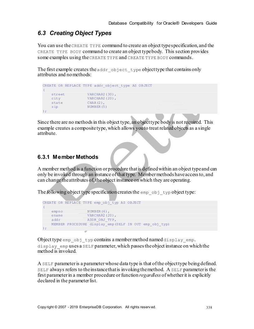
Database Compatibility for Oracle® Developers Guide
Copy right © 2007 - 2019 EnterpriseDB Corporation. All rights reserv ed.
338
6.3 Creating Object Types
You can use the CREATE TYPE command to create an object type specification, and the
CREATE TYPE BODY command to create an object type body. This section provides
some examples using the CREATE TYPE and CREATE TYPE BODY commands.
The first example creates the addr_object_type object type that contains only attributes and no methods:
CREATE OR REPLACE TYPE addr_object_type AS OBJECT
(
street VARCHAR2(30),
city VARCHAR2(20),
state CHAR(2),
zip NUMBER(5)
);
Since there are no methods in this object type, an object type body is not required. This
example creates a composite type, which allows you to treat related objects as a single attribute.
6.3.1 Member Methods
A member method is a function or procedure that is defined within an object type and can only be invoked through an instance of that type. Member methods have access to, and can change the attributes of, the object instance on which they are operating.
The following object type specification creates the emp_obj_typ object type:
CREATE OR REPLACE TYPE emp_obj_typ AS OBJECT
(
empno NUMBER(4),
ename VARCHAR2(20),
addr ADDR_OBJ_TYP,
MEMBER PROCEDURE display_emp(SELF IN OUT emp_obj_typ)
);
Object type emp_obj_typ contains a member method named display_emp.
display_emp uses a SELF parameter, which passes the object instance on which the method is invoked.
A SELF parameter is a parameter whose data type is that of the object type being defined.
SELF always refers to the instance that is invoking the method. A SELF parameter is the first parameter in a member procedure or function regardless of whether it is explicitly declared in the parameter list.

Database Compatibility for Oracle® Developers Guide
Copy right © 2007 - 2019 EnterpriseDB Corporation. All rights reserv ed.
339
The following code snippet defines an object type body for emp_obj_typ:
CREATE OR REPLACE TYPE BODY emp_obj_typ AS
MEMBER PROCEDURE display_emp (SELF IN OUT emp_obj_typ)
IS
BEGIN
DBMS_OUTPUT.PUT_LINE('Employee No : ' || empno);
DBMS_OUTPUT.PUT_LINE('Name : ' || ename);
DBMS_OUTPUT.PUT_LINE('Street : ' || addr.street);
DBMS_OUTPUT.PUT_LINE('City/State/Zip: ' || addr.city || ', ' ||
addr.state || ' ' || LPAD(addr.zip,5,'0'));
END;
END;
You can also use the SELF parameter in an object type body. To illustrate how the SELF
parameter would be used in the CREATE TYPE BODY command, the preceding object type body could be written as follows:
CREATE OR REPLACE TYPE BODY emp_obj_typ AS
MEMBER PROCEDURE display_emp (SELF IN OUT emp_obj_typ)
IS
BEGIN
DBMS_OUTPUT.PUT_LINE('Employee No : ' || SELF.empno);
DBMS_OUTPUT.PUT_LINE('Name : ' || SELF.ename);
DBMS_OUTPUT.PUT_LINE('Street : ' || SELF.addr.street);
DBMS_OUTPUT.PUT_LINE('City/State/Zip: ' || SELF.addr.city || ', ' ||
SELF.addr.state || ' ' || LPAD(SELF.addr.zip,5,'0'));
END;
END;
Both versions of the emp_obj_typ body are completely equivalent.
6.3.2 Static Methods
Like a member method, a static method belongs to a type. A static method, however, is
invoked not by an instance of the type, but by using the name of the type. For example,
to invoke a static function named get_count, defined within the emp_obj_type type, you would write:
emp_obj_type.get_count();
A static method does not have access to, and cannot change the attributes of an object instance, and does not typically work with an instance of the type.
The following object type specification includes a static function get_dname and a member procedure display_dept:
CREATE OR REPLACE TYPE dept_obj_typ AS OBJECT (
deptno NUMBER(2),
STATIC FUNCTION get_dname(p_deptno IN NUMBER) RETURN VARCHAR2,
MEMBER PROCEDURE display_dept
);

Database Compatibility for Oracle® Developers Guide
Copy right © 2007 - 2019 EnterpriseDB Corporation. All rights reserv ed.
340
The object type body for dept_obj_typ defines a static function named get_dname
and a member procedure named display_dept:
CREATE OR REPLACE TYPE BODY dept_obj_typ AS
STATIC FUNCTION get_dname(p_deptno IN NUMBER) RETURN VARCHAR2
IS
v_dname VARCHAR2(14);
BEGIN
CASE p_deptno
WHEN 10 THEN v_dname := 'ACCOUNTING';
WHEN 20 THEN v_dname := 'RESEARCH';
WHEN 30 THEN v_dname := 'SALES';
WHEN 40 THEN v_dname := 'OPERATIONS';
ELSE v_dname := 'UNKNOWN';
END CASE;
RETURN v_dname;
END;
MEMBER PROCEDURE display_dept
IS
BEGIN
DBMS_OUTPUT.PUT_LINE('Dept No : ' || SELF.deptno);
DBMS_OUTPUT.PUT_LINE('Dept Name : ' ||
dept_obj_typ.get_dname(SELF.deptno));
END;
END;
Within the static function get_dname, there can be no references to SELF. Since a static
function is invoked independently of any object instance, it has no implicit access to any object attribute.
Member procedure display_dept can access the deptno attribute of the object
instance passed in the SELF parameter. It is not necessary to explicitly declare the SELF parameter in the display_dept parameter list.
The last DBMS_OUTPUT.PUT_LINE statement in the display_dept procedure includes
a call to the static function get_dname (qualified by its object type name dept_obj_typ).
6.3.3 Constructor Methods
A constructor method is a function that creates an instance of an object type, typically by assigning values to the members of the object. An object type may define several
constructors to accomplish different tasks. A constructor method is a member function (invoked with a SELF parameter) whose name matches the name of the type.
For example, if you define a type named address, each constructor is named address. You may overload a constructor by creating one or more different constructor functions with the same name, but with different argument types.

Database Compatibility for Oracle® Developers Guide
Copy right © 2007 - 2019 EnterpriseDB Corporation. All rights reserv ed.
341
The SPL compiler will provide a default constructor for each object type. The default constructor is a member function whose name matches the name of the type and whose
argument list matches the type members (in order). For example, given an object type such as:
CREATE TYPE address AS OBJECT
(
street_address VARCHAR2(40),
postal_code VARCHAR2(10),
city VARCHAR2(40),
state VARCHAR2(2)
)
The SPL compiler will provide a default constructor with the following signature:
CONSTRUCTOR FUNCTION address
(
street_address VARCHAR2(40),
postal_code VARCHAR2(10),
city VARCHAR2(40),
state VARCHAR2(2)
)
The body of the default constructor simply sets each member to NULL.
To create a custom constructor, declare the constructor function (using the keyword
constructor) in the CREATE TYPE command and define the construction function in the
CREATE TYPE BODY command. For example, you may wish to create a custom
constructor for the address type which computes the city and state given a street_address and postal_code:
CREATE TYPE address AS OBJECT
(
street_address VARCHAR2(40),
postal_code VARCHAR2(10),
city VARCHAR2(40),
state VARCHAR2(2),
CONSTRUCTOR FUNCTION address
(
street_address VARCHAR2,
postal_code VARCHAR2
) RETURN self AS RESULT
)
CREATE TYPE BODY address AS
CONSTRUCTOR FUNCTION address
(
street_address VARCHAR2,
postal_code VARCHAR2
) RETURN self AS RESULT
IS
BEGIN
self.street_address := street_address;
self.postal_code := postal_code;
self.city := postal_code_to_city(postal_code);

Database Compatibility for Oracle® Developers Guide
Copy right © 2007 - 2019 EnterpriseDB Corporation. All rights reserv ed.
342
self.state := postal_code_to_state(postal_code);
RETURN;
END;
END;
To create an instance of an object type, you invoke one of the constructor methods for that type. For example:
DECLARE
cust_addr address := address('100 Main Street', 02203');
BEGIN
DBMS_OUTPUT.PUT_LINE(cust_addr.city); -- displays Boston
DBMS_OUTPUT.PUT_LINE(cust_addr.state); -- displays MA
END;
Custom constructor functions are typically used to compute member values when given
incomplete information. The preceding example computes the values for city and state when given a postal code.
Custom constructor functions are also used to enforce business rules that restrict the state
of an object. For example, if you define an object type to represent a payment, you can
use a custom constructor to ensure that no object of type payment can be created with an
amount that is NULL, negative, or zero. The default constructor would set
payment.amount to NULL so you must create a custom constructor (whose signature matches the default constructor) to prohibit NULL amounts.

Database Compatibility for Oracle® Developers Guide
Copy right © 2007 - 2019 EnterpriseDB Corporation. All rights reserv ed.
343
6.4 Creating Object Instances
To create an instance of an object type, you must first declare a variable of the object
type, and then initialize the declared object variable. The syntax for declaring an object variable is:
object obj_type
object is an identifier assigned to the object variable.
obj_type is the identifier of a previously defined object type.
After declaring the object variable, you must invoke a constructor method to initialize the object with values. Use the following syntax to invoke the constructor method:
[NEW] obj_type ({expr1 | NULL} [, {expr2 | NULL} ] [, ...])
obj_type is the identifier of the object type’s constructor method; the constructor
method has the same name as the previously declared object type.
expr1, expr2, … are expressions that are type-compatible with the first attribute of the
object type, the second attribute of the object type, etc. If an attribute is of an object type,
then the corresponding expression can be NULL, an object initialization expression, or any expression that returns that object type.
The following anonymous block declares and initializes a variable:
DECLARE
v_emp EMP_OBJ_TYP;
BEGIN
v_emp := emp_obj_typ (9001,'JONES',
addr_obj_typ('123 MAIN STREET','EDISON','NJ',08817));
END;
The variable (v_emp) is declared with a previously defined object type named
EMP_OBJ_TYPE. The body of the block initializes the variable using the emp_obj_typ and addr_obj_type constructors.
You can include the NEW keyword when creating a new instance of an object in the body
of a block. The NEW keyword invokes the object constructor whose signature matches the arguments provided.
The following example declares two variables, named mgr and emp. The variables are
both of EMP_OBJ_TYPE. The mgr object is initialized in the declaration, while the emp object is initialized to NULL in the declaration, and assigned a value in the body.
DECLARE
mgr EMP_OBJ_TYPE := (9002,'SMITH');

Database Compatibility for Oracle® Developers Guide
Copy right © 2007 - 2019 EnterpriseDB Corporation. All rights reserv ed.
344
emp EMP_OBJ_TYPE;
BEGIN
emp := NEW EMP_OBJ_TYPE (9003,'RAY');
END;
Note: In Advanced Server, the following alternate syntax can be used in place of the constructor method.
[ ROW ] ({ expr1 | NULL } [, { expr2 | NULL } ] [, ...])
ROW is an optional keyword if two or more terms are specified within the parenthesis-
enclosed, comma-delimited list. If only one term is specified, then specification of the ROW keyword is mandatory.
6.5 Referencing an Object
Once an object variable is created and initialized, individual attributes can be referenced using dot notation of the form:
object.attribute
object is the identifier assigned to the object variable. attribute is the identifier of an object type attribute.
If attribute, itself, is of an object type, then the reference must take the form:
object.attribute.attribute_inner
attribute_inner is an identifier belonging to the object type to which attribute
references in its definition of object.
The following example expands upon the previous anonymous block to display the
values assigned to the emp_obj_typ object.
DECLARE
v_emp EMP_OBJ_TYP;
BEGIN
v_emp := emp_obj_typ(9001,'JONES',
addr_obj_typ('123 MAIN STREET','EDISON','NJ',08817));
DBMS_OUTPUT.PUT_LINE('Employee No : ' || v_emp.empno);
DBMS_OUTPUT.PUT_LINE('Name : ' || v_emp.ename);
DBMS_OUTPUT.PUT_LINE('Street : ' || v_emp.addr.street);
DBMS_OUTPUT.PUT_LINE('City/State/Zip: ' || v_emp.addr.city || ', ' ||
v_emp.addr.state || ' ' || LPAD(v_emp.addr.zip,5,'0'));
END;

Database Compatibility for Oracle® Developers Guide
Copy right © 2007 - 2019 EnterpriseDB Corporation. All rights reserv ed.
345
The following is the output from this anonymous block.
Employee No : 9001
Name : JONES
Street : 123 MAIN STREET
City/State/Zip: EDISON, NJ 08817
Methods are called in a similar manner as attributes.
Once an object variable is created and initialized, member procedures or functions are called using dot notation of the form:
object.prog_name
object is the identifier assigned to the object variable. prog_name is the identifier of
the procedure or function.
Static procedures or functions are not called utilizing an object variable. Instead the procedure or function is called utilizing the object type name:
object_type.prog_name
object_type is the identifier assigned to the object type. prog_name is the identifier
of the procedure or function.
The results of the previous anonymous block can be duplicated by calling the member procedure display_emp:
DECLARE
v_emp EMP_OBJ_TYP;
BEGIN
v_emp := emp_obj_typ(9001,'JONES',
addr_obj_typ('123 MAIN STREET','EDISON','NJ',08817));
v_emp.display_emp;
END;
The following is the output from this anonymous block.
Employee No : 9001
Name : JONES
Street : 123 MAIN STREET
City/State/Zip: EDISON, NJ 08817
The following anonymous block creates an instance of dept_obj_typ and calls the
member procedure display_dept:
DECLARE
v_dept DEPT_OBJ_TYP := dept_obj_typ (20);
BEGIN
v_dept.display_dept;
END;

Database Compatibility for Oracle® Developers Guide
Copy right © 2007 - 2019 EnterpriseDB Corporation. All rights reserv ed.
346
The following is the output from this anonymous block.
Dept No : 20
Dept Name : RESEARCH
The static function defined in dept_obj_typ can be called directly by qualifying it by the object type name as follows:
BEGIN
DBMS_OUTPUT.PUT_LINE(dept_obj_typ.get_dname(20));
END;
RESEARCH
6.6 Dropping an Object Type
The syntax for deleting an object type is as follows.
DROP TYPE objtype;
objtype is the identifier of the object type to be dropped. If the definition of objtype
contains attributes that are themselves object types or collection types, these nested object types or collection types must be dropped last.
If an object type body is defined for the object type, the DROP TYPE command deletes the object type body as well as the object type specification. In order to recreate the
complete object type, both the CREATE TYPE and CREATE TYPE BODY commands must be reissued.
The following example drops the emp_obj_typ and the addr_obj_typ object types
created earlier in this chapter. emp_obj_typ must be dropped first since it contains
addr_obj_typ within its definition as an attribute.
DROP TYPE emp_obj_typ;
DROP TYPE addr_obj_typ;
The syntax for deleting an object type body, but not the object type specification is as follows.
DROP TYPE BODY objtype;
The object type body can be recreated by issuing the CREATE TYPE BODY command.
The following example drops only the object type body of the dept_obj_typ.
DROP TYPE BODY dept_obj_typ;

Database Compatibility for Oracle® Developers Guide
Copy right © 2007 - 2019 EnterpriseDB Corporation. All rights reserv ed.
347
7 Open Client Library
The Open Client Library provides application interoperability with the Oracle Call Interface – an application that was formerly “locked in” can now work with either an
EDB Postgres Advanced Server or an Oracle database with minimal to no changes to the application code. The EnterpriseDB implementation of the Open Client Library is written in C.
The following diagram compares the Open Client Library and Oracle Call Interface application stacks.
For detailed usage information about the Open Client Library and the supported
functions, please see the EDB Postgres Advanced Server OCI Connector Guide, available at:
https://www.enterprisedb.com/resources/product-documentation
Please note: EnterpriseDB does not support use of the Open Client Library with Oracle Real Application Clusters (RAC) and Oracle Exadata; the aforementioned Oracle products have not been evaluated nor certified with this EnterpriseDB product.

Database Compatibility for Oracle® Developers Guide
Copy right © 2007 - 2019 EnterpriseDB Corporation. All rights reserv ed.
348
8 Oracle Catalog Views
The Oracle Catalog Views provide information about database objects in a manner
compatible with the Oracle data dictionary views. Information about the supported views is now available in the Database Compatibility for Oracle® Developer’s Reference Guide, available at:
https://www.enterprisedb.com/resources/product-documentation

Database Compatibility for Oracle® Developers Guide
Copy right © 2007 - 2019 EnterpriseDB Corporation. All rights reserv ed.
349
9 Tools and Utilities
Compatible tools and utility programs can allow a developer to work with Advanced Server in a familiar environment. The tools supported by Advanced Server include:
EDB*Plus
EDB*Loader
EDB*Wrap
The Dynamic Runtime Instrumentation Tools Architecture (DRITA)
For detailed information about the functionality supported by Advanced Server, please consult the Database Compatibility for Oracle® Developer’s Tools and Utilities Guide, available at:
https://www.enterprisedb.com/resources/product-documentation

Database Compatibility for Oracle® Developers Guide
Copy right © 2007 - 2019 EnterpriseDB Corporation. All rights reserv ed.
350
10 Table Partitioning
In a partitioned table, one logically large table is broken into smaller physical pieces. Partitioning can provide several benefits:
Query performance can be improved dramatically in certain situations, particularly when most of the heavily accessed rows of the table are in a single partition or a small number of partitions. Partitioning allows you to omit the
partition column from the front of an index, reducing index size and making it more likely that the heavily used parts of the index fits in memory.
When a query or update accesses a large percentage of a single partition, performance may improve because the server will perform a sequential scan of
the partition instead of using an index and random access reads scattered across the whole table.
A bulk load (or unload) can be implemented by adding or removing partitions, if
you plan that requirement into the partitioning design. ALTER TABLE is far faster
than a bulk operation. It also entirely avoids the VACUUM overhead caused by a bulk DELETE.
Seldom-used data can be migrated to less-expensive (or slower) storage media.
Table partitioning is worthwhile only when a table would otherwise be very large. The exact point at which a table will benefit from partitioning depends on the application; a
good rule of thumb is that the size of the table should exceed the physical memory of the database server.
This document discusses the aspects of table partitioning compatible with Oracle databases that are supported by Advanced Server.
Note: This document and particularly the partitioning presented in this chapter do not
describe the declarative partitioning feature, which has been introduced with PostgreSQL version 10. Note that PostgreSQL declarative partitioning is supported in Advanced
Server 10 in addition to the table partitioning compatible with Oracle databases as described in this chapter. For information about declarative partitioning, please see the PostgreSQL core documentation available at:
https://www.postgresql.org/docs/11/static/ddl-partitioning.html
The PostgreSQL 9.6 INSERT… ON CONFLICT DO NOTHING/UPDATE clause (commonly known as UPSERT) is not supported on Oracle-styled partitioned tables. If
you include the ON CONFLICT DO NOTHING/UPDATE clause when invoking the INSERT command to add data to a partitioned table, the server will return an error.

Database Compatibility for Oracle® Developers Guide
Copy right © 2007 - 2019 EnterpriseDB Corporation. All rights reserv ed.
351
10.1 Selecting a Partition Type
When you create a partitioned table, you specify LIST, RANGE, or HASH partitioning rules. The partitioning rules provide a set of constraints that define the data that is stored
in each partition. As new rows are added to the partitioned table, the server uses the partitioning rules to decide which partition should contain each row.
Advanced Server can also use the partitioning rules to enforce partition pruning,
improving performance when responding to user queries. When selecting a partitioning type and partitioning keys for a table, you should take into consideration how the data that is stored within a table will be queried, and include often-queried columns in the partitioning rules.
List Partitioning
When you create a list-partitioned table, you specify a single partitioning key column. When adding a row to the table, the server compares the key values specified in the partitioning rule to the corresponding column within the row. If the column value
matches a value in the partitioning rule, the row is stored in the partition named in the rule.
Range Partitioning
When you create a range-partitioned table, you specify one or more partitioning key columns. When you add a new row to the table, the server compares the value of the
partitioning key (or keys) to the corresponding column (or columns) in a table entry. If the column values satisfy the conditions specified in the partitioning rule, the row is stored in the partition named in the rule.
Hash Partitioning
When you create a hash-partitioned table, you specify one or more partitioning key
columns. Data is divided into (approx.) equal-sized partitions amongst the specified partitions. When you add a row to a hash-partitioned table, the server computes a hash
value for the data in the specified column (or columns), and stores the row in a partition according to the hash value.
Note: When upgrading Advanced Server, you must rebuild each hash-partitioned table on the upgraded version server.
Subpartitioning
Subpartitioning breaks a partitioned table into smaller subsets. All subsets must be stored
in the same database server cluster. A table is typically subpartitioned by a different set of columns, and may be a different subpartitioning type than the parent partition. If one partition is subpartitioned, then each partition will have at least one subpartition.

Database Compatibility for Oracle® Developers Guide
Copy right © 2007 - 2019 EnterpriseDB Corporation. All rights reserv ed.
352
If a table is subpartitioned, no data will be stored in any of the partition tables; the data will be stored instead in the corresponding subpartitions.
10.2 Using Partition Pruning
Advanced Server's query planner uses partition pruning to compute an efficient plan to
locate a row (or rows) that matches the conditions specified in the WHERE clause of a
SELECT statement. To successfully prune partitions from an execution plan, the WHERE clause must constrain the information that is compared to the partitioning key column specified when creating the partitioned table. When querying a:
list-partitioned table, partition pruning is effective when the WHERE clause compares a literal value to the partitioning key using operators like equal (=) or AND.
range-partitioned table, partition pruning is effective when the WHERE clause compares a literal value to a partitioning key using operators such as equal (=), less than (<), or greater than (>).
hash-partitioned table, partition pruning is effective when the WHERE clause compares a literal value to the partitioning key using an operator such as equal (=).
The partition pruning mechanism uses two optimization techniques:
Fast Pruning
Constraint exclusion
Partition pruning techniques limit the search for data to only those partitions in which the values for which you are searching might reside. Both pruning techniques remove partitions from a query's execution plan, increasing performance.
The difference between the fast pruning and constraint exclusion is that fast pruning
understands the relationship between the partitions in an Oracle-partitioned table, while constraint exclusion does not. For example, when a query searches for a specific value
within a list-partitioned table, fast pruning can reason that only a specific partition may hold that value, while constraint exclusion must examine the constraints defined for each partition. Fast pruning occurs early in the planning process to reduce the number of
partitions that the planner must consider, while constraint exclusion occurs late in the planning process.
Using Constraint Exclusion
The constraint_exclusion parameter controls constraint exclusion. The
constraint_exclusion parameter may have a value of on, off, or partition. To

Database Compatibility for Oracle® Developers Guide
Copy right © 2007 - 2019 EnterpriseDB Corporation. All rights reserv ed.
353
enable constraint exclusion, the parameter must be set to either partition or on. By default, the parameter is set to partition.
For more information about constraint exclusion, see:
https://www.postgresql.org/docs/11/static/ddl-partitioning.html
When constraint exclusion is enabled, the server examines the constraints defined for each partition to determine if that partition can satisfy a query.
When you execute a SELECT statement that does not contain a WHERE clause, the query planner must recommend an execution plan that searches the entire table. When you
execute a SELECT statement that does contain a WHERE clause, the query planner determines in which partition that row would be stored, and sends query fragments to that partition, pruning the partitions that could not contain that row from the execution plan. If you are not using partitioned tables, disabling constraint exclusion may improve performance.
Fast Pruning
Like constraint exclusion, fast pruning can only optimize queries that include a WHERE
(or join) clause, and only when the qualifiers in the WHERE clause match a certain form. In both cases, the query planner will avoid searching for data within partitions that cannot possibly hold the data required by the query.
Fast pruning is controlled by a boolean configuration parameter named
edb_enable_pruning. If edb_enable_pruning is ON, Advanced Server will fast
prune certain queries. If edb_enable_pruning is OFF, the server will disable fast pruning.
Please note: Fast pruning cannot optimize queries against subpartitioned tables or optimize queries against range-partitioned tables that are partitioned on more than one column.
For LIST-partitioned tables, Advanced Server can fast prune queries that contain a
WHERE clause that constrains a partitioning column to a literal value. For example, given a LIST-partitioned table such as:
CREATE TABLE sales_hist(..., country text, ...)
PARTITION BY LIST(country)
(
PARTITION americas VALUES('US', 'CA', 'MX'),
PARTITION europe VALUES('BE', 'NL', 'FR'),
PARTITION asia VALUES('JP', 'PK', 'CN'),
PARTITION others VALUES(DEFAULT)
)

Database Compatibility for Oracle® Developers Guide
Copy right © 2007 - 2019 EnterpriseDB Corporation. All rights reserv ed.
354
Fast pruning can reason about WHERE clauses such as:
WHERE country = 'US'
WHERE country IS NULL;
Given the first WHERE clause, fast pruning would eliminate partitions europe, asia, and
others because those partitions cannot hold rows that satisfy the qualifier: WHERE country = 'US'.
Given the second WHERE clause, fast pruning would eliminate partitions americas, europe, and asia because those partitions cannot hold rows where country IS NULL.
The operator specified in the WHERE clause must be an equal sign (=) or the equality operator appropriate for the data type of the partitioning column.
For range-partitioned tables, Advanced Server can fast prune queries that contain a
WHERE clause that constrains a partitioning column to a literal value, but the operator may be any of the following:
>
>=
=
<=
<
Fast pruning will also reason about more complex expressions involving AND and BETWEEN operators, such as:
WHERE size > 100 AND size <= 200
WHERE size BETWEEN 100 AND 200
But cannot prune based on expressions involving OR or IN.
For example, when querying a RANGE-partitioned table, such as:
CREATE TABLE boxes(id int, size int, color text)
PARTITION BY RANGE(size)
(
PARTITION small VALUES LESS THAN(100),
PARTITION medium VALUES LESS THAN(200),
PARTITION large VALUES LESS THAN(300)
)
Fast pruning can reason about WHERE clauses such as:
WHERE size > 100 -- scan partitions 'medium' and 'large'

Database Compatibility for Oracle® Developers Guide
Copy right © 2007 - 2019 EnterpriseDB Corporation. All rights reserv ed.
355
WHERE size >= 100 -- scan partitions 'medium' and 'large'
WHERE size = 100 -- scan partition 'medium'
WHERE size <= 100 -- scan partitions 'small' and 'medium'
WHERE size < 100 -- scan partition 'small'
WHERE size > 100 AND size < 199 -- scan partition 'medium'
WHERE size BETWEEN 100 AND 199 -- scan partition 'medium'
WHERE color = 'red' AND size = 100 -- scan 'medium'
WHERE color = 'red' AND (size > 100 AND size < 199) -- scan 'medium'
In each case, fast pruning requires that the qualifier must refer to a partitioning column and literal value (or IS NULL/IS NOT NULL).
Note that fast pruning can also optimize DELETE and UPDATE statements containing WHERE clauses of the forms described above.

Database Compatibility for Oracle® Developers Guide
Copy right © 2007 - 2019 EnterpriseDB Corporation. All rights reserv ed.
356
10.2.1 Example - Partition Pruning
The EXPLAIN statement displays the execution plan of a statement. You can use the
EXPLAIN statement to confirm that Advanced Server is pruning partitions from the execution plan of a query.
To demonstrate the efficiency of partition pruning, first create a simple table:
CREATE TABLE sales
(
dept_no number,
part_no varchar2,
country varchar2(20),
date date,
amount number
)
PARTITION BY LIST(country)
(
PARTITION europe VALUES('FRANCE', 'ITALY'),
PARTITION asia VALUES('INDIA', 'PAKISTAN'),
PARTITION americas VALUES('US', 'CANADA')
);
Then, perform a constrained query that includes the EXPLAIN statement:
EXPLAIN (COSTS OFF) SELECT * FROM sales WHERE country = 'INDIA';
The resulting query plan shows that the server will scan only the sales_asia table - the table in which a row with a country value of INDIA would be stored:
edb=# EXPLAIN (COSTS OFF) SELECT * FROM sales WHERE country = 'INDIA';
QUERY PLAN
---------------------------------------------------
Append
-> Seq Scan on sales_asia
Filter: ((country)::text = 'INDIA'::text)
(3 rows)
If you perform a query that searches for a row that matches a value not included in the partitioning key:
EXPLAIN (COSTS OFF) SELECT * FROM sales WHERE dept_no = '30';
The resulting query plan shows that the server must look in all of the partitions to locate the rows that satisfy the query:
edb=# EXPLAIN (COSTS OFF) SELECT * FROM sales WHERE dept_no = '30';
QUERY PLAN

Database Compatibility for Oracle® Developers Guide
Copy right © 2007 - 2019 EnterpriseDB Corporation. All rights reserv ed.
357
-------------------------------------------
Append
-> Seq Scan on sales_americas
Filter: (dept_no = '30'::numeric)
-> Seq Scan on sales_europe
Filter: (dept_no = '30'::numeric)
-> Seq Scan on sales_asia
Filter: (dept_no = '30'::numeric)
(7 rows)
Constraint exclusion also applies when querying subpartitioned tables:
CREATE TABLE sales
(
dept_no number,
part_no varchar2,
country varchar2(20),
date date,
amount number
)
PARTITION BY RANGE(date) SUBPARTITION BY LIST (country)
(
PARTITION "2011" VALUES LESS THAN('01-JAN-2012')
(
SUBPARTITION europe_2011 VALUES ('ITALY', 'FRANCE'),
SUBPARTITION asia_2011 VALUES ('PAKISTAN', 'INDIA'),
SUBPARTITION americas_2011 VALUES ('US', 'CANADA')
),
PARTITION "2012" VALUES LESS THAN('01-JAN-2013')
(
SUBPARTITION europe_2012 VALUES ('ITALY', 'FRANCE'),
SUBPARTITION asia_2012 VALUES ('PAKISTAN', 'INDIA'),
SUBPARTITION americas_2012 VALUES ('US', 'CANADA')
),
PARTITION "2013" VALUES LESS THAN('01-JAN-2015')
(
SUBPARTITION europe_2013 VALUES ('ITALY', 'FRANCE'),
SUBPARTITION asia_2013 VALUES ('PAKISTAN', 'INDIA'),
SUBPARTITION americas_2013 VALUES ('US', 'CANADA')
)
);
When you query the table, the query planner prunes any partitions or subpartitions from the search path that cannot possibly contain the desired result set:
edb=# EXPLAIN (COSTS OFF) SELECT * FROM sales WHERE country = 'US' AND date =
'Dec 12, 2012';
QUERY PLAN
-----------------------------------------------------------------------------
------------------------------------
Append
-> Seq Scan on sales_americas_2012
Filter: (((country)::text = 'US'::text) AND (date = '12-DEC-12
00:00:00'::timestamp without time zone))

Database Compatibility for Oracle® Developers Guide
Copy right © 2007 - 2019 EnterpriseDB Corporation. All rights reserv ed.
358
(3 rows)

Database Compatibility for Oracle® Developers Guide
Copy right © 2007 - 2019 EnterpriseDB Corporation. All rights reserv ed.
359
10.3 Partitioning Commands Compatible with Oracle Databases
The following sections provide information about using the table partitioning syntax compatible with Oracle databases supported by Advanced Server.
10.3.1 CREATE TABLE…PARTITION BY
Use the PARTITION BY clause of the CREATE TABLE command to create a partitioned
table with data distributed amongst one or more partitions (and subpartitions). The command syntax comes in the following forms:
List Partitioning Syntax
Use the first form to create a list-partitioned table:
CREATE TABLE [ schema. ]table_name
table_definition
PARTITION BY LIST(column)
[SUBPARTITION BY {RANGE|LIST|HASH} (column[, column ]...)]
(list_partition_definition[, list_partition_definition]...);
Where list_partition_definition is:
PARTITION [partition_name]
VALUES (value[, value]...)
[TABLESPACE tablespace_name]
[(subpartition, ...)]
Range Partitioning Syntax
Use the second form to create a range-partitioned table:
CREATE TABLE [ schema. ]table_name
table_definition
PARTITION BY RANGE(column[, column ]...)
[SUBPARTITION BY {RANGE|LIST|HASH} (column[, column ]...)]
(range_partition_definition[, range_partition_definition]...);
Where range_partition_definition is:
PARTITION [partition_name]
VALUES LESS THAN (value[, value]...)
[TABLESPACE tablespace_name]
[(subpartition, ...)]
Hash Partitioning Syntax
Use the third form to create a hash-partitioned table:
Database Compatibility for Oracle® Developers Guide
Copy right © 2007 - 2019 EnterpriseDB Corporation. All rights reserv ed.
360
CREATE TABLE [ schema. ]table_name
table_definition
PARTITION BY HASH(column[, column ]...)
[SUBPARTITION BY {RANGE|LIST|HASH} (column[, column ]...)]
(hash_partition_definition[, hash_partition_definition]...);
Where hash_partition_definition is:
[PARTITION partition_name]
[TABLESPACE tablespace_name]
[(subpartition, ...)]
Subpartitioning Syntax
subpartition may be one of the following:
{list_subpartition | range_subpartition | hash_subpartition}
where list_subpartition is:
SUBPARTITION [subpartition_name]
VALUES (value[, value]...)
[TABLESPACE tablespace_name]
where range_subpartition is:
SUBPARTITION [subpartition_name]
VALUES LESS THAN (value[, value]...)
[TABLESPACE tablespace_name]
where hash_subpartition is:
[SUBPARTITION subpartition_name]
[TABLESPACE tablespace_name]
Description
The CREATE TABLE… PARTITION BY command creates a table with one or more partitions; each partition may have one or more subpartitions. There is no upper limit to
the number of defined partitions, but if you include the PARTITION BY clause, you must specify at least one partitioning rule. The resulting table will be owned by the user that creates it.
Use the PARTITION BY LIST clause to divide a table into partitions based on the values
entered in a specified column. Each partitioning rule must specify at least one literal value, but there is no upper limit placed on the number of values you may specify.
Include a rule that specifies a matching value of DEFAULT to direct any un-qualified rows

Database Compatibility for Oracle® Developers Guide
Copy right © 2007 - 2019 EnterpriseDB Corporation. All rights reserv ed.
361
to the given partition; for more information about using the DEFAULT keyword, see Section 10.4.
Use the PARTITION BY RANGE clause to specify boundary rules by which to create partitions. Each partitioning rule must contain at least one column of a data type that has
two operators (i.e., a greater-than or equal to operator, and a less-than operator). Range
boundaries are evaluated against a LESS THAN clause and are non-inclusive; a date boundary of January 1, 2013 will include only those date values that fall on or before December 31, 2012.
Range partition rules must be specified in ascending order. INSERT commands that store rows with values that exceed the top boundary of a range-partitioned table will fail unless
the partitioning rules include a boundary rule that specifies a value of MAXVALUE. If you
do not include a MAXVALUE partitioning rule, any row that exceeds the maximum limit specified by the boundary rules will result in an error.
For more information about using the MAXVALUE keyword, see Section 10.4.
Use the PARTITION BY HASH clause to create a hash-partitioned table. In a HASH partitioned table, data is divided amongst equal-sized partitions based on the hash value
of the column specified in the partitioning syntax. When specifying a HASH partition, choose a column (or combination of columns) that is as close to unique as possible to
help ensure that data is evenly distributed amongst the partitions. When selecting a partitioning column (or combination of columns), select a column (or columns) that you frequently search for exact matches for best performance.
Note: If you are upgrading Advanced Server, you must rebuild the hash-partitioned table on the upgraded version server.
Use the TABLESPACE keyword to specify the name of a tablespace on which a partition or subpartition will reside; if you do not specify a tablespace, the partition or subpartition will reside in the default tablespace.
If a table definition includes the SUBPARTITION BY clause, each partition within that table will have at least one subpartition. Each subpartition may be explicitly defined or system-defined.
If the subpartition is system-defined, the server-generated subpartition will reside in the default tablespace, and the name of the subpartition will be assigned by the server. The server will create:
A DEFAULT subpartition if the SUBPARTITION BY clause specifies LIST.
A MAXVALUE subpartition if the SUBPARTITION BY clause specifies RANGE.

Database Compatibility for Oracle® Developers Guide
Copy right © 2007 - 2019 EnterpriseDB Corporation. All rights reserv ed.
362
The server will generate a subpartition name that is a combination of the partition table
name and a unique identifier. You can query the ALL_TAB_SUBPARTITIONS table to review a complete list of subpartition names.
Parameters
table_name
The name (optionally schema-qualified) of the table to be created.
table_definition
The column names, data types, and constraint information as described in the
PostgreSQL core documentation for the CREATE TABLE statement, available at:
https://www.postgresql.org/docs/11/static/sql-createtable.html
partition_name
The name of the partition to be created. Partition names must be unique amongst
all partitions and subpartitions, and must follow the naming conventions for object identifiers.
subpartition_name
The name of the subpartition to be created. Subpartition names must be unique
amongst all partitions and subpartitions, and must follow the naming conventions for object identifiers.
column
The name of a column on which the partitioning rules are based. Each row will be stored in a partition that corresponds to the value of the specified column(s).
(value[, value]...)
Use value to specify a quoted literal value (or comma-delimited list of literal values) by which table entries will be grouped into partitions. Each partitioning
rule must specify at least one value, but there is no limit placed on the number of
values specified within a rule. value may be NULL, DEFAULT (if specifying a LIST partition), or MAXVALUE (if specifying a RANGE partition).
When specifying rules for a list-partitioned table, include the DEFAULT keyword in the last partition rule to direct any un-matched rows to the given partition. If you do not
include a rule that includes a value of DEFAULT, any INSERT statement that attempts to

Database Compatibility for Oracle® Developers Guide
Copy right © 2007 - 2019 EnterpriseDB Corporation. All rights reserv ed.
363
add a row that does not match the specified rules of at least one partition will fail, and return an error.
When specifying rules for a list-partitioned table, include the MAXVALUE keyword in the last partition rule to direct any un-categorized rows to the given partition. If you do not
include a MAXVALUE partition, any INSERT statement that attempts to add a row where the partitioning key is greater than the highest value specified will fail, and return an error.
tablespace_name
The name of the tablespace in which the partition or subpartition resides.
10.3.1.1 Example - PARTITION BY LIST
The following example creates a partitioned table (sales) using the PARTITION BY
LIST clause. The sales table stores information in three partitions (europe, asia, and americas):
CREATE TABLE sales
(
dept_no number,
part_no varchar2,
country varchar2(20),
date date,
amount number
)
PARTITION BY LIST(country)
(
PARTITION europe VALUES('FRANCE', 'ITALY'),
PARTITION asia VALUES('INDIA', 'PAKISTAN'),
PARTITION americas VALUES('US', 'CANADA')
);
The resulting table is partitioned by the value specified in the country column:
edb=# SELECT partition_name, high_value from ALL_TAB_PARTITIONS;
partition_name | high_value
----------------+---------------------
EUROPE | 'FRANCE', 'ITALY'
ASIA | 'INDIA', 'PAKISTAN'
AMERICAS | 'US', 'CANADA'
(3 rows)
Rows with a value of FRANCE or ITALY in the country column are stored in the
europe partition.
Rows with a value of INDIA or PAKISTAN in the country column are stored in the asia partition.

Database Compatibility for Oracle® Developers Guide
Copy right © 2007 - 2019 EnterpriseDB Corporation. All rights reserv ed.
364
Rows with a value of US or CANADA in the country column are stored in the americas partition.
The server would evaluate the following statement against the partitioning rules, and store the row in the europe partition:
INSERT INTO sales VALUES (10, '9519a', 'FRANCE', '18-Aug-2012',
'650000');
10.3.1.2 Example - PARTITION BY RANGE
The following example creates a partitioned table (sales) using the PARTITION BY
RANGE clause. The sales table stores information in four partitions (q1_2012, q2_2012, q3_2012 and q4_2012) :
CREATE TABLE sales
(
dept_no number,
part_no varchar2,
country varchar2(20),
date date,
amount number
)
PARTITION BY RANGE(date)
(
PARTITION q1_2012
VALUES LESS THAN('2012-Apr-01'),
PARTITION q2_2012
VALUES LESS THAN('2012-Jul-01'),
PARTITION q3_2012
VALUES LESS THAN('2012-Oct-01'),
PARTITION q4_2012
VALUES LESS THAN('2013-Jan-01')
);
The resulting table is partitioned by the value specified in the date column:
edb=# SELECT partition_name, high_value from ALL_TAB_PARTITIONS;
partition_name | high_value
----------------+----------------------
Q1_2012 | '01-APR-12 00:00:00'
Q2_2012 | '01-JUL-12 00:00:00'
Q3_2012 | '01-OCT-12 00:00:00'
Q4_2012 | '01-JAN-13 00:00:00'
(4 rows)
Any row with a value in the date column before April 1, 2012 is stored in a
partition named q1_2012.

Database Compatibility for Oracle® Developers Guide
Copy right © 2007 - 2019 EnterpriseDB Corporation. All rights reserv ed.
365
Any row with a value in the date column before July 1, 2012 is stored in a partition named q2_2012.
Any row with a value in the date column before October 1, 2012 is stored in a partition named q3_2012.
Any row with a value in the date column before January 1, 2013 is stored in a partition named q4_2012.
The server would evaluate the following statement against the partitioning rules and store the row in the q3_2012 partition:
INSERT INTO sales VALUES (10, '9519a', 'FRANCE', '18-Aug-2012',
'650000');
10.3.1.3 Example - PARTITION BY HASH
The following example creates a partitioned table (sales) using the PARTITION BY HASH clause. The sales table stores information in three partitions (p1, p2, and p3:
CREATE TABLE sales
(
dept_no number,
part_no varchar2,
country varchar2(20),
date date,
amount number
)
PARTITION BY HASH (part_no)
(
PARTITION p1,
PARTITION p2,
PARTITION p3
);
The table will return an empty string for the hash partition value specified in the
part_no column:
edb=# SELECT partition_name, high_value from ALL_TAB_PARTITIONS;
partition_name | high_value
----------------+------------
P1 |
P2 |
P3 |
(3 rows)
Use the following command to view the hash value of the part_no column.

Database Compatibility for Oracle® Developers Guide
Copy right © 2007 - 2019 EnterpriseDB Corporation. All rights reserv ed.
366
edb=# \d+ sales
Partitioned table "public.sales"
Column | Type | Collation | Nullable | Default | Storage |
---------+-----------------------------+-----------+----------+---------+----------+-----
dept_no | numeric | | | | main |
part_no | character varying | | | | extended |
country | character varying(20) | | | | extended |
date | timestamp without time zone | | | | plain |
amount | numeric | | | | main |
Partition key: HASH (part_no)
Partitions: sales_p1 FOR VALUES WITH (modulus 3, remainder 0),
sales_p2 FOR VALUES WITH (modulus 3, remainder 1),
sales_p3 FOR VALUES WITH (modulus 3, remainder 2)
The table is partitioned by the hash value of the values specified in the part_no column.
edb=# SELECT partition_name, partition_position from ALL_TAB_PARTITIONS;
partition_name | partition_position
----------------+--------------------
P1 | 1
P2 | 2
P3 | 3
(3 rows)
The server will evaluate the hash value of the part_no column and distribute the rows into approximately equal partitions.
10.3.1.4 Example - PARTITION BY RANGE, SUBPARTITION BY LIST
The following example creates a partitioned table (sales) that is first partitioned by the
transaction date; the range partitions (q1_2012, q2_2012, q3_2012 and q4_2012) are then list-subpartitioned using the value of the country column.
CREATE TABLE sales
(
dept_no number,
part_no varchar2,
country varchar2(20),
date date,
amount number
)
PARTITION BY RANGE(date)
SUBPARTITION BY LIST(country)
(
PARTITION q1_2012
VALUES LESS THAN('2012-Apr-01')
(
SUBPARTITION q1_europe VALUES ('FRANCE', 'ITALY'),
SUBPARTITION q1_asia VALUES ('INDIA', 'PAKISTAN'),
SUBPARTITION q1_americas VALUES ('US', 'CANADA')
),

Database Compatibility for Oracle® Developers Guide
Copy right © 2007 - 2019 EnterpriseDB Corporation. All rights reserv ed.
367
PARTITION q2_2012
VALUES LESS THAN('2012-Jul-01')
(
SUBPARTITION q2_europe VALUES ('FRANCE', 'ITALY'),
SUBPARTITION q2_asia VALUES ('INDIA', 'PAKISTAN'),
SUBPARTITION q2_americas VALUES ('US', 'CANADA')
),
PARTITION q3_2012
VALUES LESS THAN('2012-Oct-01')
(
SUBPARTITION q3_europe VALUES ('FRANCE', 'ITALY'),
SUBPARTITION q3_asia VALUES ('INDIA', 'PAKISTAN'),
SUBPARTITION q3_americas VALUES ('US', 'CANADA')
),
PARTITION q4_2012
VALUES LESS THAN('2013-Jan-01')
(
SUBPARTITION q4_europe VALUES ('FRANCE', 'ITALY'),
SUBPARTITION q4_asia VALUES ('INDIA', 'PAKISTAN'),
SUBPARTITION q4_americas VALUES ('US', 'CANADA')
)
);
This statement creates a table with four partitions; each partition has three subpartitions:
edb=# SELECT subpartition_name, high_value, partition_name FROM
ALL_TAB_SUBPARTITIONS;
subpartition_name | high_value | partition_name
-------------------+---------------------+----------------
Q1_EUROPE | 'FRANCE', 'ITALY' | Q1_2012
Q1_ASIA | 'INDIA', 'PAKISTAN' | Q1_2012
Q1_AMERICAS | 'US', 'CANADA' | Q1_2012
Q2_EUROPE | 'FRANCE', 'ITALY' | Q2_2012
Q2_ASIA | 'INDIA', 'PAKISTAN' | Q2_2012
Q2_AMERICAS | 'US', 'CANADA' | Q2_2012
Q3_EUROPE | 'FRANCE', 'ITALY' | Q3_2012
Q3_ASIA | 'INDIA', 'PAKISTAN' | Q3_2012
Q3_AMERICAS | 'US', 'CANADA' | Q3_2012
Q4_EUROPE | 'FRANCE', 'ITALY' | Q4_2012
Q4_ASIA | 'INDIA', 'PAKISTAN' | Q4_2012
Q4_AMERICAS | 'US', 'CANADA' | Q4_2012
(12 rows)
When a row is added to this table, the value in the date column is compared to the values specified in the range partitioning rules, and the server selects the partition in
which the row should reside. The value in the country column is then compared to the values specified in the list subpartitioning rules; when the server locates a match for the value, the row is stored in the corresponding subpartition.
Any row added to the table will be stored in a subpartition, so the partitions will contain no data.

Database Compatibility for Oracle® Developers Guide
Copy right © 2007 - 2019 EnterpriseDB Corporation. All rights reserv ed.
368
The server would evaluate the following statement against the partitioning and subpartitioning rules and store the row in the q3_europe partition:
INSERT INTO sales VALUES (10, '9519a', 'FRANCE', '18-Aug-2012',
'650000');

Database Compatibility for Oracle® Developers Guide
Copy right © 2007 - 2019 EnterpriseDB Corporation. All rights reserv ed.
369
10.3.2 ALTER TABLE...ADD PARTITION
Use the ALTER TABLE… ADD PARTITION command to add a partition to an existing partitioned table. The syntax is:
ALTER TABLE table_name ADD PARTITION partition_definition;
Where partition_definition is:
{list_partition | range_partition }
and list_partition is:
PARTITION [partition_name]
VALUES (value[, value]...)
[TABLESPACE tablespace_name]
[(subpartition, ...)]
and range_partition is:
PARTITION [partition_name]
VALUES LESS THAN (value[, value]...)
[TABLESPACE tablespace_name]
[(subpartition, ...)]
Where subpartition is:
{list_subpartition | range_subpartition | hash_subpartition}
and list_subpartition is:
SUBPARTITION [subpartition_name]
VALUES (value[, value]...)
[TABLESPACE tablespace_name]
and range_subpartition is:
SUBPARTITION [subpartition_name ]
VALUES LESS THAN (value[, value]...)
[TABLESPACE tablespace_name]
Description
The ALTER TABLE… ADD PARTITION command adds a partition to an existing partitioned table. There is no upper limit to the number of defined partitions in a partitioned table.

Database Compatibility for Oracle® Developers Guide
Copy right © 2007 - 2019 EnterpriseDB Corporation. All rights reserv ed.
370
New partitions must be of the same type (LIST, RANGE or HASH) as existing partitions. The new partition rules must reference the same column specified in the partitioning rules that define the existing partition(s).
You can use the ALTER TABLE… ADD PARTITION statement to add a partition to a table
with a DEFAULT rule as long as there are no conflicting values between existing rows in the table and the values of the partition to be added.
You cannot use the ALTER TABLE… ADD PARTITION statement to add a partition to a table with a MAXVALUE rule.
You can alternatively use the ALTER TABLE… SPLIT PARTITION statement to split an existing partition, effectively increasing the number of partitions in a table.
RANGE partitions must be specified in ascending order. You cannot add a new partition
that precedes existing partitions in a RANGE partitioned table.
Include the TABLESPACE clause to specify the tablespace in which the new partition will reside. If you do not specify a tablespace, the partition will reside in the default tablespace.
If the table is indexed, the index will be created on the new partition.
To use the ALTER TABLE... ADD PARTITION command you must be the table owner, or have superuser (or administrative) privileges.
Parameters
table_name
The name (optionally schema-qualified) of the partitioned table.
partition_name
The name of the partition to be created. Partition names must be unique amongst
all partitions and subpartitions, and must follow the naming conventions for object identifiers.
subpartition_name
The name of the subpartition to be created. Subpartition names must be unique
amongst all partitions and subpartitions, and must follow the naming conventions for object identifiers.
(value[, value]...)

Database Compatibility for Oracle® Developers Guide
Copy right © 2007 - 2019 EnterpriseDB Corporation. All rights reserv ed.
371
Use value to specify a quoted literal value (or comma-delimited list of literal
values) by which rows will be distributed into partitions. Each partitioning rule must specify at least one value, but there is no limit placed on the number of
values specified within a rule. value may also be NULL, DEFAULT (if specifying
a LIST partition), or MAXVALUE (if specifying a RANGE partition).
For information about creating a DEFAULT or MAXVALUE partition, see Section 10.4.
tablespace_name
The name of the tablespace in which a partition or subpartition resides.
10.3.2.1 Example - Adding a Partition to a LIST Partitioned Table
The example that follows adds a partition to the list-partitioned sales table. The table was created using the command:
CREATE TABLE sales
(
dept_no number,
part_no varchar2,
country varchar2(20),
date date,
amount number
)
PARTITION BY LIST(country)
(
PARTITION europe VALUES('FRANCE', 'ITALY'),
PARTITION asia VALUES('INDIA', 'PAKISTAN'),
PARTITION americas VALUES('US', 'CANADA')
);
The table contains three partitions (americas, asia, and europe) :
edb=# SELECT partition_name, high_value FROM ALL_TAB_PARTITIONS;
partition_name | high_value
----------------+---------------------
EUROPE | 'FRANCE', 'ITALY'
ASIA | 'INDIA', 'PAKISTAN'
AMERICAS | 'US', 'CANADA'
(3 rows)
The following command adds a partition named east_asia to the sales table:
ALTER TABLE sales ADD PARTITION east_asia
VALUES ('CHINA', 'KOREA');
After invoking the command, the table includes the east_asia partition:

Database Compatibility for Oracle® Developers Guide
Copy right © 2007 - 2019 EnterpriseDB Corporation. All rights reserv ed.
372
edb=# SELECT partition_name, high_value FROM ALL_TAB_PARTITIONS;
partition_name | high_value
----------------+---------------------
EUROPE | 'FRANCE', 'ITALY'
ASIA | 'INDIA', 'PAKISTAN'
AMERICAS | 'US', 'CANADA'
EAST_ASIA | 'CHINA', 'KOREA'
(4 rows)
10.3.2.2 Example - Adding a Partition to a RANGE Partitioned Table
The example that follows adds a partition to a range-partitioned table named sales:
CREATE TABLE sales
(
dept_no number,
part_no varchar2,
country varchar2(20),
date date,
amount number
)
PARTITION BY RANGE(date)
(
PARTITION q1_2012
VALUES LESS THAN('2012-Apr-01'),
PARTITION q2_2012
VALUES LESS THAN('2012-Jul-01'),
PARTITION q3_2012
VALUES LESS THAN('2012-Oct-01'),
PARTITION q4_2012
VALUES LESS THAN('2013-Jan-01')
);
The table contains four partitions (q1_2012, q2_2012, q3_2012, and q4_2012):
edb=# SELECT partition_name, high_value FROM ALL_TAB_PARTITIONS;
partition_name | high_value
----------------+----------------------
Q1_2012 | '01-APR-12 00:00:00'
Q2_2012 | '01-JUL-12 00:00:00'
Q3_2012 | '01-OCT-12 00:00:00'
Q4_2012 | '01-JAN-13 00:00:00'
(4 rows)
The following command adds a partition named q1_2013 to the sales table:
ALTER TABLE sales ADD PARTITION q1_2013
VALUES LESS THAN('01-APR-2013');

Database Compatibility for Oracle® Developers Guide
Copy right © 2007 - 2019 EnterpriseDB Corporation. All rights reserv ed.
373
After invoking the command, the table includes the q1_2013 partition:
edb=# SELECT partition_name, high_value FROM ALL_TAB_PARTITIONS;
partition_name | high_value
----------------+----------------------
Q1_2012 | '01-APR-12 00:00:00'
Q2_2012 | '01-JUL-12 00:00:00'
Q3_2012 | '01-OCT-12 00:00:00'
Q4_2012 | '01-JAN-13 00:00:00'
Q1_2013 | '01-APR-13 00:00:00'
(5 rows)

Database Compatibility for Oracle® Developers Guide
Copy right © 2007 - 2019 EnterpriseDB Corporation. All rights reserv ed.
374
10.3.3 ALTER TABLE… ADD SUBPARTITION
The ALTER TABLE… ADD SUBPARTITION command adds a subpartition to an existing subpartitioned partition. The syntax is:
ALTER TABLE table_name MODIFY PARTITION partition_name
ADD SUBPARTITION subpartition_definition;
Where subpartition_definition is:
{list_subpartition | range_subpartition}
and list_subpartition is:
SUBPARTITION [subpartition_name]
VALUES (value[, value]...)
[TABLESPACE tablespace_name]
and range_subpartition is:
SUBPARTITION [subpartition_name]
VALUES LESS THAN (value[, value]...)
[TABLESPACE tablespace_name]
Description
The ALTER TABLE… ADD SUBPARTITION command adds a subpartition to an existing partition; the partition must already be subpartitioned. There is no upper limit to the number of defined subpartitions.
New subpartitions must be of the same type (LIST, RANGE or HASH) as existing subpartitions. The new subpartition rules must reference the same column specified in the subpartitioning rules that define the existing subpartition(s).
You can use the ALTER TABLE… ADD SUBPARTITION statement to add a subpartition to
a table with a DEFAULT rule as long as there are no conflicting values between existing rows in the table and the values of the subpartition to be added.
You cannot use the ALTER TABLE… ADD SUBPARTITION statement to add a subpartition to a table with a MAXVALUE rule.
You can split an existing subpartition with the ALTER TABLE… SPLIT SUBPARTITION statement, effectively adding a subpartition to a table.

Database Compatibility for Oracle® Developers Guide
Copy right © 2007 - 2019 EnterpriseDB Corporation. All rights reserv ed.
375
You cannot add a new subpartition that precedes existing subpartitions in a range subpartitioned table; range subpartitions must be specified in ascending order.
Include the TABLESPACE clause to specify the tablespace in which the subpartition will reside. If you do not specify a tablespace, the subpartition will be created in the default tablespace.
If the table is indexed, the index will be created on the new subpartition.
To use the ALTER TABLE... ADD SUBPARTITION command you must be the table owner, or have superuser (or administrative) privileges.
Parameters
table_name
The name (optionally schema-qualified) of the partitioned table in which the subpartition will reside.
partition_name
The name of the partition in which the new subpartition will reside.
subpartition_name
The name of the subpartition to be created. Subpartition names must be unique
amongst all partitions and subpartitions, and must follow the naming conventions for object identifiers.
(value[, value]...)
Use value to specify a quoted literal value (or comma-delimited list of literal
values) by which table entries will be grouped into partitions. Each partitioning rule must specify at least one value, but there is no limit placed on the number of
values specified within a rule. value may also be NULL, DEFAULT (if specifying a LIST partition), or MAXVALUE (if specifying a RANGE partition).
For information about creating a DEFAULT or MAXVALUE partition, see Section 10.4.
tablespace_name
The name of the tablespace in which the subpartition resides.

Database Compatibility for Oracle® Developers Guide
Copy right © 2007 - 2019 EnterpriseDB Corporation. All rights reserv ed.
376
10.3.3.1 Example - Adding a Subpartition to a LIST-RANGE Partitioned
Table
The following example adds a RANGE subpartition to the list-partitioned sales table. The sales table was created with the command:
CREATE TABLE sales
(
dept_no number,
part_no varchar2,
country varchar2(20),
date date,
amount number
)
PARTITION BY LIST(country)
SUBPARTITION BY RANGE(date)
(
PARTITION europe VALUES('FRANCE', 'ITALY')
(
SUBPARTITION europe_2011
VALUES LESS THAN('2012-Jan-01'),
SUBPARTITION europe_2012
VALUES LESS THAN('2013-Jan-01')
),
PARTITION asia VALUES('INDIA', 'PAKISTAN')
(
SUBPARTITION asia_2011
VALUES LESS THAN('2012-Jan-01'),
SUBPARTITION asia_2012
VALUES LESS THAN('2013-Jan-01')
),
PARTITION americas VALUES('US', 'CANADA')
(
SUBPARTITION americas_2011
VALUES LESS THAN('2012-Jan-01'),
SUBPARTITION americas_2012
VALUES LESS THAN('2013-Jan-01')
)
);
The sales table has three partitions, named europe, asia, and americas. Each partition has two range-defined subpartitions:
edb=# SELECT partition_name, subpartition_name, high_value FROM
ALL_TAB_SUBPARTITIONS;
partition_name | subpartition_name | high_value
----------------+-------------------+----------------------
EUROPE | EUROPE_2011 | '01-JAN-12 00:00:00'
EUROPE | EUROPE_2012 | '01-JAN-13 00:00:00'
ASIA | ASIA_2011 | '01-JAN-12 00:00:00'
ASIA | ASIA_2012 | '01-JAN-13 00:00:00'

Database Compatibility for Oracle® Developers Guide
Copy right © 2007 - 2019 EnterpriseDB Corporation. All rights reserv ed.
377
AMERICAS | AMERICAS_2011 | '01-JAN-12 00:00:00'
AMERICAS | AMERICAS_2012 | '01-JAN-13 00:00:00'
(6 rows)
The following command adds a subpartition named europe_2013:
ALTER TABLE sales MODIFY PARTITION europe
ADD SUBPARTITION europe_2013
VALUES LESS THAN('2015-Jan-01');
After invoking the command, the table includes a subpartition named europe_2013:
edb=# SELECT partition_name, subpartition_name, high_value FROM
ALL_TAB_SUBPARTITIONS;
partition_name | subpartition_name | high_value
----------------+-------------------+----------------------
EUROPE | EUROPE_2011 | '01-JAN-12 00:00:00'
EUROPE | EUROPE_2012 | '01-JAN-13 00:00:00'
EUROPE | EUROPE_2013 | '01-JAN-15 00:00:00'
ASIA | ASIA_2011 | '01-JAN-12 00:00:00'
ASIA | ASIA_2012 | '01-JAN-13 00:00:00'
AMERICAS | AMERICAS_2011 | '01-JAN-12 00:00:00'
AMERICAS | AMERICAS_2012 | '01-JAN-13 00:00:00'
(7 rows)
Note that when adding a new range subpartition, the subpartitioning rules must specify a range that falls after any existing subpartitions.
10.3.3.2 Example - Adding a Subpartition to a RANGE-LIST Partitioned Table
The following example adds a LIST subpartition to the RANGE partitioned sales table.
The sales table was created with the command:
CREATE TABLE sales
(
dept_no number,
part_no varchar2,
country varchar2(20),
date date,
amount number
)
PARTITION BY RANGE(date)
SUBPARTITION BY LIST (country)
(
PARTITION first_half_2012 VALUES LESS THAN('01-JUL-2012')
(
SUBPARTITION europe VALUES ('ITALY', 'FRANCE'),
SUBPARTITION americas VALUES ('US', 'CANADA')
),
PARTITION second_half_2012 VALUES LESS THAN('01-JAN-2013')
(
Database Compatibility for Oracle® Developers Guide
Copy right © 2007 - 2019 EnterpriseDB Corporation. All rights reserv ed.
378
SUBPARTITION asia VALUES ('INDIA', 'PAKISTAN')
)
);
After executing the above command, the sales table will have two partitions, named
first_half_2012 and second_half_2012. The first_half_2012 partition has
two subpartitions, named europe and americas, and the second_half_2012 partition has one partition, named asia:
edb=# SELECT partition_name, subpartition_name, high_value FROM
ALL_TAB_SUBPARTITIONS;
partition_name | subpartition_name | high_value
------------------+-------------------+---------------------
SECOND_HALF_2012 | ASIA | 'INDIA', 'PAKISTAN'
FIRST_HALF_2012 | AMERICAS | 'US', 'CANADA'
FIRST_HALF_2012 | EUROPE | 'ITALY', 'FRANCE'
(3 rows)
The following command adds a subpartition to the second_half_2012 partition, named east_asia:
ALTER TABLE sales MODIFY PARTITION second_half_2012
ADD SUBPARTITION east_asia VALUES ('CHINA');
After invoking the command, the table includes a subpartition named east_asia:
edb=# SELECT partition_name, subpartition_name, high_value FROM
ALL_TAB_SUBPARTITIONS;
partition_name | subpartition_name | high_value
------------------+-------------------+---------------------
SECOND_HALF_2012 | ASIA | 'INDIA', 'PAKISTAN'
SECOND_HALF_2012 | EAST_ASIA | 'CHINA'
FIRST_HALF_2012 | AMERICAS | 'US', 'CANADA'
FIRST_HALF_2012 | EUROPE | 'ITALY', 'FRANCE'
(4 rows)

Database Compatibility for Oracle® Developers Guide
Copy right © 2007 - 2019 EnterpriseDB Corporation. All rights reserv ed.
379
10.3.4 ALTER TABLE...SPLIT PARTITION
Use the ALTER TABLE… SPLIT PARTITION command to divide a single partition into two partitions, and redistribute the partition's contents between the new partitions. The command syntax comes in two forms.
The first form splits a RANGE partition into two partitions:
ALTER TABLE table_name SPLIT PARTITION partition_name
AT (range_part_value)
INTO
(
PARTITION new_part1
[TABLESPACE tablespace_name],
PARTITION new_part2
[TABLESPACE tablespace_name]
);
The second form splits a LIST partition into two partitions:
ALTER TABLE table_name SPLIT PARTITION partition_name
VALUES (value[, value]...)
INTO
(
PARTITION new_part1
[TABLESPACE tablespace_name],
PARTITION new_part2
[TABLESPACE tablespace_name]
);
Description
The ALTER TABLE...SPLIT PARTITION command adds a partition to an existing LIST
or RANGE partitioned table. Please note that the ALTER TABLE… SPLIT PARTITION
command cannot add a partition to a HASH partitioned table. There is no upper limit to the number of partitions that a table may have.
When you execute an ALTER TABLE...SPLIT PARTITION command, Advanced Server creates two new partitions, and redistributes the content of the old partition between them (as constrained by the partitioning rules).
Include the TABLESPACE clause to specify the tablespace in which a partition will reside. If you do not specify a tablespace, the partition will reside in the default tablespace.
If the table is indexed, the index will be created on the new partition.

Database Compatibility for Oracle® Developers Guide
Copy right © 2007 - 2019 EnterpriseDB Corporation. All rights reserv ed.
380
To use the ALTER TABLE... SPLIT PARTITION command you must be the table owner, or have superuser (or administrative) privileges.
Parameters
table_name
The name (optionally schema-qualified) of the partitioned table.
partition_name
The name of the partition that is being split.
new_part1
The name of the first new partition to be created. Partition names must be unique
amongst all partitions and subpartitions, and must follow the naming conventions for object identifiers.
new_part1 will receive the rows that meet the partitioning constraints specified
in the ALTER TABLE… SPLIT PARTITION command.
new_part2
The name of the second new partition to be created. Partition names must be
unique amongst all partitions and subpartitions, and must follow the naming conventions for object identifiers.
new_part2 will receive the rows are not directed to new_part1 by the
partitioning constraints specified in the ALTER TABLE… SPLIT PARTITION command.
range_part_value
Use range_part_value to specify the boundary rules by which to create the
new partition. The partitioning rule must contain at least one column of a data
type that has two operators (i.e., a greater-than-or-equal to operator, and a less-
than operator). Range boundaries are evaluated against a LESS THAN clause and are non-inclusive; a date boundary of January 1, 2010 will include only those date values that fall on or before December 31, 2009.
(value[, value]...)
Use value to specify a quoted literal value (or comma-delimited list of literal
values) by which rows will be distributed into partitions. Each partitioning rule

Database Compatibility for Oracle® Developers Guide
Copy right © 2007 - 2019 EnterpriseDB Corporation. All rights reserv ed.
381
must specify at least one value, but there is no limit placed on the number of values specified within a rule.
For information about creating a DEFAULT or MAXVALUE partition, see Section 10.4.
tablespace_name
The name of the tablespace in which the partition or subpartition resides.
10.3.4.1 Example - Splitting a LIST Partition
Our example will divide one of the partitions in the list-partitioned sales table into two
new partitions, and redistribute the contents of the partition between them. The sales table is created with the statement:
CREATE TABLE sales
(
dept_no number,
part_no varchar2,
country varchar2(20),
date date,
amount number
)
PARTITION BY LIST(country)
(
PARTITION europe VALUES('FRANCE', 'ITALY'),
PARTITION asia VALUES('INDIA', 'PAKISTAN'),
PARTITION americas VALUES('US', 'CANADA')
);
The table definition creates three partitions (europe, asia, and americas). The following command adds rows to each partition:
INSERT INTO sales VALUES
(10, '4519b', 'FRANCE', '17-Jan-2012', '45000'),
(20, '3788a', 'INDIA', '01-Mar-2012', '75000'),
(40, '9519b', 'US', '12-Apr-2012', '145000'),
(20, '3788a', 'PAKISTAN', '04-Jun-2012', '37500'),
(40, '4577b', 'US', '11-Nov-2012', '25000'),
(30, '7588b', 'CANADA', '14-Dec-2012', '50000'),
(30, '9519b', 'CANADA', '01-Feb-2012', '75000'),
(30, '4519b', 'CANADA', '08-Apr-2012', '120000'),
(40, '3788a', 'US', '12-May-2012', '4950'),
(10, '9519b', 'ITALY', '07-Jul-2012', '15000'),
(10, '9519a', 'FRANCE', '18-Aug-2012', '650000'),
(10, '9519b', 'FRANCE', '18-Aug-2012', '650000'),
(20, '3788b', 'INDIA', '21-Sept-2012', '5090'),
(40, '4788a', 'US', '23-Sept-2012', '4950'),

Database Compatibility for Oracle® Developers Guide
Copy right © 2007 - 2019 EnterpriseDB Corporation. All rights reserv ed.
382
(40, '4788b', 'US', '09-Oct-2012', '15000'),
(20, '4519a', 'INDIA', '18-Oct-2012', '650000'),
(20, '4519b', 'INDIA', '2-Dec-2012', '5090');
The rows are distributed amongst the partitions:
edb=# SELECT tableoid::regclass, * FROM sales;
tableoid | dept_no | part_no | country | date | amount
----------------+---------+---------+----------+--------------------+--------
sales_americas | 40 | 9519b | US | 12-APR-12 00:00:00 | 145000
sales_americas | 40 | 4577b | US | 11-NOV-12 00:00:00 | 25000
sales_americas | 30 | 7588b | CANADA | 14-DEC-12 00:00:00 | 50000
sales_americas | 30 | 9519b | CANADA | 01-FEB-12 00:00:00 | 75000
sales_americas | 30 | 4519b | CANADA | 08-APR-12 00:00:00 | 120000
sales_americas | 40 | 3788a | US | 12-MAY-12 00:00:00 | 4950
sales_americas | 40 | 4788a | US | 23-SEP-12 00:00:00 | 4950
sales_americas | 40 | 4788b | US | 09-OCT-12 00:00:00 | 15000
sales_europe | 10 | 4519b | FRANCE | 17-JAN-12 00:00:00 | 45000
sales_europe | 10 | 9519b | ITALY | 07-JUL-12 00:00:00 | 15000
sales_europe | 10 | 9519a | FRANCE | 18-AUG-12 00:00:00 | 650000
sales_europe | 10 | 9519b | FRANCE | 18-AUG-12 00:00:00 | 650000
sales_asia | 20 | 3788a | INDIA | 01-MAR-12 00:00:00 | 75000
sales_asia | 20 | 3788a | PAKISTAN | 04-JUN-12 00:00:00 | 37500
sales_asia | 20 | 3788b | INDIA | 21-SEP-12 00:00:00 | 5090
sales_asia | 20 | 4519a | INDIA | 18-OCT-12 00:00:00 | 650000
sales_asia | 20 | 4519b | INDIA | 02-DEC-12 00:00:00 | 5090
(17 rows)
The following command splits the americas partition into two partitions named us and canada:
ALTER TABLE sales SPLIT PARTITION americas
VALUES ('US')
INTO (PARTITION us, PARTITION canada);
A SELECT statement confirms that the rows have been redistributed:
edb=# SELECT tableoid::regclass, * FROM sales;
tableoid | dept_no | part_no | country | date | amount
--------------+---------+---------+----------+--------------------+--------
sales_canada | 30 | 7588b | CANADA | 14-DEC-12 00:00:00 | 50000
sales_canada | 30 | 9519b | CANADA | 01-FEB-12 00:00:00 | 75000
sales_canada | 30 | 4519b | CANADA | 08-APR-12 00:00:00 | 120000
sales_europe | 10 | 4519b | FRANCE | 17-JAN-12 00:00:00 | 45000
sales_europe | 10 | 9519b | ITALY | 07-JUL-12 00:00:00 | 15000
sales_europe | 10 | 9519a | FRANCE | 18-AUG-12 00:00:00 | 650000
sales_europe | 10 | 9519b | FRANCE | 18-AUG-12 00:00:00 | 650000
sales_asia | 20 | 3788a | INDIA | 01-MAR-12 00:00:00 | 75000
sales_asia | 20 | 3788a | PAKISTAN | 04-JUN-12 00:00:00 | 37500
sales_asia | 20 | 3788b | INDIA | 21-SEP-12 00:00:00 | 5090
sales_asia | 20 | 4519a | INDIA | 18-OCT-12 00:00:00 | 650000
sales_asia | 20 | 4519b | INDIA | 02-DEC-12 00:00:00 | 5090
sales_us | 40 | 9519b | US | 12-APR-12 00:00:00 | 145000
sales_us | 40 | 4577b | US | 11-NOV-12 00:00:00 | 25000
sales_us | 40 | 3788a | US | 12-MAY-12 00:00:00 | 4950
sales_us | 40 | 4788a | US | 23-SEP-12 00:00:00 | 4950
sales_us | 40 | 4788b | US | 09-OCT-12 00:00:00 | 15000
(17 rows)

Database Compatibility for Oracle® Developers Guide
Copy right © 2007 - 2019 EnterpriseDB Corporation. All rights reserv ed.
383
10.3.4.2 Example - Splitting a RANGE Partition
This example divides the q4_2012 partition (of the range-partitioned sales table) into
two partitions, and redistribute the partition's contents. Use the following command to create the sales table:
CREATE TABLE sales
(
dept_no number,
part_no varchar2,
country varchar2(20),
date date,
amount number
)
PARTITION BY RANGE(date)
(
PARTITION q1_2012
VALUES LESS THAN('2012-Apr-01'),
PARTITION q2_2012
VALUES LESS THAN('2012-Jul-01'),
PARTITION q3_2012
VALUES LESS THAN('2012-Oct-01'),
PARTITION q4_2012
VALUES LESS THAN('2013-Jan-01')
);
The table definition creates four partitions (q1_2012, q2_2012, q3_2012, and q4_2012). The following command adds rows to each partition:
INSERT INTO sales VALUES
(10, '4519b', 'FRANCE', '17-Jan-2012', '45000'),
(20, '3788a', 'INDIA', '01-Mar-2012', '75000'),
(40, '9519b', 'US', '12-Apr-2012', '145000'),
(20, '3788a', 'PAKISTAN', '04-Jun-2012', '37500'),
(40, '4577b', 'US', '11-Nov-2012', '25000'),
(30, '7588b', 'CANADA', '14-Dec-2012', '50000'),
(30, '9519b', 'CANADA', '01-Feb-2012', '75000'),
(30, '4519b', 'CANADA', '08-Apr-2012', '120000'),
(40, '3788a', 'US', '12-May-2012', '4950'),
(10, '9519b', 'ITALY', '07-Jul-2012', '15000'),
(10, '9519a', 'FRANCE', '18-Aug-2012', '650000'),
(10, '9519b', 'FRANCE', '18-Aug-2012', '650000'),
(20, '3788b', 'INDIA', '21-Sept-2012', '5090'),
(40, '4788a', 'US', '23-Sept-2012', '4950'),
(40, '4788b', 'US', '09-Oct-2012', '15000'),
(20, '4519a', 'INDIA', '18-Oct-2012', '650000'),
(20, '4519b', 'INDIA', '2-Dec-2012', '5090');

Database Compatibility for Oracle® Developers Guide
Copy right © 2007 - 2019 EnterpriseDB Corporation. All rights reserv ed.
384
A SELECT statement confirms that the rows are distributed amongst the partitions as expected:
edb=# SELECT tableoid::regclass, * FROM sales;
tableoid | dept_no | part_no | country | date | amount
---------------+---------+---------+----------+--------------------+--------
sales_q1_2012 | 10 | 4519b | FRANCE | 17-JAN-12 00:00:00 | 45000
sales_q1_2012 | 20 | 3788a | INDIA | 01-MAR-12 00:00:00 | 75000
sales_q1_2012 | 30 | 9519b | CANADA | 01-FEB-12 00:00:00 | 75000
sales_q2_2012 | 40 | 9519b | US | 12-APR-12 00:00:00 | 145000
sales_q2_2012 | 20 | 3788a | PAKISTAN | 04-JUN-12 00:00:00 | 37500
sales_q2_2012 | 30 | 4519b | CANADA | 08-APR-12 00:00:00 | 120000
sales_q2_2012 | 40 | 3788a | US | 12-MAY-12 00:00:00 | 4950
sales_q3_2012 | 10 | 9519b | ITALY | 07-JUL-12 00:00:00 | 15000
sales_q3_2012 | 10 | 9519a | FRANCE | 18-AUG-12 00:00:00 | 650000
sales_q3_2012 | 10 | 9519b | FRANCE | 18-AUG-12 00:00:00 | 650000
sales_q3_2012 | 20 | 3788b | INDIA | 21-SEP-12 00:00:00 | 5090
sales_q3_2012 | 40 | 4788a | US | 23-SEP-12 00:00:00 | 4950
sales_q4_2012 | 40 | 4577b | US | 11-NOV-12 00:00:00 | 25000
sales_q4_2012 | 30 | 7588b | CANADA | 14-DEC-12 00:00:00 | 50000
sales_q4_2012 | 40 | 4788b | US | 09-OCT-12 00:00:00 | 15000
sales_q4_2012 | 20 | 4519a | INDIA | 18-OCT-12 00:00:00 | 650000
sales_q4_2012 | 20 | 4519b | INDIA | 02-DEC-12 00:00:00 | 5090
(17 rows)
The following command splits the q4_2012 partition into two partitions named
q4_2012_p1 and q4_2012_p2:
ALTER TABLE sales SPLIT PARTITION q4_2012
AT ('15-Nov-2012')
INTO
(
PARTITION q4_2012_p1,
PARTITION q4_2012_p2
);
A SELECT statement confirms that the rows have been redistributed across the new partitions:
edb=# SELECT tableoid::regclass, * FROM sales;
tableoid | dept_no | part_no | country | date |amount
------------------+---------+---------+----------+--------------------+------
sales_q1_2012 | 10 | 4519b | FRANCE | 17-JAN-12 00:00:00 | 45000
sales_q1_2012 | 20 | 3788a | INDIA | 01-MAR-12 00:00:00 | 75000
sales_q1_2012 | 30 | 9519b | CANADA | 01-FEB-12 00:00:00 | 75000
sales_q2_2012 | 40 | 9519b | US | 12-APR-12 00:00:00 |145000
sales_q2_2012 | 20 | 3788a | PAKISTAN | 04-JUN-12 00:00:00 | 37500
sales_q2_2012 | 30 | 4519b | CANADA | 08-APR-12 00:00:00 |120000
sales_q2_2012 | 40 | 3788a | US | 12-MAY-12 00:00:00 | 4950
sales_q3_2012 | 10 | 9519b | ITALY | 07-JUL-12 00:00:00 | 15000
sales_q3_2012 | 10 | 9519a | FRANCE | 18-AUG-12 00:00:00 |650000
sales_q3_2012 | 10 | 9519b | FRANCE | 18-AUG-12 00:00:00 |650000
sales_q3_2012 | 20 | 3788b | INDIA | 21-SEP-12 00:00:00 | 5090
sales_q3_2012 | 40 | 4788a | US | 23-SEP-12 00:00:00 | 4950
sales_q4_2012_p1 | 40 | 4577b | US | 11-NOV-12 00:00:00 | 25000
sales_q4_2012_p1 | 40 | 4788b | US | 09-OCT-12 00:00:00 | 15000
sales_q4_2012_p1 | 20 | 4519a | INDIA | 18-OCT-12 00:00:00 |650000

Database Compatibility for Oracle® Developers Guide
Copy right © 2007 - 2019 EnterpriseDB Corporation. All rights reserv ed.
385
sales_q4_2012_p2 | 30 | 7588b | CANADA | 14-DEC-12 00:00:00 | 50000
sales_q4_2012_p2 | 20 | 4519b | INDIA | 02-DEC-12 00:00:00 | 5090
(17 rows)

Database Compatibility for Oracle® Developers Guide
Copy right © 2007 - 2019 EnterpriseDB Corporation. All rights reserv ed.
386
10.3.5 ALTER TABLE...SPLIT SUBPARTITION
Use the ALTER TABLE… SPLIT SUBPARTITION command to divide a single subpartition into two subpartitions, and redistribute the subpartition's contents. The command comes in two variations.
The first variation splits a range subpartition into two subpartitions:
ALTER TABLE table_name SPLIT SUBPARTITION subpartition_name
AT (range_part_value)
INTO
(
SUBPARTITION new_subpart1
[TABLESPACE tablespace_name],
SUBPARTITION new_subpart2
[TABLESPACE tablespace_name]
);
The second variation splits a list subpartition into two subpartitions:
ALTER TABLE table_name SPLIT SUBPARTITION subpartition_name
VALUES (value[, value]...)
INTO
(
SUBPARTITION new_subpart1
[TABLESPACE tablespace_name],
SUBPARTITION new_subpart2
[TABLESPACE tablespace_name]
);
Description
The ALTER TABLE...SPLIT SUBPARTITION command adds a subpartition to an existing subpartitioned table. There is no upper limit to the number of defined
subpartitions. When you execute an ALTER TABLE...SPLIT SUBPARTITION command, Advanced Server creates two new subpartitions, moving any rows that contain values that are constrained by the specified subpartition rules into new_subpart1, and any remaining rows into new_subpart2.
The new subpartition rules must reference the column specified in the rules that define the existing subpartition(s).
Include the TABLESPACE clause to specify a tablespace in which a new subpartition will reside. If you do not specify a tablespace, the subpartition will be created in the default tablespace.

Database Compatibility for Oracle® Developers Guide
Copy right © 2007 - 2019 EnterpriseDB Corporation. All rights reserv ed.
387
If the table is indexed, the index will be created on the new subpartition.
To use the ALTER TABLE... SPLIT SUBPARTITION command you must be the table owner, or have superuser (or administrative) privileges.
Parameters
table_name
The name (optionally schema-qualified) of the partitioned table.
subpartition_name
The name of the subpartition that is being split.
new_subpart1
The name of the first new subpartition to be created. Subpartition names must be
unique amongst all partitions and subpartitions, and must follow the naming conventions for object identifiers.
new_subpart1 will receive the rows that meet the subpartitioning constraints
specified in the ALTER TABLE… SPLIT SUBPARTITION command.
new_subpart2
The name of the second new subpartition to be created. Subpartition names must
be unique amongst all partitions and subpartitions, and must follow the naming conventions for object identifiers.
new_subpart2 will receive the rows are not directed to new_subpart1 by the
subpartitioning constraints specified in the ALTER TABLE… SPLIT
SUBPARTITION command.
(value[, value]...)
Use value to specify a quoted literal value (or comma-delimited list of literal
values) by which table entries will be grouped into partitions. Each partitioning rule must specify at least one value, but there is no limit placed on the number of
values specified within a rule. value may also be NULL, DEFAULT (if specifying
a LIST subpartition), or MAXVALUE (if specifying a RANGE subpartition).
For information about creating a DEFAULT or MAXVALUE partition, see Section 10.4.
tablespace_name

Database Compatibility for Oracle® Developers Guide
Copy right © 2007 - 2019 EnterpriseDB Corporation. All rights reserv ed.
388
The name of the tablespace in which the partition or subpartition resides.
10.3.5.1 Example - Splitting a LIST Subpartition
The following example splits a list subpartition, redistributing the subpartition's contents
between two new subpartitions. The sample table (sales) was created with the command:
CREATE TABLE sales
(
dept_no number,
part_no varchar2,
country varchar2(20),
date date,
amount number
)
PARTITION BY RANGE(date)
SUBPARTITION BY LIST (country)
(
PARTITION first_half_2012 VALUES LESS THAN('01-JUL-2012')
(
SUBPARTITION p1_europe VALUES ('ITALY', 'FRANCE'),
SUBPARTITION p1_americas VALUES ('US', 'CANADA')
),
PARTITION second_half_2012 VALUES LESS THAN('01-JAN-2013')
(
SUBPARTITION p2_europe VALUES ('ITALY', 'FRANCE'),
SUBPARTITION p2_americas VALUES ('US', 'CANADA')
)
);
The sales table has two partitions, named first_half_2012, and
second_half_2012. Each partition has two range-defined subpartitions that distribute the partition's contents into subpartitions based on the value of the country column:
edb=# SELECT partition_name, subpartition_name, high_value FROM
ALL_TAB_SUBPARTITIONS;
partition_name | subpartition_name | high_value
------------------+-------------------+-------------------
SECOND_HALF_2012 | P2_AMERICAS | 'US', 'CANADA'
SECOND_HALF_2012 | P2_EUROPE | 'ITALY', 'FRANCE'
FIRST_HALF_2012 | P1_AMERICAS | 'US', 'CANADA'
FIRST_HALF_2012 | P1_EUROPE | 'ITALY', 'FRANCE'
(4 rows)
The following command adds rows to each subpartition:
INSERT INTO sales VALUES
(10, '4519b', 'FRANCE', '17-Jan-2012', '45000'),
(40, '9519b', 'US', '12-Apr-2012', '145000'),
(40, '4577b', 'US', '11-Nov-2012', '25000'),

Database Compatibility for Oracle® Developers Guide
Copy right © 2007 - 2019 EnterpriseDB Corporation. All rights reserv ed.
389
(30, '7588b', 'CANADA', '14-Dec-2012', '50000'),
(30, '9519b', 'CANADA', '01-Feb-2012', '75000'),
(30, '4519b', 'CANADA', '08-Apr-2012', '120000'),
(40, '3788a', 'US', '12-May-2012', '4950'),
(10, '9519b', 'ITALY', '07-Jul-2012', '15000'),
(10, '9519a', 'FRANCE', '18-Aug-2012', '650000'),
(10, '9519b', 'FRANCE', '18-Aug-2012', '650000'),
(40, '4788a', 'US', '23-Sept-2012', '4950'),
(40, '4788b', 'US', '09-Oct-2012', '15000');
A SELECT statement confirms that the rows are correctly distributed amongst the subpartitions:
edb=# SELECT tableoid::regclass, * FROM sales;
tableoid | dept_no | part_no | country | date | amount
-------------------+---------+---------+---------+--------------------+--------
sales_p1_americas | 40 | 9519b | US | 12-APR-12 00:00:00 | 145000
sales_p1_americas | 30 | 9519b | CANADA | 01-FEB-12 00:00:00 | 75000
sales_p1_americas | 30 | 4519b | CANADA | 08-APR-12 00:00:00 | 120000
sales_p1_americas | 40 | 3788a | US | 12-MAY-12 00:00:00 | 4950
sales_p1_europe | 10 | 4519b | FRANCE | 17-JAN-12 00:00:00 | 45000
sales_p2_americas | 40 | 4577b | US | 11-NOV-12 00:00:00 | 25000
sales_p2_americas | 30 | 7588b | CANADA | 14-DEC-12 00:00:00 | 50000
sales_p2_americas | 40 | 4788a | US | 23-SEP-12 00:00:00 | 4950
sales_p2_americas | 40 | 4788b | US | 09-OCT-12 00:00:00 | 15000
sales_p2_europe | 10 | 9519b | ITALY | 07-JUL-12 00:00:00 | 15000
sales_p2_europe | 10 | 9519a | FRANCE | 18-AUG-12 00:00:00 | 650000
sales_p2_europe | 10 | 9519b | FRANCE | 18-AUG-12 00:00:00 | 650000
(12 rows)
The following command splits the p2_americas subpartition into two new subpartitions, and redistributes the contents:
ALTER TABLE sales SPLIT SUBPARTITION p2_americas
VALUES ('US')
INTO
(
SUBPARTITION p2_us,
SUBPARTITION p2_canada
);
After invoking the command, the p2_americas subpartition has been deleted; in its
place, the server has created two new subpartitions (p2_us and p2_canada):
edb=# SELECT partition_name, subpartition_name, high_value FROM
ALL_TAB_SUBPARTITIONS;
partition_name | subpartition_name | high_value
------------------+-------------------+-------------------
FIRST_HALF_2012 | P1_EUROPE | 'ITALY', 'FRANCE'
FIRST_HALF_2012 | P1_AMERICAS | 'US', 'CANADA'
SECOND_HALF_2012 | P2_EUROPE | 'ITALY', 'FRANCE'
SECOND_HALF_2012 | P2_US | 'US'
SECOND_HALF_2012 | P2_CANADA | 'CANADA'
(5 rows)

Database Compatibility for Oracle® Developers Guide
Copy right © 2007 - 2019 EnterpriseDB Corporation. All rights reserv ed.
390
Querying the sales table demonstrates that the content of the p2_americas subpartition has been redistributed:
edb=# SELECT tableoid::regclass, * FROM sales;
tableoid | dept_no | part_no | country | date |amount
-------------------+---------+---------+---------+--------------------+------
sales_p1_americas | 40 | 9519b | US | 12-APR-12 00:00:00 |145000
sales_p1_americas | 30 | 9519b | CANADA | 01-FEB-12 00:00:00 | 75000
sales_p1_americas | 30 | 4519b | CANADA | 08-APR-12 00:00:00 |120000
sales_p1_americas | 40 | 3788a | US | 12-MAY-12 00:00:00 | 4950
sales_p1_europe | 10 | 4519b | FRANCE | 17-JAN-12 00:00:00 | 45000
sales_p2_canada | 30 | 7588b | CANADA | 14-DEC-12 00:00:00 | 50000
sales_p2_europe | 10 | 9519b | ITALY | 07-JUL-12 00:00:00 | 15000
sales_p2_europe | 10 | 9519a | FRANCE | 18-AUG-12 00:00:00 |650000
sales_p2_europe | 10 | 9519b | FRANCE | 18-AUG-12 00:00:00 |650000
sales_p2_us | 40 | 4577b | US | 11-NOV-12 00:00:00 | 25000
sales_p2_us | 40 | 4788a | US | 23-SEP-12 00:00:00 | 4950
sales_p2_us | 40 | 4788b | US | 09-OCT-12 00:00:00 | 15000
(12 rows)
10.3.5.2 Example - Splitting a RANGE Subpartition
The following example splits a range subpartition, redistributing the subpartition's
contents between two new subpartitions. The sample table (sales) was created with the command:
CREATE TABLE sales
(
dept_no number,
part_no varchar2,
country varchar2(20),
date date,
amount number
)
PARTITION BY LIST(country)
SUBPARTITION BY RANGE(date)
(
PARTITION europe VALUES('FRANCE', 'ITALY')
(
SUBPARTITION europe_2011
VALUES LESS THAN('2012-Jan-01'),
SUBPARTITION europe_2012
VALUES LESS THAN('2013-Jan-01')
),
PARTITION asia VALUES('INDIA', 'PAKISTAN')
(
SUBPARTITION asia_2011
VALUES LESS THAN('2012-Jan-01'),
SUBPARTITION asia_2012
VALUES LESS THAN('2013-Jan-01')
),
PARTITION americas VALUES('US', 'CANADA')

Database Compatibility for Oracle® Developers Guide
Copy right © 2007 - 2019 EnterpriseDB Corporation. All rights reserv ed.
391
(
SUBPARTITION americas_2011
VALUES LESS THAN('2012-Jan-01'),
SUBPARTITION americas_2012
VALUES LESS THAN('2013-Jan-01')
)
);
The sales table has three partitions (europe, asia, and americas). Each partition
has two range-defined subpartitions that sort the partitions contents into subpartitions by the value of the date column:
edb=# SELECT partition_name, subpartition_name, high_value FROM
ALL_TAB_SUBPARTITIONS;
partition_name | subpartition_name | high_value
----------------+-------------------+----------------------
EUROPE | EUROPE_2011 | '01-JAN-12 00:00:00'
EUROPE | EUROPE_2012 | '01-JAN-13 00:00:00'
ASIA | ASIA_2011 | '01-JAN-12 00:00:00'
ASIA | ASIA_2012 | '01-JAN-13 00:00:00'
AMERICAS | AMERICAS_2011 | '01-JAN-12 00:00:00'
AMERICAS | AMERICAS_2012 | '01-JAN-13 00:00:00'
(6 rows)
The following command adds rows to each subpartition:
INSERT INTO sales VALUES
(10, '4519b', 'FRANCE', '17-Jan-2012', '45000'),
(20, '3788a', 'INDIA', '01-Mar-2012', '75000'),
(40, '9519b', 'US', '12-Apr-2012', '145000'),
(20, '3788a', 'PAKISTAN', '04-Jun-2012', '37500'),
(40, '4577b', 'US', '11-Nov-2012', '25000'),
(30, '7588b', 'CANADA', '14-Dec-2012', '50000'),
(30, '9519b', 'CANADA', '01-Feb-2012', '75000'),
(30, '4519b', 'CANADA', '08-Apr-2012', '120000'),
(40, '3788a', 'US', '12-May-2012', '4950'),
(10, '9519b', 'ITALY', '07-Jul-2012', '15000'),
(10, '9519a', 'FRANCE', '18-Aug-2012', '650000'),
(10, '9519b', 'FRANCE', '18-Aug-2012', '650000'),
(20, '3788b', 'INDIA', '21-Sept-2012', '5090'),
(40, '4788a', 'US', '23-Sept-2012', '4950'),
(40, '4788b', 'US', '09-Oct-2012', '15000'),
(20, '4519a', 'INDIA', '18-Oct-2012', '650000'),
(20, '4519b', 'INDIA', '2-Dec-2012', '5090');
A SELECT statement confirms that the rows are distributed amongst the subpartitions:
edb=# SELECT tableoid::regclass, * FROM sales;
tableoid | dept_no | part_no | country | date | amount
---------------------+---------+---------+----------+--------------------+--------
sales_americas_2012 | 40 | 9519b | US | 12-APR-12 00:00:00 | 145000
sales_americas_2012 | 40 | 4577b | US | 11-NOV-12 00:00:00 | 25000
sales_americas_2012 | 30 | 7588b | CANADA | 14-DEC-12 00:00:00 | 50000
sales_americas_2012 | 30 | 9519b | CANADA | 01-FEB-12 00:00:00 | 75000

Database Compatibility for Oracle® Developers Guide
Copy right © 2007 - 2019 EnterpriseDB Corporation. All rights reserv ed.
392
sales_americas_2012 | 30 | 4519b | CANADA | 08-APR-12 00:00:00 | 120000
sales_americas_2012 | 40 | 3788a | US | 12-MAY-12 00:00:00 | 4950
sales_americas_2012 | 40 | 4788a | US | 23-SEP-12 00:00:00 | 4950
sales_americas_2012 | 40 | 4788b | US | 09-OCT-12 00:00:00 | 15000
sales_europe_2012 | 10 | 4519b | FRANCE | 17-JAN-12 00:00:00 | 45000
sales_europe_2012 | 10 | 9519b | ITALY | 07-JUL-12 00:00:00 | 15000
sales_europe_2012 | 10 | 9519a | FRANCE | 18-AUG-12 00:00:00 | 650000
sales_europe_2012 | 10 | 9519b | FRANCE | 18-AUG-12 00:00:00 | 650000
sales_asia_2012 | 20 | 3788a | INDIA | 01-MAR-12 00:00:00 | 75000
sales_asia_2012 | 20 | 3788a | PAKISTAN | 04-JUN-12 00:00:00 | 37500
sales_asia_2012 | 20 | 3788b | INDIA | 21-SEP-12 00:00:00 | 5090
sales_asia_2012 | 20 | 4519a | INDIA | 18-OCT-12 00:00:00 | 650000
sales_asia_2012 | 20 | 4519b | INDIA | 02-DEC-12 00:00:00 | 5090
(17 rows)
The following command splits the americas_2012 subpartition into two new subpartitions, and redistributes the contents:
ALTER TABLE sales
SPLIT SUBPARTITION americas_2012
AT('2012-Jun-01')
INTO
(
SUBPARTITION americas_p1_2012,
SUBPARTITION americas_p2_2012
);
After invoking the command, the americas_2012 subpartition has been deleted; in its
place, the server has created two new subpartitions (americas_p1_2012 and americas_p2_2012):
edb=# SELECT partition_name, subpartition_name, high_value FROM
ALL_TAB_SUBPARTITIONS;
partition_name | subpartition_name | high_value
----------------+-------------------+----------------------
EUROPE | EUROPE_2011 | '01-JAN-12 00:00:00'
EUROPE | EUROPE_2012 | '01-JAN-13 00:00:00'
ASIA | ASIA_2011 | '01-JAN-12 00:00:00'
ASIA | ASIA_2012 | '01-JAN-13 00:00:00'
AMERICAS | AMERICAS_2011 | '01-JAN-12 00:00:00'
AMERICAS | AMERICAS_P1_2012 | '01-JUN-12 00:00:00'
AMERICAS | AMERICAS_P2_2012 | '01-JAN-13 00:00:00'
(7 rows)
Querying the sales table demonstrates that the subpartition's contents are redistributed:
edb=# SELECT tableoid::regclass, * FROM sales;
tableoid | dept_no | part_no | country | date | amount
------------------------+---------+---------+----------+--------------------+--------
sales_americas_p1_2012 | 40 | 9519b | US | 12-APR-12 00:00:00 | 145000
sales_americas_p1_2012 | 30 | 9519b | CANADA | 01-FEB-12 00:00:00 | 75000
sales_americas_p1_2012 | 30 | 4519b | CANADA | 08-APR-12 00:00:00 | 120000
sales_americas_p1_2012 | 40 | 3788a | US | 12-MAY-12 00:00:00 | 4950
sales_americas_p2_2012 | 40 | 4577b | US | 11-NOV-12 00:00:00 | 25000
sales_americas_p2_2012 | 30 | 7588b | CANADA | 14-DEC-12 00:00:00 | 50000
sales_americas_p2_2012 | 40 | 4788a | US | 23-SEP-12 00:00:00 | 4950
sales_americas_p2_2012 | 40 | 4788b | US | 09-OCT-12 00:00:00 | 15000
sales_europe_2012 | 10 | 4519b | FRANCE | 17-JAN-12 00:00:00 | 45000
sales_europe_2012 | 10 | 9519b | ITALY | 07-JUL-12 00:00:00 | 15000
sales_europe_2012 | 10 | 9519a | FRANCE | 18-AUG-12 00:00:00 | 650000
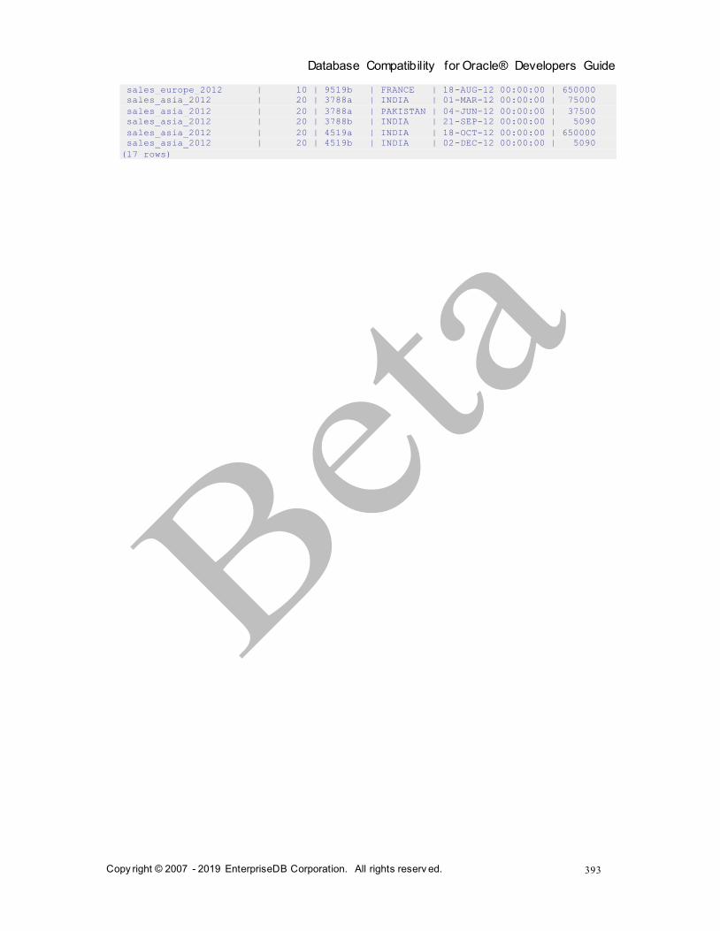
Database Compatibility for Oracle® Developers Guide
Copy right © 2007 - 2019 EnterpriseDB Corporation. All rights reserv ed.
393
sales_europe_2012 | 10 | 9519b | FRANCE | 18-AUG-12 00:00:00 | 650000
sales_asia_2012 | 20 | 3788a | INDIA | 01-MAR-12 00:00:00 | 75000
sales_asia_2012 | 20 | 3788a | PAKISTAN | 04-JUN-12 00:00:00 | 37500
sales_asia_2012 | 20 | 3788b | INDIA | 21-SEP-12 00:00:00 | 5090
sales_asia_2012 | 20 | 4519a | INDIA | 18-OCT-12 00:00:00 | 650000
sales_asia_2012 | 20 | 4519b | INDIA | 02-DEC-12 00:00:00 | 5090
(17 rows)

Database Compatibility for Oracle® Developers Guide
Copy right © 2007 - 2019 EnterpriseDB Corporation. All rights reserv ed.
394
10.3.6 ALTER TABLE… EXCHANGE PARTITION
The ALTER TABLE…EXCHANGE PARTITION command swaps an existing table with a partition. If you plan to add a large quantity of data to a partitioned table, you can use the
ALTER TABLE… EXCHANGE PARTITION command to implement a bulk load. You can
also use the ALTER TABLE… EXCHANGE PARTITION command to remove old or unneeded data for storage.
The command syntax is available in two forms.
The first form swaps a table for a partition:
ALTER TABLE target_table
EXCHANGE PARTITION target_partition
WITH TABLE source_table
[(INCLUDING | EXCLUDING) INDEXES]
[(WITH | WITHOUT) VALIDATION];
The second form swaps a table for a subpartition:
ALTER TABLE target_table
EXCHANGE SUBPARTITION target_subpartition
WITH TABLE source_table
[(INCLUDING | EXCLUDING) INDEXES]
[(WITH | WITHOUT) VALIDATION];
Description
When the ALTER TABLE… EXCHANGE PARTITION command completes, the data originally located in the target_partition will be located in the source_table,
and the data originally located in the source_table will be located in the target_partition.
The ALTER TABLE… EXCHANGE PARTITION command can exchange partitions in a LIST, RANGE or HASH partitioned table. The structure of the source_table must
match the structure of the target_table (both tables must have matching columns and
data types), and the data contained within the table must adhere to the partitioning constraints.
If the INCLUDING INDEXES clause is specified with EXCHANGE PARTITION, then
matching indexes in the target_partition and source_table are swapped. Indexes
in the target_partition with no match in the source_table are rebuilt and vice
versa (that is, indexes in the source_table with no match in the target_partition are also rebuilt).

Database Compatibility for Oracle® Developers Guide
Copy right © 2007 - 2019 EnterpriseDB Corporation. All rights reserv ed.
395
If the EXCLUDING INDEXES clause is specified with EXCHANGE PARTITION, then matching indexes in the target_partition and source_table are swapped, but the
target_partition indexes with no match in the source_table are marked as
invalid and vice versa (that is , indexes in the source_table with no match in the target_partition are also marked as invalid).
The previously used matching index term refers to indexes that have the same attributes
such as the collation order, ascending or descending direction, ordering of nulls first or nulls last, and so forth as determined by the CREATE INDEX command.
If both INCLUDING INDEXES and EXCLUDING INDEXES are omitted, then the default action is the EXCLUDING INDEXES behavior.
The same behavior as previously described applies for the target_subpartition used
with the EXCHANGE SUBPARTITION clause.
You must own a table to invoke ALTER TABLE… EXCHANGE PARTITION or ALTER TABLE… EXCHANGE SUBPARTITION against that table.
Parameters:
target_table
The name (optionally schema-qualified) of the table in which the partition or subpartition resides.
target_partition
The name of the partition to be replaced.
target_subpartition
The name of the subpartition to be replaced.
source_table
The name of the table that will replace the target_partition or
target_subpartition.
10.3.6.1 Example - Exchanging a Table for a Partition
The example that follows demonstrates swapping a table for a partition (americas) of the sales table. You can create the sales table with the following command:

Database Compatibility for Oracle® Developers Guide
Copy right © 2007 - 2019 EnterpriseDB Corporation. All rights reserv ed.
396
CREATE TABLE sales
(
dept_no number,
part_no varchar2,
country varchar2(20),
date date,
amount number
)
PARTITION BY LIST(country)
(
PARTITION europe VALUES('FRANCE', 'ITALY'),
PARTITION asia VALUES('INDIA', 'PAKISTAN'),
PARTITION americas VALUES('US', 'CANADA')
);
Use the following command to add sample data to the sales table:
INSERT INTO sales VALUES
(40, '9519b', 'US', '12-Apr-2012', '145000'),
(10, '4519b', 'FRANCE', '17-Jan-2012', '45000'),
(20, '3788a', 'INDIA', '01-Mar-2012', '75000'),
(20, '3788a', 'PAKISTAN', '04-Jun-2012', '37500'),
(10, '9519b', 'ITALY', '07-Jul-2012', '15000'),
(10, '9519a', 'FRANCE', '18-Aug-2012', '650000'),
(10, '9519b', 'FRANCE', '18-Aug-2012', '650000'),
(20, '3788b', 'INDIA', '21-Sept-2012', '5090'),
(20, '4519a', 'INDIA', '18-Oct-2012', '650000'),
(20, '4519b', 'INDIA', '2-Dec-2012', '5090');
Querying the sales table shows that only one row resides in the americas partition:
edb=# SELECT tableoid::regclass, * FROM sales;
tableoid | dept_no | part_no | country | date | amount
----------------+---------+---------+----------+--------------------+--------
sales_americas | 40 | 9519b | US | 12-APR-12 00:00:00 | 145000
sales_europe | 10 | 4519b | FRANCE | 17-JAN-12 00:00:00 | 45000
sales_europe | 10 | 9519b | ITALY | 07-JUL-12 00:00:00 | 15000
sales_europe | 10 | 9519a | FRANCE | 18-AUG-12 00:00:00 | 650000
sales_europe | 10 | 9519b | FRANCE | 18-AUG-12 00:00:00 | 650000
sales_asia | 20 | 3788a | INDIA | 01-MAR-12 00:00:00 | 75000
sales_asia | 20 | 3788a | PAKISTAN | 04-JUN-12 00:00:00 | 37500
sales_asia | 20 | 3788b | INDIA | 21-SEP-12 00:00:00 | 5090
sales_asia | 20 | 4519a | INDIA | 18-OCT-12 00:00:00 | 650000
sales_asia | 20 | 4519b | INDIA | 02-DEC-12 00:00:00 | 5090
(10 rows)
The following command creates a table (n_america) that matches the definition of the sales table:
CREATE TABLE n_america
(
dept_no number,
part_no varchar2,
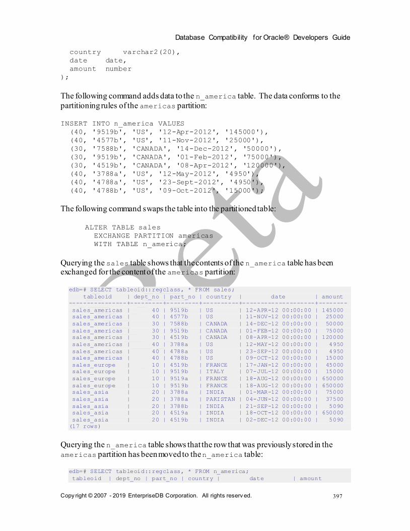
Database Compatibility for Oracle® Developers Guide
Copy right © 2007 - 2019 EnterpriseDB Corporation. All rights reserv ed.
397
country varchar2(20),
date date,
amount number
);
The following command adds data to the n_america table. The data conforms to the
partitioning rules of the americas partition:
INSERT INTO n_america VALUES
(40, '9519b', 'US', '12-Apr-2012', '145000'),
(40, '4577b', 'US', '11-Nov-2012', '25000'),
(30, '7588b', 'CANADA', '14-Dec-2012', '50000'),
(30, '9519b', 'CANADA', '01-Feb-2012', '75000'),
(30, '4519b', 'CANADA', '08-Apr-2012', '120000'),
(40, '3788a', 'US', '12-May-2012', '4950'),
(40, '4788a', 'US', '23-Sept-2012', '4950'),
(40, '4788b', 'US', '09-Oct-2012', '15000');
The following command swaps the table into the partitioned table:
ALTER TABLE sales
EXCHANGE PARTITION americas
WITH TABLE n_america;
Querying the sales table shows that the contents of the n_america table has been exchanged for the content of the americas partition:
edb=# SELECT tableoid::regclass, * FROM sales;
tableoid | dept_no | part_no | country | date | amount
----------------+---------+---------+----------+--------------------+--------
sales_americas | 40 | 9519b | US | 12-APR-12 00:00:00 | 145000
sales_americas | 40 | 4577b | US | 11-NOV-12 00:00:00 | 25000
sales_americas | 30 | 7588b | CANADA | 14-DEC-12 00:00:00 | 50000
sales_americas | 30 | 9519b | CANADA | 01-FEB-12 00:00:00 | 75000
sales_americas | 30 | 4519b | CANADA | 08-APR-12 00:00:00 | 120000
sales_americas | 40 | 3788a | US | 12-MAY-12 00:00:00 | 4950
sales_americas | 40 | 4788a | US | 23-SEP-12 00:00:00 | 4950
sales_americas | 40 | 4788b | US | 09-OCT-12 00:00:00 | 15000
sales_europe | 10 | 4519b | FRANCE | 17-JAN-12 00:00:00 | 45000
sales_europe | 10 | 9519b | ITALY | 07-JUL-12 00:00:00 | 15000
sales_europe | 10 | 9519a | FRANCE | 18-AUG-12 00:00:00 | 650000
sales_europe | 10 | 9519b | FRANCE | 18-AUG-12 00:00:00 | 650000
sales_asia | 20 | 3788a | INDIA | 01-MAR-12 00:00:00 | 75000
sales_asia | 20 | 3788a | PAKISTAN | 04-JUN-12 00:00:00 | 37500
sales_asia | 20 | 3788b | INDIA | 21-SEP-12 00:00:00 | 5090
sales_asia | 20 | 4519a | INDIA | 18-OCT-12 00:00:00 | 650000
sales_asia | 20 | 4519b | INDIA | 02-DEC-12 00:00:00 | 5090
(17 rows)
Querying the n_america table shows that the row that was previously stored in the
americas partition has been moved to the n_america table:
edb=# SELECT tableoid::regclass, * FROM n_america;
tableoid | dept_no | part_no | country | date | amount
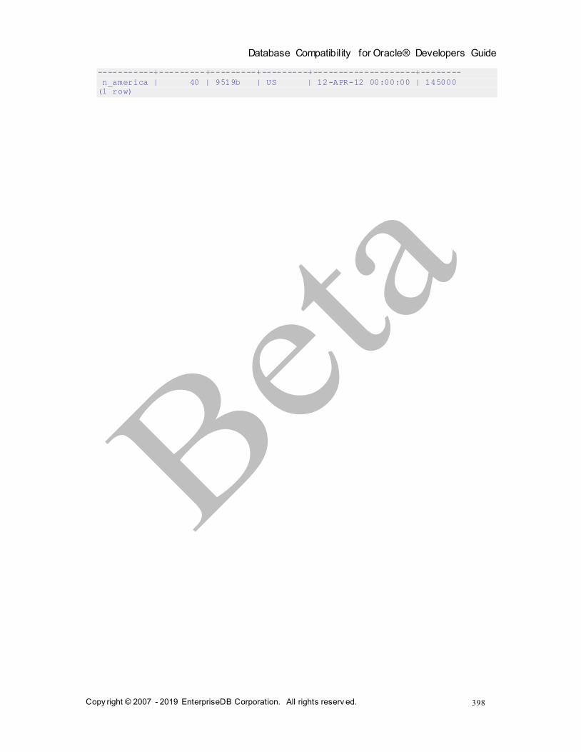
Database Compatibility for Oracle® Developers Guide
Copy right © 2007 - 2019 EnterpriseDB Corporation. All rights reserv ed.
398
-----------+---------+---------+---------+--------------------+--------
n_america | 40 | 9519b | US | 12-APR-12 00:00:00 | 145000
(1 row)

Database Compatibility for Oracle® Developers Guide
Copy right © 2007 - 2019 EnterpriseDB Corporation. All rights reserv ed.
399
10.3.7 ALTER TABLE… MOVE PARTITION
Use the ALTER TABLE… MOVE PARTITION command to move a partition to a different tablespace. The command takes two forms.
The first form moves a partition to a new tablespace:
ALTER TABLE table_name
MOVE PARTITION partition_name
TABLESPACE tablespace_name;
The second form moves a subpartition to a new tablespace:
ALTER TABLE table_name
MOVE SUBPARTITION subpartition_name
TABLESPACE tablespace_name;
Description
The ALTER TABLE…MOVE PARTITION command moves a partition from its current
tablespace to a different tablespace. The ALTER TABLE… MOVE PARTITION command can move partitions of a LIST, RANGE or HASH partitioned table.
The same behavior as previously described applies for the subpartition_name used
with the MOVE SUBPARTITION clause.
You must own the table to invoke ALTER TABLE… MOVE PARTITION or ALTER TABLE… MOVE SUBPARTITION.
Parameters
table_name
The name (optionally schema-qualified) of the table in which the partition or subpartition resides.
partition_name
The name of the partition to be moved.
subpartition_name
The name of the subpartition to be moved.
tablespace_name
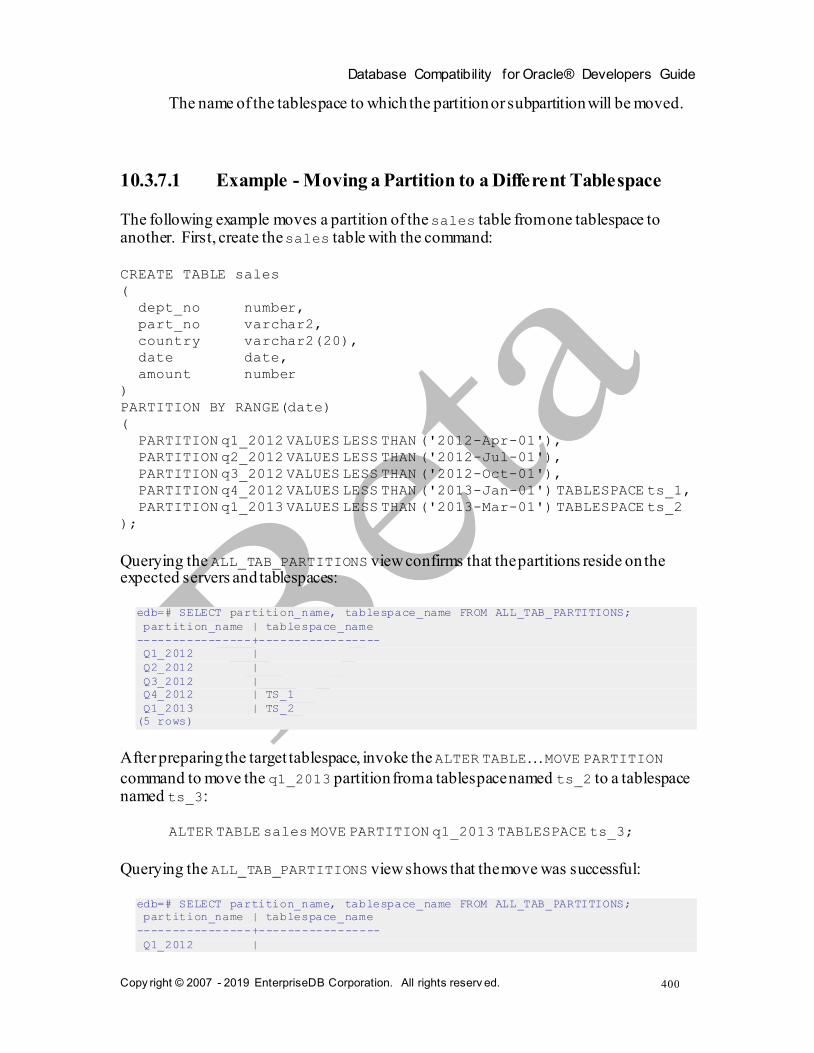
Database Compatibility for Oracle® Developers Guide
Copy right © 2007 - 2019 EnterpriseDB Corporation. All rights reserv ed.
400
The name of the tablespace to which the partition or subpartition will be moved.
10.3.7.1 Example - Moving a Partition to a Different Tablespace
The following example moves a partition of the sales table from one tablespace to another. First, create the sales table with the command:
CREATE TABLE sales
(
dept_no number,
part_no varchar2,
country varchar2(20),
date date,
amount number
)
PARTITION BY RANGE(date)
(
PARTITION q1_2012 VALUES LESS THAN ('2012-Apr-01'),
PARTITION q2_2012 VALUES LESS THAN ('2012-Jul-01'),
PARTITION q3_2012 VALUES LESS THAN ('2012-Oct-01'),
PARTITION q4_2012 VALUES LESS THAN ('2013-Jan-01') TABLESPACE ts_1,
PARTITION q1_2013 VALUES LESS THAN ('2013-Mar-01') TABLESPACE ts_2
);
Querying the ALL_TAB_PARTITIONS view confirms that the partitions reside on the expected servers and tablespaces:
edb=# SELECT partition_name, tablespace_name FROM ALL_TAB_PARTITIONS;
partition_name | tablespace_name
----------------+-----------------
Q1_2012 |
Q2_2012 |
Q3_2012 |
Q4_2012 | TS_1
Q1_2013 | TS_2
(5 rows)
After preparing the target tablespace, invoke the ALTER TABLE… MOVE PARTITION
command to move the q1_2013 partition from a tablespace named ts_2 to a tablespace named ts_3:
ALTER TABLE sales MOVE PARTITION q1_2013 TABLESPACE ts_3;
Querying the ALL_TAB_PARTITIONS view shows that the move was successful:
edb=# SELECT partition_name, tablespace_name FROM ALL_TAB_PARTITIONS;
partition_name | tablespace_name
----------------+-----------------
Q1_2012 |

Database Compatibility for Oracle® Developers Guide
Copy right © 2007 - 2019 EnterpriseDB Corporation. All rights reserv ed.
401
Q2_2012 |
Q3_2012 |
Q4_2012 | TS_1
Q1_2013 | TS_3
(5 rows)

Database Compatibility for Oracle® Developers Guide
Copy right © 2007 - 2019 EnterpriseDB Corporation. All rights reserv ed.
402
10.3.8 ALTER TABLE… RENAME PARTITION
Use the ALTER TABLE… RENAME PARTITION command to rename a table partition. The syntax takes two forms.
The first form renames a partition:
ALTER TABLE table_name
RENAME PARTITION partition_name
TO new_name;
The second form renames a subpartition:
ALTER TABLE table_name
RENAME SUBPARTITION subpartition_name
TO new_name;
Description
The ALTER TABLE… RENAME PARTITION command renames a partition.
The same behavior as previously described applies for the subpartition_name used
with the RENAME SUBPARTITION clause.
You must own the specified table to invoke ALTER TABLE… RENAME PARTITION or ALTER TABLE… RENAME SUBPARTITION.
Parameters
table_name
The name (optionally schema-qualified) of the table in which the partition or subpartition resides.
partition_name
The name of the partition to be renamed.
subpartition_name
The name of the subpartition to be renamed.
new_name
The new name of the partition or subpartition.

Database Compatibility for Oracle® Developers Guide
Copy right © 2007 - 2019 EnterpriseDB Corporation. All rights reserv ed.
403
10.3.8.1 Example - Renaming a Partition
The following command creates a list-partitioned table named sales:
CREATE TABLE sales
(
dept_no number,
part_no varchar2,
country varchar2(20),
date date,
amount number
)
PARTITION BY LIST(country)
(
PARTITION europe VALUES('FRANCE', 'ITALY'),
PARTITION asia VALUES('INDIA', 'PAKISTAN'),
PARTITION americas VALUES('US', 'CANADA')
);
Query the ALL_TAB_PARTITIONS view to display the partition names:
edb=# SELECT partition_name, high_value FROM ALL_TAB_PARTITIONS;
partition_name | high_value
----------------+---------------------
EUROPE | 'FRANCE', 'ITALY'
ASIA | 'INDIA', 'PAKISTAN'
AMERICAS | 'US', 'CANADA'
(3 rows)
The following command renames the americas partition to n_america:
ALTER TABLE sales
RENAME PARTITION americas TO n_america;
Querying the ALL_TAB_PARTITIONS view demonstrates that the partition has been successfully renamed:
edb=# SELECT partition_name, high_value FROM ALL_TAB_PARTITIONS;
partition_name | high_value
----------------+---------------------
EUROPE | 'FRANCE', 'ITALY'
ASIA | 'INDIA', 'PAKISTAN'
N_AMERICA | 'US', 'CANADA'
(3 rows)

Database Compatibility for Oracle® Developers Guide
Copy right © 2007 - 2019 EnterpriseDB Corporation. All rights reserv ed.
404
10.3.9 DROP TABLE
Use the PostgreSQL DROP TABLE command to remove a partitioned table definition, it's partitions and subpartitions, and delete the table contents. The syntax is :
DROP TABLE table_name
Parameters
table_name
The name (optionally schema-qualified) of the partitioned table.
Description
The DROP TABLE command removes an entire table, and the data that resides in that table. When you delete a table, any partitions or subpartitions (of that table) are deleted as well.
To use the DROP TABLE command, you must be the owner of the partitioning root, a member of a group that owns the table, the schema owner, or a database superuser.
Example
To delete a table, connect to the controller node (the host of the partitioning root), and
invoke the DROP TABLE command. For example, to delete the sales table, invoke the following command:
DROP TABLE sales;
The server will confirm that the table has been dropped:
edb=# drop table sales;
DROP TABLE
edb=#
For more information about the DROP TABLE command, please see the PostgreSQL core documentation at:
https://www.postgresql.org/docs/11/static/sql-droptable.html

Database Compatibility for Oracle® Developers Guide
Copy right © 2007 - 2019 EnterpriseDB Corporation. All rights reserv ed.
405
10.3.10 ALTER TABLE… DROP PARTITION
Use the ALTER TABLE… DROP PARTITION command to delete a partition definition, and the data stored in that partition. The syntax is:
ALTER TABLE table_name DROP PARTITION partition_name;
Parameters
table_name
The name (optionally schema-qualified) of the partitioned table.
partition_name
The name of the partition to be deleted.
Description
The ALTER TABLE… DROP PARTITION command deletes a partition and any data stored
on that partition. The ALTER TABLE… DROP PARTITION command can drop partitions
of a LIST or RANGE partitioned table; please note that this command does not work on a
HASH partitioned table. When you delete a partition, any subpartitions (of that partition) are deleted as well.
To use the DROP PARTITION clause, you must be the owner of the partitioning root, a member of a group that owns the table, or have database superuser or administrative privileges.
10.3.10.1 Example - Deleting a Partition
The example that follows deletes a partition of the sales table. Use the following command to create the sales table:
CREATE TABLE sales
(
dept_no number,
part_no varchar2,
country varchar2(20),
date date,
amount number
)
PARTITION BY LIST(country)
(
PARTITION europe VALUES('FRANCE', 'ITALY'),

Database Compatibility for Oracle® Developers Guide
Copy right © 2007 - 2019 EnterpriseDB Corporation. All rights reserv ed.
406
PARTITION asia VALUES('INDIA', 'PAKISTAN'),
PARTITION americas VALUES('US', 'CANADA')
);
Querying the ALL_TAB_PARTITIONS view displays the partition names:
edb=# SELECT partition_name, high_value FROM ALL_TAB_PARTITIONS;
partition_name | high_value
----------------+---------------------
EUROPE | 'FRANCE', 'ITALY'
ASIA | 'INDIA', 'PAKISTAN'
AMERICAS | 'US', 'CANADA'
(3 rows)
To delete the americas partition from the sales table, invoke the following command:
ALTER TABLE sales DROP PARTITION americas;
Querying the ALL_TAB_PARTITIONS view demonstrates that the partition has been successfully deleted:
edb=# SELECT partition_name, high_value FROM ALL_TAB_PARTITIONS;
partition_name | high_value
----------------+---------------------
EUROPE | 'FRANCE', 'ITALY'
ASIA | 'INDIA', 'PAKISTAN'
(2 rows)

Database Compatibility for Oracle® Developers Guide
Copy right © 2007 - 2019 EnterpriseDB Corporation. All rights reserv ed.
407
10.3.11 ALTER TABLE… DROP SUBPARTITION
Use the ALTER TABLE… DROP SUBPARTITION command to drop a subpartition definition, and the data stored in that subpartition. The syntax is:
ALTER TABLE table_name DROP SUBPARTITION subpartition_name;
Parameters
table_name
The name (optionally schema-qualified) of the partitioned table.
subpartition_name
The name of the subpartition to be deleted.
Description
The ALTER TABLE… DROP SUBPARTITION command deletes a subpartition, and the data
stored in that subpartition. To use the DROP SUBPARTITION clause, you must be the owner of the partitioning root, a member of a group that owns the table, or have superuser or administrative privileges.
10.3.11.1 Example - Deleting a Subpartition
The example that follows deletes a subpartition of the sales table. Use the following command to create the sales table:
CREATE TABLE sales
(
dept_no number,
part_no varchar2,
country varchar2(20),
date date,
amount number
)
PARTITION BY RANGE(date)
SUBPARTITION BY LIST (country)
(
PARTITION first_half_2012 VALUES LESS THAN('01-JUL-2012')
(
SUBPARTITION europe VALUES ('ITALY', 'FRANCE'),
SUBPARTITION americas VALUES ('CANADA', 'US'),

Database Compatibility for Oracle® Developers Guide
Copy right © 2007 - 2019 EnterpriseDB Corporation. All rights reserv ed.
408
SUBPARTITION asia VALUES ('PAKISTAN', 'INDIA')
),
PARTITION second_half_2012 VALUES LESS THAN('01-JAN-2013')
);
Querying the ALL_TAB_SUBPARTITIONS view displays the subpartition names:
edb=# SELECT subpartition_name, high_value FROM ALL_TAB_SUBPARTITIONS;
subpartition_name | high_value
-------------------+---------------------
EUROPE | 'ITALY', 'FRANCE'
AMERICAS | 'CANADA', 'US'
ASIA | 'PAKISTAN', 'INDIA'
SYS0101 | DEFAULT
(4 rows)
To delete the americas subpartition from the sales table, invoke the following command:
ALTER TABLE sales DROP SUBPARTITION americas;
Querying the ALL_TAB_SUBPARTITIONS view demonstrates that the subpartition has been successfully deleted:
edb=# SELECT subpartition_name, high_value FROM ALL_TAB_SUBPARTITIONS;
subpartition_name | high_value
-------------------+---------------------
EUROPE | 'ITALY', 'FRANCE'
ASIA | 'PAKISTAN', 'INDIA'
SYS0101 | DEFAULT
(3 rows)
Database Compatibility for Oracle® Developers Guide
Copy right © 2007 - 2019 EnterpriseDB Corporation. All rights reserv ed.
409
10.3.12 TRUNCATE TABLE
Use the TRUNCATE TABLE command to remove the contents of a table, while preserving the table definition. When you truncate a table, any partitions or subpartitions of that table are also truncated. The syntax is:
TRUNCATE TABLE table_name
Description
The TRUNCATE TABLE command removes an entire table, and the data that resides in that table. When you delete a table, any partitions or subpartitions (of that table) are deleted as well.
To use the TRUNCATE TABLE command, you must be the owner of the partitioning root, a member of a group that owns the table, the schema owner, or a database superuser.
Parameters
table_name
The name (optionally schema-qualified) of the partitioned table.
10.3.12.1 Example - Emptying a Table
The example that follows removes the data from the sales table. Use the following
command to create the sales table:
CREATE TABLE sales
(
dept_no number,
part_no varchar2,
country varchar2(20),
date date,
amount number
)
PARTITION BY LIST(country)
(
PARTITION europe VALUES('FRANCE', 'ITALY'),
PARTITION asia VALUES('INDIA', 'PAKISTAN'),
PARTITION americas VALUES('US', 'CANADA')
);
Populate the sales table with the command:

Database Compatibility for Oracle® Developers Guide
Copy right © 2007 - 2019 EnterpriseDB Corporation. All rights reserv ed.
410
INSERT INTO sales VALUES
(10, '4519b', 'FRANCE', '17-Jan-2012', '45000'),
(20, '3788a', 'INDIA', '01-Mar-2012', '75000'),
(40, '9519b', 'US', '12-Apr-2012', '145000'),
(20, '3788a', 'PAKISTAN', '04-Jun-2012', '37500'),
(40, '4577b', 'US', '11-Nov-2012', '25000'),
(30, '7588b', 'CANADA', '14-Dec-2012', '50000'),
(30, '9519b', 'CANADA', '01-Feb-2012', '75000'),
(30, '4519b', 'CANADA', '08-Apr-2012', '120000'),
(40, '3788a', 'US', '12-May-2012', '4950'),
(10, '9519b', 'ITALY', '07-Jul-2012', '15000'),
(10, '9519a', 'FRANCE', '18-Aug-2012', '650000'),
(10, '9519b', 'FRANCE', '18-Aug-2012', '650000'),
(20, '3788b', 'INDIA', '21-Sept-2012', '5090'),
(40, '4788a', 'US', '23-Sept-2012', '4950'),
(40, '4788b', 'US', '09-Oct-2012', '15000'),
(20, '4519a', 'INDIA', '18-Oct-2012', '650000'),
(20, '4519b', 'INDIA', '2-Dec-2012', '5090');
Querying the sales table shows that the partitions are populated with data:
edb=# SELECT tableoid::regclass, * FROM sales;
tableoid | dept_no | part_no | country | date | amount
----------------+---------+---------+----------+--------------------+--------
sales_americas | 40 | 9519b | US | 12-APR-12 00:00:00 | 145000
sales_americas | 40 | 4577b | US | 11-NOV-12 00:00:00 | 25000
sales_americas | 30 | 7588b | CANADA | 14-DEC-12 00:00:00 | 50000
sales_americas | 30 | 9519b | CANADA | 01-FEB-12 00:00:00 | 75000
sales_americas | 30 | 4519b | CANADA | 08-APR-12 00:00:00 | 120000
sales_americas | 40 | 3788a | US | 12-MAY-12 00:00:00 | 4950
sales_americas | 40 | 4788a | US | 23-SEP-12 00:00:00 | 4950
sales_americas | 40 | 4788b | US | 09-OCT-12 00:00:00 | 15000
sales_europe | 10 | 4519b | FRANCE | 17-JAN-12 00:00:00 | 45000
sales_europe | 10 | 9519b | ITALY | 07-JUL-12 00:00:00 | 15000
sales_europe | 10 | 9519a | FRANCE | 18-AUG-12 00:00:00 | 650000
sales_europe | 10 | 9519b | FRANCE | 18-AUG-12 00:00:00 | 650000
sales_asia | 20 | 3788a | INDIA | 01-MAR-12 00:00:00 | 75000
sales_asia | 20 | 3788a | PAKISTAN | 04-JUN-12 00:00:00 | 37500
sales_asia | 20 | 3788b | INDIA | 21-SEP-12 00:00:00 | 5090
sales_asia | 20 | 4519a | INDIA | 18-OCT-12 00:00:00 | 650000
sales_asia | 20 | 4519b | INDIA | 02-DEC-12 00:00:00 | 5090
(17 rows)
To delete the contents of the sales table, invoke the following command:
TRUNCATE TABLE sales;
Now, querying the sales table shows that the data has been removed but the structure is intact:
edb=# SELECT tableoid::regclass, * FROM sales;
tableoid | dept_no | part_no | country | date | amount
----------+---------+---------+---------+------+--------
(0 rows)

Database Compatibility for Oracle® Developers Guide
Copy right © 2007 - 2019 EnterpriseDB Corporation. All rights reserv ed.
411
For more information about the TRUNCATE TABLE command, please see the PostgreSQL documentation at:
https://www.postgresql.org/docs/11/static/sql-truncate.html

Database Compatibility for Oracle® Developers Guide
Copy right © 2007 - 2019 EnterpriseDB Corporation. All rights reserv ed.
412
10.3.13 ALTER TABLE… TRUNCATE PARTITION
Use the ALTER TABLE… TRUNCATE PARTITION command to remove the data from the specified partition, leaving the partition structure intact. The syntax is:
ALTER TABLE table_name TRUNCATE PARTITION partition_name
[{DROP|REUSE} STORAGE]
Description
Use the ALTER TABLE… TRUNCATE PARTITION command to remove the data from the specified partition, leaving the partition structure intact. When you truncate a partition, any subpartitions of that partition are also truncated.
ALTER TABLE… TRUNCATE PARTITION will not cause ON DELETE triggers that might
exist for the table to fire, but it will fire ON TRUNCATE triggers. If an ON TRUNCATE
trigger is defined for the partition, all BEFORE TRUNCATE triggers are fired before any
truncation happens, and all AFTER TRUNCATE triggers are fired after the last truncation occurs.
You must have the TRUNCATE privilege on a table to invoke ALTER TABLE…
TRUNCATE PARTITION.
Parameters
table_name
The name (optionally schema-qualified) of the partitioned table.
partition_name
The name of the partition to be deleted.
DROP STORAGE and REUSE STORAGE are included for compatibility only; the clauses are parsed and ignored.
10.3.13.1 Example - Emptying a Partition
The example that follows removes the data from a partition of the sales table. Use the
following command to create the sales table:
CREATE TABLE sales

Database Compatibility for Oracle® Developers Guide
Copy right © 2007 - 2019 EnterpriseDB Corporation. All rights reserv ed.
413
(
dept_no number,
part_no varchar2,
country varchar2(20),
date date,
amount number
)
PARTITION BY LIST(country)
(
PARTITION europe VALUES('FRANCE', 'ITALY'),
PARTITION asia VALUES('INDIA', 'PAKISTAN'),
PARTITION americas VALUES('US', 'CANADA')
);
Populate the sales table with the command:
INSERT INTO sales VALUES
(10, '4519b', 'FRANCE', '17-Jan-2012', '45000'),
(20, '3788a', 'INDIA', '01-Mar-2012', '75000'),
(40, '9519b', 'US', '12-Apr-2012', '145000'),
(20, '3788a', 'PAKISTAN', '04-Jun-2012', '37500'),
(40, '4577b', 'US', '11-Nov-2012', '25000'),
(30, '7588b', 'CANADA', '14-Dec-2012', '50000'),
(30, '9519b', 'CANADA', '01-Feb-2012', '75000'),
(30, '4519b', 'CANADA', '08-Apr-2012', '120000'),
(40, '3788a', 'US', '12-May-2012', '4950'),
(10, '9519b', 'ITALY', '07-Jul-2012', '15000'),
(10, '9519a', 'FRANCE', '18-Aug-2012', '650000'),
(10, '9519b', 'FRANCE', '18-Aug-2012', '650000'),
(20, '3788b', 'INDIA', '21-Sept-2012', '5090'),
(40, '4788a', 'US', '23-Sept-2012', '4950'),
(40, '4788b', 'US', '09-Oct-2012', '15000'),
(20, '4519a', 'INDIA', '18-Oct-2012', '650000'),
(20, '4519b', 'INDIA', '2-Dec-2012', '5090');
Querying the sales table shows that the partitions are populated with data:
edb=# SELECT tableoid::regclass, * FROM sales;
tableoid | dept_no | part_no | country | date | amount
----------------+---------+---------+----------+--------------------+--------
sales_americas | 40 | 9519b | US | 12-APR-12 00:00:00 | 145000
sales_americas | 40 | 4577b | US | 11-NOV-12 00:00:00 | 25000
sales_americas | 30 | 7588b | CANADA | 14-DEC-12 00:00:00 | 50000
sales_americas | 30 | 9519b | CANADA | 01-FEB-12 00:00:00 | 75000
sales_americas | 30 | 4519b | CANADA | 08-APR-12 00:00:00 | 120000
sales_americas | 40 | 3788a | US | 12-MAY-12 00:00:00 | 4950
sales_americas | 40 | 4788a | US | 23-SEP-12 00:00:00 | 4950
sales_americas | 40 | 4788b | US | 09-OCT-12 00:00:00 | 15000
sales_europe | 10 | 4519b | FRANCE | 17-JAN-12 00:00:00 | 45000
sales_europe | 10 | 9519b | ITALY | 07-JUL-12 00:00:00 | 15000
sales_europe | 10 | 9519a | FRANCE | 18-AUG-12 00:00:00 | 650000
sales_europe | 10 | 9519b | FRANCE | 18-AUG-12 00:00:00 | 650000
sales_asia | 20 | 3788a | INDIA | 01-MAR-12 00:00:00 | 75000
sales_asia | 20 | 3788a | PAKISTAN | 04-JUN-12 00:00:00 | 37500

Database Compatibility for Oracle® Developers Guide
Copy right © 2007 - 2019 EnterpriseDB Corporation. All rights reserv ed.
414
sales_asia | 20 | 3788b | INDIA | 21-SEP-12 00:00:00 | 5090
sales_asia | 20 | 4519a | INDIA | 18-OCT-12 00:00:00 | 650000
sales_asia | 20 | 4519b | INDIA | 02-DEC-12 00:00:00 | 5090
(17 rows)
To delete the contents of the americas partition, invoke the following command:
ALTER TABLE sales TRUNCATE PARTITION americas;
Now, querying the sales table shows that the content of the americas partition has been removed:
edb=# SELECT tableoid::regclass, * FROM sales;
tableoid | dept_no | part_no | country | date | amount
--------------+---------+---------+----------+--------------------+--------
sales_europe | 10 | 4519b | FRANCE | 17-JAN-12 00:00:00 | 45000
sales_europe | 10 | 9519b | ITALY | 07-JUL-12 00:00:00 | 15000
sales_europe | 10 | 9519a | FRANCE | 18-AUG-12 00:00:00 | 650000
sales_europe | 10 | 9519b | FRANCE | 18-AUG-12 00:00:00 | 650000
sales_asia | 20 | 3788a | INDIA | 01-MAR-12 00:00:00 | 75000
sales_asia | 20 | 3788a | PAKISTAN | 04-JUN-12 00:00:00 | 37500
sales_asia | 20 | 3788b | INDIA | 21-SEP-12 00:00:00 | 5090
sales_asia | 20 | 4519a | INDIA | 18-OCT-12 00:00:00 | 650000
sales_asia | 20 | 4519b | INDIA | 02-DEC-12 00:00:00 | 5090
(9 rows)
While the rows have been removed, the structure of the americas partition is still intact:
edb=# SELECT partition_name, high_value FROM ALL_TAB_PARTITIONS;
partition_name | high_value
----------------+---------------------
EUROPE | 'FRANCE', 'ITALY'
ASIA | 'INDIA', 'PAKISTAN'
AMERICAS | 'US', 'CANADA'
(3 rows)

Database Compatibility for Oracle® Developers Guide
Copy right © 2007 - 2019 EnterpriseDB Corporation. All rights reserv ed.
415
10.3.14 ALTER TABLE… TRUNCATE SUBPARTITION
Use the ALTER TABLE… TRUNCATE SUBPARTITION command to remove all of the data from the specified subpartition, leaving the subpartition structure intact. The syntax is:
ALTER TABLE table_name
TRUNCATE SUBPARTITION subpartition_name
[{DROP|REUSE} STORAGE]
Description
The ALTER TABLE… TRUNCATE SUBPARTITION command removes all data from a specified subpartition, leaving the subpartition structure intact.
ALTER TABLE… TRUNCATE SUBPARTITION will not cause ON DELETE triggers that
might exist for the table to fire, but it will fire ON TRUNCATE triggers. If an ON
TRUNCATE trigger is defined for the subpartition, all BEFORE TRUNCATE triggers are
fired before any truncation happens, and all AFTER TRUNCATE triggers are fired after the last truncation occurs.
You must have the TRUNCATE privilege on a table to invoke ALTER TABLE… TRUNCATE SUBPARTITION.
Parameters
table_name
The name (optionally schema-qualified) of the partitioned table.
subpartition_name
The name of the subpartition to be truncated.
The DROP STORAGE and REUSE STORAGE clauses are included for compatibility only; the clauses are parsed and ignored.
10.3.14.1 Example - Emptying a Subpartition
The example that follows removes the data from a subpartition of the sales table. Use the following command to create the sales table:
CREATE TABLE sales
(
dept_no number,

Database Compatibility for Oracle® Developers Guide
Copy right © 2007 - 2019 EnterpriseDB Corporation. All rights reserv ed.
416
part_no varchar2,
country varchar2(20),
date date,
amount number
)
PARTITION BY RANGE(date) SUBPARTITION BY LIST (country)
(
PARTITION "2011" VALUES LESS THAN('01-JAN-2012')
(
SUBPARTITION europe_2011 VALUES ('ITALY', 'FRANCE'),
SUBPARTITION asia_2011 VALUES ('PAKISTAN', 'INDIA'),
SUBPARTITION americas_2011 VALUES ('US', 'CANADA')
),
PARTITION "2012" VALUES LESS THAN('01-JAN-2013')
(
SUBPARTITION europe_2012 VALUES ('ITALY', 'FRANCE'),
SUBPARTITION asia_2012 VALUES ('PAKISTAN', 'INDIA'),
SUBPARTITION americas_2012 VALUES ('US', 'CANADA')
),
PARTITION "2013" VALUES LESS THAN('01-JAN-2015')
(
SUBPARTITION europe_2013 VALUES ('ITALY', 'FRANCE'),
SUBPARTITION asia_2013 VALUES ('PAKISTAN', 'INDIA'),
SUBPARTITION americas_2013 VALUES ('US', 'CANADA')
)
);
Populate the sales table with the command:
INSERT INTO sales VALUES
(10, '4519b', 'FRANCE', '17-Jan-2011', '45000'),
(20, '3788a', 'INDIA', '01-Mar-2012', '75000'),
(40, '9519b', 'US', '12-Apr-2012', '145000'),
(20, '3788a', 'PAKISTAN', '04-Jun-2012', '37500'),
(40, '4577b', 'US', '11-Nov-2012', '25000'),
(30, '7588b', 'CANADA', '14-Dec-2011', '50000'),
(30, '4519b', 'CANADA', '08-Apr-2012', '120000'),
(40, '3788a', 'US', '12-May-2011', '4950'),
(20, '3788a', 'US', '04-Apr-2012', '37500'),
(40, '4577b', 'INDIA', '11-Jun-2011', '25000'),
(10, '9519b', 'ITALY', '07-Jul-2012', '15000'),
(20, '4519b', 'INDIA', '2-Dec-2012', '5090');
Querying the sales table shows that the rows have been distributed amongst the subpartitions:
edb=# SELECT tableoid::regclass, * FROM sales;
tableoid | dept_no | part_no | country| date | amount
-------------------+---------+---------+--------+--------------------+------
sales_americas_2011 | 30| 7588b | CANADA | 14-DEC-11 00:00:00 | 50000

Database Compatibility for Oracle® Developers Guide
Copy right © 2007 - 2019 EnterpriseDB Corporation. All rights reserv ed.
417
sales_americas_2011 | 40| 3788a | US | 12-MAY-11 00:00:00 | 4950
sales_europe_2011 | 10| 4519b | FRANCE | 17-JAN-11 00:00:00 | 45000
sales_asia_2011 | 40| 4577b | INDIA | 11-JUN-11 00:00:00 | 25000
sales_americas_2012 | 40| 9519b | US | 12-APR-12 00:00:00 | 145000
sales_americas_2012| 40| 4577b | US | 11-NOV-12 00:00:00 | 25000
sales_americas_2012| 30| 4519b | CANADA | 08-APR-12 00:00:00 | 120000
sales_americas_2012| 20| 3788a | US | 04-APR-12 00:00:00 | 37500
sales_europe_2012 | 10| 9519b | ITALY | 07-JUL-12 00:00:00 | 15000
sales_asia_2012 | 20| 3788a | INDIA | 01-MAR-12 00:00:00 | 75000
sales_asia_2012 | 20| 3788a |PAKISTAN| 04-JUN-12 00:00:00 | 37500
sales_asia_2012 | 20| 4519b | INDIA | 02-DEC-12 00:00:00 | 5090
(12 rows)
To delete the contents of the 2012_americas partition, invoke the following command:
ALTER TABLE sales TRUNCATE SUBPARTITION "americas_2012";
Now, querying the sales table shows that the content of the americas_2012 partition has been removed:
edb=# SELECT tableoid::regclass, * FROM sales;
tableoid | dept_no| part_no | country | date |amount
-------------------+--------+---------+----------+--------------------+------
sales_americas_2011| 30| 7588b | CANADA | 14-DEC-11 00:00:00 | 50000
sales_americas_2011| 40| 3788a | US | 12-MAY-11 00:00:00 | 4950
sales_europe_2011 | 10| 4519b | FRANCE | 17-JAN-11 00:00:00 | 45000
sales_asia_2011 | 40| 4577b | INDIA | 11-JUN-11 00:00:00 | 25000
sales_europe_2012 | 10| 9519b | ITALY | 07-JUL-12 00:00:00 | 15000
sales_asia_2012 | 20| 3788a | INDIA | 01-MAR-12 00:00:00 | 75000
sales_asia_2012 | 20| 3788a | PAKISTAN | 04-JUN-12 00:00:00 | 37500
sales_asia_2012 | 20| 4519b | INDIA | 02-DEC-12 00:00:00 | 5090
(8 rows)
While the rows have been removed, the structure of the 2012_americas partition is still intact:
edb=# SELECT subpartition_name, high_value FROM ALL_TAB_SUBPARTITIONS;
subpartition_name | high_value
-------------------+---------------------
EUROPE_2011 | 'ITALY', 'FRANCE'
ASIA_2011 | 'PAKISTAN', 'INDIA'
AMERICAS_2011 | 'US', 'CANADA'
EUROPE_2012 | 'ITALY', 'FRANCE'
ASIA_2012 | 'PAKISTAN', 'INDIA'
AMERICAS_2012 | 'US', 'CANADA'
EUROPE_2013 | 'ITALY', 'FRANCE'
ASIA_2013 | 'PAKISTAN', 'INDIA'
AMERICAS_2013 | 'US', 'CANADA'
(9 rows)

Database Compatibility for Oracle® Developers Guide
Copy right © 2007 - 2019 EnterpriseDB Corporation. All rights reserv ed.
418
10.4 Handling Stray Values in a LIST or RANGE Partitioned Table
A DEFAULT or MAXVALUE partition or subpartition will capture any rows that do not meet the other partitioning rules defined for a table.
Defining a DEFAULT Partition
A DEFAULT partition will capture any rows that do not fit into any other partition in a
LIST partitioned (or subpartitioned) table. If you do not include a DEFAULT rule, any
row that does not match one of the values in the partitioning constraints will result in an error. Each LIST partition or subpartition may have its own DEFAULT rule.
The syntax of a DEFAULT rule is:
PARTITION [partition_name] VALUES (DEFAULT)
Where partition_name specifies the name of the partition or subpartition that will
store any rows that do not match the rules specified for other partitions.
The last example created a list partitioned table in which the server decided which
partition to store the data based upon the value of the country column. If you attempt
to add a row in which the value of the country column contains a value not listed in the rules, Advanced Server reports an error:
edb=# INSERT INTO sales VALUES
edb-# (40, '3000x', 'IRELAND', '01-Mar-2012', '45000');
ERROR: no partition of relation "sales_2012" found for row
DETAIL: Partition key of the failing row contains (country) = (IRELAND).
The following example creates the same table, but adds a DEFAULT partition. The server
will store any rows that do not match a value specified in the partitioning rules for europe, asia, or americas partitions in the others partition:
CREATE TABLE sales
(
dept_no number,
part_no varchar2,
country varchar2(20),
date date,
amount number
)
PARTITION BY LIST(country)
(
PARTITION europe VALUES('FRANCE', 'ITALY'),
PARTITION asia VALUES('INDIA', 'PAKISTAN'),
PARTITION americas VALUES('US', 'CANADA'),
PARTITION others VALUES (DEFAULT)
);

Database Compatibility for Oracle® Developers Guide
Copy right © 2007 - 2019 EnterpriseDB Corporation. All rights reserv ed.
419
To test the DEFAULT partition, add row with a value in the country column that does not match one of the countries specified in the partitioning constraints:
INSERT INTO sales VALUES
(40, '3000x', 'IRELAND', '01-Mar-2012', '45000');
Querying the contents of the sales table confirms that the previously rejected row is
now stored in the sales_others partition:
edb=# SELECT tableoid::regclass, * FROM sales;
tableoid | dept_no | part_no | country | date | amount
----------------+---------+---------+----------+--------------------+--------
sales_americas | 40 | 9519b | US | 12-APR-12 00:00:00 | 145000
sales_americas | 40 | 4577b | US | 11-NOV-12 00:00:00 | 25000
sales_americas | 30 | 7588b | CANADA | 14-DEC-12 00:00:00 | 50000
sales_americas | 30 | 9519b | CANADA | 01-FEB-12 00:00:00 | 75000
sales_americas | 30 | 4519b | CANADA | 08-APR-12 00:00:00 | 120000
sales_americas | 40 | 3788a | US | 12-MAY-12 00:00:00 | 4950
sales_americas | 40 | 4788a | US | 23-SEP-12 00:00:00 | 4950
sales_americas | 40 | 4788b | US | 09-OCT-12 00:00:00 | 15000
sales_europe | 10 | 4519b | FRANCE | 17-JAN-12 00:00:00 | 45000
sales_europe | 10 | 9519b | ITALY | 07-JUL-12 00:00:00 | 15000
sales_europe | 10 | 9519a | FRANCE | 18-AUG-12 00:00:00 | 650000
sales_europe | 10 | 9519b | FRANCE | 18-AUG-12 00:00:00 | 650000
sales_asia | 20 | 3788a | INDIA | 01-MAR-12 00:00:00 | 75000
sales_asia | 20 | 3788a | PAKISTAN | 04-JUN-12 00:00:00 | 37500
sales_asia | 20 | 3788b | INDIA | 21-SEP-12 00:00:00 | 5090
sales_asia | 20 | 4519a | INDIA | 18-OCT-12 00:00:00 | 650000
sales_asia | 20 | 4519b | INDIA | 02-DEC-12 00:00:00 | 5090
sales_others | 40 | 3000x | IRELAND | 01-MAR-12 00:00:00 | 45000
(18 rows)
Advanced Server provides the following methods to re-assign the contents of a DEFAULT partition or subpartition:
You can use the ALTER TABLE… ADD PARTITION command to add a partition to
a table with a DEFAULT rule as long as there are no conflicting values between existing rows in the table and the values of the partition to be added. You can
alternatively use the ALTER TABLE… SPLIT PARTITION command to split an existing partition. Examples are shown following this bullet point list.
You can use the ALTER TABLE… ADD SUBPARTITION command to add a
subpartition to a table with a DEFAULT rule as long as there are no conflicting values between existing rows in the table and the values of the subpartition to be
added. You can alternatively use the ALTER TABLE… SPLIT SUBPARTITION command to split an existing subpartition.
Adding a Partition to a Table with a DEFAULT Partition
Using the table that was created with the CREATE TABLE sales command shown at the
beginning of this section, the following shows use of the ALTER TABLE... ADD

Database Compatibility for Oracle® Developers Guide
Copy right © 2007 - 2019 EnterpriseDB Corporation. All rights reserv ed.
420
PARTITION command assuming there is no conflict of values between the existing rows in the table and the values of the partition to be added:
edb=# ALTER TABLE sales ADD PARTITION africa values ('SOUTH AFRICA',
'KENYA');
ALTER TABLE
However, the following shows the error when there are conflicting values when the following rows have been inserted into the table:
edb=# INSERT INTO sales (dept_no, country) VALUES
(1,'FRANCE'),(2,'INDIA'),(3,'US'),(4,'SOUTH AFRICA'),(5,'NEPAL');
INSERT 0 5
Row (4,'SOUTH AFRICA') conflicts with the VALUES list in the ALTER TABLE... ADD PARTITION statement, thus resulting in an error.
edb=# ALTER TABLE sales ADD PARTITION africa values ('SOUTH AFRICA',
'KENYA');
ERROR: updated partition constraint for default partition "sales_others"
would be violated by some row
Splitting a DEFAULT Partition
The following example splits a DEFAULT partition, redistributing the partition's content
between two new partitions. The table was created with the CREATE TABLE sales command shown at the beginning of this section.
The following inserts rows into the table including rows into the DEFAULT partition:
INSERT INTO sales VALUES
(10, '4519b', 'FRANCE', '17-Jan-2012', '45000'),
(10, '9519b', 'ITALY', '07-Jul-2012', '15000'),
(20, '3788a', 'INDIA', '01-Mar-2012', '75000'),
(20, '3788a', 'PAKISTAN', '04-Jun-2012', '37500'),
(30, '9519b', 'US', '12-Apr-2012', '145000'),
(30, '7588b', 'CANADA', '14-Dec-2012', '50000'),
(40, '4519b', 'SOUTH AFRICA', '08-Apr-2012', '120000'),
(40, '4519b', 'KENYA', '08-Apr-2012', '120000'),
(50, '3788a', 'CHINA', '12-May-2012', '4950');
The partitions include the DEFAULT others partition:
edb=# SELECT partition_name, high_value FROM all_tab_partitions;
partition_name | high_value
----------------+---------------------
EUROPE | 'FRANCE', 'ITALY'
ASIA | 'INDIA', 'PAKISTAN'
AMERICAS | 'US', 'CANADA'

Database Compatibility for Oracle® Developers Guide
Copy right © 2007 - 2019 EnterpriseDB Corporation. All rights reserv ed.
421
OTHERS | DEFAULT
(4 rows)
The following shows the rows distributed amongst the partitions:
edb=# SELECT tableoid::regclass, * FROM sales;
tableoid | dept_no | part_no | country | date | amount
--------------+--------+---------+--------------+--------------------+--------
sales_americas| 30 | 9519b | US | 12-APR-12 00:00:00 | 145000
sales_americas| 30 | 7588b | CANADA | 14-DEC-12 00:00:00 | 50000
sales_europe | 10 | 4519b | FRANCE | 17-JAN-12 00:00:00 | 45000
sales_europe | 10 | 9519b | ITALY | 07-JUL-12 00:00:00 | 15000
sales_asia | 20 | 3788a | INDIA | 01-MAR-12 00:00:00 | 75000
sales_asia | 20 | 3788a | PAKISTAN | 04-JUN-12 00:00:00 | 37500
sales_others | 40 | 4519b | SOUTH AFRICA | 08-APR-12 00:00:00 | 120000
sales_others | 40 | 4519b | KENYA | 08-APR-12 00:00:00 | 120000
sales_others | 50 | 3788a | CHINA | 12-MAY-12 00:00:00 | 4950
(9 rows)
The following command splits the DEFAULT others partition into two partitions named africa and others:
ALTER TABLE sales SPLIT PARTITION others VALUES
('SOUTH AFRICA', 'KENYA')
INTO (PARTITION africa, PARTITION others);
The partitions now include the africa partition along with the DEFAULT others partition:
edb=# SELECT partition_name, high_value FROM all_tab_partitions;
partition_name | high_value
----------------+-------------------------
EUROPE | 'FRANCE', 'ITALY'
ASIA | 'INDIA', 'PAKISTAN'
AMERICAS | 'US', 'CANADA'
AFRICA | 'SOUTH AFRICA', 'KENYA'
OTHERS | DEFAULT
(5 rows)
The following shows that the rows have been redistributed across the new partitions:
edb=# SELECT tableoid::regclass, * FROM sales;
tableoid |dept_no | part_no | country | date | amount
---------------+--------+---------+-------------+--------------------+--------
sales_americas | 30 | 9519b | US | 12-APR-12 00:00:00 | 145000
sales_americas | 30 | 7588b | CANADA | 14-DEC-12 00:00:00 | 50000
sales_europe | 10 | 4519b | FRANCE | 17-JAN-12 00:00:00 | 45000
sales_europe | 10 | 9519b | ITALY | 07-JUL-12 00:00:00 | 15000
sales_asia | 20 | 3788a | INDIA | 01-MAR-12 00:00:00 | 75000
sales_asia | 20 | 3788a | PAKISTAN | 04-JUN-12 00:00:00 | 37500
sales_africa | 40 | 4519b | SOUTH AFRICA| 08-APR-12 00:00:00 | 120000
sales_africa | 40 | 4519b | KENYA | 08-APR-12 00:00:00 | 120000
sales_others_1 | 50 | 3788a | CHINA | 12-MAY-12 00:00:00 | 4950
(9 rows)
Defining a MAXVALUE Partition

Database Compatibility for Oracle® Developers Guide
Copy right © 2007 - 2019 EnterpriseDB Corporation. All rights reserv ed.
422
A MAXVALUE partition (or subpartition) will capture any rows that do not fit into any
other partition in a range-partitioned (or subpartitioned) table. If you do not include a
MAXVALUE rule, any row that exceeds the maximum limit specified by the partitioning
rules will result in an error. Each partition or subpartition may have its own MAXVALUE partition.
The syntax of a MAXVALUE rule is:
PARTITION [partition_name] VALUES LESS THAN (MAXVALUE)
Where partition_name specifies the name of the partition that will store any rows that do not match the rules specified for other partitions.
The last example created a range-partitioned table in which the data was partitioned
based upon the value of the date column. If you attempt to add a row with a date that exceeds a date listed in the partitioning constraints, Advanced Server reports an error:
edb=# INSERT INTO sales VALUES
edb-# (40, '3000x', 'IRELAND', '01-Mar-2013', '45000');
ERROR: no partition of relation "sales" found for row
DETAIL: Partition key of the failing row contains (date) = (01-MAR-13
00:00:00).
The following CREATE TABLE command creates the same table, but with a MAXVALUE partition. Instead of throwing an error, the server will store any rows that do not match
the previous partitioning constraints in the others partition:
CREATE TABLE sales
(
dept_no number,
part_no varchar2,
country varchar2(20),
date date,
amount number
)
PARTITION BY RANGE(date)
(
PARTITION q1_2012 VALUES LESS THAN('2012-Apr-01'),
PARTITION q2_2012 VALUES LESS THAN('2012-Jul-01'),
PARTITION q3_2012 VALUES LESS THAN('2012-Oct-01'),
PARTITION q4_2012 VALUES LESS THAN('2013-Jan-01'),
PARTITION others VALUES LESS THAN (MAXVALUE)
);
To test the MAXVALUE partition, add a row with a value in the date column that exceeds
the last date value listed in a partitioning rule. The server will store the row in the others partition:

Database Compatibility for Oracle® Developers Guide
Copy right © 2007 - 2019 EnterpriseDB Corporation. All rights reserv ed.
423
INSERT INTO sales VALUES
(40, '3000x', 'IRELAND', '01-Mar-2013', '45000');
Querying the contents of the sales table confirms that the previously rejected row is
now stored in the sales_others partition :
edb=# SELECT tableoid::regclass, * FROM sales;
tableoid | dept_no | part_no | country | date | amount
---------------+---------+---------+----------+--------------------+--------
sales_q1_2012 | 10 | 4519b | FRANCE | 17-JAN-12 00:00:00 | 45000
sales_q1_2012 | 20 | 3788a | INDIA | 01-MAR-12 00:00:00 | 75000
sales_q1_2012 | 30 | 9519b | CANADA | 01-FEB-12 00:00:00 | 75000
sales_q2_2012 | 40 | 9519b | US | 12-APR-12 00:00:00 | 145000
sales_q2_2012 | 20 | 3788a | PAKISTAN | 04-JUN-12 00:00:00 | 37500
sales_q2_2012 | 30 | 4519b | CANADA | 08-APR-12 00:00:00 | 120000
sales_q2_2012 | 40 | 3788a | US | 12-MAY-12 00:00:00 | 4950
sales_q3_2012 | 10 | 9519b | ITALY | 07-JUL-12 00:00:00 | 15000
sales_q3_2012 | 10 | 9519a | FRANCE | 18-AUG-12 00:00:00 | 650000
sales_q3_2012 | 10 | 9519b | FRANCE | 18-AUG-12 00:00:00 | 650000
sales_q3_2012 | 20 | 3788b | INDIA | 21-SEP-12 00:00:00 | 5090
sales_q3_2012 | 40 | 4788a | US | 23-SEP-12 00:00:00 | 4950
sales_q4_2012 | 40 | 4577b | US | 11-NOV-12 00:00:00 | 25000
sales_q4_2012 | 30 | 7588b | CANADA | 14-DEC-12 00:00:00 | 50000
sales_q4_2012 | 40 | 4788b | US | 09-OCT-12 00:00:00 | 15000
sales_q4_2012 | 20 | 4519a | INDIA | 18-OCT-12 00:00:00 | 650000
sales_q4_2012 | 20 | 4519b | INDIA | 02-DEC-12 00:00:00 | 5090
sales_others | 40 | 3000x | IRELAND | 01-MAR-13 00:00:00 | 45000
(18 rows)
Please note that Advanced Server does not have a way to re-assign the contents of a
MAXVALUE partition or subpartition:
You cannot use the ALTER TABLE… ADD PARTITION statement to add a partition
to a table with a MAXVALUE rule, but you can use the ALTER TABLE… SPLIT PARTITION statement to split an existing partition.
You cannot use the ALTER TABLE… ADD SUBPARTITION statement to add a
subpartition to a table with a MAXVALUE rule , but you can split an existing
subpartition with the ALTER TABLE… SPLIT SUBPARTITION statement.

Database Compatibility for Oracle® Developers Guide
Copy right © 2007 - 2019 EnterpriseDB Corporation. All rights reserv ed.
424
10.5 Specifying Multiple Partitioning Keys in a RANGE Partitioned Table
You can often improve performance by specifying multiple key columns for a RANGE partitioned table. If you often select rows using comparison operators (based on a
greater-than or less-than value) on a small set of columns, consider using those columns in RANGE partitioning rules.
Specifying Multiple Keys in a Range-Partitioned Table
Range-partitioned table definitions may include multiple columns in the partitioning key. To specify multiple partitioning keys for a range-partitioned table, include the column names in a comma-separated list after the PARTITION BY RANGE clause:
CREATE TABLE sales
(
dept_no number,
part_no varchar2,
country varchar2(20),
sale_year number,
sale_month number,
sale_day number,
amount number
)
PARTITION BY RANGE(sale_year, sale_month)
(
PARTITION q1_2012
VALUES LESS THAN(2012, 4),
PARTITION q2_2012
VALUES LESS THAN(2012, 7),
PARTITION q3_2012
VALUES LESS THAN(2012, 10),
PARTITION q4_2012
VALUES LESS THAN(2013, 1)
);
If a table is created with multiple partitioning keys, you must specify multiple key values when querying the table to take full advantage of partition pruning:
edb=# EXPLAIN SELECT * FROM sales WHERE sale_year = 2012 AND sale_month = 8;
QUERY PLAN
----------------------------------------------------------------------------
Append (cost=0.00..14.35 rows=1 width=250)
-> Seq Scan on sales_q3_2012 (cost=0.00..14.35 rows=1 width=250)
Filter: ((sale_year = '2012'::numeric) AND (sale_month =
'8'::numeric))
(3 rows)

Database Compatibility for Oracle® Developers Guide
Copy right © 2007 - 2019 EnterpriseDB Corporation. All rights reserv ed.
425
Since all rows with a value of 8 in the sale_month column and a value of 2012 in the
sale_year column will be stored in the q3_2012 partition, Advanced Server searches only that partition.
10.6 Retrieving Information about a Partitioned Table
Advanced Server provides five system catalog views that you can use to view information about the structure of partitioned tables.
Querying the Partitioning Views
You can query the following views to retrieve information about partitioned and subpartitioned tables:
ALL_PART_TABLES
ALL_TAB_PARTITIONS
ALL_TAB_SUBPARTITIONS
ALL_PART_KEY_COLUMNS
ALL_SUBPART_KEY_COLUMNS
The structure of each view is explained in Section 10.6.1, Table Partitioning Views. If you are using the EDB-PSQL client, you can also discover the structure of a view by entering:
\d view_name
Where view_name specifies the name of the table partitioning view.
Querying a view can provide information about the structure of a partitioned or subpartitioned table. For example, the following code snippet displays the names of a subpartitioned table:
edb=# SELECT subpartition_name, partition_name FROM ALL_TAB_SUBPARTITIONS;
subpartition_name | partition_name
-------------------+----------------
EUROPE_2011 | EUROPE
EUROPE_2012 | EUROPE
ASIA_2011 | ASIA
ASIA_2012 | ASIA
AMERICAS_2011 | AMERICAS
AMERICAS_2012 | AMERICAS
(6 rows)
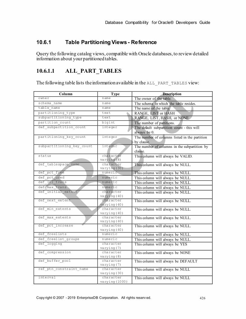
Database Compatibility for Oracle® Developers Guide
Copy right © 2007 - 2019 EnterpriseDB Corporation. All rights reserv ed.
426
10.6.1 Table Partitioning Views - Reference
Query the following catalog views, compatible with Oracle databases, to review detailed information about your partitioned tables.
10.6.1.1 ALL_PART_TABLES
The following table lists the information available in the ALL_PART_TABLES view:
Column Type Description owner name The owner of the table. schema_name name The schema in which the table resides. table_name name The name of the table. partitioning_type text RANGE, LIST or HASH subpartitioning_type text RANGE, LIST, HASH, or NONE partition_count bigint The number of partitions. def_subpartition_count integer The default subpartition count - this will
always be 0. partitioning_key_count integer The number of columns listed in the partition
by clause. subpartitioning_key_count integer The number of columns in the subpartition by
clause. status character
varying(8) This column will always be VALID.
def_tablespace_name character
varying(30) This column will always be NULL.
def_pct_free numeric This column will always be NULL. def_pct_used numeric This column will always be NULL. def_ini_trans numeric This column will always be NULL. def_max_trans numeric This column will always be NULL. def_initial_extent character
varying(40) This column will always be NULL.
def_next_extent character
varying(40) This column will always be NULL.
def_min_extents character
varying(40) This column will always be NULL.
def_max_extents character
varying(40) This column will always be NULL.
def_pct_increase character
varying(40) This column will always be NULL.
def_freelists numeric This column will always be NULL. def_freelist_groups numeric This column will always be NULL. def_logging character
varying(7) This column will always be YES
def_compression character
varying(8) This column will always be NONE
def_buffer_pool character
varying(7) This column will always be DEFAULT
ref_ptn_constraint_name character
varying(30) This column will always be NULL
interval character
varying(1000) This column will always be NULL

Database Compatibility for Oracle® Developers Guide
Copy right © 2007 - 2019 EnterpriseDB Corporation. All rights reserv ed.
427
10.6.1.2 ALL_TAB_PARTITIONS
The following table lists the information available in the ALL_TAB_PARTITIONS view:
Column Type Description table_owner name The owner of the table. schema_name name The schema in which the table resides. table_name name The name of the table. composite text YES if the table is subpartitioned; NO if it is
not subpartitioned. partition_name name The name of the partition. subpartition_count bigint The number of subpartitions for this partition. high_value text The high partitioning value specified in the
CREATE TABLE statement. high_value_length integer The length of high partitioning value. partition_position integer The ordinal position of this partition. tablespace_name name The tablespace in which this partition resides. pct_free numeric This column will always be 0. pct_used numeric This column will always be 0. ini_trans numeric This column will always be 0. max_trans numeric This column will always be 0. initial_extent numeric This column will always be NULL. next_extent numeric This column will always be NULL. min_extent numeric This column will always be 0. max_extent numeric This column will always be 0. pct_increase numeric This column will always be 0. freelists numeric This column will always be NULL freelist_groups numeric This column will always be NULL logging character
varying(7) This column will always be YES.
compression character
varying(8) This column will always be NONE.
num_rows numeric The approx. number of rows in this partition. blocks integer The approx. number of blocks in this partition. empty_blocks numeric This column will always be NULL avg_space numeric This column will always be NULL chain_cnt numeric This column will always be NULL avg_row_len numeric This column will always be NULL sample_size numeric This column will always be NULL last_analyzed timestamp
without time
zone
This column will always be NULL
buffer_pool character
varying(7) This column will always be NULL
global_stats character
varying(3) This column will always be YES.
user_stats character
varying(3) This column will always be NO.
backing_table regclass OID of the backing table for this partition.

Database Compatibility for Oracle® Developers Guide
Copy right © 2007 - 2019 EnterpriseDB Corporation. All rights reserv ed.
428
10.6.1.3 ALL_TAB_SUBPARTITIONS
The following table lists the information available in the ALL_TAB_SUBPARTITIONS view:
Column Type Description table_owner name The name of the owner of the table. schema_name name The name of the schema in which the table
resides. table_name name The name of the table. partition_name name The name of the partition. subpartition_name name The name of the subpartition. high_value text The high partitioning value specified in the
CREATE TABLE statement. high_value_length integer The length of high partitioning value. subpartition_position integer The ordinal position of this subpartition. tablespace_name name The tablespace in which this subpartition resides. pct_free numeric This column will always be 0. pct_used numeric This column will always be 0. ini_trans numeric This column will always be 0. max_trans numeric This column will always be 0. initial_extent numeric This column will always be NULL. next_extent numeric This column will always be NULL. min_extent numeric This column will always be 0. max_extent numeric This column will always be 0. pct_increase numeric This column will always be 0. freelists numeric This column will always be NULL. freelist_groups numeric This column will always be NULL. logging character
varying(7) This column will always be YES.
compression character
varying(8) This column will always be NONE.
num_rows numeric The approx. number of rows in this subpartition. blocks integer The approx. number of blocks in this
subpartition. empty_blocks numeric This column will always be NULL. avg_space numeric This column will always be NULL. chain_cnt numeric This column will always be NULL. avg_row_len numeric This column will always be NULL. sample_size numeric This column will always be NULL. last_analyzed timestamp
without time
zone
This column will always be NULL.
buffer_pool character
varying(7)
This column will always be NULL.
global_stats character
varying(3)
This column will always be YES.
user_stats character
varying(3) This column will always be NO.
backing_table regclass OID of the backing table for this subpartition.

Database Compatibility for Oracle® Developers Guide
Copy right © 2007 - 2019 EnterpriseDB Corporation. All rights reserv ed.
429
10.6.1.4 ALL_PART_KEY_COLUMNS
The following table lists the information available in the ALL_PART_KEY_COLUMNS view:
Column Type Description owner name The name of the table owner. schema_name name The name of the schema on which the table
resides. name name The name of the table. object_type character(5) This column will always be TABLE. column_name name The name of the partitioning key column. column_position integer The position of this column within the
partitioning key (the first column has a column
position of 1, the second column has a column
position of 2...)
10.6.1.5 ALL_SUBPART_KEY_COLUMNS
The following table lists the information available in the ALL_SUBPART_KEY_COLUMNS view:
Column Type Description owner name The name of the table owner. schema_name name The name of the schema on which the table
resides. name name The name of the table. object_type character(5) This column will always be TABLE. column_name name The name of the partitioning key column. column_position integer The position of this column within the
subpartitioning key (the first column has a
column position of 1, the second column has a
column position of 2...)

Database Compatibility for Oracle® Developers Guide
Copy right © 2007 - 2019 EnterpriseDB Corporation. All rights reserv ed.
430
11 ECPGPlus
EnterpriseDB has enhanced ECPG (the PostgreSQL pre-compiler) to create ECPGPlus. ECPGPlus allows you to include embedded SQL commands in C applications; when you
use ECPGPlus to compile an application that contains embedded SQL commands, the SQL code is syntax-checked and translated into C.
ECPGPlus supports Pro*C compatible syntax in C programs when connected to an Advanced Server database. ECPGPlus supports:
Oracle Dynamic SQL – Method 4 (ODS-M4).
Pro*C compatible anonymous blocks.
A CALL statement compatible with Oracle databases.
As part of ECPGPlus' Pro*C compatibility, you do not need to include the BEGIN DECLARE SECTION and END DECLARE SECTION directives.
For more information about using ECPGPlus, please see the EDB Postgres Advanced Server ECPG Connector Guide available from the EnterpriseDB website at:
https://www.enterprisedb.com/resources/product-documentation

Database Compatibility for Oracle® Developers Guide
Copy right © 2007 - 2019 EnterpriseDB Corporation. All rights reserv ed.
431
12 dblink_ora
dblink_ora provides an OCI-based database link that allows you to SELECT, INSERT, UPDATE or DELETE data stored on an Oracle system from within Advanced Server.
Connecting to an Oracle Database
To enable Oracle connectivity, download Oracle's freely available OCI drivers from their website, presently at:
http://www.oracle.com/technetwork/database/database-technologies/instant-client/overview/index.html
For Linux, if the Oracle instant client that you've downloaded does not include the
libclntsh.so library, you must create a symbolic link named libclntsh.so that points to the downloaded version. Navigate to the instant client directory and execute the following command:
ln -s libclntsh.so.version libclntsh.so
Where version is the version number of the libclntsh.so library. For example:
ln -s libclntsh.so.12.1 libclntsh.so
Before creating a link to an Oracle server, you must tell Advanced Server where to find the OCI driver.
Set the LD_LIBRARY_PATH environment variable on Linux (or PATH on Windows) to the lib directory of the Oracle client installation directory.
For Windows only, you can instead set the value of the oracle_home configuration
parameter in the postgresql.conf file. The value specified in the oracle_home configuration parameter will override the Windows PATH environment variable.
The LD_LIBRARY_PATH environment variable on Linux (PATH environment variable or
oracle_home configuration parameter on Windows) must be set properly each time you start Advanced Server.
When using a Linux service script to start Advanced Server, be sure LD_LIBRARY_PATH
has been set within the service script so it is in effect when the script invokes the pg_ctl utility to start Advanced Server.
For Windows only: To set the oracle_home configuration parameter in the postgresql.conf file, edit the file, adding the following line:
Database Compatibility for Oracle® Developers Guide
Copy right © 2007 - 2019 EnterpriseDB Corporation. All rights reserv ed.
432
oracle_home = 'lib_directory '
Substitute the name of the Windows directory that contains oci.dll for lib_directory.
After setting the oracle_home configuration parameter, you must restart the server for the changes to take effect. Restart the server from the Windows Services console.
12.1 dblink_ora Functions and Procedures
dblink_ora supports the following functions and procedures.
12.1.1 dblink_ora_connect()
The dblink_ora_connect() function establishes a connection to an Oracle database
with user-specified connection information. The function comes in two forms; the signature of the first form is:
dblink_ora_connect(conn_name, server_name, service_name,
user_name, password, port, asDBA)
Where:
conn_name specifies the name of the link.
server_name specifies the name of the host.
service_name specifies the name of the service.
user_name specifies the name used to connect to the server.
password specifies the password associated with the user name.
port specifies the port number.
asDBA is True if you wish to request SYSDBA privileges on the Oracle server.
This parameter is optional; if omitted, the default value is FALSE.
The first form of dblink_ora_connect() returns a TEXT value.
The signature of the second form of the dblink_ora_connect() function is:
dblink_ora_connect(foreign_server_name, asDBA)
Database Compatibility for Oracle® Developers Guide
Copy right © 2007 - 2019 EnterpriseDB Corporation. All rights reserv ed.
433
Where:
foreign_server_name specifies the name of a foreign server.
asDBA is True if you wish to request SYSDBA privileges on the Oracle server.
This parameter is optional; if omitted, the default value is FALSE.
The second form of the dblink_ora_connect() function allows you to use the
connection properties of a pre-defined foreign server when establishing a connection to the server.
Before invoking the second form of the dblink_ora_connect() function, use the
CREATE SERVER command to store the connection properties for the link to a system
table. When you call the dblink_ora_connect() function, substitute the server name specified in the CREATE SERVER command for the name of the link.
The second form of dblink_ora_connect() returns a TEXT value.
12.1.2 dblink_ora_status()
The dblink_ora_status() function returns the database connection status. The signature is:
dblink_ora_status(conn_name)
Where:
conn_name specifies the name of the link.
If the specified connection is active, the function returns a TEXT value of OK.
12.1.3 dblink_ora_disconnect()
The dblink_ora_disconnect() function closes a database connection. The signature is:
dblink_ora_disconnect(conn_name)
Where:
conn_name specifies the name of the link.

Database Compatibility for Oracle® Developers Guide
Copy right © 2007 - 2019 EnterpriseDB Corporation. All rights reserv ed.
434
The function returns a TEXT value.
12.1.4 dblink_ora_record()
The dblink_ora_record() function retrieves information from a database. The signature is:
dblink_ora_record(conn_name, query_text)
Where:
conn_name specifies the name of the link.
query_text specifies the text of the SQL SELECT statement that will be invoked on the Oracle server.
The function returns a SETOF record.
12.1.5 dblink_ora_call()
The dblink_ora_call() function executes a non-SELECT statement on an Oracle database and returns a result set. The signature is:
dblink_ora_call(conn_name, command, iterations)
Where:
conn_name specifies the name of the link.
command specifies the text of the SQL statement that will be invoked on the Oracle server.
iterations specifies the number of times the statement is executed.
The function returns a SETOF record.
12.1.6 dblink_ora_exec()
The dblink_ora_exec() procedure executes a DML or DDL statement in the remote database. The signature is:

Database Compatibility for Oracle® Developers Guide
Copy right © 2007 - 2019 EnterpriseDB Corporation. All rights reserv ed.
435
dblink_ora_exec(conn_name, command)
Where:
conn_name specifies the name of the link.
command specifies the text of the INSERT, UPDATE, or DELETE SQL statement that will be invoked on the Oracle server.
The function returns a VOID.
12.1.7 dblink_ora_copy()
The dblink_ora_copy() function copies an Oracle table to an EnterpriseDB table. The dblink_ora_copy() function returns a BIGINT value that represents the number of rows copied. The signature is:
dblink_ora_copy(conn_name, command, schema_name,
table_name, truncate, count)
Where:
conn_name specifies the name of the link.
command specifies the text of the SQL SELECT statement that will be invoked on the Oracle server.
schema_name specifies the name of the target schema.
table_name specifies the name of the target table.
truncate specifies if the server should TRUNCATE the table prior to copying;
specify TRUE to indicate that the server should TRUNCATE the table. truncate is
optional; if omitted, the value is FALSE.
count instructs the server to report status information every n record, where n is
the number specified. During the execution of the function, Advanced Server
raises a notice of severity INFO with each iteration of the count. For example, if
FeedbackCount is 10, dblink_ora_copy() raises a notice every 10 records. count is optional; if omitted, the value is 0.

Database Compatibility for Oracle® Developers Guide
Copy right © 2007 - 2019 EnterpriseDB Corporation. All rights reserv ed.
436
12.2 Calling dblink_ora Functions
The following command establishes a connection using the dblink_ora_connect() function:
SELECT dblink_ora_connect('acctg', 'localhost', 'xe', 'hr',
'pwd', 1521);
The example connects to a service named xe running on port 1521 (on the localhost)
with a user name of hr and a password of pwd. You can use the connection name acctg to refer to this connection when calling other dblink_ora functions.
The following command uses the dblink_ora_copy() function over a connection
named edb_conn to copy the empid and deptno columns from a table (on an Oracle
server) named ora_acctg to a table located in the public schema on an instance of
Advanced Server named as_acctg. The TRUNCATE option is enforced, and a feedback
count of 3 is specified:
edb=# SELECT dblink_ora_copy('edb_conn','select empid,
deptno FROM ora_acctg', 'public', 'as_acctg', true, 3);
INFO: Row: 0
INFO: Row: 3
INFO: Row: 6
INFO: Row: 9
INFO: Row: 12
dblink_ora_copy
-----------------
12
(1 row)
The following SELECT statement uses dblink_ora_record() function and the acctg connection to retrieve information from the Oracle server:
SELECT * FROM dblink_ora_record( 'acctg', 'SELECT
first_name from employees') AS t1(id VARCHAR);
The command retrieves a list that includes all of the entries in the first_name column of the employees table.

Database Compatibility for Oracle® Developers Guide
Copy right © 2007 - 2019 EnterpriseDB Corporation. All rights reserv ed.
437
13 System Catalog Tables
The system catalog tables contain definitions of database objects that are available to
Advanced Server; the layout of the system tables is subject to change. If you are writing an application that depends on information stored in the system tables, it would be prudent to use an existing catalog view, or create a catalog view to isolate the application from changes to the system table.
For detailed information about the system catalog tables, please see the Database Compatibility for Oracle® Developer’s Reference Guide, available at:
https://www.enterprisedb.com/resources/product-documentation

Database Compatibility for Oracle® Developers Guide
Copy right © 2007 - 2019 EnterpriseDB Corporation. All rights reserv ed.
438
14 Acknowledgements
The PostgreSQL 8.3, 8.4, 9.0, 9.1, 9.2, 9.3, 9.4, 9.5, 9.6, 10, 11, and 12 Documentation
provided the baseline for the portions of this guide that are common to PostgreSQL, and is hereby acknowledged:
Portions of this EnterpriseDB Software and Documentation may utilize the following copyrighted material, the use of which is hereby acknowledged.
PostgreSQL Documentation, Database Management System
PostgreSQL is Copyright © 1996-2018 by the PostgreSQL Global Development Group and is distributed under the terms of the license of the University of California below.
Postgres95 is Copyright © 1994-5 by the Regents of the University of California.
Permission to use, copy, modify, and distribute this software and its documentation for any purpose, without fee, and without a written agreement is hereby granted, provided that the above copyright notice and this paragraph and the following two paragraphs appear in all copies.
IN NO EVENT SHALL THE UNIVERSITY OF CALIFORNIA BE LIABLE TO ANY PARTY
FOR DIRECT, INDIRECT, SPECIAL, INCIDENTAL, OR CONSEQUENTIAL DAMAGES,
INCLUDING LOST PROFITS, ARISING OUT OF THE USE OF THIS SOFTWARE AND ITS
DOCUMENTATION, EVEN IF THE UNIVERSITY OF CALIFORNIA HAS BEEN ADVISED OF
THE POSSIBILITY OF SUCH DAMAGE.
THE UNIVERSITY OF CALIFORNIA SPECIFICALLY DISCLAIMS ANY WARRANTIES,
INCLUDING, BUT NOT LIMITED TO, THE IMPLIED WARRANTIES OF
MERCHANTABILITY AND FITNESS FOR A PARTICULAR PURPOSE. THE SOFTWARE
PROVIDED HEREUNDER IS ON AN "AS-IS" BASIS, AND THE UNIVERSITY OF
CALIFORNIA HAS NO OBLIGATIONS TO PROVIDE MAINTENANCE, SUPPORT, UPDATES,
ENHANCEMENTS, OR MODIFICATIONS.


![kkt_6_dan_7_pemupukan_2014 [Compatibility Mode]](https://static.fdokumen.com/doc/165x107/6322b43c28c445989105e2db/kkt6dan7pemupukan2014-compatibility-mode.jpg)