Data Mining Application For CH-47D Aft Swashplate Bearing Fault Detection Project #2

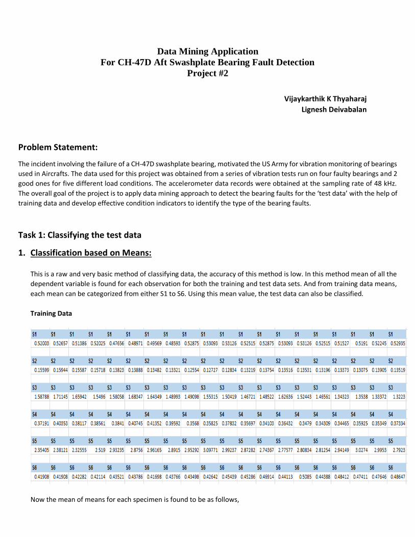
Data Mining Application

For CH-47D Aft Swashplate Bearing Fault Detection

Project #2

Vijaykarthik K Thyaharaj

Lignesh Deivabalan

Problem Statement:

The incident involving the failure of a CH-47D swashplate bearing, motivated the US Army for vibration monitoring of bearings

used in Aircrafts. The data used for this project was obtained from a series of vibration tests run on four faulty bearings and 2

good ones for five different load conditions. The accelerometer data records were obtained at the sampling rate of 48 kHz.

The overall goal of the project is to apply data mining approach to detect the bearing faults for the ‘test data’ with the help of

training data and develop effective condition indicators to identify the type of the bearing faults.

Task 1: Classifying the test data

1. Classification based on Means:

This is a raw and very basic method of classifying data, the accuracy of this method is low. In this method mean of all the

dependent variable is found for each observation for both the training and test data sets. And from training data means,

each mean can be categorized from either S1 to S6. Using this mean value, the test data can also be classified.

Training Data

Now the mean of means for each specimen is found to be as follows,

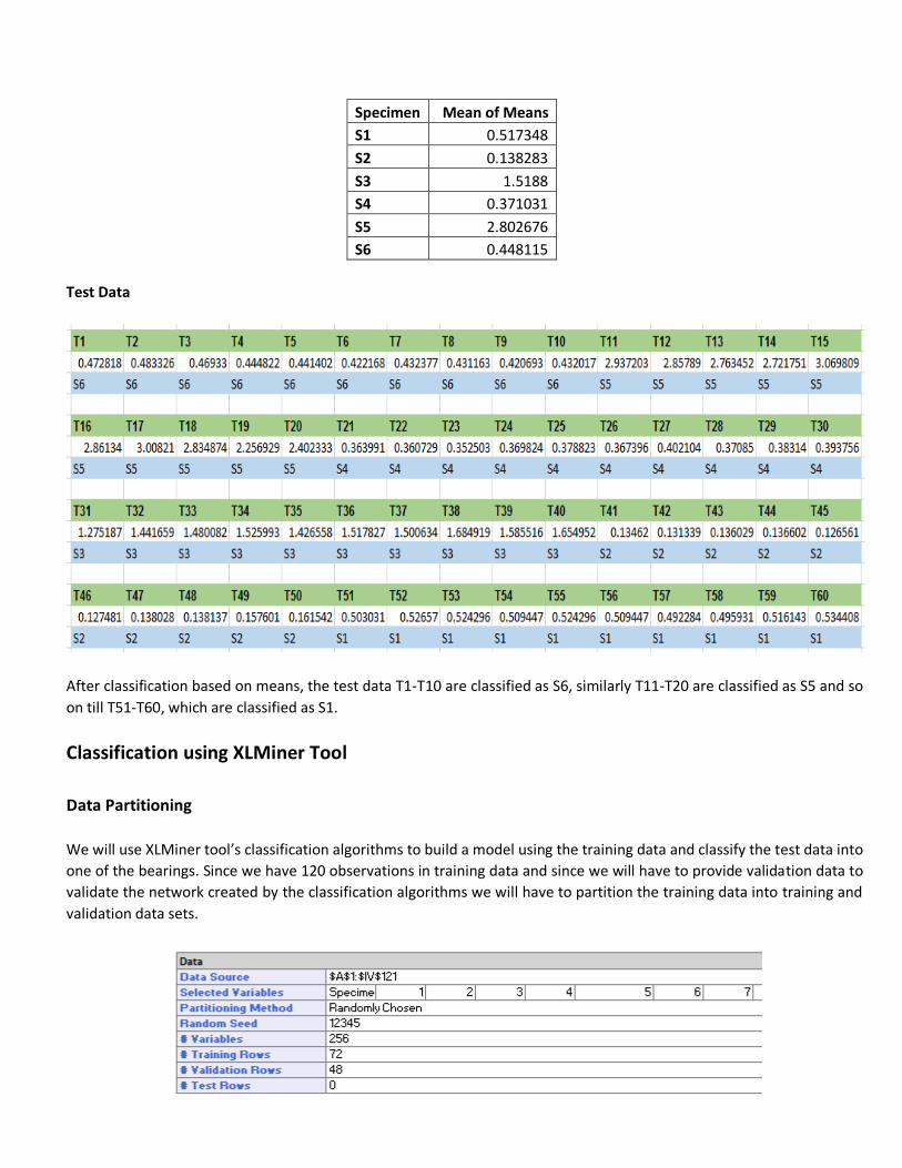
Specimen Mean of Means

S1 0.517348

S2 0.138283

S3 1.5188

S4 0.371031

S5 2.802676

S6 0.448115

Test Data

After classification based on means, the test data T1-T10 are classified as S6, similarly T11-T20 are classified as S5 and so

on till T51-T60, which are classified as S1.

Classification using XLMiner Tool

Data Partitioning

We will use XLMiner tool’s classification algorithms to build a model using the training data and classify the test data into

one of the bearings. Since we have 120 observations in training data and since we will have to provide validation data to

validate the network created by the classification algorithms we will have to partition the training data into training and

validation data sets.

Using Data Partition in XLMiner, the training data was split into 60% and 40% for training and validating the models. So 72

data points will be used for training and 48 will be used for validation.

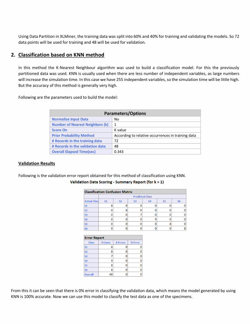
2. Classification based on KNN method

In this method the K-Nearest Neighbour algorithm was used to build a classification model. For this the previously

partitioned data was used. KNN is usually used when there are less number of independent variables, as large numbers

will increase the simulation time. In this case we have 255 independent variables, so the simulation time will be little high.

But the accuracy of this method is generally very high.

Following are the parameters used to build the model:

Parameters/Options Normalize Input Data No

Number of Nearest Neighbors (k) 1

Score On K value

Prior Probability Method According to relative occurrences in training data

# Records in the training data 72

# Records in the validation data 48

Overall Elapsed Time(sec) 0.343

Validation Results

Following is the validation error report obtained for this method of classification using KNN.

From this it can be seen that there is 0% error in classifying the validation data, which means the model generated by using

KNN is 100% accurate. Now we can use this model to classify the test data as one of the specimens.

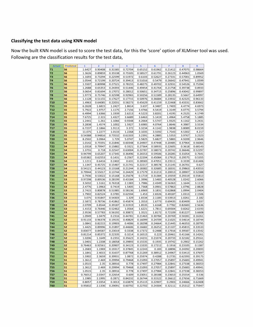
Classifying the test data using KNN model

Now the built KNN model is used to score the test data, for this the ‘score’ option of XLMiner tool was used.

Following are the classification results for the test data,

Actual Predicted 1 2 3 4 5 6 7 8 9

T1 S6 1.6427 0.90408 0.31585 0.72704 0.65152 0.61962 0.21412 0.47075 0.98664

T2 S6 1.3626 0.89859 0.35538 0.75505 0.58527 0.61791 0.26123 0.44963 1.0569

T3 S6 1.1693 0.73294 0.22599 0.51972 0.6103 0.52627 0.27331 0.57001 0.89952

T4 S6 1.0544 0.72199 0.20724 0.39413 0.51016 0.5479 0.26642 0.47941 1.0599

T5 S6 1.5507 0.80998 0.27521 0.78155 0.48275 0.49702 0.32931 0.54526 0.75394

T6 S6 1.2688 0.65353 0.24393 0.51446 0.49454 0.41764 0.21758 0.39738 0.8933

T7 S6 3.0654 0.81694 0.17072 0.28012 0.50651 0.34715 0.25896 0.43042 0.99897

T8 S6 1.9773 0.75746 0.32598 0.92965 0.50256 0.51589 0.28135 0.5667 0.64997

T9 S6 1.1128 0.51155 0.17627 0.17715 0.50976 0.36684 0.23932 0.42325 0.96133

T10 S6 1.4963 0.64085 0.22031 0.58273 0.45629 0.41159 0.22468 0.43331 0.83662

T11 S5 6.2628 1.6815 1.2427 1.8614 3.637 4.3487 1.7403 4.4774 4.6973

T12 S5 5.7922 1.9757 1.1175 2.7156 3.4766 4.5419 1.3149 4.0775 3.5794

T13 S5 6.4994 1.6366 1.1939 2.6213 4.5223 3.8201 1.4195 4.2525 4.1749

T14 S5 7.6725 2.315 1.4327 3.6689 3.6463 5.1419 1.4964 5.4758 5.1885

T15 S5 1.2441 1.261 1.1066 0.9348 4.2664 5.5747 1.9325 4.1162 3.2431

T16 S5 3.2838 1.4574 1.1002 1.5927 3.6985 4.0764 1.8646 4.3987 3.5534

T17 S5 6.7237 2.1866 1.9113 3.372 3.3234 4.1142 1.9838 3.8089 8.0159

T18 S5 11.075 1.2277 1.0133 1.2268 3.1035 3.5592 1.7543 4.5302 4.217

T19 S5 0.54388 0.94816 0.73532 0.61503 3.2391 4.2885 1.5353 3.9767 3.2323

T20 S5 8.2502 3.0964 1.729 5.0747 3.5825 5.6827 1.5883 4.9209 2.9646

T21 S4 1.0142 0.75591 0.21846 0.60348 0.24907 0.47448 0.20485 0.37964 0.56065

T22 S4 1.0318 0.79947 0.15882 0.3321 0.27364 0.58935 0.22605 0.3618 0.68143

T23 S4 1.3755 0.718 0.22547 0.63004 0.22787 0.58073 0.20742 0.36646 0.52297

T24 S4 0.94799 0.65207 0.17345 0.36496 0.26553 0.59506 0.20285 0.31054 0.7641

T25 S4 0.65382 0.62553 0.1431 0.2567 0.22204 0.45084 0.17913 0.29575 0.5355

T26 S4 1.1211 0.6416 0.2402 0.631 0.28583 0.47051 0.23511 0.3339 0.61406

T27 S4 1.1347 0.45725 0.15487 0.21741 0.22217 0.38578 0.21145 0.26701 0.627

T28 S4 0.54121 0.44123 0.13168 0.21244 0.18382 0.32685 0.18331 0.29863 0.43553

T29 S4 0.79944 0.55017 0.13744 0.24429 0.17579 0.31213 0.20013 0.28907 0.52388

T30 S4 0.7936 0.53022 0.15168 0.25678 0.1719 0.31384 0.19359 0.29319 0.55813

T31 S3 0.97298 0.89536 0.28199 0.43184 1.3996 2.5483 0.40528 1.0242 2.6066

T32 S3 3.5032 1.5161 0.76318 2.1383 1.7986 2.4349 0.56363 1.1644 3.1132

T33 S3 2.4776 1.0963 0.7419 1.5405 1.7368 3.0901 0.57863 1.0796 2.8828

T34 S3 2.7415 0.80878 0.51985 0.58136 1.6969 3.1831 0.62868 1.0994 2.0404

T35 S3 1.7902 0.82524 0.3785 0.62594 1.453 2.8326 0.49187 1.0313 2.1506

T36 S3 3.075 0.91847 0.54303 1.329 1.6534 2.1185 0.53913 1.0261 2.182

T37 S3 2.5872 0.78736 0.41862 0.45874 1.3553 1.6773 0.69435 0.83409 3.037

T38 S3 2.0709 0.8544 0.39187 0.31919 1.8535 1.6168 0.7782 0.82683 2.5636

T39 S3 1.4153 0.76446 0.52462 1.0564 1.6221 1.7811 0.69304 0.8262 2.6193

T40 S3 2.9536 0.57783 0.56192 0.30872 1.3521 1.8172 0.72109 0.81227 3.6608

T41 S2 1.0949 1.0479 0.2316 0.44781 0.21463 0.30784 0.20769 0.50281 0.16261

T42 S2 0.91133 0.96378 0.19535 0.40829 0.16099 0.24709 0.21025 0.54614 0.18744

T43 S2 1.0841 0.82215 0.19903 0.4006 0.18298 0.24664 0.21445 0.46353 0.28795

T44 S2 1.4425 0.89996 0.21897 0.44606 0.16682 0.26252 0.21107 0.45815 0.33533

T45 S2 0.83077 0.84587 0.23019 0.3338 0.17372 0.2488 0.17916 0.39587 0.13542

T46 S2 0.81214 0.85372 0.22335 0.3214 0.16515 0.223 0.20461 0.41166 0.14261

T47 S2 1.0206 1.1649 0.2355 0.35623 0.14231 0.21074 0.20733 0.32182 0.29161

T48 S2 1.0401 1.2208 0.18058 0.29893 0.15535 0.1935 0.19742 0.2902 0.15262

T49 S2 0.76463 0.92561 0.20907 0.34123 0.13335 0.17212 0.1916 0.23105 0.1387

T50 S2 1.2683 1.1969 0.19317 0.37845 0.12243 0.183 0.18896 0.24392 0.20693

T51 S1 1.1841 2.4015 0.31637 0.87768 0.21269 0.38912 0.24967 0.53413 0.37697

T52 S1 1.5902 2.3659 0.39931 1.0872 0.25974 0.4288 0.2735 0.62393 0.39175

T53 S1 1.3612 2.469 0.29994 0.79468 0.21093 0.27057 0.25897 0.25683 0.49941

T54 S1 1.0515 2.35 0.28916 0.778 0.17497 0.27984 0.22841 0.27338 0.38353

T55 S1 1.3612 2.469 0.29994 0.79468 0.21093 0.27057 0.25897 0.25683 0.49941

T56 S1 1.0515 2.35 0.28916 0.778 0.17497 0.27984 0.22841 0.27338 0.38353

T57 S1 0.76012 2.0347 0.22654 0.609 0.23051 0.28188 0.23653 0.25554 0.536

T58 S1 1.1985 2.1995 0.2871 0.84232 0.26744 0.31522 0.26612 0.27656 0.71669

T59 S1 0.8057 2.0354 0.3013 0.63879 0.25115 0.22907 0.2903 0.24666 0.62408

T60 S1 0.95832 2.1336 0.29091 0.60792 0.22702 0.24304 0.32111 0.25312 0.75947

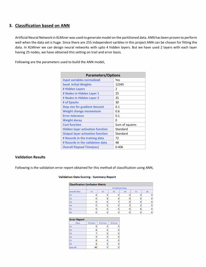
3. Classification based on ANN

Artificial Neural Network in XLMiner was used to generate model on the partitioned data. ANN has been proven to perform

well when the data set is huge. Since there are 255 independent varibles in this project ANN can be chosen for fitting the

data. In XLMiner we can design neural networks with upto 4 hidden layers. But we have used 2 layers with each layer

having 25 nodes, we have obtained this setting on trail and error basis.

Following are the parameters used to build the ANN model,

Parameters/Options Input variables normalized Yes

Seed: Initial Weights 12345

# Hidden Layers 2

# Nodes in Hidden Layer 1 25


# of Epochs 30

Step size for gradient descent 0.1

Weight change momentum 0.6

Error tolerance 0.1

Weight decay 0

Cost function Sum of squares

Hidden layer activation function Standard

Output layer activation function Standard

# Records in the training data 72

# Records in the validation data 48


Validation Results

Following is the validation error report obtained for this method of classification using ANN,

On observing the validation error report it can be found to be identical to the one obtained by KNN method, and ANN also

classifies the validation data set with 100% accuracy.

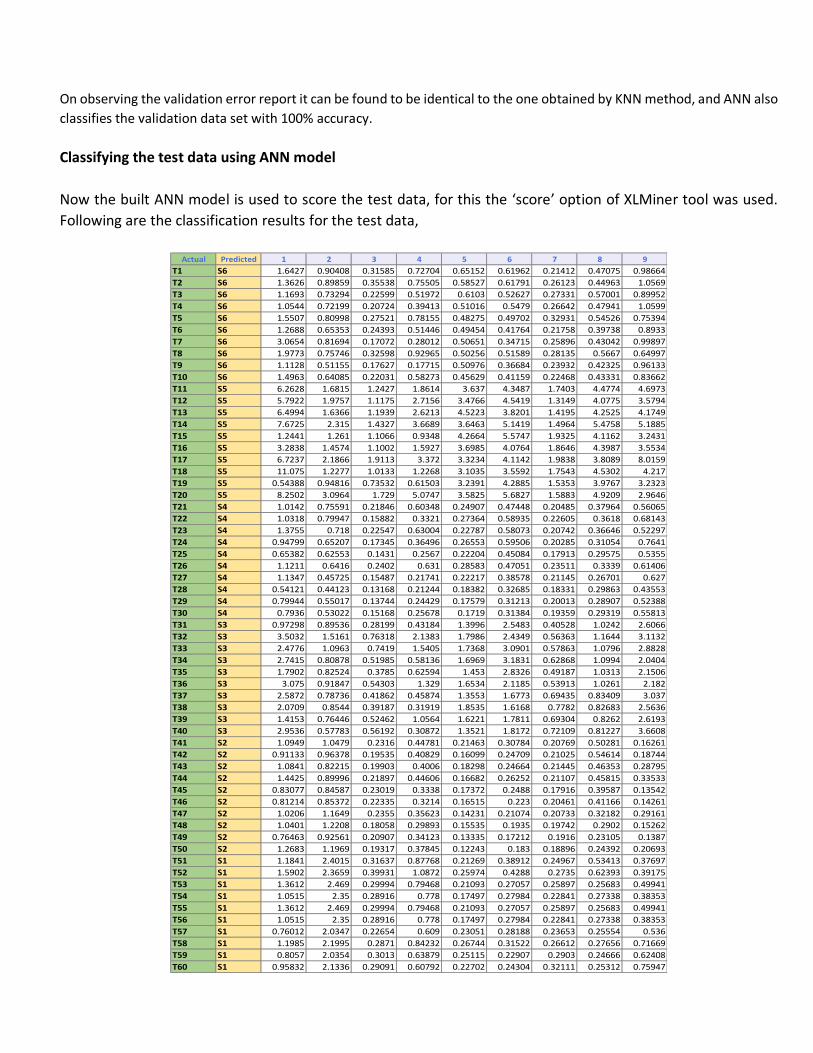
Classifying the test data using ANN model

Now the built ANN model is used to score the test data, for this the ‘score’ option of XLMiner tool was used.

Following are the classification results for the test data,

Actual Predicted 1 2 3 4 5 6 7 8 9

T1 S6 1.6427 0.90408 0.31585 0.72704 0.65152 0.61962 0.21412 0.47075 0.98664

T2 S6 1.3626 0.89859 0.35538 0.75505 0.58527 0.61791 0.26123 0.44963 1.0569

T3 S6 1.1693 0.73294 0.22599 0.51972 0.6103 0.52627 0.27331 0.57001 0.89952

T4 S6 1.0544 0.72199 0.20724 0.39413 0.51016 0.5479 0.26642 0.47941 1.0599

T5 S6 1.5507 0.80998 0.27521 0.78155 0.48275 0.49702 0.32931 0.54526 0.75394

T6 S6 1.2688 0.65353 0.24393 0.51446 0.49454 0.41764 0.21758 0.39738 0.8933

T7 S6 3.0654 0.81694 0.17072 0.28012 0.50651 0.34715 0.25896 0.43042 0.99897

T8 S6 1.9773 0.75746 0.32598 0.92965 0.50256 0.51589 0.28135 0.5667 0.64997

T9 S6 1.1128 0.51155 0.17627 0.17715 0.50976 0.36684 0.23932 0.42325 0.96133

T10 S6 1.4963 0.64085 0.22031 0.58273 0.45629 0.41159 0.22468 0.43331 0.83662

T11 S5 6.2628 1.6815 1.2427 1.8614 3.637 4.3487 1.7403 4.4774 4.6973

T12 S5 5.7922 1.9757 1.1175 2.7156 3.4766 4.5419 1.3149 4.0775 3.5794

T13 S5 6.4994 1.6366 1.1939 2.6213 4.5223 3.8201 1.4195 4.2525 4.1749

T14 S5 7.6725 2.315 1.4327 3.6689 3.6463 5.1419 1.4964 5.4758 5.1885

T15 S5 1.2441 1.261 1.1066 0.9348 4.2664 5.5747 1.9325 4.1162 3.2431

T16 S5 3.2838 1.4574 1.1002 1.5927 3.6985 4.0764 1.8646 4.3987 3.5534

T17 S5 6.7237 2.1866 1.9113 3.372 3.3234 4.1142 1.9838 3.8089 8.0159

T18 S5 11.075 1.2277 1.0133 1.2268 3.1035 3.5592 1.7543 4.5302 4.217

T19 S5 0.54388 0.94816 0.73532 0.61503 3.2391 4.2885 1.5353 3.9767 3.2323

T20 S5 8.2502 3.0964 1.729 5.0747 3.5825 5.6827 1.5883 4.9209 2.9646

T21 S4 1.0142 0.75591 0.21846 0.60348 0.24907 0.47448 0.20485 0.37964 0.56065

T22 S4 1.0318 0.79947 0.15882 0.3321 0.27364 0.58935 0.22605 0.3618 0.68143

T23 S4 1.3755 0.718 0.22547 0.63004 0.22787 0.58073 0.20742 0.36646 0.52297

T24 S4 0.94799 0.65207 0.17345 0.36496 0.26553 0.59506 0.20285 0.31054 0.7641

T25 S4 0.65382 0.62553 0.1431 0.2567 0.22204 0.45084 0.17913 0.29575 0.5355

T26 S4 1.1211 0.6416 0.2402 0.631 0.28583 0.47051 0.23511 0.3339 0.61406

T27 S4 1.1347 0.45725 0.15487 0.21741 0.22217 0.38578 0.21145 0.26701 0.627

T28 S4 0.54121 0.44123 0.13168 0.21244 0.18382 0.32685 0.18331 0.29863 0.43553

T29 S4 0.79944 0.55017 0.13744 0.24429 0.17579 0.31213 0.20013 0.28907 0.52388

T30 S4 0.7936 0.53022 0.15168 0.25678 0.1719 0.31384 0.19359 0.29319 0.55813

T31 S3 0.97298 0.89536 0.28199 0.43184 1.3996 2.5483 0.40528 1.0242 2.6066

T32 S3 3.5032 1.5161 0.76318 2.1383 1.7986 2.4349 0.56363 1.1644 3.1132

T33 S3 2.4776 1.0963 0.7419 1.5405 1.7368 3.0901 0.57863 1.0796 2.8828

T34 S3 2.7415 0.80878 0.51985 0.58136 1.6969 3.1831 0.62868 1.0994 2.0404

T35 S3 1.7902 0.82524 0.3785 0.62594 1.453 2.8326 0.49187 1.0313 2.1506

T36 S3 3.075 0.91847 0.54303 1.329 1.6534 2.1185 0.53913 1.0261 2.182

T37 S3 2.5872 0.78736 0.41862 0.45874 1.3553 1.6773 0.69435 0.83409 3.037

T38 S3 2.0709 0.8544 0.39187 0.31919 1.8535 1.6168 0.7782 0.82683 2.5636

T39 S3 1.4153 0.76446 0.52462 1.0564 1.6221 1.7811 0.69304 0.8262 2.6193

T40 S3 2.9536 0.57783 0.56192 0.30872 1.3521 1.8172 0.72109 0.81227 3.6608

T41 S2 1.0949 1.0479 0.2316 0.44781 0.21463 0.30784 0.20769 0.50281 0.16261

T42 S2 0.91133 0.96378 0.19535 0.40829 0.16099 0.24709 0.21025 0.54614 0.18744

T43 S2 1.0841 0.82215 0.19903 0.4006 0.18298 0.24664 0.21445 0.46353 0.28795

T44 S2 1.4425 0.89996 0.21897 0.44606 0.16682 0.26252 0.21107 0.45815 0.33533

T45 S2 0.83077 0.84587 0.23019 0.3338 0.17372 0.2488 0.17916 0.39587 0.13542

T46 S2 0.81214 0.85372 0.22335 0.3214 0.16515 0.223 0.20461 0.41166 0.14261

T47 S2 1.0206 1.1649 0.2355 0.35623 0.14231 0.21074 0.20733 0.32182 0.29161

T48 S2 1.0401 1.2208 0.18058 0.29893 0.15535 0.1935 0.19742 0.2902 0.15262

T49 S2 0.76463 0.92561 0.20907 0.34123 0.13335 0.17212 0.1916 0.23105 0.1387

T50 S2 1.2683 1.1969 0.19317 0.37845 0.12243 0.183 0.18896 0.24392 0.20693

T51 S1 1.1841 2.4015 0.31637 0.87768 0.21269 0.38912 0.24967 0.53413 0.37697

T52 S1 1.5902 2.3659 0.39931 1.0872 0.25974 0.4288 0.2735 0.62393 0.39175

T53 S1 1.3612 2.469 0.29994 0.79468 0.21093 0.27057 0.25897 0.25683 0.49941

T54 S1 1.0515 2.35 0.28916 0.778 0.17497 0.27984 0.22841 0.27338 0.38353

T55 S1 1.3612 2.469 0.29994 0.79468 0.21093 0.27057 0.25897 0.25683 0.49941

T56 S1 1.0515 2.35 0.28916 0.778 0.17497 0.27984 0.22841 0.27338 0.38353

T57 S1 0.76012 2.0347 0.22654 0.609 0.23051 0.28188 0.23653 0.25554 0.536

T58 S1 1.1985 2.1995 0.2871 0.84232 0.26744 0.31522 0.26612 0.27656 0.71669

T59 S1 0.8057 2.0354 0.3013 0.63879 0.25115 0.22907 0.2903 0.24666 0.62408

T60 S1 0.95832 2.1336 0.29091 0.60792 0.22702 0.24304 0.32111 0.25312 0.75947

Classification using MATLAB Tool

MATLAB is widely used for generating various simulations especially when the data sets are large. In this project we will use

MATLAB’s ANN fitting toolbox and ANN Pattern Recognition toolbox to classify the test data into one of the specimens.

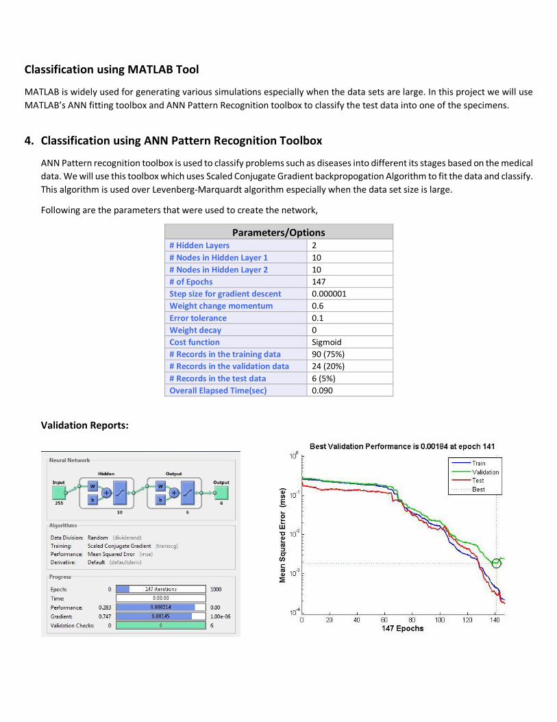
4. Classification using ANN Pattern Recognition Toolbox

ANN Pattern recognition toolbox is used to classify problems such as diseases into different its stages based on the medical

data. We will use this toolbox which uses Scaled Conjugate Gradient backpropogation Algorithm to fit the data and classify.

This algorithm is used over Levenberg-Marquardt algorithm especially when the data set size is large.

Following are the parameters that were used to create the network,

Parameters/Options # Hidden Layers 2



# of Epochs 147

Step size for gradient descent 0.000001

Weight change momentum 0.6

Error tolerance 0.1

Weight decay 0

Cost function Sigmoid

# Records in the training data 90 (75%)

# Records in the validation data 24 (20%)

# Records in the test data 6 (5%)


Validation Reports:

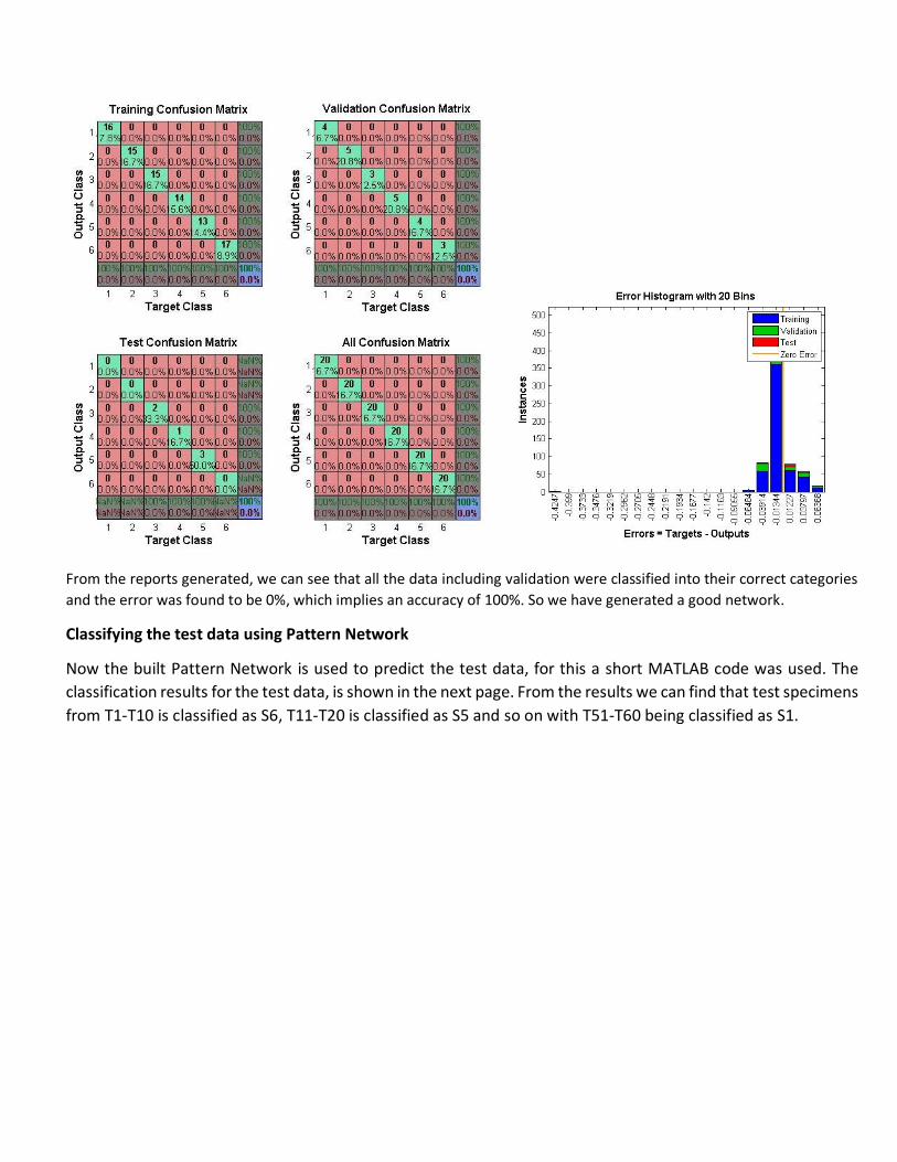
From the reports generated, we can see that all the data including validation were classified into their correct categories

and the error was found to be 0%, which implies an accuracy of 100%. So we have generated a good network.

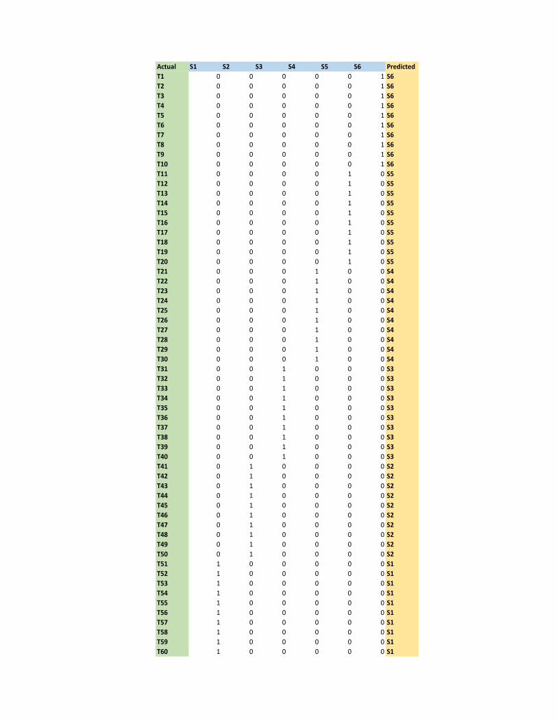
Classifying the test data using Pattern Network

Now the built Pattern Network is used to predict the test data, for this a short MATLAB code was used. The

classification results for the test data, is shown in the next page. From the results we can find that test specimens

from T1-T10 is classified as S6, T11-T20 is classified as S5 and so on with T51-T60 being classified as S1.

Actual S1 S2 S3 S4 S5 S6 Predicted

T1 0 0 0 0 0 1 S6

T2 0 0 0 0 0 1 S6

T3 0 0 0 0 0 1 S6

T4 0 0 0 0 0 1 S6

T5 0 0 0 0 0 1 S6

T6 0 0 0 0 0 1 S6

T7 0 0 0 0 0 1 S6

T8 0 0 0 0 0 1 S6

T9 0 0 0 0 0 1 S6

T10 0 0 0 0 0 1 S6

T11 0 0 0 0 1 0 S5

T12 0 0 0 0 1 0 S5

T13 0 0 0 0 1 0 S5

T14 0 0 0 0 1 0 S5

T15 0 0 0 0 1 0 S5

T16 0 0 0 0 1 0 S5

T17 0 0 0 0 1 0 S5

T18 0 0 0 0 1 0 S5

T19 0 0 0 0 1 0 S5

T20 0 0 0 0 1 0 S5

T21 0 0 0 1 0 0 S4

T22 0 0 0 1 0 0 S4

T23 0 0 0 1 0 0 S4

T24 0 0 0 1 0 0 S4

T25 0 0 0 1 0 0 S4

T26 0 0 0 1 0 0 S4

T27 0 0 0 1 0 0 S4

T28 0 0 0 1 0 0 S4

T29 0 0 0 1 0 0 S4

T30 0 0 0 1 0 0 S4

T31 0 0 1 0 0 0 S3

T32 0 0 1 0 0 0 S3

T33 0 0 1 0 0 0 S3

T34 0 0 1 0 0 0 S3

T35 0 0 1 0 0 0 S3

T36 0 0 1 0 0 0 S3

T37 0 0 1 0 0 0 S3

T38 0 0 1 0 0 0 S3

T39 0 0 1 0 0 0 S3

T40 0 0 1 0 0 0 S3

T41 0 1 0 0 0 0 S2

T42 0 1 0 0 0 0 S2

T43 0 1 0 0 0 0 S2

T44 0 1 0 0 0 0 S2

T45 0 1 0 0 0 0 S2

T46 0 1 0 0 0 0 S2

T47 0 1 0 0 0 0 S2

T48 0 1 0 0 0 0 S2

T49 0 1 0 0 0 0 S2

T50 0 1 0 0 0 0 S2

T51 1 0 0 0 0 0 S1

T52 1 0 0 0 0 0 S1

T53 1 0 0 0 0 0 S1

T54 1 0 0 0 0 0 S1

T55 1 0 0 0 0 0 S1

T56 1 0 0 0 0 0 S1

T57 1 0 0 0 0 0 S1

T58 1 0 0 0 0 0 S1

T59 1 0 0 0 0 0 S1

T60 1 0 0 0 0 0 S1

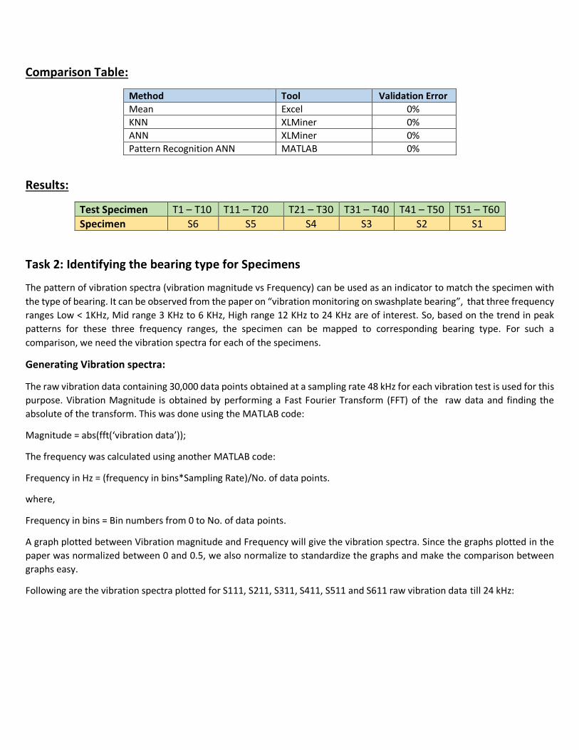
Comparison Table:

Method Tool Validation Error

Mean Excel 0%

KNN XLMiner 0%

ANN XLMiner 0%

Pattern Recognition ANN MATLAB 0%

Results:

Test Specimen T1 – T10 T11 – T20 T21 – T30 T31 – T40 T41 – T50 T51 – T60

Specimen S6 S5 S4 S3 S2 S1

Task 2: Identifying the bearing type for Specimens

The pattern of vibration spectra (vibration magnitude vs Frequency) can be used as an indicator to match the specimen with

the type of bearing. It can be observed from the paper on “vibration monitoring on swashplate bearing”, that three frequency

ranges Low < 1KHz, Mid range 3 KHz to 6 KHz, High range 12 KHz to 24 KHz are of interest. So, based on the trend in peak

patterns for these three frequency ranges, the specimen can be mapped to corresponding bearing type. For such a

comparison, we need the vibration spectra for each of the specimens.

Generating Vibration spectra:

The raw vibration data containing 30,000 data points obtained at a sampling rate 48 kHz for each vibration test is used for this

purpose. Vibration Magnitude is obtained by performing a Fast Fourier Transform (FFT) of the raw data and finding the

absolute of the transform. This was done using the MATLAB code:

Magnitude = abs(fft(‘vibration data’));

The frequency was calculated using another MATLAB code:

Frequency in Hz = (frequency in bins*Sampling Rate)/No. of data points.

where,

Frequency in bins = Bin numbers from 0 to No. of data points.

A graph plotted between Vibration magnitude and Frequency will give the vibration spectra. Since the graphs plotted in the

paper was normalized between 0 and 0.5, we also normalize to standardize the graphs and make the comparison between

graphs easy.

Following are the vibration spectra plotted for S111, S211, S311, S411, S511 and S611 raw vibration data till 24 kHz:

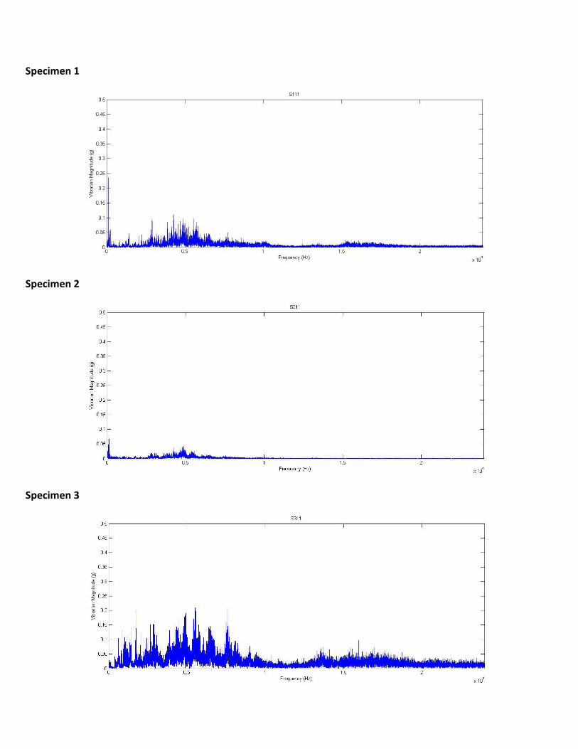
Specimen 1

Specimen 2

Specimen 3

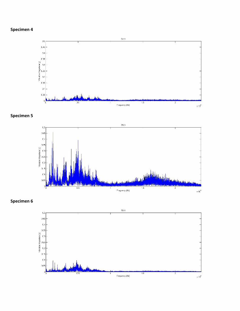
Specimen 4

Specimen 5

Specimen 6

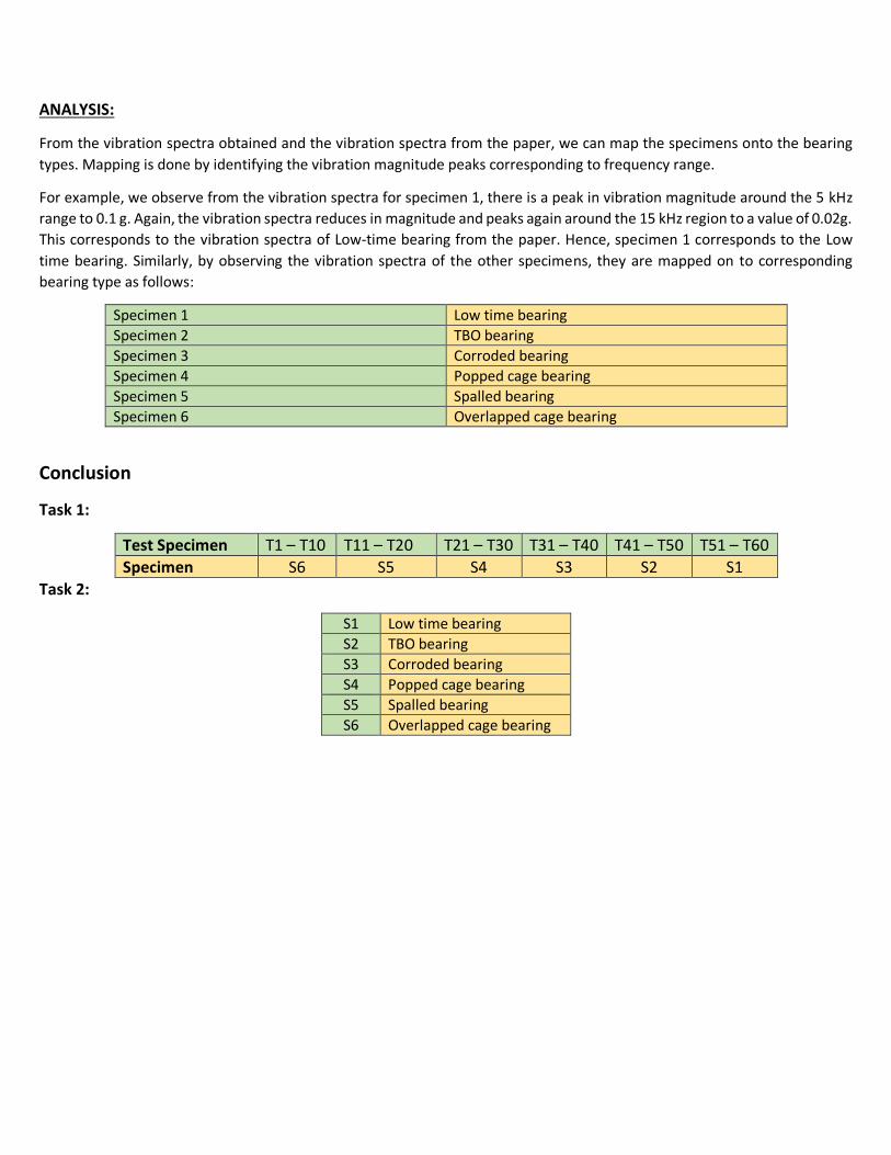
ANALYSIS:

From the vibration spectra obtained and the vibration spectra from the paper, we can map the specimens onto the bearing

types. Mapping is done by identifying the vibration magnitude peaks corresponding to frequency range.

For example, we observe from the vibration spectra for specimen 1, there is a peak in vibration magnitude around the 5 kHz

range to 0.1 g. Again, the vibration spectra reduces in magnitude and peaks again around the 15 kHz region to a value of 0.02g.

This corresponds to the vibration spectra of Low-time bearing from the paper. Hence, specimen 1 corresponds to the Low

time bearing. Similarly, by observing the vibration spectra of the other specimens, they are mapped on to corresponding

bearing type as follows:

Specimen 1 Low time bearing

Specimen 2 TBO bearing

Specimen 3 Corroded bearing

Specimen 4 Popped cage bearing

Specimen 5 Spalled bearing

Specimen 6 Overlapped cage bearing

Conclusion

Task 1:

Test Specimen T1 – T10 T11 – T20 T21 – T30 T31 – T40 T41 – T50 T51 – T60

Specimen S6 S5 S4 S3 S2 S1

Task 2:

S1 Low time bearing

S2 TBO bearing

S3 Corroded bearing

S4 Popped cage bearing

S5 Spalled bearing

S6 Overlapped cage bearing

Data Mining Application For CH-47D Aft Swashplate Bearing Fault Detection Project #2

Documents

Transcript of Data Mining Application For CH-47D Aft Swashplate Bearing Fault Detection Project #2