Data Analysis: Strengthening Inferences in Quantitative ... - ERIC

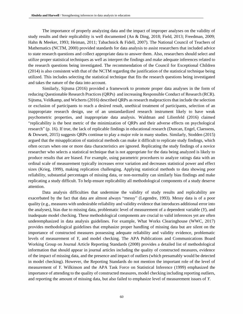
59

EDUCATIONAL SCIENCES: THEORY & PRACTICE eISSN: 2148-7561, ISSN: 2630-5984

Received: 22 November 2019

Revision received: 13 December 2019 Copyright © 2020 JESTP

Accepted: 21 January 2020 www.jestp.com

DOI 10.12738/jestp.2020.1.005 ⬧ January 2020 ⬧ 20(1) ⬧ 59-78

Article

Data Analysis: Strengthening Inferences in Quantitative Education Studies Conducted by

Novice Researchers

Abstract

Data analysis is a significant methodological component when conducting quantitative education studies. Guidelines

for conducting data analyses in quantitative education studies are common but often underemphasize four important

methodological components impacting the validity of inferences: quality of constructed measures, proper handling of

missing data, proper level of measurement of a dependent variable, and model checking. This paper highlights these

components for novice researchers to help ensure statistical inferences are valid. We used empirical examples

involving contingency tables, group comparisons, regression analysis, and multilevel modelling to illustrate these

components using the Program for International Student Assessment (PISA) data. For every example, we stated a

research question and provided evidence related to the quality of constructed measures since measures with weak

reliability and validity evidence can bias estimates and distort inferences. The adequate strategies for handling missing

data were also illustrated. The level of measurement for the dependent variable was assessed and the proper statistical

technique was utilized accordingly. Model residuals were checked for normality and homogeneity of variance.

Recommendations for obtaining stronger inferences and reporting related evidence were also illustrated. This work

provides an important methodological resource for novice researchers conducting data analyses by promoting

improved practice and stronger inferences.

Keywords

quantitative studies • novice researchers • data quality • missing data • model checking

Correspondence to Mohammed A. A. Abulela, PhD, Quantitative Methods in Education Program, Department of Educational Psychology, University of Minnesota, USA.; Assistant Professor at Department of Educational Psychology, South Valley University, Egypt. E-mail:

[email protected]

Citation: Abulela, M. A. A., & Harwell, M. M. (2020). Data analysis: Strengthening inferences in quantitative education studies conducted by

novice researchers. Educational Sciences: Theory and Practice, 20(1), 59 - 78. http://dx.doi.org/10.12738/jestp.2020.1.005

Mohammed A. A. Abulela University of Minnesota, USA

South Valley University, Egypt

Michael M. Harwell University of Minnesota, USA

T Abulela and Harwell / Strengthening inferences in data analysis in education

60

The importance of properly analyzing data and the impact of improper analyses on the validity of

study results and their replicability is well documented (An & Ding, 2018; Field, 2013; Freedman, 2009;

Hahn & Meeker, 1993; Heiman, 2011; Tabachnick & Fidell, 2007). The National Council of Teachers of

Mathematics (NCTM, 2000) provided standards for data analysis to assist researchers that included advice

to state research questions and collect appropriate data to answer them. Also, researchers should select and

utilize proper statistical techniques as well as interpret the findings and make adequate inferences related to

the research questions being investigated. The recommendation of the Council for Exceptional Children

(2014) is also consistent with that of the NCTM regarding the justification of the statistical technique being

utilized. This includes selecting the statistical technique that fits the research questions being investigated

and takes the nature of the data into account.

Similarly, Sijtsma (2016) provided a framework to promote proper data analyses in the form of

reducing Questionable Research Practices (QRPs) and increasing Responsible Conduct of Research (RCR).

Sijtsma, Veldkamp, and Wicherts (2016) described QRPs as research malpractices that include the selection

or exclusion of participants to reach a desired result, unethical treatment of participants, selection of an

inappropriate research design, use of an unstandardized research instrument likely to have weak

psychometric properties, and inappropriate data analysis. Waldman and Lilienfeld (2016) claimed

“replicability is the best metric of the minimization of QRPs and their adverse effects on psychological

research” (p. 16). If true, the lack of replicable findings in educational research (Duncan, Engel, Claessens,

& Dowsett, 2015) suggests QRPs continue to play a major role in many studies. Similarly, Stodden (2015)

argued that the misapplication of statistical methods can make it difficult to replicate study findings, which

often occurs when one or more data characteristics are ignored. Replicating the study findings of a novice

researcher who selects a statistical technique that is not appropriate for the data being analyzed is likely to

produce results that are biased. For example, using parametric procedures to analyze ratings data with an

ordinal scale of measurement typically increases error variation and decreases statistical power and effect

sizes (Krieg, 1999), making replication challenging. Applying statistical methods to data showing poor

reliability, substantial percentages of missing data, or non-normality can similarly bias findings and make

replicating a study difficult. To help ensure replicability all methodological components of a study deserve

attention.

Data analysis difficulties that undermine the validity of study results and replicability are

exacerbated by the fact that data are almost always “messy” (Legendre, 1993). Messy data is of a poor

quality (e.g., measures with undesirable reliability and validity evidence that introduces additional error into

the analyses), bias due to missing data, problematic level of measurement of a dependent variable (Y), and

inadequate model checking. These methodological components are crucial to valid inferences yet are often

underemphasized in data analysis guidelines. For example, What Works Clearinghouse (WWC, 2017)

provides methodological guidelines that emphasize proper handling of missing data but are silent on the

importance of constructed measures possessing adequate reliability and validity evidence, problematic

levels of measurement of Y, and model checking. The APA Publications and Communications Board

Working Group on Journal Article Reporting Standards (2008) provides a detailed list of methodological

information that should appear in journal articles including the quality of constructed measures, evidence

of the impact of missing data, and the presence and impact of outliers (which presumably would be detected

in model checking). However, the Reporting Standards do not mention the important role of the level of

measurement of Y. Wilkinson and the APA Task Force on Statistical Inference (1999) emphasized the

importance of attending to the quality of constructed measures, model checking including reporting outliers,

and reporting the amount of missing data, but also failed to emphasize level of measurement issues of Y.


61

In short, educational researchers planning data analyses can find guidelines reflecting recommended

practice (e.g., WWC, 2017) but these often fail to sufficiently emphasize the importance of constructing

measures with adequate reliability and validity evidence, proper handling of missing data, employing a

dependent variable Y with a level of measurement consistent with the questions being asked and the analyses

being performed, and providing evidence a statistical model is appropriate (model checking). Insufficient

attention to these methodological components can produce invalid and unreplicable study findings even

when studies are performed by experienced researchers who possess a good deal of quantitative expertise.

For novice researchers still developing their expertise attending to these important methodological

components may be particularly challenging since most statistics textbooks in the social sciences presuppose

a level of quantitative expertise that these researchers may not yet have. These texts generally focus on data

analyses and provide little to no coverage of other important methodological components such as the quality

of measures, proper handling of missing data, linking the level of measurement of variables to appropriate

analyses and inferences, and ensuring accurate inferences by examining the plausibility of model

assumptions (e.g., Agresti & Findlay, 2014; Glass & Hopkins, 1996; Howell, 2017; Moore, McCabe, &

Craig, 2017; Ness-Evans, 2014). Our goal is to describe and illustrate these under-emphasized components

for novice researchers using easy to understand language and empirical examples in ways that promote valid

inferences. Novice researchers include new faculty, individuals beginning non-faculty roles such as a

working in a university-affiliated research center or a government-funded education center, faculty

transitioning to more research-oriented work, and students conducting their own research, graduate

students).

Underemphasized Methodological Components

Quality of constructed measures (variables). Many quantitative education studies construct

measures to meet study needs, for example, measures of student proficiency with fractions. Constructing

measures following the guidelines of the American Educational Research Association [AERA], American

Psychological Association [APA], and the National Council on Measurement in Education (NCME, 2014)

should enhance data quality and the validity and reliability of interpretations for proposed uses; ignoring

these guidelines can lead to substantial measurement error (unreliability) which in a data analysis inflates

the sampling error and increases the likelihood of distorted statistical results. Constructing a measure of

student proficiency with fractions following AERA/APA/NCME guidelines that will serve as a dependent

variable involves defining the content to be assessed, relying on experts to construct items reflecting the

specified content, piloting the measure and performing item analyses using pilot data to identify items that

are not operating as intended, and revising the measure accordingly. Following these steps is likely to

produce less measurement error and increases the likelihood of valid statistical inferences. On the other

hand, constructing a measure of proficiency that fails to follow AERA/APA/NCME guidelines is more

likely to produce more measurement error that in turn inflates sampling error and reduces the likelihood of

valid inferences.

Creswell (2012) pointed out that researchers have three options with respect to a measure: Use an

existing standardized measure whose psychometric properties are known to be strong, modify an existing

measure to meet the particular needs of a study, or construct a new measure. These authors argued that the

first option is preferred to the second, and that the first and second options are overwhelmingly preferred to

the third. However, Abulela and Harwell (2019) provided evidence the third option, which is relatively

common in educational research, typically involves a time-consuming and resource-intensive process which

may not produce a new measure with strong psychometric properties. For example, a novice researcher who


62

constructs their own measure is likely to discover this process can take several months because of the

multiple steps outlined in the AERA/APA/NCME guidelines.

Abulela and Harwell (2019) also emphasized that measures with weak psychometric properties

invite biased statistical results and inferences, which is a particular concern when a researcher constructs

their own instrument. As noted above, unacceptably low reliability of scores means greater measurement

error is present and appears in the error term used in statistical analyses (e.g., mean square error in

regression). The net effect is to reduce statistical power and bias estimates including effect sizes. Relatedly,

low reliability also impacts correlations among variables regardless of the true value of the correlation in

the population. Bandalos (2018) showed that the correlation between two variables X and Y is less than or

equal to the square root of the product of the score reliabilities of the two variables. When the reliability of

scores is low, the correlation is attenuated, meaning the results of statistical analyses involving the X, Y

correlation will be negatively-biased. For example, a dependent variable and predictor with low score

reliability will produce a negatively-biased slope in a regression analysis and reduce the predictive power

of the model. In short, there is no shortcut to constructing measures with strong psychometric properties,

and no educational research setting where measures with unsatisfactory psychometric properties are

acceptable.

Missing data. It is often not possible to collect data for all subjects on all variables of interest, and

missing data in educational research are common (Peng, Harwell, Liou, & Ehman, 2006). Explanations for

missing data include subject attrition (e.g., students move out of a school district during the study), data

collection errors (e.g., errors in a computer program used to record subject responses), unclear instructions

or intrusive questions on a survey (e.g., questions about income), and poor data entry or record keeping

(Van den Broeck, Cunningham, Eeckels, & Herbst, 2005). In describing missing data, it is generally the

proportion of missing data that is referred to not the percentage of subjects lost because of missing values.

Peugh and Enders (2004) surveyed 545 education studies appearing in 23 journals and reported that

42% had missing data. Peng et al. (2006) surveyed 1,666 articles appearing in 11 education journals

published between 1998-2004 and reported 48% had missing data and 16% did not provide sufficient

information to determine if missing data were present, and Rousseau, Simon, Bertrand, and Hachey (2012)

reported 34% of the education studies in their survey had missing data. These surveys did not disaggregate

missing data percentages by data origin (i.e., local/regional, national, international), but missing data can

undermine inferences in any dataset even those based on random sampling and large samples such as the

Trends in International Mathematics and Science Study [TIMSS] (Martin, Mullis, & Chrostowski, 2004)

and the Programme for International Student Assessment [PISA] (Schulz, 2006). For example, Carnoy,

Khavenson, Loyalka, Schmidt, and Zakharov (2016) reported that 10% of their TIMSS sample was missing

but did not report the percentage of missing data for individual variables. Similarly, Mijs (2016) analyzed

PISA data and reported that the percentage of missing data on variables used for statistical control ranged

between 0 - 1.34% but did not report the percentage missing for other study variables, and Niehaus and

Adelson (2014) focused on English language learners (ELLs) within the Early Childhood Longitudinal

Study-Kindergarten (ECLS-K) data and reported this information was missing for 35% of the sample.

Whatever the reason(s) and the amount, missing data can introduce substantial bias into the

statistical results and inferences (Becker & Powers, 2001; Becker & Walstad, 1990; WWC, 2017).

Specifically, estimated parameters such as means, variances, slopes and associated statistical tests such as

t-, F, and chi-square tests will typically be impacted because subjects with incomplete responses (i.e., have

missing data on one or more variables) may differ from those providing complete data (i.e., no missing data)

in ways that affect inferences.


63

For example, students with missing Y data (measure of proficiency with fractions) may

disproportionately come from households in which English is not the native language and whose proficiency

with fractions is below average. This raises the possibility the sample then consists disproportionately of

students more proficient with fractions and thus no longer represents a population with a broad range of

proficiency values. If a researcher draws conclusions about mean differences (e.g., treatment versus control

conditions) based on subjects who responded and generalizes the conclusions to a population with a broad

range of proficiency with fractions, these conclusions will be biased. Missing data also typically lowers the

accuracy with which parameters like means and variances are estimated as well as the power of statistical

tests based on these statistics (Anderson, Basilevsky, & Hum, 1983; Peng et al., 2006) because of a reduction

in sample size.

An often-overlooked consequence of missing data is the loss of time and funding spent on subjects

who produce missing data (Buu, 1999; Van den Broeck et al., 2005). In the presence of missing data,

researchers sometimes allocate additional resources to obtain complete data from subjects who provided

incomplete data, but these efforts typically have limited success. As Carpenter (2009) noted the only

solution to the problem of missing data is finding the data. This implies that researchers should respond to

the challenge of missing data head-on.

Responding to missing data begins with characterizing how values are missing (i.e., identifying the

missing data mechanism). Suppose data for Y, X1,…,Xq variables (Y = dependent variable, Xq = independent

or predictor variable) are collected and 20% of the Y values are described as missing (missing data on

predictors are more difficult to handle - see Allison, 2002; Carpenter, 2009). Rubin (1976) characterized

missing data using three missing data mechanisms: (i) Missing Completely at Random (MCAR), (ii)

Missing at Random (MAR), and (iii) Not Missing at Random (NMAR). Identifying the nature of the

“missingness” provides researchers with options for properly handling missing data.

If missing data are MCAR, there is no difference in the distributions of the variables with complete

and incomplete (missing) data so inferences based on available data are unbiased, although statistical power

and accuracy in estimating parameters will be reduced. Put another way, MCAR means the distributions of

obtained and missing data are identical which happens when the reason(s) data are missing are completely

random, i.e., data missingness is not linked to any study variable or to what Y represents. For example,

students who fail to provide data for a test of proficiency with fractions because they were sick on the day

of testing implies missingness is MCAR and the reason(s) Y data are missing cannot be accounted for by

study variables or by what Y represents.

For MAR the reason(s) Y data are missing can be accounted for by study variables but are not due

to what Y represents. Suppose data for a test of proficiency with fractions for a sample of rural and urban

school districts are obtained. In examining the data, a researcher discovers no Y scores are available for

students in a particular rural school district and subsequently learns that school in this district was cancelled

the day of testing due to inclement weather. Adding a predictor to this effect (i.e., 1 = missing test data due

to weather-related school cancellation, 0 = no) in the data analyses that includes students with and without

complete data accounts for the missingness and helps to ensure unbiased inferences based on analyses of

available data. In practice, identifying a factor such as inclement weather as responsible for missing test

data is relatively easy compared to many settings in which the reasons data are missing may be unclear. The

third missing data mechanism occurs when missingness is due to what is being measured by Y, for example,

students miss a test because parents keep their children home out of fear their children will perform poorly.

This is known as NMAR and is challenging to deal with statistically.


64

There are several strategies for handling missing data assumed to be MCAR or MAR (Peng et al.,

2006), and the two reviewed here are widely used to produce complete (no missing) data. One strategy uses

mean imputation. Suppose a multiple regression analysis with three predictors (X1, X2, X3) and a dependent

variable Y is to be performed but Y has missing values. One strategy for handing missing data is to impute

the mean of Y computed using available Y values for the missing values. Thus, if there are 10 missing Y

values and �̄�= 105 based on available Y scores, 105 is imputed (substituted) for the 10 missing Y values.

This strategy assumes missing data are MCAR and is often reasonable if the percentage of missing Y values

is small (e.g., 2%), but imputing �̄� for larger amounts of missing data artificially reduces the variability

of Y scores in ways that can bias parameter estimates and statistical tests. This option is available in many

data analysis programs such as SPSS Missing Value Analysis and the AMELIA II missing data software

(Honaker, King, & Blackwell, 2011) which is part of the R package.

A second strategy for handling missing data is regression-based in which missing Y values are

imputed using predicted Y values (�̂�𝑖) computed using available data. Specifically,�̂�𝑖 values are computed

using available data for Y, X1, X2, X3 and used to impute missing Y values. Software that will perform

regression-based imputation includes SPSS Missing Values Analysis and the AMELIA II software

(Honaker et al., 2011). More sophisticated regression-based methods are available (e.g., EM algorithm,

multiple imputation in which a missing Y value is imputed several times to account for sampling error) but

all require missingness to be MCAR or MAR. Good introductions to missing data include Allison (2002),

Peng et al. (2006), and Schafer and Graham (2002).

Proper level of measurement of Y. An under-appreciated component of strengthening inferences

in quantitative education studies centers on employing a proper level of measurement of a dependent

variable (Y). Most researchers are familiar with the four levels of measurement (nominal, ordinal, interval,

ratio) covered in introductory data analysis classes. A nominal scale for Y is present when values simply

distinguish groups such as gender (males, females) or ethnicity (Black, Hispanic, Asian, White, Other) and

do not represent a rank-ordering. An ordinal scale is present when Y values reflect a rank-ordering but

differences among adjacent values in what is being measured are unequal (e.g., socio-economic status [SES]

represented as high, medium, and low). An interval scale of measurement is present when Y values refer to

quantitative (numerical) scores on a scale in which differences among adjacent values in what is being

measured mean the same thing across the entire scale (e.g., proficiency with fractions scores from a

standardized test) but there is no meaningful zero. Y possesses a ratio scale if interval scale properties are

present but there is also a meaningful zero such as the number of children in a family. Harwell and Gatti

(2001) provide additional details of the four scales of measurement.

A critical factor in the choice of Y is the research question being asked. A question asking whether

a new mathematics curriculum significantly increases student understanding of fractions compared to an

existing curriculum, and if so by how much, suggests Y should possess an interval scale to ensure mean

differences, slopes, and effect sizes such as Cohen's d and measures of explained variation such as R2 are

interpretable. A Y variable based on an average of 5 Likert-type items reflecting student understanding of

fractions in which each item is scored using 4 = Proficient, 3 = Nearly proficient, 2 = Somewhat proficient,

and 1 = Lacks proficiency almost certainly possesses an ordinal scale that can make interpreting mean

differences, slopes, Cohen's d, and R2 measures problematic. For example, it is unlikely that a student whose

average score on the 5 Likert-type items was 4 is exactly twice as proficient as a student whose average

score was 2. On the other hand, interpreting mean differences, slopes, Cohen's d, and R2 when Y reflects

scores on a standardized test of fractions constructed following AERA/APA/NCME guidelines are likely to


65

be interpretable. Treating ordinal data as interval-scaled can also produce biased parameter estimates and

statistical test results (Embretson, 1996; Krieg, 1999).

Decisions about how best to analyze Y if it shows a nominal scale are usually clear, for example,

asking whether a mathematics curriculum for teaching fractions (new versus old) is related to student race

implies a nominal scale of measurement. Similarly, if Y has an interval or ratio scale statistical procedures

requiring normality are generally appropriate (a normal distribution assumes at least an interval scale) (Lord

& Novick, 1968). However, there is a divide in the research community on appropriate analyses for data

showing an ordinal scale, which is unfortunate because most Y variables in educational research appear to

possess an ordinal scale (Clogg & Shihadeh, 1994; Harwell & Gatti, 2001). Some authors argue that what

counts is the meaningfulness of a statistical analysis based on Y not its scale of measurement per se (Lord,

1953). Other authors argue that normality can never be assumed for ordinally-scaled data (Stevens, 1951;

Townsend & Asby, 1984) and hence statistical techniques requiring normality cannot be performed for such

variables.

Even measures known to have impressive psychometric properties technically possess an ordinal

scale. For example, the Scholastic Aptitude Test (SAT) and Graduate Record Exam (GRE) are taken by

many students as part of applying to undergraduate and graduate educational programs. These measures

possess exemplary reliability and validity evidence and are universally treated as possessing an interval

scale yet technically possess an ordinal scale. Assume the quantitative section of the GRE has a mean and

standard deviation (SD) of 500 and 100 and suppose three students take the GRE and earn quantitative

scores of 250, 500, and 750, respectively. These scores do not satisfy the requirements of a ratio scale

because there is no meaningful zero; moreover, the properties of an interval scale are unlikely to be satisfied

because it is not plausible to conclude the quantitative proficiency of a student with a score of 500 is exactly

twice that of a student with a score of 250, or that a student scoring 750 is exactly three times as

quantitatively proficient as a student scoring 250. Harwell and Gatti (2001) provide a rigorous definition of

ordinal and interval scales). In short, most Y variables in quantitative educational research treated as having

an interval scale of measurement likely have an ordinal scale.

A reasonable compromise is to treat variables with many possible numerical values such as SAT

and GRE scores as possessing an approximate interval scale of measurement that supports meaningful

inferences and potentially the assumption of normality. Variables such as a total score based on summing

Likert-type items possessing an ordinal scale should be examined carefully to decide if a label of

approximately-interval or the possibility of a normal distribution is deserved. For example, suppose Y

represents how useful students believe math is based on summing 25 versus 4 Likert-type items each of

which is scored 4 = very useful, 3 = somewhat useful, 2 = not very useful, 1 = not useful. Other things being

equal, Y scores based on 25 items likely deserve to be treated as showing an approximate interval scale of

measurement that could potentially be normally-distributed because there are many more numerical values

compared to Y scores based on summing 4 items. Relatedly, larger numbers of response categories (e.g., 5

or 6) can help to justify treating Y as possessing an approximate interval scale compared to smaller numbers

of response categories (e.g., 3 or 4) (Bandalos, 2018).

Model checking. Another important methodological component of data analysis is model checking,

which focuses on the plausibility of model assumptions underlying statistical techniques needed to ensure

valid statistical inferences: Assumptions that are plausible imply that estimated effects and statistical test

results can be treated as accurate whereas important violations of these assumptions imply statistical results

are not trustworthy. For example, a researcher conducting a statistical test may set the probability of

rejecting a true statistical hypothesis (Type I error) to α = .05, but because of assumption violations the true


66

Type I error rate may be .08, .12, .22 or higher. Model assumption violations can also reduce statistical

power. In short, violations of assumptions can result in invalid results and incorrect inferences (APA

Publications and Communications Board Working Group on Journal Article Reporting Standards, 2008;

WWC, 2017; Zimmerman, 1998).

Frequently used statistical models and statistical tests typically require independence, normality,

and homoscedasticity of the data. Obsorne (2010) pointed out that “many authors are under the erroneous

impression that most statistical procedures are robust to violations of most assumptions” (p. 63), which may

explain why surveys of quantitative education studies have reported that 64% - 90% of the surveyed studies

did not report any model checking (Namasivayama, Yana, Wong, & Van Lieshout, 2015; Osborne, Kocher,

& Tillman, 2012).

It is a good practice to screen data before performing analyses to detect coding errors, outliers, or

other irregularities. However, data analyses that require normality depend on model residuals to assess

underlying statistical assumptions rather than Y scores (Neter, Kutner, Nachtsheim, & Wasserman, 1996).

For example, in multiple regression the residual for each subject represents the extent to which the predictive

model over- or under-predicted their actual Y score - it is the residuals that must satisfy the standard

assumptions of independence, normality, and homoscedasticity.

Central to model checking is identifying outliers and their impact. There are multiple definitions of

outliers, but all are consistent with Moore et al.'s (2017) definition of an observation (residual) that falls

outside the overall pattern of a data distribution. For example, if a variable follows a normal distribution it

is common to treat values greater than ±3SDs as outliers although such criteria are context-specific. Outliers

are important because they can have a disproportionate impact on parameter estimates and statistical tests

by increasing (or shrinking) key statistics such as means, variances, and slopes (Neter et al., 1996). Outliers

are also often responsible for model violations such as non-normality and heteroscedasticity.

Outliers occur for many reasons including data recording errors (e.g., errors in a computer program

used to record subject responses, data entry errors attributable to typing values into an electronic file),

unintended sampling problems (e.g., inadvertently sampling subjects from multiple populations such as

including ELLs in a study in which these students were to be omitted), and measurement error (e.g., error

in measuring proficiency with fractions produces artificially high or low values) (Van den Broeck et al.,

2005). It is important to try to identify the source of outliers because this guides how to respond. For

example, tracing outliers to data recording errors in a computer program or to data entry errors, or to

unintended sampling problems may allow outliers to be effectively dealt with. Detecting, correcting, and/or

removing inaccurate records and outliers is sometimes described as data cleaning (Van den Broeck et al.,

2005), and data cleaning programs like OpenRefine (formerly Google Refine), Trifecta Wrangler (formally

Data Wrangler), and the R package Tidyr (R Core Team, 2015) are available to assist researchers.

The presence of outliers is also likely to raise questions about whether these values should be

omitted for subsequent analyses or remain in the sample and perhaps subjected to a nonlinear data

transformation like a logarithmic transformation with the goal of reducing their impact. There is no

universally accepted practice for omitting or keeping outliers in a sample--this decision depends on multiple

factors including evidence of the source of outliers, how far a value falls from the overall data pattern (e.g.,

3SD versus 5SD), and the number of outliers relative to sample size (e.g., 1% versus 15%). In all cases, the

process used to assess data quality and the results should be described to allow readers to judge their

appropriateness (Appelbaum et al., 2018).

Independence of model residuals. Independence of model residuals is required for statistical

techniques like t-tests, ANOVA, and multiple regression. Independence means no subgroup of residuals can


67

predict any other subgroup of residuals beyond chance (Draper & Smith, 1981). Violating this assumption

in data analyses has a devastating impact on statistical findings that worsens as sample size increases.

Harwell (1991) used a computer simulation study to show that the true Type I error rate was .25 (not α =

.05) for N = 10 and a correlation of .20 among residuals for a two-sample t-test of independent means; for

N = 18 and a correlation of .20 among residuals the true Type I error rate increased to .39. Dependency

among residuals is usually detected by examining the conduct of the study (e.g., subjects were discovered

to have communicated with each other during the study), and empirically through a test of serial correlation

of the residuals available in software like SPSS or R (Field, 2013). Evidence of dependency generally leaves

researchers with two options: (i) abandon statistical testing and rely on descriptive analyses, (ii) add

predictors to a regression model to try to capture the reason(s) for the dependency, such as adding a predictor

indicating whether a subject had a sibling in the study sample.

Normality of residuals. The assumption that data (residuals) follow a normal distribution is familiar

to many researchers, as is the robustness of many statistical procedures to modest departures from normality

because of the central limit theorem (Neter et al., 1996). Plots and summary statistics like skewness

computed for model residuals provide descriptive evidence of the plausibility of normality. Per the earlier

discussion, it is particularly important to examine residuals for evidence of outliers because these values

can seriously distort estimates and statistical test results. Data analysis software such as SPSS and R provide

standardized residuals to help researchers identify outliers (e.g., residuals outside ±3SDs). For more

information about methods for handling outlier’s novice researchers can turn to Hoaglin and Iglewicz

(1987).

Homoscedasticity of residuals. A standard assumption in data analysis is that variances of groups

are equal, or the residual variance is equal across values of Xq. A plot of residuals that shows similar spread

across values of an independent variable provides evidence of homoscedasticity. In practice, residuals are

usually plotted against �̂�𝑖 (which reflects the combined impact of the Xq). Similar variability (spread) in

residuals across all values of �̂�𝑖 provides evidence of homoscedasticity; unequal spread in residuals across

�̂�𝑖 provides evidence of heteroscedasticity. Violating this assumption can bias estimates and statistical tests

which by default assume equal error variances (e.g., t-tests, ANOVA, regression, multilevel models).

Outliers can also trigger heteroscedasticity. Remedies for heteroscedasticity include adding predictors to a

model that account for heteroscedasticity (e.g., subject age, ELL status), omitting subjects whose data

appears to be responsible for the heteroscedasticity, performing a nonlinear transformation of Y, or

employing a more complicated regression model that allows unequal error variances such as weighted least

squares (Neter et al., 1996).

In short, model checking is an integral part of data analyses. Non-independence, non-normality, and

heteroscedasticity of residuals can lead to biased estimates and misleading statistical test results in ways that

negatively impact the quality of inferences. Novice researchers are advised to pay special attention to

outliers since they are often mainly responsible for non-normality and heteroscedasticity of residuals. Once

detected, sensitivity analyses (performing analyses with and without outliers) can be performed. If the

results of sensitivity analyses with and without outliers are similar, those based on the original data should

be reported. If results of the sensitivity analyses differ with and without outliers, the researcher must decide

whether to omit outliers from the analyses, use a nonlinear transformation of the data to reduce the impact

of outliers, or add predictors to the model that capture explanations for outliers (e.g., add age as a predictor

if outliers appear to be the youngest subjects).


68

Empirical Examples

We provide empirical examples involving contingency tables, group comparisons, regression

analysis, and multilevel models to illustrate the underemphasized methodological components using the

PISA (2003) data. PISA is a system of international assessments that measure 15-year-olds’ capabilities in

reading literacy, mathematics literacy, and science literacy every 3 years. To implement PISA, each country

selects a nationally representative sample of 15-year-olds regardless of grade level. The U.S. 2003 sample

consisted of 17,051 students each of whom completed a 2-hour paper and pencil assessment and a 30-minute

background questionnaire collecting information on their background and attitudes toward learning. We use

the variables gender, SES, standardized mathematics, reading, and science scores and create a new variable

by rescaling mathematics scores into quartiles. The PISA variables have strong psychometric properties as

documented in technical manuals accompanying these data. For each statistical technique, we specify a

research question and then assess (where appropriate) the quality of constructed measures, respond to

missing data, employ a proper level of measurement of Y given the research question and statistical analyses,

and perform model checking with a particular focus on detecting outliers.

Example of a contingency table analysis. Research question: Is there a relationship between

student gender and mathematics performance when the latter is represented using quartiles? The result is a

4 (mathematics quartile) x 2 (gender) contingency (frequency) table (see Table 1). To test whether there is

a relationship between gender and the mathematics quartiles variable would typically involve the Pearson

chi-square test for contingency tables. A description of how to perform this test is given in Howell (2017).

First, assessing the quality of constructed measures in a contingency table begins by examining the

variables comprising the table. Student gender was not a constructed measure (0 = male, 1 = female) whereas

the mathematics score variable represented in quartiles was and a rationale for using the quartiles variable

should be provided. For example, scoring students on the mathematics test as 4 = Proficient, 3 = Nearly

proficient, 2 = Somewhat proficient, or 1 = Lacks proficiency because school district policy uses this grading

system for students rather than traditional A - F grading, could provide a rationale for constructing the

mathematics quartile variable.

Second, the resulting student sample of n = 16,273 means 17,051 - 16,273 = 778 students were

“lost” in this analysis, and an examination of the data showed all missing values occurred for the

mathematics, science, and reading score variables. The researcher may choose to ignore missing data

because less than 5% of the cases were omitted or try to learn why scores were missing (i.e., was the

missingness MCAR, MAR, or NMAR). If the missing values are MCAR it's appropriate to proceed to the

major analyses because the results will not be biased by the missing values and the remaining sample size

(n = 16,273) is large enough to ensure precise estimates and substantial statistical power; if MAR holds then

predictors capturing the reason(s) scores were missing should be added to the data analyses. This would

likely prompt the use of logistic regression (Neter et al., 1996) to analyze the contingency table data. Missing

mathematics scores could also be imputed using under MCAR or MAR. We chose to ignore the missing

data because it was a relatively small percentage (4.78%) of the total sample.

Third, the mathematics quartile (Y) variable possesses an ordinal scale of measurement whereas

gender is treated as nominally-scaled. The scale of Y means that inferences about differences between

response categories should be limited to being higher or lower and cannot be used to infer numerical

amounts of proficiency. For example, a student in the 4th quartile (Proficient) has a higher mathematics

performance than a student in the 2nd quartile (Somewhat proficient) but is not exactly twice as proficient as

the student in the 2nd quartile.


69

The statistical null hypothesis posits that gender and the mathematics quartile variable have no

relationship, i.e., Ho: V = 0 versus H1: V = 0, where V is Cramer's measure of the correlation between the

two variables defining the table. The Pearson chi-square test is available in software such as SPSS and R

and for Table 1 produces 𝜒2= 31.11 (p < .001). Assuming α = .05, the p-value value indicates Ho should be

rejected and the conclusion is that student gender and mathematics performance (via quartiles) are

correlated. The Pearson chi-square test treats the variables defining the table as nominally-scaled and re-

analyzing Table 1 using the Kruskal-Wallis test for ordered contingency tables takes into account the ordinal

scale of the mathematics quartile variable (Marascuilo & McSweeney, 1977) and produces a slightly more

powerful statistical test.

Table 1. Pearson chi-square test for mathematics achievement represented in quartiles for boys (n = 8084)

and girls (n = 8189)

Boys Girls

Mathematics n % n % χ2 (3) Cramer’s V

1st quartile 1997 24.7 2066 25.23

31.11*** .044

2nd quartile 1926 23.82 2144 26.18

3rd quartile 1992 24.64 2075 25.34

4th quartile 2169 26.84 1904 23.25

Total 8084 100 8189 100

Note. ***p < .001

Fourth, model checking in a contingency table often takes the form of examining expected cell

frequencies (assuming Ho is true) to ensure they are > 5 (Howell, 2017), which Table 1 satisfies. This ensure

that the resulting p-value is accurate and hence the decision to reject Ho likely correct. The other assumption

of this analysis is that the 16,273 subjects are independent of each other, a difficult assumption to check

with such data. However, a review of PISA materials shows that instructions for completing the PISA

materials provided to students by test administrators encouraged independent responses.

Example of group comparison analysis. Research question: Do males and females score on

average the same in mathematics, reading, and science? This question suggests an independent samples t-

test be used to test the equality of means for each dependent variable separately. Details of this procedure

are given in Howell (2017).

First, assess the quality of the constructed measures. A review of PISA materials shows that

mathematics, reading, and science measures were constructed following recommended guidelines and

possess strong reliability of scores and validity evidence. This minimizes the impact of measurement error

on the analyses and enhances the quality of inferences.

Second, as illustrated in example 1, the resulting student sample of n = 16,273 means there is

missing data for 778 students on the mathematics, reading, and science variables (i.e., these students did not

provide data on any of these variables). A researcher who chose to explore the reasons data were missing

responsibility must try to characterize the missingness as MCAR, MAR, or NMAR. If the missing values

are MCAR it is appropriate to proceed to the analysis because the results will not be biased by the missing

values and the remaining sample size (n = 16,273) is large enough to ensure precise estimates and substantial

statistical power; otherwise multiple imputation could be used.

On the other hand, if missingness is MAR then predictors capturing the reason(s) scores were

missing should be added to the data analyses. For example, suppose for most of the 778 students the missing

mathematics, reading, and science scores can be attributed to their school not administering PISA on the


70

specified date because of administrative errors. Creating a predictor X (1= missing data due to administrative

error, 0 = not due to an administrative error) and adding this variable to the analysis would reduce the bias

that would otherwise distort the statistical findings. Multiple imputation could potentially be used to produce

values for the missing mathematics, reading, and science scores. We again chose to ignore the missing data

because it was a small percentage (4.78%) of the total sample. If multiple imputation was used, the

percentage of missing data would be zero.

Third, the level of measurement of gender is treated as nominal whereas the mathematics, reading,

and science (Y) variables are treated as possessing an interval scale, and thus an independent samples t-test

was employed. The statistical null hypothesis for the t-test is Ho:(μboys - μgirls) = 0 versus, Ho:(μboys - μgirls) ≠

0, where μboys is the population mean for mathematics, reading, or science variables for boys, and μgirls is the

population mean for mathematics, reading, or science variables for girls. Assuming α = .05 the results in

Table 2 indicate there are statistically significant but small differences between boys and girls that appeared

to favor boys on mathematics and science scores (t = 4.06, p < .001, Cohen's d = .06 SD; t = 2.19, p < .05,

d = .03). Table 2 also shows there are statistically significant differences on reading that appear to favor

girls (t = 19.46, p < .001, d = .30 SD). The assumption of an interval scale supports meaningful interpretation

of gender differences. For example, d = .30 SD can be interpreted as boys on average scoring .30 SD higher

than girls on the science measure or, equivalently, that 62% of the boys scored above the girls mean on this

measure.

Table 2. Gender differences in mathematics, reading, and science between boys (n = 8084) and girls (n =

8189)

Achievement Boys Girls t(16271) p Cohen’s d

M SD M SD

Mathematics 514.75 97.61 508.75 91.19 4.06 < .001 .06

Reading 492.26 99.79 521.52 91.96 19.46 < .001 .30

Science 519.89 107.55 516.29 102.24 2.19 .028 .03 Note. M = mean; SD = standard deviation; p = p-value.

Fourth, model checking began with determining whether model residuals are independent of one

another, which is initially assessed by providing evidence students responded independently. As noted in

example 1, a review of PISA materials shows that instructions for completing the PISA materials provided

to students by test administrators encouraged independent responses. The Durbin-Watson statistic can also

be used to test serial dependency (Neter et al., 1996) and is available in software such as SPSS and R. The

assumption of normality appeared to be plausible after examining residual plots and summary statistics such

as skewness and kurtosis values that ranged from -.35 to .12 (for a normal distribution these values are 0).

There was also no clear evidence of outliers. Homoscedasticity was supported after visually examining plots

of gender against residuals.

Example of multiple regression analysis. Research question: How much variance in mathematics

achievement is explained by gender, reading, and science? The gender, reading, and science variables served

as predictors and mathematics scores as the dependent variable. An introduction to performing a multiple

regression analysis appears in Howell (2017) and a detailed description of this procedure is given in Neter

et al. (1996). First, assess the quality of constructed measures. As mentioned in example 2, the mathematics,

reading, and science variables have strong reliability and validity evidence. Second, for missing data, the


71

variables involved in the multiple regression example are the same as those in example 2 and consequently

the same recommendations apply.

Third, the Y variable (mathematics score) likely possesses an interval (or approximately interval)

scale of measurement and multiple regression analysis was employed. The assumption of an interval scale

supports meaningful interpretation of statistical results such as slopes and helps to make the assumption of

a normal distribution of residuals plausible. The statistical null hypothesis for the test can be written

𝐻𝑜: 𝜌𝑦�̂� = 0 versus 𝐻1: 𝜌𝑦�̂� > 0, where 𝜌𝑦�̂� is the population correlation between observed and model-

predicted Y scores (Neter et al., 1996).

Table 3 summarizes the descriptive statistics and intercorrelations among the predictor and

dependent variable and shows that reading and science scores are positively correlated with mathematics

scores, meaning that students with above average reading and science scores tend to have above average

mathematics scores (and vice versa). On the other hand, gender (0 = boys, 1 = girls) is negatively correlated

with mathematics scores, indicating that boys on average score higher than girls.

Table 3. Means, standard deviations, and intercorrelations for mathematics achievement as the dependent

variable and gender, reading, and science as predictor variables

Variables M SD 1 2 3

Mathematics 511.73 94.48 -.03*** .81*** .86***

Predictors

Gender 0.50 0.50 - .15*** -.02***

Reading 506.98 97.04 - .86***

Science 518.08 104.92 - Note. ***p < .001, M = mean; SD = standard deviation.

The multiple regression results in Table 4 indicate that the gender, reading, and science predictors

explain 77% of the variance in mathematics achievement (R2 = .77, F = 17754.7, p < .001). The gender slope

(-13.86) was statistically significant at α = .05 (t = -18.24, p < .001), meaning that with the other predictors

held constant girls on average scored approximately 14 points (or .07 SD) lower on mathematics than boys.

The reading slope (.33) was also statistically significant (t = 33, p < .001), meaning with the other predictors

held constant a one-unit increase in reading score was associated with a gain in mathematics scores of about

one-third of a point. A similar interpretation holds for the significant science slope (.51) (t = 51, p < .001).

Table 4. Regression analysis summary for gender, reading, and science predicting mathematics

achievement

Variables B SE B β t p

Constant 86.46 1.94 44.57 < .001

Gender -13.86 0.76 -.07 -18.24 < .001

Reading 0.33 0.01 .33 33 < .001

Science 0.51 0.01 .51 51 < .001 Note. p = p-value, B = estimated slope, SE B = standard error of estimated slopes, β = standardized slope, t = t-test.

Fourth, model checking began by checking independence of residuals as described in example 2.

The Durbin–Watson statistic was used to test for serial dependency and the results were consistent with

independence. To check normality of residuals we examined standardized residuals for the presence of

outliers (defined as standardized values exceeding ±3SD) and none were detected. Plots of the

unstandardized residuals suggested a normal distribution was plausible (skewness and kurtosis close to 0).


72

Homoscedasticity of residuals was examined by plotting the unstandardized residuals against �̂�𝑖 , and

provided evidence of homoscedasticity because there was similar variability (spread) in residuals across

values of �̂�𝑖.

Example of multilevel modeling analysis. Research question: How much variance in mathematics

achievement is explained within schools by student gender and SES, and how much variance in school

intercepts (mathematics achievement means) is explained by the percentage of female students at a school

when the multilevel (hierarchical) structure of the data (students-nested-within-schools) is taken into

account? The research question implies a two-level (multilevel) model should be used which for the PISA

data involved 20,787 students (level-1 units) and 496 schools (level-2 units), and the dependent variable is

mathematics score. Details for performing these analyses appear in Raudenbush and Bryk (2002). Multilevel

software includes HLM (Raudenbush, Bryk, Cheong, Congdon, & du Toit, 2011), the lmer package in R

(Bates, Maechler, Bolker, & Walker, 2015), and ProcMixed in SAS (SAS Institue, 2012). Because of the

complexity of multilevel modeling, we provide a slightly more detailed example.

Analyzing data using multilevel models usually includes fitting several models dictated by the

research question(s). For the PISA data we fitted the following models: (i) An unconditional (random

intercepts) model (model 1) was fitted to estimate the amount of variance in mathematics scores within and

between schools. These variances are used to compute the intra-class correlation coefficient (ICC) which

reflects the percentage of variation in Y due to schools. The ICC is central to multilevel modeling- near zero

values mean a multilevel model is not needed and a regression analysis using students is appropriate,

whereas larger ICC values mean a multilevel model is appropriate. For the PISA data the results for the

unconditional model show that ICC = .23 meaning 23% of the variation in mathematics scores is between-

schools. This value justifies a multilevel model. (ii) Next student gender and SES were added as level-1

predictors (their slopes were allowed to vary across schools) (model 2). (iii) The percentage of female

students in a school was added as a predictor to the level-2 intercepts and slopes models to try to explain

variation in school intercepts (average mathematics score in a school) as well as variation in slopes across

schools (model 3). Student gender and SES slopes varied across schools.

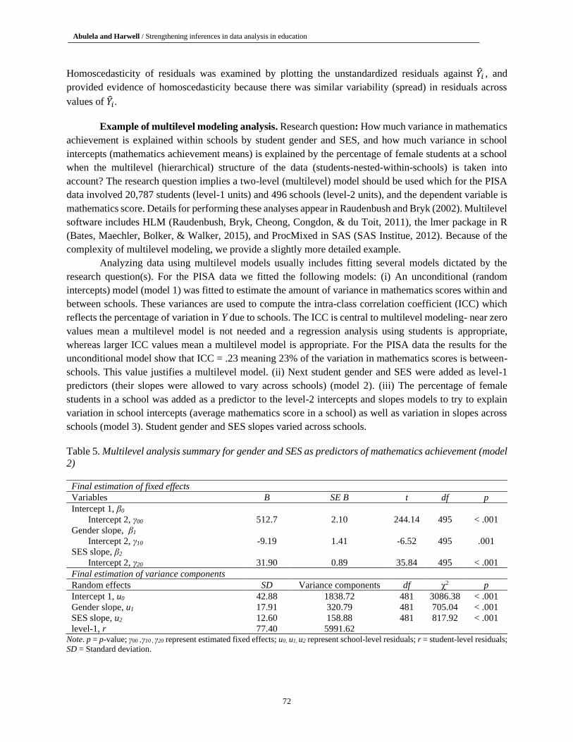
Table 5. Multilevel analysis summary for gender and SES as predictors of mathematics achievement (model

2)

Final estimation of fixed effects

Variables B SE B t df p

Intercept 1, β0

Intercept 2, γ00 512.7 2.10 244.14 495 < .001

Gender slope, β1

Intercept 2, γ10 -9.19 1.41 -6.52 495 .001

SES slope, β2

Intercept 2, γ20 31.90 0.89 35.84 495 < .001

Final estimation of variance components

Random effects SD Variance components df χ2 p

Intercept 1, u0 42.88 1838.72 481 3086.38 < .001

Gender slope, u1 17.91 320.79 481 705.04 < .001

SES slope, u2 12.60 158.88 481 817.92 < .001

level-1, r 77.40 5991.62 Note. p = p-value; γ00 ,γ10 , γ20 represent estimated fixed effects; u0, u1, u2 represent school-level residuals; r = student-level residuals;

SD = Standard deviation.


73

Table 5 reports the results for model 2. To determine the amount of variance explained by adding

gender and SES, we calculated the reduction in error variance which equals (variance within schools for

model 1 - variance within schools for model 2 with gender and SES/variance within schools for model 1).

The resulting value of .13 means student gender and SES explained approximately 13% of the variance in

students’ mathematics achievement within schools relative to model 1. The average student gender slope in

Table 5 of -9.19 (p < .001) means that on average (with other model predictors held constant) boys scored

on average about 9 points higher on mathematics than girls; similarly, students with above average SES

tended to have above average mathematics scores (average SES slope = 31.90, p < .001) and vice versa.

Next the percentage of girls in a school was added to level-2 (model 3) and the results reported in

Table 6. To determine how much random intercept (school mathematics means) variance is due to this

predictor compared to model 1 we computed (intercept variance in model 1 - intercept variance in model

3/intercept variance in model 1). Approximately 11% of the variance in school mathematics means is due

to the percentage of girls in a school. The school-level slope capturing the impact of percentage of girls in

a school was not a significant predictor of school mathematics means (slope = -11.93, p > .05) or students’

SES (slope = 7.84, p > .05). However, it was a significant predictor of gender slopes (slope = 18.91, p <

.01) meaning that increases in the percentage of girls in a school tended to decrease the difference between

boys and girls in mathematics performance.

Table 6. Multilevel analysis summary for gender, SES, and percentage of girls at schools as predictors of

mathematics achievement (model 3)

Final estimation of fixed effects

Variables B SE B t df p

Intercept 1, β0

Intercept 2, γ00 518.31 4.66 111.23 494 > .001

Percentage of girls, γ01 -11.93 8.70 -1.37 494 .171

Gender slope, β1

Intercept 2, γ10 -18.38 3.29 -5.59 494 .001

Percentage of girls, γ11 18.91 6.15 3.07 494 .002

SES slope, β2

Intercept 2, γ20 27.74 2.34 11.85 494 > .001

Percentage of girls, γ21 7.84 4.60 1.70 494 .089

Final estimation of variance components

Random effects SD Variance components df χ2 p

Intercept 1, u0 42.91 1841.75 480 3087.02 < .001

Gender slope, u1 17.61 310.17 480 696.19 < .001

SES slope, u2 12.59 158.42 480 821.50 < .001

level-1, r 77.40 5990.71 Note. p = p-value; γ00 ,γ10 , γ20 , γ01 ,γ11 , γ21 represent estimated fixed effects; u0, u1, u2 represent school-level residuals; r = student-

level residuals; SD = Standard deviation.

First, assess the quality of constructed measures which would be mathematics achievement, SES,

and percentage of female students in a school. Mathematics achievement was assessed in earlier examples.

The SES measure was developed for PISA and a review of PISA materials demonstrates this variable was

constructed by drawing on available literature, extensively piloted, and is supported by evidence of validity

and reliability. A rationale for using percentage of female students at a school as a level-2 predictor should

be provided that explains what this variable is intended to capture. For example, is the impact of percentage

of girls on mathematics scores posited to be greater in schools with higher or lower percentages? Thus, the


74

contribution of measurement error to the multilevel error terms within and between schools should be

minimal.

Second, there were missing data for 4.77% of the students and 2.6% of the schools. Multilevel

modelling does not allow missing data in level-2 predictors, meaning 2.6% of the 496 schools were excluded

from the final analysis in Tables 5 and 6. We ignored the missing data because both student and school

samples were quite large and the percentages of missing data were relatively small. Larger percentages of

excluded schools due to missing data (e.g., 15%) would prompt us to try to identify the nature of the missing

school data (MCAR, MAR) and to impute the missing values.

Third, the mathematics, SES, and percentage of female students in a school variable are treated as

possessing an approximate interval scale of measurement and there is ample evidence to support this

decision. This enhances interpretations of statistical findings and the plausibility of the assumption of

normality.

Fourth, multilevel models have many assumptions but the most critical for valid inferences are that

schools are independent of one another with respect to mathematics scores and that residuals for the level-

2 models are normally-distributed. The sampling strategy described in PISA materials provides evidence

that schools are independent. Normality of level-2 residuals was assessed by examining plots of these values

and no clear evidence of non-normality emerged.

Discussion

Guidelines for conducting data analyses in quantitative education studies are common but often

underemphasize four important methodological components: quality of constructed measures, proper

handling of missing data, proper level of measurement of a dependent variable, and model checking. This

paper highlights these components with novice researchers in mind and provides empirical examples of

these components using PISA data to illustrate contingency table analysis, group comparisons, multiple

regression analysis, and multilevel modelling. The goal is for the paper serve as an important methodological

resource for novice researchers conducting data analyses by promoting improved practice and stronger

inferences.

To summarize, novice researchers performing data analyses should include careful consideration of

the following methodological components in the planning, execution, and write-up of their study.

For quality of constructed measures: (i) special attention should be paid to a measure’s validity and

reliability evidence and its consistency with the research questions being investigated; (ii) the results of the

statistical analyses may be seriously distorted if data were collected by measures with unsatisfactory

psychometric properties; (iii) employing or modifying an existing measure is more likely to minimize the

role of measurement error than constructing a new measure. The latter is more likely to seriously bias

statistical results and inferences.

To proper handling of missing data: (i) substantial efforts should be made to avoid or minimizing

missing data in study planning; (ii) if the percentage of missing data is less than 5% it is likely that no

additional steps are required if the overall sample is large. Otherwise the reason(s) data are missing should

be investigated. (iii) Missingness that is MCAR supports unbiased inferences using available data as does

MAR if predictors capturing the reason(s) for missing data are included in the analyses. Missingness that is

NMAR is difficult to handle and is likely to cause the analyses to be aborted. (iv) In most cases, multiple

imputation should be used to impute missing values.


75

For a proper level of measurement of the dependent variable Y: (i) identifying the proper level of

measurement helps to select appropriate statistical techniques; (ii) proper interpretations of parametric

statistical analyses generally requires that Y possess an interval (or approximately interval) scale of

measurement, whereas nonparametric analyses are appropriate for Y variables with nominal or ordinal levels

of measurement; (iii) larger numbers of response categories (e.g., 5 or more) producing ordinal data help to

justify treating these data as possessing an approximately interval scale of measurement.

For model checking: (i) data should be screened prior to data analysis for coding errors, outliers,

and other irregularities; (ii) statistical assumptions such as normality and homogeneity of variance apply to

model residuals rather than Y values; plots of residuals are typically sufficient to check the plausibility of

assumptions of normality and homoscedasticity, which play a crucial role in the validity of inferences; (iii)

a brief summary of the results of model checking should be reported alongside findings of the major

analyses.

References

Abulela, M. A. A., & Harwell, M. (2019). Strengthening inferences in quantitative education studies conducted by

novice researchers: Capitalizing on standards for sampling, research design, and instrumentation. In W. Wu,

& S. Alan (Eds.), Research highlights in education and science (pp. 99-130). Ames: IA: ISRES Publishing.

Allison, P. D. (2002). Missing data. Thousand Oaks, CA: Sage.

Agresti, A., & Finlay, B. (2014). Statistic methods for the social sciences (4th ed). Harlow, U.K.: Pearson Limited.

American Educational Research Association, American Psychological Association & National Council on

Measurement in Education (2014). Standards for educational and psychological testing. Washington, DC:

American Educational Research Association.

An, W., & Ding, Y. (2018). The landscape of causal inference: Perspective from citation network Analysis. The

American Statistician, 72(3), 265 - 277. https://doi.org/10.1080/00031305.2017.1360794

Anderson, A. B., Basilevsky, A., & Hum, D. P. J. (1983). Missing data: A review of the literature. In P. H. Rossi, J.

D. Wright, & A. B. Anderson (Eds.), Handbook of survey research (pp. 415-494). San Diego, CA: Academic

Press.

Appelbaum, M., Cooper, H., Kline, R. B., Mayo-Wilson, E., Nezu, A. M., & Rao, S. M. (2018). Journal article

reporting standards for quantitative research in psychology: The APA publications and communications board

task force report. American Psychologist, 73, 3 - 25. https://doi.org/10.1037/amp0000191

APA Publications and Communications Board Working Group on Journal Article Reporting Standards. (2008).

Reporting standards for research in psychology: Why do we need them? What might they be? American

Psychologist, 63(9), 839 - 851. https://doi.org/10.1037/0003-066X.63.9.83

Bandalos, D. L. (2018). Measurement theory and applications for the social sciences. New York, NY: The Guilford

Press.

Bates, D., Maechler, M., Bolker, B., & Walker, S. (2015). Fitting linear mixed-effects models using lme4. Journal of

Statistical Software, 67(1), 1 - 48.

Becker, W. E., & Powers, J. R. (2001). Student performance, attrition, and class size given missing student data.

Economics of Education Review, 20(4), 377 - 388. https://doi.org/10.1016/S0272-7757(00)00060-1

Becker, W. E., & Walstad, W. B. (1990). Data loss from pretest to posttest as a sample selection problem. The Review

of Economics and Statistics, 72(1), 184 - 188.

Buu, A. (1999). Analysis of longitudinal data with missing values: A methodological comparison (Unpublished

doctoral dissertation). Indiana University.

Carpenter, J. R. (2009). Statistical methods for clinical studies with missing data: What's hot, what's cool, and what's

useful? (Unpublished paper). Available: http://www.iscb2009.info/RSystem/Soubory/Prez%20Tuesday/S18

.1%20Carpenter.pdf.

https://doi.org/10.1080/00031305.2017.1360794

https://doi.org/10.1037/amp0000191

https://doi.org/10.1037/0003-066X.63.9.83

https://doi.org/10.1016/S0272-7757(00)00060-1


76

Carnoy, M., Khavenson, T., Loyalka, P., Schmidt, W. H., & Zakharov, A. (2016). Revisiting the relationship between

international assessment outcomes and educational production: Evidence from a longitudinal PISA-TIMSS

sample. American Educational Research Journal, 53(4), 1054 - 1085. https://doi.org/10.3102/00028312166

53180

Clogg, C. C., & Shihadeh, E. S. (1994). Statistical models for ordinal variables. Thousand Oaks, CA: Sage.

Council for Exceptional Children. (2014). Standards for evidence-based practices in special education. Arlington,

VA: Council for Exceptional Children.

Creswell, J. W. (2012). Educational research: Planning, conducting, and evaluating quantitative and qualitative

research (4th ed.). Boston, MA: Pearson.

Draper, N. R., & Smith, H. (1981). Applied regression analysis (2nd ed.). New York, NY: Wiley.

Duncan, G. J., Engel, M., Claessens, A., & Dowsett, C. J. (2015). The value of replication for developmental science.

Retrieved from http://sites.uci.edu/gduncan/files/2013/06/Replication-paper-single-spaced.pdf

Embretson, S. E. (1996). Item response theory and spurious interaction effects in factorial ANOVA designs.

Applied Psychological Measurement, 20(3), 201 - 212. https://doi.org/10.1177/014662169602000302

Field, A. (2013). Discovering statistics using IBM SPSS statistics (4th ed.). Thousand Oaks, CA: Sage Publications.

Freedman, D. (2009). Statistical models and causal inference: A dialogue with the social sciences. In D. Collier, J.

Sekhon, & P. Stark (Eds.), Cambridge: Cambridge University Press. https://doi.org/10.1017/CBO97805118

15874

Glass, G., & Hopkins, K. D. (1996). Statistical methods in education and psychology (3rd. ed). Cliffbury, NJ: Pearson.

Hahn, G. J., & Meeker, W. Q. (1993). Assumptions for statistical inference. The American Statistician, 47(1), 1 - 12.

https://doi.org/10.1080/00031305.1993.10475924

Harwell, M. R. (1991). Using randomization tests when errors are unequally correlated. Computational Statistics and

Data Analysis, 11, 75 - 85.

Harwell, M. R., & Gatti, G. G. (2001). Rescaling ordinal data to interval data in educational research. Review of

Educational Research, 71(1), 105 - 131. https://doi.org/ 10.3102/00346543071001105

Heiman, G. W. (2011). Basic statistics for behavioral science (6th ed.). Belmont, CA: Cengage Learning.

Hoaglin, D. C., & Iglewicz, B. (1987). Fine-tuning some resistant rules for outlier labeling. Journal of American

Statistical Association, 82(400), 1147 - 1149. https://doi.org/10.1080/01621459.1987.10478551

Honaker, J, Gary King, G., & Blackwell, M. (2011). AMELIA II: A program for missing data. Journal of Statistical

Software, 45(7), 1 - 47.

Howell, D. C. (2017). Fundamental statistics for the behavioral sciences (9th ed). Boston, MA: Cengage Learning.

Krieg Jr, E. F. (1999). Biases induced by course measurement scales. Educational and Psychological

Measurement, 59(5), 749 - 766. https://doi.org/10.1177/00131649921970125

Legendre, P. (1993). Real data are messy. Statistics and Computing, 3, 197 - 199.

Lord, F. M. (1953). On the statistical treatment of football numbers. American Psychologist, 8(12), 750 - 751.

https://doi.org/ 10.1037/h0063675

Lord, F. M., & Novick, M. R. (1968). Statistical theories of mental test scores. Reading, MA: Addison-Wesley.

Marascuilo, L. A., & McSweeney, M. (1977). Nonparametric and distribution-free methods for the social sciences.

Monterey, CA: Brooks/Cole.

Martin, M. O., Mullis, I. V. S., & Chrostowski, S. J. (2004). TIMSS 2003 technical report: Findings from IEA's Trends

in International Mathematics and Science Study at the fourth and eighth grades. Boston College, Chestnut

Hill, MA: TIMSS & PIRLS International Study Center.

Mijs, J. (2016). Stratified failure: Educational stratification and students’ attributions of their mathematics performance

in 24 countries. Forthcoming in Sociology of Education 89(2), 1 - 17. https://doi.org/10.1177/0038040716

636434

Moore, D. S., McCabe, G. P., & Craig, B. A. (2017). Introduction to the practice of statistics (9th ed.). New York, NY:

Freeman Macmillan Learning.

http://sites.uci.edu/gduncan/files/2013/06/Replication-paper-single-spaced.pdf

https://doi.org/10.1177%2F014662169602000302

https://doi.org/10.1080/00031305.1993.10475924

https://doi.org/10.1080/01621459.1987.10478551

https://doi.org/10.1177%2F00131649921970125


77

Namasivayama, A. K., Yana, T., Wonga, W. Y. S., & Van Lieshouta, P. (2015). Quality of statistical reporting in

developmental disability journals. International Journal of Rehabilitation Research, 38(4), 364 - 369.

https://doi.org/10.1097/MRR.0000000000000138

National Council for Teaching Mathematics. (2000). Principles and standards for school mathematics. Reston, VA:

The National Council of Teachers of Mathematics.

Ness-Evans, A. (2014). Using basic statistics in the behavioral and social sciences (5th ed.). Thousand Oaks, CA:

Sage.

Niehaus, K., & Adelson, J. L. (2014). School support, parental involvement, and academic and social-emotional

outcomes for English language learners. American Educational Research Journal, 51(4), 810 - 844.

https://doi.org/10.3102/0002831214531323

Neter, J., Kutner, M. H., Nachtsheim, C. J., & Wasserman, W. (1996). Applied linear statistical models (4th ed.).

Chicago, IL: Irwin.

Obsorne, J. W. (2010). Correlation and other measures of association. In G. R. Hancock, & R. O. Mueller (eds.), The

reviewers guide to quantitative methods in the social sciences (pp. 55-68). New York, NY: Taylor and Francis.

Osborne, J. W., Kocher, B., & Tillman, D. (2012, April). Sweating the small stuff: Do authors in APA journals clean

data or test assumptions (and should anyone care if they do). Paper presented at the Annual Meeting of the

Eastern Education Research Association, Hilton Head, SC.

Peng, C. Y., Harwell, M. R., Liou, S. M., & Ehman, L. H. (2006). Advances in missing data methods and implications

for educational research. In S. S. Sawilowsky (Ed.), Real data analysis (pp. 31-78). New York: Information

Age.

Peugh, J. L., & Enders, C. K. (2004). Missing data in educational research: A review of reporting practices and

suggestions for improvement. Review of Educational Research, 74(4), 525 - 556. https://doi.org/10.3102/003

46543074004525

R Core Team. (2015). R: A language and environment for statistical computing [Computer software manual]. Vienna,

Austria. Retrieved from http://www.R-project.org/(Version 3.0.1).

Raudenbush, S. W., & Bryk, A. S. (2002). Hierarchical linear models: Applications and data analysis methods (2nd

ed). Newbury Park, CA: Sage.

Raudenbush, S. W., Bryk, A. S., Cheong, Y. F., Congdon, R. T., & du Toit, M. (2011). HLM 7: Hierarchical linear

and nonlinear modeling [Computer software]. Lincolnwood, IL: Scientific Software International.

Rousseau, M., Simon M., Bertrand, R., & Hachey, K. (2012). Reporting missing data: A study of selected articles

published from 2003–2007. Quality & Quantity, 46(5), 1393 - 1406. https://doi.org/10.1007/s11135-011-

9452-y

Rubin, D. B. (1976). Inference and missing data. Biometrika, 63(3), 581 - 592. https://doi.org/10.2307/2335739

SAS Institute. (2012). SAS/STAT 9.4 User’s guide [Computer software manual]. Cary, NC: SAS Institute.

Schafer J. L., & Graham, J. W. (2002). Missing data: Our view of the state of the art. Psychological Methods, 7(2),

147 - 177. https://doi.org/10.1037//1082-989X.7.2.147

Schulz, W. (2006, April). Measuring the socio-economic background of students and its effect on achievement in PISA

2000 and PISA 2003. Paper presented at the Annual Meeting of the American Educational Research

Association (AERA), San Francisco.

Sijtsma, K. (2016). Playing with data - or how to discourage questionable research practices and stimulate researchers

to do things right. Psychometrika, 81(1), 1 - 15. https://doi.org/10.1007/s11336-015-9446-0

Sijtsma, K., Veldkamp, C. L. S., & Wicherts, J. M. (2016). Improving the conduct and reporting of statistical analysis

in psychology. Psychometrika, 81(1), 33 - 38. https://doi.org/10.1007/s11336-015-9444-2

Stevens, S. S. (1951). Mathematics, measurement, and psychophysics. In S. S. Stevens (Ed.), Handbook of

experimental psychology (pp. 1-49). Oxford, England: Wiley.

Stodden, V. (2015). Reproducing statistical results. The Annual Review of Statistics and its Application, 2, 1 - 19.

https://doi.org/10.1146/annurev-statistics-010814-020127

Tabachnick, B. G., & Fidell, L. S. (2007). Using multivariate statistics (5th ed.). Boston, MA: Pearson Education.

https://doi.org/10.2307/2335739

https://doi.org/10.1037/1082-989X.7.2.147


78

Townsend, J. T., & Ashby, F. G. (1984). Measurement scales and statistics: The misconception misconceived.

Psychological Bulletin, 96(2), 394 - 401. http://dx.doi.org/10.1037/0033-2909.96.2.394

Van den Broeck, J., Cunningham, S. A., Eeckels, R., & Herbst, K. (2005). Data cleaning: Detecting, diagnosing, and

editing data abnormalities. PLoS Medicine, 2(10), 966 - 970. https://doi.org/10.1371/journal.pmed.0020267

Waldman, I. D., & Lilienfeld, S. O. (2016). Thinking about data research methods and statistical analysis: Comments

on Sijtsma’s (2014) “playing with data”. Psychometrika, 81(1), 16 - 26. https://doi.org/10.1007/s11336-015-

9447-z

What Works Clearinghouse. (2017). Procedures and standards handbook (Version 4). Retrieved from https://ies.ed.gov

/ncee/wwc/handbooks

Wilkinson, L., & APA Task Force on Statistical Inference. (1999). Statistical methods in psychology journals:

Guidelines and explanations. American Psychologist, 54(8), 594 - 604. https://doi.org/10.1037/0003-066X.

54.8.59

Zimmerman, D. W. (1998). Invalidation of parametric and nonparametric statistical tests by concurrent violations of

two assumptions. The Journal of Experimental Education, 67(1), 55 - 68. https://doi.org/10.1080/00220

979809598344.

Data Analysis: Strengthening Inferences in Quantitative ... - ERIC

Documents

Transcript of Data Analysis: Strengthening Inferences in Quantitative ... - ERIC