DATA ANALYSIS FOR DECISION MAKING IN HSBC
29
DATA ANALYSIS FOR DECISION MAKING IN HSBC Business Decision Making NGUYEN NGOC MINH – F06B PREPARE FOR: BOARD OF DIRECTOR OF HSBC
Transcript of DATA ANALYSIS FOR DECISION MAKING IN HSBC

DATA ANALYSIS FOR DECISION MAKING IN HSBC
Business Decision Making
NGUYEN NGOC MINH – F06B
PREPARE FOR: BOARD OF DIRECTOR OF HSBC

Executive summary
As the newly appointed Junior Data Research Officer work in
HSBC which branch located in Vietnam, the report show 3 tasks
related to the financial services departments in the banks and provide
the suitable recommendation for the bank to increase the efficiency
and productivity. The bank should use multiplicative model method
for calculating and forecasting the actual sales of bank in the next
year. There are 5 useful software which are recommended for the
bank to help them increase the efficiency and productivity. The report
has create the detail plan for the bank to follow which is reasonable
and have the lowest cost. In the final test, the report have shown the
way to evaluate the project by 2 method NPV and IRR and make the
conclusion for the bank to choose which one is the good project for
the bank in the future.
Contents
Executive summary ......................................................................................................................... 0
Introduction ..................................................................................................................................... 1
Task 1: Forecasting techniques ...................................................................................................... 2
I. Additive model..................................................................................................................... 2
The seasonal variations for 4 years’ sales (‘000) are as follows: ........................................... 2
The estimate of average quarterly variation: .......................................................................... 3
Calculating the forecast of sales for 2013 ............................................................................... 4
The diagram to show the trend-line and forecast sales ........................................................... 5
II. Multiplicative model ........................................................................................................ 6
1. The seasonal variations for 4 years’ sales (‘000) are as follows: ................................. 6
The estimate of average quarterly variation: .......................................................................... 7
Calculating the forecast of sales for 2013 ............................................................................... 7
The diagram to show the trend-line and forecast sales ........................................................... 8
III. Least squares regression model ........................................................................................ 9
1. The regression line – trend line .................................................................................... 9
The diagram of the trend-line ............................................................................................... 10
IV. Conclusion ...................................................................................................................... 11
Task 2: Information processing tools ............................................................................................ 13
Task 3: Project planning ............................................................................................................... 17
I. The activities comprise a project of customer services ..................................................... 17
II. The network diagram for the activity of HSBC bank in financial services ................... 17
III. The grant chart which show the planning of the project ................................................ 18
Task 4: Discount cash flow (DCF) methods ................................................................................. 20
I. The Net Present Value method (NPV)............................................................................... 20
V. The Internal Rate of Return method (IRR) .................................................................... 20
“Papa loves Mommy” investment ........................................................................................ 21
“Family” investment ............................................................................................................. 22
Conclusion .................................................................................................................................... 25
References ..................................................................................................................................... 26

Introduction
As the newly appointed Junior Data Research Officer work in HSBC which branch located
in Vietnam, the report show 3 task related to the financial services departments in the banks. At
the first task is the forecasting technique, which shows various way to calculate the actual sales of
the bank in the future, and then show the formal report for the Board of director. In the next task
in the reports, there is the information processing tools which shows the decision level and
information types in each department and the recommendation for the software for each part of
department. In the third task, the project planning have been show the way to prepare the schedule
of giving gift for customer and the number of employee should have in this project. In the last task,
it is the evaluation of two projects – “PLM” and “Family”. The calculation and recommendation
of the suitable project are provide in the end of the report.
ITP – F06-092
2
BDM A2 - Max
Task 1: Forecasting techniques
To find out the trend-line sales of the company in the different quarters, I will calculate
firstly moving total of 4 quarters’ sales, following by calculating the moving total of 8 quarters’
sales. After that, I will estimate the trend-line and find the seasonal variation with the various
methods and also the forecast sales of the company in 4 quarters in 2013.
I. Additive model
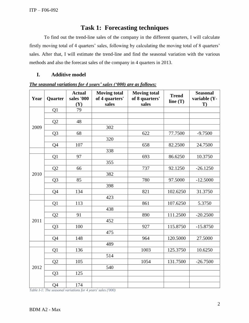
The seasonal variations for 4 years’ sales (‘000) are as follows:
Year Quarter
Actual
sales '000
(Y)
Moving total
of 4 quarters'
sales
Moving total
of 8 quarters'
sales
Trend
line (T)
Seasonal
variable (Y-
T)
2009
Q1 79
Q2 48
302
Q3 68 622 77.7500 -9.7500
320
Q4 107 658 82.2500 24.7500
338
2010
Q1 97 693 86.6250 10.3750
355
Q2 66 737 92.1250 -26.1250
382
Q3 85 780 97.5000 -12.5000
398
Q4 134 821 102.6250 31.3750
423
2011
Q1 113 861 107.6250 5.3750
438
Q2 91 890 111.2500 -20.2500
452
Q3 100 927 115.8750 -15.8750
475
Q4 148 964 120.5000 27.5000
489
2012
Q1 136 1003 125.3750 10.6250
514
Q2 105 1054 131.7500 -26.7500
540
Q3 125
Q4 174 Table I-1: The seasonal variations for 4 years' sales ('000)
ITP – F06-092
3
BDM A2 - Max
Explanation:
o At first, I summed the actual sales of four quarters in 2009 which are 79, 48, 68 and 107
respectively, the result of this calculation (302) was the first “Moving total of 4 quarters’
sales”. The total sales of four quarters from 2nd quarter of 2009 to the 1st quarter of 2010
which are 48, 68, 107 and 97, is the second result of “Moving total of 4 quarters’ sales”.
Keep going like this, I got all the results of “Moving total of 4 quarters’ sales” from 2009
to 2012
o In the next step, I continued to calculate the “Moving total of 8 quarters’ sales”. The result
of this part is the sum of two consecutive numbers of the before part – “Moving total of 4
quarters’ sales”. (302+320=622). Continue calculating like this I got all the result for this
part from 2009 to 2012.
o To calculate the trend-line, in each respective result of “moving total of 8 quarters’ sales”,
I divided this result by 8 which are (622/8=77.75) in 3rd Quarter 2009. After that, I
calculated continuously to get all the approximate results for the “Trend line” from 2009
to 2012.
o In the last column – “seasonal variation”, I calculated them by taking the “actual sales” of
respective quarter minus the “Trend-line” as (68-77.75= -9.75) in the 3rd quarter 2009. And
then, I find out all the result of seasonal variation from 2009 to 2012.
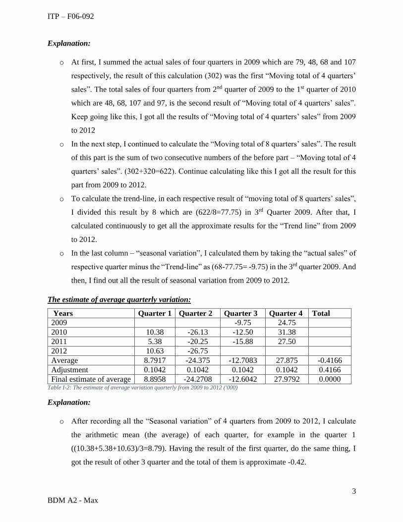
The estimate of average quarterly variation:
Years Quarter 1 Quarter 2 Quarter 3 Quarter 4 Total
2009 -9.75 24.75
2010 10.38 -26.13 -12.50 31.38
2011 5.38 -20.25 -15.88 27.50
2012 10.63 -26.75
Average 8.7917 -24.375 -12.7083 27.875 -0.4166
Adjustment 0.1042 0.1042 0.1042 0.1042 0.4166
Final estimate of average 8.8958 -24.2708 -12.6042 27.9792 0.0000 Table I-2: The estimate of average variation quarterly from 2009 to 2012 ('000)
Explanation:
o After recording all the “Seasonal variation” of 4 quarters from 2009 to 2012, I calculate
the arithmetic mean (the average) of each quarter, for example in the quarter 1
((10.38+5.38+10.63)/3=8.79). Having the result of the first quarter, do the same thing, I
got the result of other 3 quarter and the total of them is approximate -0.42.
ITP – F06-092
4
BDM A2 - Max
o To increase the total variance to 0, I added 0.42 in “Adjustment”, and divided into 4 quarter
by dividing the result by 4. So that, I had approximate 0.104 in each quarter.
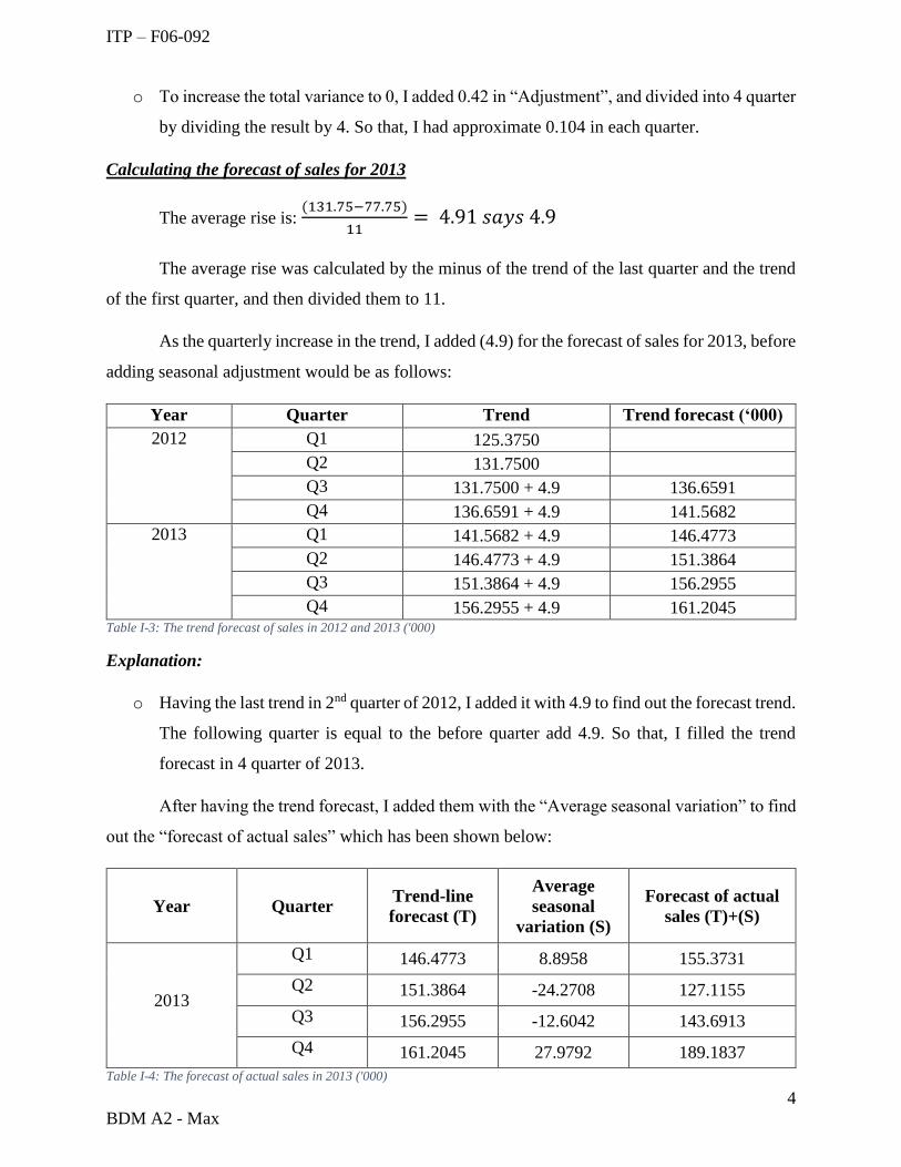
Calculating the forecast of sales for 2013
The average rise is: (131.75−77.75)
11= 4.91 𝑠𝑎𝑦𝑠 4.9
The average rise was calculated by the minus of the trend of the last quarter and the trend
of the first quarter, and then divided them to 11.
As the quarterly increase in the trend, I added (4.9) for the forecast of sales for 2013, before
adding seasonal adjustment would be as follows:
Year Quarter Trend Trend forecast (‘000)
2012 Q1 125.3750
Q2 131.7500
Q3 131.7500 + 4.9 136.6591
Q4 136.6591 + 4.9 141.5682
2013 Q1 141.5682 + 4.9 146.4773
Q2 146.4773 + 4.9 151.3864
Q3 151.3864 + 4.9 156.2955
Q4 156.2955 + 4.9 161.2045 Table I-3: The trend forecast of sales in 2012 and 2013 ('000)
Explanation:
o Having the last trend in 2nd quarter of 2012, I added it with 4.9 to find out the forecast trend.
The following quarter is equal to the before quarter add 4.9. So that, I filled the trend
forecast in 4 quarter of 2013.
After having the trend forecast, I added them with the “Average seasonal variation” to find
out the “forecast of actual sales” which has been shown below:
Year Quarter Trend-line
forecast (T)
Average
seasonal
variation (S)
Forecast of actual
sales (T)+(S)
2013
Q1 146.4773 8.8958 155.3731
Q2 151.3864 -24.2708 127.1155
Q3 156.2955 -12.6042 143.6913
Q4 161.2045 27.9792 189.1837
Table I-4: The forecast of actual sales in 2013 ('000)
ITP – F06-092
5
BDM A2 - Max
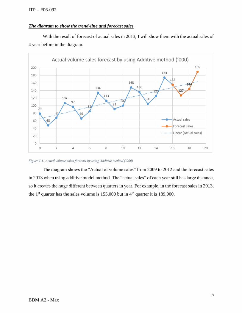
The diagram to show the trend-line and forecast sales
With the result of forecast of actual sales in 2013, I will show them with the actual sales of
4 year before in the diagram.
Figure I-1: Actual volume sales forecast by using Additive method (‘000)
The diagram shows the “Actual of volume sales” from 2009 to 2012 and the forecast sales
in 2013 when using additive model method. The “actual sales” of each year still has large distance,
so it creates the huge different between quarters in year. For example, in the forecast sales in 2013,
the 1st quarter has the sales volume is 155,000 but in 4th quarter it is 189,000.
79
48
68
10797
66
85
134
113
91100
148
136
105
125
174
155
127
144
189
155
127
144
189
0
20
40
60
80
100
120
140
160
180
200
0 2 4 6 8 10 12 14 16 18 20
Actual volume sales forecast by using Additive method (‘000)
Actual sales
Forecast sales
Linear (Actual sales)
ITP – F06-092
6
BDM A2 - Max
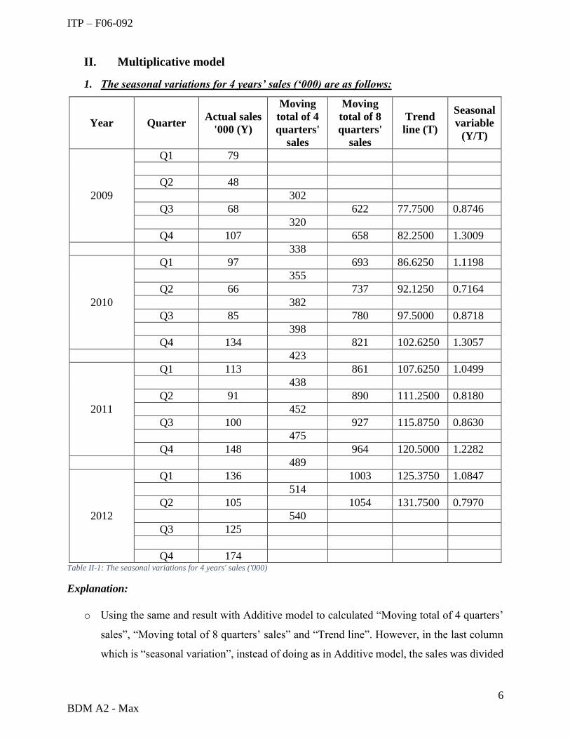
II. Multiplicative model
1. The seasonal variations for 4 years’ sales (‘000) are as follows:
Year Quarter Actual sales
'000 (Y)
Moving
total of 4
quarters'
sales
Moving
total of 8
quarters'
sales
Trend
line (T)
Seasonal
variable
(Y/T)
2009
Q1 79
Q2 48
302
Q3 68 622 77.7500 0.8746
320
Q4 107 658 82.2500 1.3009
338
2010
Q1 97 693 86.6250 1.1198
355
Q2 66 737 92.1250 0.7164
382
Q3 85 780 97.5000 0.8718
398
Q4 134 821 102.6250 1.3057
423
2011
Q1 113 861 107.6250 1.0499
438
Q2 91 890 111.2500 0.8180
452
Q3 100 927 115.8750 0.8630
475
Q4 148 964 120.5000 1.2282
489
2012
Q1 136 1003 125.3750 1.0847
514
Q2 105 1054 131.7500 0.7970
540
Q3 125
Q4 174 Table II-1: The seasonal variations for 4 years' sales ('000)
Explanation:
o Using the same and result with Additive model to calculated “Moving total of 4 quarters’
sales”, “Moving total of 8 quarters’ sales” and “Trend line”. However, in the last column
which is “seasonal variation”, instead of doing as in Additive model, the sales was divided
ITP – F06-092
7
BDM A2 - Max
by the trend line. By that way, I calculated all the results of “Seasonal variation” from 2009
to 2012.
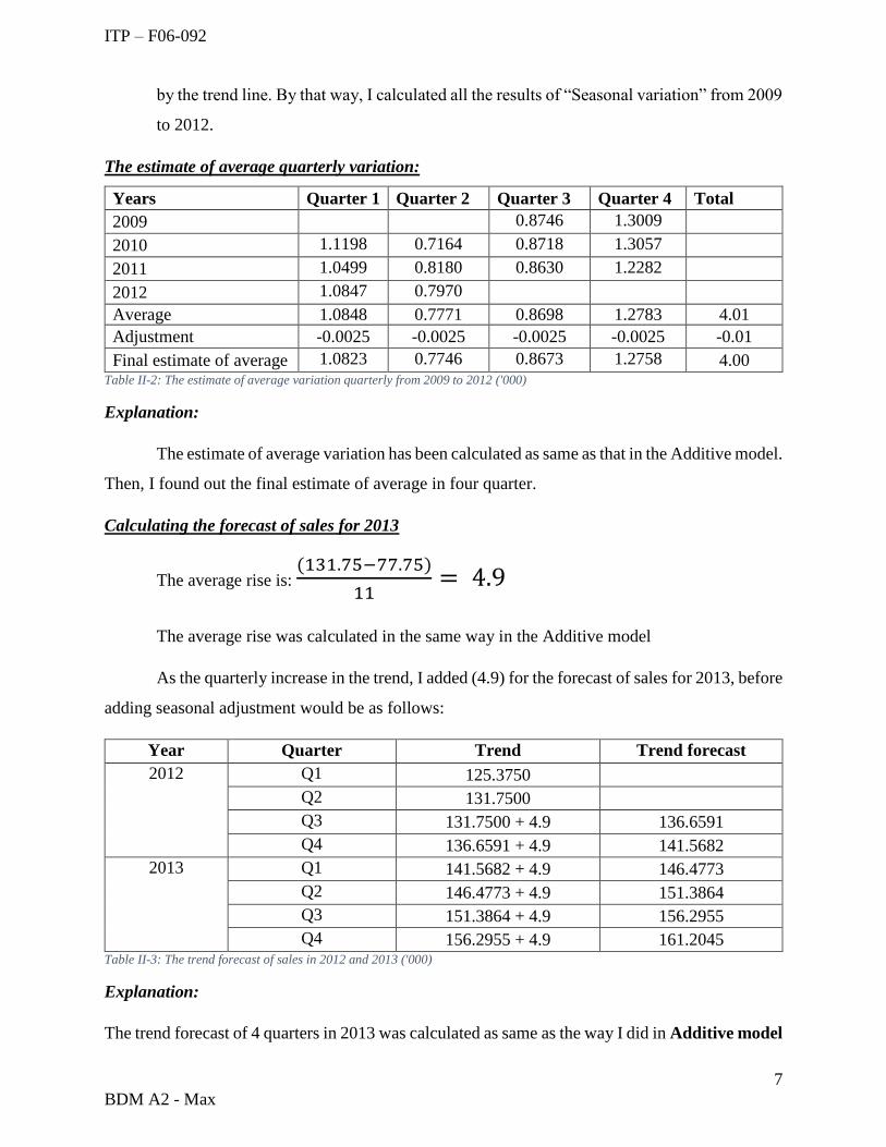
The estimate of average quarterly variation:
Years Quarter 1 Quarter 2 Quarter 3 Quarter 4 Total
2009 0.8746 1.3009
2010 1.1198 0.7164 0.8718 1.3057
2011 1.0499 0.8180 0.8630 1.2282
2012 1.0847 0.7970
Average 1.0848 0.7771 0.8698 1.2783 4.01
Adjustment -0.0025 -0.0025 -0.0025 -0.0025 -0.01
Final estimate of average 1.0823 0.7746 0.8673 1.2758 4.00 Table II-2: The estimate of average variation quarterly from 2009 to 2012 ('000)
Explanation:
The estimate of average variation has been calculated as same as that in the Additive model.
Then, I found out the final estimate of average in four quarter.
Calculating the forecast of sales for 2013
The average rise is: (131.75−77.75)
11= 4.9
The average rise was calculated in the same way in the Additive model
As the quarterly increase in the trend, I added (4.9) for the forecast of sales for 2013, before
adding seasonal adjustment would be as follows:
Year Quarter Trend Trend forecast
2012 Q1 125.3750
Q2 131.7500
Q3 131.7500 + 4.9 136.6591
Q4 136.6591 + 4.9 141.5682
2013 Q1 141.5682 + 4.9 146.4773
Q2 146.4773 + 4.9 151.3864
Q3 151.3864 + 4.9 156.2955
Q4 156.2955 + 4.9 161.2045 Table II-3: The trend forecast of sales in 2012 and 2013 ('000)
Explanation:
The trend forecast of 4 quarters in 2013 was calculated as same as the way I did in Additive model
ITP – F06-092
8
BDM A2 - Max
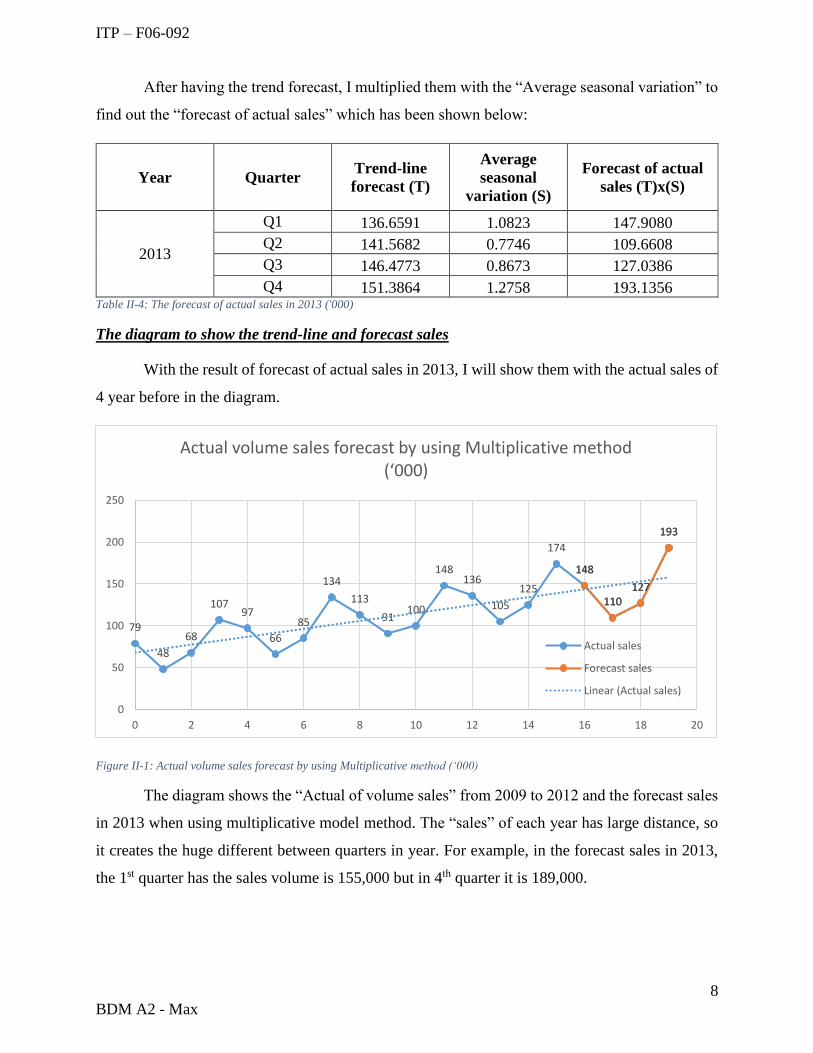
After having the trend forecast, I multiplied them with the “Average seasonal variation” to
find out the “forecast of actual sales” which has been shown below:
Year Quarter Trend-line
forecast (T)
Average
seasonal
variation (S)
Forecast of actual
sales (T)x(S)
2013
Q1 136.6591 1.0823 147.9080
Q2 141.5682 0.7746 109.6608
Q3 146.4773 0.8673 127.0386
Q4 151.3864 1.2758 193.1356 Table II-4: The forecast of actual sales in 2013 ('000)
The diagram to show the trend-line and forecast sales
With the result of forecast of actual sales in 2013, I will show them with the actual sales of
4 year before in the diagram.
Figure II-1: Actual volume sales forecast by using Multiplicative method (‘000)
The diagram shows the “Actual of volume sales” from 2009 to 2012 and the forecast sales
in 2013 when using multiplicative model method. The “sales” of each year has large distance, so
it creates the huge different between quarters in year. For example, in the forecast sales in 2013,
the 1st quarter has the sales volume is 155,000 but in 4th quarter it is 189,000.
79
48
68
10797
66
85
134
113
91100
148136
105
125
174
148
110127
193
148
110127
193
0
50
100
150
200
250
0 2 4 6 8 10 12 14 16 18 20
Actual volume sales forecast by using Multiplicative method (‘000)
Actual sales
Forecast sales
Linear (Actual sales)
ITP – F06-092
9
BDM A2 - Max
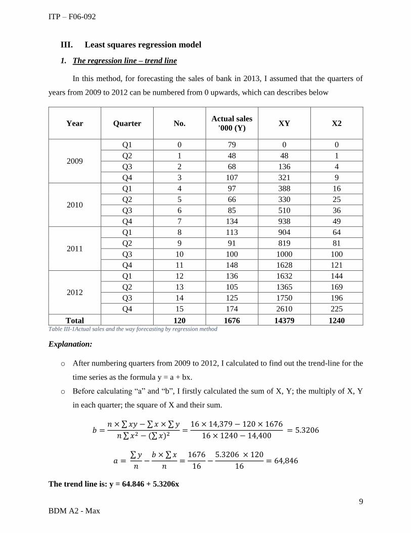
III. Least squares regression model
1. The regression line – trend line
In this method, for forecasting the sales of bank in 2013, I assumed that the quarters of
years from 2009 to 2012 can be numbered from 0 upwards, which can describes below
Year Quarter No. Actual sales
'000 (Y) XY X2
2009
Q1 0 79 0 0
Q2 1 48 48 1
Q3 2 68 136 4
Q4 3 107 321 9
2010
Q1 4 97 388 16
Q2 5 66 330 25
Q3 6 85 510 36
Q4 7 134 938 49
2011
Q1 8 113 904 64
Q2 9 91 819 81
Q3 10 100 1000 100
Q4 11 148 1628 121
2012
Q1 12 136 1632 144
Q2 13 105 1365 169
Q3 14 125 1750 196
Q4 15 174 2610 225
Total 120 1676 14379 1240 Table III-1Actual sales and the way forecasting by regression method
Explanation:
o After numbering quarters from 2009 to 2012, I calculated to find out the trend-line for the
time series as the formula y = a + bx.
o Before calculating “a” and “b”, I firstly calculated the sum of X, Y; the multiply of X, Y
in each quarter; the square of X and their sum.
𝑏 =𝑛 × ∑ 𝑥𝑦 − ∑ 𝑥 × ∑ 𝑦
𝑛 ∑ 𝑥2 − (∑ 𝑥)2=
16 × 14,379 − 120 × 1676
16 × 1240 − 14,400 = 5.3206
𝑎 = ∑ 𝑦
𝑛−
𝑏 × ∑ 𝑥
𝑛=
1676
16−
5.3206 × 120
16= 64,846
The trend line is: y = 64.846 + 5.3206x
ITP – F06-092
10
BDM A2 - Max
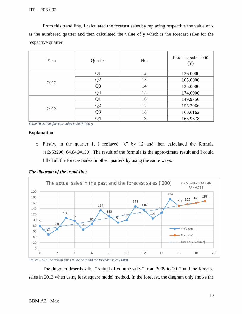
From this trend line, I calculated the forecast sales by replacing respective the value of x
as the numbered quarter and then calculated the value of y which is the forecast sales for the
respective quarter.
Year Quarter No. Forecast sales '000
(Y)
2012
Q1 12 136.0000
Q2 13 105.0000
Q3 14 125.0000
Q4 15 174.0000
2013
Q1 16 149.9750
Q2 17 155.2966
Q3 18 160.6162
Q4 19 165.9378 Table III-2: The forecast sales in 2013 ('000)
Explanation:
o Firstly, in the quarter 1, I replaced “x” by 12 and then calculated the formula
(16x53206+64.846=150). The result of the formula is the approximate result and I could
filled all the forecast sales in other quarters by using the same ways.
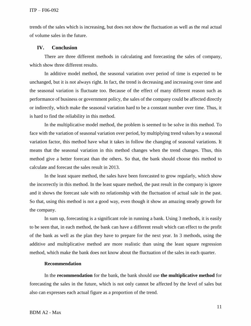
The diagram of the trend-line
Figure III-1: The actual sales in the past and the forecast sales ('000)
The diagram describes the “Actual of volume sales” from 2009 to 2012 and the forecast
sales in 2013 when using least square model method. In the forecast, the diagram only shows the
79
48
68
10797
66
85
134
113
91100
148136
105
125
174
150 155 161 166
150 155 161 166
y = 5.3206x + 64.846R² = 0.736
0
20
40
60
80
100
120
140
160
180
200
0 2 4 6 8 10 12 14 16 18 20
The actual sales in the past and the forecast sales ('000)
Y-Values
Column1
Linear (Y-Values)
ITP – F06-092
11
BDM A2 - Max
trends of the sales which is increasing, but does not show the fluctuation as well as the real actual
of volume sales in the future.
IV. Conclusion
There are three different methods in calculating and forecasting the sales of company,
which show three different results.
In additive model method, the seasonal variation over period of time is expected to be
unchanged, but it is not always right. In fact, the trend is decreasing and increasing over time and
the seasonal variation is fluctuate too. Because of the effect of many different reason such as
performance of business or government policy, the sales of the company could be affected directly
or indirectly, which make the seasonal variation hard to be a constant number over time. Thus, it
is hard to find the reliability in this method.
In the multiplicative model method, the problem is seemed to be solve in this method. To
face with the variation of seasonal variation over period, by multiplying trend values by a seasonal
variation factor, this method have what it takes in follow the changing of seasonal variations. It
means that the seasonal variation in this method changes when the trend changes. Thus, this
method give a better forecast than the others. So that, the bank should choose this method to
calculate and forecast the sales result in 2013.
In the least square method, the sales have been forecasted to grow regularly, which show
the incorrectly in this method. In the least square method, the past result in the company is ignore
and it shows the forecast sale with no relationship with the fluctuation of actual sale in the past.
So that, using this method is not a good way, even though it show an amazing steady growth for
the company.
In sum up, forecasting is a significant role in running a bank. Using 3 methods, it is easily
to be seen that, in each method, the bank can have a different result which can effect to the profit
of the bank as well as the plan they have to prepare for the next year. In 3 methods, using the
additive and multiplicative method are more realistic than using the least square regression
method, which make the bank does not know about the fluctuation of the sales in each quarter.
Recommendation
In the recommendation for the bank, the bank should use the multiplicative method for
forecasting the sales in the future, which is not only cannot be affected by the level of sales but
also can expresses each actual figure as a proportion of the trend.
ITP – F06-092
12
BDM A2 - Max
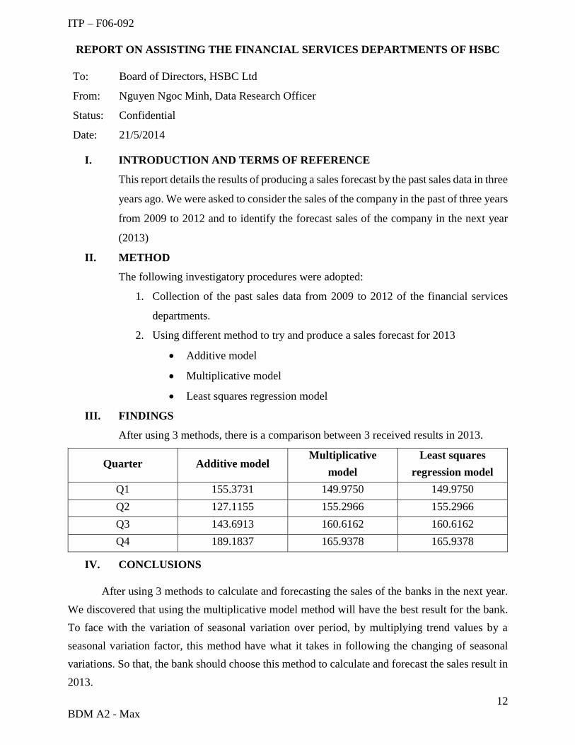
REPORT ON ASSISTING THE FINANCIAL SERVICES DEPARTMENTS OF HSBC
To: Board of Directors, HSBC Ltd
From: Nguyen Ngoc Minh, Data Research Officer
Status: Confidential
Date: 21/5/2014
I. INTRODUCTION AND TERMS OF REFERENCE
This report details the results of producing a sales forecast by the past sales data in three
years ago. We were asked to consider the sales of the company in the past of three years
from 2009 to 2012 and to identify the forecast sales of the company in the next year
(2013)
II. METHOD
The following investigatory procedures were adopted:
1. Collection of the past sales data from 2009 to 2012 of the financial services
departments.
2. Using different method to try and produce a sales forecast for 2013
Additive model
Multiplicative model
Least squares regression model
III. FINDINGS
After using 3 methods, there is a comparison between 3 received results in 2013.
Quarter Additive model Multiplicative
model
Least squares
regression model
Q1 155.3731 149.9750 149.9750
Q2 127.1155 155.2966 155.2966
Q3 143.6913 160.6162 160.6162
Q4 189.1837 165.9378 165.9378
IV. CONCLUSIONS
After using 3 methods to calculate and forecasting the sales of the banks in the next year.
We discovered that using the multiplicative model method will have the best result for the bank.
To face with the variation of seasonal variation over period, by multiplying trend values by a
seasonal variation factor, this method have what it takes in following the changing of seasonal
variations. So that, the bank should choose this method to calculate and forecast the sales result in
2013.
ITP – F06-092
13
BDM A2 - Max
Task 2: Information processing tools
Important of Manager Information System (MIS) with HSBC Bank
No Department Decision
level
Information
type Instrument Image Staff
1 Human
Resources
Strategic
level
Executive
Support
Systems (ESS)
Prophix’s
personnel planning
Executive
2 Finance
Department
Management
level
Management
Information
Systems (MIS)
Axiom EPM's
Budgeting and
Forecasting
Finance
manager
3 Marketing
Department
Knowledge
level
Office
Automation
System (OAS)
CorelDRAW
Marketing
online staff
4
Research and
Development
Department
Management
level
Decision
supporting
system (DSS)
Tyler Analytics
R&D
Manager
5 Accounting
Department
Operating
level
Transaction
Processing
system (TPS)
IBM Transaction
processing
Accounting
Staff
Prophix’s personnel planning for Human Resources Department
Belong to the Strategic level, the Executive Support System (ESS) help Human resources
director with long-term planning, to ensure changes in the external environment which are matched
by the company’s capabilities. The ESS pools data from internal and external source and provide
the senior managers with easy access to key internal and external information, which are drawn
from internal MIS and DSS and from external data of competitors, external database… To meet
such needs of senior managers, the large-scale integrated corporate systems known as Enterprise
resource planning, which is essential and depend on the complexity of the undertaking and the
degree of competition.
ITP – F06-092
14
BDM A2 - Max
As one of many software in Enterprise resource planning (ERP), Prophix have its own
function to help the director prepare: (Prophix, n.d.)
Detailed personnel reporting aligned with overall company reporting (internal
resources)
The potential to hold department managers accountable by streamlining the payroll
planning process.
A true depiction of employee costs by department, versus a strictly consolidated view.
Applying in the HBSC bank, the main reason why this software should be used in the bank
is that it is suitable with the purpose of the ESS. It helps the manager have the large vision about
the personnel plan in the bank and help him sync all the information from internal and external
resources such as TPS data, financial data or share prices, Market research.
Axiom EPM's Budgeting and Forecasting for Finance department
In the management-level, the system in this level help the manager monitor and control.
These systems check if things are working well or not. The Management Information System
(MIS) will interact with the same systems as that at operational level. The MIS condenses and
converts TPS data into information. For the manager to prepare annual budget, the instrument
suitable with him is Axiom EPM's Budgeting and Forecasting for the bank, which have various
function: (Axiomepm, 2014)
Test and understand how changing assumptions impact financial results using
drivers such as interest rates, deposit growth rates, number of new accounts, and
other variable income and expense factors
Align business measurement with business planning
Create full annual budget for the bank which have the best-practice
Applying in HSBC bank, because of the various function of this software, the finance
manager can convert directly data from TPS into information, which can help him to create the
budget for the bank each year. With the high-technology and beautiful design, the software suitable
for him to plan a suitable budget for the bank each year.
CorelDraw for Marketing department
The knowledge-level system help knowledge and data workers design products, distribute
information and perform administrative tasks. These systems help the company integrate new and
ITP – F06-092
15
BDM A2 - Max
existing knowledge into the business and to reduce the reliance on paper documents. In this level,
the employee uses Knowledge Work System (KWS) which are information systems that facilitate
the creation and integration of new knowledge into an organization. Such as in the manufacturing
department in the bank, the employee who have responsibility to design the credit card for the
customer have to have a software to improve the quality of result and save time. The designer
software he should use is CorelDRAW which will increase the work productivity.
Its function are (Corel, 2012):
Designing the prototype of banner advertise for each services, event…
Extracting the completed design for manufacturing
Repaid and renew the design of image immediately
Applying in the HSBC bank, using this software for the jobs of designer, the employee
who have responsibility in increase bank’s image, have more tool to draw his idea and perform it
well on the laptop or PC, which easy for him to send for the manager or repaid in the future.
Besides, the software help him to extract the completed design in the right form with high quality
which make easier to post it on the website, newspaper, and banner.
Tyler Analytics for Research and Development department
Also in the management-level system, the type of information called “Decision supporting
system” allow the manager evaluate the alternative in variable situation. For research and
development department, DSS used for evaluating the potential to consider which one is the good
change to invest. In HSBC Bank, the step is quite important to analysis all the information to make
the final decision. Thus, the tools available for types of information is Tyler Analytics software.
Its functions are (T.A.C, 2012):
Bank industry data comparisons
Forecasting
Decision analysis
Ratio Analysis
Prepare a report of full information analysis
Apply to the HSBC bank, this software help the R&D manager to analyses the information
from lower level to have the fully vision. Because of many functions, the software give the
ITP – F06-092
16
BDM A2 - Max
manager the various decision or action for selecting the best and make him more understand and
communicate with the potentials and the risks out-side the bank.
IBM Transaction processing for Accounting department
The software system which is called Transaction Processing Systems (TPS) helps the bank
to keep track of daily activities. In the bank industry, the suggestion for the HSBC bank is the IBM
transaction processing which is useful for the accounting manager and his staff to collect, storage
and control the transaction data (IBM Corperation, 2013). IBM transaction processing have
function of
Provides a flexible entry solution into network computing and e-business, with a
scalable and reliable growth path.
Delivers comprehensive client support for IBM and non-IBM platforms
Applying in the HBSC bank, the accounting staff are supported to keep the daily activities
of bank. With the high connection to the data server, this software help the accounting manager to
see overall the activities of bank in day or month, and have the full vision of the bank to make a
report which provide information to the higher level of system.
ITP – F06-092
17
BDM A2 - Max
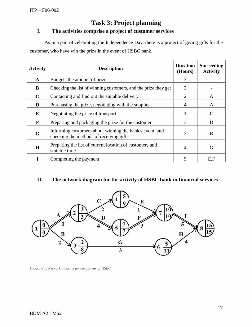
Task 3: Project planning
I. The activities comprise a project of customer services
As in a part of celebrating the Independence Day, there is a project of giving gifts for the
customer, who have win the prize in the event of HSBC bank.
Activity Description Duration
(Hours)
Succeeding
Activity
A Budgets the amount of prize 3 -
B Checking the list of winning customers, and the prize they get 2 -
C Contacting and find out the suitable delivery 2 A
D Purchasing the prize, negotiating with the supplier 4 A
E Negotiating the price of transport 1 C
F Preparing and packaging the prize for the customer 3 D
G Informing customers about winning the bank's event, and
checking the methods of receiving gifts 3 B
H Preparing the list of current location of customers and
suitable time 4 G
I Completing the payment 5 E,F
II. The network diagram for the activity of HSBC bank in financial services
Diagram 1: Network diagram for the activity of HSBC

ITP – F06-092
18
BDM A2 - Max
Path Duration (Hours)
A-C-E-I 3+2+1+5 11
A-D-F-I 3+4+3+5 15
B-G-H 2+3+4 9
The critical path is A-D-F-I, with a duration of 15 weeks.
III. The grant chart which show the planning of the project
Chart 1: The planning project and the number of staff required
In the chart 1, activity C and D cannot start until activity A is completed. Therefore, C and
D are drawn as starting at the end of week 3 on the chart. Besides, the activity E which follows C
and activity F which follows D, have the time to start right after activity C and D complete
respectively. From that, we can easy identify the time of each activity. However, the number of
staff required each hour is simply obtained by adding the staff requirements per activity for
relevant hour number, which shows the fluctuate histogram below.
TIME WORKS
ACTIVITY
2 2 1 3 3 3 2 2 2 1 1 1 1 1 1
6
Duration of activity Float time of activity
14 159 10 11 12
A
B
C
7 81 2 3 4 5
No. Staff
D
E
F
G
H
I
13
0
0.5
1
1.5
2
2.5
3
3.5
1 2 3 4 5 6 7 8 9 10 11 12 13 14 15
Number of staff
Number of staffChart 2: The number of staff required in the projects per hour
ITP – F06-092
19
BDM A2 - Max
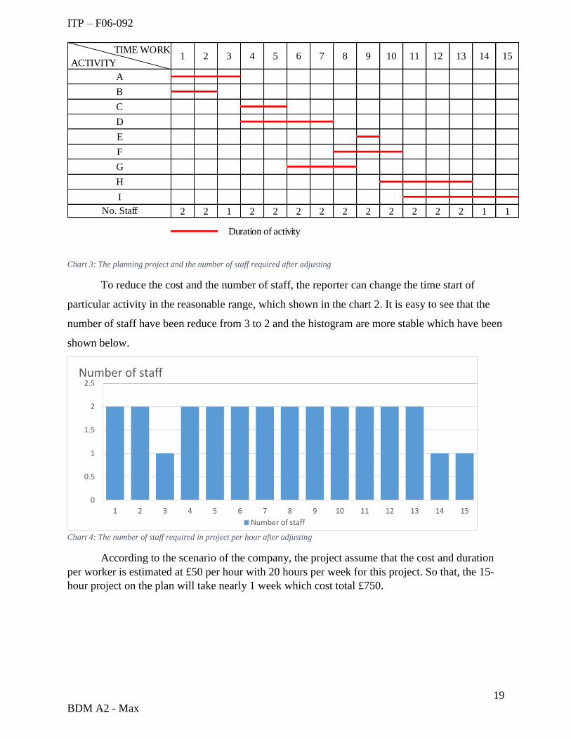
Chart 3: The planning project and the number of staff required after adjusting
To reduce the cost and the number of staff, the reporter can change the time start of
particular activity in the reasonable range, which shown in the chart 2. It is easy to see that the
number of staff have been reduce from 3 to 2 and the histogram are more stable which have been
shown below.
According to the scenario of the company, the project assume that the cost and duration
per worker is estimated at £50 per hour with 20 hours per week for this project. So that, the 15-
hour project on the plan will take nearly 1 week which cost total £750.
TIME WORKS
ACTIVITY
2 2 1 2 2 2 2 2 2 2 2 2 2 1 1
Duration of activity
13 14
G
H
I
1 2 3 4
C
D
E
F
No. Staff
12 15
A
B
6 7 8 9 10 115
0
0.5
1
1.5
2
2.5
1 2 3 4 5 6 7 8 9 10 11 12 13 14 15
Number of staff
Number of staff
Chart 4: The number of staff required in project per hour after adjusting
ITP – F06-092
20
BDM A2 - Max
Task 4: Discount cash flow (DCF) methods
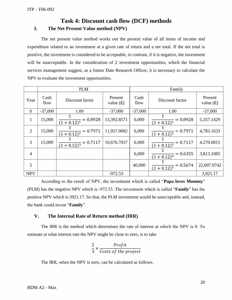
I. The Net Present Value method (NPV)
The net present value method works out the present value of all items of income and
expenditure related to an investment at a given rate of return and a net total. If the net total is
positive, the investment is considered to be acceptable, in contrast, if it is negative, the investment
will be unacceptable. In the consideration of 2 investment opportunities, which the financial
services management suggest, as a Junior Date Research Officer, it is necessary to calculate the
NPV to evaluate the investment opportunities.
PLM Family
Year Cash
flow Discount factor
Present
value (£) Cash
flow Discount factor
Present
value (£)
0 -37,000 1.00 -37,000 -37,000 1.00 -37,000
1 15,000 1
(1 + 0.12)1= 0.8928 13,392.8571 6,000
1
(1 + 0.12)1= 0.8928 5,357.1429
2 15,000 1
(1 + 0.12)2= 0.7971 11,957.9082 6,000
1
(1 + 0.12)2= 0.7971 4,783.1633
3 15,000 1
(1 + 0.12)3= 0.7117 10,676.7037 6,000
1
(1 + 0.12)3= 0.7117 4,270.6815
4 6,000 1
(1 + 0.12)4= 0.6355 3,813.1085
5 40,000 1
(1 + 0.12)5= 0.5674 22,697.0742
NPV -972.53 3,921.17
According to the result of NPV, the investment which is called “Papa loves Mommy”
(PLM) has the negative NPV which is -972.53. The investment which is called “Family” has the
positive NPV which is 3921.17. So that, the PLM investment would be unacceptable and, instead,
the bank could invest “Family”.
V. The Internal Rate of Return method (IRR)
The IRR is the method which determines the rate of interest at which the NPV is 0. To
estimate at what interest rate the NPV might be close to zero, is to take
2
3×
𝑃𝑟𝑜𝑓𝑖𝑡
𝐶𝑜𝑠𝑡𝑠 𝑜𝑓 𝑡ℎ𝑒 𝑝𝑟𝑜𝑗𝑒𝑐𝑡
The IRR, when the NPV is zero, can be calculated as follows.
ITP – F06-092
21
BDM A2 - Max
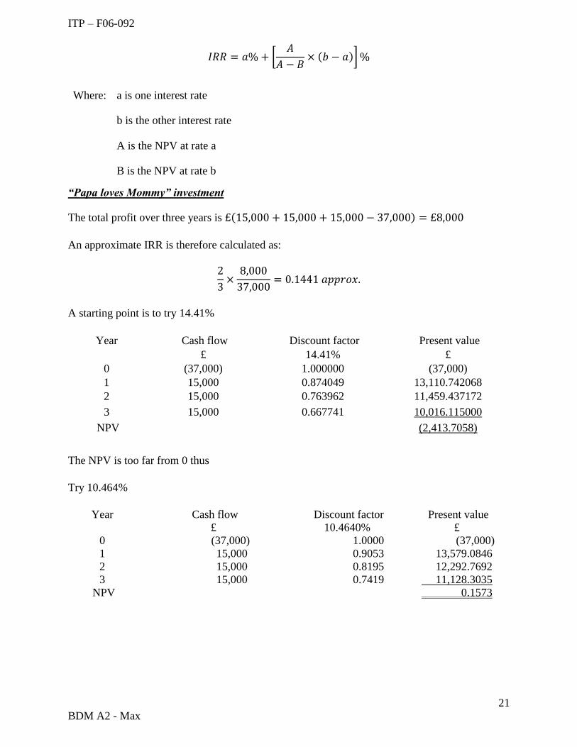
𝐼𝑅𝑅 = 𝑎% + [𝐴
𝐴 − 𝐵× (𝑏 − 𝑎)] %
Where: a is one interest rate
b is the other interest rate
A is the NPV at rate a
B is the NPV at rate b
“Papa loves Mommy” investment
The total profit over three years is £(15,000 + 15,000 + 15,000 − 37,000) = £8,000
An approximate IRR is therefore calculated as:
2
3×
8,000
37,000= 0.1441 𝑎𝑝𝑝𝑟𝑜𝑥.
A starting point is to try 14.41%
Year Cash flow Discount factor Present value
£ 14.41% £
0 (37,000) 1.000000 (37,000)
1 15,000 0.874049 13,110.742068
2 15,000 0.763962 11,459.437172
3 15,000 0.667741 10,016.115000
NPV (2,413.7058)
The NPV is too far from 0 thus
Try 10.464%
Year Cash flow Discount factor Present value
£ 10.4640% £
0 (37,000) 1.0000 (37,000)
1 15,000 0.9053 13,579.0846
2 15,000 0.8195 12,292.7692
3 15,000 0.7419 11,128.3035
NPV 0.1573
ITP – F06-092
22
BDM A2 - Max
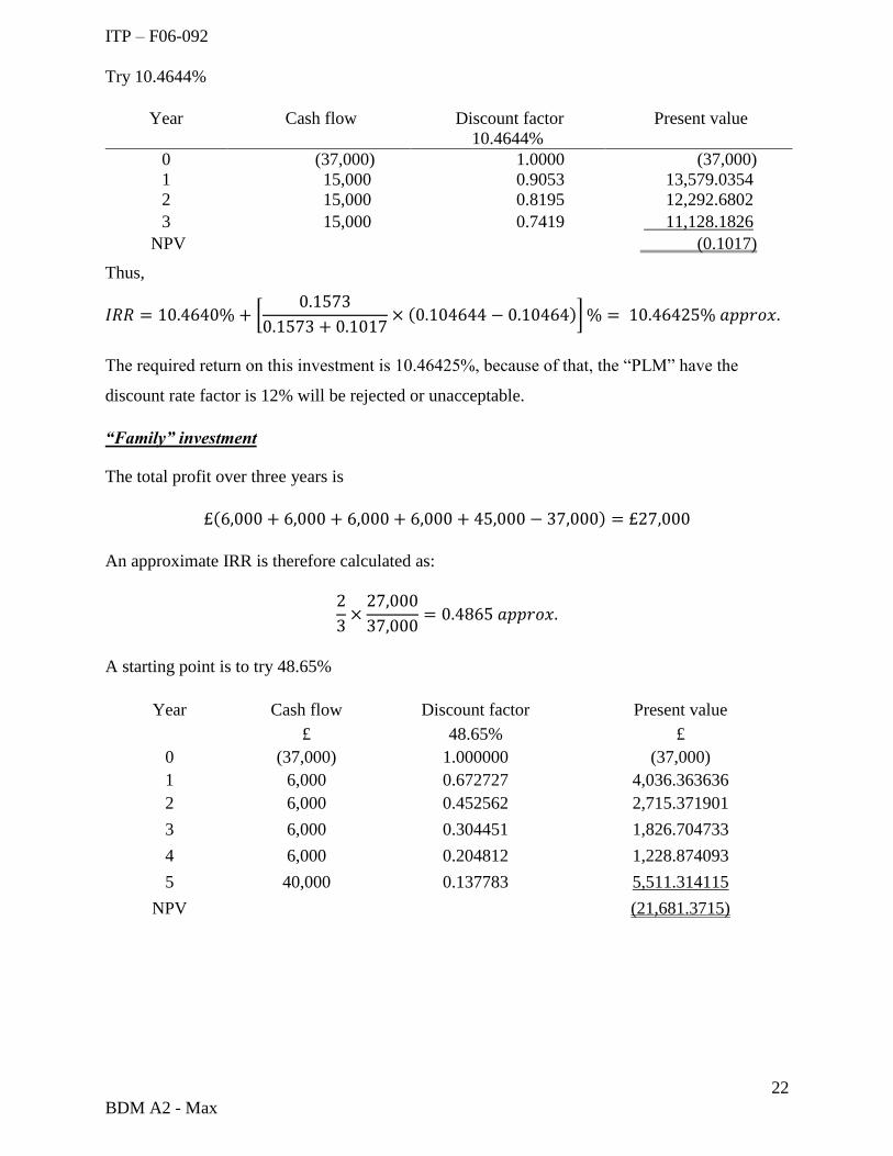
Try 10.4644%
Year Cash flow Discount factor Present value
10.4644%
0 (37,000) 1.0000 (37,000)
1 15,000 0.9053 13,579.0354
2 15,000 0.8195 12,292.6802
3 15,000 0.7419 11,128.1826
NPV (0.1017)
Thus,
𝐼𝑅𝑅 = 10.4640% + [0.1573
0.1573 + 0.1017× (0.104644 − 0.10464)] % = 10.46425% 𝑎𝑝𝑝𝑟𝑜𝑥.
The required return on this investment is 10.46425%, because of that, the “PLM” have the
discount rate factor is 12% will be rejected or unacceptable.
“Family” investment
The total profit over three years is
£(6,000 + 6,000 + 6,000 + 6,000 + 45,000 − 37,000) = £27,000
An approximate IRR is therefore calculated as:
2
3×
27,000
37,000= 0.4865 𝑎𝑝𝑝𝑟𝑜𝑥.
A starting point is to try 48.65%
Year Cash flow Discount factor Present value
£ 48.65% £
0 (37,000) 1.000000 (37,000)
1 6,000 0.672727 4,036.363636
2 6,000 0.452562 2,715.371901
3 6,000 0.304451 1,826.704733
4 6,000 0.204812 1,228.874093
5 40,000 0.137783 5,511.314115
NPV (21,681.3715)
ITP – F06-092
23
BDM A2 - Max
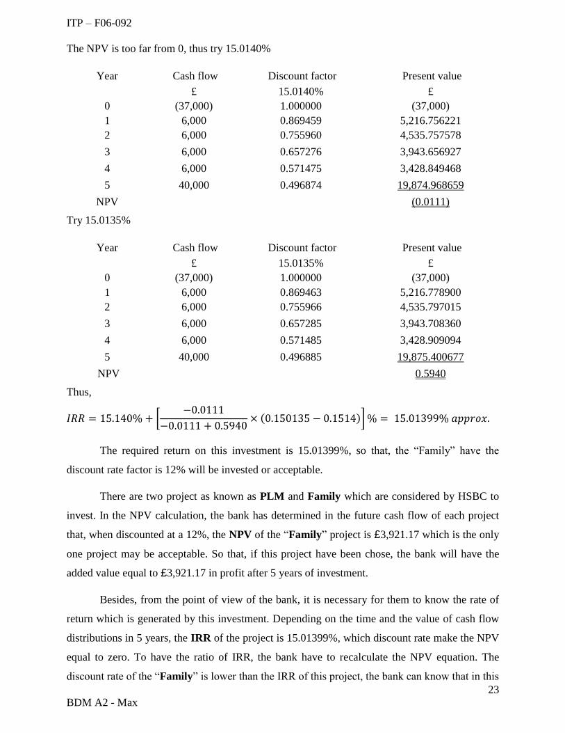
The NPV is too far from 0, thus try 15.0140%
Year Cash flow Discount factor Present value
£ 15.0140% £
0 (37,000) 1.000000 (37,000)
1 6,000 0.869459 5,216.756221
2 6,000 0.755960 4,535.757578
3 6,000 0.657276 3,943.656927
4 6,000 0.571475 3,428.849468
5 40,000 0.496874 19,874.968659
NPV (0.0111)
Try 15.0135%
Year Cash flow Discount factor Present value
£ 15.0135% £
0 (37,000) 1.000000 (37,000)
1 6,000 0.869463 5,216.778900
2 6,000 0.755966 4,535.797015
3 6,000 0.657285 3,943.708360
4 6,000 0.571485 3,428.909094
5 40,000 0.496885 19,875.400677
NPV 0.5940
Thus,
𝐼𝑅𝑅 = 15.140% + [−0.0111
−0.0111 + 0.5940× (0.150135 − 0.1514)] % = 15.01399% 𝑎𝑝𝑝𝑟𝑜𝑥.
The required return on this investment is 15.01399%, so that, the “Family” have the
discount rate factor is 12% will be invested or acceptable.
There are two project as known as PLM and Family which are considered by HSBC to
invest. In the NPV calculation, the bank has determined in the future cash flow of each project
that, when discounted at a 12%, the NPV of the “Family” project is £3,921.17 which is the only
one project may be acceptable. So that, if this project have been chose, the bank will have the
added value equal to £3,921.17 in profit after 5 years of investment.
Besides, from the point of view of the bank, it is necessary for them to know the rate of
return which is generated by this investment. Depending on the time and the value of cash flow
distributions in 5 years, the IRR of the project is 15.01399%, which discount rate make the NPV
equal to zero. To have the ratio of IRR, the bank have to recalculate the NPV equation. The
discount rate of the “Family” is lower than the IRR of this project, the bank can know that in this

ITP – F06-092
24
BDM A2 - Max
project the NPV will be positive with 12% of discount rate. Thus, it is easy to see that the IRR
measurement have ability to show the return of investment opportunities and compare them.
However, NPV is better than IRR in the long time, because of basing on discount rate factor at
present. In the fluctuation of the rate on the time changed, the IRR may be wrong. So that, The
NPV is useful in evaluate the long-time investment, and the IRR is good way for company to
evaluate the short one.

ITP – F06-092
25
BDM A2 - Max
Conclusion
In sum up, the report have been shown detail and correctly the information of the company
in each task and provide the suitable recommendation for the bank to increase the efficiency and
productivity. In task 1, the bank should use multiplicative model method for calculating and
forecasting the actual sales of bank in the next year. In the second task, there are 5 useful software
which are recommended for the bank to help them increase the efficiency and productivity. In the
task 3, the report has create the detail plan for the bank to follow which is reasonable and have the
lowest cost. In the final test, the report have shown the way to evaluate the project by 2 method
NPV and IRR and make the conclusion for the bank to choose which one is the good project for
the bank in the future.

ITP – F06-092
26
BDM A2 - Max
References
Axiomepm, 2014. BUDGETING AND FORECASTING. [Online]
Available at: http://www.axiomepm.com/solutions/industry/banking/budgeting
[Accessed 23 May 2014].
Corel, 2012. http://www.corel.com. [Online]
Available at: http://www.corel.com/corel/product/index.jsp?pid=prod5190074
[Accessed 1 June 2014].
IBM Corperation, 2013. Http://www.IBM.Com. [Online]
Available at: http://www-03.ibm.com/software/products/en/category/transaction-processing
[Accessed 1 June 2014].
Prophix, n.d. prophix.com. [Online]
Available at: http://www.prophix.com/solutions/personnel-planning/
[Accessed 23 May 2014].
T.A.C, 2012. http://www.tyleranalytics.com/. [Online]
Available at: http://www.tyleranalytics.com/products/banking.asp
[Accessed 1 June 2014].