Daily and monthly temperature and precipitation statistics as performance indicators for regional...

CLIMATE RESEARCHClim Res

Vol. 44: 135–150, 2010doi: 10.3354/cr00932

Published December 10

1. INTRODUCTION

Regional climate models (RCMs) are powerful toolsthat have the potential to provide high-resolution infor-mation both in space and time on the properties of arange of climate variables. On some occasions, data froma range of different RCM simulations are considered. Aquestion in this context is how individual regional cli-mate change scenarios can be converted into probabilis-tic climate change signals. This is relatively straight-forward if models are used as they are withoutacknowledging the fact that different models are more orless good at representing today’s climate. However, ifmodel performance is to be considered, the situation be-comes more complicated. To take this larger complexityinto account, one idea, pursued in the ENSEMBLES pro-

ject (Hewitt & Griggs 2005, van der Linden & Mitchell2009), is the weighting of RCMs according to how ade-quately they simulate the recent past climate of the lastdecades. In this context, a number of different weightsmeasuring various aspects of RCM realism have beenconsidered (Christensen et al. 2010, this Special). Here,as part of the ENSEMBLES effort, we investigated thematch of RCM-simulated probability density distribu-tions for maximum and minimum temperature and pre-cipitation to those based on observational data.

Forced with boundary data from reanalysis productssuch as ERA40 (Uppala et al. 2005), RCMs have beenshown to adequately simulate important aspects of theclimate of the recent past decades, including not justlong-term seasonal means but also extreme events ofe.g. temperature and precipitation (Christensen et al.

© Inter-Research 2010 · www.int-res.com*Email: erik.kjellströ[email protected]

Daily and monthly temperature and precipitationstatistics as performance indicators for regional

climate models

Erik Kjellström1,*, Fredrik Boberg2, Manuel Castro3, Jens Hesselbjerg Christensen2, Grigory Nikulin1, Enrique Sánchez3

1Rossby Centre, Swedish Meteorological and Hydrological Institute, 60176 Norrköping, Sweden2Danish Climate Centre, Danish Meteorological Institute, Lyngbyvej 100, 2100 Copenhagen Ø, Denmark3Facultad de Ciencias del Medio Ambiente, Universidad de Castilla-La Mancha (UCLM), Toledo, Spain

ABSTRACT: We evaluated daily and monthly statistics of maximum and minimum temperatures andprecipitation in an ensemble of 16 regional climate models (RCMs) forced by boundary conditionsfrom reanalysis data for 1961–1990. A high-resolution gridded observational data set for land areasin Europe was used. Skill scores were calculated based on the match of simulated and observedempirical probability density functions. The evaluation for different variables, seasons and regionsshowed that some models were better/worse than others in an overall sense. It also showed that nomodel that was best/worst in all variables, seasons or regions. Biases in daily precipitation were mostpronounced in the wettest part of the probability distribution where the RCMs tended to overesti-mate precipitation compared to observations. We also applied the skill scores as weights used to cal-culate weighted ensemble means of the variables. We found that weighted ensemble means wereslightly better in comparison to observations than corresponding unweighted ensemble means formost seasons, regions and variables. A number of sensitivity tests showed that the weights werehighly sensitive to the choice of skill score metric and data sets involved in the comparison.

KEY WORDS: Regional climate models · Probability distributions · Skill score metrics · Weightedensemble · Europe

Resale or republication not permitted without written consent of the publisher

Contribution to CR Special 23 ‘Regional Climate Model evaluation and weighting’ OPENPEN ACCESSCCESS

Clim Res 44: 135–150, 2010

2007). When forced by global climate models (GCMs),RCMs have been found to sometimes produce largebiases in the mean climate (e.g. Räisänen et al. 2004,Jacob et al. 2007) and even more so in terms of extremeconditions (e.g. Moberg & Jones 2004, Beniston et al.2007, Kjellström et al. 2007, Rockel & Woth 2007,Nikulin et al. 2010). Kjellström et al. (2007) showedthat there is a considerably larger spread betweenRCMs at the tails of the temperature probability distri-butions than in simulated means both in today’s cli-mate and in the simulated climate change signals. Thisspread in the climate change signal was large evenwhen the forcing conditions were taken from the sameGCM following the same emissions scenario. Such alarge spread indicates a sensitivity of the results to theformulation of the RCM.

Kjellström et al. (2007) investigated the daily maxi-mum and minimum temperature by studying fixed per-centiles from the empirical probability distributions.This approach gave a first indication of some of thequantiles of the probability distributions which had thelargest biases, but did not give information on thewhole distribution. Here we evaluated the models’ abil-ity to represent the whole probability distributions si-multaneously by using the skill score (SS) metric pre-sented by Perkins et al. (2007). Earlier, Boberg et al.(2009a,b) used this method to compare the daily precip-itation in the PRUDENCE (Christensen& Christensen 2007) and ENSEMBLESsimulations by comparison with the Eu-ropean Climate Assessment (ECA;Klein Tank et al. 2002) observationaldata set. In addition to evaluating dailydata of precipitation and minimum andmaximum temperatures, we also per-formed a comparison of probability dis-tributions of monthly precipitationdata. By looking at those 2 data sets si-multaneously, we obtained a broaderpicture of how RCMs reproduce the ob-served climate. Examples are given ofmodel behaviour in different regions ofEurope and in different seasons. Re-sults from 16 downscaling experimentsof the ERA40 reanalysis data to 25 kmhorizontal resolution were evaluatedagainst observations. Further, we cal-culated combined weights based on theevaluation for each model. The result-ing weights (SSs) are dimensionlessnumbers ranging between 0 and 1 thatare suitable for weighting model re-sults in order to construct probabilisticclimate change scenarios based on agiven experimental setup as in the EN-

SEMBLES project (Christensen et al. 2010, Déqué & So-moto 2010, both this Special). Finally, we investigatedwhether a weighted mean outperforms an unweightedmean when evaluated against observations.

2. DATA AND METHODS

2.1. RCM data

We used data from 16 climate simulations with RCMsrun at approximately 25 km grid spacing (Table 1). Allmodels that operated on a rotated latitude–longitudegrid had the majority of their model domain in common(Fig. 1), i.e. they worked on an identical grid (seeTable 1). The other models operated on Lambert-conformal grids that were not internally identical andnot identical to the rotated ones. Data from these othermodels were interpolated to the common rotated lati-tude–longitude grid shared by the others. All modelswere forced by lateral boundary conditions and seasurface temperatures from the European Centre forMedium Range Weather Forecasts (ECMWF) reanalysisproduct ERA40 (Uppala et al. 2005).

From the models, we used time series of daily mini-mum and maximum temperatures at the 2 m level anddaily precipitation as well as monthly precipitation for

136

Number Institute Model Time step Source(min)

1a C4I RCA3 15 Kjellström et al. (2005)

2 CHMI ALADIN 15 Farda et al. (2010)

3 CNRM RM4.5 22.5 / 6 hb Radu et al. (2008)

4a DMI HIRHAM5 10 Christensen et al. (2006)

5a ETH CLM 2 / 3 hb Böhm et al. (2006)

6 ICTP RegCM3 1.25 / 10b Giorgi & Mearns (1999)

7a KNMI RACMO2 12 van Meijgard et al. (2008)

8 Met.No HIRHAM 3.75 Haugen & Haakenstad(2006)

9a Hadley Centre HadRM3Q0 5 Collins et al. (2009)



12a MPI-M REMO 2 Jacob (2001)

13 OURANOS MRCC4.2.3 10 Plummer et al. (2006)

14a RPN GEMLAM 12 Côté et al. (1998),Zadra et al. (2008)

15a SMHI RCA3.0 15 Kjellström et al. (2005)

16 UCLM PROMES 0.83 / 10b Sanchez et al. (2004)aModels that used the same rotated longitude–latitude gridbThe first number (left) represents the RCM time step; the second number(right) is the sampling interval used for maximum and minimum temperatures

Table 1. Regional climate models from which data were analysed. RPN:Recherche en Prévision Numérique. Full forms of other institutes in Table 1

of Christensen et al. (2010, this Special)

Kjellström et al.: Temperature and precipitation in the ENSEMBLES RCMs

the time period 1961–1990. Data were downloadedfrom the ENSEMBLES regional data distribution cen-tre at DMI (http://ensemblesrt3.dmi.dk). The timesteps used in the different RCMs for calculating dailymaximum and minimum temperatures varied between2 and 15 min, except for the ETH and CNRM models,for which they were estimated based on instantaneous3- or 6-hourly data (Table 1).

2.2. Daily and monthly observational data

Model results were compared to daily minimum andmaximum temperature and precipitation from a griddedobservational data set (E-OBS) that is based on thelargest existing pan-European data set with daily dataextending back to 1950 (Haylock et al. 2008, Klok &Klein Tank 2009). A benefit from using this particulardata set is that it is constructed on the same rotated lati-tude/longitude grid that was used by most of the RCMs,implying that no further interpolation was needed formost of the RCMs. In a comparison with other existingdata sets from more dense networks in smaller regions,

Hofstra et al. (2009) found that E-OBS correlated wellwith these other data sets. However, they also found thatrelative differences in precipitation could be large, andthat they were usually biased toward lower values in E-OBS. Monthly precipitation was calculated as the sum ofall precipitation on each day of a month.

2.3. Metrics used for daily data

A description of the metric we used for comparingdaily minimum and maximum temperatures and pre-cipitation to E-OBS is given by Perkins et al. (2007).Empirical probability distribution functions (PDFs)were first constructed by binning data in N number ofbins according to temperature or precipitation amount,and then generating a dimensionless ‘match metric’ orSS based on the overlap of the RCM and observationPDFs. A perfect overlap results in an SS of 1, whereasthe score is close to 0 for a low degree of overlap:

(1)

2.4. Metrics used for monthly precipitation data

For the monthly precipitation data, we used the sameSS as defined in Eq. (1) but for the discussion also an ad-ditional metric to test the sensitivity of the resultingweights to the choice of scoring metric. This secondmetric was taken from Sánchez et al. (2009) and con-sisted of a collection of 5 functions measuring differentaspects of model probability distribution characteristics.

(2)

(3)

(4)

(5)

(6)

where ARCM and ACRU are the areas below the empiri-cal cumulative distribution functions (CDFs obtainedfrom normalised PDFs) of the RCMs and observationsrespectively, A+ and A– are the corresponding areas tothe right and left of the 50th percentile, respectively, Pis the spatial and temporal average of precipitation ineach season and region and σ is the standard devia-

f RCM CRU

CRU5

0 5

12

= − −⎛⎝⎜

⎞⎠⎟

σ σσ·

.

fP P

P

RCM CRU

CRU

4

0 5

12

= −−⎛

⎝⎜⎞⎠⎟·

.

fA A

ARCM CRU

CRU3

0 5

12

= − −⎛⎝⎜

⎞⎠⎟

− −

−·

.

fA A

ARCM CRU

CRU2

0 5

12

= − −⎛⎝⎜

⎞⎠⎟

+ +

+·

.

fA A

ARCM CRU

CRU1

0 5

12

= − −⎛⎝⎜

⎞⎠⎟·

.

SS PDF PDFRCM E-OBSbin

bin

==

=

∑ min( , )1

N

137

0

BI

IP

FR

ME

SC

AL

MD

EA

50 100 200 500 750 1000 1500 2000 2500

Elevation (m)

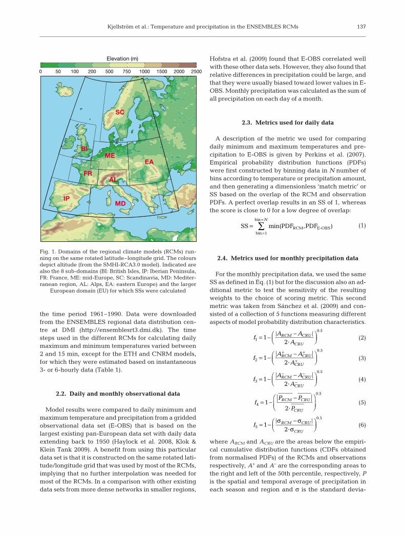
Fig. 1. Domains of the regional climate models (RCMs) run-ning on the same rotated latitude–longitude grid. The coloursdepict altitude (from the SMHI-RCA3.0 model). Indicated arealso the 8 sub-domains (BI: British Isles, IP: Iberian Peninsula,FR: France, ME: mid-Europe, SC: Scandinavia, MD: Mediter-ranean region, AL: Alps, EA: eastern Europe) and the larger

European domain (EU) for which SSs were calculated

Clim Res 44: 135–150, 2010

tion. Each of the factors takes into account differentaspects of the behaviour of the model precipitation.These are: the distribution as a whole in terms of mean(Eq. 5) and total area (Eq. 2), the precipitation amountsfor more intense precipitation in the upper (Eq. 3) andmoderate precipitation in the lower (Eq. 4) half of thedistribution divided by the median and the width of thedistribution through the variance (Eq. 6). These 5 mea-sures are all constructed so that a value close to 1 indi-cates that the RCM is close to observations while avalue close to 0 indicates that the RCM is far from theobservations. Finally, the 5 numbers are multiplied byeach other giving a final dimensionless SS that also isbetween 0 and 1.

(7)

2.5. Data handling including area averaging

SSs were calculated for 8 European regions (Fig. 1)as well as for the entire continental land area between36° and 70° N and 10.5° W and 30° E (EU) for each nom-inal season (winter: DJF, spring: MAM, summer: JJA,autumn: SON) and as an annual mean calculated asthe average of the SSs for the 4 seasons (annual: ANN).

Daily maximum and minimum temperatures werebinned into 0.5°C intervals for all grid boxes for whichobservational data were available, i.e. land areas. Dif-ferent methods of averaging over different regionswere tested for all models: (1) by pooling data from allgrid points within each region into 1 common probabil-ity distribution before calculating the SSs, and (2) byfirst averaging temperatures for each day in a regionand then calculating the SSs. We note here that thefirst method keeps all fine details but mixes spatial andtemporal variability. The second method smootheslocal, fine details. We also used a third method (3), inwhich SSs were first calculated for each grid box, andthereafter averaged over the area. In this case, datafrom models operating on other grids were first inter-polated to the common rotated latitude–longitude gridbefore SSs are calculated. The first method was ourreference, while the 2 others were only used to test thesensitivity of the score to the aggregation procedure.

For the daily precipitation analyses, we defined drydays as days with precipitation <1 mm and removedthese from the precipitation data. PDFs were then cal-culated from the remaining daily data for each regionand model by first binning the data into bins of 1 mmwidth starting at 1 mm. The impact of using a thresholdis discussed in Section 4.3.

For the monthly precipitation analysis, data wereaggregated in the regions according to the first methodoutlined above (this section) for daily data. This pool-

ing of data provided a large sample for deriving theempirical percentiles. We note here that these monthlydata also included dry days, which were excluded fromthe daily precipitation analyses.

2.6. Comparing RCM results to observations atdifferent parts of the PDFs

To obtain a more detailed picture of why some RCMsachieved high and others low SSs, we calculatedbiases for each RCM with regard to the observations ata number of percentiles (1, 5, 10, 25, 50, 75, 90, 95 and99) based on all data in a region. These biases in differ-ent parts of the PDFs allowed us to identify where dif-ferent RCMs had problems and may help explain whySSs differed between models.

2.7. Combination of SSs into one weight per RCM

A combined weight (wirs) for each model (i), region (r)and season (s) based on our model evaluation was cal-culated according to:

(8)

with SS as in Eq. (1). Indices PRD, PRM, TXD andTMD denote daily and monthly precipitation and dailymaximum and minimum temperatures, respectively. Itcan be seen from Eq. (8) that the influence of monthlydata was downgraded, as we took the square root ofthe resulting weight (SSPRM) when combining it withthe others. The rationale for this downgrading is thatwhile the daily data are seen as largely representingregional information and hence form a relevant RCMmetric, the monthly precipitation fields are much morestrongly controlled by the driving GCM but are stillworthwhile to evaluate as discussed in Section 4.1below. The dimensionless weight (wirs) was normalisedand takes a number between 0 and 1.

A final overall weight for each model (wi) was calcu-lated by averaging all individual weights (wirs) over the4 seasons and the 8 European regions. This finalweight (wi) was intended to be used in the weightingsystem described by Christensen et al. (2010).

3. RESULTS

3.1. Daily maximum and minimum temperatures

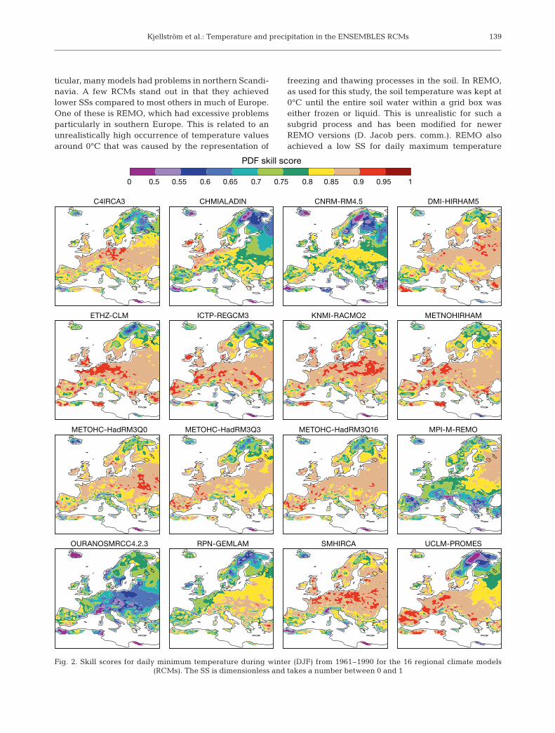
Fig. 2 shows the geographical distribution of the SSsfor daily minimum temperatures in winter. The SSswere generally highest in an area in western centralEurope and lower in the north and in the south. In par-

wirs = + +( ) +( )13

2SS SS SS SSPRD TXD TMD PRM/

SS = f f f f f1 2 3 4 5· · · ·

138


ticular, many models had problems in northern Scandi-navia. A few RCMs stand out in that they achievedlower SSs compared to most others in much of Europe.One of these is REMO, which had excessive problemsparticularly in southern Europe. This is related to anunrealistically high occurrence of temperature valuesaround 0°C that was caused by the representation of

freezing and thawing processes in the soil. In REMO,as used for this study, the soil temperature was kept at0°C until the entire soil water within a grid box waseither frozen or liquid. This is unrealistic for such asubgrid process and has been modified for newerREMO versions (D. Jacob pers. comm.). REMO alsoachieved a low SS for daily maximum temperature

139

C4IRCA3 CHMIALADIN CNRM-RM4.5 DMI-HIRHAM5

ETHZ-CLM ICTP-REGCM3 KNMI-RACMO2 METNOHIRHAM

METOHC-HadRM3Q0 METOHC-HadRM3Q3 METOHC-HadRM3Q16 MPI-M-REMO

OURANOSMRCC4.2.3 RPN-GEMLAM SMHIRCA UCLM-PROMES

0 0.5 0.55 0.6 0.65 0.7 0.75 0.8 0.85 0.9 0.95 1

PDF skill score

Fig. 2. Skill scores for daily minimum temperature during winter (DJF) from 1961–1990 for the 16 regional climate models (RCMs). The SS is dimensionless and takes a number between 0 and 1

Clim Res 44: 135–150, 2010

during winter but in an area more to the east and northwhere temperatures are generally lower (not shown).MRCC4.2.3 generally had low SSs for minimum tem-peratures, most pronounced in parts of eastern andcentral Europe and also in southern Sweden. Adetailed comparison for different parts of the PDFs inthe Scandinavian region revealed that MRCC4.2.3simulated temperatures were generally too low(Fig. 3), which led to an overly extensive snow cover inthis region, further exacerbating the cold bias (notshown). Most other models gave higher temperatures,and differed relatively substantially from E-OBS, innorthern Scandinavia (Fig. 3). A more detailed lookinto the biases in that region at different temperatureintervals revealed that all models except REMO andMRCC4.2.3 showed the largest positive biases duringthe coldest days (e.g. 1st or 5th percentiles), whilebiases were smaller in situations with relativelywarmer conditions. As the horizontal and vertical gridspacings in the RCMs were fairly coarse (25 × 25 km inthe horizontal, and typically the lowest model levelwas some 50 to 100 m above ground) they did not allowfor a fair representation of strong inversions or localconditions. Strong near-surface inversions are commonin winter in this area. Furthermore, many of the obser-vational stations in the area are located in valleys thatmay be much colder than the surrounding terrainwhen these strong inversions prevail. Alternatively,biases may reflect the fact that the station density islow in this area (Haylock et al. 2008), or that thestations are representative of open land conditionswhile model results represented a mixture of differentvegetation types dominated by forests in this region

(Nikulin et al. 2010). Taken together, these potentialproblems with RCMs and observational data indicatethat the biases are more a consequence of the fact thatthe 2 data sets represent different features than anindication of a systematic model error. We also notethat the problem was less pronounced for maximumtemperatures in winter (not shown), further indicatingthat this is a problem mostly concerning the coldestsituations.

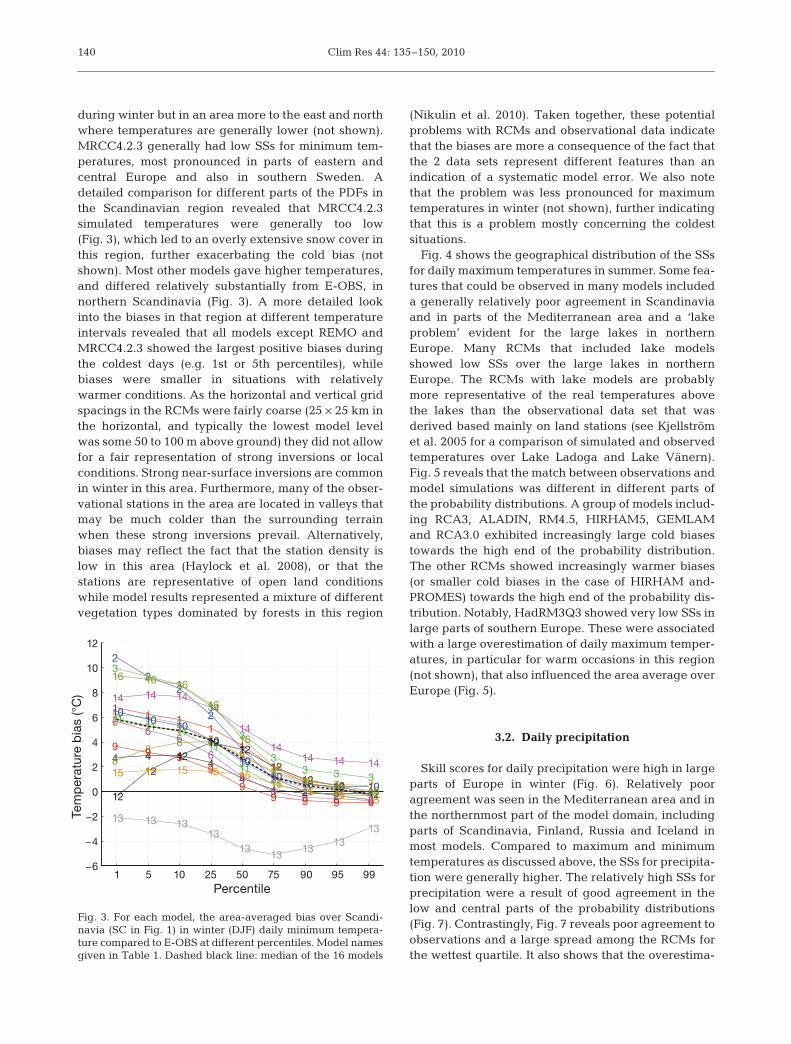
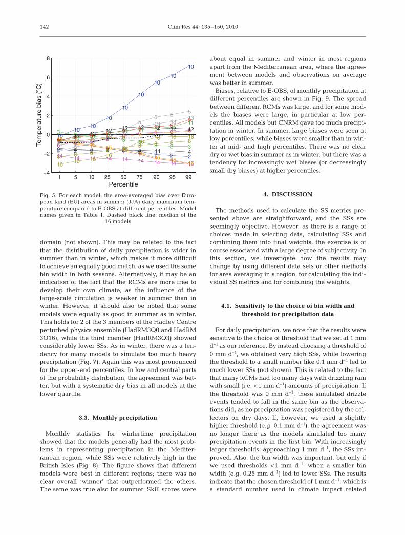
Fig. 4 shows the geographical distribution of the SSsfor daily maximum temperatures in summer. Some fea-tures that could be observed in many models includeda generally relatively poor agreement in Scandinaviaand in parts of the Mediterranean area and a ‘lakeproblem’ evident for the large lakes in northernEurope. Many RCMs that included lake modelsshowed low SSs over the large lakes in northernEurope. The RCMs with lake models are probablymore representative of the real temperatures abovethe lakes than the observational data set that wasderived based mainly on land stations (see Kjellströmet al. 2005 for a comparison of simulated and observedtemperatures over Lake Ladoga and Lake Vänern).Fig. 5 reveals that the match between observations andmodel simulations was different in different parts ofthe probability distributions. A group of models includ-ing RCA3, ALADIN, RM4.5, HIRHAM5, GEMLAMand RCA3.0 exhibited increasingly large cold biasestowards the high end of the probability distribution.The other RCMs showed increasingly warmer biases(or smaller cold biases in the case of HIRHAM and-PROMES) towards the high end of the probability dis-tribution. Notably, HadRM3Q3 showed very low SSs inlarge parts of southern Europe. These were associatedwith a large overestimation of daily maximum temper-atures, in particular for warm occasions in this region(not shown), that also influenced the area average overEurope (Fig. 5).

3.2. Daily precipitation

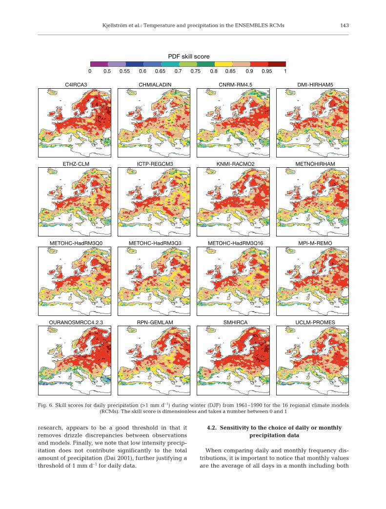
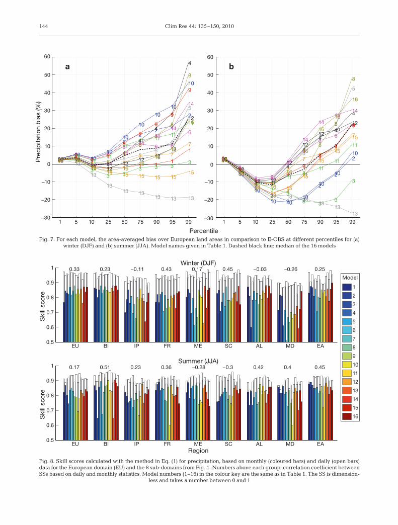
Skill scores for daily precipitation were high in largeparts of Europe in winter (Fig. 6). Relatively pooragreement was seen in the Mediterranean area and inthe northernmost part of the model domain, includingparts of Scandinavia, Finland, Russia and Iceland inmost models. Compared to maximum and minimumtemperatures as discussed above, the SSs for precipita-tion were generally higher. The relatively high SSs forprecipitation were a result of good agreement in thelow and central parts of the probability distributions(Fig. 7). Contrastingly, Fig. 7 reveals poor agreement toobservations and a large spread among the RCMs forthe wettest quartile. It also shows that the overestima-

140

1 5 10 25 50 75 90 95 99−6

−4

−2

0

2

4

6

8

10

12

11 1

1

1

1

11

1

2

22

2

2

2

2 2 2

33

3

3

3

33 3 3

4 4 44

44 4 4 4

5 55

5

5

55 5 5

66

6

6

6

66 6 6

77 7

7

7

77 7 7

88

8 8

8

88 8 8

99 9

9

99 9 9 9

1010

10

10

10

1010 10 10

1111

11

11

11

1111 11 1112

12

12

1212

12

1212

12

13 13 1313

1313

1313

13

14 14 1414

14

1414 14 14

15 15 15 15 1515

15 15 15

16 16 16

16

16

16

16 16 16

Tem

pera

ture

bia

s (°C

)

Percentile

Fig. 3. For each model, the area-averaged bias over Scandi-navia (SC in Fig. 1) in winter (DJF) daily minimum tempera-ture compared to E-OBS at different percentiles. Model namesgiven in Table 1. Dashed black line: median of the 16 models


tion in precipitation became worse with increasingprecipitation in most models. One exception wasMRC4.2.3, which simulated drier conditions than indi-cated by the observations. This overestimated heavyprecipitation is in agreement with the findings of vanMeijgard et al. (2008), who investigated precipitation

extremes in a majority of the RCMs used here as com-pared to the E-OBS data. Here we note that this maybe related to precipitation associated with extremeevents in E-OBS being too low (Hofstra et al. 2009).

In summer the SSs were slightly lower than in winterin a majority of the models and in large parts of the

141





0 0.5 0.55 0.6 0.65 0.7 0.75 0.8 0.85 0.9 0.95 1

PDF skill score

Fig. 4. Skill scores for daily maximum temperature during summer (JJA) from 1961–1990 for the 16 regional climate models (RCMs). The SS is dimensionless and takes a number between 0 and 1

Clim Res 44: 135–150, 2010

domain (not shown). This may be related to the factthat the distribution of daily precipitation is wider insummer than in winter, which makes it more difficultto achieve an equally good match, as we used the samebin width in both seasons. Alternatively, it may be anindication of the fact that the RCMs are more free todevelop their own climate, as the influence of thelarge-scale circulation is weaker in summer than inwinter. However, it should also be noted that somemodels were equally as good in summer as in winter.This holds for 2 of the 3 members of the Hadley Centreperturbed physics ensemble (HadRM3Q0 and HadRM3Q16), while the third member (HadRM3Q3) showedconsiderably lower SSs. As in winter, there was a ten-dency for many models to simulate too much heavyprecipitation (Fig. 7). Again this was most pronouncedfor the upper-end percentiles. In low and central partsof the probability distribution, the agreement was bet-ter, but with a systematic dry bias in all models at thelower quartile.

3.3. Monthly precipitation

Monthly statistics for wintertime precipitationshowed that the models generally had the most prob-lems in representing precipitation in the Mediter-ranean region, while SSs were relatively high in theBritish Isles (Fig. 8). The figure shows that differentmodels were best in different regions; there was noclear overall ‘winner’ that outperformed the others.The same was true also for summer. Skill scores were

about equal in summer and winter in most regionsapart from the Mediterranean area, where the agree-ment between models and observations on averagewas better in summer.

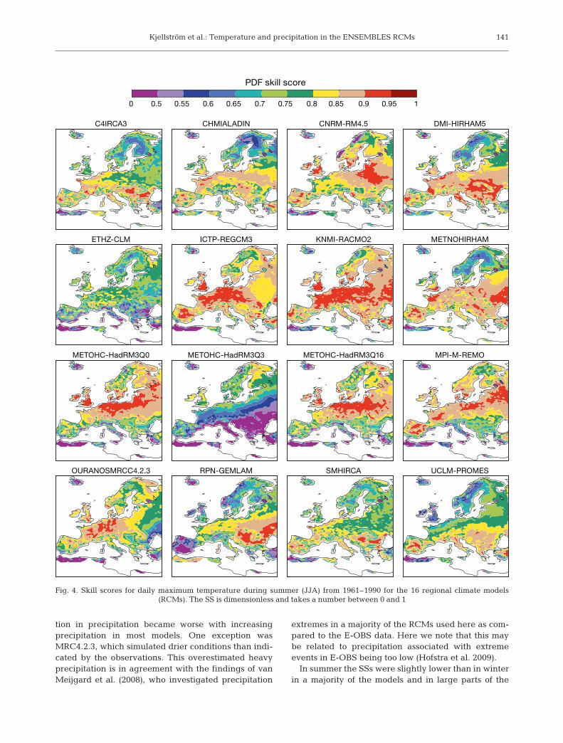
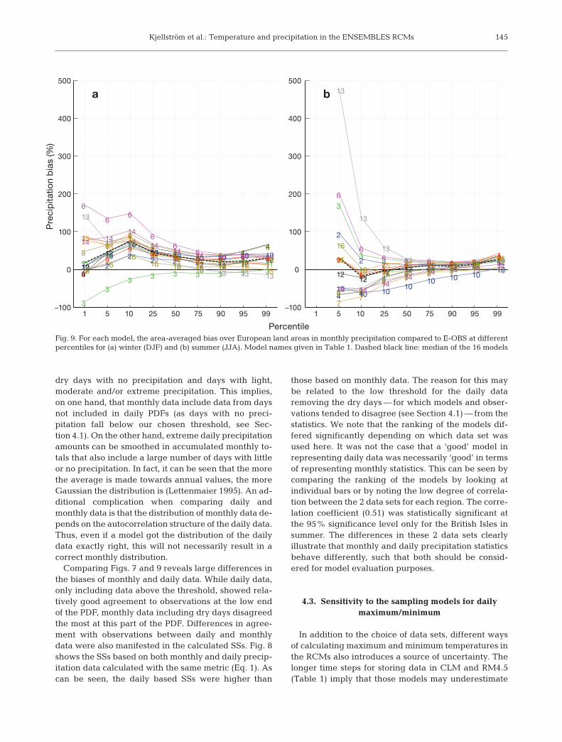
Biases, relative to E-OBS, of monthly precipitation atdifferent percentiles are shown in Fig. 9. The spreadbetween different RCMs was large, and for some mod-els the biases were large, in particular at low per-centiles. All models but CNRM gave too much precipi-tation in winter. In summer, large biases were seen atlow percentiles, while biases were smaller than in win-ter at mid- and high percentiles. There was no cleardry or wet bias in summer as in winter, but there was atendency for increasingly wet biases (or decreasinglysmall dry biases) at higher percentiles.

4. DISCUSSION

The methods used to calculate the SS metrics pre-sented above are straightforward, and the SSs areseemingly objective. However, as there is a range ofchoices made in selecting data, calculating SSs andcombining them into final weights, the exercise is ofcourse associated with a large degree of subjectivity. Inthis section, we investigate how the results maychange by using different data sets or other methodsfor area averaging in a region, for calculating the indi-vidual SS metrics and for combining the weights.

4.1. Sensitivity to the choice of bin width andthreshold for precipitation data

For daily precipitation, we note that the results weresensitive to the choice of threshold that we set at 1 mmd–1 as our reference. By instead choosing a threshold of0 mm d–1, we obtained very high SSs, while loweringthe threshold to a small number like 0.1 mm d–1 led tomuch lower SSs (not shown). This is related to the factthat many RCMs had too many days with drizzling rainwith small (i.e. <1 mm d–1) amounts of precipitation. Ifthe threshold was 0 mm d–1, these simulated drizzleevents tended to fall in the same bin as the observa-tions did, as no precipitation was registered by the col-lectors on dry days. If, however, we used a slightlyhigher threshold (e.g. 0.1 mm d–1), the agreement wasno longer there as the models simulated too manyprecipitation events in the first bin. With increasinglylarger thresholds, approaching 1 mm d–1, the SSs im-proved. Also, the bin width was important, but only ifwe used thresholds <1 mm d–1, when a smaller binwidth (e.g. 0.25 mm d–1) led to lower SSs. The resultsindicate that the chosen threshold of 1 mm d–1, which isa standard number used in climate impact related

142

−4

−2

0

2

4

6

8

11 1 1 1

11 1

1

2 2 2 2 2 22 2 2

33 3 3 3 3

3 3 34 4 4 4 4 4 44 455

55

5

55 5

5

6 6 6 66

6 6 6 6

7 7 7 7 7 7 7 7 7

8 8 8 88 8 8 8 89

9 9 9 9 9 9 99

1010

10

10

10

10

10

10

10

1111 11

11 11 11 11 1111

1212 12

12 12 12 12 12 12

13 13 1313

1313

13 1313

14 14 14 14 14 14 14 14 14

1515 15 15 15

1515 15

151616 16

1616

1616 16 16

1 5 10 25 50 75 90 95 99

Tem

pera

ture

bia

s (°C

)

Percentile

Fig. 5. For each model, the area-averaged bias over Euro-pean land (EU) areas in summer (JJA) daily maximum tem-perature compared to E-OBS at different percentiles. Modelnames given in Table 1. Dashed black line: median of the

16 models


research, appears to be a good threshold in that itremoves drizzle discrepancies between observationsand models. Finally, we note that low intensity precip-itation does not contribute significantly to the totalamount of precipitation (Dai 2001), further justifying athreshold of 1 mm d–1 for daily data.

4.2. Sensitivity to the choice of daily or monthlyprecipitation data

When comparing daily and monthly frequency dis-tributions, it is important to notice that monthly valuesare the average of all days in a month including both

143





0 0.5 0.55 0.6 0.65 0.7 0.75 0.8 0.85 0.9 0.95 1

PDF skill score

Fig. 6. Skill scores for daily precipitation (>1 mm d–1) during winter (DJF) from 1961–1990 for the 16 regional climate models (RCMs). The skill score is dimensionless and takes a number between 0 and 1

Clim Res 44: 135–150, 2010144

EU BI IP FR ME SC AL MD EA

Model

0.5

0.6

0.7

0.8

0.9

1

Skill

sco

re

0.33Winter (DJF)

0.23 −0.11 0.43 0.17 0.45 −0.03 −0.26 0.25

EU BI IP FR ME SC AL MD EA0.5

0.6

0.7

0.8

0.9

1

Region

Skill

sco

re

Summer (JJA)0.17 0.51 0.23 0.36 −0.28 −0.3 0.42 0.4 0.45

1

2

3

4

5

6

7

8

9

10

11

12

13

14

15

16

Fig. 8. Skill scores calculated with the method in Eq. (1) for precipitation, based on monthly (coloured bars) and daily (open bars)data for the European domain (EU) and the 8 sub-domains from Fig. 1. Numbers above each group: correlation coefficient betweenSSs based on daily and monthly statistics. Model numbers (1–16) in the colour key are the same as in Table 1. The SS is dimension-

less and takes a number between 0 and 1

1 5 10 25 50 75 90 95 99−30

−20

−10

0

10

20

30

40

50

60

1 1

11 1 1 1

1

1

22

22

2

22

2

2

3 3

33 3

3 3 334 4

4 4

4

4

4

4

4

5 55 5

55

5

5

5

66

66

6 6 6 6

6

7 7

7 77

7 7 7

7

8 88 8

8

8

8

8

8

99

99

9

9

9

9

9

1010

10

10

10

10

10

10

10

1111

1111

1111 11

11

11

12 12

12 1212

1212

12

12

1313

13

1313 13

13 13 13

14 14

14 14

14

14

14

14

14

15 15

1515 15 15 15 15

15

16 16

1616

1616

16

16

16

Pre

cip

itatio

n b

ias (%

)

a

1 5 10 25 50 75 90 95 99−30

−20

−10

0

10

20

30

40

50

60

1

1

1

11

1

1

1

1

2

2

2

22 2

2

2

23

3

3

33

3 33

3

4

4

4 4

4

4

4

4

4

5

5

5 5

5

5

5

5

5

6

6

6 6

6

6

66

6

7

7

7 7

7

77

7

7

8

8

8

88

8

8

8

8

9

9

9 9

9

9

9

9

9

10

10

10

10 1010

10

10

1011

11

11 1111

1111

11

11

12

12

12 12

12

12

1212

12

13

13

13

13 1313

1313

13

14

14

14 14

14

14

14

1414

15

15

15

1515

15

15

15

15

16

16

16 16

16

16

16

16

16

b

Percentile

Fig. 7. For each model, the area-averaged bias over European land areas in comparison to E-OBS at different percentiles for (a) winter (DJF) and (b) summer (JJA). Model names given in Table 1. Dashed black line: median of the 16 models


dry days with no precipitation and days with light,moderate and/or extreme precipitation. This implies,on one hand, that monthly data include data from daysnot included in daily PDFs (as days with no preci-pitation fall below our chosen threshold, see Sec-tion 4.1). On the other hand, extreme daily precipitationamounts can be smoothed in accumulated monthly to-tals that also include a large number of days with littleor no precipitation. In fact, it can be seen that the morethe average is made towards annual values, the moreGaussian the distribution is (Lettenmaier 1995). An ad-ditional complication when comparing daily andmonthly data is that the distribution of monthly data de-pends on the autocorrelation structure of the daily data.Thus, even if a model got the distribution of the dailydata exactly right, this will not necessarily result in acorrect monthly distribution.

Comparing Figs. 7 and 9 reveals large differences inthe biases of monthly and daily data. While daily data,only including data above the threshold, showed rela-tively good agreement to observations at the low endof the PDF, monthly data including dry days disagreedthe most at this part of the PDF. Differences in agree-ment with observations between daily and monthlydata were also manifested in the calculated SSs. Fig. 8shows the SSs based on both monthly and daily precip-itation data calculated with the same metric (Eq. 1). Ascan be seen, the daily based SSs were higher than

those based on monthly data. The reason for this maybe related to the low threshold for the daily dataremoving the dry days — for which models and obser-vations tended to disagree (see Section 4.1) — from thestatistics. We note that the ranking of the models dif-fered significantly depending on which data set wasused here. It was not the case that a ‘good’ model inrepresenting daily data was necessarily ‘good’ in termsof representing monthly statistics. This can be seen bycomparing the ranking of the models by looking atindividual bars or by noting the low degree of correla-tion between the 2 data sets for each region. The corre-lation coefficient (0.51) was statistically significant atthe 95% significance level only for the British Isles insummer. The differences in these 2 data sets clearlyillustrate that monthly and daily precipitation statisticsbehave differently, such that both should be consid-ered for model evaluation purposes.

4.3. Sensitivity to the sampling models for dailymaximum/minimum

In addition to the choice of data sets, different waysof calculating maximum and minimum temperatures inthe RCMs also introduces a source of uncertainty. Thelonger time steps for storing data in CLM and RM4.5(Table 1) imply that those models may underestimate

145

−100

0

100

200

300

400

500

11

1

11

1 1 1 12

2

22 2 2 2 2 2

3

3

33 3 3 3 3 34

4

44 4

4 44

4

55

5

5 55 5 5 5

6

66

6

66 6 6 6

77

7

77

7 7 7 7

88

8

88

8 8 88

9

9

99 9 9 9 9 9

10

10

1010 10 10 10 10 10

1111

1111 11 11 11 11 1112

12

12

1212

12 12 1212

13

13 13

1313

13 13 13 13

14 1414

1414

14 14 14 14

1515

15

1515

15 15 15 151616

1616 16 16 16 16

16 1

11 1 1 1 1

1

2

22 2 22 2

2

3

33 3 3 3 3 3

4 4

44 4 4 4

4

5 5

55 5 5 5 5

6

66 6 6 6 6 6

77

77

7 7 7 7

8 8

88

8 8 8

89

99

9 9 9 99

1010 10

1010 10 10

10

11

1111

11 11 11 1111

1212

12 12 12 12 12 12

13

13

13

1313 13 13 13

14 1414

1414 14 14 14

15

1515 15 15 15 15

15

16

16 16 16 16 16 1616

1 5 10 25 50 75 90 95 99

Pre

cip

itatio

n b

ias (%

)

a

1 5 10 25 50 75 90 95 99

b

−100

0

100

200

300

400

500

Percentile

Fig. 9. For each model, the area-averaged bias over European land areas in monthly precipitation compared to E-OBS at differentpercentiles for (a) winter (DJF) and (b) summer (JJA). Model names given in Table 1. Dashed black line: median of the 16 models

Clim Res 44: 135–150, 2010

extremes as they may not coincide withthe fixed time steps every 3 or 6 h.Judging from the calculated SSs, itappears that CLM did not performworse than the other models for mini-mum temperatures in winter (Fig. 2).RM4.5, on the other hand, showed rela-tively low SSs. A closer look at biases indifferent parts of the PDFs revealed thatRM4.5 had exceedingly large warmbiases closer toward the cold side of thePDF, both in Scandinavia (Fig. 3), butalso in other areas (not shown). How-ever, it is difficult to judge if this isindeed a problem with sampling, asRM4.5 and ALADIN behaved very sim-ilarly, both in terms of SSs and biasstructure. The situation in summershowed that SSs for maximum tempera-tures were a bit lower in CLM than insome of the other models, includingRM4.5 (Fig. 4). This may indicate thatthe absolute maximum was not cap-tured by the 8 instantaneous numbersavailable for each day in CLM. How-ever, we also note that CLM was warmbiased in the warm part of the PDFs(above the 75th percentile, reaching about 2°C at the95th and 99th percentiles, cf. Fig. 5), implying thateven higher temperatures would not necessarily leadto a higher SS. RM4.5, which achieved a relativelyhigh SS in summer, showed an increasingly cold biasat higher percentiles in summer, possibly indicatingthat sampling was too infrequent to record the highesttemperatures in the course of the day. For the otherRCMs, differences in time steps for calculating maxi-mum and minimum temperatures were between 2 and15 min, which may also have had some impact on theresults. However, we assume that these differenceswere relatively small compared to other differencesbetween the different RCMs in terms of how they rep-resent sub-grid scale processes in their parameterisa-tion schemes and also in terms of the relatively coarsehorizontal resolution considered.

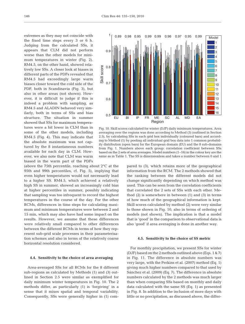
4.4. Sensitivity to the choice of area averaging

Area-averaged SSs for all RCMs for the 8 differentsub-regions as calculated by Methods (1) and (3) out-lined in Section 2.5 were similar as exemplified fordaily minimum winter temperatures in Fig. 10. The 2methods differ, as particularly (1) is ‘forgiving’ in asense that it mixes spatial and temporal variability.Consequently, SSs were generally higher in (1) com-

pared to (3), which retains more of the geographicalinformation from the RCM. The 2 methods showed thatthe ranking between the different models did notchange significantly depending on which method wasused. This can be seen from the correlation coefficientsthat correlated the 2 sets of SSs with each other. Me-thod (2) is somewhere in between (1) and (3) in termsof how much of the geographical information is kept.Skill scores calculated by method (2) were very similarto those shown in Fig. 10, also in terms of ordering ofmodels (not shown). The implication is that a modelthat is ‘good’ in the comparison to observational data isalso ‘good’ if area averaging is done in another way.

4.5. Sensitivity to the choice of SS metric

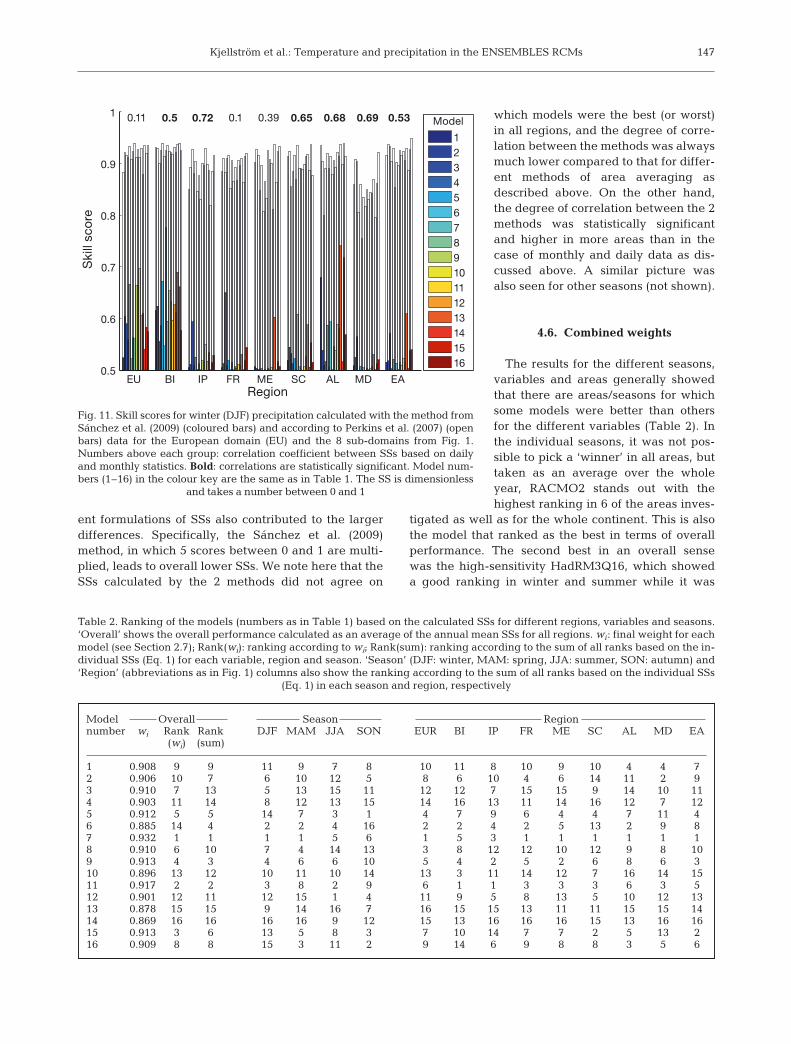
For monthly precipitation, we present SSs for winter(DJF) based on the 2 methods outlined above (Eqs. 1 & 7)in Fig. 11. The difference in absolute numbers wasvery large, with the Perkins et al. (2007) method (Eq. 1)giving much higher numbers compared to that used bySánchez et al. (2009) (Eq. 7). The difference in absolutenumbers calculated by the 2 methods was much largerthan when comparing SSs based on monthly and dailydata calculated with the same SS (Eq. 1) as presentedin Fig. 8. In addition to the inclusion of more days withlittle or no precipitation, as discussed above, the differ-

146


0.6

0.7

0.8

0.9

1

Region

Skill

sco

re

1

2

3

4

5

6

7

8

9

10

11

12

13

14

15

16

0.89 0.98 0.95 0.99 0.99 0.96 0.97 0.95 0.99 Model

Fig. 10. Skill scores calculated for winter (DJF) daily minimum temperatures. Areaaveraging over the regions was done according to Method (3) (outlined in Section2.5), by calculating SSs in each grid box individually (coloured bars) and accord-ing to Method (1) by pooling all individual grid box data into 1 common probabil-ity distribution (open bars) for the European domain (EU) and the 8 sub-domainsfrom Fig. 1. Numbers above each group: correlation coefficient between SSsbased on the 2 sets of area averages. Model numbers (1–16) in the colour key are thesame as in Table 1. The SS is dimensionless and takes a number between 0 and 1


ent formulations of SSs also contributed to the largerdifferences. Specifically, the Sánchez et al. (2009)method, in which 5 scores between 0 and 1 are multi-plied, leads to overall lower SSs. We note here that theSSs calculated by the 2 methods did not agree on

which models were the best (or worst)in all regions, and the degree of corre-lation between the methods was alwaysmuch lower compared to that for differ-ent methods of area averaging asdescribed above. On the other hand,the degree of correlation between the 2methods was statistically significantand higher in more areas than in thecase of monthly and daily data as dis-cussed above. A similar picture wasalso seen for other seasons (not shown).

4.6. Combined weights

The results for the different seasons,variables and areas generally showedthat there are areas/seasons for whichsome models were better than othersfor the different variables (Table 2). Inthe individual seasons, it was not pos-sible to pick a ‘winner’ in all areas, buttaken as an average over the wholeyear, RACMO2 stands out with thehighest ranking in 6 of the areas inves-

tigated as well as for the whole continent. This is alsothe model that ranked as the best in terms of overallperformance. The second best in an overall sensewas the high-sensitivity HadRM3Q16, which showeda good ranking in winter and summer while it was

147

0.11 0.5 0.72 0.1 0.39 0.65 0.68 0.69 0.53


0.6

0.7

0.8

0.9

1

Region

Skill

sco

re

1

2

3

4

5

6

7

8

9

10

11

12

13

14

15

16

Model

Fig. 11. Skill scores for winter (DJF) precipitation calculated with the method fromSánchez et al. (2009) (coloured bars) and according to Perkins et al. (2007) (openbars) data for the European domain (EU) and the 8 sub-domains from Fig. 1.Numbers above each group: correlation coefficient between SSs based on dailyand monthly statistics. Bold: correlations are statistically significant. Model num-bers (1–16) in the colour key are the same as in Table 1. The SS is dimensionless

and takes a number between 0 and 1

Model Overall Season Regionnumber wi Rank Rank DJF MAM JJA SON EUR BI IP FR ME SC AL MD EA

(wi) (sum)

1 0.908 9 9 11 9 7 8 10 11 8 10 9 10 4 4 72 0.906 10 7 6 10 12 5 8 6 10 4 6 14 11 2 93 0.910 7 13 5 13 15 11 12 12 7 15 15 9 14 10 114 0.903 11 14 8 12 13 15 14 16 13 11 14 16 12 7 125 0.912 5 5 14 7 3 1 4 7 9 6 4 4 7 11 46 0.885 14 4 2 2 4 16 2 2 4 2 5 13 2 9 87 0.932 1 1 1 1 5 6 1 5 3 1 1 1 1 1 18 0.910 6 10 7 4 14 13 3 8 12 12 10 12 9 8 109 0.913 4 3 4 6 6 10 5 4 2 5 2 6 8 6 310 0.896 13 12 10 11 10 14 13 3 11 14 12 7 16 14 1511 0.917 2 2 3 8 2 9 6 1 1 3 3 3 6 3 512 0.901 12 11 12 15 1 4 11 9 5 8 13 5 10 12 1313 0.878 15 15 9 14 16 7 16 15 15 13 11 11 15 15 1414 0.869 16 16 16 16 9 12 15 13 16 16 16 15 13 16 1615 0.913 3 6 13 5 8 3 7 10 14 7 7 2 5 13 216 0.909 8 8 15 3 11 2 9 14 6 9 8 8 3 5 6

Table 2. Ranking of the models (numbers as in Table 1) based on the calculated SSs for different regions, variables and seasons.‘Overall’ shows the overall performance calculated as an average of the annual mean SSs for all regions. wi: final weight for eachmodel (see Section 2.7); Rank(wi): ranking according to wi; Rank(sum): ranking according to the sum of all ranks based on the in-dividual SSs (Eq. 1) for each variable, region and season. ‘Season’ (DJF: winter, MAM: spring, JJA: summer, SON: autumn) and‘Region’ (abbreviations as in Fig. 1) columns also show the ranking according to the sum of all ranks based on the individual SSs

(Eq. 1) in each season and region, respectively

Clim Res 44: 135–150, 2010

intermediate among the other models during the tran-sition seasons. A few models that performed less wellthan the others in most areas and seasons can beidentified from Table 2. Many of the other modelsshowed good performance during part of the year, orin part of the domain, and worse agreement in others.An example of such behaviour is REMO, which wasthe overall best model in summer, while its perfor-mance during spring ranked among the poorest mod-els. The latter may be related to the temperaturebiases close to 0°C, as discussed above. Other similarexamples include the RCA3.0 and ALADIN, whoseperformance was among the best in some areas, whilein others those particular models ranked among theworst. These results clearly show that depending onarea and season of interest, different models have dif-ferent skills in representing the observed climate. Animplication of this is that a general measure of overallskill in the whole model domain, and/or for all sea-sons, is not necessarily the best measure of skill inindividual regions and seasons.

4.7. Evaluation of the weighting

As a test of the use of the weights in order to improvean RCM ensemble, we tested whether a weightedmodel mean outperforms an unweighted arithmeticmean. The weighted ensemble mean (WEMj) was cal-culated as

(9)

where wirs is the model specific weight(Eq. 8) and VARj is the variable inquestion. Weighted ensemble meanseasonal averages showed very smalldifferences with regard to the un-weighted averages (not shown). Fordaily maximum and minimum temper-ature, this means generally < 0.1°C formost grid boxes and correspondingly<±30% for precipitation, althoughlarger relative biases do occur inmountainous areas and in the dryMediterranean area in summer. Thesesmall differences are a result of thesmall spread in the overall weights(Table 2).

An additional test was done inwhich we constructed more discrimi-nating weights based on the overallranking of the models (Table 2). Thiswas achieved simply by assigning

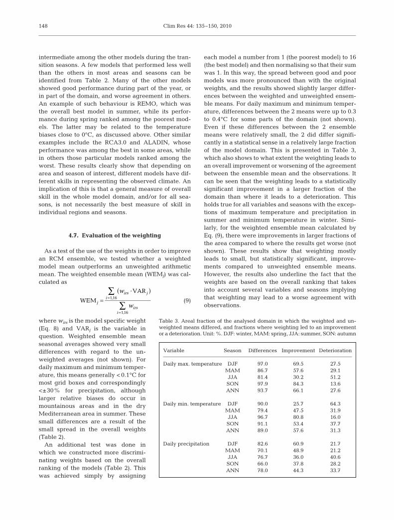
each model a number from 1 (the poorest model) to 16(the best model) and then normalising so that their sumwas 1. In this way, the spread between good and poormodels was more pronounced than with the originalweights, and the results showed slightly larger differ-ences between the weighted and unweighted ensem-ble means. For daily maximum and minimum temper-ature, differences between the 2 means were up to 0.3to 0.4°C for some parts of the domain (not shown).Even if these differences between the 2 ensemblemeans were relatively small, the 2 did differ signifi-cantly in a statistical sense in a relatively large fractionof the model domain. This is presented in Table 3,which also shows to what extent the weighting leads toan overall improvement or worsening of the agreementbetween the ensemble mean and the observations. Itcan be seen that the weighting leads to a statisticallysignificant improvement in a larger fraction of thedomain than where it leads to a deterioration. Thisholds true for all variables and seasons with the excep-tions of maximum temperature and precipitation insummer and minimum temperature in winter. Simi-larly, for the weighted ensemble mean calculated byEq. (9), there were improvements in larger fractions ofthe area compared to where the results get worse (notshown). These results show that weighting mostlyleads to small, but statistically significant, improve-ments compared to unweighted ensemble means.However, the results also underline the fact that theweights are based on the overall ranking that takesinto account several variables and seasons implyingthat weighting may lead to a worse agreement withobservations.

WEM

VAR

j

irs ji

irsi

w

w=

( )=

=

∑

∑

·,

,

116

116

148

Variable Season Differences Improvement Deterioration

Daily max. temperature DJF 97.0 69.5 27.5MAM 86.7 57.6 29.1JJA 81.4 30.2 51.2SON 97.9 84.3 13.6ANN 93.7 66.1 27.6

Daily min. temperature DJF 90.0 25.7 64.3MAM 79.4 47.5 31.9JJA 96.7 80.8 16.0SON 91.1 53.4 37.7ANN 89.0 57.6 31.3

Daily precipitation DJF 82.6 60.9 21.7MAM 70.1 48.9 21.2JJA 76.7 36.0 40.6SON 66.0 37.8 28.2ANN 78.0 44.3 33.7

Table 3. Areal fraction of the analysed domain in which the weighted and un-weighted means differed, and fractions where weighting led to an improvementor a deterioration. Unit: %. DJF: winter, MAM: spring, JJA: summer, SON: autumn


5. SUMMARY AND CONCLUSIONS

• Biases in daily minimum temperature were large innorthern Europe during winter, most notably for lowend percentiles, when most models tended to simulatetoo warm conditions. These differences between mod-els and observations tended to be largest in northernScandinavia. Possibly, this discrepancy is more a con-sequence of the fact that observations and models rep-resent different features than an indication of a sys-tematic model error in this area.

• The highest SSs for daily maximum temperature insummer were seen in parts of central Europe in manymodels. Worse agreement was obtained in Scandi-navia and also in southern Europe in some models.Biases in different regions were different, both in signand amplitude, in different parts of the probability dis-tributions among the RCMs.

• Biases in daily precipitation were most pronouncedin the wettest part of the probability distribution wherethe RCMs tended to overestimate precipitation com-pared to the E-OBS data set. The overestimation grewwith increasing amounts of precipitation. Skill scoreswere higher for precipitation than for temperature dueto a good correspondence between models and obser-vations for moderate precipitation.

• The calculated SSs and the evaluation performedhere indicated that some models performed poorly forsome variables and seasons. The underlying reasonsfor this were not revealed by our analysis, althoughresults of this type may assist in identifying potentialproblems in different models.

• Applied on the present data set, the Perkins et al.(2007) method (Eq. 1) for calculating SSs gave a rela-tively small spread among the models. This is not sur-prising, as the method, by definition, integrates overthe entire probability distributions. Further, positiveand negative biases gave similar SSs, and biases in dif-ferent parts of the probability distribution had equalinfluence on the resulting SS.

• The evaluation performed here over different vari-ables, seasons and regions showed that some models canbe better/worse than the others in an overall sense butthat no model is best/worst in all aspects. The evaluationshowed that some models performed well in some re-gions and seasons and poorly in others. An implication ofthis is that preferably the whole ensemble should beused in studies of climate change and impact studies.Another implication is that weighting of a model ensem-ble possibly should not be based on overall performancemeasures of the models, but instead should be based ondifferent weights for different regions, seasons, vari-ables, etc., depending on individual applications.

• The sensitivity to area averaging over the regionsin Europe was small as the resulting SSs and ranking

of models were similar regardless of whether areaaveraging was done before or after calculating SSs.

• The sensitivity to choice of SS metric was verylarge. The 2 different methods used for calculating SSsfor monthly precipitation gave substantially differentnumbers and also different rankings of the models.

• The sensitivity to choice of input data was large.The same SS metric based on daily data excluding dryevents, or monthly data including both wet and dryevents, gave very different results in terms of modelranking. This was most likely a result of the fact thatthe underlying PDFs differed, and that dry days wereexcluded from the daily data.

• We found that weighted ensemble means werecloser to observations than corresponding unweightedensemble means for most, but not all, variables andseasons. This is the result of there being statisticallysignificant improvements in a larger fraction of thedomain than where the agreement deteriorated. Thisheld true both for the original weights calculated fromthe SSs presented here and for more discriminatingweights based on a ranking of the models. The differ-ences, however, were small: for daily minimum andmaximum temperatures, generally below 0.1°C formost grid boxes for the original weights, and mostoften below 0.3 to 0.4°C for the more discriminatingweights.

Acknowledgements. This work was supported by the Euro-pean Commission Programme FP6 under the contract GOCE-CT-2006-037005 (ENSEMBLES). We acknowledge the E-OBSdataset from the EU-FP6 project ENSEMBLES (http://ensembles-eu.metoffice.com) and the data providers in theECA&D project (http://eca.knmi.nl). We are grateful to allregional climate modelling groups providing their RCM dataand to DMI for providing the data at the data distribution por-tal. Part of the analysis was done within the Nordic Climateand Energy Systems project. Finally, we thank 3 anonymousreviewers for constructive comments on an earlier version ofthis manuscript.

LITERATURE CITED

Beniston M, Stephenson DB, Christensen OB, Ferro CAT andothers (2007) Future extreme events in European climate:an exploration of regional climate model projections. ClimChange 81(Suppl 1):71–95

Boberg F, Berg P, Thejll P, Gutowski WJ, Christensen JH(2009a) Improved confidence in climate change projec-tions of precipitation evaluated using daily statistics fromthe PRUDENCE ensemble. Clim Dyn 32:1097–1106

Boberg F, Berg P, Thejll P, Gutowski WJ, Christensen JH(2009b) Improved confidence in climate change projec-tions of precipitation further evaluated using daily statis-tics from ENSEMBLES models. Clim Dyn doi:10.1007/s00382-009-0683-8

Böhm U, Kücken M, Ahrens W, Block A, Hauffe D, Keuler K,Rockel B, Will A (2006) CLM — the climate version of LM:brief description and long-term applications. COSMONewsletter 6

149

Clim Res 44: 135–150, 2010

Christensen JH, Christensen OB (2007) A summary of thePRUDENCE model projections of changes in Europeanclimate by the end of the century. Clim Change 81:7–30

Christensen OB, Drews M, Christensen JH, Dethloff K,Ketelsen K, Hebestadt I, Rinke A (2006) The HIRHAMRegional Climate Model Version 5 (β). DMI, Tech Rep 06-17

Christensen JH, Hewitson B, Busuioc A, Chen A and others(2007) Regional climate projections. In: Solomon S, Qin D,Manning M, Chen Z and others (eds) Climate change2007: the physical science basis. Contribution of WorkingGroup I to the Fourth Assessment Report of the Intergov-ernmental Panel on Climate Change. Cambridge Univer-sity Press, Cambridge, p 847–940

Christensen JH, Kjellström E, Giorgi F, Lenderink G, Rum-mukainen M (2010) Weight assignment in regional cli-mate models. Clim Res 44:179–194

Collins M, Booth BB, Bhaskaran B, Harris GR, Murphy JM,Sexton DMH, Webb MJ (2010) Climate model errors,feedbacks and forcings: a comparison of perturbedphysics and multi-model ensembles. Clim Dyn doi: 10.1007/s00382-010-0808-0

Côté J, Gravel S, Methot A, Patoine A, Roch M, Staniforth A(1998) The operational CMC/MRB Global EnvironmentalMultiscale (GEM) model. I. design considerations and for-mulation. Mon Weather Rev 126:1373–1395

Dai A (2001) Global precipitation and thunderstorm frequen-cies. I. Seasonal and interannual variations. J Clim 14:1092–1111

Déqué M, Somot S (2010) Weighted frequency distributionsexpress modelling uncertainties in the ENSEMBLESregional climate experiments. Clim Res 44:195–209

Farda A, Déqué M, Somot S, Horanyi A, Spiridonov V, TothH (2010) Model ALADIN as regional climate model forcentral and eastern Europe. Stud Geophys Geod 54:313–332

Giorgi F, Mearns LO (1999) Introduction to special section:regional climate modeling revisited. J Geophys Res 104:6335–6352

Haugen JE, Haakenstad H (2006) Validation of HIRHAM ver-sion 2 with 50 and 25 km resolution. RegClim Gen TechRep 9:159–173

Haylock MR, Hofstra N, Klein Tank AMG, Klok EJ, Jones PD,New M (2008) A European daily high-resolution griddeddataset of surface temperature and precipitation. J Geo-phys Res 113:D20119 doi:10/1029/2009JD011799

Hewitt C, Griggs D (2005) Ensembles-based predictions ofclimate changes and their impacts. Eos Trans Am GeophysUnion 85:566

Hofstra N, Haylock M, New M, Jones PD (2009) Testing E-OBS European high-resolution gridded dataset of dailyprecipitation and surface temperature. J Geophys Res 114:D21101 doi:10.1029/2009JD011799

Jacob D (2001) A note to the simulation of the annual andinter-annual variability of the water budget over the BalticSea drainage basin. Meteorol Atmos Phys 77:61–73

Jacob D, Bärring L, Christensen OB, Christensen JH and others(2007) An inter-comparison of regional climate models forEurope: design of the experiments and model performance.Clim Change 81:31–52

Kjellström E, Bärring L, Gollvik S, Hansson U and others(2005) A 140-year simulation of European climate with thenew version of the Rossby Centre regional atmospheric cli-mate model (RCA3). Rep Meteorol Climatol 108. SwedishMeteorological and Hydrological Institute, Norrköping

Kjellström E, Bärring L, Jacob D, Jones R, Lenderink G,Schär C (2007) Modelling daily temperature extremes:

recent climate and future changes over Europe. ClimChange 81:249–265

Klein Tank AMG, Wijngaard JB, Können GP, Böhm R andothers (2002) Daily dataset of 20th-century surface airtemperature and precipitation series for the European Cli-mate Assessment. Int J Climatol 22:1441–1453

Klok EJ, Klein Tank AM (2009) Updated and extended Euro-pean dataset of daily climate observations. Int J Climatol29:1182–1191

Lettenmaier D (1995) Stochastic modeling of precipitationwith applications to climate model downscaling. In: VonStorch H, Navarra A (eds) Analysis of climate variability;applications of statistical techniques. Springer, Berlin,p 197–212

Moberg A, Jones PD (2004) Regional climate model simula-tions of daily maximum and minimum near-surface tem-peratures across Europe compared with observed stationdata 1961–1990. Clim Dyn 23:695–715

Nikulin G, Kjellström E, Hansson U, Jones C, Strandberg G,Ullerstig A (2010) Evaluation and future projections oftemperature, precipitation and wind extremes overEurope in an ensemble of regional climate simulations.Tellus Ser A Dyn Meterol Oceanogr (in press) doi:10.1111/j.1600-0870.2010.00466.x

Perkins SE, Pitman AJ, Holbrook NJ, McAneney J (2007)Evaluation of the AR4 climate models’ simulated dailymaximum temperature, minimum temperature, and pre-cipitation over Australia using probability density func-tions. J Clim 20:4356–4376

Plummer D, Caya D, Coté H, Frigon A and others (2006) Cli-mate and climate change over North America as simu-lated by the Canadian regional climate model. J Clim 19:3112–3132

Radu R, Déqué M, Somot S (2008) Spectral nudging in a spec-tral regional climate model. Tellus Ser A Dyn MeterolOceanogr 60:898–910

Räisänen J, Hansson U, Ullerstig A, Döscher R and others(2004) European climate in the late 21st century: regionalsimulations with two driving global models and two forc-ing scenarios. Clim Dyn 22:13–31

Rockel B, Woth K (2007) Extremes of near-surface wind speedover Europe and their future changes as estimated froman ensemble of RCM simulations. Clim Change 81:267–280

Sánchez E, Gallardo C, Gaertner MA, Arribas A, Castro M(2004) Future climate extreme events in the Mediter-ranean simulated by a regional climate model: a firstapproach. Glob Planet Change 44:163–180

Sánchez E, Romera R, Gaertner MA, Gallardo C, Castro M(2009) A weighting proposal for an ensemble of regionalclimate models over Europe driven by 1961–2000 ERA40based on monthly precipitation probability density func-tions. Atmos Sci Lett 10:241–248

Uppala SM, Kållberg PW, Simmons AJ, Andrae U and others(2005) The ERA-40 re-analysis. QJR Meteorol Soc 131:2961–3012

van der Linden P, Mitchell JFB (eds) (2009) ENSEMBLES: cli-mate change and its impacts: summary of research andresults from the ENSEMBLES project. Met Office, HadleyCentre, Exeter

van Meijgaard E, van Ulft LH, van de Berg WJ, Bosveld FC,van den Hurk BJJM, Lenderink G, Siebesma AP (2008)The KNMI regional atmospheric climate model RACMO,version 2.1. TR-302, KNMI, De Bilt

Zadra A, Caya D, Côté J, Dugas B, and others (2008) The nextCanadian Regional Climate Model. Phys Can 64:75–83

150

Submitted: February 10, 2010; Accepted: September 7, 2010 Proofs received from author(s): November 17, 2010

Daily and monthly temperature and precipitation statistics as performance indicators for regional...

Documents

Transcript of Daily and monthly temperature and precipitation statistics as performance indicators for regional...