d9d1d-pkpup-3-2021.pdf - JUPEM

. 2 .

antara koordinat yang berpunca daripada penggunaan datum geodetik yang

berlainan ini, jika sekiranya tidak diuruskan dengan baik, boleh dan sering

menimbulkan kesilapan di dalam kerja-kerja pengukuran serta produk ukur

dan pemetaan.

2.4. Oleh itu, maklumat mengenai kaedah penukaran koordinat, transformasi

datum dan unjuran peta yang sedia ada wajar dikemaskini dan

didokumentasikan supaya ianya sentiasa relevan dengan kehendak dan

tuntutan semasa serta dapat dijadikan panduan dan rujukan kepada para

pengguna dalam menguruskan kerja-kerja yang mempunyai kaitan dengan

koordinat. Sehubungan dengan itu, Pekeliling ini diharapkan akan dapat

membantu pengguna-pengguna produk-produk pemetaan, kadaster, utiliti

dan sebagainya untuk memahami kaedah-kaedah tersebut dan seterusnya

dapat menggunakannya dengan cara yang betul di dalam urusan kerja

mereka, terutamanya di dalam era penggunaan teknologi GNSS yang

semakin meluas di Malaysia.

3. PERKEMBANGAN PEMBANGUNAN INFRASTRUKTUR GEODETIK DI

MALAYSIA

3.1. Sejak penubuhan Jabatan Ukur dan Pemetaan Malaysia (JUPEM) lebih

daripada 135 tahun yang lalu, datum geodetik yang digunapakai untuk

kegunaan ukur dan pemetaan telah mengalami pelbagai perubahan. Dalam

hal ini, sebelum tahun 1990an, Datum Kertau telah pun menjadi tulang

belakang kepada Malayan Revised Triangulation 1968 (MRT68) di

Semenanjung Malaysia, manakala bagi Sabah, Sarawak dan Labuan pula,

Borneo Triangulation 1968 (BT68) merujuk kepada Datum Timbalai sebagai

asasnya.

3.2. Dengan perkembangan teknologi GNSS yang meluas sekitar tahun

1980-an, JUPEM telah membangunkan rangkaian kawalan ukur geodetik

yang baharu dengan menggunakan teknologi tersebut untuk menentukan

koordinat bagi stesen-stesen kawalan. Bagi Semenanjung Malaysia,

rangkaian ini telah ditubuhkan dalam tahun 1994 dan dikenali sebagai

Peninsular Malaysia Geodetic Scientific Network 1994 (PMGSN94).

Manakala di Sabah, Sarawak dan Labuan pula, rangkaian kawalan ukur

geodetiknya adalah East Malaysia Geodetic Scientific Network 1997

(EMGSN97), yang ditubuhkan pada tahun 1997.

. 3 .

3.3. Antara tahun 1998 dan 2001 pula, JUPEM telah membangunkan

rangkaian Malaysia Active GPS System (MASS) dan ini telah diikuti

dengan Malaysia Real-Time Kinematic GNSS Network (MyRTKnet)

antara tahun 2002 dan 2008. Dalam pada itu, pada 26 Ogos 2003,

JUPEM telah melancarkan Geocentric Datum of Malaysia 2000

(GDM2000), iaitu datum rujukan geodetik baharu yang seragam bagi

kerja-kerja ukur dan pemetaan di Malaysia.

3.4. Walau bagaimanapun, GDM2000 telah mengalami anjakan yang

signifikan, lanjutan daripada berlakunya beberapa siri gempa bumi besar

di Indonesia, terutamanya pada tahun 2004 dan 2005. Sehubungan itu,

datum ini telah disemak dan dihitung semula dengan mengambil kira

penambahan stesen MyRTKnet pada tahun 2006 yang dikenali sebagai

GDM2000 (Rev 2006). Pada tahun 2007, telah berlaku satu gempa bumi

besar di Sumatera, Indonesia yang juga telah menyebabkan anjakan

signifikan dan JUPEM telah melaksanakan semakan dan hitungan

semula berdasarkan anjakan ke atas stesen-stesen MyRTKnet dan

menghasilkan GDM2000 (Rev 2009).

3.5. Koordinat GDM2000 dan siri-siri kemaskininya diklasifikasikan sebagai

datum statik di mana koordinat dianggap tidak berubah dan merujuk

kepada International Terrestrial Reference Frame (ITRF) 2000 pada

epok 1 Januari 2000. Koordinat dalam datum statik perlu sentiasa

dikemaskini bagi mengekalkan ketepatan dengan mengambilkira kesan

daripada fenomena alam seperti gempa bumi, pergerakan plat tektonik

dan deformasi setempat. Pada masa yang sama, ITRF juga telah

dikemaskini beberapa kali dan realisasi terkini dikenali sebagai

ITRF2014 yang diperkenalkan pada 22 Januari 2016.

3.6. Bagi mengekalkan ketepatan koordinat pada stesen-stesen MyRTKnet,

JUPEM telah membangunkan datum baharu berasaskan konsep semi

kinematik melalui permodelan pergerakan stesen-stesen yang terlibat

dan koordinat dikemaskini mengikut sela masa tertentu.

3.7. Maklumat lebih lanjut mengenai sistem rujukan koordinat terkandung di

dalam Pekeliling Ketua Pengarah Ukur dan Pemetaan Malaysia Bilangan 2

Tahun 2021 bertarikh 13 Oktober 2021 bertajuk Garis Panduan Mengenai

Sistem Rujukan Koordinat Bagi Tujuan Ukur dan Pemetaan di Malaysia. Ia

. 4 .

menyenaraikan semua jenis sistem rujukan koordinat yang telah

dibangunkan oleh JUPEM di Malaysia di samping memberi maklumat-

maklumat teknikal mengenainya.

4. GARIS PANDUAN PENUKARAN KOORDINAT, TRANSFORMASI DATUM

DAN UNJURAN PETA UNTUK TUJUAN UKUR DAN PEMETAAN

Penerangan lebih lanjut tentang amalan penggunaan penukaran koordinat,

transformasi datum dan unjuran peta terkandung di dalam dokumen Technical

Guide to the Coordinate Conversion, Datum Transformation, Map Projection

seperti di Lampiran ‘A’ yang disertakan. Intisari garis panduan tersebut adalah

seperti berikut:

Perenggan Perkara

1. INTRODUCTION

2. COORDINATE CONVERSION

2.1 GEOGRAPHICAL AND CARTESIAN COORDINATES

2.2 CONVERSION BETWEEN GEOGRAPHICAL

COORDINATES AND CARTESIAN COORDINATES

2.3 TEST EXAMPLE

3. DATUM TRANSFORMATION

3.1 INTRODUCTION

3.2 BURSA-WOLF DATUM TRANSFORMATION

FORMULAE

3.3 MULTIPLE REGRESSION MODEL

3.4 TIME-DEPENDENT REFERENCE FRAME

3.5 TEST EXAMPLES

4. MAP PROJECTION

4.1 RECTIFIED SKEW ORTHOMORPHIC PROJECTION

(RSO)

4.2 CASSINI-SOLDNER PROJECTION

4.3 POLYNOMIAL FUNCTION

4.4 REDEFINITION OF STATE ORIGINS IN GDM2000

AND GDM2020

4.5 TEST EXAMPLES

5. CONCLUSION

. 6 .

Salinan Edaran Dalaman:

Timbalan Ketua Pengarah Ukur dan Pemetaan I

Timbalan Ketua Pengarah Ukur dan Pemetaan II

Salinan Edaran Luaran:

Setiausaha Bahagian (Kanan)

Tanah, Ukur dan Geospatial

Kementerian Tenaga dan Sumber Asli

Wisma Sumber Asli

No. 25, Persiaran Perdana, Presint 4

62574 PUTRAJAYA

Ketua Pengarah

Jabatan Kerajaan Tempatan

Bahagian Penyelidikan dan Perundangan Teknikal

Kementerian Kesejahteraan Bandar, Perumahan dan Kerajaan Tempatan

Aras 25 - 29, No. 51 , Persiaran Perdana, Presint 4

62100 PUTRAJAYA

Ketua Pengarah

PLANMalaysia (Jabatan Perancangan Bandar dan Desa)

Aras 13, Blok F5, Parcel F, Presint 1

Pusat Pentadbiran Kerajaan Persekutuan

62675 PUTRAJAYA

Pengarah

lnstitut Tanah dan Ukur Negara

Kementerian Tenaga dan Sumber Asli

Behrang

35950 TANJUNG MALIM

. 7 .

Pengarah

Cawangan Jalan

Tingkat 10, Blok F, lbu Pejabat JKR

Jin Sultan Salahuddin

50582 KUALA LUMPUR

Ketua Penolong Pengarah Kanan

Bahagian Ukur Tanah

Cawangan Kejuruteraan lnfrastruktur Pengangkutan

lbu Pejabat JKR Malaysia

Aras 19, No. 50, Menara PJD

Jalan Tun Razak

50400 KUALA LUMPUR

Setiausaha

Lembaga Jurukur Tanah Malaysia (LJT)

Level 5-7, Wisma LJT

Lorong Perak, Pusat Bandar Melawati

53100 KUALA LUMPUR

Presiden

Persatuan Jurukur Tanah Bertauliah Malaysia

2735A, Jalan Permata 4

Taman Permata, Ulu Kelang

53300 WP KUALA LUMPUR

. 1 .

Lampiran ‘A’

Technical Guide

to the Coordinate Conversion,

Datum Transformation

and Map Projection

. 2 .

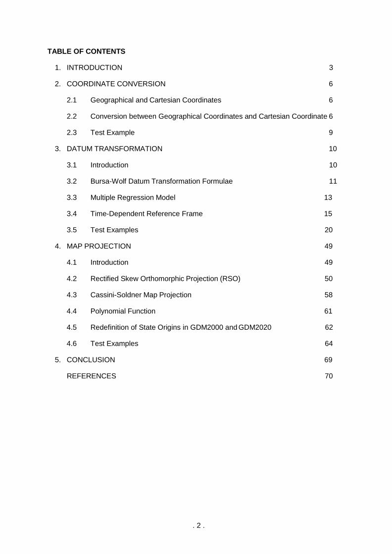
TABLE OF CONTENTS

1. INTRODUCTION 3

2. COORDINATE CONVERSION 6

2.1 Geographical and Cartesian Coordinates 6

2.2 Conversion between Geographical Coordinates and Cartesian Coordinate 6

2.3 Test Example 9

3. DATUM TRANSFORMATION 10

3.1 Introduction 10

3.2 Bursa-Wolf Datum Transformation Formulae 11

3.3 Multiple Regression Model 13

3.4 Time-Dependent Reference Frame 15

3.5 Test Examples 20

4. MAP PROJECTION 49

4.1 Introduction 49

4.2 Rectified Skew Orthomorphic Projection (RSO) 50

4.3 Cassini-Soldner Map Projection 58

4.4 Polynomial Function 61

4.5 Redefinition of State Origins in GDM2000 and GDM2020 62

4.6 Test Examples 64

5. CONCLUSION 69

REFERENCES 70

. 3 .

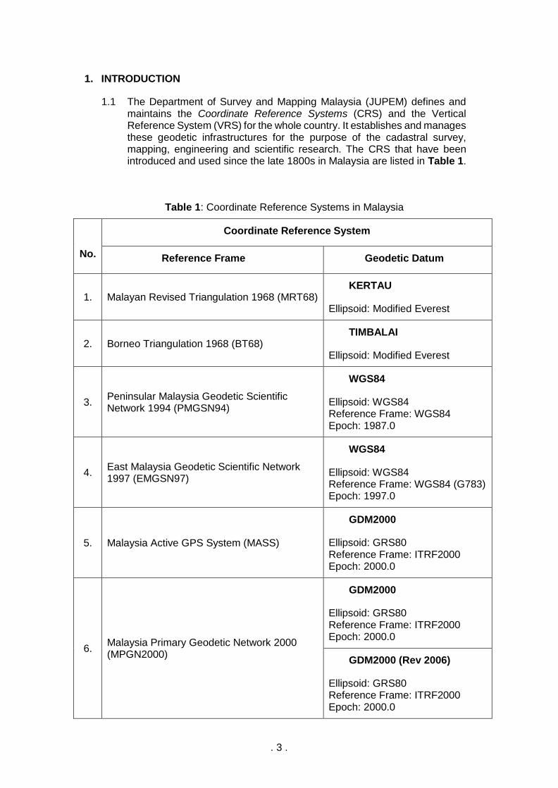
1. INTRODUCTION

1.1 The Department of Survey and Mapping Malaysia (JUPEM) defines and maintains the Coordinate Reference Systems (CRS) and the Vertical Reference System (VRS) for the whole country. It establishes and manages these geodetic infrastructures for the purpose of the cadastral survey, mapping, engineering and scientific research. The CRS that have been introduced and used since the late 1800s in Malaysia are listed in Table 1.

Table 1: Coordinate Reference Systems in Malaysia

No.

Coordinate Reference System

Reference Frame Geodetic Datum

1. Malayan Revised Triangulation 1968 (MRT68) KERTAU

Ellipsoid: Modified Everest

2. Borneo Triangulation 1968 (BT68) TIMBALAI

Ellipsoid: Modified Everest

3. Peninsular Malaysia Geodetic Scientific Network 1994 (PMGSN94)

WGS84

Ellipsoid: WGS84 Reference Frame: WGS84 Epoch: 1987.0

4. East Malaysia Geodetic Scientific Network 1997 (EMGSN97)

WGS84

Ellipsoid: WGS84 Reference Frame: WGS84 (G783) Epoch: 1997.0

5. Malaysia Active GPS System (MASS)

GDM2000

Ellipsoid: GRS80 Reference Frame: ITRF2000 Epoch: 2000.0

6. Malaysia Primary Geodetic Network 2000 (MPGN2000)

GDM2000


GDM2000 (Rev 2006)


. 4 .

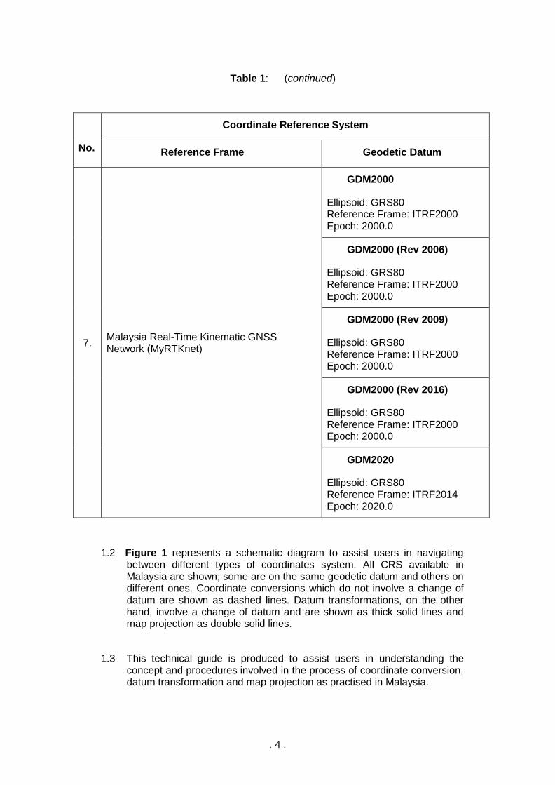
Table 1: (continued)

No.

Coordinate Reference System

Reference Frame Geodetic Datum

7. Malaysia Real-Time Kinematic GNSS Network (MyRTKnet)

GDM2000


GDM2000 (Rev 2006)


GDM2000 (Rev 2009)


GDM2000 (Rev 2016)


GDM2020


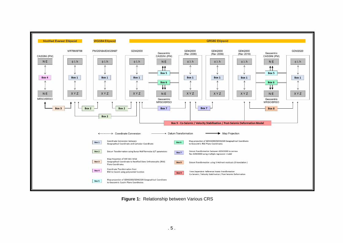
1.2 Figure 1 represents a schematic diagram to assist users in navigating between different types of coordinates system. All CRS available in Malaysia are shown; some are on the same geodetic datum and others on different ones. Coordinate conversions which do not involve a change of datum are shown as dashed lines. Datum transformations, on the other hand, involve a change of datum and are shown as thick solid lines and map projection as double solid lines.

1.3 This technical guide is produced to assist users in understanding the concept and procedures involved in the process of coordinate conversion, datum transformation and map projection as practised in Malaysia.

. 5 .

Figure 1: Relationship between Various CRS

. 6 .

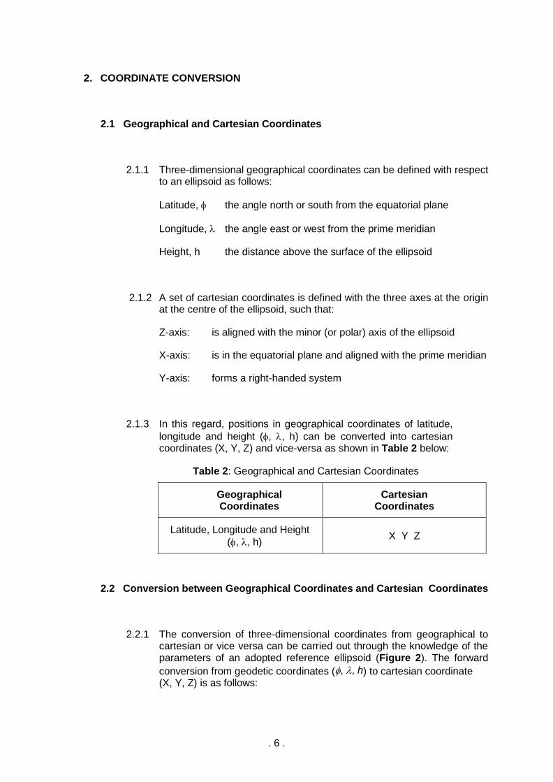
2. COORDINATE CONVERSION

2.1 Geographical and Cartesian Coordinates

2.1.1 Three-dimensional geographical coordinates can be defined with respect to an ellipsoid as follows:

Latitude, the angle north or south from the equatorial plane

Longitude, the angle east or west from the prime meridian

Height, h the distance above the surface of the ellipsoid

2.1.2 A set of cartesian coordinates is defined with the three axes at the origin at the centre of the ellipsoid, such that:

Z-axis: is aligned with the minor (or polar) axis of the ellipsoid

X-axis: is in the equatorial plane and aligned with the prime meridian

Y-axis: forms a right-handed system

2.1.3 In this regard, positions in geographical coordinates of latitude,

longitude and height (, , h) can be converted into cartesian coordinates (X, Y, Z) and vice-versa as shown in Table 2 below:

Table 2: Geographical and Cartesian Coordinates

Geographical Coordinates

Cartesian Coordinates

Latitude, Longitude and Height

(, , h) X Y Z

2.2 Conversion between Geographical Coordinates and Cartesian Coordinates

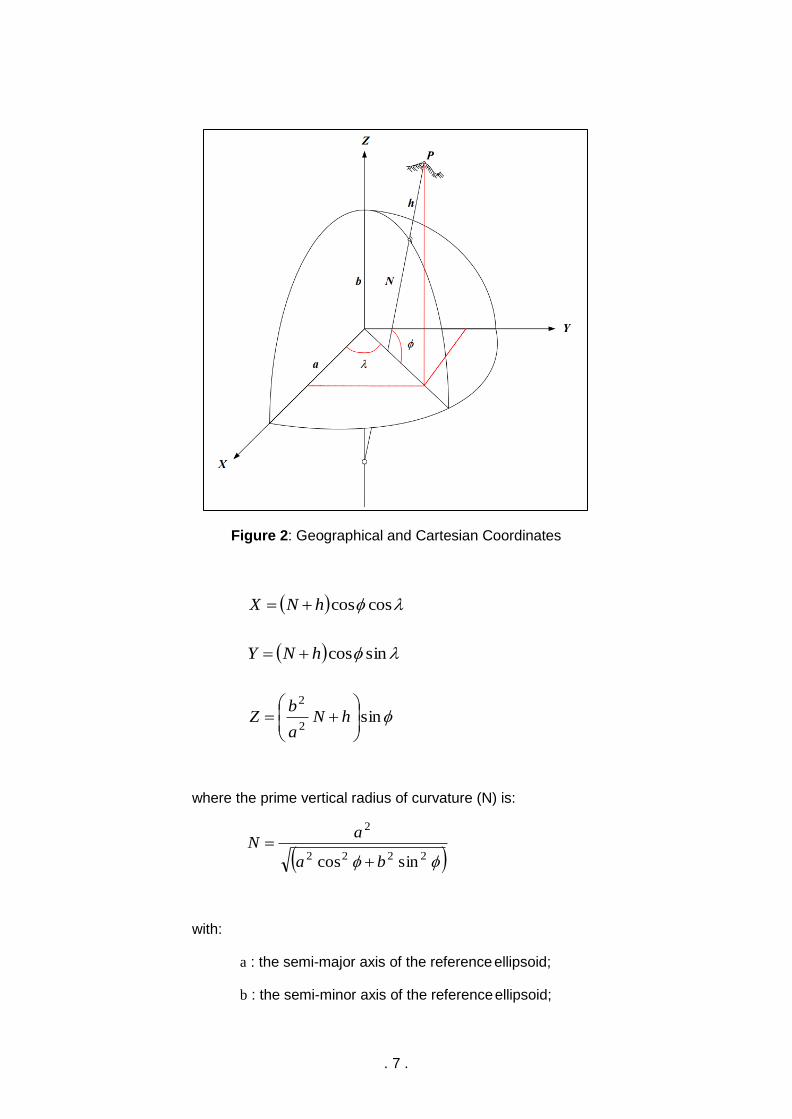
2.2.1 The conversion of three-dimensional coordinates from geographical to cartesian or vice versa can be carried out through the knowledge of the parameters of an adopted reference ellipsoid (Figure 2). The forward

conversion from geodetic coordinates (, , h) to cartesian coordinate (X, Y, Z) is as follows:

. 7 .

Figure 2: Geographical and Cartesian Coordinates

where the prime vertical radius of curvature (N) is:

with:

a : the semi-major axis of the reference ellipsoid;

b : the semi-minor axis of the reference ellipsoid;

( ) coscoshNX +=

( ) sincoshNY +=

sin2

2

+= hN

a

bZ

( ) 2222

2

sincos ba

aN

+

=

. 8 .

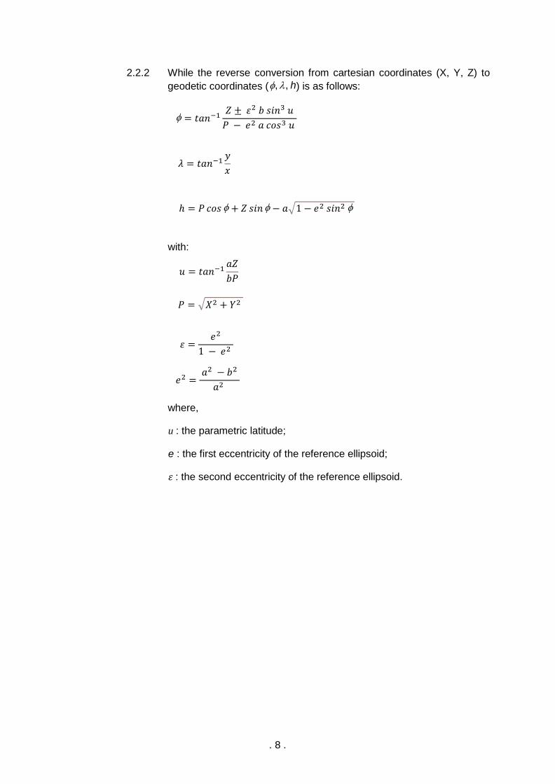
2.2.2 While the reverse conversion from cartesian coordinates (X, Y, Z) to

geodetic coordinates ( , , h) is as follows:

with:

where,

u : the parametric latitude;

e : the first eccentricity of the reference ellipsoid;

휀 : the second eccentricity of the reference ellipsoid.

= 𝑡𝑎𝑛−1𝑍 ± 휀2 𝑏 𝑠𝑖𝑛3 𝑢

𝑃 − 𝑒2 𝑎 𝑐𝑜𝑠3 𝑢

𝜆 = 𝑡𝑎𝑛−1𝑦

𝑥

ℎ = 𝑃 𝑐𝑜𝑠 + 𝑍 𝑠𝑖𝑛 − 𝑎√1 − 𝑒2 𝑠𝑖𝑛2

𝑢 = 𝑡𝑎𝑛−1𝑎𝑍

𝑏𝑃

𝑃 = √𝑋2 + 𝑌2

휀 = 𝑒2

1 − 𝑒2

𝑒2 = 𝑎2 − 𝑏2

𝑎2

. 9 .

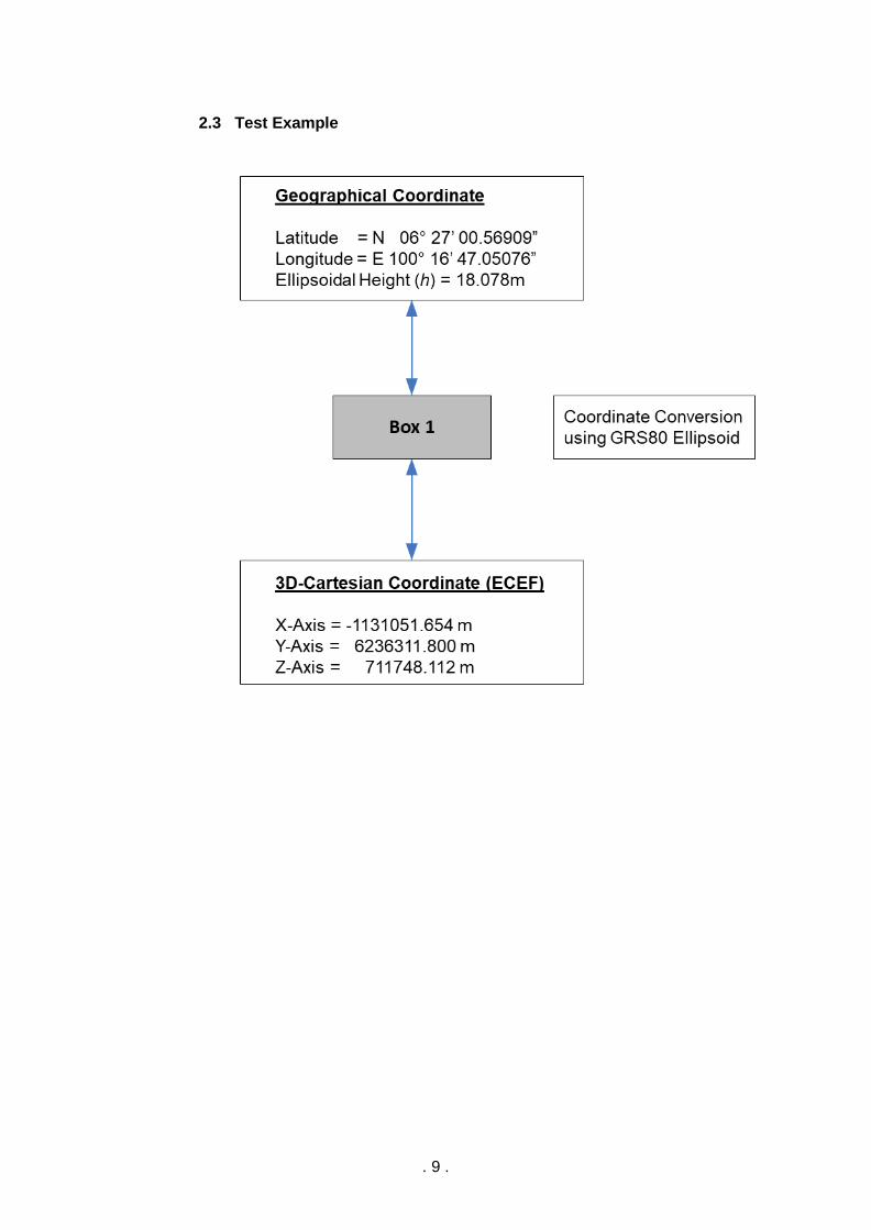
2.3 Test Example

. 10 .

3. DATUM TRANSFORMATION

3.1 Introduction

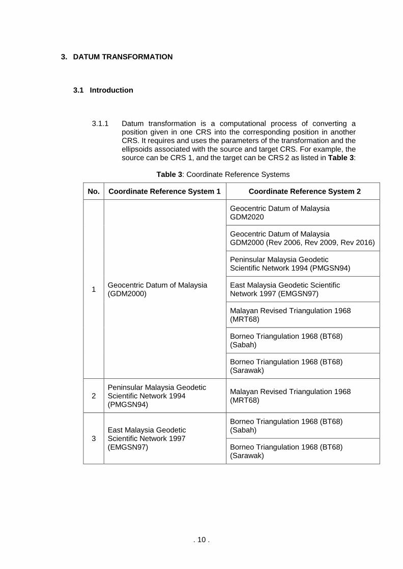
3.1.1 Datum transformation is a computational process of converting a position given in one CRS into the corresponding position in another CRS. It requires and uses the parameters of the transformation and the ellipsoids associated with the source and target CRS. For example, the source can be CRS 1, and the target can be CRS 2 as listed in Table 3:

Table 3: Coordinate Reference Systems

No. Coordinate Reference System 1 Coordinate Reference System 2

1 Geocentric Datum of Malaysia (GDM2000)

Geocentric Datum of Malaysia GDM2020

Geocentric Datum of Malaysia GDM2000 (Rev 2006, Rev 2009, Rev 2016)

Peninsular Malaysia Geodetic Scientific Network 1994 (PMGSN94)

East Malaysia Geodetic Scientific Network 1997 (EMGSN97)

Malayan Revised Triangulation 1968 (MRT68)

Borneo Triangulation 1968 (BT68) (Sabah)

Borneo Triangulation 1968 (BT68) (Sarawak)

2 Peninsular Malaysia Geodetic Scientific Network 1994 (PMGSN94)

Malayan Revised Triangulation 1968 (MRT68)

3 East Malaysia Geodetic Scientific Network 1997 (EMGSN97)

Borneo Triangulation 1968 (BT68) (Sabah)

Borneo Triangulation 1968 (BT68) (Sarawak)

. 11 .

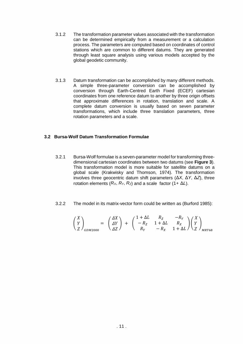
3.1.2 The transformation parameter values associated with the transformation can be determined empirically from a measurement or a calculation process. The parameters are computed based on coordinates of control stations which are common to different datums. They are generated through least square analysis using various models accepted by the global geodetic community.

3.1.3 Datum transformation can be accomplished by many different methods. A simple three-parameter conversion can be accomplished by conversion through Earth-Centred Earth Fixed (ECEF) cartesian coordinates from one reference datum to another by three origin offsets that approximate differences in rotation, translation and scale. A complete datum conversion is usually based on seven parameter transformations, which include three translation parameters, three rotation parameters and a scale.

3.2 Bursa-Wolf Datum Transformation Formulae

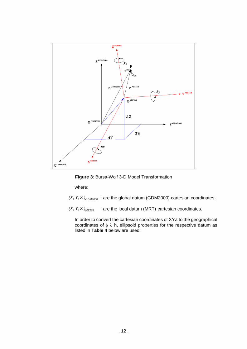
3.2.1 Bursa-Wolf formulae is a seven-parameter model for transforming three-dimensional cartesian coordinates between two datums (see Figure 3). This transformation model is more suitable for satellite datums on a global scale (Krakwisky and Thomson, 1974). The transformation

involves three geocentric datum shift parameters (ΔX, ΔY, ΔZ), three

rotation elements (RX, RY, RZ) and a scale factor (1+ ΔL).

3.2.2 The model in its matrix-vector form could be written as (Burford 1985):

( 𝑋 𝑌𝑍

)

𝐺𝐷𝑀2000

= ( 𝛥𝑋 𝛥𝑌𝛥𝑍

) + ( 1 + ∆𝐿 𝑅𝑍 −𝑅𝑌

− 𝑅𝑍 1 + ∆𝐿 𝑅𝑋

𝑅𝑌 − 𝑅𝑋 1 + ∆𝐿 )(

𝑋𝑌𝑍

)

𝑀𝑅𝑇68

. 12 .

Figure 3: Bursa-Wolf 3-D Model Transformation

where;

(X, Y, Z )GDM2000 : are the global datum (GDM2000) cartesian coordinates;

(X, Y, Z )MRT68 : are the local datum (MRT) cartesian coordinates.

In order to convert the cartesian coordinates of XYZ to the geographical

coordinates of h, ellipsoid properties for the respective datum as listed in Table 4 below are used:

𝜟𝑿

𝜟𝒁

𝜟𝒀

. 13 .

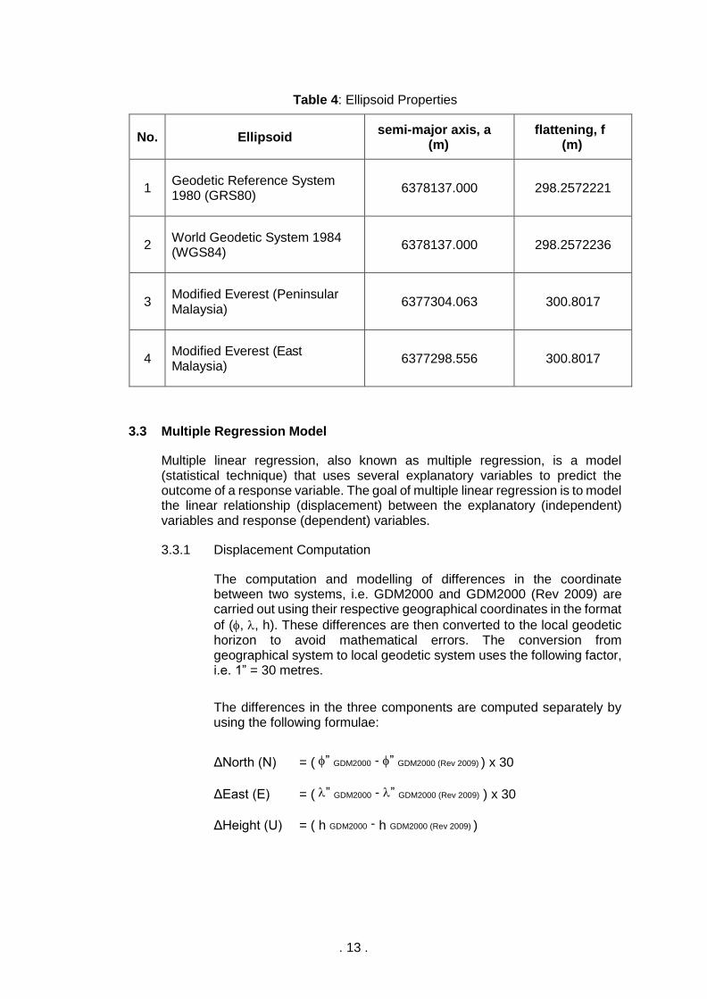
Table 4: Ellipsoid Properties

No. Ellipsoid semi-major axis, a

(m) flattening, f

(m)

1 Geodetic Reference System 1980 (GRS80)

6378137.000 298.2572221

2 World Geodetic System 1984 (WGS84)

6378137.000 298.2572236

3 Modified Everest (Peninsular Malaysia)

6377304.063 300.8017

4 Modified Everest (East Malaysia)

6377298.556 300.8017

3.3 Multiple Regression Model

Multiple linear regression, also known as multiple regression, is a model (statistical technique) that uses several explanatory variables to predict the outcome of a response variable. The goal of multiple linear regression is to model the linear relationship (displacement) between the explanatory (independent) variables and response (dependent) variables.

3.3.1 Displacement Computation

The computation and modelling of differences in the coordinate between two systems, i.e. GDM2000 and GDM2000 (Rev 2009) are carried out using their respective geographical coordinates in the format

of (, , h). These differences are then converted to the local geodetic horizon to avoid mathematical errors. The conversion from geographical system to local geodetic system uses the following factor, i.e. 1” = 30 metres.

The differences in the three components are computed separately by using the following formulae:

ΔNorth (N) = ( ” GDM2000 - ” GDM2000 (Rev 2009) ) x 30

ΔEast (E) = ( ” GDM2000 - ” GDM2000 (Rev 2009) ) x 30

ΔHeight (U) = ( h GDM2000 - h GDM2000 (Rev 2009) )

. 14 .

3.3.2 Displacement Modelling

The differences in coordinate of every GPS station are similarly computed between the two systems, i.e. GDM2000 and GDM2000 (Rev 2009), using their respective coordinates in the format of E and N. The coordinate differences are then gridded to derive the Regression Coefficient. The gridding method uses the polynomial regression with the power to the second order. The surface definition uses the bi-linear saddle regression coefficient with the following formulae:

Z(E,N,U) = A00 + A01 N + A10 E + A11 EN

where,

Z = Value of regression coefficient or the value of displacement correction for each component (i.e. East, North and Up)

E = East coordinate in decimal degree

N = North coordinate in decimal degree

3.3.3 Basic Formulae

To convert the coordinate in GDM2000 to GDM2000 (Rev 2009), the following formulae shall be used:

GDM2000 (Rev 2009) = GDM2000 + correction

” GDM2000 (Rev 2009) = ” GDM2000 + (ZN / 30)

” GDM2000 (Rev 2009) = ” GDM2000 + (ZE / 30)

h GDM2000 (Rev 2009) = h GDM2000 + ZU

where,

” = Latitude in second of arc

” = Longitude in second of arc

h = Ellipsoidal Height in meter

ZN = Displacement correction in northing

ZE = Displacement correction in easting

ZU = Displacement correction in height

A00, A01, A10 and A11 are the coefficients of the multiple regression model.

. 15 .

3.4 Time-Dependent Reference Frame

3.4.1 Introduction

A more accurate and current Malaysian geodetic reference frame has

been determined, fully aligned and compatible with ITRF2014 by taking

advantage of the GNSS data availability from MyRTKnet. This

reference frame is based on the kinematic concept, where time-

dependent elements are modelled as an implicit component of the

Continuously Operating Reference Stations (CORS) coordinates. A

kinematic datum includes a deformation model consisting of a velocity

field that allows the estimation of the plate velocity at any point in the

country and patches of modelled displacements to account for

substantial ground movements.

Continuously changing coordinates in a kinematic datum present

significant challenges for most spatial data users, particularly in the

cadastral database acquired at different epochs that need to be

integrated harmoniously to meet the legal requirements. On the

contrary, a semi-kinematic reference frame enables the time-dependent

coordinates to be transformed consistently and accurately to a fixed

reference epoch over time; thus, providing a more practical approach in

handling spatial databases coordinate systems.

Table 5: Types of Geodetic Reference Frames Concerning the Time-Dependent Coordinates

Reference Frames

Trajectory Models

Static 𝑋(𝑡) = 𝑋(𝑡0) 1

Kinematic 𝑋(𝑡) = 𝑋(𝑡0) + 𝑋𝑣(𝑡 − 𝑡0) + 𝛿𝑋𝑃𝑆𝐷(𝑡) 2

Semi-Kinematic 𝑋(𝑡) = 𝑋(𝑡0) + 𝑋𝑣(𝑡 − 𝑡0) + 𝛿𝑋𝑃𝑆𝐷(𝑡) 3

𝑋(𝑡𝐷𝐵) = 𝑋(𝑡) + 𝑋𝑣(𝑡𝐷𝐵 − 𝑡) + 𝛿𝑋𝑃𝑆𝐷(𝑡𝐷𝐵) − 𝛿𝑋𝑃𝑆𝐷(𝑡) 4

Remarks:

1 CORS and databases coordinates are fixed at a specific pre-seismic reference

epoch 𝑡0

2 CORS and databases coordinates are continuously updated

3 CORS coordinates are continuously updated

4 Quasi-static databases coordinates are fixed at a specific post-seismic

reference epoch 𝑡𝐷B

Table 5 above provides the description of static, kinematic and semi-

kinematic geodetic reference frame with respect to the time-dependent

coordinates. A semi-kinematic geodetic reference frame consists of

both kinematic and quasi-static coordinates. The quasi-static

. 16 .

coordinates of the spatial databases in a semi-kinematic geodetic

reference frame always refer to a specific epoch and do not vary until

they exceed a certain critical level and the geodetic reference frame is

updated while the CORS kinematic coordinates are updated regularly.

The coordinates of CORS and spatial databases in a kinematic geodetic

reference frame change regularly with time.

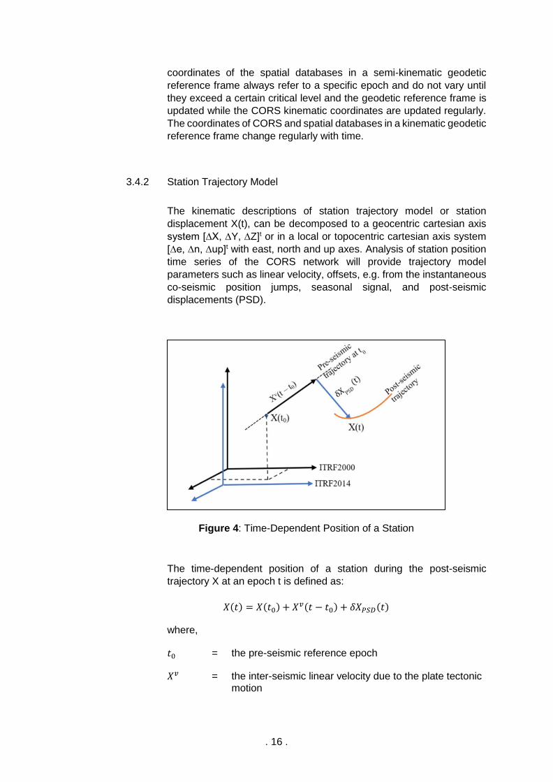
3.4.2 Station Trajectory Model

The kinematic descriptions of station trajectory model or station

displacement X(t), can be decomposed to a geocentric cartesian axis

system [∆X, ∆Y, ∆Z]t or in a local or topocentric cartesian axis system

[∆e, ∆n, ∆up]t with east, north and up axes. Analysis of station position

time series of the CORS network will provide trajectory model

parameters such as linear velocity, offsets, e.g. from the instantaneous

co-seismic position jumps, seasonal signal, and post-seismic

displacements (PSD).

Figure 4: Time-Dependent Position of a Station

The time-dependent position of a station during the post-seismic

trajectory X at an epoch t is defined as:

𝑋(𝑡) = 𝑋(𝑡0) + 𝑋𝑣(𝑡 − 𝑡0) + 𝛿𝑋𝑃𝑆𝐷(𝑡)

where,

𝑡0 = the pre-seismic reference epoch

𝑋𝑣 = the inter-seismic linear velocity due to the plate tectonic motion

. 17 .

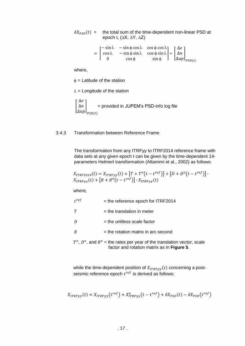
𝛿𝑋𝑃𝑆𝐷(𝑡) = the total sum of the time-dependent non-linear PSD at epoch t, (∆X, ∆Y, ∆Z)

= ⌈

− sin −sin cos cos coscos −sin sin cos sin

0 cos sin ⌉ ∗ [

∆𝑒∆𝑛∆𝑢𝑝

]

𝑃𝑆𝐷(𝑡)

where,

= Latitude of the station

= Longitude of the station

[∆𝑒∆𝑛∆𝑢𝑝

]

𝑃𝑆𝐷(𝑡)

= provided in JUPEM’s PSD-info log file

3.4.3 Transformation between Reference Frame

The transformation from any ITRFyy to ITRF2014 reference frame with

data sets at any given epoch t can be given by the time-dependent 14-

parameters Helmert transformation (Altamimi et al., 2002) as follows:

𝑋𝐼𝑇𝑅𝐹2014(𝑡) = 𝑋𝐼𝑇𝑅𝐹𝑦𝑦(𝑡) + [𝑇 + 𝑇𝑣(𝑡 − 𝑡𝑟𝑒𝑓)] + [𝐷 + 𝐷𝑣(𝑡 − 𝑡𝑟𝑒𝑓)] ∙

𝑋𝐼𝑇𝑅𝐹𝑦𝑦(𝑡) + [𝑅 + 𝑅𝑣(𝑡 − 𝑡𝑟𝑒𝑓)] ∙ 𝑋𝐼𝑇𝑅𝐹𝑦𝑦(𝑡)

where,

𝑡𝑟𝑒𝑓 = the reference epoch for ITRF2014

𝑇 = the translation in meter

𝐷 = the unitless scale factor

𝑅 = the rotation matrix in arc-second

𝑇𝑣, 𝐷𝑣, and 𝑅𝑣 = the rates per year of the translation vector, scale factor and rotation matrix as in Figure 5.

while the time-dependent position of 𝑋𝐼𝑇𝑅𝐹𝑦𝑦(𝑡) concerning a post-

seismic reference epoch 𝑡𝑟𝑒𝑓 is derived as follows:

𝑋𝐼𝑇𝑅𝐹𝑦𝑦(𝑡) = 𝑋𝐼𝑇𝑅𝐹𝑦𝑦(𝑡𝑟𝑒𝑓) + 𝑋𝐼𝑇𝑅𝐹𝑦𝑦𝑣 (𝑡 − 𝑡𝑟𝑒𝑓) + 𝛿𝑋𝑃𝑆𝐷(𝑡) − 𝛿𝑋𝑃𝑆𝐷(𝑡𝑟𝑒𝑓)

. 18 .

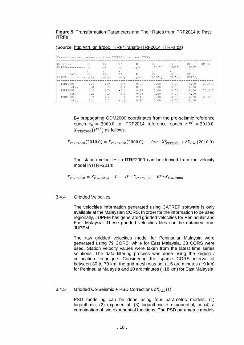
Figure 5: Transformation Parameters and Their Rates from ITRF2014 to Past ITRFs

(Source: http://itrf.ign.fr/doc_ITRF/Transfo-ITRF2014_ITRFs.txt)

By propagating GDM2000 coordinates from the pre-seismic reference

epoch 𝑡0 = 2000.0 to ITRF2014 reference epoch 𝑡𝑟𝑒𝑓 = 2010.0,

𝑋𝐼𝑇𝑅𝐹2000(𝑡𝑟𝑒𝑓) as follows:

𝑋𝐼𝑇𝑅𝐹2000(2010.0) = 𝑋𝐼𝑇𝑅𝐹2000(2000.0) + 10𝑦𝑟 ∙ 𝑋𝐼𝑇𝑅𝐹2000𝑣 + 𝛿𝑋𝑃𝑆𝐷(2010.0)

The station velocities in ITRF2000 can be derived from the velocity

model in ITRF2014:

𝑋𝐼𝑇𝑅𝐹2000𝑣 = 𝑋𝐼𝑇𝑅𝐹2014

𝑣 − 𝑇𝑣 − 𝐷𝑣 ∙ 𝑋𝐼𝑇𝑅𝐹2000 − 𝑅𝑣 ∙ 𝑋𝐼𝑇𝑅𝐹2000

3.4.4 Gridded Velocities

The velocities information generated using CATREF software is only available at the Malaysian CORS. In order for the information to be used regionally, JUPEM has generated gridded velocities for Peninsular and East Malaysia. These gridded velocities files can be obtained from JUPEM.

The raw gridded velocities model for Peninsular Malaysia were generated using 79 CORS, while for East Malaysia, 38 CORS were used. Station velocity values were taken from the latest time series solutions. The data filtering process was done using the kriging / collocation technique. Considering the sparse CORS interval of between 30 to 70 km, the grid mesh was set at 5 arc minutes (~9 km) for Peninsular Malaysia and 10 arc minutes (~18 km) for East Malaysia.

3.4.5 Gridded Co-Seismic + PSD Corrections 𝛿𝑋𝑃𝑆𝐷(𝑡)

PSD modelling can be done using four parametric models: (1) logarithmic, (2) exponential, (3) logarithmic + exponential, or (4) a combination of two exponential functions. The PSD parametric models

http://itrf.ign.fr/doc_ITRF/Transfo-ITRF2014_ITRFs.txt

. 19 .

were determined from the MyRTKnet daily position time series at sites where the PSD was judged to be significant. The adjustment of the PSD parametric models was operated separately for the east, north and height components.

The PSD correction for specific epochs was calculated based on the information stored in the PSD’s SINEX file, i.e., “psdmodel.snx”. CORS affected by the earthquakes have been listed in the file as one of the data inputs, which comprised a total of 55 CORS (active and decommissioned) in Peninsular Malaysia. For stations affected by multiple earthquakes, the PSD corrections computation will iteratively loop through all earthquake events prior to the epoch date. The total cumulative PSD correction is then applied at the observation epoch.

Time-based grid models are formulated to regionally estimate the amount of cumulative co-seismic + PSD correction for the semi-kinematic reference frame. These gridded PSD files can be obtained from JUPEM.

. 20 .

3.5 Test Examples

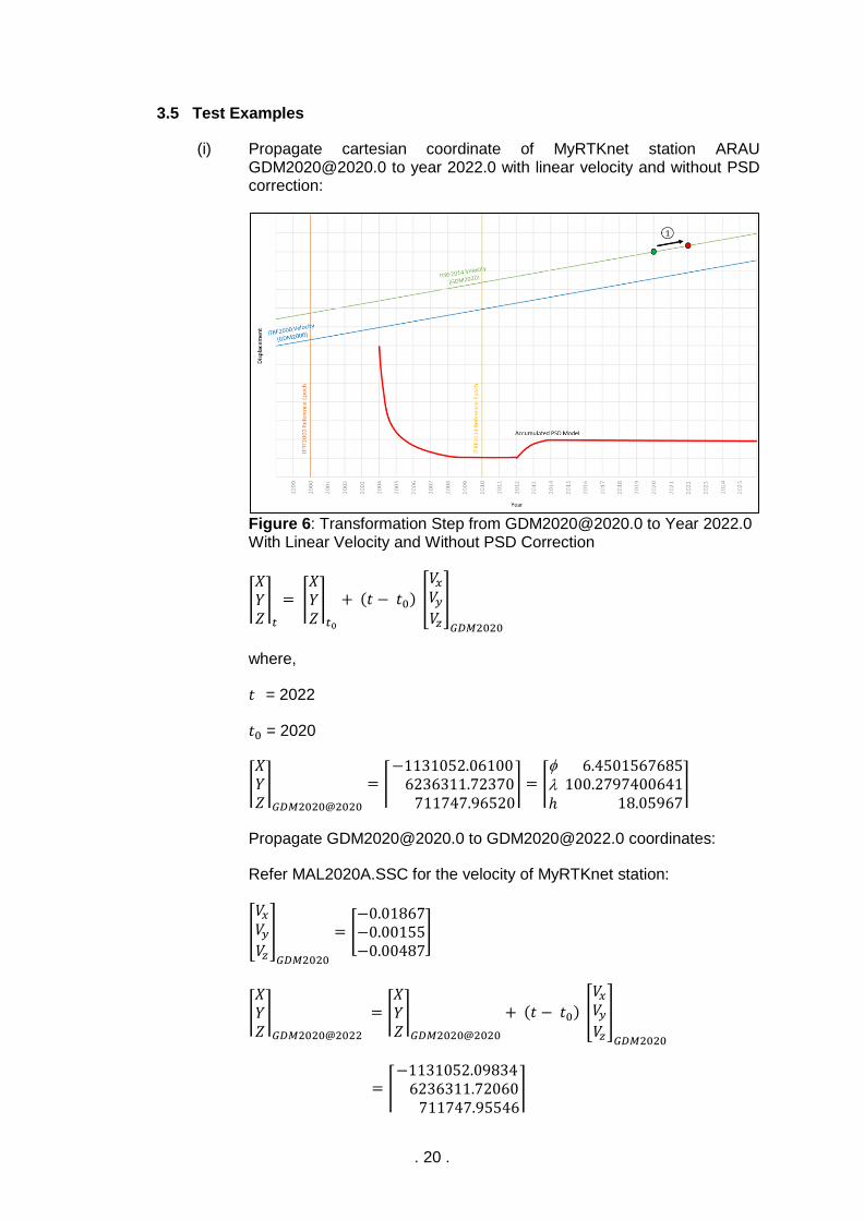
(i) Propagate cartesian coordinate of MyRTKnet station ARAU [email protected] to year 2022.0 with linear velocity and without PSD correction:

Figure 6: Transformation Step from [email protected] to Year 2022.0 With Linear Velocity and Without PSD Correction

⌈𝑋𝑌𝑍⌉

𝑡

= ⌈𝑋𝑌𝑍⌉

𝑡0

+ (𝑡 − 𝑡0) [

𝑉𝑥𝑉𝑦𝑉𝑧

]

𝐺𝐷𝑀2020

where,

𝑡 = 2022

𝑡0 = 2020

⌈𝑋𝑌𝑍⌉

𝐺𝐷𝑀2020@2020

= ⌈−1131052.06100 6236311.72370 711747.96520

⌉ = ⌈

ℎ 6.4501567685100.2797400641 18.05967

⌉

Propagate [email protected] to [email protected] coordinates:

Refer MAL2020A.SSC for the velocity of MyRTKnet station:

[


]

𝐺𝐷𝑀2020

= [−0.01867−0.00155−0.00487

]

⌈𝑋𝑌𝑍⌉

𝐺𝐷𝑀2020@2022


𝐺𝐷𝑀2020@2020

+ (𝑡 − 𝑡0) [


]

𝐺𝐷𝑀2020

= ⌈−1131052.09834 6236311.72060 711747.95546

⌉

. 21 .

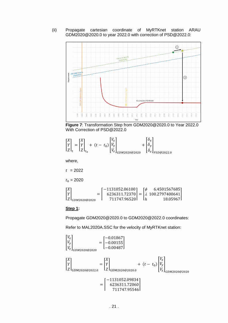
(ii) Propagate cartesian coordinate of MyRTKnet station ARAU [email protected] to year 2022.0 with correction of [email protected]:

Figure 7: Transformation Step from [email protected] to Year 2022.0 With Correction of [email protected]

⌈𝑋𝑌𝑍⌉

𝑡


𝑡0

+ (𝑡 − 𝑡0) [


]

𝐺𝐷𝑀2020@2020

+ [

𝛿𝑥

𝛿𝑦

𝛿𝑧

]

𝑃𝑆𝐷@2022.0

where,

𝑡 = 2022

𝑡0 = 2020

⌈𝑋𝑌𝑍⌉

𝐺𝐷𝑀2020@2020

= ⌈−1131052.06100 6236311.72370 711747.96520

⌉ = ⌈

ℎ 6.4501567685100.2797400641 18.05967

⌉

Step 1:


Refer to MAL2020A.SSC for the velocity of MyRTKnet station:

[


]

𝐺𝐷𝑀2020@2020

= [−0.01867−0.00155−0.00487

]

⌈𝑋𝑌𝑍⌉

[email protected]


[email protected]

+ (𝑡 − 𝑡0) [


]

𝐺𝐷𝑀2020@2020

= ⌈−1131052.09834 6236311.72060 711747.95546

⌉

. 22 .

Step 2:

Apply [email protected] for [email protected] coordinates using geodetic

(, , h) coordinates:

[

𝛿𝑥

𝛿𝑦

𝛿𝑧

]

𝑃𝑆𝐷@2022.0

= ⌈


0 cos sin ⌉ ∗ [


]

𝑃𝑆𝐷@2022.0

Refer to 22001psd-info.log


]

𝑃𝑆𝐷@2022.0

= [−0.05148

00

]

[

𝛿𝑥

𝛿𝑦

𝛿𝑧

]

𝑃𝑆𝐷@2022.0

= [−0.05065 0.00919 0.00000

]

So,

⌈𝑋𝑌𝑍⌉

𝐺𝐷𝑀2020@2022


[email protected]

+ [

𝛿𝑥

𝛿𝑦

𝛿𝑧

]

𝑃𝑆𝐷@2022.0

= ⌈−1131052.04769 6236311.72979 711747.95546

⌉

. 23 .

(iii) Propagate cartesian coordinate of MyRTKnet station ARAU [email protected] with correction of [email protected] to year 2010.0 and correction of [email protected]:

Figure 8: Transformation Step from [email protected] With Correction of [email protected] to Year 2010.0 and Correction of [email protected]

⌈𝑋𝑌𝑍⌉

𝑡


𝑡0

− [

𝛿𝑥

𝛿𝑦

𝛿𝑧

]

𝑃𝑆𝐷@2020.0

+ (𝑡 − 𝑡0) [


]

𝐺𝐷𝑀2020

+ [

𝛿𝑥

𝛿𝑦

𝛿𝑧

]

𝑃𝑆𝐷@2010.0

where,

𝑡 = 2010

𝑡0 = 2020

⌈𝑋𝑌𝑍⌉

𝐺𝐷𝑀2020@2020

= ⌈−1131052.06100 6236311.72370 711747.96520

⌉ = ⌈

ℎ

6.4501567685100.2797400641 18.05967

⌉

Step1:

Correction of GDM2020@2020 coordinates by removing [email protected]

using geodetic (, , h) coordinates:

[

𝛿𝑥

𝛿𝑦

𝛿𝑧

]

𝑃𝑆𝐷@2020.0

= ⌈


0 cos sin ⌉ ∗ [


]

𝑃𝑆𝐷@2020.0

Refer to 20001psd-info.log


]

𝑃𝑆𝐷@2020.0

= [−0.05147 0.00000 0.00000

]

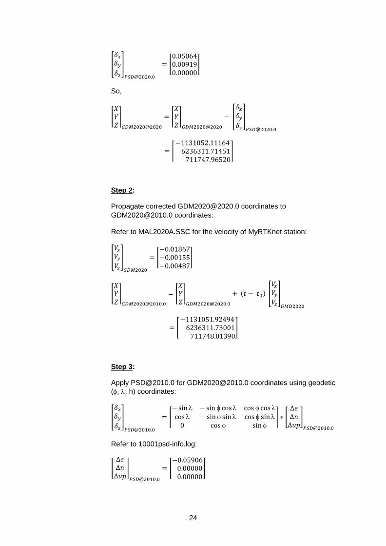
. 24 .

[

𝛿𝑥

𝛿𝑦

𝛿𝑧

]

𝑃𝑆𝐷@2020.0

= [0.050640.009190.00000

]

So,

⌈𝑋𝑌𝑍⌉

𝐺𝐷𝑀2020@2020


𝐺𝐷𝑀2020@2020

− [

𝛿𝑥

𝛿𝑦

𝛿𝑧

]

𝑃𝑆𝐷@2020.0

= ⌈−1131052.11164 6236311.71451 711747.96520

⌉

Step 2:

Propagate corrected [email protected] coordinates to

[email protected] coordinates:

Refer to MAL2020A.SSC for the velocity of MyRTKnet station:

[


]

𝐺𝐷𝑀2020

= [−0.01867−0.00155−0.00487

]

⌈𝑋𝑌𝑍⌉

𝐺𝐷𝑀[email protected]



+ (𝑡 − 𝑡0) [


]

𝐺𝑀𝐷2020

= [−1131051.92494 6236311.73001 711748.01390

]

Step 3:

Apply [email protected] for [email protected] coordinates using geodetic


[

𝛿𝑥

𝛿𝑦

𝛿𝑧

]

𝑃𝑆𝐷@2010.0

= ⌈


0 cos sin ⌉ ∗ [


]

𝑃𝑆𝐷@2010.0

Refer to 10001psd-info.log:


]

𝑃𝑆𝐷@2010.0

= [−0.05906 0.00000 0.00000

]

. 25 .

[

𝛿𝑥

𝛿𝑦

𝛿𝑧

]

𝑃𝑆𝐷@2010.0

= [0.058110.01054

0]

So,

⌈𝑋𝑌𝑍⌉

𝐺𝐷𝑀2020@2010



+ [

𝛿𝑥

𝛿𝑦

𝛿𝑧

]

𝑃𝑆𝐷@2010.0

= ⌈−1131051.86683 6236311.74055 711748.01390

⌉

. 26 .

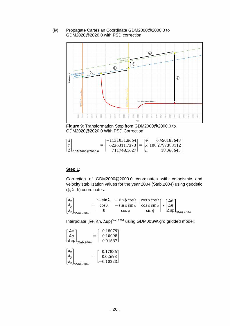
(iv) Propagate Cartesian Coordinate [email protected] to [email protected] with PSD correction:

Figure 9: Transformation Step from [email protected] to [email protected] With PSD Correction

⌈𝑋𝑌𝑍⌉


= ⌈−1131051.8664 6236311.7373 711748.1627

⌉ = ⌈

ℎ

6.450185648100.2797383112 18.060645

⌉

Step 1:

Correction of [email protected] coordinates with co-seismic and

velocity stabilization values for the year 2004 (Stab.2004) using geodetic


[

𝛿𝑥

𝛿𝑦

𝛿𝑧

]

𝑆𝑡𝑎𝑏.2004

= ⌈


0 cos sin ⌉ ∗ [


]


Interpolate [∆e, ∆n, ∆up]Stab.2004 using GDM00SW.grd gridded model:


]


= [−0.18079−0.10098−0.01687

]

[

𝛿𝑥

𝛿𝑦

𝛿𝑧

]


= [ 0.17886 0.02693−0.10223

]

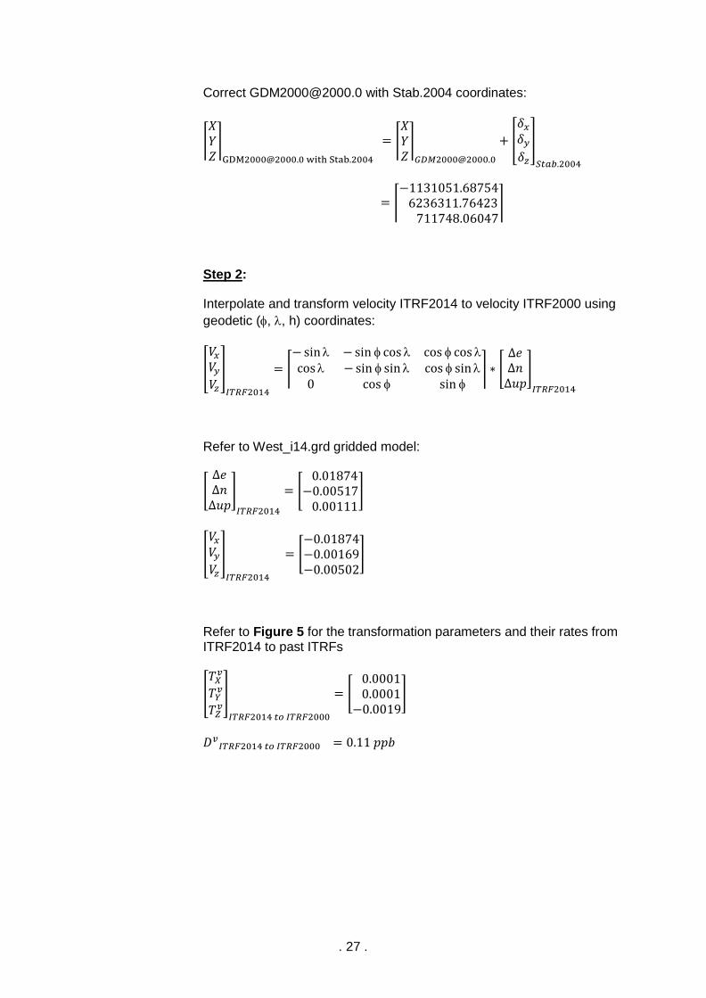
. 27 .

Correct [email protected] with Stab.2004 coordinates:

⌈𝑋𝑌𝑍⌉

[email protected] with Stab.2004



+ [

𝛿𝑥

𝛿𝑦

𝛿𝑧

]


= ⌈−1131051.68754 6236311.76423 711748.06047

⌉

Step 2:

Interpolate and transform velocity ITRF2014 to velocity ITRF2000 using

geodetic (, , h) coordinates:

[


]

𝐼𝑇𝑅𝐹2014

= ⌈


0 cos sin ⌉ ∗ [


]


Refer to West_i14.grd gridded model:


]


= [ 0.01874−0.00517 0.00111

]

[


]


= [−0.01874−0.00169−0.00502

]

Refer to Figure 5 for the transformation parameters and their rates from ITRF2014 to past ITRFs

[

𝑇𝑋𝑣

𝑇𝑌𝑣

𝑇𝑍𝑣]

𝐼𝑇𝑅𝐹2014 𝑡𝑜 𝐼𝑇𝑅𝐹2000

= [ 0.0001 0.0001−0.0019

]

𝐷𝑣𝐼𝑇𝑅𝐹2014 𝑡𝑜 𝐼𝑇𝑅𝐹2000 = 0.11 𝑝𝑝𝑏

. 28 .

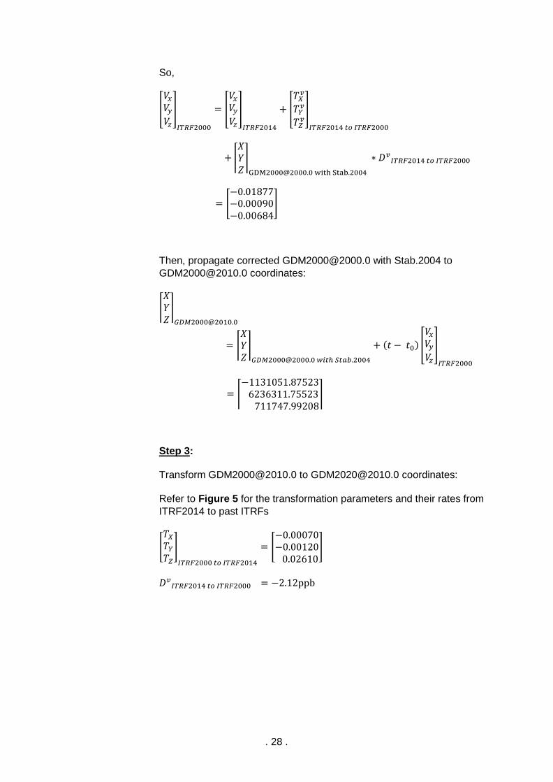
So,

[


]


= [


]


+ [

𝑇𝑋𝑣

𝑇𝑌𝑣

𝑇𝑍𝑣]


+ ⌈𝑋𝑌𝑍⌉


∗ 𝐷𝑣𝐼𝑇𝑅𝐹2014 𝑡𝑜 𝐼𝑇𝑅𝐹2000

= [−0.01877−0.00090−0.00684

]

Then, propagate corrected [email protected] with Stab.2004 to

[email protected] coordinates:

⌈𝑋𝑌𝑍⌉



𝐺𝐷𝑀[email protected] 𝑤𝑖𝑡ℎ 𝑆𝑡𝑎𝑏.2004

+ (𝑡 − 𝑡0) [


]


= ⌈−1131051.87523 6236311.75523 711747.99208

⌉

Step 3:

Transform [email protected] to [email protected] coordinates:

Refer to Figure 5 for the transformation parameters and their rates from

ITRF2014 to past ITRFs

[

𝑇𝑋

𝑇𝑌

𝑇𝑍

]


= [−0.00070−0.00120 0.02610

]

𝐷𝑣𝐼𝑇𝑅𝐹2014 𝑡𝑜 𝐼𝑇𝑅𝐹2000 = −2.12ppb

. 29 .

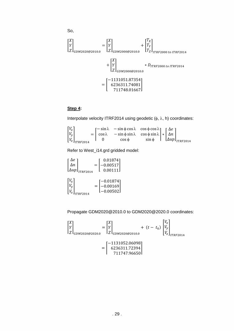
So,

[𝑋𝑌𝑍]


= [𝑋𝑌𝑍]


+ [𝑇𝑋

𝑇𝑌

𝑇𝑍

]


+ [𝑋𝑌𝑍]


∗ 𝐷𝐼𝑇𝑅𝐹2000 𝑡𝑜 𝐼𝑇𝑅𝐹2014

= [−1131051.87354 6236311.74081 711748.01667

]

Step 4:

Interpolate velocity ITRF2014 using geodetic (, , h) coordinates:

[


]


= ⌈


0 cos sin ⌉ ∗ [


]




]


= [ 0.01874−0.00517 0.00111

]

[


]


= [−0.01874−0.00169−0.00502

]


⌈𝑋𝑌𝑍⌉




+ (𝑡 − 𝑡0) [


]


= ⌈−1131052.06098 6236311.72394 711747.96650

⌉

. 30 .

Step 5:

Interpolate [email protected] using geodetic (, , h) coordinates:

[

𝛿𝑥

𝛿𝑦

𝛿𝑧

]

𝑃𝑆𝐷@2020.0

= ⌈


0 cos sin ⌉ ∗ [


]

𝑃𝑆𝐷@2020.0

Refer to PSD2020.grd gridded model:


]

𝑃𝑆𝐷@2020.0

= [−0.05141−0.01356 0.00000

]

[

𝛿𝑥

𝛿𝑦

𝛿𝑧

]

𝑃𝑆𝐷@2020.0

= [ 0.05031 0.01067−0.01348

]

So,

⌈𝑋𝑌𝑍⌉




+ [

𝛿𝑥

𝛿𝑦

𝛿𝑧

]

𝑃𝑆𝐷@2020.0

= ⌈−1131052.01066 6236311.73462 711747.95303

⌉

. 31 .

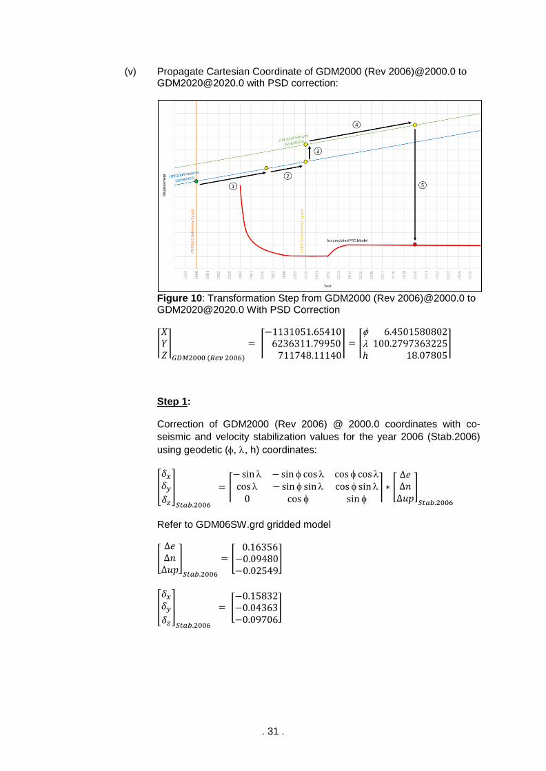
(v) Propagate Cartesian Coordinate of GDM2000 (Rev 2006)@2000.0 to [email protected] with PSD correction:

Figure 10: Transformation Step from GDM2000 (Rev 2006)@2000.0 to [email protected] With PSD Correction

⌈𝑋𝑌𝑍⌉

𝐺𝐷𝑀2000 (𝑅𝑒𝑣 2006)

= ⌈−1131051.65410 6236311.79950 711748.11140

⌉ = ⌈

ℎ

6.4501580802100.2797363225 18.07805

⌉

Step 1:

Correction of GDM2000 (Rev 2006) @ 2000.0 coordinates with co-

seismic and velocity stabilization values for the year 2006 (Stab.2006)

using geodetic (, , h) coordinates:

[

𝛿𝑥

𝛿𝑦

𝛿𝑧

]


= ⌈


0 cos sin ⌉ ∗ [


]


Refer to GDM06SW.grd gridded model


]


= [ 0.16356−0.09480−0.02549

]

[

𝛿𝑥

𝛿𝑦

𝛿𝑧

]


= [−0.15832−0.04363−0.09706

]

. 32 .

Update GDM2000 (Rev 2006)@2000.586.0 coordinates:

⌈𝑋𝑌𝑍⌉

GDM2000(Rev 2006)@2006.586.0


𝐺𝐷𝑀2000 (𝑅𝑒𝑣 2006)

+ [

𝛿𝑥

𝛿𝑦

𝛿𝑧

]


= ⌈−1131051.81242 6236311.75587 711748.01434

⌉

Step 2:

Interpolate and transform velocity ITRF2014 to velocity ITRF2000 using

geodetic (, , h) coordinates:

[


]


= ⌈


0 cos sin ⌉ ∗ [


]




]


= [ 0.01874 0.00517 0.00111

]

[


]


= [−0.01854−0.00283 0.00527

]


[

𝑇𝑋𝑣

𝑇𝑌𝑣

𝑇𝑍𝑣]


= [ 0.0001 0.0001−0.0019

]

𝐷𝑣𝐼𝑇𝑅𝐹2014 𝑡𝑜 𝐼𝑇𝑅𝐹2000 = 0.11𝑝𝑝𝑏

. 33 .

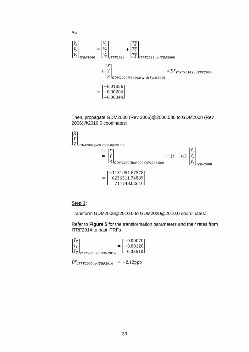
So,

[


]


= [


]


+ [

𝑇𝑋𝑣

𝑇𝑌𝑣

𝑇𝑍𝑣]





= [−0.01856−0.00204−0.00344

]

Then, propagate GDM2000 (Rev 2006)@2006.586 to GDM2000 (Rev

2006)@2010.0 coodinates:

⌈𝑋𝑌𝑍⌉

𝐺𝐷𝑀2000(𝑅𝑒𝑣 2006)@2010.0


𝐺𝐷𝑀2000(𝑅𝑒𝑣 2006)@2006.586

+ (𝑡 − 𝑡0) [


]


= ⌈−1131051.87578 6236311.74889 711748.02610

⌉

Step 3:

Transform [email protected] to [email protected] coordinates:



[𝑇𝑋

𝑇𝑌

𝑇𝑍

]


= [−0.00070−0.00120 0.02610

]

𝐷𝑣𝐼𝑇𝑅𝐹2000 𝑡𝑜 𝐼𝑇𝑅𝐹2014 = −2.12ppb

. 34 .

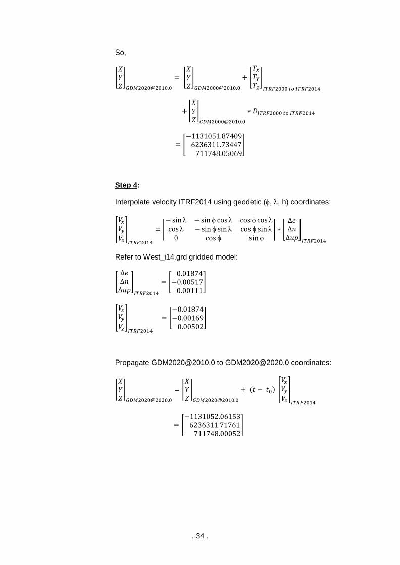
So,

[𝑋𝑌𝑍]


= [𝑋𝑌𝑍]


+ [𝑇𝑋

𝑇𝑌

𝑇𝑍

]


+ [𝑋𝑌𝑍]



= [−1131051.87409 6236311.73447 711748.05069

]

Step 4:


[


]


= ⌈


0 cos sin ⌉ ∗ [


]




]


= [ 0.01874−0.00517 0.00111

]

[


]


= [−0.01874−0.00169−0.00502

]


⌈𝑋𝑌𝑍⌉




+ (𝑡 − 𝑡0) [


]


= ⌈−1131052.06153 6236311.71761 711748.00052

⌉

. 35 .

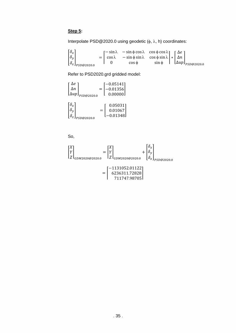
Step 5:


[

𝛿𝑥

𝛿𝑦

𝛿𝑧

]

𝑃𝑆𝐷@2020.0

= ⌈


0 cos sin ⌉ ∗ [


]

𝑃𝑆𝐷@2020.0



]

𝑃𝑆𝐷@2020.0

= [−0.05141−0.01356 0.00000

]

[

𝛿𝑥

𝛿𝑦

𝛿𝑧

]

𝑃𝑆𝐷@2020.0

= [ 0.05031 0.01067−0.01348

]

So,

⌈𝑋𝑌𝑍⌉




+ [

𝛿𝑥

𝛿𝑦

𝛿𝑧

]

𝑃𝑆𝐷@2020.0

= ⌈−1131052.01122 6236311.72828 711747.98705

⌉

. 36 .

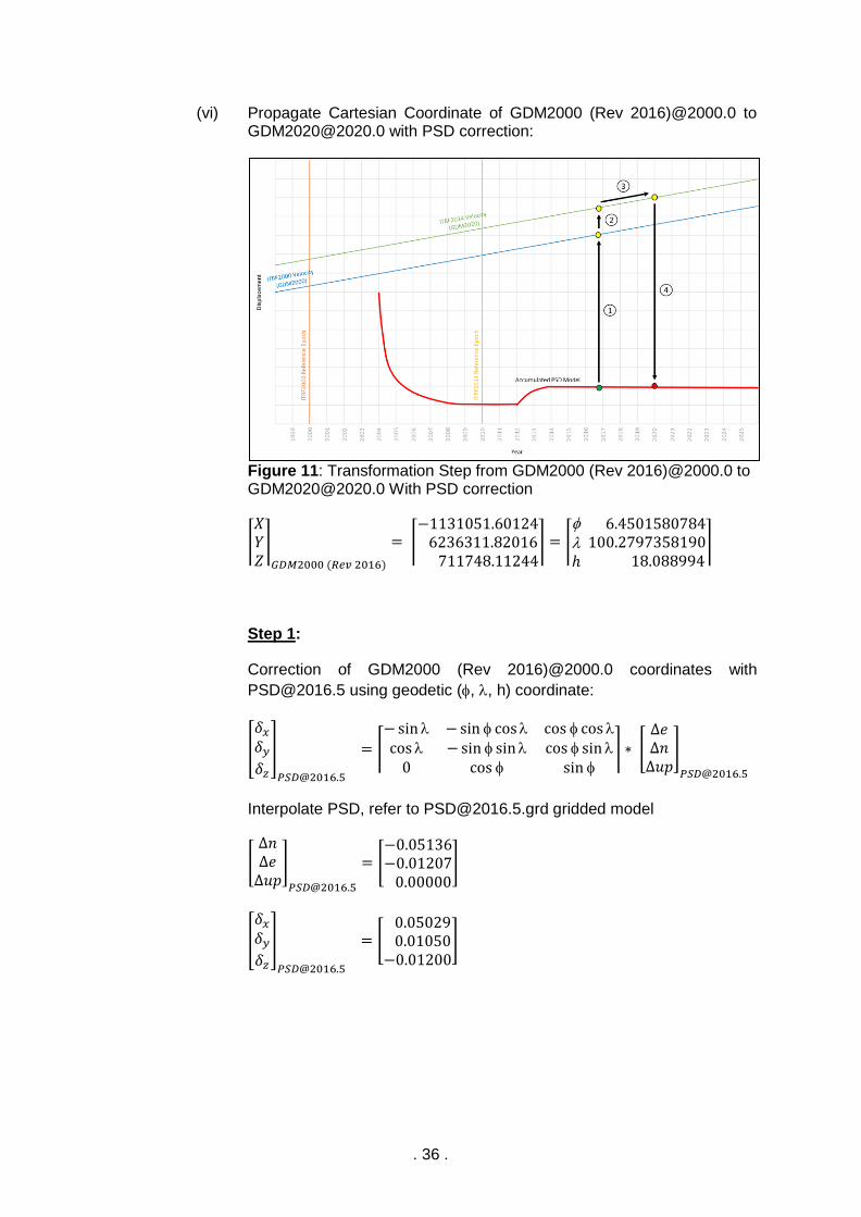
(vi) Propagate Cartesian Coordinate of GDM2000 (Rev 2016)@2000.0 to [email protected] with PSD correction:

Figure 11: Transformation Step from GDM2000 (Rev 2016)@2000.0 to [email protected] With PSD correction

⌈𝑋𝑌𝑍⌉

𝐺𝐷𝑀2000 (𝑅𝑒𝑣 2016)

= ⌈−1131051.60124 6236311.82016 711748.11244

⌉ = ⌈

ℎ

6.4501580784100.2797358190 18.088994

⌉

Step 1:

Correction of GDM2000 (Rev 2016)@2000.0 coordinates with

[email protected] using geodetic (, , h) coordinate:

[

𝛿𝑥

𝛿𝑦

𝛿𝑧

]

𝑃𝑆𝐷@2016.5

= ⌈


0 cos sin ⌉ ∗ [


]

𝑃𝑆𝐷@2016.5

Interpolate PSD, refer to [email protected] gridded model

[∆𝑛∆𝑒∆𝑢𝑝

]

𝑃𝑆𝐷@2016.5

= [−0.05136−0.01207 0.00000

]

[

𝛿𝑥

𝛿𝑦

𝛿𝑧

]

𝑃𝑆𝐷@2016.5

= [ 0.05029 0.01050−0.01200

]

. 37 .

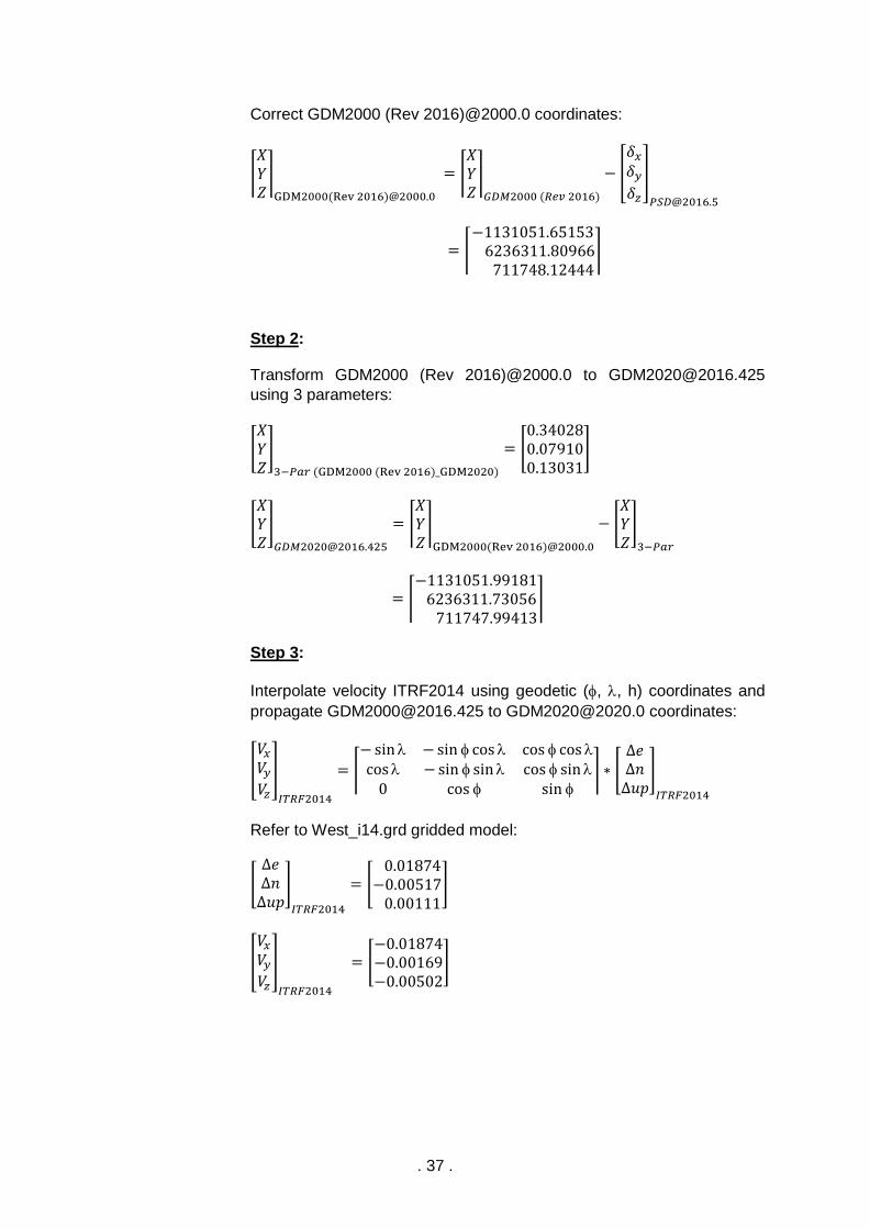
Correct GDM2000 (Rev 2016)@2000.0 coordinates:

⌈𝑋𝑌𝑍⌉

GDM2000(Rev 2016)@2000.0


𝐺𝐷𝑀2000 (𝑅𝑒𝑣 2016)

− [

𝛿𝑥

𝛿𝑦

𝛿𝑧

]

𝑃𝑆𝐷@2016.5

= ⌈−1131051.65153 6236311.80966 711748.12444

⌉

Step 2:

Transform GDM2000 (Rev 2016)@2000.0 to [email protected]

using 3 parameters:

[𝑋𝑌𝑍]

3−𝑃𝑎𝑟 (GDM2000 (Rev 2016)_GDM2020)

= [0.340280.079100.13031

]

[𝑋𝑌𝑍]



GDM2000(Rev 2016)@2000.0

− [𝑋𝑌𝑍]

3−𝑃𝑎𝑟

= ⌈−1131051.99181 6236311.73056 711747.99413

⌉

Step 3:

Interpolate velocity ITRF2014 using geodetic (, , h) coordinates and

propagate [email protected] to [email protected] coordinates:

[


]


= ⌈


0 cos sin ⌉ ∗ [


]




]


= [ 0.01874−0.00517 0.00111

]

[


]


= [−0.01874−0.00169−0.00502

]

. 38 .

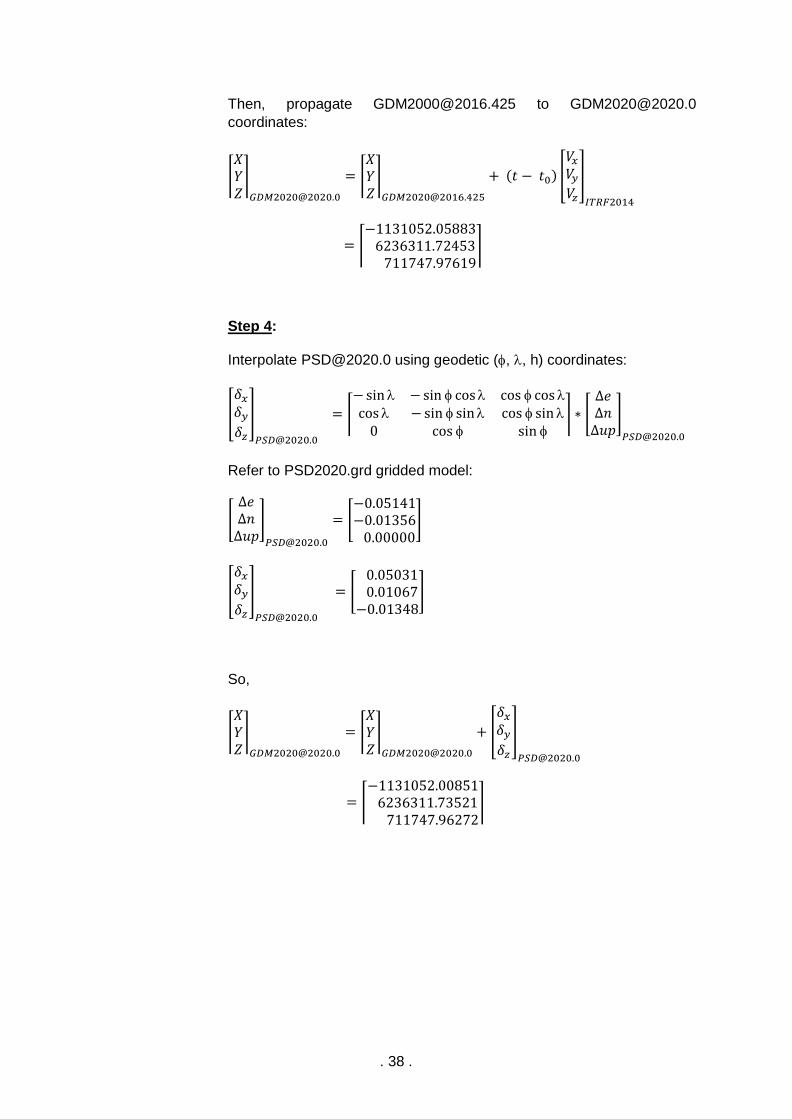
Then, propagate [email protected] to [email protected]

coordinates:

⌈𝑋𝑌𝑍⌉




+ (𝑡 − 𝑡0) [


]


= ⌈−1131052.05883 6236311.72453 711747.97619

⌉

Step 4:


[

𝛿𝑥

𝛿𝑦

𝛿𝑧

]

𝑃𝑆𝐷@2020.0

= ⌈


0 cos sin ⌉ ∗ [


]

𝑃𝑆𝐷@2020.0



]

𝑃𝑆𝐷@2020.0

= [−0.05141−0.01356 0.00000

]

[

𝛿𝑥

𝛿𝑦

𝛿𝑧

]

𝑃𝑆𝐷@2020.0

= [ 0.05031 0.01067−0.01348

]

So,

⌈𝑋𝑌𝑍⌉




+ [

𝛿𝑥

𝛿𝑦

𝛿𝑧

]

𝑃𝑆𝐷@2020.0

= ⌈−1131052.00851 6236311.73521 711747.96272

⌉

. 39 .

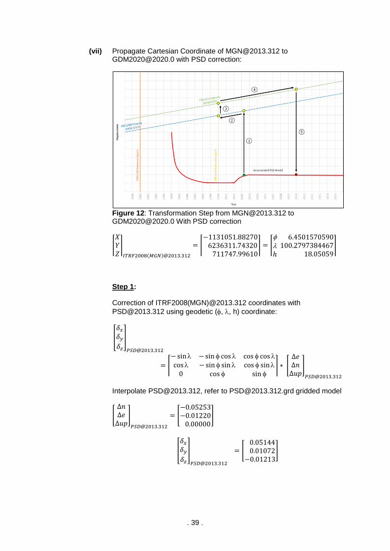
(vii) Propagate Cartesian Coordinate of [email protected] to [email protected] with PSD correction:

Figure 12: Transformation Step from [email protected] to [email protected] With PSD correction

⌈𝑋𝑌𝑍⌉

𝐼𝑇𝑅𝐹2008(𝑀𝐺𝑁)@2013.312

= ⌈−1131051.88270 6236311.74320 711747.99610

⌉ = ⌈

ℎ

6.4501570590100.2797384467 18.05059

⌉

Step 1:

Correction of ITRF2008(MGN)@2013.312 coordinates with

[email protected] using geodetic (, , h) coordinate:

[

𝛿𝑥

𝛿𝑦

𝛿𝑧

]

𝑃𝑆𝐷@2013.312

= ⌈


0 cos sin ⌉ ∗ [


]

𝑃𝑆𝐷@2013.312

Interpolate [email protected], refer to [email protected] gridded model

[∆𝑛∆𝑒∆𝑢𝑝

]

𝑃𝑆𝐷@2013.312

= [−0.05253−0.01220 0.00000

]

[

𝛿𝑥

𝛿𝑦

𝛿𝑧

]

𝑃𝑆𝐷@2013.312

= [ 0.05144 0.01072−0.01213

]

. 40 .

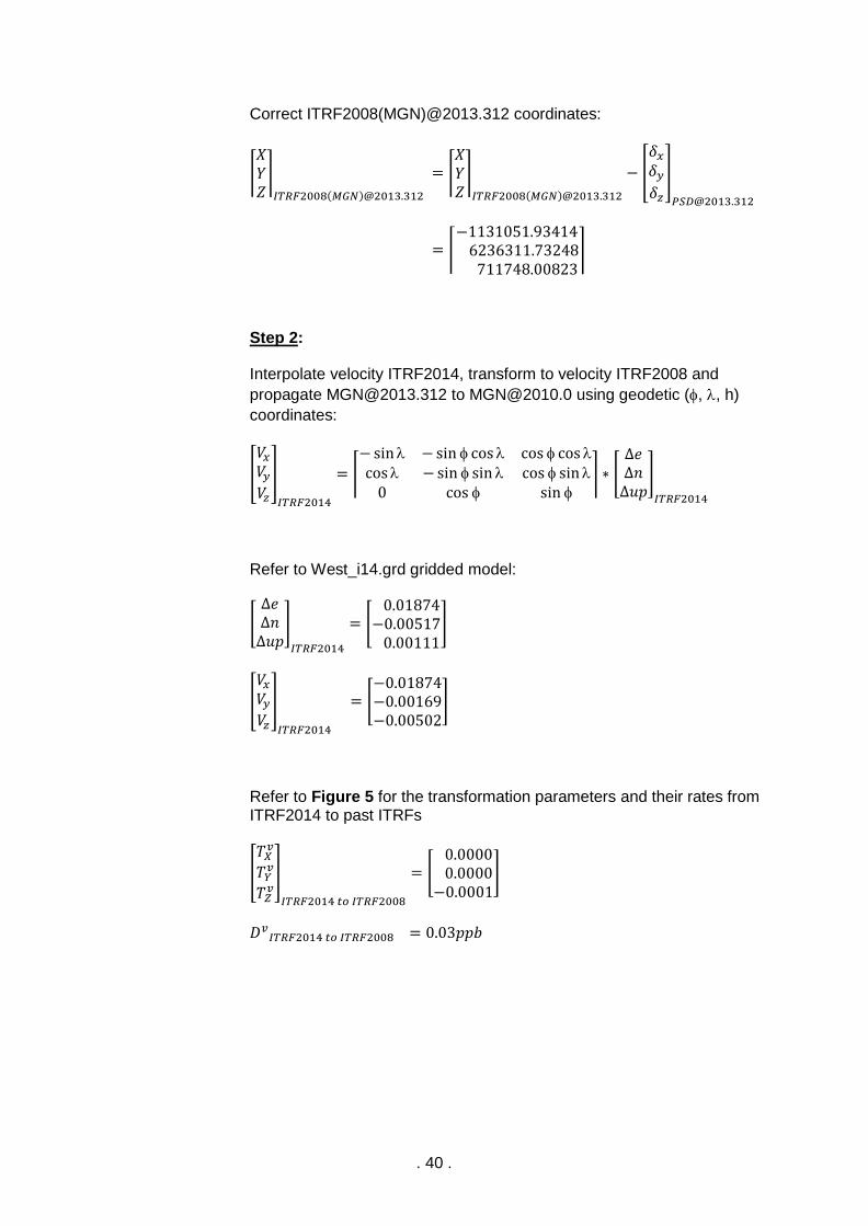
Correct ITRF2008(MGN)@2013.312 coordinates:

⌈𝑋𝑌𝑍⌉

𝐼𝑇𝑅𝐹2008(𝑀𝐺𝑁)@2013.312


𝐼𝑇𝑅𝐹2008(𝑀𝐺𝑁)@2013.312

− [

𝛿𝑥

𝛿𝑦

𝛿𝑧

]

𝑃𝑆𝐷@2013.312

= ⌈−1131051.93414 6236311.73248 711748.00823

⌉

Step 2:

Interpolate velocity ITRF2014, transform to velocity ITRF2008 and

propagate [email protected] to [email protected] using geodetic (, , h)

coordinates:

[


]


= ⌈


0 cos sin ⌉ ∗ [


]




]


= [ 0.01874−0.00517 0.00111

]

[


]


= [−0.01874−0.00169−0.00502

]


[

𝑇𝑋𝑣

𝑇𝑌𝑣

𝑇𝑍𝑣]


= [ 0.0000 0.0000−0.0001

]

𝐷𝑣𝐼𝑇𝑅𝐹2014 𝑡𝑜 𝐼𝑇𝑅𝐹2008 = 0.03𝑝𝑝𝑏

. 41 .

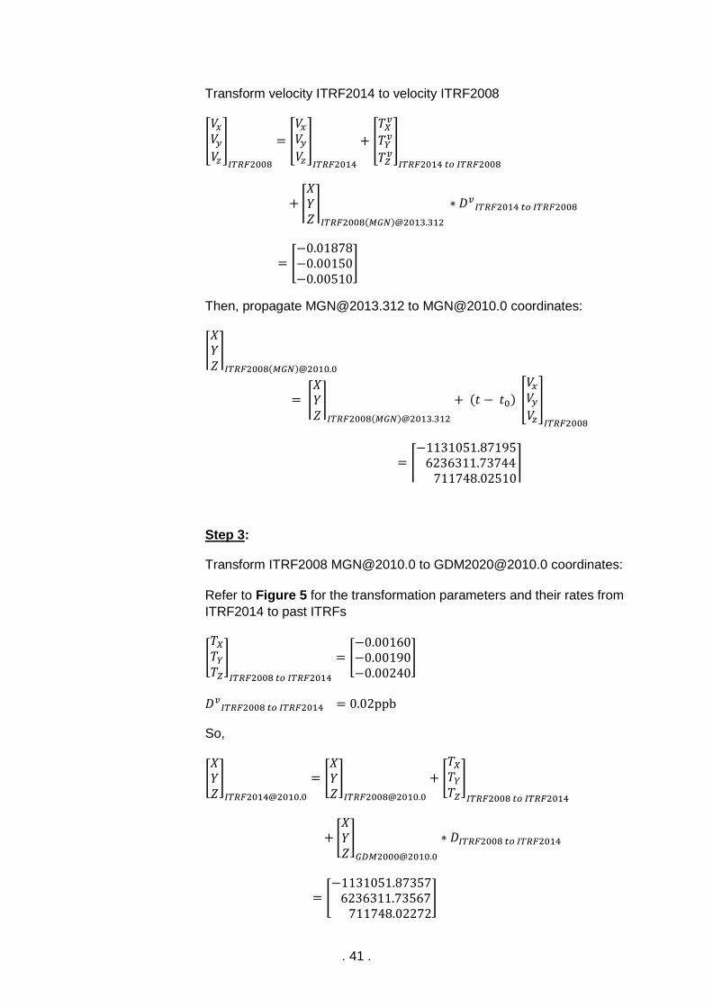
Transform velocity ITRF2014 to velocity ITRF2008

[


]


= [


]


+ [

𝑇𝑋𝑣

𝑇𝑌𝑣

𝑇𝑍𝑣]



𝐼𝑇𝑅𝐹2008(𝑀𝐺𝑁)@2013.312


= [−0.01878−0.00150−0.00510

]

Then, propagate [email protected] to [email protected] coordinates:

⌈𝑋𝑌𝑍⌉

𝐼𝑇𝑅𝐹2008(𝑀𝐺𝑁)@2010.0


𝐼𝑇𝑅𝐹2008(𝑀𝐺𝑁)@2013.312

+ (𝑡 − 𝑡0) [


]


= ⌈−1131051.87195 6236311.73744 711748.02510

⌉

Step 3:

Transform ITRF2008 [email protected] to [email protected] coordinates:



[𝑇𝑋

𝑇𝑌

𝑇𝑍

]


= [−0.00160−0.00190−0.00240

]

𝐷𝑣𝐼𝑇𝑅𝐹2008 𝑡𝑜 𝐼𝑇𝑅𝐹2014 = 0.02ppb

So,

[𝑋𝑌𝑍]

𝐼𝑇𝑅𝐹[email protected]

= [𝑋𝑌𝑍]

𝐼𝑇𝑅𝐹[email protected]

+ [

𝑇𝑋

𝑇𝑌

𝑇𝑍

]


+ [𝑋𝑌𝑍]



= [−1131051.87357 6236311.73567 711748.02272

]

. 42 .

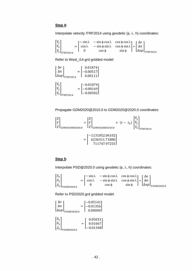
Step 4:


[


]


= ⌈


0 cos sin ⌉ ∗ [


]




]


= [ 0.01874−0.00517 0.00111

]

[


]


= [−0.01874−0.00169−0.00502

]


⌈𝑋𝑌𝑍⌉




+ (𝑡 − 𝑡0) [


]


= ⌈−1131052.06102 6236311.71880 711747.97255

⌉

Step 5:


[

𝛿𝑥

𝛿𝑦

𝛿𝑧

]

𝑃𝑆𝐷@2020.0

= ⌈


0 cos sin ⌉ ∗ [


]

𝑃𝑆𝐷@2020.0



]

𝑃𝑆𝐷@2020.0

= [−0.05141−0.01356 0.00000

]

[

𝛿𝑥

𝛿𝑦

𝛿𝑧

]

𝑃𝑆𝐷@2020.0

= [ 0.05031 0.01067−0.01348

]

. 43 .

So,

⌈𝑋𝑌𝑍⌉




+ [

𝛿𝑥

𝛿𝑦

𝛿𝑧

]

𝑃𝑆𝐷@2020.0

= ⌈−1131052.01070 6236311.72948 711747.95907

⌉

. 44 .

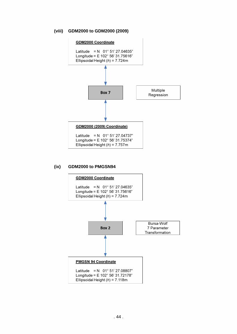
(viii) GDM2000 to GDM2000 (2009)

(ix) GDM2000 to PMGSN94

. 45 .

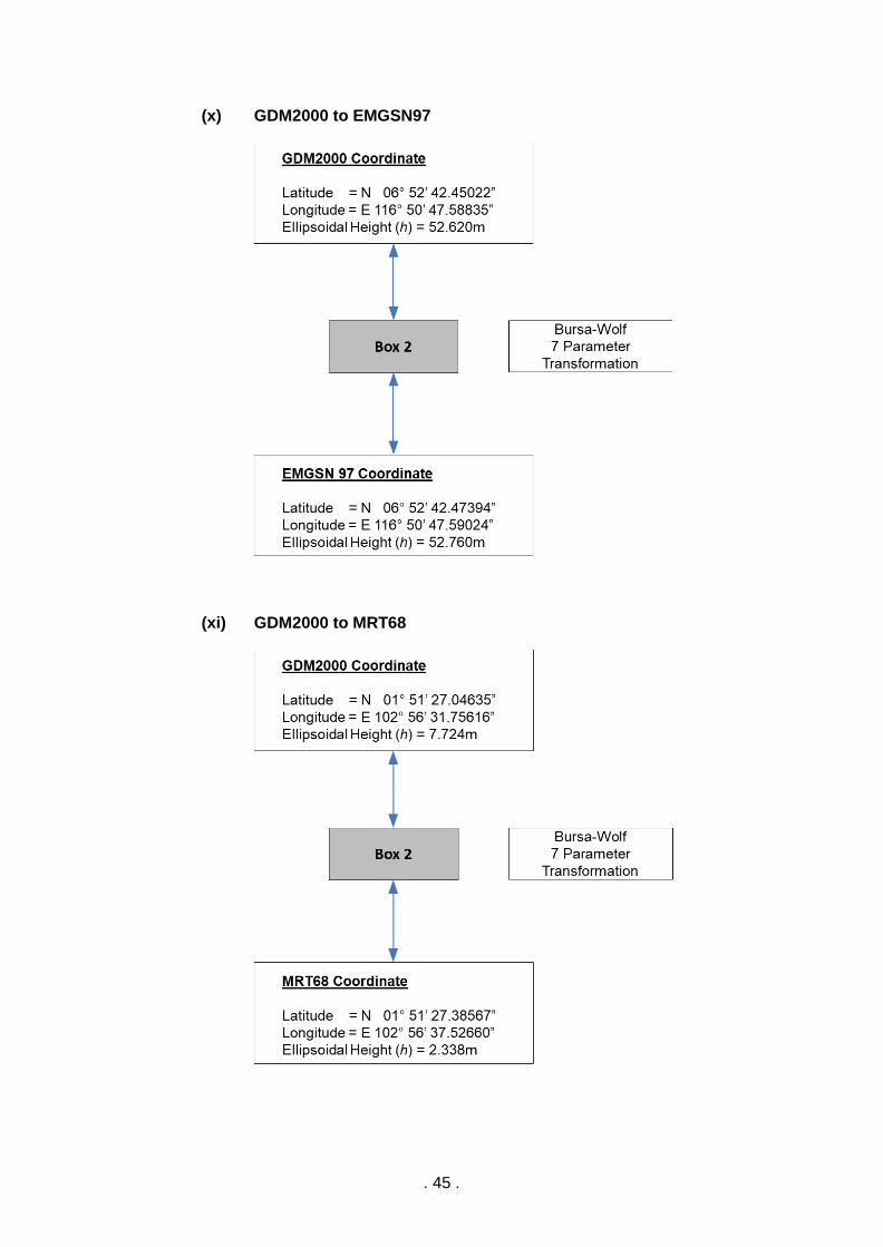
(x) GDM2000 to EMGSN97

(xi) GDM2000 to MRT68

. 46 .

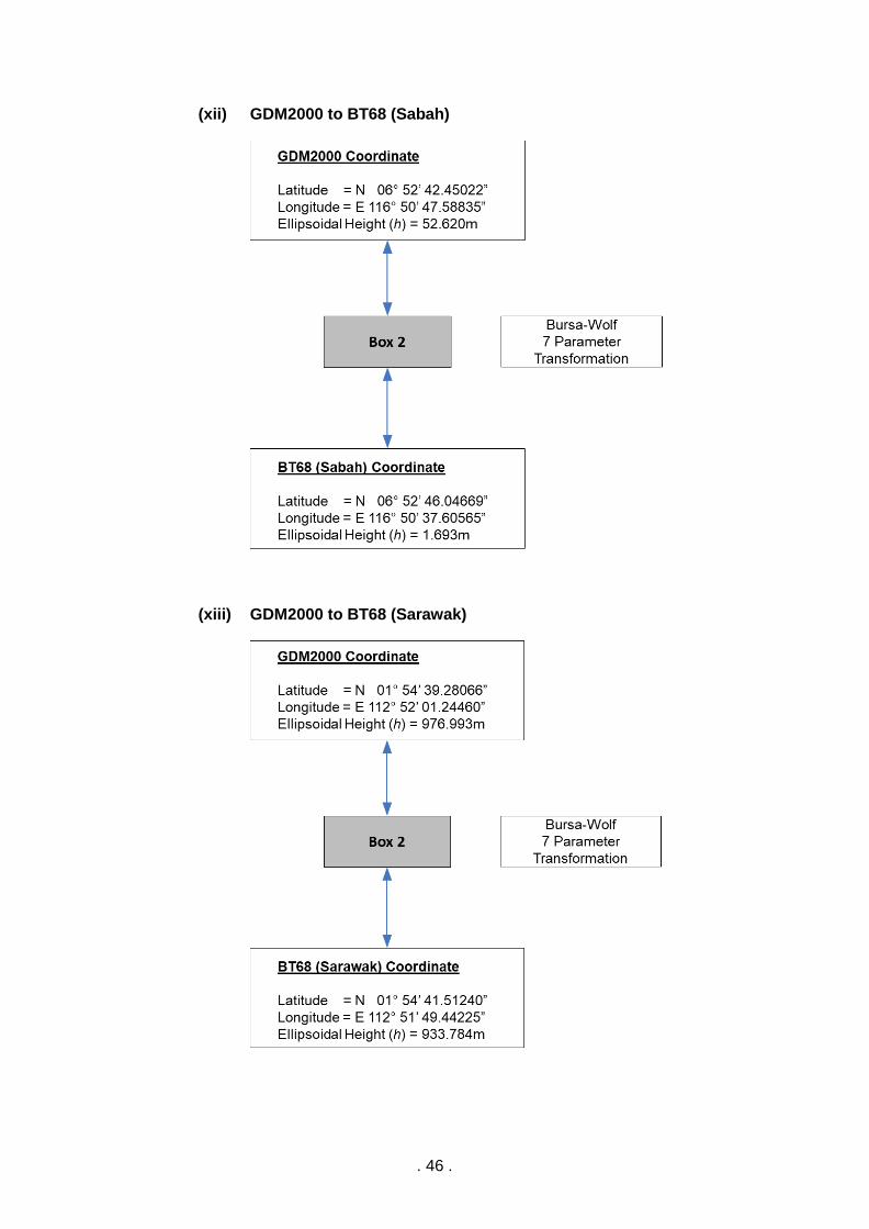
(xii) GDM2000 to BT68 (Sabah)

(xiii) GDM2000 to BT68 (Sarawak)

. 47 .

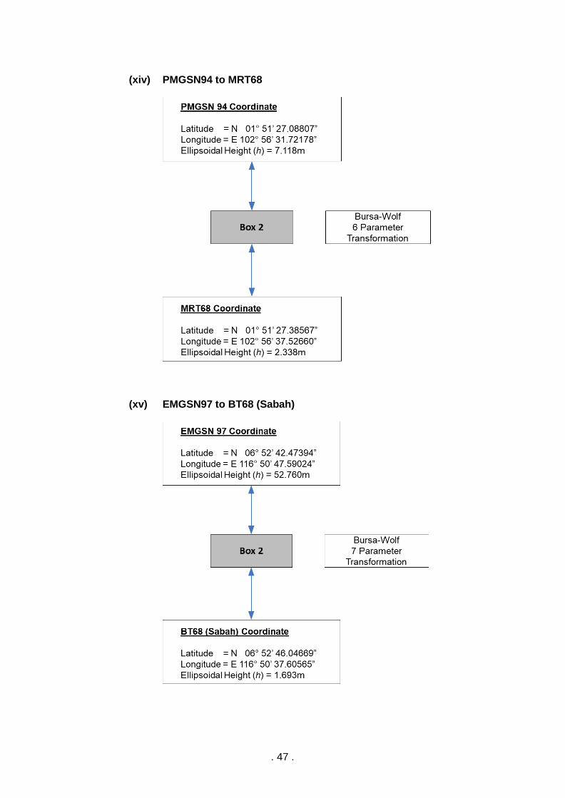
(xiv) PMGSN94 to MRT68

(xv) EMGSN97 to BT68 (Sabah)

. 48 .

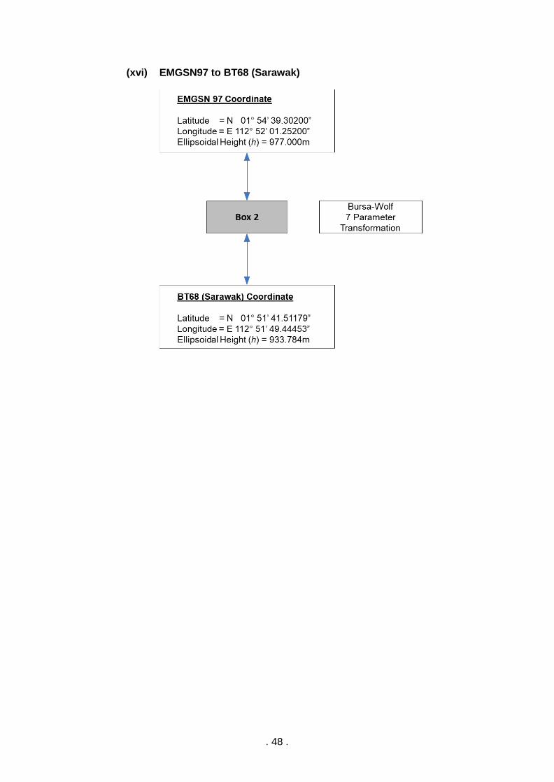
(xvi) EMGSN97 to BT68 (Sarawak)

. 49 .

4. MAP PROJECTION

4.1 Introduction

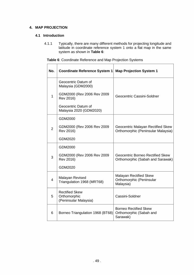
4.1.1 Typically, there are many different methods for projecting longitude and latitude in coordinate reference system 1 onto a flat map in the same system as shown in Table 6:

Table 6: Coordinate Reference and Map Projection Systems

No. Coordinate Reference System 1 Map Projection System 1

1

Geocentric Datum of Malaysia (GDM2000)

GDM2000 (Rev 2006 Rev 2009 Rev 2016)

Geocentric Datum of Malaysia 2020 (GDM2020)

Geocentric Cassini-Soldner

2

GDM2000

GDM2000 (Rev 2006 Rev 2009 Rev 2016)

GDM2020

Geocentric Malayan Rectified Skew Orthomorphic (Peninsular Malaysia)

3

GDM2000

GDM2000 (Rev 2006 Rev 2009 Rev 2016)

GDM2020

Geocentric Borneo Rectified Skew Orthomorphic (Sabah and Sarawak)

4 Malayan Revised Triangulation 1968 (MRT68)

Malayan Rectified Skew Orthomorphic (Peninsular Malaysia)

5 Rectified Skew Orthomorphic (Peninsular Malaysia)

Cassini-Soldner

6 Borneo Triangulation 1968 (BT68) Borneo Rectified Skew Orthomorphic (Sabah and Sarawak)

. 50 .

4.2 Rectified Skew Orthomorphic (RSO) Map Projection

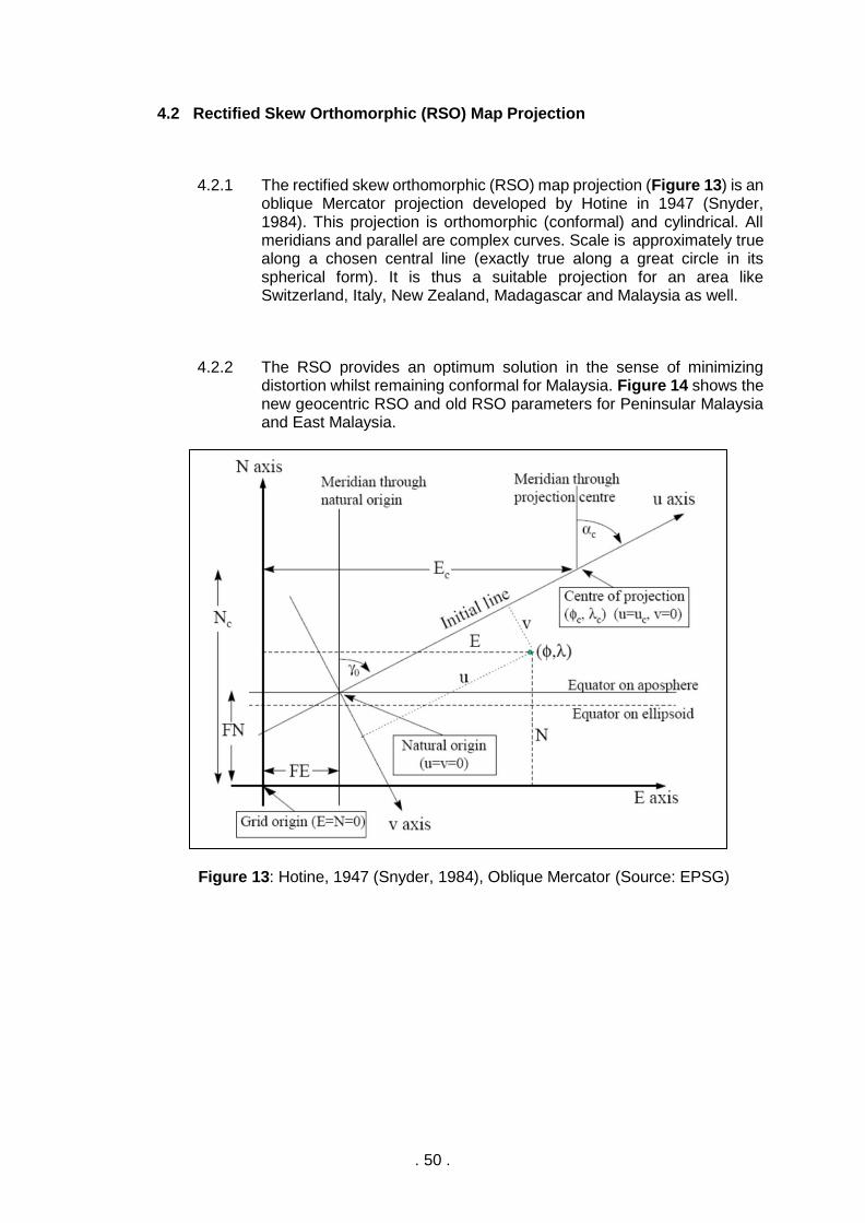
4.2.1 The rectified skew orthomorphic (RSO) map projection (Figure 13) is an oblique Mercator projection developed by Hotine in 1947 (Snyder, 1984). This projection is orthomorphic (conformal) and cylindrical. All meridians and parallel are complex curves. Scale is approximately true along a chosen central line (exactly true along a great circle in its spherical form). It is thus a suitable projection for an area like Switzerland, Italy, New Zealand, Madagascar and Malaysia as well.

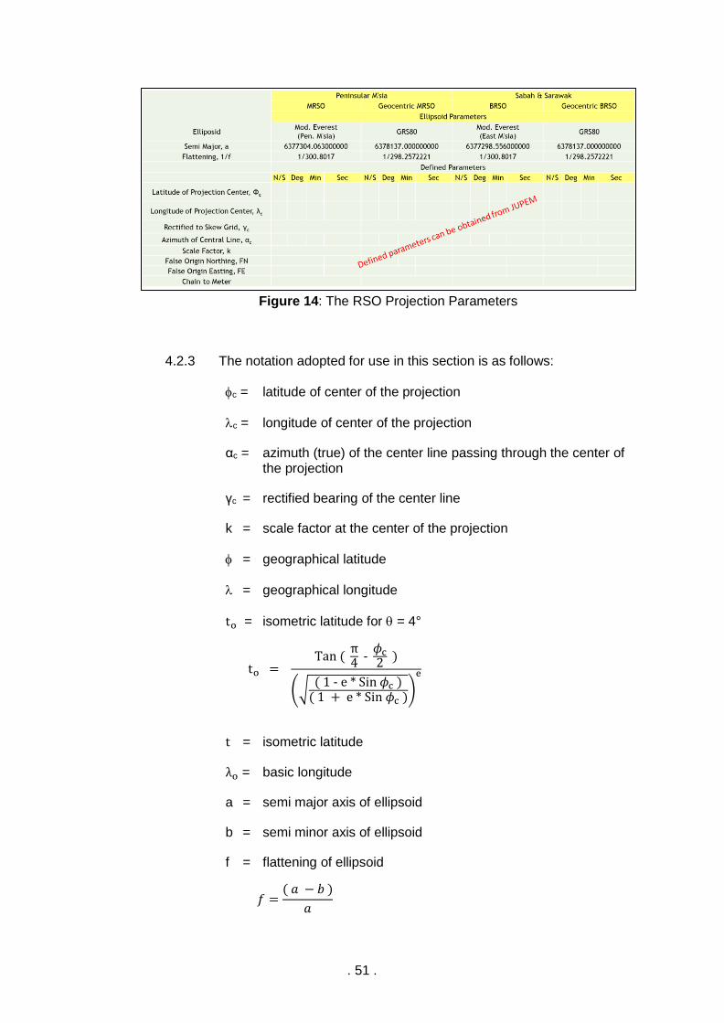
4.2.2 The RSO provides an optimum solution in the sense of minimizing distortion whilst remaining conformal for Malaysia. Figure 14 shows the new geocentric RSO and old RSO parameters for Peninsular Malaysia and East Malaysia.

Figure 13: Hotine, 1947 (Snyder, 1984), Oblique Mercator (Source: EPSG)

. 51 .

Figure 14: The RSO Projection Parameters

4.2.3 The notation adopted for use in this section is as follows:

c = latitude of center of the projection

c = longitude of center of the projection

αc = azimuth (true) of the center line passing through the center of the projection

γc = rectified bearing of the center line

k = scale factor at the center of the projection

= geographical latitude

= geographical longitude

to = isometric latitude for = 4°

t = isometric latitude

λo = basic longitude

a = semi major axis of ellipsoid

b = semi minor axis of ellipsoid

f = flattening of ellipsoid

to = Tan (

π4 -

𝜙c2 )

(√( 1 - e * Sin 𝜙c )

( 1 + e * Sin 𝜙c ))

e

𝑓 =( 𝑎 − 𝑏 )

𝑎

. 52 .

e = eccentricity of the ellipsoid

u = skew coordinate parallel to initial line

v = skew coordinate at right angles to initial line

𝛾 = skew convergence at meridians

𝛾𝑅 = rectified convergence of meridians

N = Northing map coordinate

E = Easting map coordinate

FE = False Easting at the natural origin

FN= False Northing at the natural origin

where,

The Constants of the Projection are given as follows:

To avoid problems with computation of F, if D<1, make D2 = 1

e = √ ( a2 - b2 )

a2 e' = √

( a2 - b2 )

b2

B = √1 + ( e2 Cos4 𝜙c )

( 1 - e2 )

A = a * B * k √(1 - e2)

( 1 - e2 * Sin2 𝜙c )

D = B * √ ( 1 - e2 )

Cos 𝜙c * √ ( 1 - e2 Sin2 𝜙c )

F = D + Sign 𝜙c * √ ( D2 - 1 )

H = F * toB

G = F -

1F

2

γo = Sin-1 ( Sin αc

D)

𝛾𝑅 = 𝛾 + 36° 52' 11.6314"

. 53 .

Basic Longitude:

4.2.4 The projection formulae are as follows:

(a) Conversion of Geographical to Rectangular and vice versa

Forward Case: To compute (E, N) from a given (, ):

For the Hotine Oblique Mercator (where the FE and FN values have been specified with respect to the origin of the (u, v) axes):

The rectified skew coordinates are then derived from:

λo = λc - Sin-1 ( G * Tan γo )

B

v = A ln (

1 - U1 + U)

2B

U = S Sin γo − V Cos γo

T

S = Q -

1Q

2

Q = H

tB

t = Tan (

π4

- 𝜙2

)

(√( 1 - e * Sin 𝜙 )

( 1 + e * Sin 𝜙 ))

e

T = Q +

1Q

2

V = Sin [ B ( λ - λo ) ]

u = A

B Tan-1 (

S Cos γo + V Sin γo

Cos [ B ( λ - λo ) ])

E = v Cos γc + u Sin γc + FE

N = u Cos γc − v Sin γc + FN

. 54 .

Reverse Case: Compute (, ) from a given (E, N):

For the Hotine Oblique Mercator:

Then the other parameters can be calculated.

v' = ( E - FE ) * Cos γc - ( N - FN ) * Sin γc

u' = ( N - FN ) * Cos γc + ( E - FE ) * Sin γc

Q' = exp (−B v'

A)

S' = Q' -

1Q'

2

T' = Q' +

1Q'

2

V' = Sin (B u'

A)

U' = V' Cos γc + S' Sin γc

T'

t' =

[

H

√ ( 1 + U' )( 1 − U' )]

1B

𝜒 = (π

2 ) - 2 * ( Tan-1 t' )

λ = λo -

Tan-1 (S' Cos γc - V' Sin γc

Cos B u'A

)

B

𝜙 = 𝜒 + ( Sin 2 𝜒 )* (e2

2 +

5 e4

24 +

e6

12 +

13 e8

360)

+ ( Sin 4 𝜒 ) * (7 e4

48 +

29 e6

240 +

811 e6

11520)

+ ( Sin 6 𝜒 ) * (7 e6

120 +

81 e8

1120)

+ ( Sin 8 𝜒 ) * (4279 e4

161280)

. 55 .

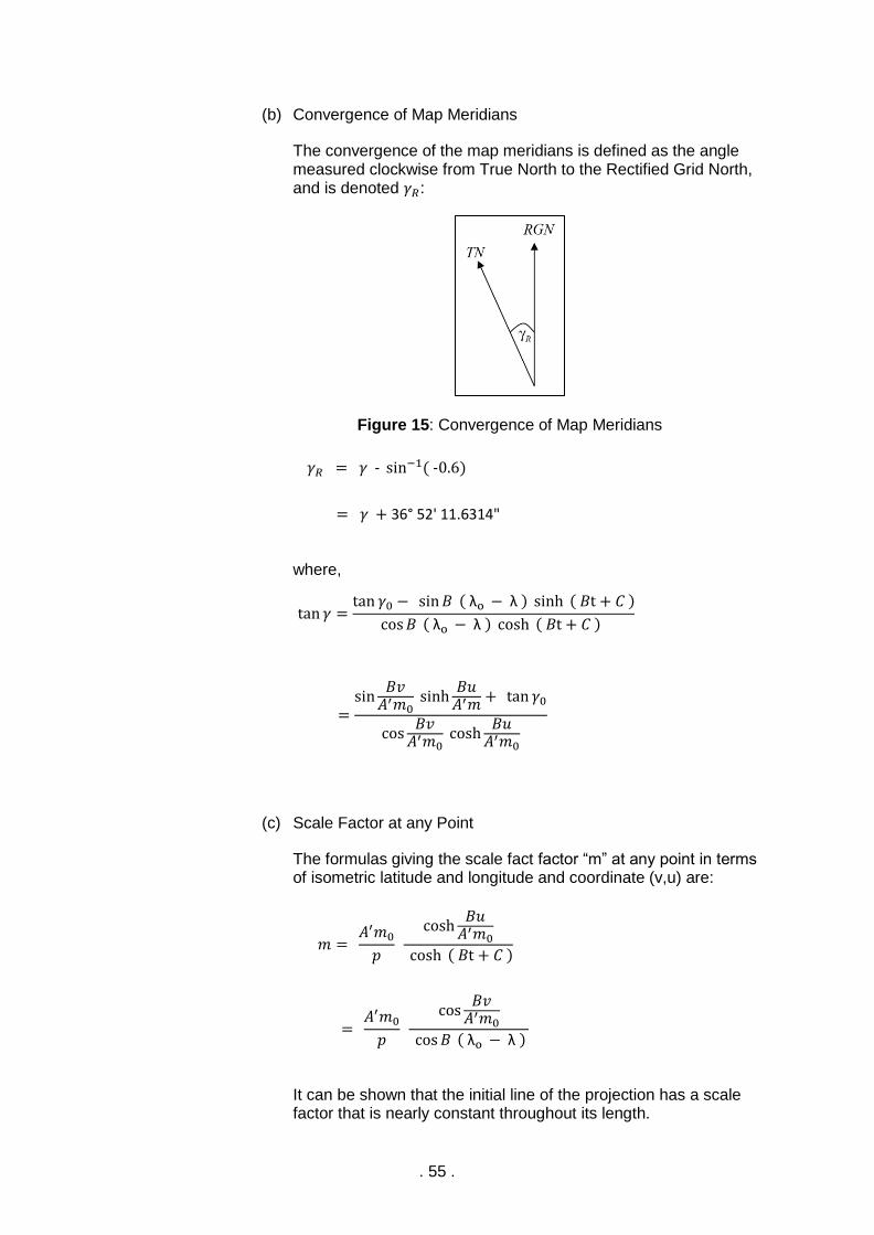
(b) Convergence of Map Meridians

The convergence of the map meridians is defined as the angle measured clockwise from True North to the Rectified Grid North, and is denoted 𝛾𝑅:

Figure 15: Convergence of Map Meridians

where,

(c) Scale Factor at any Point

The formulas giving the scale fact factor “m” at any point in terms of isometric latitude and longitude and coordinate (v,u) are:

It can be shown that the initial line of the projection has a scale factor that is nearly constant throughout its length.

= 𝛾 + 36° 52' 11.6314"

𝛾𝑅 = 𝛾 - sin−1( -0.6)

tan 𝛾 =tan 𝛾0 − sin𝐵 ( λo − λ ) sinh ( 𝐵t + 𝐶 )

cos𝐵 ( λo − λ ) cosh ( 𝐵t + 𝐶 )

=sin

𝐵𝑣𝐴′𝑚0

sinh𝐵𝑢𝐴′𝑚 + tan 𝛾0

cos𝐵𝑣

𝐴′𝑚0 cosh

𝐵𝑢𝐴′𝑚0

𝑚 = 𝐴′𝑚0

𝑝

cosh𝐵𝑢

𝐴′𝑚0

cosh ( 𝐵t + 𝐶 )

= 𝐴′𝑚0

𝑝

cos𝐵𝑣

𝐴′𝑚0

cos𝐵 ( λo − λ )

. 56 .

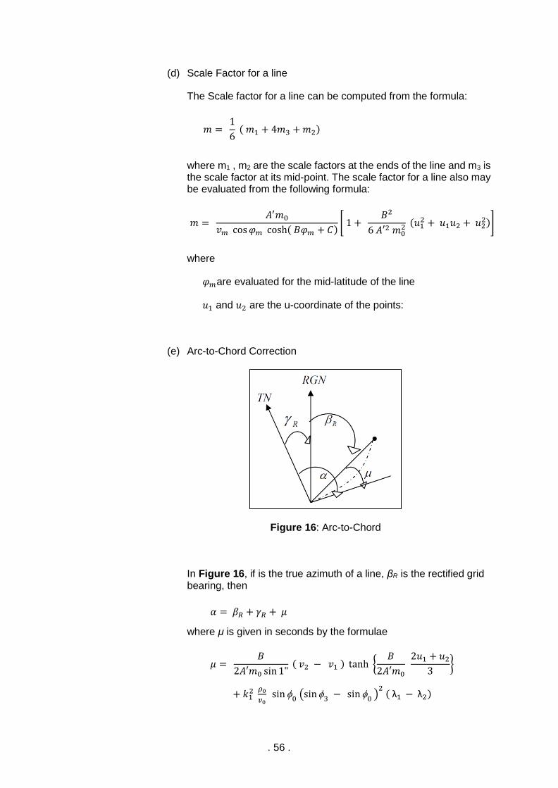
(d) Scale Factor for a line

The Scale factor for a line can be computed from the formula:

where m1 , m2 are the scale factors at the ends of the line and m3 is the scale factor at its mid-point. The scale factor for a line also may be evaluated from the following formula:

where

𝜑𝑚are evaluated for the mid-latitude of the line

𝑢1 and 𝑢2 are the u-coordinate of the points:

(e) Arc-to-Chord Correction

Figure 16: Arc-to-Chord

In Figure 16, if is the true azimuth of a line, βR is the rectified grid bearing, then

where μ is given in seconds by the formulae

𝑚 = 1

6 ( 𝑚1 + 4𝑚3 + 𝑚2)

𝑚 = 𝐴′𝑚0

𝑣𝑚 cos𝜑𝑚 cosh( 𝐵𝜑𝑚 + 𝐶)[ 1 +

𝐵2

6 𝐴′2 𝑚02 (𝑢1

2 + 𝑢1𝑢2 + 𝑢22)]

𝛼 = 𝛽𝑅 + 𝛾𝑅 + 𝜇

𝜇 = 𝐵

2𝐴′𝑚0 sin1" ( 𝑣2 − 𝑣1 ) tanh {

𝐵

2𝐴′𝑚0 2𝑢1 + 𝑢2

3}

+ 𝑘12

𝜌0

𝑣0 sin

0 (sin3

− sin 0 )

2 ( λ1 − λ2)

. 57 .

where,

and is measured in seconds.

For a line not exceeding 113 km (70 miles) in length, the maximum value of the second term of the formula is 0.007”; it can therefore bsafely neglected.

3

= 1

3 ( 2

1+

2 )

( λ1 − λ2)

. 58 .

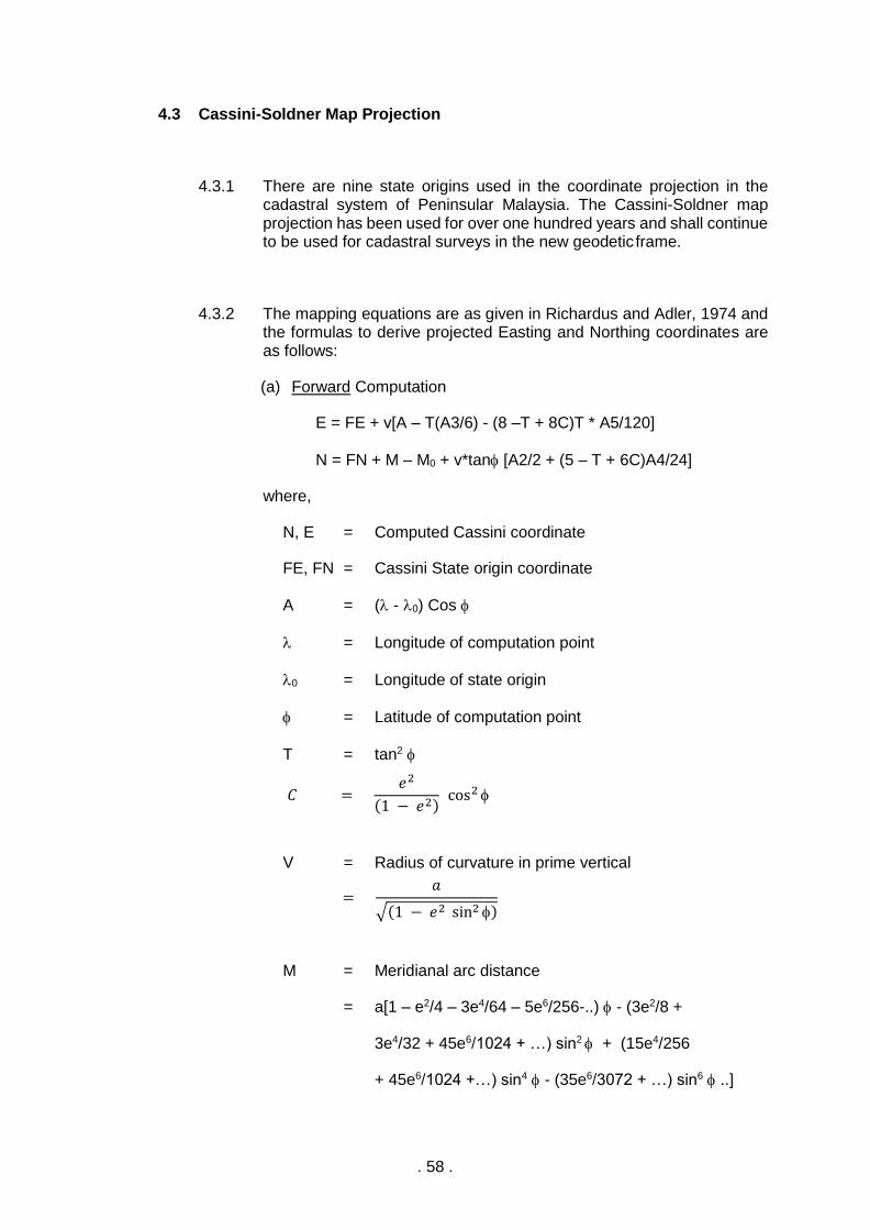
4.3 Cassini-Soldner Map Projection

4.3.1 There are nine state origins used in the coordinate projection in the cadastral system of Peninsular Malaysia. The Cassini-Soldner map projection has been used for over one hundred years and shall continue to be used for cadastral surveys in the new geodetic frame.

4.3.2 The mapping equations are as given in Richardus and Adler, 1974 and the formulas to derive projected Easting and Northing coordinates are as follows:

(a) Forward Computation

E = FE + v[A – T(A3/6) - (8 –T + 8C)T * A5/120]

N = FN + M – M0 + v*tan [A2/2 + (5 – T + 6C)A4/24]

where,

N, E = Computed Cassini coordinate

FE, FN = Cassini State origin coordinate

A = ( - 0) Cos

= Longitude of computation point

0 = Longitude of state origin

= Latitude of computation point

T = tan2

V = Radius of curvature in prime vertical

M = Meridianal arc distance

= a[1 – e2/4 – 3e4/64 – 5e6/256-..) - (3e2/8 +

3e4/32 + 45e6/1024 + …) sin2 + (15e4/256

+ 45e6/1024 +…) sin4 - (35e6/3072 + …) sin6 ..]

𝐶 = 𝑒2

(1 − 𝑒2) cos2

= 𝑎

√(1 − 𝑒2 sin2 )

. 59 .

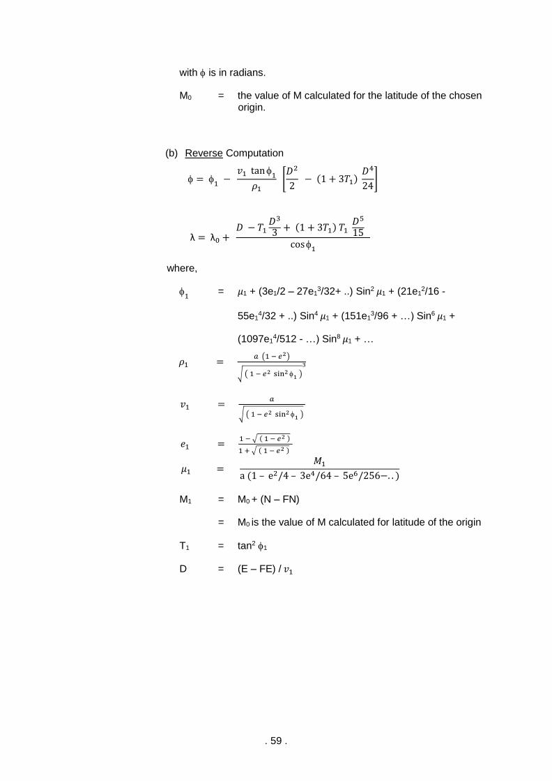
with is in radians.

M0 = the value of M calculated for the latitude of the chosen origin.

(b) Reverse Computation

where,

1 = 𝜇1 + (3e1/2 – 27e1

3/32+ ..) Sin2 𝜇1 + (21e12/16 -

55e14/32 + ..) Sin4 𝜇1 + (151e1

3/96 + …) Sin6 𝜇1 +

(1097e14/512 - …) Sin8 𝜇1 + …

M1 = M0 + (N – FN)

= M0 is the value of M calculated for latitude of the origin

T1 = tan2 1

D = (E – FE) / 𝑣1

= 1

− 𝑣1 tan

1

𝜌1 [

𝐷2

2 − (1 + 3𝑇1)

𝐷4

24]

λ = λ0 + 𝐷 − 𝑇1

𝐷3

3+ (1 + 3𝑇1) 𝑇1

𝐷5

15

cos1

𝜌1 = 𝑎 (1 − 𝑒2)

√ ( 1 − 𝑒2 sin2 1 )

3

𝑣1 = 𝑎

√ ( 1 − 𝑒2 sin2 1 )

𝑒1 = 1 − √ ( 1 − 𝑒2 )

1 + √ ( 1 − 𝑒2 )

𝜇1 = 𝑀1

a (1 – e2/4 – 3e4/64 – 5e6/256−. . )

. 60 .

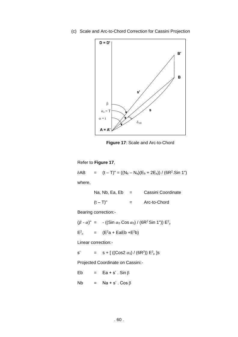
(c) Scale and Arc-to-Chord Correction for Cassini Projection

Figure 17: Scale and Arc-to-Chord

Refer to Figure 17,

AB = (t – T)" = ((Nb – Na)(Eb + 2Ea)) / (6R2.Sin 1")

where,

Na, Nb, Ea, Eb = Cassini Coordinate

(t – T)" = Arc-to-Chord

Bearing correction:-

(𝛽 - 𝛼)" = - ((Sin 𝛼0 Cos 𝛼0) / (6R2 Sin 1")) E2

E2 = (E2a + EaEb +E2b)

Linear correction:-

s’ = s + [ ((Cos2 𝛼0) / (6R2)) E2 ]s

Projected Coordinate on Cassini:-

Eb = Ea + s’ . Sin

Nb = Na + s’ . Cos

. 61 .

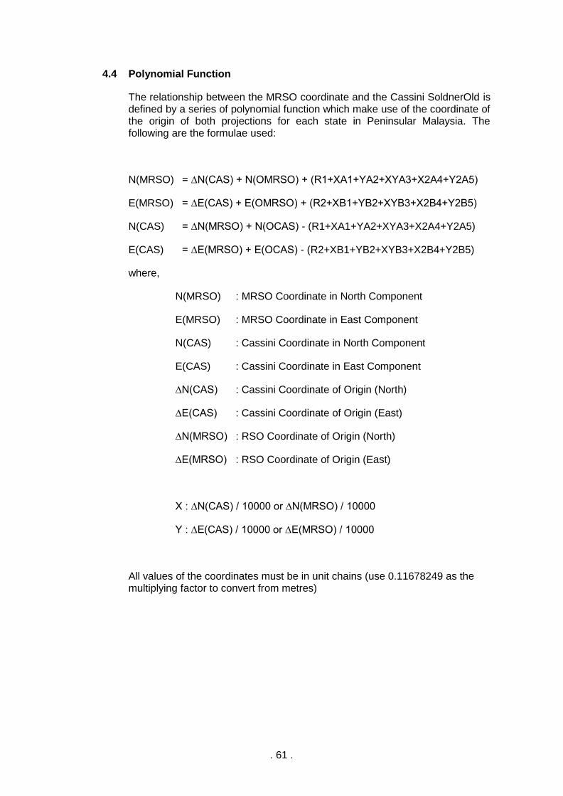
4.4 Polynomial Function

The relationship between the MRSO coordinate and the Cassini SoldnerOld is defined by a series of polynomial function which make use of the coordinate of the origin of both projections for each state in Peninsular Malaysia. The following are the formulae used:

N(MRSO) = ∆N(CAS) + N(OMRSO) + (R1+XA1+YA2+XYA3+X2A4+Y2A5)

E(MRSO) = ∆E(CAS) + E(OMRSO) + (R2+XB1+YB2+XYB3+X2B4+Y2B5)

N(CAS) = ∆N(MRSO) + N(OCAS) - (R1+XA1+YA2+XYA3+X2A4+Y2A5)

E(CAS) = ∆E(MRSO) + E(OCAS) - (R2+XB1+YB2+XYB3+X2B4+Y2B5)

where,

N(MRSO) : MRSO Coordinate in North Component

E(MRSO) : MRSO Coordinate in East Component

N(CAS) : Cassini Coordinate in North Component

E(CAS) : Cassini Coordinate in East Component

∆N(CAS) : Cassini Coordinate of Origin (North)

∆E(CAS) : Cassini Coordinate of Origin (East)

∆N(MRSO) : RSO Coordinate of Origin (North)

∆E(MRSO) : RSO Coordinate of Origin (East)

X : ∆N(CAS) / 10000 or ∆N(MRSO) / 10000

Y : ∆E(CAS) / 10000 or ∆E(MRSO) / 10000

All values of the coordinates must be in unit chains (use 0.11678249 as the multiplying factor to convert from metres)

. 62 .

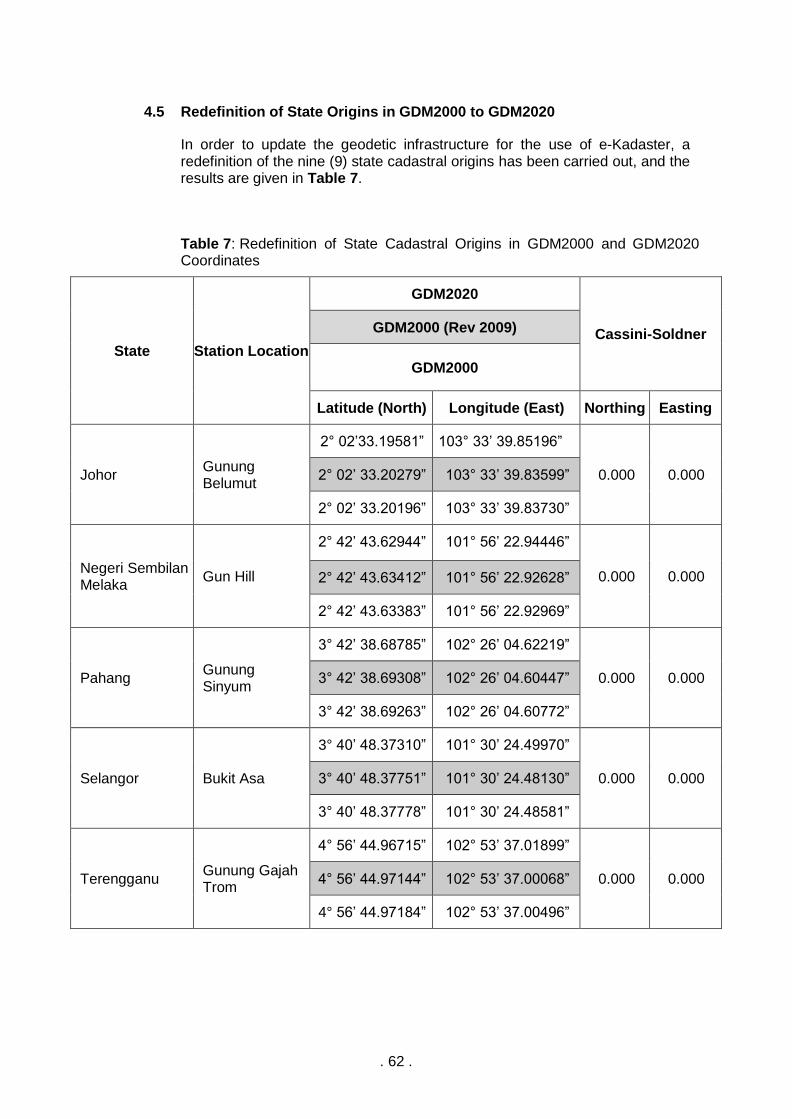
4.5 Redefinition of State Origins in GDM2000 to GDM2020

In order to update the geodetic infrastructure for the use of e-Kadaster, a redefinition of the nine (9) state cadastral origins has been carried out, and the results are given in Table 7.

Table 7: Redefinition of State Cadastral Origins in GDM2000 and GDM2020 Coordinates

State Station Location

GDM2020

Cassini-Soldner GDM2000 (Rev 2009)

GDM2000

Latitude (North) Longitude (East) Northing Easting

Johor Gunung Belumut

2° 02’33.19581” 103° 33’ 39.85196”

0.000 0.000 2° 02’ 33.20279” 103° 33’ 39.83599”

2° 02’ 33.20196” 103° 33’ 39.83730”

Negeri Sembilan Melaka

Gun Hill

2° 42’ 43.62944” 101° 56’ 22.94446”

0.000 0.000 2° 42’ 43.63412” 101° 56’ 22.92628”

2° 42’ 43.63383” 101° 56’ 22.92969”

Pahang Gunung Sinyum

3° 42’ 38.68785” 102° 26’ 04.62219”

0.000 0.000 3° 42’ 38.69308” 102° 26’ 04.60447”

3° 42’ 38.69263” 102° 26’ 04.60772”

Selangor Bukit Asa

3° 40’ 48.37310” 101° 30’ 24.49970”

0.000 0.000 3° 40’ 48.37751” 101° 30’ 24.48130”

3° 40’ 48.37778” 101° 30’ 24.48581”

Terengganu Gunung Gajah Trom

4° 56’ 44.96715” 102° 53’ 37.01899”

0.000 0.000 4° 56’ 44.97144” 102° 53’ 37.00068”

4° 56’ 44.97184” 102° 53’ 37.00496”

. 63 .

Table 7: (continued)

State Station Location

GDM2020

Cassini-Soldner GDM2000 (Rev 2009)

GDM2000

Latitude (North) Longitude (East) Northing Easting

Pulau Pinang Seberang Perai

Fort Cornwallis

5° 25’ 15.19941” 100° 20’ 40.77228”

0.000 0.000 5° 25’ 15.20204” 100° 20’ 40.75188”

5° 25’ 15.20433” 100° 20’ 40.76024”

Kedah Perlis

Gunung Perak

5° 57’ 52.81746” 100° 38’ 10.94996”

0.000 0.000 5° 57’ 52.81981” 100° 38’ 10.93028”

5° 57’ 52.82155” 100° 38’ 10.93860”

Perak Gunung Hijau Larut

4° 51’ 32.64021” 100° 48’ 55.48363”

0.000 0.000 4° 51’ 32.64361” 100° 48’ 55.46334”

4° 51’ 32.64488” 100° 48’ 55.47038”

Kelantan Bukit Panau (Baru)

5° 53’ 37.07511” 102° 10’ 32.25823”

0.000 0.000 5° 53’ 37.07908” 102° 10’ 32.24004”

5° 53’ 37.07975” 102° 10’ 32.24529”

. 64 .

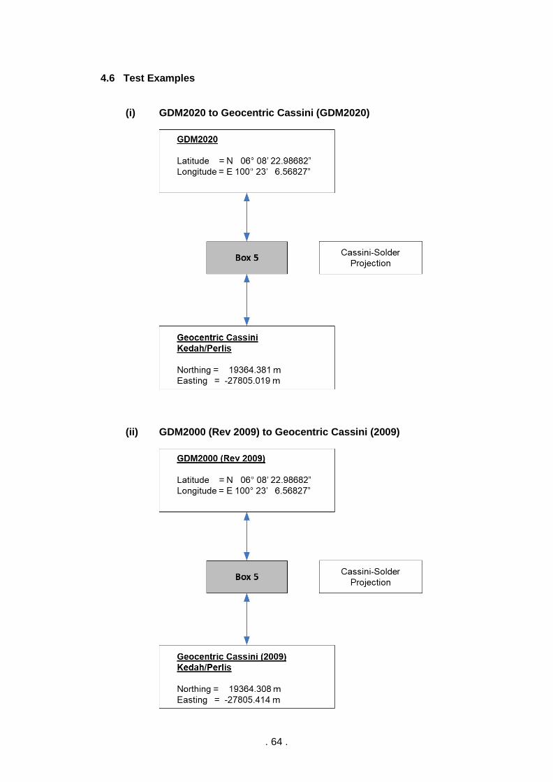
4.6 Test Examples

(i) GDM2020 to Geocentric Cassini (GDM2020)

(ii) GDM2000 (Rev 2009) to Geocentric Cassini (2009)

. 65 .

(iii) GDM2000 to Geocentric Cassini

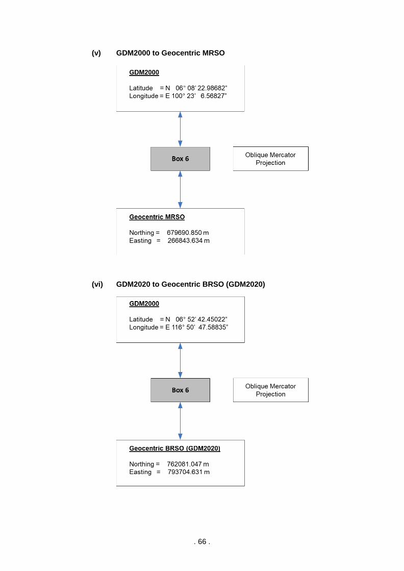
(iv) GDM2020 to Geocentric MRSO (GDM2020)

. 66 .

(v) GDM2000 to Geocentric MRSO

(vi) GDM2020 to Geocentric BRSO (GDM2020)

. 67 .

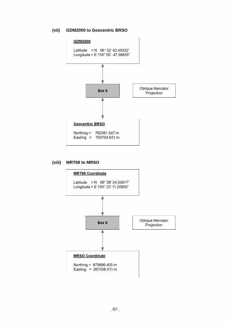
(vii) GDM2000 to Geocentric BRSO

(viii) MRT68 to MRSO

. 68 .

(ix) MRSO to Cassini Soldner

(x) BT68 to BRSO

. 69 .

5. CONCLUSION

5.1 The determination of a position requires the choice of a coordinate reference system. A situation now exists whereby it is common for a user acquiring data in a coordinate system that is completely different to which the data will be ultimately required.

5.2 In order to facilitate the conversion of various coordinates system in Malaysia, JUPEM has produced numerous sets of datum transformation and map projection parameters to relate the different types of coordinate system. This technical guide is designed as a practical solution to those who encountered datums transformation and map projections problems.

5.3 The parameter values relating to different coordinate reference systems are derived from standard coordinate conversion formulae, Bursa-Wolf transformation formulae and multiple regression model.

5.4 In addressing the effects of plate tectonic motion due to natural disasters such as earthquakes on the coordinates reference system and vertical datum systems for the whole country, JUPEM has successfully established a more accurate, precise and contemporary GDM2020. This newly derived geodetic datum system is fully aligned to ITRF2014, where velocities and PSD are modelled as an intrinsic component of the kinematic/ semi-kinematic concept of the CORS coordinates.

. 70 .

REFERENCES

Azhari, M., Altamimi, Z., Azman, G., Kadir, M., Simons, W., Sohaime, R., Yunus, M.Y., Irwan, M.J., Asyran, C.A., Soeb, N., Fahmi, A., & Saiful, A. (2020). Semi-kinematic geodetic reference frame based on the ITRF2014 for Malaysia, Journal of Geodetic Science, 10(1), 91-109. doi: https://doi.org/10.1515/jogs-2020-0108.

Altamimi Z., Billard P. and Boucher C., ITRF2000, 2002, A new release of the International Terrestrial Reference Frame for earth science applications, JGR Vol. 107, No.B10, 2214.

Altamimi Z., Sillard P., Boucher C., 2006, CATREF Software Combination and Analysis of Terrestrial Reference Frames, IGN, France.

Altamimi Z., Collilieux X. and Metivier L., 2011, ITRF2008: An Improved Solution of The International Terrestrial ReferenceFrame, Journal of Geodesy, 85, 457-473.

Altamimi Z. Rebischung P., Melvier P. and Collilieux X., 2016, ITRF2014: A new release of the International Terrestrial Reference Frame, modelling non-linear station motions, JGR, Vol.121, Issue 8.

Bowring, B.R. (1985), The accuracy of geodetic latitude and height equations, Survey Review 28(218): 202-206.

Burford, B.J. (1985), A further examination of datum transformation parameters in Australia The Australian Surveyor, vol.32 no. 7, pp. 536-558.

Bursa, M. (1962), The theory of the determination of the non-parallelism of the minor axis of the reference ellipsoid and the inertial polar axis of the Earth, and the planes of the initial astronomic and geodetic meridians from observations of artificial Earth Satellites, Studia Geophysica et Geodetica, no. 6, pp. 209-214.

Defence Mapping Agency (DMA), (1987), Department of defence World Geodetic System 1984: its definition and relationship with local geodetic systems (second edition). Technical report no. 8350.2, Defence Mapping Agency, Washington.

Heiskanen and Moritz (1967), Physical Geodesy, W. H Freeman and Company, San Francisco, USA.

Richardus, Peter, and Adler, R. K., (1974), Map Projections for Geodesists, Cartographers and Geographers: Amsterdam, North-Holland Pub. Co.

Snyder, J.P. (1984), Map projections used by the U.S. Geological Survey. Geological Survey Bulletin 1532, U.S. Geological Survey.

Wolf, H. (1963), Geometric connection and re-orientation of three-dimensional triangulation nets. Bulletin Geodesique. No, 68, pp165-169.

d9d1d-pkpup-3-2021.pdf - JUPEM

Documents

Transcript of d9d1d-pkpup-3-2021.pdf - JUPEM