D3.6.2 - Algorithm Theoretical Basis Document – Volume II – BA Algorithm Development

fire_cci

D3.6.2 - Algorithm Theoretical Basis Document

– Volume II – BA Algorithm Development ATBD II, BA Algorithm Development, version 2

Project Name ESA CCI ECV Fire Disturbance (fire_cci)

Contract N° 4000101779/10/I-NB

Project Manager Arnd Berns-Silva

Last Change Date 09/09/2014

Version 2.2

State Final

Author José Miguel Cardoso Pereira, Bernardo Mota, Duarte Oom, Teresa Calado, Itziar Alonso, Patricia Oliva, Federico González-Alonso

Document Ref: Fire_cci_Ph3_ISA_D3_6_2_ATBD_II_v2_2

Document Type: Public

fire_cci

Doc. No.: Fire_cci_Ph3_ISA_D3_6_2_ATBD_II_v2_2

Issue/Rev-No.: 2.2

D3.6.2 ATBD II - BA Algorithm Development Page II

Project Partners

Distribution

Affiliation Name Address Copies

ESA - ECSAT Stephen Plummer (ESA – ECSAT) [email protected] electronic copy

Project Team Emilio Chuvieco, (UAH)

Itziar Alonso (UAH)

Stijn Hantson (UAH)

Marc Padilla Parellada (UAH)

Dante Corti (UAH)

Arnd Berns-Silva(GAF)

Christopher Sandow (GAF)

Stefan Saradeth (GAF)

Jose Miguel Pereira (ISA)

Duarte Oom (ISA)

Gerardo López Saldaña (ISA)

Kevin Tansey (UL)

Oscar Pérez (GMV)

Luis Gutiérrez (GMV)

Ignacio García Gil (GMV)

Andreas Müller (DLR)

Martin Bachmann (DLR)

Kurt Guenther (DLR)

Veronika Gstaiger (DLR)

Eric Borg (DLR)

Martin Schultz (JÜLICH)

Angelika Heil (JÜLICH)

Florent Mouillot (IRD)

Philippe Ciais (LSCE)

Patricia Cadule (LSCE)

Chao Yue (LSCE)

[email protected]

[email protected]

[email protected]

[email protected]

[email protected]

[email protected]

[email protected]

[email protected]

[email protected]

[email protected]

[email protected]

[email protected]

[email protected]

[email protected]

[email protected]

[email protected]

[email protected]

[email protected]

[email protected]

[email protected]

[email protected]

[email protected]

[email protected]

[email protected]

[email protected]

[email protected]

electronic copy

Prime Contractor/

Scientific Lead

- UAH - University of Alcalá de Henares (Spain)

Project Management - GAF AG, (Germany)

System Engineering Partners - GMV - Aerospace & Defence (Spain)

- DLR - German Aerospace Centre (Germany)

Earth Observation Partners - INIA-CIFOR (Spain)

- ISA - Instituto Superior de Agronomia (Portugal)

- UL - University of Leicester (United Kingdom)

- DLR – German Aerospace Centre (Germany)

Climate Modelling Partners - IRD-CNRS - L’Institut de Recherche pour le Développement - Centre National de la

Recherche Scientifique (France)

- JÜLICH - Forschungszentrum Jülich GmbH (Germany)

- LSCE - Laboratoire des Sciences du Climat et l’Environnement (France)

fire_cci


Issue/Rev-No.: 2.2

D3.6.2 ATBD II - BA Algorithm Development Page III

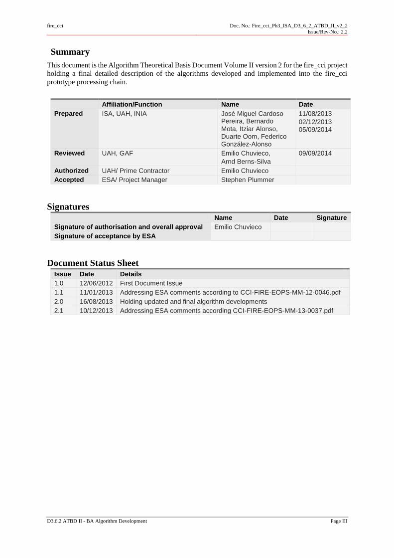
Summary

This document is the Algorithm Theoretical Basis Document Volume II version 2 for the fire_cci project

holding a final detailed description of the algorithms developed and implemented into the fire_cci

prototype processing chain.

Affiliation/Function Name Date

Prepared ISA, UAH, INIA José Miguel Cardoso Pereira, Bernardo Mota, Itziar Alonso, Duarte Oom, Federico González-Alonso

11/08/2013

02/12/2013 05/09/2014

Reviewed UAH, GAF Emilio Chuvieco,

Arnd Berns-Silva

09/09/2014

Authorized UAH/ Prime Contractor Emilio Chuvieco

Accepted ESA/ Project Manager Stephen Plummer

Signatures Name Date Signature

Signature of authorisation and overall approval Emilio Chuvieco

Signature of acceptance by ESA

Document Status Sheet Issue Date Details

1.0 12/06/2012 First Document Issue

1.1 11/01/2013 Addressing ESA comments according to CCI-FIRE-EOPS-MM-12-0046.pdf

2.0 16/08/2013 Holding updated and final algorithm developments

2.1 10/12/2013 Addressing ESA comments according CCI-FIRE-EOPS-MM-13-0037.pdf

fire_cci


Issue/Rev-No.: 2.2

D3.6.2 ATBD II - BA Algorithm Development Page IV

Document Change Record # Date Request Location Details

1.1 11/01/2013 ISA Section 2 Changing sub-sections index for “Heat” and “Smoke”;

Renaming sub-section “Burned Area” into “Scar”

Section 3.3.2 Paragraph shortened

Section 3.6 Introducing chapter “Conclusions”

Section 4.1 Introducing general statement

Section 4.1.1.3 Introducing paragraph referring to scientific papers on MRF

Section 4.3.3

Section 4.3.3.1

Restructuring of sub-sections

Elaborating on post-fire composites and annual trends

Restructuring and elaborating annual reference trends

2.0 12/08/2013 ISA Section 4.2,

Figure 3

Updating BA classification and mapping algorithm

Section 4.2.1.3.1 Introducing sub-section “Compromise programming”

Section 4.2.1.3.2,

page 23

Introducing sub-section “Selection of changepoints in single-pixel time series”

Introducing Figure 12

Section 4.2.1.3.3 Introducing sub-section “Fire seasonality score”

Section 4.2.1.3.4

Page 24 – 25

Introducing sub-section “Scoring annual

changepoint maps”

Introducing Figures 13, 14, 15, 16

Section 4.2.1.4.3 Introducing Figure 18

Section 4.3 Updating and further remarks

Section 4.3.1

Page 29

Page 32

Page 33

Updating and further remarks

Updating Figure 19


Introducing description to Table 2,3 and 4

Section 4.3.3.1 Introducing chapter “Compositing length”

Section 4.3.3.2 Introducing chapter “Post-fire composites”

Section 4.3.3.3

Page 36

Introducing chapter “Closest day to the HS”

Introducing Figure 26, 27, 28

Section 4.3.3.4

Page 37

Introducing chapter “2nd NIR minima”

Introducing Figure 29, 30

Section 4.3.3.5

Page 38

Introducing chapter “Final compositing criterion”


Section 4.3.4 Introducing Figure 33

Section 4.3.5.1

Page 39

Introducing chapter “Criteria for selecting seed pixels”


Section 4.3.5.2

0

Page 41

Introducing chapter “Identification of burned statistics



Section 4.3.5.3

Page 41

Introducing chapter “Final seed selection”

Updating Figure 37

Section 4.3.6

Page 42


Updating Figure 38

fire_cci


Issue/Rev-No.: 2.2

D3.6.2 ATBD II - BA Algorithm Development Page V

# Date Request Location Details

Section 4.4

Page 43

Page 44

Page 45


Updating Figure 39, Introducing Figure 40


Introducing Table 5

2.1

10/12/2013

ISA,UAH

Section 1.1

Section 2.1.3

Section 3.5, 2nd paragraph

Section 4.1, 4.2

Section 4.2.1.3.4

Section 4.3

Section 4.3.1

Section 4.3.2

Section 4.3.3.5

Section 4.3.5.2

Rephrasing text;

Rephrasing text;

Rephrasing text;

Rephrasing text; Updating bibliography

Updating annotation of Figure 13 and 14

Rephrasing and updating text;

Updating Figure 20

Updating Figure 22; Updating annotation of Figure 23

Updating Figure 30

Updating annotation Figure 33

2.2 06/09/2014 ISA,UAH Section 4.2.1.2

Section 4.2.1.3

Section 4.2.1.4

Section 4.3.2

Section 4.3.3

Section 4.3.4.5

Section 4.3.5

Section 4.3.6.1

Section 4.3.6.2

Section 4.3.6.3

Section 4.3.7

Whole document

Updated references; Adoption of Changepoint detection

Updating changepoint selection and scoring

Rephrasing

Introducing chapter “Generation of spectral indices” separately

Indicating HS value extraction from Thiessen matrix

Updating composition criterion

Updated description of GEMI

Introducing additional temporal change constraint

Upgrading Identification of burned statistics; Updating Figure 33

Updating Final seed selection

Upgrading Region growing

Typo/grammar corrections and rephrasing; Tables renumbered; Updating references

fire_cci


Issue/Rev-No.: 2.2

D3.6.2 ATBD II - BA Algorithm Development Page VI

Table of Contents 1 Executive Summary ...................................................................................................................... 1

1.1 Purpose of the document ......................................................................................................... 1 1.2 Applicable Documents ............................................................................................................ 1 1.3 Document Structure ................................................................................................................. 1

2 Introduction ................................................................................................................................... 2

2.1 State of the Art ........................................................................................................................ 2 2.1.1 Remote sensing of fire signals........................................................................................................... 2 2.1.2 Char ................................................................................................................................................... 2 2.1.3 Scar.................................................................................................................................................... 4 2.1.4 Heat ................................................................................................................................................... 4 2.1.5 Smoke................................................................................................................................................ 5

3 Overview of pre-existing global burned area products .............................................................. 6

3.1 AVHRR-based global burned area products ........................................................................... 6 3.2 MODIS-based global burned area products ............................................................................ 6 3.3 (A)ATSR-based global burned area products ......................................................................... 7

3.3.1 GlobScar ............................................................................................................................................ 7 3.3.2 GlobCarbon ....................................................................................................................................... 7

3.4 The SPOT VGT-based global burned area products ............................................................... 8 3.4.1 GBA2000 .......................................................................................................................................... 8 3.4.2 L3JRC ............................................................................................................................................... 8

3.5 MERIS-based burned area studies........................................................................................... 9 3.6 Conclusions ........................................................................................................................... 10

4 (A)ATSR, SPOT Vegetation and MERIS algorithms .............................................................. 11

4.1 Introduction ........................................................................................................................... 11 4.2 (A)ATSR and SPOT Vegetation detailed algorithm descriptions ......................................... 11

4.2.1 Change detection algorithm ............................................................................................................ 13 4.2.1.1 Time series pre-processing ..................................................................................................... 13 4.2.1.2 Changepoint Detection ........................................................................................................... 15 4.2.1.3 Changepoint selection and scoring ......................................................................................... 17 4.2.1.4 Markov random field image segmentation ............................................................................. 27

4.3 MERIS detailed algorithm description .................................................................................. 30 4.3.1 MERIS algorithm general scheme .................................................................................................. 30 4.3.2 Generation of spectral indices ......................................................................................................... 31 4.3.3 Mask threshold identification .......................................................................................................... 32 4.3.4 Generation of post-fire composites and annual trends .................................................................... 36

4.3.4.1 Compositing length ................................................................................................................ 36 4.3.4.2 Post-fire composites: NIR-HS, GEMI-HS. ............................................................................ 36 4.3.4.3 Closest day to the HS ............................................................................................................. 36 4.3.4.4 2nd NIR minima ...................................................................................................................... 38 4.3.4.5 Final compositing criterion ..................................................................................................... 39

4.3.5 Annual reference trends .................................................................................................................. 41 4.3.6 Seed selection .................................................................................................................................. 41

4.3.6.1 Criteria for selecting seed pixels ............................................................................................ 41 4.3.6.2 Identification of burned statistics ........................................................................................... 42 4.3.6.3 Final seed selection................................................................................................................. 43

4.3.7 Region growing ............................................................................................................................... 44

5 References .................................................................................................................................... 46

fire_cci


Issue/Rev-No.: 2.2

D3.6.2 ATBD II - BA Algorithm Development Page VII

List of Tables

Table 1: PELT algorithm for identifying multiple changepoints. ......................................................... 16

Table 2: HS matrix dates. ...................................................................................................................... 34

Table 3: Dates for the composite when cloud and haze thresholds are set to 30. ................................. 35

Table 4: Dates for the composite when cloud and haze thresholds are set to 30 and 40 respectively. . 35

List of Figures

Figure 1: Typical spectral reflectance signatures of pure charcoal, green vegetation and dry vegetation

............................................................................................................................................... 3

Figure 2: Fire-induced spectral reflectance changes in a mid-infrared (ρETM5, 1.65μm) versus near-

infrared (ρETM4, 0.86μm) bi-spectral space. Data from a Landsat 7 Enhanced Thematic

Mapper scene from the Western Province, Zambia, dated September 2000 (Pereira 2003). 4

Figure 3: SPOT-VGT / (A)ATSR burned area classification and mapping algorithm ......................... 12

Figure 4: Original SPOT-VEGETATION time series (grey) for a single pixel over one full year. Turning

points are shown in green (maxima) and red (minima). Dashed arrows show examples of

non-turning points and solid arrows show spurious oscillations, which generate positive

outliers in the time series of minima. .................................................................................. 14

Figure 5: SPOT-VEGETATION time series (grey) for a single pixel over one full year. Turning points

are shown in green (maxima) and red (minima). Blue line shows time series of minima

without high values produced by spurious oscillations. Black line shows time series of

minima with spikes removed by robust filtering. ................................................................ 15

Figure 6: Changepoints (vertical purple bars) detected on the time series of filtered minima (black line),

using the PELT algorithm, with SIC penalty function ........................................................ 17

Figure 7: VGT NIR reflectance time series of a pixel in the Australia study site (2005) showing four

changepoints detected with PELT ....................................................................................... 20

Figure 8: Global MEF distribution of the best fit von Mises (uni- or bimodal) distribution ................ 21

Figure 9: Unimodal von Mises distribution fit to fire frequency data from Angola 0.5⁰ grid cell. Fire

season is considered to start in mid-May and end in early October. Bars represent fire counts

in 10-day composites, the green cloud is the fitted von Mises distribution, and the green dot

on circumference is the central date of the fire season. ....................................................... 22

Figure 10: Bimodal von Mises distribution fit to fire frequency data from Kazakhstan 0.5⁰ grid cell. Fire

season is considered to start in April and end in mid-October. Bars represent fire counts in

10-day composites, the green cloud is the fitted von Mises distribution, and the green dots

on the circumference are the central dates of each fire sub-season. .................................... 22

Figure 11: Multimodal von Mises distribution fit to fire frequency data from Indonesia 0.5⁰ grid cell.

No clear fire season is discernible, in spite of some data concentration in February-April,

with secondary modes of activity in June and October. No fire seasonality filter is applied in

cases with more than two modes, implying processing data for the full year. Bars represent

fire counts in 10-day composites, the green cloud is the fitted von Mises distribution, and the

green dots on the circumference are the central dates of each fire sub-season. Distribution fit

is poor (low MEF) and central dates are inaccurate. ........................................................... 22

Figure 12: Smoothed, normalized von Mises fire count probability density function (black line). The

coloured lines show the contributing pdf contained with the 5 x 5 Gaussian filter kernel. . 23

Figure 13: Changepoint density scatterplot from Angola 10° X 10° tile (L10C19). The red polygon

represent the convex hull of a set of ideal points. The blue lines represent the constant value

anti-ideal levels of 0.02 and 0.2 units, respectively for mean segment reflectance decrease

and post-change point segment reflectance ......................................................................... 24

Figure 14: Reflectance decrease map .................................................................................................... 25

file://gaf.de/GAF/Projects/7596_World_ESA_CCI/03_1_Deliverables/Task_3_5_System_Prototyping/D3_6_2_ATBD_II_v2_Algorithm_Theoretical_Basis_Document_Vol_II_Burned_Area_Algorithms_version_2/20141102%20Final%20review/Fire_cci_Ph3_ISA_D3_6_2_ATBD_II_v2_2.docx%23_Toc402686962


fire_cci


Issue/Rev-No.: 2.2

D3.6.2 ATBD II - BA Algorithm Development Page VIII

Figure 15: Post-changepoint segment mean reflectance map ............................................................... 25

Figure 16: Minimum Euclidean distance to the set of ideal points map ............................................... 26

Figure 17: Smallest of the two orthogonal distances to the anti-ideal values ....................................... 26

Figure 18: Changepoint score based on reflectance change, post changepoint reflectance and fire

seasonality. Higher values (red) are closer to ideal, i.e. more likely to represent burned areas.

............................................................................................................................................. 27

Figure 19: Topology of the graph of the MAP-MRF problem for a 10 x 10 pixel area. The pairs of

connected pixels are spatial first-order neighbours and have detection dates at most 20 days

apart. The solution of the MAP-MRF problem is partition of the pixels in an "unburned" and

a "burned" component defined by the minimum cut in this graph. ..................................... 28

Figure 20: MRF revised burned area map, Australia, 2007 .................................................................. 29

Figure 21: Approach for burned area detection algorithm .................................................................... 31

Figure 22: Temporal evolution GEMI and NIR reflectance (MERIS B10) for a burned pixel in

Kazakhstan. The fire occurred at day 260, indicated by the arrow. .................................... 32

Figure 23: Temporal evolution of R and NIR reflectance for a pixel in Kazakhstan. All available images

of the year with less than 30 % of clouds are included. ...................................................... 33

Figure 24: Temporal evolution of R and NIR reflectance for the same pixel represented in Figure 22.

Images with haze > 40 % have been discarded. .................................................................. 33

Figure 25: Australian study site, the red box corresponds to the area where values were extracted for

Tables 2, 3 and 4 for September 2005. ................................................................................ 34

Figure 26: Thiessen matrix for Australian study site in October 2005 ................................................. 37

Figure 27: Julian dates associated to MERIS images for Australia October 2005 ................................ 37

Figure 28: NIR reflectances related to the Julian dates in Figure 274 .................................................. 38

Figure 29: NIR second minima for October 2005 in the Australian study site ..................................... 38

Figure 30: Julian dates associated to the selection of the NIR second minima ..................................... 39

Figure 31: NIR final composite for Australia in October 2005 ............................................................. 40

Figure 32: Julian dates for Australia in October 2005 .......................................................................... 40

Figure 33: Maximum GEMI for 2005, GEMI in October 2005 and DifferenceGEMI composites for the

Australian study site. ........................................................................................................... 41

Figure 34: HS vs MERIS pixels. ........................................................................................................... 42

Figure 35: Threshold based on decile 10 of the unburned CDF for cases with worse (a) and better (b)

separation between classes, correspondent to May 2008 in tile L03C07 (Canada) and June

2008 in L11C20 (South Africa) respectively. In a) TB for seed and growing phases remains

the same (single arrow). In b) TB for the seed phase corresponds to decile 8 (left arrow) and

TB for the growing phase corresponds to decile 9 (right arrow). ........................................ 43

Figure 36: Diagram for seed selection .................................................................................................. 44

Figure 37: Region growing phase ......................................................................................................... 45

Figure 38: Julian dates of burned areas identified with the MERIS BA algorithm for the Australian study

site in year 2006. ................................................................................................................. 45









fire_cci


Issue/Rev-No.: 2.2

D3.6.2 ATBD II - BA Algorithm Development Page IX

List of Abbreviations

AATSR Advanced Along-Track Scanning Radiometer

AD Applicable Document

ASAR Advanced Synthetic Aperture Radar

ATBD Algorithm Theoretical Basis Document

ATSR-2 Along-Track Scanning Radiometer

AVHRR Advanced Very High Resolution Radiometer

AWiFS Advanced Wild Field Sensor

BA Burned Area

BAI Burned Area Index

BASA Burned Area Synergic Algorithm

BRDF Bidirectional Reflectance Distribution Function

CART Classification And Regression Trees

CCI Climate Change Initiative

CP Compromise Programming

CPD Change Point Detection

DARD Data Access Requirements Document

ENVISAT ENVIronmental SATellite

ESA European Space Agency

ECV Essential Climate Variables

FAO Food and Agriculture Organization

FR Full Resolution

GBA Global burned Area

GCOS Global Climate Observing System

GEMI Global Environmental Monitoring Index

HS HotSpot

IPCC Intergovernmental Panel on Climate Change

JRC Joint Research Centre

MCDA Multi-Criteria Decision Analysis

MEF Model Efficiency Index

MERIS MEDium Resolution Imaging Spectrometer

MLP Multi-Layer Perceptron

MODIS Moderate Resolution Imaging Spectroradiometer

MIR Mid-InfraRed

MRF Markov Random Field

NASA National Aeronautics and Space Administration

NDVI Normalized Difference Vegetation Index

NIR Near-InfraRed

NOAA National Oceanic and Atmospheric Administration

PELT Pruned Exact Linear Time

QUEST Quick, Unbiased, Efficient Statistical Trees

R

“R”

Red

R software environment for statistical computing

RR Reduced Resolution

SAI Spectral Angle Images

SPOT Satellite Pour l’Observation de la Terre

SVM Support Vector Machine

SWIR Short-Wave InfraRed

TIR Thermal InfraRed

UTL Technical University of Lisbon

VEGETATION CNES Earth’s observation sensor onboard SPOT-4/SPOT-5

VIS VISible

fire_cci


Issue/Rev-No.: 2.2

D3.6.2 ATBD II – BA Algorithm Development Page 1

1 Executive Summary

1.1 Purpose of the document

The importance of fire in e.g. the emissions of greenhouse gases and aerosols, the carbon cycle and land

cover changes, led to the need of high quality, long-term burned area estimates. On the other hand, the

global warming as a result of increases of radiative gases (e.g. CO2, CH4) in the atmosphere caused by

human activities (IPCC 2007) may have a profound impact on fire activity. In fact, the apparent global

increase in the incidence, extent and severity of uncontrolled burning led to calls for international

environmental policies concerning fire (FAO 2007).

The use of remote sensing allowed a remarkable development of burned area mapping on regional and

global scales, since instruments on-board satellites are currently the only available operational systems

capable to collect cost-effective burned area information at adequate spatial and temporal resolutions

(Chuvieco, 2008).

The importance of fire on environmental studies and Earth resources management activities together

with the availability of remote sensing data led to the growing number of multi-year, global burned area

products, such as Global Burned Area (GBA) 2000 (Tansey et al. 2004), L3JRC (Tansey et al. 2008),

GLOBSCAR (Simon 2004), the 1-km GLOBCARBON burned area product (Plummer et al. 2006), the

AQL2004 project developed by RedLaTIF (Chuvieco et al. 2008a) and MCD45A1 product (Roy et al.

2008).

The Algorithm Theoretical Basis Document (ATBD), vol. II, describes in detail the burned area

algorithms developed using the multi-sensor data archives from AATSR, VGT and MERIS FRS. These

algorithms currently are adapted to the specifications of European sensors (A)ATSR, VEGETATION

and MERIS, which are the core of fire_cci. In this first project phase data are analysed for the periods

1995-2009 time series for specific test sites (see Calado et al. 2011), along with global mosaics for

specific years.

This version of the document presents the final algorithms developed by the (A)ATSR/VGT and MERIS

teams. Following the CCI Statement of Work [AD-1], this document evolved during the progress of the

project.

1.2 Applicable Documents

[AD-1] ESA Climate Change Initiative (CCI) Phase 1, Scientific User Consultation and

Detailed Specification, Statement of Work, EOP-SEP/SOW/0031-09/SP, v1.4,

2009, https://www.esa-fire-cci.org/webfm_send/110

1.3 Document Structure

The fire_cci ATBD II is structured as follows:

Section 1 is the Executive Summary.

Section 2 is the state of the art and focus on several aspects related to fires.

Section 3 gives an overview of the existing global burned area products, including product

comparison.

Section 4 describes the (A)ATSR, VGT and MERIS algorithms for burned area detection.

Section 5 contains the references.

https://www.esa-fire-cci.org/webfm_send/110

fire_cci


Issue/Rev-No.: 2.2


2 Introduction

2.1 State of the Art

Burned Area (BA) is the primary variable of the fire disturbance ECV and is part of the ESA Climate

Change Initiative (CCI) programme. The programme aims at taking full advantage of the long-term

global Earth Observation archives that ESA and its Member states have established over the last years,

in the generation of ECV databases as stated by the Global Climate Observing System (GCOS, 2009).

Accordingly, the fire_cci project shall focus on the generation of burned area (BA) products, that will

be adapted to the climate modelling community, using (A)ATSR, VEGETATION and MERIS data.

2.1.1 Remote sensing of fire signals

Wildfire generates various types of remotely sensed signal as a result of the biomass combustion process.

Some fire effects, such as heat and smoke last for relatively short periods of time. Others, like the char

residue left on the surface, and especially the altered vegetation structure are more persistent (Robinson

1991; Pereira et al. 1999b). Surface charring is a quite unique consequence of vegetation combustion,

but has relatively short duration and tends to be strongly attenuated by wind and rainfall in a few weeks

or months after the fire. Burned patches and vegetation removal by fire are more stable (although its

persistence may vary from a few weeks in tropical grasslands, to decades in boreal forest ecosystems),

but less significant to discriminate fire effects, since partial or complete removal of plant canopies also

may be due to other factors such as harvesting, grazing, wind throw, water stress, or the action of insects

and pathogens.

2.1.2 Char

The consumption of plant biomass by fire leaves charcoal on the ground is one of its most abundant

residues. The magnitude and direction of spectral changes caused by the surface charring depends on

the condition of the vegetation prior to burning. In ecosystems dominated by herbaceous vegetation (e.g.

savannas, steppe, grasslands), there is a marked annual phenological cycle, and the aboveground plant

parts typically are dead and dry at the time fires occur. The major spectral change is a sharp decrease in

surface reflectance over the entire 0.4 - 3m region, i.e., from bright dry grass to charred soil surface.

By contrast, in most forests and shrub lands, the aboveground vegetation is live and green during the

fire season. In this case, the drop in NIR reflectance tends to be smaller than in savannas, steppes and

grasslands. Spectral reflectance changes in the SWIR are more complex, because tall, dense vegetation

is dark and replacing this kind of land cover by a charcoal layer may not darken the surface much further.

When a bright soil background is exposed as a result of the fire-induced erosion, SWIR surface

reflectance may display a small increase. Spectral signatures of charcoal, green vegetation and dry

vegetation are shown in Figure 1.

Pereira et al. (1999b) provided an overview of the spectral properties of burned areas in the spectral

range from visible to microwave, and covering various biomes. They indicate that the visible spectral

range is not very effective for discriminating burns and suggest various reasons: 1) Like recent burns,

several common land cover types, namely water bodies, wetlands, dense conifer forests, and many soil

types are quite dark in the visible. These similarities reduce the possibility of using the visible range to

discriminate burns; 2) The dynamic range available with Earth observation satellites for discriminating

between these different types of surfaces, all of which are dark in the visible, is narrow; 3) path radiance,

an important component of the atmospheric effect, predominates in the visible range especially over

dark surfaces, and causes a loss of contrast between different land cover types.

fire_cci


Issue/Rev-No.: 2.2


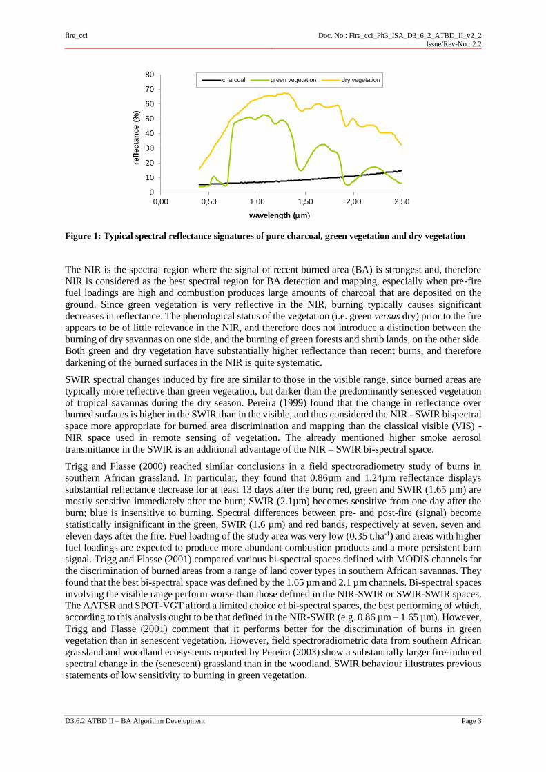
Figure 1: Typical spectral reflectance signatures of pure charcoal, green vegetation and dry vegetation

The NIR is the spectral region where the signal of recent burned area (BA) is strongest and, therefore

NIR is considered as the best spectral region for BA detection and mapping, especially when pre-fire

fuel loadings are high and combustion produces large amounts of charcoal that are deposited on the

ground. Since green vegetation is very reflective in the NIR, burning typically causes significant

decreases in reflectance. The phenological status of the vegetation (i.e. green versus dry) prior to the fire

appears to be of little relevance in the NIR, and therefore does not introduce a distinction between the

burning of dry savannas on one side, and the burning of green forests and shrub lands, on the other side.

Both green and dry vegetation have substantially higher reflectance than recent burns, and therefore

darkening of the burned surfaces in the NIR is quite systematic.

SWIR spectral changes induced by fire are similar to those in the visible range, since burned areas are

typically more reflective than green vegetation, but darker than the predominantly senesced vegetation

of tropical savannas during the dry season. Pereira (1999) found that the change in reflectance over

burned surfaces is higher in the SWIR than in the visible, and thus considered the NIR - SWIR bispectral

space more appropriate for burned area discrimination and mapping than the classical visible (VIS) -

NIR space used in remote sensing of vegetation. The already mentioned higher smoke aerosol

transmittance in the SWIR is an additional advantage of the NIR – SWIR bi-spectral space.

Trigg and Flasse (2000) reached similar conclusions in a field spectroradiometry study of burns in

southern African grassland. In particular, they found that 0.86µm and 1.24µm reflectance displays

substantial reflectance decrease for at least 13 days after the burn; red, green and SWIR (1.65 µm) are

mostly sensitive immediately after the burn; SWIR (2.1µm) becomes sensitive from one day after the

burn; blue is insensitive to burning. Spectral differences between pre- and post-fire (signal) become

statistically insignificant in the green, SWIR (1.6 µm) and red bands, respectively at seven, seven and

eleven days after the fire. Fuel loading of the study area was very low (0.35 t.ha-1) and areas with higher

fuel loadings are expected to produce more abundant combustion products and a more persistent burn

signal. Trigg and Flasse (2001) compared various bi-spectral spaces defined with MODIS channels for

the discrimination of burned areas from a range of land cover types in southern African savannas. They

found that the best bi-spectral space was defined by the 1.65 µm and 2.1 µm channels. Bi-spectral spaces

involving the visible range perform worse than those defined in the NIR-SWIR or SWIR-SWIR spaces.

The AATSR and SPOT-VGT afford a limited choice of bi-spectral spaces, the best performing of which,

according to this analysis ought to be that defined in the NIR-SWIR (e.g. 0.86 µm – 1.65 µm). However,

Trigg and Flasse (2001) comment that it performs better for the discrimination of burns in green

vegetation than in senescent vegetation. However, field spectroradiometric data from southern African

grassland and woodland ecosystems reported by Pereira (2003) show a substantially larger fire-induced

spectral change in the (senescent) grassland than in the woodland. SWIR behaviour illustrates previous

statements of low sensitivity to burning in green vegetation.

0

10

20

30

40

50

60

70

80

0,00 0,50 1,00 1,50 2,00 2,50

refl

ecta

nce (

%)

wavelength (m)

charcoal green vegetation dry vegetation

fire_cci


Issue/Rev-No.: 2.2


Silva et al. (2004) specifically addressed the issue of fire-induced spectral reflectance changes as a

function of pre-fire vegetation phenology (quantified with the NDVI), using SPOT-VGT data from

study areas in boreal forests, tropical savannas, and temperate forests and shrub lands. NIR reflectance

was found to decrease markedly after burning in all land cover types considered in the three different

study areas. All burned areas in the grasslands and croplands showed NIR and SWIR reflectance

decrease. In evergreen needle leaf forest, mixed forest, woodland and wooded grassland, spectral

changes induced by fire displayed two distinct responses: a simultaneous decrease of SWIR and NIR

reflectance; or a small increase in SWIR reflectance and a decrease in NIR reflectance. The expected

post-fire decrease in SWIR reflectance, owing to strong absorption by charcoal (Pereira et al. 1999a,

Fraser et al. 2000), occurs mostly in dry vegetation, such as grassland, which has high pre-fire SWIR

reflectance. In contrast, green vegetation, which has low pre-fire SWIR reflectance due to high moisture

content, displays smaller reflectance changes due to burning (Figure 2). In very green vegetation,

burning may even cause a small increase in SWIR reflectance (Silva et al. 2004).

Figure 2: Fire-induced spectral reflectance changes in a mid-infrared (ρETM5, 1.65μm) versus near-

infrared (ρETM4, 0.86μm) bi-spectral space. Data from a Landsat 7 Enhanced Thematic

Mapper scene from the Western Province, Zambia, dated September 2000 (Pereira 2003).

2.1.3 Scar

Fire alters the vegetation structure by consuming leaves, twigs and fine branches. The resulting spectral

changes last longer than those caused by the deposition of ash and charcoal. Persistence of the fire scar

signal is a function of vegetation type, net primary productivity and plant succession dynamics, and may

range from a few weeks in tropical grasslands to decades in boreal forests. Modifications of the three

dimensional structure of vegetation affect its shading pattern, while consumption of photosynthetically

active plant parts eliminates the greenness signal. The soil background exposed by vegetation removal

will also contribute to the overall spectral signal of the fire-affected area. This is, however, dependent

on severity. If a stand replacing fire occurs, then shadowing can be neglected. In a ground fire, only the

surface vegetation layer at the bottom is affected, and thus the signal is weak and of

ephemeral.Considering the specifications of the present project, which relies on daily, or near-daily data

for the detection of burned areas, the post-fire signal is expected to be strongly dominated by the char

signal.

2.1.4 Heat

Both the (A)ATSR / VGT and the MERIS algorithm incorporate active fire data, based on sensing the

heat from vegetation burning, hence this brief overview of the thermal signal. Temperatures of 1000K

and 600K can be assumed as representative of typical flaming and smouldering combustion phases of

vegetation fires, respectively (Lobert and Warnatz 1993). According to Wien’s Displacement Law, the

fire_cci


Issue/Rev-No.: 2.2


peak emission of radiance for flames and smouldering surfaces would be located in the middle infrared

(MIR), between 3m and 5m. For an ambient temperature of 290K (17C), the peak of radiance

emission is located at approximately 10m. Active fire detection from remote sensing exploits this

behaviour, and typically relies on some combination of brightness temperature measured in the 3m -

5m and 10m - 12m regions. The key “active fire signal” is, therefore, an increase of the observed

radiance in the 3m - 5m region, relatively to surrounding areas. For increasingly smaller and/or cooler

fires, this contrast is progressively attenuated and becomes difficult to discriminate from natural spatial

variability of the land surface temperature field. Additional perturbation sources for active fire detection

may be the presence of atmospheric water vapour, a strong reflection of solar radiation in the 3m -

5m region, or the presence of sub-pixel clouds (Kaufman and Justice 1998).

2.1.5 Smoke

Smoke from vegetation burning often interferes with observation of the land surface, influencing the

choice of the spectral domains of observation, and affecting burned area mapping timeliness and

accuracy. Data pre-processing for this project incorporated screening of smoke-contaminated imagery,

but residual contamination may be present in the data used by the BA classification algorithms, which

is why the smoke signal is addressed here. Biomass burning in wildfires is not fully efficient, due to

high fuel moisture, insufficient oxygenation of the reaction zone, inefficient heat transfer, etc. The more

efficient phase of flaming combustion yields products such as char (partially oxidised wood) coexists

with less efficient smouldering combustion, the phase that takes place behind the active flame front and

yields substantial amounts of smoke. Since the objective is to detect and map fire effects at the land

surface, smoke is seen as an atmospheric disturbance that interferes with this objective. Mie scattering

is strongest when particle radius corresponds to the wavelength of radiation. Smoke aerosol particles

range in size from 0.01 to 1.0μm, which makes them efficient scatterers of solar radiation (Jacob 1999).

Biomass burning smoke is also an absorbing aerosol, because it contains high concentrations of black

carbon (Dubovik et al. 2002; Kaufman et al. 2002). The perturbation caused by smoke aerosol to

observation of the land surface from satellite can be quantified calculating the aerosol transmittance, τaλ

(Iqbal 1983), which increases strongly with wavelength. Smoke aerosol transmittance is very low in the

visible spectral domain, which becomes inadequate to monitor the land surface when biomass burning

emissions are present in the atmosphere in significant amounts. Under such circumstances burned area

mapping is better accomplished using near-infrared (NIR: 0.7-1.2 µm) and shortwave-infrared (SWIR,

1.4-2.5 µm) spectral data (Kaufman et al. 1997; Pereira 1999, 2003).

fire_cci


Issue/Rev-No.: 2.2


3 Overview of pre-existing global burned area products

Several methods based on remote sensing imagery for continental and global burned area mapping have

been developed in the past few years (Barbosa et al. 1999, Roy et al. 2002, Govaerts et al. 2002, Tansey

et al. 2004, Giglio et al. 2009), using a variety of change detection techniques. This is a complex

problem, for a number of reasons, such as the dependence of the burned area spectral signature on the

type and quantity of vegetation burned, variable burn severity and combustion completeness, the post

fire rates of combustion product (charcoal and ash) scatter and vegetation recovery rate. First a brief

overview of global burned area products based on the AVHRR and MODIS sensors is given, followed

by a more detailed analysis of products derived from (A)ATSR and SPOT-VGT imagery (see sections

3.3 and 3.4, respectively). Also studies to assess the capability of MERIS for BA detection are addressed

(see section 3.5).

3.1 AVHRR-based global burned area products

Carmona-Moreno et al. (2005) used daily global observations from the NOAA/AVHRR between 1982

and 1999 to create a weekly global burned area product at 8km spatial resolution. The algorithm for

identifying burned surfaces uses data from AVHRR channels 1–3, extending the approach of Barbosa

et al. (1999a, b). Comparison with independently available fire data indicate that the time-series is

inadequate to make quantitative and accurate estimates of global burned area, it is suitable to assess

changes in location and season of burning at the global scale. Fire seasonality and fire distribution data

sets were integrated as 0.5º fire probability grid maps.

Riaño et al. (2007) analysed spatial and temporal patterns of global burned area with the Daily Tile US

NOAA/AVHRR Pathfinder 8 km Land dataset between 1981 and 2000. Burned area mapping relied on

algorithms previously developed for Africa by Barbosa et al. (1999b) and Moreno-Ruiz et al. (1999),

but using imagery which addressed the solar zenith angle errors affecting previous datasets. The studied

focused on the identification of large scale fire seasonality patterns in the northern and southern

hemispheres, and on the detection of regional trends in burned area extent.

Even with the solar zenith angle correction, the Pathfinder 8km dataset still is affected by spurious

temporal trends, which limit the temporal consistency of burned area products. Its low spatial resolution

very likely leads to substantial underestimation of area burned in extensive areas of the planet. The

global burned area products of Carmona-Moreno et al. (2005) and Riaño et al. (2007) both apply, at the

global scale, an algorithm originally developed to map burns over Africa, which may also lead to higher

inaccuracies over temperate and boreal regions.

3.2 MODIS-based global burned area products

Roy et al. (2002) inverted a bi-directional reflectance model against multi-temporal land surface

reflectance data, obtaining expectation and uncertainty estimates of subsequent observations through

time. Their algorithm deals with angular variations in multi-temporal data and use a statistical measure

to detect change from a previously state. Large discrepancies between predicted and observed values

are attributed to change. A temporal consistency threshold is used to differentiate between sporadic

changes, considered as noise, and persistent changes interpreted as burns. The algorithm is adaptive to

the number, viewing and illumination geometry of the observations, and to the level of data noise. Roy

et al. (2008) presented first results of this algorithm for 12 consecutive months of the NASA Moderate

Resolution Imaging Spectroradiometer (MODIS) global burned area product. Globally the total area

burned detected by the MODIS product was 3.66×106 km2 for July 2001 to June 2002. Comparison with

the MODIS global active fire product showed that the MODIS burned area product labels a greater

proportion of the landscape as burned Globally, the burned area product reports a smaller amount of

area burned than the active fire product in croplands and evergreen forest and deciduous needle leaf

forest classes, comparable areas for mixed and deciduous broadleaf forest classes, and a greater amount

of area burned for the non-forest classes.

fire_cci


Issue/Rev-No.: 2.2


Giglio et al. (2006) proposed a method for estimating monthly burned area globally at 1º spatial

resolution, with MODIS Terra imagery and ancillary vegetation cover information. They constructed

regression trees for 14 different global regions, calibrating MODIS active fire observations to burned

area estimates from MODIS 500-m imagery, assuming proportionality between burned area and active

fire counts. Regional regression trees were applied to the full archive of MODIS Terra fire data, yielding

a monthly global burned area product ranging from late 2000 through mid-2005. Annual burned area

estimates thus derived compare well with independent annual estimates for Canada, the United States,

and Russia. Global annual burned area estimates for the years 2001–2004 varied between 2.97 million

and 3.74 million km2, with the maximum in 2001.

3.3 (A)ATSR-based global burned area products

There is significant previous experience with the use of (A)ATSR data for burned area mapping at the

global scale. A brief overview of methods, results and assessment of the two available global burned

area products developed from these sensors is provided below.

3.3.1 GlobScar

The European Space Agency GlobScar Project produced global monthly burned area maps at 1km

spatial resolution using day-time data of the Along Track Scanning Radiometer (ATSR-2) instrument

onboard the ESA ERS-2 satellite from the year 2000. The image classification procedure combines two

distinct algorithms: K1 is a contextual algorithm based on the geometrical characteristics of the burned

pixels in the near-infrared (NIR, 0.87µm) / thermal infrared (TIR, 11 µm) space, while the E1 algorithm

is a series of fixed thresholds applied to the data from four spectral channels.

The products were validated against other field and remote sensing data (Simon, 2004). Commission

errors were uncommon and affected mostly scattered pixels. The only large area of commission errors

is due to older burned areas, in the mixed and evergreen needle leaf forests of Canada and, probably,

also in similar ecosystems across Russia. Omission errors were common and very important in some

regions, such as the United States (open shrubland and grassland areas), Australia (open shrubland),

Zimbabwe (cropland), and Brazil (broadleaf evergreen forests).

3.3.2 GlobCarbon

The European Space Agency GlobCarbon project generated a global monthly 1-km burned-area product,

using two regional GBA2000 algorithms and the GLOBSCAR algorithms applied to 1-km SPOT

VEGETATION and ERS2–ATSR2/ENVISAT AATSR data, respectively. The two GBA2000

algorithms are the IFI algorithm (Ershov and Novik 2001) developed for the Eurasian boreal forest and

the Technical University of Lisbon (UTL) algorithm (Silva et al. 2002, 2003) developed for southern

Africa. The GLOBSCAR algorithm, applied to ERS2–ATSR2 for 1998–2002 and to ENVISAT AATSR

data for 2003–2007, is based on two separate algorithms. The K1 GLOBSCAR algorithm (Piccolini

1998) and the E1 GLOBSCAR algorithm (Eva and Lambin 1998) A first validation of the

GLOBCARBON products was performed using 72 Landsat images (Globcarbon, 2007), using linear

regression analysis based on hexagonal grids of equal area. Results were very diverse in different

ecosystems and algorithms. For the global validation, results varied from mean correlations of 0.34

(Globscar algorithm) to 0.85 (logical combination of two or more algorithms), with a high standard

deviation.

fire_cci


Issue/Rev-No.: 2.2


3.4 The SPOT VGT-based global burned area products

There is extensive experience with SPOT-VGT data for regional, continental, and global burned area

mapping. Here we briefly review methods, results and assessment of the two available global burned

area products developed using SPOT-VGT imagery.

3.4.1 GBA2000

The GBA2000 project relied on SPOT-VEGETATION data to estimate global burned area at 1 km

spatial resolution, during the year 2000. Tansey et al. (2004) reported estimates of BA size and number

for four broad vegetation classes and at country level. They mapped over 3.5 million km2 of burned

areas, approximately 80% of which occurred in shrublands and woodlands. About 17% of the burned

area affected grasslands and croplands, and 3% occurred in forests. Almost 600,000 individual BA were

mapped.

The GBA2000 project was based on an international network of partners for the development and testing

of a series of regional algorithms and for the production of continental/regional burned area maps.

Different methods were considered necessary to deal with specificities of the burned area remotely

sensed signal throughout the major biomes of the World (e.g., boreal forest, tropical forest, grasslands).

The various continental/regional maps were subsequently patched together, to form a global product. A

total of 11 regional algorithms were developed from temporal and spatial subsets of VGT S1 data. In

general, algorithms were applied on multitemporal composited data, using a change detection approach.

Data classification approaches used included multiple logistic regression, Multi-Layer Perceptron

(MLP) neural networks, expectation-based BRDF model inversion, classification and regression trees,

and linear discriminant analysis.

Although global validation of the GBA2000 product was not performed, Tansey et al. (2004) mention

problems detecting sub-pixel burned areas (a significant problem in regions of tropical forest), mapping

burns in cloudy regions, and the false detection of burned areas caused by flooding or dark soils.

3.4.2 L3JRC

The L3JRC project was developed under a partnership between the EC Joint Research Centre (JRC),

the University of Leicester, the University of Louvain-la-Neuve, and the Tropical Research Institute,

Lisbon. Global burned area maps, at 1km spatial resolution were developed for seven fire years (2000

to 2007), using a modified version of a Global Burned Area (GBA) 2000 algorithm. The total area

burned each year (2000–2007) was estimated to range from 3.5×106 km2 to 4.5×106 km2. Validation was

based on 72 Landsat TM scenes, and correlation statistics between TM and VGT estimated burned areas

were reported for major vegetation types. Accuracy of the global data set was found to depend

substantially on vegetation type (Tansey et al. 2008).

The main processing L3JRC algorithm uses a temporal index in the 0.83 m channel of VGT. This

index, I, is computed as:

I = (S1NIR – ICNIR) / (S1NIR + ICNIR)

where S1NIR is the pixel value of the NIR band of the S1 daily product and ICNIR an intermediate

composite product. The intermediate composite consists of averaged NIR reflectance derived from all

observations prior to observation on the day being considered. No calculation or detection is performed

where S1NIR or ICNIR equals zero. Mean and standard deviation values are computed for the index I over

a spatially roving window. A pixel is flagged as burned if the pixel value in the roving window, I, is

lower than the mean value minus two standard deviations. Two further checks are made on reflectance

values in the 0.83 µm (S1 pixel value < 260) and 1.66 m (S1 pixel value > 250) channels to confirm

the burned area (Tansey et al. 2008).

A first validation of the L3JRC burned area product was based on 72 Landsat TM scenes. Estimated

accuracy extremely varied from one land cover to the other, with values as low as 3% for mosaic of land

covers and maximum values of 56% in herbaceous cover (both in terms of regression slope: Tansey et

al. 2008). Accuracy also changed with latitude-ecosystem, with good performances for boreal forest and

fire_cci


Issue/Rev-No.: 2.2


much lower in semi-arid Australia and Africa. Under detection by L3JRC seems to be more significant

in areas of shrubs and grasses rather than forests. As the original GBA2000 algorithm that was modified

for L3JRC had been developed for detecting boreal forest burns, this might be expected. The L3JRC

algorithm also underestimates burned area over cultivated and managed lands, possibly because their

size is too small for detection by SPOT VEGETATION (Tansey et al. 2008).

3.5 MERIS-based burned area studies

MERIS was primarily designed to provide quantitative ocean-colour measurements (Rast et al. 1999).

However, its spectral characteristics make it appropriate to also serve applications like land surface and

atmospheric characterisation (see (Calado et al. 2011). It is well known that one of the major drawbacks

of MERIS images, for BA identification, is the lack of SWIR bands, which has proven to be crucial to

discriminate burned surfaces from water and non-combustible land cover. On the other hand, its multi-

spectral imaging capabilities in the VIS/NIR region of the spectrum, moderate spatial resolution and 3

day repeat cycle, may in part circumvent this limitation. In fact, MERIS bands are so narrow that it is

possible to detect absorption bands and estimate its depth. Moreover, the sensor was especially designed

to detect chlorophyll concentration having though bands in the red edge (bands located in the maximum

of chlorophyll absorption). Such bands allow the use of indices of chlorophyll concentration, that may

be of use for BA detection, since an abrupt decrease in the chlorophyll content may be related to a fire.

Regarding fire applications, very few studies have been conducted using MERIS instrument. Among

the existing studies, there is one developed by Huang and Siegert (2004), where Level 1b MERIS RR

product was used to identify plumes and the BA detection was achieved combining night-time AATSR

fire hot spots with BA detected with Advanced Synthetic Aperture Radar (ASAR). Another study

concerning the estimation of fire severity using MERIS FR Level 2 imagery and MODIS daily

reflectivity product (MOD09GHK) was conducted by Roldán-Zamarrón et al. (2006). The BA mapping

was performed applying the matched filtering method (Boardman et al. 1995) to Landsat TM data and

the fire severity levels were then estimated through use of different techniques to MERIS and MODIS

images. The authors concluded that, in general, the fire severity estimation performed by MERIS was

more accurate than the one performed by MODIS. Gonzaléz-Alonso et al. (2007) also applied the same

technique to MERIS FR Level 1b imagery to estimate fire severity levels and BA at a local scale.

Validation was then performed comparing obtained results with the ones obtained using SPOT-5,

showing a fairly high correlation between both sensors. Aiming to evaluate the ability of some sensors

on the estimation of fire severity levels, Chuvieco et al. (2007) performed a comparative study using

SPOT-5, Landsat TM, MERIS and MODIS and concluded that Landsat TM was the one presenting the

best performance. Nevertheless, MERIS proved to be capable of correctly identify the spatial pattern of

the distribution of the severity levels.

It is worth noting that the above studies are not specifically oriented to burn area mapping, but rather to

the analysis of some aspects related to level of damage caused by fires.

Only two works have been found in literature in relation to burned area mapping. The first one used

Spectral Angle Images (SAI) technique at a regional scale (Oliva and Martín 2007; Oliva et al. 2010).

The SAI methodology makes use of a reference spectrum (endmembers) that in present case was

obtained from the image (SAI-image) and from the field spectral measurements (SAI-field). The study

used MERIS FR Level 2 images and compared BA discrimination using traditional vegetation indices

(e.g., BAI, GEMI, , NDVI) with SAI technique and validation was carried out using AWiFS images.

Obtained results showed that index (a component of the GEMI calculation) and the SAI-image were

the ones that presented higher accuracy. According to the authors, NIR bands in the red edge (bands 9

to 12) region present a higher power of burned area discrimination than NIR bands (bands 13 to 15) in

the spectral region traditionally used by the sensors designed for Earth observation (Oliva 2009). From

these ones, when using only one post-fire image, band 10 (in the spectral range 750 nm – 757.5 nm) is

the one with the highest discrimination power, even though all NIR bands (from band 10 to band 14)

present similar discrimination power. On the other hand, when using spectral indices for purposes of

burned pixels detection, band 10 in the red edge and band 8 in the red region, were the ones with highest

discrimination power. The second study was conducted by González-Alonso et al. (2009). It used

MERIS FR Level 1b data for burned land discrimination at a regional scale. The method used in a

fire_cci


Issue/Rev-No.: 2.2


synergetic way fire hotspots from MODIS with NIR reflectance values from MODIS and MERIS

imagery. Basically, the algorithm consisted in finding the threshold that maximizes the agreement

between the burned area discriminated using the NIR band of a post-fire image and the existence of an

active fire as detected by MODIS. Again validation was performed using an image from AWiFS and

obtained results were very similar when using MODIS and MERIS reflectance values, although slightly

better in the case of MERIS. It is worth mentioning that these studies have only been applied to the

North-western part of the Iberian Peninsula to the summer of 2006 and to the Province of Heilongiang

in the North of China, in the framework of the ESA DRAGON-2 project (González-Alonso et al. 2009).

While studies performed at regional scale show the potential of this sensor to detect burned areas,

especially when using hybrid algorithms, to date MERIS has not been used to obtain a global burned

area product.

3.6 Conclusions

Both (A)ATSR-based burned area products result from the global application of pre-existing regional

algorithms. Classification accuracy was very variable regionally, and relatively low at the global scale.

The VGT-based GBA2000 product was developed combining a large number of regional algorithms,

with undesirable effects on global consistency. No global accuracy assessment was performed for this

product. The L3JRC product, also derived from VGT data, relied on a modified version of a GBA2000

algorithm developed for the Eurasian boreal region, applied at global scale. Burned area classification

accuracy was also found to vary substantially with land cover type and was low globally.

There is no previous experience with the use of MERIS data for global burned area mapping, and even

regional scale research is very scarce.

Burned area products developed under the scope of the present project are meant to overcome the main

methodological limitations of previous work. They rely on new algorithms, designed with data from ten

regional study sites covering all major Earth biomes with moderate to high fire incidence. The VGT and

(A)ATSR products were developed from a single algorithm applied at global scale, with minor

modifications to accommodate specifically distinct features of each sensor. The MERIS-based product

also results from the application of a single, global scope algorithm. Although newly designed, VGT,

(A)ATSR, and MERIS algorithms incorporate previously developed data, techniques, and concepts for

burned area mapping.

fire_cci


Issue/Rev-No.: 2.2


4 (A)ATSR, SPOT Vegetation and MERIS algorithms

4.1 Introduction

The perceived main methodological limitations behind the available (A)ATSR-based and VGT-based

products are the global application of regional algorithms, the creation of global products “mosaicked”

from a multiplicity of regional algorithms, and the simplistic nature of some algorithms used, all of these

contributing towards relatively low classification accuracy. Our goal is to develop a single algorithm,

robust enough for global application with both sensors, with minor modifications. For MERIS, given

the lack of global-scale burned area algorithms/products based on data from this sensor, no similar

analysis can be performed, and the algorithm evolves from previous experience at regional scale.

The VGT / (A)ATSR algorithm relies on a single-channel time series change detection approach,

complemented with fire seasonality weighting, and spatial-temporal contextual revision of single pixel

burned area classification. The time series change detection component of the algorithm has similarities

with the algorithms of Govaerts et al. (2002) and Roy et al. (2002). The MERIS algorithm follows a

hybrid approach to obtain burned areas on a global scale. It uses temporal composites of individual

channels and spectral indices, combined with active fires and a region growing procedure, to detect and

map burned areas. The algorithm incorporates concepts from previous hybrid approaches combining the

reflective and the thermal signal associated with vegetation burning (Fraser et al. 2000; Giglio et al.

2009; Roy et al. 1999), especially those based on MERIS imagery (González-Alonso and Merino de

Miguel 2009; González-Alonso et al. 2010).

4.2 (A)ATSR and SPOT Vegetation detailed algorithm descriptions

The algorithm for mapping burned areas using SPOT-VEGETATION and (A)ATSR imagery relies on

spectral, temporal, and spatial data. More precisely, it looks for spatial and temporal patterns in spectral

data that indicate vegetation burning. We analyse single channel (near infrared, NIR) time series of

surface reflectance data, which were previously screened for clouds, smoke and haze. Permanent and

temporary water bodies were also masked out of the dataset (Bachmann et al. 2014).

The algorithm is designed to answer a series of questions:

a) Was there a spectral change, at a given date? (change point detection)

b) Does it look like burning and does it happen at a plausible date? (selecting and scoring change

points)

c) Is there evidence of burning in that neighbourhood, that day and during previous days?

(Markov Random Field segmentation)

The first three questions are addressed analysing time series of data at the level of a single pixel, while

answering the last question requires taking into account the information contained in areas defined by a

variable number of pixels. Question a), estimating the point in time at which the statistical properties of

a series of NIR surface reflectance data have changed, is addressed with a Change Point Detection (CPD)

technique. Once potentially multiple change points have been identified, question b) is answered by

scoring each change point based on its date of occurrence, and spectral characteristics related to the NIR

reflectance change associated with it, both in time and in space. Finally, c) revises the initial (a-b) burned

area detection and mapping, in the light of evidence of burning in the spatial neighbourhood of a given

pixel, during the day it was detected and also during a short preceding period, yielding the final burned

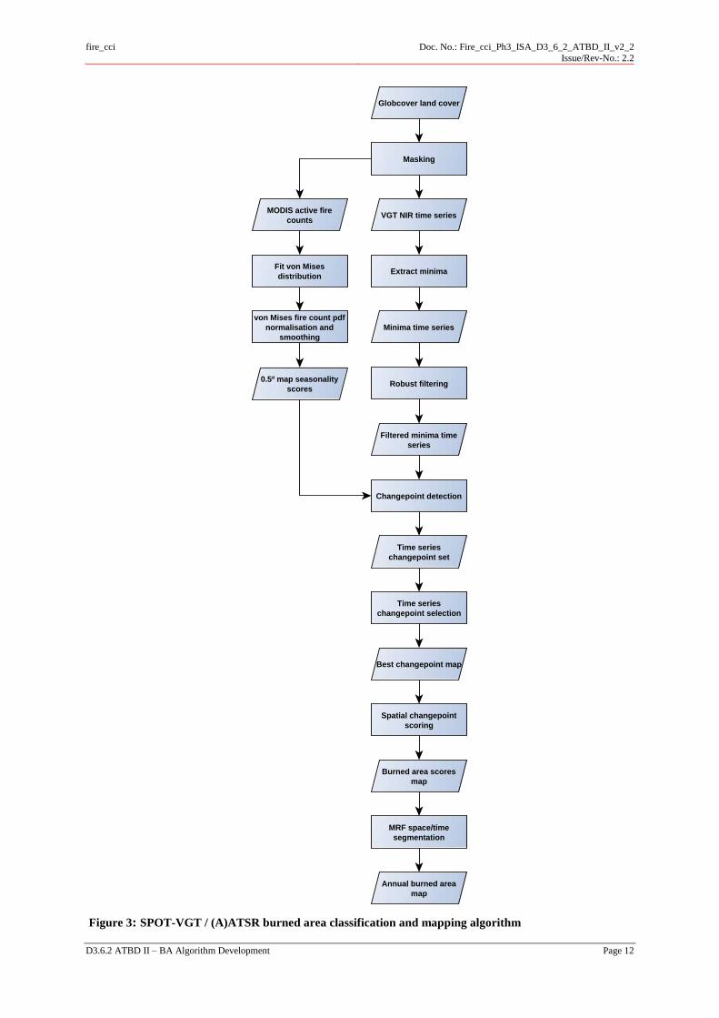
area map. Figure 3 illustrates the algorithm.

fire_cci


Issue/Rev-No.: 2.2


Figure 3: SPOT-VGT / (A)ATSR burned area classification and mapping algorithm

VGT NIR time seriesMODIS active fire

counts

Extract minima

Minima time series

Robust filtering

Filtered minima time

series

0.5º map seasonality

scores

Globcover land cover

Masking

Changepoint detection

Time series

changepoint set

Time series

changepoint selection

Best changepoint map

Spatial changepoint

scoring

Burned area scores

map

MRF space/time

segmentation

Annual burned area

map

Fit von Mises

distribution

von Mises fire count pdf

normalisation and

smoothing

fire_cci


Issue/Rev-No.: 2.2


4.2.1 Change detection algorithm

4.2.1.1 Time series pre-processing

The pre-processed surface reflectance time series display an oscillating pattern caused by variations in

illumination and observation geometry, the bidirectional reflectance distribution function (BRDF)

effect, which increases the variability of the data, independently from any actual changes occurring at

the land surface. Additionally, the time series also reveal residual atmospheric effects, which generate

positive outliers (“spikes”) in the data, again unrelated to land surface changes. The signal we are trying

to detect, vegetation burning, appears as a decrease in values of the NIR surface reflectance time series.

Although this decrease often is evident in both the maximum and the minimum of each BRDF-induced

oscillation, it tends to be more consistently and reliably expressed in the minima values, which are least

affected by residual atmospheric contamination. Therefore, we extract a time series of minima from the

original NIR surface reflectance data. These time series also contain negative outliers, usually caused

by cloud shadowing, and occasionally due to unscreened flooding, corresponding to pixels that were not

captured by the screening procedures described in Bachmann et al. (2014). Robust filtering of the time

series of surface reflectance minima is therefore applied to remove most of these negative outliers,

yielding time series suitable for CPD. The time series pre-processing step of the algorithm was used

only with the SPOT-VGT data. The (A)ATSR lower frequency of observation yields time series without

enough data for the pre-processing step to work properly. However, (A)ATSR data are substantially less

affected by BRDF effects, and thus are appropriate for immediate application of changepoint detection.

4.2.1.1.1 Extraction of local minima

Extracting local minima from a time series of observations y1:n = (y1, . . . , yn) of reflectance data entails

a series of steps:

1. Identification of “turning points”. An observation yi is a turning point, i.e. a local

minimum, ytm, (local maximum, ytM), if its two neighbours are both smaller (larger)

(Kugiumtzis and Tsimpiris, 2010).

2. Remove from the series all yi that are not turning points.

3. Calculate a time series of first-order differences and remove all turning points that differ

from one of its immediate neighbours less than 0.02 reflectance units, i.e. points

associated with minor, spurious oscillations in the series. Parameter min_diff_cutoff , min.

4. Remove all remaining local maxima, ytM. After this step, then remaining points are shown

in red in Figure 4.

5. Remove those ytm ≥ 0.4 reflectance units, which are considered contaminated by residual

atmospheric effects. Parameter max_refl_cutoff, max.

The values for the min_diff_cutoff and max_refl_cutoff parameters were estimated empirically, from

the quantitative analysis of a large number of single pixel time series, from the ten study sites available

for algorithm development.

fire_cci


Issue/Rev-No.: 2.2


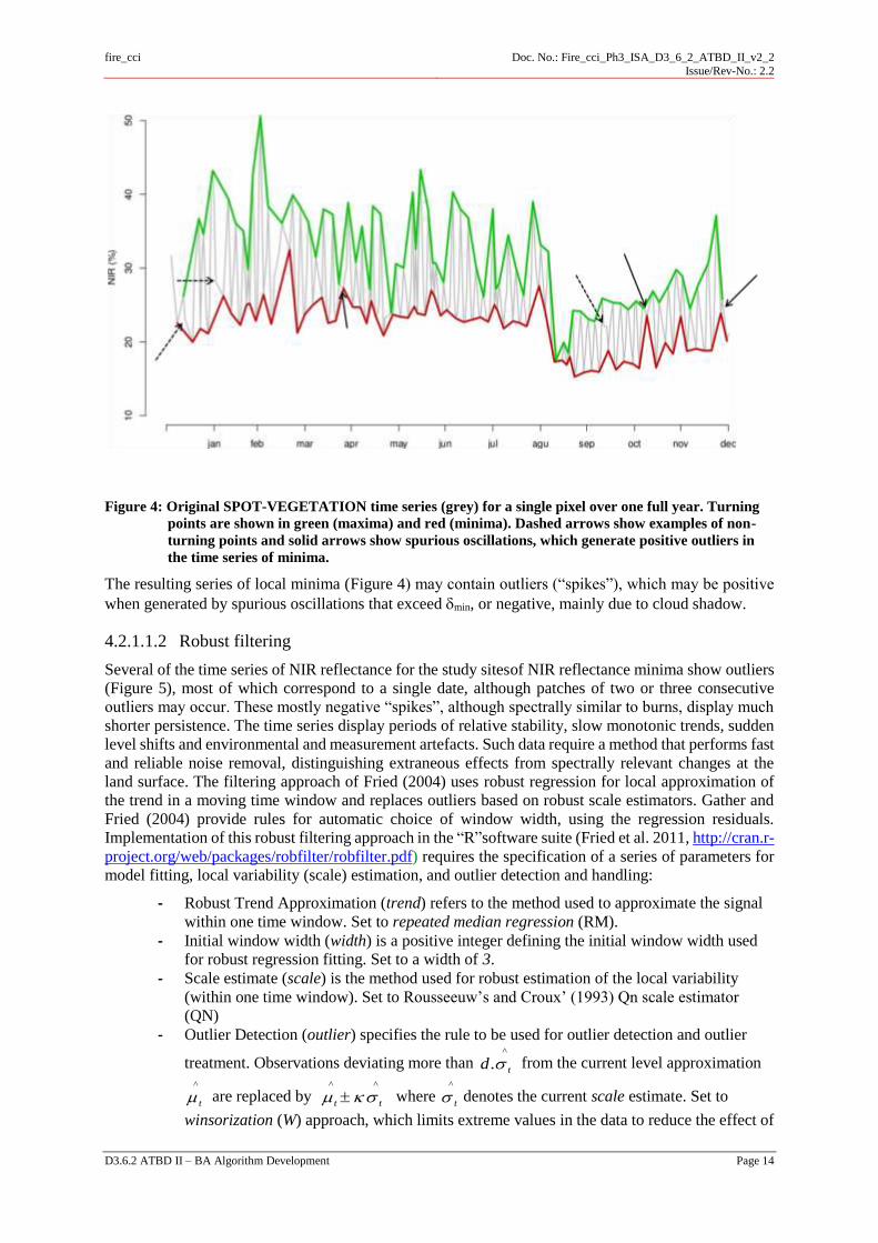
Figure 4: Original SPOT-VEGETATION time series (grey) for a single pixel over one full year. Turning

points are shown in green (maxima) and red (minima). Dashed arrows show examples of non-

turning points and solid arrows show spurious oscillations, which generate positive outliers in

the time series of minima.

The resulting series of local minima (Figure 4) may contain outliers (“spikes”), which may be positive

when generated by spurious oscillations that exceed min, or negative, mainly due to cloud shadow.

4.2.1.1.2 Robust filtering

Several of the time series of NIR reflectance for the study sitesof NIR reflectance minima show outliers

(Figure 5), most of which correspond to a single date, although patches of two or three consecutive

outliers may occur. These mostly negative “spikes”, although spectrally similar to burns, display much

shorter persistence. The time series display periods of relative stability, slow monotonic trends, sudden

level shifts and environmental and measurement artefacts. Such data require a method that performs fast

and reliable noise removal, distinguishing extraneous effects from spectrally relevant changes at the

land surface. The filtering approach of Fried (2004) uses robust regression for local approximation of

the trend in a moving time window and replaces outliers based on robust scale estimators. Gather and

Fried (2004) provide rules for automatic choice of window width, using the regression residuals.

Implementation of this robust filtering approach in the “R”software suite (Fried et al. 2011, http://cran.r-

project.org/web/packages/robfilter/robfilter.pdf) requires the specification of a series of parameters for

model fitting, local variability (scale) estimation, and outlier detection and handling:

- Robust Trend Approximation (trend) refers to the method used to approximate the signal

within one time window. Set to repeated median regression (RM).

- Initial window width (width) is a positive integer defining the initial window width used

for robust regression fitting. Set to a width of 3.

- Scale estimate (scale) is the method used for robust estimation of the local variability

(within one time window). Set to Rousseeuw’s and Croux’ (1993) Qn scale estimator

(QN)

- Outlier Detection (outlier) specifies the rule to be used for outlier detection and outlier

treatment. Observations deviating more than ^

. td from the current level approximation

^

t are replaced by ^^

tt where ^

t denotes the current scale estimate. Set to

winsorization (W) approach, which limits extreme values in the data to reduce the effect of

http://cran.r-project.org/web/packages/robfilter/robfilter.pdf

http://cran.r-project.org/web/packages/robfilter/robfilter.pdf

fire_cci


Issue/Rev-No.: 2.2


possibly spurious outliers, by shrinking large and moderately sized outliers (d = 2)

towards the current level estimate (k = 2).

- Shift detection (shiftd) is the factor by which the current scale estimate is multiplied for

shift detection. Set to 2.

- Maximal window width (max.width) a positive integer (>= width) specifying the maximal

width of the time window. Set to 7.

- Window width adaptation (adapt) is the moving window width adaptation parameter.

adapt can be either 0 or a value [0.6; 1] . adapt = 0 means that a fixed window width is

used. Otherwise, max.width is reduced whenever more than a fraction [0.6; 1] of the

residuals in a certain part of the current time window are all positive or all negative. Set to

0.8.

- Extrapolate defines the rule for data extrapolation to the edges of the time series. As

implemented, it consists of the fitted values within the first half of the first window and

within the last half of the last window.

Figure 5: SPOT-VEGETATION time series (grey) for a single pixel over one full year. Turning points are

shown in green (maxima) and red (minima). Blue line shows time series of minima without high

values produced by spurious oscillations. Black line shows time series of minima with spikes

removed by robust filtering.

4.2.1.2 Changepoint Detection

We adopt the approach of detecting changepoints in a time series through minimizing a cost function

over possible numbers and locations of changepoints. The approach relies on a new method for finding

the minimum of such cost functions, and hence the optimal number and location of changepoints, which

has a computational cost that is linear in the number of observations (Killick et al., 2012). Changepoint

detection within a time series consists of two steps: i) choice of statistical criteria to optimise and ii)

optimisation algorithm. PELT is an algorithm for the optimisation step that can implement many choices

of criteria including likelihoods. Common algorithms for the optimisation step include Dynamic

Programming (Auger and Lawrence, 1989) and Hidden Markov Models (Chib,1998) which produce

exact optimisations but are computationally slow, O(n2); and Binary Segmentation (Scott and Knott,

1974) and Genetic algorithms (Jong et al., 2004) which are computationally fast, O(n log n) but produce

approximate optimisations. In contrast PELT, which is an algorithm for the optimisation step that can

implement many choices of criteria including likelihoods (Killick et al. 2012), was chosen because it is

computationally fast (O(n)) and produces an exact optimisation.

fire_cci


Issue/Rev-No.: 2.2


4.2.1.2.1 Pruned Exact Linear Time (PELT) algorithm

The Pruned Exact Linear Time (PELT) algorithm proposed by Killick et al. (2012) produces exact

optimisation of changepoint segmentations in linear computational time. This is achieved using dynamic

programming (computational time to O(n2)) and pruning to further reduce the computational time to

O(n). For a given point n in a sequence, determining the optimal segmentation of the data prior to n with

an unknown number of segments requires consideration of 2n-1 solutions. Dynamic programming

techniques can be implemented to reduce the problem to simply consider the last change prior to n.

Thus, at a given point n, the solution is simply which of the n-1 previous locations is the last changepoint

prior to n. The number of options scales linearly with n and thus the computational time is O(n2). The

PELT algorithm extends this idea further. The intuition behind the algorithm is that once an `obvious'

change is encountered, say at n - 5, then data points before this, e.g. n–6, n–7,…, will never be the last

change prior to n. Killick et al. (2012) quantify `obvious' with a bound which ensures that the algorithm

remains an exact optimisation. Furthermore, when a likelihood is used as the criterion to optimise,

Killick et al. (2012) prove that, under regularity conditions, the computational cost of PELT is O(n). A

mathematical description of PELT is given in Table 1 and the method is available in the “R”

programming language (Crawley, 2007) package changepoint (Killick and Eckley, 2010).

Table 1: PELT algorithm for identifying multiple changepoints.

Input: A time series of the form (y1, y2 ,…, yn) where yi R.

A measure of fit C(.) dependent on the data.

A penalty independent of the number and locations of changepoints

Initialise: Let n = length of time series

Set F(0) = -, cp(0) = 0, p=0.

Iterate: For * = 1, …, n

1. Calculate )()(min)( ** :)11,,0(* yCFF p

.

2. Let

)()(arg{min ** :)1(0

1 yCF

3. Set 11* ),()( cpcp .

4. Set })()()({arg *:)1( * FKyCFp r

.

Output: The changepoints recorded in cp(n).

4.2.1.2.2 Detecting changes in mean

The PELT algorithm can be implemented with many optimisation criteria. In this work we seek to

identify changes in mean within NIR reflectance data (Figure 6). We assume that the NIR reflectance

follows a Normal distribution with a constant variance and changing mean. Following Hinkley (1970),

the optimisation criteria (C(.) above) based on the likelihood is

ii

j

j

j

j

i

i

i

i

ii

y

yyC

1

1

1

2:)1(

1

1

1

)(

)(

(1)

fire_cci


Issue/Rev-No.: 2.2


Within PELT, we used the Schwarz Information Criterion (SIC; Schwarz, 1978) as the penalty function

to penalise against identifying too many changepoints, because the larger penalty term in SIC, compared

to the more commonly used Akaïke Information Criterion (AIC), performed better in terms of avoiding

an excessive number of change points being detected. This method is implemented using the

multiple.mean.norm function in the “R” software environment (Killick and Eckley, 2010). The time

series data are not strictly normal, but the method is robust to moderate violations of this assumption.

Figure 6: Changepoints (vertical purple bars) detected on the time series of filtered minima (black line),

using the PELT algorithm, with SIC penalty function

4.2.1.3 Changepoint selection and scoring

The PELT/SIC approach to CPD may yield several changepoints per pixel / time series, and per season,

since the mean value of NIR reflectance data varies not only in response to burning, but also as a function

of cyclic weather patterns, atmospheric conditions, vegetation phenology and anthropogenic land cover

changes. Therefore, it is necessary to select the changepoint most likely to correspond to the

identification of a burning event in each pixel / time series. In order to be considered as candidates for

scoring, changepoints need to satisfy all of the following criteria:

a) The CP must be associated with a decrease in NIR reflectance ( 𝑆𝑖+1̅̅ ̅̅ ̅ − 𝑆�̅�:<0).

b) The NIR reflectance decrease must not exceed 0.2 reflectance units (𝑆𝑖+1̅̅ ̅̅ ̅ − 𝑆�̅�:<0.2).. Larger

decreases typically are associated with cloud contaminated data in the segment preceding the

CP.

c) The post CP NIR reflectance must be smaller than 0.2 reflectance units (𝑆𝑖+1̅̅ ̅̅ ̅ <0.2). Higher

reflectance values typically are not associated with fire-affected surfaces.

d) The CP requires a temporal density of 0.1 in the pre-CP segment, i.e. at least one valid

observation per each 10 days of time series segment duration

e) The CP requires a temporal density of 0.1 in the post-CP segment

f) It requires that the reflectance value of a CP is smaller than the sum of lowest reflectance

value in the post-CP segment plus 0.005 reflectance units.

g) The slope of a linear fit to the NIR reflectance time series data in a post-CP segment cannot

exceed 0.4. Higher rates of post-CP NIR reflectance recovery are inconsistent with post-fire

vegetation recovery.

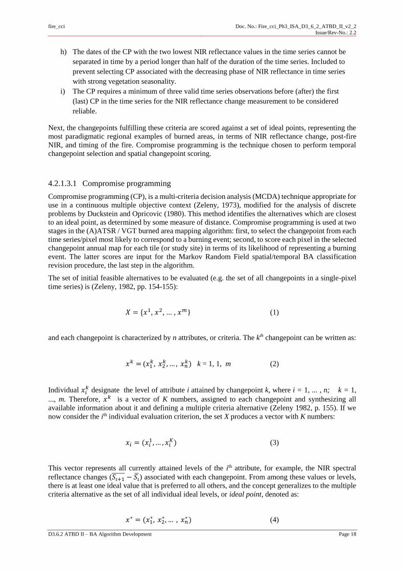
fire_cci


Issue/Rev-No.: 2.2


h) The dates of the CP with the two lowest NIR reflectance values in the time series cannot be

separated in time by a period longer than half of the duration of the time series. Included to

prevent selecting CP associated with the decreasing phase of NIR reflectance in time series

with strong vegetation seasonality.

i) The CP requires a minimum of three valid time series observations before (after) the first

(last) CP in the time series for the NIR reflectance change measurement to be considered

reliable.

Next, the changepoints fulfilling these criteria are scored against a set of ideal points, representing the

most paradigmatic regional examples of burned areas, in terms of NIR reflectance change, post-fire

NIR, and timing of the fire. Compromise programming is the technique chosen to perform temporal

changepoint selection and spatial changepoint scoring.

4.2.1.3.1 Compromise programming

Compromise programming (CP), is a multi-criteria decision analysis (MCDA) technique appropriate for

use in a continuous multiple objective context (Zeleny, 1973), modified for the analysis of discrete

problems by Duckstein and Opricovic (1980). This method identifies the alternatives which are closest

to an ideal point, as determined by some measure of distance. Compromise programming is used at two

stages in the (A)ATSR / VGT burned area mapping algorithm: first, to select the changepoint from each

time series/pixel most likely to correspond to a burning event; second, to score each pixel in the selected

changepoint annual map for each tile (or study site) in terms of its likelihood of representing a burning

event. The latter scores are input for the Markov Random Field spatial/temporal BA classification

revision procedure, the last step in the algorithm.

The set of initial feasible alternatives to be evaluated (e.g. the set of all changepoints in a single-pixel

time series) is (Zeleny, 1982, pp. 154-155):

𝑋 = {𝑥1, 𝑥2, ... , 𝑥𝑚} (1)

and each changepoint is characterized by n attributes, or criteria. The kth changepoint can be written as:

𝑥𝑘 = (𝑥1𝑘, 𝑥2

𝑘 , … , 𝑥𝑛𝑘) k = 1, 1, m (2)

Individual 𝑥𝑖𝑘 designate the level of attribute i attained by changepoint k, where i = 1, ... , n; k = 1,

..., m. Therefore, 𝑥𝑘 is a vector of K numbers, assigned to each changepoint and synthesizing all

available information about it and defining a multiple criteria alternative (Zeleny 1982, p. 155). If we

now consider the ith individual evaluation criterion, the set X produces a vector with K numbers:

𝑥𝑖 = (𝑥𝑖1, … , 𝑥𝑖

𝐾) (3)

This vector represents all currently attained levels of the ith attribute, for example, the NIR spectral

reflectance changes (𝑆𝑖+1̅̅ ̅̅ ̅ − 𝑆�̅�) associated with each changepoint. From among these values or levels,

there is at least one ideal value that is preferred to all others, and the concept generalizes to the multiple

criteria alternative as the set of all individual ideal levels, or ideal point, denoted as:

𝑥∗ = (𝑥1∗, 𝑥2

∗, … , 𝑥𝑛∗ ) (4)

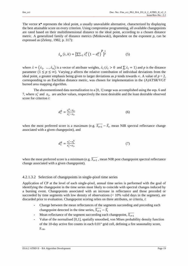
fire_cci


Issue/Rev-No.: 2.2


The vector x* represents the ideal point, a usually unavailable alternative, characterized by displaying

the best attainable score on every criterion. Using compromise programming, all available changepoints

are rated based on their multidimensional distance to the ideal point, according to a chosen distance

metric. A generalized family of distance metrics (Minkowski), dependent on the exponent p, can be

expressed as (Zeleny, 1982, p. 317):

𝐿𝑝 (, 𝑘) = [∑ 𝑖𝑝𝑛

𝑖=1 (1 − 𝑑𝑖𝑘)

𝑝]

1

𝑝 (5)

where = (1, … ,𝑛) is a vector of attribute weights, 𝑖 (𝑖 > 0 and ∑𝑖 = 1) and p is the distance

parameter (1 ≤ 𝑝 ≤ ∞). Varying p affects the relative contribution of individual deviations from the

ideal point, a greater emphasis being given to larger deviations as p tends towards . A value of p = 2,

corresponding to an Euclidian distance metric, was chosen for implementation in the (A)ATSR/VGT

burned area mapping algorithm.

The abovementioned data normalization to a [0, 1] range was accomplished using the eqs. 6 and

7, where 𝑥𝑖∗ and 𝑥𝑖∗ are anchor values, respectively the most desirable and the least desirable observed

score for criterion i:

𝑑𝑖𝑘 =

𝑥𝑖𝑘−𝑥𝑖∗

𝑥𝑖∗−𝑥𝑖∗

(6)

when the most preferred score is a maximum (e.g. 𝑆𝑖+1̅̅ ̅̅ ̅ − 𝑆�̅�, mean NIR spectral reflectance change

associated with a given changepoint), and

𝑑𝑖𝑘 =

𝑥𝑖∗−𝑥𝑖

𝑘

𝑥𝑖∗−𝑥𝑖∗

(7)

when the most preferred score is a minimum (e.g. 𝑆𝑖+1̅̅ ̅̅ ̅ , mean NIR post changepoint spectral reflectance

change associated with a given changepoint).

4.2.1.3.2 Selection of changepoints in single-pixel time series

Application of CP at the level of each single-pixel, annual time series is performed with the goal of

identifying the changepoint in the time series most likely to coincide with spectral changes induced by

a burning event. Changepoints associated with an increase in reflectance and those preceded or

succeeded by time segments with low density of observations (< 10% valid days in the segment), are

discarded prior to evaluation. Changepoint scoring relies on three attributes, or criteria, i:

- Change between the mean reflectances of the segments succeeding and preceding each

changepoint detected in the time series, 𝑆𝑖+1̅̅ ̅̅ ̅ − 𝑆�̅�

- Mean reflectance of the segment succeeding each changepoint, 𝑆𝑖+1̅̅ ̅̅ ̅

- Value of the normalised [0,1], spatially smoothed, von Mises probability density function

of the 10-day active fire counts in each 0.01º grid cell, defining a fire seasonality score,

FvM.

fire_cci


Issue/Rev-No.: 2.2


The ideal point for the set of changepoints detected in each single-pixel time series is composed of the

largest NIR reflectance change, the lowest succeeding mean reflectance value, and the largest fire

seasonality score. It is possible that no changepoint detected in an annual time series corresponds to an

actual burning event. Nevertheless, the changepoint closest to the ideal point, under a Euclidean (p=2)

distance metric will be chosen as the best candidate for inclusion in the annual map.

Figure 7 shows VGT NIR reflectance time series of a pixel in the Australia study site (2005), showing

four changepoints detected with PELT. The changepoint more likely to represent a burning event is

marked with the red vertical line. This point displays neither the largest 𝑆𝑖+1̅̅ ̅̅ ̅ − 𝑆�̅�, nor the smallest

𝑆𝑖+1̅̅ ̅̅ ̅. However, it is the closest to the ideal point in the 3-criteria evaluation space.

4.2.1.3.3 Fire seasonality score

The fire seasonality score is the most complex of the four criteria used in time series changepoint

selection. The following describes the rational for its use and how it is derived.

Global vegetation fire displays temporal patterns that are determined by a combination of climatic and

anthropogenic factors (Giglio et al. 2006; Le Page et al. 2008, 2010) and typically occur during the local

dry season, which varies greatly in duration and timing. The fire season was defined on a 1º grid cell

and 10-day composites, using MODIS global monthly active fire location product (MCD14ML,

collection 5) for the period 2001 - 2009. The data were previously screened using the approach of Mota

et al. (2006) and Oom and Pereira (2013). The total number of active fires detected in each grid cell and

time composite over the study period was plotted as a circular histogram and fitted with a mixture of N

von Mises probability distributions (Fisher, 1995), the analogue of the normal distribution, for circular

data. The number of von Mises distributions used varied from 1 to 2 corresponding, to uni- and bimodal

distributions, respectively. For each component (j) the probability density function is defined by Eq. 5:

𝑣𝑀𝑗(𝜃; κ𝑗; 𝜇𝑗) = 1

2𝜋𝐼0(κ𝑗)exp [κ𝑗 cos(𝜃 − 𝜇𝑗)] , 0 ≤ 𝜃 < 2𝜋 (5)

Figure 7: VGT NIR reflectance time series of a pixel in the Australia study site (2005) showing four

changepoints detected with PELT

fire_cci


Issue/Rev-No.: 2.2


where, κj ≥ 0 and 0 ≤ µj < 2π are the concentration and mean parameters, respectively. The probability

model of the mixture of von Mises distributions mvM(Ѳ) is given by Eq. 6:

𝑚𝑣𝑀(𝜃) = ∑ 𝜔𝑗𝑣𝑀𝑗𝑁𝑗=1 (𝜃) (6)

where, 0.05 ≤ ωj ≤ 0.95 is the mixture proportion of each component and ∑ 𝜔𝑗 = 1𝑁𝑗=1 (Mardia and Jupp,

2000; Jones, 2006).

The mixture model was optimised by estimating its parameters to obtain the best fit between observed

and predicted active fire cumulative frequency (e.g. Carta et al. 2007). In each grid cell, fire counts in

each temporal composite were normalised by dividing them into the maximum number of fire counts

recorded as a single composite, for scaling between 0 and 1. The single independent variable was the

day of the year (recoded in radians). Non-linear curve fitting was performed with the automatic Newton

search method, aiming at minimizing the square of absolute differences between observations and

estimates (Coleman and Li, 1994). The only constraint applied to the parameter search space was κj ≥

0.5, to avoid fitting uniform distributions (Fisher, 1993) to data without significant fire seasonality.

Model performance was evaluated with the model efficiency index (hereafter, MEF), a measure of

model predictive power (Nash and Sutcliffe, 1970). The index was calculated considering the observed

and estimated normalised, non-cumulative, fire frequency. For each pixel, the circular mixture model

with the highest MEF was selected, regardless of the number of parameters involved, guaranteeing the

best possible fit. Cells with MEF < 0.7 were considered poor fits to the data, and no fire season start and

end were estimated for these cells. Fire seasonality scores only were determined for cells containing a

total of least 270 fire counts over the nine years of data, and with fire observations in at least 2 years.

Figure 8 shows the distribution of the best MEF obtained at global scale. About 80% and 70% of the

pixels have MEF higher than 0.6 and 0.75, respectively, showing the good overall model fit.

Figure 8: Global MEF distribution of the best fit von Mises (uni- or bimodal) distribution

Figure 9 - Figure 11 show the circular distribution of observed and estimated frequencies for 0.5º cells

located in Angola, Kazakhstan, and Indonesia. The seasonal distribution of fire activity was, unimodal

and bimodal in Figure 9 and Figure 10. Figure 11 shows data for a cell where the distribution is

multimodal, model fit is poor, and no seasonality filter is applied, i.e. the full year is processed.

fire_cci


Issue/Rev-No.: 2.2


Figure 9: Unimodal von Mises distribution fit to fire frequency data from Angola 0.5⁰ grid cell. Fire

season is considered to start in mid-May and end in early October. Bars represent fire counts in

10-day composites, the green cloud is the fitted von Mises distribution, and the green dot on

circumference is the central date of the fire season.

Figure 10: Bimodal von Mises distribution fit to fire frequency data from Kazakhstan 0.5⁰ grid cell. Fire

season is considered to start in April and end in mid-October. Bars represent fire counts in 10-

day composites, the green cloud is the fitted von Mises distribution, and the green dots on the

circumference are the central dates of each fire sub-season.

Figure 11: Multimodal von Mises distribution fit to fire frequency data from Indonesia 0.5⁰ grid cell. No

clear fire season is discernible, in spite of some data concentration in February-April, with

secondary modes of activity in June and October. No fire seasonality filter is applied in cases

with more than two modes, implying processing data for the full year. Bars represent fire counts

in 10-day composites, the green cloud is the fitted von Mises distribution, and the green dots on

the circumference are the central dates of each fire sub-season. Distribution fit is poor (low

MEF) and central dates are inaccurate.

fire_cci


Issue/Rev-No.: 2.2


The von Mises probability density function map was smoothed with a 5 x 5 Gaussian filter, which also

filled gaps left by cells that did not satisfy either the model fit or data availability conditions. Figure 12

shows the pdf of a filtered cell, after normalisation to a 0 – 1 range.

Figure 12: Smoothed, normalized von Mises fire count probability density function (black line). The

coloured lines show the contributing pdf contained with the 5 x 5 Gaussian filter kernel.

4.2.1.3.4 Scoring annual changepoint maps

An annual burned area candidate changepoint map is constructed for each global tile, containing three

of the layers corresponding to the time series changepoint evaluation criteria. A new ideal point is

defined, where the alternatives under evaluation are the changepoints selected out of each pixel/time

series, and each pixel is scored in the same way as previously done for the single-pixel annual time

series.

Global-scale scoring of the candidate changepoints from each time series/pixel relies on the calculation

of Euclidean distances to an ideal and to an anti-ideal, which are represented by sets of points, rather

than by single points. The ideal set contains one point/site/year from 9 of the 10 project regional study

sites (Borneo was excluded due to lack of exemplary cases of burned areas, during the study period),

representing the most paradigmatic examples of fire-affected pixels, in terms of non-rescaled values

variables mean segment reflectance decrease, the post-change point segment reflectance, and the

associated seasonal weight. Definition of ideal points at the scale of each study site/tile contextualizes

the scoring procedure, taking into account the global variability in the fire-induced spectral changes that

result from heterogeneity in vegetation, meteorological conditions, and land-use. The convex hull of this

set of ideal points was determined and distances between the change point selected from each time

series/pixel and the ideal set are calculated. The distance to the nearest point in the convex hull is selected

(minimum distance) as the distance to the ideal set, according to a mathematical definition of distance

between a point and a set of points. Distances to an anti-ideal set were also calculated for each pixel as

the shortest of the orthogonal distances to a constant value of 0.02 and 0.2 units, respectively for mean

segment reflectance decrease and post-change point segment reflectance (Figure 13,). Changepoints

corresponding to a reflectance decrease higher than 0.2 were considered an effect of residual

atmospheric contamination, while post changepoint segments with mean reflectance lower than 0.05

typically correspond to unmasked dynamic water bodies. Finally, for each time series/pixel, the

distances to the ideal (Dii) and anti-ideal (Daii) sets were combined to obtain the p-scores. Figure 13

illustrate the global-scale scoring of the candidate changepoints fot Angola 10° x 10° tile.

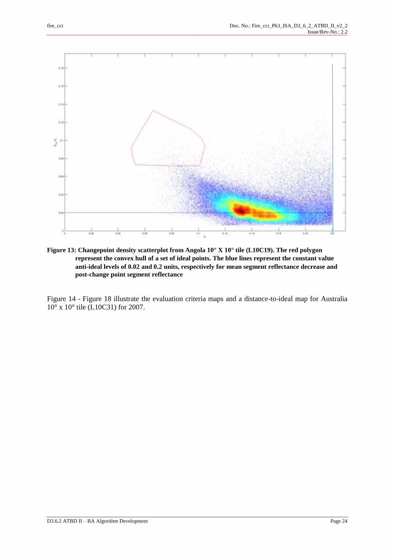
fire_cci


Issue/Rev-No.: 2.2


Figure 13: Changepoint density scatterplot from Angola 10° X 10° tile (L10C19). The red polygon

represent the convex hull of a set of ideal points. The blue lines represent the constant value

anti-ideal levels of 0.02 and 0.2 units, respectively for mean segment reflectance decrease and

post-change point segment reflectance

Figure 14 - Figure 18 illustrate the evaluation criteria maps and a distance-to-ideal map for Australia

10° x 10° tile (L10C31) for 2007.

fire_cci


Issue/Rev-No.: 2.2


Figure 14: Reflectance decrease map

Figure 15: Post-changepoint segment mean reflectance map

fire_cci


Issue/Rev-No.: 2.2


Figure 16: Minimum Euclidean distance to the set of ideal points map

Figure 17: Smallest of the two orthogonal distances to the anti-ideal values

fire_cci


Issue/Rev-No.: 2.2


Figure 18: Changepoint score based on reflectance change, post changepoint reflectance and fire

seasonality. Higher values (red) are closer to ideal, i.e. more likely to represent burned areas.

4.2.1.4 Markov random field image segmentation

The pixels with no computed score or detection date are not classified as burned or unburned. The

remaining pixels are classified according to the procedure described below.

The previous steps of the algorithm lead to a characterisation of each pixel of the image through two

variables: score and detection date. The rationale behind this last processing step is to establish a global

classification of the pixels of the image taking into account the spatial relations between pixels and the

time relations between dates of detection. The algorithm is a standard image processing algorithm that

solves the maximum a posteriori – Markov random field (MAP-MRF) problem, which arises in image

segmentation or image restoration.

4.2.1.4.1 Parameters

To define the graph from the score and date of detection values we first need to establish the spatial

neighbourhood for each pixel (e.g. 4 or 8 neighbours) and we need to set four parameters: min_score,

max_score, max_diff and v0 which can be understood as follows: The parameters min_score and

max_score establish respectively the score values below and above which the classification of the pixel

is set solely by the score. If score<min_score the pixel is classified as “unburned”; if score>max_score

the pixel is classified as “burned”. The parameters v0 (a number between 0 and 1) and max_diff (in

days) establish the role of the detection dates in the image segmentation problem. If pixel X is a spatial

neighbour of pixel Y, and if the detection dates for X and Y differ D days, then the value v(X,Y) of the

connection between X and Y is a number between 0 and 1. V0 equals 1 when D=0 and decreases linearly

to 0 until D = max_diff. Formally, v(X,Y) is defined as: if D > max_diff then v(X,Y) is 0; if D <=

max_diff the value is v0 *(1-D/max_diff). Hence, the value of the connection between two neighbours

is highest when the detection date for both neighbours is the same and vanishes to 0 when the dates of

detection are more than max_diff days apart.

fire_cci


Issue/Rev-No.: 2.2


4.2.1.4.2 Graph

The vertices of the graph are the pixels with known score and detection dates. There are two additional

vertices that represent the classes “burned” and “unburned”. There are two types of edges in the graph.

The first type of edges connect either the vertex “unburned” to a pixel X, or connect X to the vertex

“burned”. If for a pixel X, score<mean_score, where mean_score is the average of min_score and

max_score, then there is a directed edge from the vertex “unburned” to the pixel X, with weight given

by the logit of p_score. The variable p_score takes values in [0,0.5] and is defined by p_score = (score-

min_score)/(max_score-min_score) if score > min_score, and it is the minimum value of those p_score

if score<= min_score (to prevent p_score = 0). The logit function is defined by integer nearest to Logit

(p) = 100 * p/(1-p). If score >= mean_score for pixel X, there is a directed edge in the graph from X to

“burned”, with weight given by Logit(p_score), where p_score is defined as before, but takes values in

[0.5,1], and is always lower than 1. The second type of edges in the graph connect pixels X and Y that

have a positive value v(X,Y) as defined earlier. If X and Y are connected, then we add to the graph two

directed edges, one from X to Y with weight Logit (v(X,Y)) and the other from Y to X with the same

weight. As for the p_score, to prevent v = 0 or v = 1, we assign to it the minimum or maximum p_score

value in the range (0,1). Figure 19 displays the topology of a MAP - MRF graph for an illustrative 10 *

10 pixel area.

4.2.1.4.3 Solution of the problem

The solution of the problem is the minimum source/sink-cut in the graph, where the source is the vertex

“unburned” and the sink is the vertex “burned”. The minimum cut defines a 2-partition of the pixels in

the graph: the first element of the partition are the pixels connected to the vertex “unburned” and the

second element of the partition are the pixels connected to the vertex “unburned”. This partition gives

the segmentation of the image into unburned and burned pixels.

Figure 19: Topology of the graph of the MAP-MRF problem for a 10 x 10 pixel area. The pairs of connected

pixels are spatial first-order neighbours and have detection dates at most 20 days apart. The

solution of the MAP-MRF problem is partition of the pixels in an "unburned" and a "burned"

component defined by the minimum cut in this graph.

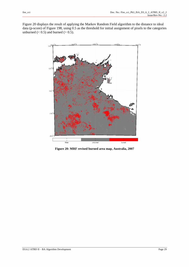
fire_cci


Issue/Rev-No.: 2.2


Figure 20 displays the result of applying the Markov Random Field algorithm to the distance to ideal

data (p-score) of Figure 198, using 0.5 as the threshold for initial assignment of pixels to the categories

unburned (< 0.5) and burned (> 0.5).

Figure 20: MRF revised burned area map, Australia, 2007

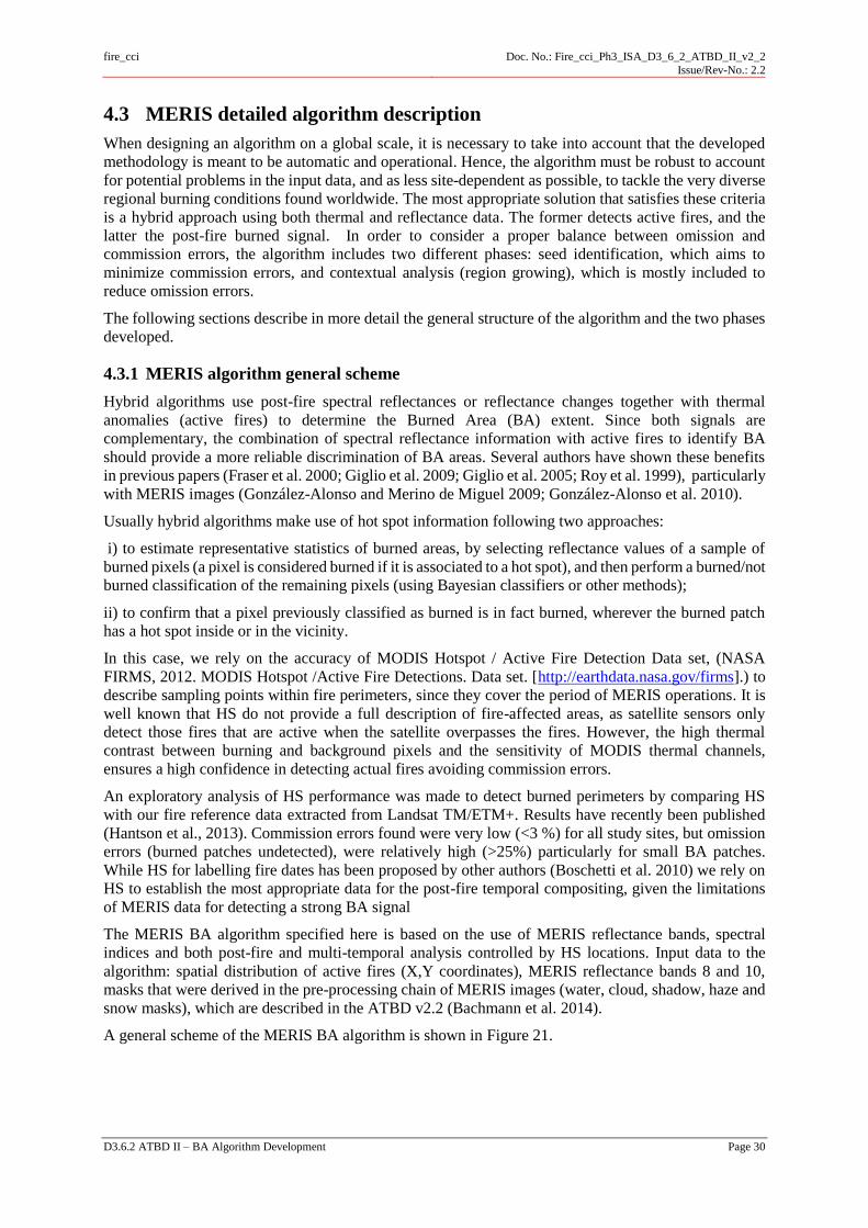
fire_cci


Issue/Rev-No.: 2.2


4.3 MERIS detailed algorithm description

When designing an algorithm on a global scale, it is necessary to take into account that the developed

methodology is meant to be automatic and operational. Hence, the algorithm must be robust to account

for potential problems in the input data, and as less site-dependent as possible, to tackle the very diverse

regional burning conditions found worldwide. The most appropriate solution that satisfies these criteria

is a hybrid approach using both thermal and reflectance data. The former detects active fires, and the

latter the post-fire burned signal. In order to consider a proper balance between omission and

commission errors, the algorithm includes two different phases: seed identification, which aims to

minimize commission errors, and contextual analysis (region growing), which is mostly included to

reduce omission errors.

The following sections describe in more detail the general structure of the algorithm and the two phases

developed.

4.3.1 MERIS algorithm general scheme

Hybrid algorithms use post-fire spectral reflectances or reflectance changes together with thermal

anomalies (active fires) to determine the Burned Area (BA) extent. Since both signals are

complementary, the combination of spectral reflectance information with active fires to identify BA

should provide a more reliable discrimination of BA areas. Several authors have shown these benefits

in previous papers (Fraser et al. 2000; Giglio et al. 2009; Giglio et al. 2005; Roy et al. 1999), particularly

with MERIS images (González-Alonso and Merino de Miguel 2009; González-Alonso et al. 2010).

Usually hybrid algorithms make use of hot spot information following two approaches:

i) to estimate representative statistics of burned areas, by selecting reflectance values of a sample of

burned pixels (a pixel is considered burned if it is associated to a hot spot), and then perform a burned/not

burned classification of the remaining pixels (using Bayesian classifiers or other methods);

ii) to confirm that a pixel previously classified as burned is in fact burned, wherever the burned patch

has a hot spot inside or in the vicinity.

In this case, we rely on the accuracy of MODIS Hotspot / Active Fire Detection Data set, (NASA

FIRMS, 2012. MODIS Hotspot /Active Fire Detections. Data set. [http://earthdata.nasa.gov/firms].) to

describe sampling points within fire perimeters, since they cover the period of MERIS operations. It is

well known that HS do not provide a full description of fire-affected areas, as satellite sensors only

detect those fires that are active when the satellite overpasses the fires. However, the high thermal

contrast between burning and background pixels and the sensitivity of MODIS thermal channels,

ensures a high confidence in detecting actual fires avoiding commission errors.

An exploratory analysis of HS performance was made to detect burned perimeters by comparing HS

with our fire reference data extracted from Landsat TM/ETM+. Results have recently been published

(Hantson et al., 2013). Commission errors found were very low (<3 %) for all study sites, but omission

errors (burned patches undetected), were relatively high (>25%) particularly for small BA patches.

While HS for labelling fire dates has been proposed by other authors (Boschetti et al. 2010) we rely on

HS to establish the most appropriate data for the post-fire temporal compositing, given the limitations

of MERIS data for detecting a strong BA signal

The MERIS BA algorithm specified here is based on the use of MERIS reflectance bands, spectral

indices and both post-fire and multi-temporal analysis controlled by HS locations. Input data to the

algorithm: spatial distribution of active fires (X,Y coordinates), MERIS reflectance bands 8 and 10,

masks that were derived in the pre-processing chain of MERIS images (water, cloud, shadow, haze and

snow masks), which are described in the ATBD v2.2 (Bachmann et al. 2014).

A general scheme of the MERIS BA algorithm is shown in Figure 21.

http://earthdata.nasa.gov/firms

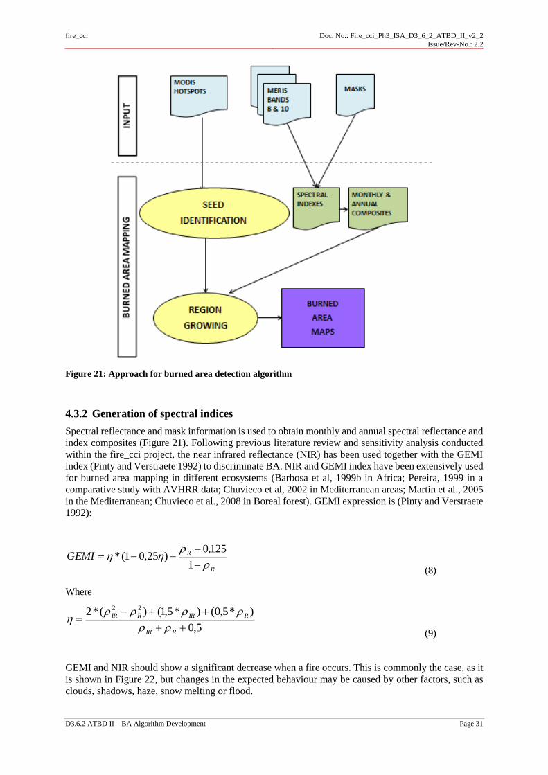
fire_cci


Issue/Rev-No.: 2.2


Figure 21: Approach for burned area detection algorithm

4.3.2 Generation of spectral indices

Spectral reflectance and mask information is used to obtain monthly and annual spectral reflectance and

index composites (Figure 21). Following previous literature review and sensitivity analysis conducted

within the fire_cci project, the near infrared reflectance (NIR) has been used together with the GEMI

index (Pinty and Verstraete 1992) to discriminate BA. NIR and GEMI index have been extensively used

for burned area mapping in different ecosystems (Barbosa et al, 1999b in Africa; Pereira, 1999 in a

comparative study with AVHRR data; Chuvieco et al, 2002 in Mediterranean areas; Martin et al., 2005

in the Mediterranean; Chuvieco et al., 2008 in Boreal forest). GEMI expression is (Pinty and Verstraete

1992):

R

RGEMI

1

125,0)25,01(*

(8)

Where

5,0

)*5,0()*5,1()(*2 22

RIR

RIRRIR

(9)

GEMI and NIR should show a significant decrease when a fire occurs. This is commonly the case, as it

is shown in Figure 22, but changes in the expected behaviour may be caused by other factors, such as

clouds, shadows, haze, snow melting or flood.

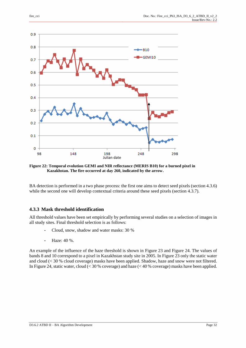
fire_cci


Issue/Rev-No.: 2.2


Figure 22: Temporal evolution GEMI and NIR reflectance (MERIS B10) for a burned pixel in

Kazakhstan. The fire occurred at day 260, indicated by the arrow.

BA detection is performed in a two phase process: the first one aims to detect seed pixels (section 4.3.6)

while the second one will develop contextual criteria around these seed pixels (section 4.3.7).

4.3.3 Mask threshold identification

All threshold values have been set empirically by performing several studies on a selection of images in

all study sites. Final threshold selection is as follows:

- Cloud, snow, shadow and water masks: 30 %

- Haze: 40 %.

An example of the influence of the haze threshold is shown in Figure 23 and Figure 24. The values of

bands 8 and 10 correspond to a pixel in Kazakhstan study site in 2005. In Figure 23 only the static water

and cloud (< 30 % cloud coverage) masks have been applied. Shadow, haze and snow were not filtered.

In Figure 24, static water, cloud (< 30 % coverage) and haze (< 40 % coverage) masks have been applied.

Julian date

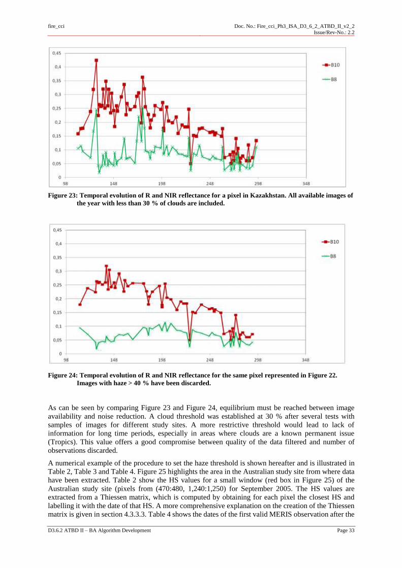
fire_cci


Issue/Rev-No.: 2.2


Figure 23: Temporal evolution of R and NIR reflectance for a pixel in Kazakhstan. All available images of

the year with less than 30 % of clouds are included.

Figure 24: Temporal evolution of R and NIR reflectance for the same pixel represented in Figure 22.

Images with haze > 40 % have been discarded.

As can be seen by comparing Figure 23 and Figure 24, equilibrium must be reached between image

availability and noise reduction. A cloud threshold was established at 30 % after several tests with

samples of images for different study sites. A more restrictive threshold would lead to lack of

information for long time periods, especially in areas where clouds are a known permanent issue

(Tropics). This value offers a good compromise between quality of the data filtered and number of

observations discarded.

A numerical example of the procedure to set the haze threshold is shown hereafter and is illustrated in

Table 2, Table 3 and Table 4. Figure 25 highlights the area in the Australian study site from where data

have been extracted. Table 2 show the HS values for a small window (red box in Figure 25) of the

Australian study site (pixels from (470:480, 1,240:1,250) for September 2005. The HS values are

extracted from a Thiessen matrix, which is computed by obtaining for each pixel the closest HS and

labelling it with the date of that HS. A more comprehensive explanation on the creation of the Thiessen

matrix is given in section 4.3.3.3. Table 4 shows the dates of the first valid MERIS observation after the

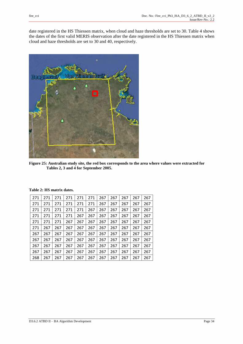
fire_cci


Issue/Rev-No.: 2.2


date registered in the HS Thiessen matrix, when cloud and haze thresholds are set to 30. Table 4 shows

the dates of the first valid MERIS observation after the date registered in the HS Thiessen matrix when

cloud and haze thresholds are set to 30 and 40, respectively.

Figure 25: Australian study site, the red box corresponds to the area where values were extracted for

Tables 2, 3 and 4 for September 2005.

Table 2: HS matrix dates.

271 271 271 271 271 271 267 267 267 267 267

271 271 271 271 271 271 267 267 267 267 267

271 271 271 271 271 267 267 267 267 267 267

271 271 271 271 267 267 267 267 267 267 267

271 271 271 267 267 267 267 267 267 267 267

271 267 267 267 267 267 267 267 267 267 267

267 267 267 267 267 267 267 267 267 267 267

267 267 267 267 267 267 267 267 267 267 267

267 267 267 267 267 267 267 267 267 267 267

267 267 267 267 267 267 267 267 267 267 267

268 267 267 267 267 267 267 267 267 267 267

fire_cci


Issue/Rev-No.: 2.2


Table 3: Dates for the composite when cloud and haze thresholds are set to 30.

272 300 300 300 300 300 300 300 -4 300 272

300 300 300 300 300 272 300 300 -4 300 300

300 300 300 -4 -4 300 300 300 300 300 300

300 300 300 -4 -4 -4 -4 300 300 300 300

300 272 300 -4 -4 -4 -4 -4 300 300 300

272 272 300 -4 -4 -4 -4 -4 300 300 300

300 300 300 300 -4 -4 -4 -4 300 300 300

300 300 300 300 -4 -4 -4 -4 300 300 300

300 300 300 300 300 -4 300 300 300 300 300

300 300 300 300 300 300 300 300 300 300 300

272 300 300 300 300 300 300 300 300 300 300

Table 4: Dates for the composite when cloud and haze thresholds are set to 30 and 40 respectively.

272 272 272 272 272 272 272 300 300 269 269

272 272 272 272 272 272 272 300 300 269 269

272 272 272 272 272 269 272 269 269 269 269

272 272 272 272 269 269 269 269 269 269 269

272 272 272 272 -4 269 269 269 269 269 269

272 272 272 300 -4 269 269 269 269 269 269

272 272 272 300 300 269 269 269 269 269 269

300 300 300 300 300 269 269 269 269 269 269

300 300 269 272 300 269 269 269 269 269 269

272 272 272 272 272 269 269 269 269 269 269

269 272 272 269 272 300 300 269 269 269 269

As can be concluded from the direct comparison of HS matrix Table 2 and the composite dates (Table

3), the dates obtained through the images available (Table 3) have a delay of about 30 days when

compared to the HS dates, and for some pixels there is no valid data available within a 45 days range (-

4 value). The conclusion is that a modification on the cloud threshold will not introduce relevant

changes, but an increase in the haze threshold would. In Table 4, when the haze threshold is set to 40,

most of the pixels have a date closer to the HS matrix obtained from the Thiessen polygons (Table 2)

and most of the non-available data have been replaced by proper dates. Haze threshold is therefore set

to 40.

fire_cci


Issue/Rev-No.: 2.2


4.3.4 Generation of post-fire composites and annual trends

MERIS temporal resolution characteristics and the exploratory analysis led to the conclusion that the

best algorithm implementation would be based on a series of temporal composites. Two aspects have to

be considered: the length of the compositing period and the criteria to select the most adequate pixel

from the time series.

4.3.4.1 Compositing length

After analyzing different alternatives (from monthly to annual composites) the monthly composite

option is selected. This length is a good balance between the number of images to obtain a cloud free

composite while keeping the spectral contrast of the post-fire burned signal. The composite is generated

with images from 60 consecutive days, but monthly aggregated. Therefore, 12 composites are obtained,

each one of them containing information from the specific month and from the month after. Seed pixel

identification and region growing phases of the algorithm are performed using the post-fire and annual

reference composites. Generation of these composites is detailed in the following sections.

4.3.4.2 Post-fire composites: NIR-HS, GEMI-HS.

The compositing criterion should focus on emphasizing the post-fire reflectance signal. In order to do

so, there is a need to establish a method to select the day with the most adequate observation, and the

band or spectral index that will be computed for the selected date to obtain the final composite.

After exploring different possibilities developed for other sensors (Chuvieco et al. 2005) and different

compositing techniques to obtain the monthly composite, the two implementations that present better

results in terms of spatial or temporal consistency are:

4.3.4.3 Closest day to the HS

The idea behind this option is to select the date that will most likely be burned, following the HS spatial

distribution. The computation of this composite is based on the Thiessen polygon matrix, which defines

the area that is closer to a particular HS than to another HS. An example of this matrix is shown in Figure

26 for the Australian study site in October 2005. Spectral index values (GEMI) and NIR reflectance for

the date obtained from the HS matrix are computed per pixel. If no data exists for that day or the data is

considered not valid (it is filtered by the mask thresholds) the next available day is used to compute the

spectral index and so on until the last day of the bi-monthly space is reached. The main advantage of

this technique is that it ensures temporal consistency within the MERIS data. Nevertheless, when there

are few fires, the Thiessen matrix creates artificial spatial structures that are not associated to fire events.

This effect is also enhanced by the fact that images do not have any BRDF correction applied and hence

images from different illumination and observation conditions are being used as equivalent. This issue

may need resolving in later work to test the actual effect. An example of the Julian dates from the MERIS

images that are being used to create the composite is shown in Figure 27. Figure 28 represents the NIR

values associated to these dates; the spatial structures are highlighted with the red circle.

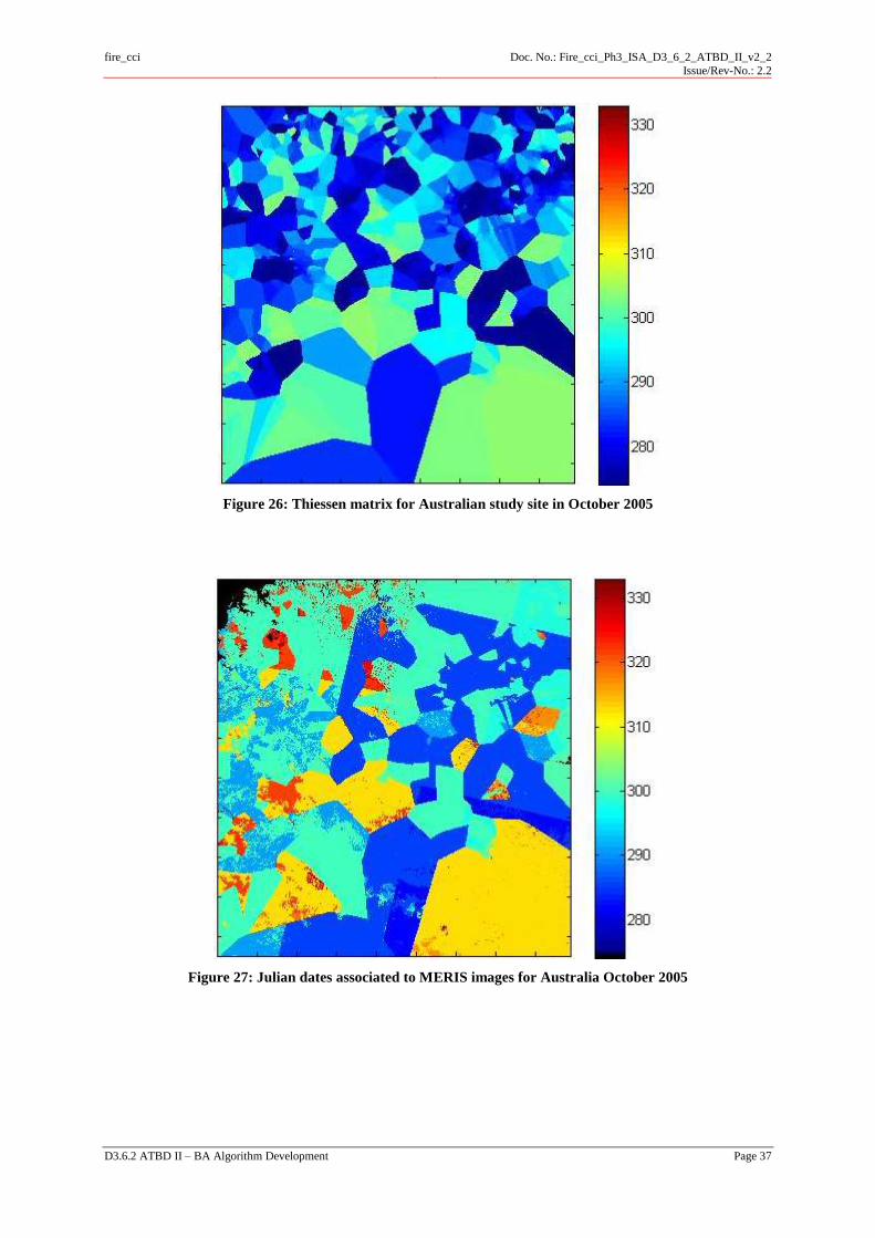
fire_cci


Issue/Rev-No.: 2.2


Figure 26: Thiessen matrix for Australian study site in October 2005

Figure 27: Julian dates associated to MERIS images for Australia October 2005

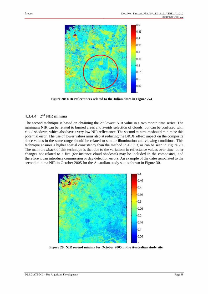
fire_cci


Issue/Rev-No.: 2.2


4.3.4.4 2nd NIR minima

The second technique is based on obtaining the 2nd lowest NIR value in a two month time series. The

minimum NIR can be related to burned areas and avoids selection of clouds, but can be confused with

cloud shadows, which also have a very low NIR reflectance. The second minimum should minimize this

potential error. The use of lower values aims also at reducing the BRDF effect impact on the composite

since values in the same range should be related to similar illumination and viewing conditions. This

technique ensures a higher spatial consistency than the method in 4.3.3.3, as can be seen in Figure 29.

The main drawback of this technique is that due to the variations in reflectance values over time, other

changes not related to a fire (for instance cloud shadows) may be included in the composites, and

therefore it can introduce commission or day detection errors. An example of the dates associated to the

second minima NIR in October 2005 for the Australian study site is shown in Figure 30.

Figure 28: NIR reflectances related to the Julian dates in Figure 274

Figure 29: NIR second minima for October 2005 in the Australian study site

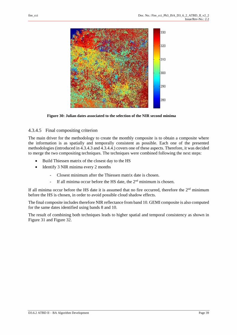
fire_cci


Issue/Rev-No.: 2.2


4.3.4.5 Final compositing criterion

The main driver for the methodology to create the monthly composite is to obtain a composite where

the information is as spatially and temporally consistent as possible. Each one of the presented

methodologies (introduced in 4.3.4.3 and 4.3.4.4.) covers one of these aspects. Therefore, it was decided

to merge the two compositing techniques. The techniques were combined following the next steps:

Build Thiessen matrix of the closest day to the HS

Identify 3 NIR minima every 2 months

- Closest minimum after the Thiessen matrix date is chosen.

- If all minima occur before the HS date, the 2nd minimum is chosen.

If all minima occur before the HS date it is assumed that no fire occurred, therefore the 2nd minimum

before the HS is chosen, in order to avoid possible cloud shadow effects.

The final composite includes therefore NIR reflectance from band 10. GEMI composite is also computed

for the same dates identified using bands 8 and 10.

The result of combining both techniques leads to higher spatial and temporal consistency as shown in

Figure 31 and Figure 32.

Figure 30: Julian dates associated to the selection of the NIR second minima

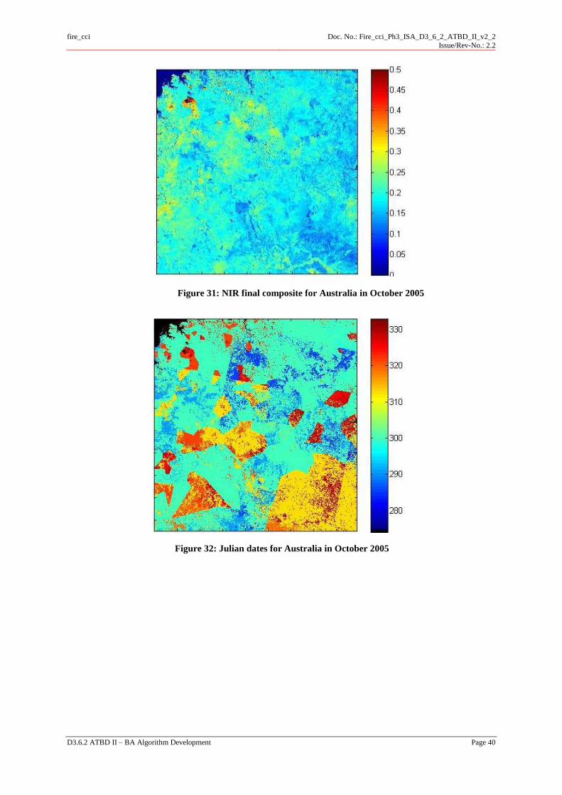
fire_cci


Issue/Rev-No.: 2.2


Figure 31: NIR final composite for Australia in October 2005

Figure 32: Julian dates for Australia in October 2005

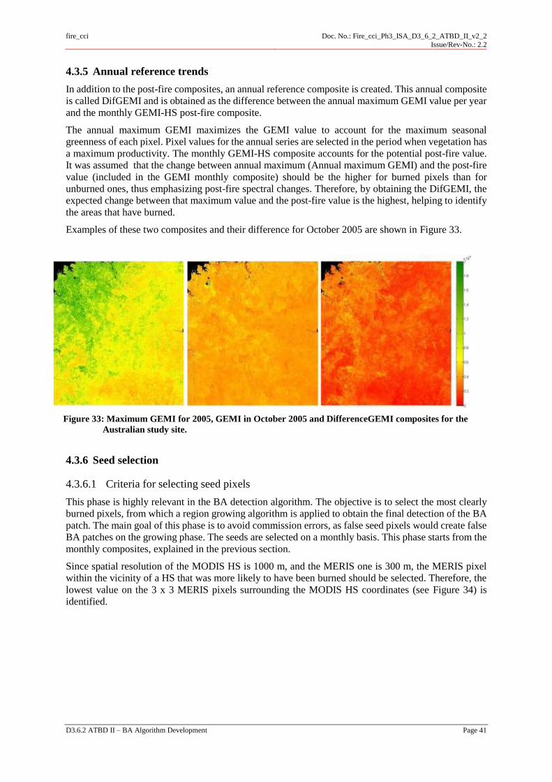
fire_cci


Issue/Rev-No.: 2.2


4.3.5 Annual reference trends

In addition to the post-fire composites, an annual reference composite is created. This annual composite

is called DifGEMI and is obtained as the difference between the annual maximum GEMI value per year

and the monthly GEMI-HS post-fire composite.

The annual maximum GEMI maximizes the GEMI value to account for the maximum seasonal

greenness of each pixel. Pixel values for the annual series are selected in the period when vegetation has

a maximum productivity. The monthly GEMI-HS composite accounts for the potential post-fire value.

It was assumed that the change between annual maximum (Annual maximum GEMI) and the post-fire

value (included in the GEMI monthly composite) should be the higher for burned pixels than for

unburned ones, thus emphasizing post-fire spectral changes. Therefore, by obtaining the DifGEMI, the

expected change between that maximum value and the post-fire value is the highest, helping to identify

the areas that have burned.

Examples of these two composites and their difference for October 2005 are shown in Figure 33.

4.3.6 Seed selection

4.3.6.1 Criteria for selecting seed pixels

This phase is highly relevant in the BA detection algorithm. The objective is to select the most clearly

burned pixels, from which a region growing algorithm is applied to obtain the final detection of the BA

patch. The main goal of this phase is to avoid commission errors, as false seed pixels would create false

BA patches on the growing phase. The seeds are selected on a monthly basis. This phase starts from the

monthly composites, explained in the previous section.

Since spatial resolution of the MODIS HS is 1000 m, and the MERIS one is 300 m, the MERIS pixel

within the vicinity of a HS that was more likely to have been burned should be selected. Therefore, the

lowest value on the 3 x 3 MERIS pixels surrounding the MODIS HS coordinates (see Figure 34) is

identified.

Figure 33: Maximum GEMI for 2005, GEMI in October 2005 and DifferenceGEMI composites for the

Australian study site.

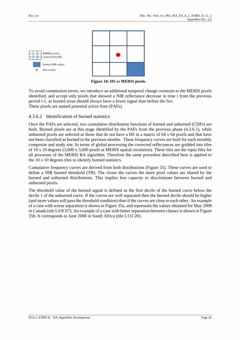
fire_cci


Issue/Rev-No.: 2.2


To avoid commission errors, we introduce an additional temporal change constrain to the MERIS pixels

identified, and accept only pixels that showed a NIR reflectance decrease in time t from the previous

period t-1, as burned areas should always have a lower signal than before the fire.

These pixels are named potential active fires (PAFs).

4.3.6.2 Identification of burned statistics

Once the PAFs are selected, two cumulative distribution functions of burned and unburned (CDFs) are

built. Burned pixels are at this stage identified by the PAFs from the previous phase (4.3.6.1), while

unburned pixels are selected as those that do not have a HS in a matrix of 64 x 64 pixels and that have

not been classified as burned in the previous months. These frequency curves are built for each monthly

composite and study site. In terms of global processing the corrected reflectances are gridded into tiles

of 10 x 10 degrees (3,600 x 3,600 pixels at MERIS spatial resolution). These tiles are the input files for

all processes of the MERIS BA algorithm. Therefore the same procedure described here is applied to

the 10 x 10 degrees tiles to identify burned statistics.

Cumulative frequency curves are derived from both distributions (Figure 35). These curves are used to

define a NIR burned threshold (TB). The closer the curves the more pixel values are shared by the

burned and unburned distributions. This implies less capacity to discriminate between burned and

unburned pixels.

The threshold value of the burned signal is defined as the first decile of the burned curve below the

decile 1 of the unburned curve. If the curves are well separated then the burned decile should be higher

(and more values will pass the threshold condition) than if the curves are close to each other. An example

of a case with worse separation is shown in Figure 35a, and represents the values obtained for May 2008

in Canada (tile L03C07). An example of a case with better separation between classes is shown in Figure

35b. It corresponds to June 2008 in South Africa (tile L11C20).

Figure 34: HS vs MERIS pixels.

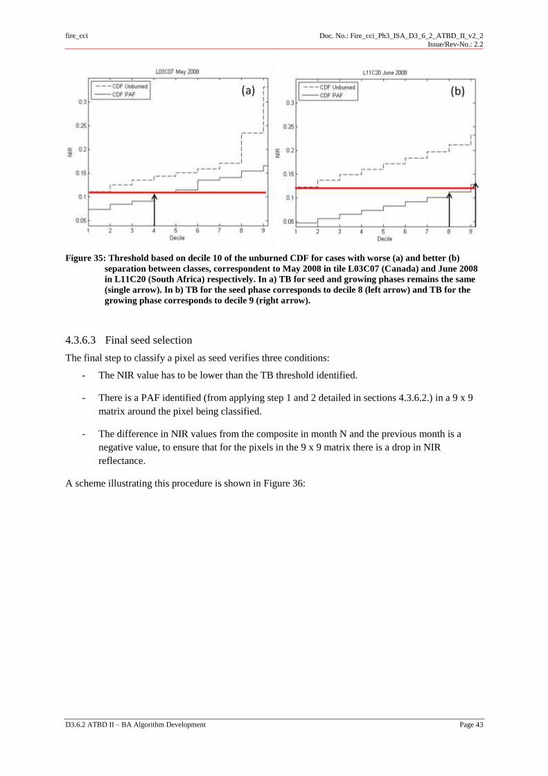
fire_cci


Issue/Rev-No.: 2.2


Figure 35: Threshold based on decile 10 of the unburned CDF for cases with worse (a) and better (b)

separation between classes, correspondent to May 2008 in tile L03C07 (Canada) and June 2008

in L11C20 (South Africa) respectively. In a) TB for seed and growing phases remains the same

(single arrow). In b) TB for the seed phase corresponds to decile 8 (left arrow) and TB for the

growing phase corresponds to decile 9 (right arrow).

4.3.6.3 Final seed selection

The final step to classify a pixel as seed verifies three conditions:

- The NIR value has to be lower than the TB threshold identified.

- There is a PAF identified (from applying step 1 and 2 detailed in sections 4.3.6.2.) in a 9 x 9

matrix around the pixel being classified.

- The difference in NIR values from the composite in month N and the previous month is a

negative value, to ensure that for the pixels in the 9 x 9 matrix there is a drop in NIR

reflectance.

A scheme illustrating this procedure is shown in Figure 36:

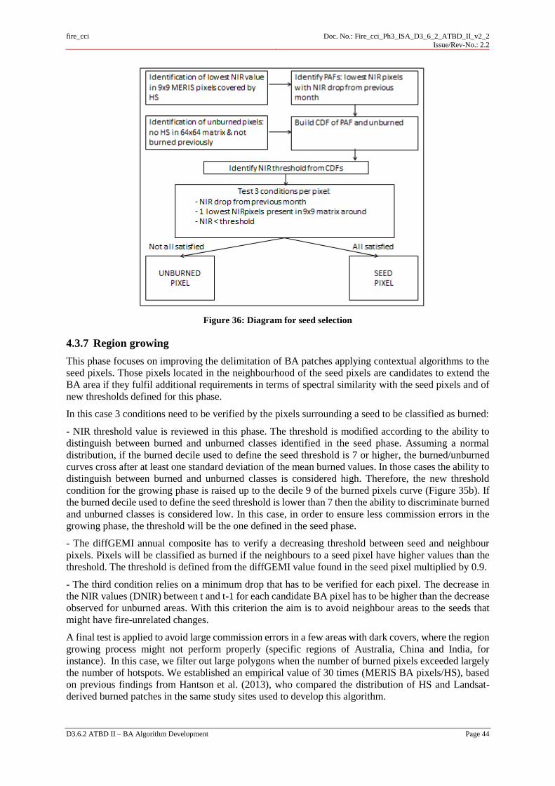
fire_cci


Issue/Rev-No.: 2.2


Figure 36: Diagram for seed selection

4.3.7 Region growing

This phase focuses on improving the delimitation of BA patches applying contextual algorithms to the

seed pixels. Those pixels located in the neighbourhood of the seed pixels are candidates to extend the

BA area if they fulfil additional requirements in terms of spectral similarity with the seed pixels and of

new thresholds defined for this phase.

In this case 3 conditions need to be verified by the pixels surrounding a seed to be classified as burned:

- NIR threshold value is reviewed in this phase. The threshold is modified according to the ability to

distinguish between burned and unburned classes identified in the seed phase. Assuming a normal

distribution, if the burned decile used to define the seed threshold is 7 or higher, the burned/unburned

curves cross after at least one standard deviation of the mean burned values. In those cases the ability to

distinguish between burned and unburned classes is considered high. Therefore, the new threshold

condition for the growing phase is raised up to the decile 9 of the burned pixels curve (Figure 35b). If

the burned decile used to define the seed threshold is lower than 7 then the ability to discriminate burned

and unburned classes is considered low. In this case, in order to ensure less commission errors in the

growing phase, the threshold will be the one defined in the seed phase.

- The diffGEMI annual composite has to verify a decreasing threshold between seed and neighbour

pixels. Pixels will be classified as burned if the neighbours to a seed pixel have higher values than the

threshold. The threshold is defined from the diffGEMI value found in the seed pixel multiplied by 0.9.

- The third condition relies on a minimum drop that has to be verified for each pixel. The decrease in

the NIR values (DNIR) between t and t-1 for each candidate BA pixel has to be higher than the decrease

observed for unburned areas. With this criterion the aim is to avoid neighbour areas to the seeds that

might have fire-unrelated changes.

A final test is applied to avoid large commission errors in a few areas with dark covers, where the region

growing process might not perform properly (specific regions of Australia, China and India, for

instance). In this case, we filter out large polygons when the number of burned pixels exceeded largely

the number of hotspots. We established an empirical value of 30 times (MERIS BA pixels/HS), based

on previous findings from Hantson et al. (2013), who compared the distribution of HS and Landsat-

derived burned patches in the same study sites used to develop this algorithm.

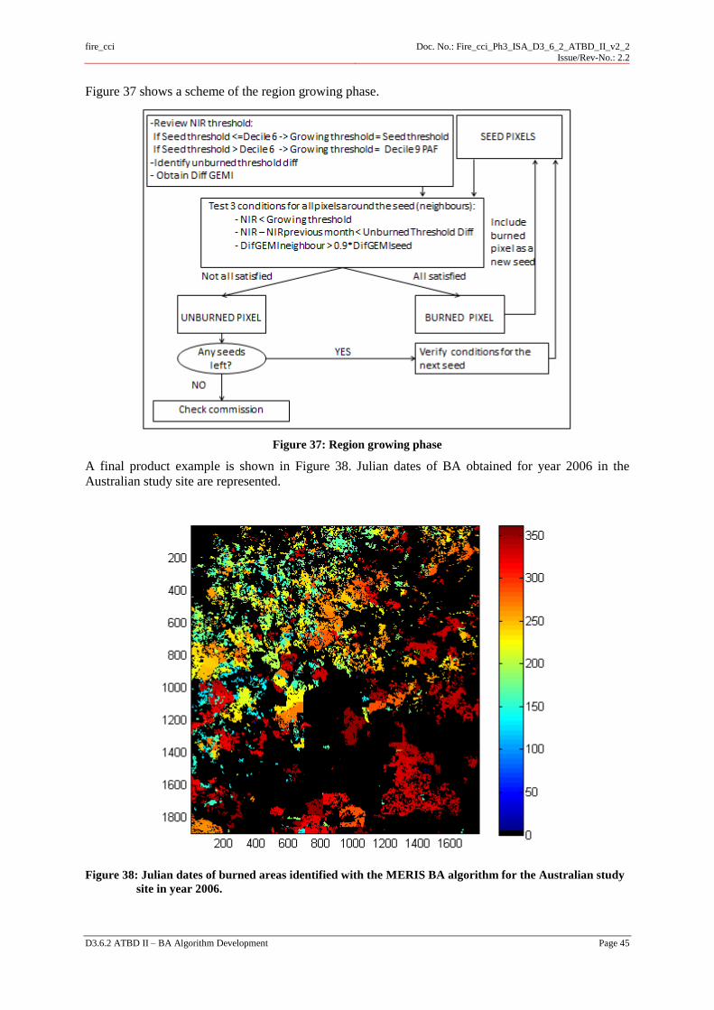
fire_cci


Issue/Rev-No.: 2.2


Figure 37 shows a scheme of the region growing phase.

Figure 37: Region growing phase

A final product example is shown in Figure 38. Julian dates of BA obtained for year 2006 in the

Australian study site are represented.

Figure 38: Julian dates of burned areas identified with the MERIS BA algorithm for the Australian study

site in year 2006.

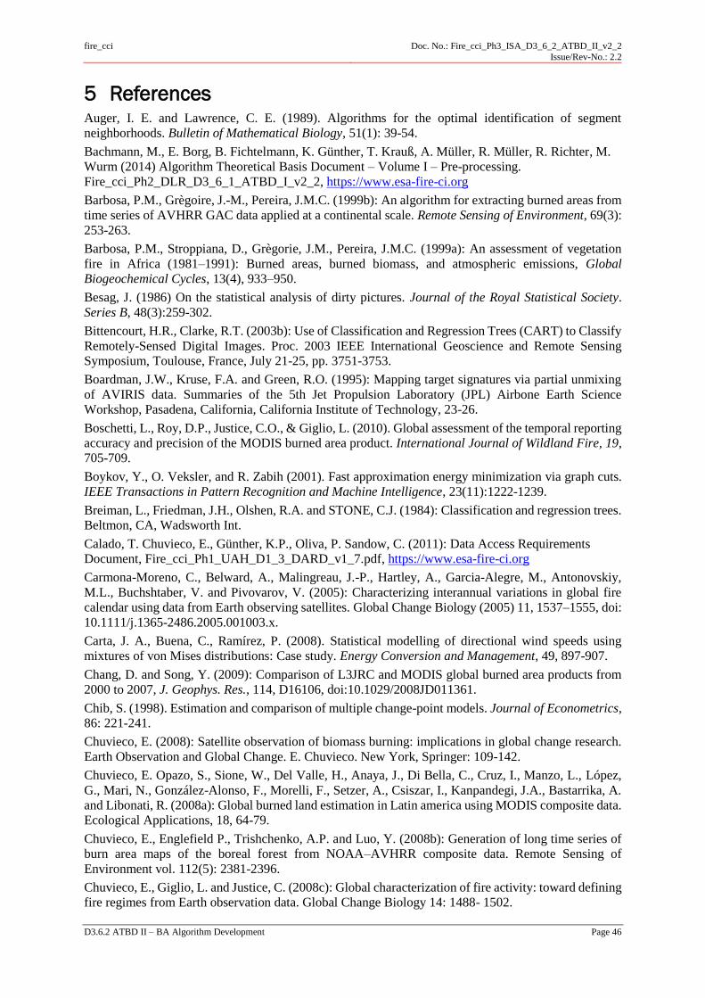
fire_cci


Issue/Rev-No.: 2.2


5 References Auger, I. E. and Lawrence, C. E. (1989). Algorithms for the optimal identification of segment

neighborhoods. Bulletin of Mathematical Biology, 51(1): 39-54.

Bachmann, M., E. Borg, B. Fichtelmann, K. Günther, T. Krauß, A. Müller, R. Müller, R. Richter, M.

Wurm (2014) Algorithm Theoretical Basis Document – Volume I – Pre-processing.

Fire_cci_Ph2_DLR_D3_6_1_ATBD_I_v2_2, https://www.esa-fire-ci.org

Barbosa, P.M., Grègoire, J.-M., Pereira, J.M.C. (1999b): An algorithm for extracting burned areas from

time series of AVHRR GAC data applied at a continental scale. Remote Sensing of Environment, 69(3):

253-263.

Barbosa, P.M., Stroppiana, D., Grègorie, J.M., Pereira, J.M.C. (1999a): An assessment of vegetation

fire in Africa (1981–1991): Burned areas, burned biomass, and atmospheric emissions, Global

Biogeochemical Cycles, 13(4), 933–950.

Besag, J. (1986) On the statistical analysis of dirty pictures. Journal of the Royal Statistical Society.

Series B, 48(3):259-302.

Bittencourt, H.R., Clarke, R.T. (2003b): Use of Classification and Regression Trees (CART) to Classify

Remotely-Sensed Digital Images. Proc. 2003 IEEE International Geoscience and Remote Sensing

Symposium, Toulouse, France, July 21-25, pp. 3751-3753.

Boardman, J.W., Kruse, F.A. and Green, R.O. (1995): Mapping target signatures via partial unmixing

of AVIRIS data. Summaries of the 5th Jet Propulsion Laboratory (JPL) Airbone Earth Science

Workshop, Pasadena, California, California Institute of Technology, 23-26.

Boschetti, L., Roy, D.P., Justice, C.O., & Giglio, L. (2010). Global assessment of the temporal reporting

accuracy and precision of the MODIS burned area product. International Journal of Wildland Fire, 19,

705-709.

Boykov, Y., O. Veksler, and R. Zabih (2001). Fast approximation energy minimization via graph cuts.

IEEE Transactions in Pattern Recognition and Machine Intelligence, 23(11):1222-1239.

Breiman, L., Friedman, J.H., Olshen, R.A. and STONE, C.J. (1984): Classification and regression trees.

Beltmon, CA, Wadsworth Int.

Calado, T. Chuvieco, E., Günther, K.P., Oliva, P. Sandow, C. (2011): Data Access Requirements

Document, Fire_cci_Ph1_UAH_D1_3_DARD_v1_7.pdf, https://www.esa-fire-ci.org

Carmona-Moreno, C., Belward, A., Malingreau, J.-P., Hartley, A., Garcia-Alegre, M., Antonovskiy,

M.L., Buchshtaber, V. and Pivovarov, V. (2005): Characterizing interannual variations in global fire

calendar using data from Earth observing satellites. Global Change Biology (2005) 11, 1537–1555, doi:

10.1111/j.1365-2486.2005.001003.x.

Carta, J. A., Buena, C., Ramírez, P. (2008). Statistical modelling of directional wind speeds using

mixtures of von Mises distributions: Case study. Energy Conversion and Management, 49, 897-907.

Chang, D. and Song, Y. (2009): Comparison of L3JRC and MODIS global burned area products from

2000 to 2007, J. Geophys. Res., 114, D16106, doi:10.1029/2008JD011361.

Chib, S. (1998). Estimation and comparison of multiple change-point models. Journal of Econometrics,

86: 221-241.

Chuvieco, E. (2008): Satellite observation of biomass burning: implications in global change research.

Earth Observation and Global Change. E. Chuvieco. New York, Springer: 109-142.

Chuvieco, E. Opazo, S., Sione, W., Del Valle, H., Anaya, J., Di Bella, C., Cruz, I., Manzo, L., López,

G., Mari, N., González-Alonso, F., Morelli, F., Setzer, A., Csiszar, I., Kanpandegi, J.A., Bastarrika, A.

and Libonati, R. (2008a): Global burned land estimation in Latin america using MODIS composite data.

Ecological Applications, 18, 64-79.

Chuvieco, E., Englefield P., Trishchenko, A.P. and Luo, Y. (2008b): Generation of long time series of

burn area maps of the boreal forest from NOAA–AVHRR composite data. Remote Sensing of

Environment vol. 112(5): 2381-2396.

Chuvieco, E., Giglio, L. and Justice, C. (2008c): Global characterization of fire activity: toward defining

fire regimes from Earth observation data. Global Change Biology 14: 1488- 1502.

https://www.esa-fire-ci.org/

https://www.esa-fire-ci.org/

fire_cci


Issue/Rev-No.: 2.2


Chuvieco, E., De Santis, A., Riaño, D. and Halligan, K. (2007): Simulation approaches for burn severity

estimation using remotely sensed images. Journal of Fire Ecology, 3, 129-150.

Chuvieco, E., Martín, M.P., & Palacios, A. (2002). Assessment of different spectral indices in the red-

near-infrared spectral domain for burned land discrimination. International Journal of Remote Sensing,

23, 5103-5110.

Chuvieco, E. and Martín, M.P. (1994): Global fire mapping and fire danger estimation using AVHRR

images. Photogrammetric Engineering and Remote Sensing, 60: 563-570.

Clark, R.N. and Roush, T.L. (1984): Reflectance spectroscopy: Quantitative analysis techniques for

remote sensing applications. Journal of Geophysical Research 89: 6329-6340.

Coleman, T. F., & Li, Y. (1994). On the Convergence of Reflective Newton Methods for Large-Scale

Nonlinear Minimization Subject to Bounds. Mathematical Programming, 67(2), 189-224.

Crawley, M.J. (2007) The R Book. Wiley-Blackwell, 950 p.

Dubovik, O., Holben, B., Eck, T. F., Smirnov, A., Kaufman, Y. J., King, M. D., Tanre, D. and Slutsker,

I. (2002): Variability of absorption and optical properties of key aerosol types observed in worldwide

locations, J. Atmos. Sci., 59, 590-608.

Ershov, D.V. and Novik, V.P. (2001): Mapping burned areas in Russia with SPOT4 VEGETATION

(S1 product) imagery, final report, Contract 18176-2001-07-F1EI ISP RU, Eur. Comm. Joint Res. Cent.,

Brussels.

Eva, H. and Lambin, E.F. (1998): Burnt area mapping in Central Africa using ATSR data, Int. J. Remote

Sens., 19, 3473– 3497.

Fisher, N.I. (1995). Statistical Analysis of Circular Data. Revised edition. Cambridge University Press.

Fraser, R.H., Li, Z. and Cihlar, J. (2000): Hotspot and NDVI differencing synergy (HANDS): a new

technique for burned area mapping over boreal forest. Remote Sensing of Environment, 74, 362−376.

Fried, R. (2004) Robust filtering of time series with trends. Nonparametric Statistics, 16(3–4): 313–328.

Fried, R., K. Schettlinger and M. Borowski (2011). robfilter: Robust Time Series Filters. R package

version 3.0. http://CRAN.R-project.org/package=robfilter.

Friedl, M.A. and Brodley, C.E. (1997): Decision tree classification of land cover from remotely sensed

data. Remote Sensing of Environment 61: 399-409.

Gather, U., Fried, R. (2004), Methods and Algorithms for Robust Filtering, COMPSTAT 2004:

Proceedings in Computational Statistics, J. Antoch (eds.), Physika-Verlag, Heidelberg, 159-170.

Geman, S. and S. Geman (1984) Stochastic relaxation, Gibbs distributions, and the Bayesian restoration

of images. IEEE Transactions in Pattern Recognition and Machine Intelligence, 6(6): 721-741.

Giglio, L., I. Csiszar, and C.O. Justice (2006) Global distribution and seasonality of active fires as

observed with the Terra and Aqua Moderate Resolution Imaging Spectroradiometer (MODIS) sensors.

Journal of Geophysical Research, 111, G02016, doi:10.1029/2005JG000142.

Giglio, L., Loboda, T., Roy, D.P., Quayle, B. and Justice, C.O. (2009): An active-fire based burned area

mapping algorithm for the MODIS sensor. Remote Sensing of Environment 113: 408-420.

Giglio, L., van der Werf, G.R., Randerson, J.T., Collatz, G.J. and Kasibhatla, P. (2006b): Global

estimation of burned area using MODIS active fire observations. Atmospheric Chemistry and Physics

6: 957-974.

Global Climate Observing System (GCOS) (2009). Guidelines for the generation of satellite-based

datasets and products meeting GCOS requirements. Geneva: World Meteorological Organization

GlobCarbon (2007). Demonstration Products and Qualification Report. In (pp. 1-69): ESA

González-Alonso, F. and Merino-de-Miguel, S. (2009): Integration of AWiFS and MODIS active fire

data for burn mapping at regional level using the Burned Area Synergic Algorithm (BASA).

International Journal of Wildland Fire, 18, 404-414.

González-Alonso,F., Merino de Miguel, S. and Huesca, M. (2010): A burned area synergistic algorithm

using MERIS-ENVISAT images and MODIS thermal anomalies. ESA Living Planet Symposium.

Bergen. June, 2010

http://cran.r-project.org/package=robfilter

fire_cci


Issue/Rev-No.: 2.2


González-Alonso, F., Salgado, V., Calle, V., Casanova, J.L., Sanz, J., de la Fuente, D., Goldammer,

J.G., Li, Z., Qin, X., Zhang, X., Deng, G., Liu, Q., Li, G., Cai, H. and Huang, Z. (2009): Forest burn in

China by means of MERIS and MODIS images. 2009 Dragon 2 Symposium, June 2009, Barcelona.

Govaerts, Y.M., Pereira, J.M., Pinty, B. and Mota, B. (2002): Impact of fires on surface albedo dynamics

over the African continent, 107, 4629, doi:10.1029/2002JD002388.

Greig, D.M., B.T. Porteous, and A.H. Seheult (1989). Exact maximum a posteriori estimation for binary

images. Journal of the Royal Statistical Society, Series B, 51(2):271-279.

Hinkley, D. V. (1970). Inference about the change-point in a sequence of random variables. Biometrika,

57: 1-17.

Huang, S. and Siegert, F. (2004): ENVISAT multisensor data for fire monitoring and impact assessment.

International Journal of Remote Sensing 25(20): 4411-4416.

IPCC Fourth Assessment Report: Climate Change (2007) (AR4).

Iqbal, M. (1983): An Introduction to solar radiation. Academic Press, New York.

Jacob, D.J. (1999): Introduction to atmospheric chemistry. (Princeton University Press: Princeton).

Jones, T.A. (2006). MATLAB functions to analyze directional (azimuthal) data – I: Single-sample

inference. Computers & Geosciences, 32, 166-175.

Jong, K., Marchiori, E., Meijer, G., Vaart, A. v. d., and Ylstra, B. (2004). Breakpoint identification and

smoothing of array comparative genomic hybridization data. Bioinformatics, 20(18): 3636-3637.

Kaufman, Y. J., Tanré, D., Remer, L.A., Vermote, E.F., Chu, D.A., and Holben, B.N. (1997): Remote

sensing of tropospheric aerosol from EOS-MODIS over the land using dark targets and dynamic aerosol

models, J. Geophys. Res., 102, 17,051– 17,067.

Kaufman, Y.J. and Justice, C.O. (1998): MODIS Fire Products Algorithm Technical Background

Document (Version 2.2). Available at:

http://eospso.gsfc.nasa.gov/ftp_ATBD/REVIEW/MODIS/ATBD-MOD-14/atbd-mod-14.pdf

Kaufman, Y.J., Martins, J.V., Remer, L.A., Schoebrel, M.R. and Yamasoe, M.A., (2002): Satellite

retrieval of aerosol absorption over the sunglint. Geophysical Research Letters, vol. 29, 19, 1928. doi:

10.1029/2002GL015403.

Killick, R. and Eckley, I. A. (2010). R package- changepoint: Analysis of Changepoint Models.

Lancaster University, Lancaster, UK.

Killick, R., Fearnhead, P., and Eckley, I. A. (2012). Optimal detection of changepoints with a linear

computational cost. In Submission.

Kugiumtzis, D. and A. Tsimpiris (2010). Measures of Analysis of Time Series (MATS): A MATLAB

toolkit for computation of multiple measures on time series data bases. Journal of Statistical Software,

33(5): 1-30.

Kumar, R., & Silva, L.F. (1977). Separability of agricultural cover types by remote sensing in the visible

and infrared wavelength regions. IEEE Transactions on Geoscience Electronics, 15, 49-59.

Le Page, Y., D. Oom, J.M.N. Silva, P. Jönsson, and J.M.C. Pereira (2010) Seasonality of vegetation

fires as modified by human action: observing the deviation from eco-climatic fire regimes. Global

Ecology and Biogeography. 19 (4): 575-588. DOI: 10.1111/j.1466-8238.2010.00525.x

Le Page, Y., J.M.C. Pereira, R. Trigo, C. da Camara, D. Oom, and B. Mota (2008) Global fire activity

patterns (1996–2006) and climatic influence: an analysis using the World Fire Atlas. Atmospheric

Chemistry and Physics, 8, 1911–1924.

Lobert, J.M. and Warnatz, J. (1993): Emissions from the combustion process in vegetation. In PJ

Crutzen and JG Goldammer (Eds.) Fire in the Environment: the Ecological, Atmospheric, and Climatic

Importance of Vegetation Fires. John Wiley and Sons,Chichester, UK.

Loh, W.Y. and Shih, Y.-S. (1997): Split selection methods for classification trees. Statistica Sinica 7:

815-840.

Mardia, K.V., Jupp, P.E. (2000). Directional Statistics. 2nd ed. New York: John Wiley and Sons.

Martín, M.P., Gomez, I. and Chuvieco, E. (2006): Burned Area Index (BAIM) for burned area

discrimination at regional scale using MODIS data. Forest Ecology and Management, 234S, S221.

http://eospso.gsfc.nasa.gov/ftp_ATBD/REVIEW/MODIS/ATBD-MOD-14/atbd-mod-14.pdf

fire_cci


Issue/Rev-No.: 2.2


Martín, M.P. (1998). Cartografía e inventario de incendios forestales en la Península Ibérica a partir de

imágenes NOAA-AVHRR. In, Departamento de Geografía. Alcalá de Henares: Universidad de Alcalá.

Mather, P.M., & Coch, M. (2011). Computer Processing of Remotely Sensed Images, 4th Edition.

Chichester: John Wiley & Sons.

Moreno-Ruiz, J.A., Barbosa, P.M., Carmona-Moreno, C., Gregoire, J.M., Belward, A.S. (1999):

GLINTS-BS – Global Burn Scar Detection System. European Union Technical Note I.99.167. May

1999.

Mota, B., J.M.C. Pereira, D. Oom, M.J.P. Vasconcelos, and M. Schultz (2006). Screening the ESA

ATSR-2 World Fire Atlas (1997-2002). Atmospheric Chemistry and Physics, 6: 1409-1424.

Mutanga, O., Skidmore, A.K. and Prins, H.H.T. (2004): Predicting in situ pasture quality in the Kruger

National Park, South Africa, using continuum-removed absorption features. Remote Sensing of

Environment 89: 393-408.

Nash, J. E., & Sutcliffe, J. V. (1970). River flow forecasting through conceptual models part I — A

discussion of principles. Journal of Hydrology, 10 (3), 282–290.

Oliva, P. (2009): Métodos para la cartografía de área quemada con imágenes del sensor envisat-meris

en la cuenca mediterránea, Ph. D. Dissertation, University of Alcalá .

Oliva, P. and Martín, M.P. (2007): Mapping burned area by using Spectral Angle Mapper in MERIS

images. In Proceedings of 6th International workshop on remote Sensing and GIS Applications to Forest

Fire Management: Fire Effects Assessment. Thessaloniki, Greece, September 2007.

Oliva, P., Martín, M.P. and Chuvieco, E. (2010): Burned area mapping with MERIS post-fire image.

International Journal of Remote Sensing in press.

Oom, D., J.M.C. Pereira (2013) Spatial autocorrelation in global vegetation fires: exploratory analysis

of screened MODIS hotspot data. International Journal of Earth Observation and Geoinformation.

Padilla, M., Oliva P. and Chuvieco, E. (2012): Product Validation and Algorithm Selection Report,

Fire_cci_Ph2_UAH_D2_5_PVASR_v2_0.pdf, http://www.esa-fire-cci.org/webfm_send/581

Peel M.C, Finlayson B.L, McMahon T.A, (2007) Updated world map of the Köppen-Geiger climate

classification. Hydrol. Earth Syst. Sci. 11 (5): 1633-1644.

Pereira, J.M.C. (2003): Remote sensing of burned areas in tropical savannas. International Journal of

Wildland Fire 12 (3-4):259-270.

Pereira, J.M.C., Flasse, S., Hoffman, A., Pereira, J.A.R., González-Alonso, F. and Trigg, S. (2000):

Operational use of remote sensing for fire monitoring and management: regional case studies. In F.

Ahern, J.-M. Grégoire and C. Justice, (Eds.), Forest Fire Monitoring and Mapping: A Component of

Global Observation of Forest Cover (pp. 98-110). European Commission, Joint Research Centre, EUR

19588 EN.

Pereira, J.M.C. (1999): A comparative evaluation of NOAA/AVHRR vegetation indexes for burned

surface detection and mapping. IEEE Transactions on Geoscience and Remote Sensing, 37(1), 217-226.

Pereira, J.M.C., Pereira, B.S., Barbosa, P., Stroppiana, D., Vasconcelos, M.J.P. and Grégoire, J-M.

(1999a): Satellite monitoring of fire in the EXPRESSO study area during the 1996 dry season

experiment: active fires, burnt area and atmospheric emissions. Journal of Geophysical Research, 104,

D23: 30,701-30,712

Pereira, J.M.C., A.C.L. Sá, A.M.O. Sousa, J.M.N. Silva, T.N. Santos, e J.M.B. Carreiras (1999b)

Spectral characterisation and discrimination of burnt areas. Em Remote Sensing of Large Wildfires in

the European Mediterranean Basin, pp.123-138 (E. Chuvieco, ed), Springer-Verlag, Berlin.

Pereira, J.M.C, Sousa, A.M.O., Sá, A. C. L. (1999c): Regional-scale burnt area mapping in Southern

Europe using NOAA-AVHHR 1 km data. In ‘Remote sensing of large wildfires’. (Ed. EP Chuvieco)

pp. 139–155. (Springer: Berlin).

Pereira, J.M.C. and Setzer, A.W. (1993): Spectral characteristics of fire scars in Landsat-5 TM images

of Amazonia. International Journal of Remote Sensing, 14, 2061–2078.

Piccolini, I. (1998: Development and validation of an adaptive algorithm for burn scar detection using

ERS/ATSR-2 data, Ph.D. thesis, Univ. La Sapienza, Rome.

http://www.esa-fire-cci.org/webfm_send/581

fire_cci


Issue/Rev-No.: 2.2


Pinty, B., & Verstraete, M.M. (1992). GEMI: a non-linear index to monitor global vegetation from

satellites. Vegetatio, 101, 15-20.

Plummer, S., Arino, O., Simon, M. and Steffen, W. (2006): Establishing an earth observation product

service for the terrestrial carbon community: The GLOBCARBON Initiative. Mitigation and adaptation

strategies for Global Change 11: 97-111.

Rast, M., Bézy, J.L. and Bruzzi, S. (1999): The ESA Medium Resolution Imaging Spectrometer MERIS

- a review of the instrument and its mission. International Journal of Remote Sensing 20(9): 1681-1702

Riaño, D., Moreno Ruiz, J.A., Isidoro, D. and Ustin, S.L. (2007): Global spatial patterns and temporal

trends of burned area between 1981 and 2000 using NOAA-NASA Pathfinder. Global Change Biology

(2007) 13, 40–50.

Robinson, J.M. (1991: Problems in global fire evaluation: is remote sensing the solution? In ‘Global

Biomass Burning: Atmospheric, Climatic, and Biospheric Implications’ (Ed JS Levine) pp. 67-73. (MIT

Press: Cambridge, MA).

Roldán-Zamarrón, A., Merino de Miguel, S., González-Alonso, F., García-Gigorro, S. and Cuevas, J.M.

(2006): Minas de Rio Tinto (south Spain) forest fire: Burned area assessment and fire severity mapping

using Landsat 5-TM, Envisat-MERIS, and Terra-MODIS postfire images. Journal of Geophysical

Research 111(G04S11).

Rousseeuw, J., Croux, C. (1993): Alternative to the median absolute deviation. Journal of the American

Statisticak Association, Vol. 88, nº 424.

Roy, D. and Boschetti, L. (2009): Southern Africa Validation of the MODIS, L3JRC and GlobCarbon

Burned Area Products. IEEE transactions on Geoscience and Remote Sensing, 47, 4, 1032 – 1044,

doi:10.1109/TGRS.2008.2009000

Roy, D., Boschetti L., Justice, C.O. and Ju, J. (2008): The collection 5 MODIS burned area product -

Global evaluation by comparison with the MODIS active fire product. Remote Sensing of Environment

112: 3690-3707.

Roy, D.P., Lewis, P.E. and Justice, C.O. (2002): Burned area mapping using multi-temporal moderate

spatial resolution data—a bi-directional reflectance model-based expectation approach. Remote Sensing

of Environment, 83, 263–286.

Roy, D.P., Giglio, L., Kendall, J.D., & Justice, C.O. (1999). Multi-temporal active-fire based burn scar

detection algorithm. International Journal of Remote Sensing, 20, 1031-1038.

Schowengerdt, R.A. (2007). Remote sensing, models, and methods for image processing. Burlington,

MA: Elsevier Academic Press.

Schwarz, G. (1978). Estimating the dimension of a model. The Annals of Statistics, 6(2): 461-464.

Scott, A. J. and Knott, M. (1974). A cluster analysis method for grouping means in the analysis of

variance. Biometrics, 30(3): 507-512.

Silva, J.M.N., Pereira, J.M.C., Cabral, A., Sá, A.C.L., Vasconcelos, M.J.P., Mota, B., and Grégoire, J.-

M. (2003): The area burned in southern Africa during the 2000 dry season, J. Geophys. Res., 108(D13),

8498,doi:10.1029/2002JD002320.

Silva, J.M.N., Sousa, A.M.O., Pereira, J.M.C., Tansey, K. and Grégoire, J.-M., (2002): A contribution

for a global burned area map, in Forest Fire Research and Wildland Fire Safety [CD-ROM], edited by

D. X. Viegas, Millpress, Rotterdam.

Simon, M., Plummer, S., Fierens, F., Hoelzemann, J.J. and Arino, O. (2004): Burnt area detection at

global scale using ATSR-2: The GLOBSCAR products and their qualification. Journal of Geophysical

Research 109(D14S02).

Stijn Hantson, Marc Padilla, Dante Corti, & Chuvieco, E. (in review). A Global characterization of

MODIS hotspots using high resolution burned area data. Remote Sensing of Environment.

Tansey, K., Grégoire, J.M., Defourny, P., Leigh, R., Pekel, J.F., van Bogaert, E. and Bartholomé, E.

(2008): A new, global, multi-annual (2000-2007) burned area product at 1 km resolution. Geophysical

Research Letters 35(L01401): 6.

fire_cci


Issue/Rev-No.: 2.2


Tansey, K., Grégoire, J.M., Binaghi, E., Boschetti, L., Brivio, P.A., Ershov, D., Flasse, S., Fraser, R.,

Graetz, D., Maggi, M., Peduzzi, P., Pereira, J., Silva, J.M.N., Sousa, A.M.O. and Sroppiana, D. (2004):

A global inventory of burned areas at 1 Km resolution for the year 2000 derived from SPOT-

VEGETATION data. Climatic Change 67(2-3): 345-377.

The ESA Climate Change Initiative – Description issue 1 revision 0 - 30/09/09 EOP-SEP/TN/0030-

09/SP (available online at: http://earth.esa.int/workshops/esa_cci/ESA_CCI_Description.pdf

Trigg, S. and Flasse, S. (2001): An evaluation of different bi-spectral spaces for discriminating burned

shrub-savannah. International Journal of Remote Sensing, 22, 2641−2647.

Trigg, S. and Flasse, S. (2000): Characterising the spectral-temporal response of burned savannah using

in situ spectroradiometry and infrared thermometry. International Journal of Remote Sensing, 21, 3161–

3168.

Van der MEER, F.D. (2000): Spectral curve shape matching with a continuum removed CCSM

algorithm. International Journal of Remote Sensing 21(16): 3179-3185.

D3.6.2 - Algorithm Theoretical Basis Document – Volume II – BA Algorithm Development

Documents

Transcript of D3.6.2 - Algorithm Theoretical Basis Document – Volume II – BA Algorithm Development