D G M K Research Report 718-2

D G M K Research Report

718-2

Mineral Vein Dynamics Modelling (FRACS II)

DGMKDeutsche Wissenschaftliche Gesellschaft

für Erdöl, Erdgas und Kohle e.V.

Das diesem DGMK-Forschungsbericht zugrundeliegende Vorhaben wurde aus Mitteln der deutschenErdöl- und Erdgasgewinnungsindustrie gefördert.

Die DGMK und die Bearbeiter haben das Vorhaben mit wissenschaftlicher Genauigkeit und Sorgfalt durchgeführt. Es wird keine Gewähr für die Anwendbarkeit der in diesem Bericht mitgeteilten

Ergebnisse übernommen.

Alle Rechte, auch die der Übersetzung, des auszugsweisen Nachdrucks, der Herstellung von Mikrofilmen und der fotomechanischen

Wiedergabe, nur mit ausdrücklicher schriftlicher Genehmigung der DGMK

All rights reserved. No part of this publication may be reproduced, stored in a retrieval system, or transmitted in any form or by any means,

electronic, mechanical, photocopying, recording, or otherwise, without the prior written permission of DGMK

Als Manuskript gedruckt.

ISSN 0937-9762 ISBN 978-3-941721-70-8

Preis: EUR 90,00 (DGMK-Mitglieder: EUR 45,00)

zuzügl. ges. MwSt.

Verbreitung und Verkauf nur durch:

DGMK

Deutsche Wissenschaftliche Gesellschaft für Erdöl, Erdgas und Kohle e.V.

Überseering 40, 22297 Hamburg Telefon: (040) 63 90 04-0 Telefax: (040) 63 90 04 50 Bankverbindung:Postbank HamburgIBAN: DE 22 2001 0020 0071 1272 06BIC: PBNKDEFF

Amtsgericht Hamburg 69 VR 6898

DGMK

German Society for Petroleum and Coal Science and Technology

DGMK-Research Report 718-2


Abstract:The Mineral Vein Dynamics Modeling group “FRACS" started out as a team of 7 research groups in its first phase and continued with a team of 5 research groups at the Universities of Aachen, Tuebingen, Karlsruhe, Mainz and Glasgow during its second phase “FRACS II”. The aim of the group was to develop an advanced understanding of the interplay between fracturing, fluid flow and fracture healing with a special emphasis on the comparison of field data and numerical models. Field areas comprised the Oman mountains in Oman (which where already studied in detail in the first phase), a siliciclastic sequence in the Internal Ligurian Units in Italy (closed to Sestri Levante) and cores of Zechstein carbonates from a Lean Gas reservoir in Northern Germany. Numerical models of fracturing, sealing and interaction with fluid that were developed in phase I where expanded in phase II. They were used to model small scale fracture healing by crystal growth and the resulting influence on flow, medium scale fracture healing and its influence on successive fracturing and healing, as well as large scale dynamic fluid flow through opening and closing fractures and channels as a function of fluid overpressure. The numerical models were compared with structures in the field and we were able to identify first proxies for mechanical vein-hostrock properties and fluid overpressures versus tectonic stresses. Finally we propose a new classification of stylolites based on numerical models and observations in the Zechstein cores and continued to develop a new stress inversion tool to use stylolites to estimate depth of their formation.

Length of Report: 227 p., 158 fig., 11 tab.

Duration of Project: 01.07.2012 - 30.06.2015

Project Scientists:

Project Advisors:

Project Coordination:

DGMK-Division:

Prof. Dr. J. Urai, Dr. S. Virgo, Dr. M. Arndt, Dr. S. Abe, RWTH Aachen Dr. F. Enzmann, Dr. J.-O. Schwarz, Universität Mainz Dr. D. Koehn (project leader), A. Varga-Vass, M. Pataki-Rood, University of GlasgowProf. Dr. P. Blum, T. Kling, Karlsruhe Institute of Technology Prof. Dr. P. Bons, Dr. T. Sachau, Dr. E Gomez-Rivas, Universität Tübingen

M. Berger, Dr. H.-M. Rumpel, DEA Deutsche Erdoel AG, Hamburg Dr. J. Schönherr, Dr. F. Brauckmann, ExxonMobil Production Deutschland GmbH, HannoverDr. K. Bierbrauer, ENGIE E&P Deutschland GmbH, Lingen Dr. F. Schäfer, Wintershall Holding GmbH, Kassel

Dr. H. Doloszeski, DGMK, Hamburg

Exploration and Production

Publication: Hamburg, August 2016

DGMK

German Society for Petroleum and Coal Science and Technology

DGMK-Research Report 718-2


Abstract:The Mineral Vein Dynamics Modeling group “FRACS” started out as a team of 7 research groups in its first phase and continued with a team of 5 research groups at the Universities of Aachen, Tuebingen, Karlsruhe, Mainz and Glasgow during its second phase “FRACS II”. The aim of the group was to develop an advanced understanding of the interplay between fracturing, fluid flow and fracture healing with a special emphasis on the comparison of field data and numerical models. Field areas comprised the Oman mountains in Oman (which where already studied in detail in the first phase), a siliciclastic sequence in the Internal Ligurian Units in Italy (closed to Sestri Levante) and cores of Zechstein carbonates from a Lean Gas reservoir in Northern Germany. Numerical models of fracturing, sealing and interaction with fluid that were developed in phase I where expanded in phase II. They were used to model small scale fracture healing by crystal growth and the resulting influence on flow, medium scale fracture healing and its influence on successive fracturing and healing, as well as large scale dynamic fluid flow through opening and closing fractures and channels as a function of fluid overpressure. The numerical models were compared with structures in the field and we were able to identify first proxies for mechanical vein-hostrock properties and fluid overpressures versus tectonic stresses. Finally we propose a new classification of stylolites based on numerical models and observations in the Zechstein cores and continued to develop a new stress inversion tool to use stylolites to estimate depth of their formation.

Length of Report: 227 p., 158 fig., 11 tab.

Duration of Project: 01.07.2012-30.06.2015

Project Scientists:

Project Advisors:

Project Coordination:

DGMK-Division:

Publication:

Prof. Dr. J. Urai, Dr. S. Virgo, Dr. M. Arndt, Dr. S. Abe, RWTFI Aachen Dr. F. Enzmann, Dr. J.-O. Schwarz, Universität Mainz Dr. D. Koehn (project leader), A. Varga-Vass, M. Pataki-Rood, University of GlasgowProf. Dr. P. Blum, T. Kling, Karlsruhe Institute of Technology Prof. Dr. P. Bons, Dr. T. Sachau, Dr. E Gomez-Rivas, Universität Tübingen

M. Berger, Dr. Fl.-M. Rumpel, DEA Deutsche Erdoel AG, Hamburg Dr. J. Schönherr, Dr. F. Brauckmann, ExxonMobil Production Deutschland GmbH, HannoverDr. K. Bierbrauer, ENGIE E&P Deutschland GmbH, Lingen Dr. F. Schäfer, Wintershall Holding GmbH, Kassel


Exploration and Production

Hamburg, August 2016

DGMK


DGMK-Forschungsbericht 718-2


Kurzfassung:Die “Mineral Vein Dynamics Modeling” Gruppe “FRACS” bestand in der ersten Phase aus einem Team von 7 und in der zweiten Phase “FRACS II” aus 5 Forschungseinrichtungen an den Universitäten Aachen, Tübingen, Karlsruhe, Mainz und Glasgow. Das Ziel der Gruppe war die Entwicklung eines erweiterten Verständnisses der Interaktion von Brüchen, Fluidfluss und Bruchheilung mit Fokus auf den Vergleich zwischen Geländebeobachtungen und numerischen Modellen. Die Geländegebiete bestanden aus den Oman Bergen in Oman (welche schon in Phase I im Detail untersucht wurden), einer siliziklastischen Serie von Sedimenten in den Internen Ligurischen Einheiten in Italien (in der Nähe von Sestri Levante) und Bohrkernen aus Zechsteinkarbonaten von einem Gasvorkommen in Norddeutschland. Die in Phase I aufgebauten numerischen Modelle der Bruchbildung, Bruchheilung und der Interaktion mit Fluid wurden in Phase II erweitert. Mit den Modellen wurde kleinskalige Bruchheilung mit Kristallwachstum und Fluidfluss simuliert, mittelskalige Bruchheilung und deren Einfluss auf die Mechanik und Bruchbildung untersucht und die Interaktion zwischen Fluidüberdruck und Bruchbildung/Heilung auf der Reservoir Skala modelliert. Die numerischen Modelle wurden mit den Ergebnissen der Geländeuntersuchungen verglichen und Proxies wurden identifiziert, die verwendet werden können um mechanische Ader-Nebengestein Verhältnisse zu erkennen und um Unterschiede zwischen Fluidüberdruck und tektonischen Spannungen zu identifizieren. Zusätzlich entwickelte die Gruppe eine neue Klassifikation von Styloliten basierend auf numerischen Modellen und Erkenntnissen aus den Zechstein Kernen und generierte eine Weiterentwicklung der Spannunginversionsmethode an Styloliten um deren Bildungstiefe zu errechnen.

Berichtsumfang: 227 p., 158 fig., 11 tab.

Laufzeit des Projektes: 01.07.2012-30.06.2015

Projektbearbeiter:

Projektbegleitung:

Projektkoordination:

DGMK-Fachbereich:

Prof. Dr. J. Urai, Dr. S. Virgo, Dr. M. Arndt, Dr. S. Abe, RWTH Aachen Dr. F. Enzmann, Dr. J.-O. Schwarz, Universität Mainz Dr. D. Koehn (project leader), A. Varga-Vass, M. Pataki-Rood, University of GlasgowProf. Dr. P. Blum, T. Kling, Karlsruhe Institute of Technology Prof. Dr. P. Bons, Dr. T. Sachau, Dr. E Gomez-Rivas, Universität Tübingen

M. Berger, Dr. H.-M. Rumpel, DEA Deutsche Erdoel AG, Hamburg Dr. J. Schönherr, Dr. F. Brauckmann, ExxonMobil Production Deutschland GmbH, HannoverDr. K. Bierbrauer, ENGIE E&P Deutschland GmbH, Lingen Dr. F. Schäfer, Wintershall Holding GmbH, Kassel


Aufsuchung und Gewinnung

Veröffentlichung: Hamburg, August 2016

Table of ContentsS um m ary....................................................................................................................... 1

Zusam m enfassung......................................................................................................4

1 Overview of the Mineral Vein Dynamics Modeling Project (FRACS I I ) .... 9

2 Overview of field laboratories (Oman Mountains, Ligurian Units,Zechste in)............................................................................................................. 15

3 Vein systems in the Oman M ounta ins........................................................... 17

3.1 Structural phases......................................................................................17

3.2 Vein and fault m icrostructure................................................................. 19

4 Veins in the Internal Ligurian Units in the Northern Apennines (Italy).... 23

4.1 Introduction................................................................................................23

4.2 Methods......................................................................................................26

4.3 Field observations and measurements............................................... 27

4.4 Vein orientation prior to fo ld ing ............................................................. 38

4.5 Fluid inclusion m icrothermometry.........................................................46

4.6 D iscussion................................................................................................. 48

4.7 Conclusions...............................................................................................52

5 Zechste in ..............................................................................................................54

5.1 Geological se tting .....................................................................................54

5.2 Methods......................................................................................................57

5.2.1 Characterization of statistical properties of stylolite networks,and measurement of other structures (veins, fractures)...........57

5.2.2 Petrographic and geochemical analysis...................................... 59

5.2.3 Paleostress analysis from bedding-parallel s ty lo lites............... 59

5.3 Results I: stylolite depth scaling in the Zechste in ............................. 60

5.4 Results II: new stylolite classification based on Zechstein Ca2samples, sealing and non-sealing s ty lo lites ...................................65

5.4.1 Zechstein stylolites........................................................................... 67

5.4.2 Numerical m ode l...............................................................................68

5.5 Modeling resu lts .......................................................................................69

5.5.1 C lassification......................................................................................71

5.5.2 Compaction estimates..................................................................... 72

5.5.3 Sealing/non-sealing.......................................................................... 73

5.5.4 Structures observed in well A .........................................................75

5.5.5 Observed structures in well B .........................................................77

5.5.6 Statistical distribution of stylolite netw orks..................................78

5.5.7 Relative timing of structure form ation...........................................79

5.5.8 Geochemical d a ta ............................................................................ 82

6 Comparison of field laboratories and summary............................................84

7 Modeling mineral vein dynamics across sca les ............................................89

8 Modeling crystal growth in cracks....................................................................91

8.1 Introduction................................................................................................91

8.2 Methods..................................................................................................... 92

8.3 Hydrothermal experiments for quartz vein form ation.......................... 93

8.3.1 Phase-field m ode l............................................................................ 96

8.4 Results and discussion.........................................................................104

8.4.1 Single crystal................................................................................... 105

8.4.2 Polycrystal........................................................................................107

8.4.3 Validation: Large system .............................................................110

8.5 Conclusion...............................................................................................115

9 Cracking and healing I: modeling vein systems with the Discrete ElementMethod................................................................................................................ 117

9.1 DEM study 1: Fracture - vein interaction styles................................117

9.2 DEM study 2: evolution of vein networks in changing stress fields........................................................................................................ 120

9.3 DEM 3: Effect of boundary conditions on fracture-vein interactions...............................................................................................................123

10 Cracking and healing II, progressive cracking and healing....................126

10.1 Introduction..............................................................................................126

10.2 M odel........................................................................................................ 127

10.3 Results......................................................................................................127

10.3.1 Influence of healing.......................................................................128

10.3.2 Fracture evo lu tion .........................................................................129

10.3.3 Importance of breaking strength and elastic modulus of thehealed bonds................................................................................... 131

10.3.4 Seals and fluid pressure gradients in multilayered systems. 134

10.4 Conclusions............................................................................................. 135

11 Development of hydrofractures and hydraulic b recc ias......................... 138

11.1 Hydromechanic m odelling ................................................................... 139

11.2 Modelling fracturing and sealing of fractu res............................ 142

11.3 Hydraulic fracturing, effective stress direction switch and the creationof hydraulic breccias.......................................................................... 148

11.4 Localisation of fluid pathways in over-pressured and fracturedsystems, switch from pervasive flow to flow through mobile.hydrochannels...............................................................................................152

11.5 Conclusions.............................................................................................. 155

12 Fracture network characterization................................................................. 156

12.1 Graph theory and complex netw orks................................................. 156

12.2 Characterizing fracture networks with M athem atica.........................161

12.3 Results...................................................................................................... 162

12.3.1 Experiment A ....................................................................................163

12.3.2 Experiment D .................................................................................. 167

12.3.3 Hydrobreccia....................................................................................170

12.4 Discussion: comparison of all experiments........................................173

12.5 Conclusions.............................................................................................179

13 Flow along healing fractures and fa u lts .......................................................181

13.1 Introduction..............................................................................................181

13.2 Methods....................................................................................................182

13.2.1 Phase-field modeling of vein sealing..........................................182

13.2.2 Fluid flow sim ulations......................................................................184

13.2.3 Properties of fractures................................................................... 186

13.3 Results and analysis..............................................................................189

13.3.1 Global hydraulic fracture properties........................................... 190

13.3.2 Relation of mechanical and hydraulic apertures...................... 192

13.3.3 Local fracture properties - Mechanic and hydraulic aperturef ie ld ....................................................................................................195

13.4 Conclusions.............................................................................................197

14 Crustal scale fluid flo w .....................................................................................198

14.1 Introduction..............................................................................................198

14.2 Dynamic crustal fluid flow in the numerical m ode l............................ 201

14.3 Results......................................................................................................203

14.3.1 Application of the concept of dynamic flow to fluid mixing in oredeposits............................................................................................ 205

14.3.2 Outlook and future perspectives for the analysis of crustal fluiddynam ics.......................................................................................... 206

14.4 Conclusion...............................................................................................207

15 Comparison of field and simulation, what can we lea rn? ......................... 209

15.1 H ea ling .....................................................................................................209

15.2 Fluid Overpressure..................................................................................211

15.3 Fluid f lo w ................................................................................................. 213

16 Conclusions of Phase I I .................................................................................. 216

17 R eferences........................................................................................................ 218

Summary

Prediction of the behaviour of fractured and tight reservoirs is hindered by a lack of understanding of dissolution (forming stylolites) and the formation and healing of fractures (producing veins). These processes can significantly change geometrical characteristics, mechanical properties, and fluid transport in reservoirs. In the FRACS project (DGMK Project 718) researchers at four German and one British University are working to understand the coupling between healing of fractures/faults, fluid-flow evolution, and creation of fluid pathways through fracturing. The main objective is to achieve an improved understanding of the dynamic fluid-flow characteristics of a variety of heterogeneous, fractured and rehealed reservoirs. Such an understanding can form the basis for the development of predictive tools.

The FRACS (DGMK Project 718) research group developed new methods and numerical tools to study specific processes and started to merge these tools into a more general model in phase I. We explored our natural laboratory in Oman and created a large set of lithological, mechanical and structural data. Statistical methods were developed to classify the recorded fracture and vein sets. Our results have shown that fracture, vein and fault networks in Oman are currently sealed even though vein and fault networks show evidence of paleo-fluid flow. In order to explain these observations, we need to understand how dynamic permeability changes affect the systems, changes that are associated with local fracturing due to high fluid pressures, fluid pulses and rehealing of the system by mineral precipitation, which was done in phase II.

Both field areas in Oman and Italy show how important it is to include small, sub-seismic scale structures such as veins and stylolites in an analysis to derive large scale tectonic events. Oman and the Ligurian Units show large scale stress rotations that fit the geodynamic setting. The Italian field area shows polyphase deformation in an accretionary wedge that experienced phases of local fluid overpressure. Two main folding directions, NW-SE and NE-SW, were found that created tight isoclinals folds on a variety of scales and alternating juxtaposition of normal and overturned sequences. The unfolding of conjugate veins along the second folding axes showed the rotation of the main horizontal stresses. Oldest conjugates formed during the deformation in a SE- dipping subduction zone with NW-SE compression. As a subduction polarity- flip occurred and the subduction zone migrated towards its current strike direction, NW-SE, the main horizontal stresses also rotated forming conjugates triggered by E-W, NE-SW and N-S compression. In the Oman mountains, stress directions change from N-S directed compression to extension, which is then followed by a strike-slip regime with a rotation of the main compressive stress from N-S to NW-SE. These strike slip regimes produce important hydrocarbon traps south of the field area.

Both field areas, Oman and the Ligurian Units in Italy show structures that indicate the presence of high fluid overpressure in the system. The typical proxies for fluid overpressure are veins that have chaotic shapes and do not orient themselves relative to the far field tectonic stress. In addition, switches

1

in fracture or vein orientation from horizontal to vertical also indicate high fluid overpressure, when the orientation of the principal effective stresses rotate. In the case of Oman fluid pressure veins seem to be more chaotic, whereas Veins in the Ligurian Units in Italy show a transition from layer parallel to layer perpendicular orientations. The hypothesis that these veins are developing due to fluid overpressure is also underpinned by their local occurrence next to large- scale thrusts. Layer perpendicular, well spaced and well oriented vein sets of mainly conjugate nature fill whole bedding planes and are thus not localized and represent tectonic stresses.

The main difference of the Zechstein field area to Oman and Italy is the fact that the studied Zechstein rocks are from 4000m deep cores and not from surface outcrops. Since most geological observations are based on surface outcrop data an obvious questions is whether or not surface outcrops are representative of what the rocks look like at depth. Potential fluid pathways seem to be better preserved in the Zechstein cores, probably because the system was active while it was cored. If this is true, the consequence may be that outcrop data has to be treated with care, since it does not necessarily show the paleo permeability that the system had at depth. Neither the Italian nor the Oman outcrops show networks of partly filled veins like the Zechstein.

We present a detailed classification of stylolite shapes that can be used to estimate compaction at stylolites and their sealing properties and indicates which stylolites are best for stress estimates. Stylolites that are pinned by layers or fossils show largest teeth growth and can be best used for compaction estimates, however, they are not good for paleo-stress analysis. Rough stylolites without layer pinning grow non-linear, are not good for compaction estimates but can be used for paleo-stress analysis. Paleo-stress analysis of the Zechstein cores shows that the sedimentary stylolites where still active at or close to the maximum burial depth (in the Cretaceous) and that compaction at stylolites may be as much as 30 percent. The stylolites clearly influence vertical fluid flow, where stylolites with pronounced teeth show leaking at teeth flanks whereas relatively flat and wavy stylolites are better seals.

Our simulations show that it is important to understand and quantify healing of fractures. On the small-scale growing crystals in open veins change the flow properties of the fractures so that the cubic law for flow breaks down when the fractures are starting to close up. On the larger fracture network scale the properties of the healing material are important. Existing veins change properties of the system, new fractures may deflect at older veins and even the direction of fracturing may change in a material that contains oriented vein networks. The breaking strength of veins or healed fractures is the most important parameter for the system. If the breaking strength of new fractures is lower than that of the matrix or if the fractures are not completely healed (and thus break easier), the fracture network has a memory and will refracture mainly at existing veins. In addition the fracture and vein networks vary significantly when veins are either harder or easier to break than the matrix. Veins that break easier form crack seal veins or fibrous veins, they reopen along existing veins and thus the veins typically are thick and show a well developed spacing. Veins that are hard to break form a dense fracture network.

2

The numerical simulations show that effective stresses change in a complex and anisotropic manner. A local increase in fluid pressure and thus the creation of an “over-pressure” does not change the main principal stresses in the same way. This means that fluid overpressure can change fracture patterns significantly and can thus alter tectonic stress patterns. It is very important to know boundary conditions of systems, where is the fluid coming from or created and what are far field fluid pressures and stress/strain conditions. Fluid flow through an overpressureized system can take place along a stable fracture network or through dynamically opening and closing fractures. A typical scenario for a simple draining network is injection of fluid at a stable source so that fractures can open and help to drain the source. In a more complex system fluid enters at variable localities and thus a complex fracture network develops that can resemble a hydraulic breccia. Even without healing theses systems may form draining channels and compacted areas inbetween channels. Depending on the input of fluid these channels may change location but retain a given spacing unless the overall fluid overpressure is increased. If these fractures heal fast enough, a set of mobile hydrofractures develops that drains a fluid source. The concept of dynamic fluid flow finds an important application in the explanation of hydrothermal ore deposits in the German Black Forest. These ore deposits display unambiguous geochemical signals indicating fluid mixing of deep, basement derived fluids and meteoric fluids. A physically consistent explanation was lacking until recently, when the peculiar dynamics of crustal fluid flow were taken into account. Fluid batches which ascend rapidly within mobile hydraulic fractures are capable of tapping fluids from a large range of crustal levels and mix during ascent. The rapid rise of fluids provides for the first time a consistent explanation for the phenomenon. It is very likely that the concept can be at least partially applied to similar deposits (for instance MVT deposits) at other locations.

3

Zusammenfassung

Die Vorhersage des Verhaltens eines Reservoirs, welches nicht-permeabel und mit Brüchen durchzogen ist, ist nicht einfach, da das Verständnis von Lösungsstrukturen, wie Styloliten, und the Entstehung und Heilung von Brüchen (Adersysteme) nicht vollständig verstanden ist. Diese Prozesse können das geometrische und mechanische Verhalten sowie den Fluidfluss in Reservoiren beeinflussen. In dem FRACS Projekt (DGMK Projekt 718) untersuchen vier Deutsche und eine Britische Unitersität die Kopplung zwischen Bruch- oder Störungsheilung, Fluidfluss und die Entstehung von Fluidkanälen durch neue Bruchbildung. Die Hauptzielsetzung des Projekts ist es die Entwicklung eines fortgeschrittenen Verständnisses der Dynamik des Fluidflusses in einer Variation von heterogenen, gebrochenen und verheilten Reservoiren zu verstehen. Dieses Verständniss kann dann die Basis für die Entwicklung von Vorhersagen bilden.

Die FRACS (DGMK Projekt 718) Forschungsgruppe entwickelte neue Methoden und numerische Ansätze, um Prozesse zu studieren und hat in Phase I damit begonnen, diese Methoden in einem allgemeineren Modell zu vereinen. W ir erkundeten unser natürliches Labor in Oman und bauten einen Datensatz auf, der lithologische, mechanische und strukturelle Messungen enthält. Statistische Methoden wurden entwickelt, um die aufgezeichneten Bruch- und Adernetzwerke zu klassifizieren. Unsere Ergebnisse haben gezeigt, dass Bruch-, Ader- und Störungsnetzwerke im Oman derzeit versiegelt sind, obwohl Ader- und Störungsnetzwerke Anzeichen von Palaofluidfluss zeigen. Um diese Beobachtungen zu erklären, haben wir in Phase II untersucht, wie dynamische, durch Fluidpulse induzierte Permeabilitätsveränderungen die Systeme betreffen und wie eine Verheilung des Systems durch Mineralausfällung das Fliessverhalten beinflusst.

Unsere beiden Geländegebiete in Oman und Italien zeigen wie wichtig es ist, Mikrostrukturen wie Adern oder Stylolithe zu verwenden um gross-skalige tektonische Ereignisse herzuleiten. Oman und die Ligurischen Einheiten in Italien zeigen Spannungsfeldrotationen, die in den grossskaligen geodynamischen Zusammenhang passen. Beobachtungen im Gelände in Italien zeigen die mehrphasige Deformation in einem Akkretionskeil, der Zeiten eines lokalen Fluidüberdrucks erfahren hat. Zwei Hauptspannungsrichtungen, NW-SE und NE-SW, wurden gefunden, welche enge isoklinale Falten entwickelten, die auf unterschiedlichen Grössenordnungen gefunden werden und normale und ueberkippte Bereiche der Schichten nebeneinanderlegen. Die erste Faltung hatte eine Einengungsrichtung von NW-SE, wahrend die zweite Einengungsrichtung in Richtung NE-SW war. Die Orientierung der konjugierten Adersysteme nach der Entfaltung der Schichten entlang der Faltenachsen verdeutlicht die Drehung der Haupthorizontalspannungen. Die ältesten Systeme entwickelten sich bei der Verformung über einer nach SE- abtauchenden Subduktionszone. Als die Subduktionspolarität wechselte und die Subduktionszone in Richtung der aktuellen Streichrichtung, NW-SE, drehte, drehte auch die Hauptspannungsrichtung und bildete Adersysteme ausgelöst durch E-W, NE-SW und N-S gerichtete Kompression. Im

4

Gelandegebiet in Oman wechselt das Spannungsfeld von N-S Kompression zu N-S Extensions gefolgt von einem Blattverschiebungssystem mit einer Rotation der Hauptspannung von N-S zu NW-SE. Dieses Blattverschiebungssystem wird auch mit wichtigen Kohlenwasserstoff Vorkommen südlich des Geländegebiets in Verbindung gebracht.

Beide Geländegebiete, Oman und die Ligurische Einheiten in Italien enthalten Strukturen, die das Vorhandensein von hohem Fluidüberdruck im System anzeigen. Die typischen Proxies für einen Fluidüberdruck sind Adern, die chaotische Form haben und sich nicht in Bezug auf den tektonischen Stress orientieren. Änderungen in der Orientierung der Adern von horizontal zu vertikal zeigen auch hohe Fluidüberdrucke, welche die Orientierung der effektiven Hauptspannungen rotieren lässt. In Oman scheinen Fluiddruck induzierte Adern chaotischere Orientierungen zu haben. Adern in den Ligurischen Einheiten in Italien zeigen eher einen Übergang von schichtparallel zu senkrecht zur Schichtung. Die Hypothese, dass diese Adern sich aufgrund von Fluidüberdruck entwickeln, wird auch durch ihr lokales Vorkommen in der Nähe von Überschiebungen untermauert. Schicht senkrechte, gut verteilt und gut orientierte Adersysteme, die hauptsächlich konjugierte Natur haben, ganze Schichtflächen füllen und somit nicht lokalisiert sind, representieren eher tektonische Spannungen und keine hohen Fluidüberdrücke.

Der Hauptunterschied zwischen den Zechsteinproben und denGeländegebieten in Oman und Italien ist die Tatsache, dass die untersuchten Zechsteingesteine aus 4000m Tiefe stammen und nicht vonOberflächenaufschlüssen. Da die meisten geologischen Beobachtungen auf Oberflachedaten basieren, stellt sich die Frage, wie repräsentativ diese Daten für Gesteine in der Tiefe sind. Fluidwege scheinen besser in den Zechstein Kernen erhalten zu sein, wahrscheinlich, weil das System aktiv war, während es entkernt wurde. Wenn dies generell der Fall ist, dann ist die Folge, dass Aufschlussdaten mit Sorgfalt behandelt werden müssen, da sie nicht notwendigerweise die Paläopermeabilität zeigen, die das System in der Tiefe hatte. W eder die italienischen noch die Oman Aufschlüsse zeigen Netzwerke von teilweise gefüllten Brüchen wie der Zechstein.

W ir präsentieren eine detaillierte Klassifizierung von Stylolith Formen, die verwendet werden können, Verdichtung an Stylolithen und ihre Durchlässigkeit abzuschätzen. Stylolithe, die durch Lagen oder Fossilien gepinnt werden, entwickeln grosse Zähne und sind die Besten Kompaktionsindikatoren. Sie können allerdings nicht gut für eine Paläospannungsanalyse verwendet werden. Rauhe Stylolithe ohne Lagen wachsen nicht-linear und sind deshalb nicht gut für eine Kompaktionsabschatzung. Dafür sind diese Stylolithen die Besten für eine Spannungsanalyse. Eine Palaospannungsanalyse der sedimentären Zechsteinstylolithe zeigt, dass diese wahrscheinlich noch in der tiefsten Versenkung (in der Kreide) aktiv waren und dass die Kompaktion an Stylolithen sogar 30 Prozent erreichen kann. Die sedimentären Stylolithe beinflussen den vertikalen Fluidfluss, wobei Stylolithe mit grossen Zahnen an den Flanken der Zähne durchlässig sind, wärend relativ flache Stylolithe abdichten könnnen.

5

Unsere Simulationen zeigen, dass es wichtig ist, die Heilung von Brüchen zu verstehen und zu quantifizieren. Auf dem kleinen Maßstab ändern wachsende Kristalle in Brüchen die Strömungseigenschaften, so dass die kubischen Gesetz für die Strömung nicht verwendet werden können, wenn die Brüche sich zu schließen beginnen. Auf der Skala von Bruchnetzwerken sind die Eigenschaften des verheilenden Materials wichtig. Bestehende Adern verändern die Eigenschaften des Systems und können die Richtung neuer Brüche ablenken. In einem Gestein das bereits Adern enthält, können lokale Bruchorientierungen vom tektonischen Spannungsfeld abweichen. Die Bruchfestigkeit der Adern oder geheilter Brüche ist der wichtigste Parameter für das System. Wenn die Bruchfestigkeit neuer Brüche niedriger ist als die der Matrix oder wenn die Brüche nicht vollständig geheilt werden (und somit einfacher brechen), hat das Bruchnetzwerk ein Gedächtnis und das Gestein wird entlang bestehender Adern brechen. Darüber hinaus unterscheiden sich die Bruch- und Adernetze deutlich, wenn Adern entweder schwerer oder leichter als die Matrix brechen. Adern, die einfacher brechen, bilden Crack-seal oder faserige Adern, öffnen entlang bestehender Adern, sind normalerweise dicker und zeigen eine gut ausgebauten Abstand.

Die numerischen Simulationen zeigen, dass sich effektive Spannungen in einer komplexen und anisotropen Weise verändern. Eine lokale Erhöhung des Fluiddrucks, und damit die Schaffung eines "Überdrucks", verändert die wichtigsten Hauptspannungen nicht in der gleichen Art und Weise. Dies bedeutet, dass Fluidüberdrucke Bruchmuster verändern und damit auch tektonische Spannungrichtungen überpragen können. Es ist sehr wichtig die Randbedingungen der Systeme zu kennen, wo der Fluidüberdruck erzeugt wird und welche Fluiddrücke und Spannungsbedingungen im Nebengestein herrschen. Der Fluidfluss durch ein System mit Fluidüberdruck kann entlang eines stabilen Bruchnetzwerkes geschehen oder durch sich dynamisch öffnen und schließende Brüche. Ein typisches Szenario für ein einfaches Netzwerk ist die Injektion von Flüssigkeit in einer lokalen Quelle (z.B. Bohrloch), so dass Brüche sich öffnen und helfen, die Quelle zu entleeren. In einem komplexeren System erhöht sich der Fluiddruck an unterschiedlichen Punkten im System, so dass sich ein komplexes Bruchnetzwerk entwickelt, dass einer hydraulischen Brekzie ähnelt. Solche Systeme können auch ohne Heilung der Brüche dynamisch werden und durchlässige Kanäle bilden, die das Fluid entwässern lassen. In Abhängigkeit von den Fluidquellen wandern die Kanäle, halten aber einen bestimmten Abstand, solange der gesamte Fluidüberdruck nicht signifikant erhöht wird. Wenn diese Brüche schnell genug heilen, können sich mobile Fluidbrüche bilden, die den Fluidüberdruck entwässern.

Das Konzept der dynamischen Flüssigkeitsströmung findet eine wichtige Anwendung in der Erklärung der hydrothermalen Erzlagerstätten im deutschen Schwarzwald. Diese Erzlager zeigen eindeutig geochemische Signale, die Flüssigkeitsmischung zwischen tiefen, vom Grundgebirge abgeleiteten Fluiden mit meteorischen Fluiden von der Oberfläche. Fluidbereiche, die schnell in mobilen hydraulischen Brüchen steigen, sind in der Lage, Flüssigkeiten aus einem großen Bereich von Krustenniveaus zu erreichen und während des Aufstiegs zu mischen. Der rasche Anstieg des Fluids bietet zum ersten Mal

6

eine konsistente Erklärung für das Phänomen. Es ist sehr wahrscheinlich, dass das Konzept zumindest teilweise auf ähnliche Ablagerungen an anderen Standorten angewendet werden kann (zum Beispiel MVT Ablagerungen).

7

1 Overview of the Mineral Vein Dynamics Modeling Project (FRACS II)

The understanding of fluid flow and fluid-rock interaction is of fundamental importance for hydrocarbon reservoirs. It governs the migration of oil, gas and mineralized fluids through various rock types. In general, two main flows are considered, flow through porous rocks and flow through fractures. If the permeability of the rock is too low, fluid pressures can build up and the rock might fracture and develop discrete fracture networks (DFN). This will enhance the permeability and flow will percolate through the fractured rock mass. The development of such DFN due to a natural or hydraulically induced rise in fluid pressure has been the focus of many recent studies [1]. The reason for this interest is the research of geothermal reservoirs, but also the increase in extraction of hydrocarbons from tight reservoirs (i.e. shale gas or unconventional gas) using hydraulic and thermally induced fracturing and/or chemically enhanced re-opening of fractures. Flowever, once the fracture permeability is created, it might not be stable with time and the fractures could clog or seal again. Thus, the understanding of the dynamic permeability changes on various scales in such reservoirs is essential for the development and explorations of such fractured or initially sealed reservoirs.

Fluid mixing leads to reactions

Fig. 1.1 Feedback mechanisms between mechanics, transport and reactions. Mechanics can lead to fracturing and thus enhancing transport. Transport can lead to fluid infiltration and reactions that either enhances permeability or closes it. The properties of the fracture healing material influence the mechanics of the system. Transport itself can also lead to fracturing due to high fluid pressure gradients.

On the mm- to cm-scale fracture healing occurs because transport of a supersaturated fluid along a fracture may trigger precipitation of minerals (vein growth) leading to fracture closure [2], Therefore, in order to understand the

9

complete geological system we have to model the (1) transport, (2) reaction and (3) mechanics of the system. Mechanics include the initial fracturing process of layered rocks as well as later fracturing of a rock that contains healed veins and faults. Transport includes transport of fluids through a porous rock matrix as well as localized or even channeled transport along fractures, faults and stylolites. Reactions include the growth of crystals in veins, faults and stylolites and the successive healing of the system, the effects of growing crystals on permeability and changes in mechanical properties. Previous studies show complex feedback mechanisms between these coupled processes, indicating that the dynamic coupling of these processes is crucial for a comprehensive understanding of reactive transport (Fig. 1.1). In our field studies in the Oman Mountains we can observe most of these processes, including fracturing, healing and re-fracturing as well as isotopic evidence for fluid flow (Fig. 1.2).

Sigma 2: 358/70 angle conjugates: 54°

Sigma 2: 355/80 angle conjugates: 30°

strike-slip regimes like oil fields!

Fig. 1.2 Different vein sets in the Oman mountains that show evidence for fluid flow during strike slip deformation. The first vein set that is associated with strike slip shows a SE-NW directed compression that switches in the second vein set to an E-W compression. Vein sets and principal stresses are shown in stereographic projections (lower hemisphere).Intersection of the vein sets is steep indicating strike slip deformation. This deformation is supposed to be responsible for the development of traps in oil fields Sl/V of the field area.

If we go towards a larger scale (cm- to dm-scale), stylolites become increasingly more important. Stylolites are rough dissolution seams that contain insoluble material within them. Their hydraulic and mechanical properties are not well understood since they are complex multi-component surfaces that might show strong anisotropies both in mechanical properties and permeability ([3], [4]). They tend to interact with fractures that either connect stylolites or cut through them and are later filled with vein material that most likely originates from the stylolites themselves (Fig. 1.3). Furthermore, stylolites and fractures are associated with faults and can form preferred fluid pathways.

10

Dissolved material is transport from the stylolites into the neighbouring fractures or faults and can therefore impact the percolation and the permeability of the system. On the other hand, faults might also be saturated and mineral precipitation results in the sealing of the faults.

Fig. 1.3 Complex stylolites in Oman that are filled later on with vein material (white calcite) at the flanks of the stylolite teeth.

On the m- to km-scale of reservoirs, small-scale (< m-scale) behavior in fractures and veins is fundamental for understanding the permeability changes due to pressure variation and/or healing events. To be able to incorporate such spatial and temporal changes, new model concepts have to be developed due to the fact that simple Darcy-type flow is not sufficient for such simulations. In the first phase of FRACS, a new model concept, which uses a self-organized system, was developed in the program Elle. The latter is now applied to simulate the transition between steady-state and pulsating fluid flow in a reservoir.

The type of DFN and the chosen sampling methods to study the DFN also impact the permeability of reservoirs. Results of the first phase of FRACS could demonstrate that for example the censoring bias during the sampling of fractures is very important for the fracture network statistics and might strongly influence the evaluated permeability tensor. In FRACS II we develop a new fracture quantification based on topology network descriptions from mathematics and physics.

11

UPSCALING

The D ynam ic ApproachFRACAS

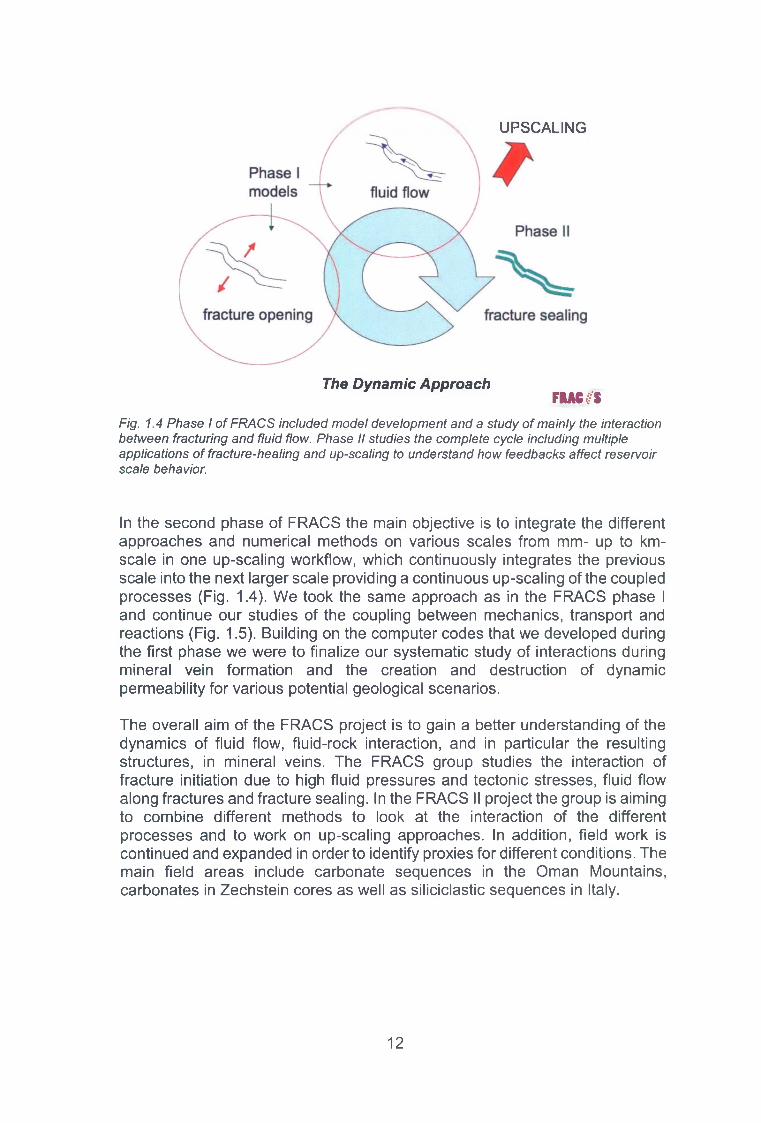
Fig. 1.4 Phase I of FRACS included model development and a study of mainly the interaction between fracturing and fluid flow. Phase II studies the complete cycle including multiple applications of fracture-healing and up-scaling to understand how feedbacks affect reservoir scale behavior.

In the second phase of FRACS the main objective is to integrate the different approaches and numerical methods on various scales from mm- up to km- scale in one up-scaling workflow, which continuously integrates the previous scale into the next larger scale providing a continuous up-scaling of the coupled processes (Fig. 1.4). We took the same approach as in the FRACS phase I and continue our studies of the coupling between mechanics, transport and reactions (Fig. 1.5). Building on the computer codes that we developed during the first phase we were to finalize our systematic study of interactions during mineral vein formation and the creation and destruction of dynamic permeability for various potential geological scenarios.

The overall aim of the FRACS project is to gain a better understanding of the dynamics of fluid flow, fluid-rock interaction, and in particular the resulting structures, in mineral veins. The FRACS group studies the interaction of fracture initiation due to high fluid pressures and tectonic stresses, fluid flow along fractures and fracture sealing. In the FRACS II project the group is aiming to combine different methods to look at the interaction of the different processes and to work on up-scaling approaches. In addition, field work is continued and expanded in order to identify proxies for different conditions. The main field areas include carbonate sequences in the Oman Mountains, carbonates in Zechstein cores as well as siliciclastic sequences in Italy.

12

Mechanics

KoehnHydrofractures

Stylolites/Fracture/Fault

Enzmann Fault sealing \

Transport BonsDynamic fluid flow

Reactions

BlumUpscaling

Urai, Hilgers Vein Growth

Vein Mechanics

Koehn/UraiCoordination

FRACASFig. 1.5 Integration of different approaches in FRACS II

In the FRACS II phase we are focusing on healing of fractures and the effects that the healing has on hydraulic properties, as well as the mechanical properties of rocks. Numerical simulations show that on the small scale the shape of partly healed fractures, due to kinetically or surface energy-driven crystal growth, can be quite different and this will have an effect on fluid flow. On the larger scale the healing models show that the properties of veins, mainly their breaking strength and orientation relative to a potentially rotating stress field have a strong effect on the mechanical properties of rocks. This in turn means that newly developing fractures will be strongly influenced by existing veins depending on the properties of these veins. In addition, we are working on a joint effort to include material transport in the larger scale simulations so that we can model realistic fracture healing. This includes the addition of advection-diffusion equations to the models. Research in the field areas in Oman, Italy, Zechstein and Benicassim in Spain continues in order to classify the vein systems and stylolites found in these areas, to compare them to the numerical models and develop proxies to predict rock and vein properties and to continue to develop upscaling approaches.

The FRACS II project has crucial and direct industry relevance. The dynamic opening and sealing of fractures in tight reservoirs and their consequences on the evolution of fracture permeability is a major topic for the oil and gas industry, and its importance will be significantly increased in the future. This project focuses on the basics of these processes from a modern and multidisciplinary approach using a combination of dynamic numerical modelling and field observations and classifications of these systems. Our work aims to contribute

13

to the better understanding of fracture permeability distribution, fracturing of tight reservoirs, sealing of fractures, classification and prediction of fluid fluxes and flow regimes along fracture/fault networks, as well as evolution of hydraulic fracture networks. These processes are of crucial importance for predicting fracturing-sealing mechanisms in producing reservoirs undergoing EOR (Enhanced Oil Recovery) or fracking operations, such as water, brine or steam injection. Additionally, our research results can potentially be used for the improvement of reservoir flow simulations by incorporating dynamic processes, such as fracturing and healing, or by improving the existing tools to predict and capture flow properties of fracture networks and other structures, like stylolites. These results may also be helpful to improve development and production plans of new reservoirs, and can also be taken into account for exploration purposes.

14

2 Overview of field laboratories (Oman Mountains, Ligurian Units, Zechstein)

The main field laboratories that the FRACS group worked on in the second phase are a continuation of the field work in the Oman mountains; a deformed siliciclastic sequence in the Internal Ligurian Units in northern Italy and cores from the Zechstein carbonates in northern Germany (Fig. 2.1). Each field area had a different setting or different rock units. Oman was dominated by carbonates with veins that mainly showed extension and strike slip. The Ligurian Units in Italy are siliciclastics that show compression in several directions. Both of these field areas have been exhumed and are studied at the Earth’s surface. In contrast the Zechstein units are cores from 4000m deep reservoir rocks. They have mainly seen compaction and burial with a small inversion in their later history followed by a quite period.

Oman t a p J Ligurian UnitsCarbonates Siliciclastic

Compression, extension compression

strike slip ZechsteinCarbonates, deep

Normal burial, some uplift

Fig. 2.1 Comparison of rocks and settings of different field areas.

The Mesozoic succession of the Jabal Akhdar dome in the Oman Mountains hosts complex networks of fractures and veins in carbonates, which are a clear example of dynamic fracture opening and sealing in a system with potentially high fluid over-pressures. The area underwent several tectonic events during the Late Cretaceous and Cenozoic, including the obduction of the Samail ophiolite and Hawasina nappes, followed by uplift and compression (leading to strike-slip deformation) due to the Arabia-Eurasia convergence. Some of the Early Cretaceous formations in neighbouring areas host large oil reserves. This means that studying the Jabal Akhdar area is not only important in order to unravel fracture and vein network development, but, despite differences in metamorphic and tectonic history, may also help to understand subseismic- scale fracture distributions in the oil fields of the NE Arabian plate. The Oman field area was discussed in detail in the first FRACS report. One major outcome of the Oman field work showed how important a microstructural analysis of veins and stylolites can be and how such an analysis can be used to derive large scale tectonic processes. Chapter 3 presents some new results on the interactions of veins in the southern flank of the Jabal Akhdar dome.

In contrast to the limestone dominated sedimentary sequence in Oman that represents obduction, extension and strike-slip deformation, the Internal Ligurian Units in Italy is a siliciclastic sequence that has been deformed mainly

15

by compression with a rotating stress field leading to polyphase folding as well as intense veining. The early sequence shows sets of thick bedding parallel veins as well as veins that change from bed-perpendicular to bed-parallel. These early veins indicate the presence of local high fluid over-pressure. Later veins are forming roughly bedding-perpendicular sets that quite often form conjugate arrays with steep intersections showing various compression directions that can be linked to large-scale tectonic events, a rotation of the compression from N-S to WSW-ENE during a switch in polarity of the subduction system and obduction of the units onto the Italian continent. Chapter 4 gives a detailed description of the geological setting, the large- and small-scale structures, cleavages, stylolites and veins. In addition, a fluid inclusion study of some of the veins is presented and the vein sets are used to derive the large scale plate tectonics.

The Zechstein cores that were studied during the FRACS II phase come from the Zechstein 2 unit, the Stassfurt carbonate or Ca2. The locality lies in the Lower Saxony Basin in Northwest Germany and is an important Lean Gas field. Since the unit is made up of carbonates it is comparable to Oman. However, the cores are taken from a depth of about 4000m. This is important because it means that we can compare fracture and vein patterns from outcrops with patterns that are found 4000m deep in an active reservoir. The results of the Zechstein studies are presented in detail in chapter 5, including a study of the sedimentary stylolites in the sequence as well as veins and dissolution features as well as some effects of dolomitization and calcitization reactions.

16

3 Vein systems in the Oman Mountains

In the second phase of the project we focused on providing a classification of the brittle deformation structures that can be found on the southern slope of the Jabal Akhdhar anticline in the Oman Mountains. Each structural phase is carefully constrained from collected field data by a multitude of well- documented relative age observations and orientation analysis in multiple outcrops. Particular attention is given to the specific lateral and stratigraphic variation of the different phases, which are -in addition to different interaction styles of subsequent vein generations- the main mechanisms to produce the high variability in vein patterns that can be found in the field. We identified several mechanisms that have the potential to produce this stratigraphic and spatial variability of structures and assessed their implications on the evolution of this highly dynamic high pressure cell. The structural field study was accompanied by an extensive study of the vein microstructures based on transmitted light microscopy, cathodoluminescence and scanning electron microscopy. We describe six main microstructural domains in veins from the field area of which two have not been described before. These are namely the columnar calcite texture and the blocky-neighbor texture. A hypothesis on the formation mechanism of the blocky neighbor texture was furthermore tested in a series of fracture experiments analyzed by scanning electron microscopy.

3.1 Structural phases

Seven phases of regionally developed deformation structures were identified that show stable and consistent age relationships (Fig. 3.1). The first phase includes previously unrecognized bedding-parallel extension veins and bitumen-filled veins. It is followed by two phases (II and III) of sub-vertical bedding-confined veins that document an anticlockwise rotation of the lowest principal stress. Phase IV comprises normal to oblique faults and associated veins under N-S directed extension. We propose top-to-east shear to be related to this event as a result of the east-dipping principal stress and weak bedding planes. The phase of extension is followed by two phases of horizontal compression in E-W (Phase V) and NE-SW direction (Phase VI) that reactivate preexisting fault planes in strike-slip mode, and lead to the development of strike-slip faults and conjugate en-echelon vein sets. The last phase of veining consists of E-W-striking micro-veins and joints in multiple directions as a result of doming and surface-near decompression. The micro-vein cement lacks deformation twins, unlike any other vein generation in the area. The open joints predominantly follow the anisotropy provided in the host rock by preexisting veins and micro-veins and may not directly reflect the recent stress field. We attribute the top-to-east bedding-parallel shearing to phase IV. We have evidence for two phases of top-to-south bedding-parallel shear, one before and one after normal faulting, their exact temporal relation to the other vein phases could, however, not be ultimately resolved. Top-to-NNE predates normal faulting in our interpretation but cannot be placed in temporal context with other structures. The multitude of different vein patterns that can be found in outcrop is the result of stratigraphic and spatial variability of the vein sets as well as different vein-vein interaction mechanisms. The bedding-confined veins of

17

phase II and III exhibit a high stratigraphic variability, while their occurrence and appearance within a bed is laterally very stable. Fault-related veins of phase IV, V and VI show a very high bedding-parallel variability in occurrence and appearance, while their stratigraphic variability is less significant. Spatial and stratigraphic variability can result from various factors.

Except for the top-to-east bedding-parallel shearing that we attribute to phase IV, we cannot provide any further findings to contribute to the current debate on the timing of bedding parallel shear events.

Fig. 3.1 Overview on the deformation phases distinguished in this study with a possible relation to geodynamic events and generations defined by other Authors. A representative stereonet for each phase is shown with a reconstruction of the orientation of principle stresses (where possible).

18

3.2 Vein and fault microstructure

From the analysis of over 80 thin sections covering all of the proposed structural phases we have identified six main microstructural textures in the veins of the Oman Mountains. These are namely the columnar calcite, blocky, stretched crystal, elongate blocky, blocky neighbour and laminated texture (Fig. 3.2).

Fig. 3.2 Schematic drawings of six main vein textures observed. (A) Elongate blocky syntaxial. (B) Block texture, sometimes with euhedral quartz. (C) Columnar texture. (D) Blocky neighbor texture. (E) Elongate-blocky stretched vein. (F) Laminated shear vein with host rock inclusions indicating shear sense.

Blocky texture is by far the most abundant in the field area and can be found in veins of most of the structural phases. In some veins the calcite is associated with euhedral quartz in the vein center that shields the surrounding calcite grains from twinning.

The formation of classic elongate blocky textures caused by growth competition into open voids is restricted to veins and/or faults of late tectonic phases (IV-b -V I ) .

The columnar texture was described for the first time as a vein cement and is interpreted to derive from a pseudomorphosis of either bladed calcite or acicular aragonite, which both are an indicator for cement growth in the shallow marine-phreatic zone [5], As the columnar texture is found in some Phase III- a, Phase lll-b (NW-SE-striking veins at high angle to bedding and their sinistral reactivation) and Phase lll-d veins (NW-SE boudinage related veins) it needs to be considered that those formed at very shallow depths.

19

The formation of a laminated texture is restricted to shear veins and faults. The development of the laminated texture seems to be controlled by the fracture mode. We propose that the texture will not form in veins caused by extension fractures (open mode I). Thus the final vein aperture does not reflect an opening perpendicular to the vein orientation. Indicators for the circulation of hot, hydrothermal fluids are found in Phase IV faults at a deep stratigraphic position. The occurrence of saddle dolomite and fluorite might indicate the ingress of hydrothermal fluids originated deeper in the stratigraphy.

With few exceptions, all vein calcites are plastically deformed as shown by mechanical twins, which are sometimes found being kinked or even folded. Late veins (Phases VI and VII) are all lacking mechanical twinning. As there is an ambiguity of mechanical twinning observed in Phase V, it is proposed that during or shortly after Phase V differential stresses and temperatures decreased below the critical values to form mechanical twins in calcite [6],

Table 3.1: Occurrence of microstructural domains in veins of the structural phases

MicrostructuralDomains

Tectonic Phases and Vein Generations0 I III IV V V I V IIBPVtt-S BPVtt-NNE lb l - e III a ill b Ill-C Ml-d r v a IV-b

colum nar texture o o 0 0 O 0 0 0 O oblocky texture • • 0 0 O O 0 0 • •el-blocky stretched-crystals • • 0 0 0 • 0 • •el-blocky grow lh com petition • • •blocky-neighbor texture 0 0 0 0 •lam inated texture • • • •blocky cc-qz texture •m echanical tw inning calcite • • • • 0 0 • • • • 0 o ofolded/kinked mech twins • • • 0 o 0vein-bound quartz • •Saddle dolom ite iz fluorite •F eO -cry stals 0 •fault gouge • • •# frcqentiy observed O never observed & portly observed N o te Phases I-a , I I and I l l-e were not characterised: el—block]/ Elongate-block]/, ce-gz alcitc-guart:. tt-S top-to-South: tt-.VJVF: top-to-Northnortheast

The ‘blocky-neighbour texture’ can be observed in microveins that show maximum opening widths of less than 50 pm. In these veins it is common that single crystals fill the entire vein, connecting both vein-host rock interfaces. Accordingly, each blocky single crystal has two neighbors in 2D Section. The single crystal’s lateral extends are up to ten times larger than the vein aperture. The texture is usually developed in fine-grained limestones (mudstones, sometimes with dispersed bioclasts). One of the most peculiar features of the blocky neighbour microstructure is the complete lack of any indicators for growth competition. This is at odds with the established models of fracture

2 0

sealing that do predict a strong growth competition in veins with a cement mineralogy compatible to the host rock.

In a scanning electron microscopy study on broken samples we were able to show that the vein-spanning crystals are epitaxial overgrowth of small micrite grains that were transgranularly fractured. We analysed fracture surface morphologies and fracture paths of artificially broken samples. While some samples were broken at room temperature, others have been heated to 200°C. Transgranular fractures are only observed at large carbonate particles in hot samples, while in cold samples also micrite grains are transgranularly fractured. The overall microstructure in both samples is dominated by intergranular fracture trajectories. Fracture surface morphologies of transgranularly fractured grains range from planar, smooth, cleavage controlled morphologies to complex, conchoidal morphologies.

Fig. 3.3 Blocky-neighbor texture in microveins. (A) Single crystals are entirely spanning the straight microvein. The grain boundaries have partly developed sharp edges. XPL (B/C) Evidence for epitaxial growth at a vein intersection, as a single, cross-shaped crystal continues laterally into two intersecting veins. (D) Microvein featuring similar single crystals with large lateral extents. The crystals are separated from the host rock by a thin rim of small calcite crystals that have grown into the vein. A carbonate particle’s crystal has grown epitaxially into the vein (yellow arrow). All thin sections parallel to bedding.

We interpret that epitaxial growth in microveins at burial conditions is restricted to transgranularly fractured grains. This effect leads to a limited number of growing calcite grains that eventually seal the entire microfracture. The diameters of vein filling crystals can exceed the average host rock crystal size by several orders of magnitudes even if the vein formed by a single crack-seal event.

21

Fig. 3.4 Detailed view of the fracture plane of a cold broken specimen of micritic rock. The path of a secondary fracture can be followed. The fracture path mostly follows the contacts of micritic grains (yellow arrows). The red arrows mark the begin and the end of one of the few trans-granular segments of the fracture path.

2 2

4 Veins in the Internal Ligurian Units in the Northern Apennines (Italy)

4.1 Introduction

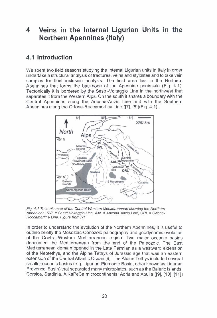
We spent two field seasons studying the Internal Ligurian units in Italy in order undertake a structural analysis of fractures, veins and stylolites and to take vein samples for fluid inclusion analysis. The field area lies in the Northern Apennines that forms the backbone of the Apennine peninsula (Fig. 4.1). Tectonically it is bordered by the Sestri-Voltaggio Line in the northwest that separates it from the Western Alps. On the south it shares a boundary with the Central Apennines along the Ancona-Anzio Line and with the Southern Apennines along the Ortona-Roccamorfina Line ([7], [8])(Fig. 4.1).

Fig. 4.1 Tectonic map of the Central-Western Mediterannean showing the Northern Apennines. SVL = Sestri-Voltaggio Line, AAL = Ancona-Anzio Line, ORL = Ortona- Roccamorfina Line. Figure from [7],

In order to understand the evolution of the Northern Apennines, it is useful to outline briefly the Mesozoic-Cenozoic paleography and geodynamic evolution of the Central-Western Mediterranean region. Two major oceanic basins dominated the Mediterranean from the end of the Paleozoic. The East Mediterranean domain opened in the Late Permian as a westward extension of the Neotethys, and the Alpine Tethys of Jurassic age that was an eastern extension of the Central Atlantic Ocean [9]. The Alpine Tethys included several smaller oceanic basins (e.g. Ligurian-Piemonte Basin, other known as Ligurian Provencal Basin) that separated many microplates, such as the Baleric Islands, Corsica, Sardinia, AIKaPeCa microcontinents, Adria and Apulia ([9], [10], [11])

2 3

The evolution of the Central Western Mediterranean was mainly controlled by the movements of the three major plates (Europe, Adria and Africa) and the existing microplates within the area. The convergence of Africa towards Europe resulted in a continuous E-SE-dipping subduction zone between Europe, Corsica-Sardinia and Adria in the Early-Late Cretaceous ([7], [12], [13]) (Fig. 4.2a). This led to a W-vergent accretionary prism which formed the Western Alps and the Alpine belt of Corsica. In the Early-Middle Eocene, however, the subduction halted due to the arrival of the Corsican distal continental margin, which caused an orogenic collapse, slab break-off and rapid exhumation of Corsica, where the induced erosion supplied debris for turbidite sequences ([7], [14], [15]). This polarity flip led to the initiation of a W-NW Apenninic subduction from the Late Eocene - Middle Oligocene (Fig. 4.2b). The change in subduction is widely recognized in early W-vergent deformation structures that are overprinted by E-vergent deformation [16], The Apennine accretion over the Adriatic margin took place during the Late Oligocene due to the counterclockwise rotation of Corsica-Sardinia [17] and the N-S Adria movement. The Apennine-related back-arc rifting and the rollback of the subduction hinge formed the present-day Ligurian Sea (Late Oligocene - Early Miocene) (Fig. 4.2c), whereas further south it caused the opening of the Tyrrhenian Sea in the Late Miocene ([7], [18]) (Fig. 4.2d). The identified late orogenic structures (faults and folds) indicate orogen-parallel, i.e. NW-SE, compression during the last ~8 million years ([19], [20]).

Fig. 4.2 Paleotectonics of the Central-Western Mediterranean from the Late Cretaceous showing the formation of Alps and Apennines. Figure modified after [7],

The Paleogene geodynamics of the Central-Western Mediterranean therefore can be characterized by a dynamic subduction zone between Europe/Corsica and Adria that (1) changed polarity from E to W and (2) migrated from a NE- SW to a NNW-SSE orientation. This subduction and accretion formed the Northern Apennines.

2 4

The Northern Apennines is usually grouped into five major units based on their tectonic and stratigraphic variations ([7], [21]):• Late, post-orogenic continental to shallow marine sediments (Late Eocene to Pliocene) lying uncomfortably on the Ligurian Units;

• Umbria-Romagna-Marche Units (Jurassic to Pleistocene) comprising carbonates and shallow-marine continental sediments;

• Tuscan Units (Late Carboniferous to Early Miocene) that includes carbonates, shales and siliciclastic turbidites;

• Sub-Ligurian Units (Cretaceous to Miocene) with sandstones, siliciclastics and marls;

• Ligurian Units (Late Jurassic to Miocene) comprising ophiolites and a wide range of sedimentary deposits.

The Umbria-Romagna-Marche Units together with the Tuscan Units form the lower nappes of the Apenninnic wedge and have an Adriatic plate origin, whereas the upper nappe (Ligurian Units) originated from the Alpine Tethys [22], The Ligurian Unit can be further divided into two groups: the Internal Ligurian Unit and the External Ligurian Unit. In the following, we will outline the stratigraphy of the Internal Ligurian Unit and place it in a tectonic framework.

The Internal Ligurian Unit (ILU) is considered to be one of the best preserved and most complete oceanic lithosphere of the Alpine Tethys [23], The lowermost part of this unit is the ophiolite sequence that represents the oceanic basement of the Liguria-Piemonte basin and therefore has a Jurassic age. The ophiolite is overlain by hemipelagic and pelagic sediments: radiolarian cherts, Calpionella Limestone (Early Cretaceous) and Palombini Shales (Early-Late Cretaceous) ([21], [23], [24]). The Palombini Shale grades into the overlying Val Lavagna Shale Unit. Three subunits have been identified within the Val Lavagna: the Manganiferous Shale, Verzi Marls and the Zoned Shales ([21], [25], [26]). The Val Lavagna, together with overlying Gottero Sandstone, are considered to be distal and proximal turbidite sequences ([25], [27]). The upper boundary of the Gottero marks an unconformity with the overlying sequence, the Bocco Shale, which represents debris flow and slide deposition [12].

Deposits within the ILU were confirmed to have Corsica plate origin ([12], [27]), which fits the geodynamic evolution of the area described earlier. The complete ILU sequence in general reflects nicely the evolution of the advancing accretionary wedge which was thrust over the Tuscan and Umbria-Romagna- Marche Units during the Late Oligocene - Middle Miocene ([14], [28]).

The deformation history of the ILU is quite complex, it involved the entire sequence, and only a few studies in the late ‘80s and early ‘90s attempted to define and characterize deformation events (Table 4.1).

Table 4.1 Deformation phases in the internal Ligurian Units according to different researchers as referenced.

2 5

D1 D2 D3 D4 D5

[26]

[21]

[29]

Tight, isoclinal, SW facing

folds with NW- plunging axes.

Axial planar foliation.

Open folds with vertical

axes and NW strike. No foliation.

Tight to open, asymmetrical folds with NE

vergence. Flat- lying

crenulationcleavage.

Open folds with steep

axialplane. No foliation.

Gentlefolds

[25]

[23]

[30]

[31]

Noncylindrical,

isoclinals folds facing NW/SE to NE/SW and

have axes orientation of

NE/SE,plunging NE to

NW. Axial planar

foliation.

Assymetrical folds with NE vergence and

axesorientation of SE to S, and

N/NWplunge. Axial

planar foliation.

Open folds with

subvertical axial planes

and axes oriented SE to

S. Fracture cleavage.

[4] Open folds with

subvertical axial

planes

The researchers agree that the first deformation phase corresponds to the east-dipping subduction zone and the underplating of the oceanic lithosphere ([21], [23], [25], [30], [32]). Its timing is therefore probably latest Early Paleocene ([29], [33]). D2 has been associated with extension [33], exhumation [25] and thrusting [23], The subsequent deformation events are even more debatable but it is a currently accepted view that all the deformation took place before the thrusting (i.e. stacking of nappes on the Adria continental margin), and therefore was completed by the Early Oligocene [29].

4.2 Methods

Field mapping was carried out during two weeks in September 2013 and 2014. The studied area was stretching between Riva Trigoso and Framura, Italy, along the coast of the Ligurian Sea (Fig. 4.3a). This location was chosen due to the following reasons:• thick shale sequences can be found here, which lithology is in the focus of the FRACS project;• the shale has a high density of veins, which makes it possible to study a variety of vein types with regard to their formation;• high fluid pressures were presumed to play an important role in some of the vein formation.

The outcrops in the studied area are one of the best representations of the entire ILU sequence (Fig. 4.3). The bottom of the sequence (the ophiolite) is juxtaposed to the Palombini Shale at Framura. As moving northwest, this first grades into the Val Lavagna, then the thick Gottero Sandstone unit, which dominates the area around Deiva Marina. Moneglia shows an alternating

2 6

Palombini and Val Lavagna sequence, which is then followed by the Gottero stretching up until Riva. In Riva the Bocco Shale representing the top of the ILU also outcrops in a thin zone. The Val Lavagna then comes back and characterizes the northwestern part of the studied area. The coastline is clearly shaped by the geology. Since shale is weaker than the sandstone, areas where the Val Lavagna and Palombini crop out were favored by erosion processes, creating bays where the towns (Riva Trigoso, Moneglia and Framura) are located. Hard sandstones resisting the erosion separate the bays.

a

Monaglt

1283G o t la r o S a n d s to n «

p ' " j Val L a v a g n a S h a l«

P a lo m b ln l S h a l« and C a lp io n a ila L im e s to n e

B a s a lts , o p h to lttk brsc e ia a . c h a rts

I G a b b ro ic c o m p ta x .I m a n tis uttra m a f ic «

T h ru s ts a n d m a m faults

.J I 1 Antola Unit

f-!*M ML Gottero UnitBracco / Val Graveglia

------; Unit___I ColH / Tavarone Unit

External Ligurian Unit

S V \ Tuscan Unit

b

Oi*gocene

Early

IN T E R N A L L IG U R IA N U N IT S

EedyLate“

M id d a P1 L 250 Early ■ 0 m

3 Goflero Sana »lone

Vai Lavagna Shale

Patom btfli Sna*e

C a ip « n e i| j L im estone

C herts^ Oceanic Basem ent

(Opfwktesl

Fig. 4.3 Location and geological map of the studied area (a), along with the stratigraphic column of the Internal Ligurian Unit (b). Map after [31], stratigraphic column after [28],

While the focus was on the outcrops directly along the coast (purely because of their easy accessibility and good exposure quality), outcrops further up in the hills along different hiking trails were also examined. As the goal was to examine the veining and place it in the deformation framework of the ILU, both mapping of the structures (e.g. observing bedding-cleavage relationships, measuring orientations) and sampling were necessary. The available geological map and cross-sections, along with the literature were only considered as guidelines. Although the stratigraphical description of the ILU had helped to identify the different rock units on the field, the observed structures were not influenced by the literature.

4.3 Field observations and measurements

Overall the bedding in the field area displays a wide range of orientations (Fig. 4.4, Fig. 4.5a). In Riva Trigoso while the dip of the beds varies from shallow to steep, their dip direction is relatively constant; it is characterized by two distinct orientations: a few dipping towards the ESE-SE, whereas the majority dips in westerly directions (NW-W-SW) (Fig. 4.5a). Bedding data from Framura fall under the same westerly distribution. In Moneglia, however, bedding measurements are even more dispersing than elsewhere. Here the poles to the bedding occupy three quarters of the stereonet, which indicates that

2 7

another dip direction, N and NE also appears (Fig. 4.5a). Many layers dip towards the westerly directions similarly to Riva and Framura, but the additional inclinations towards the N and NE result in complex structures in the field.

Deiva Marina

Bocco Shale

Gottero Sandstone

Val Lavagna Shale

Palombini Shale

Ophiolite

Faults

Moneglia

1 km

Fig. 4.4 Geological map and the main structures of the studied area. Map compiled based on our and Giancarlo Molli’s field work (2013 and 2014).

Cleavages were often difficult to distinguish from the bedding due to the low angles between them. The shallow to steep cleavages were generally dipping towards westerly directions (NW-W-SW), similarly to the bedding (Fig. 4.5c). Observing the bedding-cleavage relationship, where it was possible, helped to identify whether the sequence was normal or overturned. The area was generally characterized by tight, alternating normal and overturned sequences.

2 8

Fold axesPoles to beddings

b)

c ) Cleavagesblack = Riva Trigoso red = Moneglia green = Framura blue = Deiva Marina

Fig. 4.5 The poles to beddings (a), the fold axes (b) and the cleavage planes with their poles are presented for each part of the field area. Two axes of the second crenulation cleavage are also shown on b) (labeled as diamonds).

Folds were more visible when the sequence included stiffer (e.g. more sandy) layers. The shales instead of folding often seemed to accommodate the deformation by filling the space in between the limbs of the folded stiffer layers. In addition to this, shales further away from the stiffer layers showed either very gentle folds or barely any. The most commonly observed folds were isoclinal folds that had relatively shallow axial planes (Fig. 4.6a). In addition to this, assymetrical folds with highly non-cylindrical nature (Fig. 4.6b), and locally open folds (especially in Framura) with sub-vertical axial planes were also found.

2 9

Fig. 4.6 Isoclinal (a) and asymmetrical (b) folds with shallow plunging fold axes in Framura.

The measured fold axes in Riva Trigoso and Framura again display similarities. Two general fold axes directions were identified: one plunging shallow towards the NW, whereas the other is perpendicular to this direction, plunging shallow towards the SW (and a couple towards the NE) (Fig. 4.5b). Fold axes in Moneglia are not only steeper than measured elsewhere, but also plunge more towards the W. Although it was rarely possible to establish an age relationship between the two folding directions, a few outcrops showed that the NE-SW- plunging fold axes were folded by the NW-plunging ones. Moneglia also contained some vertical fold axis, which may be intersections between the two shallow ones.

In Riva one crenulation cleavage was measured where the crenulation axis was plunging shallowly towards NW, whereas in Moneglia it was plunging towards the WNW (Fig. 4.7b). A few more (five) sets of crenulation were observed in Moneglia (Fig. 4.7). The first cleavage (S1) was striking NE-ENE - SW-WSW with mainly medium dips. The second cleavage (S2) was generally steep and had an orientation of N-NNW - S-SSE. Only one S2 had similar orientation and dip to the S1.

3 0

Crenulation cleavage sets

colors indicate separate sets

solid line = S1 dashed line = S2

Fig. 4.7 Crenulation cleavage sets indicating first a NNW-SSE compression followed by a more E-W to ENE-WSW compression.

As mentioned in chapter 5, stylolites are great indicators of tectonic stresses. They develop as a result of compressive stresses forming a dissolution surface along which insoluble materials accumulate. Their planes are perpendicular, whereas their teeth are parallel to the largest compressive stress. A stylolite forming at high angles to the bedding is termed tectonic stylolite. In Framura within the Palombini Shale eight tectonic stylolites were identified. Two main sets, perpendicular to each other, showed a N-NNE, whereas the other an ENE compression direction (Fig. 4.8).

Tectonic stylolites

Fig. 4.8 Stereonet illustrating the orientations (planes and poles) of tectonic stylolites found in Framura showing first a N-S followed by an ENE-WSW compression.

31

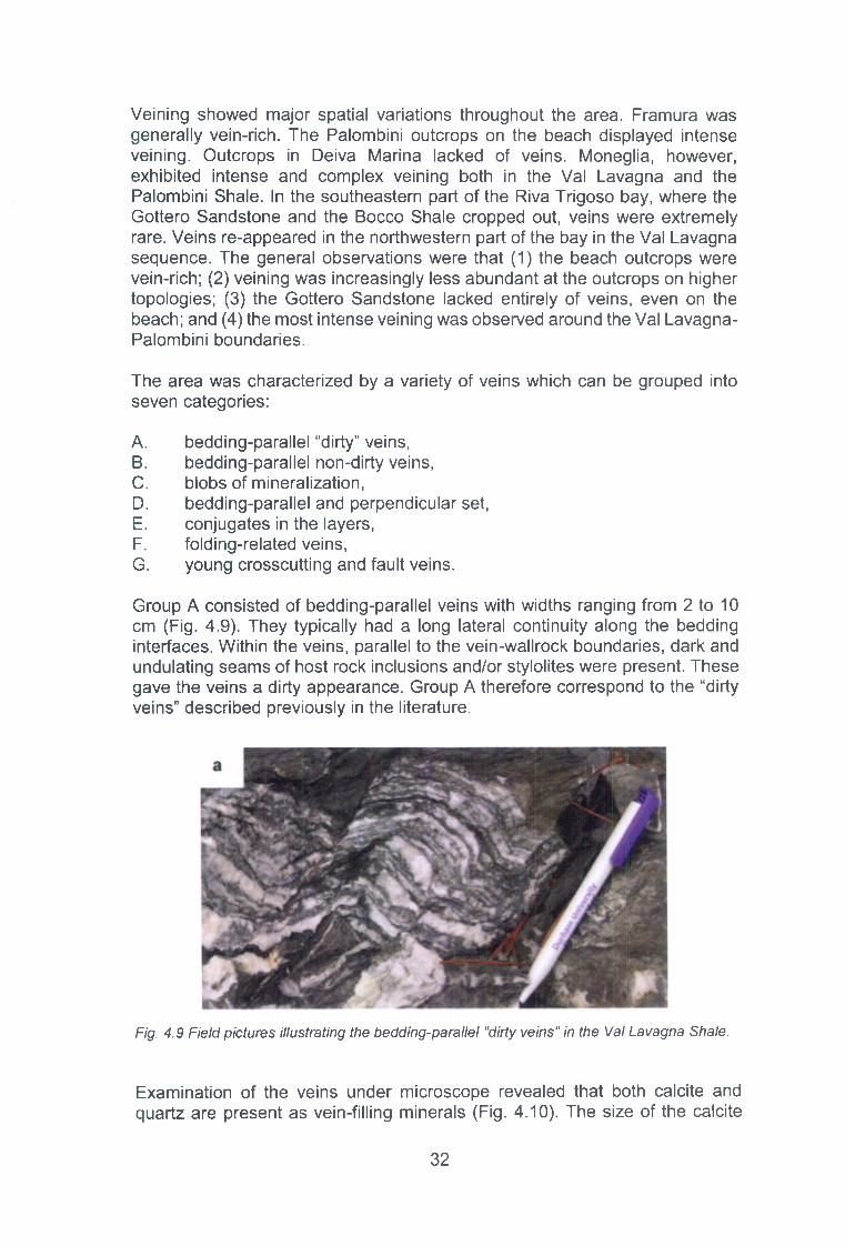
Veining showed major spatial variations throughout the area. Framura was generally vein-rich. The Palombini outcrops on the beach displayed intense veining. Outcrops in Deiva Marina lacked of veins. Moneglia, however, exhibited intense and complex veining both in the Val Lavagna and the Palombini Shale. In the southeastern part of the Riva Trigoso bay, where the Gottero Sandstone and the Bocco Shale cropped out, veins were extremely rare. Veins re-appeared in the northwestern part of the bay in the Val Lavagna sequence. The general observations were that (1) the beach outcrops were vein-rich; (2) veining was increasingly less abundant at the outcrops on higher topologies; (3) the Gottero Sandstone lacked entirely of veins, even on the beach; and (4) the most intense veining was observed around the Val Lavagna- Palombini boundaries.

The area was characterized by a variety of veins which can be grouped into seven categories:

A. bedding-parallel “dirty” veins,B. bedding-parallel non-dirty veins,C. blobs of mineralization,D. bedding-parallel and perpendicular set,E. conjugates in the layers,F. folding-related veins,G. young crosscutting and fault veins.

Group A consisted of bedding-parallel veins with widths ranging from 2 to 10 cm (Fig. 4.9). They typically had a long lateral continuity along the bedding interfaces. Within the veins, parallel to the vein-wallrock boundaries, dark and undulating seams of host rock inclusions and/or stylolites were present. These gave the veins a dirty appearance. Group A therefore correspond to the “dirty veins” described previously in the literature.

Fig. 4.9 Field pictures illustrating the bedding-parallel "dirty veins" in the Val Lavagna Shale.

Examination of the veins under microscope revealed that both calcite and quartz are present as vein-filling minerals (Fig. 4.10). The size of the calcite

3 2

crystals in the veins varies between a few hundred microns to a few millimeters. They generally have anhedral crystal shapes with a few subhedral grains too. The crystals are heavily twinned and the three cleavage directions are usually very distinct (Fig. 4.10). These, along with the apparent impurities, often make the crystals cloudy. The calcites host a great amount of fluid inclusions (and trails) which are frequently not very clear due to the heavily deformed and cloudy crystal characteristics.

Fig. 4.10 Thin sections under cross polarized light showing the typical microstructure of the dirty veins (a) and the heavily deformed calcite crystals (b).

Many bedding-parallel veins did not have a dirty appearance, i.e. they lacked of vein-parallel host rock inclusions and stylolites (Group B) (Fig. 4.11). These also had long lateral continuities and widths of up to 3 cm. Their microstructures show completely different characteristics compared to the dirty veins, since (1) no dissolution seams are present, (2) the majority of crystals are blocky or elongated, (3) the crystals touch each other and (4) the calcite is subordinate to the quartz. The quartz grains can reach three millimeters in lengths and their longer boundaries are parallel to the veins (and thus bedding). Subgrains as well as recrystallized smaller quartz grains are frequent between the larger quartz crystals (Fig. 4.12a).

3 3

Fig. 4.11 F ield image of a bed-parallel, non dirty vein in a fold hinge in the Val Lavagna Shale.

Fig. 4.12 Thin sections under cross polarized light showing the bed-parallel, non-dirty veins, (a) Long quartz grains with recrystallized quartz. The light band perpendicular to the grain boundaries indicates a younger crosscutting vein, (b) Deformed calcites and groups of twinned plagioclase (left of the image).

Outcrop walls showing bedding-perpendicular section of layers often displayed heavy mineralization on certain layer surfaces (i.e. on the surface perpendicular to the bed). These blobs of mineralization (Group C) had

3 4

irregular appearances and surfaces, and were not continuous along the layers. As a result they did not appear as classical veins with well-defined boundaries but rather as separate mineralized bodies that were only confined by the layers. Their short lateral continuity in the field and their nature did not make it possible to relate them to veins observed elsewhere.

Certain shale layers were bounded on both sides by bedding-parallel veins which were connected by perpendicular sets of veins (Group D) (Fig. 4.13, Fig. 4.14). This type of veining could be best observed in Moneglia in the Val Lavagna Shale. Both the parallel and the perpendicular veins had maximum widths of up to a few millimeters. The spacing between the parallel veins varied between a few hundred microns and few millimeters. The thickness of the layers containing these sets of veins had an effect on the spacing variations. Thinner layers contained more closely spaced veins than the thicker ones. This relationship between the layer thickness and the spacing, however, did not seem to be linear as opposed to what has been reported in the literature.

Fig. 4.13 Field examples of the bedding-parallel and perpendicular vein set in the Val Lavagna Shale, Moneglia. Width of view 15cm.

3 5

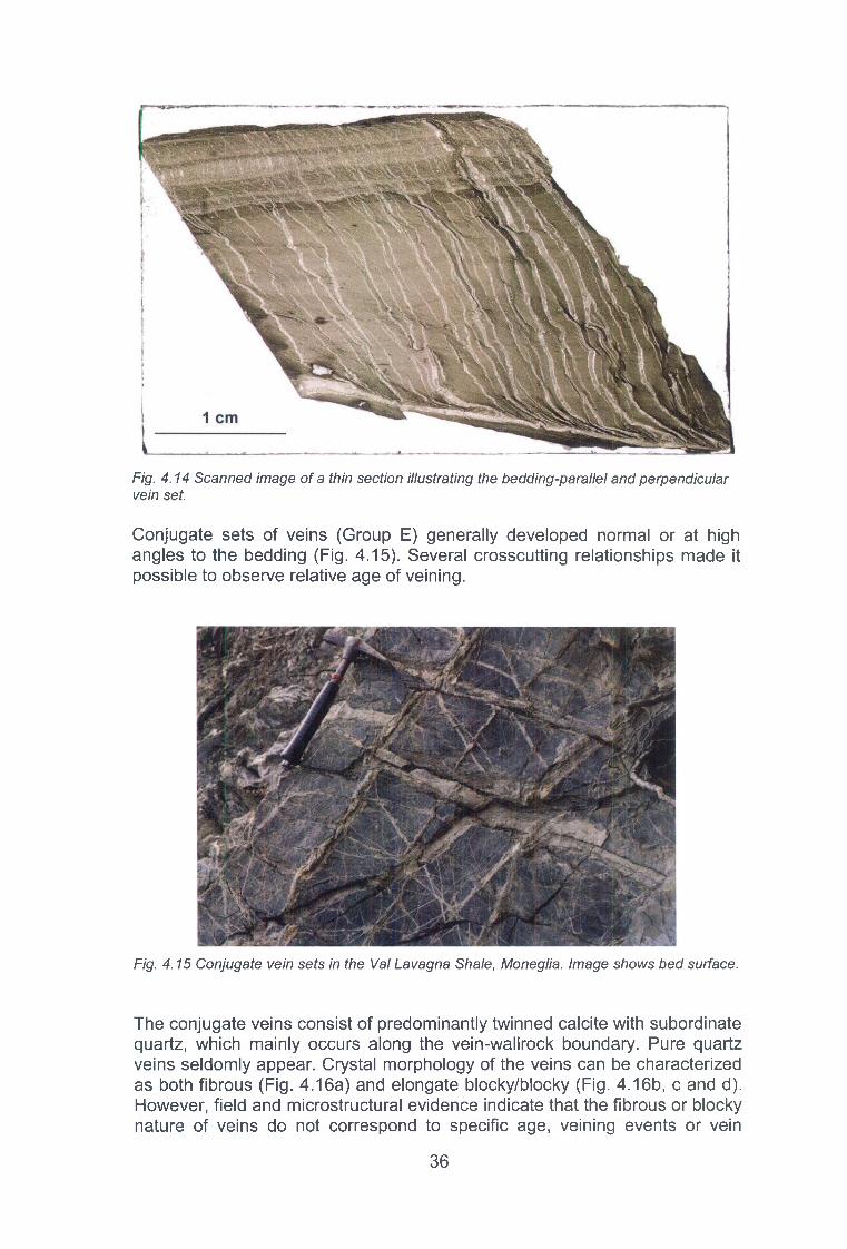
Fig. 4.14 Scanned image of a thin section illustrating the bedding-parallel and perpendicular vein set.

Conjugate sets of veins (Group E) generally developed normal or at high angles to the bedding (Fig. 4.15). Several crosscutting relationships made it possible to observe relative age of veining.

Fig. 4.15 Conjugate vein sets in the Val Lavagna Shale, Moneglia. Image shows bed surface.

The conjugate veins consist of predominantly twinned calcite with subordinate quartz, which mainly occurs along the vein-wallrock boundary. Pure quartz veins seldomly appear. Crystal morphology of the veins can be characterized as both fibrous (Fig. 4.16a) and elongate blocky/blocky (Fig. 4.16b, c and d). Flowever, field and microstructural evidence indicate that the fibrous or blocky nature of veins do not correspond to specific age, veining events or vein

3 6

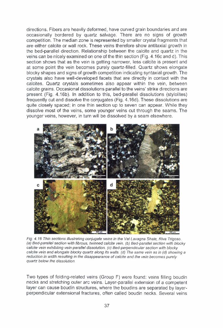
directions. Fibers are heavily deformed, have curved grain boundaries and are occasionally bordered by quartz salvage. There are no signs of growth competition. The median zone is represented by smaller crystal fragments that are either calcite or wall rock. These veins therefore show antitaxial growth in the bed-parallel direction. Relationship between the calcite and quartz in the veins can be nicely examined on one of the thin section (Fig. 4.16c and d). This section shows that as the vein is getting narrower, less calcite is present and at some point the vein becomes purely quartz-filled. Quartz shows elongate blocky shapes and signs of growth competition indicating syntaxial growth. The crystals also have well-developed facets that are directly in contact with the calcites. Quartz crystals sometimes also appear within the vein, between calcite grains. Occasional dissolutions parallel to the veins’ strike directions are present (Fig. 4.16b). In addition to this, bed-parallel dissolutions (stylolites) frequently cut and dissolve the conjugates (Fig. 4.16d). These dissolutions are quite closely spaced; in one thin section up to seven can appear. While they dissolve most of the veins, some younger veins cut through the seams. The younger veins, however, in turn will be dissolved by a seam elsewhere.

Fig. 4.16 Thin sections illustrating conjugate veins in the Val Lavagna Shale, Riva Trigoso.(a) Bed-parallel section with fibrous, twinned calcite vein, (b) Bed-parallel section with blocky calcite vein exhibiting vein-parallel dissolution, (c) Bed-perpendicular section with blocky calcite vein and elongate blocky quartz along its walls, (d) The same vein as in (d) showing a reduction in width resulting in the disappearance of calcite and the vein becomes purely quartz below the dissolution.

Two types of folding-related veins (Group F) were found: veins filling boudin necks and stretching outer arc veins. Layer-parallel extension of a competent layer can cause boudin structures, where the boudins are separated by layer- perpendicular extensional fractures, often called boudin necks. Several veins

3 7

filling these boudin necks were observed in the field (Fig. 4.17a). These developed in stiff layers bounded by less competent and highly cleaved layers. Stiffer layers that were folded also often showed veins in their outer arcs (Fig. 4.17b). The outer arc of the folded layer undergoes stretching that creates extensional fractures. These fractures were observed in the field as veins.

Fig. 4.17 Veins formed in boudin necks (a) and in tensional fractures on the outer arc of the folded layer (b).

Veins that crosscut several layers were quite abundant (Group G) (Fig. 4.18a). They had long lateral (up to 10 m) and vertical (few meters) continuity, and were not affected by folding. Their orientation was consistent over the field area dipping towards the W-NW. In addition to this, the identified faults cutting through the sequences occasionally hosted veins too (Fig. 4.18b).

4.4 Vein orientation prior to folding

In order to obtain the pre-folding vein orientations, two main types of veins were used: (1) conjugate sets (Group E) and (2) veins that did not form conjugates but were clearly folded by the same folding event. These vein orientations were rotated and unfolded along the fold axes and the bedding measurements. As the veins in all cases pre-dated the NW-plunging folding event (or at least were simultaneous with it), this folding direction was used to rotate and unfold the veins. The exact fold axis orientation that was used in the calculations was either directly measured on the bed that contained the veins or was a general orientation measured in the vicinity of the outcrop. In the following I present the pre-folding vein orientations for each location, Riva Trigoso, Moneglia and Framura.

3 8

Fig. 4.18 Young crosscutting vein (a) and fault vein (b) in the field.

In Riva Trigoso 33 vein orientations, measured in both normal and overturned layers, were rotated and unfolded on the stereonet. Generally, the complicated cross-cutting relationship prevented to establish age relationships between the veins. Most of the veins became steeper after the rotation and unfolding. The orientations are plotted on separate stereonets shown on Fig. 4.19. Fig. 4.19a: Four medium-dipping veins striking SW-WSW and one striking N were measured in an overturned bed. Crosscutting relationship unfortunately was not possible to recognize. By rotating the veins we obtain a general strike direction from NNW to N and E-W, respectively. Fig. 4.19b: Rotation and unfolding two veins striking NNE and another striking E yielded similar strike directions but a change in dip magnitudes. While the NNE-striking set became much steeper, almost sub-vertical, the ESE became slightly shallower. Fig. 4.19c: Two veins perpendicular to each other were measured in a normal bed. The older vein, striking SW, contained a vein-parallel stylolite, whereas the younger vein with NE strike was folded. The pre-folding orientations reveal similar strike directions but a dip change; the old vein became shallower, while the young folded one steeper.

3 9

a b

9 h

Fig. 4.19 Stereonets presenting pre-folding vein orientations (planes and poles) obtained in Riva Trigoso. Each stereonet corresponds to different outcrops in the area. Red indicates a younger vein relative to the other vein (or veins) measured on the same outcrop. The older vein on (c) (solid black line) is also accompanied by a vein-parallel stylolite.

Fig. 4.19d: Four veins oriented between NNE and E in an overturned layer displayed unknown age relationship. The rotation yielded new orientations between NW and NE. Fig. 4.19e: Two sets of conjugate veins in a normal layer showed N-NNE and W-WNW strike directions. Age relationship between the two sets is unknown. The rotation conserved the strike directions and just slightly changed the dips magnitudes. Fig. 4.19f: Veins with a variety of strike directions in an overturned bed exhibited a complex crosscutting relationship. The rotated veins can be characterized by NE, N, NW and WNW strike directions. Fig. 4.19g: Four veins with strike directions ranging from N to ENE displayed complicated crosscutting relationship. The rotation resulted in

4 0

steeper veins and orientations between NNW and NE. Fig. 4.19h: Two conjugate vein sets perpendicular to each other showed clear crosscutting relationship. The older set was striking W-NW, whereas the younger NNE-NE. The rotation steepened the veins and shifted the strikes slightly so that the older set became NW and the younger set became NE-oriented. Integrating the pre-folding vein orientations on one stereonet thus reveals two general vein directions: a NNE-NE and a NW trend (Fig. 4.20).

Fig. 4.20 Summary stereonet including the poles to the pre-folding vein orientations in Riva Trigoso.

In Moneglia 37 veins were measured mainly in overturned beds. The prefolding vein orientations are plotted on separate stereonets illustrated on Fig. 4.21. Fig. 4.21a: Two conjugate vein sets with unknown age relationship were measured. One set showed an initial N-NNE orientation, whereas the other set consisting of three veins were striking NE. The rotation of the data resulted in the former set to strike NE and SW, and the latter set to be oriented between NNE and NE. Fig. 4.21b: Rotation of a conjugate set striking S and SSW yielded opposite-dipping steep veins striking SSE and NNW. Fig. 4.21c: The rotation of a conjugate set with one vein initially striking N-S and another NE resulted in a NW and SW-striking vein, respectively. Fig. 4.21 d: Three veins that formed a conjugate set were striking NNW and NE. The rotation caused the former to be oriented N-S and the latter to be NW. Fig. 4.21 e: Vein orientations in the only normal bed where conjugates were measured displayed NNE and ENE strikes. The rotation did not change the former’s orientation, whereas the latter shifted slightly to the NE. The veins became significantly steeper. Fig. 4.21 f: Rotation of a conjugate set striking SSW resulted in a steep, NW-striking vein set. Another conjugate including three veins striking NE, NNE and SSW yielded new orientations of ENE, SW and SE, respectively. Fig. 4.21 g: While the measured veins were consistent in orientations (N-NNE), the rotation caused them to span out more. The veins became steep striking NE, NNW, WSW and WNW. Fig. 4.21 h: The strike of the conjugate veins changed from N-S to E and SE. Fig. 4.21 i: Four conjugate vein sets with strike directions NW-NNW and NE became much steeper due to the rotation. The vein orientations changed only slightly to N-S, whereas the NE strike remained. On

41

an overturned bed two veins and a stylolite were found, where one of the veins were dissolved by the stylolite itself. By rotating the orientation of these structures, the veins obtained a NE-ENE, whereas the stylolite a SE orientation (Fig. 4.22).

Fig. 4.21 Stereonets presenting the pre-folding vein orientations in Moneglia. Each stereonet corresponds to different outcrops in the area, grey colors and dashed planes correspond to separate conjugate sets.

4 2

Fig. 4.22 Pre-folding orientations (planes and poles) of a vein (black solid line), a dissolved vein (black dashed line), a stylolite (red) and its teeth (hollow red circle).

The pre-folding vein orientations in Moneglia are thus characterized by steep to sub-vertical veins with the majority striking around NW-SE and NE-SW (Fig. 4.23).

Fig. 4.23 Summary stereonet including the pre-folding vein orientations (poles) in Moneglia.

In Framura, 30 veins were measured mostly in normal sequences in the Palombini Shale, and then rotated and unfolded on the stereonet. The prefolding vein orientations are plotted on separate stereonets (Fig. 4.24).

4 3

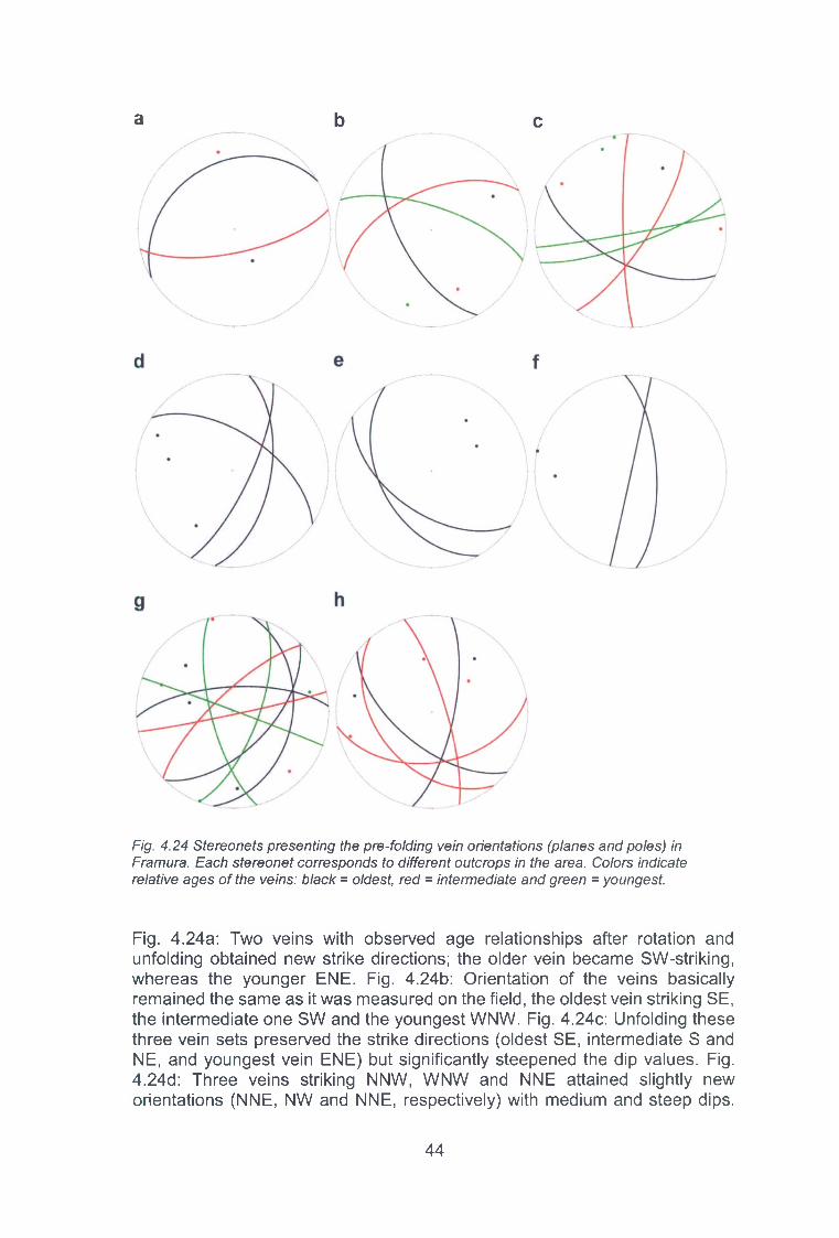
a b c

Fig. 4.24 Stereonets presenting the pre-folding vein orientations (planes and poles) in Framura. Each stereonet corresponds to different outcrops in the area. Colors indicate relative ages of the veins: black = oldest, red = intermediate and green = youngest.

Fig. 4.24a: Two veins with observed age relationships after rotation and unfolding obtained new strike directions; the older vein became SW-striking, whereas the younger ENE. Fig. 4.24b: Orientation of the veins basically remained the same as it was measured on the field, the oldest vein striking SE, the intermediate one SW and the youngest WNW. Fig. 4.24c: Unfolding these three vein sets preserved the strike directions (oldest SE, intermediate S and NE, and youngest vein ENE) but significantly steepened the dip values. Fig. 4.24d: Three veins striking NNW, WNW and NNE attained slightly new orientations (NNE, NW and NNE, respectively) with medium and steep dips.

4 4

Crosscutting relationship could not be established. Fig. 4.24e: Orientation of a conjugate vein set (striking SE and SSE with medium dips) barely changed after the unfolding. Fig. 4.24f: Orientation of the only conjugate vein set (striking W and SW) measured in an overturned bed shifted almost 90° due to the unfolding. They obtained new strike directions NNE and N, respectively. Fig. 4.24g: Strike directions of the three sets of veins with recorded crosscutting relationship remained the same as measured, only the dip magnitudes changed due to unfolding. The oldest veins strike NNE, NE and W; the intermediate veins SW and WSW; whereas the youngest set SSE, NNE and WNW. Fig. 4.24h: Unfolding also retained the strike directions of these veins, where the youngest set was striking NNE and NW, whereas the older set was striking E, SW and NNW. Three sets of conjugate veins presented a clear age relationship, where the oldest set was oriented N-S, the intermediate set NW and the youngest set ENE (Fig. 4.25). These orientations were not rotated and unfolded.

Fig. 4.25 Three sets of conjugate veins plotted on a stereonet illustrate relative age relationships in Framura. Black = oldest, red = intermediate and green = youngest vein set.

Plotting all the pre-folding vein orientations on one stereonet reveals three major vein directions: NNE-SSW, NW-SE and ENE-WNW (Fig. 4.26).

Fig. 4.26 Summary stereonet presenting all the pre-folding vein orientations (poles) in Framura.

4 5

4.5 Fluid inclusion microthermometry

Four different veins in the Val Lavagna Shale were collected for fluid inclusion microthermometry: non-dirty bed-parallel veins (one calcite and one quartz), blobs of mineralization (consisting of quartz and calcite) and one vein perpendicular to this one. Examination of the wafers showed that (1) quartz crystals hosted significant amount of inclusions, often impeding the view for analysis, (2) occasional calcites were quite deformed and usually not inclusion- rich, (3) both the quartz and calcite crystals were not as clear as expected, so the measurable inclusions were limited, (4) the maximum inclusion size was 4x2 pm, but the average was generally 2x2 pm or less in size and (4) the measured inclusions consisted two phases, liquid and vapor with vapor occupying 10-15% of the inclusions (Fig. 4.27). As the inclusions were extremely small and the crystals not very clear, only two (one from the nondirty veins and another from the blobs) ice melting temperatures were obtained, -4°C and -8°C (corresponding to 6.5 wt% and 13.1 wt% NaCI content). This amount of measurement, however, is certainly not representative and therefore should be used with caution. In addition to this, defining the inclusions’ origin (primary / secondary / pseudosecondary) was problematic due to the crystals’ shape and lack of zoning. No cracks or healed fractures, along which secondary trails would generally occur, were observed within the veins. Neither were transgranular trails (inclusion trails across several grains), which would also indicate secondary origin. The inclusions mainly occurred in random distribution or in groups within single crystals and thus exhibited primary characteristics. Flowever, as uncertainty is quite large, we will refer to them as inclusions with unknown origin. These observations, i.e. crystal and inclusion characteristics, inclusion size and problematic origin, stand for all the wafers.

Fig. 4.27 Microscope images of the largest inclusions found in quartz crystals developed in the blob of mineralization (a) and in the non-dirty bed-parallel vein.

The bed-parallel non-dirty veins were the only ones where fluid inclusions in calcite were also measured. The obtained homogenization temperatures (TH) are illustrated on Fig. 4.28. Inclusions in quartz crystals display relatively constant temperatures: the peak T h is in the range of 160-170°C, with a smaller but distinct peak between 150°C and 160°C. Only a few measurements show smaller/larger values. The calcite inclusions, on the other hand, homogenized

4 6

at slightly higher temperatures. Most of them had T h around 200°C with a few homogenizing at 220°C, 243°C and 273°C. Homogenization temperatures of the fluid inclusions in the blobs and a blob-perpendicular vein revealed two distinct ranges: one centered around 160°C, whereas the other around 220°C (Fig. 4.29).

25

20

S' 15C633a-03•t 10

il ca leite H quartz

. 1 I I I130 150 170 190 210 230 250 270 TH(°C)

Fig. 4.28 Homogenization temperatures for non-dirty, bed-parallel veins of quartz and calcite.

25■ Blob

Fig. 4.29 Homogenization temperatures of fluid inclusions within the (quartz) blobs of mineralization and in a blob-perpendicular vein.

Compiling all the data on one chart the dominance of two T h ranges, 150-160°C and 160-170°C, is apparent (Fig. 4.30). Lower and higher temperatures are subordinate.

4 7

45

40

35

30>>g 25OlS' 20

15

105

o t130

DlI I IOd DDl.0 □150 170 190 210 230 250 270 THrC )

Fig. 4.30 Summary of the homogenization temperatures measured in the different samples.

4.6 Discussion

Outcrop patterns indicate that a NW-SE compression (forming the NE-SW- plunging folds) pre-dated a NE-SW compression which developed the NW-SE folds. Most of the older cleavages represent compression in the northwesterly direction, whereas the second cleavages (S2) mainly show an E-W to NE-SW compression. Tectonic stylolites further revealed an easterly compression. Considering these two compression directions, NW-SE and NE-SW, as well as their presumed relative timing, we can look at the tectonic model (Fig. 4.31). According to this model these stress orientations can be clearly traced from the Late Mesosoic up to the Neogene period. A NW-SE-directed compression can be attributed to the E-SE-dipping subduction zone between Corsica and Adria during the Late Cretaceous (Fig. 4.31a). This subduction zone, which experienced a polarity flip during the Eocene, migrated anticlockwise towards the NW. This migration caused the rotation of the maximum horizontal stress from E-W to NE-SW, the latter characterizing the main accretion phase (Fig. 4.31b to d). The geodynamic evolution highlights a continuous subduction and accretion, which caused deformation of the Internal Ligurian Unit (among others). This continuity is one of the reasons why identifying and separating the different deformation phases in this area are difficult, giving rise to a variety of tectonic models and debates between different researchers. In the current study, however, we are considering two deformation phases: the first (D1) related to a NW-SE, and the second related to an E-W to NE-SW compression (D2). Deformation occurring after the polarity flip is considered to be D2.

4 8

Europe

Africa

Fig. 4.32 outlines the orientations of different deformation structures that could form as a result of a NW-SE and an E-W to NE-SW compression. A N-S compression has been added to the D2. Tectonic stylolites showed evidence for this compression direction. Occurrence of a late (post-orogenic) N-S and orogen-parallel compression has also been reported in the literature ([7], [19], [20]).

Fig. 4.31 Tectonic map presenting the evolution of the Northern Apennines with the indication of the field area (red dot) and the main stress directions (green arrows). Figure modified after Molli (2008).

LateCretaceous(c. 70 Ma)

Late Eocene(35-33 Ma)

Late Oligocene Middle Miocene(30-25 Ma) (c. 10 Ma)

4 9

Fig. 4.32 Expected orientations of different structures (folds, normal and strike-slip faults, tensional fractures/veins and conjugate fractures/veins) formed during the defined D1 and D2 phases.

Pre-D2 (conjugate) vein orientations and their age relations are also in accordance with the outlined major horizontal stress directions. Stylolites related to veins indicate NE-SW compression (Fig. 4.32), which would mark the major accretion phase. Only one conjugate set contradicts the relative timing of stresses. The large- and meso-scale deformation structures are in agreement with previously reported compression directions. The accretion phase representing the major deformation has formed tightly folded sequences with rotating orientations. The lower part of the Internal Ligurian Unit (ILU), the Palombini Shale, is in fault contact with the underlying ophiolite sequence (see at Framura). This fault contact represents one of the major thrusts that exist in the area. The orogen-parallel faults (striking NW-SE) have only been shown on a few previous geological maps (Giancarlo Molli, personal communication). Their orientations, as well as the fault contact between the Palombini Shale and ophiolite, would suggest that these are part of the major thrusts that form the Northern Apennines.

The veins generally showed elongate blocky textures that correspond to syntaxial vein formation. This indicates that in most cases there was a fluid- filled fracture where mineral-precipitation occurred. As most veins therefore probably formed as fractures, it is worth to discuss what could have triggered and influenced fracturing. Bed-perpendicular fractures likely formed either due to the overburden stress or layer-stretching during folding. The layer-parallel stylolites in the host rock, as well as the vein-parallel dissolution seams within the bed-parallel veins both in the Palombini and Val Lavagna shales suggest that the overburden stress not only contributed to major dissolution within the sequences but probably to bed-perpendicular fracture formation as well.

Conjugates found in the shales nicely reflect the dominance of horizontally oriented compression generated by the subduction and accretion. The

5 0

compression is further supported by the tectonic stylolites within the host rocks, as well as the dissolution seams along bed-perpendicular veins.

Formation of the bed-parallel veins could generally be attributed to three processes: (1) horizontal compression that overcomes the overburden stress (i.e. compressional regimes), (2) elevated fluid pressures that can modify the stress directions and magnitudes causing horizontal failure, and (3) a combination of both. It is a widely accepted view that the ILU sequence was mainly affected and deformed by a compressional regime that would promote horizontal fracturing. The subduction and accretion, however, cause both the increase of overburden by accreting sediments onto the continental crust and decrease of overburden due to the exhumation of sequences by erosion or detachment faults that bring nappes to upper crustal levels. These competing effects influence the relationship between the lithostatic and major horizontal stresses, and would thus also affect horizontal failure. W hether fluid pressures contributed to horizontal failure is difficult to determine. Fluids have been known to lower shear stresses of sequences (interfaces), so they could have promoted horizontal failure. According to Marroni [23] the dirty veins are hydrofractures formed in unlithified sediments as pressures built up due to the lithified and low-permeability overlying layers. The bedding-parallel and perpendicular veins seem to mimic fluid flow and in theory could have formed due to high fluid pressure gradients.

Microstructural analysis of these bed-parallel and perpendicular sets revealed that the veins are in continuum, i.e. crystals grow out from the bed-parallel veins and these seed the parallel sets. Other samples (e.g. dirty and non-dirty veins) showed that perpendicular veins provide bridges between parallel ones and are in continuum with them too. Bed-parallel stylolites have also been found to dissolve some conjugate veins, while leaving others unaffected. All these, in addition to the co-existence of bed-parallel and perpendicular stylolites, indicate that the ILU sequence was subjected to alternating cycles of horizontal and vertical compression. These alternating stresses in the earlier veins may represent variations in fluid overpressure in the sequence during sediment accretion and obduction.

Field observations showed that the intensity of veining is increasing towards the Val Lavagna-Palombini Shale boundary. The boundary itself was a zone, rather thatn a distinct line, which exhibited complex structures including chaotic, occasionally broken beds, and cleavages. Due to this and the general characteristics of the two shale formation, it was difficult to distinguish between the Palombini and Val Lavagna outcrops close to the boundary. Previous geological maps assigned a fault contact between the two lithologies. A fault between these two formations could also justify the increased veining intensity in these areas. This would therefore suggest that veining occurred due to a localized fluid flow along a fault. Other transport mechanisms, such as diffusion or pervasive flow, would not form increasing vein intensity adjacent to a fault contact. Fluid flow through the fault could also transport calcium from deeper levels that might have provided the source for calcium veining.

51

Fluid inclusion analysis was performed to gain an insight into the pressure- temperature conditions during veining. Inclusions from bed-parallel veins and blobs of mineralization were measured, where the homogenization temperatures (T h) correlated well with each other indicating that the two are hydraulically (and thus structurally) related. The relatively wide distribution of T h between 150-230°C could either indicate one generation of crystallization from a cooling fluid or could mark two generations of precipitation; one with a T h around 160°C and a second generation with 200-220°C. Due to the underrepresentation of the high homogenization temperatures (>200°C) more measurements would be required to define whether the inclusions represent one or two generations.

Pressure-temperature conditions of the host rocks are relatively well- documented. The ILU was subjected to metamorphism under sub-greenschist facies. This already limits pressure-temperature conditions, and is further supported by recent Raman analysis of the Val Lavagna host rock where a maximum temperature of 250°C was found that affected the shale sequence (Giancarlo Molli, unpublished data). Taking this into account the ILU was subjected to a maximum pressure of around 300 MPa (considering the metamorphic facies diagram). Assuming that 300 MPa corresponds to the maximum lithostatic pressure, a maximum of ~11 km depth can be inferred. This depth not only lies within the reported range of 8-12 km (Meneghini et al., 2009), but would also suggest a geothermal gradient of 22°C/km, slightly below the average 30°C/km, which is expected in an accretionary wedge. As the bed- parallel veins represent the earliest vein formations affected by polyphase deformation (folding), it is a reasonable assumption to consider that the host rocks during the veining were close to their maximum P-T conditions. Even though P-T conditions of the host rock seem to be solid, it is important to mention that these conditions can be (and probably were) quite heterogeneous within the ILU sequence (and within each unit). This can be attributed to the temporal and spatial variations in the overburden thickness, as well as the structural levels at which the formations appeared. Especially the existence of a fault between boundaries can create heterogeneous P-T conditions. These are the reasons why it is extremely hard to estimate the P-T environment at the studied area at time of veining.

4.7 Conclusions

The Internal Ligurian Unit (ILU) of the Northern Apennines, Italy show polyphase deformation in an accretionary wedge that experienced phases of local fluid overpressure. Two main folding directions, NW-SE and NE-SW, were found that created tight isoclinals folds on a variety of scales and alternating juxtaposition of normal and overturned sequences. Orientations of the large- scale structures, synclines and anticlines, showed rotation and were generally 90° to each other. Field observations, fold axes and crenulation cleavages indicated that the first folding had a direction of NW-SE, whereas the second main folding was in the direction of NE-SW. These orientations are in accordance with previous studies attributing the first folding to a E-SE-dipping, early subduction, and the second (main) folding to the accretion of the

5 2

sequence towards the NE in a W-SW-dipping subduction zone. The unfolding of conjugate veins along the second folding axes showed the rotation of the main horizontal stresses. Oldest conjugates formed during the deformation in the SE-dipping subduction zone. As the subduction polarity-flip occurred and the subduction zone migrated towards its current strike direction, NW-SE, the main horizontal stresses also rotated forming conjugates triggered by E-W, NE- SW and N-S compression. Tectonic stylolites found in the Val Lavagna Shale also reflect these compression directions. In addition to conjugates, several other vein types (e.g. bed-parallel and perpendicular, folding-related veins, blobs of mineralization) were observed in the Palombini and Val Lavagna Shale. As the veins intensity was increasing towards the Palombini-Val Lavagna boundary that is considered a fault-contact, fluid overpressures along the fault were probably responsible for the veining. Microstructural evidence also suggests that diffusion from the host rock and dissolution of the veins could have contributed locally to material transport. Fluid inclusion microthermometry was carried out on the bed-parallel veins. Homogenization temperatures of the solid-vapor NaCI-H20 inclusions peaked at 150-160°C with a few homogenizing at higher temperatures (up to 230°C). Assuming trapping temperatures between 230°C and 308°C, and considering a minimum depth of 3 km, bed-parallel veining took place at pressures between 80-317 MPa, but more likely in the 140-318 MPa range. These data and observations can provide a good basis for further analyses in order to better construct the tectonic and structural evolution, and the deformation history of the Internal Ligurian Unit in relation to the Northern Apennines.

5 3

5 Zechstein

The Stassfurt Carbonate or Ca2 of the Lean Gas area (Lower Saxony Basin, Northwest Germany) is one of the Upper Permian Carbonates of the Second Zechstein Cycle, and constitutes one of the most prolific gas plays in onshore continental Europe [34, 35]. Drill cores of this area, owned by ExxonMobil Production Germany, offer an excellent opportunity to study the interplay between fracturing, stylolite formation and flow of diagenetic fluids in real reservoir conditions. Since one of the main objectives of the FRACS II alliance is to understand how dynamic permeability changes affect rock properties and reservoir characteristics, we have taken the opportunity of studying six cores of this Zechstein rock unit. Data from these cores have been used to characterize changes in dynamic reservoir systems, such as those associated with local dissolution, fracturing due to high fluid pressures, fluid pulses and resealing of the system by mineral precipitation. Some of the results from this study are compared to those from numerical simulations.

Specifically, we use these Zechstein cores for the following objectives:

(i) Characterize the development of bedding-parallel and tectonic stylolites during the subsidence and exhumation of the Zechstein Ca2 Stassfurt Carbonate.

(ii) Analyze the relative timing and relationship between stylolite development and other tectonic structures (veins and open fractures), as well as different diagenetic processes (dolomitization, calcitization, dissolution and sulfide precipitation), in order to reveal the tectonic and diagenetic evolution of this unit.

(iii) Use the different stylolite morphologies to propose a new classification of bedding-parallel stylolites, their potential sealing capacity and their use as paleostress/paleodepth estimators.

Tthe results presented here summarize the MSc thesis of Simon Gast (University of Tübingen), and the BSc final reports of Janis Alexis and Ailsa Quirie from the University of Glasgow.

5.1 Geological setting

The study area is situated in Northwestern Germany, about 50 km to the west of Bremen (Fig. 5.1). The investigated core samples were taken from the Zechstein 2 carbonate (Stassfurt Carbonate, or Ca2), situated at the southern margin of the Southern Permian Zechstein Basin ([36], [37]) (Fig. 5.1). This gas reservoir occurs at a depth between 2000 and 4500 meters [38] and is predominantly sourced from Upper Carboniferous coal seams [39], Minor contributions are from source rocks of the Ca2 slope and basinal carbonates. The Ca2 reservoir belongs to the Lower or Basal Zechstein [40], and underlies thick salt deposits of the younger Zechstein cycles Z2 to Z8 (Fig. 5.2). The reservoir quality is controlled by five major diagenetic events, which are meteoric leaching, dolomitization, displacive and replacive anhydritization and

5 4

anhydrite cementation, dedolomitization and halite cementation. This unit directly overlies the Werra Anhydrite (A1) and is overlain and sealed by the Basal Anhydrite unit (A2) of the second Zechstein cycle [34] (Fig. 5.2). It encompasses both transgressive and highstand system tracts of the Zechstein sequence ZS3, and lowstand system tracts of the Zechstein sequence ZS4 (Fig. 5.2). The Ca2 has a thickness of approximately 20-80 meters in the platform and between 10 and 250 metres in the slope (Fig. 5.3). The platform is made up of mainly dolomitized, shallow-water carbonates and overlies an approximately 300m-thick sequence of shallow water, salina to sabkha-type, anhydrites assigned of the A1 sulfate platform [34], The maximum flooding of the Ca2 corresponds to the flooding of the A1 sulfate platform [34], Fig. 5.3 provides a more detailed view on the facies distribution of the Zechstein 2. The slope carbonates of the Ca2 are formed by dolomite and calcite.

The Polish-North German and southern North Sea started to develop at the onset of the late Permian. The basin is filled with more than 10 km of different sediments and represents a complex system of rift subbasins that were active during different times in the Mesozoic [41]. A period dominated by rifting took place during the Late Permian and Triassic. This occurred along three main NNE to NNW-striking rift-zones. The first major rifting occurred during the Middle Buntsandstein. The second one developed during the Middle Keuper, breaking the Triassic overburden and giving rise to the migration of salt into faults and gaps. This is the main phase of diapirism in NW Germany and the southern North Sea [41].

North Sea Baltic Sea

Ca2 Deposits along the Southern Margin of the

Fig. 5.1 Approximate location of the wells is within the red frame (NL: The Netherlands, PL: Poland, CZ: Czech Republic) (after [34])

5 5

T rm p itxm p lCycto

F r ie s la n d

O h r*

Bgwdad C gggt A ^ y T ''«

S la w e n San

R o t l ie g e n d e s

C a r b o n i f e r o u s

G e r m a n Z e c h s te m Qarman a th » i# .nL ith o s tra tig ra p h y

■UUIIMMUIC oa s ta l O n lap Saquanca S tra tig rap hy Eustatic Sea Level

ü v v S t ü c k * * ctvafar' M S !

Frtaa m i mmFneslarvl AnhyOn'»

Z S 8Fneaurvj cUy

Ohr« SanO tva A rhv tK iia

Boundary Anhydma

ZSB8mamPegm awa Anhydma

Z S 7Rad Saw CUy

c S B ?

Le ine Z S 6M il ' ’ A n *y d 'itf

UM mePiaty Dotomaa HSTJaJTadono-EuatetK

2S4 3 Sea L a v» M ighttarid 7Z S 5

Staaafun ZSS5Z S 4B asa l A n h y d r ite

c»2 Staasfurt CarbonateZ S 3

Upp*- 1 :h ?WerraMSI

A n h y d r iteZ S 2

W a rra zsp;Z S 1 Sea Level H igtvitand

Z S f l tE a r ly P e r m ia n

Fig. 5.2 Stratigraphy of the German Zechstein comparing Zechstein lithostratigraphy (Zechstein cycles Z1 to Z8 7) with Zechstein depositional sequences ZS1 to ZS8. LST: lowstand systems tract, TST: transgressive systems tract, HST: highstand systems tract,ZSB: Zechstein sequence boundary, mfs: maximum flooding surface, CS: condensed section (after [34]).

The Lower Saxony basin started to experience rifting during the Early and Middle Jurassic [42], The horsts and grabens of this basin did not experience an identical evolution, since some faults became inactive at the end of the Jurassic, while rifting continued through the Early Cretaceous [41], until the Middle Aptian. Most of those grabens became inverted during the Coniacian and Santonian [43], After this inversion, a new rifting period took place in the Rhine graben and Roer Valley during the Tertiary. However, in NW Germany and the German North Sea this did not lead to strong tectonic activity. Migration of salt and reactivation of basement faults triggered by salt took place [41]. The boundary faults of the Horn Graben and their extensions towards the Ems rift were reactivated in the Late Miocene, while the Glückstadt Graben System experienced inversion and uplift. Many of the Late Cretaceous reverse- and thrust faults were reactivated during the Tertiary, acting as normal faults [41].

5 6

A2 A

Fig. 5.3 Schematic sketch of the Zechstein 2 Carbonate (Ca2) facies and subfacies distribution (colored area) in relation to the underlying palaeorelief formed by the Werra Anhydrite (A1), with the overlying (sealing) Basal Anhydrite (A2). The Ca2 sequence stratigraphy is also shown, together with six idealized vertical subfacies successions representing the Ca2 platform-to-basin transition. The lowermost illustration shows the palaeogeographic situation of the area between. Figure after [34], Abbreviations are as those in Fig. 5.2.

5.2 Methods

Six cores provided by ExxonMobil Production Germany were studied. Their names and exact locations are not provided due to a confidentiality agreement. Photos of cores were taken, and the images were scaled to be able to take measurements of structures on the photos. Each box contained approximately 1m of drill core, comprising six photos. A total of 83 samples were collected from the cores: 21 for the Tübingen team, 21 for Glasgow and 41 for Aachen.

5.2.1 Characterization of statistical properties of stylolite networks, and measurement of other structures (veins, fractures)

A tectonic survey was performed along two selected cores (labelled A and B). The following structures were measured:

- Bedding-parallel (sedimentary stylolites): Bedding-parallel stylolites formed owing to overburden pressure

5 7

- Tectonic stylolites: stylolites formed by tectonic stresses. They have been identified considering that they are oriented at an angle to bedding

- Vuggy veins: veins of an irregular shape, mostly filling dissolution vugs- Fracture veins: elongated, straight and regular veins, filling fractures- Intermediate veins: veins with geometries in between vuggy and fracture

veins- Partially open fractures: features that separate the rock it into two or

more pieces, being partially sealed by mineral precipitates- Partially open vugs: small- to medium sized cavities within the rock

material that are not completely filled with cements- Pores: empty spaces in the rock- Induced fractures: fractures associated with stresses during or after

drilling. Observed induced fractures were mainly disking fractures cracking of the rock normal to the axis of the borehole into usually concave to convex disks.

The relative percentages of the rock’s volume occupied by host rock and veins were estimated using the core photos. Bedding-parallel stylolites were systematically logged using the scanline method [44], Since veins and fractures have different orientations and are not generally parallel to layers we did not logged them with this method. However, we observed their cross-cutting relationships with other structures. The spacing and teeth height of bedding- parallel stylolites were acquired. The scanline technique provides a onedimensional survey of the stylolite networks, which is affected the orientation bias, truncation bias, censoring bias and size bias [44]:

- Orientation bias arises when structures are oblique to the direction of the scanline, and causes an underestimation of some measured parameters (e.g. spacing). Most of the stylolites are perpendicular to the core direction. However, in some cases layers and hence bedding- parallel stylolites are tilted with respect to the core direction. In such situations we have calculated the true spacing between adjacent stylolites using the Terzaghi correction method (e.g. [45]) when the angle between the core direction and the layers was higher than 10°.

- Truncation bias: this is caused by unavoidable resolution limits, so that parameters such as fracture/stylolite width or length are not detectable below a certain scale. A lower cutoff for stylolite teeth heights smaller than 0.5 mm was applied. Stylolite spacings smaller than 0.5 cm were discarded

- Censoring bias: this is related to a limited field of vision, associated with covered areas, uneven outcrops, etc. The studied cores were sometimes broken with missing material. This was corrected by measuring the so called effective length, defined as the actual core length without gaps, where the structures can be recorded.

- Size bias: this is associated with the scanline sampling method as the probability of a fracture/styolite to intersect a scanline is proportional to its length. Since bedding-parallel stylolites appeared continuous we did not correct for this. However, size bias certainly affects other structures, such as veins and fractures. However, due to the limited field of vision no correction methods can be applied here.

5 8

The cumulative distribution (e.g. [46], [47]) was chosen to describe the stylolite data. It describes the number of a given property which is greater than another given property x. The distributions can be fitted to different distribution functions: For stylolite networks the most common distributions are potentially [44]:

- power-law: y - a ■ xb- exponential: y = a ■ e'bx- log-normal: y = a • log(x) + b

where x represents the measured value and y is the counted number of occurrences with values larger than or equal to x. a and b are distribution coefficients, which vary depending on the equation. Curve fitting was performed using log-log space for power-law distributions, a normal-log space for exponential distributions and a log-normal space the log normal distributions. For the statistical analysis of stylolite networks we used the same approach as the FRACS-funded MSc thesis of Stark [48] and BSc thesis of Heilan [49],

5.2.2 Petrographic and geochemical analysis

Double-polished thin sections and covered thin sections were made from the samples. These have used to scan stylolites for the paleostress analyses, and also for studying the evolution of cross-cutting relationships between different structures and diagenetic phases.

Stable carbon and oxygen isotopes were measured on 25 samples from the cores A and B. We used a micro drill to sample the following diagenetic products: (i) calcite host rocks (which are actually composed of calcitized dolomite), (ii) preserved dolomite, (iii) calcite veins and (iv) calcite cements filling vugs. Additionally, nine sulfur isotopes were measured from several mineral phases: anhydrite, galena, sphalerite and pyrite. Both C -0 and S isotopes were measured at the University of Tübingen.

We recently created six wafers for fluid inclusion analysis of calcite veins and anhydrite cements. These will be analyzed with a Linkam TFIMSG 600 fluid inclusion stage.

5.2.3 Paleostress analysis from bedding-parallel stylolites

To describe the developing stylolite roughness a self-affine scaling function with a specific roughness (or Hurst) exponent can be used ([50], [51]). When a stylolite shows a self-affine scaling property, its roughness shows different amplitude over wavelength ratios at different scales. Stylolites can be described as self-affine if the roughness component is below 1.0, stylolites with such surface would look flat on the larger scale and rougher on the smaller scale [52], Schmittbuhl et al. [51] produced 3D high resolution measurements

5 9

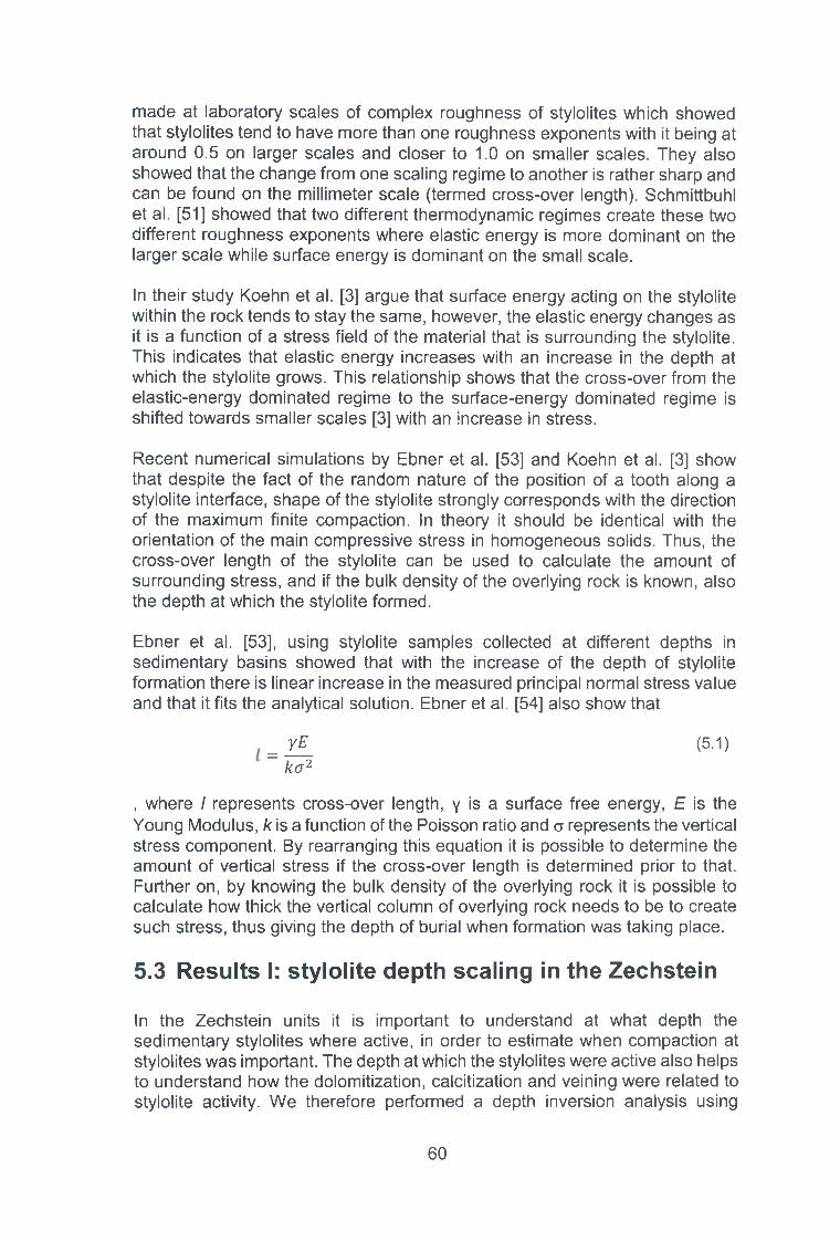
made at laboratory scales of complex roughness of stylolites which showed that stylolites tend to have more than one roughness exponents with it being at around 0.5 on larger scales and closer to 1.0 on smaller scales. They also showed that the change from one scaling regime to another is rather sharp and can be found on the millimeter scale (termed cross-over length). Schmittbuhl et al. [51] showed that two different thermodynamic regimes create these two different roughness exponents where elastic energy is more dominant on the larger scale while surface energy is dominant on the small scale.

In their study Koehn et al. [3] argue that surface energy acting on the stylolite within the rock tends to stay the same, however, the elastic energy changes as it is a function of a stress field of the material that is surrounding the stylolite. This indicates that elastic energy increases with an increase in the depth at which the stylolite grows. This relationship shows that the cross-over from the elastic-energy dominated regime to the surface-energy dominated regime is shifted towards smaller scales [3] with an increase in stress.

Recent numerical simulations by Ebner et al. [53] and Koehn et al. [3] show that despite the fact of the random nature of the position of a tooth along a stylolite interface, shape of the stylolite strongly corresponds with the direction of the maximum finite compaction. In theory it should be identical with the orientation of the main compressive stress in homogeneous solids. Thus, the cross-over length of the stylolite can be used to calculate the amount of surrounding stress, and if the bulk density of the overlying rock is known, also the depth at which the stylolite formed.

Ebner et al. [53], using stylolite samples collected at different depths in sedimentary basins showed that with the increase of the depth of stylolite formation there is linear increase in the measured principal normal stress value and that it fits the analytical solution. Ebner et al. [54] also show that

= YE (5.1)k o 2

, where / represents cross-over length, y is a surface free energy, E is the Young Modulus, k is a function of the Poisson ratio and a represents the vertical stress component. By rearranging this equation it is possible to determine the amount of vertical stress if the cross-over length is determined prior to that. Further on, by knowing the bulk density of the overlying rock it is possible to calculate how thick the vertical column of overlying rock needs to be to create such stress, thus giving the depth of burial when formation was taking place.

5.3 Results I: stylolite depth scaling in the Zechstein

In the Zechstein units it is important to understand at what depth the sedimentary stylolites where active, in order to estimate when compaction at stylolites was important. The depth at which the stylolites were active also helps to understand how the dolomitization, calcitization and veining were related to stylolite activity. We therefore performed a depth inversion analysis using

6 0

sedimentary stylolites from core scans and thin-sections. First results showed that the core-scans are not of the required small scale resolution to find the cross-over, indicating that it must sit at relatively small scales. Therefore we used high-resolution thin-section scans to extract the roughness signal. Fig.5.4 shows a small amplitude stylolite in a thin section, scanned on a high resolution scanner (7070 pixel in width). The stylolite is redrawn from the thin section to produce a one-dimensional function without holes. The drawing is read as a BW image in Matlab, converted to a one-dimensional function and tilted to the horizontal for the analysis

Fig. 5.4 Example of a sedimentary Zechstein stylolite that was used for the roughness analysis. Width of view is 20mm.

The roughness of the stylolite can be analyzed using either a correlation function or the Fast Fourier Transform. The aim is to determine the cross-over length scale where the scaling changes from a roughness exponent of 0.3 to 0.5 on the large scale (shallow slope) to a roughness exponent of 0.8 to 1.0 (steep slope) on the small scale (Fig. 5.5 and Fig. 5.6).

61

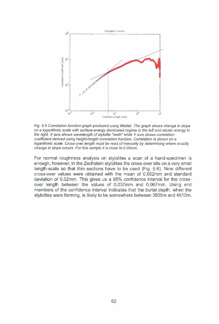
Cnrrp.latinn Function

Fig. 5.5 Correlation function graph produced using Matlab. The graph shows change in slope on a logarithmic scale with surface-energy dominated regime to the left and elastic-energy to the right. X axis shows wavelength ofstylolite “teeth” while Y axis shows correlation coefficient derived using height-height correlation function. Correlation is shown on a logarithmic scale. Cross-over length must be read of manually by determining where exactly change in slope occurs. For this sample it is close to 0.05mm.

For normal roughness analysis on stylolites a scan of a hand-specimen is enough, however, in the Zechstein stylolites the cross-over sits on a very small length-scale so that thin sections have to be used (Fig. 5.6). Nine different cross-over values were obtained with the mean of 0.052mm and standard deviation of 0.02mm. This gives us a 95% confidence interval for the crossover length between the values of 0.037mm and 0.067mm. Using end members of the confidence interval indicates that the burial depth, when the stylolites were forming, is likely to be somewhere between 3805m and 4510m.

6 2

Fig. 5.6 Correlation function graph (a) and Fourier method graph (b) for the same sample produced using Matlab. Correlation function graph provides a cross-over length of 0.04mm while best-fit value produced by the Fourier method is 0.071mm. Although the difference is rather small and is predicted to occur, it alters the end result significantly in the case of carbonates from large depth.

6 3

Cretaceous

Late Triassic to Jurassic

Early Triassic

Early Triassic

Late Triassic to Jurassic

Cretaceous

Fig. 5.7 Long stylolite teeth in the Zechstein may represent different episodes of compaction and can thus be considered to be windows into time.

These depth figures indicate that the stylolites were active at maximum burial or close to maximum burial. Theoretically the acquired signal should give us the last activity on the stylolites. A striking feature of these stylolites is that only small amplitude stylolites give a clear signal. This may be related to the latest burial and thus latest dissolution activity. At the proposed depth this latest activity should be of Cretaceous origin, just before the inversion of the sequence in the Middle Cretaceous. At this stage the stylolite probably had already most of their dissolution history during earlier compaction stages behind them. The latest compaction represents only up to an additional 1000m burial in a rock that already had a low porosity. Therefore we expect the dissolution at stylolites to be only in the order of several mm (per stylolite). This means that the signal that shows the deepest burial can only be reset in the small amplitude stylolites. If the stylolite has amplitude of several cm, an additional dissolution of less than a cm will not change its signal completely but produce a mixed signal. We expect that this is the reason why we see a clear signal only in the small stylolites, because these can be reset.

Our results indicate that sedimentary stylolites probably have been active throughout the whole compaction history of the basin. This means that age relationships using sedimentary stylolites may be hard to interpret because of their long history. However, it also means that stylolites with very long teeth

6 4

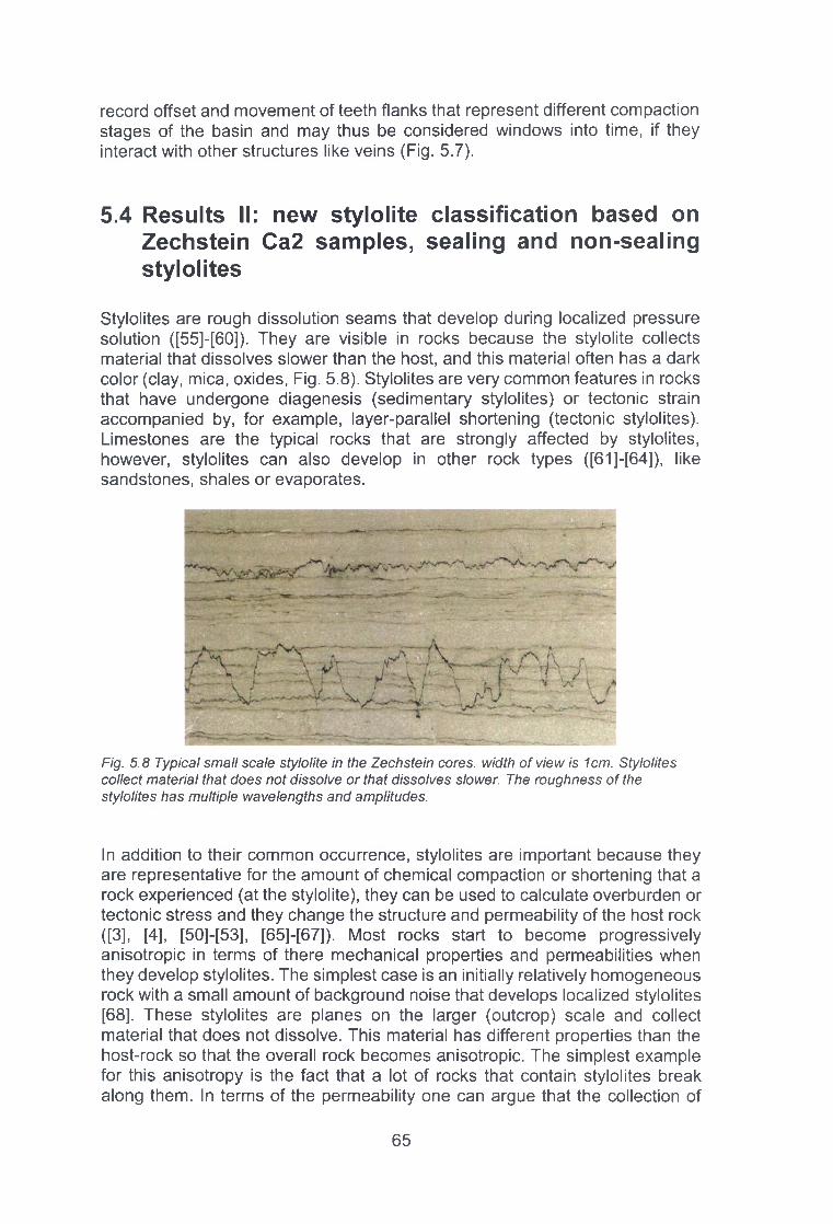
record offset and movement of teeth flanks that represent different compaction stages of the basin and may thus be considered windows into time, if they interact with other structures like veins (Fig. 5.7).

5.4 Results II: new stylolite classification based on Zechstein Ca2 samples, sealing and non-sealing stylolites

Stylolites are rough dissolution seams that develop during localized pressure solution ([55]-[60]). They are visible in rocks because the stylolite collects material that dissolves slower than the host, and this material often has a dark color (clay, mica, oxides, Fig. 5.8). Stylolites are very common features in rocks that have undergone diagenesis (sedimentary stylolites) or tectonic strain accompanied by, for example, layer-parallel shortening (tectonic stylolites). Limestones are the typical rocks that are strongly affected by stylolites, however, stylolites can also develop in other rock types ([61]-[64]), like sandstones, shales or evaporates.

Fig. 5.8 Typical small scale stylolite in the Zechstein cores, width of view is 1cm. Stylolites collect material that does not dissolve or that dissolves slower. The roughness of the stylolites has multiple wavelengths and amplitudes.

In addition to their common occurrence, stylolites are important because they are representative for the amount of chemical compaction or shortening that a rock experienced (at the stylolite), they can be used to calculate overburden or tectonic stress and they change the structure and permeability of the host rock ([3], [4], [50]-[53], [65]-[67]). Most rocks start to become progressively anisotropic in terms of there mechanical properties and permeabilities when they develop stylolites. The simplest case is an initially relatively homogeneous rock with a small amount of background noise that develops localized stylolites [68], These stylolites are planes on the larger (outcrop) scale and collect material that does not dissolve. This material has different properties than the host-rock so that the overall rock becomes anisotropic. The simplest example for this anisotropy is the fact that a lot of rocks that contain stylolites break along them. In terms of the permeability one can argue that the collection of

6 5

material like clays in the stylolite creates a seal, so that the permeability perpendicular to the stylolite is low ([69]-[74]), even though researchers have noted that flanks of teeth may be areas of increased permeability ([75]-[80]). Recent experiments have challenged this simple view indicating that at least some stylolites do not seem to affect a rock’s overall permeability ([81]-[82]). However a general model on stylolite permeability is not yet available.

Stylolites are complex surfaces that are commonly not flat but show a roughness on several scales [83], sometimes with pronounced teeth. Several classifications of stylolite shapes exists ([57], [74], [84]). The classification of [57] uses up to six different shapes (rectangular up and down, seismograph, wavy, sutured, sharp-peak), however it is not always easy to apply and is not yet consistent with an understanding of the stylolite’s dynamic evolution. Alsharhan and Sadd [74] use a much simpler classification (rectangular or highamplitude; solution seams or wave-like; wispy seams or horse-tail), which also incorporates the connectivity of stylolite networks. However, this classification is very general and does not include realistic compaction estimates, because the authors do not separate linear-amplitude growth from non-linear amplitude growth [52], This is important because otherwise the actual chemical compaction at the stylolites is highly underestimated. With chemical compaction we mean dissolution at the stylolite interface (and precipitation of material in pores or transported away) that leads to compaction of the overall system. In order to attain realistic chemical compaction estimates in a stylolite dominated rock a new or advanced stylolite classification is needed, one that can be used for compaction and sealing estimates.

Stylolites are dynamic interfaces with self-affine properties and they are typically rough on the small scale and flat on the large scale ([50], [51], [53], [85], [86]). The growth of the roughness is triggered by noise in the rock, for example in the form of impurities that change the dissolution. Recent research suggests that this noise may trigger localized dissolution (for example through a chemical effect) and thus leads to the development of the stylolite plane in the first place [68], The noise is pinning the interface [87], leads to a dissolution at only one side of the stylolite and thus to the growth of teeth [3]. Surface and elastic energies on the other hand work against the roughness and favor a flat surface. On the small-scale surface energy dominates and the stylolites are relatively round whereas on the larger scale elastic energy takes over and the styolites become rough ([51]-[52]). This transition in scales is also happening through time, the stylolite is initially growing in the surface energy dominated regime (unless the grain size is very large) with a very slow non-linear growth (growth exponent of about 0.5, [54]). Once the growing wavelength of the stylolite has reached a critical scale, the amplitudes start to grow in the elastic energy dominated regime where the roughness grows faster (growth exponent around 0.7 to 0.8; [3]). This type of stylolite has a roughness on several scales, grows initially very slowly and is not very reliable when it comes to estimates of shortening or chemical compaction. A non-linear growth law is proposed and can be used to estimate stylolite compaction [3], but since it is non-linear and the parameters are based on numerical simulations only, the estimates are not very precise. However, if a larger grain or fossil pins the stylolite surface the growth becomes linear and the full stylolite compaction can be recorded [52],

6 6

Some stylolites, typically the rectangular type, show very straight and sometimes very long teeth (Fig. 5.9) with a pronounced dark layer at the top/bottom of the teeth. We study a variety of stylolites from Zechstein cores from a Lean Gas Field in northern Germany with the aim to present a new classification of stylolites that is coherent with their formation, allows the separation of non-linear from linear growth and can be used to estimate the stylolite’s influence on rock mechanics and permeability.

Fig. 5.9 Example of a Zechstein stylolite that shows a distinct relation to layers. Upper and lower flat parts of teeth show layering and concentration of non-dissolvable materials. Note also that some stylolite flanks show veins indicating that the flanks are prone to fluid flow. Width of view is 2cm.

5.4.1 Zechstein stylolites

The sedimentary stylolites that can be found in the Zechstein cores are quite often linked to layers that seem to pin stylolite teeth and can produce some extremely long stylolite spikes. The Zechstein 2 deposited on paleosurfaces of the Werra Anhydrite and the cores represent slope deposits [34], The Zechstein 2 is an important lean gas deposit that is sealed by the overlying basal Anhydrite [40], After the initial sedimentation in the Permian the area was subject to fast subsidence in the Mid Triassic (down to 2500m), a slow subsidence at the beginning of the Cretaceous (down to 3800m), a fast subsidence in the Mid Cretaceous reaching the maximum burial depth (about 4700m) and an uplift event at the end of the Cretaceous to 3750 or 4000m followed by only minor events up to date [88], The original limestone units have been dolomitized and dedolomitized and there is evidence for several phases of fracturing and fluid fluxes that partly result in leaching, and healing (forming veins). The stylolites seem to influence reactions and fluid flow. Dissolution holes develop at stylolite teeth and reactions (calcitization of dolomitized units) is shielded by stylolites and stylolites separate different parts of reactive rocks (Fig. 5.10, Fig. 5.11).

6 7

Fig. 5.10 Holes in the Zechstein cores indicate leaching (probably hydrothermal) fluids. Dissolution holes develop at the stylolites below the teeth. Width of view is 4cm.

The cores contain an abundance of sedimentary stylolites of various shapes and a minor amount of tectonic stylolites. The amplitude of the sedimentary stylolites varies by more than a magnitude from small mm-amplitude stylolites up to teeth that are longer than 40mm. We looked at these geometries in detail and used a preexisting model that can simulate roughening of stylolites to understand the growth evolution.

Fig. 5.11 SEM image showing dolomitized (darker grey) and calcitized (light grey) units separated by a stylolite (black layers). Width of view is 0.5 mm.

5.4.2 Numerical model

We use the software “ELLE - Latte” ([89], [90]) for the simulations with a similar setup to the work of Koehn et al. ([3], [52], [91] and Ebner et al. [54], The model is two-dimensional with dissolution being triggered at an initially flat interface. The model is compressed vertically with displacement-controlled boundaries, whereas the boundaries on the left and right hand side being friction free. The solid is described by a lattice spring model where circular particles of a uniform size are connect with each other by six linear elastic springs that experience normal and shear forces [92], The model lattice is triangular with horizontal rows of particles where each second row is offset. Dissolution of particles at the interface is a function of the difference in elastic energy between a stressed and a non-stressed solid, differences in surface energy between a flat and a curved interface (with a convex interface driving dissolution and a concave

6 8

interface precipitation) and differences in normal stress along the whole interface assuming that the fluid has an average saturation. Each particle has a given mass and this mass is used to calculate which particle dissolves fastest during a time step. Only the fastest dissolving particle is taken out of the model, the solid is relaxed and the next particle can dissolve. A linear rate law with a given rate constant is used to calculate the dissolution rate of single particles [52]. Quenched noise is added to the system in three different ways using a linear dissolution constant. The smallest noise is set on the particles themselves, so that a given amount of particles in the model has a dissolution constant that is a factor x smaller than the overall dissolution constant. A larger scale noise can be put on “grains” that are inherited by a given microstructure, where grains consist of a given cluster of particles that have a different dissolution constant than other grains [52]. Lastly, whole horizontal layers (for example bedding in a real rock) can have different dissolution constants relative to the rest of the model. Generally we apply at least two noises, the small scale noise in addition to either larger scale grains or layers. Noises are overlapping, so that for example the grains themselves also contain a smaller scale noise. Noise is essential for roughening, without noise the system does not develop stylolites.

5.5 Modeling results

We performed about 100 simulations with mainly layer-dominated stylolite growth. All simulations have a lattice size of 200 particles in the x-dimension (overall lattice has 46000 particles), last 30000 time steps and start with a row of particles taken out in the middle of the model. Parameters of the simulations are: dissolution constant for calcite is 0.0001 mol/(m2s), the molar volume for calcite is 0.00004 m3/mol, the temperature 300 K, the surface free energy 0.27 J/m2, the Poisson ratio 0.33, the Young’s modulus 40 GPa and the real physical width of the system 10 mm.

Stylolites that grow in a host-rock with a uniform distribution of small pinning units collect material that cannot be well dissolved and may develop into seals depending on how much material they collect. Stylolites that grow in a similar system that contains some larger grains or fossils that pin typically grow pronounced teeth. Stylolites that nucleate within layers that do not dissolve as fast as the surrounding rock show a different pattern. They grow in three distinct stages. Stage I represents the initial growth in the layer until the stylolite interface reaches the boundaries of the layer (Fig. 5.12). Normally the initial roughness leads to a variation of the position of the remainder of the initial layer on either side of the stylolite interface. In stage II the layer pins and the stylolite roughens very fast. If the layer is dissolved (stage III) as well after a certain amount of time, then the stylolite becomes almost stationary and does not grow in amplitude, it only becomes a bit more rounded. If the layer does not dissolve completely, extremely spiky stylolites develop (indicated as stage lib in Fig. 5.12).

6 9

Stage III Stylolite "freezes", layer gone, rounding of edges

Fig. 5.12 Evolution ofstylolites that grow because of layer pinning. Graphs show different strength of layer pinning, where the layer dissolves 0.7, 0.68, 0.66, 0.64, 0.62 and 0.6 times the hostrock (hostrock is 1.0). The slower dissolving layers (0.62 and 0.6) pin the interface completely and develop extreme spikes.

This stylolite growth has some implication on their sealing properties. In contrast to stylolites that develop into seals because they collect insoluble materials within them, these layer controlled stylolites offset the initial seal (the initial layer) so that fluid can travel across the sides of teeth. Thus these structures potentially enhance permeability.

a) Simulation of layer stylolite (layer in green)

b) Layer stylolite in Zechstein c) Stylolite influence reactions

Fig. 5.13 Layer stylolite in simulation (a) and thin section (b), width of image 1cm. (c) shows SEM image (0.1mm) with the stylolite interface in black, dolomite in dark grey and calcite in light grey.

SEM observations show that stylolites can capture dolomitized parts of the rock. In addition they quite often separate dedolomitized units from dolomitized units (Fig. 5.13). W hether this is a direct effect of the influence of stylolites on

7 0

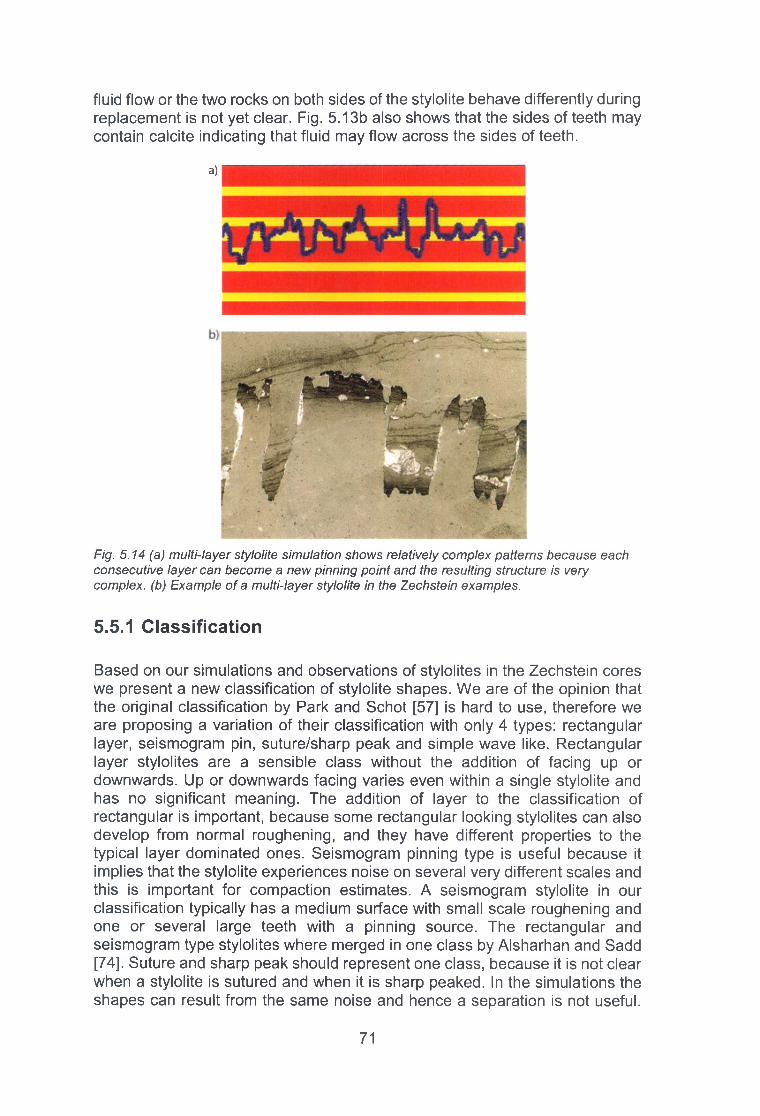
fluid flow or the two rocks on both sides of the stylolite behave differently during replacement is not yet clear. Fig. 5.13b also shows that the sides of teeth may contain calcite indicating that fluid may flow across the sides of teeth.

a)

Fig. 5.14 (a) multi-layer stylolite simulation shows relatively complex patterns because each consecutive layer can become a new pinning point and the resulting structure is very complex, (b) Example of a multi-layer stylolite in the Zechstein examples.

5.5.1 Classification

Based on our simulations and observations of stylolites in the Zechstein cores we present a new classification of stylolite shapes. We are of the opinion that the original classification by Park and Schot [57] is hard to use, therefore we are proposing a variation of their classification with only 4 types: rectangular layer, seismogram pin, suture/sharp peak and simple wave like. Rectangular layer stylolites are a sensible class without the addition of facing up or downwards. Up or downwards facing varies even within a single stylolite and has no significant meaning. The addition of layer to the classification of rectangular is important, because some rectangular looking stylolites can also develop from normal roughening, and they have different properties to the typical layer dominated ones. Seismogram pinning type is useful because it implies that the stylolite experiences noise on several very different scales and this is important for compaction estimates. A seismogram stylolite in our classification typically has a medium surface with small scale roughening and one or several large teeth with a pinning source. The rectangular and seismogram type stylolites where merged in one class by Alsharhan and Sadd [74]. Suture and sharp peak should represent one class, because it is not clear when a stylolite is sutured and when it is sharp peaked. In the simulations the shapes can result from the same noise and hence a separation is not useful.

71

This class would incorporate normal growing stylolites (with only small scale noise) as well as layer-growth where the layer is gone. The latter are hard to distinguish from normal roughening stylolites, therefore they are both included in one class. The last class may be simple wave-like stylolites, which are not very common in the Zechstein cores. The first two classes, rectangular and seismogram typically show signs of pinning grains, fossils or layers. The last two types, suture/sharp peak and simple wave-like do not show evidence of larger scale pinning structures and they lack straight teeth.

5.5.2 Compaction estimates

Our classification of stylolites can be directly used for compaction estimates. Rectangular layer stylolites pin best and grow linear as a function of chemical stylolite compaction. They can be used to get a realistic chemical compaction estimate for rocks (for the stylolite compaction) and may be representative for dissolution on the other stylolites as well. Compaction estimates are still underestimated even for these stylolites, because their nucleation stage involves non-linear growth. The second class, seismogram pinning type stylolites have typically a bi-modal roughness. Similar to rectangular stylolites the pinning teeth may represent most of the actual compaction. This is especially true if the teeth contain remnants of layers. If the teeth represent fossils or grain pinning, then only part of the compaction is recorded, from the moment the fossil or grain meets the stylolite up to when compaction stops. In these cases the longest teeth give the most reliable estimates. Seismogram stylolites often have a median surface. If this surface can be identified, then only one tooth is enough to measure compaction. The compaction on the stylolite is a least two times the distance between the tooth tip and the medium surface. The longest tooth will always be the most reliable estimate. The last two classes of stylolites are not very good for compaction estimates. Normal suture and sharp peak type stylolites grow non-linear. Therefore a measurement of the roughness amplitude is not representative for the amount of dissolution on the stylolite and a non-linear scaling equation has to be used to estimate compaction ([3], [52]). In the Zechstein cores this compaction estimate on a small suture or sharp peak stylolite then gives the same order of compaction as the rectangular layer types (up to 4cm). This may mean that all stylolites have experienced a similar chemical compaction. However, more testing is needed to make these estimates reliable. Simple wave-like stylolites are the worst, because they may represent dissolution seams that have not seen much chemical compaction. Therefore they are very unreliable at present.

7 2

making seal

t0t

t i

Fig. 5.15 Illustration of how stylolites can become seals when they collect sealing material (figure on left hand side, evolution from time tO to time t1), and how stylolite teeth destroy seals by offsetting sealing layers (figure on the right hand side).

5.5.3 Sealing/non-sealing

Our classification can also help in assessing the anisotropy of the permeability across different stylolites. In general stylolites can perform three different structural changes in seals, they can collect impermeable material and thus build up a seal, they can intensify the existing sealing properties of layers and they can offset existing seals (Fig. 5.15 and Fig. 5.16). Collecting and intensifying creates seals whereas offsetting destroys seals. Rectangular layer- type stylolites are characterized by an intensification of seals at the tips of the teeth and an offsetting of initial layering creating new pathways for fluids across the flanks of teeth. This class of stylolites creates very anisotropic permeabilities but potentially destroys seals. The seismograph pinning type is more complicated. As long as layers pin at the teeth the structuring is similar to the rectangular layer type. However, the structuring of the median surface is more complicated and depends on how much material can be collected in the stylolites and what properties that material has. If the material is sealing and the median surface is not very rough, then it can develop into a seal that is only breached at the existing larger teeth.

destroying seal to |

7 3

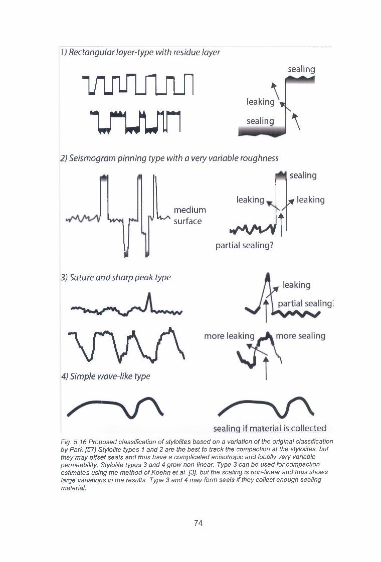
1) Rectangular layer-type with residue layer

vmanjuii r u u r

sealing

leaking ^

sealing \2) Seismogram pinning type with a very variable roughness

. 1

medium ^ surface

leakingN. /

sealing

^ leaking

► y 'A /v 'V

partial sealing?I

3) Suture and sharp peak type

\ r w \4) Simple wave-like type

sealing if material is collectedFig. 5.16 Proposed classification of stylolites based on a variation of the original classification by Park [57] Stylolite types 1 and 2 are the best to track the compaction at the stylolites, but they may offset seals and thus have a complicated anisotropic and locally very variable permeability. Stylolite types 3 and 4 grow non-linear. Type 3 can be used for compaction estimates using the method of Koehn et al. [3], but the scaling is non-linear and thus shows large variations in the results. Type 3 and 4 may form seals if they collect enough sealing material.

7 4

Suture and sharp peak types are generally collecting material. In this case they may create seals especially if they do not become very rough and if the collected material is sealing. Local spikes may still breach the seal (for example [52]. Simple wave-like stylolites may represent dissolution seams, quite often contain insoluble material and can represent original sedimentary layers. This class can build good seals, because the stylolites are not rough and are thus not offsetting the seal.

5.5.4 Structures observed in well A

The investigated rocks of well A range from 3908 to 3966 m depth. Bedding and bedding-parallel stylolites are clearly identified, as well as some disconformities at bioturbated zones (at 3928-3932 m and 3962-3964 m). Bedding is generally poorly developed, although it is well distinguishable at the intervals 3908-3910 m and 3954-3957 m. The host rock is mostly formed by calcitized dolomite (referred to as dedolomite), with a characteristic light grey colour. Some areas display darker grey rock, which is preserved dolomite. This is mostly observed at 3917-3921 m depth.

Stylolites appear in the whole section, although with varying densities (Fig. 5.17). Single stylolites showing teeth heights of more than 1 cm are distributed all over the well, and a higher average teeth height is observed between 3925 and 3957 m. The mean stylolite density is relatively high, with more than 25 stylolites per metre at the top of the well and a sudden decrease to about 5-15 stylolites per metre at a depth of about 3912 m. A slight increase to values around 15 stylolites per metre is observed from 3928-3956 m. In the lower part of the well (from about 3957 to 3966 m) there are high densities, similar to the values at the top of the core. The highest stylolite densities are found within rock material interpreted to consist of calcite (calcitized dolomite or dedolomite). There are almost no veins in these sections of the well. An anticorrelation between the occurrence of vuggy and intermediate veins and the stylolite density is found in this log. Their teeth heights range from the microscopic scale up to ~1.6 cm. Teeth are normally vertical to subvertical with respect to the stylolite planes and their shape is often irregular or sinusoidal with strong lateral variations. Larger teeth are often found in rectangular stylolites. There are tectonic stylolites at 3908-3911 m and 3933-3934 m, especially at locations of relatively low vuggy and intermediate vein occurrence.

Cemented gashes and thin veins in well A present variable thicknesses of up to 20 mm, and are commonly filled with calcite, with occasional anhydrite. There are some partially open fractures, as well as partially filled vugs. Microfractures filled with calcite can be found in thin sections. The partially open fractures and veins present high angles (between 60 and 90°) to bedding. Higher vein occurrences are found at 3930-3936 m and 3947-3955 m. Partially open fractures are regularly distributed over the well, with increased densities at 3914-3916 m, 3928-3932 m and 3949-3957 m. Most of the fractures seem to be extensional, as they appear almost perpendicular to bedding and without conjugate shear sets. In some parts of the core vugs and en-echelon veins are found (3912-3915 m, 3917-3921 m, 3928-3930 m and 3934-3936 m). Partially open fractures and cemented gashes are often observed together with

7 5

stylolites. Vuggy veins filled with anhydrite are found at 3912-3921 m. Vuggy and intermediate veins are about 5% of the rock’s volume at the top of the core, and decrease downwards to be absent at the base. Fracture veins are below 5% of the rock’s volume, having the highest densities at the top of the well. They are absent at the intervals 3917-3921 m and from 3953-3956 m. Horizontal fractures along this core are interpreted as induced. The amount of dissolution fluctuates from one interval to the next, ranging from 2% per metre to slightly more than 4% per metre. Higher values are located at the lower part of the well.

Fig. 5.17 Stylolite density, veins and dissolution in well A. Black lines indicate the weighted arithmetic mean of the interval. The standard deviation is indicated with gray bars. White gaps between the black lines are areas without core rock.

7 6

5.5.5 Observed structures in well B

This well ranges from 3987 m to 4020 m, and is located ~14 km away from well A. Lamination in this core is more visible at its upper half. Some disconformities occur in bioturbated zones (at about 3959-3964 m and 3988-3992 m). The rock is mainly composed of dedolomite, with some preserved dolomite (at about 3959-3965 m). Stylolites are ubiquitious in the well (Fig. 5.17), showing varying frequencies with depth. A higher amount of stylolites presenting larger teeth heights of more than 1cm is observed in the deepest part of the well. Their teeth are similar to those of well A. The stylolite density generally decreases from values close to 30 stylolites per m at the top to about 10-15 stylolites per m between 3921 and 3936 m depth. An increase in the highest average density is found below 3936 meters, followed by a sudden decrease to about 10-15 stylolites per m at 3965-3961 m. Below, an increase is observed again, reaching a density of about 40 stylolites per m at 3976-3981 m. From 3981 m to the core bottom the density is between 20 and 35 stylolites per m.

Macroscopic fractures mainly occur as thin veins or cemented gashes filled with calcite. Zones with bedding-perpendicular partially open fractures are found at 3972-3975m, 3980-3985 m and 4012-4018 m (Fig. 5.18). Veins are also vertical/subvertical, and are distributed along the whole core, with higher occurrence at 3945-3955 m. As in well A, fracture sets are interpreted to have formed in extensional settings. Vuggy veins and partially open vugs are found through the whole core. They are mostly filled with anhydrite and sometimes with calcite. The occurrence of vuggy and intermediate veins is highest towards the top of the core, with about 10% of the rock’s volume. Below, at 3936-3980 m this decreases to less than 3%. From 3980 m down to the bottom two sections of generally decreasing vein material are observed. At the top of these sections, a sudden increase occurs respectively. The lower section reveals a stepwise decrease in vein percentage from more than 5% to almost zero. Fracture veins are about 0.1-0.3% of the rock’s volume at the upper part, but with strong variations. This volume increases to 1% from 3937 to 3951 m. Between this depth and 4008 m it decreases again down to 0.3%. At the lowest part of the core (below 3985 m) the percentage ranges between 0.3 and 1%. Dissolution features form about 2% of the rock’s volume at the top of the core, then they increases to 5% at a depth of 3952-3957 m and decrease again until 3990 m. At the lowest part of the well the volume of dissolved material increases to 12-14% (below 4014 m).

7 7

Stylolite density |n/m] Vuggy and Intermediate veins (% ]| Fracture veins |%]0 5 10 15 20 0 0.5 1 1.5 2 2 5 DissoluHnn/m (%]0 5 10 15

Fig. 5.18 Stylolite density, veins and dissolution in well B. Black lines indicate the weighted arithmetic mean of the interval. The standard deviation is indicated with gray bars. White gaps between the black lines are areas without core rock.

3905391539253935394539553965397539853995400540154025

5.5.6 Statistical distribution of stylolite networks

The cumulative distribution of bedding-parallel stylolite spacing in wells A and B fit best to an exponential function (Fig. 5.19). This distribution plots well for spacings up to 9 cm for well A and between 2 and 7 cm for well B. Higher values are more scattered, and potentially fit to a different exponential function. The measurement of longer spacings was strongly influenced by two error sources. The first occurs because a lower number of large spacings could be measured because of the higher probability of finding a gap of an unknown amount of rock material between two neighboring stylolites. This results in an underestimation of larger spacings. The second error happens because there is a higher probability of missing small stylolites placed in between two larger stylolites. This results in an overestimation of larger spacing values.

7 8

No clear distribution is found for teeth height. Exponential, log-normal and power-law distributions only fit to a small range of the data. A higher proportion of teeth heights can be explained with a log-normal fit. This can be due to the non-linear roughness stylolite growth [3], since growth slows down with time and can even be saturated. Apparently, smaller teeth heights rather are explained with a log-normal distribution whereas larger teeth heights roughly follow an exponential distribution.

Fig. 5.19 Exponential fit in normal-log space of stylolite spacings of wells A (upper graph) and B (lower graph), respectively. The ordinate shows the number (n) of measured spacing values that are larger or equal to the spacing values (S) on the axis of abscissae. Back lines show the fitting curve based on the data indicated with the black dots. Dark grey dots and lines indicate the applied fit in each graph for a second fit if a second slope can be found. Bright grey squares mark the data that were not used for the calculations.

5.5.7 Relative timing of structure formation

Sedimentary stylolites are generally younger than vuggy veins, and there are almost no vuggy veins cutting stylolites. There is clear evidence that sedimentary stylolites were active at different times during the evolution of this unit, since there are young stylolites with large teeth heights dissolving older stylolites that became inactive, and with smaller teeth amplitudes. There are fracture veins cutting old stylolites and being cut at the same time by younger

7 9

ones (Fig. 5.20). Some stylolites cut and dissolve fractures vein being penetrated by other ones. Moreover, there are fracture veins cutting other fracture veins, indicating that fracture veins also formed at different stages. Tectonic stylolites started to develop after sedimentary stylolites. There is no clear evidence of vuggy veins or fracture veins being younger than tectonic stylolites. However, there are very few crosscutting relationships to prove this observation. According to the literature, there was only one event of horizontal compression in the area, during the Late Cretaceous inversion. Therefore, we interpret the tectonic stylolites to have been formed during that time. As most of the vuggy veins are cut by the sedimentary stylolites which are preferentially cut by the tectonic stylolites and no vuggy vein was observed to cut a tectonic stylolite, there might be a tendency for the majority of the vuggy veins to predate this inversion period.

There are very few crosscutting relationships between vuggy and fracture veins, and they tend to show chaotic arrangements. There is a transition between calcite veins with a vuggy shape to those filling discrete fractures. Intermediate veins between these two end members form networks and appear to have the same age as them. Some fracture veins are cut by vuggy anhydrite veins. Anhydrite generally tends to be more present in vuggy veins, which also contain some calcite. However, the more elongated fracture and intermediate veins are commonly filled with calcite, with occasional very minor contributions of anhydrite. Anhydrite can be transported into the system by dissolution- precipitation processes from the anhydrite formations above or below the Ca2 carbonates. Some veins penetrate through several stylolites and are cut and dissolved by others, thus indicating different relative dates of stylolite origin or activity which is also suggested by, mostly larger, stylolites that consume smaller older ones. Fractures generally appear either parallel or perpendicular to each other, and there are no indications of conjugate fracture sets or slip along fractures. Therefore, we interpret these fractures as extensional.

The stylolite density, amount of dissolution and occurrence of fracture veins is in general higher in well B than in well A. Contrarily, vuggy and intermediate veins are more common in well B. An anti-correlation between the occurrence of vuggy/intermediate veins and stylolites is detected in well A. However, this trend is only observed at a ~24 m-thick interval in well B. Since there are not changes in lithology, we interpret these changes as being caused by small differences in stress or rock’s solubility along the wells. A lower differential stress would enhance vein formation and precipitation of cements in vugs, while higher differential stresses would result in an increase in dissolution. These differences seem more pronounced in well A than in B.

Vuggy and intermediate veins preferentially appear towards the upper part of the wells, while dissolution features are more frequent at the lower parts of the well, especially in well B. This could be related to higher fluid pressures with respect to the lithostatic pressure at the upper part of the wells, if the overlying evaporite units were acting as a seal. Such higher fluid pressures would have enhanced the formation of extensional fractures.

8 0

Fig. 5.20 Micrographs of cross-cutting relationships between different structures and diagenetic products, (a) pyrite within stylolite that separates an anhydrite blobby vein from host de-dolomite. Galena precipitated in the stylolite. (b) anhydrite blobby veins bounded by a stylolite and host preserved dolomite, (c) breccia with angular clasts of preserved and calcitized host rock. Anhydrite cements the space between the clasts. Stylolites continued dissolving after the breccias formed, (d) Stylolites protect preserved dolomite from being calcitized. Blobs of anydrite are present, (e) Sedimentary sylolites acting as a calcitization front. There are anhydrite crystals growing on both sides, and veins being cut by the stylolites. (f) Calcite vein cutting sedimentary stylolite. All micrographs are taken in cross- polarized light, except (d) that was captured in plane-polarized light.

81

5.5.8 Geochemical data

2 5 carbon-oxygen stable isotopes were measured from host rocks and veins. Host rocks include: (i) calcite formed by calcitization of dolomite and (ii) preserved dolomite. Veins include: (iii) calcite fracture veins and (iv) calcite vuggy veins. The results are shown in Fig. 5 . 2 0 , and compared to those by Below [93]. Our data is clearly organized in two clouds. Calcitized dolomite (dedolomite) and preserver dolomite present a similar isotopic composition. 1850 which is for host rocks similar to that of Below [93], although there is a shift of about 2 to 5 % o in S13C. This can be due to different degree of interaction of the rocks with organic matter in the two studied wells, compared to the wells studied by Below [93]. The isotopic compositions of veins are more variable, and display a wide range of oxygen values. This is probably associated with some of the calcite cements in veins having precipitated at higher temperatures. The data by Below [93] also show wide differences in oxygen isotope compositions of veins. As in the case of host rocks, it seems that our data present persistent lower carbon isotope values than that of Below [93]. This could also be due to differences in the technique and equipment to measure the isotope values.

Fig. 5.21 Carbon-oxygen stable isotope composition of host rocks and cements. Our new data, shown by scatter points, is compared with that of Below [93] indicated with clouds.

The composition of 534S isotopes was also measured from nine samples, including anhydrite, sphalerite, galena and pyrite (Table 5.1). Anydrite fills vuggy veins, and sphalerite, galena and pyrite are associated with calcite veins. The use of fractionation equations of Ohmote and Rye [94] and Kajiwara and

8 2

Krouse [95] reveal that pyrite and sphalerite could have precipitated at the same time. We have estimated the likely temperatures and associated burial depths of these minerals, in conjunction with anhydrite. If sphalerite precipitated with anhydrite, then both did it at 212°C (at 6.05 km depth assuming a geotherm of 30°C/km). If pyrite precipitated with anyhidrite both did it at 232°C (at about 6.7 km). The precipitation of galena is not compatible with the synchronous formation of other minerals. Therefore, if galena precipitated alone it would have been at either 111°C or 260°C (2.7 and 7.65 km, respectively).

Table 5.1. Sulfur isotope compositions of our samples

Mineral <?4S (% o)

Anhydrite 1 4 . 1 8

Anhydrite 1 4 . 2 1

Anhydrite 1 6 . 7 9

Anhydrite 1 2 . 0 9

Galena - 2 . 2 2

Galena - 6 . 3 2

Sphalerite - 1 2 . 3 1

Pyrite - 1 0 . 6 6

Pyrite - 1 0 . 7 7

8 3

6 Comparison of field laboratories and summary

In this chapter we shortly discuss differences and similarities of the three field areas before the numerical approaches are described in chapters 7-14. Chapter 15 then comes back to the field areas and gives a synthesis of field and modelling. Our main aims were:

a) to understand the use of microstructures to infer tectonic processes,b) to understand the use of microstructures as proxies for fluid

overpressure,c) derive an understanding of fluid fluxes and thus permeability through the

systems,d) find out whether or not there is a difference between siliciclastic versus

carbonate dominated sequences,e) find out whether or not there is a difference between surface outcrops

and actual reservoirs.

Both Oman and the Internal Ligurian Units in Italy have shown that veins and stylolites are very useful to understand large-scale deformation processes. Especially conjugate vein sets that occur at a steep angle to bedding and develop during layer parallel shortening or extension veins that develop during layer-parallel extension are very useful to estimate large scale tectonic stress direction. Of course caution has to be taken to rotate folded and tilted sequence back to horizontal to estimate the right stress orientation. In addition, multiple outcrops over larger areas have to be merged to get the larger scale picture. Very reasonable stress rotations have been found for Oman and the Ligurian Units that fit with large scale tectonic events, illustrating the importance of the study of sub-seismic scale structures.

Fig. 6.1 Potential hydrofractures in the basement of the Oman mountains.

8 4

Deriving proxies for fluid overpressures is not an easy task and will be discussed in detailed in modeling chapters 10 and 11. Fluid overpressures are expected when the veins have chaotic shapes (Fig. 6.1) and do not necessarily orient themselves relative to the stress field (Fig. 6.2). An explanation for this behavior is given in detail in chapter 11 (see also [96]). In addition, switches in fracture or vein orientation from horizontal to vertical may also indicate high fluid overpressure that switches the orientation of the principal effective stresses (Fig. 6.3). Again, both field areas, Oman and the Ligurian Units in Italy show such structures. In the case of Oman fluid pressure veins seem to be more chaotic.

Fig. 6.3 Early veins in the Ligurian siliciclastic units that show bedding parallel and bedding perpendicular sets.

8 5

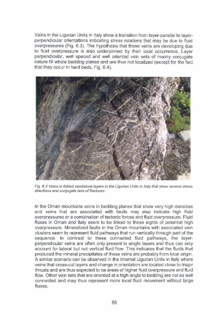
Veins in the Ligurian Units in Italy show a transition from layer-parallel to layer- perpendicular orientations indicating stress rotations that may be due to fluid overpressures (Fig. 6.3). The hypothesis that these veins are developing due to fluid overpressure is also underpinned by their local occurrence. Layer perpendicular, well spaced and well oriented vein sets of mainly conjugate nature fill whole bedding planes and are thus not localized (except for the fact that they occur in hard beds, Fig. 6.4).

Fig. 6.4 Veins in folded sandstone layers in the Ligurian Units in Italy that show several stress directions and conjugate sets of fractures.

In the Oman mountains veins in bedding planes that show very high densities and veins that are associated with faults may also indicate high fluid overpressures or a combination of tectonic forces and fluid overpressure. Fluid fluxes in Oman and Italy seem to be linked to these sights of potential high overpressure. Mineralized faults in the Oman mountains with associated vein clusters seem to represent fluid pathways that run vertically through part of the sequence. In contrast to these connected fluid pathways, the layer- perpendicular veins are often only present in single layers and thus can only account for lateral but not vertical fluid flow. This indicates that the fluids that produced the mineral precipitates of these veins are probably from local origin. A similar scenario can be observed in the Internal Ligurian Units in Italy where veins that cross-cut layers and change in orientation are located close to major thrusts and are thus expected to be areas of higher fluid overpressure and fluid flow. Other vein sets that are oriented at a high angle to bedding are not as well connected and may thus represent more local fluid movement without large fluxes.

8 6

The Oman and Italy field areas that are situated at the Earth’s surface show no significant variation in patterns even though Oman is mainly made up of limestone and the Italian units mainly siliciclastics. Both areas show similar structures. They both contain veins that are oriented at a high angle to bedding, often with conjugate sets that are restricted to stiff beds. Both areas also show veins that are indicative of high fluid overpressures either because the vein orientations are chaotic or because they show variations of orientation from bedding-perpendicular to bedding-parallel.

Differences in deformation style in both areas do not seem to be strongly linked to the rock lithology (in terms of carbonates versus siliciclastic units). The main difference in the limestone units is the strong stylolitization in Oman, which is not very pronounced in the Italian sequence. Otherwise the fracturing and veining seems to be more linked to elastic properties of rocks, hard layers fracture and form veins with a high angle to bedding, whereas the soft units often show no veins. Therefore the patterns that form rely on difference in competence between layers in the sequence rather than on whether or not the hard layers are limestone or sandstone. Overall, the tectonic history seems to be more important than the lithology and produces some variations in the patterns in Oman versus Italy. Especially veins that indicate high fluid overpressure show different structures, they are chaotic in the basement in Oman, whereas Italy shows patches of veining where layer parallel and perpendicular orientations switch. In addition, the strong deformation in the Italian sequence produces additional veins during folding and the development of faults in the cores of folds. This leads to a connection of part of the sequence so that fluids can flow across the sequence. In the layered limestone sequence in Oman this connectivity seems to be mainly restricted to normal and strike- slip faults.

8 7

The Zechstein units are dominated by carbonates and thus show a strong influence of stylolites on deformation in accordance with the Oman field area. However, the main difference to Oman and Italy is the fact that the studied Zechstein rocks are from 4000m deep cores and not from surface outcrops. Since most geological observations are based on surface outcrop data, an obvious question is whether or not surface outcrops are representative of what the rocks look like at depth. The main difference between the Oman/ltalian surface outcrops and the Zechstein cores is that the Zechstein shows dissolution holes and partly filled veins (Fig. 5.10, Fig. 6.5) whereas the surface outcrop fractures are mainly sealed.

Potential fluid pathways seem to be better preserved in the Zechstein cores, probably because the system was active while it was cored. If this is true, the consequence may be that outcrop data has to be treated with care, since it does not necessarily show the paleo permeability that the system had at depth. Neither the Italian nor the Oman outcrops show networks of partly filled veins. At least in Oman fluid flow at the surface can be identified by sinter deposits and these seem to be linked to fractures or joints along bedding planes and faults. The aperture of these permeable structures is very thin and not well linked to the veins found in the outcrops, indicating that fluid flow at the surface is different to paleo fluid flow at depth.

8 8

7 Modeling mineral vein dynamics across scales

In chapters 8 to 14 we present numerical models of fracture and vein systems at different scales and with different boundary conditions. In chapter 8 we illustrate how single cracks fill with crystals and how the partly sealed veins change their flow properties because of the growing crystals. These small- scale results are used in an up-scaling approach in chapter 13 to seal larger scale fractures.

Laver scale Reservoir scale

Fig. 7.1 Mineral vein dynamic modeling across scales from crystal scale all the way to reservoir and crustal scales.

In chapter 9 a numerical approach of fracture patterns that develop in layers under extension is shown. Here the fractures are healed by filling them with cohesive materials and the subsequent fracturing patterns are observed. Depending on the elastic properties of the veins and their orientation, new fractures are influenced differently, from reactivating the old fractures to fracturing across old veins. In chapter 10 a similar approach to the one presented in chapter 9 is taken to understand the influence of healing fractures on mechanical properties and permeability of systems. In this case a vertically- oriented 2D section is modeled with initial gravity and hydrostatic fluid pressure. The system is loaded by horizontal extension and/or input of fluid pressure at the base of the model. Healing of fractures is dynamic by reconnecting broken units with unstressed bonds. Chapter 11 shows a continuation of the model presented in chapter 10 with an emphasis on the influence of high fluid overpressures and the development of mobile permeability pathways. An emphasis is put on the complexity of effective stress patterns in the Earth’s crust and the resulting development of hydraulic fracture patterns and hydraulic breccia. Chapter 12 illustrates how graph theory can be used to understand scaling properties of fracture networks with examples from mud-crack and

8 9

hydro-breccia simulations. Chapter 13 deals with flow along healing fractures and faults and uses small-scale data from chapter 8 for flow simulations. Chapter 14 shows how mobile hydrofractures can represent fluid flow through the Earth’s crust in a dynamic way and links this dynamic flow to fluid mixing.

9 0

8 Modeling crystal growth in cracks

8.1 Introduction

Tectonic mineral veins bear the traces of former deformation, fracturing and fluid transport processes, and constitute a record of the complex geochemical, hydraulic and mechanical history of the rock. For example, a sporadic or cyclic reopening of completely or partially sealed veins may occur, as proposed for the crack-sealing process [97]. In growing antitaxial veins, new material is accumulated at the boundary of the initial crack and the growing vein crystals, which follow the trajectory of the opening crack, whereas in syntaxial veins sealing starts from the fracture surfaces and propagates to the inside of the crack [98]. According to their microstructural evolution during crystal growth, four major types of veins have been identified (e.g. [99], [100], [101]). Fibrous veins are composed of grains with very large length to width ratios, often separated by curved boundaries [102]. It was proposed that they form by pressure dissolution - precipitation mechanism [100], involving diffusive transport from nearby rock or assuming cyclic crack-sealing with very small crack increments ([103], [104], [105]). Veins with elongate-blockymicrostructure are assumed to result from growth competition between grains starting as epitaxial overgrowths of rock wall grains [99]. Here, larger crack aperture leads to the development of crystal facets, i.e. euhedral crystal terminations at the liquid interface. Stretched crystal veins are composed of grains with serrated boundaries bridging the whole distance between both sides of an original fracture. They are supposed to form by continuous cracksealing, where rock wall material and fluid inclusions mark former vein-rock boundaries [99]. Veins filled with grains showing no signs of directional growth are termed ‘blocky veins’, and a mechanism of homogeneous nucleation and free growth following the fracture opening was proposed [106],

Experimental studies under well-defined conditions are essential to test these models, but are rare in the literature. Lee et al. [107] and Lee & Morse [108] studied calcite growth in a synthetic unitaxial vein of 10 cm length and 2 mm aperture with a single Iceland spar crystal as substrate. Linder laminar flow calcite crystals started growing from micron-sized, isolated seeds, forming aggregates of 30 to 60pm diameter without well-defined facets in one month. The authors concluded that either very high flow velocities or low supersaturations are necessary to completely seal larger portions of a vein. Hilgers and coworkers published several studies using the cubic mineral alum as a vein filling analogue in a transparent flow-through cell with mm-sized gap ([2], [109], [110]). At the upstream inlet of the channel the precipitation rate was higher and lead to punctual sealing during the late stage, where individual crystals dominated the remaining flow path. Observable difference in material precipitation occurs on lengths of several 100m [2], Hydrothermal sealing of micro-fractures of 10-20pm width under strong uniaxial compression and confinement pressure was observed by Hilgers & Tenthorey [111]. However, no details on the flow or growth mechanism during sealing were provided. Flow-through hydrothermal experiments with apertures of ~300gm under

91

defined (p, T, c) conditions were carried out recently by Okamoto et al. [112] and Okamoto & Sekine [113] for different quartz rocks. These well-controlled experiments are used in the present study for calibration and evaluation of the numerical simulations.

Numerical models are useful for unraveling the relationship between the microstructural pattern and the transport process. They can help to quantify timing of vein closure and predict temperature, composition, pressure of the mineralizing fluid. To date, numerical models have required simplifications to reduce the complexity of the physico-chemical processes. A purely kinetic approach with an orientation-dependent growth-rate function was used in the vein-growth model by Bons[114]. It takes into account crystal symmetry and represents interfaces as discrete line segments. For antitaxial growth, growth competition and tracking of grains at rock wall asperities were simulated ([102], [115]), deformation related fibrous growth [116] and zeolite growth [117]. The simulation software prism3D is based on a cellular automaton model and has been applied to study diagenetic pore-scale mineralization processes in quartz [118] and carbonate rock [119], Although only a limited set of grain orientations is used, differentiation between slow kinetics of facets and fast growth of nonfacet orientations is captured and explains experimentally observed features such as nucleation discontinuities. On the other hand, reactive transport models incorporate processes which are specific to the mineral system under consideration such as diffusion, advection, heat transport and include chemical reactions (e.g. [120]), and have been successfully applied to model isotropic mineral growth ([121], [122]); however, they do not account for crystalline anisotropy and polycrystalline fabric. Hence, on the microstructural scale they can be applied up to date successfully for nearly isotropic mineral growth. Phase-field models (PFM) have become standard tools to describe microstructure evolution in materials science, and in addition to diffusive- and fluid-transport can capture multi-component phase transitions and kinetics of crystal interfaces [123]. For a more detailed review on PFM, please refer to Ankit et al. [124] and Wendler et al.[125].

In the present work, we want to close this gap and adapt a phase-field model to hydrothermal quartz growth, to describe one of the most important precipitation processes in rock fractures. Whereas previous phase-field approaches to mineral growth relied on a qualitative description of a static crystal shape, in this work we define the combined anisotropy of kinetics and surface free energy, which can capture the observed shape variability of natural crystals. This crystal anisotropy is of special importance for non-fibrous vein growth, where competition between crystals occurs. Because the physical parameters used as input to the model are not all available or are known only to limited accuracy, a hydrothermal experiment is analyzed.

8.2 Methods

Fig. 8.1 presents a flowchart of the strategy applied here: data for interfacial energies and thermodynamics close to the studied pressure, temperature and composition (p, T, c) of the fluid is selected from the literature. To provide input

9 2

data for the kinetic anisotropy function, crystal shapes from experimental micrographs are analyzed. This defines the initial model setup, which is then applied for simulations of single crystal and polycrystalline quartz growth. As a subset of the model parameters are still uncertain, these are modified and tested again within small-scale simulations. In a final step, the model is compared to the experimentally obtained morphologies and textures for validation. This is achieved by using statistical measures for grain number and orientation distribution as function of the growth distance.

Q .Oo—’cro

<U1ro

- C

5o

3ft

QJnftftufterafty>cu3KTco■a

Fig. 8.1 Flowchart of the model adaption process: Available parameters from literature (interfacial energies, quartz kinetics and solubility data) are supplemented with experimental data under the actual conditions (31 MPa, 430°C). Together with the PFM evolution equations the initial setup is defined, which is tested in restricted scenarios like single crystal or small ensemble growth. Especially anisotropy functions and interface energies are modified within the range of reported values to reveal observed morphologic details. This final model setup is validated in larger simulations reaching the length scale of the experiment.

8.3 Hydrothermal experiments for quartz vein formation

Previous hydrothermal experiments on quartz vein growth by Okamoto et al. [112] and Okamoto & Sekine [113] are used to extract the missing physical parameters and to give a validation case for the present model. Here, we introduce these experiments briefly. Both experiments were carried out in a

9 3

pipe-like hydrothermal flow-through reactor with inner diameter of 10.8 mm. Supersaturated solution was produced by dissolution of quartz sand in the first vessel at temperatures of 365°C and fluid pressure of 31 MPa and subsequently precipitation of silica minerals occurred in a second vessel by changing the temperature [113]. As the silica solubility in the chosen temperature range is retrograde [(Fournier & Potter 1982), the temperature increase to T = 430°C in the second vessel leads to supersaturation. Previously, dissolution experiments were conducted at T = 150- 390°C and p = 31 MPa to determine the quartz precipitation rate constants used in this study [112]. Furthermore, different mechanisms of mineralization were found, depending on the solution chemistry: Pure silica solutions by dissolution of quartz sand gave rise to precipitation of amorphous and microcrystalline polymorphs of quartz. From the solution made by dissolution of granite sand, silica precipitation occurred mainly as epitaxial overgrowth of existing grains ([112], [113]) and was attributed to impurity concentrations of Na, K and AI in the range of several ppm in the solution.

Small blocks of different quartz-bearing rocks with dimension 5 mm x 5 mm x

20 mm were aligned sequentially in the reactor [113]. They were cut at the upstream side to create a synthetic ‘fracture’ of about 300 microns aperture. Flow of the supercritical solution was established by a pressure difference of < 0.2 MPa across the precipitation reactor. From the geometry and flow rate of about 0.017 g/s an average initial velocity of about 1.3 mm/s can be deduced, indicating vigorous flow. Fluid could pass through the slit as well as along the outer boundaries of the rock blocks, hence quartz precipitation was observed on either location. As the blocks are immersed in fluid within a circular tube, flow velocity in the slit might have been different and have broken down during sealing. The silica concentrations at the fluid inlet and outlet of the reactor were determined by an inductively coupled plasma atomic emission spectrometer (ICP-AES; Hitachi P-4000). The final crystallized blocks were weighted to determine the average silica concentration at the position of each rock block, using the precipitated mass and the recorded in- and outlet concentrations. 2D thin sections were analyzed under polarized light to determine the c-axis direction of the quartz grains by an optical birefringence method.

9 4

Table 8.1 Properties of the two rock samples used for analysis in this study. In addition to the saturation index of the input solution, concentration and saturation indices were determined a posteriori using sampled inlet- and outlet concentration and the weighted amount of precipitate along the flow path.

Rock typeAbundancequartz

Grainsize[pm]

Saturation input sol.

Sicone.[ppm]

Saturationcalc.

growthtime[h]

slitwidth[um]

metachert 0.98 65 3.6US-147 1 .2 - 1.5 336 311

sandstone 0.52 80 3.6127176 1 .3 - 1.8 188 353

For the calibration of the growth model in the present study, it is necessary to determine the full orientation, which fixes the cross-sectional shape of the crystals in the prepared samples. To this end, two of the rock samples, listed in Table 8.1, were characterized again in the present study with respect to grain orientations. With an SEM (Hitachi S3400N) forward-scattering images of thin sections at the outer rock wall were taken with up to 80fold magnification. Electron backscatter diffraction (EBSD) images taken at selected spots were analyzed automatically to give crystal orientations in form of Euler angle triples (z-x’-z” convention). Several hundred grown crystals at the outer boundary of the rock blocks and grains from the neighboring rock matrix were analyzed. From both optical and EBSD images it was deduced that all surface-bound crystals are epitaxial overgrowths of rock grains underneath. Fig. 8.2 shows an example of an optical and forward-scattering image from the same location on the outer surface of the metachert sample. In the optical image, the former rock wall can be seen as fine dark line, not visible in the forward-scattering image.

(A) (B)

Fig. 8.2 Experimental image details. (A) Optical micrograph (polarized light) of outer boundary of the metachert sample. The initial rock wall is still visible as a thin dark line (white arrow, black scale bar is 300 pm) (B) EBSD forward-scattering image of grain 308 and neighbors (rightmost crystal in(A)). The orientations of all grains at the sample boundary were determined by analysis of the Kikuchi pattern at the locations marked by squares.Intersection lines between ideal crystal facets and the plane of view are plotted after fitting the facet distance relations dm/dz and dr/dz to determine the crystal shape. Dark patches are multiple small and a few larger fluid inclusions at the initial rock wall (white dotted line in (B)).

9 5

8.3.1 Phase-field model

The multi-phase-field model (PFM) used in this work has been discussed and applied to mineral growth previously (e.g. [124], [126]). For a detailed overview on the applied PFM, please refer to [125].

Input parameters for quartz growth

The task to find appropriate values as input parameters for the PFM is a central part of the modeling process (strategy outlined in Fig. 8.1). For the mineral exquartz, three different crystal forms are commonly observed (Fig. 8.3A): (1) six {1010} (m) facets of the hexagonal prism capped by two nonequivalent rhombohedral facets: (2) the positive rhombohedron {1011} (z face) and (3) the negative rhombohedron {0111} (r face). The latter is often faster growing as in the example of a natural needle crystal in Fig. 8.3B, related to a higher impurity uptake [127], The atomically rough c face ({0001}) is the fastest growth direction and does not appear on euhedral crystals. The trigonal crystal system of quartz (point group 32) allows two enantiomorphic left and right handed variants, appearing in equal proportions in nature. We neglect this differentiation here, as the chiral facets {2111} and {6151} were not observed on the experimentally grown crystals.

Interface energies: The free energy of the interfaces between quartz and an aqueous liquid is not a unique property. Values between 1.08 J/m2 for the fully water coordinated {0001} face, and 0.12 J/m2 for the undercoordinated {0001} face have been found by atomistic simulations [128]. From the analysis of fluid inclusions in a greenschist facies metapelite formed at approximately 300°C and 600 MPa, Hiraga et al. [129] reports a value of 0.145 ± 0.055 J/m2, which is estimated as quite low due to the effect of high pressure. For this study, we adopt the average values of Parks [130] under ambient conditions and attribute it to the dominant z face, hence defining ysi = ysi(z) = 0.360 J/m2 (s and I indicate solid and liquid). All other facet energies are then defined in relation to this energy by calibration of the anisotropy function, thus generating the expected W ulff shape. Due to its influence on the local curvature at the crystal-crystal- liquid junctions, also the grain boundary energy ySs is an important parameter in competitive growth.

9 6

Fig. 8.3 Typical growth shape of quartz. (A) z (,{1011}/) and r ('{OlllJJ faces are nonequivalent rhombohedral faces, m ({1010}, {OllOjJ are prism faces (hexagonal unit cell used for indexing). (B) Natural needle shaped Brazilian quartz crystal (diameter * 5 mm) which shows dominant slow growing z faces related to impurity uptake, as analyzed using microinfrared spectroscopy of growth zone impurities (reprinted with permission from [127],

For textural equilibrium, the observed dihedral angle 0 indicates the ratio of grain boundary energy and solid-liquid energy and can be calculated from Young’s law as 2cos(0/2) = yss / ysi. Holness [131] found a linearly increasing equilibrium dihedral angle for quartz from 60° at 400°C to 80° at 600°C (p = 400 MPa). This is supported by [129], who reports an angle of 45° for an estimated temperature of 250 - 300°C. We therefore choose the dihedral angle according to this linear relationship for the temperature of 430°C as 61°, equivalent to a ratio yss: ysi = 1.72.

Analysis of relative growth rates: The growth shape of a freely growing quartz is determined by the differences in growth rate of its various faces. As no precise data on atomistic growth rates under our experimental conditions are available from literature, we analyzed the shapes of selected needle crystals after the end of the experiment, using thin section images. We assume the crystal shape to preserve the symmetry of the point group; i.e. all equivalent faces have the same distance from the ideal crystal center. The crystal center is thought to be located in the middle of the 2D grain area at the surface of the artifical fracture from which epitaxial overgrowth initially starts (the 2D ‘seed’ area). To reduce the degrees of freedom we assume that this area is circular. As a consequence, the two relations that determine the final shape are the growth rate of m to z faces, vm/vz and that of r to z faces, v r/vz. As we only choose well-defined euhedral crystals (Fig. 8.2A, the three larger crystals at the right side) the ratio of growth rates can be approximated by the ratio of distances from the crystal center, e.g. vm/vz » dm/dz. To extract these 3D shape parameters from the 2D thin sections, we apply the following geometrical analysis: we start with an ideal quartz crystal in the reference coordinate frame, its a-axis being parallel to the x coordinate direction, and c-axis parallel to the z-direction. The normal vectors of all facets are calculated in the frame of reference. The distances of the r and m facets (dr and dm) from the center are predefined to typical values, where z distance is taken as unity, dz = 1. Subsequently, the transformation into the grain reference system is done by rotation using the three Euler angles from the EBSD measurements. The

9 7

intersection lines between the hypothetical crystal shape and the thin section plane are calculated and plotted as an overlay onto the image (Fig. 8.2B). In most of the cases the slopes of the intersection lines unambiguously identify the facet index. A linear scaling is applied to give an optimal match to the width, length or facet section length. In an iterative procedure, dm/dz (the most sensitive parameter) dr/dz and the vertical z coordinate of the location of the crystal center are changed, in order to iteratively improve the fitting. An example for the resulting fit is shown in Fig. 8.2B for grain no. 308 of the metachert sample. Here, the crystal section is bounded by two z and two m facets with dm/dz = 0.3 and dr/dz =1.1 .

Table 8.2 Growth rates of different quartz forms, as determined from comparable hydrothermal growth experiments or used as input parameters in simulations (last two rows in table). Dimensionless ratios scaled with the rate of the reference z-facet ({1011}) are listed. Dimensional values forz and c faces in mm/day are also given. *Exception: In the data from [133], the minor rhombohedral face is taken as reference.

r

{0111}

m

{1010}

z

{1011} [mm/day]

c

{0001} [mm/day] Reference

1.67 0.0/0.17 1 0.03 8.33 0.25 (Iwasaki et al. [132]), Table 1

1 0.05 0.15* 2.87 0.43 (Ostapenko & Mitsyuk [133])2

1.03 - >1 0.007 21.5 0.16 [118]3 , exp.

1 0.16 1 0.007 20 0.14 [118]4, sim.

1.07 0.24 1 0.03 815 0.26 this work5

'Grown by industrial process in alkaline Na2C03/Na0 H solution (345°C, 88 MPa).2 Data from Fig. 1 in [133] . Grown in hydrothermal reactor (1 M NaOH solution, 360°C, 100 MPa) by dissolution of large c-oriented single crystal due to temperature drop of 10K at 360°C (relative supersaturation: 2.4 - 2.8%).3 Grown in 0.3 M Na2C 03 solution (69 MPa, 350°C) from single crystalline quartz feed material by temperature drop to 300°C.4 Adapted to data from Table 2 inLander et al. [118].5 Grown from natural quartz sand (T = 370°C, p = 31 MPa) by temperature step to T = 430°C in [113],

To additionally get absolute values for the growth rates, the size of a few selected crystal grains were measured, where the pyramidal tips in c-axis direction were visible in the section plane (sandstone sample, growth duration 311 h). The distance from rock wall to tip was found to be approximately 400 ± 20 pm. Using the geometric relationship between c-axis and rhombohedral faces, an absolute average growth velocity of vz = 0.03 ± 0.003 mm/day (3.6 x

10'10 m/s) was calculated. The average growth rates found by the geometric calibration procedure are given in Table 8.2 in comparison to previous studies of hydrothermal growth at comparable conditions. Here, all rates from the literature are scaled with the rate of the reference z-facet {1011}. In addition, for z- and c-facets the absolute value in mm/day is given. The vz/vr ratio of about 1 : 1.1 and the vm/vz ratio are quite constant (our ratio of 1:5 is a lower bound), whereas the c/z ratio shows greater changes. On the other hand, when comparing absolute growth rates, the atomically rough c-face seems to be to be the proper reference with the smallest variability under pressure and temperature changes. This is mainly due to the lack of a nucleation barrier for

9 8

this face, whereas growth and dissolution rate of flat faces are determined by the presence and number of screw dislocations. Our growth rate data compares well to the literature, especially for the industrial quartz growth data from Iwasaki et al. [132], It must be noted that we could not determine the growth rate of the non-euhedral c face experimentally, and have chosen a similar factor of Vc/vz = 8.6, giving a total rate of 0.03 mm/day.

Construction of anisotropy functions: In the approach of the PFM, the crystal growth shape results from a superposition of anisotropy of kinetics an interfacial energy, in accordance to basic crystal growth theory [134], For vanishing driving force, the interface evolves according to capillary anisotropy a™p(n ) only, whereupon the W ulff shape is formed (n is the surface normal vector). For larger driving forces, this shape is modulated by the kinetic anisotropy a£*tn(n ) to take into account facet specific kinetics, hence the normal velocity varies according to the product of both, (n ) ~ acs?p(n ) ■ a § n(h ). Fig. 8.4(A,B) represents a 2D schematic of this idea where the compact W ulff shape in Fig. 8.4A is superposed by a kinetic W ulff shape (Fig. 8.4B) with the same facets, albeit at different distances from the crystal center to give the growth shape defined above. The equilibrium crystal shape (Wulff shape) is defined here mathematically by a fully facetted interfacial energy anisotropy ([124], [126]). The polar plot of the capillary anisotropy function is depicted in Fig. 8.4C for the two-dimensional case (bold red), constructed as a piecewise composition of circular arcs (spheres in 3D). Due to a lack of reliable facet energies from literature, we evaluated different ratios of the solid-liquid energy of m to z faces (Fig. 8.1). The choice of yst(m): ysi(z ) = a™p(m ) : acsf p(z) = 0.786 results in the depicted aspect ratio of Fig. 8.4A and resembles closely natural quartz crystals grown close to equilibrium [135]. In the 3D simulations, we assume that both rhombohedral r and z faces have the same interfacial energy.

For the kinetic anisotropy a£/n(n ), we first choose a different set of vertex vectors (blue) that maintain identical facet directions, but lead to the high aspect ratio shape in Fig. 8.4D (solid black). This shape is implicitly defined by demanding that both capillary and kinetic anisotropy together give the growth ratios found by the calibration procedure (Table 8.2), e.g. for the m-facet v(m ) ~ acsf p(m) ■ a£/n(m ) = 0.786 • 0.3 = 0.24 . The rhombohedral z-facet {1011} again constitutes the reference, for which we define a£/"(z) = asap(z) = 1. The corresponding polar plot is indicated by the bold red dashed line in Fig. 8.4D, with the result that the velocity of the vertical prism (m) faces are slowed down. Second, we want to prescribe a high value of growth velocity for the c-axis (non-euhedral) direction [118]. This leads to a fast development of the crystalline facets. For this purpose, the kinetic anisotropy is modified as detailed in Wendler et al. [125] and given schematically as polar plot in Fig. 8.4D (bold solid red). In our setup, we choose a factor of 8.6 for the ratio of c to z-direction, close to the hydrothermal growth velocities given by Iwasaki et al. [132],

9 9

Fig. 8.4 2D Schematic: Combination of capillary and kinetic anisotropies (only pyramidal and prism facets depicted): For a given equilibrium crystal shape (= Wulff shape) (A), using the functional form the capillary anisotropy (C) is defined via the vertex vectors of the polyhedron. To get a growth shape with same growth faces but larger aspect ratio (B), additionally the kinetic anisotropy (D) is defined (in c and d polar plots of the anisotropy functions are given in red, the resulting crystal shape in black and the vertex vectors in blue). In Fig. D the red solid curve indicates the extended kinetic anisotropy, which allows for high growth rates in non- euhedral directions (here given as 3:1 for the growth ratio of c to z faces, extension to three dimensions is analogous).

Driving force: Whereas the crystalline anisotropies determine relative rates, absolute rates depend on the driving force for crystallization and reaction kinetics, which both need to be defined as functions of the supersaturation. Quartz growth and dissolution can be described by the overall reaction (phase indices s: solid, I: liquid, aq: dissolved)

Si02(s)+ 2 H20(V) «-» H4Si04(aq) (8'1)

In the context of solution thermodynamics, the driving force of the reaction is given by the free energy difference between crystal and aqueous solution. The change in Gibbs free energy for crystallization of 1 mole of quartz from solution at temperature T is given by ([136], [137])

A G = RT In = RT ln(S)(8 .2)

, where R is the gas constant, Ksp(T) the temperature-dependent solubility product, and Q is the activity product:

Q =a H45 t0 4

a S i 0 2 a H 20CHtSiO .

(8.3)

100

In the case of low salinity, the activities of water and dissolved silica equal unity, and we can approximate aHiSi04 by cHiSi0ii , the molar concentration of orthosilicic acid, and Ksp by ceHqsi0 , the equilibrium concentration determined for our experimental conditions (98ppm, [112]). The driving force is the deviation of the saturation index S = Q/Ksp from unity. For a solution concentration of 350 ppm, S = 3.6, and the Gibbs free energy difference is 7322 J/mol. In the thermodynamic formulation, Helmholtz free energy densities of liquid and solid phase as function of temperature and chemical composition are necessary. The mechanical work due to the change in molar volume during

crystallization at 31 MPa equals p AV = p (v £ tz - y£*Sl0^ aq^ * 145 J/mol

and can therefore be neglected. Hence, we may approximate the Helmholtz free energy F - G - pVW\\h the Gibbs free energy.To convert Eq. (8.3) into a free energy density it has to be divided by the molar volume of quartz, . One has to bear in mind that one unit volume of solution includes solute of a much smaller volume of quartz when precipitated. For a dilute solution this fraction is given by the difference of actual and equilibrium silica concentration, multiplied with the ratio of dissolved silica molecular volume to water molecular volume. Although water is in a supercritical state at our experimental conditions, we assume the volume fraction of silica and water to be well approximated by v£ tz / V^2° at low temperatures. Thus, the free energy density difference is

& f { C H 4S i 0 4 ) — ( c H 4 S i 0 4

l)ln (S ) ,

c eql H 4 S i 0 4 j

\ V m t Z R T . ( C H 4 S i Q 4 \ _ „ e q R T (

I v H 2 O v Q t z l n I e q - L H 4 S i 0 4 V H 2 0 W7 v m v LH , c i n . / ^ V ™weq

4 S 1 O 4 f

(8.4)

giving A f = 1.059-105 J/m3. In the bulk free energy formulation we assign to each solid phase (representing a crystal grain) a free energy of fs = 0, and to the aqueous solution the value from Eq (8.4), fi = Af. The difference establishes the driving force for crystallization, A f = fs - fi, which is assumed to be constant according to a constant supersaturation at all quartz interfaces. This implies that diffusion and advection is neglected and the growth rate of the grains is assumed to be completely dominated by interface kinetics. This assumption is admissible if: (1) the rate of advection at the crystal interface is large compared to the rate of diffusion, (2) the average flow velocity is large compared to the growth rate of the crystal, and (3) the flow is mostly laminar and uniform, ensuring a constant gradient at the thin concentration boundary layer adjoining the crystal-liquid border. If we set the characteristic length scale in the flow problem to the fracture aperture of 300 pm, the estimated average velocity of 1 mm/s and take density and viscosity of water at the given supercritical conditions [228], the calculated Reynolds number of Re = 1.8 indicates that the final condition is met. The first two conditions can be evaluated by calculation of the dimensionless Peclet number Pe and Damkohler number of second kind Dan, (see e.g. [138]). Pe is defined as quotient of advective vs. diffusive transport rate, and Dan as ratio of reaction rate to diffusion rate. With the diffusivity of silica in supercritical water at our growth conditions of 5-1 O'8 m2/s [139], Pe = 7 follows, and taking the average quartz growth velocity of v = 3.5-1 O’10 m/s, Dan = 3-10^. Hence, under the actual experimental conditions,

101

diffusion is fast compared to crystal growth. It was previously demonstrated that the crystallization process is dominated by interface kinetics and not solute transport [112]. According to the Peclet number, advection and diffusion are nearly of the same order, so that no concentration depleted crystal-liquid boundary layers are to be expected in laminar flow. A similar argument was given for a simulation study of quartz growth by Lander et al. [118], Nevertheless, the estimations given here will break down in the late stage of crack sealing, because the characteristic length scale then reduces to typical pore sizes.

Interface kinetics: For a supersaturation of the inlet fluid of S = 3.6, the experimental growth velocity was evaluated to be 0.03 mm/day. For general situations, the value of the kinetic coefficient co in the phase-field equation as function of supersaturation and temperature must be given. Assuming that the growth rate rgr of the quartz-solution interface depends linearly on the saturation index, transition state theory gives

rar ( c H4S i0 4 L H 4S l 0 4

k - ( S - 1),(8.5)

where k- is the precipitation rate coefficient [136] for a system containing 1 kg of solute and 1 m2 of quartz surface area. From Eq. (8.5) we get an equivalent interface velocity by multiplication with the quartz molar volume and division by the ratio of surface area and solute mass as

V = V f z rgr / ( As/M) = z k _{S - 1) (8 6)

[136], where k _ is now the rate coefficient with units in mol rrr2 s '1. Dissolution- precipitation series in the temperature and pressure range of our experimental setup were carried out in [112], from which the rate coefficient was determined as lo g (k ) = -0.0886 - 2638/T s 1 (T in K) and the surface-to-mass ratio As/M = 33.6 kg/m2 for T = 390°C.At higher supersaturation, when curvature effects can be neglected, the growth velocity in the PFM scales for a solid-liquid boundary as v = od°sl Af ([125]). With Eq. (8.6) and the free energy difference Eq. (8.4) the model kinetic coefficient can now be defined as

/ — <»slVA /

u Q t z , , H 20 vm vm

c eq .'~H4S i 0 4 {A/M) RT ln(S)

(8.7)

With the values of molar data given in Table 8.3C, the kinetic coefficient amounts co°, = 2.39-1 O'15 m4/Js. In the derivation of Eq. (8.7) a value of S substantially larger than 1 has been imposed. The kinetic coefficient for grain boundary motion w°s is chosen two orders of magnitude smaller to avoid substantial grain boundary migration within the simulation time. It must be noted that grain boundary motion is an important process for longer time scales in the evolution of metamorphic rocks, and has been simulated with this model for the case of partial melts in [140],

1 02

Parameter set: For the simulations, each model parameter with physical units is non-dimensionalized by dividing it by the respective scale quantity, and listed in column 5 of Tables 8.3A-C. From a simple dimensional analysis of the phase-field equation the scales for energy density fO, surface tension y0, length

y l 210, time tO and kinetic coefficient coO are related as / 0 = — and t0 = —1— [140],

lo Mo YoHence, choosing a scale for length and interface tension determines the energy scale (an inaccurately chosen interface tension will change the driving force), and choosing a scale for the kinetic coefficient gives the time scale, provided that length and interface energy are fixed. Here, we set I0 = Ax = 1 pm as the distance between two grid points to well resolve the smallest grains, Yo = 0-36 J/m2 as the solid-liquid interface tension of quartz and the above defined kinetic coefficient as coO = 2.39-10-15 m4/Js. From this, an energy density scale of fO = 3.6-105 J/m3 and a time scale of tO = 1162 s follow.

Table 8.3A. Numerical and model parameters.

Numerical parameter symbol Eq.dim.

valuedim.less

value

grid spacing Ax 1 pm 1.0time stepwidth At - 58 s 0.05

interface width 8 1,2,3 4 pm 4.0

higher order potential parameter 5 3 4.32J/m2 12.0

Table 8.3B Interfacial parameters (s: solid, 1: liquid).Interfacial symb Eq parameter ol . dim. value dim.less

value reference

s-l interface tension (z face) ysi(z) 2,3 0.36 J/m2 1.0 [130]

interface energy defined by W ulff shape:anisotropy 2 Ysi(r):ySi(z):Ysi(m) = 1:1 : this work

function 0.786s-s interface

tension Yss 2,3 0.62 J/m2 1.72 [129];[131]

s-l kinetic2.39-10'15 . n

m4/Jsexp., this

workcoefficient (z

face)<400 6

kinetic coefficient defined by kinetic Wulffanisotropy 6 shape: vr:vz:vm = 1 : 1.07 : this work

function 0.3s-s kinetic coefficient

✓ ,0 <*-*ss 6 2.39-1 O’17 m4/Js 0.01

1 0 3

Table 8.3C Bulk parameters. Physical parameters (for S = 3.6) are given without nondimensional values, as they only enter the calculation of the free energies (scale parameters are given in the text).________________________________________________________________

dim.lessBulk parameters symbol Eg. dim, value______ value____________

calculat ed, this

free energy, liquid fi 4 0 0 workfree energy, fs 4 1.059-105 0.294 calculat

crystal J/m3 ed, thiswork

temperature T 15,18 703 K [113]

H4SiC>4 equil. r eqcone. ^H4Si04

FUSiCT*concentration C H4S i0 4

rate coefficient forquartz k+(T)

precipitationratio quartz

surface area vs. A s /M

mass

u 98-1 O'6

(i 350-1 O'6

k- = -0.0886-2638/T s'1

33.6 m2/kg

u

u

[112]

u

8.4 Results and discussion

The phase-field model is ultimately applied for quartz growth starting from single nuclei and polycrystalline seeds mimicking the rock wall. In all simulations, we use the parameters from Table 8.3A-C with one exception: According to the parameter adaption procedure given in Fig. 8.1, supersaturation indices S in the range of the experimentally determined values are varied to account for observed differences between simulation results and experiment (Table 8.1). The respective driving forces and kinetic coefficients are then calculated according to Eqs. (8.6) and (8.8). For vein growth the three- dimensionality of the processes is essential, as morphogenesis by growth competition involves fast growing directions on the whole orientation space of the crystal. Nonetheless, as a computationally faster approach to test various parameter configurations we also applied 2D simulations. The phase-field equations are solved here using combined finite difference and finite volume techniques on a regular grid, with an explicit time update and a second order accurate spatial discretization. Computation time is reduced by parallelization and algorithmic optimization [141], so that the simulations presented in this work could be solved on a quadruple core desktop PC.

1 0 4

8.4.1 Single crystal

The simplest test of the model is the shape evolution of a single crystal in 2D. Growth started from a circular seed of 60 pm diameter according to the typical grain size and a driving force of A/ = 0.15 was applied, corresponding to a supersaturation of S = 2.7. The growth velocity was determined from the phase- field locations = 0.5 along facet normals. The velocity of the z (inclined) and m (vertical) facets and of the c-direction (long axis of crystal) is plotted vs. logarithmic time in Fig. 8.5A, with the solid phase-field depicted at different time steps as insets. During the development of the facets, the velocities asymptotically converge to the theoretically predicted values given by v (h ) = a>°[ a£/n(n)a^ap( n ) A / , which here is v(z) = 0.15 and v(m) = 0.035. When the faceting is complete, the c-axis velocity drops quickly by a factor of about 9 (given by the selected kinetic anisotropy). This dynamical change results in an initial velocity advantage for the non-euhedral orientations. Thus, larger fracture openings will privilege growth of non-euhedrally terminated grains during the crack-seal process, followed by competitive growth for crystals with well-developed facets [104], The crystal finally achieves a constant shape ratio of dm : dz = 0.21 : 1 after a duration t = 8.8 days (physical time, to = 904s) having a long axis of 0.5 mm (Fig 8.5B). To simulate solid-liquid equilibrium conditions, we use a method which adjusts the actual driving force in each time step as to conserve the initial volume of the crystal [141]. Starting from a circular crystal of 200 pm diameter, the shape in Fig. 8.5C finally develops. This is close to the geometry we used as input for the capillary anisotropy (Fig. 8.4A) and confirms that evolution is now dominated by interface energy minimization.

The evolution of a 3D quartz crystal was also simulated with the anisotropy combination according to the calibration procedure described above. In this case, a spherical nuclei of 40 pm diameter at a supersaturation of S = 3.9 grew within a physical period of 6.1 days to a size of 0.5 mm (Fig. 8.6A). The growth rates in 2D and 3D of 0.05-0.08 mm/day compare well to the estimated experimental value of 0.03 mm/day. Crystal facets of the same crystal zone with different growth rates will change their relative size in time. This may lead to the complete elimination of the faster growing facet [142], In the simulations this can be observed as a slow decay of the minor rhombohedral r faces, for which we have set a slightly higher growth rate vr/vz = 1.1 in relation to the z faces, see Fig. 8.6A (right image). This change in relative size of z versus r faces in time has also been found in natural quartz crystals by analysis of growth sectors [127], In Fig. 8.6B the initial stage of the same process is shown, where a spherical nucleus has been set. The crystal has relaxed into the 3D W ulff shape with its compact habit and now starts to grow predominantly along the c-axis direction, which was rotated here for 55° versus the y-axis.

1 0 5

B

fi%

1 2

1

0 8

14

£ 06

I 0.4

0.2

0

10 100 trm e !"o rd r» n u n its I

10001

C

Fig. 8.5 (A) Facet velocities from a 2D simulation of single crystal growth from a circular nuclei of 60 pm diameter (grid size: 600x600). The velocities along the z and m facets approach the theoretical values (dotted line), and along the non-euhedral c-axis a velocity transition after full development of facets is observed. Phase-field profiles are displayed as insets at four time steps (indicated by arrows). (B) A crystal grown from a 40 pm seed reaches its c-m aspect ratio of 8.2 predicted by the model at a growth distance of about 1200 pm. c) At vanishing driving force, the crystal shape changes to the equilibrium shape (ECS) given by the interface energy anisotropy.

A B

Fig. 8.6 (A) Evolution of a 3D single crystal into its growth shape (grid size: 120 x 120 x 500). As the growth ratio of z- to r-faces was defined as vrA/z = 1.1, the major rhombohedral faces (z) gradually grow larger while the minor r faces decrease. (B) In the initial stage, a spherical nucleus relaxes into its equilibrium shape, before elongated growth along c-axis sets in (color indicates spatial orientation).

1 0 6

8.4.2 Polycrystal

After ensuring that the habits and growth rates of simulated and real single crystals coincide well, we studied polycrystalline growth with a focus on morphological details. In this case, the triple junction (quadruple junction in 3D) dynamics become important. The dynamics are influenced by the magnitude of the grain boundary energy, but this parameter is not well determined and deviations from the reference value in Table 8.3B were also tested (see the procedure given in Fig. 8.1).

In a 2D scenario, equally-sized crystals with random orientation were placed adjacent to form flat films of constant height, as to reproduce the respective rock surface prepared by a micro-cutter in the experiment. Periodic boundary conditions were applied along the x-direction, i.e. a horizontal wrapping of the simulation box. First, simulations were repeated at least 20 times with the standard model setup (Table 8.3A-C) always using different grain orientations. Fig. 8.7(A-C) shows that, after an initial competition process, quartz crystals with c-axes subnormal to the substrate prevail. The widening crystal bases closely resemble the sectional images of the samples (e.g. Fig. 8.7E). Grain boundaries between the larger crystals are chiefly straight. The grain boundary directions can be well explained by the propagation of the adjoining facets in normal direction according to their velocity, as proposed previously by Urai et al. [104], Sudden directional changes appear, when one of the triple junction facets gets consumed and is replaced by another one of the same crystal. Especially at small grain size, curved boundaries evolve in competitive growth, where capillary forces must have rotated the triple junction. As an example, a detail from a forward-scattering image (metachert sample) with similar features is included in Fig. 8.7E, where the c-axis orientations of the neighboring crystals projected to the plane of view are comparable to the 2D simulation. The fast kinetics we have defined for the c-axis orientation causes a nearly instantaneous formation of pyramidal crystal tips for those grains aligned subnormal to the rock wall (Fig. 8.7A). These have clearly an initial advantage over the stronger misaligned ones, which form facets without propagating much into the liquid. This effect becomes more pronounced with increasing size of the seed grain and is probably responsible for several exceedingly large crystals found in the quartz thin sections, which protrude further into the solution space than the well-aligned crystals (see Fig. 8.2A, leftmost crystal).

1 0 7

A B C

Fig. 8.7 2D quartz growth from rock wall with 10 equisized seeds (color scale for c-axis angle given in A, grid size: 350 * 400, supersaturation S = 2.35, same initial configuration). (A-C) Time sequence showing quartz needle evolution, using the combined anisotropy developed for the experimental conditions. (D) Compact quartz surface results when applying the same anisotropy function for surface energy also for kinetics. In both cases, crystals aligned normal to the fracture surface (orange to red) prevail, and 'bicrystal’ shape develops. (E) Sample detail with c-axis orientations of grains comparable to simulation and adapted to the same length scale, (f) Liquid phase-field showing partially wet grain boundaries for specific orientations (red stripes, indicated by arrow).

Another noticeable feature commonly found both in 2D and 3D simulations and sample images are ‘bicrystals’ composed of two grains with slightly differing c- axis orientations that adopt a common convex shape during growth (e. g. Fig. 8.7B and E, left sides). The liquid phase-field profile of the final stage is given in Fig. 8.7F. Obviously, a small amount of liquid phase is incorporated into the grain boundary during propagation of the bicrystal triple junction. From analysis of simulations with different orientation, we conclude that this partially wet film predominantly appears between grain pairs with similar c-axis orientation. Hence, the wet boundaries track approximately the direction of the quartz prism (m) faces, and furthermore remains stable only if supersaturations are chosen lower than S = 3.0. The existence of a stable liquid film at a small driving force is not an artifact of the model. It follows from the value of the grain boundary energy relative to that of the solid-liquid free energy of an m-face that a total wetting condition is fulfilled (2 y si(m ) = 1.57 < yss = 1.72, Table 8.3B). In the sample images, grain boundaries with trails of fluid inclusions are frequently found (example indicated by an arrow in Fig. 8.7E), which may be a remainder

1 0 8

of a wet boundary. Also, sometimes larger fluid inclusions appear as worm-like features (at the base of the rightmost crystal in Fig. 8.2B).

Fig. 8.8 Test of the 3D phase-field model in a micro-setup, with grain size and full orientation determined from EBSD measurements (laterally periodic boundaries, grid size: 150 x 90 x 150, color represents surface orientation). (A-C) Three time steps showing the evolution of 5 grains (no. 235, 236, 239, 241=242, 243 from Fig. 8E) in perspective view. Central prismatic grain is no. 236. (D) Final stage with grain structure shown as intersection. (E) Forwardscattering image showing the grain ensemble and numbering. Rock wall position is indicated as grey dashed line.

Capillary and kinetic anisotropy were defined in the model using different shapes. This leads to a dependence of the evolution of quartz equilibrium and growth shapes on driving force. To test whether we can remove this degree of freedom, both anisotropies were configured with the same W ulff shape in a second simulation setup. A final time frame is shown in Fig. 8.7D. Again, growth competition occurs, but a more contiguous quartz surface develops, significantly different from the micrographs.

To verify the measured orientation parameters (Euler angles) and to perform a direct comparison with the experiment, ensembles of four to eight quartz grains were selected from the sample micrographs and 3D simulations were carried out. From micrographs and EBSD measurements, the width of the grains at the former rock wall boundary and their orientation was determined. Using this as input, a starting scenario as depicted in Fig. 8.8A was created. The initial seed shapes were chosen as ellipsoids with the grain width as major axis, and the center position approximated by performing the shape fitting procedure as described above. The ellipsoidal shaped sample grains were embedded in a tiling composed of grains with c-axis sub-parallel to the rock wall, to account

1 0 9

for neighbors in the third dimension (Fig. 8.8A). For this specific configuration the central subnormally aligned grain no. 236 had a left and right neighbor (241 and 242) with identical orientation, and it is hence treated as a single grain (Fig. 8.8E). Fig. 8.8 (A-C) shows the evolution of one specific micro-geometry over the physical time of 8 days, with the final structure intersected at the expected position (Fig. 8.8A, white dashed line) in Fig. 8.8D. An additional grain growing into the field of view externally from outside of the section (sample image in Fig. 8.8E, no. 237) was not taken into account. The unknown details of the initial geometry introduce a source of error in the simulations. Nevertheless, a good agreement is found, especially when comparing absolute size of grains and orientation of facet intersections (central grain no. 236 in Fig. 8.8D).

8.4.3 Validation: Large system

As a final step, the hydrothermal growth of quartz on a length scale comparable to the size of the synthetic fracture aperture (-300 pm) was studied. In contrast to the micro-ensemble simulations, random configurations of grains sizes and orientations were applied, and averaged properties describing evolution of grain number, texture and sealing time analyzed. The simulation grid size was adapted to match the physical size of the experiment and the number of grains chosen so that the average grain size of the rock samples (Table 8.1) was reproduced.In Fig. 8.9A the final stage of the experiment after 311 h is shown for free growth at the outer rock wall of the metachert sample. Mostly crystals with c- axis orientation subnormal to the wall rock advance, and those inclined for more than 45° are completely replaced. For the 2D simulation under corresponding growth conditions 50 grains with random orientations in the range of -90° to +90° and average grain size of 65 pm were used. Fig. 8.9B shows the simulation after a physical time of 200 hours when the largest quartz crystals reached the same size as in the micrograph (Fig. 8.9A) of 350 pm. Both experiment and simulation show the evolution of a crystallographically preferred orientation (CPO) as the orange-to-red colored grains prevail, with their fast growing c-axis oriented subnormal to the wall (note the difference in color scaling from 0 - 45° for experiment and simulation). An unexpected effect is the dependence of crystal fabric on the supersaturation (or driving force): The same setup with saturation index reduced from 3.6 to 1.8 results in the microstructure given in Fig. 8.9C, where the competition sets in much faster and leaves only the well-aligned crystals growing in isolation. When decreasing the supersaturation further down to values of S « 1.8 growth cedes for most seeds, with the exception of few grains which finally occupy the whole liquid space. The reason for this behaviour is a predominace of capillary forces in this low supersaturation regime: crystal tips as well as grain-grain-liquid junctions produce interface curvature, which constitutes a negative driving force preventing growth or even inducing dissolution of specifically oriented grains. Accordingly, 3D simulations of free polycrystal growth were carried out using an initial setup of 150 randomly oriented grains at the bottom of a simulation box of 600 pm x 600 pm x 540 pm size, for which we used doubled grid spacing Ax = 2 pm to lower computational costs.

110

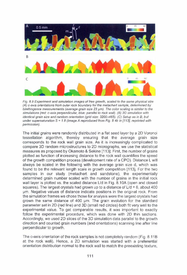
Fig. 8.9 Experiment and simulation images of free growth, scaled to the same physical size. (A) c-axis orientations from outer rock boundary for the metachert sample, determined by birefringence measurements (average grain size 23 pm). The color scaling is similar to the simulations (red: c-axis perpendicular, blue: parallel to rock wall). (B) 2D simulation with identical grain size and random orientation (grid size: 3200x465). (C) Setup as in B, but under supersaturation S = 1.8 (Image A reproduced from Fig. 8.4b in [113], reprinted with permission).

The initial grains were randomly distributed in a flat seed layer by a 2D Voronoi tessellation algorithm, thereby ensuring that the average grain size corresponds to the rock wall grain size. As it is increasingly complicated to compare 3D random microstructures to 2D micrographs, we use the statistical measures as proposed by Okamoto & Sekine [113]: First, the number of grains plotted as function of increasing distance to the rock wall quantifies the speed of the growth competition process (development rate of a CPO). Distance L will always be scaled in the following with the average grain size d, which was found to be the relevant length scale in growth competition [113], For the two samples in our study (metachert and sandstone), the experimentally determined grain number scaled with the number of grains in the initial rock wall layer is plotted vs. the scaled distance L/d in Fig. 8.10A (open and closed squares). The largest crystals had grown up to a distance of L/d = 6, about 400 pm. Negative values of distance indicate positions in the original rock. From the simulation frames we chose those for analysis were the largest crystals had grown the same distance of 400 pm. The grain evolution for the standard parameter set in 2D (red line) and 3D (small red circles) both fit very well to the experimental value. To get comparable results, it was important to exactly follow the experimental procedure, which was done with 2D thin sections. Accordingly, we used 2D slices of the 3D simulation data parallel to the growth direction and counted grain numbers (and orientations) scanning line after line perpendicular to growth.

The c-axis orientation of the rock samples is not completely random (Fig. 8.11B at the rock wall). Hence, a 2D simulation was started with a preferential orientation distribution normal to the rock wall to match the preexisting texture,

111

which gives a similarly good agreement (#3 in Fig. 8.10A, blue line). In contrast, a simulation with low supersaturation S = 1.8 (#2, resulting in the microstructure in Fig. 8.10C), indicated by the green line, clearly deviates from the experimental data. The stronger decay of the grain number plot indicates a fast initial selection process.

In addition, deviation of the observed orientation distribution R Obs(0) of an analyzed set of grains from a random orientation distribution R m d(0 ) can be determined by calculating the V-index [113]:

v =n

- Robs(e)\d8 * y |Rrnd(9) - Robsm M (8 .8)with A0 = ^ and Rrnd(6) = cos ( f - d) - cos ( f - (0 + A 0))

The integral in this calculation extends over the possible angles between the c-axis orientation and the fracture normal 0 from 0 to 90°, and is approximated in Eq. (8.8) by a discrete summation of n (here n = 9) bins of angular width A0. Thus, a V-index of 0 indicates complete random fabric, whereas the maximum of 1.67 (for n = 9) is reached for perfect alignment of all grain c-axes. Grain orientations have been analyzed along lines perpendicular to the fracture boundary in a thin section (or in 2D simulation images, for 3D simulations layer slices were used in the same way). The V-index plotted again as function of scaled distance L/d from the seed plane is depicted in Fig. 8.1 OB for both rock samples and the 2D and 3D simulation discussed above. The 2D simulation results (#1, #2) obviously deviate in magnitude from the experiment, but show the same general trend. The metachert sample shows a step-like increase at the rock wall, which could be attributed to a selective growth of grains with subnormal c-axis orientations. To test this hypothesis, we modified the orientation distribution in one simulation to describe preferentially subnormal oriented starting grains, resulting in a much better agreement thereafter (#3 in Fig. 8.10B). When analyzing the 3D simulation (#4 in Fig. 8.10B), which was adapted to the metachert grain size, no such mechanism is necessary to explain the initial high texture index. To reduce the fluctuations, five 2D scans at different slices of the simulation box were averaged to give the results in Fig. 8.1 OB (red circles). The major characteristics of textural evolution are reproduced by the 3D simulation well.

112

Fig. 8.10 Statistical comparison of experiment and simulations (solid lines for 2D and small circles for 3D) for competitive free growth. Sample data is given by filled and open black squares. Simulations #1 - #3 are in 2D, #4 in 3D. Supersaturations are S = 3.6, except simulation #2 (S = 1.8). All simulations start with random grain orientations, except simulation #3, where a preferentially subnormal c-orientation distribution was created. (A) Number of surviving crystals, normalized with number of grains at the initial vein/host rock boundary. (B) c-axis fabric measure (V-index) quantifying deviation from random c-axis orientation distribution.

As a simplified model of the geological process under consideration, we reproduced the syntaxial sealing of the synthetic hydrothermal vein from both sides of the open space. An experimental microstructure is given in Fig. 8.11 A for the metachert sample [113], with the initial rock wall boundary indicated as dashed line. An example for a simulated fracture filling in 2D is shown on Fig. 8.11B at a time step, where the remaining liquid space is comparable to the experiment. As the width of the slit aperture cut into the rock material is large

1 1 3

compared to the average grain size, grain orientations on upper and lower parts of the 'fracture' are not correlated and thus were chosen independently in the simulation. This may be different in naturally occurring cracks, which would leave grains with identical orientations on both sides. Although the simulation was performed in 2D, many details appear similar: strongly misaligned grains (blue) are quickly overgrown in the competition process. Even the short distance of the vein aperture (300 pm) is sufficient to produce a grain fabric in the fracture with dominating c-axis angles from 45° to 90°, similar to the results of the hydrothermal growth process. When subnormal oriented grains (forming a sharp tip) impinge on their counterparts during vein closure, characteristic wavy grain boundaries are formed at several places. An example in which the encountering grains have similar orientations in experiment and simulation, is indicated by ovals in Fig. 8.11. These structures would be recognizable in the completely sealed vein structure and could be used as a marker for the boundary between upper and lower part.

A

Fig. 8.11 Syntaxial vein sealing (color scale as in Fig. 8.9): (A) c-axis orientations of partly sealed synthetic vein in metachert sample JU4-4IK with grain size 140 pm from previous study (image reproduced from Fig. 8.7d in [113] with permission), pore space: grey, black scale bar: 0.3 mm. (B) Simulation results, pore space in white color.

Fig. 8.12 shows four time steps of a 3D sealing simulation for a smaller fracture with aperture width of 80 pm and accordingly reduced average grain size of 7 pm. This was done to reduce the computational costs. The simulation starts with a longer initial phase of rest with low mineral mass accretion, in which mainly the grain facets are formed (Fig. 8.12A). The retardation can be explained by the small grain size leading to a higher average interface curvature, which is equivalent to a negative driving force. Thereafter, the well aligned crystals finally protrude into the open space and grow fast in the form of quartz needles (Fig. 8.12B), and finally bridge the gap with an interlocking structure. Complete hydraulic sealing appears here at t = 10.3 days (Fig. 8.12D), with a remnant porosity of 2%. With the approximation of a constant supersaturation assumed in the simulation, this sealing time must be regarded as a lower limit, as in the late stage of growth the reduced fluid transport capability must be taken into account.

114

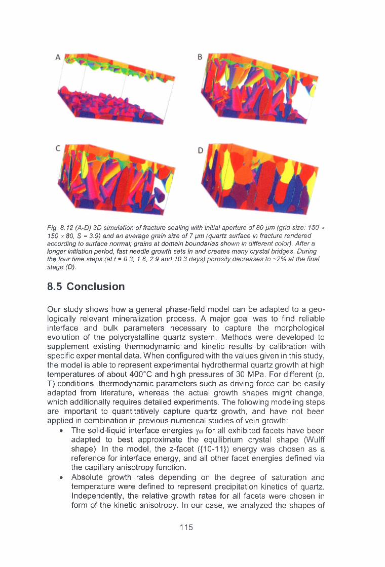
Fig. 8.12 (A-D) 3D simulation of fracture sealing with initial aperture of 80 pm (grid size: 150 x 150 x80, S = 3.9) and an average grain size of 7 pm (quartz surface in fracture rendered according to surface normal; grains at domain boundaries shown in different color). After a longer initiation period, fast needle growth sets in and creates many crystal bridges. During the four time steps (at t = 0.3, 1.6, 2.9 and 10.3 days) porosity decreases to ~2% at the final stage (D).

8.5 Conclusion

Our study shows how a general phase-field model can be adapted to a geologically relevant mineralization process. A major goal was to find reliable interface and bulk parameters necessary to capture the morphological evolution of the polycrystalline quartz system. Methods were developed to supplement existing thermodynamic and kinetic results by calibration with specific experimental data. When configured with the values given in this study, the model is able to represent experimental hydrothermal quartz growth at high temperatures of about 400°C and high pressures of 30 MPa. For different (p, T) conditions, thermodynamic parameters such as driving force can be easily adapted from literature, whereas the actual growth shapes might change, which additionally requires detailed experiments. The following modeling steps are important to quantitatively capture quartz growth, and have not been applied in combination in previous numerical studies of vein growth:

• The solid-liquid interface energies ysi for all exhibited facets have been adapted to best approximate the equilibrium crystal shape (Wulff shape). In the model, the z-facet ({10-11}) energy was chosen as a reference for interface energy, and all other facet energies defined via the capillary anisotropy function.

• Absolute growth rates depending on the degree of saturation and temperature were defined to represent precipitation kinetics of quartz. Independently, the relative growth rates for all facets were chosen in form of the kinetic anisotropy. In our case, we analyzed the shapes of

1 1 5

free grown needle crystals to estimate their values and found facet- specific rates which compare well to results from other experimental studies. In addition, we defined fast growth rates for non-euhedral directions, which in the simulation favors quartz crystals aligned normal to the boundary.

• The driving force for crystallization, corresponding to the difference of free energies of solid and liquid phase, was determined, and it controls whether silica is precipitated or dissolved. Microstructure and overall growth rate depend intricately on the driving force, which is a function of the supersaturation - assumed as constant in this work - and also depends on the interfacial energy between liquid and crystal, which changes with the local geometry.

In the quartz veins examined here, crystal aggregates evolve by interaction, starting as epitaxial overgrowth of the rock fabric. This growth competition process leads to the formation of a crystallographic preferred orientation and texture evolution, which closely resembles the hydrothermal experiment. As a consequence from the comparison of simulation and experimental results, we propose the scaled grain number and the V-index as appropriate measures of validation. It was found that both parameters plotted as a function of the scaled distance from the initial wall are very sensitive to changes in the growth model parameters, variance of grain sizes and the existence of a predominant texture in the rock matrix.

A strong dependency of morphology on the driving force has been found in the simulations: Whereas high supersaturation leads to more contiguous polycrystalline growth fronts, low supersaturation favours isolated growth of quartz needles and increases orientation selection. The predictions possible with this model might help to unravel aspects of the formation of vein microstructures and the estimation of growth conditions. For the late stages of vein sealing, when pore spaces are filled, transport by flow and diffusion should be considered in future work.

1 1 6

9 Cracking and healing I: modeling vein systems with the Discrete Element Method

The Discrete Element Method (DEM) ([143], [144], [145]) is a well-established technique in rock mechanics and particularly well suited to model fracture mechanical processes at the micro- and outcrop scale. DEM uses a large number of packed spherical particles that interact with their nearest neighbors via brittle, frictional elastic or plastic interaction to simulate the response of a material to applied stress and strain.

The Software that was used for the results presented in chapter 9 is the open source DEM simulation package EsyS-Particle ([146], [147])(https://launchpad.net/esvs-particle/). EsyS-Particle is fully parallelized which allows the computation of very large models (> 1 million particles) on a high performance computer cluster in reasonable time spans. The script-driven interface and the broad range of implemented particle interactions enable the creation of complex simulation setups in 3D and 2D likewise. The open source architecture allows for complex workflows such as polyphase simulations of crack seal.

We have conducted three parametrical studies on the mechanical interaction between fractures and veins. Each of the studies aimed to provide insights into specific aspects of repeated fracturing in crack-seal systems. The detailed results of all three studies were published in the Journal of Geophysical research ([148]-[150]) and are also part of the Dissertation of Simon Virgo [151].

9.1 DEM study 1: Fracture - vein interaction styles

In the first study we used a simple setup to investigate the interactions between fractures and veins at the scale of a single vein embedded in a homogeneous host rock. Servo-controlled diverging sidewalls were used to induce uniaxial tension in the models, which allowed a mode-l fracture to initiate at a notch, propagate through the model and to interact with the vein (Fig. 9.1).

1 1 7

https://launchpad.net/esvs-particle/

100 model unitsh \

10 model units

Fig. 9.1 Simulation setup used in the study: the plate-shaped volume consists of <250 000 densely packed particles connected via brittle bonds to their direct neighbors as well as to the left and right sidewalls. The model is deformed by moving the sidewalls apart at a constant rate. Blue and red particles are connected to the sidewalls via elastic bonds. The misorientation angle a of the vein (light grey particles) is defined as the angle between the normal of the vein interfaces and the extension direction. The notch at the bottom of the particle volume initiates fracturing. The bond cohesion between particles belonging to the vein differs from the bond cohesion between host rock particles resulting in different strength of host rock and vein. The fracture behaviour of the model and the interaction of the propagating fracture with the vein was systematically analyzed for a range of different combinations of 1. relative strength of vein and host rock and 2. orientation of the vein.

The results of this parametrical study show range of vein-fracture interactions, which fall in different, robust, “structural styles” (Fig. 9.2). If the veins are weaker than the host rock they tend to localize fracturing into the vein, even at high misorientation angles. Deflection at the outside of the vein host rock interface occurs if the veins are stronger than the hostrock. The fractures propagate in mixed mode along the vein interface mostly in the weaker host rock. This process can produce hostrock inclusion bands in stacked veins.

1 1 8

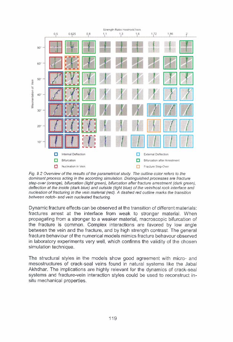
Strength Ratio Hostrock/Vein

Fig. 9.2 Overview of the results of the parametrical study. The outline color refers to the dominant process acting in the according simulation. Distinguished processes are fracture step-over (orange), bifurcation (light green), bifurcation after fracture arrestment (dark green), deflection at the inside (dark blue) and outside (light blue) of the vein/host rock interface and nucleation of fracturing in the vein material (red). A dashed red outline marks the transition between notch- and vein nucleated fracturing.

Dynamic fracture effects can be observed at the transition of different materials: fractures arrest at the interface from weak to stronger material. When propagating from a stronger to a weaker material, macroscopic bifurcation of the fracture is common. Complex interactions are favored by low angle between the vein and the fracture, and by high strength contrast. The general fracture behaviour of the numerical models mimics fracture behavour observed in laboratory experiments very well, which confirms the validity of the chosen simulation technique.

The structural styles in the models show good agreement with micro- and mesostructures of crack-seal veins found in natural systems like the Jabal Akhdhar. The implications are highly relevant for the dynamics of crack-seal systems and fracture-vein interaction styles could be used to reconstruct in- situ mechanical properties.

1 1 9

Misorientation angle: 30° Strength ratio hostrock/vein: 1:2

Fig. 9.3 View on the face of fracture deflected at a vein. The vein is twice as strong as the hostrock. Depending on the relative strength of the interface, slivers ofhostrock remauin at the fracture face and get incorporated into the vein as hostrock inclusions. (A) strong interface: the hostrock inclusion is almost continous. (B) weak interface: only isolated patches of hostrock remain on the fracture face.

9.2 DEM study 2: evolution of vein networks in changing stress fields

The second DEM study on fracture-vein interaction aimed to investigate the influence of veins on fracturing at the scale of a whole layer and the formation of complex vein patterns, which form in multiple generations of fracturing and sealing in variable stress fields [149]. At this larger scale, the effect of multiple simultaneously propagating fractures has to be considered and therefore a different loading mechanism was chosen that resembles true triaxial boundary conditions in a rock with an alternating stratigraphy. The setup consists of a brittle layer, sandwiched between two layers of quasi-viscous DEM material. A vertical compressional loading was applied and two moving sidewalls allowed a uniaxial horizontal expansion of the model. The result is a distributed tensile stress, induced in the brittle layer, parallel to the extension direction by frictional drag of the deforming ductile layers (“boudinage loading”). In contrast to the

120

first study where a single fracture spanning the whole model prevents any further accumulation of tensile loading, this setup allows multiple subparallel fractures to form in the brittle layer.

To model the dynamic growth of crack seal vein networks we implemented a workflow into ESyS-Particle that detects fracture in a model and seals them with vein cement so that the result geometry of one simulation provides the input geometry of another simulation (Fig. 9.4). This enables us to study the evolution of complex vein networks in changing stress conditions without defining a priori vein geometries.

The set of extension fractures that forms during the first deformation phase is sealed, rotated around a vertical axis and deformed again. The parameters varied are the relative strength of the veins and the host rock as well as the amount of rotation in between the phases of extension.

We find different types of fracture behavior in the second generation depending on the strength contrast between veins and host rock and amount of rotation:

Fractures reactivate existing veins even if the misorientation is very high. Shortly after the reactivation of the veins a second type of fractures forms in the hostrock at a high angle to the reactivated veins (Fig. 9.5). The orientation of these antithetic fractures depends on misorientation angle of the veins, but not on the strength contrast between hostrock and veins. Neither the reactivated veins nor the antithetic fractures are normal to the bulk extension direction of the model for intermediate misorientation angles of the veins.

Weak veins in misorientation to fracturing always enhance the lateral connectivity of the fractures in our models and lead to increased hydraulic conductivity parallel to the extension direction. This finding is of major importance for the assesment of permeability in vein containing fractured reservoirs as well as for the paleostress analysis on the basis of complex vein systems.

Misoriented veins that are stronger than the hostrock do not have such a strong effect on the fracture behavior. The orientation of second-generation fractures is influenced only locally at the veins where external deflection occurs. The connectivity of the fracture system is reduced for very high strength contrasts that prevent the veins to break even at high strain. The deflection length along stronger veins is usually short because the strain can transfers to one of the closely spaced existing fractures across the vein. Models with thicker veins have shown vein aperture does not have a significant influence on the deflection length.

121

1. deformation simulation

2. relaxation

3. rotation + sealing

Y Y

Fig. 9.4 Schematic representation of the workflow used to model a crack-seal cycle: (1) a brittle layer of bonded particles is deformed between two quasi-viscous layers under vertical compression and uniaxial horizontal extension, (2) the fractured brittle layer (in map view) is extracted and fed into a simulation with high damping that minimizes the potential energy and equilibrates the geometry with free boundary conditions, and (3) open space in the relaxed geometry is filled up with vein particles and is rotated around a central vertical axis. Particles outside the new boundary box are discarded, and the empty corners of the new boundary box are filled with new host rock particles. New bonds are created between neighboring particles, and finally, the top and bottom dashpot layers are added. The geometry can now be used as the input for the deformation simulation.

122

^ vein parade

— sira ned bond (tensile)

# broken host rock bond

# broken vein bond

# broken interface bond

Fig. 9.5 State of the second generation model with 30° of rotation and a vein bonds 50% weaker than host rock bonds at 3 timesteps during the deformation. The upper half of the roseplot shows the normalized orientation of all fractures in the model at the given timestep while the lower half only takes fractures into account that have formed within the last 2500 timesteps. The visualized models indicate veins with grey particles. The hostrock is transparent. Broken bonds are depicted as colored disks. Broken vein bonds are red, broken interface bonds green and broken hostrock bonds blue. Bonds that are currently under high tensile strain are highlighted in red to indicate the state of the stress field. t= 17500: fractures have reactivated most of the veins. At some vein tips the fracture has already left the vein and resumes propagation in the host rock. t=30000: the veins are fully reactivated. The first hybrid fractures have started propagation into the hostrock at a high angle to the reactivated veins. t=50000: the reactivated veins are fully connected by antithetic fractures. Fractures that have formed normal to the extension direction in the distal host rock have started to curve towards the free surface of reactivated veins.

9.3 DEM 3: Effect of boundary conditions on fracture- vein interactions

In the third DEM study we compare the differences between the two loading methods introduced in the earlier studies and investigate how the styles of fracture-vein interactions change in regard to the boundary conditions. The main question is whether the mechanism of fracture-vein interaction remains stable at the scale of a single fracture tip interacting with a vein or if different processes determine the fracture behavior under the different loading conditions. For this we deform some of the model geometries used in the first parametrical study again with differnet boundary conditions. Instead of uniaxial

1 2 3

tension, the models are deformed under boudinage boundary conditions, similar to those introduced above.

In total, 7 models of the 65 models from the initial parametric study are re-used to simulate the vein-fracture interaction under boudinage loading for comparison.

One fundamental difference in the fracture behavior under the different loading conditions is that in uniaxial tension a single fracture can release all stress in the model since the stress is applied only from the left and right wall and requires a bonded connection between these walls to be sustained. In boudinage loading conditions the stress is induced parallel to bedding across the entire brittle layer. This allows multiple subparallel fractures to form and also leads to more distributed fracturing within the model. Under boudinage loading multiple fractures can grow simultaneously, leading to a higher degree of fracture-fracture interaction which is reflected in a higher tortuosity of the fractures.

Weak veins have a very similar effect on the fracture development in both loading scenarios: fractures tend to nucleate in the vein rather than in the stronger hostrock. At low misorientations of the vein, these fractures deflect and interconnect at the vein-hostrock interface. In boudinage loading the fractures have a higher tendency to extend from the vein into the surrounding hostrock, but only after the vein is fully reactivated. Vein reactivation and internal deflection of fractures are very robust fracture-vein interaction styles under both loading conditions (Fig. 9.6).

A relatively strong vein at misorientation to the fracture can deflect incoming fractures at its interface (external deflection). This phenomenon was observed in both boudinage- and uniaxial tension loading (Fig. 9.7), however, in boudinage loading conditions it requires the strength contrast to be higher. In most boudinage simulations stronger veins were overcome via the fracture- step over mechanism [152], where a fracture joins with a fracture that has nucleated on the opposite side of the vein. External deflection and fracture step-over can be regarded as competing mechanisms, the latter being more effective in boudinage loading conditions because of the better availability of suitable fractures.

Under certain configurations of vein strength and misorientation dynamic bifurcation of the fracture can be observed in uniaxial tension simulations when a fracture tip accelerates to a critical speed upon entering the weaker material. This behavior was never observed under boudinage loading conditions. Here the ductile layers above and below the brittle layer act as a damper which inhibits the large fracture tip acceleration. Furthermore, and more importantly, the numerous simultaneously propagating fracture tips in the boudinage models prevent that one single fracture tip can propagate over a larger distance without interfering with preexisting fractures which dramatically decreases the probability of acceleration to critical speed and dynamic bifurcation.

1 2 4

Fig. 9.6 Comparison of a model deformed in uniaxial tension (a) and boudinage boundary conditions (b). The vein is half as strong as the host rock and the vein misorientation amounts to 40°. Fractures in both models initiate as en echelons within the weaker vein and deflect at the vein/host rock interface. Under boudinage conditions the fractures propagte in various location into the stronger host rock.

Fig. 9.7 Comparison of a model deformed in uniaxial tension (a) and boudinage boundary conditions (b). In both models the misorientation of the vein is 30° and the vein is twice as strong as the host rock. The fractures that develop in the models are not able to penetrate the stronger veins and interact with the veins via external deflection. In boudinage loading the fractures initiate not only at the notch but also in the host rock above the vein and deflect at the vein at both interfaces.

1 2 5

10 Cracking and healing II, progressive cracking and healing

The findings o f this chapter are also presented in Vass et al., [153]

10.1 Introduction

Fracturing due to fluid overpressures within the rock is a process termed hydrofracturing. Hydrofracturing can be induced and of natural origin. Induced hydrofracturing has long been used as a well stimulation technique in hydrocarbon and geothermal wells to enhance well productivity by fracturing the reservoir and inducing flow towards the well. Natural hydrofracturing takes place in the Earth’s crust as a result of elevated fluid pressures that are accounted for the formation of horizontal extensional fractures at great depths in the crust. Natural hydrofracturing has long been recognized as an important deformation process within the rock systems ([154]-[156]).

Fluid overpressures within the crust can be triggered by various processes, such as those that directly affect the system’s porosity (e.g. deformation, cementation/healing of fractures), the amount of fluid within the system (e.g. due to dewatering, thermal fluid expansion or hydrocarbon generation) or the fluid density ([157]-[161 ])(). These processes directly influence the fluid pressure and can induce overpressures in the rock systems. These overpressures have been shown to induce seepage forces that can locally modify the principal stresses ([62], [163]), Heterogeneities and mechanical anisotropies within the rock suite can also reorientate principal stresses [165]. These processes altogether lead to the small- and large-scale deformation of the rock system.

Both the importance of hydrofracturing and the lack of detection of the process in nature have provoked a great amount of numerical models ([1], [96], [165]- [173]). The different models face the same complexity as hydrofracturing involves (1) elastic deformation of the matrix triggered by fluid pressure, (2) fluid flow inside the fracture and (3) fracture propagation [174], The numerical simulations demonstrated that the porosity and the mechanical failure of the media are crucial in the initiation and propagation of the hydrofractures. However, most of these models lack the coupling between the fluid diffusion and deformation, as well as real (scaled) values. Their spatial and temporal resolutions are limited, they mostly deal with granular media and they do not consider healing of fractures. These limitations provided inspiration for further work in terms of numerical modeling.

We continued the work by Ghani et al. [96] and [173] (FRACS I), who presented a 2D coupled hydro-mechanical model through which the dynamics of layered porous systems were examined. We focussed on the influence of the changing material properties (e.g. breaking strength and elastic modulus) on the development of fracture and vein patterns in single and multilayered systems

1 2 6

under loading, tectonic stretching and high fluid pressures. We show that healing and vein properties play a crucial role in the dynamics of the rock systems. These large temporal and spatial scale simulations demonstrate how faults evolve that drain the system and how the system reaches a steady-state by accommodating strain on pre-existing fractures.

10.2 Model

In order to study the interplay between gravitational, tectonic and fluid forces we use a numerical model that we extend from the work of Koehn et al. (2005) and Ghani et al. [173]. Those models were based on the numerical scheme presented in [167], [168] and [171], [172],

The Latte extension of the Elle modeling environment is being used to simulate the dynamic fracturing and healing of a pressurized sedimentary sequence ([89], [175]). The basic framework for the simulations is a 2D hybrid triangular lattice data structure where equal sized, disk-shaped particles (nodes) are connected to their neighbors via linear elastic springs representing the discrete elastic solid. This lattice is superimposed on a stationary square grid through which the continuum diffusion of fluid pressure takes place. The model therefore is underlain by two main computations. One deals with the linear elastic behavior of the system, whereas the other solves the porosity- dependent fluid pressure diffusion. Detailed description of the underlying computations can be found in Ghani et al. ([96], [173]) and references therein, whereas the model description can be found in chapters 11.1 and 11.2.

Elastic and tensile constants in the model are based on a non-dimensional coordinate system where the default values are set to 1.0 (equals 10 GPa) and 0.0017 (equals 17 MPa), respectively. First, we set the matrix properties and then all other parameters for the layers or healed bonds are set relative to the matrix. This means that for instance if we set the matrix elastic modulus to 0.75 (real scale 7.5 GPa), a layer with elastic constant 8.0 would scale to 60 GPa. The breaking strength is characterized by a normal distribution between 15 MPa and 300 MPa, but in all cases the overall breaking strength of the matrix is 20MPa. The Possion ratio as a result of the lattice geometry is 0.3333. One time step in the simulation corresponds to 1000 days. All the simulations run for 20000 time steps, which therefore represents roughly 55k years. The extensional strain rate 10e'14 s~1 in the model is geologically plausible.

10.3 Results

We present six simulations with different geometries. The first four are based on a setting with a horizontal stiff layer inserted in the upper half section of the model to simulate a simple layered system with uniform porosities. The latter two simulations contain four layers (at regular intervals) where the lowermost ones are seals to illustrate a sealed reservoir.

1 2 7

We first introduce the model by examining how the healing influences the fracture patterns, and how the stress and porosity of the system evolve through time. We then present the progressive fracture development throughout 20000 time steps, which is then followed by investigating how the veins breaking strength and elastic modulus influence the deformation patterns.In the last example we examine the fracture patterns in a multi-layered sealed system. Two scenarios are shown, one where the seal has a high stiffness and one where the seal is soft. The latter simulation is presented along with the fluid pressure gradient to detect possible fluid flow.

10.3.1 Influence of healing

Experiments were performed both without and with healing in order to investigate its influence on fracture patterns, porosity- and stress evolution. Fig.10.1 shows two simulations with identical material properties (Table 10.1), wherethe deformation boxes contain a layer with an elastic modulus eight times and a breaking strength twice the matrix.

|c

timesteps

timesleps

Fig. 10.1 Two identical simulations but one without healing (a) and one where healing is applied (b). They show the open fractures (black), the porosity, and the stress (ho = differential stress, oxx = horizontal stress, oyy = vertical stress) and porosity (<p) evolution of the system, respectively, throughout 20000 time steps. Black rectangle in the middle represents a stiff layer embedded in a soft matrix. Healed bonds have the same breaking strength and stiffness as the matrix.

Table 10.1 Real scale properties for simulations shown on Fig. 10.1 to Fig. 10.4. E = elastic modulus, ou = breaking strength, <p = porosity. The default overall breaking strength is 20 MPa, whereas the corresponding 200 MPa for the healed bonds on Fig. 10.3 represent a local value.

1 2 8

Fig. 10.1 Fig. 10.2 Fig. 10.3 Fig. 10.4E (GPa) 7.5 7.5 7 .5 7.5Matrix Ou (MPa) 2 0 20 2 0 2 0

<P ( % ) 2 6 .9 2 6 .9 2 6 .9 2 6 .9E (GPa) 60 60 60 60Layer ou (MPa) 4 0 2 0 2 0 2 0

<P ( % ) 2 6 .9 2 6 .9 2 6 .9 2 6 .9

2 .2 5 ; 5 .6 3 ;E (GPa) 7 .5 15 7 .5 17; 3 7 .5 ;Healed 75bonds 8ou (MPa) 2 0 20 2 0 2 0

2 0 0

In case healing is not applied (Fig. 10.1a) a considerable amount of open fractures can be seen that are directly linked to higher porosity values. Places that are not fractured the porosities are uniformly low. The major fracture that cuts through the entire system shows the highest porosities due to constant refracturing. Looking at the porosity evolution it is clear that if healing is not applied, the porosity increases almost linearly with progressive deformation from the initial 26.9% to almost 27.8%.

Healing certainly has a great effect on the number of open fractures (Fig. 10.1b). Less open fractures are present, since they are exposed to closure throughout the entire simulation. Towards the end of the simulation a throughgoing fracture develops that, similarly the non-healing case, represents the most porous area of the system. The porosity evolution, on the other hand, significantly differs from the non-healing case. The porosity first declines and only starts to rise after time step 6000, which in turn results in overall porosity increase of the system (from 26.9% to 27.2%).

Stress evolution in both cases is almost identical. Upon deformation stress builds up, and when the differential stress reaches its maximum value the system relaxes due to major fracturing and only minor fluctuations (slip/fracturing along existing fractures and minor fracturing in matrix) can be observed. Although this behavior is similar both in case of the horizontal (oxx) and the vertical stress component (Oyy), their maximum values are reached at different timesteps. The Oxx quickly moves from compressional to the tensional regime around timestep 1000 and experiences its highest magnitude during time step 4 - 6000. The oyy on the other hand stays in the compressional regime during the entire simulation and reaches its maximum well after time step 14000. The linear increase of the oyy is observed until timestep 8000 after which the magnitude increase is no longer linear.

10.3.2 Fracture evolution

Evolution of fractures when healing is applied is shown in Fig. 10.2. The layer’s elastic modulus is eight times and the healed bonds’ elastic moduli are twice

1 2 9

the matrix (Table 10.1). The stiffness of the layer causes the layer to develop larger tensile stresses at lower strains. This results in fracturing in the layer first, whereas the matrix shows only small amount of fracturing. Fractures propagate by interconnections of smaller cracks. Even though the first bed- confined fractures step out from the layer at a relatively early stage of the deformation (T = 1900), their propagation within the matrix is not significant until there is major fracturing in the layer (T = 5700). After this stage fracturing in the layer is subordinate, whereas fracture propagation in the matrix is becoming the dominant process. Fracturing is limited after time step 9500, only the large fracture zone on the left boundary shows continuing deformation. This therefore indicates that the system is approaching a somewhat steady-state.

T = 950 T = 1900 T = 3600

Fig. 10.2 Evolution of open fractures (black) throughout 20000 time steps when healing is applied. T is the model time, whereas the shaded grey rectangle in the middle represents a stiff layer embedded in a softer matrix. Healed bonds have the same breaking strength and stiffness as the matrix.

1 3 0

10.3.3 Importance of breaking strength and elastic modulus of the healed bonds

The influence of breaking strength (or ultimate stress, ctu) of the healed bonds was investigated by varying only this parameter in the same simulation setup (Table 10.1). Three cases are presented in Fig. 10.3; one where the breaking strength of the veins is 0.4 times of the matrix, one where it is the same and one where it is ten times the matrix.

'.frfarV,

Fracture age Healing age PorosityNumber of crack-seal eventslow high20 000 ts

L'

u . . i .

10.0

Fig. 10.3 Three simulations involving different vein strength, one where the breaking strength (ou) of the healed bonds are quarter of the matrix (0.4), one where they are the same (1.0), and one where they are ten times the matrix (10.0). Shaded grey rectangle represents a stiff layer embedded in a softer matrix. We can examine the effects of the veins’ strength on the evolving fracture and healing patterns, crack-seal cycles and porosity (a-d). The age of the fracturing and healing is also shown (a), indicating that in all cases new fractures are localized at the throughgoing faults, whereas the new veins form at different locations. When the veins are relatively weak, the bottom of the box and layer heal intensely, whereas when they are strong, the new veins are more localized to the open fractures. Generally, the harder the veins, the less open fractures are present and the more intense the healing is. In case the veins are hard, the system at each healing event becomes progressively stronger, thus

131

undergoes less crack-seal cycles. The corresponding stress (Act = differential stress, oxx = horizontal stress, ayy = vertical stress) and porosity (cp) evolution is therefore entirely different (e). Stresses are elevated and the porosity drops significantly when the veins are hard. In all cases, however, the system tends to reach a steady-state represented by a relatively constant stress state with only small fluctuations.

Extremely different behavior can be observed in all aspects (Fig. 10.3a). The stronger the new bonds, the less open fractures are present (Fig. 10.3a). Not only the amount of fractures but the age of them also differs. When the healed bonds are the weakest many older fractures (i.e. those that formed at earlier time steps) are still open, whereas most of these are closed when the veins are strong. In all cases, formation of new fractures is mainly localized by the throughgoing faults.

The healing patterns reflect a dramatic change from a moderately healed system to a system which is basically clogged up (Fig. 10.3b). When the new bonds are weaker, the oldest veins appear mainly above and in the layer and subordinately in the matrix. Veins are progressively getting younger towards the bottom. In case the new bonds are the strongest the older veins still appear mainly in the layer but as the entire system is constantly healing it is difficult to observe any preferred locations of the younger veins. The youngest veins, however, seem to be associated with the fault.

Examining the number of crack-seal events reveals how the breaking strength of the healed fractures localizes the refracturing and healing (Fig. 10.3c). When the veins are weaker than the matrix, they tend to fracture easily. This is reflected in the similarity of the healing and the crack-seal (7<) pattern, which implies that after the bonds heal they will constantly fail and heal again. Localities that experienced less crack-seal events (2-6) coincide mainly with the younger open fractures. Slightly different behavior can be seen when the veins have the same strength as the matrix. Fewer veins undergo more than seven crack-seal events, whereas most of the veins and fractures only experiences limited crack-sealing (2-6 events). However, when the breaking strength of the veins is ten times the matrix, most of the box only fracture and heal once (see the older veins in the background in Fig. 10.3b). As healing now makes the entire system progressively stronger, initiation of new fractures is impeded. Even if failing occurs it seems to be restricted to the layer and to a few bigger fracture zones. Only a limited amount of localities experience more than 7 crack-seal events. Relative porosities in all cases seem to have same characteristics (Fig. 10.3d). Large through-going faults are associated with the highest porosities, whereas healed fractures decrease the local porosities.

The stress and porosity curves clearly illustrate how the behavior of the systems changes with increasing vein hardness (Fig. 10.3e). In the first case when the veins are 0.4 times of the matrix’s strength, the vertical stress component (oyy) linearly increases until time step 9000 after which the increase is less intense and the o yy rather fluctuates around a mean value. In the early stages of deformation the slope of horizontal stress component (Oxx) is steeper than the oyy but it progressively flattens out as smaller shear fractures form. Major fall at time step 9000 marks a sudden failure of the system, which, as mentioned above, relaxes stresses afterwards. The porosity (cp) shows a

1 3 2

sudden drop to the value of 26.45% at the beginning of the simulation which is then followed by a porosity-increase towards the end of the simulation reaching a value of 27.2%. The point where the porosity begins to rise coincides with the maximum differential stress (Aa).

Stress and porosity evolution is quite similar when the veins are the same strength as the matrix. The only difference is that the porosity reaches its minimum at 26.6% and its maximum at 27.4%. When the veins are the hardest the Oxx and therefore the Act magnitudes during the entire simulation are much higher than they were in the weaker cases. As the system after each healing is becoming successively harder, elevated stresses are expected. Stress curves suggest that the stress build-up is prolonged and the quasi steady-state, when the stresses show only minor fluctuations, is reached at a later stage of the deformation. Similarly to the weaker cases the system experiences its maximum Act at earlier stages (around time step 7000) but the porosity continuously decreasing till time step 17000 and reaches its maximum 25.6% at the end of the simulation. These delayed behaviors can be explained with the system being too strong to fracture efficiently.

Fig. 10.4 Open fractures (black) and healed bonds (medium grey) are shown when the veins’ elastic moduli is one third (a) and three fourth of the matrix (b), same as the matrix (c), five (d) and ten times (e) the matrix. Shaded light grey rectangle represents a stiff layer embedded in a softer matrix. All simulations show the patterns after 20000 time steps. As opposed to the soft veins, stiff veins tend to refracture affecting the fracture geometries. The effect of the elastic modulus especially in the (c), (d) and (e) case is not that significant considering the magnitude change and comparing the results from the breaking strength simulations shown on Fig. 10.3.

1 3 3

After investigating how the breaking strength of the veins affects the deformation of the system, we focused on the effects of their elastic moduli. Five simulations were performed where the breaking strength of the veins were set to default (same as matrix), all other parameters were identical to the simulation shown in Fig. 10.2, and only the elastic moduli varied between third to ten times the matrix (Table 10.1). Fig. 10.4 shows how the progressively stiffening veins influence the fracture and healing patterns of the system. It is clear that the stiffer the veins, the more open fractures are present. This is coupled with the healing pattern as the increasing number of open fractures is due to the decrease in healing in general, and to the fact that the veins are more prone to opening. Even though these differences are observable, the elastic moduli of the veins do not seem to have as great affect as the breaking strength on the deformation of the system.

10.3.4 Seals and fluid pressure gradients in multilayered systems

Multilayered seal reservoirs are quite common in nature. In these simulations we therefore introduce four layers out of which the lowermost is a seal with 0.51% porosity (Table 10.2).

Table 10.2 Real scale properties for simulations shown on Figure 5. E =elastic modulus, ou = breaking strength, <p = porositFig. 10.5a y- Fig. 10.5bMatrix E (GPa) 7.5 7.5ou (MPa) 20 20

<P (%) 26.9 26.9Bottom layer E (GPa) 60 2.25ou (MPa) 20 20<P (% ) 0.51 0.51Other layers E (GPa) 60 60Ou (MPa) 20 20<P (% ) 26.9 26.9Healedbonds E (GPa) 7.5 7.5ou (MPa) 20 20

All the layers are eight times stiffer than the matrix in simulation shown on Fig. 10.5a. The seal does not seem to have great effect on the fracture patterns, since the layers and the matrix throughout the entire deformation box fractures uniformly. The beds interact with each other by connecting the closely-spaced layer-confined fractures. These then evolve to large throughgoing faults that not only localize crack-sealing, but also provide direct communication between the lower and upper part of the system.

1 3 4

Fig. 10.5 Multilayered simulations after 20000 time steps. Dark grey shaded rectangles represent stiff layers, whereas the white one is a soft layer. In simulations (a) and (b) the lower layers are seals with porosities of 0.51%. The other layers have background porosity 26.9%. The seal seems to be only effective when it is soft as fracturing is limited within. Correspondingly, large fluid pressure gradients evolve within the seal and smaller gradients seem to intrude along the larger fractures and through-going fault (c) possibly indicating drainage.

The same simulation was performed with only lowering the seal’s elastic modulus down to third of the matrix in order to inhibit fracturing within and thus stimulating fluid pressure build-up. This scenario does seem to have a greater effect on the developing patterns (Fig. 10.5b). Compared to the previous scenario not only is the seal more intact but the two middle layers and matrix around are too. The seal in this case acts like a stress barrier that hamper fluid pressure gradients to transfer through the seal, thus inhibiting fracture initiation and decreasing fracture spacing in the middle beds. This behavior, however, no longer seems to affect the uppermost layer which shows fracturing and spacing similar to Fig. 10.5a. Even though the existence of the soft seal at the bottom makes the deformation more restricted, a fault still develops linking the top with the bottom. The development of this fault allows fluid pressures to decrease. Fluid pressure gradients are illustrated as stress fringes, which means that the thinner the fringes, the higher the gradients (Fig. 10.5c). The seal experiences the largest fluid pressure gradients, but the fringes along the throughgoing fault might indicate drainage as fluid can be pushed in from below due to the difference in gradients. These gradients might weaken the fault plane [176].

10.4 Conclusions

In summary, Vass et al.[153] show that the breaking strength of veins (relative to the breaking strength of the host rock) is a very important parameter for the mechanical behavior of the rock and thus also for the successive development of fractures in addition to the actual vein pattern that these systems produce. Fig. 10.6 shows that the vein stiffness is not very important, whereas the vein strength has a significant effect.

1 3 5

t k

10

JCoilc

</>G'<5>

0 .4

strong and soft veins strong and stiff veins

weak and soft veins weak and stiff veins

0 .4 vein stiffness 10

Fig. 10.6 Different fracture and vein networks develop depending on the vein properties relative to the host rock [153],

Vein networks (in blue, lower right hand side of figures) show intense veining when the veins are relatively strong, whereas veining is much less intense when the veins are relatively weak. Active fractures, however, are very common in systems with weak veins indicating that these systems are prone to fluid flow. Systems with strong veins, on the other hand, clog the rock and impede fluid flow, unless the whole system breaks along a large connecting fracture (or fault). In Fig. 10.7 two examples of very different vein patterns from the field area in Italy are shown. Fig. 10.7a may indicate a system with strong veins in a weak matrix leading to multiple fracturing and veining events. In case of open fractures, this system should be relatively closed according to the models. Indeed, these type of veins are thought to have formed very early in the geological history when the host rock was still soft (based on completely independent observations). Fig. 10.7b shows veins that seem to refracture and localize deformation, and thus could fit into the category of strong matrix with weak veins. The hostrock is in this field example is a folded sandstone , and the veins formed at a much later stage than those in Fig. 10.7a.

1 3 6

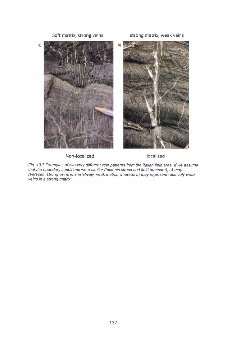
a)

Soft matrix, strong veins strong matrix, weak veins

N on-lo ca lized localized

Fig. 10.7 Examples of two very different vein patterns from the Italian field area. If we assume that the boundary conditions were similar (tectonic stress and fluid pressure), a) may represent strong veins in a relatively weak matrix, whereas b) may represent relatively weak veins in a strong matrix.

1 3 7

11 Development of hydrofractures and hydraulic breccias

The dynamic development of fracturing, fluid flow and mineralization of fractures within the Earth’s crust is complicated and depends on several processes that act on different scales. The initial development of fracture networks depends on various factors including solid stress distribution as a function of gravitational or tectonic stresses as well as the influence of the fluid pressure or fluid overpressure on the solid leading to effective stresses. Once fractures develop they change the permeability of the system and lead to localized fluid flow, material transport and eventually fracture closure either mechanical or due to mineralization. This system can be highly dynamic especially in tight rocks and in over-pressured compartments leading to partly sealed systems, hydraulic breccia development and self-organized fluid pulses [177]. On the larger scale recent research in sedimentary basins has shown that fluid overpressure should be taken into account for the effective stress law and that the effects of the fluid pressure can be anisotropic ([163], [178]). In over-pressurized sedimentary basins below seals the effective stress leads to a decrease of the differential stress [178],

Transport modes of fluids in the Earth’s crust may vary depending on the permeability of the system and the fluid input (Fig. 11.1). Slow flow in the matrix may be purely diffusional, whereas higher fluid input favors fluid flow either through a permeable matrix or along faults and fractures that form a stable network. An alternative transport mode are mobile hydrofractures that open and close depending on the local fluid overpressure. These systems may also heal and form veins, which then can re-fracture and open again leading to crack-seal veins, which are found quite often in natural systems.

Transport modes

Diffusional flow Fluid flow

Advection Mobile hydrofractures

▼ fFlow through faults/fractures Pervasive flow

Fig. 11.1 Transport modes in the crust.

1 3 8

In the following we will first discuss a numerical model of hydrofracturing that was introduced in the FRACS I report ([173]). We will have a look at the effects of layering and healing in the model and then progress to discuss the development of hydraulic breccia due to a stress switch in overpressurized systems followed by a discussion of the development of dynamic permeability networks in larger fractured systems that can be compared to mobile hydrofractures.

11.1 Hydromechanic modelling

A coupled hydro-mechanical model is developed in order to model fluid driven fracturing in a porous material that is structured as layered reservoir. In the model the solid elastic continuum is described by a hybrid lattice-particle model based on a discrete element approach coupled with a fluid continuum lattice that is used to solve Darcy pressure diffusion. The model assumes poro-elastic effects and yields real time dynamic aspects of the fracturing and effective stress evolution under the influence of excess fluid pressure gradients. It is assumed that at local scale (particle scale) the seepage force, which is a function of the fluid pressure evolution gradients, induces localized perturbation in the effective stress field, which may lead to rock deformation. Therefore, the continuum fluid phase is determined exclusively in terms of the pressure field P (x ,y ) , where (x,_y) are the coordinates of the two dimensional grid space. The inertia of the fluid is not considered in the model, which is justified for a fluid flow with low Reynolds number as in the concerned case where the fracture aperture or the particle movement is comparable to the diameter of the particles.

Using Darcy law in order to express the seepage velocity through the porous media., a time dependent governing equation (11.1) of pressure diffusion is established from the mass conservation of fluid and solid ([169], [172], [179]))

*ßdp— + uV -P = V-dt

(1 + ß P )— VP -(1 + ß P )V u (11.1)

where <j) = \ - p is the porosity, ß is the fluid compressibility, P is the fluid pressure and u is the solid velocity field. K and p stand for permeability and dynamic fluid viscosity respectively. The implementation of the diffusion equation is obtained by an unconditionally stable time implicit Alternate Direction Implicit (ADI) method routine [180]. In the model, the pressure gradient over a given volume develops according to the permeability K , an explicit output of the discrete elastic model as a function of variation in local porosity 0 ( x ,^ ) . Fluid compressibility is derived by isothermal ideal gas law (

p f a; P ), whereas local permeability K (0) is determined through the density

dependent Kozeny-Carman relation given by:

K (p ,a ) r 2 (1 - P ? 45 p 2

( 11.2 )

1 3 9

where r is spherical particle radius and 45 is an empirical constant valid for a packing of spherical beads.

The DEM elasto-plastic module ‘Latte’ of software package ‘Elle’ ([89], [90]) is used to simulate brittle deformation in porous rocks. The setup is a 2D hybrid lattice-particle model in which the discrete elements are connected with linear elastic springs. The DEM model determines the discrete description of isotropic elastic continua of a real system with elastic spring constant k as a function of the macro-scale elastic material property E .Deformation mechanics of the coupled continuum-elastic model is governed by a mutual momentum exchange between the solid and fluid phase at the scale of a unit volume cell of the continuum system. The net force F " acting on a

particle / is composed of three components: interaction force f e from neighboring particles either connected with a spring or repulsive forces, seepage force f p resulting from interstitial fluid pressure and external forces,

which are gravity f g and tectonic forces determined by imposed large scale

strains. The net force is given as

K = f . + f P+fg ■ (11.3)

In the elastic part of the model, each spring inherits a spring constant k and an equilibrium length a, which is identical to the sum of the initial radii of two connected particles. The inter-particle force f e, which acts along the connected elastic springs, is proportional to the given spring constant

= (1 1 4 )j

where the sum is over all connected neighbor nodes j , x> and x j are the

positions of the connected nodes, and «,v is the unit vector pointing from the

centroid of node / to node j .

The seepage force is generated due to the gradient of the non-hydrostatic part of the pressure field and is a result of the momentum exchange between the elastic material and the viscous fluid flowing in the reservoir. Assuming negligible fluid-solid friction at the interface surface, the only coupling force is the pore pressure gradient AP induced by a fluid source in the reservoir. The pressure force f p on the surface normal of a given particle configuration in the

unit grid cell of surface area dA is calculated by an area-weight smoothing function.

/ , = - \ PdA ’ O '!-5>

where P - P0- p f g z , with P0 the local fluid pressure in the reservoir at some

reference depth z , p f the fluid density, and g the gravity constant.

1 4 0

In the coupled model the term gravitational force incorporates the gravity effects of both the fluid and solid, where the latter together with the hydrostatic part of pore pressure determines the effective stress field a cff = {ps - p f )gz in

the system. The gravity force on each particle in the elastic module is inferred using the formulation

f « = p sxR -g C , (11.6)

where p, is the solid mass density, with S the dimension of the real

system (1000m), g is the acceleration of gravity and C=2/3 is a scale factor

derived in Ghani et al. [173] to acquire a compatible one dimensional lithostatic stress for an isotropic 2D linear elastic solid.

The two-way interaction between the porous solid and the hydrodynamic phase is achieved through the use of a projection operator from the discrete space to the fluid grid space, using a smoothing function s(rt - r 0) , which distributes the weight of a particle over the four neighboring fluid grid nodes.

\( / \ 1--- 2V Ax, 1 AvJ if lx < Ax, lv < Ay (11.7)

0 otherwise

where rt(x ,y ) , ro(x ,y) are the positions of the particle and grid node

respectively, lx - \x i - x a\ and /, = |_y.- y a\ are the relative distances and Ax ,

Ay are the lattice constant along thex and y coordinates. This setup is also called “cloud in cell” method, which renders the translation of mass m and velocity v of individual particles into continuous local particle densityP(ro) = ^ i S(ri ~ ro) and velocity fields u(r0) = i.ujs(ri - r 0) , where subscript i

runs over the number of particles present in a unit area associated with a particular grid node at position ro . The same smoothing function is also used

to obtain the drag force f p = - ] T a - r 0) ( vp/ pJ on a single particle due to fluid

pressure, index k runs over four nearest grid nodes. The basic approximations to this approach are the multiplication of the calculated 2D solid fraction with 2/3, as well as setting of a lower cutoff of the 2D solid fraction e.g., p mm =0.25, detailed descriptions are given in [173]. This type of models for the fluid-solid coupling and of mapping from 2D to 3D has been validated by successful comparison with experiments on mixed fluid / dense granular flows, in aerofracture ([169], [181], [182])( or instable sedimentation ([179], [183], [184], [185]) situations.

The numerical model is used to study the formation of different fracture patterns in heterogeneous geological settings. We show that the formation and propagation of hydrofractures is highly sensitive to different mechanical and tectonic conditions. In cases where fluid pressure is the driving force, sealing

141

layers induce permutations between the principal directions of the local stress tensor, which regulates the growth of vertical fractures and may result in irregular pattern formation or sub-horizontal failure below the seal. Stiffer layers tend to concentrate differential stresses and lead to vertical fracture growth, whereas the layer-contact tends to fracture if the strength of the neighboring rock is high. The stress field at the onset of fracturing becomes anisotropic, which eventually leads to the development of large-scale failure in the system by linking isolated tensile fractures. If the model is under extension for a long time, large-scale hydrofractures develop by linking up confined tensile fractures in competent layers (Fig. 11.2). This leads to the growth of large-scale normal faults in the layered systems, so that subsequently the effective permeability is highly variable over time and the faults drain the system. The simulation results are well consistent with some of the field observations carried out in the Oman Mountains, where abnormal fluid pressure is reported to be a crucial factor in the development of several generations of regional fracture and fault sets, including bedding-normal and bedding-parallel fracturing.

timestep 3600 timestep MOO timestep 6400

timestep 7200 timestep 17000 timestep 25000

Fig. 11.2 Fracture development in a layered sequence. Box size is 1x1km, 1 timestep represents 0.1 days, the model is extended slowly in the horizontal and fluid pressure is increased from the bottom. Horizontal layers are stiff and less permeable [961.

11.2 Modelling fracturing and sealing of fractures

Healing or the development of “veins” is applied by reconnecting springs. The simulation lattice is normally ordered representing a triangular lattice so that each normal particle has six neighbors and is directly connected to them. Once the system fractures single springs are removed from the network. Particles still retain repulsion so that each time step the model checks whether or not a non-connected neighbor also pushes into a particle. Once the system finishes fracturing during a time step the healing is applied. The healing function contains three parameters: a healing probability and the strength and elasticity

1 4 2

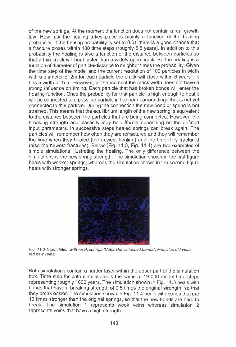
of the new springs. At the moment the function does not contain a real growth law. How fast the healing takes place is mainly a function of the healing probability. If the healing probability is set to 0.01 there is a good chance that a fracture closes within 100 time steps (roughly 5.5 years). In addition to this probability the healing is also a function of the distance between particles so that a thin crack will heal faster than a widely open crack. So the healing is a function of diameter of particle/distance to neighbor times the probability. Given the time step of the model and the current resolution of 100 particles in width with a diameter of 2m for each particle the crack will close within 6 years if it has a width of 1cm. However, at the moment the crack width does not have a strong influence on timing. Each particle that has broken bonds will enter the healing function. Once the probability for that particle is high enough to heal it will be connected to a possible particle in the near surroundings that is not yet connected to this particle. During the connection the new bond or spring is not strained. This means that the equilibrium length of the new spring is equivalent to the distance between the particles that are being connected. However, the breaking strength and elasticity may be different depending on the defined input parameters. In successive steps healed springs can break again. The particles will remember how often they are refractured and they will remember the time when they healed (the newest healing) and the time they fractured (also the newest fractures). Below (Fig. 11.3, Fig. 11.4) are two examples of simple simulations illustrating the healing. The only difference between the simulations is the new spring strength. The simulation shown in the first figure heals with weaker springs, whereas the simulation shown in the second figure heals with stronger springs.

Fig. 11.3 A simulation with weak springs (Color shows healed bonds/veins, blue old veins, red new veins).

Both simulations contain a harder layer within the upper part of the simulation box. Time step for both simulations is the same at 19 000 model time steps representing roughly 1000 years. The simulation shown in Fig. 11.3 heals with bonds that have a breaking strength of 0.5 times the original strength, so that they break easier. The simulation shown in Fig. 11.4 heals with bonds that are 10 times stronger than the original springs, so that the new bonds are hard to break. The simulation 1 represents weak veins whereas simulation 2 represents veins that have a high strength.

1 4 3

Fig. 11.4 A simulation with strong bonds (Color shows healed bonds/veins, blue old veins, red new veins).

The two simulations show a very different behavior. Weak springs lead to a localization of deformation and the material is weakening. Strong springs show a completely different behavior where the material is not refracturing but fractures around existing veins or healed bonds. This leads to a widespread healing in the whole system. In addition, the material becomes progressively more strong so that the overall behavior changes. Initial wide spread healing is taken over by a localization of deformation with a few large fractures or faults that run through the system (see younger veins in red). The initial simulations have already shown that the behavior of the system can change completely if the veins have a different strength than the host-rock.

Cyclic System s

"Real h yd ro -frac tu res"Gravity (1000m deep)

Fixed side WallsFluid pressure periodic

Fluid produced | at random locations

Hydrostatic fluid pressure

1000m

Hydrostatic fluid pressure

No tec to n ic forcing

Fig. 11.5 Setup of the model.

1 4 4

We continued to develop our hydromechanical - reactive model and continued the simulations. In our example the solid is represented by a two-dimensional cut through a part of the Earth’s crust at the depth of 1000m, where the simulation box has a height of 1000m. Gravity is applied vertically as a force in the upper boundary, and gravity forces within the box are a function of the weight of particles (or solid units). The side and bottom wall are confined elastically with free-slip boundaries (Fig. 11.5).

Fluid pressure in the simulation environment is adjusted to hydrostatic conditions as a function of model depth. Additional fluid pressure is inserted at random locations in the simulation environment to mimic local fluid pressure production. No tectonic forcing is applied, so the developing fractures are pure hydro-fractures that develop as a function of local fluid pressure gradients and gravitational forces. Fractures can heal in order to produce veins. We show four different cases with a variation in breaking strength of the newly formed bonds (veins) in relation to the host rock and we also vary the probability of healing (and hence the sealing rate).

Fluid pressure gradients

<000

Fig. 11.6 The evolution of open fractures (blue) over time in a case where healing is slow and veins break easily. The upper graph shows the evolution of the fluid pressure gradients in the model and the lower graph the increase in the amount of open fractures in the model.

The time evolution of a simulation with weak veins (that break easier than the matrix) and slow sealing is shown in Fig. 11.6. The overall amount of open fractures increases over time, however, after time step 170 a pronounced healing cycle that coincides with low fluid pressure gradients results in a reduction of the amount of open fractures. Overall, healing seems to be more pronounced in the lower parts of the model where blue dots indicate partly healed fractures. The final pattern of open fractures in the four different models

1 4 5

can be seen in Fig. 11.7. In the weak case where new veins break easy fracturing localizes leading to a pronounced fracture network through the system.

Spacing of the open fractures seems to be controlled by the speed of fracture healing. Slow healing results in a much tighter spacing of open fractures than fast healing. The slow-weak healing simulation produces a pronounced fracture network through the system that seems to be connected and could lead to drainage of fluid pressures. The fast healing system seals the fracture too fast to be interconnected across the whole system. In contrast to the patterns shown in the weak vein examples, the strong veins produce a very different pattern. Here healing seems to be very pervasive irrespective of whether healing is fast or slow. The system does hardly contain any well developed open fractures but is characterized by a pervasive porosity made up a number of partly sealed patches.

Fast strong Fast weak

Slow strong Slow weak

Fig. 11.7 Figure shows the open fractures in the 4 different cases at the end of the model runs (all the same time).

Strong veins seem to seal the system, because the system continuously becomes harder to break during sealing, whereas the weak systems lead to an increase of fracturing and thus to a well-defined open fracture network. The developing vein networks show almost the opposite pattern with the hard vein cases showing a well developed vein network (Fig. 11.8) and the weak vein cases vein networks that are not as well defined. Especially the slow weak case shows almost no healing in the upper parts of the model but more pronounced healing in the lower parts, where open fractures are sparse (Fig. 11.7).

1 4 6

Fast strong Fast weak

S low s trong S low w e a k

Fig. 11.8 Healed bonds in the system (red particles).

What does this behavior mean for the interpretation of field examples of vein and fracture networks? It seems that the observation of a well pronounced network of veins does not mean that the system had a good fracture permeability. In the simulation the system with the best defined open fracture network is the system that shows no nice vein network (slow weak case). On the contrary, the slow-strong case shows a well-defined vein network but the open fracture plot shows that this network is not representing a connected fracture network but rather a dispersed network of partly or completely sealed porosity. These partly open systems are similar to partly sealed veins that can be found in the Zechstein cores.

In an additional set of models we looked at fracturing and vein development below seals (Fig. 11.9, seal in blue). In this case also strong or hard veins produce intensive veining but not many open fractures, whereas weak veins show a well-developed fracture network but not many veins.

1 4 7

Example of a numerical simulation with seapage forces below a seal (here in blue color).

W eakveins

Hardveins

Hard veins = many veins but NOT many open fractures

Weak veins = small amount of veins but connected fracture network!

Fig. 11.9 Simulation of fracture and vein development below a seal (in blue). Fluids are entering the system below the seal. The upper two figures show a simulation with weak veins that refracture easily, with the open fracture network on the left hand side and the veins on the right hand side. The lower two figures show a simulation with hard veins that do not fracture easily, again with the open fractures on the left hand side and the veins on the right hand side.

11.3 Hydraulic fracturing, effective stress direction switch and the creation of hydraulic breccias

Vein systems that indicate paleofracture geometries can be found in variable settings including typical layer-perpendicular and layer-parallel veins. Some natural examples show layer-parallel and perpendicular veins that appear to form synchronously. One example is shown in Fig. 11.10, where veins form layer-perpendicular sets with very irregular spacing and where veins sometimes deflect at layers to form layer-parallel veins. Thin section observations of these systems indicate that the veins formed at the same time. Cobbold and Rodrigues [163] argue that layer-parallel veins can form as a function of seepage forces that develop due to fluid pressure gradients in an over-pressurized system. Fluid pressures are thought to be important in the example shown in Fig. 11.10, where these siliciclastic rocks are part of an accretionary wedge with partly high fluid overpressures.

1 4 8

Fig. 11.10 Vein network from the Ligurian Units in Italy showing interactions of layer parallel and layer perpendicular fracturing.

A more drastic example of fluid overpressures is the development of hydraulic breccias where the fractures also do not show a specific orientation.

In order to understand the interaction of fluid pressure, effective solid stress and fracturing we use a hydrodynamic numerical model [173] and try to reproduce the effects predicted by Hillis [178] and Cobbold and Rodrigues [163]. The solid in the numerical model is represented by elements connected with linear elastic springs with normal and shear forces and the fluid is represented by fluid pressure that evolves throughout the model as a function of time, permeability and boundary conditions. Fluid pressure gradients can exert forces on the solid network and the solid network defines the permeability and porosity for the fluid. In the model we simulate a 2-dimensional cross section through the crust at a depth of 3000m and a dimension of 1000*1000m. A horizontal seal is present in the middle of the model and the left and right hand sides are fixed mimicking an endless system. The initial solid stress is gravitational and the fluid pressure hydrostatic in order to simulate a sedimentary basin. We then inject fluid locally into the system below the seal. An example of a simulation is given in Fig. 11.11, where the effective or solid stresses are plotted as a function of model time. The model system shows the behaviour predicted by Hillis [178], the differential stress decreases initially with the mean stress leading to an anisotropic effect of the increase in fluid pressure. This effect can be explained by the boundary conditions, the solid is fixed horizontally and is affected by the increase in fluid pressure, whereas vertically the upper boundary condition is gravity, so that the fluid overpressure can work against this force and reduce the vertical effective stress by a larger amount than the horizontal effective stress.

1 4 9

Gravity (3000m)

time

Fig. 11.11 Effective stress evolution (average of stress below seal) and final fracture pattern in the numerical model. Graph shows evolution of stress through time. Fractures are shown in black.

After an initial increase the differential stress stabilizes and then increases towards the end of the simulation. The increase in differential stress is an effect of the seepage forces that push upwards and lead to large scale horizontal fracturing below the seal. Fracture orientation changes throughout the simulation from an initial development of vertical to conjugate shear fracture systems as an effect of local over-pressure to a change of orientation of the least principal stress from horizontal to vertical so that horizontal fractures develop. This switch between vertical to horizontal orientation of the least principal stress was predicted and observed by Cobbold and Rodrigues [163] and can also lead to the development of hydraulic breccias with no preferred fracture orientation. The effective stress switch is also illustrated in Fig. 11.12. The maximum effective stress (in red) decreases, while the least principal effective stress (initially horizontal) decreases as well. Since the side boundaries of the model are fixed simulating an endless system that increases fluid pressure (like a sedimentary basin), the horizontal effective stress cannot become tensile, so it converges to zero. The vertical effective stress, however, has an open boundary condition at the top of the model and the fluid can thus push against gravity. This leads to a switch of the vertical effective stress from compressive to tensile. It also means that the orientation of the principal effective stresses switches from the main effective stress being vertical initially to a horizontal orientation because it becomes tensile and thus is smaller than

1 50

the horizontal effective stress. This behaviour is also illustrated in the Mohr circle, the Mohr circle for effective stress moves towards the left hand side and shrinks at the same time. The rock basically fluidizes and all effective stresses go to zero. After the Mohr circle becomes a point at zero the principal effective stresses switch in orientation and the vertical stress becomes tensile. This leads to horizontal hydro-fractures.

CT(MPa) '

Fig. 11.12 Local stress switch in the model in detail (left) and corresponding Mohr circle diagram (right). Note that compressive stresses in the model are negative. Blue is the horizontal stress and red the vertical stress, green the differential stress [96],

151

11.4 Localisation of fluid pathways in over-pressured and fractured systems, switch from pervasive flow to flow through mobile hydro-channels

The following simulations are performed with a new version of the hydrofracture simulator of Ghani et al. ([96], [173]). In the new version the fluid pressure gradients are passed back to the solid model in a more localized fashion leading to more localized effects of the fluid over-pressure. All presented simulations have a system size of 1000*1000 m and represent a burial depth of the simulation box of 1000 m with gravity applied at the upper part of the box and with the box itself. The fluid is represented by an initial hydrostatic fluid pressure gradient representing 1000 m at the top and 2000 m at the bottom of the box. The first simulation (Fig. 11.13) shows a simulation with a vertical seal with low porosity and fluid is injected at random locations below the seal. The simulation shown in Fig. 11.14 contains no seal and fluid is injected randomly in the box, except for the left and right hand boundary in order to avoid boundary effects. The third simulation (Fig. 11.15) contains no seal and show injection throughout the whole simulation box simulating an endless system like a sedimentary basin.

Tim e = 10 Tim e = 30 Tim e = 50

Tim e = 60 Tim e = 70 Tim e = 80

Tim e = 90 Tim e = 100 Tim e = 110

Fig. 11.13 Time evolution of porosity below a seal (seal in yellow). Red is high porosity and yellow low porosity. Fluid is added randomly below the seal, gravity is applied vertically. The permeability channels are very variable and dynamic and drain a horizontal hydro-channel at the base.

1 5 2

The fluid drainage in these simulations becomes very dynamic, which can be seen in all simulations. Fig. 11.13 shows a low resolution simulation with a high fluid input that shows a dynamic behavior from the very start. Fluid below the seal is released through permeability channels with high porosity. These are mainly horizontal at the bottom of the simulation and then merge into more vertical channels that drain the fluid. The model is highly fractured and does not heal. This does not affect the dynamics of the model, even without healing the fluid flow is localized in opening and closing permeability networks, indicating that sealing is not essential for the development of “mobile hydrofractures” .

Time = 0

Time = 700 Time = 800Fig. 11.14 Porosity evolution over time with high porosity in blue/red and low porosity in yellow. In this example gravity is vertical and the left and right hand boundaries of the model have lower fluid pressure in order to avoid boundary effects. This scenario leads to mainly vertical porosity channels that drain a horizontal source layer at the bottom. The cannels are not stable but highly dynamic. Fluid pressure is added randomly in the whole model (except for the right and left hand boundary).

1 5 3

Fig. 11.14 and Fig. 11.15 have higher resolutions and show a switch in behavior. Initially the porosity is distributed in a random fashion and the fluid drains without developing channels. At time step 700 in the simulation shown on Fig. 11.14, and time step 2000 in the simulation shown on Fig. 11.15, the systems switch to a bimodal porosity distribution with permeability channels that are dynamic.

Time = 0 Time = 1500

Time = 2000 Time = 3500Fig. 11.15 Development of permeability channels in the model. Red is high porosity and blue low porosity. Gravity is applied vertically and the boundaries are fixed on the left and right hand side allowing now escape of fluid towards the sides. This leads to vertical channels at the boundaries and horizontal channels in the model that drain the fluid. Fluid is added randomly throughout the model.

The orientation of the channels varies depending on the boundary conditions, additional gradients towards the sides in the simulation in Fig. 11.14 leads to a dominant vertical drainage from a horizontal source at the bottom. In contrast to this, the simulation on Fig. 11.15 shows a development of a more horizontal channel network with vertical drainage at the system boundaries. The

1 5 4

development of the channels is also illustrated on Fig. 11.16 that shows the porosity evolution for the simulation shown on Fig. 11.15. The development of the channels leads to a decrease in overall porosity even though fluid is still pumped into the system. A possible interpretation of this behavior is the development of compaction “bands” between the horizontal channels with the fluid pushing against the matrix once the channels develop and thus compacting the matrix.

porosity• w

Fig. 11.16 Evolution of the porosity in the model shows the development of the channels at around time step 2000. The channeling leads to a compaction of the matrix and thus reduces the overall porosity, but increases the permeability through the channels.

11.5 Conclusions

The main conclusions that can be drawn from the hydrofracture modeling are the following:

• Effective stresses in natural systems are complicated and depend on local and far-field fluid overpressure and boundary conditions.

• Effective stresses often change anisotropically. Simplifications oft he effective stress law (for example assuming no differential stress change) are dangerous and may lead to wrong results.

• Anisotropic effective stress switches lead to hydraulic breccia and sets of vertical and horizontal fractures/veins.

• If the fluid overpressure is high, a fractured system can develop into a dynamic network of permeability channels that may represent mobile hydrofractures.

• The dynamics of opening and closing permeability networks do not necessarily require healing to stay dynamic.

1 5 5

12 Fracture network characterization

Fig. 12.1 Fracture network in a simulation of mudcracks.

12.1 Graph theory and complex networks

Graph theory can be used to study and describe the properties of fracture patterns (Fig. 12.1). It is the study of graphs which can be traced back to the famous mathematician, Leonhard Euler, and his famous Seven Bridges of Königsberg paper published in 1736 [186]. Euler attempted to solve the problem to find a walk in the city of Königsberg which traversed all the seven bridges but only once. The separated landmasses represented the main points which were connected to each other by bridges (lines). This problem and its representation provided the foundation for the graph theory. Graphs are mathematical structures that consist of vertices (or nodes) that are connected to each other by lines (edges) (Fig. 12.2).

1 5 6

Vertex degree

v, = 1 v 2 = 3 v 3 = 2 v4=1 vi = 1

Adjacency matrix v, v2 v3 v4 v5

vi 0 1 0 0 0 V2 1 0 1 0 1 v3 0 1 0 1 0 v« 0 0 1 0 0 vs 0 1 0 0 0

Fig. 12.2 Basic examples of graphs, a) Undirected, unweighted graph with numbered vertices (dots) which are connected by edges. The degree of vertices (number of neighbors) and the graphs’ adjacency matrix is also shown, b) Directed, unweighted graph where the connection only exists in the arrows' directions, c) Undirected, weighted graph where the edges are assigned numerical values. Edges with larger values will be of larger weight during any calculation.

The simplest graph is an undirected graph where the edges are lines that connect the vertices in both directions. Directed graphs, on the other hand, are made up of arrows indicating the direction of the edges, which means that the vertices are only connected in one direction. An example of this could be fluid flow, where the fluid flows from A to B but not the other way around. A graph can also be weighted by applying numerical values to either its vertices, edges or both. These numerical values can be based on characteristics, such as edge length or number of vertex neighbors. Labeling the graph this way allows identifying elements of the graph that contribute more to the structure and therefore are more important.

Vertices / and j are connected or adjacent if an edge exists between them. It is common to represent the connectivity of a graph by its adjacency matrix. The adjacency matrix is a square matrix where the entries show if there is an edge between the vertices (1 - there is an edge between vertices i and j, 0 - there is no edge between vertices i and j). For a graph with no loops this will give 0 to the diagonal elements. Undirected graphs have a symmetric adjacency matrix since a/y=a;/. The adjacency matrix of a directed graph will also include the direction of edges; if the edge points from vertex / to vertex j then a,j=0 but aji=1.

Two vertices that are not directly connected to each other (i.e. are not neighbors) might be still reachable from one to the other. The sequence of edges that lead from vertex / to j is called a path and the number of edges it contains is the path length. Certainly, several paths can exist between two vertices. In this case, one might be interested in the shortest path which means the minimum number of edges traversed to get from vertex /' to j (Fig. 12.3).

1 5 7

In general, a graph is said to be connected if a path exists between every pair of vertices.

3

Fig. 12.3 A simple, undirected graph explaining the definition of paths. Connection between vertex 1 and 3 exist through two different paths: red indicates a path with a length of two, whereas green shows a path with a length of one. This is the shortest path between them.

The total number of vertices (N) defines the order of the graph, whereas the total number of edges represents the size of the network in graph theory. It is, however, a common practice to use N as the size of the network. A graph is called a complete graph if all possible pairs of vertices are connected and thegraph exhibits its maximum edge number, . Trees represent one classof the undirected graphs, where each edge has exactly one parent vertex which results in N-1 edges. Trees therefore have a typical hierarchical structure providing a graph where deletion of any edge disconnects the tree.

Graphs are characterized by a wide range of measures. The number of edges that each vertex has gives the vertex degree. The vertex degree is three when the vertex is a triple junction as it has three edges towards its neighbors. A vertex has zero degree if it does not have any edges and therefore is disconnected from the graph. Vertices in directed graphs have both in-degrees (the number of edges terminating at the vertex) and out-degrees (the number of edges starting at the vertex). Each vertex will therefore have a total vertex degree that is the sum of the in- and out-degree. The probability that a randomly chosen vertex has degree k defines the degree distribution P(k). In the case of directed graphs two distributions, P(kin) and P(k°ut), need to be considered. The degree distribution provides the most basic measure of the graph’s topology.

Internal structures of the graphs can be well described by distance measurements. The most efficient transfer between any pairs of vertices is the shortest path between them. For this reason, the average shortest path length (L) gives a good indication of the graph structure and is defined by

L =1

2 X ( 12.1)

where N is the number of vertices and dij is the length of the shortest path between vertex / and j [187]. While this definition provides a good measure for connected graphs, it diverges for disconnected ones since if vertex / and j are

1 5 8

not connected, dij=°o. One way to eliminate this problem is to only calculate with vertices that belong to the largest connected component. However, if there are many unconnected vertices then L will diverge even more and would not be representative of the entire graph. For unconnected graphs a new measure, the so-called global efficiency (E), was introduced ([188], [189]), which calculates with the harmonic mean of the shortest path length and is defined by

1 1E = ---------- Y —

N { N - l ) % d „( 12.2 )

This formula avoids the divergence of Equation 12.1 since 1 /°° = 0 and therefore is more suitable for calculations on disconnected graphs.

Graphs can also be evaluated using the clustering concept. Clustering refers to the tendency of forming cliques near any vertex and is measured by the clustering coefficient. Two main clustering coefficients exist, global and local. The global clustering coefficient, also known as transitivity (T), is calculated as

3* number o f triangles number o f connected triplets o f vertices (12.3)

where the triplets are three vertices that are connected by two or three edges [190], In the latter case, the triplet is closed and called a triangle. The local clustering coefficient (c,) introduced by Watts and Strogatz [187] shows how close a given / vertex’s neighbors are of being a complete graph, therefore is calculated as

(12.4)

where the e, is the number of edges between the vertex’s neighbors and the k, is the degree of vertex / (Fig. 12.4). It is worth noting that Equation 12.4 is identical to the graph density measure. The difference is that the graph density takes into account the total number of edges and vertices (TV), therefore gives an overall measurement, which provides information on how complete the entire network is. The local clustering coefficient, on the other hand, looks at subgraphs, little clusters of vertices within the graph and calculates the same measure locally. Averaging the local clustering coefficients of each vertex gives the (mean) clustering coefficient of the entire graph by

(12.5)

1 5 9

1

c2 = 1/3 c2 = 0

Fig. 12.4 Simple sketches explaining the local clustering coefficient. A vertex has a local clustering coefficient of 1 if all the possible connections are present between its neighbors; and 0 if its neighbors are not connected at all or it only has one neighbor.

Quantifying graph heterogeneity is another important measurement. On way to characterize graph heterogeneity is by analyzing the vertex degree variance [191]. While this gives valuable heterogeneity information for large graphs with a wide spread of vertex degrees, graphs with a small range of vertex degrees would not stand out. In this case it might be more effective to look at the entropy of vertex degree distribution. Entropy generally refers to the lack of predictability and provides information about the amount of randomness in the analyzable data. In graph theory one can calculate the entropy of any list of data, such as the shortest paths between any pairs of vertices or local clustering coefficients. Yet, the entropy of vertex degree distribution provides the classic measure of a graph’s heterogeneity [(192], [193]). The entropy (H) is calculated as

= -£ /> (* ) log P(*) (12.6)k

where P(k) is the probability that the vertex has a degree of k [192],

Another network characteristic is to examine whether there is a preferential attachment of the vertices with regard to their degrees, i.e. do vertices with similar degrees tend to cluster together or low-degree vertices rather connect to high-degree ones? This degree-correlation is referred to as graph assortativity or assortative mixing, and is generally defined by the assortative coefficient (Pearson correlation coefficient) as

r - (12.7)

where ji and ki are the vertex degrees at the end of the ith edge in a graph with i=1,... M (M being the number of edges in the graph) [196], The coefficient lies between — 1 < r < 1, where -1 marks a disassortative and 1 an assortative network. Disassortative mixing refers to the preferential attachments of nodes with different degrees, whereas an assortative mixing represents a network with similar-degree connectivity.

1 6 0

Real networks have another important characteristic, and that is to create shortcuts between vertices. This bridging allows a more efficient communication in the network by decreasing the shortest path lengths between vertices. Many networks have found to exhibit small average shortest path length in spite of their large sizes. This characteristic is termed as small-world property and was first investigated in social studies [194]. Analyzing networks in terms of shortest path lengths revealed that both real and random networks (graphs) are associated with this property [195]. In order to distinguish between real and random networks, Watts and Strogatz [187] proposed the definition small-world on networks that have both small average shortest path lengths and high clustering coefficients. This definition therefore only applies to real networks, as those typically exhibit high clustering.

12.2 Characterizing fracture networks with Mathematica

Two main types of networks that provide the base for calculations presented here are mudcracks and hydrobreccia. All the presented networks are numerical experiment results obtained through the Elle modeling environment.

A mudcrack pattern is a hexagonal fracture pattern that forms as a result of the shrinkage of a muddy layer due to the loss of water. The dried-out layer develops this typical crack pattern, which is also similar to those formed during basalt cooling creating hexagonal columns. Mudcrack patterns were produced using the Elle software. The deformation box in this case represented the top surface of the layer which was shrinking to produce the mudcrack patterns. The layer’s mechanical properties (breaking strength and Young’s modulus) were varied to examine the pattern change. Hydrobreccias form along fault zones as a result of high fluid overpressures that break the rock creating breccia, which are usually mineralized. Hydrobreccia can also be modeled as building up fluid pressures under a seal and examine the fracture network evolution. This is how the hydrobreccia pattern was created using the Elle software. The deformation box represented a vertical section of the crust, with a size of 1000 m and 3000 m of overlying sediment. The box was confined on the sides and at the bottom, while the upper boundary, along which the gravity was applied, was open. A soft seal with a mean Young’s modulus of 3 GPa, breaking strength of 34 MPa and a mean porosity of 4% was embedded in the lower part of the deformation box. The matrix itself had a mean elastic modulus of 20 GPa, breaking strength of 17 MPa and porosity of %. Fluid was injected at random locations in each time step below the seal. This therefore allowed the initially hydrostatic fluid pressure to increase under the seal. In this experiment, while gravity was applied on top, the fluid provided the major stress on the system and therefore was the driving force for deformation.

The reason for choosing these types of fractures (i.e. mudcracks and hydrobreccia) was twofold: (1) their final patterns represented well-connected networks and (2) it was possible to examine the pattern evolution over time.

161

Prior to network analysis, image pre-processing was necessary. In case of the Elle simulation images this was simple. The images were imported into Mathematica (version 10.0.1.0), where they were binarized, color converted, thinned and then converted into graphs. The graph conversion only works on binarized and thinned images. The function itself is based on finding the junctions and end-points of the skeleton (vertices) and creating links between connected ones (edges). This eliminates the shape and the angle of the initial line (in this case fracture), and only concerns about the relationship between the vertices.

The finished image was then converted to graph using the MorphologicalGraph[image] function. This, unless the user specifies it otherwise, automatically weights the edges based on their lengths (number of pixels). Once the graph is created, it can be used for various calculations. A wide range of measures can characterize graphs. This thesis, however, limited the measures to those that provide essential measures for network connectivity and topology. For a graph g the VertexCountfg] and EdgeCountfg] function gives the number of vertices and edges that make up the graph, whereas GraphDensity[g] shows how far the graph is from being complete (that is all pairs of vertices are connected). Once these basic measures were obtained, VertexDegreefg] function was applied to list the degrees of all vertices. The entropy of the degree distribution was then calculated usingEntropy[VertexDegree[g]] to characterize the homogeneity of the degrees in the network. In addition to this, the probability that a randomly chosen vertex has a degree k was calculated and illustrated using the probability density function as DiscretePlot[PDF[Dj, x], (x, 1, 5)], where D, =EmpiricalDistribution[VertexDegree[g]] and x corresponds to the degrees between one and five. To characterize the clustering in the network, MeanClusteringCoefficientfg] and GlobalClusteringCoefficient[g] functions were applied, whereas the assortativity was obtained through GraphAssortativityfg] to illustrate the tendency of similar-degree vertex connectivity. For disconnected graphs calculating the global efficiency involved several steps. First, the dist = GraphDistanceMatrix[g] listed the shortest distances between all pairs of vertices in matrix form. As the edges of the graph were weighted automatically based on their lengths, the distances were also weighted. This essentially resulted in real relative distances between vertex pairs. As a vertex has zero distance to itself, the diagonal elements of the distance matrix are zero. These needed to be eliminated as the next step was to get the reciprocal distance, and the reciprocal of zero is undefined. Due to this, the positive distances were picked out using pos = Pick[[dist], Positive[dist]], and then the reciprocal of these were taken by div = 1/[pos]. By adding the values together Total[Total[div]] and multiplying this by 1/N(N-1), where N = VertexCount[g], the global efficiency is obtained.

12.3 Results

Six mudcrack experiments with different mechanical parameters (Young’s modulus and breaking strength) are analyzed. Changing these parameters

1 6 2

result in different style of fracture nucleation and propagation. In light of this, it is especially interesting to see whether the evolved fracture networks differ in a quantitative manner as well. Experiments A to E are new simulations and experiment F is a published experiment from the book of Bons and co-workers [89] using the same model. The mechanical parameters (Young’s modulus and breaking strength) in the model and their scaled values are listed in Table 12.1.

Table 12.1 Model and real scale properties of the mudcrack experiments.

Model scaleReal scale

(m ean values o f the normal distribution)

Young’sm odulus

Breakingstrength

Young’sm odulus

(GPa)

Breakingstrength

(MPa)ExperimentA 0.6 1 6 17

ExperimentB 1 1 10 17

ExperimentC

5 1 50 17

ExperimentD 10 1 100 17

ExperimentE

10 5 100 85

In the following we only present a full analysis of the two, fundamentally different mudcrack experiments (A and D), as well as the hydrobreccia and then compare all experiments. Detailed description of all the experiments can be found in the PhD dissertation of Varga-Vass [197],

12.3.1 Experiment A

Experiment A represents shrinkage of a soft layer with a mean Young’s modulus of 6 GPa, whereas the breaking strength of the material is kept at default (i.e. 17 MPa - mean). Even though the layer is softer than those in the other experiments, fracturing still takes place early on. Fracturing initiates at one part of the simulation box (Fig. 12.5). This fracture propagates in all directions, and eventually reaches the box boundaries. At this point the fracture propagation shifts focus onto non-fractured areas. By time step 4000 the entire box is fractured. The second half of the simulation is characterized by bridging. Bridging refers to a process where new fractures form between existing ones. This causes the areas between the fractures (polygons) to decrease in size as the new fractures cut through the unfractured areas (i.e. polygons) (see polygon sizes in time steps 4500 and 7580 on Fig. 12.5).

Converting the simulation results to graph, we can look at the fracture evolution in a quantitative manner. Only during the earliest stages of simulation (see Fig. 12.6,100 time steps) is the probability for a vertex degree 1 higher than a vertex degree 3. After this stage, the probability for a degree of 1 is successively

1 6 3

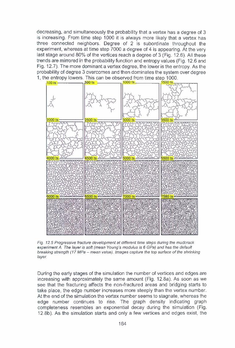
decreasing, and simultaneously the probability that a vertex has a degree of 3 is increasing. From time step 1000 it is always more likely that a vertex has three connected neighbors. Degree of 2 is subordinate throughout the experiment, whereas at time step 7000 a degree of 4 is appearing. At the very last stage around 80% of the vertices reach a degree of 3 (Fig. 12.6). All these trends are mirrored in the probability function and entropy values (Fig. 12.6 and Fig. 12.7). The more dominant a vertex degree, the lower is the entropy. As the probability of degree 3 overcomes and then dominates the system over degree 1, the entropy lowers. This can be observed from time step 1000.

100 t s -----------------------|500 ts 1 0 0 0 ts 1500 ts .

Fig. 12.5 Progressive fracture development at different time steps during the mudcrack experiment A. The layer is soft (mean Young’s modulus is 6 GPa) and has the default breaking strength (17 MPa - mean value). Images capture the top surface of the shrinking layer.

During the early stages of the simulation the number of vertices and edges are increasing with approximately the same amount (Fig. 12.8a). As soon as we see that the fracturing affects the non-fractured areas and bridging starts to take place, the edge number increases more steeply than the vertex number. At the end of the simulation the vertex number seems to stagnate, whereas the edge number continues to rise. The graph density indicating graph completeness resembles an exponential decay during the simulation (Fig. 12.8b). As the simulation starts and only a few vertices and edges exist, the

1 6 4

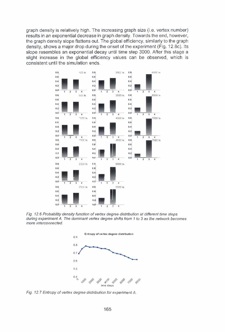
graph density is relatively high. The increasing graph size (i.e. vertex number) results in an exponential decrease in graph density. Towards the end, however, the graph density slope flattens out. The global efficiency, similarly to the graph density, shows a major drop during the onset of the experiment (Fig. 12.8c). Its slope resembles an exponential decay until time step 3000. After this stage a slight increase in the global efficiency values can be observed, which is consistent until the simulation ends.

100 ts 3000 ts o.a 6000 ts

1 I . “ B I3500 ts o.a

I J 1 11000 ts o.a

0 6

U ■ I1500 ts

0 2 ■ i y1 2 3 4

2000 ts 0 .8 ,

0.6 ■■

B _ J I « i i I __4

2500 ts o.a

1 2 3 4

I I : ■ P

6500 ts

4000 ts

1 2 3 40.8 4500 ts

5000 ts

5500 ts

1 2 3 4

500 s

0.6

4

Fig. 12.6 Probability density function of vertex degree distribution at different time steps during experiment A. The dominant vertex degree shifts from 1 to 3 as the network becomes more interconnected.

Entropy of vertex degree distribution0.9

0.8

0.7

0.6

0.5

0.4O4 ? c f ' r S ? ^ ^

time steps

Fig. 12.7 Entropy of vertex degree distribution for experiment A.

1 6 5

Looking at the mean and global clustering coefficients we see that they follow the same trend, therefore it is more convenient to describe them together (Fig. 12.8d). As opposed to the previous measures the clustering coefficients do not show a clearly defined trend. During the first 1000 time steps the clustering coefficients are zero. Approximately around the time when the number of edges overcomes the vertices, the coefficients start to increase. Except for time steps 3000 and 7000, the clustering coefficients show a dynamic increase. The drop at 3000 time steps can be simultaneously detected in the global efficiency values. As opposed to this, the drop at 7000 time steps is not reflected in a decrease but a slight increase in the global efficiency. The assortativity values are all positive indicating assortative mixing and show a general increase throughout the simulation with only minor fluctuations (Fig. 12.9). Its maximum is around 0.55, which is reached at the end of the simulation.

3 )• Vertex number > Graph density♦ Edfle number o.05

Fig. 12.8 Charts showing the vertex and edge number (a), the graph density (b), global efficiency (c) and clustering coefficients (d) of the fracture network in experiment A.

D e g r e e a s s o r t a t i v i t y

0.6

time steps

Fig. 12.9 Vertex degree assortativity indicating the network evolution during experiment A.

1 6 6

12.3.2 Experiment D

Fig. 12.10 Progressive fracture development at different time steps during the mudcrack experiment D. The layer has a mean stiffness of 100 GPa representing an extreme case, and a mean breaking strength of 17 MPa. Images capture the top surface of the shrinking layer.

Experiment D represents the stiftest case where the layer’s mean Young’s modulus is 100 GPa and its breaking strength is kept at the default value (17 MPa - mean). Due to the extreme stiffness the fracture evolution is fundamentally different from Experiment A. Fractures nucleate at random locations in the deformation box (Fig. 12.10). As these fractures do not seem to propagate, the deformation is dominated by fracturing of areas further away from the initial fractures (see time steps 500 to 2000, Fig. 12.10). This process creates fracture clusters that appear all over the deformation box. As the clusters become close to each other and most of the layer is deformed, the clusters interconnect (from time step 4000). This creates a network which will further evolve due to bridging. The non-fractured domains (polygons) become smaller as fracture bridges cut through them (from time step 7500).

1 6 7

0.8

0.6

0.4

0.20.00.8

0.60.4

0.20.00.8

0.60.40.20.00.80.6

0.40.20.0

I100 ts

U L

0.8

0.0

0.8

0.20.0

L1

I .

4500 ts

4

1 2 4

I1 2 3 4

0-8 2000 ts

0.6

0.4

0.2 l2500 ts

I ■

0.80.60.40.20.00.80.00.4

0.2

0.0

! ■3500 ts 0.8

0.6

0.4

0.2 0.0

7000 ts

3 44000 ts 0.8

I1 2 3 4

1000 ts 0.8

0 6

0.4

0.200 r ~ r 3 4

1500 ts 0.8 0.60.4

0.2

0.00.8

0.6

0.4

0.2

0.00.80.60.40.20.0

5500 ts

l ■

3000 ts 0.8

0 6

I ■

4500 ts

5000 ts 0.8

6000 ts

3 46500 ts

2 3 4

0 0

0.60. 4

4

0.6

0.4

1 3

Fig. 12.11 Probability density function of vertex degree distribution at different time steps during experiment D. The network is dominated by vertices with one connected neighbor until time step 8000. At the last two stages, however, triple junctions are more abundant than vertices with one neighbor.

The graph measures overall are also different from Experiment A. Looking at the probabilities of vertex degree distribution it is apparent that a degree 1 dominates the network until time step 7500 (Fig. 12.11). This dominance is slowly decreasing during the simulation as the degree 3 is rising. At time step 8000 the degree 1 and 3 equalizes, after which most of the vertices have three connected neighbors.

The probability for a vertex to have two or four connected neighbors is also higher during the entire simulation than it was during Experiment A. These characteristics are reflected in the entropy values, which show an increasing trend due to the relative vertex degree probabilities (Fig. 12.12). The vertex and edge numbers exhibit a dynamic increase. Until time step 7500 the network consists of more vertices than edges (Fig. 12.13a). Flowever, from time step

1 6 8

8000 the number of edges rises more steeply than the vertices. This results in a large network (vertices around 10000) with even more edges.

Entropy of vertex degree distribution

Fig. 12.12 Entropy of vertex degree distribution for experiment D.

The graph density values are in different orders as in Experiment A (Fig. 12.13b). As the network evolves the graph density exponentially decreases.

a)

14000

•i Vertex number 4» Edge number

b) Graph density0 014

d)0.12

* Global clustering coefficient

4 ^time steps

Fig. 12.13 Charts illustrating the vertex and edge numbers (a), graph density (b), global efficiency (c) and clustering coefficients (d) for experiment D.

The initial (until time step 1000) steep decrease of the global efficiency slows down until time step 7000 (Fig. 12.13c). After this stage, however, a significant increase can be observed reaching a final value of 0.0045. This value is close to the efficiency values of the previous experiments. The rising efficiency

1 6 9

correlates well with the increase in edges relative to the vertices, as well as with the switch in vertex degree dominance. The clustering coefficients are significantly higher than in Experiment A. There is a continuous, relatively slow rise throughout the simulation (Fig. 12.13d). However, the slopes of the coefficients are steeping from time step 7500, which coincides with the efficiency value rise at the end of the experiment. The network shows assortative mixing from the start of the simulation, which increases towards the end (Fig. 12.15). The last two stages especially show preferential attachments of similar degree vertices to each other. The assortativity reaches a maximum value of 0.55 at the end of the simulation.

Degree assortativity0.60.5

0.4

0.3

time steps

Fig. 12.14 Vertex degree assortativity for experiment D.

12.3.3 Hydrobreccia

The hydrobreccia simulation differs in two ways from the previous mudcrack experiments. First of all, the orientation of the simulation box relative to the stresses is different. All the previous simulation networks (i.e. images) were oriented parallel to the stresses that were responsible for the deformation. The hydrobreccia experiment, however, represents a cross section of the crust where gravity is applied on the top of the simulation box. This means that the stress acts perpendicular to the developing network (analyzed images). Second of all, during this simulation fluid pressures also contribute to the deformation and thus to the network development. These differences make it especially interesting to compare the evolution of the hydrobreccia with the earlier networks in a quantitative and qualitative manner. Deformation is initially characterized by vertical fracture formation (Fig. 12.15). These fractures appear in clusters and until time step 4000, propagate mainly in the vertical direction, i.e. in the direction of the gravity. Images from the successive time steps show that fracture propagation shifts in the horizontal direction. This is due to the fluid pressure build-up below the seal, which causes the main stress direction to switch from vertical to horizontal. The horizontal fractures make it possible for the clusters to interconnect. As a result, a well-connected fracture network is developed by the end of the simulation. Graph equivalents show that at time steps 3000 and 4000 the network is dominated by vertices with one

1 7 0

connected neighbor and only a small amount of vertices have three connected ones (Fig. 12.16). At time step 5000, however, the degree 3 starts to rise, which coincides with the formation of the horizontal fractures. Time step 6000 still shows that slightly more vertices have one connected neighbor rather than three. The successive time steps, however, exhibit the increasing dominance of degree 3 over 1 as the network becomes more connected.

3000 ts

8000

9000

Fig. 12.15 Progressive development of the hydrobreccia network. Images are binarized and thinned. They represent a cross section through the crust, and the area between the seal (on top) and the bottom of the deformation box.

0.8| 4000 ts

0.8 9000 ts

Fig. 12.16 Probability density function of the vertex degree distribution during the hydrobreccia experiment.

171

The entropy is initially small as the network is mainly made up of vertices with degree 1 (Fig. 12.17). As the degree 1 and 3 probabilities are equalizing, the entropy increases. When the degree 3 becomes increasingly dominant, the entropy starts to fall, which points to a more heterogeneous system.

Entropy of vertex degree distribution

0.8

0.4

0.33000 4000 5000 6000 7000 8000 9000

time steps

Fig. 12.17 Entropy of vertex degree distribution during the hydrobreccia experiment.

The slope for the vertex and edge number is converging until time step 6000, after which they diverge (Fig. 12.18a). While new vertices barely form at the end of the simulation (the slope flattens out), new edges still develop between existing ones. The numbers clearly reflect the vertex degree shift seen on Fig. 12.16.

a)• Vertex number♦ Edge number

1200

b)Graph density

0.006

time steps

0.005»

0.004

0.003

0.002

0.001

03000 4000 5000 6000 7000 8000 9000

time steps

C)0.012

Global efficiency

3000 4000 5000 6000 7000 8000 9000

time steps

d)0.03

• Mean clustering coefficient♦ Global clustering coefficient

Fig. 12.18 Charts showing the vertex and edge numbers (a), graph density (b), global efficiency (c) and clustering coefficients (d) for the hydrobreccia experiment.

1 7 2

The graph density values fall until time step 7000 (Fig. 12.18b). There is a slight increase in the graph density at time steps 8000 and 9000, which coincides with the entropy decrease described before. The global efficiency stays relatively constant until time step 5000, and steeply increases throughout the simulation (Fig. 12.18c). The maximum value of 0.01 is reached at the end of the simulation, which is larger than in any of the previous cases. The clustering coefficients during time steps 3000 and 4000 are zero. They show a general rise afterwards with a minor drop at time step 7000 (Fig. 12.18d). The network, similarly to the previous cases, exhibits increasing assortative mixing reaching a maximum value of 0.047 (Fig. 12.20). This is close to what was found in the other experiments.

Degree assortativity0.5

3000 4000 5000 6000 7000 8000 9000

time steps

Fig. 12.19 Vertex degree assortativity during hydrobreccia experiment.

12.4 Discussion: comparison of all experiments

Fracture initiation and the developed patterns during experiments A to E show fundamental differences. These differences can be attributed to the mechanical properties of the layer. Experiments A and B represented layers with low stiffness. Under the same strain, a material which has low stiffness breaks harder than the one which has a higher stiffness. The driving stress for fracturing is the differential stress, and if this overcomes the strength of the material, fracturing will take place. In the case of experiments A and B the soft layer develops low stresses in response to deformation, and thus fracturing is impeded. When a fracture finally initiates, the driving stress (i.e. differential stress) at the tip of this fracture is larger than the stress developed elsewhere, which means that it takes less stress to propagate an existing fracture than to initiate another one at a different location in the deformation box. This allows fracture propagation, which explains why the entire fracture network is developed from one fracture that initiated at the start of the simulation. In contrast to this, the network develops by joining separate clusters during experiments C and D. This is due to the existence of a high stiffness layer, which develops higher stresses and therefore can fracture more easily than the softer ones. When a fracture initiates, the stresses at the tips are lower than those developed elsewhere in the layer. This will impede the propagation and favor the formation of new fractures elsewhere in the deformation box. The result is the development of fracture clusters all over the box, which will eventually interconnect. In experiment E the stiffness of the layer is

1 7 3

compensated with high breaking strength, which counteracts the stiffness and allows fracture propagation. As seen in experiment F, the scaled mean of 20 GPa still favors the propagation, therefore the switch between the two types of fracturing should be somewhere between 20 and 50 GPa in the model.

The hydrobreccia experiment illustrates the importance of fluid pressures. As the seal’s stiffness impedes fracturing, the fluid pressure can build up below it leading to a switch in the main stress direction. This is clearly responsible for the formation of the horizontal fractures which allows the development of a connected network.

Characterizing topology of the fracture network can be approached from many directions. In this chapter I presented the following dynamic measures: probability density function of vertex degree distribution, entropy of vertex degree distribution, number of vertices and edges, graph density, global efficiency, mean and global clustering coefficients, and graph assortativity. Looking at the probability that a randomly chosen vertex has a certain degree can shed some light on the network connectivity. Vertices in the networks shown here have degrees between 1 and 4. If the probability for a degree 1 is higher than any other, then most of the vertices have only one connected neighbor. These can correspond to dead ends in a larger fracture or in smaller disconnected segments (e.g. two vertices linked to each other but not to the main fracture). During the initial stages, all the experiments showed higher probabilities for degree 1. This was due to either the dominance of fracture propagation over interconnections (experiments A, B, E, F) or dominance of disconnected fracture clusters (experiments C, D). The fact that most of the vertices have a degree of 1 therefore does not mean that the network is not well connected. It can be fully connected and have lots of dead ends, and fractures could act as local percolation sites. The small amount of links, however, indicates that the network is not very robust against edge-removal, which -in geological terms- means that if one fracture heals, the system can become fully disconnected. The probability for degree 1 is decreasing in all cases, whereas the probability for a degree of 3 simultaneously increases. The timing for the switch in dominance depends on the mechanical properties. During experiments A, B, E and F, the switch takes place by time step 500 (or in the latter case by time step 240). This early timing can be explained by the fracturing characteristics. The network is much tighter (small spacing), which means that the cracks are much closer to each other. The high differential stresses surround their tips as shadows, which, due to the small spacing, can easily overlap each other. Fractures will propagate into these areas causing the dead end segments to join together and the vertices with a degree 1 to disappear. This is the main process that decreases the degree 1 and ultimately increases the probability for degree 3. During experiment C and D the switch between these two major probabilities occurs much later, by time steps 8500. This can be due to the formation of fracture clusters all over the deformation box as explained before. Since fracture spacing in the beginning is quite large and the differential stresses at the fracture tips are too small, fractures do not interact, which result in many dead ends (i.e. vertices with only one connected neighbor). Clusters only interconnect at the end of the simulations resulting in the probability switch. In general we can say that the higher the probability is

1 7 4

for a vertex degree 3, the more interconnected the network. The degree 2 is relatively subordinate during all the experiments, which can be explained by the fact that these vertices tend to become triple junctions quite quickly. A vertex having four connected neighbors is also rare due to the nature of the networks (fractures rather halt at existing ones than to crosscut them).

The entropy of the vertex degree distribution is often considered as a tool to characterize disorder in the system. A high disorder, that is a heterogeneous network, features high entropy values, whereas a homogeneous one would have low entropy. It is apparent from the entropy definition that its values are completely unrelated to any connectivity measures. A network with low entropy can represent a system with all its vertices having one connected neighbor, as well as a system with all its vertices being triple junctions. In both cases, the networks are considered homogenous but the connectivity and other measures can be (and are) fundamentally different. Yet, the evolution of the entropy in the experiments nicely shows that the networks are in the process of becoming more homogenous by increasing the dominance of triple junctions.

The relative quantity of edges to vertices is indicative of the connection in the system. A nucleating fracture has two vertices and one edge. If this fracture propagates, the edge becomes longer but the vertex number remains the same. When a junction forms both the edges and vertices increase but the vertices still overcome the edges in number. In case an edge forms between two existing vertices, the number of edges starts to rise faster than the vertices. These interconnections lead to a higher amount of edges relative to vertices. During the early stages of experiments more vertices exist than edges. As the latter overcomes the former (and this coincides with the probability degree 1 and 3 switch), their slopes diverge which shows the increasing interconnections in the system. The timing of this depends on the mechanical properties - similarly to what has already been described earlier. In general the larger the difference between the vertex and edge numbers, the larger is the difference between the probability for a degree 1 and 3 as well.

The graph density in all cases decreases with increasing graph size. This indicates that the networks are getting further away from being complete graphs in spite of the interconnections. This is an artifact emerging from segmenting the fractures. Fig. 12.20 illustrates why the graphs in this chapter cannot reach completeness. A graph is complete (reach a density of 1) if all the pairs of vertices are joined together. While some can be linked without crossing any existing edges, others do need to cut through them. As in our definition when two edges cross each other, a vertex is placed at the junction. This process therefore creates more vertices, which ultimately makes the network further away from completeness since even more edges needed to connect all the vertices. As discussed before, by defining networks in a different way like Andersen and co-workers [198] did, the graph equivalents would have much higher densities.

1 7 5

Fig. 12.20 Example illustrating why the graphs cannot reach completeness, i.e. high density, (a) A simple fracture pattern and its graph equivalent (b). (c) Same graph with more connections but not complete. By linking the vertices, a few edges do not cross other edges (black dashed lines). Red dashed lines are the links that connect even more vertices but by doing so they cut through existing edges and - in our definition - create even more vertices.

Global efficiency shows how efficient the network is in transferring information. It is defined as the average shortest path distance between all the pairs of vertices. The efficiency evolution of the mudcrack experiments reveal that in all cases there is a decrease in efficiency during the early stages of deformation. This can be explained by two processes. (1) Fracture propagation elongate the edges, creating a longer path through which information also travels longer, making the network less efficient. In addition to this, (2) as the network is becoming larger the vertices are getting further away from each other, which also decreases the efficiency. As the experiments proceed and more interconnections form linking vertices far away from each other, the efficiency values start to increase. This indicates that the shortest path between vertices decrease due the newly formed edges. In geological terms this suggests that fluids could flow through the fracture network much more efficiently (and faster) than earlier. The timing of this permeability increase - again - is highly dependent on the mechanical properties of the matrix. A stiff rock could easily fracture but would (could) delay the development of a network. On the other hand, it would take more stress to fracture a softer rock but a network might develop earlier.

When comparing the efficiencies of the mudcrack and hydrobreccia experiments, evidently not only do the values differ but the slope characteristics too (Fig. 12.21). The efficiency slopes clearly diverge, which can be explained by network orientation relative to the main stress directions. Mudcracks were oriented parallel, whereas the hydrobreccia perpendicular to the main stress direction. This could imply that the mudcracks in cross-sections are much more efficient networks than parallel to the layers. Conversely, the hydrobreccia could be more efficient (has higher permeability) in the presented orientation than layer-parallel.

1 7 6

0.04

Global efficiency

♦ Experiment A♦ Experiment B

Experiment C♦ Experiment D► Experiment E ■ Experiment F► Hydrobreccia

Fig. 12.21 Composite global efficiency chart including all the mudcrack and the hydrobreccia experiments.

The efficiency measure can be of much importance in a geological framework. It can be applied to networks with different nature and appearance to compare their relative efficiency in transferring fluids. Prior to comparison, however, one needs to be aware (1) whether their networks are edge-weighted and (2) if so what do the weights correspond to. In addition, (3) in case the weights are automatically assigned based on the lengths, only networks represented on same-sized images (same pixel width and heights) can be compared. Certainly, if one is dealing with a network and an image where scale is indicated (e.g. outcrop picture showing a scale), it is better to weight the edges based on the true scale, which would get rid of the image-size dependence. Similarly, image size becomes irrelevant when one is carrying out calculations on images that are produced by the same model. This can correspond to the mudcrack and hydrobreccia networks in this chapter. As both types of networks were produced in a default size simulation box by Elle, the captured images have the same (pixel) size, which makes it possible to compare the different values. Moving onto the clustering coefficients that represent the amount of clustering (tight connections) in the system, we have seen that they do not show a continuous trend, but rather a general one with fluctuations. This can be explained by the fact that both the coefficients calculated in the classical way are very sensitive to where new edges form. The measurements only take the first neighbors into account, which means that in a simple triangle (having a maximum coefficient) if a new edge initiates from the middle of an existing one, the clustering coefficients drop down to zero since the direct connection between the first neighbors is interrupted. The network is still tightly connected but this is no longer reflected in the clustering coefficients. To eliminate this one could calculate the clustering by considering the second, third and so forth order neighbors. This is what Andresen and co-workers [198] also suggested. While their measure gets rid of the described issue, the classical clustering formulas also give relevant (and reasonable) results of the presented networks.

1 7 7

Most of the analyzed networks in this chapter were targets for dynamic measures to quantify the evolution. Provided that during one stage the clustering issue affected the coefficient values, they quickly got restored due to the fracture propagation and interaction. This is confirmed by all the experiments; if the coefficient decreases at one stage, it does not keep falling but restores and even increases (Fig. 12.22). In addition to this, the general trends clearly indicate increasing connections between the vertices, and thus increasing connectivity of the network overall. However, analysis of a single network (i.e. without any evolution data) would probably require a more precise formula for the clustering, such as the one presented by [198],

Mean clustering coefficient Global clustering coefficient0 07 0.12

■ Experiment A• Experiment B

Experiment C* Experiment D ► Experiment E n Hydrobreccia

time steps time steps

Fig. 12.22 Mean and global clustering coefficients for the mudcrack and hydrobreccia experiments.

The classical clustering formulas can also produce higher values for a disconnected network. This can be seen at experiments C and D, where the disconnected systems show much higher clustering than the other, connected ones. Around time step 9000, however, most of the experiments reach (or are about to reach) the high coefficient values produced by experiments C and D. In general, large clustering indicates tightly connected areas in the network where intense percolation could occur.

All the presented networks exhibit assortative mixing, which means there is a tendency for similar-degree vertices to join together. This finding could be a result of (1) the way the network is defined as a graph (i.e. segmentation) and/or (2) the nature of these networks. I believe the latter is more important in this case. Mudcracks generally represent hexagonal networks, which ultimately are assortative. A tightly fractured rock (breccia) would also certainly have assortative mixing. Andersen and co-workers [198] showed that an artificial and a natural network of the same type have assortative and disassortative mixing, respectively. They therefore argue that characterizing networks produced by various models are not -a t least statistically- representative of real networks. In order to validate this argument much more artificial and real geological networks need to be tested. I believe that the way of representing networks as graphs and the types of networks have important influences on all the values, including assortativity.

1 7 8

Based on the findings, the perfect geological fracture network would have (1) high global efficiency, (2) high clustering and (3) assortative mixing. High global efficiency is necessary for the fluids to move through the rock faster and more efficiently, which corresponds to well-interconnected fractures raising the potential permeability of the rock suite. High clustering is needed indicating a tightly connected network, which can provide percolation sites. The assortative nature generates a robust network against healing. The same applies to the high efficiency and clustering. In case the fluid that is flowing through the fractures is saturated, mineral precipitation can fully block (heal) open fractures decreasing the permeability. In the graphs this would be represented by removing edges. Provided that the network has those attributes mentioned above, there are more pathways (i.e. fractures) for the fluids to flow into. This means that while the permeability might decrease as a result of healing, it can still remain due to the well-connected network.

12.5 Conclusions

Characterizing fracture networks is of crucial importance in many areas, such as oil or geothermal reservoir modeling. The main interests focus on network topology, connectivity and the evolution of these features. The purpose of this chapter was to present the graph theory as a possible tool to extract this information. The study was based on a collection of patterns (mudcracks and hydrobreccia) produced by the Elle numerical model. Images from the experiments were imported into Mathematica, where after binarization and skeletonization the patterns were converted into graphs made up of vertices and edges. Vertices represented fracture junctions or dead ends, whereas the edges were the fracture segments linking the vertices.

Calculations on the graphs included vertex degree distribution and its entropy, vertex and edge numbers, global efficiency, clustering coefficients and assortativity. The defined measures indicated increasing connectivity with network growth. The dominance of triple junctions over dead end fractures, the increasing edge number over vertices and the clustering showed more links in the system, which could potentially provide more pathways for the fluid to flow through. This was also reflected in the global efficiency values that started to rise due to the fracture interconnections. High global efficiency has shown to be more important than high clustering, since calculating the clustering in the classical way can correspond to a disconnected network with high coefficients.

We conclude that a rock in which the fracture network has (1) more edges than vertices, (2) high global efficiency, (3) high clustering and (4) high assortativity would represent a very robust reservoir. The fracture connectivity contributes to high permeability, whereas the topology can potentially make the system robust against healing.

Graph theory opens possibilities to characterize networks in a quantitative and qualitative manner. It can be applied to networks of different nature and size.

1 7 9

Using the presented method and measures it is possible to examine grain microfractures in a thin section, fracture and vein patterns in a hand sample or on an outcrop, fracture traces obtained by scan-line mapping or appearing on other geological maps, and any linear patterns generated by computer models or laboratory experiments. Combined with other methods, graph theory can be a powerful tool to characterize fracture networks and their dynamic evolution.

1 8 0

13 Flow along healing fractures and faults

13.1 Introduction

Fluid flow in fractured rocks plays a crucial role in basic and applied earth sciences such as hydrogeology, economic geology, reservoir engineering and geothermal energy. Single-phase flow in fractures is mainly controlled by the geometric properties of the fracture and is studied from the micro to the reservoir scale. It is generally assumed that the geometry of a fracture remains constant during fluid flow, however, this assumption is not fulfilled in the case of reactive transport ([199]-[203]). In such settings, the hydraulic properties of a fracture evolve with time in response to either fracture sealing or wall rock dissolution. In this study, we investigate the evolution of sealing fractures by numerical techniques. At distinct time steps, the changed fracture geometries are used to compute the hydraulic properties of the fracture, which are then compared to predictions which apply the cubic law approximation.

Common remnants of reactive transport along fractures are tectonic veins. They are defined as mineral aggregates that form by precipitation from a fluid in dilatational sites [101]. Such structures form by single or multiple fracture generation events, followed by reactive transport and fracture sealing, i.e. crystallization. These processes are dynamically coupled and influence each other ([173], [202]). Reactive fluid flow in fractures plays a major role for (i) mass transfer processes in the Earth’s crust as documented by the ubiquitous occurrence of tectonic veins in the upper crust [205] and (ii) as an unwanted phenomenon in engineered applications, like enhanced geothermal systems ([206]-[208]), and for the sequestration of carbon dioxide [209]. For such applications understanding of the correlation between transport properties of the fracture(s) and ongoing sealing is crucial.Fracture sealing is a special case of crystallization from a fluid under geological conditions. Rates of crystallization at such conditions depend upon the transport of solute species to the growth front and their incorporation into the crystalline material at the fluid-crystal interface [2010]. These processes operate in sequence and so the overall rate of crystallization depends on the slowest process, i.e. the rate-limiting step [211]. Transport can be either limited by diffusion (including dispersion) or advection ([203], [212]). The rate of transport must be seen in relation to the reaction rate which is typically conceptualized as Damköhler and Peclet numbers, as discussed in [213] and [214], However, the effectiveness of transport is also influenced by the properties of the fluid. The rate of reactant incorporation at the fluid-crystal interface depends both on the properties of the fluid, e.g. the degree of supersaturation, the fluid velocity [210] and the kinetics at the mineral interfaces, therefore enabling a dynamic interplay between these processes.

In the current work, crystallization and related fracture sealing are simulated for settings corresponding to hydrothermal quartz veins by a phase-field model (PFM) by W endler et al.[125]. The numerical model is designed to mimic syntaxial quartz veins which are characterized by (i) posttectonic sealing of the

181

fracture from both sides of the wall rock and (ii) generation of the fracture geometry by a single cracking event. Syntaxial veins are a common vein type in nature [101] and many studies use their characteristics to reproduce veins in experiments ([2], [110], [113]). The phase-field model generates two quartz habits (prismatic, needle) depending on the boundary conditions and so the impact of the crystal shape on the fracture geometry is investigated as well.

Laminar fluid flow on fractures from the macro- to the micro-scale is typically characterized by the cubic law (215], [216]), which relates flow rate directly to the mechanical aperture of the fracture. Fracture roughness is the main reason for deviations from the cubic law and so corrections have been introduced ([217]-[219]. However, ongoing research has shown that deviations from the cubic law exist for which no adequate corrections are possible ([218], [220]) or which completely deviate from the underlying assumptions, e.g. the occurrence of fluid channeling in single fractures [221]. Additionally, studies of fluid flow at the pore scale ([222], [223]) have shown that a comprehensive understanding of fluid flow in geomaterials is only possible by explicit consideration of the fracture geometry at this scale. For this reason, we derive the hydraulic fracture properties by solving the Navier-Stokes equation for the fracture geometries and try to derive a correction parameter for the cubic law (respectively the hydraulic-mechanical aperture relation) in a second step that reproduces the observed fracture characteristics similar to formulations by [224],

13.2 Methods

13.2.1 Phase-field modeling of vein sealing

Up to date, only few approaches have been undertaken to model mineralization processes in rock veins at the scale of the mineral crystal grains, taking into account the full physical scenario including interface kinetics and thermodynamic driving forces like supersaturation of the fluids. In the last years phase-field models (PFM) have been proven to correctly capture the dynamics of crystal growth for various related scenarios in geosciences, e.g. single olivine crystals in the Fe-Mg system [225], for polycrystalline growth ([126], 226]) and syntectonic unitaxial vein sealing [124], A short introduction into the method, which can be considered a microscale reactive transport model, is presented for example in [227], The interface morphology is captured on a regular numerical grid by a time dependent indicator field (|>(x, t), which passes a steep but smooth transition from the level <() = 1 in the interior to <|> = 0 in the exterior of the crystalline, liquid phase regions. The governing equation for the dynamic evolution of the interface (phase-field equation) is derived from a Helmholtz free energy functional and takes into account bulk thermodynamics as well as interface energy (Gibbs-Thomson effect) and interface kinetics. Generally, the phase-field equation is solved numerically coupled to a nonlinear diffusion equation and a flow equation for mass transport.For this study, we use the formerly proposed phase-field model for quartz growth ([125], see chapter 8), which was calibrated by and compared to hydrothermal flow-through experiments mimicking vein sealing of natural

1 8 2

sandstone and metachert rock [113]. Due to the low reaction rates in the quartz system, some simplifying assumption was applied (Table 13.1).

Table 13.1. Physical conditions of flow through experiments, which were adapted for the simulation study. References: (1) (Okamoto & Sekine,[113]): fluid pressure p, temperature T, pressure gradient dp/dx, average initial fluid velocity vini, Crystal growth velocity vgrowth (2) (IAPWS [228]) International steam tables IAPWS-IF97: dynamical viscosity p, density p. (3) (Walton, [139]): Silica diffusivity D.____________________________________________________

p V g ro w th Pplcx V in i V g ro w th P P D

31 3-10'10 <0.2 MPa 1.2 10 3 3-10 '10 3.26-1 O'5 Pa 191.81 4.9-10'8MPa m/s n r1 m/s m/s s kg/m3 m2/s

(1) (2) (3)

Table 13.2. Relevant dimensionless numbers for describing flow and mineralization in sealing fracture: Reynolds number Re, ratio of velocity components longitudinal - perpendicular y, dimensionless roughness s, Damköhler numbers for advection Dai and diffusion Dan.

R e = p- ^ 7 = W / U G = G r m s / BkL

Da, = —V

kL2Da„ = - -

< 1 . 8 <4-1 O'5 < 2 10'6

Fig. 13.1 Upper panel: PF simulation of quartz sealing of a planar fracture with 300 grains. Initial aperture w as 70 pm (grid size: 150x150x80, S = 3.9) and average grain size 7 pm. Lower panel: Top view on the evolving 3D liquid surface filling the fracture, with time steps as in upper panel. (A) Growth of quartz needles creates rough surface (t = 50). (B) Crystals bridge the fracture space, visible as holes (t = 270). (C) At the final stage, porosity has decreased down to 1.5% and pore channels formed (t = 720).

Fig. 13.1 shows results of the PF simulation overtim e of quarz sealing starting in a planar fracture with 300 grains. The quartz needles growing and creating a rough fracture surface (A). With further growing, the crystals bridging the

1 8 3

fracture space (B) and at the final stage, thin pore channels formed (C) and the fracture porosity decreased dramatically.

13.2.2 Fluid flow simulations

A sealing fracture consists of the fluid filled fracture (pure liquid region) and the solid host rock (quartz) as depicted in Fig. 13.2. At the beginning of the simulation, the fracture is defined by two parallel plates, and the fluid enters the system through the left hand XY planes and leaves the fracture through the right hand XY plane. The flow in the pure liquid region is described for viscous, incompressible fluids and stationary flows. Conservation of momentum and conservation of mass can be written as the stationary Navier-Stokes equations in the pressure - velocity formulation:

—iuA u + (p u ■ V)u + Vp = f NS (13.1)

V ■ w = 0 (13.2)

In equations (13.1) and (13.2), u is the fluid velocity, p is the pressure, p is the fluid viscosity, p stands for the density and f is a force density. The simulations compute the velocity field for a given pressure drop using periodic boundary conditions on the computational box and a Dirichlet boundary conditions for the pressure. At the solid-fluid interface the no-slip boundary condition is used:

u = 0 (13.3)

Fluid flow is computed by solving the incompressible, stationary Navier-Stokes equation by an explicit finite volume (EFV) solver that employs either the SIMPLE [229] or the SIMPLEC method [230]. For the simulations a commercial implementation of this solver enabling full parallelization of calculations called GeoDict (Math2Market) is used. The required input for the solver is a voxelbased representation of the fracture geometry for which the fluid velocity in every voxel is computed. In a post-processing step, the code computes the fracture permeability according to Darcy’s law as described in Kehrwald [231] and Schulz et al.[232]. Since Darcy’s equation describes permeability in a porous medium, permeability is defined with respect to the entire computational domain. If the exclusive permeability of the fracture should be considered, a correction method for the Darcy permeability has to be applied as outlined below.

The simulations are carried out for a fluid with the physical properties of water at a temperature of 20°C and the respective values for density and dynamic viscosity. For the fracture with needle-shaped quartz, one cycle of simulations was executed under geological condition of hydrothermal quartz generation, i.e. a temperature of 430°C and a pressure of 310 bars [233], W ater at these conditions is supercritical and has a density of a fluid but a viscosity of a gas. W ater properties at these conditions are calculated according to Wagner et al.[234]. The pressure drop across the fracture geometry was adjusted in a way that the Reynold’s number for the initial fracture geometry is about 0.1. This

184

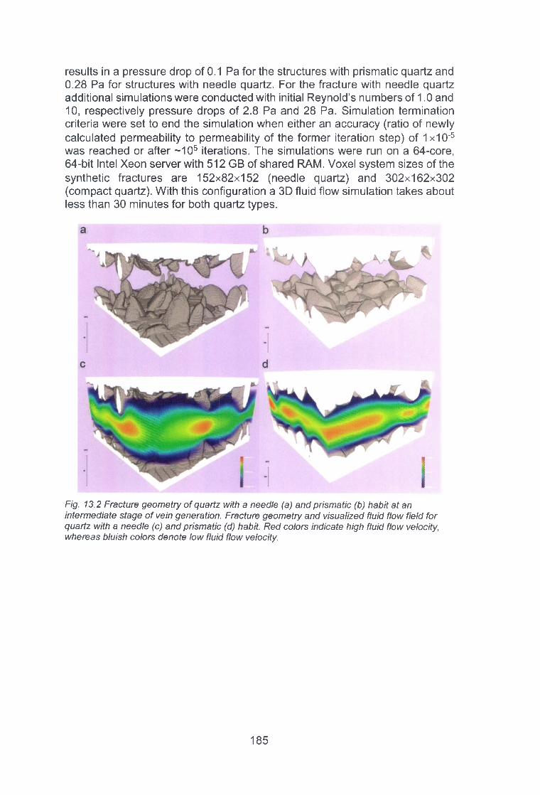
results in a pressure drop of 0.1 Pa for the structures with prismatic quartz and 0.28 Pa for structures with needle quartz. For the fracture with needle quartz additional simulations were conducted with initial Reynold’s numbers of 1.0 and 10, respectively pressure drops of 2.8 Pa and 28 Pa. Simulation termination criteria were set to end the simulation when either an accuracy (ratio of newly calculated permeability to permeability of the former iteration step) of 1x10'5 was reached or after ~105 iterations. The simulations were run on a 64-core, 64-bit Intel Xeon server with 512 GB of shared RAM. Voxel system sizes of the synthetic fractures are 152x82x152 (needle quartz) and 302x162x302 (compact quartz). With this configuration a 3D fluid flow simulation takes about less than 30 minutes for both quartz types.

Fig. 13.2 Fracture geometry of quartz with a needle (a) and prismatic (b) habit at an intermediate stage of vein generation. Fracture geometry and visualized fluid flow field for quartz with a needle (c) and prismatic (d) habit. Red colors indicate high fluid flow velocity, whereas bluish colors denote low fluid flow velocity.

1 8 5

Fig. 13.3 Formation of tortuous flow paths: Magnitude of velocity vector displayed with color scale for needle quartz morphology (fort = 18).

13.2.3 Properties of fractures

13.2.3.1 Fracture aperture

A fracture can be approximated by a pair of smooth, parallel walls with a noslip boundary, for which the stationary solution of the Navier-Stokes equation results in a parabolic velocity profile. Integrating this profile across the aperture of width a gives for the volumetric flow rate (Q in m3/s) the well-known cubic law [235], "

a3w dp 12p dx

(13.4)

where p is the dynamic viscosity, dp/dx the pressure gradient along the flow direction (x), and w the width perpendicular to flow. More generally, the cubic law (CL) expresses the linear relation between flow rate and pressure gradient,

T dp (13.5)Q = — f - Vp dx

with the transmissivity T = wa3/12 in case of parallel plates [224], Dividing Eq. (13.5) by the cross sectional area A gives the average velocity, for which the equivalent permeability of a fracture of

follows according to Darcy’s law.

(1 3 .6 )

1 8 6

When progressively rough fracture surfaces are involved, increasing deviations occur. These necessitate the introduction of correction parameters for the aperture [219] or the redefinition of the cubic law on a local basis [218], For the characterization of rough fractures, two different apertures are distinguished: (i) the mechanic aperture (am) and (ii) the hydraulic aperture (ah). am is defined as the perpendicular width of an open fracture to its reference frame where the definition of the later may be ambiguous in nature due to e.g. roughness [218]. However, the definition of the reference frame is straight forward here because smooth parallel plates (ideal fracture) are used as the initial geometry. The hydraulic aperture represents the aperture of a virtual ideal fracture that is required to allow a certain volumetric flow rate. For ideal fractures, mechanic and hydraulic aperture are identical but for non-ideal fractures ah is always smaller than am. Several studies addressed this relationship and describe ah as a function of am and the fracture roughness (e.g. [224]).

In this study, the global mechanic aperture is calculated from the vein growth simulations by integrating the whole fluid volume and dividing it by the fracture area (given by A = L2 = 150 pmx150 pm). This is equivalent to locally summing up the fluid voxel volumes for each (x, z) coordinate and averaging over all positions. The global hydraulic aperture is computed from fluid flow simulations for the sealing fractures by Eq. (13.4) based on the volumetric flow rate. Q is calculated by areal integration of all fluid velocity components perpendicular to a slice of the simulation box that is perpendicular to the pressure gradient direction.

For homogeneous porous materials, the Kozeny equation

(13.7)

gives an expression for the permeability as function of porosity <(> (ratio of fluid volume and bulk volume) and the specific surface S (ratio of liquid surface area and bulk volume). The constant co varies according to the microgeometry, which is different for granular packings, fibers or elongated pore channels. As we found a fairly good agreement of Eq. (13.7) with the measured permeability in the simulations (Fig. 13.7), an analogous form for the hydraulic aperture is derived here. First, the hydraulic aperture is related to permeability as k = ah2/12, hence with Eq. (13.7), we get

a„ = y i 2 ^ ^ (13.8)

The material variables <|> and S are related to bulk porosity, so we need to find an adequate description for planar fractures in terms of mechanical aperture and aperture standard deviation. In case of a sealing fracture, porosity is the ratio of liquid volume to initial volume, hence is defined via the actual mechanical aperture am and the initial aperture a0. We have to get rid of the latter quantity, which is hard to be defined for a partly sealed fracture sample. Hence we approximate a0 by the average peak difference between upper and

1 8 7

lower liquid surfaces apeak, which is the sum of am and a ‘roughness amplitude’, which is a multiple of aa. Thus, following porosity is derived

, _ Om _ 1^■peak Om “I" ol Op 1 + £T ( 1 3 .9 )

dm

The liquid interface can be imagined initially as a two distinct polyhedral surfaces, for which the average asperity height (given by growing crystals) depends on the aperture standard deviation aa.

13.2.3.2 Fracture perm eability

Care has to be taken to evaluate the permeability derived from Darcy’s law, which principally assumes a homogeneous material with porosity <|>. To calculate the average permeability of the fracture, Darcy’s law in the form

, k dp with (v ) = v /(p { V } ~ p d x (13.10)

is applied, so that one has to discern the superficial (Darcy) velocity averaged in the whole flux surface v and the effective velocity averaged in the liquid phase regions (v ). For each fracture morphology evolving in time we assume here a lateral continuation in the x-z plane. To correct for the increasing amount of solid precipitate we divide the superficial velocity (Eq. 13.10) by the fracture porosity, so the initial plane fracture at t = 0 will have exactly the permeability from the planar channel is given by Eq. (13.10) with a = am. As the flux rate is Q = v A with A the complete cross-sectional area of our simulation domain, then from Eqs. (13.5) and (13.10) follows

Qn _ v p (13.11)(f)Adp/dx (j)dp /dx

Additionally, the pressure drop and fluid velocity have to be considered in the permeability evaluation. If the fluid flow velocity leaves the Stokes regime of creeping flows i.e. Reynolds numbers larger than 1 ([236], [237]), then the relation between pressure drop and mean velocity is not linear anymore and even at constant viscosity, permeability is no more a real material property [238],

13.2.3.3 Reynolds number:

The dimensionless Reynolds number follows from a non-dimensionalization of the Navier-Stokes equation and expresses the ratio of inertial forces (dynamic pressure) to viscous drag forces (h: height of fluid element perpendicular to flow direction, u: velocity change due to acceleration along flow direction):

Re =0.5 p u 2

du

0.5 p u 2a

0.5 h p u L p u

p p

(1 3 .1 2 )

1 8 8

To follow this idea, the maximum velocity in the planar channel center should be used for u, and either the half aperture or the fourth of the aperture used for L (also according to different definitions in literature). For a very rough channel, the lateral distance of asperities could also give the characteristic length, if these are smaller than the typical channel aperture.To overcome the ambiguity in the definition of L, Konzuk & Kueper [239] applied the following procedure: as characteristic length, the hydraulic diameter Dh = 4A/p is used with A the cross-sectional area and p the perimeter of the fracture perpendicular to the flow direction. The characteristic velocity is gained from the overall flow rate by u = Q/A. The area A is averaged over several perpendicular sections of the fracture, where also p is determined with the upper and lower fracture contours and the averaged aperture. Hence, we obtain

pQDh 4 pQ (13.13)Re = — — = ------

Ap pp

Generally, morphological, mechanical and hydraulic properties of rock fractures may be scale-dependent, heterogeneous and anisotropic [240], In this work, we simplify the complex macro-scale geometry of a natural rock fracture by a planar fracture on the micro-scale were we study effects of precipitation. Our simulation domain is assumed to represent a typical microscopic close-in of this large fracture, which can be thought to be an infinite periodic alignment of the simulation box (Fig. 13.2). The roughness develops in time during the simulation of competitive growth of many random crystal seeds, which has been proven to provide a good representation of the real mineralization process. The domain is assumed to be large enough to be a representative part of the fracture, but anisotropy is also studied: flow-through simulations are carried out in the x- as well as the z-direction (Fig. 13.2, Fig. 13.3). The time sequence of simulation frames represents a fracture with changing morphology, especially roughness and aperture, for which two general questions are studied:

• How do the fluid properties of a mineralizing quartz system change in time?

• How can geometrical characteristics (especially roughness, mechanic aperture, fractal dimension) be used to estimate the hydraulic conductivity in a crystal-filled fracture, and are existing descriptions from literature applicable?

13.3 Results and analysis

The simulation results are split in two parts: (i) a first paragraph where the global fracture properties are discussed and (ii) a second part which deals with local fracture characteristics. Simulations of fluid flow in the fractures generated by the PFM represent the hydraulic conditions at distinct time steps in the generation of a vein. Taken together they illustrate the evolution of the hydraulic

1 8 9

fracture properties during sealing. In general, we use the fracture permeability, hydraulic aperture and the relation between hydraulic and mechanic aperture for the characterization of the hydraulic properties of the sealing fracture.

13.3.1 Global hydraulic fracture properties

The influence of pressure, temperature and pressure drop within the applied range do not have any visible effect on the permeability and on the relation between mechanic and hydraulic aperture. For this reason, only the data of the simulations at ambient conditions and at a pressure gradient resulting in a Reynold’s number of 0.1 for the initial fracture geometry are given here.

In general, the fluid flow simulations show a negative correlation between fracture sealing and the hydraulic transport properties. However, the degree of this correlation depends on the hydraulic parameter and further properties of the numerical experiment. The results demonstrate that the crystal shape has a substantial impact on the hydraulic properties and their evolution (Fig. 13.6). The most prominent impacts of the crystal shape are (i) the different velocity at which the fracture is closed (Fig. 13.4, Fig. 13.5) and (ii) the influence on the average fluid velocity and related permeability (Fig. 13.6). To avoid bulky terms, the fracture which is sealed by the simulation of crystallization of needle quartz is termed needle fracture and accordingly the other one is called prismatic fracture.

The varying speed of fracture sealing is potentially an artifact of the setup. The initial aperture for the needle fracture is 69 pm wide and for the prismatic fracture 298 pm. Hence, even if both quartz types grow at the same rate, with respect to volume, the needle fracture will close faster simply because of the smaller amount of fracture volume available for crystallization. However, the decrease in average fluid velocity and permeability is more pronounced for the needle fracture than for the prismatic fracture. After sealing 20% of both fractures, the needle fracture exposes less than 20% of its initial permeability whereas the prismatic one still disposes more than 40% (Fig. 13.6). Because both fractures are equally sealed with respect to their initial fluid volume, the differences in the initial aperture cannot be responsible for this difference. Thus, this effect is attributed to the different crystal habitus.

The average fluid velocity in the prismatic fracture drops over the entire simulation period by almost eight orders of magnitude, whereas only a drop over five orders is observed for the needle fracture. However, the velocity drop in the needle fracture has more impact on the hydraulic properties since the major portion of the drop occurs at the beginning of fracture sealing whereas the main velocity drop in the prismatic fracture occurs towards the end of the fracture sealing. A velocity drop by one order of magnitude occurs after -20% of sealing in the needle fracture whereas the same drop requires fracture sealing of about 50% in the case of the prismatic fracture.

1 9 0

Needle quartz

2□t:0)a.raoömE

u01

itr4

i(r*

iff*

■ Degree of seating

• Average fluid velocity

* Hydraulic aperture

A Mechanic aperture

0 200 400 600 800

U ic750in03

*->UreO00CT0Q

Time [nondim. units ]

Fig. 13.4 Evolution of the hydraulic properties of the fracture sealed by needle quartz. Sealing is displayed as the ratio between crystallized material and initial fluid volume of the fracture.

Prism atic quartz

U)cre0C/)0k .3Ure0 0 0 i_01 0 O

0 200 400 60Q 000

Tim e [nondim . units ]

Fig. 13.5 Evolution of the hydraulic properties of the fracture sealed by prismatic quartz. Sealing is displayed as the ratio between crystallized material and initial fluid volume of the fracture.

iii I*323t£ 10«Q.rereI? 10*

0)>

• *............... .■..................

\ X

■ D egree o f sealing

Average flu id ve loc ity

* H ydrau lic aperture

a M echan ic aperture

120

O)re0

0040

!5raaiE« 0 CL

. • O ’ • • ♦ • ♦

• . #

Perm eability needle quartz

• Sealing needle quartz

■ Perm eability com pact quartz

• Sealing com pact quartz

i \V #

Time [nondim. units ]

Fig. 13.6 Evolution of the permability and sealing in percent for compact and needle quartz.

0 >00 bUO

191

Mechanic and hydraulic aperture both decrease with increasing fracture sealing. Apart from the initial geometry, the hydraulic aperture is always smaller than the mechanical one. This is perfectly in agreement with theoretical expectations. Since sealing roughens the fractures in comparison to the initial ideal fracture geometry and roughness generally represents obstacles for fluid flow, the aperture of an ideal fracture that is required to conduct the same amount of fluid as a rough fracture will be smaller. Hence, the increasing deviation of the hydraulic aperture from the mechanical one is interpreted as a successively increasing deviation of the sealing fracture from the ideal starting geometry. Fracture sealing for both fractures did not reach 100%, because fluid flow through the fracture is completely inhibited before entire closure. This leads to the formation of isolated areas of fluid that successively become depleted in chemical reactants, thus crystallization terminates.

Normal water, Ap = 2.8 Pa

m e c h a n ic a p e rtu re1000 h y d ra u lic a p e rtu re

p e rm e a b ility x -d ir .

p e rm , x -d ir . s u p e rc r it.1 r~2K o z e n y k = Cq p /S

k * c0 * ' / S

0.01

0.001

0.0001

100 200 300 400 500 600 700 800

time [nondim. units]

Fig. 13.7 Needle quartz, time evolution of global flow properties: Evolution of average geometric aperture (black) and average hydraulic aperture (red). Development of fracture permeability (blue) is compared to the Kozeny-Carman equation. No changes for different flow regimes were observed (Re < 1.8).

13.3.2 Relation of mechanical and hydraulic apertures

Several formulations exists that predict the correlation between hydraulic and mechanic aperture (e.g. [224]). These functions have the form of a correction factor for the mechanical aperture am and depend on a roughness measure, for which either the aperture standard deviation scaled with the mechanical aperture aa/am, the fractal dimension Df or the joint roughness coefficient (JRC) is applied. We use the standard deviation here and investigate the following two frequently applied forms: From a statistical treatment, assuming isotropic distribution of the apertures, the relation

1 3ah - 0-m (1 3 .1 4 )

1 9 2

Eq. 52 in [224] can be derived. Furthermore, [241] found the empirical formula

a3h = a3, (1 - 0.9 e- ° S(,a™laa), (13.15)

for experimentally determined roughness values aa/am between 0.17 and 2.0. Both equations are frequently used and provide a good agreement in experiments with various fractured rocks and sample sizes of tens of centimeters [241],

Applying equations (13.14) and (13.15) to the data from our simulations heavily overestimates the hydraulic aperture for a given roughness. aa/am varies in our case from 0 to 2.3 for the needle fracture and from 0 to 2.1 for the prismatic fracture. A better matching of the simulated hydraulic apertures for a short initial period (t = 0 - 100, see Fig. 13.7 below) can be achieved by scaling up the roughness with factors of 5 or 10, thereby artificially increasing it.

The Kozeny relation (Eq. 13.7) gave a good agreement for the permeability during the period of sealing. Starting from this, a similar expression was derived for the hydraulic aperture by replacing specific surface area S and porosity <[> by equivalent descriptions in terms of oa and am. The resulting simple form is

and plotted in Fig. 13.8 providing a good match over nearly the whole time span of the evolving fracture. The coefficient a can be interpreted as a measure for the influence of the different crystal geometries on the flow properties. For our crystal habits, we get an optimal matching for a = 2.5 in case of needle quartz, and a = 2.0 in case of the prismatic quartz geometry.

(13.16)

1 9 3

a) Fibre quartz

Fig. 13.8 Hydraulic apertures as function of oa and am for the needle and compact quartz growth simulations. Comparison of several formulas from literature relating hydraulic (red s triangles) to mechanic (black squares) aperture am and to the aperture standard deviation a (dotted curve, abscissa at the right). Solid green: Eq. 52 from [224], solid blue: from [241], Only when scaling a with factors of 5 to 10, some initial matching can be established (t = 0 100).

For this simulations and analyses of results, we can conclude the following:

• Permeabilities are independent of Re number;• Absolute values of k about one of magnitude smaller than in microfluidic

experiments of pillar arrays with comparable porosity/aperture.

1 9 4

13.3.3 Local fracture properties - Mechanic and hydraulic aperture field

The hydraulic properties of rough fractures are not defined by an average aperture size, but depend also on the spatial distribution of aperture sizes [223], For this reason, the spatial distribution of aperture size (SDAS) and fluid flow rates for needle and prismatic quartz are computed. Complementary to these fracture representations, the aperture size distributions (ASD) are given for further details. The SDAS for the mechanical aperture is computed by summing up the voxel lengths of all fluid voxels for each (x,z) coordinate and displaying the results as a 2D image (Fig. 13.9). The SDAS for the hydraulic aperture is calculated for each (x,z) coordinate of the fracture based on the cubic law (Eq. 13.4). Required variables are the local volumetric flow rate and the pressure gradient. The local flow rate is determined by summing up all fluid velocities for one coordinate and multiplying it with the cross sectional area, i.e. area of a voxel face times the number of fluid voxels fo rtha t coordinate (Fig. 13.10) The local pressure gradient is computed based on the calculated pressure value for each voxel as computed by the numerical simulations. Similar to the mechanical aperture, all pressure values for one coordinate (x, z) are summed up and then averaged by the number of fluid voxels in that coordinate. From the average pressure, the pressure gradient for one position (x, z) is calculated by building the difference with the next voxel that lies up-pressure with respect to the overall pressure gradient, i.e. for a pressure gradient in the x-direction (x-1, z).

On the basis of the SDAS for the mechanical and hydraulic aperture, the ASD are generated by rearranging the aperture data in histograms (Fig. 13.11).

o

(A’57 100X

150

Needle quartz70

60

50

40 a)

300)

20 Q. <

10

00 50 100 150

Z-axis [pm]0 200 400 600

Z-axis [pm]

Fig. 13.9 Spatial distribution of mechanical apertures for vein sealing simulations for quartz with needle and prismatic habit. Time step in both simulations represents a fracture closureof -20%.

1 9 5

Ape

rtur

e [p

m]

Z-axis [|jm]0 200 400 600

Z-axis [pm]

Fig. 13.10 Spatial distribution of flow rates for quartz with needle and prismatic habit. Time step in both simulations represents a fracture closure of -20%.

3000

>HÜ 2000

0)3CT£LL. 1000

Needle quartz

o-o 20 40 60 80 100

Aperture size [pm]100 140 180 220 260 300

Aperture size [pm]

Fig. 13.11 ASD for the mechanical, hydraulic and initial aperture for quartz with needle and prismatic habit. Time step in both simulations represents a fracture closure of -20%.

The results show that the sealing behavior of a fracture depends amongst other parameters on the crystal habit of the sealing phase. In the case of needle quartz, several areas exist where the elongated crystals from both sides of the wall rock touch each other or are almost touching i.e. forming “bridges” (Fig. 13.9). These locations represent effective barriers for fluid flow and result in areas of distinctly reduced fluid velocities / flow rates (Fig. 13.10) and to a dramatic reduction of the fracture aperture (Fig. 13.11). Crystallization of quartz in its prismatic habit does not lead that fast to bridging, so the drop in permeability is not as pronounced as for the needle quartz. However, regions with a lower aperture build barriers for fluid flow as well and lead to the development of preferred fluid path ways on the fracture (Fig. 13.3).

The ASD for the mechanical and hydraulic aperture show that the median of the hydraulic aperture is smaller than the one of the mechanical one. However, the distributions and additional calculations illustrate that in parts the hydraulic aperture exceeds the mechanical one and can even exceed the initial one as well. This means that in some parts of the fracture, more fluid is conducted than it is anticipated by the cubic law. Similar observations have been made by other

1 9 6

Flow

rat

e [p

m3/s

]

researchers [242], They attributed this behavior to the fact that the hydraulic characteristics at such localities are not entirely defined by the local parameters of aperture and pressure gradient, but depend also on the properties of the surrounding fracture parts. This explanation is supported by our simulations because such deviations are missing on the large scale, where the hydraulic aperture is always smaller than the mechanical one (Fig. 13.7).

13.4 Conclusions

Sealing of fractures does not proceed in a homogeneous way and is rather heterogeneous with respect to the distribution of crystallized material (e.g. quartz). Sealing of quartz is fast at the beginning of the simulation and slows down towards the end. The only possible reasons are the decrease of free growth surface with time, for closing of remnant porosity increasing interface curvature has to be overcome. If the effect of fluid mass transport would have been included, a distinct drop in average fluid flow rate and related nutrient transport should have appeared, additionally increasing the total sealing time significantly. As a general trend, the hydraulic aperture is smaller than the mechanical aperture and with increasing sealing the difference between them also increases.

Fluid flow characteristics of fractures respond sensitive to small changes in the ratio of crystallized fracture volume to initial fracture volume for crystallized fracture volume below -75% . This behavior is probably related to the ratio of crystal size to fracture size. The crystallization process potentially influences the roughness of the fracture.

The proposed simulation scenarios are well suited for highly supersaturated flow enforcing crystallization conditions without transport limitation everywhere in the fracture. Nevertheless, this merely affects the closing time scale and does not touch the significance of the revealed aperture - permeability relations, as the morphologies still evolves in a realistic way.

The role of stress in the rock matrix is also important in fracture sealing and was not considered yet in our study. Flence, it should be noted that for real fractures under compressive stress, mixed dissolution-precipitation reactions have to be expected for mildly supersaturated to under saturated fluid conditions. This can lead to complex increase-decrease cycles for the permeability due to growth or dissolution of bridging asperities [243]. Larger fractures or discrete fracture networks likely require models that consider concentration and temperature gradients and therefore require a direct coupling of PFM und CFD models.

1 9 7

14 Crustal scale fluid flow

In this chapter we discuss the dynamics of crustal fluid flow as (1) a conceptual model, (2) in numerical simulations and (3) applied to hydrothermal ore deposits from the Black Forest, which shows geochemical evidence of fluids from different crustal levels. Abundant field evidence shows that fluid flow on the crustal scale is highly dynamic. The dynamics is caused by large local permeability contrasts in space and time, induced by repeated cycles of local fluid pressure increase, hydraulic fracture formation, rapid pressure decrease and closure and healing of the fractures. Below we confirm the concept in numerical simulations, which are also used to describe the phenomenon with statistical means. We further apply the concept of dynamic flow in hydraulic fractures to provide a hydro-mechanically viable explanation for hydrothermal ore deposits from the Black Forest. These deposits are the product of the mixing of deep basement brines with fluids derived from the near-surface. Finally, an outlook to future projects will be given, where the current statistics- based analytical concepts will be furthered and improved using multi-fractal methods.

14.1 Introduction

Fluids (and their pressure state) and the movement of fluids play an important role in a multitude of geological and geophysical processes in the Earth's crust. The porosity and permeability of rocks is usually assumed to vary smoothly in space and time. However, mineral deposits in basins (MVT deposits) and just below (for example Black Forest hydrothermal deposits) are indicative for fluid flow in intermittent fluid pulses. During the project we investigated the fluid dynamics numerically and based on field work. The field work occurred in mineral deposits originally deposited 1-2 km below the basin, and in mineral vein bearing sedimentary basins in the Oman [2441 and in Benicassim, Spain ([245], [246]).

In the following text we take a closer look at the dynamics of crustal scale fluid flow, as evidenced by our numerical studies of fluid flow and hydraulic fracturing [247], The concept is then applied to the explanation of hydrothermal ore deposits in the German Black Forest region [248. Due to their gravitational load rocks in the crust usually experience a purely compressive stress field, without any tensile components. Under these stress conditions the formation of extensional fractures should be impossible. In reality, however, mineral bearing veins and open fractures are ubiquitous in geological systems. This indicates that extensional fractures are a common phenomenon, even under the conditions of the crustal stress field. The existence of extension fractures implies that an additional force is necessary, in order to initiate fracturing. It is now accepted knowledge in the geosciences that this additional force is provided by over-pressured pore fluids, which exceed the sum of the compressive stress and the breaking strength of the solid rock ([249] and references therein). As a result, tensile fractures will form. This situation can

1 9 8

arise if either fluid is produced within a rock-volume or fluid-influx into the rockvolume occurs, while the permeability of the connected pore space of the rock is not sufficient to drain the additional fluid mass (Fig. 14.1).

Fig. 14.1 Left: slow fluid flow in the connected pore space of rocks. If the local fluid production or the influx is to large to be conducted through the pore space, fluid pressure builds up. This will ultimately lead to the formation hydraulic fractures perpendicular to the minimal principal stress o3.

The difference between the solid pressure and the fluid pressure is termed the effective pressure Pe ff = a - Pfiuid, with a the solid stress and Pfluid the fluid pressure. The quantity is termed the effective stress if instead of the solid pressure one of the minimal principal normal stresses a3 is used. Tensile fracturing occurs then if Peff is smaller than the tensile strength ä of the material (here assuming the convention that tensile stress is negative). In a system where the pressure is exclusively generated by the vertical load, the maximum principal normal stress a1 is vertical, while o3 is horizontal. Consequently, the walls of hydraulic tensile fractures usually show a subvertical orientation, perpendicular to a3. As a result, the vertical permeability of the system is greatly increased by tensile hydraulic fracturing, while the permeability for horizontal flow remains constant.

It is often assumed that in the upper parts of the crust - where fluid is still connected and can communicate - the pressure gradient in water will be in the order of 10 kPa/m (hydrostatic gradient), while the pressure gradient in rock is about 27 kPa/m (lithostatic gradient) (Fig. 14.2a). Substantial evidence suggests that fluid pressure in many parts of the crust is close to lithostatic ([249] and references therein). Many geological phenomena (for instance mineral bearing veins, hydraulic breccia or crack-seal veins) point to hydraulic fracturing as an important means of fluid transport in the Earth's crust.

In the uppermost crust open fracture networks and highly permeable geological media usually permit the flow and exchange of fluids. During burial the pore space of rocks is being compacted, elastically and by viscous flow. The reduction of the pore space mobilizes pore fluids, which will mainly flow upward. At a few kilometer depths, however, the pore space is significantly reduced while fractures are much less common, leading to the confinement of remaining pore fluids. From this point on the remaining pore fluids are compressed together with the compacting pore space. As a result, fluid

1 9 9

pressure increases and is often very close to the lithostatic pressure of the surrounding rock mass.

Two noteworthy processes can then decrease the effective pressure and initiate tensile fracturing:

• unloading due to uplift or crustal thinning, which reduces the gravitational load on the solid but reduces the pore pressure only with a time delay. As a result effective stress decreases and may initiate tensile fracture formation. Or

• metamorphic dehydration reactions which release water due to the change in pressure temperature conditions during subsidence. Since the pore pressure is already close to lithostatic, the water generation by the reaction doesn't have to be large in order to generate tensile fractures.

Fig. 14.2 (a) Steady increase of lithostatic (black) and hydrostatic (blue) stress in the crust, with the effective stress the difference between both. Note the larger slope of hydrostatic stress in comparison, (b) Sketch of a mobile hydraulic fracture (after [101]). If fluid pressure is in equilibrium with the rockpressure somewhere within the fracture, the different slopes of the hydrostatic and the lithostatic pressure gradient cause an fluid overpressure at the tip of the fracture and an underpressure at the lower tip. If the overpressure is large enough, the open fracture will propagate upwards.

Fluid flow follows the gradient of the corrected fluid pressure, which is a function of the fluid pressure and the depth of the fluid. Since fluid pressure at the Earth's surface is approximately zero, a gradient - if present at all - is generally directed toward the Earth's surface. This means in effect, that the preferred direction of fluid flow due to overpressure is towards the surface.

The existence of hydraulic fractures and of a generally vertical fluid pressure gradient has strong implications for the of crustal scale fluid flow. Flow in the connected pore space of rocks must be thought of as being extremely slow. Flow in open fractures, however, is extremely quick. Thus, once the effective pressure in the pore space of rocks is smaller than the tensile strength of the rock, fracturing will be initiated and the vertical flow-velocity increases at once

2 0 0

and dramatically, leading to the rapid drainage of the local fluid reservoir and the rapid decrease of the fluid pressure (this has been termed a "toggle-switch mechanism" by some authors [250].

The toggle-switch effect is able to cause so-called mobile hydraulic fractures, where short bursts of fluid transport are separated by relatively long periods (* weeks, months; [177]) of stagnation. When a fracture is filled with a stagnant fluid, the vertical fluid pressure gradient is smaller than the pressure gradient in the adjacent wall rock (Fig. 14.2b). If fluid pressure is equal to the lithostatic pressure at one level in the fracture, they will not be in equilibrium at other levels. A fluid overpressure develops at the upper tip of the fracture and a fluid underpressure at the lower end. Above a critical height (in the order of tens of meters for fluid-filled fractures) the rock cannot sustain the overpressure at the upper tip and the fracture will propagate upwards ([204], [251], [252]). Propagation velocity is controlled by the viscosity of the fluid that flows upwards with the propagating fracture tip, and by the closure rate of the fracture at its base. It is assumed that the propagation velocity can reach values in the range of up to m/s [253],

The Schwarzwald district in southwest Germany is rich in Mesozoic, unconformity-related hydrothermal deposits. The geochemistry of these deposits suggests that mixing of (1) hot, basement-derived fluids from below and (2) cooler, surface or sediment-derived fluids from above is invoked in the absence of igneous activity to drive fluid circulation ([254], [255] and references therein). However, despite the strong geochemical evidence for fluid mixing, the physics behind the mixing process remains unclear. Below we discuss how the concept of dynamic crustal fluid flow explains mixing of fluids from different crustal levels.

14.2 Dynamic crustal fluid flow in the numerical model

Existing numerical models for crustal scale flow usually do not consider the interplay between fluid flow and hydraulic fracturing, but assume that the intrinsic matrix permeability of rocks is the only relevant parameter (e.g. [256],[257]). Models that do integrate this kind of interplay are not based on realistic parameters, but concentrate on the principal idea of the Toggle-switch mechanism [250]. This made it necessary to develop a new numerical model of crustal-scale fluid flow, in order to study the dynamics introduced by hydraulic fracturing.

The numerical model developed and applied during this project is the first discrete crustal scale 2D model which integrates fluid flow dynamics and hydrofracture formation. This setup permits modeling of dynamic hydraulic fracture networks and the derivation of the key control factors. The setup is intentionally simple compared to the “real” crust, since (1) we are interested in the general characteristics of the fracture patterns and the efficiency of the transport mechanism and (2) fracturing of rocks beyond the micro- and mesoscale involves a number of highly complex and just partly understood subprocesses, so that it makes sense to focus on control parameters directly involved with the formation and propagation of fractures.

201

The model consists of a vertical section through a significant part of the crust. Fluid flow through porous rocks and fractures is modeled as Darcian flow (Eq. 14.1), which is being solved by a Monte Carlo scheme applied to an explicit finite difference solution. The scheme is capable of solving the flow equation for strongly heterogeneous anisotropic materials, which makes it suitable for the modeling of flow through partly fractured materials.

q = K % ,

where h is the hydraulic head, / is the length of the fluid traversed element and K is the hydraulic conductivity. Nodes in the model represent either fractured or intact material with a distinct, oriented hydraulic conductivity depending on the existence and the direction of fractures in the material volume. A variety of fluid sources can be and have been applied to the system, depending on the particular focus of the scientific question.

Nucleation and growth of fractures are considered separate processes. While a fracture nucleus forms once the local fluid pressure in a node exceeds the fracture threshold, fracture propagation relies on the pressure in the adjacent nodes and has been implemented according to Fig. 14.3a. The model represents fractures as tectonic breccia and sets the fracture permeability to a value typical for a breccia. The closure of fractures is viscous, meaning that wall material needs to flow into the interstices of the breccia-clasts (Fig. 14.3b). Healing of fractures restores the chemical bonds with a time-dependent algorithm derived from the principals of damage mechanics and according to Eq. 14.2:

f ( t ) = 1 — e x p ( a t ) , (14.2)where f is a state variable for the breaking strength of the material and a is a predefined healing rate. The time-dependent restoration of the breaking strength after failure is illustrated in Fig. 14.3c.

The model makes the simplifying assumption of a homogeneous crust without external stress, thus the initial setup consists of a constant conductivity and a constant permeability over the whole crustal column, coupled with lithostatic stress conditions for the solid and hydrostatic stress conditions for the fluid. Also the material viscosity and the healing rate of fractures are assumed to be homogeneous. In order to model the inherent disorder of geological materials a Gaussian distribution is applied to the material parameters permeability and breaking strength and on the local fluid production rate, so that each node has slightly different properties.

2 0 2

Fig. 14.3 Implementation of some physical processes in the numerical model, (a) propagation of fluid-filled fractures depends on the pressure state of neighbor nodes, (b) Representation of fractures as tectonic breccia. Closure of the fracture once the fluid overpressure ceases occurs as viscous flow of the walls into the fracture, (c) Subsequent to (b) occurs time- dependent healing of the fault, represented by a state-variable.

14.3 Results

Fig. 14.4 shows a set of mobile hydraulic fractures, which form at a horizontal line source at 15 km depth and propagate upwards towards the surface. Because the model setup lacks stratigraphic layers, the propagation of the mobile fractures occurs unhindered.

The periodic process of fluid flow - consisting of sudden fluid drainage with closure and healing of the fractures and subsequent renewed pressure built- up - leads to periodic non-radom f ~ a type signal, where the signal can be either the amount of fluid that reaches the surface or the fractured area. This process leads to a non-random time series of the signal. Once the system is in a dynamic equilibrium, the noise is in the range of pink to Brownian noise, characterized by a power spectral density with slope a in the range 1 < a < 2 (Fig. 14.5). For comparison: fully random white noise has an ar-value close to 0 .

Fig. 14.4 Example time series of a few rising sets of mobile hydraulic fractures in the numerical simulation. Fractures are white, the matrix rock is brown. The simulation represents a 16 km high vertical section through the crust. Fluid source is a line source at 15 km depth.

2 0 3

This means in practice that - over time - fluid is transported by a large number of small scale drainage events, overlain by a smaller number of large scale events where relatively huge amounts of fluid mass are being transported at once. This relation is true for drainage events on all scales, including the rare occurrence of drainage events of catastrophic dimension. Fig. 14.5 compares the time-signal from numerical experiments with results from laboratory experiments conducted by [ M l ] .

7 .4 7.8 8.2 94 94.4 94.8 95.2 95.6 96time

model data

IX . wo

timestep

lab data

Fig. 14.5 Top: Time series of the fractured area given by the model. Pink noise is indicated by the slope of the power spectral density. Below: Time series of the drained fluid volume, measured in lab experiments by [177], The noise varies between pink and Brownian noise, indicated by the power spectral density of the time series.

A short overview of the most important results of the numerical simulations:

• Mobile hydraulic fractures are a ubiquitous phenomenon and are responsible for the majority of large scale fluid transport.

• Rates for fracture closure and fluid production need to be in sync in order to establish dynamic fluid flow on mobile hydraulic fractures: Fractures need to close and heal quickly enough with regard to the build up of fluid pressure, so that stable networks cannot be established. The production or influx of fluid mass needs to be large enough, so that it can't be accommodated by flow through the pore space alone. While this sounds restrictive, in practice the permeability of the Earth's crust is being considerably reduced with depth, while the healing and closure rates of fractures are increasing. Hence, below some point at depth virtually any fluid production will cause the formation of mobile hydraulic fractures.

• Dewatering events occur in non-random intervals over time, which can be characterized as l / f ~ a noise.

2 0 4

14.3.1 Application of the concept of dynamic flow to fluid mixing in ore deposits

The hydrothermal deposits of the German Black Forest are a result of the mixing of hot, basement-derived fluids with relatively cool sediment- or surface derived fluid. It can be excluded that fluid circulation is driven by either topography or by igneous activity ([248] and references therein, [254]). It has been argued that it is physically unlikely that two fluids coming from above and below can converge at the reaction/precipitation point ([101], [248]). Considering this, most exiting conceptual models of fluid mixing need to be reevaluated in order to take fluid mechanics and fluid dynamics into account.

To explain hydrothermal ores derived from fluid mixing it is necessary to transport hot, deep-seated fluids rapidly upwards, fast enough to prevent cooling. A mechanism for mixing which has been rarely - if ever - considered before is by rising mobile hydraulic fractures ([177], [247]). These hydraulic fractures transport batches of fluid upwards, in the manner described and shown above. Since these fluid batches move in a material with geological heterogeneity (for instance geological layers) and previously fractured and partly healed material, they will typically move along preferred pathways (Fig. 14.6a). The inherent dynamics of the process, which manifests as variable ascent rates of batches, coupled with converging ascent paths leads to merging of fluid batches and hence variable mixtures of fluids from different crustal levels ([177], [248]).

To achieve a mixing signature between meteoric and metamorphic fluid origin, surface-derived fluids must have been brought down first. One mechanism to achieve this would be e. g. by pre-orogenic burial [258]. A way to achieve downflow of surface derived fluids is by desiccation of fluids via mineral hydration reactions at depth ([248], [259], [260]). Desiccation may cause surface fluids or fluids stored in the pore space of sediments close to the surface (Fig. 14.6b).

a) Getting fluid up

land§ Iä£la landsurfacek t e r o d e d s u r fa c e

b) Getting fluid down

landsurface

r ! I i ' fluid rock interaction: f - consumption of H2O

- increase in salinity

Fig. 14.6 Getting fluid up (a) and down (b). In (a) fractures tap fluids from various crustal levels and transport them in batches with ascending mobile fractures. Mixing occurs if these fluid batches merge, (b) Surface-derived fluids replenish desiccated fluid at depth. Desiccation occurs by mineral hydration reactions.

2 0 5

14.3.2 Outlook and future perspectives for the analysis of crustal fluid dynamics

Our studies during the FRACS project increased our awareness of the necessity to refine and develop further statistical methods for analyzing and describing crustal scale dynamic fluid flow. This task will be an important part of intended future projects which will continue and deepen the work done during FRACS. A possible approach is described below.

14.3.2.1 Fractals and multifractals

A promising way to analyze crustal flow dynamics is by observing its fractal characteristics. The concept of fractals introduces the principle of scale symmetry which implies that objects (or measurements) look the same on many scales of observation. Flowever, natural phenomena are usually complex and most of the processes once recognized as fractal are in fact multifractal. Multifractals are a generalization of a fractal system in which a single exponent is not enough to describe complex dynamics, such as in diffusion limited aggregation, turbulence and Brownian motion [261]. Instead, a continuous spectrum of exponents is needed - the so-called singularity spectrum [262], Multifractals can be seen as spatially intertwined monofractals. Multifractal analysis is concerned with describing the local singular behaviour of measures or functions in a geometrical and statistical fashion and is a powerful multiscale resolution technique, well suited to understand the complex features of real world processes.

The evidence for a dynamic crust and the aforementioned aspects suggest multifractal analysis. The resulting singularity spectrum is able to give us information about the heterogeneity of crustal processes on different scales.

14.3.2.2 The continuous wavelet transform

One possibility for multifractal analysis is the continuous wavelet transform (CWT), a technique suited for investigating the spatial distribution of singularities in multifractal signals. This tool is able to analyze both, 1-D signals like time series and 2-D photos of e.g. fracture networks and breccias and to investigate their dynamic properties.

In 1D, the CWT compares a signal to shifted and stretched versions of a mother wavelet (Fig. 14.7a). Stretching or compressing a wavelet corresponds to the physical notion of scale. By comparing the signal to the wavelet at diverse scales and positions, one gets a function of these parameters. By varying the values of the scale parameter and the position parameter, one obtains the CWT coefficients (Fig. 14.8b). Abrupt transitions in signals result in large coefficients (the bright zones in Fig. 14.8b) and the resulting characteristic pattern indicate self-similarity. At least one maxima line points towards each singularity (Fig. 14.8c). The continuous wavelet transform is the tool par excellence for detecting discontinuities (or singularities) of a signal.

2 0 6

Fig. 14.7 (a) scaling and translation of a wavelet along a function f(x). The stretching indicates the properties of the signal at progressively larger scales. The wavelet coefficients are a measure of the similarity between the wavelet and the signal for different positions and scales, (b) above a function f(x), below amplitude of wavelet transform of function f(x) at a certain scale. As one goes to smaller scales the local modulus maxima converge to the singularities of the function. (Modified after [263]).

With the possibility of 1D and 2D analysis and the prospect of interpolation in the 3rd dimension, different applications of CWT are possible. CWT analysis of seismic data can show discontinuities and faults more clearly than other techniques [264]. The diverse field of multifractal analysis is a good basis to digging deeper into the complex dynamics of the Earth’s crust.

14.4 Conclusion

Hydraulic fractures caused by local overpressure are responsible for extreme positive changes of the local permeability. This is contrary to the common simplifying assumption of rather gradual permeability changes within the Earth's crust. In addition, the permeability increase caused by hydraulic fractures is strongly anisotropic and perpendicular to the direction of the minimal principal stress. As a result, fluid flow caused by pressure built-up in low-permeability rocks is a highly dynamic process where fluids ascent in the form of intermittent batches along with fluid-filled so-called mobile hydraulic fractures. We were able to model this process numerically, showing that the ascent of fluids is essentially non-random and follows an l / f -a dynamics.

The process of hydraulic fracturing and movement of mobile hydraulic fractures causes rapid changes of the distribution of permeability and porosity within the crustal column and can b responsible for thermal and hydrothermal pulses in basins. This can potentially affect the maturation of hydrocarbons in basins and their migration pathways. The process plays further an important role in the genesis of relevant deposits, for instance in hydrothermal ore deposits in the Black Forest or in deposits of the Mississippi Valley Type.

2 0 7

a)Anayzed Signal (langrn = 4096)

XX) »«10 IM U 2000 2500 3000 3500 4Q0Q

Fig. 14.8 (a) Analyzed time-series of propagating hydrofractures from one of our simulations, (b) Continuous wavelet transform (CWT) coefficients plot. Scale and position are on the vertical and horizontal axes, respectively. The coefficients are plotted between min and max. The CWT decomposition consist of calculating a resemblance index between the signal and the wavelet. If the index is large, the resemblance is strong. If a signal is similar to itself at different scales, the CWT coefficients also will be similar at different scales. In the plot, which shows scale on the vertical axis, the self-similarity generates a characteristic pattern, (c) wavelet transform modulus maxima (WTMM) plot. The WTMM are disposed on connected curves in the space-scale half-plane, called maxima lines. An important feature of these maxima lines is that there is at least one maxima line pointing towards each singularity.

The concept of dynamic fluid flow finds an important application in the explanation of hydrothermal ore deposits in the German Black Forest. These ore deposits display unambiguous geochemical signals indicating fluid mixing of deep, basement derived fluids and meteoric fluids. A physically consistent explanation was lacking until recently, when the peculiar dynamics of crustal fluid flow was taken into account. Fluid batches which ascend rapidly within mobile hydraulic fractures are capable of tapping fluids from a large range of crustal levels and mix during ascent. The rapid rise of provide for the first time a consistent explanation for the phenomenon. It is very likely that the concept can be at least partially applied to similar deposits (for instance MVT deposits) at other locations.

2 0 8

15 Comparison of field and simulation, what can we learn?

15.1 Healing

Most paleofractures are studied using veins assuming that the veins represent locations of paleo-fracture sets that are healed. This approach has at least three problems:

a) what was the open fracture network of the paleo-system (including apertures and connectivity of fractures) at a given time,

b) are we missing important paleo-fractures that are not sealed and cannot be seen and

c) if the fracture networks are mobile, do we expect a connected network at all at a given time?

Our simulations have shown that it is important to understand and quantify healing of fractures. On the small scale chapters 8 and 13 show that growing crystals in open veins change the flow properties of the fractures and that the cubic law for flow breaks down when the fractures are starting to close up. In addition chapters 9, 10 and 11 show that on the larger fracture network scale the properties of the healing material are important. Existing veins change properties of the system, new fractures may deflect at older veins and even the direction of fracturing may change in a material that contains oriented vein networks. This result is very important when fracture network orientations are used to determine tectonic stress orientations. Local fracture orientations in a rock that already contains veins may deviate from fractures in homogenous rocks. Chapters 10 and 11 show that the breaking strength of the veins (or healed fractures) is the most important parameter for the system.

Fig. 15.1 Veins from Oman (left hand side) and a simulation (right hand side) with veins that fracture easily and heal fast. Such a system produces localized well spaced vein sets where veins continuously refracture.

If the breaking strength of new fractures is lower than that of the matrix or if the fractures are not completely sealed (and thus break easier), the fracture network has a memory and will refracture mainly at existing veins. In addition, the fracture and vein networks vary significantly when veins are either harder

2 0 9

or easier to break than the matrix. Veins that break easier form crack seal vein or fibrous veins, they reopen along existing veins and thus the veins typically are thick and show a well developed spacing (Fig. 15.1). Fracture networks can develop quite nicely in these systems. Typical examples from our field areas represent the vein sets in Oman and Italy with veins that are developing at a high angle to bedding. In addition the partly filled veins in the Zechstein also fall into this category. The Zechstein sequence does also develop a well- connected network through the partly sealed veins, which is expected to develop according to the numerical simulations (Fig. 15.2).

Fig. 15.2 Simulation (left hand side, fractures in blue) and field example (right hand side) of a system with partly filled veins. Partly filled vein or fracture systems retain a memory effect so that existing networks refracture and may thus be stable over longer time. Such networks may be sealed completely in surface outcrops.

Veins that are hard to fracture, however, tend to repel new fractures, so that the rock matrix becomes progressively fractured and veined and the rock becomes harder. This leads to a lot of small veins but not to a well-developed open fracture network. In such a system the veins clog the permeability and prevent new fracturing. An example from the field areas could be the small, early, fluid pressure related veins in the Italian sequence. Another example could be ore deposits that make the rock very hard.

Fig. 15.3 Intense veining from the field area in Italy. These veins are thought to develop when the sediments are not compact, so that veins are harder.

2 1 0

15.2 Fluid Overpressure

An important part of the FRACS research was the study of the effects of fluid pressure or fluid over-pressure. In chapter 11 we have shown that effective stresses change in a complex and anisotropic manner. A local increase in fluid pressure and thus the creation of an “over-pressure” does not change the main principal stresses in the same way. This means that fluid overpressure can change fracture patterns significantly and can thus alter tectonic stress patterns. It is very important to know boundary conditions of systems, where the fluid is coming from or created, and what the far-field fluid pressures and stress/strain conditions are.

Fig. 15.4 Overview of veins in the Oman mountains after [96], (a), (c) and (e) photographs and (b), (d) and (f) sketches of the vein patterns. According to the simulations fluid overpressures are thought to increase from (a) to (e).

211

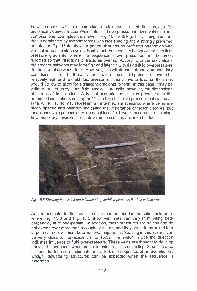
In accordance with our numerical models we present first proxies for tectonically derived fracture/vein sets, fluid overpressure derived vein sets and combinations. Examples are shown in Fig. 15.4 with Fig. 15.4a being a pattern that is dominated by tectonic forces with nice spacing and a strongly preferred orientation. Fig. 15.4e shows a pattern that has no preferred orientation with vertical as well as steep veins. Such a pattern seems to be typical for high fluid pressure gradients, where the sequence is over-pressured and becomes fluidized so that directions of fractures overlap. According to the simulations the steeper networks may form first and later on with rising fluid overpressures the horizontal networks form. However, this will depend strongly on boundary conditions. In order for these systems to form local, fluid pressures have to be relatively high and far-field fluid pressures either above or towards the sides should be low to allow for significant gradients to form. In this case it may be valid to term such systems fluid overpressure cells, however, the dimensions of this “cell” is not clear. A typical scenario that is also presented in the numerical simulations in chapter 11 is a high fluid overpressure below a seal. Finally, Fig. 15.4c may represent an intermediate scenario, where veins are nicely spaced and oriented, indicating the importance of tectonic forces, but local dense vein patches may represent local fluid over-pressures. It is not clear how these local overpressures develop unless they are linked to faults.

Fig. 15.5 Showing how veins are influenced by bedding planes in the Italian field area.

Another indicator for fluid over-pressure can be found in the Italian field area, where Fig. 15.3 and Fig. 15.5 show vein sets that vary from being bed- perpendicular to bed-parallel. In addition, these structures are patchy and do not extend over more than a couple of meters and they seem to be linked to a larger scale detachment between two major units. Spacing in this system can be very close to non-existent (Fig. 15.3). The switch in opening direction indicates influence of fluid over-pressure. These veins are thought to develop early in the sequence when the sediments are still compacting. Since the area represents deep-sea sediments and a turbidite sequence of an accretionary wedge, dewatering structures can be expected when the sequence is deformed.

2 1 2

15.3 Fluid flow

How does fluid flow through sequences that are affected by healing and the build up of fluid overpressures? As long as fracture networks remain open, fluid overpressures are probably released from reservoirs, because the fluid will simply flow along gradients and release the overpressure. Once systems become more closed due to the development of horizontal seals, due to fracture healing or because the permeability is too low to release fluids fast enough, overpressures will build up if fluids are created or brought into the system. The reaction of a reservoir to the increase in overpressure can be variable. As long as the system is permeable enough, Darcy flow will lead to a decrease of overpressure. Once the overpressure is too high, fractures will develop that increase the permeability. If the fluid source is local, for example in the case of fluid injection in a well, the developing fracture pattern will create enough permeability to create a stable pressure gradient and fluid will flow into the system. This is illustrated in Fig. 15.6, where the fluid pressure with time increases until fractures form and the fluid pressure stabilizes.

P ,

centre

t

Fig. 15.6 Stabilization of fluid pressure during fluid injection at a point. Developing fractures lead to a stable fluid flux into the system.

For a geological scenario this would mean that a fluid source brings in fluid and as a result fractures form that lead to the drainage of that system. In this case the fracture system is stable and remains open. In a more complicated setup fluid pressure may rise below a seal and fluid is brought in at several places. In this case the source may not be stable and hence the fractures that drain one source may not be able to drain other sources. The result is a complex fracture network that develops. Depending on how fast the fluid can leave the system and whether or not horizontal seals exist that lead to high vertical pressure gradients, such a system can lead to stress rotations and the development of hydraulic breccias. If these systems now heal, the behavior

2 1 3

becomes more dynamic, where the system develops local fractures that release fluid and then heal again. If the healing is not fast enough to heal complete fractures before new fluid pulses run through the system, we expect to see a similar system compared to our Zechstein reservoir. In this case partly sealed and open fractures represent the fluid pathways and completely sealed fractures represent old fluid pathways or parts of the paths that are not needed any more for fluids to flow. This also indicates that the Zechstein example is indeed a real active system that is partly open and releases fluids. If the fluid input is increased even more in a scenario that may represent deeper parts in the Earth’s crust or local fast production of fluids, the system may go into another transport mode. An example is given at the end of chapter 11, where permeability channels develop that drain the fluid. In this case the system switches from local fracture development and matrix plus fracture flow to a strong localization of flow in channels. These cannels are mobile, they open and close and they lead to a compaction of the solid in between channels. They also show a characteristic wavelength and develop a spacing, which can be termed compaction length and is theoretically predicted to develop in melt-solid systems ([265], [266]). These channels drain the system through a network of horizontal and vertical channels. It is interesting to note that the channels develop without fracture healing, through an interaction of solid and fluid pressures. W hether these permeability channels can be applied to the field areas is not clear. However, if they can be used, then the compaction length would give an indication on spacing of permeability channels in a reservoir, and this would be very useful for predictive purposes as well as oil and gas recovery.

Fig. 15.7 Permeability channels developing in a model that is under high fluid overpressure. Red, green and light blue are high porosities and dark blue low porosities. Both models are stressed vertically assuming gravitational loading, the model on the left hand side has wrapping boundary conditions whereas the model on the right hand side lower fluid pressures at the left and right hand boundary representing a laterally restricted high fluid pressure cell.

Chapter 14 discusses large scale fluid flow through mobile hydrofractures, which can be seen as similar structures than the fluid channels shown in Fig. 15.7. Large-scale increase in fluid pressure thus leads to the development of

2 1 4

mobile networks of fractures or permeability channels that drain the system and lead to mixing of different fluid sources. These networks are not stable even though they develop characteristic wavelengths like the ones shown in Fig. 15.7.

2 1 5

16 Conclusions of Phase II

The most important overall conclusions of phase II of FRACS can be summarized as follows:

• Importance o f small subseismic scale structures for tectonic analysis: Our studies have consistently shown that small scale structures like veins, vein-networks, faults and stylolites can be used to derive large scale tectonic events. This is especially well documented for the Oman mountains that experienced compression, extension and several strike slip events as well as the Internal Ligurian Units in Italy where a flip in subduction direction led to a rotation of the compressive stress field. Sub-seismic structures are a very powerful tool for structural analysis and they may help in understanding seismic scale observations. In general, stylolites (sedimentary and tectonic) should be included in an analysis if they are present. They are very good indicators for stress directions and timing of deformation. In addtion they can be used to determine depth of deformation and magnitude of tectonic stress.

• Outcrop versus cores, how representative are outcrops: Even though the analysis of outcrops is very important and, as mentioned above, can be used to derive changes in tectonic history, it has limitations. One major limitation is the problem that the paleopermeability of partly healed fracture networks may be lost when rocks are exhumed. The studied Zechstein cores show a paleopermeability through a partly healed fracture network that is not present in the two studied outcrop equivalents (Oman and Italy). If we assume that the field areas in Oman and Italy had a paleopermeability that was equivalent to the Zechstein cores, then this feature is lost in the outcrop equivalents. The conclusion could be that potentially outcrops do not really reveal paleopermeabilities of reservoirs. However, this needs to be further tested in a case where we have access to exactly the same units in cores and in outcrops.

• Crystal growth and flow: Simulations of crystal growth in cracks and associated fluid flow have shown that as a general trend, the hydraulic aperture is smaller than the mechanical aperture and with increasing sealing the difference between the two increases. Flow in partly sealed fractures may thus vary significantly from flow in open fractures.

• Mechanical properties o f systems that contain veins: Veins can significantly alter the mechanical properties of rocks and they can also alter fracturing. These effects become significant once veins are either harder or easier to fracture than the host-rock. If veins are harder to fracture, successive fracturing will take place in the host-rock and the system will harden progressively. The results are many small veins

2 1 6

potentially replacing the whole host-rock and a reduction of open fractures. If the veins break easily, they will refracture and the veins have a memory effect. This scenario is similar to partly healed veins that can also fracture easier. The results are thick crack-seal veins with many fractures with potentially a well-defined spacing. These system soften and can lead to well developed open fracture networks. Once stress directions change the existing veins will influence the new fractures leading to bifurcations or direction changes of successive vein sets. A detailed study of the vein patterns can help to estimate relative mechanical paleo-properties of veins and matrix.

• Veins are not representing open fractures: Following on the previous point, outcrop patterns of vein networks are not easy to interpret in terms of paleofracture networks that were connected and open at a given snapshot in time. A system that has many veins does not necessarily represent a high paleo-permeability.

• Effective stresses may change anisotropically during increasing fluid pressure: Numerical models and field observations show that effective stresses change in an anisotropic manner during fluid pressure increase. Local fluid pressure increase may lead to an isotropic decrease of effective stress, so that the developing fracture orientation is governed by the tectonic or overburden stress. However, once the overall fluid pressure increases boundary conditions become important. In a system with overburden stresses like a sedimentary basin the increase in fluid pressure below a seal leads to an anisotropic effective stress change. All principal stresses go to zero and then the vertical stress that is represented by the gravitiational overload becomes tensile. Such a scenario leads to the development of either unoriented fractures or a switch from vertical (or conjugate) to horizontal fracturing and can produce hydraulic breccias.

• Dynamics o f flow, stable versus changing networks: Flow in a fracture system that is produced by fluid overpressure can be complex. If the fluid overpressure is local and the fluid influx is constant, a stable fracture pattern may develop that drains the fluid. However, once fluid influx is non-local and relatively high, multiple fracture networks develop that become dynamic. They locally drain fluid but then close again either mechanically or by healing. The resulting system is highly dynamic and either produces permeability channels with a given spacing that change position to drain an overpressurized system or mobile hydrofractures that travel upwards and heal again. Field observations indicate that such systems exist including indicators for fluid mixing, hydraulic breccias, crack seal veining and chaotic vein geometries.

2 1 7

17 References

[1] Wangen, M., Journal of Petroleum Science and Engineering, 77(3-4), 274285, (2011)

[2] Hilgers, C, Dilg-Gruschinski, K., Urai, J. L , Geology, 32, 261-264, (2004)[3] Koehn, D., Renard, F., Toussaint, R., Passchier, C.W., Earth and Planetary

Science Letters, 257, 582-595, (2007)[4] Ebner, M., Toussaint, R., Schmittbuhl, J., Koehn, D., Bons, P, Journal of

Geophysical Research, 115(B06403), (2010)[5] Flügel, E., Springer Berlin Heidelberg, Berlin, Germany, (2004)[6] Burkhard, M., Journal of Structural Geology, 15(3-5), 351-368, (1993)[7] Molli, G., Geological Society of London Special Publications, 298, 413-442,

(2008)[8] Patacca, E., Scandone, P, The Lithosphere in Italy: Advances in Earth

Science Research, Accademia Nazionale Lincei, Rome, 157-176, (1989)

[9] Stampfli, G.M., Geological Society of London Special Publications, 173, 123, (2000)

[10] Stampfli, G.M., Atlases in Geoscience, 1, Elsevier B. V., 747-766, (2005)[11] Stampfli, G.M., Hochard, C., Orogens and Modern Analogues, 327, 89

111, (2009)[12] Bracciali, L., Marroni, M., Pandolfi, L., Rocchi, S., Sedimentary

Provenance and Petrogenesis: Perspectives from Petrography and Geochemistry, 420, 73-93, (2007)

[13] Carminati, E., Lustrino, M., Doglioni, C., Tectonophysics, 579(0), 173-192,(2012)

[14] Argnani, A., Italian Journal of Geosciences, 128(2), 317-330, (2009)[15] Molli, G., Malavieille, J., International Journal of Earth Sciences, 100(5),

1207-1224, (2011)[16] Argnani, A., Tectonophysics, 579, 207-219, (2012)[17] Advokaat, E.L., van Hinsbergen, D.J.J., Maffione, M., Langereis, C.G.,

Vissers, R.L.M., Cherchi, A., Schroeder, R., Madani, H. & Columbu, S., Earth and Planetary Science Letters, 401, 183-195, (2014)

[18] Rosenbaum, G., Lister, G.S., Duboz, C., Journal of the Virtual Explorer, 8,107-130, (2002)

[19] Carosi, R., Montomoli, C., Pertusati, P.C., Bollettino della SocietaGeologica Italiana, 1, 167-180, (2002)

[20] Carosi, R., Montomoli, C., Pertusati, P.C., Geodinamica Acta, 17, 253-273,(2004)

[21] van Wamel, W.A., Bons, A.J., Franssen, R.C.M.W., Lingen, W. van,Postuma, W., van Zutphen, A.C.A., Geologie En Mijnbouw, 64(2), 181197, (1985)

[22] Perrone, V., Perrotta, S., Marsaglia, K., Di Staso, A., Tiberi, V.,Palaeogeography Palaeoclimatology Palaeoecology, 394, 128-143, (2014)

[23] Marroni, M., Memoire della Societa Geologica Italiana, 47, 179-194, (1994)[24] Marroni, M., Pandolfi, L., International Journal of Earth Sciences, 96(6),

1059-1078, (2007)

2 1 8

[25] Marroni, M., Bollettino della Societa Geologica Italiana, 110, 727-736,(1991)

[26] van Zutphen, A.C.A., van Wamel, W.A., Bons, A.J., Geologie En Mijnbouw,64(4), 373-384, (1985)

[27] Nilsen, T.H., Abbate, E., Geo-Marine Letters, 3, 193-197, (1984)[28] Codegone, G., Festa, A., Dilek, Y., Pini, G.A., Tectonophysics, 568, 170

184, (2012)[29] van Wamel, W.A., Tectonophysics, 142(1), 87-98, (1987)[30] Leoni, L., Marroni, M., Sartori, F., Tamponi, M., European Journal of

Mineralogy, 8(1), 35-50, (1996)[31] Marroni, M., Pandolfi, L., Geodinamica Acta, 9(1), 13-29, (1996)[32] Meneghini, F., Marroni, M., Pandolfi, L., Journal of Structural Geology,

29(3), 515-529, (2007)[33] Hoogerduijn Strating, E.H., Tectonophysics, 238(1-4), 255-273, (1994)[34] Strohmenger, C., Antonini, M., Jager, G., Rockenbauch, K., Strauss, C.,

BCRDP, 20, 1-35, (1996)[35] Karnin, W.D., Rockenbauch, K., Ruijtenberg, PA., First Break, 10, 233

240, (1992)[36] Ziegler, PA., Shell Internationale Petroleum Maatschappij B.V., The

Hague, 1990[37] Taylor, J.C.M., Blackwell Scientific Publications, Oxford, 153-190, (1990)[38] Swanenberg, H.C., Führer, F.X., AAPG Memoir, 42, 246-253, (1991)[39] Budny, M., First Break, 9, 55-64, (1991)[40] Sannemann, D., Zimdars, J., Plein, E., Zeitschrift der Deutschen

Geologischen Gesellschaft, 129, 33-69, (1978)[41] Kockel, F„ Geologie en Mijnbouw, 81(2), 149-158, (2002)[42] Baldschuhn, R., Binot, F., Fleig, S., Kockel, F., Geologisches Jahrbuch A

153, 1-40, (2001)[43] Baldschuhn, R., Best, G., Kockel, F., Special publication of the European

Association of Petroleum Geoscientists, 1, Oxford University Press, Oxford, 149-159, (1991)

[44] Zeeb, C., Gomez-Rivas, E., Bons, P.D., Blum, P, AAPG Bulletin, 97(9),1545-1566, (2013)

[45] Priest, S.D., Chapman&Hall, London, United Kingdom, 473 pp., (1993)[46] Bonnet, E., Bour, O., Odling, N.E., Davy, P, Main, I., Cowie, P, Berkowitz,

B., Reviews of Geophysics, 39(3), 347-383, (2001)[47] Bons, P.D., Becker, J.K., Eiburg, M.A., Urston, K., Earth and Environmental

Sciene Transactions of the Royal Society of Edinburgh, 100, 105-115, (2009)

[48] Stark, L., MSc thesis, University of Tübingen, Germany, (2011)[49] Heiland, S., BSc thesis, University of Tübingen, Germany, (2014)[50] Renard, F., Schmittbuhl, J., Gratier, J.P, Meakin, P, Merino, E., Journal of

Geophysical Research-Solid Earth, 109(B03209), (2004)[51] Schmittbuhl, J., Renard, F., Gratier, J.P , Toussaint, R., Physical Review

Letters, 93, 238501, (2004)[52] Koehn, D., Ebner, M., Renard, F., Toussaint, R., Passchier, C.W., Earth

and Planetary Science Letters, 341, 104-113, (2012)[53] Ebner, M., Koehn, D., Toussaint, R., Renard, F., Journal of Structural

Geology, 31,72-82, (2009)

2 1 9

[54] Ebner, M., Koehn, D., Toussaint, R., Renard, F., Schmittbuhl, J., Earth andPlanetary Science Letters, 277, 394-398, (2009)

[55] Stockdale, P.B., Indiana University Studies, 9(55), 1-97, (1922)[56] Dunnington, H.V., Journal of Sedimentary Petrology, 24, 27-49, (1954)[57] Park, W.C., Schot, E.H., Journal of Sedimentary Petrology, 38, 175-191,

(1968)[58] Merino, E., American Scientist, 80, 466-473, (1992)[59] Railsback, L.B., Journal of Sedimentary Petrology, 63, 513-522, (1993)[60] Gratier, J.P, Muquet, L., Hassani, R., Renard, F., Journal of Structural

Geology, 27, 89-100, (2005)[61] Young, R.B., Geological Society of South Africa Transactions, 47, 137

142, (1945)[62] Heald, M.T., The Journal of Geology, 63, 101-114, (1955)[63] Wright, T.O., Platt, L.B., American Journal of Science, 282, 122-135,

(1982)[64] Rutter, E.H., Journal of the Geological Society of London, 140, 725-740,

(1983)[65] Rispoli, R., Tectonophysics, 75, T29-T36, (1981)[66] Petit, J.P., Mattauer, M., Journal of Structural Geology, 17, 245-256, (1995)[67] Laronne Ben-ltzhak, L., Aharonov, E., Toussaint, R., Sagy, A., Earth and

Planetary Science Letters, 337-338, 186-196, (2012)[68] Aharonov, E., Katsman, R., American Journal of Science, 309(7), 607-632,

(2009)[69] Dunnington, H.V., 7th World Petroleum Congress, 2 -9 April 1967, Mexico

City, Mexico, 2(12129), 339-352, (1967) “[70] Nelson, R.A., AAPG Bulletin, 65, 2417-2425, (1981)[71] Koepnick, R.B, Society of Petroleum Engineers Formation Evaluation,

2(02), 137-142, (1987)[72] Finkei, E.A., Wilkinson, B.H, AAPG Bulletin, 74, 174-186, (1990)[73] Dutton, S.P., Willis, B.J, Journal of Sedimentary Research, 68, 890-900,

(1998)[74] Alsharhan, A., Sadd, J.L, Society for Sedimentary Geology Special

Publication, 69, 185-207, (2000)[75] Carozzi, A.V., von Bergen, D, Journal of Petroleum Geology, 10, 267-282,

(1987)[76] Dawson, W. C., American Association of Petroleum Geologists Annual

Convention, Houston, Texas, 20-23, (1988)[77] Raynaud, S., Carrio-Schaffhauser, E., Journal of Structural Geology, 14,

973-980, (1992)[78] Van Geet, M., Swennen, R., Wevers, M., Sedimentary Geology, 132, 25

36, (2000)[79] Gingras, M.K., MacMillan, B., Balcom, B.J., Bulletin of Canadian Petroleum

Geology, 50, 363-369, (2002)[80] Harris, N.B., Journal of Sedimentary Research, 76, 444-459, (2006)[81] Lind, I., Nykjaer, O., Priisholm, S., Springer, N., Journal of Petroleum

Technology, 46, 986-993, (1994)[82] Heap, M.J., Baud, P., Reuschle, T., Meredith, P.G., Geology, 42(1), S I-

54, (2014)[83] Karcz, Z., Scholz, C.H. 2003. Journal of Structural Geology, 25(8), 1301

1316, (2003)

2 2 0

[84] Vandeginste, V., John, C.M., Journal of Sedimentary Research, 83, 226240, (2013)

[85] Rolland, A., Toussaint, R., Baud, P., Schmittbuhl, J., Conil, N., Koehn, D.,Renard, F., Gratier, J.P., Journal of Geophysical Research-Solid Earth, 117(6), B06403, (2012)

[86] Rolland, A., Toussaint, R., Baud, P., Conil, N., Landrein, InternationalJournal of Rock Mechanics and Mining Sciences, 67, 212-225, (2014)

[87] Ebner, M., Piazolo, S., Renard, F., Koehn, D., Journal of StructuralGeology, 32, 1070-1084, (2010)

[88] Bruns, B., di Primio, R., Berner, U., Littke, R., Geofluids, 13(2), 246— 271,(2013)

[89] Bons, P., Koehn, D., Jessell, M., Microdynamics Simulation, Lecture Notesin Earth Sciences, 106, Springer, Berlin, (2008)

[90] Koehn, D., Bons, P.D., Passchier, C.W., Journal of Structural Geology,25(2), 263-275, (2003)

[91] Koehn, D., Malthe-Sorenssen, A., Passchier, C., Chemical Geology,230(3-4), 207-219, (2006)

[92] Sachau, T., Koehn, D., Geoscientific Model Development, 7(1), 243-247,(2014)

[93] Below, A., Berichte Report Nr. 60, Christian-Albrechts-Universität, D-24098, Kiel, (1992)

[94] Ohmoto, H., Rye, R.O., Geochemistry of Hydrothermal Ore Deposits, 2nded„ Wiley, New York, 509-567, (1979)

[95] Kajiwara, Y., Krouse, H.R., Canadian Journal of Earth Sciences, 8, 236238, (1971)

[96] Ghani, I., Koehn, D., Toussaint, R., Passchier, C.W., Frontiers in Physics,3:67, (2015)

[97] Ramsay, J, Nature, 284, 135-139, (1980)[98] Durney, D.W, Ramsay, J.G., Gravity and Tectonics, John Wiley & Sons,

New York, 67-96, (1973)[99] Bons, P.D., Journal of the Virtual Explorer, 2, (2000)[100] Oliver, N.H.S., Bons, P.D., Geofluids, 1, 137-162, (2001)[101] Bons, P.D., Eiburg, M.A., Gomez-Rivas, E., Journal of Structural

Geology, 43, 33-62, (2012)[102] Hilgers, C., Koehn, D., Bons, P.D., Urai, J.L., Journal of Structural

Geology, 23, 873-885, (2001)[103] Cox, S.F., Etheridge, M.A., Tectonophysics, 92, 147-170, (1983)[104] Urai, J.L., Williams, P.F., van Roermund, H.L.M., Journal of Structural

Geology, 13, 823-836, (1991)[105] Fisher, D.M., Brantley, S.L., Journal of Geophysical Research, 97(B13),

20043-20061, (1992)[106] Okamoto, A., Tsuchiya, N., Geology, 37(6), 563-566, (2009)[107] Lee, Y.-J., Morse, J.W., Wiltschko, D.V., Chemical Geology, 130, 203

215, (1996)[108] Lee, Y.-J., Morse, J.W., Chemical Geology, 156, 151-170, (1999)[109] Hilgers, C., Urai, J.L., Journal of Structural Geology, 24, 1029-1043,

(2002)

[110] Nollet, S „ Hilgers, C., Urai, J.L., Geofluids, 6, 185-200, (2006)[111] Hilgers, C., Tenthorey, E., Terra Nova, 16(4), 173-178, (2004)

221

[112] Okamoto, A., Saishu, H., Hirano, N., Tsuchya, N., Geochimica et Cosmochimica Acta, 74, 3692-3706, (2010)

[113] Okamoto, A., Sekine, K., Journal of Structural Geology, 33, 1764-1775,(2011)

[114] Bons, P.D., Journal of Structural Geology, 23, 865-872, (2001)[115] Nollet, S., Urai, J.L., Bons, P.D., Hilgers, C., Journal of Structural

Geology, 27, 217-230, (2005)[116] Koehn, D., Bons, P.D., Hilgers, C., Passchier, C.W., Journal of the Virtual

Explorer, 4, 25-30, (2001)[117] Bons, A.-J., Bons, P.D., Microporous and Mesoporous Materials, 62, 9

16, (2003)[118] Lander, R.H., Larese, R.E., Bonnell, L.M., AAPG Bulletin, 92(11), 1537

1563, (2008)[119] Gale, J.F.W., Lander, R.H., Reed, R.M., Laubach, S.E., Journal of

Structural Geology, 32(9), 1201-1211, (2010)[120] Steefel, C., Depaolo, D., Lichtner, P., Earth and Planetary Science

Letters, 240, 539-558, (2005)[121] Yoon, H., Valocchi, A.J., Werth, C.J., Dewers, T., W ater Resources

Research, 48, W02524, (2012)[122] Li, X., Huang, H., Meakin, P., Water Resources Research, 44, W12407,

(2008)[123] Hecht, U., Granasy, L., Pusztai, T , Böttger, B., Apel, M., Witusiewicz, V.,

Ratke, L., De Wilde, J., Froyen, L., Camel, D., Drevet, B., Faivre, G., Fries, S.G., Legendre, B., Rex, S., Materials Science and Engineering: R, 46, 1-49, (2004)

[124] Ankit, K., Nestler, B., Selzer, M., Reichardt, M., Contributions to Mineralogy and Petrology, 166, 1709-1723, (2013)

[125] Wendler, F „ Okamoto, A., Blum, P „ Geofluids, 1468-8123, (2015)[126] Wendler, F., Mennerich, C., Nestler, B., Journal of Crystal Growth,

Elsevier, 327, 189-201, (2011)[127] Ihinger, P.D., Zink, S.I., Nature, 404, 865-869, (2000)[128] De Leeuw, N.H., Computer Methods in Mineralogy and Geochemistry,

Seminarios de la Sociedad Espanola de Mineralogia, 4, Sociedad Espanola de Mineralogia, Madrid, 66-102, (1992)

[129] Hiraga, T., Nishikawa, O., Nagase, T , Akizuki, M., Kohlstedt, D.L., Contributions to Mineralogy and Petrology, 143, 664-672, (2002)

[130] Parks, G.A., Journal of Geophysical Research: Solid Earth, 89(B6), 3997-4008, (1984)

[131] Holness, M.B., Earth and Planetary Science Letters, 117, 363-377, (1993)

[132] Iwasaki, H., Iwasaki, F., Yokokawa, H., Kurashige, M., Oba, K., Journalof Crystal Growth, 234, 711-720, (2002)

[133] Ostapenko, G.T., Mitsyuk, B.M., Journal of Crystal Growth, 294, 330338, (2006)

[134] Sekerka, R.F., Crystal Research Technology, 40(4-5), 291-306, (2005)[135] Suzuki, T., Kasahara, H., Crystal Research and Technology, 45(12),

1305-1308, (2010)[136] Rimstidt, J.D., Barnes, H.L., Geochimica et Cosmochimica Acta, 44,

1683-1699, (1980)

2 2 2

[137] Dove, P., Han, N., AIP Conference Proceedings, Am. Inst. Physics Conference Series, 916, 215-234, (2007)

[138] Dijk, P., Berkowitz, B., Water Resources Research, 34(3), 457-470, (1998)

[139] Walton, M., American Journal of Science, 258, 385-401, (1960)[140] Wendler, F., Becker, J.K., Nestler, B., Bons, P.D., Walte, N.P.,

Computers & Geosciences, 35(9), 1907-1916, (2009)[141] Nestler, B., Garcke, H., Stinner, B., Physical Review E, 71, 041609,

(2008)[142] Iwasaki, H., Iwasaki, F., Journal of Crystal Growth, 151,348-358, (1995)[143] Cundall, P.A., Strack O.D.L., Geotechnique, 29(1), 47-65, (1979)[144] Mora, P., Place, D., Pure Applied Geophysics, 143(1-3), 61-87, (1994)[145] Potyondy, D.O., Cundall, P.A., International Journal of Rock Mechanics

and Mining Sciences, 41(8), 1329-1364, (2004)[146] Abe, S., Place, D., Mora, P., Computational Earthquake Science Part II,

2265-2277, Springer, Basel, (2004).[147] Weatherley, D., Geophysical Research Abstracts, 13, EGU2011-9476,

(2011)[148] Virgo, S., Abe, S., Urai, J.L., Journal of Geophysical Research: Solid

Earth, 118, 5236-5251, (2013)[149] Virgo, S., Abe, S., Urai, J.L., Journal of Geophysical Research: Solid

Earth, 2014JB011520, (2014)[150] Virgo, S., Abe, S., Urai, J.L., Journal of Geophysical Research: Solid

Earth, (accepted), (2016)[151] Virgo, S., Diploma dissertation, RWTH Aachen, Aachen, Germany,

(2016)[152] Helgeson, D.E., Aydin, A., Journal of Structural Geology, 13(8), 897-911,

(1991)[153] Vass, A., Koehn, D., Toussaint, R., Ghani, I., Piazolo, S., Journal of

Structural Geology, 67, 94-106, (2014)[154] Engelder, T., Lacazette, A., Rock joints, A.A. Balkema, Rotterdam, 35

44, (1990)[155] Hunt, J.M., AAPG Bulletin, 74, 1-12, (1990)[156] Bruno, M.S., Nakagawa, F.M., Journal of Rock Mechanics and Mining

Sciences & Geomechanics Abstracts, 28, 261-273, (1991)[157] Fyfe, W.S., Price, N.J., Thompson, A.B., Elsevier, Amsterdam, (1978)[158] Bethke, C.M., Journal of Geophysical Research, 90, 6817-6828, (1985)[159] Oliver, J „ Geology, 14, 99-102, (1986)[160] Swarbrick, R.E., Osborne, M.J., Yardley, G.S., Pressure Regimes in

Sedimentary Basins and Their Prediction, 76, AAPG Memoir, 1-12, (2002)

[161] Cook, J., Gordon, J.E., Proceedings of the Royal Society, London, SeriesA, 282, 508-520, (2005)

[162] Mourgues, R., Cobbold, P.R.,Tectonophysics, 376, 75-97, (2003)[163] Cobbold, P.R., Rodrigues, N., Geofluids, 7, 313-332, (2007)[164] Hu, J.-C., Angelier, J., Journal of Geophysical Research, 109(B9),

B09403, (2004)[165] Tzschichholz, R., Herrmann, H.J., Roman, H.E., Pfuff, M., Physical

Review, B 49, 7056-7059, (1994)[166] Dahm, T., Geophysical Journal International, 141, 623-638, (2000)

2 2 3

[167] McNamara, S., Flekkoy, E.G., Mäloy, K.J., Physical Review, E 6 1 ,40544059, (2000)

[168] Flekkoy, E.G., Malthe-Sorenssen, A., Jamtveit, B., Journal of Geophysical Research, 107(B8), 2151, (2002)

[169] Johnsen, 0 ., Toussaint, R., Mäloy, K.J, Flekkoy, E.G., Physical ReviewE 74, 011301,(2006)

[170] Olson, J.E., Laubach, S.E., Lander, R.H., AAPG Bulletin 93, 1535-1549,(2009)

[171] Goren, L., Aharonov, E., Sparks, D., Toussaint, R., Journal of Geophysical Research, 115(B9), B09216, (2010)

[172] Goren, L., Aharonov, E., Sparks, D., Toussaint, R., Pure and Applied Geophysics, 168, 2289-2323, (2011)

[173] Ghani, I., Koehn, D., Toussaint, R., Passchier, C.W., Pure and AppliedGeophysics, 170(11), 1685-1703, (2013)

[174] Adachi, J., Siebrits, E., Peirce, A., Desroches, J., International Journal ofRock Mechanics & Mining Sciences, 44, 739-757, (2007)

[175] Koehn, D., Arnold, J., Passchier, C.W., Geological Society of London,Special Publications, 243, 11-24, (2005)

[176] Zoback, M.D., Harjes, H.-P., Journal of Geophysical Research: Solid Earth, 102(B8), 18477-18491, (1997)

[177] Bons, P.D., van Milligen, B.P., Geology, 29, 919-922, (2001)[178] Hillis, R.R., Geological Society of London, Special Publications, 216, 359

368, (2003)[179] Niebling, M.J., Flekkoy, E.G., Mäloy, K.J., Toussaint, R., Physical Review

E 82, 051302, (2010)[180] Press, W.H., Teukolsky, S.A., Vetterling, W.T., Flannery B.P., Cambridge

University Press, Cambridge, (1992)[181] Niebling, M., Toussaint, R., Flekkoy, E.G., Mäloy, K.J., Physical Review

E 86, 061315, (2012)[182] Niebling, M., Toussaint, R., Flekkoy, E.G., Mäloy, K.J., Revista Cubana

de Fisica, 29, (2012)[183] Vinningland, J.L., Johnsen, 0 ., Flekkoy, E.G., Toussaint, R., Mäloy, K.J.,

Physical Review Letters, 99, 048001, (2007)[184] Vinningland, J.L., Johnsen, 0 ., Flekkoy, E.G., Toussaint, R., Mäloy, K.J.,

Physical Review, E 76, 051306, (2007)[185] Niebling, M.J., Flekkoy, E.G., Mäloy, K.J., Toussaint, R., Physical Review

E 82, 011301, (2010)[186] Norman, L.B., Lloyd, E.K., Wilson, R.J., Clarendon Press, (1986)[187] Watts, D.J., Strogatz, S.H., Nature, 393(6684), 440-442, (1998)[188] Latora, V., Marchiori, M., Physics Review Letters, 87(198701), (2001)[189] Marchiori, M., Latora, V., Physica A, 285(3-4), 539-546, (2000)[190] Newman, M.E.J., SIAM Review, 45(2), 167-25, (2003)[191] Snijders, T.A.B., Social Networks, 3(3), 163-174, (1981)[192] Costa, L.D.F., Rodrigues, F.A., Travieso, G., Boas, P.R.V., Advances in

Physics, 56(1), 167-242, (2007)[193] Wang, B., Tang, H., Guo, C., Xiu, Z., Physica A: Statistical Mechanics

and its Applications, 363(2), 591-596, (2006)[194] Milgram, S., Psychology Today, 1(1), 61-67, (1967)[195] Boccaletti, S., Latora, V., Moreno, Y., Chavez, M., Hwang, D.U., Physics

Reports, 424(4-5), 175-308, (2006)

2 2 4

[196] Newman, M.E.J., Physical Review Letters, 89(20), (2002)[197] Varga-Vass, A., PhD Dissertation, University of Glasgow, Glasgow,

United Kingdom, (2015)[198] Andresen, C.A., Hansen, A., Le Goc, R., Davy, P., Hope, S.M., Frontiers

in Physics, 1(7), (2013)[199] Chi, G., Xue, C., Geoscience Frontiers, 2(3), 423-438, (2011)[200] Cohen, C.E., Ding, D., Quintard, M., Bazin, B., Chemical Engineering

Science, 63(12), 3088-3099, (2008)[201] Cooper, A.H., Special Publications in Engineering Geology, 265-275,

Geological Society of London, London, (1998)[202] Yasuhara, H., Polak, A., Mitani, Y., Grader, A.S., Halleck, P.M., Elsworth,

D., Earth and Planetary Science Letters, 244(1-2), 186-200, (2006)[203] Noiriel, C., Steefel, C.I., Yang, L., Bernard, D., Advances in W ater

Resources, doi:10.1016/j.advwatres.2015.11.013, (2015)[204] Bons, P.D., Tectonophysics, 336(1-4), 1-17, (2001)[205] Ferry, J.M., Journal of Geophysical Research, 99(B8), 15487-15498,

(1994)[206] Asaye, M., Aluto Langano Power Plant, Ethiopia, Geothermal Training

Programm, Reykjavik, Report 3, 1-24, (2004)[207] Xu, T., Ontoy, Y., Moiling, P., Spycher, N., Parini, M., Pruess, K.,

Geothermics, 33, 477-491, (2004)[208] Borgia, A., Pruess, K., Kneafsey, T.J., Oldenburg, C.M., Pan, L.,

Geothermics, 44, 13-22, (2012)[209] Klein, E., De Lucia, M., Kempka, T., Kühn, M., International Journal of

Greenhouse Gas Control, 19, 720-730, (2013)[210] Mullin, J. W., Crystallization, Butterworth-Heinemann, (2001)[211] Fisher, G.W., Geochimica et Cosmochimica Acta, 42, 1035-1050, (1978)[212] Menke, H.P., Bijeljic, B., Andrew, M.G., Blunt, M.J., Environmental

Science and Technology, 49, 4407-4414, (2015)[213] Dijk, P.E., Berkowitz, B., W ater Resources Research, 35(12), 3955-3959,

(1999)[214] Zhao, Z., Li, B., Jiang, Y., Rock Mechanics and Rock Engineering, 47,

2279-2286, (2014) '[215] Lomize, G., Gosenergoizdat, Moscow, 127, 197, (1951)[216] Louis, C., Thesis, University of Karlsruhe, Karlsruhe, Germany, (1967)[217] Berkowitz, B., Advances in Water Resources, 25(8-12), 861-884, (2002)[218] Oron, A.P., Berkowitz, B., W ater Resources Research, 34, 2811-2825,

(1998)[219] Witherspoon, P.A., Wang, J.S.Y., Iwai, K., Gale, J.E., Water Resources

Research, 16, 1016-1024, (1980)[220] Pyrak-Nolte, L.J., Cook, N.G.W., Nolte, D.D., Geophysical Research

Letters, 15(11), 1247-1250, (1988)[221] Brown, S., Caprihan, A., Hardy, R., Journal of Geophysical Research:

Solid Earth, 103(B3), 5125-5132, (1998)[222] Crandall, D., Bromhai, G., Karpyn, Z.T., International Journal of Rock

Mechanics and Mining Sciences, 47, 784-796, (2010)[223] Schwarz, J.-O., Enzmann, F., Transport in Porous Media, 96(3), 501-525,

(2013)[224] Zimmerman, R., Bodvarsson, G., Transport in Porous Media, 23, 1-30,

(1996)

2 2 5

[225] Miura, H., Journal of Crystal Growth, 367, 8-17, (2013)[226] Hubert, J., Emmerich, H., Urai, J.L., Journal of Metamorphic Geology, 27,

523-530, (2009)[227] Qin, R.S., Bhadeshia, H.K., Materials Science and Technology, 26, 803-

S11, (2010)[228] IAPWS, IAPWS Release on the Values of Temperature, Pressure and

Density of Ordinary and Heavy Water, 2007[229] Patankar, S.V., Spalding, D.B., International Journal of Heat and Mass

Transfer, 15, 1787-1806, (1972)[230] van Doormaal, J.P., Raithby, G.D., Numerical Heat Transfer, 7, 147-163,

(1984)[231] Kehrwald, D., Kaiserslautern, (2004)[232] Schulz, V., Kehrwald, D., Wiegmann, A., Steiner, K., Proceedings of

NAFEMS CFD Seminar, Simulation of Complex Flows, Niedernhausen/Wiesbaden, Germany, (2005)

[233] Yasuhara, H., Kinoshita, N., Ohfuji, H., Lee, D.S., Nakashima, S., Kishida,K., Applied Geochemistry, 26(12), 2074-2088, (2011)

[234] Wagner, W., Kretzschmar, H.-J., Springer Science & Business Media,(2007)

[235] Taylor, W.L., Pollard, D.D., Aydin, A., Journal of Geophysical Research,104(B12), 28,983-29,006, (1999)

[236] Prandtl, L., Oertel, H., Vieweg, Braunschweig, (2001)[237] Sukop, M.C., Thorne, D.T., Jr., Springer, Berlin, Heidelberg, New York,

(2006)[238] Wiegmann, A., Iliev, O., Schindelin, A., Global Guide of the Filtration and

Separation Industry, 191-198, (2010)[239] Konzuk, J.S., Kueper, B.H., Water Resources Research, 40(2), (2004)[240] Fardin, N., PhD thesis, KTH, Stockholm, Sweden, (2003)[241] Patir, N., Cheng, H.S., Journal of Lubrication Technology, 100, 12-17,

(1978)[242] Neuville, A., Toussaint, R., Schmittbuhl, J., Physical Review E, 82(3),

036317, (2010)[243] Singurindy, O., Berkowitz, B., Advances in Water Resources, 28, 507

21, (2005)[244] Gomez-Rivas, E., Bons, P.D., Koehn, D., Urai, J.L., Arndt, M., Virgo, S.,

Laurich, B., Zeeb, C., Stark, L., Blum, P., American Journal of Science, 314, 1104-39, (2014)

[245] Gomez-Rivas, E., Warber, K., Kulzer, F., Bons, P.D., Koehn, D., MartinMartin, J.D., Geogaceta, 51, 79-82, (2012)

[246] Gomez-Rivas, E., Corbella, M., Martin-Martin, J.D., Stafford, S.L., Teixell,A., Bons, P.D., Griera, A., Cardellach, E, Marine and Petroleum Geology, 55, 26-42, (2014)

[247] Sachau, T., Bons, P.D., Gomez-Rivas, E., Frontiers in Physics, 3, (2015)[248] Bons, P.D., Fusswinkel, T., Gomez-Rivas, E., Markl, G., Wagner, T.,

Walter, B „ Geology, 42(12), 1035-1038, (2014)[249] Jamtveit, B., Chapman and Hall, London, (1997)[250] Miller, S., Nur, A., Earth and Planetary Science Letters, 183, 133-46,

(2000)[251] Weertmann, J., Journal of Geophysical Research, 76, 1171-83, (1971)[252] Secor, D., Pollard, D., Geophysical Research Letters, 2, 510-513, (1975)

2 2 6

[253] Oliver, N.H.S., Rubenach, M.J., Fu, B., Baker, T., Blenkinsop, T.G., Cleverley, J.S., Marshall, L.J, Ridd, P.J., Geofluids, 6, 346-58, (2006)

[254] Staude, S., Mordhorst, T., Nau, S., Pfaff, K., Brügmann, G., Jacob, D. E.,Markl, G., Canadian Mineralogist, 50, 1401-1434, (2012)

[255] Staude, S., Bons, P.D., Markl, G., Earth and Planetary Science Letters,286, 387-395, (2009)

[256] Connolly J, Podlachikov Y., Springer, Berlin, 599-658, (2013)[257] Hasenclever, J., Theissen-Krah, S., Rüpke, H., Morgan, J., Iyer, K.,

Petersen, S., Nature, 508, 508 - 512, (2014)[258] Clark, C., Hand, M., Faure, K., Schmidt-Mumm, A., Journal of

Metamorphic Geology, 24, 367-387, (2006)[259] Bons, P.D., Gomez-Rivas, E., Economic Geology and the Bulletin of the

Society of Economic Geologists, 108, 1195-1201, (2013)[260] Stöber, I., Bucher, K „ Geofluids, 4, 143-151, (2004)[261] Cheng, Q., Computers and Geosciences, 25(9), 949-961, (1999)[262] Agterberg, F.P., Cheng, Q., Brown, A., Good, D., Computers and

Geosciences, 22(5), 497-507, (1996)[263] Enescu, B., Ito, K., Struzik, Z.R., Annuals of Disaster Prevention

Research Institute Annuals, 47B, 1-13, (2004)[264] Saadatinejad, M.R., Hassani, H., Nonlinear Processes in Geophysics, 20,

231-238, (2013)

2 2 7

577-2/2

577-2/3

577-2/4

718-1

721

DGMK


Weitere DGMK-Forschungsberichte aus dem Fachbereich Aufsuchung und Gewinnung zum Themenkreis „Explorationsgeologie“

(DGMK-Reports concerning „Exploration Geology“)

Structure and Evolution of the Central European Basin System according to 3D modeling(Struktur und Entwicklung des zentraleuropäischen Beckensystems auf Basis einer 3D Modellierung)Autoren: Dr. Y. Maystrenko, Prof. Dr. U. Bayer,Dr. M. Scheck-Wenderoth, 201090 p„ 24 fig., ISBN 978-3-941721-08-1EUR 80,00 (DGMK-Mitglieder: EUR 40,00) zzgl. MwSt.

Dynamics of the Central European Basin System (CEBS): Large scale Paleozoic petroleum system models of the North German Basin (Dynamik des zentraleuropäischen Beckensystems (CEBS): Großräumige paläozoische Kohlenwasserstoffmodelle des Norddeutschen Beckens) Autoren: Dipl.-Geol. A. K. Uffmann, Dipl.-Geol. B. Bruns,Prof. Dr. R. Littke, 2010129 p„ 86 fig., 11 tab., ISBN 978-3-941721-12-8 EUR 80,00 (DGMK-Mitglieder: EUR 40,00) zzgl. MwSt.

Classification of the Central European Basin System (CEBS) (Klassifizierung des zentraleuropäischen Beckensystems (CEBS))Autor: Dr. H.-J. Brink, 201063 p„ 51 fig., 2 tab., ISBN 978-3-941721-13-5EUR 80,00 (DGMK-Mitglieder: EUR 40,00) zzgl. MwSt.

Mineral Vein Dynamics Modeling / Phase 1 (Dynamik von Kluftfüllungen / Phase 1)Autoren: Dr. D. Koehn, Prof. Dr. J. Urai, etal., 2013 217 p., 148 fig., 8 tab., ISBN 978-3-941721-40-1 EUR 90,00 (DGMK-Mitglieder: EUR 45,00) zzgl. MwSt.

Prediction of Tectonic Stresses and Fracture Networks with Geomechanical Reservoir Models(Prognose von tektonischen Spannungen und Kluftnetzwerken mit geomechanischen Lagerstättenmodellen)Autoren: Prof. Dr. A. Henk, M.Sc. K. Fischer, 2014 204p., 113 fig., 23 tab., ISBN 978-3-941721-49-4 EUR 90,00 (DGMK-Mitglieder: EUR 45,00) zzgl.MwSt.

D G M K Research Report 718-2

Documents

Transcript of D G M K Research Report 718-2