Crustal strain near the Big Bend of the San Andreas Fault: Analysis of the Los Padres-Tehachapi...

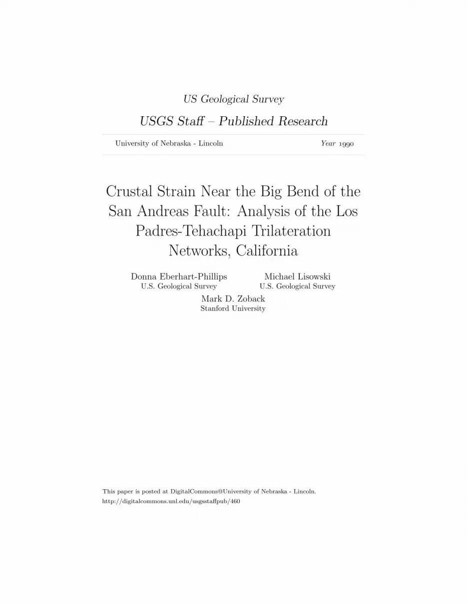
US Geological Survey

USGS Staff – Published Research

University of Nebraska - Lincoln Year

Crustal Strain Near the Big Bend of the

San Andreas Fault: Analysis of the Los

Padres-Tehachapi Trilateration

Networks, California

Donna Eberhart-Phillips Michael LisowskiU.S. Geological Survey U.S. Geological Survey

Mark D. ZobackStanford University

This paper is posted at DigitalCommons@University of Nebraska - Lincoln.

http://digitalcommons.unl.edu/usgsstaffpub/460

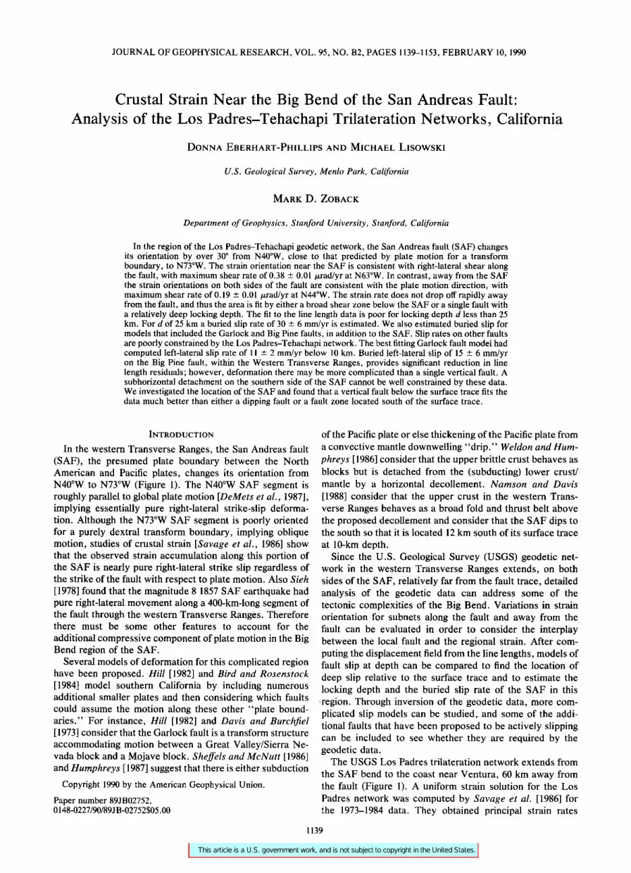
JOURNAL OF GEOPHYSICAL RESEARCH, VOL. 95, NO. B2, PAGES 1139-1153, FEBRUARY 10, 1990

Crustal Strain Near the Big Bend of the San Andreas Fault' Analysis of the Los Padres-Tehachapi Trilateration Networks, California

DONNA EBERHART-PHILLIPS AND MICHAEL LISOWSKI

U.S. Geological Survey, Menlo Park, California

MARK D. ZOBACK

Department of Geophysics, Stanford University, Stanford, California

In the region of the Los Padres-Tehachapi geodetic network, the San Andreas fault (SAF) changes its orientation by over 30 ø from N40øW, close to that predicted by plate motion for a transform boundary, to N73øW. The strain orientation near the SAF is consistent with right-lateral shear along the fault, with maximum shear rate of 0.38 _+ 0.01 txrad/yr at N63øW. In contrast, away from the SAF the strain orientations on both sides of the fault are consistent with the plate motion direction, with maximum shear rate of 0.19 _ 0.01 txrad/yr at N44øW. The strain rate does not drop off rapidly away from the fault, and thus the area is fit by either a broad shear zone below the SAF or a single fault with a relatively deep locking depth. The fit to the line length data is poor for locking depth d less than 25 km. For d of 25 km a buried slip rate of 30 _ 6 mm/yr is estimated. We also estimated buried slip for models that included the Garlock and Big Pine faults, in addition to the SAF. Slip rates on other faults are poorly constrained by the Los Padres-Tehachapi network. The best fitting Garlock fault model had computed left-lateral slip rate of 11 _+ 2 mm/yr below 10 km. Buried left-lateral slip of 15 _ 6 mm/yr on the Big Pine fault, within the Western Transverse Ranges, provides significant reduction in line length residuals; however, deformation there may be more complicated than a single vertical fault. A subhorizontal detachment on the southern side of the SAF cannot be well constrained by these data. We investigated the location of the SAF and found that a vertical fault below the surface trace fits the data much better than either a dipping fault or a fault zone located south of the surface trace.

INTRODUCTION

In the western Transverse Ranges, the San Andreas fault (SAF), the presumed plate boundary between the North American and Pacific plates, changes its orientation from N40øW to N73øW (Figure 1). The N40øW SAF segment is roughly parallel to global plate motion [DeMets et al., 1987], implying essentially pure right-lateral strike-slip deformation. Although the N73øW SAF segment is poorly oriented for a purely dextral transform boundary, implying oblique motion, studies of crustal strain [Savage et al., 1986] show that the observed strain accumulation along this portion of the SAF is nearly pure right-lateral strike slip regardless of the strike of the fault with respect to plate motion. Also $ieh [1978] found that the magnitude 8 1857 SAF earthquake had pure right-lateral movement along a 400-km-long segment of the fault through the western Transverse Ranges. Therefore there must be some other features to account for the

additional compressive component of plate motion in the Big Bend region of the SAF.

Several models of deformation for this complicated region have been proposed. Hill [1982] and Bird and Rosenstock [1984] model southern California by including numerous additional smaller plates and then considering which faults could assume the motion along these other "plate bound- aries." For instance, Hill [1982] and Davis and Burchfiel [ 1973] consider that the Garlock fault is a transform structure accommodating motion between a Great Valley/Sierra Ne- vada block and a Mojave block. Sheffels and McNutt [1986] and Humphreys [1987] suggest that there is either subduction

Copyright 1990 by the American Geophysical Union.

Paper number 89JB02752. 0148-0227/90/89JB-02752505.00

of the Pacific plate or else thickening of the Pacific plate from a convective mantle downwelling "drip." Weldon and Hum- phreys [1986] consider that the upper brittle crust behaves as blocks but is detached from the (subducting) lower crust/ mantle by a horizontal decollement. Namson and Davis [1988] consider that the upper crust in the western Trans- verse Ranges behaves as a broad fold and thrust belt above the proposed decollement and consider that the SAF dips to the south so that it is located 12 km south of its surface trace

at 10-km depth. Since the U.S. Geological Survey (USGS) geodetic net-

work in the western Transverse Ranges extends, on both sides of the SAF, relatively far from the fault trace, detailed analysis of the geodetic data can address some of the tectonic complexities of the Big Bend. Variations in strain orientation for subnets along the fault and away from the fault can be evaluated in order to consider the interplay between the local fault and the regional strain. After com- puting the displacement field from the line lengths, models of fault slip at depth can be compared to find the location of deep slip relative to the surface trace and to estimate the locking depth and the buried slip rate of the SAF in this region. Through inversion of the geodetic data, more complicated slip models can be studied, and some of the additional faults that have been proposed to be actively slipping can be included to see whether they are required by the geodetic data.

The USGS Los Padres trilateration network extends from

the SAF bend to the coast near Ventura, 60 km away from the fault (Figure 1). A uniform strain solution for the Los Padres network was computed by Savage et al. [1986] for the 1973-1984 data. They obtained principal strain rates

1139

1140 EBERHART-PHILLIPS ET AL.' STRAIN NEAR SAN ANDREAS BIG BEND

35 ø

I I I I I I i I I I I I

Tem

Wh2,

32

TEHACHAPI

Sal

LOS PADRES

_ ,•

VENTURA PACIFIC OCEAN

30 KM

ß ½ i I I I I

120 ø 119 o

SANTA MONICA

I

118 ø

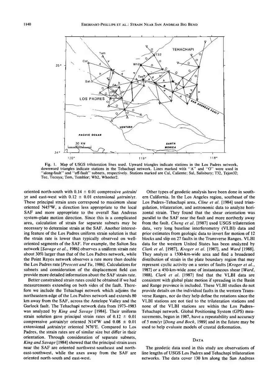
Fig. 1. Map of USGS trilateration lines used. Upward triangles indicate stations in the Los Padres network, downward triangles indicate stations in the Tehachapi network. Lines marked with "A" and "O" were used in "along-fault" and "off-fault" subnets, respectively. Stations marked are Cal, Caliente; Sal, Salisbury; T32, Tejon32; Tec, Tecuya; Tern, Temblor; Wh2, Wheeler2.

oriented north-south with 0.14 ___ 0.01 compressive/astrain/ yr and east-west with 0.12 ___ 0.01 extensional /xstrain/yr. These principal strain axes correspond to maximum shear oriented N45øW, a direction less appropriate to the local SAF and more appropriate to the overall San Andreas system-plate motion direction. Since this is a complicated area, calculation of strain for separate subnets may be necessary to determine strain at the SAF. Another interest- ing feature of the Los Padres uniform strain solution is that the strain rate is lower than typically observed on well- oriented segments of the SAF. For example, the Salton Sea network [Savage et al., 1986] observes a uniform strain rate about 30% larger than that of the Los Padres network, while the Point Reyes network observes a rate more than double the Los Padres rate [Prescott and Yu, 1986]. Calculations for subnets and consideration of the displacement field can provide more detailed information about the SAF strain rate.

Better constrained strain rates could be obtained if we had

measurements extending on both sides of the fault. There- fore we include the Tehachapi network which adjoins the northeastern edge of the Los Padres network and extends 80 km away from the SAF, across the Antelope Valley and the Garlock fault. The Tehachapi network data from 1973-1983 was analyzed by King and Savage [1984]. Their uniform strain solution gave principal strain rates of 0.12 ___ 0.01 compressive /xstrain/yr oriented N14øW and 0.08 -+ 0.01 extensional /xstrain/yr oriented N76øE. Compared to Los Padres, the strain rates are of similar size but differ in their orientation. Through consideration of separate subnets, King and Savage [1984] showed that the principal strain axes near the SAF are oriented northwest-southeast and north-

east-southwest, while the axes away from the SAF are oriented north-south and east-west.

Other types of geodetic analysis have been done in southern California. In the Los Angeles region, southeast of the Los Padres-Tehachapi area, Cline et al. [1984] used trian- gulation, trilateration, and astronomic data to analyze horizontal strain. They found that the shear orientation was parallel to the SAF near the fault and more northerly away from the fault. Cheng et al. [1987] used USGS trilateration data, very long baseline interferometry (VLBI) data and prior estimates from geologic data to invert for motion of 12 blocks and slip on 27 faults in the Transverse Ranges. VLBI data for the western United States has been analyzed by Clark et al. [1987], Kroger et al. [1987], and Ward [1988]. They analyze a 1500-km-wide area and find a broadened distribution of strain in the plate boundary region that may represent cyclic activity on a series of faults [Kroger et al., 1987] or a 450-km-wide zone of instantaneous shear [Ward, 1988]. Clark et al. [1987] find that the VLBI data are consistent with global plate motion if spreading in the Basin and Range province is included. These VLBI studies do not provide details on the individual faults in the western Trans- verse Ranges, nor do they help define the rotations since the VLBI stations are not tied to the trilateration stations and

none of the VLBI stations are within the Los Padres-

Tehachapi network. Global Positioning System (GPS) measurements, begun in 1987, have a repeatability and accuracy of 5 mm/yr [Dong and Bock, 1989] and in the future may be used to help evaluate models of crustal deformation.

DATA

The geodetic data used in this study are observations of line lengths of USGS Los Padres and Tehachapi trilateration networks. The data cover 130 km along the San Andreas

EBERHART-PHILLIPS ET AL.: STRAIN NEAR SAN ANDREAS BIG BEND 1141

TABLE 1. Uniform Strain Solutions

Area

Strain Rate Components, /•strain/yr

b12 b22 Dilatation

Max Shear Strain

•rad/yr

Max Shear Orientation

deg Description

L

T

L,T L

T

L

Le

0 15 _+ 0.01 0 13 _+ 0.01

0 15 _+ 0.01

0 10 _+ 0.01

009 _+ 0.01

0 17 _+ 0.01

008 ___ 0.01

T 0.16 _ 0.01

Le, T 0.17 _ 0.01

0.01 + 0.004 -0.13 + 0.01 0.02 _+ 0.01 0.27 _+ 0.01 -46.7 _+ 0.9 all Los Padres net

0.07 + 0.004 -0.12 + 0.01 0.01 _+ 0.01 0.29 _+ 0.01 -59.6 _+ 0.8 all Tehachapi net 0.04 + 0.003 -0.13 _+ 0.01 0.02 _+ 0.01 0.28 + 0.01 -53.4 _+ 0.6 all data

-0.003 + 0.01 -0.08 + 0.01 0.02 + 0.02 0.18 _+ 0.02 -43.9 _ 2.2 off-fault

-0.005 _+ 0.01 -0.10 _+ 0.01 -0.01 _+ 0.02 0.19 _+ 0.01 -43.5 _+ 2.1 off-fault

0.01 _+ 0.01 -0.17 _+ 0.01 -0.00 _+ 0.02 0.34 _+ 0.01 -47.0 _+ 1.1 along-fault 0.07 + 0.01 -0.18 + 0.01 -0.10 _+ 0.02 0.30 -+ 0.02 -58.6 _+ 1.8 excluding Temblor,

Caliente, Salisbury 0.12 _+ 0.01 -0.14 _+ 0.01 0.02 _+ 0.01 0.38 _+ 0.02 -64.6 _+ 0.9 along-fault 0.07 _+ 0.004 -0.16 + 0.01 -0.02 _+ 0.01 0.37 _+ 0.01 -62.8 _+ 0.7 along-fault

L, Los Padres; T, Tehachapi; Le, excluding stations northwest of bend.

fault and 140 km across the fault. The Tehachapi network is located east of the Los Padres network but joins the Los Padres network at two stations, Wheeler2 and Tecuya (Fig- ure 1). Thus the networks balance each other well across the fault from northeast to southwest. However, stations on the east and west peripheries of the combined network will be only weakly constrained in displacement solutions.

Distances between monuments were measured with a

Geodolite, and corrected for reftactivity as described by Savage and Prescott [1973]. The data cover the period 1973-1987, although the temporal distribution of measurements varies somewhat from line to line. Some stations were

added to the networks during the time period. Some stations have had to be replaced because of vandalism or environ- mental problems, and measurements to replacement stations have been reduced to correspond to the original stations.

In surveying lines, some observations may actually be erroneous measurements, called blunders. We do not want to include any blunders, but we do not want to discard observations simply because they do not fit our models of strain accumulation. Thus we applied the simple and con- servative criterion suggested by Savage et al. [1986]: a linear fit in time is done separately for each survey line, and any measurement that deviates from the linear fit by greater than three observed standard errors, as calculated for that survey line, is considered to be a surveying blunder. Only one measurement in the original data set was considered a blunder. A total of 881 observations of 73 lines remained for

this study.

UNIFORM STRAIN SOLUTIONS

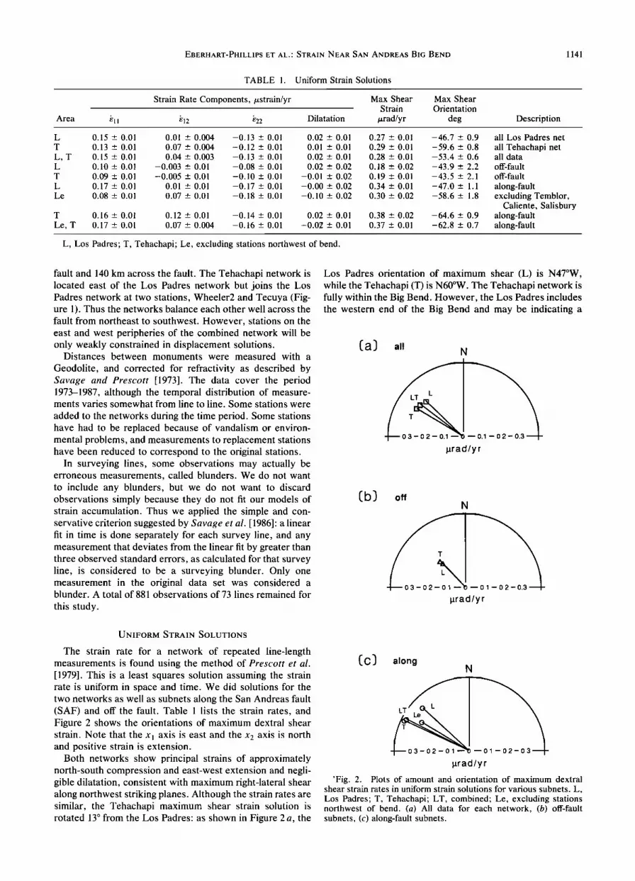
The strain rate for a network of repeated line-length measurements is found using the method of Prescott et al. [1979]. This is a least squares solution assuming the strain rate is uniform in space and time. We did solutions for the two networks as well as subnets along the San Andreas fault (SAF) and off the fault. Table 1 lists the strain rates, and Figure 2 shows the orientations of maximum dextral shear strain. Note that the x] axis is east and the x2 axis is north and positive strain is extension.

Both networks show principal strains of approximately north-south compression and east-west extension and negligible dilatation, consistent with maximum right-lateral shear along northwest striking planes. Although the strain rates are similar, the Tehachapi maximum shear strain solution is rotated 13 ø from the Los Padres: as shown in Figure 2 a, the

Los Padres orientation of maximum shear (L) is N47øW, while the Tehachapi (T) is N60øW. The Tehachapi network is fully within the Big Bend. However, the Los Padres includes the western end of the Big Bend and may be indicating a

grad/yr

off

grad/yr

along N

grad/yr

'Fig. 2. Plots of amount and orientation of maximum dextral shear strain rates in uniform strain solutions for various subnets. L, Los Padres; T, Tehachapi; LT, combined; Le, excluding stations northwest of bend. (a) All data for each network, (b) off-fault subnets, (c) along-fault subnets.

1142 EBERHART-PHILLIPS ET AL.: STRAIN NEAR SAN ANDREAS BiG BEND

35"

l

Los Padres

T

0 20 ILtstrain/yr

hapi

i i

I i i I I 120' 119' 118'

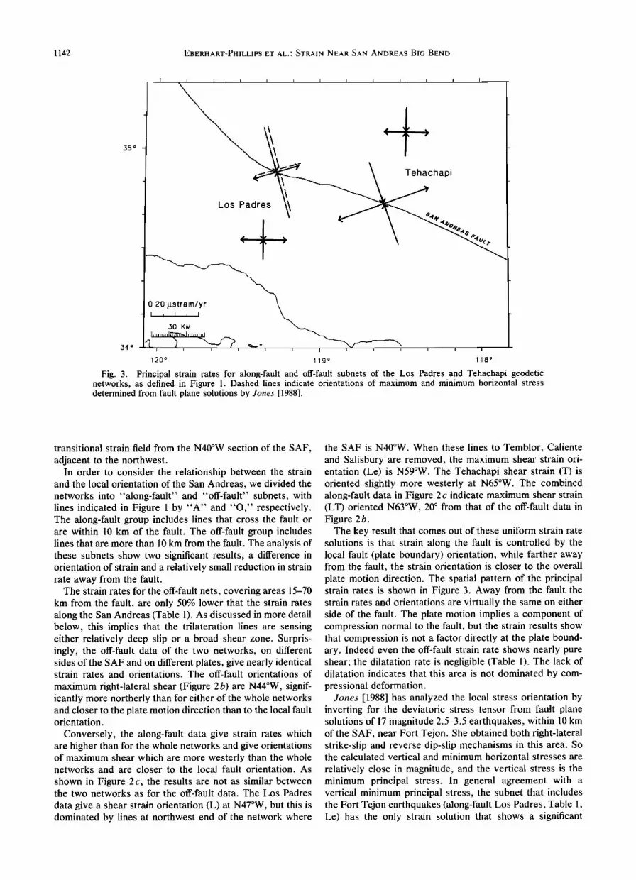
Fig. 3. Principal strain rates for along-fault and off-fault subnets of the Los Padres and Tehachapi geodetic networks, as defined in Figure 1. Dashed lines indicate orientations of maximum and minimum horizontal stress determined from fault plane solutions by Jones [1988].

transitional strain field from the N40øW section of the SAF,

adjacent to the northwest. In order to consider the relationship between the strain

and the local orientation of the San Andreas, we divided the networks into "along-fault" and "off-fault" subnets, with lines indicated in Figure 1 by "A" and "O," respectively. The along-fault group includes lines that cross the fault or are within 10 km of the fault. The off-fault group includes lines that are more than 10 km from the fault. The analysis of these subnets show two significant results, a difference in orientation of strain and a relatively small reduction in strain rate away from the fault.

The strain rates for the off-fault nets, covering areas 15-70 km from the fault, are only 50% lower that the strain rates along the San Andreas (Table 1). As discussed in more detail below, this implies that the trilateration lines are sensing either relatively deep slip or a broad shear zone. Surpris- ingly, the off-fault data of the two networks, on different sides of the SAF and on different plates, give nearly identical strain rates and orientations. The off-fault orientations of

maximum right-lateral shear (Figure 2b) are N44øW, significantly more northerly than for either of the whole networks and closer to the plate motion direction than to the local fault orientation.

Conversely, the along-fault data give strain rates which are higher than for the whole networks and give orientations of maximum shear which are more westerly than the whole networks and are closer to the local fault orientation. As

shown in Figure 2 c, the results are not as similar between the two networks as for the off-fault data. The Los Padres

data give a shear strain orientation (L) at N47øW, but this is dominated by lines at northwest end of the network where

the SAF is N40øW. When these lines to Temblor, Caliente and Salisbury are removed, the maximum shear strain orientation (Le) is N59øW. The Tehachapi shear strain (T) is oriented slightly more westerly at N65øW. The combined along-fault data in Figure 2 c indicate maximum shear strain (LT) oriented N63øW, 20 ø from that of the off-fault data in Figure 2 b.

The key result that comes out of these uniform strain rate solutions is that strain along the fault is controlled by the local fault (plate boundary) orientation, while farther away from the fault, the strain orientation is closer to the overall plate motion direction. The spatial pattern of the principal strain rates is shown in Figure 3. Away from the fault the strain rates and orientations are virtually the same on either side of the fault. The plate motion implies a component of compression normal to the fault, but the strain results show that compression is not a factor directly at the plate boundary. Indeed even the off-fault strain rate shows nearly pure shear; the dilatation rate is negligible (Table 1). The lack of dilatation indicates that this area is not dominated by compressional deformation.

Jones [1988] has analyzed the local stress orientation by inverting for the deviatoric stress tensor from fault plane solutions of 17 magnitude 2.5-3.5 earthquakes, within 10 km of the SAF, near Fort Tejon. She obtained both right-lateral strike-slip and reverse dip-slip mechanisms in this area. So the calculated vertical and minimum horizontal stresses are

relatively close in magnitude, and the vertical stress is the minimum principal stress. In general agreement with a vertical minimum principal stress, the subnet that includes the Fort Tejon earthquakes (along-fault Los Padres, Table 1, Le) has the only strain solution that shows a significant

EBERHART-PHILLIPS ET AL ' STRAIN NEAR SAN ANDREAS BIG BEND 1143

35 ø

34 ø

Preferred Slip Direction N39W

120 ø 119 ø 118 ø

•o

(b)

•o

(c)

lo

E E

:;, 0 ,'•_

o ,•o •o •o

....... Ns •-•:ø dist,•no•, •økm

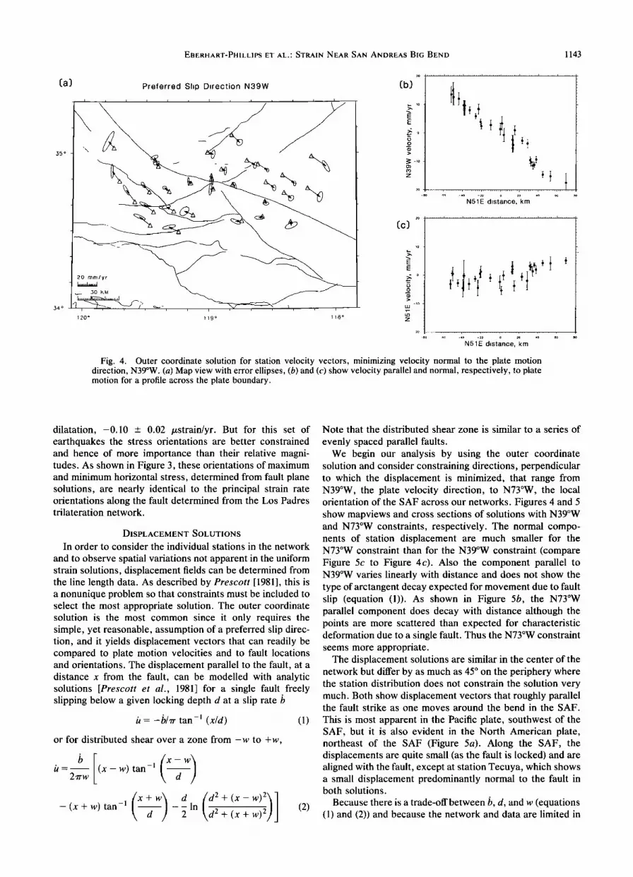
Fig. 4. Outer coordinate solution for station velocity vectors, minimizing velocity normal to the plate motion direction, N39øW. (a) Map view with error ellipses, (b) and (c) show velocity parallel and normal, respectively, to plate motion for a profile across the plate boundary.

dilatation, -0.10 _+ 0.02 /xstrain/yr. But for this set of earthquakes the stress orientations are better constrained and hence of more importance than their relative magni- tudes. As shown in Figure 3, these orientations of maximum and minimum horizontal stress, determined from fault plane solutions, are nearly identical to the principal strain rate orientations along the fault determined from the Los Padres trilateration network.

DISPLACEMENT SOLUTIONS

In order to consider the individual stations in the network

and to observe spatial variations not apparent in the uniform strain solutions, displacement fields can be determined from the line length data. As described by Prescott [1981], this is a nonunique problem so that constraints must be included to select the most appropriate solution. The outer coordinate solution is the most common since it only requires the simple, yet reasonable, assumption of a preferred slip direction, and it yields displacement vectors that can readily be compared to plate motion velocities and to fault locations and orientations. The displacement parallel to the fault, at a distance x from the fault, can be modelled with analytic solutions [Prescott et al., 1981] for a single fault freely slipping below a given locking depth d at a slip rate •

/t = -•/rr tan -1 (x/d) (1)

or for distributed shear over a zone from -w to +w,

/t= (x-w) tan -1 x-w 2rrw d

_(x+w) tan-, (x+w) d (d2+(x-w)i) ] d -•ln •+(x+w) (2)

Note that the distributed shear zone is similar to a series of

evenly spaced parallel faults. We begin our analysis by using the outer coordinate

solution and consider constraining directions, perpendicular to which the displacement is minimized, that range from N39øW, the plate velocity direction, to N73øW, the local orientation of the SAF across our networks. Figures 4 and 5 show mapviews and cross sections of solutions with N39øW and N73øW constraints, respectively. The normal components of station displacement are much smaller for the N73øW constraint than for the N39øW constraint (compare Figure 5c to Figure 4c). Also the component parallel to N39øW varies linearly with distance and does not show the type of arctangent decay expected for movement due to fault slip (equation (1)). As shown in Figure 5b, the N73øW parallel component does decay with distance although the points are more scattered than expected for characteristic deformation due to a single fault. Thus the N73øW constraint seems more appropriate.

The displacement solutions are similar in the center of the network but differ by as much as 45 ø on the periphery where the station distribution does not constrain the solution very much. Both show displacement vectors that roughly parallel the fault strike as one moves around the bend in the SAF.

This is most apparent in the Pacific plate, southwest of the SAF, but it is also evident in the North American plate, northeast of the SAF (Figure 5a). Along the SAF, the displacements are quite small (as the fault is locked) and are aligned with the fault, except at station Tecuya, which shows a small displacement predominantly normal to the fault in both solutions.

Because there is a trade-offbetween •, d, and w (equations (1) and (2)) and because the network and data are limited in


35 ø

34 ø

Preferred Slip Direction N73W

120 ø 119 ø 118 ø

._

z

so -•o -4o • o 2o 4o •o 8c

N17• distance, km

Cc) -ø

-'øN 17• ø dist;nce, •m Fig. 5. Outer coordinate solution for station velocity vectors, minimizing velocity normal to the local orientation of

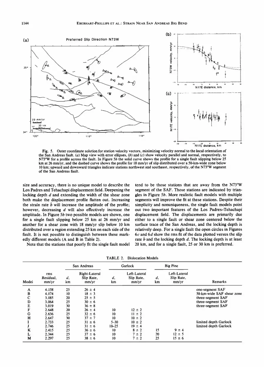
the San Andreas fault. (a) Map view with error ellipses, (b) and (c) show velocity parallel and normal, respectively, to N73øW for a profile across the fault. In Figure 5b the solid curve shows the profile for a single fault slipping below 25 km at 26 mm/yr, and the dashed curve shows the profile for 18 mm/yr of slip distributed over a 50-km-wide zone below 10 km; upward and downward triangles indicate stations northwest and southeast, respectively, of the N73øW segment of the San Andreas fault.

size and accuracy, there is no unique model to describe the Los Padres and Tehachapi displacement field. Deepening the locking depth d and extending the width of the shear zone both make the displacement profile flatten out. Increasing the strain rate b will increase the amplitude of the profile; however, decreasing d will also effectively increase the amplitude. In Figure 5b two possible models are shown, one for a single fault slipping below 25 km at 26 mm/yr and another for a shear zone with 18 mm/yr slip below 10 km distributed over a region extending 25 km on each side of the fault. It is not possible to distinguish between these markedly different models (A and B in Table 2).

Note that the stations that poorly fit the single fault model

tend to be those stations that are away from the N73øW segment of the SAF. Those stations are indicated by triangles in Figure 5b. More realistic fault models with multiple segments will improve the fit at these stations. Despite their simplicity and nonuniqueness, the single fault models point out two important features of the Los Padres-Tehachapi displacement field. The displacements are primarily due either to a single fault or shear zone centered below the surface trace of the San Andreas, and the locking depth is relatively deep. For a single fault the open circles in Figures 6c and 6d show the rms fit of the data plotted versus the slip rate b and the locking depth d. The locking depth is at least 20 km, and for a single fault, 25 or 30 km is preferred.

TABLE 2. Dislocation Models

Model

rms

Residual, mm/yr

d,

San Andreas

Right-Lateral Slip Rate,

mm/yr

Garlock

Left-Lateral

d, Slip Rate, d, km mm/yr km

Big Pine

Left-Lateral

Slip Rate, mm/yr Remarks

A

B

C D

E

F

G H

I

J K

L

M

4.158

4.174

3.185 3.064

3.019 2.648

2.636

2.647

2.733

2.746 2.415

2.344

2.297

25

10

20

25

30

20

25

30

25

25

25 25

25

26_+4

18_+3

25_+5 30_+6

36_+8

26_+4

32_+6

37_+7

31_+6

31_+6

36_+6

37_+6

38_+6

10 12 _+ 2

10 11 _+2

10 10 _+ 2

5-30 10 _+ 2 10-25 19 _+ 4

10 8_+2

10 7-+2 10 7-+2

15

20 25

9_+4 12_+5

15_+6

one-segment SAF 50-km-wide SAF shear zone

three-segment SAF three-segment SAF three-segment SAF

limited depth Garlock limited depth Garlock

EBERHART-PHILLIPS ET AL' STRAIN NEAR SAN ANDREAS BIG BEND 1145

2.0 0

-5

.E -lO

._

-20

0

'D -5

• '• -10 E o E •

o. O -15 .-- .

03 -20 ß

5O

03 30

20

10 2.0

2.0

3O

03 20

0

o 20

•o •0 o

0

3.0 4.0 5.0 , i , , I .... ' .... '

Ol

• 2o

.? m lO

[c)

3.0 4.0 5'.0 rmsres (mm/¾r)

3.0 4.0 5.0 r ß ß ß i .... i i i i i I

A 0

/l"lCIA 0 eee ß A 0

A 0

,

E ,

ll-I

i-1 ß

ß

ß

ß

ß

.... i ß , , i .... i

0 3.0 4.0 5.0

rmsres (mm/¾r)

O 1-seg SAF

• 3-seg SAF

ß Off-trace SAF

[] SAF, Garlock

ß L•m•ted depth Garlock

ß SAF, Garlock,

B,g P•ne

Fig. 6. Summary of multiple fault slip dislocation model solutions. Upper plots show computed slip in millimeters per year for the (c) San Andreas, (b) Garlock, and (a) Big Pine faults versus rms residual. Lower plots show assigned locking depth in kilometers for the (d) San Andreas, (e) Garlock, and (f) Big Pine faults versus rms residual. For the Garlock fault, lines indicate solutions with slip only within limited depths.

MULTIPLE FAULT SLIP SOLUTIONS

While modeling with a single fault can provide some useful insights, clearly, this region is characterized by numerous fault segments of varied orientation. The San Andreas changes its orientation markedly across these networks, and other adjoining Quarternary faults, such as the Garlock and Big Pine, strike through the area at angles completely different from the SAF.

In order to include many fault segments of any given

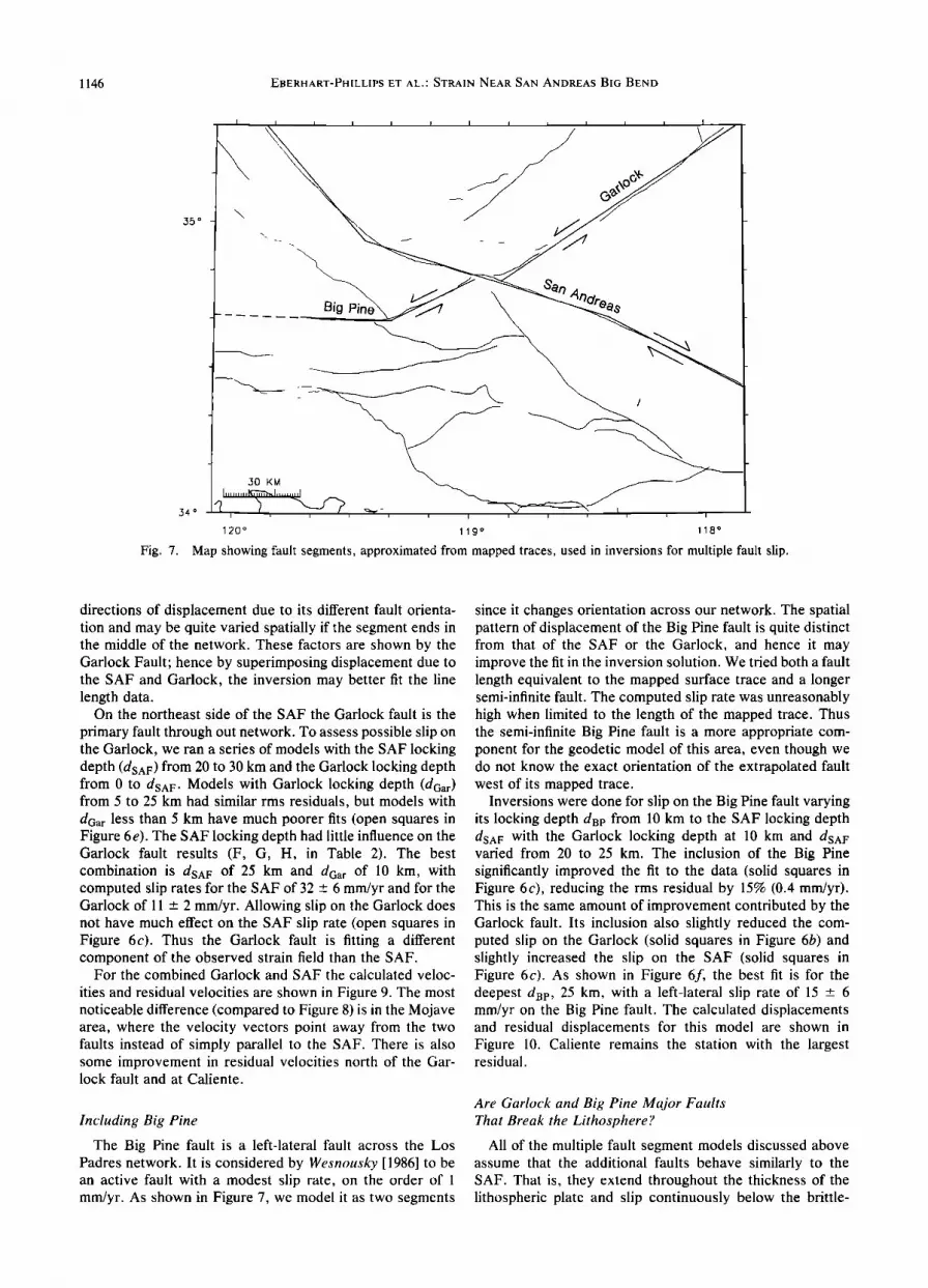
orientation and sense of slip, we used the program of Savage et al. [1979] to invert for multiple fault slip. The segments tested are shown in Figure 7. The SAF is divided into three segments: a semi-infinite N40øW segment, the local N73øW segment, and a semi-infinite N63øW segment. Since we are modeling deep slip, small segments contribute little to the total slip, and greater detail of the fault bend is not necessary. Secondary faults were also considered. For the SAF, Garlock, and Big Pine faults the results of this analysis were fairly stable regardless of changes in fault parameters, and so these are the only faults discussed in the solutions for this set of geodetic data. With these data we were unable to resolve slip on other faults that were tested, the Santa Ynez, White Wolf, and San Gabriel.

San Andreas Fault

For comparison, we initially did a series of solutions for slip on a single fault, striking N73øW with locking depth d, ranging from 15 to 30 km. The residuals for these were all similar, although the d = 25 solution is slightly better. The locking depth primarily effects the slip rate: d = 25 km gives a calculated slip rate of 26 mm/yr, while d = 15 km gives 18 mm/yr.

Next we approximated the SAF with the three segments described in Figure 7. However, our network does not constrain the slip on the two semi-infinite segments very well, as along these segments there are only a few stations near the ends. The simplest assumption is to have a uniform rate of slip on the whole length of the SAF. Thus we fixed the slip on the two end segments to be the same as the slip that is computed for the middle segment.

Figure 6 shows, for a wide range of multiple fault models, the slip rates and locking depths plotted versus the rms residual of each model. Each type of model is shown with a different symbol, and the rms error is shown for the calculated slip rates. There is clearly a dramatic decrease in rms residual when the SAF is modelled with three segments instead of one (compare triangles and circles in Figure 6c). For the three-segment SAF the rms residuals are similar for models with locking depths d from 25 to 40 km, but the fits for models with d less than 25 km are noticeably worse (triangles in Figure 6d). For a locking depth of 25 km the computed slip rate is 30 -+ 6 mm/yr (D in Table 2). Figure 8 shows the calculated velocities for the d = 25 km model, as well as the residual velocity vectors computed from the set of individual line length residuals. (The residual velocities are plotted at a scale roughly 3 times larger than the model velocities.) Since the model serves to remove the fault- related displacements, there should not necessarily be any remaining systematic displacement, and hence the inner coordinate solution [Prescott, 1981] is used to compute the residual velocity vectors (J. Savage, oral communication, 1988). Note that in order to compute a displacement solution we can only use a closed network. Hence stations that have only one line are not used in Figure 8b, although they are used in the inversions for fault slip. Particularly large residual velocities remain at station Caliente, on the northwest edge of the network, and at many stations in the area between the SAF and Garlock faults.

Including Garlock Fault

The displacement field of a secondary fault segment will be distinct from that of the SAF. It may have different


35 ø -

I I I I • I I I I

30 KM

I ......... I ,,•---"•r,d,•u• ,•1• 120 ø 119 ø

i

118 ø

Fig. 7. Map showing fault segments, approximated from mapped traces, used in inversions for multiple fault slip.

directions of displacement due to its different fault orientation and may be quite varied spatially if the segment ends in the middle of the network. These factors are shown by the Garlock Fault; hence by superimposing displacement due to the SAF and Garlock, the inversion may better fit the line length data.

On the northeast side of the SAF the Garlock fault is the

primary fault through out network. To assess possible slip on the Garlock, we ran a series of models with the SAF locking depth (dsA F) from 20 to 30 km and the Garlock locking depth from 0 to dSA F. Models with Gadock locking depth (dGar) from 5 to 25 km had similar rms residuals, but models with dGa r less than 5 km have much poorer fits (open squares in Figure 6e). The SAF locking depth had little influence on the Garlock fault results (F, G, H, in Table 2). The best combination is dsA F of 25 km and dGa r of 10 km, with computed slip rates for the SAF of 32 ___ 6 mm/yr and for the Garlock of 11 ___ 2 mm/yr. Allowing slip on the Garlock does not have much effect on the SAF slip rate (open squares in Figure 6c). Thus the Garlock fault is fitting a different component of the observed strain field than the SAF.

For the combined Garlock and SAF the calculated veloc-

ities and residual velocities are shown in Figure 9. The most noticeable difference (compared to Figure 8) is in the Mojave area, where the velocity vectors point away from the two faults instead of simply parallel to the SAF. There is also some improvement in residual velocities north of the Gar- lock fault and at Caliente.

Including Big Pine

The Big Pine fault is a left-lateral fault across the Los Padres network. It is considered by Wesnousky [1986] to be an active fault with a modest slip rate, on the order of 1 mm/yr. As shown in Figure 7, we model it as two segments

since it changes orientation across our network. The spatial pattern of displacement of the Big Pine fault is quite distinct from that of the SAF or the Garlock, and hence it may improve the fit in the inversion solution. We tried both a fault length equivalent to the mapped surface trace and a longer semi-infinite fault. The computed slip rate was unreasonably high when limited to the length of the mapped trace. Thus the semi-infinite Big Pine fault is a more appropriate component for the geodetic model of this area, even though we do not know the exact orientation of the extrapolated fault west of its mapped trace.

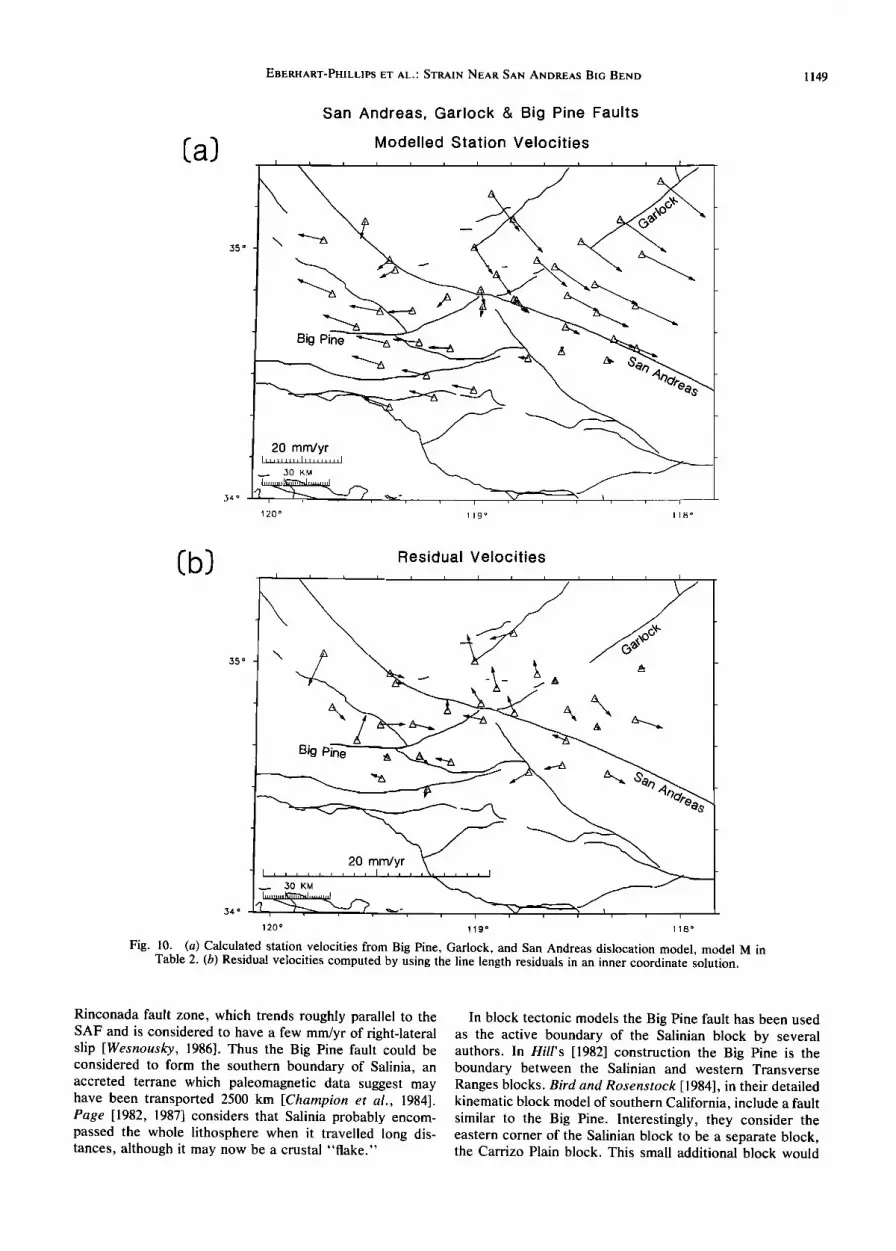
Inversions were done for slip on the Big Pine fault varying its locking depth dBp from 10 km to the SAF locking depth dsA F with the Garlock locking depth at 10 km and dsA F varied from 20 to 25 km. The inclusion of the Big Pine significantly improved the fit to the data (solid squares in Figure 6c), reducing the rms residual by 15% (0.4 mm/yr). This is the same amount of improvement contributed by the Garlock fault. Its inclusion also slightly reduced the computed slip on the Garlock (solid squares in Figure 6b) and slightly increased the slip on the SAF (solid squares in Figure 6c). As shown in Figure 6f, the best fit is for the deepest dBp, 25 km, with a left-lateral slip rate of 15 ___ 6 mm/yr on the Big Pine fault. The calculated displacements and residual displacements for this model are shown in Figure 10. Caliente remains the station with the largest residual.

Are Garlock and Big Pine Major Faults That Break the Lithosphere?

All of the multiple fault segment models discussed above assume that the additional faults behave similarly to the SAF. That is, they extend throughout the thickness of the lithospheric plate and slip continuously below the brittle-

EBERHART-PHILLIPS ET AL.' STRAIN NEAR SAN ANDREAS BIG BEND 1147

San Andreas Fault

Modelled Station Velocities

120 ø 1 19 ø 1 18 ø

35 ø

Residual Velocities

54ø '"•- - , I , , • • , 1 •20 o •9o •8 o

Fig. 8. (a) Calculated station velocities from three-segment San Andreas dislocation model, model D in Table 2. (b) Residual velocities computed by using the line length residuals in an inner coordinate solution; note that only closed lines could be used for this plot. In all these plots the scale of the vectors is indicated by the 20 mm/yr bar in the lower left corner.

ductile transition. Alternatively, the surface faults could end abruptly within the crust and the lower crust/mantle could deform independently, thus creating some sort of regional horizontal detachment at the brittle-ductile transition, as

implied by such deformation models as Kroger et al. [1987]. In their interpretation of a Consortium for Crustal Recon- naissance Using Seismic Techniques (COCORP) seismic reflection line across the eastern portion of the Garlock fault,

Cheadle et al. [1986] suggest that the Garlock fault does not extend below 9 km. Contradicting this, Astiz and Allen [1983] find that the Garlock is a seismically active fault, with earthquakes occurring down to 15 km (typical depths for earthquakes along the SAF). They infer that the western portion, through the Tehachapi geodetic network, is creep- ing but that there is potential for large earthquel•.e• on the eastern portion. They estimate the Garlock slip rate to be


(a)

35 ø

.34 ø

San Andreas and Oarlock Faults


120 ø 119 o

i

118 ø

(b)

L i Residual Velocities

i i i i ] i i i

35 ø

y

2_0 mm/yr •-- 34 ø •...- [ • • , • , ,

120 ø 119 o 118 ø

Fig. 9. (a) Calculated station velocities from Oarlock and San Andreas dislocation model, model G in Table 2. Residual velocities computed by using the line length residuals in an inner coordinate solution.

approximately 7 mm/yr, similar to the 6-11 mm/yr that we compute for a 10-km locking depth.

To investigate this issue, we ran a series of models with the Garlock fault having finite depth extent. The depth of the Garlock fault can be tested without including the implied decollement since such a horizontal feature would be fitting a different component of the displacement field than the Garlock fault. The upper locking depth varied from 5 to l0 km, and the vertical extent of the freely slipping fault segment varied from 10 to 25 km. All these models had

slightly higher rms (by about 0.1 mm/yr) residuals than the models discussed earlier with unlimited depth extent (Fig- ures 6b and 6e; Table 2, models I and J). For this type of model the best fit is obtained with slip confined to a depth interval of 5-30 or $-25 km. Thus the geodetic data can be reasonably fit by a fault extending only through the crust to 25 km, but the geodetic data cannot be fit by a Garlock fault that only extends to 9 km depth, as suggested by the COCORP interpretation.

The Big Pine fault could be extended to join with the


Ca)

San Andreas, Garlock & Big Pine Faults


• I I I I I I I I I 35 ø '•

Big

34ø • , • • • --7 ......

120ø 119 ø 1 18"

Cb) Residual Velocities

I . I I I I i I i i i i i I

35 ø

• _ _

34 ø

120ø 119 ø 118 ø

Fig. 10. (a) Calculated station velocities from Big Pine, Gatlock, and San Andreas dislocation model, model M in Table 2. (b) Residual velocities computed by using the line length residuals in an inner coordinate solution.

Rinconada fault zone, which trends roughly parallel to the SAF and is considered to have a few mm/yr of right-lateral slip [Wesnousky, 1986]. Thus the Big Pine fault could be considered to form the southern boundary of Salinia, an accreted terrane which paleomagnetic data suggest may have been transported 2500 km [Champion et al., 1984]. Page [1982, 1987] considers that Salinia probably encom- passed the whole lithosphere when it travelled long distances, although it may now be a crustal "flake."

In block tectonic models the Big Pine fault has been used as the active boundary of the Salinian block by several authors. In Hill's [1982] construction the Big Pine is the boundary between the Salinian and western Transverse Ranges blocks. Bird and Rosenstock [1984], in their detailed kinematic block model of southern California, include a fault similar to the Big Pine. Interestingly, they consider the eastern corner of the Salinian block to be a separate block, the Carrizo Plain block. This small additional block would

1150 EBERHART-PHILLIPS ET AL.; STRAIN NEAR SAN ANDREAS BIG BEND

contain the station Caliente, which was poorly fit by our multiple fault models.

Based on our analysis, we can only say that our solution is consistent with the idea that the Big Pine fault is an active left-lateral boundary of the Salinian block. Since the best locking depth for this fault was relatively deep, 25 kin, it could not be fit with a fault of limited depth extent, such as was done above for the Garlock. So a throughgoing lithospheric fault may be favored.

DISCUSSION

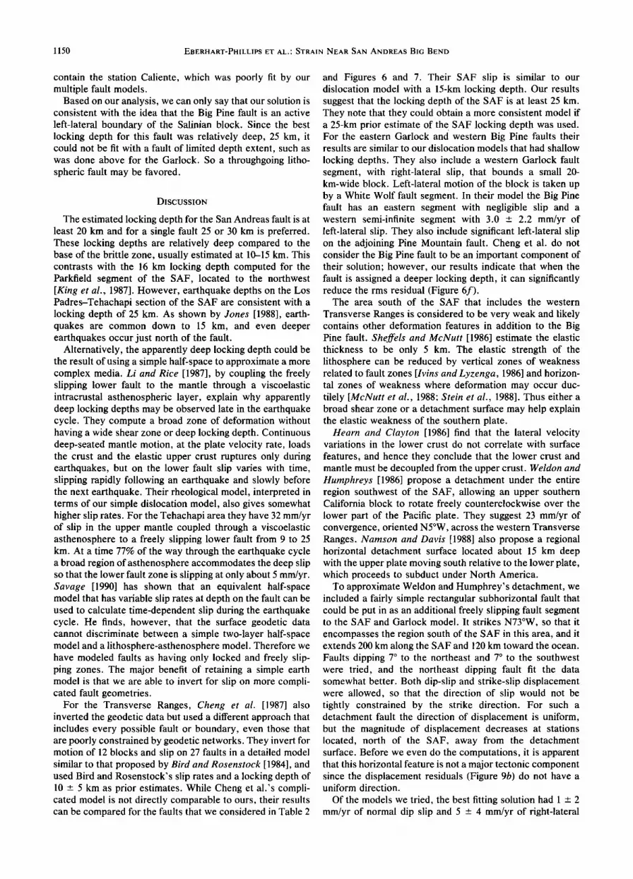
The estimated locking depth for the San Andreas fault is at least 20 km and for a single fault 25 or 30 km is preferred. These locking depths are relatively deep compared to the base of the brittle zone, usually estimated at 10-15 km. This contrasts with the 16 km locking depth computed for the Parkfield segment of the SAF, located to the northwest [King et al., 1987]. However, earthquake depths on the Los Padres-Tehachapi section of the SAF are consistent with a locking depth of 25 km. As shown by Jones [1988], earthquakes are common down to 15 km, and even deeper earthquakes occur just north of the fault.

Alternatively, the apparently deep locking depth could be the result of using a simple half-space to approximate a more complex media. Li and Rice [1987], by coupling the freely slipping lower fault to the mantle through a viscoelastic intracrustal asthenospheric layer, explain why apparently deep locking depths may be observed late in the earthquake cycle. They compute a broad zone of deformation without having a wide shear zone or deep locking depth. Continuous deep-seated mantle motion, at the plate velocity rate, loads the crust and the elastic upper crust ruptures only during earthquakes, but on the lower fault slip varies with time, slipping rapidly following an earthquake and slowly before the next earthquake. Their rheological model, interpreted in terms of our simple dislocation model, also gives somewhat higher slip rates. For the Tehachapi area they have 32 mm/yr of slip in the upper mantle coupled through a viscoelastic asthenosphere to a freely slipping lower fault from 9 to 25 km. At a time 77% of the way through the earthquake cycle a broad region of asthenosphere accommodates the deep slip so that the lower fault zone is slipping at only about 5 mm/yr. Savage [1990] has shown that an equivalent half-space model that has variable slip rates at depth on the fault can be used to calculate time-dependent slip during the earthquake cycle. He finds, however, that the surface geodetic data cannot discriminate between a simple two-layer half-space model and a lithosphere-asthenosphere model. Therefore we have modeled faults as having only locked and freely slipping zones. The major benefit of retaining a simple earth model is that we are able to invert for slip on more complicated fault geometries.

For the Transverse Ranges, Cheng et al. [1987] also inverted the geodetic data but used a different approach that includes every possible fault or boundary, even those that are poorly constrained by geodetic networks. They invert for motion of 12 blocks and slip on 27 faults in a detailed model similar to that proposed by Bird and Rosenstock [1984], and used Bird and Rosenstock's slip rates and a locking depth of 10 _+ 5 km as prior estimates. While Cheng et al.'s complicated model is not directly comparable to ours, their results can be compared for the faults that we considered in Table 2

and Figures 6 and 7. Their SAF slip is similar to our dislocation model with a 15-km locking depth. Our results suggest that the locking depth of the SAF is at least 25 km. They note that they could obtain a more consistent model if a 25-km prior estimate of the SAF locking depth was used. For the eastern Garlock and western Big Pine faults their results are similar to our dislocation models that had shallow

locking depths. They also include a western Garlock fault segment, with right-lateral slip, that bounds a small 20- km-wide block. Left-lateral motion of the block is taken up by a White Wolf fault segment. In their model the Big Pine fault has an eastern segment with negligible slip and a western semi-infinite segment with 3.0 -+ 2.2 mm/yr of left-lateral slip. They also include significant left-lateral slip on the adjoining Pine Mountain fault. Cheng et al. do not consider the Big Pine fault to be an important component of their solution; however, our results indicate that when the fault is assigned a deeper locking depth, it can significantly reduce the rms residual (Figure 6f).

The area south of the SAF that includes the western

Transverse Ranges is considered to be very weak and likely contains other deformation features in addition to the Big Pine fault. Sheffels and McNutt [1986] estimate the elastic thickness to be only 5 km. The elastic strength of the lithosphere can be reduced by vertical zones of weakness related to fault zones [Ivins and Lyzenga, 1986] and horizontal zones of weakness where deformation may occur duc- tilely [McNutt et al., 1988; Stein et al., 1988]. Thus either a broad shear zone or a detachment surface may help explain the elastic weakness of the southern plate.

Hearn and Clayton [1986] find that the lateral velocity variations in the lower crust do not correlate with surface

features, and hence they conclude that the lower crust and mantle must be decoupled from the upper crust. Weldon and Humphreys [1986] propose a detachment under the entire region southwest of the SAF, allowing an upper southern California block to rotate freely counterclockwise over the lower part of the Pacific plate. They suggest 23 mm/yr of convergence, oriented N5øW, across the western Transverse Ranges. Namson and Davis [1988] also propose a regional horizontal detachment surface located about 15 km deep with the upper plate moving south relative to the lower plate, which proceeds to subduct under North America.

To approximate Weldon and Humphrey's detachment, we included a fairly simple rectangular subhorizontal fault that could be put in as an additional freely slipping fault segment to the SAF and Garlock model. It strikes N73øW, so that it encompasses the region south of the SAF in this area, and it extends 200 km along the SAF and 120 km toward the ocean. Faults dipping 7 ø to the northeast and 7 ø to the southwest were tried, and the northeast dipping fault fit the data somewhat better. Both dip-slip and strike-slip displacement were allowed, so that the direction of slip would not be tightly constrained by the strike direction. For such a detachment fault the direction of displacement is uniform, but the magnitude of displacement decreases at stations located, north of the SAF, away from the detachment surface. Before we even do the computations, it is apparent that this horizontal feature is not a major tectonic component since the displacement residuals (Figure 9b) do not have a uniform direction.

Of the models we tried, the best fitting solution had 1 _+ 2 mm/yr of normal dip slip and 5 -+ 4 mm/yr of right-lateral


strike slip on a fault that dips 7øNE from the surface to a depth of 1:5 km at the SAF. While these values are poorly constrained, they are not similar to Weldon and Humphreys' in either direction or magnitude. However, we found that we could adjust the depth, location, strike, and dip of the detachment surface to get solutions with almost any slip, reverse or normal, right or left lateral. Therefore we cannot directly use these geodetic data to confirm or deny a detachment.

It has been proposed that crustal deformation along the Pacific-North American plate boundary results from an extremely broad and deep shear zone. Ward [1988] showed that a wide shear zone can fit VLBI data in the western

United States. To test this model, we have considered a shear zone, as in equation (2), with w of :500 km and b of 48 mm/yr below a depth D. It has infinite length and is centered along the N40øW central California SAF segment, similar to the model of Ward [1988], but unlike the Ward model, multiple faults were included in the plate above the shear zone. The other faults were allowed to slip from their locking depth to the shear zone depth D.

Including a broad deep shear zone improved the fit to the line length data for models that included only the three- segment SAF. The most improvement is for a fairly deep shear zone, D greater than 140 km. The fit was worsened if D was less than 80 km. In models that included other faults, the deep shear zone had little effect. There was a slight improvement for models that included the Garlock and a slight degradation for models that also included the Big Pine. Thus the trilateration data do not necessarily provide evidence for a broad shear zone, but they suggest that if such a feature exists, it must represent some type of deep deformation process such as asthenospheric flow.

Another widely discussed feature of the western Trans- verse Ranges is the location of the San Andreas fault at depth. Sheffets and McNutt [1986] use a flexural plate model of two plates with a load attached to the end of the southern plate to approximate a subducted slab. In order to match the gravity profile, they put the plate boundary south of the surface trace of the SAF by several tens of kilometers. In their constructed western Transverse Range cross section, Namson and Davis [1988] also place the SAF at depth 20 km south of its surface trace.

Since we are using geodetic networks that extend over 50 km either side of the SAF, we can use the geodetic data to help resolve the issue of the fault location at depth. We tested models with the SAF located 10, 20, and 30 km south of its surface trace, as well as one model with the fault dipping 60 ø to the south. Because it is difficult to imagine how such segments would connect with the adjoining N40øW trending SAF segment and the Garlock and Big Pine faults, we tested models with only a single infinite SAF segment. The results are shown as solid circles in Figures 6½ and 6d. We also considered :50- and 80-km-wide SAF shear zones

centered 10 and 20 km south of the surface trace. All of the

off-trace SAF solutions are significantly worse than any of the other one-segment SAF solutions. Therefore we can conclude that the plate boundary at depth is not located away from the mapped SAF but rather is essentially directly below the surface trace.

However, it is intriguing that both Sheffels and McNutt's "subduction" feature and Humphreys' [1987] "drip" feature both are east-west striking subsurface features located south

of the SAF in the western Transverse Ranges. They explain that this feature is due to the component of compression resulting from the mismatch between the local SAF orientation and the plate motion direction. We decided to look at this residual plate motion in detail.

If at some depth below the fractured brittle crust the Pacific and North American plates are large continuous plates moving N40øW and S40øE, respectively, at 48 mm/yr [DeMets et at., 1987], then near the Big Bend, there will be some plate motion that cannot be accounted for by movement on the SAF. For a reasonable, yet simple, model of the long-term SAF motion, we consider a vertical boundary between the lithospheric plates with 36 mm/yr of right-lateral slip along all segments of the fault (the calculated rate for deep slip below 30 km, Table 2, model E). Then the residual plate motion displacement field will be this SAF displacement field subtracted from the motion of each plate, as shown in Figure 11. Note that in the western Transverse Ranges (west of l 18ø40'), the area with the largest amount of residual displacement is not centered along the SAF but is centered far south of the SAF.

The residual plate motion is compared to Humphreys et at. [1984] teleseismic P velocity inversion results in Figure 11. The outlined area shows the region that has relatively high seismic velocity at 100 km depth. If we consider that the area with the most compressive residual plate motion is repre- sented by the area of large nearly north-south directed residual displacements in Figure 11, then it is similar in location and orientation to Humphreys et al. high-velocity feature.

Therefore we propose that the location of the east-west striking subsurface feature is not at all surprising but rather is very similar to what we would expect to be caused by deep slip on a SAF plate boundary extending below the surface trace. Since Sheffels and McNutt have shown that a sub-

ducting slab model does not fit the mapped SAF location, our conclusion favors some other sort of mechanism for

mantle downwelling, such as Humphreys' [1987] thermal instability/drip ideas. Perhaps the gravity could also be fit by a plate, broken at the mapped SAF, but with the subsurface load distributed away from the end of the southern plate.

CONCLUSIONS

In the region of the Los Padres-Tehachapi geodetic network the San Andreas fault changes its orientation by over 30 ø from N40øW, close to that predicted by plate motion for a transform boundary, to N73øW. The geodetic data can be used to tell us where the fault is located at depth and what type of motion occurs on the SAF and secondary faults, as well as provide insight into the relationship between the SAF plate boundary and plate motion.

We divided the network into along-fault and off-fault subnets and then calculated the strain, uniform in space and time, for each subnet. The strain rates along-fault showed maximum shear of 0.38 _+ 0.01 /xrad/yr at N63øW. Virtually identical strain rates are found for the two off-fault subnets, on either side of the SAF, with maximum shear of 0.19 -+ 0.01/xrad/yr at N44øW. The local fault orientation apparently controls the strain along the SAF, while the overall plate motion direction dominates the strain away from the fault. Thus the compressional component of plate motion is not a factor directly at the plate boundary.

1152 EBERHART-PHILLIPS ET AL.: STRAIN NEAR SAN ANDREAS BIG BEND

I [ [ I I [ I I • ] [ [ I

120 ø 1 19 ø 1 18 ø 1 17 ø 1 16 ø 1 15 ø

FJS. ]]. ComparJso• of SAF slip rate a•d plate motion. Vectors J•dicate the residual plate motJo• displacemere field, that is the compo•em of plate motio• •ot accoumed for by the Sa• A•dreas fault in the BiB Bend resJo•. Displacemere from 36 mm/yr slip o• the SAF subtracted from 48 mm/yr plate motion. The outli•ed area shows N•phre•x et •1. []984] resio• of relatively hJSh seismic velocity at 100 km depth.

The geodetic data indicate a relatively deep locking depth on the SAF and a slip rate of approximately 30 mm/yr. The station velocity vectors can be fit by either a broad shear zone below the SAF or a single fault. For instance, for a fault zone with uniform orientation a 50-kin-wide zone below 10

km depth with 18 mm/yr of distributed shear or a single fault with 26 mm/yr of slip below 25 km is reasonable. A significantly better fit to the data is obtained by modelling a more realistic SAF with varied orientation through an inversion of the line length data. The fit is poor for locking depth d less than 25 km. For d of 25 km the computed slip rate is 30 +- 6 mm/yr, and the rms residual is 3.1 mm/yr.

We also computed multiple fault slip models that included the Garlock and Big Pine faults, in addition to the SAF. We tried adding other faults, such as the Santa Ynez, San Gabriel, and White Wolf, but their calculated slip was unconstrained and they did not provide any significant reduction in rms residual. Therefore, with this particular data set the only secondary faults that we can determine to be actively slipping are the Garlock and Big Pine.

The best fitting Garlock fault model had computed slip of 11 +_ 2 mm/yr below 10 km and had an rms residual of 2.6 mm/yr. Thus the Garlock fault may be a significant feature with potential for a large earthquake.

Left-lateral shear deformation is indicated within the

western Transverse Ranges. The addition of the Big Pine fault on the southern side of the SAF resulted in an rms

residual of 2.3 mm/yr for 15 ___ 6 mm/yr of slip below 25 km. The Big Pine fault runs through the Los Padres network and is the fault that provides the most significant reduction in line length residuals; however, the plate on the southern side of the SAF is relatively weak, and the deformation there is probably more complicated than a single vertical fault below the mapped Big Pine.

The remaining rms residual, about 2 mm/yr, is larger than the expected rms residual due to survey error, l.l mm/yr. The theoretical standard deviation of the rate of line length change for each line is calculated using Savage and Pres-

cott's [1973] formula for the precision of geodetic measurements. Forty-two percent of the residuals are less than the theoretical standard deviations, and 82% of the residuals are less than 3 times the theoretical standard deviations. The

lines most poorly fit by the model are to station Tejon32, near the White Wolf fault, so there may be some unmodelled slip on that fault. The next most poorly fit line crosses the SAF on the edge of the network from Caliente to Pattiway. Variable slip on the SAF and greater detail for the fault bend geometry might improve the fit for this line.

A subhorizontal detachment on the southern side of the

SAF cannot be well constrained by these data. By adjusting the size, location, and depth of the detachment surface, almost any amount and orientation of slip could be calculated with a slight improvement in rms residual.

We investigated the location of the SAF since it has been suggested that the fault at depth is located 20-30 km south of the mapped trace. We found that a simple vertical fault below the surface trace fits the line length data much better than either a dipping fault or a fault zone located south of the surface trace. However there is actually no contradiction between the surface-trace location of the SAF and Hum-

phreys et al.'s [1984] more southern east-west trending high-seismic-velocity feature. The residual plate motion displacement, obtained by subtracting the displacement field of SAF motion from uniform plate motion, would predict the observed location of a subsurface compressional feature.

Acknowledgments. This work grew out of a seminar at Stanford and benefited from discussion with Colleen Barton, Will Prescott, Beth Robinson, and Paul Segall. We appreciate comments and advice from Jim Savage. Reviews by Lucy Jones, Jim Savage, and two anonymous reviewers improved the manuscript.

REFERENCES

Astiz, L., and C. R. Allen, Seismicity of the Garlock fault, Califor- nia, Bull. Seismol. Soc. Am., 73, 1721-1734, 1983.

Bird, P., and R. W. Rosenstock, Kinematics of present crust and


mantle flow in southern California, Geol. Soc. Am. Bull., 95, 946-957, 1984.

Champion, D. E., D. G. Howell, and C. S. Gromme, Paleomagnetic and geologic data indicating 2500 km of northward displacement for the Salinian and related terranes, California, J. Geophys. Res., 89, 7736-7752, 1984.

Cheadle, M. J., B. L. Czuchra, C. J. Ando, T. Byrne, L. D. Brown, J. E. Oliver, and S. Kaufman, in Reflection Seisinology: The Continental Crust, Geodyn. Ser., vol. 14, edited by M. Barazangi and L. Brown, pp. 305-312, AGU, Washington, D.C., 1986.

Cheng, A., D. D. Jackson, and M. Matsu'ura, Aseismic crustal deformation in the Transverse Ranges of southern California, Tectonophysics, 144, 159-180, 1987.

Clark, T. A., D. Gordon, W. E. Himwich, C. Ma, A. Mallama, and J. W. Ryan, Determination of relative site motions in the western United States using MarkIll very long baseline interferometry, J. Geophys. Res., 92, 12,741-12,750, 1987.

Cline, M. W., R. A. Snay, and E. L. Timmerman, Regional deformation of the Earth model for the Los Angeles region, California, Tectonophysics, 107, 279-314, 1984.

Davis, G. A., and B.C. Burchfiel, Garlock fault: An intracontinental transform structure, southern California, Geol. Soc. Am. Bull., 84, 1407-1422, 1973.

DeMets, C., R. G. Gordon, S. Stein, and D. F. Argus, A revised estimate of Pacific-North America motion and implications for western North America plate boundary zone tectonics, Geophys. Res. Lett., 14, 911-914, 1987.

Dong, D.-N., and Y. Bock, Global positioning system network analysis with phase ambiguity resolution applied to crustal deformation studies in California, J. Geophys. Res., 94, 3949-3966, 1989.

Hearn, T. M., and R. W. Clayton, Lateral velocity variations in southern California, II, Results for the lower crust from Pn waves, Bull. Seismol. Soc. Am., 76, 511-520, 1986.

Hill, D. P., Contemporary block tectonics: California and Nevada, J. Geophys. Res., 87, 5433-5450, 1982.

Humphreys, E., Mantle dynamics of the southern Great Basin- Sierra Nevada region (abstract), Eos Trans. AGU, 68, 1450, 1987.

Humphreys, E., R. W. Clayton, and B. H. Hager, A tomographic image of mantle structure beneath southern California, Geophys. Res. Lett., 11,625-627, 1984.

Ivins, E. R., and G. A. Lyzenga, Stress patterns in an interplate shear zone: An effective anisotropic model and implications for the Transverse Ranges, California, Philos. Trans. R. Soc. London Set. A, 318, 285-347, 1986.

Jones, L. M., Focal mechanisms and the state of stress on the San Andreas fault in southern California, J. Geophys. Res., 93, 8869-8891, 1988.

King, N. E., and J. C. Savage, Regional deformation near Palmdale, California, 1973-1983, J. Geophys. Res., 89, 2471-2477, 1984.

King, N. E., P. Segall, and W. Prescott, Geodetic measurements near Parkfield, California, 1959-1984, J. Geophys. Res., 92, 2747-2766, 1987.

Kroger, P.M., G. A. Lyzenga, K. S. Wallace, and J. M. Davidson, Tectonic motion in the western United States from very long baseline interferometry measurements, 1980-1986, J. Geophys. Res., 92, 14,151-14,163, 1987.

Li, V. C., and J. R. Rice, Crustal deformation in great California earthquake cycles, J. Geophys. Res., 92, 11,533-11,551, 1987.

McNutt, M. K., M. Diament, and M. G. Kogan, Variations in elastic

plate thickness at continental thrust belts, J. Geophys. Res., 93, 8825-8838, 1988.

Namson, J., and T. Davis, Structural transect of the western Transverse Ranges, California: Implications for lithospheric kinematics and seismic risk evaluation, Geology, 16,675-679, 1988.

Page, B. M., Migration of Salinian composite block, California, and disappearance of fragments, Am. J. Sci., 282, 1694-1734, 1982.

Page, B. M., Geology and tectonics of the southern Coast Ranges, central California: Current models and major uncertainties, Eos Trans. A G U, 68, 1365, 1987.

Prescott, W. H., The determination of displacement fields from geodetic data along a strike-slip fault, J. Geophys. Res., 86, 6067-6072, 1981.

Prescott, W. H., and S.-B. Yu, Geodetic measurement of horizontal deformation in the northern San Francisco Bay region, California, J. Geophys. Res., 91, 7475-7484, 1986.

Prescott, W. H., J. C. Savage, and W. T. Kinoshita, Strain accumulation rates in the western United States between 1970 and

1978, J. Geophys. Res., 84, 5423-5435, 1979. Prescott, W. H., M. Lisowski, and J. C. Savage, Geodetic measure-

ment of crustal deformation on the San Andreas, Hayward, and Calaveras faults near San Francisco, California, J. Geophys. Res., 86, 10,853-10,869, 1981.

Savage, J. C., Equivalent strike-slip earthquake cycles in half-space and lithosphere-asthenosphere Earth models, J. Geophys. Res., in press, 1990.

Savage, J. C., and W. H. Prescott, Precision of geodolite distance measurements for determining fault movements, J. Geophys. Res., 78, 6001-6008, 1973.

Savage, J. C., W. H. Prescott, M. Lisowski, and N. King, Defor- mation across the Salton Trough, California, 1973-1977, J. Geo- phys. Res., 84, 3069-3080, 1979.

Savage, J. C., W. H. Prescott, and G. Gu, Strain accumulation in southern California, 1973-1984, J. Geophys. Res., 91, 7455-7473, 1986.

Sheffels, B., and M. McNutt, Role of subsurface loads and regional compensation in the isostatic balance of the Transverse Ranges, California: Evidence for intracontinental subduction, J. Geophys. Res., 91, 6419-6431, 1986.

Sieh, K. E., Slip along the San Andreas Fault associated with the great 1857 earthquake, Bull. Seismol. Soc. Am., 76, 1421-1448, 1978.

Stein, R. S., G. C. P. King, J. B. Rundle, The growth of geological structures by repeated earthquakes, 2, Field examples of continental dip-slip faults, J. Geophys. Res., 93, 13,319-13,331, 1988.

Ward, S., North America-Pacific plate boundary, an elastic-plastic megashear: Evidence from very long baseline interferometry, J. Geophys. Res., 93, 7716-7728, 1988.

Weldon, R., and E. Humphreys, A kinematic model of southern California, Tectonics, 5, 33-48, 1986.

Wesnousky, S. G., Earthquakes, Quarternary faults, and seismic hazard in California, J. Geophys. Res., 91, 12,587-12,631, 1986.

D. Eberhart-Phillips and M. Lisowski, U.S. Geological Survey, Office of Earthquakes, Volcanoes and Engineering, 345 Middlefield Road, Menlo Park, CA 94025.

M.D. Zoback, Department of Geophysics, Stanford University, Stanford, CA 94305.

(Received March 29, 1989; revised August 11, 1989;

accepted August 21, 1989.)

Crustal strain near the Big Bend of the San Andreas Fault: Analysis of the Los Padres-Tehachapi...

Documents

Transcript of Crustal strain near the Big Bend of the San Andreas Fault: Analysis of the Los Padres-Tehachapi...