Crop growth, soil water and nitrogen balance simulation on three experimental field plots using the...

Ecological Modelling 190 (2006) 116–132

Crop growth, soil water and nitrogen balance simulation on threeexperimental field plots using the Opus model—A case study

Martin Wegehenkel∗, Wilfried Mirschel

Centre of Agricultural Landscape Research, Institute of Landscape Systems Analysis,Eberswalder Strasse 84, D-15374 Muncheberg, Germany

Received 23 October 2003; received in revised form 21 December 2004; accepted 28 February 2005Available online 13 June 2005

Abstract

Over a period of 5 years, the agro-ecosystem model Opus was used to simulate soil water and nitrogen balance as well as cropgrowth for three experimental field plots. At these plots, different agricultural management practices were applied. The data setobtained from these plots consists of automatically recorded time series of daily volumetric soil water contents measured byTRIME-probes as well as daily pressure heads measured by tensiometer. Aboveground total biomass, yield, nitrogen-uptake bycrops as well as nitrate contents in the soil were measured at 6–10 sample times per year. The objective of this study was anevaluation of the accuracy of Opus regarding the simulation of crop growth, soil water and nitrogen balance. The simulationsof soil water contents and pressure heads correspond with the commonly measured trends in soil depths shallower than 60 cm.In depths deeper than 60 cm, some differences between measured and simulated soil water contents as well as pressure headsc trastt ion of cropg©

K

1

eg

f

ur-taskrch,toolsge-e

95

n,

0

ould be observed. Nitrate contents in the root zone and the aboveground total biomass were simulated satisfactorily. In cono that, simulated and observed yields show greater discrepancies. This indicates the need of a site specific calibratrowth parameters within the Opus model.2005 Elsevier B.V. All rights reserved.

eywords: Agro-ecosystem; Modelling; Nitrogen cycle; Crop growth; Soil water balance

. Introduction

The quantification and prediction of the potentialffects of agricultural management practices on croprowth, soil water and nitrogen balance – especially

∗ Corresponding author. Tel.: +49 33432 82275;ax: +49 33432 82334.

E-mail address: [email protected] (M. Wegehenkel).

nitrogen leaching, which can affect the quality of sface and shallow groundwater – is an essentialin any agro-ecological research. Within this reseasimulation models were developed and used asto predict the potential effects of agricultural manament practices (e.g.Addiscott and Whitmore, 1987; dWilligen, 1991; Neeteson, 1990; Rodda et al., 19).Among such simulation models are, e.g. SwaP (VanDam et al., 1997), Leachm-N (Wagenet and Hutso

304-3800/$ – see front matter © 2005 Elsevier B.V. All rights reserved.doi:10.1016/j.ecolmodel.2005.02.020

M. Wegehenkel, W. Mirschel / Ecological Modelling 190 (2006) 116–132 117

1990), Ceres (Godwin et al., 1989), SoilN (Bergstromet al., 1991), Opus (Smith, 1992a), Wave (Vancloosteret al., 1995) and Daisy (Svendsen et al., 1995). Suchmodels have to be validated by comparing simulatedmodel outputs with those measured in the field. Valida-tion studies with different models have been carried outat different locations (e.g.Bonilla et al., 1999; Smith,1995; de Willigen, 1991; Diekkruger et al., 1995; Porteret al., 1993).

This study is a summary of a 5 year long applicationof the Opus model on three experimental field plots tosimulate soil water and nitrogen balance in the rootzone as well as crop growth. The objective of the studywas an evaluation of the accuracy of Opus regardingthe simulation of crop growth, soil water and nitrogenbalance dynamics under the conditions of the north-eastGerman lowlands, which are characterized by meanannual precipitation rates of about 500 mm year−1 andsandy soils with high percolation rates as well as lowsoil water storage.

2. Material and methods

2.1. Field data

Three field plots were established for a long-termmonitoring of soil water balance, crop growth andnitrogen balance in the root zone at the experimentalfi rch( and1w tw waso edo

• adi-indera-theren-

• oil

• soilcon-ters

Fig. 1. Sensor installation scheme at the field plots (fromWenkeland Mirschel, 1995, modified).

and Time Domain Reflectometry with IntelligentMicroElements (TRIME)-probes.

• Gravimetric determination of soil moisture as wellas analysis of nitrate contents in the root zone on thebasis of 6–10 sample dates per year.

• Determination of aboveground total biomass, yieldand crop nitrogen content on the basis of 6–10 sam-ple dates within the growing seasons.

The soil type on the experimental field is aEutric Cambisol according to the FAO-classification.A description of the soil profiles at the three field plotscan be found inTable 1(Schindler, 1980).

For the measurement of depth-averaged soilwater contents for the 0–30, 30–60, 60–90, 90–120,and 120–150 cm compartments, TRIME-probes wereinstalled vertically in depths of 15, 45, 75, 105, and135 cm at each field plot (Fig. 1). This installationscheme also enables the estimation of the total soilwater mass down to 150 cm depth including the amountof soil water storage available for soil evaporation andcrop transpiration. However, this installation schemecan cause effects such as possible underestimationsconcerning the soil water dynamics due to the fact, thatthe heads of the probes with a diameter of 63 mm canreact as small barriers, and therefore, delay percolation.Tensiometers were installed at soil depths of 30, 60,90, 120, 150, 200 and 300 cm (Fig. 1). At each depth,one TRIME-probe and one tensiometer were installed.During frost periods, tensiometers in the depths of 30a time

eld of the Centre for Agricultural Landscape ReseaZALF), Muncheberg, Germany. Between 1993997, a crop rotation consisting of sugar beet→ winterheat→ winter barley→ winter rye→ sugar beeas established on every plot, each of whichf the size 107 m× 28 m. The data set consistf:

Daily weather data such as precipitation, global ration, maximum and minimum air temperature, wspeed, relative air humidity as well as soil temptures taken from an automatically recording weastation located at the southern part of the experimtal field.Soil data including texture, bulk density and shydraulic properties.Continuous measurements of daily values ofwater pressure heads and volumetric soil watertents using automatically recording tensiome
nd 60 cm were removed. The data set covers the

118 M. Wegehenkel, W. Mirschel / Ecological Modelling 190 (2006) 116–132

Table 1Soil properties, saturated hydraulic conductivityKs, Brooks–Corey parametershb, λ, α, saturated and residual soil water contentsθs andθr,descriptions of the layers according to AGBoden (1994)

Horizon Depthfrom to(cm)

Sand(%)

Clay(%)

Silt(%)

Bulkdensity(g cm−3)

Org. C(%)

Ks (mm d−1) hb (mm) λ α θs (mm3

mm−3)θr (mm3

mm−3)

Plot no. 1Ap 0–30 90 7 3 1.45 0.45 936 −47 0.503 3.51 0.385 0.0218Ael 30–60 90 5 5 1.50 0.26 1632 −45 0.580 3.74 0.319 0.0244Bt 60–90 80 12 8 1.48 0.10 312 −35 0.534 3.60 0.302 0.0623C1 90–120 90 4 6 – 0.0 1632 −45 0.580 3.74 0.319 0.0244C2 120–150 90 3 7 – 0.0 1632 −45 0.580 3.74 0.310 0.0244C3 150–225 90 2 8 – 0.0 1632 −45 0.580 3.74 0.310 0.0244

Plot no. 2Ap 0–30 85 5 10 1.45 0.45 936 −47 0.503 3.51 0.385 0.0218Ael 30–90 90 5 5 1.51 0.26 1632 −45 0.580 3.74 0.319 0.0244Bt1 90–130 80 12 8 1.48 0.10 312 −35 0.534 3.60 0.302 0.0623Bt2 130–170 80 10 10 – 0.0 312 −35 0.534 3.60 0.302 0.0623C1 170–180 90 5 5 – 0.0 1632 −45 0.580 3.74 0.319 0.0244C2 180–225 90 5 5 – 0.0 1632 −45 0.580 3.74 0.319 0.0244

Plot no. 3Ap 0–30 85 6 9 1.45 0.45 936 −47 0.503 3.51 0.385 0.0208Ael 30–100 90 5 5 1.51 0.26 1632 −45 0.580 3.74 0.319 0.0244Bt1 100–110 81 13 6 1.48 0.10 312 −35 0.534 3.60 0.302 0.0623Bt2 110–225 80 11 9 – 0.0 312 −35 0.534 3.60 0.302 0.0623

period from 1 January 1993 to 31 December 1997. TheTRIME-probes in the soil compartments 90–120 and120–150 cm were installed later in 1995. At 6–10 (sam-ple) dates per year, soil samples were taken from thelayers 0–30, 30–60 and 60–90 cm at each plot usingan auger for the purpose of gravimetric soil moisturedetermination. This data were also used to calibratethe TRIME-system. The accuracy of the calibratedTRIME-system was at±2.5 vol% (Wegehenkel, 1998).A detailed overview of the soil hydrological measure-ment techniques is given inWegehenkel (1998, 2005).Additionally at some sampling days, 12–14 spatiallydistributed individual soil samples from each layerwere sampled randomly from each plot, and for eachsample, the soil water content was determined. Fromthese soil water contents, mean values and standarddeviations for the corresponding soil layers were calcu-lated. The standard deviations as one potential measurefor the spatial variability of the soil water contents inthe field plots were between 0.4 and 2.5 vol%. In astudy of Dekker et al. (1999), which deals with thespatial variability of soil water contents in depths from

0 to 35 cm on two fields with sandy soil located also innorth-east Germany, the corresponding standard devi-ations of soil water contents were between 1.8 and5.5 vol%.

Each field plot was treated with a separate manage-ment practice. However, seeding and harvest dates wereidentical at all field plots. At plot no. 1, an intensiveagriculture was applied using chemical plant protectionand inorganic fertilization on a high level. The secondmanagement practice at plot no. 2, an organic agri-culture, only used organic fertilizer and non-chemicalplant protection. At plot no. 3, an extensive agricul-ture was applied using a mixture of both, inorganic andorganic fertilizers as well as chemical plant protectionon a low level (Table 2). An additional description of theinvestigations carried out at the three field plots is givenin Wenkel and Mirschel (1995). The main objective ofthese investigations was the analysis of the effects ofdifferent management practices on water and matterbalance as well as assembling a database for rigoroustests of agro-ecosystem models (Wenkel and Mirschel,1995). This database was used in our study.


Table 2Selected management data of the field plots (ANL: ammonium-nitrate–lime; LAU: liquid ammonium urea)

Crop type Seeding date Harvest date Fertilizer type Amount (kg ha−1) Date of application

Plot no. 1Sugar beet 26.4.93 6.10.93 LAU 80 N 01.05.93

Inorganic fertilizer 30 P, 160 K, 50 Mg 12.10.93

Winter wheat 15.10.93 29.7.94 LAU 50 N 06.04.94LAU 40 N 04.05.94ANL 50 N 27.05.94Inorganic fertilizer 120 K 12.09.94

Winter barley 26.9.94 21.7.95 LAU 35 N 20.03.95LAU 40 N 11.05.95LAU 30 N 17.05.95LAU 40 N 30.05.95Inorganic fertilizer 30 P, 160 K, 50 Mg 11.09.95

Winter rye 2.10.95 21.8.96 LAU 40 N 19.04.96LAU 30 N 17.05.96LAU 30 N 05.06.96ANL 60 N 09.09.96

Sugar beet 3.4.97 23.9.97 Inorganic fertilizer 45 P, 171 K, 118 Mg 06.03.97LAU 70 N 10.04.97ANL 60 N 02.06.97

Plot no. 2Sugar beet 26.4.93 6.10.93 Farmyard manure 33000 02.09.92

Farmyard manure 11100 14.10.93

Winter wheat 15.10.93 29.7.94 Liquid manure 30 N 27.04.94Liquid manure 30 N 09.05.94

Winter barley 26.9.94 21.7.95 Liquid manure 37 N 09.03.95

Winter rye 2.10.95 21.8.96 Liquid manure 64 N 29.04.96Farmyard manure 11100 04.09.96

Sugar beet 3.4.97 23.9.97 Inorganic fertilizer 45 P, 149 K, 30 Mg 06.03.97

Plot no. 3Sugar beet 26.4.93 6.10.93 Farmyard manure 33000 02.09.92

LAU 80 N 01.05.93

Winter wheat 15.10.93 29.7.94 Farmyard manure 11000 14.10.93LAU 40 N 06.04.94LAU 50 N 04.05.94Inorganic fertilizer 120 K 12.09.94

Winter barley 26.9.94 21.7.95 LAU 35 N 20.03.95LAU 60 N 11.05.95Inorganic fertilizer 30 P, 160 K, 50 Mg 11.09.95

Winter rye 2.10.95 21.8.96 LAU 30 N 19.04.96LAU 45 N 17.05.96

Sugar beet 3.4.97 23.9.97 Farmyard manure 33000 04.09.96ANL 40 N 09.09.96Inorganic fertilizer 45 P, 171 K, 118 Mg 06.03.97LAU 70 N 10.04.97ANL 40 N 02.06.97


2.2. Model Opus

Opus is a deterministic agro-ecosystem model withthe following basic components: evapotranspiration,infiltration, surface runoff and erosion, unsaturatedflow in the soil profile, crop growth, nitrogen, car-bon, phosphorus and pesticides (Smith, 1992a). Sim-ilar models are, e.g. SwaP (Van Dam et al., 1997),CropSyst (Stoeckle et al., 2003), animo (Groenendijkand Kroes, 1997), Coupmodel (Jansson and Karl-berg, 2004), Wave (Vanclooster et al., 1995) andDaisy (Svendsen et al., 1995). All these deterministic,research-oriented models describe the processes with ahigh degree of accuracy and thus require a large numberof input data. At present, these models are state-of-the-art within research oriented agro-ecosystem modelling(e.g.Shaffer et al., 2001). When developing Opus, thedesign goals were:

• to create a model suitable to use without calibration;• to maintain a balance regarding the complexity of

different model components and process detail;• to create a model that is easy to operate since it

should be useful for both, research and managementapplications (Smith, 1992a,b).

Therefore, we decided to select Opus for the appli-cation in our study. More detailed information aboutOpus can be obtained fromSmith (1992a,b).

2the

m to2

sf

E

w ndh urpia

racyo odi atav is ofa ser-

vation Service. The model simulates one-dimensionalmovement of soil water using the Richards’ equation:

Cc(h)∂h

∂t=

∂[K(h) ∂h

∂z+ K(h)

]∂z

+ qe (2)

whereCc(h) is the slope of the curve∂θ/∂h, h the soilwater pressure head in mm,t the time,z the depthin mm, K(h) the hydraulic conductivity andqe is asink due to the removal of water by plants and/orlosses of water by evaporation from soil surface layers,both in mm d−1. A modification of the Brooks–Coreyfunctions (Brooks and Corey, 1964; Smith, 1992a)describes the soil water retention and hydraulic char-acteristics:

θ − θr

θs − θr=

(1 +

(h

hb

)α)−λ/α

(3)

K = Ks

(θ − θr

θs − θr

)(2+3λ)/λ

(4)

where θ is the actual volumetric soil water contentin mm3 mm−3, θr and θs the residual and saturatedsoil water contents in mm3 mm−3, hb the an air-entryparameter in mm,λ the pore-size distribution index,α

the curvature coefficient affecting the shape of theθ(h)curve nearhb, K the unsaturated soil hydraulic conduc-tivity and Ks is saturated hydraulic conductivity, bothin mm d−1.

2the

c il ares idued )N rt ofa udest verr char-a pa-n tot ther liedt thea soilz tely.P mu-l d to

.2.1. Soil water balanceUp to six soil horizons can be represented by

odel and the total soil profile is subdivided in up0 numerical layers.

Evapotranspiration (Et in mm d−1) is calculated aollows:

t = (1 + cw)∆(Ri (1 − ξ)/58.3)

∆ + 0.68(1)

herecw is a coefficient expressing effects of wind aumidity, ∆ the slope of curve for saturation vaporessure at mean air temperature in mbar K−1, Ri the

ncoming solar radiation in langley d−1 and ξ is thelbedo of the field surface.

Runoff modelling depends on the degree of accuf available rainfall data. An infiltration-based meth

s used for pluviographic data. When only daily dalues are available, runoff is estimated on the basmodified curve number method of the Soil Con

.2.2. Nitrogen balanceThe dynamics of the soil microbial system and

arbon, nitrogen and phosphorus cycles in the soimulated using the approaches of the organic resecomposition model Century of Parton et al. (1987.itrogen and phosphorus from any source are pacarbon-based organic matter system, which incl

hree pools of carbon material with different turnoates. Plant residue and organic carbon pools arecterized by C:N ratios. Decomposition is accomied by mineralization or immobilization according

he relative C:N ratios of the source material andeceiving organic carbon pool. The model is appo three activity zones, i.e. the surface litter zone,ctive upper soil zone (upper 20 cm) and the lowerone below 20 cm, all three being treated separarocesses of nitrification and denitrification are si

ated similar to the soil water movement and linke


local soil water and soil nitrogen contents as well as soiltemperatures. The following processes are accountedto determine changes in the mineral nitrogen contentinside each layer:

• incorporation of surface vegetal litter;• additions of structural and metabolic nitrogen to

active, passive, and slow soil organic pools;• atmospheric contributions;• biological nitrogen fixation;• amount of applied fertilizer;• losses from leaching, volatilization and erosion;• extraction by crops;• immobilization of residue nitrogen.

To simulate the transport of partially soluble andpartially adsorbed chemicals in the unsaturated zone,Opus considers two kinds of solute adsorption pro-cesses:

• instantaneous equilibrium, described by a linearadsorption isotherm;

• first order kinetic reaction, the rate of transferbetween adsorbed and solution phases is a linearfunction of the current phase ratio compared to theinstantaneous equilibrium.

Nitrate movement is simulated with a linear equi-librium isotherm model with the same arrangement ofnumerical layers in the soil profile as used for watermovement. The following equation is used for the massb

w ink nd-iM on-st on-d call

2stic

m eafa terp ater

content and available nutrients:

dM = ceRifg(DM)ftS (6)

in which dM is the daily rate of biomass growth andDM presents the total amount of accumulated biomass,both in kg dry matter ha−1,ce is a plant specific biomassconversion factor in kg dry matter ha−1 langley−1, Ri

the daily global radiation in langley (cal (cm2 d)−1),fg a growth limit coefficient which goes to zero as theplant nears its physiological size limit,fL the photosyn-thetic area factor which is calculated from LAI, whichis a function of DM,fT a senescence coefficient whichgoes to zero as the plant ontogenesis reaches maturityin thermal time (◦C days) andS is a stress factor rep-resenting the most critical of independently calculatedstresses from water, temperature and nutrients. Imme-diately after the emergence of the crop, daily plantmaterial production is allocated among root, stem andleaf as well as fruit material. Physiological crop stagesare not described, but water and nitrogen-uptake by theplant stand, leaf area and yield are simulated betweenthe time of emergence and maturity (Smith, 1992a,1995).

2.2.4. Modelling proceduresIn our study, the simulation period of Opus lasted

from 1 January 1993 to 31 December 1997 on allfield plots. The soil profile of each field plot was dis-cretized by Opus in 17 numerical layers with variablet urew ot-i1 ep-r netp tionr itiono theT soilw atedf –90,9

wk tf ,1 terc pac-

alance (Smith, 1992a):

∂C

∂t(Vw + KdMs) =

∑CiQi −

∑CoQo (5)

hereC is the nitrate content in the soil solutiong l−1, Vw the volume of water held in the correspo

ng layer in litre,Kd the adsorption constant in l kg−1,s the mass of soil in the numerical layer under c

ideration in kg ha−1, Q the flow rate in l d−1, andhe subscriptsi and o are used to represent the citions upon entry into and exit from the numeri

ayer (Smith, 1992a).

.2.3. Crop growthCrop growth is simulated with a simple mechani

odel which relates daily dry matter production to lrea index LAI and solar radiation. Daily dry matroduction is limited by temperature, root zone w

hickness. This discretization is an internal procedithin Opus and is determined by the maximum ro

ng depth of the crops defined by the model user (Smith,992a,b; Table 3). The upper system boundary is resented by the evapotranspiration and the dailyrecipitation rate (precipitation rate minus intercepate). The lower system boundary was the condf free drainage. To enable a comparison withRIME-measurements, the simulated volumetricater contents of the numerical layers were integr

or the corresponding soil layers in 0–30, 30–60, 600–120, and 120–150 cm depth.

The soil hydraulic data for each field plot inTable 1ere calculated from the existing functionsh(θ) and

(h) according tovan Genuchten (1980), which resulrom former field investigations at the plots (Schindler980). For the simulation runs, the initial soil waontents of all layers were set equally to the field ca


Table 3Parameters used in the crop growth model within Opus

Crop Max. LAI Maturity SSDM(◦C days)

Potential dry matter,PDM (kg ha−1)

Potential yield,PY (kg ha−1)

Max. root depth(mm)

Max. soilcover

Sugar beet 4.0 5500 16500 8429 1500 0.79Winter wheat 5.0 3500 15000 7000 1100 0.99Winter rye 4.3 2000 16800 6000 1100 0.99Winter barley 5.0 1500 16800 6000 1100 0.99

Crop Max. plantheight (m)

Min. growdays

Base temperature,Tbase(◦C)

Optimum temperature,Topt (◦C)

Sowing-emergenceduration (◦C days)

Biomass conversion factor,ce (kg (ha langley)−1)

Sugar beet 0.3 81 2 15 5 25Winter wheat 1.0 39 2 15 170 40Winter rye 1.1 43 2 15 197 47Winter barley 1.1 44 2 15 170 40

ity. The initial nitrate contents in the root zone wereestimated from field data (Wenkel and Mirschel, 1995).

Within the data set for the crop growth model inTable 3, the most sensitive parameters are base andoptimum temperaturesTbaseandTopt which control thetemperature stress for the crop, the biomass conversionfactorce, the potential (no stress) amount of dry mat-ter at maturity (PDM) and potential yield (PY) as wellas the thermal time up to maturity (SSDM) in◦C days(Smith, 1995). LAI is assumed to be a sine function ofrelative aboveground dry matter, i.e. it increases mostrapidly when the plant is young and reaches a max-imum target value Max.LAI (Table 3). In our study,these parameters were obtained fromSmith (1992b).Tbase, Topt, SSDM and Max.LAI were modified forEuropean conditions according toBoons-Prins et al.(1993). The effects of the different plant protection pro-cedures applied at the three field plots on crop growthwere neglected in the study.

No optimization or calibration procedures were car-ried out for parameter sets used for the model runs.

The fit between simulated and observed model out-puts was analyzed using the modelling efficiency indexIA according toWillmott (1982) and the root meansquared error, RMSE, and is stated as follows:

IA = 1−∑n

i=1(θsim − θobs)2∑ni=1[|θsim−θobs−mean|+|θobs−θobs−mean|]2

(7)

R

whereθsimandθobsare the simulated and measured val-ues andθobs−meanrepresent the measured mean value.IA is in a range between 0 and 1. The closer it is to1 the better is the fit between observed and simulatedvalues. Both IA and RMSE are common tools to val-idate simulation models (e.g.Diekkruger et al., 1995;Eitzinger et al., 2004).

3. Results

3.1. Soil water balance

As an example, the time courses of the simulatedsoil water contents and pressure heads for plot nos. 1and 2 are presented inFigs. 2–5. At both plots, sim-ulated soil water contents in depths shallower than60 cm mostly run similar with those measured bygravimetry and TRIME (Figs. 2 and 4). Only in thesummer period of 1996, measured soil water con-tents in the compartment 30–60 cm indicate no rootwater uptake due to transpiration in contrast to thesimulated ones at all field plots (Figs. 2 and 4). Atplot no. 1, simulated soil water contents in the com-partment 60–90 cm show a higher dynamic betweenlow and high soil moisture in comparison with themeasured ones (Fig. 2). The simulated soil watercontents in 90–120 and 120–150 cm depth showlower values and lower dynamics than the observedones (Fig. 2). At plot no. 2, most of the mea-s –90a ones(

MSE=√∑n

i=1(θsim − θobs)2

n(8)

ured soil water contents in the compartments 60nd 90–120 cm were higher than the simulatedFig. 4).


Fig. 2. Daily precipitation rates (Prc) in mm d−1 and simulated andobserved volumetric soil water contents (vol%) in the compartments0–30, 30–60, 60–90, 90–120, 120–150 cm (Swc30, Swc60, Swc90,Swc120, Swc150), plot no. 1.

In the winter periods, with soil water contentsmainly near or above field capacity (Figs. 2 and 4),most of the simulated and measured soil water pres-sure heads are in the same order (Figs. 3 and 5). Incontrast to the simulated pressure heads in the summerperiods, observed pressure heads indicate only a lowroot water uptake, especially in the soil depths of 60and 90 cm (Figs. 3 and 5).

The annual rates of precipitation and simulatedrunoff ranged within 421–655 and 0–11 mm year−1,respectively (Table 4). The long-term average ofthe annual precipitation rate is at 529 mm year−1

(Krumbiegel and Schwinge, 1991). The simulatedannual rates of evapotranspiration and percolationwere within 405 and 473 mm year−1 as well as 0 and271 mm year−1 (Table 4).

Fig. 3. Daily precipitation rates (Prc) in mm d−1 and simulated andobserved pressure heads (hPa) in the depths 30, 60, 90, 120, 150 cm(Prh30, Prh60, Prh90, Prh120, Prh150), plot no. 1.

3.2. Nitrogen balance

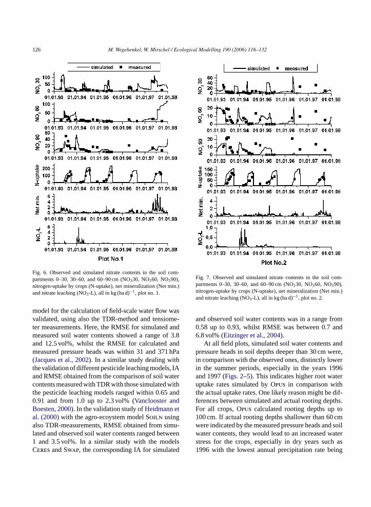
At all field plots, the largest part of simulated nitratecontents in the compartment 0–30 cm are in the sameorder as the measured contents (Figs. 6 and 7). In 1996,however, simulated nitrate contents in the compart-ments 30–60 and 60–90 cm were significantly lowerthan the measured ones (Figs. 6 and 7). One year later,in 1997, calculated nitrate contents increase in all soilcompartments of plot no. 1. In the same year, only lownitrate contents were simulated by Opus at plot no. 2(Figs. 6 and 7).

Between 1993 and 1995, simulated crop nitrogen-uptake rates are overestimated at plot no. 1; in 1996and 1997, however, they were simulated quite well incomparison with the measured ones (Fig. 6). At plot no.2, the nitrogen-uptake was overestimated by Opus dur-ing the whole simulation period (Fig. 7). The highest


Fig. 4. Daily precipitation rates (Prc) in mm d−1 and simulated andobserved volumetric soil water contents (vol%) in the compartments0–30, 30–60, 60–90, 90–120, 120–150 cm (Swc30, Swc60, Swc90,Swc120, Swc150), plot no. 2.

nitrogen-uptake with 241 kg ha−1 (winter barley, 1995)was calculated at plot no. 1, the lowest with 103 kg ha−1

(winter rye, 1996) at plot no. 2 (Figs. 6 and 7; Table 4).The daily rates of simulated nitrogen (N)-net min-

eralization (nitrification and mineralization) were upto 8 kg (ha d)−1. In 1993 and 1997, simulated dailyrates of N-net mineralization at plot no. 1 were sig-nificantly higher in comparison with those at plot no.2 (Figs. 6 and 7).

At plot no. 1, simulated daily nitrogen leaching rateswere up to 5.8 kg (ha d)−1. At plot no. 2, daily leach-ing rates were up to 1.2 kg (ha d)−1 (Figs. 6 and 7).At plot nos. 1 and 3, the calculated nitrogen bal-ance components were in the same order (Table 4).In comparison with plot nos. 1 and 3, a lowerannual nitrogen supply by fertilizer application corre-sponds with lower annual rates of N-net mineralization,

Fig. 5. Daily precipitation rates (Prc) in mm d−1 and simulated andobserved pressure heads (hPa) in the depths 30, 60, 90, 120, 150 cm(Prh30, Prh60, Prh90, Prh120, Prh150), plot no. 2.

nitrogen leaching and nitrogen-uptake at plot no. 2(Table 4).

3.3. Crop growth

At all three field plots, the accumulation of theaboveground total biomass is simulated sufficiently incomparison with the observed data (Fig. 8). In theyear 1993, Opus underestimated the aboveground totalbiomass at plot nos. 2 and 3, as it did in the year 1997at all field plots (Fig. 8). Opus overestimated the yieldsat plot no. 1 in the years 1993 and 1994 and under-estimated the yields in the following years (Table 5).The yield calculated by Opus at plot no. 2 in 1993 istoo high, whereas, in the following years, simulatedyields are significantly too low in comparison with theobserved ones. At plot no. 3, Opus generally underes-timated the yields (Table 5).


Table 4Annual rates of precipitation (Prc) and amount of nitrogen fertilizer (N-fertilizer) as well as the simulated components of water and nitrogenbalance, runoff (Roff), actual evapotranspiration (Etr), percolation (Perc.), N-net mineralization, nitrogen leaching (N-leaching) and nitrogen-uptake by crops (N-uptake)

Prc (mmyear−1)

Roff (mmyear−1)

Etr (mmyear−1)

Perc. (mmyear−1)

N-fertilizer(kg (ha year)−1)

N-net mineralization(kg (ha year)−1)

N-leaching(kg (ha year)−1)

N-uptake by crops(kg (ha year)−1)

Plot no. 11993 594 11 430 154 80 196 15 1471994 655 0 413 261 140 51 84 2201995 483 3 424 120 145 75 3 2411996 421 6 424 3 160 73 0 1751997 440 0 419 24 130 288 1 144

Plot no. 21993 594 11 469 118 66 112 5 1561994 655 0 409 256 60 80 32 1321995 483 3 422 124 40 119 7 1421996 421 6 409 0 130 41 0 1541997 440 0 406 42 0 110 1 103

Plot no. 31993 594 11 473 109 146 166 8 1601994 655 0 405 271 90 64 69 1661995 483 3 415 119 95 74 16 1961996 421 6 405 5 323 102 0 1581997 440 0 405 47 110 264 9 144

Table 5Comparison of simulated and measured yields

Crop type and year of harvest Yield (kg ha−1)

Plot no. 1 Plot no. 2 Plot no. 3

Measured Calculated Measured Calculated Measured Calculated

Sugar beet, 1993 8455 9960 9467 12015 15427 12293Winter wheat, 1994 4516 4773 3245 891 4797 2645Winter barley, 1995 5562 3412 3020 1823 5681 1978Winter rye, 1996 6812 1863 2450 1734 5135 1829Sugar beet, 1997 11639 9187 11762 4638 12419 9060

4. Discussion

At all field plots, the simulation accuracy regardingthe soil water contents shows two different patterns. Inthe soil compartments with 0–30 and 30–60 cm depth,IA and RMSE ranged within 0.58 and 0.75 and from3.6 up to 4.6 vol%, respectively (Table 6). In the deepercompartments, IA was within 0.10 and 0.57 whilstRMSE ranged from 1.6 up to 10.4 vol% (Table 6). Asimilar trend could be observed regarding the pressureheads. In the depth of 30 cm at plots nos. 1 and 3, IAranged within 0.58 and 0.68 and RMSE from 105 upto 152 hPa. At the plots in depths deeper than 30 cm,

IA and RMSE ranged within 0.10 and 0.41 and from28 up to 185 hPa, respectively. At plot no. 2, how-ever, the best IA = 0.68 and the best RMSE = 16 hPacould be observed in the depth of 150 cm (Table 6).At an international workshop on the validity of 18different agro-ecosystem models held at Brunswick,Germany, in 1993, the simulation quality was evalu-ated using also RMSE obtained from simulated andobserved soil water contents as well as pressure heads.At this workshop, RMSE was within 2.0 and 12.6 vol%regarding the soil water contents and within 100 and555 hPa with respect to the pressure heads (Diekkrugeret al., 1995). In the study ofJacques et al. (2002), a


Fig. 6. Observed and simulated nitrate contents in the soil com-partments 0–30, 30–60, and 60–90 cm (NO330, NO360, NO390),nitrogen-uptake by crops (N-uptake), net mineralization (Net min.)and nitrate leaching (NO3-L), all in kg (ha d)−1, plot no. 1.

model for the calculation of field-scale water flow wasvalidated, using also the TDR-method and tensiome-ter measurements. Here, the RMSE for simulated andmeasured soil water contents showed a range of 3.8and 12.5 vol%, whilst the RMSE for calculated andmeasured pressure heads was within 31 and 371 hPa(Jacques et al., 2002). In a similar study dealing withthe validation of different pesticide leaching models, IAand RMSE obtained from the comparison of soil watercontents measured with TDR with those simulated withthe pesticide leaching models ranged within 0.65 and0.91 and from 1.0 up to 2.3 vol% (Vanclooster andBoesten, 2000). In the validation study ofHeidmann etal. (2000)with the agro-ecoystem model Soiln usingalso TDR-measurements, RMSE obtained from simu-lated and observed soil water contents ranged between1 and 3.5 vol%. In a similar study with the modelsCeres and Swap, the corresponding IA for simulated

Fig. 7. Observed and simulated nitrate contents in the soil com-partments 0–30, 30–60, and 60–90 cm (NO330, NO360, NO390),nitrogen-uptake by crops (N-uptake), net mineralization (Net min.)and nitrate leaching (NO3-L), all in kg (ha d)−1, plot no. 2.

and observed soil water contents was in a range from0.58 up to 0.93, whilst RMSE was between 0.7 and6.8 vol% (Eitzinger et al., 2004).

At all field plots, simulated soil water contents andpressure heads in soil depths deeper than 30 cm were,in comparison with the observed ones, distinctly lowerin the summer periods, especially in the years 1996and 1997 (Figs. 2–5). This indicates higher root wateruptake rates simulated by Opus in comparison withthe actual uptake rates. One likely reason might be dif-ferences between simulated and actual rooting depths.For all crops, Opus calculated rooting depths up to100 cm. If actual rooting depths shallower than 60 cmwere indicated by the measured pressure heads and soilwater contents, they would lead to an increased waterstress for the crops, especially in dry years such as1996 with the lowest annual precipitation rate being


Fig. 8. Comparison of simulated and observed above ground total biomass (ABM in kg ha−1) at all three field plots (Sb: sugar beet, Ww: winterwheat, Wb: winter barley, Wr: winter rye).

421 mm year−1 (Table 4). This would limit the accu-mulation of the actual aboveground total biomass andshould lead to a distinct overestimation of the simu-lated aboveground total biomass in comparison with

the measured one. However, in 1996, this overestima-tion could not be observed (Fig. 8). Therefore, actualrooting depths shallower than 60 cm are not indicatedby the comparison of simulated and measured above-

Table 6IA and RMSE obtained from the comparisons of simulated with measured soil water contents with TRIME (SWC–IA, SWC–RMSE) as well aspressure heads (PRH–IA, PRH–RMSE)

Compartment–TRIME (cm) SWC–IA SWC–RMSE (vol%) Depth of tensiometer (cm) PRH–IA PRH–RMSE (hPa)

Plot no. 10–30 0.73 3.9 30 0.58 15230–60 0.58 4.4 60 0.41 13660–90 0.52 4.4 90 0.10 13090–120 0.57 6.6 120 0.21 185120–150 0.51 3.5 150 0.23 28

Plot no. 20–30 0.59 4.6 30 0.25 14930–60 0.75 3.6 60 0.15 22960–90 0.36 10.4 90 0.14 12590–120 0.39 4.4 120 0.36 38120–150 0.10 1.6 150 0.68 16

Plot no. 30–30 0.59 4.1 30 0.64 10530–60 0.68 3.7 60 0.13 16560–90 0.47 5.9 90 0.18 10990–120 0.23 5.3 120 0.21 80120–150 0.15 5.2 150 0.31 37


ground total biomass. Another reason may be errorsin the TRIME and tensiometer measurements. Theaccuracy of the calibrated TRIME was at±2.5 vol%(Wegehenkel, 1998, 2005) and the time courses of soilwater contents measured by TRIME and gravimetrymostly run similar (Figs. 2 and 4). Moreover, ten-siometer are precise instruments provided that theyare properly operated. Errors in the parameterizationof the functionsθ(h) andk(h) can also lead to differ-ences between measured and simulated model outputs,especially in the winter periods with mainly downwardsoil water fluxes. However, the observed differencesbetween measured and calculated soil water contentsas well as pressure heads are concentrated in summerperiods with low soil water contents often reaching thewilting point and a high dynamic in the case of precipi-tation events (Figs. 2–5). This indicates, that parameter-ization errors in theθ(h) andk(h)-functions are also notthe reason for the differences between simulated andobserved soil water contents as well as pressure headsin the soil compartments deeper than 30 cm. Therefore,the most probable reason might be the impact of spatialheterogeneities of soil and plant properties such as soilwater storage capacity, soil cover or rooting depth atthe field plots. However, a clear reason for these dif-ferences between measured and simulated soil watercontents and pressure heads was difficult to identify.

Moreover, two patterns of simulation accuracycould be observed regarding the simulated nitrate con-tents in the root zone. At all field plots in the compart-m .91a -m thin0A ro-e roms zonewI

between nitrate contents in the root zone simulated bythe model Apsim and observed ones was at 9 kg ha−1.In a similar study with the CropSyst model, the corre-sponding IA was at 0.23 (Bellocchi et al., 2002). Thepeaks in the time courses of the simulated nitrate con-tents in 0–30 cm depth correspond with the dates of thefertilizer applications (Figs. 6 and 7). The low simu-lated nitrate contents in the root zone of both field plotsat the end of 1994, 1995, and 1996 are due to high nitro-gen leaching rates in 1994 and low net mineralizationrates in 1995 and 1996 (Figs. 6 and 7). Furthermore,most of the nitrogen supplied by fertilizer applicationsin 1995 and 1996 was used for the simulated nitrogen-uptake of crops (Figs. 6 and 7). In 1997, the simulatedincreases in nitrate contents in the root zone at plot no.1 are due to high N-net mineralization rates and lownitrogen leaching rates as well as fertilizer application(Fig. 6). At plot no. 2, where only organic fertilizerconsisting of farmyard and liquid manure was applied,the comparison of measured and simulated nitrate con-tents, especially in the years 1994, 1996, and 1997,indicates an underestimation of the mineralization ofthe manure by Opus (Fig. 7). Since nitrogen-uptakeby crops is simulated satisfactorily at all plots, thediscrepancies between simulated and measured nitratecontents in the deeper compartments might be causedby errors in the N-net mineralization rates calculatedby Opus. However, N-net mineralization rates are spa-tially and temporally variable making them difficult tomeasure or model (Jarvis et al., 1996).

sc e-m nd aRst n ofs and0 -i

TI ulated -uptakeo RMSE

Pn

RMSE60–90

1 12 92 11 93 12 8

ent 0–30 cm, IA and RMSE range from 0.62 to 0nd from 10 to 19 kg ha−1 (Table 7). In the compartents deeper than 30 cm, IA and RMSE were wi.32 and 0.60 as well as 8 and 15 kg ha−1 (Table 7).t the international workshop on the validity of agcosystem models in 1993, the RMSE obtained fimulated and observed nitrate contents in the rootas within 5 and 42 kg ha−1 (Diekkruger et al., 1995).

n a study carried out byAsseng et al. (2000), the RMSE

able 7A and RMSE (in kg ha−1) obtained from the comparisons of simf crops (IA-Nupt, RMSE-Nupt), aboveground biomass (IA-crop,

loto.

IA-N0–30 cm

RMSE-N0–30 cm

IA-N30–60 cm

RMSE-N30–60 cm

IA-N60–90 cm

0.86 19 0.55 14 0.600.62 13 0.32 8 0.340.91 10 0.52 15 0.45

The accumulation of the aboveground total biomasalculated by Opus in comparison with the measurents resulted in an IA between 0.90 and 0.94 aMSE between 2708 and 2942 kg ha−1 (Table 7). In atudy evaluating the performance of theCeres model,he corresponding IA obtained from the comparisoimulated and observed biomass was within 0.87.96 (Bacsi and Zemankovics, 1995). In two other sim

lar studies using the CropSyst model, IA and RMSE

with measured soil nitrate contents (IA-N, RMSE-N), nitrogen-crop) and crop yields (IA-yield, RMSE-yield)

-Ncm

IA-Nupt RMSE-Nupt

IA-crop RMSE-crop

IA-yield RMSE-yield

0.91 39 0.93 2708 0.77 2490.74 46 0.90 2942 0.55 3280.90 35 0.94 2778 0.75 289


Table 8Nitrogen (Nstress) and water (Wstress) stresses at the field plots simulated with the Opus model

Year Nstress Wstress

Plot no. 1 Plot no. 2 Plot no. 3 Plot no. 1 Plot no. 2 Plot no. 3

Sums of stress ratios1993 1 7 0 6 11 131994 28 52 41 24 17 201995 13 44 31 16 29 121996 50 57 54 23 17 221997 0 54 0 34 20 36

Sum of stress days per year1993 16 55 5 10 19 201994 45 74 60 31 19 241995 28 63 51 22 34 171996 67 71 67 34 21 341997 4 83 4 41 24 43

regarding aboveground biomass ranged within 0.86 and0.996 and from 786 up to 1030 kg ha−1 (Bellocchi et al.,2002; Stoeckle et al., 2003). In the study with the Apsimmodel, RMSE obtained from simulated and observedaboveground biomass was at 1200 kg ha−1 (Asseng etal., 2000).

IA and RMSE obtained from the comparisonof observed yields with those simulated by Opusranged within 0.55 and 0.77 and between 2499 and3289 kg ha−1 (Table 7). In the two validation studieswith the CropSyst model, IA and RMSE regardingyields ranged within 0.90 and 0.975 as well as 383and 560 kg ha−1 (Bellocchi et al., 2002; Stoeckle et al.,2003). In the study with the Apsim model, RMSE wasat 800 kg ha−1 (Asseng et al., 2000). In the year 1994,the yields calculated by Opus were at 891 kg ha−1 atplot no. 2 and 2645 kg ha−1 at plot no. 3 in com-parison with the measured ones which were at 3245and 4797 kg ha−1 (Table 5). However, in 1994, above-ground total biomass is simulated quite well at plot no.2 and only slightly underestimated at plot no. 3 (Fig. 8).In Opus, the partitioning of total biomass to plant leaf,root and fruit is a function of the relative plant age(RDM) and the relative thermal time (Smith, 1992a).RDM is defined as the ratio between total accumu-lated biomass (DM) and the potential dry matter (PDM)whilst the relative thermal time is the ratio betweenthe actual thermal time (SSD) and the thermal time atmaturity (SSDM inTable 3). RDM is also influencedby nitrogen and water stress suffered by the crops.I days

Fig. 9. Simulated relative plant development (RDM), accumulationof total biomass (TBM) and yield at all three plots (Sb: sugar beet,Ww: winter wheat, Wb: winter barley, Wr: winter rye).
n Opus, nitrogen stress days and water stress


are defined as days, where the actual nitrogen-uptake(ANU) and the actual evapotranspiration (AET) ratesare below the corresponding potential uptake (PNU)and potential evapotranspiration rates (PET). The sumsof stress ratios are the sums of the ratios ANU:PNUand AET:PET. At plots nos. 2 and 3, the accumulationof biomass is much more limited by nitrogen-stress incomparison with plot no. 1 (Table 8). In comparisonwith plot no. 1, this leads to a lower RDM at both plotsand causes a low partitioning of total biomass DM tothe fruit or yield fraction especially in the years from1994 up to 1997 (Fig. 9; Table 5). These effects areknown from an earlier publication (Smith, 1995).

In our study, IA and RMSE regarding thenitrogen-uptake by crops ranged within 0.90–0.93 and35–39 kg ha−1 (Table 7). In a validation study ofthe model Daisy, IA obtained from simulated andobserved nitrogen-uptake was at 0.97 (Hansen et al.,2001). In the study with the Apsim model, the corre-sponding RMSE was at 28.5 kg ha−1 (Asseng et al.,2000).

5. Summary and conclusions

The application of the Opus simulation model in ourstudy showed that the model adequately simulated thedynamics of soil water contents and pressure heads insoil depths shallower than 60 cm. Nitrate contents weresimulated well in the soil compartment 0–30 cm. Ind sim-u headsa g thep likelyr ilityo them atials ner-a icf

lb imu-l tedb wthm alet

m field

plots were used in our study. If such data are notavailable, the use of estimation procedures fork(h)andθ(h)-functions, such as pedotransfer functions, canlead to further errors in the model calculations (e.g.Wegehenkel, 2005). Therefore, one goal of the modeldevelopers – the use of Opus without calibration – isonly partly fulfilled, if an overall simulation quality ofOpus similar to all corresponding references cited inour study is required.

The results of our study showed also that the use ofdifferent procedures for the statistical evaluation of thequality of the fit between simulated and observed modeloutputs can sometimes lead to contradictory results.When taking the compartment 120–150 cm at plot no.2 as an example, the RMSE = 1.6 vol% indicates thebest and the corresponding IA = 0.10 the lowest sim-ulation quality (Table 6). In spite of correct temporalpatterns, a general over- or underestimation trend of themodel can, therefore, not be differentiated from thoseshowing incorrect temporal patterns, if one only usesdeviance measures such as RMSE (Fig. 4; Table 6). Themodelling efficiency index IA directly compares sim-ulations with observations and is, therefore, proposedas a more appropriate measure of the correspondencebetween simulated and observed time patterns of modeloutputs than RMSE (Mayer and Butler, 1993). There-fore, a combined use of IA and RMSE allows a morecritical evaluation of the model performance than theisolated use of one of those procedures.

In most of the references regarding the validationo ours ser-v sia illae l.,2 sten,2 he 5y

A

in-i ure( -m ) oft ipl.I a-

eeper soil compartments, discrepancies betweenlated and measured soil water contents, pressurend nitrate contents could be observed. Regardinressure heads and soil water contents, the mosteason for that is the impact of the spatial variabf soil properties. Regarding the nitrate contents,ost likely reasons are, besides the impact of sp

oil heterogeneities, underestimations of N-net milization rates by Opus, especially in the case of organ

ertilizer application at plot no. 2.Whilst the accumulation of aboveground tota

iomass and the nitrogen-uptake by crops were sated quite well, the yields were mostly underestimay Opus. Therefore, the parameters of the crop groodel in Opus have to be calibrated at the local sc

o get an optimum precision of yield estimations.Furthermore,k(h) andθ(h)-functions obtained from

easured soil water retention data of the three

f agro-ecosystem models with field data cited intudy, only 1–3 year periods of model output obations were available (e.g.Asseng et al., 2000; Bacnd Zemankovics, 1995; Bellocchi et al., 2002; Bont al., 1999; Diekkruger et al., 1995; Eitzinger et a004; Heidmann et al., 2000; Vanclooster and Boe000). These validation periods are shorter than tear period used in our study.

cknowledgements

The work was founded by the German Federal Mstry of Consumer Protection, Food and AgricultBMVEL) and the Ministry of Agriculture, Environental Protection and Regional Planning (MLUR

he Federal State of Brandenburg. Many thanks to Dng. Michael Bahr for the supervision of the field me


surements and to Mrs. Sigrid Dittmar for the prepara-tion of the experimental data.

References

Addiscott, T.M., Whitmore, A.P., 1987. Computer simulation ofchanges in soil mineral nitrogen and crop nitrogen duringautumn, winter and spring. J. Agricult. Sci. Camb. 108, 141–157.

Asseng, S., van Keulen, H., Stol, W., 2000. Performance and appli-cation of the Apsim Nwheat model in the Netherlands. Eur. J.Agron. 12, 37–54.

Bacsi, Z.S., Zemankovics, F., 1995. Validation, an objective or atool? Results on a winter wheat simulation model. Ecol. Model.81, 251–263.

Bellocchi, G., Silvestri, N., Mazzoncini, M., Menini, S., 2002. Usingthe CropSyst Model in continuous rainfed maize (Zea maisL.) using alternative management options. Ital. J. Agron. 6 (1),43–56.

Bergstrom, L., Johnsson, H., Tortensson, J., 1991. Simulation ofnitrogen dynamics using the SOILN model. Fertil. Res. 27,181–188.

Bonilla, C.A., Munoz, J.J., Vauclin, M., 1999. Opus simulation ofwater dynamics and nitrate transport in a field plot. Ecol. Model.122, 69–80.

Boden, A.G., 1994. Bodenkundliche Kartieranleitung. 3. Aufl.Schweizerbart, Stuttgart.

Boons-Prins, E.R., de Koning G.H.J., van Diepen, C.A., Penningde Vries, F.W.T., 1993. Crop specific simulation parameters foryield forecasting across the European Community. SimulationReports CABO-TT, No. 32, Wageningen, the Netherlands.

Brooks, R., Corey, A., 1964. Hydraulic Properties of Porous Media.Hydrology Paper 3. Colorado State University, USA.

de Willigen, P., 1991. Nitrogen turnover in the soil–crop-system;27,

D , K.,tionsther-.

D .,of

Ecol.

E 4.gsoil

G hos-3.5.

G erslop-

H odel-

model. In: Shaffer, M.J., Liwang, M., Hansen, S. (Eds.), Model-ing Carbon and Nitrogen Dynamics for Soil Management. LewisPublishers, Boca Raton, pp. 511–549.

Heidmann, T., Thomsen, A., Schelde, K., 2000. Modelling soil waterdynamics in winter wheat using different estimates of canopydevelopment. Ecol. Model. 129, 229–243.

Jacques, D., Simunek, J., Timmerman, A., Feyen, J., 2002. Calibra-tion of Richards’ and convection-dispersion equations to field-scale water flow and solute transport under rainfall conditions. J.Hydrol. 259, 15–31.

Jansson, P.E., Karlberg, L., 2004. Coupled Heat and Mass TransferModel for Soil–Plant–Atmosphere Systems. Royal Institute ofTechnology, Dept. of Civil and Environmental Engineer-ing, Stockholm, 435 pp ftp://www.lwr.kth.se/CoupModel/CoupModel.pdf.

Jarvis, S.C., Stockdale, E.A., Shepard, M.A., Powlson, D.S., 1996.Nitrogen mineralization in temperate agricultural soils. Ad.Agron. 57, 187–235.

Krumbiegel, D., Schwinge, W., 1991. Witterung-Klima Mecklen-burg-Vorpommern. Brandenburg, Berlin. DWD, Wetteramt Pots-dam, 51.

Mayer, D.G., Butler, D.G., 1993. Statistical validation. Ecol. Model.68, 21–32.

Neeteson, J.J., 1990. Development of nitrogen fertilizer recommen-dations for arable crops in the Netherlands. Fertil. Res. 26,201–208.

Parton, W., Schimel, D., Cole, C., Ojima, D., 1987. Analysis offactors controlling soil organic matter levels in Great Plains grass-lands. Soil Sci. Soc. Am. J. 51, 1173–1179.

Porter, J.P., Jamieson, P.D., Wilson, D.R., 1993. Comparison ofthe wheat simulation models Afrcwheat2, Ceres-Wheat andSwheat for non-limiting conditions of crop growth. Field CropsRes. 33, 131–157.

Rodda, H., Scholefield, D., Webb, B., Walling, D., 1995. Manage-ment model for predicting nitrate leaching from grassland catch-

rol.

S sser-en.

S rboners,

S s-DA,

S s-DA,

S ear

S89–

S f cropgroe-

comparison of fourteen simulation models. Fertil. Res.141–149.

ekker, L.W., Ritsema, J.C., Wendroth, O., Jarvis, N., OostindiePohl, W., Larsson, M., Gaudet, J.P., 1999. Moisture distribuand wetting rates of soils at experimental fields in the Nelands, France, Sweden and Germany. J. Hydrol. 215, 4–22

iekkruger, B., Sondgerath, D., Kersebaum, K.C., McVoy, C.W1995. Validity of agroecosystem models—a comparisonresults of different models applied to the same data set.Model. 81, 3–29.

itzinger, J., Trnka, M., Hobsch, J., Zalud, Z., Dubrovsky, M., 200Comparison of Ceres, Wofost and Swap models in simulatinsoil water content during growing season under differentconditions. Ecol. Model. 171, 223–246.

roenendijk, P., Kroes, J.G., 1997. Modelling the Nitrogen and Pphorus Leaching to Groundwater Surface Water. AnimoReport 144. DLO, Winand Staring Centre, Wageningen.

odwin, D.C., Ritchie, J.T., Singh, U., Hunt, L., 1989. A UsGuide to Ceres–Wheat V2.10. International Fertilizer Devement Center, Muscle Shoals, AL.

ansen, S., Thirup, C., Refsgaard, J.C., Jensen, L.S., 2001. Ming nitrate leaching at different scales—application of the Daisy

ments in the United Kingdom. 1. Model development. HydSci. J. 40 (4), 433–451.

chindler, U., 1980. Ein Schnellverfahren zur Messung der Waleitfahigkeit im teilgesattigten Boden an StechzylinderprobArch. Acker, Pflanzenbau und Bodenkunde 24, 1–7.

haffer, M.J., Liwang, M., Hansen, S. (Eds.), 2001. Modeling Caand Nitrogen Dynamics for Soil Management. Lewis PublishBoca Raton, p. 651.

mith, R., 1992a. Opus: An Integrated Simulation Model for Tranport of Non-point-Source Pollutants at Field Scale, vol. I. USWashington, DC, Documentation, USDA ARS-98.

mith, R., 1992b. Opus: An Integrated Simulation Model for Tranport of Non-point-Source Pollutants at Field Scale, vol. II. USWashington, DC, Users Manual, USDA ARS-98.

mith, R., 1995. Opus: Simulation of a wheat–sugar beet plot nNeuenkirchen, Germany. Ecol. Model. 81, 121–132.

toeckle, C.O., Donatelli, M., Nelson, R., 2003. CropSyst, acropping systems simulation model. Eur. J. Agron. 18, 2307.

vendsen, H., Hansen, S., Jensen, H., 1995. Simulation oproduction, water and nitrogen balances in two German acosystems using DAISY model. Ecol. Model., 197–212.


Van Dam, J.C., Huygen, J.C., Wesseling, J.G., Feddes, R.A.,Kabat, P., vam Walsum, P.E.V., Groenendijk, P., van Diepen,C.A., 1997. Theory of SWAP-Version 2.0. Simulation ofWater Flow, Solute Transport and Plant Growth in theSoil–Water–Atmosphere–Plant Environment. Report 71, Depart-ment Water Resources Wageningen University, Technical docu-ment 45, Alterra, Wageningen, the Netherlands, 167 pp.

van Genuchten, M., 1980. A closed form equation for predicting thehydraulic conductivity of unsaturated soils. Soil Sci. Soc. Am. J.44, 892–898.

Vanclooster, M., Viaene, P., Diels, J., Feyen, J., 1995. A deterministicevaluation analysis applied to an integrated soil-crop model. Ecol.Model. 81, 183–197.

Vanclooster, M., Boesten, J.J.T.I., 2000. Application of pesticide sim-ulation models to the Vredepeel data set I. Water, solute and heattransport. Agricult. Water Manag. 44, 105–117.

Wagenet, R., Hutson, J., 1990. Leach-M: A Process Based Model ofWater and Solute Movement, Transformations, Plant Uptake, andChemical Reactions in Unsaturated Zone, Version 2. Departmentof Agronomy, Cornell University, Ithaca, NY, USA.

Wegehenkel, M., 1998. Zum Einsatz von TRIME-TDR zur Messungder Bodenfeuchte auf leichten Sandboden. Zeitschrift f. Pflanzen-ernahrung und Bodenkunde 161, 577–582.

Wegehenkel, M., 2005. Validation of a soil water balance model usingsoil water content and pressure head data. Hydrol. Processes 19,1139–1164.

Wenkel, K.O., Mirschel, W. (Eds.), 1995. Agrarokosystem-modellierung – Grundlage fur die Abschatzung von Auswirkun-gen moglicher Landnutzungs – und Klimaanderungen. ZALF-Bericht no. 24.

Willmott, C.J., 1982. Some comments on the evaluation of modelperformance. Bull. Am. Meteorol. Soc. 64, 1309–1313.

Crop growth, soil water and nitrogen balance simulation on three experimental field plots using the...

Documents

Transcript of Crop growth, soil water and nitrogen balance simulation on three experimental field plots using the...