Crime and punishment: the economic burden of impunity

EPJ manuscript No.(will be inserted by the editor)

Crime and punishment: the economic burden of impunity

Mirta B. Gordon1, J. R. Iglesias2, Viktoriya Semeshenko1, and J.-P. Nadal3

1 Laboratoire TIMC-IMAG (UMR 5525), University of Grenoble I, Domaine de La Merci - Jean Roget, F-38706 La Tronche,France

2 Instituto de Fısica and Faculdade de Ciencias Economicas, Universidade Federal do Rio Grande do Sul, 91501-970 PortoAlegre, Brazil

3 Laboratoire de Physique Statistique (UMR8550), Ecole Normale Superieure, 24, rue Lhomond, F-75231 Paris Cedex 05 andCentre d’Analyse et de Mathematique Sociales (CAMS) (UMR8557) Ecole des Hautes Etudes en Sciences Sociales, 54, Bd.Raspail, F - 75270 Paris Cedex 06, France

Received: date / Revised version: date

Abstract. Crime is an economically important activity, sometimes called the “industry of crime”. It mayrepresent a mechanism of wealth distribution but also a social and economic charge because of the costof the law enforcement system. Sometimes it may be less costly for the society to allow for some level ofcriminality. A drawback of such policy may lead to a high increase of criminal activity that may becomehard to reduce. We investigate the level of law enforcement required to keep crime within acceptable limitsand show that a sharp phase transition is observed as a function of the probability of punishment. Wealso analyze the growth of the economy, the inequality in the wealth distribution (the Gini coefficient) andother relevant quantities under different scenarios of criminal activity and probability of apprehension.

PACS. 89.65-s Social and economic systems – 89.65.Ef Social organizations; anthropology – 89.65.GhEconomics; econophysics

1 Introduction

Crime is a human activity probably older than the crudelycalled “oldest profession”. Criminal activity may have manydifferent causes: envy, like in the case of Cain and Abel [1],jealousy like in the opera Carmen, or financial gain like Ja-cob cheating Esau with the lentil pottage (and his fatherwith the lamb skin) to obtain the birthright [2]. This isto say that crime can have many different causes, some ofthem “passional”, sometimes “logical” or “rational” [3].

All along history, organized societies have tried to pre-vent and to deter criminality through some kind of pun-ishment. In all the societies and all the times punishmenthas been in some way proportional to the gravity of theoffense. Methods ranged from the lex talionis “an eye foran eye”, to fines, imprisonment, and the death penalty.Most of the literature on crime considered criminals as de-viant individuals. Usual explanations of why people offenduse concepts like insanity, depravity, anomia, etc. In 18thCentury England criminals were massively “exported” toAustralia because it was thought that the criminal condi-tion was hereditary and incurable: incapacitation was thesolution.

In any case the increase of criminal activity in differ-ent countries have led some sectors of the population, aswell as politicians, to ask for harder penalties. The un-derstated idea is that a hard sentence, besides incapacita-

tion of convicted criminals, would have a deterrent effecton other possible offenders and would also prevent recidi-vism. Yet, the deterrent effect of punishment is a polemicsubject and law experts diverge with respect to whetheroffenders should be rehabilitated or simply punished (seefor example the recent public discussion in France [4]).In many countries, incapacitation is the main reason forimprisonment of criminals. For instance the Argentineanconstitution states that prisons are not there for the pun-ishment of the inmates but for the security of the society:criminals are isolated, not punished [5].

Although the idea that the decision of committing acrime results from a trade off between the expected profitand the risk of punishment dates back to the eighteenand nineteenth centuries, it is only recently that crimemodeling emerged as a field worth of being investigated.

In a review paper, Alfred Blumstein [6] traces back therecent interest in crime modeling to 1966, when the USAPresident’s Commission on Law Enforcement and Admin-istration of Justice created a Task Force on Science andTechnology. Composed mainly by engineers and scientists,its aim was to introduce simulation modeling of the Ameri-can criminal justice system. The model allowed to evaluatethe resource requirements and costs associated to a crim-inal case, from arrest to release, by considering the flowthrough the justice system. For example, it estimated theopportunity of incarceration of convicted criminals and

arX

iv:0

710.

3751

v1 [

nlin

.AO

] 1

9 O

ct 2

007

2 Mirta B. Gordon et al.: Crime and punishment: the economic burden of impunity

the length of the incarceration time. In his concluding re-marks, Blumstein states that: “We are still not fully clearon the degree to which the deterrent and incapacitation ef-fects of incarceration are greater than any criminalizationeffects of the incarceration, and who in particular can beexpected to have their (tendency to)1 crime reduced andwho might be made worse by the punishment”.

In a now classical article G. Becker [7] presents forthe first time an economic analysis of costs and benefitsof crime, with the aim of developing optimal policies tocombat illegal behavior. Considering the social loss fromoffenses, which depends on their number and on the pro-duced harm, the cost of aprehension and conviction andthe probability of punishment per offense, the model triesto determine how many offenses should be permitted andhow many offenders should go unpunished, through min-imization of the social loss function.

Using a similar point of view, Ehrlich [8,9] develops aneconomic theory to explain participation in illegitimate ac-tivities. He assumes that a person’s decision to participatein an illegal activity is motivated by the relation betweencost and gain, or risks and benefits, arising from such ac-tivity. The model seemed to provide strong empirical evi-dence of the deterrent effectiveness of sanctions. However,according to Blumstein [6] the results “... were sufficientlycomplex that the U.S. Justice Department called on theNational Academy of Sciences to convene a panel to as-sess the validity of the Erlich results. The report of thatpanel highlighted the sensitivity of these econometric mod-els to details of the model specification, to the particulartime series of the data used, and to the sensitivity of theinstrumental variable used for identification, and so calledinto question the validity of the results”. In fact, the issueof what constitutes an optimal crime control policy is stillcontroversial.

Another controversial subject is the relationship be-tween raising of income inequality and victimization. Becker’seconomic model of crime would suggest that as incomedistribution becomes wider, the richer become increas-ingly attractive targets to the poorer. There are manyreasons why this hypothesis may not be correct. For ex-ample, Deutsch et al. [10] consider the impact of wealthdistribution on crime frequency and, contrary to the gen-eral consensus in the literature, conclude that variations ofthe wealth differences between “rich” and “poor” do notexplain variations in the rates of crime. Bourguignon et al[11] based on data from seven Colombian cities concludethat in crime modeling the average income of the pop-ulation determines the expected gain, but that potentialcriminals belong to the segment of the population whoseincome is below 80% of the mean. More recently, Dahlbergand Gustavsson [12] pointed out that in crime statisticsone should distinguish between permanent and transitoryincomes. Disentangling these income components basedon tax reports in Sweden, they find that an increase in in-equality in permanent income (measured through the vari-ance of the distribution) yields a positive and significanteffect on crime rates, while an increase in the inequality

1 We added these words in parenthesis

due to a transitory income has no significant effect. Levitt[13] concludes from empirical data that, probably becauserich people engage in behavior that reduces their victim-ization, the trends between 1970 and 1990 is that propertycrime victimization has become increasingly concentratedon the poor.

As pointed out by many authors, the fact that policereduces crime is far from being demonstrated. Realizingthat (at least in the U.S.A.) the number of police officersincreases mostly in election years, Levitt [14] has studiedthe correlation between these variations (uncorrelated tocrime) and variations in crime reduction. He finds that in-creases in the size of police forces substantially reduce vi-olent crime, but have a smaller impact on property crime.Moreover, the social benefit of reducing crime is not largerthan the cost of hiring additional police. Similar conclu-sions have been drawn by Freeman [15], who estimatesthat the overall cost of crime in the US is of the order of 4percent of the GDP, 2 per cent lost to crime and 2 percentspent on controlling crime. This amounts to an average ofabout 54, 000 dollars/year for each of the 5 million or somen incarcerated, put on probation or paroled.

In most models, punishment of crime has two distinctaspects: on one side there is the frequency at which illegalactions are punished (which corresponds to the punish-ment probability in the models), and on the other, theseverity of the punishment. In a review paper, Eide [16]comments that although many empirical studies concludethat the probability of punishment has a preventive effecton crime, the results are ambiguous.

More recent reviews of the research literature considerthe factors influencing crime trends [17] and present somerecent modeling of crime and offending in England andWales [3]. They both note the above mentioned difficultiesin estimating the parameters of the models and the costof crime.

Most of the models in the literature follow Becker’seconomic approach. Ehrlich [9] presents a market modelof crime assuming that individuals decisions are “ratio-nal”: a person commits an offense if his expected utilityexceeds the utility he could get with legal activities. Atthe “equilibrium” between the supply of crimes and the“demand” (or tolerance) to crime — reflected by the ex-penditures for protection and law enforcement – neithercriminals, private individuals nor government can expectto improve their benefits by changing their behaviors. Inparticular, the model is based on standard assumptionsin economic models, with “well behaved” monotonic sup-ply and demand curves, which cannot explain situationswhere social interactions are important [18,19]. Indeed,Glaeser et al [20] attribute to social interactions the largevariance in crime on different cities of the US.

Another kind of models [21,3] treat criminality as anepidemics problem, which spreads over the population dueto contact of would-be criminals with “true” criminals(who have already committed crime). This kind of mod-els incorporates effects due to social interactions, whichintroduce large nonlinearities in the level of crime asso-ciated to different combinations of the parameters. These

Mirta B. Gordon et al.: Crime and punishment: the economic burden of impunity 3

may explain the wide differences reported in the empiricalliterature.

In this paper we focus on economic crimes, where thecriminal agents try to obtain an economic advantage bymeans of the accomplished felony. No physical aggressionor death of the victim will be considered, and on the sideof punishment we consider the standard of most devel-oped civilized countries, i.e. fines and imprisonment. Weassume that [22] “most criminal acts are not undertakenby deviant psychopathic individuals, but are more likely tobe carried out by ordinary people reacting to a particu-lar situation with a unique economic, social, environmen-tal, cultural, spatial and temporal context. It is these re-actionary responses to the opportunities for crime whichattract more and more people to become involved in crim-inal activities rather than entrenched delinquency”.

We simulate a population of heterogeneous individu-als. They earn different wages, have different tastes forcriminality, and modify their behaviors according to therisk of punishment. We assume that both the probabil-ity and the severity of the punishment increase with themagnitude of the crime. We are interested in the conse-quences of the punishment policy on the costs of crime,in the wealth distribution consistent with different levelsof criminality, in the economic growth of the society as afunction of time, and in the (possibly bad) consequencesof allowing for some criminal activity in order to minimizethe cost of the law enforcement apparatus. In section 2 wedescribe the model, in section 3 we explain its dynamics.We present the results of the simulations in 4 and leavethe conclusions to section 5

2 Description of the model

We consider a model of society with a constant numberof agents, N , who perceive a periodic (monthly) positiveincome Wi (that we call wage), spend part of it eachmonth and earns the rest. Wages remain constant dur-ing the simulated period. In our simulations, the wagesdistribution has a finite support: Wi ∈ [Wmin,Wmax]. Inthis utopian society there is not unemployment, and it isassumed that the minimum wage is enough to provide forthe minimum needs of each agent, i.e. a person perceivingthe minimum wage will expend it completely within themonth. These wages and possibly the booties of success-fully realized crimes constitute the only income source ofthe individuals. Besides the living expenses, capitals maydecrease due to plunders and to the taxes or fines relatedto conviction, as explained later.

We assume that each agent has an inclination to abideby the law, that is represented by a honesty index Hi (i ∈[1, N ]) which, at the beginning of the simulations rangesbetween a minimum and a maximum: Hi ∈ [Hmin, Hmax].This inclination — that may be psychological, ethical, orreflect educational level and/or socio-economical environ-ment — is not an intrinsic characteristic of the individuals.It changes from month to month according to the risk ofapprehension upon performing a crime.

In our simulations, the individual decision of commit-ting a crime depends (not exclusively) on both the hon-esty index and the monthly income, which are initiallydrawn at random from distributions pH and pW respec-tively, without any correlation among them. This is justi-fied by the lack of empirical evidence that the poorer aremore or less law abiders than the rich.

The honesty index of all the individuals but the crimi-nal increases by a small amount each time a crime is pun-ished. Otherwise it decreases, but at a different rate for thecriminal than for the rest of the population. The honestyindex is not affected by the importance of the punishment.This assumption is an extreme simplification of the obser-vation [6] that the crime rate is more sensitive to the riskof apprehension than to the severity of punishment. Wehave studied different distributions pH and pW and differ-ent treatments of the honesty index. The latter differ inthe way we treat the lower bound of the distribution pH ,namely Hmin. Hereafter we describe in details the sim-plest case: we consider that Hmin is an absolute minimumof the honesty. Hmin corresponds thus to the honesty in-dex of the most recalcitrant offenders. But we also addthe hypothesis (that is certainly controversial) that forthose agents with this lowest honesty there is no possibleredemption, i.e. when the honesty index of an agent de-creases down to Hmin it remains there for ever. We leaveto forthcoming discussions the possible variations of thisscheme.

As a consequence of this treatment, there are intrinsiccriminals (those with Hi = Hmin). Indeed, a finite frac-tion, NC(0), of intrinsically criminal agents is assumedfrom the very beginning of the simulation, according withthe idea that there always have been and will be a finitenumber of not redemptible criminals in a society. All theN − NC(0) other agents are “susceptible”: their degreeof honesty Hi(0), drawn at random from the probabilitydistribution pH , satisfies Hmin < Hi(0) ≤ Hmax.

Individuals have also “social” connections: encountersbetween criminals and victims may only occur between so-cially linked individuals. These connections are not meantto represent social closeness but rather the fact that thoseindividuals share common daily trajectories or live in closeneighborhoods, or meet each other just by chance. Forsimplicity, here we consider the latter situation: every in-dividual may be connected to every other individual.

Notice that the nature of social interactions in ourmodel is very different from the mimetic interactions con-sidered by Glaeser et al [20], or the social pressure in-troduced by Campbell et al. [21]. We study just the caseof individual crimes. No illicit criminal associations (“maf-fia”) nor collective victims (like in bank assaults) are goingto be considered.

The characteristics of the simulated population evolveon time. We assume that every month there is a numberof possible criminal attempts. This number depends onthe honesty index of the population as is explained later.Among these attempts, some are successful, i.e. the crimi-nal spoils his victim of a (random) fraction of his earnings.


In contrast with most models, crimes are punishedwith a probability that depends on the magnitude of theloot. When punished, the criminal returns part of thebooty to the victim, pays a fine that may be considered asa contribution to the public enforcement system and goesto jail for a number of months that also depends on thestolen amount. Maintaining each criminal in prison bearsa fixed cost per month to the society, that we evaluate.

In our simulations we study the month to month evo-lution of different quantities that characterize the system,and how these depend on the probability of punishment.

3 Monthly dynamics

Starting from initial conditions of honesty, wages and earn-ings described in section 3.1, we simulate the model for afixed number of months. Within each month, there is arandom number of criminal attempts correlated with thehonesty level of the population (section 3.2). However, notall the attempts end up with a crime: the potential crimi-nal has to satisfy some reasonable conditions that we ex-plicit in section 3.3. If there is crime, there is a transferof the stolen value from the victim to the criminal, as de-tailed in section 3.4. Some of the offenders are detectedand punished (section 3.5): part of the stolen amount isthen returned to the victim and a fine or tax is levied fromthe criminal’s earnings. In turn, the honesty of the pop-ulation evolves after each crime, according to the successor failure in crime repression (section 3.6).

We keep track of the individuals’ wealth, taking intoaccount the monthly incomes, the living expenses, theplunders, and the cost of imprisonment, as detailed in sec-tion 3.7.

In the following paragraphs we describe in details thedynamics of the model.

3.1 Initial conditions

The individuals have initial honesty indexes Hi(0) andwages Wi drawn with uncorrelated probability densityfunctions (pdf) pH and pW respectively. We assume thatthe majority of the population is honest and also that themajority earn low salaries, i.e. pH has a maximum at largeH while pW has its maximum at small W . The results de-scribed below have been obtained considering triangulardistributions, because they are the simplest way of in-troducing the desired individual inhomogeneities. Thus,pW is a triangular distribution of wages, with Wmin = 1and Wmax = 100 (in some arbitrary monetary unit), withits maximum at Wmin and a mean value W = Wmin +(Wmax −Wmin)/3. As already explained, there is an ini-tial number of “intrinsic” criminals NC(0) drawn at ran-dom, with Hi = Hmin. In our simulations this number hasbeen set to 5% of the population (NC(0) = 0.05N). Thehonesty index of the remaining (susceptible) individualsis triangular, from Hmin = 0 up to Hmax = 100, with themaximum at Hmax.

Individuals’ initial endowments are arbitrarily set tofive months wages: Ki(0) = 5Wi. This initial amount con-trols the time needed for the dynamics to fully develop.Smaller initial endowments result in transients dominatedby the size of the possible loots, because these cannot ex-ceed the victims’ capitals.

3.2 Attempts

The number of criminal attempts each monthm isA(m) =[A(m)] where [. . . ] represents the integer part, and

A(m) =

1 + r(m) cAN+ Hmax(m)−H(m)

H(m)NC(m)

ifH(m) 6= Hmin ,

1 + r(m) cAN+ 2NC(m)ifH(m) = Hmin .

(1)

r(m) ∈ [0, 1] is a random number drawn afresh each month,0 < cA < 1 is a coefficient (in the simulations cA = 0.01)and NC(m) are the number of intrinsic offenders (whohave Hi = 0) at month m. With these considerations thereis always a ground level of criminal attempts given by theterm proportional to N . Criminality increases with thenumber of intrinsic offenders and with a decreasing aver-age honesty. When the latter equals Hmin all the popu-lation has the minimum of honesty, i.e. everybody is an“intrinsic” offender. In this case, to avoid the divergencein the first of equations (1), the prefactor of NC was setarbitrarily to 2.

At each criminal attempt a potential offender is se-lected as explained in subsection 3.3 and the number ofremaining attempts for the month is decreased by one,even if the crime is aborted.

3.3 Criminals

We consider that the possible criminals have low honestyindexes, and that it is more likely that they have lowwages. Then, at each attempt, a potential criminal k isdrawn at random among the population of free (not im-prisoned) individuals (we discuss in 3.5 when and how longpunished offenders go in jail). We also select at randoman upper bound HU to the honesty index in the interval[Hmin, Hmax]. If

Hk < HU , (2)

then the offense takes place with a probability:

pk = e−Wk/W , (3)

that is higher the lower the potential criminal wages. Thus,we select a random number in [0, 1). If it is larger than pk,the criminal attempt is aborted.


3.4 Crime

If crime is actually committed, a victim v among the so-cial neighbors (not in jail) of k is selected at random. Wedo not take into account the wealth of the victim, whichmay be an important incentive for the criminal’s decision.Thus, our treatment may be adequate for minor larcenies,like stealing in public transportation. In the crimes con-sidered in this paper, the victim is robbed of a randomamount S that cannot be larger than his actual capital.In the simulation, this amount is proportional to the vic-tim’s wage:

S = rS cS Wv, (4)

where rS ∈ [0, 1] is a random number drawn afresh ateach attempt and cS > 0 is a coefficient (here we usecS = 10, implying that robbery may concern amounts upto 10 times the victim’s wage). If the value given by (4)is larger than the victim’s capital Kv, we set S = Kv.Correspondingly, the victim’s capital is decreased by thestolen amount, to become Kv − S while the criminal’scapital is in turn increased to Kk + S.

3.5 Punishment

The criminal may be catched and punished with proba-bility

π(S) =p1

1 + p1−p0p0

e− S

K(m)

, (5)

a monotonic function that starts at its minimal value p0

(for S = 0 ), increases almost linearly with S for values ofS smaller than ≈ K(m), the population’s average wealth,and gets close to the asymptotic value p1 for large booties.

A punished criminal is imprisoned for a number ofmonths 1+[S/W ] (the square brackets mean integer part),i.e. proportional to the stolen amount. During this timehe does not earn his monthly wage and cannot be selectedas a potential offender nor as a victim.

Beyond incarceration, the convicted criminal suffers afinancial loss. He is deprived of an amount (fR + fD)S,larger than the loot but that cannot exceed his total wealth(we do not allow for negative capitals). It is worth to re-mark that the financial loss is not limited to reimburse thestolen capital. A monetary punishment (a fine) is inflictedto the offender together with the time in prison (that rep-resents, in addition to be incarcerated, also a monetaryloss). The total amount deduced from the offender’s cap-ital is composed of a fraction fRS (with fR < 1), that isreturned to the victim, and an amount, fDS (or Kk−fRSif fDS > Kk), considered as a duty. Cumulated duties or“taxes” constitute the total income of fines. In this simu-lation fR = 0.75 and fD = 0.45, meaning that both crimi-nals and victims contribute to taxes, since the victims onlyrecover a fraction 1 − fR of the stolen amount. However,with the assumed values of fR and fD, fR + fD = 1.2,implying that the criminals also afford part of the costs.

3.6 Honesty dynamics

We assume that punishment has a dissuasive effect onthe population, although not necessarily on the convict.Thus, whenever a criminal is convicted, the honesty in-dex of all the population but the criminal, is increasedby a fixed amount δH. Convicted criminals do not changetheir honesty level. On the contrary, when the crime is notpunished, the entire population but the criminal decreasetheir honesty index by δH, while the criminal decreases hisby 2δH: unpunished criminals become even less honest.

In the present simulations we do not allow Hi to be-come negative. Moreover, the lower bound of the distribu-tion is absorbing. Thus, individuals reaching Hi = Hmin

have their honesty index freezed, and henceforth are con-sidered as “intrinsic” criminals.

A dynamics with a non-absorbing bound for the hon-esty dynamics gives similar results to those presented here.A variant that we did not implement yet is to modify thehonesty level of the criminal proportionally to the impor-tance of the loot.

3.7 Monthly earnings and costs

At the end of each month m, after the A(m) criminalattempts are completed, the individuals’ cumulated cap-itals Ki(m) are updated: the total capital of each agent,Ki(m), is increased with his salary and decreased withhis monthly expenses. Notice that the criminals’ and thevictims’ capitals have been further modified during themonth, according to the results of the criminal attempts.

We assume that individuals need an amount Wmin +f × (Wi −Wmin) with f < 1 to cover their monthly ex-penses. Thus, individuals with higher wages spend a pro-portional part of their income in addition to the mini-mum wage Wmin. This is a simplifying assumption whichmay be questionable since the richer the individuals, thesmaller the fraction of income they need for living but, onthe other hand, rich people spent more in luxury goods.Assuming a more involved model for the expenses wouldmodify the monthly wealth distribution, making it moreunequal, but we do not expect that the qualitative resultsof our simulations would be modified.

In order to quantify the expenditure of conviction andimprisonment, we assume that the monthly cost of main-taining a criminal in jail is equal to the minimal wage.This is clearly a too simple hypothesis, that does not takeinto account the fixed costs of maintaining the public en-forcement against crime. It is just a mean of assessingsome social cost proportional to the criminal activity. Thecumulated taxes, obtained through punishment of con-victed criminals are thus decreased by an amount Wmin

per month for each convict in jail.At the end of each month, the time that inmates have

to remain in prison (excluding the criminals convicted dur-ing that month) is decreased by one; those having com-pleted their arrest punishment are freed.


4 Simulation results

Starting with the initial conditions, there are A(m) crimi-nal attempts each month m as described in the subsection3.2. As a consequence of the criminal activity, during themonth the capitals of criminals and victims are modified,as well as the honesty index of the population. With theabove dynamics, the earnings and the honesty distribu-tions are shifted and distorted. The system may even con-verge to a population where all the initially susceptibleindividuals end up as intrinsically criminal.

We simulated systems of N = 1 000 agents for a pe-riod of 240 months, under different distributions of hon-esty and wages. Here we report results corresponding tothe triangular distributions described in section 2: wageshave a linearly decreasing distribution in [Wmin,Wmax]with Wmin = 1 and Wmax = 100: there are more individ-uals with low wages than with high ones. The honesty dis-tribution is also triangular, but increasing: starting withpH(Hmin) = 0, it increases linearly reaching its maximumat pH(Hmax), which corresponds to assuming that thereare more honest than dishonest individuals.

4.1 Evolution of criminality with time

The system’s evolution is very sensitive to the punishmentprobability. Generally, the first months the rate of crimeis low because the number of intrinsic criminals is smalland the stolen amounts cannot be larger than the initialendowments. But after some months (the number dependson the initial conditions and on the values of p0 and p1)the crime rate increases to a stationary value.

Figure 1 shows a typical monthly evolution of the num-ber of attempts, the number of crimes, the number of con-victed criminals (which are the criminals punished in thecorresponding month) and of inmates. The left figure cor-responds to relatively low values of both p0 (the probabil-ity of punishing small offenses) and p1 (the probability ofpunishing large offenses) in (5). Beyond about 75 monthsthe number of attempts increases through an avalancheto reach its saturation value, while the number of inmatesgrows to reach almost all the population, producing a dropin crime. This drop is not due to a deterrent effect of pun-ishment but rather to the absence of possible criminals(they are all in jail). Eventually the system evolves to asmaller number of inmates, but the population is essen-tially composed of individuals with the smallest honestyindex: the punishment rate is not enough to keep criminal-ity below any acceptable level. The figure on the right (seethe change in the ordinate scale) corresponds to a slightlyhigher value of p1, showing the impressive impact of in-creasing the probability of punishment of big offenses. Allthe quantities (attempts, crimes, etc.) present a dramaticdecrease with respect to the values in the left hand sidefigure. Notice that the fluctuations on the reported quan-tities are of the same order of magnitude in both figures:they are due to the probabilistic nature of the quantitiesinvolved (see equations (1) to (5) ).

Correspondingly, the earned capital per individual (fig-ure 2 upper left) increases almost linearly with time whencrime is limited. In contrast, in the highly criminal soci-ety (p1 = 0.5) it begins to decrease as soon as the regimeof high criminality is reached, mainly because most crimi-nals are convicted and do not receive their wages, but alsobecause, since the number of punished crimes is also high,the amount retained in the form of taxes is discountedfrom the total wealth of the society. Moreover, the highcost of imprisonment, proportional to the total number ofinmates, drains also part of the capital and contributes todecrease the capital per capita. This is illustrated on figure2 upper right, where the total capital per agent is decom-posed into the capital hold by the intrinsic criminals andthe part hold by the susceptible population (with honestyindex Hi > 0). When the system reaches the high crim-inality regime the latter drops to zero because there areno more susceptible individuals. Clearly, when the level ofpunishment is not high enough to guarantee an effectivecontrol of criminality, the cost of the repressive system isvery high. It is remarkable that a very small increase ofthe upper value p1 in (5) is enough for a complete changein the scenario.

The lower figure 2 presents the evolution of the Giniindex of the population, defined by:

G =

∑N−1j=1

∑Ni=j+1 |Ki −Kj |

(N − 1)∑N

i Ki

. (6)

The Gini index spans in the interval [0, 1] and measuresthe inequality in the wealth distribution of the popula-tion. Its minimal value, G = 0, corresponds to a perfectlyequalitarian society. The Gini index of the initial endow-ment, distributed according with a triangular probabil-ity density, is G(0) = 0.4. Due to the dynamics, whencrime level is moderate (p1 = 0.6) G is seen to slightly in-crease. However, in the high criminality regime (p1 = 0.5)it oscillates, and when the high crime rate sets in, it firstplummets down because successful criminals, mostly indi-viduals with small incomes according to the probability ofcrime (3), increase their wealths at the victims’ expense.As a result, the wealth distribution becomes more evenlydistributed. However, on the long run, the Gini index in-creases dramatically. This is so because if everybody is alawbreaker (lowest honesty index) criminals and victimsare the same, just one stealing the other. So when oneagent is in the victim role he becomes poor because of therobbery, and when he behaves as a crook he also finishespoor (generally), mainly because he pays taxes and alsodoes not earn his wage when in jail. So, just a few agentsare able to hold large capitals thanks to crime, increasinginequality in this society.

In fact, when p0 is smaller than a critical value ofthe order of 0.5, on increasing p1, the system presentsan abrupt transition between a high crime — low honestypopulation to a low crime — high honesty one. This tran-sition, apparent on all the quantities, as may be seen belowon figure 3, corresponds to a swing of the system betweena regime of high criminality to one where the criminalitylevel is moderately low.


0 50 100 150 200

0

500

1000

1500

2000

0 50 100 150 200

0

5

10

15

20

25

30

35

40

45

Fig. 1. Statistics of criminality per month. Attempts: number of criminal attempts in the month. Crimes: number of crimescommitted in the month. Convicted: number of criminals punished in the month. Inmates: number of criminals in jail. Thedifference between the left (a) and the right (b) panels is the maximum punishment probability p1, p1 = 0.5 in the left paneland p1 = 0.6 in the right panel. Therefore, a small change in the probability of punishment induce a enormous change in thecriminality (see the difference in scale in the ordinate axis).

In the high criminality side, cumulated earnings aresmall, taxes are high and the Gini index is large. Con-versely, on the low criminality side, i.e. for sufficiently highp1, the cumulated wealth increases monthly according tothe earned wages, and the Gini index reflects the distri-bution of the latter. We will show in Figures 4, below,typical histograms of wealth distribution at both sides ofthe transition, as well as the initial distribution.

4.2 Changing the punishment probability

In the previous section we have discussed the time evolu-tion of criminality. Let’s now consider the final state of thesociety (after 240 months) as a function of the probabilityof punishment. In order to make comparable experimentswe have studied societies with the same initial conditionssubjected to different levels of punishment. Notice thatthese levels are constant during the simulated 240 months.

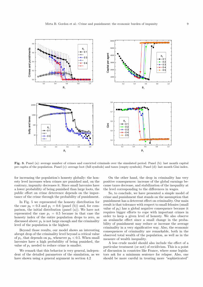
We consider different values of p0 smaller than a crit-ical value of the order of 0.5, and we study the variationof several social indicators as a function of p1. We observethat the system ends up with either a high crime-low hon-esty population (for p1 lower than a critical value) or a lowcrime-high honesty one. This transition, apparent on allthe quantities, as may be seen on figures 3, corresponds toa swing of the system between a regime of high criminalityto one of moderate criminality.

In the upper left panel of Figs. 3 the number of crimesand punishments per agent is represented for three repre-sentative values of p0: 0.1, 0.3 and 0.4. There is a sharptransition in the criminality when p1 increases but the crit-ical value strongly depends on the value of p0. While forp0 = 0.4 the transition happens for p1 ' 0.52, for p0 = 0.1the critical value grows up to p1 = 0.65. This is an indica-tion that the permissiveness in coping with small crimes

have a deleterious effect, since the probability of punish-ment needed to deter important crimes increases.

A simple argument allows to understand the abrupttransition found in the simulations, which is correlatedwith a drop in the honesty level of the population. Theaverage honesty level of the population increases roughly(we neglect the influence of criminal’s different dynamics)by about δH if crimes are punished, and decreases by thesame amount if not punished. Thus, we expect: H(m +1) ≈ H(m) + (1 − π)δH − πδH per crime, where π isthe probability of the crime being punished. Clearly, thereshould be a change from an increasing honesty dynamicsto a decresaing one for π = 1/2. If crimes were punishedwith the same probability whatever the value of the loot(p0 = p1), the change in the honesty dynamics would arisewhen this probability is equal to 1/2. If small crimes haveless probability of punishment, p0 < 1/2, then p1 mustincrease to keep the same dynamics on the average.

The upper right panel shows the total capital of the so-ciety. The effect of wrongdoing is evident. From a strictlyeconomic point of view the worse situation arises closelybelow the critical point: a high level of criminal actionstogether with a relatively high frequency of punishment(although not enough to control criminality) have as aconsequence a strong decrease in the total capital (becausethe cumulated effect of booties and taxes strongly reducesthe total capital of the population). On the other hand,once the delinquency is under control the total capital ofthe society arrives to a maximum level.

The opposite effect is observed in the plot of the bootiesand taxes (left low panel). They are very high in the highcriminality region (low values of p1) and decrease stronglywhen p1 is above its critical value.

Finally in the right low panel we have represented theGini coefficient. If we observe this figure together with the


0 50 100 150 200

0

1000

2000

3000

4000

5000

6000

0 50 100 150 200

0

200

400

600

800

1000

1200

1400

1600

1800

0 50 100 150 2000,30

0,35

0,40

0,45

0,50

0,55

0,60

0,65

0,70

0,75

Fig. 2. Capital and Gini monthly statistics: panel (a) shows the cumulated capital per agent as a function of time (the blackcurve corresponds to p1 = 0.5 and the red one to p1 = 0.6), panel (b) shows the participation in the total capital of intrinsiccriminals (blue line) and susceptible ones (green line) just for the case of high criminality, p1 = 0.5; panel (c) shows the Ginicoefficient for two values of p1, as in panel (a).

evolution of the wealth of the society we can conclude thatlow criminality implies higher economic growth and lessinequality. As the Gini coefficient is an average indicator,we present in Fig. 4 the wealth distribution histograms,in order to supply a complementary indicator. The twopanels on top of Fig. 4 correspond to the histograms forthe two values of p0 and p1 used on figures 1 and 2. It isclear that, for p1 = 0.5, more than half of the agents havea vanishingly small capital, so explaining the high valueof the Gini coefficient, while the total wealth of the popu-lation (represented by the total area of the histogram) issmaller that in the case of larger p1. On the other hand, forp1 = 0.6 the number of agents with wealth near zero fallsdown to 10% of the population. Finally and just for com-parison the lower figure represents the wealth distributionfor the initial state (or, equivalently, the wages distribu-tion).

We would like to emphasize that the results presentedin this section are averages over 100 independent samplesat the end of 240 months of evolution. We expect thatmodifying either p0 or p1 or both as a function of time

(as it may happen in real societies in order to correct anabnormal increase of criminality) would produce differentresults because the initial conditions before the change inthe probabilities are different (recall that here we assumea low initial number of low honesty agents). In fact if onestarts in a state of high criminality, a very high probabil-ity of punishment (much higher than the critical valueshere presented) should be needed in order to reduce thecriminality back to acceptable levels. Once more, preven-tive actions should be less expensive and easier to applythan trying to recover from a very deteriorated securitysituation.

5 Discussion and conclusion

A central hypothesis of our model is that the honesty levelof the population is correlated with the mere existence(or absence) of punishment, but not with its importance(which is proportional to the size of the loot). Thus, pun-ishing small crimes is as effective as punishing large ones


0,2 0,4 0,6 0,8 1,0

0,0

0,2

0,4

0,6

0,8

0,2 0,4 0,6 0,8 1,0

1000

2000

3000

4000

5000

6000

0.2 0.4 0.6 0.8 1.01

10

100

1000

10000

0,2 0,4 0,6 0,8 1,0

0,4

0,5

0,6

0,7

0,8

Fig. 3. Panel (a): average number of crimes and convicted criminals over the simulated period. Panel (b): last month capitalper capita of the population. Panel (c): average loot (full symbols) and taxes (empty symbols). Panel (d): last month Gini index.

for increasing the population’s honesty globally: the hon-esty level increases when crimes are punished and, on thecontrary, impunity decreases it. Since small larcenies havea lower probability of being punished than large loots, thepublic effort on crime deterrence depends on the impor-tance of the crime through the probability of punishment.

In Fig. 5 we represented the honesty distribution forthe case p0 = 0.3 and p1 = 0.6 (panel (b)) and, for com-parison, the initial distribution (panel (a)). We have notrepresented the case p1 = 0.5 because in that case thehonesty index of the entire population drops to zero, asdiscussed above: p1 is not large enough and the criminalitylevel of the population is the highest.

Beyond those results, our model shows an interestingabrupt drop of the criminality level beyond a critical valueof p1, that depends on p0, whenever p0 < 0.5. When smalllarcenies have a high probability of being punished, thevalue of p1 needed to reduce crime is smaller.

We remark that this behavior is very general, indepen-dent of the detailed parameters of the simulation, as wehave shown using a general argument in section 4.2

On the other hand, the drop in criminality has verypositive consequences: increase of the global earnings be-cause taxes decrease, and stabilization of the inequality atthe level corresponding to the differences in wages.

So, to conclude, we have presented a simple model ofcrime and punishment that stands on the assumption thatpunishment has a deterrent effect on criminality. Our mainresult is that tolerance with respect to small felonies (smallvalue of p0) has a global negative consequence because itrequires bigger efforts to cope with important crimes inorder to keep a given level of honesty. We also observean avalanche effect since a small change in the proba-bility of punishment may reduce or increase the averagecriminality in a very significative way. Also, the economicconsequences of criminality are remarkable, both in theobserved total wealth of the population, as well as in themeasure of wealth inequality.

A less crude model should also include the effect of aparticular treatment (or not) of recidivism. This is a pointof discussion in countries like France, where some legisla-tors ask for a minimum sentence for relapse. Also, oneshould be more careful in treating more “sophisticated”


0 20 40 60 80 1000

50

500

550

600

650

0 20 40 60 80 1000

25

50

0 20 40 60 80 1000

25

50

Fig. 4. Histograms of the population wealth. Upper figures: at the end of the 240 months with p1 = 0.5 (a) and p1 = 0.6 (b).Lower figure (c): initial state.

0 20 40 60 80 1000

50

0 20 40 60 80 1000

10

20

30

40

50

400

500

Fig. 5. Histograms of the population’s honesty index. (a) initial distribution, where the small peak at zero honesty correspondsto the initial 5% concentration of intrinsic criminals. (b) final distribution for p0 = 0.3 and p1 = 0.6: more than half of thepopulation exhibits a honesty index ≥ 100 while the number of intrinsic criminals remains the initial one. For p0 = 0.3 andp1 = 0.5 the honesty index of all the agents drops down to zero (and for this reason the plot is not included): a small change inthe probability of punishment clearly induces a big change in the average honesty of the population.


criminality, like organized crime, or criminals that choosethe victim according to the expected loot. It would be in-teresting to analyze the effect of imprisonment: either torecover or to increase the inmates criminal tendencies. Weare presently working on these points, which are of greatimportance.

References

1. Bible. The Holy Bible, The Book of Genesis. New York:American Bible Society: 1999, 4,8, king James Version edi-tion, (1999).

2. Bible. The Holy Bible, The Book of Genesis. New York:American Bible Society: 1999, 27,1, king James Versionedition, (1999).

3. Robin Marris et al. Modelling crime and of-fending: recent developments in England andWales. Technical report, Home Office, RDSwebsite http://www.homeoffice.gov.uk/rds/pdfs2/occ80modelling.pdf, (2003).

4. Denis Salas. Punir n’est pas la seule finalite.L’Express Sep 6, 2006 http://www.lexpress.fr/info /quo-tidien/actu.asp?id=5964, (2006).

5. Constitutional Convention. Constitucion de la Nacion Ar-gentina. Primera parte, Capıtulo Primero, Art. 18, (1994).

6. A. Blumstein. Crime modeling. Operations Research,50/1:16–24, (2002).

7. G. Becker. Crime and punishment: an economic approach.Journal of Political Economy, 76:169–217, (1968).

8. I. Ehrlich. The deterrent effect of capital punishment: Aquestion of life and death. American Economic Review,65:397–417, (1975).

9. I. Ehrlich. Crime, punishment, and market for offenses.The Journal of Political Perspectives, 10:43–67, (1996).

10. Joseph Deutsch, Uriel Spiegel, and Joseph Templeman.Crime and income inequality: An economic approach.AEJ, 20:46–54, (1992).

11. F. Bourguignon, J. Nunez, and F. Sanchez. What part ofthe income distribution does matter for explaining crime?the case of colombia. Working paper N 2003-04, DELTA,http://www.delta.ens.fr, (2002).

12. Matz Dahlberg and Magnus Gustavsson. Inequality andcrime: separating the effects of permanent and transitoryincome. Working paper 2005:19, Institute for Labour Mar-ket Policy Evaluation (IFAU), (2005).

13. Steven D. Levitt. The changing relationship betweenincome and crime victimization. FRBNY ECONOMICPOLICY REVIEW / SEPTEMBER 1999, :88–98, (1999).

14. S. Levitt. Using electoral cycles in police hiring to estimatethe effect of police on crime. American Economic Review,87(3):270–290, (1997).

15. Richard B. Freeman. Why do so many young americanmen commit crimes and what might we do about it? Jour-nal of Economic Perspectives, 10:25–42, (1996).

16. Erling Eide. Economics of Criminal Behavior, chapter8100, pages 345–389. Edward Elgar and University ofGhent, http://encyclo.findlaw.com/8100book.pdf, (1999).

17. Robin Marris and Volterra Consulting. Sur-vey of the research litterature on the crimino-logical and economic factors influencing crimetrends. Technical report, HomeOffice, RDS web-site (http://www.homeoffice.gov.uk/rds/pdfs2/occ80modellingsup.pdf), (2003).

18. J.-P. Nadal, D. Phan, M. B. Gordon, and J. Vannimenus.Multiple equilibria in a monopoly market with hetero-geneous agents and externalities. Quantitative Finance,5(6):557–568, (2006). Presented at the 8th Annual Work-shop on Economics with Heterogeneous Interacting Agents(WEHIA 2003).

19. M. B. Gordon, J.-P. Nadal, D. Phan, and V. Semesh-enko. Discrete choices under social influence: generic prop-erties. http://halshs.archives-ouvertes.fr/halshs-00135405,(2007).

20. E. L. Glaeser, B. Sacerdote, and J. A. Scheinkman. Crimeand social interactions. Quarterly Journal of Economics,111:507–548, (1996).

21. M. Campbell and P. Ormerod. Social interactions and thedynamics of crime. Volterra Consulting Preprint, , (1997).

22. Jill Dando Institute of Crime Science, (2001).

Crime and punishment: the economic burden of impunity

Documents

Transcript of Crime and punishment: the economic burden of impunity