Count-Based Research in Management: Suggestions for Improvement

Count-based Research in Management:

Suggestions for Improvement

Dane Blevins

School of Management

Binghamton University

Eric W.K. Tsang


University of Texas, Dallas

Seth M. Spain


Binghamton University

1

MANUSCRIPT IN PRESS AT ORGANIZATIONAL RESEARCH METHODS

DO NOT CITE WITHOUT PERMISSION

Count-based Research in Management: Suggestions for

Improvement

ABSTRACT

We review ten years (2001-2011) of management research using

count-based dependent variables in ten leading management

journals. We find that approximately 1 out of 4 of papers use the

most basic Poisson regression model in their studies. However,

due to potential concerns of overdispersion, alternative

regression models may have been more appropriate. Furthermore, in

many of these papers the overdispersion may have been caused by

excess zeros in the data, suggesting that an alternative zero-

inflated model may have been a better fit for the data. To 2

illustrate the potential differences among the model

specifications, we provide a comparison of the different models

using previously published data. Additionally, we simulate data

using different parameters. Finally, we offer a simplified

decision-tree guideline to improve future count-based research.

Keywords: Poisson, negative binomial, overdispersion, zero-

inflated, simulation

3

In management research it is often valuable to use dependent

variables that count the number of times that an event has

occurred. For example, the number of patents that a company has

obtained (Penner-Hahn & Shaver, 2005), the number of suggestions

an employee makes to their boss (Ohly, Sonnentag & Pluntke,

2006), or the number of product innovations (Un, 2011)—all of

which are important outcomes that may yield insight into future

research. Certainly, the ability to estimate the number of times

critical events occur is important since it allows for theories

to be empirically tested, and in turn, allows for theories and

their constructs to develop (Miller & Tsang, 2011).

However, using a count-based dependent variable often means

that scholars must use more specialized models based on Poisson,

or iterations of the Poisson model. This is because the

application of a linear regression model (LRM) is inappropriate

for data with a count-based dependent variable (Cameron &

Trivedi, 1998), and can result in inefficient, inconsistent, and

biased regression models (Long, 1997). Consequently, the use of

count-based regression models is increasingly common in

management research. In our review of ten leading management 4

journals—Academy of Management Journal (AMJ), Administrative Science

Quarterly (ASQ), Journal of Applied Psychology (JAP), Journal of International

Business Studies (JIBS), Journal of Organizational Behavior (JOB), Journal of

Management (JOM), Organizational Behavior and Human Decision Process

(OBHDP), Organization Science (OS), Personnel Psychology (PS), and Strategic

Management Journal (SMJ)—we found that count-based dependent

variables were used in 164 papers during the past decade (from

2001-2011).

Past surveys have shown that management researchers receive

limited training in statistical analysis during their doctoral

studies (Shook et al., 2003, p. 1235). Therefore, it is crucial

that our exemplar journals feature both the most accurate and

rigorous methodology that can be used to explain a phenomenon—

since training in some doctoral programs may be insufficient

(Bettis, 2012). While Poisson is generally more appropriate for

count-based dependent variables than LRMs, the most basic Poisson

regression model has defining characteristics specifying that the

dependent variable’s variance equals the mean (Cameron &

Trivandi, 1998). This key assumption of the basic Poisson

regression model is referred to as equidispersion (Greene, 2003; 5

Long, 1997). Greene (2008; p. 586) directly notes that “observed

data will almost always display pronounced overdispersion.”

Accordingly, alternative Poisson-based models (e.g., negative

binomial, zero-inflated Poisson, zero-inflated negative binomial)

are often recommended since equidispersion rarely exists in

practice.

Hoetker and Agarwal (2007) propose that when the ratio of

the standard deviation exceeds 30% of the mean, overdispersion is

likely a problem. In our review of 164 papers using count-based

regressions 49 papers used Poisson-based models, 39 of which used

the most basic Poisson and the rest used panel Poisson. Out of

these 39 papers, we found that 85% of them exceeded the 1.30

suggested ratio with an overall average ratio of 2.86, suggesting

potential problems related to overdispersion. Moreover, most of

these papers did not explicitly mention whether they compared

their results with alternative regression analysis such as the

negative binomial regression, or other more advanced

specifications such as the zero-inflated Poisson or zero-inflated

negative binomial.

6

While it is uncertain if these papers’ findings would change

with alternative models, failure to address overdispersion can

sometimes have important implications (which we will later

illustrate with replicated examples, along with a simulation).

For example in the worst case scenarios, misspecification can

cause independent variables’ significance levels to change, or

even worse—the coefficients’ signs may reverse (Allison &

Waterman, 2002). By directly illustrating the consequences of

failing to address overdispersion, and other problems found in

count data such as when the data contains an abundance of zeros,

our paper offers a framework to help future management

researchers (and reviewers) identify the best model to use when

estimating regressions on count-based dependent variables. In

doing so, our paper addresses four issues: (1) commonly used

count based models, (2) problems related to overdispersion, (3)

the importance of dealing with excess zeros, and (4) a guideline

that researchers may use to improve their methodology when

choosing topics that have a focus on the count of a particular

phenomenon occurring. In the following section we provide an

overview of the Poisson and negative binomial models.7

Commonly Used Count Based Models

Dependent variables that measure the count of the number of times

an event occurs are quite common in management research. For

example, scholars may be interested in understanding the

frequency of harassment in the work place (Berdahl & Moore, 2006)

or a scholar may be concerned with the number of alliances that a

firm has formed (Park, Chen, & Gallagher, 2002). Indeed, the

overall use of count-based dependent variables appears to be on

an upward trend in recent years, as shown in Figure 1 (growing

from just 8 articles in 2001 to a peak of 28 articles in 2010).

[Insert Table 1 and Figure 1 about here]

The descriptive findings presented in Table 1 are helpful in

revealing the common methodological approaches used in estimating

regressions with count based data. Approximately 30% of

management scholars used Poisson-based approaches (24% used the

most basic Poisson), whereas 59% used models related to the

negative binomial distribution, and 11% of the models published

in the journals we reviewed used either the negative binomial or

Poisson zero-inflated models. As previously noted the Poisson

8

regression model makes the strong assumption of equidispersion

structured as follows:

Equidispersion: var(Y) = E(Y) = μ.

The stringent assumption of equidispersion has led some to argue

that the most basic Poisson regression model is unreasonable. For

example, Kennedy (2003, p. 264) directly notes that these

assumptions are “thought to be unreasonable since contagious

processes typically cause occurrences to influence the

probability of future occurrences, and the variance of the number

of occurrences usually exceeds the expected number of

occurrences.” This problem alludes to the issue of

overdispersion. Dispersion can result from missing variables,

interaction terms, the existence of large outliers, or positive

correlation among the observations and so on. Failure to properly

address such issues may lead to biased results, and one commonly

used model in order to remedy overdispersion is the negative

binomial model.

The negative binomial regression model can be viewed as an

extension of Poisson since it has the same mean structure as

Poisson, but adds a parameter to allow for over-dispersion.9

Specifically, data y1, …, yn that follow a negative binomial

distribution, neg-bin(𝛼,𝛽), are equivalent to Poisson

observations with rate parameters λ1, …, λn that follow a

Gamma(𝛼,𝛽) distribution. The variance of the negative binomial

is: β+1β

αβ, which is always larger than its mean

αβ, in contrast

to the Poisson, whose variance is equal to its mean (Gelman,

Carlin, Stern, Dunson, Vehtari, & Rubin, 2013). In the limit, as

𝛽 approaches ∞, the gamma distribution approaches a spike (i.e.,

all of the probability is associated with a single point, and

zero elsewhere), and the negative binomial therefore approaches

the Poisson, with rate parameter equal to the spike in the

underlying Gamma distribution (Gelman, et al., 2013). That is,

the gamma distribution underlying the different Poisson

parameters in the mixture only allows for a single parameter

value, and so the mixture of Poissons converges to a single

Poisson.

Zero-inflated Models

While the negative binomial is generally a good fit for dealing

with overdispersion relative to Poisson, another important

10

potential cause of overdispersion can be due to data with

excessive zeros. For example, Wang et al. (2010) study how work

conflict leads to the number of alcoholic drinks consumed, and

specifically note that their data has excessive zeros, since work

conflict may not necessarily lead to alcohol consumption.

Similarly, a researcher may be interested in counting the number

of acquisitions a firm makes in a year (Lin, Peng, Yang, & Sun,

2009). However, some firms may not make an acquisition in a given

year, or even over multiple years. On the other hand, other firms

in the data may have an acquisition-based strategy that leads to

a wave of acquisitions (Haleblian, McNamara, Kolev, & Dykes,

2012). Due to the simultaneous combination of data having a

relatively high frequency of firms with zero acquisitions and

firms with acquisitions in waves, overdispersion may arise.

When there are excessive zeros found in the data,

alternative models to the negative binomial and Poisson may be

appropriate. Specifically, zero-inflated models, both the zero-

inflated Poisson (see Pe’Er & Gottschlag, 2011 for a recent

example) and the zero-inflated negative binomial (see Corredoira

& Rosenkopf, 2010 and Soh, 2010 for recent examples), offer 11

potential remedies for dealing with excessive zeros. Despite the

benefits of using these models, the use of zero-inflated models

is only recently starting to gain traction in management

research. Indeed, it is relatively easy to fit these models with

cross-sectional data and test the models’ assumptions in popular

statistical software such as R, SAS, and STATA.

Our review showed that only a small percentage of management

scholars (11%) used such models. Due to the predominate standard

of displaying just the mean and standard deviation in the

descriptive statistics table, it was difficult to ascertain

exactly how many papers may have excess zeros, and unlike Wang et

al. (2010), most papers did not directly note the underlying

data’s characteristics. Of the few papers reporting zero-inflated

models, one paper noted that nearly 90% of the observations had a

value of zero (Chang et al., 2006), whereas another paper with

just 7% of the observations taking a value of zero found that the

zero-inflated model provided a better fit than the more basic

underlying Poisson or negative binomial (Antonakis et al., 2014).

Moreover, it is important to emphasize that changes from the

most basic Poisson to zero-inflated models can be drastic. To 12

help demonstrate the extent of the difference between results, we

use data that was published in Antonakis et al.’s (2014) study

aiming to understand why articles are cited. Their paper is an

exemplary model for researchers and it utilizes the zero-inflated

negative binomial specification. Additionally, they not only note

the level of zeros (7%), but also clearly specify which variable

they use to predict the zero inflation in their data, namely

article age. When using zero-inflated methodology, software such

as STATA allows the user to specify which variables may be

related to the zero observations.

In our review most of the papers using zero-inflated models

did not specify whether they used any variables to predict the

zero inflation or they just allowed the constant to be adjusted

(the default option in STATA). Accordingly, this is an area where

future research may be improved, as specifications may provide a

better fit when accounting for specific variables germane to the

excess zeros. In Table 2, we use the data from Antonakis and

colleagues to illustrate what the results of their zero-inflated

negative binomial analysis would have looked like had they used

the most basic Poisson estimation. Table 2 compares the results 13

of the basic Poisson model with those of their zero-inflated

negative binomial.

[Insert Table 2 about here]

Table 2 shows that 11 out of 15 variables experienced a

change in their level of significance, with each of the 11

changes resulting in a decline in their level of significance

when specifying the zero-inflated negative binomial. Furthermore,

in two cases, the direction of the coefficient’s sign reverse

when using the better fitting zero-inflated model that accounts

for the excess zeros found in the data. These findings help

underscore the importance of exploring and understanding

alternative models when underlying count-based data has strong

characteristics leading to overdispersion, such as excessive

zeros.

Panel Count Data

Longitudinal analysis with panel data is commonly used. This is

because scholars may want to study patent development over time,

or the effects of work conflict on alcohol consumption over

years. Panel data permits more types of individual heterogeneity,

14

which is particularly valuable in the study of organizations over

time. Another advantage is that panel data can allow for

estimation of Poisson rates for each sampling unit, which may

allow the basic Poisson to fit what might otherwise appear to be

overdispersed data (Gelman & Hill, 2007). In general, the

standard methods of fixed effects vs. random effects (and their

assumptions) designed for panel data in linear regression models

extend to Poisson regression models (Cameron & Trivedi, 1998).

Furthermore, the pros and cons associated with fixed and random

effects are also quite similar to those identified in linear

regression models, with one key difference that the individual

specific effects in Poisson regression models are multiplicative

rather than additive (Cameron & Trivedi, 1998).

Hausman, Hall and Griliches’ (1984) study is probably the

most well-known and earliest paper to use panel data on a count

based dependent variable for investigating the relationship

between past research and development (R&D) expenditures and the

subsequent number of patents awarded. Their paper specifically

addressed the issues regarding the use of fixed effects vs.

random effects in their panel of patents awarded, and used a 15

conditional likelihood method for negative binomial regression

that is now widely used and readily available in popular

statistical software such as STATA, and SAS. However, some

scholars have argued that this model allows for individual-

specific variation in the dispersion parameter rather than in the

conditional mean (Allison & Waterman, 2002). This means that

time-invariant covariates can get non-zero coefficient estimates

for those variables, and these covariates are often statistically

significant. Indeed, there is a significant debate surrounding

the best practices within panel based count data and often in

practice there is less of a clear cut decision for which of the

two effects to use—and in some cases, such as Soh (2010),

researchers may find no systematic difference between the two

approaches.

Within the broader approach of fixed effects vs. random

effects, the three most common methods for analyzing count based

data are maximum likelihood, conditional maximum likelihood, and

dynamic models. Of the three, the maximum likelihood method is

often considered the simplest (Cameron & Trivedi, 1998). However,

if the number of observations is small this model may not be 16

easily estimated. Increasingly popular are dynamic panel count

models. Dynamic models introduce dependence over time, and can be

applied to both random and fixed effects. While there are

advocates for both fixed and random effects models, overall, the

decision needs to be made on a case by case basis. That said, the

fixed effects model is generally preferred in cases where

conclusions need to be made on the sample, but where overall

populations are studied (often not the case in management

research) random effects models may be more appropriate.

The primary focus of our paper is to address the more

germane issues of overdispersion and excess zeros. As with linear

data, the choice of random vs. fixed effects is idiosyncratic to

the underlying data, so there is no clear recommendation for one

or the other. It is important to note that, while panel Poisson

and negative binomial extensions are widely available in

statistical software packages, zero-inflated extensions are not

generally available for panel data. As a result generally the

negative binomial distribution is recommended for panel count

17

data, but some have argued that the Poisson distribution is less

problematic in a panel setting.1

In sum, there are different types of models that can deal

with count based variables, in cross-sectional or longitudinal

studies. Overdispersion can arise due to different reasons

ranging from sampling problems to excessive zeros. Fortunately,

there are ways to address problems of overdispersion—and, there

are also ways to subsequently confirm which models provide a

better fit for the data (Vuong, 1989). In the following section

we replicate early published data with the aforementioned

approaches using corporate interlock data from Ornstein’s (1976)

study of Canadian board and executives. It should be noted that

only recently are zero-inflated panel models being estimated, due

to the complex computation process.

Corporate Interlocks: An Example of Different Count Based

Specifications

In order to show how results may change with different regression

models, we use an example that is an extension of the data

1 Hurdle models may also be appropriate, but due to their additional level of complexity, and our parsimonious focus on overdispersion and excess zeros we do not discuss such models.

18

presented in Fox and Weisberg (2009)—namely, Ornstein's (1976)

study of director interlocks among major Canadian firms. We

demonstrate fitting the aforementioned models to the freely

available data, from the car package (Fox & Weisberg, 2009, who

use it in examples for Poisson and negative binomial regression)

in R (R Development Core Team, 2013), and also as STATA

download.2

The mean number of interlocks is 13.58, and the standard

deviation is 16.08. Accordingly, the ratio of the standard

deviation to the mean is just 1.18, which is below the threshold

noted by Hoetker and Agarwal (2007), and also below the average

ratio of the past papers that used Poisson in our review.


The variables presented in the study fall within the two broad

categories, nations, and industries. We first fit a standard Poisson

regression model, predicting interlocks from log-assets, nations

(Canada (base level), UK, US, and other), and industry sector

(Agriculture base level). All models are significant at p < .001.

As shown in Table 3 the variables “assets”, the nations of the

2 The code for R is provided in an Appendix for the purpose of replication.

19

“UK”, “US”, and sectors “MIN” and “WOD” are all highly

significant (p < 0.001), and the sector “CON” is also significant

at the p < 0.05 level. If such variables were of interest to our

underlying hypotheses we would have strong results—of course

assuming that the signs were in the direction we hypothesized.

Such strong results may also allow additional control variables

suggested by reviewers to enter the model without much effect on

our key independent variables of interest. Despite a ratio lower

than Hoetker and Agarwal’s (2007) 1.30 threshold, the dependent

variable does not meet the assumption of equidispersion.

Accordingly, it would be important to at least re-estimate the

model with the negative binomial regression model as well (Hess &

Rothaermel, 2011).

Interestingly, with the negative binomial model (Model II)

the results show substantial changes in some of the variables

that were previously highly significant in the standard Poisson

model. For example, the effect of the nation level variable “UK”

and industry level variables “MIN” and “WOD” have dropped from

highly significant (p < 0.001) to insignificant or marginally

significant. Further, the likelihood-ratio test of alpha = 0 is 20

significant with the Chi-squared value of 800, strongly

supporting the use of negative binomial over Poisson (p < .001).

A nice feature of the “nbreg” function in STATA is that the

Poisson model is already nested within it. Moreover, when

estimating the negative binomial model with the STATA “nbreg”

command, if there is no evidence of overdispersion then the

results will not vary from the Poisson estimate (Drukker, 2007).

As the comparison between Models I and II shows, failure to

address overdispersion can have significant consequences for the

results of the regressions reported. Despite that negative

binomial is a significantly better option than the basic Poisson

model, there could also be more issues at hand—namely if there

are excess zeros in the data measuring the dependent variable.

In Ornstein’s data there are 28 zeros, or just over 11% of

the data. It would be difficult to know this information unless

the author self-discloses it or the reader has past experience

with the same or a similar data set. Accordingly, during the

review process reviewers should request more information in this

area if the authors have not disclosed such information, and we

21

recommend that the nature and the number of zeros found in the

data should always be discussed in count-based regressions.

On top of the negative binomial regression, alternative

zero-inflated models may be more appropriate3. The first model

that we use to examine whether there is a better fit is the zero-

inflated Poisson model. When compared to the basic Poisson model,

the results are largely similar except for the sector “MAN” which

is now significant (p < 0.01), and the sector “BNK” which is not

close to being significant anymore but had weak support (p <

0.10) in the basic Poisson model. The sector “TRN” has also

changed from a significance level of p < 0.10 to p < 0.05. The

“Vuong” test compares the fit of the zero-inflated Poisson and

the basic Poisson models (see STATA guide for details; this test

is also available in both R and SAS). In this case, the Vuong

test provides strong support (p < .001) that the zero-inflated

model is superior to the basic Poisson model.

In addition to the zero-inflated Poisson model, a zero-

inflated negative binomial model could also be appropriate for

3 For simplicity and comparison purposes we only inflate the constant. As noted previously in the Antonakis et al. (2014) replication, controlling for which variables may be causing the excess zeros is encouraged.

22

data with overdispersion and many zeros (Corredoira & Rosenkopf,

2010). Zero-inflated negative binomial models are generally more

appropriate than their zero-inflated Poisson counterparts when

the data display an abundance of zeros and when the likelihood

ratio test of alpha = 0 is significant (Long, 1997). Similar to

the zero-inflated Poisson, using the Vuong test can help identify

whether the model is a better fit compared with the basic

negative binomial.

When comparing the results to the basic Poisson model, the

findings were very similar to the differences found between the

basic negative binomial model and the basic Poisson. However,

whereas the “UK” variable is only significant in the basic

negative binomial model at the p < .10, and it is now significant

at the p < 0.05). The Vuong test suggests that zero-inflated

negative binomial is more appropriate than basic negative

binomial.

Finally a useful tool in STATA is the countfit. This command

runs all of the aforementioned models, and generates a range of

statistical tests. It also generates a graph showing the fit of

23

all of the models. We have included the graph from this output in

Figure 2.

[Insert Figure 2 here]

The graph shows the deviations from the models’ predictions, to

the actual data at different counts of interlocks. As expected at

zero, both the zero-inflated Poisson and zero-inflated negative

binomial provide a much better fit than the basic Poisson and

negative binomial. However, when the observation value was a

higher count, the predictive values of the basic and zero-

inflated models begin to converge. In an effort to help

understand when more complex models may be more appropriate we

conducted a Monte Carlo simulation.

A Simulation Study

We conducted a Monte Carlo study to examine the degree of

agreement of various different regression models: Poisson, quasi-

Poisson4, negative binomial, zero-inflated Poisson, and zero-

inflated negative binomial. In every case, the data were

4 Quasi-Poisson and negative binomial models have equal number of parameters, but differ in the sense that the quasi-Poisson is a linear function of the mean, whereas the negative binomial is a quadratic function.

24

generated from a zero-inflated Poisson distribution with mean

function:

2.68+0.36X1−0.001X2−0.01X3−0.014+0.08X5−0.08X6

where the predictor variables Xp were drawn from a standard

normal distribution. We varied the sample size (250, 500, 1000),

the proportion of zeros (.20, .35, .55) and the variance (6, 10),

yielding a set of 18 (3 × 3 × 2) possible combinations. Each

Monte Carlo replication was composed of 1000 trials. Our primary

intent here is to demonstrate the fit of the different models to

the data and evaluate the basic Poisson regression when the data

are over-dispersed with excess zeros.


Table 4 provides the primary results of this simulation,

which is the mean Vuong statistic across all 1000 replications

comparing the negative binomial (NegBin) model to the Poisson,

the zero-inflated Poisson (ZIP) to the negative binomial, and the

zero-inflated negative binomial (ZINB) to the ZIP, for each cell

of the design. The quasi-Poisson is not included in this table

since it does not produce a true likelihood, which is needed to

25

calculate the Vuong statistic. This table shows that for all

cells of the design, there is sufficient evidence to reject the

Poisson fit at the p < .05 level and to choose the ZINB over the

ZIP. Interestingly, when the percentage of zeros is somewhat

modest (.20) there is not sufficient evidence, regardless of

sample size, to reliably choose between the ZIP and the negative

binomial model—the excess variance is the primary problem at this

level, and the structural zeros are subsumed by it.


Table 5 shows the mean log-likelihoods for these models.

Here, it can again be seen that for relatively low percentages of

structural zeros, the negative binomial model appears to be a

substantially better fit than the basic Poisson. The ZINB always

provides the best fit, showing substantial improvement in model

fit over both the negative binomial and the ZIP.

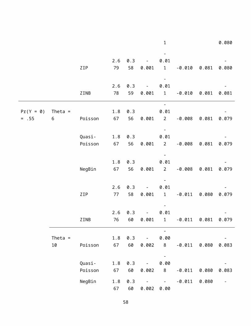
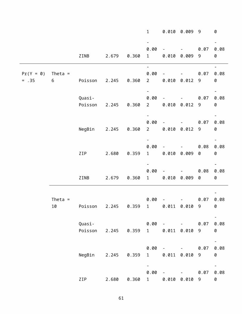
Finally, we compare the results of the simulation to the

true parameter values, Tables 6 through 8 show the mean parameter

estimates for sample sizes of 250, 500, and 1000, respectively.

Across all sample sizes, all models do a reasonable job of

recovering the true parameter values for the six predictor 26

variables, but only the zero-inflated models do a good job of

recovering the correct value of the intercept—which is a clear

advantage of the zero-inflated models versus even the negative

binomial model, which seems to otherwise fit the data adequately

when the percentage of zeros is low. Notably, even for the

largest sample sizes, the estimates of the intercept continue to

be quite poor for the Poisson, quasi-Poisson, and negative

binomial model, even though they provide good estimates of the

parameters.

[Insert Table 6, 7, and 8 about here]

A Concise Guideline

Figure 3 presents a simple decision tree for guiding the choice

among the four types of models: Poisson, negative binomial, and

their zero-inflated versions. We only focus on the two main

factors presented in this article, namely overdispersion and

excess zeros—issues that management researchers frequently face

when working on count-based dependent variables. As previously

noted, most statistical software has not implemented the panel

versions of the zero-inflated models. There are complex ways to

specify these models, and so far zero-inflated panels have been 27

shown to be a superior fit to more basic Poisson and negative

binomial panel regressions (Boucher & Guillen, 2009).

Accordingly, the recommendations generally hold for both panel

and cross-sectional data; however, panel data with zero-inflated

models is a much bigger challenge to implement in practice.

Moreover, we do not deal with other more subtle and technical

issues, such as whether it is important to estimate the

probability distribution of an individual count (Gardner et al.,

1995), nor do we go into detail whether fixed or random effects

are more appropriate, since as previously noted this is an area

that is germane to each unique dataset.

[Insert Figure 3 About here]

In line with most statistical textbooks (Cameron & Trivedi,

1998), unless the data displays equidispersion, the negative

binomial should be where most researchers begin their analysis.

Only in compelling cases should the basic Poisson model be used,

especially given that most statistical software such as STATA

will default to the basic Poisson in the scenario of

equidispersion. Therefore, given the simplicity of estimating the

negative binomial, some comparison of the models should be 28

implemented. The more complicated decision is where a researcher

has to determine whether there is a presence of excess zeros in

the data, which is probably the most common cause of

overdispersion in management research. There is little guidance

in the literature with respect to the threshold percentage of

zeros above which the data set is considered having excess zeros.

Based on our findings from the replication of Ornstein’s data,

along with the simulation we adopt a conservative threshold of

10% of the observations taking the value of zero. When the count

of zeros is below this level, the basic negative binomial may be

appropriate, but a Vuong test can aid in such scenarios.

When the percentage of zeros exceeds 10% we recommend

running the zero-inflated Poisson or zero-inflated negative

binomial model together with the Vuong test, which compares a

zero-inflated model with its corresponding basic version. The

Vuong statistic has a standard normal distribution with

significantly positive values favoring the zero-inflated model

and with significantly negative values favoring the basic version

(Long, 1997). A caveat here is that if the Vuong test is

conducted on a zero-inflated Poisson model and a significantly 29

negative statistic is generated, we recommend against using the

basic Poisson model for the simple reason that the model is

unsuitable for analyzing overdispersed data. The researcher

should drop the zero-inflated Poisson model, try zero-inflated

negative binomial, and re-run the Vuong test. If the Vuong

statistic is still significantly negative, the basic negative

binomial model should be adopted. If the Vuong statistic is

significantly positive, the likelihood ratio test of alpha = 0

has to be conducted. A significant test result indicates that the

zero-inflated negative binomial model should be adopted while an

insignificant result indicates that either of the zero-inflated

models is appropriate. Finally, if the absolute value of the

Vuong statistic is close to zero, neither the zero-inflated nor

the basic model is favored. In this case, the researcher may

choose among the negative binomial and the two zero-inflated

models. Ultimately, the final choice may depend on factors that

are not discussed in this paper.

Conclusion

By illustrating with simulation and replicated data, we highlight

some of the challenges that researchers face when deciding how to30

specify models when the outcome variable is a count-based

measure. Our motivation for this paper stemmed from the

disappointing discovery of having the results of a research

project change from strongly significant under the basic Poisson

estimation, to no longer significant with a more appropriately

specified negative binomial model. Originally, we used the

Poisson model “following past literature” as many others do. We

just so happened to pick one of the papers using the basic

Poisson model as a starting point since it was widely cited.

However, upon reviewing more papers we realized that our data

displayed signs of overdispersion, and consequently, we also

realized that our once significant results were no longer

significant with the proper statistical estimation.

Admittedly frustrated by the results, we were interested to

see if others might have made similar mistakes, but nevertheless

made it through the review process. To our surprise, we found

that approximately 1 out of 4 of the papers that had count-based

outcomes presented the basic Poisson regression only. Moreover,

in most of those articles there was little discussion about

whether or not alternative models were tested. 31

In sum, our goal is to provide a succinct and relatively

simple overview of potential problems and solutions when

analyzing data with count-based dependent variables. Our review

highlights that there are opportunities to improve upon existing

research. We show that there can be substantial changes in

findings, depending on the type of count-based model that is

specified. In general our simulation and replication show that

the negative binomial model is often more appropriate than the

basic Poisson model, and should be the starting point for most

count-based research (especially in cross-sectional data). When

there are excess zeros in the data, zero-inflated Poisson and

zero-inflated negative binomial models are also viable

alternatives to basic Poisson—and in our examples, are both

clearly a better fit. Moreover, we recommend that authors offer

more transparency in the proportion of zeros comprising their

data, and the specification addressing the zeros, which would

help readers judge whether the best model is being used.

Our paper underscores management researchers’ need to

understand the challenges and limitations of their data (Ketchen,

Boyd, & Bergh, 2009). This is important, since surveys indicate 32

that most management doctoral students are not well trained with

count-based regression models such as Poisson or negative

binomial (Shook et al., 2003). By providing a concise and simple

guideline in count-based analysis we hope that management

journals can continue leading the way in using the most rigorous

and advanced methodology when compared to other disciplines.

33

REFERENCES

Allison, P. D., & Waterman, R. P. 2002. Fixed–effects negative binomial regression models. Sociological Methodology, 32(1): 247–265.

Antonakis, J., Bastardoz, N., Liu, Y., & Schriesheim, C. A. 2014.What makes articles highly cited? Leadership Quarterly, 25(1), 152-179.

Berdahl, J. L., & Moore, C. 2006. Workplace harassment: double jeopardy for minority women. Journal of Applied Psychology, 91(2), 426.

Bettis, R. A. 2012. The search for asterisks: Compromised statistical tests and flawed theories. Strategic Management Journal, 33(1): 108-113.

Blundell, R., Griffith, R., & Van Reenen, J. 1995. Dynamic count data models of technological innovation. Economic Journal, 333-344.

Boucher, J. P., Denuit, M., & Guillén, M. 2009. Number of Accidents or Number of Claims? An Approach with Zero‐Inflated Poisson Models for Panel Data. Journal of Risk and Insurance, 76(4),821-846.

Cameron, A. C., & Trivedi, P. K. 1998. Regression Analysis of Count Data. Cambridge University Press, New York.

Cardinal, L. B. 2001. Technological innovation in the pharmaceutical industry: The use of organizational control in managing research and development. Organization Science, 12(1): 19–36.

Chang, S. J., Chung, C. N., & Mahmood, I. P. 2006. When and how does business group affiliation promote firm innovation? A tale of two emerging economies. Organization Science, 17: 637–656.

34

Corredoira, R. A., & Rosenkopf, L. 2010. Should auld acquaintancebe forgot? The reverse transfer of knowledge through mobility ties. Strategic Management Journal, 31(2): 159–181.

Drukker, D. M. 2007. My raw data contain evidence of both overdispersion and “excess zeros”. Stata. Available at: [http://www.stata.com/support/faqs/statistics/overdispersion- and-excess-zeros/]

Fox, J., & Weisberg, S. (2009). An R companion to applied regression. Thousand Oaks, CA: Sage.

Gelman, A., & Hill, J. 2007. Data analysis using regression and multilevel/hierarchical models. New York, NY: Cambridge University Press.

Gelman, A., Carlin, J.B., Stern, H.S., Dunson, D.B., Vehtari, A.,& Rubin, D.B. 2013. Bayesian Data Analysis (3rd Ed.). New York, NY: CRC Press.

Greene, W. H. 2008. Functional forms for the negative binomial model for count data. Economics Letters, 99(3): 585–590.

Greene, W. H. 2003. Econometric analysis. Prentice Hall, Upper Saddle River, NJ.

Haleblian, J. J., McNamara, G., Kolev, K., & Dykes, B. J. 2012. Exploring firm characteristics that differentiate leaders fromfollowers in industry merger waves: a competitive dynamics perspective. Strategic Management Journal, 33: 1037-1052.

Hausman, J. A., Hall, B. H., & Griliches, Z. 1984. Econometric models for count data with an application to the patents-R&D relationship. Econometrica, 52: 909-938.

Hess, A. M., & Rothaermel, F. T. 2011. When are assets complementary? Star scientists, strategic alliances, and innovation in the pharmaceutical industry. Strategic Management Journal, 32(8): 895–909.

35

Hoetker, G., & Agarwal, R. 2007. Death hurts, but it isn’t fatal:the postexit diffusion of knowledge created by innovative companies. Academy of Management Journal, 50(2): 446–467.

Horton, N.J., Kim, E., & Saitz, R. 2007. A cautionary note regarding count models of alcohol consumption in randomized controlled trials. BMC Medical Research Methodology, 7:9.

Kennedy, P. 2003. A Guide to Econometrics. MIT Press, Cambridge.

Ketchen, D.J., Boyd, B.K., & Bergh, D.D. 2009. Research methods in strategic management: Past accomplishments and future challenges. Organizational Research Methods, 11: 643-658.

Lin, Z. J., Peng, M. W., Yang, H., & Sun, S. L. 2009. How do networks and learning drive M&As? An institutional comparison between China and the United States. Strategic Management Journal,30: 1113–1132.

Long, J. S. 1997. Regression Models for Categorical and Limited Dependent Variables. Sage Publications, London.

Lord, D., Washington, S., & Ivan, J.N. 2005. Poisson, gamma-Poisson and zero-inflated regression models of motor vehicle crashes: balancing statistical fit and theory. Accident Analysis &Prevention, 37: 35 – 46.

Miller, K. D., & Tsang, E. W. K. 2011. Testing management theories: critical realist philosophy and research methods. Strategic Management Journal, 32(2): 139–158.

Ohly, S., Sonnentag, S., & Pluntke, F. 2006. Routinization, work characteristics and their relationships with creative and proactive behaviors. Journal of Organizational Behavior, 27(3): 257-279.

Ornstein, M. D. 1976. The boards and executives of the largest Canadian corporations: Size, composition, and interlocks. Canadian Journal of Sociology/Cahiers canadiens de sociologie, 411-437.

36

Park, S. H., Chen, R., & Gallagher, S. 2002. Firm resources as moderators of the relationship between market growth and strategic alliances in semiconductor start-ups. Academy of Management Journal, 45: 527–545.

Pe’Er, A., & Gottschalg, O. 2011. Red and Blue: the relationship between the institutional context and the performance of leveraged buyout investments. Strategic Management Journal, 32: 1356–1367.

Penner-Hahn, J., & Shaver, J. M. 2005. Does international research and development increase patent output? An analysis of Japanese pharmaceutical firms. Strategic Management Journal, 26(2): 121–140.

Perumean-Chaney, S. E., Morgan, C., McDowall, D., & Aban, I. Zero-inflated and overdispersed: what’s one to do? Journal of Statistical Computation and Simulation, (forthcoming).

R Development Core Team. 2013. R: A language and environment for statistical computing. R Foundation for Statistical Computing,Vienna, Austria. URL http://www.R-project.org/.

Shook, C. L., Ketchen, D. J., Cycyota, C. S., & Crockett, D. 2003. Data analytic trends and training in strategic management. Strategic Management Journal, 24(12): 1231–1237.

Soh, P. H. 2010. Network patterns and competitive advantage before the emergence of a dominant design. Strategic Management Journal, 31(4): 438–461.

Un, C. A. 2011. The advantage of foreignness in innovation. Strategic Management Journal, 32: 1232-1242.

Vuong, Q. H. 1989. Likelihood ratio tests for model selection andnon-nested hypotheses. Econometrica: Journal of the Econometric Society, 57: 307–333.

Wang, M., Liu, S., Zhan, Y., & Shi, J. 2010. Daily work–family conflict and alcohol use: Testing the cross-level moderation

37

effects of peer drinking norms and social support. Journal of Applied Psychology, 95(2), 377.

Zeileis, A., Kleiber, C., & Jackman, S. 2008. Regression models for count data in R. Journal of Statistical Software, 27(8). URL: http://www.jstatsoft.org/v27/i08/

38

Figure 1: Trend of Count-Based Papers in Exemplar Management Journals (164 total)

2001 2002 2003 2004 2005 2006 2007 2008 2009 2010 201102468101214161820

PoissonNegative BinomialZero Inflated

Figure 2: Fit of Different Models

39

Figure 3. Decision Tree with Count-Based Dependent Variables

41

What is theresult of the

No

Are there a fairlylarge (>10%) number

of zeros in the

Yes

No

Yes

Negativebinomial

Significantly

Zero-inflatedPoisson or

zero-inflatednegative

Negativebinomial

Significantly

Close to zero

Negative binomial, zero-inflated

Poisson or zero-inflated

Is there anysign of

Poiss

Is the likelihood-ratio test of alpha

Zero-inflatednegativebinomial

Yes

No

Table 1: Use of Count-based Regressions by Journal (2001-2011)

JournalsPoisson*

Mean toS.D.a

Ratio(Average)

Neg.Binomia

l

Zero-InflatedModels

TotalPapers

AMJ 9 270% 20 6 35ASQ 5 573% 19 3 27JIBS 4 235% 13 1 18OS 2 300% 12 2 16SMJ 14 290% 19 5 38JAP 6 243% 5 0 11PS 2 106% 2 0 4JOM 1 280% 2 0 3JOB 3 296% 3 1 7OBHDP 3 158% 2 0 5

Total (Percentage) 49(30%) 275% 97

(59%) 18(11%) 164

ASR 5(21%) 204% 19

(89%) 6(25%) 24

*39 of these 49 used the most basic Poisson methodology, with an average mean to standard deviation ratio of 2.86.

a Standard deviation

42

TABLE 2: Changes from Basic Poisson to Zero-Inflated Negative Binomial

Variables Basic Poisson

in LOSa

in Sign ZINBb

# of authors 0.04*** (8.56) YES NO 0.09** (3.1

8)

Artic. Age -0.04*** (6.32) YES NO -0.05 (1.3

8)

Cited references

0.01***

(42.34) NO NO 0.01*** (5.4

7)

Quantitative 0.46***

(16.16)

YES NO 0.35** (2.9

5)

Theory 0.48***

(16.50)

YES NO 0.33* (2.5

9)

Review 0.68***

(21.23)

YES NO 0.52** (2.7

8)

Comment/discuss.

-0.25*** (4.48) Y

ES NO -0.12 (0.57)

Method 0.59***

(10.30)

YES NO 0.58* (2.3

0)

Agent simulation -0.51* (2.41)

YES NO -0.51† (1.70)

Author cites -0.00* (2.42) YES YES 0.00† (1.7

4)

Author articles

0.00*** (7.81)

YES YES -0.00 (0.86)

Aff. Rank 0.00*** (8.54)

YES NO 0.00* (2.08)

44

TABLE 2: Changes from Basic Poisson to Zero-Inflated Negative Binomial

# articles pub

-0.04***

(31.47)

NO NO -

0.04***(8.62)

(a) x (b) 0.01***

(45.60)

NO NO 0.01*** (7.1

5)

Constant 1.96***

(15.16)

NO NO

1.89***(4.01)

N=776, † p < 0.10, * p < 0.05, ** p < 0.01, *** p < 0.001

a Level of significance, b Zero-inflated negative binomial

45

Table 3: Regressions on the Ornstein Data Basic Poissona D Neg.

Binomial Zero-Inflated Poisson

Zero-inflatedNeg. Binomial

Variables Model I Model II Model III Model IV

(Intercept) -0.84***(0.14)

-0.83*

(0.38)

-0.35*

(0.14) -0.28

(0.35)

log2(assets) 0.31***

(0.01)

0.32**

*(0.04

)

0.27*

**(0.01) 0.27***

(0.03)

nationOTH -0.11(0.07) -0.10

(0.23) -0.06

(0.08) 0.02

(0.21)

nationUK -0.39***(0.09)

-0.39†

(0.24)

-0.41*

**(0.09) -0.42*

(0.21)

nationUS -0.77***(0.05)

-0.79**

*(0.13

)

-0.69*

**(0.05) -0.69***

(0.12)

sectorBNK -0.17†(0.10) -0.41

(0.38) 0.06

(0.10) -0.04

(0.35)

sectorCON -0.49*(0.21)

-0.76†

(0.46)

-0.60*

*(0.21) -0.87*

(0.40)

sectorFIN -0.11(0.08) -0.10

(0.25) -0.05

(0.08) -0.04

(0.22)

sectorHLD -0.01(0.12) -0.21

(0.35) 0.05

(0.12) -0.10

(0.32)

sectorMAN 0.12(0.08) 0.08

(0.19)

0.22*

*(0.08) 0.18

(0.18)

sectorMER 0.06(0.09) 0.08

(0.23) 0.01

(0.09) 0.01

(0.21)

46

sectorMIN 0.25***(0.07) 0.24

(0.19)

0.25*

**(0.07) 0.21

(0.17)

sectorTRN 0.15†(0.08) 0.10

(0.25)

0.17*

(0.08) 0.09

(0.22)

sectorWOD 0.50***(0.08)

0.39†

(0.23)

0.49*

**(0.08) 0.39†

(0.20)

loglikelihood -1222 -822 - 1106 -804

df 14 15 28 29N=100, † p < 0.10, * p < 0.05, ** p < 0.01, *** p < 0.001

47

TABLE 4. Mean Vuong statistic for model comparisons across

simulation replications.

NegBin vs.Poisson

ZIP vs.NegBin

ZINB vs.ZIP

N = 250Pr(Y = 0) =.2

Theta = 6 7.64 0.49 4.76

Theta = 10 10.80 7.63 5.30

Pr(Y = 0) =.35

Theta = 6 9.05 10.94 4.26

Theta = 10 9.41 11.33 3.38

Pr(Y = 0) =.55

Theta = 6 8.32 15.26 3.46

Theta = 10 9.27 16.65 2.72

N = 500Pr(Y = 0) =.2

Theta = 6 10.69 -0.38 6.57

Theta = 10 10.80 7.63 5.30

Pr(Y = 0) =.35

Theta = 6 11.91 15.57 5.98

Theta = 10 11.88 15.55 5.90

Pr(Y = 0) =.55

Theta = 6 10.90 21.59 4.89

48

Theta = 10 13.08 24.37 3.86

N = 1000Pr(Y = 0) =.2

Theta = 6 15.13 -1.59 9.26

Theta = 10 15.15 11.50 7.48

Pr(Y = 0) =.35

Theta = 6 16.73 22.17 8.20

Theta = 10 18.76 23.05 6.67

Pr(Y = 0) =.55

Theta = 6 15.03 30.60 6.85

Theta = 10 17.35 33.96 5.53

Note. Italicized entries indicate a lack of statistical significance at the .05level. The Vuong statistic is distributed as a standard normal under the null hypothesis that the models being compared are indistinguishable (Zeileis, Kleiber, & Jackman, 2008), so the critical value associated with alpha = .05 for a two-tailed test is +/- 1.96. Theta is the variance parameter for the negative binomial (count) component of the ZINB model.

49

Table 5. Mean log-likelihoods for models across 1000 simulation replications (smaller is better).

Poisson NegBin ZIP ZINB

N = 250Pr(Y = 0) = .2

Theta = 6 -1503.07 -991.00 -911.04 -785.40

Theta = 10 -2775.57 -2405.88 -1634.64 -1514.00

Pr(Y = 0) = .35

Theta = 6 -1738.41 -1721.76 -796.73 -697.04

Theta = 10 -1675.90 -1675.04 -721.71 -673.09

Pr(Y = 0) = .55

Theta = 6 -1775.02 -1771.77 -597.20 -534.93

Theta = 10 -1755.92 -1754.91 -551.78 -521.42

N = 500Pr(Y = 0) = .2

Theta = 6 -2975.90 -1867.94 -1821.00 -1567.79

Theta = 10 -2775.57 -2405.88 -1634.64 -1514.00

Pr(Y = 0) = .35

Theta = 6 -3558.82 -3556.78 -1617.32 -1402.66

Theta = 10 -3461.24 -3461.09 -1593.99 -1391.89

Pr(Y = 0) = .55

Theta = 6 -3694.36 -3694.19 -1222.02 -1082.97

Theta = 10 -3529.63 -3529.53 -1111.82 -1048.22

N = 1000 Pr(Y = 0) Theta = -5969.11 -3593.03 -3659.40 -3146.87

50

= .2 6

Theta = 10 -5588.81 -4999.99 -3284.45 -3036.32

Pr(Y = 0) = .35

Theta = 6 -6789.12 -6788.84 -3170.19 -2776.61

Theta = 10 -6656.71 -6656.54 -2904.57 -2704.11

Pr(Y = 0) = .55

Theta = 6 -7295.86 -7295.53 -2446.48 -2167.60

Theta = 10 -7125.40 -7125.22 -2247.75 -2110.75

51

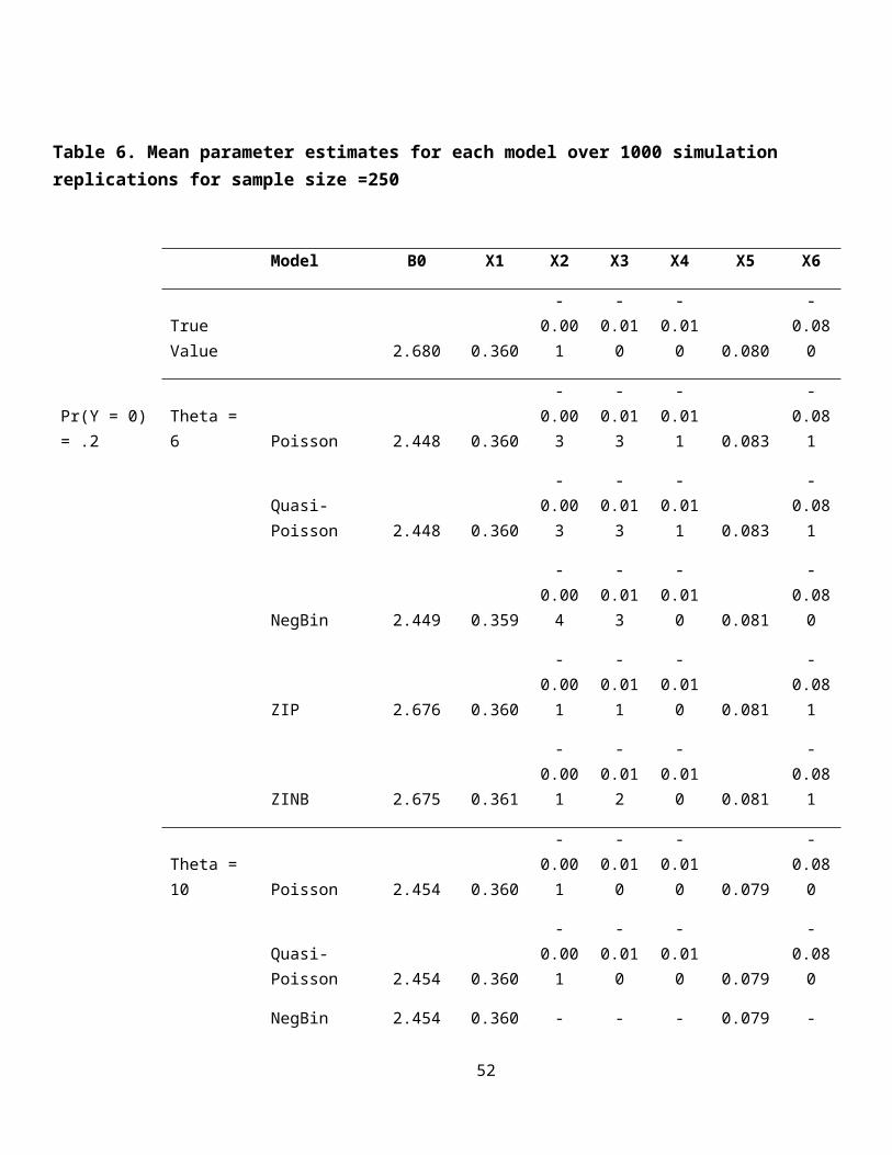
Table 6. Mean parameter estimates for each model over 1000 simulation replications for sample size =250

Model B0 X1 X2 X3 X4 X5 X6

True Value 2.680 0.360

-0.001

-0.010

-0.010 0.080

-0.080

Pr(Y = 0)= .2

Theta = 6 Poisson 2.448 0.360

-0.003

-0.013

-0.011 0.083

-0.081

Quasi-Poisson 2.448 0.360

-0.003

-0.013

-0.011 0.083

-0.081

NegBin 2.449 0.359

-0.004

-0.013

-0.010 0.081

-0.080

ZIP 2.676 0.360

-0.001

-0.011

-0.010 0.081

-0.081

ZINB 2.675 0.361

-0.001

-0.012

-0.010 0.081

-0.081


-0.001

-0.010

-0.010 0.079

-0.080


-0.001

-0.010

-0.010 0.079

-0.080

NegBin 2.454 0.360 - - - 0.079 -

52

0.001

0.010

0.010

0.080

ZIP 2.680 0.360

-0.002

-0.009

-0.010 0.080

-0.080

ZINB 2.679 0.361

-0.001

-0.010

-0.010 0.080

-0.080

Pr(Y = 0)= .35


-0.001

-0.010

-0.012 0.081

-0.078


-0.001

-0.010

-0.012 0.081

-0.078

NegBin 2.238 0.359

-0.001

-0.010

-0.012 0.082

-0.078

ZIP 2.677 0.358

-0.001

-0.011

-0.011 0.078

-0.080

ZINB 2.676 0.360

-0.001

-0.011

-0.011 0.079

-0.080


-0.001

-0.011

-0.007 0.080

-0.075


-0.001

-0.011

-0.007 0.080

-0.075

53

NegBin 2.236 0.360

-0.001

-0.011

-0.007 0.080

-0.075

ZIP 2.677 0.358

-0.002

-0.010

-0.009 0.078

-0.078

ZINB 2.677 0.360

-0.001

-0.010

-0.009 0.079

-0.079

Pr(Y = 0)= .55


0.001

-0.015

-0.009 0.080

-0.079


0.001

-0.015

-0.009 0.080

-0.079

NegBin 1.851 0.3580.001

-0.014

-0.009 0.080

-0.079

ZIP 2.673 0.3590.001

-0.011

-0.009 0.079

-0.080

ZINB 2.671 0.3610.001

-0.011

-0.009 0.080

-0.080


-0.001

-0.012

-0.008 0.082

-0.078


-0.001

-0.012

-0.008 0.082

-0.078

54

NegBin 1.858 0.360

-0.001

-0.012

-0.008 0.082

-0.078

ZIP 2.676 0.359

-0.001

-0.011

-0.011 0.081

-0.078

ZINB 2.675 0.360

-0.001

-0.010

-0.011 0.081

-0.078

55



True Value

2.680

0.360

-0.001

-0.010 -0.010 0.080

-0.080

Pr(Y = 0)= .2

Theta = 6 Poisson

2.451

0.359

-0.001

-0.012 -0.008 0.080

-0.080

Quasi-Poisson

2.451

0.359

-0.001

-0.012 -0.008 0.080

-0.080

NegBin2.452

0.359

-0.001

-0.012 -0.009 0.080

-0.080

ZIP2.679

0.359

-0.001

-0.011 -0.009 0.080

-0.081

ZINB2.677

0.360

-0.001

-0.011 -0.010 0.080

-0.081

Theta = 10 Poisson

2.454

0.360

-0.001

-0.010 -0.010 0.079

-0.080

Quasi-Poisson

2.454

0.360

-0.001

-0.010 -0.010 0.079

-0.080

NegBin 2.454

0.360

-0.001

-0.01

-0.010 0.079 -0.080

56

0

ZIP2.680

0.360

-0.002

-0.009 -0.010 0.080

-0.080

ZINB2.679

0.361

-0.001

-0.010 -0.010 0.080

-0.080

Pr(Y = 0)= .35

Theta = 6 Poisson

2.243

0.360 0.000

-0.009 -0.008 0.081

-0.083

Quasi-Poisson

2.243

0.360 0.000

-0.009 -0.008 0.081

-0.083

NegBin2.243

0.360 0.000

-0.009 -0.008 0.081

-0.083

ZIP2.679

0.359

-0.001

-0.010 -0.009 0.081

-0.081

ZINB2.678

0.360

-0.001

-0.010 -0.010 0.081

-0.081

Theta = 10 Poisson

2.241

0.358

-0.001

-0.011 -0.010 0.084

-0.080

Quasi-Poisson

2.241

0.358

-0.001

-0.011 -0.010 0.084

-0.080

NegBin 2.241

0.358

-0.001

-0.01

-0.010 0.084 -

57

1 0.080

ZIP2.679

0.358

-0.001

-0.011 -0.010 0.081

-0.080

ZINB2.678

0.359

-0.001

-0.011 -0.010 0.081

-0.081

Pr(Y = 0)= .55

Theta = 6 Poisson

1.867

0.356 0.001

-0.012 -0.008 0.081

-0.079

Quasi-Poisson

1.867

0.356 0.001

-0.012 -0.008 0.081

-0.079

NegBin1.867

0.356 0.001

-0.012 -0.008 0.081

-0.079

ZIP2.677

0.358

-0.001

-0.011 -0.011 0.080

-0.079

ZINB2.676

0.360

-0.001

-0.011 -0.011 0.081

-0.079

Theta = 10 Poisson

1.867

0.360

-0.002

-0.008 -0.011 0.080

-0.083

Quasi-Poisson

1.867

0.360

-0.002

-0.008 -0.011 0.080

-0.083

NegBin 1.867

0.360

-0.002

-0.00

-0.011 0.080 -

58

8 0.083

ZIP2.678

0.358

-0.002

-0.010 -0.011 0.081

-0.082

ZINB2.677

0.358

-0.002

-0.010 -0.011 0.081

-0.081

59



True Value 2.680 0.360

-0.001

-0.010

-0.010

0.080

-0.080

Pr(Y = 0)= .2


-0.001

-0.008

-0.009

0.081

-0.080


-0.001

-0.008

-0.009

0.081

-0.080

NegBin 2.455 0.360

-0.001

-0.008

-0.008

0.082

-0.080

ZIP 2.680 0.3590.000

-0.008

-0.009

0.080

-0.080

ZINB 2.679 0.3600.000

-0.009

-0.009

0.081

-0.080


0.000

-0.010

-0.009

0.079

-0.079


0.000

-0.010

-0.009

0.079

-0.079

NegBin 2.455 0.3590.000

-0.010

-0.009

0.079

-0.079

ZIP 2.680 0.360 -0.00

- - 0.07 -0.08

60

1 0.010 0.009 9 0

ZINB 2.679 0.360

-0.001

-0.010

-0.009

0.079

-0.080

Pr(Y = 0)= .35


-0.002

-0.010

-0.012

0.079

-0.080


-0.002

-0.010

-0.012

0.079

-0.080

NegBin 2.245 0.360

-0.002

-0.010

-0.012

0.079

-0.080

ZIP 2.680 0.359

-0.001

-0.010

-0.009

0.080

-0.080

ZINB 2.679 0.360

-0.001

-0.010

-0.009

0.080

-0.080


0.001

-0.011

-0.010

0.079

-0.080


0.001

-0.011

-0.010

0.079

-0.080

NegBin 2.245 0.3590.001

-0.011

-0.010

0.079

-0.080

ZIP 2.680 0.360

-0.001

-0.010

-0.010

0.079

-0.080

61

ZINB 2.679 0.360

-0.001

-0.010

-0.010

0.080

-0.080

Pr(Y = 0)= .55


-0.001

-0.010

-0.009

0.079

-0.081


-0.001

-0.010

-0.009

0.079

-0.081

NegBin 1.875 0.360

-0.001

-0.010

-0.009

0.079

-0.081

ZIP 2.679 0.359

-0.001

-0.010

-0.009

0.079

-0.079

ZINB 2.677 0.360

-0.001

-0.010

-0.010

0.079

-0.080


-0.001

-0.008

-0.010

0.082

-0.078


-0.001

-0.008

-0.010

0.082

-0.078

NegBin 1.877 0.357

-0.001

-0.008

-0.010

0.082

-0.078

ZIP 2.678 0.359

-0.001

-0.010

-0.010

0.081

-0.080

62

ZINB 2.678 0.360

-0.001

-0.010

-0.010

0.081

-0.080

63

APPENDIX

The following appendix presents the full syntax in R to replicate the analyses of the Ornstein data on corporate board interlocks.

First, you may need to install some R packages, especially the car package that houses the Ornstein data, using the function "install.packages("packagename")" at the R prompt.

In R, the hash-symbol (#) denotes a comment (text that is ignored by the R interpreter). We include some comments below to describe some specific functions in more detail.rm(list=ls())library(arm) # loads the MASS package and other utility functionslibrary(pscl) # for zip and zinb models and vuong testlibrary(car) #Ornstein data and Anova function

We begin by working through the code example from Fox and Weisberg (2009), before extending it using zero-inflated models. The "data(Ornstein)" commandloads the Ornstein data. You must run the "library(car)"" command before this, or else the data() command will not work.data(Ornstein) ## fit model using using basic Poisson mod.ornstein <- glm(interlocks ~ log2(assets) + nation + sector, family=poisson, data=Ornstein)summary(mod.ornstein)

Call:glm(formula = interlocks ~ log2(assets) + nation + sector, family = poisson, data = Ornstein)

Deviance Residuals: Min 1Q Median 3Q Max -6.711 -2.316 -0.459 1.282 6.285

Coefficients: Estimate Std. Error z value Pr(>|z|) (Intercept) -0.8394 0.1366 -6.14 8.1e-10 ***log2(assets) 0.3129 0.0118 26.58 < 2e-16 ***nationOTH -0.1070 0.0744 -1.44 0.15030 nationUK -0.3872 0.0895 -4.33 1.5e-05 ***nationUS -0.7724 0.0496 -15.56 < 2e-16 ***sectorBNK -0.1665 0.0958 -1.74 0.08204 . sectorCON -0.4893 0.2132 -2.29 0.02174 *

64

sectorFIN -0.1116 0.0757 -1.47 0.14046 sectorHLD -0.0149 0.1192 -0.13 0.90051 sectorMAN 0.1219 0.0761 1.60 0.10949 sectorMER 0.0616 0.0867 0.71 0.47760 sectorMIN 0.2498 0.0689 3.63 0.00029 ***sectorTRN 0.1518 0.0789 1.92 0.05445 . sectorWOD 0.4983 0.0756 6.59 4.4e-11 ***---Signif. codes: 0 '***' 0.001 '**' 0.01 '*' 0.05 '.' 0.1 ' ' 1

(Dispersion parameter for poisson family taken to be 1)

Null deviance: 3737.0 on 247 degrees of freedomResidual deviance: 1547.1 on 234 degrees of freedomAIC: 2473

Number of Fisher Scoring iterations: 5

## ---------------------------------------## provide an estimate of over-dispersion: phi is the scale parameter.## Phi is assumed to be 1 for the basic Poisson.## See Fox & Weisberg (2009) for more details.## ---------------------------------------phiest <- sum(residuals(mod.ornstein, type="pearson")^2)/df.residual(mod.ornstein)summary(mod.ornstein, dispersion=phiest)

Call:glm(formula = interlocks ~ log2(assets) + nation + sector, family = poisson, data = Ornstein)

Deviance Residuals: Min 1Q Median 3Q Max -6.711 -2.316 -0.459 1.282 6.285

Coefficients: Estimate Std. Error z value Pr(>|z|) (Intercept) -0.8394 0.3456 -2.43 0.0152 * log2(assets) 0.3129 0.0298 10.51 < 2e-16 ***nationOTH -0.1070 0.1881 -0.57 0.5696 nationUK -0.3872 0.2264 -1.71 0.0872 . nationUS -0.7724 0.1256 -6.15 7.7e-10 ***sectorBNK -0.1665 0.2422 -0.69 0.4918 sectorCON -0.4893 0.5393 -0.91 0.3643 sectorFIN -0.1116 0.1915 -0.58 0.5601 sectorHLD -0.0149 0.3016 -0.05 0.9606

65

sectorMAN 0.1219 0.1926 0.63 0.5269 sectorMER 0.0616 0.2193 0.28 0.7789 sectorMIN 0.2498 0.1742 1.43 0.1516 sectorTRN 0.1518 0.1997 0.76 0.4471 sectorWOD 0.4983 0.1912 2.61 0.0092 ** ---Signif. codes: 0 '***' 0.001 '**' 0.01 '*' 0.05 '.' 0.1 ' ' 1

(Dispersion parameter for poisson family taken to be 6.399)



Anova(mod.ornstein, test="F")

Warning: dispersion parameter estimated from the Pearson residuals, nottaken as 1

Analysis of Deviance Table (Type II tests)

Response: interlocks SS Df F Pr(>F) log2(assets) 731 1 114.28 < 2e-16 ***nation 276 3 14.38 1.2e-08 ***sector 103 9 1.78 0.072 . Residuals 1497 234 ---Signif. codes: 0 '***' 0.001 '**' 0.01 '*' 0.05 '.' 0.1 ' ' 1

We now fit using quasi-likelihood methods, which allows estimation of a scale parameter, and negative-binomial regression.

## fit using quasi-Poissonmod.ornstein.quasi <- glm(interlocks ~ log2(assets) + nation + sector, family=quasipoisson, data=Ornstein)summary(mod.ornstein.quasi)

Call:glm(formula = interlocks ~ log2(assets) + nation + sector, family = quasipoisson, data = Ornstein)

Deviance Residuals: Min 1Q Median 3Q Max

66

-6.711 -2.316 -0.459 1.282 6.285

Coefficients: Estimate Std. Error t value Pr(>|t|) (Intercept) -0.8394 0.3456 -2.43 0.0159 * log2(assets) 0.3129 0.0298 10.51 < 2e-16 ***nationOTH -0.1070 0.1881 -0.57 0.5701 nationUK -0.3872 0.2264 -1.71 0.0885 . nationUS -0.7724 0.1256 -6.15 3.3e-09 ***sectorBNK -0.1665 0.2422 -0.69 0.4925 sectorCON -0.4893 0.5393 -0.91 0.3652 sectorFIN -0.1116 0.1915 -0.58 0.5606 sectorHLD -0.0149 0.3016 -0.05 0.9606 sectorMAN 0.1219 0.1926 0.63 0.5275 sectorMER 0.0616 0.2193 0.28 0.7792 sectorMIN 0.2498 0.1742 1.43 0.1529 sectorTRN 0.1518 0.1997 0.76 0.4478 sectorWOD 0.4983 0.1912 2.61 0.0098 ** ---Signif. codes: 0 '***' 0.001 '**' 0.01 '*' 0.05 '.' 0.1 ' ' 1

(Dispersion parameter for quasipoisson family taken to be 6.399)

Null deviance: 3737.0 on 247 degrees of freedomResidual deviance: 1547.1 on 234 degrees of freedomAIC: NA


## ---------------------------------------## Use the automated negative binomial procedure from the MASS package.## This procedure estimates "theta"--the amount of overdispersion ## relative to the basic Poisson. See Fox & Weisberg (2009), pp. 279 -## 280 for this parameterization of the negative binomial model.## ---------------------------------------mod.ornstein.nb <- glm.nb(interlocks ~ log2(assets) + nation + sector, data=Ornstein)summary(mod.ornstein.nb)

Call:glm.nb(formula = interlocks ~ log2(assets) + nation + sector, data = Ornstein, init.theta = 1.639034209, link = log)

Deviance Residuals: Min 1Q Median 3Q Max

67

-2.809 -0.990 -0.189 0.430 2.408

Coefficients: Estimate Std. Error z value Pr(>|z|) (Intercept) -0.8254 0.3798 -2.17 0.030 * log2(assets) 0.3162 0.0359 8.80 < 2e-16 ***nationOTH -0.1045 0.2300 -0.45 0.649 nationUK -0.3894 0.2357 -1.65 0.099 . nationUS -0.7882 0.1320 -5.97 2.4e-09 ***sectorBNK -0.4085 0.3773 -1.08 0.279 sectorCON -0.7570 0.4571 -1.66 0.098 . sectorFIN -0.1035 0.2518 -0.41 0.681 sectorHLD -0.2110 0.3498 -0.60 0.546 sectorMAN 0.0768 0.1860 0.41 0.680 sectorMER 0.0776 0.2325 0.33 0.738 sectorMIN 0.2399 0.1884 1.27 0.203 sectorTRN 0.1013 0.2475 0.41 0.682 sectorWOD 0.3908 0.2325 1.68 0.093 . ---Signif. codes: 0 '***' 0.001 '**' 0.01 '*' 0.05 '.' 0.1 ' ' 1

(Dispersion parameter for Negative Binomial(1.639) family taken to be 1)



Theta: 1.639 Std. Err.: 0.192

2 x log-likelihood: -1645.257

The following code chunk fits zero-inflated Poisson and negative binomial models. The models fitted below only inflate the intercept (the "|1" in the formula descriptions), but meaningful regressors can be placed here. If the "|1" construction is omitted, the pscl package default is to model the zero-inflation component with the same regression model as the count component (we demonstrate the ZIP version at the end of the appendix).

mod.ornstein.zip <- zeroinfl(interlocks ~ log2(assets) + nation + sector|1, data=Ornstein)summary(mod.ornstein.zip)

68

Call:zeroinfl(formula = interlocks ~ log2(assets) + nation + sector | 1, data = Ornstein)

Pearson residuals: Min 1Q Median 3Q Max -2.494 -1.302 -0.190 0.957 6.383

Count model coefficients (poisson with log link): Estimate Std. Error z value Pr(>|z|) (Intercept) -0.3892 0.1403 -2.77 0.00553 ** log2(assets) 0.2752 0.0120 22.85 < 2e-16 ***nationOTH -0.0571 0.0753 -0.76 0.44816 nationUK -0.4083 0.0895 -4.56 5.1e-06 ***nationUS -0.6994 0.0498 -14.03 < 2e-16 ***sectorBNK 0.0474 0.0977 0.49 0.62741 sectorCON -0.5890 0.2134 -2.76 0.00577 ** sectorFIN -0.0540 0.0759 -0.71 0.47676 sectorHLD 0.0531 0.1197 0.44 0.65701 sectorMAN 0.2271 0.0775 2.93 0.00338 ** sectorMER 0.0212 0.0875 0.24 0.80817 sectorMIN 0.2547 0.0694 3.67 0.00024 ***sectorTRN 0.1713 0.0789 2.17 0.02991 * sectorWOD 0.4988 0.0762 6.55 5.9e-11 ***

Zero-inflation model coefficients (binomial with logit link): Estimate Std. Error z value Pr(>|z|) (Intercept) -2.17 0.22 -9.88 <2e-16 ***---Signif. codes: 0 '***' 0.001 '**' 0.01 '*' 0.05 '.' 0.1 ' ' 1

Number of iterations in BFGS optimization: 20 Log-likelihood: -1.13e+03 on 15 Df

mod.ornstein.zinb <- zeroinfl(interlocks ~ log2(assets) + nation + sector|1, data=Ornstein, dist="negbin")summary(mod.ornstein.zinb)

Call:zeroinfl(formula = interlocks ~ log2(assets) + nation + sector | 1, data = Ornstein, dist = "negbin")

Pearson residuals: Min 1Q Median 3Q Max

69

-1.286 -0.792 -0.161 0.516 3.785

Count model coefficients (negbin with log link): Estimate Std. Error z value Pr(>|z|) (Intercept) -0.5684 0.3655 -1.56 0.120 log2(assets) 0.2934 0.0345 8.52 < 2e-16 ***nationOTH -0.0386 0.2249 -0.17 0.864 nationUK -0.4066 0.2172 -1.87 0.061 . nationUS -0.7518 0.1222 -6.15 7.8e-10 ***sectorBNK -0.1783 0.3733 -0.48 0.633 sectorCON -0.8072 0.4175 -1.93 0.053 . sectorFIN -0.0707 0.2276 -0.31 0.756 sectorHLD -0.1391 0.3331 -0.42 0.676 sectorMAN 0.1415 0.1806 0.78 0.433 sectorMER 0.0519 0.2141 0.24 0.809 sectorMIN 0.2489 0.1736 1.43 0.152 sectorTRN 0.1027 0.2264 0.45 0.650 sectorWOD 0.4135 0.2150 1.92 0.054 . Log(theta) 0.7528 0.1474 5.11 3.3e-07 ***

Zero-inflation model coefficients (binomial with logit link): Estimate Std. Error z value Pr(>|z|) (Intercept) -2.892 0.463 -6.25 4.1e-10 ***---Signif. codes: 0 '***' 0.001 '**' 0.01 '*' 0.05 '.' 0.1 ' ' 1

Theta = 2.123 Number of iterations in BFGS optimization: 24 Log-likelihood: -820 on 16 Df

## compare models -- no direct test for quasi-Poissonvuong(mod.ornstein.zinb,mod.ornstein.zip)

Vuong Non-Nested Hypothesis Test-Statistic: 6.449 (test-statistic is asymptotically distributed N(0,1) under the null that the models are indistinguishible)in this case:model1 > model2, with p-value 5.634e-11

vuong(mod.ornstein.zip,mod.ornstein.nb)

Vuong Non-Nested Hypothesis Test-Statistic: -6.182 (test-statistic is asymptotically distributed N(0,1) under the null that the models are indistinguishible)in this case:model2 > model1, with p-value 3.164e-10

70

Modeling zero-inflation fully:mod.ornstein.zip.1 <- zeroinfl(interlocks ~ log2(assets) + nation + sector, data=Ornstein)summary(mod.ornstein.zip.1)

Call:zeroinfl(formula = interlocks ~ log2(assets) + nation + sector, data = Ornstein)

Pearson residuals: Min 1Q Median 3Q Max -4.536 -1.317 -0.403 1.058 6.300

Count model coefficients (poisson with log link): Estimate Std. Error z value Pr(>|z|) (Intercept) -0.3533 0.1388 -2.54 0.0109 * log2(assets) 0.2725 0.0120 22.78 < 2e-16 ***nationOTH -0.0572 0.0752 -0.76 0.4474 nationUK -0.4109 0.0895 -4.59 4.4e-06 ***nationUS -0.6894 0.0493 -13.97 < 2e-16 ***sectorBNK 0.0561 0.0975 0.58 0.5646 sectorCON -0.5975 0.2132 -2.80 0.0051 ** sectorFIN -0.0535 0.0757 -0.71 0.4793 sectorHLD 0.0481 0.1194 0.40 0.6872 sectorMAN 0.2229 0.0766 2.91 0.0036 ** sectorMER 0.0138 0.0871 0.16 0.8744 sectorMIN 0.2491 0.0689 3.61 0.0003 ***sectorTRN 0.1680 0.0786 2.14 0.0325 * sectorWOD 0.4921 0.0759 6.48 8.9e-11 ***

Zero-inflation model coefficients (binomial with logit link): Estimate Std. Error z value Pr(>|z|) (Intercept) 3.796 1.827 2.08 0.03778 * log2(assets) -0.692 0.200 -3.46 0.00054 ***nationOTH 1.565 1.029 1.52 0.12817 nationUK 0.127 1.187 0.11 0.91456 nationUS 1.506 0.604 2.50 0.01259 * sectorBNK 4.688 1.752 2.68 0.00744 ** sectorCON -17.935 7735.986 0.00 0.99815 sectorFIN -14.867 3494.975 0.00 0.99661 sectorHLD 1.308 1.262 1.04 0.30016 sectorMAN 0.427 0.608 0.70 0.48277 sectorMER -1.017 1.289 -0.79 0.42998 sectorMIN -0.317 0.744 -0.43 0.66974 sectorTRN -16.583 3765.565 0.00 0.99649

71

sectorWOD -0.553 1.178 -0.47 0.63856 ---Signif. codes: 0 '***' 0.001 '**' 0.01 '*' 0.05 '.' 0.1 ' ' 1

Number of iterations in BFGS optimization: 28 Log-likelihood: -1.11e+03 on 28 Df

Here, we can see that the intercept, log2(assets), the dummy variable for US, and the dummy variable BNK are significant predictors of the zero-inflation component.

This document was produced using R markdown and the knitr package in RStudio.

AUTHOR BIOGRAPHIES

Dane P. Blevins is an assistant professor of strategy at Binghamton University. He received his PhD in strategic management from the University of Texas at Dallas. His research interests include corporate governance, initial public offerings, global strategy, and ethics.

Eric W. K. Tsang is the Dallas World Salute Distinguished Professor of Global Strategy in the School of Management, University of Texas at Dallas. He is also an honorary professor of Sun Yat-Sen Business School. He receivedhis PhD from the University of Cambridge. His research interests include organizational learning, strategic alliances, initial public offerings, corporate social responsibility, and philosophical analysis of management research issues.

Seth M. Spain is an assistant professor of organizational behavior at Binghamton University. He received his PhD in industrial/organizational psychology from University of Illinois, Urbana-Champaign. His research focuses on the assessment of individual differences and their role in leadership, especially the dark side of personality, and research methods.

72

Count-Based Research in Management: Suggestions for Improvement

Documents

Transcript of Count-Based Research in Management: Suggestions for Improvement