Correlation-Type Goodness of Fit Test for Extreme Value Distribution Based on Simultaneous Closeness

PLEASE SCROLL DOWN FOR ARTICLE

This article was downloaded by: [McMaster University]On: 26 April 2011Access details: Access Details: [subscription number 933551707]Publisher Taylor & FrancisInforma Ltd Registered in England and Wales Registered Number: 1072954 Registered office: Mortimer House, 37-41 Mortimer Street, London W1T 3JH, UK

Communications in Statistics - Simulation and ComputationPublication details, including instructions for authors and subscription information:http://www.informaworld.com/smpp/title~content=t713597237

Correlation-Type Goodness of Fit Test for Extreme Value DistributionBased on Simultaneous ClosenessN. Balakrishnana; Katherine F. Daviesb; Jerome P. Keatingc; Robert L. Masond

a Department of Mathematics and Statistics, McMaster University, Hamilton, Ontario, Canada b

Department of Statistics, University of Manitoba, Winnipeg, Manitoba, Canada c Department ofManagement Science & Statistics, University of Texas at San Antonio, San Antonio, Texas, USA d

Southwest Research Institute, San Antonio, Texas, USA

Online publication date: 14 April 2011

To cite this Article Balakrishnan, N. , Davies, Katherine F. , Keating, Jerome P. and Mason, Robert L.(2011) 'Correlation-Type Goodness of Fit Test for Extreme Value Distribution Based on Simultaneous Closeness', Communications inStatistics - Simulation and Computation, 40: 7, 1074 — 1095To link to this Article: DOI: 10.1080/03610918.2011.563004URL: http://dx.doi.org/10.1080/03610918.2011.563004

Full terms and conditions of use: http://www.informaworld.com/terms-and-conditions-of-access.pdf

This article may be used for research, teaching and private study purposes. Any substantial orsystematic reproduction, re-distribution, re-selling, loan or sub-licensing, systematic supply ordistribution in any form to anyone is expressly forbidden.

The publisher does not give any warranty express or implied or make any representation that the contentswill be complete or accurate or up to date. The accuracy of any instructions, formulae and drug dosesshould be independently verified with primary sources. The publisher shall not be liable for any loss,actions, claims, proceedings, demand or costs or damages whatsoever or howsoever caused arising directlyor indirectly in connection with or arising out of the use of this material.

http://www.informaworld.com/smpp/title~content=t713597237

http://dx.doi.org/10.1080/03610918.2011.563004

http://www.informaworld.com/terms-and-conditions-of-access.pdf

Communications in Statistics—Simulation and Computation®, 40: 1074–1095, 2011Copyright © Taylor & Francis Group, LLCISSN: 0361-0918 print/1532-4141 onlineDOI: 10.1080/03610918.2011.563004

Correlation-Type Goodness of Fit Test for ExtremeValue Distribution Based on Simultaneous Closeness

N. BALAKRISHNAN1�∗, KATHERINE F. DAVIES2,JEROME P. KEATING3, AND ROBERT L. MASON4

1Department of Mathematics and Statistics, McMaster University,Hamilton, Ontario, Canada2Department of Statistics, University of Manitoba, Winnipeg,Manitoba, Canada3Department of Management Science & Statistics, University of Texasat San Antonio, San Antonio, Texas, USA4Southwest Research Institute, San Antonio, Texas, USA

In reliability studies, one typically would assume a lifetime distribution for theunits under study and then carry out the required analysis. One popular choicefor the lifetime distribution is the family of two-parameter Weibull distributions(with scale and shape parameters) which, through a logarithmic transformation,can be transformed to the family of two-parameter extreme value distributions (withlocation and scale parameters). In carrying out a parametric analysis of this type,it is highly desirable to be able to test the validity of such a model assumption. Abasic tool that is useful for this purpose is a quantile–quantile (QQ) plot, but inits use, the issue of the choice of plotting position arises. Here, by adopting theoptimal plotting points based on Pitman closeness criterion proposed recently byBalakrishnan et al. (2010b), and referred to as simultaneous closeness probability(SCP) plotting points, we propose a correlation-type goodness of fit test for theextreme value distribution. We compute the SCP plotting points for various samplesizes and use them to determine the mean, standard deviation and critical values forthe proposed correlation-type test statistic. Using these critical values, we carry outa power study, similar to the one carried out by Kinnison (1989), through which wedemonstrate that the use of SCP plotting points results in better power than withthe use of mean ranks as plotting points and nearly the same power as with theuse of median ranks. We then demonstrate the use of the SCP plotting points andthe associated correlation-type test for Weibull analysis with an illustrative example.Finally, for the sake of comparison, we also adapt two statistics proposed by Ganand Koehler (1990), in the context of probability–probability (PP) plots, based onSCP plotting points and compare their performance to those based on mean ranks.The empirical study also reveals that the tests from the QQ plot have better powerthan those from the PP plot.

Received July 24, 2010; Accepted February 9, 2011∗Visiting professor at King Saud University, Riyadh, Saudi Arabia, and National

Central University, Taiwan.Address correspondence to Katherine F. Davies, Department of Statistics, University of

Manitoba, Winnipeg, Manitoba R3T 2N2, Canada; E-mail: [email protected]

1074

Downloaded By: [McMaster University] At: 17:30 26 April 2011

Correlation-Type Goodness of Fit Test Based on SCP 1075

Keywords Correlation-type test; Extreme value distribution; Plotting points;Simultaneous closeness; Weibull distribution.

Mathematics Subject Classification 62N03; 62N05.

1. Introduction

Determining if a model fits a set of data well is a challenging task. A quantile–quantile (QQ) plot is a common and basic technique used for this purpose.When comparing an observed sample to a theoretical distribution, a QQ plot is ascatterplot of the sample quantiles and estimates of the theoretical quantiles (i.e.,population quantiles) which are based on the assumed distribution. More precisely,a QQ plot plots Yi�n against F−1�ai�n�, where ai�n is an empirical estimate of F�Yi�n�and Yi�n denotes the ith order statistic from a sample size of n. We refer to ai�n as aplotting point, or plotting position. When constructing a QQ plot, one needs to decidewhich plotting position will be used. The most common choice of ai�n is perhaps��i− 0�5�/n�, while two other typical plotting points are those based on the meanand median rank of uniform order statistics. The mean rank, denoted by ei�n, isbased on the fact that

� �F �Yi�n�� =i

n+ 1= ei�n� (1)

since F�Yi�n�d= Ui�n, the ith order statistic in a sample of size n from the uniform

�(0,1) distribution.One can alternatively use the median rank. First, we recall that when Y has

an absolutely continuous distribution with cumulative distribution function (cdf)F�y�, then Yi�n is such that F�Yi�n� ∼ ��i� n− i+ 1�, where �� ) denotes the betadistribution with parameters � and . Using this fact and letting � �Y � denote themedian of Y , the median rank, mi�n, of the ith order statistic is given by

� �F �Yi�n�� = b0�5i�n−i+1 = mi�n� (2)

where b0�5�� is the median of � �� . The median rank is more robust than themean rank and is therefore used in the case of skewed distributions, such as theextreme value. For further details about these plotting points and variations ofthem, one may refer to D’Agostino et al. (1986) and Castillo et al. (2005).

A new plotting position was recently introduced by Balakrishnan et al. (2010b).These plotting points are based on simultaneous closeness probabilities (SCP) whichare in turn defined as the simultaneous closeness of an order statistic to a populationquantile among all order statistics in the sample. Closeness in this definition isPitman’s measure of closeness, and one may refer to Keating et al. (1993) for furtherdetails. The SCP plotting point for a given order statistic Yi�n coming from a sampleof size n is found by maximizing the simultaneous closeness probability with respectto p. The expression to be maximized, for a location-scale family G, has been givenin Balakrishnan et al. (2010a) as

�i�n�p� =(

ni− 1

)pi−1�1− p�n−i+1


https://www.researchgate.net/publication/235724438_Simultaneous_closeness_among_order_statistics_to_population_quantiles?el=1_x_8&enrichId=rgreq-f914bc00-d06e-4a07-9e0f-edf005e1bd8b&enrichSource=Y292ZXJQYWdlOzIyMDUwNTA0MztBUzoxOTk3NDcxOTAxNjk2MDBAMTQyNDYzNDg0OTA2MA==

https://www.researchgate.net/publication/254408091_Computation_of_optimal_plotting_points_based_on_Pitman_closeness_with_an_application_to_goodness-of-fit_for_location-scale_families?el=1_x_8&enrichId=rgreq-f914bc00-d06e-4a07-9e0f-edf005e1bd8b&enrichSource=Y292ZXJQYWdlOzIyMDUwNTA0MztBUzoxOTk3NDcxOTAxNjk2MDBAMTQyNDYzNDg0OTA2MA==

1076 Balakrishnan et al.

+ n!�i− 1�!�n− i�!

∫ p

0

{1−G

[2G−1�p�−G−1�u�

]}n−iui−1du

− n!�i− 2�!�n− i+ 1�!

∫ p

0

{1−G

[2G−1�p�−G−1�u�

]}n−i+1ui−2du� (3)

for i = 2� � � � � n− 1. Thus, by differentiating Eq. (3) with respect to p and equatingit to zero, we obtain the equation

∫ p

0

{G[G−1�u�− 2G−1�p�

]}n−i−1g(G−1�u�− 2G−1�p�

)ui−2

× {�n− i�u− �i− 1�G

[G−1�u�− 2G−1�p�

]}du = 0� (4)

the solution of which yields the SCP plotting points for any specified distribution G.When assessing the goodness of fit of an assumed distribution to observed

data, a specific test statistic will be quite useful. Though chi-squared tests are theconventional tests in general, it has been suggested that more powerful tests arethose based on the sample cdf. One such test is the correlation coefficient test.Introduced by Filliben (1975), the correlation coefficient test was proposed fortesting normality. In this case, the test involves computing the correlation coefficientbetween the ranked data and the expected value of the order statistic with thesame rank. If the hypothesized model is indeed correct, we would expect the pointsto lie close to a straight line thus resulting in a large positive correlation; so,small values of the correlation coefficient would form a critical region for theassociated testing procedure. With a similar objective, Kinnison (1989) took theQQ plot from an exploratory visual tool for goodness of fit and converted itinto a decision making tool for determining if an assumed distribution could orcould not be rejected at a certain level of significance. Using Filliben’s correlationcoefficient test, Kinnison (1989) assessed the goodness of fit of Type-I extremevalue distribution and examined its power properties for various alternative models.Through an elaborate power study (with various sample sizes and levels), Kinnison(1989) demonstrated that this correlation test does indeed have good power to rejectthe Type-I extreme value model, also known as Gumbel distribution, for manydifferent alternative distributions. The formulation of the correlation coefficient testuses the plotting points. Kinnison used, of course, the mean ranks as plotting points.

In this article, we develop SCP plotting points for the extreme value distributionin Sec. 2. In Sec. 3, we demonstrate the use of these SCP plotting points in testingthe goodness of fit of extreme value distribution. We also present the results of apower study for the correlation coefficient test for an extreme value distributionbased on SCP plotting points. For illustrative purposes, in Sec. 4, we consider adata set from the reliability literature and apply the proposed test for verifyingthe assumption of Weibull distribution for these data. In Sec. 5, we consider twotest statistics proposed by Gan and Koehler (1990), in the context of PP plots(probability–probability plots), based on SCP plotting points and then evaluate theirpower properties in comparison to those tests based on mean ranks through MonteCarlo simulation. Finally, in Sec. 6, we make some concluding remarks.


https://www.researchgate.net/publication/240468557_The_Probability_Plot_Correlation_Coefficient_Test_for_Normality?el=1_x_8&enrichId=rgreq-f914bc00-d06e-4a07-9e0f-edf005e1bd8b&enrichSource=Y292ZXJQYWdlOzIyMDUwNTA0MztBUzoxOTk3NDcxOTAxNjk2MDBAMTQyNDYzNDg0OTA2MA==


2. SCP Plotting Points for Extreme Value Distribution

For the standard extreme value distribution, we have (see Johnson et al., 1995)

g�w� = e−ewew� −� < w < ��

G�w� = 1− e−ew � � < w < ��

G−1�u� = log�− log�1− u�� 0 < u < 1�

From Eq. (4), upon substituting the above expressions, we observe that the SCPplotting points for the extreme value distribution can be computed by solving theequation

∫ p

0

ui−2

ln�1− u�e�n−i��ln�1−p��2/ln�1−u�

[�n− i�u− �i− 1�e�ln�1−p��2/ln�1−u�

]du = 0 (5)

for i = 2� � � � � n− 1. We shall denote the solution to Eq. (5), i.e., the SCP plottingpoints, by si�n. Note that the optimal SCP plotting points cannot be determined fori = 1 and n, and for this reason we take the corresponding SCP plotting points asthe mid-points of the intervals �0� s2�n� and �sn−1�n� 1�, respectively, viz., s1�n ≡ s2�n

2 andsn�n ≡ 1+sn−1�n

2 . For sample sizes n = 10�5�50, the SCP plotting points for the extremevalue distribution so determined are presented in Table 1.

3. Correlation Coefficient Goodness of Fit Test Basedon SCP Plotting Points

3.1. Computation

Balakrishnan et al. (2010b) made use of the SCP optimal plotting points indiscussing the correlation test for the goodness of fit of normality, and it canbe described as follows. For an observed sample y1� � � � � yn, with ordered valuesdenoted by y1�n ≤ y2�n ≤ · · · ≤ yn�n, they defined the correlation coefficient statistic tobe the correlation between the vector of these order statistics and �−1 evaluatedat the corresponding SCP plotting points si�n, where �−1 denotes the inverseof the standard normal cdf. Based on Monte Carlo simulations of size 5,000,they determined the averages, variances and critical values of the correlationcoefficient statistic for various sample sizes. They then used these critical valuesto empirically evaluate the power values of this correlation test of normality forvarious alternatives, including exponential and Cauchy. Here, we consider the sameproblem for the case of the extreme value distribution and illustrate its applicationin Weibull analysis in reliability theory.

In the case of testing for extreme value distribution, all that is required is toreplace �−1�si�n� by G−1�si�n� = log�− log�1− si�n�� in the above formulation. Bymeans of Monte Carlo simulation, we estimate the distribution of the correlationcoefficient statistic in the case of extreme value distribution and the critical valuesof the test statistic for some significance levels. For comparative purposes, wealso estimate the distribution of the correlation coefficient statistic based onthe mean rank plotting points, i.e., the correlation between the ordered valuesand G−1�i/�n+ 1�� = log �− log ��n− i+ 1�/�n+ 1��, as well as the median ranks.Based on 100,000 simulations, the numerical values of the means and standard


https://www.researchgate.net/publication/237107634_Continuous_Univariate_Distributions_-_II?el=1_x_8&enrichId=rgreq-f914bc00-d06e-4a07-9e0f-edf005e1bd8b&enrichSource=Y292ZXJQYWdlOzIyMDUwNTA0MztBUzoxOTk3NDcxOTAxNjk2MDBAMTQyNDYzNDg0OTA2MA==


Table 1SCP plotting points for the extreme value distribution for samples of size n

i\n 10 15 20 25 30 40 50

1 0.06966 0.04637 0.03474 0.02779 0.02315 0.01736 0.013892 0.13933 0.09273 0.06948 0.05559 0.04631 0.03472 0.027783 0.24412 0.16258 0.12192 0.09751 0.08127 0.06093 0.048744 0.34612 0.23060 0.17291 0.13829 0.11525 0.08644 0.069145 0.44730 0.29798 0.22344 0.17873 0.14894 0.11170 0.089366 0.54814 0.36506 0.27376 0.21900 0.18248 0.13688 0.109497 0.64899 0.43208 0.32397 0.25916 0.21597 0.16197 0.129568 0.75017 0.49899 0.37414 0.29930 0.24941 0.18702 0.149659 0.85321 0.56589 0.42425 0.33939 0.28283 0.21211 0.1696610 0.92661 0.63278 0.47439 0.37947 0.31621 0.23713 0.1897411 – 0.69971 0.52448 0.41953 0.34962 0.26218 0.2097712 – 0.76677 0.57457 0.45959 0.38296 0.28722 0.2297713 – 0.83417 0.62466 0.49966 0.41635 0.31227 0.2498114 – 0.90290 0.67476 0.53966 0.44972 0.33729 0.2698315 – 0.95145 0.72489 0.57972 0.48307 0.36231 0.2898216 – – 0.77506 0.61977 0.51643 0.38731 0.3098617 – – 0.82534 0.65982 0.54981 0.41232 0.3298318 – – 0.87591 0.69988 0.58314 0.43733 0.3498619 – – 0.92745 0.73995 0.61648 0.46237 0.3698620 – – 0.96372 0.78004 0.64987 0.48736 0.3898921 – – – 0.82017 0.68323 0.51236 0.4099022 – – – 0.86040 0.71660 0.53740 0.4298923 – – – 0.90085 0.74997 0.56239 0.4499024 – – – 0.94215 0.78336 0.58739 0.4699225 – – – 0.97108 0.81676 0.61242 0.4899226 – – – – 0.85022 0.63742 0.5099127 – – – – 0.88375 0.66244 0.5299228 – – – – 0.91746 0.68744 0.5498929 – – – – 0.95189 0.71244 0.5699330 – – – – 0.97595 0.73747 0.5899631 – – – – – 0.76249 0.6099432 – – – – – 0.78754 0.6299733 – – – – – 0.81256 0.6499534 – – – – – 0.83758 0.6699535 – – – – – 0.86263 0.6899836 – – – – – 0.88774 0.7099437 – – – – – 0.91287 0.7300038 – – – – – 0.93819 0.7499939 – – – – – 0.96402 0.7699940 – – – – – 0.98201 0.7899841 – – – – – – 0.8100142 – – – – – – 0.8300243 – – – – – – 0.8500744 – – – – – – 0.8700845 – – – – – – 0.8901446 – – – – – – 0.9101947 – – – – – – 0.9303548 – – – – – – 0.9506049 – – – – – – 0.9712750 – – – – – – 0.98563



Table 2Mean and standard deviation (SD) of correlation statistic for the extreme valuedistribution for samples of size n based on mean ranks, median ranks, and SCP

plotting points

Mean rank Median rank SCP

n Mean SD Mean SD Mean SD

10 0.9612 0.0284 0.9616 0.0271 0.9602 0.029915 0.9683 0.0240 0.9689 0.0221 0.9679 0.024220 0.9730 0.0211 0.9737 0.0191 0.9730 0.020625 0.9761 0.0195 0.9768 0.0174 0.9763 0.018730 0.9787 0.0177 0.9794 0.0157 0.9789 0.016740 0.9821 0.0154 0.9827 0.0136 0.9824 0.014250 0.9844 0.0138 0.9850 0.0120 0.9848 0.0125

Table 3Critical values of correlation statistic for the extreme value distribution for samples

of size n based on mean ranks

Level of significance

n 0.001 0.01 0.025 0.05 0.10 0.25 0.50 0.75 0.95

10 0.7996 0.8562 0.8837 0.9046 0.9255 0.9506 0.9690 0.9805 0.990215 0.8120 0.8767 0.9020 0.9212 0.9395 0.9606 0.9750 0.9839 0.991420 0.8286 0.8893 0.9142 0.9326 0.9485 0.9670 0.9791 0.9864 0.992425 0.8355 0.8967 0.9220 0.9387 0.9544 0.9712 0.9819 0.9881 0.993330 0.8464 0.9065 0.9291 0.9455 0.9593 0.9744 0.9839 0.9895 0.994040 0.8631 0.9187 0.9387 0.9532 0.9657 0.9788 0.9866 0.9912 0.994950 0.8767 0.9267 0.9463 0.9589 0.9700 0.9817 0.9885 0.9924 0.9956


of size n based on median ranks


n 0.001 0.01 0.025 0.05 0.10 0.25 0.50 0.75 0.95

10 0.8081 0.8639 0.8886 0.9081 0.9271 0.9507 0.9687 0.9803 0.990315 0.8282 0.8873 0.9094 0.9255 0.9419 0.9610 0.9747 0.9837 0.991320 0.8450 0.9009 0.9223 0.9373 0.9511 0.9674 0.9788 0.9861 0.992325 0.8513 0.9084 0.9298 0.9443 0.9572 0.9717 0.9816 0.9878 0.993130 0.8611 0.9172 0.9369 0.9506 0.9620 0.9749 0.9837 0.9892 0.993840 0.8762 0.9284 0.9462 0.9582 0.9682 0.9792 0.9865 0.9909 0.994850 0.8892 0.9355 0.9530 0.9635 0.9725 0.9821 0.9884 0.9922 0.9954




of size n based on SCP plotting points


n 0.001 0.01 0.025 0.05 0.10 0.25 0.50 0.75 0.95

10 0.7915 0.8498 0.8779 0.8998 0.9220 0.9490 0.9687 0.9805 0.990315 0.8117 0.8766 0.9015 0.9204 0.9387 0.9600 0.9747 0.9839 0.991420 0.8324 0.8925 0.9164 0.9339 0.9489 0.9667 0.9788 0.9863 0.992425 0.8408 0.9014 0.9255 0.9412 0.9553 0.9711 0.9816 0.9880 0.993230 0.8522 0.9119 0.9333 0.9485 0.9607 0.9744 0.9836 0.9893 0.993940 0.8705 0.9251 0.9439 0.9567 0.9673 0.9788 0.9864 0.9910 0.994850 0.8853 0.9333 0.9514 0.9624 0.9718 0.9818 0.9883 0.9922 0.9955

Table 6Power against normal alternative for correlation

statistic for samples of size n based on mean ranks,median ranks, and SCP plotting points

Level

Method n 0.05 0.10

Mean rank 10 0.086 0.159Median rank 0.112 0.194SCP 0.091 0.167









Table 7Power against exponential alternative for correlationstatistic for samples of size n based on mean ranks,

median ranks, and SCP plotting points

Level

Method n 0.05 0.10








deviations were determined for all three methods and these results are displayed inTable 2, while the critical values for the three methods are presented in Tables 3–5.

3.2. Power Study

With the primary goal of assessing the performance of this goodness of fit test forextreme value distribution, we carried out a power study. For comparative purposes,we compared the proposed test with the correlation coefficient tests based on meanranks and median ranks. For determining the power of the test, we simulatedsamples from a wide array of distributions such as exponential, gamma, lognormal,and Student’s t , and determined the power values for the correlation coefficienttest (i.e., proportion of times the extreme value assumption was rejected) based on100,000 simulations, and the results so obtained are presented in Tables 6–10 forthe correlation test using all three plotting points for various sample sizes and thechoices of significance level as 5% and 10%.

From Tables 6–10, we observe that the test based on SCP plotting points givesconsistently better power than the test based on mean ranks for all cases considered.



Table 8Power against gamma(�) alternatives for correlation statistic for samples of size n

based on mean ranks, median ranks, and SCP plotting points

Level

� = 2 � = 3 � = 4 � = 6

Method n 0.05 0.10 0.05 0.10 0.05 0.10 0.05 0.10

Mean rank 10 0.440 0.578 0.350 0.485 0.299 0.429 0.250 0.370Median rank 0.510 0.641 0.416 0.548 0.359 0.490 0.303 0.427SCP 0.448 0.585 0.358 0.495 0.307 0.440 0.258 0.381







In particular, in the case of normal alternatives, the test based on SCP plottingpoints performs substantially better than mean ranks (Table 6). We also see thatthe test based on median ranks perform the best for small sample sizes (say, whenn ≤ 20). However, as the sample size n increases, the power of the test based onmedian ranks and SCP plotting points become very nearly the same in all casesconsidered here.

4. An Application to Weibull Analysis

4.1. Estimation of Parameters

The test described in the preceding section could be adapted to test whether the datahave come from the Weibull distribution. In the case when the assumed distributionF belongs to the location-scale family with location � and scale �, QQ plots can alsobe used to estimate these parameters. For a location-scale distribution F , let ai�n bean empirical estimate of F�Yi�n� = G

(Yi�n−�

�

), where G is the standard distribution and



Table 9Power against lognormal�0� � alternatives for correlation statistic for samples of

size n based on mean ranks, median ranks, and SCP plotting points

Level

= 1 = 0�5 = 0�25

Method n 0.05 0.10 0.05 0.10 0.05 0.10

Mean rank 10 0.773 0.856 0.438 0.567 0.230 0.344Median rank 0.822 0.889 0.502 0.625 0.280 0.398SCP 0.776 0.858 0.446 0.577 0.239 0.355







i = 1� 2� � � � � n. Then, Yi�n−�

�≈ G−1�ai�n�, so that Yi�n ≈ � + �G−1�ai�n�. Thus, from a

QQ plot, one could use least-squares regression to produce estimates of the locationand scale parameters as the intercept and slope, respectively. This fact becomesparticularly useful in the Weibull analysis described below.

Suppose we have data from the Weibull(�� ) distribution with probabilitydensity function (pdf):

f�x �� = �x�−1

��e−�x/�� x ≥ 0� � > 0� � > 0�

In order to use the correlation coefficient test for testing the validity of thisdistribution, it is necessary to transform it into a location-scale distribution. For thisreason, we take the log of the data so as to transform it to data from the extremevalue distribution with location parameter log�� and scale parameter 1/�.



Table 10Power against student’s t alternatives for correlation statisticfor samples of size n based on mean ranks, median ranks, and

SCP plotting points

Level

= 3 = 5

Method n 0.05 0.10 0.05 0.10

Mean rank 10 0.226 0.318 0.152 0.240Median rank 0.243 0.332 0.176 0.262SCP 0.234 0.330 0.159 0.251







More precisely, letting Y1� Y2� � � � � Yn denote the obtained extreme value samplewith corresponding order statistics Y1�n ≤ Y2�n ≤ · · · ≤ Yn�n, we arrive at

Yi�n − log��1/�

≈ log�− log�1− ai�n��

which leads to Yi�n ≈ log��+ 1��log�− log�1− ai�n��. Hence, by using for ai�n the

mean ranks, median ranks and SCP plotting points, we could get the correspondingleast-squares type estimates of the Weibull parameters as �̂ = exp�b0� and �̂ = b−1

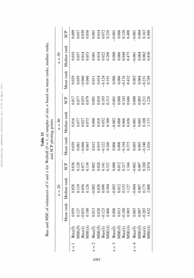
1 ,where b0 and b1 are the intercept and slope estimates from the regression. So, bytaking � = 1, without loss of generality, we computed the bias and mean squarederror (MSE) of �̂ and �̂ based on 10,000 simulated Weibull samples of sizes n =20, 40, and 50 for all three methods and these results are presented in Table 11.We observe near unbiasedness in the estimates of � obtained by methods based onmedian ranks and SCP plotting points. As the sample size n increases, the estimatesobtained by methods based on median ranks and SCP plotting points are observed


Table

11Biasan

dMSE

ofestimatorsof

�an

d�forWeibu

ll(�

=1�

�)samples

ofsize

nba

sedon

meanrank

s,medianrank

s,an

dSC

Pplotting

points

n=

20n=

40n=

50

Meanrank

Medianrank

SCP

Meanrank

Medianrank

SCP

Meanrank

Medianrank

SCP

�=

1Bias��̂�

0.059

0.028

0.036

0.039

0.016

0.017

0.029

0.010

0.009

MSE

��̂�

0.127

0.119

0.120

0.081

0.077

0.077

0.059

0.057

0.057

Bias��̂�

−0.055

0.056

0.077

−0.060

0.027

0.053

−0.060

0.014

0.039

MSE

��̂�

0.100

0.126

0.130

0.065

0.075

0.079

0.048

0.053

0.056

�=

2Bias��̂�

0.013

−0.002

0.002

0.012

0.000

0.001

0.011

0.001

0.001

MSE

��̂�

0.028

0.028

0.028

0.019

0.018

0.018

0.014

0.014

0.014

Bias��̂�

−0.123

0.098

0.141

−0.122

0.052

0.103

−0.124

0.022

0.072

MSE

��̂�

0.406

0.504

0.521

0.260

0.300

0.313

0.191

0.208

0.218

�=

3Bias��̂�

0.008

−0.002

0.000

0.006

−0.002

−0.001

0.006

0.000

−0.001

MSE

��̂�

0.013

0.012

0.012

0.008

0.008

0.008

0.006

0.006

0.006

Bias��̂�

−0.180

0.153

0.217

−0.194

0.066

0.143

−0.176

0.044

0.120

MSE

��̂�

0.905

1.127

1.166

0.575

0.656

0.686

0.432

0.475

0.498

�=

4Bias��̂�

0.003

−0.004

−0.002

0.005

−0.001

0.000

0.003

−0.001

−0.001

MSE

��̂�

0.007

0.007

0.007

0.005

0.005

0.005

0.004

0.004

0.004

Bias��̂�

−0.265

0.175

0.260

−0.240

0.108

0.211

−0.231

0.062

0.163

MSE

��̂�

1.632

2.008

2.074

1.016

1.173

1.226

0.769

0.850

0.890

1085



Table 12Times to breakdown (in minutes) of aninsulating fluid at a voltage of 34kV,

taken from Nelson (1982)

Breakdown Times

0.96 32.524.15 3.160.19 4.850.78 2.788.01 4.6731.75 1.317.35 12.066.50 36.718.27 72.8933.91

to be nearly the same. In all cases, the estimate for � by the method based onmean ranks turns out to be better in terms of mean squared error even though it isconsiderably more biased in this case than the other two methods.

4.2. Illustrative Example

Here, we consider a data set containing 19 times to breakdown for an electricalinsulating fluid which was subjected to a constant voltage stress of 34kV, which arepresented in Table 12.

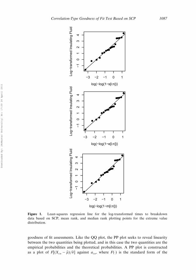
Suppose we wish to test whether a Weibull distribution is a reasonable modelfor these data. Taking the logarithm of the times and using the least-squaresprocedure described earlier, we obtained �̂ = 11�9788 and �̂ = 0�8000 as estimates ofthe Weibull parameters by using the SCP plotting points. The fitted regression linefor all three methods is shown in Fig. 1.

For assessing the goodness of fit of the Weibull distribution using thecorrelation coefficient test (for the transformed extreme value distribution) based onthe SCP plotting points, we found the value of the correlation statistic to be 0.9838,and the corresponding p-value to be 0.6724, determined from 10,000 Monte Carlosimulations. This strongly suggests that a Weibull distribution is a good model forthe data in Table 12. It is of interest to mention here that while using the mean rankplotting points, we found the value of the correlation statistic to be 0.9861, and thecorresponding p-value to be 0.7529. Furthermore, using the median ranks, we foundthe value of the correlation statistic to be 0.9856, and the corresponding p-value tobe 0.7453. In this example, though the sample size is as small as 19, all three plottingmethods resulted in high p-values and also in close agreement, thus suggesting theWeibull model to be a suitable model for the data at hand.

5. Goodness of Fit Based on PP Plots

An alternative goodness of fit tool to the QQ plot is the so-called probability–probability (PP) plot. Gan and Koehler (1990) looked at the use of PP plots in



Figure 1. Least-squares regression line for the log-transformed times to breakdowndata based on SCP, mean rank, and median rank plotting points for the extreme valuedistribution.

goodness of fit assessments. Like the QQ plot, the PP plot seeks to reveal linearitybetween the two quantities being plotted, and in this case the two quantities are theempirical probabilities and the theoretical probabilities. A PP plot is constructedas a plot of F��Xi�n − �̂�/�̂� against ai�n, where F�·� is the standard form of the



Table 13Mean and standard deviation (SD) for k2 and k20 statistics for the extreme valuedistribution for samples of size n based on mean ranks and SCP plotting points

k2 k20

Mean rank SCP Mean rank SCP

n Mean SD Mean SD Mean SD Mean SD

10 0.9429 0.0371 0.9417 0.0393 0.9179 0.0599 0.9157 0.063015 0.9592 0.0254 0.9588 0.0261 0.9423 0.0412 0.9415 0.042320 0.9683 0.0194 0.9681 0.0196 0.9556 0.0314 0.9552 0.031925 0.9741 0.0158 0.9740 0.0159 0.9638 0.0256 0.9636 0.025930 0.9782 0.0131 0.9782 0.0132 0.9698 0.0212 0.9697 0.021340 0.9835 0.0098 0.9835 0.0098 0.9772 0.0159 0.9772 0.016050 0.9866 0.0079 0.9866 0.0079 0.9816 0.0128 0.9816 0.0128

hypothesized theoretical distribution and �̂ and �̂ are the estimates of the locationand scale parameters, respectively. As pointed out in Sec. 1, the choice of plottingposition is a decision which needs to be made beforehand. Moreover, unlike in thecase of QQ plot, the estimates of � and � need to be computed in this case beforethe plot can be constructed.

We propose using SCP plotting points in the test statistics proposed by Gan andKoehler (1990). They constructed two statistics associated with the PP plot, namelythe squared correlation coefficient (k2) and a modification to it (k20), which are as

Table 14Critical values of k2 and k20 statistics for the extreme value distribution for samples

of size n based on mean ranks


Statistic n 0.001 0.01 0.025 0.05 0.10 0.25 0.50 0.75 0.95

k2 10 0.7314 0.8124 0.8451 0.8704 0.8953 0.9274 0.9523 0.9687 0.9832k20 10 0.5630 0.6999 0.7559 0.7986 0.8411 0.8957 0.9349 0.9587 0.9784k2 15 0.8104 0.8693 0.8922 0.9098 0.9269 0.9487 0.9656 0.9768 0.9868k20 15 0.6867 0.7906 0.8310 0.8604 0.8906 0.9273 0.9538 0.9701 0.9834k2 20 0.8562 0.9008 0.9176 0.9308 0.9434 0.9601 0.9732 0.9818 0.9893k20 20 0.7614 0.8399 0.8708 0.8941 0.9162 0.9442 0.9644 0.9768 0.9869k2 25 0.8792 0.9185 0.9329 0.9436 0.9541 0.9676 0.9781 0.9850 0.9911k20 25 0.8027 0.8681 0.8946 0.9140 0.9321 0.9547 0.9709 0.9810 0.9892k2 30 0.9014 0.9324 0.9441 0.9526 0.9614 0.9727 0.9815 0.9873 0.9924k20 30 0.8365 0.8914 0.9126 0.9285 0.9433 0.9622 0.9758 0.9840 0.9908k2 40 0.9264 0.9489 0.9578 0.9644 0.9709 0.9794 0.9860 0.9903 0.9941k20 40 0.8760 0.9180 0.9340 0.9461 0.9574 0.9716 0.9817 0.9879 0.9929k2 50 0.9394 0.9585 0.9657 0.9713 0.9766 0.9834 0.9886 0.9921 0.9952k20 50 0.9007 0.9341 0.9468 0.9566 0.9657 0.9771 0.9852 0.9902 0.9942



follows:

k2 = �∑n

i=1�Zi −�Z��pi − p̄��2

�∑n

i=1�Zi −�Z�2 ∑ni=1�pi − p̄�2�

and

k20 =�∑n

i=1�Zi − 0�5��pi − 0�5��2

�∑n

i=1�Zi − 0�5�2∑n

i=1�pi − 0�5�2��

where pi are the plotting positions and Zi = F��Xi�n − �̂�/�̂�. For pi, they used themean ranks and we therefore adapt the same statistics with SCP plotting pointsinstead of mean ranks. Through an elaborate power study, Gan and Koehler (1990)showed that k20 possesses good power against various alternatives in comparison toother statistics typically calculated from a PP plot.

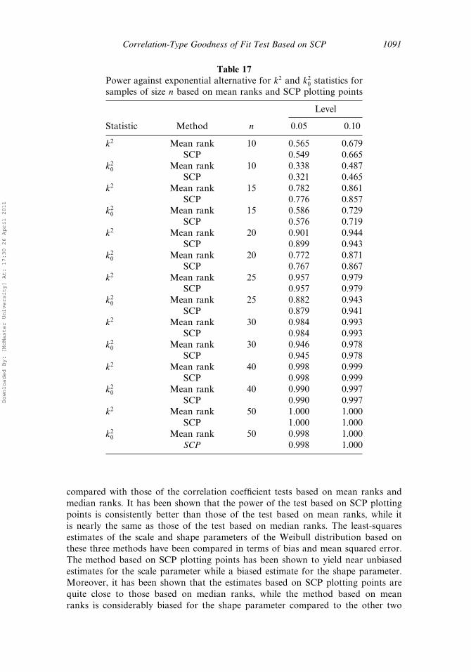
Here, we shall conduct a similar power study for the aforementioned statisticsfor the same alternatives considered earlier in Sec. 3. Table 13 presents the meansand standard deviations of the two statistics based on mean ranks and SCP plottingpoints. Furthermore, Tables 14 and 15 give the critical values for the two statisticseach based on the two plotting positions. Corresponding to these critical values,Tables 16–20 present the power values for different alternatives. Tables 16–20 showthat k2 overall produces better power than k20. However, when comparing the powervalues between the two choices of plotting points for the two statistics, the powervalues based on SCP are nearly identical to those based on mean ranks as n getslarge, with minimal differences for small n. This observation is especially true in thecase of k2. A comparison of these power values with the corresponding results of

Table 15Critical values of k2 and k20 statistics for the extreme value distribution for samples

of size n based on SCP plotting points


Statistic n 0.001 0.01 0.025 0.05 0.10 0.25 0.50 0.75 0.95

k2 10 0.7149 0.8027 0.8380 0.8649 0.8913 0.9258 0.9518 0.9689 0.9837k20 10 0.5482 0.6875 0.7451 0.7896 0.8342 0.8924 0.9340 0.9689 0.9791k2 15 0.8048 0.8662 0.8901 0.9080 0.9256 0.9480 0.9654 0.9769 0.9869k20 15 0.6806 0.7864 0.8270 0.8577 0.8884 0.9262 0.9534 0.9769 0.9837k2 20 0.8535 0.8996 0.9168 0.9300 0.9429 0.9599 0.9731 0.9818 0.9894k20 20 0.7590 0.8378 0.8688 0.8928 0.9152 0.9437 0.9642 0.9818 0.9870k2 25 0.8786 0.9178 0.9325 0.9432 0.9538 0.9674 0.9780 0.9850 0.9911k20 25 0.8005 0.8669 0.8937 0.9133 0.9315 0.9544 0.9708 0.9850 0.9892k2 30 0.9011 0.9322 0.9439 0.9524 0.9613 0.9727 0.9815 0.9873 0.9924k20 30 0.8354 0.8908 0.9121 0.9280 0.9430 0.9620 0.9757 0.9873 0.9909k2 40 0.9262 0.9488 0.9577 0.9644 0.9708 0.9794 0.9859 0.9903 0.9941k20 40 0.8755 0.9177 0.9338 0.9459 0.9573 0.9715 0.9817 0.9903 0.9929k2 50 0.9393 0.9585 0.9657 0.9713 0.9766 0.9833 0.9886 0.9921 0.9952k20 50 0.9004 0.9340 0.9467 0.9565 0.9656 0.9771 0.9852 0.9921 0.9942



Table 16Power against normal alternative for k2 and k20 statistics for

samples of size n based on mean ranks and SCP plotting points

Level

Statistic Method n 0.05 0.10

k2 Mean rank 10 0.109 0.176SCP 0.110 0.180

k20 Mean rank 10 0.120 0.198SCP 0.117 0.197

k2 Mean rank 15 0.137 0.212SCP 0.138 0.216

k20 Mean rank 15 0.138 0.224SCP 0.138 0.224

k2 Mean rank 20 0.163 0.243SCP 0.165 0.247

k20 Mean rank 20 0.158 0.246SCP 0.158 0.247

k2 Mean rank 25 0.189 0.278SCP 0.191 0.281

k20 Mean rank 25 0.175 0.269SCP 0.175 0.269

k2 Mean rank 30 0.216 0.310SCP 0.218 0.313

k20 Mean rank 30 0.197 0.294SCP 0.197 0.295

k2 Mean rank 40 0.271 0.372SCP 0.273 0.375

k20 Mean rank 40 0.231 0.341SCP 0.232 0.342

k2 Mean rank 50 0.325 0.435SCP 0.327 0.437

k20 Mean rank 50 0.267 0.382SCP 0.267 0.383

the correlation tests based on QQ plots presented earlier in Sec. 3 readily revealsthat the latter is more powerful than the former in most cases considered.

6. Concluding Remarks

In this article, following along the lines of Balakrishnan et al. (2010b), wedetermined the SCP plotting points for the extreme value distribution for samplesizes n = 10�5�50. For a goodness of fit for the extreme value distribution,we presented a table of critical values for the correlation coefficient test based onthese SCP plotting points. The performance of this test has been assessed through aMonte Carlo power study against various alternatives. These results have then been



Table 17Power against exponential alternative for k2 and k20 statistics forsamples of size n based on mean ranks and SCP plotting points

Level

Statistic Method n 0.05 0.10

k2 Mean rank 10 0.565 0.679SCP 0.549 0.665

k20 Mean rank 10 0.338 0.487SCP 0.321 0.465

k2 Mean rank 15 0.782 0.861SCP 0.776 0.857

k20 Mean rank 15 0.586 0.729SCP 0.576 0.719

k2 Mean rank 20 0.901 0.944SCP 0.899 0.943

k20 Mean rank 20 0.772 0.871SCP 0.767 0.867

k2 Mean rank 25 0.957 0.979SCP 0.957 0.979

k20 Mean rank 25 0.882 0.943SCP 0.879 0.941

k2 Mean rank 30 0.984 0.993SCP 0.984 0.993

k20 Mean rank 30 0.946 0.978SCP 0.945 0.978

k2 Mean rank 40 0.998 0.999SCP 0.998 0.999

k20 Mean rank 40 0.990 0.997SCP 0.990 0.997

k2 Mean rank 50 1.000 1.000SCP 1.000 1.000

k20 Mean rank 50 0.998 1.000SCP 0.998 1.000

compared with those of the correlation coefficient tests based on mean ranks andmedian ranks. It has been shown that the power of the test based on SCP plottingpoints is consistently better than those of the test based on mean ranks, while itis nearly the same as those of the test based on median ranks. The least-squaresestimates of the scale and shape parameters of the Weibull distribution based onthese three methods have been compared in terms of bias and mean squared error.The method based on SCP plotting points has been shown to yield near unbiasedestimates for the scale parameter while a biased estimate for the shape parameter.Moreover, it has been shown that the estimates based on SCP plotting points arequite close to those based on median ranks, while the method based on meanranks is considerably biased for the shape parameter compared to the other two



Table 18Power against gamma(�) alternative for k2 and k20 statistics for samples of size n

based on mean ranks and SCP plotting points

Level

� = 2 � = 3 � = 4 � = 6

Statistic Method n 0.05 0.10 0.05 0.10 0.05 0.10 0.05 0.10

k2 Mean rank 10 0.381 0.504 0.303 0.421 0.262 0.374 0.218 0.321SCP 0.371 0.494 0.298 0.413 0.257 0.368 0.215 0.318

k20 Mean rank 10 0.184 0.308 0.135 0.237 0.107 0.199 0.082 0.162SCP 0.175 0.293 0.128 0.226 0.102 0.190 0.079 0.156

k2 Mean rank 15 0.569 0.686 0.463 0.589 0.403 0.527 0.332 0.456SCP 0.565 0.682 0.461 0.586 0.401 0.526 0.332 0.456

k20 Mean rank 15 0.344 0.502 0.252 0.396 0.204 0.339 0.154 0.271SCP 0.337 0.493 0.247 0.390 0.200 0.333 0.152 0.267

k2 Mean rank 20 0.716 0.809 0.601 0.714 0.529 0.650 0.440 0.563SCP 0.715 0.809 0.601 0.714 0.530 0.651 0.442 0.566

k20 Mean rank 20 0.510 0.663 0.383 0.540 0.314 0.468 0.239 0.379SCP 0.505 0.657 0.379 0.535 0.311 0.463 0.236 0.375

k2 Mean rank 25 0.819 0.891 0.712 0.809 0.634 0.747 0.538 0.661SCP 0.819 0.891 0.713 0.809 0.635 0.748 0.540 0.663

k20 Mean rank 25 0.645 0.781 0.506 0.665 0.422 0.584 0.323 0.483SCP 0.640 0.778 0.502 0.662 0.419 0.581 0.321 0.480

k2 Mean rank 30 0.889 0.939 0.799 0.878 0.725 0.822 0.626 0.740SCP 0.890 0.940 0.800 0.879 0.726 0.824 0.628 0.743

k20 Mean rank 30 0.761 0.866 0.622 0.763 0.529 0.685 0.415 0.579SCP 0.759 0.865 0.620 0.762 0.527 0.683 0.413 0.577

k2 Mean rank 40 0.964 0.983 0.910 0.952 0.855 0.917 0.770 0.857SCP 0.964 0.983 0.911 0.953 0.856 0.918 0.772 0.859

k20 Mean rank 40 0.899 0.955 0.792 0.891 0.706 0.831 0.586 0.738SCP 0.898 0.954 0.791 0.891 0.705 0.830 0.585 0.737

k2 Mean rank 50 0.990 0.996 0.963 0.983 0.928 0.963 0.866 0.925SCP 0.990 0.996 0.963 0.983 0.929 0.964 0.867 0.925

k20 Mean rank 50 0.964 0.987 0.897 0.954 0.829 0.914 0.724 0.844SCP 0.964 0.987 0.897 0.954 0.828 0.914 0.724 0.845

methods. A reliability data set has been used to illustrate the estimation as well asgoodness of fit of the Weibull distribution by the proposed method. Finally, twotest statistics proposed by Gan and Koehler (1990), in the context of probability–probability plots, have been adapted to SCP plotting points and then their powerproperties have been compared to those of tests based on mean ranks. It has beenshown that the k2 statistic has better power in most cases and that the use of SCPplotting and mean ranks in this test produce almost the same power. A comparisonof these power values with the corresponding results of the correlation test from



Table 19Power against lognormal�0� � alternative for k2 and k20 statistics for samples of

size n based on mean ranks and SCP plotting points

Level

= 1 = 0�5 = 0�25

Statistic Method n 0.05 0.10 0.05 0.10 0.05 0.10

k2 Mean rank 10 0.708 0.793 0.388 0.502 0.205 0.308SCP 0.696 0.783 0.382 0.495 0.204 0.306

k20 Mean rank 10 0.516 0.646 0.204 0.319 0.078 0.153SCP 0.499 0.627 0.196 0.308 0.075 0.147

k2 Mean rank 15 0.893 0.935 0.576 0.685 0.313 0.431SCP 0.890 0.933 0.573 0.683 0.313 0.432

k20 Mean rank 15 0.772 0.863 0.369 0.516 0.145 0.255SCP 0.766 0.858 0.364 0.510 0.143 0.252

k2 Mean rank 20 0.964 0.980 0.717 0.806 0.409 0.533SCP 0.963 0.980 0.718 0.807 0.412 0.537

k20 Mean rank 20 0.907 0.951 0.527 0.669 0.219 0.351SCP 0.904 0.950 0.523 0.665 0.217 0.348

k2 Mean rank 25 0.989 0.995 0.818 0.886 0.505 0.629SCP 0.989 0.995 0.819 0.887 0.508 0.631

k20 Mean rank 25 0.965 0.985 0.657 0.784 0.297 0.450SCP 0.964 0.984 0.655 0.781 0.295 0.448

k2 Mean rank 30 0.997 0.999 0.888 0.936 0.587 0.705SCP 0.997 0.999 0.889 0.936 0.590 0.709

k20 Mean rank 30 0.988 0.996 0.768 0.866 0.383 0.541SCP 0.988 0.996 0.767 0.865 0.382 0.541

k2 Mean rank 40 1.000 1.000 0.960 0.980 0.737 0.829SCP 1.000 1.000 0.961 0.981 0.739 0.831

k20 Mean rank 40 0.999 1.000 0.897 0.951 0.547 0.702SCP 0.999 1.000 0.897 0.951 0.546 0.702

k2 Mean rank 50 1.000 1.000 0.987 0.995 0.834 0.902SCP 1.000 1.000 0.988 0.995 0.836 0.903

k20 Mean rank 50 1.000 1.000 0.961 0.984 0.680 0.810SCP 1.000 1.000 0.961 0.984 0.680 0.810

QQ plot reveals that the latter is more powerful than the former in most casesconsidered.

In conclusion, the SCP plotting method introduced here performs well forthe estimation of Weibull parameters as well as for the Weibull model validityin comparison with the methods based on median and mean ranks. Its overallperformance is quite close to the one based on median ranks and is consistentlybetter than the one based on mean ranks, and therefore provides a viable methodin the analysis of Weibull data. The empirical study also reveals that the tests fromthe QQ plot have better power than those from the PP plot.



Table 20Power against Student’s t alternative for k2 and k20 statistics for samples of size n

based on mean ranks and SCP plotting points

Level

= 3 = 5

Statistic Method n 0.05 0.10 0.05 0.10

k2 Mean rank 10 0.197 0.272 0.137 0.210SCP 0.204 0.282 0.142 0.217

k20 Mean rank 10 0.099 0.158 0.142 0.217SCP 0.101 0.161 0.053 0.101

k2 Mean rank 15 0.284 0.369 0.195 0.280SCP 0.293 0.380 0.201 0.288

k20 Mean rank 15 0.163 0.241 0.201 0.288SCP 0.167 0.246 0.090 0.158

k2 Mean rank 20 0.358 0.445 0.250 0.342SCP 0.367 0.456 0.257 0.351

k20 Mean rank 20 0.225 0.312 0.257 0.351SCP 0.229 0.317 0.128 0.208

k2 Mean rank 25 0.425 0.517 0.297 0.398SCP 0.433 0.525 0.303 0.404

k20 Mean rank 25 0.280 0.378 0.303 0.404SCP 0.283 0.382 0.160 0.254

k2 Mean rank 30 0.491 0.582 0.348 0.453SCP 0.497 0.590 0.353 0.459

k20 Mean rank 30 0.339 0.442 0.353 0.459SCP 0.342 0.446 0.199 0.302

k2 Mean rank 40 0.610 0.693 0.447 0.551SCP 0.615 0.697 0.451 0.556

k20 Mean rank 40 0.452 0.562 0.451 0.556SCP 0.455 0.565 0.276 0.398

k2 Mean rank 50 0.703 0.777 0.535 0.640SCP 0.705 0.780 0.538 0.643

k20 Mean rank 50 0.549 0.656 0.538 0.643SCP 0.551 0.658 0.354 0.484

References

Balakrishnan, N., Davies, K., Keating, J. P. (2009). Pitman closeness of order statisticsto population quantiles. Communications in Statistics – Simulation and Computation38:802–820.

Balakrishnan, N., Davies, K. F., Keating, J. P., Mason, R. L. (2010a). Simultaneouscloseness among order statistics to population quantiles. Journal of Statistical Planningand Inference 140:2408–2415.

Balakrishnan, N., Davies K. F., Keating, J. P., Mason, R. L. (2010b). Computation ofoptimal plotting points based on Pitman Closeness with an application to goodness of fitfor location-scale families. Submitted to Computational Statistics & Data Analysis.



Castillo, E., Hadi, A. S., Balakrishnan, N., Sarabia, J. M. (2005). Extreme Value and RelatedModels with Applications in Engineering and Science. Hoboken, NJ: John Wiley & Sons.

D’Agostino, R. B., Stephens, M. A. eds. (1986). Goodness of Fit Techniques. New York:Marcel Dekker.

Filliben, J. J. (1975). The probability plot correlation coefficient test for normailty.Technometrics 17:111–117.

Gan, F. F., Koehler, K. J. (1990). Goodness of fit based on P-P probability plots.Technometrics 32:289–303.

Johnson, N. L., Kotz, S., Balakrishnan, N. (1995). Continuous Univariate Distributions. 2nded. Vol. 2, New York: John Wiley & Sons.

Keating, J. P., Mason, R. L., Sen, P. K. (1993). Pitman’s Measure of Closeness: A Comparisonof Statistical Estimators. Philadelphia: Society for Industrial and Applied Mathematics.

Kinnison, R. (1989). Correlation coefficient goodness of fit test for extreme valuedistribution. The American Statistician 43:98–100.

Nelson, W. (1982). Applied Life Data Analysis. New York: John Wiley & Sons.


Correlation-Type Goodness of Fit Test for Extreme Value Distribution Based on Simultaneous Closeness

Documents

Transcript of Correlation-Type Goodness of Fit Test for Extreme Value Distribution Based on Simultaneous Closeness