Copyright By Chanpol Visitsathapong December, 2014

Copyright By

Chanpol Visitsathapong

December, 2014

Path Switching Delay Measurements in Software-Defined Networks

A Thesis

Submitted to The Faculty of Engineering Technology

University of Houston

In Partial Fulfillment

of the Requirements

for the Degree of

Master of Science in Engineering Technology

By

Chanpol Visitsathapong

December 2014

Acknowledgements

First and foremost, I would like to sincerely thank to my thesis advisor, Dr. Deniz Gurkan, for

her insight guidance, understanding, and encouragement toward the completion of the thesis.

Also, I would like to thank Dr. Driss Benhaddou and Dr. Luca Pollonini for being my committee

members as well as giving me valuable feedbacks. Lastly, I would like to express my gratitude to

my parents, friends, and colleagues for their support from the beginning till the end of my thesis.

iii

Table of Contents

Acknowledgements ........................................................................................................................ iii

Table of Contents ........................................................................................................................... iv

List of Figures ................................................................................................................................. v

Lists of Tables ............................................................................................................................... vii

Abstract .......................................................................................................................................... ix

Chapter 1: Introduction ................................................................................................................... 1

1. Problem Statement and Thesis Work ...................................................................................... 1

2. Thesis Organization ................................................................................................................ 1

Chapter 2: Literature Review ......................................................................................................... 2

1. Related Work .......................................................................................................................... 2

2. Tools ..................................................................................................................................... 13

Chapter 3: Implementation ........................................................................................................... 14

1. Application Explanation ....................................................................................................... 14

1.1 Class StaticFlowPusher ................................................................................................... 14

1.2 Class Topology ............................................................................................................... 15

1.3 Class TrafficMonitor ....................................................................................................... 16

2. Algorithm Flow Chart and Explanation ................................................................................ 16

2.1 Initial Phase ..................................................................................................................... 17

2.2 Monitoring Phase ............................................................................................................ 18

iv

Chapter 4: Measurement and Results ........................................................................................... 20

1. Measurement Timeline and Explanation .............................................................................. 20

1.1 Overall Details ................................................................................................................ 20

1.2 Timeline Measurement Results....................................................................................... 28

2. Other Measurement Elements ............................................................................................... 35

2.1 Overall Details ................................................................................................................ 35

2.2 Experimental Scenarios and Results ............................................................................... 35

Chapter 5: Conclusion................................................................................................................... 49

Appendix A ................................................................................................................................... 50

Appendix B ................................................................................................................................... 75

References ..................................................................................................................................... 77

List of Figures

Figure 1: SDN Stack ....................................................................................................................... 4

Figure 2: OpenFlow Protocol and OpenFlow-enabled Switch [4] ................................................. 5

Figure 3: ElasticTree Model ........................................................................................................... 7

Figure 4: Leaf-Spine Datacenter Network .................................................................................... 10

Figure 5: Hamiltonian Ring (Left) and Tree Sub Network (Right) .............................................. 12

Figure 6: Application Flow Chart ................................................................................................. 17

Figure 7: : Application Timeline with Measurement Points Part 1 .............................................. 22

Figure 8: Application Timeline with Measurement Points Part 2 ................................................ 23

v

Figure 9: Application Timeline with Measurement Points Part 3 ................................................ 24

Figure 10: 3-Host-4-Switch Topology .......................................................................................... 36

Figure 11: Combination of Traffic Monitoring Results ................................................................ 37

Figure 12: Traffic Monitoring Results for Each OVS port when the link utilization has been

spiked at iteration 22th for 80% switching, and the other at iteration 59th for 20% switching ..... 39

Figure 13: Number of Lost Packets .............................................................................................. 40

Figure 14: sFlow-RT's Update Time Cycle for each OVS over 45 Iterations .............................. 42

Figure 15: NSFNET Topology ..................................................................................................... 43

Figure 16: Shortest Paths from End-hosts within NSFNET Topology......................................... 44

Figure 17: Combination of Traffic Monitoring Results in NSFNET Topology ........................... 44

Figure 18: Traffic Monitoring Results for Each OVS port when the link utilization has been

spiked at iteration 56th for 80% switching, and the other at iteration 98th for 20% switching ..... 45

Figure 19: 3-Host-10-Switch Topology ........................................................................................ 46

Figure 20: Processing Time of Application in the Initial Stage .................................................... 47

Figure 21: Processing Time of Application in the Initial Stage without Flow Establishment ..... 47

Figure 22: The Dashboard Page from Floodlight Web GUI ......................................................... 51

Figure 23: The Topology Page from Floodlight Web GUI .......................................................... 51

Figure 24: The Switches Page from Floodlight Web GUI ........................................................... 52

Figure 25: The Architecture of Floodlight Controller .................................................................. 52

Figure 26: SDN Stack Related to sFlow-RT Controller ............................................................... 55

Figure 27: sFlow-RT Web GUI's Main Page ................................................................................ 56

Figure 28: sFlow-RT Web GUI's RESTflow API Page ............................................................... 57

Figure 29: sFlow-RT Web GUI's Agent Information Page .......................................................... 57

vi

Figure 30: sFlow-RT Web GUI's Real-Time Graph ..................................................................... 58

Figure 31: OVS Architecture ........................................................................................................ 59

Figure 32: OVS Major Components ............................................................................................. 60

Figure 33: An Example of a Custom Topology ............................................................................ 62

Figure 34: A Custom Topology Created by Mininet .................................................................... 64

Figure 35: Virtual Machine Stack ................................................................................................. 65

Figure 36: VM and Underlying Host Stack .................................................................................. 66

Figure 37: Dijkstra's Algorithm Implementation .......................................................................... 67

Figure 38: Shell Scapy Sending a Packet ..................................................................................... 70

Figure 39: Wireshark GUI ............................................................................................................ 73

Figure 40: Wireshark Plug-in List ................................................................................................ 73

Lists of Tables

Table 1: Methods and Explanations of Class Topology ............................................................... 16

Table 2: t(FM-SFP) Delay Measurements and Summary Experiment over 120 Iterations .......... 28

Table 3: t(SFPDif) Delay Measurements and Summary Experiment over 110 Iterations ............. 29

Table 4: t(FMDif) Delay Measurements and Summary Experiment over 110 Iterations .............. 30

Table 5: t(Resp) Delay Measurements and Summary Experiment over 100 Iterations ............... 31

Table 6: t(sFlowU) Delay Measurements and Summary Experiment over 45 Iterations .............. 32

Table 7: t(RCVU-GETU) Delay Measurements and Summary Experiment over 300 Iterations .. 33

Table 8: t(RCVFBC-GETFBC) Delay Measurements and Summary Experiment over 220 Iterations

....................................................................................................................................................... 34

Table 9: Other Measurement Elements and Explanations ............................................................ 35

Table 10: Floodlight REST API ................................................................................................... 54

vii

Table 11: Methods and Explanations of NetworkX ..................................................................... 69

Table 12: Scapy Functions ............................................................................................................ 71

viii

Abstract

The research fundamentally focuses on a study of the multipath switching in software-defined

networks. On the one hand, the thesis aims to measure and determine the latency cost in the

process of traffic engineering of the multipath software-defined networks. On the other hand, the

thesis intends to enhance link utilization in the software-defined networks with dynamic path

switching. To experiment and collect measurement data, a northbound application for multipath

switching was programmed and implemented in the virtual network environment. The

application was capable of exchanging related information with a network controller in order to

dynamically manage the traffic between network end points. The research investigated all

necessary parts of the executing process including traffic characteristics before and after path

switching, time for message exchanging in control plane, and reaction time between control

plane and data plane network elements.

ix

Chapter 1: Introduction

1. Problem Statement and Thesis Work

The new paradigm of software-defined networking may enable a logically centralized view of

the network topology. Although link utilization through traffic load balancing has been proposed

and implemented through protocols such as TRILL, measurements of such dynamic path

switching have not been systematic within the OpenFlow-enabled network frameworks. The

delay in such switching may significantly degrade the performance observed by applications and

therefore, prove to be detrimental to the goal. We proposed to conduct investigations to measure

and report delay elements in such multi-path switching scenarios within the OpenFlow-enabled

software-defined networks (SDN). In this thesis, we present link utilization as one of the

scenarios where one might use the path switching technique. With the thesis's completion, we

expected to create a systematic guideline for researchers and developers in measuring delay

elements related to path switching in an SDN environment.

2. Thesis Organization

The thesis is organized as follows. In Chapter 2, we review and summarize related perspectives

from previous works. Then, Chapter 3 presents our implementation of a northbound application

in details. We demonstrates our designed measurements and results in Chapter 4, and makes

conclusions of the thesis in Chapter 5.

1

Chapter 2: Literature Review

Chapter 2 will elucidate related work which significantly impacts the thesis development from

the beginning to the completion. Background information primarily includes the research on

SDN related topics, potential use cases for path switching , and measurements in computer

networks. Chapter 2 will also introduce tools that we used in our experiments.

1. Related Work

First, we purposed to launch a thesis work based on the software-defined network, because we

could recognize potential changes of the current network system toward this new paradigm. We

studied concepts of SDN and summarized them to 2 related topics. Section 1.1 will elaborate

about characteristics of SDN, while Section 1.2 will describe about a protocol used in SDN. In

Section 1.3, the paper pointed out advantages and disadvantages of the centralized network

management approach, which shown some concerns about an SDN architecture.

Second, besides theories of SDN and OpenFlow, we tried to identify some use cases that

required a path switching mechanism so that we could meaningfully develop our testing

application. Section 1.4 and 1.5 will explain critical use cases that are involved with path

switching based on an energy-saving criteria.

Third, we explored several application models that were implemented for dictating a routing

policy of networks. The models would assist us in designing an application structure to fulfill the

thesis requirements. In Section 1.6, ElasticTree demonstrated on how to separate application

modules to manage a routing mechanism for a data center. Section 1.7 also purposed a

theoretical model for an SDN controller used for creating green Internet.

2

Next, before developing our application, we investigated on factors that should be considered

while developing a policy. In an obvious case, an energy-saving policy would impact a speed of

networks. Section 1.8 explicated recommended variables to create a green network, whereas

Section 1.9 gave details on the trade-off between energy-efficiency and traffic-optimum

networks.

Lastly, from Section 1.10 to 1.15, we would like to expound about measurement elements used

to validate network performance. These measurement definitions would benefit us when we

designed and systemized measurements related to a dynamic path switching behavior.

1.1 Software-Defined Network (SDN)

Based on the white paper from Open Networking Foundation (ONF) [1], SDN is a novel

networking architecture that has three main characteristics. First, SDN decouples the control

plane from the data plane. Second, the SDN network is managed with the centralized approach

rather than distributed. And third, the underlying network infrastructure is both abstracted and

simplified by applications.

In SDN world , the network consists of three major layers including infrastructure layer, control

layer, and application layer as shown in Figure 1. The infrastructure layer or data plane has a

cluster of forwarding elements, such as switches and routers, that is used to forward traffic from

sources to destinations. The control plane, on the other hand, manages traffic decisions over the

data plane through the control data plane interface. In control layer, the SDN will has a network

controller which is capable of handling management traffic from the data plane and controlling

directions of the traffic based on a user policy. A user application running on top of the control

plane is called a northbound application. The northbound application can communicate with the

3

controller via provided API. Thus, developers can create various applications to support their

demanded use cases.

Since SDN uses the centralized approach to manage a network, it can obtain several benefits as

follows. First, users can have all information of the network within one place, which facilitates

the users in controlling traffic on their network without the anxiety of vendor diversity. Second,

SDN can increase network reliability and security, because configuring only in one place can

reduce the error margin, and can uniform the policy enforcement. Finally, users can easily

automate the network with a single place control.

Last but not least, SDN simplifies and abstracts a network for a user space. Users can innovate

their own application without the need to wait for vendors. A northbound application can

automate the policy enforcement across a network with a dynamic manner rather than the static

[2].

Figure 1: SDN Stack

4

1.2 OpenFlow Protocol as a Southbound Interface

OpenFlow protocol [3] is a key protocol used in SDN in order to make a communication

between an OpenFlow controller, such as Floodlight, RYU, and POX controller, and OpenFlow

switches, such as Open vSwitch and LINC switches. Based on the Figure 2, the OpenFlow

switch consists of a secure channel used to exchange OpenFlow messages, and a group and flow

tables used as a part to forward packets.

Through OpenFlow protocol, a controller can retrieve available information from the switch,

such as flow tables, switch statistics, and switch status. Besides, the controller can push flow

entries to the switches to dictate forwarding direction across the network. The flow table is a

main component for packet forwarding which basically consists of two main parts: matching

field and action field. The matching field includes several matching criteria, such as MAC

address, IP address, and ingress port of the switch. Once a packet enter to the switch, it will

check with the matching field of the flow table before taking actions. The action field will

instruct which actions the packet has to perform. For example, the controller can push a flow

entry stating that a switch needs to forward packets to port number 2 for every packet with

source IP address 10.0.0.1.

Figure 2: OpenFlow Protocol and OpenFlow-enabled Switch [4]

5

1.3 Centralized Routing and Distributed Routing Protocol For Dynamic Routing

Theoretical advantages and disadvantages of the centralized routing and distributed routing

protocol for dynamic routing [5] could be mainly characterized to several aspects. For

centralized approach, the Routing Control Center or RCC requires the global knowledge of a

network to manage the traffic and control flows in the network. Several advantages of the

centralized management are that it is easy to find the optimal paths, it is capable of reducing

CPU consumption of each network element, and it requires less convergence time. In contrast,

centralized routing protocol has some disadvantages which are the heavy load over RCC, the

fault tolerance of RCC, and global knowledge requirement. For distributed approach, the

advantages are better fault tolerance and compatible with a hierarchical topology, whereas the

disadvantages are that it has more complex structure and worse convergent time.

1.4 An Energy Saving Routing Algorithm for a Green OSPF Protocol

Energy-Aware Routing (EAR) [6] was an approach to enhance energy-saving with the Green

OSPF Protocol. EAR separated routers into three groups: exporter routers (ERs), importer

routers (IRs), and neutral routers (NRs). The exporter routers are used to calculate the Shortest

Path Trees (STPs) to fix the paths. The importer routers acts as references for the ERs to identify

their own STPs and to select links for switching off. NRs are routers that use normal OSPF to

identify paths.

Computing EAR requires three phases. First, it chooses ERs and their STPs. Second, each IR

calculates its Modified Path Tree (MPT) and determine which links can be switched off. Finally,

each router can use only available paths after the second step.

6

The results measured by this paper illustrated an average traffic load on active links, a traffic

load variation for each active link, and the percentage of links that could be turned off.

1.5 Link Sleeping Optimization for Green Virtual Network Infrastructures

Link Sleeping Optimization [7] aims to minimize power consumption, while being able to satisfy

the demand from virtual networks. It used an offline heuristic algorithm for computing possible

links that could be in a sleep stage. The algorithm consists of six steps. First, it calculates stress

rate (SRk) for all substrate network links. SRk is defined as the number of virtual networks

running over link k. Second, it computes off-peak available capacity of links. Third, it sorts links

based on SRk and off-peak link capacity. From step 4 to 6, the algorithm checks each link one-

by-one to determine whether the link is possible to sleep or not.

The paper measure the performance of the algorithm by presenting a graph of percentage of

possible sleep links and a graph of link utilization.

1.6 ElasticTree: Saving Energy in Data Center Networks

The ElasticTree model [8] was implemented to serve energy-saving purpose in the data center by

applying an SDN paradigm.

Figure 3: ElasticTree Model

7

The model, shown in Figure 3, composes of three modules: optimizer, power control, and

routing. The optimizer finds the minimum sub network which can satisfy on-demand traffic. The

power control is used to manage switches' power consumption as well as to get related

information from the switches. The routing module select needed paths and push flows to a

network.

1.7 Centralized Energy-efficient Routing Control for Greener Internet

A centralized energy-saving strategy [9] could be achieved with an SDN technology. A

controller has four main functions in this case. First, the controller is used to monitor link status,

especially link utilization. The number of the maximized-utilization links should be minimal

since there is a load balancer to distribute traffic. Second, the controller should be able to select

sleeping links. Two selecting criteria in this paper were the links that are underutilized and the

links that have less flows. Third, when the links hit some threshold, the paper assumed the links

were potentially congested, and activated sleeping links to balance the load. Finally, the paper

suggested to integrate link status forecasting function to prepare for the future traffic.

1.8 A New Evaluation Model on Green Low Carbon Energy Network for Cloud

Computing-- Quality of Green (QoG)

The green network [10] means the network that can use the minimum amount of energy, while

being able to satisfy the Quality of Service (QoS). The green network can be evaluated by the

model called Quality of Green (QoG). The QoG includes three steps to build the evaluation

matrix. First, we have to quantify the green energy consumption indexes which covers fourteen

indexes based on three main aspects: eight indexes for performance, two indexes for traffic, and

four indexes for topology. Second, we need to calculate four green fuzzy indexes including

8

fluctuation, vulnerability, persistence, and recoverability. Finally, we will build the evaluation

matrix by using the membership of the fourteen green energy consumption indexes and four

green fuzzy indexes.

1.9 Impact of Ethernet Multipath Routing on Data Center Network Consolidations

A matching repeated heuristic approach [11] was implemented to compare the trade-off between

traffic engineering (TE) and energy efficiency (EE) in the data center network (DCN)

consolidations. The approach could enable multipath feature and find the benefit of multipath

forwarding in data center networks. The results showed that the multipath routing can be

counterproductive if the TE is not the main concern of the DCN optimization, because using

multipath may free some VMs which can assist VM container consolidations to switch off

unused containers. Thus, the multipath cannot be used to communicate with switched-off

containers. Another result also indicated that TE can be fairly improved while EE is significantly

decreased if TE is the primary goal of the DCN.

1.10 Exploring the Performance Benefits of End-to-End Path Switching

Two main factors that could enhance end-to-end path switching performance were the logic

behind path switching decision and the configurations required to obtain multiple paths [12]. The

paper stated that the path switching could improve the performance if it met some requirements.

First, the network must contain sufficient diversity of paths to support path switching. Second,

alternative paths should meet sufficient performance criteria to be selected. Lastly, we requires

the monitoring of current traffic as well as the traffic prediction. The paper set up the experiment

to measure the path switching performance based on delay, packet loss, and loss duration.

9

1.11 On the Data Path Performance of Leaf-Spine Datacenter Fabrics

In order to identify factors that were important to the network performance, Alizadeh and Edsall

analyzed a Leaf-Spine topology (Figure 4) under realistic workloads [13].

Figure 4: Leaf-Spine Datacenter Network

The study evaluated the performance based on flow completion time (FCT) and query

completion time (QCT). Three selected parameters were (1)link speed, (2)oversubscription, and

(3)buffer size. For the link speed, The paper proved that using higher speed links in the fabric

can improve the performance of Equal Cost Multipath (ECMP). That is, the FCT is faster with

link speed 100 Gbps and 40 Gbps than 10 Gbps. Second, the paper concluded that

oversubscription does not significantly affect the performance, but it can make the network

become more fragile with a traffic. Finally, the research recognized that if the buffer size of one

tier is much higher than others, it will not be very useful. For example, the QCT of 100MB-

buffer spine switches and 2MB-buffer leaf switches are almost the same as the QCT of 2MB-

buffer spine and leaf switches. However, compare to the QCT of 100MB-buffer spine switches

and 2MB-buffer leaf switches, the QCT of 2MB-buffer spine switches and 100MB-buffer leaf

switches can perform better.

10

1.12 OFAR-CM: Efficient Dragonfly Networks with Simple Congestion

Management

OFAR [14] refers to On-the-Fly Adaptive Routing. This mechanism allows Dragonfly networks

to avoid packet deadlock by providing a deadlock-free escape sub network. However, under the

high traffic load, OFAR faces two main pitfalls. First, the network throughput will be dropped to

the speed of the escape sub network, which is much slower and can cause congestion. Second,

due to the congestion, packets can switch a path from the canonical network to the escape

network, resulting in unbounded network paths.

The paper introduced OFAR-CM (On-the-Fly Adaptive Routing with a simple congestion

management) to solve these problems. The study experimented OFAR-CM in three aspects.

First, the research evaluated two congestion-mitigated mechanisms including Base Congestion

Management (BCM) and Escape Congestion Management (ECM). BCM requires a "bubble" in

order to prevent packet injection into a congested network. Unless there is enough space in the

next queue plus the bubble, a packet cannot be injected. ECM will use local buffers of the escape

sub networks to identify the congestion. If the degree of the local buffers is higher than selected

threshold, packets will not be injected and need to wait for other cycle. Second, the paper

assessed OFAR-CM according to the two escape sub network topologies: a Hamiltonian ring and

a tree as shown in Figure 5. Finally, the paper evaluated the problem of unfairness and

unbounded paths.

11

Figure 5: Hamiltonian Ring (Left) and Tree Sub Network (Right)

1.13 Identification of network measurement challenges in OpenFlow-based service

chaining.

Since implementation of the firewall in SDN related to several delay factors [15], the paper tried

to measure those delay elements to evaluate firewall's performance in SDN. The measurements

focused on measuring the time used in exchanging information between the northbound

application and the Floodlight controller, and the time Floodlight used to interact with OVS on

firewall perspectives.

1.14 Load-Balancing Multipath Switching System with Flow Slice

Flow Slice (FS) [16] was used to divide each traffic flow into several flow slices and balance the

load through various paths in a network. The paper claimed that if the setting of a slicing

threshold was 1 to 4 milliseconds, the FS strategy could obtain nearly optimal performance.

Based on the measurement, the paper presented various slice thresholds with other variables,

such as Flow-Slice packet count, Flow-Slice size, and Flow-Slice number, to find the their

impact. Finally, the paper measured delay, packet loss rate, and out-of-order packet value to

determine the performance of the FS scheme.

12

1.15 Ethane: Taking Control of the Enterprise

Ethane [17] allows users to manage a unified network policy and implement on the enterprise

network. Ethane requires flow-based switches and a controller for its implementation. The

authors measured performance of the Ethane architecture with several aspects. First, the research

collected statistical data for references. Then, the paper evaluated the number of flows that the

controller could handle, which was up to 11,000 flows per second. The paper also assessed the

number of hosts that a single controller could handle. Finally, the research measured the

performance during link failure by using round-trip-time value.

2. Tools

We utilized various open source tools including Floodlight Controller, sFlow-RT Controller,

Open vSwitch, Mininet, VMware Workstation, Scapy, IPERF, NetworkX, and Wireshark. In this

Section, we will introduce only basic features of the tools so as to give clearer pictures for an

implementation as well as results. We included detailed descriptions of all tools in Appendix A.

In our implementation, Floodlight was used as a primary controller connected with our

northbound application to manage traffic in the data plane. sFlow-RT, on the other hand, was

implemented as a secondary controller and also attached with the application to monitor real-

time traffic. Mininet was a simulator application running on top of Ubuntu operating system

which was preinstalled on VMware hypervisor. We executed Mininet in order to create virtual

topologies related with our investigation. Scapy and IPERF were two traffic generators that we

applied their usages on Mininet. NetworkX was imported as a Python library to calculate

13

centralized shortest paths. Finally, we implemented Wireshark for monitoring traffic behaviors

and collected measurement data.

Chapter 3: Implementation

We developed a northbound application for our experiments in order to understand path

switching behavior in an SDN environment. The behavior would guide us to identify critical

measurement points and definitions so that we could systemize factors and methods for future

study regarding to path switching in SDN.

1. Application Explanation

The northbound application was written in Python version 2.7. It requires connections to

Floodlight and sFlow-RT in order to manage the traffic within a network. The program has three

main classes including class StaticFlowPusher(object), class Topology(), and class

TrafficMonitor(object). One by one, we have included an explanation for each of the classes

below. We tried to separate the functionality so there is a way to plug and play with the

components of the application as our project evolved. For example, the paths between end points

have been calculated by relying on the Dijkstra’s algorithm (See Appendix A(6)). A primary

path calculation function has been utilized after all paths are identified through the Dijkstra’s

algorithm.

1.1 Class StaticFlowPusher

The class StaticFlowPusher was modified based on the source code from Floodlight official

website (http://www.openflowhub.org/display/floodlightcontroller/Static+Flow+Pusher+API+%

28New%29). We adjusted methods inside the class so that it could be flexibly used with several

Floodlight REST APIs. The purposes of this class is to send HTTP GET and POST to the

14

Floodlight controller depending on the URI (Uniform Resource Identifier). For example,

'http://<controller_ip>:8080/wm/ topology/links/json' is used for retrieving topology information.

Or, 'http://<controller_ip>:8080/ wm/staticflowentrypusher/json' is created for pushing flows to

OVS.

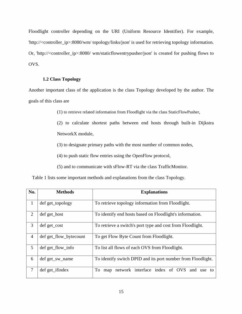
1.2 Class Topology

Another important class of the application is the class Topology developed by the author. The

goals of this class are

(1) to retrieve related information from Floodlight via the class StaticFlowPusher,

(2) to calculate shortest paths between end hosts through built-in Dijkstra

NetworkX module,

(3) to designate primary paths with the most number of common nodes,

(4) to push static flow entries using the OpenFlow protocol,

(5) and to communicate with sFlow-RT via the class TrafficMonitor.

Table 1 lists some important methods and explanations from the class Topology.

No. Methods Explanations

1 def get_topology To retrieve topology information from Floodlight.

2 def get_host To identify end hosts based on Floodlight's information.

3 def get_cost To retrieve a switch's port type and cost from Floodlight.

4 def get_flow_bytecount To get Flow Byte Count from Floodlight.

5 def get_flow_info To list all flows of each OVS from Floodlight.

6 def get_sw_name To identify switch DPID and its port number from Floodlight.

7 def get_ifindex To map network interface index of OVS and use to

15

communicate with sFlow-RT.

8 def get_bandwidth To specify the maximum bandwidth of an OVS's port based

on the cost from method def get_cost.

9 def multi_spaths To compute all shortest paths from every source-destination

pair with NetworkX library.

10 def flow_pusher To push flow entries to Floodlight.

11 def save_file To save all shortest paths computed from def multi_spaths

into a file for designating primary paths.

12 def get_NUnodes To find primary paths from source-destination pairs.

13 def path_group To group shortest paths that have the same source-destination

pairs.

Table 1: Methods and Explanations of Class Topology

1.3 Class TrafficMonitor

The class TrafficMonitor was also derived from the class StaticFlowPusher. However, the

functionality of this class focuses on the communication between the application and sFlow-RT

REST API. The only purpose of the class TrafficMonitor is to get the percentage of the link

utilization from sFlow-RT and convert that value to match a port maximum bandwidth.

2. Algorithm Flow Chart and Explanation

Besides three major classes, the application also has the main function which is the starting point

of every process inside the program. In this section, we will describe the algorithm flow of the

main function which can be distinguished into initial phase and monitoring phase. Figure 6

illustrates the flow chart of overall mechanism.

16

Figure 6: Application Flow Chart

2.1 Initial Phase

In the initial phase, the application retrieve link, edge node, and link cost information from

Floodlight via class Topology. After getting all information, it tries to calculate all shortest paths

by def multi_spaths from the class Topology. Then, the program will save those shortest-path

information to a file and execute the primary path finder function.

The application will be designated primary paths as well as back-up paths of each source-

destination pair. The primary paths mean the paths that consist of the highest number of common

nodes. In contrast, the back-up paths or secondary paths represent the paths that contain some

other nodes.

17

Once the primary paths from every source-destination pair are identified, the application will

establish initial flow entries through the Floodlight which will send OpenFlow Flow Mod

packets to related OVS based on those primary path information. At this point, the end hosts can

start communicating to each other using the established paths, and the initial phase is completed.

2.2 Monitoring Phase

To begin with the monitoring phase, the application needs to map the network interface index

(ifIndex) from each OVS to be compatible with the sFlow-RT. In reality, the ifIndex is based on

the SNMP protocol to specify unique numbers for every port of each OVS inside the network.

Nonetheless, as we used Mininet in our experiment, mapping the ifIndex could be done

internally on Ubuntu by calling method get_ifindex from class Topology.

Then, the process will shift into the monitoring loop. For every loop cycle, the application

retrieves link utilization of each OVS port from the sFlow-RT. The link utilization received is in

the percentage, and the value depends on OpenFlow port type information. For instance, if the

port type is OFPPF_100MB_FD, it means that the port has 100 Mbps transmission speed with

full-duplex communication. However, due to Mininet's constraint, the only port type that can be

used is OFPPF_10GB_FD, which supports 10 Gbps forwarding speed and full duplex. Thus, in

our experiment with Mininet, we tried to limit the maximum bandwidth of an OVS port instead

of changing the port type, and added a function to interpret the link-utilization percentage from

sFlow to the correct percentage value. In addition, the program retrieves flow byte count from

the Floodlight every loop cycle so as to sort which flow consumes the highest bandwidth when

the traffic hits 80 percent.

As soon as the traffic information is ready, the application check if-else condition whether the

accumulated traffic from each link matches with 80/20 threshold or not. The 80/20 threshold

18

means that if the traffic in primary paths reaches 80 percent of the maximum bandwidth, the

application will switch a path of the highest-bandwidth consumption flow to a back-up path.

Conversely, if the traffic in secondary paths drops to below 20 percent of the maximum

bandwidth, the program will switch all flow traffics back to the primary paths. To create more

sophisticated application, we developed some exceptions for the 80/20 threshold rule. Firstly, if

there is only one flow in a primary path, the application will not switch that path to the secondary

path because it cannot any significance in terms of end-to-end load balancing. Secondly, after

switching flows from primary paths to the back-up paths, the application will wait for 2 loop

cycles so that the traffic can become more stable. If the program does not delay path switching

for some time, the flow will switch back and forth between the paths as it is not capable of

increasing the traffic to a stable stage immediately. Lastly, the application will not switch flows

if the accumulated traffic from both primary and secondary paths is at the level between 20 to 80

percent.

The application will keep executing in the monitoring until it is terminated. According to the

process, we also aware of topology change issues, such as link failure and new switch/host

establishment, but these problems are out of the scope of the thesis.

19

Chapter 4: Measurement and Results

We present measurement timeline, measurement definitions, and results that we designed and

validated based on the application process. All measurement points have been determined with

sensitivity to the clock synchronization and reference frame of measurements. In this respect,

differences in timestamps are taken into consideration rather than nominal time instances.

Our use cases are around the simple link utilization triggering the path switching mechanism. We

have increased the number of switching involved through number of switches and other factors.

Note that the link utilization is taken as a triggering mechanism to enable our measurements for

such a switching and it is not the main focus of this thesis work. In this respect, more involved

algorithms and rigorous verification of link utilization calculations based on validated

monitoring may be developed further.

1. Measurement Timeline and Explanation

1.1 Overall Details

From Figure 7 to 9, we displayed the application timeline with measurement points. The first

three measurement points are the time that the application retrieves basic information from

Floodlight controller at the initial stage including the time retrieving link information (t(RCVlnk -

GETlnk)), edge node information (t(RCVEdge - GETEdge)), and cost information (t(RCVCost -

GETCost)). Although we did not measure them separately, they were a part used to analyze

application performance later. Next measurement point is the time to push initial flows. For each

flow, we measured the processing time that Floodlight needs before sending an OpenFlow

FlowMod packet to an OVS (t(FM - SFP)), and the time that switch changes its previous flow

entry to the new one (t(Resp)). Also, we measured the time interval of each flow pushing

20

(t(SFPDif)), and the time interval of OpenFlow FlowMod packet generating t(FMDif). Then, in the

monitoring phase, we evaluated the time difference of each OVS to send updates to sFlow-RT

(t(sFlowU)). After that, we measured the time that the application requests for link utilization

from sFlow-RT and receive that information (t(RCVU-GETU)). Lastly, before establishing new

paths which has the same measurement input as setting up the initial flows, we investigated the

time that the application requires to request a flow byte count from Floodlight (t(RCVFBC-

GETFBC)).

21

Figure 7: : Application Timeline with Measurement Points Part 1

22

Figure 8: Application Timeline with Measurement Points Part 2

23

Figure 9: Application Timeline with Measurement Points Part 3

24

Based on Figure 7 to 9 and the discussion above, we will elucidate each measurement point in

details. First, t(RCVlnk - GETlnk) is the time that the application uses HTTP to get and receive

link information from Floodlight 'http://<controller_ip>:8080/wm/topology/links/json'. Link

information is a list containing dictionaries inside. The general structure of the link information

is [{'direction', 'src-port', 'dst-switch', 'src-switch', 'dst-port', 'type'}]. For example, [{u'direction':

u'bidirectional', u'src-port': 1, u'dst-switch': u'00:00:d6:5c:c0:1f:83:45', u'src-switch':

u'00:00:4e:8d:fd:91:2a:4c', u'dst-port': 2, u'type': u'internal'}]. Second, t(RCVEdge - GETEdge) is

the time that the application uses HTTP to get and receive host information from Floodlight

'http://<controller_ip>:8080/wm/device/'. Host information is a list containing dictionaries inside.

The general structure of the host information is[{"entityClass", "mac", "ipv", "vlan",

"attachmentPoint":[{"switchDPID", "port", "errorStatus"}], "lastSeen"}]. For example,

[{"entityClass":"DefaultEntityClass", "mac":["02:a2:e1:09:c2:39"], "ipv4":["10.10.1.1"], "vlan":

[], "attachmentPoint": [{"switchDPID":"00:00:de:9f:83:e0:0f:40", "port":1, "errorStatus":null}],

"lastSeen":1413301852475}]. Third, t(RCVCost - GETCost) is The time that the application uses

HTTP to get and receive cost information from Floodlight 'http://<controller_ip>:8080/wm/

core/switch/all/features/json'. Cost information is a list containing dictionaries inside. The

general structure of the cost information is [{"<switch_dpid>":{"actions", "buffers",

"capabilities", "datapathId", "length", "ports":[{"portNumber", "hardwareAddress", "name",

"config", "state", "currentFeatures", "advertisedFeatures", "supportedFeatures", "peerFeatures"}]

, "tables", "type", "version", "xid"}]. For example, {"00:00:46:62:ea:c5:9e:4c":{"actions":4095,

"buffers":256, "capabilities":199, "datapathId":"00:00:46:62:ea:c5:9e:4c", "length":224,

"ports":[{"portNumber":3, "hardwareAddress":"1e:13:c0:b0:8e:e3", "name":"3622128020872",

"config":0, "state":0, "currentFeatures":0,"advertisedFeatures":0,"supportedFeatures":0,

25

"peerFeatures":0}],"tables":-2,"type":"FEATURES_REPLY","version":1,"xid":5}. Forth, t(SFP

- FM) is the time duration of Floodlight receiving an HTTP Post message from Static Flow

Pusher function of the application and generating an OpenFlow FlowMod message to a switch.

Fifth, t(SFPDif) is the time difference between sending one static flow pusher and the next one.

Sixth, t(FMDif) is the time difference between sending one Flow Mod and the next one. Seventh,

t(Resp) is the time duration of an OVS receiving FlowMod message from Floodlight and writing

a flow entry within itself. Eigth, t(sFlowU) is the time difference between each OVS to send

sFlow update to sFlow-RT. Ninth, t(RCVU-GETU) is the time that the application uses HTTP to

get and receive link utilization from sFlow-RT 'http://<sFlow-RT_ip>:8008/metric/

<sFLow_agent>/<ifindex>.ifoututilization/json'. Link utilization is a list containing one

dictionary of a specific interface utilization information inside. The general structure of the link

utilization is [{"agent", "dataSource", "lastUpdate", "lastUpdateMax", "lastUpdateMin",

"metricN", "metricName", "metricValue"}]. For example, [{"agent": "127.0.0.1","dataSource":

"10","lastUpdate": 330,"lastUpdateMax": 330,"lastUpdateMin": 330,"metricN":1,"metricName":

"10.ifinutilization","metricValue": 0}]. Finally, t(RCVFBC-GETFBC) is The time that the

application uses HTTP to get and receive flow information of a particular switch from Floodlight

'http://<controller_ip>:8080/wm/core/switch/<switch_dpid>/flow/json'. Flow information is a

dictionary of flows set up in a particular switch. The general structure of the flow information is

{<switch_dpid>:[{"tableId","match":{"dataLayerDestination","dataLayerSource","dataLayerTyp

e","dataLayerVirtualLan","dataLayerVirtualLanPriorityCodePoint","inputPort","networkDestina

tion","networkDestinationMaskLen","networkProtocol","networkSource","networkSourceMask

Len","networkTypeOfService","transportDestination","transportSource","wildcards","durationSe

conds","durationNanoseconds","priority","idleTimeout","hardTimeout","cookie","packetCount",

26

"byteCount","actions":[{"type","length","port","maxLength","lengthU"}]}]}. For example,

{"00:00:00:00:00:00:00:01":[{"tableId":0,"match":{"dataLayerDestination":"00:00:00:00:00:01"

, "dataLayerSource":"00:00:00:00:00:02","dataLayerType":"0x0000","dataLayerVirtualLan":-1,

"dataLayerVirtualLanPriorityCodePoint":0, "inputPort":2, "networkDestination":"0.0.0.0",

"networkDestinationMaskLen":0, "networkProtocol":0, "networkSource":"0.0.0.0", "network

SourceMaskLen":0, "networkTypeOfService":0, "transportDestination":0, "transportSource":0,

"wildcards":3678448}, "durationSeconds":3, "durationNanoseconds":247000000, "priority":0,

"idleTimeout":5, "hardTimeout":0, "cookie":9007199254740992, "packetCount":5, "byteCount":

434, "actions": [{"type":"OUTPUT", "length":8, "port":1, "maxLength":-1, "lengthU":8}]}]}.

27

1.2 Timeline Measurement Results

1. t(SFP - FM): Floodlight Controller's Processing Time

Table 2 includes the graph illustrated the measurement result of processing time when Floodlight

receives HTTP POST from StaticFlowPusher and generates OpenFLow FlowMod packets (see

details in Section 1.1 and Figure 7). The processing time is bounded by the maximum value of

15.729 millisecond and the minimum value of 1.423 millisecond.

Average 3.543 millisecond

Standard Deviation 2.796

Maximum Value 15.729 millisecond

Minimum Value 1.423 millisecond

Table 2: t(FM-SFP) Delay Measurements and Summary Experiment over 120 Iterations

02468

1012141618

1 11 21 31 41 51 61 71 81 91 101 111 121

Tim

e (m

s)

Iteration

t(FM-SFP)

t(FM-SFP)

28

2. t(SFPDif): Application to Floodlight Controller Flow Processing Time

Table 3 displays the graph indicating the time delay of the application to generate each flow

entry by StaicFlowPusher (see details in Section 1.1 and Figure 7). We can explain from the

result that the average time of t(SFPDif) is 41.608 millisecond mostly within the range of plus or

minus 14.174 millisecond.





Table 3: t(SFPDif) Delay Measurements and Summary Experiment over 110 Iterations

0

20

40

60

80

100

120

140

1 11 21 31 41 51 61 71 81 91 101

Tim

e (m

s)

Iteration

t(SFPDif)

Diff Time of SFP

29

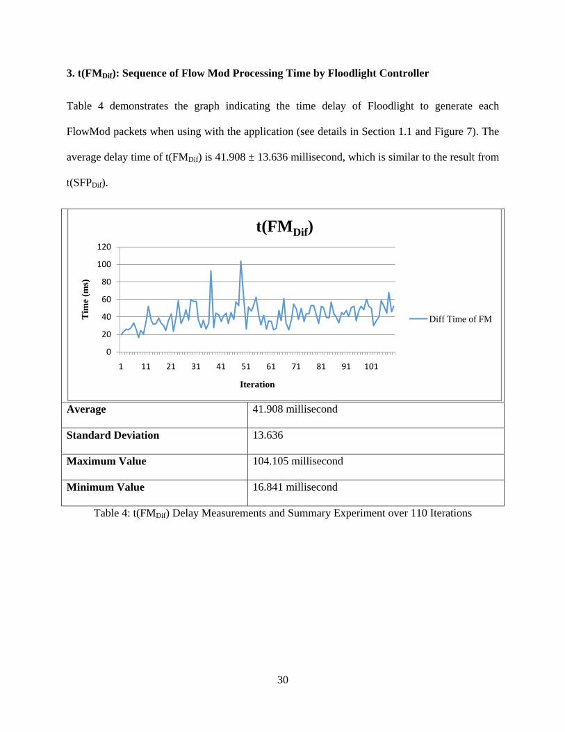
3. t(FMDif): Sequence of Flow Mod Processing Time by Floodlight Controller

Table 4 demonstrates the graph indicating the time delay of Floodlight to generate each

FlowMod packets when using with the application (see details in Section 1.1 and Figure 7). The

average delay time of t(FMDif) is 41.908 ± 13.636 millisecond, which is similar to the result from

t(SFPDif).





Table 4: t(FMDif) Delay Measurements and Summary Experiment over 110 Iterations

0

20

40

60

80

100

120

1 11 21 31 41 51 61 71 81 91 101

Tim

e (m

s)

Iteration

t(FMDif)

Diff Time of FM

30

4. t(Resp): Flow in Action Time after a Flow Mod is Received

Table 5 showed the result of the responsiveness of the OVS in establishing flow entries after

receiving FlowMod from Floodlight (see details in Section 1.1 and Figure 7). The average value

of t(Resp) is 1.86291 millisecond with the standard deviation of 2.316604.





Table 5: t(Resp) Delay Measurements and Summary Experiment over 100 Iterations

0

2

4

6

8

10

12

14

1 11 21 31 41 51 61 71 81 91

Tim

e (m

s)

Iteration

t(Resp)

t(Resp)

31

5. t(sFlowU): OVS to sFlow-RT Updating Time Delay Interval

Table 6 exhibits the graph of the delay between one OVS interface updating its utilization and

the next one (see details in Section 1.1 and Figure 8). The delay is mostly within range of 0.176

to 0.480 millisecond and the average of 0.328 millisecond.





Table 6: t(sFlowU) Delay Measurements and Summary Experiment over 45 Iterations

0

0.2

0.4

0.6

0.8

1

1.2

1.4

1 11 21 31 41

Tim

e (m

s)

Iteration

t(sFlowU)

t(Sub2 - Sub1)

t(Sub3 - Sub2)

32

6. t(RCVU-GETU): Application to sFlow-RT Link Utilization Responded Time

Table 7 shows the measurement result of the duration that the application sent HTTP GET to

sFow-RT for current link utilization information and received that data (see details in Section 1.1

and Figure 8). The average duration is 5.037 millisecond with the standard deviation of 6.829.





Table 7: t(RCVU-GETU) Delay Measurements and Summary Experiment over 300 Iterations

0

10

20

30

40

50

60

70

1 11 21 31 41 51 61 71 81 91 101

111

121

131

141

151

161

171

181

191

201

211

221

231

241

251

261

271

281

291

Tim

e (m

s)

Iteration

t(RCVU-GETU)

t(RCV(U)-GET(U))

33

7. t(RCVFBC-GETFBC): Application to Floodlight Flow Byte Count Responded Time

Table 8 reveals collected data of the duration that the application requested flow byte count and

received the information from Floodlight (see details in Section 1.1 and Figure 8). The average

delay in this process is 0.328 millisecond with standard deviation of 0.152.





Table 8: t(RCVFBC-GETFBC) Delay Measurements and Summary Experiment over 220 Iterations

020406080

100120140160180200

1 11 21 31 41 51 61 71 81 91 101

111

121

131

141

151

161

171

181

191

201

211

221

Tim

e (m

s)

Iteration

t(RCV-GET)

t(RCV-GET)

34

2. Other Measurement Elements

2.1 Overall Details

Besides measurement points explained in timeline and table above, we also designed specific

scenarios to measure some other related elements listed in Table 9.

No. Measurement Elements Explanations

1 Traffic The percentage of the link utilization of each OVS network

interface over cycles of the application.

2 Packet Lost The number of packets lost during flow writing in OVS.

3 Application Performance The processing speed of the application.

4 sFlow Agent Update

Time Cycle

The time sFlow agent updates information to sFlow-RT in a

cycle.

Table 9: Other Measurement Elements and Explanations

2.2 Experimental Scenarios and Results

Since we were able to measure delay in path switching, we tested our implementation on very

basic link utilization use cases. We had three different topology cases to examine our

measurements.

1. 3-Host-4-Switch

1.1 Fundamental Details of an Experimental Scenario

The first scenario was implemented to test basic functionality and examine some measurement

points of the application in path switching. As shown in Figure 10, The experiment included 4

OVS and 3 hosts running on Mininet. OVS1 (DPID: 00:00:00:00:00:00:00:01) was connected to

35

OVS2 (DPID: 00:00:00:00:00:00:00:02) and OVS3 (DPID: 00:00:00:00:00:00:00:03) with port

number 2 and 3 sequentially. OVS2 and OVS3 were also linked with OVS4 (DPID:

00:00:00:00:00:00:00:04) via their port number 2. Lastly, Host1 was attached with OVS1, while

Host2 and Host3 were attached with OVS4. All three hosts were in the same subnet, and the IP

addresses of Host1, Host2, and Host3 were 10.0.0.1/24, 10.0.0.2/24, and 10.0.0.3/24

consecutively.

Lastly, all OVS were connected to Floodlight controller and sFlow-RT which were executing on

a localhost (127.0.0.1). Floodlight and sFlow-RT reserved their default ports 6633 and 6343 in

sequence for their communication with OVS.

Figure 10: 3-Host-4-Switch Topology

36

1.2 Results

1.2.1 Traffic Monitoring

Figure 11: Combination of Traffic Monitoring Results

In this experiment, we would like to test the basic functionality of the application by monitoring

traffic from related OVS and ports. After the application was executed, Dijkstra module in

NetworkX provided two shortest paths from every end host as OVS1-OVS3-OVS4 and OVS1-

OVS2-OVS4. The primary path selected from both Host1 to Host2 and Host1 to Host3 was

OVS1-OVS3-OVS4, whereas the secondary path was OVS1-OVS2-OVS4. The traffic threshold

of the application was preset to 80:20 meaning that the application will activate the back-up path

and do the path switching on the highest bandwidth-consumption flows to load balance the

traffic if the accumulated traffic in the primary path hits 80 percent. Conversely, if the

accumulated traffic in the secondary path decreases to less than 20 percent, all flows in the back-

up path will be switched back to use the primary path.

We generated two traffic cases from Host1 to Host2 and from Host1 to Host3 by using Scapy.

The traffic generator was programmed into two sets. The first set of the traffic sending from

00.10.20.30.40.50.60.70.80.9

1 6 11 16 21 26 31 36 41 46 51 56 61 66 71 76 81 86 91 96 101

106

111

116

Util

izat

ion

Iteration

Traffic

OVS2:P2

OVS3:P2

OVS1:P3

OVS1:P2

37

Host1 to Host2 was constant and transmitted at the rate about 30 percent of the maximum

bandwidth. For the second set of the traffic, Host1 transmitted packets to Host3 at three different

phases: 30 percent, 50 percent, and 10 percent sequentially. Based on Figure 11, the combination

of both traffic sets started at the rate of 60 percent of the maximum bandwidth. During this stage,

OVS1:Port3 and OVS3:Port2, as switches and ports in the primary path, displayed the traffic

around 60 percent. Nevertheless, since the secondary path was not used, there was no traffic on

OVS1:Port2 and OVS2:Port2. When the second set of the traffic changed to phase two, which

could add up the accumulated traffic to around 80 percent of the maximum bandwidth, the

application load balanced the traffic switching traffic from Host1 to Host3 to the secondary path.

The traffic on OVS1:Port3 and OVS3:Port2 immediately decreased to 30 percent, while the

traffic on OVS1:Port2 and OVS2:Port2 increased to 50 percent. Finally, the second set of the

traffic moved to phase three decreasing the traffic from Host1 to Host3 to 10 percent. The

application switched the secondary path back to the primary one, causing the traffic on

OVS1:Port3 and OVS3:Port2 augmented up to 40 percent and the traffic on OVS1:Port2 and

OVS2:Port2 reduced to zero again. Figure 12 separately displays the traffic graph of each OVS

port for comparison.

38

Figure 12: Traffic Monitoring Results for Each OVS port when the link utilization has been spiked at iteration 22th for 80% switching, and the other at iteration 59th for 20% switching

39

1.2.2 Packet Loss in Path Switching

Figure 13: Number of Lost Packets

In experiment 1.2.2, we only focused on examining whether there is packet loss during the path

switching or not. As we disabled Floodlight forwarding module before starting the controller, we

needed to define several static flows to all OVS. Appendix B includes an example list of flow

sets pushed through Floodlight's REST API by CURL command for 3-Switch-3-Host topology.

We established the first set of flows, so that the initial traffic from Host1 would be able to

traverse to Host2. Also, we prepared the second set of flows to another path, which the traffic

would use once the first path was switched. Afterward, we began to transmit UDP packets with

IPERF command. In this case, Host1 would be an IPERF Client while Host2 would be an IPERF

Server. The commands used on Host1 was "iperf -c 10.0.0.2 -b 700M -i 0.5 -t 20", and on Host2

was "iperf -s -u -i 0.5". After Host2 started IPERF server, Host1 generated UDP packets to Host2

with the speed of 700 Mbps for 20 seconds. During the transmission, we switched the path from

the first path to the second by pushing flows via the third set of CURL command again.

0

50

100

150

200

250

300

1 2 3 4 5 6 7 8 9 10 11 12 13 14 15 16 17 18 19 20

Num

br o

f Los

t Pac

kets

Iteration

Number of Lost Packets

Topo-1

Topo-2

Topo-3

40

As shown in Figure 13, three topologies used in this experiments were 3-Switch-3-Host (Topo-

1), NSFNET (Topo-2), and 10-Switch-3-Host (Topo-3). The details of NSFNET and 10-Switch-

3-Host topologies will be in part 2 and 3 sequentially. The experiment was repeated for 20 times,

and the results proved that there were packets lost during the path switching. The number of lost

packets during transmission were similar, because we required only two new flows to switch a

path for every topology. The average number of lost packets in Topo-1were 156.2, whereas the

average number of lost packets in Topo-2 and Topo-3 were 159.85 and 160 sequentially.

1.2.3 sFlow Agent Update Time Cycle

For the sFlow agent update time cycle, we randomly selected three OVS from the topology and

monitored sFlow traffic sending from OVS to the sFlow-RT. Assuming that OVS1, OVS2, and

OVS3 were selected, we then set up each OVS with the following commands.

ovs-vsctl -- --id=@sflow create sflow agent="127.0.0.1" target=\"127.0.0.1:6343\"

sampling=1000 polling=1 -- -- set bridge OVS1 sflow=@sflow





Every OVS now was connecting to the sFlow-RT with the one-second polling interval. That was

an OVS would update their traffic status to the sFlow-RT for every one second.

41

Figure 14: sFlow-RT's Update Time Cycle for each OVS over 45 Iterations

Figure 14 illustrated that the average time of each OVS's updating cycle was 1.000954 second

with the standard deviation of 0.000575.

2. NSFNET Topology with 3 Hosts


The second experimental scenario was implemented to confirm the functionality of the

application in the NSFNET topology. The topology consists of 14 OVS, 21 links, and 3 Hosts

running on Mininet as demonstrated in Figure 15. Host1 was attached to OVS6, whereas Host2

and Host3 were attached to OVS11. Like the experiment 1, we set up all three hosts in the same

subnet with IP address 10.0.0.1/24 for Host1, 10.0.0.2/24 for Host2, and 10.0.0.3/24 for Host3.

In addition, we connected every OVS to the Floodlight controller and sFlow-RT with the same

setting as experiment 1.

0.9980.999

11.0011.0021.003

1 3 5 7 9 11 13 15 17 19 21 23 25 27 29 31 33 35 37 39 41 43

Tim

e (s

)

Iteration

Update Time Cycle

Sub-Agent-ID0

Sub-Agent-ID1

Sub-Agent-ID2

42

Figure 15: NSFNET Topology

2.2 Results

2.2.1 Traffic Monitoring

Once the application was executed, there were only three shortest paths from every source-

destination pair. Figure 16 was captured from a part of NFSNET topology to show the paths

from Host1 to Host2 and Host3 including OVS6-OVS5-OVS4-OVS11, OVS6-OVS13-OVS12-

OVS11, and OVS6-OVS13-OVS14-OVS11. The primary path nominated in this case were

OVS6-OVS13-OVS12-OVS11, while the back-up paths from Host1 to Host2 and Host3 were

OVS6-OVS5-OVS4-OVS11 and OVS6-OVS13-OVS14-OVS11.

43

Figure 16: Shortest Paths from End-hosts within NSFNET Topology

We used the same experimental steps as mentioned in 1.2.1 to observe the functionality of the

application. The results, displayed in Figure 17 and 18, proved that the application performed

correctly as the traffic from the primary path OVS6-OVS13-OVS12-OVS11 could switch to the

secondary path OVS6-OVS5-OVS4-OVS11 if it hit 80 percent threshold. In opposition, once the

traffic dropped to less than 20 percent in the secondary path, the application switched all traffic

back to the primary path.

Figure 17: Combination of Traffic Monitoring Results in NSFNET Topology

0

0.2

0.4

0.6

0.8

1

1 7 13 19 25 31 37 43 49 55 61 67 73 79 85 91 97 103

109

115

121

127

133

139

145

151

157

Util

izat

ion

Iteration

Traffic

SW6:P3

SW6:P5

SW5:P1

SW4:P3

SW13:P2

SW12P2

44

Figure 18: Traffic Monitoring Results for Each OVS port when the link utilization has been spiked at iteration 56th for 80% switching, and the other at iteration 98th for 20% switching

45

3. 3-Host-10-Switch

Figure 19: 3-Host-10-Switch Topology


The third scenario was implemented with 3-Host-4-Switch and NSFNET topology in order to

determine factors which can impact the application processing time. The performance's

measurement concentrated only on the time in the initial stage of the application including the

duration of the topology information discovery (t(RCVlnk - GETlnk), t(RCVEdge - GETEdge), and

t(RCVCost - GETCost) mentioned in Chapter 4 (1.2)), the shortest path calculation, and the primary

path selection.

We selected the topoplogies that had various variables, such as the number of nodes, links, and

paths. For example, the 3-Host-4-Switch contained 4 links, whereas the 3-Host-10-Switch

(Figure 19) and NSFNET topologies consisted of 12 and 19 links consecutively. Another

difference was the number of flows pushed to establish the communication between end hosts. It

was obvious that the number of flows in the 3-Host-4-Switch topology was less than in the 3-

46

Host-10-Switch and NSFNET toplogies. However, considering the 3-Host-10-Switch topology,

we recognized that we needed to push 20 flow entries to the OVS in a shortest path, while we

used only 16 flow entries to set up communications in the NSFNET topology.

Figure 20: Processing Time of Application in the Initial Stage

Figure 21: Processing Time of Application in the Initial Stage without Flow Establishment

According to Figure 20 and Figure 21, Topo-1 represented the 3-Host-4-Switch topology, Topo-

2 refered to the 3-Host-10-Switch topology, and Topo-3 stood for NSFNET topology. The time

demonstrated in this graph also included the "printing" time, which would cause the total become

more delay.

0

0.5

1

1.5

2

2.5

1 4 7 10 13 16 19

Tim

e (s

)

Iteration

Processing Time

Topo-1

Topo-2

Topo-3

00.5

11.5

2

1 4 7 10 13 16 19

Tim

e (s

)

Iteration

Processing Time without Flow

Establishing Process

Topo-1

Topo-2

Topo-3

47

From the measurement, we concluded that four main factors capable of affecting processing time

were the number of nodes, links, paths, and flows. The higher the number of the nodes, links,

paths, and flows are, the more time the application takes to process data. We also realized that

the topology with less nodes, links, and paths might take more time to process if the application

had to push more entries to switches.

48

Chapter 5: Conclusion

As we were able to indicate and measure delays of dynamic path switching in SDN, we could

summarize our thesis as following points.

(1) Although load balancing by using a dynamic path switching technique can improve the

performance of SDN networks, we have to be aware of delay factors which may worsen optimal

results. For example, a northbound application requires some time in exchanging information

with a controller, while the controller also needs time to send and receive data with a switch;

thus, the network traffic is not possible to react with exact real time. However, a network

administrator can specify estimated time of delays and implement the application with the

awareness of error margins.

(2) While writing flow entries, software switches are at risk to drop some packets. This

phenomenon occurs because the software switches require processing time throughout their

functions while getting, executing, and storing data within a memory.

(3) For end-to-end path switching in centralized approach, the number of network elements,

paths, and flows can affect the performance of a northbound application. As a topology grows

bigger, the northbound application demands more time to process more information. A developer

should be concerned with an algorithm structure so as to reduce the processing time as much as

possible.

49

Appendix A

1 Floodlight Controller

According to the data from Floodlight official website (http://www.projectfloodlight.org/),

Floodlight controller is an SDN controller written in Java programming language by Big Switch

Networks organization. It is an open source controller which currently can support OpenFlow

protocol version 1.0. It is also compatible with both hardware and software switches, such as

Open vSwitch (OVS), Dell Z9000, and IBM 8264 (http://docs.projectfloodlight.org/display/

floodlightcontroller/Compatible+Switches).

Moreover, Floodlight has the Web GUI (Graphic User Interface) which comforts user space

usage. The users can access to the main page of the Floodlight GUI via

http://<controller_ip>:8080/ui/index.html. The web page consists of four major pages:

Dashboard, Topology, Switches, and Hosts. The Dashboard page as shown in Figure 22

illustrates overall details of the Floodlight controller including controller's uptime, active

modules, switch information, and host information. The Topology page (Figure 23) has the

image of a network topology. It shows links, switch DPIDs, and host MAC/IP addresses. The

third page from Figure 24 is the Switches page, which demonstrates switch port information and

active flow details. Finally, similar to the host information in Dashboard page, the Hosts page

has a list of hosts with their information.

50

Figure 22: The Dashboard Page from Floodlight Web GUI

Figure 23: The Topology Page from Floodlight Web GUI

51

Figure 24: The Switches Page from Floodlight Web GUI

Based on the structure of Floodlight from Figure 25, developers can develop their own

algorithms and integrate to Floodlight in two ways.

Figure 25: The Architecture of Floodlight Controller

52

First, they can internally add new Java modules to Floodlight for supporting their use cases.

Some examples of new modules are VirtualNetworkFilter, Firewall, and Port Down

Reconciliation. Another way which we used in this thesis is to develop a northbound application

for particular use cases. The northbound application does not need to be developed in Java-based

applications, but we can use any programming language which can support the communication

with Floodlight controller via REST API (Representational State Transfer Application

Programming Interface). The REST API consists of three main methods for its usage including

GET, POST, and DELETE. GET method is called when developers want to retrieve information

form Floodlight controller. POST method, on the other hand, is used for writing information into

Floodlight. And finally, DELETE method is called for deleting content in Floodlight. Based to

these methods, the developers can request for action and information from several URI listed in

http://www.openflowhub.org/display/floodlightcontroller/Floodlight+REST+API. Nevertheless,

in this case, we will briefly review some URIs that are used as parts of our northbound

application (Table 10).

No. URIs Methods Descriptions

1 /wm/topology/links/json GET Use for retrieving network links

among switches inside a topology.

2 /wm/device/ GET Use for getting host details, such

as MAC address, IP address,

VLAN, and attachment point.

3 /wm/core/switch/all/features/json GET Use for showing switch

information, such as DPID, port

numbers, and port types.

53

4 /wm/core/switch/<switch_dpid>/flow/json GET Use for listing flow entries' details

on a specific switch. Each flow

entry has its matching field,

actions, and some flow statistics

(e.g. flow byte count)

5 /wm/staticflowentrypusher/json POST Use for pushing static flow entries

to a switch.

Table 10: Floodlight REST API

In order to push static flow entries to http://<controller_ip>:8080/wm/staticflowentrypusher/json,

a developer needs to understand a basic flow structure used in OpenFlow protocol. The flow

entries consists of two main parts which are a matching field and an action field. According to

the Floodlight web site, pushing static flow entries via the Static Flow Pusher API requires a

string that has the structure as the same the dictionary in Python. The string needs to have both a

key and its value. For example, '{"switch": "00:00:00:00:00:00:00:03", "name":"flow-mod-1",

"priority":"32768","src-mac":"00:00:00:00:00:01","dst-mac":"00:00:00:00:00:02","active":"true"

,"actions":"output=2"}' means that the Floodlight will push a flow entry named name flow-mod-

1 with the priority 32768 to the switch DPID 00:00:00:00:00:00:00:03. The flow entry has 3

matching criteria which are the source MAC address 00:00:00:00:00:01, the destination MAC

address 00:00:00:00:00:02, the active port status. If a packet can match with those criteria, the

switch will respond with the action of the flow. In this case, the flow entry's action is to forward

the packet to port number. All matching criteria and actions of the Floodlight Static Flow Pusher

was already posted at http://www.openflowhub.org/display/floodlightcontroller/Static+Flow+

Pusher+API+%28New%29.

54

2 sFlow-RT Controller

Unlike Floodlight Controller, sFlow-RT Controller was developed by InMon Corp. in order to

monitor and analyze real-time traffic within a data plane of a network. sFlow-RT is a free Java-

based application which can be downloaded from http://www.inmon.com/products/sFlow-

RT.php. The Figure 26 shows the SDN stack where sFlow-RT is running on top of the data

plane. Although sFlow-RT alone cannot be used to manage the network policy, such as pushing

flow entries or executing a firewall, it tremendously strengthen the weakness of the Floodlight.

The Floodlight official website stated that the Floodlight data-plane measurement may not be

sufficiently accurate because it relies on the OpenFlow stat request, which periodically exchange

to every switch in the network. The Floodlight developers suggest that "[d]ata-plane

measurements are best handled by third party applications".

Figure 26: SDN Stack Related to sFlow-RT Controller

55

The sFlow-RT controller also supports web GUI accessing the main page through http://<sFlow-

RT_ip>:8008/html/index.html as shown in Figure 27. The web page composes of several key

sFlow-RT functionalities including RESTflow API, Agents, Metrics, Flows, Thresholds, and

Events. According to Figure 28, the RESTflow API page explains all REST API features of the

sFlow-RT. Agents page demonstrates a list of sFlow agents which are switches that activate the

connection with the sFlow-RT. From Agents page, the user can link to each agent's information

(Figure 29) which will have details, such as port utilization, port ifIndex, and port type. The rest

of the web GUI pages, which are Metrics, Flows, Threshold, and Events are used for defining

particular flows as well as their traffic conditions in order to help users detect events if the

current traffic can meet the defined flow definitions and conditions. Furthermore, as shown in

Figure 30, sFlow-RT web GUI provides real-time graph status monitoring. The graphs can

illustrate current flow traffic, packets per second, and percentage of link utilization.

Figure 27: sFlow-RT Web GUI's Main Page

56

Figure 28: sFlow-RT Web GUI's RESTflow API Page

Figure 29: sFlow-RT Web GUI's Agent Information Page

57

Figure 30: sFlow-RT Web GUI's Real-Time Graph

Besides exchanging data with sFlow-RT via the web GUI, developers can use the REST API to

retrieve and post information to sFlow-RT as well. Though sFlow-RT supports various REST

URIs, the thesis focuses only on the interface percentage utilization which can be received from

'http://<sFlow-RT_ip>:8008/metric/<sFLow_agent>/<ifindex>.ifoututilization/json'.

As we used Mninet running OVS virtual topology, we needed to do some set up on the OVS

before sFlow-RT could receive any statistical updates from switches. Once the Mininet was

launched, we had to use xterm command to log into a particular OVS. From Open vSwitch

official web site (http://openvswitch.org/support/config-cookbooks/sflow/), we executed the

command 'ovs-vsctl -- --id=@sflow create sflow agent=<agent_ip> target=<sFlow-

RT_ip>:<sFlow-RT_port> sampling=<sampling_number> polling=<polling_time_interval> -- --

set bridge <bridge_name> sflow=@sflow' on the OVS command prompt in order to create a

bridge attached to the sFlow-RT. For instance, if we want to launch OVS sFlow agent to connect

to the sFlow-RT controller at the IP address of 54.68.181.83:6343 with the sampling rate of 1 in

1000 packets and the update time interval of every 1 second, the command is 'ovs-vsctl -- --

id=@sflow create sflow agent=eth0 target=\"54.68.181.83:6343\" sampling=1000 polling=1 -- --

set bridge s1 sflow=@sflow'.

58

3 Open vSwitch (OVS)

OVS is a software-based switch which was developed in C programming language and which is

executed on top of the management domain or hypervisors to provide connectivity between

virtual machines and their physical interfaces [18]. It is capable of supporting several key

components used in our experiment. First, OVS is compatible with network protocols, such as

OpenFlow, sFlow, Spanning Tree Protocol (STP (IEEE 802.1D-1998)), and other fundamental

layer 2 and 3 protocols. Second, OVS can be installed on Ubuntu and implemented with Mininet.

The environments required are GNU make, a C-compiler, and libssl from OpenSSL, and Python

at least version 2.4.

Figure 31: OVS Architecture

According to Figure 31, the architecture of OVS consists of three main interfaces: configuration,

forwarding path, and connectivity management. Similar to a common hardware switch, the

configuration interface residing in the slow path or userspace is used to read and write

configuration state of the OVS, such as activating port mirroring, enabling QoS, and running

interface logging. The forwarding path interface or fast path allows users to manipulate the

forwarding table directly. The users can determine on how OVS will respond with packets based

59

on their header fields. The actions comprehends the decisions to forward, to drop, and to

en/decapsulate the packets. Lastly, the connectivity management interface facilitates users to

create a virtual topology on one or several hosts by running multiple switches mapping various

virtual and physical interfaces.

Figure 32: OVS Major Components

Moreover, while executing, OVS enable three major components (Figure 32) to support its

functionality. First component is ovsdb-server, which is a database of the OVS. Ovsdb-server is

used to store and handle the OVS configuration via the management protocol called JSON-RPC.

Some commands used to communicate with ovsdb-server are ovs-vsctl, ovsdb-tool, ovsdb-

server, and ovsdb-client. Ovs-vswitchd, on the other hand, is the core process of the OVS

covering tasks such as, communicating with controllers, ovsdb-server, and kernel. Besides, it

represents the configuration interface in terms of configuring switch state. At last, the

openvswitch_mod.ko is an OVS kernel handling packet forwarding tasks as well as packet

modification.

60

4 Mininet

According to Mininet official wesite (http://mininet.org/), "Mininet creates a realistic virtual

network, running real kernel, switch and application code, on a single machine". To be precise,

Mininet is the application that facilitates users to create an SDN virtual network consisting of

hosts and OVS running within a single host. The topology created by Mininet is capable of

performing like a real SDN network. The links between nodes are established by virtual Ethernet

pairs from Linux kernel [19]. Therefore, packets can start traversing from a source host through a

cluster of OVS, and deliver to a destination host within Mininet. Users can independently access

specific hosts and switches via SSH or xterm command to make any configuration. A host in

Mininet will have the same functionality as the underlying host. For example, if the underlying

host installs IPERF command, the host in Mininet will be able to use IPERF command as well.

Like a real OVS, the OVS in Mininet can execute every OVS command, such as ovs-vsctl, ovs-

ofctl, and ovs-appctl. It can also connect to either an internal Mininet controller or a remote

controller.

Developers can instantiate topology with Mininet in two ways. First, Mininet provides several

default topologies, such as Linear Topology, SingleSwitch Topology, and SingleSwitchReversed

Topology which can be executed by commands, for example, 'sudo mn --topo linear' or 'sudo mn

--topo single,3'. Another method to generate topology is programming a custom topology. The

custom topology is any random topology designed by users using Python. The Python file needs

to include the Mininet library 'from mininet.topo import Topo' before constructing a topology.

Below is an example code for creating a 3-switch mesh topology with one host attached to each

switch as shown in Figure 33.

61

Figure 33: An Example of a Custom Topology

from mininet.topo import Topo

class MyTopo( Topo ):

def __init__( self ):

Topo.__init__( self )

#Add Hosts

h1 = self.addHost( 'h1' )



# Add Switches

s1 = self.addSwitch( 's1' )



62

# Add links for hosts

self.addLink( h1, s1, bw=1000 )



# Add links for switches

self.addLink( s1, s2, bw=1000 )



topos = { 'mytopo': ( lambda: MyTopo() ) }

The code starts by declaring class MyTopo which has a constructor def __init__( self ). Once the

code begins, it initializes by calling Topo.__init__( self ) from Mininet library. Then, it add hosts

named h1, h2, and h3 as well as switches named s1, s2, and s3 to the topology via self.addHost( )

and self.addSwitch() sequentially. Afterward, it attaches network elements together with a link

speed of 1 Mbps through self.addLink(). The last line of the code let users represent the class

with a string 'mytopo'. Thus, users can generate this topology to connect with a remote

controller via Mininet command 'sudo mn --custom <filename.py> --topo mytopo --link=tc --

mac --controller=remote,ip=<controller_ip>, port=<controller_port>'. Figure 34 illustrates the

execution of Mninet in creating a custom topology. Finally, when users finish experimenting

with Mininet, they can exit from the Mininet terminal by using exit() command and clean it up

by 'sudo mn -c' from the underlying host.

63

Figure 34: A Custom Topology Created by Mininet

5 VMware Workstation

Thanks to the study from Sugerman, Venkitachalam, and Lim [20], we can conclude the main

concept of a virtual machine, especially VMware Workstation. A virtual machine was firstly

introduced by IBM. They defined a virtual machine as "a fully protected and isolate copy of the

underlying physical machine's hardware".

64

Figure 35: Virtual Machine Stack

According to Figure 35, a virtual machine is running on top of the virtual machine monitor

(VMM) which corresponds with a physical machine. The virtual machine is isolated from each

other, so it can run its own platforms and applications.

VMware Workstation can be installed on Windows operating system. It is capable of virtualizing

I/O devices based on the design named the Hosted Virtual Machine Architecture. Once a pre-

existing host starts VMware, the VMApp will load drivers to VMDriver which grants VMM a

privilege to interact directly with hardware. Now that host world and VMM world are initiated

like Figure 36, the VMDriver will play a role in exchanging hardware controls between two

sides. Thus, this architecture helps a virtual machine to perform as nearly as the underlying host.

Also, based on the document Timekeeping in VMware Virtual Machines Timing by VMware, it

confirmed that the performance measurements reported by an operating system running on a

virtual machine are significantly as accurate as the ones informed by the operating system

running directly on a physical hardware.

65

Figure 36: VM and Underlying Host Stack

6 NetworkX

NetworkX is an open source Python library created to facilitate graph computational algorithms.

Developers can freely generate their network topology with NetworkX. Unlike Mininet, creating

the topology from NetworkX does not have any direct impact to a hypervisor, virtual interfaces,

and physical interfaces. In other words, NetworkX is only used to simulate the topology inside

the program based on input values. Not only can NetworkX be used to simulate any interesting

graphs, it is also capable of analyzing the graphs with various algorithms. For instance,

NetworkX can calculate a shortest path or multiple shortest paths from source-destination pairs

of the graph, which directly benefits our application algorithm.

The k-shortest path algorithm in NetworkX is implemented by Dijkstra's algorithm. Jasika et al.

[21] summarized Dijkstra's algorithm into several sequential steps listed below.

1. Select the starting node

66

2. Define an empty set S of vertices. Once the algorithm completes every cycle of the

loop, the set S will store all vertices that are parts of the shortest path.

3. Label the source node with 0 and add into the set S.

4. Label immediate vertex that connects to the latest vertex in S with the name of label

plus the length of edge. However, if the vertex was previously labeled, its new label will

be the minimum value between the old label and the label of newly inserted vertex.

5. Select the immediate vertex that has the smallest label, and add to S.

6. Repeat from step 4 until the destination node is in S. If the destination vertex is

labeled, the label represents the distance from the source to destination; otherwise, there

is no path to the destination.

Figure 37: Dijkstra's Algorithm Implementation

67

Jasika et al. (2012) also provided an example to implement Dijkstra's algorithm as illustrated in

Figure 37. Although the original Dijkstra's algorithm uses to find a single shortest path from a

source-destination pair, NetworkX applies this algorithm with 'while loop' in the source code so

that it can calculate multiple shortest paths from a source-destination pair.

In order to integrate NetworkX in a Python application, developers have to import NetworkX

package with the code 'import networkx as nx'. In our case, we will apply the functionality of

NetworkX solely to generate a topology based on Floodlight's information, and to compute k-

shortest paths according to the generated topology. Table 11 is a list of methods and explanations

related to our application.

No. Methods/Classes Explanations

1 G = nx.Graph() A class is used for generating an undirected graph. In this table,

we assume that G is an object of the class Graph from nx.

2 G.add_node() A method is used for adding one node to the graph. For example,

G.add_node('OVS1') means the node OVS1 will be added to the

graph.

3 G.add_nodes_from()

A method is used for adding a list of node to the graph. For

example, G.add_nodes_from(['OVS1','OVS2','OVS3']) means the

nodes OVS1, OVS2, and OVS3 will be added to the graph at the

same time.

4 G.nodes() A method is used for listing all nodes within the graph.

5 G.add_edge() A method is used for connecting two nodes together. For instance,

G.add_edge('OVS1','OVS2') means that OVS1 is attached to

68

OVS2 in the graph. Users can also add weight of the links by

inserting parameter {'weight':weight_cost}, such as G.add_edge

('OVS1','OVS2',{'weight':10}).

6 G.add_edges_from() A method is used for adding a list of links among nodes to the

graph. For instance, G.add_edges_from([('OVS1','OVS2'),('OVS2'

,'OVS3')]) means that OVS1 is connected to OVS2, and OVS2 is

connected to OVS3.

7 nx.all_shortest_paths() A method is used to calculate all possible shortest paths from each

source and destination. The method consists of four main

parameters: G, source, target, and weight. G represents the graph

object which is declared by G = nx.Graph(). Source is the starting

node of the path. Target is the last node of the path. And, weight

is the weight of each link. If the weight is not identified, the

default is 1 and every link has the same weight.

Table 11: Methods and Explanations of NetworkX

7 Packet Generators

7.1 Scapy

The Scapy official web page (http://www.secdev.org/projects/scapy/) highlights that Scapy is a

packet manipulation application which is capable of crafting or decoding packets with various

protocols. Scapy allows users to experiment with several features, such as tracerouting, probing,

sniffing, and tcpdump. And, the most important functionality of Scapy that supports our

experiment is a packet generator.

69

Developers can implement Scapy in two modes. First, the users are able to execute the Scapy

applicaiton directly from terminal. In this mode, Scapy allows users to run Scapy command

promptly via shell. For instance, typing command 'send(IP(dst="10.0.0.1")/ICMP()' will transmit

an ICMP packet from a source host to destination IP address 10.0.0.1 as demonstrated in Figure

38.

Figure 38: Shell Scapy Sending a Packet

Another way to use Scapy is to integrate it as a Python library with 'from scapy.all import *'. In

this case, developers can use Scapy like other Python library by calling classes and methods.

Table 12 is a table of essential methods and explanations of Scapy related to our thesis.

No. Methods Explanations

1 Ether() These four methods used to create a packet consisting of two sections:

packet headers and load information. Ether() corresponds to the layer 2

Ethernet header, which basically contains three parameters including source

MAC address (src), destination MAC address (dst), and type. Next is the IP

header field represented by IP(). IP header includes version, ihl, tos, len, id,

flags, frag, ttl, proto, chksum, source IP (src), destination IP (dst), and

options. The last header field is TCP header or TCP() which constructed by

source port (sport), destination port (dport), seq, ack, dataofs, reserved,

2 IP()

3 TCP()

4 RAW()

70

flags, window, chksum, urgptr, and options fields. RAW() is the load field.

Users can input any string into this field that benefits to an experiment.

From these four fields, we can construct a layer 4 TCP packet, such as

Ether(dst='00:00:00:00:00:02',src='00:00:00:00:00:01')/IP(dst='10.0.0.2',src

='10.0.0.1')/TCP()/Raw(load='Hello World').

5 sendpfast() This method is used for sending packets via TCPreplay. sendpfast() consists

of five parameters: pkt (a packet constructed by Scapy using methods from

1 to 4), pps (the number of packets per second), mbps (transmission speed

with mbps unit) , loop (the number of times sending the packet), and iface

(the specific network interface used for listening to the response). For

example, sendpfast(pkt, pps=55, loop=1800) means that a host will generate

packet pkt and send through the network with the speed 55 packets per

second for 1800 packets.

Table 12: Scapy Functions

Since sendpfast() uses TCPreplay, we will explicate the general information of TCPreplay.

Based on http://tcpreplay.synfin.net/ , TCPreplay is under the development of AppNeta, and is

programmed by Aaron Turner. TCPreplay is used to generate traffic based on a pcap file. While

transmitting packets with TCPreplay, users may face with some inaccuracy of the speed that was

predefined. The reason is TCPreplay needs to call sleep function while sending packets so that it

can dictate the forwarding speed. However, once the process is in a sleep mode, it has to relied

on a wake-up interrupt from the operating system to continue the process. And, the wake-up

interrupt of each operating system has different accuracy level depending on timing of software

and hardware. Hence, this issue can cause the some inaccuracy of Scapy sendpfast().

71

7.2 IPERF

Iperf was an application firstly developed to measure bandwidth performance of a network by

NLANR/DAST. Nonetheless, we can apply the usage of Iperf to become a traffic generator as

well. Iperf requires two-side communication. On one side, a host needs to run Iperf server, and

waits for a connection from a client. On the other side, another host needs to execute Iperf client

and makes a connection to the server. In our case, we used Iperf to generate UDP traffic from

clients to servers. On server machines, we executed command 'sudo iperf -s -u -i 1' meaning that

the hosts would perform as servers (-s) waiting for UDP packets (-u) and showing results for

every 1 second (-i 1). On the other hand, client machines ran command 'sudo iperf -c

<server_ip> -u -i 1 -b <transmission_speed> -t <time>'. For instance, 'sudo iperf -c 10.0.0.1 -u -b

100M -i 1 -t 20' means that a client (-c) will connect to a server 10.0.0.1 transmitting UDP

packets at the speed limit of 100 Mbps (-b 100M) for 20 seconds (-t 20).

8 Wireshark

Wireshark is a GUI network analysis tool that is capable of capturing traffic and reviewing

packets from network interfaces. Similar to other network analyzers, Shimonski (2013) [22]

mentioned that Wireshark is composed of three major panes (Figure 39): summary, detail, and

hex. For summary pane, Wireshark can display fundamental packet information, such as time of

the capture, source and destination address, protocol, and basic information. Second, Wireshark

is able to decode packets into several layers depending on their protocols and interpret those data

into human-readable forms. Finally, Wireshark can illustrate a raw form of each packet in a

hexadecimal format.

72

Figure 39: Wireshark GUI

In Ubuntu, Wireshark requires extra installation to be able to decode OpenFlow packets. This

additional feature is called OpenFlow Wireshark Dissector. Once it is installed correctly,

Wireshark will show 'openflow.so' on its plugins as demonstrated in Figure 40.

Figure 40: Wireshark Plug-in List

73

Besides, Wireshark supports two interesting features which are packet filter and export function.

For packet filter function, Wireshark allows users to concentrate on any particular packets. For

example, if we apply 'of.fm_command == 2' to the filter, Wireshark will display only OpenFlow

packets that contain FlowMod command inside. For export function, users can save captured

packets with various detail options into '.pcapng' file. If users are interested only timestamp of

particular packets, the users can begin with filtering the packets, and then export only timestamp

of those filtered packets.

74

Appendix B

1. CURL Commands to Establish Flow in 4-Switch-3-Host Topology

1.1 First Flow Set

curl -d '{"switch": "00:00:00:00:00:00:00:01", "name":"flow-mod-1", "priority":"32768",

"ingress-port":"1","active":"true", "actions":"output=2"}'

http://127.0.0.1:8080/wm/staticflowentrypusher/json
















75

1.2 Second Flow Set













1.3 Third Flow Set







76

References

[1] Foundation, Open Networking. "Software-defined networking: The new norm for networks." ONF White Paper (2012).

[2] Handigol, Nikhil, SrinivasanSeetharaman, Mario Flajslik, Nick McKeown, and Ramesh Johari. "Plug-n-Serve: Load-balancing web traffic using OpenFlow."ACM SIGCOMM Demo (2009).

[3] McKeown, Nick, Tom Anderson, HariBalakrishnan, Guru Parulkar, Larry Peterson, Jennifer Rexford, Scott Shenker, and Jonathan Turner. "OpenFlow: enabling innovation in campus networks." ACM SIGCOMM Computer Communication Review 38, no. 2 (2008): 69-74.

[4] Pfaff, B. "OpenFlow Switch Specification Version 1.1. 0 Implemented (Wire Protocol 0x02)." (2011).

[5] Jing, Zhan. "Centralized routing and distributed routing protocol for dynamic routing." In World Automation Congress (WAC), 2012, pp. 1-4. IEEE, 2012.

[6] Zhang, Xiaoning, and Haoran Wang. "Centralized energy-efficient routing control for greener internet." In Communications and Networking in China (CHINACOM), 2013 8th International ICST Conference on, pp. 594-598. IEEE, 2013.

[7] Ghazisaeedi, Ebrahim, Ning Wang, and Rahim Tafazolli. "Link sleeping optimization for green virtual network infrastructures." In Globecom Workshops (GC Wkshps), 2012 IEEE, pp. 842-846.IEEE, 2012.

[8] Heller, Brandon, SrinivasanSeetharaman, PriyaMahadevan, YiannisYiakoumis, Puneet Sharma, Sujata Banerjee, and Nick McKeown. "ElasticTree: Saving Energy in Data Center Networks." In NSDI, vol. 10, pp. 249-264. 2010.

[9] Zhang, Xiaoning, and Haoran Wang. "Centralized energy-efficient routing control for greener internet." In Communications and Networking in China (CHINACOM), 2013 8th International ICST Conference on, pp. 594-598. IEEE, 2013.

[10] Haizhuo Lin; Jilong Wang, "A new evaluation model on green low carbon energy network for cloud computing— Quality of green(QoG)," Cloud Computing Congress (APCloudCC), 2012 IEEE Asia Pacific , vol., no., pp.1,6, 14-17 Nov. 2012.

[11] Belabed, Dallal; Secci, Stefano; Pujolle, Guy; Medhi, Deep, "Impact of Ethernet Multipath Routing on Data Center Network Consolidations," Distributed Computing Systems Workshops (ICDCSW), 2014 IEEE 34th International Conference on , vol., no., pp.57,62, June 30 2014-July 3 2014.

[12] Tao, Shu, KuaiXu, Ying Xu, TengFei, LixinGao, Roch Guerin, Jim Kurose, Don Towsley, and Zhi-Li Zhang. "Exploring the performance benefits of end-to-end path switching." In Network Protocols, 2004. ICNP 2004. Proceedings of the 12th IEEE International Conference on, pp. 304-315. IEEE, 2004.

77

[13] Alizadeh, M.; Edsall, T., "On the Data Path Performance of Leaf-Spine Datacenter Fabrics," High-Performance Interconnects (HOTI), 2013 IEEE 21st Annual Symposium on , vol., no., pp.71,74, 21-23 Aug. 2013.

[14] Garcia, M.; Vallejo, E.; Beivide, R.; Valero, M.; Rodriguez, G., "OFAR-CM: Efficient Dragonfly Networks with Simple Congestion Management," High-Performance Interconnects (HOTI), 2013 IEEE 21st Annual Symposium on , vol., no., pp.55,62, 21-23 Aug. 2013.

[15] Narisetty, RajaRevanth, and Deniz Gurkan. "Identification of network measurement challenges in OpenFlow-based service chaining." In Local Computer Networks Workshops (LCN Workshops), 2014 IEEE 39th Conference on, pp. 663-670. IEEE, 2014.

[16] Shi, Lei, Bin Liu, Changhua Sun, Zhengyu Yin, LaxmiBhuyan, and H. Jonathan Chao. "Load-balancing multipath switching system with flow slice." Computers, IEEE Transactions on 61, no. 3 (2012): 350-365.

[17] Casado, Martin, Michael J. Freedman, Justin Pettit, JianyingLuo, Nick McKeown, and Scott Shenker. "Ethane: Taking control of the enterprise." ACM SIGCOMM Computer Communication Review 37, no. 4 (2007): 1-12.

[18] Pfaff, Ben, Justin Pettit, Keith Amidon, Martin Casado, Teemu Koponen, and Scott Shenker. "Extending Networking into the Virtualization Layer." In Hotnets. 2009.

[19] Wang, Shie-Yuan. "Comparison of SDN OpenFlow network simulator and emulators: EstiNet vs. Mininet." In Computers and Communication (ISCC), 2014 IEEE Symposium on, pp. 1-6. IEEE, 2014.

[20] Sugerman, Jeremy, Ganesh Venkitachalam, and Beng-Hong Lim. "Virtualizing I/O Devices on VMware Workstation's Hosted Virtual Machine Monitor." InUSENIX Annual Technical Conference, General Track, pp. 1-14. 2001.

[21] Jasika, Nadira, Naida Alispahic, Arslanagic Elma, Kurtovic Ilvana, Lagumdzija Elma, and Novica Nosovic. "Dijkstra's shortest path algorithm serial and parallel execution performance analysis." In MIPRO, 2012 Proceedings of the 35th International Convention, pp. 1811-1815. IEEE, 2012.

[22] Shimonski, Robert. The Wireshark Field Guide: Analyzing and Troubleshooting Network Traffic. Newnes, 2013.

78

Copyright By Chanpol Visitsathapong December, 2014

Documents

Transcript of Copyright By Chanpol Visitsathapong December, 2014