Copyright by Aboulghasem Kazemi Nia Korrani 2014 - CORE

Copyright

by

Aboulghasem Kazemi Nia Korrani

2014

The Dissertation Committee for Aboulghasem Kazemi Nia Korrani Certifies that

this is the approved version of the following dissertation:

Mechanistic Modeling of Low Salinity Water Injection

Committee:

Kamy Sepehrnoori, Supervisor

Mojdeh Delshad

Kishore K. Mohanty

David DiCarlo

Gary R. Jerauld

Mohammad H. Kalaei


by

Aboulghasem Kazemi Nia Korrani, B.E.; M.S.

Dissertation

Presented to the Faculty of the Graduate School of

The University of Texas at Austin

in Partial Fulfillment

of the Requirements

for the Degree of

Doctor of Philosophy

The University of Texas at Austin

December 2014

Dedication

To my parents, brothers, and sisters

v

Acknowledgements

It is a great honor for me to express my sincere gratitude to my supervising

professor, Dr. Kamy Sepehrnoori, for his excellent guidance, patience, support, and

encouragement. I have learned a lot from his keen observations, scientific intuition, and

vast knowledge. It was a privilege to have had an opportunity to work with him.

I greatly appreciate David L. Parkhurst of the United States Geological Survey for

his four years of continuous advice, direction, and support in coupling IPhreeqc with both

the UTCOMP and UTCHEM simulators. David responded to more than hundred emails

of mine and I really acknowledge his patience with my basic questions. Without his help

the coupling of IPhreeqc with the simulators, which is the main part of my dissertation,

would not have been possible.

I appreciate the time, valuable comments, and feedback of my committee

members Dr. Mojdeh Delshad, Dr. Gary Jerauld, Dr. Kishore Mohanty, Dr. David

DiCarlo, and Dr. Mohammad H. Kalaei. Special thanks go to Dr. Chowdhury Mamun for

his review and comments of my dissertation. I also enjoyed technical discussion with Dr.

Abdoljalil Varavei.

I would like to acknowledge the staff of the Petroleum and Geosystems

Engineering Department at The University of Texas at Austin, Dr. Roger Terzian, Tim

Guinn, John Cassibry, Michelle Mason, Phyllis Harmon, Joanna Castillo, Frankie Hart,

Mary Pettengill, and Glen Baum for their technical and administrative support.

I express my extreme appreciation to Raymond Choo, EOR Deployment

Manager, and Dr. Gary R. Jerauld, Reservoir Engineering Advisor, for the opportunity to

intern at BP America Inc. Inclusion of the hydrocarbon phase effect on the aqueous-rock

geochemistry was implemented in UTCOMP-IPhreeqc during my internship with BP.

vi

I appreciate my close friend Mojtaba Ghasemi Doroh for his help in parallelizing

the geochemistry module of the UTCOMP-IPhreeqc and UTCHEM-IPhreeqc simulators.

Also, I have enjoyed helpful technical discussions with my great friends Mohsen

Rezaveisi, Hamidreza Lashgari, Saeedeh Mohebbinia, and Javad Behseresht. I

acknowledge Wensi Fu in providing user’s manual and technical guide for UTCOMP-

IPhreeqc.

I will definitely miss my great officemates Wei Yu, Mahmoud Shakiba, Ali

Abouie, Shayan Tavassoli, Jose Sergio, Hamidreza Lashgari, Emad Al-Shalabi, Reza

Ganjdenesh, Walter Fair, Yifei Xu, and Wensi Fu.

I would like to thank my friends Mohsen Rezaveisi, Mojtaba Ghasemi Doroh,

Javad Behseresht, Saeedeh Mohebbinia, Amir Frooqnia, Rohollah Abdollah-Pour, Amir

Kianinejad, Behzad Eftekhari, Ali Goudarzi, Mahdy Shirdel, Hamed Darabi, Ali Moinfar,

Mohsen Taghavifar, Mehdi Haghshenas, Soheil Ghanbarzadeh, Morteza Elahi Naraghi,

Amirreza Rahmani, Ali Farhadinia, Mohammad Lotfollahi, Mohammadreza Beigi,

Mahdi Haddad, Saeid Enayat-Pour, Ehsan Saadat-Pour, Rouzbeh Ghanbarnezhad, Amin

Ettehadtavakkol, Ahmad Sakhaee-Pour, Abdolhamid Hadibeik, Zoya Heidari, Vahid

Shabro, Ali Rasheed, Akand Islam, Ali Afshaar-Pour, Mehran Hosseini, Ayaz Mehmani,

Yashar Mehmani, Maryam Mirabolghasemi, Alireza Sanaei, Mohammad Eshkalak,

Masoud Behzadi, and Pooneh Hosseininoosheri as well as many other friends and

classmates whom I did not name explicitly.

I express my gratitude to Abu Dhabi National oil Company (ADNOC) along with

the member of companies of Reservoir Simulation Joint Industry Project (RSJIP) at The

University of Texas at Austin for their financial support for this research.

vii


Aboulghasem Kazemi Nia Korrani, Ph.D.

The University of Texas at Austin, 2014

Supervisor: Kamy Sepehrnoori

Low salinity waterflooding is an emerging enhanced oil recovery (EOR)

technique in which the salinity of the injected water is substantially reduced to improve

oil recovery over conventional higher salinity waterflooding. Although there are many

low salinity experimental results reported in the literature, publications on modeling this

process are rare. While there remains some debate about the mechanisms of low salinity

waterflooding, the geochemical reactions that control the wetting of crude oil on the rock

are likely to be central to a detailed description of the process. Since no comprehensive

geochemical-based modeling has been applied in this area, we decided to couple a state-

of-the-art geochemical package, IPhreeqc, developed by the United States Geological

Survey (USGS) with UTCOMP, the compositional reservoir simulator developed at the

Center for Petroleum and Geosystems Engineering in The University of Texas at Austin.

A step-by-step algorithm is presented for integrating IPhreeqc with UTCOMP.

Through this coupling, we are able to simulate homogeneous and heterogeneous (mineral

dissolution/precipitation), irreversible, and ion-exchange reactions under non-isothermal,

non-isobaric and both local-equilibrium and kinetic conditions. Consistent with the

literature, there are significant effects of water-soluble hydrocarbon components (e.g.,

viii

CO2, CH4, and acidic/basic components of the crude) on buffering the aqueous pH and

more generally, on the crude oil, brine, and rock reactions. Thermodynamic constrains

are used to explicitly include the effect of these water-soluble hydrocarbon components.

Hence, this combines the geochemical power of IPhreeqc with the important aspects of

hydrocarbon flow and compositional effects to produce a robust, flexible, and accurate

integrated tool capable of including the reactions needed to mechanistically model low

salinity waterflooding. The geochemical module of UTCOMP-IPhreeqc is further

parallelized to enable large scale reservoir simulation applications.

We hypothesize that the total ionic strength of the solution is the controlling

factor of the wettability alteration due to low salinity waterflooding in sandstone

reservoirs. Hence, a model based on the interpolating relative permeability and capillary

pressure as a function of total ionic strength is implemented in the UTCOMP-IPhreeqc

simulator. We then use our integrated simulator to match and interpret a low salinity

experiment published by Kozaki (2012) (conducted on the Berea sandstone core) and the

field trial done by BP at the Endicott field (sandstone reservoir).

On the other hand, we believe that during the modified salinity waterflooding in

carbonate reservoirs, calcite is dissolved and it liberates the adsorbed oil from the surface;

hence, fresh surface with the wettability towards more water-wet is created. Therefore,

we model wettability to be dynamically altered as a function of calcite dissolution in

UTCOMP-IPhreeqc. We then apply our integrated simulator to model not only the oil

recovery but also the entire produced ion histories of a recently published coreflood by

Chandrasekhar and Mohanty (2013) on a carbonate core.

We also couple IPhreeqc with UTCHEM, an in-house research chemical flooding

reservoir simulator developed at The University of Texas at Austin, for a mechanistic

integrated simulator to model alkaline/surfactant/polymer (ASP) floods. UTCHEM has a

ix

comprehensive three phase (water, oil, microemulsion) flash calculation package for the

mixture of surfactant and soap as a function of salinity, temperature, and co-solvent

concentration. Similar to UTCOMP-IPhreeqc, we parallelize the geochemical module of

UTCHEM-IPhreeqc. Finally, we show how apply the integrated tool, UTCHEM-

IPhreeqc, to match three different reaction-related chemical flooding processes: ASP

flooding in an acidic active crude oil, ASP flooding in a non-acidic crude oil, and

alkaline/co-solvent/polymer (ACP) flooding.

x

Table of Contents

List of Tables .................................................................................................................. xiii

List of Figures ............................................................................................................... xviii

Chapter 1: Introduction ....................................................................................................1

1.1 Description of the Problem .................................................................................. 1

1.2 Research Objectives ............................................................................................. 3

1.3 Brief Description of Chapters .............................................................................. 4

Chapter 2: Towards a Mechanistic Tool for Modeling Low Salinity Waterflooding..7

2.1 UTCOMP Description.......................................................................................... 8

2.2 Implementation of the Transport of Geochemical Species in UTCOMP .......... 15

2.3 Batch Reaction Calculation ................................................................................ 50

2.4 Coupling EQBATCH with UTCOMP ............................................................... 56

2.5 PHREEQC Description ...................................................................................... 80

2.6 IPhreeqc Description .......................................................................................... 82

2.7 Coupling IPhreeqc with UTCOMP .................................................................... 85

2.7.1 Including the Hydrocarbon Phase Effect on the Aqueous-Rock

Geochemistry ............................................................................................................. 89

2.7.2 UTCOMP-IPhreeqc Verifications ............................................................ 101

2.8 Significance of Ion Activity in Geochemical Modeling .................................. 116

2.9 Significance of Temperature and Pressure in Geochemical Modeling ............ 126

2.10 UTCOMP-IPhreeqc Using Higher-Order Method ........................................... 139

2.11 Implementation of Wettability Alteration Module in UTCOMP-IPhreeqc ..... 162

2.12 Parallelization of the UTCOMP-IPhreeqc Hydrocarbon-Aqueous Phase

Composition Calculation Module ............................................................................... 179

2.12.1 Parallelization of the UTCOMP-IPhreeqc Hydrocarbon Phase Composition

Calculation Module ................................................................................................. 183

2.12.2 Parallelization of the UTCOMP-IPhreeqc Aqueous Phase Composition

Calculation Module ................................................................................................. 193

2.13 Restart Option in UTCOMP-IPhreeqc ............................................................. 238

2.14 Development of UTCOMP-IPhreeqc to be used along with TDRM ............... 252

xi

Chapter 3: Mechanistic Modeling of Low Salinity Waterflooding in Sandstone

Reservoirs .......................................................................................................................253

3.1 Low Salinity Waterflooding in Sandstone Reservoirs ..................................... 253

3.1.1 Laboratory Works on Low Salinity Waterflooding in Sandstones ........... 253

3.1.2 Field Applications on Low Salinity Waterflooding in Sandstones ........... 256

3.1.3 Modeling Low Salinity Waterflooding in Sandstone Reservoirs ............. 257

3.2 Mechanistic Modeling Using UTCOMP-IPhreeqc .......................................... 261

3.3 Multi-Phase Reactive-Transport Modeling in UTCOMP-IPhreeqc ................. 263

3.4 Modeling Low Salinity in a Sandstone Coreflood ........................................... 274

3.5 Modeling the Endicott Field Trial .................................................................... 284

3.6 Implementation of other Mechanistic Models in UTCOMP-IPhreeqc ............ 294

Chapter 4: Mechanistic Modeling of Modified Salinity Waterflooding in Carbonate

Reservoirs .......................................................................................................................301

4.1 Modified Salinity Waterflooding in Carbonate Reservoirs.............................. 301

4.2 Mechanistic Modeling Using UTCOMP-IPhreeqc .......................................... 308

4.3 Experiment Description.................................................................................... 312

4.4 Model Description ............................................................................................ 313

4.5 Results and Discussions ................................................................................... 317

Chapter 5: A Mechanistic Integrated Geochemical and Chemical Flooding Tool for

Alkaline/Surfactant/Polymer Floods ............................................................................334

5.1 Alkaline/Surfactant/Polymer Flooding ............................................................ 335

5.2 Coupling IPhreeqc with UTCHEM for Mechanistic Modeling of ASP .......... 341

5.3 Verifying UTCHEM-IPhreeqc against PHREEQC ......................................... 350

5.4 UTCHEM-IPhreeqc versus UTCHEM-EQBATCH ........................................ 358

5.5 ASP Coreflood Using an Acidic Crude Oil ..................................................... 370

5.6 ASP Coreflood Using Non-Acidic Crude Oil .................................................. 393

5.7 ACP Coreflood Using Acidic Crude Oil .......................................................... 408

5.8 Pros and Cons of UTCHEM-IPhreeqc ............................................................. 413

Chapter 6: Scale Deposition and Groundwater Modeling Using UTCOMP-IPhreeqc

and UTCHEM-IPhreeqc ...............................................................................................420

xii

6.1 Scale Deposition Modeling .............................................................................. 420

6.1.1 Quantifying Scales .................................................................................... 425

6.1.2 Synthetic Case Study ................................................................................ 427

6.2 Groundwater Modeling .................................................................................... 433

Chapter 7: Conclusions and Recommendations for Future Research ......................440

7.1 Summary and Conclusions ............................................................................... 440

7.2 Recommendations for Future Research ........................................................... 445

Appendix A: Basic Geochemistry Definitions .............................................................448

Appendix B: UTCOMP-EQBATCH and UTCHEM-EQBATCH Sample Input Files453

Appendix C: Using IPhreeqc Methods in a Simplified Code .....................................483

Appendix D: Detailed UTCOMP-IPhreeqc Computational Flowchart ...................504

Appendix E: UTCOMP-IPhreeqc Input Files .............................................................507

Appendix F: Parallel Version of the Simplified Code ................................................570

Appendix G: Store Gridblocks Geochemistry Data from Computer Memory into a

File in UTCOMP-IPhreeqc ...........................................................................................592

Appendix H: UTCHEM-IPhreeqc Input Files for the ACP Coreflood Presented in

Chapter 5 ........................................................................................................................597

References .......................................................................................................................609

xiii

1 List of Tables

Table 2-1: Reservoir characteristics for 3D considered to verify the implementation of the

transport of geochemical species in UTCOMP against UTCHEM ...................... 34

Table 2-2: Wells condition and injecting element concentrations for the 3D case .......... 35

Table 2-3: Corey’s parameters for oil and water relative permeabilities .......................... 35

Table 2-4: Initial concentrations of geochemical elements .............................................. 38

Table 2-5: Reservoir characteristics for 1D case .............................................................. 59

Table 2-6: Aqueous reactions ........................................................................................... 60

Table 2-7: Solid reactions ................................................................................................. 61

Table 2-8: Ion compositions for the initial and injected waters........................................ 61

Table 2-9: Initial concentration of solids .......................................................................... 62

Table 2-10: Reservoir characteristics for 1D verification case ......................................... 70

Table 2-11: Aqueous reactions ........................................................................................ 71

Table 2-12: Solid reactions .............................................................................................. 71

Table 2-13: Exchange reactions ........................................................................................ 71

Table 2-14: Ion compositions of initial and injected waters ............................................. 72

Table 2-15: Initial solid concentrations ............................................................................ 72

Table 2-16: Initial concentration of the exchange species ................................................ 72

Table 2-17: Cation exchange capacity of the exchanger site ............................................ 73

Table 2-18: Capabilities in different geochemical packages (Zhu and Anderson, 2002) . 79

Table 2-19: Ion compositions for initial and injected waters ......................................... 104

Table 2-20: Endicott water compositions (McGuire et al., 2005; Korrani et al., 2014a) 107

Table 2-21: All potential solids considering Endicott water compositions .................... 108

Table 2-22: Reservoir characteristics for 1D verification case ....................................... 119

xiv

Table 2-23: Water analysis for South American formation (in ppm) (Kazempour et al.,

2013) ................................................................................................................... 120

Table 2-24: Aqueous reaction ......................................................................................... 147

Table 2-25: Solid reaction ............................................................................................... 147

Table 2-26: Ion compositions of initial and injected waters ........................................... 148

Table 2-27: Reservoir characteristics for 3D verification case ....................................... 166

Table 2-28: Initial concentration for the geochemical elements ..................................... 166

Table 2-29: Wells condition and injecting element concentrations for 3D case ............ 167

Table 2-30: Corey’s parameters of the initial set of relative permeability ..................... 169

Table 2-31: Final set of relative permeability ................................................................. 175

Table 2-32: Reservoir characteristics for the 3D case .................................................... 186

Table 2-33: Overall mole fraction of initial and injected hydrocarbon components ...... 187

Table 2-34: Total computational time and the time spent for the hydrocarbon phase

composition calculations ..................................................................................... 192

Table 2-35: Case descriptions for the 1D Case ............................................................... 197

Table 2-36: Formation brine (FB) and SW/50 ion concentrations (from Chandrasekhar,

2013) ................................................................................................................... 198

Table 2-37: Case 1- total computational time and the time spent for the aqueous








xv

Table 2-41: Case descriptions for the 2D Case ............................................................... 210



Table 2-43: Case 6- total computational time ................................................................. 216

Table 2-44: Overall mole fraction and thermodynamic properties of hydrocarbon

components ......................................................................................................... 218





Table 2-48: Case 10- total computational time ............................................................... 231

Table 2-49: Case 11- total computational time using constant or automatic time stepping

approaches for cases with and without the hydrocarbon phase effect included in

aqueous-rock geochemistry ................................................................................ 234


approaches for cases with and without the hydrocarbon phase effect included in

aqueous-rock geochemistry ................................................................................ 236

Table 2-51: Reservoir characteristics for the 3D case .................................................... 243


2013). Ion concentrations are in ppm and the total ionic strength is in mol/kgw 244

Table 3-1: Endicott seawater and diluted (2000 and 8000 ppm) waters composition .... 266

Table 3-2: Fluid properties for the experiment at 85 oC and 10 S

-1 (Kozaki, 2012) ....... 275

Table 3-3: Log(K) values of the organometallic complexes on the exchanger for chosen

the sensitivity analysis purpose ........................................................................... 297

xvi

Table 3-4: Minimum threshold values in Eq. ( 3.18) for chosen the sensitivity analysis

purpose ................................................................................................................ 299

Table 4-1: Core geometry and petrophysical properties (Chandrasekhar and Mohanty,

2013). .................................................................................................................. 313

Table 4-2: Formation brine (FB) and “SW/50” ion concentrations (Chandrasekhar and

Mohanty, 2013). .................................................................................................. 313

Table 4-3: Geometrical and petrophysical properties of the quarter five-spot. .............. 329

Table 5-1: How the geochemical species are partitioned among the phases and

transported in UTCHEM-IPhreeqc ..................................................................... 349

Table 5-2: total computational time ................................................................................ 356

Table 5-3: Initial and injected (i.e., pure water) ion concentrations. .............................. 360

Table 5-4: Initial solid concentrations. ........................................................................... 360

Table 5-5: Aqueous and solid reactions. ......................................................................... 361

Table 5-6: Exchange reactions ........................................................................................ 365

Table 5-7: WATEQ or Extended activity coefficient parameters used in the model (values

are taken from phreeqc.dat (Parkhurst and Appelo, 2013)) ................................ 369

Table 5-8: Reactions considered to model the Case AII coreflood ................................ 373

Table 5-9: Synthetic brine composition (Mohammadi, 2008) ........................................ 395

Table 5-10: Composition of synthetic brine (PCNSSB) (Xu, 2012) .............................. 410

Table 5-11: Comparison of the CPU time using UTCHEM-IPhreeqc with different

thermodynamic databases released with IPhreeqc (Charlton and Parkhurst, 2011)

............................................................................................................................. 417

Table 5-12: Comparison of the CPU time between UTCHEM-IPhreeqc with different

number of processors and UTCHEM-EQBATCH ............................................. 418

Table 6-1: Common scales in oilfield damage (Moghadasi et al., 2003b) ..................... 421

xvii

Table 6-2: Initial water composition used in the synthetic case study ........................... 429

Table 6-3: Water analysis of the injection waters (Solutions #1 through 4) used in the

synthetic case study............................................................................................. 430


synthetic case study............................................................................................. 430

Table 6-5: Case descriptions for the 3D Case ................................................................. 436

2

xviii

List of Figures

Figure 2-1: Simplified UTCOMP calculation flowchart. ................................................. 14

Figure 2-2: Simplified UTCOMP calculation flowchart after implementation of the

transport of geochemical species. ......................................................................... 17

Figure 2-3: 1D model to verify the transport of geochemical species in UTCOMP against

the analytical solution. .......................................................................................... 28

Figure 2-4: Verification of the UTCOMP normalized concentration profiles against the

analytical solution at NPe=100 but different injected pore volumes. .................... 29


analytical solution at tD=0.5 but different dimensionless Peclet numbers. ........... 29

Figure 2-6: Well locations in the 3D case considered to verify the implementation of the

transport of geochemical species in UTCOMP against UTCHEM. ..................... 33

Figure 2-7: Distribution of porosity for the 3D case......................................................... 36

Figure 2-8: Distribution of the absolute permeability (in md) in the x-direction for the 3D

case. ....................................................................................................................... 36

Figure 2-9: Distribution of the absolute permeability (in md) in the y-direction for the 3D

case. ....................................................................................................................... 37

Figure 2-10: Distribution of the absolute permeability (in md) in the z-direction for the

3D case. ................................................................................................................. 37

Figure 2-11: Oil recovery of the 3D case (verification of the mass conservation equation

implemented in UTCOMP for the geochemical elements against UTCHEM). ... 38

Figure 2-12: Average reservoir pressure of the 3D case (verification of the mass

conservation equation implemented in UTCOMP for the geochemical elements

against UTCHEM). ............................................................................................... 39

xix

Figure 2-13: Ba concentration histories at two gridblocks of the 3D case (verification of

the mass conservation equation implemented in UTCOMP for the geochemical

elements against UTCHEM). ................................................................................ 39

Figure 2-14: Na concentration histories at two gridblocks of the 3D case (verification of



Figure 2-15: Ca concentration histories at two gridblocks of the 3D case (verification of



Figure 2-16: Pressure histories at two gridblocks of the 3D case (verification of the mass


against UTCHEM). ............................................................................................... 41

Figure 2-17: Water saturation histories at two gridblocks of the 3D case (verification of




implemented in UTCOMP for the geochemical elements against UTCHEM). ... 42



against UTCHEM). ............................................................................................... 43




xx

Figure 2-21 Na concentration histories at two gridblocks of the 2D case (verification of








against UTCHEM). ............................................................................................... 45




Figure 2-25: Oil recovery of the 2D case using higher- and lower-order methods

(verification of the mass conservation equation implemented in UTCOMP for the

geochemical elements against UTCHEM). ........................................................... 46

Figure 2-26: Average reservoir pressure of the 2D case using higher- and lower-order

methods (verification of the mass conservation equation implemented in

UTCOMP for the geochemical elements against UTCHEM). ............................. 47

Figure 2-27: Ba concentration history at gridblock (4,9,1) of 2D case using higher- and

lower-order methods (verification of the mass conservation equation implemented

in UTCOMP for the geochemical elements against UTCHEM). ......................... 47

Figure 2-28: Na concentration history at gridblock (4,9,1) of 2D case using higher- and



xxi

Figure 2-29: Ca concentration history at gridblock (4,9,1) of 2D case using higher- and



Figure 2-30: Pressure history at gridblock (4,9,1) of 2D case using higher- and lower-

order methods (verification of the mass conservation equation implemented in

UTCOMP for the geochemical elements against UTCHEM). ............................. 49

Figure 2-31: Water saturation history at gridblock (4,9,1) of 2D case using higher- and



Figure 2-32: History of effluent pH (UTCOMP-EQBATCH verification against

UTCHEM-EQBATCH). ....................................................................................... 62

Figure 2-33: History of effluent Pb+2

concentration (UTCOMP-EQBATCH verification

against UTCHEM-EQBATCH). ........................................................................... 63

Figure 2-34: History of effluent Mg+2



Figure 2-35: History of effluent Ca+2



Figure 2-36: History of effluent Na+ concentration (UTCOMP-EQBATCH verification


Figure 2-37: History of effluent Al+3



Figure 2-38: History of effluent CO3-2



Figure 2-39: History of effluent MgOH+ concentration (UTCOMP-EQBATCH

verification against UTCHEM-EQBATCH). ....................................................... 66

xxii

Figure 2-40: History of effluent CaOH+ concentration (UTCOMP-EQBATCH


Figure 2-41: History of effluent Al(SO4)2- concentration (UTCOMP-EQBATCH


Figure 2-42: History of effluent PbCl2 concentration (UTCOMP-EQBATCH verification


Figure 2-43: History of effluent Pb(CO3)2-2

concentration (UTCOMP-EQBATCH



UTCHEM-EQBATCH for two-phase and single-phase cases). ........................... 73



against UTCHEM-EQBATCH for two-phase and single-phase cases). .............. 74

Figure 2-46: History of effluent SO4-2





Figure 2-48: History of effluent HSO4- concentration (UTCOMP-EQBATCH verification


Figure 2-49: History of effluent CaSO4 concentration (UTCOMP-EQBATCH verification


Figure 2-50: History of effluent NaSO4 concentration (UTCOMP-EQBATCH

verification against UTCHEM-EQBATCH for two-phase and single-phase cases).

............................................................................................................................... 76

xxiii



............................................................................................................................... 77

Figure 2-52: Conceptual hard coupling (left panel) (e.g., IPhreeqc coupling, discussed in

Section 2.6) and soft coupling with PHREEQC (right panel) (Muller et al., 2011).

............................................................................................................................... 82

Figure 2-53: Comparing computational times for different coupling approaches

(normalized with the direct use of PHREEQC) (Muller et al. (2011)). ................ 84

Figure 2-54: PHREEQC simulated results against the measured values for the CO2

solubility in the aqueous phase (Parkhurst and Appelo, 2013). ............................ 91

Figure 2-55: Equilibrium in water/oil/naphthenic acid systems at low pH (Havre et al.,

2003). .................................................................................................................... 93

Figure 2-56: Simplified UTCOMP-IPhreeqc calculation flowchart with the hydrocarbon

phase effect on the aqueous-rock geochemistry included. .................................... 99

Figure 2-57: Simplified UTCOMP-IPhreeqc calculation flowchart when the effect of the

hydrocarbon phase on the aqueous-rock geochemistry is neglected. ................. 101

Figure 2-58: Ba elemental concentration at 100th

gridblock in UTCOMP-IPhreeqc,

PHREEQC, and the analytical solution for two Peclet numbers of 125 and 500.

............................................................................................................................. 103

Figure 2-59: UTCOMP-IPhreeqc verification for example problem 11 of PHREEQC

(Parkhurst and Appelo, 2013) at NPe=∞. ............................................................ 105


(Parkhurst and Appelo, 2013) at NPe=40. ........................................................... 105

Figure 2-61: Sequence of injecting different Endicott water compositions in a 1D case to

verify UTCOMP-IPhreeqc against PHREEQC. ................................................. 109

xxiv

Figure 2-62: History of effluent Na+ concentration (UTCOMP-IPhreeqc verification

against PHREEQC). ............................................................................................ 110


concentration (UTCOMP-IPhreeqc verification

against PHREEQC). ............................................................................................ 110

Figure 2-64: History of effluent Cl- concentration (UTCOMP-IPhreeqc verification

against PHREEQC). ............................................................................................ 111



against PHREEQC). ............................................................................................ 111

Figure 2-66: History of effluent HSO4- concentration (UTCOMP-IPhreeqc verification

against PHREEQC). ............................................................................................ 112

Figure 2-67: History of effluent CaSO4 concentration (UTCOMP-IPhreeqc verification

against PHREEQC). ............................................................................................ 112

Figure 2-68: History of effluent pH (UTCOMP-IPhreeqc verification against

PHREEQC). ........................................................................................................ 113

Figure 2-69: History of effluent Ba+2


against PHREEQC). ............................................................................................ 113

Figure 2-70: History of effluent HCO3- concentration (UTCOMP-IPhreeqc verification

against PHREEQC). ............................................................................................ 114

Figure 2-71: History of effluent Fe+2


against PHREEQC). ............................................................................................ 114



against PHREEQC). ............................................................................................ 115

Figure 2-73: History of effluent Sr+2


against PHREEQC). ............................................................................................ 115

xxv

Figure 2-74: History of effluent Na+ concentration (significance of the ion activity

coefficients in the reactive-transport modeling). ................................................ 121


concentration (significance of the ion activity


Figure 2-76: History of effluent Cl- concentration (significance of the ion activity


Figure 2-77: History of effluent pH (significance of the ion activity coefficients in the

reactive-transport modeling). .............................................................................. 122




Figure 2-79: History of effluent HCO3- concentration (significance of the ion activity








Figure 2-82: History of calcite concentration in the first gridblock (significance of the ion

activity coefficients in the reactive-transport modeling). ................................... 125

Figure 2-83: History of dolomite concentration in the first gridblock (significance of the

ion activity coefficients in the reactive-transport modeling). ............................. 125

Figure 2-84: History of effluent Na+ concentration (significance of the temperature in the



concentration (significance of the temperature in the


xxvi

Figure 2-86: History of effluent Cl- concentration (significance of the temperature in the


Figure 2-87: History of effluent pH (significance of the temperature in the reactive-

transport modeling). ............................................................................................ 130




Figure 2-89: History of effluent HCO3- concentration (significance of the temperature in

the reactive-transport modeling). ........................................................................ 131


concentration (significance of the temperature in

the reactive-transport modeling). ........................................................................ 131




Figure 2-92: History of calcite concentration in the first gridblock (significance of the

temperature in the reactive-transport modeling). ................................................ 132


temperature in the reactive-transport modeling). ................................................ 133

Figure 2-94: History of effluent Na+ concentration (significance of the pressure in the



concentration (significance of the pressure in the


Figure 2-96: History of effluent Cl- concentration (significance of the pressure in the


Figure 2-97: History of effluent pH (significance of the pressure in the reactive-transport

modeling). ........................................................................................................... 135

xxvii




Figure 2-99: History of effluent HCO3- concentration (significance of the pressure in the









pressure in the reactive-transport modeling). ...................................................... 138

Figure 2-103: History of effluent dolomite concentration in the first gridblock

(significance of the pressure in the reactive-transport modeling). ...................... 138

Figure 2-104: Simulation results for the Na+ concentration history of the effluent solution

using UTCOMP-IPhreeqc with the higher-order method and PHREEQC. ........ 140

Figure 2-105: Simulation results for the Ca+2

concentration history of the effluent

solution using UTCOMP-IPhreeqc with the higher-order method and PHREEQC.

............................................................................................................................. 141

Figure 2-106: Simulation results for the Cl- concentration history of the effluent solution


Figure 2-107: Simulation results for the SO4-2



............................................................................................................................. 142

Figure 2-108: Simulation results for the HSO4-1



............................................................................................................................. 142

xxviii

Figure 2-109: Simulation results for the CaSO4 concentration history of the effluent


............................................................................................................................. 143

Figure 2-110: Simulation results for the pH history of the effluent solution using

UTCOMP-IPhreeqc with the higher-order method and PHREEQC. ................. 143

Figure 2-111: Simulation results for the Ba+2



............................................................................................................................. 144

Figure 2-112: Simulation results for the HCO3- concentration history of the effluent


............................................................................................................................. 144

Figure 2-113: Simulation results for the Fe+2

concentration history of the effluent solution


Figure 2-114: Simulation results for the Mg+2



............................................................................................................................. 145

Figure 2-115: Simulation results for the Sr+2




concentration profile at 0.5 PV using

UTCOMP-/UTCHEM-IPhreeqc and UTCOMP-/UTCHEM-EQBATCH with the

higher-order method and PHREEQC.................................................................. 149





xxix





Figure 2-119: Simulation results for the CaSO4 concentration profile at 0.5 PV using



Figure 2-120: Simulation results for the pH profile at 0.5 PV using UTCOMP-

/UTCHEM-IPhreeqc and UTCOMP-/UTCHEM-EQBATCH with the higher-

order method and PHREEQC. ............................................................................ 151




lower-order method and PHREEQC. .................................................................. 151













/UTCHEM-IPhreeqc and UTCOMP-/UTCHEM-EQBATCH with the lower-order

method and PHREEQC....................................................................................... 153

xxx

Figure 2-126: Simulation results for pH profile at 0.5 PV using UTCOMP-/UTCHEM-

IPhreeqc and UTCOMP-/UTCHEM-EQBATCH with the higher-order method

and PHREEQC.................................................................................................... 155









Figure 2-129: Simulation results for the Na+ concentration profile at 0.5 PV using



Figure 2-130: Simulation results for the CO3-2











Figure 2-133: Simulation results for the NaSO4- concentration profile at 0.5 PV using



xxxi

Figure 2-134: Simulation results for the NaCO3- concentration profile at 0.5 PV using



Figure 2-135: Simulation results for the NaHCO3 concentration profile at 0.5 PV using



Figure 2-136: Simulation results for the HCO3-1




Figure 2-137: Simulation results for the CaOH+ concentration profile at 0.5 PV using



Figure 2-138: Simulation results for the CaHCO3+ concentration profile at 0.5 PV using



Figure 2-139: Distribution of permeabilities (in md) in x and y directions for the 2D case.

............................................................................................................................. 167

Figure 2-140: Distribution of porosity for the 2D case. ................................................. 168

Figure 2-141: Well locations in the 2D case considered to verify the implementation of

the wettability alteration module in UTCOMP. .................................................. 168

Figure 2-142: Oil recovery (verification of the wettability alteration module implemented

in UTCOMP). IWALT=0: no wettability alteration is modeled; IWALT=1:

wettability alteration is applied with identical initial and altered sets of relative

permeabilities. ..................................................................................................... 169

xxxii

Figure 2-143: Average reservoir pressure (verification of the wettability alteration

module implemented in UTCOMP). IWALT=0: no wettability alteration is

modeled; IWALT=1: wettability alteration is applied with identical initial and

altered sets of relative permeabilities. ................................................................. 170

Figure 2-144: Ba concentration histories of two gridblocks (verification of the wettability

alteration module implemented in UTCOMP). IWALT=0: no wettability

alteration is modeled; IWALT=1: wettability alteration is applied with identical

initial and altered sets of relative permeabilities. ................................................ 170

Figure 2-145: Na concentration histories of two gridblocks (verification of the wettability




Figure 2-146: Ca concentration histories of two gridblocks (verification of the wettability




Figure 2-147: Pressure histories of two gridblocks (verification of the wettability




Figure 2-148: Water saturation histories of two gridblocks (verification of the wettability




Figure 2-149: Initial (dashed lines) and final (solid lines) relative permeabilities. ........ 175

xxxiii


in UTCOMP against UTCHEM). IWALT=0: no wettability alteration is modeled;

IWALT=1: wettability alteration is included in the model. ................................ 176


module implemented in UTCOMP against UTCHEM). IWALT=0: no wettability

alteration is modeled; IWALT=1: wettability alteration is included in the model.

............................................................................................................................. 176

Figure 2-152: Ba concentration histories at two gridblocks (verification of the wettability

alteration module implemented in UTCOMP against UTCHEM). IWALT=0: no

wettability alteration is modeled; IWALT=1: wettability alteration is included in

the model. ............................................................................................................ 177

Figure 2-153: Na concentration histories at two gridblocks (verification of the wettability



the model. ............................................................................................................ 177

Figure 2-154: Ca concentration histories at two gridblocks (verification of the wettability



the model. ............................................................................................................ 178

Figure 2-155: Pressure histories at two gridblocks (verification of the wettability



the model. ............................................................................................................ 178

Figure 2-156: Water saturation histories at two gridblocks (verification of the wettability


xxxiv


the model. ............................................................................................................ 179

Figure 2-157: Computational algorithm of parallel-processing version of PHAST

(Parkhurst et al., 2010)........................................................................................ 180

Figure 2-158: Well locations in the 3D case considered to verify the parallelization of the

hydrocarbon phase behavior calculation in UTCOMP. ...................................... 187

Figure 2-159: Oil recovery (using UTCOMP-IPhreeqc with multiple processors for the

hydrocarbon phase composition calculations). ................................................... 188

Figure 2-160: Average reservoir pressure (using UTCOMP-IPhreeqc with multiple

processors for the hydrocarbon phase composition calculations)....................... 188

Figure 2-161: Oil surface production rate (using UTCOMP-IPhreeqc with multiple


Figure 2-162: Gas surface production rate (using UTCOMP-IPhreeqc with multiple


Figure 2-163: Oil saturation map of the first layer at 0.1 PV (using UTCOMP-IPhreeqc

with 1 processor (top-left panel), 6 processors (top-right panel), and 10 processors

(bottom panel) for the hydrocarbon phase composition calculations). ............... 190

Figure 2-164: Gas saturation map of the first layer at 0.1 PV (using UTCOMP-IPhreeqc

with 1 processor (top-left panel), 6 processors (top-right panel), and 10 processors

(bottom panel) for the hydrocarbon phase composition calculations). ............... 191

Figure 2-165: Total computational time and the time spent for the hydrocarbon phase

composition calculations versus number of processors. ..................................... 192

Figure 2-166: Speedup curve for the total simulation and hydrocarbon phase composition

calculations versus number of processors. .......................................................... 193

Figure 2-167: 1D case with 100 gridblocks (1 injector and 1 producer). ....................... 196

xxxv

Figure 2-168: Case 1- produced chloride concentration history (using UTCOMP-

IPhreeqc with multiple processors for geochemical calculations). ..................... 198

Figure 2-169: Case 1- produced pH history (using UTCOMP-IPhreeqc with multiple

processors for geochemical calculations). .......................................................... 199

Figure 2-170: Case 1- total computational time and the time spent for the aqueous


Figure 2-171: Case 1- speedup curve for the total simulation and aqueous phase


Figure 2-172: Case 2- Total computational time and the time spent for the aqueous





IPhreeqc with multiple processors for geochemical calculations). ..................... 204


processors for geochemical calculations). .......................................................... 205









Figure 2-180: 2D case with 900 gridblocks (15 injectors and 10 producers). ................ 211

xxxvi

Figure 2-181: Case 5- chloride concentration history at gridblock (12,12,1) (using

UTCOMP-IPhreeqc with multiple processors for geochemical calculations). ... 211

Figure 2-182: Case 5- pH history at gridblock (12,12,1) (using UTCOMP-IPhreeqc with

multiple processors for geochemical calculations). ............................................ 212





Figure 2-185: 2D case with 10000 gridblocks (45 injectors and 36 producers). ............ 215

Figure 2-186: Case 6- chloride concentration history at gridblcok (30,20,1) (using


Figure 2-187: Case 6- pH history at gridblcok (30,20,1) (using UTCOMP-IPhreeqc with


Figure 2-188: Case 6- total computational time versus number of processors. .............. 217

Figure 2-189: Case 6- speedup curve for the total simulation versus number of

processors. ........................................................................................................... 217





Figure 2-192: Case 7- total computational time versus number of processors for cases

with and without the hydrocarbon phase effect included in the geochemical

calculations. ........................................................................................................ 221

xxxvii

Figure 2-193: Case 7- speedup curves versus number of processors for cases with and

without the hydrocarbon phase effect included in the geochemical calculations.

............................................................................................................................. 222

Figure 2-194: 3D case with 3600 gridblocks (15 injectors and 10 producers). .............. 223





Figure 2-197: Case 8- total computational time and the time spent for the aqueous phase




Figure 2-199: 3D case with 20000 gridblocks (45 injectors and 36 producers). ............ 226





Figure 2-202: Case 9- total computational time versus number of processors. .............. 228


processors. ........................................................................................................... 229





Figure 2-206: Case 10- total computational time versus number of processors. ............ 231

xxxviii


processors. ........................................................................................................... 232

Figure 2-208: Case 11- total computational time using constant (MDT=0) or automatic

time stepping (MDT=1) approaches for cases with and without the hydrocarbon

phase effect included in aqueous-rock geochemistry. ........................................ 234

Figure 2-209: Case 11- speedup curves using constant (MDT=0) or automatic time

stepping (MDT=1) approaches for cases with and without the hydrocarbon phase

effect included in aqueous-rock geochemistry. .................................................. 235


time stepping (MDT=1) approaches for cases with and without the hydrocarbon

phase effect included in aqueous-rock geochemistry. ........................................ 237


stepping (MDT=1) approaches for cases with and without the hydrocarbon phase

effect included in aqueous-rock geochemistry. .................................................. 237

Figure 2-212: Well locations in the 3D case considered to verify the restart option

implemented in UTCOMP-IPhreeqc. ................................................................. 244

Figure 2-213: Absolute permeability (in md) distribution in x and y directions. ........... 245

Figure 2-214: Absolute permeability (in md) distribution in z-direction. ...................... 245

Figure 2-215: Porosity distribution. ................................................................................ 246

Figure 2-216: Average reservoir pressure (verification of the restart option implemented

in UTCOMP-IPhreeqc). ...................................................................................... 246

Figure 2-217: Oil recovery (verification of the restart option implemented in UTCOMP-

IPhreeqc). ............................................................................................................ 247

Figure 2-218: pH histories at two gridblocks (verification of the restart option

implemented in UTCOMP-IPhreeqc). ................................................................ 247

xxxix

Figure 2-219: CaCO3 concentration histories at two gridblocks (verification of the restart

option implemented in UTCOMP-IPhreeqc). ..................................................... 248

Figure 2-220: NaCO3- concentration histories at two gridblocks (verification of the restart


Figure 2-221: Ca+2

concentration histories at two gridblocks (verification of the restart


Figure 2-222: CO3-2



Figure 2-223: CaOH+ concentration histories at two gridblocks (verification of the restart


Figure 2-224: MgSO4 concentration histories at two gridblocks (verification of the restart


Figure 2-225: Na+ concentration histories at two gridblocks (verification of the restart


Figure 2-226: Mg+2



Figure 3-1: a) schematic of electric double-layer and oil components adsorbed to the

divalents through the double-layer; b) the thickness of double-layer when high

salinity water is in contact with the clay surface; c) the thickness of double-layer

when low salinity water is in contact with the clay surface (figures are taken from

Lee et al. (2010) with minor modifications). ...................................................... 262

Figure 3-2: Initial and altered relative permeability curves. ........................................... 267

Figure 3-3: Na+ concentration history of the effluent solution (effect of the hydrocarbon

phase on the aqueous-rock geochemistry). ......................................................... 267

xl


concentration (effect of the hydrocarbon phase on the

aqueous-rock geochemistry). .............................................................................. 268

Figure 3-5: History of effluent Cl- concentration (effect of the hydrocarbon phase on the

aqueous-rock geochemistry). .............................................................................. 268


concentration (effect of the hydrocarbon phase on

the aqueous-rock geochemistry). ........................................................................ 269

Figure 3-7: History of effluent HSO4- concentration (effect of the hydrocarbon phase on


Figure 3-8: History of effluent CaSO4 concentration (effect of the hydrocarbon phase on


Figure 3-9: History of effluent pH (effect of the hydrocarbon phase on the aqueous-rock

geochemistry). ..................................................................................................... 270



Figure 3-11: History of effluent HCO3- concentration (effect of the hydrocarbon phase on











Figure 3-15: Effect of including the hydrocarbon phase in geochemistry calculation on oil

recovery............................................................................................................... 273

Figure 3-16: Experimental procedure followed in the work of Kozaki (2012). ............. 274

xli

Figure 3-17: UTCOMP-IPhreeqc simulated result against the experimental normalized

produced tracer concentration (Kozaki, 2012). ................................................... 276

Figure 3-18: UTCOMP-IPhreeqc simulated result against the experimental oil recovery

(Kozaki, 2012). ................................................................................................... 277

Figure 3-19: UTCOMP-IPhreeqc simulated result against the experimental ion histories

(Kozaki, 2012). ................................................................................................... 277

Figure 3-20: UTCOMP-IPhreeqc simulated results against the experimental high salinity

and low salinity oil recoveries (Kozaki, 2012). .................................................. 279

Figure 3-21: UTCOMP-IPhreeqc simulated result against the experimental ion

concentrations during low salinity injection (Kozaki, 2012). ............................. 280

Figure 3-22: UTCOMP-IPhreeqc simulated result for the pH of the effluent solution

during the low salinity injection. ........................................................................ 280

Figure 3-23: UTCOMP-IPhreeqc simulated result with no cation exchanger and minerals

included against the experimental sodium concentration during the low salinity

injection (Kozaki, 2012). .................................................................................... 281


included against the experimental potassium concentration during the low salinity



included against the experimental calcium concentration during the low salinity



included against the experimental magnesium concentration during the low

salinity injection (Kozaki, 2012). ........................................................................ 283

xlii


included for the pH of the effluent solution during the low salinity injection. ... 283

Figure 3-28: Endicott field trial map (Seccombe et al., 2010). ...................................... 284

Figure 3-29: A cross-sectional case to model the Endicott inter-well field trial. ........... 286

Figure 3-30: UTCOMP-IPhreeqc simulated results (high salinity and low salinity) against

the measured water cut of the Endicott field trial. .............................................. 289

Figure 3-31: UTCOMP-IPhreeqc simulated results (high salinity, low salinity, and

freshening) against the measured alkalinity concentration of the Endicott field

trial. ..................................................................................................................... 289


freshening) against the measured calcium concentration of the Endicott field trial.

............................................................................................................................. 290


freshening) against the measured magnesium concentration of the Endicott field

trial. ..................................................................................................................... 290


freshening) against the measured sodium concentration of the Endicott field trial.

............................................................................................................................. 291


freshening) against the measured barium concentration of the Endicott field trial.

............................................................................................................................. 291



............................................................................................................................. 292

xliii


freshening) against the measured strontium concentration of the Endicott field

trial. ..................................................................................................................... 292


freshening) against the measured iron concentration of the Endicott field trial. 293


freshening) against the measured chloride concentration of the Endicott field trial.

............................................................................................................................. 293


freshening) against the measured pH of the Endicott field trial. ........................ 294

Figure 3-41: Schematic which qualitatively relates the wettability of a sandstone rock to

number of organometallic complexes on the rock surface. ................................ 295

Figure 3-42: Oil recovery at the secondary injection mode (sensitivity analysis on log(K)

of the organometallic complexes on the clay surface). ....................................... 298

Figure 3-43: Oil recovery at the tertiary injection mode (sensitivity analysis on log(K) of

the organometallic complexes on the clay surface). ........................................... 298

Figure 3-44: Oil recovery at the secondary injection mode (sensitivity analysis on the

minimum threshold of the interpolating parameter). .......................................... 299

Figure 3-45: Oil recovery at the tertiary injection mode (sensitivity analysis on the

minimum threshold of the interpolating parameter). .......................................... 300

Figure 4-1: Top: Before the modified salinity waterflooding oil is attached to the surface

(i.e., oil-wet surface). Bottom: Due to the modified salinity waterflooding,

dissolution occurs that takes away the oil attached to the surface (i.e., water-wet

surface) (Hiorth et al., 2010). .............................................................................. 310

xliv

Figure 4-2: Absolute permeability (in md) distribution perpendicular to the flow direction

(x-direction) in the model.................................................................................... 316

Figure 4-3: Initial (dashed lines) and altered (solid lines) relative permeability curves

used in the model. ............................................................................................... 317

Figure 4-4: UTCOMP-IPhreeqc simulated results against the measured oil recovery data

of the coreflood. .................................................................................................. 319

Figure 4-5: UTCOMP-IPhreeqc simulated results against the measured pH of the aqueous

solution produced from the core. ........................................................................ 320

Figure 4-6: UTCOMP-IPhreeqc simulated results against the measured sodium

concentration of the aqueous solution produced from the core. ......................... 320

Figure 4-7: UTCOMP-IPhreeqc simulated results against the measured calcium


Figure 4-8: UTCOMP-IPhreeqc simulated results against the measured magnesium


Figure 4-9: UTCOMP-IPhreeqc simulated results against the measured chloride


Figure 4-10: UTCOMP-IPhreeqc simulated results against the measured sulfate


Figure 4-11: Calculated TDS against the case in which TDS is treated as an inactive

tracer. .................................................................................................................. 323

Figure 4-12: Calculated TIS against the case in which TIS is treated as an inactive tracer.

............................................................................................................................. 324

Figure 4-13: UTCOMP-IPhreeqc predictions for the oil recovery due to the modified

salinity waterflooding in a carbonate core at different temperatures. ................. 326

Figure 4-14: A quarter five-spot pattern. ........................................................................ 328

xlv

Figure 4-15: Simulated oil recovery of the quarter five-spot pattern when high salinity,

low salinity with the CO2 effect on the aqueous-rock geochemistry included, and

low salinity without the CO2 effect on the aqueous-rock geochemistry included

are injected in the secondary mode of injection. ................................................. 330


low salinity with the CO2 effect on the aqueous-rock geochemistry included, and

low salinity without the CO2 effect on the aqueous-rock geochemistry included

are injected in the tertiary mode of injection. ..................................................... 330

Figure 4-17: Map of the interpolating parameter (1: water-wet, 0: oil-wet) in the first

layer at PV = 0.5; with the CO2 effect on the aqueous-rock geochemistry

included. .............................................................................................................. 331


layer at PV = 0.5; without the CO2 effect on the aqueous-rock geochemistry

included. .............................................................................................................. 331


layer at PV = 1.0; with the CO2 effect on the aqueous-rock geochemistry included

............................................................................................................................. 332


layer at PV = 1.0; without the CO2 effect on the aqueous-rock geochemistry

included. .............................................................................................................. 332

Figure 4-21: Simulated oil recoveries when core is saturated with the synthetic live-oil

(with and without the CO2 effect on the aqueous-rock geochemistry included)

against the experimental data with dead oil. ....................................................... 333

Figure 5-1: Equilibria in water/oil/naphthenic acid systems at low pH (Havre et al.,

2003). .................................................................................................................. 336

xlvi

Figure 5-2: Simplified UTCHEM calculation flowchart (Korrani et al., 2013). ............ 342

Figure 5-3: Simplified UTCHEM flowchart after coupling with IPhreeqc (Korrani et al.,

2013). .................................................................................................................. 345

Figure 5-4: UTCHEM-IPhreeqc verification for example problem 11 of PHREEQC

(Parkhurst and Appelo, 2013) at Pe=∞. ............................................................... 350


(Parkhurst and Appelo, 2013) at Pe=40. ............................................................. 351

Figure 5-6: History of effluent Na+ concentration (the parallel version of UTCHEM-

IPhreeqc verification against PHREEQC). ......................................................... 352


concentration (the parallel version of UTCHEM-


Figure 5-8: History of effluent Cl- concentration (the parallel version of UTCHEM-


Figure 5-9: History of effluent pH (the parallel version of UTCHEM-IPhreeqc

verification against PHREEQC). ........................................................................ 354




Figure 5-11: History of effluent HCO3- concentration (the parallel version of UTCHEM-








Figure 5-14: Total computational time versus number of processors. ............................ 357

Figure 5-15: Speedup curve for the total simulation versus number of processors. ....... 357

xlvii

Figure 5-16: pH profile at 0.5 PV of UTCHEM-IPhreeqc, UTCHEM-EQBATCH, and

PHREEQC - the same reactions are considered in three tools with no exchange

site included in the model. Moreover, activity coefficients of the aqueous species

are close to unity in UTCHEM-IPhreeqc and PHREEQC.................................. 362

Figure 5-17: Ca+2

concentration profile at 0.5 PV of UTCHEM-IPhreeqc, UTCHEM-

EQBATCH, and PHREEQC - the same reactions are considered in three tools

with no exchange site included in the model. Moreover, activity coefficients of

the aqueous species are close to unity in UTCHEM-IPhreeqc and PHREEQC. 362

Figure 5-18: SO4-2





Figure 5-19: Na+ concentration profile at 0.5 PV of UTCHEM-IPhreeqc, UTCHEM-




Figure 5-20: NaSO4- concentration profile at 0.5 PV of UTCHEM-IPhreeqc, UTCHEM-




Figure 5-21: NaCO3- concentration profile at 0.5 PV of UTCHEM-IPhreeqc, UTCHEM-




xlviii


PHREEQC when an exchange site is included in the model– In solid lines

molalities are used for both aqueous and exchange species where in the dashed

lines activities (for both aqueous and exchange species) are applied (no activities

have been implemented in the current version of UTCHEM-EQBATCH). ....... 366

Figure 5-23: Ca+2


EQBATCH, and PHREEQC when an exchange site is included in the model– In

solid lines molalities are used for both aqueous and exchange species where in the

dashed lines activities (for both aqueous and exchange species) are applied (no

activities have been implemented in the current version of UTCHEM-

EQBATCH). ....................................................................................................... 366

Figure 5-24: SO4-2






EQBATCH). ....................................................................................................... 367






EQBATCH). ....................................................................................................... 367



xlix




EQBATCH). ....................................................................................................... 368






EQBATCH). ....................................................................................................... 368

Figure 5-28: UTCHEM-IPhreeqc simulation results versus measured data for cumulative

oil recovery and oil cut. ...................................................................................... 373

Figure 5-29: UTCHEM-IPhreeqc simulation results versus measured data for pressure

drop. .................................................................................................................... 374

Figure 5-30: UTCHEM-IPhreeqc simulation results for effective salinity, CSEL, CSEU,

and IFT at 0.5 PV. ............................................................................................... 374

Figure 5-31: Contribution of different mechanisms in increasing the oil recovery. ....... 375

Figure 5-32: The effect of change in the “pH of the injected ASP slug” on Cumulative oil

recovery............................................................................................................... 376

Figure 5-33: The effect of change in the “pH of the injected ASP slug” on Oil cut. ..... 377

Figure 5-34: The effect of change in the “pH of the injected ASP slug” on Effluent pH

history. ................................................................................................................ 377

Figure 5-35: The effect of change in the “pH of the injected ASP slug” on Soap total

concentration profile at 0.5 PV. .......................................................................... 378

l

Figure 5-36: The effect of change in “the initial acid concentration in the crude oil

(CAC2I)” on cumulative oil recovery. ................................................................ 378

Figure 5-37: UTCHEM-IPhreeqc simulation results when Type III is excluded from the

simulation versus measured data for cumulative oil recovery and oil cut. ......... 380


simulation versus measured data for pressure drop. ........................................... 380

Figure 5-39: UTCHEM-IPhreeqc simulation results using different thermodynamic

databases (with different types of ion-association aqueous models and number of

reactions) versus measured data for cumulative oil recovery. ............................ 382


databases (with different types of ion activities and number of reactions) versus

measured data for pressure drop. ........................................................................ 382

Figure 5-41: UTCHEM-IPhreeqc simulation results at different temperatures using Pitzer

thermodynamic database versus measured data for cumulative oil recovery –

temperature effect is isolated to the geochemical reactions. ............................... 384


thermodynamic database versus measured data for pressure drop - temperature

effect is isolated to the geochemical reactions. ................................................... 384

Figure 5-43: UTCHEM-IPhreeqc simulation results at different pressure using Pitzer

thermodynamic database versus measured data for cumulative oil recovery. .... 385


thermodynamic database versus measured data for pressure drop. .................... 386

Figure 5-45: Sodium produced ion history for the example 11 of PHREEQC when the

calcite kinetic reaction is included at different injection rates. ........................... 388

li

Figure 5-46: Chloride produced ion history for the example 11 of PHREEQC when the


Figure 5-47: Potassium produced ion history for the example 11 of PHREEQC when the


Figure 5-48: Calcium produced ion history for the example 11 of PHREEQC when the



calcite mineral is included with different saturation index. ................................ 390







Figure 5-53: Simulation results using UTCHEM-IPhreeqc and UTCHEM-EQBATCH

(Mohammadi, 2008) versus measured data for cumulative oil recovery and oil cut.

............................................................................................................................. 396


(Mohammadi, 2008) versus measured data for pressure drop. ........................... 396


(Mohammadi, 2008) versus measured data for surfactant concentration. .......... 397


(Mohammadi, 2008) versus measured data for EGBE concentration. ............... 397


(Mohammadi, 2008) versus measured data for effluent pH. .............................. 398

lii


(Mohammadi, 2008) versus measured data for CO3-2

. ....................................... 398


(Mohammadi, 2008) versus measured data for HCO3-. ...................................... 399

Figure 5-60: The effect of “alkaline agent injection” on surfactant adsorption. ............ 400

Figure 5-61: The effect of “alkaline agent injection” on cumulative oil recovery and oil

cut. ....................................................................................................................... 400

Figure 5-62: Porosity distribution of the field. ............................................................... 402

Figure 5-63: Absolute permeability (in md) distribution in x- and y-direction of the field.

............................................................................................................................. 402

Figure 5-64: Absolute permeability (in md) distribution in z-direction of the field. ...... 403

Figure 5-65: A five-spot designed for the ASP flooding in the field (hydraulic wells are

not shown). .......................................................................................................... 403

Figure 5-66: UTCHEM-IPhreeqc and UTCHEM-EQBATCH simulation results for the

oil rate from the pilot. ......................................................................................... 405


cumulative oil recovery from the pilot................................................................ 405

Figure 5-68: UTCHEM-IPhreeqc and UTCHEM-EQBATCH simulation results for

bottomhole pressure of one of injection well of the pilot. .................................. 406

Figure 5-69: pH of the produced water. .......................................................................... 406

Figure 5-70: Oil saturation map of layer 9th

before waterflooding. ................................ 407


after 13.5 years of waterflooding. ............. 407


after ASP flooding. ................................... 408

liii

Figure 5-73: Simulation results using UTCHEM-IPhreeqc and UTCHEM-simplified ASP

module (Xu et al., 2013) versus measured data for cumulative oil recovery and oil

cut of the ACP experiment. ................................................................................. 411

Figure 5-74: Simulation results using UTCHEM-IPhreeqc and UTCHEM simplified ASP

module (Xu et al., 2013) versus measured data for pressure drop of the ACP

experiment........................................................................................................... 411


module (Xu et al., 2013) versus measured data for oil saturation of the ACP

experiment........................................................................................................... 412


module versus measured data for effluent pH for the ACP experiment. (pH for the

simplified ASP module was modeled in the current work). ............................... 412

Figure 5-77: Soap total concentration profile at 0.5 PV. ................................................ 413

Figure 5-78: Computational time versus number of processors using UTCHEM-IPhreeqc

for the field case. ................................................................................................. 419

Figure 5-79: Speedup versus number of processors using UTCHEM-IPhreeqc for the

field case. ............................................................................................................ 419

Figure 6-1: The schematic of 2D model and well locations for synthetic case study. ... 429

Figure 6-2: Porosity of the injection gridblock versus injected pore volume for different

solutions. ............................................................................................................. 431

Figure 6-3: Permeability of the injection gridblock versus injected pore volume for

different solutions. .............................................................................................. 431

Figure 6-4: Permeability map (in md) of the zoomed area near the injection well (point

(11,12) is where the injection well located) for the injection solution#1 at PV=0.1.

............................................................................................................................. 432

liv



............................................................................................................................. 432

Figure 6-6: Well locations in the 3D case considered for groundwater modeling. ........ 434

Figure 6-7: Distribution of the absolute permeability (in md) in the x- and y-direction for

the 3D case. ......................................................................................................... 435

Figure 6-8: Distribution of the porosity in the 3D case. ................................................. 435

Figure 6-9: Ba+2

concentration (in mol/l) map of layer 10th

at 0.325 PV. ...................... 437

Figure 6-10: Ca+2


at 0.325 PV. .................... 437

Figure 6-11: CaSO4 concentration (in mol/l) map of layer 10th

at 0.325 PV. ................ 438

Figure 6-12: pH map of layer 10th

at 0.325 PV. ............................................................. 438

Figure 6-13: Cl-1


at 0.325 PV. ..................... 439

Figure 6-14: Mg+2


at 0.325 PV. ................... 439

1

1 Chapter 1: Introduction

This chapter discusses the main objectives and the overall scope of this

dissertation. Moreover, we briefly describe the structure and different chapters of this

dissertation.

1.1 DESCRIPTION OF THE PROBLEM

Waterflooding as a secondary oil recovery technique is still the most common and

versatile method since 1865. This is on account of various reasons, ranging from high

efficiency in displacing light to medium gravity crude oils, ease of injection into oil-

bearing formations, availability and low cost water to lower the project capital and

operating costs. This obviously leads to favorable economics compared to other improved

oil recovery (IOR) methods. However, in recent years a tertiary effect of waterflooding

has been observed, depending on the composition and the salinity of the injected water.

Literature shows that the adjustment of injected brine composition of a mature waterflood

can cause an increase in oil production. This means that the quality of injected water is as

important as the quantity and the former should be monitored. If the salinity of the

injected water is controlled the process is called low salinity waterflooding. This

technique is known as LoSal®1

, SmartWater Flood2, Smart Water

3, Advanced Ion

Note: Throughout this dissertation care was taken to cite the trademarks properly. However, the author

disclaims responsibility for specifying which trademarks are owned by which companies.

1 LoSal

® is a trademark of BP p.l.c

2 SmartWater Flood was proposed by Saudi Aramco people (Yousef et al., 2010; 2012)

3 Smart Water is frequently used by Austad and his co-researchers at the University of Stavanger (Austad et

al., 2010; 2011)

2

ManagementSM1

, Designer WaterfloodingTM2

, and Modified Salinity FloodingTM3

in the

literature. We refer to this process as low salinity waterflooding (mainly for sandstones)

or modified salinity waterflooding (mainly for carbonates) in this dissertation.

It is not until relatively recently that it has begun to be thought of waterflooding

as a chemical as well as a physical process where the ionic composition of the brine can

impact oil recovery by changing wettability (Yildiz and Morrow, 1996; Tang and

Morrow 1996). Evidence from the laboratory and field studies have definitively shown

that using low salinity can substantially increase oil recovery compared to conventional

high salinity waterflooding, with incremental recovery in the range of 5% to 40% of the

base waterflood (Tang and Morrow 1996; Webb et al., 2004; McGuire et al., 2005; Webb

et al., 2005; Robertson, 2007; Lager et al., 2008a; Lager et al., 2008b; Patil et al., 2008;

Seccombe et al., 2008; Pu et al., 2010; Seccombe et al., 2010; Vledder et al., 2010; Rivet

et al., 2010; Nasralla et al., 2011a; 2011b; Mahani et al., 2011; Hadia et al., 2011; Lager

et al., 2011; Callegaro et al., 2013 Austad et al., 2008; Chandrasekhar and Mohanty,

2013; Chandrasekhar, 2013; Alotaibi et al., 2010; Al-Attar et al., 2013; Gupta et al.,

2011; Hognesen et al., 2005; Fathi et al., 2012; Romanuka et al., 2012; Zhang et al.,

2007; Austad et al., 2005; Austad et al., 2011; Strand et al., 2006; Tweheyo et al., 2006;

Shariatpanahi et al., 2011; Fernø et al., 2011; Sultani et al., 2012; Rezaei Gomari and

Hamouda, 2006; Hamouda et al., 2008; Gupta and Mohanty; 2011; Chukwudeme and

Hamouda, 2009). Some of these reports are discussed later.

Optimization of any EOR processes requires a predictive model. A predictive

model is also needed to fully understand the underlying mechanisms driving the EOR

1 Advanced Ion Management is the service mark of Exxon Mobil

2 Designer Waterflooding is the trademark of Shell

3 Modified salinity flooding

TM is used in Zekri et al. (2011).

3

processes. Unfortunately, publications on modeling low salinity waterflooding are

limited. It is widely believed that low salinity waterflooding changes wettability through

geochemical reactions (Lager et al., 2008a; Austad et al., 2010; Pu et al., 2010; Farooq et

al., 2011; Nasralla et al., 2011a; 2011b; RezaeiDoust et al., 2011; Fjelde et al., 2012;

Brady and Krumhansl, 2012; Dang et al., 2013; Emadi and Sohrabi, 2013; Austad et al.,

2008; Fathi et al., 2012; Strand et al., 2006; Austad et al., 2005). Hence, mechanistic

modeling of this process is possible only by modeling geochemical reactions. To the best

author’s knowledge, there is no comprehensive geochemical-based reservoir simulation

model in the industry for low salinity waterflooding. Models proposed for low salinity

waterflooding are not mechanistic (i.e., no geochemistry modeling is included) (Jerauld et

al., 2008; Wu and Bai, 2009; Gupta et al., 2011; Aladasani et al., 2012; Al-Shalabi et al.,

2014a) or they are simple in the sense of geochemistry or reservoir simulation (Omekeh

et al., 2011; Dang et al., 2013; Al-Shalabi et al., 2014b).

1.2 RESEARCH OBJECTIVES

In this dissertation, we model low salinity waterflooding mechanistically and

comprehensively based on the geochemical reactions. In line with several experimental

observations published in the literature we hypothesize that wettability alteration is the

underlying mechanism in low (or modified) salinity waterflooding. Hence, the key

objective in our approach is to link the water-rock chemistry to changes in the state of a

rock (e.g., wettability). Because geochemical reactions are the basis for this mechanistic

modeling, we would need a geochemical engine to handle complicated geochemical

reactions of the process. Toward this goal, we coupled IPhreeqc (Charlton and Parkhurst,

2011), developed by the United States Geological Survey (USGS), with UTCOMP, a

compositional reservoir simulator, developed in The University of Texas at Austin, to

4

build a robust, accurate, and flexible integrated tool for modeling low salinity

waterflooding. IPhreeqc is used in our modeling because we need a robust state-of-the-art

geochemical package to handle complex geochemical reactions involved in this process.

This geochemical package was coupled with a reservoir simulator to expand its capability

from one-dimensional and single-phase to multi-dimensional and multi-phase oil field

reactive-transport problems (IPhreeqc can model single-phase and one-dimensional

reactive-transport problems). We intentionally used a compositional reservoir simulator

for this purpose to include the buffering effect of commonly occurring hydrocarbon phase

components (e.g., CO2, CH4, and acidic/basic) on the aqueous-rock geochemistry. In

other words, we model reactive transport processes along with phase equilibrium

calculation in an EOS compositional model. We then apply our integrated tool (i.e.,

UTCOMP-IPhreeqc) to model low salinity waterflooding in both sandstone and

carbonate reservoirs.

1.3 BRIEF DESCRIPTION OF CHAPTERS

Chapter 2 discusses with details all implementations applied in UTCOMP towards

building a comprehensive simulator for modeling low (or modified) salinity

waterflooding. The chapter includes the formulation (i.e., the mass conservation

equation) implemented in UTCOMP to transport the geochemical species. EQBATCH

(Bhuyan, 1989) is then coupled with UTCOMP to handle geochemical reactions.

However, the physics included in EQBATCH is limited and also EQBATCH is not

robust due to numerical convergence problems. To tackle the issues involved in

EQBATCH, IPhreeqc (Charlton and Parkhurst, 2011) is integrated with UTCOMP that

provides a complete geochemical package to model geochemical reactions. On the other

hand, compare with UTCOMP-EQBATCH, UTCOMP-IPhreeqc requires more

5

computational time and computer memory. Hence, we parallelize the geochemistry

module of UTCOMP-IPhreeqc for large-scale reservoir simulation applications.

Chapter 3 presents the low salinity waterflooding in sandstone reservoirs. In this

chapter we first review the literature on the laboratory works, field applications, and

models proposed in sandstone formations. A mechanistic model, based on the total ionic

strength of the solution, is then implemented in UTCOMP-IPhreeqc to relate the

wettability alteration to geochemical reactions. Finally, we apply our integrated tool to

match and interpret a low salinity coreflood published by Kozaki (2012) and the field

trial at the Endicott field.

Chapter 4 discusses the modified salinity waterflooding in carbonate reservoirs.

Similar to Chapter 3, we first review the literature and then implement a model, based on

calcite dissolution, in UTCOMP-IPhreeqc for modified salinity waterflooding in

carbonates. Finally we validate the model implemented in UTCOMP-IPhreeqc against a

coreflood published by Chandrasekhar and Mohanty (2013).

Chapter 5 describes the procedure through which IPhreeqc is coupled with

UTCHEM, an in-house research chemical flooding reservoir simulator developed in The

University of Texas at Austin, towards a mechanistic simulator for modeling

Alkaline/Surfactant/Polymer (ASP) floods. Similar to UTCOMP-IPhreeqc, we parallelize

the geochemistry module of UTCHEM-IPhreeqc. UTCHEM-IPhreeqc is then applied to

match three different reaction-related chemical flooding processes: ASP flooding in an

acidic active crude oil, ASP flooding in a non-acidic crude oil, and alkaline/co-

solvent/polymer (ACP) flooding.

Chapter 6 illustrates capability of the UTCHEM-IPhreeqc and UTCOMP-

IPhreeqc integrated simulators to model variety of reactive-transport problems (other than

6

low salinity waterflooding and chemical floods) including scale depositions and

groundwater modeling.

Chapter 7 presents the summary of the dissertation and the concluding remarks.

We further propose some recommendations that can be accomplished for further

enhancements in both UTCOMP-IPhreeqc and UTCHEM-IPhreeqc simulators.

Appendix A briefly explains geochemical concepts used throughout this

dissertation. Appendix B provides sample input files for UTCOMP-EQBATCH and

UTCHEM-EQBATCH simulators. Appendix C presents a simplified code along with a

verification case showing how methods available in IPhreeqc are applied to communicate

between this geochemical package and a client simulator (i.e., UTCOMP or UTCHEM).

Appendix D illustrates the detailed computational flowchart applied in UTCOMP-

IPhreeqc. Appendix E provides UTCOMP-IPhreeqc input files of a sample case.

Moreover, Appendix E shows how gridblocks geochemistry data are stored in the

computer memory; how geochemistry of gridblocks are modified in each simulation time

step; how IPhreeqc outputs are organized in the computer memory to be transferred to

UTCOMP. The parallel version of the simplified code, provided in Appendix C, is given

in Appendix F. Included in Appendix F is also a case that verifies our parallelization

procedure and shows the decrease in computational time due to the parallel processing.

Appendix G provides command lines implemented in UTCOMP-IPhreeqc that store

gridblocks geochemistry data from the computer memory into a file to resume the

simulation (i.e., simulation restart files). Finally, Appendix H provides the UTCHEM-

IPhreeqc input files applied to model the ACP coreflood presented in Chapter 5.

7

2 Chapter 2: Towards a Mechanistic Tool for Modeling Low Salinity

Waterflooding1

As discussed in Chapter 1, we believe that mechanistic modeling of low (or

modified) salinity waterflooding is possible only through consideration of geochemical

reactions. Hence, to comprehensively model this process, we first implement the mass

conservation equation in UTCOMP, The University of Texas at Austin in-house

compositional reservoir simulator (Chang, 1990), in order to model the transport of

geochemical elements (e.g., Na, Ca, Mg, S, C, etc.) in this simulator. Geochemical

species are not like inactive tracers. Hence, a geochemical engine should also be included

in the modeling simulator (i.e., UTCOMP) to determine the equilibrium state in terms of

geochemistry in reservoir gridblocks at each time step. Towards this goal, we couple

EQBATCH, a previously developed geochemical module by Bhuyan (1989) at The

University of Texas at Austin, to UTCOMP. To make the simulator more flexible, robust,

and accurate, we also integrate IPhreeqc (Charlton and Parkhurst, 2011), the modules-

based version of PHREEQC, the USGS geochemical package (Parkhurst and Appelo,

1 Some parts of Chapters 2 and 3 are published in the following citation:

Korrani, A. K. N., Jerauld, G. R., and Sepehrnoori, K. 2014. Coupled Geochemical-Based Modeling of

Low Salinity Waterflooding. SPE Improved Oil Recovery Symposium, Tulsa, Oklahoma, USA,

12-16 April. http://dx.doi.org/10.2118/169115-MS.

Below briefly describes nature of coathors’contribution.

- Gray R. Jerauld: The idea of expanding UTCOMP-IPhreeqc from single-phase to multi-phase reactive-

transport problems through considering the fugacity, including the acid/basic component using the

pseudo-fugacity concept, set up the TDRM scripts and modified some parts of the TDRM code to do

low salinity waterflooding, performing the original runs in the history matching of Endicott trial, and

revising the manuscript.

- Kamy Sepehrnoori: The idea of coupling PHREEQC with UTCOMP for mechanistic modeling of low

salinity water injection, technical support, and revising the manuscript.

http://dx.doi.org/10.2118/169115-MS

8

1999; 2013), to UTCOMP. One of the hypotheses we make in this dissertation is that the

wettability alteration is the underlying mechanism in low salinity waterflooding. Hence,

to enable applying UTCOMP-IPhreeqc for mechanistic modeling of low salinity

waterflooding, a wettability alteration model, based on the interpolating technique, is

included in this integrated simulator.

Although IPhreeqc provides a complete geochemical package for geochemical

modeling, UTCOMP-IPhreeqc requires more computer memory and computational time

compared with UTCOMP-EQBATCH. To tackle this issue, we parallelize the

geochemistry module of UTCOMP-IPhreeqc. There are other capabilities (e.g., restart

option and expanding the UTCOMP-IPhreeqc simulator to be used along with Top-Down

Reservoir Modeling, BP’s history matching tool (Williams et al., 2004; Jerauld et al.,

2010)) that we added to the UTCOMP-IPhreeqc simulator. What follows below presents

the description of entire set of features included in UTCOMP towards a mechanistic

simulator for low (or modified) salinity waterflooding.

2.1 UTCOMP DESCRIPTION

UTCOMP is a non-isothermal, three-dimensional, equation-of-state, implicit in

pressure and explicit compositions (IMPEC), compositional reservoir simulator

developed upon extensive research, at The University of Texas at Austin (Chang, 1990;

Khan, 1992; Xiao, 1994; Cheng et al., 2000; Vikas, 2002; Ghasemi Doroh, 2012; Li,

2012; Darabi, 2014; Korrani, 2014b; Mohebbinia et al., 2013; Mohebbinia, 2013;

Shirdel, 2013; Rezaveisi et al., 2014a; 2014b; Shakiba, 2014; UTCOMP Technical

Documentation, 2011). UTCOMP is capable of modeling up to four-phase (an aqueous, a

gas, and two liquid hydrocarbon phases) flow behavior. This simulator has been

9

developed as general purpose code for miscible and immiscible gas injection EOR

processes.

Figure 2-1 gives the simplified UTCOMP flowchart where we start the simulation

at time t after the initialization step is completed. In the initialization step, gridblock

pressures are corrected for gridblock depths; phase behavior calculation is performed

using the overall hydrocarbon mole fractions provided by the user; constant terms of the

transmissibilities are calculated.

After the initialization step, pressure equation is solved implicitly. The UTCOMP

pressure equation is derived based on the fact that the pore volume should be filled

completely by the total fluid volume (Chang, 1990):

(‎2.1)

where

total fluid volume (ft3)

pore volume (ft3)

pressure (psi)

component moles

In Eq. (‎2.1), the pore volume is only a function of pressure while the occupying

fluids depend on both the pressure and total number of moles of each component. After

the rigorous calculation, the final pressure equation, according to UTCOMP, is as follows

(Chang, 1990):

t PV P,N V P ,

tV

pV

P

N

10

(‎2.2)

where

pore volume at reference pressure (ft3)

formation compressibility (psi-1

)

total fluid volume (ft3)

pressure (psi)

time (day)

bulk volume (ft3)

number of components

the partial derivative of total fluid volume with respect to component i

(ft3/lbmole)

number of phases

absolute permeability diagonal tensor (md)

relative mobility of phase j (cp-1

)

molar density of phase j (lbmoles/ft3)

mole fraction of component i in phase j

capillary pressure of phase 2 and phase j (psi)

specific weight of phase j (psi/ft)

depth from the datum plane (ft)

10

1 1

1

2

1 1

1 1

1 1 1

0.006328

0.006328

,

pc

pc

pc c

nn

tp f b ti rj j ij

i j

nn

b ti rj j ij c j j

i j

nn n

b ti j j ij ti i

i j i

V PV c V V k x P

P t

V V k x P D

V V S K x V q

0

pV

fc

tV

P

t

bV

cn

tiV

pn

k

rj

j

ijx

2c jP

j

D

11

porosity (fraction)

dispersion tensor (ft2/day)

saturation of phase j

molar flowrate of component i (lbmoles/day)

The value of 0.006328 in Eq. (‎2.2) is the conversion factor from Darcy units to

field units. All the terms in the right hand side of Eq. (‎2.2) are known from the previous

time step and pressure is the only unknown in the left hand side (coefficients are

calculated using the previous time step data). After discretization of the pressure

equation, a linear system of NB (number of gridblocks) equations needs to be solved for

the gridblock pressures. Discritization of the pressure equation is well documented in

Chang (1990) and is not repeated here.

Once the gridblock pressures are updated, mass conservation equation is solved to

explicitly calculate the total moles of hydrocarbon components. Mass conservation

equation for each component in UTCOMP is as follows (Chang, 1990):

(‎2.3)

where

number of moles of component i (lbmoles)

time (day)

bulk volume (ft3)

number of phases

K

jS

iq

1

c 1

0.006328 0

1,2,..., ,n ,

pn

ib j rj ij j j j j ij ij i

j

c

NV k x P D S K x q

t

for i n

iN

t

bV

pn

12

molar density of phase j (lbmoles/ft3)



)

mole fraction of component i in phase j (lbmoles/lbmoles)

pressure (psi)



porosity (fraction)

saturation of phase j


molar flowrate of component i (lbmoles/day)

The equation above is written in terms of total moles (in lbmoles) per unit time

(i.e., day); qi is positive if the component i is injected and negative if the component is

produced. Dispersion is described by the Fick’s law and the full dispersion tensor is

modeled for the physical dispersion.

(‎2.4)

where


diagonal elements of the dispersion tensor for component i in phase j

(ft2/day)

j

k

rj

ijx

P

j

D

jS

K

iq

, , ,

, , ,

, , ,

,

xx ij xy ij xz ij

yx ij yy ij yz ij

zx ij zy ij zz ij

K K K

K K K K

K K K

K

, ,xx yy zzK K K

13

off-diagonal elements of the dispersion tensor for component i in phase j

(ft2/day)

Molecular diffusion and mechanical dispersion contribute to all the elements of

the above tensor. The mass conservation equation is discretized and then solved explicitly

in UTCOMP (see Chang (1990) for details of discritization).

Next step in the UTCOMP computational flowchart is to determine number of

hydrocarbon phases and their amounts and phase compositions using the flash

calculation. UTCOMP employs two widely used Peng-Robinson (Peng and Robinson,

1976) and Modified Redlich-Kwong (Turek et al., 1984) cubic equation of states.

Stability analysis is performed prior to flash calculation and the latter determines the

number of equilibrium phases evolving from the mixture at given temperature, pressure,

and overall fluid compositions. UTCOMP also has the capability of three-hydrocarbon

phase equilibrium calculation to properly model the CO2-EOR at temperatures below

about 120 oF (UTCOMP Technical Documentation, 2011). Other than conventional phase

equilibrium calculation methods, reduced phase equilibrium calculatutions are also

implemented in UTCOMP (Okuno et al., 2010). Furthermore, Rezaveisi et al. (2014a;

2014b) implemented several robust tie-line-based phase equilibrium calculation methods

in UTCOMP. Noteworthy, Mohebbinia (2013) implemented four-phase flash calculation

in UTCOMP by introducing the water component in the phase equilibrium calculation.

Once UTCOMP finishes the flash calculation, phase properties (e.g., molar and mass

densities) are evaluated and consequently phase saturations are calculated. The phase

saturations are then used to calculate the relative permeability and capillary pressure. For

non-isothermal cases, the energy balance equation is solved to compute gridblock

, ,

, ,

, ,

, ,

, ,

,

xy ij yx ij

xz ij zx ij

yz ij zy ij

K K

K K

K K

14

temperatures. The module for solving the energy balance equation was recently

implemented in UTCOMP by Darabi (2014). It should be noted that the UTCOMP

version used in this dissertation is isothermal. Finally, reservoir rock (e.g., porosity) and

fluid properties (e.g., viscosity) are updated for the new component compositions,

pressure, and temperature. The same algorithm will be followed for the next time-step

until the end of the simulation. A detailed description of UTCOMP can be found in

Chang (1990) and the UTCOMP Technical Documentation (2011). It is worth noting

that UTCOMP has been recently enhanced with Embedded Discrete Fracture Model

(EDFM) to handle complex fracture geometries (Shakiba, 2014).

Figure 2-1: Simplified UTCOMP calculation flowchart.

15

2.2 IMPLEMENTATION OF THE TRANSPORT OF GEOCHEMICAL SPECIES IN UTCOMP

The main goal in this dissertation is to model the low (or modified) salinity

waterflooding mechanistically based on the geochemical reactions. Towards this goal, a

geochemical module should be augmented in the UTCOMP computational algorithm to

solve the mass conservation equation and handle the geochemical reactions involved in

the process. Hence, in the first step, the transport of geochemical elements needs to be

transcribed into the UTCOMP simulator. In other words, besides the hydrocarbon

components, the mass conservation equation should be solved for the geochemical

species at each time step. Once at each time step the element concentrations are known

for gridblocks, a geochemical package is required to find the equilibrium state at each

gridblock.

Although the conservation equation should be solved for any component present

in the system, rather than solving the mass conservation equation for the entire fluid

species, it is common that the mass conservation equation be solved for the master

elements. In other words, if for example, an aqueous phase contains Na+, NaHSO4, NaCl,

Na2CO3, Na2SO4, NaHCO3, CO3-2

, HCO3-, HSO4

-, SO4

-2, HCl, H

+, and OH

- fluid species,

rather than solving the mass conservation equation for all the fluid species, the mass

conservation equation is solved only for the constituting elements of the fluid species

(i.e., Na, S, Cl, C, H, and O). This approach is applied in the works of Bhuyan (1989),

Parkhurst et al. (2010), and Wei (2011; 2012). In this approach the lumped element

concentration is evaluated from the fluid species using the stoichiometric coefficient

multiplies by the fluid species concentration. For example, the lumped concentration of

the sodium element for the above mentioned aqueous species is calculated as follows:

2 3 2 4 4 32 2 .Na NaCl Na CO Na SO NaHSO NaHCONa

C C C C C C C (‎2.5)

16

Using the same concept, the concentrations of the other geochemical elements

constituting the fluid species (i.e., S, Cl, C, H, and O) are evaluated. The mass

conservation equation is solved for the lumped element concentrations and the newly

calculated concentrations are fed to a geochemical engine to find the new equilibrium

state. This assumption is valid if the molecular diffusion of the entire set of fluid species

is the same. It should be also noted that using this approach accelerates the computational

time because the mass conservation equation is solved for less number of components.

Considering the assumption addressed above, a new module is implemented in

UTCOMP to solve the mass conservation equation for geochemical elements. We further

assume that the geochemical elements are transported only through the aqueous phase.

However, as we discuss later (cf. Section 2.7.1) aqueous species can interact with

hydrocarbon components (such as CO2, CH4, H2S and acidic/basic components) during

the batch reaction calculation. Shown in Figure 2-2 is the UTCOMP algorithm after the

implementation of the mass conservation equation for the geochemical elements.

17

Figure 2-2: Simplified UTCOMP calculation flowchart after implementation of the

transport of geochemical species.

Eq. (‎2.6) presents the mass conservation equation to be solved for the

geochemical species:

(‎2.6)

where

moles of geochemical species i (lbmoles)

time (day)

1

0 1,2,..., ,pn

ib j ij j j j ij ij i gc

j

NV x u S K x q for i n

t

iN

t

18

bulk volume (ft3)

mass density of phase j (lb/ft3)

geochemical species concentration (lbmoles/lb)

total flux of phase j (ft/day)

porosity (fraction)

saturation of phase j (fraction)


molar flowrate of geochemical species i (lbmoles/day)

number of geochemical species

The mass conservation equation solved for the geochemical species is very

similar to the one solved for the hydrocarbon components (i.e., Eq. (‎2.3)). However, Eq.

(‎2.6) is written based on phase mass densities rather than phase molar densities used in

Eq. (‎2.3). It is worth mentioning that although we assume geochemical species remain

with the aqueous phase, Eq. (‎2.6) is still written in the full form that includes all the

phases.

Although in reality transport and chemical reactions occur simultaneously, similar

to PHAST, we separate the transport and the geochemistry and solve the coupled system

through a sequential non-iterative approach (SNIA). PHAST is the USGS groundwater

simulator (Parkhurst et al., 2010). In this approach, no chemical reactions are included

when solving the mass conservation equation. In other words, geochemical species are

treated as inactive tracers when solving the mass conservation equation. This approach is

non-iterative because no iteration is performed between the transport and geochemical

reactions.

bV

j

ijx

ju

jS

ijK

iq

gcn

19

Total flux of phase j is defined as Eq. (‎2.7):

(‎2.7)

where

total flux of phase j (ft/day)



)

pressure of phase j (psi)



Substituting the total flux of phase j (i.e., Eq. (‎2.7)) in the mass conservation

equation (i.e., Eq. (‎2.6)) results in

(‎2.8)

All the terms are defined in Eqs. (‎2.6) and (‎2.7). Transmissibilities in different

directions are defined as follows (equations are taken from Chang (1990) and modified

for the phase mass densities):

(‎2.9)

0.006328 ,j rj j ju k P D

ju

k

rj

jP

j

D

1 1

0.006328

0 1,2,..., .

p pn n

ib j ij rj j j b j j ij ij

j j

i gc

NV x k P D V S K x

t

q for i n

1/2 1/2

1

2,

n n

j rj jx x

x xx x

y zT

x x

k k

20

(‎2.10)

(‎2.11)

where

transmissibility of phase j in m direction (lb/day/psi)

absolute permeability in the x-, y-, and z-directions (md)

grid size in the x-, y-, and z-directions (ft)

The physical dispersion term containing a full tensor can be expanded as follows

(the equation is taken from Chang (1990) and modified for the phase mass densities):

(‎2.12)

Using the central difference scheme of discritization, the physical dispersion term

is approximated as shown below (the equations below are taken from Chang (1990) and

modified for the phase mass densities):

1/2 1/2

1

2,

n n

j rj jy y

y yy y

x zT

y y

k k

1/2 1/2

1

2,

n n

j rj jz z

z zz z

x yT

z z

k k

1/2j m

T

, ,x y zk k k

, ,x y z

, , ,

, , ,

, , ,

j j ij ij

ij ij ij

j j xx ij xy ij xz ij

ij ij ij

j j yx ij yy ij yz ij

ij ij ij

j j zx ij zy ij zz ij

S K x

x x xS K K K

x x y z

x x xS K K K

y x y z

x x xS K K K

z x y z

.

21

(‎2.13)

where

(‎2.14)

,n n n

j j ij ij xij yij zijS K x J J J

1/2 1/2

1, 1/2

1

1/2 1 1/2 1

, 1/21 1

1/2 1 1/2 1

, 1/21 1

12

0.5

0.5

n n n

xij x ij x ij

n n

n ij ijx xj j xx ij x

x x x

n n

ij ijn x y x y

j j xy ij xy y y

n n

ij ijn x z x z

j j xz ij xz z z

J J J

x xS K

x x x

x xS K

y y y

x xS K

z z z

1, 1/2

1

1/2 1 1/2 1

, 1/21 1

1/2 1 1/2 1

, 1/21 1

12

0.5

,0.5

n n

n ij ijx xj j xx ij x

x x x

n n

ij ijn x y x y

j j xy ij xy y y

n n

ij ijn x z x z

j j xz ij xz z z

x xS K

x x x

x xS K

y y y

x xS K

z z z

22

(‎2.15)

1/2 1/2

1/2 1 1/2 1

, 1/21 1

1

, 1/21

1/2 1 1/2 1

, 1/21 1

1

0.5

2

0.5

n n n

yij y ij y ij

n n

ij ijn y x y x

j j yx ij yy x x x

n n

ij ijn y y

j j yy ij yy y

n n

ij ijn y z y z

j j yz ij yz z z

J J J

x xS K

y x x x

x xS K

y y

x xS K

z z z

1/2 1 1/2 1

, 1/21 1

1

yy, 1/21

1/2 1 1/2 1

, 1/21 1

1

0.5

2

,0.5

n n

ij ijn y x y x

j j yx ij yy x x x

n n

ij ijn y y

j j ij yy y

n n

ij ijn y z y z

j j yz ij yz z z

x xS K

y x x x

x xS K

y y

x xS K

z z z

23

(‎2.16)

Considering the transmissibility equations (Eqs. (‎2.9) through (‎2.11)) and the

approximations for the physical dispersion term (Eqs. (‎2.14) through (‎2.16)) one can

rewrite the mass conservation equation as

(‎2.17)

where the pressure and gravity terms are discretized as follows:

1/2 1/2

1/2 1 1/2 1

, 1/21 1

1/2 1 1/2 1

, 1/21 1

1zz, 1/2

1

1

0.5

0.5

2

n n n

zij z ij z ij

n n

ij ijn z x z x

j j zx ij zz x x x

n n

ij ijn z y z y

j j zy ij zy y y

n n

n ij ijz zj j ij z

z z

J J J

x xS K

z x x x

x xS K

y y y

x xS K

z z

1/2 1 1/2 1

, 1/21 1

1/2 1 1/2 1

zy, 1/21 1

1zz, 1/2

1

1

0.5

0.5

2 .

n n

ij ijn z x z x

j j zx ij zz x x x

n n

ij ijn z y z y

j j ij zy y y

n n

n ij ijz zj j ij z

z z

x xS K

z x x x

x xS K

y y y

x xS K

z z

1 1

2

1

1

1,..., ,

p

p

nn n

n n n n

i i ij j c j ij j j

j i

n

n n n

b xij yij zij gc

j

N N t x T P P x T D

V J J J q for i n

24

(‎2.18)

(‎2.19)

Notations used in this dissertation are consistent with those applied in Chang

(1990). Both higher- and lower-order schemes of discretization are considered for the

geochemical species. More details on discretizing different terms in the mass

conservation equation are provided in Chang (1990). Moreover, the tracer module

implemented in UTCOMP by Maroongroge (1994) was very helpful to develop a stand-

alone module for solving the mass conservation equation of the geochemical species.

The new implementation in UTCOMP is verified against the analytical solution of

the convective-diffusion (CD) (for 1D and single-phase case) and also against UTCHEM,

an in-house research chemical flooding reservoir simulator developed at The University

1

2

1 1

2 21/2 1

1 1

2 21/2 1

1 1

2 21/2 1

1 1

2 21/2 1

1/2

nn n

ij j c j

nn n n n

ij j c j c jx x x

nn n n n

ij j c j c jx x x

nn n n n

ij j c j c jy y y

nn n n n

ij j c j c jy y y

nn

ij j z

x T P P

x T P P P P

x T P P P P

x T P P P P

x T P P P P

x T P

1 1

2 21

1 1

2 21/2 1,

n n n

c j c jz z

nn n n n

ij j c j c jz z z

P P P

x T P P P P

1 11/2 1/2

1 11/2 1/2

1 11/2 1/2,

n

ij j j

n n

ij j j x x ij j j x xx x

n n

ij j j y y ij j j y yy y

n n

ij j j z z ij j j z zz z

x T D

x T D D x T D D

x T D D x T D D

x T D D x T D D

25

of Texas at Austin (Delshad et al., 1996), for a complicated multi-dimensional and multi-

phase case.

The CD equation describes conservation of the displacing component with mass

concentration of C (Lake 1989) as

(‎2.20)

where

porosity (fraction)

time (day)

mass concentration (lb/lb or lbmoles/lb)

bulk fluid velocity (ft/day)

distance (ft)

longitudinal dispersion coefficient (ft2/day)

To derive Eq. (‎2.20), it is assumed that fluid and rock are incompressible; mixing

is ideal; and a single phase flows.

Eq. (‎2.21) gives the dimensionless form of CD equation (Lake, 1989).

(‎2.21)

where

dimensionless concentration

dimensionless time

2

20,L

C C Cu K

t x x

t

C

u

x

LK

2

2

10,D D D

D D Pe D

C C C

t x N x

oD

J o

C CC

C C

D

utt

L

26

dimensionless distance

dimensionless Peclet number

initial tracer concentration (lb/lb or lbmoles/lb)

injected tracer concentration (lb/lb or lbmoles/lb)

Darcy velocity (ft/day)

reservoir length (ft)


Because the above partial differential equation (PDE) is second order in space and

first order in time, obviously one initial and two boundary conditions are required to

solve the equation. The CD equation can be solved analytically for the following initial

and boundary conditions (Eq. (‎2.22)):

(‎2.22)

and the analytical solution is (Lake, 1989):

(‎2.23)

Second term in Eq. (‎2.23) is neglected and this makes the concentration profile

symmetric. In fact, the second term in Eq. (‎2.23) exponentially approaches zero at large

xD and NPe values no matter what (Lake, 1989). For 1D flow, the longitudinal dispersion

coefficient KL is given by

D

xx

L

Pe

L

uLN

K

0C

JC

u

L

LK

,0 0, 0

, 0, 0 ,

0, 1, 0

D D D

D D D D

D D D

C x x

C x t t

C t t

1.

2 2 2 2

D Pex N

Pe PeD D D DD

D D

N Nx t x teC erfc erfc

t t

27

(‎2.24)

where


effective binary molecular diffusion coefficient between the miscible and

displacing and displaced fluids (ft2/day)

properties of the permeable medium and the flow regime

average particle diameter (ft)

If the interstitial velocity is greater than about 3 cm/day, the local mixing term in

the equation dominates the first term (Lake, 1989); hence,

(‎2.25)

where


the longitudinal dispersivity (ft)

interstitial velocity (ft/day)

Thus the dimensionless Peclet number now becomes independent of the velocity

as

(‎2.26)

1 2 ,pL

o o

v DKC C

D D

LK

oD

1 2, ,C C

pD

2 ,po

L o l

o

v DDK C D v

F D

LK

L

v

.Pe

L

LN

28

A 1D case study (shown in Figure 2-3) is designed using UTCOMP and the

analytical solution. Ba is the only tracer element considered with initial and injected

concentrations of 0 and 1, respectively.

Figure 2-3: 1D model to verify the transport of geochemical species in UTCOMP against

the analytical solution.

Figures 2-4 and 2-5 verify UTCOMP normalized concentration profiles against

the analytical solution at different injected pore volumes of 0.2, 0.5, and 0.8 (NPe=100)

and different Peclet numbers of 10, 100, and 1000 (tD=0.5).

29


analytical solution at NPe=100 but different injected pore volumes.


analytical solution at tD=0.5 but different dimensionless Peclet numbers.

30

The implementation in UTCOMP was also verified against the UTCHEM tracer

module for a complicated case.

Some points should be considered when verifying UTCOMP against UTCHEM.

UTCHEM (version 2011) is a chemical flooding simulator with no gas phase flow (the

gas phase flow module was recently implemented in UTCHEM by Lashgari, 2014).

Hence, initial pressure and the producing bottomhole pressures are considered above the

bubble point pressure and no gas is evolved from the crude oil. Therefore, only two

phases (i.e., water and oil) flow in UTCOMP and UTCHEM.

For heterogeneous cases, care must be taken to assign the same properties (e.g.,

porosity, absolute permeabilities, initial water saturation, etc.) to reservoir gridblocks in

UTCOMP and UTCHEM. Both UTCOMP and UTCHEM read the gridblock properties

through a linear vector from the input file. Properties are then assigned to the gridblocks

with the order defined in these simulators. The fastest direction in UTCHEM is the x-

direction, the y-direction varies next fastest, and the z-direction varies the slowest

(UTCHEM User’s Guide, 2011). However, in UTCOMP, the y-direction is the fastest

moving grid, then z-direction, and x-direction is the slowest (UTCOMP User’s Guide,

2012). For example, for xy-2D cases, porosity and absolute permeability matrices in the

UTCHEM input file are the transpose of those placed in the UTCOMP input file.

In the UTCHEM simulator, gridblocks with porosity less than 0.01 or absolute

permeability in the x-direction less than 1×10-5

md are considered as inactive cells. If

either of the conditions holds (i.e., porosity less than 0.01 or absolute permeability less

than 1×10-5

md) then water saturation, porosity, and absolute permeability in both x and y

directions are internally modified to 1.0, 0.01, and 1×10-5

md, respectively (UTCHEM

User’s Guide (2000), see also the resread.f routine in the UTCHEM source code). This

31

assumption has not been included in the UTCOMP reservoir simulator. Hence, to make

UTCOMP and UTCHEM consistent in this regards, we need to make sure that the

porosities and the absolute permeabilities of the entire gridblocks are above 0.01 and

1×10-5

md, respectively.

Oil viscosity is another point that should be emphasized in this validation. In

UTCHEM, oil and water viscosities are constant and are input parameters (of course,

they are functions of the gridblock temperature), whereas in UTCOMP, water viscosity is

the only phase viscosity that is constant. Hydrocarbon phase viscosities are functions of

phase compositions and are calculated using compositional correlations, such as Lohrenz

et al. (1964) (UTCOMP Technical Documentation, 2011). To make the oil viscosity

consistent in UTCHEM and UTCOMP simulators, we temporarily skip the compositional

viscosity calculation in the UTCOMP code and assign constant oil viscosity, identical to

the input in the UTCHEM input file. We could also handle the discrepancy between

UTCOMP and UTCHEM oil viscosity as follows: by considering a synthetic oil in

UTCOMP and then through tuning the critical volume (VC) of hydrocarbon components,

we can achieve the same oil viscosity used in UTCHEM1.

UTCOMP always corrects gridblock pressures for gridblock depths (i.e., potential

rather than pressure is applied for the calculation). To be consistent with UTCOMP, the

“IDEN” flag in the UTCHEM input file is also considered to be 2. Through this we make

UTCHEM use potential rather than pressure in its calculation. However, this introduces

another inconsistency between UTCHEM and UTCOMP. In UTCHEM oil density is

constant and its dependency to the pressure is defined through the oil compressibility

1 Personal communication with G. R. Jerauld. 2013. Houston: BP America Inc.

32

factor, whereas in UTCOMP, oil density at each gridblock is evaluated using oil

composition obtained from the flash calculation (see dens.f routine of UTCOMP).

Because we consider reservoir pressure to be always above the saturation (or bubble

point) pressure, during the entire simulation, oil composition hence remains unchanged

and is identical to the initial oil composition. However, oil density in UTCOMP still

changes as a function of gridblock pressure (oil compressibility is zero in the UTCHEM

input file). Hence, some discrepancies are expected between UTCOMP and UTCHEM

results for 3D cases.

Automatic time stepping can be applied in both the UTCHEM and UTCOMP

simulators. Because reservoir pressure is above the bubble point pressure the ISINGLE

keyword in the UTCOMP input file is equal to 1 to skip the phase equilibrium calculation

and accelerate the simulation. Peaceman wellbore model (Peaceman, 1978) is used in

both UTCHEM and UTCOMP.

Considering all the remarks discussed above, a 3D very heterogeneous and non-

isotropic case is modeled using UTCOMP and UTCHEM (see Figure 2-6 for the

reservoir geometry and wells pattern). Tables 2-1 and 2-2 present detailed reservoir

characteristics and recurrent data for the case considered, respectively. Oil and water

relative permeability data are provided in Table 2-3. Figures 2-7 through 2-10 illustrate

the porosity and the absolute permeability maps (in x- and y-direction). Six injection

wells, injecting Na, Ca, and Ba at different concentrations into the reservoir, and four

production wells are operating with constant bottomhole pressure of 3000 psi (see Table

2-2). Wells are perforated in all layers. It is worth mentioning that although Ba, Na, and

Ca are geochemical species, no geochemical calculations are performed in UTCOMP and

33

UTCHEM and these species are treated as inactive tracers. Initial concentrations of the

geochemical species are reported in Table 2-4.

Figure 2-6: Well locations in the 3D case considered to verify the implementation of the

transport of geochemical species in UTCOMP against UTCHEM.

34

Table 2-1: Reservoir characteristics for 3D considered to verify the implementation of the

transport of geochemical species in UTCOMP against UTCHEM

No. of gridblocks 1200 (20×20×3)

Δx(ft) 25.0

Δy(ft) 25.0

Δz(ft) 4.0

Permeability (md)

x-direction Heterogeneous

y-direction Heterogeneous

z-direction Heterogeneous

Porosity Heterogeneous

Rock compressibility (psi-1

) 0.

Water compressibility (psi-1

) 0.

Initial water saturation 0.45

Irreducible water saturation 0.2

Reservoir temperature (oF) 105

Initial pressure (psi) 4000.0

Reservoir depth (ft) 0.

Water viscosity (cp) 0.79

Oil viscosity (cp) 6.3

Number of wells 10 6 injectors

4 producers

Simulation time(days) 1000.0

35

Table 2-2: Wells condition and injecting element concentrations for the 3D case

Well

No. I J

Perforated

Layer rw (ft) Type Operating Condition

Concentration (meq/ml)

Ba Na Ca

1 1 1 1-3 0.33 Inj. Qw=300 bbl/Day 0.02 0. 0.05

2 10 10 1-3 0.33 Prod. BHP=3000 psia - - -

3 5 5 1-3 0.33 Inj. Qw=300 bbl/Day 0.2 0.3 0.75

4 8 7 1-3 0.33 Prod. BHP=3000 psia - - -

5 18 17 1-3 0.33 Inj. Qw=300 bbl/Day 1.0 0.78 0.4

6 4 18 1-3 0.33 Prod. BHP=3000 psia - - -

7 16 4 1-3 0.33 Inj. Qw=300 bbl/Day 0.02 0. 0.05

8 1 20 1-3 0.33 Inj. Qw=300 bbl/Day 0.02 0. 0.05

9 20 20 1-3 0.33 Prod. BHP=3000 psia - - -

10 20 1 1-3 0.33 Inj. Qw=300 bbl/Day 0.2 0. 0.5

Table 2-3: Corey’s parameters for oil and water relative permeabilities

Residual

saturation

Water 0.2

Oil 0.2

Exponent

Water 1.5

Oil 2.5

Endpoint Water 0.21

Oil 0.7

36

Figure 2-7: Distribution of porosity for the 3D case.

Figure 2-8: Distribution of the absolute permeability (in md) in the x-direction for the 3D

case.

37

Figure 2-9: Distribution of the absolute permeability (in md) in the y-direction for the 3D

case.

Figure 2-10: Distribution of the absolute permeability (in md) in the z-direction for the

3D case.

38

Table 2-4: Initial concentrations of geochemical elements

Ba Na Ca

Initial concentration

(meq/ml) 0. 0.1 0.

Figures 2-11 and 2-12 compare UTCOMP results for cumulative oil recovery and

average reservoir pressure against those of the UTCHEM simulator, respectively. Also,

Figures 2-13 through 2-17 present UTCOMP and UTCHEM simulation results for

concentration histories of Ba, Na, and Ca as well as pressure and water saturation at two

different gridblocks of (4,9,2) and (3,7,2).


implemented in UTCOMP for the geochemical elements against UTCHEM).

39


conservation equation implemented in UTCOMP for the geochemical elements against

UTCHEM).


the mass conservation equation implemented in UTCOMP for the geochemical elements

against UTCHEM).

40

Figure 2-14: Na concentration histories at two gridblocks of the 3D case (verification of


against UTCHEM).



against UTCHEM).

41



UTCHEM).



against UTCHEM).

42

As discussed above, discrepancies between UTCOMP and UTCHEM results in

3D cases are because of the fact that the oil density is treated differently in UTCOMP and

UTCHEM simulators. To confirm this, rather than considering three layers, only the first

layer (i.e., a 2D case) is considered in the simulation. Also, we modify the injection rates

from 300 bbl/day per injection well to 100 bbl/day per injection well.

Figures 2-18 and 2-19 present cumulative oil recovery and average pressure of the

2D case and Figures 2-20 through 2-24 illustrate concentration histories of Ba, Na, and

Ca along with pressure and water saturation at gridblocks (4,9,1) and (3,7,1). As the

figures show, results are in very good agreement between the UTCOMP and UTCHEM

simulators for the 2D case.


implemented in UTCOMP for the geochemical elements against UTCHEM).

43



UTCHEM).



against UTCHEM).

44

Figure 2-21 Na concentration histories at two gridblocks of the 2D case (verification of


against UTCHEM).



against UTCHEM).

45



UTCHEM).



against UTCHEM).

46

The same 2D case described above is also used to verify the total variation

diminishing (TVD) higher-order scheme of discretization implemented in UTCOMP for

the geochemical species against the UTCHEM simulator (see Liu et al. (1994) for the

TVD higher-order discretization scheme). Figures 2-25 through 2-31 compare the

UTCOMP and UTCHEM results (the “TVD higher-order” and “lower-order” methods

are simply labeled as “higher-order” and “lower-order” in the figures, respectively).

Figures 2-27 through 2-31 are plotted for gridblock (4,9,1). Obviously, the discrepancy

between the higher-order and the lower-order methods is because of numerical

dispersion. It is assumed that the TVD higher-order method is numerical dispersion-free,

whereas, the dispersivity coefficient introduced to the problem by applying the lower-

order method is approximately Δx/2 (Δx is the gridblock length in each direction).

Figure 2-25: Oil recovery of the 2D case using higher- and lower-order methods

(verification of the mass conservation equation implemented in UTCOMP for the

geochemical elements against UTCHEM).

47

Figure 2-26: Average reservoir pressure of the 2D case using higher- and lower-order

methods (verification of the mass conservation equation implemented in UTCOMP for

the geochemical elements against UTCHEM).

Figure 2-27: Ba concentration history at gridblock (4,9,1) of 2D case using higher- and

lower-order methods (verification of the mass conservation equation implemented in

UTCOMP for the geochemical elements against UTCHEM).

48

Figure 2-28: Na concentration history at gridblock (4,9,1) of 2D case using higher- and



Figure 2-29: Ca concentration history at gridblock (4,9,1) of 2D case using higher- and



49

Figure 2-30: Pressure history at gridblock (4,9,1) of 2D case using higher- and lower-

order methods (verification of the mass conservation equation implemented in UTCOMP

for the geochemical elements against UTCHEM).

Figure 2-31: Water saturation history at gridblock (4,9,1) of 2D case using higher- and



50

2.3 BATCH REACTION CALCULATION

Geochemical species are not like inactive tracers; they in fact interact with other

geochemical species present in the system through geochemical reactions. Hence, after

solving the mass balance equation for the geochemical species and evaluating the new

geochemical element concentrations in each gridblcok, geochemical reactions between

the elements must be taken into account. We treat each gridblock as a batch cell. Batch

reaction can simply be conceptualized as a solution plus a set of reactants put into a

beaker and allowed to react (Zhu and Anderson, 2002). All of the moles of elements in

the solution and in the reactants are combined in the beaker and a new system is

calculated.

We explain the batch reaction calculation through a simple example. Let us

assume that an aqueous solution containing Ba, S(6), Na, and Cl with certain

concentrations is poured into a beaker. We further assume that followings are the only

geochemical reactions occurring in the aqueous phase:

(‎2.27)

(‎2.28)

(‎2.29)

(‎2.30)

(‎2.31)

We also add some BaSO4(s) solid to the beaker. The BaSO4(s) reaction is shown

in Eq. (‎2.32).

,Na Cl NaCl

2

4 2 4,Na SO Na SO

2

4 4 ,Na SO NaSO

2

22 ,Ba Cl BaCl

2 2

4 4( ).Ba SO BaSO aq

51

(‎2.32)

The equilibrium state of the system is determined if concentrations of Na+, ,

NaCl, SO4-2

, Na2SO4, NaSO4-1

, Ba+2

, BaCl2, and BaSO4(aq), existing in the aqueous

phase, and the new concentration of BaSO4(s) (some of the barium sulfate may be

precipitated or dissolved) are known. In other words, 10 equations are required to define

a unique solution for the equilibrium state of the batch cell.

Four equations can be set up using the material balance for each element, which

simply suggests that the initial mole for each element should be conserved during the

geochemical calculations. Material balance equations for this simple case can be written

as follows:

(‎2.33)

(‎2.34)

(‎2.35)

(‎2.36)

Another five equations are defined through mass-action reactions occurring in the

aqueous phase.

2 2

4 4( ) .Ba SO BaSO s

-Cl

12 4 4

2 ,initialNa NaCl Na SONa NaSO

n n n n n

22 ,

initialCl NaCl BaClCln n n n

2 12 4 44

(6) 4,

initialS Na SO BaSOSO NaSOn n n n n

24 2

.initialBa BaSO BaClBa

n n n n

52

(‎2.37)

2 4

2 22

4

,Na SO

KNa SO

(‎2.38)

(‎2.39)

(‎2.40)

(‎2.41)

In the equations above brackets represent the molality concentrations of the

species. The last required equation is obtained using the solubility product of the solid

phase present in the system (see Eq. (‎2.42)).

(‎2.42)

If the solid is not present, the corresponding solubility product constraint is

inequality; if the solid is present, the constraint is equality (Bhuyan, 1989).

Eqs. ( 2.33) through ( 2.42) can be rearranged as follows:

(‎2.43)

1 ,

NaClK

Na Cl

4

3 2

4

,NaSO

KNa SO

2

4 22

,BaCl

KBa Cl

4

5 2 2

4

( ).

BaSO aqK

Ba SO

2 2

4 .spBa SO K

12 4 4

2 0,initialNa NaCl Na SONa NaSO

n n n n n

53

(‎2.44)

(‎2.45)

(‎2.46)

(‎2.47)

2

2

2 4 2 4 0,K Na SO Na SO (‎2.48)

(‎2.49)

(‎2.50)

(‎2.51)

(‎2.52)

where Ki’s and KSP are pressure- and temperature-dependent and can be found in the

literature for each reaction.

The above ten equations (i.e., Eqs. (‎2.43) through (‎2.52)) should be solved for ten

unknowns. These equations are highly coupled and nonlinear. Iterative methods like the

Newton-Raphson method can be used to find the solution to this highly nonlinear set of

equations.

In Eqs. (‎2.43) through (‎2.52), molalities are considered in the mass-action

equations; however, molalities can be applied in ideal cases where the salinity of solution

is very low. The deviation from the ideal case is taken into account through the ion

2

2 0,initialCl NaCl BaClCl

n n n n

2 12 4 44

(6) 40,

initialS Na SO BaSOSO NaSOn n n n n

24 2

0,initialBa BaSO BaClBa

n n n n

1 0,K Na Cl NaCl

2

3 4 4 0,K Na SO NaSO

2

2

4 2 0,K Ba Cl BaCl

2 2

5 4 4 ( ) 0,K Ba SO BaSO aq

2 2

4 ,spBa SO K

54

activity coefficient. Hence, ion activity coefficient multiplied by the molality is applied

for the mass-action reactions. The ion activity coefficient of a species multiplied by its

molality is called ion activity of that species (see Appendix A for basic geochemical

concepts). The concept of ion activity coefficient for the geochemical species in the

aqueous phase is equivalent to the fugacity coefficient for the hydrocarbon components

(Zhu and Anderson, 2002). What follows below presents Eqs. (‎2.47) through (‎2.52) with

the ion activity coefficient included:

(‎2.53)

22 44

22

2 4 2 4 0,Na SONa SOK Na SO Na SO

(‎2.54)

(‎2.55)

(‎2.56)

(‎2.57)

(‎2.58)

where ’s are the activity coefficients of the aqueous species i. Davies (Davies, 1962;

Parkhurst and Appelo, 1999; 2013) or the extended or WATEQ Debye-Huckel equation

(extended form of Debye-Huckel model (Debye and Huckel, 1954)) are the models

through which the activity coefficients can be evaluated. These models are presented

below.

Davies equation (Davies, 1962; Parkhurst and Appelo, 1999; 2013):

1 0,NaClNa ClK Na Cl NaCl

24 4

2

3 4 4 0,Na SO NaSO

K Na SO NaSO

22

22

4 2 0,BaClBa ClK Ba Cl BaCl

2 244

2 2

5 4 ( ) 4( ) 0,BaSO aqBa SOK Ba SO BaSO aq

2 24

2 2

4 ,spBa SOBa SO K

i

55

(‎2.59)

Extended or WATEQ Debye-Huckel equation (Truesdell and Jones, 1974;

Parkhurst and Appelo, 1999; 2013):

(‎2.60)

where

i activity coefficient of the aqueous or exchange species i

iz ionic charge of aqueous phase species i

A,B constants dependent only on temperature (see Appendix A for the temperature

dependency)

o

i ia ,b ion-specific parameters

I total ionic strength of the solution (mol/kgw)

The total ionic strength of the solution is function of the entire aqueous species

concentrations and defined as Eq. (‎2.61):

(‎2.61)

where

molality of species i (moles/kgw)

2

i i

Ilog Az 0.3I .

1 I

2

ii io

i

Az Ilog b I,

1 Ba I

2

i i

i

1I C z ,

2

iC

56

Davies (Davies, 1962; Parkhurst and Appelo, 1999; 2013) and Extended or

WATEQ Debye-Huckel models (Truesdell and Jones, 1974; Parkhurst and Appelo, 1999;

2013) are discussed with more details later (cf. Section 2.8 and Chapter 5).

Including ion activity coefficients in mass-action equations introduces more non-

linearity to the set of equations. The reason is each species appears in the equations

encompasses a coefficient, which is a function of entire existing species present in the

aqueous solution. To this end, in situations the salinity is not low enough to apply

molalities, Eqs. (‎2.43) through (‎2.46), along with Eqs. (‎2.53) through (‎2.58), are solved to

find the equilibrium state of the batch cell.

The batch calculation discussed above can be expanded to include other

geochemical features, such as surfactant cation associated, surface complexation, kinetic,

and exchange reactions. Further details of the batch reaction can be found in Parkhurst

and Appelo (1999; 2013) and Bhuyan (1989).

EQBATCH (Bhuyan, 1989) is a geochemical module that performs batch reaction

calculation. We integrate EQBATCH to UTCOMP to apply the batch reaction calculation

for each reservoir gridblock at each time step. What follows below describes this

geochemical module and the procedure through which we couple EQBATCH to

UTCOMP.

2.4 COUPLING EQBATCH WITH UTCOMP

EQBATCH is a geochemical package developed in The University of Texas at

Austin by Bhuyan (1989) and later generalized (UTCHEM Technical Documentation,

2000). The original intention for developing EQBATCH was modeling ASP floods with

some limited reactions that may have significant impact on the process. EQBATCH takes

into the account not all but essential geochemical reactions involved in the ASP flooding

57

such as soap generation, alkali precipitation with aqueous divalents, and alkaline

consumption in ion exchange reactions. The EQBATCH formulations are well

documented in Bhuyan (1989). The EQBTACH related routines (i.e., georead.f, gauss.f,

solve.f, jacup.f, manipl.f, reactr.f, renam1.f, renam2.f, totals.f, and alloc3.f) are publicly

available through the free version of UTCHEM (visit Center for Petroleum and

Geosystems Engineering website1 to download the UTCHEM free version). More details

on EQBATCH will be presented in Chapter 5. We couple EQBATCH with UTCOMP to

calculate the equilibrium state in terms of geochemistry for gridblocks at each time step.

The structure of geochemistry section in the UTCOMP-EQBATCH input file is

very close to that of UTCHEM-EQBATCH (a sample input file will be provided later). In

this dissertation, both “UTCHEM” and “UTCHEM-EQBATCH” refer to the same

version of UTCHEM. In fact, UTCHEM-EQBATCH is used to emphasize on the

geochemical engine (i.e., EQBATCH) applied in the UTCHEM simulator. We applied

some modifications to make the input file consistent with the other sections in the

UTCOMP input file. Furthermore, since no surfactant phase behavior calculation is

performed in UTCOMP, when integrating EQBATCH to UTCOMP, oil acidic/aqueous

reaction (partitioning and dissociation reaction of the oil acidic component) and

surfactant cation associated reactions are excluded from this geochemical module (i.e.,

EQBATCH). It should be noted that in UTCHEM-EQBATCH, the entire set of non-

reacting ions is lumped and transported through the component number 5. The

concentration for the lumped species is required for the batch reaction calculation if the

charge balance or oxygen balance is desired. The initial and injecting concentrations of

the non-reacting element in UTCOMP-EQBATCH are the last value entered at the

1 http://www.cpge.utexas.edu/

58

corresponding places where other element concentrations are entered in the input file. In

UTCOMP-EQBATCH, ion compositions of the injected water are entered right after the

injection flowrates.

We verify UTCOMP-EQBATCH against UTCHEM-EQBATCH for two different

case studies.

Case 1

Case 1 is aqueous single-phase with 100 gridblocks in x-direction. Table 2-5

presents the case descriptions. This case is based on the example 45 of the UTCHEM

simulator (released along with the free version of UTCHEM). The dimensionless Peclet

number is 40 which includes the physical dispersion coefficient of 0.08 ft and the

numerical dispersion of 0.02 ft (based on the gridblock length in the flow direction which

is 0.04 ft). Injection rate is 4×10-5

bbl/day and the production well is operating at constant

bottomhole pressure of 4890 psi. No exchange reaction is included in the model. Because

UTCOMP always performs the phase equilibrium calculation for the hydrocarbon phase,

initial concentration for the entire hydrocarbon components cannot be zero. In other

words, the initial water saturation cannot be exactly 1.0 in UTCOMP. To tackle this

issue, 0.999 is used for the initial water saturation. Tables 2-6 and 2-7 present aqueous

and solid reactions along with the equilibrium constants, respectively. Because gridblock

pore volumes are fully saturated with the aqueous phase, units of moles/pore volume and

meq/pore volume for the solids and exchange species, respectively, are equal to

moles/kgw and meq/kgw (“kgw” is kilogram of water). Initial element concentrations in

the aqueous phase and solid concentrations are reported in Tables 2-8 and 2-9,

respectively. Input files for both UTCHEM-EQBATCH and UTCOMP-EQBATCH are

provided in Appendix B.

59

Figures 2-32 through 2-43 compare UTCOMP-EQBATCH histories of produced

ions from the 100th

gridblock against those of the UTCHEM-EQBATCH simulator. As

the figures illustrate, UTCOMP-EQBTACH matches the UTCHEM-EQBATCH

simulation results very well.

Table 2-5: Reservoir characteristics for 1D case


Δx(ft) 0.04

Δy(ft) 0.15

Δz(ft) 0.15

Permeability (md) x-direction 100

Porosity 0.25


) 0.


) 0.

Initial water saturation 1.0 (0.999 in UTCOMP)


Reservoir temperature (oF) 212.0




Number of wells 2 1 injector

1 producer

Simulation time(PV) 1.5

60

Table 2-6: Aqueous reactions

Reaction Reaction

eqK eqK

2H O H OH 14.010 2 2

44Pb Cl PbCl 1.3810

4 4 3 4H SiO H H SiO 9.9310 22 2

3 3 22Pb CO Pb CO

10.6410

2

2Mg H O Mg OH H 11.7910 2

2Pb H O Pb OH H

7.7110

2 2

3 3Mg CO MgCO 2.98102 3

2 22Pb H O Pb OH H 6.3610

2 2

3 3Mg H CO MgHCO 11.40102 2

4 4Pb SO PbSO 2.7510

2 2

4 4Mg SO MgSO 2.25102 2

3 3Pb CO PbCO 7.2410

2

2Ca H O Ca OH H 12.6010

22 2

4 4 22Pb SO Pb SO

3.4710

2 2

3 3Ca H CO CaHCO 11.33102 2

3 3Pb H CO PbHCO 13.2010

2 2

3 3Ca CO CaCO 3.15102

3 3H CO HCO 10.3310

2 2

4 4Ca SO CaSO 2.31102

3 2 32H CO H CO 16.6810

2

3 3Na CO NaCO 1.27102

4 4H SO HSO 1.9910

2

3 3Na H CO NaHCO 10.2810 3

222 2Cr OH H H O Cr

9.6210

2

4 4Na SO NaSO 0.710 2

22Cr OH H H O Cr OH

5.6210

23

2Al H O Al OH H 4.9910 2

222Cr OH H Cl H O CrCl

9.3710

3

2 22 2Al H O Al OH H

10.1010 2 222 2 2Cr OH H Cl H O CrCl

8.6610

3 2

4 4Al SO AlSO 3.0210 2

4 4 222 2Cr OH H SO CrSO H O

10.9710

3 2

4 4 22Al SO Al SO

4.9210 2

4 4 22Cr OH H SO CrOHSO H O

8.2810

2Pb Cl PbCl 1.6010 2 2

4 2 4 22 22 2 2Cr OH H SO Cr OH SO H O

16.1610

2

22Pb Cl PbCl 1.810 2

4 2 4 22 2 22 2 2 2Cr OH H SO Cr OH SO H O

17.9310

2

33Pb Cl PbCl 1.7010

61

Table 2-7: Solid reactions

Solid Name Reaction KSP

Calcite

Gibbsite

Gypsum

SiO2(a)

Cerrusite

Anglesite

Cr(OH)3

Table 2-8: Ion compositions for the initial and injected waters

Cinitial

(meq/ml)

Cinjection

(meq/ml)

Cr+3

3.00×10-08

3.00×10-04

H+ 1.53×10

-02 1.66×10

+00

Pb+2

2.00×10-08

2.00×10-05

Mg+2

4.00×10-03

4.00×10-03

Ca+2

1.55×10-02

4.80×10-02

Na+ 1.30×10

-03 1.30×10

-03

Al+3

3.36×10-08

5.04×10-03

Si+4

7.80×10-03

7.80×10-03

Cl- 1.30×10

-03 1.30×10

-03

CO3-2

1.13×10-02

4.80×10-02

SO4-2

1.32×10-02

9.01×10-03

O-2

Oxygen balance is applied

Non-reacting ion 2.54×10-03

4.83×10-02

2 2

3 3CaCO Ca CO 8.4710

3

233 3Al OH H Al H O 8.7710

2 2

4 2 4 2.2 2CaSO H O Ca SO H O 4.8510

2 2 4 42SiO H O H SiO 2.7110

2 2

3 3PbCO Pb CO 13.1310

2 2

4 4PbSO Pb SO 7.7910

23 2Cr OH H Cr OH H O

0.7510

62

Table 2-9: Initial concentration of solids

Cinitial

(mole/kgw)

Calcite 1.83×10-02

Gibbsite 2.50×10-03

Gypsum 8.99×10-04

SiO2(a) 3.98×10-01

Cerrusite 0.00×10+00

Anglesite 0.00×10+00

Cr(OH)3 0.00×10+00


UTCHEM-EQBATCH).

63

Figure 2-33: History of effluent Pb+2


against UTCHEM-EQBATCH).




64






65

Figure 2-37: History of effluent Al+3



Figure 2-38: History of effluent CO3-2



66

Figure 2-39: History of effluent MgOH+ concentration (UTCOMP-EQBATCH

verification against UTCHEM-EQBATCH).



67

Figure 2-41: History of effluent Al(SO4)2- concentration (UTCOMP-EQBATCH


Figure 2-42: History of effluent PbCl2 concentration (UTCOMP-EQBATCH verification


68

Figure 2-43: History of effluent Pb(CO3)2-2

concentration (UTCOMP-EQBATCH


Case 2

We also verify UTCOMP-EQBATCH against the UTCHEM-EQBATCH

simulator for a case with exchange reactions and the charge balance option included. This

case includes two exchange reactions and concentration for the chloride is adjusted to

make the solution balanced in charge. Table 2-10shows the case description. Aqueous,

solid, and exchange reactions considered in this case are illustrated in Table 2-11, Table

2-12, and Table 2-13, respectively. Initial and injecting ion compositions are reported in

Table 2-14. In fact, the case is flushed with the pure water. Tables 2-15 and 2-16 present

the initial solid and exchange species concentrations, respectively. Cation exchange

capacity (CEC) of the exchanger site is 0.1 moles/kgw (see Table 2-17). Injection rate is

4×10-5

bbl/day and the production well is operating with the constant bottomhole

pressure of 4890.0 psi. The dimensionless Peclet number is 111.1 (the physical

69

dispersivity coefficient is 0.016 ft and the approximated numerical dispersion coefficient

is 0.02 ft). Figures 2-44 through 2-51 compare UTCOMP-EQBATCH produced ion

histories for some aqueous species against the UTCHEM-EQBATCH outputs.

Included in Figures 2-44 through 2-51 are results for the case in which two-phase

flow is applied in both UTCHEM-EQBATCH and UTCOMP-EQBATCH. The initial

water saturation is 0.6 (everything else is identical to that described for Case 2) and there

is no interaction between the oleic and aqueous phases. In other words, oleic and aqueous

phases are two separate phases being transported in UTCOMP or UTCHEM. As shown

in the figures, UTCOMP-EQBATCH matches the UTCHEM-EQBATCH results very

well for both single-phase and two-phase flow cases.

Comparison of the ion histories of the two-phase flow with those of the single-

phase flow reveals the fact that even when no interaction is assumed between the aqueous

and oleic phases (e.g., dead oil), modeling ion histories of a two-phase flow case using a

single-phase geochemical package (e.g., PHREEQC, Parkhurst and Appelo, 2013) might

introduce significant errors in interpreting the results. The difference between ion

histories of multi-phase with those of single-phase reactive-transport problems is more

pronounced if the oleic phase (i.e., live oil containing soluble hydrocarbon components)

interacts with the aqueous phase (discussed in Chapter 3).

70

Table 2-10: Reservoir characteristics for 1D verification case


Δx(ft) 0.04

Δy(ft) 0.15

Δz(ft) 0.15


Porosity 0.25


) 0.


) 0.

Initial water saturation 1.0 (0.999 in UTCOMP)







1 producer


71

Table 2-11: Aqueous reactions

Reaction

Table 2-12: Solid reactions

Solid reaction

Table 2-13: Exchange reactions

Exchange Reaction

eqK

2H O H OH 14.010

2

4 4SO H HSO 1.98810

2 2

4 4Ca SO CaSO 2.30102

4 4Na SO NaSO 0.7102

3 3Na CO NaCO 1.27102

3 3Na H CO NaHCO 10.079102

3 3H CO HCO 10.329102 2

3 3Ca CO CaCO 3.22410

2

2Ca H O CaOH H 12.7810

2 2

3 3Ca CO H CaHCO 11.435102 2

4 4Ca SO H CaHSO 3.06810

2Na H O NaOH H 24.010

SPK

2 2

4 4CaSO S Ca SO 4.3610

2 2

3 3CaCO S Ca CO 8.4810

exK

Na X H H X Na 1.0102

22Na X Ca Ca X Na 0.810

72

Table 2-14: Ion compositions of initial and injected waters

Cinitial

(meq/ml)

Cinjection

(meq/ml)

H 1.11×10+02

1.11×10+02

Ca 2.18×10-01

0.

S 1.83×10-02

0.

Na 1.00×10-01

0.

CO3-2

2.00×10-02

0.

Cl Charge balance element

Non-reacting ion 2.00×10-01

0.

Table 2-15: Initial solid concentrations

Cinitial

(mole/kgw)

Anhydrite 9.09×10-02

Calcite 1.00×10-01

Table 2-16: Initial concentration of the exchange species

Cinitial

(mole/kgw)

HX 0.

CaX2 0.

NaX 0.

73

Table 2-17: Cation exchange capacity of the exchanger site

Cation Exchange capacity

(mole/kgw)

Exchanger 0.1


UTCHEM-EQBATCH for two-phase and single-phase cases).

74



against UTCHEM-EQBATCH for two-phase and single-phase cases).




75



Figure 2-48: History of effluent HSO4- concentration (UTCOMP-EQBATCH verification


76

Figure 2-49: History of effluent CaSO4 concentration (UTCOMP-EQBATCH verification


Figure 2-50: History of effluent NaSO4 concentration (UTCOMP-EQBATCH


77



Assumptions that have been made in developing EQBATCH, as well as

limitations involved in this geochemical module, are listed below:

Activity coefficients of all reactive species are unity so that molar

concentrations replace activities in reaction equilibria calculations (ideal

solution).

The activity of water is equal to unity (ideal solution).

Activity of the exchange species is equal to its molality.

No redox reactions are present.

All reactions are reversible.

No surface complexation is allowed.

All reactions attain thermodynamic equilibrium (no kinetics is allowed).

78

Supersaturation and undersaturation of minerals are not included and

saturation index of minerals is always zero.

Equilibrium constants of geochemical reactions are independent of

pressure and temperature.

This geochemical module is not connected to a thermodynamic database

and the users need to set up the input which can be tedious.

No gas phase is allowed. Hence, the effect of soluble hydrocarbon

components (e.g., CO2, CH4, and H2S) cannot be included in geochemical

calculations. The significant effect of the hydrocarbon phase on the

aqueous-rock geochemistry is discussed in Chapter 3.

No Hetrogeneity in the mineralogy can be applied. In other words,

gridblocks are initially identical in EQBATCH.

EQBATCH is not robust due to numerical convergence problems.

Rather than enhancing EQBATCH to take into account some of the crucial

geochemical aspects required for the reactive-transport modeling (such as ion activity

coefficients, surface complexation, kinetics, inclusion of the hydrocarbon phase effect in

geochemical calculations, etc.), we decided to couple a more comprehensive geochemical

package to UTCOMP. It is worth noting that Luo et al. (2015) included the ion activity

coefficients in the EQBATCH geochemical module.

Table 2-18 is taken from Zhu and Anderson (2002) where they compare

capabilities of several geochemical packages available (i.e., MINTEQA2, PHREEQC,

EQ3/6, and GWB, Geochemist’s WorkBench®1

). Among these geochemical packages,

PHREEQC has more capabilities. In fact, modeling the surface complexation (triple-

1 Geochemist’s WorkBench

® is a registered trademark of Aqueous Solutions LLC

79

layer) and pitzer activity coefficient models are now available in PHREEQC version

3.1.1.8288 (July, 2014). However, this does not mean that no more features have been

added to the other geochemical packages presented in the table (as the reference where

the table is taken from is fairly old).

Table 2-18: Capabilities in different geochemical packages (Zhu and Anderson, 2002)

Based on the discussion above, PHREEQC is now a complete geochemical

package that provides all the essential capabilities required for comprehensive reactive-

transport modeling. What follows below presents more details on PHREEQC.

80

2.5 PHREEQC DESCRIPTION

PHREEQC (pH-REdox-EQuilibrium in C programing language) is a free, open-

source state-of-the-art geochemical package of the USGS (Parkhurst and Appelo, 1999;

2013). It is based on the Fortran®1

program PHREEQE (Parkhurst et al., 1980) and

supported by the USGS since 1980. PHREEQC is a very general and flexible tool for

modeling reactive-transport studies with rich databases (Parkhurst and Appelo, 1999;

2013). Lawrence Livermore National Laboratory model and WATEQ4F models based on

ion-association aqueous as well as the Pitzer specific-ion-interaction aqueous model and

the SIT (Specific ion Interaction Theory) are the models through which ion-association

aqueous can be modeled in PHREEQC. This geochemical package has the capability of

equilibria calculation that includes aqueous, mineral, gas, solid-solution, surface-

complexation, and ion-exchange equilibria; capabilities of speciation and saturation index

calculation; batch-reaction and one-dimensional transport; reversible and irreversible

reactions; kinetic reaction; mixing solutions; inverse modeling in which the temperature

(van’t Hoff expression or an analytical expression is used) and pressure effects are

included (Parkhurst and Appelo, 1999; 2013). The importance of ion activities,

temperature, and pressure in the reactive-transport modeling is investigated later.

If PHREEQC is coupled with a petroleum reservoir simulator, the entire

geochemical capabilities of this geochemical simulator can be applied in a multi-

dimensional and multi-phase reservoir simulator to comprehensively model reactive-

related problems in the oil industry. We decided to couple PHREEQC with UTCOMP to

combine the geochemical power of a state-of-the-art geochemical package with the

1 Fortran

® is a registered trademark of Intel Corporation

81

important aspects of hydrocarbon flow and compositional effects to mechanistically

model low salinity waterflooding.

Soft coupling and hard coupling are two coupling approaches that can be applied

to couple PHREEQC with UTCOMP. Compared to the hard coupling, soft coupling is

easy to implement. In the soft coupling, reservoir simulator (i.e., UTCOMP) first writes

the PHREEQC input file and then PHREEQC is run externally using the created input

file to find the equilibrium state of all gridblocks. When PHREEQC is done with the

calculation, the reservoir simulator reads the output of PHREEQC. Because of the writing

and reading of the input and output files, soft coupling is computationally slow. On the

other hand, in the hard coupling, the PHREEQC source code is modified to transfer data

between the reservoir simulator and PHREEQC through the computer memory. Although

the hard coupling is preferred for the sake of computational speed, due to the complicated

data structures in PHREEQC and data dependencies between these structures, hard

coupling is difficult to program (Charlton and Parkhurst, 2011). Figure 2-52 summarizes

the soft and hard coupling approaches of PHREEQC to client software (Muller et al.,

2011).

82

Figure 2-52: Conceptual hard coupling (left panel) (e.g., IPhreeqc coupling, discussed in

Section 2.6) and soft coupling with PHREEQC (right panel) (Muller et al., 2011).

PHREEQC has been previously coupled with MPRS, Shell’s in-house reservoir

simulator (Wei, 2011; 2012). Later Farajzadeh et al. (2012) expanded MPRS-PHREEQC

for mechanistic modeling of ASP processes. However, from the papers published on

MPRS-PHREEQC it is not clear how the coupling is applied in their integrated simulator.

To address the difficulties discussed above concerning coupling method, the

USGS released IPhreeqc, with all the PHREEQC capabilities, designed to be integrated

with any transport simulator (Charlton and Parkhurst, 2011).

2.6 IPHREEQC DESCRIPTION

IPhreeqc is free and open-source modules of the PHREEQC geochemical package

(Parkhurst and Appelo, 1999; 2013) designed to be used in scripting languages and

integrated into C++, C, and Fortran® programs (Charlton and Parkhurst, 2011). IPhreeqc

is identical to PHREEQC in modeling capability. In fact, the “I” in IPhreeqc stands for

83

“Interface1”. Hence, IPhreeqc provides an interface through which a client simulator can

easily and efficiently communicate with the PHREEQC geochemical package.

In using IPhreeqc, all data transfer between reservoir simulator and PHREEQC is

achieved through a well-defined set of methods without writing and reading files (similar

to the hard coupling approach) (Charlton and Parkhurst, 2011). Coupling with IPhreeqc

makes the simulation runs roughly an order of magnitude faster compared to soft

coupling with PHREEQC (Muller et al., 2011). It should be noted that the gained

speedup for IPhreeqc over PHREEQC is not only because of skipping writing and

reading of files but also because of the followings: 1) IPhreeqc loads the database once

throughout the entire simulation (compare with soft coupling with PHREEQC in which

database is loaded at each time step) and 2) compared with PHREEQC which evaluates

the solution speciation at each time step, IPhreeqc performs the solution speciation once

and only at the first time step. For the rest of simulations, IPhreeqc modifies the solution

speciation rather than recalculating it. The latter is the most important aspect through

which IPhreeqc accelerates the simulation. For IPhreeqc to skip the solution speciation

calculations at each time step, it is necessary to transport H, O, and charge imbalance, in

addition to any other elements in the system to maintain complete solution composition

and correct charge imbalances. This will be discussed with more details later (cf. Section

2.7).

Muller et al. (2011) compared the computational times for the direct use of

PHREEQC and the different coupling methods. In their study, direct use of PHREEQC

was considered as the base case for the comparison. The bar plot labeled “CPP” in Figure

1 Personal communication with D. L. Parkhurst of the USGS. 2014 (through email).

84

2-53 stands for the case where IPhreeqc is coupled with the client software written in the

C++ programming language. “COM” (Component Object Model) is for the case in which

IPhreeqc COM interfaces with Python. “DLL” (Dynamically Linked Library) is for the

case where IPhreeqc is coupled with client software written in Python and the last, the

soft coupling is labeled as “external” in this figure.

As we can see from Figure 2-53 the CPU time decreases about 8 times for the

case where IPhreeqc is used as a dynamically linked library (DLL) to client software

compared to the case where PHREEQC is soft coupled.

Figure 2-53: Comparing computational times for different coupling approaches

(normalized with the direct use of PHREEQC) (Muller et al. (2011)).

IPhreeqc is being widely integrated with several transport simulators to embed an

exhaustive geochemistry in different research areas (Wissmeier and Barry, 2011; Nardi et

85

al., 2012; Huber et al., 2012; Elakneswaran and Ishida, 2014; Nardi et al., 2014). To this

end, due to the advantages of IPhreeqc over PHREEQC in terms of the coupling, we

follow a step-by-step approach to couple IPhreeqc with UTCOMP. The coupling

approach will be presented in sections below.

2.7 COUPLING IPHREEQC WITH UTCOMP

The way by which a reactive-transport problem is designed in UTCOMP-

IPhreeqc has been tried to be very close to PHAST (Parkhurst et al., 2010). In UTCOMP-

IPhreeqc, transport-related parameters are defined in “INPUT.DAT” which is the main

UTCOMP input file (equivalent to prefix.trans.dat in PHAST). In modeling reactive-

transport problems, IGEOCHEM flag is “true” in this input file. Through using another

flag (i.e., IPhreeqc_FLAG) the users can define if EQBATCH (coupled with UTCOMP

in Section 2.4) or IPhreeqc is applied to the simulation.

Complete geochemistry information is provided through four input files in the

UTCOMP-IPhreeqc simulator. What follows below is a brief description of the

UTCOMP-IPhreeqc geochemistry input files:

GCINPUT.DAT: through this input file the users can control UTCOMP-

IPhreeqc output files (ion histories and maps; aqueous histories and maps;

solid histories and maps; surface histories and maps; exchange histories and

maps). Moreover, number of hydrocarbon components to be included in

geochemical calculations (cf. Section 2.7.1) is defined in this file.

IPhreeqc_Database.DAT (equivalent to phast.dat in PHAST): is the main

geochemistry database required by IPhreeqc. Usually one of the geochemistry

databases released along with PHREEQC is used (e.g., phreeqc.dat, pitzer.dat,

etc.).

86

IPhreeqc_Database.inc: additional geochemical reactions can be defined in

this input file. Obviously, the same reactions can be also added in the

“IPhreeqc_Database.DAT file”.

IPhreeqc_INPUT.DAT (equivalent to prefix.chem.dat in PHAST): is the input

file through which the users define initial cells conditions and injected

solutions. The format of this input file is identical to the PHREEQC input file.

Hence, all the PHREEQC capabilities are functional in this input file to define

the initial and injection solutions. Aqueous solutions (using SOLUTION) for

cells 1 through NB (NB is number of gridblocks) must be defined in this input

file. In other words, initial aqueous solutions of all the gridblocks must be

initially defined. Cells may be heterogeneous in terms of geochemistry. For

clarity, IPhreeqc/PHREEQC keywords are all capital letters and in bold font

in this dissertation (e.g., SOLUTION, EQUILIBRIUM_PHASES). Injection

solutions are also defined in the IPhreeqc_INPUT.DAT file and the solution

numbers are given in the INPUT.DAT file where the injection flowrates is

provided (similar to PHAST).

In using IPhreeqc, batch cells (i.e., each reservoir gridblock is treated as a batch

cell) are completely defined in the IPhreeqc_INPUT.DAT input file using SOLUTION

(to define aqueous ion compositions, temperature, and pressure, etc.),

EQUILIBRIUM_PHASES (to define the solid phases initially present or later appear),

EXCHANGE (to define ion-exchange sites), KINETICS (to define kinetic reaction),

and SURFACE (to define the surface complex) keywords.

In the initialization step, CreateIPhreeqc (italic expressions containing several

words capitalized in the first letter are IPhreeqc methods) of IPhreeqc is first used to

87

define an IPhreeqc module in the computer memory (see Table A.1 provided in Charlton

and Parkhurst (2011) for complete list of methods available for a Fortran®

IPhreeqc

module). LoadDatabase is then applied to load the thermodynamic database (i.e.,

IPhreeqc_Database.DAT file) in the just created IPhreeqc module.

We always store the following dummy reaction along with the database to better

numerical convergence:

SOLUTION_SPECIES; H2O + 0.01e- = H2O-0.01; log_k -9

The dummy reaction above is suggested in the PHREEQC user manual (Parkhurst

and Appelo, 2013). To store any data in the IPhreeqc module, AccumulateLine is used.

For example, what follows below shows the process of accumulating in the computer

memory the dummy reaction given above.

Ierr=AccumulateLine(Id_phreeqc_initialization,'SOLUTION_SPE

CIES;H2O + 0.01e- = H2O-0.01; log_k -9')

If the IPhreeqc_Database.inc file exists in the run directory, it will be also stored

in the memory. After accumulating all the geochemical reaction required, we load

IPhreeqc_INPUT.DAT input file in the IPhreeqc module through using AccumulateLine

and INCLUDE$ keywords available in IPhreeqc. RunAccumulated,

GetComponentCount, and GetComponent are applied to obtain the number and name of

geochemical species, respectively. Using the number of geochemical species, we allocate

the entire variables involved in geochemical calculations.

At later time steps, we just modify the previously defined batch cells for any

changes occurring in solution, solid phase, exchange site, kinetic reaction, or surface

complex using SOLUTION_MODIFY, EQUILIBRIUM_PHASES_MODIFY,

88

EXCHANGE_MODIFY, KINETICS_MODIFY, and SURFACE_MODIFY,

respectively. In this coupling approach, once the concentrations of aqueous geochemical

species are calculated, the IPhreeqc input is stored in the computer memory using

AccumulateLine method available in IPhreeqc. IPhreeqc module is then run using

RunAccumulated method to calculate the new equilibrium state for all batch cells.

Finally, GetSelectedOutputColumnCount, GetSelectedOutputRowCount, and

GetSelectedOutputValue methods are used to transfer the IPhreeqc’s outputs to

UTCOMP.

As mentioned earlier, besides the total moles of geochemical elements existing in

the aqueous phase, total moles of hydrogen and oxygen and charge balance must be

transported in order to maintain complete solution composition and correct charge

imbalances in IPhreeqc. TOTMOLE("H"), TOTMOLE("O"), and

CHARGE_BALANCE available in IPhreeqc returns total moles of hydrogen and

oxygen along with the charge balance of each batch cell, respectively.

Charge balance is treated similar to other geochemical elements (e.g., Ca, Na, H,

etc.) present in the system. The same as other geochemical elements, mass balance

equation is solved for the charge balance. However, care must be taken to the fact that

contrary to the geochemical element concentrations that must be always positive, charge

balance can have negative values (if the sum equivalent of anions present in the gridblock

is greater than that for cations). Hence, mass balance equation for the charge balance is

solved regardless if it is negative or positive1. A simplified code is provided in Appendix

C that shows how we use the methods available in IPhreeqc to communicate between this


89

geochemical package and a client simulator (i.e., UTCOMP) through the computer

memory. This simplified code is the expanded version of advect.f90 example file released

with IPhreeqc (Charlton and Parkhurst, 2011). Basically, we apply the same approach in

the UTCOMP-IPhreeqc (and later in Chapter 5 for UTCHEM-IPhreeqc) simulator.

However, compared with the simplified code that simple cell shifting is applied to

introduce the transport into the problem, in the UTCOMP-IPhreeqc simulator, the mass

conservation equation (i.e., Eq. (‎2.17)) is solved to transport geochemical species. No

physical dispersion has been included in the simplified code provided in Appendix C.

Because IPhreeqc automatically saves moles of the solid phases; moles of ions on

exchange sites; and moles of surface complexes after each batch cell calculation, hence, it

is often the case that only aqueous phase is modified at each time step using the

SOLUTION_MODIFY keyword (Charlton and Parkhurst, 2011; Korrani et al., 2013).

Later we also use EQUILIBRIUM_PHASES_MODIFY to include the hydrocarbon

phase effect on the aqueous-rock geochemistry.

2.7.1 Including the Hydrocarbon Phase Effect on the Aqueous-Rock Geochemistry

Several researchers have investigated the impact of water-soluble hydrocarbon

phase components on multi-phase reactive-transport. In particular, the significant effect

of CO2 on the reactive-transport modeling has been extensively studied in the research

area of the CO2 storage and sequestration (Nghiem et al., 2004; Cantucci et al., 2009;

Xiao et al., 2009; Xu et al., 2010; Liu et al., 2010; Zhang et al., 2011; Xu et al., 2011).

CO2 dissolves in the aqueous phase, particularly at high reservoir pressure, and carbonic

acid is formed. As a result, not only the pH of the system will be affected but also

carbonate anion in the system can interact with the cations present in the water to form

insoluble carbonates. Zhang et al. (2012) discussed the importance of the hydrocarbon

90

phase effect on the aqueous-rock geochemistry. They believe in the multi-phase reactive-

transport modeling, hydrocarbon does not have to come into the sight through an

additional phase but, as a geochemical entity. Hydrocarbon components can coat mineral

surfaces and reduce the effective surface area of the mineral for precipitation and

dissolution (Zhang et al., 2012). Also, hydrocarbon components can directly affect the

mineral dissolution/precipitation (as discussed above for CO2).

Acidic/basic components of the crude oil can also exchange between the

hydrocarbon and aqueous phases (Havre et al., 2003; Austad et al., 2010; RezaeiDoust et

al., 2011). Broadly speaking, acidic components refer to all carboxylic acids with the

general formula of RCOOH existing in the crude oil. These components can be found in

the resin and asphaltene fractions (Farooq et al., 2011). The importance of these

components has been highly emphasized for years for processes such as alkaline and

alkaline/surfactant/polymer floodings (deZabala et al., 1982; Bhuyan, 1989; Mohammadi

et al., 2009). The significant role of acidic components during ASP floods is discussed

with more details in Chapter 5. On the other hand, hetrocylic aromatic compounds with

one nitrogen atom and one or more aromatic rings are referred to as basic components

(Farooq et al., 2011). Acidic/basic components have been recently studied to interpret the

underlying mechanisms behind the low salinity water injection (Austad et al., 2010;

RezaeiDoust et al., 2011; Farooq et al., 2011). For these reasons, it is clear that water

soluble hydrocarbon components are an integral part of multi-phase reactive-transport.

UTCOMP is a compositional reservoir simulator capable of modeling the effects

of soluble hydrocarbon gas components (e.g., CH4 and CO2) and acidic/basic components

of the hydrocarbon phase. Based on the discussion above, there are two types of

hydrocarbon components that should be taken into considerations for proper multi-phase

91

oil-field reactive-transport modeling: 1) Soluble hydrocarbon components (e.g., CH4 and

CO2) 2) Acidic/basic components.

IPhreeqc/PHREEQC can be used to properly take into account the effect of the

hydrocarbon phase on the aqueous-rock geochemistry. Figure 2-54 compares the

IPhreeqc/PHREEQC simulated results for the CO2 solubility in the aqueous phase against

the measured values at different temperatures and high range of pressure values. As the

figure presents, IPhreeqc/PHREEQC predicts the solubility of CO2 in the aqueous phase

fairly well. Moreover, IPhreeqc/PHREEQC considers the hydrocarbon solubility

reactions along with other reaction occurring in the aqueous phase. Hence, the calculated

CO2 solubility in the aqueous phase is somehow salinity dependent.

Figure 2-54: PHREEQC simulated results against the measured values for the CO2

solubility in the aqueous phase (Parkhurst and Appelo, 2013).

92

Different approaches can be followed to take the effect of the soluble

hydrocarbon components into account: the sequential iterative approach (Mangold et al.,

1991; Yeh et al., 1991) and the simultaneous solution method (also referred as fully-

coupled approach) (Steefel et al., 1992; Nghiem et al., 2004). In the sequential iterative

approach, flow equation and geochemistry equations are in an iteration loop and solved

separately and sequentially until the convergence achieved. On the other hand, in the

fully-coupled approach, Newton’s method is applied to solve system of equations (flow

and geochemistry reactions) simultaneously (Nghiem et al., 2004). It appears the

sequential iterative approach uses much less computer memory than a fully-coupled

approach. The sequential iterative approach is followed in this work. Below presents how

UTCOMP-IPhreeqc was developed to take into account the effect of the hydrocarbon

phase in geochemical calculations.

Soluble hydrocarbon components (CH4 and CO2)

Basic thermodynamic concept that a soluble hydrocarbon component will have

identical fugacities in oil, gas, and water phases is used to model the solubility of gases.

For example, at the equilibrium, the fugacity of the CO2 and CH4 components should be

the same in all three phases of gas, oil, and water phase.

(‎2.62)

Acidic/ Basic Components

Figure 2-55 presents how acidic/basic components partition between the aqueous

and oleic phases and consequently affect the aqueous-rock geochemistry state.

.

,

444

222

w

CH

g

CH

o

CH

w

CO

g

CO

o

CO

fff

fff

93

Figure 2-55: Equilibrium in water/oil/naphthenic acid systems at low pH (Havre et al.,

2003).

Acidic and basic components are partitioned between the aqueous and

hydrocarbon phases as given in the following equation (Bhuyan 1989; Havre et al.,

2003):

(‎2.63)

This geochemical reaction is known as partitioning reaction with the equilibrium

constant shown below:

(‎2.64)

where

concentration of the acidic component in the aqueous phase (mole/l)

concentration of the acidic component in the oleic phase (mole/l)

partition coefficient

The partitioned acid in the aqueous phase will dissociate in the aqueous phase

according to Eq. (‎2.65):

.ow HAHA

,o

wwo

HA

HAK

wHA

oHA

woK

94

(‎2.65)

With the reaction constant following the equilibrium relationship (Bhuyan 1989;

Havre et al., 2003):

(‎2.66)

The IPhreeqc database is modified to include the acidic/basic geochemical

reactions along with the other reactions in UTCOMP-IPhreeqc. A new component, Aw, is

defined using SOLUTION_MASTER_SPECIES to be representative of the acidic/basic

component. Moreover, SOLUTION_SPECIES is used to include the association

reaction of the acidic/basic component. Oil-aqueous partitioning reaction of the

acidic/basic component is rearranged as follows before implementation in the IPhreeqc

database:

(‎2.67)

(‎2.68)

(‎2.69)

(‎2.70)

(‎2.71)

. HAHA ww

.w

wa

HA

AHK

w

wo

o

HAK = ,

HA

w wo oHA =K HA ,

w owo

grmoleHA grmoleHA=K ,

Litof water Litof oil

w owo3 3

lbmoleHA lbmoleHA=K ,

ft of water ft of oil

w owo3 3

w w3 3

lbmoleHA lbmoleHA1 1=K ,

ft of water ft of oillbof water lbof waterρ ρ

ft of water ft of water

95

(‎2.72)

(‎2.73)

(‎2.74)

where

mole fraction of the acidic/basic component in the oil phase (acidic/basic

component is defined as a hydrocarbon component in the UTCOMP input file)

molar density of the oil phase (lbmole/ft3)

mass density of the water phase (lb/ft3)

Eq. (‎2.74) is now consistent with the solubility reaction of IPhreeqc shown in Eq.

(‎2.75).

(‎2.75)

where

molality of species i (mol/kgw)

activity coefficient of species i in water

equilibrium constant

partial pressure (atm)

fugacity coefficient (which is 1.0 if the ideal gas law is applied) (Parkhurst and

Appelo, 2013)

Awwwo 3

w

x lbmoleof oil-phasegrof HA 1=K ,

grof water ft of oil ρ

w Aw owo

w

grof HA x ρ=1000K ,

Kgof water ρ

Aw ow wo

w

x ρmolalityof HA =1000K ,

ρ

Awx

o

w

,PKm iHii

im

i

HK

P

i

96

Comparing Eq. (‎2.75) with Eq. (‎2.74) leads us to this conclusion where, if a new

phase (HAw) with the equilibrium constant of is defined in IPhreeqc then,

of the acidic/basic component can be treated similar to the partial pressure (or

fugacity) of the soluble hydrocarbon components. Eq. (‎2.75) is also generalized with the

water activity coefficient ( ) included. Hence, the solubility reaction of IPhreeqc can be

applied for both soluble hydrocarbon components as well as the acidic/basic components.

Therefore, PHASES of IPhreeqc is used to define a new phase, HAw, with equilibrium

constant of 1000Kwo and during the simulation we treat of the acidic/basic

components the same as hydrocarbon component fugacities. Hereafter, we refer to the

term as pseudo-fugacity. Because the formulation in the UTCHEM and UTCOMP

simulators are different, the acidic component is treated differently in UTCHEM-

IPhreeqc for mechanistic modeling of ASP floods. This is discussed with details in

Chapter 5.

GAS_PHASE (at constant pressure), GAS_PHASE (at constant volume), and

EQUILIBRIUM_PHASES are the three options by which a gas phase can be defined in

IPhreeqc (Parkhurst and Appelo, 2013). Shown in below is how a gas phase in contact

with an aqueous phase is defined using these options.

GAS_PHASE

-fixed_volume -volume

-temperature

CO2(g) -moles

H2S(g) -moles

CH4(g) -moles

woK1000

w

oAwx

i

w

oAwx

w

oAwx

97

END

GAS_PHASE

-fixed_pressure

-pressure

-temperature

CO2(g) -moles

H2S(g) -moles

CH4(g) -moles

END

EQUILIBRIUM_PHASES

CO2(g) Log(PCO2) -moles

END

To be consistent with the fugacity calculation in UTCOMP, complete

composition of the gas phase must be defined if GAS_PHASE keyword (either at

constant pressure or constant volume) is used in IPhreeqc, whereas the

EQUILIBRIUM_PHASES keyword provides the opportunity to define individual gas

components at desired partial pressures. Because limited number of hydrocarbon phase

components (and not the entire components) with certain fugacities are interested in

terms of multi-phase reactive-transport modeling hence, EQUILIBRIUM_PHASES

keyword is the only suitable option for our purpose. Moreover, ideal gas law (Henry’s

law) is applied in IPhreeqc and component fugacities (rather than partial pressures) are

considered in EQUILIBRIUM_PHASES. IPhreeqc applies ideal gas law, rather than the

Peng-Robinson equation-of-state (Peng and Robinson, 1976), if critical temperatures and

pressures of the hydrocarbon phase components are not defined in the database

(Parkhurst and Appelo, 2013). The same rigorous approach is used for the components in

the oil phase if the hydrocarbon phase is oil single-phase.

Figure 2-56 gives a simplified UTCOMP flowchart after coupling with IPhreeqc

and including the hydrocarbon phase effect on the aqueous-rock geochemistry (a more

98

detailed algorithm is provided in Appendix D). In this computational algorithm, after

solving the mass conservation equation for hydrocarbon components and geochemical

elements, SOLUTION_MODIFY is used to modify the aqueous phase for the updated

total moles of the geochemical elements. EQUILIBRIUM_PHASES_MODIFY is then

applied to update fugacities, pseudo-fugacities, and total moles of the hydrocarbon phase

components in contact with the aqueous phase. While the updated total moles are used,

fugacities and pseudo-fugacities have not been updated yet. Once all the required

information is stored in the computer memory, IPhreeqc is run to find the new

equilibrium state of the system. According to applied assigned fugacities, hydrocarbon

phase components dissolve into the aqueous phase or evolve from the aqueous phase into

the hydrocarbon phase. Total moles of the hydrocarbon phase components are then

updated in UTCOMP for any changes occurred (EQUI_DELTA of IPhreeqc returns this

for each component) and consequently flash calculations for the hydrocarbon phase are

performed. New calculated fugacities (and pseudo-fugacities) of the hydrocarbon phase

components are compared with the previous fugacities (and pseudo-fugacities) used in

the geochemical calculations. If the difference is greater than a desired tolerance,

fugacities, pseudo-fugacities, and total moles of the hydrocarbon phase components are

restored in the computer memory for the IPhreeqc calculation and the iteration loop is

followed until convergence is achieved. For the cases studied, bisection method turns out

to be more efficient than successive substitution for updating the fugacities of the next

iteration. Broadly speaking, to account for the solubility of hydrocarbon phase

components, the flash calculation module in UTCOMP was modified to two sequential

flash calculations (hydrocarbon-aqueous phase and oil-gas flash calculations). The

developed modules in UTCOMP were written in a general way to account for the effects

99

of arbitrary number of hydrocarbon phase components (for example, H2S along with CO2

and CH4) on the multi-phase reactive-transport modeling. After convergence is achieved

in the flash module, hydrocarbon phase properties (e.g., molar and mass densities) are

evaluated and subsequently phase saturations are calculated. Rest of the computational

algorithm was previously discussed.

Figure 2-56: Simplified UTCOMP-IPhreeqc calculation flowchart with the hydrocarbon

phase effect on the aqueous-rock geochemistry included.

It should be noted that very similar to PHAST (Parkhurst et al., 2010), batch cell

calculations in UTCOMP-IPhreeqc are based on 1 Kg of water. Hence, before going to

the geochemistry module, total moles of the entire geochemical species and total moles of

100

all the hydrocarbon components (if the hydrocarbon phase effect is included in the

geochemical calculations) of gridblocks are divided by water mass existing in each

gridblock. When UTCOMP-IPhreeqc is done with the geochemical calculation, total

moles of geochemical species and hydrocarbon components (if the effect is included on

the aqueous-rock geochemistry) are multiplied by water mass of gridblocks. The reason

for this is the fact that IPhreeqc/PHREEQC works the best if water mass is within a

couple of orders of magnitude of 1 Kg1. Contrary to PHAST (Parkhurst et al., 2010)

where concentrations of geochemical species are used for the transport, the UTCOMP

mass conservation equations (for hydrocarbon; tracers; geochemical components) are

solved based on the total moles. Noteworthy, in UTCOMP-IPhreeqc, except where the

iteration is followed to make identical component fugacities among the phases, finding

new equilibrium states of gridblocks is not performed one by one. At each time step, we

modify all the gridblocks in the memory (using AccumulateLine) and then run IPhreeqc

(using RunAccumulated) to find new equilibrium states of the entire gridblocks. This

accelerates the simulation to some extent.

For single-phase cases (only aqueous phase) or two-phase cases with dead oil

(with insignificant amount of soluble hydrocarbon components), the effect of the

hydrocarbon phase on the aqueous-rock geochemistry is negligible. If this is the case, the

phase composition calculation of the hydrocarbon and the aqueous phases are

independent; hence, the computational algorithm shown in Figure 2-57 (rather than the

one presented in Figure 2-56) is followed in UTCOMP-IPhreeqc. This computational

algorithm is very close to that of UTCHEM-IPhreeqc described in Chapter 5.


101

Figure 2-57: Simplified UTCOMP-IPhreeqc calculation flowchart when the effect of the

hydrocarbon phase on the aqueous-rock geochemistry is neglected.

2.7.2 UTCOMP-IPhreeqc Verifications

We verify our integrated simulator, UTCOMP-IPhreeqc, against PHREEQC’s

single-phase and one-dimensional reactive-transport case studies. First, we make sure that

the transports are identical in both UTCOMP-IPhreeqc and PHREEQC; second, we

introduce geochemical reactions to verify the reactive-transport.

Verification of UTCOMP-IPhreeqc against PHREEQC - Transport

A 1D test case with 100 gridblocks was set up with injecting in the 1st gridblock

and producing from the 100th

gridblock. As mentioned previously, in order to model a

single-phase flow in UTCOMP, initial water saturation is considered 0.999 in all

102

gridblocks. Barium is the only element considered in this case and the IPhreeqc and

PHREEQC geochemical database was modified to make sure that no reaction occurs.

Since there is no reaction, barium is like a conservative tracer where it can also be

verified against the analytical solution (previously discussed in Section 2.2). The

dispersion coefficient, injection rate, gridblock size in the direction of flow, gridblock

cross-sectional area perpendicular to the flow, and porosity are considered in the way that

dispersivity is independent of the fluid velocity (discussed in Section 2.2). It should be

noted that the lower-order method (i.e., one-point upstream weighted method) of

discretization is applied in UTCOMP-IPhreeqc. The numerical dispersion for the lower-

order method is approximated as Δx/2 (Δx is the gridblock size in the flow direction). We

assume PHREEQC is numerical dispersion free. Below shows how we assign identical

dimensionless Peclet numbers between UTCOMP-IPhreeqc and PHREEQC.

(‎2.76)

In Eq. (‎2.76), “N” is the number of gridblocks in UTCOMP-IPhreeqc and

PHREEQC (for the case studied, N = 100 in both UTCOMP-IPhreeqc and PHREEQC).

Figure 2-58 compares the barium concentration history at the last gridblock (i.e., 100th

) of

UTCOMP-IPhreeqc, PHREEQC, and the analytical solution at two different Peclet

numbers of 125 and 500.

PHREEQC

UTCOMP-IPhreeqc

.

2physical

physical

N x N x

x

103

Figure 2-58: Ba elemental concentration at 100th

gridblock in UTCOMP-IPhreeqc,

PHREEQC, and the analytical solution for two Peclet numbers of 125 and 500.

Verification of UTCOMP-IPhreeqc against PHREEQC - Reactive-Transport

UTCOMP-IPhreeqc has been verified against PHREEQC for several reactive-

transport cases; two realistic cases are presented in this dissertation. In the first case,

UTCOMP-IPhreeqc is verified for the example problem 11 from Parkhurst and Appelo

(2013). A 1D case with 40 cells is designed. Cells are initially saturated with a solution of

sodium-potassium-nitrate (see Table 2-19 for ion compositions of the initial water) and

they are in equilibrium with a cation-exchanger (with the cation exchange capacity of

0.0011 moles/kgw). Three pore volumes of calcium chloride (CaCl2) solution is then

injected into the column (see Table 2-19 for the ion compositions of the water injected).

Appendix E provides UTCOMP-IPhreeqc input files for this case; how cells data are

104

stored in the computer memory (presented only for one cell); how UTCOMP-IPhreeqc

modifies the cell data at each time step; how the IPhreeqc’s output file is organized in the

computer memory to be read by UTCOMP, respectively. Included in this Appendix is

also the PHREEQC input file. Figures 2-59 and 2-60 verify the UTCOMP-IPhreeqc

results against PHREEQC for two different Peclet numbers of infinity (or dispersion free

case) and 40, respectively.

Table 2-19: Ion compositions for initial and injected waters

Ion Initial Injected

pH adjusted for charge balance

pe 12.5 O2(g) -0.68

Na (mmol/kgw) 1.0 0.

K(mmol/kgw) 0.2 0.

N(5) (mmol/kgw) 1.2 0.

Ca(mmol/kgw) - 0.6

Cl (mmol/kgw) - 1.2

105


(Parkhurst and Appelo, 2013) at NPe=∞.


(Parkhurst and Appelo, 2013) at NPe=40.

106

To obtain very good agreements between the integrated simulator (i.e.,

UTCOMP-IPhreeqc) and PHREEQC (particularly pH and redox potential, pe), the

geochemical elements, including the total H and O as well as the charge imbalance, must

be transported with very high precision, at least by 13 digits (Wissmeier and Barry, 2010;

Appelo and Rolle, 2010; Korrani et al., 2013; Korrani et al., 2014c). If the transport

simulator is in Fortran®

programming language (i.e. in UTCOMP or UTCHEM discussed

in Chapter 5), DOUBLE PRECISION (or REAL*8) is used.

In the second case, we verify UTCOMP-IPhreeqc against PHREEQC for a more

realistic case with more complexity in reactive-system. 1D single-phase with 100

gridblocks is set up in both UTCOMP-IPhreeqc and PHREEQC. Endicott connate water

(see Table 2-20 for the ion compositions) is assumed to be initially present (chloride

concentration is adjusted to make the solutions charge-balanced). More description of

Endicott is provided in Chapter 3. Table 2-21 shows the list of possible solid phases

modeled in this verification case (considering connate water, seawater, produced and low

salinity water compositions for Endicott). Initial mole and saturation index (SI) of solid

phases are assumed to be zero. Saturation index of a solid phase is the logarithm of ratio

of ionic products over the solid solubility product (see Appendix A for basic geochemical

concepts). The dimensionless Peclet number is 125 in this case.

107

Table 2-20: Endicott water compositions (McGuire et al., 2005; Korrani et al., 2014a)

Elements

Ion compositions (mg/l)

Connate water Sea water Produced water

(High salinity) Low salinity

Al 0.0 0.5 0.0 0.0

Ba 7.0 0.02 0.55 0.048

B 0. 0.0 57.0 0.22

Ca 320.0 401.67 158.0 28.8

Fe+2

10.0 0.3 0.0 0.0

Li 0.0 0.0 2.09 0.0

Mg 48.0 1265 386.0 4.4

Mn+2

0.0 0.05 0.184 0.0

P 0.0 0.0 0.0 1.2

K 110.0 386.33 174.0 3.3

Si 0.0 2.0 0.0 0.0

Na 11850.0 10812.0 9796.0 56.1

Sr 24.0 7.38 6.9 0.1

Zn 0.0 0.5 0.0 0.0

HCO3- 2000.0 147.02 1920 146

Br 0.0 67.63 0.0 0.0

Cl 17275.0 18963.83 15262.0 49.0

F 0.0 0.81 0.0 0.0

S(6) 63.0 2645.83 510.0 27.0

TDS 31707.0 34700.87 28272.724 316.168

108

Table 2-21: All potential solids considering Endicott water compositions

No. Solid Name No. Solid Name No. Solid Name

1 Anhydrite 18 Melanterite 35 Chrysotile

2 Aragonite 19 Pyrite 36 Fluorite

3 Barite 20 Siderite 37 Gibbsite

4 Calcite 21 Strontianite 38 Hausmannite

5 Celestite 22 Sulfur 39 Illite

6 Dolomite 23 Sylvite 40 K-feldspar

7 Fe(OH)3(a) 24 Witherite 41 K-mica

8 FeS(ppt) 25 Al(OH)3(a) 42 Kaolinite

9 Goethite 26 Albite 43 Manganite

10 Gypsum 27 Alunite 44 Pyrochroite

11 Halite 28 Anorthite 45 Pyrolusite

12 Hematite 29 Ca-Montmorillonite 46 Quartz

13 Jarosite-K 30 Chalcedony 47 Rhodochrosite

14 Mackinawite 31 Chlorite(14A) 48 Sepiolite

15 Smithsonite 32 SiO2(a) 49 Sepiolite(d)

16 Sphalerite 33 Talc 50 Willemite

17 Zn(OH)2(e) 34 Hydroxyapatite

This case is flooded for 3.0 PV of waters with different compositions (first, 0.5

PV seawater, then 0.5 PV produced water (or high salinity water), 0.5 PV low salinity

water, and finally with 1.5 PV produced water). Figure 2-61 shows the sequence of

injections.

109

Figure 2-61: Sequence of injecting different Endicott water compositions in a 1D case to

verify UTCOMP-IPhreeqc against PHREEQC.

The default PHREEQC database, phreeqc.dat, (provided in Appendix E) is used

in this modeling and around 200 geochemical reactions are activated during this process.

Figures 2-62 through 2-73 present the verification results between UTCOMP-IPhreeqc

and PHREEQC for effluent Na+, Ca

+2, , SO4

-2, HSO4, CaSO4, Ba

+2, HCO3

-, Fe

+2,

Mg+2

, and Sr+2

as well as the pH histories of the aqueous solution. As these figures

demonstrate, very good agreement between results of UTCOMP-IPhreeqc and

PHREEQC results were achieved.

-Cl

110

Figure 2-62: History of effluent Na+ concentration (UTCOMP-IPhreeqc verification

against PHREEQC).



against PHREEQC).

111

Figure 2-64: History of effluent Cl- concentration (UTCOMP-IPhreeqc verification

against PHREEQC).



against PHREEQC).

112

Figure 2-66: History of effluent HSO4- concentration (UTCOMP-IPhreeqc verification

against PHREEQC).

Figure 2-67: History of effluent CaSO4 concentration (UTCOMP-IPhreeqc verification

against PHREEQC).

113

Figure 2-68: History of effluent pH (UTCOMP-IPhreeqc verification against

PHREEQC).



against PHREEQC).

114

Figure 2-70: History of effluent HCO3- concentration (UTCOMP-IPhreeqc verification

against PHREEQC).



against PHREEQC).

115



against PHREEQC).



against PHREEQC).

116

It should be noted that de Bruin (2012) coupled IPhreeqc with his simplified

transport code based on Buckley-Leverett equation (Buckley and Leverett, 1941) to

expand the IPhreeqc capability from single-phase to multi-phase flow (still limited to

one-dimensional cases) and model low salinity waterflooding. However, based on the

description documented, it appears that IPhreeqc was applied improperly in de Bruin

(2012)’s work. Although charge balance, total hydrogen, and total oxygen must be

transported when using IPhreeqc (as discussed in our coupling approach), it seems that de

Bruin (2012) ignored this important fact and instead, they used water mass (or water

saturation) for IPhreeqc batch reactions. That is why his coupled simplified transport

code with IPhreeqc does not match the PHREEQC results appropriately for single-phase

and one-dimensional cases (see de Bruin, 2012).

By coupling IPhreeqc with UTCOMP, the entire geochemical capabilities of

IPhreeqc/PHREEQC can be used in a multi-dimensional and multi-phase reservoir

simulator for a comprehensive simulation of reactive-transport flow. Next section gives

the results of sensitivity analyses to investigate the importance of including ion activities

rather than molalities, and temperature and pressure effects on the reactive-transport

modeling.

2.8 SIGNIFICANCE OF ION ACTIVITY IN GEOCHEMICAL MODELING

The ion activity measures the deviation from the ideal behavior of a component in

an aqueous solution (Zhu and Anderson, 2002). IPhreeqc uses the ion activities (real

solution) rather than ion concentrations (ideal solution) in finding the equilibrium state of

a system. IPhreeqc has the options of using Davies (Davies, 1962; Parkhurst and Appelo,

1999; 2013) or the extended or WATEQ Debye-Huckel (Truesdell and Jones, 1974;

Parkhurst and Appelo, 1999; 2013) equation to calculate the activity coefficients. Pitzer

117

and SIT aqueous-association models can be also used through two separate databases

released with IPhreeqc. The Davies and WATEQ Debye-Huckel models are presented

below:


(‎2.77)



(‎2.78)

where



I ionic strength of solution (mol/kgw)

A,B constants dependent only on temperature (see Appendix A for the temperature

dependency)

o


Unless otherwise specified in the IPhreeqc database file or the input data set,

Davies equation is used for the calculation of ion activity coefficients. For uncharged

species, the first term of the activity coefficient in the WATEQ Debye-Huckel equation is

zero. Unless defined in the input file or database file, bi is assumed to be 0.1 for all the

uncharged species (Parkhurst and Appelo, 1999; 2013).

2

i i

Ilog Az 0.3I .

1 I

2

ii io

i

Az Ilog b I,

1 Ba I

118

To show the importance of ion activity on geochemistry state of a system, a two-

phase 1D coreflood is designed using UTCOMP-IPhreeqc. Initial oil saturation in the

core is 0.7 (dead-oil with no hydrocarbon-aqueous interaction) (see Table 2-22 for the

case descriptions) and is initially saturated with the produced water of the South

American reservoir (see Table 2-23, Kazempour et al., 2013). Aragonite, calcite,

celestite, dolomite, halite, strontianite, sylvite, and witherite are the minerals considered.

Except calcite and dolomite with initial concentration of 0.1 moles/kg of water, initial

concentrations for other minerals are zero. It is also assumed that a cation-exchanger with

cation exchange capacity (CEC) of 0.01 moles/kgw is at equilibrium with the initial

solution. Injection rate is 0.0023 ft3/day and the producing well is operating with the

constant bottomhole pressure of 4000.0 psi. The core is then flooded with the following

sequence of waters 0.7 PV IW1 followed by 0.7 PV PW1 and 0.7 SW1. Water ion

compositions are shown in Table 2-23. Two cases are compared. In one case, the

IPhreeqc database (“phreeqc.dat” is used in this simulation) is modified to make the ion

activity coefficients very close to one (ideal solution) for all the components in the

aqueous solution (by considering 1×109 for ai and zero for bi in the WATEQ Debye-

Huckel activity coefficient model1; this trick is discussed in Chapter 5 where we verify

UTCHEM-IPhreeqc against UTCHEM-EQBATCH). However, in the second case, the

“phreeqc.dat” database with no modification is used in the simulation.


119



Δx(ft) 0.04

Δy(ft) 0.15

Δz(ft) 0.15

Permeability (md) x-direction 100.0

Porosity 0.25


) 0.


) 0.








1 producer


120

Table 2-23: Water analysis for South American formation (in ppm) (Kazempour et al.,

2013)

Ions Produced water (PW1) Injection water (IW1) Fresh water (SW1)

Na+ 2430 2083 40

K+ 66 75 < 5

Ca+2

300 310 12 Mg

+2 47 50 3

Ba+2

20 70 - Sr

+2 26 28 1

Cl- 4343 3926 18

SO4-2

- - 7 HCO3

- 512 928 110

TDS 8410 7680 215

Figures 2-74 through 2-81 compare the ion histories of some aqueous species

along with the pH of the produced aqueous solution. Figures 2-82 and 2-83 also present

solid concentrations (in moles/kgw) of calcite and dolomite in the 1st gridblock, which is

the injection gridblock. These figures clearly emphasize the importance of inclusion of

the ion activity coefficients in the reactive-transport modeling.

121

Figure 2-74: History of effluent Na+ concentration (significance of the ion activity

coefficients in the reactive-transport modeling).




122

Figure 2-76: History of effluent Cl- concentration (significance of the ion activity


Figure 2-77: History of effluent pH (significance of the ion activity coefficients in the

reactive-transport modeling).

123




Figure 2-79: History of effluent HCO3- concentration (significance of the ion activity


124







125

Figure 2-82: History of calcite concentration in the first gridblock (significance of the ion

activity coefficients in the reactive-transport modeling).


ion activity coefficients in the reactive-transport modeling).

126

2.9 SIGNIFICANCE OF TEMPERATURE AND PRESSURE IN GEOCHEMICAL MODELING

IPhreeqc/PHREEQC uses the van’t Hoff expression or an analytical expression to

define the temperature dependency of the equilibrium constants. The van’t Hoff equation

is presented in Eq. (‎2.79).

(‎2.79)

where

equilibrium constant at temperature T

equilibrium constant at 298 K

ΔHro298 = the standard enthalpy change of the process (j/mole)

gas constant (8.314 j/mol/K)

temperature (K)

The van’t Hoff model is often a useful approximation over small temperature

intervals (Zhu and Anderson, 2002; Parkhurst and Appelo, 1999; 2013).

An analytical expression, shown in Eq. (‎2.80), for the temperature dependence of

logarithm of the equilibrium constant for a reaction may also be defined in IPhreeqc

through the “-ANALYTICAL_EXPRESSION” keyword (Parkhurst and Appelo, 1999;

2013). In this model, at each temperature, log K is directly calculated using Eq. (‎2.80).

(‎2.80)

where

0

298298

1 1,

2.3025 298.15

rT

HLog K Log K

R T

TK

298K

R

T

3 510 1 2 4 10 2

,A A

Log K A A T A Log TT T

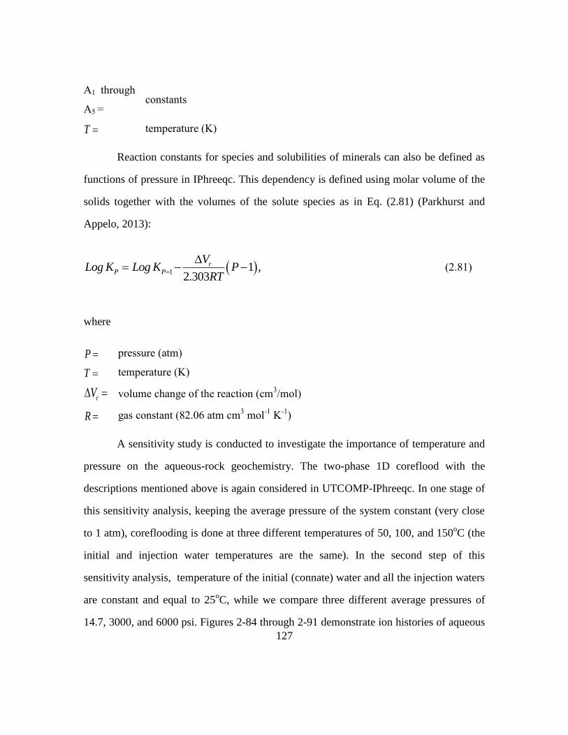
127

A1 through

A5 = constants

temperature (K)

Reaction constants for species and solubilities of minerals can also be defined as

functions of pressure in IPhreeqc. This dependency is defined using molar volume of the

solids together with the volumes of the solute species as in Eq. (‎2.81) (Parkhurst and

Appelo, 2013):

(‎2.81)

where

pressure (atm)

temperature (K)

volume change of the reaction (cm3/mol)

gas constant (82.06 atm cm3 mol

-1 K

-1)

A sensitivity study is conducted to investigate the importance of temperature and

pressure on the aqueous-rock geochemistry. The two-phase 1D coreflood with the

descriptions mentioned above is again considered in UTCOMP-IPhreeqc. In one stage of

this sensitivity analysis, keeping the average pressure of the system constant (very close

to 1 atm), coreflooding is done at three different temperatures of 50, 100, and 150oC (the

initial and injection water temperatures are the same). In the second step of this

sensitivity analysis, temperature of the initial (connate) water and all the injection waters

are constant and equal to 25oC, while we compare three different average pressures of

14.7, 3000, and 6000 psi. Figures 2-84 through 2-91 demonstrate ion histories of aqueous

T

1 1 ,2.303

rP P

VLog K Log K P

RT

P

T

rV

R

128

species as well as the pH of the produced solution with different temperatures. Figures

2-92 and 2-93 present calcite and dolomite mineral concentrations (mol/kgw) at the

injection gridblock. Except the Na and Cl elements which are not reactive (particularly

Cl), the effect of the temperature on the aqueous-rock geochemistry is significant in ion

histories of the other aqueous species including the pH, and solids concentrations (i.e.,

calcite and dolomite solids). As expected, the temperature does not show the same effect

on the aqueous ion histories, pH and the mineral concentrations. For example, by

increasing the temperature, ion concentrations for Ca+2

, Ba+2

, and Sr+2

decrease while the

Mg+2

concentration increases or, although by increasing the temperature the calcite

solubility decreases, the dolomite solubility increases.

Figure 2-84: History of effluent Na+ concentration (significance of the temperature in the


129




Figure 2-86: History of effluent Cl- concentration (significance of the temperature in the


130

Figure 2-87: History of effluent pH (significance of the temperature in the reactive-

transport modeling).




131

Figure 2-89: History of effluent HCO3- concentration (significance of the temperature in

the reactive-transport modeling).


concentration (significance of the temperature in

the reactive-transport modeling).

132





temperature in the reactive-transport modeling).

133


temperature in the reactive-transport modeling).

For the case studied, the effect of pressure on the aqueous-rock geochemistry is

not as pronounced as the temperature effect (see Figures 2-94 through 2-101 for the ion

histories and pH of the aqueous solution produced from the 100th

gridblock). Calcite and

dolomite concentrations in the 1st gridblock are also presented in Figures 2-102 and

2-103. Although by increasing the average pressure, concentrations of Ca+2

, pH, HCO3-,

Sr+2

, Ba+2

are affected to some extent, the change in the calcite and dolomite solubilities

can be ignored.

134

Figure 2-94: History of effluent Na+ concentration (significance of the pressure in the





135

Figure 2-96: History of effluent Cl- concentration (significance of the pressure in the


Figure 2-97: History of effluent pH (significance of the pressure in the reactive-transport

modeling).

136




Figure 2-99: History of effluent HCO3- concentration (significance of the pressure in the


137







138


pressure in the reactive-transport modeling).

Figure 2-103: History of effluent dolomite concentration in the first gridblock

(significance of the pressure in the reactive-transport modeling).

139

It should be emphasized that the conclusions drawn from the sensitivity studies

regarding the change in ion histories and solids precipitation as a function pressure and

temperature should not be generalized. The purpose of these sensitivity studies is to show

the importance of the inclusion of ion activity coefficients and the temperature and the

pressure effects on the aqueous-rock geochemistry. It should be noted that similar results

can be reproduced using UTCHEM-IPhreeqc (Korrani et al., 2014c).

2.10 UTCOMP-IPHREEQC USING HIGHER-ORDER METHOD

For a reason unclear to the author, some oscillations appeared in histories of ions

with low concentrations (less than 10-6

) when the higher-order discretization method

(hereafter, simply called higher-order method) is applied in UTCOMP-IPhreeqc. The

higher-order method is applied in the UTCOMP input file through the IUPSTW flag.

UTCOMP has four different schemes of discretization (IUPSTW = 1 through 4) (see

Chang (1990) and UTCOMP Technical Documentation (2011) for the discretization

details). Later we show that this issue is not limited to the UTCOMP-IPhreeqc simulator

and that perhaps it is a general issue for reactive-transport modeling.

We apply the higher-order method in UTCOMP-IPhreeqc and rerun Case 2 (with

the Endicott water compositions) modeled in Section 2.7.2. We believe that the total

variation diminishing (TVD) higher-order method (i.e., IUPSTW = 4 in UTCOMP)

avoids all the dispersion due to numerical discretization. Hence, Eq. (‎2.82) (rather than

Eq. (‎2.76)) is applied to consider identical Peclet numbers in UTCOMP-IPhreeqc and

PHREEQC. No physical dispersion is included in the model. Hence, the dimensionless

Peclet number is infinite. Here we refer to third-order TVD method simply as the higher-

order method.

140

(‎2.82)

Figures 2-104 through 2-115 show histories of some fluid species and pH of the

solution produced from the case. As the figures illustrate, when the higher-order method

is applied in UTCOMP-IPhreeqc, this integrated simulator does not match the

PHREEQC’s results very well for low concentration ions (including the solution pH

which is in fact the decimal logarithm of reciprocal of the hydrogen ion activity, Zhu and

Anderson, 2002). Noteworthy, the fact that UTCOMP-IPhreeqc fairly well matches the

PHREEQC’s output for the chloride ion (as an inactive geochemical species) reveals that,

Peclet numbers are almost identical in UTCOMP-IPhreeqc and PHREEQC. Hence, the

discrepancies observed are not due to different Peclet numbers in UTCOMP-IPhreeqc

and PHREEQC simulators.

Figure 2-104: Simulation results for the Na+ concentration history of the effluent solution

using UTCOMP-IPhreeqc with the higher-order method and PHREEQC.

UTCOMP-IPhreeqc PHREEQC

.physical physical

N x N x

141




Figure 2-106: Simulation results for the Cl- concentration history of the effluent solution


142







143

Figure 2-109: Simulation results for the CaSO4 concentration history of the effluent


Figure 2-110: Simulation results for the pH history of the effluent solution using

UTCOMP-IPhreeqc with the higher-order method and PHREEQC.

144

Figure 2-111: Simulation results for the Ba+2



Figure 2-112: Simulation results for the HCO3- concentration history of the effluent


145

Figure 2-113: Simulation results for the Fe+2



Figure 2-114: Simulation results for the Mg+2



146

Figure 2-115: Simulation results for the Sr+2



A simple case is designed in UTCOMP-/UTCHEM-IPhreeqc, UTCOMP-

/UTCHEM-EQBATCH, and PHREEQC to investigate if the problem is because of

inherent nature of the higher-order method or the procedure applied to integrate IPhreeqc

with UTCOMP. IPhreeqc was integrated with UTCHEM to comprehensively model ASP

floods. Details on UTCHEM-IPhreeqc are well documented in Chapter 5. Two aqueous

reactions (shown in Table 2-24) and the anhydrite reaction (shown in Table 2-25) are

included in the model. Table 2-26 presents ion compositions of initial and injecting

waters. Initial anhydrite concentration is 0.091 moles/kgw. For the sake of comparison

with EQBATCH, IPhreeqc and PHREEQC are forced to apply molalities rather than ion

activities in geochemical calculations. As discussed in Section 2.4, EQBATCH (version

2011) considers molalities rather than ion activities for geochemical calculations.

147

IPhreeqc/PHREEQC multiplies molality times the ion activity coefficient to find the ion

activity (see Appendix A). Hence, to make ion activity coefficients equal to one, the

WATEQ Debye-Huckel’s model is applied in IPhreeqc/PHREEQC with high value for

ai0 and zero for bi (also pointed out in Section 2.8). No Exchange reaction is included in

the model because to the best of author’s knowledge there is no way through that activity

coefficient calculation of IPhreeqc/PHREEQC can be completely ignored for the

exchange species. In fact, even if the WATEQ Debye-Huckel activity coefficients are

forced to be one for the exchange species, IPhreeqc/PHREEQC still uses the equivalent

fractions for the exchange species while EQBATCH applies the molalities in the

geochemical calculations. Furthermore, the IPhreeqc/PHREEQC database is modified to

consider only the geochemical reactions shown in Tables 2-24 and 2-25. We

comprehensively discuss the difference between EQBATCH and IPhreeqc/PHREEQC in

Chapter 5.

Table 2-24: Aqueous reaction

Reaction KSP

Table 2-25: Solid reaction

Solid Name Reaction KSP

Anhydrite

2

4 4SO H HSO 1.98810

2 2

4 4Ca SO CaSO 2.310

2 2

4 4CaSO Ca SO 4.36010

148

Table 2-26: Ion compositions of initial and injected waters

Ion CInitial

(mol/kgw)

CInjected

(mol/kgw)

Ca 0.11 0.

S 0.0092 0.

Cl charge balance element

Figures 2-116 through 2-120 compare simulation results of produced Ca+2

, SO4-2

,

HSO4-1

, CaSO4, and pH using the UTCOMP-/UTCHEM-IPhreeqc, UTCOMP-

/UTCHEM-EQBATCH simulators with the higher-order method against PHREEQC

outputs.

Although the results of the simulators are in agreement for Ca+2

, SO4-2

, CaSO4

fluid species, the discrepancies among these tools are highly pronounced for HSO4-1

and

pH. However, UTCOMP-EQBATCH matches UTCOMP-IPhreeqc outputs and also we

obtain identical results using UTCHEM-EQBATCH and UTCHEM-IPhreeqc. Hence,

even if the oscillation observed in UTCOMP-IPhreeqc or UTCHEM-IPhreeqc is due to a

potential programming bug, the programming bug should be in the module where the

higher-order method is applied, not the IPhreeqc coupling related routines. The difference

between the higher-order method implemented in UTCOMP and the previously

developed module in UTCHEM is in order of 10-6

. That is why UTCOMP-IPhreeqc/-

EQBATCH does not reproduce the UTCHEM-IPhreeqc/-EQBATCH results. It is worth

mentioning that if the lower-order method (i.e., one-point upstream weighted method) is

applied instead, the results for all the five simulators (i.e., UTCOMP-/UTCHEM-

IPhreeqc, UTCOMP-/UTCHEM-EQBATCH, and PHREEQC) match fairly well (see

Figures 2-121 through 2-125).

149



UTCOMP-/UTCHEM-IPhreeqc and UTCOMP-/UTCHEM-EQBATCH with the higher-

order method and PHREEQC.





150








151


/UTCHEM-IPhreeqc and UTCOMP-/UTCHEM-EQBATCH with the higher-order

method and PHREEQC.



UTCOMP-/UTCHEM-IPhreeqc and UTCOMP-/UTCHEM-EQBATCH with the lower-


152









153





/UTCHEM-IPhreeqc and UTCOMP-/UTCHEM-EQBATCH with the lower-order

method and PHREEQC.

154

The oscillation in pH or ions with small concentration is not always observed. To

confirm this, Case 2 presented in Section 2.4 is used in UTCOMP-/UTCHEM-

EQBATCH, UTCOMP-/UTCHEM-IPhreeqc, and PHREEQC. As previously discussed,

if an exchange site is included into a model, there is no way through which we can obtain

the same results using EQBATCH (coupled with UTCHEM or UTCOMP) and IPhreeqc

(coupled with UTCHEM and UTCOMP). Hence, here we exclude the exchange reactions

from Case 2.

Figures 2-126 through 2-138 present histories of pH and some of the fluid species

produced from the case. As the figures illustrate, although the higher-order method is

applied in UTCOMP-/UTCHEM-IPhreeqc, UTCOMP-/UTCHEM-EQBATCH, these

simulators match the PHREEQC’s results fairly well for a complicated case. Once again,

we emphasize on the fact that ion activity coefficients of aqueous species are forced to be

one in the IPhreeqc/PHREEQC thermodynamic database in order to apply molalities

rather than ion activities for geochemical calculations (similar to EQBATCH).

155

Figure 2-126: Simulation results for pH profile at 0.5 PV using UTCOMP-/UTCHEM-

IPhreeqc and UTCOMP-/UTCHEM-EQBATCH with the higher-order method and

PHREEQC.





156





Figure 2-129: Simulation results for the Na+ concentration profile at 0.5 PV using



157

Figure 2-130: Simulation results for the CO3-2








158




Figure 2-133: Simulation results for the NaSO4- concentration profile at 0.5 PV using



159

Figure 2-134: Simulation results for the NaCO3- concentration profile at 0.5 PV using



Figure 2-135: Simulation results for the NaHCO3 concentration profile at 0.5 PV using



160

Figure 2-136: Simulation results for the HCO3-1




Figure 2-137: Simulation results for the CaOH+ concentration profile at 0.5 PV using



161

Figure 2-138: Simulation results for the CaHCO3+ concentration profile at 0.5 PV using



Out of the four schemes of discretization available in UTCOMP (IUPSTW = 1

through 4) and UTCHEM (IDISP = 0 through 3), UTCOMP-IPhreeqc with IUPSTW = 1

and UTCHEM-IPhreeqc with IDISP = 0 are the only options that always match

PHREEQC results. Oscillations in low concentration ions are worse when IUPSTW = 3

is applied compared with IUPSTW = 2. IUPSTW = 4 shows the worst oscillations.

Broadly speaking, schemes of discretization other than the lower-order method

(i.e., one-point upstream weighted method) are not recommended to model processes in

which fluid species with low concentrations play a significant role in the physics of the

process. For example, geochemistry, particularly pH of the aqueous solution, is the

fundamental basis for high-pH flooding or ASP processes. Hence, using the higher-order

scheme of discretization to model these processes might lead to misleading results. High

pH values (usually above 11) are considered in high-pH flooding or ASP processes. The

162

pH value, say 11, by definition means the hydrogen ion activity of 10-11

. For the time

being, UTCOMP-/UTCHEM-IPhreeqc stops if methods other than the lower-order

method are considered for the simulation. Hereafter in this dissertation the lower-order

scheme is applied in all the simulation runs.

2.11 IMPLEMENTATION OF WETTABILITY ALTERATION MODULE IN UTCOMP-

IPHREEQC

One of the hypotheses made in this dissertation is that the wettability alteration is

the underlying mechanism behind low (or modified) salinity waterflooding. This

hypothesis is based on several experimental observations published in the literature (more

details are provided in Chapters 3 and 4). Hence, to be able to apply UTCOMP-IPhreeqc

for mechanistic modeling of low salinity waterflooding, a wettability alteration model

should be included in this integrated simulator.

The wettability alteration model based on the interpolating technique is

implemented in the UTCOMP-IPhreeqc simulator. In this modeling approach, a single set

of oil-wet curves corresponding to the oil-wet condition and another set corresponding to

the water-wet condition are considered and then during the simulation, the altered relative

permeabilities or capillary pressure are computed as weighted averages between two

previously defined oil-wet and water-wet curves (see Eqs. (‎2.83) and (‎2.84)).

(‎2.83)

(‎2.84)

where

θ1, θ2 = process dependent interpolation factors

1 11 ,altered initial final

rl rl rlk k k

2 21 ,altered initial final

c c cP P P

163

krl = relative permeability of the phase l

Pc = capillary pressure (psi)

The interpolating technique was implemented in UTCHEM to model the

wettability alteration due to chemical floods such as surfactant and alkaline flooding

(Najafabadi, 2009; Anderson, 2006; Goudarzi et al., 2012; 2013). For example, in one of

the mechanistic model implemented in UTCHEM, the interpolating parameter is defined

as a function of adsorbed surfactant on the rock surface. Through this model, wettability

alteration due to the surfactant flooding is introduced. In other words, the more surfactant

adsorbed on the grain, the more chance there is to change the wettability of the rock from

mixed-wet toward water-wet (Najafabadi, 2009; Anderson, 2006; Goudarzi et al., 2012;

2013).

In UTCOMP-IPhreeqc when phase saturations are known for reservoir

gridblocks, they are used to separately calculate “initial” and “final” relative

permeabilities and capillary pressure. Routines to evaluate the “initial” and “final”

relative permeabilities and capillary pressure are basically the same except different

relative permeability parameters are applied. For example, residual saturations,

endpoints, and exponents if the Corey’s model is considered. These parameters are

defined by the users in the UTCOMP input file. The calculated “initial” and “final”

relative permeabilities and capillary pressure are used along with the interpolating

parameter in a separate routine (i.e., wetmodel.f in UTCOMP-IPhreeqc) to evaluate the

“altered” relative permeabilities and capillary pressure using Eqs. (‎2.83) and (‎2.84). In

fact, the “altered” relative permeabilities are applied for the transmissibility and

subsequently the gridblocks pressure calculations.

164

In this work we assume the same interpolating parameter for the relative

permeability and the capillary pressure (i.e., θ1 = θ2). Based on the literature (discussed in

Chapters 3 and 4), the underlying mechanisms for low salinity water injection in

sandstone and carbonate reservoirs are different. Hence, to introduce this discrepancy in

the model, we define different interpolating parameters for sandstone (see Chapter 3) and

carbonate (see Chapter 4) reservoirs.

The wettability alteration module implemented in UTCOMP is not limited to

modeling the low salinity waterflooding, but can be also applied to model the wettability

alteration due to other processes. For example, Mohebbinia (2013) and Mohebbinia et al.

(2014) applied the UTCOMP wettability alteration module to model wettability alteration

due to the asphaltene deposition on the rock surface. It is widely accepted that when

asphaltene is deposited on the rock surface, it changes the rock wettability from the

water-wet condition towards the oil-wet condition. Noteworthy, to model wettability

alteration due to asphaltene deposition, the initial set of relative permeabilities is water-

wet and the final set is oil-wet (just the opposite of low salinity waterflooding).

Two different scenarios are applied to verify the wettability alteration model

implemented in the UTCOMP-IPhreeqc simulator.

Case 1

In the first scenario; a heterogeneous 2D case is designed in UTCOMP-IPhreeqc.

Table 2-27 presents the case descriptions. Barium (Ba), sodium (Na), and calcium (Ca)

are the geochemical species present in the connate water and also injected with different

concentrations into the reservoir (through the 6 injection wells included in the case).

Tables 2-28 and 2-29 illustrate ion compositions of geochemical species for initial and

injecting waters, respectively. This case is heterogeneous in porosity and absolute

165

permeability (in both x and y directions). Isotropic permeability is assumed. Figure 2-139

shows the map for the x- and y-direction permeabilities and Figure 2-140 presents the

porosity distribution map. The injection pattern is line drive with 6 injection and 3

production wells (see Figure 2-141). The capillary pressure is assumed to be zero. Initial

and final sets of relative permeability curves are identical (Corey’s relative permeability

model is applied with the parameters shown in Table 2-30) and the interpolating

parameter for the relative permeability is constant and equal to 0.3. This case is verified

against an identical case but without wettability alteration and only with one set of

relative permeability curves. In fact, because the initial and final sets of relative

permeability curves are identical for the case with the wettability alteration, results for

this case should match those of the case with one set of relative permeability (i.e., no

wettability alteration is applied).

Figures 2-142 through 2-148 demonstrate results of the case with the wettability

alteration included (shown with IWALT=1 in the figures) with those from the case

without wettability alteration (shown with IWALT =0 in the figures). Figures 2-142 and

2-143 show oil recovery and average reservoir pressure and Figures 2-144 through 2-148

present the ion histories of Ba, Na, and Ca; pressure; water saturation at two gridblocks

of (50,30,1) and (30,50,1). As the figures show, results are identical for the cases

compared.

166



Δx(ft) 25.0

Δy(ft) 25.0

Δz(ft) 20.0

Permeability (md)





) 0.


) 0.









3 producers


Table 2-28: Initial concentration for the geochemical elements

Ba Na Ca

Initial concentration

(meq/ml) 0. 0.1 0.1

167

Table 2-29: Wells condition and injecting element concentrations for 3D case

Well

No. I J

Perforated

layer rw (ft) Type Operating Condition

Concentration (meq/ml)

Ba Na Ca

1 10 10 1-1 0.33 Inj. Qw=200 bbl/Day 0.02 0. 0.05

2 10 90 1-1 0.33 Inj. Qw=200 bbl/Day 0.2 0.3 0.75

3 90 10 1-1 0.33 Inj. Qw=200 bbl/Day 1.1 0.48 0.2

4 90 90 1-1 0.33 Inj. Qw=200 bbl/Day 0.2 0. 0.5

5 50 50 1-1 0.33 Prod. BHP=1000 psia - - -

6 90 50 1-1 0.33 Inj. Qw=200 bbl/Day 0.2 0. 0.5

7 10 50 1-1 0.33 Inj. Qw=200 bbl/Day 0.02 0. 0.05

8 50 90 1-1 0.33 Prod. BHP=1000 psia - - -

9 50 10 1-1 0.33 Prod. BHP=1000 psia - - -

Figure 2-139: Distribution of permeabilities (in md) in x and y directions for the 2D case.

168

Figure 2-140: Distribution of porosity for the 2D case.

Figure 2-141: Well locations in the 2D case considered to verify the implementation of

the wettability alteration module in UTCOMP.

169

Table 2-30: Corey’s parameters of the initial set of relative permeability

Residual

saturation

Water 0.25

Oil 0.2

Exponent

Water 1.5

Oil 2.5

Endpoint Water 0.21

Oil 0.7


in UTCOMP). IWALT=0: no wettability alteration is modeled; IWALT=1: wettability

alteration is applied with identical initial and altered sets of relative permeabilities.

170


module implemented in UTCOMP). IWALT=0: no wettability alteration is modeled;

IWALT=1: wettability alteration is applied with identical initial and altered sets of

relative permeabilities.

Figure 2-144: Ba concentration histories of two gridblocks (verification of the wettability

alteration module implemented in UTCOMP). IWALT=0: no wettability alteration is

modeled; IWALT=1: wettability alteration is applied with identical initial and altered sets

of relative permeabilities.

171

Figure 2-145: Na concentration histories of two gridblocks (verification of the wettability




Figure 2-146: Ca concentration histories of two gridblocks (verification of the wettability




172

Figure 2-147: Pressure histories of two gridblocks (verification of the wettability




Figure 2-148: Water saturation histories of two gridblocks (verification of the wettability




173

Case 2

In the second scenario; the implemented wettability alteration module in the

UTCOMP-IPhreeqc integrated simulator is verified against the UTCHEM simulator.

Towards this goal, the case described above (i.e., Case 1) is also designed using

UTCHEM. Initial and final sets of relative permeability curves are now different. Table

2-30 and Table 2-31present the Corey’s parameters for the initial and final sets of relative

permeability curves, respectively (Figure 2-149 provides the plot). All the notes

discussed in Section 2.2 are taken into consideration when comparing UTCHEM to

UTCOMP-IPhreeqc. Moreover, because the case considered is a 2D case, the small

discrepancy in terms of the oil gravity between UTCHEM and UTCOMP-IPhreeqc is

eliminated (discussed in Section 2.2). The interpolating parameter is 0.5 in both

UTCHEM and UTCOMP-IPhreeqc simulators. It is worth noting that in UTCHEM by

default the wettability alteration with constant interpolating parameter is applied only for

the surfactant flooding. Hence, we temporarily change the “wetmodel.f” routine of

UTCHEM to consider the constant interpolating parameter even in the absence of the

surfactant. The following presents the temporary changes applied in the UTCHEM source

code:

Originally in the “wetmodel.f” routine:

IF (IWALF.EQ.0) THEN

DO 20 I = 1,NBL

IF (CTOT(I,3).GT.EPSME) IWTHIS(I) = 1

IF (IWTHIS(I).EQ.1) THEN

DO 25 L = 1,NPHAS

RPERM(I,L) = FW1*RPERMW(I,L)+(1-

FW1)*RPERM(I,L)

PRC(I,L) = PCW1*PRCW(I,L)+(1-PCW1)*PRC(I,L)

25 CONTINUE

ENDIF

174

20 CONTINUE

ENDIF

is temporarily changed to:

IF (IWALF.EQ.0) THEN

DO 20 I = 1,NBL

CC IF (CTOT(I,3).GT.EPSME) IWTHIS(I) = 1

CC IF (IWTHIS(I).EQ.1) THEN

DO 25 L = 1,NPHAS

RPERM(I,L) = FW1*RPERMW(I,L)+(1-

FW1)*RPERM(I,L)

PRC(I,L) = PCW1*PRCW(I,L)+(1-PCW1)*PRC(I,L)

25 CONTINUE

CC ENDIF

20 CONTINUE

ENDIF

Figures 2-150 through 2-156 verify UTCOMP-IPhreeqc results (i.e., dashed lines)

against UTCHEM (i.e., solid lines) outputs. Included in these figures are also results for

the case in which no wettability alteration (θ1 = θ2 = 0) is considered in the UTCHEM and

UTCOMP-IPhreeqc simulators.

Because only three geochemical elements (i.e., Ba, Na, and Ca) are included in

the two cases considered for the verification, the IPhreeqc database is modified in the

way that no extra geochemical calculations are performed. This speeds up the simulation

in UTCOMP-IPhreeqc to some extent.

175

Table 2-31: Final set of relative permeability

Residual

saturation

Water 0.2

Oil 0.1

Exponent

Water 2.5

Oil 1.5

Endpoint Water 0.1

Oil 0.85

Figure 2-149: Initial (dashed lines) and final (solid lines) relative permeabilities.

176


in UTCOMP against UTCHEM). IWALT=0: no wettability alteration is modeled;

IWALT=1: wettability alteration is included in the model.


module implemented in UTCOMP against UTCHEM). IWALT=0: no wettability

alteration is modeled; IWALT=1: wettability alteration is included in the model.

177

Figure 2-152: Ba concentration histories at two gridblocks (verification of the wettability


wettability alteration is modeled; IWALT=1: wettability alteration is included in the

model.

Figure 2-153: Na concentration histories at two gridblocks (verification of the wettability



model.

178

Figure 2-154: Ca concentration histories at two gridblocks (verification of the wettability



model.

Figure 2-155: Pressure histories at two gridblocks (verification of the wettability



model.

179

Figure 2-156: Water saturation histories at two gridblocks (verification of the wettability



model.

2.12 PARALLELIZATION OF THE UTCOMP-IPHREEQC HYDROCARBON-AQUEOUS

PHASE COMPOSITION CALCULATION MODULE

IPhreeqc is a complete geochemical package that overcomes all the EQBATCH

limitations for comprehensive reactive-transport modeling. However, although an

efficient algorithm was followed to couple IPhreeqc with UTCOMP, using IPhreeqc for

geochemical calculations requires more computational time for the simulation. The

increase in CPU time in UTCOMP-IPhreeqc is consistent with that of PHAST where the

required computational time for the geochemistry calculation is at least twice of the total

time spent on other calculations (i.e., flow and transport) (Parkhurst et al., 2010). To

tackle this issue and enhance UTCOMP-IPhreeqc to large-scale reservoir simulation, we

parallelize the geochemistry module of this integrated simulator.

180

Figure 2-157 illustrates the computational algorithm applied in PHAST (Parkhurst

et al., 2010). In this computational algorithm, multiple computing processors (or simply

“processors”) are initialized at the beginning of the simulation. However, except the

geochemistry section in which the task is distributed among the processors (master and

slave processors), master processor performs all the other calculations including solving

the pressure matrix, mass conservation equation, and reporting the output results.

Figure 2-157: Computational algorithm of parallel-processing version of PHAST

(Parkhurst et al., 2010)

We apply the similar approach to parallelize the phase composition calculation

(aqueous and hydrocarbon) module in UTCOMP-IPhreeqc. Massage Passing Interface

(MPI) (Barney, 2009) is used as the parallel processing interface. MPI_INIT,

MPI_COMM_RANK, and MPI_COMM_SIZE available in MPI are applied to initialize

and assigning the ranks to the processors. Master processor (processor with the rank 0 is

181

considered as the master processor) performs the entire calculations such as reading the

input files, allocating the variables, setting up the pressure matrix, solving the pressure

matrix, and calculating the total moles of the hydrocarbon and geochemical species (i.e.,

solving the mass conservation equation) till it reaches the phase composition calculation

module. Within the time period that the master processor performs the calculations, all

the other processors (i.e., slave processors) have skipped the calculations and are waiting

for the master processor before getting into the geochemistry module. MPI_BARRIER of

MPI is used to block the slave processors until the master processor reaches the routine.

Once the master processor joins the slave processors, it shares the updated geochemistry

data (MPI_SEND and MPI_RECV of MPI are used for sharing the data among the

processors) and then all the processors (including the master processor) perform the

thermodynamic calculation of the phases for certain number of gridblocks. It should be

noted that some of the data is transferred from the master processor to the slave ones once

and only in the first time step; however, there are some data that needs to be updated in

the slave processors at each time step. For example, number of geochemical elements

involved in the simulation is constant during the simulation. Hence, the master processor

sends the number of geochemical species to the slave processors in the first time step. On

the other hand, total moles of the geochemical species in each gridblock are updated at

each time step by solving the mass conservation equation. Hence, we need to update the

total moles of the geochemical elements in the slave processors at each time step. This

will be discussed with more details later.

Another point is the number gridblocks assigned to each computing processor. If

the number of gridblocks is divisible by the number of processors, then equal number of

gridblocks is assigned for each processor. Otherwise, some processors have an extra

182

gridblock for thermodynamic calculations. For example, if the number of gridblocks and

the number of processors (including the master processor) are 100 and 7, respectively; in

the geochemistry module, two processors perform the calculations for 15 gridblocks and

the other 5 processors have 14 gridblocks for the calculation. The reason for having this

flexibility is the fact that when evaluating the thermodynamic equilibrium of either

aqueous or hydrocarbon phase, reservoir gridblocks are independent and treated as batch

cells.

All the computing processors call the same routines for phase composition

calculations (either hydrocarbon or the aqueous phase). “Do loops” in these routines are

all from 1 to NB where NB is the local number of gridblocks in each processor. We

change the number of gridblocks in the master processor to the local value before it starts

the phase composition calculation. Number of gridblocks in the master processor is

returned back to the main number of gridblocks when it finishes with the phase

composition calculations.

Computational times required for the thermodynamic calculations of gridblocks

are not identical. Some gridblocks require more iterations in IPhreeqc or between

UTCOMP and IPhreeqc (based on the algorithm shown in Figure 2-56) to converge to the

solution. Hence, the total computational time that takes for each processor to finish the

phase composition calculations of its entire assigned gridblocks might not be the same for

all the processors. However, if a processor finishes the calculations sooner compared with

other processors, it should wait for other processors to finish their tasks as well. When all

the processors are done with their calculations, the equilibrium data of the gridblocks

assigned to the slave processors are transferred to the master processor. Slave processors

183

are now free and will be waiting for the master processor to perform the rest of

calculations and reach the phase composition calculation module again.

2.12.1 Parallelization of the UTCOMP-IPhreeqc Hydrocarbon Phase Composition

Calculation Module

As shown in Figure 2-56, if the effect of the hydrocarbon phase on the aqueous-

rock geochemistry is included in the model, UTCOMP-IPhreeqc follows a sequential

iterative scheme between the hydrocarbon flash calculation of UTCOMP and the aqueous

phase flash calculation of IPhreeqc (finding the equilibrium state of the aqueous is a kind

of flash calculation in the aqueous phase). The sequential iterative algorithm is followed

to make fugacities identical (within a desired tolerance) among the phases. If multiple

processors are applied, the same solution scheme should be applied in each processor.

Hence, the hydrocarbon flash calculation module of UTCOMP should be also

parallelized along with the IPhreeqc coupling related routines. If the effect of the

hydrocarbon phase on the aqueous-rock geochemistry is not included in the model,

parallelization is applied only for the phase composition calculation of the aqueous phase

and no longer for the hydrocarbon phase. Hence, in this case the entire hydrocarbon flash

calculations are performed by the master processor.

To parallelize the hydrocarbon flash calculation module of UTCOMP-IPhreeqc,

the thermodynamic properties of hydrocarbon components that remain unchanged during

the simulation, such as Tc (critical temperature), Pc (critical pressure), Vc (critical

volume), and ω (acentric factor), are shared with the slave processors by the master

processor only at the first time step. On the other hand, total moles of the hydrocarbon

components are transferred from the master processor to the slave processor in each time

step. When all the processors finish the hydrocarbon phase behavior calculation, the slave

184

processors send the equilibrium data of their local gridblocks to the master processor.

These data are: number of phases in each gridblock, component compositions of the

phases, phase compressibility factors, and phase mole ratios.

A synthetic case is designed to verify the procedure through which we

parallelized the hydrocarbon phase behavior module of UTCOMP-IPhreeqc. The

geochemistry option is set zero (IGEOCHEM = 0 in the UTCOMP input file) in this case.

Tables 2-32 and 2-33 show case descriptions and the initial overall mole fraction of the

hydrocarbon components, respectively. This case is a homogeneous quarter five-spot

pattern (see Figure 2-158) with one well at a corner injecting 5 MMScf/day mixture of

C1-C3 (0.8-0.2 overall mole fraction) and the other well at the opposite corner producing

from the reservoir at the constant bottomhole pressure of 3100.0 psi. Figures 2-159

through 2-162 show oil recovery, average reservoir pressure, and gas and oil surface

production rates when different number of computing processors is used. Figures 2-163

and 2-164 show oil and gas saturation maps of the first layer at 0.1 PV using 1, 6, and 10

processors. As Figures 2-159 through 2-164 demonstrate, results are in very good

agreements when different number processors are applied for the hydrocarbon phase

behavior calculation. Table 2-34 presents the computational time spent in the

hydrocarbon flash calculation module and also the total computational time using

different number of processors. Simulations are run on two different clusters of

processors (i.e., TACC-Lonestar cluster and PETROS). TACC (Texas Advanced

Computing Center) is a high performance computing center owned by The University of

Texas at Austin. Lonestar has 1888 compute nodes with two 6-cores per node (22656

CPU cores in total). Each node in the Lonestar 64-bit has 24 gigabytes memory with the

frequency of the cores (clock-speed) of 3.33 GHz (TACC, 2014). PETROS is the Unix-

http://www.tacc.utexas.edu/

185

based in-house cluster of processors in the Petroleum and Geosystems Engineering

(PGE) department of The University of Texas at Austin. PETROS has 32 compute nodes

with 4 processors (128 CPU cores in total) with the frequency of 2.73 GHz in each node.

Each computing nodes in PETROS has 16 gigabytes of memory.

Figure 2-165 presents the total computational time and the time spent in the phase

behavior calculation module (CPU times obtained from TACC are used). Speedup plot is

provided in Figure 2-166. Speedup is computational time using one processor over the

computational time for the parallel run (using multiple processors).

186

Table 2-32: Reservoir characteristics for the 3D case


Δx(ft) 75.0

Δy(ft) 75.0

Δz(ft) 50.0

Permeability (md)

x-direction 100.0

y-direction 100.0

z-direction 100.0

Porosity 0.3


) 50.0×10-6


) 3.0×10-6








1producer


187

Table 2-33: Overall mole fraction of initial and injected hydrocarbon components

Component Zinitial Zinjected

C1 0.5 0.8

C3 0.03 0.2

C6 0.07 -

C10 0.2 -

C15 0.15 -

C20 0.05 -

Figure 2-158: Well locations in the 3D case considered to verify the parallelization of the

hydrocarbon phase behavior calculation in UTCOMP.

188

Figure 2-159: Oil recovery (using UTCOMP-IPhreeqc with multiple processors for the

hydrocarbon phase composition calculations).

Figure 2-160: Average reservoir pressure (using UTCOMP-IPhreeqc with multiple

processors for the hydrocarbon phase composition calculations).

189

Figure 2-161: Oil surface production rate (using UTCOMP-IPhreeqc with multiple


Figure 2-162: Gas surface production rate (using UTCOMP-IPhreeqc with multiple


190

Figure 2-163: Oil saturation map of the first layer at 0.1 PV (using UTCOMP-IPhreeqc with

1 processor (top-left panel), 6 processors (top-right panel), and 10 processors (bottom

panel) for the hydrocarbon phase composition calculations).

191

Figure 2-164: Gas saturation map of the first layer at 0.1 PV (using UTCOMP-IPhreeqc

with 1 processor (top-left panel), 6 processors (top-right panel), and 10 processors (bottom

panel) for the hydrocarbon phase composition calculations).

192

Table 2-34: Total computational time and the time spent for the hydrocarbon phase

composition calculations

PETROS TACC-Lonestar

No. of

Processor(s)

in

UTCOMP

Phase behavior

computational

time (seconds)

Total

computational

time (seconds)

Phase behavior

computational

time (seconds)

Total

computational

time (seconds)

1PRC 2450.04 4730.21 1512.07 2233.0

2PRCs 1352.1 3625.82 792.27 1514.0

4PRCs 756.5 3000.37 433.69 1155.0

6PRCs 700.28 2817.06 311.80 1034.0

8PRCs 660.13 2888.86 249.93 971.0

10PRCs 756.05 3031.51 227.34 972.0

Figure 2-165: Total computational time and the time spent for the hydrocarbon phase

composition calculations versus number of processors.

193

Figure 2-166: Speedup curve for the total simulation and hydrocarbon phase composition

calculations versus number of processors.

Using robust solvers for parallel processing is highly recommended. PETSc

(Portable Extensible Toolkit for Scientific computation) (Brown, 2010) is applied over

the two UTCOMP solvers based on biconjucate gradient algorithm (i.e., IPRESS=3 in the

UTCOMP input file) and biconjucate gradient squared algorithm (i.e., IPRESS=4 in the

UTCOMP input file). PETSc is a comprehensive package for solving the linear and non-

linear system of equations and has been developed in the Argonne National Laboratory

(Brown, 2010).

2.12.2 Parallelization of the UTCOMP-IPhreeqc Aqueous Phase Composition

Calculation Module

IPhreeqc (Charlton and Parkhurst, 2011) has been designed very intelligently

making the parallelization straightforward. IPhreeqc modules are independent; hence,

194

each processor has its own IPhreeqc module and performs part of geochemical

calculation tasks of the aqueous phase (Parkhurst and Appelo, 2011). What follows below

presents the procedure through which we parallelized the aqueous phase composition

calculation module in UTCOMP-IPhreeqc.

At the first time step all the slave processors create their own IPhreeqc modules

using CreateIPhreeqc method of IPhreeqc. Subsequently slave processors load the

IPhreeqc thermodynamic database using LoadDatabase. The geochemistry information

of the entire gridblocks is then accumulated in the slave processors (i.e.,

IPhreeqc_INPUT.DAT is stored in the memory of processors using AccumulateLine and

INCLUDE$). Each processor keeps the information of its assigned gridblocks;

information of the extra gridblocks is deleted from the processors (using DELETE

available in IPhreeqc). The master processor distributes the total moles of geochemical

elements (to be used along with SOLUTION_MODIFY for each gridblock), mole

fraction of the geochemical species in the aqueous phase, water saturations, and pressures

among the slave processors at each time step. Appendix F provides the parallel version of

the simplified code previously presented in Appendix C. Included in Appendix F is also a

sample case study that verifies the parallel version of the simplified code using different

number of processors.

Hereafter in this dissertation “the parallel version of UTCOMP-IPhreeqc” and,

later in Chapter 5, “the parallel version of UTCHEM-IPhreeqc” mean the UTCOMP-

IPhreeqc and UTCHEM-IPhreeqc simulators which are parallel in only the phase

composition calculations (hydrocarbon and aqueous phases).

195

Verification of the Parallel version of UTCOMP-IPhreeqc

Several case studies (1D, 2D, and 3D) are presented below that show the benefits

in terms of the computational time due to the parallelization of the phase composition

calculation in the UTCOMP-IPhreeqc simulator. For all the cases presented below Na+,

Ca+2

, Cl-, SO4

-2, HSO4

-1, CaSO4, Ba

+2, HCO3

-1, Fe

+2, Mg

+2, Sr

+2, and pH histories were

verified when different number of processors is applied. However, only pH value

(representative of an ion (i.e., H+) with small concentration) and chloride concentrations

(representative of a non-reacting ion or a tracer-like geochemical species) are presented.

All simulations presented below were run on Lonestar cluster of TACC (see

Section 2.12.1 for TACC characteristics). The upper limit for the jobs submitted to

TACC is 24 hours. Hence, for simulation runs that take more than 24 hours, the

UTCOMP-IPhreeqc restart option (cf. Section 2.13) is used to resume the simulation. The

restart files are stored each 500 time steps. We believe that using the restart option should

not introduce more than 5% error in the computational times.

1D Case Studies

Case 1

A 1D case with 100 gridblocks (see Figure 2-167) is designed using the parallel

version of the UTCOMP-IPhreeqc simulator. The case descriptions are shown in Table

2-35. Calcite and dolomite are the solids present in the system. Saturation indices for

these solids are -0.4 and 0.4, respectively. The pitzer.dat database of IPhreeqc is used in

this simulation. About 0.5 of the “SW/50” is injected first and then chased with 0.6 PV of

the “FB” (formation water). Table 2-36 presents ion compositions for the “SW/50” and

“FB” waters. Injection flowrate is constant and equal to 4×10-5

bbl/day and the

production well is operating with the constant bottomhole pressure of 4890 psi.

196

This simulation is performed using UTCOMP-IPhreeqc with 1, 2, 4, 6, 8, and 10

processors. Histories of the chloride ion and pH produced from the core are shown in

Figures 2-168 and 2-169, respectively. We obtain identical results for arbitrary number of

processors. Table 2-37 shows the total computational time and time spent solely in the

geochemistry module versus the number of processors and Figure 2-170 gives the plot.

Figure 2-171 illustrates the speedup plot.

Figure 2-167: 1D case with 100 gridblocks (1 injector and 1 producer).

197

Table 2-35: Case descriptions for the 1D Case


Δx(ft) 0.04

Δy(ft) 0.15

Δz(ft) 0.15


Porosity 0.25


) 0.


) 0.








1 producer


198


2013)

Ion Formation brine

(FB) (ppm)

SW/50 (ppm)

Na+ 49933 274

Mg+2

3248 32.4

Ca+2

14501 10.42

Cl- 111810 489.36

SO4-2

234 66.2

HCO3- - -

Ionic strength

(mol/kgw) 3.658 0.017

TDS (mg/L) 179730 872


IPhreeqc with multiple processors for geochemical calculations).

199


processors for geochemical calculations).



No. of processor(s) in

UTCOMP-IPhreeqc

CPU time spent in

geochemistry

(seconds)

Total computational

time (seconds)

1PRC 194.8279 199

2PRCs 109.3308 112

4PRCs 64.33192 68

6PRCs 51.05515 54

8PRCs 44.24679 48

10PRCs 41.31858 44

200





201

Computational time for modeling a reactive-transport problem using UTCOMP-

IPhreeqc highly depends on the initial and injecting aqueous ion compositions and

number of gridblocks. To confirm this, two different scenarios are modeled. In the first

scenario, Case 1 is considered and number of gridblocks is increased to 1000 (i.e., Case

2). In the second scenario, both 100 and 1000 gridblocks are run using the Endicott water

ion compositions (i.e., Cases 3 and 4).

Case 2

Case 2 is identical to the Case 1 except the number of gridblocks in this case is

1000 (we enlarge Case 1 rather than refining it). Table 2-38 shows the total

computational time and the time spent for geochemical calculations. Figure 2-172

presents the plot of computational times versus the number of processors. Speedup is

shown in Figure 2-173. The computational times reported in Table 2-37 should not be

directly compared with those of Table 2-38. Because, although the injection rate in Case

1 and Case 2 is identical, total pore volume of Case 2 is 10 times of that in Case 1 (i.e.,

1000 gridblocks in Case 2 versus 100 gridblocks in Case 1). Hence, it takes about 10

times to inject 1.1 PV in Case 2 compared with Case 1. Therefore, the CPU times

presented in Table 2-38 should be divided by 10 before comparing the values reported in

Table 2-37. For the case studied, the dependency of computational time is almost a linear

function of the number of gridblocks.

202



No. of processor in

UTCOMP-IPhreeqc

CPU time spent in

geochemistry

(seconds)

Total

computational

time (seconds)

1PRC 18359.04 18695

2PRCs 9588.363 9925

4PRCs 5422.25 5758

6PRCs 4110.603 4448

8PRCs 3490.897 3826

10PRCs 3142.104 3545

Figure 2-172: Case 2- Total computational time and the time spent for the aqueous


203



Case 3

Descriptions for this case are identical to those of Case 1 (see Table 2-35).

However, the geochemistry of the problem is different. This case is initially filled with

the Endicott connate water (Endicott water compositions were shown in Table 2-20). All

the potential minerals considering Endicott waters compositions (see Table 2-21) are

included in the model. This case is flooded with 0.5 PV, 0.5 PV, 0.5 PV, and 1.5 PV of

Endicott seawater, Endicott produced water (or high salinity water), Endicott low salinity

water, and Endicott high salinity water, respectively. The phreeqc.dat database of

IPhreeqc is used in the simulation. Figures 2-174 and 2-175 compare histories of pH and

the chloride ion produced from this case using different number of processors. Results are

in very good agreements using UTCOMP-IPhreeqc with different number of processors.

Computational time of the entire simulation and also the time spent in the geochemistry

204

module are reported in Table 2-39 (Figure 2-176 shows the plot). Figure 2-177 illustrates

the speedup of the total simulation and the geochemistry module. As Figure 2-177 shows,

speedup for the entire simulation is very close to that of the geochemistry module. This

clearly reveals the fact that most of the computational time is spent for geochemical

calculations. Comparison of the computational times reported in Table 2-39 with those of

Table 2-37 clearly reveals the high dependency of the CPU time, required to model a

reactive-transport problem, to the geochemistry of the problem. It is worth mentioning

that as we applied the automatic time stepping option of UTCOMP-IPhreeqc to model

both Case 1 and Case 3, some portion of the difference in the CPU times may be due to

different time steps in the two cases.


IPhreeqc with multiple processors for geochemical calculations).

205


processors for geochemical calculations).




UTCOMP-IPhreeqc

CPU time spent in

geochemistry

(seconds)

Total

computational

time (seconds)

1PRC 7457.906 7503

2PRCs 4000.51 4046

4PRCs 2265.906 2313

6PRCs 1691.573 1744

8PRCs 1375.574 1426

10PRCs 1190.969 1244

206





207

Case 4

Case 3 is modified for the number of gridblocks and the injected pore volumes.

Number of gridblocks in Case 4 is 1000 and all the waters are injected for 0.1 PV with

the sequence as applied in Case 3. Table 2-40 shows the total computational time and the

time spent in the geochemistry module versus the number of processors used (see Figure

2-178 for the plot). Figure 2-179 gives the speedup plot.




UTCOMP-IPhreeqc

CPU time spent in

geochemistry

(seconds)

Total

computational

time (seconds)

1PRC 66461.63 66931

2PRCs 36814.33 37226

4PRCs 21775.61 22185

6PRCs 15746.58 16156

8PRCs 12688.96 13099

10PRCs 10602.76 11060

20PRCs 6712.145 7133

30PRCs 5572.182 5997

40PRCs 4947.919 5446

50PRCs 4467.391 4975

208





209

2D Case Studies

Case 5

A 2D case is designed using UTCOMP-IPhreeqc. Table 2-41 shows the reservoir

descriptions and Figure 2-180 presents the well pattern. A large number of injection wells

is included in the model to disturb the geochemistry equilibrium state of more gridblocks

at each time step. Obviously, as the number of injection wells increases, the wall-clock

time required to simulate the case also decreases. In fact, because higher amount of water

is injected into the reservoir per time step, simulation time required to inject certain

amount (say 1 PV) of water into the reservoir becomes less. It should be noted that rather

than using several vertical wells in a line drive pattern, a horizontal well could be also

applied.

“FB” with the ion compositions shown in Table 2-36 is the connate water. Calcite

and dolomite are the solids present in the system. Saturation indices for these solids are -

0.4 and 0.4, respectively. The phreeqc.dat database of IPhreeqc is applied for the

simulation. Although this case is a two-phase case with live-oil, the hydrocarbon effect

on the aqueous-rock geochemistry is neglected. All the injection wells are injecting

“SW/50” at constant flowrate of 200 bbl/day and production wells are operating at the

constant bottomhole pressure of 1000.0 psi. The sequence of water flooding is as follows:

0.5 PV of “SW/50” is injected first and then followed by 0.5 PV of the “FB” water.

Figures 2-181 and 2-182 show the histories of the chloride ion and pH of the

aqueous solution for the gridblock (12,12,1). These figures verify the parallel version of

UTCOMP-IPhreeqc when different number of processors is applied. Table 2-42 and

Figure 2-183 show the computational time of the total simulation and the phase

210

composition calculation module when different number of computing processors is

applied. Figure 2-184 presents the plot of speedup.



Δx(ft) 25.0

Δy(ft) 25.0

Δz(ft) 20.0

Permeability (md) x-direction 300.0

y-direction 300.0

Porosity 0.25


) 0.


) 0.








10 producers


211

Figure 2-180: 2D case with 900 gridblocks (15 injectors and 10 producers).


UTCOMP-IPhreeqc with multiple processors for geochemical calculations).

212


multiple processors for geochemical calculations).




UTCOMP-IPhreeqc

CPU time spent in

geochemistry

(seconds)

Total computational

time (seconds)

1PRC 1697.47 1724

2PRCs 872.46 899

4PRCs 470.03 497

6PRCs 347.26 375

8PRCs 280.04 308

10PRCs 242.78 274

12PRCs 223.33 256

213





214

Case 6

Case 6 is identical to Case 5 except in number of gridblocks and number of wells.

The number of gridblocks and number of wells in Case 6 are 10000 (100×100×1) and 81

wells (45 injectors and 36 producers), respectively (see Figure 2-185). Figures 2-186 and

2-187 verify the parallel version of UTCOMP-IPhreeqc for histories of the chloride ion

and pH at the gridblock (30,20,1). The total simulation time using different number of

processors is shown in Table 2-43 (see Figure 2-188 for the plot). Figure 2-189 shows the

speedup of the total simulation time. As this figure shows, up to 12 processors, we

observe super-linear speedup. The reason for the super-linear speedup lies in efficiencies

related to usage of cache memory. This occurs when the size of the problem is greater

than the CPU cache memory. Hence, by using larger number of processors, we in fact

break down the size of problem per processor (Ghasemi Doroh, 2012). The super-linear

speedup in parallelization is discussed with details in the works of Abate et al. (2001) and

Ghasemi Doroh (2012).

215




216



Table 2-43: Case 6- total computational time

No. of Processor(s) in

UTCOMP-IPhreeqc

Total

computational

time (hrs)

1PRC 99.30

2PRCs 40.85

4PRCs 18.85

6PRCs 13.11

8PRCs 10.37

10PRCs 8.98

12PRCs 7.95

16PRCs 6.86

20PRCs 6.11

24PRCs 5.70

30PRCS 5.25

40PRCs 4.82

50PRCs 4.56

60PRCs 4.45

100PRCs 4.36

217

Figure 2-188: Case 6- total computational time versus number of processors.


processors.

218

Case 7

Case 7 is designed to investigate the effect of the hydrocarbon phase on the

computational time, when included in geochemical calculations. Everything in Case 7 is

identical to that of Case 6 except that in Case 7, the effect of CO2 of the hydrocarbon

phase on the aqueous-rock geochemistry is included in the model. Table 2-44 shows the

overall mole fraction and some important thermodynamic properties of the hydrocarbon

components used in the case. Histories of the chloride ion and pH at the gridblock

(30,20,1), the same gridblcok used for the verification in Case 6, are shown in Figures

2-190 and 2-191, respectively. Comparing Figure 2-191 with Figure 2-187 clearly shows

the buffering effect of CO2 on the pH of the aqueous solution.

Table 2-44: Overall mole fraction and thermodynamic properties of hydrocarbon

components

Component Overall Mole Fraction Pc (psi) Tc(oR)

CO2 0.0337 1069.87 547.56 C1 0.0861 667.20 343.08

C2-C3 0.1503 652.56 619.57 C4-C6 0.1671 493.07 833.80 C7-C15 0.3304 315.44 1090.35 C16-C27 0.1611 239.90 1351.83

C28 0.0713 238.12 1696.46

Table 2-45 reports the computational time for Case 7 using UTCOMP-IPhreeqc

with different number of processors. As the table shows, through parallelization we can

significantly decrease the computational time to model reactive-transport problems.

Figures 2-192 and 2-193 present the plots of the total computational time and the speedup

versus the number of processors, respectively. Included in these figures is the

computational times for the case in which the effect of the hydrocarbon phase on the

219

aqueous-rock geochemistry is ignored (i.e., the Case 6 results). Based on the results

presented in Figures 2-192 and 2-193, we can conclude that benefits due to parallelizing

the phase composition calculation module of UTCOMP-IPhreeqc are significantly

pronounced when the hydrocarbon phase effect is included in geochemical calculations.

When the hydrocarbon phase effect is included in the case, we obtain super-linear

speedup up to 50 computing processors. However, we believe that as the case becomes

larger, using the restart option introduces more errors in the computed CPU times (say

less than 6 processors).

It should be noted that the speedup curve of Case 7 is evaluated by considering

the CPU time of UTCOMP-IPhreeqc-2PRCs as the base case. Hence, rather than the

actual computational time of 242.71 hours for UTCOMP-IPhreeqc-1PRC, 155.92 hours

(2×CPUUTCOMP-IPhreeqc-2PRCs=2×77.96 hours) is used in the calculation. By comparing the

computational times reported in Table 2-43 (without the hydrocarbon phase effect

included) with those documented in Table 2-45 (with the hydrocarbon phase effect

included) one can conclude that inclusion of the hydrocarbon phase effect in geochemical

calculations slows down the simulation by a factor of about 2-2.5. However, we need to

note that the automatic time stepping option is applied in these simulations (MDT=1 in

the UTCOMP input file). Hence, the time step might not increase in one case (say the

case with the hydrocarbon phase effect included) as it builds up in another case (without

the hydrocarbon phase effect included). Two more cases (i.e., Cases 11 and 12) are

presented later to discuss the hydrocarbon phase effect on the computational time and

time stepping.

220





221



UTCOMP-IPhreeqc

Total

computational

time (hrs)

Total computational

time (days)

1PRC 242.71 10.11

2PRCs 77.96 3.25

4PRCs 27.71 1.15

6PRCs 16.45 0.69

8PRCs 11.92 0.50

10PRCs 9.76 0.41

12PRCs 7.90 0.33

16PRCs 5.99 0.25

20PRCs 5.13 0.21

24PRCs 4.46 0.19

30PRCS 4.11 0.17

40PRCs 3.26 0.14

50PRCs 3.01 0.13

60PRCs 2.84 0.12

100PRCs 2.39 0.10

Figure 2-192: Case 7- total computational time versus number of processors for cases

with and without the hydrocarbon phase effect included in the geochemical calculations.

222

Figure 2-193: Case 7- speedup curves versus number of processors for cases with and

without the hydrocarbon phase effect included in the geochemical calculations.

3D Case Studies

Case 8

Case 8 is identical to Case 5 except in this case four numerical layers are

considered in z-direction. The reservoir geometry and the well pattern are provided in

Figure 2-194 (number of gridblocks are 3600 (30×30×4) in Case 8). The histories of the

chlorine ion and pH of the aqueous solution at gridblock (14,14,2) are shown in Figures

2-195 and 2-196, respectively. Total simulation time and the time spent in the

geochemistry module are reported in Table 2-46 (Figure 2-197 provides the plot) and

Figure 2-198 illustrates the speedup curve. Comparison of Figure 2-198 with Figure

2-184 reveals the fact that as the number of gridblocks increases, the speedup achieved

through the parallelization approaches to the linear speedup.

223




224






UTCOMP-IPhreeqc

CPU time spent

in geochemistry

(seconds)

Total computational

time (seconds)

1PRC 23692 23307.61

2PRCs 11528 11142.99

4PRCs 6293 5863.49

6PRCs 4534 4149.849

8PRCs 3732 3348.51

10PRCs 3318 2932.35

12PRCs 3070 2676.69

16PRCs 2661 2277.73

20PRCs 2487 2100.39

225

Figure 2-197: Case 8- total computational time and the time spent for the aqueous phase




226

Case 9

Case 9 is similar to Case 6 except 2 numerical layers are considered in the model

(see Figure 2-199 for the reservoir geometry and well pattern). Number of gridblocks in

Case 9 is 20000 (100×100×2).

Figures 2-200 and 2-201 verify the parallel version of UTCOMP-IPhreeqc for the

chloride concentration and pH at gridblock (10,10,1). Table 2-47 provides the total

computational time using different number of processors (see Figure 2-202 for the plot).

The speedup curve is also presented in Figure 2-203.


227





228



UTCOMP-IPhreeqc

Total

computational

time (hrs)

Total computational

time (days)

1PRC 412.71 17.20

2PRCs 155.43 6.48

4PRCs 63.30 2.64

6PRCs 40.82 1.70

8PRCs 31.99 1.33

10PRCs 26.57 1.11

12PRCs 23.44 0.98

16PRCs 19.43 0.81

20PRCs 17.31 0.72

30PRCs 14.70 0.61

40PRCs 13.59 0.57

60PRCs 12.28 0.51

80PRCs 11.72 0.49

100PRCs 11.47 0.48


229


processors.

Case 10

Case 9 is repeated when 3 numerical layers are included in the model (number of

gridblocks = 30000, 100×100×3). Histories for the chloride ion and pH of the aqueous

solution at gridblock (30,20,2) are shown in Figures 2-204 and 2-205, respectively (using

2, 10, 20, 30, 50, and 100 processors). Table 2-48 and Figure 2-206 present the total

computational time and Figure 2-207 provides the speedup curve. As Table 2-48 shows,

by applying 20 processors the simulation time decreases from 45.5 days to about 1.3

days. To plot the speedup curve, the total simulation time of UTCOMP-IPhreeqc-2PRCs

is considered as the base case.

230





231



UTCOMP-IPhreeqc

Total computational

time (hrs)

Total

computational

time (days)

1PRC 1090.58 45.44

2PRCs 356.25 14.84

4PRCs 129.11 5.38

6PRCs 82.47 3.44

8PRCs 61.30 2.55

10PRCs 50.18 2.09

12PRCs 44.48 1.85

16PRCs 36.10 1.50

20PRCs 31.71 1.32

30PRCs 24.30 1.01

40PRCs 24.30 1.01

50PRCs 22.78 0.95

60PRCs 22.29 0.93

80PRCs 21.18 0.88

100PRCs 20.26 0.84

252PRCs 19.75 0.82


232


processors.

Based on the results presented for Cases 6, 7, 9, and 10, we observe super-linear

speedup when the number of gridblocks is greater than 10000. Moreover, the speedup

due to parallelization is more pronounced for cases with the hydrocarbon phase effect

included in geochemical calculations.

Two more cases are designed to investigate the effect of the hydrocarbon phase

on the computational time and time stepping, when included in geochemical calculations.

Case 11

Case 1 is modified to include the effect of the soluble hydrocarbon components

on the aqueous-rock geochemistry. Hence, initial water saturation is modified to 0.2 in

Case 11 (Swi = 0.999 in Case 1). Only the effect of the CO2 component of the

hydrocarbon phase is included in geochemical calculations. Table 2-49 compares the total

233

computational time for the case with the hydrocarbon-CO2 effect on the aqueous-rock

geochemistry included against the case in which the hydrocarbon-CO2 effect is ignored.

Results for both automatic and constant time stepping criteria are included in the table.

For the automatic time stepping, maximum and minimum time steps are 0.1 and 0.0001

days, respectively, whereas, the time step is 0.01 days when constant time stepping

criterion is applied. Figure 2-208 provides the plot of the total simulation time versus the

number of processors. MDT in this figure refers to the flag in the UTCOMP input file

through which the users assign automatic or constant time stepping criterion for the

simulation (MDT =0 and 1 refer to constant time stepping and automatic time stepping,

respectively). Figure 2-209 illustrates the speedup plot.

Based on the results presented for Case 11, three conclusions are drawn: 1)

inclusion of the hydrocarbon phase on the aqueous-rock geochemistry slows down the

simulation maximum by a factor of 1.3; 2) inclusion of the hydrocarbon phase appears

not to change time step selection in UTCOMP; 3) we achieve more beneficial out of

parallelizing the UTCOMP-IPhreeqc simulator for cases where the hydrocarbon-CO2

effect is included (see Figure 2-209). The last point confirms our previous conclusion in

Case 7.

We need to emphasize on the fact that these conclusions are solely for Case 11

and they may not be generalized to other cases.

234


approaches for cases with and without the hydrocarbon phase effect included in aqueous-

rock geochemistry

No. of

processor(s) in

UTCOMP-

IPhreeqc

CPU time (seconds)

Automatic Time Stepping Constant Time Step

With HC phase

effect included

Without HC

phase effect

included

With HC phase

effect included

Without HC

phase effect

included

1PRC 378 287 509 402

2PRCs 190 168 266 221

4PRCs 117 98 149 137

6PRCs 89 79 114 108

8PRCs 77 70 95 95

10PRCs 68 64 83 88


time stepping (MDT=1) approaches for cases with and without the hydrocarbon phase

effect included in aqueous-rock geochemistry.

235


stepping (MDT=1) approaches for cases with and without the hydrocarbon phase effect

included in aqueous-rock geochemistry.

Case 12

Case 12 is modified from Case 3. Initial water saturation in Case 3 is changed to

0.5 and the hydrocarbon-CO2 is included in phase composition calculation. Table 2-50

presents the total computational time when automatic or the constant time stepping

criterion is applied in UTCOMP-IPhreeqc (plot is provided in Figure 2-210). It appears

from the table that we did not choose appropriate time stepping criteria; hence, the total

simulation time is higher when automatic time stepping is applied (although the opposite

is expected). For the automatic time stepping, maximum and minimum time steps are

0.25 and 0.001 days, respectively. Whereas, when constant time stepping is applied, time

step for the 1st slug is 0.005 days and for the 2

nd, 3

rd, and 4

th slugs, 0.01 days is

considered for the time step.

236

In this case, inclusion of the hydrocarbon phase effect in geochemical calculations

slows down the simulation by a factor of 1.2. This factor is almost the same no matter if

the automatic time or constant time stepping criterion is applied in UTCOMP-IPhreeqc.


approaches for cases with and without the hydrocarbon phase effect included in aqueous-

rock geochemistry

No. of

processor(s) in

UTCOMP-

IPhreeqc

CPU time (seconds)

Automatic Time Stepping Constant Time Step

With HC phase

effect included

Without HC

phase effect

included

With HC phase

effect included

Without HC

phase effect

included

1PRC 10206 8417 5658.0 4583.0

2PRCs 5519 4476 2997.0 2483.0

4PRCs 3105 2534 1662.0 1392.0

6PRCs 2288 1884 1215.0 1034.0

8PRCs 1877 1550 974.0 843.0

10PRCs 1587 1357 830.0 740.0

237


time stepping (MDT=1) approaches for cases with and without the hydrocarbon phase

effect included in aqueous-rock geochemistry.


stepping (MDT=1) approaches for cases with and without the hydrocarbon phase effect

included in aqueous-rock geochemistry.

238

2.13 RESTART OPTION IN UTCOMP-IPHREEQC

Restart option is needed in a reservoir simulator, particularly if long simulation

runs are desired. By using the restart option in the simulator, one can resume the

simulation without the need to restart from the beginning. Moreover, the restart option

can be also useful if, for any reason, simulation crashes before it finishes successfully. If

this is the case, simulation can be resumed after some manipulation for example in the

time stepping criteria. For a reservoir simulator to have the restart option, data required to

run the simulator for a time step are stored in a file (usually a binary file) at certain

frequencies. If a simulation run is to be resumed, the restart files (rather than the main

input files) are used to initialize the reservoir parameters.

The UTCOMP simulator already has the restart option (implemented in

UTCOMP by Chang, 1990). If ISTORE=1 in the UTCOMP input file, then during

simulation runs, UTCOMP stores porosity, permeabilities, molar and mass densities, total

moles of the hydrocarbon components, overall mole fractions, and total moles of the

tracer components (if included in the model) at certain frequencies (defined through the

NSTSKIP keyword in the input file by the user) in the restart file (i.e., TEST.STO). If

restart option is applied in UTCOMP (i.e., ISTART=2), rather than INPUT.DAT (i.e., the

main UTCOMP input file), the TEST.STO file is used for the initialization.

The main goal in this section is to include the restart option in the UTCOMP-

IPhreeqc integrated simulator. To make the restart option available in UTCOMP-

IPhreeqc, along with the other data stored in the TEST.STO file, total moles of

geochemical species transported in UTCOMP as well as concentrations of the

geochemical species in the aqueous phase should be stored in this file. Moreover, exactly

at the same time at which UTCOMP writes the TEST.STO file, the geochemistry data

239

accumulated in the computer memory, used for the IPhreeqc calculations, should be

dumped into a file (labeled as TESTGC.STO). Hence, if the restart option is applied in

UTCOMP-IPhreeqc, TEST.STO (rather than INPUT.DAT) is used to initialize the

transport related parameters and TESTGC.STO (rather than IPhreeqc_INPUT.DAT) is

accumulated in the computer memory for the IPhreeqc to initialize the geochemistry of

the gridblocks. We use DUMP along with SetDumpFileOn(ID_PHREEQC, .TRUE.) and

RunAccumulated methods (ID_PHREEQC is the main IPhreeqc module ID in the

UTCOMP-IPhreeqc simulator) available in IPhreeqc to get the geochemistry data of the

gridblocks from the computer memory and store them in the TESTGC.STO file. Right

after dumping the TESTGC.STO file, SetDumpFileOn(ID_PHREEQC, .FALSE.) should

be used to disable continuous dumping of the geochemistry data from the computer

memory for the later unnecessary time steps. In other words, we dump the geochemistry

data with the same frequency by which the restart files are stored. Dumping the

geochemistry data at each time step drastically slows down simulation runs.

Storing the TESTGC.STO file (i.e., the geochemistry restart file) becomes more

complicated when multiple processors are used in the simulation. In this case, the master

processor does not have the geochemistry information of the entire gridblocks but only of

some of the gridblocks that it performs geochemical calculations for them (the same for

slave processors). Hence, before the master processor writes the restart file (in general, in

the parallel processing writing the output files should be done only through the master

processor), it should first collect the geochemistry data accumulated in slave processors’

memories.

We use SetDumpStringOn, AccumulateLine, RunAccumulated,

GetDumpStringLineCount, GetDumpStringLine methods of IPhreeqc to get the

240

geochemistry data accumulated in each of the slave processor memories and save them in

a temporary string variable. We then use MPI_SEND of MPI to send the string from the

slave processors to the master processor. The master processor receives the massages

from the slave processors using the MPI_RECV of MPI. COPY and DELETE methods

available in IPhreeqc are applied in the master processor to put the geochemistry data in

the actual order that they should be. For example, if 3 processors (ranked from 0 through

2) are considered to model a reactive-transport case with 75 gridblocks, each processor

has the geochemistry data of 25 gridblocks. The processor with rank 0 (i.e., master

processor) has the geochemistry data for the gridblocks 1 through 25 and gridblocks 26

through 50 and 51 through 75 are stored in the processors with rank 1 and 2, respectively.

As mentioned previously, all the processors call the same routines with “do loops”

starting from 1 through NB. Hence, the geochemistry data in all the processors (either

slave or master) is from cell 1 through 25. Therefore, with massage received from a slave

processor to the master, data should be sorted to the actual order. With this, geochemistry

data of gridblocks 1 through 25 received from the processor with rank 1 and 2 are

reordered to 26 through 50 and 51 through 75 gridblocks in the master processor,

respectively. It is worth mentioning that in the master processor, ID_PHREEQC is the

IPhreeqc module ID used for geochemical calculations, whereas ID_PHREEQC_STORE

is the IPhreeqc module ID applied for storing the TESTGC.STO file (multiple

independent IPhreeqc modules can be created in each processor using the

CreateIPhreeqc method). In fact, data received from slave processors (for gridblocks 26

through 75) are directly accumulated in the ID_PHREEQC_STORE module. On the

other hand, because the master processor already has geochemistry data of gridblocks 1

through 25, they are just transferred from the ID_PHREEQC module to the

241

ID_PHREEQC_STORE module. Once the master processor has all the data collected and

reordered in the ID_PHREEQC_STORE module ID, DUMP is applied in the master

processor that stores the geochemistry data in the TESTGC.STO file. Appendix G

presents the command lines followed in UTCOMP-IPhreeqc to write the restart file when

using the single- or multiple-processor code. Obviously, because the geochemistry data

of the entire gridblocks are stored in a single file (rather than a strange approach in which

each processor writes its own TESTGC.STO file), not necessarily the same number of

processors should be considered if the restart files (i.e., TEST.STO and TESTGC.STO)

are to be used later to resume the simulation.

If the restart option is applied in the parallel version of UTCOMP-IPhreeqc, only

the master processor reads the TEST.STO file; however, all the processors (slaves and

the master) read the TESTGC.STO file (rather than IPhreeqc_INPUT.DAT). The

geochemistry data for extra gridblocks are then deleted from the processors. The reason

that the slave processors do not read the TEST.STO file is that the slave processors are

not involved in any calculations other than the phase composition calculations.

The implementation of the restart option in UTCOMP-IPhreeqc can be verified

against the continuous simulation. Hence, we design a case using UTCOMP-IPhreeqc

and run it for about 1.1 PV. The same case is then simulated for 0.1 PV and the

UTCOMP-IPhreeqc restart files are used to resume the simulation to 0.2 PV. The same

sequence is followed till 1.1 PV is injected into the reservoir. Table 2-51presents the case

descriptions and well pattern is shown in Figure 2-212. Absolute permeability (in all

directions) and porosity are heterogeneous and absolute permeabilities in the x and y

directions are identical (see Figures 2-213 through 2-215 for porosity and permeability

maps). The parallel version of UTCOMP-IPhreeqc is applied for the simulation and

242

different number of processors is considered to run each 0.1-PV subinterval. Wettability

alteration (described in Section 2.11) is included in the model with the interpolating

parameter as a function of the total ionic strength of the solution (the wettability

alteration model is described in Chapter 3). “FB” is the connate water (see Table 2-52)

and dolomite and calcite with the saturation index of -0.4 and 0.4, respectively, are the

reservoir minerals. Rate for the injection wells is 200 bbl/day (“SW/50” shown in Table

2-52 is the injecting water) and the bottomhole pressure of the production wells is 1100.0

psi.

Figures 2-216 through 2-226 verify the average reservoir pressure, cumulative oil

recovery, and some ion histories of two different gridblocks (i.e., (10,10,1) and (9,15,3))

of the continuous simulation with those of using the restart option.

243

Table 2-51: Reservoir characteristics for the 3D case


Δx(ft) 25.0

Δy(ft) 25.0

Δz(ft) 4.0

Permeability (md)



z-direction Heterogeneous



) 50.0×10-6


) 0.0





Reservoir depth (ft) 2500.0



2 producers


244


2013). Ion concentrations are in ppm and the total ionic strength is in mol/kgw

Ion FB SW/50

Na+ 49933 274

Mg+2

3248 32.4

Ca+2

14501 10.42

Cl- 111810 489.36

SO4-2

234 66.2

HCO3- - -

Total ionic

strength 3.658 0.017

TDS (mg/L) 179730 872

Figure 2-212: Well locations in the 3D case considered to verify the restart option

implemented in UTCOMP-IPhreeqc.

245

Figure 2-213: Absolute permeability (in md) distribution in x and y directions.

Figure 2-214: Absolute permeability (in md) distribution in z-direction.

246

Figure 2-215: Porosity distribution.

Figure 2-216: Average reservoir pressure (verification of the restart option implemented

in UTCOMP-IPhreeqc).

247

Figure 2-217: Oil recovery (verification of the restart option implemented in UTCOMP-

IPhreeqc).

Figure 2-218: pH histories at two gridblocks (verification of the restart option

implemented in UTCOMP-IPhreeqc).

248

Figure 2-219: CaCO3 concentration histories at two gridblocks (verification of the restart

option implemented in UTCOMP-IPhreeqc).

Figure 2-220: NaCO3- concentration histories at two gridblocks (verification of the restart


249

Figure 2-221: Ca+2



Figure 2-222: CO3-2



250

Figure 2-223: CaOH+ concentration histories at two gridblocks (verification of the restart


Figure 2-224: MgSO4 concentration histories at two gridblocks (verification of the restart


251

Figure 2-225: Na+ concentration histories at two gridblocks (verification of the restart


Figure 2-226: Mg+2



252

2.14 DEVELOPMENT OF UTCOMP-IPHREEQC TO BE USED ALONG WITH TDRM

UTCOMP-IPhreeqc is flexible enough that can be enhanced to be used along with

any post-processing or history matching tool. For example, we added several routines to

generate the appropriate output file read by a history matching tool called TDRM. TDRM

(Top-Down Reservoir Modeling), developed by BP, for automatic history-matching. This

history matching tool uses Genetic algorithm and the Nelder-Mead simplex to perform

the automatic history matching (Williams et al., 2004; Jerauld et al., 2010). We take

advantage of TDRM in modeling low salinity waterflooding of sandstone reservoirs (cf.

Chapter 3).

253

3 Chapter 3: Mechanistic Modeling of Low Salinity Waterflooding in

Sandstone Reservoirs

The goal of this chapter is to review the important findings published in the

literature on low salinity waterflooding in sandstone formations. We then implement a

mechanistic model proposed by Ligthelm et al. (2009) in UTCOMP-IPhreeqc (the

integrated simulator developed in Chapter 2) to mechanistically model low salinity

waterflooding in sandstone reservoirs. UTCOMP-IPhreeqc with the model implemented

is then applied to model a coreflood published by Kozaki (2012) and the Endicott field

trial.

3.1 LOW SALINITY WATERFLOODING IN SANDSTONE RESERVOIRS

Increase in recovery of crude oil with decrease in salinity has been observed for

numerous laboratory and field application waterfloods in sandstone formations. Some of

these reports are discussed in the following sections.

3.1.1 Laboratory Works on Low Salinity Waterflooding in Sandstones

Tang and Morrow (1996) conducted coreflooding experiments in a sandstone

core. They injected water with different salinities into the core consecutively. For the first

cycle, water with salinity identical to the reservoir brine is injected into the core and then

in the second cycle, water salinity was decreased to 0.1 of the initial formation salinity. In

the last cycle, total salinity was kept the same as that in the second cycle but

concentration ratio for the Ca/Na ions was increased to 10. Additional oil recovery after

the injection of second cycle was 5.8% of the OOIP. However, no additional oil was

recovered in the third cycle of injection.

254

Zhang et al. (2007)’s experimental results conducted on sandstone reservoir cores

demonstrate that low salinity waterflooding can show promising results in both secondary

and tertiary modes. Low salinity water (with the salinity of 1,479 ppm) when injected in

tertiary mode, improves oil recovery by about 7-14% OOIP compare with the high

salinity water (with salinity of 29,690 ppm). Moreover, the secondary oil recovery to low

salinity water is significantly higher than that of high saline water. Change in pH of the

effluent solution during the low saline waterflooding is negligible. On the other hand,

pressure drop across the core increases during the process. Their experimental results also

show no tertiary oil recovery when the low salinity water is switched with 8000 ppm

sodium chloride. However, tertiary oil recovery substantially increases if the salinity of

the sodium chloride solution is decreased to 1500 ppm.

Patil et al. (2008) presented coreflood results for low salinity water injection. This

experiment was done in a secondary recovery mode using the core from in Alaska North

Slope (ANS) formation. Brine salinity for the injected water ranged from 5,500 to 22,000

mg/l. All of their coreflood results confirm up to 20% reduction in oil saturation. They

proposed wettability alteration as the main mechanism for low salinity water injection.

Cissokho et al. (2010) ran an experiment on an outcrop sandstone containing

9.2% total clay content (with no kaolinite). Their experimental results show that

decreasing the salinity of the water, when injected in the tertiary mode, from 50 g/l to 1

g/l improves oil recovery by about 10% OOIP. Cissokho et al. (2010) observed increase

in pH and pressure drop during low salinity waterflooding does not correlate with

incremental oil recovery. Their experimental results also show that oil recovery due to

low salinity waterflooding is a temperature-dependent process. While oil recovery in the

255

secondary mode is higher at elevated temperatures, moderate temperatures are more

favorable in tertiary mode.

Rivet et al. (2010) conducted several corefloods to study the effect of low salinity

waterflooding on oil recovery, residual oil saturation, and relative permeability curves.

They observed a decrease in end-point water relative permeability and an increase in end-

point oil relative permeability. The authors claimed that injecting low salinity brine

produced a persistent wettability alteration that eliminates the dependency of the oil

recovery to salinity in subsequent floods. No additional oil was recovered in cases where

water is injected in the tertiary mode or when cores are strongly water-wet. They

proposed wettability alteration as the main mechanism for low salinity water injection.

Experimental results documented by Gamage et al. (2011), conducted on Berea

outcrop, show that low salinity waterflooding improves oil recovery in both secondary

and tertiary modes (2-8% OOIP). However, incremental oil recovery is higher when low

salinity water is injected in secondary mode. On the other hand, low salinity

waterflooding improves oil recovery from the Minnelusa reservoir cores only when

injected in secondary mode (10-22% OOIP). Gamage et al. (2011) also observed increase

in pH of solution during low salinity water injection in both Berea outcrop and Minnelusa

reservoir cores.

Hadia et al. (2011) conducted several corefloods on the Frøy reservoir cores.

Their results show that injecting low salinity water decreases the residual oil saturation

by 4-9% which leads in 6-14% OOIP incremental oil recovery. However, the incremental

oil recovery in corefloods is along with substantial decrease in core permeabilities.

Nasralla et al. (2011c)’s experimental results conducted on eight Berea sandstone

outcrop cores demonstrate that low salinity water, when injected in secondary mode,

256

significantly improves oil recovery (up to 22%) compare with seawater (with the salinity

of 54,680). Deionized and aquifer (with the salinity of 5,436 mg/l) waters are used as the

low salinity waters and salinity of formation water is 174,156ppm in this work.

Interestingly enough, no additional oil recovery is produced when low saline water is

injected in the tertiary mode. These results are confirmed using two different crude oils.

Nasralla et al. (2011c) proposed cation exchange as the underlying mechanism behind

low salinity waterflooding in sandstones.

3.1.2 Field Applications on Low Salinity Waterflooding in Sandstones

To confirm the lab results obtained for low salinity water injection, for the first

time, Webb et al. (2004) conducted a log-inject-log through a clastic reservoir to see how

low salinity water injection changes the remaining oil saturation near the wellbore. They

observed a 25-50% reduction in residual oil saturation when low salinity water is injected

into the reservoir. Waters with salinities of 220,000, 170,000, and 3,000 mg/l were

injected in sequence into the reservoir. After stabilization of each test, the log-inject-log

was run in the wellbore. Results show that the remaining oil saturation is not changed

when waters with salinities of 220,000 and 170,000 mg/l are injected into the reservoir,

while the remaining oil saturation significantly decreases, between 25-50%, for water

with the salinity of 3,000 mg/l.

McGuire et al. (2005) ran single-well chemical tracer tests (SWCTT) in sandstone

reservoirs in Alaska and showed that the lab results can be replicated in the field. This

field test was run in the tertiary mode. Residual oil saturation was drastically reduced

with an increase in oil recovery of 6 to 12 % of the original oil in place (OOIP).

Lager et al. (2008b) have reported another successful experience for low salinity

water injection into an Alaskan reservoir. Low salinity water injection caused a

257

significant drop in the water oil ratio and the oil production rate was doubled during

nearly 12 months of production. Although in some of the previous corefloodings, clay

swelling or pore plugging was observed during low salinity water injection, Lager et al.

(2008b) did not see any evidences of these issues during their field study.

Vledder et al. (2010) presented results for a full field-scale flood in Omar field in

Syria. They described a field-scale proof of wettability alteration using low salinity water

injection in mixed to oil-wet Omar sandstone formation. The reservoir has light oil with

viscosity of 0.3 cp, formation water salinity of 90,000 mg/l, and bivalent cations of 5000

mg/l. Low salinity water was injected in the secondary mode using river water with

salinity of 500 mg/l and less than 100 mg/l bivalent cations. Their results showed that an

additional 10-15% of OOIP was recovered using low salinity water injection into mixed

to oil-wet sandstone reservoirs

3.1.3 Modeling Low Salinity Waterflooding in Sandstone Reservoirs

The first model for low salinity waterflooding was proposed by Jerauld et al.

(2008). This model applies the interpolating technique and makes oil and water relative

permeabilities salinity-dependent between salinity thresholds. In fact, in this model,

residual oil saturation is salinity dependent and interpolating parameter is defined as a

function of residual oil saturation. Eqs. ( 3.1) through ( 3.5) present the Jerauld et al.

(2008)’s model formulation:

* *1 ,HS LS

rw rw rwk k S k S ( 3.1)

* *1 ,HS LS

row row rowk k S k S ( 3.2)

258

* *( ) (1 ) ( ),HS LS

cow cow cowP P S P S ( 3.3)

( ) / ( ),LS HS LS

orw orw orw orwS S S S ( 3.4)

* ( ) / (1 ),o orw wr orwS S S S S ( 3.5)

where

rwk relative permeability to water phase

HS

rwk relative permeability to water phase of high salinity set

LS

rwk relative permeability to water phase of low salinity set

interpolation parameter (θ = 1 for high salinity water and θ = 0 for low salinity

water)

rowk relative permeability to oil phase

HS

rowk relative permeability to oil phase of high salinity set

LS

rowk relative permeability to oil phase of low salinity set

cowP oil/water capillary pressure (psi)

HS

cowP oil/water capillary pressure of high salinity set (psi)

LS

cowP oil/water capillary pressure of low salinity set (psi)

orwS residual oil saturation

LS

orwS residual oil saturation to low salinity waterflood

HS

orwS residual oil saturation to high salinity waterflood

wrS irreducible water saturation

259

Wu and Bai (2009) formulated a model that does not interpolate between two sets

of relative permeabilities through an interpolating parameter. Similar to Jerauld et al.

(2008)’s model, in this model, using the total salinity, residual oil saturation is

interpolated between low salinity and high salinity residual oil saturations. However, the

calculated residual oil saturation is then directly used to evaluate the relative

permeabilities. Wu and Bai (2009)’s formulations are presented below:

2

,rw w w ck S S X ( 3.6)

2

1 ,ro o wk S S

( 3.7)

,1

w wrw

wr

S SS

S

( 3.8)

,

1

o or c

o

wr

S S XS

S

( 3.9)

where

rwk relative permeability to water phase

the Brooks-Corey exponential index

cX salt mass fraction in the aqueous phase

rok relative permeability to oil phase

wS water saturation


260

orS residual oil saturation

Wu and Bai (2009) proposed the following correlation that makes the residual oil

saturation salinity-dependent:

2 8

1 1 2

0.1083 1.244 4.694 10,

0.1353

c c

or c or or or

c

X XS X S S S

X

( 3.10)

where

orS residual oil saturation

1orS residual oil saturation to high salinity waterflood (at high salt mass fraction

Xc1)

2orS residual oil saturation to low salinity waterflood (at high salt mass fraction

Xc2)

the Brooks-Corey exponential index

cX salt concentration in the aqueous phase

rok relative permeability to oil phase

wS water saturation


Omekeh et al. (2011) conducted a single-phase experiment in Berea sandstone

cores using several brines with different ion compositions. Consistent with their

experimental observations, they proposed a model for low salinity waterflooding. Their

proposed model interpolates between two extreme sets of relative permeability and

261

capillary pressure with the interpolating parameter as a function of divalent cation

desorption from the ion-exchanger.

Dang et al. (2013) modeled wettability alteration due to low salinity water

waterflooding as a function of Ca2+

equivalent fraction on the ion exchanger. In this

model as more Ca2+

ion adsorbs on the rock, wettability changes from oil-wet towards

water-wet. Dang et al. (2013)’s model is also based on the interpolating technique

between two extreme sets of relative permeability and capillary pressure.

3.2 MECHANISTIC MODELING USING UTCOMP-IPHREEQC

Sandstone reservoirs contain clays and clays are negatively charged. This

provides an opportunity for positive ions (i.e., cations) to get close to the clay surface and

adsorb on the surface. This is well illustrated in the work of Lee et al. (2010) (i.e., Figure

3-1a). It is believed that there are two layers of ions surrounding the clay surface. The

first layer is “stern layer” and the second layer is called “diffuse layer.” The stern layer

contains only cations (i.e., Na+, Ca

+2, Mg

+2, etc.) however, the diffuse layer is sufficiently

far from the rock surface that even negative oil components might have the chance to

enter. Negative oil components can attach to the divalents (i.e., Ca+2

, Mg+2

, etc.), present

in the stern layer, and that makes the clay surface oil-wet. Figures 3-1b and 3-1c compare

the thickness of double-layer (i.e., combination of stern and diffuse layers) when high and

low salinity waters are in contact with the rock surface. As these figures demonstrate,

during the low salinity waterflooding double-layer expands and that decreases the chance

of oil components to get close to the stern layer and attach to the divalents. That is how

low salinity waterflooding changes the wettability of the rock from oil-wet towards the

water-wet condition.

262

Figure 3-1: a) schematic of electric double-layer and oil components adsorbed to the divalents

through the double-layer; b) the thickness of double-layer when high salinity water is in

contact with the clay surface; c) the thickness of double-layer when low salinity water is in

contact with the clay surface (figures are taken from Lee et al. (2010) with minor

modifications).

263

A low salinity model is implemented in UTCOMP-IPhreeqc that relates rock

wettability to geochemical calculations. This model is based on the interpolating

technique with the interpolating parameter as a function of the total ionic strength (shown

in Eq. ( 3.11)). Total ionic strength is believed to be the controlling parameter if the

double-layer expansion is the dominant mechanism for low salinity waterflooding in

sandstones. This philosophy is first proposed by Ligthelm et al. (2009) and later

supported by Nasralla et al. (2011a; 2011b; 2011c)’s and Xie et al. (2014)’s

experimental observations.

,

,

minmax

max

TISTIS

txTISTIS

( 3.11)

where

interpolating parameter

maxTIS total ionic strength value above which no wettability alteration is occurred

,TIS x t total ionic strength of each gridblock at certain simulation time

minTIS total ionic strength value at which maximum wettability alteration is

occurred

3.3 MULTI-PHASE REACTIVE-TRANSPORT MODELING IN UTCOMP-IPHREEQC

Before applying UTCOMP-IPhreeqc to model low salinity waterflooding in

sandstone reservoirs, we demonstrate the significant effect of soluble hydrocarbon

components on the aqueous-rock geochemistry. To study this, a 1D case is designed and

three following cases are compared:

264

The core is saturated with the Endicott live oil composition and the effect

of the soluble hydrocarbon components (both CO2 and CH4) is included in

multi-phase reactive-transport modeling.

The core is saturated with the Endicott live oil composition and the

aqueous and hydrocarbon phases are two separate phases with no

interaction.

The core is saturated with the Endicott dead oil composition (at 212ºF and

14.7 psi) and the effect of the soluble hydrocarbon components (both CO2

and CH4) is included on multi-phase reactive-transport modeling.

For all the three cases, initial oil saturation is 0.7 and the same injection sequence

presented in Figure 2-61 is applied. We assumed the maximum and minimum thresholds

as the corresponding total ionic strengths of Endicott diluted seawaters with total

dissolved salts of 8000 and 2000 ppm, respectively. Table 3-1 presents the detailed ion

compositions as well as the total ionic strengths for the seawater and diluted seawaters

with the TDS of 8000 and 2000 ppm’s. Maximum and minimum thresholds

corresponding to these TDS values are 0.1478 and 0.03759 mol/kgw, respectively. In

other words, Eq. ( 3.12) is the interpolating parameter considered in the simulation. Figure

3-2 shows the initial and altered oil and water relative permeability curves to be used

along with the interpolating parameter to model the wettability alteration.

.03759.01478.0

,1478.0

txTIS ( 3.12)

Figures 3-3 through 3-14 compare the predicted ion production of some aqueous

ions for the cases considered. As expected, dead oil carries little soluble hydrocarbon

265

components hence, the effect of the hydrocarbon phase on the ion production is

insignificant. This can be clearly seen in Figures 3-3 through 3-14 where the ion histories

for the core “saturated with the live oil and no hydrocarbon interaction” are very close to

the case “saturated with the dead oil and with hydrocarbon interaction”. However, except

Na+, which is essentially a tracer, the ion production of the core “saturated with the live

oil and with hydrocarbon interaction” are significantly different than the other two cases.

The initially produced ion concentrations are also different because the simulation starts

at the equilibrium (aqueous phase is saturated with the fugacities of the soluble

hydrocarbon components).

Figure 3-15 compares the oil recoveries of the three cases considered. Because

the dead oil is more viscous than the live oil, the core saturated with the dead oil shows

lower oil recovery compared to the other two cases with the live oil. The interesting point

is the difference between the “live oil with HC interaction” and “live oil without HC

interaction” cases. The CO2 that dissolves into the aqueous phase from the hydrocarbon

phase changes the total ionic strength of the aqueous phase which results in different

breakthrough times and final oil recoveries between the two cases.

266

Table 3-1: Endicott seawater and diluted (2000 and 8000 ppm) waters composition

Elements Ion compositions (mg/l)

Sea water Diluted sea water

(2000 ppm)

Diluted sea water

(8000 ppm)

Al 0.5 0.028818 0.115271

Ba 0.02 0.001153 0.004611

B 0.0 0.0 0.0

Ca 401.67 23.15043 92.60171

Fe+2

0.3 0.017291 0.069163

Li 0.0 0.0 0.0

Mg 1265 72.90883 291.6353

Mn+2

0.05 0.002882 0.011527

P 0.0 0.0 0.0

K 386.33 22.2663 89.0652

Si 2.0 0.115271 0.461084

Na 10812.0 623.1544 2492.618

Sr 7.38 0.42535 1.701398

Zn 0.5 0.028818 0.115271

HCO3- 147.02 8.473563 33.89425

Br 67.63 3.897885 15.59154

Cl 18963.83 1092.989 4371.955

F 0.81 0.046685 0.186739

S(6) 2645.83 152.4936 609.9743

TDS 34700.87 2000 8000

Total ionic strength

(mol/kgw)

0.6313 0.03759 0.1478

267

Figure 3-2: Initial and altered relative permeability curves.

Figure 3-3: Na+ concentration history of the effluent solution (effect of the hydrocarbon

phase on the aqueous-rock geochemistry).

268


concentration (effect of the hydrocarbon phase on the

aqueous-rock geochemistry).

Figure 3-5: History of effluent Cl- concentration (effect of the hydrocarbon phase on the

aqueous-rock geochemistry).

269



the aqueous-rock geochemistry).

Figure 3-7: History of effluent HSO4- concentration (effect of the hydrocarbon phase on


270



Figure 3-9: History of effluent pH (effect of the hydrocarbon phase on the aqueous-rock

geochemistry).

271



Figure 3-11: History of effluent HCO3- concentration (effect of the hydrocarbon phase on


272







273




Figure 3-15: Effect of including the hydrocarbon phase in geochemistry calculation on oil

recovery.

274

3.4 MODELING LOW SALINITY IN A SANDSTONE COREFLOOD

Kozaki (2012) reported two corefloods investigating low salinity water injection

(labeled “Waterflood 1” and “Waterflood 2” in her thesis). In this work, two secondary

high salinity waterfloods are compared against two secondary low salinity waterfloods.

Figure 3-16 presents the experimental procedure.

Figure 3-16: Experimental procedure followed in the work of Kozaki (2012).

275

Corefloods are all conducted on Berea sandstone core. High salinity and low

salinity waters have the total dissolved salts of 33,793 ppm and 1,000 ppm, respectively.

Table 3-2 presents the detailed fluid properties used in this experimental study. Further

details about the corefloods are given in Kozaki (2012).

Table 3-2: Fluid properties for the experiment at 85 oC and 10 S

-1 (Kozaki, 2012)

Synthetic

Formation Brine

(SFB)

Concentration (ppm)

28620 NaCl

650 KCl

2710 CaCl2

3890 MgCl2-6H2O

33793 TDS

Viscosity (cp) 0.47

Low Salinity

Brine (LSB)

Concentration (ppm) 1000 NaCl

1000 TDS

Viscosity (cP) 0.47

Crude oil (Crude

A)

Viscosity (cp) 12

We followed Kozaki (2011)’s experimental procedure to model the first set

(“Waterflood 1”) of this work. In the first step, tracer test was conducted to determine the

pore volume of the core. Figure 3-17 shows measured values of normalized produced

tracer concentration along with UTCOMP-IPhreeqc match and the analytical solution. It

is worth mentioning that we believe the reported pore volume is overstated by 5% (we

used 58.72 mL rather than reported value of 61.81 mL).

276

Figure 3-17: UTCOMP-IPhreeqc simulated result against the experimental normalized

produced tracer concentration (Kozaki, 2012).

High Salinity Water Injection

UTCOMP-IPhreeqc is used to model the secondary high salinity waterflooding. A

synthetic oil composition is used which reproduces the reported oil viscosity of 12 cp at

85 oC (oil viscosity is the only reported property of the oil used in the experiment). Initial

oil saturation and oil end-point relative permeability are 0.78 and 0.45, respectively. The

reported parameters (initial oil saturation and oil end-point relative permeability) are set

and the other parameters, residual oil saturation, water end-point relative permeability,

and exponents for oil and water relative permeabilities, are adjusted to get the best fit.

Figures 3-18 and 3-19 show the match to oil recovery and produced ion histories,

respectively. It should be noted that TDRM, BP’s history matching tool, (Williams et al.,

2004; Jerauld et al., 2010) is applied for assisted history matching (discussed in Chapter

2).

277

Figure 3-18: UTCOMP-IPhreeqc simulated result against the experimental oil recovery

(Kozaki, 2012).

Figure 3-19: UTCOMP-IPhreeqc simulated result against the experimental ion histories

(Kozaki, 2012).

278

Low Salinity Water Injection

After the high salinity waterflood, crude oil is injected into the core to establish

the oil saturation (see Figure 3-16). Reported initial oil saturation and the oil end-point

relative permeability are 0.74 and 0.48, respectively. Pure sodium chloride low salinity

water, with the ion composition shown in Table 3-2, is then injected into the core for 9

PV. Different categories of parameters adjusted to get the best fit are

Initial set of relative permeability curves: residual oil saturation, water

end-point relative permeability, and oil and water relative permeability

exponents (determined by matching the high salinity flood).

Interpolating parameter: interpolating parameter is function of the total

ionic strength (see Eq. ( 3.11)). Maximum and minimum thresholds are

tuning parameters.

Altered set of relative permeability curves: residual oil, oil and water

exponents of the relative permeability, and water endpoints of the relative

permeability.

Geochemistry of the rock: kaolinite, illite, calcite, dolomite, and chlorite

are only minerals that are affecting ion histories. The saturation indices of

the minerals were used as matching parameters. An exchanger (initially at

equilibrium with the solution) is also included. Cation exchange

capacitance (CEC) of the exchanger is an adjusted parameter.

Figures 3-20 and 3-21 present UTCOMP-IPhreeqc simulated results for the oil

recovery and produced ions, respectively. No history was reported for the pH of the

effluent solution. However, Figure 3-22 illustrates the simulated pH of the effluent

279

solution. The increasing trend of pH during the low salinity flood is consistent with many

in the literature (e.g., Cissokho et al., 2010; Gamage et al., 2011; Hamouda and

Valderhaug, 2014; RezaeiDoust et al., 2011; Aksulu et al., 2012; Xie et al., 2014).

Including the exchanger and minerals are crucial to model the ion histories. Because the

low salinity water contains only sodium and chloride, if no exchanger and soluble

minerals were included, the effluent ion concentrations for calcium, magnesium, and

potassium would approach zero after pushing out the connate water from the core. The

dip in the ion concentrations of calcium and magnesium below the final value is due to

ion exchange. Dissolution accounts for the continued production of ions not injected.

Figure 3-20: UTCOMP-IPhreeqc simulated results against the experimental high salinity

and low salinity oil recoveries (Kozaki, 2012).

280

Figure 3-21: UTCOMP-IPhreeqc simulated result against the experimental ion

concentrations during low salinity injection (Kozaki, 2012).

Figure 3-22: UTCOMP-IPhreeqc simulated result for the pH of the effluent solution

during the low salinity injection.

281

To emphasize on the importance of geochemistry during the low salinity

waterflood, the same case is simulated with no exchanger and minerals included (i.e.,

freshening case). Figures 3-23 through 3-27 show simulated ion histories of the

freshening case against the measured data. Because the low salinity water contains only

sodium and chloride (see Table 3-2) hence, as it is expected, the effluent ion histories for

the calcium, magnesium, and potassium should approach to zero after pushing out the

connate water from the core. This fact is consistent with the simulated results shown in

Figures 3-24 through 3-26.


included against the experimental sodium concentration during the low salinity injection

(Kozaki, 2012).

282


included against the experimental potassium concentration during the low salinity

injection (Kozaki, 2012).


included against the experimental calcium concentration during the low salinity injection

(Kozaki, 2012).

283


included against the experimental magnesium concentration during the low salinity

injection (Kozaki, 2012).


included for the pH of the effluent solution during the low salinity injection.

284

3.5 MODELING THE ENDICOTT FIELD TRIAL

Endicott, located on the North Slope of Alaska, is where the BP’s first

comprehensive inter-well field trial for low salinity EOR was implemented. After several

studies including core measurements, single well chemical tracer tests (SWCTT), and

simulations; reduced-salinity water injection in the Endicott pilot was put on the

operation in June 2008 and continued for one year. In this pilot test, reduced-salinity

water is injected through well “3-35” (see Figure 3-28) and production well is “3-37”

which is 1040 ft far away (Seccombe et al., 2010). Detailed ion compositions of the

Endicott waters (connate, seawater, produced water, and low salinity) were previously

presented in Table 2-20. Injecting the reduced-salinity water in this pilot test successfully

decreased the residual oil saturation from 0.41 (before the low salinity injection) down to

0.27 (after the low salinity injection) (Seccombe et al., 2010). More details about the field

and the pilot can be found in the work of Seccombe et al. (2010) and lager et al. (2011).

Figure 3-28: Endicott field trial map (Seccombe et al., 2010).

285

Lager et al. (2011) applied the single-phase and one-dimensional reactive-

transport capability of PHREEQC (Parkhurst and Appelo, 2013) and history matched the

ion histories of the Endicott pilot. In this model, complex interaction between certain

brine cations, the polar components in the oil, and the mineral surfaces is included by

using a surface complexation model. Taking advantage of UTCOMP-IPhreeqc for

modeling multi-phase and multi-dimensional oil-field problems with hydrocarbon

buffering, we modeled both oil recovery and ion histories of the Endicott trial. We used

the same form of surface complexation model proposed by Lager et al. (2011) and a 12-

component Peng-Robinson equation of state (Peng and Robinson, 1976) characterization

calibrated to Endicott oil in our work.

By accounting for effect of the region outside the pilot with a non-communicating

layer, the Endicott pilot can be modeled with a cross-sectional model. Seccombe et al.

(2010)’s compositional interpretation of the produced water reveals: the water production

split is 55% from the pilot injector and 45% from outside the pilot region. Hence,

injection rate and the thickness of the non-communicating layer are adjusted to satisfy the

Seccombe et al. (2010)’s interpretation. A multilayer model was used because some

degree of layering is apparent in the ion histories. Figure 3-29 shows the cross-sectional

model used. TDRM (Williams et al., 2004; Jerauld et al., 2010) is applied for assisted

history matching.

286

Figure 3-29: A cross-sectional case to model the Endicott inter-well field trial.

Figures 3-30 through 3-40 show the Endicott measured data as well as UTCOMP-

IPhreeqc match for the watercut and produced ion histories for both cases of low salinity

and a hypothetical high salinity waterflooding. The match to the ions is equivalent or

better than obtained by Lager et al. (2011). The fact that the effects are seen in a 4 layer

model demonstrates that the geochemical effects seen are robust – the details of the

match are different from Lager et al. (2011)’s but the overall character is the same. An

interesting improvement is that including the effect of the soluble hydrocarbon

components on the aqueous-rock geochemistry leads to the correct trend for pH of the

produced water (see Figure 3-40). Also included in the ion histories figures are ion

histories of freshening model in which the surface complexation model and the exchanger

are excluded from the model. As pointed out by Lager et al. (2011), alkalinity and iron

match very poorly in the freshening model. Stabilized alkalinity during the low salinity

flood is about 995 ppm in the freshening model while the measured value is around 1230

ppm. Furthermore, no peak is seen in the iron concentration history. The discrepancies

287

between the freshening and low salinity results demonstrate the importance of the

geochemical reactions to low salinity waterflooding. Lager et al. (2011) studied four

possibilities to interpret the increase in the alkalinity:

Calcite and dolomite dissolution

More CO2 dissolution in the produced water due to the decrease in salinity

of the water

A possible mechanism linked to sulfate concentration

Dissolution of the organic oils in the produced water due to the release of

the polar components from the kaolinite

They concluded that the last possibility was the only feasible reason for the

increase in the alkalinity. RezaeiDoust et al. (2011) on the other hand, believed the

increase in alkalinity of the Endicott pilot during the low salinity water flooding is due to

the presence of CO2 in the reservoir. Our studies indicate RezaeiDoust et al. (2011)

interpretations are not valid. For Endicott oil composition, temperature, and pressure;

CO2 fugacity can be estimated as 32.58 atm at the reservoir condition. The estimated

solubility of CO2 in the aqueous phase at the given fugacity and the Endicott reservoir

temperature (with no salinity effect included) is roughly 0.36 mol/kgw (Duan and Sun,

2003; Parkhurst and Appelo, 2013). Including the impact of the CO2 solubility on the

geochemistry calculations, alkalinity increases by 63 ppm. For two reasons this is the

maximum increase that can occur in the aqueous alkalinity due to the presence of CO2.

First, we estimated the solubility of CO2 with no salinity effect included and, as the

literature shows, CO2 solubility in the aqueous phase decreases as the aqueous salinity

increases (Duan and Sun, 2003). Second, the estimated value is at the reservoir condition

while the alkalinity was measured at the separator condition with much lower CO2

288

fugacity. Hence, we conclude that the 235 ppm increase (1230 ppm measured value

versus 995 for the freshening case) in the alkalinity is too high to be interpreted due to the

CO2 solubility in the aqueous phase. Therefore, RezaeiDoust et al. (2011)’s interpretation

is not valid.

RezaeiDoust et al. (2011)’s interpretation for the iron is not valid because a wrong

reaction was addressed in their paper. The relevant reactions from the “phreeqc.dat”

database of PHREEQC geochemical package (Parkhurst and Appelo, 2013) are

2 3.915,aFeS H Fe HS pK ( 3.13)

2

2 9.5,aFe H O FeOH H pK ( 3.14)

2 12.918,aHS S H pK ( 3.15)

2 14.0.aH OH H O pK ( 3.16)

Summing all the reactions above will result in the following reaction:

2 12.33310 .aFeS OH FeOH S K ( 3.17)

The equilibrium constant of the reaction given in Eq. ( 3.17) shows, the solubility

of the iron sulfide, FeS, does not increase by more than 5 orders of magnitude in the

alkaline water. This observation is not consistent with the interpretation claimed in the

work of RezaeiDoust et al. (2011).

289

Figure 3-30: UTCOMP-IPhreeqc simulated results (high salinity and low salinity) against

the measured water cut of the Endicott field trial.


freshening) against the measured alkalinity concentration of the Endicott field trial.

290




freshening) against the measured magnesium concentration of the Endicott field trial.

291


freshening) against the measured sodium concentration of the Endicott field trial.


freshening) against the measured barium concentration of the Endicott field trial.

292




freshening) against the measured strontium concentration of the Endicott field trial.

293


freshening) against the measured iron concentration of the Endicott field trial.


freshening) against the measured chloride concentration of the Endicott field trial.

294


freshening) against the measured pH of the Endicott field trial.

3.6 IMPLEMENTATION OF OTHER MECHANISTIC MODELS IN UTCOMP-IPHREEQC

There are a number of more detailed approaches to modeling low salinity

waterflooding that UTCOMP-IPhreeqc enables which have the potential to be more

direct and mechanistic. We believe what makes a sandstone rock oil-wet is the attaching

of the carboxylic branches through divalent cations on the rock surface (particularly the

clay surface). When water with modified ion composition is injected into the reservoir, it

disturbs the initial equilibrium established between crude oil, rock, and brine. Under

favorable conditions, carboxylic-divalent (organometallic) complexes on the rock surface

are exchanged with divalents with no attached carboxylic branch and/or monovalent ions.

Hence, depending on how many of these organometallic complexes detached from the

rock surface, the wettability of the rock is changed from oil-wet towards water-wet (see

Figure 3-41).

295

Figure 3-41: Schematic which qualitatively relates the wettability of a sandstone rock to

number of organometallic complexes on the rock surface.

Clearly, there are a number of ways of modeling this process, depending on the

details of the chemical mechanisms envisioned and the way this is translated into a

change in wettability and ultimately changes in relative permeability and capillary

pressure. UTCOMP-IPhreeqc provides a realistic tool to test ideas and ultimately choose

the most effective approach. We explore a couple of approaches in this section.

Keeping the same concept, the interpolating parameter is defined as follows:

,

,

minmax

max

tx ( 3.18)

where

max fraction of organometallic complexes on the exchanger above which no

wettability alteration would occur

,x t fraction of organometallic complexes on the exchanger in each gridblock at

296

certain simulation time

min fraction of organometallic complexes on the exchanger at which maximum

wettability alteration would occur

ζ is given in Eq. ( 3.19).

,

i ww w w i

I A XFeA X MgA X CaA X

CEC CEC

( 3.19)

where

wA the carboxylic branch

X exchanger site

iI divalent cations

CEC= the cation exchange capacity of the exchanger

The same philosophy is applied if the attachment of the oil component on the rock

surface occurs through surface complexes, as proposed by Lager et al. (2011), rather than

simple carboxylic-divalent complex. ζ for this case is the mole fraction of the oil

component on the surface complex sites.

To test the model, a sensitivity analysis is performed to investigate how oil

recovery behaves by changing different parameters in this mechanistic modeling

approach. A coreflood is modeled using UTCOMP-IPhreeqc. Initial and altered oil and

water relative permeability curves presented in Figure 3-2 are used. Sensitivity analysis is

studied at both secondary and tertiary injection of low salinity water. Water initially

present (Swi=0.3) in the core is Endicott high salinity water (composition given in Table

297

2-20) and sequence of injected waters at secondary and tertiary injection modes are as

follows (water compositions were given in Table 2-20):

Secondary mode: 1) 3.5 PV of low salinity water

Tertiary mode: 1) 1 PV of high salinity water 2) 1.7 PV of low salinity

water 3) 0.8 PV of high salinity water

Sensitivity analysis is performed on the equilibrium constant of the

organometallic complexes on the exchanger and ζmin (minimum threshold) of Eq. ( 3.18).

Affinities of the organometallic complexes towards the clay surface are expected to be

related to the tendency of the constituting divalent cations of the organometallic complex.

For example, CaAw+ has more tendency towards the clay surface than MgAw

+ just

because Ca+2

has more affinity towards the clay surface than Mg+2

(Austad et al., 2010).

However, in our sensitivity analysis we assume that all the organometallic complexes

have the same affinity toward the rock surface (i.e., equilibrium constant of all the

organometallic complexes on the exchanger is the same).

Table ‎3-3 shows different log(K) values of the organometallic complexes on the

exchanger chosen for the sensitivity analysis purpose. Figures ‎3-42 and 3-43 demonstrate

how differently oil recovery (at both secondary and tertiary injection modes) behaves by

changing the log(K) of the organometallic complexes on the clay surface.

Table 3-3: Log(K) values of the organometallic complexes on the exchanger for chosen

the sensitivity analysis purpose

Case 1 Case 2 Base case Case 3 Case 4 Case 5

Log(K) 0.5 0.7 0.9 1.0 1.2 1.3

298

Figure 3-42: Oil recovery at the secondary injection mode (sensitivity analysis on log(K)

of the organometallic complexes on the clay surface).

Figure 3-43: Oil recovery at the tertiary injection mode (sensitivity analysis on log(K) of

the organometallic complexes on the clay surface).

299

Shown in Table 3-4 are different minimum threshold values chosen for the

sensitivity analysis purpose. Oil recoveries at secondary and tertiary mode of injection

are presented in Figures 3-44 and 3-45, respectively. It is difficult to differentiate

between these models based on predictions oil recovery for base and simple low salinity

floods. The performance of these models for a wider variety of injectants and more

detailed chemical analysis of the effluents would be necessary.

Table 3-4: Minimum threshold values in Eq. ( 3.18) for chosen the sensitivity analysis

purpose

Base Case Case 1 Case 2 Case 3

ζmin(moles) 3.8×10-4

4.5×10-5

5.5×10-5

6.5×10-5

Figure 3-44: Oil recovery at the secondary injection mode (sensitivity analysis on the

minimum threshold of the interpolating parameter).

300

Figure 3-45: Oil recovery at the tertiary injection mode (sensitivity analysis on the

minimum threshold of the interpolating parameter).

301

4 Chapter 4: Mechanistic Modeling of Modified Salinity

Waterflooding in Carbonate Reservoirs

Low primary recovery factor in carbonate reservoirs brings about a tremendous

potential for EOR. However, reservoir conditions limit the number of applicable EOR

methods in these reservoirs. Recently, several investigations have focused on tuning ion

compositions of the injected water to improve oil recovery. While this new process is

supported by extensive promising laboratory and single-well chemical tracer tests, the

underlying mechanism of this process is still a subject of ardent debate.

In line with Hiorth et al. (2010), we believe that during the modified salinity

waterflooding in carbonates, calcite is dissolved and it liberates the adsorbed oil from the

surface; hence, fresh surface with the wettability towards more water-wet is created.

Therefore, we model wettability to be dynamically altered as a function of calcite

dissolution in the UTCOMP-IPhreeqc simulator. We then apply our integrated simulator

to model and interpret a systematic coreflood published by Chandrasekhar and Mohanty

(2013). What follows in this chapter, reviews important findings published in the

literature on the modified salinity waterflooding in carbonate reservoirs; describes the

model proposed for the modified salinity waterflooding in carbonates; presents the

description of experimental and modeling procedures; interprets the coreflood modeled.

4.1 MODIFIED SALINITY WATERFLOODING IN CARBONATE RESERVOIRS

Carbonate reservoirs account for more than half of the world’s hydrocarbon

reserves. However, about 90% of carbonate reservoirs are neutral to oil-wet making the

average oil recovery from carbonate reservoir to about 30% which is lower than that of

302

sandstones (Austad et al., 2008; Chandrasekhar and Mohanty, 2013; Chandrasekhar,

2013). Low primary recovery factor in carbonate reservoirs ushers a tremendous potential

for EOR. However, harsh reservoir conditions, such as high temperature and high

salinity, high level of heterogeneity, and initial state of the rock wettability (i.e., mostly

oil-wet) of carbonate reservoirs, limit the use of recovery processes in the likes of;

surfactant-polymer flooding, gas injection, and conventional waterflooding.

Recently, investigations have been directed toward improving the oil recovery

from carbonate reservoirs through tuning the injected water salinity (either by modifying

the injected water for certain ions or by decreasing a certain lumped geochemical

property of the injected water, such as the total salinity or the total ionic strength of

injected water). The new proposed process is supported by several laboratory studies

(Chandrasekhar and Mohanty, 2013; Chandrasekhar, 2013; Zekri et al., 2011; Yousef et

al., 2010; Alotaibi et al., 2010; Al-Attar et al., 2013a; 2013b) and also by a single-well

chemical tracer test (Yousef et al., 2012). Some of these reports are discussed:

Al-Attar et al. (2013a; 2013b) conducted low salinity water experiment on five

carbonate core samples taken from Bu Hasa field in Abu Dhabi. Their results show that

reducing the salinity of water from 197,357 to 5,000 ppm enhances the oil recovery from

63 to 84.5%.

Al-Harrasi et al. (2012)’s experimental work show that reducing the salinity of

the injected or imbibed water improves the oil recovery of a sample taken from a

carbonate reservoir (mainly composed calcite with very small amounts of dolomite

minerals) in Oman. Incremental oil recoveries for coreflood and imbibition tests are 3 to

5% and 16 to 21% of OOIP, respectively. Measured IFT at room temperature shows

303

slight decrease (one unit) with the diluted water. The injected water improves the oil

recovery where its salinity is at the high level of 97,000 ppm.

Experimental work conducted by Sharifi and Al-Shaikh (2013) shows that oil

recovery from calcites is related to the contact angle. However, not necessarily diluted

waters lead in lowering the contact angle. Hence, they believe that contact angle is better

criteria for the injected water compare with salinity level. Based on the results reported in

this work, modified salinity waterflooding improves the oil recovery by 12-18

percentages.

Understanding the mechanisms behind any EOR process is essential for

successful oil production modeling. McGuire et al. (2005) proposed the interfacial

tension (IFT) reduction as the dominant mechanism for modified salinity waterflooding.

Based on the observed trend of decreasing IFT with decreasing salinity, Okasha and Al-

Shiwaish (2009) also drew the similar conclusion. However, Okasha and Al-Shiwaish

(2009) did not notice that oil-water IFT should drop to ultra-low values (e.g., 10-3

dyne/cm) to contribute to oil recovery (Lohne et al., 2012; Patacchini et al., 2012;

Najafabadi et al., 2008). There are some experimental data in which oil recovery does not

show any correlation with the pH increase of the system and the interfacial tension (Al-

Attar et al., 2013a; 2013b). This is also consistent with the works of Yousef et al. (2010)

and Al Harrasi et al. (2012) where although the modified salinity waterflooding shows

the incremental oil recovery, IFT decreases only for one unit.

Evidence of wettability alteration is more pronounced in recent laboratory

observations (Austad et al., 2008; Chandrasekhar and Mohanty, 2013; Chandrasekhar,

2013; Zekri et al., 2011; Yousef et al., 2010; Alotaibi et al., 2010; Al-Attar et al., 2013a;

2013b; Yousef et al., 2012; Al Harrasi et al., 2012; Gupta et al., 2011). However, the

304

process by which the wettability alteration occurs is still in debate. Researchers have tried

to correlate oil recovery to either lumped geochemical properties, such as the total

dissolved salts (TDS) and total ionic strength (TIS), or the presence/absence of certain

ions, called potential determining ions, in the injected water.

Some researchers have observed the increase in oil recovery when the injected

water is simply diluted (Chandrasekhar and Mohanty, 2013; Chandrasekhar, 2013; Al-

Attar et al., 2013a; 2013b; Bagci et al., 2001). However, experimental data of Sharifi and

Al-Shaikh (2013) show that lowering the salinity of the water has no significant effect on

the contact angle; hence, the total salinity might not be the main contributor in improving

oil recovery due to modified saline or brackish waterflooding. Furthermore, experimental

results of Hognesen et al. (2005) also present oil recoveries that are different for waters

with identical salinities but different ion compositions. Also, the modified salinity

waterflooding shows incremental oil recovery when the salinity of the injected water is at

a high value of 97,000 ppm (Al Harrasi et al., 2012). This reveals that under favorable

conditions, it is not necessary that the total salinity should be reduced to observe the

modified salinity waterflooding effect. Moreover, Gupta et al. (2011) observed

incremental oil recovery even when water with higher salinity is injected into the core.

Experimental results of Fathi et al. (2012) also illustrate the detrimental effect of the

injected diluted water.

On the other hand, Romanuka et al. (2012) believe that the total ionic strength is

the controlling factor of the wettability alteration due to modified salinity waterflooding

in carbonates. Their belief is contrary to several experimental works in which the

incremental oil recovery was observed through tuning ion compositions of the injected

305

water by keeping the total ionic strength of the solution unchanged (Chandrasekhar and

Mohanty, 2013; Chandrasekhar, 2013; Al-Attar et al., 2013a; 2013b).

A large group of researchers pointed out the important role of certain ions during

modified salinity waterflooding in carbonates (Austad et al., 2008; Chandrasekhar and

Mohanty, 2013; Chandrasekhar, 2013; Alotaibi et al., 2010; Al-Attar et al., 2013a;

2013b; Gupta et al., 2011; Hognesen et al., 2005; Fathi et al., 2012; Romanuka et al.,

2012; Zhang et al., 2007; Austad et al., 2005; Austad et al., 2011; Strand et al., 2006;

Tweheyo et al., 2006; Shariatpanahi et al., 2011; Fernø et al., 2011; Sultani et al., 2012;

Rezaei Gomari and Hamouda, 2006; Hamouda et al., 2008; Gupta and Mohanty; 2011;

Chukwudeme and Hamouda, 2009). In their opinion, modified salinity waterflooding is

effective if it is just tuned for the potential determining ions. Austad et al. (2005)

concluded that sulfate (SO4-2

), calcium (Ca+2

), and magnesium (Mg+2

) are potential

determining ions for the modified salinity waterflooding in chalk formations and their

effect is more pronounced at elevated temperatures. This hypothesis is further supported

by the works of Zhang et al. (2007); Austad et al. (2008); Austad et al. (2011); Fathi et

al. (2012); Strand et al. (2006); Tweheyo et al. (2006). In the proposed mechanism by

Zhang et al. (2007) as the sulphate adsorbs to the positive chalk surface it diminishes the

positive charge of the surface and consequently gives the calcium ion the opportunity to

get close to the surface and reacts with the carboxylic branches attached to the surface

and liberates them from the surface. Through this mechanisms, wettability of rock

changes from oil-wet towards the water-wet. This mechanism interprets the temperature

dependency of low salinity waterflooding in carbonates in the way that at elevated

temperatures Mg+2

can directly displace the calcium-carbonate complexes from the rock

surface that promotes oil recovery. Strand et al. (2006) studied the affinity of the sulfate

306

ion towards the chalk surface. In this work a non-potential ion, SCN-, and a potential

determining ion, SO4-2

, are simultaneously injected into a chalk core. SCN- shows earlier

breakthrough compare with SO4-2

which clearly shows the affinity of the sulfate ion

towards the carbonate surface.

Works of Al-Attar et al. (2013a; 2013b), Alotaibi et al. (2010), Hognesen et al.

(2005), and Shariatpanahi et al. (2011) also confirm the potential determining effect of

sulfate. However, there is an upper limit beyond which sulfate has detrimental effect on

oil recovery. On the other hand, experimental results of Fernø et al. (2011) show that a

not necessarily high sulfate concentration leads to the incremental oil recovery even at

high temperature of 130 oC. Also, Sultani et al. (2012) observed no significant increase in

the oil recovery when sulfate concentration is tuned in the seawater; however, the Mg+2

ion improves oil recovery significantly. Gupta et al. (2011) introduced borate (BO3-3

) and

phosphate (PO4-3

) as two new potential determining ions during modified salinity

waterflooding in carbonates. Furthermore, they presented a case in which formation

water containing no SO4-2

, no Ca+2

and Mg+2

and even with higher total dissolved salts

shows incremental oil recovery over the formation water. Their observation is in line with

the work of Alotaibi et al. (2010), where Ca+2

has the detrimental effect during modified

salinity waterflooding. Rezaei Gomary and Hamouda (2006) concluded that potential of

Mg+2

and SO4-2

ions to alter the wettability of calcite is pH-dependent. Compared with

Mg+2

, the effect of SO4-2

is more pronounced at low pH values. Mg+2

becomes more

effective as pH increases while the SO4-2

effect on wettability alteration has an optimum

pH value (about 7) beyond which wettability changes towards more oil-wet in the

presence of the sulfate ion. Laboratory work of Chandrasekhar and Mohanty (2013) and

Chandrasekhar (2013) show that Mg+2

and SO4-2

ions alone or combined with other

307

potential determining ions can change wettability. However, Ca+2

ion is effective only if

it is used along with both Mg+2

and SO4-2

. Also, experiments conducted by Hamouda et

al. (2008) illustrate that Mg+2

and SO4-2

are potential determining ions in chalks and that

Mg+2

is more effective than SO4-2

. These observations, however, are in contrast with the

work of Gupta and Mohanty (2011) where Mg+2

, used alone, is not a potential

determining ion while Ca+2

at high concentration is a wettability modifier for calcite

plates. Imbibition experiment of Chukwudeme and Hamouda (2009) presents that Mg+2

and SO4-2

have negative and positive effects, respectively, on incremental oil recovery

from chalk cores. Based on experimental observations, Hognesen et al. (2005) reported

the ratio of Ca+2

to the SO4-2

concentration as one of the most important parameter in

modified salinity waterflooding in carbonates. Fathi et al. (2012) pointed out the

modified salinity waterflooding is more effective if the injected water is diluted for non-

potential determining ions (e.g., Na+ and Cl

-1). In fact, through this the potential

determining ions (i.e., Ca+2

, Mg+2

, and SO4-2

) have more space on the surface to act

efficiently. They believed although Ca+2

, Mg+2

, and SO4-2

are the potential determining

ions in carbonates, non-potential determining ions (i.e., Na+ and Cl

-) may affect the easy

access of these potential determining ions to the rock surface. This hypothesis is in line

with their imbibition test where keeping the concentration of Ca+2

, Mg+2

, and SO4-2

unchanged in the imbibing brine, final oil recovery and the imbibition rate increase by

decreasing the Na+ and Cl

- concentrations. This observation is confirmed at different

temperatures of 100, 110, and 120 oC. However, Romanuka et al. (2012) conducted an

experiment on a limestone sample showing that injecting seawater without Na+ and Cl

-1

ions has no positive effect on oil recovery over the seawater with Na+ and Cl

-1 ions.

308

Observations from experiments conducted by Bagci et al. (2001) on

unconsolidated carbonate sandpack show that addition of KCl makes modified salinity

waterflooding more efficient in carbonate reservoirs and CaCl2 has no positive effect.

It is hard to draw a conclusion out of the extensive research performed in this area

laden with several contradictions. We believe that the main reason no definitive

mechanism has been proposed yet for this process is the fact that most of the researchers

have not tried to take into the account the effects of ion compositions of the injected and

initial waters, mineralogy of the rock, and type of the oil (composition and dead/live) all

together when interpreting their results. In fact, some researchers tried to interpret their

results based on just the ion compositions of injected water, the initial water, or the

mineralogy of the rock. However, all the factors should be included to better interpret

modified salinity waterflooding.

4.2 MECHANISTIC MODELING USING UTCOMP-IPHREEQC

With all these uncertainties, with regards to the underlying mechanism for

modified salinity waterflooding, some researchers have still tried to model this process.

Aladasani et al. (2012) and Gupta et al. (2011) applied the model first proposed by

Jerauld et al. (2008) to model low salinity waterflooding. Jerauld et al. (2008)’s model

treats the TDS as a lumped inactive tracer in the system. This model introduces the

wettability alteration in the system through interpolation between two extreme relative

permeability and capillary pressure curves (i.e., water-wet and oil-wet set) using the TDS

concentration at each gridblock. However, because of geochemical features present in the

system (e.g., dissolution/precipitation of minerals, exchanging of ions with the exchanger

and surface complexation), ion compositions of the injected water might be significantly

changed when passing through the system. Hence, we believe that even if the lumped

309

geochemical properties (e.g., TDS or TIS) are assumed to be the controlling parameters

for modified salinity waterflooding, these parameters need to be evaluated during

simulation by applying the comprehensive geochemical calculation rather than being

treated as an inactive tracer. The validity of this assumption is investigated later in the

chapter (cf. Section 4.5). Al-Shalabi et al. (2014a) applied a different approach to model

two sets of corefloods published by Yousef et al. (2010). In the Yousef et al. (2010)’s

experimental work, seawater is first injected into a composite core and then followed by

four modified salinity waters with different TDS levels (with the diluting factors of 1/2,

1/10, 1/20, and 1/100 of total seawater salinity). Al-Shalabi et al. (2014a) considered

different relative permeability exponents and endpoints for each cycle to successfully

match the measured oil recoveries.

By injecting water with modified ion compositions, the equilibrated system

among crude oil, brine, and rock (COBR) is in fact disturbed. Hence, it appears that the

underlying mechanism behind the process should be somehow related to geochemical

reactions. Few researchers have tried to model or interpret this process by addressing the

geochemistry of the problem (Al-Shalabi et al., 2014b; Andersen et al., 2012a; 2012b;

Yu et al., 2009). However, none of these researchers have modeled histories of produced

ions, along with the oil recovery, for more robust interpretations.

Hiorth et al. (2010) tried to interpret the modified salinity waterflooding effects

using surface reactions. However, predictions of their surface model developed were not

consistent with several experimental observations documented in the literature. On the

other hand, they were able to interpret the observations, assuming calcite dissolution as

the dominant controlling parameter in the underlying modified salinity waterflooding. In

their opinion, during modified salinity waterflooding in carbonates, calcite is dissolved

310

and liberates the adsorbed oil from the surface; hence, a fresh surface leaning more

towards water-wetting is created. Figure 4-1 compares the rock surface before (top panel)

and after (bottom panel) injection of modified saline or brackish water. The proposed

model is also supported by Vo et al. (2012), Zahid et al. (2012), and Gupta et al. (2011).

Figure 4-1: Top: Before the modified salinity waterflooding oil is attached to the surface

(i.e., oil-wet surface). Bottom: Due to the modified salinity waterflooding, dissolution

occurs that takes away the oil attached to the surface (i.e., water-wet surface) (Hiorth et

al., 2010).

Based on the model proposed by Hiorth et al. (2010), we apply the interpolating

technique in UTCOMP-IPhreeqc and dynamically alter the wettability of the rock as a

function of calcite dissolution. Hence, in each time step after IPhreeqc provides the

equilibrated data of entire gridblocks, UTCOMP evaluates the interpolating parameter for

each gridblock using the following equation:

311

max

max min

,,

x t

( 4.1)

where, ζ(x,t) is the amount of calcite in each gridblock, ζmax is the amount of calcite

above which no wettability alteration would occur. In other words, certain amount of

calcite should be dissolved for the wettability alteration to occur. ζmin is the value at

which enough amount of calcite is dissolved making the rock totally water-wet.

Maximum and minimum thresholds in Eq.(‎4.1) are the matching parameters.

The θ calculated from Eq.(‎4.1) is then used to interpolate between the two

extreme relative permeability and capillary pressure sets (see Eqs. ( 4.2) and ( 4.3)) to find

the altered relative permeability and capillary pressure at each gridblock.

1altered oil wet water wet

rl rl rlk k k ( 4.2)

1altered oil wet water wet

c c cP P P ( 4.3)

We need to point out that one feature stands out in this model: calcite dissolution

customarily occurs if the injected solution is undersaturated for either the calcium or the

carbonate ions; it thus appears that the modified salinity waterflooding effect should be

more pronounced should the Ca+2

and CO3-2

ions be selectively removed from the

injected solution. However, while to the best of author’s knowledge, the effect of CO3-2

has not been investigated in any experimental work published anywhere, reports of both

detrimental and beneficial effects of Ca+2

ions removed from the injected solution can be

found (as discussed in Section 4.1).

We assume the dissolution of calcite to be the underlying mechanism for

wettability alteration. Furthermore, we hypothesize that this model should perhaps be

312

generalized to include the dissolution of entire spectrum of existing minerals, not a

specific mineral type (e.g., calcite proposed by Hiorth et al., 2010). Dissolution, if

occurring on any oil-wet mineral, creates a fresh surface and can alter rock wettability. It

should be noted that while in one hand the CO3-2

concentration gives the determining ion

controlling calcite dissolution and on the other hand some of CO3-2

are always fed to the

aqueous phase, on account of buffering of CO2 in the hydrocarbon phase, it is crucial to

include the effect of hydrocarbon phase on aqueous-rock geochemistry. We quantify this

importance later in the chapter (cf. Section 4.5).

UTCOMP-IPhreeqc, with wettability alteration model implemented, applied to

model a systematic coreflood published by Chandrasekhar (2013) and Chandrasekhar and

Mohanty (2013). Section 4.3 describes the experiment.

4.3 EXPERIMENT DESCRIPTION

Chandrasekhar (2013) documented several modified salinity waterflooding

experiments conducted on carbonate cores. One of the corefloods (labeled as “SW/50 in

Tertiary Mode” in his thesis) is modeled in this work using UTCOMP-IPhreeqc.

Petrophysical properties of the core are shown in Table 4-1. The coreflood was conducted

at 120 oC. Prior to the waterflooding, core had been aged at 80

oC for at least 30 days.

The core is first flooded with the formation brine (“FB”) for 5 PV followed by “SW/50”

(which is 50 times diluted seawater) water for 9 PV. Ion compositions of “SW/50” and

“FB” are given in Table 4-2. Oil viscosity and the total acid number are 1cp at 120 oC

and 2.45 KOH/g oil, respectively. Coreflood configuration is vertical with the injection at

the bottom and production at the top. The water viscosity is about 0.9 cp at the

experiment temperature1.

1 Personal communication with S. Chandrasekhar and K.K. Mohanty. 2014. Austin: The University of

313

Table 4-1: Core geometry and petrophysical properties (Chandrasekhar and Mohanty,

2013).

Diameter (mm) 37.7

Length (mm) 75.9

Porosity 0.155

Soi 0.76

Kair(md) 64.7

Kbrine(md) 10.3

Table 4-2: Formation brine (FB) and “SW/50” ion concentrations (Chandrasekhar and

Mohanty, 2013).

Ion Formation brine

(FB) (ppm)

SW/50 (ppm)

Na+ 49933 274

Mg+2

3248 32.4

Ca+2

14501 10.42

Cl- 111810 489.36

SO4-2

234 66.2

HCO3- - -

Total ionic strength

(mol/kgw) 3.658 0.017

TDS (mg/L) 179730 872

4.4 MODEL DESCRIPTION

To mimic heterogeneity inherent in carbonate reservoirs, a 2D (5×1×25) model is

designed in UTCOMP-IPhreeqc. Dimension and petrophysical properties considered in

UTCOMP-IPhreeqc are all consistent with those reported from the experiment. Injection

rate in UTCOMP-IPhreeqc is 3.32×10-4

bbl/day (0.0366 cc/min) which produces 1 ft/day

(3.53×10-6

m/s) for the velocity applied in the experiment. Also, producing pressure is 50

psi (Chandrasekhar, 2013). Similar to the coreflood design, we first flooded the core with

5 PV of the formation water and then followed by 9 PV of “SW/50” (ion compositions

Texas at Austin.

314

provided in Table 4-2). What follows below presents the assumptions and the matching

parameters considered to model the coreflood.

Geochemistry

- The pitzer.dat database of IPhreeqc is considered for the geochemical

calculations. The Pitzer aqueous model is suitable for high-salinity waters

where the Debye-Hückel model (the ion-association aqueous model used in

the phreeqc.dat database) is not applicable. However, we assume the pitzer.dat

database can be used at high temperature of 120 oC of the experiment.

- Because the core is carbonate, calcite and dolomite are assumed to be the only

minerals present in the core.

- It is assumed that at lab condition, fluid velocity is high enough that kinetics

of the minerals can be introduced into the model through

super/undersaturation. Hence, saturation indices of calcite and dolomite are

matching parameters.

- To properly model the effluent pH history, cation exchanger is also included

in the model.

- Ion histories are measured after cooling down the effluent aqueous solution in

the presence of atmospheric CO2 (Chandrasekhar, 2013). Hence, 10-2.0

atm

and 30 oC are assumed to be the CO2 partial pressure and the temperature at

which ion histories are measured.

- Inclusion of surface complexation in the model is mandatory to model the

effluent ion histories. This confirms the extensive discussion in the literature

on the importance of calcium, magnesium, and sulfate surface reactions in

carbonates during modified salinity waterflooding (see Section 4.1).

315

Consistent with observations in the literature, Ca+2

, Mg+2

, and SO4-2

are the

ions assumed on the surface. Stoichiometric coefficients of these ions on the

surface are the matching parameters.

Core geometry

- Although the dimension in the x-direction is 0.033 m (the model and the core

have the same cross-sectional area). Gridblcok widths in the x-direction are

adjusted.

Transport

- A synthetic dead oil composition, which satisfies the oil viscosity of 0.9 cp

reported by Chandrasekhar (2013) is used.

- Absolute permeability in the flow direction (z-direction) is constant and equal

to the average value reported from the experiment (KBrine = 10.3 md given in

Table 4-1). However, the core absolute permeability perpendicular to the flow

(x-direction) is adjusted to better match the experimental data. Figure 4-2

shows the permeability distribution in x-direction of the tuned model. Average

permeability in the x-direction is 0.1 md with the Dykstra-Parson coefficient

of 0.1.

- As discussed previously, two relative permeability sets (initial state or oil-wet

set and final state or water-wet set) are considered to model the wettability

alteration. Initial oil saturation (Soi) of the oil-wet set in the model is 0.76 as

measured in the experiment. We assume enough pore volumes of oil are

injected to saturate the core. Hence, residual water saturation of the oil-wet set

is 0.24 in the model. Residual oil saturation (Sor) and oil and water endpoints

and exponents of the oil-wet set are the matching parameters. Residual oil

saturation is the main controlling parameter to match the final oil recovery (Sor

316

= 0.42 in the tuned model). Oil and water residual saturations, exponents, and

endpoints of the second (or the water-wet) set are adjusted to better match the

coreflood. Figure 4-3 presents the initial and the altered relative permeability

curves of the tuned model. We further assume that the pressure gradient in the

coreflood is high enough that capillary pressure can be ignored.

- Amounts of calcite dissolution at which wettability alteration is start and

completed (ζmax and ζmin in Eq. ( 3.1)) are the matching parameters.

Dispersion

- Low order method of discretization is applied in UTCOMP and numerical

dispersion (with α=Δx/2) is assumed to provide the physical dispersion

involved in the experiment (Jerauld et al. (2008)). In other words, Peclet

number is assumed to be 50 at the lab scale.

Figure 4-2: Absolute permeability (in md) distribution perpendicular to the flow direction

(x-direction) in the model.

317

Figure 4-3: Initial (dashed lines) and altered (solid lines) relative permeability curves

used in the model.

4.5 RESULTS AND DISCUSSIONS

Figures 4-4 through 4-10 present the UTCOMP-IPhreeqc simulated results for the

oil recovery, effluent ion histories, and pH against the experimental data. Initial and

injected concentrations are shown with the black dashed lines in the figures. Although we

obtain reasonable matches to the oil recovery, ion histories, and pH (to some extent), our

match for Ca+2

is poor. In fact, if we tried to model the Ca+2

ion we would mismatch the

Mg+2

ion. Our tuned model shows that the wettability alteration starts when 2.5% of the

calcite is dissolved and the maximum wettability alteration (extreme water-wet) takes

place when 5% of calcite is dissolved. However, we believe that a fraction of these values

is actually effective for the modified salinity waterflooding because dissolution continues

318

at places where they have been already altered to the water-wet condition. It should be

also noted that the initial chloride concentration of the formation brine is 111,810 ppm.

However, the chloride (-Cl ) concentration initially produced from the core is about

17,143.02 ppm (see Figure 4-9). This is contrary with the fact that -Cl and Br

- are usually

treated as inactive tracer in reactive-transport problems (Cartwright et al., 2006; Alcalá

and Custodio, 2008). No solid explanation was presented in the works of Chandrasekhar

and Mohanty (2013) and Chandrasekhar (2013) which interpret so much decrease in the

chloride concentration. Also, we could not find any physical basis for this phenomenon to

occur. Because the solubility product (KSP) of the halite mineral is sufficiently high

(about 37.17 at 25 oC, the pitzer.dat database of PHREEQC (Parkhurst and Appelo,

2013), halite precipitation cannot also justify this phenomenon. Moreover, the difference

is too large to be interpreted as an experimental measurement error. To model the

coreflood, rather than the actual value of 111,810 ppm, 17,143.02 ppm is used. We did

not consider the actual value because considering high concentration for chloride

significantly changes the total ionic strength of the solution which consequently affects

the aqueous speciation of the other ions.

To study the importance of the geochemical reaction, particularly the surface

reactions during the modified salinity waterflooding, a freshening case (blue dashed line)

is also included in Figures 4-4 through 4-10. While calcite and dolomite are still included

in the freshening model, the surface complexation and the exchange reactions are

excluded from this case. The difference between the freshening case and the full model

reveals the significant role of surface reactions in carbonate reservoirs. Interestingly

enough, no incremental oil recovery is observed in the freshening case over the formation

brine flooding. Based on the results we hypothesize that although calcite dissolution is

319

the main mechanism controlling the wettability alteration, surface reaction are mandatory

for seeing modified salinity effect in carbonate reservoirs. Our hypothesis is in line with

the works of Zaretskiy (2012) and Vo et al. (2012) where it is concluded that neither rock

dissolution nor the ion-exchange (or in general, surface reactions) alone can interpret the

incremental oil recovery by conducting modified salinity waterflooding in carbonates.

Figure 4-4: UTCOMP-IPhreeqc simulated results against the measured oil recovery data

of the coreflood.

320

Figure 4-5: UTCOMP-IPhreeqc simulated results against the measured pH of the aqueous

solution produced from the core.

Figure 4-6: UTCOMP-IPhreeqc simulated results against the measured sodium

concentration of the aqueous solution produced from the core.

321

Figure 4-7: UTCOMP-IPhreeqc simulated results against the measured calcium


Figure 4-8: UTCOMP-IPhreeqc simulated results against the measured magnesium


322

Figure 4-9: UTCOMP-IPhreeqc simulated results against the measured chloride


Figure 4-10: UTCOMP-IPhreeqc simulated results against the measured sulfate


323

In contrast to the conclusion drawn by Austad et al. (2011), where the anhydrite

dissolution is the main controlling parameter for the modified salinity flooding in

carbonates, if we include anhydrite in our model, the trend for the sulfate ion is always

increasing. Hence, although the modified salinity waterflooding improves the oil

recovery in this coreflood, it appears there is no anhydrite present in the core.

Figure 4-11 compares TDS when it is calculated during the simulation with the

case in which TDS is treated as an inactive tracer. As the figure shows, because of

possible dissolution/precipitation, surface complexation, and exchange reactions

occurring in the core, the total dissolved salts might significantly change when passing

through the core; hence, treating it as an inactive tracer is not a good assumption. The

same conclusion applies to the total ionic strength of the solution (see Figure 4-12).

Figure 4-11: Calculated TDS against the case in which TDS is treated as an inactive

tracer.

324

Figure 4-12: Calculated TIS against the case in which TIS is treated as an inactive tracer.

Several laboratory observations clearly illustrate the pronounced effect of

elevated temperatures on the modified salinity waterflooding in carbonates (Austad et al.,

2008; Hognesen et al., 2005; Fathi et al., 2012; Chukwudeme and Hamouda, 2009; Yi

and Sharma, 2012). If the surface complexation included in our model is assumed to be

exothermic, our model predicts the right trend of increased oil recovery as temperature

increases. Figure 4-13 shows the simulated oil recoveries when 2 PV of “SW/50” with

different temperatures is injected into the core in the secondary mode of injection. For

each individual case shown in the figure, we assume that the formation brine and the

injected water have identical temperatures (i.e., no energy balance equation is solved).

With a good approximation, we further assume that the temperature has the similar effect

on both water and oil viscosities; so the decrease in the oil viscosity is compensated by

the drop in the water viscosity. Hence, the overall effect of temperature in improving oil

325

recovery through increasing the oil mobility is negligible; particularly for this case in

which oil viscosity is fairly small (i.e., 1 cp) and the core configuration is vertical with

injection at the bottom and production at the top. Moreover, the measured oil viscosities

at different temperatures provided in Chandrasekhar (2013) show that the oil viscosity

does not have strong dependency on temperature in the range of 60-120 oC (i.e., 1.8 cp at

60 oC compare with 1.0 cp at 120

oC). Also, we ignore the potential effect of temperature

on the wettability of the rock. Hence, all of wettability alteration owe to because of

modified salinity waterflooding.

Based on the experimental observation, Austad et al. (2008) reported that the

temperature effect is more pronounced in the temperature range between 100 and 130 oC.

This is somehow consistent with the work of Hognesen et al. (2005), in which modified

salinity waterflooding shows more promising results for temperatures of 90 to 120 oC,

compared to the case where temperature increases from 60 to 90 oC. We have not

included any physics into our model to predict this phenomenon; however, our simulation

results presented in Figure 4-13 are accidentally consistent with the Hognesen et al.

(2005) and the Austad et al. (2008) experimental observations.

326

Figure 4-13: UTCOMP-IPhreeqc predictions for the oil recovery due to the modified

salinity waterflooding in a carbonate core at different temperatures.

It should also be noted that our model predicts identical oil recoveries when

different concentrations (i.e., 4x, 2x, and 0x) of sulfate, calcium, and magnesium are

injected into the core. This is in line with several experimental observations, but not

entirely consistent with some other laboratory works (see Section 4.1).

Chandrasekhar and Mohanty (2013) and Chandrasekhar (2013) properly

hypothesized that if the rock dissolution is the controlling factor in incremental oil

recovery due to the modified salinity waterflooding in carbonates, then modified salinity

effect should be observed only in lab scales. The reason: the injected water becomes

saturated for the ions (i.e., Ca+2

and CO3-2

), when it penetrates only small distance into

the reservoir; hence, no more dissolution occurs afterwards. Even the single well

327

chemical tracer test conducted by Yousef et al. (2012) cannot decline this hypothesis

because the region of study in the single well chemical tracer test is limited to several feet

around the well.

To verify this hypothesis, the design of the coreflood is applied to a synthetic

quarter five-spot pattern (shown in Figure 4-14). Important reservoir characteristics are

presented in Table 4-3. Injection rate is 400 bbl/day and the production well operates

with the constant bottomhole pressure of 4925.0 psi. The live oil corresponding to the

synthetic dead oil used to model the coreflood is considered in the quarter five-spot

pattern. We still assume that kinetics of the mineral can be ignored when scaling up the

coreflood to the field case. This might not be a good assumption far from the wells when

the fluid velocity is fairly low.

Figure 4-15 compares oil recoveries for cases in which about 1.4 PV of modified

salinity (i.e., the blue line) and high salinity (i.e., the orange line) waters are injected into

the reservoir in the secondary mode of injection. This figure clearly illustrates that the

modified salinity waterflooding shows promising results even in large scales. We believe

that although the calcite dissolution is the controlling factor changing the wettability of

the rock, however, as discussed in Figure 4-4, the effect does not solely depend on the

calcite dissolution. Besides the calcite dissolution, surface reactions play a significant

role that makes the process effective. This might be the main reason why the modified

salinity waterflooding also shows promising results when applied in large scales.

To show the importance of the CO2 buffering of the hydrocarbon phase on the

aqueous-rock geochemistry and consequently on the performance of the modified salinity

waterflooding, the result of the case without the CO2 effect of the hydrocarbon phase

included is also shown in Figure 4-15 (i.e., the green line).

328

Figure 4-16 presents the same cases as discussed in Figure 4-15, except that the

modified saline waters are injected in the tertiary mode of injection (about 0.5 PV of the

formation water is injected first and then chased with about 0.8 PV of the modified saline

water). The effect of modified salinity waterflooding is also observed during the tertiary

mode of injection.

Figures 4-17 and 4-18 illustrate maps of the interpolating parameter (i.e., θ) of the

first layer at 0.5 PV (in the secondary mode of injection) for case with the hydrocarbon-

CO2 effect on the aqueous-rock geochemistry included and the case in which the effect is

ignored, respectively. The corresponding maps at 1.0 PV are presented in Figure 4-19 and

Figure 4-20. The front of the wettability alteration penetrates more into the reservoir for

the case in which the CO2 effect is ignored compared with the case in which the CO2

effect is included. Hence, more oil recovery is observed when the CO2 effect is excluded

from the simulation.

Figure 4-14: A quarter five-spot pattern.

329

Table 4-3: Geometrical and petrophysical properties of the quarter five-spot.


Δx(ft) 25.0

Δy(ft) 25.0

Δz(ft) 4.0

Permeability (md)

x-direction 200.0

y-direction 200.0

z-direction 30.0

Porosity 0.25


) 50.0×10-6


) 0.

Initial Water saturation 0.3







1 producer


330


low salinity with the CO2 effect on the aqueous-rock geochemistry included, and low

salinity without the CO2 effect on the aqueous-rock geochemistry included are injected in

the secondary mode of injection.


low salinity with the CO2 effect on the aqueous-rock geochemistry included, and low

salinity without the CO2 effect on the aqueous-rock geochemistry included are injected in

the tertiary mode of injection.

331


layer at PV = 0.5; with the CO2 effect on the aqueous-rock geochemistry included.


layer at PV = 0.5; without the CO2 effect on the aqueous-rock geochemistry included.

332


layer at PV = 1.0; with the CO2 effect on the aqueous-rock geochemistry included


layer at PV = 1.0; without the CO2 effect on the aqueous-rock geochemistry included.

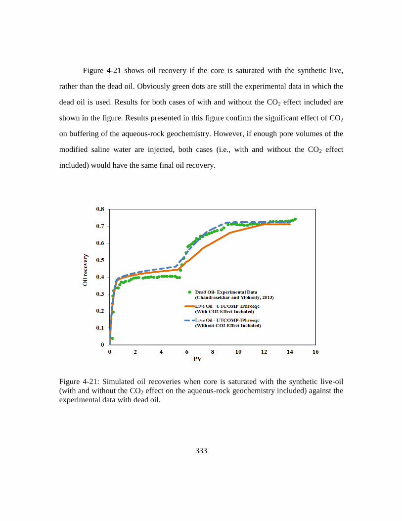
333

Figure 4-21 shows oil recovery if the core is saturated with the synthetic live,

rather than the dead oil. Obviously green dots are still the experimental data in which the

dead oil is used. Results for both cases of with and without the CO2 effect included are

shown in the figure. Results presented in this figure confirm the significant effect of CO2

on buffering of the aqueous-rock geochemistry. However, if enough pore volumes of the

modified saline water are injected, both cases (i.e., with and without the CO2 effect

included) would have the same final oil recovery.

Figure 4-21: Simulated oil recoveries when core is saturated with the synthetic live-oil

(with and without the CO2 effect on the aqueous-rock geochemistry included) against the

experimental data with dead oil.

334

5 Chapter 5: A Mechanistic Integrated Geochemical and Chemical

Flooding Tool for Alkaline/Surfactant/Polymer Floods1

Mechanistic simulation of alkaline/surfactant/polymer (ASP) flooding considers

chemical reactions between the alkali and the oil to form in-situ soap and reactions

between the alkali and the minerals and brine. A comprehensive mechanistic modeling of

such process remains a challenge, mainly due to the complicated ASP phase behavior and

the complexity of geochemical reactions that occur in the reservoir. Due to the lack of the

microemulsion phase and/or lack of reactions that may lead to the consumption of alkali

and resulting lag in the pH, a simplified ASP phase behavior is often used.

In this chapter we couple IPhreeqc with UTCHEM for a robust, flexible, and

accurate integrated tool to mechanistically model ASP floods. UTCHEM has a

comprehensive three phase (water, oil, microemulsion) flash calculation package for the

mixture of surfactant and soap as a function of salinity, temperature, and co-solvent

concentration. IPhreeqc has rich databases of chemical species and also the flexibility to

include the alkaline reactions required for modeling ASP floods. Hence, to the best of our

knowledge, for the first time, the important aspects of ASP flooding are truly considered.

1 Some parts of Chapter 5 are published in the following citation:

Korrani, A. K. N., Sepehrnoori, K., and Delshad, M. 2014b. A Mechanistic Integrated Geochemical and

Chemical Flooding Tool for Alkaline/Surfactant/Polymer Floods. Society of Petroleum Engineers.

doi:10.2118/169094-MS.

Below briefly describes nature of coathors’contribution.

- Kamy Sepehrnoori: The idea of coupling PHREEQC with UTCHEM for mechanistic modeling of

Alkaline/Surfactant/Polymer floods, technical support, and revising the manuscript.

- Mojdeh Delshad: Technical support in applying the UTCHEM simulator for chemical floods and

revising the manuscript.

335

In this chapter we first review the important findings published in the literature on

ASP flooding. An algorithm is then presented for modeling the geochemistry in an

IMPEC (implicit in pressure and explicit in concentration) solution algorithm. Finally, we

show how to apply the integrated tool, UTCHEM-IPhreeqc, to match three different

reaction-related chemical flooding processes: ASP flooding in an acidic active crude oil,

ASP flooding in a non-acidic crude oil, and alkaline/co-solvent/polymer (ACP) flooding.

5.1 ALKALINE/SURFACTANT/POLYMER FLOODING

Surfactant/polymer (SP) flooding is an EOR process in which surfactant is added

to the injected water to lower the interfacial tension (IFT) between the aqueous and oil

phases, increase the capillary number and consequently mobilize the residual oil

saturation beyond that of waterflood (Tavassoli et al., 2014a; 2014b). Polymer is

included in this EOR process for the mobility control purpose. Although the SP process is

very well-established and technically successful, because of high chemical costs, it is not

considered as one of the cost-efficient EOR processes (Kon et al., 2002). For years,

researchers have tried to come up with promising modifications to make the SP process

more economical. Alkaline/polymer (AP) flood is an alternative process proposed to the

SP flooding because the cost of alkali is considerably lower than that of surfactant. The

essence of the AP flooding is to react alkaline agents (e.g., Na2CO3, NaOH, NaBO2,

K2CO3, and KOH) with acidic components in the crude oil and generate the in-situ

surfactant (soap). Similar to the SP process, the role of the polymer is to increase the

sweep efficiency.

336

Figure 5-1 presents how acidic component of the crude oil is partitioned between

the aqueous and the oleic phases and how soap (Aw-) is generated in the aqueous phase.

The partitioning reaction of the acidic component is given in Eq. ( 5.1):

( 5.1)

where

acid component in the aqueous phase

acid component in the oleic phase

Figure 5-1: Equilibria in water/oil/naphthenic acid systems at low pH (Havre et al.,

2003).

This geochemical reaction is known as partitioning reaction with the equilibrium

constant given in Eq. ( 5.2):

( 5.2)

where

.w oHA HA

wA

oA

,o

wwo

HA

HAK

337

partition coefficient of the acid component between the aqueous and oleic

phase

The partitioned acid in the aqueous phase will dissociate in the aqueous phase

according to Eq. ( 5.3):

( 5.3)

With the reaction constant following the equilibrium relationship:

,

w

a

w

H AK

HA

( 5.4)

where

equilibrium constant for the dissociation reaction of the acid component in the

aqueous phase.

Alkaline agents are injected into the reservoir to raise the pH and generate soap

when crude oil has high acid number and to lower the surfactant adsorption among other

benefits. Le Chatelier's principle for geochemical reactions proposes that when a system

at equilibrium experiences a change (e.g., in concentration, partial pressure, and

temperature), the equilibrium shifts to counteract the imposed change and establish a new

equilibrium (Le Chatelier, 1884; Monk, 2008). Hence, based on the Le Chatelier's

principle, more soap (Aw-) is generated if the H

+ concentration of the system is decreased

(see Eq. ( 5.3)).

The H+ concentration can be diminished through injecting the alkaline agents. For

example, injecting Na2CO3 increases the CO3-2

concentration of the aqueous phase which

woK

.w wHA A H

aK

338

shifts the carbonic acid reaction (Eq. ( 5.5)) to the left (based on the Le Chatelier's

principle); hence, H+ concentration of the system decreases and consequently, more soap

is generated. The same principle is applied for other alkaline agents such as NaOH and

NaBO2.

( 5.5)

In the AP process, in one hand, the generated soap (Aw-) has very low optimum

salinity and narrow salinity window (Nelson et al., 1984; Mohammadi, 2008); hence, the

brine salinity should be low enough to achieve the ultra-low IFT. On the other hand,

sufficiently high amount of alkaline agents should be injected to compensate the alkali

consumption by the acidic component; divalent ions in the aqueous; and ion-exchange.

Injecting large amount of alkaline agents increases the salinity of the brine (Peru and

Lorenz, 1990; Mohammadi, 2008; Fortenberry et al., 2013). The dilemma involved in the

AP process makes the process impractical most of the times. It seems that the AP

flooding can be applied only in reservoirs with low salinity brine. Nelson et al. (1984)

solved the AP flooding dilemma by adding small concentration of co-surfactant in the

chemical slug. Co-surfactant favorably increases the optimum salinity to alkali

concentration high enough for deep propagation into the reservoir (Nelson et al., 1984;

Kon et al., 2002; Sheng, 2013). Including the alkaline agents in the SP process makes the

process cost-efficient not only through generating the soap but also the injected alkali can

significantly decrease the surfactant (Song et al., 1995; Al-Hashim et al., 1996; Wang

and Gu, 2003; Hirasaki et al., 2004; Liu et al., 2008; Liu, 2007; Mohan, 2009; Sheng,

2013) and polymer (Song et al., 1995) adsorptions on the rock, alter the wettability of the

2

2 3 32H CO H CO

339

rock (Kon et al., 2002; Wang and Gu, 2003; Liu, 2007; Sundstrom, 2011; Sheng, 2013;

Fortenberry et al., 2013), and accelerate the equilibrium time, shortening the coalesce

time (Jackson, 2006). Several researchers have reported successful laboratory and field

pilot studies of the ASP flooding. Some of these reports are discussed:

Gao et al. (1995) conducted a coreflood using Daqing reservoir core. They

reported incremental oil recovery of 20% and 33% original oil in place (OOIP) after

injecting 0.2 and 0.3 PV of ASP into the core, respectively. Mohammadi (2008)

documented several ASP corefloods conducted at The University of Texas at Austin.

Injecting ASP shows promising results in all the corefloods reported in her dissertation

(with more than 90% recovery of the residual oil in most cases). We model and present

the simulation results of one of the coreflood reported by Mohammadi (2008). Song et al.

(1995) applied ASP flooding on a pilot area (containing 4 inverted five-spot patterns) in

the waterflooded Gudong oil field with the oil viscosity and the acid number of 41.25 cp

and 3.11 mg of KOH/g of oil, respectively. ASP successfully reduced the watercut from

98% to 74.2% with the cumulative oil production of 20,667.7 t (tonnes) from the pilot

(Song et al., 1995). The feasibility of implementing ASP on the Saudi Arabian carbonate

reservoirs was studied in the work of Al-Hashim et al. (1996). Crude oil in this field has

the acid number of 0.3 mg of KOH/g of oil and the viscosity of 0.7 at 90 oC. Na2CO3 and

NaHCO3, the alkaline agents used in this work, showed very promising results in

decreasing the surfactant adsorption. Their results showed that ASP could significantly

improve the oil recovery even in carbonate reservoirs with harsh reservoir condition.

Results presented for one of their coreflood showed 18.2% of OOIP additional oil

recovery after injecting 0.6 PV of ASP chased with 5.66 PV of water in the Arab-D

sample core. Demin et al. (1997) reported the results of the implementation of two ASP

340

pilot tests (i.e., PO and XF pilots) in Daqing oil field (with the acid number of 0.1 KOH

mg/g of oil). Early response was observed when injecting only 0.07 PV and 0.05 PV of

ASP solution in the PO and XF pilots, respectively. Due to the ASP injection, average

watercut of the PO pilot reduced from 88.4% to 68.8% with the 20.8% OOIP incremental

oil recovery over the waterflood. Their estimation for the XF pilot gave 25% OOIP

incremental oil recovery over the waterflood. Due to the promising results observed for

the PO and XF pilot tests, the ASP flooding was further expanded to a larger scale in

Daqing oil field (Yang et al., 2003). Field results were also in line with the pilot tests

where the maximum reduction in the watercut was about 40% (Yang et al., 2003). Demin

et al. (1998) applied the ASP flooding in four inverted five-spot patterns with 4 injectors

and 9 producers. The reduction in watercut started after 0.09 PV ASP injected. By 1998,

the additional oil recovery for the pilot was 12.8% OOIP and the ultimate oil recovery

was estimated to be about 16 to 17% OOIP. ASP flooding in Cambridge Minnelusa field

(located in Wyoming, USA) gave 1.143 MM bbls incremental oil recovery (Vargo et al.,

2000). The implemented design on this pilot was 0.307 PV of the ASP solution that was

followed by 0.297 PV of the polymer slug. Qi et al. (2000) documented the ASP flooding

in the Karamay oil field in China. ASP flooding in this pilot started in 1995 and lasted for

three years. Prior to the ASP injection, NaCl brine was injected for about a year.

Incremental oil recovery due to the ASP injection is 23.15% OOIP with the watercut of

92.5%. The pilot test in Qi et al. (2000) contained 9 production and 4 injection wells in

an inverted five-spot pattern. Xu (2012) simulated two corefloods performed at The

University of Texas at Austin by Pope et al. using ACP flooding (Weerasooriya and

Pope, 2011; Fortenberry, 2013; Fortenberry et al., 2013; Taghavifar, 2014). As the result

of the ACP injection, residual oil saturation reduced from about 45% to 14% in one core

341

(labeled “PCN-1”) and from about 36% to nearly 0% in the another one (labeled “PCN-

4”). PCN-1 is modeled and discussed in this chapter.

Optimization, interpretation, and design of EOR processes require a predictive

model. A predictive model is needed to fully understand the underlying mechanisms

driving the EOR processes. Mechanistic modeling of the ASP flooding is highly

challenging mainly due to the complicated ASP phase behavior and complexity of the

geochemical reactions that occur in the reservoir. UTCHEM, an in-house research

chemical flooding reservoir simulator has a comprehensive three-phase (water, oil,

microemulsion) phase behavior model for the mixture of surfactant and soap as a

function of salinity, temperature, and co-solvent concentration (Bhuyan, 1989;

Mohammadi, 2008). Geochemical module (hereafter, EQBATCH) of UTCHEM was

developed by Bhuyan (1989) and later generalized (UTCHEM Technical Documentation,

2000). EQBATCH takes into account not all but essential geochemical reactions relevant

to ASP flooding such as soap generation, alkali precipitation with aqueous divalents, and

alkaline consumption in ion exchange reactions. Assumptions and limitations of

EQBATCH were previously discussed in Chapter 2. IPhreeqc (Charlton and Parkhurst,

2011) overcomes all the simplifying assumptions and limitations inherent in EQBATCH.

Hence, we coupled IPhreeqc with UTCHEM to build a comprehensive simulator for

mechanistic modeling of ASP floods. Sections below present the procedure through

which we coupled IPhreeqc with UTCHEM.

5.2 COUPLING IPHREEQC WITH UTCHEM FOR MECHANISTIC MODELING OF ASP

Figure 5-2 gives UTCHEM flowchart where we start the simulation at time t after

the initialization step is completed. We solve pressure equation implicitly first and then

solve component concentrations explicitly. The overall concentrations (defined per unit

342

gridblock pore volume) for the volume occupying components (oil, water, co-solvent,

surfactant, and gas) are then used to find phase saturations at each gridblock using

Hand’s rule. The phase saturations are used to calculate the relative permeability and

capillary pressure. For non-isothermal cases, the energy balance equation is solved to

compute the gridblock temperature (see Lashgari et al., 2014a; 2014b for details on

thermal flooding using UTCHEM). Finally, reservoir rock and fluid properties are

updated for the new component concentrations and temperature. For example, if polymer

is considered, water viscosity is calculated as a function of polymer concentration,

effective salinity (which is function of total salinity and divalent concentrations), and

shear rate (see Li and Delshad (2013) and UTCHEM Technical Documentation (2000)

for details on the UTCHEM polymer models). The same algorithm will be followed for

the next time-step until the end of the simulation (UTCHEM Technical Documentation,

2000; Korrani et al., 2013).

Figure 5-2: Simplified UTCHEM calculation flowchart (Korrani et al., 2013).

343

To integrate IPhreeqc with UTCHEM, the UTCHEM computing algorithm is

modified based on the work of Charlton and Parkhurst (2011) as follows:

Once the aqueous geochemical species in UTCHEM are calculated (the

mass conservation equation was previously implemented and verified for

the geochemical elements in UTCHEM by Bhuyan (1989), the IPhreeqc

input is accumulated in the computer memory using AccumulateLine

method available in IPhreeqc;

IPhreeqc is run using RunAccumulated method to calculate the new

equilibrium state for all batch cells;

Use GetSelectedOutputValue method to transfer the results from IPhreeqc

to UTCHEM. The latter includes concentrations for the ions in the

aqueous phase, moles for solid phases, and concentrations of ions on ion-

exchangers, if there is any. We discussed the IPhreeqc methods with more

details in Chapter 2. Figure 5-3 highlights the modified solution algorithm.

Similar to UTCOMP-IPhreeqc, element concentrations in the aqueous phase,

moles for solid phases, and moles for exchangers of each simulation gridblock are

defined in the first time-step through using SOLUTION, EQUILIBRIUM_PHASES,

and EXCHANGE keywords, respectively. For the next time steps, IPhreeqc uses

SOLUTION_MODIFY, EQUILIBRIUM_PHASES_MODIFY (if it is required), and

EXCHANGE_MODIFY (if it is required) rather than the corresponding keywords of

SOLUTION, EQUILIBRIUM_PHASES, and EXCHANGE, respectively, In addition,

we must transport charge balance (CHARGE_BALANCE of IPhreeqc returns this for

each gridblock), total moles of hydrogen (TOTMOLE("H") is used), and oxygen

(TOTMOLE("O") is used) along with the elements present in the system.

344

Similar to PHAST (Parkhurst et al., 2010) transport and the chemical-reaction

calculation are separate in the UTCOMP-IPhreeqc and UTCHEM-IPhreeqc simulators.

There is no iteration between the transport and reaction calculation during a time step. If

kinetic reactions are included in the model, IPhreeqc applies the operator splitting and

separates the chemical equilibrium reactions from the kinetic reactions. In this case,

Newton-Raphson method is first applied to solve the nonlinear chemical equilibrium

equations. An Explicit Runge-Kutta method or CVODE algorithm (Cohen and

Hindmarsh, 1996), for stiff differential equations, are then followed to solve the ordinary

differential equations of the kinetic-reaction equations. Using Runge-Kutta or CVODE

algorithms, IPhreeqc evaluates the reaction rates at several intermediate times within the

overall time interval equal to the transport time step (i.e., the time step in UTCHEM). To

control the errors, IPhreeqc applies an automatic time stepping algorithm when

integrating the kinetic reaction rates (Parkhurst et al., 2010). It is worth noting that the

transport time-step size (i.e., time-step in UTCHEM) is selected based on relative

changes for all the components (UTCHEM User’s Guide, 2011).

345

Figure 5-3: Simplified UTCHEM flowchart after coupling with IPhreeqc (Korrani et al.,

2013).

Including the exchange of the acidic component among the aqueous,

microemulsion, and oil phases is the most important development that needs to be

implemented in UTCHEM-IPhreeqc for mechanistic modeling of ASP. At the

equilibrium state, the acid element (A) is partitioned into three fluid species as HAw,

HAo, and Aw- (soap). These fluid species are respectively carried along with the water,

oil, and surfactant components. Concentrations of HAw, HAo, and Aw- are related to each

other through the aqueous-oleic partitioning and acid dissociation reactions. Hence, these

two reactions (i.e., Eqs. ( 5.1) and ( 5.3)) must be properly included in the IPhreeqc

database when modeling an ASP process using UTCHEM-IPhreeqc.

SOLUTION_MASTER_SPECIES and SOLUTION_SPECIES of IPhreeqc are

used to define new components as representative of the acid component in the aqueous

346

and oleic phases (the total moles of the acid element (A) is the sum of moles in the

aqueous (Aw) and oleic phases (Ao)). Because aqueous reactions in the IPhreeqc database

are defined in the association rather than dissociation form (Parkhurst and Appelo, 2013),

association form of Eq. ( 5.3) is simply included in the IPhreeqc database.

By default, all reactions defined in IPhreeqc must be balanced in both charge and

elemental. However, the identifier “-NO_CHECK” can be used to disable checking the

elemental balance. The aqueous-oleic partitioning reaction (Eq. ( 5.1)) is not completely

balanced in the elements. While equivalent for the hydrogen element is the same in both

sides; this reaction is not balanced in terms of the acid element (Aw in the left side while

Ao in the right side). Hence, we must use the “-NO_CHECK” identifier to be able to

include this reaction in the IPhreeqc thermodynamic database.

The following shows how the acidic/oleic reaction as well as the acid dissociation

reactions can be defined in the IPhreeqc database. In this example, the partitioning

constant and the equilibrium constant for the acid dissociation reaction are assumed to be

10-3.6

and 10-8

, respectively. The value of 59.05 is the molecular weight of the acid

component. IPhreeqc uses molecular weights of the elements only if the concentration

units are mass unit (Parkhurst and Appelo, 1999; 2013).

SOLUTION_MASTER_SPECIES

Aw Aw- 1.0 59.05 59.05 Ao Ao- 1.0 59.05 59.05

SOLUTION_SPECIES Aw- = Aw-; log_k 0 Ao- = Ao-; log_k 0

Aw- + H+ = HAw; log_k +8.0 HAw = HAo; log_k +3.6; -no_check; -mole_balance Aw

347

These reactions are considered along with other aqueous geochemical reactions in

modeling an ASP process in UTCHEM-IPhreeqc. Acid concentration in the oleic phase

(HAo) is defined as an independent aqueous species when Newton-Raphson is applied to

find the equilibrium state (Bhuyan, 1989). That is why the equilibrium constant of both

the partitioning and the acid dissociation reactions are function of relative volumes of

water and oil (Bhuyan, 1989; Mohammadi, 2008). However, in UTCHEM-IPhreeqc only

the constant partition coefficient needs to be defined as a function of volumes of water

and oil. Hence, at each simulation time-step, the partition coefficient is updated and

stored in the computer memory through AccumulateLine of IPhreeqc.

In general water saturation might be different in reservoir gridblocks. Hence, the

equilibrium constant of the partitioning reaction (which is a function of water saturation

of gridblocks) is different for each gridblock. On the other hand, if the same geochemical

reaction with different equilibrium constants is stored in the computer memory, IPhreeqc

considers the last equilibrium constant for geochemical calculations. To this end, if we

accumulate the geochemistry data of the entire gridblocks in the computer memory all at

once, the equilibrium constant of the partitioning reaction evaluated based on the water

saturation of the last gridblock is applied to find the equilibrium state of all gridblocks.

To avoid this inconsistency, we evaluate the new equilibrium state of gridblocks one by

one rather than all together. In other words, when using UTCHEM-IPhreeqc for ASP

floods, the modified geochemistry data of a single gridblock is accumulated in the

computer memory using AccumulateLine. The stored data is then run using

RunAccumulated. Finally, GetSelectedOutputValue is used to transfer the new

equilibrium state of that gridblock to UTCHEM. The same procedure is followed for

348

other gridblocks. Finding the equilibrium state of gridblocks individually, rather than all

together, slows down the simulation to some extent.

As mentioned above, in using IPhreeqc, charge balance and total moles of

hydrogen and oxygen must be transported along with other geochemical elements present

in the system (Charlton and Parkhurst, 2011; Korrani et al., 2013; Korrani et al., 2014c).

For ASP simulations, care must be taken to partition the charge balance and the total

moles of hydrogen and oxygen among different phases. At the equilibrium state, the total

acid element (A) is partitioned into three fluid species as HAw, HAo, and . is the

generated soap and will be used along with the injected synthetic surfactant for the phase

behavior calculations. Phase behavior of the in-situ generated surfactant (soap) can be

defined either the same as or different from that of the injected synthetic surfactant. If the

phase behavior of the soap is different from the injected surfactant, nonlinear mixing rule

is applied to find the combined surfactant and soap phase behavior (Delshad et al., 2013).

Because hydrogen (H) and acid (A) elements are involved in HAw, HAo, and

fluid species, hydrogen (H) and acid (A) elements must be transported differently than

other geochemical elements present in the system. Geochemical elements other than “H”

and “A” are carried by the water component; depending on how water component is

partitioned between aqueous and microemulsion phases corresponding to different

Winsor types, these geochemical elements are partitioned correspondingly. However, the

hydrogen element is not carried only by the water component but also by the oil

component (hydrogen element in the HAw and HAo fluid species are carried along with

water and oil components, respectively). Hence, some amount of hydrogen is partitioned

among the phases corresponding to the water component (i.e., hydrogen element in the

HAw fluid species) and the rest is shared between the phases corresponding to the oil

wA

wA

wA

349

component (i.e., hydrogen element in the HAo fluid species). The same concept applies

for the acid element (A) and the charge balance. Because the acid component is carried

along with water, oil, and surfactant components, HAw, HAo, and are respectively

shared among the phases containing water, oil, and surfactant components. Finally,

because fluid species carries charge, charge balance is carried along with the water

and surfactant components. The amount of charge balance that is transported along with

the surfactant component is and that for the water component is the total charge

balance minus the amount that is transported by the surfactant component (i.e., ).

Table 5-1 summarizes the amount of each geochemical species (i.e., hydrogen, acid

component, charge balance, and other geochemical species including oxygen) carried

along with the volume-occupying components (i.e., water, oil, and surfactant) in

UTCHEM-IPhreeqc.

Table 5-1: How the geochemical species are partitioned among the phases and

transported in UTCHEM-IPhreeqc

Geochemical Element

Amount of the geochemical element carried along with the

volume-occupying components to be partitioned among the

phases

Water Surfactant Oil

Hydrogen (H)

Total hydrogen of the system

minus the amount of hydrogen in

HAo

- HAo

Acid component (A)

Total acid component of the

system minus the amount of the

acid component in Aw- and HAo

Aw- HAo

Charge balance

Lumped charge balance of the

aqueous solution minus the

amount charge in Aw-

Aw- -

Other geochemical

species including

oxygen (O)

Entirely by the water component - -

wA

wA

wA

wA

350

Similar to UTCOMP-IPhreeqc, we also parallelized the geochemistry module of

UTCHEM-IPhreeqc (hereafter, the parallel version of UTCHEM-IPhreeqc). Restart

option is also available in both single- and multiple-processor version of UTCHEM-

IPhreeqc.

5.3 VERIFYING UTCHEM-IPHREEQC AGAINST PHREEQC

We verified our integrated tool, UTCHEM-IPhreeqc against PHREEQC’s single

phase and one-dimensional reactive-transport case studies. UTCHEM-IPhreeqc is

verified for the example problem 11 from Parkhurst and Appelo (2013). The case

description was previously discussed in Section 2.7.2. Figures 5-4 and 5-5 verify the

UTCHEM-IPhreeqc results against PHREEQC for two different dimensionless Peclet

numbers of infinity (or dispersion-free case) and 40, respectively.


(Parkhurst and Appelo, 2013) at Pe=∞.

351


(Parkhurst and Appelo, 2013) at Pe=40.

We verify UTCHEM-IPhreeqc against PHREEQC for another realistic case. The

characteristics for this case are similar to the case previously used in Section 2.8. A 1D

single phase model with 100 gridblocks is used in both UTCHEM-IPhreeqc and

PHREEQC. Aragonite, calcite, celestite, dolomite, halite, strontianite, sylvite, and

witherite are the minerals that are considered. Except calcite and dolomite with initial

concentration of 0.1 moles/kg of water, initial concentrations for other minerals are zero.

It is also assumed that a cation-exchanger with cation exchange capacitance (CEC) of

0.01 moles/kg of water is at equilibrium with the initial solution. Injection rate is 0.0023

ft3/day and the producing well is operating with the constant bottomhole pressure of

4000.0 psi. Produced water from the South American formation water is assumed to be

initially present. Waters with different ion compositions are injected into the case: 0.5

pore volume of IW1 (injection water), 0.5 PW1 (produced water), 0.5 SW1 (fresh water),

352

and finally 1.5 PV of PW1 (produced water). Water compositions for IW1, PW1, and

SW1 are shown in Table 2-23. The phreeqc.dat database of IPhreeqc is applied in this

simulation and around 150 geochemical reactions are activated during this process. The

dimensionless Peclet number is 50.0 in this case. Figures 5-6 through 5-13 present the

verification results between the parallel version of UTCHEM-IPhreeqc (using different

number processor) and PHREEQC for Na+, Ca

+2, Cl

-, HCO3

-, Mg

+2, and Sr

+2, as well as

the pH histories of the aqueous solution produced from the 100th

gridblock.

Table 5-2 shows the computational time of the total simulation versus different

number of processors applied in the simulation (plot is provided in Figure 5-14). Figure

5-15 presents the plot of speedup.

Figure 5-6: History of effluent Na+ concentration (the parallel version of UTCHEM-

IPhreeqc verification against PHREEQC).

353




Figure 5-8: History of effluent Cl- concentration (the parallel version of UTCHEM-


354

Figure 5-9: History of effluent pH (the parallel version of UTCHEM-IPhreeqc

verification against PHREEQC).




355

Figure 5-11: History of effluent HCO3- concentration (the parallel version of UTCHEM-





356




Table 5-2: total computational time


UTCHEM-IPhreeqc

Total

computational

time (seconds)

1PRC 297.9

2PRCs 166.82

4PRCs 81.05

6PRCs 58.57

8PRCs 45.77

10PRCs 36.80

12PRCs 34.82

357

Figure 5-14: Total computational time versus number of processors.

Figure 5-15: Speedup curve for the total simulation versus number of processors.

358

5.4 UTCHEM-IPHREEQC VERSUS UTCHEM-EQBATCH

EQBATCH lacks several capabilities that are included (e.g., considering super-

and under-saturation reactions for the minerals; kinetic; surface complexation; and

irreversible reactions). None of these capabilities can be used when verifying UTCHEM-

IPhreeqc against UTCHEM-EQBATCH (refers to the original UTCHEM where

EQBATCH is used for the geochemical calculations). However, EQBATCH solves

aqueous, solid (with zero for the saturation index), and the exchange reactions. Due to

specific assumptions in EQBATCH, it is not straightforward to verify UTCHEM-

IPhreeqc against UTCHEM-EQBATCH. While IPhreeqc uses activities in finding the

equilibrium state, molalities are used for both aqueous and exchange species in

EQBATCH. Davies (Davies, 1962; Parkhurst and Appelo, 1999; 2013) and the extended

or WATEQ Debye-Huckel (Truesdell and Jones, 1974; Parkhurst and Appelo, 1999;

2013) that is the extended form of Debye-Huckel model (Debye and Huckel, 1954) are

the models (see Appendix A) through which IPhreeqc calculates the activity coefficients

of the aqueous and exchange species. Pitzer and SIT aqueous-association models can be

also used through two separate databases (i.e., pitzer.dat and sit.dat) released with

IPhreeqc.

IPhreeqc uses the product of the activity coefficient times the molality to calculate

the activity of the aqueous species (Parkhurst and Appelo, 1999; 2013). To verify

UTCHEM-IPhreeqc against UTCHEM-EQBATCH, the IPhreeqc database is modified to

make ion activity coefficients of the aqueous species close to one. This approach is

discussed in the work of Farajzadeh et al. (2012) when verifying MPRS-PHREEQC

against UTCHEM-EQBATCH. Towards this goal, WATEQ Debye-Huckel activity

359

coefficient model is applied with a high value (say 1×109) for a

oi and zero for bi

1.

However, this approach does not make the exchange reaction modeling identical in

IPhreeqc and EQBATCH. IPhreeqc calculates the activity of the exchange species by

multiplying the activity coefficients times the equivalent fraction (Parkhurst and Appelo,

1999; 2013). Hence, even with the activity coefficients of the exchange species equal to

unity, IPhreeqc applies the equivalent fractions while EQBATCH uses molalities for the

species on the exchange site. For example, what follows below presents how the Na-Ca

exchange reaction (i.e., 2NaX + Ca+2

CaX2 + 2Na+) is modeled in EQBATCH and

IPhreeqc. This exchange reaction is defined through two half-reactions in IPhreeqc

(Parkhurst and Appelo, 1999; 2013, Farajzadeh et al., 2012):

EQBATCH IPhreeqc

where

activity coefficient of the calcium on the ion exchange X

activity coefficient of the aqueous species i, dimensionless

activity coefficient of the sodium on the ion exchange X

equilibrium constant of the exchange reaction


2

2

22

exNa CaX

KCa NaX

2

2

22

2

2

2

2

2

2

2

CaXNa

ex

NaXCa

CaXNa

CaX NaXK

NaXCa

CaX NaX

2CaX

i

NaX

exK

360

molality of species in the aqueous, mol/kgw (molality is assumed to equal

molarity in this work, mol/L)

An identical single-phase and 1D model is simulated in UTCHEM-IPhreeqc,

UTCHEM-EQBATCH, and PHREEQC. Tables 5-3 and 5-4 present initial and injected

ion concentrations and initial solid concentrations, respectively. Table 5-5 gives the list of

geochemical reactions of the aqueous phase. Figures 5-16 through 5-21 illustrate pH and

fluid species concentration profiles at 0.5 PV of UTCHEM-IPhreeqc, UTCHEM-

EQBATCH, and PHREEQC. In this case, no exchange reaction is included and ion

activities are close to unity in UTCHEM-IPhreeqc and PHREEQC. As the figures show,

results of the three geochemical tools are in good agreements.

Table 5-3: Initial and injected (i.e., pure water) ion concentrations.

Ion CInitail

(mol/l)

CInjected

(mol/l)

pH 12.63 7.0

Ca 0.1092 0.

S 0.0092 0.

Cl Charge balance element

Na 0.1 0.

CO3-2

0.01 0.

Table 5-4: Initial solid concentrations.

Solid Name Formula CInitail (mol/l of PV)

Anhydride CaSO4 0.091

Calcite CaCO3 0.1

361

Table 5-5: Aqueous and solid reactions.

Reaction

eqK

2H O H OH 14.010

2

4 4SO H HSO 1.988102 2

4 4Ca SO CaSO 2.30102

4 4Na SO NaSO 0.7102

3 3Na CO NaCO 1.27102

3 3Na H CO NaHCO 10.07910

2

3 3H CO HCO 10.329102 2

3 3Ca CO CaCO 3.22410

2

2Ca H O CaOH H 12.7810

2 2

3 3Ca CO H CaHCO 11.43510

2 2

4 4Ca SO H CaHSO 3.06810

2Na H O NaOH H 24.010

2 2

4 4CaSO S Ca SO 4.3610

2 2

3 3CaCO S Ca CO 8.4810

362


PHREEQC - the same reactions are considered in three tools with no exchange site

included in the model. Moreover, activity coefficients of the aqueous species are close to

unity in UTCHEM-IPhreeqc and PHREEQC.

Figure 5-17: Ca+2


EQBATCH, and PHREEQC - the same reactions are considered in three tools with no

exchange site included in the model. Moreover, activity coefficients of the aqueous

species are close to unity in UTCHEM-IPhreeqc and PHREEQC.

363

Figure 5-18: SO4-2









364









365

Figures 5-22 through 5-27 compare the results when the exchange reactions

shown in Table 5-6 are included. In solid blue and red lines activity coefficients are

assumed to be one for both aqueous and exchange species in UTCHEM-IPhreeqc and

PHREEQC, respectively. However, as discussed above, even in this case molalities are

used for the aqueous species and fractions of molalities are applied for the exchange

species in UTCHEM-IPhreeqc and PHREEQC. On the other hand, molalities are

considered for the aqueous and exchange species in the current version of UTCHEM-

EQBATCH. Although this has not been pointed out in the work of Farajzadeh et al.

(2012), for the case studied, the discrepancies between the solid green line (i.e.,

UTCHEM-EQBATCH) and solid red (i.e., PHREEQC) and blue (i.e., UTCHEM-

IPhreeqc) lines are insignificant (some discrepancies can be seen for Na+ and Ca

+2 ions).

Included in the Figures 5-22 through 5-27 are also UTCHEM-IPhreeqc and PHREEQC

results (i.e., blue and red dashed lines) in which activity coefficients of both aqueous and

exchange species are included. Table 5-7 summarizes the WATEQ or extended Debye-

Huckel activity coefficient parameters considered for the aqueous and exchange reactions

(values are taken from the phreeqc.dat database of PHREEQC (Parkhurst and Appelo,

2013)). pH, NaSO4-, and NaCO3

- show some discrepancies when the activity coefficients

are included and the difference is more pronounced for Ca+2

, and SO4-2

ions. This clearly

shows the fundamental role of activities in reactive-transport modeling.

Table 5-6: Exchange reactions

Exchange Reaction

exK

Na X H H X Na 1.0102

22Na X Ca Ca X Na 0.810

366


PHREEQC when an exchange site is included in the model– In solid lines molalities are

used for both aqueous and exchange species where in the dashed lines activities (for both

aqueous and exchange species) are applied (no activities have been implemented in the

current version of UTCHEM-EQBATCH).

Figure 5-23: Ca+2


EQBATCH, and PHREEQC when an exchange site is included in the model– In solid

lines molalities are used for both aqueous and exchange species where in the dashed lines

activities (for both aqueous and exchange species) are applied (no activities have been

implemented in the current version of UTCHEM-EQBATCH).

367

Figure 5-24: SO4-2











368











369

Table 5-7: WATEQ or Extended activity coefficient parameters used in the model (values

are taken from phreeqc.dat (Parkhurst and Appelo, 2013))

Reactions Reactions

3.5 0 5.4 0

9.0 0. - -

4.0 0.075 - -

3.5 0.015 6.0 0.

5.0 -0.04 - -

5.4 0. - -

- - - -

- - - -

5.4 0 4.08 0.082

- - 9.0 0.

- - 5.0 0.165

The difference between UTCHEM-IPhreeqc and UTCHEM-EQBATCH results is

more pronounced as more geochemical elements and reactions are included.

Two notes on UTCHEM-IPhreeqc:

Similar to UTCHEM-EQBATCH, geochemical calculations are skipped

for the gridblocks with porosity of less than 0.01 and/or with water

saturation of less than 10-4

.

Although UTCHEM-EQBATCH includes the surfactant associated cation

reactions in batch reaction calculations (UTCHEM Technical

Documentation, 2000), no surfactant associated cations are modeled in the

current version of UTCHEM-IPhreeqc. However, we believe these

reactions can be included in the UTCHEM-IPhreeqc simulator through

0

ia b0

ia b

2H O H OH 2

3 3H CO HCO

H H 2 2

3 3Ca CO CaCO

Na Na 2

2Ca H O CaOH H

Cl Cl 2 2

3 3Ca CO H CaHCO

2 24 4SO SO 2 2

4 4Ca SO H CaHSO

2 23 3CO CO

2Na H O NaOH H

2

4 4SO H HSO 2 2

4 4CaSO S Ca SO

2 2

4 4Ca SO CaSO 2 2

3 3CaCO S Ca CO

2

4 4Na SO NaSO Na X Na X

2

3 3Na CO NaCO H X H X

2

3 3Na H CO NaHCO 2 2

2Ca X Ca X

370

using the SURFACE keyword available in IPhreeqc.

We use UTCHEM-IPhreeqc to model three coreflood experiments: 1) ASP

flooding of an acidic crude oil (active oil), 2) ASP flooding of a non-reactive crude oil,

and 3) ACP flooding of an acidic crude.

5.5 ASP COREFLOOD USING AN ACIDIC CRUDE OIL

Mohammadi (2008) simulated several ASP corefloods with acidic crude oils. We

use UTCHEM-IPhreeqc to model the coreflood labeled “Case AII.” Crude oil has an acid

number of 0.5 mg KOH/g oil. Oil and water viscosities are 19 and 0.5 cp, respectively.

The coreflood configuration is vertical with the injection at the bottom and production at

the top. ASP slug is injected into the core with the oil is at its residual saturation to water

of 0.43. The ASP slug is injected for 0.3 PV and chased with about 1.5 PVs of the

polymer slug. C20-24 IOS (0.1 wt%) and C16 bABS (0.1 wt%) are the injected

surfactants and 0.1wt% Diethylene Glycol Butyl Ether (DGBE) is injected as co-solvent.

3000 ppm of Flopaam 3630S polymer is included in the ASP slug for the mobility

control. Brine salinity of the ASP slug is 27500 ppm Na2CO3 in 0.6 wt% NaCl and that of

polymer slug is 0.6 wt% NaCl. pH of the ASP slug is about 11.5. Further details about

the coreflood are given in Mohammadi (2008).

Using the experimental data, surfactant phase behavior and polymer properties

were previously modeled (Mohammadi, 2008) and directly used in our model. Below

presents the assumptions and matching parameters applied by Mohammadi (2008) in

modeling this coreflood:

Geochemistry: Only the essential reactions for the ASP flooding are considered,

which includes; oil/aqueous partitioning reaction of the acid component,

371

dissociation reaction of the acid component in the aqueous phase; exchange

reaction which exchanges only the hydrogen and sodium ions. Reaction for

H2CO3 and HCO3- were also added to the model. It is assumed that the injection

rate is high enough at the lab scale, which makes the effect of kinetics of the

mineral negligible on the geochemistry of the problem. Hence, no solid reaction is

included when modeling the coreflood (the significance of the kinetic reaction

will be discussed later in this chapter). However, this assumption might not be

valid at the field scale where the fluid velocity is fairly low far from the wells.

Partitioning coefficient, dissociation coefficient of the acid component in the

aqueous phase, cation exchange capacitance of the exchanger, and equilibrium

constant of the Na-H exchange reaction are the adjusting parameters.

Surfactant and Soap Phase Behavior: Upper (CSEU) and lower salinities (CSEL);

and the equivalent weight of the generated soap are matching parameters

(equivalent weight of the surfactant and soap are used when applying the mixing

rule to the surfactant and soap phase behaviors).

Surfactant Adsorption on the Rock: Consistent with the literature, in UTCHEM,

between certain pH threshold values, surfactant adsorption decreases linearly with

increasing pH. The surfactant adsorption is pH-independent for values less than

the lower threshold value and becomes a small constant fraction for the values

higher than the upper threshold (see Mohammadi, 2008). Upper and lower

thresholds used in this model are matching parameters (7 and 13 are values of the

lower and upper thresholds in the tuned model, respectively).

Relative Permeability Curves: Microemulsion residual saturation and endpoint

relative permeability at high IFT (or low capillary number) and water, oil, and

372

microemulsion phase exponents at high IFT are tuning parameters. At low IFT,

relative permeabilities of the oil, water, and microemulsion phases are assumed to

be linear with no residual saturation and 1.0 for both endpoint and exponent.

Experimental measurements are used for the residual oil (i.e., 0.43) and residual

water saturations (i.e., 0.32); and water (i.e., 0.05) and oil (i.e., 0.6) endpoint

relative permeabilities.

To verify UTCHEM-IPhreeqc against UTCHEM-EQBATCH, except for the ion-

exchange parameters and dispersivity coefficients (explained below), everything is

identical to the input file provided by Mohammadi (2008). Hence, similar to Mohammadi

(2008)’s model, we consider only essential reactions such as in-situ generation of soap

and aqueous reactions involving the alkali. An ion exchanger is also included. Sodium

and hydrogen are the only elements involved in the ion exchange reaction. Moreover, ion

activity coefficients of the aqueous and exchange species are close to unity in UTCHEM-

IPhreeqc. Table 5-8 presents the reactions considered in the UTCHEM-IPhreeqc

thermodynamic database to model this coreflood. As discussed earlier in this chapter,

because exchange reactions are modeled differently between IPhreeqc and EQBATCH,

exchange parameters in UTCHEM-IPhreeqc are adjusted to reproduce the same pH lag as

that for UTCHEM-EQBATCH. Physical dispersion (longitudinal dispersivities) was

modified to improve the match.

Figures 5-28 and 5-29 present simulated results against the experimental

measurements for cumulative oil recovery, oil cut, and pressure drop. Figure 5-30 shows

a plot of Winsor's Type III region salinity and the IFT profiles at 0.5 PV. Ultra-low IFT is

achieved when the salinity is between the upper and the lower salinity boundaries (i.e.,

Winsor Type III).

373

Table 5-8: Reactions considered to model the Case AII coreflood

Reaction

Figure 5-28: UTCHEM-IPhreeqc simulation results versus measured data for cumulative

oil recovery and oil cut.

eqK

o wHA HA 3.96610

w wHA H A 8.010

2

3 3CO H HCO 10.324102

3 2 32CO H H CO 16.68910

Na HX NaX H 6.73110

374

Figure 5-29: UTCHEM-IPhreeqc simulation results versus measured data for pressure

drop.

Figure 5-30: UTCHEM-IPhreeqc simulation results for effective salinity, CSEL, CSEU,

and IFT at 0.5 PV.

375

To model this coreflood different mechanisms are considered. Injecting alkaline

agents increase pH, which results in generating more soap. The generated soap along

with the injected surfactant decreases the IFT between oil and water and consequently

mobilizes and produces the residual oil saturation. Also included in the model is the

dependency of the surfactant adsorption on pH. Figure 5-31 quantifies the contribution of

the different mechanisms in increasing the oil recovery during the ASP flooding in this

coreflood.

Figure 5-31: Contribution of different mechanisms in increasing the oil recovery.

To emphasize on the importance of the geochemistry during ASP processes,

sensitivity studies are performed on the pH of the ASP slug and initial acid concentration

of the crude oil (i.e., CAC2I). It is noted that the pH of the ASP slug and the initial acid

concentration in the experiment were 11.5 and 0.00729 mol/l of oil, respectively. Figures

5-32 through 5-35 present the effect of pH of the ASP slug on the cumulative oil

376

recovery, oil cut, the effluent pH history, and the soap total concentration profile at 0.5

PV. As these figures show, the soap total concentration increases by increasing the pH

which results in higher oil recovery. Below certain pH value (9.5 in this case) alkaline

effect is more pronounced in decreasing the surfactant adsorption on the rock surface

than generating soap in-situ. These numerical results and their trend need to be verified

against systematic laboratory experiments. Figure 5-36 illustrates how the oil recovery

changes as a function of the initial acid concentration of the crude oil. Consistent with the

literature, more benefit, can be achieved during injecting ASP in acidic crude oils.

Figure 5-32: The effect of change in the “pH of the injected ASP slug” on Cumulative oil

recovery.

377

Figure 5-33: The effect of change in the “pH of the injected ASP slug” on Oil cut.

Figure 5-34: The effect of change in the “pH of the injected ASP slug” on Effluent pH

history.

378

Figure 5-35: The effect of change in the “pH of the injected ASP slug” on Soap total

concentration profile at 0.5 PV.

Figure 5-36: The effect of change in “the initial acid concentration in the crude oil

(CAC2I)” on cumulative oil recovery.

379

The tuned model is used to investigate the significance of common assumptions

made during modeling an ASP process. To emphasize on the importance of the including

Type III during the ASP modeling, we run the tuned model (through which we match the

experimental data) by considering equal values for Type III upper (CSEU) and lower

(CSEL) effective salinities for both the surfactant and soap. By doing this we ignore the

salinity window and subsequently Type III during the simulation. Figures 5-37 and 5-38

present UTCHEM-IPhreeqc simulation results when Type III is excluded from the

simulation versus the experimental data. There is a significant mismatch in the oil

recovery and pressure drop when Type III is excluded in the simulations. This

emphasizes the importance of the Type III during an ASP process. It is worth noting that

to the best of the author’s knowledge, MPRS-PHREEQC (Wei, 2011; 2012; Farajzadeh

et al., 2012) excludes Type III. This may explain MPRS-PHREEQC difficulties in

matching the pressure drop (see the work of Farajzadeh et al., 2012). The importance of

modeling Type III region was also discussed in the work of Mohammadi (2008).

380


simulation versus measured data for cumulative oil recovery and oil cut.


simulation versus measured data for pressure drop.

381

Ideal solution is another assumption made in ASP modeling (i.e., UTCHEM-

EQBATCH). Also, rather than considering the entire thermodynamically equilibrated

system, the most important reactions (i.e., acid component/alkali reaction and alkali

consumption due to the exchanger or precipitation reactions) are selectively considered.

To investigate the important role of geochemical reactions during an ASP flood, rather

than the limited number of reactions used to model the coreflood, we use different

thermodynamic databases released along with the IPhreeqc geochemical package. Figures

5-39 and 5-40 show the simulated oil recovery and pressure drop, respectively, when

phreeqc.dat, pitzer.dat, llnl.dat, sit.dat, and wateq4.dat geochemistry databases are used.

These databases are different in number of reactions as well as their approach to evaluate

the ion activities. More details on these databases can be found in Parkhurst and Appelo

(1999; 2013). Figures 5-39 and 5-40 show the significance of the number of reactions as

well as ion-association model considered on the performance of the ASP processes. To

make the plots clearer, oil cut plots are excluded from Figure 5-39.

382


databases (with different types of ion-association aqueous models and number of

reactions) versus measured data for cumulative oil recovery.


databases (with different types of ion activities and number of reactions) versus measured

data for pressure drop.

383

The effects of temperature and pressure on geochemical reactions are usually

neglected in reactive-transport modeling. In our previous work, we studied the

temperature and pressure effects in reactive-transport modeling in general (Korrani et al.,

2014c). In this chapter their effects are specifically investigated for ASP processes.

Towards this goal, the tuned model of Case AII is run at different temperatures. Initial

and injected waters have the same temperature (i.e., no energy equation is solved in

UTCHEM-IPhreeqc). Although a non-isothermal case can be modeled using UTCHEM-

IPhreeqc, to isolate the effect of the temperature for the geochemistry of the problem,

transport-related parameters such as viscosity, surfactant and soap phase behaviors, etc.

are assumed to be temperature-independent. Hence, any change in the oil recovery is

solely due to the effect of the temperature on the geochemical reactions. Figures 5-41 and

5-42 present UTCHEM-IPhreeqc simulation results at different temperatures versus the

measured data for the cumulative oil recovery and pressure drop. It is worth noting that

pitzer.dat database is used for all the temperatures. These figures clearly show the

significant effect of the temperature on the geochemical reactions and consequently on

the oil recovery and the pressure drop (i.e., oil recovery decreases by increasing the

temperature). Again, we emphasize on the fact that we assumed the temperature has no

effect on the viscosities and surfactant and soap phase behaviors.

384


thermodynamic database versus measured data for cumulative oil recovery – temperature

effect is isolated to the geochemical reactions.


thermodynamic database versus measured data for pressure drop - temperature effect is

isolated to the geochemical reactions.

385

Figures 5-43 and 5-44 compare simulated results for the oil recovery and the

pressure drop when pressure effect is included in the geochemical calculation. Pressures

shown in the figures are approximately the average pressure during the simulation. To

change the average pressure in the core, we modify the initial and injecting pressures.

Based on the results shown in Figures 5-43 and 5-44 we conclude that the pressure has

minor effect on the geochemical reactions and its effect can be neglected in modeling

ASP processes.


thermodynamic database versus measured data for cumulative oil recovery.

386


thermodynamic database versus measured data for pressure drop.

In modeling the coreflood “Case AII” and also the two more corefloods that will

be presented later in this chapter we assume the injection flowrate at the lab condition is

high enough that with a good approximation we can neglect the kinetics of the minerals

from the geochemistry of the problem (the same assumption was also applied in the work

of Farajzadeh et al. (2012) and Mohammadi et al. (2009)). However, this assumption

might not be valid at the field scale far from the wellbore where the velocity is very low

compared with the velocity at the lab scale. To study the significance of the kinetics in

reactive-transport problems (e.g., ASP flooding and AP flooding) the UTCHEM-

IPhreeqc case based on the example 11 of PHREEQC is considered (this case was

previously used to verify UTCHEM-IPhreeqc against PHREEQC). We include calcite

with initial moles of 7×10-4

in all the cells through using the KINETICS keyword of

IPhreeqc. PHREEQC proposed kinetic reaction rate for the calcite

387

precipitation/dissolution (Parkhurst and Appelo, 1999; 2013) is considered. Figures 5-45

through 5-48 present the produced ion histories at different injection rates. Injection flow

rate of the base case (shown as “q” in the figures) is about 2.3×10-3

ft3/day. Also,

included in the figures is a case in which no calcite is present in the system (shown with

circles). These figures show as the injection rate increases aqueous solution does not have

enough time to equilibrate with the calcite, hence produced ion histories are approaching

towards the case with no calcite included. These figures clearly show that the local

equilibrium assumption holds only at low velocities.

Setting aside the complexity of the modeling of kinetic reactions, including the

kinetics drastically increases the simulation time (5 times or even more). This might be

the main reason that the local equilibrium assumption is usually preferred in modeling

reactive-transport problems. When the local equilibrium is assumed, the kinetic nature of

the minerals can be introduced in the problem through the supersaturation (at low

velocities) and undersaturation (at high velocities) of the minerals. To show this, the

UTCHEM-IPhreeqc case based on example 11 of PHREEQC is again considered but

now calcite is included in the model through the EQUILIBRIUM_PHASES keyword

(rather than KINETICS) of IPhreeqc. Figures 5-49 through 5-52 present the produced

ion histories when different saturation indices are assumed for calcite of the system.

Produced ion histories for the case with the local equilibrium assumption (i.e., zero

saturation index) are shown with circles in the figures. As these figures illustrate, when

the saturation index is negative (i.e., undersaturation) produced calcium concentration is

lower than the case in which the local equilibrium is assumed. On the other hand, more

calcium is produced when the calcite saturation index is positive (i.e., supersaturation).

388

More details on kinetics versus local equilibrium assumption can be found in Zhu and

Anderson (2002).


calcite kinetic reaction is included at different injection rates.

389





390




calcite mineral is included with different saturation index.

391





392



As mentioned earlier in Chapter 2, IPhreeqc provides kinetic, supersaturation and

undersaturation capabilities and also geochemical reactions are the temperature- and

pressure-dependent. Moreover, there are many discussions in the literature on the

importance of surface reactions in carbonate reservoirs (Strand et al., 2006; Austad et al.,

2008; Hiorth et al., 2010; Fathi et al., 2012). While EQBATCH lacks the surface

complexation modeling, IPhreeqc has the capability to model the surface complexation

through different generalized two-layer model (Dzombak and Morel; 1990), a two-layer

model that explicitly calculates the diffuse-layer composition (Borkovec and Westall,

1983), and a non-electrostatic surface-complexation model (Davis and Kent, 1990).

Details on these surface complexation models are beyond the scope of this work and can

be found in Parkhurst and Appelo (1999; 2013).

393

5.6 ASP COREFLOOD USING NON-ACIDIC CRUDE OIL

ASP flood in non-acidic crude oil reservoirs (crude oils with low acid number) is

usually referred to high-pH surfactant/polymer flood. In this process, alkaline agent is

injected as sacrificial agent to improve the phase behavior and decrease the surfactant

adsorption on the rock.

High-pH surfactant/polymer corefloods were performed at UT chemical flooding

laboratory and were simulated by Mohammadi (2008). A coreflood, labeled “BM-07”, is

modeled in this chapter using UTCHEM-IPhreeqc. Table 5-9 presents detailed ion

compositions of the synthetic brine. The ASP slug is injected for 0.15 PV and contains 2

wt% surfactant, 3 wt% ethylene glycol butyl ether (EGBE), 0.85 wt% sodium carbonate,

and 2500 ppm AN125 polymer. The ASP slug is then chased with 0.2 PV of polymer

drive with polymer concentration of 2200 ppm and 1.5 wt% EGBE and 0.65 wt% sodium

carbonate and then followed by 1.5 PV of 1800 ppm polymer. The ASP slug and two

polymer slugs are injected along with the synthetic brine into the core. Using the

experimental data, Mohammadi (2008) documented surfactant phase behavior, surfactant

adsorption, and polymer parameters to model this coreflood using UTCHEM-

EQBATCH. The same parameters are considered in our work. Following presents the

assumptions and matching parameters used in the model:

Geochemistry: Contrary to the work of Mohammadi (2008) where only certain

ions and reactions are considered, we use “phreeqc.dat” database where about 35

reactions are activated. However, the phreeqc.dat database of PHREEQC is

designed for the low-temperature geochemical calculation (Parkhurst and Appelo,

1999). Hence, we assume this database is applicable at 115 oF at which the

coreflood was conducted. Furthermore, we assume the ion-association aqueous

394

model included in the phreeqc.dat database is sufficient to model the coreflood. A

cation exchange site (initially equilibrated with the aqueous solution) is included

in the model. The cation exchange capacitance of the exchanger is a tuning

parameter. To better match the pH, hydrogen is also assumed to be an existing

cation on the exchanger (hydrogen is not an exchanging cation in phreeqc.dat).

The equilibrium constant of the hydrogen half-reaction (i.e., H++X

- ↔HX) is

adjusted in our model. Similar to the coreflood AII, no kinetic reaction is

included. We also tune the partitioning coefficient of the acid component (Kwo)

and the equilibrium constant of the acid component in the aqueous phase.

Relative Permeability Curves: While measured values are applied for the oil and

water residual saturations and endpoint relative permeabilities (Mohammadi,

2008); the oil, water, and microemulsion relative permeability exponents and the

microemulsion residual saturation and endpoint at low capillary number are the

matching parameters. Moreover, linear relative permeabilities are assumed for the

three phases at high capillary number (i.e., zero residual saturation and 1.0 for the

endpoint and exponent).

Surfactant and Soap Phase Behavior: Upper (CSEU) and lower effective salinities

(CSEL) for Type III; and the equivalent weight of the generated soap are

matching parameters.

Surfactant Adsorption on the Rock Surface: Upper and lower thresholds of the

model through which the dependency of surfactant adsorption on the rock surface

is defined in UTCHEM are adjusting parameters (6 and 11 are the lower and

upper thresholds in the tuned model, respectively).

395

Table 5-9: Synthetic brine composition (Mohammadi, 2008)

Ion Concentration (ppm)

Na 900

Ca 20.

Mg 5

K 15

Cl 800

SO4 18

HCO3- 1100

Total dissolved

solids

2858

Figures 5-53 through 5-59 present UTCHEM-IPhreeqc (solid lines) and

UTCHEM-EQBATCH (dashed lines), modeled by Mohammadi (2008), simulation

results against the measured data. Having several capabilities in IPhreeqc, we

significantly improve the match for pH, carbonate, and bicarbonate compared with the

work of Mohammadi (2008). We believe the main reason for this is introducing more

physics to the numerical models by including activities and all possible geochemical

reactions.

396


(Mohammadi, 2008) versus measured data for cumulative oil recovery and oil cut.


(Mohammadi, 2008) versus measured data for pressure drop.

397


(Mohammadi, 2008) versus measured data for surfactant concentration.


(Mohammadi, 2008) versus measured data for EGBE concentration.

398


(Mohammadi, 2008) versus measured data for effluent pH.


(Mohammadi, 2008) versus measured data for CO3-2

.

399


(Mohammadi, 2008) versus measured data for HCO3-.

To show how successfully the injected alkaline agent decreased the surfactant

adsorption, this case is compared against a case where no alkaline agent is injected.

Figures 5-60 and 5-61 present effluent surfactant concentration and the cumulative oil

recovery for the cases compared. As we expect, when no alkaline agent is injected, the

surfactant adsorption increases and consequently oil recovery decreases.

400

Figure 5-60: The effect of “alkaline agent injection” on surfactant adsorption.

Figure 5-61: The effect of “alkaline agent injection” on cumulative oil recovery and oil

cut.

401

To investigate the performance of this coreflood in a large-scale application,

similar design is applied to a real field case with 33×35×16 gridblocks. Out of 18480

gridblocks, 2323 are inactive cells. The permeability/porosity maps are shown in Figures

5-62 through 5-64. This pilot contains 8 production and 3 injection wells. However, 4

injection and 2 production wells are hydraulic wells for conformance. The hydraulic

injection wells are injecting water, which is already at equilibrium with the reservoir

brine. The pilot of study is a five-spot pattern with 4 injection and 1 production wells (see

Figure 5-65). Hydraulic wells are not shown in this figure. Each pilot injection well is

injecting at constant flow rate of about 500 bbl/day and the production well is operating

with the constant bottomhole pressure of 700 psi. Relative permeabilities and initial oil

saturation of the field is used. However, oil; surfactant phase behavior; polymer rheology;

initial brine salinity and composition are based on the coreflood results. Prior to the ASP

flooding, this field was waterflooded for 13.5 years. 2 wt% surfactant, 3 wt% ethylene

glycol butyl ether (EGBE), 0.85 wt% sodium carbonate, and 2500 ppm AN125 polymer

is flooded for 125 days. Polymer drive (i.e., 2200 ppm and 1.5 wt% EGBE and 0.65 wt%

sodium carbonate) is then injected for 119 days. Rather than injecting the last polymer

drive as the design of the coreflood (i.e., 1800 ppm polymer), water is injected for 76

days in the field. The pilot test takes about 320 days.

402

Figure 5-62: Porosity distribution of the field.

Figure 5-63: Absolute permeability (in md) distribution in x- and y-direction of the field.

403

Figure 5-64: Absolute permeability (in md) distribution in z-direction of the field.

Figure 5-65: A five-spot designed for the ASP flooding in the field (hydraulic wells are

not shown).

404

Figures 5-66 through 5-69 show the simulated oil rate produced from the pilot

wells (not the whole field), cumulative oil production produced from the pilot,

bottomhole pressure of one of the pilot injection well, and pH of the produced aqueous

solution using both UTCHEM-IPhreeqc and UTCHEM-EQBATCH. Simulation results

for 320 days waterflooding are also included in these figures for comparison. Although

the simulated cumulative oil recoveries are different between UTCHEM-IPhreeqc and

UTCHEM-EQBATCH, both tools show significant increase in oil recovery for ASP.

UTCHEM-IPhreeqc simulation results appear to be more accurate because more

comprehensive geochemistry is applied in this integrated tool compare with the

simplified EQBATCH geochemistry module in the original UTCHEM. The simulated

produced pH history confirms the difference observed between UTCHEM-IPhreeqc and

UTCHEM-EQBATCH in modeling the coreflood. Figures 5-70 through 5-72 show the

maps of the initial oil saturation; oil saturation before the ASP flooding (i.e., after 13.5

years of water injection); and oil saturation after ASP flooding for the layer 9. The

images indicate a successfully ASP with significant reduction in the residual oil

saturation to nearly zero.

405


oil rate from the pilot.


cumulative oil recovery from the pilot.

406

Figure 5-68: UTCHEM-IPhreeqc and UTCHEM-EQBATCH simulation results for

bottomhole pressure of one of injection well of the pilot.

Figure 5-69: pH of the produced water.

407


before waterflooding.


after 13.5 years of waterflooding.

408


after ASP flooding.

It is worth noting that when scaling up an ASP coreflood to a field application,

care must be taken to properly include the effect of the solution and free gas on the

surfactant and soap phase behavior as well as on the geochemical reactions. We neglected

the effect of gas in the field case studied. The effect of the gas on performance of the

ASP flooding has been discussed in the work of Farajzadeh et al. (2013) and Jang et al.

(2014). It should be also noted that no kinetics of the minerals is included in the model

when scaling up the coreflood to the field. The significance of kinetics of minerals on the

performance of ASP flooding is the scope of our future work.

5.7 ACP COREFLOOD USING ACIDIC CRUDE OIL

ACP flood, if applicable, is a cost efficient alternate process to ASP flooding

(Weerasooriya and Pope, 2011; Fortenberry, 2013; Fortenberry et al., 2013; Taghavifar,

2014). In this process no synthetic surfactant is injected and the alkaline agent-oil

409

reaction is intended to provide adequate amount of surfactant in-situ. Polymer is

responsible for the mobility control and co-solvent is added to the slug to make the in-situ

soap compatible with the polymer injected and also to reduce the microemulsion

viscosity (Xu et al., 2013; Fortenberry et al., 2013). It seems that this process is

applicable in high acidic crude oil with relatively fresh water.

Xu (2012) and Xu et al. (2013) applied the simplified ASP module of UTCHEM

(Delshad et al., 2013) and successfully simulated two ACP corefloods (labeled “PCN-1”

and “PCN-4”). We use UTCHEM-IPhreeqc (“phreeqc.dat” database is used) and model

the “PCN-1” coreflood reported and simulated by Xu et al. (2013). The core is initially at

the residual oil saturation of 0.443. Water and oil viscosities at the reservoir conditions

are 0.53 and 170 cp, respectively. The ACP slug contains 1.5% Huntsmann n-Butyl-5EO

as co-solvent; 6,000 ppm Na2CO3; and 2750 ppm Flopaam 3630S polymer. ACP slug is

injected for 0.5 PV and then followed by 1.4 PV of polymer drive with the composition

of 2250 ppm Flopaam 3630S. Synthetic brine (PCNSSB) with total dissolved solids of

934 ppm is initially in the core (see Table 5-10). More details about this coreflood (e.g.,

activity map, polymer, and microemulsion properties, etc.) can be found in Xu et al.

(2013). Assumptions and matching parameters considered to model the coreflood are

listed below (UTCHEM-IPhreeqc input files are provided in Appendix H):

Geochemistry: We use the phreeqc.dat database to model the PCN-1 coreflood

and all the assumptions addressed for the coreflood BM-07 are applied here. Also,

similar to the BM-07 coreflood, an exchange site is included in the model; and the

hydrogen exchange reaction is considered.

Soap Phase Behavior: The co-solvent and soap phase behavior parameters; and

polymer and microemulsion viscosity and adsorption parameters are matching

410

parameters.

Relative Permeability Curves: The oil, water, and microemulsion relative

permeability exponents and the microemulsion residual saturation and endpoint at

low capillary number are matching parameters and linear relative permeabilities

are assumed for the three phases at high capillary number.

Table 5-10: Composition of synthetic brine (PCNSSB) (Xu, 2012)

Ion Concentration (ppm)

Potassium 11.59

Sodium 300.00

Magnesium 0

Calcium 0

Chlorine 140.81

Sulfate 310.41

Bicarbonate 176.95

Total Dissolved

Solid

939.77

Figures 5-73 through 5-76 compare UTCHEM-IPhreeqc (solid lines) and

UTCHEM-simplified ASP module (dashed lines), modeled by Xu et al. (2013),

simulation results against measured oil recovery, oil cut, pressure drop, average oil

saturation in the core, and the effluent pH history. It is worth noting that the simulated pH

for the simplified ASP module has not been reported by Xu et al. (2013) and modeled in

the current work using the provided input file. Through tuning the microemulsion

viscosity parameters in UTCHEM-IPhreeqc, we significantly improved the match for the

pressure drop and to some extent the effluent pH compared with the work of Xu (2012)

and Xu et al. (2013). The profile of total soap concentration (simulated using UTCHEM-

IPhreeqc) at 0.5 PV is shown in Figure 5-77.

411

Figure 5-73: Simulation results using UTCHEM-IPhreeqc and UTCHEM-simplified ASP

module (Xu et al., 2013) versus measured data for cumulative oil recovery and oil cut of

the ACP experiment.


module (Xu et al., 2013) versus measured data for pressure drop of the ACP experiment.

412


module (Xu et al., 2013) versus measured data for oil saturation of the ACP experiment.


module versus measured data for effluent pH for the ACP experiment. (pH for the

simplified ASP module was modeled in the current work).

413

Figure 5-77: Soap total concentration profile at 0.5 PV.

5.8 PROS AND CONS OF UTCHEM-IPHREEQC

Assumptions made in developing EQBATCH are not always valid. For example,

the ideal solution assumption is not valid unless the water salinity is low. This makes

EQBATCH applicable to limited conditions. EQBATCH is not robust and has numerical

convergence problems for some simulation case studies. This geochemical module is

limited to modeling aqueous, solid (mineral), and exchange (micelles and rock) reactions.

The original intention was for modeling ASP floods with some limited reactions that may

have significant impact on the process. The module is not connected to a geochemical

database and the users need to set up the input which can be tedious. On the other hand,

the full capabilities of IPhreeqc, discussed earlier in this chapter and Chapter 2, (Charlton

and Parkhurst, 2011) are functional in UTCHEM-IPhreeqc. Compared to UTCHEM-

EQBATCH, UTCHEM-IPhreeqc is robust and user-friendly to setup the initial and

injection geochemical states. Geochemical reactions are coupled and highly nonlinear.

414

Iterative methods like the Newton-Raphson method is used to find the solution to this set

of nonlinear equations (i.e., EQBATCH). Two problems should be noted when the

Newton-Raphson method is used for chemical equilibria. First, for this method to

converge the initial guess values must be sufficiently close to the equilibrium values;

second, if the chemical reactions for a set of phases are not linearly independent, this

method may encounter with the singularity in the matrix (Parkhurst and Appelo, 1999).

Both of these problems are frequently occurring in EQBATCH. To avoid the occurrence

of the singular matrix, IPhreeqc/PHREEQC applies an optimization technique proposed

by Barrodale and Roberts (1980) based on modification of the simplex linear

programming algorithm. This optimization technique also provides the opportunity for

IPhreeqc/PHREEQC to add inequality constraints of the solid phases to the problem

(Parkhurst and Appelo, 1999). Moreover, while EQBATCH always uses the aqueous

concentrations of the previous time-step as the initial guesses, PHREEQC applied

rigorous strategies in selecting the initial estimates. More details on how

IPhreeqc/PHREEQC handles the numerical convergence are well documented in

Parkhurst and Appelo (1999; 2013). Similar to UTCOMP-IPhreeqc (described in Chapter

2), the way by which a reactive-transport problem is designed in UTCHEM-IPhreeqc has

been tried to be very close to PHAST, the USGS groundwater simulator (Parkhurst et al.,

2010). In UTCHEM-IPhreeqc, transport parameters, thermodynamic database, and the

initial geochemical states of gridblocks are defined through individual input files which

are respectively equivalent to “prefix.trans.dat”, “phast.dat”, and “prefix.chem.dat” files

in PHAST.

Although the algorithm applied to couple IPhreeqc with UTCHEM is efficient

(see Charlton and Parkhurst, 2011; Muller et al., 2011), UTCHEM-IPhreeqc normally

415

will require longer CPU times and larger amounts of computer memory than UTCHEM-

EQBATCH. For cases studied, the increased computational time using UTCHEM-

IPhreeqc compare with UTCHEM-EQBATCH per time step and for the total simulation

time ranges from a factor of 1.0 to 2.9 and 1.5 to 8.9, respectively. The CPU time

required to model a reactive-transport model using UTCHEM-IPhreeqc depends on the

number of gridblocks; number of aqueous species (this was not observed in MPRS-

PHREEQC (Wei, 2012)); number of reactions and the ion-association aqueous model

applied or in other words the database used for the simulation (e.g., Table 5-11 shows the

CPU time when different databases used to produce the results presented in Figures 5-39

and 5-40); the initial gridblock conditions (e.g., kinetics significantly slows down the

simulation, as it has been also reported for MPRS-PHREEQC (Wei, 2012)); and the

injected fluid composition. It appears that the difference between the total simulation

time of UTCHEM-IPhreeqc and UTCHEM-EQBATCH is more pronounced for large

cases (the more gridblocks the larger difference). For the field case studied in this work

(with 16157 active gridblocks), UTCHEM-EQBATCH is about 36 times faster than

UTCHEM-IPhreeqc (3.9 hrs versus 143.2 hrs, see Table 5-12). However, it should be

noted that for the field case the number of geochemical reactions (in other words, number

of equations in terms of geochemistry that is solved per time-step) in UTCHEM-IPhreeqc

(i.e., 35 reactions) and UTCHEM-EQBATCH (i.e., 9 reactions) is different. As shown in

Table 5-11, the computational time to model a reactive-transport model highly depends

on the number of active reactions and the ion-association aqueous model applied (the

phreeqc.dat database of PHREEQC was used for the field case). The observed increased

in the CPU time of UTCHEM-IPhreeqc (in which the coupling approach is close to hard

coupling) is consistent with that of PHAST of the USGS (Parkhurst et al., 2010) and

416

PHT3D (Appelo and Rolle, 2010) but not consistent with the claim reported for MPRS-

PHREEQC in which geochemical calculation, through calling PHREEQC, slows down

the simulation by less than three times in a 3D case with 29934 active gridblocks when a

single processor is used (Wei, 2012). In PHAST, PHREEQC has been hard coupled with

HST3D (i.e., a transport simulator) (Parkhurst et al., 2010) and in PHT3D, PHREEQC is

hard coupled with MODFLOW-2000 and MT3DMS, as the transport simulator, (Appelo

and Rolle, 2010). PHAST and PHT3D have been designed for groundwater modeling.

The difference between the increase in CPU time per time step and for the total

simulation time in UTCHEM-IPhreeqc reveals the fact that “time-step” does not build up

in UTCHEM-IPhreeqc as it increases in UTCHEM-EQBATCH. Our investigations show

that frequently, charge balance is the controlling element for the time step size. It is

reminded that charge balance and total moles of hydrogen and oxygen must be

transported in UTCHEM-IPhreeqc (Charlton and Parkhurst, 2011; Korrani et al., 2013;

Korrani et al., 2014c). For the time being, charge balance and total hydrogen and oxygen

affect the time-step through the same automatic time-step algorithm used for other

geochemical species. Literature shows other strategies that can be applied to diminish the

CPU time involved in modeling reactive-transport problems (De Lucia and Kuhn, 2013).

We applied Message Passing Interface (MPI) (Barney, 2009) and parallelized the

geochemistry module of UTCHEM-IPhreeqc to compensate for the increase in the CPU

time. Figures 5-78 and 5-79 respectively present the total simulation time and speedup

using different number of processors to simulate the same field case presented earlier in

this chapter (corresponding CPU time values are shown in Table 5-12). Simulations were

run on Lonestar-cluster of Texas Advanced Computing Center (TACC) at The University

of Texas at Austin. TACC characteristics were previously described in Chapter 2. As

417

Figure 5-79 shows, the speedup is; super-linear when number of processors is less than

16; is linear when the number of processor is equal to 16; and sub-linear afterwards. The

same trend was observed for other large cases studied in Chapter 2 on UTCOMP-

IPhreeqc (particularly when the number of gridblocks is above 10,000). The maximum

time limit for the jobs submitted to TACC is 24 hours. Hence, for the cases when 1, 2,

and 4 processors is used the total simulation time beyond 24 hours is estimated using the

remaining number of time steps (which can be found from the cases finished within 24

hours) multiplied by the average time spent per each time step. The average time spent in

each time step is 13.6, 5.9, and 3.3 seconds when 1, 2, and 4 processors are used,

respectively. Based on the results presented, we conclude that UTCHEM-IPhreeqc with

single processor is suitable for lab scales (less than 1000 gridblocks). However, at least

10 processors (the most decrease in the CPU time occurs when 10 processors are

considered) are required to use UTCHEM-IPhreeqc integrated tool for large-scale field

applications.

Table 5-11: Comparison of the CPU time using UTCHEM-IPhreeqc with different

thermodynamic databases released with IPhreeqc (Charlton and Parkhurst, 2011)

Database Total CPU time (seconds)

sit.dat 6598.4

llnl.dat 4647.2

wateq4f.dat 1165.3

pitzer.dat 805.9

phreeqc.dat 633.3

418

Table 5-12: Comparison of the CPU time between UTCHEM-IPhreeqc with different

number of processors and UTCHEM-EQBATCH

No. of processer(s) Total

computational

time (hrs)

Speedup

UTCHEM-EQBATCH-1PRC 3.9

UTCHEM-IPhreeqc-1PRC 143.2* 1.0

UTCHEM-IPhreeqc-2PRCs 58.6* 2.4

UTCHEM-IPhreeqc-4PRCs 30.1* 4.8

UTCHEM-IPhreeqc-6PRCs 19.6 7.3















*time beyond 24 hrs is estimated based on the average time spent in each time step.

419

Figure 5-78: Computational time versus number of processors using UTCHEM-IPhreeqc

for the field case.

Figure 5-79: Speedup versus number of processors using UTCHEM-IPhreeqc for the

field case.

420

6 Chapter 6: Scale Deposition and Groundwater Modeling Using

UTCOMP-IPhreeqc and UTCHEM-IPhreeqc

Both UTCHEM-IPhreeqc and UTCOMP-IPhreeqc simulators can be applied to

comprehensively model variety of reactive-transport problems such as scale deposition,

groundwater, matrix acidizing, and CO2 sequestration modelings. Scale deposition and

groundwater modelings are briefly discussed in the chapter.

6.1 SCALE DEPOSITION MODELING

The precipitation of solid minerals from brine is known as scale precipitation in

the oil industry. Oilfield scales result from changes in the physicochemical properties

(pH, temperature, pressure, etc.) of the produced fluids and/or the major source of scale

which is the chemical incompatibility between waters of different compositions (e.g.,

formation brine and injection brine) (Mitchell et al., 1980; Mackay, 2003; Moghadasi et

al., 2003b; Moghadasi et al., 2003a; Merdhah and Yassin, 2008; Merdhah and Yassin,

2009; Elmorsey, 2013). Hence, before injecting water into the reservoir, it must be

monitored for chemical compatibility with the reservoir brine particularly nowadays that

the new technology of low (or modified) salinity waterflooding has become popular in

the oil field industry (as discussed in Chapters 3 and 4).

Scale deposition inflicts the most serious oilfield problems to water injection

systems primarily when two incompatible waters are involved. Moreover, the risk posed

by deposition of mineral scales to the injection and production wells during such

operations has been studied extensively. Precipitation of mineral scales causes many

problems in oil and gas production operations, such as formation damage, production

421

losses, increased workovers in producers and injectors, poor injection water quality, and

equipment failures due to deposit due to corrosion.

Common scales include calcium carbonate and barium and strontium sulfates

(Wright et al., 1994; Yeboah et al., 1993; Merdhah and Yassin, 2009). The sulfate scales

are generally the result of mixing incompatible waters (Merdhah and Yassin, 2009).

Sulfate scales can cause severe operational problems when sulfate-rich water, such as

seawater, is used to waterflood oil reservoirs with high concentrations of barium and/or

strontium in the formation water. Calcium carbonate may be formed in reservoirs

containing CO2 in the associated gas. However, scales are not limited to these minerals

and there have recently been reports of unusual scale types, such as zinc and lead sulfides

(Collins and Jordan, 2003; Okocha and Sorbie, 2013) or iron oxides, iron sulfides and

iron carbonate (Merdhah and Yassin, 2008; Okocha and Sorbie, 2013). The most

common oilfield scales are listed in Table 6-1 along with the primary variables that affect

their solubility (Moghadasi et al., 2003b).

Table 6-1: Common scales in oilfield damage (Moghadasi et al., 2003b)

Name Chemical Formula Primary Variables

Calcium Carbonate CaCO3 Partial pressure of CO2, temperature, total

dissolved salts, pH

Calcium Sulphate:

Gypsum

Hemi hydrate

Anhydrite

CaSO4.2H2O

CaSO4.1/2H2O

CaSO4

Temperature, total dissolved salts

Barium Sulfate BaSO4 Temperature, pressure, total dissolved salts

Iron Compounds:

Ferrous Carbonate

Ferrous Sulphate

Ferrous Hydroxide

Ferric Hydroxide

FeCO3

FeS

Fe(OH)2

Fe(OH)3

Corrosion, dissolved gases, pH

422

The severity of scales may significantly change from one reservoir to another and

even in the same field over time due to variation of temperature and pressure. Many cases

of oil well damages due to scales of calcium carbonate, calcium sulfate, strontium sulfate,

and barium sulfate have been reported. Some of these reports are discussed next.

Mitchell et al. (1980) reported serious plugging of the wells in the Forties field

due to scales caused by mixing of Forties formation and injection waters and

precipitation of calcium carbonate from due to variations in pressure and temperature in

the production system.

Both carbonate and sulfate scales have had a major influence on production from

the Glamis field. Carbonate deposited within tubes during water production and sulfate

scales appeared at the perforations, following seawater breakthrough. Downhole injection

and inhibitor squeezing are tried to inhibit scaling problems (Wright et al., 1994).

Tjomsland et al. (2001) reported the scaling problem in the Veslefrikk field of the

Norwegian sector of the North Sea. Seawater was injected into this field for the purpose

of pressure maintenance. Comparing to other North Sea formation waters, severe scale

formation had been identified. This is probably due to high reservoir temperature of 125

oC and comingled production. BaSO4 is reported to be the most important type of scale in

this field. However, carbonate scale may also cause problems as pressure decreases in

this field.

Injected seawater mixing with aquifer brines is the main reason behind the scaling

in the Alba field in the North Sea (Paulo et al., 2001). Sulfate scale deposition near the

injection and production wellbores caused considerable disruption to hydrocarbon

production after water breakthrough.

423

Qing et al. (2002) documented the scale precipitation during ASP flooding in the

Daqing oil field in China. Silicate deposition caused frequent downhole operation failures

in the producer tubings. The alkaline agent (NaOH) reacts and dissolves the reservoir

rock, the dissolved materials plug the porous media or will propagate towards the

production wells. Wang et al. (2004), Kazempour et al. (2012; 2013), Alwi et al. (2013),

and Hunter et al. (2013) also investigated the significance of scales and/or the water-rock

interaction during the ASP or high-pH enhanced oil recovery floods.

Continuous precipitation of calcium sulfate caused the oil production to decrease

to almost one tenth of the typical rate in Gemsa oil field in Egypt. Water incompatibility

between the formation water and the injection water was offered as the main reason for

the calcium sulfate precipitation. Several screening tests were conducted to find a suitable

chemical to remove this scale. Elmorsey proposed a highly efficient new chemical, SAG-

01, as a good calcium sulfate remover (Elmorsey, 2013).

Moghadasi et al. (2003b) reported severe formation damage occurred in Siri field

in Iran. Water injection in Siri commenced in 1984 with 9100 bbl/day for pressure

maintenance and increasing oil recovery purposes. However, a rapid decrease was seen in

the injectivity of the injection well, where by 1990 they were able to inject only 2200

bbl/day and finally stopped the water injection in this field. Sulfate and carbonate are two

main types of scale reported for this field.

Scale removal is not only expensive but sometimes nearly impossible to achieve

(particularly for BaSO4), it is therefore scale prevention is preferred compared to its

removal using chemical inhibitors or mechanical treatments. Hence, modeling and

prediction of scale is needed for field developments. Several researchers have tried to

quantify the reservoir permeability impairment due to scale precipitations. For example,

424

Ohen and Civan (1989) proposed a model for the prediction of petroleum reservoir

permeability impairment based on the solid-liquid interactions. They considered

combined effects of clay swelling, external particles invasion, fines generation,

migration, and retention in their model. Mikhailov and Chirkov (2010) also studied

methods to upscale the scaling from the laboratory to the field by taking into account the

process of formation damage during reservoir development. Their analysis on the

laboratory experiments results shows that permeability has similar kinetics of alteration

for different damaging mechanisms. Many other researchers have tried to quantify the

scaling problems (Liu and Civan, 1995; Chekani and Mackay, 2006; Civan, 2007;

Fadairo et al., 2008; Lohne et al., 2009; Bedrikovetsky et al., 2010).

In general, due to the complexity of the precipitation kinetics and ion

exchange/chemical reaction processes, geochemical-based models to quantify amount of

scales are fairly simplistic. They have neglected various important aspects, such as ion

activity coefficients (by assuming ideal solutions), temperature, and pressure effects on

geochemical reactions. As a result, large errors may occur in scale prediction in some

cases. In some other models, a specific ion effect is considered where solubility and scale

formation is predicted only for one mineral. In these models, the effect of scale formation

of other minerals in the same solution is simply ignored. Hence, the need to develop an

accurate, reliable, and easy-to-use model for predicting the formation of the common

oilfield scales is the aim of this section. IPhreeqc provides factors neglected by the

current models. In this work, we develop UTCHEM-IPhreeqc further to consider the

comprehensive geochemistry for the scales predictions for field applications. However,

similar developments can be implemented in the UTCOMP-IPhreeqc simulator.

425

6.1.1 Quantifying Scales

Scales are quantified by including the dissolution or the precipitation of all

minerals (either initially present or precipitated later due to the injected waters) on the

reservoir porosity and consequently on the permeability. Eq. ( 6.1) updates the porosities

in each gridblock and time-step

( 6.1)

where

time update of porosity in ith

gridblock

current time step porosity of the ith

gridblock

change in concentrations (moles) of the κth

solid of the current time-step

(EQUI_DELTA of IPhreeqc is used to find this value for each solid)

gram formula weight of the solid κ (GFW along with PHASE_FORMULA of

IPhreeqc return this value for each solid phase)

density for the κth

solid

the ith

gridblock bulk volume

Δnk in Eq. ( 6.1) is negative (porosity increases) while Δnk is positive (porosity

decreases) for solids that are precipitating.

Three common permeability-porosity approaches (Modified Fair-Hatch, MFH,

(Chadam et al., 1986), Kozeny-Carman, KC, (Kozeny, 1927; Carman, 1956), and Verma-

Pruess, VP, (Verma and Pruess, 1988)) are implemented in UTCHEM-IPhreeqc to reflect

the change in porosities and the resulting change in permeabilities (the same relationship

is used to modify the x-, y-, and z-direction permeabilities). These models are described

1 ,

k k

kn n ki i

Bi

n Mw

V

1n

i

n

i

kn

kMw

k

BiV

426

as follows (in all of the models, ki and ϕi are absolute permeability and porosity of

gridblock i and (n+1) and (n) superscripts are time-steps).

The permeability-porosity model was proposed by Kozeny (1927) and later

modified by Carman (1956) referred to KC. KC model considered the porous medium as

a bundle of cylindrical pores. The KC equation has the form of

( 6.2)

Fair-Hatch, FH, model was derived from dimensional analysis and validated

experimentally (Bear, 2013). Later Chadam et al. (1986) modified this model as

( 6.3)

where ϕf is the final porosity after all the dissolutions (or the precipitations) have

occurred and E1 is an arbitrary constant (matching parameter).

Verma and Pruess (1988) derived a permeability-porosity relationship from a

pore-body-and-throat model in which permeability can be reduced to zero with a finite

(critical) porosity remaining as follows (see Eq. ( 6.4)):

( 6.4)

where

3 21 1

1

1.

1

n n ni i i

n n n

i i i

k

k

22 2

3 31 11

2 21 13 3

1

1,

1

n nn ni f ii i

n nn n

i ii f i

Ek

k E

1 1

,

nn ni i c

n n

i i c

k

k

427

critical porosity at which permeability reduces to zero (it was proposed to be

0.8 of the initial porosity of gridblock i

a power law exponent

Parameters ϕc and n in Eq. ( 6.4) are medium-dependent.

6.1.2 Synthetic Case Study

A synthetic five-spot pattern (see Figure 6-1) is modeled using the UTCHEM-

IPhreeqc integrated simulator. High resolution grid near the injection well is

recommended. Reservoir formation is carbonate (50 vol% dolomite and 50 vol% calcite)

with the initial porosity of 0.25. The initial pressure, temperature, and water saturation

are 4890 psi, 219 oF, and 0.3, respectively. The permeability is homogenous and isotropic

and equal to 100 md. Four production wells are operating with constant bottomhole

pressure, while the injection well is injecting water at the reservoir temperature with

constant flowrate of 0.1 PV/year. T-Block formation water with ion compositions

presented in Table 6-2 (Mazzolini et al., 1992) is assumed to be the water initially present

in this reservoir. Seven different water compositions (see Tables 6-3 and 6-4) are then

injected to investigate their impact in generating scales in the reservoir. Verma-Pruess

model (Verma and Pruess, 1988) with the power law exponent of 3.0 is used in this

simulation study (based on the initial porosity; the critical porosity is 0.2). As pointed out

previously, keeping the same initial water, depending on the injection water, the possible

solids considered in Eq. ( 6.1) are different. For example, when the injection water is

Solution#1 (see Table 6-3), solids considered are: anhydrite, aragonite, barite, calcite,

celestite, dolomite, gypsum, halite, strontianite, sylvite, and witherite, while if the

injection water is Solution#5 (see Table 6-4), 10 more solid phases (Fe(OH)3(a),

FeS(ppt), goethite, gypsum, hematite, jarosite-K, mackinawite, melanterite, pyrite, and

c

n

428

siderite) should be included in the simulation. PHREEQC (Parkhurst and Appelo, 2013)

is run externally using the initial (connate) and the injection solutions to find all the

possible solids involved.

Figures 6-2 and 6-3 present porosity and permeability of the injection gridblock

during injection of different solutions into the reservoir. As these figures demonstrate,

different solutions show significantly different effects on the reservoir properties. The

precipitation of different scales, solutions numbers 1, 3, 5, 6, and 7 drastically reduce

porosity and permeability of the injection gridblock whereas solutions numbers 2 and 4

seem compatible with the connate water without reducing porosity and permeability. In

fact, when solution #4 is injected, solid dissolution, rather than precipitation, occurs

which enhances the porosity and permeability of the injection gridblock. However, it

should be noted that our model is very simple that does not take into account the damage

due to potential clay swelling, if any present in the system. Figures 6-4 and 6-5

demonstrate permeability maps of near the injection well at PV=0.1 for solutions #1 and

7, respectively. As these figures present, the main precipitations (or dissolutions) occur

near the injection well and reduces away from the well.

429

Figure 6-1: The schematic of 2D model and well locations for synthetic case study.

Table 6-2: Initial water composition used in the synthetic case study

Ions T-Block formation water

(Mazzollni et al., 1992)

(mg/l)

Na 36360

K 1720

Mg 365

Ca 3790

Sr 355

Ba 930

Cl 65840

S 2

HCO3- --

Alkalinity 560

430


synthetic case study

Ions Solution#1

(Al-Harrasi et al.,

2012)

(kg/m3)

Solution#2

(Dang et al., 2013)

(LoSal®1

-

composition)

(mol/l)

Solution#3

(Dang et al., 2013)

(Sea water-

composition)

(mol/l)

Solution#4

(de Bruin, 2012)

(LSW

composition)

(ppm)

Na 59.970 0.01326 0.45011 295

K -- 0.00006 0.01006 --

Mg 2.153 0.00018 0.04451 --

Ca 11.618 0.00148 0.01299 --

Sr -- -- -- --

Ba -- -- -- --

Cl 118.791 0.01661 0.52513 455

S 0.689 0.00001 0.02401 --

HCO3- 0.009 -- -- --


synthetic case study

Ions Solution#5

(Elmorsey et al., 2013)

(Nukhul Formation)

(mg/l)

Solution#6

(Kazempour et al., 2013)

(Injection water)

(ppm)

Solution#7

(Kazempour et al., 2013)

(Produced water)

(ppm)

Na 60146 2083 2430

K 12709 75 66

Mg 1145 50 47

Ca 6625 310 300

Fe 4.46 -- --

Sr 393 28 26

Ba 1.296 70 20

Cl 120104.6 3926 4343

F 47.50 -- --

Br 519 -- --

S 685.25 -- --

HCO3- 199.8 928 512

1 LoSal

® is the trademark of BP p.l.c

431

Figure 6-2: Porosity of the injection gridblock versus injected pore volume for different

solutions.

Figure 6-3: Permeability of the injection gridblock versus injected pore volume for

different solutions.

432





433

6.2 GROUNDWATER MODELING

Considering water saturation equal to one, both the UTCHEM-IPhreeqc and

UTCOMP-IPhreeqc (water saturation is 0.999 for water single-phase flow in UTCOMP-

IPhreeqc) simulators can be applied for groundwater modeling. As mentioned previously,

these simulators have been tried to be very similar to PHAST of the USGS groundwater

simulator (Parkhurst et al., 2010), in terms of designing a model and the computational

algorithm. However, UTCHEM-IPhreeqc is preferred over UTCOMP-IPhreeqc for

groundwater modeling. The reason is, through ICF keyword available in UTCHEM-

IPhreeqc, one can skip extra calculations for components excluded from the simulation.

For example, oleic, surfactant phase behavior, and polymer calculations can be easily

excluded from the simulation using UTCHEM-IPhreeqc. However, UTCOMP-IPhreeqc

has been designed based on the assumption that the hydrocarbon phase is always present

in the system. Hence, hydrocarbon phase behavior calculations are performed at all times

(by using the ISINGL keyword available in UTCOMP we can skip the phase composition

calculations for single hydrocarbon phase). That is why water saturation must be 0.999,

rather than 1.0, even for single-phase flow of water in UTCOMP-IPhreeqc.

A synthetic case is designed using UTCHEM-IPhreeqc. Figure 6-6 shows

reservoir geometry and wells locations and Table 6-5 summarizes case descriptions.

Also, Figure 6-7 illustrates x- and y-direction permeability distributions and Figure 6-8

presents the porosity distribution of the model (porosity and permeability distribution

data are taken from Case Study 28 of Li (2012)). The Endicott connate water (see Table

2-20) is initially present in the system. All the solids presented in Table 2-21 are included

in the model. Saturation index and initial mole of the entire solids are set to zero. Six

injection wells are injecting Endicott seawater (see Table 2-20 for the ion compositions)

434

at constant flowrate of 1123 ft3/day into the reservoirs. Production wells are operating at

constant bottomhole pressure of 1000.0 psi. The simulation was carried out on TACC

facilities (see Chapter 2 for TACC characteristics). Using 120 computing processors,

after 24 hours, which is the upper limit to submit a job in TACC, about 0.325 PV of the

Endicott seawater is injected into the reservoir.

Figures 6-9 through 6-14 illustrate maps of some fluid species (Ba+2

, Ca+2

,

CaSO4, Cl-1

, Mg+2

) and pH of the solution for the last layer at about 0.325 PV. Contrary

to the fluid species that show either continuous decreasing (e.g., Ba+2

) or increasing (e.g.,

Ca+2

) trend from the injection to the production well, solution pH is low at the front and

starts increasing near the injection wells.

Figure 6-6: Well locations in the 3D case considered for groundwater modeling.

435

Figure 6-7: Distribution of the absolute permeability (in md) in the x- and y-direction for

the 3D case.

Figure 6-8: Distribution of the porosity in the 3D case.

436


No. of gridblocks 100,000 (100×100×10)

Δx(ft) 25.0

Δy(ft) 25.0

Δz(ft) 2.0

Permeability (md)



z-direction 10.0



) 0.


) 0.





3 producers


437

Figure 6-9: Ba+2


at 0.325 PV.

Figure 6-10: Ca+2


at 0.325 PV.

438

Figure 6-11: CaSO4 concentration (in mol/l) map of layer 10th

at 0.325 PV.

Figure 6-12: pH map of layer 10th

at 0.325 PV.

439

Figure 6-13: Cl-1


at 0.325 PV.

Figure 6-14: Mg+2


at 0.325 PV.

440

7 Chapter 7: Conclusions and Recommendations for Future Research

This chapter presents the summary and the conclusions of this dissertation and

provides some recommendations for further extensions of this work.

7.1 SUMMARY AND CONCLUSIONS

In the following, we present the summary and conclusions of this study:

In this dissertation, we modeled low (or modified) salinity waterflooding

mechanistically and comprehensively.

Because in low salinity water injection, only water with the modified ion

concentrations is injected into the reservoir, it appears no matter the manner

and details of the mechanism, the improved oil recovery must be due to the

ions and geochemical reactions. Hence, we believe mechanistic modeling of

this process is possible only by including geochemical reactions.

In line with several experimental observations published in the literature we

hypothesized that wettability alteration is the underlying mechanism in low

(or modified) salinity waterflooding in both sandstone and carbonate

reservoirs. However, the mechanism through which rock wettability changes

is different in sandstone and carbonate reservoirs.

To handle the complicated geochemical reactions involved in low salinity

waterflooding, we first integrated EQBATCH, a geochemical module

previously developed by Bhuyan (1989), to UTCOMP, The University of

Texas at Austin in-house compositional reservoir simulator. However, the

physics in EQBATCH is limited and also EQBATCH is not robust due to

numerical convergence problems. To overcome the issues involved in

441

EQBATCH, we coupled IPhreeqc (Charlton and Parkhurst, 2011), the state-

of-the-art geochemical package of the USGS, with UTCOMP, to generate a

robust, accurate, and flexible integrated simulator (i.e., UTCOMP-IPhreeqc)

to model low salinity waterflooding mechanistically based on geochemical

reactions. We parallelized the geochemistry module of UTCOMP-IPhreeqc

for large scale reservoir simulation applications.

Thermodynamic constraints, equality of components fugacities and pseudo-

fugacities (defined in this dissertation) in all phases, were used to explicitly

include the buffering effect of the hydrocarbon phase on the aqueous-rock

geochemistry in UTCOMP-IPhreeqc.

We presented the importance of ion activities, temperature, and pressure on

reactive transport modeling.

UTCOMP-IPhreeqc is flexible enough to allow implementation of a variety of

geochemically based models of low salinity water injection. A model based on

the interpolating relative permeability and capillary pressure as a function of

total ionic strength was implemented along with two more direct and

mechanistic models (based on the fraction of organometallic components on

the exchanger; based on change in moles of the organic oil component in the

surface complex) in UTCOMP-IPhreeqc to model low salinity waterflooding

in sandstone reservoirs.

UTCOMP-IPhreeqc was used to match both oil recovery and produced ion

histories for Kozaki (2012)’s experimental coreflood (Berea sandstone core)

as well as the Endicott field trial (sandstone reservoir). Key conclusions from

the modeling are

442

- Buffering of CO2 from the oil phase accounts for the trend of decreasing

pH seen at the Endicott trial

- Quantitative modeling shows that the mechanisms proposed by

RezaeiDoust et al. (2011) do not account for the observed alkalinity and

production of iron during the Endicott trial.

We implemented the model proposed by Hiorth et al. (2010) in UTCOMP-

IPhreeqc to take into the account the wettability alteration and mechanistically

model the modified salinity waterflooding in carbonate reservoirs. This model

assumes during this process, calcite is dissolved and liberates the adsorbed oil

from the surface; hence, a fresh surface leaning more towards water-wetting is

created.

We hypothesized that calcite dissolution model should perhaps be generalized

to include the dissolution of entire spectrum of existing minerals, not a

specific mineral type. Dissolution, if occurring on any oil-wet mineral, creates

a fresh surface and can alter rock wettability.

Fairly reasonable, UTCOMP-IPhreeqc matches the experimental data recently

published by Chandrasekhar and Mohanty (2013) conducted on a carbonate

core. For the time being, we cannot interpret the significant decrease in the

initial chloride concentration produced from the core. Surface reactions play

significant role in carbonate reservoirs. Moreover, if we assume surface

complex reaction is exothermic, our model predicts the right trend of

increased oil recovery with increasing temperature.

We believe although the calcite dissolution is the controlling factor that

changes the rock wettability, the effect does not solely depend on the calcite

443

dissolution but also the surface reactions. Hence, the modified salinity

waterflooding effect is not limited to small scales. The effect of hydrocarbon

phase (e.g., CO2 component) must be included in multi-phase reactive-

transport modeling.

We coupled IPhreeqc with our in-house chemical flooding simulator,

UTCHEM, to develop a mechanistic integrated simulator, UTCHEM-

IPhreeqc, to model ASP flooding.

We coupled IPhreeqc to the UTCHEM simulator to be used in conjunction

with the comprehensive three phase (water, oil, microemulsion) flash package

for the mixture of surfactant and soap option in the UTCHEM simulator.

However, the proposed procedure can be implemented in any existing

reservoir simulator.

Coupling of IPhreeqc with a client simulator (i.e., UTCHEM) becomes more

difficult if there are partitioning and exchange of certain species between fluid

phases (e.g., acidic component in ASP). For these cases, special care must be

taken to properly transport geochemical elements (including total H and O) as

well as the charge balance in the system.

UTCHEM-IPhreeqc successfully history matched three laboratory corefloods:

ASP for an acidic crude oil, ASP for a non-acidic crude oil, and ACP for an

acidic oil.

We scaled up the ASP coreflood conducted using non-acidic crude oil and

applied it with similar chemical injection design to a model based on real field

data. Both UTCHEM-IPhreeqc and UTCHEM-EQBATCH (i.e., the original

version of UTCHEM where EQBATCH is used for geochemical calculations)

444

show very promising results when ASP is injected compared with the

waterflooding.

We studied the importance of common assumptions made in modeling ASP

floods. Our investigations show that geochemistry plays a very important role

in modeling ASP process i.e. different IPhreeqc thermodynamic databases

predict different oil recovery. The local equilibrium can be applied only at low

fluid velocities in reactive-transport modeling. Modeling Type III

microemulsion phase is critical. Moreover, while the pressure effect on the

geochemical calculation can be neglected, temperature significantly affects

the geochemical calculation and consequently the performance of the ASP

flooding.

The importance of geochemistry during the ASP process was addressed

through performing sensitivity studies.

Although UTCHEM-IPhreeqc is robust, accurate, and flexible in terms of the

geochemistry calculations, this integrated tool requires longer CPU times and

larger computer memory compared to UTCHEM-EQBATCH. However,

through parallelization of the geochemistry module of UTCHEM-IPhreeqc, it

can be used for large scale field cases.

We illustrated that both UTCOMP-IPhreeqc and UTCHEM-IPhreeqc can be

applied for groundwater modeling (UTCHEM-IPhreeqc is preferred) and also

to comprehensively model oil-field scales. However, these integrated

simulators can also be used to model variety of reactive-transport problems,

particularly matrix-acidizing and CO2 sequestration (only UTCOMP-

IPhreeqc).

445

- We quantified the scale through inclusion of dissolution/precipitation of

all possible minerals on porosity and permeability.

- We implemented three commonly used permeability-porosity models

(Modified Fair-Hatch, Kozeny-Carman, and Verma-Pruess models) to

quantify the impact of scales on reservoir permeability.

7.2 RECOMMENDATIONS FOR FUTURE RESEARCH

In the following the recommendations for further study in this area are presented:

In Chapter 3, we described several direct and mechanistic approaches to

model low (or modified) salinity waterflooding (based on detachment of acid

components from the rock surface). However, we did not validate our

mechanistic and direct approaches against any experimental results. Hence, it

would be of more interest if low salinity waterflooding is modeled using direct

models.

Throughout this dissertation, we assumed local-equilibrium between the

minerals and the aqueous solution. Nevertheless, the reactions may not be

always in equilibrium within the time and space of interest. Hence, we

recommend applying the kinetics approach when local equilibrium

assumption is violated (e.g., high velocity flow).

The UTCOMP version used in this dissertation was isothermal. However,

several laboratory observations clearly illustrate the pronounced effect of

elevated temperatures on the modified salinity waterflooding in carbonates.

Hence, it would be more realistic if the energy balance equation is also

included in the UTCOMP-IPhreeqc simulator to properly model the modified

salinity waterflooding in carbonates.

446

Several laboratory and field studies show the significant effect of low salinity

waterflooding in improving the oil recovery. However, there is always a

salinity threshold below which clay swelling becomes a serious problem in

sandstone reservoirs. For the time being, the UTCOMP-IPhreeqc simulator

does not model the clay swelling in sandstone reservoirs. Hence, we

recommend a clay swelling model to be implemented in UTCOMP-IPhreeqc

so with that clay swelling is also taken into account when modeling low

salinity waterflooding.

We neglected the effect of gas on the surfactant and soap phase behavior

calculations when modeling ASP floods. We recommend investigating the

effect of the gas phase on the surfactant and soap phase behaviors and

consequently on SP and ASP processes.

In reality, cations resided on the surfactant micelles might be exchanged with

those in the aqueous phase (similar to the aqueous-rock exchange reactions).

The surfactant associated cation reactions have been included in the

UTCHEM-EQBATCH simulator by Bhuyan (1989). However, no surfactant

associated cations are modeled in the current version of UTCHEM-IPhreeqc.

For some cases, time-step does not increase in UTCHEM-IPhreeqc as it builds

up in UTCHEM-EQBATCH. Our investigations show that frequently, charge

balance is the controlling element for the time step size (charge balance must

be transported along with geochemical species in UTCHEM-IPhreeqc).

Hence, different time-step criteria should be investigated for the charge

balance to resolve the time-step issue in the UTCHEM-IPhreeqc simulator.

Feasibility of using the Gibbs free energy approach (Venkatraman, 2014)

447

rather than the sequential iterative approach, presented in this research, for

multi-phase reactive-transport modeling can be also studied.

448

8 Appendix A: Basic Geochemistry Definitions

Unless otherwise cited specifically, all definitions below are taken from Zhu and

Anderson (2002):

Activity coefficient: is a dimensionless quantity through which the deviation from

the ideal state of an aqueous species is defined. Below presents the Davies (Davies, 1962;

Parkhurst and Appelo, 1999; 2013) and the extended or WATEQ Debye-Huckel

(extended form of Debye-Huckel model (Debye and Huckel, 1954)) models through

which IPhreeqc calculates the activity coefficients of the aqueous and exchange species:


2

i i

Ilog Az 0.3I .

1 I

(A.1)



2

ii io

i

Az Ilog b I,

1 Ba I

(A.2)

where



A,B constants dependent only on temperature

o


449

I total ionic strength of the solution (mol/kgw)

A and B in the Eqs. (A.1) and (A.2) are constant at a given temperature and are

defined as follows: (Parkhurst and Appelo, 1999; 2013).

0.52

0

2 A

r B

e NB

k T

(A.3)

2

02.303 8 r B

e BA

k T

(A.4)

where

e electrostatic unit of charge, 4.803×10-10

esu

AN Avogadro’s number, 6.022×1023

molecules per mole

0 the permittivity of the free space (or vacuum), also called the electric constant,

8.85×10-12

F/m

r the relative permittivity of the material in which the charges are immersed,

dimensionless, the relative permittivity of the water is about 80 at 20 oC

Bk the Boltzmann constant, 1.38×10-16

erg/Kelvin

T temperature, kelvin

pi number, a mathematical constant, 3.14159

A and B at 25 oC are 0.51 mol

-1/2dm

3/2 and 3.29 nm

-1mol

-1/2dm

3/2, respectively.

Activity: for an aqueous species is defined as molalities times the activity

coefficient of that aqueous species (Parkhurst and Appelo, 1999; 2013).

Equivalent fraction of a species on the ion exchange: is equivalent of a species

on the ion exchange divided by the sum equivalents of the entire cations present on the

450

exchanger (or the cation exchange capacitance (CEC) of an exchanger because at

equilibrium the total equivalents of the cations present on the exchanger is equal to CEC).

Equivalent: for a species is the molality of the species multiplied by the ionic

charge of that species.

Exchange reaction: is a reaction between a geochemical species in the solution

and an electrolyte attached to a solid surface. A general exchange reaction is shown as

Eq. (A.5):

+X A X B AB (A.5)

Ion exchange reaction is similar to the adsorption phenomenon. Clays are one of

the most important exchangers in the petroleum reservoirs (Green and Willhite, 1998).

Ionic strength: for a solution is a function of the entire ions concentration present

in the solution and defined as follows:

21

2i i

i

I m z

(A.6)

where

im molality of aqueous species i (mole/kgw)


Irreversible reaction: geochemical reactions in which reactants convert to the

products while the products cannot convert back to the reactants.

451

Kinetic reaction: is defined versus the local equilibrium assumption. While

thermodynamic is defined at equilibrium, kinetics explains the rate (or how fast) a

reaction takes place.

Local equilibrium: assumes both homogenous (aqueous reactions) and

heterogeneous (precipitation/dissolution of the solids) reactions occur at the same

reaction rate (Zhu and Anderson, 2002). This assumption is valid at low velocities.

Molality: the amount of substance (in mole) in one kilogram of solvent.

Molarity: the amount of substance (in mole) in one liter of solution. Molarity is

usually assumed to be equal to molality.

pH: the decimal logarithm of reciprocal of the hydrogen ion activity. pH is

defined as follows:

H

pH Log a (A.7)

where aH+ is the hydrogen ion activity.

Redox reaction: reaction between the same element but different state(s) of

oxidation or valance(s) (e.g., Fe+2

and Fe+3

).

Reversible reaction: geochemical reactions in which reactants and products are

never fully consumed. In fact, they are dynamically reacting and being produced.

Saturation index (SI): is the logarithm of ratio of the ion activity product (IAP) of

a solid divided by the solubility product (KSP) of that solid. Saturation index is defined as

follows (Eq. (A.8)):

SP

IAPSI Log

K

(A.8)

452

Eq. (A.9) shows definition of the saturation index for calcite,

2 2 2 23 3Ca Ca CO CO

Calcite

SP

C CSI Log

K

(A.9)

Solubility product reaction: the dissolution/precipitation equilibrium reaction of

solids is called solubility product reaction and shown with Ksp. At zero saturation index

equilibrium, the solubility product (KSP) of a solid is equal to the ion activity product

(IAP) of the constituting species of that solid. For example, the solubility product of

calcite at zero saturation index is shown in Eq. (A.10):

2 2 2 23 3

2 2

3 3 .SP Ca Ca CO COCaCO S Ca CO K C C

(A.10)

Super/under saturation: if the saturation index (SI) of a solid is positive, solution

is supersatured with respect to that solid hence, solid is precipitated in the system. On the

other hand, if the saturation index (SI) of the solid is negative, solution is undersaturated

with respect to that solid hence, solid, if presented in the system, is dissolved to the

aqueous phase.

Surface complexation: is a general form of the ion-exchanger except the fact that

species are attached to the existing functional group of the solid surface of amorphous

aluminosilicates, metal oxides/hydroxides and organic matters (Deutsch, 1997). In

reactive-transport modeling, ion-exchange concept is usually applied for the major ions

while the surface complexation concepts are used for minor and trace components (Zhu

and Anderson, 2002). Moreover, in the surface complexation the electrical potential of

the surface is taken into account in the sorption of species on the surface (Appelo and

Rolle, 2010).

453

9 Appendix B: UTCOMP-EQBATCH and UTCHEM-EQBATCH

Sample Input Files

B.1 UTCOMP-EQBATCH INPUT FILES

To run UTCOMP-EQBATCH two input files are required (INPUT.DAT and

GCINPUT.DAT). INPUT.DAT is the main UTCOMP input file and the geochemistry

data are defined in the GCINPUT.DAT file. Both the INPUT.DAT and GCINPUT.DAT

files are provided below. UTCHEM-EQBATCH input file for the same case is also

given.

B.1.1 INPUT.DAT

CC*********************************************************************

**

CC *

CC BRIEF DESCRIPTION OF DATA SET: UTCOMP ( VERSION 3.8)

*

CC

*

CC*********************************************************************

**

CC

*

CC

*

CC

*

CC LENGTH(FT): INJECTION FLUID : WATERFLOOD

*

CC HEIGHT(FT): INJECTION RATE : *

CC WIDTH(FT) : W/O REL. PERM : Corey *

CC POROSITY : G/O REL. PERM : Corey *

CC ABS. PERM : 3-PHASE REL. PERM: Corey *

CC TEMP(F) : WETTIBILITY: none *

CC PRE(PSI) : *

CC SOR : *

CC SWC : *

CC AVG. DEPTH(FT) : *

454

CC

*

CC "FFT" *

CC *

CC

*

CC

*

CC

*

CC*********************************************************************

**

CC

*

CC HYDROCARBON DATA AND FLASH CALCULATION OPTIONS

*

CC

*

CC*********************************************************************

**

CC

CC..+....1....+....2....+....3....+....4....+....5....+....6...+...7..

CC***********SOME CONSTANTS AND MAXIMUM VALUES FOR MODELS**************

CC

CC NXM, NYM, NZM, NPM, NCM, NWM POSTPROCESSOR

100 1 1 3 12 2 2

CC

CC NS1M,NBWM,NPRM,NPFM,NCTM,NHSM

1 401 50 10 10 10000

CC

CC IC2,NCMT,NREG,NTAB

2 4 6 25

CC

CC EE, NZPM

0.5761 3

CC

CC TOLP, TOLVOL, QLIM

0.5D-1 0.5D-4 1.0D-30

CC

CC NUMAX,INQUA,INCON,INVEL,NOSWTM,NUMPRE,NUMOUT,NUMPVT,NST,IFLIP

10 3 3 5 10 30 12 30 20 0

CC*********************************************************************

CC CASE NAME WITH FORMAT ( 17A4, A2 ) OF TOTAL 70 COLUMNS.

*----HEADER

1D CO2+NG INJECTION INVOLVING 3 HC PHASES

CC

CC NUMBER OF COMPONENTS.

*--------NC

12

CC COMPONENT NAMES WITH FORMAT ( 1X, A8 ), NC CARDS.

CC..+..8

455

*----NAME

CO2

C1N2

C2

C3

C4

C5

C6

C710

C1113

C1419

C2029

C30P

CC

CC BLACK OIL OPTION; AQUIFER SALINITY (ppm); AQUIFER OPTION

*-----IBOST SLNTY IAQUIF

0 0. 0

CC CRITICAL PRESS. (PSI), TEMP. (R) AND VOL. (CU FT/LB-MOLE),

CC MOLECULAR WT. (LB/LB-MOLE), ACENTRIC FACTOR, PARACHOR. NC CARDS.

*--------PC TC VC MW OM PARACH

VSP

1070.535624 547.5 2.243201575 44 0.2276 49 0

666.972984 342.5 1.442237287 16.1 0.0109 71 0

707.6591358 549.6 2.371294757 30.1 0.099 134.825 0

616.2902348 665.6 3.252343124 44.1 0.1518 233.048 0

544.3147329 756.4 4.122115282 58.1 0.1885 394.499 0

489.3334468 838.4 4.883768876 72.1 0.24 707.76 0

476.1379381 913.8 5.423128436 84 0.2711 1035.85 0

412.859476 1048.7 6.959539271 113.3 0.3683 1035.85

0

318.1916979 1196.4 10.20105981 161.9 0.5239 1035.85

0

249.6150391 1328.9 14.31231704 226 0.6932 1035.85

0

192.4345015 1475.9 21.23608053 331.5 0.9 1035.85 0

133.6545083 1574.9 37.15367911 588 1.2 1035.85 0

CC EOS parameters (Ac and Bc)

CC NC CARDS.

*---- PARAA PARAB

0.457236 0.077796

0.457236 0.077796

0.457236 0.077796

0.457236 0.077796

0.457236 0.077796

0.457236 0.077796

0.457236 0.077796

0.457236 0.077796

0.457236 0.077796

0.457236 0.077796

0.457236 0.077796

0.457236 0.077796

456

CC

CC BINARY INTERACTION COEFFICIENTS, CIJ. NC CARDS.

*-----DELTA

0

0.105 0

0.125 0.0028 0

0.12 0.0089 0.0017 0

0.12 0.0156 0.0053 0.001 0

0.12 0.0216 0.009 0.0029 0.0005 0

0.12 0.0257 0.0118 0.0045 0.0013 0.0002

0

0.12 0.0369 0.0198 0.01 0.0047 0.0022

0.0011 0

0.13 0.0575 0.0359 0.0223 0.0141 0.0093

0.0069 0.0025 0

0.13 0.0789 0.0538 0.037 0.0263 0.0198

0.0161 0.009 0.002 0

0.13 0.1072 0.0784 0.0584 0.045 0.0365

0.0316 0.0213 0.0093 0.0027 0

0.13 0.1523 0.1193 0.0954 0.0788 0.0677

0.0612 0.0469 0.0284 0.0156 0.0054 0

CC

CC BINARY INTERACTION COEFFICIENTS, DIJ. NC CARDS.

*-------DIJ

0

0 0

0 0 0

0 0 0 0

0 0 0 0 0

0 0 0 0 0 0

0 0 0 0 0 0 0

0 0 0 0 0 0 0 0

0 0 0 0 0 0 0 0 0

0 0 0 0 0 0 0 0 0 0

0 0 0 0 0 0 0 0 0 0 0

0 0 0 0 0 0 0 0 0 0 0

0

CC

CC reduction method: (0: OFF, 1: ON)

*-------IFLASHTYPE irfla irsa

1 0 0

CC

CC MAXIMUM NUMBER OF PHASES ( 3 OR 4 )

*--------NP IVISC IVISC_COEF ISINGL ISOLU

3 1 0 0 0

CC IEOS: 1, IPEM: 0 OR 1

CC ISTAM: -1, 0 OR 1, IEST: 0 OR 1 KI: 0, 1 OR 2

457

*---IEOS IPEM ISTAM IEST IVSP KI

1 1 -1 1 0 0

CC

CC ITERATION TOLERANCES FOR PERSCHKE'S FLASH ROUTINES.

*----TOLFLA TOLFLM TOLPD TOLSAM TOLSAS TOLSUM

1.0E-08 1.0E-8 1.0E-10 1.0E-8 1.0E-8 1.0E-08

CC

CC MAXIMUM NUMBER OF ITERATIONS FOR PERSCHKE'S FLASH ROUTINES.

*----MAXFLA MAXFLM MAXPD MAXSAM MAXSAS

30000 1000 1000 1000 30000 20

CC

CC VECTOR FLASH OPTION

*--IVCFL TOLVFL MAXVFL

0 1.E-10 30

CC

CC SWITCHING PARAMETERS FOR PERSCHKE'S FLASH ROUTINES.

*----SWIPCC SWIPSA

1.e-3 1.e-3

CC

CC PHASE IDENTIFICATION PARAMETERS FOR PERSCHKE'S FLASH ROUTINES.

*------IOIL ITRK DMSLIM

1 2 25.

CC

CC IFLAGT ( 0 : OFF, 1 : ON )

*------IFLAGT IGEOCHEM IPhreeqc IASPR

0 1 0 0

CC

CC*********************************************************************

**

CC *

CC OUTPUT OPTIONS *

CC *

CC*********************************************************************

**

CC

CC

CC HISTORY PRINTING PARAMETER FOR <<HISTORY.CPR>>.

*--- NHSSKIP NSTSKIP IPV

20 20 1

CC

CC REFERENCE CONCENTRATION, CONC0, USED FOR EFFLUENT CONCENTRATION.

*-----CONC0

1.0 1.0 1.0 1.0 1.0 1.0 1.0 1.0 1.0 1.0 1.0 1.0

CC

CC

*------

0

CC

CC NUMBER OF PRINTS FOR <<PROFILE.CPR>>.

*-------NPF

0

458

CC

CC NUMBER OF PRINTS FOR <<CONTOUR.CPR>>.

*-------NCT

0

CC

CC*********************************************************************

**

CC *

CC RESERVOIR AND WELL DATA *

CC *

CC*********************************************************************

**

CC

CC A FLAG FOR RESERVOIR GEOMETRY:

CC 2-D: 11(Y), 12(X), 13(Z), 2-D: 21(XY), 22(YZ), 23(XZ), 3-D: 31

*-----IGEOM INUG

12 0

CC

CC NUMBER OF GRID BLOCKS IN X, Y, AND Z.

*--------NX NY NZ

100 1 1

CC

CC NUMBER OF WELLS, AND FLAG FOR WELLBORE MODEL

*--------NW IWM

2 1

CC

CC WELLBORE RATIUS (FT). NW NUMBERS.

*--------RW: (NW)

0.33 0.33

CC

CC WELL LOCATIONS. NW CARDS.

*-------LXW LYW IDIR LZWF LZWL

1 1 3 1 1

100 1 3 1 1

CC

CC A FLAG ( 0 OR 1 ) FOR GRID BLOCK SIZE IN X-DIRECTION.

*-------MDX

0

CC

CC CONSTANT GRID BLOCK SIZE IN X-DIRECTION (FT).

*--------DX

0.04

CC

CC A FLAG ( 0 OR 1 ) FOR GRID BLOCK SIZE IN Y-DIRECTION.

*-------MDY

0

CC

CC CONSTANT GRID BLOCK SIZE IN Y-DIRECTION (FT).

*--------DY

0.15

CC

459

CC A FLAG ( 0 OR 1 ) FOR GRID BLOCK SIZE IN Z-DIRECTION.

*-------MDZ

0

CC

CC CONSTANT GRID BLOCK SIZE IN Z-DIRECTION (FT).

*--------DZ

0.15

CC

CC A FLAG ( 0 OR 1 ) FOR FORMATION DEPTH.

*--------MD

0

CC

CC DEPTH (FT) OF THE MOST UPPER LAYER.

*---------D

0.

CC

CC A FLAG ( 0 OR 1 ) FOR FORMATION POROSITY.

*------MPOR

0

CC

CC HOMOGENEOUS POROSITY (FRACTION) AT PF.

*----PORSTD

0.25

CC

CC A FLAG ( 0 OR 1 ) FOR PERMEABILITY IN X-DIRECTION.

*----MPERMX

0

CC

CC HOMOGENEOUS PERMEABILITY (MD) IN X-DIRECTION.

*-----PERMX

100

CC

CC A FLAG ( 0 OR 1 ) FOR PERMEABILITY IN Y-DIRECTION.

*----MPERMY

0

CC

CC HOMOGENEOUS PERMEABILITY (MD) IN Y-DIRECTION.

*-----PERMY

100

CC

CC FLAG ( 0 OR 1 ) FOR PERMEABILITY IN Z-DIRECTION.

*----MPERMZ

0

CC

CC HOMOGENEOUS PERMEABILITY (MD) IN Z-DIRECTION.

*-----PERMZ

10.00

CC

CC FORMATION COMPRESSIBILITY (1/PSI) AND REFERENCE PRESSURE (PSI).

*--------CF PF

0. 14.67

460

CC H2O COMPRESSIBILITY (1/PSI), REFERENCE PRESSURE (PSI) AND

CC MOLAR DENSITY (LB-MOLE/CU FT).

*--------CW PW DENMWS

0. 14.67 3.467

CC

CC WATER MOLECULAR WT. (LBM/LBM-MOLE) AND VISCOSITY (CP).

*-------WTW VISCW

18. 0.79

CC

CC FORMATION TEMPERATURE (F).

*-----TEMPF

212.0

CC

CC STANDARD TEMPERATURE (F) AND STANDARD PRESSURE (PSI).

*-----TFSTD PSTD

60. 14.67

CC

CC A FLAG ( 1, 2, 3 OR 4 ) FOR NUMERICAL DISPERSION CONTROL.

*----IUPSTW

1

CC

CC ITC ( 0 : NO 2ND ORDER TIME, 1 : 2ND ORDER TIME ON )

*----ITC

0

CC RESTART OPTIONS.

CC ISTART ( 1 OR 2 ), ISTORE ( 0 OR 1 ).

*----ISTART ISTORE

1 1

CC

CC A FLAG ( 0 OR 1 ) FOR AUTOMATIC TIME-STEP SELECTION ( = 1 ).

*-------MDT

1

CC

CC A FLAG ( 0 OR 1 ) FOR PHYSICAL DISPERSION CALCULATION.

*-----MDISP

1

CC MOLECULAR DIFFUSION COEFFICIENTS ( FT*FT/DAY ).

CC NP CARDS AND EACH CARD HAS NC NUMBERS.

*----DIFFUN

0. 0. 0. 0. 0. 0. 0. 0. 0. 0. 0. 0.

0. 0. 0. 0. 0. 0. 0. 0. 0. 0. 0. 0.

0. 0. 0. 0. 0. 0. 0. 0. 0. 0. 0. 0.

CC

CC TORTUOSITY FACTOR.

*-------TAU

1.

CC

CC LONGITUDINAL AND TRANSVERSE DISPERSIVITIES (FT). NP CARDS.

*----ALPHAL ALPHAT

0.08 0.0

0. 0.0

461

0. 0.0

CC

CC YOUNG'S DISPERSION MODEL

*-----BETAL BETAT ALMAX ATMAX

0.0 0.0 0.2 0.005

CC FLAGS FOR RELATIVE PERMEABILITY MODEL AND CAPILLARY PRESSURE.

CC IPERM ( 1 OR 2 ), ICPRES ( 0 OR 1 ).

*-----IPERM ICPRES ICAP IRPERM

4 0 0 0

CC CAPILLARY PRESSURE PARAMETERS AND

CC WATER/OIL INTERFACIAL TENSION (DYNES/CM).

*-------EPC CPC RIFTWO RIFTWG RIFTWL

2. 2.0 20. 24. 30.

CC

CC HIGH IFT RESIDUAL SATURATIONS.

*-----S1RW S2RW1 S2RW2 S3RW S4RW1 S4RW2

0.05 0.18 .25 0.05 0.2 0.2

CC

CC LOW IFT RESIDUAL SATURATIONS.

*------S1RC S2RC1 S2RC2 S3RC S4RC1 S4RC2

0 .0 .0 0. 0. 0.

CC

CC HIGH IFT END POINT RELATIVE PERMEABILITY.

*------P1RW P2RW P3RW P4RW

0.383 1.0 0.35 0.35

CC

CC LOW IFT END POINT RELATIVE PERMEABILITY.

*------P1RC P2RC P3RC P4RC

1. 1 1 1.

CC

CC HIGH IFT EXPONENT OF RELATIVE PERMEABILITY.

*-------E1W E2W1 E2W2 E3W E4W1 E4W2

1.59 3.22 2.5 2.5 2.5 2.5

CC

CC LOW IFT EXPONENT OF RELATIVE PERMEABILITY.

*-------E1C E2C1 E2C2 E3C E4C1 E4C2

1. 1. 1. 1. 1. 1.

CC

CC WATER AND L1 PHASE CAPILLARY DESATURATION PARAMETERS.

*-------T11 T12 T211 T221 T212 T222

-.4 1.6 -0.5 2.2 -.04 1.6

CC

CC GAS AND L2 PHASE CAPILLARY DESATURATION PARAMETERS.

*-------T31 T32 T411 T421 T412 T422

-0.5 2.2 -0.5 2.2 -.4 1.6

CC

CC

*------ IWALT IWALF

0 0

CC

CC A FLAG FOR PRESSURE EQUATION SOLVER ( 1, 2, 3, 4 OR 5 ).

462

*----IPRESS IPREC METHSL OMEGA IHYPRE

4 2 1 1.0 1 0

CC

CC ITERATIVE PRESSURE SOLVER PARAMETERS.

*-----ITMAX LEVLIT IDGTS NS1 NS2 ZETA

1000 1 1 5 1000000 1.E-07

CC

CC INITIAL TIME (DAYS).

*---------T

0

CC

CC A FLAG ( 0 OR 1 ) FOR INITIAL PRESSURE.

*--------MP

0

CC

CC CONSTANT INITIAL PRESSURE (PSIA).

*---------P

4890

CC

CC A FLAG ( 0 OR 1 ) FOR INITIAL WATER SATURATION.

*------MSAT

0

CC

CC CONSTANT INITIAL WATER SATURATION (FRACTION).

*-------SAT

0.999

CC

CC A FLAG ( 0 OR 1 ) FOR INITIAL OVERALL COMPOSITION.

*-----MOMFR

0

CC

CC CONSTANT INITIAL COMPOSITION (MOLE FRACTION).

*------OMFR

0.12837 0.42134 0.05557 0.02662 0.01535

0.00985 0.00835 0.06971 0.03578 0.07131

0.07629 0.08146

CC

CC*********************************************************************

**

CC *

CC RECURRENT DATA

*

CC *

CC*********************************************************************

**

CC Sea Water Injection

*

CC*********************************************************************

**

CC MAXIMUM TIME (DAYS), TIME STEP (DAYS) AND WELL DATA.

*--------TM DT NWELLS GORLIM WORLIM

463

1.5 1E-3 2 -1 -1

CC

CC

*-----DTMAX DTMIN DSLIM DPLIM DVLIM DMFACT

DMFACTG

0.1 0.001 0.05 0.005 0.05 0.03 0.05

CC

CC WELL NO. AND WELL TYPE.

*--------LW IQTYPE

1 4

CC

CC (B/D) (MSCF/D)

*----QPSVC(1) QPSVC(3) NCOMP ISWITCH PBHC

4E-5 0 0 0 6000

CC

CC

*---

0.0003 1.660228 0.00002 0.004 0.048046 0.0013

5.036216E-03 7.799387E-03 0.0013 0.048 9.006128E-03

0.04826

CC


*--------LW IQTYPE

2 -2

CC

CC CONSTANT BHP PRODUCER (PSI)

*--------PBHC

4890.0

CC

CC END OF INPUT.

*--------TM DT NWELLS GORLIM WORLIM ----------------

-1.0 -1. -1 -1.E10 -1.E10

B.1.2 GCINPUT.DAT

CC

CC*******************************************************

CC *

CC GEOCHEMISTRY SECTION *

CC *

CC*******************************************************

CC

CC

*-----NELET NFLD NSLD NSORB ITCHARGE

12 51 7 0 0

CC

CC

*----- NIAQ NEX NSLEL NOXY

12 0 9 12

464

CC

CC NAME AND CHARGE FOR THE ELEMENTS

*----

Cr+3 3

H+1 1

Pb+2 2

MG+2 2

Ca+2 2

Na+1 1

Al+3 3

Si+4 4

Cl-1 -1

CO3-2 -2

SO4-2 -2

OXYGEN -2

CC

CC

*------ FLDSPS(I)

Cr(OH)2+

H+1

Pb+2

Mg+2

Ca+2

Na+1

Al+3

H4SiO4

Cl-1

CO3-2

SO4-2

WATER

OH-

H3SiO4 -

MgOH +

MgCO3 AQ

MgHCO3 +

MgSO4 AQ

CaOH +

CaHCO3 +

CaCO3 AQ

CaSO4 AQ

NaCO3 -

NaHCO3 AQ

NaSO4 -

AlOH +2

Al(OH)2 +

AlSO4 +

Al(SO4)2 -

PbCl +

PbCl2 AQ

PbCl3 -

PbCl4 -2

465

Pb(CO3)2-2

PbOH +

Pb2OH +3

PbSO4 AQ

PbCO3 AQ

Pb(SO4)2-2

PbHCO3 +

HCO3 -

H2CO3 AQ

HSO4 -

Cr+3

Cr(OH)+2

CrCl+2

CrCl2 +

CrSO4 +

CrOHSO4 AQ

Cr2OH2SO4+2

Cr2OH2SO42

CC

CC-

*-------- SLDPS(I)

CALCITE

GIBBSITE (C)

GYPSUM

SIO2(A,PT)

CERRUSITE

ANGLESITE

CR(OH)3 (A)

CC

CC

*------- SORBSP(I)

CC

CC- (IF NSORB>0)

*-------- NSORBX(I)

CC

CC

*----- AR(I,J)

1. 0. 0. 0. 0. 0. 0. 0. 0. 0. 0. 0. 0. 0. 0.

0. 0. 0. 0. 0. 0. 0. 0. 0. 0. 0. 0. 0. 0. 0.

0. 0. 0. 0. 0. 0. 0. 0. 0. 0. 0. 0. 0. 1. 1.

1. 1. 1. 1. 2. 2.

2. 1. 0. 0. 0. 0. 0. 4. 0. 0. 0. 2. 1. 3. 1.

0. 1. 0. 1. 1. 0. 0. 0. 1. 0. 1. 2. 0. 0. 0.

0. 0. 0. 0. 1. 1. 0. 0. 0. 1. 1. 2. 1. 0. 1.

0. 0. 0. 1. 2. 2.

0. 0. 1. 0. 0. 0. 0. 0. 0. 0. 0. 0. 0. 0. 0.

0. 0. 0. 0. 0. 0. 0. 0. 0. 0. 0. 0. 0. 0. 1.

1. 1. 1. 1. 1. 2. 1. 1. 1. 1. 0. 0. 0. 0. 0.

0. 0. 0. 0. 0. 0.

466

0. 0. 0. 1. 0. 0. 0. 0. 0. 0. 0. 0. 0. 0. 1.

1. 1. 1. 0. 0. 0. 0. 0. 0. 0. 0. 0. 0. 0. 0.

0. 0. 0. 0. 0. 0. 0. 0. 0. 0. 0. 0. 0. 0. 0.

0. 0. 0. 0. 0. 0.

0. 0. 0. 0. 1. 0. 0. 0. 0. 0. 0. 0. 0. 0. 0.

0. 0. 0. 1. 1. 1. 1. 0. 0. 0. 0. 0. 0. 0. 0.

0. 0. 0. 0. 0. 0. 0. 0. 0. 0. 0. 0. 0. 0. 0.

0. 0. 0. 0. 0. 0.

0. 0. 0. 0. 0. 1. 0. 0. 0. 0. 0. 0. 0. 0. 0.

0. 0. 0. 0. 0. 0. 0. 1. 1. 1. 0. 0. 0. 0. 0.

0. 0. 0. 0. 0. 0. 0. 0. 0. 0. 0. 0. 0. 0. 0.

0. 0. 0. 0. 0. 0.

0. 0. 0. 0. 0. 0. 1. 0. 0. 0. 0. 0. 0. 0. 0.

0. 0. 0. 0. 0. 0. 0. 0. 0. 0. 1. 1. 1. 1. 0.

0. 0. 0. 0. 0. 0. 0. 0. 0. 0. 0. 0. 0. 0. 0.

0. 0. 0. 0. 0. 0.

0. 0. 0. 0. 0. 0. 0. 1. 0. 0. 0. 0. 0. 1. 0.

0. 0. 0. 0. 0. 0. 0. 0. 0. 0. 0. 0. 0. 0. 0.

0. 0. 0. 0. 0. 0. 0. 0. 0. 0. 0. 0. 0. 0. 0.

0. 0. 0. 0. 0. 0.

0. 0. 0. 0. 0. 0. 0. 0. 1. 0. 0. 0. 0. 0. 0.

0. 0. 0. 0. 0. 0. 0. 0. 0. 0. 0. 0. 0. 0. 1.

2. 3. 4. 0. 0. 0. 0. 0. 0. 0. 0. 0. 0. 0. 0.

1. 2. 0. 0. 0. 0.

0. 0. 0. 0. 0. 0. 0. 0. 0. 1. 0. 0. 0. 0. 0.

1. 1. 0. 0. 1. 1. 0. 1. 1. 0. 0. 0. 0. 0. 0.

0. 0. 0. 2. 0. 0. 0. 1. 0. 1. 1. 1. 0. 0. 0.

0. 0. 0. 0. 0. 0.

0. 0. 0. 0. 0. 0. 0. 0. 0. 0. 1. 0. 0. 0. 0.

0. 0. 1. 0. 0. 0. 1. 0. 0. 1. 0. 0. 1. 2. 0.

0. 0. 0. 0. 0. 0. 1. 0. 2. 0. 0. 0. 1. 0. 0.

0. 0. 1. 1. 1. 2.

2. 0. 0. 0. 0. 0. 0. 4. 0. 0. 0. 1. 1. 4. 1.

0. 0. 0. 1. 0. 0. 0. 0. 0. 0. 1. 2. 0. 0. 0.

0. 0. 0. 0. 1. 1. 0. 0. 0. 0. 0. 0. 0. 0. 1.

0. 0. 0. 1. 2. 2.

CC

CC

*---- BR(I,J)

0. 0. 0. 0. 0. 0. 1.

0. 3. 4. 0. 0. 0. 3.

0. 0. 0. 0. 1. 1. 0.

0. 0. 0. 0. 0. 0. 0.

1. 0. 1. 0. 0. 0. 0.

0. 0. 0. 0. 0. 0. 0.

0. 1. 0. 0. 0. 0. 0.

0. 0. 0. 1. 0. 0. 0.

0. 0. 0. 0. 0. 0. 0.

1. 0. 0. 0. 1. 0. 0.

0. 0. 1. 0. 0. 1. 0.

0. 3. 2. 2. 0. 0. 3.

467

CC

CC

*----------- DR(I,J)

CC

CC

*------------ BB(I,J)

1.0 0.0 0.0 0.0 0.0 0.0 0.0 0.0 0.0 0.0 0.0 0.0

0.0 1.0 0.0 0.0 0.0 0.0 0.0 0.0 0.0 0.0 0.0 0.0

0.0 0.0 1.0 0.0 0.0 0.0 0.0 0.0 0.0 0.0 0.0 0.0

0.0 0.0 0.0 1.0 0.0 0.0 0.0 0.0 0.0 0.0 0.0 0.0

0.0 0.0 0.0 0.0 1.0 0.0 0.0 0.0 0.0 0.0 0.0 0.0

0.0 0.0 0.0 0.0 0.0 1.0 0.0 0.0 0.0 0.0 0.0 0.0

0.0 0.0 0.0 0.0 0.0 0.0 1.0 0.0 0.0 0.0 0.0 0.0

0.0 0.0 0.0 0.0 0.0 0.0 0.0 1.0 0.0 0.0 0.0 0.0

0.0 0.0 0.0 0.0 0.0 0.0 0.0 0.0 1.0 0.0 0.0 0.0

0.0 0.0 0.0 0.0 0.0 0.0 0.0 0.0 0.0 1.0 0.0 0.0

0.0 0.0 0.0 0.0 0.0 0.0 0.0 0.0 0.0 0.0 1.0 0.0

0.0 0.0 0.0 0.0 0.0 0.0 0.0 0.0 0.0 0.0 0.0 1.0

0.0 -1.0 0.0 0.0 0.0 0.0 0.0 0.0 0.0 0.0 0.0 0.0

0.0 -1.0 0.0 0.0 0.0 0.0 0.0 1.0 0.0 0.0 0.0 0.0

0.0 -1.0 0.0 1.0 0.0 0.0 0.0 0.0 0.0 0.0 0.0 0.0

0.0 0.0 0.0 1.0 0.0 0.0 0.0 0.0 0.0 1.0 0.0 0.0

0.0 1.0 0.0 1.0 0.0 0.0 0.0 0.0 0.0 1.0 0.0 0.0

0.0 0.0 0.0 1.0 0.0 0.0 0.0 0.0 0.0 0.0 1.0 0.0

0.0 -1.0 0.0 0.0 1.0 0.0 0.0 0.0 0.0 0.0 0.0 0.0

0.0 1.0 0.0 0.0 1.0 0.0 0.0 0.0 0.0 1.0 0.0 0.0

0.0 0.0 0.0 0.0 1.0 0.0 0.0 0.0 0.0 1.0 0.0 0.0

0.0 0.0 0.0 0.0 1.0 0.0 0.0 0.0 0.0 0.0 1.0 0.0

0.0 0.0 0.0 0.0 0.0 1.0 0.0 0.0 0.0 1.0 0.0 0.0

0.0 1.0 0.0 0.0 0.0 1.0 0.0 0.0 0.0 1.0 0.0 0.0

0.0 0.0 0.0 0.0 0.0 1.0 0.0 0.0 0.0 0.0 1.0 0.0

0.0 -1.0 0.0 0.0 0.0 0.0 1.0 0.0 0.0 0.0 0.0 0.0

0.0 -2.0 0.0 0.0 0.0 0.0 1.0 0.0 0.0 0.0 0.0 0.0

0.0 0.0 0.0 0.0 0.0 0.0 1.0 0.0 0.0 0.0 1.0 0.0

0.0 0.0 0.0 0.0 0.0 0.0 1.0 0.0 0.0 0.0 2.0 0.0

0.0 0.0 1.0 0.0 0.0 0.0 0.0 0.0 1.0 0.0 0.0 0.0

0.0 0.0 1.0 0.0 0.0 0.0 0.0 0.0 2.0 0.0 0.0 0.0

0.0 0.0 1.0 0.0 0.0 0.0 0.0 0.0 3.0 0.0 0.0 0.0

0.0 0.0 1.0 0.0 0.0 0.0 0.0 0.0 4.0 0.0 0.0 0.0

0.0 0.0 1.0 0.0 0.0 0.0 0.0 0.0 0.0 2.0 0.0 0.0

0.0 -1.0 1.0 0.0 0.0 0.0 0.0 0.0 0.0 0.0 0.0 0.0

0.0 -1.0 2.0 0.0 0.0 0.0 0.0 0.0 0.0 0.0 0.0 0.0

0.0 0.0 1.0 0.0 0.0 0.0 0.0 0.0 0.0 0.0 1.0 0.0

0.0 0.0 1.0 0.0 0.0 0.0 0.0 0.0 0.0 1.0 0.0 0.0

0.0 0.0 1.0 0.0 0.0 0.0 0.0 0.0 0.0 0.0 2.0 0.0

0.0 1.0 1.0 0.0 0.0 0.0 0.0 0.0 0.0 1.0 0.0 0.0

0.0 1.0 0.0 0.0 0.0 0.0 0.0 0.0 0.0 1.0 0.0 0.0

0.0 2.0 0.0 0.0 0.0 0.0 0.0 0.0 0.0 1.0 0.0 0.0

0.0 1.0 0.0 0.0 0.0 0.0 0.0 0.0 0.0 0.0 1.0 0.0

1.0 2.0 0.0 0.0 0.0 0.0 0.0 0.0 0.0 0.0 0.0 0.0

468

1.0 1.0 0.0 0.0 0.0 0.0 0.0 0.0 0.0 0.0 0.0 0.0

1.0 2.0 0.0 0.0 0.0 0.0 0.0 0.0 1.0 0.0 0.0 0.0

1.0 2.0 0.0 0.0 0.0 0.0 0.0 0.0 2.0 0.0 0.0 0.0

1.0 2.0 0.0 0.0 0.0 0.0 0.0 0.0 0.0 0.0 1.0 0.0

1.0 1.0 0.0 0.0 0.0 0.0 0.0 0.0 0.0 0.0 1.0 0.0

2.0 2.0 0.0 0.0 0.0 0.0 0.0 0.0 0.0 0.0 1.0 0.0

2.0 2.0 0.0 0.0 0.0 0.0 0.0 0.0 0.0 0.0 2.0 0.0

CC

CC

*------- EXSLD(I,J)

0.0 0.0 0.0 0.0 1.0 0.0 0.0 0.0 0.0 1.0 0.0 0.0

0.0 -3.0 0.0 0.0 0.0 0.0 1.0 0.0 0.0 0.0 0.0 0.0

0.0 0.0 0.0 0.0 1.0 0.0 0.0 0.0 0.0 0.0 1.0 0.0

0.0 0.0 0.0 0.0 0.0 0.0 0.0 1.0 0.0 0.0 0.0 0.0

0.0 0.0 1.0 0.0 0.0 0.0 0.0 0.0 0.0 1.0 0.0 0.0

0.0 0.0 1.0 0.0 0.0 0.0 0.0 0.0 0.0 0.0 1.0 0.0

1.0 -1.0 0.0 0.0 0.0 0.0 0.0 0.0 0.0 0.0 0.0 0.0

CC

CC

*-------- CHARGE(I), FOR I=1, NFLD

1.0 1.0 2.0 2.0 2.0 1.0 3.0 0.0 -1.0 -2.0 -2.0 0.0

-1.0 -1.0 1.0 0.0 1.0 0.0 1.0 1.0 0.0 0.0 -1.0 0.0

-1.0 2.0 1.0 1.0 -1.0 1.0 0.0 -1.0 -2.0 -2.0 1.0 3.0

0.0 0.0 -2.0 1.0 -1.0 0.0 -1.0 3.0 2.0 2.0 1.0 1.0

0.0 2.0 0.0

CC

CC (IF NSORB>0)

*------- SCHARGE (I,J)

CC

CC

*------- EQK(I)

0.1000000000000E+01 0.1000000000000E+01 0.1000000000000E+01

0.1000000000000E+01 0.1000000000000E+01 0.1000000000000E+01

0.1000000000000E+01 0.1000000000000E+01 0.1000000000000E+01

0.1000000000000E+01 0.1000000000000E+01 0.1000000000000E+01

0.1000000000000E-13 0.1175000000000E-09 0.1622000000000E-11

0.9550000000000E+03 0.2512000000000E+12 0.1778000000000E+03

0.2512000000000E-12 0.2138000000000E+12 0.1412000000000E+04

0.2042000000000E+03 0.1862000000000E+02 0.1905460000000E+11

0.5011872300000E+01 0.1023293000000E-04 0.7943282000000E-10

0.1047128500000E+04 0.8317637700000E+05 0.3981071700000E+02

0.6309573400000E+02 0.5011872300000E+02 0.2398832900000E+02

0.4365158000000E+11 0.1949844000000E-07 0.4365158000000E-06

0.5623413300000E+03 0.1737800800000E+08 0.2951209200000E+04

0.1584893000000E+14 0.2137962000000E+11 0.4786300000000E+17

0.9772372200000E+02 0.4168693000000E+10 0.4168693800000E+06

0.2344228000000E+10 0.4570881000000E+09 0.9332543000000E+11

0.1905460000000E+09 0.1445439000000E+17 0.8511380000000E+18

CC

CC-

469

*----------EXK(I,J)

CC

CC-

*-------- EXEX(I,J,K)

CC

CC- (IF NEX>0)

*------- REDUC(I,J)

CC

CC-

*-------- EXCAI(I)

CC

CC- (IF NSLD>0)

*--------- SPK(I)

0.3388441000000E-08 0.5888438000000E+09 0.1412537000000E-04

0.1949844600000E-02 0.7413107300000E-13 0.1621810000000E-07

0.1778279400000E+00

CC

CC

*-------- CELAQI(J)

0.3000000000000E-07 0.1530386041025E-01 0.2000000000000E-07

0.4000000000000E-02 0.1551935201385E-01 0.1300000000000E-02

0.3360166316048E-07 0.7803332339265E-02 0.1300000000000E-02

0.1130958182209E-01 0.1316977019176E-01 0.2540363606000E-02

CC

CC-

*------- CAQI(J)

0.8133276056620e-08 0.2317756800271E-06 0.5542315747452E-09

0.1268460852414E-02 0.4702576290752E-02 0.1276700137574E-02

0.7331683328725E-11 0.1949844600000E-02 0.1299999971197E-02

0.7205499263593E-06 0.3003751375130E-02 0.2673101911424E-07

CC

CC-

*-------- NSLDI(I)

0.1834950908896E-01 0.2499999991088E-02 0.8994349041223E-03

0.3979999669152E+00 0.0000000000000E+00 0.0000000000000E+00

0.0000000000000E+00

CC

CC-

*------ CSORBI(I)

B.2 UTCHEM-EQBATCH INPUT FILE

CC*******************************************************************

CC *

CC BRIEF DESCRIPTION OF DATA SET : UTCHEM (VERSION 2011) *

470

CC *

CC*******************************************************************

CC *

CC GEOCHEMISTRY 1D TEST RUN *

CC *

CC LENGTH (FT) : PROCESS : *

CC THICKNESS (FT) : INJ. RATE (FT3/DAY) : *

CC WIDTH (FT) : COORDINATES : *

CC POROSITY : *

CC GRID BLOCKS : *

CC DATE : *

CC *

CC*******************************************************************

CC

CC*******************************************************************

CC *

CC RESERVOIR DESCRIPTION *

CC *

CC*******************************************************************

CC

CC Run number

*---- RUNNO

UTEX45

CC

CC Title and run description

*---- title(i)

run ex45

GEOCHEMISTRY - PB AND CR

SINGLE PHASE FLOW

CC

CC SIMULATION FLAGS

*---- IMODE IMES IDISPC ICWM ICAP IREACT IBIO ICOORD ITREAC ITC IGAS

IENG IPhreeqc

1 1 0 0 0 2 0 1 0 1 0

0 0

CC

CC no. of gridblocks,flag specifies constant or variable grid size,unit

*---- NX NY NZ IDXYZ IUNIT

100 1 1 0 0

CC

CC constant grid block size in x,y,and z

*---- dx1 dy1 dz1

0.04 0.15 0.15

CC

CC total no. of components,no. of tracers,no. of gel components

*----n no ntw nta ngc ng noth

19 0 0 0 11 0 0

CC

CC Name of the components

*----spname(i) for i=1 to n

Water

471

Oil

Surf.

Polymer

Chloride

Calcium

Alcohol 1

Alcohol 2

gc-1

gc-2

gc-3

gc-4

gc-5

gc-6

gc-7

gc-8

gc-9

gc-10

gc-11

CC

CC flag indicating if the component is included in calculations or not

*----icf(kc) for kc=1,n

1 1 1 1 1 1 0 0 1 1 1 1 1 1 1 1 1 1 1

CC

CC*******************************************************************

CC *

CC OUTPUT OPTIONS *

CC *

CC*******************************************************************

CC

CC

CC FLAG TO WRITE TO UNIT 3,FLAG FOR PV OR DAYS TO PRINT OR TO STOP THE

RUN

*---- ICUMTM ISTOP IOUTGMS

0 1 0

CC

CC FLAG INDICATING IF THE PROFILE OF KCTH COMPONENT SHOULD BE WRITTEN

*---- IPRFLG(KC),KC=1,N

1 1 1 1 1 1 0 0 1 1 1 1 1 1 1 1 1 1 1

CC

CC FLAG FOR PRES.,SAT.,TOTAL CONC.,TRACER CONC.,CAP.,GEL, ALKALINE

PROFILES

*---- IPPRES IPSAT IPCTOT IPBIO IPCAP IPGEL IPALK IPTEMP IPOBS

0 0 1 0 0 0 1 0 0

CC

CC FLAG FOR WRITING SEVERAL PROPERTIES TO UNIT 4 (Prof)

*---- ICKL IVIS IPER ICNM ICSE IHYSTP IFOAMP INONEQ

0 0 0 0 0 0 0 0

CC

CC FLAG for variables to PROF output file

*---- IADS IVEL IRKF IPHSE

0 0 0 0

472

CC

CC*******************************************************************

CC *

CC RESERVOIR PROPERTIES *

CC *

CC*******************************************************************

CC

CC

CC MAX. SIMULATION TIME ( DAYS)

*---- TMAX

1.5

CC

CC ROCK COMPRESSIBILITY (1/PSI), STAND. PRESSURE(PSIA)

*---- COMPR PSTAND

0 0

CC

CC FLAGS INDICATING CONSTANT OR VARIABLE POROSITY, X,Y,AND Z

PERMEABILITY

*---- IPOR1 IPERMX IPERMY IPERMZ IMOD

0 0 0 0 0 0 0 0

CC

CC CONSTANT POROSITY FOR WHOLE RESERVOIR

*---- PORC1

0.25

CC

CC CONSTANT X-PERMEABILITY FOR WHOLE RESERVOIR

*---- PERMXC

100

CC

CC CONSTANT Y-PERMEABILITY FOR WHOLE RESERVOIR

*---- PERMYC

100

CC

CC CONSTANT Z-PERMEABILITY FOR WHOLE RESERVOIR

*---- PERMZC

10

CC

CC FLAG FOR CONSTANT OR VARIABLE DEPTH, PRESSURE, WATER

SATURATION,INITIAL AQUEOUS PHASE cOMPOSITIONS

*----IDEPTH IPRESS ISWI ICWI

0 0 0 -1

CC

CC CONSTANT DEPTH (FT)

*---- D111

0

CC

CC CONSTANT PRESSURE (PSIA)

*---- PRESS1

4890

CC

CC CONSTANT INITIAL WATER SATURATION

473

*---- SWI

1

CC

CC BRINE SALINITY AND DIVALENT CATION CONCENTRATION (MEQ/ML)

*---- C50 C60

0.05892 0.00271

CC

CC*******************************************************************

CC *

CC PHYSICAL PROPERTY DATA *

CC *

CC*******************************************************************

CC

CC

CC OIL CONC. AT PLAIT POINT FOR TYPE II(+)AND TYPE II(-), CMC

*---- c2plc c2prc epsme ihand

0 1 0.0001 0

CC

CC flag indicating type of phase behavior parameters

*---- ifghbn

0

CC SLOPE AND INTERCEPT OF BINODAL CURVE AT ZERO, OPT., AND 2XOPT

SALINITY

CC FOR ALCOHOL 1

*---- hbns70 hbnc70 hbns71 hbnc71 hbns72 hbnc72

0 0.016 0 0.016 0 0.016

CC SLOPE AND INTERCEPT OF BINODAL CURVE AT ZERO, OPT., AND 2XOPT

SALINITY

CC FOR ALCOHOL 2

*---- hbns80 hbnc80 hbns81 hbnc81 hbns82 hbnc82

0 0 0 0 0 0

CC

CC LOWER AND UPPER EFFECTIVE SALINITY FOR ALCOHOL 1 AND ALCOHOL 2

*---- csel7 cseu7 csel8 cseu8

0.65 0.9 0 0

CC

CC THE CSE SLOPE PARAMETER FOR CALCIUM AND ALCOHOL 1 AND ALCOHOL 2

*---- beta6 beta7 beta8

0 0 0

CC

CC FLAG FOR ALCOHOL PART. MODEL AND PARTITION COEFFICIENTS

*---- ialc opsk7o opsk7s opsk8o opsk8s

0 0 0 0 0

CC

CC NO. OF ITERATIONS, AND TOLERANCE

*---- nalmax epsalc

20 0.0001

CC

CC ALCOHOL 1 PARTITIONING PARAMETERS IF IALC=1

*---- akwc7 akws7 akm7 ak7 pt7

4.671 1.79 48 35.31 0.222

474

CC

CC ALCOHOL 2 PARTITIONING PARAMETERS IF IALC=1

*---- akwc8 akws8 akm8 ak8 pt8

0 0 0 0 0

CC

CC ift model flag

*---- ift

0

CC

CC INTERFACIAL TENSION PARAMETERS

*---- g11 g12 g13 g21 g22 g23

13 -14.8 0.007 13 -14.5 0.01

CC

CC LOG10 OF OIL/WATER INTERFACIAL TENSION

*---- xiftw

1.477

CC

CC ORGANIC MASS TRANSFER FLAG

*---- imass icor

0 0

CC

CC

*--- IWALT IWALF

0 0

CC

CC CAPILLARY DESATURATION PARAMETERS FOR PHASE 1, 2, AND 3

*---- itrap t11 t22 t33

0 1865 28665.46 364.2

CC

CC FLAG FOR RELATIVE PERMEABILITY AND CAPILLARY PRESSURE MODEL

*---- iperm

0 0

CC

CC FLAG FOR CONSTANT OR VARIABLE REL. PERM. PARAMETERS

*---- isrw iprw iew

0 0 0

CC

CC CONSTANT RES. SATURATION OF PHASES 1,2,AND 3 AT LOW CAPILLARY NO.

*---- s1rwc s2rwc s3rwc

0.147 0.4 0.147

CC

CC CONSTANT ENDPOINT REL. PERM. OF PHASES 1,2,AND 3 AT LOW CAPILLARY

NO.

*---- p1rwc p2rwc p3rwc

0.13771 0.9148 0.13771

CC

CC CONSTANT REL. PERM. EXPONENT OF PHASES 1,2,AND 3 AT LOW CAPILLARY

NO.

*---- e1wc e2wc e3wc

2.1817 1.40475 2.1817

CC

475

CC WATER AND OIL VISCOSITY , RESERVOIR TEMPERATURE

*---- VIS1 VIS2 TSTAND

0.79 2.5 0

CC

CC COMPOSITIONAL PHASE VISCOSITY PARAMETERS

*---- ALPHAV1 ALPHAV2 ALPHAV3 ALPHAV4 ALPHAV5

2.25812 0.9967113 0 0.9 0.7

CC

CC PARAMETERS TO CALCULATE POLYMER VISCOSITY AT ZERO SHEAR RATE

*---- AP1 AP2 AP3

74.3 1106 6376

CC

CC PARAMETER TO COMPUTE CSEP,MIN. CSEP, AND SLOPE OF LOG VIS. VS. LOG

CSEP

*---- BETAP CSE1 SSLOPE

2 0.01 0

CC

CC PARAMETER FOR SHEAR RATE DEPENDENCE OF POLYMER VISCOSITY

*---- GAMMAC GAMHF POWN

0 10 1.8 0 0 0 0 0

CC

CC CC FLAG FOR POLYMER PARTITIONING, PERM. REDUCTION PARAMETERS

*---- IPOLYM EPHI3 EPHI4 BRK CRK

1 1 0.9 1000 0.0186 0

CC

CC SPECIFIC WEIGHT FOR COMPONENTS 1,2,3,7,8 ,Coeffient of oil and

GRAVITY FLAG

*---- DEN1 DEN2 DEN23 DEN3 DEN7 DEN8 IDEN

0.4368 0.3462 0.3462 0.4333 0.346 0 1

CC

CC FLAG FOR CHOICE OF UNITS ( 0:BOTTOMHOLE CONDITION , 1: STOCK TANK)

*----- ISTB

0

CC

CC COMPRESSIBILITY FOR VOL. OCCUPYING COMPONENTS 1,2,3,7,AND 8

*---- COMPC(1) COMPC(2) COMPC(3) COMPC(7) COMPC(8)

0 0 0 0 0

CC

CC CONSTANT OR VARIABLE PC PARAM., WATER-WET OR OIL-WET PC CURVE FLAG

*---- ICPC IEPC IOW

0 0 0

CC

CC CAPILLARY PRESSURE PARAMETER, CPC0

*---- CPC0

0

CC

CC CAPILLARY PRESSURE PARAMETER, EPC0

*---- EPC0

2

CC

CC MOLECULAR DIFFUSION COEF. KCTH COMPONENT IN PHASE 1

476

*---- D(KC,1),KC=1,N

0 0 0 0 0 0 0

0 0 0 0 0 0

0 0 0 0 0 0

CC


*---- D(KC,2),KC=1,N

0 0 0 0 0 0 0

0 0 0 0 0 0

0 0 0 0 0 0

CC


*---- D(KC,3),KC=1,N

0 0 0 0 0 0 0

0 0 0 0 0 0

0 0 0 0 0 0

CC

CC LONGITUDINAL AND TRANSVERSE DISPERSIVITY OF PHASE 1

*---- ALPHAL(1) ALPHAT(1)

0.08 0

CC



0. 0

CC



0. 0

CC

CC flag to specify organic adsorption calculation

*---- iadso

0

CC

CC SURFACTANT AND POLYMER ADSORPTION PARAMETERS

*---- AD31 AD32 B3D AD41 AD42 B4D IADK IADS1 FADS

REFK

0.17 0 1000 0.17 0 100 0 0 0

0

2 0 804

12 51 7 0 0 0

12 0 9 0

2 6 5 4 10

7 8 12

Cr+3 3

H+1 1

Pb+2 2

MG+2 2

Ca+2 2

Na+1 1

Al+3 3

Si+4 4

477

Cl-1 -1

CO3-2 -2

SO4-2 -2

OXYGEN -2

Cr(OH)2+

H+1

Pb+2

Mg+2

Ca+2

Na+1

Al+3

H4SiO4

Cl-1

CO3-2

SO4-2

WATER

OH-

H3SiO4 -

MgOH +

MgCO3 AQ

MgHCO3 +

MgSO4 AQ

CaOH +

CaHCO3 +

CaCO3 AQ

CaSO4 AQ

NaCO3 -

NaHCO3 AQ

NaSO4 -

AlOH +2

Al(OH)2 +

AlSO4 +

Al(SO4)2 -

PbCl +

PbCl2 AQ

PbCl3 -

PbCl4 -2

Pb(CO3)2-2

PbOH +

Pb2OH +3

PbSO4 AQ

PbCO3 AQ

Pb(SO4)2-2

PbHCO3 +

HCO3 -

H2CO3 AQ

HSO4 -

Cr+3

Cr(OH)+2

CrCl+2

CrCl2 +

478

CrSO4 +

CrOHSO4 AQ

Cr2OH2SO4+2

Cr2OH2SO42

CALCITE

GIBBSITE (C)

GYPSUM

SIO2(A,PT)

CERRUSITE

ANGLESITE

CR(OH)3 (A)

1. 0. 0. 0. 0. 0. 0. 0. 0. 0. 0. 0. 0. 0. 0.

0. 0. 0. 0. 0. 0. 0. 0. 0. 0. 0. 0. 0. 0. 0.

0. 0. 0. 0. 0. 0. 0. 0. 0. 0. 0. 0. 0. 1. 1.

1. 1. 1. 1. 2. 2.

2. 1. 0. 0. 0. 0. 0. 4. 0. 0. 0. 2. 1. 3. 1.

0. 1. 0. 1. 1. 0. 0. 0. 1. 0. 1. 2. 0. 0. 0.

0. 0. 0. 0. 1. 1. 0. 0. 0. 1. 1. 2. 1. 0. 1.

0. 0. 0. 1. 2. 2.

0. 0. 1. 0. 0. 0. 0. 0. 0. 0. 0. 0. 0. 0. 0.

0. 0. 0. 0. 0. 0. 0. 0. 0. 0. 0. 0. 0. 0. 1.

1. 1. 1. 1. 1. 2. 1. 1. 1. 1. 0. 0. 0. 0. 0.

0. 0. 0. 0. 0. 0.

0. 0. 0. 1. 0. 0. 0. 0. 0. 0. 0. 0. 0. 0. 1.

1. 1. 1. 0. 0. 0. 0. 0. 0. 0. 0. 0. 0. 0. 0.

0. 0. 0. 0. 0. 0. 0. 0. 0. 0. 0. 0. 0. 0. 0.

0. 0. 0. 0. 0. 0.

0. 0. 0. 0. 1. 0. 0. 0. 0. 0. 0. 0. 0. 0. 0.

0. 0. 0. 1. 1. 1. 1. 0. 0. 0. 0. 0. 0. 0. 0.

0. 0. 0. 0. 0. 0. 0. 0. 0. 0. 0. 0. 0. 0. 0.

0. 0. 0. 0. 0. 0.

0. 0. 0. 0. 0. 1. 0. 0. 0. 0. 0. 0. 0. 0. 0.

0. 0. 0. 0. 0. 0. 0. 1. 1. 1. 0. 0. 0. 0. 0.

0. 0. 0. 0. 0. 0. 0. 0. 0. 0. 0. 0. 0. 0. 0.

0. 0. 0. 0. 0. 0.

0. 0. 0. 0. 0. 0. 1. 0. 0. 0. 0. 0. 0. 0. 0.

0. 0. 0. 0. 0. 0. 0. 0. 0. 0. 1. 1. 1. 1. 0.

0. 0. 0. 0. 0. 0. 0. 0. 0. 0. 0. 0. 0. 0. 0.

0. 0. 0. 0. 0. 0.

0. 0. 0. 0. 0. 0. 0. 1. 0. 0. 0. 0. 0. 1. 0.

0. 0. 0. 0. 0. 0. 0. 0. 0. 0. 0. 0. 0. 0. 0.

0. 0. 0. 0. 0. 0. 0. 0. 0. 0. 0. 0. 0. 0. 0.

0. 0. 0. 0. 0. 0.

0. 0. 0. 0. 0. 0. 0. 0. 1. 0. 0. 0. 0. 0. 0.

0. 0. 0. 0. 0. 0. 0. 0. 0. 0. 0. 0. 0. 0. 1.

2. 3. 4. 0. 0. 0. 0. 0. 0. 0. 0. 0. 0. 0. 0.

1. 2. 0. 0. 0. 0.

0. 0. 0. 0. 0. 0. 0. 0. 0. 1. 0. 0. 0. 0. 0.

1. 1. 0. 0. 1. 1. 0. 1. 1. 0. 0. 0. 0. 0. 0.

0. 0. 0. 2. 0. 0. 0. 1. 0. 1. 1. 1. 0. 0. 0.

0. 0. 0. 0. 0. 0.

479

0. 0. 0. 0. 0. 0. 0. 0. 0. 0. 1. 0. 0. 0. 0.

0. 0. 1. 0. 0. 0. 1. 0. 0. 1. 0. 0. 1. 2. 0.

0. 0. 0. 0. 0. 0. 1. 0. 2. 0. 0. 0. 1. 0. 0.

0. 0. 1. 1. 1. 2.

2. 0. 0. 0. 0. 0. 0. 4. 0. 0. 0. 1. 1. 4. 1.

0. 0. 0. 1. 0. 0. 0. 0. 0. 0. 1. 2. 0. 0. 0.

0. 0. 0. 0. 1. 1. 0. 0. 0. 0. 0. 0. 0. 0. 1.

0. 0. 0. 1. 2. 2.

0. 0. 0. 0. 0. 0. 1.

0. 3. 4. 0. 0. 0. 3.

0. 0. 0. 0. 1. 1. 0.

0. 0. 0. 0. 0. 0. 0.

1. 0. 1. 0. 0. 0. 0.

0. 0. 0. 0. 0. 0. 0.

0. 1. 0. 0. 0. 0. 0.

0. 0. 0. 1. 0. 0. 0.

0. 0. 0. 0. 0. 0. 0.

1. 0. 0. 0. 1. 0. 0.

0. 0. 1. 0. 0. 1. 0.

0. 3. 2. 2. 0. 0. 3.

1.0 0.0 0.0 0.0 0.0 0.0 0.0 0.0 0.0 0.0 0.0 0.0

0.0 1.0 0.0 0.0 0.0 0.0 0.0 0.0 0.0 0.0 0.0 0.0

0.0 0.0 1.0 0.0 0.0 0.0 0.0 0.0 0.0 0.0 0.0 0.0

0.0 0.0 0.0 1.0 0.0 0.0 0.0 0.0 0.0 0.0 0.0 0.0

0.0 0.0 0.0 0.0 1.0 0.0 0.0 0.0 0.0 0.0 0.0 0.0

0.0 0.0 0.0 0.0 0.0 1.0 0.0 0.0 0.0 0.0 0.0 0.0

0.0 0.0 0.0 0.0 0.0 0.0 1.0 0.0 0.0 0.0 0.0 0.0

0.0 0.0 0.0 0.0 0.0 0.0 0.0 1.0 0.0 0.0 0.0 0.0

0.0 0.0 0.0 0.0 0.0 0.0 0.0 0.0 1.0 0.0 0.0 0.0

0.0 0.0 0.0 0.0 0.0 0.0 0.0 0.0 0.0 1.0 0.0 0.0

0.0 0.0 0.0 0.0 0.0 0.0 0.0 0.0 0.0 0.0 1.0 0.0

0.0 0.0 0.0 0.0 0.0 0.0 0.0 0.0 0.0 0.0 0.0 1.0

0.0 -1.0 0.0 0.0 0.0 0.0 0.0 0.0 0.0 0.0 0.0 0.0

0.0 -1.0 0.0 0.0 0.0 0.0 0.0 1.0 0.0 0.0 0.0 0.0

0.0 -1.0 0.0 1.0 0.0 0.0 0.0 0.0 0.0 0.0 0.0 0.0

0.0 0.0 0.0 1.0 0.0 0.0 0.0 0.0 0.0 1.0 0.0 0.0

0.0 1.0 0.0 1.0 0.0 0.0 0.0 0.0 0.0 1.0 0.0 0.0

0.0 0.0 0.0 1.0 0.0 0.0 0.0 0.0 0.0 0.0 1.0 0.0

0.0 -1.0 0.0 0.0 1.0 0.0 0.0 0.0 0.0 0.0 0.0 0.0

0.0 1.0 0.0 0.0 1.0 0.0 0.0 0.0 0.0 1.0 0.0 0.0

0.0 0.0 0.0 0.0 1.0 0.0 0.0 0.0 0.0 1.0 0.0 0.0

0.0 0.0 0.0 0.0 1.0 0.0 0.0 0.0 0.0 0.0 1.0 0.0

0.0 0.0 0.0 0.0 0.0 1.0 0.0 0.0 0.0 1.0 0.0 0.0

0.0 1.0 0.0 0.0 0.0 1.0 0.0 0.0 0.0 1.0 0.0 0.0

0.0 0.0 0.0 0.0 0.0 1.0 0.0 0.0 0.0 0.0 1.0 0.0

0.0 -1.0 0.0 0.0 0.0 0.0 1.0 0.0 0.0 0.0 0.0 0.0

0.0 -2.0 0.0 0.0 0.0 0.0 1.0 0.0 0.0 0.0 0.0 0.0

0.0 0.0 0.0 0.0 0.0 0.0 1.0 0.0 0.0 0.0 1.0 0.0

0.0 0.0 0.0 0.0 0.0 0.0 1.0 0.0 0.0 0.0 2.0 0.0

0.0 0.0 1.0 0.0 0.0 0.0 0.0 0.0 1.0 0.0 0.0 0.0

0.0 0.0 1.0 0.0 0.0 0.0 0.0 0.0 2.0 0.0 0.0 0.0

480

0.0 0.0 1.0 0.0 0.0 0.0 0.0 0.0 3.0 0.0 0.0 0.0

0.0 0.0 1.0 0.0 0.0 0.0 0.0 0.0 4.0 0.0 0.0 0.0

0.0 0.0 1.0 0.0 0.0 0.0 0.0 0.0 0.0 2.0 0.0 0.0

0.0 -1.0 1.0 0.0 0.0 0.0 0.0 0.0 0.0 0.0 0.0 0.0

0.0 -1.0 2.0 0.0 0.0 0.0 0.0 0.0 0.0 0.0 0.0 0.0

0.0 0.0 1.0 0.0 0.0 0.0 0.0 0.0 0.0 0.0 1.0 0.0

0.0 0.0 1.0 0.0 0.0 0.0 0.0 0.0 0.0 1.0 0.0 0.0

0.0 0.0 1.0 0.0 0.0 0.0 0.0 0.0 0.0 0.0 2.0 0.0

0.0 1.0 1.0 0.0 0.0 0.0 0.0 0.0 0.0 1.0 0.0 0.0

0.0 1.0 0.0 0.0 0.0 0.0 0.0 0.0 0.0 1.0 0.0 0.0

0.0 2.0 0.0 0.0 0.0 0.0 0.0 0.0 0.0 1.0 0.0 0.0

0.0 1.0 0.0 0.0 0.0 0.0 0.0 0.0 0.0 0.0 1.0 0.0

1.0 2.0 0.0 0.0 0.0 0.0 0.0 0.0 0.0 0.0 0.0 0.0

1.0 1.0 0.0 0.0 0.0 0.0 0.0 0.0 0.0 0.0 0.0 0.0

1.0 2.0 0.0 0.0 0.0 0.0 0.0 0.0 1.0 0.0 0.0 0.0

1.0 2.0 0.0 0.0 0.0 0.0 0.0 0.0 2.0 0.0 0.0 0.0

1.0 2.0 0.0 0.0 0.0 0.0 0.0 0.0 0.0 0.0 1.0 0.0

1.0 1.0 0.0 0.0 0.0 0.0 0.0 0.0 0.0 0.0 1.0 0.0

2.0 2.0 0.0 0.0 0.0 0.0 0.0 0.0 0.0 0.0 1.0 0.0

2.0 2.0 0.0 0.0 0.0 0.0 0.0 0.0 0.0 0.0 2.0 0.0

0.0 0.0 0.0 0.0 1.0 0.0 0.0 0.0 0.0 1.0 0.0 0.0

0.0 -3.0 0.0 0.0 0.0 0.0 1.0 0.0 0.0 0.0 0.0 0.0

0.0 0.0 0.0 0.0 1.0 0.0 0.0 0.0 0.0 0.0 1.0 0.0

0.0 0.0 0.0 0.0 0.0 0.0 0.0 1.0 0.0 0.0 0.0 0.0

0.0 0.0 1.0 0.0 0.0 0.0 0.0 0.0 0.0 1.0 0.0 0.0

0.0 0.0 1.0 0.0 0.0 0.0 0.0 0.0 0.0 0.0 1.0 0.0

1.0 -1.0 0.0 0.0 0.0 0.0 0.0 0.0 0.0 0.0 0.0 0.0

1.0 1.0 2.0 2.0 2.0 1.0 3.0 0.0 -1.0 -2.0 -2.0 0.0

-1.0 -1.0 1.0 0.0 1.0 0.0 1.0 1.0 0.0 0.0 -1.0 0.0

-1.0 2.0 1.0 1.0 -1.0 1.0 0.0 -1.0 -2.0 -2.0 1.0 3.0

0.0 0.0 -2.0 1.0 -1.0 0.0 -1.0 3.0 2.0 2.0 1.0 1.0

0.0 2.0 0.0

0.1000000000000E+01 0.1000000000000E+01 0.1000000000000E+01

0.1000000000000E+01 0.1000000000000E+01 0.1000000000000E+01

0.1000000000000E+01 0.1000000000000E+01 0.1000000000000E+01

0.1000000000000E+01 0.1000000000000E+01 0.1000000000000E+01

0.1000000000000E-13 0.1175000000000E-09 0.1622000000000E-11

0.9550000000000E+03 0.2512000000000E+12 0.1778000000000E+03

0.2512000000000E-12 0.2138000000000E+12 0.1412000000000E+04

0.2042000000000E+03 0.1862000000000E+02 0.1905460000000E+11

0.5011872300000E+01 0.1023293000000E-04 0.7943282000000E-10

0.1047128500000E+04 0.8317637700000E+05 0.3981071700000E+02

0.6309573400000E+02 0.5011872300000E+02 0.2398832900000E+02

0.4365158000000E+11 0.1949844000000E-07 0.4365158000000E-06

0.5623413300000E+03 0.1737800800000E+08 0.2951209200000E+04

0.1584893000000E+14 0.2137962000000E+11 0.4786300000000E+17

0.9772372200000E+02 0.4168693000000E+10 0.4168693800000E+06

0.2344228000000E+10 0.4570881000000E+09 0.9332543000000E+11

0.1905460000000E+09 0.1445439000000E+17 0.8511380000000E+18

0.3388441000000E-08 0.5888438000000E+09 0.1412537000000E-04

0.1949844600000E-02 0.7413107300000E-13 0.1621810000000E-07

481

0.1778279400000E+00

0.2540363606000E-02 0.1551935201385E-01

0.3000000000000E-07 0.1530386041025E-01 0.2000000000000E-07

0.4000000000000E-02 0.1300000000000E-02

0.3360166316048E-07 0.7803332339265E-02 0.1300000000000E-02

0.1130958182209E-01 0.1316977019176E-01 0.1560691274518E-01

0.8133276056620e-08 0.2317756800271E-06 0.5542315747452E-09

0.1268460852414E-02 0.4702576290752E-02 0.1276700137574E-02

0.7331683328725E-11 0.1949844600000E-02 0.1299999971197E-02

0.7205499263593E-06 0.3003751375130E-02 0.2673101911424E-07

0.1834950908896E-01 0.2499999991088E-02 0.8994349041223E-03

0.3979999669152E+00 0.0000000000000E+00 0.0000000000000E+00

0.0000000000000E+00

CC

CC*******************************************************************

CC *

CC WELL DATA *

CC *

CC*******************************************************************

CC

CC

CC FLAG FOR SPECIFIED BOUNDARY AND ZONE IS MODELED

*---- IBOUND IZONE

0 0

CC

CC TOTAL NUMBER OF WELLS, WELL RADIUS FLAG, FLAG FOR TIME OR COURANT

NO.

*---- NWELL IRO ITIME NWREL

2 2 1 2

CC

CC WELL ID,LOCATIONS,AND FLAG FOR SPECIFYING WELL TYPE, WELL RADIUS,

SKIN

*---- IDW IW JW IFLAG RW SWELL IDIR IFIRST ILAST

IPRF

1 1 1 1 0.5 0 3 1 1

0

CC

CC WELL NAME

*---- WELNAM

INJECTOR

CC

CC ICHEK , MAX. AND MIN. ALLOWABLE BOTTOMHOLE PRESSURE AND RATE

*---- ICHEK PWFMIN PWFMAX QTMIN QTMAX

0 0 5000 0 1000

CC


SKIN

*---- IDW IW JW IFLAG RW SWELL IDIR IFIRST ILAST

IPRF

2 100 1 2 0.5 0 3 1 1

0

482

CC

CC WELL NAME

*---- WELNAM

PRODUCER

CC

CC ICHEK , MAX. AND MIN. ALLOWABLE BOTTOMHOLE PRESSURE AND RATE

*---- ICHEK PWFMIN PWFMAX QTMIN QTMAX

0 0 5000 0 50000

CC

CC ID,INJ. RATE AND INJ. COMP. FOR RATE CONS. WELLS FOR EACH PHASE

(L=1,3)

*---- ID QI(M,L) C(M,KC,L)

1 7.12378E-06 1 0 0 0 0.04826

0.048046 0 0 0.0003 1.660228 0.00002

0.004 0.0013 5.036216E-03 7.799387E-03 0.0013

0.048 9.006128E-03 1.620164

1 0 0 0 0 0 0 0 0 0 0 0 0 0 0 0 0 0

0 0 0

1 0 0 0 0 0 0 0 0 0 0 0 0 0 0 0 0 0

0 0 0

CC

CC ID, BOTTOM HOLE PRESSURE FOR PRESSURE CONSTRAINT WELL (IFLAG=2 OR 3)

*---- ID PWF

2 4890

CC

CC CUM. INJ. TIME , AND INTERVALS (PV OR DAY) FOR WRITING TO OUTPUT

FILES

*---- TINJ CUMPR1 CUMHI1 WRHPV WRPRF RSTC

1.5 150 150 10 50 400

CC

CC FOR IMES=2 ,THE INI. TIME STEP,CONC. TOLERANCE,MAX.,MIN. courant

numbers

*---- DT DCLIM CNMAX CNMIN

0.01 0.1 0.5 0.0001

483

10 Appendix C: Using IPhreeqc Methods in a Simplified Code

A simplified code is provided that shows how IPhreeqc methods are applied to

communicate between this geochemical package (i.e., IPhreeqc) and a client simulator

(i.e., UTCOMP or UTCHEM) through the computer memory. This code is the expanded

version of advect.f90 example file released with IPhreeqc (Charlton and Parkhurst, 2011).

The simplified code includes two subroutines: main.f90 and ehandler.f90. Both

subroutines are provided below. Basically, the same IPhreeqc methods are applied in the

UTCOMP-IPhreeqc and UTCHEM-IPhreeqc simulators. Compare with this simplified

code in which simple cell shifting is used for the transport, in the UTCOMP-IPhreeqc and

UTCHEM-IPhreeqc simulators, mass conservation equation is solved.

C. 1 SIMPLIFIED CODE

C. 1.1 The main.f90 subroutine:

!! THE UNIVERSITY OF TEXAS AT AUSTIN - 2014

!! ABOULGHASEM KAZEMI NIA KORRANI, MAY 2014

!! [email protected]

PROGRAM MAIN

IMPLICIT NONE

INTEGER, ALLOCATABLE :: VT(:,:)

DOUBLE PRECISION, ALLOCATABLE :: AVAR_LIB(:,:)

CHARACTER, ALLOCATABLE :: SV(:,:)

CHARACTER (LEN=32), ALLOCATABLE :: STR_ELE(:)

CHARACTER (LEN=80), ALLOCATABLE :: STR_PRINT(:)

484

CHARACTER (LEN=64) :: DUMMY_STR

INTEGER :: DUMMY_INT, NO_CELLS, NO_SLUGS

INTEGER, ALLOCATABLE :: NO_SHIFTS(:), INJ_SOLUTIONS(:)

INTEGER :: NELE, I, J, IPHREEQC_ID, N_COLUMN, N_ROW, IERR,

SHIFT, KK, JJ

INTEGER :: TOTAL_SHIFTS

INTEGER :: NO_PRINT

DOUBLE PRECISION, ALLOCATABLE:: CONC(:,:),

OTHER_GEOCHEMISTRY_VALUES(:,:)

CHARACTER (LEN=32), ALLOCATABLE :: INJ_SOLUTIONS_STRING(:)

! STRING

LOGICAL :: FILE_EXISTS

DOUBLE PRECISION, ALLOCATABLE :: INJ_CONCENTRATIONS(:,:)

INCLUDE "IPHREEQC.F90.INC"

! ****** USER INPUT PARAMETERS ********************

NO_CELLS = 1000 ! USER INPUT PARAMETER

NO_SLUGS = 3 ! USER INPUT PARAMETER

ALLOCATE(NO_SHIFTS(1:NO_SLUGS))

ALLOCATE(INJ_SOLUTIONS(1:NO_SLUGS))

NO_SHIFTS= (/700, 700, 700/) ! USER INPUT PARAMETER,

NO OF SHIFTS IN EACH SLUG

INJ_SOLUTIONS= (/1001, 1002, 1003/) ! USER INPUT PARAMETER,

NUMBERS MUST BE DIFFERENT

NO_PRINT=8 ! USER INPUT PARAMETER

ALLOCATE(STR_PRINT(1:NO_PRINT))

STR_PRINT(1) = 'MOL("Na+")' ! USER INPUT PARAMETER

STR_PRINT(2) = 'MOL("Ca+2")' ! USER INPUT PARAMETER

STR_PRINT(3) = 'MOL("Cl-")' ! USER INPUT PARAMETER

STR_PRINT(4) = '-LA("H+")' ! USER INPUT PARAMETER

STR_PRINT(5) = 'MOL("Ba+2")' ! USER INPUT PARAMETER

STR_PRINT(6) = 'MOL("HCO3-")' ! USER INPUT PARAMETER

STR_PRINT(7) = 'MOL("Mg+2")' ! USER INPUT PARAMETER

STR_PRINT(8) = 'MOL("Sr+2")' ! USER INPUT PARAMETER

! ****** END OF USER INPUT PARAMETERS ***************

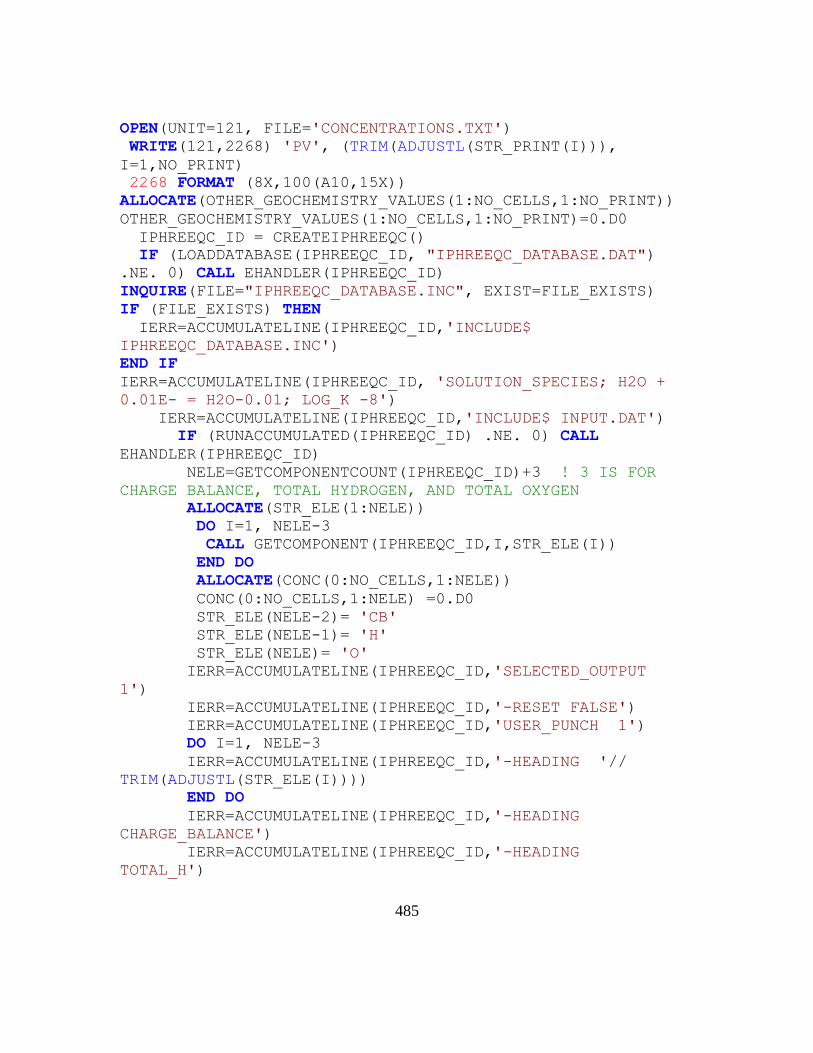
485

OPEN(UNIT=121, FILE='CONCENTRATIONS.TXT')

WRITE(121,2268) 'PV', (TRIM(ADJUSTL(STR_PRINT(I))),

I=1,NO_PRINT)

2268 FORMAT (8X,100(A10,15X))

ALLOCATE(OTHER_GEOCHEMISTRY_VALUES(1:NO_CELLS,1:NO_PRINT))

OTHER_GEOCHEMISTRY_VALUES(1:NO_CELLS,1:NO_PRINT)=0.D0

IPHREEQC_ID = CREATEIPHREEQC()

IF (LOADDATABASE(IPHREEQC_ID, "IPHREEQC_DATABASE.DAT")

.NE. 0) CALL EHANDLER(IPHREEQC_ID)

INQUIRE(FILE="IPHREEQC_DATABASE.INC", EXIST=FILE_EXISTS)

IF (FILE_EXISTS) THEN

IERR=ACCUMULATELINE(IPHREEQC_ID,'INCLUDE$

IPHREEQC_DATABASE.INC')

END IF

IERR=ACCUMULATELINE(IPHREEQC_ID, 'SOLUTION_SPECIES; H2O +

0.01E- = H2O-0.01; LOG_K -8')

IERR=ACCUMULATELINE(IPHREEQC_ID,'INCLUDE$ INPUT.DAT')

IF (RUNACCUMULATED(IPHREEQC_ID) .NE. 0) CALL

EHANDLER(IPHREEQC_ID)

NELE=GETCOMPONENTCOUNT(IPHREEQC_ID)+3 ! 3 IS FOR

CHARGE BALANCE, TOTAL HYDROGEN, AND TOTAL OXYGEN

ALLOCATE(STR_ELE(1:NELE))

DO I=1, NELE-3

CALL GETCOMPONENT(IPHREEQC_ID,I,STR_ELE(I))

END DO

ALLOCATE(CONC(0:NO_CELLS,1:NELE))

CONC(0:NO_CELLS,1:NELE) =0.D0

STR_ELE(NELE-2)= 'CB'

STR_ELE(NELE-1)= 'H'

STR_ELE(NELE)= 'O'

IERR=ACCUMULATELINE(IPHREEQC_ID,'SELECTED_OUTPUT

1')

IERR=ACCUMULATELINE(IPHREEQC_ID,'-RESET FALSE')

IERR=ACCUMULATELINE(IPHREEQC_ID,'USER_PUNCH 1')

DO I=1, NELE-3

IERR=ACCUMULATELINE(IPHREEQC_ID,'-HEADING '//

TRIM(ADJUSTL(STR_ELE(I))))

END DO

IERR=ACCUMULATELINE(IPHREEQC_ID,'-HEADING

CHARGE_BALANCE')


TOTAL_H')

486


TOTAL_O')

DO I=1, NO_PRINT


TRIM(ADJUSTL(STR_PRINT(I))))

END DO

DO I=1, NELE-3

WRITE(DUMMY_STR,*) (I)*10

IERR=ACCUMULATELINE(IPHREEQC_ID,

TRIM(ADJUSTL(DUMMY_STR))//' PUNCH TOTMOLE("'//

TRIM(ADJUSTL(STR_ELE(I)))//'")')

END DO

WRITE(DUMMY_STR,*) (NELE-2)*10

IERR=ACCUMULATELINE(IPHREEQC_ID,TRIM(ADJUSTL(DUMMY_STR))//

'PUNCH CHARGE_BALANCE')


IERR=ACCUMULATELINE(IPHREEQC_ID,TRIM(ADJUSTL(DUMMY_STR))//'

PUNCH TOTMOLE("H")')

WRITE(DUMMY_STR,*) (NELE)*10


PUNCH TOTMOLE("O")')

DO I=1, NO_PRINT

WRITE(DUMMY_STR,*) (NELE+I)*10


TRIM(ADJUSTL(DUMMY_STR))//' PUNCH '//


END DO

IERR=SETCURRENTSELECTEDOUTPUTUSERNUMBER(IPHREEQC_ID,1)

!CC CALL OUTPUTACCUMULATEDLINES(IPHREEQC_ID)

ALLOCATE(INJ_SOLUTIONS_STRING(1:NO_SLUGS)) !

STRING

DO KK=1, NO_SLUGS

WRITE(INJ_SOLUTIONS_STRING(KK), *)

INJ_SOLUTIONS(KK)

END DO

WRITE(DUMMY_STR,*) NO_CELLS

IERR=ACCUMULATELINE(IPHREEQC_ID,'RUN_CELLS; -

CELLS;')

487

IERR=ACCUMULATELINE(IPHREEQC_ID,'1-'//

TRIM(ADJUSTL(DUMMY_STR)))

DO KK=1, NO_SLUGS


TRIM(ADJUSTL(INJ_SOLUTIONS_STRING(KK))))

END DO

IERR=ACCUMULATELINE(IPHREEQC_ID,'END')



N_ROW=GETSELECTEDOUTPUTROWCOUNT(IPHREEQC_ID)

N_COLUMN=GETSELECTEDOUTPUTCOLUMNCOUNT(IPHREEQC_ID)

ALLOCATE(AVAR_LIB(1:N_ROW,1:N_COLUMN))

ALLOCATE(VT(1:N_ROW,1:N_COLUMN))

ALLOCATE(SV(1:N_ROW,1:N_COLUMN))

AVAR_LIB(1:N_ROW,1:N_COLUMN)=0.D0

DO I=1, N_ROW

DO J=1, N_COLUMN

IERR =

GETSELECTEDOUTPUTVALUE(IPHREEQC_ID,I,J,VT(I,J),AVAR_LIB(I,J

),SV(I,J))

END DO

END DO

CONC(1:NO_CELLS,1:NELE)= AVAR_LIB(1:NO_CELLS,1:NELE)

ALLOCATE(INJ_CONCENTRATIONS(1:NO_SLUGS,1:NELE))

INJ_CONCENTRATIONS(1:NO_SLUGS,1:NELE) =0.D0

INJ_CONCENTRATIONS(1:NO_SLUGS,1:NELE)=

AVAR_LIB(NO_CELLS+1:N_ROW,1:NELE)

DEALLOCATE(AVAR_LIB, VT, SV)

!CC-- END OF INITILIZATION

ALLOCATE(AVAR_LIB(1:NO_CELLS,1:NELE+NO_PRINT))

ALLOCATE(VT(1:NO_CELLS,1:NELE+NO_PRINT))

ALLOCATE(SV(1:NO_CELLS,1:NELE+NO_PRINT))

TOTAL_SHIFTS = 0

DO JJ=1, NO_SLUGS

WRITE(DUMMY_STR,*) JJ

WRITE(*,*) '----------------------------------------------

---'

WRITE(*,*) 'START INJECTING SLUG: '//

TRIM(ADJUSTL(DUMMY_STR))

WRITE(*,*) '----------------------------------------------

----'

WRITE(122,*) '--------------------------------------------

-----'

488

WRITE(122,*) 'START INJECTING SLUG: '//


WRITE(122,*) '--------------------------------------------

------'

CONC(0,1:NELE) = INJ_CONCENTRATIONS(JJ,1:NELE)

DO SHIFT =1, NO_SHIFTS(JJ)

!CC -- SHIFT THE CELLS (I.E., DO THE TRANSPORT)

!CC -- IN UTCOMP-IPHREEQC MASS BALANCE EQUATION IS SOLVED

INSTEAD

DO I= NO_CELLS,1, -1

CONC(I,1:NELE) = CONC(I-1,1:NELE)

END DO

!CC -- END

DO I=1, NO_CELLS

WRITE(DUMMY_STR,*) I

IERR=ACCUMULATELINE(IPHREEQC_ID,'SOLUTION_MODIFY

'// TRIM(ADJUSTL(DUMMY_STR)))

WRITE(DUMMY_STR,*) CONC(I,NELE-2)

IERR=ACCUMULATELINE(IPHREEQC_ID,'-CB

'//TRIM(ADJUSTL(DUMMY_STR)))

WRITE(DUMMY_STR,*) CONC(I,NELE-1)

IERR=ACCUMULATELINE(IPHREEQC_ID,'-TOTAL_H


WRITE(DUMMY_STR,*) CONC(I,NELE)

IERR=ACCUMULATELINE(IPHREEQC_ID,'-TOTAL_O


IERR=ACCUMULATELINE(IPHREEQC_ID,'-TOTALS; ')

DO J=1,NELE-3

WRITE(DUMMY_STR,*) CONC(I,J)

IERR=ACCUMULATELINE(IPHREEQC_ID,TRIM(ADJUSTL(STR_ELE(J)))//

' '//TRIM(ADJUSTL(DUMMY_STR)))

END DO !! FOR J

END DO !! FOR I



IERR=ACCUMULATELINE(IPHREEQC_ID,'RUN_CELLS; -CELLS

1-'// TRIM(ADJUSTL(DUMMY_STR))//'; END')



489




DO I=1, N_ROW

DO J=1, N_COLUMN

IERR =


),SV(I,J))

END DO

END DO

CONC(1:NO_CELLS,1:NELE)= AVAR_LIB(1:NO_CELLS,1:NELE)

OTHER_GEOCHEMISTRY_VALUES(1:NO_CELLS,1:NO_PRINT)=

AVAR_LIB(1:NO_CELLS,NELE+1:NELE+NO_PRINT)

TOTAL_SHIFTS = TOTAL_SHIFTS + 1

WRITE(*,*) 'SHIFT NO. =', SHIFT

WRITE(121,2267) (TOTAL_SHIFTS+0.5)/NO_CELLS,

OTHER_GEOCHEMISTRY_VALUES(NO_CELLS,:)

END DO !! SHIFT

END DO !! NO_SLUGS

2267 FORMAT (2X,1000(F20.10,2X))

END PROGRAM MAIN

! END OF KAZEMI NIA, MAY 2014

C.1.2 The ehandler.f90 subroutine:

SUBROUTINE EHANDLER(IPHREEQC_ID)

IMPLICIT NONE

INTEGER :: IPHREEQC_ID


CALL OUTPUTERRORSTRING(IPHREEQC_ID)

STOP

END SUBROUTINE EHANDLER

490

C.2 COMPILING THE SIMPLIFIED CODE IN A WINDOWS®1

-BASED MACHINE

Follow the procedure below to add IPhreeqc libraries before compiling the code

in Microsoft® Visual Studio

®: This procedure is based on Microsoft

® Visual Studio

®

(2008). However, we believe the same procedure should work in other versions.

1) Adding the directory of IPhreeqc libraries (see Figure C-1).

“project> project properties>linker>General>Additional Library Directories”

For example, we add the followings:

“D:\Dropbox\Softwares\IPhreeqc\IPhreeqc-3.1.2-8538-vs2005-win32\lib”

Figure C-1: Adding IPhreeqc library directories in Microsoft®

Visual Studio®.

1 Windows

®, Microsoft

®, and Visual Studio

® are registered trademarks of Microsoft Corporation

491

2) Adding the IPhreeqc library (“IPhreeqcd.lib” for the Debug mode and

“IPhreeqc.lib” for the Release mode) (see Figure C-2).

“project> project properties>linker>General>Input>Additional Dependencies”

Figure C-2: Adding IPhreeqc library in Microsoft®

Visual Studio®.

3) Adding the IPhreeqc include files (i.e., IPhreeqc.f90.inc for Fortran® 90/95) as

shown in Figure C-3:

“project> project properties>Fortran>General>Additional Include Directories”

For example, we add the followings:

“D:\Dropbox\Softwares\IPhreeqc\IPhreeqc-3.1.2-8538-vs2005-win32\include”

492

Figure C-3: Adding IPhreeqc include directory in Visual Studio®.

C.3 COMPILING THE SIMPLIFIED CODE IN A LINUX®1

-BASED MACHINE

Use the Makefile provided below.

Important Note: Command lines in Makefile must begin with a tab character

(see http://en.wikipedia.org/wiki/Make_%28software%29 for Makefile rules).

## THE UNIVERSITY OF TEXAS AT AUSTIN - 2014

## ABOULGHASEM KAZEMI NIA KORRANI, MAY 2014

## [email protected]

#FFLAGS = -O -pg

#FFLAGS = -O -fast

#FFLAGS = -g

FSRCS = \

main.f90 ehandler.f\

1 Linux

® is a registered trademark of Linus Torvalds

http://en.wikipedia.org/wiki/Make_%28software%29

493

IPhreeqc_LIB_PATH=/home1/02950/kazemi/lib ## directory

where IPhreeqc libraries were installed

IPhreeqc_INCLUDE_PATH=/home1/02950/kazemi/include/ ##

directory where IPhreeqc libraries were installed

IPhreeqc_LIBRARIES=-Wl,-rpath $(IPhreeqc_LIB_PATH) -

L/$(IPhreeqc_LIB_PATH) $(IPhreeqc_LIB_PATH)/libiphreeqc-

3.1.2.so $(IPhreeqc_LIB_PATH)/libiphreeqc.a

$(IPhreeqc_LIB_PATH)/libiphreeqc.so

ifdef tight

FFLAGS = -c -CB -r8 -g -traceback -check all -

fltconsistency -align all -debug all -I

$(IPhreeqc_INCLUDE_PATH)

else

FFLAGS= -c -g -O3 -I $(IPhreeqc_INCLUDE_PATH)

endif

PROG = exe

FORT = ifort

FOBJS = $(FSRCS:.f=.o)

PARA_OBJ = $(FSRCS_PARA:.f=.o)

OBJS = $(FOBJS) $(PARA_OBJ)

.f.o:

$(FORT) $(FFLAGS) $*.f

.F.o:

$(FORT) $(FFLAGS) $*.F

$(PROG): $(OBJS)

$(FORT) -o $(PROG) $(OBJS) $(IPhreeqc_LIBRARIES) -I


clean:

rm -f *.o

rm -f *.mod

rm -f *.exe

rm -f $(PROG)

C.4 VERIFICATION OF THE SIMPLIFIED CODE

A 1D case with 1000 cells is designed using the simplified code and PHREEQC.

This case is initially saturated with the produced water of the South American formation

(Kazempour et al., 2013). Aragonite, calcite, celestite, dolomite, halite, strontianite,

494

sylvite, and witherite are the minerals included in the model. Except calcite and dolomite

with initial concentration of 0.1 moles/kg of water, initial concentrations for other

minerals are zero. It is also assumed that a cation-exchanger with cation exchange

capacitance (CEC) of 0.01 moles/kgw is at equilibrium with the initial solution. The case

is then flushed with 0.7 PV IW1 followed by 0.7 PV PW1 and finally 0.7 SW1 (0.7 PV in

this case is about 700 shifts). Table C-1 shows ion compositions of the waters.

Temperature of the initial and injection solutions is 100 oC. The phreeqc.dat database is

used for the simulation. The PHREEQC input file is also provided. The same input file

with no SELECTED_OUTPUT and TRANSPORT is used in the simplified code.

SELECTED_OUTPUT is defined in the simplified code (rather than being defined in

the input file). Also, because transport is performed by cell shifting in the simplified

code, hence, there is no need to use the TRANSPORT keyword in the simplified code

input file. The input file loaded in the simplified code is also given below. Figures C-4

through C-11 verify the simplified code results (shown as “Advection” in the figures)

versus PHREEQC outputs.

495

Table C-1: Water analysis for South American formation (in ppm) (Kazempour et al.,

2013)

Ions Produced water

(PW1)

Injection water

(IW1)

Fresh water (SW1)

Na+ 2430 2083 40

K+ 66 75 < 5

Ca+2

300 310 12

Mg+2

47 50 3

Ba+2

20 70 -

Sr+2

26 28 1

Cl- 4343 3926 18

SO4-2

- - 7

HCO3- 512 928 110

TDS 8410 7680 215

PHREEQC Input File:

PRINT

-reset false

## PRODUCED WATER

SOLUTION 1-1000

-units ppm

-temp 100.0000

-water 1.0 ## kg

Na 2430

K 66

Ca 300

Mg 47

Ba 20

Sr 26

Cl 4343

S(6) 0.

C(4) 512 as HCO3-

END

EQUILIBRIUM_PHASES 1-1000

Aragonite 0. 0.

Calcite 0. 0.1

Celestite 0. 0.

Dolomite 0. 0.1

Halite 0. 0.

Strontianite 0. 0.

Sylvite 0. 0.

Witherite 0. 0.

END

EXCHANGE 1-1000

496

X 0.01

-equilibrate 1

END

## INJECTION WATER

SOLUTION 1001

-units ppm

-temp 100.0000 ### Endicott Reservoir Temperature

-water 1.0

Na 2083

K 75

Ca 310

Mg 50

Ba 70

Sr 28

Cl 3926

S(6) 0.

C(4) 928 as HCO3-

END

## PRODUCED WATER

SOLUTION 1002

-units ppm

-temp 100.0000

-water 1.0

Na 2430

K 66

Ca 300

Mg 47

Ba 20

Sr 26

Cl 4343

S(6) 0.

C(4) 512 as HCO3-

END

## FRESH WATER

SOLUTION 1003

-units ppm

-temp 100.0000

-water 1.0

Na 40

K 5

Ca 12

Mg 3

Ba 0

Sr 1

Cl 18

S(6) 7

C(4) 110 as HCO3-

END

## INJECTION WATER INJECTION

COPY solution 1001 0

497

END

SELECTED_OUTPUT

-file selected.out

-reset false

USER_PUNCH

-Heading PV

-Heading Na+

-Heading Ca+2

-Heading Cl-

-Heading pH

-Heading Ba+2

-Heading HCO3-

-Heading Mg+2

-Heading Sr+2

1 PUNCH STEP_NO

2 PUNCH MOL("Na+")

3 PUNCH MOL("Ca+2")

4 PUNCH MOL("Cl-")

5 PUNCH -la("H+")

6 PUNCH MOL("Ba+2")

7 PUNCH MOL("HCO3-")

8 PUNCH MOL("Mg+2")

9 PUNCH MOL("Sr+2")

END

TRANSPORT

-cells 1000

-initial_time 0.

-length 0.012192 #m

-shifts 700

-time_step 1 #s

-flow_direction forward

-boundary_cond flux flux

-diffc 0.0e-9

-dispersivity 0. #m

-punch_cells 1000

-punch_frequency 1

END

## PRODUCED WATER INJECTION


END

TRANSPORT; -shifts 700

END

## FRESH WATER INJECTION


END

TRANSPORT; -shifts 700

END

Input File Loaded in the Simplified Code:

SOLUTION 1-1000

-water 1.0 ## water mass in each grid block

498

-units ppm

-temp 100.0000

Na 2430

K 66

Ca 300

Mg 47

Ba 20

Sr 26

Cl 4343

S(6) 0.

C(4) 512 as HCO3-

END

EQUILIBRIUM_PHASES 1-1000

Aragonite 0. 0.

Calcite 0. 10.0

Celestite 0. 0.

Dolomite 0. 10.0

Halite 0. 0.

Strontianite 0. 0.

Sylvite 0. 0.

Witherite 0. 0.

END

EXCHANGE 1-1000

X 0.01

-equilibrate 1

END

SOLUTION 1001

-units ppm

-temp 100.0000

-water 1.0

Na 2083

K 75

Ca 310

Mg 50

Ba 70

Sr 28

Cl 3926

S(6) 0.

C(4) 928 as HCO3-

END

SOLUTION 1002

-units ppm

-temp 100.0000

-water 1.0

Na 2430

K 66

Ca 300

Mg 47

Ba 20

499

Sr 26

Cl 4343

S(6) 0.

C(4) 512 as HCO3-

END

SOLUTION 1003

-units ppm

-temp 100.0000

-water 1.0

Na 40

K 5

Ca 12

Mg 3

Ba 0

Sr 1

Cl 18

S(6) 7

C(4) 110 as HCO3-

END

Figure C-4: pH history of the effluent solution (the simplified code verification against

PHREEQC).

500

Figure C-5: Na+ concentration history of the effluent solution (the simplified code


Figure C-6: Ca+2

concentration history of the effluent solution (the simplified code


501

Figure C-7: Cl- concentration history of the effluent solution (the simplified code


Figure C-8: Ba+2



502

Figure C-9: HCO3- concentration history of the effluent solution (the simplified code


Figure C-10: Mg+2



503

Figure C-11: Sr+2



504

11 Appendix D: Detailed UTCOMP-IPhreeqc Computational

Flowchart

This appendix presents the UTCOMP-IPhreeqc computational algorithm with

more details. In this algorithm only the effect of hydrocarbon-CO2 on the aqueous-rock

geochemistry is considered. However, we apply the same procedure if multiple

hydrocarbon components (e.g., CH4 and H2S components besides the CO2 component)

are included in calculations. TNKi, TNKTGi, fi, and SIi used in the algorithm are total

moles of the hydrocarbon component i, total moles of the geochemical element i, fugacity

of the component i, and saturation index of phase i, respectively. In IPhreeqc, saturation

index for gas is logarithm partial pressure (fugacity in UTCOMP-IPhreeqc).

507

12 Appendix E: UTCOMP-IPhreeqc Input Files

The following presents the description of different sections in Appendix E:

Appendix E.1 provides UTCOMP-IPhreeqc input files that produce the

outputs of PHREEQC example 11. To run UTCOMP-IPhreeqc the

following files are required: INPUT.DAT, GCINPUT.DAT,

IPhreeqc_Database.DAT, and IPhreeqc_INPUT.DAT. Description of each

file is provided in Chapter 2.

Appendix E.2 shows how gridblocks geochemistry data are stored in the

computer memory (for the case presented in Appendix E.1).

Appendix E.3 presents how we modify the gridblock geochemistry data in

the computer memory (for the case presented in Appendix E.1).

Appendix E.4 illustrates how IPhreeqc outputs are organized in the

computer memory to be transferred to UTCOMP (for the case presented in

Appendix E.1).

E.1: UTCOMP-IPHREEQC SAMPLE INPUT FILES

E.1.1 INPUT.DAT

CC*********************************************************************

**

CC *

CC BRIEF DESCRIPTION OF DATA SET: UTCOMP

*

508

CC

*

CC*********************************************************************

**

CC

*

CC

*

CC

*

CC LENGTH(FT): INJECTION FLUID :

*

CC HEIGHT(FT): INJECTION RATE :

*

CC WIDTH(FT) : W/O REL. PERM :

*

CC POROSITY : G/O REL. PERM :

*

CC ABS. PERM : 3-PHASE REL. PERM:

*

CC TEMP(F) : WETTIBILITY:

*

CC PRE(PSI) :

*

CC SOR :

*

CC SWC :

*

CC AVG. DEPTH(FT) :

*

CC

*

CC

*

CC

*

CC

*

CC

*

CC

*

CC*********************************************************************

**

CC

*

CC HYDROCARBON DATA AND FLASH CALCULATION OPTIONS

*

CC

*

509

CC*********************************************************************

**

CC

CC..+....1....+....2....+....3....+....4....+....5....+....6...+...7..

CC***********SOME CONSTANTS AND MAXIMUM VALUES FOR MODELS**************

CC

CC NXM, NYM, NZM, NPM, NCM, NWM POSTPROCESSOR

40 1 1 3 12 3 2

CC

CC NS1M,NBWM,NPRM,NPFM,NCTM,NHSM

1 401 50 10 10 10000

CC

CC IC2,NCMT,NREG,NTAB

2 4 6 25

CC

CC EE, NZPM

0.5761 3

CC

CC TOLP, TOLVOL, QLIM

0.5D-1 0.5D-4 1.0D-30

CC

CC NUMAX,INQUA,INCON,INVEL,NOSWTM,NUMPRE,NUMOUT,NUMPVT,NST,IFLIP

10 3 3 5 10 30 12 30 20 0

CC*********************************************************************

CC CASE NAME WITH FORMAT ( 17A4, A2 ) OF TOTAL 70 COLUMNS.

*----HEADER

1D CO2+NG INJECTION INVOLVING 3 HC PHASES

CC

CC NUMBER OF COMPONENTS.

*--------NC

12

CC COMPONENT NAMES WITH FORMAT ( 1X, A8 ), NC CARDS.

CC..+..8

*----NAME

CO2

C1N2

C2

C3

C4

C5

C6

C710

C1113

C1419

C2029

C30P

CC

CC BLACK OIL OPTION; AQUIFER SALINITY (ppm); AQUIFER OPTION

*-----IBOST SLNTY IAQUIF

0 0. 0

CC CRITICAL PRESS. (PSI), TEMP. (R) AND VOL. (CU FT/LB-MOLE),

510

CC MOLECULAR WT. (LB/LB-MOLE), ACENTRIC FACTOR, PARACHOR. NC CARDS.

*--------PC TC VC MW OM PARACH

VSP

1070.535624 547.5 2.243201575 44 0.2276 49 0

666.972984 342.5 1.442237287 16.1 0.0109 71 0

707.6591358 549.6 2.371294757 30.1 0.099 134.825 0

616.2902348 665.6 3.252343124 44.1 0.1518 233.048 0

544.3147329 756.4 4.122115282 58.1 0.1885 394.499 0

489.3334468 838.4 4.883768876 72.1 0.24 707.76 0

476.1379381 913.8 5.423128436 84 0.2711 1035.85 0

412.859476 1048.7 6.959539271 113.3 0.3683 1035.85

0

318.1916979 1196.4 10.20105981 161.9 0.5239 1035.85

0

249.6150391 1328.9 14.31231704 226 0.6932 1035.85

0

192.4345015 1475.9 21.23608053 331.5 0.9 1035.85 0

133.6545083 1574.9 37.15367911 588 1.2 1035.85 0

CC EOS parameters (Ac and Bc)

CC NC CARDS.

*---- PARAA PARAB

0.457236 0.077796

0.457236 0.077796

0.457236 0.077796

0.457236 0.077796

0.457236 0.077796

0.457236 0.077796

0.457236 0.077796

0.457236 0.077796

0.457236 0.077796

0.457236 0.077796

0.457236 0.077796

0.457236 0.077796

CC

CC BINARY INTERACTION COEFFICIENTS, CIJ. NC CARDS.

*-----DELTA

0

0.105 0

0.125 0.0028 0

0.12 0.0089 0.0017 0

0.12 0.0156 0.0053 0.001 0

0.12 0.0216 0.009 0.0029 0.0005 0

0.12 0.0257 0.0118 0.0045 0.0013 0.0002

0

0.12 0.0369 0.0198 0.01 0.0047 0.0022

0.0011 0

511

0.13 0.0575 0.0359 0.0223 0.0141 0.0093

0.0069 0.0025 0

0.13 0.0789 0.0538 0.037 0.0263 0.0198

0.0161 0.009 0.002 0

0.13 0.1072 0.0784 0.0584 0.045 0.0365

0.0316 0.0213 0.0093 0.0027 0

0.13 0.1523 0.1193 0.0954 0.0788 0.0677

0.0612 0.0469 0.0284 0.0156 0.0054 0

CC

CC BINARY INTERACTION COEFFICIENTS, DIJ. NC CARDS.

*-------DIJ

0

0 0

0 0 0

0 0 0 0

0 0 0 0 0

0 0 0 0 0 0

0 0 0 0 0 0 0

0 0 0 0 0 0 0 0

0 0 0 0 0 0 0 0 0

0 0 0 0 0 0 0 0 0 0

0 0 0 0 0 0 0 0 0 0 0

0 0 0 0 0 0 0 0 0 0 0

0

CC

CC reduction method: (0: OFF, 1: ON)

*-------IFLASHTYPE irfla irsa

1 0 0

CC

CC MAXIMUM NUMBER OF PHASES ( 3 OR 4 )

*--------NP IVISC IVISC_COEF ISINGL ISOLU

3 1 0 0 0

CC IEOS: 1, IPEM: 0 OR 1

CC ISTAM: -1, 0 OR 1, IEST: 0 OR 1 KI: 0, 1 OR 2

*---IEOS IPEM ISTAM IEST IVSP KI

1 1 -1 1 0 0

CC

CC ITERATION TOLERANCES FOR PERSCHKE'S FLASH ROUTINES.

*----TOLFLA TOLFLM TOLPD TOLSAM TOLSAS TOLSUM

1.0E-08 1.0E-8 1.0E-10 1.0E-8 1.0E-8 1.0E-08

CC

CC MAXIMUM NUMBER OF ITERATIONS FOR PERSCHKE'S FLASH ROUTINES.

*----MAXFLA MAXFLM MAXPD MAXSAM MAXSAS

30000 1000 1000 1000 30000 20

CC

CC VECTOR FLASH OPTION

*--IVCFL TOLVFL MAXVFL

0 1.E-10 30

CC

CC SWITCHING PARAMETERS FOR PERSCHKE'S FLASH ROUTINES.

*----SWIPCC SWIPSA

512

1.e-3 1.e-3

CC

CC PHASE IDENTIFICATION PARAMETERS FOR PERSCHKE'S FLASH ROUTINES.

*------IOIL ITRK DMSLIM

1 2 25.

CC

CC IFLAGT ( 0 : OFF, 1 : ON )

*------IFLAGT IGEOCHEM IPhreeqc IASPR

0 1 1 0

CC

CC*********************************************************************

**

CC *

CC OUTPUT OPTIONS *

CC *

CC*********************************************************************

**

CC

CC

CC HISTORY PRINTING PARAMETER FOR <<HISTORY.CPR>>.

*--- POSTPROCESSOR NHSSKIP NSTSKIP IPV

20 20 1

CC

CC REFERENCE CONCENTRATION, CONC0, USED FOR EFFLUENT CONCENTRATION.

*-----CONC0

1.0 1.0 1.0 1.0 1.0 1.0 1.0 1.0 1.0 1.0 1.0 1.0

CC

CC

*------

0

CC

CC NUMBER OF PRINTS FOR <<PROFILE.CPR>>.

*-------NPF

0

CC

CC NUMBER OF PRINTS FOR <<CONTOUR.CPR>>.

*-------NCT

0

CC

CC*********************************************************************

**

CC *

CC RESERVOIR AND WELL DATA *

CC *

CC*********************************************************************

**

CC

CC A FLAG FOR RESERVOIR GEOMETRY:

CC 2-D: 11(Y), 12(X), 13(Z), 2-D: 21(XY), 22(YZ), 23(XZ), 3-D: 31

*-----IGEOM INUG

12 0

513

CC

CC NUMBER OF GRID BLOCKS IN X, Y, AND Z.

*--------NX NY NZ

40 1 1

CC

CC NUMBER OF WELLS, AND FLAG FOR WELLBORE MODEL

*--------NW IWM

2 1

CC

CC WELLBORE RATIUS (FT). NW NUMBERS.

*--------RW: (NW)

0.33 0.33

CC

CC WELL LOCATIONS. NW CARDS.

*-------LXW LYW IDIR LZWF LZWL

1 1 3 1 1

40 1 3 1 1

CC

CC A FLAG ( 0 OR 1 ) FOR GRID BLOCK SIZE IN X-DIRECTION.

*-------MDX

0

CC

CC CONSTANT GRID BLOCK SIZE IN X-DIRECTION (FT).

*--------DX

0.04

CC

CC A FLAG ( 0 OR 1 ) FOR GRID BLOCK SIZE IN Y-DIRECTION.

*-------MDY

0

CC

CC CONSTANT GRID BLOCK SIZE IN Y-DIRECTION (FT).

*--------DY

0.15

CC

CC A FLAG ( 0 OR 1 ) FOR GRID BLOCK SIZE IN Z-DIRECTION.

*-------MDZ

0

CC

CC CONSTANT GRID BLOCK SIZE IN Z-DIRECTION (FT).

*--------DZ

0.15

CC

CC A FLAG ( 0 OR 1 ) FOR FORMATION DEPTH.

*--------MD

0

CC

CC DEPTH (FT) OF THE MOST UPPER LAYER.

*---------D

0.

CC

CC A FLAG ( 0 OR 1 ) FOR FORMATION POROSITY.

514

*------MPOR

0

CC

CC HOMOGENEOUS POROSITY (FRACTION) AT PF.

*----PORSTD

0.25

CC

CC A FLAG ( 0 OR 1 ) FOR PERMEABILITY IN X-DIRECTION.

*----MPERMX

0

CC

CC HOMOGENEOUS PERMEABILITY (MD) IN X-DIRECTION.

*-----PERMX

100

CC

CC A FLAG ( 0 OR 1 ) FOR PERMEABILITY IN Y-DIRECTION.

*----MPERMY

0

CC

CC HOMOGENEOUS PERMEABILITY (MD) IN Y-DIRECTION.

*-----PERMY

100

CC

CC FLAG ( 0 OR 1 ) FOR PERMEABILITY IN Z-DIRECTION.

*----MPERMZ

0

CC

CC HOMOGENEOUS PERMEABILITY (MD) IN Z-DIRECTION.

*-----PERMZ

10.00

CC

CC FORMATION COMPRESSIBILITY (1/PSI) AND REFERENCE PRESSURE (PSI).

*--------CF PF

0. 14.67

CC H2O COMPRESSIBILITY (1/PSI), REFERENCE PRESSURE (PSI) AND

CC MOLAR DENSITY (LB-MOLE/CU FT).

*--------CW PW DENMWS

0. 14.67 3.467

CC

CC WATER MOLECULAR WT. (LBM/LBM-MOLE) AND VISCOSITY (CP).

*-------WTW VISCW

18. 0.79

CC

CC FORMATION TEMPERATURE (F).

*-----TEMPF

212.0

CC

CC STANDARD TEMPERATURE (F) AND STANDARD PRESSURE (PSI).

*-----TFSTD PSTD

60. 14.67

CC

515

CC A FLAG ( 1, 2, 3 OR 4 ) FOR NUMERICAL DISPERSION CONTROL.

*----IUPSTW

1

CC

CC ITC ( 0 : NO 2ND ORDER TIME, 1 : 2ND ORDER TIME ON )

*----ITC

0

CC RESTART OPTIONS.

CC ISTART ( 1 OR 2 ), ISTORE ( 0 OR 1 ).

*----ISTART ISTORE

1 1

CC

CC A FLAG ( 0 OR 1 ) FOR AUTOMATIC TIME-STEP SELECTION ( = 1 ).

*-------MDT

1

CC

CC A FLAG ( 0 OR 1 ) FOR PHYSICAL DISPERSION CALCULATION.

*-----MDISP

1

CC MOLECULAR DIFFUSION COEFFICIENTS ( FT*FT/DAY ).

CC NP CARDS AND EACH CARD HAS NC NUMBERS.

*----DIFFUN

0. 0. 0. 0. 0. 0. 0. 0. 0. 0. 0. 0.

0. 0. 0. 0. 0. 0. 0. 0. 0. 0. 0. 0.

0. 0. 0. 0. 0. 0. 0. 0. 0. 0. 0. 0.

CC

CC TORTUOSITY FACTOR.

*-------TAU

1.

CC

CC LONGITUDINAL AND TRANSVERSE DISPERSIVITIES (FT). NP CARDS.

*----ALPHAL ALPHAT

0.02 0.0

0. 0.0

0. 0.0

CC

CC YOUNG'S DISPERSION MODEL

*-----BETAL BETAT ALMAX ATMAX

0.0 0.0 0.2 0.005

CC FLAGS FOR RELATIVE PERMEABILITY MODEL AND CAPILLARY PRESSURE.

CC IPERM ( 1 OR 2 ), ICPRES ( 0 OR 1 ).

*-----IPERM ICPRES ICAP IRPERM

4 0 0 0

CC CAPILLARY PRESSURE PARAMETERS AND

CC WATER/OIL INTERFACIAL TENSION (DYNES/CM).

*-------EPC CPC RIFTWO RIFTWG RIFTWL

2. 2.0 20. 24. 30.

CC

CC HIGH IFT RESIDUAL SATURATIONS.

*-----S1RW S2RW1 S2RW2 S3RW S4RW1 S4RW2

0.05 0.18 .25 0.05 0.2 0.2

516

CC

CC LOW IFT RESIDUAL SATURATIONS.

*------S1RC S2RC1 S2RC2 S3RC S4RC1 S4RC2

0 .0 .0 0. 0. 0.

CC

CC HIGH IFT END POINT RELATIVE PERMEABILITY.

*------P1RW P2RW P3RW P4RW

0.383 1.0 0.35 0.35

C

CC LOW IFT END POINT RELATIVE PERMEABILITY.

*------P1RC P2RC P3RC P4RC

1. 1 1 1.

CC

CC HIGH IFT EXPONENT OF RELATIVE PERMEABILITY.

*-------E1W E2W1 E2W2 E3W E4W1 E4W2

1.59 3.22 2.5 2.5 2.5 2.5

CC

CC LOW IFT EXPONENT OF RELATIVE PERMEABILITY.

*-------E1C E2C1 E2C2 E3C E4C1 E4C2

1. 1. 1. 1. 1. 1.

CC

CC WATER AND L1 PHASE CAPILLARY DESATURATION PARAMETERS.

*-------T11 T12 T211 T221 T212 T222

-.4 1.6 -0.5 2.2 -.04 1.6

CC

CC GAS AND L2 PHASE CAPILLARY DESATURATION PARAMETERS.

*-------T31 T32 T411 T421 T412 T422

-0.5 2.2 -0.5 2.2 -.4 1.6

CC

CC

*------ IWALT IWALF

0 0

CC

CC A FLAG FOR PRESSURE EQUATION SOLVER ( 1, 2, 3, 4 OR 5 ).

*----IPRESS IPREC METHSL OMEGA IHYPRE

11 2 1 1.0 1 0

CC

CC ITERATIVE PRESSURE SOLVER PARAMETERS.

*-----ITMAX LEVLIT IDGTS NS1 NS2 ZETA

1000 1 1 5 1000000 1.E-07

CC

CC INITIAL TIME (DAYS).

*---------T

0

CC

CC A FLAG ( 0 OR 1 ) FOR INITIAL PRESSURE.

*--------MP

0

CC

CC CONSTANT INITIAL PRESSURE (PSIA).

*---------P

517

4890

CC

CC A FLAG ( 0 OR 1 ) FOR INITIAL WATER SATURATION.

*------MSAT

0

CC

CC CONSTANT INITIAL WATER SATURATION (FRACTION).

*-------SAT

0.999

CC

CC A FLAG ( 0 OR 1 ) FOR INITIAL OVERALL COMPOSITION.

*-----MOMFR

0

CC

CC CONSTANT INITIAL COMPOSITION (MOLE FRACTION).

*------OMFR

0.12837 0.42134 0.05557 0.02662 0.01535

0.00985 0.00835 0.06971 0.03578 0.07131

0.07629 0.08146

CC

CC*********************************************************************

**

CC *

CC RECURRENT DATA

*

CC *

CC*********************************************************************

**

CC LoSal INJECTION

*

CC*********************************************************************

**

CC MAXIMUM TIME (DAYS), TIME STEP (DAYS) AND WELL DATA.

*--------TM DT NWELLS GORLIM WORLIM

2.5 0.05 2 -1 -1

CC

CC

*-----DTMAX DTMIN DSLIM DPLIM DVLIM DMFACT

DMFACTG

0.1 0.001 0.05 0.005 0.05 0.03 0.05

CC


*--------LW IQTYPE

1 4

CC

CC (B/D) (MSCF/D)

*----QPSVC(1) QPSVC(3) NCOMP ISWITCH PBHC

4E-5 0 0 0 6000

CC

CC

*--- INJ_SOLUTION_NO

518

0

CC


*--------LW IQTYPE

2 -2

CC

CC CONSTANT BHP PRODUCER (PSI)

*--------PBHC

4890.0

CC

CC END OF INPUT.

*--------TM DT NWELLS GORLIM WORLIM ----------------

-1.0 -1. -1 -1.E10 -1.E10

E.1.2 GCINPUT.DAT

CC

CC*******************************************************

CC *


CC *

CC*******************************************************

CC

CC

*------- RIUNITS NO_HC_GC NO_ACID_BASE IITERATION

0 0 0 1

CC

CC*******************************************************

CC *

CC GEOCHEMISTRY OUTPUT SECTION *

CC *

CC*******************************************************

CC

CC

*--- IPRES IPWELL IPTDRM IPWET

1 0 0 0

CC****************** RESERVOIR SECTION **********************

CC

*---- PRINT_NUMBER_ELEMENT ELEMENT_HISTORY ELEMENT_PROFILE

FREQUENCY_HIS(TIME STEP) FREQUENCY_PROF(TIME STEP)

0 1 1

1 1

CC

CC

*---- NSLDP SOLID_HISTORY SOLID_PROFILE FREQUENCY_HIS (TIME STEP)

FREQUENCY_PROF(TIME STEP)

0 1 1 1 1

CC

519

CC

*---- NAQSP AQS_HISTORY AQS_PROFILE FREQUENCY_HIS(TIME STEP)

FREQUENCY_PROF(TIME STEP)

0 1 1 10

1000

CC

CC

*---- NSORBP SORBED_HISTORY ELEMENT_PROFILE FREQUENCY_HIS (TIME

STEP) FREQUENCY_PROF (TIME STEP)

0 1 1 1

1

CC

CC

*---- NPRINTG PRINTG_HISTORY PRINTG_PROFILE FREQUENCY_HIS (TIME

STEP) FREQUENCY_PROF(TIME STEP)

4 1 0 1

1

CC

CC

*-------- NO OF GRIDBLOCKS

1

CC

CC

*----- (I,J,K)

40

1

1

CC

CC

*------ OTHER GEOCHEMICAL PROPERTIES NAMES

TOT("Na")*1E3

TOT("Cl")*1E3

TOT("K")*1E3

TOT("Ca")*1E3

E.1.3 IPhreeqc_INPUT.DAT

## GRIDBLOCK INITIALIZATION

SOLUTION 1-40

-water 1.0 ## water mass in each grid block

units mmol/kgw

temp 25.0

pH 7.0 charge

pe 12.5 O2(g) -0.68

Na 1.0

K 0.2

N(5) 1.2

END

520

EXCHANGE 1-40

-equilibrate 1

X 0.0011

END

# INJECTION SOLUTIONS

SOLUTION 0

-water 1 ## kg

units mmol/kgw

temp 25.0

pH 7.0 charge

pe 12.5 O2(g) -0.68

Ca 0.6

Cl 1.2

END

E.1.4 IPhreeqc_Database.DAT

# PHREEQC.DAT for calculating pressure dependence of reactions, with

# molal volumina of aqueous species and of minerals, and

# critical temperatures and pressures of gases used in Peng-

Robinson's EOS.

# Details are given at the end of this file.

SOLUTION_MASTER_SPECIES

#

#element species alk gfw_formula element_gfw

#

H H+ -1.0 H 1.008

H(0) H2 0.0 H

H(1) H+ -1.0 0.0

E e- 0.0 0.0 0.0

O H2O 0.0 O 16.0

O(0) O2 0.0 O

O(-2) H2O 0.0 0.0

Ca Ca+2 0.0 Ca 40.08

Mg Mg+2 0.0 Mg 24.312

Na Na+ 0.0 Na 22.9898

K K+ 0.0 K 39.102

Fe Fe+2 0.0 Fe 55.847

Fe(+2) Fe+2 0.0 Fe

Fe(+3) Fe+3 -2.0 Fe

Mn Mn+2 0.0 Mn 54.938

Mn(+2) Mn+2 0.0 Mn

Mn(+3) Mn+3 0.0 Mn

Al Al+3 0.0 Al 26.9815

Ba Ba+2 0.0 Ba 137.34

521

Sr Sr+2 0.0 Sr 87.62

Si H4SiO4 0.0 SiO2 28.0843

Cl Cl- 0.0 Cl 35.453

C CO3-2 2.0 HCO3 12.0111

C(+4) CO3-2 2.0 HCO3

C(-4) CH4 0.0 CH4

Alkalinity CO3-2 1.0 Ca0.5(CO3)0.5 50.05

S SO4-2 0.0 SO4 32.064

S(6) SO4-2 0.0 SO4

S(-2) HS- 1.0 S

N NO3- 0.0 N 14.0067

N(+5) NO3- 0.0 N

N(+3) NO2- 0.0 N

N(0) N2 0.0 N

N(-3) NH4+ 0.0 N

#Amm AmmH+ 0.0 AmmH 17.0

B H3BO3 0.0 B 10.81

P PO4-3 2.0 P 30.9738

F F- 0.0 F 18.9984

Li Li+ 0.0 Li 6.939

Br Br- 0.0 Br 79.904

Zn Zn+2 0.0 Zn 65.37

Cd Cd+2 0.0 Cd 112.4

Pb Pb+2 0.0 Pb 207.19

Cu Cu+2 0.0 Cu 63.546

Cu(+2) Cu+2 0.0 Cu

Cu(+1) Cu+1 0.0 Cu

# redox-uncoupled gases

Hdg Hdg 0 Hdg 2.016 # H2 gas

Oxg Oxg 0 Oxg 32 # Oxygen gas

Mtg Mtg 0.0 Mtg 16.032 # CH4 gas

Sg H2Sg 1.0 H2Sg 34.08

Ntg Ntg 0 Ntg 28.0134 # N2 gas

SOLUTION_SPECIES

H+ = H+

-gamma 9.0 0.0

-dw 9.31e-9

e- = e-

H2O = H2O

Ca+2 = Ca+2

-gamma 5.0 0.1650

# -gamma 4.5 0.23 # anhydrite in NaCl solutions, Freyer and

Voigt, 2004, GCA 68, 307

-dw 0.793e-9

-Vm -0.3456 -7.252 6.149 -2.479 1.239 5 1.60 -57.1 -

6.12e-3 1 # supcrt modified

Mg+2 = Mg+2

-gamma 5.5 0.20

-dw 0.705e-9

522

-Vm -1.410 -8.6 11.13 -2.39 1.332 5.5 1.29 -32.9 -5.86e-

3 1 # supcrt modified

Na+ = Na+

-gamma 4.0 0.075

-gamma 4.08 0.082 # halite solubility

-dw 1.33e-9

-Vm 1.403 -2.285 4.419 -2.726 -5.125e-5 4.0 0.162 47.67

-3.09e-3 0.725 # supcrt modified

# for calculating densities (rho) when I > 3...

# -Vm 1.403 -2.285 4.419 -2.726 -5.125e-5 2.0 0.162 47.67

-3.09e-3 0.4

K+ = K+

-gamma 3.5 0.015

-dw 1.96e-9

-Vm 3.322 -1.473 6.534 -2.712 9.06e-2 3.5 0 29.7 0 1 #

supcrt modified

Fe+2 = Fe+2

-gamma 6.0 0.0

-dw 0.719e-9

-Vm -0.3255 -9.687 1.536 -2.379 0.3033 5.5 -4.21e-2 37.96

0 1 # supcrt modified

Mn+2 = Mn+2

-gamma 6.0 0.0

-dw 0.688e-9

-Vm -.1016 -8.0295 8.9060 -2.4471 1.4006 6 # supcrt

Al+3 = Al+3

-gamma 9.0 0.0

-dw 0.559e-9

-Vm -3.3404 -17.1108 14.9917 -2.0716 2.8711 9 # supcrt

Ba+2 = Ba+2

-gamma 5.0 0

-gamma 4.0 0.153 # Barite solubility

-dw 0.848e-9

-Vm 2.063 -10.06 1.9534 -2.36 0.4218 5 1.58 -12.03 -

8.35e-3 1 # supcrt modified

Sr+2 = Sr+2

-dw 0.794e-9

-gamma 5.260 0.121

-Vm -1.57e-2 -10.15 10.18 -2.36 0.860 5.26 0.859 -27.0 -

4.1e-3 1.97 # supcrt modified

H4SiO4 = H4SiO4

-dw 1.10e-9

-Vm 10.5 1.7 20 -2.7 0.1291 # supcrt + 2*H2O in a1

Cl- = Cl-

-gamma 3.5 0.015

-gamma 3.63 0.017 # cf. pitzer.dat

-dw 2.03e-9

-Vm 4.465 4.801 4.325 -2.847 1.748 0 -0.331 20.16 0 1 #

supcrt modified

CO3-2 = CO3-2

-gamma 5.4 0.0

523

-dw 0.955e-9

-Vm 6.95 0 0 -5.98 8.32 0 -0.115 167 -0.026 1 # supcrt

modified

SO4-2 = SO4-2

-gamma 5.0 -0.04

-dw 1.07e-9

-Vm 8.0 2.51 -42.5 5.41 4.23 0 0 0 0 1 # supcrt modified

NO3- = NO3-

-gamma 3.0 0.0

-dw 1.9e-9

-Vm 6.392 6.78 0 -3.06 0.449 0 0.80 0 -1.05e-2 1 #

supcrt modified

#AmmH+ = AmmH+

# -gamma 2.5 0.0

# -dw 1.98e-9

# -Vm 4.837 2.345 5.522 -2.88 1.096 3 -1.456 75.0 7.17e-3

1 # supcrt modified

H3BO3 = H3BO3

-dw 1.1e-9

-Vm 7.0643 8.8547 3.5844 -3.1451 -.2000 # supcrt

PO4-3 = PO4-3

-gamma 4.0 0.0

-dw 0.612e-9

-Vm -.5259 -9.0654 9.3131 -2.4042 5.6114 # supcrt

F- = F-

-gamma 3.5 0.0

-dw 1.46e-9

-Vm .6870 1.3588 7.6033 -2.8352 1.787 # supcrt

Li+ = Li+

-gamma 6.0 0.0

-dw 1.03e-9

-Vm -.0237 -.0690 11.5800 -2.7761 .4862 6 # supcrt

Br- = Br-

-gamma 3.0 0.0

-dw 2.01e-9

-Vm 5.2690 6.5940 4.7450 -3.1430 1.3858 # supcrt

Zn+2 = Zn+2

-gamma 5.0 0.0

-dw 0.715e-9

-Vm -1.0677 -10.3884 9.8331 -2.3495 1.4574 5 # supcrt

Cd+2 = Cd+2

-dw 0.717e-9

-Vm .0537 -10.7080 16.5176 -2.3363 1.2528 5 # supcrt

Pb+2 = Pb+2

-dw 0.945e-9

-Vm -.0051 -7.7939 8.8134 -2.4568 1.0788 4.5 # supcrt

Cu+2 = Cu+2

-gamma 6.0 0.0

-dw 0.733e-9

-Vm -1.1021 -10.4726 9.8662 -2.3461 1.4769 6 # supcrt


524

Hdg = Hdg # H2

-dw 5.13e-9

-Vm 6.52 0.78 0.12 # supcrt

Oxg = Oxg # O2

-dw 2.35e-9

-Vm 5.7889 6.3536 3.2528 -3.0417 -0.3943 # supcrt

Mtg = Mtg # CH4

-dw 1.85e-9

-Vm 7.7 # CH4 solubility, 25-100C, 1-700atm

Ntg = Ntg # N2

-dw 1.96e-9

-Vm 7 # Pray et al., 1952, IEC 44. 1146

H2Sg = H2Sg # H2S

-dw 2.1e-9

-Vm 7.81 2.96 -0.46 # supcrt

# aqueous species

H2O = OH- + H+

-analytic 293.29227 0.1360833 -10576.913 -123.73158 0 -

6.996455e-5

-gamma 3.5 0.0

-dw 5.27e-9

-Vm -9.66 28.5 80.0 -22.9 1.89 0 1.09 0 0 1 # supcrt modified

2 H2O = O2 + 4 H+ + 4 e-

-log_k -86.08

-delta_h 134.79 kcal

-dw 2.35e-9

-Vm 5.7889 6.3536 3.2528 -3.0417 -0.3943 # supcrt

2 H+ + 2 e- = H2

-log_k -3.15

-delta_h -1.759 kcal

-dw 5.13e-9

-Vm 6.52 0.78 0.12 # supcrt

CO3-2 + H+ = HCO3-

-log_k 10.329


-analytic 107.8871 0.03252849 -5151.79 -38.92561

563713.9

-gamma 5.4 0.0

-dw 1.18e-9

-Vm 8.60 0 -12.0 0 1.643 0 0 167 0 1 # supcrt modified

CO3-2 + 2 H+ = CO2 + H2O

-log_k 16.681


-analytic 464.1965 0.09344813 -26986.16 -165.75951

2248628.9

-dw 1.92e-9

-Vm 20.85 -46.93 -79.0 27.9 -0.193 # supcrt modified

CO3-2 + 10 H+ + 8 e- = CH4 + 3 H2O

-log_k 41.071


-dw 1.85e-9

525

-Vm 7.7

SO4-2 + H+ = HSO4-

-log_k 1.988

-delta_h 3.85 kcal

-analytic -56.889 0.006473 2307.9 19.8858 0.0

-dw 1.33e-9

-Vm 8.2 9.2590 2.1108 -3.1618 1.1748 0 -0.3 15 0 1 # supcrt

modified

HS- = S-2 + H+

-log_k -12.918

-delta_h 12.1 kcal

-gamma 5.0 0.0

-dw 0.731e-9

SO4-2 + 9 H+ + 8 e- = HS- + 4 H2O

-log_k 33.65


-gamma 3.5 0.0

-dw 1.73e-9

-Vm 5.0119 4.9799 3.4765 -2.9849 1.4410 # supcrt

HS- + H+ = H2S

-log_k 6.994

-delta_h -5.30 kcal

-analytical -11.17 0.02386 3279.0

-dw 2.1e-9

-Vm 7.81 2.96 -0.46 # supcrt

H2Sg = HSg- + H+

-log_k -6.994

-delta_h 5.30 kcal

-analytical 11.17 -0.02386 -3279.0

-dw 2.1e-9

-Vm 5.0119 4.9799 3.4765 -2.9849 1.4410 # supcrt

NO3- + 2 H+ + 2 e- = NO2- + H2O

-log_k 28.570


-gamma 3.0 0.0

-dw 1.91e-9

-Vm 5.5864 5.8590 3.4472 -3.0212 1.1847 # supcrt

2 NO3- + 12 H+ + 10 e- = N2 + 6 H2O

-log_k 207.08


-dw 1.96e-9

-Vm 7 # Pray et al., 1952, IEC 44. 1146

NO3- + 10 H+ + 8 e- = NH4+ + 3 H2O

log_k 119.077

delta_h -187.055 kcal

-gamma 2.5 0.0

-dw 1.98e-9

-Vm 4.837 2.345 5.522 -2.88 1.096 3 -1.456 75.0 7.17e-3

1 # supcrt modified

#AmmH+ = AmmH+

526

# -gamma 2.5 0.0

# -dw 1.98e-9

# -Vm 4.837 2.345 5.522 -2.88 1.096 3 -1.456 75.0 7.17e-3

1 # supcrt modified

NH4+ = NH3 + H+

-log_k -9.252

-delta_h 12.48 kcal

-analytic 0.6322 -0.001225 -2835.76

-dw 2.28e-9

-Vm 5.09 2.8 8.62 -2.88 -0.05 # supcrt

#AmmH+ = Amm + H+

# -log_k -9.252

# -delta_h 12.48 kcal

# -analytic 0.6322 -0.001225 -2835.76

# -dw 2.28e-9

# -Vm 5.09 2.8 8.62 -2.88 -0.05 # supcrt

NH4+ + SO4-2 = NH4SO4-

log_k 1.11

# -gamma 5.0 0.0

#AmmH+ + SO4-2 = AmmHSO4-

# -log_k 1.11

H3BO3 = H2BO3- + H+

-log_k -9.24

-delta_h 3.224 kcal

H3BO3 + F- = BF(OH)3-

-log_k -0.4

-delta_h 1.850 kcal

H3BO3 + 2 F- + H+ = BF2(OH)2- + H2O

-log_k 7.63

-delta_h 1.618 kcal

H3BO3 + 2 H+ + 3 F- = BF3OH- + 2 H2O

-log_k 13.67


H3BO3 + 3 H+ + 4 F- = BF4- + 3 H2O

-log_k 20.28


PO4-3 + H+ = HPO4-2

-log_k 12.346


-gamma 5.0 0.0

-dw 0.69e-9

-Vm 3.6315 1.0857 5.3233 -2.8239 3.3363 # supcrt

PO4-3 + 2 H+ = H2PO4-

-log_k 19.553


-gamma 5.4 0.0

-dw 0.846e-9

-Vm 6.4875 8.0594 2.5823 -3.1122 1.3003 # supcrt

H+ + F- = HF

-log_k 3.18

-delta_h 3.18 kcal

527

-analytic -2.033 0.012645 429.01

-Vm 3.4753 .7042 5.4732 -2.8081 -.0007 # supcrt

H+ + 2 F- = HF2-

-log_k 3.76

-delta_h 4.550 kcal

-Vm 5.2263 4.9797 3.7928 -2.9849 1.2934 # supcrt

Ca+2 + H2O = CaOH+ + H+

-log_k -12.78

Ca+2 + CO3-2 = CaCO3

-log_k 3.224

-delta_h 3.545 kcal

-analytic -1228.732 -0.299440 35512.75 485.818

-dw 4.46e-10 # complexes: calc'd with the Pikal formula

-Vm -.2430 -8.3748 9.0417 -2.4328 -.0300 # supcrt

Ca+2 + CO3-2 + H+ = CaHCO3+

-log_k 11.435


-analytic 1317.0071 0.34546894 -39916.84 -517.70761

563713.9

-gamma 6.0 0.0

-dw 5.06e-10

-Vm 3.1911 .0104 5.7459 -2.7794 .3084 5.4 # supcrt

Ca+2 + SO4-2 = CaSO4

-log_k 2.25

-delta_h 1.325 kcal

-dw 4.71e-10

-Vm 2.7910 -.9666 6.1300 -2.7390 -.0010 # supcrt

Ca+2 + HSO4- = CaHSO4+

-log_k 1.08

Ca+2 + PO4-3 = CaPO4-

-log_k 6.459

-delta_h 3.10 kcal

-gamma 5.4 0.0

Ca+2 + HPO4-2 = CaHPO4

-log_k 2.739

-delta_h 3.3 kcal

Ca+2 + H2PO4- = CaH2PO4+

-log_k 1.408

-delta_h 3.4 kcal

-gamma 5.4 0.0

#Ca+2 + F- = CaF+

# -log_k 0.94

# -delta_h 4.120 kcal

# -Vm .9846 -5.3773 7.8635 -2.5567 .6911 5.5 # supcrt

# -gamma 5.5 0.0

Mg+2 + H2O = MgOH+ + H+

-log_k -11.44


-gamma 6.5 0.0

Mg+2 + CO3-2 = MgCO3

-log_k 2.98

528

-delta_h 2.713 kcal

-analytic 0.9910 0.00667

-dw 4.21e-10

-Vm -.5837 -9.2067 9.3687 -2.3984 -.0300 # supcrt

Mg+2 + H+ + CO3-2 = MgHCO3+

-log_k 11.399


-analytic 48.6721 0.03252849 -2614.335 -18.00263

563713.9

-dw 4.78e-10

-Vm 2.7171 -1.1469 6.2008 -2.7316 .5985 4 # supcrt

-gamma 4.0 0.0

Mg+2 + SO4-2 = MgSO4

-log_k 2.37

-delta_h 4.550 kcal

-dw 4.45e-10

-Vm 2.4 -0.97 6.1 -2.74 # est'd

Mg+2 + PO4-3 = MgPO4-

-log_k 6.589

-delta_h 3.10 kcal

-gamma 5.4 0.0

Mg+2 + HPO4-2 = MgHPO4

-log_k 2.87

-delta_h 3.3 kcal

Mg+2 + H2PO4- = MgH2PO4+

-log_k 1.513

-delta_h 3.4 kcal

-gamma 5.4 0.0

Mg+2 + F- = MgF+

-log_k 1.82

-delta_h 3.20 kcal

-Vm .6494 -6.1958 8.1852 -2.5229 .9706 4.5 # supcrt

-gamma 4.5 0.0

Na+ + OH- = NaOH

-log_k -10 # remove this complex

Na+ + CO3-2 = NaCO3-

-log_k 1.27

-delta_h 8.91 kcal

-dw 5.85e-10

-Vm 3.99 0 15.3 -8.12 3.11 0 2.7 0 0.026 1

#-gamma 5.4 0.0

Na+ + HCO3- = NaHCO3

-log_k -0.25

-delta_h -1 kcal

-dw 6.73e-10

-Vm 0.51

Na+ + SO4-2 = NaSO4-

-log_k 0.7

-delta_h 1.120 kcal

-dw 6.18e-10

529

-Vm 1e-5 19.3 1.07 -2.05 3.41 0 4.7 0 0 0.77 # not in

supcrt

-gamma 5.4 0.0

Na+ + HPO4-2 = NaHPO4-

-log_k 0.29

-gamma 5.4 0.0

Na+ + F- = NaF

-log_k -0.24

-Vm 2.7483 -1.0708 6.1709 -2.7347 -.030 # supcrt

K+ + SO4-2 = KSO4-

-log_k 0.85

-delta_h 2.250 kcal

-analytical 3.106 0.0 -673.6

-dw 7.46e-10

-gamma 5.4 0.0

K+ + HPO4-2 = KHPO4-

-log_k 0.29

-gamma 5.4 0.0

Fe+2 + H2O = FeOH+ + H+

-log_k -9.5

-delta_h 13.20 kcal

-gamma 5.0 0.0

Fe+2 + 3H2O = Fe(OH)3- + 3H+

-log_k -31.0

-delta_h 30.3 kcal

-gamma 5.0 0.0

Fe+2 + Cl- = FeCl+

-log_k 0.14

Fe+2 + CO3-2 = FeCO3

-log_k 4.38

Fe+2 + HCO3- = FeHCO3+

-log_k 2.0

Fe+2 + SO4-2 = FeSO4

-log_k 2.25

-delta_h 3.230 kcal

Fe+2 + HSO4- = FeHSO4+

-log_k 1.08

Fe+2 + 2HS- = Fe(HS)2

-log_k 8.95

Fe+2 + 3HS- = Fe(HS)3-

-log_k 10.987

Fe+2 + HPO4-2 = FeHPO4

-log_k 3.6

Fe+2 + H2PO4- = FeH2PO4+

-log_k 2.7

-gamma 5.4 0.0

Fe+2 + F- = FeF+

-log_k 1.0

Fe+2 = Fe+3 + e-

-log_k -13.02

-delta_h 9.680 kcal

530

-gamma 9.0 0.0

Fe+3 + H2O = FeOH+2 + H+

-log_k -2.19

-delta_h 10.4 kcal

-gamma 5.0 0.0

Fe+3 + 2 H2O = Fe(OH)2+ + 2 H+

-log_k -5.67

-delta_h 17.1 kcal

-gamma 5.4 0.0

Fe+3 + 3 H2O = Fe(OH)3 + 3 H+

-log_k -12.56

-delta_h 24.8 kcal

Fe+3 + 4 H2O = Fe(OH)4- + 4 H+

-log_k -21.6

-delta_h 31.9 kcal

-gamma 5.4 0.0

Fe+2 + 2H2O = Fe(OH)2 + 2H+

-log_k -20.57


2 Fe+3 + 2 H2O = Fe2(OH)2+4 + 2 H+

-log_k -2.95

-delta_h 13.5 kcal

3 Fe+3 + 4 H2O = Fe3(OH)4+5 + 4 H+

-log_k -6.3

-delta_h 14.3 kcal

Fe+3 + Cl- = FeCl+2

-log_k 1.48

-delta_h 5.6 kcal

-gamma 5.0 0.0

Fe+3 + 2 Cl- = FeCl2+

-log_k 2.13

-gamma 5.0 0.0

Fe+3 + 3 Cl- = FeCl3

-log_k 1.13

Fe+3 + SO4-2 = FeSO4+

-log_k 4.04

-delta_h 3.91 kcal

-gamma 5.0 0.0

Fe+3 + HSO4- = FeHSO4+2

-log_k 2.48

Fe+3 + 2 SO4-2 = Fe(SO4)2-

-log_k 5.38

-delta_h 4.60 kcal

Fe+3 + HPO4-2 = FeHPO4+

-log_k 5.43

-delta_h 5.76 kcal

-gamma 5.0 0.0

Fe+3 + H2PO4- = FeH2PO4+2

-log_k 5.43

-gamma 5.4 0.0

Fe+3 + F- = FeF+2

531

-log_k 6.2

-delta_h 2.7 kcal

-gamma 5.0 0.0

Fe+3 + 2 F- = FeF2+

-log_k 10.8

-delta_h 4.8 kcal

-gamma 5.0 0.0

Fe+3 + 3 F- = FeF3

-log_k 14.0

-delta_h 5.4 kcal

Mn+2 + H2O = MnOH+ + H+

-log_k -10.59

-delta_h 14.40 kcal

-gamma 5.0 0.0

Mn+2 + 3H2O = Mn(OH)3- + 3H+

-log_k -34.8

-gamma 5.0 0.0

Mn+2 + Cl- = MnCl+

-log_k 0.61

-Vm 2.7448 -1.0793 6.1743 -2.7344 .3686 # supcrt

-gamma 5.0 0.0

Mn+2 + 2 Cl- = MnCl2

-log_k 0.25

Mn+2 + 3 Cl- = MnCl3-

-log_k -0.31

-gamma 5.0 0.0

Mn+2 + CO3-2 = MnCO3

-log_k 4.9

Mn+2 + HCO3- = MnHCO3+

-log_k 1.95

-gamma 5.0 0.0

Mn+2 + SO4-2 = MnSO4

-log_k 2.25

-delta_h 3.370 kcal

-Vm 2.4377 -1.8292 6.4690 -2.7034 -.0300 # supcrt

Mn+2 + 2 NO3- = Mn(NO3)2

-log_k 0.6


Mn+2 + F- = MnF+

-log_k 0.84

-gamma 5.0 0.0

Mn+2 = Mn+3 + e-

-log_k -25.51

-delta_h 25.80 kcal

-gamma 9.0 0.0

Al+3 + H2O = AlOH+2 + H+

-log_k -5.0

-delta_h 11.49 kcal

-analytic -38.253 0.0 -656.27 14.327

-Vm -1.4649 -11.3582 10.2143 -2.3095 1.6668 5.4 # supcrt

-gamma 5.4 0.0

532

Al+3 + 2 H2O = Al(OH)2+ + 2 H+

-log_k -10.1

-delta_h 26.90 kcal

-analytic 88.50 0.0 -9391.6 -27.121

-gamma 5.4 0.0

Al+3 + 3 H2O = Al(OH)3 + 3 H+

-log_k -16.9

-delta_h 39.89 kcal

-analytic 226.374 0.0 -18247.8 -73.597

Al+3 + 4 H2O = Al(OH)4- + 4 H+

-log_k -22.7

-delta_h 42.30 kcal

-analytic 51.578 0.0 -11168.9 -14.865

-gamma 4.5 0.0

Al+3 + SO4-2 = AlSO4+

-log_k 3.5

-delta_h 2.29 kcal

-gamma 4.5 0.0

Al+3 + 2SO4-2 = Al(SO4)2-

-log_k 5.0

-delta_h 3.11 kcal

-gamma 4.5 0.0

Al+3 + HSO4- = AlHSO4+2

-log_k 0.46

Al+3 + F- = AlF+2

-log_k 7.0

-delta_h 1.060 kcal

-gamma 5.4 0.0

Al+3 + 2 F- = AlF2+

-log_k 12.7

-delta_h 1.980 kcal

-gamma 5.4 0.0

Al+3 + 3 F- = AlF3

-log_k 16.8

-delta_h 2.160 kcal

Al+3 + 4 F- = AlF4-

-log_k 19.4

-delta_h 2.20 kcal

-gamma 4.5 0.0

# Al+3 + 5 F- = AlF5-2

# log_k 20.6

# delta_h 1.840 kcal

# Al+3 + 6 F- = AlF6-3

# log_k 20.6

# delta_h -1.670 kcal

H4SiO4 = H3SiO4- + H+

-log_k -9.83

-delta_h 6.12 kcal

-analytic -302.3724 -0.050698 15669.69 108.18466 -

1119669.0

-Vm 7.94 1.0881 5.3224 -2.8240 1.4767 # supcrt + H2O in a1

533

-gamma 4 0.0

H4SiO4 = H2SiO4-2 + 2 H+

-log_k -23.0

-delta_h 17.6 kcal

-analytic -294.0184 -0.072650 11204.49 108.18466 -

1119669.0

-gamma 5.4 0.0

H4SiO4 + 4 H+ + 6 F- = SiF6-2 + 4 H2O

-log_k 30.18


-Vm 8.5311 13.0492 .6211 -3.3185 2.7716 # supcrt

-gamma 5.0 0.0

Ba+2 + H2O = BaOH+ + H+

-log_k -13.47

-gamma 5.0 0.0

Ba+2 + CO3-2 = BaCO3

-log_k 2.71

-delta_h 3.55 kcal

-analytic 0.113 0.008721

-Vm .2907 -7.0717 8.5295 -2.4867 -.0300 # supcrt

Ba+2 + HCO3- = BaHCO3+

-log_k 0.982

-delta_h 5.56 kcal

-analytical -3.0938 0.013669 0.0 0.0 0.0

Ba+2 + SO4-2 = BaSO4

-log_k 2.7

Sr+2 + H2O = SrOH+ + H+

-log_k -13.29

-gamma 5.0 0.0

Sr+2 + CO3-2 + H+ = SrHCO3+

-log_k 11.509

-delta_h 2.489 kcal

-analytic 104.6391 0.04739549 -5151.79 -38.92561

563713.9

-gamma 5.4 0.0

Sr+2 + CO3-2 = SrCO3

-log_k 2.81

-delta_h 5.22 kcal

-analytic -1.019 0.012826

-Vm -.1787 -8.2177 8.9799 -2.4393 -.0300 # supcrt

Sr+2 + SO4-2 = SrSO4

-log_k 2.29

-delta_h 2.08 kcal

-Vm 6.7910 -.9666 6.1300 -2.7390 -.0010 # celestite

solubility

Li+ + SO4-2 = LiSO4-

-log_k 0.64

-gamma 5.0 0.0

Cu+2 + e- = Cu+

-log_k 2.72

-delta_h 1.65 kcal

534

-gamma 2.5 0.0

Cu+ + 2Cl- = CuCl2-

-log_k 5.50

-delta_h -0.42 kcal

-gamma 4.0 0.0

Cu+ + 3Cl- = CuCl3-2

-log_k 5.70

-delta_h 0.26 kcal

-gamma 5.0 0.0

Cu+2 + CO3-2 = CuCO3

-log_k 6.73

Cu+2 + 2CO3-2 = Cu(CO3)2-2

-log_k 9.83

Cu+2 + HCO3- = CuHCO3+

-log_k 2.7

Cu+2 + Cl- = CuCl+

-log_k 0.43

-delta_h 8.65 kcal

-gamma 4.0 0.0

Cu+2 + 2Cl- = CuCl2

-log_k 0.16

-delta_h 10.56 kcal

Cu+2 + 3Cl- = CuCl3-

-log_k -2.29

-delta_h 13.69 kcal

-gamma 4.0 0.0

Cu+2 + 4Cl- = CuCl4-2

-log_k -4.59

-delta_h 17.78 kcal

-gamma 5.0 0.0

Cu+2 + F- = CuF+

-log_k 1.26

-delta_h 1.62 kcal

Cu+2 + H2O = CuOH+ + H+

-log_k -8.0

-gamma 4.0 0.0

Cu+2 + 2 H2O = Cu(OH)2 + 2 H+

-log_k -13.68

Cu+2 + 3 H2O = Cu(OH)3- + 3 H+

-log_k -26.9

Cu+2 + 4 H2O = Cu(OH)4-2 + 4 H+

-log_k -39.6

2Cu+2 + 2H2O = Cu2(OH)2+2 + 2H+

-log_k -10.359


-analytical 2.497 0.0 -3833.0 0.0 0.0

Cu+2 + SO4-2 = CuSO4

-log_k 2.31

-delta_h 1.220 kcal

Cu+2 + 3HS- = Cu(HS)3-

-log_k 25.9

535

Zn+2 + H2O = ZnOH+ + H+

-log_k -8.96

-delta_h 13.4 kcal

Zn+2 + 2 H2O = Zn(OH)2 + 2 H+

-log_k -16.9

Zn+2 + 3 H2O = Zn(OH)3- + 3 H+

-log_k -28.4

Zn+2 + 4 H2O = Zn(OH)4-2 + 4 H+

-log_k -41.2

Zn+2 + Cl- = ZnCl+

-log_k 0.43

-delta_h 7.79 kcal

-Vm 1.5844 -3.9128 7.2879 -2.6172 .2025 4

-gamma 4.0 0.0

Zn+2 + 2 Cl- = ZnCl2

-log_k 0.45

-delta_h 8.5 kcal

-Vm 5.0570 4.5665 3.9552 -2.9678 -.0010

Zn+2 + 3Cl- = ZnCl3-

-log_k 0.5

-delta_h 9.56 kcal

-Vm 9.5417 15.5168 -.3487 -3.4205 1.2513

-gamma 4.0 0.0

Zn+2 + 4Cl- = ZnCl4-2

-log_k 0.2

-delta_h 10.96 kcal

-Vm 14.6628 28.0213 -5.2636 -3.9374 2.6662

-gamma 5.0 0.0

Zn+2 + H2O + Cl- = ZnOHCl + H+

-log_k -7.48

Zn+2 + 2HS- = Zn(HS)2

-log_k 14.94

Zn+2 + 3HS- = Zn(HS)3-

-log_k 16.1

Zn+2 + CO3-2 = ZnCO3

-log_k 5.3

Zn+2 + 2CO3-2 = Zn(CO3)2-2

-log_k 9.63

Zn+2 + HCO3- = ZnHCO3+

-log_k 2.1

Zn+2 + SO4-2 = ZnSO4

-log_k 2.37

-delta_h 1.36 kcal

Zn+2 + 2SO4-2 = Zn(SO4)2-2

-log_k 3.28

Zn+2 + Br- = ZnBr+

-log_k -0.58

Zn+2 + 2Br- = ZnBr2

-log_k -0.98

Zn+2 + F- = ZnF+

-log_k 1.15

536

-delta_h 2.22 kcal

Cd+2 + H2O = CdOH+ + H+

-log_k -10.08

-delta_h 13.1 kcal

Cd+2 + 2 H2O = Cd(OH)2 + 2 H+

-log_k -20.35

Cd+2 + 3 H2O = Cd(OH)3- + 3 H+

-log_k -33.3

Cd+2 + 4 H2O = Cd(OH)4-2 + 4 H+

-log_k -47.35

2Cd+2 + H2O = Cd2OH+3 + H+

-log_k -9.39

-delta_h 10.9 kcal

Cd+2 + H2O + Cl- = CdOHCl + H+

-log_k -7.404

-delta_h 4.355 kcal

Cd+2 + NO3- = CdNO3+

-log_k 0.4

-delta_h -5.2 kcal

Cd+2 + Cl- = CdCl+

-log_k 1.98

-delta_h 0.59 kcal

Cd+2 + 2 Cl- = CdCl2

-log_k 2.6

-delta_h 1.24 kcal

Cd+2 + 3 Cl- = CdCl3-

-log_k 2.4

-delta_h 3.9 kcal

Cd+2 + CO3-2 = CdCO3

-log_k 2.9

Cd+2 + 2CO3-2 = Cd(CO3)2-2

-log_k 6.4

Cd+2 + HCO3- = CdHCO3+

-log_k 1.5

Cd+2 + SO4-2 = CdSO4

-log_k 2.46

-delta_h 1.08 kcal

Cd+2 + 2SO4-2 = Cd(SO4)2-2

-log_k 3.5

Cd+2 + Br- = CdBr+

-log_k 2.17

-delta_h -0.81 kcal

Cd+2 + 2Br- = CdBr2

-log_k 2.9

Cd+2 + F- = CdF+

-log_k 1.1

Cd+2 + 2F- = CdF2

-log_k 1.5

Cd+2 + HS- = CdHS+

-log_k 10.17

Cd+2 + 2HS- = Cd(HS)2

537

-log_k 16.53

Cd+2 + 3HS- = Cd(HS)3-

-log_k 18.71

Cd+2 + 4HS- = Cd(HS)4-2

-log_k 20.9

Pb+2 + H2O = PbOH+ + H+

-log_k -7.71

Pb+2 + 2 H2O = Pb(OH)2 + 2 H+

-log_k -17.12

Pb+2 + 3 H2O = Pb(OH)3- + 3 H+

-log_k -28.06

Pb+2 + 4 H2O = Pb(OH)4-2 + 4 H+

-log_k -39.7

2 Pb+2 + H2O = Pb2OH+3 + H+

-log_k -6.36

Pb+2 + Cl- = PbCl+

-log_k 1.6

-delta_h 4.38 kcal

-Vm 2.8934 -.7165 6.0316 -2.7494 .1281 6

Pb+2 + 2 Cl- = PbCl2

-log_k 1.8

-delta_h 1.08 kcal

-Vm 6.5402 8.1879 2.5318 -3.1175 -.0300

Pb+2 + 3 Cl- = PbCl3-

-log_k 1.7

-delta_h 2.17 kcal

-Vm 11.0396 19.1743 -1.7863 -3.5717 .7356

Pb+2 + 4 Cl- = PbCl4-2

-log_k 1.38

-delta_h 3.53 kcal

-Vm 16.4150 32.2997 -6.9452 -4.1143 2.3118

Pb+2 + CO3-2 = PbCO3

-log_k 7.24

Pb+2 + 2 CO3-2 = Pb(CO3)2-2

-log_k 10.64

Pb+2 + HCO3- = PbHCO3+

-log_k 2.9

Pb+2 + SO4-2 = PbSO4

-log_k 2.75

Pb+2 + 2 SO4-2 = Pb(SO4)2-2

-log_k 3.47

Pb+2 + 2HS- = Pb(HS)2

-log_k 15.27

Pb+2 + 3HS- = Pb(HS)3-

-log_k 16.57

3Pb+2 + 4H2O = Pb3(OH)4+2 + 4H+

-log_k -23.88

-delta_h 26.5 kcal

Pb+2 + NO3- = PbNO3+

-log_k 1.17

Pb+2 + Br- = PbBr+

538

-log_k 1.77

-delta_h 2.88 kcal

Pb+2 + 2Br- = PbBr2

-log_k 1.44

Pb+2 + F- = PbF+

-log_k 1.25

Pb+2 + 2F- = PbF2

-log_k 2.56

Pb+2 + 3F- = PbF3-

-log_k 3.42

Pb+2 + 4F- = PbF4-2

-log_k 3.1

PHASES

Calcite

CaCO3 = CO3-2 + Ca+2

-log_k -8.48


-analytic -171.9065 -0.077993 2839.319 71.595

-Vm 36.9 cm3/mol # MW (100.09 g/mol) / rho (2.71 g/cm3)

Aragonite

CaCO3 = CO3-2 + Ca+2

-log_k -8.336


-analytic -171.9773 -0.077993 2903.293 71.595

-Vm 34.04

Dolomite

CaMg(CO3)2 = Ca+2 + Mg+2 + 2 CO3-2

-log_k -17.09


-Vm 64.5

Siderite

FeCO3 = Fe+2 + CO3-2

-log_k -10.89


-Vm 29.2

Rhodochrosite

MnCO3 = Mn+2 + CO3-2

-log_k -11.13


-Vm 31.1

Strontianite

SrCO3 = Sr+2 + CO3-2

-log_k -9.271


-analytic 155.0305 0.0 -7239.594 -56.58638

-Vm 39.69

Witherite

BaCO3 = Ba+2 + CO3-2

-log_k -8.562

-delta_h 0.703 kcal

539

-analytic 607.642 0.121098 -20011.25 -236.4948

-Vm 46

Gypsum

CaSO4:2H2O = Ca+2 + SO4-2 + 2 H2O

-log_k -4.58


-analytic 68.2401 0.0 -3221.51 -25.0627

-Vm 73.9 # 172.18 / 2.33 (Vm H2O = 13.9 cm3/mol)

Anhydrite

CaSO4 = Ca+2 + SO4-2

-log_k -4.36


-analytic 84.90 0 -3135.12 -31.79 # 50 - 160oC, 1 - 1e3 atm,

anhydrite dissolution, Blount and Dickson, 1973, Am. Mineral. 58, 323.

-Vm 46.1 # 136.14 / 2.95

Celestite

SrSO4 = Sr+2 + SO4-2

-log_k -6.63


# -analytic -14805.9622 -2.4660924 756968.533 5436.3588 -

40553604.0

-analytic -7.14 6.11e-3 75 0 0 -1.79e-5 # Howell et al., 1992,

JCED 37, 464.

-Vm 46.4

Barite

BaSO4 = Ba+2 + SO4-2

-log_k -9.97

-delta_h 6.35 kcal

-analytic 136.035 0.0 -7680.41 -48.595

-Vm 51.9

Hydroxyapatite

Ca5(PO4)3OH + 4 H+ = H2O + 3 HPO4-2 + 5 Ca+2

-log_k -3.421


-Vm 128.9

Fluorite

CaF2 = Ca+2 + 2 F-

-log_k -10.6

-delta_h 4.69 kcal

-analytic 66.348 0.0 -4298.2 -25.271

-Vm 15.7

SiO2(a)

SiO2 + 2 H2O = H4SiO4

-log_k -2.71

-delta_h 3.340 kcal

-analytic -0.26 0.0 -731.0

Chalcedony


-log_k -3.55

-delta_h 4.720 kcal

-analytic -0.09 0.0 -1032.0

540

-Vm 23.1

Quartz


-log_k -3.98

-delta_h 5.990 kcal

-analytic 0.41 0.0 -1309.0

-Vm 22.67

Gibbsite

Al(OH)3 + 3 H+ = Al+3 + 3 H2O

-log_k 8.11


Al(OH)3(a)

Al(OH)3 + 3 H+ = Al+3 + 3 H2O

-log_k 10.8


Kaolinite

Al2Si2O5(OH)4 + 6 H+ = H2O + 2 H4SiO4 + 2 Al+3

-log_k 7.435


Albite

NaAlSi3O8 + 8 H2O = Na+ + Al(OH)4- + 3 H4SiO4

-log_k -18.002


Anorthite

CaAl2Si2O8 + 8 H2O = Ca+2 + 2 Al(OH)4- + 2 H4SiO4

-log_k -19.714


K-feldspar

KAlSi3O8 + 8 H2O = K+ + Al(OH)4- + 3 H4SiO4

-log_k -20.573


K-mica

KAl3Si3O10(OH)2 + 10 H+ = K+ + 3 Al+3 + 3 H4SiO4

-log_k 12.703


Chlorite(14A)

Mg5Al2Si3O10(OH)8 + 16H+ = 5Mg+2 + 2Al+3 + 3H4SiO4 + 6H2O

-log_k 68.38


Ca-Montmorillonite

Ca0.165Al2.33Si3.67O10(OH)2 + 12 H2O = 0.165Ca+2 + 2.33 Al(OH)4-

+ 3.67 H4SiO4 + 2 H+

-log_k -45.027


Talc

Mg3Si4O10(OH)2 + 4 H2O + 6 H+ = 3 Mg+2 + 4 H4SiO4

-log_k 21.399


Illite

K0.6Mg0.25Al2.3Si3.5O10(OH)2 + 11.2H2O = 0.6K+ + 0.25Mg+2 +

2.3Al(OH)4- + 3.5H4SiO4 + 1.2H+

541

-log_k -40.267


Chrysotile

Mg3Si2O5(OH)4 + 6 H+ = H2O + 2 H4SiO4 + 3 Mg+2

-log_k 32.2


-analytic 13.248 0.0 10217.1 -6.1894

Sepiolite

Mg2Si3O7.5OH:3H2O + 4 H+ + 0.5H2O = 2 Mg+2 + 3 H4SiO4

-log_k 15.760


Sepiolite(d)

Mg2Si3O7.5OH:3H2O + 4 H+ + 0.5H2O = 2 Mg+2 + 3 H4SiO4

-log_k 18.66

Hematite

Fe2O3 + 6 H+ = 2 Fe+3 + 3 H2O

-log_k -4.008


Goethite

FeOOH + 3 H+ = Fe+3 + 2 H2O

-log_k -1.0


Fe(OH)3(a)

Fe(OH)3 + 3 H+ = Fe+3 + 3 H2O

-log_k 4.891

Pyrite

FeS2 + 2 H+ + 2 e- = Fe+2 + 2 HS-

-log_k -18.479


FeS(ppt)

FeS + H+ = Fe+2 + HS-

-log_k -3.915

Mackinawite

FeS + H+ = Fe+2 + HS-

-log_k -4.648

Sulfur

S + 2H+ + 2e- = H2S

-log_k 4.882

-delta_h -9.5 kcal

Vivianite

Fe3(PO4)2:8H2O = 3 Fe+2 + 2 PO4-3 + 8 H2O

-log_k -36.0

Pyrolusite # H2O added for surface calc's

MnO2:H2O + 4 H+ + 2 e- = Mn+2 + 3 H2O

-log_k 41.38


Hausmannite

Mn3O4 + 8 H+ + 2 e- = 3 Mn+2 + 4 H2O

-log_k 61.03


Manganite

542

MnOOH + 3 H+ + e- = Mn+2 + 2 H2O

-log_k 25.34

Pyrochroite

Mn(OH)2 + 2 H+ = Mn+2 + 2 H2O

-log_k 15.2

Halite

NaCl = Cl- + Na+

log_k 1.570

-delta_h 1.37

#-analytic -713.4616 -.1201241 37302.21 262.4583 -

2106915.

-Vm 27.1

Sylvite

KCl = K+ + Cl-

log_k 0.900

-analytic 3.984 0.0 -919.55

Vm 37.5

CO2(g)

CO2 = CO2

-log_k -1.468


-analytic 109.534 1.9913e-2 -6986.04 -40.83 669370

-T_c 304.2 # critical T, K

-P_c 72.86 # critical P, atm

-Omega 0.225 # acentric factor

H2O(g)

H2O = H2O

-log_k 1.506; delta_h -44.03 kJ

-T_c 647.3

-P_c 217.60

-Omega 0.344

-analytic -16.5066 -2.0013E-3 2710.7 3.7646 0 2.24E-6

# Gases from LLNL...

O2(g)

O2 = O2

-log_k -2.8983

-analytic -7.5001 7.8981e-3 0.0 0.0 2.0027e5

-T_c 154.6

-P_c 49.80

-Omega 0.021

H2(g)

H2 = H2

-log_k -3.1050

-delta_h -4.184 kJ

-analytic -9.3114 4.6473e-3 -49.335 1.4341 1.2815e5

-T_c 33.2

-P_c 12.80

-Omega 0.225

N2(g)

N2 = N2

543

-log_k -3.1864

-analytic -58.453 1.818e-3 3199 17.909 -27460

-T_c 126.2

-P_c 33.50

-Omega 0.039

H2S(g)

H2S = H+ + HS-

-log_k -7.9759

-analytic -97.354 -3.1576e-2 1.8285e3 37.44 28.56

-T_c 373.2

-P_c 88.20

-Omega 0.1

CH4(g)

CH4 = CH4

-log_k -2.8502

-analytic -24.027 4.7146e-3 372.27 6.4264 2.3362e5

-T_c 190.6

-P_c 45.40

-Omega 0.008

NH3(g)

NH3 = NH3

-log_k 1.7966

-analytic -18.758 3.3670e-4 2.5113e3 4.8619 39.192

-T_c 405.6

-P_c 111.3

-Omega 0.25

#Amm(g)

# Amm = Amm

# -log_k 1.7966

# -analytic -18.758 3.3670e-4 2.5113e3 4.8619 39.192

# -T_c 405.6

# -P_c 111.3

# -Omega 0.25


Oxg(g)

Oxg = Oxg

-analytic -7.5001 7.8981e-3 0.0 0.0 2.0027e5

-T_c 154.6 ; -P_c 49.80 ; -Omega 0.021

Hdg(g)

Hdg = Hdg

-analytic -9.3114 4.6473e-3 -49.335 1.4341 1.2815e5

-T_c 33.2 ; -P_c 12.80 ; -Omega 0.225

Ntg(g)

Ntg = Ntg

-analytic -58.453 1.81800e-3 3199 17.909 -27460

T_c 126.2 ; -P_c 33.50 ; -Omega 0.039

Mtg(g)

Mtg = Mtg

-analytic -24.027 4.7146e-3 3.7227e2 6.4264 2.3362e5

-T_c 190.6 ; -P_c 45.40 ; -Omega 0.008

544

H2Sg(g)

H2Sg = H+ + HSg-

-analytic -97.354 -3.1576e-2 1.8285e3 37.44 28.56

-T_c 373.2 ; -P_c 88.20 ; -Omega 0.1

Melanterite

FeSO4:7H2O = 7 H2O + Fe+2 + SO4-2

-log_k -2.209

-delta_h 4.910 kcal

-analytic 1.447 -0.004153 0.0 0.0 -214949.0

Alunite

KAl3(SO4)2(OH)6 + 6 H+ = K+ + 3 Al+3 + 2 SO4-2 + 6H2O

-log_k -1.4


Jarosite-K

KFe3(SO4)2(OH)6 + 6 H+ = 3 Fe+3 + 6 H2O + K+ + 2 SO4-2

-log_k -9.21


Zn(OH)2(e)

Zn(OH)2 + 2 H+ = Zn+2 + 2 H2O

-log_k 11.5

Smithsonite

ZnCO3 = Zn+2 + CO3-2

-log_k -10.0

-delta_h -4.36 kcal

Sphalerite

ZnS + H+ = Zn+2 + HS-

-log_k -11.618

-delta_h 8.250 kcal

Willemite 289

Zn2SiO4 + 4H+ = 2Zn+2 + H4SiO4

-log_k 15.33


Cd(OH)2

Cd(OH)2 + 2 H+ = Cd+2 + 2 H2O

-log_k 13.65

Otavite 315

CdCO3 = Cd+2 + CO3-2

-log_k -12.1


CdSiO3 328

CdSiO3 + H2O + 2H+ = Cd+2 + H4SiO4

-log_k 9.06


CdSO4 329

CdSO4 = Cd+2 + SO4-2

-log_k -0.1


Cerrusite 365

PbCO3 = Pb+2 + CO3-2

-log_k -13.13

-delta_h 4.86 kcal

545

Anglesite 384

PbSO4 = Pb+2 + SO4-2

-log_k -7.79

-delta_h 2.15 kcal

Pb(OH)2 389

Pb(OH)2 + 2H+ = Pb+2 + 2H2O

-log_k 8.15


EXCHANGE_MASTER_SPECIES

X X-

EXCHANGE_SPECIES

X- = X-

-log_k 0.0

Na+ + X- = NaX

-log_k 0.0

-gamma 4.08 0.082

K+ + X- = KX

-log_k 0.7

-gamma 3.5 0.015

-delta_h -4.3 # Jardine & Sparks, 1984

Li+ + X- = LiX

-log_k -0.08

-gamma 6.0 0.0

-delta_h 1.4 # Merriam & Thomas, 1956

# !!!!!

# H+ + X- = HX

# -log_k 1.0

# -gamma 9.0 0.0

NH4+ + X- = NH4X

log_k 0.6

-gamma 2.5 0.0

delta_h -2.4 # Laudelout et al., 1968

# AmmH+ + X- = AmmHX

# -log_k 0.6

# -gamma 2.5 0.0

# -delta_h -2.4 # Laudelout et al., 1968

Ca+2 + 2X- = CaX2

-log_k 0.8

-gamma 5.0 0.165

-delta_h 7.2 # Van Bladel & Gheyl, 1980

Mg+2 + 2X- = MgX2

546

-log_k 0.6

-gamma 5.5 0.2

-delta_h 7.4 # Laudelout et al., 1968

Sr+2 + 2X- = SrX2

-log_k 0.91

-gamma 5.26 0.121


Ba+2 + 2X- = BaX2

-log_k 0.91

-gamma 5.0 0.0


Mn+2 + 2X- = MnX2

-log_k 0.52

-gamma 6.0 0.0

Fe+2 + 2X- = FeX2

-log_k 0.44

-gamma 6.0 0.0

Cu+2 + 2X- = CuX2

-log_k 0.6

-gamma 6.0 0.0

Zn+2 + 2X- = ZnX2

-log_k 0.8

-gamma 5.0 0.0

Cd+2 + 2X- = CdX2

-log_k 0.8

-gamma 0.0 0.0

Pb+2 + 2X- = PbX2

-log_k 1.05

-gamma 0.0 0.0

Al+3 + 3X- = AlX3

-log_k 0.41

-gamma 9.0 0.0

AlOH+2 + 2X- = AlOHX2

-log_k 0.89

-gamma 0.0 0.0

SURFACE_MASTER_SPECIES

Hfo_s Hfo_sOH

Hfo_w Hfo_wOH

SURFACE_SPECIES

# All surface data from

547

# Dzombak and Morel, 1990

#

#

# Acid-base data from table 5.7

#

# strong binding site--Hfo_s,

Hfo_sOH = Hfo_sOH

-log_k 0.0

Hfo_sOH + H+ = Hfo_sOH2+

-log_k 7.29 # = pKa1,int

Hfo_sOH = Hfo_sO- + H+

-log_k -8.93 # = -pKa2,int

# weak binding site--Hfo_w

Hfo_wOH = Hfo_wOH

-log_k 0.0

Hfo_wOH + H+ = Hfo_wOH2+

-log_k 7.29 # = pKa1,int

Hfo_wOH = Hfo_wO- + H+

-log_k -8.93 # = -pKa2,int

###############################################

# CATIONS #

###############################################

#

# Cations from table 10.1 or 10.5

#

# Calcium

Hfo_sOH + Ca+2 = Hfo_sOHCa+2

-log_k 4.97

Hfo_wOH + Ca+2 = Hfo_wOCa+ + H+

-log_k -5.85

# Strontium

Hfo_sOH + Sr+2 = Hfo_sOHSr+2

-log_k 5.01

Hfo_wOH + Sr+2 = Hfo_wOSr+ + H+

-log_k -6.58

Hfo_wOH + Sr+2 + H2O = Hfo_wOSrOH + 2H+

-log_k -17.6

# Barium

Hfo_sOH + Ba+2 = Hfo_sOHBa+2

-log_k 5.46

548

Hfo_wOH + Ba+2 = Hfo_wOBa+ + H+

-log_k -7.2 # table 10.5

#

# Cations from table 10.2

#

# Cadmium

Hfo_sOH + Cd+2 = Hfo_sOCd+ + H+

-log_k 0.47

Hfo_wOH + Cd+2 = Hfo_wOCd+ + H+

-log_k -2.91

# Zinc

Hfo_sOH + Zn+2 = Hfo_sOZn+ + H+

-log_k 0.99

Hfo_wOH + Zn+2 = Hfo_wOZn+ + H+

-log_k -1.99

# Copper

Hfo_sOH + Cu+2 = Hfo_sOCu+ + H+

-log_k 2.89

Hfo_wOH + Cu+2 = Hfo_wOCu+ + H+

-log_k 0.6 # table 10.5

# Lead

Hfo_sOH + Pb+2 = Hfo_sOPb+ + H+

-log_k 4.65

Hfo_wOH + Pb+2 = Hfo_wOPb+ + H+

-log_k 0.3 # table 10.5

#

# Derived constants table 10.5

#

# Magnesium

Hfo_wOH + Mg+2 = Hfo_wOMg+ + H+

-log_k -4.6

# Manganese

Hfo_sOH + Mn+2 = Hfo_sOMn+ + H+

-log_k -0.4 # table 10.5

Hfo_wOH + Mn+2 = Hfo_wOMn+ + H+

-log_k -3.5 # table 10.5

# Iron, strong site: Appelo, Van der Weiden, Tournassat & Charlet, EST

36, 3096

Hfo_sOH + Fe+2 = Hfo_sOFe+ + H+

-log_k -0.95

# Iron, weak site: Liger et al., GCA 63, 2939, re-optimized for D&M

Hfo_wOH + Fe+2 = Hfo_wOFe+ + H+

-log_k -2.98

Hfo_wOH + Fe+2 + H2O = Hfo_wOFeOH + 2H+

-log_k -11.55

549

###############################################

# ANIONS #

###############################################

#

# Anions from table 10.6

#

# Phosphate

Hfo_wOH + PO4-3 + 3H+ = Hfo_wH2PO4 + H2O

-log_k 31.29

Hfo_wOH + PO4-3 + 2H+ = Hfo_wHPO4- + H2O

-log_k 25.39

Hfo_wOH + PO4-3 + H+ = Hfo_wPO4-2 + H2O

-log_k 17.72

#


#

# Borate

Hfo_wOH + H3BO3 = Hfo_wH2BO3 + H2O

-log_k 0.62

#


#

# Sulfate

Hfo_wOH + SO4-2 + H+ = Hfo_wSO4- + H2O

-log_k 7.78

Hfo_wOH + SO4-2 = Hfo_wOHSO4-2

-log_k 0.79

#

# Derived constants table 10.10

#

Hfo_wOH + F- + H+ = Hfo_wF + H2O

-log_k 8.7

Hfo_wOH + F- = Hfo_wOHF-

-log_k 1.6

#

# Carbonate: Van Geen et al., 1994 reoptimized for D&M model

#

Hfo_wOH + CO3-2 + H+ = Hfo_wCO3- + H2O

-log_k 12.56

Hfo_wOH + CO3-2 + 2H+= Hfo_wHCO3 + H2O

-log_k 20.62

RATES

#######

# Example of quartz kinetic rates block:

#KINETICS

550

#Quartz

#-m0 158.8 # 90 % Qu

#-parms 23.13 1.5

#-step 3.1536e8 in 10

#-tol 1e-12

# Rate definition:

Quartz

-start

#1 rem Specific rate k from Rimstidt and Barnes, 1980, GCA 44,1683

#2 rem k = 10^-13.7 mol/m2/s (25 C), Ea = 90 kJ/mol

#2 rem sp. rate * parm(2) due to salts (Dove and Rimstidt, MSA Rev.

29, 259)

#4 rem parm(1) = A (m2) recalc's to mol/s

#5 rem parm(2) salt correction: (1 + 1.5 * c_Na (mM)), < 35

10 dif_temp = 1/TK - 1/298

20 pk_w = 13.7 + 4700.4 * dif_temp

40 moles = parm(1) * parm(2) * (m/m0)^0.67 * 10^-pk_w * (1 -

SR("Quartz"))

# Integrate...

50 save moles * time

-end

###########

#K-feldspar

###########

# Example of KINETICS data block for K-feldspar rate:

# KINETICS 1

# K-feldspar

# -m0 2.16 # 10% K-fsp, 0.1 mm cubes

# -m 1.94

# -parms 1.36e4 0.1

K-feldspar

-start

#1 rem specific rate from Sverdrup, 1990, in kmol/m2/s

#2 rem parm(1) = 10 * (A/V, 1/dm) (recalc's sp. rate to mol/kgw)

#3 rem parm(2) = corrects for field rate relative to lab rate

#4 rem temp corr: from p. 162. E (kJ/mol) / R / 2.303 = H in H*(1/T-

1/298)

10 dif_temp = 1/TK - 1/298

20 pk_H = 12.5 + 3134 * dif_temp

30 pk_w = 15.3 + 1838 * dif_temp

40 pk_OH = 14.2 + 3134 * dif_temp

50 pk_CO2 = 14.6 + 1677 * dif_temp

#60 pk_org = 13.9 + 1254 * dif_temp # rate increase with DOC

70 rate = 10^-pk_H * ACT("H+")^0.5 + 10^-pk_w + 10^-pk_OH * ACT("OH-

")^0.3

71 rate = rate + 10^-pk_CO2 * (10^SI("CO2(g)"))^0.6

551

#72 rate = rate + 10^-pk_org * TOT("DOC")^0.4

80 moles = parm(1) * parm(2) * rate * (1 - SR("K-feldspar")) * time

81 rem decrease rate on precipitation

90 if SR("K-feldspar") > 1 then moles = moles * 0.1

100 save moles

-end

###########

#Albite

###########

# Example of KINETICS data block for Albite rate:

# KINETICS 1

# Albite

# -m0 0.43 # 2% Albite, 0.1 mm cubes

# -parms 2.72e3 0.1

Albite

-start

#1 rem specific rate from Sverdrup, 1990, in kmol/m2/s

#2 rem parm(1) = 10 * (A/V, 1/dm) (recalc's sp. rate to mol/kgw)

#3 rem parm(2) = corrects for field rate relative to lab rate

#4 rem temp corr: from p. 162. E (kJ/mol) / R / 2.303 = H in H*(1/T-

1/298)

10 dif_temp = 1/TK - 1/298

20 pk_H = 12.5 + 3359 * dif_temp

30 pk_w = 14.8 + 2648 * dif_temp

40 pk_OH = 13.7 + 3359 * dif_temp

#41 rem ^12.9 in Sverdrup, but larger than for oligoclase...

50 pk_CO2 = 14.0 + 1677 * dif_temp

#60 pk_org = 12.5 + 1254 * dif_temp # ...rate increase for DOC

70 rate = 10^-pk_H * ACT("H+")^0.5 + 10^-pk_w + 10^-pk_OH * ACT("OH-

")^0.3

71 rate = rate + 10^-pk_CO2 * (10^SI("CO2(g)"))^0.6

#72 rate = rate + 10^-pk_org * TOT("DOC")^0.4

80 moles = parm(1) * parm(2) * rate * (1 - SR("Albite")) * time

81 rem decrease rate on precipitation

90 if SR("Albite") > 1 then moles = moles * 0.1

100 save moles

-end

########

#Calcite

########

# Example of KINETICS data block for calcite rate:

# KINETICS 1

# Calcite

# -tol 1e-8

# -m0 3.e-3

# -m 3.e-3

# -parms 50 0.6

552

Calcite

-start

1 rem parm(1) = A/V, 1/dm parm(2) = exponent for m/m0

10 si_cc = si("Calcite")

20 if (m <= 0 and si_cc < 0) then goto 200

30 k1 = 10^(0.198 - 444.0 / (273.16 + tc) )

40 k2 = 10^(2.84 - 2177.0 / (273.16 + tc) )

50 if tc <= 25 then k3 = 10^(-5.86 - 317.0 / (273.16 + tc) )

60 if tc > 25 then k3 = 10^(-1.1 - 1737.0 / (273.16 + tc) )

70 t = 1

80 if m0 > 0 then t = m/m0

90 if t = 0 then t = 1

100 moles = parm(1) * 0.1 * (t)^parm(2)

110 moles = moles * (k1 * act("H+") + k2 * act("CO2") + k3 *

act("H2O"))

120 moles = moles * (1 - 10^(2/3*si_cc))

130 moles = moles * time

140 if (moles > m) then moles = m

150 if (moles >= 0) then goto 200

160 temp = tot("Ca")

170 mc = tot("C(4)")

180 if mc < temp then temp = mc

190 if -moles > temp then moles = -temp

200 save moles

-end

#######

#Pyrite

#######

# Example of KINETICS data block for pyrite rate:

# KINETICS 1

# Pyrite

# -tol 1e-8

# -m0 5.e-4

# -m 5.e-4

# -parms -5.0 0.1 .5 -0.11

Pyrite

-start

1 rem parm(1) = log10(A/V, 1/dm) parm(2) = exp for (m/m0)

2 rem parm(3) = exp for O2 parm(4) = exp for H+

10 if (m <= 0) then goto 200

20 if (si("Pyrite") >= 0) then goto 200

30 rate = -10.19 + parm(1) + parm(3)*lm("O2") + parm(4)*lm("H+") +

parm(2)*log10(m/m0)

40 moles = 10^rate * time


60 if (moles >= (mol("O2")/3.5)) then moles = mol("O2")/3.5

200 save moles

-end

553

##########

#Organic_C

##########

# Example of KINETICS data block for Organic_C rate:

# KINETICS 1

# Organic_C

# -tol 1e-8

# # m in mol/kgw

# -m0 5e-3

# -m 5e-3

Organic_C

-start

10 if (m <= 0) then goto 200

20 mO2 = mol("O2")

30 mNO3 = tot("N(5)")

40 mSO4 = tot("S(6)")

50 rate = 1.57e-9*mO2/(2.94e-4 + mO2) + 1.67e-11*mNO3/(1.55e-4 +

mNO3)

60 rate = rate + 1.e-13*mSO4/(1.e-4 + mSO4)

70 moles = rate * m * (m/m0) * time


200 save moles

-end

###########

#Pyrolusite

###########

#

# Postma, and Appelo., GCA 64, 1237

#

# Example of KINETICS data block for Pyrolusite

# KINETICS 1-12

# Pyrolusite

# -tol 1.e-7

# -m0 0.1

# -m 0.1

Pyrolusite

-start

5 if (m <= 0.0) then goto 200

7 sr_pl = sr("Pyrolusite")

9 if abs(1 - sr_pl) < 0.1 then goto 200

10 if (sr_pl > 1.0) then goto 100

#20 rem initially 1 mol Fe+2 = 0.5 mol pyrolusite. k*A/V = 1/time

(3 cells)

#22 rem time (3 cells) = 1.432e4. 1/time = 6.98e-5

30 Fe_t = tot("Fe(2)")

32 if Fe_t < 1.e-8 then goto 200

40 moles = 6.98e-5 * Fe_t * (m/m0)^0.67 * time * (1 - sr_pl)

50 if moles > Fe_t / 2 then moles = Fe_t / 2

554

70 if moles > m then moles = m

90 goto 200

100 Mn_t = tot("Mn")

110 moles = 2e-3 * 6.98e-5 * (1-sr_pl) * time

120 if moles <= -Mn_t then moles = -Mn_t

200 save moles

-end

END

# For the reaction aA + bB = cC + dD,

# with delta_v = c*Vm(C) + d*Vm(D) - a*Vm(A) - b*Vm(B),

# PHREEQC adds the pressure term to log_k: -= delta_v * (P - 1) /

(2.3RT).

# Vm(A) is volume of A, cm3/mol, P is pressure, atm, R is the gas

constant, T is Kelvin.

# Gas-pressures and fugacity coefficients are calculated with Peng-

Robinson's EOS.

# Binary interaction coefficients from Soreide and Whitson, 1992, FPE

77, 217 are

# hard-coded in calc_PR():

# kij CH4 CO2 H2S N2

# H2O 0.49 0.19 0.19 0.49

#

=======================================================================

======================

# The molar volumes of solids are entered with

# -Vm vm cm3/mol

# vm is the molar volume, cm3/mol (default), but dm3/mol and m3/mol

are permitted.

# Data for minerals' vm (= MW (g/mol) / rho (g/cm3)) are defined using

rho from

# Deer, Howie and Zussman, The rock-forming minerals, Longman.

# --------------------

# Temperature- and pressure-dependent volumina of aqueous species are

calculated with a Redlich-

# type equation (cf. Redlich and Meyer, Chem. Rev. 64, 221), from

parameters entered with

# -Vm a1 a2 a3 a4 W a0 i1 i2 i3 i4

# The volume (cm3/mol) is

# Vm(T, pb, I) = 41.84 * (a1 * 0.1 + a2 * 100 / (2600 + pb) + a3 /

(T - 228) +

# a4 * 1e4 / (2600 + pb) / (T - 228) - W *

QBrn)

# + z^2 / 2 * Av * f(I^0.5)

# + (i1 + i2 / (T - 228) + i3 * (T - 228)) * I^i4

# Volumina at I = 0 are obtained using supcrt92 formulas (Johnson et

al., 1992, CG 18, 899).

# 41.84 transforms cal/bar/mol into cm3/mol.

# pb is pressure in bar.

# W * QBrn is the energy of solvation, calculated from W and the

pressure dependence of the

555

# Born equation (i.e. of the dielectric constant of water (f(P, T),

see below).

# z is charge of the solute species.

# Av is the Debye-Hueckel limiting slope.

# a0 is the ion-size parameter in the extended Debye-Hueckel

equation:

# f(I^0.5) = I^0.5) / (1 + a0 * DH_B * I^0.5),

# a0 = -gamma x for cations, = 0 for anions.

# Av (P, T) is calculated using the dielectric constant of water from

Bradley and Pitzer, 1979, JPC 83, 1599,

# and the compressibility of pure water.

# The density of pure water at water saturation pressure is calculated

with eqn 2.6 from

# Wagner and Pruss, 2002, J. Phys. Chem. Ref. Data 31, 387. At higher

P,T with polynomials

# interpolated from IAPWS table 3 (2007).

#

# Data for species' parameters, commented with ‘# supcrt modified’,

were fitted from data

# compiled by Laliberte, 2009, J. Chem. Eng. Data 54, 1725, +

additions, see Appelo, Parkhurst and Post (in prep.)

# H+ has the reference volume of 0 at all P, T and I.

# For Cl-, parameters were obtained from densities of HCl solutions up

to 176 oC, 1 - 280 atm.

# The numbers for cations were extracted from the densities of cation-

Cl-solutions.

# Other anions and OH- then follow from the measured densities of

cation-anion solutions.

# Water dissociation was fitted from Bandura and Lvov, 2006, J. Phys.

Chem. Ref. Data, 35, 15, 0-200 oC, 1-2000 atm.

# --------------------

# If -Vm is not defined, the a-f values from -Millero a b c d e f (if

available) will be used for calculating

# Vm(t, I) = a + b * t + c * t^2 + z^2 / 2 * Av * I^0.5 + (d + e * t

+ f * t^2) * I

# t is temperature in oC.

#

# redox-uncoupled gases have been added for H2 (Hdg), O2 (Oxg), CH4

(Mtg), N2 (Ntg),

# H2S (H2Sg, species HSg-, etc.).

#

#

=======================================================================

======================

# It remains the responsibility of the user to check the calculated

results, for example with

# measured solubilities as a function of (P, T).

556

E.2 ACCUMULATED GRIDBLOCKS DATA IN THE COMPUTER MEMORY

Below presents the geochemistry data stored in the computer memory of only the

first gridblock.

SOLUTION_RAW 1 Solution after simulation 7.

-temp 25

-pressure 1

-total_h 111.012433603

-total_o 55.510351939604

-cb -3.417099389371e-16

-density 0.9971127227024

-totals

K 0.00020000000000015

N(0) 1.7476550759565e-19

N(3) 2.4854400960601e-16

N(5) 0.0012000000000009

Na 0.0010000000000007

O(0) 0.00053513810546585

-pH 6.9968880929022

-pe 13.630010728329

-mu 0.001200104501848

-ah2o 0.99995464776062

-mass_water 1

-soln_vol 1.0030097496249

-total_alkalinity -7.3060382879865e-12

-activities

E -13.630010728329

H(0) -29.99987998955

K -3.7159437816406

N(-3) -30.017179792123

N(0) -29.99987998955

N(3) -30.01708526827

N(5) -2.9379040222219

Na -3.0167861963007

O(0) -29.99987998955

-gammas

EXCHANGE_RAW 1 Exchange assemblage after simulation 7.

# EXCHANGE_MODIFY candidate identifiers #

-exchange_gammas 1

-component X

# EXCHANGE_MODIFY candidate identifiers #

-totals

H 1.228218068467e-62

K 0.00055065220435679

557

N 3.0705451711675e-63

Na 0.00054934779600379

X 0.0011000000003606

-charge_balance 0

-la 2.698454701226

-phase_proportion 0

-formula_z 0

# EXCHANGE_MODIFY candidates with new_def=true #

-new_def 0

-solution_equilibria 0

-n_solution -999

# Exchange workspace variables #

-totals

E.3 HOW UTCOMP MODIFIES GRIDBLOCKS GEOCHEMISTRY DATA

OutputAccumulatedLines (see Table A.1 provided in Charlton and Parkhurst,

2011) of IPhreeqc is used to show the data stored in the memory.

SOLUTION_MODIFY 1

-total_h 111.0143854887

-total_o 55.5111480283

-cb 0.0000000000

-totals;

Ca 2.998719125473029E-005

Cl 5.997438250943572E-005

K 1.900077860989028E-004

N 1.140046716593692E-003

Na 9.500389304944622E-004

END

SOLUTION_MODIFY 2

-total_h 111.0124336766

-total_o 55.5103519764

-cb 0.0000000000

-totals;

Ca 0.000000000000000E+000

Cl 0.000000000000000E+000

K 2.000000001328174E-004

N 1.200000000797194E-003

Na 1.000000000664033E-003

END

SOLUTION_MODIFY 3

-total_h 111.0124336728

-total_o 55.5103519745

-cb 0.0000000000

-totals;

558

Ca 0.000000000000000E+000

Cl 0.000000000000000E+000

K 2.000000001258349E-004

N 1.200000000755299E-003

Na 1.000000000629120E-003

END

SOLUTION_MODIFY 4

-total_h 111.0124336728

-total_o 55.5103519745

-cb 0.0000000000

-totals;

Ca 0.000000000000000E+000

Cl 0.000000000000000E+000

K 2.000000001258349E-004

N 1.200000000755299E-003

Na 1.000000000629120E-003

END

SOLUTION_MODIFY 5

-total_h 111.0124336689

-total_o 55.5103519726

-cb 0.0000000000

-totals;

Ca 0.000000000000000E+000

Cl 0.000000000000000E+000

K 2.000000001188524E-004

N 1.200000000713404E-003

Na 1.000000000594207E-003

END

SOLUTION_MODIFY 6

-total_h 111.0124336728

-total_o 55.5103519745

-cb 0.0000000000

-totals;

Ca 0.000000000000000E+000

Cl 0.000000000000000E+000

K 2.000000001258349E-004

N 1.200000000755299E-003

Na 1.000000000629120E-003

END

SOLUTION_MODIFY 7

-total_h 111.0124336611

-total_o 55.5103519687

-cb 0.0000000000

-totals;

Ca 0.000000000000000E+000

Cl 0.000000000000000E+000

K 2.000000001048873E-004

N 1.200000000629614E-003

Na 1.000000000524382E-003

END

SOLUTION_MODIFY 8

559

-total_h 111.0124336689

-total_o 55.5103519726

-cb 0.0000000000

-totals;

Ca 0.000000000000000E+000

Cl 0.000000000000000E+000

K 2.000000001188524E-004

N 1.200000000713404E-003

Na 1.000000000594207E-003

END

SOLUTION_MODIFY 9

-total_h 111.0124336611

-total_o 55.5103519687

-cb 0.0000000000

-totals;

Ca 0.000000000000000E+000

Cl 0.000000000000000E+000

K 2.000000001048873E-004

N 1.200000000629614E-003

Na 1.000000000524382E-003

END

SOLUTION_MODIFY 10

-total_h 111.0124336611

-total_o 55.5103519687

-cb 0.0000000000

-totals;

Ca 0.000000000000000E+000

Cl 0.000000000000000E+000

K 2.000000001048873E-004

N 1.200000000629614E-003

Na 1.000000000524382E-003

END

SOLUTION_MODIFY 11

-total_h 111.0124336611

-total_o 55.5103519687

-cb 0.0000000000

-totals;

Ca 0.000000000000000E+000

Cl 0.000000000000000E+000

K 2.000000001048873E-004

N 1.200000000629614E-003

Na 1.000000000524382E-003

END

SOLUTION_MODIFY 12

-total_h 111.0124336573

-total_o 55.5103519667

-cb 0.0000000000

-totals;

Ca 0.000000000000000E+000

Cl 0.000000000000000E+000

K 2.000000000979048E-004

560

N 1.200000000587719E-003

Na 1.000000000489469E-003

END

SOLUTION_MODIFY 13

-total_h 111.0124336573

-total_o 55.5103519667

-cb 0.0000000000

-totals;

Ca 0.000000000000000E+000

Cl 0.000000000000000E+000

K 2.000000000979048E-004

N 1.200000000587719E-003

Na 1.000000000489469E-003

END

SOLUTION_MODIFY 14

-total_h 111.0124336495

-total_o 55.5103519629

-cb 0.0000000000

-totals;

Ca 0.000000000000000E+000

Cl 0.000000000000000E+000

K 2.000000000839397E-004

N 1.200000000503928E-003

Na 1.000000000419644E-003

END

SOLUTION_MODIFY 15

-total_h 111.0124336534

-total_o 55.5103519648

-cb 0.0000000000

-totals;

Ca 0.000000000000000E+000

Cl 0.000000000000000E+000

K 2.000000000909222E-004

N 1.200000000545823E-003

Na 1.000000000454557E-003

END

SOLUTION_MODIFY 16

-total_h 111.0124336534

-total_o 55.5103519648

-cb 0.0000000000

-totals;

Ca 0.000000000000000E+000

Cl 0.000000000000000E+000

K 2.000000000909222E-004

N 1.200000000545823E-003

Na 1.000000000454557E-003

END

SOLUTION_MODIFY 17

-total_h 111.0124336456

-total_o 55.5103519609

-cb 0.0000000000

561

-totals;

Ca 0.000000000000000E+000

Cl 0.000000000000000E+000

K 2.000000000769572E-004

N 1.200000000462033E-003

Na 1.000000000384731E-003

END

SOLUTION_MODIFY 18

-total_h 111.0124336456

-total_o 55.5103519609

-cb 0.0000000000

-totals;

Ca 0.000000000000000E+000

Cl 0.000000000000000E+000

K 2.000000000769572E-004

N 1.200000000462033E-003

Na 1.000000000384731E-003

END

SOLUTION_MODIFY 19

-total_h 111.0124336495

-total_o 55.5103519629

-cb 0.0000000000

-totals;

Ca 0.000000000000000E+000

Cl 0.000000000000000E+000

K 2.000000000839397E-004

N 1.200000000503928E-003

Na 1.000000000419644E-003

END

SOLUTION_MODIFY 20

-total_h 111.0124336379

-total_o 55.5103519570

-cb 0.0000000000

-totals;

Ca 0.000000000000000E+000

Cl 0.000000000000000E+000

K 2.000000000629921E-004

N 1.200000000378242E-003

Na 1.000000000314906E-003

END

SOLUTION_MODIFY 21

-total_h 111.0124336418

-total_o 55.5103519590

-cb 0.0000000000

-totals;

Ca 0.000000000000000E+000

Cl 0.000000000000000E+000

K 2.000000000699747E-004

N 1.200000000420138E-003

Na 1.000000000349819E-003

END

562

SOLUTION_MODIFY 22

-total_h 111.0124336418

-total_o 55.5103519590

-cb 0.0000000000

-totals;

Ca 0.000000000000000E+000

Cl 0.000000000000000E+000

K 2.000000000699747E-004

N 1.200000000420138E-003

Na 1.000000000349819E-003

END

SOLUTION_MODIFY 23

-total_h 111.0124336379

-total_o 55.5103519570

-cb 0.0000000000

-totals;

Ca 0.000000000000000E+000

Cl 0.000000000000000E+000

K 2.000000000629921E-004

N 1.200000000378242E-003

Na 1.000000000314906E-003

END

SOLUTION_MODIFY 24

-total_h 111.0124336340

-total_o 55.5103519551

-cb 0.0000000000

-totals;

Ca 0.000000000000000E+000

Cl 0.000000000000000E+000

K 2.000000000560096E-004

N 1.200000000336347E-003

Na 1.000000000279993E-003

END

SOLUTION_MODIFY 25

-total_h 111.0124336340

-total_o 55.5103519551

-cb 0.0000000000

-totals;

Ca 0.000000000000000E+000

Cl 0.000000000000000E+000

K 2.000000000560096E-004

N 1.200000000336347E-003

Na 1.000000000279993E-003

END

SOLUTION_MODIFY 26

-total_h 111.0124336301

-total_o 55.5103519532

-cb 0.0000000000

-totals;

Ca 0.000000000000000E+000

Cl 0.000000000000000E+000

563

K 2.000000000490270E-004

N 1.200000000294452E-003

Na 1.000000000245081E-003

END

SOLUTION_MODIFY 27

-total_h 111.0124336340

-total_o 55.5103519551

-cb 0.0000000000

-totals;

Ca 0.000000000000000E+000

Cl 0.000000000000000E+000

K 2.000000000560096E-004

N 1.200000000336347E-003

Na 1.000000000279993E-003

END

SOLUTION_MODIFY 28

-total_h 111.0124336263

-total_o 55.5103519512

-cb 0.0000000000

-totals;

Ca 0.000000000000000E+000

Cl 0.000000000000000E+000

K 2.000000000420445E-004

N 1.200000000252557E-003

Na 1.000000000210168E-003

END

SOLUTION_MODIFY 29

-total_h 111.0124336263

-total_o 55.5103519512

-cb 0.0000000000

-totals;

Ca 0.000000000000000E+000

Cl 0.000000000000000E+000

K 2.000000000420445E-004

N 1.200000000252557E-003

Na 1.000000000210168E-003

END

SOLUTION_MODIFY 30

-total_h 111.0124336224

-total_o 55.5103519493

-cb 0.0000000000

-totals;

Ca 0.000000000000000E+000

Cl 0.000000000000000E+000

K 2.000000000350620E-004

N 1.200000000210662E-003

Na 1.000000000175255E-003

END

SOLUTION_MODIFY 31

-total_h 111.0124336263

-total_o 55.5103519512

564

-cb 0.0000000000

-totals;

Ca 0.000000000000000E+000

Cl 0.000000000000000E+000

K 2.000000000420445E-004

N 1.200000000252557E-003

Na 1.000000000210168E-003

END

SOLUTION_MODIFY 32

-total_h 111.0124336185

-total_o 55.5103519474

-cb 0.0000000000

-totals;

Ca 0.000000000000000E+000

Cl 0.000000000000000E+000

K 2.000000000280795E-004

N 1.200000000168767E-003

Na 1.000000000140343E-003

END

SOLUTION_MODIFY 33

-total_h 111.0124336224

-total_o 55.5103519493

-cb 0.0000000000

-totals;

Ca 0.000000000000000E+000

Cl 0.000000000000000E+000

K 2.000000000350620E-004

N 1.200000000210662E-003

Na 1.000000000175255E-003

END

SOLUTION_MODIFY 34

-total_h 111.0124336146

-total_o 55.5103519454

-cb 0.0000000000

-totals;

Ca 0.000000000000000E+000

Cl 0.000000000000000E+000

K 2.000000000210969E-004

N 1.200000000126871E-003

Na 1.000000000105430E-003

END

SOLUTION_MODIFY 35

-total_h 111.0124336185

-total_o 55.5103519474

-cb 0.0000000000

-totals;

Ca 0.000000000000000E+000

Cl 0.000000000000000E+000

K 2.000000000280795E-004

N 1.200000000168767E-003

Na 1.000000000140343E-003

565

END

SOLUTION_MODIFY 36

-total_h 111.0124336108

-total_o 55.5103519435

-cb 0.0000000000

-totals;

Ca 0.000000000000000E+000

Cl 0.000000000000000E+000

K 2.000000000141144E-004

N 1.200000000084976E-003

Na 1.000000000070517E-003

END

SOLUTION_MODIFY 37

-total_h 111.0124336146

-total_o 55.5103519454

-cb 0.0000000000

-totals;

Ca 0.000000000000000E+000

Cl 0.000000000000000E+000

K 2.000000000210969E-004

N 1.200000000126871E-003

Na 1.000000000105430E-003

END

SOLUTION_MODIFY 38

-total_h 111.0124336069

-total_o 55.5103519415

-cb 0.0000000000

-totals;

Ca 0.000000000000000E+000

Cl 0.000000000000000E+000

K 2.000000000071319E-004

N 1.200000000043081E-003

Na 1.000000000035605E-003

END

SOLUTION_MODIFY 39

-total_h 111.0124336108

-total_o 55.5103519435

-cb 0.0000000000

-totals;

Ca 0.000000000000000E+000

Cl 0.000000000000000E+000

K 2.000000000141144E-004

N 1.200000000084976E-003

Na 1.000000000070517E-003

END

SOLUTION_MODIFY 40

-total_h 111.0124336073

-total_o 55.5103519417

-cb 0.0000000000

-totals;

Ca 0.000000000000000E+000

566

Cl 0.000000000000000E+000

K 2.000000000078469E-004

N 1.200000000047371E-003

Na 1.000000000039180E-003

END

RUN_CELLS;-CELLS;1-40;END

567

E.4 HOW IPHREEQC OUTPUTS ARE ORGANIZED IN THE MEMORY TO BE TRANSFERRED TO UTCOMP

Table E-1 presents how IPhreeqc outputs are arranged in the computer memory (using SELECTED_OUTPUT) to be

transferred to UTCOMP. SetSelectedOutputFileOn method of IPhreeqc was used to print the outputs from the computer

memory to Table E-1 (see Table A.1 provided in Charlton and Parkhurst, 2011). Each row in Table E-1 contains the output

data of a certain gridblock (i.e., number of rows is equal to the number of gridblocks). Element concentrations (i.e., columns 1

through 5 for this case), charge balance (i.e., column 10), total hydrogen (i.e., column 11), and total oxygen (i.e., column 12)

are mandatory outputs that must be obtained from IPhreeqc at each time step. The reason is that element concentrations, charge

balance, total hydrogen, and total oxygen must be transported (either by simple cell-shifting or solving the mass conservation

equation) at each time step. Columns 6 through 9 are user-defined and obtained from IPhreeqc only to be printed for certain

gridblocks. In other words, sodium, chloride, potassium, and calcium concentrations (in mmol/kgw) are transferred from

IPhreeqc to UTCOMP to be printed for gridblocks defined by the user.

Table E-1: IPhreeqc output file printed from the computer memory using SetSelectedOutputFileOn

Ca Cl K N Na TOT("Na")*1E3 TOT("Cl")*1E3 TOT("K")*1E3 TOT("Ca")*1E3 Charge Total_H Total_O

3.99E-08 6.00E-05 2.08E-04 1.14E-03 9.92E-04 9.92E-01 6.00E-02 2.08E-01 3.99E-05 2.68E-16 1.11E+02 5.55E+01

0.00E+00 0.00E+00 2.00E-04 1.20E-03 1.00E-03 1.00E+00 0.00E+00 2.00E-01 0.00E+00 -4.78E-16 1.11E+02 5.55E+01

568

0.00E+00 0.00E+00 2.00E-04 1.20E-03 1.00E-03 1.00E+00 0.00E+00 2.00E-01 0.00E+00 -4.54E-16 1.11E+02 5.55E+01

0.00E+00 0.00E+00 2.00E-04 1.20E-03 1.00E-03 1.00E+00 0.00E+00 2.00E-01 0.00E+00 -4.54E-16 1.11E+02 5.55E+01

0.00E+00 0.00E+00 2.00E-04 1.20E-03 1.00E-03 1.00E+00 0.00E+00 2.00E-01 0.00E+00 -4.28E-16 1.11E+02 5.55E+01

0.00E+00 0.00E+00 2.00E-04 1.20E-03 1.00E-03 1.00E+00 0.00E+00 2.00E-01 0.00E+00 -4.54E-16 1.11E+02 5.55E+01

0.00E+00 0.00E+00 2.00E-04 1.20E-03 1.00E-03 1.00E+00 0.00E+00 2.00E-01 0.00E+00 -3.77E-16 1.11E+02 5.55E+01

0.00E+00 0.00E+00 2.00E-04 1.20E-03 1.00E-03 1.00E+00 0.00E+00 2.00E-01 0.00E+00 -4.28E-16 1.11E+02 5.55E+01

0.00E+00 0.00E+00 2.00E-04 1.20E-03 1.00E-03 1.00E+00 0.00E+00 2.00E-01 0.00E+00 -3.77E-16 1.11E+02 5.55E+01

0.00E+00 0.00E+00 2.00E-04 1.20E-03 1.00E-03 1.00E+00 0.00E+00 2.00E-01 0.00E+00 -3.77E-16 1.11E+02 5.55E+01

0.00E+00 0.00E+00 2.00E-04 1.20E-03 1.00E-03 1.00E+00 0.00E+00 2.00E-01 0.00E+00 -3.77E-16 1.11E+02 5.55E+01

0.00E+00 0.00E+00 2.00E-04 1.20E-03 1.00E-03 1.00E+00 0.00E+00 2.00E-01 0.00E+00 -3.52E-16 1.11E+02 5.55E+01

0.00E+00 0.00E+00 2.00E-04 1.20E-03 1.00E-03 1.00E+00 0.00E+00 2.00E-01 0.00E+00 -3.52E-16 1.11E+02 5.55E+01

0.00E+00 0.00E+00 2.00E-04 1.20E-03 1.00E-03 1.00E+00 0.00E+00 2.00E-01 0.00E+00 -3.01E-16 1.11E+02 5.55E+01

0.00E+00 0.00E+00 2.00E-04 1.20E-03 1.00E-03 1.00E+00 0.00E+00 2.00E-01 0.00E+00 -3.27E-16 1.11E+02 5.55E+01

0.00E+00 0.00E+00 2.00E-04 1.20E-03 1.00E-03 1.00E+00 0.00E+00 2.00E-01 0.00E+00 -3.27E-16 1.11E+02 5.55E+01

0.00E+00 0.00E+00 2.00E-04 1.20E-03 1.00E-03 1.00E+00 0.00E+00 2.00E-01 0.00E+00 -2.77E-16 1.11E+02 5.55E+01

0.00E+00 0.00E+00 2.00E-04 1.20E-03 1.00E-03 1.00E+00 0.00E+00 2.00E-01 0.00E+00 -2.77E-16 1.11E+02 5.55E+01

0.00E+00 0.00E+00 2.00E-04 1.20E-03 1.00E-03 1.00E+00 0.00E+00 2.00E-01 0.00E+00 -3.01E-16 1.11E+02 5.55E+01

0.00E+00 0.00E+00 2.00E-04 1.20E-03 1.00E-03 1.00E+00 0.00E+00 2.00E-01 0.00E+00 -2.27E-16 1.11E+02 5.55E+01

0.00E+00 0.00E+00 2.00E-04 1.20E-03 1.00E-03 1.00E+00 0.00E+00 2.00E-01 0.00E+00 -2.51E-16 1.11E+02 5.55E+01

0.00E+00 0.00E+00 2.00E-04 1.20E-03 1.00E-03 1.00E+00 0.00E+00 2.00E-01 0.00E+00 -2.51E-16 1.11E+02 5.55E+01

0.00E+00 0.00E+00 2.00E-04 1.20E-03 1.00E-03 1.00E+00 0.00E+00 2.00E-01 0.00E+00 -2.27E-16 1.11E+02 5.55E+01

0.00E+00 0.00E+00 2.00E-04 1.20E-03 1.00E-03 1.00E+00 0.00E+00 2.00E-01 0.00E+00 -2.01E-16 1.11E+02 5.55E+01

0.00E+00 0.00E+00 2.00E-04 1.20E-03 1.00E-03 1.00E+00 0.00E+00 2.00E-01 0.00E+00 -2.01E-16 1.11E+02 5.55E+01

0.00E+00 0.00E+00 2.00E-04 1.20E-03 1.00E-03 1.00E+00 0.00E+00 2.00E-01 0.00E+00 -1.77E-16 1.11E+02 5.55E+01

0.00E+00 0.00E+00 2.00E-04 1.20E-03 1.00E-03 1.00E+00 0.00E+00 2.00E-01 0.00E+00 -2.01E-16 1.11E+02 5.55E+01

0.00E+00 0.00E+00 2.00E-04 1.20E-03 1.00E-03 1.00E+00 0.00E+00 2.00E-01 0.00E+00 -1.52E-16 1.11E+02 5.55E+01

0.00E+00 0.00E+00 2.00E-04 1.20E-03 1.00E-03 1.00E+00 0.00E+00 2.00E-01 0.00E+00 -1.52E-16 1.11E+02 5.55E+01

569

0.00E+00 0.00E+00 2.00E-04 1.20E-03 1.00E-03 1.00E+00 0.00E+00 2.00E-01 0.00E+00 -1.26E-16 1.11E+02 5.55E+01

0.00E+00 0.00E+00 2.00E-04 1.20E-03 1.00E-03 1.00E+00 0.00E+00 2.00E-01 0.00E+00 -1.52E-16 1.11E+02 5.55E+01

0.00E+00 0.00E+00 2.00E-04 1.20E-03 1.00E-03 1.00E+00 0.00E+00 2.00E-01 0.00E+00 -1.01E-16 1.11E+02 5.55E+01

0.00E+00 0.00E+00 2.00E-04 1.20E-03 1.00E-03 1.00E+00 0.00E+00 2.00E-01 0.00E+00 -1.26E-16 1.11E+02 5.55E+01

0.00E+00 0.00E+00 2.00E-04 1.20E-03 1.00E-03 1.00E+00 0.00E+00 2.00E-01 0.00E+00 -7.47E-17 1.11E+02 5.55E+01

0.00E+00 0.00E+00 2.00E-04 1.20E-03 1.00E-03 1.00E+00 0.00E+00 2.00E-01 0.00E+00 -1.01E-16 1.11E+02 5.55E+01

0.00E+00 0.00E+00 2.00E-04 1.20E-03 1.00E-03 1.00E+00 0.00E+00 2.00E-01 0.00E+00 -3.43E-16 1.11E+02 5.55E+01

0.00E+00 0.00E+00 2.00E-04 1.20E-03 1.00E-03 1.00E+00 0.00E+00 2.00E-01 0.00E+00 -7.47E-17 1.11E+02 5.55E+01

0.00E+00 0.00E+00 2.00E-04 1.20E-03 1.00E-03 1.00E+00 0.00E+00 2.00E-01 0.00E+00 -3.43E-16 1.11E+02 5.55E+01

0.00E+00 0.00E+00 2.00E-04 1.20E-03 1.00E-03 1.00E+00 0.00E+00 2.00E-01 0.00E+00 -3.43E-16 1.11E+02 5.55E+01

0.00E+00 0.00E+00 2.00E-04 1.20E-03 1.00E-03 1.00E+00 0.00E+00 2.00E-01 0.00E+00 -3.43E-16 1.11E+02 5.55E+01

570

13 Appendix F: Parallel Version of the Simplified Code

The followings are subroutines for the parallel version of the simplified code

provided in Appendix C. This code includes one module and three subroutine files. All

the files are provided below. Similar to UTCOMP-IPhreeqc and UTCHEM-IPhreeqc,

Massage Passing Interface (MPI) (Barney, 2009) is applied for parallelization of the

code.

F.1 ROUTINES FOR THE PARALLEL VERSION OF THE SIMPLIFIED CODE

F.1.1 The main.f90 subroutine

!! THE UNIVERSITY OF TEXAS AT AUSTIN - 2014

!! ABOULGHASEM KAZEMI NIA KORRANI, MAY 2014

!! [email protected]

PROGRAM MAIN

USE MODULEPARA

IMPLICIT NONE

INTEGER, ALLOCATABLE :: VT(:,:), VT_NODAL(:,:)

DOUBLE PRECISION, ALLOCATABLE :: AVAR_LIB(:,:),

AVAR_LIB_NODAL(:,:)

CHARACTER, ALLOCATABLE :: SV(:,:), SV_NODAL(:,:)

CHARACTER (LEN=32), ALLOCATABLE :: STR_ELE(:)

CHARACTER (LEN=32), ALLOCATABLE :: INJ_SOLUTIONS_STRING(:)

! STRING

CHARACTER (LEN=80), ALLOCATABLE :: STR_PRINT(:)

CHARACTER (LEN=64) :: DUMMY_STR, DUMMY_STR2, DUMMY_STR3

INTEGER :: DUMMY_INT, NO_CELLS, NO_SLUGS

INTEGER, ALLOCATABLE :: NO_SHIFTS(:), INJ_SOLUTIONS(:)

DOUBLE PRECISION, ALLOCATABLE :: INJ_CONCENTRATIONS(:,:)

571

INTEGER :: NELE, I, J, JJ,KK, IPHREEQC_ID, N_COLUMN,

N_ROW, IERR, SHIFT

INTEGER :: NO_PRINT

DOUBLE PRECISION, ALLOCATABLE:: CONC(:,:),

OTHER_GEOCHEMISTRY_VALUES(:,:)

DOUBLE PRECISION, ALLOCATABLE:: CONC_NODAL(:,:)

INTEGER :: DEST, SRC, TAG

INTEGER, ALLOCATABLE :: ISTAT(:)

DOUBLE PRECISION :: TIME_END,TIME_START

LOGICAL :: FILE_EXISTS

INTEGER :: NO_CELLS_NODAL, NERR

INTEGER, ALLOCATABLE :: NO_CELLS_NODAL_EXTRA(:),

SUM_CELL_EXTRA(:)

DOUBLE PRECISION :: TEMP_DBL

INTEGER :: TEMP_INT, TOTAL_SHIFTS

DOUBLE PRECISION :: TIME_START_TRANSPORT,

TIME_END_TRANSPORT,&

TIME_TOTAL_TRANSPORT, TIME_START_GEOCHEMISTRY,

TIME_END_GEOCHEMISTRY,&

TIME_TOTAL_GEOCHEMISTRY, TIME_START_TOTAL, TIME_END_TOTAL


INCLUDE 'MPIF.H'

CALL CPU_TIME(TIME_START_TOTAL)

NERR=0

NUMPRC=1

MYPRC=0

CALL SETPRCS(NERR)

PRINT *, 'PROCESSER ', MYPRC, ' OF ', NUMPRC, ' IS ALIVE'

! ****** USER INPUT PARAMETERS ********************

NO_CELLS = 1000 ! USER INPUT PARAMETER

NO_SLUGS = 3 ! USER INPUT PARAMETER

ALLOCATE(NO_SHIFTS(1:NO_SLUGS))

ALLOCATE(INJ_SOLUTIONS(1:NO_SLUGS))

NO_SHIFTS= (/700, 700, 700/) ! USER INPUT PARAMETER,

NO OF SHIFTS IN EACH SLUG

572

INJ_SOLUTIONS= (/1001, 1002, 1003/) ! USER INPUT PARAMETER,

NUMBERS MUST BE DIFFERENT

NO_PRINT=8 ! USER INPUT PARAMETER

ALLOCATE(STR_PRINT(1:NO_PRINT))

STR_PRINT(1) = 'MOL("Na+")' ! USER INPUT PARAMETER

STR_PRINT(2) = 'MOL("Ca+2")' ! USER INPUT PARAMETER

STR_PRINT(3) = 'MOL("Cl-")' ! USER INPUT PARAMETER

STR_PRINT(4) = '-LA("H+")' ! USER INPUT PARAMETER

STR_PRINT(5) = 'MOL("Ba+2")' ! USER INPUT PARAMETER

STR_PRINT(6) = 'MOL("HCO3-")' ! USER INPUT PARAMETER

STR_PRINT(7) = 'MOL("Mg+2")' ! USER INPUT PARAMETER

STR_PRINT(8) = 'MOL("Sr+2")' ! USER INPUT PARAMETER

! ****** END OF USER INPUT PARAMETERS ***************

IF (MYPRC .EQ. 0) THEN

OPEN(UNIT=121, FILE='CONCENTRATIONS.TXT')

OPEN(UNIT=122, FILE='CPU_TIME.TXT')

END IF ! MYPRC


WRITE(121,2268) 'PV', (TRIM(ADJUSTL(STR_PRINT(I))),

I=1,NO_PRINT)

2268 FORMAT (8X,100(A10,15X))

END IF

TEMP_DBL = NO_CELLS/NUMPRC

NO_CELLS_NODAL = FLOOR(TEMP_DBL)

ALLOCATE(NO_CELLS_NODAL_EXTRA(0:NUMPRC-1))

NO_CELLS_NODAL_EXTRA(0:NUMPRC-1) = 0

ALLOCATE(SUM_CELL_EXTRA(0:NUMPRC-1))

SUM_CELL_EXTRA(0:NUMPRC-1) = 0

IF (MOD(NO_CELLS, NUMPRC) .NE. 0) THEN

DO I= 0, MOD(NO_CELLS, NUMPRC)-1

NO_CELLS_NODAL_EXTRA(I) = 1

END DO

END IF !

DO I=1, NUMPRC-1

DO J=0, I-1

SUM_CELL_EXTRA(I) = SUM_CELL_EXTRA(I) +

NO_CELLS_NODAL_EXTRA(J)

END DO

END DO

ALLOCATE(ISTAT(MPI_STATUS_SIZE))

IPHREEQC_ID = CREATEIPHREEQC()

573

IF (LOADDATABASE(IPHREEQC_ID, "IPHREEQC_DATABASE.DAT")

.NE. 0) CALL EHANDLER(IPHREEQC_ID)

INQUIRE(FILE="IPHREEQC_DATABASE.INC", EXIST=FILE_EXISTS)

IF (FILE_EXISTS) THEN

IERR=ACCUMULATELINE(IPHREEQC_ID,'INCLUDE$

IPHREEQC_DATABASE.INC')

END IF

IERR=ACCUMULATELINE(IPHREEQC_ID, 'SOLUTION_SPECIES; H2O +

0.01E- = H2O-0.01; LOG_K -8')

!CC -- NO OF COMPONENTS

IERR=ACCUMULATELINE(IPHREEQC_ID,'INCLUDE$ INPUT.DAT')



NELE=GETCOMPONENTCOUNT(IPHREEQC_ID)+3

ALLOCATE(STR_ELE(1:NELE))

DO I=1, NELE-3

CALL GETCOMPONENT(IPHREEQC_ID,I,STR_ELE(I))

END DO

STR_ELE(NELE-2)= 'CB'

STR_ELE(NELE-1)= 'H'

STR_ELE(NELE)= 'O'

ALLOCATE(INJ_CONCENTRATIONS(1:NO_SLUGS,1:NELE))

INJ_CONCENTRATIONS(1:NO_SLUGS,1:NELE) =0.D0


ALLOCATE(CONC(0:NO_CELLS,1:NELE))

CONC(0:NO_CELLS,1:NELE) =0.D0

ALLOCATE(OTHER_GEOCHEMISTRY_VALUES(1:NO_CELLS,1:NO_PRINT))

OTHER_GEOCHEMISTRY_VALUES(1:NO_CELLS,1:NO_PRINT)=0.D0

END IF !! MYPRC

ALLOCATE(CONC_NODAL(1:NO_CELLS_NODAL+NO_CELLS_NODAL_EXTRA(M

YPRC),1:NELE))

CONC_NODAL(1:NO_CELLS_NODAL+NO_CELLS_NODAL_EXTRA(MYPRC),1:N

ELE) =0.D0

IERR=ACCUMULATELINE(IPHREEQC_ID,'SELECTED_OUTPUT

1')

IERR=ACCUMULATELINE(IPHREEQC_ID,'-RESET FALSE')

IERR=ACCUMULATELINE(IPHREEQC_ID,'USER_PUNCH 1')

DO I=1, NELE-3

574


TRIM(ADJUSTL(STR_ELE(I))))

END DO


CHARGE_BALANCE')


TOTAL_H')


TOTAL_O')

DO I=1, NO_PRINT



END DO

DO I=1, NELE-3

WRITE(DUMMY_STR,*) (I)*10


TRIM(ADJUSTL(DUMMY_STR))//' PUNCH TOTMOLE("'//

TRIM(ADJUSTL(STR_ELE(I)))//'")')

END DO


IERR=ACCUMULATELINE(IPHREEQC_ID,TRIM(ADJUSTL(DUMMY_STR))//

' PUNCH CHARGE_BALANCE')



PUNCH TOTMOLE("H")')

WRITE(DUMMY_STR,*) (NELE)*10


PUNCH TOTMOLE("O")')

DO I=1, NO_PRINT

WRITE(DUMMY_STR,*) (NELE+I)*10


TRIM(ADJUSTL(DUMMY_STR))//' PUNCH '//


END DO

IERR=SETCURRENTSELECTEDOUTPUTUSERNUMBER(IPHREEQC_ID,1)

!CC CALL OUTPUTACCUMULATEDLINES(IPHREEQC_ID)



CELLS 1-'// TRIM(ADJUSTL(DUMMY_STR))//'; END')

575










DO I=1, N_ROW

DO J=1, N_COLUMN

IERR =


),SV(I,J))

END DO

END DO

CONC(1:NO_CELLS,1:NELE)=

AVAR_LIB(1:NO_CELLS,1:NELE)


! FIND ELEMENT CONCENTRATIONS FOR THE INJECTING SOLUTIONS

ALLOCATE(INJ_SOLUTIONS_STRING(1:NO_SLUGS)) !

STRING

DO KK=1, NO_SLUGS

WRITE(INJ_SOLUTIONS_STRING(KK), *)

INJ_SOLUTIONS(KK)

END DO


CELLS;')

DO KK=1, NO_SLUGS


TRIM(ADJUSTL(INJ_SOLUTIONS_STRING(KK))))

END DO










576

DO I=1, N_ROW

DO J=1, N_COLUMN

IERR =


),SV(I,J))

END DO

END DO

INJ_CONCENTRATIONS(1:NO_SLUGS,1:NELE)=

AVAR_LIB(1:NO_SLUGS,1:NELE)


!! -- END FOR "FIND ELEMENT CONCENTRATIONS FOR THE

INJECTING SOLUTIONS"

END IF !! MYPRC

!CC-- END OF INITILIZATION

!! DELETE EXTRA CELLS FROM EACH PROCESSOR

IF (NUMPRC .GT. 1) THEN


WRITE(DUMMY_STR,*)

NO_CELLS_NODAL+NO_CELLS_NODAL_EXTRA(MYPRC)+1

WRITE(DUMMY_STR2,*) NO_CELLS

IERR=ACCUMULATELINE(IPHREEQC_ID,'DELETE; -CELLS

'//TRIM(ADJUSTL(DUMMY_STR))//'-

'//TRIM(ADJUSTL(DUMMY_STR2)))

ELSEIF (MYPRC .EQ. NUMPRC-1) THEN

WRITE(DUMMY_STR,*)

MYPRC*NO_CELLS_NODAL+SUM_CELL_EXTRA(MYPRC)

IERR=ACCUMULATELINE(IPHREEQC_ID,'DELETE; -CELLS 1-


ELSE

WRITE(DUMMY_STR,*)

MYPRC*NO_CELLS_NODAL+SUM_CELL_EXTRA(MYPRC)

WRITE(DUMMY_STR2,*)

(MYPRC+1)*NO_CELLS_NODAL+SUM_CELL_EXTRA(MYPRC)+NO_CELLS_NOD

AL_EXTRA(MYPRC)+1

WRITE(DUMMY_STR3,*) NO_CELLS

IERR=ACCUMULATELINE(IPHREEQC_ID,'DELETE; -CELLS 1-


IERR=ACCUMULATELINE(IPHREEQC_ID,'DELETE; -CELLS

'//TRIM(ADJUSTL(DUMMY_STR2))//'-


END IF


577



END IF ! FOR "IF (NUMPRC .GT. 1) THEN"

!! END FOR "DELETE EXTRA CELLS FROM EACH PROCESSOR"

ALLOCATE(AVAR_LIB_NODAL(1:NO_CELLS_NODAL+NO_CELLS_NODAL_EXT

RA(MYPRC),1:NELE+NO_PRINT))

ALLOCATE(VT_NODAL(1:NO_CELLS_NODAL+NO_CELLS_NODAL_EXTRA(MYP

RC),1:NELE+NO_PRINT))

ALLOCATE(SV_NODAL(1:NO_CELLS_NODAL+NO_CELLS_NODAL_EXTRA(MYP

RC),1:NELE+NO_PRINT))

CALL WAITALL()

TOTAL_SHIFTS = 0

DO JJ=1, NO_SLUGS


WRITE(DUMMY_STR,*) JJ

WRITE(*,*) '----------------------------------------------

---'

WRITE(*,*) 'START INJECTING SLUG: '//


WRITE(*,*) '----------------------------------------------

----'

WRITE(122,*) '--------------------------------------------

-----'

WRITE(122,*) 'START INJECTING SLUG: '//


WRITE(122,*) '--------------------------------------------

------'

CONC(0,1:NELE) = INJ_CONCENTRATIONS(JJ,1:NELE)

END IF

CALL WAITALL()

DO SHIFT =1, NO_SHIFTS(JJ)


CALL CPU_TIME(TIME_START_TRANSPORT)

!CC -- SHIFT THE CELLS (I.E., DO THE TRANSPORT)

!CC -- IN UTCOMP-IPHREEQC MASS BALANCE EQUATION IS SOLVED

INSTEAD

DO I= NO_CELLS,1, -1

CONC(I,1:NELE) = CONC(I-1,1:NELE)

END DO

!CC -- END

578

CALL CPU_TIME(TIME_END_TRANSPORT)

TIME_TOTAL_TRANSPORT = TIME_TOTAL_TRANSPORT +

(TIME_END_TRANSPORT-TIME_START_TRANSPORT)

CONC_NODAL(1:NO_CELLS_NODAL+NO_CELLS_NODAL_EXTRA(MYPRC),1:N

ELE)=CONC(1:NO_CELLS_NODAL+NO_CELLS_NODAL_EXTRA(MYPRC),1:NE

LE)

TAG=100

DO J=1, NUMPRC-1

DEST=J

CALL

MPI_SEND(CONC(J*NO_CELLS_NODAL+SUM_CELL_EXTRA(J)+1:(J+1)*NO

_CELLS_NODAL+SUM_CELL_EXTRA(J)+NO_CELLS_NODAL_EXTRA(J),1:NE

LE),(NO_CELLS_NODAL+NO_CELLS_NODAL_EXTRA(J))*NELE,MPI_DOUBL

E_PRECISION,DEST,TAG,MPI_COMM_WORLD,IERR)

END DO

ELSEIF (MYPRC .NE. 0) THEN

TAG=100

SRC=0

CALL

MPI_RECV(CONC_NODAL(1:NO_CELLS_NODAL+NO_CELLS_NODAL_EXTRA(M

YPRC),1:NELE),(NO_CELLS_NODAL+NO_CELLS_NODAL_EXTRA(MYPRC))*

NELE,MPI_DOUBLE_PRECISION,SRC,TAG,MPI_COMM_WORLD,ISTAT,IERR

)

END IF !! MYPRC

CALL WAITALL()

IF (MYPRC .EQ. 0) CALL CPU_TIME(TIME_START_GEOCHEMISTRY)

DO I=1, NO_CELLS_NODAL + NO_CELLS_NODAL_EXTRA(MYPRC)

WRITE(DUMMY_STR,*)

I+MYPRC*NO_CELLS_NODAL+SUM_CELL_EXTRA(MYPRC)

IERR=ACCUMULATELINE(IPHREEQC_ID,'SOLUTION_MODIFY

'// TRIM(ADJUSTL(DUMMY_STR)))

WRITE(DUMMY_STR,*) CONC_NODAL(I,NELE-2)

IERR=ACCUMULATELINE(IPHREEQC_ID,'-CB


WRITE(DUMMY_STR,*) CONC_NODAL(I,NELE-1)

IERR=ACCUMULATELINE(IPHREEQC_ID,'-TOTAL_H


WRITE(DUMMY_STR,*) CONC_NODAL(I,NELE)

IERR=ACCUMULATELINE(IPHREEQC_ID,'-TOTAL_O


IERR=ACCUMULATELINE(IPHREEQC_ID,'-TOTALS; ')

DO J=1,NELE-3

579

WRITE(DUMMY_STR,*) CONC_NODAL(I,J)

IERR=ACCUMULATELINE(IPHREEQC_ID,TRIM(ADJUSTL(STR_ELE(J)))//

' '//TRIM(ADJUSTL(DUMMY_STR)))

END DO !! FOR J


END DO !! FOR I

WRITE(DUMMY_STR,*)

MYPRC*NO_CELLS_NODAL+SUM_CELL_EXTRA(MYPRC)+1

WRITE(DUMMY_STR2,*)

(MYPRC+1)*NO_CELLS_NODAL+SUM_CELL_EXTRA(MYPRC)+NO_CELLS_NOD

AL_EXTRA(MYPRC)

IERR=ACCUMULATELINE(IPHREEQC_ID,'RUN_CELLS; -CELLS

'// TRIM(ADJUSTL(DUMMY_STR))//'-

'//TRIM(ADJUSTL(DUMMY_STR2))//'; END')





AVAR_LIB_NODAL(1:N_ROW,1:N_COLUMN)=0.D0

DO I=1, N_ROW

DO J=1, N_COLUMN

IERR =

GETSELECTEDOUTPUTVALUE(IPHREEQC_ID,I,J,VT_NODAL(I,J),AVAR_L

IB_NODAL(I,J),SV_NODAL(I,J))

END DO

END DO

CALL WAITALL()


CALL CPU_TIME(TIME_END_GEOCHEMISTRY)

TIME_TOTAL_GEOCHEMISTRY = TIME_TOTAL_GEOCHEMISTRY +

(TIME_END_GEOCHEMISTRY-TIME_START_GEOCHEMISTRY)

END IF

IF (MYPRC .NE. 0) THEN

TAG=200

DEST=0

CALL

MPI_SEND(AVAR_LIB_NODAL(1:NO_CELLS_NODAL+NO_CELLS_NODAL_EXT

RA(MYPRC),1:NELE+NO_PRINT),(NO_CELLS_NODAL+NO_CELLS_NODAL_E

XTRA(MYPRC))*(NELE+NO_PRINT),MPI_DOUBLE_PRECISION,DEST,TAG,

MPI_COMM_WORLD,IERR)

ELSEIF (MYPRC .EQ. 0) THEN

580

CONC(1:NO_CELLS_NODAL+NO_CELLS_NODAL_EXTRA(MYPRC),1:NELE)=A

VAR_LIB_NODAL(1:NO_CELLS_NODAL+NO_CELLS_NODAL_EXTRA(MYPRC),

1:NELE)

OTHER_GEOCHEMISTRY_VALUES(1:NO_CELLS_NODAL+NO_CELLS_NODAL_E

XTRA(MYPRC),1:NO_PRINT)=AVAR_LIB_NODAL(1:NO_CELLS_NODAL+NO_

CELLS_NODAL_EXTRA(MYPRC),NELE+1:NELE+NO_PRINT)

TAG=200

DO J=1, NUMPRC-1

SRC =J

CALL

MPI_RECV(AVAR_LIB_NODAL(1:NO_CELLS_NODAL+NO_CELLS_NODAL_EXT

RA(J),1:NELE+NO_PRINT),(NO_CELLS_NODAL+NO_CELLS_NODAL_EXTRA

(J))*(NELE+NO_PRINT),MPI_DOUBLE_PRECISION,SRC,TAG,MPI_COMM_

WORLD,ISTAT,IERR)

CONC(J*NO_CELLS_NODAL+SUM_CELL_EXTRA(J)+1:(J+1)*NO_CELLS_NO

DAL+SUM_CELL_EXTRA(J)+NO_CELLS_NODAL_EXTRA(J),1:NELE)=AVAR_

LIB_NODAL(1:NO_CELLS_NODAL+NO_CELLS_NODAL_EXTRA(J),1:NELE)

OTHER_GEOCHEMISTRY_VALUES(J*NO_CELLS_NODAL+SUM_CELL_EXTRA(J

)+1:(J+1)*NO_CELLS_NODAL+SUM_CELL_EXTRA(J)+NO_CELLS_NODAL_E

XTRA(J),1:NO_PRINT)=AVAR_LIB_NODAL(1:NO_CELLS_NODAL+NO_CELL

S_NODAL_EXTRA(J),NELE+1:NELE+NO_PRINT)

END DO

END IF !! MYPRC

TOTAL_SHIFTS = TOTAL_SHIFTS + 1

CALL WAITALL()


WRITE(DUMMY_STR,*) SHIFT

WRITE(*,*) 'SHIFT NO. = '//


WRITE(122,*) 'SHIFT NO. = '//


WRITE(121,2267) (TOTAL_SHIFTS+0.5)/NO_CELLS,

OTHER_GEOCHEMISTRY_VALUES(NO_CELLS,:)

END IF

CALL WAITALL()

END DO !! SHIFT

CALL WAITALL()

END DO !! NO_SLUGS

CALL CPU_TIME(TIME_END_TOTAL)

581

IF (MYPRC .EQ. 0) WRITE(*,*) 'TOTAL TIME ELAPSED(S)

=', TIME_END_TOTAL - TIME_START_TOTAL

IF (MYPRC .EQ. 0) WRITE(*,*) 'TOTAL CPU TIME SPENT

FOR TRANSPPORT CALCULATION(S) =', TIME_TOTAL_TRANSPORT

IF (MYPRC .EQ. 0) WRITE(*,*) 'TOTAL CPU TIME SPENT

FOR GEOCHEMISTRY CALCULATION(S) =', TIME_TOTAL_GEOCHEMISTRY

IF (MYPRC .EQ. 0) WRITE(122,*) 'TOTAL TIME ELAPSED(S)

=', TIME_END_TOTAL - TIME_START_TOTAL

IF (MYPRC .EQ. 0) WRITE(122,*) 'TOTAL CPU TIME SPENT

FOR TRANSPPORT CALCULATION(S) =', TIME_TOTAL_TRANSPORT

IF (MYPRC .EQ. 0) WRITE(122,*) 'TOTAL CPU TIME SPENT

FOR GEOCHEMISTRY CALCULATION(S) =', TIME_TOTAL_GEOCHEMISTRY

2267 FORMAT (2X,1000(F20.10,2X))

CALL KILLPRC()

END PROGRAM MAIN

! END OF KAZEMI NIA, MAY 2014

F.1.2 The ehandler.f90 subroutine

SUBROUTINE EHANDLER(IPHREEQC_ID)

IMPLICIT NONE

INTEGER :: IPHREEQC_ID


CALL OUTPUTERRORSTRING(IPHREEQC_ID)

STOP

END SUBROUTINE EHANDLER

F.1.3 The modulepara.f90 module file

MODULE MODULEPARA

INTEGER :: NUMPRC,MYPRC

END MODULE MODULEPARA

582

F.1.4 Subroutine Containing the MPI Functions

All the following subroutines are defined in a file labeled “para.f”.

SUBROUTINE SETPRCS (NERR)

C ROUTINE SETS MULTIPROCESSOR PARAMETERS INCLUDING NUMBER

OF PROCESSORS,

C PROCESSOR NUMBER, AND PROCESS ID (IF APPROPRIATE).

C NERR = ERROR NUMBER STEPED BY 1 ON ERROR (INPUT &

OUTPUT, INTEGER)

USE MODULEPARA

INCLUDE 'MPIF.H'

CHARACTER*14 PARROU

IERR=0

PARROU='MPI_INIT'

CALL MPI_INIT (IERR)

IF (IERR.GT.0) GO TO 13

PARROU='MPI_COMM_RANK'

CALL MPI_COMM_RANK (MPI_COMM_WORLD,MYPRC,IERR)


PARROU='MPI_COMM_SIZE'

CALL MPI_COMM_SIZE (MPI_COMM_WORLD,NUMPRC,IERR)


RETURN

13 NERR=NERR+1

WRITE (*,14) PARROU

14 FORMAT (/' ERROR # 202; PARALLEL ROUTINE ',A14,'

FAILED')

END

SUBROUTINE KILLPRC ()

C ROUTINE TERMINATES A MULTIPROCESSOR SIMULATION.

LOGICAL FLAG

INTEGER IERR

FLAG = .FALSE.

CALL MPI_INITIALIZED(FLAG,IERR)

IF (FLAG) THEN

CALL MPI_FINALIZE(IERR)

ENDIF

END

583

SUBROUTINE WAITALL ()

INCLUDE 'MPIF.H'

CALL MPI_BARRIER(MPI_COMM_WORLD,IERR)

END

SUBROUTINE SPREADI (NUMVAL, IVEC)

C SENDS ONE OR MORE INTEGER VALUES FROM PROCESSOR ZERO TO

ALL OTHER

C PROCESSORS. THIS ROUTINE MUST BE CALLED BY ALL

PROCESSORS IF IT IS

C CALLED BY ANY PROCESSOR.

C NUMVAL = NUMBER OF VALUES IN IVEC (INPUT, INTEGER)

C (MUST BE THE SAME ON ALL PROCESSORS)

C IVEC() = DATA TO BE TRANSMITTED (INPUT AND OUTPUT,

INTEGER)

C**********************************************************

***********

INCLUDE 'MPIF.H'

INTEGER IVEC(*)

CALL

MPI_BCAST(IVEC,NUMVAL,MPI_INTEGER,0,MPI_COMM_WORLD,IERR)

END

SUBROUTINE SPREADD (NUMVAL, RVEC)

C SENDS ONE OR MORE REAL*8 VALUES FROM PROCESSOR ZERO TO

ALL OTHER


PROCESSORS IF IT IS


C NUMVAL = NUMBER OF VALUES IN RVEC (INPUT, INTEGER)


C RVEC() = DATA TO BE TRANSMITTED (INPUT AND OUTPUT,

REAL*8)

INCLUDE 'MPIF.H'

REAL*8 RVEC(*)

CALL MPI_BCAST(RVEC,NUMVAL,MPI_DOUBLE_PRECISION,0,

& MPI_COMM_WORLD,IERR)

END

SUBROUTINE SPREADS (NUMVAL, RVEC)

C SENDS ONE OR MORE REAL*8 VALUES FROM PROCESSOR ZERO TO

ALL OTHER


PROCESSORS IF IT IS


C NUMVAL = NUMBER OF VALUES IN RVEC (INPUT, INTEGER)

584


C RVEC() = DATA TO BE TRANSMITTED (INPUT AND OUTPUT,

REAL*8)

INCLUDE 'MPIF.H'

CHARACTER*32 RVEC(*)

CALL MPI_BCAST(RVEC,NUMVAL,MPI_CHARACTER,0,

& MPI_COMM_WORLD,IERR)

END

F.2 COMPILING THE SIMPLIFIED CODE IN A WINDOWS®-BASED MACHINE

We are able to compile and run the parallel version of the simplified code (as well

as the UTCOMP-IPhreeqc and UTCHEM-IPhreeqc simulators) in Microsoft® Visual

Studio®. The procedure will be reported later by Wensi Fu, MS student, at The University

of Texas at Austin.

F.3 COMPILING THE SIMPLIFIED CODE IN A LINUX®-BASED MACHINE

Use the Makefile provided below.

Important Note: Command lines in Makefile must begin with a tab character

(see http://en.wikipedia.org/wiki/Make_%28software%29 for Makefile rules).

## THE UNIVERSITY OF TEXAS AT AUSTIN

## ABOULGHASEM KAZEMI NIA KORRANI, MAY 2014

## [email protected]

#FFLAGS = -O -pg

#FFLAGS = -O -fast

#FFLAGS = -g

FSRCS = \

modulepara.f main.f90 ehandler.f\

FSRCS_PARA = para.f\

IPhreeqc_LIB_PATH=/home1/02950/kazemi/lib ## directory

where IPhreeqc libraries were installed

IPhreeqc_INCLUDE_PATH=/home1/02950/kazemi/include/ ##

directory where IPhreeqc libraries were installed

http://en.wikipedia.org/wiki/Make_%28software%29

585

IPhreeqc_LIBRARIES=-Wl,-rpath $(IPhreeqc_LIB_PATH) -

L/$(IPhreeqc_LIB_PATH) $(IPhreeqc_LIB_PATH)/libiphreeqc-

3.1.2.so $(IPhreeqc_LIB_PATH)/libiphreeqc.a

$(IPhreeqc_LIB_PATH)/libiphreeqc.so

ifdef tight

FFLAGS = -c -CB -r8 -g -traceback -check all -

fltconsistency -align all -debug all -I


else

FFLAGS= -c -g -O3 -I $(IPhreeqc_INCLUDE_PATH)

endif

PROG = exe

FORT = mpif90 ## IN CASE THIS COMPILER DOES NOT WORK, YOU

MIGHT ALSO TRY mpif77

FOBJS = $(FSRCS:.f=.o)

PARA_OBJ = $(FSRCS_PARA:.f=.o)

OBJS = $(FOBJS) $(PARA_OBJ)

.f.o:

$(FORT) $(FFLAGS) $*.f

.F.o:

$(FORT) $(FFLAGS) $*.F

$(PROG): $(OBJS)

$(FORT) -o $(PROG) $(OBJS) $(IPhreeqc_LIBRARIES) -I


clean:

rm -f *.o

rm -f *.mod

rm -f *.exe

rm -f $(PROG)

F.4 VERIFICATION OF THE PARALLEL VERSION OF THE SIMPLIFIED CODE

The same case applied to verify the simplified code in Appendix C is used to

verify the parallel version (see Appendix C for the case descriptions). Figures F-1

through F-8 verify results for the parallel version of the simplified code (with different

number of processors) against PHREEQC outputs. Table F-1 presents the computational

time versus number of processors applied for the simulation (plot is provided in Figure F-

586

9) and Figure F-10 shows the speedup plot. Simulations were run on TACC

computational facilities at The University of Texas at Austin (see Chapter 2 for the

TACC characteristics).

Figure F-1: pH history of the effluent solution (the parallel version of the simplified code


587

Figure F-2: Na+ concentration history of the effluent solution (the parallel version of the

simplified code verification against PHREEQC).

Figure F-3: Ca+2

concentration history of the effluent solution (the parallel version of the


588

Figure F-4: Cl- concentration history of the effluent solution (the parallel version of the


Figure F-5: Ba+2



589

Figure F-6: HCO3- concentration history of the effluent solution (the parallel version of

the simplified code verification against PHREEQC).

Figure F-7: Mg+2



590

Figure F-8: Sr+2



Table F-1: Total computational time versus number of processors

No. of Processor

Simplified Code

Total

computational

time (seconds)

1PRC 1034.91

2PRCs 537.84

4PRCs 313.69

6PRCs 243.34

8PRCs 203.38

10PRCs 180.47

12PRCs 168.07

591

Figure F-9: Total computational time versus number of processors.

Figure F-10: Speedup curve for the total simulation versus number of processors.

592

14 Appendix G: Store Gridblocks Geochemistry Data from Computer

Memory into a File in UTCOMP-IPhreeqc

This appendix provides command lines implemented in UTCOMP-IPhreeqc that

store gridblocks geochemistry data from the computer memory into the file.

Geochemistry data stored in the file can be used along with the UTCOMP restart file to

resume the simulation. Appendices G.1 and G.2 present command lines implemented in

the single- and multiple-processor versions of UTCOMP-IPhreeqc, respectively.

G.1 SINGLE-PROCESSOR VERSION OF UTCOMP-IPHREEQC

CC RESTART FILE SECTION IN UTCOMP-IPhreeqc

CC THE UNIVERSITY OF TEXAS AT AUSTIN

CC ABOULGHASEM KAZEMI NIA KORRANI, APRIL 2014

CC [email protected]

IF ((MOD(ICNT,NSTSKIP) .EQ. 0).AND. ISTORE.EQ.1 )

THEN

IERR=ACCUMULATELINE(ID_PHREEQC, 'DUMP;-FILE

+ TESTGC.STO ; -ALL; END ')

IERR = SETDUMPFILEON(ID_PHREEQC,.TRUE.)

IF (RUNACCUMULATED(ID_PHREEQC) .NE. 0) CALL

+ EHANDLER(ID_PHREEQC)

IERR= SETDUMPFILEON(ID_PHREEQC,.FALSE.)



IGCSTORE = .TRUE.

CC STOP

END IF

CC -- END OF KAZEMI NIA KORRANI, APRIL 2014

G.2 MULTIPLE-PROCESSOR VERSION OF UTCOMP-IPHREEQC

CC RESTART FILE SECTION IN UTCOMP-IPhreeqc (PARALLEL

VERSION)

CC THE UNIVERSITY OF TEXAS AT AUSTIN

593

CC ABOULGHASEM KAZEMI NIA KORRANI, MAY 2014

CC [email protected]

IF (IGEOCHEM .EQ. 1 .AND.

+ (MOD(ICNT,NSTSKIP) .EQ. 0) .AND. ISTORE .EQ. 1)

THEN

IERR = SETDUMPSTRINGON(ID_PHREEQC,.TRUE.)

IERR = ACCUMULATELINE(ID_PHREEQC, 'DUMP; -ALL;

END ')



DUMP_COUNT_LOCAL =

GETDUMPSTRINGLINECOUNT(ID_PHREEQC)

ALLOCATE(DUMP_LINE(1:DUMP_COUNT_LOCAL))

DO J=1, DUMP_COUNT_LOCAL

CALL GETDUMPSTRINGLINE(ID_PHREEQC,J,DUMP_LINE(J))

END DO


ALLOCATE(DUMP_COUNT(0:NUMPRC-1))

DUMP_COUNT(0:NUMPRC-1) = 0

END IF


TAG=100

DEST=0

CALL MPI_SEND(DUMP_COUNT_LOCAL

+ , 1

+ , MPI_INTEGER,DEST,TAG,MPI_COMM_WORLD,IERR)


WRITE(DUMMY_STR,*) 1

WRITE(DUMMY_STR2,*) NB_MAIN

IERR=ACCUMULATELINE(ID_PHREEQC_STORE,

'DELETE; -CELLS '//

+ TRIM(ADJUSTL(DUMMY_STR))//'-'//

TRIM(ADJUSTL(DUMMY_STR2)))

IERR=ACCUMULATELINE(ID_PHREEQC_STORE,

'END')

IF (RUNACCUMULATED(ID_PHREEQC_STORE) .NE.

0)

+ CALL EHANDLER(ID_PHREEQC_STORE)

DUMP_COUNT(MYPRC) = DUMP_COUNT_LOCAL

TAG=100

594

DO I=1, NUMPRC-1

SRC = I

ALLOCATE(ITEMP1(1))

ITEMP1(1) = 0

CALL MPI_RECV(ITEMP1(1)

+ , 1

+ , MPI_INTEGER, SRC, TAG,

MPI_COMM_WORLD,ISTAT,IERR)

DUMP_COUNT(I) = ITEMP1(1)

DEALLOCATE(ITEMP1)

END DO

END IF

CALL WAITALL()


TAG =100

DEST =0

CALL MPI_SEND(

+ DUMP_LINE(1:DUMP_COUNT_LOCAL)

+ , DUMP_COUNT_LOCAL*80

+ , MPI_CHARACTER,DEST,TAG,MPI_COMM_WORLD,IERR)


TAG =100

DO J= NUMPRC-1, 1, -1

SRC = J

ALLOCATE(DUMP_LINE_TEMP(1:DUMP_COUNT(J)))

CALL MPI_RECV(

+ DUMP_LINE_TEMP(1:DUMP_COUNT(J))

+ , DUMP_COUNT(J)*80

+ , MPI_CHARACTER, SRC, TAG,

MPI_COMM_WORLD,ISTAT,IERR)

DO I=1, DUMP_COUNT(J)

IERR=ACCUMULATELINE(ID_PHREEQC_STORE,TRIM(DUMP_LINE_TEMP(I)

))

END DO

DEALLOCATE(DUMP_LINE_TEMP)

DO I=1, NUMBER_GRIDS(J)


WRITE(DUMMY_STR2,*) START_GRID(J) + I - 1

IERR=ACCUMULATELINE(ID_PHREEQC_STORE, 'COPY

CELL '//

+ TRIM(ADJUSTL(DUMMY_STR)) // '


595

END DO

IERR=ACCUMULATELINE(ID_PHREEQC_STORE, 'END')

DO I=1, NUMBER_GRIDS(J)


IERR=ACCUMULATELINE(ID_PHREEQC_STORE, 'DELETE;

-CELLS '//

+ TRIM(ADJUSTL(DUMMY_STR)))

END DO

IERR=ACCUMULATELINE(ID_PHREEQC_STORE, 'END')

IF (RUNACCUMULATED(ID_PHREEQC_STORE) .NE. 0)

+ CALL EHANDLER(ID_PHREEQC_STORE)

END DO ! FOR J

CC ACCUMULATE CELLS OF THE MASTER PROCESSOR

DO I=1, DUMP_COUNT(0)

IERR=ACCUMULATELINE(ID_PHREEQC_STORE,TRIM(DUMP_LINE(I)))

END DO

C--

CC ACCUMULATE THE INJECTION SOLUTIONS

IERR = SETDUMPSTRINGON(ID_PHREEQC_INJECTION,.TRUE.)

IERR = ACCUMULATELINE(ID_PHREEQC_INJECTION, 'DUMP;

-ALL; END ')

IF (RUNACCUMULATED(ID_PHREEQC_INJECTION) .NE. 0)

CALL

+ EHANDLER(ID_PHREEQC_INJECTION)

DUMP_COUNT_LOCAL =

GETDUMPSTRINGLINECOUNT(ID_PHREEQC_INJECTION)

ALLOCATE(DUMP_LINE_INJ(1:DUMP_COUNT_LOCAL))

DO J=1, DUMP_COUNT_LOCAL

CALL

GETDUMPSTRINGLINE(ID_PHREEQC_INJECTION,J,DUMP_LINE_INJ(J))

END DO

DO I=1, DUMP_COUNT_LOCAL

IERR=ACCUMULATELINE(ID_PHREEQC_STORE,TRIM(DUMP_LINE_INJ(I))

)

END DO

IERR =

SETDUMPSTRINGON(ID_PHREEQC_INJECTION,.FALSE.)

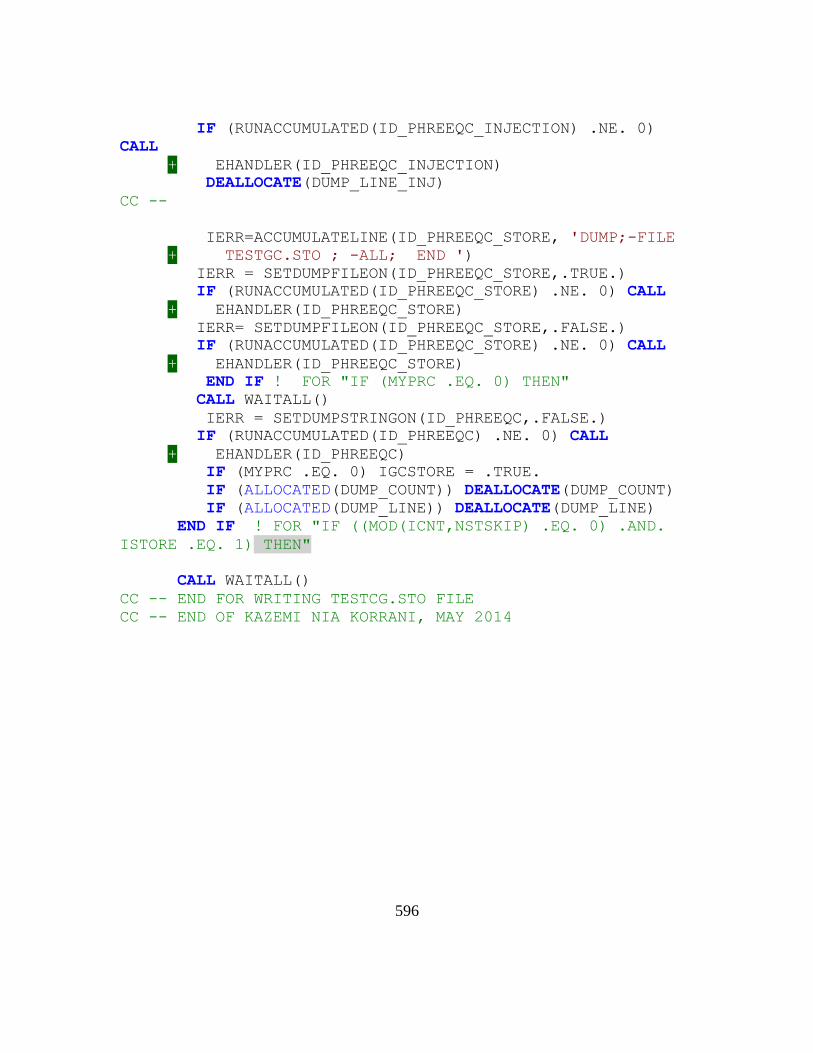
596

IF (RUNACCUMULATED(ID_PHREEQC_INJECTION) .NE. 0)

CALL

+ EHANDLER(ID_PHREEQC_INJECTION)

DEALLOCATE(DUMP_LINE_INJ)

CC --

IERR=ACCUMULATELINE(ID_PHREEQC_STORE, 'DUMP;-FILE

+ TESTGC.STO ; -ALL; END ')

IERR = SETDUMPFILEON(ID_PHREEQC_STORE,.TRUE.)

IF (RUNACCUMULATED(ID_PHREEQC_STORE) .NE. 0) CALL

+ EHANDLER(ID_PHREEQC_STORE)

IERR= SETDUMPFILEON(ID_PHREEQC_STORE,.FALSE.)

IF (RUNACCUMULATED(ID_PHREEQC_STORE) .NE. 0) CALL

+ EHANDLER(ID_PHREEQC_STORE)

END IF ! FOR "IF (MYPRC .EQ. 0) THEN"

CALL WAITALL()

IERR = SETDUMPSTRINGON(ID_PHREEQC,.FALSE.)



IF (MYPRC .EQ. 0) IGCSTORE = .TRUE.

IF (ALLOCATED(DUMP_COUNT)) DEALLOCATE(DUMP_COUNT)

IF (ALLOCATED(DUMP_LINE)) DEALLOCATE(DUMP_LINE)

END IF ! FOR "IF ((MOD(ICNT,NSTSKIP) .EQ. 0) .AND.

ISTORE .EQ. 1) THEN"

CALL WAITALL()

CC -- END FOR WRITING TESTCG.STO FILE

CC -- END OF KAZEMI NIA KORRANI, MAY 2014

597

15 Appendix H: UTCHEM-IPhreeqc Input Files for the ACP

Coreflood Presented in Chapter 5

To run UTCHEM-IPhreeqc five input files are required (INPUT, HEAD,

GCINPUT.DAT, IPhreeqc_Database.DAT, and IPhreeqc_INPUT.DAT). These files are

presented below.

H.1 HEAD

UTEXAS

NX NY NZ N NWELL

1 1 100 20 2

NTW NTA

0 0

NO NPHAS

0 3

NSUB MSUB

0 0

H.2 INPUT

CC*******************************************************************

CC *

CC BRIEF DESCRIPTION OF DATA SET : UTCHEM-IPhreeqc (VERSION 2014) *

CC *

CC*******************************************************************

CC *

CC ACP FLOODING *

CC *

CC LENGTH (FT) : PROCESS : A/C/P FLOODING *

CC THICKNESS (FT) : INJ. PRESSURE (PSI) : *

CC WIDTH (FT) : COORDINATES : CARTESIAN *

CC POROSITY : *

CC GRID BLOCKS : *

CC DATE : *

CC *

CC*******************************************************************

CC

CC*******************************************************************

CC *

CC RESERVOIR DESCRIPTION *

CC *

CC*******************************************************************

CC

CC

*----RUNNO

CC

598

CC

*----HEADER

PCN

EXPERIMENT

***********************************************************

CC

CC SIMULATION FLAGS

*---- IMODE IMES IDISPC ICWM ICAP IREACT IBIO ICOORD ITREAC ITC IGAS

IENG IPHREEQC

1 4 0 0 0 3 0 1 0 0 0 0

1

CC

CC NUMBER OF GRID BLOCKS AND FLAG SPECIFIES CONSTANT OR VARIABLE GRID

SIZE

*----NX NY NZ IDXYZ IUNIT

1 1 100 0 0

CC

CC CONSTANT GRID BLOCK SIZE IN X, Y, AND Z

*----DX DY DZ

0.145489216 0.145489216 0.00971129

CC

CC TOTAL NO. OF COMPONENTS, NO. OF TRACERS, NO. OF GEL COMPONENTS

*----N NO NTW NTA NG NOTH

8 0 0 0 0 0

CC

CC

*---- SPNAME(I),I=1,N

WATER

OIL

SURFACTANT

POLYMER

ANION

CALCIUM

ALC1

ALC2

CC

CC FLAG INDICATING IF THE COMPONENT IS INCLUDED IN CALCULATIONS OR NOT

*----ICF(KC) FOR KC=1,N

1 1 1 1 1 1 0 0

CC

CC*******************************************************************

CC *

CC OUTPUT OPTIONS *

CC *

CC*******************************************************************

CC

CC

CC FLAG FOR PV OR DAYS FOR OUTPUT AND STOP THE RUN

*----ICUMTM ISTOP IOUTGMS IS3G

1 1 0 0

CC

599

CC FLAG INDICATING IF THE PROFILE OF KCTH COMPONENT SHOULD BE WRITTEN

*----IPRFLG(KC),KC=1,N

1 1 1 1 1 1 0 0

CC

CC FLAG FOR PRES,SAT.,TOTAL CONC.,TRACER CONC.,CAP.,GEL, ALKALINE

PROFILES

*----IPPRES IPSAT IPCTOT IPBIO IPCAP IPGEL IPALK ITEMP IPOBS

1 1 1 0 0 0 1 0 0

CC

CC FLAG FOR WRITING SEVERAL PROPERTIES

*----ICKL IVIS IPER ICNM ICSE IFOAM IHYST INONEQ

1 1 1 1 1 0 0 0

CC

CC FLAG FOR WRITING SEVERAL PROPERTIES TO PROF

*----IADS IVEL IRKF IPHSE

1 0 1 1

CC

CC*******************************************************************

CC *

CC RESERVOIR PROPERTIES *

CC *

CC*******************************************************************

CC

CC

CC MAX. SIMULATION TIME ( PV)

*---- TMAX

1.9

CC

CC ROCK COMPRESSIBILITY (1/PSI), STAND. PRESSURE(PSIA)

*----COMPR PSTAND

0. 0.

CC

CC FLAGS INDICATING CONSTANT OR VARIABLE POROSITY, X,Y,AND Z

PERMEABILITY

*----IPOR1 IPERMX IPERMY IPERMZ IMOD ITRANZ INTG

0 0 3 3 0 0 0

CC

CC CONSTANT POROSITY

*----PORC1

.21

CC

CC CONSTANT X-PERMEABILITY (MILIDARCY) FOR LAYER K = 1,NZ

*----PERMX

2507

CC

CC Y DIRECTION PERMEABILITY IS DEPENDENT ON X DIRECTION PERMEABILITY

*---- CONSTANT PERMEABILITY MULTIPLIER FOR Y DIRECTION PERMEABILITY

1

CC

CC Z DIRECTION PERMEABILITY IS DEPENDENT ON X DIRECTION PERMEABILITY

*---- CONSTANT PERMEABILITY MULTIPLIER FOR Z DIRECTION PERMEABILITY

600

1

CC

CC FLAG FOR CONSTANT OR VARIABLE DEPTH, PRESSURE, WATER SATURATION

*----IDEPTH IPRESS ISWI ICWI

0 0 0 -1

CC

CC CONSTANT DEPTH (FT)

*----D111

0.

CC

CC INITIAL PRESSURE (PSIA)

*----PINIT DEPTH

14.7 0.0

CC

CC CONSTANT INITIAL WATER SATURATION (RESIDUAL OIL)

*----SWI

0.565

CC

CC CONSTANT CHLORIDE AND CALCIUM CONCENTRATIONS (MEQ/ML)

*----C50 C60

0.66296 0.0921

CC

CC*******************************************************************

CC *

CC PHYSICAL PROPERTY DATA *

CC *

CC*******************************************************************

CC

CC 3.4.1 OIL CONC. AT PLAIT POINT FOR TYPE II(+)AND TYPE II(-), CMC

CC CMC

*---- C2PLC C2PRC EPSME IHAND

0 1 0.001 0

CC

CC 3.4.2 FLAG INDICATING TYPE OF PHASE BEHAVIOR PARAMETERS

*---- IFGHBN=0 FOR INPUT HEIGHT OF BINODAL CURVE; =1 FOR INPUT SOL.

RATIO

0

CC 3.4.3 SLOPE AND INTERCEPT OF BINODAL CURVE AT ZERO, OPT., AND 2XOPT

SALINITY

CC FOR ALCOHOL 1

*---- HBNS70 HBNC70 HBNS71 HBNC71 HBNS72 HBNC72

0 0.15 0 0.13 0 0.15

CC 3.4.5 SLOPE AND INTERCEPT OF BINODAL CURVE AT ZERO, OPT., AND 2XOPT

SALINITY

CC FOR ALCOHOL 2

*---- HBNS80 HBNC80 HBNS81 HBNC81 HBNS82 HBNC82

0 0 0 0 0 0

CC

CC 3.4.6 LOWER AND UPPER EFFECTIVE SALINITY FOR ALCOHOL 1 AND ALCOHOL 2

*---- CSEL7 CSEU7 CSEL8 CSEU8

0.1415 0.2264 0 0

601

CC 3.4.7 THE CSE SLOPE PARAMETER FOR CALCIUM AND ALCOHOL 1 AND ALCOHOL

2

CC CA ALCOHOL#1 ALCOHOL#2

*---- BETA6 BETA7 BETA8

0 0 0

CC

CC 3.4.8 FLAG FOR ALCOHOL PART. MODEL AND PARTITION COEFFICIENTS

*---- IALC OPSK7O OPSK7S OPSK8O OPSK8S

0 0 0 0 0

CC THESE ARE USED ONLY FOR ALCOHOL PARTITIONING IN A TWO ALCOHOL

SYSTEM:

CC 3.4.9 NO. OF ITERATIONS, AND TOLERANCE

*---- NALMAX EPSALC

20 0.0001

CC 3.4.10 ALCOHOL 1 PARTITIONING PARAMETERS IF IALC=1

CC AQ-OLEIC AQ-OLEIC SURF-OLEIC

*---- AKWC7 AKWS7 AKM7 AK7 PT7

4.671 1.79 48 35.31 0.222

CC

CC 3.4.11 ALCOHOL 2 PARTITIONING PARAMETERS IF IALC=1

*---- AKWC8 AKWS8 AKM8 AK8 PT8

0 0 0 0 0

CC

CC 3.4.22 IFT MODEL FLAG

*---- IFT=0 FOR HEALY&REED; =1 FOR CHUN HUH CORREL.

1

CC 3.4.24 INTERFACIAL TENSION PARAMETERS

CC TYP=.1-.35 TYP=5-20

*---- CHUH AHUH

0.3 10

CC 3.4.25 LOG10 OF OIL/WATER INTERFACIAL TENSION

CC UNITS OF LOG 10 DYNES/CM = MN/M

*---- XIFTW

1.3

CC 3.4.26 ORGANIC MASS TRANSFER FLAG

CC IMASS=0 FOR NO OIL SOL. IN WATER. ICORR=0 FOR CONSTANT MTC

*---- IMASS ICOR

0 0

CC

CC

*--- IWALT IWALF

0 0

CC 3.4.31 CAPILLARY DESATURATION PARAMETERS FOR PHASE 1, 2, AND 3

CC AQ OLEIC ME

*---- ITRAP T11 T22 T33

2 1865 59074 364.2

CC

CC 3.4.32 FLAG FOR RELATIVE PERMEABILITY AND CAPILLARY PRESSURE MODEL

*---- IPERM=0 FOR CONSTANT; =1 VARIES BY LAYER; =2 VARIES BY GRIDBLOCK

0 0

CC

602

CC 3.4.35 FLAG FOR CONSTANT OR VARIABLE REL. PERM. PARAMETERS

*---- ISRW IPRW IEW

0 0 0

CC

CC CONSTANT RES. SATURATION OF PHASES 1,2,AND 3 AT LOW CAPILLARY NO.

*----S1RWC S2RWC S3RWC

.19 .443 .17

CC

CC CONSTANT ENDPOINT REL. PERM. OF PHASES 1,2,AND 3 AT LOW CAPILLARY

NO.

*----P1RW P2RW P3RW

.07 0.95 .07

CC

CC CONSTANT REL. PERM. EXPONENT OF PHASES 1,2,AND 3 AT LOW CAPILLARY

NO.

*----E1W E2W E3W

5.6 1.55 3.0

CC

CC RES. SATURATION OF PHASES 1,2,AND 3 AT HIGH CAPILLARY NO.

*----S1RC S2RC S3RC

.0 .0 .0

CC

CC ENDPOINT REL. PERM. OF PHASES 1,2,AND 3 AT HIGH CAPILLARY NO.

*----P1RC P2RC P3RC

1.0 1.0 1.0

CC

CC REL. PERM. EXPONENT OF PHASES 1,2,AND 3 AT HIGH CAPILLARY NO.

*----E13CW E23C E31C

1.0 1.0 1.0

CC 3.4.61 WATER AND OIL VISCOSITY , RESERVOIR TEMPERATURE

CC WATER OIL =0 FOR ISOTHERMAL MODELING

*---- VIS1 VIS2 TSTAND

0.534 170 100.4

CC

CC 3.4.80 COMPOSITIONAL PHASE VISCOSITY PARAMETERS FOR MICROEMULSION

*---- ALPHAV1 ALPHAV2 ALPHAV3 ALPHAV4 ALPHAV5

0.1 5.0 0.1 0.0 0.0

CC

CC 3.4.81 PARAMETERS TO CALCULATE POLYMER VISCOSITY AT ZERO SHEAR RATE

*---- AP1 AP2 AP3 47.9 346 638

230 280 1500

CC

CC 3.4.82 PARAMETER TO COMPUTE CSEP,MIN. CSEP, AND SLOPE OF LOG VIS.

VS. LOG CSEP

*---- BETAP CSE1 SSLOPE

1 0.01 -0.4435

CC

CC 3.4.83 PARAMETER FOR SHEAR RATE DEPENDENCE OF POLYMER VISCOSITY

*---- GAMMAC GAMHF POWN IPMOD ISHEAR RWEFF GAMHF2

4 10.0 2.3 0 0 0.25 0.0

CC

603

CC 3.4.84 FLAG FOR POLYMER PARTITIONING, PERM. REDUCTION PARAMETERS

*---- IPOLYM EPHI3 EPHI4 BRK CRK RKCUT

1 1.0 0.93 100 0 10

CC 3.4.85 SPECIFIC WEIGHT FOR COMPONENTS 1,2,3,7,8 ,COEFFIENT OF OIL

AND GRAVITY FLAG

CC IF IDEN=1 IGNORE GRAVITY EFFECT; =2 THEN INCLUDE GRAVITY EFFECT

*---- DEN1 DEN2 DEN23 DEN3 DEN7 DEN8 IDEN

0.44 0.40689 0.40689 0.42 0.346 0 2

CC ISTB=0:BOTTOMHOLE CONDITION , 1: STOCK TANK

CC 3.4.93 FLAG FOR CHOICE OF UNITS WHEN PRINTING

*----- ISTB

0

CC

CC 3.4.95 COMPRESSIBILITY FOR VOL. OCCUPYING COMPONENTS 1,2,3,7,AND 8

*---- COMPC(1) COMPC(2) COMPC(3) COMPC(7) COMPC(8)

0.0000033 0.0000234 0 0 0

CC IOW=0 WATER WET, =1 OIL WET, =2 MIXED WET

CC 3.4.99 CONSTANT OR VARIABLE PC PARAM., WATER-WET OR OIL-WET PC CURVE

FLAG

*---- ICPC IEPC IOW

0 0 0

CC

CC 3.4.100 CAPILLARY PRESSURE PARAMETER, CPC0

*---- CPC0

0

CC

CC 3.4.103 CAPILLARY PRESSURE PARAMETER, EPC0

*---- EPC0

0

CC

CC 3.4.117 MOLECULAR DIFFUSION COEF. KCTH COMPONENT IN PHASE 1

*---- D(KC,1),KC=1,N

0 0 0 0 0 0 0

0 0 0 0 0

CC


*---- D(KC,2),KC=1,N

0 0 0 0 0 0 0

0 0 0 0 0

CC


*---- D(KC,3),KC=1,N

0 0 0 0 0 0 0

0 0 0 0 0

CC

CC 3.4.121 LONGITUDINAL AND TRANSVERSE DISPERSIVITY OF PHASE 1


0.005 0.001

CC



604

0.005 0.001

CC



0.005 0.001

CC

CC 3.4.125 FLAG TO SPECIFY ORGANIC ADSORPTION CALCULATION

*---- IADSO=0 IF ORGANIC ADSORPTION IS NOT CONSIDERED

0

CC

CC 3.4.130 SURFACTANT AND POLYMER ADSORPTION PARAMETERS

*---- AD31 AD32 B3D AD41 AD42 B4D IADK IADS1 FADS

REFK

1.6 0.1 1000 0.48 0. 100 0 0 0

50

CC

CC*******************************************************************

CC *

CC WELL DATA *

CC *

CC*******************************************************************

CC

CC

CC FLAG FOR PRESSURE CONST. BOUNDARIES

*---- IBOUND IZONE

0 0

CC

CC TOTAL NUMBER OF WELLS, WELL RADIUS FLAG, FLAG FOR TIME OR COURANT

NO.

*----NWELL IRO ITIME NWREL

2 2 0 2

CC


SKIN

*----IDW IW JW IFLAG RW SWELL IDIR IFIRST ILAST

IPRF

1 1 1 1 .003 0. 3 100 100 0

CC

CC WELL NAME

*---- WELNAM

INJECTOR

CC

CC ICHEK MAX. AND MIN. ALLOWABLE BOTTOMHOLE PRESSURE AND RATE

*----ICHEK PWFMIN PWFMAX QTMIN QTMAX

0 0.0 5000. 0.0 50000.

CC

CC WELL ID, LOCATION, AND FLAG FOR SPECIFYING WELL TYPE, WELL RADIUS,

SKIN

*----IDW IW JW IFLAG RW SWELL IDIR IFIRST ILAST IPRF

2 1 1 2 .003 0. 3 1 1 0

CC

605

CC WELL NAME

*---- WELNAM

PRODUCER

CC

CC MAX. AND MIN. ALLOWABLE BOTTOMHOLE PRESSURE AND RATE

*----ICHEK PWFMIN PWFMAX QTMIN QTMAX

0 0.0 5000. 0.0 50000.

CC


(L=1,3)

*----ID QI(M,L) C(M,KC,L) 2.75 WT% SODIUM CARBONATE, 1.3 FT/D CL

CA

1 0.004445094 0.985 0. 0.015 0.275 0.0132 0.

0. 0.

1 0. 0. 0. 0. 0. 0. 0. 0. 0.

1 0. 0. 0. 0. 0. 0. 0. 0. 0.

CC

CC

*---- INJ_SOLUTION

101

CC

CC ID,

*----ID PWF

2 14.7

CC

CC CUM. INJ. TIME , AND INTERVALS (PV OR DAY) FOR WRITING TO OUTPUT

FILES

*----TINJ CUMPR1 CUMHI1 WRHPV WRPRF RSTC

0.5 0.03 0.03 0.03 0.03 0.3

CC

CC FOR IMES=2 ,THE INI. TIME STEP,CONC. TOLERANCE,MAX.,MIN. COURANT NO.

*----DT DCLIM CNMAX CNMIN

0.0001 17*0.01 0.01 0.001

CC****** INJECT NO SURFACTANT *********************

CC FLAG FOR INDICATING BOUNDARY CHANGE

*---- IBMOD

0

CC

CC IRO, ITIME, NEW FLAGS FOR ALL THE WELLS

*---- IRO ITIME IFLAG

2 0 1 2

CC

CC NUMBER OF WELLS CHANGES IN LOCATION OR SKIN OR PWF

*---- NWEL1

0

CC

CC NUMBER OF WELLS WITH RATE CHANGES, ID

*---- NWEL2 ID

1 1

CC

606


(L=1,3)

*---- ID QI(M,L) WATER OIL SURF POLYMER CHLOR DIVALENT CL

CA

1 0.004445094 1.0 0. 0.0 0.225 0.0132 0.

0. 0.

1 0. 0. 0. 0. 0. 0. 0. 0. 0.

1 0. 0. 0. 0. 0. 0. 0. 0. 0.

CC

CC

*--- INJ_SOLUTION

102

CC

CC CUM. INJ. TIME , AND INTERVALS (PV) FOR WRITING TO OUTPUT FILES

*---- TINJ CUMPR1 CUMHI1 WRHPV WRPRF RSTC

1.9 0.01 0.03 0.03 0.03 2.0

CC

CC FOR IMES=4 ,THE INI. TIME STEP,CONC. TOLERANCE,MAX.,MIN. TIME STEPS

*---- DT DCLIM CNMAX CNMIN

0.0001 17*0.01 0.01 0.001

H.3 GCINPUT.DAT

CC

CC*******************************************************

CC *


CC *

CC*******************************************************

CC

CC

*---- IRSPS IPHAD EQW(Equivalent weight of surfactant)

2 1 804

CC

CC

*--- PHC PHT PHT1 HPHAD(The constant by which the surfactant adsorption

is reduced)

7 13 13 0.1

CC

CC

*---- CSELP(meq/ml) CSEUP(meq/ml)

0.2 0.33

CC

CC

*-----IMIX

0

CC

CC

*------HBN0 HBN1 HBN2

0.3 0.2 0.3

CC

CC

607

*---- AW_MW EQWPS Log(Kp) (HAo=HAw) Log(Kd) (HAw= H+ +

Aw-)

59.05 600.0 -4.142173494 -8.0

CC

CC*******************************************************

CC *

CC GEOCHEMISTRY OUTPUT SECTION *

CC *

CC*******************************************************

CC

CC

*---- PRINT_NUMBER_ELEMENT ELEMENT_HISTORY ELEMENT_MAP

FREQUENCY_HIS(TIME STEP) FREQUENCY_MAP(TIME STEP)

0 0 1

100 100

CC

CC

*---- NSLDP SOLID_HISTORY SOLID_MAP FREQUENCY_HIS (TIME STEP)

FREQUENCY_MAP(TIME STEP)

0 1 1 1 1

CC

CC

*---- NAQSP AQS_HISTORY AQS_MAP FREQUENCY_HIS(TIME STEP)

FREQUENCY_MAP(TIME STEP)

0 0 1 1

1

CC

CC

*---- NSORBP SORBED_HISTORY ELEMENT_MAP FREQUENCY_HIS (TIME STEP)

FREQUENCY_MAP (TIME STEP)

0 1 1 1

1

CC

CC

*---- NPRINTG PRINTG_HISTORY PRINTG_MAP FREQUENCY_HIS (TIME

STEP) FREQUENCY_MAP(TIME STEP)

0 0 1 100000

1

H.4 IPHREEQC_DATABASE.DAT

The thermodynamic database used in this case is phreeqc.dat. This database is

presented in Appendix E (i.e., Section E.1.4).

H.5 IPHREEQC_INPUT.DAT

## GRIDBLOCK INITIALIZATION

SOLUTION 1-100

-water 1.0

-units ppm

608

-pH 7.51

K 11.59

Na 300.00

Mg 0.0

Ca 0.0

Cl 140.81

S(6) 310.41

C(4) 176.95

Aw 2879.886276 ## ACID COMPONENT CONCENTRATION

END

EXCHANGE 1-100

X 0.001302982

-equilibrate 1

END

## INJECTION SOLUTIONS

SOLUTION 101 ## ACP FLOOD

-water 1.0 ## kg

-units ppm

-pH 7 charge

K 11.59

Na 2903.773585

Mg 0.0

Ca 0.0

Cl 140.81

S(6) 310.41

C(4) 3573.176415

END

SOLUTION 102 ## POLYMER FLOOD

-water 1.0 ## kg

-units ppm

-pH 7.51

K 11.59

Na 300.00

Mg 0.0

Ca 0.0

Cl 140.81

S(6) 310.41

C(4) 176.95

END

609

16 References

Abate, J., Wang, P., and Sepehrnoori, K. 2001. Parallel compositional reservoir

simulation on clusters of PCs. International Journal of High Performance

Computing Applications, 15(1), 13-21. doi: 10.1177/109434200101500102.

Aksulu, H., Hamsø, D., Strand, S., Puntervold, T., and Austad, T. 2012. Evaluation of

low-salinity enhanced oil recovery effects in sandstone: effects of the temperature

and pH gradient. Energy & Fuels, 26(6), 3497-3503.

Al Harrasi, A., Al-maamari Rashid Salim, and Masalmeh, S. K. 2012. Laboratory

Investigation of Low Salinity Waterflooding for Carbonate Reservoirs. Abu

Dhabi International Petroleum Conference and Exhibition. Abu Dhabi, UAE. 11-

14 November. doi:10.2118/161468-MS.

Aladasani Ahmad, Bai, B., and Wu, Y.-S. 2012. Investigating Low Salinity

Waterflooding Recovery Mechanisms in Carbonate Reservoirs. SPE EOR

Conference at Oil and Gas West Asia. Muscat, Oman. 16-18 April.

doi:10.2118/155560-MS.

Al-Attar, H. H., Mahmoud, M. Y., Zekri, A. Y., Almehaideb, R. A. and Ghannam, M. T.

2013a. The Impact of LoSal on Oil Recovery from a Selected Carbonate

Reservoir in Abu Dhabi-An Experimental Approach. SPE Middle East Oil and

Gas Show and Conference, Manama, Bahrain. 10-13 March.

http://dx.doi.org/10.2118/164331-MS.

Al-Attar, H. H., Mahmoud, M. Y., Zekri, A. Y., Almehaideb, R., and Ghannam, M.

2013b. Low-salinity flooding in a selected carbonate reservoir: experimental

approach. Journal of Petroleum Exploration and Production Technology, 3(2),

139-149. doi: 0.1007/s13202-013-0052-3.

Alcalá, F. J., and Custodio, E. 2008. Using the Cl/Br ratio as a tracer to identify the origin

of salinity in aquifers in Spain and Portugal. Journal of Hydrology, 359(1), 189-

207. doi: 10.1016/j.jhydrol.2008.06.028.

Al-Hashim, H. S., Obiora, V., Al-Yousef, H. Y., Fernandez, F., and Nofal, W. 1996.

Alkaline Surfactant Polymer Formulation for Saudi Arabian Carbonate

Reservoirs. SPE/DOE Improved Oil Recovery Symposium, Tulsa, Oklahoma, 21-

24 April. http://dx.doi.org/10.2118/35353-MS.



610

Alotaibi, M. B., Azmy, R., and Nasr-El-Din, H. A. 2010. Wettability Challenges in

Carbonate Reservoirs. SPE Improved Oil Recovery Symposium. Tulsa,

Oklahoma, USA. 24-28 April. doi:10.2118/129972-MS.

Al-Shalabi, E. W., Sepehrnoori, K., and Delshad, M. 2014a. Mechanisms behind low

salinity water injection in carbonate reservoirs. Fuel, 121, 11-19.

Al-Shalabi, E. W., Sepehrnoori, K., and Pope, G. 2014b. Geochemical Interpretation of

Low Salinity Water Injection in Carbonate Oil Reservoirs. SPE Improved Oil

Recovery Symposium. Tulsa, Oklahoma, USA. 12-16 April. doi:10.2118/169101-

MS.

Alwi, N., Salleh, I.K., Irevine-Fortescue, J., Graham, G., Dyer, S., Wright, R., Simpson,

C., Kidd, S., and Stalker, R. 2013. Scale and Scale Inhibition Challenges for an

Alkaline Surfactant Polymer Flood in a Seawater Flooded Reservoir. SPE:

Society of Petroleum Engineers. doi:10.2118/164058-MS.

Andersen, P. Ø., Evje, S., Madland, M. V., and Hiorth, A. 2012a. A geochemical model

for interpretation of chalk core flooding experiments. Chemical engineering

science, 84, 218-241. doi: 10.1016/j.ces.2012.08.038.

Andersen, P. Ř., and Evje, S. 2012b. A Mathematical Model for Interpretation of Brine-

Dependent Spontaneous Imbibition Experiments. In ECMOR XIII-13th European

Conference on the Mathematics of Oil Recovery.

Anderson, A. G. 2006. Simulation of Chemical Flood Enhanced Oil Recovery Processes

Including the Effects of Reservoir Wettability. MS Thesis, The University of

Texas at Austin, Austin, Texas (May 2006).

Appelo, C. A. J., and Rolle, M. 2010. PHT3D: A reactive multicomponent transport

model for saturated porous media. Groundwater, 48(5), 627-632.

doi: 10.1111/j.1745-6584.2010.00732.x.

Austad, T., RezaeiDoust, A., and Puntervold, T. 2010. Chemical Mechanism of Low

Salinity Water Flooding in Sandstone Reservoirs. SPE: Society of Petroleum

Engineers. doi:10.2118/129767-MS.

Austad, T., Shariatpanahi, S. F., Strand, S., Black, C. J. J., and Webb, K. J. 2011.

Conditions for a low-salinity enhanced oil recovery (EOR) effect in carbonate oil

reservoirs. Energy & fuels, 26(1), 569-575. doi: 10.1021/ef201435g.

611

Austad, T., Strand, S., Høgnesen, E. J., and Zhang, P. 2005. Seawater as IOR fluid in

fractured chalk. SPE International Symposium on Oilfield Chemistry. The

Woodlands, Texas. 2-4 February. http://dx.doi.org/10.2118/93000-MS.

Austad, T., Strand, S., Madland, M. V., Puntervold, T., and Korsnes, R. I. 2008. Seawater

in chalk: An EOR and compaction fluid. SPE Reservoir Evaluation &

Engineering, 11(04), 648-654. doi: http://dx.doi.org/10.2118/118431-PA.

Bagci, S., Kok, M. V., and Turksoy, U. 2001. Effect of brine composition on oil recovery

by waterflooding. Petroleum science and technology, 19(3-4), 359-372. doi:

10.1081/LFT-100000769.

Barney, B. 2009. Message passing interface (mpi). Lawrence Livermore National

Laboratory, https://computing. llnl. gov/tutorials/mpi/, available online, 2010.

Barrodale, I., and Roberts, F. D. K. 1980. Algorithm 552: Solution of the Constrained I 1

Linear Approximation Problem [F4]. ACM Transactions on Mathematical

Software (TOMS), 6(2), 231-235. doi:10.1145/355887.355896.

Bear, J. 2013. Dynamics of fluids in porous media. Courier Dover Publications.

Bedrikovetsky, P. G., Siqueira, F. D., Furtado, C. J. A., and Serra de Souza, A. L. 2010.

Quantitative Theory for Fines Migration and Formation Damage. SPE: Society of

Petroleum Engineers. doi:10.2118/128384-MS.

Bhuyan, D. 1989. Development of an Alkaline/Surfactant/Polymer Compositional

Reservoir Simulator. PhD dissertation, The University of Texas at Austin, Austin,

Texas (December 1989).

Borkovec, M., and Westall, J. 1983. Solution of the Poisson-Boltzmann equation for

surface excesses of ions in the diffuse layer at the oxide-electrolyte interface.

Journal of Electroanalytical Chemistry and Interfacial Electrochemistry, 150(1),

325-337. DOI: 10.1016/S0022-0728(83)80214-9.

Brady, P. V., and Krumhansl, J. L. 2012. A surface complexation model of oil–brine–

sandstone interfaces at 100° C: Low salinity waterflooding. Journal of Petroleum

Science and Engineering, 81, 171–176.

Brown, J. 2010. The Portable Extensible Toolkit for Scientific computing.

Buckley, S. E., and Leverett, M. C. 1941. Mechanism of fluid displacement in sands.

Trans. Aime, 146.


http://dx.doi.org/10.2118/118431-PA

http://dx.doi.org/10.1145/355887.355896

612

Callegaro, C., Bartosek, M., Masserano, F., Nobili, M., Parasiliti Parracello, V. P.,

Pizzinelli, C. S., and Caschili, A. 2013. Opportunity of Enhanced Oil Recovery

Low Salinity Water Injection: From Experimental Work to Simulation Study up

to Field Proposal. SPE: Society of Petroleum Engineers. doi:10.2118/164827-MS.

Cantucci, B., Montegrossi, G., Vaselli, O., Tassi, F., Quattrocchi, F., and Perkins, E. H.

2009. Geochemical modeling of CO2 storage in deep reservoirs: The Weyburn

Project (Canada) case study. Chemical Geology, 265(1), 181–197.

Carman, P. C. 1956. Flow of gases through porous media. Butterworths Scientific

Publications London.

Cartwright, I., Weaver, T. R., and Fifield, L. K. 2006. Cl/Br ratios and environmental

isotopes as indicators of recharge variability and groundwater flow: an example

from the southeast Murray Basin, Australia. Chemical Geology, 231(1), 38-56.

doi: 10.1016/j.chemgeo.2005.12.009.

Chadam, J., Hoff, D., Merino, E., Ortoleva, P., and Sen, A. 1986. Reactive infiltration

instabilities. IMA Journal of Applied Mathematics, 36(3), 207–221.

Chandrasekhar, S. 2013. Wettability alteration with brine composition in high

temperature carbonate reservoirs. MS Thesis. The University of Texas at Austin,

Austin, Texas (August 2013).

Chandrasekhar, S., and Mohanty, K. K. 2013. Wettability Alteration with Brine

Composition in High Temperature Carbonate Reservoirs. SPE Annual Technical

Conference and Exhibition. New Orleans, Louisiana, USA. 30 September-2

October. doi:10.2118/166280-MS.

Chang, Y. B. 1990. Development and application of an equation of state compositional

simulator. PhD dissertation. Austin, Texas, University of Texas at Austin (August

1990).

Charlton, S. R., and Parkhurst, D. L. 2011. Modules based on the geochemical model

PHREEQC for use in scripting and programming languages. Computers &

Geosciences, 37(10), 1653–1663. doi:10.1016/j.cageo.2011.02.005.

Chekani, M., and Mackay, E. J. 2006. Impact on Scale Management of the Engineered

Depressurization of Waterflooded Reservoirs: Risk Assessment Principles and

Case Study. SPE-86472-PA. doi:10.2118/86472-PA.

613

Cheng, L., Reme, A. B., Shan, D., Coombe, D. A., and Rossen, W. R. 2000. Simulating

Foam Processes at High and Low Foam Qualities. SPE/DOE Improved Oil

Recovery Symposium. Tulsa, Oklahoma. 3-5 April. doi:10.2118/59287-MS.

Chukwudeme, E. A., and Hamouda, A. A. 2009. Oil recovery from polar components

(asphaltene and SA) treated chalk rocks by low salinity water and water

containing SO4-2

and Mg2+

at different temperatures. Colloids and Surfaces A:

Physicochemical and Engineering Aspects, 336(1), 174-182. doi:

10.1016/j.colsurfa.2008.11.051.

Cissokho, M., Boussour, S., Cordier, P., Bertin, H., and Hamon, G. 2010. Low salinity oil

recovery on clayey sandstone: Experimental study. Petrophysics, 51(5), 305.

Civan, F. 2007. Formation Damage Mechanisms and Their Phenomenological Modeling-

An Overview. SPE: Society of Petroleum Engineers. doi:10.2118/107857-MS.

Cohen, S.D., and Hindmarsh, A.C. 1996, CVODE, A stiff/nonstiff ODE solver in C.

Computers in Physics.10(2). 138.

Collins, I. R., and Jordan, M. M. 2003. Occurrence, Prediction, and Prevention of Zinc

Sulfide Scale Within Gulf Coast and North Sea High-Temperature and High-

Salinity Fields. SPE-84963-PA. doi:10.2118/84963-PA.

Dang, C. T. Q., Nghiem, L. X., Chen, Z. J., and Nguyen, Q. P. 2013. Modeling Low

Salinity Waterflooding: Ion Exchange, Geochemistry and Wettability Alteration.

SPE: Society of Petroleum Engineers. doi:10.2118/166447-MS.

Darabi, H. 2014. Development of a Non-Isothermal Compositional Reservoir Simulator

to Model Asphaltene Precipitation, Flocculation, and Deposition and

Remediation. PhD dissertation. Austin, Texas, University of Texas at Austin.

(May 2014).

Darabi, H., Sepehrnoori, K., and Kalaei, M. H. 2012. Modeling of Wettability Alteration

Due to Asphaltene Deposition in Oil Reservoirs. SPE: Society of Petroleum


Davies, C. W. 1962. Ion association (p. 190). London: Butterworths.

Davis, J. A., and Kent, D. B. 1990. Surface complexation modeling in aqueous

geochemistry. Reviews in Mineralogy and Geochemistry, 23(1), 177-260.

De Bruin BSc, W. J. 2012. Simulation of Geochemical Processes during Low Salinity

Water Flooding by Coupling Multiphase Buckley-Leverett Flow to the

614

Geochemical Package PHREEQC. MS Thesis. Delft University of Technology.

Delft, The Netherland (August 2012).

De Lucia, M., and Kühn, M. 2013. Coupling R and PHREEQC: an interactive and

extensible environment for efficient programming of geochemical models. In

EGU General Assembly Conference Abstracts Vol. 15, p. 9719.

Debye, P., and Huckel, E. 1954. Translated from Physikalische Zeitschrift, 24(q), 1923,

pages 185-206. The Collected Papers of Peter JW Debye, 217.

Delshad, M., Han, C., Veedu, F., et al. 2013. A simplified model for simulations of

alkaline–surfactant–polymer floods. Journal of Petroleum Science and

Engineering, 108(0), 1–9. doi:10.1016/j.petrol.2013.04.006.

Delshad, M., Pope, G. A., and Sepehrnoori, K. 1996. A compositional simulator for

modeling surfactant enhanced aquifer remediation, 1 formulation. Journal of

Contaminant Hydrology, 23(4), 303–327. doi:10.1016/0169-7722(95)00106-9.

Demin, W., Zhenhua, Z., Jiecheng, C., Jingchun, Y., Shutang, G., and Li, L. 1997. Pilot

Test of Alkaline Surfactant Polymer Flooding in Daqing Oil Field. SPE Reservoir

Engineering 12(4): 229-233. SPE-36748-PA. http://dx.doi.org/10.2118/36748-PA.

Deutsch, W. J. 1997. Groundwater geochemistry: fundamentals and applications to

contamination. CRC press.

deZabala, E. F., Vislocky, J. M., Rubin, E., and Radke, C. J. 1982. A Chemical Theory

for Linear Alkaline Flooding. SPE-8997-PA. doi:10.2118/8997-PA.

Duan, Z., and Sun, R. 2003. An improved model calculating CO2 solubility in pure water

and aqueous NaCl solutions from 273 to 533 K and from 0 to 2000 bar. Chemical

Geology, 193(3), 257–271.

Dzombak, D.A., and Morel, F.M.M.. 1990. Surface complexation modeling-Hydrous

ferric oxide: New York, John Wiley.

Elakneswaran, Y., and Ishida, T. 2014. Development and Verification of an Integrated

Physicochemical and Geochemical Modelling Framework for Performance

Assessment of Cement-Based Materials. Journal of Advanced Concrete

Technology, 12(4): 111-126. http://dx.doi.org/10.3151/jact.12.9.

Elmorsey, S. A. 2013. Challenge and Successful Application for Scale Removal Gemsa

Oil Field, Egypt: Field Study. SPE: Society of Petroleum Engineers.

doi:10.2118/164274-MS.


http://dx.doi.org/10.3151/jact.12.9

615

Emadi, A., and Sohrabi, M. 2013. Visual Investigation of Oil Recovery by Low Salinity

Water Injection: Formation of Water Micro-Dispersions and Wettability

Alteration. SPE: Society of Petroleum Engineers. doi:10.2118/166435-MS.

Fadairo, A. S., Omole, O., and Falode, O. 2008. Effect of Oilfield Scale Deposition on

Mobility Ratio. SPE: Society of Petroleum Engineers. doi:10.2118/114488-MS.

Farajzadeh, R., Ameri, A., Faber, M. J., Van Batenburg, D. W., Boersma, D. M., and

Bruining, J. 2013. Effect of Continuous, Trapped, and Flowing Gas on

Performance of Alkaline Surfactant Polymer (ASP) Flooding. SPE Enhanced Oil

Recovery Conference. Kuala Lumpur, Malaysia, 2-4 July. doi:10.2118/165238-

MS.

Farajzadeh, R., Matsuura, T., van Batenburg, D., and Dijk, H. 2012. Detailed Modeling

of the Alkali/Surfactant/Polymer (ASP) Process by Coupling a Multipurpose

Reservoir Simulator to the Chemistry Package PHREEQC. SPE Reservoir

Evaluation & Engineering. 15(4): 423-435. SPE-143671.

http://dx.doi.org/10.2118/143671-PA.

Farooq, U., Asif, N., Tweheyo, M. T., Sjoblom, J., and Øye, G. 2011. Effect of low-

saline aqueous solutions and pH on the desorption of crude oil fractions from

silica surfaces. Energy & Fuels, 25(5), 2058–2064.

Fathi, S. J., Austad, T., and Strand, S. 2012. Water-Based Enhanced Oil recovery (EOR)

by “Smart Water” in Carbonate Reservoirs. SPE EOR Conference at Oil and Gas

West Asia. Muscat, Oman. 16-18 April. doi:10.2118/154570-MS.

Fernø, M. A., Grønsdal, R., Åsheim, J., Nyheim, A., Berge, M., and Graue, A. 2011. Use

of Sulfate for Water Based Enhanced Oil Recovery during Spontaneous

Imbibition in Chalk. Energy & fuels, 25(4), 1697-1706. doi: 10.1021/ef200136w.

Fjelde, I., Asen, S. M., and Omekeh, A. V. 2012. Low Salinity Water Flooding

Experiments and Interpretation by Simulations. SPE: Society of Petroleum


Fortenberry, R. P. 2013. Experimental Demonstration and Improvement of Chemical

EOR Techniques in Heavy Oils. MS Thesis, The University of Texas at Austin,

Austin, Texas (May 2013).

Fortenberry, R. P., Kim, D. H., Nizamidin, N., Adkins, S., Pinnawala Arachchilage, G.

W. P., Koh, H. S., Weerasooria, U., and Pope, G. A. 2013. Use of Co-Solvents to

Improve Alkaline-Polymer Flooding. SPE Annual Technical Conference and


616

Exhibition, New Orleans, Louisiana, 30 September-2 October.

http://dx.doi.org/10.2118/166478-MS.

Gamage, S., Hasanka, P., and Thyne, G. D. 2011. Comparison of oil recovery by low

salinity waterflooding in secondary and tertiary recovery modes. In SPE Annual

Technical Conference and Exhibition. Society of Petroleum Engineers.

Gao, S., Li, H., and Li, H. 1995. Laboratory Investigation of Combination of Alkaline-

Surfactant-Polymer for Daqing EOR. SPE Reservoir Engineering. 10(3): 194-197.

SPE-27631-PA. http://dx.doi.org/10.2118/27631-PA.

Ghasemi Doroh, M. 2012. Development and application of a parallel compositional

reservoir simulator. MS Thesis, The University of Texas at Austin, Austin, Texas

(August 2012).

Goudarzi, A., Delshad, M., and Sepehrnoori, K. 2013. A Critical Assessment of Several

Reservoir Simulators for Modeling Chemical Enhanced Oil Recovery Processes.


Goudarzi, A., Delshad, M., Mohanty, K. K., and Sepehrnoori, K. 2012. Impact of Matrix

Block Size on Oil Recovery Response Using Surfactants in Fractured Carbonates.


Green, D. W., and Willhite, G. P. 1998. Enhanced oil recovery. Richardson, Tex.: Henry

L. Doherty Memorial Fund of AIME, Society of Petroleum Engineers.

Gupta, R., and Mohanty, K. K. 2011. Wettability alteration mechanism for oil recovery

from fractured carbonate rocks. Transport in porous media, 87(2), 635-652. doi:

10.1007/s11242-010-9706-5.

Gupta, R., Smith, G. G., Hu, L., Willingham, T., Lo Cascio, M., Shyeh, J. J., and Harris,

C. R. 2011. Enhanced Waterflood for Carbonate Reservoirs - Impact of Injection

Water Composition. SPE Middle East Oil and Gas Show and Conference.

Manama, Bahrain. 25-28 September. doi:10.2118/142668-MS.

Hadia, N., Lehne, H. H., Kumar, K. G., Selboe, K. A., Stensen, F. Å., and Torsater, O.

2011. Laboratory Investigation of Low Salinity Waterflooding on Reservoir Rock

Samples from the FrØy Field. SPE: Society of Petroleum Engineers.

doi:10.2118/141114-MS.

Hamouda, A. A., and Valderhaug, O. M. 2014. Investigating Enhanced Oil Recovery

from Sandstone by Low-Salinity Water and Fluid/Rock Interaction. Energy &

Fuels, 28(2), 898-908.



617

Hamouda, A. A., Karoussi, O., and Chukwudeme, E. A. 2008. Relative permeability as a

function of temperature, initial water saturation and flooding fluid compositions

for modified oil-wet chalk. Journal of Petroleum Science and Engineering, 63(1),

61-72. doi: 10.1016/j.petrol.2008.10.002.

Havre, T. E., Sjöblom, J., and Vindstad, J. E. 2003. Oil/water‐partitioning and interfacial

behavior of naphthenic acids. Journal of dispersion science and technology,

24(6), 789-801. doi:10.1081/DIS-120025547.

Hiorth, A., Cathles, L. M., and Madland, M. V. 2010. The impact of pore water chemistry

on carbonate surface charge and oil wettability. Transport in porous media. 85(1),

1-21. doi: 10.1007/s11242-010-9543-6.

Hirasaki, G., and Zhang, D. L. 2004. Surface Chemistry of Oil Recovery From Fractured,

Oil-Wet, Carbonate Formations. SPE Journal 9(2): 151-162. SPE-88365-PA.

http://dx.doi.org/10.2118/88365-PA.

Hognesen, E. J., Strand, S., and Austad, T. 2005. Waterflooding of preferential oil-wet

carbonates: Oil recovery related to reservoir temperature and brine composition.

SPE Europec/EAGE Annual Conference. Madrid, Spain. 13-16 June.

doi:10.2118/94166-MS.

Huber, P., Nivelon, S., Ottenio, P., and Nortier, P. 2012. Coupling a chemical reaction

engine with a mass flow balance process simulation for scaling management in

papermaking process waters. Industrial & Engineering Chemistry Research,

52(1), 421-429. DOI: 10.1021/ie300984y.

Hunter, K. D., Kerr, S. H., Ellis-Toddington, T. T., and McInnis, L. E. 2013. The Use of

Modeling and Monitoring to Control Scale in Alberta ASP Floods. SPE: Society

of Petroleum Engineers. doi:10.2118/165285-MS.

Jackson, A.C. 2006. Experimental Study of the Benefits of Sodium Carbonate on

Surfactants for Enhanced Oil Recovery. MS Thesis, The University of Texas at

Austin, Austin, Texas (December 2006).

Jang, S. H., Liyanage, P. J., Lu, J., Kim, D. H., Arachchilage, G. W. P. P., Britton, C., …

Pope, G. A. 2014. Microemulsion Phase Behavior Measurements Using Live Oils

at High Temperature and Pressure. SPE Improved Oil Recovery Symposium,

Tulsa, Oklahoma, USA. 12-16 April. doi:10.2118/169169-MS.

Jerauld, G. R., Webb, K. J., Lin, C.Y., and Seccombe, J. C. 2008. Modeling Low-Salinity

Waterflooding. SPE Reservoir Evaluation & Engineering. 11(06): 1000-1012.

SPE-102239-PA. doi:10.2118/102239-PA.


618

Jerauld, G., Mohammadi, H., and Webb, K. J. 2010. Interpreting Single Well Chemical

Tracer Tests. SPE: Society of Petroleum Engineers. doi:10.2118/129724-MS.

Kazempour, M., Manrique, E. J., Alvarado, V., Zhang, J., and Lantz, M. 2013. Role of

active clays on alkaline–surfactant–polymer formulation performance in

sandstone formations. Fuel, 104, 593–606.

Kazempour, M., Sundstrom, E., and Alvarado, V. 2012. Geochemical modeling and

experimental evaluation of high-pH floods: Impact of Water–Rock interactions in

sandstone. Fuel, 92(1), 216–230.

Khan, S. A. 1992. An expert system to aid in compositional simulation of miscible gas

flooding. PhD dissertation. Austin, Texas, University of Texas at Austin.

Kon, W., Pitts, M. J., and Surkalo, H. 2002. Mature Waterfloods Renew Oil Production

by Alkaline-Surfactant-Polymer Flooding. SPE Eastern Regional Meeting,

Lexington, Kentucky, 23-26 October. http://dx.doi.org/10.2118/78711-MS.

Korrani, A. K. N., Jerauld, G. R., and Sepehrnoori, K. 2014a. Coupled Geochemical-

Based Modeling of Low Salinity Waterflooding. SPE Improved Oil Recovery

Symposium, Tulsa, Oklahoma, USA, 12-16 April.

http://dx.doi.org/10.2118/169115-MS.

Korrani, A. K. N., Sepehrnoori, K., and Delshad, M. 2013. A Novel Mechanistic

Approach for Modeling Low Salinity Water Injection. SPE: Society of Petroleum


Korrani, A. K. N., Sepehrnoori, K., and Delshad, M. 2014b. A Mechanistic Integrated

Geochemical and Chemical Flooding Tool for Alkaline/Surfactant/Polymer

Floods. Society of Petroleum Engineers. doi:10.2118/169094-MS.

Korrani, A. K. N., Sepehrnoori, K., and Delshad, M. 2014c. A Comprehensive

Geochemical-Based Approach to Quantify the Scale Problems. SPE: Society of


Kozaki, C. 2012. Efficiency of low salinity polymer flooding in sandstone cores. MS

Thesis, Austin, Texas, The University of Texas at Austin. (May 2012).

Kozeny, J. 1927. Uber kapillare Leitung der Wasser in Boden, Sitzungsber.

Sitzungsberichte der Akademie der Wissenschaften in Wien 136: 271–306.

Lager, A., Webb, K. J., Black, C. J. J., Singleton, M., and Sorbie, K. S. 2008a. Low

salinity oil recovery--An experimental investigation. Petrophysics, 49(1), 28.



619

Lager, A., Webb, K. J., Collins, I. R., and Richmond, D. M. 2008b. LoSal Enhanced Oil

Recovery: Evidence of Enhanced Oil Recovery at the Reservoir Scale. SPE:


Lager, A., Webb, K., and Seccombe, J. 2011. Low Salinity Waterflood, Endicott, Alaska:

Geochemical Study & Field Evidence of Multicomponent Ion Exchange. In IOR

2011.

Lake, L.W., Enhanced Oil Recovery, Prentice-Hall, Inc, Englewood Cliffs, NJ, 1989,

142-148.

Lashgari, H. 2014. Development of a Four-Phase Thermal-Chemical Reservoir Simulator

for Heavy Oil. PhD dissertation. Austin, Texas, University of Texas at Austin.

(December 2014).

Lashgari, H., Delshad, M., Sepehrnoori, K., and De Rouffignac, E. P. 2014a.

Development of Electrical Joule’’s Heating Simulation for Heavy Oil Reservoirs.


Lashgari, H., Lotfollahi, M., Delshad, M., Sepehrnoori, K., and De Rouffignac, E. P.

2014b. Steam-Surfactant-Foam Modeling in Heavy Oil Reservoirs. Society of


Le Chatelier, H. L. 1884. Comptes rendus. 99, 786-789.

Lee, S. Y., Webb, K. J., Collins, I., Lager, A., Clarke, S., O’Sullivan, M., Routh, A. F.,

Wang, X. 2010. Low Salinity Oil Recovery: Increasing Understanding of the

Underlying Mechanisms. Society of Petroleum Engineers. doi:10.2118/129722-

MS.

Li, X. 2012. A collection of case studies for verification of reservoir simulators. MS

Thesis, Austin, Texas, The University of Texas at Austin. (August 2012).

Li, Z., and Delshad, M. 2013. Development of an Analytical Injectivity Model for Non-

Newtonian Polymer Solutions. Society of Petroleum Engineers.

doi:10.2118/163672-MS.

Ligthelm, D. J., Gronsveld, J., Hofman, J., Brussee, N., Marcelis, F., and van der Linde,

H. 2009. Novel Waterflooding Strategy By Manipulation Of Injection Brine

Composition. SPE: Society of Petroleum Engineers. doi:10.2118/119835-MS.

Liu, J., Delshad, M., Pope, G. A., and Sepehrnoori, K. 1994. Application of higher-order

flux-limited methods in compositional simulation. Transport in Porous media,

16(1), 1-29.

620

Liu, Q., and Maroto-Valer, M. M. 2010. Investigation of the pH effect of a typical host

rock and buffer solution on CO2 sequestration in synthetic brines. Fuel

Processing Technology, 91(10), 1321–1329.

Liu, S. 2007. Alkaline Surfactant Polymer Enhanced Oil recovery Process. PhD

dissertation. Rice University, Houston, Texas (December 2007).

Liu, S., Zhang, D., Yan, W., Puerto, M., Hirasaki, G. J., and Miller, C. A. 2008.

Favorable Attributes of Alkaline-Surfactant-Polymer Flooding. SPE Journal.

13(1): 5-16. SPE-99744-PA. http://dx.doi.org/10.2118/99744-PA.

Liu, X., and Civan, F. 1995. Formation Damage by Fines Migration Including Effects of

Filter Cake, Pore Compressibility, and Non-Darcy Flow - A Modeling Approach

to Scaling From Core to Field. SPE: Society of Petroleum Engineers.

doi:10.2118/28980-MS.

Lohne, A., Han, L., van der Zwaag, C., van Velzen, H., Mathisen, A.-M., Twyman, A.,

… Hatzignatiou, D. G. 2009. Formation-Damage and Well-Productivity

Simulation. SPE-122241-PA. doi:10.2118/122241-PA.

Lohne, A., Purwanto, E., and Fjelde, I. 2012. Gravity Segregated Flow in Surfactant

Flooding. SPE Europec/EAGE Annual Conference. Copenhagen, Denmark. 4-7

June. doi:10.2118/154495-MS.

Lohrenz, J., Bray, B. G., and Clark, C. R. 1964. Calculating viscosities of reservoir fluids

from their compositions. Journal of Petroleum Technology, 16(10), 1-171.

Luo, H., Al-Shalabi, E. W., Delshad, M., Panthi, K., Sepehrnoori, K. 2015. A Robust

Geochemical Simulator to Model Improved Oil Recovery Methods. To be

presented in SPE Reservoir Simulation Symposium, 23-25 February 2015,

Houston, Texas.

Mackay, E. J. 2003. Modeling In-Situ Scale Deposition: The Impact of Reservoir and

Well Geometries and Kinetic Reaction Rates. SPE-81830-PA. doi:10.2118/81830-

PA.

Mahani, H., Sorop, T., Ligthelm, D. J., Brooks, D., Vledder, P., Mozahem, F., and Ali, Y.

2011. Analysis of field responses to low-salinity waterflooding in secondary and

tertiary mode in Syria. SPE: Society of Petroleum Engineers.

doi:10.2118/142960-MS.

Mangold, D.C., and Tsang, C.F. 1991. A Summary of Subsurface Hydrological and

Hydrochemical Models. Review of Geophysics.


621

Maroongroge, V. 1994. Modeling and application of tracers for reservoir

characterization. PhD dissertation. Austin, Texas, The University of Texas at

Austin (December 1994).

Mazzolini, E. I., Bertero, L., and Truefitt, C. S. 1992. Scale prediction and laboratory

evaluation of BaSO4 scale inhibitors for seawater flood in a high-barium

environment. SPE production engineering, 7(02), 186-192.

McGuire, P. L., Chatham, J. R., Paskvan, F. K., Sommer, D. M., and Carini, F. H. 2005.

Low Salinity Oil Recovery: An Exciting New EOR Opportunity for Alaska’s

North Slope. SPE Western Regional Meeting. Irvine, California. 30 March-1

April. doi:10.2118/93903-MS.

Merdhah, A. B. B., and Yassin, A. A. M. 2009. Scale Formation Due to Water Injection

in Malaysian Sandstone Cores. American Journal of Applied Sciences, 6(8).

Merdhah, A. B., and Yassin, A. M. 2008. Formation damage due to scale formation in

porous media resulting water injection. System, 14, 15.

Mikhailov, N., and Chirkov, M. 2010. Formation Damage Kinetics and its Effect on Oil

Reservoir Productivity. SPE: Society of Petroleum Engineers.

doi:10.2118/128403-MS.

Mitchell, R. W., Grist, D. M., and Boyle, M. J. 1980. Chemical Treatments Associated

With North Sea Projects. SPE-7880-PA. doi:10.2118/7880-PA.

Moghadasi, J., Jamialahmadi, M., Müller-Steinhagen, H., and Sharif, A. 2003a. Scale

Formation in Oil Reservoir and Production Equipment during Water Injection

(Kinetics of CaSO4 and CaCO3 Crystal Growth and Effect on Formation

Damage). SPE: Society of Petroleum Engineers. doi:10.2118/82233-MS.

Moghadasi, J., Jamialahmadi, M., Müller-Steinhagen, H., Sharif, A., Ghalambor, A.,

Izadpanah, M. R., and Motaie, E. 2003b. Scale Formation in Iranian Oil Reservoir

and Production Equipment During Water Injection. SPE: Society of Petroleum


Mohammadi, H. 2008. Mechanistic Modeling, Design, and Optimization of

Alkaline/Surfactant/Polymer Flooding. PhD dissertation. The University of Texas

at Austin, Austin, Texas (December 2008).

Mohammadi, H., Delshad, M., and Pope, G. A. 2009. Mechanistic Modeling of

Alkaline/Surfactant/Polymer Floods. SPE Reservoir Evaluation & Engineering

12(4): 518-527. SPE-110212-PA. http://dx.doi.org/10.2118/110212-PA.


622

Mohan, K. 2009. Alkaline Surfactant Flooding for Tight Carbonate Reservoirs. SPE

Annual Technical Conference and Exhibition, New Orleans, Louisiana, 4-7

October. http://dx.doi.org/10.2118/129516-STU.

Mohebbinia, S. 2013. Advanced Equation of State Modeling for Compositional

Simulation of Gas Floods. PhD dissertation. Austin, Texas, University of Texas at

Austin (December 2013).

Mohebbinia, S., Sepehrnoori, K., and Johns, R. T. 2013. Four-Phase Equilibrium

Calculations of Carbon Dioxide/Hydrocarbon/Water Systems With a Reduced

Method. SPE-154218-PA. doi:10.2118/154218-PA.

Mohebbinia, S., Sepehrnoori, K., and Johns, R. T., and Korrani, A. K. N. 2014.

Simulation of Asphaltene Precipitation during Gas Injection Using PC-SAFT

EOS. SPE: Society of Petroleum Engineers.

Monk, P. M. 2008. Physical chemistry: understanding our chemical world. John Wiley

and Sons.

Muller, M., Parkhurst, D., L., and Charlton, S., R. 2011. Programming PHREEQC

Calculations with C++ and Python a Comparative Study.

Najafabadi, F. N. 2009. Modeling Chemical EOR Processes Using IMPEC and Fully

Implicit Reservoir Simulators. PhD dissertation. Austin, Texas, University of

Texas at Austin (August 2009).

Najafabadi, N. F., Delshad, M., Sepehrnoori, K., Nguyen, Q. P., and Zhang, J. 2008.

Chemical Flooding of Fractured Carbonates Using Wettability Modifiers. Society

of Petroleum Engineers. SPE Symposium on Improved Oil Recovery. Tulsa,

Oklahoma, USA. 20-23 April. doi:10.2118/113369-MS.

Nardi, A., Idiart, A., Trinchero, P., de Vries, L. M., and Molinero, J. 2014. Interface

COMSOL-PHREEQC (iCP), an efficient numerical framework for the solution of

coupled multiphysics and geochemistry. Computers & Geosciences, 69(0), 10–21.

doi:10.1016/j.cageo.2014.04.011.

Nardi, A., Trinchero, P., de Vries, L., Idiart, A., and Molinero, J. 2012. Coupling

multiphysics with geochemistry: The COMSOL-PHREEQC interface. In

COMSOL Conference.

Nasralla, R. A., Alotaibi, M. B., and Nasr-El-Din, H. A. 2011a. Efficiency of Oil

Recovery by Low Salinity Water Flooding in Sandstone Reservoirs. SPE: Society

of Petroleum Engineers. doi:10.2118/144602-MS.

http://dx.doi.org/10.2118/129516-STU

623

Nasralla, R. A., and Nasr-El-Din, H. A. 2011b. Impact of Electrical Surface Charges and

Cation Exchange on Oil Recovery by Low Salinity Water. SPE: Society of


Nasralla, R. A., Bataweel, M. A., and Nasr-El-Din, H. A. 2011c. Investigation of

Wettability Alteration by Low Salinity Water. Offshore Europe.

Nelson, R. C., Lawson, J. B., Thigpen, D. R., and Stegemeier, G. L. 1984. Cosurfactant-

Enhanced Alkaline Flooding. SPE Enhanced Oil Recovery Symposium, Tulsa,

Oklahoma, 15-18 April. http://dx.doi.org/10.2118/12672-MS.

Nghiem, L., Sammon, P., Grabenstetter, J., and Ohkuma, H. 2004. Modeling CO2

Storage in Aquifers with a Fully-Coupled Geochemical EOS Compositional

Simulator. SPE: Society of Petroleum Engineers. doi:10.2118/89474-MS.

Ohen, H. A., and Civan, F. 1989. Formation Damage In Petroleum Reservoirs I:

Modeling. SPE-19380-MS.

Okasha, T. M., and Al-Shiwaish, A. A. 2009. Effect of Brine Salinity on Interfacial

Tension in SPE Middle East Oil and Gas Show and Conference Society of

Petroleum Engineers. Bahrain, Bahrain. 15-18 March. doi:10.2118/119600-MS.

Okocha, C. and Sorbie, K. 2013. Scale Prediction for Iron, Zinc, and Lead Sulfides and

Its Relation to Scale Test Design. SPE: Society of Petroleum Engineers.

doi:10.2118/164111-MS.

Okuno, R., Johns, R.T., and Sepehrnoori, K. 2010. Three-Phase Flash in Compositional

Simulation Using a Reduced Method. SPE Journal, 15(3), 689-703. doi:

http://dx.doi.org/10.2118/125226-PA.

Omekeh, A. V., Evje, S., Fjelde, I., and Friis, H. A. 2011. Experimental and modeling

investigation of ion exchange during low salinity waterflooding. In SCA 2011-038

presented at the International Symposium of the Society of Core Analysts, Austin,

Texas, USA (pp. 18–21).

Parkhurst, D. L., and Appelo, C. A. J. 1999. User’s guide to PHREEQC (Version 2): A

computer program for speciation, batch-reaction, one-dimensional transport, and

inverse geochemical calculations.

Parkhurst, D. L., and Appelo, C. A. J. 2013. Description of Input and Examples for

PHREEQC Version 3--a Computer Program for Speciation, Batch-reaction, One-

dimensional Transport, and Inverse Geochemical Calculations.



624

Parkhurst, D. L., Kipp, K. L., and Charlton, S. R. 2010. PHAST Version 2-A program for

simulating groundwater flow, solute transport, and multicomponent geochemical

reactions. US Geological Survey Techniques and Methods, 6, A35.

Parkhurst, D.L., Thorstenson, D.C., and Plummer, L.N. 1980. PHREEQE--A computer

program for geochemical calculations.

Patacchini, L., De Loubens, R., and Moncorge, A. 2012. Four-fluid-phase, fully implicit

simulation of surfactant flooding. Society of Petroleum Engineers. Abu Dhabi

International Petroleum Conference and Exhibition. Abu Dhabi, UAE. 11-14

November. doi:10.2118/161630-MS.

Patil, S. B., Dandekar, A. Y., Patil, S., and Khataniar, S. 2008. Low Salinity Brine

Injection for EOR on Alaska North Slope (ANS). IPTC: International Petroleum

Technology Conference. doi:10.2523/12004-MS.

Paulo, J., Mackay, E. J., Menzies, N., and Poynton, N. 2001. Implications of Brine

Mixing in the Reservoir for Scale Management in the Alba Field. SPE: Society of


Peaceman, D. W. 1978. Interpretation of well-block pressures in numerical reservoir

simulation (includes associated paper 6988). Society of Petroleum Engineers

Journal, 18(03), 183-194.

Peng, D. Y., and D. B. Robinson. 1976. A New Two-Constant Equation of State.

Industrial & Engineering Chemistry Fundamentals 15(1): 59-64.

Peru, D. A., and Lorenz, P. B. 1990. Surfactant-Enhanced Low-pH Alkaline Flooding.

SPE Reservoir Engineering. 5(3): 327 - 332. SPE-17117-PA.


Pu, H., Xie, X., Yin, P., and Morrow, N. R. 2010. Low-Salinity Waterflooding and

Mineral Dissolution. SPE: Society of Petroleum Engineers. doi:10.2118/134042-

MS.

Qi, Q., Gu, H., Li, D., and Dong, L. 2000. The Pilot Test of ASP Combination Flooding

in Karamay Oil Field. International Oil and Gas Conference and Exhibition in

China, Beijing, China, 7-10 November. doi:10.2118/64726-MS.

Qing, J., Zhou, B., Zhang, R., Chen, Z., and Zhou, Y. 2002. Development and

Application of a Silicate Scale Inhibitor for ASP Flooding Production Scale. SPE:



625

Rezaei Gomari, K. A., and Hamouda, A. A. 2006. Effect of fatty acids, water

composition and pH on the wettability alteration of calcite surface. Journal of

petroleum science and engineering, 50(2), 140-150. doi:

10.1016/j.petrol.2005.10.007.

RezaeiDoust, A., Puntervold, T., and Austad, T. 2011. Chemical verification of the EOR

mechanism by using low saline/smart water in sandstone. Energy & Fuels, 25(5),

2151–2162.

Rezaveisi, M., Johns, R. T., and Sepehrnoori, K. 2014a. Application of Multiple Mixing-

Cell Method to Improve Speed and Robustness of Compositional Simulation. SPE

Improved Oil Recovery Symposium. Tulsa, Oklahoma, USA. 12-16 April.

doi:10.2118/169063-MS.

Rezaveisi, M., Sepehrnoori, K., and Johns, R. T. 2014b. Tie-Simplex-Based Phase-

Behavior Modeling in an IMPEC Reservoir Simulator. SPE Journal. 19(02): 327-

339. SPE-163676-PA. doi:10.2118/163676-PA.

Rivet, S., Lake, L. W., and Pope, G. A. 2010. A Coreflood Investigation of Low-Salinity

Enhanced Oil Recovery. SPE: Society of Petroleum Engineers.

doi:10.2118/134297-MS.

Robertson, E. P. 2007. Low-Salinity Waterflooding to Improve Oil Recovery-Historical

Field Evidence. SPE: Society of Petroleum Engineers. doi:10.2118/109965-MS.

Romanuka, J., Hofman, J., Ligthelm, D. J., Suijkerbuijk, B., Marcelis, F., Oedai, S., …

Austad, T. 2012. Low Salinity EOR in Carbonates. SPE Improved Oil Recovery

Symposium. Tulsa, Oklahoma, USA. 14-18 April. doi:10.2118/153869-MS.

Saad, N. 1989. Field Scale Simulation of Chemical Flooding. PhD dissertation, The

University of Texas at Austin, Austin, Texas (August 1989).

Seccombe, J. C., Lager, A., Webb, K. J., Jerauld, G., and Fueg, E. 2008. Improving

Wateflood Recovery: LoSalTM EOR Field Evaluation. SPE: Society of


Seccombe, J., Lager, A., Jerauld, G., Jhaveri, B., Buikema, T., Bassler, S., … Fueg, E.

2010. Demonstration of Low-Salinity EOR at Interwell Scale, Endicott Field,

Alaska. SPE: Society of Petroleum Engineers. doi:10.2118/129692-MS.

Shakiba, M. 2014. Modeling and Simulation of Fluid Flow in Naturally and

Hydraulically Fractured Reservoirs Using Embedded Discrete Fracture Model

626

(EDFM). MS Thesis, Austin, Texas, The University of Texas at Austin.

(December 2014).

Shariatpanahi, S. F., Strand, S., and Austad, T. 2011. Initial wetting properties of

carbonate oil reservoirs: effect of the temperature and presence of sulfate in

formation water. Energy & Fuels, 25(7), 3021-3028. doi: 10.1021/ef200033h.

Sharifi, M., and Shaikh, M. 2013. Investigation of Optimum Salinity of Injected Water in

Carbonate Reservoirs using Wettability Measurement and Core Flooding. SPE

Reservoir Characterization and Simulation Conference and Exhibition. Abu

Dhabi, UAE. 16-18 September. doi:10.2118/165992-MS.

Sheng, J. J. 2013. A Comprehensive Review of Alkaline-Surfactant-Polymer (ASP)

Flooding. SPE Western Regional & AAPG Pacific Section Meeting 2013 Joint

Technical Conference, Monterey, California, USA, 19-25 April.

http://dx.doi.org/10.2118/165358-MS.

Shirdel, M. 2013. Development of a Coupled Wellbore-Reservoir Compositional

Simulator for Damage Prediction and Remidiation. PhD dissertation. Austin,

Texas, University of Texas at Austin. (August 2013).

Song, W., Yang, C., Han, D., Qu, Z., Wang, B., and Jia, W. 1995. Alkaline-Surfactant-

Polymer Combination Flooding For Improving Recovery of the Oil with High

Acid Value. International Meeting on Petroleum Engineering, Beijing, China, 14-

17 November. http://dx.doi.org/10.2118/29905-MS.

Steefel, C.I., and Lasaga, A.C. 1992. Putting Transport into Water-Rock Interaction

Models. Journal of Geology.

Strand, S., Standnes, D. C., and Austad, T. 2006. New wettability test for chalk based on

chromatographic separation of SCN− and SO4

2−. 2006. Journal of Petroleum

Science and Engineering, 52(1), 187-197. doi: 10.1016/j.petrol.2006.03.021.

Sultani, B., Szabo, G., Zeng, H., and Abdallah, W. 2012. Novelty in Smart Water

Screening and Designing. SPE EOR Conference at Oil and Gas West Asia.

Muscat, Oman. 16-18 April. doi:10.2118/155643-MS.

Sundstrom, E. A. 2011. Impact of Rock-Fluid and Fluid-Fluid Interaction in Chemical

Flooding. MS Thesis. University of Wyoming, Laramie, Wyoming (August

2011).

TACC (Texas Advanced Computing Center). 2014. https://www.tacc.utexas.edu/user-

services/user-guides/lonestar-user-guide.



https://www.tacc.utexas.edu/user-services/user-guides/lonestar-user-guide

https://www.tacc.utexas.edu/user-services/user-guides/lonestar-user-guide

627

Taghavifar, M. 2014. Enhanced Heavy Oil Recovery by Hybrid Thermal-Chemical

Processes. PhD dissertation. Austin, Texas, University of Texas at Austin. (May

2014).

Tang, G. Q., and Morrow, N. R. 1996. Effect of temperature, salinity and oil composition

on wetting behavior and oil recovery by waterflooding. In SPE annual technical

conference (pp. 45–60).

Tavassoli, S., Lu, J., Pope, G. A., and Sepehrnoori, K. 2014a. Investigation of the Critical

Velocity Required for a Gravity-Stable Surfactant Flood. SPE Journal. 19(5): 931-

942. http://dx.doi.org/10.2118/163624-PA.

Tavassoli, S., Pope, G. A., and Sepehrnoori, K. 2014b. Frontal Stability Analysis

of Surfactant Floods. Paper SPE 169118 presented at the SPE Improved Oil

Recovery Symposium, Tulsa, OK, USA.

Tjomsland, T., Grotle, M. N., and Vikane, O. 2001. Scale Control Strategy and

Economical Consequences of Scale at Veslefrikk. SPE: Society of Petroleum


Truesdell, A. H., and Jones, B. F. 1974. WATEQ, a computer program for calculating

chemical equilibria of natural waters (p. 73). US Department of the Interior,

Geological Survey.

Turek, E. A., R. S. Metcalfs, L. Yarborough, and R. L. Robinson Jr. 1984. Phase

Equilibria in CO2 - Multicomponent Hydrocarbon Systems: Experimental Data and

an Improved Prediction Technique. SPE Journal 24(3): 308-324.

Tweheyo, M. T., Zhang, P., and Austad, T. 2006. The Effects of Temperature and

Potential Determining Ions Present in Seawater on Oil Recovery From Fractured

Carbonates. SPE/DOE Symposium on Improved Oil Recovery. Tulsa, Oklahoma,

USA. 22-26 April. doi:10.2118/99438-MS.

UTCHEM Technical Documentation 9. 2000. The University of Texas at Austin.

UTCHEM User’s Guide 7. 2011. The University of Texas at Austin.

UTCOMP Technical Documentation 3.8. 2011. The University of Texas at Austin.

UTCOMP User’s Guide. 2012. The University of Texas at Austin.

Vargo, J., Turner, J., Bob, V., Pitts, M. J., Wyatt, K., Surkalo, H., and Patterson, D. 2000.

Alkaline-Surfactant-Polymer Flooding of the Cambridge Minnelusa Field. SPE


628

Reservoir Evaluation & Engineering. 3(6): 552-558. SPE-68285-PA.


Venkatraman, A. 2014. Gibbs free energy minimization for flow in porous media. PhD

dissertation, The University of Texas at Austin, Austin, Texas (May 2014).

Verma, A., and Pruess, K. 1988. Thermohydrological conditions and silica redistribution

near high‐level nuclear wastes emplaced in saturated geological formations.

Journal of Geophysical Research: Solid Earth (1978–2012), 93(B2), 1159–1173.

Vikas. 2002. Simulation of CO2 Sequestration. PhD dissertation. Austin, Texas.

University of Texas at Austin (2002).

Vledder, P., Gonzalez, I. E., Carrera Fonseca, J. C., Wells, T., and Ligthelm, D. J. 2010.

Low Salinity Water Flooding: Proof of Wettability Alteration On A Field Wide

Scale. SPE: Society of Petroleum Engineers. doi:10.2118/129564-MS.

Vo, L. T., Gupta, R., and Hehmeyer, O. J. 2012. Ion Chromatography Analysis of

Advanced Ion Management Carbonate Coreflood Experiments. Abu Dhabi

International Petroleum Conference and Exhibition. Abu Dhabi, UAE. 11-14

November. doi:10.2118/161821-MS.

Wang, W., and Gu, Y. 2003. Detection and Reuse of the Produced Chemicals in

Alkaline-Surfactant-Polymer Floods. SPE Annual Technical Conference and

Exhibition, Denver, Colorado, 5-8 October. http://dx.doi.org/10.2118/84075-MS.

Wang, Y., Liu, J., Liu, B., Liu, Y., Wang, H., and Chen, G. 2004. Why Does Scale Form

in ASP Flood? How to Prevent from It?--A Case Study of the Technology and

Application of Scaling Mechanism and Inhibition in ASP Flood Pilot Area of N-

1DX Block in Daqing. SPE: Society of Petroleum Engineers. doi:10.2118/87469-

MS.

Webb, K. J., Black, C. J. J., and Al-Ajeel, H. 2004. Low Salinity Oil Recovery - Log-

Inject-Log. SPE: Society of Petroleum Engineers. doi:10.2118/89379-MS.

Webb, K. J., Black, C. J. J., and Edmonds, I. J. 2005. Low salinity oil recovery–The role

of reservoir condition corefloods. In 13th European Symposium on Improved Oil

Recovery.

Weerasooriya, U. P., and Pope, G. A. 2011. Surfactant-Less Alkaline-Polymer

Formulations for Recovering Reactive Crude Oil. U.S. Patent Application

13/115,433.



629

Wei, L. 2011. Interplay of capillary, convective mixing and geochemical reactions for

long-term CO2 storage in carbonate aquifers. First Break, 29(1).

Wei, L. 2012. Sequential Coupling of Geochemical Reactions with Reservoir Simulations

for Waterflood and EOR Studies. SPE Journal. 17(2): 469-484. SPE-138037-PA.

http://dx.doi.org/10.2118/138037-PA.

Williams, G. J. J., Mansfield, M., MacDonald, D. G., and Bush, M. D. 2004. Top-Down

Reservoir Modelling. SPE: Society of Petroleum Engineers. doi:10.2118/89974-

MS.

Wissmeier, L., and Barry, D. A. 2011. Simulation tool for variably saturated flow with

comprehensive geochemical reactions in two-and three-dimensional domains.

Environmental Modelling & Software, 26(2), 210-218. doi:

10.1016/j.envsoft.2010.07.005.

Wright, R. J., and Hall, J. R. F. 1994. Scale Prediction, Measurement, and Control in a

Subsea Satellite Field. SPE: Society of Petroleum Engineers. doi:10.2118/27606-

MS.

Wu, Y.S., and Bai, B. 2009. Efficient Simulation for Low Salinity Waterflooding in

Porous and Fractured Reservoirs. SPE: Society of Petroleum Engineers.

doi:10.2118/118830-MS.

Xiao, S. 1994. Multigrid methods with application to reservoir simulation. PhD

dissertation. Austin, Texas. University of Texas at Austin (May 1994).

Xiao, Y., Xu, T., and Pruess, K. 2009. The effects of gas-fluid-rock interactions on CO2

injection and storage: Insights from reactive transport modeling. Energy

Procedia, 1(1), 1783–1790.

Xie, Q., Liu, Y., Wu, J., and Liu, Q. 2014. Ions tuning water flooding Experiments and

interpretation by thermodynamics of wettability. Journal of Petroleum Science

and Engineering. DOI: 10.1016/j.petrol.2014.07.015.

Xu, H. 2012. Potential for Non-Thermal Cost-Effective Chemical Augmented Waterflood

for Producing Viscous oils. MS thesis. The University of Texas at Austin, Austin,

Texas, (December 2012).

Xu, H., Kim, D. H., and Delshad, M. 2013. Potential for Non-thermal Cost-effective

Chemical Augmented Waterflood for Producing Viscous Oils. SPE Western

Regional & AAPG Pacific Section Meeting 2013 Joint Technical Conference,

Monterey, California, USA, 19-25 April, http://dx.doi.org/10.2118/165350-MS.



630

Xu, T., Kharaka, Y. K., Doughty, C., Freifeld, B. M., and Daley, T. M. 2010. Reactive

transport modeling to study changes in water chemistry induced by CO2 injection

at the Frio-I Brine Pilot. Chemical Geology, 271(3), 153–164.

Xu, T., Zheng, L., and Tian, H. 2011. Reactive transport modeling for CO2 geological

sequestration. Journal of Petroleum Science and Engineering, 78(3), 765–777.

Yang, X., Liao, G., Han, P., Yang, Z., and Yao, Y. 2003. An Extended field Test Study

on Alkaline-surfactant-polymer flooding in Beiyiduanxi of Daqing Oilfield. SPE

Asia Pacific Oil and Gas Conference and Exhibition, Jakarta, Indonesia. 9-11

September. http://dx.doi.org/10.2118/80532-MS.

Yeboah, Y. D., Somuah, S. K., and Saeed, M. R. 1993. A New and Reliable Model for

Predicting Oilfield Scale Formation. SPE: Society of Petroleum Engineers.

doi:10.2118/25166-MS.

Yeh, G.T., and Tripathi, V.S. 1989, A critical evaluation of recent developments in

hydrogeochemical transport models of reactive multichemical components. Water

Resources Research, 25(1), 93–108.

Yi, Z., and Sarma, H. K. 2012. Improving Waterflood Recovery Efficiency in Carbonate

Reservoirs through Salinity Variations and Ionic Exchanges: A Promising Low-

Cost “Smart-Waterflood” Approach. Abu Dhabi International Petroleum

Conference and Exhibition. Abu Dhabi, UAE. 11-14 November.

doi:10.2118/161631-MS.

Yildiz, H. O., and Morrow, N. R. 1996. Effect of brine composition on recovery of

Moutray crude oil by waterflooding. Journal of Petroleum Science and

Engineering, 14(3), 159–168.

Yousef, A. A., Al-Saleh, S., Al-Kaabi, A. U., and Al-Jawfi, M. S. 2010. Laboratory

Investigation of Novel Oil Recovery Method for Carbonate Reservoirs. Canadian

Unconventional Resources and International Petroleum Conference. Calgary,

Alberta, Canada. 19-21 October. doi:10.2118/137634-MS.

Yousef, A. A., Liu, J. S., Blanchard, G. W., Al-Saleh, S., Al-Zahrani, T., Al-Tammar, H.,

Al-Mulhim, N. 2012. Smart Waterflooding: Industry’s First Field Test in

Carbonate Reservoirs. SPE Annual Technical Conference and Exhibition. San

Antonio, Texas, USA. 8-10 October. doi:10.2118/159526-MS.

Yu, L., Evje, S., Kleppe, H., Kårstad, T., Fjelde, I., and Skjaeveland, S. M. 2009.

Spontaneous imbibition of seawater into preferentially oil-wet chalk cores-


631

Experiments and simulations. Journal of petroleum science and engineering,

66(3), 171-179. doi: 10.1016/j.petrol.2009.02.008.

Zahid, A., Stenby, E. H., and Shapiro, A. A. 2012. Smart Waterflooding (High Sal/Low

Sal) in Carbonate Reservoirs. SPE Europec/EAGE Annual Conference.

Copenhagen, Denmark. 4-7 June. doi:10.2118/154508-MS.

Zaretskiy, Y. 2012. Towards Modeling Physical and Chemical Effects during Wettability

Alteration in Carbonates at pore and Continuum Scales. PhD Dissertation, Heriot-

Watt University, (May 2012).

Zekri, A. Y., Nasr, M. S., and Al-Arabai, Z. I. 2011. Effect of LoSal on Wettability and

Oil Recovery of Carbonate and Sandstone Formation. International Petroleum

Technology Conference. Bangkok, Thailand. 15-17 November.

doi:10.2523/14131-MS.

Zhang, G., and Villegas, E. I. 2012. Geochemical Reactive Transport Modeling in Oil &

Gas Industry-Business Drivers, Challenges and Solutions. Proceedings, tough

Symposium.

Zhang, P., Tweheyo, M. T., and Austad, T. 2007. Wettability alteration and improved oil

recovery by spontaneous imbibition of seawater into chalk: Impact of the

potential determining ions Ca2+

, Mg2+

, and SO42−

. Colloids and Surfaces A:

Physicochemical and Engineering Aspects, 301(1), 199-208. doi:

10.1016/j.colsurfa.2006.12.058.

Zhang, W., Li, Y., and Omambia, A. N. 2011. Reactive transport modeling of effects of

convective mixing on long-term CO2 geological storage in deep saline

formations. International Journal of Greenhouse Gas Control, 5(2), 241–256.

Zhu, C., and Anderson, G. 2002. Environmental applications of geochemical modeling.

Cambridge University Press. 393 p.

Copyright by Aboulghasem Kazemi Nia Korrani 2014 - CORE

Documents

Transcript of Copyright by Aboulghasem Kazemi Nia Korrani 2014 - CORE