Coordination of Self-Organizing Network (SON) functions in next ...
147
HAL Id: tel-01883316 https://pastel.archives-ouvertes.fr/tel-01883316 Submitted on 28 Sep 2018 HAL is a multi-disciplinary open access archive for the deposit and dissemination of sci- entific research documents, whether they are pub- lished or not. The documents may come from teaching and research institutions in France or abroad, or from public or private research centers. L’archive ouverte pluridisciplinaire HAL, est destinée au dépôt et à la diffusion de documents scientifiques de niveau recherche, publiés ou non, émanant des établissements d’enseignement et de recherche français ou étrangers, des laboratoires publics ou privés. Coordination of Self-Organizing Network (SON) functions in next generation radio access networks Ovidiu Constantin Iacoboaiea To cite this version: Ovidiu Constantin Iacoboaiea. Coordination of Self-Organizing Network (SON) functions in next generation radio access networks. Machine Learning [stat.ML]. Telecom paristech, 2015. English. tel-01883316
-
Upload
khangminh22 -
Category
Documents
-
view
3 -
download
0
Transcript of Coordination of Self-Organizing Network (SON) functions in next ...

HAL Id: tel-01883316https://pastel.archives-ouvertes.fr/tel-01883316
Submitted on 28 Sep 2018
HAL is a multi-disciplinary open accessarchive for the deposit and dissemination of sci-entific research documents, whether they are pub-lished or not. The documents may come fromteaching and research institutions in France orabroad, or from public or private research centers.
L’archive ouverte pluridisciplinaire HAL, estdestinée au dépôt et à la diffusion de documentsscientifiques de niveau recherche, publiés ou non,émanant des établissements d’enseignement et derecherche français ou étrangers, des laboratoirespublics ou privés.
Coordination of Self-Organizing Network (SON)functions in next generation radio access networks
Ovidiu Constantin Iacoboaiea
To cite this version:Ovidiu Constantin Iacoboaiea. Coordination of Self-Organizing Network (SON) functions in nextgeneration radio access networks. Machine Learning [stat.ML]. Telecom paristech, 2015. English.tel-01883316

N°: 2009 ENAM XXXX
Télécom ParisTech école de l’Institut Mines Télécom – membre de ParisTech
46, rue Barrault – 75634 Paris Cedex 13 – Tél. + 33 (0)1 45 81 77 77 – www.telecom-paristech.fr
TT
HH
EE
SS
EE
2015-ENST-0067
EDITE ED 130
présentée et soutenue publiquement par
Ovidiu-Constantin IACOBOAIEA
le 2 octobre 2015
Coordination des fonctionnalités auto-organisantes (SON)
dans les réseaux d'accès radio du futur
Doctorat ParisTech
T H È S E
pour obtenir le grade de docteur délivré par
Télécom ParisTech
Spécialité “ Signal et Images ”
Directeur de thèse : Pascal BIANCHI
Directrice de thèse : Berna SAYRAC
Co-directrice de thèse : Sana BEN JEMAA
T
H
È
S
E
Rapporteur
Rapporteur
Examinateur
Examinateur
Invité
Directeur de thèse
Directrice de thèse
Co- directrice de thèse
Jury
M. Eitan ALTMAN, Directeur de recherche, INRIA, France
M. Samson LASAULCE, Directeur de recherche CNRS, Supélec, France
M. Tijani CHAHED, Professor, Telecom SudParis, France
M. Henning SANNECK, Senior Research Engineer, Nokia, Allemagne
M. Christophe LE MARTRET, Senior Research Engineer, Thales, France
M. Pascal BIANCHI, Professeur, TSI, Télécom ParisTech, France
Mme. Berna SAYRAC, Senior Research Engineer, Orange Labs, France
Mme. Sana BEN JEMAA, Senior Research Engineer, Orange Labs, France


Telecom ParisTech - Orange Labsi
Coordination of Self-Organizing Network (SON)
functions in next generation radio access networks
- Ph.D. Thesis -
Ovidiu-Constantin IACOBOAIEA
Telecom ParisTech and Orange Labs
Thesis director: Pascal BianchiThesis director: Berna Sayrac
Thesis co-director: Sana Ben Jemaa
October 2nd, 2015
i


Acknowledgements
I am grateful to Berna Sayrac and Sana Ben Jemaa from Orange Labs, and to Pascal Bianchifrom Telecom ParisTech, whose expertise, support and generous guidance allowed me to engagein a very interesting topic. Your rigour and constructing advices have been a constant source ofmotivation and have urged me to do better. Thank you for your time and eort.
I wish to show my appreciation to the members of the jury for accepting to evaluate the workof my thesis: Mr. Samson Lasaulce, Mr. Eitan Altman, Mr. Henning Sanneck, Mr. ChristopheLe Martret and Mr. Tijani Chahed, I deeply value your opinions and I am thankful for beingable to benet from your broad experience.
As most of my work was done in the framework of the European project SEMAFOUR, I amalso grateful for the unique experience this project has oered me and for the great momentsspent with the project colleagues. I wish to tank Christoph Schmelz and Colin Willcock for theinspiring leadership and valuable advices during the project.
During my thesis I was fortunate to work in the team of Radio CEC, Performance, Optim-ization and Tools in Orange Labs where I have made some great friends. I wish to acknowledgethe the help received from my managers Benoît Badard, Salah Eddine El Ayoubi and LaurentMarceron for their eorts in funding my conference participations and for creating a remarkableworking environment. I would also like to express my thanks to my gang: Aymen, Abdoulaye,Sudhir, Hajer, Ahlem, Yu Ting, Yasir, Hind, Maroua and Riad and all the friends I have madehere for all the good times that we have spent together.
I would also like to thank my family and all my friends for their support, for their patience,for their frankness and for encouraging me to pursue my aspirations.
Ovidiu
iii


Synthèse en français
1. Introduction
Le trac de données ne cesse d'augmenter. En conséquence l'Union Internationale des Télécom-munications (UIT) a rédigé la demande de l'International Mobile Telecommunications-Advanced(IMT-A) pour la 4eme génération de réseaux mobiles (4G) [1]. An de rester compétitifs, lesopérateurs de réseaux doivent trouver des solutions pour répondre à ces demandes. Le LongTerm Evolution (LTE), notamment son évolution le LTE-Advanced (LTE-A), est le candidat leplus important pour un système 4G [2]. LTE est standardisé dans la Release 8 du 3rd GenerationPartnership Project (3GPP) et LTE-A est considéré comme la Release 10 du 3GPP. À part leLTE, les réseaux mobiles utilisent les technologies anciennes comme le Global System for MobileCommunications (GSM), l'Universal Mobile Telecommunications System (UMTS), etc. De plus,les réseaux hétérogènes représentent aussi une tendance majeure. Gérer toutes ces technologiesse traduit par une augmentation de dépenses en capital (CAPEX) et de dépenses opérationnelles(OPEX).
Envisageant ces augmentations de coûts, 3GPP a introduit, dès la Release 8, les réseaux auto-organisant (Self Organizing Network, SON). Il y a principalement trois catégories de fonctionsSON : auto-conguration, auto-optimisation et auto-guérison [2]. Dans cette thèse, nous nousfocalisons sur les fonctions d'auto-optimisation. Par la suite, SON fait référence à cette catégorie.
Un opérateur réseau peut choisir d'acheter plusieurs fonctions SON pour atteindre ses objec-tifs en termes de satisfaction de l'utilisateur nal. Avoir plusieurs fonctions SON peut entraînerdes conits, notamment si les fonctions SON viennent de diérents fournisseurs, mais pas seule-ment.
Pour que toutes ces SON fonctionnent ecacement ensemble, nous devons nous assurer qu'ilsne sont pas en conit, ou si un conit existe, nous devons le détecter et appliquer un mécanismede résolution. Pour faire face à ces conits SON, 3GPP a introduit dans la Release 10 la fonctionde coordination SON (SON COordinator, SONCO) [3], [4]. Selon [4], les tâches du SONCOincluent : la prévention des conits (SONCO-A, Avoidance), la détection et le diagnostic desconits (SONCO-D), et la résolution des conits (SONCO-R).
Il y a plusieurs stratégies pour coordonner les fonctions SON. Une des approches est d'avoirun co-design des fonctions SON. Cela est possible si les fonctions SON sont toutes construitespar un seul fournisseur (ou si plusieurs fournisseurs collaborent sur une telle conception).
Une autre approche est d'élaborer indépendamment les fonctions SON. Ceci est plus probabledans le cadre d'un environnement multi-fournisseur. Deux cas peuvent être identiés pour cetteapproche. Dans un cas, les fournisseurs partagent les algorithmes utilisés par les fonctions SON.Ainsi nous disons que les fonctions SON sont considérées comme des boîtes blanches. Le designerde SONCO peut donc concevoir une solution englobant toutes ces connaissances. En tout cas, ilest très improbable que les fournisseurs de SON partageront les algorithmes.
Ceci nous amène au deuxième cas où les vendeurs ne partagent pas les algorithmes SON. Dansce cas, les fonctions SON sont considérées comme des boîtes noires. Cela crée un environnementapproprié aux fournisseurs pour pouvoir proposer des fonctions SON sans être obligé de révéler les
Figure 1: LTE et SON dans 3GPP
v

viTelecom ParisTech - Orange Labs
algorithmes. Donc, un opérateur réseau peut acheter et orchestrer les fonctions SON provenantde diérents fournisseurs en fonction de ses besoins.
Avec les considérations précédentes nous avons l'objectif de concevoir un SONCO capablede gérer les fonctions SON conçues indépendamment, vues comme des boîtes noires. Dans cettethèse :
1. Nous abordons la détection et le diagnostic des conits SON (SONCO-D) en utilisant leClassicateur Naïve Bayésien (NBC). Concrètement une fonction SON, en essayant d'at-teindre son objectif, pourrait être trop ambitieuse. Cela peut aecter les autres fonctionsSON dans le sens où elles sont empêchées d'atteindre leurs objectifs. Le SONCO-D ap-prend des expériences précédentes, quelle est la cause la plus probable (SON) de cettesous-performance.
2. Nous abordons le problème de la résolution des conits (SONCO-R) en utilisant un cadred'apprentissage par renforcement (Reinforcement Learning, RL). Nous nous concentronssur la résolution de conits : sur les mesures et sur les paramètres. Les conits sur lesmesures font référence à la stabilité du réseau, c'est-à-dire l'élimination des changementsinutiles de paramètres qui se produisent à cause des interdépendances parasites entre lesmesures utilisées et les paramètres réglés par les diérentes fonctions SON. La résolutiondes conits sur les paramètres traite le cas où deux fonctions SON (au moins) demandentle changement d'un paramètre de réseau dans des directions opposées.
3. Nous faisons des recommandations sur l'utilisation des paramètres de réseau. Tout au longde notre travail, nous avons utilisé des paramètres de HandOver (HO) établis par-cellule,c'est-à-dire que les paramètres de HO sont les mêmes pour toutes les cellules voisines. Enutilisant des paramètres de HO par-cellule nous limitons la man÷uvrabilité de la mobilitéde l'UE. Si nous utilisons des paramètres de HO par-paire-de-cellules, cela peut conduireà la création de zones soumises à des HOs Enchaînés Continus (Continuous Chained HOs,CCH). Nous présentons une analyse détaillée pour motiver notre choix.
2. La modélisation du LTE-A et du SON
Tout au long de notre travail, nous avons utilisé un simulateur LTE-A développé en C/C++ avecune résolution temporelle d'une milliseconde. Nous présentons les détails dans les sous-sectionssuivantes.
Le LTE
Dans notre simulateur, les UEs apparaissent dans le réseau de manière aléatoire. Leur emplace-ment est mise à jour chaque chaque milliseconde. Soit RxPowκn la puissance moyenne reçue parl'UE κ de la cellule n exprimée en dBs (on ignore l'index temporelle). Si l'UE κ veut téléchargerdes données, il passe d'abord par une procédure d'Établissement de Connexion (Connection Es-tablishment , Figure 2) an de s'attacher a une cellule du réseau. Plus précisément, il s'attache ala cellule :
iCellκ = argmaxn (RxPowκn + CIOn) (1)
où CIOn est l'oset individuel de la cellule n (Cell Individual Oset, CIO) [5]. Si la connexiona réussi, l'UE passera à la procédure de Réception de Données (Receive Data), autrement l'UEest supprimé. Nous considérons un trac ressemblant au FTP, c'est-à-dire que chaque UE quiarrive dans le réseau vise à télécharger un chier (de taille xe FS [MBits/UE]).
Si la cellule de desserte n'ore plus un bon (ou le meilleur) canal radio, l'UE cherchera unenouvelle cellule qui ore un (ou le) meilleur canal radio. Cette procédure s'appelle ReCongu-ration de Connexion (Connection ReConguration) ou HandOver (HO). Plus précisément, un
vi

CHAPITRE 0. SYNTHÈSE EN FRANÇAISTelecom ParisTech - Orange Labs
vii
Figure 2: Les procédures des UEs
UE attaché à la cellule sCell déclenchera le compte à rebours d'un compteur (Time To Trigger)pour eectuer un HO à une cellule cible tCell 6=sCell si :
tCellκ (t) = argmaxn(RxPowκn (t) + CIOn +HY SsCellIn=sCell
)(2)
où HY SsCell est le Hystérésis de HO (HYS) de sCell [5].Au cours de son téléchargement de données et même pendant une procédure de HO, l'UE
peut perdre la connexion avec la cellule de desserte. Nous appelons cela un échec de liaison radio(Radio Link Failure, RLF). Si un tel événement se produit alors l'UE entrera dans la procédurede Rétablissement de Connexion (Connection ReEstablishment) où l'UE tentera de se connecterà une cellule du réseau en utilisant des pas similaires à celles de l'Établissement de Connexion.Si un RLF se produit pendant la procédure de Rétablissement de Connexion, alors l'UE estsupprimée.
En ce qui concerne les entrées des fonctions SON, nous nous intéressons aussi aux événementssuivants :
HO trop tard : Un RLF se produit après que l'UE soit resté pendant une longue période detemps attaché à une cellule ; l'UE tente de rétablir la connexion avec une cellule diérente.
HO trop tôt : Un RLF se produit peu après un HO réussi, d'une cellule de desserte à unecellule cible, ou si un échec de HO se produit pendant la procédure de HO ; l'UE tente derétablir la connexion à la cellule de desserte[6].
HO vers la mauvaise cellule : Un RLF se produit peu après un HO réussi, d'une cellule dedesserte à une cellule cible, ou si un échec de HO se produit pendant la procédure de HO ;l'UE tente de rétablir la connexion avec une autre cellule que la cellule de desserte et lacellule cible [6],
HO ping-pong : Un HO réussi, d'une cellule de desserte à une cellule cible, est suivi peuaprès, par un autre HO réussi vers la cellule de desserte initiale. [7],
HO enchaîné (Chained HO, CH) : Un HO réussi, survient peu après un autre HO réussi.
A remarquer que dans l'équation (1) et l'équation (2), nous avons rencontré deux paramètres deréseau : le CIO et le HYS. Nous les appelons paramètres de mobilité/HO et ils font aussi l'objetd'études par la suite. Le CIO est utilisé pour déplacer les bordures des cellules. Le HYS est utilisépour retarder les HOs, ce qui crée un eet d'hystérésis sur la procédure de HO. Nous notons quecette procédure est basée sur l'événement A3 du 3GPP [5]. Le CIO et le HYS sont utilisés dansla résolution de plusieurs problèmes pratiques (voir [6, 8]) parmi lesquels : équilibrer les chargeset prévenir les HO ping-pongs et les RLFs.
Nous choisissons d'utiliser les paramètres de HO par-cellule, et non par-paire-de-cellules, and'éviter les zones où les UE sont prise dans des CH Continus (CCH). Nous donnons plus dedétails dans une des sections suivantes.
An de réduire l'interférence vers leur voisines, certains cellules pourraient être interdites àtransmettre. Une trame LTE a une durée de 10 ms. Elle est composée par 10 sous-trames de 1ms chacune. Pour plus de détails, voir [9]. Nous appelons un Almost Blank Sub-frame (ABS)une sous-trame où il y a pas de données transmises. Cella permet de réduire l'interférence versles cellules voisines. La technique est utilisée das les réseaux hétérogènes quand la couverturedes cellules Pico est étendue. An de protéger les UEs forcés à s'attacher aux cellules Pico, nouspouvons employer les ABSs sur les cellules Macro.
vii

viiiTelecom ParisTech - Orange Labs
Figure 3: Les fonctions SON
Figure 4: Les dimensions de coordination
Les fonctions SON et SONCO
Envisageant des augmentations de coûts pour les opérateurs de réseaux mobiles, 3GPP introduità partir de la Release 8, les fonctionnalités de réseau auto-organisant (Self Organizing Network,SON), voir Figure 3. Une fonction SON est une boucle de contrôle qui règle les paramètresde réseau, an d'améliorer ses indicateurs de performance (Key Performance Indicators, KPIs).Il y a principalement trois catégories de fonctions SON : auto-conguration, auto-optimisationet auto-guérison [2]. Les fonctions d'auto-conguration sont destinées à fournir des capacitésplug-and-play aux équipements de réseau. Les fonctions d'auto-optimisation sont destinées àoptimiser les réseaux quand ils sont opérationnels. Les fonctionnalités d'auto-guérison traitentde la résolution des pannes de réseau. Dans cette thèse, nous nous focalisons sur les fonctionsd'auto-optimisation. Par la suite, SON fait référence à cette catégorie.
Nous dénissons une instance (d'une fonction) SON comme une réalisation d'une fonctionSON (ou de l'un de ses composants), exécutée sur une cellule. Les instances SON peuvent colla-borer entre elles, surtout si elles sont des instances de la même fonction SON. Mais, ce n'est pastoujours le cas, notamment dans un environnent multi-fournisseur. Cela pourrait créer des conitset baisser les performances de réseau [2]. Nous considérons deux types de conits potentiels :
conits sur les paramètres : 2 instances SON ciblent le même paramètre.
conits sur les mesures : le paramètre ciblé par une instance SON inuence les mesuresd'une autre instance SON.
Deux dimensions doivent être considérées pour ces conits (voir Figure 4) :
La dimension instance SON : Envisagez un scénario avec des instances SON indépendantesappartenant à la même fonction SON, par exemple MLB. Les instances peuvent appartenirà deux fournisseurs diérents, mais, même dans le cas d'un seul fournisseur nous pouvonsêtre confrontés à des situations de ce genre.
La dimension fonction SON : Envisagez un scénario avec des instances SON indépendantesappartenant à des fonctions SON diérentes, par exemple MLB et MRO. Cela pourraitêtre le cas dans un environnent multi-fournisseur, mais pas uniquement.
Pour faire face à des conits SON potentiels, la Release 10 du 3GPP a introduit la fonction deCOordination SON (le SONCO)[3], [4]. Selon [4], les tâches d'un SONCO incluent (voir Figure5) :
éviter autant que possible les conits SON (SONCO-A),
détecter et diagnostiquer les conits SON (SONCO-D),
fournir des mécanismes de résolution des conits si nécessaire (SONCO-R). Le SONCO-Rreçoit toutes les demandes de mise à jour des paramètres.
Nous dénissons une instance (d'une fonction) SONCO-A/D/R comme une réalisation d'unefonction SONCO-A/D/R (ou de l'un de ses composants).
En cas de conit, le SONCO-R doit savoir quand il doit favoriser une instance SON ouune autre. Par exemple, disons que un SONCO-R reçoit deux demandes opposées : l'une d'une
Figure 5: Les composants du SONCO
viii

CHAPITRE 0. SYNTHÈSE EN FRANÇAISTelecom ParisTech - Orange Labs
ix
Figure 6: Réseau Hétérogène
instance MLB et l'autre d'une instance MRO. La question est : laquelle d'entre elles il acceptera ?Nous proposons que les demandes de mise à jour comprennent l'information sur leur criticité.Cette information nous permettra d'aborder judicieusement un conit en faveur de la demandela plus critique. Cella assure une certaine équité entre les fonctions SON. Plus de détails sur lafaçon dont l'équité est atteinte seront présentés plus tard. Donc, nous proposons que la demandede mise à jour soit une valeur réelle en adoptant la convention suivante :
u > 0 est une demande d'augmentation. Plus |u| est grande, plus la demande est critique,
u < 0 est une demande de réduction. Plus |u| est grande, plus la demande est critique,
u = 0 est une demande de maintenir la valeur.
3. Diagnostiquer les conits SON
Typiquement, un mécanisme de dépannage est composé par 3 étapes : la détection de défaut,le diagnostic et le déploiement de solution. Dans cette section, nous nous concentrons sur ladeuxième étape (SONCO-D). Diagnostiquer les conits sur les paramètres est simple. Une simplevérication, s'il y a ou pas des demandes opposées ciblant le même paramètre, pourrait être su-sante. Les conits sur les mesures sont plus diciles à diagnostiquer, donc nous nous concentronssur ces conits.
Le SONCO-D est chargé d'identier lesquelles des fonctions SON (et potentiellement lesquelsde leurs paramètres) sont à l'origine des conits. Dans un environnement multi-fournisseur l'in-formation sur l'algorithme utilisé par les SONs, en général, n'est pas partagée, c'est-à-dire queles fonctions SON sont considérées comme des boîtes noires. Quelques travaux proches peuventêtre trouvés dans la littérature. Dans [10], [11, 12]et [13] une fonction d'undo est appliquée aucas où un défaut survienne après une mise à jour des paramètres de réseau. Dans [14] les auteursutilisent des alarmes soulevées par les fonctions SON pour déclencher d'autres fonctions SON.D'autres travaux considèrent connu l'algorithme à l'intérieur des fonctions SON, c'est-à-dire queles fonctions SON sont considérées comme des boîtes blanches, par exemple [15].
Dans notre travail, nous considérons les fonctions SON comme des boîtes noires. Nous em-ployons un mécanisme de dépannage automatisé, basé sur le Classicateur Naïf Bayésien (NBC)[16] car il a fait preuve d'être une bonne technique de diagnostic pour les réseaux mobiles[17, 18, 11, 19, 20, 12]. Dans ce travail, nous utilisons le NBC pour identier les erreurs deconguration (mauvais réglages) des fonctions SON.
La contribution de ce travail est résumée comme suit : nous proposons une solution SONCO-D où nous utilisons le NBC en considérant les fonctions SON comme des boîtes noires ; nousfournissons une étude de cas dans un scénario basé sur un réseau hétérogène, en utilisant 3fonctions SON : MLB via Cell Range Expansion (CRE), MRO et eICIC.
La description du système
Considérons un groupe (cluster) de cellules constitué par une cellule Macro et N−1 cellules Picosous sa couverture destinées à augmenter la capacité (voir Figure 6). Nous indexons la celluleMacro avec n = 1 et les cellules Pico avec N = 2, .., N.
Soient le CIO, le HYS et le nombre d'ABS, les K = 3 paramètres de réseau qui nous inté-ressent, indexés (dans cet ordre) par K = 1, ..,K. Le CIO et le HYS sont deux paramètresutilisés pour le management de la mobilité, comme présentés dans l'équation (1) et l'équation(2).L'ABS établit le nombre de sous-trames où la cellule Macro ne transmet pas des données, ande réduire l'interférence vers les cellules voisines [6].
ix

xTelecom ParisTech - Orange Labs
Nous employons Z = 3 fonctions SON : la fonction (MLB via) CRE, la fonction MROet la fonction eICIC indexées (dans cet ordre) par Z = 1, ..., Z. Nous considérons qu'ellessont synchronisées, c'est-à-dire qu'elles envoient périodiquement les demandes de mise à jour deparamètres, à la n d'un intervalle de temps T = 5min. Toutes les demandes sont acceptées etappliquées immédiatement dans le réseau (par le SONCO-R). En bref, à un moment donné (onfait abstraction de l'index temporel), on a :
MLB via CRE (on l'appelle simplement CRE) prend comme mesures d'entrée le vecteur decharges (LD) de toutes les cellulesM1,LD, ...,MN,LD. Sa tâche est de réduire la charge maximale(parmi toutes les cellules), c'est-à-dire d'éviter d'avoir des cellules surchargées. Soit :
MLD = maxn∈2,...,N
Mn,LD. (3)
Dans ce but, CRE crée des demandes de mise à jour visant le CIO des cellules Pico (augmen-tation/ diminution /maintien). Les réglages du CRE sont les seuils utilisés pour déclencher lesdemandes de mise à jour des paramètres (THLD et TLLD). Soit ∆CIO la taille de pas pour le CIO.Pour simplier, nous la considérons comme un réglage du CRE, même si ce n'est pas le cas.
MRO prend comme mesures d'entrée le pourcentage de HOs trop tard (TL)M2,TL, ...,MN,TL
et de HOs Ping Pong (PP ) M2,PP , ...,MN,PP (par rapport à toutes les HOs) originaires unique-ment des cellules Pico. Nous ignorons ceux originaires des cellules Macro parce que, en général,ils sont beaucoup moins fréquents. La tâche du MRO est de réduire les moyennes des deux, surtoutes les cellules. Soit :
MTL =∑
n∈2,...,N
Mn,TL/N et MPP =∑
n∈2,...,N
Mn,PP /N. (4)
Dans ce but, MRO crée des demandes de mise à jour visant seulement le HYS des cellulesPico (augmentation/ diminution /maintien). Les instances MRO pourraient également cibler leCIO, mais nous n'activons pas cette option (dans cette section) an d'éviter les conits sur lesparamètres. Les réglages du MRO sont les seuils utilisés pour déclencher les demandes de miseà jour des paramètres (TH/LTL et TH/LPP ). Soit ∆HY S la taille de pas pour le HYS. Pour simplier,nous la considérons comme un réglage du MRO, même si ce n'est pas le cas.
eICIC prend comme mesures d'entrée le rapport de débits (TR), plus précisément le rapportentre le débit moyen des UEs Macro et le débit moyen des tous les UEs protégés : M1,TR. LesUEs protégés sont tous les utilisateurs attachés à une cellule Pico, qui seront attachés à la celluleMacro si les paramètres CIO, HYS et TTT étaient nuls. Soit :
MTR = M1,TR (5)
Son objectif est de maintenir ce rapport entre certaines limites an de garantir une certaineéquité entre les débits des UEs. Dans ce but, eICIC crée des demandes de mise à jour visantl'ABS sur la cellule Macro (augmentation/ diminution /maintien). Les réglages de l'eICIC sontles seuils utilisés pour déclencher les demandes de mise à jour des paramètres (THTR et TLTR).Soit ∆ABS la taille de pas pour le nombre d'ABS. Pour simplier nous la considérons comme unréglage de l'eICIC, même si ce n'est pas le cas.
Nous considérons que toutes les demandes de mise à jour sont acceptées (par le SONCO-R) etimmédiatement appliquées dans le réseau. L'indicateur de criticité n'a pas d'impact dans cettesection. L'entrée du SONCO-D est constituée par toutes les composantes des I = 4 mesuresd'intérêt : LD, TL, PP et TR indexées (dans cet ordre) par I = 1, .., I.
x

CHAPITRE 0. SYNTHÈSE EN FRANÇAISTelecom ParisTech - Orange Labs
xi
Figure 7: SON interdépendance
Les conits SON
Les fonctions SON regardent les mesures et en conséquence mettent à jour les paramètres deréseau à la n de chaque intervalle de temps t ∈ N (de durée T ). Nous utilisons I = 4 symptômesoù chacun est basé sur l'une des I = 4 mesures. Nous dénissons les symptômes comme lepourcentage de temps où la moyenne de la mesure (correspondante) est supérieure à un seuil :
Si (t) =100
ai
ai−1∑j=0
I
1
bi
bi−1∑j=0
Mi (t− i− j) > ci
(6)
où I est la fonction indicateur (I (true) = 1, I (false) = 0). Les valeurs ai, bi et ci (∀i ∈LD, TL, PP, TR) sont dénies plus tard.
Nous dénissons Si, ∀i ∈ LT, TL, PP, TR comme la performance ciblée par rapport auxsymptômes. Au moment t nous disons qu'il y a un défaut si ∃i ∈ LT, TL, PP, TR tel queSi (t) > Si.
Selon la Figure 7 nous pouvons voir que le CRE peut avoir un impact sur le MRO et l'eICIC,et que l'eICIC peut avoir un impact sur le CRE. Ainsi, nous dénissons un ensemble de causesde 1er ordre :C1 = CRE, eICIC, avec le cardinal |C1| = 2. Nous notons que le problème peutprovenir d'un des diérents réglages de la fonction SON, comme les seuils de déclenchement (T)ou la taille de pas pour les paramètres ciblé (∆). Ainsi, nous dénissons un ensemble de causesde 2eme ordre : C2 = CRE, eICIC×T,∆, avec le cardinal |C2| = 4. Ensuite, si nous détaillonsplus, nous pouvons également cibler d'identier le degré d'altération (l'éloignement de la bonnevaleur) du réglage (SON) problématique : faible (low, l), moyenne (m), haute (h). Ainsi, nousdénissons un ensemble de causes de 3eme ordre : C3 = CRE, eICIC×T,∆×l, m, h , avec lecardinal |C3| = 12. Dans ce travail, nous comparons le diagnostic pour les 3 ensembles de causes.
Le diagnostic
Selon la règle de Bayes nous avons, ∀c ∈ Cl ( pour toute l ∈ 1, 2, 3) :
P (C = c|S = s) =P (S = s|C = c)P (C = c)
P (S = s)(7)
où s = (si)i∈LD,TL,PP,TR représente l'ensemble de valeurs observées en ce qui concerne lessymptômes.
À noter que P (S = s) est le même pour toute cause. Ainsi, an d'identier la cause la plusprobable, nous ne devons pas le calculer forcément. Donc nous nous concentrons uniquement surle numérateur. P (C = c) est la probabilité d'apparition de la cause c, et peut être facilementobtenue. Le calcul/estimation du P (S = s|C = c) peut être très dicile et peu pratique, surtoutsi nous avons beaucoup de symptômes. Pour cette raison, nous supposons que i) les symptômessont indépendants et ii) il peut y avoir une seule cause à la fois. Même si en réalité, c'est rarementle cas, des résultats signicatifs ont été obtenus en vertu de ces hypothèses (e.g. [17]). La simplicitédu modèle a des avantages évidents. Par conséquent l'équation (7) devient :
P (C = c|S = s) =
∏i P (Si = si|C)P (C = c)
P (S = s)(8)
L'équation ci-dessus représente le NBC, et il sert de modèle de diagnostic. La méthode d'inférencede la cause donne simplement la cause la plus probable selon l'équation (8).
Les résultats des simulations
xi

xiiTelecom ParisTech - Orange Labs
Figure 8: La topologie de réseau
SON CRE eICIC MRORéglage THLD TLLD = ∆CIO TTR ∆nABS
[rapport] [rapport] [dB] [rapport] [rapport]
REF. 0.85
THLD − 0.1
1 2.1 1
THTL = 0.1 [rapport],
THPP = 0.2 [rapport],∆HY S = 1 [dB]
CRE-T-l 0.80 1 2.1 1/40CRE-T-m 0.75 1 2.1 1/40CRE-T-h 0.70 1 2.1 1/40CRE-∆-l 0.85 3 2.1 1/40CRE-∆-m 0.85 5 2.1 1/40CRE-∆-h 0.85 6 2.1 1/40eICIC-T-l 0.85 1 1.9 1/40eICIC-T-m 0.85 1 1.7 1/40eICIC-T-h 0.85 1 1.5 1/40eICIC-∆-l 0.85 1 2.1 3/40eICIC-∆-m 0.85 1 2.1 5/40eICIC-∆-h 0.85 1 2.1 6/40
Table 1: Le sommaire des scénarios
Nous analysons la faisabilité d'utiliser le NBC pour le design du SONCO-D. Pour cela, nousemployons un réseau avec 9 cellules Macro. Sous une des cellules Macro (nous l'appelons M),nous mettons au hasard 2 cellules Pico (nous les appelons P1 et P2). Les fonctions SON sontappliquées sur le groupe de cellules formé par M, P1 et P2 (voir la zone en pointillé dans laFigure 6).
Nous considérons un trac FTP. Les UEs arrivent au hasard dans le réseau. Le taux d'arrivéedes UEs est ΛG[UEs/s] sur tout le réseau, et supplémentaire ΛHS [Mb/s] autour des cellules Pico.Le taux d'arrivée est soumis à une variation périodique (2 heures), ∀j ∈ G,HS :
Λj (temps[h]) = λj (0.9− 0.1 · sin (π · temps[h]))
où temps[h] est le temps mesuré en heures et λi est le taux d'arrivée moyen.Nous considérons 13 scénarios avec diérents réglages des fonctions SON. L'un d'eux est le
scénario de référence (REF) et les 12 autres correspondent à une des causes comprises dansl'ensemble C3 (et implicitement dans C2 et C1 ). Pour plus de détails, voir la Table 1. Nousutilisons les paramètres de symptômes présentés dans la Table 2.
Nous utilisons 1000 échantillons de chaque scénario sauf REF, étiquetés manuellement , pourentraîner le NBC. Ensuite, considérons que nous nous concentrons sur l'ensemble de causesd'ordre i : Ci. Nous obtenons P (S|C) et P (C) en utilisant des histogrammes.
Puis, nous utilisons 400 autres échantillons, non étiquetés, et nous testons le SONCO-D.La probabilité d'identication correcte de la faute est présentée dans la Figure 9 pour tousles trois ordres. Nous voyons une performances : supérieure à 91,7% pour la détection de lafonction SON problématique (cause de 1er ordre), supérieure à 82,5% si nous voulons égalementdétecter le réglage problématique (cause de 2eme ordre) et supérieure à 52% dans le cas où nousvoulons détecter le degré d'altération du réglage (cause de 3eme ordre). Comme attendu, il y amoins d'erreurs pour détecter seulement la fonction SON problématique que pour l'identicationcomplète du problème : fonction SON problématique, le réglage problématique et son degréd'altération.
Figure 9: Le pourcentage de diagnostic correct
xii

CHAPITRE 0. SYNTHÈSE EN FRANÇAISTelecom ParisTech - Orange Labs
xiii
Symptôme : i = LD TL PP TR
Si 1.0% 3.5% 4.0% 1.7%ai 1440bi 3 12 12 3ci 0.85 0.08 0.015 2.25
Table 2: Les paramètres des symptômes
Figure 10: Les interactions SONCO-R ↔ SON
4. La résolution de conits SON
Dans la littérature, le problème de la résolution des conits SON (SONCO-R) est abordé deplusieurs façons. Certaines études proposent une élaboration jointe des fonctions SON [21, 22,23, 24, 25]. Une autre approche considère des fonctions SON conçues indépendamment, dont lesalgorithmes d'optimisation sont connus [15, 26, 27]. Ainsi, les fonctions SON sont considéréescomme des boîtes blanches. La troisième approche que nous avons identiée considère les fonctionsSON conçues indépendamment, dont les algorithmes d'optimisation sont inconnus [28, 29, 30,31, 32, 33, 34, 35, 36, 37, 38, 39]. Ainsi, les fonctions SON sont considérées comme des boîtesnoires.
Dans notre travail, nous considérons les fonctions SON comme des boîtes noires. En plus,nous supposons qu'ils sont sans mémoire. Contrairement à la littérature existante, nous propo-sons d'utiliser les informations sur l'impact de nos décisions passées. Le SONCO-R apprend lesdécisions optimales de coordination en interagissant avec les fonctions SON. Une technique trèsecace et bien connue pour ça est l'apprentissage par renforcement (Reinforcement Learning,RL) [40]. RL a été largement utilisé dans le cadre d'auto-optimisation [41, 23].
Nous employons RL et nous décrivons les compromis qui doivent être faits an d'obtenir dessolutions passables à l'échelle. Nous fournissons la description du système, nous présentons leSONCO-R comme un Processus de Décision Markovien (MDP) et la technique d'approximationet estimation des fonctions avec l'algorithme RL associé. Nous analysons plusieurs scénarios, enemployant diérentes approximations.
La description du système
An de simplier les notations nous proposons la convention suivante : pour toute variable X(paramètre, demande de mise à jour, action, etc.), si nous l'indexons avec l'ensemble I le sensest : XI = (Xi)i∈I .
Considérons un segment de réseau composé par C clusters (c'est-à-dire groupes disjoints) decellules (voisines), indexe par C = 1, ..., C (voir Figure 10). Nous nous concentrons sur un seulcluster, considérons le cluster c ∈ C, comme s'il était indépendant des autres clusters. Soit N lenombre des cellules appartenant à ce cluster, indexé par N = 1, ..., N. Nous dénissons Nn,∀n ∈ N , comme l'ensemble contenant la cellule n et ses voisines (seulement celles appartenantau cluster c). Chaque instance SON envoie des demandes de mise à jour ciblant les paramètresde la cellule hôte. Nous considérons des demandes vides (void) pour le cas où l'instance SONn'est pas intéressée d'ajuster certains paramètres.
Considerons que chaque fonction SON ajuste K paramètres (CIO, HYS, le tilt de l'antenne,etc) sur chaque cellule. Nous les indexons par k ∈ K = 1, ...,K.
À une instance de temps donnée (on fait abstraction de l'index temporel), soit :
Pn,k la valeur du paramètre k ∈ K de la cellule n ∈ N et Pn,k l'ensemble de valeurs possiblede Pn,k. Soit P = PN ,K et P = PN ,K.
U zn,k la valeur de la demande de mise à jour de l'instance de la fonction SON z ∈ Z exécutéesur la cellule n ∈ N ciblant le paramètre k ∈ K (Pn,k) et Uzn,k ⊆ [−1; 1]∪void l'ensemble
xiii

xivTelecom ParisTech - Orange Labs
Figure 11: Le kernel de transition
de valeurs possibles de U zn,k. Soit U = UZN ,K et U = UZN ,K.
Le SONCO-R
Au lieu d'exécuter directement les changements de paramètres souhaités, les instances SONenvoient leurs demandes de mise à jour à une instance SONCO-R qui décide si elles sont acceptées(et immédiatement exécutées) ou refusées. Les instances SON sont considérées comme des boîtesnoires par le SONCO-R, c'est-à-dire qu'il ne connaît pas les algorithmes à l'intérieur des boîtes.Il connaît seulement les demandes de mise à jour actuelles (U) et la conguration actuelle desparamètres de réseau (P ). La tâche du SONCO-R est de trouver une résolution juste des conits,an d'assurer une certaine équité entre les instances SON. Nous voulons que dans le cas où noussommes confrontés à une situation de conit, le SONCO-R choisisse quelles demandes serontacceptées, telles que, lors de la prochaine étape, la criticité maximale parmi toutes les demandessoit minimale.
Les instances SON sont synchronisées. Elles envoient les demandes de mise à jour simulta-nément, à la n d'une fenêtre temporelle périodique de taille T . Le SONCO-R est égalementsynchronisé avec les instances SON. Il reçoit les demandes de mise à jour de toutes les instancesSON et décide quelles demandes sont acceptées et lesquelles sont refusées. Nous employons uneapproche de RL car elle permet d'utiliser les informations sur les eets de décisions antérieures.RL est fondée sur un MDP décrit ensuite.
Le Processus de Décision Markovien Nous décrivons la dynamique du système commeune interaction entre la conguration des paramètres actuels P , les demandes de mise à jour desfonctions SON U et la décision du SONCO-R A. Dans ce but, nous les interprétons comme desprocessus stochastiques sur un espace probabiliste, gouverné par le MDP suivant (voir Figure11) :
L'espace d'états S : Un état s = (p, u) ∈ S a deux composants : la conguration des pa-ramètres de réseau (p = pNK) et les demandes de mise à jour (u = uZNK). Nous dénissonsS(t) =
(P(t), U(t)
)le processus de l'état où t ∈ N est l'index temporel.
L'espace d'actions A : Une action a ∈ A est un vecteur de taille NK, c'est-à-dire a = aNK.Le composant an,k de l'action a permet d'augmenter/ diminuer la valeur du paramètre k de lacellule n seulement s'il existe au moins une demande de le faire, et si la valeur n'est pas déjàau maximum/minimum dans l'ensemble des valeurs possibles Pn,k. Concrètement la prochainevaleur du paramètre k pour la cellule n est :
p′n,k =
min x ∈ Pn,k : x > pn,k , si an,k > 0, pn,k 6= maxPn,k et ∃z ∈ Z t.q. uzn,k > 0
max x ∈ Pn,k : x < pn,k , si an,k < 0, pn,k 6= minPn,k et ∃z ∈ Z t.q. uzn,k < 0
pn,k, autrement(9)
Nous pouvons voir dans l'équation (9) que le vecteur p′, représentant la conguration future desparamètres de réseau, est une fonction déterministe de la conguration courante des paramètresp, des demandes de mise à jour u et de l'action a, c'est-à-dire :
p′ = g ((p, u) , a) =(gn,k
((pn,k, u
Zn,k
), an,k
))n,k
(10)
où les fonctions g : P×U×A → P et gn,k : Pn,k×Un,k×An,k → P sont détaillées dans l'équation(9).
Le kernel de transition T (s′|s, a) : décrit la probabilité que s′ = (p′, u′) ∈ S est l'état suivantsi s = (p, u) ∈ S est l'état courant et a est l'action courante :
T(s′|s, a
)= P
(St+1 = s′|St = s,At = a
).
xiv

CHAPITRE 0. SYNTHÈSE EN FRANÇAISTelecom ParisTech - Orange Labs
xv
Le regret : r(s, a) est l'espérance mathématique du regret associé à la paire état-action (s, a).Nous introduisons
(R(t)
)tle processus des regrets instantanés. En conséquence ∀t ∈ N :
E[R(t+1)|S(t) = s,A(t) = a
]= r (s, a)
Nous supposons aussi que :R(t) = ρ
(U(t)
)=∑i∈I
ρi (u) (11)
pour des fonctions ρ, ρi : U → R pour tout i ∈ I.
Les fonctions valeur Pour toute politique π, an de mesurer ses performances, nous intro-duisons la fonction valeur-état (V π) et la fonction valeur-action (Qπ) :
V π(s) = Eπ[∑∞
t=0 γtR(t+1) |S(0) = s
], (12)
Qπ(s, a) = Eπ[∑∞
t=0 γtR(t+1) |S(0) = s,A(0) = a
]. (13)
où 0 ≤ γ < 1 est le facteur de dévaluation et Eπ est l'espérance pour le cas où la politique suivieest π.
Selon [42] V ∗ (s) est la valeur-état optimale de l'état s ∈ S, si elle représente la valeurminimale :
V ∗ (s) ≤ V π (s) (14)
pour toute politique π, étant donné que le processus commence dans l'état s. De la même façon,Q∗ (s, a) est la valeur-action optimale si Q∗ (s, a) ≤ Qπ (s, a)pour toute politique π.
La simplication de la fonction valeur-action Le théorème suivant permet de simplierl'équation (13). Nous dénissons ri : P → R, pour tout i ∈ I, où :
ri (p) = E[ρi(U(t)
)|P(t) = p
].
Théorème 1. Pour toute politique π il existe certaines fonctions W πi : P → R, telles que pour
tout (s, a) ∈ S ×A :Qπ (s, a) =
∑i∈I
W πi (g (s, a)) . (15)
Aussi, pour tout i ∈ I, W πi résolut l'équation du point xe :
W πi (p) = ri (p) + γ
∑u∈U
P[U(t) = u|P(t) = p
]·∑a∈A
π ((p, u) , a) ·W πi (g ((p, u) , a)) . (16)
Démonstration. Voir Annexe 4.1.
Remarque 1. Il est connu que la politique optimale π∗ est une fonction déterministe, c'est-à-direque π∗ : S → A et nous avons selon [40] : π∗ (s) = arg minaQ
∗ (s, a).
Approximation linéaire
Même si le Théorème 1 permet de simplier l'équation (13) à l'ensemble de fonctions avec undomaine réduit P, la complexité grandis de façon exponentielle avec le nombre de cellules N .En conséquence nous eectuons une Approximation Linéaire de Fonction [40], au détriment dela performance, mais qui permet de réduire l'espace d'états de I · |P| à
∑i Ji.
Nous faisons l'approximation de chaqueW ∗i (p) avec W ∗i (p), qui dépend de p par une fonctionlinéaire de quelques descripteurs Fi (p). Soit Ji le nombre de descripteurs , c'est-à-dire Fi : P →RJi . Le choix des descripteurs est très important et il est spécique pour chaque cas. Nousfournissons des exemples plus tard. Donc W ∗i est donné par :
W ∗i (p) = 〈θ∗i , Fi (p)〉 (17)
où 〈x, y〉 est le produit scalaire de x et y, et θ∗i doit être choisi tel qu'il minimise la diérenceentre W ∗i (p) et W ∗i (p).
xv

xviTelecom ParisTech - Orange Labs
Algorithme 1 SONCO-RFonction Init :
Initialiser,pour toute i ∈ I, θi = 0Ji
Fonction SONCO-R :Observer la conguration courante des paramètres p et des demandes u, calculez le regretr = ρ (u),
Calculer a = arg mina∈A∑
i∈I 〈θi, Fi (g ((p, u) , a))〉Mettre à jour θi = θi + α [r + γ 〈θi, Fi (g ((p, u) , a))〉 − 〈θi, Fi (p)〉]Fi (p)
Choisir l'action courante a en utilisant la politique ε-glouton :π ((p, u) , a) = (1− ε) Ia=a + ε
3NK
Exécuter l'action a.
L'apprentissage par renforcement
Nous ne pouvons pas calculer directement θ∗i parce que nous n'avons qu'une connaissance partiellesur le kernel. Au lieu de cela, (d'après [40]) nous pouvons utiliser la récursion résumée dans l'Alg.1 qui est basée sur l'apprentissage par renforcement. La Fonction Init doit être appelée pourl'initialisation de l'algorithme et la Fonction SONCO-R doit être appelée à chaque fois aprèsavoir reçu les demandes des instances SON. À remarquer que nous ne pouvons pas nous attendreà une convergence de l'algorithme parce que nous utilisons un pas de taille xe α. Au plus, nouspouvons espérer d'avoir une convergence dans la moyenne. Même cela ne peut pas être garantipour toutes les approximations. En tout cas, ce sera le cas dans notre scénario selon les résultats.À remarquer que 100 · ε% du temps nous explorons et 100 · (1− ε)% du temps nous exploitons.
Le regret multi-dimension Dans cette section, au lieu de considérer que le regret est unesomme de I composants, nous supposons que le regret est en fait un vecteur de taille D. Ainsi,pour toute instance temporelle nous pouvons écrire le regret instantané dans l'Algorithme 1comme un vecteur r = (rd)d∈D ∈ RD (D = 1, .., D). Nous considérons encore que le regret rest une fonction des demandes de mise à jour (u) : r = ρ (u) et rd = ρd (u).
Évidemment, pour D = 1 nous sommes dans le cadre ci-dessus. Pour D > 1 le cadre esttoujours valable jusqu'à un certain point. L'extension des dénitions des fonctions valeur Vdans (12) et Q dans (13) est évidente. Elles deviennent tout simplement des vecteurs de tailleD. Le premier problème est la politique optimale dans la Remarque 1 parce que l'arg min n'aplus de sens pour une fonction Q multi-dimension. Pour résoudre ce problème, nous dénissonsune méthode pour comparer des vecteurs :
Considérons deux vecteurs de taille D : x, y ∈ RD. Soient x′, y′ ∈ RD les vecteurs x et y,respectivement, triés descendant, c'est-à-dire x′1 > x′2 > .... Si x′1 > y′1 nous disons que x est plusgrand que y . Si x′1 < y′1 nous disons que x est plus petit que y. Si x′1 = y′1 nous passons à lacomparaison de x′2 et y′2 de la même manière, et ainsi de suite. Si x′d = y′d pour tout d ∈ I, nousdisons que les deux vecteurs sont égaux ou équivalents (à remarquer que ça n'est pas la mêmechose que x = y). Pour D = 1 cela est cohérent avec les règles de comparaison des scalaires.
An de simplier les choses, pour D > 1 nous considérons γ = 0, c'est-à-dire que la politiqueest myope. En utilisant le même raisonnement que dans le cas unidimensionnel nous nous retrou-vons avec l'estimation de W ∗ (p) qui est un vecteur de taille D. Donc nous approximons chaquecomposent W ∗d (p) en utilisant un ensemble de Jd descripteurs Fd (p) : P → RJd , c'est-à-direW ∗d (p) = 〈θ∗d, Fd (p)〉. L'algorithme que nous proposons pour une instance SONCO-R est résumédans Alg. 2.
Si D > 1 le raisonnement ne tient pas pour γ > 0 en raison de non-linéarité des opérationsmin/max.
xvi

CHAPITRE 0. SYNTHÈSE EN FRANÇAISTelecom ParisTech - Orange Labs
xvii
Algorithme 2 SONCO-R pour le regret multi-dimensionFonction Init :
Initialiser, pour toute d ∈ D, θd = 0Jd
Fonction SONCO-R :Observer la conguration courante des paramètres p et des demandes u, calculez le regretr = ρ (u),
Computer a = arg mina∈A 〈θd, Fd (g ((p, u) , a))〉d∈DMettre à jour θd = θd + α
[r + γ 〈θd, Fd (g ((p, u) , a))〉d∈D − 〈θd, Fd (p)〉d∈D
]Fd (p)
Choisir l'action courante a en utilisant la politique ε-glouton :π ((p, u) , a) = (1− ε) Ia=a + ε
3NK
Exécuter l'action a.
Les scénarios d'application
Pour valider notre cadre, nous analysons plusieurs scénarios. Au début, nous utilisons le regretunidimensionnel/scalaire pour deux cas correspondant aux types de conits : sur les mesures etsur les paramètres. Pour chacun, nous fournissons des évaluations pour quand le regret peut oune peut pas être écrit comme une somme de plusieurs composants. Ces évaluations sont eectuéesdans un réseau homogène qui ne contient que des cellules Macro.
Ensuite, nous utilisons le regret multi-dimension en mettant l'accent sur la résolution desconits sur les paramètres. Ces évaluations sont eectuées dans un réseau hétérogène qui contientdes cellules Macro et des cellules Pico.
Lorsque le regret peut être décomposé en une somme de sous-regrets, ou en un vecteur desous-regrets, et que nous avons plusieurs composants Wi, nous disons que l'apprenant (Leaner)est Distribué (LD). Sinon, si le regret ne peut être divisé en sous-regrets alors nous avons un seulcomposant Wi et nous disons que l'apprenant (Learner) est Centralisé (LC).
Pour avoir un aperçu des scénarios, nous fournissons un résumé dans le Tableau 3 et lesdétails dans la suite.
Regret Conit sur Apprenant fonctions SON
Scalairemesures
LCMLB
LD
paramètresLC
MLB, MROLD
Vecteur paramètresLC
MLB( via CRE), MRO, eICICLD
Table 3: Scénarios d'application
La résolution de conits sur les mesures
Dans cette section nous abordons le problème de la coordination, notamment sur la dimension del'instance. Nous utilisons 12 cellules avec une seule fonction SON, spéciquement MLB, instanciéeindépendamment sur chaque cellule. Cela a un impact sur la stabilité du réseau, c'est-à-dire quenous observons des changements inutiles de la conguration de paramètres. Le but de l'instanceSONCO-R est d'éliminer cette instabilité en trouvant la conguration (état) avec le plus petitregret, en orientant le réseau vers cette conguration et après en évitant de s'éloigner d'elle.
Regret non-distribuable
Premièrement, nous considérons que le regret est un simple scalaire. Le plus simple designSONCO-R est le cas optimal, où il y a pas d'approximation et toutes les cellules forment unseul cluster, c'est-à-dire qu'elles sont toutes gouvernées par une seule instance SONCO-R. Dans
xvii

xviiiTelecom ParisTech - Orange Labs
:/3.PHD/PhD Manuscris/graphs/SONCOR/V TCFall2014/resregret”.eps
(a) Le regret moyen (fenêtre glissante de 48h)
:/3.PHD/PhD Manuscris/graphs/SONCOR/V TCFall2014/resNoCIOupdperhour”.eps
(b) Le numéro moyen des changements de CIO [#/h] pendant les derniers 48h
:/3.PHD/PhD Manuscris/graphs/SONCOR/V TCFall2014/resutlz”.eps
(c) La charge moyenne pendant les dernières 48h
Figure 12: Résultats : regret scalaire, non-distribuable (conits sur les mesures)
ce cas F grandis de façon exponentielle avec le nombre de cellules. Pour régler ça, une des solu-tions est de diviser la zone d'intérêt en plusieurs sous-zones, dont chacune représente un clusterde cellules. Évidemment, cela est une solution sous-optimale parce que les clusters ne seront pastotalement indépendants. Nous évaluons 5 scénarios codés comme suit :
SFo : les instances MLB sont désactivées,
SCo : les instances MLB sont activées, SONCO-R activé
SC-LC : SONCO-R activé, toutes les cellules das un seule cluster,
SC6-LC : SONCO-R activé, 6 cellules par cluster,
SC3-LC : SONCO-R activé, 3 cellules par cluster.
Nous voyons dans la Figure 12a que le regret moyen est réduit lorsque le SONCO-R est activé,avec le plus gros gain pour le SONCO-R centralisé (SC-LC). Plus le système est distribué, plusle regret est grand. C'est le prix à payer pour le passage à l'échelle. La Figure 12b contientle maximum et la moyenne (sur toutes les cellules) des moyennes-temporelles des numéros dechangements du CIO. Nous pouvons voir que le SONCO-R élimine la plupart des changementsinutiles (73-84%). Dans la Figure 12c nous traçons le maximum et la moyenne (sur toutes lescellules) des moyennes-temporelles des charges ; nous pouvons voir que les instances MLB arriventencore à accomplir leur tâche, en gardant la charge plus bas que le seuil (THLD = 0.8).
Regret distribuable
Dans cette section nous évaluons les avantages de pouvoir écrire le regret comme une somme desous-regrets, notamment un par cellule. Chaque sous-regret Rn dépend uniquement des demandesde mise à jour ciblant la cellule n (UZn,K). Sans aucune approximation, chaqueWn dépend de tousles paramètres de réseau PN ,K. Nous disons que cette solution est optimale, c'est-à-dire qu'il n'ya aucune approximation, mails elle n'est pas passable à l'échelle. Pour résoudre ce problème nousconsidérons que Wn (qui correspond au regret n) ne dépend que des paramètres de la cellule n etses voisines (∀n ∈ N ). Pour faire ça, nous utilisons l'agrégation des états et nous nous retrouvonsavec un Fn de taille
∣∣PNn,K∣∣, donc le passage à l'échelle de F est linéaire avec le nombre descellules. Au cause des approximations, nous disons que cette solution est sous-optimale,
Nous évaluons 4 scénarios codés comme suit :
SFo : les instances MLB sont désactivées,
SCo : les instances MLB sont activées, SONCO-R activé
SC-LD : SONCO-R activé, toutes les cellules das un seul cluster, solution optimale,
SC-LD-SA : SONCO-R activé, toutes les cellules das un seul cluster, solution sous-optimale,
La Figure 13a montre que le regret moyen est réduit lorsque le SONCO-R est activé. Lapolitique sous-optimale (SC-LD) converge vers le même regret que la politique optimale (SC-LD-SA). Dans la Figure 13b nous traçons le maximum et la moyenne (sur toutes les cellules) des
xviii

CHAPITRE 0. SYNTHÈSE EN FRANÇAISTelecom ParisTech - Orange Labs
xix
:/3.PHD/PhD Manuscris/graphs/SONCOR/PIMRC2014/resregret”.eps
(a) Le regret moyen (fenêtre glissante de 48h)
:/3.PHD/PhD Manuscris/graphs/SONCOR/PIMRC2014/resNoCIOupd”.eps
(b) Le numéro moyen des changements de CIO [#/h] pendant les derniers 48h
:/3.PHD/PhD Manuscris/graphs/SONCOR/PIMRC2014/resutlz”.eps
(c) La charge moyenne pendant les dernières 48h
Figure 13: Résultats : regret scalaire, distribuable (conits sur les mesures)
moyennes-temporelles des nombres de changements du CIO. Nous pouvons voir une baisse de77-82% si SONCO-R est activé. Dans la Figure 13c nous traçons le maximum et la moyenne (surtoutes les cellules) des moyennes-temporelles des charges. Nous pouvons voir que les instancesMLB arrivent encore a accomplir leur tâche comme la charge est plus bas que le seuil (THLD = 0.8).
La résolution de conits sur les paramètres
Dans cette section nous abordons le problème de la coordination sur la dimension de la fonction.Nous utilisons 21 cellules avec deux fonctions SON, notamment MLB et MRO, instanciées surchaque cellule. Les deux ciblent à régler le CIO. À part ça, MRO règle aussi le HYS. Le SONCO-R eectuera une résolution de conit sur les paramètres, pour assurer un degré d'équité entre lesdeux fonctions. Comme dans la section précédente le problème ciblé est la taille du vecteur dedescripteurs (F ), c'est-à-dire le passage à l'échelle.
D'abord, nous proposons de négliger les paramètres qui ne sont pas une source importantede conit. Dans notre cas nous faisons référence au HYS, c'est-à-dire que nous considérons quele HYS n'impacte pas de manière signiante le MLB. Quand même, sans aucune approximationsupplémentaire, nous avons toujours un grand nombre de descripteurs :
∣∣PN ,CIO∣∣. Il granditexponentiellement avec le nombre de cellules. Dans la suite nous analysons les deux stratégiesque nous avons utilisées dans la section précédente, par rapport à écrire le regret comme unesomme de plusieurs composants.
Regret non-distribuable
Premièrement nous considérons que le regret est un simple scalaire. Le plus simple designSONCO-R est celui où toutes les cellules forment un seul cluster, c'est-à-dire qu'elles sont toutesgouvernées par une seule instance SONCO-R. Dans ce cas, F grandit de façon exponentielleavec le nombre de cellules. Par rapport à ça, une des solutions est de diviser la zone d'intérêt enplusieurs sous-zones, dont chacune représentera un cluster de cellules. Nous évaluons 2 scénarioscodés comme suit :
SC-LC-SA : SONCO-R activé, toutes les cellules das un seul cluster,
SC7-LC-SA : SONCO-R activé, 7 cellules par cluster.
Dans les Figures 14a, 14c et 14b nous traçons le maximum (sur toutes les cellules) des moyennes-temporelles des charges (de la cellule), des numéros des HOs trop retardés et des numéros deHOs ping-pongs pour les deux scénarios. Nous pouvons voir qu'une priorité plus grande pour leMLB est bénéque pour réduire la charge maximale. Par contre, une priorité plus grande pourle MRO est plus bénéque pour réduire le nombre de HOs trop retardés et de HOs ping-pongs.
Dans la Figure 14d nous pouvons voir que le design centralisé peut atteindre des valeurs plusbas pour le regret.
Regret distribuable
Dans cette section nous évaluons les avantages de pouvoir écrire le regret comme une somme desous-regrets dans deux scénarios. Dans le premier scénario nous considérons un sous-regret par
xix

xxTelecom ParisTech - Orange Labs
:/3.PHD/PhD Manuscris/graphs/SONCOR/IWSON/L0”.eps
(a) La charge moyenne maximale
:/3.PHD/PhD Manuscris/graphs/SONCOR/IWSON/TL0”.eps
(b) Le numéro moyen de HOs trop tardé maximal
:/3.PHD/PhD Manuscris/graphs/SONCOR/IWSON/PP0”.eps
(c) Le numéro moyen de HO ping-pongs maximal
:/3.PHD/PhD Manuscris/graphs/SONCOR/IWSON/resreward”.eps
(d) Le regret moyen (pendant les derniers 24h)
Figure 14: Résultats : regret scalaire, non-distribuable (conits sur les paramètres)
:/3.PHD/PhD Manuscris/graphs/SONCOR/SIGCOMM2014/L0”.eps
(a) La charge moyenne
:/3.PHD/PhD Manuscris/graphs/SONCOR/SIGCOMM2014/TL0”.eps
(b) Le numéro moyen de HOs trop tardé
:/3.PHD/PhD Manuscris/graphs/SONCOR/SIGCOMM2014/PP0”.eps
(c) Le numéro moyen de HO ping-pongs
Figure 15: Résultats : regret scalaire, non-distribuable, SA (conits sur les paramètres)
cellule. Chaque sous-regret Ri dépend uniquement des demandes de mise à jour de la cellule n(UZn,K). Cette solution n'est pas passable à l'échelle. Pour résoudre ce problème nous considéronsque Wn (qui correspondent au regret n) ne dépend que des paramètres de la cellule n et sesvoisines (∀n ∈ N ). Pour implémenter ça nous utilisons l'agrégation des états. Nous évaluons 1scénario codé comme suit :
SC-LD-SA : SONCO-R activé, toutes les cellules das un seul cluster, nous utilisons l'agrégationdes états.
Dans le deuxième scénario nous considérons un sous-regret par demande de mise à jour, pourseulement les demandes ciblant le CIO, en dépendant uniquement de cette demande (U zn,k). Cettesolution, aussi, n'est pas passable à l'échelle. Pour résoudre ce problème nous considérons queWi
(qui correspond à la demande U zn,k) ne dépend que des paramètres de la cellule n et ses voisines(∀n ∈ N ). Pour implémenter cela nous utilisons des descripteurs linéaires. Nous évaluons 1scénario codé comme suit :
SC-LD-LF : SONCO-R activé, toutes les cellules das un seul cluster, nous utilisons des des-cripteurs linéaires
Pour le scénario SC-LD-SA, nous traçons dans les Figures 15a, 15b et 15c le maximum (surtoutes les cellules) des moyennes-temporelles des charges, des numéros des HOs trop tardés etdes numéros de HOs ping-pongs. Pour le scénario SC-LD-LF, nous traçons les mêmes graphiquesdans les Figures 15a, 15b et 15c, respectivement.
Nous pouvons voir que donner une priorité plus grande pour le MLB est bénéque pourréduire la charge maximale. Par contre, donner une priorité plus grande pour le MRO est plusbénéque pour réduire le nombre de HOs trop retardés et de HOs ping-pongs.
Les regrets vecteurs
Nous considérons un réseau hétérogène. Les cellules Pico sont destinés à augmenter la capacité.Dans cette section nous dénissons le cluster comme un groupe de cellules composé d'une celluleMacro et des cellules Pico sous sa couverture. Nous employons 3 fonctions SON : CRE (qui
xx

CHAPITRE 0. SYNTHÈSE EN FRANÇAISTelecom ParisTech - Orange Labs
xxi
:/3.PHD/PhD Manuscris/graphs/SONCOR/GLOBECOM2014/L0”.eps
(a) La charge moyenne
:/3.PHD/PhD Manuscris/graphs/SONCOR/GLOBECOM2014/TL0”.eps
(b) Le numéro moyen de HOs trop tardé
:/3.PHD/PhD Manuscris/graphs/SONCOR/GLOBECOM2014/PP0”.eps
(c) Le numéro moyen de HO ping-pongs
Figure 16: Résultats : regret scalaire, non-distribuable, LF (conits sur les paramètres)
Figure 18: La moyenne-temporelle des KPIs
règle le CIO), MRO (qui règle le CIO et le HYS) et eICIC (qui règle le nombre d'ABS). Noussupposons que le HYS n'a pas un impact signiant sur le CRE et le eICIC, donc nous nousfocalisons sur les conits causés par le CIO et le nombre d'ABS.
Nous évaluons 2 scénarios codés comme suit :
SC-LD-SA : SONCO-R activé, regret uni-dimensionnel D = 1.
SC-LD-LF : SONCO-R activé, regret multi-dimensionnel D = 2 (2N − 1) > 1. Plus précisé-ment deux composants de regret pour chaque demande de mise à jour visant le CIO et leABS.
Les résultats des 2 scénarios sont mathématiquement diérents, mais suivent le même cible :fournir un sens d'équité entre les fonctions SON.
Nous utilisons trois clusters de cellules (voir Figure 17)dont chacun contient une cellule Macroet deux cellules Pico. Nous rappelons que chaque cluster est gouverné par une instance SONCO.
Le réglage de l'équité La Figure 18 montre les KPIs, pour diérents poids w, visés par lesfonctions SON : la charge moyenne, le nombre moyen des HOs ping-pongs , le nombre des HOstrop tardés moyen, et le rapport moyen entre le débit des utilisateurs Macro et le débit desutilisateurs Pico trouvé au bord de la cellule. Nous pouvons voir que si nous donnons la prioritéau CRE la charge baissera. par contre, si nous donnons la priorité au MRO c'est le nombre deHOs trop tardé qui baisse.
Figure 17: La topologie de réseau
Les capacités de suivi Nous voulons montrer comment un SONCO-R, qui a déjà convergé,réagit (en termes de regret) aux variations du trac :
Le temps nécessaire aux algorithmes pour converger à nouveau
L'augmentation de regret pendant la période de nouvelle convergence.
Pour chaque design, SC-LD-SA et SC-LD-LF, nous considérons deux cas. Dans le premier cas letrac augmente de 0.9λ à λ et dans le deuxième de 0.95λ à λ. Dans la Figure 19 nous traçonsla moyenne-temporelle du sous-regret instantané maximal. Nous utilisons une fenêtre temporelleglissante de 2,5 jours. Nous pouvons voir que pour le design SC-LD-LF le temps nécessaire auxalgorithmes pour converger à nouveau et la performance (en terme de regret) pendant cettepériode, sont beaucoup mieux que ceux du design SC-LD-SA.
Figure 19: Les capacités de suivi
xxi

xxiiTelecom ParisTech - Orange Labs
Figure 20: Zones CCH
5. Paramètres de mobilité
Tout au long de notre travail, nous avons utilisé des paramètres de HO établis par-cellule. Danscette section nous motivons notre choix. Dans la littérature il y a généralement deux approches :
paramètres de HO par-paire-de-cellules : chaque cellule a des paramètres de HO indépen-dantes pour chaque voisine [43, 44, 45, 46, 47, 48].
paramètres de HO par-cellule : chaque cellule a les mêmes paramètres de HO pour toutesles voisines [49, 50, 28, 33, 51, 34]. Ceci peut être vu comme un cas particulier de la premièreapproche.
L'utilisation des paramètres de HO par-paire-de-cellules peut sembler une stratégie prometteusepermettant des congurations individuelles pour chaque voisine, par rapport à l'utilisation desparamètres de HO par-cellule qui limite la maniabilité de la mobilité des UEs. En fait, nousmontrons que l'utilisation de paramètres de HO par-paire-de-cellules crée le risque d'avoir deszones où nous sommes exposés à des HOs continus enchaînés (Continuous Chained HO, CCH).Un HO enchaîné (Chained HO, CH) est l'événement où un HO réussi est eectué peu de tempsaprès un autre HO réussi. Nous mentionnons que l'événement A3, qui aide au déclenchement duHO, prévoit des paramètres de HO par-cellule [5].
La description du problème
Pour un ensemble arbitraire de cellules A,B, .... et tout UE à l'emplacement ` ∈ D nousdénissons la fonction de HO comme suit :
fi (`) =
i si Ti,j (`) ≤ 0, ∀j ∈ A,B, .... \ iargmaxj∈A,B,....\iTi,j (`) autrement
(18)
avecTij (`) = RxPowj (`)−RxPowi (`) + CIOji − CIOij −HY Sij (19)
où RxPowi (`) est la puissance moyenne reçue dans l'emplacement `, CIOij est l'oset de HOde la cellule i vers la cellule j et HY Sij est le hystérésis de HO de la cellule i vers la cellule j.Le fait que fi (`) = k signie que les UEs dans l'emplacement ` attaches à la cellule i doiventeectuer un HO vers la cellule k. Évidemment, si i = fi (`) nous n'aurons pas de HO.
Nous montrons que l'utilisation de paramètres de HO par-paire-de-cellules, bien qu'elle puisseavoir les avantages mentionnés, créera très probablement des zones CCH. Nous dénissons la zoneCCH comme la zone où f est cyclique.
Proposition 1 (HO tests). Pour une instance temporelle, pour toute i, j ∈ A,B, .... où i 6= j,ayant Ti,j (`) > 0 implique Tj,i (`) ≤ 0.
La proposition 1 garantit qu'aucun UE (statique ou avec une vitesse basse) n'est susceptibled'eectuer en continu des CHs entre deux cellules i et j (dans un environnent statique). Parcontre, il y a toujours le risque d'avoir de CHs entre plusieurs cellules. Pour mieux comprendrele problème, nous représentons das la Figure 20 un exemple. Nous utilisons 3 cellules A, B et C.La zone noire représente une zone CCH, dans laquelle toute UE eectuera des HOs sans s'arrêterdans le sens A→ C → B → A.
Remarque 2 (per-cell parameters). L'utilisation de paramètres de HO par-cellule est un casparticulier de l'utilisation des paramètres par-paire-de-cellules, c'est-à-dire que pour un ensemblede cellules A,B, ... nous avons CIOij = CIOi et HY Sij = HY Si ∀i, j ∈ A,B, ..., i 6= j, oùCIOi et HY Si sont les paramètres de HO, respectivement l'oset et le hystérésis, dénit pour lacellule i.
xxii

CHAPITRE 0. SYNTHÈSE EN FRANÇAISTelecom ParisTech - Orange Labs
xxiii
Préliminaires
Nous ciblons de rechercher les conditions pour ne pas avoir des zones CCH et de quantier leurtaille lorsque ces zones existent. Pour cela, nous considérons 3 cellules A, B et C (comme dansla section précédente), non-colinéaires, omnidirectionnelles (voir Figure 20).
Nous nous concentrons sur le cas général avec les paramètres de HO par-paire-de-cellules.Nous dénissons γ = (CIO,HYS) une conguration arbitraire des paramètres de HO, où :
CIO = (CIOij)i,j∈A,B,C,i 6=j , HYS = (HY Sij)i,j∈A,B,C,i 6=j . (20)
Nous rappelons que les éléments de la matrice H sont non négatifs. Nous dénissons Γ commel'ensemble de valeurs possibles de γ. Nous introduisons la marge de HO : HOMij = CIOij −CIOji +HY Sij pour toute i, j ∈ A,B,C, i 6= j,.
Nous considérons A = (xA, yA), B = (xB, yB) et C = (xC , yC) comme les coordonnées des 3cellules A,B et C, respectivement, où A,B, C ∈ D. Soit d(`1,`2) la distance entre deux points `1 et`2, où `1, `2 ∈ D. Nous notons c = d(A,B), a = d(B,C) et b = d(C,A). Nous explicitons RxPow
κA (t)
en utilisant un modèle typique d'aaiblissement du signal :
RxPowA (`) = TxPow + k − α10log10d(A,`) (21)
où k est le coecient de gain de propagation [dB], α > 0 est l'exposant de gain de propagation etTxPow est la puissance de transmission des cellules en[dB]. De la même manière, nous pouvonségalement expliciter RxPowκB (t) et RxPowκC (t).
L'équation de la frontière de HO, par exemple pour le HO de la cellule A à la cellule B, peutêtre écrite comme suit :
BAB =` ∈ D : log10d(A,`) −HOMAB/α = log10d(B,`)
=` ∈ D : d(A,`) · ρAB = d(B,`)
(22)
où ρAB = 10−HOMAB/α. De même manière, ∀i, j ∈ A,B,C, i 6= j, ρij = 10−HOMAB/α.Finalement nous récupérons l'équation d'une ligne ou d'un cercle d'Apollonius [52, 53].
Lemme 1. Nous considérons le cercle d'Apollonius B (`1, `2, z) =` ∈ D : d(`1,`) · z = d(`2,`)
correspondant aux points `1, `2 ∈ Det pour le rapport z. Nous pouvons expliciter les frontières deHO comme suit :
BAB = B (A,B, ρAB) = B (B,A, 1/ρAB) (23)
et de même manière toutes les autres frontières. Pour z = 1 le cercle est en fait une ligne.
Pour les théorèmes dans la section principale qui permettront d'identier les congurationsde réseau qui créent des zones CCH, nous fournissons d'abord deux lemmes qui aident à lesprouver. Ainsi, nous considérons 3 variables aléatoires zAB, zBC , zCA ∈ (0,∞) et nous analysonsl'intersection des suivantes : B (A,B, zAB), B (B, C, zBC) et B (C,A, zCA), c'est-à-dire toutes lesfrontières de HO pour les 3 cellules (indépendamment de la direction). D'abord, nous identionsles conditions d'intersection par paire.
Lemme 2. Nous considérons 3 cellules A,B et C. Pour tout zAB, zBC , zCA ∈ (0,∞) nous avons :
B (A,B, zAB) ∩ B (B, C, zBC) 6= ∅ ⇔ (a · zCA + b/zBC)2 ≥ c2 ≥ (a · zCA − b/zBC)2 ,
B (B, C, zBC) ∩ B (C,A, zCA) 6= ∅ ⇔ (c · zBC + a/zAB)2 ≥ b2 ≥ (c · zBC − a/zAB)2 ,
B (C,A, zCA) ∩ B (A,B, zAB) 6= ∅ ⇔ (b · zAB + c/zCA)2 ≥ a2 ≥ (b · zAB − c/zCA)2 .
(24)
Démonstration. Voir Annexe 5.1.
Ensuite, nous identions les conditions dans lesquelles toutes les frontières ont un pointcommun.
Lemme 3. Nous considérons 3 cellules A,B et C. Pour tout zAB, zBC , zCA ∈ (0,∞) les suivantessont équivalentes :
xxiii

xxivTelecom ParisTech - Orange Labs
1. B (A,B, zAB) ∩ B (B, C, zBC) ∩ B (C,A, zCA) 6= ∅
2. zAB · zBC · zCA = 1 et (b · zAB + c/zCA)2 ≥ a2 ≥ (b · zAB − c/zCA)2
3. zAB · zBC · zCA = 1 et (c · zBC + a/zAB)2 ≥ b2 ≥ (c · zBC − a/zAB)2
4. zAB · zBC · zCA = 1 et (a · zCA + b/zBC)2 ≥ c2 ≥ (a · zCA − b/zBC)2
Démonstration. Voir Annexe 5.2.
Résultats principaux
Dans cette section, nous évaluons le domaine de congurations qui nous assure de ne pas avoir dezones CCH. Nous dénissons ΓABCA l'ensemble de congurations γ pour lesquelles nous avonsdes zones CCH dans le sens A→ B → C → A :
ΓABCA = γ : ∃` ∈ D s.t. f` (A) = B, f` (B) = C, f` (C) = A ; (25)
de la même manière nous dénissons ΓACBA pour l'autre sens :
ΓACBA = γ : ∃` ∈ D s.t. f` (A) = C, f` (C) = B, f` (B) = A . (26)
Les théorèmes suivants identient les congurations de réseau pour lesquelles il existe deszones CCH. Ce genre de zones peut créer des problèmes majeurs. Les UEs qui préforment desHO continus entre les cellules de réseau consomment une quantité importante de ressources quise traduit par une mauvaise qualité de service pour tous les UEs.
Théorème 2. Nous considérons 3 cellules A,B et C, une conguration de réseau γ ∈ ΓABCA siet seulement si les conditions suivantes sont simultanément satisfaites :
ρAB · ρBC · ρCA > 1c/ρCA < a+ b · ρABb/ρBC < c+ a · ρCAa/ρAB < b+ c · ρBC
(27)
A remarquer que ρAB · ρBC · ρCA > 1 est équivalent à HOMAB + HOMBC + HOMCA =−αlog10ρAB · ρBC · ρCA < 0.
Démonstration. Voire Annexe 5.3.
Le Théorème 2 peut être simplement adapté pour γ ∈ ΓACBA en commutant B et C. Lethéorème suivant se concentre sur les paramètres de HO par-cellule, qui est un cas particulier deparamètres de HO établi par-paire-de-cellules.
Théorème 3. Dans le cas des paramètres de HO par-cellule il n'existe pas de zones CCH.
Démonstration. Voir Annexe5.2.
Les résultats numériques.
Figure 21: Les congurations sans zones CCH pour a = b = c et H[dB] = 0
Les congurations problématiques de réseau Dans la Figure 21 nous représentons ledomaine de (HOMAB, HOMBC , HOMCA) pour lequel nous n'avons pas de zones CCH. Nousconsidérons : i) A, B et C sont les sommets d'un triangle équilatéral (a = b = c) et ii) pour touti, j ∈ A,B,C, i 6= j nous mettons Hij [dB] = 0 (implicitement HOMij = −HOMji). Nousreprésentons uniquement les points à l'intérieur de la sphère HOM2
AB +HOM2BC +HOM2
CA =502.
xxiv

CHAPITRE 0. SYNTHÈSE EN FRANÇAISTelecom ParisTech - Orange Labs
xxv
Figure 22: La taille de la zone CCH, en [%] par rapport à S#ABC
L'enveloppe de la sphère reète la zone d'intérêt. La partie pleine de la sphère représenteles congurations sans zones CCH. Pour faciliter la compréhension de la gure, nous identionspour le lecteur que la partie pleine de la sphère contient 3 volumes symétriques et un plan(HOMAB +HOMBC +HOMCA = 0) qui coupe la sphère. Nous pouvons voir que la sphère esten fait assez vide. Nous pouvons donc tirer la conclusion qu'il y a beaucoup de congurationsavec des zones CCH. Selon le Théorème 3 ceci ne peut pas arriver si nous utilisons des paramètresde HO par-cellule. Nous pouvons également identier ces congurations dans la Figure 21 commele plan mentionné précédemment, qui coupe la sphère.
La quantication de la zone CCH An d'avoir une idée de la taille de la zone CCH,nous fournissons ensuite des résultats numériques. Il est trop dicile de présenter des résultatspour toute conguration de réseau, c'est-à-dire ∀γ ∈ Γ et ∀A,B, C ∈ D. Nous choisissons uncas particulier pour faciliter la lecture. Ainsi, nous considérons le cas général en utilisant desparamètres de HO par-paire-de-cellules, où : i)A, B et C sont les sommets d'un triangle équilatéralii) la distance e inter-site est 500 m et ii) α = 4.
Dans cet exemple, nous analysons seulement la taille de la zone CCH dans le sens A →C → B → A que nous notons par S•. Nous dénissons S#ABC la taille de la surface du cerclecirconscrit du triangle ∆ABC . Nous remarquons que S#ABC est comparable à la taille d'unecellule.
En regardant le Théorème 2 nous avons eu l'intuition que pour ΓACBA la valeur de ρBA ·ρAC ·ρCB pouvait être très importante. Implicitement la valeur de Σ = HOMBA+HOMAC+HOMCB
semble être très importante. Donc, ce que nous nous attendons est que déjà la valeur de Σ four-nisse une quantité importante d'information sur la taille de la zone CCH, sans connaître indi-viduellement HOMBA, HOMAC et HOMCB. Dans la Figure 22 nous donnons des valeurs durapport S•/S#ABC en fonction de HOMBA et HOMCB pour diérentes valeurs de Σ. Implicite-ment HOMAC = Σ−HOMBA−HOMCB. Nous pouvons voir que pour Σ = 0 (ρBAρACρCB = 1)la taille de la zone est nulle et, si Σ s'éloigne de 0, la taille de la zone CCH augmente en touchant25% de S#ABC .
L'existence de ce problème a été vériée avec un simulateur réseau.
6. Conclusions
Les fonctions de réseau auto-organisé (SON) sont actuellement l'un des principaux dés pour lesréseaux mobiles, Elles sont destinées à automatiser les réglages du réseau. Ainsi, les opérateursde réseaux peuvent remplacer l'intervention humaine coûteuse en ce qui concerne les tâchesrépétitives. Cela peut considérablement améliorer la vitesse de réponse et la Qualité de Service(QoS) oerte à leurs clients.
Pour pouvoir acheter les fonctions SON des diérents fournisseurs, lorsqu'ils sont mis en-semble, nous devons nous assurer d'avoir toujours une bonne performance du réseau. Pour cela,nous avons analysé les conits potentiels qui peuvent être rencontrés lorsque nous utilisons plu-sieurs fonctions SON conçues indépendamment. De plus, les fournisseurs SON orent des infor-mations très limitées sur les algorithmes utilisés. Ainsi, dans notre approche, nous avons considéréles fonctions SON comme des boîtes noires, Pour faire face aux conits SON, 3GPP a proposél'utilisation d'un COordonnateur SON (SONCO). Le but de cette thèse est de proposer dessolutions pour le SONCO.
Tout d'abord, nous montrons comment nous pouvons identier les conits SON potentiels.Puis, nous fournissons une méthodologie pour diagnostiquer lesquels des conits potentiels sontactifs (SONCO-D), c'est-à-dire ils ont un impact négatif sur les KPIs . Pour cela, nous avonsutilisé le Classicateur Naïf Bayésien (NBC). Les résultats montrent la capacité d'identierla cause des conits, notamment la fonction SON qui est la source du problème. En allant
xxv

xxviTelecom ParisTech - Orange Labs
plus loin dans les détails, nous essayons d'identier également quel réglage de la fonction SONest responsable des mauvaises performances. Évidemment, dés que nous rentrons plus dans lesdétails, la précision de diagnostic baisse. Surtout, le NBC a prouvé qu'il est un bon candidatpour le diagnostic des conits SON.
Après avoir identié les conits actifs dans le réseau, la prochaine étape est leur résolution.Une façon de le faire est de rendre les conits inactifs en recongurant les fonctions SON. Uneautre solution est d'appliquer un mécanisme de résolution des conits (SONCO-R). Nous consi-dérons que le SONCO-R reçoit toutes les demandes de mise à jour créées par les fonctions SONet il doit décider lesquelles d'entre elles seront acceptées et lesquelles seront rejetées, en assurantl'équité entre les fonctions SON. Pour cela nous utilisons l'apprentissage par renforcement (RL)car il permet de proter de renseignements des décisions passées pour améliorer l'avenir. Nousavons analysé plusieurs designs de RL et nous avons montré comment rendre l'algorithme pas-sable à l'échelle (en utilisant l'agrégation des états ou des descripteurs linéaires). Les résultatsmontrent que l'agrégation d'états est un bon candidat pour réduire l'espace d'états. L'utilisationdes descripteurs linéaires réduit encore plus l'espace d'états, mais nous devons faire attentionparce que l'approximation pourrait être trop imprécise.
Dans toutes nos études, nous avons utilisé des paramètres de HO par-cellule. Nous motivonsnotre choix en montrant que si nous utilisons des paramètres de HO par-paire-de-cellules nousrisquons de créer des zones où les UE seront en HO continu.
L'une des prochaines étapes devrait être d'améliorer le concept de fonction SON. Les fonc-tions SON doive être plus plus facile à coordonner. Par exemple, la fonction SON doit mieuxcomprendre l'environnement et reconnaître les autres fonctions SON exécutées en parallèle. Ilserait utile si elle peut prévoir comment elle est impacté par les autres fonctions SON et mêmedéclencher des alarmes si elle estime que sa performance est détériorée à cause de cela.
Les algorithmes du SONCO doive évoluer en conséquence. Il doit être prêt à coordonner desfonctions SON plus intelligentes.
Une lacune du travail actuel est le manque des données réelles. Les fonctions SON ne sontpas encore largement déployées. Une fois que cela se produira, il sera intéressant de tester lesalgorithmes avec des données réelles.
xxvi

Contents
Acknowledgements iii
Synthèse en français v
Abstract xxxvii
Nomenclature xxxviii
List of Figures xlii
List of Tables xliii
1 Introduction 1
1.1 Context . . . . . . . . . . . . . . . . . . . . . . . . . . . . . . . . . . . . . . . . . 11.2 Motivation . . . . . . . . . . . . . . . . . . . . . . . . . . . . . . . . . . . . . . . . 31.3 Scope and methodology . . . . . . . . . . . . . . . . . . . . . . . . . . . . . . . . 31.4 Contributions and structure of the thesis . . . . . . . . . . . . . . . . . . . . . . . 41.5 Publications . . . . . . . . . . . . . . . . . . . . . . . . . . . . . . . . . . . . . . . 5
2 LTE-A and SON modelling 7
2.1 LTE-A introduction . . . . . . . . . . . . . . . . . . . . . . . . . . . . . . . . . . 72.1.1 UE mobility . . . . . . . . . . . . . . . . . . . . . . . . . . . . . . . . . . 82.1.2 Almost Blank Sub-frames . . . . . . . . . . . . . . . . . . . . . . . . . . . 10
2.2 Introduction to Self Organizing Networks . . . . . . . . . . . . . . . . . . . . . . 102.2.1 SON Coordination . . . . . . . . . . . . . . . . . . . . . . . . . . . . . . . 132.2.2 SEMAFOUR project . . . . . . . . . . . . . . . . . . . . . . . . . . . . . . 14
2.3 Simulator snapshot . . . . . . . . . . . . . . . . . . . . . . . . . . . . . . . . . . . 15
3 SON Conict Diagnosis 17
3.1 State of the Art . . . . . . . . . . . . . . . . . . . . . . . . . . . . . . . . . . . . . 173.2 System description . . . . . . . . . . . . . . . . . . . . . . . . . . . . . . . . . . . 183.3 SON conict diagnosis . . . . . . . . . . . . . . . . . . . . . . . . . . . . . . . . . 20
3.3.1 Symptoms . . . . . . . . . . . . . . . . . . . . . . . . . . . . . . . . . . . . 203.3.2 Causes . . . . . . . . . . . . . . . . . . . . . . . . . . . . . . . . . . . . . . 20
3.4 Diagnosis based on the Naive Bayes Classier . . . . . . . . . . . . . . . . . . . . 223.5 Simulation results . . . . . . . . . . . . . . . . . . . . . . . . . . . . . . . . . . . . 233.6 Logical framework architecture . . . . . . . . . . . . . . . . . . . . . . . . . . . . 253.7 Concluding remarks . . . . . . . . . . . . . . . . . . . . . . . . . . . . . . . . . . 26
4 SON Conict Resolution 27
4.1 State of the Art . . . . . . . . . . . . . . . . . . . . . . . . . . . . . . . . . . . . . 274.2 System Description . . . . . . . . . . . . . . . . . . . . . . . . . . . . . . . . . . . 284.3 SON conict resolution . . . . . . . . . . . . . . . . . . . . . . . . . . . . . . . . . 29
4.3.1 Markov Decision Process . . . . . . . . . . . . . . . . . . . . . . . . . . . . 304.3.2 Value functions . . . . . . . . . . . . . . . . . . . . . . . . . . . . . . . . . 32
xxvii

xxviiiTelecom ParisTech - Orange Labs
CONTENTS
4.3.3 Action-value function simplication . . . . . . . . . . . . . . . . . . . . . . 324.3.4 Linear Function Approximation . . . . . . . . . . . . . . . . . . . . . . . . 33
4.4 Reinforcement learning . . . . . . . . . . . . . . . . . . . . . . . . . . . . . . . . 344.4.1 Algorithm . . . . . . . . . . . . . . . . . . . . . . . . . . . . . . . . . . . . 344.4.2 Multi-dimension regret . . . . . . . . . . . . . . . . . . . . . . . . . . . . . 354.4.3 Complexity analysis . . . . . . . . . . . . . . . . . . . . . . . . . . . . . . 36
4.5 Application Scenarios . . . . . . . . . . . . . . . . . . . . . . . . . . . . . . . . . 374.5.1 Scalar regret: measurement conict resolution . . . . . . . . . . . . . . . 374.5.2 Scalar regret: parameter conict resolution . . . . . . . . . . . . . . . . . 444.5.3 Vector regret: parameter conict resolution . . . . . . . . . . . . . . . . . 51
4.6 Logical framework architecture . . . . . . . . . . . . . . . . . . . . . . . . . . . . 564.7 Concluding remarks . . . . . . . . . . . . . . . . . . . . . . . . . . . . . . . . . . 56
5 Mobility parameters 59
5.1 Problem description . . . . . . . . . . . . . . . . . . . . . . . . . . . . . . . . . . 605.1.1 HandOver test: two cells . . . . . . . . . . . . . . . . . . . . . . . . . . . . 605.1.2 Generalization . . . . . . . . . . . . . . . . . . . . . . . . . . . . . . . . . 605.1.3 Problematic HO parameter congurations . . . . . . . . . . . . . . . . . . 61
5.2 Preliminaries . . . . . . . . . . . . . . . . . . . . . . . . . . . . . . . . . . . . . . 625.3 Main results . . . . . . . . . . . . . . . . . . . . . . . . . . . . . . . . . . . . . . . 645.4 Numerical results. . . . . . . . . . . . . . . . . . . . . . . . . . . . . . . . . . . . 65
5.4.1 Problematic network congurations . . . . . . . . . . . . . . . . . . . . . 655.4.2 CCH area quantication . . . . . . . . . . . . . . . . . . . . . . . . . . . 665.4.3 Simulation results . . . . . . . . . . . . . . . . . . . . . . . . . . . . . . . 66
5.5 Concluding remarks . . . . . . . . . . . . . . . . . . . . . . . . . . . . . . . . . . 69
6 Conclusions and future work 71
A Simulator details 73
1.1 Channel Model . . . . . . . . . . . . . . . . . . . . . . . . . . . . . . . . . . . . . 731.2 UE procedures . . . . . . . . . . . . . . . . . . . . . . . . . . . . . . . . . . . . . 791.3 Almost Blank Sub-frames . . . . . . . . . . . . . . . . . . . . . . . . . . . . . . . 79
B SON functions for Macro Network scenarios 89
2.1 MLB for a Macro Network . . . . . . . . . . . . . . . . . . . . . . . . . . . . . . . 892.2 MRO for a Macro Network . . . . . . . . . . . . . . . . . . . . . . . . . . . . . . 89
C SON functions for HetNet scenarios 91
3.1 (MLB via) CRE for a HetNet . . . . . . . . . . . . . . . . . . . . . . . . . . . . . 913.2 MRO for a HetNet . . . . . . . . . . . . . . . . . . . . . . . . . . . . . . . . . . . 923.3 eICIC for a HetNet . . . . . . . . . . . . . . . . . . . . . . . . . . . . . . . . . . 93
D Reinforcement Learning 95
4.1 Proof of Theorem 4.1 . . . . . . . . . . . . . . . . . . . . . . . . . . . . . . . . . . 954.2 Proof of proposition 4.1 . . . . . . . . . . . . . . . . . . . . . . . . . . . . . . . . 95
E Mobility Parameters 97
5.1 Proof of Lemma 5.2 . . . . . . . . . . . . . . . . . . . . . . . . . . . . . . . . . . 975.2 Proof of Lemma 5.3 . . . . . . . . . . . . . . . . . . . . . . . . . . . . . . . . . . 995.3 Proof of Theorem 5.1 . . . . . . . . . . . . . . . . . . . . . . . . . . . . . . . . . 995.4 Proof of Theorem 5.2 . . . . . . . . . . . . . . . . . . . . . . . . . . . . . . . . . 102
Bibliography 102
xxviii

Abstract
The demand for mobile data is continuously increasing. Consequently the International Telecom-munications Union (ITU) has released the International Mobile Telecommunications-Advanced(IMT-A) requirements for the 4th generation of mobile telecommunications technology (4G) .The Long Term Evolution (LTE), specically its evolution LTE-Advanced (LTE-A), is the mostsignicant candidate for a 4G system. LTE is standardized in Release 8 of the 3rd GenerationPartnership Project (3GPP) and LTE-A is considered to be Release 10 of 3GPP. Continuouslyadding new technologies in the network leads to an increased management complexity. This trans-lates into increased CAPital EXpenditures (CAPEX) and OPerational EXpenditures (OPEX)especially in the case of Heterogeneous Networks (HetNets).
Envisaging these cost augmentations 3GPP has introduced, already from Release 8, the SelfOrganizing Network (SON) functions. There are mainly three categories of SON functions:self-conguration, self-optimization and self-healing [2]. In this thesis we focus on the self-optimization functions. In the sequel SON refers particularly to this category.
A network operator might choose to purchase several functions depending on its targets interms of network performance. Having several SON functions in the network might lead toconicts, especially in a multi-vendor environment.
For all these SON functions to work properly together we have to ensure that they do notconict, or if a conict exists we have to detect it and enforce a resolution mechanism. Todeal with potential SON conicts Release 10 of 3GPP has introduced the SON COordinator(SONCO) function [3], [4]. The 3GPP description of the SONCO is conceptual. No detailedspecications on the SONCO implementation is given. According to [4], the tasks of a SONCOinclude: conict avoidance, conict detection, conict diagnosis and conict resolution.
In this thesis we tackle the problem of the coordinating SON functions. Specically we focuson the SON conict detection and diagnosis (SONCO-D), and on the SON conict resolution(SONCO-R). For this purpose we had to develop an LTE-A network simulator, modelling indetail several User Equipment (UE) procedures: Connection Establishment, Connection ReEs-tablishment and Connection ReConguration (HandOver, HO). The radio channel modelling isbased on the 3GPP TS 363.814 [54] and the ITU-R M2134 [55]. Thus, in the thesis manuscript,we provide a brief description of the simulator. Next we follow with an introduction to the SONfunctions and the formalization of the SON conict problem. As a solution to this we introducethe SONCO.
For the SONCO-D we propose a framework based on Naive Bayesian Classier (NBC). Thetarget is to identify which of the SON function is the root of network faults, i.e. bad networkKey Performance Indicators (KPIs). We evaluate the performance of the proposed SONCO-Don a scenario with 3 SON functions: MLB via Cell Range Expansion (CRE), MRO and eICIC.NBC proves to be a good candidate.
For the SONCO-R we propose a framework based on Reinforcement Learning (RL). To makethe RL solution scalable we make use of two avours of linear function approximation: stateaggregation and linear features. We then analyse several scenarios where we apply the framework.First we focus on the measurement conicts, i.e when the parameter tuned by one SON instanceaects the input measurements of a dierent SON instance aecting the network stability. Thenwe focus on the parameter conicts, i.e. when two SON functions have dierent requests on howto change the same network parameter. We analyse the benets of centralized vs. distributedalgorithm implementations w.r.t. the achieved network performance, their convergence time and
xxix

xxxTelecom ParisTech - Orange Labs
the computational complexity. In our application examples we make use of several SON functionslike: MLB, MRO, MLB via CRE and eICIC.
Throughout our work we have considered the HO parameters to be established per-cell, i.e.the HO parameters are the same for all neighbouring cells. We motivate our choice by presentingthe risks coming with the alternative, which is using per-cell-pair HO parameters, i.e. it allowsfor dierent HO parameters w.r.t. each of the neighbouring cells.
xxx


xxxiiTelecom ParisTech - Orange Labs
xxxii

List of Figures
1.1 LTE and SON in 3GPP releases . . . . . . . . . . . . . . . . . . . . . . . . . . . . 11.2 SON function classication [56] . . . . . . . . . . . . . . . . . . . . . . . . . . . . . 21.3 SONCO components . . . . . . . . . . . . . . . . . . . . . . . . . . . . . . . . . . . 2
2.1 EPS architecture . . . . . . . . . . . . . . . . . . . . . . . . . . . . . . . . . . . . . 82.2 UE procedures. . . . . . . . . . . . . . . . . . . . . . . . . . . . . . . . . . . . . . . 92.3 Tracked Events . . . . . . . . . . . . . . . . . . . . . . . . . . . . . . . . . . . . . . 102.4 LTE frame . . . . . . . . . . . . . . . . . . . . . . . . . . . . . . . . . . . . . . . . 102.5 SON function . . . . . . . . . . . . . . . . . . . . . . . . . . . . . . . . . . . . . . . 102.6 Management reference model [100] . . . . . . . . . . . . . . . . . . . . . . . . . . . 122.7 SON conicts . . . . . . . . . . . . . . . . . . . . . . . . . . . . . . . . . . . . . . . 122.8 Coordination dimensions . . . . . . . . . . . . . . . . . . . . . . . . . . . . . . . . 122.9 SON - SONCO instances interaction . . . . . . . . . . . . . . . . . . . . . . . . . . 132.10 Update requests . . . . . . . . . . . . . . . . . . . . . . . . . . . . . . . . . . . . . . 142.11 SEMAFOUR Integrated SON Management functional architecture [57] . . . . . 152.12 Simulator Cycle - Block Diagram . . . . . . . . . . . . . . . . . . . . . . . . . . . 152.13 SON and SONCO in the simulator . . . . . . . . . . . . . . . . . . . . . . . . . . 162.14 GNUplot interface . . . . . . . . . . . . . . . . . . . . . . . . . . . . . . . . . . . . 16
3.1 HetNet . . . . . . . . . . . . . . . . . . . . . . . . . . . . . . . . . . . . . . . . . . . 183.2 SONCO-D ↔ SON interactions . . . . . . . . . . . . . . . . . . . . . . . . . . . . . 193.3 Symptom calculation . . . . . . . . . . . . . . . . . . . . . . . . . . . . . . . . . . . 203.4 SON interaction . . . . . . . . . . . . . . . . . . . . . . . . . . . . . . . . . . . . . 213.5 Naive Bayes Classier . . . . . . . . . . . . . . . . . . . . . . . . . . . . . . . . . . 223.6 Network topology . . . . . . . . . . . . . . . . . . . . . . . . . . . . . . . . . . . . . 233.7 Fault frequency . . . . . . . . . . . . . . . . . . . . . . . . . . . . . . . . . . . . . . 253.8 Correct fault diagnosis . . . . . . . . . . . . . . . . . . . . . . . . . . . . . . . . . 263.9 SONCO-D architecture . . . . . . . . . . . . . . . . . . . . . . . . . . . . . . . . . 26
4.1 SONCO-R ↔ SON interactions . . . . . . . . . . . . . . . . . . . . . . . . . . . . . 294.2 Reinforcement Leaner . . . . . . . . . . . . . . . . . . . . . . . . . . . . . . . . . . 304.3 Transition Kernel . . . . . . . . . . . . . . . . . . . . . . . . . . . . . . . . . . . . . 304.4 Network topology . . . . . . . . . . . . . . . . . . . . . . . . . . . . . . . . . . . . . 384.5 Results: scalar non-distributable regret (for measurement conict resolution) . . 394.6 Complexity: scalar non-distributable regret (for measurement conict resolu-
tion) . . . . . . . . . . . . . . . . . . . . . . . . . . . . . . . . . . . . . . . . . . . . 404.7 Network topology - local learning. . . . . . . . . . . . . . . . . . . . . . . . . . . . 404.8 Results: scalar distributable regret (for measurement conict resolution) . . . . . 424.9 Complexity: scalar distributable regret (for measurement conict resolution) . . 424.10 Network topology . . . . . . . . . . . . . . . . . . . . . . . . . . . . . . . . . . . . . 444.11 Results: scalar non-distributable regret (for parameter conict resolution) . . . . 454.12 Complexity: scalar distributable regret (for parameter conict resolution) . . . . 464.13 Network topology . . . . . . . . . . . . . . . . . . . . . . . . . . . . . . . . . . . . . 464.14 Results: scalar distributable regret - SA (for parameter conict resolution). . . . 47
xxxiii

xxxivTelecom ParisTech - Orange Labs
LIST OF FIGURES
4.15 Results: scalar distributable regret - LF (for parameter conict resolution). . . . 494.16 Complexity: scalar distributable regret (for parameter conict resolution) . . . . 494.17 Network topology . . . . . . . . . . . . . . . . . . . . . . . . . . . . . . . . . . . . 514.18 Time-averaged parameters . . . . . . . . . . . . . . . . . . . . . . . . . . . . . . . . 534.19 Time-averaged KPIs . . . . . . . . . . . . . . . . . . . . . . . . . . . . . . . . . . . 534.20 Tracking capabilities . . . . . . . . . . . . . . . . . . . . . . . . . . . . . . . . . . . 544.21 Complexity: vector regret, distributed learner (parameter conict resolution) . . 544.22 SONCO-R architecture. . . . . . . . . . . . . . . . . . . . . . . . . . . . . . . . . . 56
5.1 HandOver mechanism . . . . . . . . . . . . . . . . . . . . . . . . . . . . . . . . . . 605.2 CCH areas . . . . . . . . . . . . . . . . . . . . . . . . . . . . . . . . . . . . . . . . . 625.3 Border representation BAB for dierent values of HOMAB (Apollonian circles) . 635.4 Border intersections . . . . . . . . . . . . . . . . . . . . . . . . . . . . . . . . . . . 635.5 CCH free congurations for a = b = c and HYS[dB] = 0 . . . . . . . . . . . . . . 655.6 CCH area evaluation . . . . . . . . . . . . . . . . . . . . . . . . . . . . . . . . . . . 675.7 Surface of CCH area in [%] w.r.t. S#ABC . . . . . . . . . . . . . . . . . . . . . . . 685.8 Simulation map . . . . . . . . . . . . . . . . . . . . . . . . . . . . . . . . . . . . . . 685.9 CH evaluations . . . . . . . . . . . . . . . . . . . . . . . . . . . . . . . . . . . . . . 69
A.1 Map Wrap Around: 2 tiers . . . . . . . . . . . . . . . . . . . . . . . . . . . . . . . 74A.2 Benchmark. . . . . . . . . . . . . . . . . . . . . . . . . . . . . . . . . . . . . . . . . 74A.3 Antenna pattern #0 (ITU UMa) and #1 (3GPP Case 1) . . . . . . . . . . . . . . 76A.4 LTE - SAE protocol stack . . . . . . . . . . . . . . . . . . . . . . . . . . . . . . . 80A.5 UE states Connection Establishment . . . . . . . . . . . . . . . . . . . . . . . . . 81A.6 UE states Connection Reconguration HO . . . . . . . . . . . . . . . . . . . . . . 82A.7 UE states Connection ReEstablishment . . . . . . . . . . . . . . . . . . . . . . . . 83A.8 UE states Physical and MAC Connection . . . . . . . . . . . . . . . . . . . . . . . 84A.9 UE states Receive Data . . . . . . . . . . . . . . . . . . . . . . . . . . . . . . . . . 85A.10 LTE frame . . . . . . . . . . . . . . . . . . . . . . . . . . . . . . . . . . . . . . . . 86
B.1 MLB Function . . . . . . . . . . . . . . . . . . . . . . . . . . . . . . . . . . . . . . 89B.2 MRO Function . . . . . . . . . . . . . . . . . . . . . . . . . . . . . . . . . . . . . . 90
C.1 HetNet CRE Function . . . . . . . . . . . . . . . . . . . . . . . . . . . . . . . . . . 91C.2 HetNet MRO Function . . . . . . . . . . . . . . . . . . . . . . . . . . . . . . . . . . 92C.3 HetNet eICIC Function . . . . . . . . . . . . . . . . . . . . . . . . . . . . . . . . . 93
xxxiv

List of Tables
3.1 Simulator summary . . . . . . . . . . . . . . . . . . . . . . . . . . . . . . . . . . . 243.2 Summary of scenarios . . . . . . . . . . . . . . . . . . . . . . . . . . . . . . . . . . 243.3 Symptom parameters . . . . . . . . . . . . . . . . . . . . . . . . . . . . . . . . . . 24
4.1 Application scenarios . . . . . . . . . . . . . . . . . . . . . . . . . . . . . . . . . . . 374.2 Scenario summaries: scalar regret for measurement conict resolution . . . . . . 434.3 Scenario summaries: scalar regret for parameter conict resolution . . . . . . . . 504.4 Scenario summaries: vector regret for parameter conict resolution . . . . . . . . 55
5.1 HO automata for cell A . . . . . . . . . . . . . . . . . . . . . . . . . . . . . . . . . 615.2 CCH area examples. . . . . . . . . . . . . . . . . . . . . . . . . . . . . . . . . . . . 665.3 Scenarios . . . . . . . . . . . . . . . . . . . . . . . . . . . . . . . . . . . . . . . . . 68
A.1 Radio channel models . . . . . . . . . . . . . . . . . . . . . . . . . . . . . . . . . . 73A.2 Inter Site Distance . . . . . . . . . . . . . . . . . . . . . . . . . . . . . . . . . . . . 75A.3 LOS/NLOS probability . . . . . . . . . . . . . . . . . . . . . . . . . . . . . . . . . 75A.4 Pathloss . . . . . . . . . . . . . . . . . . . . . . . . . . . . . . . . . . . . . . . . . . 75A.5 Feeder loss . . . . . . . . . . . . . . . . . . . . . . . . . . . . . . . . . . . . . . . . 76A.6 Antenna characteristics . . . . . . . . . . . . . . . . . . . . . . . . . . . . . . . . . 76A.7 Penetration loss . . . . . . . . . . . . . . . . . . . . . . . . . . . . . . . . . . . . . . 77A.8 Shadowing . . . . . . . . . . . . . . . . . . . . . . . . . . . . . . . . . . . . . . . . . 77A.9 Noise Figure . . . . . . . . . . . . . . . . . . . . . . . . . . . . . . . . . . . . . . . 79A.10 Bandwidth . . . . . . . . . . . . . . . . . . . . . . . . . . . . . . . . . . . . . . . . . 79A.11 Timers . . . . . . . . . . . . . . . . . . . . . . . . . . . . . . . . . . . . . . . . . . . 80A.12 Parameters. . . . . . . . . . . . . . . . . . . . . . . . . . . . . . . . . . . . . . . . . 87
xxxv


Chapter 1
Introduction
In this thesis we consider a mobile network running in parallel several automated optimizationalgorithms, so called Self-Organizing Network (SON) algorithms. Each algorithm is intendedto optimize some network performance indicators by tuning a set of network parameters. Weconsider the algorithms to be independent, and thus there is a risk that at some point they mayconict. The thesis focuses on the management system of the optimization algorithms. It aimsto deal with the potential conicts between the optimization algorithms. First we tackle thediagnosis problem which identies the conict. Then we provide a resolution mechanism whichdecides when to favour one algorithm or the other, by deciding which of the parameter updates(suggested by the optimization algorithms) will be enforced in the network. Finally, we alsoanalyse the trade-os for restricting the values of some network parameters in order to avoidhaving bad network performances.
1.1 Context
The demand for mobile data is continuously increasing. Consequently the International Telecom-munications Union (ITU) has released the International Mobile Telecommunications-Advanced(IMT-A) requirements for the 4th generation of mobile telecommunications technology (4G) [1].They set nominal data rates of 1 Gbit/s for low mobility and 100 Mbit/s for high mobility, peaklink spectral eciency of 15 bit/s/Hz in the downlink and 6.75 bit/s/Hz in the uplink, etc. Inorder to remain competitive the network operators have to nd solutions of answering these de-mands. The Long Term Evolution (LTE), specically its evolution LTE-Advanced (LTE-A), isthe most signicant candidate for a 4G system [2] (see Fig. 1.1). LTE is standardized in Release8 of the 3rd Generation Partnership Project (3GPP) and LTE-A is considered to be Release 10of 3GPP. Besides LTE, mobile networks still have a lot of legacy technologies like Global Systemfor Mobile Communications (GSM), Universal Mobile Telecommunications System (UMTS), etc.Moreover, Heterogeneous Networks (HetNets), i.e. the use of small cells besides Macro cells, isalso one major trend today. Managing all these technologies translates into increased CAPitalEXpenditures (CAPEX) and OPerational EXpenditures (OPEX).
Envisaging these cost augmentations, 3GPP has introduced, already from Release 8, the SelfOrganizing Network (SON) functions. There are mainly three categories of SON functions (Fig.
Release 13Release 12Release 11Release 10Release 9Release 8
LTE
2009 2010 2011 2013 2015
LTE-Advanced
SON SON Coordination
Figure 1.1: LTE and SON in 3GPP releases
1

2Telecom ParisTech - Orange Labs
1.1. CONTEXT
Figure 1.2: SON function classication [56]
1.2): self-conguration, self-optimization and self-healing [2]. The self-conguration functionsare meant to provide plug-and-play capabilities to the network equipments. Examples of suchfunctions include: Automatic Neighbour Relationship (ANR), Physical Cell ID (PCI) Allocation,LTE-A relay auto-connectivity, etc. The self-optimization functions tackle the run-time optim-ization of the network. Examples of such functions include: Mobility Load Balancing (MLB),Mobility Robustness Optimization (MRO), Coverage and Capacity Optimization (CCO), en-hanced Inter-Cell Interference Coordination (eICIC), etc. The self-healing functions deal withnetwork failure troubleshooting (e.g. failing cells). Examples of such functions include: CellOutage Compensation (COC), cell degradation detection and diagnosis, etc.
In this thesis we focus on the self-optimization functions. In the sequel SON refers particularlyto this category. A network operator might choose to purchase several SON functions dependingon its targets in terms of end-user experience, and could even prefer a multi-vendor solution.In this case we have several SON functions coming from dierent vendors. As each vendorindependently develops its SON solutions, it is likely that these SON functions will conict.
For all these SON functions to work properly together we have to ensure that they do notconict, or if a conict exists we have to detect it and enforce a resolution mechanism. Todeal with potential SON conicts Release 10 of 3GPP has introduced the SON COordinator(SONCO) function [3], [4], see Fig. 1.1. The 3GPP description of the SONCO is conceptual. Nodetailed specications on the SONCO implementation are given. According to [4], the tasks of aSONCO include: conict avoidance, conict detection, conict diagnosis and conict resolution.
Figure 1.3: SONCO components
The conict avoidance function (SONCO-A, Fig. 1.3) must properly choose the settingsof the SON functions such that the conicts are reduced to a minimum and the network stillachieves its target performance.
The conict detection and diagnosis function (SONCO-D, Fig. 1.3) has to be able to identifywhat are the potential conicts and which of them are active conicts, i.e. they eectivelydegrade the network performance. One consequent action might be to change the settings ofthe SON functions in order to prevent the conict from occurring in the future (via the conictavoidance function), i.e. make the conict in-active.
Another consequent action can be to employ a resolution mechanism (SONCO-R, Fig. 1.3)
2

CHAPTER 1. INTRODUCTIONTelecom ParisTech - Orange Labs
3
which does not eliminate the conict but instead, at the moment when the conict occurs, ittakes the decision to favour (the requests of) one SON function or another based on predenedcriteria. The SONCO-D and the SONCO-R should receive relevant information from the SONfunctions, e.g. parameter update requests, input measurements, etc.
1.2 Motivation
There are several strategies in coordinating the SON functions. One approach is to have a co-design of the SON functions. This is possible if the SON functions are all built by one vendor(or if several vendors collaborate on such a design).
Another approach is to have independent designs of the SON functions. Thus, a networkoperator can purchase and orchestrate independently designed SON functions. This is usefulmostly in a multi-vendor environment, but not only. Two cases can be identied for this approach.In one case the vendors share the algorithms inside the SON functions. Thus we say that theSON functions are seen as white boxes. The SONCO designer can thus come up with a solutionencompassing all this knowledge. However, it is highly unlikely that the SON vendors wouldshare the algorithm inside the SON functions as it represents their proprietary knowledge.
This takes us to the second case where the vendors do not share the algorithm inside theSON function. Thus, in this case the SON functions are seen as black boxes. This creates aproper environment for vendors to be able to propose SON functions without having to revealthe proprietary algorithms.
Under these considerations we target to answer the following questions:
1. Given some network failure (e.g. bad network performance) what is the cause of this?We do not consider the case where the network is under-dimensioned, i.e. there existsat least one behaviour of the SON functions which can achieve the desired performance.In the context of several independent SON functions it is quite dicult to identify theroot of a network failure. If one of the SON functions cannot achieve the desired networkperformance, in order to identify the cause we have to take into account all the inter-dependencies between the SON function.
2. Once the conict is identied, what resolution method can we apply such that we canjudiciously decide when to accept and when to deny the parameter update requests of theconicting SON functions? This decision is quite problematic. First, we need a criterionbased on which to establish the best decision. This criterion should not only focus onthe instantaneous situation, it should consider a more long term performance. Second, innding the best decisions we have to be reasonable in terms of the demanded computationaleort and the available information.
3. Are there any restrictions which can be applied on the tuned parameters in order to avoidsome undesired behaviour which leads to bad network KPIs? The diculty here is toidentify the trade-os between the restrictions and benets.
1.3 Scope and methodology
With the above considerations we target to design a SONCO which is capable of managingindependently designed SON functions, seen as black boxes. In this thesis we provide someanswers to the questions outlined in the previous section.
1. We tackle the SON conict detection and diagnosis (SONCO-D) making use of a NaiveBayesian Classier framework. Concretely a SON function, in trying to achieve its targetmight be over-ambitious. This can aect the other SON functions in the sense that theycan no longer achieve their targets. The SONCO-D learns from previous experiences whatis the most probable root (SON function) of this under-performance.
3

4Telecom ParisTech - Orange Labs1.4. CONTRIBUTIONS AND STRUCTURE OF THE THESIS
2. We tackle the problem of conict resolution (SONCO-R) making use of a ReinforcementLearning framework. We focus on two problems: measurement conict resolution andparameter conict resolution. The measurement conict occurs when the tuned parameterof one SON function impacts the input of a dierent SON function, aecting the networkstability by triggering unnecessary parameter changes. The parameter conict resolutiontreats the case where two SON functions request a network parameter to change in oppositedirections. The SONCO-R receives all the update requests from the SON functions anddecides which are accepted and which are denied. It learns the best actions from pastexperience.
3. We study the benets of applying some restrictions on the network parameters, specicallythe mobility/ HandOver (HO) parameters. If we consider a network cell, the general caseaccounts for dierent HO parameter congurations w.r.t. all its neighbouring cells, i.e.per-cell-pair HO parameters. The restriction considers the same HO parameters w.r.t. allits neighbouring cells, i.e. per-cell HO parameters. Restricting the HO parameters to beestablished per-cell eliminates the risks of having areas where users experience continuousHOs, but trades o the manoeuvrability of the user mobility.
We focus on LTE(-A) networks as they are the main candidates for the 4G networks. Ourwork could be easily extrapolated to other technologies. The work shall serve as an input toSON/SONCO deployments (architecture, algorithms, etc.). It also contributes to the Europeanproject SEMAFOUR. The SEMAFOUR project is meant to design and develop a unied self-management system, which enables the network operators to holistically manage and operatetheir complex heterogeneous mobile networks. The ultimate goal is to create a managementsystem that enables an enhanced quality of user experience, improved network performance,improved manageability and reduced operational costs [57].
1.4 Contributions and structure of the thesis
In this thesis we tackle the problem of designing a SONCO. Specically we focus on the SONconict detection and diagnosis, and on the SON conict resolution. Briey, the contribution ofthe thesis consists of the following: i) we build an LTE-A simulator in C/C++ which modelsin detail the mobility procedures, ii) we propose an enhancement of the SON update requestsby including a criticalness indicator, iii) we propose, formalize and evaluate a SONCO-D designbased on an NBC framework, iv) we propose, formalize and evaluate a SONCO-R design basedon a RL framework, showing how we can exploit the specicities of our problem in order to makethe RL solution scalable v) we give recommendations on restrictions for the HO parameters inorder to avoid having areas where users experience continuous HOs.
In order to have a realistic and accurate platform which can sustain the employed SONfunctions, in the thesis we have developed an LTE-A simulator, modelling in detail several UEprocedures: Connection Establishment, Connection ReEstablishment, Connection ReCongur-ation (HO), etc. The interest is to have access to details concerning events like Radio LinkFailures, HO ping-pongs, etc. The radio channel modelling is based on the 3GPP TS 363.814[54] and the ITU-R M2134 [55]. We briey present the simulator in chapter 2. In the samechapter we introduce the SON functions and the problems which come with them, namely theSON conicts. As a solution to this we follow with the introduction of the SONCO. As mostof the work has been done within the framework of the European project SEMAFOUR [57], weprovide a short description how our work ts in this project .
In chapter 3 we propose a framework for SON conict diagnosis (SONCO-D). First we identifythe symptoms, i.e. the network Key Performance Indicators (KPIs), which are used to detect anetwork fault. Second we identify all the potential causes which might have lead to the networkfault. Then, by making use of a Naive Bayesian Classier (NBC) we present the cause inferencemethod. This consists of outputting the most probable cause given the symptoms. We showresults for 3 orders of details of the cause dictionary. In this chapter we consider a heterogeneous
4

CHAPTER 1. INTRODUCTIONTelecom ParisTech - Orange Labs
5
network (i.e. two cell sizes: Macro and Pico) and use three SON functions: MLB via Cell RangeExpansion (CRE), MRO and eICIC.
In chapter 4 we propose a framework for SON conict resolution (SONCO-R). We assumethat all requests of the SON functions are received by the SONCO-R entity. The SONCO-Rdecides which requests to accept and which to deny. To do this, we propose that the SON updaterequests include a criticalness indicator reecting how important the request is w.r.t. the targetperformance indicators of the SON function. Then we propose a SONCO-R design based onReinforcement Learning (RL). RL allows to improve the future decisions based on the outcomepast experience. Specically we aim to minimize the highest criticalness among the requests andthe RL learns which decisions allows us to do so. It is widely know that RL faces scalabilityproblems. To make the RL solution scalable we make use of two avours of linear function ap-proximation: state aggregation and linear features. Briey, we make the RL solution scalable byrestricting the dependencies of the learned information. We then analyse several scenarios wherewe apply the framework. We show how our solution deals with measurement conicts, improvingthe network stability by eliminating unnecessary parameter changes. Also, we show how we candeal with parameter conicts, i.e. SON functions which target the same network parameters andhave opposite requests on how to change them. Throughout our application examples we stemploy a homogeneous network (only Macro cells) make use of two SON functions: MLB andMRO, and then we employ a heterogeneous network making use of three SON functions: MLBvia CRE, MRO and eICIC.
In chapter 5 we analyse the impact of the choice of the HO parameters. In a general case theHO parameters can be established per-cell-pair, i.e. each cell has one set of HO parameters foreach neighbouring cell. Throughout our work (chapters 3 and 4) we have put a restriction onthe HO parameters and considered them to be established per cell, i.e. each cell uses the sameHO parameters w.r.t. all its neighbouring cells. In this chapter we motivate our choice. Usingper-cell HO parameters limits the manoeuvrability of the user mobility. Alternatively, if we useper-cell-pair HO parameters, this can lead to creating areas where users would HO continuously.We call them Continuous Chained HO (CCH) areas.
In chapter 5 we outline the conclusions of this thesis and provide directions for future work.
1.5 Publications
Under peer review
[J1] O. Iacoboaiea, B. Sayrac, S. Ben Jemaa, and P. Bianchi, On mobility parametercongurations that can lead to chained Handovers submitted to IEEE Transactionson Vehicular Technology,
[J2] O. Iacoboaiea, B. Sayrac, S. Ben Jemaa, and P. Bianchi, SON Coordination inHeterogeneous Networks. A Reinforcement Learning Framework submitted to IEEETransactions on Wireless Communications.
Published
[C1] O. Iacoboaiea, B. Sayrac, S. Ben Jemaa, and P. Bianchi, SON Conict Diagnosis inHeterogeneous Networks, in IEEE PIMRC 2015,
[C2] O. Iacoboaiea, B. Sayrac, S. Ben Jemaa, and P. Bianchi, Low Complexity SONCoordination using Reinforcement Learning, in IEEE GLOBECOM 2014,
[C3] O. Iacoboaiea, B. Sayrac, S. Ben Jemaa, and P. Bianchi, SON Conict Resolution us-ing Reinforcement Learning with State Aggregation, in SIGCOMM 2014, All thingscellular Workshop,
[C4] O. Iacoboaiea, B. Sayrac, S. Ben Jemaa, and P. Bianchi, Coordinating SON In-stances: A Reinforcement Learning Framework, in IEEE VTCFall 2014,
5

6Telecom ParisTech - Orange Labs
1.5. PUBLICATIONS
[C5] O. Iacoboaiea, B. Sayrac, S. Ben Jemaa, and P. Bianchi, Coordinating SON In-stances: Reinforcement Learning with Distributed Value Function, in IEEE PIMRC2014,
[C6] O. Iacoboaiea, B. Sayrac, S. Ben Jemaa, and P. Bianchi, SON coordination forparameter conict resolution: A reinforcement learning framework, in IEEE WCNC2014, SONET Workshop,
6

Chapter 2
LTE-A and SON modelling
In order to have a realistic and accurate platform which can sustain the employed Self OrganizingNetwork (SON) functions, in the thesis we have developed an LTE-A simulator in C++, witha time granularity of 1 ms. In this section, rst we present the details of how we model theLTE-A network in our simulator with all the features which are relevant to the SON functions'implementation. We follow with the description of the SON functions, giving more details onthe ones which are later used in our work, and with the description of the SON COordinator(SONCO). Finally, we provide a summary of how the simulator works including the LTE-Afeatures, the SON functions, the SONCO, etc.
2.1 LTE-A introduction
The Long Term Evolution (LTE), specically its evolution LTE-Advanced (LTE-A), is the mostsignicant candidate for a 4G system [2]. LTE is standardized in Release 8 of the 3rd GenerationPartnership Project (3GPP) and LTE-A is considered to be Release 10 of 3GPP. To be able tocope with the LTE characteristics a new system architecture was also introduced in Release 8of 3GPP, namely the Evolved Packet System (EPS). For details we refer the reader to [9]. TheEPS contains two main components (see Fig. 2.1):
the Evolved Packed Core (EPC) as a result of the System Architecture Evolution (SAE)study. Its main components are:
the Mobility Management Entity (MME): It provides a direct logical connection withthe User Equipment (UE), it stores the UE context information, it generates thetemporary identities for the UE and it deals with the UE mobility.
the Serving Gateway (S-GW): Its main task is to forward the data to the UE.
the Packet Data Network (PDN) Gateway (P-GW): It is the gateway to the packetdata network.
the Home Subscriber Service (HSS): It manages the user proles.
the Policy Charging Enforcement Function (PCEF). It enforces the policy and char-ging rules.
the Evolved Universal Terrestrial Radio Access Network(E-UTRAN) as a result of theLTE study. It consists only of the evolved Node B (eNB) which interfaces to the UEs.A given eNB is connected with neighbouring eNBs via the X2 interface. Throughout thismanuscript the terms eNB, cell and sector are synonymously used.
In our work we have built a network simulator modelling only the E-UTRAN/LTE(-A) com-ponent. The EPC is not modelled. In the following section we describe in more details thesystem model and present our simulation choices and assumptions.
7

8Telecom ParisTech - Orange Labs
2.1. LTE-A INTRODUCTION
MME S-GW
External IP networks,IMS, Internet
S5
UE
eNB
LTE Uu
S11
HSSS6a
MME S10
SGi
Non 3GPPTrusted IP
Non 3GPPNonTrusted IP
WLAN Non 3GPPNonTrusted IP
S2aS2c
ePDGEvolved Packet
Data Gateway
+PCEFPolicy Charging
Enforcement F..
S2b
Wn
EPC
(SAE)
X2
S1-MME
S1-U
E-UTRAN
(LTE)
eNB
P-GW
Figure 2.1: EPS architecture
2.1.1 UE mobility
In our simulator UEs pop up randomly in the network according to Space Poisson Point Processes(SPPPs) [58]. They may have dierent speeds and movement directions. Their location isupdated every every millisecond, i.e. every LTE sub-frame. We consider an File Transfer Protocol(FTP)-like trac, i.e. each UE which arrives in the network aims to download a le (of xedsize FS [MBits/UE]). When a UE arrives in the network and wants to download its le, it rsthas to attach to a cell. Let RxPowκn be the received signal power of UE κ from cell n (layer 3ltered, see Annex 1.1 for details). Normally it should choose the one which has the best channelconditions.
At a given time instance, if UE κ wants to download data it rst goes through the ConnectionEstablishment procedure (Fig. 2.2) in order to attach to a network cell. Specically, it attachesto cell iCellκ (the time index is omitted):
iCellκ = argmaxn (RxPowκn + CIOn) (2.1)
where CIOn is the Cell Individual Oset (CIO) of cell n [5]. If the Connection Establishment issuccessful then the UE goes into the Receive Data procedure, otherwise the UE is dropped.
If the serving cell no longer oers good (or the best) radio channel condition then the UEsearches for a new target cell which oers better (or the best) channel conditions. This procedureis called Connection ReConguration or HandOver (HO). To be precise a UE attached to cellsCell starts a Time To Trigger (TTT) countdown for a HO to a target cell tCell 6=sCell if:
tCellκ = argmaxn(RxPowκn + CIOn +HY SsCellIn=sCell
)(2.2)
where HY SsCell is the HO Hysteresis (HYS) of sCell [5] .During its data download and even during a HO procedure a UE may loose connection with
its serving cell. We call this a Radio Link Failure (RLF). If such an event occurs then the UEgoes into the Connection ReEstablishment procedure where the UE attempts to connect to acell using similar steps as in the Connection Establishment. If the RLF occurs while in theConnection ReEstablishment procedure then the UE is dropped.
Figure 2.2: UE procedures
8

CHAPTER 2. LTE-A AND SON MODELLINGTelecom ParisTech - Orange Labs
9
sCell tCell
RLF
X2
ConnectionReEstablishment
RLF message
(a) Too Late HO
sCell tCell
RLF
X2
Indicates a to late HO
HO Report
HO
Indicates there was actually a to early HO
RLF message
ConnectionReEstablishment
(b) Too Early HO
X2
X2
X2
HO Report
sCell tCell
RLF
wCell
HO
ConnectionReEstablishment
RLF message
(c) HO to Wrong Cell
sCell tCell
RLF
X2
HOHO
(d) HO Ping Pong
Figure 2.3: Tracked Events
The previously mentioned procedures (Fig. 2.2) basically consist of a certain message ex-change sequence on dierent LTE protocol layers between an eNB and a UE. We do provide thedetails of all the procedures as modelled/ implemented in our simulator in Appendix 1.2.
We now present a set of events which are of interest for the SON functions (to be introducedin section 2.2) employed throughout our work:
Too late HO: An RLF occurs after the UE has stayed for a long period of time in the cell;the UE attempts to re-establish the radio link connection in a dierent cell [6], see Fig.2.3a.
Too early HO: An RLF occurs shortly after a successful handover from a source cell to atarget cell or a handover failure occurs during the handover procedure; the UE attemptsto re-establish the radio link connection in the source cell [6], see Fig. 2.3b.
HO to wrong cell: An RLF occurs shortly after a successful handover from a source cell toa target cell or a handover failure occurs during the handover procedure; the UE attemptsto re-establish the radio link connection in a cell other than the source cell and the targetcell [6], see Fig. 2.3c
Ping pong HO: A successful HO occurs shortly after another successful HO. The targetcell of the second HO is the source cell of the rst HO [7], see Fig. 2.3d.
Chained HO (CH): A successful HO occurs shortly after another successful HO. Note thatthis is generalization of the ping pong HO.
Note that in eq. (2.1) and eq. (2.2) we have come across two network conguration paramet-ers: the CIO and the HYS. They are called mobility/HO parameters and are involved in manyof our studies presented in the sequel. The CIO is used to shift the cell borders. The HYS isused to delay the HOs between cells, creating a hysteresis eect on the HO procedure. Note thatthis HO procedure is based on the 3GPP A3-event [5]. The A3-event is used to trigger the UEto send measurement reports to the serving cell in order to help prepare a HO. Basically the UEsays to the serving cell that a neighbouring cell has better radio channel conditions. The CIOand HYS are used in solving several practical problems (see [6, 8]) among which we mention:
9

10Telecom ParisTech - Orange Labs2.2. INTRODUCTION TO SELF ORGANIZING NETWORKS
load balancing: The UEs attached to overloaded cells are forced to HO to neighbouringcells.
prevent HO ping-pongs: Typically this is a problem that the UEs at the cell border arefacing.
prevent link failures due to too late HOs, too early HOs and HOs to wrong cell.
We have chosen to use per-cell HO parameters, and not per-cell-pair, in order to avoid Continu-ous CH (CCH) areas. The per-cell-pair HO parameters allow the cells to have individual HOparameters for all its neighbouring cells. The per-cell HO parameters sets for each cell the sameHO parameter for all its neighbouring cells. This is argued in Section 5 .
2.1.2 Almost Blank Sub-frames
In order to reduce the interference towards the neighbouring cells some cells might be forbiddento transmit at certain time instances. To better understand this we present in Fig. 2.4 thestructure of an LTE downlink frame. Thus, a frame has a length of 10 ms. It is composed of 10sub-frames of 1 ms each. In our simulator, the resources of each sub-frame are allocated to onlyone user. We assume that all the cells are synchronized on a frame basis. A sub-frame whereno user data is transmitted is called an Almost Blank Sub-frame (ABS). The ABS helps reducethe interference towards neighbouring cells. The technique is used typically in heterogeneousnetworks where sometimes the range of the Pico (or other small) cells is extended and in orderto protect the UEs at the cell edge which we forced to attach to the Pico cells we can employsuch ABSs on the Macro cells. For details see Appendix 1.3.
sub-frame #0 sub-frame #1 sub-frame #9
1 ms
frame = 10 ms
Figure 2.4: LTE frame
2.2 Introduction to Self Organizing Networks
SONSON Get
Network
KPIs
Set
Network
Parameters
SON
SON settings
Figure 2.5: SON function
LTE-A is the most signicant candidate for a 4G system [2]. However it comes the cost ofincreased CAPital EXpenditures (CAPEX) and OPerational EXpenditures (OPEX). Envisagingthese cost augmentation 3GPP has introduced, already from Release 8, the Self OrganizingNetwork (SON) functions (Fig. 2.5). A SON function is a control loop which tunes the networkparameters in order to improve the network Key Performance Indicators (KPIs). It replaces themanual network operation and optimization task. The SON settings allow to alter the behaviourof the SON function, e.g: triggering thresholds, algorithm coecients etc.
10

CHAPTER 2. LTE-A AND SON MODELLINGTelecom ParisTech - Orange Labs
11
Figure 2.6: Management reference model [100]
There are mainly three categories of SON functions: self-conguration, self-optimizationand self-healing [2]. The self-conguration functions are meant to provide a plug-and-play cap-abilities to the network equipments. Examples of such functions include: Automatic Neigh-bour Relationship (ANR), Physical Cell ID Allocation, LTE-A relay auto-connectivity, etc. Theself-optimization functions tackle the run-time optimization of the network. Examples of suchfunctions include: Mobility Load Balancing (MLB), Mobility Robustness Optimization (MRO),Coverage and Capacity Optimization (CCO), enhanced Inter-Cell Interference Coordination (eI-CIC), etc. The self-healing functions deal with network failure troubleshooting (e.g. failingcells). Examples of such functions include: Cell Outage Compensation (COC), cell degradationdetection and diagnosis, etc.
In the sequel we focus on the self-optimization functions category and SON will refer partic-ularly to this. The 3GPP TR.902 [8] contains the specications on their input, on their outputsand on their targets. The algorithms inside the SON functions are not standardized, they arevendor specic.
For our work we are particularly interested in the following SON functions:
MLB : This SON functions aims to balance the load among cells in order to avoid havingover-loaded cells. To do so it tunes the mobility parameters, typically the CIO. In theliterature we can nd a signicant amount of work on this: [59, 48, 43, 47, 60, 61, 62, 63,64, 65] etc.
MRO: This SON function aims to reduce the number of ping-pong HOs, the number oftoo late HOs, the number of too early HOs and the number of HOs to wrong cell. It doesso by tuning the mobility parameters, typically the CIO and the HYS. In the literature wecan nd a signicant amount of work on this: [66, 67, 68, 69, 70, 71, 72, 73, 74, 75, 76, 77]etc.
MLB via Cell Range Expansion(CRE) : This SON function is specic to heterogeneousnetworks (HetNets), i.e. networks encompassing various cell sizes. It helps the Macrocells o-load on the Pico cells by extending the range of the Pico cells. It tunes theCIOs of the Pico cells. In the literature we can nd a signicant amount of work on this:[78, 79, 80, 81, 82, 83, 84, 85, 86, 87] etc.
eICIC: This SON function is HetNet specic. It aims to improve the Quality of Service(QoS) of the Pico users situated at the cell edge. It does so by using ABSs on the Macrocell. Typically it is used to counteract the eects of the CRE. In the literature we can nda signicant amount of work on this: [88, 89, 90, 91, 92, 93, 94, 95, 96, 97, 98, 99] etc.
In our work we use typical versions of these SON functions. Their details of our SON designsare summarized in Annexes B and C.
The standardization eort on the SON functions architecture (the Integration ReferencePoint, IRP) is included in the 3GPP 32.500 series, for example TS 32.522 [4]. In Fig. 2.6 weoutline the components of this architecture, namely: the Network Manager (NM), the DomainManager (DM) and the Element Manager (EM), which contain management functions on dier-ent levels, and the Network Element (NE) which is the element to be managed (the eNB). Thecomponents of the SON functions and of their management entities are to be spread over thecomponents of this architecture depending on their implementation requirements (i.e. if theyare centralized, distributed or hybrid - see [4]). Just informatively, we also identify the mostimportant interfaces: the Northbound Interface (Itf-N), the Southbound Interface (Itf-S) andthe Peer-to-Peer Interface (Itf-P2P).
We dene a SON (function) instance to be a realization of a SON function (or of one ofits components) running on one cell. The SON instances might collaborate among themselves,
11

12Telecom ParisTech - Orange Labs2.2. INTRODUCTION TO SELF ORGANIZING NETWORKS
SON 1
SON 2
Network
parameters
Network
KPIs
SON
instances
(a) parameter conict
SON 1
SON 2
Network
parameters
Network
KPIs
SON
instances
(b) measurement conict
Figure 2.7: SON conicts
Figure 2.8: Coordination dimensions
especially if they are instances of the same SON function. However this is not always the caseespecially in a multi-vendor environment, and so, having several independent SON instances inthe network might create conicts and lead to bad network KPIs [2]. We consider two types ofpotential conicts (see Fig. 2.7):
parameter conicts: 2 SON instances target the same parameter and request oppositechanges,
measurement conicts: the parameter targeted by one SON instance aects the measure-ments of a dierent SON instance.
Two dimensions have to be considered for these conicts (see Fig. 2.8):
The SON instance dimension: consider a scenario with independent instances of the sameSON function: say MLB. The instances can correspond to two vendors, but even in thecase of one vendor we might be facing situations like this.
The SON function dimension: consider a scenarios with independent instances of twodierent SON functions: say MLB and MRO. As for the previous dimension this might bethe case in a multi-vendor environment, but not only.
2.2.1 SON Coordination
SON Coordination in 3GPP
To deal with potential SON conicts Release 10 of 3GPP has introduced the SONCO function[3], [4]. According to [4], the tasks of a SONCO include:
to Avoid as much as possible having conicts (SONCO-A),
to Detect and to Diagnose the conicts (SONCO-D),
to provide conict Resolution mechanisms when needed (SONCO-R).
The SONCO-A must properly choose the settings of the SON functions such that the conictsare reduced to a minimum and the network still achieves its target performance. The SONCO-Dhas to be able to identify what are the potential conicts and which of them are active conicts,i.e. they eectively degrade the network performance. One consequent actions might be tochange the settings of the SON functions in order to prevent the conict from occurring in thefuture (via the SONCO-A), i.e. make the conict in-active. Another consequent action couldbe to employ a resolution mechanism (SONCO-R) which does not eliminate the conict but
12

CHAPTER 2. LTE-A AND SON MODELLINGTelecom ParisTech - Orange Labs
13
update requests
parameter updates
network parameters
SONCOSONSONSON SONCO
network KPIs
Figure 2.9: SON - SONCO instances interaction
instead, at the moment when the conict occurs, it shall take the decision to favour one SONfunction or another based on predened criteria. Thus, every update request must go throughthe SONCO-R (see Fig 2.9). Based on the conict types the tasks of the SONCO-R are:
measurement conict resolution: the aim is to improve network stability by reducing thenumber of unnecessary parameter changes (those which are undone shortly after) causedby the dependence between the parameter tuned by one SON instance and the input ofanother.
parameter conict resolution: the aim is to nd a judicious way to decide which of updaterequests to accept and which to deny when facing opposite requests from dierent SONinstances targeting the same parameter
We dene, a SONCO-A/D/R instance to be a realization of a SONCO-A/D/R function (or ofone of its components).
SON related requirements
In case of a conict, the SONCO-R must know when to favour one SON instance or another. Forexample say that a SONCO-R receives two opposite requests, one from an MLB instance andthe other from an MRO instance. The question is which of them to accept? In the literaturewe typically nd update requests encompassing 3 possible values representing the request toincrease, decrease and maintain the value of the targeted parameter [28, 29, 44, 33, 21, 30] (Fig.2.10a). At most it also species by how much the value should be changed. We propose thatthe update requests shall also include the information on how critical they are (Fig. 2.10b).This sort of information would allow to judiciously tackle a conict in favour of the most criticalrequest, thus enforcing a certain degree of fairness among the SON functions. More details onhow fairness is achieved will be presented in chapter 4. On this note we propose that each updaterequest u (see Fig. 2.9) is a real value for which we adopt the following convention:
The case u > 0 is an increase request. The bigger |u| is the more critical the request is.
The case u < 0 is a decrease request. As before, the bigger |u| is the more critical therequest is.
The case u = 0 is a maintain request.
. We make use of this feature in the SONCO-R designs presented in Section 4. Note that inour work we consider that the criticalness indicator is established by the SON instance sending
13

14Telecom ParisTech - Orange Labs
2.3. SIMULATOR SNAPSHOT
the request. In case we would not trust the SON instance, i.e. in case it is too aggressive andexaggerates on the criticalness, then this indicator could also be calculated outside the SONinstance, by another entity. The output of such an entity should simply reect the gap betweenthe current network performance and the targeted network performance. In our work, the updaterequests do not include any information related to by how much the parameters should be altered.
(a) Simple (b) With criticalness indicator
Figure 2.10: Update requests
2.2.2 SEMAFOUR project
Most of the work of this thesis has been done within the framework of the European projectSEMAFOUR [57]. In this subsection we provide some details concerning this project and we showhow our work ts in it. Fist we note that it is not the rst project to tackle SON functions andtheir management. Similar investigations have been done in UniverSelf [101] and SOCRATES[56]. Due to the increasing interest on the topic, the project SEMAFOUR aimed to furtherimprove the design solutions of the SON functions and of their management. The functionalarchitecture of the Integrated SON Management is represented in Fig. 2.11.
The interaction of the SON functions with the network operator is mainly performed throughthe Policy-Based SON Management (PBSM). The PBSM introduces a functionality that mapsoperator-dened technical objectives into the appropriate conguration for the individual SONfunctions. These settings should instrument the SON functions to work towards the denedobjectives. Thus, the network operator can focus on high level objectives, whereas how they areachieved is transparent for it.
The SONCO deals with the conicts that may occur among the SON functions. On this noteit performs the following: conict detection, conict resolution and troubleshooting. Our workfocuses on the SONCO in particular. As represented in Figure 2.11 its tasks overlap with theones of some of the other components.
The Monitoring and Diagnosis (MD) collects and evaluates the network performance inform-ation. The results are provided to the PBSM, to the SONCO and to the Decision Support System(DSS).
The DSS provides upgrade suggestions to the operator anticipating the network trac evol-ution.
2.3 Simulator snapshot
All the previously mentioned elements are put together in an LTE simulator built using C++and GNUplot. The major components are represented in Fig. 2.12. The simulator has a timegranularity of 1 ms, in order to properly assess the HO events. At each time step: i) the UEsmove, ii) their radio conditions get updated, iii) the communication procedure gets updated, iv)the UEs (in the Receive Data procedure) get scheduled and receive data accordingly, v) users thatnished the download (or cannot reconnect to a cell) are deleted, vi) new users are generated ina random manner and vii) the SON and the SONCO instances collect measurements and checktheir timers.
14

CHAPTER 2. LTE-A AND SON MODELLINGTelecom ParisTech - Orange Labs
15
SON
Policy Based
SON Management
Decision
Support System
Monitoring
and Diagnosis
Network Operator
SON SON
SONCO-D
SONCO-R
SONCO-ASONCO-DSONCO-D SONCO-ASONCO-A
SONCO-RSONCO-R
Figure 2.11: SEMAFOUR Integrated SON Management functional architecture [57]
reset measure-
ments
update UE
position
update UE procedure
& state
update measurements
UE schedule and data
download
generate UEs
update UE radio channel
delete UEs
Run Network Optimization (SON/SONCO)
Figure 2.12: Simulator Cycle - Block Diagram
The measurements are for example: the HO event counter, the RLFs counter, the Too lateHO event counter, the load of the cells, the counter for number of UEs in the network, thecell/UEs throughout, etc. We reset them at the beginning of each time step. They are up-dated throughout each time step. The measurements serve as inputs as inputs to the networkoptimization functions, i.e. the SON functions.
The SON mechanisms make use of a guard window where the SON functions do not collectmeasurements, for instance immediately after a network parameter has been changed (see Fig.2.13). In all our simulations we have considered the SON functions and the SONCO to besynchronous. They run their algorithm at the end of a time window of size T (a multiple ofthe time granularity). The SONCO-R receives and enforces the update requests. All SONCOcomponents can have access to measurements and network parameters.
1ms
guard window
measurementcollect window
Execute SON and SONCOt t+1
SON and SONCO periodicity = T
Figure 2.13: SON and SONCO in the simulator
For debugging and presentation purposes we use a graphic interface built with GNUplot. Wepresent it in Fig. 2.14 where we identify Macro cells (sectors) in cyan , Pico cells in green andUEs connected with (black) lines to the serving cells.
15

16Telecom ParisTech - Orange Labs
2.3. SIMULATOR SNAPSHOT
Figure 2.14: GNUplot interface
16

Chapter 3
SON Conict Diagnosis
In this chapter we propose and formalize a design for the SON functions' conict diagnosis. Firstwe establish what a faulty network is in terms of network KPIs. Then we show how to identifyall potential causes. We consider that the network is properly dimensioned, so the target KPIscould be achieved by using the SON functions. This means that we assume that the only causesof network failures are the misconguration of the SON functions' settings. Based on theseassumptions we formalize a diagnosis method based on the Naive Bayesian Classier which weuse to identify most probable cause for bad network KPIs.
The contribution of this chapter is summarized as follows: i) we propose an operator-centricSONCO-D, considering the SON functions as black-boxes, ii) we propose and formalize a SONCO-D design based on NBC and iii) we provide a study case in a heterogeneous network (HetNet)scenario with 3 SON functions: Mobility Load Balancing (MLB) via Cell Range Expansion(CRE), Mobility Robustness Optimization (MRO) and enhanced Inter-Cell Interference Coordin-ation (eICIC).
In section 3.2 we provide the system description, section 3.3 contains the diagnosis method-ology based on NBC, results are contained in section 3.5 and section 3.7 concludes the chapter.
3.1 State of the Art
Typically a troubleshooting mechanism consists of 3 steps: fault detection, cause diagnosis andsolution deployment. In this section we focus on the rst two steps. We employ a fault detectionmechanism which evaluates if we have bad KPIs (making use of some predened thresholds), andfocus mainly on the conict diagnosis (SONCO-D). Diagnosing parameter conicts is straightfor-ward, i.e. a simple check whether or not there are opposite requests targeting the same parametercould be sucient. However measurement conicts are more dicult to diagnose, thus we focuson these conicts in particular.
The SONCO-D is responsible for identifying which of the SON functions (and potentiallywhich of their settings) are causing the conicts. The SONCO-D concept was introduced fairlyrecently in 3GPP (Release 10).
Some tangent work on the SON diagnosis can be found in the literature. One approachis to consider the algorithm inside the SON function to be unknown, i.e. the SON functionsare seen as black-boxes. In [10] the authors make use of an undo function in case the KPIs havemoved away from their targets. The evaluation is done for Automatic Neighbour Relation (ANR)and Physical Cell Identity (PCI) allocation. In [13] an undo function is applied in case a faultoccurs after a network parameter update. Evaluations are provided with CCO and MRO. In [14]the authors make use of alarms raised by the SON functions which cannot achieve their targetperformance indicators solely by means of their tuned parameters, and so the alarms triggerother SON functions which can help on this point. Other works consider the algorithm insidethe SON functions to be known, i.e. SON functions are seen as white-boxes, e.g. [15] where thediagnosis is done by studying the stability of a system of ordinary dierential equations whichrepresent the approximations of the SON functions.
17

18Telecom ParisTech - Orange Labs
3.2. SYSTEM DESCRIPTION
Slave Pico cells
Macro cell
Figure 3.1: HetNet
In our work we consider the SON functions as black-boxes. To render the diagnosis processautonomous there are several algorithms which can be used like: linear classiers, decision trees,neural networks, etc. We employ a mechanism based on a linear classier, namely the NaiveBayes Classier (NBC) [16], as it has proved itself to be a good diagnosis technique. The NBCmakes use of a probabilistic model, linking the fault symptoms (performance indicators) and alist of potential causes. First this NBC has to be trained using some labelled data, i.e. where thecause is already (manually) identied. Then it can be applied to diagnose the unlabelled data.For example, in [17] and [18] the authors use the NBC in troubleshooting UMTS networks. In[11, 12] and [19]the authors focus on the knowledge acquisition for the NBC model. In [20] wehave an evaluation comparing the performances of dierent levels of NBC model approximations.In this work we use NBC to identify the misconguration (bad settings) of the SON functions.
3.2 System description
Consider a network segment containing several Macro cells and Pico cells. For simplicity (ofnotations) we focus on a cell cluster (i.e. a group of cells) formed by a Macro cell and the N − 1slave Pico cells under its coverage meant to boost the capacity (see Fig. 3.1). We index theMacro cell with n = 1 and the Pico cells with N = 2, .., N.
Let the Cell Individual Oset (CIO), the HandOver (HO) Hysteresis (HYS) and the numberof Almost Blank Sub-frames (ABS) be theK = 3 network parameters of interest, indexed (in thisorder) by K = 1, ..,K. The CIO and the HYS are two parameters that are used in mobilitymanagement as presented in section 2.1.1. The ABS establishes the number of sub-frames wherethe (Macro) cell will not transmit data in order to reduce interference to the slave Pico cells [6],see Section 2.1.2.
We employ Z = 3 SON functions: the CRE function, the MRO function and the eICICfunction indexed (in this order) by Z = 1, ..., Z (see Fig. 3.2). We consider them to besynchronized, i.e. they perform the desired network parameter changes periodically at the end ofa time interval of size T = 5min. All the update requests are accepted and immediately enforcedin the network. The description of the SON functions is given in Appendix C. Briey, at a giventime instance (we disregard the time index) :
(MLB via) CRE takes as input measurements the vector of loads (LD) of all cellsM1,LD, ...,MN,LD. Its task is to reduce the maximum load (among all cells), i.e. avoid having overloadedcells. For simplicity in the sequel we just call it CRE. Let
MLD = maxn∈2,...,N
Mn,LD. (3.1)
CRE creates update requests targeting the CIO of the Pico cells. The main settings of the CREare: the thresholds used to trigger parameter changes (TL/HLD ). Let ∆CIO be the CIO step sizeand 0, ∆CIO, 2∆CIO ,... the CIO possible values. For simplicity, we consider the problemscaused by the size of ∆CIO as a CRE setting problem, even-though ∆CIO is not a CRE setting.
18

CHAPTER 3. SON CONFLICT DIAGNOSISTelecom ParisTech - Orange Labs
19
SONCO-D
Cell NCell 2Cell 1
SON
func. Z
SON
func. 2
SON
func. 1
SON
SON
SON
SON
SON
SON
SON
SON
SON
network KPIs
Figure 3.2: SONCO-D ↔ SON interactions
MRO takes as input measurements the percentage of too late HandOvers (HOs) (TL)M2,TL,..., MN,TL and of ping pong HOs (PP ) M2,PP , ...,MN,PP (over all HOs) originating only fromthe Pico cells. We do not look at the ones originating from the Macro cells as typically theyare considerably less frequent. Its task is to reduce the averages (over all Pico cells) of the twomeasurements. Let
MTL =∑
n∈2,...,N
Mn,TL/N (3.2)
andMPP =
∑n∈2,...,N
Mn,PP /N. (3.3)
MRO creates update requests targeting the HYS of the Pico cells. The MRO instance couldalso target the CIO but we do not activate this feature in order to avoid parameter conicts.This feature will be used in other chapters. The settings of the MRO are the thresholds usedto trigger parameter changes (TL/HTL and TL/HPP ). Let ∆HY S be the HYS step-size and 0, ∆HY S ,2∆HY S ,... the HYS possible values. For simplicity, we consider the problems caused by the sizeof ∆HY S as a MRO setting problem, even-though ∆HY S is not an MRO setting.
eICIC takes as input measurements the throughput ratio (TR), specically the ratio betweenthe average throughput of the Macro users and the average throughput of all the protected usersM1,TR. By protected users we refer to all other (Pico) users that would be attached to the Macrocell if the CIO, HYS and TTT were null. Let
MTR = M1,TR (3.4)
Its target is to keep this ratio between certain bounds in order to guaranty some degree of fairnessamong the network users (i.e. comparable throughput) . For this eICIC creates update requeststargeting the ABS on the Macro cell. The settings of the eICIC are: the thresholds used totrigger parameter changes (TL/HTR ). Let ∆ABS be the step-size of the number of ABS and 0,∆ABS , 2∆ABS ,... the ABS possible values. For simplicity, we consider the problems caused bythe size of ∆ABS as a eICIC setting problem, even-though ∆ABS is not an eICIC setting.
19

20Telecom ParisTech - Orange Labs
3.3. SON CONFLICT DIAGNOSIS
We consider that all the update requests are accepted (by the SONCO-R) and immediatelyenforced in the network, thus the criticalness indicator has no impact in this chapter. Hence theinput of the SONCO-D consists of all the components of the I = 4 measurements of interest:LD, TL, PP and TR which we index (in this order) by I = 1, .., I.
3.3 SON conict diagnosis
In this section we rst identify the network KPIs which we also call symptoms, that are usedto identify the network faults. Then we identify the set of potential conicts among the SONfunctions representing the set of causes for the network failures. Finally we provide the method-ology to diagnose the network faults which links the observation of certain symptom values tothe most probable cause.
3.3.1 Symptoms
tMi
Threshold
check tS i
Averaging sliding
window of size ai
ai
t t-ai+1>ci ?
10
Averaging sliding
window of size bi
bi
t t-bi+1
tMi
Figure 3.3: Symptom calculation
As mentioned, the SON functions look at the measurements and change the network parametersaccordingly at the end of every time step (of size T ). We use I = 4 symptoms calculated atevery time step t ∈ N each of which is based on one of the 4 measurements. First we calculatethe average of the aggregated measurements Mi (t) within a sliding time window of size bi (seeFig. 3.3), for any i ∈ LD, TL, PP, TR, as:
Mi (t) =1
bi
bi−1∑j=0
Mi (t− j) (3.5)
Next we dene the corresponding symptoms as the percentage of time the average Mi (t) is largerthan a threshold ci, considering a sliding time-window of size ai:
Si (t) =100
ai
ai−1∑j=0
I(Mi (t− j) > ci
)(3.6)
where I is the indicator function (I (true) = 1 , I (false) = 0). The values of ai, bi and ci(∀i ∈ LD, TL, PP, TR) are provided later on in section 3.5. Let S (t) = (Si (t))i∈LT,TL,PP,TR,for any t ∈ N.
We dene Si, ∀i ∈ LT, TL, PP, TR, to be the target performance w.r.t. the symptoms.For a given time instance t ∈ N, we say that there is a network fault if ∃i ∈ LT, TL, PP, TRs.t. Si (t) > Si. For simplicity, in the sequel we disregard the time index.
3.3.2 Causes
In this section we wish to identify the potential causes of network failures. An easy solutionwould be to consider that any of the SON functions (for some given settings) could impact someother SON functions by degrading their performance, and so any of them may represent a cause.
20

CHAPTER 3. SON CONFLICT DIAGNOSISTelecom ParisTech - Orange Labs
21
CIO
ABS
LD
TR
CRE
MRO
eICIC
CRE
MRO
eICIC
TL
PPHYS
SON functions
Network parameters
Network measurements
SON functions
inout dep
desired coupling undesired coupling
Figure 3.4: SON interaction
However, in order to avoid wasting resources (especially for when we have many SON functionsin the network), we next propose a method to precisely identify the potential conicts, i.e. theminimum dictionary of causes.
Let Γout be the Z × K matrix where Γout (z, k) = 1 if SON z tunes the parameter k andΓout (z, k) = 0 otherwise. In our example (see Fig. 3.4) we have:
Γout =CREMROeICIC
CIO
HYS
ABS
1 0 00 1 00 0 1
(3.7)
We note that it just happens that Γout is a unit matrix, it is not a rule.Let Γin be the I×Z matrix where Γin (i, z) = 1 if SON function z takes as input measurement
i and Γin (i, z) = 0 otherwise. In our example (see Fig. 3.4) we have:
Γin =
LDTLPPTR
CRE
MRO
eICIC
1 0 00 1 00 1 00 0 1
(3.8)
Next, let Γdep be the K × I (dependencies) matrix where Γdep (k, i) = 1 if parameter k isexpected to have a signicant impact on measurement i and Γdep (k, i) = 0 otherwise. Thismatrix is obtained through expert knowledge, i.e. experienced mobile network engineers. In ourexample we propose the following matrix:
Γdep =CIOHYSABS
LD
TL
PP
TR 1 1 0 1
0 1 1 01 0 0 1
(3.9)
where we consider that the CIO does not signicantly impact the PP, the HYS does not sig-nicantly impact the LD and the TR, and ABS does not signicantly impact the TL and thePP.
21

22Telecom ParisTech - Orange Labs
3.4. DIAGNOSIS BASED ON THE NAIVE BAYES CLASSIFIER
C=c|C|
S1=s1 S2=s2 SI=sI
C=c1
Figure 3.5: Naive Bayes Classier
In order to nd out which SON functions may end up conicting we simply calculate, usingBoolean algebra (1 ≡ true, 0 ≡ false):
Γ = ΓoutΓdepΓin =CREMROeICIC
CRE
MRO
eICIC
1 1 10 1 01 0 1
(3.10)
If Γ (z1, z2) = 1 it means that SON function z1 may have a negative impact (conict) on SONfunction z2. Note that CRE may impact MRO and eICIC, and eICIC may impact CRE.
From eq. (3.10) we identify that 2 SONs may be the root cause of conicts, namely CREand eICIC. Thus we dene a 1st order cause-set:
C1 = CRE, eICIC (3.11)
with cardinality |C1| = 2. We note that the problem may come from one of the dierent settingsof the SON functions like: the triggering thresholds (T) or the step size for the tuned parameters(∆), and so we dene the 2nd order cause-set:
C2 = CRE, eICIC × T,∆ (3.12)
with cardinality |C2| = 4. Moreover, if we go into even more details we can also target to identifythe alteration degree of the problematic SON setting (i.e. how far it is from the value whichwould ensure a good performance) : low (l), medium (m), high (h) and so we dene the 3rd ordercause-set:
C3 = CRE, eICIC × T,∆ × l, m, h , (3.13)
with cardinality |C3| = 12. In this work we compare the diagnosis performance for the 3 ordersof cause-sets.
3.4 Diagnosis based on the Naive Bayes Classier
In the previous sections we have identied the set of symptoms and 3 sets of causes correspondingto the 3 orders of details. If a network fault occurs then to nd the most probable cause, say oforder l, we have to calculate:
maxc∈Cl
P (C = c|S = s)
where S = (Si)i∈LT,TL,PP,TR represents the observed symptoms' values (see Fig. 3.5). Accord-ing to Bayes' rule we can write, ∀c ∈ C:
P (C = c|S = s) =P (S = s|C = c)P (C = c)
P (S = s)(3.14)
Note that P (S = s) is the same for all causes so, in order to identify the most probable cause,we do not necessarily need to calculate it. Thus we focus only on the numerator. P (C = c) is
22

CHAPTER 3. SON CONFLICT DIAGNOSISTelecom ParisTech - Orange Labs
23
MP1
P2
Figure 3.6: Network topology
simply the probability that a given cause may occur, so it can be easily obtained. Calculating/estimating P (S = s|C = c) can be quite dicult and impractical especially if we have a lot ofsymptoms. For this reason we assume i) the symptoms are independent and ii) there can be onlyone cause at a time. Even if in reality this is rarely the case, still, signicant results have beenobtained under these assumptions (e.g. [17]). The simplicity of the model has its clear benets.Consequently eq. (3.14) becomes:
P (C = c|S = s) =
∏i P (Si = si|C = c)P (C = c)
P (S = s)(3.15)
The above equation represents a so-called NBC, and it serves as our diagnosis model. The causeinference method simply outputs the most probable cause according to eq. (3.15). This is knownas the maximum a posteriori decision rule [16].
The methodology of using the NBC has two steps:
Learning: we estimate P (Si = si|C = c) ,∀i ∈ LT, TL, PP, TR, and P (C = c) by using asome labelled data, i.e. where the cause has been manually identied. In a real networkthis means that an experience engineer has to troubleshoot/label several network faultsand create a database containing the symptoms and the cause. In our case we will obtainsuch data by means of simulations, see section 3.5.
Exploitation: we apply the inference method to unlabelled data. In reality, we would say thatthe cause was correctly identied if the solution associated to this cause xes the networkfailure. In our case, as we are orchestrating the simulations, the cause is known a prioryand we compare it with the output of the inference mechanism, see section 3.5.
3.5 Simulation results
In this section we target to analyse the feasibility of using NBC for the design of the SONCO-D considering the 3 dierent orders of (cause) details. For this we employ a network with 9 Macrocells, see area in Fig. 3.1. In one of the Macro cells (call it 'M') we place randomly 2 slave Picocells (call them 'P1' and 'P2'). We make use of a wraparound technique. The SON functionswill be applied to the cell cluster formed by M, P1 and P2. Thus, the measurement data Mi (t),∀i ∈ LD, TL, PP, TR, comes from this cell cluster.
We consider an FTP-like trac. User Equipments (UEs) arrive randomly in the networkaccording to a Space Poisson Point Process (SPPP) [58]. We consider a UE arrival rate ΛG[UEs/s]over all the network and an additional HotSpot (HS) UE arrival rate ΛHS [Mb/s] . The arrivalrate is subject to periodic (2 hours) variations as follows, ∀j ∈ G,HS:
Λj (time[h]) = λj (0.9− 0.1 · sin (π · time[h]))
23

24Telecom ParisTech - Orange Labs
3.5. SIMULATION RESULTS
where time[h] is the time stamp measured in hours and λj is an average UE arrival rate. UEsarrive in the network, transmit their le (xed size: FS[Mb/UE]) and then leave the network.For details see Table 3.1.
Parameter Value
Number cells 9 Macro cells, 2 Pico cellsPropagation Model #2 in Table A.1 (3GPP Case 3 [54])Bandwidth 10 MHzTxPow 49 dBm / 30 dBmTrac type FTP-like , constant le size,FS 16[Mb/UE]
λG · FS 12.5[Mb/s/Macro Hexagon Area]
λHS · FS 12.5[Mb/s/P ico HS Area]
HotSpot radius: 100m
Table 3.1: Simulator summary
We consider 13 scenarios with dierent SON function settings and for each we run simulationsof 2400 hours in order to generate enough data to test the NBC. One of them is the reference(REF) scenario where there are no network faults and the other 12 correspond to the causesin C3 (and implicitly in C2 and C1). For details see Table 3.2. We make use of the symptomparameters in Table 3.3.
SON CRE eICIC MROSetting THLD TLLD = ∆CIO THTR TLTR ∆nABS
[ratio] [ratio] [dB] [ratio] [ratio] [ratio]
REF. 0.85
THLD − 0.1
1 2.1 1.6 1
THTL = 0.1 [ratio],
THPP = 0.2 [ratio],∆HY S = 1 [dB]
CRE-T-l 0.80 1 2.1 1.6 1/40CRE-T-m 0.75 1 2.1 1.6 1/40CRE-T-h 0.70 1 2.1 1.6 1/40CRE-∆-l 0.85 3 2.1 1.6 1/40CRE-∆-m 0.85 5 2.1 1.6 1/40CRE-∆-h 0.85 6 2.1 1.6 1/40eICIC-T-l 0.85 1 1.9 1.4 1/40eICIC-T-m 0.85 1 1.7 1.2 1/40eICIC-T-h 0.85 1 1.5 1.0 1/40eICIC-∆-l 0.85 1 2.1 1.6 3/40eICIC-∆-m 0.85 1 2.1 1.6 5/40eICIC-∆-h 0.85 1 2.1 1.6 6/40
Table 3.2: Summary of scenarios
Symptom: i = LD TL PP TR
Si 1.0% 3.5% 4.0% 1.7%ai 1440bi 3 12 12 3ci 0.85 0.08 0.015 2.25
Table 3.3: Symptom parameters
Fig. 3.7 shows, for all the scenarios, the percentile of time each fault occurs (LD, TL, PP,TR) and the percentile of time at least one fault occurs (LD|TL|PP|TR). Consequently these
24

CHAPTER 3. SON CONFLICT DIAGNOSISTelecom ParisTech - Orange Labs
25
eICIC- -l
eICIC- -m
eICIC- -h
eICIC- -l
eICIC- -m
eICIC- -h
CRE- -l
CRE- -m
CRE- -h
CRE- -l
CRE- -m
CRE- -h
REF
0% ........... 100%
LD
0% ........... 100%
TL
0% ........... 100%
PP
0% ........... 100%
TR
0% ........... 100%
LD|TL|PP|TR
Figure 3.7: Fault frequency
Figure 3.8: Correct fault diagnosis
time-samples where we are experiencing network faults represent the input to our diagnosis asdescribed in Section 3.4.
We select 1000 samples (experiencing network faults) from each of the scenarios except REFwhich we manually label. Next say that we focus on the lth order cause-set: Cl. We use thislabelled data and train the NBC getting P (S|C) and P (C) by drawing the corresponding histo-grams.
We then select 400 other samples (also experiencing network faults) representing the unla-belled data and we test the SONCO-D. The percentiles of correct identication of the fault arepresented in Fig. 3.8 for all the 3 orders. We have performances of over 91.7 % for detectingthe SON function causing the problem (1st order cause), of over 82.5% if we also want to detectthe problematic setting (2nd order cause) and of over 52% in the case where we also want todetect the alteration degree of the setting (3rd order cause). As expected, detecting only theproblematic SON is less subject to errors than identifying altogether the problematic SON, theproblematic setting and its degree of alteration.
3.6 Logical framework architecture
In this section we present the architecture of the SONCO-D, i.e. how it would be implementedin a real network considering the management reference model in Fig. 2.6. Our SONCO-D onlyfocuses on diagnosing measurement conicts. Parameter conicts are straightforward, i.e. onlyidentify opposite requests.
The SONCO-D agents collect information about the network symptoms (e.g. KPIs). Thisinformation is forwarded to the SONCO-D algorithm which will output a potential cause (i.e.the malicious SON function). Initially the SONCO-D has to learn the diagnosis model. Thusseveral manual diagnoses have to be performed. After, when exploiting the diagnosis model,the SONCO-D will provide a potential cause given some symptoms. Consequently some actionshave to be taken to deal with the network fault. If the actions corresponding to the cause areecient, i.e. the fault disappears, then the diagnosis is correct, else it is wrong. This feedbackhas to be provided to the SONCO-D in order to update the diagnosis model. Thus the SONCO-D instances include several Agents (Fig. 3.9) which shall collect, aggregate and forward the
25

26Telecom ParisTech - Orange Labs
3.7. CONCLUDING REMARKS
network KPIs to the Algorithm entity. The Algorithm entity is the one that contains the NBCmodel and inference mechanism.
NM
DM
EM
eNB eNB EM
X2 X2
SON_X
SON_Y
SON_A SON_CSONCO-D
Agent
eNB
SON_B
Itf.-N
SONCO-D
Agent
SONCO-D
Agent
SONCO-D
Agent
SONCO-D
AgentSONCO-D
Algorithm
Figure 3.9: SONCO-D architecture
3.7 Concluding remarks
In this chapter we tackled the problem of conict diagnosis for SON functions. First we providethe methodology to identify all potential conict sources. Second we present a framework basedon NBC that helps identify the most probable cause. As expected, for an increased order of detailsdescribing the cause (i.e. rened cause dictionary) it is harder to correctly identify the sourceof a conict. The performance of detecting only the problematic SON function is the highestfollowed by the performance of detecting also the problematic setting, and by the performanceof detecting also the setting's alteration. Thus we nd that NBC represent a promising framefor SON conict diagnosis. Future work could focus on introducing more KPIs and also alarmswhich can be raised by the SON functions in order to help the diagnosis. Currently there is notsucient SON eld data in order to apply the SONCO-D to a real scenario, but this could beenvisaged in the near future.
26

Chapter 4
SON Conict Resolution
After having presented in the previous chapter a method to identify the SON conicts, in thischapter we propose and formalize a conict resolution framework (SONCO-R). The SON in-stances are again considered as black-boxes, i.e. the algorithm inside is unknown. All the updaterequests created by the SON functions are sent to the SONCO-R. In this chapter we exploitthe fact that the SON parameter update requests include an additional metric reecting howcritical each request is. The SONCO-R decides which requests to accept and which to deny intargeting to minimize a regret function calculated using this criticalness indication. As we haveno information on the SON black-box behaviour, we propose to learn/estimate this behaviourfrom the past experience, in order to improve the SONCO-R decisions. For this, we formalizethe problem in a Reinforcement Learning (RL) framework where we propose and exploit thefact that the RL regret is a function of the update requests. A well known problem of RL isthat its complexity does not scale well, in our case w.r.t. the number of cells. We tackle thisissue making use of several function approximation techniques. More precisely, given the factthat the Key Performance Indicators (KPIs) of one network cell are not signicantly impactedby the parameter congurations of the cells which are faraway, in certain conditions, we are ableto estimate the RL regret with local information. Thus we show how, given some specicitiesof our scenario, we are able to reduce the requirements in terms of memory and computationaleort, by using local approximations of the information (regarding the past experience).
As mentioned we employ RL outlining the compromises that have to be made in order toobtain scalable solutions. In section 4.2 we provide the system description, section 4.3 presentsthe SONCO-R with the underlying Markov Decision Process (MDP) framework and the functionapproximation, and section 4.4 contains the associated RL algorithm; results are contained insection 4.5 and section 4.7 concludes the chapter.
4.1 State of the Art
In the literature, the problem of SON conict resolution (SONCO-R) has been addressed inseveral papers. Some works propose a joint design of the SON functions: In [102] we nd ajoint optimization two SON functions: Coverage and Capacity Optimization (CCO) tuning theantenna tilt and Mobility Load Balancing (MLB) tuning the Cell Individual Oset (CIO). In [21]we nd an implicit coordination of MLB and Mobility Robustness Optimization (MRO) obtainedthrough a joint design of the two SON functions. The authors propose a per user optimizationthat attributes priorities to users for handovers based on the weights attributed to the SON func-tions. In [22] we nd a joint optimization solution for MLB, Inter-Cell Interference Coordination(ICIC) and Energy Saving Management (ESM). In [23] we have a joint implementation of MLB,MRO and Admission Control (AC) using Q-learning and fuzzy learning. In [24] we nd a jointoptimization scheme for MLB and MRO. This approach only works if the designers of the SONfunctions are one and the same. In [25] coordination between CCO instances is achieved throughcooperation, i.e. message exchanges between CCO instances. In a multi-vendor case, this impliesthat the messaging between these instances should be standardized which is not always the case.
27

28Telecom ParisTech - Orange Labs
4.2. SYSTEM DESCRIPTION
Another approach is to consider independently designed SON functions whose optimizationalgorithms are known. Thus the SON functions are seen as white boxes. In [15] the authorsassume that the algorithm of the SON function is known and propose a mechanism which alterstheir outputs to eliminate the conicts. Similar work can be found in [26] and [27].
The third approach that we have identied considers independently designed SON functionswhose optimization algorithms are unknown. Thus the SON functions are seen as black boxes.On this track we nd a great amount of work. It seems that there is a great interest to have multi-vendor SON architecture. In [28] we have a coordination of MLB and MRO through an Alignmentfunction which basically rejects all the MRO requests on the HYS in case we are dealing withoverloaded cells (which are the object of MLB). In [29] and [30] we nd a coordination betweentwo CCO mechanisms. One tunes the antenna Remote Electrical Tilt (RET) while the othertunes the cell transmission power. The coordination is done making use of a decision tree whichchecks if the update request of one of the SON functions is conicting with the requests of theother SON function. In [44] the focus is on conict avoidance through creating restrictions forthe value set of the parameters for MRO and MLB (they both tune the CIO). A similar strategyis found in [32] where the authors consider dierent Time To Trigger (TTT) values for dierentUser Equipment (UE) speeds. In [33] we nd a coordination of MRO and MLB which simplygives priority to one of the SON functions. Specically, if the SON function with higher priorityexperiences bad KPIs then the other SON function is shut down or some of its update requestsare always denied. In [34] we have a conict resolution method between MRO and MLB. Theauthors propose the following algorithm: in case one of the SON function is experiencing badKPIs, the algorithm truncates the parameters of the other SON function which are presumedto have led to this situation. In [35] we have a coordination mechanism between MLB andMRO based on a decision tree which establishes which of the SON functions is triggered. Thecoordination mechanism presented in [36] schedules (and enforces) the update requests makinguse of a token mechanism. In other words each SON function accumulates tokens according to apredened rule and the update requests are accepted if the SON function has enough tokens. In[37] we nd a coordination mechanism for MLB and MRO conict, where the scopes of the twofunctions are orthogonalized based on the UE speed as follows: MLB has priority on the low speedUEs and MRO has priority on high speed UEs. In [38] a heuristic framework is proposed wherethe coordination for the instantaneous requests is performed by means of a decision table. In[39] the authors use a multi-agent Markov Decision Process (MDP) and present two approachesto solve the conicts between the agents: articial intelligence and game-theory approaches. Noresults are provided for any of the approaches. Using a game-theory approach does not guarantyto lead to the optimal solution.
As in all the thesis, in this chapter we consider the SON functions as black boxes. Thus,in order to take the best coordination decision, we propose to learn this information from pastexperience. The SONCO-R shall learn this behaviour and provide the optimal coordinationdecisions by interacting with the SON functions, i.e. from the consequences of the past decisions.A very eective and well known technique to do this is Reinforcement Learning (RL), specicallythe Temporal Dierence learning methods [40]. RL is a technique which has been used extensivelyin the self-optimization context, e.g. for tuning relay-backhaul resource allocation parametersin [41], for tuning the CCO parameters in [103], etc. A well known problem of RL is that itscomplexity does not scale well, in our case w.r.t. the number of cells. We tackle this issue makinguse of some function approximation techniques presented in the sequel.
4.2 System Description
In order to simplify notations we make the following convention: for any variable X (be itparameter, update request, action, etc.) if we index it by a set I the meaning is XI = (Xi)i∈I .
Consider a network segment composed of C cell clusters (disjoint groups of cells), indexedby C = 1, ..., C (see Fig. 4.1). The clustering is established on a neighbour relation basis.We focus on one of the clusters, say cluster c ∈ C, as if it was independent from the other cell
28

CHAPTER 4. SON CONFLICT RESOLUTIONTelecom ParisTech - Orange Labs
29
clusters. Let N be the number of cells in this cluster, indexed by N = 1, ..., N. We note thatthese cells can be of any kind: Macro cells, Pico cells, etc. We also dene Nn, ∀n ∈ N , to be theset containing cell n and its direct neighbours (only the ones belonging to cell cluster c).
We employ Z SON functions indexed by z ∈ Z = 1, ..., Z ,e.g.: MLB, MRO, enhancedICIC (eICIC), MLB via Cell Range Expansion (CRE) etc. Each SON function is instantiated oneach and every cell, i.e. N instances per SON function (see Fig. 4.1) . Each SON instance sendsupdate requests to change the parameter conguration of the hosting cell. We also consider voidrequests for the case where the SON instance is not tuning a given parameter.
Say that there are K parameters, indexed by k ∈ K = 1, ...,K, which can be tuned onany cell by the hosted SON instances, e.g. CIO, HandOver (HO) Hysteresis (HYS), number ofAlmost Blank Sub-frames (ABS), antenna tilt, etc.
For a given time instance (we disregard the time index), let
Pn,k be the value of parameter k ∈ K of cell n ∈ N and Pn,k be the set of possible valuesof Pn,k. For simplicity, we write P = PN ,K and P = PN ,K.
U zn,k be the update request of the instance of SON function z ∈ Z running on cell n ∈ Ntargeting parameter k ∈ K (Pn,k) and Uzn,k ⊆ R∪void the set of possible values of U zn,k.For simplicity, we write U = UZN ,K and U = UZN ,K.
Cell cluster C
Cell cluster 2
Cell cluster 1
update requests
parameter updates
network parameters SONCO-Rnetwork KPIs
Cell NCell 2Cell 1
SON
func. Z
SON
func. 2
SON
func. 1
SON
SON
SON
SON
SON
SON
SON
SON
SON
Figure 4.1: SONCO-R ↔ SON interactions
4.3 SON conict resolution
Instead of directly executing the desired parameter changes in the network, the SON instancessend update requests to a SONCO-R instance which decides if they are accepted (and immedi-ately enforced) or denied. The SON instances are seen as black-boxes by the SONCO-R, so itdoes not know the algorithm running inside them. It only knows the current update requests(U) and the current network parameter conguration (P ). The task of the SONCO-R is to nd aequitable conict resolution in order to ensure some degree of fairness among SON instances. We
29

30Telecom ParisTech - Orange Labs
4.3. SON CONFLICT RESOLUTION
SONCO-R
LearnerActor
State: (Update requests
and Network configuration)
Action
SON enabled
network
Figure 4.2: Reinforcement Leaner
ttt UPS ,
tA
1tP
1tS 1tR
1tU
1tt
time
Figure 4.3: Transition Kernel
recall that each update request sent by a SON function also includes an indicator reecting howcritical the update is, see Section 2.2.1. Thus, in case we are facing a conict situation we willchoose which requests to accept such that we minimize a regret which represents an aggregatedcriticalness (over the update requests). The fairness is ensured through the choice of the regretfunction's by making it reect the most critical update requests.
The SON instances are considered to be synchronized. They send the update requests sim-ultaneously at the end of a periodic time window of size T (see Chapter 2, Fig. 2.13). TheSONCO-R is also synchronized with the SON instances. It receives the update requests from allthe SON instances and decides which requests are accepted and which are denied. We employa RL approach as it enables us to use the information on the eect of our past decisions. TheRL algorithm consists of a Learner and an Actor (see Fig. 4.2). The Leaner assimilates theinformation on the impact of past decisions. The Actor establishes the current actions (obviouslybased on the learned information) given the current state. This information is stored in valuefunctions which reect how satised we were with a given conguration. RL is founded on anMDP that is described in the sequel.
4.3.1 Markov Decision Process
We now describe the system dynamics as an interplay between the current network parameterconguration P , the SON update requests U and the SONCO-R decisions A. To that end weinterpret them as stochastic processes on some probability space, which are governed by thefollowing MDP (see also Fig. 4.3) :
State space S. A state s = (p, u) ∈ S has two components: the conguration of the networkparameters (p = pNK) and the update requests (u = uZNK). We denote by S the state space. Wedene S(t) =
(P(t), U(t)
)as the state process where t ∈ N is the time index.
Action space A. An action a ∈ A is a N by K matrix, i.e. a = aNK. The action componentan,k allows to increase/decrease the value of a parameter k on cell n only if there exists at leastone request to do so, and if the value is not already the maximum/minimum value in the set ofpossible values Pn,k. Concretely the next value of parameter k of cell n given the current value
30

CHAPTER 4. SON CONFLICT RESOLUTIONTelecom ParisTech - Orange Labs
31
pn,k is:
p′n,k =
min x ∈ Pn,k: x > pn,k , if an,k > 0, pn,k 6= maxPn,k and ∃z ∈ Z s.t. uzn,k > 0
max x ∈ Pn,k: x < pn,k , if an,k < 0, pn,k 6= minPn,k and ∃z ∈ Z s.t. uzn,k < 0
pn,k, otherwise(4.1)
As can be seen from eq. (4.1) the vector p′ representing the next network parameter congurationis a deterministic function of the current parameter conguration p, the update requests u andthe actions a, i.e:
p′ = g ((p, u) , a) =(gn,k
((pn,k, u
Zn,k
), an,k
))n,k
(4.2)
where the functions g : P×U×A → P and gn,k : Pn,k×Un,k×An,k → P, for all (n, k) ∈ N×K, aredetailed in eq. (4.1). The action is established according to a stochastic policy π : S ×A → [0, 1]where π (s, a) reects the probability that action a is taken given that the state is s.
Transition kernel T . Let us describe the probability that s′ = (p′, u′) is the next state giventhat s = (p, u) is the current state and the action is a: T (St+1 = s′|St = s,At = a). Recallthe key specicity of our transition kernel mentioned above: p′ is entirely determined by (s, a):p′ = g (s, a). Random eects are only used to model the values of the next update requests asthey cannot be deterministically obtained. Recall that the algorithm inside the SON functionsis assumed to be unknown and so this lack of knowledge is grasped by the transition kernel.Moreover we make the assumption that the SON functions are memory-less: their output attime t (∀t ∈ N) only depend on their inputs at time t which only depend on the networkparameter conguration at time t. Formally stated we assume that:
P(U(t+1) = u′|S(t) = s,A(t) = a, P(t+1) = p′
)= P
(U(t+1) = u′|P(t+1) = p′
)(4.3)
Therefore by eq. (4.2) and the chain rule our transition kernel model becomes:
T(St+1 = s′|St = s,At = a
)= P
(P(t+1) = p′, U(t+1) = u′|S(t) = s,A(t) = a
)= Ip′=g(s,a)P
(U(t+1) = u′|P(t+1) = p′
)where I is the indicator function (Itrue = 1, Ifalse = 0).
Regret r(s, a) is the expected regret associated to the state-action pair (s, a). We introduce(R(t)
)tas the process of instantaneous regrets. Consequently, ∀t ∈ N:
E[R(t+1)|S(t) = s,A(t) = a
]= r (s, a)
We consider that the instantaneous regret is a function of the update requests:
R(t) = ρ(U(t)
)(4.4)
for some function ρ : U → R. Typically the lower the number of increase/ decrease requests (orthe smaller the criticalness indicators) the smaller the regret. As an application of the transitionkernel, using eq. (4.3) and eq. (4.4), note that:
r (s, a) = E[ρ(U(t+1)
)|P(t+1) = g (s, a)
].
Assume that ρ can be written as a sum of I components, i.e. ∃ρi : U → R ( for i ∈ I =1, ..., I) such that:
ρ (u) =∑i∈I
ρi (u) (4.5)
Thus the instantaneous regret at time t can be written the sum of I sub-components. For examplethe regret could be the sum of several sub-components each of which depends only on the updaterequests of one cell (UZn,K). Another example is to have each regret component depending onlyon one update request (U zn,k). Concrete examples are provided in section 4.5.
31

32Telecom ParisTech - Orange Labs
4.3. SON CONFLICT RESOLUTION
4.3.2 Value functions
For any policy π, in order to measure its performance, we introduce the state-value function(V π) and the action-value function (Qπ):
V π(s) = Eπ[∑∞
t=0 γtR(t+1) |S(0) = s
], (4.6)
Qπ(s, a) = Eπ[∑∞
t=0 γtR(t+1) |S(0) = s,A(0) = a
]. (4.7)
where 0 ≤ γ < 1 is the regret sum discount factor and Eπ is the expectation given that thefollowed policy is π.
In [42] it is said that V ∗ (s) is the optimal state-value corresponding to state s ∈ S, if itreturns the smallest achievable expected value when the process starts from state s:
V ∗ (s) ≤ V π (s) (4.8)
for any policy π. Similarly the optimal action-value corresponding to state-action pair (s, a),Q∗ (s, a) is dened as the minimum expected regret given that the process starts in state s andthe rst action is a:
Q∗ (s, a) ≤ Qπ (s, a)
for any policy π.
4.3.3 Action-value function simplication
The following theorem allows to simplify eq. (4.7). We dene ri : P → R, for all i ∈ I, where:
ri (p) = E[ρi(U(t)
)|P(t) = p
].
Theorem 4.1. For any policy π there exists some functions W πi : P → R, s.t. for any (s, a) ∈
S ×A,Qπ (s, a) =
∑i∈I
W πi (g (s, a)) . (4.9)
Moreover, for all i ∈ I, W πi solves the following xed point equation:
W πi (p) = ri (p) + γ
∑u∈U
P[U(t) = u|P(t) = p
]·∑a∈A
π ((p, u) , a) ·W πi (g ((p, u) , a)) . (4.10)
Proof. See Appendix 4.1.
Remark 4.1. The optimal policy π∗ is known to be a deterministic policy i.e. (using a smallnotation abuse) π∗ : S → A and we have (see [40]): π∗ (s) = arg minaQ
∗ (s, a) (Q∗is the optimalaction-value function).
Corollary 4.1. According to Theorem 4.1 and Remark 4.1 the optimal policy can be recoveredby:
W ∗i (p) = ri (p) + γ∑
u∈U P[U(t) = u|P(t) = p
]W ∗i (p∗) ,
p∗ = g ((p, u) , a∗) ,a∗ = π∗ (p, u) = arg mina∈A
∑i∈IW
∗i (g ((p, u) , a))
(4.11)
Note that W ∗I has to be processed jointly (all together) as the policy π∗ is centralized, i.e. itis a function of all W ∗i components, specically of
∑iW
∗i .
32

CHAPTER 4. SON CONFLICT RESOLUTIONTelecom ParisTech - Orange Labs
33
4.3.4 Linear Function Approximation
Although Theorem 4.1 allows to simplify (4.7) to a set of functions with a reduced domain (state-space) P, the complexity still scales exponentially with the number of cells N . Therefore in thesequel we set to perform a linear function approximation [40] which trades of the optimal policydue to the loss of information coming with the approximation.
We approximate each W ∗i (p) by some W ∗i (p) which depends on p trough a linear function ofsome features Fi (p). Let Ji be the number of features, i.e. Fi : P → RJi . We provide examplesin Section 4.5. Thus W ∗i is given by:
W ∗i (p) = 〈θ∗i , Fi (p)〉 (4.12)
where 〈x, y〉 is the scalar product of x and y, and θ∗i should minimize the mean square error:
θ∗i = argminθ∈RJ∑p∈P
(W ∗i (p)− 〈θ, Fi (p)〉)2 (4.13)
This projection allows to reduce the state-space from I ·|P| to∑
i Ji. The choice of the features isvery important and it is case specic. We now propose some techniques of how to do this, whichwe use in our application examples (Section 4.5). For any i ∈ I, in the case of no approximationwe can write:
Fi (p) =(Ip=x
)x∈P
where θ∗i would implicitly be (W ∗i (p))p∈P and the mean square error in eq. (4.13) is null. Asmentioned this does not scale well. The rst linear function approximation method which wepropose to evaluate is based on State Aggregation (SA). In this case the feature vector simplybecomes:
Fi (p) =(IpOi∈x
)x∈POi
for some set Oi ⊆ N ×K. Note that in this case we have a lower (or equal) number of features,i.e. |Oi| ≤ |N × K|. This can be used for example if the regret component Ri (and implicitlyWi)depends say only on the update requests coming form one single cell say n (UZn,K) and it would bereasonable to approximate that they only depend on the parameters of cell n and its neighbours(P ¯N n,K
), i.e. Oi = N n × K. Thus the size of Fi is limited no matter how big the network is,and so the size of F scales linearly with the number of cells. This can be seen as neglecting thedependency of Wi on some non-essential parameters based on geographic considerations, i.e. theparameters of the cells which are far away from cell n.
The second linear function approximation which we propose to evaluate is based on the useof Linear Features (LF) where in the general sense we can write:
Fi (p) =∑
n∈N×Kωin,kpn,k
for some ωin,k ∈ RJi . As in the state aggregation case, by properly choosing the coecients ωin,k(specically by making some of them null) we can get Fi (p) to depend only on a subset of theparameters (Oi ⊆ N ×K):
Fi (p) =∑
(n,k)∈Oi
ωin,kpn,k.
Note that this not trivial. Depending on the function ρi which gives the regret componentRi a linear approximation of W ∗i may or may not be suitable. This is case specic and is donebased on expert knowledge of engineers with network optimization experience. In our applicationexamples (Section 4.5) we chose the regret components functions ρi as simple as possible so thatit is reasonable to approximate W ∗i making use of linear features.
Under these conditions we have to provide a method to estimate θ∗i and implicitly the ap-proximation of the optimal policy. We provide this in the next section.
33

34Telecom ParisTech - Orange Labs
4.4. REINFORCEMENT LEARNING
Algorithme 4.1 SONCO-RFunction Init :
Initialize, for all i ∈ I, θi ← 0Ji
Function SONCO-R :
Observe current parameter congurations p and update requests u,
Calculate regret ri = ρi (u), ∀i ∈ I,Compute a = arg mina∈A
∑i∈I 〈θi, Fi (g ((p, u) , a))〉
Update θi ← θi + α [ri + γ 〈θi, Fi (g ((p, u) , a))〉 − 〈θi, Fi (p)〉]Fi (p), ∀i ∈ IChoose current action a using the ε-greedy policy:
π ((p, u) , a) = (1− ε) Ia=a + ε3NK
Take action a.
4.4 Reinforcement learning
4.4.1 Algorithm
We cannot directly calculate W ∗i as we only have partial knowledge on the transition kernel.Instead, (according to [40]) we can use the following recursion: at every time instant t ∈ N, giventhe state S(t) = (p, u) we update θi (∀i ∈ I) as follows:
θi ← θi + α [ρi (u) + γ 〈θi, Fi (g ((p, u) , a))〉 − 〈θi, Fi (p)〉]Fi (p)a = argmina∈A
∑i∈I 〈θi, Fi (g ((p, u) , a))〉 (4.14)
Consequently it would be natural to dene the action at time t as A(t) = a.In practice, the construction of the feature function F (as suggested in Section 4.3.4) is
insensitive (independent) to certain components of the parameter p and their associated actions.Denote by O =
⋃i∈I Oi ⊆ N × K the set of (n, k) pairs where F is dependent on pn,k. This
means that we may have several potential outputs of the arg min in eq. (4.14). One option isto choose randomly one of them. However we choose to select the one which leads to acceptingthe biggest number of change requests.
In order to ensure that the entire state space is explored we choose and ε-greedy policy (see[40]) w.r.t. a as follows:
π ((p, u) , a) = (1− ε) Ia=a +ε
3NK(4.15)
This means that during 100 · ε% of the time we explore the state space and during 100 · (1− ε)%of the time we exploit the learned information.
The proposed algorithm for a SONCO-R instance is summarized in Alg. 4.1. Function Init
should be called for the initialization of the algorithm and Function SONCO-R should becalled every time after receiving the requests of the SON instances. Note that we cannot expectthe convergence of the algorithm as we are using a xed step size α. The use of a xed step sizeis to envisage for a non-stationary environment, i.e. the optimal policy may change during time.At most we can expect to have a convergence in the average. This cannot be guaranteed for anyfunction approximation. However this will be the case in our scenario according to the results inSection 4.5. For this, the features F have been carefully chosen such that they allow for a decentapproximation of W .
The following proposition focuses our eort on improving the scalability the particular caseof using linear features. It provides a distributed way to calculate an,k in eq. (??), thus makingthe computational eort per SONCO-R instance scale linearly with the number of governed cells.
34

CHAPTER 4. SON CONFLICT RESOLUTIONTelecom ParisTech - Orange Labs
35
Proposition 4.1. If ∀i ∈ I, the feature Fi (p) in eq. (4.12) is a linear function w.r.t. thecomponents of p, i.e. :
Fi (p) =∑n∈N
∑k∈K
ωin,kpn,k
where ωin,k ∈ RJi , then each component of an,k in eq. (??)/ Algorithm 4.1 can be computed as:
∀ (n, k) ∈ N ×K, an,k = arg minan,k∈An,k gn,k
((pn,k, u
Zn,k
), an,k
)Ωn,k (4.16)
where Ωn,k =∑
i∈I
⟨θi, ω
in,k
⟩.
Proof. See Appendix 4.2
4.4.2 Multi-dimension regret
Say that a network operator wants to diminish the most critical update request. In this case itwould be suitable to consider the regret function ρ as:
ρ (u) = maxn,k,z∣∣uzn,k∣∣
Thus in this case it is clear that we cannot write the regret as a summation of sub-regrets andit is dicult to nd a suitable approximation for this regret function. In this section, insteadof assuming that the regret is a summation of I sub-components, we assume that the regretis actually a vector of D sub-components. Thus for any given time instance we can write theinstantaneous regret in Algorithm 4.1 as a vector:
r = (rd)d∈D ∈ RD
(D = 1, .., D). We still consider that the instantaneous regret (r) is a function of the updaterequest (u): r = ρ (u) and rd = ρd (u), where u is the current update request.
For D = 1 obviously we fall in to the above framework. For D > 1 the framework is stillvalid up to a certain point. The extension of the denitions of the value functions V in (4.6)and Q in (4.7) is straight forward, they simply become vectors of size D. The rst bottleneckis the optimal policy in Remark 4.1 as the arg min has no longer a sense for multi-dimensionQ-function. To solve this problem we rst dene a methodology to compare vectors.
Consider two vectors of size D: x, y ∈ RD. Let x′, y′ ∈ RD be x and y sorted in descendingorder, respectively, i.e. x′1 > x′2 > .... If x′1 > y′1 we say that x is larger than y (we writex y). If x′1 < y′1 we say that x is smaller than y (we write x ≺ y). If x′1 = y′1 then we moveto comparing x′2 and y′2 in the same way, and so on. If x′d = y′d for all d ∈ I, then we say thatthe two vectors are equal (we write x y). Note that x y is not the same thing as x = y. ForD = 1 this is coherent with the scalar comparison rules.
By extending the previous framework for any value of D, we say that a policy π∗ is optimalif it achieves the optimal value function (V ∗ (s)) in all states (∀s ∈ S), i.e. for any policy π wehave:
V ∗ (s) V π (s) . (4.17)
To simplify things for D > 1 we only consider γ = 0, i.e. myopic policies. It is straight forewordto see that the value function of any policy including the optimal one is given by:
Q∗ (s, a) = Qπ (s, a) = r (s, a)
Using the same reasoning as in the uni-dimensional case we end up with estimatingW ∗ (p) whichis a vector of size D. Thus we approximate each component W ∗d (p) using a set of Jd featuresFd (p) : P → RJd , i.e. W ∗d (p) = 〈θ∗d, Fd (p)〉. The proposed algorithm for a SONCO-R instanceis summarized in Alg. 4.2.
IfD > 1 the reasoning does not hold for γ > 0 due to the non-linearity of min/max operationsin Remark 4.1.
35

36Telecom ParisTech - Orange Labs
4.4. REINFORCEMENT LEARNING
Algorithme 4.2 SONCO-R for multi-dimension regretFunction Init :
Initialize, for all d ∈ D, θd ← 0Jd
Function SONCO-R :
Observe current parameter congurations p and update requests u,
Calculate regret rd = ρd (u), ∀d ∈ D,Compute a = arg mina∈A 〈θd, Fd (g ((p, u) , a))〉d∈DUpdate θd ← θd + α
[rd + γ 〈θd, Fd (g ((p, u) , a))〉d∈D − 〈θd, Fd (p)〉d∈D
]Fd (p), ∀d ∈ D
Choose current action a using the ε-greedy policy:
π ((p, u) , a) = (1− ε) Ia=a + ε3NK
Take action a.
4.4.3 Complexity analysis
In this section we analyse the memory requirements and the computational complexity of theframework.
Memory requirements The main problems in terms of memory come from the size of θ, whichhas the same size as the feature vector F . For one cell cluster, i.e. one SONCO-R instance, thesize of F is given by:
complexity : F − size =∑i∈I|Ji| (4.18)
Computational complexity The number of operations that the algorithm is supposed toperform may also represent a bottleneck. Thus we outline the main components that requiremost of the computational eort:
update of θ: the number of parameter (θ) that have to be updated (worst case scenario)
complexity : θ − update (general) =∑i∈I|Ji| (4.19)
Note that in some cases this may be simplied. As we are not using eligibility traces ([40]),when the function approximation is equivalent to a state aggregation (including the no-approximation cases), we actually have to update one θ per SONCO-R instance, i.e. justthe one corresponding to the current state:
complexity : θ − update (SA) = 1 (4.20)
computing a: basically the problem is that we have to calculate the argmin in (4.11). Inthe worst case scenario this comes to exhaustively evaluating all possible actions:
complexity : a− search (general) = |A| = 3|O| (4.21)
where we recall that O ⊆ N ×K the set of (n, k) pairs where F is dependent on pn,k. Notethat in some cases Prop. 4.16 allows to simplify eq. (4.21) to:
complexity : a− search (LF scalar) = 3 |O| (4.22)
36

CHAPTER 4. SON CONFLICT RESOLUTIONTelecom ParisTech - Orange Labs
37
4.5 Application Scenarios
To validate our framework we analyse several scenarios. At rst we use the uni-dimensional/scalarregret and we focus on two cases corresponding to the conict types: measurement conicts andparameter conicts. For each of the two we provide evaluations for when the regret can orcannot be written as a summation of several sub-components. These evaluations are done in ahomogeneous network which contains only Macro cells.
Next we use the multi-dimension regret focusing on parameter conict resolution. Theseevaluations are done in a Heterogeneous Network (HetNet) which contains Macro cells and Picocells.
When the regret can be broken into a summation of sub-regrets or into a vector of sub-regrets and we deal with several components of W , we say that the Learner is Distributed (LD).Otherwise, if the regret cannot be broken into sub-components then we only have one componentof W and we say that the Learner is Centralized (LC).
To have an overview of the scenarios we provide a summary in Table 4.1, while the detailsare presented in the following sub-sections.
Regret Conict type Learner SON functions Section
Scalarmeasurement
LCMLB 4.5.1
LD
parameterLC
MLB, MRO 4.5.2LD
Vector parameterLC
(MLB via) CRE), MRO, eICIC 4.5.3LD
Table 4.1: Application scenarios
4.5.1 Scalar regret: measurement conict resolution
In this section we tackle the measurement conict resolution for a scalar regret. We focus onthe instance dimension of the SONCO-R (see Section 2.2). We make use of one SON function,namely MLB, independently instantiated on each and every cell (see Appendix B). Briey, anMLB instance tunes the CIO of the hosting cell in order to maintain its load under a predenedthreshold (THLD). We note that the MLB instance running on one cell impacts the MLB instanceon a neighbouring cell. This is a measurement conict which may aect the network stability, i.e.we experience unnecessary parameter changes. Improving the network stability (i.e. eliminatingunnecessary parameter changes) could be done by forbidding any parameter changes, but thiswould prevent SON functions from doing their job. Thus, the purpose of the SONCO-R instanceis to eliminate this instability by nding the network conguration with the smallest regret, tosteer the network towards this conguration and to prevent as much as possible diverting fromit. For this we make two evaluations. First, we consider that the regret is a scalar value whichcannot be written as a sum of sub-regrets. Second, we consider that the regret is distributableand can be expressed as a sum of sub-regrets (all scalars), e.g. one per cell.
Non-distributable regret
In this sub-section we consider that the regret is a simple scalar, more specic it can not bewritten as a summation of several sub-regrets (I = 1). We choose a regret which penalizeshaving requests to change the network parameter conguration, especially the o-load requests(i.e. the decrease CIO requests) as they represent that the cells are overloaded (i.e. their loadis above a threshold). The regret is minimum in the case of a maintain requests as it reectsthat the MLB instances are satised with the current network parameter conguration. Moreprecisely we choose the following regret function:
ρi (u) = maxn∈N
(−IuMLB
n,CIO=0 − 9IuMLBn,CIO≥0
)37

38Telecom ParisTech - Orange Labs
4.5. APPLICATION SCENARIOS
11
7 6
8 2
4 9
11
7 1 12
2
4 9
11 10
3
5
1 12
2
6 1 7
6
8 9
UE Hotspot
(a) One cluster
11
7 6
8 2
4 9
11
7 1 12
2
4 9
11 10
3
5
1 12
2
6 1 7
6
8 9
UE Hotspot
(b) Two clusters
11
7 6
8 2
4 9
11
7 1 12
2
4 9
11 10
3
5
1 12
2
6 1 7
6
8 9
UE Hotspot
(c) Four clusters
Figure 4.4: Network topology
for all i ∈ I.The simplest SONCO-R design is the one where no approximation is performed. In the
optimal case there is only one cell cluster containing all the cells, i.e. all cells are governed byone SONCO-R instance. The feature vector can be expressed as:
Fi(p) =(IpOi=x
)x∈POi
for any p ∈ P and for all i ∈ I where Oi = N × K. The size of Fi is |POi | which scalesexponentially with the number of cells. So we say that the solution is not scalable. To make itscalable one easy approach would be to divide the area of interest into several sub-areas, each ofwhich represents a cell cluster and is governed by an independent SONCO-R instance. Obviouslythis is a sub-optimal solution as it ignores the fact that the cells from one cluster impact theperformance of the cells from other clusters. Thus in this section we set out to evaluate preciselythis sub-optimality. We examine 5 scenarios coded as follows:
SFo: MLB is o,
SCo: MLB is on, SONCO-R is o,
SC-LC: MLB and SONCO-R are on, all cells are part of 1 cell cluster, see Fig. 4.4a.
38

CHAPTER 4. SON CONFLICT RESOLUTIONTelecom ParisTech - Orange Labs
39
SC6-LC: MLB and SONCO-R are on, 6 cells per cluster, see Fig. 4.4b.
SC3-LC: MLB and SONCO-R are on, 3 cells per cluster, see Fig. 4.4c.
The rest of the details can be found in Table 4.2.One can see in Fig. 4.5a that the average regret is decreased when the SONCO-R is on, with
the biggest gain being (as expected) in the centralized SONCO-R deployment (SC-LC). We cansee that the more distributed the system is the the larger the regret. This is the price to payin order to gain in scalability. It is easy to foresee that if the cell clusters of the SONCO-Rinstances in the distributed cases were independent then the performance would have been thesame as for the centralized case. In practice the cell clusters should be established such thatbetween them there is as less interaction as possible, for example if the border cells have almoststatic parameter conguration, but good results can also be obtained if this is not possible.
Since our aim is to reduce the number of CIO changes, we plot in Fig. 4.5b the maximumand the average (over all cells) of the time-averaged number of CIO changes. We can see asignicant decreased (73-84%) eliminating most of the unnecessary conguration changes andthe accompanying signalling. Also, by steering the CIOs conguration towards the one with thelowest regret, the frequency of overload events (when cells send o-load requests) is reduced by30-46%.
In Fig. 4.5c we plot the maximum and the average (over all cells) of the time-averaged loads;one can see that the MLB instances are still fullling their task keeping the load well below theo-load threshold (THLD = 0.8). Note that the dierences between all the scenarios with MLBon are very small.
-6
-5
-4
-32 3 4 5 6
Av.
reg
ret
[48
h]
time [days]
SC-LC SC6-LC SC3-LC SCoff
(a) Average regret (48h sliding window)
(b)Av-er-agenum-berofCIOchanges[#/h]overlast48h
0
0,2
0,4
0,6
0,8
Maximum Average
Loa
d [
%]
SFoff
SC-LC
SC6-LC
SC3-LC
(c) Average loads over last 48h
Figure 4.5: Results: scalar non-distributable regret (for measurement conict resolution)
39

40Telecom ParisTech - Orange Labs
4.5. APPLICATION SCENARIOS
1,0E+00
1,0E+11
1,0E+22
0 5 10 15 20 25 30 35 40 45 50
F-s
ize
No. cells
SC-LC SC6-LC SC3-LC
1,0E+00
1,0E+01
1,0E+02
0 5 10 15 20 25 30 35 40 45 50
θ-u
pd
ate
No. cells
1,0E+00
1,0E+10
1,0E+20
0 5 10 15 20 25 30 35 40 45 50
a-s
ea
rch
No. cells
Figure 4.6: Complexity: scalar non-distributable regret (for measurement conict resolution)
We plot in Figure 4.6 the complexity of F -size, θ-update and a-search, w.r.t. the numberof cells. One can see that for the centralized design (SC-LC) although the complexity of theθ-update is constant, the complexities of F -size and a-search are exponential. In the case wherewe form smaller cluster of 3 (SC3-LC) respectively 6 (SC6-LC) cells the scalability of the featurevector and of the a-search become linearly at the cost of having the complexity of the θ-updateslightly increased.
Distributable regret
11
2
4 11
12
2
4 5
12
7 6
8 9
7 1
9
11 10
3
1 2
6 1 7
6
8 9
UE Hotspot e.g. N8=8,1,3,6,7,9,10
Figure 4.7: Network topology - local learning
In this section we evaluate the benets of writing the regret as a sum of several sub-regrets.Specically we consider one sub-regret per cell (I = N ) depending only on the update requestsof that particular cell. Thus, here also, we choose a regret which penalizes having requests tochange the network parameter conguration, especially the o-load requests (i.e. the decreaseCIO requests):
ρi (u) = −IuMLBi,CIO=0 − 9IuMLB
i,CIO≥0
for any i ∈ I. Without any approximation, Wi depends on all the network parameters PN ,K, i.e.the feature vector is given by
Fi(p) =(IpOi=x
)x∈POi
40

CHAPTER 4. SON CONFLICT RESOLUTIONTelecom ParisTech - Orange Labs
41
for any i ∈ I where Oi = N ×K. We say this solution is optimal (i.e. no approximation), but itdoes not scale well. The size of each the feature vector Fi is |PN ,K|, which means that it scalesexponentially with the number of cells. To solve this problem we consider that Wi (∀i ∈ N ) onlydepends on the parameters of cell i and its neighbours (PNi,K), see Fig. 4.7. To this end we applya state aggregation simply by considering Oi = Ni ×K, i.e. we account for any conguration ofthe CIO of cell i and of its neighbours. Thus the size of the feature vector Fi becomes
∣∣PNi,K∣∣.This solutions is sub-optimal, but it clearly has its benets: the size of the vector F containingall features scales linearly with the number of cells.
We examine 4 scenarios coded as follows: :
SFo: MLB is o.
SCo: MLB is on, SONCO-R is o.
SC-LD: MLB and SONCO-R are on, 1 cluster with all the cells, we use the optimal solution(no approximation).
SC-LD-SA: MLB and SONCO-R are on, 1 cluster with all the cells, we use the sub-optimalsolution.
The rest of the details can be found in in Table 4.2.Fig. 4.8a shows that the average regret is decreased when the SONCO-R is on. Moreover
the sub-optimal policy (SC-LD) converges to the same regret as the optimal policy (SC-LD-SA).One can see that the convergence of the algorithm remains slow. This is due to the fact thatthe algorithm learns from scratch and needs to visit all the possible states a sucient number oftimes. Once the learning algorithm is trained oine on a realistic network simulator, it can beimplemented in the real network. The algorithm should then be capable of tracking and adaptingdynamically to the trac variations. We tackle this in a future section.
As mentioned our aim is to reduce the number of parameter changes. In Fig. 4.8b we plotthe maximum and the average (over all cells) of the time-averaged number of CIO changes. Onecan see that he proposed approach has eliminated a big amount of the unnecessary congurationchanges (77-82%) and implicitly the accompanying signalling. By steering the network towardsthe most rewarding CIO conguration we also reduce the frequency of overload events (concretelythe number of o-load requests) by 33-40%.
In Fig. 4.8c the maximum and the average (over all cells) of the time-averaged loads areplotted. We can see that for the SONCO-R-on cases (SC-LD, SC-LD-SA) the MLB instancesstill accomplish their task (keeping the load below THLD = 0.8) meaning that the SONCO-R doesnot prevent the MLBs from balancing the cell loads.
We plot in Figure 4.9 the complexity of F -size, θ-update and a-search, w.r.t. the number ofcells. One can see that for the optimal design (SC-LD) the F -size complexity scales exponentially,where as in the case using the state aggregation (SC-LD-SA) it scales linearly. The θ-updatecomplexity scales linearly in both cases. The a-search complexity scales exponentially (worstcase scenario).
41

42Telecom ParisTech - Orange Labs
4.5. APPLICATION SCENARIOS
-113
-112
-111
-110
-1092 3 4 5
Ave
rag
e r
eg
ret time [days]
SC-LD SC-LD-SA SCoff
(a) Average regret (48h sliding window)
(b)Av-er-agenum-berofCIOchanges[#/h]overlast48h
0
0,2
0,4
0,6
0,8
Maximum Average
Loa
d [
%]
SFoff
SC-LD
SC-LD-SA
SCoff
(c) Average loads over last 48h
Figure 4.8: Results: scalar distributable regret (for measurement conict resolution)
1,0E+00
1,0E+11
1,0E+22
0 5 10 15 20 25 30 35 40 45 50
F-s
ize
No. cells
SC-LD SC-LD-SA
1,0E+00
1,0E+01
1,0E+02
0 5 10 15 20 25 30 35 40 45 50
θ-u
pd
ate
No. cells
1,0E+00
1,0E+10
1,0E+20
0 5 10 15 20 25 30 35 40 45 50
a-s
ea
rch
No. cells
Figure 4.9: Complexity: scalar distributable regret (for measurement conict resolution)
42

CHAPTER 4. SON CONFLICT RESOLUTIONTelecom ParisTech - Orange Labs
43
Scenario: SC-LCSC6-LCSC3-LC
SC-LD SC-LD-SA
No. cells 12 Macro cells - hexagonal topology, with wraparoundClusters 1 vs 2 vs 4 1ISD 500 mCarrier/Bw/TxPow Carrier = 2 GHz, Bandwidth = 10 MHz, CellTxPower = 46 dBmPropagation Model Channel model #1 in Table A.1, (3GPP Case 1 [54])Trac type FTP-like , constant le size FS = 16[Mb/UE] , UE arrival:
SPPP,arrival rates: general over-all (λG, per hexagon) and HotSpot(λHS , per HS)
(λG;λHS)FS[Mb/s] (6; 21)
Simulated time 6 days 5 days
SON functions Z = MLB (for a Macro network, see Appendix B )Tuned parameters K = CIOCIO set [dB] Pn,CIO −9,−6,−3, 0HYS set [dB]Pn,HY S
1 (xed)
ABS set [#] Pn,ABS 0 (xed)TTT 160msTime window T 2.5 minSON settings
(TLLD;THLD
)= (0.5; 0.8)
SON priorityweights
-
Conict-solvingtarget
measurement conict resolution (network stability)
Criticalnessindicator
not used, i.e. we only use the sign of the update request
state reduction no state reduction no statereduction
stateaggregation
Distr. Learner (W ) no (centralized) per cellSONCO-R (α, γ, ε) (0.05, 0.8, 0.1)
No. Learners I = I = 1 I = |N |b is a bijection -
Learners focus∀i ∈ I, Oi =
N ×K N ×KNi ×K
∀i ∈ I,Ji = 1, .., |POi |∀p ∈ P, ∀i ∈ I,Fi(p) =
(IpOi=x
)x∈POi
size of F∑i∈I|POi |
∀u ∈ U , ∀i ∈ I,ρi (u) =
maxn∈N
(−IuMLB
n,CIO=0 − 9IuMLBn,CIO≥0
)−IuMLB
i,CIO=0 − 9IuMLBi,CIO≥0
multi-dimensionframe
no
Table 4.2: Scenario summaries: scalar regret for measurement conict resolution
43

44Telecom ParisTech - Orange Labs
4.5. APPLICATION SCENARIOS
4.5.2 Scalar regret: parameter conict resolution
In this section we tackle the parameter conict resolution for a scalar regret. We focus on thefunction dimension of the SONCO-R (see Section 2.2). We use 2 SON functions: namely MLBand MRO. An MLB instance tunes the CIO of the hosting cell in order to maintain its load undera predened threshold (THLD). An MRO instance tunes the CIO and the HYS of the hosting cellin order to reduce the number of ping pong HOs and the number of too late HOs originatingfrom it. For more details on how the two SON functions work see Appendix B. We remark thatboth MLB and MRO tune the CIO. Thus we aim for the SONCO-R to perform a parameterconict resolution ensuring a certain degree of fairness between the two SON function. As in theprevious section we tackle potential solutions of reducing the size of the feature vector (F ). First,we consider that the regret is a scalar value which cannot be written as a sum of sub-regrets.Second, we consider that the regret is distributable and can be expressed as a sum of sub-regrets(all scalars), e.g. one per cell or one per update-request.
Non-distributable regret
20
11
3 16
20
13 20
21
15
14 19
9 16
4
13
12 8
11
17
7
12 11
18 17
7
1 2
3 10
6
5
20 21 2
14 19
16 4
13
5 4 10 UE Hotspot
(a) One cluster
20
2
3 16
4
13 20
21
15
14 19
9 16
4
13
12 8
11
17
7
12 11
18 17
7
1 2
3 10
6
5
20 21 2
14 19
16 4
13
10 5 11 UE Hotspot
(b) Three clusters
Figure 4.10: Network topology
In thus sub-section we assume that the regret is non-distributable, i.e. it cannot be written as asum of sub-regrets. As we focus on the parameter conict on the CIO we dene a regret function:
ρi (u) = max(n,z)
∣∣uzn,CIO∣∣wzfor any i ∈ I = 1, i.e. it reects the most critical request targeting the CIO, where wz is aweight attributed to the SON function z. Next we reduce the number of feature by performinga state aggregation as follows:
Fi(p) =(IpOi=x
)x∈POi
for any i ∈ I = 1 where Oi = N × CIO, i.e. the impact of the HYS is neglected from theconict perspective due to its low impact on the inputs of the MLB. This still leaves us with
44

CHAPTER 4. SON CONFLICT RESOLUTIONTelecom ParisTech - Orange Labs
45
a big number of features, specically∣∣PN ,CIO∣∣, which scales exponentially with the number
of cells. Therefore, we analyse the solution to divide the area of interest into sub-areas each ofwhich represents a cell cluster and so it is governed by one independent SONCO-R instance. Weexamine 2 scenarios coded as follows: :
SC-LC-SA: SONs and SONCO-R are on, all cells part of 1 cluster, see Fig. 4.10a.
SC7-LC-SA: SONs and SONCO-R are on, 7 cells per cluster, see Fig 4.10b.
The rest of the details can be found in in Table 4.3.In Figures 4.11a, 4.11c and 4.11b we plot the maximum (over all cells) of the time-averaged
cell load, the time-averaged number of too late HOs and the time-averaged number of HO ping-pongs, respectively, for both centralized and distributed scenarios. Note that w is the weightsvector. The time-average is done over the last half of the simulation time.
0,5
0,7
0,9
SC-LC-SA SC7-LC-SA
Loa
d [
%]
w=(9,1)
w=(3,1)
w=(1,1)
w=(1,3)
w=(1,9)
(a) Maximum Average Load
0
0,5
1
1,5
SC-LC-SA SC7-LC-SA
No
. T
Ls [
#/m
in] w=(9,1)
w=(3,1)
w=(1,1)
w=(1,3)
w=(1,9)
(b) Maximum Average Number of Too Late HOs
0
0,5
1
1,5
2
SC-LC-SA SC7-LC-SA
No
. P
Ps
[#/m
in] w=(9,1)
w=(3,1)
w=(1,1)
w=(1,3)
w=(1,9)
(c) Maximum Average Number of Ping-Pongs
0
1
2
w=(9,1) w=(3,1) w=(1,1) w=(1,3) w=(1,9)
Regret
SC-LC-SA
SC7-LC-SA
(d) Average regret (last 24h)
Figure 4.11: Results: scalar non-distributable regret (for parameter conict resolution)
In Fig. 4.11a one can see that a better load balancing is achieved by giving higher weights toMLB. On the other hand giving a bigger priority to MRO causes the maximum load to degradeby up to 9.5% for SC-LC-SA and 5.7% for SC7-LC-SA, but the maximum number of too lateHOs is reduced by up to 36.5% for SC-LC-SA and 31.2% for SC7-LC-SA (Fig. 4.11c). Also, thenumber of ping-pongs is reduced by up to 38.2% in both scenarios (Fig. 4.11b).
45

46Telecom ParisTech - Orange Labs
4.5. APPLICATION SCENARIOS
In g 4.11d one can see that the centralized SONCO-R is most-likely to reach a smaller regret.However, a centralized solution is not always feasible as the state space scales exponentially withthe number of cells.
We plot in Figure 4.12 the complexity of F -size, θ-update and a-search, w.r.t. the numberof cells. As in Section 4.5.1 the scenario with one cluster (SC-LC-SA) does not scale well for thecomplexity of the F -size and a-search. The scenario where we have 7 cells per cluster (SC7-LC-SA) solves this issue making these complexities scale linearly with the number of cells.
1,0E+00
1,0E+12
1,0E+24
0 5 10 15 20 25 30 35 40 45 50
F-s
ize
No. cells
SC-LC-SA SC7-LC-SA
1,0E+00
5,0E+00
2,5E+01
0 5 10 15 20 25 30 35 40 45 50
θ-u
pd
ate
No. cells
1,0E+00
1,0E+10
1,0E+20
0 5 10 15 20 25 30 35 40 45 50
a-s
ea
rch
No. cells
Figure 4.12: Complexity: scalar distributable regret (for parameter conict resolution)
Distributable regret
11 16
21
4
13 8
17
7
10 6
10
20
3
20
13 20
15
14 19
9 16
12 11
17
7
12 11
18
1 2
3 5
20 21 2
14 19
16 4
13
5 4 e.g. N19=19,3,9,14,15,18,20
UE Hotspot
Figure 4.13: Network topology
As compared to the scenarios in the previous sub-section we now evaluate the parameter con-ict resolution in the case where the regret can be expressed as a summation of several sub-components.
For this we consider two cases: In the rst case we consider one regret component per cell,i.e. I = N . Each regret-component Ri depends only on the update requests of cell i (UZi,CIO).The regret function, is given by (∀i ∈ I, ∀u ∈ U):
ρi (u) = maxz∈Z
∣∣uzi,CIO∣∣wz46
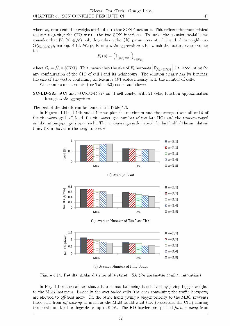
CHAPTER 4. SON CONFLICT RESOLUTIONTelecom ParisTech - Orange Labs
47
where wz represents the weight attributed to the SON function z. This reects the most criticalrequest targeting the CIO w.r.t. the two SON functions. To make the solution scalable weconsider that Wi (∀i ∈ N ) only depends on the CIO parameters of cell i and of its neighbours(PNi,CIO), see Fig. 4.13. We perform a state aggregation after which the feature vector comesto:
Fi (p) =(IpOi=x
)x∈POi
where Oi = Ni×CIO. This means that the size of Fi becomes∣∣∣PNi,CIO∣∣∣, i.e. accounting for
any conguration of the CIO of cell i and its neighbours. The solution clearly has its benets:the size of the vector containing all features (F ) scales linearly with the number of cells.
We examine one scenario (see Table 4.3) coded as follows:
SC-LD-SA: SON and SONCO-R are on, 1 cell cluster with 21 cells, function approximationthrough state aggregation.
The rest of the details can be found in in Table 4.3.In Figures 4.14a, 4.14b and 4.14c we plot the maximum and the average (over all cells) of
the time-averaged cell load, the time-averaged number of too late HOs and the time-averagednumber of ping-pongs, respectively. The time-average is done over the last half of the simulationtime. Note that w is the weights vector.
0
0,5
1
Max. Av.
Loa
d [
%]
w=(8,1)
w=(4,1)
w=(1,1)
w=(1,4)
w=(1,8)
(a) Average Load
0
0,2
0,4
0,6
0,8
Max. Av.
No
. T
Ls [
#/m
in] w=(8,1)
w=(4,1)
w=(1,1)
w=(1,4)
w=(1,8)
(b) Average Number of Too Late HOs
0
0,5
1
1,5
Max. Av.
No
. P
Ps
[#/m
in] w=(8,1)
w=(4,1)
w=(1,1)
w=(1,4)
w=(1,8)
(c) Average Number of Ping Pongs
Figure 4.14: Results: scalar distributable regret - SA (for parameter conict resolution)
In Fig. 4.14a one can see that a better load balancing is achieved by giving bigger weightsto the MLB instances. Basically the overloaded cells (the ones containing the trac hotspots)are allowed to o-load more. On the other hand giving a bigger priority to the MRO preventsthese cells from o-loading as much as the MLB would want (i.e. to decrease the CIO) causingthe maximum load to degrade by up to 9.9%. The HO borders are pushed further away from
47

48Telecom ParisTech - Orange Labs
4.5. APPLICATION SCENARIOS
the overloaded cells. Thus the number of Too Late HOs towards the overloaded cells fromneighbouring base stations is reduced at the cost of slightly increasing the number of Too LateHO from these cells towards their neighbours. Overall we reduce the maximum number of toolate HOs by up to 28.7% (Fig. 4.14b).
Typically the number of ping pongs depends mostly on the Hystereses, but as we can see inFig. 4.14c they are also impacted by the weights. If we reduce the number of too late HOs bymeans of CIO congurations then the MRO has more exibility in tuning the Hysteresis in orderto further reduce the number of HO ping-pongs (at most 33.6%).
In the second case we consider an approximation which uses linear features, i.e. the featuresare linear functions of the network parameters. For this the regret function has to be as simpleas possible such that the use of linear features makes sense. For this purpose we choose to haveone regret component per update request (only for the requests targeting the CIO). Thus wedene a bijection b : I → N × CIO × Z and we set the regret function:
ρi (u) =∣∣uzn,k∣∣ · wz
where (n, k, z) = b (i). Consequently we consider the feature vector corresponding to the regretcomponent i to be a linear function of: a constant and the dierences between the CIO of cell nand the CIOs of its neighbouring cells:
Fi (p) =( (
pn′,k − pn,k)n′∈Nn\n , 0.1
).
In this case also, the feature vector scales linearly with the number of cells. Moreover it isconsiderably smaller than in the rst case. We examine one scenario coded as follows:
SC-LD-LF: SON and SONCO-R are on, 1 cell cluster with all cells, function approximationthrough linear features.
The rest of the details can be found in in Table 4.3.We plot the maximum and the average (over all cells) of: the time-averaged cell load, the
time-averaged number of too late HOs and the time-averaged number of ping-pongs, in Figures4.15a, 4.15b and 4.15c respectively. The time-average is done over the last half of the simulationtime. Note that w is the weights vector.
Fig. 4.15a shows that assigning a bigger weight to the MLB function makes the load balancingwork better, reducing the maximum average load (bellow TLD). In our scenario what happensis that the cells with the trac hotspots are allowed to ooad more on their neighbours. Thiso-loading generates more too late HOs as the HO borders are not any-more within the actualcoverage borders (Fig. 4.15b). An increased number of too late HOs complicates the job of theMRO instances and thus the number of ping pongs also increases (Fig. 4.15c).
On the other hand giving a bigger weight to the MRO prioritizes the reduction of the numberof too late HOs (up to 25% reduction in Fig. 4.15b). As expected the price to pay is in termsof load balancing (Fig. 4.15a) where the maximum average load increases (up to 15%). Thenumber of ping pongs is also impacted by the weights, but as it is not directly part of the updaterequest sent by the MRO instances on the CIO we cannot see a trend, but the max is clearlylower than TPP /T = 2 [#/min] for any weight.
Note that in Fig. 4.15a the load dierence between the cases w = (1, 1), w = (1, 4) is quiteabrupt, whereas otherwise it is almost constant. This is due to the Linear Features. As the valuefunction is linear w.r.t. the network parameters, the optimal action is to steer the network incongurations where the parameters are either maximum or minimum (depending on the signof their coecient). So basically what we can see in Fig. 4.15a for the two weight (w = (1, 1),w = (1, 4)) is exactly the outcome of a jump of the network parameter conguration from oneextremity to the other.
48

CHAPTER 4. SON CONFLICT RESOLUTIONTelecom ParisTech - Orange Labs
49
0,5
0,7
0,9
Max. Av.
Loa
d [
%]
w=(8,1)
w=(4,1)
w=(1,1)
w=(1,4)
w=(1,8)
(a) Average Load
0,3
0,5
0,7
0,9
Max. Av.
No
. T
LHO
s
[#/m
in]
w=(8,1)
w=(4,1)
w=(1,1)
w=(1,4)
w=(1,8)
(b) Average Number of Too Late HOs [#/min]
0,5
0,7
0,9
1,1
Max. Av.
No
. P
Ps
[#/m
in] w=(8,1)
w=(4,1)
w=(1,1)
w=(1,4)
w=(1,8)
(c) Average Number of Ping Pongs [#/min]
Figure 4.15: Results: scalar distributable regret - LF (for parameter conict resolution)
1,0E+00
1,0E+03
1,0E+06
0 5 10 15 20 25 30 35 40 45 50
F-s
ize
No. cells
SC-LD-SA SC-LD-LF
1,0E+00
1,0E+01
1,0E+02
1,0E+03
0 5 10 15 20 25 30 35 40 45 50
θ-u
pd
ate
No. cells
1,0E+00
1,0E+10
1,0E+20
0 5 10 15 20 25 30 35 40 45 50
a-s
ea
rch
No. cells
Figure 4.16: Complexity: scalar distributable regret (for parameter conict resolution)
We plot in Figure 4.16 the complexity of the F -size, θ-update and a-search, w.r.t. the numberof cells, for the two scenarios SC-LD-SA and SC-LD-LF. Both prove to have a linear scalabilityof the F -size and θ-update. However, the a-search complexity scales linearly in the case of usinglinear features (SC-LD-LF) and exponentially in the other case (SC-LD-SA).
49

50Telecom ParisTech - Orange Labs
4.5. APPLICATION SCENARIOS
ScenarioSC-LC-SA
SC7-LC-SASC-LD-SA SC-LD-LF
No. cells 21 Macro cells - hexagonal topology, with wraparound
Clusters 1 vs 3 1
ISD 1732 m
Carrier/Bw/TxPow Carrier = 2 GHz, Bandwidth = 10 MHz, CellTxPower = 46 dBm (40W)
Propagation Model Channel model #2 in Table A.1, (3GPP Case 3 [54])
Trac type FTP-like , constant le size FS = 16[Mb/UE] , UE arrival: SPPP,
arrival rates: general (λG, per hexagon) and HotSpot (λHS , per HS)
(λG, λHS)FS [Mb/s] (9; (30; 25; 20)) (9; 30)
Simulated time 16 days 2 days 2 days
SON functions Z = MLB,MRO (for a Macro network, see Appendix B )
Tuned parameters CIO , Hysteresis, K = CIO,HY S,CIO set [dB] Pn,CIO −12,−9, .., 0 −12,−8, ..., 0HYS set [dB] Pn,HY S 0, 1, ..., 12ABS set [#] Pn,ABS 0 (xed)TTT 160ms
Time window T 5 min
SON settings(TLLD;TH
LD
)= (0.3; 0.8), TH
TL = 8, THPP = 10, TH
TL2 = 6
SON priority weights w = wZ (one weight per SON function)
Conict-solving target parameter conict resolution
Criticalness indicator used: Uzn,k ∈ [−1, 1]
state reductionstate
aggregation
state
aggregationlinear features
Distr. Learner (W ) no (centralized) yes (per cell) yes (per update request)
SONCO-R (α, γ, ε) (0.2; 0.8; 0.1) (0.1; 0.8; 0.1)
No. Learners I = 1 I = |N | I = |N | · |CIO| · |Z|,b is a bijection b : I → N × CIO × ZLearners focus
∀i ∈ I, Oi =
N × CIO Ni × CIO Nn × k where (n, k, z) = b (i),
∀i ∈ I,Ji = 1, .., |POi|
1, ..,
∣∣Nn
∣∣∀p ∈ P, ∀i ∈ I,Fi(p) =
(IpOi
=x)x∈POi
((pn′,k − pn,k)n′∈Nn\n , 0.1
)where (n, k, z) = b (i),
size of F∑i∈I|POi|
∑n∈N
∣∣Nn
∣∣∀u ∈ U , ∀i ∈ I,ρi (u) =
max(n,z)
∣∣uzn,CIO
∣∣wz maxz∈Z
∣∣uzi,CIO
∣∣wz
∣∣∣uzn,k∣∣∣ · wz, where (n, k, z) = b (i),
multi-dimension frame no
Table 4.3: Scenario summaries: scalar regret for parameter conict resolution
50

CHAPTER 4. SON CONFLICT RESOLUTIONTelecom ParisTech - Orange Labs
51
4.5.3 Vector regret: parameter conict resolution
In this section we tackle the parameter conict resolution for a multi-dimension/vector regret.Consider a network with Macro and Pico cells. The Pico cells are meant to help the Macro cellsproviding them with a capacity bust. In this sense we say that a Macro cell may have severalslave Pico cells, in our scenarios we consider the Pico cells under its coverage. A Pico cell is theslave of one and only one Macro cell. We identify a cell cluster to be composed of a Macro celland its slave Pico cells. Focusing on one cell cluster, let NM and NP be the set of indexes of theMacro cells and Pico cells, respectively, (NM = 1).
We use 3 SON functions: (MLB via) CRE, MRO and eICIC. For details see Appendix C.The CRE is a function which keeps the load of the Macro cell lower than a given threshold bytuning the CIOs of the slave Pico cells in order to o-load on them when needed. The MROaims to reduce the number of ping-pong HOs and of too late HOs originating from the Pico cellsby tuning the CIO and the HYS on the Pico cells. The eICIC aims to protect the users whichhave been forced to HO from the Macro cell to the slave Pico cells by tuning the number of ABSon the Macro cell.
We employ a network topology as represented in Fig. 4.17 with 3 cell clusters each of whichis composed of 1 Macro cell and 2 slave Pico cells. As mentioned earlier, we consider oneindependent SONCO-R instance governing each of the cell clusters.
19
15 16
18 19
21
7 8
9
17
18
4 5
6
11
12
4 6
10 11
12
13 14
15 1
2
3
19 20
21
14
15 8
7 8
16 17
18
4 5
10 11
UE Hotspot
Figure 4.17: Network topology
In the SONCO-R designs, rst of all we propose to neglect the parameters which are not asignicant source of conict. In our case we refer to the HYS, i.e. we assume that the HYS doesnot signicantly impact the performance of the CRE or of the eICIC. We consider two scenarios:
SC-LC-SA: In the rst case the regret is a simple scalar calculated over the entire cluster asfollows:
ρd (u) = max(n,k,z)∈Od×Z
∣∣uzn,k∣∣wzfor any d ∈ D = 1 where Od = NM ×ABS∪NP ×CIO. The feature vectors reectall the possible congurations of the CIO and of the ABS:
Fd (p) =(IpOd=x
)x∈POd
SC-LD-LF: In the second case we target to enforce an approximation using linear features. Thecomplicated formula used to calculate the regret in the st scenario does not make it suitableto use linear features. Thus we consider a multi-dimension regret D = 2 (2N − 1) > 1.More precisely 2 regret components for each update requests targeting the ABS or theCIO. For this we rst dene a bijection b : I → NM ×ABS× eICIC× ±1∪NP ×CIO × CRE,MRO × ±1 and then the regret function as:
ρd (u) =∣∣uzn,k∣∣wzIuzn,k·sg>0
for any d ∈ D, where (n, k, z, sg) = b (d). We approximate Wd with linear features asfollows:
51

52Telecom ParisTech - Orange Labs
4.5. APPLICATION SCENARIOS
for z = CRE, k = CIO and n ∈ NP and for z = eICIC, k = 3 and n ∈ NM weapproximate with a linear function of the CIOs of the cells n′ ∈ NP , the ABSs of cellsn ∈ NM and one constant:
Fd(p) = 0.1 ·(
10,(pn′,ABS
)n′∈NM
,(pn′,CIO
)n′∈N P
) for z = MRO, k = CIO and n ∈ NP we approximate with a linear function of the CIO ofcell n and one constant:
Fd(p) = 0.1 · (10, pn,CIO)
Leaving aside the approximations performed in the two designs, if we have a closer look we cansee that there is a small dierence w.r.t. what they optimize (reected in ρd). The two targetscan be summarized as follows:
SC-LC-SA: minimization of the expected worst regret:
minπEπ[∑
t γtmax(n,k,z)∈O
∣∣∣U z(t),n,k∣∣∣ · wz] =
minπEπ[∑
t γtmax(n,k,z,h)∈O×±1
∣∣∣Uk(t),n,k∣∣∣ IUk(t),n,k
h>0 · wz
]
SC-LD-LF: minimization of the worst expected regret :
minπmax(n,k,z,h)∈O×±1Eπ
[∑t
γt ·∣∣∣Uk(t),n,k∣∣∣ · IUk
(t),n,kh>0
· wz]
with a myopic approach, i.e. γ = 0.
One can see that the outcome of the 2 are mathematically dierent but they are in the samespirit which is to provide a sense of fairness among the SON functions, as they minimize themaximum criticalness among the requests of the SON functions.
Fairness biasing In this sub-section we show the results aimed at proving the biasing mechan-ism, i.e. the capability of favouring one SON function or another. For this we perform simulationswith stationary trac λ (see Table 4.4) We evaluate the network parameters and performancesduring the last half of the simulation time. Fig. 4.18 shows averages over the parameters con-trolled by the SON functions: the average CIO (over time and all Pico cells), the average HYS(over time and all Pico cells) and the average no. of ABS (over time and all Macro cells), respect-ively, for dierent weights w attributed to the SON functions. The 2 designs can be identiedby their names. They are followed by the weight of the 3 SON functions in the following order:CRE, MRO and eICIC . For simplicity we focus only on the conict between CRE and MRO.
One can see how dierent weights impact the mentioned parameters. First we try to givesome intuition in order to help the reader interpret the graphs. The CIO is the main target ofCRE. In order to ooad the Macro cell we increase the CIO of the Pico cells. However, in casethat the CIO of the Pico cell increases too much we create the risk of having a lot of too lateHOs; thus the MRO can get suocated. This is why MRO also tunes the CIO to prevent thisextreme o-loading.
We expect that a higher priority on the CRE should lead to more aggressive o-loading, i.e.bigger values of the CIO of Pico cells, and on the other hand a bigger priority of the MRO wouldrestrict this ooading, i.e. lower CIO values. The no. of ABS will also have the same trendas eICIC reacts to the changes of the CRE: the bigger the CIO the more UEs to protect andthus the bigger the number of ABS sub-frames. This trend can be seen in Fig. 4.18 for the 2designs SC-LC-SA and SC-LD-LF. The average HYS is also impacted by the dierent weights asfor example a small CIO value would reduce the number of too late HOs and would thus allowfor bigger HYS values to also reduce the ping-pong HOs.
52

CHAPTER 4. SON CONFLICT RESOLUTIONTelecom ParisTech - Orange Labs
53
As mentioned a bigger weight on the CRE leads to higher average CIO values. This forcesthe MRO to reduce the values of HYS, as can be seen in Fig. 4.18, in order to reduce the numberof too late HOs. Naturally a bigger weight on the MRO will have the opposite eect, i.e. theaverage HYS values will be bigger as the number of too late HOs will not be so critical. MROwill prot from this by increasing the HYS in order to reduce the no. of ping-pong HOs.
In Figure 4.19 we represent averages over the KPIs used as inputs for the SON functions:the average load (over time and all Macro cells, over time and all Pico cells), the average no. ofping-pong HOs and of too late HOs (over time and over all Pico cells), and the average ratioof the bit-rates of UEs attached to the Macro cells by cell-edge UEs attached to its slave Picocells (over time and all Macro cells). The latter is scaled by 0.4 in the gure. For more detailson the KPI calculation see Appendixes C. One can again see the eects of giving higher priorityto either CRE or to MRO, especially on the load of the Pico cells and also on the no. of pingpong HOs and the too late HOs. More precisely the load of the Pico cells, the no. of ping-pongHOs and the no. of too late HOs increases if we give higher priority to CRE and consequentlydecreases if a higher priority is given to MRO. We do not expect precise trends on the otherKPIs, given the more complex dependencies.
0
2
4
68
10
12
Av. CIO on Pico cells Av. HYS on Pico cells Av. no. ABS on Macro cells
w=(8,1,1) w=(1,1,1) w=(1,8,1)
w=(8,1,1) w=(1,1,1) w=(1,8,1)
SC-LC-SA:
SC-LD-LF:
Figure 4.18: Time-averaged parameters
00,20,40,60,8
1
Load
on Macro cells
(CRE)
Load
on Pico cells
(CRE)
No. PP HO
on Pico cells
(MRO)
No. TL HO
on Pico cells
(MRO)
bit-rate ratio
scaled by 0.4
(eICIC)
w=(8,1,1) w=(1,1,1) w=(1,8,1)
w=(8,1,1) w=(1,1,1) w=(1,8,1)
SC-LC-SA:
SC-LD-LF:
Figure 4.19: Time-averaged KPIs
Tracking capabilities In this sub-section we target to show how a trained SONCO-R reacts(in terms of the abstract regret) to variations of the trac:
the time needed for the algorithms to re-converge.
the regret augment during the re-convergence period as compared to after the re-convergence.
For each design, SC-LC-SA and SC-LD-LF, we consider two scenarios. In the rst scenariowe split the simulation time into 2 equal time periods of 10 days. During the rst period weconsider a stationary trac of 0.90λ (see Table 4.4) and during the second time period we consider
53

54Telecom ParisTech - Orange Labs
4.5. APPLICATION SCENARIOS
0
0,1
0,2
0,3
0,4
0,5
0,6
0,7
0,8
0,9
1
2,5 5,0 7,5 10,0 12,5 15,0 17,5 20,0
Av
era
ge
Ma
x R
eg
ret
Days [h]
2,5 days sliding window average
0.90λ 0.95λ
0.90λ 0.95λSC-LC-SA:
SC-LD-LF:
Figure 4.20: Tracking capabilities
1,0E+00
1,0E+02
1,0E+04
0 5 10 15 20 25 30 35 40 45 50
F-s
ize
No. cells
SC-LC-SA SC-LD-LF
1,0E+00
1,0E+01
1,0E+02
1,0E+03
0 5 10 15 20 25 30 35 40 45 50
θ-u
pd
ate
No. cells
1,0E+00
1,0E+01
1,0E+02
1,0E+03
0 5 10 15 20 25 30 35 40 45 50
a-s
ea
rch
No. cells
Figure 4.21: Complexity: vector regret, distributed learner (parameter conict resolution)
a stationary trac of λ. The second scenario is similar to the rst one, the only dierence beingthat during the rst time period we consider a stationary trac of 0.95λ. In Fig. 4.20 we plotthe time-average of the maximum over all instantaneous regret components making use of asliding time window of 2.5 days during the 20 days simulation period. From the performed testsone can see that the tracking capability of the SC-LD-LF design is much better then the one ofthe SC-LC-SA design. The convergence time is considerably shorter for the SC-LD-LF designand the regret augmentation during the re-convergence period as compared to the regret afterre-convergence is imperceptible.
We plot in Figures 4.21 the complexity of the F -size, θ-update and a-search, w.r.t. thenumber of cells. Both scenarios prove to have good (linear) scalability of the F -size, θ-updateand a-search. Having a more detailed look one can see that the scenario which uses linear features(SC-LD-LF) has better (smaller) values of the F -size complexity while the other one which usesstate aggregation (SC-LC-SA) has better (smaller) values of the θ-update complexity.
54

CHAPTER 4. SON CONFLICT RESOLUTIONTelecom ParisTech - Orange Labs
55
Scenario SC-LC-SA SC-LD-LF
No. cells 21 Macro cells, 6 Pico cells - hexagonal topology, with wraparound
Clusters 3 (each contains 1 Macro cell and 2 Pico cells)
ISD 1732 m
Carrier/Bw/TxPow Carrier = 2 GHz, Bandwidth = 10 MHz,
MacroCellTxPower = 49 dBm, PicoCellTxPow=30 dBm
Propagation Model Channel model #21 in Table A.1, (3GPP Case 3 [54] with Pico)
Trac type FTP-like , constant le size FS = 16[Mb/UE] , UE arrival: SPPP,
arrival rates: general (λG, per hexagon) and HotSpot (λHS , per HS)
(λG, λHS)FS [Mb/s] (14; 14)
Simulated time 20 days 20 days
SON functions Z = CRE,MRO, eICIC (for a HetNet, see Appendix C )
Tuned parameters CIO, Hysteresis K = CIO,HY S,ABSCIO set [dB]
Pn,CIO
n ∈ NM 0, 2, ..., 12 0, 1, ..., 12n ∈ N p 0
HYS. set [dB]
Pn,HY S
n ∈ NM 0, 1, ..., 12n ∈ N p 2
ABS set [#]
Pn,ABS
n ∈ NM 0 (out of 40)
n ∈ N p 0, 4, ..., 36 (out of 40)
TTT 160ms
Time window T 5 min
SON settings THLD = 0.85, TH
TL = 0.1, THPP = 0.2, TL
TR = 1.0 and THTR = 2.5
SON priority weights w = wZ (one weight per SON function)
Conict-solving target parameter conict resolution
Criticalness indicator used: Uzn,k ∈ [−1, 1]
state reduction state aggregation linear features
Distr. Learner (W ) no (centralized) yes (per update request)
SONCO-R (α, γ, ε) (0.2, 0.5, 0.1) (0.5, 0.0, 0.1)
No. Learners D = 1 2 (2 |N | − 1)
b is a bijection b : I → NM × ABS × eICIC × ±1∪NP × CIO × CRE,MRO × ±1
Learners focus
∀d ∈ D, Od =
NM × ABS∪NP × CIO
NM × ABS , if k = ABSNP × CIO , if k = CIO
where (n, k, z, sg) = b (d),
∀d ∈ D,Jd = 1, .., |POd|
N + 1, if z 6= MRO2, if z = MRO
∀p ∈ P, ∀d ∈ D,Fd(p) =
(IpOd
=x)x∈POd
if z 6= MRO :
0.1 ·(
10, (pn′,ABS)n′∈NM, (pn′,CIO)n′∈N P
),
if z = MRO :0.1 · (10, pn,CIO) ,
where (n, k, z, sg) = b (d),
size of F∑d∈D|POd
| (|NM |+ |NP |) (1 + |NM |+ |NP |) + 2 |NP |
∀u ∈ U , ∀d ∈ D,ρd (u) =
max(n,k,z)∈Od×Z
∣∣∣uzn,k∣∣∣wz
∣∣∣uzn,k∣∣∣wzIuzn,k·sg>0, where
(n, k, z, sg) = b (d)
multi-dimension frame yes
Table 4.4: Scenario summaries: vector regret for parameter conict resolution
55

56Telecom ParisTech - Orange Labs
4.6. LOGICAL FRAMEWORK ARCHITECTURE
4.6 Logical framework architecture
For the implementation of the SONCO-R we consider 2 perspectives w.r.t. the number of net-work layers: Macro Network and HetNet. In the case of Macro Network the scope area of theSONCO-R might be very large and thus (normally) as the accept/deny update request decisionis centralized it has to be taken higher up the hierarchy, i.e. above the Itf-N. The SONCO-RAgents have to collect the necessary information from the SON function and forward it to thecorresponding SONCO-R Algorithm. The Itf-N has to be able to sustain this forwarding. Wenote that the employed SON functions send update requests every 5 minutes. Thus, at this timescale, feeding information to the SONCO-R in the NM should not be a problem. The proposedarchitecture is outlined in Fig. 4.22a.
In the case of the HetNet scenario, we remind that the Pico cells act as slaves of the Macrocell, i.e. they are meant to help the Macro cell by providing additional coverage and capacity.Thus we considered cell clusters composed by a Macro cell and its slave Pico cells. Each cellcluster can be led by its Macro cell. Thus in this scenario we have proposed that each SONCO-Rinstance governs independently a cell cluster, and the SONCO-R Algorithm instance will berunning on the Macro cell/eNB. We expect the SONCO-R response time to be very good due tothe limited scope-area. Obviously this is valid if the scope of the SON functions is limited to onecell cluster. The SONCO-R Agents have to collect the necessary information and ensure that itgets to the corresponding SONCO-R Algorithm directly or via the X2 interface . The proposedarchitecture is outlined in Fig. 4.22b.
NM
DM
EM
eNB eNB EMX2 X2
SON_X
SON_Y
SON_A SON_CSONCO-R
Agent
SONCO-R
Algorithm
eNB
SON_BSONCO-R
Agent
Itf.-N
SONCO-R
Agent
SONCO-R
Agent
SONCO-R
Agent
(a) Macro Network
Cell cluster
NM
DMEM
eNB(Macro) eNB(Pico) EM
X2 X2
SON_A SON_CSONCO-R
Agent
SONCO-R
Algorithm
eNB (Pico)
SON_BSONCO -R
Agent
Itf.-N
SONCO-R
Agent
(b) HetNet
Figure 4.22: SONCO-R architecture
4.7 Concluding remarks
This work is dierent from current work found in the literature by the fact that we propose aSONCO-R that considers the SON instances as black-boxes, i.e. the algorithm inside is unknown,and we provide a RL-based SONCO-R solution. One important aspect is that we assume that
56

CHAPTER 4. SON CONFLICT RESOLUTIONTelecom ParisTech - Orange Labs
57
the parameter update requests sent by the SON functions include an additional metric reectinghow critical each request is. The SONCO-R decides which requests to accept and which to denyin targeting to minimize a regret function calculated using this criticalness indication. A wellknown problem of RL is that its complexity does not scale well. We tackle this issue making useof two function approximation techniques: state aggregations and linear features. We show howwe are able to reduce the requirements in terms of memory and computational eort.
Breaking the regret into several components provides a means to make the solutions scalable.More precisely, we perform an approximation for each component by reducing its dependenciesto a local scope. This is reasonably easy to be done through state aggregation. Moreover, the useof linear features (to approximate these components) allows for a much faster convergence andhas low memory requirements. However this is suitable only in the case of a vector of componentsand not in the case where the components are summed up to form the regret.
Breaking the focus area into several sub-areas and creating cell clusters, is a good solutionto reduce the a-search complexity. However it should be carefully done. Ideally the cell clustersshould be formed such that the inter-cluster dependencies are minimal.
57


Chapter 5
Mobility parameters
In Section 2.1.1 we have introduced the HandOver (HO) parameters: namely the Cell Indi-vidual Oset (CIO) and HO Hysteresis (HYS). Throughout our work (chapters 3 and 4) we haveconsidered that the HO parameters are established per-cell as opposed to per-cell-pair. In thissection we motivate our choice of using per-cell HO parameters. In the literature we typicallynd two approaches:
per-cell-pair HO parameters: on each cell we have a set of HO parameters for each neigh-bouring cell [43, 44, 45, 46, 47, 48].
per-cell HO parameters: on each cell we have only one set of HO parameters used for allneighbouring cells [49, 50, 28, 33, 51, 34]. Note that this can be seen as a particular caseof the rst approach.
The use of per-cell-pair HO parameters at rst seems to be a promising strategy, allowing indi-vidual HO congurations w.r.t. each neighbour, as compared to using per-cell HO parameterswhich would limit the manoeuvrability of the user mobility. However, using per-cell-pair HOparameters creates the risk of having areas where we may continuously experience Chained-HOs(CH). We consider a CH to be the event where two successful HOs are performed one shortlyafter another, regardless of the target cell. Note that a HO ping-pong event (see Section 2) is aspecial case of a CH where the the target of the second HO is the serving cell of the rst HO.We mention that the A3-event envisages per-cell parameters [5].
To the best of our knowledge this problem has not been signalled in the literature. In thischapter:
We show that using per-cell-pair HO parameters creates the risk of having Continuous CH(CCH) areas,
We give the necessary and sucient conditions under which CCH areas are avoided for thecase of per-cell-pair HO parameters,
We show that one solution to avoid the CCH areas is to use per-cell HO parameters,
We quantify the size of the CCH areas,
We show the eects of CCH areas in an LTE network simulator.
The remainder of this section is structured as follows: sub-section 5.1 describes formally theproblem, sub-section 5.2 presents some preliminary results, sub-section 5.3 presents the networkcongurations that cause CCH areas, sub-section 5.4 contains numeric results and simulationresults and sub-section 5.5 concludes the chapter.
59

60Telecom ParisTech - Orange Labs
5.1. PROBLEM DESCRIPTION
Cell A Cell B
HO
HO
Figure 5.1: HandOver mechanism
5.1 Problem description
5.1.1 HandOver test: two cells
We consider a network formed by several cells and UEs placed on a geographical area D ⊂ R2. Asmentioned, concerning the HO parameters we have identied 2 approaches: the rst one uses per-cell-pair HO parameters and the second one uses per-cell HO parameters. The second approachis a particular case of the rst approach, as in the rst case one can always set equal values forthe HO parameters w.r.t. all neighbours. Therefore we formally describe the per-cell-pair HOmodel as the general case.
Figure 5.1 shows how these parameters are used for an example with two cells: A and B.Consider a static UE at a given location ` ∈ D. Assume that this UE is served by cell A. At agiven time instance this UE checks if it should HO to a neighbouring cell, in this case the onlyoption is cell B. Say it receives an average power RxPowA from cell A and RxPowB from cellB (in dB). In order to take a HO decision. By generalizing eq. (2.2), a HO decision is taken inif the following test returns a strictly positive value :
TAB (`) = RxPowB (`)−RxPowA (`) + CIOBA − CIOAB −HY SAB (5.1)
where CIOAB and CIOBA are the CIOs concerning the cell pair A-B, HY SAB ≥ 0 is the HYSfor a HO from cell A to cell B, all in dB. More precisely, this condition has to be met for aminimum time duration, the so-called Time To Trigger (TTT) [5]. For now to simplify things weassume the TTT to be 0. Note that the HO hysteresis in dB is non-negative as it is intended todelay the HO, in this case from cell A to cell B. Similarly, a UE attached to cell B will performa HO from cell B to cell A if TBA (`) > 0.
Each pair of two cells, say A and B, has two HO osets CIOAB and CIOBA and two HOhystereses HY SAB and HY SBA. We dene the HO border from cell A to cell B as:
BAB = ` ∈ D : TAB (`) = 0 (5.2)
Similarly we dene BBA. We note that BBA 6= BAB unless the HO hystereses are null: HY SBA =HY SAB = 0. Typically HY SBA and HY SAB should be suciently large in order to avoid HOping-pongs for the users moving close to cell borders.
5.1.2 Generalization
For an arbitrary set of cells A,B, .... and any UE at location ` ∈ D we dene the HO functionas follows:
fi (`) =
i if Ti,j (`) ≤ 0, ∀j ∈ A,B, .... \ iargmaxj∈A,B,....\iTi,j (`) otherwise
(5.3)
60

CHAPTER 5. MOBILITY PARAMETERSTelecom ParisTech - Orange Labs
61
where fi (`) = k means that a user (UE) in location ` when attached to cell i should handoverto cell k. Obviously if fi (`) = i there will be no HO. The HO procedure is described in Alg. 5.1by means of a HO automata.
Algorithme 5.1 HO automataFor a UE in location `, let i (t = 0) be the initial cell attachment,At each time instance, t ∈ N, the UE will perform a HO from i (t) to i (t+ 1) = fi(t) (`)
5.1.3 Problematic HO parameter congurations
Next we show that using per-cell-pair HO parameters, although it may have the mentionedadvantages, it is very likely to create CCH areas. A CH is the UE event where a new HO isperformed shortly after another (regardless of the targeted cell). Considering the HO automatain Alg. 5.1, we dene the CCH area as the area where f is cyclic:
CCH area = `|` ∈ D, f does not converge, it is cyclic (5.4)
Proposition 5.1 (HO tests). Given some time instance, for any i, j ∈ A,B, .... where i 6= j,having Ti,j (`) > 0 implies Tj,i (`) ≤ 0.
Proof. Indeed, as HY Sij ≥ 0 and HY Sij ≥ 0 we get:
0 ≤ HY Sij +HY Sji. (5.5)
Thus, say that for a point ` ∈ D we have Ti,j (`) > 0. Lets assume that Tj,i (`) > 0. Then, byexplicitating using eq. (5.1) and adding up the two inequalities, we get that eq. (5.5) should befalse, and thus our assumption is false.
Proposition 5.1 ensures that no (static or low speed) UE is susceptible to continuously ex-periencing pairwise CHs between cells i and j (in a static environment). However, there is still aconsiderable risk of having non-pairwise CCH areas. To better understand the problem, we plotin Figure 5.2 an example of such a CCH area, making use of 3 cells A, B and C. We note thatin fact the HO borders are not necessarily lines, so Figure 5.2 contains a rough representation.To ease the reading we explicitate the HO function fA (`) in Table 5.1 w.r.t. the correspondingtests. The black area represents the CCH area. For example, say a UE arrives in this area.Without loss of generality assume it is attached to cell A. It cannot HO to B (TAB (`) ≤ 0), itcan and will perform a HO to cell C, as it is past border BAC (TAC (`) > 0). Attached to cellC, it cannot HO to cell A (TCA (`) ≤ 0), but it can and will perform a HO to cell B as it is pastborder BCB (TCB (`) > 0). Attached to cell B, it cannot HO to cell C (TBC (`) ≤ 0) but it canand will perform a HO to cell A as it is past border BBA (TBA (`) > 0). Being back in cell A,this will repeat innitely. Thus the HO automata is cyclic.
TAB (`) > 0 0 1 0 1 1 1TAC (`) > 0 0 0 1 1 1 1TAC (`) > TAB (`) - - - 0 1 0TAB (`) > TAC (`) - - - 1 0 0TAB (`) = TAC (`) - - - 0 0 1
fA (`) A B C B C B orC
Table 5.1: HO automata for cell A
Remark 5.1 (per-cell parameters). Using per-cell HO parameters is a particular case of usingper-cell-pair HO parameters, i.e. consider a set of cells A,B, ... then ∀i, j ∈ A,B, ..., i 6= j,we have that CIOij = CIOi and HY Sij = HY Si, where CIOi and HY Si are the HO oset andHO hysteresis, respectively, dened for cell i w.r.t. all neighbouring cells.
61

62Telecom ParisTech - Orange Labs
5.2. PRELIMINARIES
BB yx ,
Cell C
Cell B
AA yx ,
CC yx ,
Cell A
Figure 5.2: CCH areas
5.2 Preliminaries
We target to investigate the conditions of not having CCH areas and to quantify their size whensuch areas exist. For this we consider 3 cells A,B and C (as in the previous section), non-collinear,omnidirectional (see Fig. 5.2) and LTE capable.
We focus on the general case with per-cell-pair HO parameters. Let γ = (CIO,HYS)represent an arbitrary network conguration of the HO parameters, where:
CIO = (CIOij)i,j∈A,B,C,i 6=j , HYS = (HY Sij)i,j∈A,B,C,i 6=j . (5.6)
We recall that the elements of matrix HYS are non-negative. Let Γ be the set of all possiblevalues of γ. We introduce the notation of the HO margin (HOM): HOMij = CIOij − CIOji +HY Sij for any i, j ∈ A,B,C, i 6= j,. This allows for a characterization of the cell bordersunder the form:
Bij = ` ∈ D : RxPowi(`) +HOMij = RxPowj(`) ,∀i, j ∈ A,B,C , i 6= j. (5.7)
Consider A = (xA, yA), B = (xB, yB) and C = (xC , yC) to be the coordinates of the 3 cellsA,B and C, respectively, where A,B, C ∈ D. Let d(`1,`2) be the distance between 2 points on themap `1 and `2, where `1, `2 ∈ D. In particular we denote c = d(A,B), a = d(B,C), and b = d(C,A).We explicitate RxPowκA (t) making use of a typical pathloss model:
RxPowA (`) = TxPow + k − α10log10d(A,`) (5.8)
where k is the path gain coecient in [dB], α > 0 the path gain exponent and TxPow is the celltransmission power (the same for all cells) in [dB]. Similarly we can also explicitate RxPowκB (t)and RxPowκC (t).
Remark 5.2 (pathloss model). A more complicated model could have been used in eq. (5.8), forexample including shadowing, fast fading, etc. This would signicantly increase the complexityof derivations, making them dicult to follow, without providing a signicant change in theconclusions. However, to check if the conclusions still hold in a more realistic scenario, weprovide simulations in the results Section 5.4.3 considering the 3GPP Case 1 scenario [54] (see#1 in Table A.1).
Note that the border equation in (5.7), say for the HO from cell A to cell B, can be writtenas:
BAB =` ∈ D : log10d(A,`) −HOMAB/α = log10d(B,`)
=` ∈ D : d(A,`) · ρAB = d(B,`)
(5.9)
62

CHAPTER 5. MOBILITY PARAMETERSTelecom ParisTech - Orange Labs
63
where ρAB = 10−HOMAB/α. We extend this notation to ∀i, j ∈ A,B,C, i 6= j, ρij =10−HOMij/α. In the end we recover the equation of an Apollonian circle or line [52, 53].
Lemma 5.1. Consider the Apollonian circle B (`1, `2, z) =` ∈ D : d(`1,`) · z = d(`2,`)
corres-
ponding to location points `1, `2 ∈ D and ratio z. We can explicitate the HO borders as:
BAB = B (A,B, ρAB) = B (B,A, 1/ρAB) (5.10)
and similarly all the other borders. For z = 1 it is in fact a line.
Note that ∀i, j ∈ A,B,C, i 6= j, ρij ∈ (0,∞) given HOMij ∈ R, and as a consequence ofeq. (5.5) we have ρijρji ≤ 1.
In gure 5.3 we represent BAB corresponding to dierent values of HOMAB. One can easilyidentify that the borders are in fact Apollonian circles [52, 53]. For HOMAB[dB]→ 0 (ρAB → 1)the border is not any more a circle but a line, the perpendicular bisector of the segment [AB] .
Cell A Cell B24dB
18dB
12dB
6dB0dB−6dB
−12dB
−18dB−24dB
Figure 5.3: Border representation BAB for dierent values of HOMAB (Apollonian circles)
Next we provide two lemmas that help in proving the theorems in the main section 5.3, whichwill identify the network congurations which are subject to CCH areas. Thus, we consider 3arbitrary variables zAB, zBC , zCA ∈ (0,∞) and we analyse the intersection of the following (seeFig. 5.4): B (A,B, zAB), B (B, C, zBC) and B (C,A, zCA), i.e. any possible HO border w.r.t. the3 cell pairs (regardless of the direction).
AB
C
A
C
B
C
B
A B
Cell C
Cell B
CC yx ,
Cell A C
A
BB yx , AA yx ,
Figure 5.4: Border intersections
The following two theorems identify the conditions under which the three borders intersect.First we identify the pairwise intersection conditions.
63

64Telecom ParisTech - Orange Labs
5.3. MAIN RESULTS
Lemma 5.2. Considering 3 cells A,B and C, then for any zAB, zBC , zCA ∈ (0,∞) we have:
B (A,B, zAB) ∩ B (B, C, zBC) 6= ∅ ⇔ (a · zCA + b/zBC)2 ≥ c2 ≥ (a · zCA − b/zBC)2 ,
B (B, C, zBC) ∩ B (C,A, zCA) 6= ∅ ⇔ (c · zBC + a/zAB)2 ≥ b2 ≥ (c · zBC − a/zAB)2 ,
B (C,A, zCA) ∩ B (A,B, zAB) 6= ∅ ⇔ (b · zAB + c/zCA)2 ≥ a2 ≥ (b · zAB − c/zCA)2 .
(5.11)
Proof. See appendix 5.1.
Second we identify the conditions under which all the borders have a common point.
Lemma 5.3. Considering 3 cells A,B and C, for zAB, zBC , zCA ∈ (0,∞) the following areequivalent:
1. B (A,B, zAB) ∩ B (B, C, zBC) ∩ B (C,A, zCA) 6= ∅
2. zAB · zBC · zCA = 1 and (b · zAB + c/zCA)2 ≥ a2 ≥ (b · zAB − c/zCA)2
3. zAB · zBC · zCA = 1 and (c · zBC + a/zAB)2 ≥ b2 ≥ (c · zBC − a/zAB)2
4. zAB · zBC · zCA = 1 and (a · zCA + b/zBC)2 ≥ c2 ≥ (a · zCA − b/zBC)2
Proof. See Appendix 5.2. Lemma 5.2 is used in this proof.
An interesting observation is that given the fact that the borders are Apollonian circles/linesof a triangle (4ABC) means that if they have a common intersection point then there existsat most one more intersection point, and there are no other intersection points between any 2borders. They are called isodynamic points [52].
5.3 Main results
In this section we evaluate the conguration domain that ensures us to have no CCH areas.There are 2 possible CCH areas. We dene ΓABCA the congurations domain of γ where wehave CCH areas in the sense A→ B → C → A:
ΓABCA = γ : ∃` ∈ D s.t. f` (A) = B, f` (B) = C, f` (C) = A ; (5.12)
analogous we also dene ΓACBA for the opposite sense:
ΓACBA = γ : ∃` ∈ D s.t. f` (A) = C, f` (C) = B, f` (B) = A . (5.13)
The following theorems identify the network congurations under which we have CCH areas.This kind of area can create some major problems. UEs that continuously HO between cellsconsume a signicant amount of resources which translates into bad Quality of Service for allthe UEs.
Theorem 5.1. Considering 3 cells A,B and C, a network conguration γ ∈ ΓABCA if and onlyif the following conditions are simultaneously met:
ρAB · ρBC · ρCA > 1c/ρCA < a+ b · ρABb/ρBC < c+ a · ρCAa/ρAB < b+ c · ρBC
(5.14)
Note ρAB · ρBC · ρCA > 1 is equivalent to HOMAB +HOMBC +HOMCA = −αlog10ρAB · ρBC ·ρCA < 0.
Proof. See Appendix 5.3.
64

CHAPTER 5. MOBILITY PARAMETERSTelecom ParisTech - Orange Labs
65
Note that Theorem 5.1 can be adapted for γ ∈ ΓACBA simply by switching B and C. Thenext theorem focuses on the per-cell HO parameters, which is a particular case of per-cell-pairHO parameters.
Theorem 5.2. In the case of per-cell HO parameters there are no CCH areas.
Proof. See Appendix 5.2.
Thus, when using per-cell HO parameters we are CCH free. However, when using per-cell-pairHO parameters special precautions have to be taken to avoid having CCH areas.
We now discuss the above results. We outline two solutions for avoiding CCH in case we useper-cell-pair parameters. One is that the tuning mechanism used by the system designer shouldenvisage a simple check that the conditions in Theorem 5.1 are not met. The second solution isto patch the HO procedure by trying to hint that a UE might be caught in a CCH and forbid itto perform further HOs. This requires some caution in order not to generate radio link failuresdue to the HO restrains. We consider the later to be outside the scope of the work as it targetsthe HO procedure not the HO parameter optimization.
5.4 Numerical results.
5.4.1 Problematic network congurations
Figure 5.5: CCH free congurations for a = b = c and HYS[dB] = 0
In Fig. 5.5 we represented the domain of (HOMAB, HOMBC , HOMCA) for which we donot have CCH areas. In this scenario we consider: i) A, B and C are the vertices of an equilateraltriangle (a = b = c) and ii) for any i, j ∈ A,B,C, i 6= j set HY Sij = 0 (this implies HOMij =−HOMji). We represent only the points inside the sphereHOM2
AB+HOM2BC+HOM2
CA = 502.The sphere mesh (of radius 50) simply reects our focus area. The full part of the sphere
represents CCH free congurations. To ease the understanding of the gure we identify for thereader that the full part of the sphere contains 3 symmetric volumes and a plane (HOMAB +
65

66Telecom ParisTech - Orange Labs
5.4. NUMERICAL RESULTS.
HOMBA S•S•
S4ABCS•
S#ABC
-3 496 m2 0.45% 0.19%-6 1993 m2 1.84% 0.75%-9 4674 m2 4.31% 1.78%-12 9559 m2 8.83% 3.64%
Table 5.2: CCH area examples
HOMBC + HOMCA = 0) that cuts the sphere. One can see that the sphere is actually quiteempty, thus we can say that there are a great deal of congurations that create problems.According to Theorem 5.2 this could be avoided by using per cell HO parameters instead. Youcan also identify these congurations in Fig. 5.5 as the previously mentioned plane that cuts thesphere.
5.4.2 CCH area quantication
In order to give an idea on how big the problematic area is, we next provide some numericalresults. It is too complex to present the results for any network conguration, i.e. ∀γ ∈ Γ and∀A,B, C ∈ D. We pick a particular case to ease the reading. Thus we consider the generalcase using per-cell-pair HO parameters where: i) A, B and C are the vertices of an equilateraltriangle, ii) the Inter-Site Distance is 500 m and ii) the pathloss exponent is α = 4. Note thatthe area of triangle 4ABC is S4ABC ≈ 1.08 · 105 m2 and the area of its circumscribed circle isS#ABC ≈ 2.62 · 105 m2.
In this example we will only analyse the size of the CCH area in the sense A→ C → B → A.Lets rst consider HOMCB = 0, HOMAC = 0, HOMBA = x (i.e. a variable), and any
possible values for HOMAB, HOMBC , HOMCA. For example, in Fig. 5.6a for HOMBA = −9the dashed area represents the area where we will have CCH in the sense A → C → B → A.One can see that the dashed area delimited by P ′ and R′ will most-likely be covered by othercells. So in the following we limit our focus on the CCH area inside the circumscribed circle of4ABC; we denote the surface of this CCH area by S•.
For various values of HOMBA[dB] = x, represented in Fig. 5.6b, one can see in Table 5.2that as |HOMBA[dB]| increases the problematic area rises close to 104m2.
Note that S•, the area corresponding to CCH in the sense A → C → B → A, dependson HOMBA, HOMAC and HOMCB. Looking at all the Theorem 5.1 we got the intuitionthat for ΓACBA the value of ρBA · ρAC · ρCB may be very important. Implicitly the value ofΣ = HOMBA +HOMAC +HOMCB is very important. So what we expect is that the value ofΣ provides a signicant amount of insight on the size of the CCH area. In other words knowingΣ already gives a good idea on how big the CCH area may be, without individually knowingHOMBA, HOMAC and HOMCB. So, in Fig. 5.7 you can nd more values of S•/S#ABC as afunction of HOMBA and HOMCB for dierent values of Σ. Obviously we consider HOMAC =Σ−HOMBA−HOMCB is implicit. One can see that when Σ = 0 (ρBAρACρCB = 1) we have anull area and as Σ gets further away from 0 the CCH area increases and can reach 25% of S#ABC(S#ABC comparable to the coverage area of a cell).
5.4.3 Simulation results
To check if the conclusions are still valid in a more realistic scenario, we consider the 3GPP case1 [54] scenario with 3 cells (Channel model #1 in Appendix 1.1, Table A.1). We make use ofa wraparound technique, see Fig. 5.8. We employ a random UE arrival rate based on a SpacePoisson Point Process [58]. Each UE stay 3 minutes and then leave the network. During thisperiod we evaluate their number CHs. We set the TTT to 160 ms. To show the problems whichoccur when using the per-cell-pair HO parameters we make use of 6 scenarios as presented inTable 5.3. We note LS_BC and HS_BC are scenarios where OAB = OAB = OA thus this is
66

CHAPTER 5. MOBILITY PARAMETERSTelecom ParisTech - Orange Labs
67
A B
C
P
P ′
R′
R
Q
(a) Area identication
P3
R3
Q
P6
R6
P9
R9
A B
C
P12
R12
(b) Examples (P, R are indexed by |HOMBA[dB]|)
Figure 5.6: CCH area evaluation
Figure 5.7: Surface of CCH area in [%] w.r.t. S#ABC
67

68Telecom ParisTech - Orange Labs
5.4. NUMERICAL RESULTS.
Figure 5.8: Simulation map
equivalent to using per cell HO parameters (Remark 5.1).
LS_B LS_C LS_BC HS_B HS_C HS_BC
UE speed 3km/h 30km/hOAB -20dB 0dB
-20dB-20dB 0dB
-20dBOAC 0dB -20dB 0dB -20dBOi,j , ∀i ∈ B,C ,∀j ∈ A,B,C , i 6= j
0dB
Hi,j , ∀i, j ∈ A,B,C, i 6= j 3dB
Table 5.3: Scenarios
Figure 5.9a presents the average number of CH per UE and Figure 5.9b presents the per-centage of CH (over all HOs). Both gures focus on the total number of CHs, the number ofCHs in the sense A → B → C → A and the number of CHs in the sense A → C → B → A.One can see that the LS_BC and HS_BC experience only a few CHs. All the other scenariosexperience a large number of CHs. One can also see the amount of CHs for each of the 2 senses.This checks the result of Theorem 5.1, i.e. LS_B and HS_B have a high number of CH in thesense A→ B → C → A while for LS_C and HS_C the predominant CHs are in the other sense.
(a)Num-berofCHperUE
(b)Per-cent-ageofCH(overallHOs)
Figure 5.9: CH evaluations
68

CHAPTER 5. MOBILITY PARAMETERSTelecom ParisTech - Orange Labs
69
5.5 Concluding remarks
In this work we focus on potential risks of using per-cell-pair HO parameters (oset and hyster-esis) as compared to using per-cell HO parameters. Although we have a bigger manoeuvrability,most likely it leads to the creation of CCH areas. We have provided the necessary and sucientconditions that create these CCH areas for the case of using per-cell-pair HO parameters. Resultsof Theorem 5.1 with an example in Fig. 5.5 show that the conditions to have a CCH free con-guration are quite restrictive. We also showed that for the case of per-cell HO parameters therisk of having CCH areas is null. We have validated our results through simulations for dierentUE movement speeds. Therefore we conclude that using per-cell HO parameters is safer thanusing per-cell-pair HO parameters when considering the CCH areas, however it provides lessmanoeuvrability since we cannot individually tune the HO parameters w.r.t. each neighbouringcell. Future work can focus on a deeper analysts of the pros and cons of using per-cell-pair HOparameters.
69


Chapter 6
Conclusions and future work
Self Organizing Networks (SON) is currently one of the main challenges for mobile networks alongwith Internet of Things (IoT), Software Dened Networks (SDN), Network Function Visualization(NFV), Cloud-RAN (C-RAN), etc. SON functions are meant to automate the network tuning.Thus the network operators can replace the costly human intervention for repetitive tasks and cansignicantly improve their reactivity and the Quality of Service (QoS) oered to their end-users.
A network operator might choose to purchase several SON functions depending on its targetsin terms of end-user experience, and could even prefer a multi-vendor solution. Thus, a SONmanagement framework is required. This framework should insure that SON functions canbe bought from dierent vendors and when put together they still oer good network KeyPerformance Indicators (KPIs). In this spirit we have analysed potential conicts which mayoccur when using several independently designed SON functions. Moreover, SON vendors willmost-likely provide very limited information on the algorithms inside the SON functions. Thus inour approach we have also considered the SON functions as black-boxes, i.e. the algorithm insideis unknown. To deal with the SON conicts 3GPP has proposed the use of a SON COordinator(SONCO). The purpose of this thesis is to propose some SONCO designs and analyse theirperformance.
In Chapter 3 we show how how these potential conicts can be identied. Then we providea methodology for diagnosing which of the potential conicts are active conicts, i.e. theyactually degrade the network KPIs (SONCO-D). For this we have introduce a framework basedon the Naive Bayesian Classier (NBC). Results show that we are able to identify the root ofour conicts, i.e. the SON whose settings makes it impossible for other SON functions to achievetheir target KPIs. Going further into more details, we also try to identify which of the SONfunction's setting is responsible for the bad KPIs. Obviously, the further we go into details theless accurate the results will be. Overall, NBC has proved to be a good candidate for SONconict diagnosis.
After identifying the active conicts in the network the next rational step is to deal with them.One way of doing this is to try to eliminate the conict by reconguring the SON functions, worstcase scenario turn some SON functions o. Another solution is to enforce a conict resolutionmechanism (SONCO-R). In Chapter 4 we provide such a mechanism design. Basically theSONCO-R receives all the update requests form the SON instances and it has to decide which ofthem to accept and which to reject, ensuring some degree of fairness among the SON instances.We make use of Reinforcement Learning (RL) as it allows to make use of past information toimprove the future decisions. We have analyse several RL designs showing how to make theRL algorithm scalable using two linear function approximation avours: state aggregation andlinear features. We also study the performance costs for each of these. Results show that stateaggregation is a good candidate for reducing the RL complexity. The use of linear featuresreduces even more the complexity, but it has be carefully done as the approximation might beto imprecise.
In all our studies we use per-cell HO parameters. In the literature we have also come across amore general case that uses per-cell-pair HO parameters. In Chapter 5 we motivate our choice.
71

72Telecom ParisTech - Orange Labs
We show that using per-cell-pair HO parameters can lead to creating areas of Continuous ChainedHandOvers (CCH). On the other hand using per-cell HO parameters eliminates this risk, butlimits the manoeuvrability of the user mobility.
Future work There is still a lot of work to be done on the SON coordination. Now that wehave got a taste of what are the challenges of coordinating the SON functions, one of the nextsteps should be to improve the SON function concept. The SON functions should evolve intofacilitating their coordination. For example, a SON function may better understand the envir-onment, acknowledge the SON functions running in parallel, foresee how they can be impactedby them and even create alarms if it considers that its performance is deteriorated because this.
The algorithms of the SON coordinator should consequently evolve. They should be readyto deal with smarter SON functions.
Other machine learning algorithms could be tested for the SON conict resolution function.A fully distributed algorithm could improve the convergence time. Some approximations on theNaive Bayesian Classier could be tested for the SON conict detection. Also, one could alsoevaluate other classiers: decision trees, neural networks, etc. Another perspective would be tocreate a meta control loop to optimize the SON settings via high level policies.
One shortcoming of the current work is the lack of real data. SON functions are not yetwidely deployed. Once this happens, it is interesting to test the algorithms with real data andupdate them accordingly.
72

Appendix A
Simulator details
1.1 Channel Model
Modelling the radio channel comes down to estimating power received by the UEs from thenetwork cells. Let RxPow
κn (t) be the power received by UE κ from cell n at time t expressed in
dBs. We model it as follows:
RxPowκn (t) = TxPown (t)−FLn+AGn+AP κn (t)+PGκn (t)+Shκn (t)+Ffκn (t)−PtLn (A.1)
where TxPown (t) is the transmission power, FLn is the feeder loss, AGκn is the antenna gain,AP κn (t) is the antenna pattern, PGκn (t) is the path gain, Shκn (t) is the shadowing eect, Ffκn (t)is the fast fading eect and PtLn is the penetration loss.. For all the components the bases arethe 3GPP TS 363.814 [54] (Case 1 and 3) and the ITU-R M2134 [55] (Urban Macro) consideringalso the extensions for Heterogeneous Networks (HetNets), specically Pico cells. The details forthe channel models available in our simulator are presented later on in this section.
We dene the ltered signal, which is to be used for HO purposes, as follows:
RxPowκn (t) = FtC ·RxPowκn (t) + (1− FtC) ·RxPowκn (t− 1) (A.2)
where FtC is the lter coecient [104].
We employ a hexagonal topology (see Fig. A.1) subject to a wraparound and consider 8 radiochannel models as summarized in Table A.1.
We benchmark the channel models #0 and #1 (Table A.1) w.r.t. ITU-R UMa and 3GPPCase 1, respectively. We consider a 2 tiers topology, see Fig. A.1. In Fig. A.2a we plot thec.d.f. of the signal attenuation (RxPow -TxPow). In Fig. A.2b we plot the c.d.f. of the geometricSINR (all cells transmit with maximum power). The fast fading is disregarded for both gures.
LOS/NLOS distinctionID Macro Pico Simulator reference
#0 Yes - CM_ITU_UMa#1
No
- CM_3GPP_case1#11 No CM_3GPP_case1_wPico_model1#12 Yes CM_3GPP_case1_wPico_model2#2 - CM_3GPP_case3#21 No CM_3GPP_case3_wPico_model1#22 Yes CM_3GPP_case3_wPico_model2S#23 Yes CM_3GPP_case3_wPico_model2RS
Table A.1: Radio channel models
73

74Telecom ParisTech - Orange Labs
1.1. CHANNEL MODEL
10
55 56
57
7 8
9 34
35
36 19
20
21
16 17
18 4
5
6
13 14
15 1
2
3
46 47
48 31
32
33
43 44
45 28
29
30
25 26
27 10
11
12
22 23
24
52 53
54 40
41
42
49 50
51 37
38
39 55
56
57
34 35
36
46 47
48
11
12
49 50
51
1 2
3
22 23
24
7 8
9
4 5
6
1 2
3 34
35
36 19
20
21 7
8
9
37 38
39 22
23
24 55
56
57
52 53
54
49 50
51
Figure A.1: Map Wrap Around: 2 tiers
0%
20%
40%
60%
80%
100%
-140 -130 -120 -110 -100 -90 -80 -70 -60
c.d
.f.
RxPow-TxPow [dB]
ITU UMa (TS 36.814) 3GPP Case 1 (TS 36.814)
ITU UMa (Simulator) 3GPP Case 1 (Simulator)
(a) Benchmark RxPow-TxPow (no fast fading)
0%
20%
40%
60%
80%
100%
-10 -5 0 5 10 15 20
c.d
.f.
geometric SINR
ITU UMa (TS 36.814) 3GPP Case 1 (TS 36.814)
ITU UMa (Simulator) 3GPP Case 1 (Simulator)
(b) Benchmark geometric SINR (no fast fading)
Figure A.2: Benchmark
The Inter Site Distance (ISD) values are summarized in Table A.2.
The LOS probability is detailed in Table A.3.
The PathLoss details are presented in Table A.4.
74

APPENDIX A. SIMULATOR DETAILSTelecom ParisTech - Orange Labs
75
ISD #0 #1 #11 #12 #2 #21 #22 #23
Macro to Macro 500.0 m 1732.0 mMacro to Pico - >75m - >75mPico to Pico - >40m - >40m
Table A.2: Inter Site Distance
LOS probability
#0 Macro: min 18.0/dH , 1.0 (1.0− exp (−dH/63)) + exp (−dH/63)
#1 0#11 0#12 Macro: min 18.0/dH , 1.0 (1.0− exp (−dH/63)) + exp (−dH/63)
Pico:0.5−min 0.5; 5.0exp (−156.0/dH)+ min 0.5; 5.0exp (−dH/30)#2 0#21 0#22 Macro:exp (− (dH − 10.0) /200.0)
Pico:0.5−min 0.5, 3.0 ∗ exp (−300.0/dH)+ min 0.5, 3.0exp (−dH/95.0)
#23 Macro: exp (− (dH − 10) /1000.0)Pico:0.5−min 0.5, 3.0exp (−300.0/dH)+ min 0.5, 3.0exp (−dH/95.0)
dH is the horizontal distance between the UE and the Cell
Table A.3: LOS/NLOS probability
Pathloss
#0
34.0206 + 22.0log10(dH) if LOS and dH < 320−11.0232 + 40.0log10(dH) if LOS and dH ≥ 32019.5653 + 39.1log10(dH) if NLOS
#1#2
128.1 + 37.6log10(dH/1000)
#11#21
Macro: 128.1 + 37.6log10(dH/1000)Pico: 140.7 + 36.7log10(dH/1000)
#12#22#23
Macro:
103.4 + 24.2log10 (dH/1000) if LOS131.1 + 42.8log10 (dH/1000) if NLOS
Pico:
103.8 + 20.9log10 (dH/1000) if LOS145.4 + 37.5log10 (dH/1000) if NLOS
dH is the horizontal distance between the UE and the Cell
Table A.4: Pathloss
75

76Telecom ParisTech - Orange Labs
1.1. CHANNEL MODEL
#0 #1 #2 #11, #12 #21, #22, #23
Feeder Loss 2[dB] 0[dB] 0[dB]
Table A.5: Feeder loss
Figure A.3: Antenna pattern #0 (ITU UMa) and #1 (3GPP Case 1)
The feeder loss values are summarized in Table A.5.
The antenna gain include: antenna gain, antenna directivity horizontal and vertical. Wealso present the feeder loss in this section. The details are summarized in Table A.6. The Macrocells use directive antennas (3-sectorial sites). The Pico cells use omnidirectional antennas. InFig. A.3 we plot the antenna patter for scenario #0 (ITU-UMa).
The penetration loss is established per UE. We dene the mean and the standard deviationin Table A.7.
#0 #1 #2 #11, #12 #21, #22, #23
Antenna Gain 17[dB] 14[dB] 14[dB] Macro:14[dB], Pico: 5[dB]
Antenna Pattern H AH (ϕ) = −min
[12(
ϕϕ3dB
)2, Am
]dB.ϕ3dB = 70°
Am 20 25 Macro: 25
Antenna Pattern V AV (θ) = −min
[12(θ−θtiltθ3dB
)2, SLAv
]dB.SLAv = 20 dB
θ3dB 15° 10° Macro: 10°Antenna Tilt 12° 15° 6° Macro: 15° Macro: 6°Antenna Pattern 3D Macro:A (ϕ, θ) = −min − [AH (ϕ) +AV (θ)] , AmdB
Pico: 0dB
Table A.6: Antenna characteristics
76

APPENDIX A. SIMULATOR DETAILSTelecom ParisTech - Orange Labs
77
Penetration Loss #0 #1 #2 #11, #12 #21, #22, #23
Mean Outdoor-to-Incar: 9[dB] Outdoor-to-Indoor: 20[dB]Outdoor-to-Outdoor: 0[dB]
Std. Dev. 5[dB] 0[dB]
Table A.7: Penetration loss
Shadowing #0 #1 #2 #11, #12 #21, #22, #23
Std. Dev. LOS: 4[dB]NLOS:6[dB]
8[dB] Macro: 8[dB]Pico: 10[dB]
Macro: 8[dB]Pico:
3[dB] if LOS4[dB] if NLOS
Corr. Dist. LOS: 37[m]NLOS:50[m]
50[m] Macro: 50[m], Pico:
10[m] if LOS13[m] if NLOS
Table A.8: Shadowing
The shadowing is established per UE w.r.t. every site. We dene the standard deviation andthe correlation distance in Table A.8. As the UEs are moving we update the shadowing (w.r.t.all cells) at every time instance. Each update is correlated with the previous.
The correlation is implemented for the shadowing of UE κ w.r.t. site n as follows: First letthe shadowing correlation coecient be:
corrShκ (t) = exp(−∣∣d(`κ(t),`κ(t−1))
∣∣ /corrDistShκn (t))
(A.3)
where corrDistShκn (t) is the correlation distance established for site n and UE κ (i.e. thecorrelation distance depends on the location of UE κ) according to Table A.8. We remind that`κ (t) ∈ R2 is the location of UE κ at time t and d(`1,`2) is the distance between `1 and `2(`1, `2 ∈ R2 ). The shadowing correlations is performed as follows:
Shκn (t) =
√(corrShκn(t))2Shκn (t− 1) +
√1− (corrShκn(t))2Y κ
n (t) (A.4)
where Shκn (t) is the shadowing at time t experienced by UE κ w.r.t. site n in [dB], Y κn (t)is a
random variable (normal distribution) with mean 0 and standard deviation stdDevShκn (t) (i.e.the standard deviation depends on the location of UE κ).
We check the mean as follows:
E [Shκn (t)]
= E[corrShκn(t)Shκn (t− 1) +
√1− (corrShκn(t))2Y κ
n (t)
]= E [corrShκn(t)Shκn (t− 1)] + E
[√1− (corrShκn(t))2Y κ
n (t)
]= corrShκn(t)E [Shκn (t− 1)] +
√1− (corrShκn(t))2E [Y κ
n (t)]
= 0
(A.5)
77

78Telecom ParisTech - Orange Labs
1.1. CHANNEL MODEL
We check the standard deviation as follows:
E [Shκn (t)Shκn (t)]
= E
[(corrShκn (t)Shκn (t− 1) +
√1− (corrShκn (t))2Y κ
n (t)
)2]
= E[(corrShκn (t)Shκn (t− 1))2
]+ E
[(√1− (corrShκn (t))2Y κ
n (t)
)2]
+ 2E[corrShκn (t)
√1− (corrShκn (t))2Shκn (t− 1)Y κ
n (t)
]= (corrShκn (t))2 E
[(Shκn (t− 1))2
]+(
1− (corrShκn (t))2)E[(Y κn (t))2
]t→∞= (stdDevShκn (t))2
(A.6)
where the last equality holds if UE κ does not move (i.e. corrShκn (t) and stdDevShκn (t) areconstant).
We check the correlation as follows:
E [Sh (t)Sh (t− 1)]
= E[(corrShκn (t)Shκn (t− 1) +
√1− (corrShκn (t))2Y κ
n (t)
)Shκn (t− 1)
]= E
[corrShκn (t) (Shκn (t− 1))2
]+ E
[√1− (corrShκn (t))2Y κ
n (t)Shκn (t− 1)
]= corrShκn (t)E
[(Shκn (t− 1))2
]+√
1− (corrShκn (t))2E [Y κn (t)Shκn (t)]
= corrShκn (t)E[(Shκn (t− 1))2
](A.7)
The fast fading has a Rayleigh distribution, i.e. square root of the sum of the squaresof two variables of normal distribution. The fast fading is updated at each time step. Asin the shadowing case we correlate the current sample with the one from the previous timestep. Let F fκn (t) be the fast fading (not in dB!) at time t corresponding to cell n and UEκ: Ffκn (t) = 10log10F f
κn (t) . Let F f1κn (t) and F f2κn (t) be the two variables with normal
distribution that compose F fκn (t):
F fκn (t) =
√(F f1κn (t)
)2+(F f2κn (t)
)2(A.8)
We apply the correlation on the two components as follows:
F f1κn (t) = corrFFκ (t) F f1κn (t− 1) +√
1− (corrFfκ (t))2Y 1κn (t)√
2π−1
F f2κn (t) = corrFfκ (t) F f2κn (t− 1) +√
1− (corrFfκ (t))2Y 2κn (t)√
2π−1(A.9)
where corrFfκ (t) = exp(−2∣∣d(`κ(t),`κ(t−1))
∣∣ fc/speedOfLight) is the correlation coecient, fcis the carrier frequency, Y 1κn and Y 2κn are random variables with normal distribution of mean 0and standard deviation 1 (N (0, 1)),
√2π−1 is a correction to bring the average back to 1 and
speedOfLight = 3 · 108m/s. We remind `κ (t) ∈ R2 is the location of UE κ at time t and d(`1,`2)
is the distance between `1 and `2 (`1, `2 ∈ R2). The mean and correlation can be checked in asimilar manner as for the shadowing.
The thermal noise is -174.0 dBm.
The noise gure values are presented in Table A.9.
The carrier frequency is 2GHz.
78

APPENDIX A. SIMULATOR DETAILSTelecom ParisTech - Orange Labs
79
#0 #1, #2, #11, #12, #21, #22, #23
Noise Figure 7[dB] 9[dB]
Table A.9: Noise Figure
Bw. 1.4 [MHz] 3 [MHz] 5 [MHz] 10 [MHz] 15 [MHz] 20 [MHz]PRBs 6 15 25 50 75 100REs 76 181 301 601 901 1201
Table A.10: Bandwidth
The bandwidth can be selected as presented in Table A.10.
1.2 UE procedures
While in the network the UEs trough several procedures: Connection Establishment, ConnectionReEstablishment, Connection Reconguration (HO) and Receive Data (see Fig. 2.2). The pro-cedures basically consist of a certain message exchange sequence. The messages correspond totwo a protocol stacks according to the control plane and user plane (see Figure A.4).
In our simulator we only model the the messages exchanged between the eNB and the UEon the Media Access Control (MAC) layer, the Radio Link Control (RLC) layer, and the RadioResource Control (RRC) layer. For more details we refer the reader to [9].
In the implementation we dene one UE state for each of these messages as presented inFigures A.5, A.6, A.7, A.8, A.9. For more details we refer the reader to [5]. To ease theunderstanding of the gures we provide a short legend:
the grey square boxes represent the states
the text colour indicates the layer as follows: red is RRC (the RRC timers), green is RLCand blue is MAC. See Tables A.11 and A.12.
the message prex meaning is dened from a UE perspective as follows: s_ is for a sentmessage, w_ is for waiting for the message, r_ is for received message, pr_ is forprocess received message (i.e. message has been receive correctly) and fr_ is for failed toreceive.
1.3 Almost Blank Sub-frames
In order to reduce the interference towards the neighbouring cells some cells might be forbiddento transmit at certain time instances. To better understand this we present in Fig. A.10 thestructure of an LTE downlink frame (for 2 transmission antennas). Thus, a frame has a lengthof 10 ms. It is composed of 10 sub-frames of 1 ms each. A sub-frame contains 2 slots of 0.5ms each. A slot contains 6-7 so called Orthogonal Frequency-Division Multiplexing (OFDM)symbols, which can be seen as batches of data. The OFDM symbols can be further divided intoResource Elements (REs). In Fig. A.10 one can see the employment of the REs and how theyare grouped to form Resource Blocks (RBs). The RBs can be then allocated to dierent UEs.For more details we refer the reader to [9]. In our simulator, all the RBs of one sub-frame areallocated only to one user. This is reasonable for a FTP-like trac, which is the case in oursimulator. We assume that all the cells are synchronized on a frame basis. A sub-frame whereno user data is transmitted is called an Almost Blank Sub-frame (ABS).
79

80Telecom ParisTech - Orange Labs
1.3. ALMOST BLANK SUB-FRAMES
X2-UPHY
MAC
RLC
PDCP
IP
Ap
UE
PHY
MAC
RLC
PDCP
L1/L2
IP
UDP
eNB
GTP-U
Uu
L1/L2
IP
UDP
eNB
GTP-U
L1/L2
IP
UDP
GTP-U
L1/L2
IP
UDP
GTP-U
S-GW
P-GW
S1-U S5/S8
MME
IP
(a) Control plane protocol stack [105]
X2-C S6a
PHY
MAC
RLC
PDCP
RRC
NAS
UE
PHY
MAC
RLC
PDCP
RRC
L1/L2
IP
SCTP
S1AP
eNB
X2AP
Uu
L1/L2
IP
SCTP
eNB
X2AP
L1/L2
IP
SCTP
S1AP
NAS
L1/L2
IP
UDP
GTP-C
L1/L2
IP
UDP
GTP-C
L1/L2
IP
UDP
GTP-C
MME
MME S-GW P-GW
S1-MME S11 S5/S8
S10L1/L2
IP
SCTP
Dia-meter
L1/L2
IP
UDP
GTP-C
L1/L2
IP
SCTP
Dia-meter
HSS
(b) User plane protocol stack [105]
Figure A.4: LTE - SAE protocol stack
Figure A.5: UE states Connection Establishment
Figure A.6: UE states Connection Reconguration HO
Figure A.7: UE states Connection ReEstablishment
Figure A.8: UE states Physical and MAC Connection
Figure A.9: UE states Receive Data
80

APPENDIX A. SIMULATOR DETAILSTelecom ParisTech - Orange Labs
81
Parameter Simulator Standard Values TS 36.331
RRCT300 [ms] 100 100, 200, 300, 400, 600, 1k, 1.5k, 2kT301 [ms] 100 100, 200, 300, 400, 600, 1k, 1.5k, 2kT304 [ms] 100 100, 200, 400, 500, 1k, 2k, 4k, 8kT311 [ms] 1000 (1k), 3k, 5k, 1k, 1.5k, 20k, 30kT311a [ms] 200 parameter not standardizedT310 [ms] 1000 0, 50, 100, 200, 500, (1k), 2kN310 [#] 1 (1), 2, 3, 4, 6, 8, 10, 20N311 [#] 1 (1), 2, 3, 4, 5, 6, 8, 10
T_N310 [ms] = N310Ö200 parameter not standardizedT_N311 [ms] = N311Ö100 parameter not standardizedTTT [ms] 100 0, 40, 64, 80, 100, 128, 160, 256, 320, 480, 512, 640,
1024, 1280, 2560, 5120
Table A.11: Timers
Parameter Simulator Standard Values TS 36.331
MACpreambleTransMax [#] 3 3, 4, 5, 6, 7, 8, 10, 20, 50, 100, 200re_ResponseWindowSize [#] 2 2, 3, 4, 5, 6, 7, 8, 9, 10
BackoIndicator [sf] 100, 10, 20, 30, 40, 60, 80, 120, 160, 240,
320, 480numberOfRA_Preambles [#] Not used 2, 8, 12, 16 . . . .64sizeOfRA_PreambleGroupA [#] Not used
maxHARQ_Tx [#] 51, 2, 3, 4, (5), 6, 7, 8, 9, 10, 12, 16, 20,
24, 28maxHARQ_Msg3Tx [#] Not used 1, 2 ,3 ,4, 5, 6, 7, 8HARQ RTT Timer (ReTx) [sf] 8 ≥ 8 (TS 36.321)
RLCmaxRetxThreshold [#] 4 1, 2, 3, (4), 6, 8, 16, 32
t_PollRetransmit [ms] 455, 10, 15, . . . (45) 250, 300, 350, 400,
450, 500RRC
lterCoecientRSRP [ms] 4 0, 1, 2, 3, (4), 5, 6, 7, 8, 9, 11, 13, 15,17, 19,lterCoecientRSRQ [ms] 4
cellIndividualOset [dB] Q-OsetRange
Q-OsetRange [dB]-24, -22, -20, -18, -16, -14, -12, -10, -8,-6, -5, -4, -3, -2, -1, (0), 1, 2, 3, 4, 5, 6,
8, 10, 12, 14, 16, 18, 20, 22, 24
Table A.12: Parameters
81
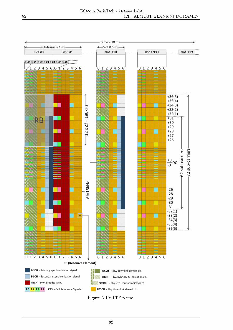
82Telecom ParisTech - Orange Labs
1.3. ALMOST BLANK SUB-FRAMES
Δf=
15
kHz
12
x Δ
f =
18
0kH
z
#0
CP #1
CP #2
CP #3
CP #4
CP #5
CP #6
CP
slot #0 slot #1 slot #10
+36(5)
+34(3)+33(2)+32(1)+31+30+29+28+27+26
-26-28-29-30-31-32(1)-33(2)-34(3)-35(4)-36(5)
0 1 2 3 4 5 6
+35(4)
DC+0-0
slot #19
0 1 2 3 4 5 6
0 1 2 3 4 5 6
0 1 2 3 4 5 6
slot #2k+1
0 1 2 3 4 5 6
P-SCH - Primary synchronization signal
S-SCH - Secondary synchronization signal
PBCH - Phy. broadcast ch.
PDCCH - Phy. downlink control ch.
PDSCH - Phy. downlink shared ch.
RE (Resource Element)
62
su
b-c
arri
ers
72
su
b-c
arri
ers
PHICH - Phy. hybridARQ indication ch.
PCFICH - Phy. ctrl. format indicator ch.
sub-frame = 1 ms Slot 0.5 ms
0 1 2 3 4 5 6
frame = 10 ms
0 1 2 3 4 5 60 1 2 3 4 5 6
RB
RE
R0 R1 R2 R3 CRS - Cell Reference Signals
Figure A.10: LTE frame
82

APPENDIX A. SIMULATOR DETAILSTelecom ParisTech - Orange Labs
83
83


Appendix B
SON functions for Macro Network
scenarios
The SON functions are dened in this appendix considering N Macro cells (indexed by n ∈1, .., N).
2.1 MLB for a Macro Network
Cell A20% load
Cell B95% load
Cell A60% load
Cell B70% loadMLB
Figure B.1: MLB Function
We consider one independent MLB instance per cell. The MLB instance targets to reduce theload of the host cell, see Fig. B.1. The tuned parameter is the CIO of the hosting cell.
Given some time instance (we disregard the time index) we dene:
Mn,LD the load of cell n calculated as the average number of occupied Physical ResourceBlocks (PRBs, [106]) of the hosting cell (the cell on which the MLB instance runs)
THLD and TLLD are triggering thresholds
ϕ is the logistic function:
ϕ (mid, sloap, x) =1
1 + exp−sloap(x−mid)(B.1)
For cell n, the update request of the MLB instance at time t for the CIO can be expressed as:
UMLBn,CIO =
−ϕ (0.9, 30,Mn,LD) , if Mn,LD > THLD1− ϕ (−0.2, 5,Mn,LD) , if Mn,LD < TLLD0, otherwise
(B.2)
2.2 MRO for a Macro Network
We consider a distributed implementation of the MRO where the MRO instances running onneighbouring cells communicate with each other. The target of the MRO instances is to reduce
85

86Telecom ParisTech - Orange Labs
2.2. MRO FOR A MACRO NETWORK
MRO
Too narrow è Ping-pongs Cell A
coverage limit
Cell B cov. lim
itHO border beyond coverageè too late HOs from B to A
Wide enough
HO borders within coverage range
Cell A Cell B Cell A Cell B
Figure B.2: MRO Function
the no. of ping-pongs, the no. of too late HOs, the no. of too early HOs and the number of HOsto wrong cells. We only focus on the rst two, as the last two are considerably less frequent. Todo this MRO tunes mainly the HYS (see Fig. B.2). Increasing the HYS should reduce the no.of ping-pongs. Reducing the HYS should reduce the no. of too late HOs. But when we wantto do both we turn to the CIO. Reducing the CIO of one cell should reduce the no. of too lateHOs originating from that cell, without aecting the no. of ping-pongs.
Given some time instance (we disregard the time index) we dene:
Mn,PP the number of HO ping-pongs originating from cell n and Mn,TL the number of toolate HOs also originating from cell n,
Mn,TL2 the number of too late HOs where cell n is the HO target cell.
THTL, THPP , TLTL = 0.25THTL, TLPP = 0.25THPP and TLTL2 are triggering thresholds
ϕ (mid, sloap, x) is the logistic function, see eq. (B.1)
Since the MRO tunes two parameters, the CIO and the Hysteresis, the MRO instance of cell nsends 2 simultaneous requests: one for each parameter. The one regarding the Hysteresis can beexpressed as follows:
UMROn,HY S =
−1, if Mn,TL > THTL and Mn,PP < TLPP1, if Mn,PP > THPP and Mn,TL < TLTL0, otherwise
(B.3)
where TTL and TPP are thresholds used to trigger events.The request regarding the CIO can be expressed as follows:
UMROn,CIO =
ϕ(1.5, 5,Mn,TL2/THTL2
)− 1 if ∃n ∈ N\n s.t. Un→n = 1
0 otherwise(B.4)
where Un→n is an intra-MRO message. The MRO instance running on cell n will receive suchmessages from all its neighbouring MRO instances (n ∈ N−n) requesting a CIO increase request,if needed:
Un→n =
1 if
((Mn,TL > THTL or Mn,PP ≥ TLPP
)or(Mn,TL > THTL or Mn,PP ≥ TLPP
))and n ∈ ξ (n)
0 otherwise(B.5)
where ξ (n) is the set on cell from which there are Too Late HOs to cell n. Increasing the CIOvalues of neighbouring cells reduces the number of too late HOs originating from them.
86

Appendix C
SON functions for HetNet scenarios
The SON functions are dened in this appendix considering one Macro cell (indexed by n = 1)and its N − 1 slave Pico cells (indexed by n ∈ 2, .., N). For the same SON function, theinstance on the Macro cell collaborate with the ones on the Pico cells.
3.1 (MLB via) CRE for a HetNet
Macro cell95% load
Slave Pico cells
70% load
15% load
20% load
CRE Macro cell82% load
Range expansion
68% load
39% load
47% load
Figure C.1: HetNet CRE Function
The purpose of a CRE instances (Fig. C.1) is to o-load (force UEs to HO to neighbouring cells)the Macro cells onto Pico cells when they are over-loaded, i.e. have a high resource utilization.The mechanism also deals with the case where the Pico cells are (or we anticipate they willbecome) over-loaded.
Given some time instance (we disregard the time index), we dene:
Mn,LD the resource utilization of cell n, i.e. the no. of used resources by the no. of availableresources (the ABS are not considered available resources),
THLD and TLLD = THLD − 0.1 are triggering thresholds,
ϕ (mid, sloap, x) is the logistic function, see eq. (B.1)
The CRE instances send update requests targeting the CIOs of the Pico cells (n ∈ 2, ..., N) asfollows:
UCREn,CIO =
ϕ (0.9, 20,M1,LD) , if M1,LD > THLD and Mn,LD < TLLD−ϕ (0.9, 20,Mn,LD) , if Mn,LD > THLD or(
M1,LD < TLLD and n = argmaxiMi,LD
)0, otherwise
(C.1)
87

88Telecom ParisTech - Orange Labs
3.2. MRO FOR A HETNET
3.2 MRO for a HetNet
The target of the MRO instances (Fig. C.2) is to reduce the no. of ping-pongs, the no. of toolate HOs, the no. of too early HOs and the number of HOs to wrong cells. We only focus onthe rst two, as the last two are considerably smaller. To do this MRO tunes mainly the HYS.Increasing the HYS should reduce the no. of ping-pongs. Reducing the HYS should reduce theno. of too late HOs. But when we want to do both we turn to the CIO. Reducing the CIO ofone cell should reduce the no. of too late HOs originating from that cell, without aecting theno. of ping-pongs. The CIO tuning feature can be deactivated (it is the case in some of ourscenarios, specically throughout chapter 3).
Macro cell
Pico cell
Too narrow è Ping-pongsMacro to pico
HO border
Pico to macro HO border
Pico coverage limit (UE min RX power) è too late HOs from Pico to Macro
Macro cell
Pico cellHO borders within
coverage range
Wide enough
MRO
Figure C.2: HetNet MRO Function
Typically the no. of too late HOs originating from the Pico cells is signicantly bigger thenthe ones that originate from the Macro cell. Thus the MRO instances focus on reducing the no.of too late HOs and ping-pong HOs originating from the Pico cells. Given some time instance(we disregard the time index), we dene:
Mn,PP and Mn,TL are the percentages of no. of ping-pongs and of too late HOs, respect-ively, originating from cell n,
THPP , THTL, TLPP = 0.25THPP and TLTL = 0.25THTL are thresholds used to trigger parameterchanges.
ϕ (mid, sloap, x) is the logistic function, see eq. (B.1)
The MRO instances send update requests targeting only the parameters of the Pico cell (n ∈2, ..., N), specically the HYS:
UMROn,HY S =
1, if Mn,PP > TPP and not
(Mn,TL ≥ TLTL and
ϕ(0.3,20,Mn,PP )ϕ(0.2,30,Mn,TL)
≤ 2
)−1, if Mn,TL > TTL and not
(Mn,PP ≥ TLPP and
ϕ(0.2,30,Mn,TL)ϕ(0.3,20,Mn,PP )
≤ 2
)0, otherwise
(C.2)
and the CIO (if activated):
UMROn,CIO =
−max
ϕ (0.3, 20,Mn,PP ) ,ϕ (0.2, 20,Mn,TL)
,
if(Mn,PP > THPP and Mn,TL ≥ TLTL
)or(
Mn,PP ≥ TLPP and Mn,TL > THTL)
0, otherwise(C.3)
88

APPENDIX C. SON FUNCTIONS FOR HETNET SCENARIOSTelecom ParisTech - Orange Labs
89
3.3 eICIC for a HetNet
Macro cell
Pico cell
Macro cell
Pico cell
Protected UEs
Macro UEsNormal Pico UEs
ABS
Protected UEs
Macro UEsNormal Pico UEs
eICIC
Figure C.3: HetNet eICIC Function
To protect the UEs which are at the Pico cell edge, especially when having CRE, the eICIC (Fig.C.3) instances tune the no. of ABS of the Macro cells. We consider that we may have at most36 ABS sub-frames out of 40 sub-frames, i.e. sub-frames 0 and 5 of every frame will never beABS. The ABS pattern is random and we reset it every frame (40 sub-frames). The protectedUEs, i.e. the ones which were forced to HO from the Macro cell to the Pico cells, will takeadvantage of the ABS sub-frames due to the proportional fair (PF) scheduler that we employ, asthe instantaneous channel conditions should be signicantly better during the ABS.
Only the Macro cell will change the no. of ABS sub-frames. Given some time instance (wedisregard the time index), we dene:
Mn,TR, is the ratio between the throughput of the UEs attached to cell n and the through-put all the protected UEs, which would normally be attached to cell n if all the CIOs,HYSs and TTTs were null.
TLTR = 1.0 and THTR = 2.5 are thresholds used to trigger parameter changes.
ϕ (mid, sloap, x) is the logistic function (see eq. B.1)
The eICIC instances send update requests targeting the ABS of the Macro cell (n = 1):
U eICICn,ABS =
ϕ (4.0, 1.0,Mn,TR) , if Mn,TR ≥ THTR−1.0 + ϕ (0.7, 5.0,Mn,TR) , if Mn,TR ≤ TLTR0 , otherwise
(C.4)
89


Appendix D
Reinforcement Learning
4.1 Proof of Theorem 4.1
Proof. To simplify (4.7), we rst calculate (∀t ∈ N) :
P(U(t+1) = u′|S(0) = s,A(0) = a, P(1) = p′
)=∑
u′′ P(U(t+1) = u′, U(1) = u′′|S(0) = s,A(0) = a, P(0) = p′
)=∑
u′′ P(U(t+1) = u′|S(1) = (p′, u′′) , S(0) = s,A(0) = a
)·
P(U(t+1) = u′′|S(0) = s,A(0) = a, P(1) = p′
)(>)=∑
u′′ P(U(t+1) = u′|S(t+1) = (p′, u′′)
)P(U(1) = u′′|P(1) = p′
)= P
(U(t+1) = u′|P(1) = p′
)(D.1)
where (>) comes from using the Markov property on the rst term and eq. (4.3) on the secondterm.
Now, from (4.7) we have:
Qπ (s, a) = Eπ[∑∞
t=0 γtR(t+1)|S(0) = s,A(0) = a
]= Eπ
[∑∞t=0 γ
tρ(U(t+1)
)|S(0) = s,A(0) = a
]A4.2= Eπ
[∑∞t=0 γ
tρ(U(t+1)
)|P(1) = g (s, a) , S(0) = s,A(0) = a
](D.1)= Eπ
[∑∞t=0 γ
tρ(U(t+1)
)|P(1) = g (s, a)
]= W π (g (s, a))
(D.2)Denote p = g (s, a). We can further develop W π (p), ∀p ∈ P, as follows:
W π (p) = Eπ[∑∞
t=0 γtρ(U(t+1)
)|P(1) = p
]=∑
i Eπ[∑∞
t=0 γtρi(U(t+1)
)|P(1) = p
]=∑
iWπi (p)
(D.3)
where we can further develop W πi (p) as follows:
W πi (p) = Eπ
[∑∞t=0 γ
tρi(U(t+1)
)|P(1) = p
]= E
[ρi(U(1)
)|P(1) = p
]+ Eπ
[∑t=1 γ
tρi(U(t+1)
)|P(1) = p
]= ri (p) + γEπ
[W πi
(P(2)
)|P(1) = p
] (D.4)
The conclusion for a policy π follows simply by detailing Eπ.
4.2 Proof of proposition 4.1
Proof. To prove Prop. 4.1 we start from the expression of a in eq. (??):
a = arg mina∈A∑
i∈I 〈θi, Fi (g ((p, u) , a))〉= arg mina∈A
∑i∈I
⟨θi,∑
n∈N∑
k∈K ωin,kgn,k
((pn,k, u
Zn,k
), an,k
)⟩= arg mina∈A
∑i∈I∑
n∈N∑
k∈K gn,k
((pn,k, u
Zn,k
), an,k
)⟨θi, ω
in,k
⟩= arg mina∈A
∑n∈N
∑k∈K gn,k
((pn,k, u
Zn,k
), an,k
)∑i∈I
⟨θi, ω
in,k
⟩= arg mina∈A
∑(n,k)∈N×K gn,k
((pn,k, u
Zn,k
), an,k
)Ωn,k
(D.5)
91

92Telecom ParisTech - Orange Labs
4.2. PROOF OF PROPOSITION 4.1
As the sum components are independent we can maximize them individually, thus ∀n, k we canwrite:
an,k = arg minan,k∈An,k gn,k
((pn,k, u
Zn,k
), an,k
)Ωn,k (D.6)
92

Appendix E
Mobility Parameters
5.1 Proof of Lemma 5.2
Proof. Consider the border B (A,B, zAB) and border B (C,A, zCA) = B (A, C, 1/zCA). DenotezAC = 1/zCA. We want to prove that the condition for the two borders to intersect B (A,B, zAB)∩B (A, C, zAC) 6= ∅ is:
(bzAB + czAC)2 ≥ a2 ≥ (bzAB − czAC)2 . (E.1)
We explicitate B (A,B, zAB) by developing d(A,`) · zAB = d(B,`) (` = (x, y)) as follows:[(x− xA)2 + (y − yA)2
]ρ2AB =
[(x− xB)2 + (y − yB)2
](E.2)
from where we easily get:(x2 + y2
) (z2AB − 1
)− 2x
(xAz
2AB − xB
)− 2y
(yAz
2AB − yB
)+(
x2AzAB − x2
B + y2AzAB − y2
B
)= 0.
If zAB 6= 1 then B (A,B, zAB) is a circle of radius and center coordinates:
r2AB = (xA−xB)2+(yA−yB)2
(z2AB−1)(1−1/z2AB)=
z2ABc2
(z2AB−1)2
xAB =xAz
2AB−xB
z2AB−1
yij (z) =yAz
2AB−yB
z2AB−1
If zAB = 1 then B (A,B, zAB) is a line xmAB + ynAB = pAB where:
mAB = 2 (xA − xB)nAB = 2 (yA − yB)pAB =
(x2A − x2
B + y2A − y2
B
) (E.3)
Similarly we express rAC , xAC , yAC ,mAC , nAC and pAC when explicitating B (A, C, zAC).Nextwe detail 4 cases based on the values of zAB and zAC .
First case is zAB 6= 1 and zAC 6= 1 so the borders B (A,B, zAB) and B (A, C, zAC) have circleequations. The condition for the 2 circles to intersect is:
rAB + rAC ≥√
(xAB − xAC)2 + (yAB − yAC)2 ≥ |rAB − rAC | (E.4)
Developing the conditions we obtain:⇒ (rAB + rAC)2 ≥ (xAB − xAC)2 + (yAB − yAC)2 ≥ (rAB − rAC)2
⇒ 2rABrAC ≥ x2AB + x2
AC − 2xABxAC + y2AB + y2
AC − 2yAByAC − r2AB − r2
AC ≥ −2rABrACWe partially replace the variables and rearrange the terms, coming to:
93

94Telecom ParisTech - Orange Labs
5.1. PROOF OF LEMMA 5.2
⇒ 2rABrAC ≥[(
xAz2AB−xB
z2AB−1
)2− (xA−xB)2z2AB
(z2AB−1)2
]+
[(xAz
2AC−xC
z2AC−1
)2− (xA−xC)2z2AC
(z2AC−1)2
]− 2 · xAz
2AB−xB
z2AB−1·
xAz2AC−xC
z2AC−1+
[(yAz
2AB−yB
z2AB−1
)2− (yA−yB)2z2AB
(ν2AB−1)2
]+
[(yAz
2AC−yC
z2AC−1
)2− (yA−yC)2z2AC
(z2AC−1)2
]− 2 · yAz
2AB−yB
z2AB−1·
yAz2AC−yC
z2AC−1≥ −2rABrAC
and we rst process the square parenthesis and then group the relevant terms obtaining:
⇒ 2rABrCAC ≥−(xA−xC)2z2AB−(xA−xB)2z2AC+(xB−xC)2
(z2AB−1)(z2AC−1)+−(yA−yC)2z2AB−(yA−yB)2z2AC+(yB−yC)2
(z2AB−1)(z2AC−1)≥
−2rABrAC
From this we easily get:
⇒ 2rABrAC ≥−b2z2AB−c
2z2AC+a2
(z2AB−1)(z2AC−1)≥ −2rABrAC
and we also replace rAB and rAC getting to:
⇒ 2cbνAB νAC|z2AB−1||z2AC−1| ≥
−b2z2AB−c2z2AC+a2
(z2AB−1)(z2AC−1)≥ − 2cbzAB zAC|z2AB−1||z2AC−1|
⇒ 2bczAB zAC ≥ −b2z2AB − c2z2
AC + a2 ≥ −2bczAB zACThus in the end we reach eq. (E.1).Second case is zAB 6= 1 and zAC = 1 so the border B (A,B, zAB) is a circle and B (C,A, zCA)
is a line. Applying the condition for a circle to intersect a line in our case we have:
r2AB
(n2AC +m2
AC
)− (xABmAC + yABnAC − pAC)2 ≥ 0 (E.5)
Developing the condition we obtain:
⇒ c2(
4 (xC − xA)2 + 4 (yC − yA)2)z2AB − [2 · (xC − xA) ·
(xAz
2AB − xB
)+ 2 · (yC − yA) ·(
yAz2AB − yB
)−(x2C − x2
A + y2C − y2
A
)·(z2AB − 1
)]2 ≥ 0
By grouping terms we easily get:
⇒ 4c2b2z2AB−
[−(
(xA − xC)2 + (yA − yC)2)z2AB +(xB − xC)2 +(yB − yC)2−(xB − xA)2 +
(yB − yA)2]2≥ 0
⇒ 4c2b2z2AB −
(−b2z2
AB + a2 − c2)2 ≥ 0
⇒(2cbzAB − b2z2
AB − c2 + a2)· (2cbzAB + b2z2
AB + c2 − a2)≥ 0
⇒(a2 − (b− c)2
)((bzAB + c)2 − a2
)≥ 0
Looking at the 2 parenthesis one option is they should be both negative:
(bzAB + c)2 < a2 < (bzAB − c)2
which is clearly impossible because zAB > 0, a > 0, b > 0 and c > 0. The other options are:both positive, rst parenthesis is null or second parenthesis is null:
I : (bzAB + c)2 > a2 > (bzAB − c)2
II : (bzAB + c)2 = a2
III : a2 = (bzAB − c)2
Using the fact that (bzAB + c)2 > (bzAB − c)2 we can rewrite the conditions in II and III as:
II : (bzAB + c)2 = a2 > (bzAB − c)2
III : (bzAB + c)2 ≥ a2 = (bzAB − c)2
Reuniting (I ∪ II) ∪ III we get the condition in eq. (E.1) with zAC = 1.The third case would be zAB = 1 and zAC 6= 1 and it can be easily solved as the second case.
94

APPENDIX E. MOBILITY PARAMETERSTelecom ParisTech - Orange Labs
95
The fourth case is zAB = 1 and zAC = 1 so the borders are lines, i.e. they may intersect inat most one point. In this case the intersection point is actually the center of the circumscribedcircle of 4ABC. As we assumed that A, B and C are the vertices of a triangle (and they are notcollinear) this means that we will always have a point of intersection. Note that if we replacezAB = zAC = 1 in eq. (E.1) we get :
b+ c ≥ a ≥ |b− c|
which is always true (due to the triangle rule), so we can say that also the fourth case has torespect the condition in eq. (E.1); although it will actually lead to no constraints but it helps tohave a general condition ∀zAB,zAC .
In all four cases we obtained the condition in eq. (E.1). Analogously we can prove theremaining statements.
5.2 Proof of Lemma 5.3
Proof. First we prove 1) is equivalent to 2).If B (A,B, zAB) ∩ B (B, C, zBC) ∩ B (C,A, zCA) 6= ∅ then this implies that B (A,B, zAB) ∩
B (B, C, zBC) 6= ∅ and according to Lemma 5.2:
B (A,B, zAB) ∩ B (B, C, zBC) 6= ∅ ⇔ (b · zAB + c/zCA)2 ≥ a2 ≥ (b · zAB − c/zCA)2
Also if the 3 borders have at least one common intersection point then ∃` ∈ D s.t. :d(A,`)zAB = d(B,`)d(B,`)zBC = d(C,`)d(C,`)zCA = d(A,`)
zABzBCzCA = 1
so we see that the conditions are necessary.To prove that they are sucient we start from the fact that we have (bzAB + c/zCA)2 ≥ a2 ≥
(bzAB− c/zCA)2 and therefore according to Lemma 5.2 B (A,B, zAB)∩B (B, C, zBC) 6= ∅. So wecan say that ∃` ∈ D s.t.:
d(A,`)zAB = d(B,`)d(C,`)zCA = d(A,`)1 = zABzBCzCA
d(C,`) = d(B,`)zBC
so the intersection point of B (A,B, zAB) and B (C,A, zCA) is also on the border B (B, C, zBC)and thus B (A,B, zAB) ∩ B (B, C, zBC) ∩ B (C,A, zCA) 6= ∅.
In a similar manner you can easily prove 1) is equivalent to 3) and to 4).
5.3 Proof of Theorem 5.1
Proof. If we have a CCH area in the sense A→ B → C → A this means that ∃` ∈ D (a point onour map) s.t.: fA (`) = B and fB (`) = C and fC (`) = A. Now we detail the conditions underwhich this could happen.
First fA (`) = B means according to Table 5.1 that we have the following possibilities:
S1: TAB (`) > 0 and TAC (`) ≤ 0S2: TAB (`) > 0 and TAC (`) > 0 and TAB (`) ≥ TAC (`)
Next we add a redundant condition in S1, namely TAB (`) ≥ TAC (`), and by reuniting with S2we get:
SAB : TAB (`) > 0 and TAB (`) ≥ TAC (`)
95

96Telecom ParisTech - Orange Labs
5.3. PROOF OF THEOREM 5.1
In the same manner for fB (`) = C and fC (`) = A, we get SBC and SCA. The intersectionS = SAB ∪ SBC ∪ SCA comes to:
S: TAB (`) > 0 and TBC (`) > 0 and TCA (`) > 0 andTAB (`) ≥ TAC (`) and TBC (`) ≥ TBA (`) and TCA (`) ≥ TCB (`)
(E.6)
Note that according to Proposition 5.1 TAB (`) > 0 implies TBA (`) ≤ 0. Thus in eq. (E.6) and asTBC (`) > 0 this makes TBC (`) ≥ TBA (`) redundant. Similarly we nd that TAB (`) ≥ TAC (`)and TCA (`) ≥ TCB (`) are redundant. Thus eq. (E.6) is equivalent to:
S': TAB (`) > 0 and TBC (`) > 0 and TCA (`) > 0 (E.7)
and by explicitating S' we get:AvRxPowA(`) +HOMAB < AvRxPowB(`)AvRxPowB(`) +HOMBC < AvRxPowC(`)AvRxPowC(`) +HOMCA < AvRxPowA(`)
⇔
d(A,`)ρAB > d(B,`)d(B,`)ρBC > d(C,`)d(C,`)ρCA ≥ d(A,`)
, (E.8)
This is true if and only if ∃πAB > 1,πBC > 1 and πAC ≥ 1 s.t.:d(A,`)ρAB = πABd(B,`)d(B,`)ρBC = πBCd(C,`)d(C,`)ρCA = πCAd(A,`)
⇔
d(A,`)
ρABπAB
= d(B,`)d(B,`)
ρBCπBC
= d(C,`)d(C,`)
ρCAπCA
= d(A,`)
(E.9)
We can see in (E.9) the equations of tree new borders:
B′AB = B(A,B, ρABπAB
)B′BC = B
(B, C, ρBCπBC
)B′CA = B
(C,A, ρCAπCA
)Using Theorem (5.3) we write the conditions to have an intersection of the 3 borders (so thatthe 3 equations have a solution):
I : b ρABπAB+ cπCAρCA
≥ a ≥∣∣∣b ρABπAB
− cπCAρCA
∣∣∣II : ρAB
πAB
ρBCπBC
ρCAπCA
= 1
III : πAB > 1IV : πBC > 1V : πCA ≥ 1
and we have to check the condition to have at least one solution (i.e. ∃πAB, πBC , πCA) thatsolves our system. We develop I obtaining:
⇔
I.i : b ρABπAB+ cπCAρCA
≥ aI.ii : a ≥ b ρABπAB
− cπCAρCAI.iii : a ≥ −b ρABπAB
+ cπCAρCAII : ρAB
πAB
ρBCπBC
ρCAπCA
= 1
III : πAB > 1IV : πBC > 1V : πCA ≥ 1
⇔
I.i,iii : bρAB∣∣∣a−cπCAρCA
∣∣∣ ≥ πABI.ii : πAB ≥ bρAB
a+cπCAρCA
II : ρABπAB
ρBCπBC
ρCAπCA
= 1
III : πAB > 1IV : πBC > 1V : πCA ≥ 1
⇔
I,III : πAB ∈
[bρAB
a+cπCAρCA
, bρAB∣∣∣a−cπCAρCA
∣∣∣]⋂
(1,∞)
II : πBC = ρABρBCρCAπABπCA
IV : πBC ∈ (1,∞)V : πCA ∈ [1,∞)
96

APPENDIX E. MOBILITY PARAMETERSTelecom ParisTech - Orange Labs
97
Clearly in order to have a solution, specically for πAB to exist in condition I,III we have thecondition: 1 < ρAB∣∣∣a−πCAρCA
c∣∣∣b. To simplify writing of the proof, for any u ∈ R we denote u+ the
smallest real number greater than u and u− the largest real number smaller than u.Explicitating the absolute of our previous condition as C1 and C2 we get:
C1 a− cπCAρCA< bρAB
C2 −a+ cπCAρCA< bρAB
⇔
C1: πCA ∈((a− bρAB) ρCAc ,∞
)C2: πCA ∈
(−∞, (a+ bρAB) ρCAc
)Thus our equations system is equivalent to:
I,III : πAB ∈
[max
bρAB
a+cπCAρCA
, 1+
, bρAB∣∣∣a−cπCAρCA
∣∣∣]6= ∅
C1,C2,V: πCA ∈((a− bρAB) ρCAc , (a+ bρAB) ρCAc
)⋂[1,∞)
II : πBC = ρABρBCρCAπABπCA
IV,II : ρABρBCρCAπABπCA
∈ (1,∞)
In order to have a solution for πCA (in C1,C2,V ) the condition is 1 < (a+ bρAB) ρCAc whichyou can write as C3:
⇔
I,III : πAB ∈
[max
bρAB
a+cπCAρCA
, 1+
, bρAB∣∣∣a−cπCAρCA
∣∣∣]6= ∅
C1,C2,V: πCA ∈[max
((a− bρAB) ρCAc
)+, 1, (a+ bρAB) ρCAc
)6= ∅
II : πBC = ρABρBCρCAπABπCA
IV,II : πAB ∈(
0, ρABρBCρCAπCA
)C3: c
ρCA< a+ bρAB
At this point we have to intersect I,III and IV,II. We have a non-void intersection if and only if2 conditions are satised:
C4: ρABρBCρCAπCA
> 1
C5: ρABρBCρCAπCA
> bρABa+c
πCAρCA
⇔
C4: πCA < ρABρBCρCA
C5: aρCA > πCA
(b
ρBC− c)
We separate in 2 cases based on the sign of bρBC− c.
Case 1: if bρBC− c > 0 then C5 becomes C5': πCA <
ρCAa(b
ρBC−c) which gets us to:
I-IV : πAB ∈
[max
bρAB
a+cπCAρCA
, 1+
,min
bρAB∣∣∣a−cπCAρCA
∣∣∣ ,(ρABρBCρCA
πCA
)−]6= ∅
C1,C2,V: πCA ∈[max
((a− bρAB) ρCAc
)+, 1, (a+ bρAB) ρCAc
)6= ∅
II : πBC = ρABρBCρCAπABπCA
C3 cρCA
< a+ bρAB
C4,C5': πCA ∈
(−∞,min
aρCA(b
ρBC−c) , ρABρBCρCA
)Considering C4,C5' and C1,C2,V the 2 equations have common solutions only if we also haveC6', C7', C8' and C9':
C6': ρABρBCρCA > 1C7': ρABρBCρCA > (a− bρAB) ρCAcC8': aρCA(
bρBC
−c) > 1
C9': aρCA(b
ρBC−c) > (a− bρAB) ρCAc
⇔
C6': ρABρBCρCA > 1C7': a
ρAB< b+ cρBC
C8': aρCA >b
ρBC− c
C9': 2acρBC + b2ρAB > ab+ bcρBCρAB
97

98Telecom ParisTech - Orange Labs
5.4. PROOF OF THEOREM 5.2
We next prove that C9' is always true given C7' and case 1 assumption ( bρBC− c > 0). If
a− bρAB ≤ 0 clearly C9' is always true. If a− bρAB > 0 considering also C7' we have :a > bρAB|·2cρBCbρAB + cρBCρAB > a|·b
2acρBC + b2ρAB > ab+ cbρBCρAB
and therefore C9' is again always true. So we can omit C9' an thus in C3, C6' and C7' and C8'we recover the conditions in equation (5.14).
Case 2: if bρBC− c ≤ 0 then C5 becomes C5: πCA ∈ R which gets us to :
I-IV : πAB ∈
[max
bρAB
a+cπCAρCA
, 1+
,min
bρAB∣∣∣a−cπCAρCA
∣∣∣ ,(ρABρBCρCA
πCA
)−]6= ∅
C1,C2,V: πCA ∈[max
((a− bρAB) ρCAc
)+, 1, (a+ bρAB) ρCAc
)6= ∅
II : πBC = ρABρBCρCAπABπCA
C3 cρCA
< a+ bρABC4,C5: πCA ∈ (−∞, ρABρBCρCA)
In order to have a common solution for C4,C5 and C1,C2,V we need that the followingconditions C6, C7 are satised:
C6: ρABρBCρCA > 1C7: ρABρBCρCA > (a− ρABb) ρCAc
⇔
C6: ρABρBCρCA > 1C7: a
ρAB< b+ cρBC
Because bρBC− c ≤ 0 (case 2 condition) and 0 < aρCA we can add an extra condition
C8:b/ρBC < c+ a · ρCA which will actually have no impact , but we do this in order to be ableto generalize. In the end (for case 2) in C3, C6, C7 and C8 we recover the conditions in eq.(5.14). Thus both cases recover the conditions in eq. (5.14).
Note that
HOMAB +HOMBC +HOMCA
= CIOAB +HY SAB − CIOBA + CIOBC +HY SBC − CIOCB + CIOCA +HY SCA − CIOAC= CIOA +HY SA − CIOB + CIOB +HY SB − CIOC + CIOC +HY SC − CIOA= HA +HB +HC ≥ 0
(E.10)where the last inequality comes from the fact that, ∀i ∈ A,B,C, HY Si ≥ 0. Thus accordingto Theorem 5.1 we have that ΓABCA = ∅. Similarly ΓACBA = ∅.
5.4 Proof of Theorem 5.2
Proof. Note that
HOMAB +HOMBC +HOMCA
= CIOAB +HY SAB − CIOBA + CIOBC +HY SBC − CIOCB + CIOCA +HY SCA − CIOAC= CIOA +HY SA − CIOB + CIOB +HY SB − CIOC + CIOC +HY SC − CIOA= HA +HB +HC ≥ 0
(E.11)where the last inequality comes from the fact that, ∀i ∈ A,B,C, HY Si ≥ 0. Thus accordingto Theorem 5.1 we have that ΓABCA = ∅. Similarly ΓACBA = ∅.
98

Bibliography
[1] ITU-R, Requirements related to technical performance for imt-advanced radio inter-face(s), Rep. M.2134, 2008.
[2] S. Hämäläinen, H. Sanneck, and C. Sartori, LTE Self-Organising Networks (SON): NetworkManagement Automation for Operational Eciency. Wiley, 2011.
[3] 3GPP, UMTS; LTE; Telecommunication management; SON; NRM; IRP; Requirements, TS 32.521, 3rd Generation Partnership Project (3GPP), 2013.
[4] 3GPP, Digital cellular telecommunications system (Phase 2+); UMTS; LTE; Telecommu-nication management; SON; NRM; IRP; Information System, TS 32.522, 3rd GenerationPartnership Project (3GPP), 2013.
[5] 3GPP, LTE; E-UTRA; Radio Resource Control; Protocol specication, TS 36.331, 3rdGeneration Partnership Project (3GPP), 2012.
[6] 3GPP, LTE; E-UTRA and E-UTRAN; Overall description, TS 36.300, 3rd GenerationPartnership Project (3GPP), 2013.
[7] 3GPP, E-UTRA; Mobility enhancements in heterogeneous networks, TR 36.839, 2012.
[8] 3GPP, E-UTRA; Self-conguring and self-optimizing network (SON) use cases and solu-tions, TR 36.902, 3rd Generation Partnership Project (3GPP), 2011.
[9] S. Sesia, I. Touk, and M. Baker, LTE - The UMTS Long Term Evolution: From Theoryto Practice 2nd Edition. Wiley, 2011.
[10] T. Tsvetkov, S. Novaczki, H. Sanneck, and G. Carle, A conguration management assess-ment method for son verication, in Wireless Communications Systems (ISWCS), 201411th International Symposium on, pp. 380384, Aug 2014.
[11] R. Barco, P. Lázaro, V. Wille, and L. Díez, Knowledge acquisition for diagnosis in cellularnetworks based on bayesian networks., in KSEM (J. Lang, F. Lin, and J. Wang, eds.),vol. 4092 of Lecture Notes in Computer Science, pp. 5565, Springer, 2006.
[12] R. Barco, P. Lázaro, V. Wille, L. Díez, and S. Patel, Knowledge acquisition for diagnosismodel in wireless networks., Expert Syst. Appl., vol. 36, no. 3, 2009.
[13] H. S. Tsvetko Tsvetkov, Szabolcs Novaczki and G. Carle., A post-action verication ap-proach for automatic conguration parameter changes in self-organizing networks., in In6th International Conference on Mobile Networks and Management (MONAMI 2014),,2014.
[14] H. S. B. B. Christoph Frenzel, Tsvetko Tsvetkov and G. Carle., Operationaltroubleshooting-enabled coordination in self-organizing networks., in In 6th InternationalConference on Mobile Networks and Management (MONAMI 2014),, 2014.
[15] A. Tall, R. Combes, Z. Altman, and E. Altman, Distributed coordination of self-organizingmechanisms in communication networks, Control of Network Systems, IEEE Transactionson, vol. 1, pp. 328337, Dec 2014.
99

100Telecom ParisTech - Orange Labs
BIBLIOGRAPHY
[16] F. JENSEN and T. Nielsen, Bayesian Networks and Decision Graphs. Information Scienceand Statistics, Springer, 2007.
[17] R. Khanafer, B. Solana, J. Triola, R. Barco, L. Moltsen, Z. Altman, and P. Lazaro, Auto-mated diagnosis for umts networks using bayesian network approach, Vehicular Techno-logy, IEEE Transactions on, vol. 57, pp. 24512461, July 2008.
[18] R. Khanafer, L. Moltsen, H. Dubreil, Z. Altman, and R. Barco, A bayesian approachfor automated troubleshooting for umts networks, in Personal, Indoor and Mobile RadioCommunications, 2006 IEEE 17th International Symposium on, pp. 15, Sept 2006.
[19] R. Barco, V. Wille, L. Díez, and M. Toril, Learning of model parameters for fault diagnosisin wireless networks, Wirel. Netw., vol. 16, pp. 255271, Jan. 2010.
[20] R. Barco, L. Díez, V. Wille, and P. Lázaro, Automatic diagnosis of mobile communicationnetworks under imprecise parameters., Expert Syst. Appl., vol. 36, no. 1, pp. 489500,2009.
[21] J. Chen, H. Zhuang, B. Andrian, and Y. Li, Dierence-based joint parameter congurationfor mro and mlb, in Vehicular Technology Conference (VTC Spring), 2012 IEEE 75th,pp. 15, 2012.
[22] J. Bartelt, A. Fehske, H. Klessig, G. Fettweis, and J. Voigt, Joint bandwidth allocationand small cell switching in heterogeneous networks, in Vehicular Technology Conference(VTC Fall), 2013 IEEE 78th, pp. 15, Sept 2013.
[23] K. T. Dinh and S. Kuklinski, Joint implementation of several lte-son functions, in Globe-com Workshops (GC Wkshps), 2013 IEEE, pp. 953957, Dec 2013.
[24] J. Zhou, Y. Mo, and B. Wang, Joint optimization between mlb and mro based on cell loadbalance for lte networks, in Wireless Communications Signal Processing (WCSP), 2013International Conference on, pp. 15, Oct 2013.
[25] S. Berger, P. Zanier, M. Soszka, A. Fehske, I. Viering, and G. Fettweis, What is theadvantage of cooperation in self-organizing networks?, inWireless Days (WD), 2013 IFIP,pp. 16, Nov 2013.
[26] K. Tsagkaris, N. Koutsouris, P. Demestichas, R. Combes, and Z. Altman, Son coordinationin a unied management framework, in Vehicular Technology Conference (VTC Spring),2013 IEEE 77th, pp. 15, June 2013.
[27] N. Koutsouris, K. Tsagkaris, P. Demestichas, Z. Altman, R. Combes, L. Mamatas, S. Clay-man, A. Galis, P. Peloso, and L. Ciavaglia, Conict free coordination of son functionsin a unied management framework: Demonstration of a proof of concept prototypingplatform, in Integrated Network Management (IM 2013), 2013 IFIP/IEEE InternationalSymposium on, pp. 10921093, May 2013.
[28] L. Schmelz, M. Amirijoo, A. Eisenblaetter, R. Litjens, M. Neuland, and J. Turk, A coordin-ation framework for self-organisation in lte networks, in Integrated Network Management(IM), 2011 IFIP/IEEE International Symposium on, pp. 193200, 2011.
[29] T. Bandh, H. Sanneck, and R. Romeikat, An experimental system for son function co-ordination, in Vehicular Technology Conference (VTC Spring), 2011 IEEE 73rd, pp. 12,2011.
[30] T. Bandh, R. Romeikat, H. Sanneck, and H. Tang, Policy-based coordination and man-agement of son functions, in Integrated Network Management (IM), 2011 IFIP/IEEEInternational Symposium on, pp. 827840, 2011.
100

BIBLIOGRAPHYTelecom ParisTech - Orange Labs
101
[31] K. Munasinghe, A. Jamalipour, and D. Sharma, Eco-inspired load optimization for lteeutran, in Wireless Communications and Networking Conference (WCNC), 2014 IEEE,pp. 20852089, April 2014.
[32] Y. Li, M. Li, B. Cao, and W. Liu, A conict avoid method between load balancing andmobility robustness optimization in lte, in Communications in China (ICCC), 2012 1stIEEE International Conference on, pp. 143148, Aug 2012.
[33] A. Lobinger, S. Stefanski, T. Jansen, and I. Balan, Coordinating handover parameteroptimization and load balancing in lte self-optimizing networks, in Vehicular TechnologyConference (VTC Spring), 2011 IEEE 73rd, pp. 15, 2011.
[34] P. Munoz, R. Barco, and S. Fortes, Conict resolution between load balancing and han-dover optimization in lte networks, Communications Letters, IEEE, vol. 18, pp. 17951798,Oct 2014.
[35] H. Y. Lateef, A. Imran, and A. Abu-Dayya, A framework for classication of self-organisingnetwork conicts and coordination algorithms, in Personal Indoor and Mobile Radio Com-munications (PIMRC), 2013 IEEE 24th International Symposium on, pp. 28982903, Sept2013.
[36] R. Romeikat, H. Sanneck, and T. Bandh, Ecient, dynamic coordination of requestbatches in c-son systems, in Vehicular Technology Conference (VTC Spring), 2013 IEEE77th, pp. 16, June 2013.
[37] N. Zia, S. Mwanje, and A. Mitschele-Thiel, A policy based conict resolution mechan-ism for mlb and mro in lte self-optimizing networks, in Computers and Communication(ISCC), 2014 IEEE Symposium on, pp. 16, June 2014.
[38] X. Gelabert, B. Sayrac, and S. Ben Jemaa, A heuristic coordination framework forself-optimizing mechanisms in lte hetnets, Vehicular Technology, IEEE Transactions on,vol. 63, pp. 13201334, March 2014.
[39] J. Moysen and L. Giupponi, A functional architecture for self-coordination in lte networks,in European Wireless 2014; 20th European Wireless Conference; Proceedings of, pp. 15,May 2014.
[40] R. Sutton and A. Barto, Reinforcement Learning: an introduction. A Bradford book, ABradford Book, 1998.
[41] R. Combes, Z. Altman, and E. Altman, Self-organizing relays: Dimensioning, self-optimization, and learning, Network and Service Management, IEEE Transactions on,vol. 9, no. 4, pp. 487500, 2012.
[42] C. Szepesvári, Algorithma for Reinforcement Learning. G - Reference,Information andInterdisciplinary Subjects Series, Morgan & Claypool, 2010.
[43] M. Sheng, C. Yang, Y. Zhang, and J. Li, Zone-based load balancing in lte self-optimizingnetworks: A game-theoretic approach, Vehicular Technology, IEEE Transactions on,vol. 63, pp. 29162925, July 2014.
[44] Z. Liu, P. Hong, K. Xue, and M. Peng, Conict avoidance between mobility robust-ness optimization and mobility load balancing, in Global Telecommunications Conference(GLOBECOM 2010), 2010 IEEE, pp. 15, 2010.
[45] P. Fotiadis, M. Polignano, D. Laselva, B. Vejlgaard, P. Mogensen, R. Irmer, and N. Scully,Multi-layer mobility load balancing in a heterogeneous lte network, in Vehicular Techno-logy Conference (VTC Fall), 2012 IEEE, pp. 15, Sept 2012.
101

102Telecom ParisTech - Orange Labs
BIBLIOGRAPHY
[46] W. Kim and Y.-J. Suh, Enhanced adaptive periodic mobility load balancing algorithmfor lte femtocell networks, in Network of the Future (NOF), 2013 Fourth InternationalConference on the, pp. 15, Oct 2013.
[47] N. Zia and A. Mitschele-Thiel, Self-organized neighborhood mobility load balancing forlte networks, in Wireless Days (WD), 2013 IFIP, pp. 16, Nov 2013.
[48] P. Munoz, R. Barco, J. Ruiz-Aviles, I. de la Bandera, and A. Aguilar, Fuzzy rule-basedreinforcement learning for load balancing techniques in enterprise lte femtocells, VehicularTechnology, IEEE Transactions on, vol. 62, pp. 19621973, Jun 2013.
[49] O. Iacoboaiea, B. Sayrac, S. Ben Jemaa, and P. Bianchi, Low complexity SON coordinationusing reinforcement learning, in GLOBECOM 2014, (Austin, USA), December 2014.
[50] O. Iacoboaiea, B. Sayrac, S. Ben Jemaa, and P. Bianchi, SON conict resolution usingreinforcement learning with state aggregation, in ACM SIGCOMM 2014 - All ThingsCellular 2014 Workshop, (Chicago, USA), August 2014.
[51] O. Iacoboaiea, B. Sayrac, S. Ben Jemaa, and P. Bianchi, SON coordination for parameterconict resolution: A reinforcement learning framework, in IEEE WCNC 2014 - Workshopon Self-Organizing Networks (WCNC'14 - SONET Workshop), (Istanbul, Turkey), Apr.2014.
[52] T. A. Moon, The apollonian circles and isodynamic points, Mathematical Reections,2010.
[53] J. Cox and M. B. Partensky, Spatial Localization Problem and the Circle of Apollonius,ArXiv Physics e-prints.
[54] 3GPP, E-UTRA; Further advancements for E-UTRA physical layer aspects, TR 36.814,3rd Generation Partnership Project (3GPP), 2010.
[55] ITU-R, Guidelines for evaluation of radio interface technologies for imt-advanced, Rep.M.2135, 2008.
[56] UniverSelf project web page http://fp7-socrates.eu/.
[57] SEMAFOUR project web page http://fp7-semafour.eu/.
[58] A. Baddeley, P. Gregori, J. Mahiques, R. Stoica, and D. Stoyan, Case Studies in SpatialPoint Process Modeling. Lecture Notes in Statistics, Springer-Verlag New York Incorpor-ated, 2006.
[59] Q. Ye, B. Rong, Y. Chen, M. Al-Shalash, C. Caramanis, and J. Andrews, User associationfor load balancing in heterogeneous cellular networks, Wireless Communications, IEEETransactions on, vol. 12, pp. 27062716, June 2013.
[60] Z. Altman, S. Sallem, R. Nasri, B. Sayrac, and M. Clerc, Particle swarm optimization formobility load balancing son in lte networks, in Wireless Communications and NetworkingConference Workshops (WCNCW), 2014 IEEE, pp. 172177, April 2014.
[61] C. Yang, Concurrent mobility load balancing in lte self-organized networks, in Telecom-munications (ICT), 2014 21st International Conference on, pp. 288292, May 2014.
[62] Y. Yang, P. Li, X. Chen, and W. Wang, A high-ecient algorithm of mobile load balancingin lte system, in Vehicular Technology Conference (VTC Fall), 2012 IEEE, pp. 15, Sept2012.
102

BIBLIOGRAPHYTelecom ParisTech - Orange Labs
103
[63] C. Yang, M. Sheng, H. Tian, and J. Li, Double threshold design for mobility load balan-cing in self-optimizing networks, in Vehicular Technology Conference (VTC Spring), 2014IEEE 79th, pp. 15, May 2014.
[64] J. Ruiz Aviles, M. Toril, S. Luna-Ramirez, V. Buenestado, and M. Regueira, Analysisof limitations of mobility load balancing in a live lte system, Wireless CommunicationsLetters, IEEE, vol. PP, no. 99, pp. 11, 2015.
[65] C. Yang, H. Li, and Y. Dai, Net utility-oriented mobility load balancing in self-optimizingnetworks, in Computer and Information Technology (CIT), 2014 IEEE International Con-ference on, pp. 1419, Sept 2014.
[66] P. Munoz, R. Barco, and I. de la Bandera, On the potential of handover parameter optim-ization for self-organizing networks, Vehicular Technology, IEEE Transactions on, vol. 62,pp. 18951905, Jun 2013.
[67] C. Fischione, G. Athanasiou, and F. Santucci, Dynamic optimization of generalized leastsquares handover algorithms, Wireless Communications, IEEE Transactions on, vol. 13,pp. 12351249, March 2014.
[68] D. Aziz, A. Ambrosy, L. T. W. Ho, L. Ewe, M. Gruber, and H. Bakker, Autonomousneighbor relation detection and handover optimization in lte, Bell Lab. Tech. J., vol. 15,pp. 6383, Dec. 2010.
[69] I. Viering, B. Wegmann, A. Lobinger, A. Awada, and H. Martikainen, Mobility robust-ness optimization beyond doppler eect and wss assumption, in Wireless CommunicationSystems (ISWCS), 2011 8th International Symposium on, pp. 186191, Nov 2011.
[70] G. Zhou and P. Legg, An evolved mobility robustness optimization algorithm for lte het-erogeneous networks, in Vehicular Technology Conference (VTC Spring), 2013 IEEE 77th,pp. 15, June 2013.
[71] A. Klein, N. Kuruvatti, J. Schneider, and H. Schotten, Fuzzy q-learning for mobilityrobustness optimization in wireless networks, in Globecom Workshops (GC Wkshps), 2013IEEE, pp. 7681, Dec 2013.
[72] H. Zhang, A user mobility analysis assistive mro algorithm for handover parameters op-timization in lte son system, in Wireless Advanced (WiAd), 2012, pp. 143148, June 2012.
[73] L. Abdullah, M. Baba, and S. Ali, Parameters optimization for handover between femto-cell and macrocell in lte-based network, in Control System, Computing and Engineering(ICCSCE), 2014 IEEE International Conference on, pp. 636640, Nov 2014.
[74] B. Wegmann, A. Awada, K. Kordybach, and I. Viering, Inter-rat mro in 3gpp rel.11: Whatworks, and what does not, in Vehicular Technology Conference (VTC Spring), 2013 IEEE77th, pp. 15, June 2013.
[75] S. Mwanje and A. Mitschele-Thiel, Distributed cooperative q-learning for mobility-sensitive handover optimization in lte son, in Computers and Communication (ISCC),2014 IEEE Symposium on, vol. Workshops, pp. 16, June 2014.
[76] W. Qin, Y. Teng, M. Song, Y. Zhang, and X. Wang, Aq-learning approach for mobility ro-bustness optimization in lte-son, in Communication Technology (ICCT), 2013 15th IEEEInternational Conference on, pp. 818822, Nov 2013.
[77] Y. Watanabe, H. Sugahara, Y. Matsunaga, and K. Hamabe, Inter-enb coordination-freealgorithm for mobility robustness optimization in lte hetnet, in Vehicular TechnologyConference (VTC Spring), 2013 IEEE 77th, pp. 15, June 2013.
103

104Telecom ParisTech - Orange Labs
BIBLIOGRAPHY
[78] K. Kikuchi and H. Otsuka, Proposal of adaptive control cre in heterogeneous networks,in Personal Indoor and Mobile Radio Communications (PIMRC), 2012 IEEE 23rd Inter-national Symposium on, pp. 910914, Sept 2012.
[79] K. Kikuchi and H. Otsuka, Parameter optimization for adaptive control cre in hetnet, inPersonal Indoor and Mobile Radio Communications (PIMRC), 2013 IEEE 24th Interna-tional Symposium on, pp. 33343338, Sept 2013.
[80] S. Matsuoka, K. Kikuchi, and H. Otsuka, Performance analysis of cooperative controlbetween cso on cre and transmission power for pico-enb in hetnet, in Ubiquitous andFuture Networks (ICUFN), 2014 Sixth International Conf on, pp. 505506, July 2014.
[81] S.-S. Sun, W. Liao, and W.-T. Chen, Trac ooading with rate-based cell range ex-pansion osets in heterogeneous networks, in Wireless Communications and NetworkingConference (WCNC), 2014 IEEE, pp. 28332838, April 2014.
[82] A. Daeinabi, K. Sandrasegaran, and P. Ghosal, A dynamic cell range expansion schemebased on fuzzy logic system in lte-advanced heterogeneous networks, in TelecommunicationNetworks and Applications Conference (ATNAC), 2014 Australasian, pp. 611, Nov 2014.
[83] C. Qvarfordt and P. Legg, Evaluation of lte hetnet deployments with realistic trac mod-els, in Computer Aided Modeling and Design of Communication Links and Networks (CA-MAD), 2012 IEEE 17th International Workshop on, pp. 307311, Sept 2012.
[84] T. Kudo and T. Ohtsuki, Cell range expansion using distributed q-learning in heterogen-eous networks, in Vehicular Technology Conference (VTC Fall), 2013 IEEE 78th, pp. 15,Sept 2013.
[85] B. Yasir, G. Su, and N. Bachache, Range expansion for pico cell in heterogeneous lte-acellular networks, in Computer Science and Network Technology (ICCSNT), 2012 2ndInternational Conference on, pp. 12351240, Dec 2012.
[86] P. Tian, H. Tian, L. Gao, J. Wang, X. She, and L. Chen, Deployment analysis andoptimization of macro-pico heterogeneous networks in lte-a system, in Wireless PersonalMultimedia Communications (WPMC), 2012 15th International Symposium on, pp. 246250, Sept 2012.
[87] T. Kudo and T. Ohtsuki, Cell selection using distributed q-learning in heterogeneous net-works, in Signal and Information Processing Association Annual Summit and Conference(APSIPA), 2013 Asia-Pacic, pp. 16, Oct 2013.
[88] S. Vasudevan, R. Pupala, and K. Sivanesan, Dynamic eicic - a proactive strategy forimproving spectral eciencies of heterogeneous lte cellular networks by leveraging usermobility and trac dynamics, Wireless Communications, IEEE Transactions on, vol. 12,pp. 49564969, October 2013.
[89] M. Kamel and K. Elsayed, Performance evaluation of a coordinated time-domain eicicframework based on absf in heterogeneous lte-advanced networks, in Global Communica-tions Conference (GLOBECOM), 2012 IEEE, pp. 53265331, Dec 2012.
[90] Y. Wang, B. Soret, and K. Pedersen, Sensitivity study of optimal eicic congurations indierent heterogeneous network scenarios, in Communications (ICC), 2012 IEEE Inter-national Conference on, pp. 67926796, June 2012.
[91] A. Weber and O. Stanze, Scheduling strategies for hetnets using eicic, in Communications(ICC), 2012 IEEE International Conference on, pp. 67876791, June 2012.
104

BIBLIOGRAPHYTelecom ParisTech - Orange Labs
105
[92] L. Jiang and M. Lei, Resource allocation for eicic scheme in heterogeneous networks, inPersonal Indoor and Mobile Radio Communications (PIMRC), 2012 IEEE 23rd Interna-tional Symposium on, pp. 448453, Sept 2012.
[93] A. Li and L. Qiu, Resource allocation in heterogeneous networks with eicic, in WirelessCommunications and Signal Processing (WCSP), 2014 Sixth International Conference on,pp. 16, Oct 2014.
[94] S. Lembo, P. Lunden, O. Tirkkonen, and K. Valkealahti, Optimal muting ratio for en-hanced inter-cell interference coordination (eicic) in hetnets, in Communications Work-shops (ICC), 2013 IEEE International Conference on, pp. 11451149, June 2013.
[95] F. B. Tesema, P. Zanier, I. Viering, A. J. Fehske, and G. P. Fettweis, Simplied schedulermodel for son algorithms of eicic in heterogeneous networks, in European Wireless 2014;20th European Wireless Conference; Proceedings of, pp. 16, May 2014.
[96] Q. Li, H. Xia, Z. Zeng, and T. Zhang, Dynamic enhanced inter-cell interference coordina-tion using reinforcement learning approach in heterogeneous network, in CommunicationTechnology (ICCT), 2013 15th IEEE International Conference on, pp. 239243, Nov 2013.
[97] G. Bartoli, R. Fantacci, D. Marabissi, and M. Pucci, Adaptive muting ratio in enhancedinter-cell interference coordination for lte-a systems, in Wireless Communications andMobile Computing Conference (IWCMC), 2014 International, pp. 990995, Aug 2014.
[98] M. Behjati and J. Cosmas, Self-organizing interference coordination for future lte-advancednetwork qos improvements, in Broadband Multimedia Systems and Broadcasting (BMSB),2014 IEEE International Symposium on, pp. 16, June 2014.
[99] K. Pedersen, Y. Wang, S. Strzyz, and F. Frederiksen, Enhanced inter-cell interferencecoordination in co-channel multi-layer lte-advanced networks, Wireless Communications,IEEE, vol. 20, pp. 120127, June 2013.
[100] 3GPP, Digital cellular telecommunications system (Phase 2+); UMTS; LTE; Telecommu-nication management; Principles and high level requirements, TS 32.101, 3rd GenerationPartnership Project (3GPP), 2014.
[101] UniverSelf project web page http://univerself-project.eu/.
[102] A. Fehske, H. Klessig, J. Voigt, and G. Fettweis, Concurrent load-aware adjustment ofuser association and antenna tilts in self-organizing radio networks, Vehicular Technology,IEEE Transactions on, vol. 62, pp. 19741988, Jun 2013.
[103] M. ul Islam and A. Mitschele-Thiel, Reinforcement learning strategies for self-organizedcoverage and capacity optimization, in Wireless Communications and Networking Con-ference (WCNC), 2012 IEEE, pp. 28182823, 2012.
[104] 3GPP, LTE; E-UTRA; Physical layer; Measurements, TS 36.214, 3rd Generation Part-nership Project (3GPP), 2012.
[105] Master Telecom Faster web page http://www.mastertelecomfaster.com.
[106] 3GPP, LTE; E-UTRA; Physical channels and modulation, TS 36.211, 3rd GenerationPartnership Project (3GPP), 2013.
105


Coordination des fonctionnalités auto-organisantes (SON) dans les
réseaux d'accès radio du futur
RESUME : Pour rester compétitifs les opérateurs de réseau doivent améliorer en permanence les
capacités de leur réseau. Cela augmente la complexité de gestion qui se traduit par une
augmentation des dépenses en capital (CAPEX) et des dépenses opérationnelles (OPEX). Le
standard 3GPP a donc introduit dès la Release 8 les fonctions de réseau auto-organisantes
(SON) qui automatisent les tâches de gestion et d’optimisation du réseau. Pour que toutes ces
fonctions SON travaillent correctement ensemble (notamment dans un environnement
multifournisseur), nous devons détecter si elles sont en conflit et appliquer un mécanisme de
résolution si c’est le cas. Pour cela, la Release 10 du 3GPP a introduit la fonction de
COordonnation des fonctions SON (SONCO). Dans cette thèse, nous nous intéressons aux deux
fonctions principale de la coordination SON : la détection (SONCO-D) et la résolution
(SONCO-R) de conflits. Le SONCO-D doit être en mesure d'identifier les conflits potentiels et
de détecter ceux qui sont actifs, c’est-à-dire ceux qui dégradent effectivement la performance du
réseau. Pour ce faire, nous utilisons un Classificateur Naïf Bayésien. Une fois que le conflit est
identifié, un mécanisme SONCO-R peut être déclenché. Il peut donc décider de favoriser une
fonction SON par rapport à une autre selon des critères prédéfinis. Comme nous considérons les
fonctions SON comme des boites noires, nous utilisons une technique d’apprentissage par
renforcement qui permet d'améliorer les décisions du SONCO-R en profitant de son expérience
passée. Tout au long de notre travail, nous considérons que les paramètres de mobilité sont
établis par cellule. Nous motivons ce choix dans un chapitre dédié.
Mots clés : Auto-optimisation; SON; coordination SON; SONCO; le diagnostic des
conflits; la résolution des conflits; LTE-A; LTE; HetNets; CAPEX; OPEX.
Coordination of SelfOrganizing Network (SON) functions in next
generation radio access networks
ABSTRACT : To remain competitive operators have to continuously improve the capabilities of
their networks. This increases the management complexity translating into increased CAPital
EXpenditures (CAPEX) and OPerational EXpenditures (OPEX). Consequently Release 8 of
3GPP introduced the Self Organizing Network (SON) functions. For all these SON functions to
work properly together (especially in a multi-vendor environment) we have to detect if they
conflict and enforce a resolution mechanism if this is the case. For this purpose Release 10 of
3GPP introduced the SON COordinator (SONCO) function. In this thesis we provide two
frameworks. The first one is for SON conflict diagnosis (SONCO-D). The SONCO-D has to be
able to identify potential and active conflicts, i.e. which ones effectively degrade the network
performance. For this purpose, we use Naive Bayesian Classifiers. The second framework is for
SON conflict resolution (SONCO-R). Once a conflict is identified, a SONCO-R mechanism can
be applied. It decides when to favor one SON function or another based on a predefined
criterion. To this end, we use a Reinforcement Learning framework as it allows us to improve
our decisions based on past experience. Throughout our work we consider the handover
parameters to be established per cell (the same for all neighboring cells). We motivate this
choice in a dedicated chapter.
Keywords : Self-optimization; SON; SON coordination; SONCO; SON conflict
diagnosis; SON conflict resolution; LTE-A; LTE; HetNets; CAPEX; OPEX.