Cooperation and Competition inHeterogeneous Environments: The Evolution of ResourceSharing in Clonal PlantsKrisztian MagoriBeáta ObornyUlf DieckmannGeza Meszena

SFI WORKING PAPER: 2003-08-047

SFI Working Papers contain accounts of scientific work of the author(s) and do not necessarily represent theviews of the Santa Fe Institute. We accept papers intended for publication in peer-reviewed journals or proceedings volumes, but not papers that have already appeared in print. Except for papers by our externalfaculty, papers must be based on work done at SFI, inspired by an invited visit to or collaboration at SFI, orfunded by an SFI grant.©NOTICE: This working paper is included by permission of the contributing author(s) as a means to ensuretimely distribution of the scholarly and technical work on a non-commercial basis. Copyright and all rightstherein are maintained by the author(s). It is understood that all persons copying this information willadhere to the terms and constraints invoked by each author's copyright. These works may be reposted onlywith the explicit permission of the copyright holder.www.santafe.edu

SANTA FE INSTITUTE

COOPERATION AND COMPETITION IN HETEROGENEOUSENVIRONMENTS:

THE EVOLUTION OF RESOURCE SHARING IN CLONAL PLANTS

Krisztián Mágori1,2, Beáta Oborny3,4*, Ulf Dieckmann2, and Géza Meszéna1,5

1. Department of Biological Physics, Eötvös University, Pázmány Péter sétány 1A, H-1117 Budapest, Hungary.2. Adaptive Dynamics Network, International Institute for Applied Systems Analysis, Schlossplatz 1, A-2361 Lax-

enburg, Austria.3. Department of Plant Taxonomy and Ecology, Eötvös University, Pázmány Péter sétány 1C, H-1117 Budapest,

Hungary.4. Santa Fe Institute, 1399 Hyde Park Rd, Santa Fe, NM 87501, USA.5. Collegium Budapest, Institute for Advanced Studies, Szentháromság utca 2, H-1117 Budapest, Hungary.* Corresponding author.

E-mail addresses: K.M.: cta@ludens.elte.hu; B.O.: beata@ludens.elte.hu; U.D.: dieckmann@iiasa.ac.at; G.M.:Geza.Meszena@elte.hu.

Keywords: Physiological integration, plant development, clonal growth, patchy habitats, spatiallystructured populations, competition, cooperation, cellular automata, adaptive dynamics.

Abstract: Plant species show great variation in the degree of physiological integration betweendevelopmental units (modules). When this degree is minimal, individual modules are self-supporting and compete with other modules. When the degree of integration is higher, modulesremain physiologically connected and “cooperate” by sharing resources like water, nutrients, andphotoassimilates taken up from their local environments. In such a manner, local differences inhabitat quality can be diminished within a group of modules. Here we investigate how the evolu-tionarily optimal degree of integration depends on habitat type – with habitats being characterizedby the proportion of resource-rich and resource-poor sites and by the turnover rate between these.Two main questions are addressed: First, how does spatial heterogeneity influence natural selec-tion for or against integration? Second, can adaptation, under reasonable ecological conditions,stabilize partial integration? A non-spatial version of the model, which assumes well-mixedpopulations, predicts the complete physiological independence of modules as the only evolution-arily stable outcome in any realistic habitat type. By contrast, a spatially explicit version of themodel reveals the adaptive advantage of integration in typical high-risk habitats, where resource-rich sites are sparsely distributed in space and transient in time. We conclude that habitat diversitywithout spatial population structure suffices to explain the evolutionary loss of physiological inte-gration. But only the additional consideration of spatial population structure can convincinglyexplain any backward transition, and the stable existence of partial integration.

2

INTRODUCTION

All vascular plants are modular, that is, they grow by reiterating discrete developmental programs(Harper 1985; Hallé 1986; Vuorisalo and Tuomi 1986; Schmid 1990). A module, in the broadsense, is ‘any distinguishable, repeated and multicellular structural unit within a genet’ (Vuorisaloand Tuomi 1986: 383). In some species, modules are highly interdependent physiologically, andan intensive transport of resources (nutrients, water, and photoassimilates) is observed betweenunits. In others species, modules attain some degree of physiological autonomy. In the extreme,each module is fully self-supporting and able to develop all plant organs (root and shoot, includinggenerative shoot) needed for their independent existence. With the fragmentation of a genetic in-dividual (genet) into multiple physiological individuals (ramets) serving as a mode of asexualreproduction, plant species with largely self-supporting modules are called ‘clonal’. Jackson et al.(1985) and de Kroon and van Groenendael (1997) provide surveys of clonal development in na-ture.

Plant species show great variation in the degree of physiological integration (Jónsdóttir andWatson 1997) and in the morphological pattern of connections (Watson 1986; Marshall and Price1997). For example, in typical ‘splitter’ clones the degree of integration is zero: each new modulebecomes self-supporting soon after its establishment, and no longer exchanges any resource withthe older parts of the genet. The offspring either physically detaches itself from the mother (as inSempervivum tectorum L.), or the physical connections persist, but carry no material transport (asin Ranunculus repens L.). Complete splitting, however, represents only one extreme: further alongthe continuum, we find species that are capable of partial autonomy (like Aster lanceolatusWilld.). Here the modules are interconnected, but can regain autonomy after the damage of rhi-zome connections (Schmid and Bazzaz 1987). Other species (like Trifolium repens L.) are closerto the other extreme, full integration, with the transport of material being intensive, rapid, and far-ranging (Marshall and Price 1997). Full integration itself, meaning that available resources areequally shared between members of a genet is an idealization. Even typical non-clonal plants, likesmall-sized annuals, show some degree of sectoriality, resulting in restrictions to transport (Wat-son 1986; Vuorisalo and Hutchings 1996). Physiological processes of resource integration, andtheir implications for the performance of genets, have been studied by radioactive labeling andthrough manipulating resource supply to different parts of the plant. For excellent reviews aboutthe differential degree of integration in various species see Pitelka and Ashmun (1985), Marshall(1990), Jónsdóttir and Watson (1997), and Marshall and Price (1997). In general, even closely re-lated species can exhibit significant differences in the degree of integration. For example,Wijesinghe and Whigham (2001) compared the response of three Uvularia species to patchy dis-tribution of nutrients, and demonstrated clear interspecific variation in the probability for newmodules to enter into bad patches. Alpert (1999) and van Kleunen et al. (2000) even found in-traspecific genetic variation in the degree of integration, between conspecific populations sampledfrom different habitats. These studies suggest that the degree of physiological integration is anevolutionarily flexible trait, and allows for adaptation to prevailing habitat conditions.

In this study we focus on the selective forces driving the evolution of integration strategies.In the course of the investigation we will suggest answers to the following questions:

• Under which environmental conditions is it selectively advantageous to split up a physio-logically integrated organism into autonomous modules?

3

• By contrast, which conditions favor (re)integration?• Are there circumstances that specifically select for intermediate degrees of integration?

A primary reason for splitting, supported by broad empirical evidence, is that physiologicalautonomy helps spreading the risks of mortality and of reproductive failure between modules (assuggested by Eriksson and Jerling 1990). Conversely, physiological integration enables risk shar-ing between modules. It has therefore been proposed that spatial heterogeneity in the quality ofhabitat sites is an important factor selecting for or against physiological integration. For illustra-tion of this point, consider a simple case of two connected modules. One module grows on afavorable site, the other experiences unfavorable conditions. When is it then advantageous for thegenet that these modules share a limiting resource, as opposed to being physiologically autono-mous? Clearly, the degree of integration that is optimal under these conditions depends on howresource availability translates into reproductive success of the modules (Eriksson and Jerling1990). If the resource utilization function describing this relation is convex, the reproductive suc-cess of a module resulting from half the amount of resources is less than half the success expectedwithout sharing, and the same applies to all other sharing ratios. Complete physiological autonomyis then favored. If, by contrast, the function is concave, sharing pays and complete integration isselected for. If the function is linear, the degree of integration is expected to be neutral. In short,unless 1+1 is more than 2 in fitness terms, we should not expect to see physiological integration.

It is evident that this simple analysis has to be extended to account for the evolution of in-tegration strategies under more realistic conditions:

• First, resource transfer clearly extends beyond modules that are nearest neighbors; there-fore interactions between more than just two modules have to be considered.

• Second, we need to account for the fact that modules with different integration strategieshave differential probabilities of being situated on sites of high or low quality.

• Third, the particular spatial structure of a heterogeneous environment modifies the costsand benefits of physiological integration. In particular, barriers of low-quality habitat mayeffectively prevent the spreading of non-integrating modules (Oborny et al. 2000, 2001;Oborny and Kun 2002).

• Fourth, previous work has not offered an explanation for the wide range of intermediateintegration strategies found in nature: selection resulting from nonlinear resource utiliza-tion efficiency, as described above, is expected to lead to modules that are eithermaximally integrated or maximally autonomous.

• Fifth, and perhaps most important, earlier studies have not shown how the evolution of in-tegration strategies is driven by environmental conditions. Establishing such a link couldprovide a compelling explanation for the supposedly recurrent evolutionary transitionsbetween integration and splitting. Plants conquering new habitat featuring different envi-ronmental conditions would then be expected to undergo corresponding evolutionarilyadjustment of their integration strategies.The aim of this study is to delineate salient environmental conditions facilitating evolu-

tionary transitions from integration to splitting and vice versa. For this purpose we analyze theimplications of spatial structure in habitats and of plant genets that can adapt their developmentalphenotype between completely integrated and completely split growth. After introducing a simpleplant population model in a spatial and a corresponding non-spatial version, we investigate the ad-aptation of the integration rate to various types of environment. We show that evolutionaryoutcomes are expected to differ dramatically between spatially structured and unstructured popu-lations. More specifically, we demonstrate that, while the diversity of habitat qualities alone

4

suffices to explain evolutionary transitions from integrated growth to splitting, spatial populationstructure is critical for convincingly explaining any backward transitions. Once spatial structure isaccounted for, the entire range of integration strategies becomes evolutionarily feasible and, inparticular, intermediate integration strategies can be evolutionarily stabilized. Actual evolutionaryoutcomes are shown to depend on the quality and temporal stability of habitats.

MODEL DESCRIPTION

We consider an environment that is a mosaic of favorable (good) and unfavorable (bad) sites,which offer different conditions for the survival and reproduction of the considered organism.Each site represents a microhabitat for a single plant module. The environment changes in discretesteps, with time steps corresponding to the generation time of the modules. Each site can changeits quality independently (from good to bad or vice versa), i.e., the habitat is fine-grained in space.Transition probabilities are set so that the total proportion of good sites remains constant overtime.

We study competition between genetic individuals with different integration strategies.Each genetic individual (genet) consists of multiple modules, occupying a corresponding numberof sites. We focus on reproduction through clonal (vegetative) growth and thus disregard recruit-ment from seeds. Modules with full integration are referred to as integrators and those withcomplete autonomy as splitters. In other words, modules of a splitter genet attain physiologicalautonomy after their establishment, whereas those of a (partial or full) integrator genet remainconnected throughout their lives. For the sake of feasibility, the exact pattern of interconnectionswithin genets is not tracked, and directional, age-, or stage-dependent modes of resource transportbetween modules are not considered. Instead, all modules belonging to the same genet are as-sumed to be connected, and transport between modules is rapid compared to the modules’generation time (as supported by earlier empirical literature; see, e.g., Marshall 1990). Each mod-ule takes up a limiting resource from its local environment, and, according to its integrationstrategy, shares a certain proportion of this uptake with the other modules of its genet. Unless thedegree of integration is zero, modules on good sites have a net export, while those on bad sitesbenefit by experiencing a net resource import.

The degree of integration is a quantitative trait (metric character, continuous strategy) un-der frequency-dependent selection. New values of this trait can appear through mutations, whichare considered to be rare on the time scale of competitive exclusion between alternative integrationstrategies. A new mutant therefore typically encounters a population of resident modules that is ator close to its ecological equilibrium. On this basis, the invasion success of the mutant genetagainst the resident genet can be evaluated. This allows assessing the outcome of the evolutionaryprocess resulting from successive successful invasions and to investigate how these outcomes de-pend on the environmental characteristics to which the population is exposed.

To highlight the effects of spatial structure on integration evolution, we consider a non-spatial and a spatial version of the model outlined above (Figure 2). The spatial version is imple-mented as a two-dimensional cellular automaton on a square lattice with von Neumannneighborhood (involving the next four neighbors of a site). Time is discrete and updating is syn-chronous. By contrast, in the non-spatial version, module growth is not restricted to next neighborsand instead all modules compete for all empty sites. This implies that the spatial distributions ofmodules and genets are excluded from consideration. In both versions of the model, a time step

5

consists of five subsequent processes: (1) environmental change, (2) resource redistribution withingenets, (3) reproduction, (4) resource redistribution within genets, and (5) survival.

Environmental change

In each time step, a site of good quality changes to bad with probability gc and a bad site becomesgood with probability bc . In the spatial version, good and bad sites are distributed randomly overthe lattice, while in the non-spatial version only the entire sets of good and bad sites need to beconsidered (Figure 2). If the total number of sites, n , is large enough, then the number of goodand bad sites, gn and bn , change deterministically,

bbggg )1( ncncn ⋅+⋅−a , (1a)

( ) bbggb 1 ncncn ⋅−+⋅a . (1b)

The case 0bg == cc corresponds to a constant environment, while 1bg == cc correspondsto one in which habitat qualities are alternating deterministically. Between these extremes, the ra-tio of good sites converges to the equilibrium value ( )bgb / cccp += . We use p (characterizinghabitat quality by the probability of a site to be of good quality) together with bg ccc += (char-acterizing habitat variability by the speed of environmental change) as the primary parameters ofour model and express the transition probabilities gc and bc accordingly,

( ) cpc ⋅−= 1g , (2a)

cpc ⋅=b

. (2b)

Notice that the consistency conditions 1,0 bg ≤≤ cc imply that, for 210 ≤≤ p , c can be

chosen from the range [ ])1/(1,0 p− , while for 121 ≤≤ p the range [ ]p/1,0 is feasible. The envi-

ronmental process is initialized at equilibrium population sizes pn =g and pn −= 1b .For 10 <≤ c , Equations (2a) and (2b) can be interpreted as indicating that a fraction c of

all sites are reallocated between good and bad quality with probabilities p and p−1 , respec-tively. Environmental states are then positively correlated over time: good sites have a probabilityof more than p to retain their quality in one time step. The case 1=c characterizes a random en-vironment, in which qualities are uncorrelated between time steps. For 21 ≤< c , environmentalstates are negatively correlated: in one time step, good sites then have a probability of less than pto keep their quality.

Resource redistribution

The amount of resource available on a single good site is set to 1, whereas bad sites provide noresource whatsoever. The integration strategy 10 ≤≤ x determines the fraction of the resourcethat a module shares with the other modules in its genet. Consider the ith genet of the population,with integration strategy ix , occupying g

in good sites and bin bad sites. The per capita amount of

resource in the genet’s resource pool then is )/( bggiiii nnnx +⋅ and is equally shared between the

6

modules of the genet. Modules on good sites have an additional amount of resource, ix−1 . Con-sequently, the resource supply to a module in a bad and in a good site are given by

bg

gb

ii

iii nn

nxR+⋅

= (3a)

andbg 1 iii RxR +−= , (3b)

respectively. The total amount of resource available to the whole genet isgbbggtotiiiiii nRnRnR =⋅+⋅= , (3c)

and is not affected by redistribution of the resource. Resource availability has to be evaluatedtwice in each time step (before reproduction and before survival) since the new modules estab-lished during reproduction affect the amount of resource that is available to other modules in thegenet.

Population dynamics: reproduction and survival

Modules reproduce by occupying empty sites in their neighborhood. In the spatial version, neigh-borhoods comprise of the four nearest neighbors of a site, whereas in the non-spatial version theneighborhood extends to the set of all sites.

Modules differ in their chances of colonizing empty sites, owing to differential fertilitiesand competitive abilities. The fertility of a module of genet i situated on a site of quality q (goodor bad) is assumed to be proportional to its resource supply q

iR . (Here and below we focus onsuch linear relations because they provide the simplest plausible assumptions.) If two or more ju-venile modules attempt to occupy the same empty site, they compete for establishment (locallottery competition; Chesson and Warner 1981).

Since juveniles are not self-supporting before establishment and import their essential re-source from their parent modules (if at all, connections are severed only after establishment), thecompetitive abilities of juvenile modules are assumed to be proportional to the resource supply

qiR of their parents. The probability that a module succeeds in first producing and then establish-

ing an offspring module on a given empty site in its neighborhood is therefore proportional to2)( q

iR . To fully determine this probability, consider an empty site with a set N of occupied sitesin its neighborhood. The probability that the module on site Nk ∈ establishes its offspring on theempty site is then

∑∈′

′′

N

2)()(

2)()( )(/)(

k

kqki

kqki RR , (4)

where )(kq is the quality of site k and )(ki is the genet occupying site k .Alternatives to the quadratic resource utilization function 2)( q

iR are highlighted in the Dis-cussion, where we also explain why, in this function, an exponent larger than 1 seems plausible tous. Even though, we use the particular choice in Equation (4) only for illustrative purposes. Since

7

this choice intrinsically favors the strategy 0=x , it renders conspicuous the effects of selectionpressures favoring physiological integration and thus departures from 0=x .

After reproduction, the resource is redistributed between the old and newly establishedmodules, and resource supplies are recalculated. A module of genet i situated on a site of qualityq survives with a probability equaling its resource supply q

iR .

Spatial and non-spatial versions of the model

The non-spatial and spatial versions of the model differ in the definition of neighborhoods, andthis only affects reproduction. However, because spatial structure is central to the latter version,implementation of these versions is entirely different. Relying on the convenient assumption ofinfinite (sufficiently large) population size, explicit recursion equations were derived and utilizedfor the non-spatial version. Corresponding results are presented in Appendix 1. By contrast, nu-merical results had to be obtained for tracing through time the dynamics of the cellular automatonon which the spatial version is based. Implementation details for both model versions are de-scribed in Appendix 2. While the non-spatial version is based on deterministic dynamics, a finitelattice had to be used for the cellular automaton (Figure 3), implying that demographic stochastic-ity was unavoidable in the spatial version.

Evolutionary invasibility analysis

To determine the evolutionary implications of the ecological setting described so far, we have em-ployed the framework of adaptive dynamics (Metz et al. 1992, 1996; Kisdi and Meszéna 1993;Dieckmann 1994, 1997; Dieckmann and Law 1996; Geritz et al. 1997, 1998). In line with the gen-eral definition of invasion fitness by Metz et al. (1992) the invasion success of a mutant strategy

mx is judged by determining its growth rate )( mrxsx while rare in the environment set by a resi-

dent strategy rx that has reached its ecological equilibrium (see also Turelli 1978). Carrying outthis investigation for many pairs of resident and mutant trait values gives information that, for one-dimensional quantitative traits, can be conveniently compiled into so-called pairwise invasibilityplots (PIPs), which depict the sign of )( mr

xsx as a function of rx and mx (Matsuda 1985; vanTienderen and de Jong 1986; Metz et al. 1992; Kisdi and Meszéna 1993; Geritz et al. 1997; seealso Taylor 1989; examples of PIPs are shown in Figures 4a and 6a). For a detailed analysis ofhow to relate the long-term fitness of a mutant to its short-term net benefit see Chesson and Peter-son (2002).

By definition, a mutant population with a trait value equal to that of a resident strategy atequilibrium neither grows nor decreases, 0)( rr

=xsx . In each PIP, the main diagonal thereforeseparates regions of possible invasion success, 0)( mr

>xsx , from those of certain invasion failure,0)( mr

<xsx . For a given resident strategy rx , we can thus determine whether evolution favors agradual increase or decrease of rx by reading off from the PIP the sign of )( mr

xsx right above andbelow the main diagonal. In this way, PIPs allow inferring the direction of evolution by smallmutation steps resulting from sequences of successive successful invasions.

In general, directional evolution converges either on an intermediate strategy or on one ofthe two extreme strategies represented in a PIP. So-called singular strategies are such internal

8

strategies for which directional evolution comes to a halt. These strategies are recognizable in aPIP as intersection points between the main diagonal and the other curves on which the sign of

)( mrxsx changes.

A singular strategy *x is locally evolutionarily stable (Maynard Smith 1982) if close-bymutants cannot invade. In the corresponding PIP this means that )( m* xsx is negative for mx aboveand below *x . By contrast, a singular strategy *x is convergence stable (acts as an evolutionaryattractor; Eshel and Motro 1981; Eshel 1983; Christiansen 1991) if close-by residents can be in-vaded by mutants that lie even closer to *x . In the corresponding PIP this means that to the left of

*x )( mrxsx is positive above the main diagonal and to the right of *x )( mr

xsx is positive belowthe main diagonal.

RESULTS

When just a single integration strategy is present in the population, both the non-spatial and thespatial versions of the model exhibit the same simple behavior: when alone, any strategy has anequilibrium population size of np ⋅ . This can be seen directly by considering that all empty sitesare filled by individuals during the reproduction step, and that the average survival of individualsduring one time step is p. The proportion p of good sites can therefore be interpreted as the car-rying capacity of the environment, and is identical for all integration strategies.

When two integration strategies are present simultaneously, it turns out that in our modelcompetitive exclusion is inevitable. We have carried out a full pairwise invasibility analysis (be-tween mutant and resident integration strategies, see previous section) for all parametercombinations and for both model versions to confirm that one of the two strategies always out-competes the other one. In other words, neither the non-spatial nor the spatial version of our modelallow for the perpetual coexistence of two or more integration strategies. However, which of anytwo considered strategies will persist and oust the inferior one is a much more complex issue: theoutcomes of this selection strongly depend on whether the non-spatial or spatial version of themodel is considered and on the environmental conditions under which the competition process un-folds. Apart from the demographic stochasticity inevitable in the finite populations of the spatialmodel version, these outcomes turned out to be independent of initial condition (characterizing,e.g., where and at what abundance the mutant was introduced). Figure 3 illustrates the process ofcompetitive exclusion by showing, for the same environmental conditions, examples of successfuland unsuccessful invasion resulting for two different pairs of resident and mutant integrationstrategies.

Non-spatial version

Figure 4a shows four typical pairwise invasibility plots (PIPs) for the non-spatial version of ourmodel. As explained in the previous section, the main diagonal rm xx = is always a zero contourline of the mutant’s invasion fitness )( mr

xsx . In the most complex case (third column), the other,non-trivial zero contour line is elliptical and has two intersections with the main diagonal. Of theresultant two singular points, the one with lower integration rate is convergence stable and thusrepresents an evolutionary attractor, whereas the other singular point is convergence unstable andthus acts as an evolutionary repellor. In the other three PIPs, either no non-trivial zero contour line

9

exists (first and fourth columns) or it intersects the main diagonal only once (second column). Allattractors prove to be locally evolutionarily stable, and all repellors are evolutionarily unstable,which is a non-trivial property of this model.

Figure 5 shows in detail how the type of PIP depends on average habitat quality ( p ) andhabitat variability ( c ). If the temporal variability of the environment is not extremely high( 10 ≤< c ), mutants can invade whenever they have a lower integration rate than the resident( rm xx < ), as can be seen from the PIP in Figure 5d. Evolution therefore always proceeds towardsplitting ( 0=x ). By increasing temporal variation such as to describe negatively autocorrelatedenvironments ( 21 ≤< c ), an evolutionary unstable internal repellor appears (Figure 5b). This im-plies that, if environmental variation is larger than random, the extreme integration strategies

0=x and 1=x can both arise as the outcomes of the evolutionary process, depending on whetherthe process commences to the left or to the right of the repellor; this gives rise to evolutionarybistability. Increasing temporal variation further leads to the appearance of an interior evolutionaryattractor and to a PIP with the elliptical zero contour line discussed above (Figure 5c). An inter-mediate degree of integration is thus the expected evolutionary outcome if evolution starts to theleft of the repellor, while starting to the right still results in complete integration. Finally, at ex-tremely high temporal variation, both intermediate singular points collide and disappear, leavingcomplete integration as the only possible evolutionary outcome (Figure 5a).

Figure 4c describes the transitions between these four fundamental evolutionary regimes inthe form of a bifurcation diagram at 4.0=p . For 1<c , 0=x is attracting and 1=x is repelling.At 1=c , a bifurcation occurs: 1=x becomes attracting with the emergence of an internal repellorwith 1<x . At 387.1=c , the singular point 0=x becomes repelling with the emergence of aninternal attractor with 0>x . Finally, at 469.1=c the internal attractor and repellor collide andthus disappear (a saddle-node bifurcation). As shown by Figure 5, bifurcation sequences for othervalues of p are either similar or simpler.

Spatial version

Figures 6 and 7 summarize the results obtained for the spatial model version. Compared to thenon-spatial version, a coarser resolution had to be chosen for the integration strategy in order toretain computational feasibility: Figure 7 is based on computing PIPs for 147 combinations ofhabitat quality p and habitat variability c . Each of these results from assessing the competitiveoutcomes of 1211111 =× combinations of resident and mutant strategy values, each of which inturn is based on 200 replicates of the individual-based, spatially explicit simulations illustrated inFigure 3, involving 300 time steps. Figure 7 thus required 1.067 billion time steps to be carried outon a lattice of 000,10100100 =× sites.

In the spatial model version, populations are not viable in environments of low averagequality, giving rise to the extinction region in Figure 7 (dark gray area on the left). Not surpris-ingly, the sloped right boundary of this area indicates that environments with low temporalvariability can sustain populations at slightly lower quality levels than highly variable environ-ments.

The distribution of evolutionary regimes in the non-spatial and spatial model versions isfundamentally different (Figures 5 and 7, respectively). In the spatial version, selection favors

• full integration in almost all negatively autocorrelated environments (Figure 7a),

10

• intermediate integration in low-quality and highly variable, yet positively autocorrelatedenvironments (Figure 7d), and

• complete splitting in high-quality and low-variability environments (Figure 7e).The two ancillary regimes depicted in Figures 7b and 7c do not play an important role;

since fitness differences around 1== cp are minute, the corresponding small parameter regionsin Figure 7, despite massive numerical investment, cannot be demarcated with high accuracy.Compared with the non-spatial model version, the most striking feature of the spatial model ver-sion is the extended range of realistic environmental conditions that select for intermediate degreesof physiological integration (Figure 7d). Notice also that in positively autocorrelated environmentshigher quality can compensate for higher variability: intermediate levels of integration remain fa-vored in highly variable environments if these at the same time offer habitat of high averagequality.

Figure 6c shows the bifurcation sequence of the spatial model version at 4.0=p . For verylow levels of temporal change c , a single evolutionary attractor is located at 0=x , indicatingthat, similar to the non-spatial model, full physiological autonomy is selectively favored undersuch conditions. For environments with more variability, this attractor departs from the boundary

0=x and leaves behind an evolutionary repellor. Further increasing the temporal variability, theattractor gradually moves from 0=x toward 1=x and arrives there for 1=c . For even largervariability, characteristic of negatively autocorrelated environments, only the boundary attractor at

1=x remains, and full integration is selected for.

Habitat bias

As a first step toward understanding the results described above, we study mp , the proportion ofgood sites among all the sites occupied by a rare mutant, when competing against a particular resi-dent. We evaluate mp for adult modules, before reproduction takes place. The departure of thisproportion from p , the overall proportion of good sites, describes the mutant’s habitat bias. For

pp >m , mutant modules in the resident’s environment are favored by a bias toward good sites,whereas for pp <m mutant modules are biased toward bad sites. The habitat bias pp −m there-fore serves as a convenient measure of module-environment correlation: only for 0m =− pp , asite’s habitat quality and its occupation by the mutant are uncorrelated.

Figures 4b and 6b show the dependence of mp on the mutant integration strategy for thedifferent evolutionary regimes occurring, respectively, in the non-spatial and spatial model ver-sions. In positively autocorrelated environments ( 1<c ), habitat bias decreases when the mutant’sintegration rate increases. The reason is that diminished integration results in higher mortality dif-ferences between mutant modules located on good and bad sites, implying a higher relativeoccupancy of good sites after survival. This relation is reversed in negatively autocorrelated envi-ronments ( 1>c ): now high integration rates promote more favorable habitat biases for the mutant.The reason is that the higher relative occupancy of good sites after survival is turned on its head bythe alternating nature of negatively autocorrelated environmental change. (As the reproductionstep does not reverse this tendency, the behavior of mp is similar when calculated after the repro-duction step.)

11

Understanding selection on physiological integration

The results we have obtained above can be understood by reference to three fundamental mecha-nisms that impose selection pressures on integration strategies:

1. Nonlinear resource utilization efficiency selects for splitting in our model.2. Habitat bias selects for splitting if 1<c and for integration if 1>c .3. The capacity for spatial spreading is enhanced by integration. Consequently, any habitat in

which the ability to spread is important, but limited, selects for integration.We now review these effects in sequence and utilize them for explaining the outcomes of integra-tion evolution found above for various environmental conditions.

As we have already highlighted in the Introduction, the potential nonlinearity of resourceutilization alone can already select for full integration or complete splitting. If the efficiency ofresource utilization decreases when more resource is available, the function that describes how thereproductive output of a module depends on its resource availability is concave. Under such cir-cumstances, passing on a certain amount of resource to an adjacent resource-deprived modulemakes the amount more valuable, as the poor recipient’s utilization efficiency exceeds that of therich donor. Sharing resource between such modules of a genet thus increases the genet’s repro-ductive output, and full integration is selected for (Eriksson and Jerling 1990). By contrast, if theresource utilization function is convex, the richest modules are maximally efficient. Under suchconditions, the sharing of resource is wasteful, and complete splitting is selected for. This primaryselection pressure operates independently of any module-environment or module-module correla-tions. In this study we have focused on a convex resource utilization function. The quadraticfunction in Equation (4) is a natural choice when assuming that the fertility of a module, as well asthe establishment success of its offspring, increases linearly with the amount of resource availableto the parent. Resource redistribution from rich to poor modules then handicaps reproduction ofthe rich modules more than its helps reproduction of the poor ones. Consequently, as shown inAppendix 1, the mutant population’s average reproductive success is a decreasing function of mx ,its degree of integration. If this selection pressure were acting alone, we would see evolution to-ward complete splitting under all environmental conditions, both for the non-spatial and spatialversions of our model.

The selection pressure arising from habitat bias leads to a first correction of this expecta-tion. Integration also affects the average amount of resource available to modules of the mutantgenet, which equals the proportion mp of mutant modules located on good sites. As shown above,this proportion is a decreasing function of mx for 1<c and an increasing function for 1>c ; forrandom environments, 1=c , there is no habitat bias. Consequently, for 1<c , habitat bias favorsdecreasing integration rates: the resultant genet is better concentrated on good sites and thus en-joys a higher average amount of resource available to its modules. Analogously, for 1>c , habitatbias favors increasing integration rates. The selection pressure resulting from habitat bias onlycomes into play when modules are not fully randomly distributed over sites; in other words, itoriginates from module-environment correlations. Such correlations are ubiquitous in nature(Caldwell and Pearcy, 1994): biases of modules toward relatively resource-rich sites have beenexplicitly measured in studies on plant foraging (Sutherland, 1990; Hutchings and de Kroon, 1994;Oborny et al., 2001).

The following relations help assessing the interplay of Effects 1 and 2 as described above:

12

A. Effect 1 gradually weakens toward, and ceases at, full integration, 1=x , as the differencebetween rich and poor modules diminishes.

B. Effect 1 weakens when mp approaches 0 or 1, since the qualities of occupied sites thenbecome more and more homogeneous.

C. Effect 2 disappears at 1=c , because random environments do not allow for biased occu-pation of good and bad sites. Habitat bias becomes stronger when c departs from 1 ineither direction.

Calculations corroborating the first two relations are presented in Appendix 1. Based on Effects 1and 2 and with the help of Relations A-C we can now explain the evolution of integration strate-gies in the non-spatial model (Figures 4 and 5).

Habitat bias selects against integration in positively autocorrelated environments. Thismeans that for 1<c Effects 1 and 2 act synergistically, implying evolution toward complete split-ting.

For negatively autocorrelated environments, 1>c , Effects 1 and 2 act antagonistically,which entails that the outcome of evolution depends on the relative strength of these selectionpressures: where the effect of habitat bias prevails, selection favors increased integration. Ac-cording to Relation C, this is the case for large values of c . By contrast, for lower values of c theimpact of habitat bias decreases and the relative strength of the two effects depends on the degreeof integration. In particular, at low values of x Effect 1 dominates and selects for decreasing inte-gration (Relation A); for higher x , Effect 2 prevails and selects for increasing integration. This isthe reason for the emergence of an evolutionary repellor at intermediate values of x (such that anyperturbation drives evolution away from the singular point). Decreasing c toward 1 reduces therange where Effect 2 dominates (Relation C), so that the position of the repellor converges to

1=x (Figure 4c).For a narrow range of c in Figure 4c, also an internal evolutionary attractor can appear.

Within this range, Effect 2 dominates Effect 1 not only for high, but also for low integration, whilefor intermediate integration Effect 1 remains stronger. Notice that this range is located at 1>c :the proportion of good sites change into bad sites within one time step thus is high. Since weaklyintegrated genets are more dependent on good sites, they experience more severe environmentalchange than do strongly integrated genets, such that mp tends to be small for low degrees of inte-gration. According to Relation B, Effect 1 then becomes weaker, enabling a balance with Effect 2.This gives rise to an internal evolutionary attractor. Convergence to this attractor applies only lo-cally, with the extent of its basin of attraction delimited by the evolutionary repellor describedabove. This means that initial integration strategies above the repellor do not converge toward theinternal evolutionary attractor but instead to full integration. The range of environmental parame-ters that allow for such an internal attractor is rather narrow: since Effect 2 rapidly weakenstoward 1=c , the attractor approaches the boundary value 0=x (Figure 4c). In the non-spatialmodel version, evolutionary convergence toward intermediate integration strategies thus is of verylimited relevance and requires positively autocorrelated environmental change, fine-tuned combi-nations of average habitat quality and habitat stability, as well as restrictive initial conditions forthe integration strategy.

The stability or instability of complete integration deserves special attention (see the line1=x in Figure 4c). At 1=x Effect 1 vanishes completely (Relation A) and the direction of evo-

lution is determined solely by Effect 2. Habitat bias favors splitting at 1<c , and supportsintegration at 1>c , with this qualitative change in selection pressure being applicable to all values

13

of p . In Figure 5 1=c therefore separates the region 1>c in which evolution locally convergestoward full integration and the region 1<c in which 1=x is repelling.

The slopes of the boundary lines between the regions characterized by Figures 5a, 5b, and5c are explained by a weakening of Effect 1 for low values of p . In random environments, 1=c ,this weakening is a direct consequence of Relation B (the habitat bias pp −m vanishes here); thesame tendency must prevail for values of c near to 1.

To further verify the validity of these explanations, which are all consistent with the resultsshown in Figure 5, we investigated two variations on the non-spatial model version. First, by usingthe linear function q

iR instead of the convex function 2)( qiR for determining the probability of off-

spring production in Equation (4), Effect 1 disappears because the values of a shared resource for adonor and a recipient module are identical. Only Effect 2 remains, which implies that completesplitting is favored for 1<c , while full integration evolves for 1>c . Second, when using the con-cave function q

iR in Equation (4), the selection pressures resulting from Effect 1 are reverted.Effects 1 and 2 are then antagonistic for 1<c and synergistically favor physiological autonomyfor 1>c . Since Effect 2 becomes stronger at lower integration rates, intermediate integrationstrategies are then evolutionarily stabilized in a region below 1=c .

The additional Effect 3 is present only in the spatial model version. With the non-spatialversion being the mean-field approximation of the spatial one (Law et al. 2001), differences ofevolutionary outcomes between the two are, by definition, a consequence of spatial populationstructure and therefore of module-module correlations. The most compelling differences are, first,a radical expansion of the range over which full integration is selected, resulting in this regime’sspanning the entire feasible parameter range for 1>c , and, second, selection for intermediate in-tegration rates over a large range of environmental conditions for 1<c (Figures 5 and 7). SinceEffects 1 and 2 are independent of module-module correlations, these striking differences can onlybe explained by a markedly increased advantage of integration in spatially structured modulepopulations. We posit that the additional benefit to integration originates from the capacity of gen-ets with integrated modules to traverse barriers of unsuitable habitat (Oborny et al. 2000, 2001;Oborny and Kun 2002).

Such a capacity for spatial spreading is essential since module clusters of finite size go ex-tinct with certainty. Integration allows genets to spread through regions of bad sites that, at anygiven moment, separate clusters of good sites. Such an improved spreading capacity confers ad-vantages in competing for newly emerging clusters of good habitat (for studies of this selectionpressure on dispersal rates in metapopulation models see Levin et al. 1984; Metz and Gyllenberg2001; Kisdi, in press). In general, therefore, spatial population structure introduces a potent selec-tion pressure toward integration.

The following intuitively evident relations help assessing the interaction of Effect 3 withEffects 1 and 2:

D. Effect 3 gradually weakens toward full integration, 1=x , as the difficulty of spreadingthrough unsuitable habitat vanishes when the differences in resource supply to modules lo-cated on good and bad sites fades.

E. Effect 3 diminishes in environments of high quality since a high proportion of good sitesintrinsically facilitates spatial spread, without depending on integration.

F. Effect 3 diminishes in environments of low variability, in which the extinction risk ofmodule clusters is low.

14

The qualitative expectations resulting from these relations are fully consistent with the results de-picted in Figures 6 and 7. For 1>c , Effect 3 acts synergistically with Effect 2, so that the twoeffects together can overcome Effect 1, except in the region corresponding to Figure 7b. For 1<c ,Effect 3 opposes Effects 1 and 2. Because of Relation D, only low values of integration allow Ef-fect 3 to dominate and to select for increasing integration. In other cases, Effects 1 and 2 driveevolution toward decreasing integration. These antagonistic effects give rise to an internal attractorfor a rather broad range of parameter combinations (Figure 7d). However, in typical low-risk envi-ronments (with high quality and low variability), Effect 3 prevails according to Relations E and F,and integration evolution converges toward full splitting (Figure 7e). Like for the non-spatial ver-sion, 1=c delineates two different regimes, since the direction of evolution at full integration issolely determined by Effect 2.

DISCUSSION

Three fundamental selection pressures on physiological integration

In this study we have investigated the interplay between three fundamental selection pressures thatare expected to jointly determine the degree of physiological integration. To our knowledge, this isthe first study that allows for a continuum of integration strategies (rather than considering onlytwo extreme types) and that systematically evaluates how environmental conditions affect gradualevolutionary change in these strategies. Salient environmental factors have been analyzed, includ-ing most importantly, the quality and stability of spatially structured habitats. To explain theirevolutionary implications, a hierarchical pattern of three mechanisms has been established and ex-amined:

• Effect 1: Nonlinear resource utilization efficiency. As Eriksson and Jerling (1990) havedemonstrated, the advantage of resource sharing depends on how the available resource isconverted into reproductive output of modules. When resource utilization functions are lin-ear, physiological integration is predicted to be selectively neutral, while convex (concave)functions select against (for) physiological integration. Effect 1 already applies to a pair ofinterconnected modules; it is particularly strong for highly nonlinear resource utilizationfunctions.

• Effect 2: Habitat bias. Depending on their integration strategy, the distribution of modulesover good and bad sites can systematically deviate from randomness. The resulting habitatbias selects for physiological autonomy in relatively stable (positively autocorrelated) envi-ronments, while in very unstable (negatively autocorrelated) environments habitat biasselects for integration. Oborny et al. (2000, 2001) have demonstrated that habitat biasreadily occurs in realistic models of spatially extended populations. Effect 2 results fromcorrelations between the quality and occupancy of sites; it is particularly strong when localhabitat quality is strongly (positively or negatively) correlated over time.

• Effect 3: Capacity for spatial spread. The degree of physiological integration also affectsthe pace at which modules can spread over a heterogeneous habitat and (re)colonize distanthigh-quality patches (Oborny and Kun 2002). Spatial barriers of low-quality habitat canonly be traversed by physiological integration, and this confers an important selective ad-vantage to integration. Effect 3 results from correlations between the occupancy of

15

neighboring sites; it is particularly strong when integration is low, habitat quality is low, orhabitat variability is high.

Understanding the evolution of integration strategies in realistic ecological settings requires thejoint consideration of all three driving forces. Effect 1, nonlinear resource utilization efficiency, issufficient for explaining integration evolution in spatially unstructured populations, supportingpredictions by Eriksson and Jerling (1990). Such reasoning, however, is limited to a pair of mod-ules, and, as shown by Oborny et al. (2001), does not suffice to predict evolution in spatiallystructured populations or environments. Effect 2, habitat bias, is superimposed on this primary ef-fect if the quality and occupancy of sites are correlated. Effects 1 and 2 together suffice to explainthe evolutionary outcomes observed in the non-spatial model version examined in this paper. Fi-nally, Effect 3, capacity for spatial spread, is superimposed on Effects 1 and 2 if occupied sites arespatially correlated. The combination of Effects 1 to 3 allows us to understand the evolutionaryoutcomes observed in the spatial model version examined in this paper.

We must thus conclude that in positively autocorrelated environments, in which utilizationof a limiting resource is described by a convex function, Effects 1 and 2 select against physiologi-cal integration. Results derived in this paper (see Figures 6 and 7) demonstrate that Effect 3 notonly counteracts the combined selection pressure from Effects 1 and 2 but that it can actually bestrong enough to provide a net evolutionary benefit to intermediate degrees of integration. Undersuch circumstances, Effect 3 is thus critical for explaining the evolutionary emergence and main-tenance of physiological integration.

Temporal autocorrelation and resource utilization functions

In order to better appreciate the finding just summarized it is interesting to reflect on the likelihoodof encountering negatively autocorrelated environments or concave resource utilization functionsin nature.

It has to be emphasized that negative temporal autocorrelation of habitat qualities is veryrare in nature, especially on the fine timescale considered here. In our model, a time unit corre-sponds to the developmental time of a module: this can range from days to years, depending on thespecies, but is most likely to be short compared to the average time it takes for habitat qualities tobecome reversed. In nature, positively autocorrelated environments must hence be considered asbeing far more widespread than negatively autocorrelated environments.

By contrast, no agreement exists in the literature about the likely shape of resource utiliza-tion functions. To illustrate the analysis in this paper, we employed a convex utilization functionof quadratic shape. Assuming probabilities of development of a new module and of maintenanceof that module until self-support to be both linearly dependent on the amount of resource availableto the mother seemed to us like a plausible minimal assumption. Yet, many other function shapescan reasonably be considered. In particular, situations in which there is such an oversupply of re-source that modules get saturated could lead to a diminishing return of resource retention and thusto concave utilization functions. Even mixed cases, in which a resource utilization function is con-vex at low resource availability and becomes concave at high availability, could then arise.However, since the resource considered in this study is limiting, such situations seem unlikely.Notice also that the separate dependences of module development and initial maintenance on re-source availability both have to be sufficiently concave for their product still not to be convex.

16

Even though there are thus reasons to expect convex rather than concave resource utiliza-tion functions, at the present stage of empirical knowledge we essentially have to remain agnosticabout their particular shape. While this may be deplorable, it leaves the main insights from ourstudy unaffected: these are based on disentangling the selection pressures acting on physiologicalintegration according to the trinity of effects presented above and on understanding how thestrengths of these selection pressures vary with environmental conditions.

It is reassuring to realize that, contrary to Effect 1, Effects 2 and 3 do not sensitively de-pend on the shape of resource utilization functions: habitat bias and a capacity for spatial spreadare expected to robustly select for splitting and integration, respectively, under realistic assump-tions about environmental conditions.

High-risk environments, dispersal limitation, and frequency dependence

The balance between the three fundamental selection pressures described above can only be ap-preciated in spatially structured evolutionary models. This balance offers an explanation for theexistence of intermediate integration strategies in nature, and for the occurrence of evolutionarytransitions from splitting to integration and back. The reason for the significance of spatial effectsis that physiological integration enables modules to disperse across gaps of low habitat quality.This facilitates the escape from shrinking patches of favorable habitat and the colonization ofnewly emerging high-quality patches. We have demonstrated that the resulting selection pressureis strong when temporal fluctuations are relatively large and average habitat quality is low. Putdifferently, integration is favored in typical high-risk environments.

This is consistent with the hypothesis, frequently suggested in the empirical literature, thatintegration helps buffering local fluctuations in site qualities (Hartnett and Bazzaz 1985; Pitelkaand Ashmun 1985; Alpert and Mooney 1986; Hutchings and Bradbury 1986; Eriksson and Jerling1990; Pennings and Callaway 2000). The results presented here shed some new light on this hy-pothesis by clarifying that buffering cannot be expected to select for integration in the absence ofdispersal limitation. In the non-spatial version of the model, dispersal is unlimited, and then evenlarge fluctuations of habitat conditions in space and time (up to random change) proved to be in-sufficient for promoting integration. Only when considering the dispersal limitation inherent in thespatial version of our model, a high risk of resource shortage combined with dispersal barriers im-posed by clusters of bad sites can exert a sufficiently strong selection pressure for integration tobecome advantageous. As shown in Figure 7, selection for full integration still ceases for particu-lar combinations of average habitat quality and stability. This underlines that the extent to whichan advantage of buffering environmental fluctuations selects for integration can only be properlyappreciated in quantitative models, which assess the balance between the various selection pres-sures that simultaneously affect the evolution of integration strategies.

The intermediate integration strategies found in our analysis are stabilized by frequency-dependent selection. This implies that in the evolutionary processes we have considered, the se-lective advantage of a particular integration strategy depends on the prevalent strategy againstwhich it competes. We believe that this basic feature is an indispensable property of realistic mod-els of competition between different strategies of physiological integration; models in which thisfeedback on fitness is not incorporated fail to capture a critical aspect of integration evolution.Analyzing the outcomes of pairwise contests allowed us to assess the expected course of evolu-tion. Such evolutionary invasibility analyses, based on quantitative characters and realisticecological dynamics involving both density- and frequency-dependent selection, lie at the heart of

17

adaptive dynamics theory (Brown and Vincent 1987; Hofbauer and Sigmund 1990; Metz et al.1992, 1996; Kisdi and Meszéna 1993; Dieckmann 1994, 1997; Dieckmann and Law 1996; Geritzet al. 1997, 1998). The evolutionary implications of many interesting ecological settings have al-ready been analyzed in such a manner (e.g., Brown and Pavlovic 1992; Meszéna et al. 1997; Kisdiand Geritz 1999; Doebeli and Dieckmann 2000; Mathias et al. 2001; Mizera and Meszéna 2003).The present study is the first to extend this approach to a cellular automaton model.

Limitations

The analysis presented here has focused on the resource budget of potentially autonomous mod-ules, and inevitably failed to capture some other interesting effects. For example, we assumed that(a) the lifespan of connections between integrated modules was unconstrained, (b) the directionand magnitude of transport did not depend on the age or developmental stage of modules, (c)modular growth was the only method for dispersal, and (d) differences in resource supply did notcause any morphological change in the direction or distance of module placement (i.e., foragingresponses were excluded). In addition, we assumed that (e) within a genet ramets shared resourcesthrough a common pool.

Assumption (e) appears to be a reasonable simplification, since resource transport is typi-cally very fast compared with clonal growth. The time scale at which a newly established moduledevelops can range from several days to years, depending on the species. By contrast, the transportof resources through the vascular system is estimated to take hours or days. For example,D’Hertefeldt and Jónsdóttir (1999) studied the translocation of a tracer, acid fuchsin dye, in Carexarenaria. They treated the root system of a single ramet by the dye, and observed the distance oftranslocation within a whole, interconnected system of ramets. They found that the dye reached90% of the distance to the rhizome apex within 72 hours. On average, the tracer diffused through28 ramet generations (with a maximum of 48 generations), and traveled more than 2 meters (witha maximum of 4 meters). Considering the rate of clonal growth of the species (D’Hertefeldt andJónsdóttir 1999), we can estimate that the development of this rhizome length requires at least 3-4years. Therefore, the product of more than 3 years of clonal growth was traversed by diffusionwithin 3 days. A common resource pool hence describes such situations adequately, provided thatthe connected parts of a genet are large against the scale of spatial heterogeneity.

The other simplifications are more critical. Several studies have suggested, directly or indi-rectly, that relaxing the assumptions (a) to (d) can influence the pattern of spatial spreading (a:Jónsdóttir and Watson 1997; b: Marshall 1990; c: Eriksson 1997; Winkler and Fischer 2002; d:Wijesinghe and Whigham 2001; Herben and Suzuki 2002; Hutchings and de Kroon 1994), andcould thus interfere with the results presented here. The potentially intricate interactions betweenthese separate effects are not yet understood in any generality. Clearly, such investigations mustremain a challenging target for future research (Cain et al. 1996; Oborny et al. 2001). As a proxi-mal aim, tactical models for specific plants could take into consideration the whole developmentalprocess of the plant as a basis for studying the selective value of integration (as nicely exemplifiedby studies on Podophyllum peltatum and Carex bigelowii by Jónsdóttir and Watson 1997). In thiscontext it is especially important to consider the morphological and physiological constraints onintegration that are characteristic for a particular species (Stuefer 1996).

18

Directions for future research

There are two exciting, more general directions for extending this study. First is the considerationof additional factors that can influence the selective advantage of physiological integration. It hasbeen convincingly argued that additional selection pressures favoring resource sharing can occurwhen modules critically depend on more than one resource (Chesson and Peterson 2002; see alsoStuefer and Hutchings 1994; Stuefer et al. 1994; Stuefer 1996; Alpert and Stuefer 1997; andHutching et al. 2000 about reciprocal translocation of limiting resources). Whereas such consid-erations clearly are beyond the scope of the present paper, it would be very worthwhile to extendthe model presented here to accommodate multiple resources, multivariate resource utilizationfunctions, and multi-component integration strategies regulating resource exchange in such amuch more complex system. Suggesting another direction of extension, connections betweenmodules may serve as pathways for the spreading of pests (Wennström 1999), thus detractingfrom the benefits of integration. In addition, interconnecting tissues may have specific functions,like storage, as can be observed in many rhizomatous and stoloniferous plants (Suzuki andHutchings 1997; Stuefer and Huber 1999; Suzuki and Stuefer 1999).

Second, the current study has focused on the evolutionary implications of temporally andspatially heterogeneous environments, the latter being characterized by the emerging module-environment and module-module correlations. To cover an even wider range of environmentalsettings, it would be interesting to consider the potential evolutionary implications of spatial auto-correlations in habitat qualities (environment-environment correlations; Oborny et al. 2000; Lawet al. 2001). In many natural systems, a high-quality site is more likely to be surrounded by othersites of comparable quality than by those of low quality. The resultant average spatial distanceover which habitat quality is correlated can be small or large and may well fine-tune the evolutionof integration strategies as described here. In addition, in a possible multi-resource extension ofour model, spatial cross-correlations between different resources (e.g., light and water) wouldcertainly influence the evolving integration strategies.

We have shown that frequency-dependent selection pressures emerging in spatially struc-tured populations are required to understand the evolution of integration. We have also describedhow the resultant evolutionary outcomes depend on the quality and stability of spatially structuredhabitats. The present results have clear implications for understanding the evolution of clonalgrowth. An important element in clonality is that individual modules attain physiological auton-omy, allowing a genetic individual (genet) to split up into multiple physiological individuals(ramets). This transition was not a unique event in plant phylogenesis (Mogie and Hutchings 1990;de Kroon and van Groenendael 1990; Klimeš et al. 1997; Sachs 2002). Instead, clonal growthseems to be an evolutionarily flexible trait, which has appeared, disappeared, and probably some-times re-appeared, on several branches on the phylogenetic tree. This observation makes itimportant to understand the selection pressures that can lead towards or away from clonality. Ourresults suggest a need for adaptation to environmental heterogeneity to play a key role for thisevolution. But the direction of selection (for or against clonality) depends on the actual pattern ofenvironmental heterogeneity. Whenever spatial spreading is limited by the scarcity or ephemeralnature of resource-rich sites, clonal growth is unlikely to emerge. By contrast, when the densityand persistence of resource-rich sites are high enough for enabling the lateral colonization ofneighborhoods, we can expect evolutionary transitions from aclonal to clonal growth.

19

ACKNOWLEDGEMENTS

We thank György Szabó for valuable advice during the work and Peter Chesson for helpful com-ments on an earlier version of this manuscript. This project was financed through grants FKFP0187/1990, OTKA T29789 and T033097, NWO 048.011.039. Research on this paper was also fa-cilitated through financial support by the Austrian Federal Ministry of Education, Science, andCultural Affairs (Contract No. GZ 308.997/2-VIII/B/8a/2000) to UD. KM acknowledges supportby the International Institute for Applied Systems Analysis, Laxenburg, Austria, for his participa-tion in the Institute’s Young Scientist Summer Program. BO thanks the Santa Fe Institute forInternational Fellowship and the Hungarian Ministry of Education for an István SzéchenyiScholarship during the time of this work. UD acknowledges support by the Austrian Science Fundand by the European Research Training Network ModLife (Modern Life-History Theory and itsApplication to the Management of Natural Resources), funded through the Human Potential Pro-gramme of the European Commission. Computer facilities for the project were partly provided bythe Computer and Automation Research Institute, Hungarian Academy of Sciences, Budapest,Hungary.

20

APPENDICES

Appendix 1: Recursion equations for the non-spatial model version

Provided that populations are large enough to be described deterministically, recursion equationsfor the non-spatial model version can be derived. The number of modules of genet i on sites ofquality q ( g=q for good sites and b=q for bad sites) is denoted by q

in .1. Environmental change. Population sizes q

in change according to Equations (1).2. Resource redistribution. Resource supplies q

iR are calculated according to Equations(3).

3. Reproduction. Population sizes qin change according to

∑∑ ⋅+⋅⋅+⋅

⋅

−+

jjjjj

iiii

j

qj

qqi

qi RnRn

RnRnnnnn

])()([)()(

2bb2gg

2bb2gg

a , (A1a)

where the summation extends over all genets. The expression in parentheses is the number ofempty sites with quality q , and the subsequent fraction follows directly from Equation (4). Noticethat in this step all empty sites become occupied. Equation (A1a) simplifies for pairwise invisibil-ity analyses, when a rare mutant genet competes against a resident genet. Given the equilibriumpopulation sizes qnr of the resident, the population sizes qnm of the rare mutant change according to

( )2b

rbr

2gr

gr

2bm

bm

2gm

gm

rmm )()()()(

RnRnRnRnnnnn qqqq

⋅+⋅⋅+⋅

⋅−+a . (A1b)

4. Resource redistribution. Resource supplies qiR are again calculated according to Equa-

tions (3).5. Survival. Population sizes q

in change according to

qi

qi

qi nRn ⋅a . (A2)

The recursion equations for the non-spatial model version are thus fully established.To study the effects of habitat bias, it is instructive to reformulate the recursion equations

for a mutant genet in terms of the mutant’s population-level averages of fecundity and survival.The change of the total mutant population size b

mgmm nnn += during a time step is

( ) mmmm 1 nFSn ⋅+⋅a , (A3a)

where mF is the mutant’s average effective fecundity (involving both offspring production andestablishment) and mS is the mutant’s average survival probability. The latter can be calculatedfrom the proportion b.s.

mp of mutant modules that are situated on good sites before the survival step,b.s.mm

b.s.m

b.s.mm

b.s.mm

b.s.m

bm

b.s.m

gm

b.s.mm )()1()1()1( pxppxpxpRpRpS =⋅−++−⋅=⋅−+⋅= . (A3b)

21

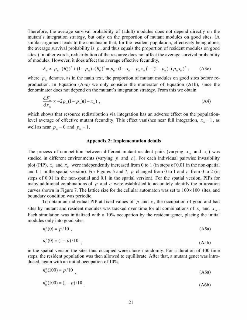
Therefore, the average survival probability of (adult) modules does not depend directly on themutant’s integration strategy, but only on the proportion of mutant modules on good sites. (Asimilar argument leads to the conclusion that, for the resident population, effectively being alone,the average survival probability is p , and thus equals the proportion of resident modules on goodsites.) In other words, redistribution of the resource does not affect the average survival probabilityof modules. However, it does affect the average effective fecundity,

2mmm

2mmmm

2bmm

2gmmm )()1()1()()1()( xppxpxpRpRpF ⋅−++−⋅=⋅−+⋅∝ , (A3c)

where mp denotes, as in the main text, the proportion of mutant modules on good sites before re-production. In Equation (A3c) we only consider the numerator of Equation (A1b), since thedenominator does not depend on the mutant’s integration strategy. From this we obtain

)1)(1(2dd

mmmm

m xppxF

−−−∝ , (A4)

which shows that resource redistribution via integration has an adverse effect on the population-level average of effective mutant fecundity. This effect vanishes near full integration, 1m =x , aswell as near 0m =p and 1m =p .

Appendix 2: Implementation details

The process of competition between different mutant-resident pairs (varying mx and rx ) wasstudied in different environments (varying p and c ). For each individual pairwise invasibilityplot (PIP), rx and mx were independently increased from 0 to 1 (in steps of 0.01 in the non-spatialand 0.1 in the spatial version). For Figures 5 and 7, p changed from 0 to 1 and c from 0 to 2 (insteps of 0.01 in the non-spatial and 0.1 in the spatial version). For the spatial version, PIPs formany additional combinations of p and c were established to accurately identify the bifurcationcurves shown in Figure 7. The lattice size for the cellular automaton was set to 100100× sites, andboundary condition was periodic.

To obtain an individual PIP at fixed values of p and c , the occupation of good and badsites by mutant and resident modules was tracked over time for all combinations of rx and mx .Each simulation was initialized with a 10% occupation by the resident genet, placing the initialmodules only into good sites.

10/)0(gr pn = , (A5a)

10/)1()0(br pn −= ; (A5b)

in the spatial version the sites thus occupied were chosen randomly. For a duration of 100 timesteps, the resident population was then allowed to equilibrate. After that, a mutant genet was intro-duced, again with an initial occupation of 10%,

10/)100(gm pn = , (A6a)

10/)1()100(bm pn −= . (A6b)

22

Sites for mutant occupation were chosen independently of their previous occupation (empty, oroccupied by a resident module). In the spatial version, sites occupied by the mutant were chosenwithin a square (the initial number of mutant modules was thus truncated to a square number).Simulations were stopped at time 300. The 100 time steps allowed for the resident dynamics andthe 200 time steps for the mutant-resident dynamics were chosen to ensure essentially completeequilibration under all conditions. For the deterministically behaving non-spatial version, a singlesimulation at each parameter combination was sufficient, whereas for the spatial version 200 repli-cations were carried out and averaged for each parameter combination to account for the effects ofdemographic stochasticity.

In the non-spatial version, changes of the population sizes of mutant and resident genetswere strictly monotonous after the establishment of an equilibrium distribution of mutant modulesbetween good and bad sites. This monotony allowed for a direct estimation of invasion fitness.However, for the spatial version, characterizing the invasion success of a mutant in a residentpopulation is not trivial because of the confounding effects of demographic stochasticity: simplycalculating the difference between mutant and resident population sizes or growth rates did notgive satisfactory results. We therefore compared the success of the mutant genet when competingagainst a resident genet with the success the mutant genet had when competing against a residentwith exactly the same strategy. For this purpose, we first evaluated the change in the mutant-to-resident ratio between times 100 and 300 ,

)100()100(

)300()300(

r

m

r

mrm n

nnn

xx −=σ . (A7a)

A negative (positive) value of rm xxσ indicates a loss (gain) of mutants between the two measure-

ments. In the absence of demographic stochasticity, we would have 0mm=xxσ , i.e., a rare mutant

genet that competes against a resident genet with exactly the same integration strategy is neutral,and its population size neither grows nor shrinks. However, in the presence of demographic sto-chasticity, the rare mutant genet is at an intrinsic disadvantage and is much more likely than theabundant resident genet to go extinct by chance effects. Therefore,

mm xxσ does not vanish on a fi-nite lattice (it tends to be negative) and we need to recalibrate the mutant’s success against theneutral case,

mmrmr)( m xxxxx xs σσ −= . (A7b)

Based on this measure of invasion fitness )( mrxsx we can conclude, both for the non-spatial and

the spatial model version, that the mutant can successfully invade the resident if )( mrxsx is posi-

tive.

23

LITERATURE CITED

Alpert, P. 1999. Clonal integration in Fragaria chiloensis differs between populations: ramets from grassland areselfish. Oecologia, 120: 69-76.

Alpert, P. and Mooney, H.A. 1986. Resource sharing among ramets in the clonal herb, Fragaria chiloensis. Oecolo-gia, 70: 227-233.

Alpert, P. and Stuefer, J. 1997. Division of labour in clonal plants. In The evolution and ecology of clonal plants (H.de Kroon and J. van Groenendael, eds), pp. 137-154. Leiden: Backhuys Publishers.

Brown, J.S. and Vincent, T.L. 1987. A theory for the Evolutionary Game. Theor. Pop. Biol., 31: 140-166.Brown, J.S. and Pavlovic, N.B. 1992. Evolution in heterogeneous environments: effects of migration on habitat spe-

cialization. Evol. Ecol., 6: 360-382.Cain, M.L., Dudle, D.A. and Evans, J.P. 1996. Spatial models of foraging in clonal plant species. Am. J. Bot., 83: 76-

85.Caldwell, M.M. and Pearcy, R.W. (eds) 1994. Exploitation of environmental heterogeneity by plants. San Diego:

Academic Press.Chesson, P.L. and Warner, R.R. 1981. Environmental variability promotes coexistence in lottery competitive systems.

Am. Nat., 117: 923-943.Chesson, P.L. and Peterson, A.G. 2002. The quantitative assessment of the benefits of physiological integration in

clonal plants. Evolutionary Ecology Research 4: 1153-1176.Christiansen, F.B. 1991. On conditions for evolutionary stability for a continuously varying character. Am. Nat., 138:

37-50.de Kroon, H. and van Groenendael, J. (eds) 1997. The evolution and ecology of clonal plants. Leiden: Backhuys Pub-

lishers.de Kroon, H. and Van Groenendael, J. 1990. Regulation and function of clonal growth in plants: an evaluation. In

Clonal growth in plants: regulation and function (J. van Groenendael and H. de Kroon, eds), pp. 79-94.The Hague: SPB Academic Publ.

D’Hertefeldt, T. and Jónsdóttir, I.S. 1999. Extensive physiological integration in intact clonal systems of Carex are-naria. Journal of Ecology, 87: 258-264.

Dieckmann, U. 1994. Coevolutionary dynamics of stochastic replicator systems. Juelich, Germany: Central Library ofthe Research Center.

Dieckmann, U. 1997. Can adaptive dynamics invade? Trends Ecol. Evol., 12: 128-131.Dieckmann, U. and Law, R. 1996. The dynamical theory of coevolution: a derivation from stochastic ecological proc-

esses. J. Math. Biol., 34: 579-612.Doebeli, M. and Dieckmann, U. 2000. Evolutionary branching and sympatric speciation caused by different types of

ecological interactions. Am. Nat., 156: S77-S101.Eriksson, O. 1997. Clonal life histories and the evolution of seed recruitment. In The evolution and ecology of clonal

plants (H. De Kroon and J. Van Groenendael, eds), pp. 211-226. Leiden: Backhuys Publishers.Eriksson, O. and Jerling, L. 1990. Hierarchical selection and risk spreading in clonal plants. In Clonal growth in

plants: regulation and function. (J. van Groenendael and H. de Kroon, eds) pp. 77-94. The Hague: SPBAcademic Publ.

Eshel, I. 1983. Evolutionary and continuous stability. J. Theor. Biol., 103: 99-111.Eshel, I. and Motro, U. 1981. Kin selection and strong stability of mutual help. Theor. Pop. Biol., 19: 420-433.Geritz S.A.H., Metz, J.A.J., Kisdi, É. and Meszéna, G. 1997. Dynamics of adaptation and evolutionary branching.

Phys. Rev. Lett., 78: 2024-2027.Geritz S.A.H., Kisdi, É., Meszéna, G. and Metz, J.A.J. 1998. Evolutionarily singular strategies and the adaptive

growth and branching of the evolutionary tree. Evol. Ecol., 12: 35-57.Hallé, F. 1986. Modular growth in seed plants. Phil. Trans. Roy. Soc. B, 313: 77-88.

24

Harper, J.L. 1985. Modules, branches, and the capture of resources. In Population biology and evolution of clonalorganisms (J.B.C. Jackson, L.W. Buss and R.E. Cook, eds), pp. 1-34. New Haven, Connecticut: Yale Uni-versity Press.

Hartnett, D.C. and Bazzaz, F.A. 1985. The integration of neighbourhood effects by clonal genets in Solidago cana-densis. J. Ecol., 73: 415-427.

Herben, T. and Suzuki, J. 2002. A simulation study of the effects of architectural constrains and resource translocationon population structure and competition in clonal plant. Evol. Ecol., 15: 403-423.

Hofbauer, J. and Sigmund, K. 1990. Adaptive dynamics and evolutionary stability. Appl. Math. Lett., 3: 75-79.Hutchings, M.J. and Bradbury, I.K. 1986. Ecological perspectives on clonal perennial herbs. BioScience, 36: 178-182.Hutchings, M.J. and de Kroon, H. 1994. Foraging in plants: the role of morphological plasticity in resource acquisi-

tion. Adv. Ecol. Res., 25: 159-238.Hutchings, M. J., Wijesinghe, D. K. and John, E.A. 2000. The effects of heterogeneous nutrient supply on plant per-

formance: a survey of responses, with secial reference to clonal herbs. In The ecological consequences ofenvironmental heterogeneity (M. J. Hutchings, E.A. John and A.J.A. Stewart,eds.), pp. 91-109. Oxford:Blackwell Science Ltd.

Jackson, J.B.C., Buss, L.W. and Cook, R.E. (eds) 1985. Population biology and evolution of clonal organisms. NewHaven, Connecticut: Yale University Press.

Jónsdóttir, I.S. and Watson, M.A. 1997. Extensive physiological integration: an adaptive trait in resource-poor envi-ronments? In The evolution and ecology of clonal plants (H. De Kroon and J. Van Groenendael, eds) pp.109-136. Leiden: Backhuys Publishers.

Kisdi, É. 2002. Dispersal: Risk spreading versus local adaptation. Am. Nat., 159: 579-596.Kisdi É. and Meszéna, G. 1993. Density dependent life history evolution in fluctuating environments. In: Adaptation

in a stochastic environment (J. Yoshimura and C. Clark, eds) pp. 26-62. Lecture Notes in Biomathematics98, Springer Verlag.

Kisdi, É. and Geritz, S.A.H. 1999. Adaptive dynamics in allele space: Evolution of genetic polymorphism by smallmutations in a heterogeneous environment. Evolution, 53: 993-1008.

Klimeš, L., Klimešová, J., Hendriks, R. and van Groenendael, J. 1997. Clonal plant architecture: a comparative analy-sis of form and function. In The evolution and ecology of clonal plants (H. De Kroon and J. VanGroenendael, eds), pp. 1-31. Leiden: Backhuys Publishers.

Law, R., Purves, D., Murrell, D. and Dieckmann, U. 2001. Causes and effects of small-scale spatial structure in plantpopulations. In Integrating ecology and evolution in a spatial context (J. Silvertown and J. Antonovics,eds), pp. 21-44. British Ecological Society Symposium Volume Series, 14, Blackwell Science.

Levin S.A., Cohen, D. and Hastings, A. 1984. Dispersal strategies in patchy environments. Theor. Pop. Biol., 26: 165-191.

Marshall, C. 1990. Source-sink relations of interconnected ramets. In Clonal growth in plants: regulation and function(J. van Groenendael and H. de Kroon, eds), pp. 23-42. The Hague: SPB Academic Publ.

Marshall, C. and Price, E. 1997. Sectoriality and its implications for physiological integration. In The evolution andecology of clonal plants. (H. de Kroon and J. van Groenendael, eds), pp. 70-107. Leiden: Backhuys Pub-lishers.

Mathias, A., Kisdi, É. and Olivieri, I. 2001. Divergent evolution of dispersal in a heterogeneous landscape. Evolution,55: 246-259.

Matsuda, H. 1985. Evolutionarily stable strategies for predator switching. J. Theor. Biol., 115: 351–366.Maynard Smith, J. 1982. Evolution and the theory of games. Cambridge: Cambridge University Press.Meszéna, G., Czibula, I. and Geritz, S.A.H. 1997. Adaptive dynamics in a 2-patch environment: a toy model for al-

lopatric and parapatric speciation. J. Biol. Systems., 5: 265-284.Metz, J.A.J., Nisbet, R. M. and Geritz, S.A.H. 1992. How should we define ‘fitness’ for general ecological scenarios?

Trends Ecol. and Evol., 7: 198-202.Metz J.A.J., Geritz, S.A.H., Meszéna, G., Jacobs, F.J.A. and van Heerwaarden, J.S. 1996. Adaptive dynamics, a geo-

metrical study of the consequences of nearly faithful reproduction. In Stochastic and spatial structures ofdynamical systems (S.J. van Strien and S.M. Verduyn Lunel, eds.) pp. 183-231. North Holland.

25

Metz J.A.J. and Gyllenberg, M. 2001. How should we define fitness in structured metapopulation models? Includingan application to the calculation of evolutionarily stable dispersal strategies. Proc. Roy. Soc. London B, 268:499-508.

Mizera, F. and Meszéna, G. 2003. Spatial niche packing, character displacement and adaptive speciation in an envi-ronmental gradient. Evol. Ecol. Res. 5: 363-382.

Mogie, M. and Hutchings, M.J. 1990. Phylogeny, ontogeny and clonal growth in vascular plants. In Clonal growth inplants: regulation and function (J. van Groenendael and H. de Kroon, eds), pp. 3-22. The Hague: SPB Aca-demic Publ.

Oborny, B., Kun, Á., Czárán, T. and Borkros, Sz. 2000. The effect of clonal integration on plant competition for mo-saic habitat space. Ecology, 81: 3291-3304.

Oborny, B., Czárán, T. and Kun, Á. 2001. Exploration and exploitation of resource patches by clonal growth: a spatialmodel on the effect of transport between modules. Ecol. Modelling, 141: 151-169.

Oborny, B. and Kun, Á. 2002. Fragmentation of clones: How does it influence dispersal and competitive ability? Evol.Ecol. 15: 319-346.

Pennings, S.C. and Callaway, R.M. 2000. The advantage of clonal integration under different ecological conditions: acommunity-wide test. Ecology, 81: 709-716.

Pitelka, L.F. and Ashmun, J.W. 1985. Physiology and integration of ramets in clonal plants. In Population biology andevolution of clonal organisms (J.B.C. Jackson, L.W. Buss and R.E. Cook, eds), pp. 399-435. New Haven,Connecticut: Yale University Press.

Sachs, T. 2002. Developmental processes and the evolution of plant clonality. Evol. Ecol., 15: 485-500.Schmid, B. 1990. Some ecological and evolutionary consequences of modular organization and clonal growth in

plants. Evol. Trends in Plants, 4: 25-34.Schmid, B. and Bazzaz, F.A. 1987. Clonal integration and population structure in perennials: effects of severing rhi-

zome connections. Ecology, 68: 2016-2022.Stuefer, J.F. 1996. Potential and limitations of current concepts regarding the responses of clonal plants to environ-

mental heterogeneity. Vegetatio, 127: 55-70.Stuefer, J.F., During, H.J. and De Kroon, H. 1994. High benefits of clonal integration in two stoloniferous species, in

response to heterogeneous light environments. J. Ecol., 82: 511-518.Stuefer J.F. and Huber, H. 1999. The role of stolon internodes for ramet survival after clone fragmentation in Poten-

tilla anserina. Ecol. Lett., 2: 135-139.Sutherland, W.J. 1990. The response of plants to patchy environments. In Living in a patchy environment (B. Shor-

rocks and I.R. Swingland, eds), pp. 45-61.Oxford: Oxford Sci. Publ.Suzuki, J. and Hutchings, M.J. 1997. Interactions between shoots of clonal plants and the effects of stored resources

on the structure of shoot populations. In The evolution and ecology of clonal plants (H. de Kroon and J. vanGroenendael, eds), pp. 311-330. Leiden: Backhuys Publishers.

Suzuki, J. and Stuefer, J.F. 1999. On the ecological and evolutionary significance of storage in clonal plants. PlantSpecies Biology, 14: 11-17.

Taylor, P.D. 1989. Evolutionary stability in one-parameter models under weak selection. Theor. Pop. Biol., 36: 125-143.

Turelli, M. 1978. Does environmental variability limit niche overlap? Proc. Nat. Acad. Sci., 75: 5085-5089.van Groenendael, J. and de Kroon, H. (eds) 1990. Clonal growth in plants: regulation and function The Hague: SPB

Academic Publ.van Kleunen, M., Fisher, M. and Schmid, B. 2000. Clonal integration in Ranunculus reptans: by-product or adapta-

tion? J. Evol. Biol., 13: 237-248.van Tienderen, P.H. and de Jong, G. 1986. Sex ratio under the haystack model: Polymorphism may occur. J. Theor.

Biol., 122: 69-81.Vuorisalo, T. and Tuomi, J. 1986. Unitary and modular organisms: criteria for ecological division. Oikos, 47: 382-385.Vuorisalo, T. and Hutchings, M.J. 1996. On plant sectoriality, or how to combine the benefits of autonomy and inte-

gration. Vegatatio, 127: 3-8.Watson, M.A. 1986. Integrated physiological units in plants. Trends Ecol. Evol., 1: 119-123.

26

Wennström, A. 1999. The effect of systemic rusts and smuts on clonal plants in natural systems. Plant Ecology, 141:93-97.

Wijesinghe, D.K. and Whigham, D.F. 2001. Nutrient foraging in woodland herbs: a comparison of three species ofUvularia (Liliaceae) with contrasting belowground morphologies. Am. J. Bot., 88: 1071-1079.

Winkler, E. and Fischer, M. 2002. The role of vegetative spread and seed dispersal for optimal life histories of clonalplants: a simulation study. Evol. Ecol., 15: 281-30.

27

Integration

Splitting

Figure 1

Implications of physiological integration and splitting for modules in resource-rich (grey) and poor(white) sites. In a complete integrator (left), modules equally share the available resource, result-ing in equal chances for survival and reproduction. In a complete splitter (right), no resource istransferred between modules. Each module survives and reproduces according to the local qualityof its own site (depicted by the larger-sized modules in the resource-rich sites). We studied howthe optimal degree of resource sharing depends on the density and temporal constancy of richsites.

28

Figure 2

Schematic representation of states and state transitions in the (a) non-spatial and (b) spatial versionof our plant population model. Sites of high habitat quality (good sites) are shown in gray, andsites occupied by a module are indicated by vertical lines. While the spatial model operates on atwo-dimensional square lattice and colonization of empty sites is strictly local, the non-spatialmodel restricts attention to the global frequencies of good and bad sites that are occupied andempty, respectively, thus relying on the assumption of the system being well mixed with regard tothese features. In (b), a reduced grid size of 3030× has been chosen for the purpose of illustra-tion.

(a) (b)

29

Figure 3 Spatial invasion dynamics of mutant integration strategies. Good sites are shown in gray. Vertical and hori-zontal lines indicate sites occupied by modules with resident and mutant integration strategies, respectively. (a)Unsuccessful invasion. At time 0=t , resident modules are introduced to a 10% fraction of randomly chosen sites,upon which their abundance and spatial structure has time to equilibrate until 99=t . At time 100=t , mutantmodules are introduced to a square-shaped subset of sites, giving the mutant an initial occupation of about 10%. Mu-tant modules decrease in abundance until 125=t and have completely vanished until 300=t . Parameters:

5.0=p , 1.0=c , 0r =x , 5.0m =x . (b) Successful invasion. After the mutant integration strategy has been in-troduced – again at 100=t – it increases in abundance, as shown for 125=t , and has replaced all residentmodules until 300=t . Parameters: 5.0=p , 1.0=c , 1r =x , 0m =x . A reduced grid size of 3030× hasbeen chosen for the purpose of these illustrations.

30

Figure 4 Illustration of evolutionary regimes in the non-spatial model version for a particular proportion of good sites,4.0=p . (a) Pairwise invasibility plots arising for four different rates of environmental change, c . In each of these

plots, combinations of resident integration strategies rx and mutant integration strategies mx for which the mutant issuccessful in invading and replacing the resident are shown in gray. Hollow arrows indicate the resultant direction ofevolution by small mutational steps. (b) Dependence of the proportion of mutant modules on good sites, mp , on mu-

tant integration strategy mx . Panels characterize the four different evolutionary regimes for a resident integration

strategy 5.0r =x ; other values of rx give qualitatively similar results. (c) Bifurcation diagram for variation of c ,showing the transitions between the four evolutionary regimes (dotted lines). Hollow arrows again show the directionof evolution. The location of convergence stable (unstable) integration strategies x is depicted by thick continuous(dashed) curves. The light gray area to the right corresponds to values of c that are infeasible at 4.0=p .

(c)

(b)

(a)c = 0.5

01

1

xr

xm

c = 1.55c = 1.25 c = 1.45

0 20

1

x

c

0

0

1

pm

1xm0

31

Figure 5 Overview of evolutionary regimes in the non-spatial model version, in dependence on habitat quality, p ,and habitat variability, c . The two light gray areas on the top correspond to infeasible combinations of p and c .Altogether four evolutionary regimes are possible; however, for negatively autocorrelated environments, 1<c , evo-lution always favors complete splitting. Also notice that the range of combinations of p and c that favorintermediate degrees of integration is narrow.

0 0.5 1

1

2

0

p

c

(a)

(b)

(c)

(d)

32

Figure 6 Illustration of evolutionary regimes in the spatial model version for a particular proportion of good sites,4.0=p . Graphical features are as in Figure 4. (a) Pairwise invasibility plots arising for three different rates of envi-

ronmental change, c . Due to demographic stochasticity, results exhibit some noise. (b) Dependence of the proportionof mutant modules on good sites, mp , on mutant integration strategy mx . Panels characterize the three different

evolutionary regimes for a resident integration strategy 5.0r =x ; other values of rx give qualitatively similar re-

sults. Dependence of mutant habitat bias pp −m on resident and mutant integration strategies for the threeevolutionary regimes. (c) Bifurcation diagram arising for variation of c , showing the transitions between the threeevolutionary regimes. Notice that, in contrast to Figure 4, intermediate degrees of integration are favored for 1<c .

(a)

(b)

01

1

xr

xm

(c)

0

01

1

xm

pm

0

33

Figure 7 Overview of evolutionary regimes in the spatial model version in dependence on habitat quality, p , andhabitat variability, c . Graphical features are as in Figure 5. The dark gray area to the left indicates combinations ofp and c for which all resident integration strategies lead to extinction, an outcome that does not occur in the non-

spatial version of the model. Four main evolutionary regimes are observed. Dashed curves in the vicinity of1== cp enclose a small region for which, even with massive numerical investment, accurate localization of bifur-

cation curves turned out to be infeasible. A feature of primary interest in this plot is the existence of a wide range ofcombinations of p and c with 1<c that favor intermediate degrees of integration.

0 0.5 1

1

2

0

p

c

(a)

(b)

(c)

(d)

(e)