Utah State University Utah State University

DigitalCommons@USU DigitalCommons@USU

Reports Utah Water Research Laboratory

January 1982

Consumptive Use and Water Requirements for Utah Consumptive Use and Water Requirements for Utah

A. Leon Huber

Frank W. Haws

Trevor C. Hughes

Jay M. Bagley

Follow this and additional works at: https://digitalcommons.usu.edu/water_rep

Part of the Civil and Environmental Engineering Commons, and the Water Resource Management

Commons

Recommended Citation Recommended Citation Huber, A. Leon; Haws, Frank W.; Hughes, Trevor C.; and Bagley, Jay M., "Consumptive Use and Water Requirements for Utah" (1982). Reports. Paper 399. https://digitalcommons.usu.edu/water_rep/399

This Report is brought to you for free and open access by the Utah Water Research Laboratory at DigitalCommons@USU. It has been accepted for inclusion in Reports by an authorized administrator of DigitalCommons@USU. For more information, please contact digitalcommons@usu.edu.

CONSUMPTIVE USE AND WATER REQUIREMENTS FOR" UTAH

Technical Publication No. 75

State of Utah

DEPARTMENT OF NATURAL RESOURCES

1982

qqqq4

scon M. MATHESON Governor

This report was prepared as a part of the Statewide cooperative water-resource investigation program administered jointly by thE? Utah Department of Natural Re­sources, Division of Water Rights and the United States Geological Survey. The program is conducted to meet the water administration and water-resource data needs of the State, as well as the water information needs of many units of government and the general public.

Temple A. Reynolds Executive Director Department of Natural Resources

Copies available at

Utah Department of Natural Resources

Division of Water Rights

1636 West North Temple. Room 220

Salt Lake City. Utah 84116

Dee C. Hansen State Engineer

Division of Water Rights

State of Utah

Division of Water Rights

CONSUMPTIVE USE AND

,WATER REQUIREMENTS FOR UTAH

Technical Publication No. 75

by

A. Leon Huber, Frank W. Haws, Trevor C. Hughes, Jay M. Bagley, Kenneth G. Hubbard

and E. Arlo Richardson

Prepared Cooperatively by the Water Rights Division, Utah Department of Natural Resources

and Utah Water Research Laboratory

Utah State University

March 1982

TABLE OF CONTENTS

INTRODUCTION •

Need for Water Use Standards . Water Requirements in Single and Aggregated Uses

AGRICULTURAL WATER REQUIREMENTS

Selection of a Potential Consumptive 'Use Formula Calculating Potential Consumptive Use • Geographical Variation in Consumptive Use Irrigation Water Requirements

Upward adjustments to crop evapotranspirational needs

Downward adjustments to crop evapotranspirational needs

Calculation of irrigation water requirement

WATER REQUIREMENTS OF DOMESTIC ANIMALS

MUNICIPAL WATER REQUIREMENTS

General Considerations • Design of Municipal Systems

Average annual use Peak demand • Instantaneous peak demand Peak day demand Outdoor water use index and peak day demand Peak month demand •

Computing Demands - An Example

INDUSTRIAL WATER REQUIREMENTS

RECREATIONAL WATER REQUIREMENTS

Types of Water Related Recreation Activities Evaluating Changes in Recreation Opportunities • Domestic Requirements at Developed Recreational Areas

REFERENCES

APPENDIX: CURVES OF CROP GROWTH STAGE COEFFICIENTS •

iii

Page

1

1 1

3

3 6

20 23

25

28 30

37

41

41 47

47 48 48 50 52 54

56

61

67

67 68 71

73

77

Figure

1

2

3

4

5

6

7

8

9

10

LIST OF FIGURES

Average July 700 millibar temperature map for Utah

Input, information flow, and output of consumptive use factor model, F, presented schematically

Illustration of increased volumes of water needed for equivalent service when salt concentration is increased .

Daily per capita withdrawal rates for 50 Utah municipal systems: Average of 1974, 1975, and 1976

Daily per capita withdrawal rates (gcd) for Bountiful, Ogden, Provo, and Salt Lake City: 1960-1976 • . . Peak instantaneous demands within municipal water systems in Utah: Utah demand function and Farmers Home Administration average standard •

Peak day demand per connection as a function of average demand

Peak day demand per person as a function of average demand

Peak day demand per connection as a function of outdoor use index

Peak day demand per person as a function of outdoor use index •

11 Peak month demand per connection as a function of average demand

12 Peak month demand per person as a function of average demand

13 Normalized water use rates for Utah's major water using industries

14 Probability of recreationists using flowing water for two types of recreation: swimming and canoe-fishing

iv

Page

21

24

26

43

46

51

53

53

55

55

57

57

65

70

Table

1

LIST OF TABLES

Seasonal and yearly comparison of average of 15 years evapotranspiration estimates, Ohio

2 Data for weather stations in Utah having continuous records of 15 years or more

3

4

5

6

7

8

9

10

11

Approximate planting dates and length of growing season for annual crops in Utah

Monthly percentage of daytime hours (p) of the year for latitudes 360 to 430 north of the equator •

Average percentage of daylight hours for principal weather station locations in Utah

Mean monthly temperatures in·degrees Fahrenheit for Utah weather station

Values of the climatic coefficient, kt, for various mean monthly air temperatures, t . .•

Sample calculation of average daily, monthly, and seasonal consumptive use by corn at Logan, Utah •

Sample calculation of average daily, monthly, and seasonal consumptive use by alfalfa at Milford,Utah

Average monthly consumptive use factors, f, Utah stations •

Seasonal consumptive-use crop coefficients (K) for irrigated crops

12 Guidelines for interpretation of water quality for irrigation

13

14

Comparison of irrigation systems in relation to site and situation factors

Values of seepage coefficient "c"

15 Multipliers to use in calculating effective precipitation

16

17

Sample calculation of effective precipitation

Average mean monthly precipitation for principal weather station locations in Utah

v

Page

4

7

9

9

10

12

14

15

16

17

19

27

29

30

31

32

33

Table

18

19

20

21

22

23

24

25

26

27

28

29

30

31

32

33

34

LIST OF TABLES (CONTIWJED)

Water requirements of cattle

Water requirements of sheep

Water requirements of pigs

Water requirements of turkeys

Water requirements of chickens

Estimated daily withdrawal rates per person (gcd) for 50 Utah municipal systems: 1960-1975.

Per capita withdrawal rate (gcd) statistics for 50 Utah municipalities: 1960-1976.

Average annual domestic water demand for design purposes

Effects on municipal water system cost of different durations of flow peak

Outdoor use index (I)

A summary of flows computed in design example

Water use rates for energy conversion industries

Utah industrial water withdrawal rates (ged) for major water using industries: average of 1974, 1975, and 1976 .

Outdoor water recreational areas rated by amount of water surface area available •

Minimum stream flow requirement by fisheries

Guidelines for water requirements of recreational campgrounds in Utah • ..

Design standards for recreational development in the State of Utah

PLATE IN POCKET

Plate 1. Seasonal Consumptive Use Factor F.

vi

Page

38

39

39

40

40

44

45

49

49

54

59

63

64

69

71

72

72

FOREWORD

Studies on the meteorological determinants of evapotranspiration were initiated at least as long ago as the 1920s and by the late 19408 had produced the Blaney-Criddle method for estimating crop consumptive use. The resulting ability to estimate water requirements by both location and crop added a new scientific dimens ion to water rights administration that was first"introduced into the courts of Utah during adjudication of water rights in the Escalante Valley in 1949.

Application of the consumptive use concept to water rights administra­tion and water resources planning, however, required a written reference. Technical Publication No. 8 entitled "Consumptive Use of Water and Irriga­tion Requirements of Crops in Utah" was published by the State Engineer in 1952.

By 1962, methods had been developed for going beyond agriculture to estimate water requirements for municipal, industrial, and recreational uses. Technical Pub licat ion No. 8 was revised and pub lished under the title "Consumptive Use and Water Requirements for Utah."

Continuing advancements in water requirements estimation have occurred over the last 20 years. The present revision, Technical Publication No. 75, updates estimation of agricultural, municipal, recreational, and industrial water uses. It presents an isogram of potential consumptive use that permits the determination of crop water requirements at any point within the state.

Dee C. Hansen State Engineer, Utah Division of Water Rights

L. Douglas James Director, Utah Water Research Laboratory Utah State University

vii

INTRODUCTION

Need for Water Use Standards

Reliable· guides or standards for estimating water requirements are essential for the planning, design, and operation of any water using enterprise. Part icularly in a state like Utah, where water demands are high relative to the availability of supplies, and where it is imperative that as many uses as possible be satisfied, it is important that water requirements in various uses be accurately quantified. If the achievement of laudable social and economic goals are not to be water limited, there must be authoritative water use standards to guide in making water alloca­tions and in monitoring water transfers and changes in use that occur over time. Cost-effective management of water in any use is both fostered and maintained on the basis of soundly conceived and properly applied water requirements information.

Recognizing the widespread importance of information on unit water use, water administrators, planners, and. managers have sought to obtain reliable values of water need, particularly for the major uses such as irrigated agriculture, municipal, and industrial. Concomitant with the establishment of the Office of the State Engineer have been efforts to determine the "duty of water" in various uses. Historically and presently, water use for irrigated agriculture has been the predominant use of water in Utah. Therefore, much research emphasis has been placed on determining water requirements of various crops grown in different regions of the state. A most significant distillation of water use information and guide to its use was Technical Publication No.8, "Consumptive Use of Water and Irrigation Requirements of Crops in Utah" published by the State Engineer in 1952. This popular publication has been widely used in Utah and else­where as a basis for estimating crop water requirements.· An updated and expanded version of the 1952 publication was issued in 1962 under the title "Consumptive Use and Water Requirements for Utah." The revised edition included information about water requirements in municipal, industrial, and recreational uses as well as agricultural. A further updating reflecting the state of the art in research and the accumulation of additional data upon which water requirements in various uses are derived constitutes this present report. A note-worthy improvement is the incorporat ion of tech­niques to permit the calculation of agricultural consumptive use at any geographic point of interest without going through some compl icated ex­trapolation from a particular weather station location.

Water Requirements in Single and Aggregated Uses

As previously mentioned, sential in planning, operating, water using enterprise. If they

unit water requirement estimates are es­and evaluating performance of an individual are to have meaningful utility for regional

1

water resources planning, management, and administration, unit water use values must be applied in a river basin perspective. In other words, values of water requirement in particular individual uses must be applied within the conceptual framework of a hydrologic flow system recognizing that all uses are related through the unifying interconnection of all surface and subsurface waters of a basin or watershed. What one user does with and to water in the use process imparts an impact which may be felt by subsequent users downstream. The impact may be substant ial or imperceptible and may be in terms of either quantity or quality or both. Important to appreciate is that different uses made from a common supply are not "homogeneous" or directly "convertible" in a hydrologic sense. For example, water use by crops is largely "consumptive"; meaning that liquid water is changed to a vapor in the use process and expelled into the atmosphere, thereby resulting in a depletion from the liquid manageable water supply of the basin. Water use in the generation of hydropower is "nonconsumptive"; meaning that water remains in the liquid state in the use process and is discharged in that form back into the general system, thereby causing no noticeable depletion from the stream sys tem itself. Most water uses are comprised of both consumptive and nonconsumptive components. Municipalities, for example, may return to their sewer system up to 90 percent of the water diverted and delivered through their supply distribution systems. Thus, while different water uses may be expressed in terms of a common unit of water measure, that does not constitute a common denominator of convertibility in a hydrologic sense. This can be readily appreciated by considering the third party impacts of changing a "nonconsumptive use" entitlement to a "consumptive use" en­t itlement. It should be kept in mind, therefore, that water requirement criteria described in this report are in terms of individual uses. In instances where a variety of water uses are aggregated and take place in parallel and sequence, reasonable care may need to be exercised so as to maintain the hydrologic integrity of any calculation or projection In­volving water use criterion tabulated herein.

2

AGRICULTURAL WATER REQUIREMENTS

Agricultural water requirements are of special significance in arid areas where water needs must be met largely through irrigation. Unlike dryland agriculture, irrigated agriculture entails the diversion, regula­tion, conveyance, and distribution of water from streams and rivers. Therefore, irrigation water requirement becomes a key standard in the allocat ion and management of water, in .the administering of water rights, and in the design of large and small irrigation projects.

Irrigation water requirement is a term used to denote the volume and regimen of flow that must be delivered at some specified point for sub­sequent distribution and placement in the soil where it can be used to satisfy the evapotranspirational needs of crops. Irrigation water require­ment is thus composed of a basic potential consumptive use requirement (which is principally a function of climate) adjusted as appropriate by 1) incremental additions of water which improve the root ing environment, and to make up for unavoidable losses of water in the process of getting the proper amount placed in the crop root zone; and 2) incremental reduc­tions from the basic consumpt ive use in those instances where precipita­tion, groundwater, or water from some other nonirrigation source satisfies a portion of the potential water need.

Selection of a Potential Consumptive Use Formula

Standards of potential consumptive use or evapotranspiration for various crops are determined from carefully controlled experiments. Measured quantities of water are placed in a controlled crop root zone and time changes in root zone moisture storage are carefully monitored. At the same time, climatic and physiologic factors that influence the eva po­transpirational process are measured. Then the climatic and physiologic factors are correlated with water changes and formulae are developed which can be used for estimating evapotranspiration under given climatic and crop regimes. A comparison of seasonal and annual predictions of consumptive use compared to actual consumptive use in lysimeters containing a deep rooted grass-legume crop is shown in Table 1 (McGuinness and Bordne 1972). Other investigators have made more recent comparisons (Samani 1981); some of which have been based on Utah data. Testing and refinement of consump­tive use formulas continues and improvements will undoubtedly be made.

After analyzing the more commonly used equations, their derivations, and their performance in various situations, the Blaney-Criddle formula as modified by the USDA (1967) was selected for estimating consumptive use in Utah. This formula utilizes data available or derivable in compatible time-increments throughout the state. The Blaney-Criddle method of deter­m1n1ng agricultural water requirements has been thoroughly tested over time and has gained scientific credibility and, hence, widespread legal acceptance where water use disputes have been litigated.

3

Table 1. Seasonal and yearly comparison of average of 15 years evapo­transpiration estimates, Ohio.

Method

Lysimeter Blaney-Criddle Thornthwaite Hamon Papadakis Grassi Stephen";'Stewart Turc Jensen-Haise Makkink Christiansen Penman Van Bave 1 Weather Bureau (Pan)

Average April-October Seasonal ET

Inches

35.16 35.01 25.83 23.22 21. 73 39.16 22.69 30.82 35.99 26.18 34.00 31.21 33.65 35.94

Percent Difference

o -0.4

-26.5 -34.0 -38.2

11.4 -35.5 -12.3

2.4 -25.5 -3.3

-11.2 -4.3

2.2

Source: McGuinnes and Bordne (1972)

Average Yearly ET

Inches

40.14 37.79 26.61 26.47 26.21 49.71 24.48 32.55 38.05 31.06 40.30 37.62 42.45 43.35

Percent Difference

o -5.9

-33.7 -34.3 -34.7

23.8 -39.0 -18.9 -5.2

-22.6 0.4

-6.3 5.8 8.0

The Blaney-Criddle formula for computing consumptive use incorporates a climatic parameter called the consumptive use factor, F, and a physi­ologic parameter called the crop coef ient, K. Consumptive use over the crop growing season is expressed by the simple empirical relation

U = KF. 0)

in which

U the growing season consumptive use of water by the crop ~n

inches K the consumptive use coefficient for the g~ven crop for the

growth period F = the growing season consumptive use factor

The growing season consumptive use factor, F, is calculated as the sum of monthly and part-month consumptive use factors, f, where

4

f == a monthly (or short period) consumptive use mult iplying the mean monthly temperature, t, percent of annual daytime hours, p

factor found by by the monthly

Since t and p are monthly values rather than growing season values, monthly consumptive use can be calculated when corresponding values of the consumptive use coefficient, k, are available. Hence,

and

In which

r' 1 = n ::

k' 1 ==

~ u = kf = k 100 (2 )

U = Eu

i=n tiPi = 1: riki 100 (3)

i=l

the fraction of the month i in which crop growth occurs the number of months of the year falling partly or entirely within the growing season the consumptive use coefficient for the crop of interes.t for month i

The monthly consumptive use coefficient, ki, has been further dis­aggregated into two components in order to separate the local climatic effects, kt ., from the crop growth stage or physiological effects, kc .. The crop grawth stage coefficient thus becomes a general and universally applicable coefficient independent of local conditions. Accordingly,

in which

(4)

is a coefficient reflecting the stage of crop growth representing month i, and is a climatic coefficient which is related to the mean air temperature, ti, by:

(5 )

With these modifications, the Blaney-Criddle equation for calculating consumptive use for a growing season becomes

i=n

u 1: i=l

t.p. 1. 1.

100 (6)

This equation has been used to determine the values of consumptive use by agricultural crops reported herein.

5

Calculating Potential Consumptive Use

The calculation of potential evapotranspiration or consumptive use for any particular crop at a location of interest requires informa­tion about 1) when the growing period begins and ends, 2) the mean monthly temperatures for the growing period, 3) the monthly percent of the po.ssible yearly daytime hours for the months involved, 4) the monthly crop growth stage coefficients, and 5) the monthly climate or temperature coefficients. These are the factors represented by the Blaney~Criddle expression given as Equation 6.

The length of the potent ial growing season is commonly taken as the interval between the last killing freeze in the spring and the first killing freeze in the fall. In calculating potential consumptive use, the average date of the last 28°F temperature in the spring is normally used as the beginning date of the growing season. The average date of the first 28°F in the fall is considered the ending date of the growing season. These dates and the growing interval are shown in Table 2 for the 130 weather stations in Utah having long term continuous temperature records. These 28°F freeze dates are needed to dete.rmine the fract ion of the month (r) for which growth occurs for those crops whose growth either begins or ends according to freeze temperatures. For other crops, dates of planting and harvest are needed in order to determine part month growth periods. Approximate planting and harvesting dates for annual crops as a function of the seasonal consumpt ive use factor, F, appl icab Ie to the locat ion are shown in Table 3.

In order to de termine the appropriate percentage of yearly dayt ime hours, p, for use in Equation 6, the latitude of the station whose weather data are being used in the calculation of consumptive use must be known. Monthly values of p for the latitudes which span Utah are given in Table 4.

For the set of long term weather stations in Utah the monthly percent of possible yearly daytime hours, p, has been determined and tabulated for convenient use in Table 5.

Mean monthly temperature, t, for the set of long term weather stations in Utah are provided in Table 6.

Values of the climatic coefficient, kt, for any given mean tempera­ture, t, for month i can be calculated by use of Equation 5 or obtained directly from Table 7.

For the commonly grown crops in Utah, the crop growth stage coeffi­cient, kc, can be obtained from the figures provided in the Appendix. The crop stage coefficient curves in the Appendix were developed by the U.S. Department of Agriculture and included in the 1970 revision of Technical Release NO. 21. With annual crops, such as corn and small grains, the values of the growth stage coefficients are plotted against the growing period expressed in terms of percent of total growing period. For perennial crops, such as alfalfa, permanent pasture, and orchards,

6

Table 2. Data for weather stations in Utah having continuous records of 15 years or more.

Blaney- Mean 280 F Elevation Latitude Longitude Criddle Freeze Dates lnterval Precipi- Tempcra-

No. Station (Feet) (Deg-Min) (Deg-Min) Seasonal (Days) tatlon ture F Spring Fall (Inches) (DEG(F»

1 Altamont 6380 40-22 110-17 29.80 May 7 Oct 13 159 8.44 43.6 2 Alton 7040 37-26 112-29 25.95 May 19 Oct 5 139 16.38 45.4 3 Antelope Island 4225 40-56 112-10 40.42 Apr 13 Oct 31 201 15.57 51.9 4 Bear River Refuge 4208 41-28 112-16 38.64 Apr 15 Oct 25 193 11.97 50.4 5 Beaver 5920 38-17 112-38 26.69 _ May 18 Sep 29 134 11.33 47.5

6 Bingham Canyon 6095 40-32 112-09 36.34 Apr 20 Nov 2 196 21. 22 47.9 7 Birdseye 5740 39-52 111-32 18.39 Jun 6 Sep 7 93 13.49 42.5 8 Black Rock 4895 38-43 1l2-57 28.61 May 11 Sep 27 139 8.61 48.6 9 Blanding 6036 37-37 109-28 34.30 Apr 28 Oct 19 174 11.82 49.7

10 Bluff 4315 37-17 109-33 42.60 Apr 5 Nov 1 210 7.55 54.6

11 Bonanza 5450 40-01 109-11 35.01 Apr 25 Oct 13 171 8.22 48.5 12 Boulder 6580 37-55 111-24 32.84 May 1 Oct 18 170 10.20 48.2 13 Brigham City 4335 41-29 112-02 38.64 Apr 16 Oct 25 192 19.31 51.1 14 Bryce Canyon FAA AP 7595 37-42 112-09 16.91 Jun 11 Sep 11 92 11. 79 40.0 15 Bryce Canyon NP IIDQ 7915 37-39 112-10 16.67 Jun 11 Sep 11 92 15.83 38.4

16 Capitol Reef NT MON 5500 38-17 111-16 36.78 Apr 25 Oct 18 176 7.24 53.2 17 Castle Dale 5660 39-13 lll-01 28.72 May 13 Oct 4 144 8.00 46.0 18 Cedar City FAA AP 5601 -37-42 113-06 33.13 Apr 30 Oct 13 166 10.33 49.8 19 Cedar City PH 5980 37-40 113-02 35.76 Apr 23 Oct 23 183 11.96 50.7 20 Cedar Point 6780 37-43 109-05 28.50 May 12 Oct 2 143 13.47 46.7

21 Circleville 6000 38-10 112-16 27.95 May 13 Oct 1 141 8.01 47.2 22 Coalville 5550 40-55 111-24 21.10 May 30 Sep 14 107 14.78 44.2 23 Corinne 4230 41-33 112-07 34.19 Apr 26 Oct 12 169 15.62 48.9 24 Cottonwood Weir 4950 40-37 111-47 42.83 Apr 5 Nov 4 213 22.69 53.7 25 Cove Fort 5980 38-36 112-35 27.56 May 15 Sep 27 135 13.01 47.5

26 Deer Creek Dam 5270 40-24 111-32 22.61 May 25 Sep 16 114 21.33 43.4 27 Delta 4630 39-21 112-34 35.41 Apr 23 Oct 13 173 7.77 50.1 28 Deseret 4585 39-17 112-39 32.17 May 3 Oct 8 _ 158 6.92 49.2 29 Desert Exp R 5252 38-36 113-45 31.21 May 5 bct 5 153 6.09 48.9 30 Duchesne 5510 40-10 110-24 28.40 May 14 Oct 3 142 8.71 45.3

31 Dugway 4340 40-11 112-56 39.04 Apr 14 Oct 23 192 6.67 51.1 32 Echo Dam 5500 40-58 111-26 25.95 May 17 Sep 25 131 13.81 45.3 33 Elberta 4690 39-57 111-57 34.60 Apr 26 Oct 14 171 10.93 50.2 34 Emery 6200 38-55 111-15 28.33 May 13 Oct 8 148 7.55 46.0 35 Enterprise Beryl Jct 5200 37-45 113-39 25.24 May 20 Sep 21 124 '9.19 47.7

36 Ephraim Sorn FD 5580 39-21 111-35 30.52 May 6 Oct 8 155 10.46 46.8 37 Escalante 5810 37-46 111-36 30.34 May 8 Oct 9 154 11.22 48.6 38 Fairfield 4876 40-16 112-05 26.04 May 19 Sep 24 128 10.61 46.5 39 Farmington USU 4340 41-01 111-54 38.38 Apr 16 Oct 25 192 19.96 51.5 40 Ferron 5925 39-06 111-08 33.94 Apr 29 Oct 18 172 8.15 47.5

41 Fillmore 5160 38-57 112-19 38.12 Apr 16 Oc't 24 191 14.78 51.6 42 Fish Spg Ref 4335 39-51 113-24 41. 56 Apr 7 Oct 29 205 5.30 53.0 43 Flaming Gorge 6270 40-56 109-25 26.22 May 17 Sep 28 134 12.45 44.0 44 Fort Duchesne 4990 40-17 109-52 28.70 May 12 Sep 30 141 7.23 44.9 45 Garfield 4310 40-43 112-12 44.23 Mar 30 Nov 13 228 15.58 52.9

46 Garland 4350 41-44 112-10 34.09 Apr 27 Oct 14 170 15.14 48.0 47 Garrison 5275 38-56 114-02 33.20 Apr 29 Oct 10 164 7.13 49.8 48 Geneva Steel 4550 40-18 111-44 38.88 Apr 15 Oct 26 194 11.46 51.4 49 Green River AVN 4070 39-00 110-10 38.81 Apr 16 Oct 20 187 6.11 52~ J

50 Gunnison 5145 39-09 111-49 25.74 May 19 Sep 20 124 7.99 47.8

51 Hanksville 4308 38-22 110-43 41.85 Apr 8 Oct 29 204 5.20 53.1 52 Hanna 6780 40-26 110-48 22.41 May 28 Sep 22 117 11.72 42.3 53 Hardware Ranch 5560 41-36 1 fl-34 11.16 Jun 22 Aug 17 56 15.44 41.7 54 Heber 5580 40-31 111-25 22.90 May 26 Sep 19 116 15.82 44.1 55 Hiawatha 7230 39-29 111-01 31.34 May 4 Oct 18 167 14.15 45.5

56 Hovenweep Mon 5400 37-23 109-04 36.66 Apr 20 Oct 17 180 10.45 51.3 57 Ibapah 5280 40-02 113-59 22.53 May 26 Sep 13 110 10.70 45.1 58 Jensen 4720 40-22 109-21 29.15 May 10 Sep 28 141 7.94 45.5 59 Kamas Ranger St 6495 40-39 111-17 22.43 May 28 Sep 20 115 17.67 43.4 60 Kanab 4985 37:"03 112-32 38.69 Apr 16 Oct 23 190 12.21 54.9

61 Koosharem 6950 38-31 Ill-53 21.07 Jun 1 Sep 18 109 9.25 43.4 62 Lake Town 5988 41-49 111-19 22.62 May 26 Sep 21 118 11.58 42.1 63 LaSal 6960 38-19 109-15 29.45 May 9 Oct 10 154 12.88 46.7 64 LaVerkin 3450 37-12 113-16 42.41 Apr 9 Oct 26 200 9.66 58.3 65 Levan 5300 39-33 Ill-52 33.92 ' Apr 28 Oct 16 171 14.66 49.1

7

Table 2. Continued.

IIlaney- Mean 280 F Mean Annual No. Station Elevation Latitude Longitude Criddie Freeze Dates Precipi- Tempera-. (Feet) (Deg-Min) (Deg-Min) Seasonal Interval

(Days) tation ture F Spring Fall (Inches) (DEG(F»

66 Lewiston 4480 41-58 111-50 28.17 May 12 Sep 30 141 17.64 45.4 67 Loa 7045 38-24 111-39 19.21 Jun 5 Sep 13 100 7.48 43.0 68 Logan lCVNU 4504 41-46 Ill-50 32.25 May 2 Oct 10 161 15.01 46.6 69 Logan USU 4785 41-45 111-49 36.57 Apr 19 Oct 26 190 17.59 48.0 70 Logan USU Exp Sta 4608 41-46 111-49 31.93 May 4 Oct 11 160 16.47 47.3

71 Manila 6420 41-00 109-43 24.87 May 22 Sep 25 126 9.71 44.1 72 Manti 5585 39-15 111-38 30.73 May 7 Oct 12 158 12.93 47.6 73 Marysvale 5975 38-27 112-14. 26.56 May 18 Sep 27 132 9.28 47.9 74 MeXican Hat 4270 37-09 109-52 45.62 Mar 31 Nov 3 217 5.95 57.2 75 Milford WSO 5028 38-26 113-01 32.60 May 2 Oct 9 160 8.40 49.2

76 Moab 4 NW 3965 38-36 109-36 44.26 Apr 5 Oct 31 209 7.94 56.3 77 Modena 5460 37-48 113-55 31.46 May 4 Oct 10 159 9.48 48.9 78 Monticello 6980 37-52 109-20 30.43 May 7 Oct 17 163 13.81 46.4 79 Monument Valley 5220 37-01 11()"'12 39.98 Apr 21 Oct 24 186 7 .12 56.1 80 Morgan 5070 41-02 111-41 25.52 May 19 Sep 24 128 17.08 45.4

81 Moroni 5525 39-32 111-35 27.98 May 12 Oct 1 142 9.70 46.6 82 Mountain Dell Dam· 5420 4()"'45 111-43 27.55 May 15 Oct 2 140 23.48 46.4 83 Myton 5030 4()"'12 110-04 32.79 May 1 Oct 12 164 6.80 45.8 84 Neola 6000 40.,25 110-03 28.85 May 12 Oct 9 150 8.14 44.0 85 Nephi 5133 39-43 ·111-50 35.77 Apr 22 Oct 15 176 13.89 51.1

86 New Harmony 5290 37-29 113-18 34.83 Apr 25 Oct 20 178 16.55 51.4 87 Oak City 5075 39-23 112-20 39.36 Apr 14 Oct 26 195 12.06 52.2 88 Ogden Pioneer PH 4400 41-15 111-57 39.58 Apr 13 Oct 28 198 20.11 51.4 89 Ogden Sugar FCT 4280 41-14 112-02 37.62 Apr 17 Oct 23 189 16.19 50.7 90 Orderville 5460 37-16 112-38 29.81 May 9 Oct 1 145 14.50 50.5

91 Ouray 4670 40-08 109-38 32.02 May 4 Oct 3 152 6.35 46.6 92 Panguitch 6720 37-49 112-27 20.09 Jun 4 Se!, 17 105 9.90 43.6 93 Park Valley 5570 41-48 113-20 32.37 May 1 Oct 14 166 10.47 46.7 94 Partoun 4750 39-39 113-53 32.28 May 3 Oct 4 154 6.15 49.9 95 Parowan 5975 37-51 112-50 31.80 May 5 Oct 12 160 12.25 50.0

96 Pine View Dam 4940 41-15 111-50 30.61 May 5 Oct 8 156 28.59 45.2 97 Piute Dam 5900 38-19 112-11 30.43 May 8 Oct 9 154 8.60 48.5 98 Pleasant Grove 4668 4()"'22 111-44 35.13 Apr 24 Oct 16 175 15.35 50.5 99 Price Warehouses 5680 39-37 n()"'50 34.63 Apr 26 Oct 17 174 9.88 48.8

100 Provo KOVO 4470 40-13 111-40 31.03 May 5 Oct 4 152 14.20 49.2

101 Ri.chfield Radio KSVC 5270 38-46 112-05 28.86 May 11 Oct 1 143 8.16 48.7 102 Richmond 4680 41-54 111-49 30.56 May 7 Oct 6 152 18.52 47.5 103 Riverdale PH 4390 41-09 112-00 37.62 Apr 18 Oct 24 189 17.50 50.7 104 Roosevelt 5094 40-18 109-59 31.17 May 6 Oct 6 153 7.44 46.5 105 St. George 2760 37-07 113-34 50.83 Mar 18 Nov 16 243 7.56 61.5

106 Salina 5190 38-57 Ill-52 30.72 May 7 Oct 3 149 10.30 49.3 107 Saltair Salt PL 4210 40-46 112-06 42.08 Apr 4 Nov 14 224 12.00 50.6 108 SLC WSFO 4220 40-46 Ill-58 38.50 Apr 15 Oct 25 193 15.17 51.0 109 Santaquin 5100 39-57 111-47 36.03 Apr 23 oct 21 181 19.66 50.1 110 Scipio 5306 39-15 112-06 28.59 May 13 Oct 2 142 12.34 47.4

111 Scofield DIIIll 7630 39-47 111-07 . 17.59 Jun 10 Sep 14 96 16.84 38.1 112 Silver L IIrighton 8740 4()"'36 111-35 15.10 Jun 18 Sep 13 87 43.81 36.4 113 Snake Creek PH 5950 40-33 111-30 22.74 May 26 Sep 21 118 23.30 43.2 114 SnOWVille 4560 41-58 112-43 25.38 May 18 Sep 22 127 11.82 44.7 115 Soldier Summi t 7470 39-55 Ill-OS 16.04 Jun 13 Sep 7 86 14.77 38.7

116 Spanish Fork PH 4711 40-05 111-36 38.18 Apr 17 Oct 24 190 18.22 51. 7 117 Strawberry RES E P 7606 40-10 111-11 16.22 Jun 7 Sep 6 91 20.62 35.6 118 Thompson 5150 38-58 109-43 40.84 Apr 11 Oct 27 199 8.92 53.0 119 Tiinpanogaa Cave 5600 40-26 111-43 36.15 Apr 21 Oct 24 186 23.84 49.1 120 Tooele 4820 40-32 112-18 40.23 Apr 10 Nov 5 209 16.31 51.0

12J Tropic 6235 37-37 112-05 27.44 May 15 Oct 3 141 12.75 47.8 122 U of U 4730 4()"'46 Ill-51 42.67 Apr 5 Nov 7 216 16.93 52.9 123 Utah Lake Lehi 4497 4()"'22 Ill-54 33.04 Apr 29 Oct 12 166 10.75 48.7 124 Vernal Airport 5280 4()"'27 109-31 27.70 May 14 Sep 29 138 7.82 44.5 125 Veyo PH 4600 37-21 113-39 36.08 Apr 23 Oct: 15 175 12.01 53.9

126 Wah Wah Ranch 4960 38-29 113-25 33.61 Apr 29 Oct 7 161 6.49 50.8 127 Wanship Dam 5940 40-48 111-24 21.51 May 31 Sap 18 110 15.68 43.0 128 Wendover WSO 4237 40-44 114-02 42.78 Apr 3 Nov 5 216 4.88 02.2 129 Woodruff 6343 41-32 111-09 16.85 Jun 12 Sap 9 89 9.26 18.0 130 Zions National Park 4050 37-13 112-59 50.65 Mar 17 Nov 16 244 14.36 hi. L

---,,--,---- _._._-8

Table 3. Approximate planting datesa and length of growing season for annual crops in Utah.

Crop

Beans CornC

Grain, spring Peas

Approximate Days to Harvest

90 120 100

90

20

6/4 5/1

Seasonal Consumptive Use Factor, Fb

24 28 32 36 40 44 52 56 60

6/17 6/8 5/29 5/19 5/9 4/29 4/18 4/10 4/1 5/25 5/18 5/7 4/21 4/13 3/31 3/22 3/12 3/2 4/24 4/16 4/9 4/1 3/21 3/15 3/9 3/1 2/21

5/26 5/15 5/3 4/24 4/14 4/2 3/26 3/22 Potatoesd 120 6/10 5/31 5/20 5/9 4/29 4/19 4/9 4/2 3/14 3/4 Small truck 90 6/15 6/5 5/26 5/17 5/8 4/30 4/13 4/7 4/5 4/4 Sorghum l35 6/11 6/19 6/23 Sugar Beets 150 4/18 4/8 3/28 Tomatoes 150 5/20 5/10 4/30 4/20 4/10 4/1 3/22 3/17

a Planting dates will vary with the soil temperature for some crops. Freeze-free dates

would allow earlier planting than shown here. b

Total seasonal consumptive use factor (F) for the period when the temperatures stay about 28 0 F.

c Corn grown in Utah is largely for silage. It will not mature when the seasonal consumptive use factor is less than 30, and except in the hottest areas of the state, getting the grain sufficiently dry for safe storage is difficult.

d When the consumptive use factor is less than 25, potatoes seldom mature but are

grown for seed purposes.

Table 4. Monthly percentage of daytime hours (p) of the year for latitudes 360 to 430 north of the equator.

Lati-tude Jan. Feb. Mar. Apr. May June July Aug. Sept. Oct. Nov. Dec.

North

36° 6.98 6.85 8.35 8.85 9.80 9.82 9.99 9.41 8.36 7.85 6.93 6.81 37° 6.92 6.82 8.34 8.87 9.85 9.89 10.05 9.44 8.37 ·7.83 .6.88' 6.74 38° 6.87 6.79 8.33 8.·89 9.90 9.96 10.11 9.47 8.37 .7.80 6.83 ·6.68 39° 6.81 6.75 8.33 8.91 9.95 10.03 10.16 9.51 . 8.38 7:78 6.18 6.61 40° 6.75 6.72 8.32 8.93 10.01 10.09 10.22 9.55 8.39 .7.75 6.73 6.54 41° 6.68 6.68 8.31 8.96 10.07 10.16 10.29 9.59 8.39 1.72 6.68 6.47 42° 6.61 6.65 8.30 8.99 10.13 10.24 10.35 9.62 8;40 7.70 6.62 6.39 43° 6.55 6.61 8.30 9.02 10.19 10.31 10.42 9.66 8.40 . 7.67 6.56 6.31

9

Table 5. Average percentage of daylight hours for principal weather station

. NO STATION JAN FEB MAR APR MAY JUN JUL AUG SEP OCT NOV DEC ANN

1 Altamont 6.72 6.71 8.32 8.94 10.03 10.12 10.25 9.56 8.39 7.74 6.71 6.51 100.00 2 Alton 6.90 6.81 8.34 8.88 9.87 9.92 10.08 9.45 8.37 7.82 6.86 6.71 100.00 3 Antelope Island 6.68 6.68 8.31 8.96 10.07 10.16 10.29 9.59 8.39 7.72 6.68 6.47 100.00 4 Bear River Refuge 6.65 6.67 8.31 8.97 10.10 10.20 10.32 9.60 8.39 7.71 6.65 6.43 100.00 5 Beaver 6.85 6.78 8.33 8.90 9.91 9.98 10.12 9.48 8.37 7.79 6.82 6.66 100.00

6 Singham Canyon 6.71 6.70 8.31 8.95 10.04 10.13 10.26 9.57 8.39 7.73 6.70 6.50 100.00 7 Birdseye 6.76 6.72 8.32 8.93 10.00 10.08 10.21 9.54 8.39 7.75 6.74 6.55 100.00 8 Slack. Rock. 6.83 6.76 8.33 8.90 9.94 10.01 10.15 9.50 8.38 7.79 6.79 6.63 100.00 9 Blanding 6.89 6.80 8.33 8.88 9.88 9.93 10.09 9.46 8.37 7.81 6.85 6.70 100.00

10 Sluff 6.91 6.81 8.34 8.88 9.86 9.91 10.07 9.45 8.37 7.82 6.87 6.72 100.00

11 Sonanza 6.75 6.72 8.32 8.93 10.01 10.09 10.22 9.55 8.39 7.75 6.73 6.54 100.00 12 Soulder 6.87 6.79 8.33 8.89 9.90 9.95 10.11 9.47 8.37 7.80 6.83 6.69 100.00 13 Srigham City 6.65 6.67 8.31· 8.97 10.10 10.20 10.32 9.60 8.39 7.71 6.65 6.43 100.00 14 Sryce Canyon FAA AP 6.88 6.80 8.33 8.88 9.88 9.94 10.09 9.46 8.37 7.81 6.84 6.70 100.00 15 Bryce Canyon NP IIDQ 6.89 6.80 8.33 8.88 9.88 9.94 10.09 9.46 8.37 7 ;81 6.85 6.70 100.00

16 Capitol Reef NT MON 6.85 6.78 8.33 8.90 9.91 9.98 10.12 9.48 8.37 7.79 6.82 6.66 100.00 17 Castle Dale 6.80 6.74 8.33 8.91 9.96 10.04 10.17 9.52 8.38 7.77 6.77 6.59 100.00 18 Cedar City FAA AP . 6.89 6.80 8.33 8.88 9.88 9.94 10.09 9.46 8.37 7.81 6.84 6.70 100.00 19 Cedar City PH 6.89 6.80 8.33 8.88 9.88 9.94 10.09 9.46 8.37 7.81 6.85 6.70 100.00 20 Cedar Point 6.88 6.80 8.33 8.88 9.89 9.94 10.09 9.46 8.37 7.81 6.84 6.70 100.00

21 Circleville 6.86 6.78 8.33 8.89 9.91 9.97 10.12 9.48 8.37 7.80 6.82 6.67 100.00 22 Coalville 6.69 6.68 8.31 8.96 10.07 10.15 10.28 9.59 8.39 7.72 6.68 6.48 100.00 23 Corinne 6.64 6.66 8.30 8.98 10.10 10.20 10.32 9.61 8.40 7.71 6.65 6.43 100.00 24 Cottonwood Weir 6.71 6.70 8.31 8.95 10.05 10.13 10.26 9.57 8.39 7.73 6.70 6.50 100.00 25 Cove Fort 6.83 6.77 8.33 8.90 9.93 10.00 10.14 9.49 8.38 7.79 6.80 6.64 100.00

26 Deer Creek Dam 6.72 6.70 8.32 8.94 10.03 10.12 10.25 9.57 8.39 7.74 6.71 6.51 100.00 27 Delta 6.79 6.74 8.33 8.92 9.97 10.05 10.18 9.52 8.~8 7.77 6.76 6.59 100.00 28 Deseret 6.79 6.74 8.33 8.92 9.97 10.05 10.18 9.52 8.38 7.77 6.77 6.59 100.00 29 Desert Fixp R 6.83 6.77 8.33 8.90· 9.93 10.00 10.14 9.49 8.38 7.79 6.80 6.64 100.00 30 Duchesne 6.74 6.71 8.32 8.93 10.02 10.10 10.23 9.56 8.39 7.74 6.72 6.53 100.00

31 Dugway 6.74 6.71 8.32 8.94 10.02 10.10 10.23 9.56 8.39 7.74. 6.72 6.53 100.00 32 Echo Darn 6.68 6.68 8.31 8.96 10.07 10.16 10.29 9.59 8.39 7.72 6.68 6.47 100.00 33 Elberta 6.75 6.72 8.32 8.93 10.01 10.09 10.22 9.55 8.39 7.75 6.73 6.54 100.00 34 Emery 6.81 6.75 8.33 8.91 9.95 10.02 10.16 9.51 8.38 7.78 6.78 6.62 100.00 35 Enterprise Beryl Jct 6.88 6.80 8.33 8.88 9.89 9.94 10.10 9.46 8.37 7.81 6.84 6.70 100.00

36 Ephraim Sorn FD 6.79 6.74 8.33 8.92 9.97 10.05 10.18 9.52 8.38 7.77 6.76 6.59 100.00 37 Escalante 6.88 6.80 8.33 8.89 9.89 9.94 10.10 9.46 8.37 7.81 6.84 6.69 100.00 38 Fairfield 6.73 6.71 8.32 8.94 10.03 10.11 10.24 9.56 8.39 7.74 6.72 6.52 100.00 39 Farmington USU 6.68 6.68 8.31 8.96 10.07 10.16 10.29 9.59 8.39 7.72 6.68 6.47 100.00 40 Ferron 6.80 6.75 8.33 8.91 9.96 10.04 10.17 9.51 8.38 7.78 6.77 6.60 100.00

41 Fillmore 6.81 6.75 8.33 8.91 9.95 10.03 10.16 9.51 8.38 7.78 6.78 6.61 100.00 42 Fish 81'S Ref 6.76 6.72 8.32 8.93 10.00 10.08 10.21 9.54 8.39 7.75 6.74 6.55 100.00 43 Flaming Gorge 6.68 6.68 8.31 8.96 10.07 10.16 10.29 9.59 8.39 7.72 6.68 6.47 100.00 44 Fort Duchesne 6.73 6.71 8.32 .8.94 10.03 10.11 10.24 9.56 8.39 7.74 6.72 6.52 100.00 45 Garfield 6.70 6.69 8.31 8.95 10.05 10.14 10.27 9.58 8.39 7.73 6.69 6.49 100.00

46 Garland 6.63 6.66 8.30 8.98 10.11 10.22 10.33 9.6i 8.40 7.71 6.64 6.41 100.00 47 Garrison 6.81 6.75 8.33 8.91 9.95 10.03 10.16 9.51 8.38 7.78 6.78 6.61 100.00 48 Geneva Steel 6.73 6.71 8.32 8.94 10.03 10.11 10.24 9.56 8.39 7.74 6.71 6.53> 100.00 49 Green River AVN 6.81 6.75 8.33 8.91 9.95 10.03 10.16 9.51 8.38 7.78 6.78 6.61 100.00 50 Gunnison 6.80 6.75 8.33 8.91 9.96 10.04 10.17 9.52 8.38 7.78 6.77 6.60 100.00

51 Hanksville 6.85 6.78 8.33 8.90 9.92 9.99 10.13 9.48 8.37 7.79 6.81 6.65 100.00 52 Hanna 6.72 6.70 8.32 8.94 10.04 10.12 10.25 9.57 8.39 7.74 6.71 6.51 100.00 53 Hardware Ranch 6.64 6.66 8.30 8.98 10.11 10.21 10.33 9.61 8.40 7.71 6.64 6.42 100.00 54 Heber 6.71 6.70 8.31 8.95 10.04 10.13 10.26 9.57 8.39 7.73 6.70 6.50 100.00 55 Hiawatha 6.78 6.74 8.33 8.92 9.98 10.06 10.19 9.53 8.38 7.77 6.76 6.58 100.00

56 Hovenweep Mon 6.90 6.81 8.34 8.88 9.87 9.92 10.07 9.45 8.37 7.82 6.86 6.72 100.00 57 Ibapah 6.75 6.72 8.32 8.93 10.01 10.09 10.22 9.55 8.39 7.75 6.73 6.54 100.00 58 Jensen 6.72 6.71 8.32 8.94 10.03 10.12 10.25 9.56 8.39 7.74 6.71 6.51 100.00 59 Kamas Ranger St 6.70 6.69 8.31 8.95 10.05 10.14 10.27 9.58 8.39 7.73 6.70 6.49 100.00 60 Kanab 6.92 6.82 8.34 8.87 9.85 9.89 10.05 9.44 8.37 7.83 6.88 6.74 100.00

61 Koosharem 6.84 6.77 8.33 8.90 9.93 10.00 10.14 9.49 8.38 7.79 6.80 6.64 100.00 62 Lake Town 6.62 6.66 8.30 8.98 10.12 10.23 10.34 9.61 8.40 7.70 6.63 6.40 100.00 63 LaSal 6.85 6.78 8.33 8.90 9.92 9.98 10.13 9.48 8.37 7.79 6.81 6.66 100.00 64 LaVerkin 6.91 6.81 8.34 8.87 9.86 9.90 10.06 9.45 8.37 7.82 6.87 6.73 100.00 65 Levan 6.78 6.73 8.32 8.92 9.98 10.06 10.19 9.53 8.39 7.76 6.75 6.57 100.00

10

Table 5. Continued.

" NO STATION JAN FEB MAR APR MAY JUN Jut AUG SEP OCT NOV DEC ANN

66 Lewiston 6.61 6.65 8.30 8.99 10.13 10.24 10.35 9.62 7.70 6.62 6.39 100.00 67 Loa 6.85 6.77 8.33 8.90 9.92 9.99 10.13 9.49 8.37 7.79 6.81 6.65 100.00 68 Logan KVNU 6.63 6.66 8.30 8.98 10.12 10.22 10.34 . 9.61 8.40 7.70 6.63 6.41 100.00 69 Logan USU 6.63 6.66 8.30 8.98 10.12 10.22 10.34 9.61 8.40 7.71 6.63 6.41 100.00 70 Logan USU Exp Sta 6.63 6.66 8.30 8.98 10.12 10.22 10.34 9.61 8.40 7.70 6.63 6.41 100.00

71 Manila 6.68 6.68 8.31 8.96 10.07 10.16 10.29 9.59 8.39 7.72 6.68 6.47 100.00 72 Manti 6.80 6.74 8.33 8.91 9.97 10.04 10.17 9.52 8.38 7.77 6.77 6.59 100.00 73 Marysvale 6.84 6.77 8.33 8.90 9.92 9.99 10.13 9.49 8.37 7.79 6.81 6.65 100.00 74 Mexican Hat 6.91 6.82 8.34 8.87 9.86 9.90 10.06 9.44 8.37 7.83 6.87 6.73 100.00 75 Milford WSO 6.84 6.77 8.33 8.90 9.92 9.99 10.13 9.49 8.37 7.79 6.81 6.65 100.00

76 Moab 4 NW 6.83 6.77 8.33 8.90 9.93 10.00 10.14 9.49 8.38 7.79 6.80 6.64 100.00 77 Modena 6.88 6.80 8.33 8.89 9.89 9.95 10.10 9.46 8.37 7.81 6.84 6.69 100.00 78 Monticello 6.88 6.79 8.33 8.89 9.89 9.95 10.10 9.47 8.37 7.80 6.84 6.69 100.00 79 Monument Valley 6.92 6.82 8.34 ·8.87 9.85 9.89 10.05 9.44 8.37 7.83 6.88 6.74 100.00 80 Morgan 6.68 6.68 8.31 8.96 10.07 10.16 10,29 9.59 8.39 7.72 6.68 6.47 100.00

81 Moroni 6.78 6.73 8.32 8.92 9.98 10.06 10.19 9.53 8,39 7.76 6.75 6.57 100.00 82 Mountain Dell Dam 6.70 6.69 8.31 8.95 10.06 10.14 . 10.27 9.58 8.39 7.73 6.69 6.49 100.00 83 Myton 6.74 6.71 8.32 8.94 10.02 10.10. 10.23 9.56 8.39 7.74 6.72 6.53 100.00 84 Neola 6.72 6.70 8.32 8.94 10.03 10.12 10.25 9.57 8.39 7.74 6.71 6.51 100.00 85 Nephi 6.77 6.73 8.32 8.92 9.99 10.07 10.20 9.54 8.39 7.76 6.74 6.56 100.00

86 New Harmony 6.90 6.81 8.34 8.88 9.87 9.92 10.08 9.45 8.37 7.82 6.86 6.71 11)0.00 87 Oak City 6.79 6.74 8.33 8.92 9.97 10.05 10.18 9.53 8.38 7.77 6.76 6.58 100.00 88 Ogden Pioneer PH 6.66 6.67 8.31 8.97 10.09 10.18 10.30 9.60 8.39 7.71 6.67 6.45 100.00 89 Ogden Sugar FCT 6.66 6.67 8.31 8.97 10.08 10.18 10.30 9.60 8.39 7.72 6.67 6.45 100.00 90 Orderville 6.91 6.81 8.34 8.88 9.86 9.91 10.07 9.45 8.37 7.82 6.87 6.72 100.00

91 Ouray 6.74 6.71 8.32 8.93 10.02 10.10 10.23 9.56 8.39 7.75 6.92 6.63 100.00 92 Panguitch 6.88 6.80 8.33 8.89 9.89 9.95 10.10 9.46 8.37 7.81 6.84 6.69 100.00 93 Park Valley 6.62 6.66 8.30 8.98 10.12 10.22 10.34 9.61 8.40 7.70 6.63 6.41 100.00 94 Partoun 6.77 6.73 8.32 8.92 9.99 10.07 10.20 9.54 8.39 7.76 6.75 6.56 100.00 95 Parowan 6.88 6.79 8.33 8.89 9.89 9.95 10.10 9.47 8.37 7.80 6.84 6.69 100.00

96 Pine View Dam 6.66 6.67 8.31 8.97 10.09 10.18 10.30 9.60 8.39 7.71 6.61 6.45 100.00 97 Piute Dam 6.85 6.78 8.33 8.90 9.92 9.98 10.13 9.48 8.37 7.19 6.81 6.66 100.00 98 Pleasant Grove 6.12 6.71 8.32 8.94 10.03 10.12 10.25 9.56 8.39 7.74 6.71 6.51 100.00 99 Price Warehouses 6.77 6.73 8.32 8.92 9.99 10.07 ID.20 9.53 8.39 1.76 6.75 6.51 100.00

100 Provo I{oVO 6.73 6.71 8.32 8.94 10.02 10.11 10.24 9.56 8.39 7.14 6.12 6.52 100.00

101 Richfield Radio KSVC 6.82 6.76 8.33 8.91 9.94 10.01 10.15 9.50 8.38 7.78 6.79 6.63 100.00 102 Richmond 6.62 6.65 8.30 8.99 10.12 ID.23 10.34 9.62 8.40 1.70 6.63 6.40 100.00 103 Riverdale PH 6.67 6.68 8.31 8.96 10.08 10.17 10.30 9.59 8.39 7.72 6.61 6.46 100.00 104 Roosevelt 6.73 6.71 8.32 8.94 10.03 10.11 10.24 9.56 8.39 7.74 6.71 6.52 100.00 105 St. George 6.91 6.82 8.34 8.87 9.86 9.90 10.06 9.44 8.37 7.83 6.87 6.73 100.00

106 Salina 6.81 6.75 8.33 8.91 9.95 10.03 10.16 9.51 8.38 7.78 6.78 6.61 100.00 107 Saltair Salt PL 6.70 6.69 8.31 8.95 10.06 10.14 10.27 9.58 8.39 1.73 6.69 6.49 100.00 108 SLC WSFO 6.70 6.691 8.31 8.95 10.06 10.14 10.21 9.58 8.39 7.73 6.69 6.49 100.00 109 Santaquin 6.75 6.72 8.32 8.93 10.01 10.09 10.22 9.55 8.39 7.75 6.73 6.54 100.00 110 Scipio 6.80 6.74 8.33 8.91 9.97 10.04 10.17 9.52 8.38 7.77 6.77 6.59 100.00

III Scofield Dam 6.76 6.73 . 8.32 8.93 10.00 10.08 10.21 9.54 8.39 7.76 6.14 6.56 100.00 112 Silver L. Brighton 6.11 6.10 8.31 8.95 10.05 10.13. 10.26 9.57 8.39 7.73 6.70 6.50 100.00 113 Snake Creek PH 6.71 6.10 8.31 8.95 10.04 10.13 10.26 9.51 8.39 7.73 6.70 6.50 100.00 114 Snowville 6.61 6.65 8.30 8.99 10.13 10.24 10.35 9.62 8.40 7.70 6.62 6.39 100.00 115 Soldier Summit 6.75 6.72 8.32 8.93 10.00 ID.09 10.21 9.55 8.39 7.75 6.73 6.55 100.00

116 Spanish Fork PH 6.14 6.72 8.32 8.93 10.01 10.10 10.23 9.55 8.39 7.75 6.73 6.53 100.00 117 Strawberry RES E P 6.14 6.71 8.32 8.93 10.02 10.10 10.23 9.56 8.39 7.74 6.12 6.53 100.00 118 Thompson 6.81 6.75 8.33 8.91 9.95 10.03 10.16 9.51 8.38 7.18 6.18 6.61 100.00 119 Timpanogas Cave 6.12 6.70 8.32 8.94 10.04 10.12 10.25 9.51 8.39 1.74 6.71 6.51 100.00 120 Tooele 6.71 6.10 8.31 8.95 10.04 10.13 10.26 9.57 8.39 1.73 6.10 6.50 100.00

121 Tropic 6.89 6.8P 8.33 8.88 9.88 9.93 10.09 9.46 8.31 7.81 6.85 6.70 100.00 122 U of U 6.70 6.69 8.31 8.95 10.06 10.14 10.27 9.58 8.39 1.73 6.69 6.49 100.00 123 Utah Lake Lehi 6.72 6.71 8.32 8.94 10.03 10.12 ID.25 9.56 8.39 7.74 6.11 6.51 100.00 124 Vernal Airport 6.12 6.10 8.32 8.94 Hl.04 10.12 10.25 9.57 8.39 7.74 6·n 6.51 100.00 125 Veyo PH 6.90 6.81 8.34 8.88 9.87 9.91 10.01 9.45 8.37 7.82 6.86 6.12 100.00

126 Wah Wah Ranch 6.84 6.77 8.33 8.90 9.92 9.99 10.13 9.49 8.37 1.79 6.81 6.65 100 •. 00 . 121 Wanship Dam 6.69 6.69 8.31 8.95 10.06 10.15 10.28 9.58 8.39 1.73 6.69 6.48 100.00 128 Wendover WSO 6.70 6.69 8.31 8.95 10.05 10.14 10.27 9.58 8.39 7.73 6.69 6.49 ·100·.00

129 Woodruff 6.64 6.66 8.30 8.98 10.10 10.20 10.32 9.61 8.40 7.71 6.65 6.43 . 100.00 130 Zions National Park 6.91 6.81 8.34 8.87 9.86 9.91 10.06 9.45 8.37 7.82 6.87 6.73 100.00

11

Table 6. Mean monthly temperatures in degrees Fahrenheit for Utah weather station.

NO STATION JAN FEB MAR APR MAY JUN JUL AUG SEP OCT NOV DEC ANN

1 Altamont 17.5 24.0 33.1 43.5 52.8 60.8 67.9 65.6 57.3 46.4 32.8 21.1 43.6 2 Alton 27.1 29.7 33.2 42.2 50.5 58.4 66.2 64.5 58.0 48.2 36.9 29.5 45.4 3 Antelope Island 28.5 33.7 40.4 48.9 59.1 68.2 78.7 76.5 65.7 53.4 39.5 30.2 51.9 4 Bear River Refuge 24.6 30.5 38.8 49.9 59.7 66.9 76.0 73.6 64.1 52.4 38.5 29.3 50.4 5 Beaver 27.7 31. 7 36.9 45.3 53.9 61.8 69.3 67.6 60.0 48.9 36.8 29.6 47.5

6 Bingham Canyon 27.5 30.7 35.3 44.7 54.2 62.0 72.0 69.7 61.6 50.3 37.4 29.8 47.9 7 Birdseye 20.5 25.3 33.0 40;7 50.4 57.7 65.0 63.3 54.0 45.1 33.3 21.9 42.5 8 Black Rock 25.4 32.3 39.8 47.3 56.1 64.7 72.5 69.3 61.0 49.2 37.5 26.8 48.6 9 Blanding 27 • .7 32.9 38;3 47.4 56.9 65.8. 73.3 70.8 63.3 51.7 38.2 29.8 49.7

10 Bluff 31.1 18.2 44.9 54.2 63.2 71.7 78.7 76.4 67.8 55.5 41.7 32.3 54.6

11 Bonanza 19;7 26.2 37.2 48.5 59.0 67.2 75.1 72.4 63.6 51.6 36.2 24.9 48.5 12 Boulder 26.7 31.4 37.6 44.5 55.0 64.4 71.3 68.9 61.3 50.8 37.6 28.9 48.2 13 Brigham City 26.9 32.6 39.3 49.3 59.3 66.9 76.9 74.3 64.3 52.9 39.4 30.5 51.1 14 Bryce Canyon FAA AI! 19.8 23.2· 28.7 37.7 46.2 54.1 61.6 59.9 52.9 4~ .• 8 30.7 22.4 40.0 15 Bryce Canyon NP HDQ 17.9 21.0 30.3 34.3 45.8 55.2 60.7 58.3 50.8 39.7 27.3 20.6 38.4

16 Capitol Reef NT MON 29.7 35.4 42.7 52.1 61.2 69.6 76.9 74.4 67.3 55.6 41.5 31. 7 53.2 17. Castle Dale 19.7 26.8 37.5 45.9 55.2 64.2 70.4 68.1 59.1 48;0 34.2 23.8 46.0 18 Cedar City FAA AI! 28.7 33.1 38.4 47.1 56.2 65.0 73.2 71.3 63.2 51.5 38.8 30.8 49.8 19 Cedar City PH 30.2 34.1 39.9 47.7 56.9 66.6 73.6 71. 4 63.7 52.1 40.1 31.7 50.7 20 Cedar Point 25.6 28.9 35.2 43.7 54.0 64.0 70.4 68.0 60.7 48.4 35.8 26.7 46.7

21 Circleville 27.4 31.1 36.9 43.7 53.5 62.3 70.5 68.0 59.2 48.9 37.1 28.0 47.2 ,22 Coalville 23.4 27.8 33.7 43.2 51.6 57.8 65.7 63.8 56.0 46.8 34.6 26.3 44.2 ,23 Corinne 24.5 30.2 37.8 48.0 57.4 64.6 73.9 71.6 62.0 50.6 37.4 28.5 48.9 24 Cottonwood Weir 31.0 35.9 41.6 50.9 60.3 68.6 79.5 77.5 68.5 56.0 41.7 33.0 53.7 25 Cove Fort 29.0 29.2 35~9 43.7 53.6 62.5 71.9 70.1 61.2 49.3 35.4 28.9 47.5

26 Deer Creek Dam 19.6 23.3 31.2 42.4 51.5 58.6 67.1 65.6 56.5 46.1 33.8 25.4 43.4 27 Delta 25.5 32.1 39.4 48.3 58.2 67.0 76.3 74.1 63.9 51.6 37.2 28.4 50.1 28 Deseret 25.5 32.2 39.3 47.9 57.0 64.6 73.9 71.6 62.0 50.4 37.0 28.4 49.2 29 Desert Exp R 26.6 32.7 37.3 46.0 56.0 64.4 73.7 71.6 62.1 50.4 38.0 28.3 48.9 30 Duchesne 17.9 24.6 34.9 45.9 55.4 62.8 70.2 67.9 59.3 48.1 33.6 22.5 45.3

31 Dugway 27.6 33.9 40.1 48.7 59.4 68.8 77.3 75.9 66.6 53.3 37.9 29.2 51.1 32 Echo Dam 23.1 27.6 33.7 43.8 52.7 59.6 68.4 66.8 58.0 47.9 35.0 26.5 45.3 33 Elberta 27.3 32.7 39.4 48.6 57.6 65.4 74.4 72.7 63.3 51.6 39.0 30.1 50.2 34 Emery 24.3 29.0 35.7 44.7 53.5 61.1 68.3 66.1 58.7 48.5 35.4 27.2 46.0 35 Enterprise Beryl Jct 26.7 32.5 38.0 45.3 54.6 62.5 70.2 68.8 59.9 48.6 36.2 28.6 47.7

36 Ephraim Sorn FD 23.8 28.5 36.1 44.0 54.1 63.3 70.3 69.3 60.3 49.8 35.8 26.0 46.8 37 Escalante 26.9 32.5 38.7 47.2 55.8 63.7 70.8 68.4 61.4 50.7 38.2 29.2 48.6 38 Fairfield 24.3 29.7 36.9 44.8 54.0 62.2 70.1 68.1 59.1 48.0 34.8 25.7 46.5 39 Farmington USU 28.7 34.3 40.6 49.8 58.9 66.3 75.7 74.0 64.4 53.6 40.2 31.6 51.5 40 Ferron 22.2 26.9 35.1 45.8 56.4 65.4. 72.4 69.7 63.9 50.4 36.3 26.5 47.5

41 Fillmore 29.0 34.2 40.4 49.3 58.4 66.8 76.2 74.3 65.8 53.8 40.1 31.3 51.6 42 Fish Spg Ref 28.7· 36.3 42.5 49.6 61.2 70.0 80.0 77.5 66.1 53.5 40.7 29.6 53.0 43 Flaming Gorge 21. 2 26.0 36:2 41.2 51.7 60.3 67.9 66.0 56.6 46.1 33.5 23.8 44.0 44 Fort Duchesne 14.6 22.2 34.2 46.2 55.9 63.5 70.8 68.8 59.8 48.2 33.2 20.9 44.9 45 Garfield 29.4 34.3 41.3 49.8 60.8 70.0 79.7 77.1 66.2 53.6 40.8 31.3 52.9

46 Garland 22.8 28.9 37.0 46.4 56.5 64.6 73.6 71.5 61.4 49.6 36.9 26.8 48.0 47 Garrison 28.2 33.7 40.1 47.9 56.6 65.5 74.2 71.9 62.4 50.3 38.9 29.4 49.8 48 Geneva Steel 28.6 33.7 41.0 48.5 59.2 68.0 76.9 74.5 65.0 53.1 38.6 30.2 51.4 49 Green River AVN 24.1 33.6 42.0 52.4 62.2 70.3 78.2 75.8 66.2 53.5 38.3 28.0 52.1 50 Gunnison 25.7 31.6 38.4 44.9 55.4 64.1 71.3 69.2 59.7 49.3 36.5 26.8 47.8

51 Hanksville 26.1 33.9 42.5 52.9 62.9 71.9 79.4 76.9 67.6 54.7 39.4 28.9 53.1 52 Hanna 20.5 25.0 31.3 39.5 49.8 57.5 65.2 63.1 55.0 45.3 32.4 22.9 42.3 53 Hardware Ranch 21.1 24.7 30.9 39.4 48.5 55.7 62.2 61.1 51.6 43.5 32.5 22.3 41. 7 54 Heber 20.7 25.5 33.2 43.2 51.9 58.4 66.9 65.3 57.1 47.4 34.5 25.2 44.1 55 Hiawatha 23.7 27.5 32.9 43.2 52.6 61.2 69.2 66.9 59.6 48.5 34.1 26.1 45.5

56 Hovenweep Mon 25.2 34.1 41.2 49.1 59.9 69.0 76.6 74.1 65.2 53.2 39.9 28.2 51. 3 57 Ibapah 25.1 30.1 36.7 44.3 52.1 60.5 69.0 67.3 57.7 46.6 25.8 25.6 45.1 58 Jensen 14.8 22.4 35.0 47.1 57.1 64.4 72.1 69.5 60.3 48.5 33.7 21.1 45.5 59 Kamas Ranger St 23.7 26.0 30.7 39.8 49.7 57.9 66.2 64.3 55.8 46.1 33.9 27.3 43.4 60 Kanab 35.2 39.3 43.9 52.1 60.6 69.1 76.4 74.4 68.0 57.3 45.1 36.9 54.9

61 Koosharem 24.9 27.3 33.4 40.0 49.8 58.5 65.3 63.3 55.5 44.5 33.7 24.7 43.4 62 Lake Town 21.2 22.9 28.3 40.2 49.9 56.4 65.0 63.3 55.0 44.7 32.8 24.9 42.1

. 63 LaS'!l . 23.5 28.3 35.2 43.4 53.2 62.3 68.9 67.1 59.0 48.1 35.9 25.6 46.7 64 LirVerkln 38.1 43.5 48,9 55.7 64.5 73.4 80.1 78.4 70.8 59.9 47.1 38.9 58.3 65 Levan 26.0 31.2 38.1 47.4 56.1 64.1 73.1 71. 3 62.9 51.6 38.4 29.4 49.1

12

Table 6. Continued.

NO STATION JAN FEB MAR APR MAY JUN JUL AUG SEP OCT NOV DEC ANN

66 Lewiston 21.0 26.5 34.2 45.1 54.2 60.8 69.5 67.6 58.2 47.4 34.9 25.3 45;4 67 Loa 23.2 27.3 32.3 41.0 49.7 57.3 64.4 62.3 55.2 45.3 33.0 24.7 43.0 68 Logan KVNU 22.1 28.7 30.5 45.7 55.8 63.8 72.2 70.4 59.7 48.5 35.9 25.6 46.6 69 Logan USU 24.0 28.9 36.1 46.9 56.3 63.1 72.9 71.4 62.0 50.7 36.7 27.5 48.0 70 Logan USU Exp Sta 24.1 28.5 36.2 45.7 55.7 63.4 71.5 69.9 60.4 49.7 36.5 26.2 47.3

71 Manila 22.2 26.2 34.1 41.7 50.9 60.1 67.8 65.8 57.1 46.4 33.6 23.5 44.1 72 Manti 25.8 30.2 37.1 46.1 54.7 62.3 70.1 68.6 60.6 50.0 37.0 28.5 47.6 73 Marysvale 28.5 32.8 37.6 44.7 54.7 63.3 69.5 67.7 59.6 49.6 37.3 29.2 47.9 74 Mexican Hat 33.3 39.0 46.1 56.0 66.1 75.3 82.3 79.7 72.3 57.8 43.5 35.4 57.2 75 Milford WSO 25.7 31.4 38.1 47.2 56.5 65.2 74.3 72.6 63.0 50.7 37.3 28.6 49.2

76 Moab 4 NW 30.5 37.8 46.1 56.5 66.2 74.2 81.3 78.7 70.1 57.6 43.2 33.3 56.3 77 Modena 27.8 32.8 38.0 46.4 55.0 63.7 72.0 70.2 62.1 50.7 38.1 29.9 48.9 78 Monticello 25.9 29.5 34.6 44.1 52.9 61.2 68.6 66.3 59.5 49.1 36.3 28.3 46.4 79 Monument Valley 31.5 38.4 46.1 52.7 64.7 74.2 80.5 78.1 70.5 57.7 44.0 34.4 56.1 80 Morgan 22.9 27.9 34.7 44.5 53.4 60.3 68.5 66.7 57.5 47.7 34.5 26.1 45.4

81 Moroni 23.5 32.8 37.2 44.4 52.9 61.7 69.0 68.3 58.1 49.4 36.1 26.2 46.6 82 Mountain Dell Dam 25.8 29.5 35.0 44.7 53.5 59.9 68.8 67.4 58.8 48.7 36.3 28.2 46.4 83 Myton 14.9 23.6 35.1 47.1 56.8 65.2 72.1 70.2 61.3 48.9 33.5 23.7 45.8 84 Neola 17.9 24.5 34.1 43.2 54.0 61.9 68.5 66.7 57.3 46.8 31.8 21.6 44.0 85 Nephi 28.7 32.9 39.4 48.5 57.5 66.2 76.1 73.1 65.0 53.6 40.1 31.5 51.1

86 New Harmony 33.1 36.6 41.1 48.1 54.8 66.6 73.8 68.9 64.6 54.3 40.4 34.2 51.4 87 Oak City 28.9 34.4 40.6 49.6 59.1 67.8 78.0 75.8 66.4 54.7 40.1 31.5 52.2 88 Ogden Pioneer PH 27.8 33.1 39.7 49.6 59.3 66.9 76.9 74.7 65.1 53.3 39.4 30.8 51.4 89 Ogden Sugar FCT 27.4 32.8 39.4 49.1 58.4 65.8 75.3 73.2 63.6 52.5 39.3 31.1 50.7 90 Orderville 30.5 34.7 39.1 46.8 56.3 65.5 72.6 70.5 63.1 52.4 40.3 32.1 50.5

91 Ouray 14.9 . 23.3 37.2 48.0 59.2 67.8 74.6 71.9 61.3 49.0 33.3 19.2 46.6 92 Panguitch 23.5 27.7 33.4 42.1 50.1 57.6 64.6 62.9 55.8 45.8 34.1 25.6 43.6 93 Park Valley 24.4 29.0 34.8 44;0 53.5 60.7 71.8 69.9 60.4 49.1 35.6 27.0 46.7 94 Partoun 27.0 33.1 39.0 47.4 57.3 66.6 75.3 73.0 62.7 50.9 37.8 28.1 49.9 95 Parowan 29.6 34.1 38.7 47.3 56.2 64.6 72.0 69.8 62.8 52.1 40.0 32.2 50.0

96 Pine View Dam 19.7 24.4 32.6 44.8 54.3 61.1 70.5 68.5 59.5 48.6 33.8 24.2 45.2 97 Piute Dam 27.5 31.9 37.2 46.0 54.8 63.1 71.3 69.7 61.3 50.5 38.6 30.1 48.5 98 Pleasant Grove 29.1 34.1 40.2 48.3 57.7 65.7 74.3 71.9 62.8 52.0 39.5 30.7 50.5 99 Price Warehouses 23.0 30.7 39.5 47.8 57.5 65.4 73.4 71.4 62.7 51.4 36.5 26.8 48.8

100 Provo KOVO 26.5 32.5 40.3 48.3 56.7 64.6 72.4 70.3 60.9 50.1 38.8 28.9 49.2

101 Richfield Radio KSVC 28.1 32.8 38.9 47.0 55.5 63.2 70.7 69.2 60.S 50.0 38.0 30.2 48.7 102 Richmond 25.3 28.3 36.9 46.0 54.6 62.4 71.3 70.1 60.1 49.0 37.1 28.0 47.5 103 Riverdale PH 27.7 33.0 39.6 49.2 58.2 65.9 75.3 13.3 63.8 52.7 39.4 30.8 50.7 104 Roosevelt 17.0 24.3 36.3 47.7 57.3 64.8 72.4 70.1 61.1 49.3 34.7 22.4 46.5 105 St. George 39.9 45.9 51.6 60.1 6.8.9 77.1 84.3 82.6 74.9 62.9 49.2 40.9 61.5

106 Salina 29.3 31.0 39.5 48.5 56.9 65.5 73.1 71.1 62.3 49.1 37.2 28.5 49.3 107 Saltair Salt PL 26.5 33.4 39.7 47.7 56.6 71.8 76.6 74.0 63.0 51.0 38.9 29.8 50.6 108 SLC WSFO 28.0 33.4 39.6 49.2 58.3 66.2 76.7 74.5 64.8 52.4 39.1 30.3 51.0 109 Santaquin 27.7 32.1 38.3 47.9 57.2 65.3 74.8 73.0 64.1 52.0 38.7 30.1 50.1 110 Scipio 24.4 30.2 37.2 45.9 54.7 62.3 71.2 69.5 60.3 49.2 36.2 27.8 47.4

111 Scof ield Dam 13.6 17.3 25.0 35.7 45.7 54.3 61.1 59.3 52.2 41.5 27.9 17.2 38.1 112 Silver L Brighton 19.0 20.4 23.5 32.2 41.2 49.2 57.9 56.3 48.9 39.2 27.5 21.2 36.4 113 Snake Creek PH 22.0 25.7 31.9 42.0 50.7 57.7 65.3 63.7 55.8 45.9 33.0 25.1 43.2 114 Snowville 21. 7 26.5 34.7 43.9 51.9 60.6 68.2 66.5 57.1 46.3 34.7 24.2 44.7 115 Soldier Summit 17.5 20.3 28.1 37.7 46.4 53.7 61.1 59.9 51.5 40.7 28.2 19.5 38.7

116 Spanish Fork PH 28.8 33.7 40.2 49.7 59.0 67.4 76.0 74.0 65.2 53.9 40.5 31.6 51.7 Il7 Strawberry RES E I' 11.3 15.8 22.4 32.8 43.8 51.5 58.4 56.9 49.0 40.0 28.6 16.7 35.6 US Thompson 27.2 34.2 41.6 51.9 61.9 70.8 78.5 76.0 67.7 55.8 40.6 30.3 53.0 119 Timpanogas Cove 26.1 32.6 38.1 46.4 56.3 64.3 73.3 71.5 63.2 51.6 36.7 28.3 49.1 120 Tooele 28.9 33.3 39.3 48.8 58.2 66.2 76.1 74.0 64.4 52.2 39.2 31.0 51.0

121 Tropic 28.3 32.5 37.4 45.5 53.9 61.7 68.7 66.2 59.6 50.3 38.5 30.7 47.8 122 U of U 29.8 35.1 41.2 47.9 58.7 67.9 77.1 74.4 77.2 53.5 41.1 31.3 52.9 123 Utah Lake Lehi 26.1 31.5 38.1 47.4 56.4 64.0 72.3 70.6 61:0 49.8 37.5 29.2 48.7 124 Vernal Airport 16.1 23.3 34.1 45.5 54.9 62.2 69.6 67.6 58.9 47.4 33.1 21.2 44.5 125 Veyo PH 34.0 38.7 43.4 50.1 59.8 69.3 75.8 74.0 66.1 55.8 43.5 36.0 53.9

126 Wah Wah Ranch 28.0 34.4 40.5 47.4 58.1 67.9 76.0 73.5 63.7 51.6 38.3 29.6 50.8 127 Wanship Dam 23.3 27.0 33.1 41.4 50.9 58.3 65.0 64.0 55.2 45.7 33.9 25.6 43.6 128 Wendover WSO 27.4 34.2 41.1 50.8 60.8 69.2 79.3 76.7 66.2 52.8 38.6 29.7 52.2 129 Woodruff 14.9 18.7 26.2 38.4 47.5 54.4 62.2 60.4 51.7 41.5 28.5 19.1 38.6 130 Zions National Park 40.2 44.6 49.3 58.0 67.5 76.7 84.2 81.8 75.7 64.0 50.4 41.6 61.2

---------.---

13

Table 7. Values of the climatic coefficient, kt, for var10US mean monthly air temperatures, t.a

t kt t kt t kt of of of

36 0.31 61 0.74 86 1.17 37 0.33 62 0.76 87 1.19 38 0.34 63 0.78 88 1.21 39 0.36 64 0.79 89 1.23 40 0.38 65 0.81 90 1.24

41 0.40 66 0.83 91 1.26 42 0.41 67 0.85 92 1.28 43 0.43 68 0.86 93 1.30 44 0.45 69 0.88 94 1. 31 45 0.46 70 0.90 95 1.33

46 0.48 71 0.91 96 1.35 47 0.50 72 0.93 97 1.36 48 0.52 73 0.95 98 1.38 49 0.53 I 74 0.97 99 1.40 50 0.55 I 75 0.98 100 1.42 ,

51 0.57 76 1.00 52 0.59 77 1.02 53 0 .. 60 78 1.04 54 0.62 79 1.05 55 0.64 80 1.07

56 0.66 81 1.09 57 0.67 82 1.11 58 0.69 83 1.12 59 0.71 84 1.14 60 0.72 85 1.16

aValues of kt are based on the formula, kt = 0.173 t - 0.314, for mean monthly temperatures less than 36°, use k t = 0.300.

where plant cover is not so variable with stage of growth, the values of the coefficient, kc, are best plotted against the actual months.

Example calculations of seasonal consumptive use by use of Equation 6 are shown in Tables 8 and 9. An annual crop, corn, grown near Logan, Utah, is used for the firs t example. A perennial crop, alfalfa, grown near Milford, Utah, is used for the second example. For the set of long term weather stations, calculations of the mean monthly consumptive use factor, f, have been made and are tabulated in Table 10. Thus, for these

14

I ••

Table 8. Sample calculation of average daily, monthly, and seasonal consumptive use by corn at Logan, Utah.

(1) (2) (3) (4) (5) (6) (7) (8) (9) (10) (11) (I2) (13)

Growing Days Percent of Fraction Mean Percent B-C Climatic Crop B-C Average Average Average Period in Growing of Air Daylight Consumptive Coeffi-· Growth Consumptive Monthly Period Daily

by Period Season to Month Temper- Hours, p Use cient, Stage Use CU CU eu Month Midpoint Crop is ature Factor, f k

t Coefficient, CoeffiCient, Inches, u Inches Inches/Day

of Period Growing, of, t kc k r

(Table 3) (Table 6) (Table 5) «4) x (5) (Table 7) (Col. 3 and «8) x (9». «7) x (10» . «4) x (11» «12) t (2» x (6) -I- 100) Figure A-3)

May 7-31 24 10.0 0.71 56.3 10.12 4.39 0.66 0.43· 0.28 1.23 0.95 0.04 ,.....

\J1 June 1-30 30 32.5 1.00 63.1 10.22 6.45 0.78 0.64 0.50 3.23 3.23 0.11

July 1-31 31 57.9 1.00 72.9 10.34 7.53 0.94 1.02 0.96 7.22 7.22 0.23

Aug. 1-31 31 84.6 1.00 71.4 9.61 6.86 0.92 1.02 0.94 1.08 1.08 0.23

Sept •. 1-4 4 98.3 0.13 62.0 8.40 0.67 0.82 0.89 0.73 0.49 0.38 0.10

Growing Season 120 18.86 0.16 Total

j

Table 9. Sample calculation of average daily, monthly, and seasonal consumptive use by alfalfa at Milford, Utah.

(1) (2) (3) (4) (5) (6) (7) (8) (9) (10) (11) (12) (13)

Growing Days Date Fraction Mean Percent B-C Climatic Crop B-C Average Average

Period in of Air Daylight Consumptive Coeffi- Growth Consumptive Monthly Period by of Month Temper- Bours, p Use Factor, f cient" Stage Use CU CU CU Period Month Midpoint Crop is ature k t Coefficient. Coeffi- Inches, u Inches Inches/Day

of Period Growing. r OF, t k cient, k c (Table 2) (Table 6) (Table 5) «4)x(5) (Table 7) (Col. 3 + «8) x (9» «7) x (10» «4)x (11» «12) 7 (2»

x (6) f 100) Figure A-2)

May 2-.31 29 May 16 0.94 56.5 9.92 5.61 0.66 1. 08 0.71 3.98 3.74 0.13

June ...... 1-30 30 June 15 1.00 65.2 9.99 6.51 0.81 1.13 0.92 5.99 5.99 0.20 (]\

July 1-31 31 July 15 1.00 74.3 10.13 7.53 0.97 1.11 1.08 8.13 8.13 0.26

August 1-31 31 Aug. 15 1.00 72.6 9.49 6.89 0.94 1.06 1.00 6.89 6.89 0.22

Sept. 1-30 30 Sept. 15 1.00 63.0 8.37 5.28 0.78 0.99 0.77 4.07 4.07 0.14

Oct. 1-9 9 Oct. 5 0.29 50. 7 7.79 3.95 0.56 0.94 0.53 2.09 0.61 0.07

Growing Season Total 160 65.59 32.63 0.90 29.43 0.18

Table 10. Average monthly consumptive use factors, f, Utah stations.

NO STATION AV(28F) JAN FEB' MAR APR MAY JUN JUL AUG SEP OCT NOV DEC

I Altamont 29.80 1.18 1.61 2.75 ).89 5.30 6.15 6.96 6.27 4.81 3.59 2.20 1.37 2 Alton 25.95 1.87 2.02 2.77 3.75 4.99 5.79 6.67 6.10 4.85 3.77 2.53 1. 98 3 Antelope Island 40.42 1.91 ' 2.25 3.36 4.38 5.95 6.93 8.09 7.33 5.51 4.12 2.64 1.96 4 Bear River Refuge 38.64 1.64 2.03 3.22 4.48 6.03 6.82 7.84 7.07 5.38 4.04 2.56 1.88 5 Beaver 26.69 1.90 2.15 3.07 4.03 5.34 6.17 7.02 6.41 5.02 3.81 2.51 1.97

6 Bingham Canyon 36.34 1.85 2.06 2.94 4.00 5.44 6.28 7.39 6.67 5.17 3.89 2.51 1.94 7 Birdseye 18.39 1.39 1.70 2.75 3.63 5.04 5.82 6.64 6.04 4.53 3.50 2.24 1.43 8 Black Rock 28.61 1. 73 2.18 3.32 4.21 5.57 6.48 7.36 6.58 5.11 3.83 2.55 1.78 9 Blanding 34.30 1.91 2.24 3.19 4.21 5.62 6.54, 7.39 6.70 5.30 4.04 2.62 2.00

10 Bluff 42.60 2.15 2.60 3.74 4.81 6.23 7.11 7.92 7.22 5.67 4.34 2.86 2.17

11 Bonanza 35.01 1.33 1.76 3.09 4.33 5.91 6.78 7.68 6.91 5.34 4.00 2.44 1.63 12 Boulder 32.84 1.84 2.13 3.13 3.96 5.44 6.41 7.20 6.52 5.13 3.96 2.57 1.93 13 Brigham City 38.64 1.79 2.17 3.26 4.42 5.99 6.82 7.94 7.14 5.40 4.0B 2.62 1.96 14 Bryce Canyon FAA AP 16.91 1.36 1.58 2.39 3.35 4.57 5.38 6.22 5.67 4.43 3.34 2.10 1.50 15 Bryce Canyon NP llDQ 16.67 1.23 1.43 2.53 3.05 4.53 5.48 6.12 5.51 4.25 3.10 1.87 1.38

16 Capitol Reef NT MON 36.78 2.04 2.40 3.56 4.63 6.07 6.95 7.79 7.05 5.63 4.33 2.83 2.11 17 Castle Dale 28.72 1.34 1.81 3.12 4.09 5.50 6.45 7.16 6.4B 4.95 3.73 2.32 1.57 18 Cedar City FAA AP 33.13 1.98 2.25 3.20 4'.18 5.56 6.46 7.39 6.75 5.29 4.02 2.66 2.06 19 Cedar City PH 35.76 2.08 2.32 3.32 4.24 5.62 6.62 7.43 6.75 5.33 4.07 2.75 2.12 20 Cedar Point 28.50 1.76 1.96 2.93 3.88 5.34 6.36 7.11 6.43 5.08 3.78 ' 2,.45 1.79

21 Circleville 27.95 1.88 2.11 3.07 3.89 5.30 6.21 7.13 6.44 4.96 3.81 2.53 1.87 22 Coalville 21.10 1.56 1.86 2.80 3.87 5.19 5.87 6.76 6.12 4.70 3.61 ' 2.31 1.70 23 Corinne 34.19 1.63 2.01 3.14 4.31 5.80 6.59 7.63 6.88 5.21 3.90 2.49 1.83 24 Cottonwood Weir 42.83 2.08 2.40 3.46 4.55 6.06 6.95 8.16 7.42 5.75 4.33 2.79 2.14 25 Cove Fort 27.56 1.98 1.98 2.99 3.89 5.32 6.25 7.29 6.66 5.13 3.84 2.41 ,1.92

26 Deer Creek Dam 22.61 1. 32 1.56 2.59 3.79 5.17 5.93 6.88 6.28 4.74 3.57 2.27 1.65 27 Delta 35.41 1.73 2.16 3.28 4.31 5.80 :6.73 7.77 7.06 5.36 4.01 2.52 1.87 28 Deseret 32.17 1. 73 2.17 3.27 4.27 5.68 6.49 7.52 6.82 5.20 3.92 2.50 1.87 29 Desert Exp R 31.21 1.82 2.21 3.11 4.09, 5.56 6.44 7.47 6.8Q 5.20 3.93 2.58 1.88 30 Duchesne 28.40 1. 21 1. 65 2.90 4.10 5.55 6.34 7.18 6.49 4.98 3.73 2.26 1.47

31 Dugway 39.04 1.86 2.28 3.34 4.35 5.95 ' 6.95 7.91 7.25 5.59 . 4.13 2.55 1.91 32 Echo Dam 25.95 1. 54 1.84 2.80 3.92 5.31 6.05 7.04 6.41 4.87 3.70 2.34 1.72 33 Elberta 34.60 1.84 2.20 3.28 4.34 5.76 6.60, 7.60 6.94· 5.31 4.00 2.63 1.97 34 Emery 28.33 1.66 1.96 2.97 3.98 5.32 6.12 6.94 6.28 4.92 '3,77 2.40 1.80 35 Enterprise Beryl Jet 25.24 1.84 2.21 3.17 4.02 5.40 6.21 7.09 .6.51 : 5.01 3,79 2.48 1.91

36 Ephraim Sorn FD 30.52 1.62 1.92 3.01 3.92 5.39 6.36 7.16 6.60 5.06 3.87 2.42 1.71 37 Escalante 30.34 1.85 2.21 3.22 4.19 5.52 6.33 7.15 6.47 5.14 3.96 2.61 1.95 38 Fairfield 26.04 1.64 1.99 3.07 4.00 5.41 6.29 7.18 6.51 4.96 3.72 2.34 1.66 39 Farmington USU 38.38 1.92 2.29 3.37 4.46 5.93 6.74 7.79 7.10 5.40 4.14 2.68 2.04 40 Ferron 33.94 1. 51 1.81 2.92 4.08 5.62 6.56 7.36 6.63 5.36 3.92 2.46 1.75

41 Fillmore 38.12 1.98 2.31 3.37 4.39 5.81 6.70 7.74 7.06 5.51 4.19 2.72 2.07 42 Fish Spg Ref 41.56 1.94 2.44 3.54 4.43 6.12 7.06 8.17 7.40 5.54 4.15 2.74 1.94 43 Flaming Gorge 26.22 1.42 1. 74 3.01 3.69 5.20 6.12 6.98 6.33 4.75 3.56 2.24 1.54 44 Fort Duchesne 28.70 0.98 1.49 2.84 4.13 5.61 6.42 7.25 6.58 5.02 3.73 2.23 1.36 45 Garfield 44.23 1.97 2.30 3.43 4.46 6.11 7.10 8.19 7.39 5.55 4.14 2.73 2.03

46 Garland 34.09 1.51 1.92 3.07 4.17 5.71 6.6p 7.61 6.87 5.16 3.82 2.45 1.72 47 Garrison 33.20 1.92 2.28 3.34 4.27 5.63 6.57 7.54 6.84 5.23 3.91 2.64 1.94 48 Geneva Steel 38.88 1.92 2.26 3.41 4.34 5.94 6.88 7.88 7.12 5.45 4.11 2.59 1.97 49 Green River AVN 38.81 1.64 2.27 3.50 4.67 6.19 7.05 7.95 7.21 5.55 4.16 2.60 1.85 50 Gunnison 25.7'. 1. 75 2.13 3.20 4.00 5.52 6.43 7.25 6.59 5.00 3.83 2.47 1.77

51 Hanksville 41.85 1. 79 2.30 3.54 4.71 6.24 7.18 8.04 7.29 5.66 4.26 2.68 1.92 52 Hanna 22.41 1.38 1.68 2.60 3.53 5.00 5.82 6.68 6.04 4.61 3.50 2.17 1.49 53 Hardware Ranch 11.16 1.40 1.65 2.57 3.54 4.90 5.69 6.42 5.87 4.33 3.35 2.16 1.4] 54 Heber 22.90 1.39 1.71 2.76 3.86 5.21 5.91 6.86 6.25 4.79 3.67 2.31 1.64 55 Hiawatha 31.34 1.61 1.85 2.74 3.85 5.25 6.16 7.05 6.38 5.00 3.77 2.30 1. 72

56 Hovenweep Mon 36.66 1. 74 2.32 3.43 4.36 5.91 6.84 7.72 7.00 5.46 4.16 2.74 1.89 57 Ibnpah 22.53 ' 1.69 2.02 3.05 3.96 5.22 6.11 7.05 6.43 4.84 3.61 1. 74 1. 67 58 .Jensen 29.15 1.00 1.50 2.91 4.21 5.73 6.51 7.39 6.65 5;06 3.74 2.26 1.37 59 Kamas Ranger St 22.43 1.59 1.74 2.55 3.56 4.99 5.87 6.80 6.16 4.68 3.56 2.27 1.77 60 Kansb 38.69 2.43 2.68 3.66 4.62 5.97 6.84 7.68 7.02 5.69 4.49 3.10 2.49

61 Koosharem 21.07 1. 70 1.85 2.78 3.56 4.94 5.85 6.62 6.01 4.65 3.47 2.29 ' 1.64 62 Lake Town 22.62 1.40 1.52 2.35 3.61 5.05 5.77 6.72 6.09 4.62 3.44 2.17 1.59 63 LaSal 29.45 1. 61 1.92 2.93 3.86 5.28 6.22 6.98 6.36 4.94 3.75 2.45 1.70 64 LaVerkin 42.41 2.63 2.96 4.08 4.94 6.36 7.27 ' 8.06 7.41 ~.93 4.69 3.24 2.62 65 Levan 33.92 1. 76 2.10 3.17 4.23 5.60 6.45 7.45 6.80 5.27 4.01 2.59 1.93

17

Table 10. Continued.

NO STATION AV(28F) FEB MAR APR MAY JUN JUL AUG SEP ,OCT NOV DEC

66 Lewiston 28.17 1.39 ,1.76 2.84 4.05 5.49 6.22 7.19 6.50 4.89 3.65 2.31 1.62 67 Loa 19.21 1.59 1.85 2.69 3.65 4.93 5.72 6.52 5.91 4.62 3.53 2.25 1.64 68 Logan KVNU 32.25 1.46 1.91 2.53 4.11 5.64 6.52 7.46 6.77 5.01 3.74 2.38 1.64 69 Logan USU 36.57, 1.59 1.92 ,3.00 4.21 5.69 6.45 7.53 6.86 5.21 3.91 2.44 1.76 70 Logan USU Exp Sta 31.93 1.60 1.90 3.01 4.11 5.63 6.48 7.39 6.72 5.07 3.83 2.42 1.68

71 Manila 24~87 1.48 1.75 2.83 3.74 5.13 6.11 6.98 6.31 4.79 3.58 2.24 1.52 72 Manti 30.73 1.75 2.04 3.09 4.11 5.45 6.26 7.13 6.53 5.08 3.89 2.50 1.88 73 Marysvale 26.56 1.95 2.22 3.13 3.98 5.43 6.32 7.04 6.42 4.99 3.86 2.54 1.94 14 Mexican Hat 45.62 2.30 2.66 3.84 4.97 6.52 7.46 8.28 7.53 6.05 4.52 2.99 2.38

, 75 Milford WSO 32.60 1. 76 2.13 3.17 4.20 5.61 6.51 7.53 6.89 5.28 3.95 2.54 1.90

76 Moab 4 NW 44.26 2.08 2.56 3.84 5.03 6.51 7.42 8.24 7.47 5.87 4.49 2.94 2.21 77 Modena 31.46 1.91 2.23 3.17 4.12 5.44 6.34 7.27 6.64 5.20 3.96 2.61 2.00 78 Monticello 30.43 1.78 2.00 2.88 3.92 5.23 6.09 6.93 6.28 4.98 3.63 2.46 1.89 79 Monument Valley 39.98 2.18 2.62 3.84 4.67 6.37 7.34 8.09 7.37 5.90 4.52 3.03 2.32 80 Marg'an 25.52 1.53 1.86 2.88 3.99 5.38 6.13 7.05 6.40 4.82 3.68 2.30 1.69

81 Moroni 27.98 1.59 2.21 3.10 3.96 5.28 6.21 7.03 6.51 4.87 3.84 2.44 1.72 82 Mountain Dell Dam 27.55 1. 73 1.97 2.91 4.00 5.38 6.08 7.07 6.46 4.,93 3.76 2.43 1.83 83 Myton 32.79 1.00 1.58 2.92 4.21 5.69 6.59 7.38 6.71 5.14 3.79 2.25 1.55 84 Neola 28.85 1.20 1.64 2.84 3.86 5.42 6.26 7.02 6.38 4.81 3.62 2.13 1.41 85 Nephi 35.77 1.94 2.21 3.28 4.33 5.75 6.67 7.76 6.97 5.45 4;16 2.70 2.07

86 New Harmony 34.83 2.28 2.49 3.43 4.27 5.41 6.61 7.44 6.51 5.41 ' 4.24 2.77 2.30 87 Oak City 39.36 1.,96 2;. 32 ::~'3. 38 4.42 5.89 6.82 7.94 7.22 5.57 4.25 ' 2.71 2.07 88 Ogden Pioneer PH 39.58 1.:85 ,2;,21,,;;,,3.30 4.45 5.98 6;81 7.92 7.17 5.46 4.11 2.63 1.99 89 Ogden Sugar FCT 37.62 1.811, ··t;~:'(;t~~ 4.40 5.89 6.70 7.76 7.03 5.34 4.05 2.62 2.01 90 Orderville 29.81 2.l1 4.15 5.55 6.49 7.31 6.66 5.28 4.10 2.77 2.16

, ,

91 Ouray 32;02 1.1:10· :;[~56 ( 3..(19 4.29 5.93 6.85 7.63 6.87 .5.14 3.80 2.24 1.25 92 20.09 1062 : 1.88 2.78 3.74 4.96 5.73 6.52 5.95 4.67 3.57 2.33 1.71 93 ;32.37 1:62 '1.93 . 2 •. 89 3.95 5.41 6.21 7.42 6.72 5.07 3.78 2.36 1.73 94 32.28 1.83 ' 2.23 3.25 4.23 5.72. 6.71 7.68 6.96 5.26 3.95 2.55 1.84 95 Parowan 31.80 2.04 2.32 3.22 4.20 5.56 6.43 7.27 6.61 5.26 4.07 2.73 2.15

96 Pine View Dam 30.61 1.31 ·1.63 2.71 4.02 5.48 6.22 7.27 6.57 4.99 3.75 2.25 1.56 97 Piute Dam 30.43 1.88 2.16 3.10 4.09 5.43 6.30 7.22 6.61 5.13 3.94 2.1i3 2.00 98 Pleasant Grove 35.13 1.96 2.29 3.34 4.32 5.79 6.65 7.61 6.88 5.27 4.02 2.65 2 .. 00 99 Price Warehouses 34.63 1.56 2.07 3.29 4.26 5.74 6.58 7.48 6.81 5.26 3.99 2.46 1. 76

100 Provo KOVO 31.03 l. 78 2.18 3.35 4.32 5.68 6.53 7.41 6.72 5.11 3.88 2.61 1.89

101 Richfield Radio KSVC 28.86 1.92 2.22 3.24 4.19 5.52 6.33 7.17 6.57 5.09 3.89 2.58 2.00 102 Richmond 30.56 1.67 1.88 3.06 4.13 5.53 6.38 7.38 6.74 5.05 3.77 2.46 1.79 103 Riverdale PH 37.62 1.85 2.20 3.29 4.41 5.87 6.70 7.76 7.03 5.35 4.07 2.63 1.99 104 Roosevelt 31.17 1.14 1.63 3.02 4.26 5.75 6.55 7.41 6.70 5.13 3.82 2.33 1.46 105 St. George 50.83 2.76 3.13 4.30 5.33 6.79 7.63 8.48 7.80 6.27 4.92 3.38 2.75

106 Salina 30.72 2.00 2.09 3.29 4.32 5.66 6.57 7.43 6.76 5.22 3.82 2.52 1.88 107 Saltai r Salt PL 42.08 1.77 2.23 3.30 4.27 5.69 7.28 7.87 7.09 5.29 3.94 2.60 1.93 108 SLC WSFO 38.50 1.87 2.23 3.29 4.40 5.86 6.72 7.88 7.14 5.44 4.05 2.62 1.97 109 Santaquin 36.03 1.87 2.16 3.19 4.28 5.72 6.59 7.64 6.97 5.38 4.03 2.61 1.97 110 Scipio 28.59 1.66 2.04 3.10 4.09 5.45 6.26 7.24 6.62 5.05 3.82 2.45 1.83

III Scofield Dam 17.59 0.92 1.16 2.08 3.19 4.57 5.47 6.24 5.66 4.38 3.22 1.88 1.13 112 Silver L Brighton 15.10 1.27 1.37 1.95 2.88 4.14 4.98 5.94 5.39 4.10 3.03 1.84 1.38 113 Snake Creek PI! 22.74 1.48 1.72 2.65 3.76 5.09 5.84 6.70 6.10 4.68 3.55 2.21 1.63 114 SnowvillE' 25.38 1.43 1.76 2.88 3.95 5.26 6.20 7.06 6.40 4.80 3.57 2.30 1.55 115 S()ldh,r Summlt 16.04 1.18 1.36 2.34 3.37 4.64 5.42 6.24 ,).72 4.32 3.16 1.90 1.28

116 SponiAh Pork I'll 38.18 1.94 2.26 3.34 4.44 5.91 6.80 7.77 7.07 5.47 4.18 2.72 2.06 117 Strawberry RES II P 16.22 0.76 1.06 1.86 2.93 4.39 5.20 5.98 5.44 4.11 3.10 1.92 1.09 118 Thompson 40.84 1.85 2.31 3.47 4.62 6.16 7.10 7.97 7.23 5.67 4.34 2.75 2.00 119 Tlmpanogas Cave 36.15 1.75 2.20 3.17 4.15 5.65 6.51 7.51 6.84 5.30 3.99 2.46 1.84 120 Tooele 40.23 1.94 2.23 3.27 4.37 5.84 6.70 7.81 7.08 5.40 4.04 2.63 2.02

121 27.44 1.95 2.21 3.12 4.04 5.33 6.13 6.93 6.26 4.99 3.93 2.64 2.06 122 U U 42.67 2.00 2.35 3.42 4.29 5.90 6.89 7.92 7.13 6.48 4.13 2.75 2.03 123 Utah Lake Lehi 33.04 1. 76 2.11 3.17 4.24 5.66 6.47 7.41 6.75 5.12 3.85 2.52 1.90 124 Vernal Airport 27.70 1.08 1.56 2.84 4.07 5.51 6.30 7.14 6.47 4.94 3.67 2.22 1.38 125 Veyo PH 36.08 2.35 2.64 3.62 4.45 5.90 6.87 7.63 6.99 5.53 4.36 2.99 2.42

126 Wah Wah Ranch 33.61 1.92 2.33 3.37 4.22 S.77 6.79 7.70 6.97 5.33 4.02 2.61 1.97 127 Wanship Dam 21.51 1.56 1.81 2.75 3.71 S.12 5.92 6.68 6.13 4.63 3.53 ' 2.27 l.fifi 128 Wendover WSO 42.78 1.84 2.29 3.42 4.55 6.11 7.02 8.15 7.35 5.55 4.G8 2.58 1. 93 129 Woodruff 16.85 0.99 1. 25 2.18 3.45 4.80 5.55 6.42 5.80 4.34 3.2G 1.89 1. 23 130 Zions National Park 50.65 2.78 3.04 4.11 5.15 6.66 7.60 8.47 7.73 6.34 5.01 3.46 2.80

18

particular locations the values of f as shown in column 7 of Tables 8 and 9 can be obtained directly from Table 10 without the need for the data in columns 5 and 6.

For estimates of total seasonal consumptive use where precise es ti­mates of the incremental (monthly) values are not required (as in Equation 6) Equation 1 can be used directly if appropriate values of K and Fare available. Seasonal consumptive crop coefficients, K, are shown in Table 11. Values of F for crops whose growing. season is between 28°F freeze date.s can be obtained from Table 2 for the set of long term weather sta­tions in Utah. F values for crops with shorter growing periods would have to be calculated by summing the appropriate full and part month f values in the manner shown in Tables 8 and 9 or by use of Table 10 with appropriate part month adjustments as dictated by beginning and ending growth dates.

Table 11. Seasonal consumptive-use crop coefficients (K) for irrigated crops.

Crop

Alfalfa Beans Corn Cotton

. Grains, small Grain, sorghums Oilseeds Orchard crops: Deciduous Pasture crops:

Grass Ladino white clover

Potatoes Soybeans Sugar beet Tomatoes Truck crops, small Vineyard

Length of Normal Growing

Season or Perioda

Between frosts 3 months 4 months 7 months 3 months 4 to 5 months 3 to 5 months Between fros ts

Between frosts Between frosts 3 to 5 months 140 days 6 months 4 months 2 to 4 months 5 to 7 months

Consumptive-use Coefficient (K)b

.to to

0.90 0.70 0.85 0.70 0.85 0.80

0.80 0.60 0.75 to 0.60 to 0.75 to 0.70 to 0.65 0.60

to 0.75 to 0.70

0.75 to 0.85 0.80 to 0.85 0.65 to 0.75 0.65 to 0.70 0.65 to 0.75 0.65 to 0.70 0.60 to 0.70 0.50 to 0.60

aLength of season depends largely on variety and time of year when the crop 1S grown. Annual crops grown during the winter period may take much longer than if grown in the summertime.

bThe lower values of (K) for use in the Blaney-Criddle formula, U = KF, are for the more humid areas, and the higher values are for the more arid c lima tes.

19

Geographical Variation in Consumptive Use

There is a potential need to estimate consumptive use and water req uirements wherever water is appl ied to crop land. Wa ter requirement s often must be determined for individual farms for water management pur­poses. The administration of water rights as between and among individual water right holders sometimes requires the determination of consumptive use on very specific sites. The determination of crop consumptive use can be made by the procedure outlined in the previous section at locations where mean monthly air temperature data are available. However, such data are generally not available at individual farm locations. The only locat ions where temperature measurements have been made and recorded over time periods sufficiently long to establish reliable norms are the cooperator stations reported by the Weather Service. The proximity of such stations to any· part icular farm site of interes t may be many miles. In the ent ire State of Utah there are only 67 climate stations with temperature records of 30 years or more. An additional 63 stations have 15 years or more of record as of 1982. Thus, there are 130 locations in Utah having data that permits reliable calculations of consumptive use. The question of interest is whether such information from particular climate stations can be ex­tended or extrapolated spacially so as to provide reliable input values for the calculation of consumptive use at any geographic point of interest.

In areas of uniform and generally level terrain, temperature, or temperature indices at a part icular measuring station may be quite repre­sentative of a large surrounding area. In Utah, however, most agricultural areas are characterized by valleys having "bench" and IIbottom" lands and mountainous borders intermittently incised by canyons serving as air drainage conduits into the valley region. Under such situations, factors of topography, exposure, land slopes, elevation, and air drainage may create local differences in air temperature that would negate the as­sumption that temperature measurements at one site are a reasonable repre­sentation of temperatures over a relatively large region surrounding that site. To the extent that temperature extrapolations contain errors, so also will any calculation of consumptive use which employs temperature as a predominant factor.

While data from standard climate stations are the customary basis of any extrapolation of temperature to other ground locations of interest, Richardson (1968) has shown that extrapolations can also be made from atmospheric temperature measurements well above ground level. For example, there are long term measurements of temperature, temperature lapse rates with elevation, and elevation of the air at the 700 millibar level of atmospheric pressure. 1 An isogram of mean July upper air temperature at the 700 mb level and associated temperature lapse rates are shown in Figure 1. Since local topographic effects are essentially absent in the higher atmosphere, isolines of mean temperature are smooth and uniformly changing such that linear interpolations to points between isolines can describe a 700 mb surface over the entire state.

lThe 700 millibar temperature refers to the temperature at a point above the earth's surface where the atmospheric pressure is about 70 per­cent of the standard pressure at mean sea level. Mean sea level pressure is 1013 millibars or 1.013 bars (14.7 psi).

20

I Figure 1.

"""1;".".10 ~~TMoq- .. n_

"" .... OO+C~~ _<{(~

:-\,I'ATE OF l'T.\H AVERAGE JULY 700 MILLIBAR

TEMPERATURE MAP (1941-1970)

___ TEMPERATURE

-1I- LAPSE RATE -'-'-ELEVATION

Average July 700 millibar temperature map for Utah.

21

From a map like Figure 1, temperature at a point on the 700 mb surface can be "lapsed" to estimate air temperatures directly below at the ground elevation. Thus, temperatures at grid points on the upper atmosphere surface can be projected vertically downward (using the temperature lapse with elevation relation) to points at ground elevations. The advantage of this kind of vertical extrapolation over a horizontal extrapolation based on existing weather service stations is that one can readily obtain a

. uniformly spaced set of ground elevation temperature estimates at far greater density than the existing nonuniformly spaced weather stations provide. Thus, using a 10,000 foot uniform grid pattern over the 700 millibar surface in the atmosphere, temperatures could be estimated at 22,000 points on the ground in a uniform spacing over the entire state. This geographic spacing of data points provides a much more dense network than is provided by the 130 nonuniformly spaced locations of existing ground stations.

Richardson f S method of estimating mean temperature at the ground surface is given by the equation

in which

ts t700 ex E700 Es

:::

= = = =

the mean air temperature in of at the ground elevation, Es the mean temperature in of at the 700 mb level the temperature lapse rate in of per 1000 ft

(7)

elevation at the 700 mb level in feet above mean sea level elevation at a corresponding point at the ground surface in feet above msl

= adjustment factor incorporating the influence of local ex­posure, slope, and air drainage at the point of ground tempera­ture determination

Values of ts can then be used as ti in Equation 6 to calculate crop consumptive use at the location of the ts estimate.

The surface temperature as calculated from Equation 7 without the correction term, t)", gives a ts estimate often referred to as the "free air temperature." At the present time, the functional relationship between t)" and the factors of exposure, slope, and air drainage have not been perfected to the point that these functions of t)" can be confidently subs tituted into Equation 7. For purposes of this study, the free air temperature value was used in generating the temperature values for the grid points at the ground surface. Slight adjustments to the calculated ground surface temperatures were made, drawing on the use of promising, but not fully proven, relations of the adjustment factor, t)", as well as local familiarity with the nature of geographic mean temperature variations with exposures, slopes, and air drainage.

Since Figure 1 gives the 700 millibar temperature only for the month of July, the ground surface tempera ture, ts. for other months of the year were obtained by correlation. The mean monthly temperatures are highly

22

correlated with the mean July temperature with the greatest variance occurring in the winter months which are not included in the growing season calculations. An illustration of how the various input variables are utilized in calculating seasonal consumptive use factor, f, at any given point is shown in Figure 2.

With the capability to get good estimates of temperature and, hence, consumptive use at any particular point (not just those points at which weather stations are located), it becomes possible to characterize the geographic variations in consumptive use quite accurately and in ways that simplify and amplify utility. Previously developed maps showing the geographic variation of consumptive use (i.e., Bagley et al. 1963, Jeppson et a1. 1968) have used information available at ground based weather stations only. As has been indicated, the location and highly nonuniform spacing of the approximately 130 Utah stations required great spacial and elevational extrapolations in the construction of consumptive use isolines. Construction of consumptive use isolines based on 22,000 ground locations uniformly spaced and better balanced in the representation of elevation differences gives a very reliable depiction of the geographic variation in consumptive use. Displayed on a state map, a practitioner can obtain an estimate of consumptive use at any site of interest without any calculation whatsoever except for the possible need to extrapolate between isolines of consumpt ive use. However, a separate consumptive use map would be needed for each crop in order to permit this one-step determination of consumptive use. A two-step compromise which uses a single map to provide the site specificity and an accompanying table to provide the crop specificity, is an expeditious way of obtaining estimates of seasonal consumptive use. Plate 1 is a map showing the geographic distribution of the full growing season consumptive use factor, F, for Utah. Superimposed on the map is a table which accomplishes the two-way link of full season F with part season F, and of the correspondence of any F to particular crop growing periods. By use of Plate 1, a user can note the F value for the geographic site of interest, enter the table with the value obtained, and read off the value of growing season consumptive use for the crop of interest. Extrapolations between isolines of F will be necessary where the site of interest falls between isolines. Sim1larly, where the value of F as derived from the map falls between the F increments in the table, extrapolation between the two relevant columnar values of consumptive use for the crop of interest will be necessary.

Comparisons were made of consumptive use values calculated with measured temperature data at the existing 130 stations with consumptive use values calculated from 700 millibar level temperatures extrapolated to the site of the 130 stations. Correlation coefficients for all crops were high ranging from 0.949 to 0.965.

Irrigation Water Requirements

Crop consumptive use requirement, as determined by procedures outlined in the previous section, establishes the basic water need for normal crop

23

N ..,...

T700

.... 0

b ... flJ ~

T --.. -S' .... ~ ---S ... flJ ... 1::J -- ~...L-l._.l....-"""...L..-l.--L..

~~ § ~ ~ ./!.'

()- ,~ ~ ')~

.;;;<:­,~ ()

.t;-

AMJJASO Mean Monthly Temperature

A'M"J'J'A'S'O FI F2

Freeze Free Growing Season

--... A'M'J'J'A'S'O

Percent Daylight Hours Each Month

~

.J

f'~Monthly Consumptive Use .Factor

Sum of monthly f's:: seasonal F

Figure 2. Input; information flow, and output of consumptive use factor model, F, presented schematically.

growth. The determination of an "irrigation water requirement" begins with the consumptive use requirement as the base or norm and then incorporates adjustments upward and/or downward according to the practicalities of placing the consumptive water requirement uniformly within the root zone of the crop, and whether and to what extent nonirrigation sources of water (such as rainfall or groundwater) provide a part of the total requirement.

The reader should be reminded that the consumptive use and irriga­tion requirements emphasized in this report are based on mean climatic conditions. Any great variance from the mean for any given year would tend to increase or decrease the actual consumptive use and irrigation requirement accordingly. The amounts reported are also independent of soil conditions, or in other words, presume that the fertility of soils is similar and that soil moisture conditions at the beginning and end of the growing season are approximately the same. Calculat ions also pre­sume that annual crops begin their consumption at the beginning of the freeze-free period and that the growing period for perennial crops such as alfalfa, grass, and deciduous orchards is the same as the normal freeze­free period.

Upward adjustments to crop evapotranspirational needs

While meeting the consumptive needs of crops (discussed in the pre­vious sect ion) is the primary purpose of. irrigat ion, there are situations that justify additions to the water required for replenishment of soil moisture. Seed germination, climate modification to delay bloom of fruit trees, frost protection, and fertilizer application are examples of bene­ficial water uses that can improve crop production. Allowance for such water needs over and above evapotranspirational needs would have to be made as site conditions warrant. However, unless such uses are perennial, one may choose to ignore their effect in the calculation of average irrigation requirement.

Poor quality water. The quality of the water available for irrigation can also influence the irrigation requirement. Where changing to a better quality supply or blending are not viable options, additional amounts of water may help to maintain full crop productivity. In the use of saline waters, for example, it is well known that equal amounts of different quali ty water do not provide "equivalent service." (See Figure 3 for an illustration of this concept.) The amount of water required to maintain a favorable salt balance, beyond that required for crop evapotranspiration, has been termed the leaching requirement. Applying certain simplifying assumptions, a steady state salt balance equation reduces to

Cr/CD . (8)

where VD, Vr, CD, and Cr are respective volumes of the irrigation water applied to the soil profile and the drainage and the corresponding salt

25

. 0 w w () a::: -:::) > a::: 3 a w w en a:::

I-w z :E w :::) ...J 2 ...J <t 0 > > :::)

a::: a w w l- n::: <t 0 ~ L&..

Pure Water Highly Sal ine

DISSOLVED SOLIDS

Figure 3. Illustration of increased volumes of water needed for equivalent service when salt concentration is increased.

concentrations (USDA Agr. Hdbk. 60·1954). Because the electrical con­ductivity (EC) of a water is generally a reliable index of total salt concentration, EC can be substituted for C in Equation 8 giving an approxi­mate equality between the leaching fraction and salinity in the irrigation and drainage waters as .

• (9)

where ECI is the measured electrical conductivity of the irrigation water and ECD is the measured elect dcal conduc t ivi ty of water draining from the soil profile.

Some general guidelines for evaluating the. suitability of waters for irrigation are given in Table 12. The reader should consult the original source for the basic assumptions for these guidelines if the water supply of interest is of such quality that it may suggest an upward adjustment in irrigation requirement.

26

Table 12. Guidelines for interpretation of water quality for irrigation.

Problem and Related Constituent (1)

Salinitya EC of irrigation water, in micromhos per centimeter

Permeability EC of irrigation water, in micromhos per centimeter Sodium hazard, adj. SARb

Specifi~ Ion ToxirityC from ROOT absorption Sodium (by adj. SAR) Chloriae "

Milliequivalents per liter Milligrams per liter or parts per million

Boron, in milligrams per liter or parts per million FOLIAR absorptione sprinkers

Sodium Milliequivalents per liter Milligrams per liter or parts per million

Chloride . Milliequivalents per liter

Milligrams per"liter or parts per million Miscel Laneousf

Nitrogen in milligrams per 'liter or parts per million, for sensitive crops "

Bicarbonate (only with overhead sprinklers) Milliequiv,alents per liter """ Milligrams per liter or parts per millions

pH

Water Quality Guidelines

No Problem

(2 )

<750

>500 <6.0

<4 <142

<0.5

0.0 <69

0.0 <106

<5

<1.5 <90

Increasing Problems

(3)

750-3000

<500 6.0-9.0

3.0-9.0

4.0-10 142-355 0.5-2.0

>3.0 >69

>3.0 >106

5-30

1.5-8.5 90-520

normal range = 6.5-8.4

Severe Problems

(4)

>3000

< 200 >9.0

>10 >355

2.0-10.0

>30

>8.5 >520

aAssumes water for crop plus needed water for leaching requirement (LR) will be applied. Crops vary in tolerance to salinity.

badj. SAR (Adjusted Sodium Adsorption Ratio) is calculated from a modified equation developed by U.S. Salinity Laboratory. The higher the salinity of the water, the less likely that permeability problems will occur.

cMost tree crops and woody ornamentals are sensitive to sodium and chloride (u values shown). Most annual crops are not sensitive.

dFor shrinking-swelling type soils (montmorillonite type clay minerals); for others, higher values apply.

"eLeaf areas wet by sprinklers (rotating heads) may show a leaf burn or chloride absorption under low-humidity high-evaporation conditions. increases ion concentration in water films on leaves between rotations heads. )

due to sodium (Evaporation

of sprinkler

fExcess N may affect production or quality of certain crops, e.g., sugar beets, aprirots, and grapes. (1 mg/l N03-N = 2.72 lb N/acre-ft of applied water or I kg/I,OOO m3.) HC03 wi th overhead sprinker irrigation may cause a white carbonate deposit to form on fruit and leaves.

Note: Interpretations are based on possible effects of constituents on crops or soils or" both. Guidelines are flexible and should be modified when warranted by lo~al experience or special conditions of crop, soil, and method of irrigation.

27

Irrigation efficiency. The process of distributing water over a field and getting the crop root zone uniformly filled is not simple. Soil characteristics, land slopes and topography, crop, method of irrigation, skill of the irrigator, and wind may all affect the uniformity and pre­cision with which irrigation water can be stored in the soil as desired. As a pract ical matter, the assurance of an adequate water supply to all areas of an irrigated field results in an inevitable oversupply to some areas. Thus, the "efficiency" with which water can be placed in the rooting zone of crops must be taken into account when estimating irrigation water requirement. For example, if the field irrigation efficiency were 50 percent, then the irrigation water requirement would be double the calcu­lated consumptive use requirement. The field irrigation efficiency appli­cable to a particular determination of irrigation water requirement IS

highly specific to site and situation factors. An indication of the relative adaptability of various irrigation systems to these site and situation factors can be seen in Table 13. Values of irrigation efficiency achievable with good practice for the various kinds of irrigation systems are also shown in the table.

An overall farm irrigation efficiency used in the estimation of irrigation water requirement should also include considerations of the efficiency of conveyance from the point of diversion to the field or farm if circumstances warrant. Losses in ditches of a given size vary widely but a useful approximation for larger ditches is given by the formula

S == 0.2 C I Q/V

where

S == seepage loss, in CFS per mile of canal Q == discharge of canal, CFS V = mean velocity of flow, FPS

. (0)

C = cubic feet of water lost in 24 hours through each square foot of wetted area of canal prism

Values of the seepage coefficient "C" are given In Table 14.

Downward adjustments to crop evapotranspirational needs

Although soi 1 moi sture carryover and an occasional inadvertent "flooding" may modify the irrigation need in specific instances, perhaps the more important factors to consider in terms of long term average irrigation requirement are the contributions from groundwater and from precipitation occurring during the growing period.

Groundwater contributions. In areas where the water table is suf­ficiently high that capillary movement into the root zone occurs, plants may receive a part or all of their consumptive needs directly from ground­water. Where such conditions exist, it becomes necessary to estimate the

28

N I,Q

Table 13. Comparison of irrigation systems in relation to site and situation factors.

Site and Situation Factors

Infiltration rate Topography Crops

Water supply

Water quality

Efficiency Labor requirement

Capital requirement Energy requirement Management skill Machinery operations

Duration of use

Weather

Chemical application

Improved Surface Systems

Redesigned Surface Systems

Moderate to low Moderate slopes All .

Large streams

All but very high salts

Average 60-70% High, training

required Low to moderate Low Moderate Medium to long

fields Short to long

All

Fair

Level Basins

Moderate Small slopes All

Very large streams

All

Average SO% Low, some

training Moderate Low Moderate Short fields

Long

All

Good

Source: Fangmeier (1977).

All

Intermittent Mechanical

Move

Level to rolling Generally shorter

crops Small stl;eams

nearly continuous Salty water may

harm plants

Average 70-S0% Moderate, some

training Moderate Moderate to high Moderate Medium fi~ld length,

small interference Short to medium

Poor in windy conditions

Good

Sprinkler Systems

Continuous Mechanical

Move

Medium to high Level to rolling All but trees and·

vineyards . Small str,eams

nearly continuous Salty water may

harm plants

Average SO% Low, /ilome training

Moderate, Moderate to high Moderate to high Some interference

circular fields Short to medium

Better in windy conditions than other sprinklers

Good

All

Solid Set and

Permanent

Level to rolling All

Small streams

Salty water may harm' plants

Average 70-Sm; Low to seasonal high,

little training High Moderate Moderate Some interference

Long term

Windy conditions reduce performance; good for cooling

Good

.I

Trickle System

Emitters and

Porous Tubes

All All High value required

Small streams, con­tinuous and clean

All-can potentially use high salt waters

Average SO-90% Low to high, some

training High Low to moderate High May have considerable

interference Long term, but

durability unknown All

Very good

Table 14. Values of seepage coefficient "C".

Type of Material

Cemented gravel and hardpan with sand loam Clay and clayey loam Sandy loam Volcanic ash Volcanic ash with sand Sand and volcanic ash or clay Sandy soil with rock Sandy and gravelly soil

Value of C

0.34 0.41 0.66 0.68 0.98 1.20 1.68 2.20

proportion of the water need being met from such sources and deduct such amounts from quantities to be provided by irrigation.

Effective precipitation. Precipitation falling directly on the land during the growing period may be consumptively used by the crops and, therefore, decrease the irrigation requirement. However, there are factors which limit the full effectiveness of precipitation, and these should be considered in judging what portion of the growing season precipitation is stored in the soil and ultimately consumed by plants. The U.S. Department of Agriculture has discussed the factors that influence the effectiveness of rainfall in considerable detail (USDA 1970). From an analysis of 50 years of precipitation records at each of 22 Weather Bureau stations in the 48 contiguous states, the USDA developed a method of estimating monthly effective precipitation as a function of the monthly amount of precipita­tion, the monthly consumptive use rate, and the net depth of water applied in each irrigation. Although the functional relationship is somewhat cumbersome mathematically, it can be simplified so that the product of three factors (incorporating the effect of each variable) provides an estimate of effective precipitation. The factor or multiplier for monthly values of each variable can be obtained from Table 15. Effective precipitation is the product of the three multipliers. Examples of how the growi ng period effect ive precipitation is calculated are given in Table 16. Average monthly precipitation values for Utah weather station locations are given in Table 17.

Calculation of irrigation water requirement

Irrigation requirement is the amount of water that must be delivered to a cropped area to assure that the consumptive use requirement will indeed be met. Beginning with the calculated value of crop consumptive use, adjustments appropriate to speci fic site condi tions and management

30

Table 15. Multipliers to use in calculating effective precipitation.

(a) (b)

Average Monthly Mp Monthly M]l Precipitation Precipitation Consumptive Use Consumptive

(inches) Factor (inches) Use Factor

0.1106 0 0 1.000 0.15 0.0329 1 1.057 0.20 0.0727 2 1.118 0.25 0.1107 3 1.182 0.30 0.1474 4 1.250 0.35 0.1830 5 1.322 0.40 0.2177 6 1.398 0.45 0.2517 7 1.478 0.50 0.2850 8 1.563 0.60 0.3499 9 1.653 0.70 0.4130 10 1. 748 0.80 0.4745 0.90 0.5346 ~c) 1.00 0.5936 MD 1.50 0.8750 Net Depth of Depth of 2.00 1.140 Water Applied Water Applied 2.50 1.394 (inches) Factor 3.00 1.638 3.50 1.876 4.00 2.107 0.75 0.72 5.00 2.556 1.00 0.77 6.00 2.990 1.50 0.86 7.00 3.410 2.00 0.93 8.00 3.820 2.50 0.97

3.00 1.00 4.00 1.02 5.00 1.04 6.00 1.06 7.00 1.07

Adapted from USDA Technical Release No. 21, revised September 1970.

practicalities are applied. The previous example calculations of con sump­t ive use for corn grown near Logan and alfalfa grown near Mi lford (see Tables 8 and 9) can provide the base for the extended calculations for estimating the average seasonal irrigation water requirement.

31

.I

Table 16. Sample calculation of effective precipitation.

(1) (2) (3) (4) 0) (6) (7)

Growing Period Mean Month Average Monthly Average by Precipitation Mp Consumptive Use Mu MD Month

Month (inches) (inches) Consumptive

Effective Precipitation Depth of Water Precipitati0r:

Factor Use Applied Factor (inches)

(See Tables Factor (Col 3 x Col :; 8 and 9) (Tab Ie 17) (Table 15) les 8,9) (Table 15) (Table 15) x Col 6)

LOGAN, UTAH

May 7-31 1.44 0.8413 0.95 1.054 1.0 0.89 June 1-30 1. 78 1.002 3.23 1. 21 1.0 1. 21

w N July 1-31 0.34 0.1759 7.22 1. 50 1.0 0.26

Aug. 1-31 0.87 0.517 7.08 1.48 1.0 0.77 Sept. 1-4 0.13 0.0167 0.38 1.022 1.0 0.02

Total 4.56 18.86 3.15

HILFORD, UTAH

May 2-31 0.57 0.3304 3.74 1. 2323 0.93 0.38 June 1-30 0.56 0.3239 5.99 1.397 0.93 0.42 July 1-31 0.51 0.2915 8.13 1. 575 0.93 0.43 Aug. 1-3 0.68 0.4020 6.89 1.393 0.93 0.52 Sept. 1-30 0.61 0.3562 4.07 1. 255 0.93 0.42 Oct. 1-9 0.23 0.955 0.61 1.035 0.93 0.09 -

Total 3.16 29.43 2.26

Table 17. Average mean monthly precipitation for principal weather station locations in Utah.

----, NO STATION JAN FEB MAR APR MAY JON JUL AUG SEP OCT NOV DEC ANN

1 Altamont 0.53 0.51 .0.54 .0.6.7 .0.78 .0.75 .0.65 .0.95 .0.84 .0.97 .0.5.0 .0.75 8.44 2 Alton 1.90 1.49 1.48 1.25 .0.78 .0.64 1.43 1.94 1.23 1.19 1. 26 l. 79 16.38 3 Antelope Island 1.42 1.34 1.46 2.25 1.72 1.55 .0.25 .0.74 .0.97 1..06 ·1.40 1.41 15.57 4 Bear River Refuge 1 • .07 .0.87 0.93 1.38 1.33 1.48 .0.24 .0.55 .0.84 .0.99 1.17 1. 12 11.97 5 Beaver .0.77 .0.95 1..00 1.14 1..0.0 .0.74 1.10 1.34 .0.85 .0.88 .0.71. .0.85 11. 33

6 Bingham Canyon 1.9.0 1.82 2.21 2.52 2.10 2;01 1..09 1.29 .0.93 1.52 1.73 2.1.0 21.22 7 Birdseye 1.47 1.26 1.28 1..05 .0.94 .0.93 .0.91 1.18 .0.8.0 1.04 1..08 1.55 13.49 8 Black Rock .0.57 .0.67 .0.92 1..0.0 .0.88 .0.48 .0.72 .0.69 .0.67 .0.85 .0.64 .0.52 8.61 9 Blanding 1.11 .0.89 .0.87 .0.86 .0.64 .0.5.0 .0.96 1.58 1..02 1.36 .0.78 1.25 11.82

10 Bluff .0.61 .0.58 .0.54 .0.52 .0.35 .0.29 .0.67 1..0.0 .0.73 .0.99 .0.51 0.76 7.55

11 Bonanza .0.52 .0.45 .0.5.0 .0.81 .0.76 .0.85 .0.48 .0.86 .0.96 1..05 .0.48 .0.48 8.22 12 Boulder .0.77 .0.6.0 .0.7.0 .0.69 .0.87 .0.59 1..07 LSD .0.94 1.15 .0.78 .0.74 10.2.0 13 Brigham City 1.99 1.59 1.88 2.34 1.95 1.9.0 .0.34 .0.71 1.14 1.49 2 • .03 1.95 19.31 14 Bryce Canyon FAA AP .0.81 .0.81 .0.96 .0.83 .0.73 .0.68 1.13 1.75 1.2.0 1..07 .0.'/7 1 • .05 11.79 15 Bryce Canyon NP IIDQ 1.28 1.21 1.42 1.19 .0.85 .0.73 1.3.0 2.41 1.5.0 LSD 1 •. .05 1.39 15.83

16 Capitol Reef NT MDN .0.28 .0.22 .0.41 .0.56 .0.6.0 .0.56 .0.96 1.2.0 .0.63 .0.99 .0.43 .0.4.0 7.24 17 Castle Dale .0.6.0 .0.57 .0.49 .0.53 .0.59 .0.54 .0.86 1..09 .0.85 .0.8.0 .0.5.0 .0.58 8 • .0.0 18 Cedar City FAA AP .0.65 .0.76 1.12 1..05 .0.68 .0.54 .0.96 1.22 .0.72 .0.89 .0.96 .0.78 1.0.33 19 Cedar City PH .0.79 .0.95 1.28 1.14 .0.79 .0.49 1.21 1.33 .0.92 1.14 1..01 .0.91 11.96 2.0 Cedar Point 1.18 .0.85 .0.82 .0.92 .0.77 .0.53 1.15 1.77 1.22 1.87 1.14 1. 25 13.47

21 Circleville .0.57 .0.37 .0.65 .0.6.0 .0.69 .0.61 .0.78 1.12 .0.72 .0.74 .0.53 .0.63 8 • .01 22 CoalVille 1. 24 1. .oS 1.46 1.53 1. 5.0 1. 37 .0.78 1..02 .0.84 1.23 1.36 1.4.0 14.78 23 Corinne 1.55 1. 29 1.4.0 1.75 1.84 1. 53 .0.39' .0.61 .0.87 l.D6 1. 61 1.72 15.62 24 Cottonwood Weir 2 • .01 1. 91 2.69 2.96 2.31 1.63 .0.67 1.23 1.11 1.84 2 • .06 2.27 22.69 25 Cove Fort .0.93 1.28 1.43 1.48 1 • .09 .0.91 .0.84 1..07 .0.83 1..03 1..06 1..06 13 • .01

26 Deer Creek Dam 2.8.0 2.31 1.93 1.75 1. 39 1.42 .0.61 1..08 .0.99 1. 75 2.33 2.97 21. 33 27 Delta .0.53 .0.83 .0.76 .0.83 .0.87 .0.56 .0.46 .0.46 .0.48 .0.74 .0.55 .0.7.0 7.77 28 Deseret .0.49 .0.41 .0.69 .0.87 .0.74 .0.5.0 .0.36 .0.6.0 .0.44 .0.66 .0.57 .0.59 6.92 29 Desert Exp R .0.27 .0.28 .0.45 .0.6.0 0.66 .0.48 .0.83 .0.77 0.4.0 .0.62 0.37 .0.36 6 • .09 3D Duchesne 0.5.0 .0.46 .0.58 .0.66 .0.82 1. 01 0.76 1..05 .0.81 .0.93 .0.49 .0.64 8.71

31 Dugway .0.46 .0.51 .0.54 .0.79 .0.66 .0.6.0 .0.42 .0.49 .0.57 .0.53 .0.53 .0.57 6.67 32 Echo Dam 1 • .05 .0.89 1.26 1.44 1.47 1.57 .0.69 .0.95 .0.79 1. 27 1.17 1.26 13.81 33 Elberta .0.85 .0.84 .0.98 1..07 1..05 .0.94 .0.62 1..05 .0.61 .0.96 0.87 1..09 1.0.93 34 Emery .0.47 .0.41 .0.45 .0.42 .0.62 .0.69 .0.71 1.17 .0.79 .0.85 0.4.0 .0.57 7.55 35 Enterprise Beryl J.ct .0.61 .0.67 .0.89 .0.88 .0.53 .0.5.0 .0.97 1.11 .0.55 .0.92 .0.86 .0.7.0 9.19

36 Ephraim Sorn FO .0.88 .0.92 .0.99 1.11 .0.91 .0.72 .0.61 .0.72 .0.87 .0.87 .0.85 1..01 10.46 37 Escalante .0.93 .0.64 0.8.0 .0.72 .0.66 .0.59 1. 29 1.9.0 .0.91 1.16 .0.66 .0.96 11.22 38 Fairfield .0.94 .0.71 .0.87 .0.89 1..05 .0.88 .0.88 .0.91 .0.7.0 .0.88 .0.91 0.99 10.61 39 Farmington USU 2.01 1. 2 • .03 2.65 2 • .06 1.73 .0.4.0 1..09 0.93 1.54 1.9.0 1.89 19.96 4.0 Ferron .0.69 D. .0.45 .0.42 .0.66 .0.63 .0.85 1.24 .0.78 .0.78 0.52 .0.60 6.15

41 Fillmore 1.36 1.52 1. 74 1.76 1.18 .0.93 .0.62 .0.99 .0.8.0 1.14 1.34 1.4.0 14.78 42 Fish Spg Ref .0.29 .0.46 .0.63 1.26 .0.82 1 • .02 .0.51 .0.47 .0.61 .0.75 .0.52 0.49 7.83 43 Flaming Gorge 0.45 .0.62 .0.85 1.65 1.54 1.41 1.14 .0.92 1.13 1.33 .0.7.0 0.71 12.45 44 Fort Duchesne 0.47 .0.36 .0.43 .0.61 .0.68 .0.86 .0.46 .0.72 .0.63 .0.89 0.51 .0.61 7.23 45 Garfield 1.09 LID 1.51 2.35 1.61 1. 31 .0.59 .0.68 1.10 1.37 1.51 1.36 15.58

46 Garland 1. 27 1.24 1.48 1.58 1.72 1.49 .0.63 .0.7.0 1.16 1. 35 1.17 1.35 15.14 47 Garrison .0.57 .0.43 0.78 .0.68 .0.66 0.45 .0.56 .0.6.0 .0.55 .0.72 .0.58 .0.55 7.13 48 Geneva Steel .0.66 .0.94 1..01 1.54 1.14 .0.97 .0.5.0 .0.69 .0.83 1.2.0 .0.96 1..0.0 11.46 49 Green River AVN 0.33 0.35 0.38 .0.49 .0.51 .0.5.0 .0.42 .0.97 .0.56 .0.77 0.39 .0.44 6.11 5.0 Gunnison .0.63 0.53 0.75 .0.92 .0.75 .0.57 .0.41 .0.63 .0.84 .0.78 0.68 .0.50 7.99

51 UankBvUle .0.22 .0.2.0 .0.3.0 .0.44 .0.33 0.38 .0.46 1..02 0.48 .0.71 .0.33 D.:lJ 5.2.0 52 Hanna .0.93 .0.70 .0.58 .0.76 1 • .03 1.15 .0.88 1.47 1.32 1..08 .0.74 1..08 11. 72 53 Hardware Ranch 1.62 1. 61 1. 22 1.68 1.3.0 1.49 .0.46 0.95· .0.97 1.14 1.42 1.58 15.44 S4 Heber 1.97 1;43 1.28 1.34 1.15 1.25 .0.68 1..05 0.85 1.29 1.61 1.92 15.82 55 Hiawatha 1..06 .0.87 1.03 1..06 1. 10 1.25 1.13 1. 99 1.19 1.35 .0.85 1. 27 14.15

56 Hovenweep Mon 0.64 D.7Z 0.86 0.79 .0.58 .0.44 .0.71 1.12 0.96 1.65 .0.97 1..01 1.0.45 57 Ibapah 0.57 .0.83 0.99 1. 27 1.46 1..02 0.8.0 1 • .03 .0.65 .0.88 .0.59 .0.61 1.0.7.0 58 Jensen .0.5.0 .0.48 .0.52 .0.75 0.61 .0.95 0.38 .0.79 .0.72 0.99 .0.51 .0.74 7.94 59 Kamas Ranger St 1.56 1. 78 1.57 1.85 1.53 1.22 0.94 1 • .07 1.17 1.60 1.7.0 1. 68 17.n7 6.0 Kanab 1. 47 1.1.0 1.21 .0.89 0.6.0 .0.44 .0.88 1. 55 .0.75 0.95 .0.96 1.41 12.21

61 Koosharem .0.61 .0.62 .0.63 .0.74 .0.86 .0.64 1..09 1.34 0.87 0.75 .0.45 .0.65 9.25 62 Lake Town .0.92 .0.82 .0.86 1.18 1.19 1.34 .0.44 0.82 .0.85 1..01 1.10 1..05 11. 58 63 LaSal .0.88 .0.9.0 .0.81 1..02 .0.92 .0.74 1.39 1. 56 1. 21 1.53 .0.86 1. 06 12.88 64 LaVerkin 1.11 1..09 1.26 0.62 0.53 0.34 .0.70 .0.89 .0.75 0.67 .0.81 0.89 9.06 65 Levan 1. 27 1. 25 1.64 1. 68 1. 33 1. 01 .0.68 1..03 .0.92 I. 19 1.2.0 1.46 14.66

33

Table 17. Continued. ~-.-- .. ----.--~, --

. __ ._- --_. ----.--.-. ----_.". NO STATION JAN FEB MAR APR MAY JUN JUL AUG SEP OCT NOV DEC liNN

. 66 Lewiston 1.70 1.43 1.60 1.96 1.99 1.92 0.46 0.98 1.02 1.18 1.59 1.61 17.64 67 Loa 0.36 0.25 0.44 0.48 0.60 0.59 1.14 1.33 0.74 0.75 0.41 0.39 7.48 68 Logan KVNU 1. 21 1.06 1.41 1.63 1.35 1. 61 0.44 0.80 1.27 1.60 1.44 1.19 15.01 69 Logan USU 1-.63 1.45 1.74 2.12 1.86 1. 78 0.34 0.87 0.94 1.43 1.79 1.64 17.59 70 Logan USU Ex!> Sta 1.65 1.21 1.57 1.94 1.54 1.62 0.41 0.83 1.13 1.50 1.50 1. 57 16.47

71 Manila 0.37 0.51 0.69 1.31 1.25 0.87 0.92 0.92 0.93 1.08 0.48 0.38 9.71 72 Manti 1.04 1.16 1.35 1.40 1.13 1.01 0.73 1.01 0.84 1.13 1.00 1.13 12.93 73 Marysvale 0.70 0.71 0.85 0.76 0.82 0.46 1.00 1.18 0.87 0.75 0.55 0.63 9.28 74 Mexican Hat 0.40 0.40 0.36 0.30 0.27 0.28 0.67 0.82 0.52 0.93 0.47 0.53 5.95 75 Milford WSO 0.61 0.70 1.04 0.90 0.61 0.56 0.51 0.68 0.61 0.78 0.67 0.73 8.40

76 Moab 4 NW 0.48 0.55 0.63 0.85 0.61 0.56 0.47 0.89 0.64 1.05 0.62 0.59 7.94 77 Modena 0.69 0.67 0.82 0.81 0.56 0.55 0.94 1.34 0.62 0.96 0.74 0.78 9.48 78 Monticello 0.93 0.78 0.96 0.99 0.91 0.58 1.57 2.18 1.21 1.64 0.84 1.22 13.81 79 Monument Valley 0.42 0.60 0.52 0.32 0.31 0.35 0.82 0.86 0.66 1.10 0.49 0.67 7.12 80 Morgan 1.66 1.45 1. 75 1.84 1.64 1.55 0.42 0.96 0.87 1.39 1.68 1.87 17.08

81 Moroni 0.93 0.86 0.77 0.79 0.67 0.77 0.54 0.91 0.77 0.84 0.77 1.08 9.70 82 Mountain De1l Dam 2.19 2.19 2.41 2.74 2.37 1.82 0.72 1.11 1.15 2.05 2.18 2.55 23.48 83 Myton 0.41 0.30 0.41 0.53 0.58 0.85 0.52 0.80 0.61 0.73 0.46 0.60 6.80 84 Neola 0.58 0.41 0.51 0.65 0.90 0.94 0.54 0.70 0.65 1.05 0.61 0.60 8.14 85 Nephi 1.23 1. 22 1.41 1.49 1.26 1.07 0.65 1.02 0.81 1.16 1.16 1.41 13.89

86 New Harmony 2.04 1.68 1.90 1. 26 0.71 0.60 1.13 1.48 0.96 1. 34 1.58 1. 87 16.55 87 Oak City 1.01 1.01 1. 27 1. 37 1.14 0.91 0.44 0.93 0.70 1.05 1.07 1.16 12.06 88 Ogden Pioneer PH 2.13 1.67 2.01 2.44 2.01 1. 79 0.56 0.96 1.01 1.61 1.89 2.03 20.11 89 Ogden Sugar FCT 1.41 1.19 1.35 2.09 1. 75 1.68 0.49 0.81 0.96 1. 37 1.59 1.50 16.19 91:l Orderville 1.77 1.52 1.47 1.14 0.62 0.60 0.90 1.38 0.97 1.18 1. 24 1.71 14.50

91 Ouray 0.35 0.41 0.22 0.58 0.61 0.71 0.45 0.61 0.84 0.71 0.40 0.46 6.35 92 Panguitch 0.53 0.56 0.72 0.73 0.65 0.69 1.49 1. 56 0.94 0.81 0.63 0.59 9.90 93 Park Va1ley 0.95 0.77 0.70 0.78 1.16 1.28 0.79 0.99 0.56 0.61 0.96 0.92 10.47 94 Partoun 0.28 0.39 0.44 0.66 0.70 0.81 0.63 0.51 0.43 0.52 0.41 0.37 6.15 95 Parowan 0.84 1.05 1.48 1.26 0.88 0.63 1.11 1.39 0.69 0.92 1.01 0.99 12.25

96 Pine View Dam 3.26 2.84 3.13 3.07 2.47 2.13 0.56 1.24 1.31 2.23 3.07 3.28 28.59 97 Piute Dam 0.60 0.55 0.72 0.71 0.71 0.60 0.80 1.20 0.79 0.70 0.63 0.59 &.60 98 Pleasant Grove 1.58 1.27 1.45 1.80 1.42 1.04 0.58 0.81 0.83 1. 61 1.29 1. 67 15.35 99 Price Warehouses 0.76 0.67 0.69 0.62 0.64 0.79 0.97 1.24 1.07 1.03 0.53 0.87 9.88

100 Provo KaVO 1.44 1.48 1.44 1.48 1.34 0.78 0.59 0.79 0.95 1.36 1.15 1.40 14.20

101 Richfield Radio KSVC 0.57 0.65 0.79 0.79 . 0.72 0.61 0.78 0.72 0.69 0.66 0.59 0.59 8.16 102 Richmond 1. 76 1.45 1.67 2.17 2.11 1.85 0.52 0.91 1.02 1.52 1.79 1. 75 18.52 103 Riverdale PH 1.65 1.27 1.64 2.29 1.86 1.68 0.52 0.89 0.96 1.51 1.64 1.59 17.50 104 Roosevelt 0.52 0.37 0.49 0.62 0.59 0.91 0.43 0.81 0.67 0.90 0.46 0.67 7.44 105 St. George 0.88 0.83 0.90 0.52 0.38 0.19 0.61 0.64 0.48 0.57 0.69 0.87 7.56

106 Salina 0.94 0.83 1.05 1.09 0.93 0.82 0.67 0.76 0.70 0.85 0.82 0.84 10.30 107 Saltair Salt PL 0.65 0.73 1.07 1.89 1.24 1.18 0.49 0.63 1.04 1.23 0.98 0.87 12.00 108 SLC WSFO 1.27 1.19 1.63 2.12 1.49 1.30 0.70 0.93 0.68 1.16 1.31 1.39 15.17 109 Santaquin 1.76 1.76 2.25 2.30 1.71 1. 41 0.81 1.34 0.95 1.76 1.71 1.90 19.66 110 Scipio 1.16 1.14 1.46 1.22 0.97 0.85 0.66 0.93 0.74 1.02 0.98 1.21 12.34

111 Scofield Dam 2.18 2.87 1. 39 1.03 0.95 1.02 1.04 1. 38 1.04 1. 22 1.15 1.60 16.84 112 Silver L Brighton 5.35 4.80 5.53 4.50 2.87 2.65 1.28 1.95 1.74 3.05 4.75 5.34 43.81 113 Snake Creek PH 3.25 2.53 2.39 1.98 1.47 1.49 0.71 1.23 1.02 1.71 2.40 3.12 23.30 114 Snowville 1.16 0.89 1.12 1.26 1.54 1.02 0.51 0.55 0.74 0.98 1.00 1.05 11.62 115 Soldier Summit 1.53 1.67 1. 57 1.07 1.11 0.62 1.18 1.31 0 •. 99 1.10 1.08 1.54 14.77

116 Spanish Fork PH 1.77 1.56 1.97 2.05 1.56 1.39 0.62 1.03 1.03 1.61 1.65 1.95 18.22 117 Strawberry RES E P 2.71l 2.02 2.22 1.41 1.40 1.13 1.35 1.50 ~.51 1.71 1.52 2.07 20.62 118 Thompson 0.65 0.53 0.66 0.81 0.70 0.66 0.61 1.21 0.81 1.11 0.54 0.63 8.92 119 Timpa'1ogas Cave 2.47 1.99 2.38 2.61 2.30 1.a3 1.00 1.37 1.19 2.10 2.01 2.59 23.84 120 Tooele 1.14 1.34 1.84 2.20 1.64 1.35 0.70 0.93 0.72 1.44 1.51 1.50 16.31

121 Tropic 1.24 0.90 0.97 0.87 0.70 0.62 1.22 2.06 1.09 1.16 0.82 1.10 12.75 122 U of U 1.58 1.55 1.71 2.17 1.87 1.08 0.58 0.88 1.02 1.49 1.45 1.55 16.93 123 Ut"h 1.ake L"ht 0.81 0.75 1.08 1.18 1.03 0.93 0.60 0.89 0.60 0.95 0.90 1.03 to.75 124 Vernal Airport 0.54 0.42 0.52 0.73 0.62 0.96 0.45 0.76 0.66 0.90 0.55 0.7J 7.82 125 Veyo PH 0.90 1.62 1.38 0.94 0.72 0.36 0.70 0.99 0.95 1.06 1. 37 1. 02 12.01

126 W.ah Wah Ranch 0.29 0.38 0.58 0.62 0.55 0.42 0.66 1.00 0.55 0.66 0.49 0.29 (>.49 127 Wanship Dam 1.13 1.16 1. 28 1.81 1.48 1.28 0.88 1.05 1.29 1.37 1.35 1.60 15.68 128 Wendover WSO 0.29 0.31 0.41 0.44 0 • .68 0.73 0.22 0.36 0.27 0.45 0.40 0.32 4.88 129 Woodruff 0.48 0.50 0.65 0.87 1.02 1.29 0.69 0.88 0.74 0.91 0.62 0.61 9.26 130 Zions National Park 1. 55 1.58 1.69 1. 27 0.69 0.62 0.84 1. 57 0.80 1.04 1.16 1. 55 14.36

~---.--

34

Given: Corn to be irrigated by the furrow method at Logan, Utah. Total dissolved solids content of irrigation water, 350 ppm (Specific Con­ductance of 590 micromhos per cm). No groundwater contribution. Net water applied is 3.0 inches/ irrigation.

Seasonal consumptive use (Table 8) Average growing season rainfall (Table 17) Average growing season effective rainfall (Table 16) Field application efficiency (Table 13)

18.86 inches 4.56 inches 3.15 inches

60%

Calculation: Net field irrigation requirement is obtained by subtracting from the seasonal potential consumptive use that water supplied from natural sources, i.e. effective precipitation and groundwater. Thus, 18.86 - 3.15 = 15.71 inches. No additional water is needed to com­pensate for poor water quality. Gross irrigation requirement at the field is obtained by dividing the net field irrigation requirement by the irrigation efficiency. Thus, 15.71 inches t 0.60 = 26.18 inches irrigation requirement.

Given: Alfalfa to be irrigated at Milford, Utah, by an intermittent mechanical move sprinkler system in moderate windy conditions. Water supplied from a deep well having 875 ppm (Specific Conductance of 1400 micromhos per cm) total dissolved solids. Net water applied per irrigation is 2.0 inches.

Seasonal consumptive use (Table 9) 29.43 inches Average growing season rainfall (Table 17) 3.14 inches Average growing season effective rainfall (Table 16) 2.26 inches Field irrigation efficiency (Table 13) 70%

Calculation: Net field irrigation requirement is 29.43 inches - 2.26 inches = 27.17 inches. No water supplied from high water table condition but the specific conductance of the groundwater used as an irrigation source exceeds 1000 micromhos per centimeter, suggesting the possibility of mild problems where water is being applied by sprinkler. (See Table 12 and Figure 3).

If we use the lower value of irrigation efficiency (Table 13) because of moderate wind condition, the gross irrigation requirement is 27.17 inches t 0.70 = 38.81 inches. Experience may suggest that this quantity may need to be increased somewhat to mitigate any adverse effects from water quality.

If there are on-farm conveyance losses these would have to be taken into account in estimating the irrigation requirement in terms of needed water delivery at the farm headgate. Water diversion requirement necessary to provide the farm irrigation requirement can be calculated by dividing the farm irrigation water requirement by the conveyance efficiency of the conveying channel.

35

.WATER REQUIREMENTS OF DOMESTIC ANIMALS

Domestic animals play an important role in the economy of the State of Utah. Beef cattle, dairy herds, sheep, turkeys, chickens, and hogs repre­sent a substantial part of the agricultural sector. This animal industry is dependent upon the local production of feed and upon an adequate supply of drinking water. During periods of drought, it is feed production that is most seriously injured, but the animals can be impaired if severely restricted in water consumption. It is important, therefore, to know how much water animals require and how to evaluate water rights acquired by watering animals, particularly on mountain or desert ranges.

Many factors influence the intake of water by livestock. In a general way, when animals are on prepared feeds, the water intake is proportional to the amount of dry matter in the feed. Cattle and sheep drink 3 to 4 pounds l of water to each pound of dry matter consumed. Pigs, horses, and fowl consume about 2 to 3 pounds of water per pound of dry matter. Water consumption tends to be higher when feed rations are high in protein content and also when rations contain high proportions of fiber.

When animals feed on pastures or ranges, the amount of drinking water is dependent upon the amount of water in the feed. Variations in water consumption due to this factor are most pronounced in cattle and sheep. Sheep on good pasture drink little or no water and can go for weeks without ever drinking water. Cattle eating succulent feeds will also substantially reduce their intake of water, but not to the same extent as that of sheep.

Another factor that affects the intake of water 1S envi ronmental temperature. During periods of hot, dry weather, moisture is lost by evaporation from body surfaces. This is particularly true of horses, which sweat profusely. In order to keep a water balance in the animal tissue, the water intake by the animal must increase. Consumption of water wi 11 increase as temperature increases unt il a maximum temperature occurs. At that point the animal begins to eat less, production (milk, eggs) decreases and the animal begins to lose weight.

The level of production also affects water consumption. The total water intake of steers on maintenance rations averages about 36 pounds per day; on fattening rations, it is about 72 pounds per day. Dry Holstein cows take in about 90 pounds of water a day; when producing 20 to 50 pounds of milk a day they may consume 160 pounds of water per day. Cows producing 80 pounds of milk a day drink as much as 190 pounds of water a day. Lactating ewes need 30 to 50 percent more water than other ewes. A sow

lOne gallon of water is 8.33 pounds.

37

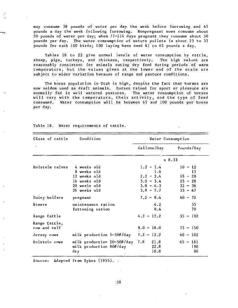
may consume 38 pounds of water per day the week before farrowing and 45 pounds a day the week following farrowing. Nonpregnant sows consume about 20 pounds of water per day; when 77-114 days pregnant they consume about 30 pounds per day. The water consumption of mature pullets is about 25 to 33 pounds for each 100 birds; 100 laying hens need 41 to 62 pounds a day.

Tables 18 to 22 give normal levels of water consumption by cattle, sheep, pigs, turkeys, and chickens, respectively. The . high values are reasonably consistent for animals eating dry feed during periods of warm temperature, but the values given at the lower end of the scale are subject to wider variation because of range and pasture conditions.

The horse population in Utah is high, despite the fact that horses are now seldom used as draft animals. Horses raised for sport or pleasure are normally fed in well watered pastures. The water consuinptiol1 of horses will vary with the temperature, their activity, and the type of feed consumed. Water consumption will be between 65 and 100 pounds per horse per day.

Table 18. Water requirements of cattle.

Class of cattle

Holstein calves

Dairy heifers

Steers

Range Cattle

Range Cattle, cow and calf

Jersey cows

Holstein cows

Condition

4 weeks old 8 weeks old

12 weeks old 16 weeks old 20 weels old 26 weeks old

pregnant

maintenance ration fattening ration

milk production 5-30#/day

milk production 20-S0fF/day milk production 80fF/day dry

Source: Adapted from Sykes (1955).

38

Water Consumption

Gallons/Day Pounds/Day

x 8.33

1.2- 1.4 10 - 12 1.6 13

2.2 - 2.4 18 - 20 3.0 - 3.4 25 - 28 3.8 - 4.3 32 - 36 3.9 - 5.7 33 - 47

7.2 - 8.4 60 - 70

4.2 35 8.4 70

4.2 - 12.2 35 - 102

9.0 - 18.0 75 - 150

7.2 - 12.2 60 - 102

7.8 21.8 65 - 181 22.8 190 10.8 90

Table 19. Water requirements of sheep.

Condition Water consumption

gallons per day pounds per day

On range or dry pasture 0.6 - 1.6 5 - 13

On range (salty feeds) 2.0 17

On ratl.ons of hay and grain, roots and grain 0.14 - 0.7 1.2 - 6

On good pasture Very little if any

Source: Adapted from Sykes (1955).

Table 20. Water requirements of pLgS.

Condition Water consumption

gallons per day pounds per day

Body weight 30 pounds 0.6 - 1.2 5 - 10

Body weight 60 - SO pounds O.S 7

Body weight 75 - 125 pounds 1.9 16

Body weight 200 - 3S0 pounds 1.4 - 3.6 12 - 30

Pregnant sows 3.6 - 4.5 30 - 37

Lactating sows 4.S - 6.0 40 - 50

Source: Adapted from Sykes (1955).

39

Table 21. Water requirements of turkeys.

Conditions

1 - 3 weeks old

4 - 7 weeks old

9-13 weeks old

15-19 weeks old

21-26 weeks old

Source: Adapted from Sykes (1955).

Table 22. Water requirements of chickens.

Condition

1-3 week old

3-6 weeks old

6-10 weeks old

9 - 13 weeks old

Pullets

Nonlaying hens

Laying hens, moderate temperature

Laying hens, temperature 90°F

Source: Adapted from Sykes (1955).

40

Water consumption gallons per 100 birds per day

1.1 - 2.6

3.7 - 8.4

8.8 - 14.3

16.7 16.9

13.6 - 15.0

Water consumption gallons per 100 birds per day

0.4 - 2.0

1.4 - 3.0

3.0 - 4.0

4.0 - 5.0

3.0 - 4.0

5.0

5.0 - 7.5

9.0

MUNICIPAL WATER REQUIREMENTS

General Considerations

Municipalities build water distribution systems for the safety and convenience of those persons who choose to reside in or maintain businesses within the municipal boundaries. The first municipal systems were built primarily for fire protection t but uses today in addition to fire fighting, include drinking water, and water for cooki ng t washing, bathing, flushing toilets, heating, cooling, watering lawns, filling swimming pools in summer and ice skating rinks in winter, street cleaning, car washing, laundries, dairies, fountains, bakeries, food processing plants, manufactories, and industries of various sorts. The total municipal need is the summation of the amounts needed for all uses. No two cities are exactly alike in use structure.

The water that is diverted from the supply source for municipal use is not all "consumed" as it is put to use, and it is difficult to measure how much water is transferred to vapor and how much is discharged through the wastewater faci Ii ty in liquid form. Some studies (Hansen et a1. 1979) indicate that anywhere from 35 to 90 percent of the water diverted is returned in liquid form to the sewer collection system and eventually back into the natural drainage source or river. Although the water returned or sewer effluent is of a lower quality (unless thoroughly treated) and is returned at a different point in the hydrologic system, it can be an important manageable part of the total hydrologic resource.

In considering the water requirements for municipal systems, it is necessary to look at historic uses and then to find techniques of extending that information to predict future needs.

In the period from 1958 to 1962, the State Engineer conducted a study of water uses and needs for municipalities along the Wasatch Front (Criddle et al. 1962). This study assembled information on the then current uses of 63 water agencies in Weber, Davis, and Salt Lake Counties and projected the needs of these agencies to the year 1975. The State Engineer used this study as a guide in processing pending applications to appropriate water for domestic uses.

Since 1960 the Utah Division of Water Rights has been monitoring water suppliers; and, beginning about 1975, other agencies have commis­sioned studies which have contributed to municipal water use information. Some of the results of these studies were published in 1979 by the Utah Water Research Laboratory and the Utah League of Cities and Towns (Hansen et a1. 1979). This study tabulated water use for 50 Utah municipalities for the years 1960 to 1976 and made some projections for the state needs to the year 2020.

Both the 1960 inventory and the more recent 1979 inventory show that when expressing water use on an average per capita daily basis

41

there is a large variability among systems. A bar graph of the average water use during 1974, 1975, and 1976 by 50 Utah municipalities is shown in Figure 4. The quantities vary from 93 to 505 gallons per capita per day. The total annual use figures reported by the municipalities were converted to a gallons per capita per day basis by dividing the total use by the total population and by 365 (the number of days in a year). These figures are reported in Table 23 and summarized by meao, minimum, and maximum values in Table 24. The time period represented is from 1960-1976.

The historic data on municipal water use have little meaning until the reasons for some of the variation among systems can be explained. A glance at the bar graph of Figure 4 will show that five municipalities, Bountiful, Centerville, North Ogden, South Ogden, and Washington Terrace, all have low withdrawal rates, 93-110 gpcd. The common element among these five communities is that all have dual water systems; that is, a separate pressurized water system exists in each to supply the outside or landscaping water needs. The munici pal system supplies essent ially no outside water. The Salt Lake City water system on the other hand supplies essentially 10(') percent of outside use. Its average withdrawal rate is 287 gpcd. Salt Lake City is also the largest system in the state and has a higher popul ation dens ity than the other systems. It also has more multiple unit dwellings, apartments, and condominiums. The high outside use would tend to make the withdrawal rate high while the !popula­tion density and multiple living units would tend to reduce the withdrawal rate. Other factors which affect the average rate of withdrawal are climate, market value of domestic residences, lot sizes, types of industry using municipal water, type of charges, use of meters, and condition of storage and conveyance system (pipe leakage and reservoir spills).

Those cities with high withdrawal rates (over 400 gpcd) are not necessarily the cities that supply 100 percent of their outside demand. The Cities of Delta, Fillmore, Hyrum, Logan, and Morgan all have high withdrawal rates but have different outside use indexes. The high with­drawal rate cannot be explained by price of water either, but may have something to do with population density, special industrial uses, and reservoir spills Or leakage. An example of unusually high unit withdrawal rates is that of the little town of Amalga in Cache Valley. Amalga had in 1979 a population of 210 and an average withdrawal rate per capita of 1682 gallons per day. The explanation is that Amalga I s water system supplies water to a large cheese manufacturing plant and several large dairy herds. About 85 percent of the total supply goes to these uses.

Planners for future water development have considered not only what has been needed in the past, but an apparent increasing per capita withdrawal rate to accommodate the increasing use of water using appliances and the trend toward more bathrooms per household, etc. It now' appears that this increasing rate has leveled off and in the future may actually decrease. As the population density in a city increases and people crowd closer together in multiple living units, i.e., apartments, condominiums, etc., the unit use appears to stabilize. The Salt Lake metropolitan area appears to have a fairly constant per capita withdrawal rate between 250 and 300 gallons per day. The long term stability of unit withdrawal rates for four metropolitan cities can be seen in the graph of Figure 5.

42

AMERICAN FORK BOUNTIFUL

BRIGHAM CITY 21 CEDAR CITY

CENTERVILLE CLEARFIELD

CLINTON DELTA 400

DUCHESNE EPHRAIM 353

FILLMORE 436 G RANGER -HUNTER

GREEN RIVER HEBER CITY 397

HYRUM KAYSVILLE

LAYTON LEHI

LOGAN MANILA

MIDVALE 333 MILFORD 493

MOAB MONTICELLO

MORGAN, 452 MURRAY

NO RTH OGDEN OGDEN OR EM

PLEASANT GROVE 360 PRICE

PROVO 317 RICHFIELD 362

RIVERDALE RIVERTON

ROOSEVELT 390 ROY

SAL T LAKE CITY SANDY

SOUTH JORDAN SOUTH OGDEN

SOUTH SAL T LAKE 293 SPANISH FORK

ST. GEORGE SUNSET TOOELE VERNAL 286

WASHINGTON TERRACE WEST JORDAN 242

WOODS CROSS 232 I

gollo ns /coplto/doy 0 100 200 300 400 500

acre - fee t /coplto/year 0 .1 .2 .3 .4 .5

Figure 4. Daily per capita withdrawal rates for 50 Utah municipal systems: Average of 1974, 1975, and 1976. (Tooele has only 1 year of rec­ord, Duchesne has 2 years of record.)

43

.I , I

Table 23. Estimated daily withdrawal rates per person (gcd) for 50 Utah municipal systems: 1960-1975

Year

County 1960 1961 1962 1963 1964 1965 1966 1967 1968 1969 1970 1971 1972 1973 1974 1975 1976

American Fork 174 166 132 159 169 163 153 164 156 188 170 186 205 180 218 231 231 Bountiful 101 130 85 109 98 107 102 106 106 109 103 110 106 113 115 106 106 Brigham City 547 408 603 577 652 750 740 365 397 421 39l 370 340 358 410 355 198 Cedar City 195 191 222 211 226 218 257 230 243 233 230 235 235 235 235 235 235 Centerville 133 123 109 98 86 137 127 125 95 89 9l 97 Clearfield 187 159 203 167 162 143 175 151 145 140 138 143 148 143 215 176 216 Clinton 78 99 102 111 131 97 157 131 135 157 133 143 160 147 146 128 128 Delta 328 328 210 340 488 484 509 548 552 560 559. 534 425 481 465 493 245 Duchesne 274 256 Ephraim 219 335 394 3'80 325 352 Fillmore 281 287 391 409 411 400 461 439 435 452 451 439 446 293 453 437 417 Granger-Hunter 110 112 119 120 126 118 158 149 149 156 154 173 174 159 165 154 156 Green River 114 109 103 49 143 124 167 167 194 284 294 208 216 215 220 226 228 Heber City 387 39l 388 383 410 435 425 428 462 Hyrum 471 451 497 518 595 594 596 580 532 492 513 486 463 432 Kaysville 234 203 198 171 194 178 181 Layton 175 171 171 183 187 169 205 170 173 195 173 178 247 204 202 164 189 Lehi 415 329 353 274 323 238 330 305 285 305 284 253 221 .203 182 176 140 Logan 432 405 442 469 403 425 447 413 428 420 491 494 506 518 509 494 512 Manila 370 339 218 274 246 244

-I> Midvale 202 260 259 268 266 264 273 276 277 330 331 333 334 -I> Milford 395 438 456 435 446 519 513

Moab 129 131 141 164 189 171 200 200 200 205 211 228 258 233 261 222 237 Monticello 371 307 325 371 355 339 357 179 308 299 292 Morgan 324 338 340 339 337 300 329 319 335 332 337 374 386 390 431 460 464 Murray 176 174 188 195 202 190 222 224 209 229 212 205 221 233 265 282 360 North Ogden 242 231 208 166 159 156 148 142 106 114 111 99 105 104 121 Ogden 240 223 236 243 231 243 272 274 266 269 279 250 266 267 258 244 255 Orem 215 237 241 241 241 255 293 276 271 304 289 300 317 296 325 260 277 Pleasant Grove 142 149 147 146 176 138 165 150 137 179 212 285 316 321 331 363 387 Price 180 238 269 206 228 258 247 226 264 248 264 258 257 Provo 301 357 305 285 280 294 315 298 285 290 275 279 315 298 305 280 288 Richfield 312 325 317 279 302 291 343 330 322 328 340 400 388 383 376 360 349 Riverdale 174 173 205 226 227 214 220 169 187 184 184 207 194 195 Riverton 203 200 271 244 116 Roosevelt 369 349 312 350 417 400 504 559 474 519 485 428 435 521 426 390 355 Roy 176 185 180 176 182 184 271 210 216 245 219 216 249 222 260 214 224 St. George 224 220 217 197 242 226 246 Salt Lake City 259 255 255 238 246 217 280 246 236 287 255 298 304 265 312 274 275 Sandy 320 217 235 South Jordan 99 96 102 105 114 100 127 127 121 133 111 154 150 151 163 195 191 South Ogden 84 79 89 77 86 88 96 78 86 87 86 98 111 109 108 107 110 South Salt Lake 219 243 248 244 269 266 250 286 293 289 293 297 Spanish Fork 216 337 295 245 236 218 249 226 217 241 258 263 221 229 198 212 250 Sunset 160 148 160 161 165 156 184 166 166 199 174 191 199 176 201 168 176 Tooele 208 Vernal 371 287 289 329 400 425 364 362 342 351 349 313 238 Washington Terrace 82 106 77 73 84 81 88 84 9l 93 100 96 101 91 102 96 104 West Jordan 158 263 260 296 260 228 238 Woods Cross 176 177 199 175 163 168 158 162 152 164 191 223 265 196 235

Table 24. Per capita withdrawal rate (gcd) statistics for 50 Utah munici-palities: 1960-1976.

Statistics

Years of Municipality Data Mean Deviation Minimum Maximum

American Fork 17 179 27.8 132 231 Bountiful 17 107 8.9 85 130 Brigham City 9 361 62.7 198 421 Cedar City 11 223 19.3 191 257 Centerville 12 109 18.7 86 133 Clearfield 17 165 27.0 138 216. Clinton 17 128 23.7 78 160 Delta 17 450 108.8 210 560 Duchesne 2 265 Ephraim 6 334 62.2 219 394 Fillmore 17 406 60.2 281 461 Granger-Hunter 17 144 12.5 110 174 Green River 13 206 49.1 124 294 Heber 9 412 27.3 387 462 Hyrum 14 516 56.2 432 596 Kaysville 7 194 21.0 171 234 Layton 17 186 20.6 169 247 Lehi 17 272 71. 7 140 415 Logan 17 459 41.5 403 519 Manila 6 282 59.8 218 370 Midvale 13 283 39.1 202 334 Milford 7 457 44.3 395 519 Moab 17 199 40.7 129 261 Monticello 11 318 54.4 179 371 Morgan 17 361 49.3 300 464 Murray 17 223 45.4 174 360 North Ogti~n 15 147 47.1 99 242 Ogden 17 254 16.6 223 279 Orem 17 273 31. 4 215 325 Pleasant Grove 17 220 (' 90.6 138 387 Price City 13 242 26.0 180 269 Provo 17 302 20.6 275 357 Richfield 17 338 34.6 279 400 Riverdale 14 197 19.7 169 227 Riverton 5 207 58.8 116 271 Roosevelt 17 429 71. 7 312 559 Roy 17 213 30.7 176 271 Salt Lake City 17 265 25.8 217 312 Sandy 3 257 South Jordan 17 132 31. 2 96 195 South Ogden 17 93 12.0 77 111 South Salt Lake 12 266 25.5 219 297 Spanish Fork 17 241 33.5 198 337 St. George 7 225 16.4 197 246 Sunset 17 174 16.2 148 201 Tooele 1 208 Vernal 13 336 53.0 226 429 Washington Terrace 17 91 9.9 73 106 West Jordan 7 245 40.1 168 296 Woods Cross 15 187 32.1 152 265

45

-0 u (!) -w .-« a:: -I

~ « 0\

~ a::: 0 I .--;:

400 rl----------------~----------------~----------------~------------------~

350

300

Salt Lake Ci ty - - -

Ogden ----

Provo

Bountiful _ .. --

/~,_ -. "'- /~ . I'" 250

'- ., _. ,... lJ " I \ ._.~"' /i ' _.-1.-." -"" "I \ ._.-><;'._ 1 ,_ I ,I '. ,.-_.'>.1 " ,I _I ,........_-. .............. .-. .-

200

150

100

50

.. , / .. .. ,

o 1960

. -" .. -\

/. -....- .. __ .-.. _ .. _ .. _- _ .. - _ .. - .. -... .. ,. ._.. .._.. ..-..

1964 1968 1972

TIM E

Figure 5. Daily per capita withdrawal rates (gcd) for Bountiful, Ogden, Provo, and Salt Lake City: 1960-1976.

1976

J "' I

The 1979 study on municipal uses in Utah did not attempt to project future needs of each water supplier. It did make the following conclusions:

(1) A good estimate of the .municipal withdrawal rate for indoor use only is 100 gpcd.

(2) For short term planning, 262 gpcd 1S a good estimation of Utah's average per capita water needs (statewide).

(3) For long term planning, 262 gpcd is excessive. water usage in the future will decline for three reasons:

(a) Water will become increasingly expensive. (b) Leakage will be controlled.

Per capita

(c) As Utahns move closer together, they will require less water on a per capita basis for outdoor use.

Design of Municipal Systems

The design parameters for new domestic water systems, subdivisions, and small rural domestic systems include:

(1) Average annual use, which is used to de fine the total amount of water needed at the source of supply, and is a measure of the water right appropriated.

(2) Instantaneous peak demand/fire flow, which 1S used to S1ze the main supply pipelines.

(3) Peak daily flow, which is used to size the treatment plant, well pumps and equalizing reservoirs.

(4) Peak monthly flow, which is used to size the raw water reservoir or determine the amount of new water acquisitions needed.

Average annual use

As previously noted, when comparing one system with another, the average annual use from a domestic water system is variable. This is not cause for concern because usually the variations can be explained by the particular demands placed upon each system. Industrial uses peculiar to one system, variation in outside demands, and the cost of water to the users which reduces use for outside purposes are all reasons for dif­ferences. There must, however, be some basis to estimate average annual use for the design of new systems.

Average annual use is not a critical parameter for system design, but it does indicate the total amount of water needed at the source

47

of supply, and is a measure of the water righ t appropriated. Beginning with the most elementary system, a single family domestic household, the Utah adjudication procedure has allowed 650 gallons per day. As a system increases to include many households and multiple dwelling units, such as apartments and condominiums, and as business uses are connected to the sys tem, the average use per connect ion increases. For rural and small urban systems, the Utah State Department of Health recommends a design standard of 800 gallons per day. (Many large community systems exceed this. The Utah average use would be about 950 gallons per con­nection. )

Table 25 gives recommended design amounts for varying system demands~

Peak demands

A municipal water system must be able to conduct peak flows as well as provide the total seasonal quantity of water needed. Peak rates of flow information is important to the planning and design of systems because each type of peak determines either the size of the water right, the size of the pipe system, the size of the treatment plant, or the raw water storage facilities, along with capital and operating costs associated with each. The primary costs affected are summarized in Table 26.

Main line pipes are designed to handle instantaneous peak demands or fire flows, whichever is greater. Water treatment plants are designed to meet peak day demands. Storage reservo which deliver raw water to treatment plants are sized to provide seasonal or monthly peak demands.

Unfortunately, peak demand values are seldom measured by water utilities. The only generally available figure is the average daily demand (total annual use divided by 365 days). For distribution system design, peak day, peak month, and instantaneous peak demands are usually estimated by applying mUltipliers to the flow rate of average daily demand. The multipliers suggested by water supply textbooks usually give a range of values. For example, Clark and Viessman (1966) suggest a peak-day flow of 120 to 400 percent of average daily and an instantaneous peak flow of 150 to 1200 percent of average. These ranges are too great for design. The State Engineer in the past has used 220 percent of average daily flow as being a reasonab Ie figure for peak daily flows. A more recent study (Hughes and Gross 1979) has derived the relationships for Utah systems reported below.

Instantaneous peak demand

Instantaneous demands are used to size main distribution lines and in-line booster pumps. Fire flows govern pipe sizes in distribution systems in central business districts and in residential areas where the pipe capacity is less than about 500 gpm (about 250 connections). One

48

Table 25. Average annual domestic water demand for design purposes.

Design conditions

Urban systems with no outside use

Recreation homes occupied 1n summer season only

Single domestic residence

Rural or small urban communities

Average demand gallons/person/

day

100

165

180

220

Average demand gallons/connection/

day

365

600

650

800

Table 26. Effects on municipal water system cost of different durations of flow peak.

Peak Flow Costs Which are Primarly Effected Period Capital Investment Operating

Monthly

Daily

Instantaneous

Raw Water Reservoir, Water Stock or Right Purchases

Treatment Plant, Well Pumps, Transmission Conduits, Equalizing Reservoirs

Distribution Mains (within ranges where fire flow does not govern), Service Lines, In-Line Booster Pumps

49

Monthly well, booster and treatment plant pumping costs, annual water purchase charges

Electrical demand charges for pumps Treatment plant start­up costs

Booster Pumps

reason for providing for high ins tant aneous flow rates in the des ign of distribution systems is to reduce the possibility of low or negative line pressures resulting from high demand and low capacity. Negative pres­sures may cause contamination of the water supply if, for example, a hose end were lying in a puddle or if a leak in the pipeline were below the water table.

Instantaneous peak flow rates per connection decline, but at a decreasing rate, with a larger number of connections in a system. After 1000 connections the decline is so small as to be negligible, and a constant unit value of instantaneous flow can be used for design pur­poses. The shape of the curve used to represent flow rate per connection from 1 to 1000 connect ions has been somewhat arbitrary because measured flows were scarce. Recent studies by the Farmers Home Administration using data from Ohio (FmHA 1976) and by Hughes and Gross (1979) using Utah data have produced the curves shown in Figure 6. Recommendations for using the curves are:

1. The Utah demand curve (Figure 6) is recommended for low dens ity rural systems where project cost is a critical issue and where no unusual characteristic (large landscaped lots, nonresidential use, or large leaks) would create higher peaks.

2. For systems where some factor suggests the possibility of high short term peaks or where pipe cost is less critical, a higher factor of safety could be achieved by using the FmHA average standard. For example, if the system serves a high value district with large landscaped lots, the FmHA average standard would be more suitable than the Utah demand funct ion which was derived from systems wh ich were in low to middle value districts. Also, if the size of the lawns to be irrigated is large or if a large percent of the households is to be unmetered, then the FmHA average standard should be used.

Peak day demand

The capacities of water supply facilities such as treatment plants, pump motors, equalizing reservoirs, etc., are determined by average de­mand during the peak 24-hour period. This peak day demand is often determined by applying a multiplier to the average daily use. The State Engineer has used 2.20 as being a reasonable multiplier. Hughes and Gross measured the flows in several Utah systems and developed regression equations to more closely approximate the relationship between average and peak demand. The correlations were very good (R2 of 0.953 and 0.938, respect ively). The equations for peak day demand as a function of average demand are given:

Dpd/c = 600 or 84 (Davg/ c ) - 207 whichever is greater. • (11)

and

Dpd/p = 165 or 2.5 (Davg/ p ) - 49 whichever is greater. . (12)

50

-c: 0 - 15 u OJ c: c: 10 0 9 u

...... 8 e 7 Cl. 6 CI

5 IJJ I- 4

VI <t "'"' 0:: :3

~ 2.5 ..J 2 LL

:lI':: 1.5 <t IJJ a..

I I 1 I I I I I I

I I I

~ I I 1 I I

D = 1268 + I. 80 C t-

,"' r-, D= Utah Intantaneous Peak Demand f-

~' ... -"- ...... C= Number of Connections r-r--..... ....

"" i'" .... ~ ~ i' -- !- ...

I I

"'" - to- :mHA A~E~AGE STANDARD ............... ---r-- . -"'--+-1-.........

UTAH DEMAND r- -

I I I I I r

2 3 4 5 678910 15 20 30 405060 100 500

NUMBER OF CONNECTIONS

Figure 6. Peak instantaneous demands within municipal water systems in Utah: Utah demand function and Farmers Home Administration aver­age standard.

.I

1000

in which

Dpd/c :::: Davg/c= Davg/p=

peak day demand in gallons per connection average demand in thousand gal per mon~n average demand in gallons per person per (fay

I

;'

/ /

per connection

These equations are plotted in Figure 7 and Figure 8. Both curves show minimum values to be used in situations with small average demand.

It has long been known that outside use (principally yard irrigation) is a very important factor in summer water use and that this component of demand varies greatly among Utah systems. Some areas have supplemental pressure pipelines or ditch systems from which all or part of the outside demand is supplied. Landscaping varies greatly between rural and urban and be tween old and new res ident ial areas. St ill another factor is climatic variation between Utah's Dixie and the higher and wetter northern valleys.

A single, easy to use index which accounts for many factors which collectively determine outside demand from a municipal-domestic system is shown in Table 27. It associates an integer between 1 and 9 with each of nine outdoor use category descriptions. These descriptions, although somewhat subjective, are reproducible ,and provide a reasonably easy means for defining the index number. The index number 1 is used for a system which provides no outside water (such ,as Bountiful City), and the index number increases as outside irrigation increases up to a maximum of 9 which represents a city in which all of the outside demand is furnished by the municipal system and from which relatively large land­scaped areas are irrigated in a hot-dry Utah climate (such as Monticello).

If the average daily demand for the system to be designed is not known, the peak day demand can be approximated by using the following equations based on regression analysis on Utah data, which relate peak day demand to the outdoor use index:

Dpd/c = 600 or 345 (I) - 82 whichever 1S greater . (13)

where peak day demand is in gallons per connection.

Dpd/p = 165 or 92.5 (I) - 21 whichever is greater . (14)

where peak day demand is in gallons per person and (I) is the outdoor use index. These equations are plotted in Figure 9 and Figure 10.

52

VI w

3000 ~

c 0 -(.) CD 2500 c: c: 0 (.)

...... III

~ 2000 0"\

t};

1:11 V'"

CI J 0 1500 ~~ Z e(

tOr>.

:::E -:.

l&.I \V

0 1000 ~~~ >-e( 0 600 min. ~ e( 500 l&.I a.

o o 5 10 15 20 25

AVERAGE DEMAND

(t housand gallons /month/connection)

Figure 7. Peak day demand per connection as a function of average demand.

30

.J

700

600

c: 0 III .. CD

'JA,O!J Q.

...... 500 ~' III c: ~ .2

1:11 ~ .2 400 '0<::> 0 1'1,,' z ", e(

:::E \'< l&.I 300 0 <::> ~ <::> >-e( 0 ~ e( 200 l&.I 165 min. a. .. a. ...... 0 100 a.

0

0 0 50 100 ISO 200 250 300

DAVG /P

: AVERAGE DEMAND

(gallons/person/day)

Figure 8. Peak day de~and per person as a function of average demand.

Table 27. Outdoor use index (I).

Index (1)

Categories Indicating Extent of Outdoor Demand From Domestic System

1. No outdoor use from domestic system--everyone has connection to pressurized dual system.

2. Almost no irrigation from domestic system--supplementary system is available which services at least 85% of outside demand.

3. Supplementary ditch system is available and landscaped areas are small (average less than 1500 square feet).

4. No supplementary system is available but landscaped areas are small (average less than 1500 square feet).

5. Ditch system available for gardens but lawns (over 60%) are irri­gated from domestic system.

6. Ditch or piped system available to some customers but most outside irrigation (over 75%) is from domestic system.

7. All outside areas are irrigated from domestic system--moderate amount of landscaping, average Utah climate.

8. Large amount of landscaping and all irrigated from domestic system-­average Utah climate.

9. Large amount of landscaping and all irrigated from domestic system-­hot and dry Utah climate.

Peak month demand

Sustained periods of high demand are important in determining storage capacity or required sustained yield from wells. Peak month demand can be estimated from the following equations:

Dpm/c = 12 or 2.96 (Davg/ c ) - 15 whichever is greater (IS)

l.n which

Dpm/c Davg/ c

peak demand month in thousand gallons per connection = average demand in thousand gallons per month per connection

54

3000

-c 0 -u

2500 Q) c c 0 u

" \I) c 2000 0

0 at -0 Z 1500 <[

:E I.LI 0

>- 1000 <[ 0

~ <[ I.LI a. 500

o 2 3 4 5 6 7 8 9

OUTDOOR USE INDEX (1)

Figure 9. Peak day demand per connection as a function of outdoor use index.

700

c 0 til .. 600 Q) 0.

" \I) c 0 500 0 at -0 400 Z <[

:E I.LI 0 300 >-<[ 0

~ 200 <[ 165 I.LI Q..

100

o 2 3 4 5 6 7 8 9

OUTDOOR USE INDEX (I) Figure 10. Peak day demand per person as a function of outdoor use index.

55

or

Dpm/p = 125 or 2.92 (Davg/ p) - 130 whichever is greater.

in which

peak month demand in gallons per person per day = average demand in gallons per person per day

These equations are plotted in Figures 11 and 12.

Computing Demands - An Example

(16)

Using the Hughes and Gross (1979) explj'ession for peak day demand as a function of average demand, and solving for average demand, the expressions are:

D + 207 D = Ed/c

avg/c 84 (17)

and

D + 49 D = Ed/E avg/p 2.5

(18)

As input to these equations, the peak day demand is estimated using Equations 13 and 14 and the appropriate outdoor use index. As an example of how these equations can be used to estimate design flows for community water systems, consider a community water system to accommodate 450 connections and a population of about 1700 persons. There is to be no supplementary outside water and landscaped areas are less than 1500 square feet per connection (outside use index = 4, Table 27). Find: 1) the instantaneous flow rate for main line pipe design; 2) peak day demand; 3) average demand and total water supply needed; and 4) peak month demand. Solving for these four flows:

(1) The instantaneous peak flow rate can be determined from Figure 6 using the Utah standard expressed by equation. The calculated value is

D.. = 12.68 450 + 1.80 = 1.83 GPM per connection J.nst

Total flow is:

450 connections x 1.83 = 823 GPM

In a low valued, small lot res ident ial area or in a recreational development this design flow may be used, otherwise use the FmHA curve on Figure 6 to read 2 GPM per connection or 900 GPM for main line capacity.

56

VI -....J

90

c: 80 0 -u CIl c: c: 70 0 U

........ 1/1 c: 0

60 c c>

'1:1 c:

'" 1/1 50 :::I 0

.I:. .... ...... 0 Z 40 « :::!E U.I 0

::E: 30 ... Z 0 :::!E ~ 20 « U.I "-

10

0 0 10 20 30 40 50 60

DAVG/C:: AVERAGE MONTHLY DEMAND

(thousand gallons 1 monthl connection)

Figure 11. Peak month demand per connection as a function of average demand.

...... >. C

~ c: 0 1/1 ... 41 Q.

........ 1/1 c: 0

c c>

0 Z « :::!E U.I 0 ::E: ... Z 0 :::!E ~ « U.I "-

800

700

600

500

400

300

200

b 125 min.

100

0 0 50

~ ~ftJ

Q'f('

o"C11 ClIO

100 150 200 250 300 350

DAVG/P AVERAGE DEMAND

(gallons 1 day 1 person)

Figure 12. Peak month demand per person as a function of average demand.

.I

(2) The peak diiY demand can be es timated from Equations 13 and 14 or from the graphs in Figures 9 and 10.

Dpd/c = 345(1) - 82

= 345(4) 82 = 1298 gallons per connection per day

Dpd/p = 92.5(1) - 21

92.5(4) - 21 349 gallons per person per day

(3) Average demand can be computed from Equations 17 or 18.

D avg/c

D avg/p

D d/ + 207 p c 84

1298 + 207 84

~+49 2.5

17,900 gallons/month/connection

= 159 gallons per day/person

Total annual water supply needed:

gallons per month x 12 x No. of connections =

17,900 x 12 x 450 = 96.66 million gallons/year

(4) Peak month demands can be estimated from Equations 15 and 16 or from graphs in Figure 11 and Figure 12.

Dpm/c 2.96 15 x Davg/c

= 2.96 - 15 (17 .9) = 38,000 gallons/connection

Dpm/p = 2.92 130 Davg/p

= 2.92 130 (159) = 334 gallons/person per day

The above computations are summarized in Table 28.

58

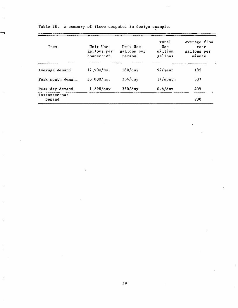
Table 28. A summary of flows computed in design example. I

-

Total Average flow Item Unit Use Unit Use Use rate

gallons per gallons per mi llion gallons per connection person gallons minute

Average demand 17)900/mo. 160/day 97/year 185

Peak month demand 38)000/mo. 334/day 17/month 387

Peak day demand 1)298/day 350/day 0.6/day 405 Instantaneous

Demand 900

59

INDUSTRIAL WATER REQUIREMENTS

Water has economic value because of its physical properties. It I s what water does when used as a secondary medium in causing or allowing changes or processes to occur that makes it a valuable resource. The weight and fluid motion of water can cause a turbine to turn and elec­tricity to be generated. Heating water with coal, oil, or nuclear energy can transform liquid to vapor and the expanding vapor can be harnessed for many kinds of useful work. The thermal properties of water can be used in manufacturing processes such as quenching heated metals to temper them, or storing or transporting heat to warm, cool, or maintain temperatures necessary in certain processes. As a fluid of given density, water can be used to separate metals, from the panning of gold to the flotation of copper. Water can be used to control dust, assure soil compaction, wash foods and transport solids; and because energy is absorbed to cause evapo­ration, water can be used as a cooling agent.

Industrial water uses are process and site specific, and therefore it is difficult to make general assessments of water required for industry. Also, few measurements are available as to how much water is used or where the water is needed and for what purpose. It is also difficult to normalize industrial use in units that are meaningful when extrapolating to other conditions. Water consumed per employee per day or water con­sumed per pound of product are not valid methods of comparison where the bulk of the water is used in a process unrelated to .number of employees or to pound of product finished. .

To obtain the relative magnitudes of industrial water use in Utah, a survey was made covering the years 1974, 1975, and 1976. It was deter­mined that industrial uses can be grouped into five major categories:

(1) energy conversion, including

(a) hydroelectric (b) steam-electric (c) oil extraction from tar sand and shales (d) geothermal (e) coal extraction (f) oil extraction, oil wells (g) natural gas extraction (h) uranium extraction (i) coal gasification (j) coal liquefaction (k) refineries, petroleum

(2) primary metals

(a) copper (b) steel

61

(3) inorganic chemicals

(4) hydraulic cement

(5) food products

A listing of some energy conversion related actlvltles with estimates of the water required is given in Table 29. New technologies and new processes could alter these estimates.

Within each of the above categories water serves at least three major functions: 1) water needed in the manufacture of a product, 2) water needed as a cooling agent, and 3) water needed for sanitary purposes including the needs of workers in the plant. The survey tabulated the percent of water used in each of these three funct ions for several dif­ferent industries. These values are shown on Table 30. The table also indicates the percentage of water returned to streams.

An attempt was made to norma lize the water requirements of various industries by computing the water used per employee per day ged Table 30. These values are shown but should be recognized as approximations as industrial use is not necessarily proportional to the number of employee days. The magnitude of the values do, however. have some comparative consistency as can be seen from similarities among plants of a given type. Average water use for selected industries is plotted in Figure 13.· Wate.r for the generation of electric energy has been omitted in these comparisons.

Perhaps the greatest industrial use of water in Utah is for energy conversion. There are several ways in which water can be used. The greatest volume of water is probably used in hydrogeneration of elec­tricity. This is a nonconsumptive use of water, and 100 percent of the flow is returned to the resource stream. Mos t Utah streams are sma 11 with steep gradients, so power generation usually entails the diversion from and drying up of a portion of the natural stream.

Steam-generation of electricity diverts less water than does hydro­generation. The difference is that the water converted to steam is not returned to the stream, but, after many condensation and recirculation cycles, eventually exits as vapor. A major use of water in steam genera­tion is that used to cool and condense the steam for recirculation. The volume of water needed for this use is dependent upon whether an open or closed cooling system is used. Open systems are once-through type where large volumes of cold water are circulated through the condenser and returned to the natural stream. The closed system returns the heated water to a cooling tower or pond, from which it. is later withdrawn and reused. As the water is reused, the dissolved solids become concentrated and eventually the water has to be replaced with fresh water. New tech­nology is making available systems which can use water of extremely high salt concentration, and hence less total volume of water consumed.

62

Water is also used in developing fossil fuel resources. t ion of mineral fuels such as coal anQ. oil requires water refining of oil into combustible fuels. Amounts depend used and the care exercised in water management. Newer to produce fuels from coal gasification or coal liquefaction crude from tar sands and oil shales will also require water.

The ext rac-as does the

on processes technologies or to extract

Table 29. Water use rates for energy conversion industries.

Energy System

Steam-electric nuclear Evaporative cooling Pond River Wet-dry radiator

Steam-electric coal Evaporative cooling Pond River Dry radiator

Geothermal

Refineries

Oil Shale

Coal gasification

Coal liquefaction

Coal extraction

oi 1 ext ract ion

Natural gas extraction

Uranium extraction

Water Needs

17,000 acre-ft/yr/lOOO m W unit 12,000 acre-ft/yr/1000 m W unit 4,000 acre-ft/yr/1000 m W unit 2,000 acre-ft/yr/lOOO m W unit

15,000 acre-ft/yr/1000 mW unit 10,000 acre/ft/yr/lOOO mW unit 3,600 acre-ft/yr/1000 mW unit 2,000 acre-ft/yr/lOOO mW unit

48,000 acre-ft/yr/lOOO mW unit

39 gal/bb1 crude

7,600 to 18,900 acre-ft/yr/lOO,OOO barrels per day plant

10,000 to 45,000 acre-ft/yr/250 million scf per day plant

20,000 to 130,000 acre-ft/yr/100,000 barrels per day plant

> 20.9 gallons/ton

> 171 ga110ns/barrel1

~ 2.9 mg/bcf

> O. 184 mg/ t on

Source: The Aerospace Corporation, 1978 Western States Council, 1974

63

.I

Table 30. Utah industrial water withdrawal rates (ged) for major water using industries: average of 1974, 1975, and 1976.

% of Withdrawal Rate Withdrawal Return Rate Flow

Product Employee (% of * Manufacture Cooling Sanitation Other ged withdrawal)

Meat Packing 1 79 17 3 1 453 80 2 95 4 1 0 1484 N.A.a

Poultry Processing 1 70 25 5 0 1194 100 Cheese 1 97 2 1 0 2486 98

2 69 20 1 10 288 90 Ice Cream 1 N.A. N.A. N.A. N.A. 507 N.A.

2 N.A. N.A. N.A. N.A. 322 N.A. Fluid Milk 1 N.A. N .A. N.A. N.A. 873 N.A.

0\ Canned Vegetables 1 N.A. N.A. N.A. N.A. 4851 N.A. .p- Flour 1 85 10 5 0 639 50

Bread 1 80 10 10 0 633 70 Candy 1 N.A. N.A. N.A. N.A. 578 N.A.

2 N.A. N.A. N.A. N.A. 312 N.A. Soft Drinks 1 N.A. N.A. N.A. N.A. 278 N.A. Inorganic Chemicals 1 82 15 1 2 8908 15 Petroleum Refining 1 33 65 Tb T 11760 N.A.

2 30 67 3 0 7860 N.A. 3 45 55 T 0 11738 N.A.

Hydraulic Cement 1 97 T 3 0 3260 3 2 95 0 T 5 3668 2

Steel Works 1 33 56 6 5 5109 10 Copper Sme It ing 1 92 6 1 1 67231 N.A.

aNot available. bLess than one percent. *Plant number where different plants were surveyed in the same industry.

0\ V1

COPPER SMELTING

OIL REFINING

INORGANIC CHEMICALS

STEEL WORKS

HYDRAULIC CEMENT

FOODS PRODUCTS

Gallons/Employee/Day

11,100

............... 8,900

5,100

_3)500

.900

67,200

1-II 1- ,- r r f I - ,_. I

o 4)000 8,000 12,000 16,000 20)000 24,000

Figure 13. Normalized water use rates for Utah's major water using indus­tries. (Hydro and steam electric generation excluded.)

,~

RECREATIONAL WATER REQUIREMENTS

Water requirements for recreational· purposes are treated differently than water requirements for agri<;ultural, municipal, or industrial pur­poses because the benefit comes not by diverting the water from the stream, but by keeping and preserving it in its natural course and setting. Water has value for recreational uses because it is there, because it has certain flow characteristics favoring the biologic environment, because it has the necessary geometry (surface area, depth, width, etc.), and because it has the proper quality (temperature, clarity, taste, odor, etc.).

Unlike other water users, the recreationist does not extract or withdraw water from the source, except for drinking on site and for sanitary purposes. (This small amount of withdrawn water is in reality a domestic use in a recreational area.) To the recreationist this water has value because it is not diverted, but left in the stream, and it is the recreationist· that is mobile .and can move to the site of choice for a specific type of activity.

Many recreational activities on streams and lakes {reservoirs} have been created or enhanced by water deve lopment for other purposes. Dams have created numerous reservoirs in Utah which attract many recreational visitors, and the water regulation provided by the reservoir has often enhanced fishing in the stream below because of decreased variability in flow. Some opportunities for river and stream recreation have been lost, however, because of changes in flow regimen· and temperature which have diminished the habitat suitability for fish. As life styles change and as public preference for outdoor recreation increases, the future may see legislative changes in the law which favor in-stream uses. The dependence of society upon agriculture and· energy may, however, dictate which direc­tion water use goes.

Types of Water Related Recreation Activities

Water related recreational activities can be grouped as follows:

(I)

(2)

Proximity uses: summer homes.

sightseeing, nature study, picnicking, camping,

Fishing, both flowing water and ponded water fishing employing such means as: wading, canoeing, low-power boating, and bank fishing.

(3) Personal water contact: includes swimming, wading, tubing, water skiing, and scuba diving.

(4) Tranquil water boating, both rivers and lakes, includes canoeing, rowing, sailing, low-power boats, and high-power boats.

67

(5) Nontranquil water boating, includes rafts, drift boats, canoes, and kayaks.

(6) Waterfowl hunting, relegated mostly to. marshlands which support migratory birds such as ducks and geese.

Most of the activities enumerated above depen~ upon the geometry of the water source and the dynamics of the system, that is whether the water is still as in ponded surfaces or moving as in flowing rivers. When moving the velocity also has importance in determining a recreational use.

A subjective evaluation as to whether a specific activity is good, fair, or poor is based on the area required for the sport. Some of these activities are given in Table 31. Swimming and canoe-fishing on flowing streams are dependent upon stream velocity and water depth. High velo­cities and shallow depths preclude the use of streams for these activities. The probability of using streams for swimming and canoe-fishing increase as the depth increase and velocity decreases as shown in Figure 14.

Evaluating Changes in Recreation Opportunities

Where· water 1S preserved in the natural streams for recreational purposes other legitimate uses which depend on regulation and diversion of natural flow must be sacrificed. Since water allocated to a specific use may preclude other uses, there is always a tradeoff in determining the most beneficial use. Striking a balance which most fully serves the identified objectives' of a dynamic society with respect to in-stream and off-stream water uses is difficult because the value of recreational water use is so difficult to quantify.

Fishing is an important recreational sport in Utah but determining the amount of water needed to support fisheries is difficult. The ideal water-site combination of quantity, velocity, depth, temperature and accessibility to create the best habitat for fish is seldom obtainable under natural conditions and is most often too costly to provide by creating conditions. Because economic uses of water for agriculture and industry take precedence in the public interest, fishing as a sport must be a shared use and exist where it can best be included in. project plans. Ponded water fishing, which in some respects is more productive than flowing water fishing, is created when reservoirs are built, and flowing water fishing is 'often enhanced when dams are operated to reduce the variability of flow below the dam. Some developments do, however, destroy fisheries and "cost" to the fishing must be evaluated in terms of lost public recreation. Sometimes concessions can be made to. maintain in-stream flows to. support fisheries and still support traditional water uses. The problem is not to be able to determine the water requirements for ideal fish habitat but to evaluate the conditions which will exist before and after a contemplated change' and to assess the relative costs to the fishery. If these costs are unreasonable, the project should probably be altered or omitted.

68

Table 31. Outdoor water recreational areas rated by amount of water surface area available.

ACTIHTY SURFACE AREA (acres)

*Advanced 4 Swimming 1

.2 *Recreational 4

Swimming 1 .1

Water 520 Skiing 250

150 Pleasure 520

Boating 250 150

Low-power 150 Boating 75

20 Non-power 25

Boating 10 5

Ice 5 Skating .3

.3 Sailing 300

150 20

*Advanced Swimming (depth> 5') generally limited to lakes. Recreation Swimming (depth < 5') limited to rivers, streams, etc.

REMARKS

Good Fair Poor

Good Fair Poor

Good Fair Poor

Good Fair Poor

Good Fair Poor

Good Fair Poor

Good Fair Poor

Good Fair Poor

Fish may be affected by changes in the stream environment during any of four life history stages: egg, fry, juvenile, and adult. Further­more, what might be considered the "ideal" stream flow conditions for one stage of development are quite different for other stages. Other critical activities such as spawning and passage can also be affected. The principal changes in stream environment are alterations in water depth, stream velocity, temperature, and quality (chemical composition).

Changes in stream conditions may cause the loss of certain fish species even though the condition may not reach lethal levels. As both juvenile and adult fish are mobile, they may leave the altered zone or stream condition before the condition becomes lethal. They may move to different zones in the same watercourse or to different streams 1n a connected river system.

69

· 100 100

>-I- 75 75 -(!)

::::!z al-ct:::iE 50 50 al:::iE 0-0::3: a..C/)

(/I. 25 25

0 0 0.5 I 1.5 2 2.5 3 2 3 4 5

VELOCITY IN ft Isec DEPTH IN ft

100 100

>-~ 75 75 1---:::t: ..JC/) aiL&: ct, 50 50 al W 00 O::z a.. ct 25 25 (/1.0

0 0 I 2 3 4 5 6 0.5 I 1.5 2 2.5

VELOCITY IN ft/sec DEPTH IN ft

Figure 14. Probability of recreationists using flowing water for two types of recreation: swimming and canoe-fishing

70

6

3

Evaluating the effect that proposed changes in stream environment will have on fishing or on othe-r related recreational activities has been expedited by_ a methodology developed by the Cooperative Instream Flow Service Group, Fort Collins, Colorado, supported by the U. S. Fish and Wildlife Service, U. S. Department of the Interior. The me thod is too complex to describe in this publication, but is available through con­sultants and the state division of fisheries. The methodology uses a com­puterized river flow simulation model into which specific river measure­ments are inputed, and through the use of probability curves the model predicts the before and after development conditions.

Existing fisheries are classified on the basis of minimum stream flows as a percentage of the average flow. These classifications are shown in Table 32.

Domestic Requirements at Developed Recreational Areas

Developed recreational sites require an adequate supply of water suitable for drinking and cooking and for sanitary disposal systems. The recreation area may be designed to accommodate day use only, such as picnickers and sightseers, or to provide overnight campgrounds, recre­ational vehicle campgrounds, marinas, resort condominiums, or clusters of seasonal or mountain cabins.

For campgrounds and day use sites, suggested use rates are given in Table 33. For sites developed with permanent buildings, Lam and Hughes (1980) measured flows at various types of recreation sites in Utah to determine if municipal design standards were adequate for recreational design. The results indicate that mountain cabins which are only seasonally used and only occupied part time have use rates less than the municipal (Utah Department of Health) standard. In contrast, condominiums which have high occupancy rates because of time sharing or "hotel" renting have higher use rates than municipal standards. Recreation vehicle parks also had higher actual use than existing standards require. The Utah standards for design of recreation areas are given in Table 34 with the suggested changes evidenced by the Lam and Hughes study.

Table 32. Minimum stream flow requirement by fisheries.

Flow % of Avg. Fishery Classification Description

Oct.-Mar. Apr.-Sept.

I Outstanding 40 60 II Excellent 30 50

III Good 20 40 IV Fair 10 30

Poor 10 10

71

Table 33. Guidelines for water requirements of recreational campgrounds 1n Utah.

Type of Establishment

Res ident Occupant: Season use Year round

Camper: No flush toilets or showers provided Flush toilets, but no showers provided Flush toilets and showers provided

Picnicker: No flush toilets provided Flush toilets provided

Swimmer: No bathhouse, flush toilets or showers provided

. Flush toilets in bathhouse, but no showers Flush toilets and showers provided

Picnic and Swim Area Participant: No bathhouse, flush toilets, or showers provided Flush toilets in bathhouse, but no showers Flush toilets and showers provided

Boat Launch Area Participants: No flush toilets provided Flush toilets provided

Source: U.S. Forest Service, Region 2 (Flack 1976)

gal/day/person

75 100

10 40 45

5 10

2 5

10

5 10 15

5 10

Table 34. Design standards for recreational development in the State of Utah.

Type of Source Capacity Source Capacity Storage Capacity Deve lopment (Dept. of Health) (Lam and Hughes) (Dept. of Health)

Summer Home 800 gpd/unit 600 gpd/unit 400 gal/unit (Mountain Cabin)

Condominium 500 gpd/unit 800 gpd/unit 250 gpd/unit

Recreation 100 gpd/vehicle 150 gpd/vehicle 50 gal/vehicle Vehicle Campground space space space

72

REFERENCES

Ayers, Robert S. 1977. Quality of water and irrigation. Journal of the Irrigation and Drainage Division, ASCE, 103(IR2). June.

Ayers, R. S., and D. W. Westcot. 1976. Water quality for agriculture. FAO Irrigation and Drainage Paper No. 29. Rom~.

Bagley, Jay M. 1963. Developing a state water plan, Utah's water re­sources--problems and needs, a challenge. Utah State University and Utah Water and Power Board.

Butcher, Jonn E. 1973. Influence of environmental variat ions on water requirements of sheep. In: Proceedings of Symposium held, June 1973, at Twin" Falls, Idaho, on Water-Animal Relations. Edited by H. F. Mayland. USDA-ARS Snake River Conservation Research Center, Kimberly, Idaho.

Clark, J. W., and W. Viessman. 1966. Water Supply and Pollution Control. International Textbook Company, Library of Congress #65-23807.

Criddle, Wayne D., Karl Harris, and Lyman S. Willardson. tive use and water requirements for Utah. Office of Technical Pub lication No.8, revised. Prepared by Engineer's Office and the Southwest Branch, Soil and tion Research Division, Agricultural Research Service, of Agriculture.

1962. Consump­State Engineer, the Utah State Water Conserva­U.S. Department

Farmers Home Administration, U.S. Department of Agriculture. 1976. Texas Engineering Seminar. Sheraton--Grest Inn, Austin, Texas.

Flack, J. E. 1976. growth areas and Colorado.

Design of water and wastewater systems for rapid resorts. Colorado State University, Fort Collins,

Hansen, Roger D., Herbert H. Fullerton, A. Bruce Bishop, and Trevor C. Hughes. 1979. Historical and projected municipal and industrial water usage in Utah 1960/2020. Water Resources Planning Series UWRL/P-79/02, Utah Water Research Laboratory, Utah State University, Logan, Utah.

Hansen, Vaughn E., Orson W. Israelsen, Glen E. Stringham. tion principles and practices. 4th Edition.

1979. Irriga-

Hughes, Trevor C., and Robert Gross. 1979. Domestic Water Resources Planning Series UWRL/P-79/04, Laboratory, Utah State University, Logan, Utah.

water demand in Utah. Utah Water Research

73

Jeppson, Roland W., G. L. Ashcroft, A. L. Huber, G. V. Skogerboe, and J. M. Bagley. 1968. Hydrologic atlas of Utah. PRWG35-1, Utah Water Research Laboratory, Utah Agricultural Experiment Station and Division of Water Resources, Utah Department of Natural Resources. November.

McGuinnes, J. L., and Erich F. Bordne. 1972. A comparison of lysimeter­derived potential evapotranspiration with computed values. Technical Bulletin No. 1452, USDA Agricultural Research Service, U.s. Govern­ment Printing Office, Washington, D.C.

Lam, Simon, and Trevor C. Hughes. 1980. Water demand at recreation deve lopmertts. Water Resources Planning Series UWRL/P-80/06, Utah Water Research Laboratory, Utah State University, Logan Utah.

Richardson, E. Arlo. 1968. Use of 700 millibar chart in estimating normal average annual temperature. Unpublished paper. UtahAgricul­tural Experiment Station, Utah State University, Logan, Utah.

Richardson, E. Arlo, and Gaylen L. Utah. Bulletin No. 486. Utah State University, Logan, Utah. 1978) .

Ashcroft. Freeze free season map of Agricultural Experiment Station, Utah (publication pending) (map printed in

Rittenhouse, Larry R., and Forest A. Sneva. 1973. The influence of selected climatological parameters on water intake of cattle. Techni­cal Paper No. 3576, Oregon Agricultural Experiment Station, Oregon State University, Corvallis, Oregon.

Roskelley, C. 0., and W. D. Criddle. 1952. Consumptive use and irrigation water requirements of crops in irrigated areas of Utah. Report of the State Engineer, Technical Publication No.8. Prepared by the Utah State Engineer's Office and the Division of Irrigation Engineering and Water Conservation Service, Research, U.S. Department 6f Agriculture.

Samani, Z. A., and G. Hargreaves. tnent es timating methods. Regional Meeting.

1981. Evaluation of some water require­Paper presented at ASAE Rocky Mountain

Sneva, Forest A., Larry R. Rittenhouse and Larry Foster. 1973. Stockwater restrictions and trailing effects on animal gain, water drunk, and mineral consumption. Technical Paper No. 3575, Oregon Agricultural Experiment Station, Oregon State University, Corvallis, Oregon.

Sykes, Joseph F. 1955. Animals and fowl and water. In: Yearbook of Agriculture, 1955. U. S. Dept. of Agriculture, Government Printing Office, Washington, D. C.

USDA. Salinity Laboratory Staff. 1954. Diagnosis and improvement of saline and alkali soils. USDA Handbook No. 60.

74

USDA. Soil Conservation Service, Engineering Division. water requirements. Technical Release No. 21. Printing Office, Washington, D.C.

1967. U. S.

Irrigation Government

USDA. Soil Conservation Service, Engineering Division. 1970. Irrigation water requirements. Technical Release No. 21, Revised. U. S. Govern­ment Printing Qffice, Washington, D.C.

USDI. Fish and Wildlife Service. Cooperative Instream Flow Service Group, Fort Collins, Colorado. 1978. Regional reconnaissance methodology to determine instream flow effects for water availability energy assess­ments under section 13(a) of the Federal Nonnuclear Act,· U.S. Water Resources Council, Washington, D.C.

75

APPENDIX

CURVES OF CROP GROWTH STAGE COEFFICIENTS

77

-.l CIJ

1.00

.80

.60

o 10

Figure A-I.

32°

of Growing

20 30 'f0 50 60 70

Crop growth stage coefficient curve for dry beans

Crop growth stage coefficient curve for dry beans.

.I

.20

.80

.60

• ~O

80 90 100

,I

I .. i . 11.20

.00

~ g~ " +~

... ~' :::: I

..... +-~

1.0 '~

I, lJ

.60 ~: , Q

"-

fIf ~1

.~O

.80

.60

.~o

Latest Mato ri t

.20 -...-+----~

Season

o 10 20 30 . flO 50 60 70 80 90 100

Crop growth stage coefficient curve for corn (grain)

Figure A-2. Crop growth stage coefficient curve for corn (grain).

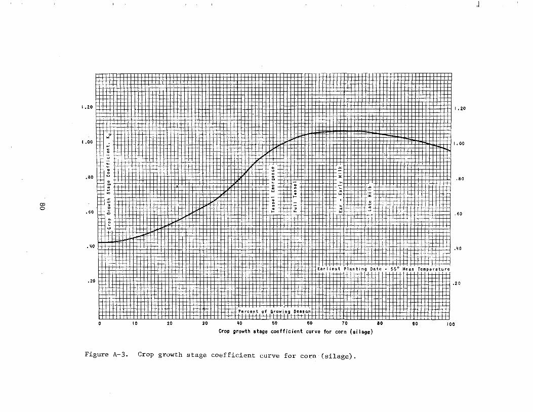
00 o

1.20

1.00

.80

.60

o

Figure A-3.

J

.20

.80

.60

10

Crop growth stage coefficient curve for corn (silage)

Crop growth stage coefficient curve for corn (silage).

.J

1.20

EJl1020

Tl . -~ __ .::

1000

.80 .80

00 ..- 060 .60

.40

.20

o 10 20 30 40 50 60 70 80 90 100

Crop growth stage coeffic;cAt curve for sweet corn

Figure A-4. Crop growth stage coefficient curve for sweet corn.

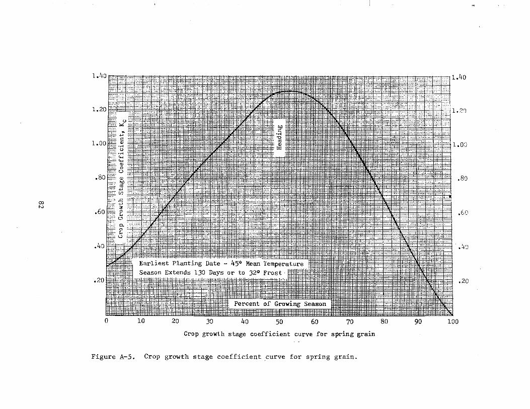
00 N

.40 r'-:t-:-:-'"I"'

o 10 20 30 40 50 60 70 Crop growth coefficient curve for spring grain

Figure A-5. Crop growth stage coefficient curve for spring grain.

,J

.80

.E,o

. • 4:3

.20

80 90 100

(XI w

1.20

1.00 ~~~~ii~~~~~~~~~~~~~~~~l.ao ..

.80

.6::1

?~ .-~

a 10 20 30 40 50 60 70 80 90 100

Crop growth stage coefficient curve for peas

Figure A-6. Crop growth stage coefficient curve for peas.

,J

00 +=-

1.00

.80

.60

.qO

.20

Figure A-7.

.J

1.00

.80

.60

.110

.20

Crop growth stage coefficient curve for small vegetables

Crop growth stage coefficient curve for small vegetables.

00 Ln

1.20

1.00m~u

.SO

.60

.110

.20

o

" u

.... .... " o u

" <71

'" .... en

"'" .... ., o .. '" ... o .. u

I

Figure A-B.

10 20 30

~--r-+ .

-~~: -LH-rr J ;_

...;J-+' , • 1-

·mii l-rtf-tH=

Earl iest Planting Date - 2S o Frost (Spring)

Latest Maturity Date - 2S o Frost (Fall)

Maximum - ISO Days

Percent of Growing Season

110 50 60 70 SO

Crop growth stage coefficient curve for sugar beets

Crop growth stage coefficient curve for sugar beets.

._: ~t_.1 .110 •• +:. ! : T ~ 1"' • ~

1.20

t-t-H---!--'-++-'---" I • 00

+}Ek-.= --t-~----

:~-~ , .,--,--"-. . ,--.-

i'---+--

--1-

. -l-t-:-j--;--­

:l~u~

.SO

.60

.110

.20

90 100

.J

.J

1.20 III1I1IIII t.20

" 1.00 !=t "" ·11 fTTnlll1 II ITII I ITTTTIII TTTTT 1 r r I I I I II 111 I 1111I :U"'fflll II I 1111i"HJ I I I I II11 I I I II , II I I II 1111111111 1• 00

... c: ., ,-" ... "" ..

• 80 [I~TTU 1111111II11111111 I I 1I1I1 I ! 111111I1I11111111111111 I 11I1111111 11I11111111 111111 III IN) II I 1 1 II II .80 .. '" .. ... .,

CO

.60 tl~ I I I 1II1I I I III I111I I I I III II II IZI II i I III I I 1111 I III I I I III I III I II II II11I I II II III1I I I I III I I I I I I II I I I I 1.60

0'<

'" . Q.

~ <.>

.~o H f1111111111111.1 II 1I1111111111111111111111111111111111111111111111111111I1III11111111 ! 1I1111 Lo

o 10 20 30 ~O 50 60 10 80 90 100

Crop growth stage coefficient curve for tomatoes

Figure A-9. Crop growth stage coefficient curve for tomatoes.

00 -....J

• '+ 0 ~==:t=:r=:::t;::~:tttt-r+t:tt:t:t:t:j

.20§ig

.00

.80

.60

.1i0

Crop

.80

~

_,,-0-< .SO

---.-f--'----

i1ilttmt1ttt;~i"'---!=---r- "-" "1 .1i0

70 80 90 100

stage coefficient curve for Irish potatoes

Figure A-lO. Crop growth stage coefficient curve for potatoes.

·J

ex; ex;

JANUARY PI'~UAn .UCN APRIL .AT JUNI JULY AueUaY SIPTE.II. oCTonR

1.25

1.00

.75

.50

o JANUAn PlnUARY .AIICH ArIUI. .AT JUN' JULY 'AueuST BlPT'.ln

Crop growth stage coefficient curve for deciduous orchards

Figure A-ll. Crop growth s coefficient curve for deciduous orchards.

J

MOVE • .,n DECEMU.

1.25

1.00

.75

.50

.25

• o MO"' •• 8 D"I ... 8

co \0

.40 II 1111!!1111111I1[11111111!11!111!.111111111111. tIf6.-thiE?~: tAmm+m+m+mm+m:t::·n·t..ji,,: "~:,,,! .!h~-h~Ji:4 1.40

.20 1.20

1.00

.80

060

.40

o 10 20 30 40 50 60 70 80 90 100

Crop growth stage coefficient curves for winter wheat

Figure A-12. Crop growth stage coefficient curves for winter wheat.

.J

\0 o

FURUARY lURCH A~ItIL MAY JUliE JULY AUGUST u~n.alR oCToaro

.50

.25

.7'"

APRIL MAY JUH·e: JULT Au.veT SlEPrl1lll8EJIl OCtOBlR:

Crop g~owth stage coefficient c~rve for pasture grasses

Figure A-i3. Crop growth stage coefficient curve for pasture grasses.

.J

IIOVllIUR O[CUln

~-;'-+"H I • 00

.75

.50

.25 NOVE.BIIt D[C OU.I It

\0 .....

o

,0

60

.~o

.2()

Figure A-14.

.J

.80

.60

.1.10

.20

Crop growth stage coefficient curve for .elon, and cantaloupes

Crop growth stage coefficient curve for melons and cantalopes.

\0 N

JANUARY FEBRUARY

1.20

1.00

.80

.60

JANUAa ... FE8RUARY

Figure A-IS.

.J

II~RCH APRIL IIAT SUN! SULT ~U;UST SEPTEII8£R OCTOBER NOVEMBER OECEM3ER

: .20

.80

.60

IIARCH APRIL IIAT SUNE JULY AUGUST SEPT ••• ER O~.£R NOVEIIBER

Crop growth stage coefficient curve for alfalfa

Crop growth stage coefficient curve for alfalfa.